drilled shafts - axial resistance - adot

Intermodal Transportation Division 206 South Seventeenth Avenue Phoenix, Arizona 85007-3213

Janice K. Brewer

Governor

John S. Halikowski Director

December 1, 2010

Floyd Roehrich Jr. State Engineer

To: Dallas Hammit, Highway Operations Sam Maroufkhani, Highway Development Robert Samour, Valley Group Larry Langer, Valley Project Management Vincent Li, Statewide Project Management Jean Nehme, Bridge Group Chris Cooper, Roadway Group Barry Crockett, Engineering Technical Group Vivien Lattibeaudiere, Engineering Consultants Section From: John Lawson Manager, Geotechnical Design Section Materials Group (068R) Subject: Geotechnical Design Policy DS-1 Load Resistance Factor Design (LRFD)

Development of Drilled Shaft Axial Resistance Charts for Use by Bridge Engineers based on Load and Resistance Factor Design (LRFD) Methodology

The AASHTO (2010) LRFD Bridge Design Specifications are mandatory for all federally funded projects. This attached policy outlines the development of drilled shaft axial resistance charts based on methods specified in AASHTO (2010). The intent of this policy is to present a general overview of the development of the information needed by the bridge designer to design substructure elements consisting of drilled shafts. Personnel, both within ADOT and design consultants working on projects that require LRFD for substructures, shall follow the attached policy. The designer should contact the ADOT Materials Group for an updated version of this policy in the event any interim revisions are made to AASHTO (2010) or a new edition of AASHTO is issued. At a minimum, the geotechnical engineer shall develop at least one (1) of each of the following drilled shaft axial resistance charts to permit the bridge designer to design a bridge substructure element. Chart 1: Strength axial resistance versus depth of embedment for various shaft diameters. Chart 2: Service axial resistance for a given vertical displacement of the shaft top versus depth of embedment

for various shaft diameters.

Depending on the project, Chart 2 may be developed for several values of vertical displacement to allow the bridge engineer to develop a third chart as follows: Chart 3: Developed axial resistance versus vertical displacement for a shaft of given diameter and depth of embedment. The procedures for development and use of each of these three charts are described in the attached policy. If you have any questions regarding this bulletin, please contact Jim Wilson at 602-712-8081 or John Lawson at 602-712-8130.

of 1

REVISION LOG ADOT Policy Memorandum: ADOT DS-1

Date of Original Issue: January 28, 2008 Development of Drilled Shaft Axial Resistance Charts for Use by Bridge Engineers Based on Load and Resistance Factor Design (LRFD) Methodology

Revision (Date) Changes 1 (December 1, 2010) 1. As appropriate, update reference to AASHTO from AASHTO

(2007) to AASHTO (2010).

2. Revise title to include reference to LRFD methodology.

3. Introduce a policy memorandum number (ADOT DS-1) on Page 1 to permit proper referencing of the memorandum in project reports and other policy memoranda.

4. On Page 1 of 14, include units (blows/ft) for N60 in Table 1.

5. On Page 2 of 14, in the last paragraph in Section I, add “by the geotechnical engineer” after “Chart 2 is developed”.

6. On of 14 revise third line from “For the factored tip resistance multiply the nominal tip resistance, Rp, with the resistance factor for side resistance, qp.” to “For the factored tip resistance multiply the nominal tip resistance, Rp, by the resistance factor for tip resistance, qp.”

7. Revise Footnote 7 on Page 4 of 14 to include new policy memorandum number (ADOT DS-2, 2010).

8. On Page 7 of 14, include the following statement in Line 12 “The same limitation applies to the 8-ft diameter shaft since its tip lies above line CD.”

9. On Page 7 of 14, include the following statement at the end of the first paragraph: “Refer to ADOT DS-3 (2010) for guidance on lateral load analysis.”

10. On Page 9 of 14, in Section VII (Closing Comments), add a paragraph that emphasizes the need for close coordination between structural and geotechnical specialists.

11. On Page 9 of 14, include references to ADOT Policy Memoranda, ADOT DS-2 and ADOT DS-3.

12. Make minor editorial changes as necessary. These changes did not affect the technical content.

of 14

To: John Lawson, P.E., Manager, Geotechnical Design Section

Date: January 28, 2008 December 1, 2010 (Revision 1)

From: Norman H. Wetz, P.E., Senior Geotechnical Engineer James D. Wilson, P.E., Geotechnical Planning Engineer

Subject: Development of Drilled Shaft Axial Resistance Charts for Use by Bridge Engineers Based on Load and Resistance Factor Design (LRFD) Methodology

ADOT POLICY MEMORANDUM: ADOT DS-1

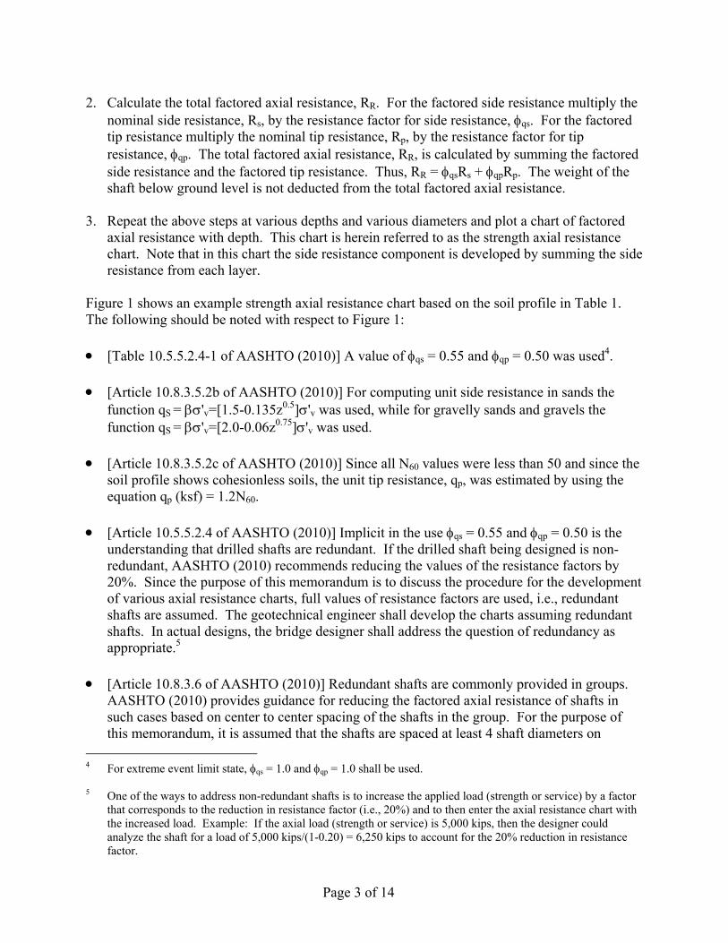
This memorandum outlines the development of drilled shaft axial resistance charts based on methods specified in AASHTO (2010). The intent of this memorandum is to present a general overview of the development of the information needed by the bridge designer to design substructure elements consisting of drilled shafts. The designer should contact ADOT Materials Group for an updated version of this memorandum in the event interim revisions to AASHTO (2010) are issued or a new edition of AASHTO LRFD Bridge Design Specifications is issued. The details regarding selection of specific equations based on the site- and project-specific geotechnical and structural conditions are omitted except as necessary to illustrate a point. For details on such issues, the reader is referred to AASHTO (2010). Furthermore, since the primary intent of this memorandum is to illustrate concepts, a hypothetical cohesionless (drained) soil profile described in Table 1 is used.1

Table 1

Hypothetical Soil Profile Depth

(ft) Soil Type Total unit weight, s,

(pcf) N60

(blows/ft) 0 – 25 Fine to coarse sands 120 25 25 – 75 Gravelly sands 125 42 75 – 90 Fine to coarse sands 120 18 90 – 130 Gravels 125 49

Notes: 1. Assume depth 0 to correspond to Elevation 1,000 ft. 2. N60 is energy-corrected Standard Penetration Test N-value. 3. Assume no groundwater was encountered and soils exhibit drained behavior. 4. Depth of 130-ft represents bottom of boring.

1 Long-term (time-dependent) consolidation type settlements should also be evaluated by the geotechnical

engineer, as appropriate, and reported to the bridge engineer, who can then evaluate whether total (immediate + long-term) settlements can be tolerated. The procedures in AASHTO (2010) shall be used for determination of long-term settlements.

Mater ials Group - Geotechnical Design Sect ion

of 14

I. Drilled Shaft Axial Resistance Charts At a minimum, the geotechnical engineer shall develop at least two (2) drilled shaft axial resistance charts to permit the bridge designer to design a bridge substructure element. Each of these charts shall show the relationship between axial resistance plotted on the abscissa and depth2 plotted on the ordinate for a range of shaft diameters. Specifically, these two charts are as follows: Chart 1: Strength axial resistance versus depth of embedment for various shaft diameters. Chart 2: Service axial resistance for a given vertical displacement of the shaft top versus depth

of embedment for various shaft diameters The bridge engineer will use Chart 1 to evaluate the strength limit state and Chart 2 to evaluate the service limit state. Depending on the project, Chart 2 may be developed for several values of vertical displacement to allow the bridge engineer to develop a third chart as follows: Chart 3: Developed axial resistance versus vertical displacement for a shaft of given diameter

and depth of embedment. Note that Chart 3 is different from Chart 2 in the sense that Chart 3 is developed by the bridge engineer only for a specific diameter and depth of embedment while Chart 2 is developed by the geotechnical engineer for a range of shaft diameters and depths of embedment. The procedures for development and use of each of these three charts are described below for the soil profile in Table 1. II. Development of Chart 1: Strength Axial Resistance Chart The strength axial resistance chart is developed as follows: 1. At a given depth3, z, and for a given diameter, D, calculate the nominal side resistance, Rs,

and nominal tip resistance, Rp, based on the appropriate predictive model in AASHTO (2010). For example, if the soil type at the depth of interest is cohesionless and the N60 value is 25, (i.e., N60 ≥ 15) then to compute the unit side resistance use the function, qs (ksf) = 'v=[1.5-0.135z0.5]'v where 'v is the effective overburden pressure in units of ksf at depth z expressed in units of feet. Similarly, to estimate the unit nominal tip resistance in cohesionless soils, use the function qp (ksf) = 1.2N60 when the value of N60 at the tip elevation is ≤ 50. To obtain the nominal values of the side and tip resistance, multiply the unit side resistance by the perimeter surface area and the unit tip resistance by tip area, respectively.

2 Both depths and elevations shall be plotted on drilled shaft axial resistance charts because ultimately shaft top

and shaft tip elevations are noted on the project plans. Anytime depth is discussed in this memorandum it should be considered that elevation is also being discussed.

3 The soil profile is commonly divided into layers and the depth z is measured to the center of a layer. The unit

side resistance is calculated at depth z and the side resistance for the layer is obtained by multiplying the unit side resistance with the perimeter area of the shaft within the layer.

of 14

2. Calculate the total factored axial resistance, RR. For the factored side resistance multiply the nominal side resistance, Rs, by the resistance factor for side resistance, qs. For the factored tip resistance multiply the nominal tip resistance, Rp, by the resistance factor for tip resistance, qp. The total factored axial resistance, RR, is calculated by summing the factored side resistance and the factored tip resistance. Thus, RR = qsRs + qpRp. The weight of the shaft below ground level is not deducted from the total factored axial resistance.

3. Repeat the above steps at various depths and various diameters and plot a chart of factored

axial resistance with depth. This chart is herein referred to as the strength axial resistance chart. Note that in this chart the side resistance component is developed by summing the side resistance from each layer.

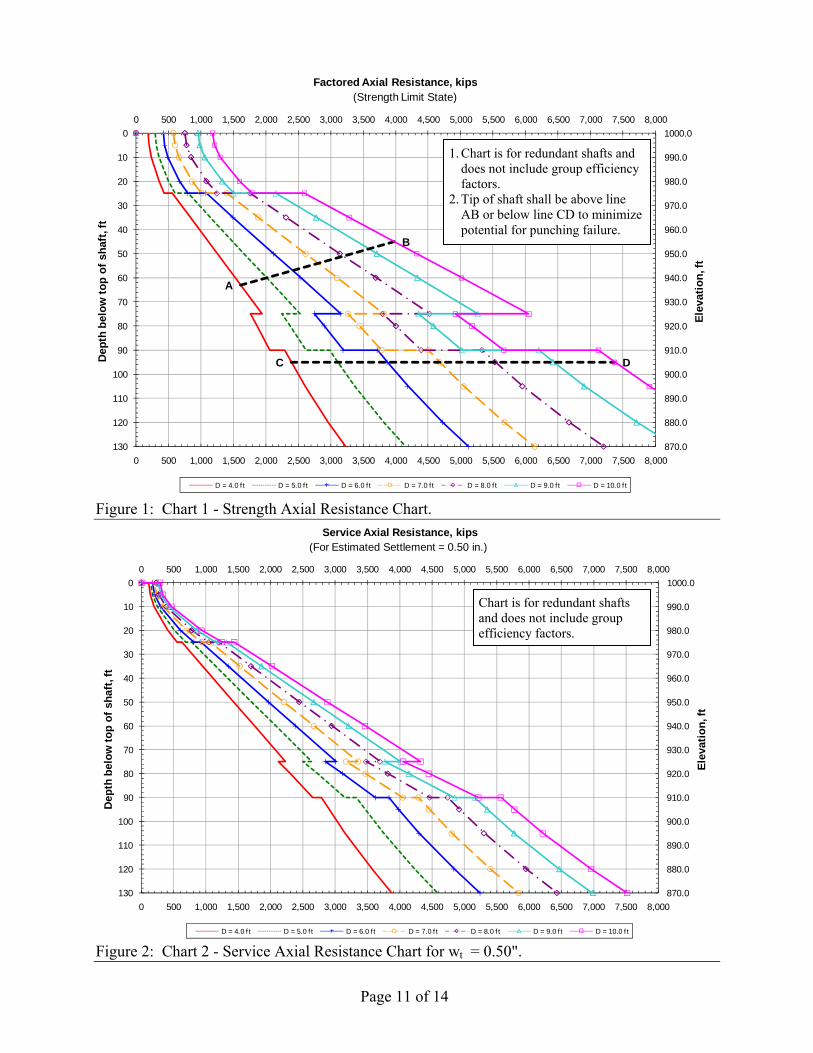
Figure 1 shows an example strength axial resistance chart based on the soil profile in Table 1. The following should be noted with respect to Figure 1:

[Table 10.5.5.2.4-1 of AASHTO (2010)] A value of qs = 0.55 and qp = 0.50 was used4.

[Article 10.8.3.5.2b of AASHTO (2010)] For computing unit side resistance in sands the function qS = 'v=[1.5-0.135z0.5]'v was used, while for gravelly sands and gravels the function qS = 'v=[2.0-0.06z0.75]'v was used.

[Article 10.8.3.5.2c of AASHTO (2010)] Since all N60 values were less than 50 and since the soil profile shows cohesionless soils, the unit tip resistance, qp, was estimated by using the equation qp (ksf) = 1.2N60.

[Article 10.5.5.2.4 of AASHTO (2010)] Implicit in the use qs = 0.55 and qp = 0.50 is the understanding that drilled shafts are redundant. If the drilled shaft being designed is non-redundant, AASHTO (2010) recommends reducing the values of the resistance factors by 20%. Since the purpose of this memorandum is to discuss the procedure for the development of various axial resistance charts, full values of resistance factors are used, i.e., redundant shafts are assumed. The geotechnical engineer shall develop the charts assuming redundant shafts. In actual designs, the bridge designer shall address the question of redundancy as appropriate.5

[Article 10.8.3.6 of AASHTO (2010)] Redundant shafts are commonly provided in groups. AASHTO (2010) provides guidance for reducing the factored axial resistance of shafts in such cases based on center to center spacing of the shafts in the group. For the purpose of this memorandum, it is assumed that the shafts are spaced at least 4 shaft diameters on

4 For extreme event limit state, qs = 1.0 and qp = 1.0 shall be used. 5 One of the ways to address non-redundant shafts is to increase the applied load (strength or service) by a factor

that corresponds to the reduction in resistance factor (i.e., 20%) and to then enter the axial resistance chart with the increased load. Example: If the axial load (strength or service) is 5,000 kips, then the designer could analyze the shaft for a load of 5,000 kips/(1-0.20) = 6,250 kips to account for the 20% reduction in resistance factor.

of 14

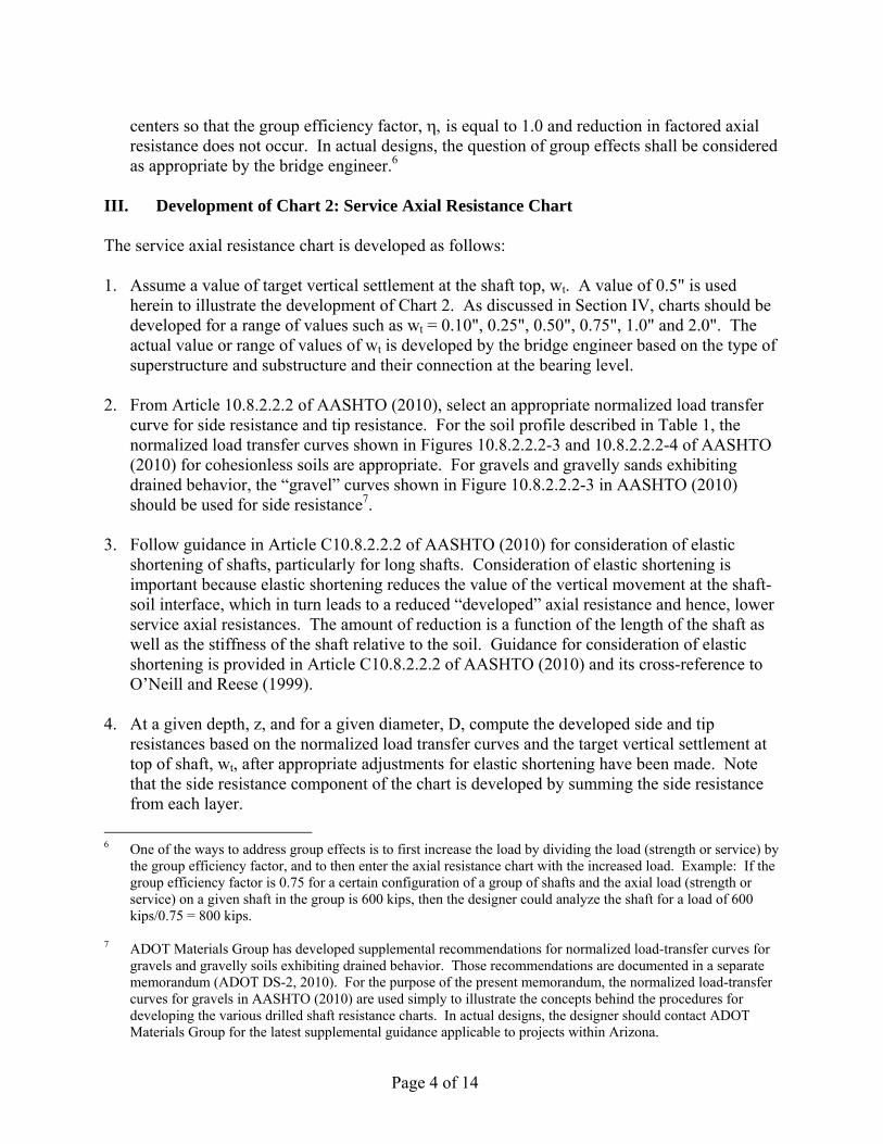
centers so that the group efficiency factor, is equal to 1.0 and reduction in factored axial resistance does not occur. In actual designs, the question of group effects shall be considered as appropriate by the bridge engineer.6

III. Development of Chart 2: Service Axial Resistance Chart The service axial resistance chart is developed as follows: 1. Assume a value of target vertical settlement at the shaft top, wt. A value of 0.5" is used

herein to illustrate the development of Chart 2. As discussed in Section IV, charts should be developed for a range of values such as wt = 0.10", 0.25", 0.50", 0.75", 1.0" and 2.0". The actual value or range of values of wt is developed by the bridge engineer based on the type of superstructure and substructure and their connection at the bearing level.

2. From Article 10.8.2.2.2 of AASHTO (2010), select an appropriate normalized load transfer

curve for side resistance and tip resistance. For the soil profile described in Table 1, the normalized load transfer curves shown in Figures 10.8.2.2.2-3 and 10.8.2.2.2-4 of AASHTO (2010) for cohesionless soils are appropriate. For gravels and gravelly sands exhibiting drained behavior, the “gravel” curves shown in Figure 10.8.2.2.2-3 in AASHTO (2010) should be used for side resistance7.

3. Follow guidance in Article C10.8.2.2.2 of AASHTO (2010) for consideration of elastic

shortening of shafts, particularly for long shafts. Consideration of elastic shortening is important because elastic shortening reduces the value of the vertical movement at the shaft-soil interface, which in turn leads to a reduced “developed” axial resistance and hence, lower service axial resistances. The amount of reduction is a function of the length of the shaft as well as the stiffness of the shaft relative to the soil. Guidance for consideration of elastic shortening is provided in Article C10.8.2.2.2 of AASHTO (2010) and its cross-reference to O’Neill and Reese (1999).

4. At a given depth, z, and for a given diameter, D, compute the developed side and tip

resistances based on the normalized load transfer curves and the target vertical settlement at top of shaft, wt, after appropriate adjustments for elastic shortening have been made. Note that the side resistance component of the chart is developed by summing the side resistance from each layer.

6 One of the ways to address group effects is to first increase the load by dividing the load (strength or service) by

the group efficiency factor, and to then enter the axial resistance chart with the increased load. Example: If the group efficiency factor is 0.75 for a certain configuration of a group of shafts and the axial load (strength or service) on a given shaft in the group is 600 kips, then the designer could analyze the shaft for a load of 600 kips/0.75 = 800 kips.

7 ADOT Materials Group has developed supplemental recommendations for normalized load-transfer curves for

gravels and gravelly soils exhibiting drained behavior. Those recommendations are documented in a separate memorandum (ADOT DS-2, 2010). For the purpose of the present memorandum, the normalized load-transfer curves for gravels in AASHTO (2010) are used simply to illustrate the concepts behind the procedures for developing the various drilled shaft resistance charts. In actual designs, the designer should contact ADOT Materials Group for the latest supplemental guidance applicable to projects within Arizona.

of 14

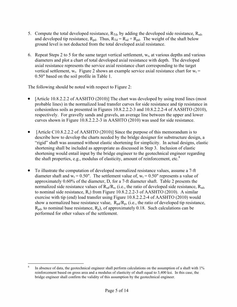
5. Compute the total developed resistance, RTd, by adding the developed side resistance, Rsd, and developed tip resistance, Rpd. Thus, RTd = Rsd + Rpd. The weight of the shaft below ground level is not deducted from the total developed axial resistance.

6. Repeat Steps 2 to 5 for the same target vertical settlement, wt, at various depths and various

diameters and plot a chart of total developed axial resistance with depth. The developed axial resistance represents the service axial resistance chart corresponding to the target vertical settlement, wt. Figure 2 shows an example service axial resistance chart for wt = 0.50" based on the soil profile in Table 1.

The following should be noted with respect to Figure 2:

[Article 10.8.2.2.2 of AASHTO (2010)] The chart was developed by using trend lines (most probable lines) in the normalized load transfer curves for side resistance and tip resistance in cohesionless soils as presented in Figures 10.8.2.2.2-3 and 10.8.2.2.2-4 of AASHTO (2010), respectively. For gravelly sands and gravels, an average line between the upper and lower curves shown in Figure 10.8.2.2.2-3 in AASHTO (2010) was used for side resistance.

[Article C10.8.2.2.2 of AASHTO (2010)] Since the purpose of this memorandum is to describe how to develop the charts needed by the bridge designer for substructure design, a “rigid” shaft was assumed without elastic shortening for simplicity. In actual designs, elastic shortening shall be included as appropriate as discussed in Step 3. Inclusion of elastic shortening would entail input by the bridge engineer to the geotechnical engineer regarding the shaft properties, e.g., modulus of elasticity, amount of reinforcement, etc.8

To illustrate the computation of developed normalized resistance values, assume a 7-ft diameter shaft and wt = 0.50". The settlement value of, wt = 0.50" represents a value of approximately 0.60% of the diameter, D, for a 7-ft diameter shaft. Table 2 presents the normalized side resistance values of Rsd/Rs, (i.e., the ratio of developed side resistance, Rsd, to nominal side resistance, Rs) from Figure 10.8.2.2.2-3 of AASHTO (2010). A similar exercise with tip (end) load transfer using Figure 10.8.2.2.2-4 of AASHTO (2010) would show a normalized base resistance value, Rpd/Rp, (i.e., the ratio of developed tip resistance, Rpd, to nominal base resistance, Rp), of approximately 0.18. Such calculations can be performed for other values of the settlement.

8 In absence of data, the geotechnical engineer shall perform calculations on the assumption of a shaft with 1%

reinforcement based on gross area and a modulus of elasticity of shaft equal to 3,400 ksi. In this case, the bridge engineer shall confirm the validity of this assumption by the geotechnical engineer.

of 14

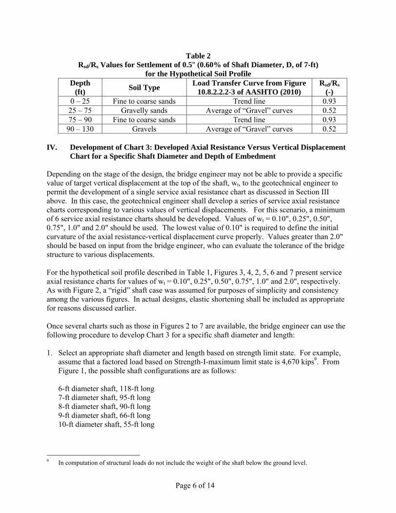
Table 2 Rsd/Rs Values for Settlement of 0.5" (0.60% of Shaft Diameter, D, of 7-ft)

for the Hypothetical Soil Profile Depth

(ft) Soil Type

Load Transfer Curve from Figure 10.8.2.2.2-3 of AASHTO (2010)

Rsd/Rs

(-) 0 – 25 Fine to coarse sands Trend line 0.93 25 – 75 Gravelly sands Average of “Gravel” curves 0.52 75 – 90 Fine to coarse sands Trend line 0.93 90 – 130 Gravels Average of “Gravel” curves 0.52

IV. Development of Chart 3: Developed Axial Resistance Versus Vertical Displacement

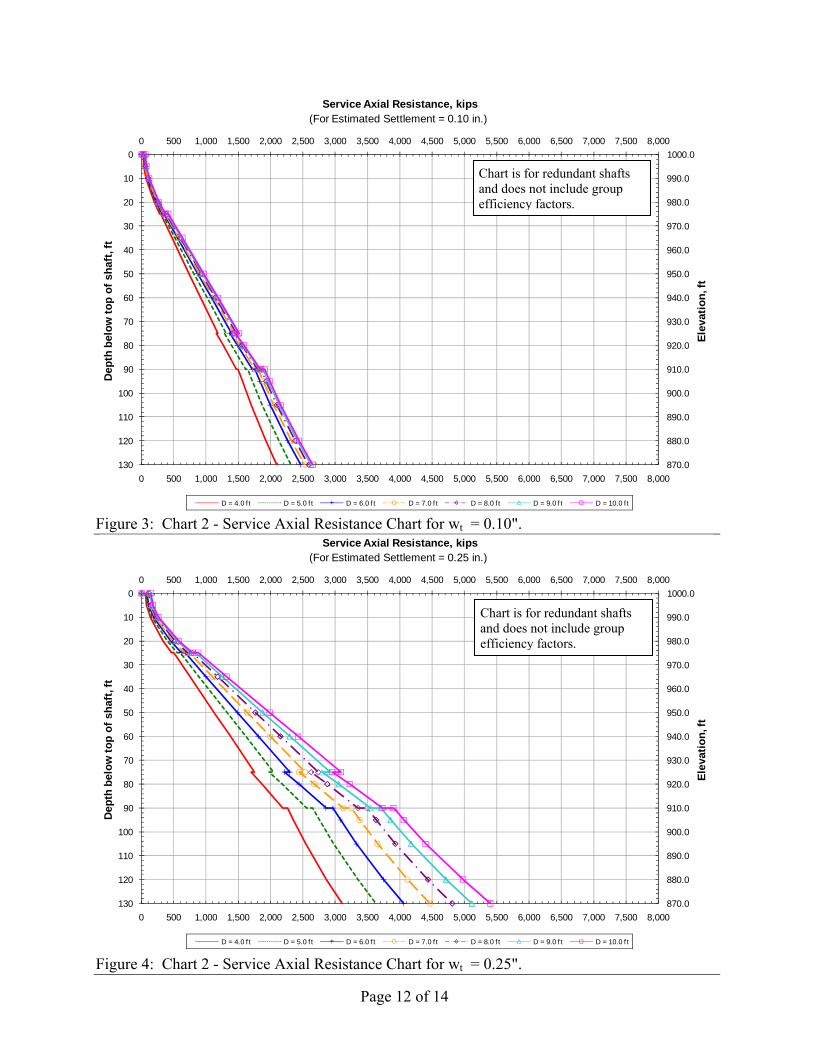
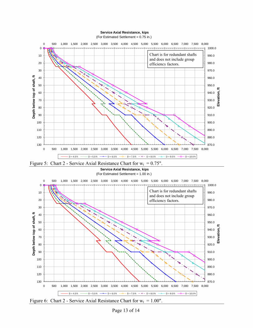
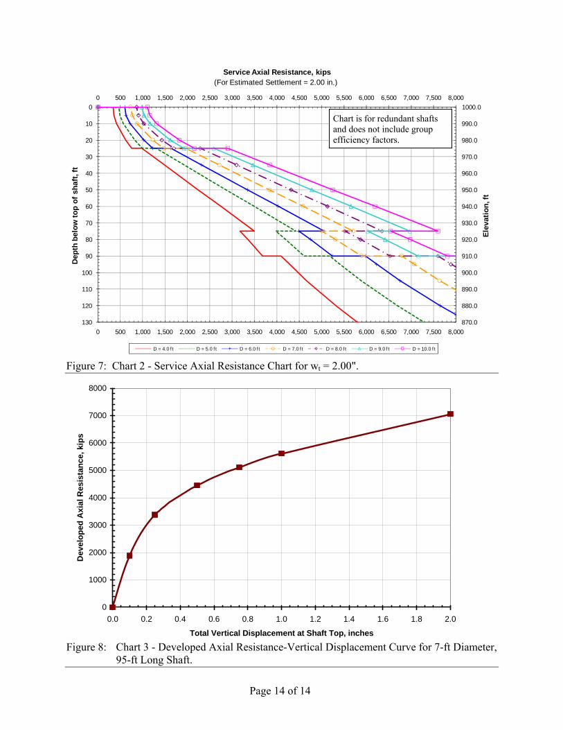
Chart for a Specific Shaft Diameter and Depth of Embedment Depending on the stage of the design, the bridge engineer may not be able to provide a specific value of target vertical displacement at the top of the shaft, wt, to the geotechnical engineer to permit the development of a single service axial resistance chart as discussed in Section III above. In this case, the geotechnical engineer shall develop a series of service axial resistance charts corresponding to various values of vertical displacements. For this scenario, a minimum of 6 service axial resistance charts should be developed. Values of wt = 0.10", 0.25", 0.50", 0.75", 1.0" and 2.0" should be used. The lowest value of 0.10" is required to define the initial curvature of the axial resistance-vertical displacement curve properly. Values greater than 2.0" should be based on input from the bridge engineer, who can evaluate the tolerance of the bridge structure to various displacements. For the hypothetical soil profile described in Table 1, Figures 3, 4, 2, 5, 6 and 7 present service axial resistance charts for values of wt = 0.10", 0.25", 0.50", 0.75", 1.0" and 2.0", respectively. As with Figure 2, a “rigid” shaft case was assumed for purposes of simplicity and consistency among the various figures. In actual designs, elastic shortening shall be included as appropriate for reasons discussed earlier. Once several charts such as those in Figures 2 to 7 are available, the bridge engineer can use the following procedure to develop Chart 3 for a specific shaft diameter and length: 1. Select an appropriate shaft diameter and length based on strength limit state. For example,

assume that a factored load based on Strength-I-maximum limit state is 4,670 kips9. From Figure 1, the possible shaft configurations are as follows:

6-ft diameter shaft, 118-ft long 7-ft diameter shaft, 95-ft long 8-ft diameter shaft, 90-ft long 9-ft diameter shaft, 66-ft long 10-ft diameter shaft, 55-ft long

9 In computation of structural loads do not include the weight of the shaft below the ground level.

of 14

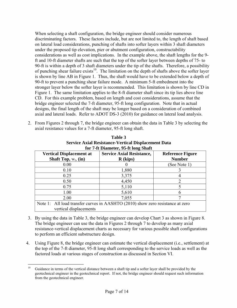
When selecting a shaft configuration, the bridge engineer should consider numerous discriminating factors. These factors include, but are not limited to, the length of shaft based on lateral load considerations, punching of shafts into softer layers within 3 shaft diameters under the proposed tip elevation, pier or abutment configuration, constructability considerations as well as cost implications. In the example above, the shaft lengths for the 9-ft and 10-ft diameter shafts are such that the top of the softer layer between depths of 75- to 90-ft is within a depth of 3 shaft diameters under the tip of the shafts. Therefore, a possibility of punching shear failure exists10. The limitation on the depth of shafts above the softer layer is shown by line AB in Figure 1. Thus, the shaft would have to be extended below a depth of 90-ft to prevent a punching shear failure mode. A minimum 5-ft embedment into the stronger layer below the softer layer is recommended. This limitation is shown by line CD in Figure 1. The same limitation applies to the 8-ft diameter shaft since its tip lies above line CD. For this example problem, based on length and cost considerations, assume that the bridge engineer selected the 7-ft diameter, 95-ft long configuration. Note that in actual designs, the final length of the shaft may be longer based on a consideration of combined axial and lateral loads. Refer to ADOT DS-3 (2010) for guidance on lateral load analysis.

2. From Figures 2 through 7, the bridge engineer can obtain the data in Table 3 by selecting the axial resistance values for a 7-ft diameter, 95-ft long shaft.

Table 3 Service Axial Resistance-Vertical Displacement Data

for 7-ft Diameter, 95-ft long Shaft Vertical Displacement at

Shaft Top, wt, (in) Service Axial Resistance,

R (kips) Reference Figure

Number 0.00 0 (See Note 1) 0.10 1,880 3 0.25 3,375 4 0.50 4,450 2 0.75 5,110 5 1.00 5,610 6 2.00 7,055 7

Note 1: All load transfer curves in AASHTO (2010) show zero resistance at zero vertical displacements

3. By using the data in Table 3, the bridge engineer can develop Chart 3 as shown in Figure 8. The bridge engineer can use the data in Figures 2 through 7 to develop as many axial resistance-vertical displacement charts as necessary for various possible shaft configurations to perform an efficient substructure design.

4. Using Figure 8, the bridge engineer can estimate the vertical displacement (i.e., settlement) at the top of the 7-ft diameter, 95-ft long shaft corresponding to the service loads as well as the factored loads at various stages of construction as discussed in Section VI.

10 Guidance in terms of the vertical distance between a shaft tip and a softer layer shall be provided by the

geotechnical engineer in the geotechnical report. If not, the bridge engineer should request such information from the geotechnical engineer.

of 14

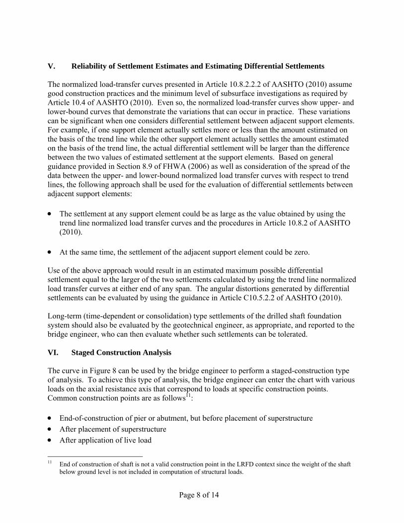
V. Reliability of Settlement Estimates and Estimating Differential Settlements The normalized load-transfer curves presented in Article 10.8.2.2.2 of AASHTO (2010) assume good construction practices and the minimum level of subsurface investigations as required by Article 10.4 of AASHTO (2010). Even so, the normalized load-transfer curves show upper- and lower-bound curves that demonstrate the variations that can occur in practice. These variations can be significant when one considers differential settlement between adjacent support elements. For example, if one support element actually settles more or less than the amount estimated on the basis of the trend line while the other support element actually settles the amount estimated on the basis of the trend line, the actual differential settlement will be larger than the difference between the two values of estimated settlement at the support elements. Based on general guidance provided in Section 8.9 of FHWA (2006) as well as consideration of the spread of the data between the upper- and lower-bound normalized load transfer curves with respect to trend lines, the following approach shall be used for the evaluation of differential settlements between adjacent support elements:

The settlement at any support element could be as large as the value obtained by using the trend line normalized load transfer curves and the procedures in Article 10.8.2 of AASHTO (2010).

At the same time, the settlement of the adjacent support element could be zero. Use of the above approach would result in an estimated maximum possible differential settlement equal to the larger of the two settlements calculated by using the trend line normalized load transfer curves at either end of any span. The angular distortions generated by differential settlements can be evaluated by using the guidance in Article C10.5.2.2 of AASHTO (2010). Long-term (time-dependent or consolidation) type settlements of the drilled shaft foundation system should also be evaluated by the geotechnical engineer, as appropriate, and reported to the bridge engineer, who can then evaluate whether such settlements can be tolerated. VI. Staged Construction Analysis

The curve in Figure 8 can be used by the bridge engineer to perform a staged-construction type of analysis. To achieve this type of analysis, the bridge engineer can enter the chart with various loads on the axial resistance axis that correspond to loads at specific construction points. Common construction points are as follows11:

End-of-construction of pier or abutment, but before placement of superstructure

After placement of superstructure

After application of live load

11 End of construction of shaft is not a valid construction point in the LRFD context since the weight of the shaft

below ground level is not included in computation of structural loads.

of 14

Evaluation of incremental displacements between various construction points when taken in conjunction with guidance on angular distortions provided in Article C10.5.2.2 of AASHTO (2010) can permit a more efficient design of the substructure as well as the superstructure. For example, settlements that occur before the placement of the superstructure can generally be compensated for by adjusting the bearing levels. Therefore, such settlements may be irrelevant with respect to their effect on the design of the superstructure itself. Properly accounting for such settlements will lead to smaller settlements for the construction stages that follow, which may be of more interest from the viewpoint of differential settlements, e.g., between end-of-construction of a pier and after placement of the superstructure. Such considerations may lead to more efficient designs for both the substructure and the superstructure. VII. Closing Comments All computations that include consideration of vertical displacements are based on the normalized load transfer curves published in AASHTO (2010). It must be realized that these curves were developed for short-term settlements only, i.e., immediate-type of settlements. The geotechnical engineer shall provide the bridge engineer with guidance to evaluate the differential settlements between adjacent support elements. Based on site- and project-specific conditions the geotechnical engineer could modify the guidance provided in Section V of this memorandum as appropriate. If such guidance is not included in the geotechnical report, the bridge engineer should request the information from the geotechnical engineer. Close interaction and communication between geotechnical and bridge specialists will be required to apply the guidance in this memorandum correctly.

VIII. References AASHTO (2010). AASHTO LRFD Bridge Design Specifications. 5th Edition. American

Association of State Highway and Transportation Officials, Washington, D.C. (including latest errata and interims).

ADOT DS-2 (2010). Interim Guidance – Design of Drilled Shafts in Gravels and Gravelly Soils Exhibiting Drained Behavior. Memorandum from N. H. Wetz and J. D. Wilson to J. Lawson, Dated December 1, 2010, Arizona Department of Transportation. Phoenix, AZ. (http://www.azdot.gov/Highways/Materials/Geotech_Design/Policy.asp)

ADOT DS-3 (2010). Analysis of Drilled Shafts Subjected to Lateral Loads Based on Load and Resistance Factor (LRFD) Methodology. Memorandum from N. H. Wetz, J. D. Wilson, A. Islam and N. Viboolmate to J. Lawson and J. Nehme, Dated December 1, 2010, Arizona Department of Transportation. Phoenix, AZ. (http://www.azdot.gov/Highways/Materials/Geotech_Design/Policy.asp)

FHWA (2006). Soils and Foundations – Volumes I and II. Authors: Samtani, N. C. and Nowatzki, E. A., Publications No. FHWA NHI-06-088 and FHWA NHI-06-089, Federal Highway Administration, Washington, D.C.

of 14

O’Neill, M. W. and L. C. Reese (1999). Drilled Shafts: Construction Procedures and Design Methods, FHWA-IF-99-025, Federal Highway Administration, U.S. Department of Transportation, Washington, D.C.

of 14

Figure 1: Chart 1 - Strength Axial Resistance Chart. Figure 2: Chart 2 - Service Axial Resistance Chart for wt = 0.50".

A

B

C D

870.0

880.0

890.0

900.0

910.0

920.0

930.0

940.0

950.0

960.0

970.0

980.0

990.0

1000.0

0 500 1,000 1,500 2,000 2,500 3,000 3,500 4,000 4,500 5,000 5,500 6,000 6,500 7,000 7,500 8,000

0

10

20

30

40

50

60

70

80

90

100

110

120

130

0 500 1,000 1,500 2,000 2,500 3,000 3,500 4,000 4,500 5,000 5,500 6,000 6,500 7,000 7,500 8,000

Elev

atio

n, ft

Dep

th b

elow

top

of s

haft

, ft

Factored Axial Resistance, kips

D = 4.0 f t D = 5.0 f t D = 6.0 f t D = 7.0 f t D = 8.0 f t D = 9.0 f t D = 10.0 f t

(Strength Limit State)

1. Chart is for redundant shafts and does not include group ef f iciency factors.2. Tip of shaf t shall be above line AB or below line CD.3. Another note4. One more note

1. Chart is for redundant shafts and does not include group efficiency factors.

2. Tip of shaft shall be above line AB or below line CD to minimize potential for punching failure.

870.0

880.0

890.0

900.0

910.0

920.0

930.0

940.0

950.0

960.0

970.0

980.0

990.0

1000.0

0 500 1,000 1,500 2,000 2,500 3,000 3,500 4,000 4,500 5,000 5,500 6,000 6,500 7,000 7,500 8,000

0

10

20

30

40

50

60

70

80

90

100

110

120

130

0 500 1,000 1,500 2,000 2,500 3,000 3,500 4,000 4,500 5,000 5,500 6,000 6,500 7,000 7,500 8,000

Elev

atio

n, ft

Dep

th b

elow

top

of s

haft

, ft

Service Axial Resistance, kips


(For Estimated Settlement = 0.50 in.)

1. Chart is for redundant shaf ts and does not include group ef f iciency factors.2. Another note

Chart is for redundant shafts and does not include group efficiency factors.

of 14

870.0

880.0

890.0

900.0

910.0

920.0

930.0

940.0

950.0

960.0

970.0

980.0

990.0

1000.0

0 500 1,000 1,500 2,000 2,500 3,000 3,500 4,000 4,500 5,000 5,500 6,000 6,500 7,000 7,500 8,000

0

10

20

30

40

50

60

70

80

90

100

110

120

130

0 500 1,000 1,500 2,000 2,500 3,000 3,500 4,000 4,500 5,000 5,500 6,000 6,500 7,000 7,500 8,000

Elev

atio

n, ft

Dep

th b

elow

top

of s

haft

, ft





Figure 3: Chart 2 - Service Axial Resistance Chart for wt = 0.10".

870.0

880.0

890.0

900.0

910.0

920.0

930.0

940.0

950.0

960.0

970.0

980.0

990.0

1000.0

0 500 1,000 1,500 2,000 2,500 3,000 3,500 4,000 4,500 5,000 5,500 6,000 6,500 7,000 7,500 8,000

0

10

20

30

40

50

60

70

80

90

100

110

120

130

0 500 1,000 1,500 2,000 2,500 3,000 3,500 4,000 4,500 5,000 5,500 6,000 6,500 7,000 7,500 8,000

Elev

atio

n, ft

Dep

th b

elow

top

of s

haft

, ft








of 14

870.0

880.0

890.0

900.0

910.0

920.0

930.0

940.0

950.0

960.0

970.0

980.0

990.0

1000.0

0 500 1,000 1,500 2,000 2,500 3,000 3,500 4,000 4,500 5,000 5,500 6,000 6,500 7,000 7,500 8,000

0

10

20

30

40

50

60

70

80

90

100

110

120

130

0 500 1,000 1,500 2,000 2,500 3,000 3,500 4,000 4,500 5,000 5,500 6,000 6,500 7,000 7,500 8,000

Elev

atio

n, ft

Dep

th b

elow

top

of s

haft

, ft






870.0

880.0

890.0

900.0

910.0

920.0

930.0

940.0

950.0

960.0

970.0

980.0

990.0

1000.0

0 500 1,000 1,500 2,000 2,500 3,000 3,500 4,000 4,500 5,000 5,500 6,000 6,500 7,000 7,500 8,000

0

10

20

30

40

50

60

70

80

90

100

110

120

130

0 500 1,000 1,500 2,000 2,500 3,000 3,500 4,000 4,500 5,000 5,500 6,000 6,500 7,000 7,500 8,000

Elev

atio

n, ft

Dep

th b

elow

top

of s

haft

, ft








of 14

870.0

880.0

890.0

900.0

910.0

920.0

930.0

940.0

950.0

960.0

970.0

980.0

990.0

1000.0

0 500 1,000 1,500 2,000 2,500 3,000 3,500 4,000 4,500 5,000 5,500 6,000 6,500 7,000 7,500 8,000

0

10

20

30

40

50

60

70

80

90

100

110

120

130

0 500 1,000 1,500 2,000 2,500 3,000 3,500 4,000 4,500 5,000 5,500 6,000 6,500 7,000 7,500 8,000

Elev

atio

n, ft

Dep

th b

elow

top

of s

haft

, ft





Figure 7: Chart 2 - Service Axial Resistance Chart for wt = 2.00". Figure 8: Chart 3 - Developed Axial Resistance-Vertical Displacement Curve for 7-ft Diameter,

95-ft Long Shaft.


0

1000

2000

3000

4000

5000

6000

7000

8000

0.0 0.2 0.4 0.6 0.8 1.0 1.2 1.4 1.6 1.8 2.0

Total Vertical Displacement at Shaft Top, inches

Dev

elop

ed A

xial

Res

ista

nce,

kip

s

drilled shafts - axial resistance - adot

Documents