drilled shaft design for sound barrier walls, signs, and signals

Report No. CDOT-DTD-R-2004-8 Final Report DRILLED SHAFT DESIGN FOR SOUND BARRIER

WALLS, SIGNS, AND SIGNALS

Jamal Nusairat

Robert Y. Liang

Rick Engel

Dennis Hanneman

Naser Abu-Hejleh

Ke Yang

October 2004 COLORADO DEPARTMENT OF TRANSPORTATION RESEARCH BRANCH

i

The contents of this report reflect the views of the

author(s), who is(are) responsible for the facts and

accuracy of the data presented herein. The contents do

not necessarily reflect the official views of the Colorado

Department of Transportation or the Federal Highway

Administration. This report does not constitute a

standard, specification, or regulation. Use of the

information contained in the report is at the sole

discretion of the designer.

ii

Technical Report Documentation Page 1. Report No. CDOT-DTD-R-2004-8

2. Government Accession No.

3. Recipient's Catalog No. 5. Report Date June 2004

4. Title and Subtitle DRILLED SHAFT DESIGN FOR SOUND BARRIER WALLS, SIGNS, AND SIGNALS

6. Performing Organization Code

7. Author(s) Jamal Nusairat, Robert Y. Liang, Rick Engel, Dennis Hanneman,

Naser Abu-Hejleh, and Ke Yang

8. Performing Organization Report No. CDOT-DTD-R-2004-8

10. Work Unit No. (TRAIS)

9. Performing Organization Name and Address E. L. Robinson Engineering of Ohio Co. 6209 Riverside Drive, Suite 100, Dublin, OH 43017, and Geocal, Inc. 13900 E. Florida Ave., Unit D, Aurora, CO 80012-5821

11. Contract or Grant No. Study # 80.19 13. Type of Report and Period Covered Final Report, June 2002-June 2004

12. Sponsoring Agency Name and Address Colorado Department of Transportation - Research 4201 E. Arkansas Ave. Denver, CO 80222

14. Sponsoring Agency Code

15. Supplementary Notes Prepared in cooperation with the US Department of Transportation, Federal Highway Administration 16. Abstract: The Colorado Department of Transportation (CDOT) uses drilled shafts to support the noise barrier walls and the large overhead signs and signals placed alongside the highways. These structures are subjected to predominantly lateral loads from wind. Current CDOT design for the drilled shafts is very conservative and lacks uniformity, which could lead to high construction costs for these shafts. CDOT commissioned a research study with the objective of identifying/developing uniform and improved design methods for these structures. Toward these goals, existing analysis methods for both capacity estimate and load-deflection predictions of drilled shafts supporting sound barrier walls, signs, and signals and typical soil and rock formations in Colorado are presented in a comprehensive manner. This includes the practice of CDOT engineers and consultants for design methods and geotechnical investigation, AASHTO design methods and specifications, and the design practice of the Ohio DOT. The accuracy of selected design methods for lateral and torsional responses of drilled shafts was evaluated by comparing predictions from these methods with measured “true” capacity and deflections from lateral and torsional load tests reported in the literature, performed in Ohio, and two new lateral load tests performed in this study as a part of the CDOT construction project along I-225 where noise barriers walls were constructed. A comprehensive geotechnical investigation program was also carried out at the two new lateral load test sites that included a pressuremeter test, Standard Penetration Test (SPT), laboratory triaxial CU tests, and direct shear tests. This allowed for evaluation of the accuracy of various testing methods employed for determining the soil parameters required in the lateral design methods. Finite element modeling have been developed and validated against the new load test data. Additional consideration of possible loading rate effect, cyclic loading effect, and ground water table fluctuations on the soil resistance are discussed. The appropriateness of the recommended factor of safety (FS) for the Broms method was further verified with LRFD calibration.

Implementation: Consider both strength limit state and serviceability limit state for design of sound walls. For the strength limit, use the Broms method and a FS of two. For the serviceability limit, use COM624p (LPILE) to estimate the lateral deflection of the drilled shaft. The permissible lateral deflection should be established by the structural engineers based on engineering judgment, structural, and aesthetic concerns. The study provides some recommendations for the permissible lateral deflections. A standard special note for performing instrumented lateral load tests has been developed, which can be adopted by CDOT engineers or consultants in developing their design plans. Appropriate geotechnical test methods are recommended for obtaining relevant cohesive and cohesionless soil parameters for various analysis methods: capacity method, deflection method, and finite element method. These included the use of triaxial and direct shear tests, pressuremeter tests, and SPT based on Liang’s correlation charts. These recommendations will result in more uniform, consistent, and cost-effective design in future CDOT sound wall projects. The proposed design/analysis approach for the I-225 project has been shown to reduce the required drilled shaft length by 25% compared to the original CDOT design approach.

17. Keywords Lateral, torsional, sound wall, sign, signals, drilled shaft, load test, p-y analysis, capacity

18. Distribution Statement No restrictions. This document is available to the public through the National Technical Information Service 5825 Port Royal Road, Springfield, VA 22161.

19. Security Classif. (of this report) Unclassified

20. Security Classif. (of this page) Unclassified

21. No. of Pages 414

22. Price

Form DOT F 1700.7 (8-72) Reproduction of completed page authorized

iii

CONVERSION TABLE

U. S. Customary System to SI to U. S. Customary System (multipliers are approximate)

Multiply To Get Multiply by To Get (symbol) by (symbol)

LENGTH Inches (in) 25.4 millimeters (mm) mm 0.039 in Feet (ft) 0.305 meters (m) m 3.28 ft yards (yd) 10.914 meters (m) m 1.09 yd miles (mi) 1.61 kilometers (km) m 0.621 mi

AREA square inches (in2) 645.2 square millimeters (mm2) mm2 0.0016 in2 square feet (ft2) 0.093 square meters (m2) m2 10.764 ft2 square yards (yd2) 0.836 square meters (m2) m2 1.195 yd2 acres (ac) 0.405 hectares (ha) ha 2.47 ac square miles (mi2) 2.59 square kilometers (km2) km2 0.386 mi2 VOLUME fluid ounces (fl oz) 29.57 milliliters (ml) ml 0.034 fl oz gallons (gal) 3.785 liters (l) l 0.264 gal cubic feet (ft3) 0.028 cubic meters (m3) m3 35.71 ft3 cubic yards (yd3) 0.765 cubic meters (m3) m3 1.307 yd3

MASS ounces (oz) 28.35 grams (g) g 0.035 oz pounds (lb) 0.454 kilograms (kg) kg 2.202 lb short tons (T) 0.907 megagrams (Mg) Mg 1.103 T

TEMPERATURE (EXACT) Farenheit (°F) 5(F-32)/9 Celcius (° C) ° C 1.8C+32 ° F (F-32)/1.8

ILLUMINATION foot candles (fc) 10.76 lux (lx) lx 0.0929 fc foot-Lamberts (fl) 3.426 candela/m (cd/m) cd/m 0.2919 fl

FORCE AND PRESSURE OR STRESS poundforce (lbf) 4.45 newtons (N) N .225 lbf poundforce (psi) 6.89 kilopascals (kPa) kPa .0145 psi

iv

Drilled Shaft Design for Sound Barrier Walls, Signs, and

Signals

By

Jamal Nusairat, E. L. Robinson Engineering of Ohio Co. Robert Y. Liang, The University of Akron

Rick Engel, E. L. Robinson Engineering of Ohio Co. Dennis Hanneman, Geocal, Inc.

Naser Abu-Hejleh, Colorado Dept. of Transportation Ke Yang, The University of Akron

Report No. CDOT-DTD-R-2004-8

Sponsored by the Colorado Department of Transportation

In Cooperation with the U.S. Department of Transportation Federal Highway Administration

June 2004

Colorado Department of Transportation Research Branch

4201 E. Arkansas Ave. Denver, CO 80222

(303) 757-9506

v

ACKNOWLEDGEMENTS

The completion of this study comes as a result of the efforts of numerous individuals and

organizations and we gratefully appreciate and acknowledge these efforts. The Colorado

Department of Transportation and the Federal Highway Administration provided funding and

support for this study. The geotechnical subsurface investigation at the load test sites was

performed by the CDOT Drilling Crew as directed by Dr. Aziz Khan. Mr. Dale Power from URS

performed the pressuremeter tests. Knight Piesold performed the laboratory tests. Dick Osmun,

Mike McMullen, Jamal Elkaissi, Mark Leonard, John Deland, Trever Wang, and Leslie Sanchez

from the CDOT Bridge Office provided an in-depth technical review of this report and valuable

comments. Their knowledge and advice kindly offered in meetings, emails and telephone

conversations were essential to the successful completion of this report. Very special thanks go

to Joan Pinamont who provided the editorial review of this report. Substantial help and support

to this research were provided by Rich Griffin, Matt Greer, C.K Su, Hsing-Cheng Liu, and Greg

Fischer. Special thanks go to Hamon Contractors and Castle Rock Construction Company for

their help and cooperation during the instrumentation and the lateral load-testing portion of the

study.

Thank you all.

vi

EXECUTIVE SUMMARY

The Colorado Department of Transportation (CDOT) adopts the use of drilled shafts to support

sound barrier walls, overhead signs, and signals. The primary loading to these foundation

elements are lateral loads, moments, and torsion. Due to complexities of the nature of soil-shaft

interaction under these applied loads, the geotechnical design of these drilled shafts has been

very conservative. There has been a lack of uniformity in design and analysis methods and

design criteria, in terms of factor of safety against ultimate capacity failure as well as the

allowable deflection (serviceability under working load). Methods for determining pertinent soil

parameters needed in both types of analysis (ultimate capacity and deflection prediction) have

not been consistently evaluated for their applicability and accuracy. Realizing the importance of

these issues, CDOT commissioned a research study with the objective of identifying/developing

uniform and improved design method for sound walls, signs, and signals.

Toward these goals, existing analysis methods for both capacity estimate and load-deflection

predictions of drilled shafts supporting sound barrier walls, signs, and signals are presented in a

comprehensive manner. Typical soil and rock formations in Colorado are also summarized in a

comprehensive manner. Then, the practice of CDOT and consultants for the design methods and

geotechnical investigation for sound walls, signs, and signals are thoroughly discussed and

evaluated. The AASHTO guidelines and specifications as well as the practice of the Ohio DOT

are reviewed and discussed.

The accuracy of the selected simple analysis methods for lateral and torsional responses of

drilled shafts was evaluated by comparing predictions from these simple methods with measured

“true” capacity and deflections from lateral load tests. The simple methods for lateral response

include the Broms method, COM624P method, sheet piling method, caissons program developed

at CDOT, Brinch Hansen method, and NAVFAC DM-7 method. The simple methods for

torsional response include two methods used by the Florida DOT and a method developed by

Richard Osmun for the Colorado DOT. Data for evaluation of these methods were obtained from

hypothetical cases, several load test databases carefully selected from literature, and from Ohio’s

load tests results. Tentative recommendations on lateral and torsional design methods were made.

vii

LRFD calibration of the compiled load tests suggested that FS of 2 for the Broms method is

appropriate. Additional consideration of possible loading rate effect, cyclic loading effect,

ground water table fluctuations, and effect of lateral force induced moment on the soil resistance

are discussed and accounted for in the study recommendations.

For further evaluation of design methods for Colorado’s sound walls, the research team has

conducted two fully instrumented lateral load tests on drilled shafts constructed at a sand soil

deposit and a clay soil deposit, respectively, near Denver, Colorado. The two lateral load tests

were performed as a part of the CDOT construction project along I-225 where noise barriers

walls were constructed. Instruments were placed to measure the applied lateral loads and the

induced lateral movements and strains of the drilled shafts at different depths. The measured load

test data included lateral loads, lateral shaft head movements, and strains and deflections along

the entire depth of the test shafts at each lateral load increment. A comprehensive geotechnical

investigation program was also carried out at the two lateral load test sites that included the

pressuremeter test, SPT, as well as laboratory triaxial UC tests and direct shear tests on the soil

samples taken from the lateral load test sites. This also allowed for evaluations of the accuracy of

various testing methods for determining the soil parameters for the design methods for sound

walls. Using a validated FEM modeling technique, the two Colorado load tests were simulated

and a very accurate estimate of p-y curve parameters was generated.

Implementation Statement

Appropriate analysis methods and the accompanying geotechnical test methods for determining

the soil parameters were recommended in this report (see Chapter 5 for justification).

For CDOT Structural Engineers and Consultants

Current CDOT practice for overhead signs and signals could continue.

The following two simple uniform strength limit state and serviceability limit state design

methods are recommended to determine the required drilled shaft length of sound walls (use

larger predicted length from the two methods). For the strength limit, use the Broms method and

viii

a F.S. of two to determine the required drilled shaft length. Lateral soil resistance in the upper

1.5 D (D is the shaft diameter) of the shaft is neglected in Broms method for cohesive soils, so

no additional depth should be neglected as may be recommended in the geotechnical report. For

the serviceability limit, use COM624P (LPILE) to estimate the lateral deflection of the drilled

shaft. From the drilled shaft performance viewpoint and to be consistent with the strength limit,

the authors of this report recommended a permissible lateral deflection of 1 inch. Mr. Dick

Osmun from Staff Bridge recommends limiting the deformation for signs and signals to the soil’s

elastic limit under repetitive loading estimated with LPILE to avoid accumulation of

irrecoverable deformation with cyclic wind loads. Other suggestions for the permissible lateral

deflection are presented in Chapter 8.

The most accurate design method for drilled shafts is to conduct a load test on test shafts

constructed as planned in the construction project. Chapter 7 provides a standard special note for

performing instrumented lateral load tests, which can be adopted by CDOT engineers or

consultants in developing their design plans. The load tests are expensive and therefore are only

considered for large projects where testing could lead to large cost savings to the project. Finite

element modeling should be considered in large or very critical projects with uncommon field

and loading conditions.

For CDOT Geotechnical Engineers and Consultants

Estimate the highest possible elevation for ground water level (GWL). The most appropriate soil

testing method to determine the cohesive soil parameters required for the Broms and COM624P

methods are:

The triaxial CU test or direct shear test as described in Chapter 5 of this report.

The pressuremeter test with FHWA (1989) soil strength interpretation equation.

The SPT method with Liang (2002) correlation charts, currently adopted by the Ohio DOT.

These are presented in Tables 3.9 and 3.10, which also provide recommendations for all the

other parameters required in the LPILE program.

The CDOT procedure for estimation of strength and LPILE parameters based on SPT could

be used but it is very conservative (i.e., underestimates strength by 50%, see Chapter 5).

ix

The most appropriate soil testing method to determine the cohesionless soil parameters required

for the Broms and COM624P methods are:

The SPT with Liang (2002) correlation provides best soil strength interpretation.

The pressuremeter test would provide reasonable soil strength interpretation as well.

The SPT with CDOT correlations methods just for strength parameters (Table 3.2) not for the

parameters required in the LPILE program.

Benefits: The research results have provided several benefits to CDOT. Foremost, the proposed

design/analysis approach has been shown to reduce the required drilled shaft length employed in

the I-225 sound barrier project from 15.7 ft to 12 ft, yielding about 24% length reduction. Thus,

it is anticipated that substantial cost savings can be realized in future CDOT sound barrier wall

projects. An equally important benefit is the advancement of a uniform and consistent

design/analysis method and acceptance design criteria (factor of safety and permissible

movement) across the board for both CDOT engineers and local consultants. This uniformity

ensures that less man-hours are needed in deciding on analysis methods. Rather, engineers can

focus more on the determination of high quality soil parameters for input into the analysis. The

research has provided recommendations for proper geotechnical test methods to characterize

pertinent soil parameters needed for both ultimate capacity prediction and p-y curve generation

in COM624P or LPILE analyses. The recommended geotechnical test methods would allow

CDOT engineers to economize resources in planning out soil testing programs, thus potentially

saving costs as well. The research has provided a standard instrumented lateral load test note,

which can be used by CDOT engineers to specify a lateral load test in the design/construction

plans. For a project that involves a lot of drilled shaft construction, or when unique soil

conditions and complex loading combination exist, the lateral load test prior to final design

decision could potentially offer cost savings to the project.

x

TABLE OF CONTENTS

1 INTRODUCTION ................................................................................................... 1-1

1.1 Background.......................................................................................................... 1-1

1.2 Objectives of the Study........................................................................................ 1-2

1.3 Scope of Work ..................................................................................................... 1-2

1.4 Outline of the Report ........................................................................................... 1-3

2 REVIEW OF ANALYSIS AND DESIGN METHODS, AND SOILS AND BEDROCK IN

COLORADO ................................................................................................................... 2-1

2.1 Review of Existing Analysis and Design Methods.............................................. 2-1

2.1.1 Lateral Response of Drilled Shafts ..................................................................... 2-1

2.1.1.1 Ultimate Capacity Estimation Methods ....................................................... 2-1

2.1.1.2 Load-Deflection Prediction Methods........................................................... 2-3

2.1.2 Torsional Response of Drilled Shafts ................................................................. 2-4

2.1.3 Finite Element Method ....................................................................................... 2-5

2.2 Colorado Soils and Bedrock .............................................................................. 2-11

2.2.1 Introduction....................................................................................................... 2-11

2.2.2 Summary of Soil and Bedrock Conditions in the Urban Front Range Corridor

.................................................................................................................................... 2-11

2.2.2.1 Soil Deposits .............................................................................................. 2-12

2.2.2.2 Bedrock ...................................................................................................... 2-15

3 CURRENT DESIGN PRACTICE BY THE COLORADO DOT, AASHTO, AND THE

OHIO DOT ...................................................................................................................... 3-1

xi

3.1 Current Sound Barrier Walls Practice in Colorado.............................................. 3-1

3.1.1 Overview............................................................................................................. 3-1

3.1.1.1 CDOT Practice............................................................................................. 3-1

3.1.1.2 Consultants Practice..................................................................................... 3-2

3.1.2 Foundation Design .............................................................................................. 3-2

3.1.2.1 Loads............................................................................................................ 3-3

3.1.2.2 Design Methods ........................................................................................... 3-5

3.1.2.3 Geotechnical Investigations ......................................................................... 3-8

3.2 Overhead Signs Practice in Colorado ................................................................ 3-18

3.2.1 CDOT Design Procedure Using Standard Plans............................................... 3-18

3.2.2 Consultant Design Practice ............................................................................... 3-19

3.3 Traffic Signals Practice in Colorado.................................................................. 3-20

3.3.1 AASHTO Design Criteria................................................................................. 3-20

3.3.2 CDOT Design Practice ..................................................................................... 3-21

3.3.3 Consultant Design Practice ............................................................................... 3-22

3.4 AASHTO Specification ..................................................................................... 3-22

3.5 ODOT Design Practice ...................................................................................... 3-23

4 COMPARISON AND EVALUATION OF ANALYSIS METHODS ................... 4-1

4.1 Hypothetical Cases............................................................................................... 4-1

4.1.1 Lateral Response of Drilled Shafts ..................................................................... 4-2

4.1.2 Torsional Response of Drilled Shafts ................................................................. 4-3

4.2 Load Test Database.............................................................................................. 4-4

4.2.1 Selected Lateral Load Test Database.................................................................. 4-4

4.2.2 Torsional Load Test Database ............................................................................ 4-6

4.3 Evaluation of Analysis Methods with Load Test Data ........................................ 4-9

4.3.1 Lateral Load Test Results ................................................................................... 4-9

xii

4.3.1.1 Hyperbolic Curve Fit ................................................................................... 4-9

4.3.1.2 Ultimate Capacity Estimation - Clay ........................................................... 4-9

4.3.1.3 Ultimate Capacity Estimation - Sand......................................................... 4-11

4.3.1.4 Load-Deflection Prediction - Clay............................................................. 4-13

4.3.1.5 Load-Deflection Prediction - Sand ........................................................... 4-13

4.3.1.6 Permissible Deflection at Drilled Shaft Head - Clay ................................. 4-14

4.3.1.7 Permissible Deflection at Ground Level - Sand ........................................ 4-15

4.3.2 Torsional Load Test Results ............................................................................. 4-16

4.4 Recommended Methods of Analysis and Design .............................................. 4-18

4.4.1 Lateral Response of Drilled Shafts ................................................................... 4-18

4.4.1.1 Ultimate Capacity Based Design - Clay .................................................... 4-18

4.4.1.2 Ultimate Capacity Based Design - Sand.................................................... 4-19

4.4.1.3 Service Limit Based Design - Clay............................................................ 4-19

4.4.1.4 Service Limit Based Design - Sand ........................................................... 4-20

4.4.2 Torsional Response of Drilled Shafts ............................................................... 4-20

4.5 Other Considerations ......................................................................................... 4-22

4.5.1 Loading Rate Effect .......................................................................................... 4-22

4.5.2 Cyclic Loading Degradation ............................................................................. 4-23

4.5.3 The Effect of Soil Saturation ............................................................................ 4-24

4.5.4 The Effect of Moment Arm .............................................................................. 4-25

4.5.5 Calibration of Resistance Factors for Lateral Design of Drilled Shafts ........... 4-25

4.5.5.1 Resistance Factors for Drilled Shafts in Clay ............................................ 4-25

4.5.5.2 Resistance Factors for Drilled Shafts in Sand............................................ 4-30

5 LATERAL LOAD TESTS ON DRILLED SHAFTS AND ANALYSIS OF TEST

RESULTS AT SELECTED NOISE WALL SITES NEAR DENVER, COLORADO... 5-1

5.1 Project Description............................................................................................... 5-1

5.2 Subsurface Conditions ......................................................................................... 5-1

5.2.1 Introduction......................................................................................................... 5-1

xiii

5.2.2 Site Conditions & Geotechnical Profile.............................................................. 5-2

5.3 Lateral Load Test and Analysis at I-225 near 6th Avenue ................................... 5-3

5.3.1 Field Installation of Instruments and Drilled Shafts Construction ..................... 5-3

5.3.2 Preparation and Setup for the Lateral Load Test ................................................ 5-4

5.3.3 Lateral Load Test Procedure............................................................................... 5-5

5.3.4 Lateral Load Test Results ................................................................................... 5-6

5.3.5 Interpretation of Soil Parameters ........................................................................ 5-7

5.3.6 Analysis of Load Test ......................................................................................... 5-9

5.3.7 Re-Design of Drilled Shafts.............................................................................. 5-14

5.3.7.1 Calculation of Design Load and Load Point.............................................. 5-14

5.3.7.2 Selection of Soil Parameters ...................................................................... 5-15

5.3.7.3 Determination of Drilled Shaft Length by the Broms Method.................. 5-15

5.3.7.4 Check the Deflection with COM624P. ...................................................... 5-15

5.3.7.5 The Final Design........................................................................................ 5-16

5.4 Lateral Load Test and Analysis at I-225 near Iliff Avenue ............................... 5-16

5.4.1 Field Installation of Instruments and Drilled Shafts Construction ................... 5-16

5.4.2 Preparation and Setup for the Lateral Load Test .............................................. 5-16

5.4.3 Lateral Load Test Procedure............................................................................. 5-17

5.4.4 Lateral Load Test Results ................................................................................. 5-18

5.4.5 Interpretation of Soil Parameters ...................................................................... 5-19

5.4.6 Analysis of Load Test ....................................................................................... 5-21

5.4.7 Re-Design of Drilled Shafts.............................................................................. 5-25

5.4.7.1 Calculation of Design Load and Load Point.............................................. 5-25

5.4.7.2 Selection of Soil Parameters ...................................................................... 5-25

5.4.7.3 Determination of Drilled Shaft Length by the Broms Method.................. 5-25

5.4.7.4 Check the Deflection with COM624P. ...................................................... 5-25

5.4.7.5 The Final Design........................................................................................ 5-26

6 FINITE ELEMENT MODELING TECHNIQUES................................................. 6-1

6.1 FEM Modeling Details ........................................................................................ 6-1

xiv

6.1.1 The Finite Elements and the Mesh...................................................................... 6-1

6.1.2 Constitutive Models for Soils ............................................................................. 6-2

6.1.2.1 Overview...................................................................................................... 6-2

6.1.2.2 Yield Criterion ............................................................................................. 6-2

6.1.2.3 Flow Potential .............................................................................................. 6-3

6.1.3 Simulation of Interaction between Shaft and Soil .............................................. 6-3

6.1.4 Simulation of Initial Condition ........................................................................... 6-5

6.2 Validation of FEM Model.................................................................................... 6-5

6.3 Simulation of CDOT Test at Clay Site ................................................................ 6-6

6.4 Simulation of CDOT Test at Sand Site................................................................ 6-8

6.5 Recommended Soil Parameters Determination for FEM Simulation.................. 6-9

6.6 Summary of FEM Simulation............................................................................ 6-10

7 DRILLED SHAFT INSTRUMENTATION AND LATERAL LOAD TESTING.7-1

7.1 Objectives of Lateral Load Tests ......................................................................... 7-1

7.2 Description........................................................................................................... 7-2

7.3 General................................................................................................................. 7-2

7.4 Materials .............................................................................................................. 7-2

7.5 Location of Load Tests ........................................................................................ 7-2

7.6 Type of Test Shafts (Production or Sacrificial) ................................................... 7-3

7.7 Acquisition of New Geotechnical Data at Sites of New Lateral Load Tests....... 7-3

7.8 Drilled Shaft Construction ................................................................................... 7-3

7.9 Testing Engineer .................................................................................................. 7-4

xv

7.10 Instrumentation .................................................................................................... 7-4

7.11 Instrumentation Specifications............................................................................. 7-5

7.12 Testing.................................................................................................................. 7-6

7.13 Equipment ............................................................................................................ 7-7

7.14 Report................................................................................................................... 7-7

7.15 Method of Measurement and Payment ................................................................ 7-8

7.16 Recommendations for Improving the Load Test ................................................. 7-9

8 CONCLUSIONS...................................................................................................... 8-1

9 RECOMMENDATIONS AND BENEFITS............................................................ 9-1

9.1 Recommendations for CDOT Structural Engineers and Consultants.................. 9-1

9.1.1 Sound Barrier Walls: Recommendations............................................................ 9-1

9.1.2 Sound Barrier Walls: Justifications .................................................................... 9-2

9.1.3 Design Methods for Overhead Signs and Signals............................................... 9-3

9.2 Recommendations for CDOT Geotechnical Engineers and Consultants ............ 9-4

9.2.1 Cohesive Soils..................................................................................................... 9-4

9.2.2 Cohesionless Soils .............................................................................................. 9-5

9.3 Benefits ................................................................................................................ 9-5

10 REFERENCES .................................................................................................. 10-1

Appendix A: Surficial Soils and Bedrock of Colorado and Geologic Overview,

with Emphasis in the Urban Front Range Corridor ………………

A-1

Appendix B: Analysis Methods for Lateral Response of Drilled Shafts ………… B-1

Appendix C: Analysis Methods for Torsional Response of Drilled Shafts ………... C-1

xvi

Appendix D: The Lateral Load Test Database …………………………………….. D-1

Appendix E: Design Spreadsheet for Lateral Loaded Drilled Shafts Supporting

Sound Walls…………………………………………………………

E-1

Appendix F: Selected Bibliography …………………………………………….. F-1

The appendices are only available in electronic format:

http://www.dot.state.co.us/Publications/PDFFiles/drilledshaft2.pdf


xvii

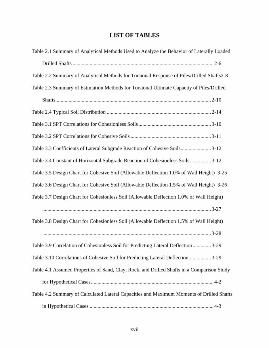
LIST OF TABLES Table 2.1 Summary of Analytical Methods Used to Analyze the Behavior of Laterally Loaded

Drilled Shafts ........................................................................................................... 2-6

Table 2.2 Summary of Analytical Methods for Torsional Response of Piles/Drilled Shafts2-8

Table 2.3 Summary of Estimation Methods for Torsional Ultimate Capacity of Piles/Drilled

Shafts...................................................................................................................... 2-10

Table 2.4 Typical Soil Distribution ............................................................................... 2-14

Table 3.1 SPT Correlations for Cohesionless Soils ....................................................... 3-10

Table 3.2 SPT Correlations for Cohesive Soils ............................................................. 3-11

Table 3.3 Coefficients of Lateral Subgrade Reaction of Cohesive Soils....................... 3-12

Table 3.4 Constant of Horizontal Subgrade Reaction of Cohesionless Soils ................ 3-12

Table 3.5 Design Chart for Cohesive Soil (Allowable Deflection 1.0% of Wall Height) 3-25

Table 3.6 Design Chart for Cohesive Soil (Allowable Deflection 1.5% of Wall Height) 3-26

Table 3.7 Design Chart for Cohesionless Soil (Allowable Deflection 1.0% of Wall Height)

................................................................................................................................ 3-27

Table 3.8 Design Chart for Cohesionless Soil (Allowable Deflection 1.5% of Wall Height)

................................................................................................................................ 3-28

Table 3.9 Correlation of Cohesionless Soil for Predicting Lateral Deflection .............. 3-29

Table 3.10 Correlations of Cohesive Soil for Predicting Lateral Deflection................. 3-29

Table 4.1 Assumed Properties of Sand, Clay, Rock, and Drilled Shafts in a Comparison Study

for Hypothetical Cases............................................................................................. 4-2

Table 4.2 Summary of Calculated Lateral Capacities and Maximum Moments of Drilled Shafts

in Hypothetical Cases .............................................................................................. 4-3

xviii

Table 4.3 Comparison of Ultimate Torsional Capacity Estimated by Various Methods in

Hypothetical Cases................................................................................................... 4-4

Table 4.4 Comparison of Calculated Torsional Stiffness at Shaft Head in Hypothetical Cases

.................................................................................................................................. 4-4

Table 4.5 Selected Database for Lateral Response of Drilled Shafts in Clay.................. 4-5

Table 4.6 Selected Database for Lateral Response of Drilled Shafts in Sand ................. 4-6

Table 4.7 Test Site Information for Drilled Shafts in Sand ............................................. 4-6

Table 4.8 Compilation of Existing Data for Torsional Response of Piles/Drilled Shafts

4-7

Table 4.9 Summary of Soil and Drilled Shaft Information of the Available Torsional Load Test

Results from Literature ............................................................................................ 4-8

Table 4.10 Parameters Used in the Calculation of Lateral Response of Drilled Shafts in Cohesive

Soils........................................................................................................................ 4-10

Table 4.11 Summary of Calculated Lateral Capacity of Drilled Shafts in Cohesive Soils 4-11

Table 4.12 Parameters Used in the Calculation of Lateral Response of Drilled Shafts in

Cohesionless Soils (After Bhushan et al., 1981).................................................... 4-12

Table 4.13 Summary of Calculated Ultimate Lateral Capacity of Drilled Shafts in Cohesionless

Soils........................................................................................................................ 4-12

Table 4.14 Summary of Calculated Lateral Capacity of Drilled Shafts by COM624P with

Different Permissible Deflections in Cohesive Soils............................................. 4-15


Different Permissible Deflections at Ground Level in Cohesionless Soils ........... 4-16

xix

Table 4.16 Comparison between Estimated Torsional Capacity and Test Results in Cohesionless

Soils........................................................................................................................ 4-17

Table 4.17 Comparison between Estimated Torsional Capacity and Test Results in Cohesive

Soils........................................................................................................................ 4-18

Table 4.18 Test Results of Strain Rate Effect on Strength of Cohesionless Soils......... 4-23

Table 4.19 Database on Measured and Predicted Lateral Capacities in Clay ............... 4-26

Table 4.20 COVs for Various In-Situ Tests (After Orchant et al., 1988)...................... 4-27

Table 4.21 Statistics for Bridge Load Components (After, Nowak, 1992) ................... 4-28

Table 4.22 Values of Target Reliability Index βT (Barker, et al. 1991)......................... 4-28

Table 4.23 Resistance Factors for Drilled Shafts in Clay by Using Reliability Method

4-29

Table 4.24 Values of Ф Calculated Using Fitting to ASD Method............................... 4-30

Table 4.25 Database on Measured and Predicted Lateral Capacities in Sand ............... 4-30

Table 4.26 Resistance Factors for Drilled Shafts in Sand by Using Reliability Method 4-31

Table 4.27 Values of Ф Calculated Using Fitting to ASD Method............................... 4-31

Table 5.1: CDOT Recommended Material Properties for Lateral Load Analysis Using LPILE.

.................................................................................................................................. 5-3

Table 5.2. Table of Instrumentation Used for Lateral Load Test. ................................... 5-4

Table 5.3 Shear Strength (Undrained Shearing) from Pressuremeter and Lab Tests ...... 5-8

Table 5.4 Elastic Modulus (psi) of Soils from Pressuremeter Test and Triaxial Test ..... 5-9

Table 5.5. Interpreted Shear Strength Parameters ......................................................... 5-10

Table 5.6. Average Strength in psi for Broms Method.................................................. 5-10

Table 5.7 Other Soil Parameters .................................................................................... 5-11

xx

Table 5.8 Calculated Lateral Capacity of Drilled Shaft #1 in CDOT Test in Clay ....... 5-12

Table 5.9 Calculated Lateral Capacity and Factor of Safety (F.S.) of Drilled Shaft #1 by

COM624P with Different Permissible Deflections at Ground Level in CDOT Test in Clay

................................................................................................................................ 5-13

Table 5.10 Shear Strength (Drained) from Pressuremeter, SPT, and Lab Tests ........... 5-20

Table 5.11 Elastic Modulus (psi) of Sands from Pressuremeter Test............................ 5-20

Table 5.12 Interpreted Shear Strength Parameters at Sand Site .................................... 5-22

Table 5.13 Average Friction Angle (Degree) for Broms Method ................................. 5-22

Table 5.14 Other Soil Parameters at Sand Site .............................................................. 5-22

Table 5.15 Calculated Lateral Capacity of South Shaft in CDOT Test in Sand............ 5-23

Table 5.16 Calculated Lateral Capacity and Factor of Safety (F.S.) of Drilled Shafts by

COM624P with Different Permissible Deflections at Ground Level in CDOT Test in Sand

................................................................................................................................ 5-24

Table 6.1 Parameters for Soils ......................................................................................... 6-6

Table 6.2 Input of Soil Parameters from Triaxial Test Results ....................................... 6-7

Table 6.3 Adjusted Soil Parameters for Match Case at Clay Site ................................... 6-8

Table 6.4 Input of Soil Parameters from Direct Shear Tests and PM Tests .................... 6-8

Table 6.5 Adjusted Soil Parameters for Match Case at Sand Site ................................... 6-9

Table 7.1 Summary of Required Instrumentation and Devices....................................... 7-5

Table 7.2 Summary of Required Material ....................................................................... 7-8

xxi

LIST OF FIGURES Figure 4.1 Schematic representation of soil profile and drilled shaft dimensions for lateral

response in hypothetical cases ................................................................................4-32

Figure 4.2 Comparison of calculated lateral capacities for hypothetical cases ..............4-33

Figure 4.3 Assumed soil profiles and drilled shaft dimensions for torsional responses in

hypothetical cases ...................................................................................................4-34

Figure 4.4 Comparison of calculated torsional capacity for hypothetical cases.............4-35

Figure 4.5 Measured over-predicted capacities of drilled shafts in clay based on load test

database...................................................................................................................4-36

Figure 4.6 Measured over-predicted capacities of drilled shafts in sand based on load test

database...................................................................................................................4-37

Figure 4.7 I-70 sound barriers, Columbus OH, shaft 1, lateral load-deflection curves ..4-38

Figure 4.8 I-70 sound barriers, Columbus OH, shaft 2, lateral load-deflection curves ..4-39

Figure 4.9 I-90 sound barriers, shaft 100 lateral load-deflection curves .......................4-40

Figure 4.10 I-90 sound barriers, shaft 101, lateral load-deflection curves ....................4-41

Figure 4.11 I-90 sound barriers, 12 ft depth, shaft 2, lateral load-deflection curves......4-42

Figure 4.12 I-90 sound barriers, 8 ft depth, shaft 1 lateral load-deflection curves.......4-43

Figure 4.13 I-90 sound barriers, 8 ft depth, shaft 2 lateral load-deflection curves.......4-44

Figure 4.14 Bhushan et al. (1981), pier 1 lateral load-deflection curve .......................4-45





xxii

Figure 4.19 Measured over-predicted capacities of drilled shafts in clay at various permissible

deflections ...............................................................................................................4-50

Figure 4.20 The assumed drilled shaft and sound wall deflection under lateral load.....4-51

Figure 4.21 Measured over-predicted capacities of drilled shafts in sand at various permissible

deflections ...............................................................................................................4-52

Figure 4.22 Measured over-predicted torsional capacities of drilled shafts in sand.......4-53

Figure 4.23 Measured over-predicted torsional capacities of drilled shafts in clay .......4-54

Figure 4.24 The mechanism of pull-push effect .............................................................4-55

Figure 5.1a Location of test shafts and test borings........................................................5-27

Figure 5.1b Location of test shafts and test borings .......................................................5-28

Figure 5.2a Test borings 1 ..............................................................................................5-29

Figure 5.2b Test borings 2 ..............................................................................................5-30

Figure 5.2c Test borings 3 ..............................................................................................5-31

Figure 5.2d Test borings 4 ..............................................................................................5-32

Figure 5.3a Location of instruments at test shaft 1.........................................................5-33

Figure 5.3b Location of instruments at test shaft 2.........................................................5-34

Figure 5.3c Location of instruments at test shaft North (Iliff Ave) ................................5-35

Figure 5.3d Location of instruments at test shaft South (Iliff Ave.)...............................5-36

Figure 5.3e Reinforcement of drilled shafts at both test sites.........................................5-37

Figure 5.4 Installation of gage on steel cages .................................................................5-38

Figure 5.5a Inclinometer assembly .................................................................................5-38

Figure 5.5b Inclinometer installation in the hole ............................................................5-39

Figure 5.6 Pouring sand to fill around the bottom 6’ of the inclinometer tube ..............5-39

xxiii

Figure 5.7 Instrumented cage transferred to the hole .....................................................5-40

Figure 5.8 Drilled shafts installed and ready for concrete ..............................................5-40

Figure 5.9 Pouring concrete in the hole ..........................................................................5-41

Figure 5.10 Picture showing the installation of the testing devices................................5-41


Figure 5.12 Picture showing the jacking devices............................................................5-42

Figure 5.13 Setup of measuring devices at shaft 2 (South) ............................................5-43

Figure 5.14 Setup of measuring devices at shaft 1 (North) ............................................5-43

Figure 5.15 General view of the load test .......................................................................5-44

Figure 5.16 Running the test and watching the instruments...........................................5-44

Figure 5.17 Picture showing opening behind the shaft during the test ...........................5-45

Figure 5.18 Picture showing data collection devices used in the test .............................5-45

Figure 5.19 Load-deflection curve at the top of test shaft #1 from dial gages ...............5-46

Figure 5.20 Load-deflection curves at the top of test shaft #2 from dial gages..............5-47

Figure 5.21 Load-deflection curve at the top of test shaft #1 from inclinometer ...........5-48

Figure 5.22 Load-deflection curve at the top of test shaft #2 from inclinometer ...........5-49

Figure 5.23. Load-deflection curve along the depth of test shaft #1 from inclinometer 5-50

Figure 5.24 Load-deflection curves along the depth of test shaft #2 from inclinometer5-51

Figure 5.25. Test shaft #1, strain vs. depth on compression side ...................................5-52

Figure 5.26. Test shaft #1, strain vs. depth on tension side ............................................5-53

Figure 5.27. Test shaft #1, measured angle of tilt...........................................................5-54

Figure 5.28. Test shaft #2, strain vs. depth on compression side ...................................5-55

Figure 5.29. Test shaft #2, strain vs. depth on tension side ............................................5-56

xxiv

Figure 5.30. Test shaft #2, measured angle of tilt...........................................................5-57

Figure 5.31 The shaft setup and soil profile interpreted for analysis at clay site ...........5-58

Figure 5.32 Typical pressuremeter test plot....................................................................5-59

Figure 5.33. Lateral load-deflection curves based on SPT and lab test results for CDOT test in

clay, shaft # 1 ..........................................................................................................5-60

Figure 5.34. Lateral load-deflection curves based pressuremeter test results for CDOT test in

clay, shaft # 1 ..........................................................................................................5-61

Figure 5.35. Zoomed load-deflection curves based on SPT and lab test results for CDOT test in

clay, shaft # 1 ..........................................................................................................5-62

Figure 5.36. Zoomed load-deflection curves based on pressuremeter test results for CDOT test in

clay, shaft # 1 ..........................................................................................................5-63

Figure 5.37 P-y curves derived by strain and deflection data versus by (a) Lab and SPT soil

parameters, and (b) pressuremeter data ..................................................................5-64

Figure 5.38 Back analysis of load-deflection from measured p-y curves.......................5-65

Figure 5.39 Load-deflection curve of new design for CDOT test at clay site ................5-66

Figure 5.40 Installation of gage on steel cages ...............................................................5-67

Figure 5.41a Inclinometer assembly ...............................................................................5-67

Figure 5.41b Inclinometer installation in the hole ..........................................................5-68

Figure 5.42 Pouring sand to fill around the bottom 6’ of the inclinometer tube ............5-68

Figure 5.43 Instrumented cage transferred to the hole ...................................................5-69

Figure 5.44 Drilled shafts installed and ready for concrete ............................................5-69

Figure 5.45 Pouring concrete in the hole ........................................................................5-70


xxv


Figure 5.48 Picture showing the jacking devices............................................................5-71

Figure 5.49 Setup of measuring devices at shaft 2 (South) ............................................5-72

Figure 5.50 Setup of measuring devices at shaft 1 (North) ............................................5-72

Figure 5.51 General view of the load test .......................................................................5-73

Figure 5.52 Running the test and watching the instruments...........................................5-73

Figure 5.53 Picture showing opening behind the shaft during the test ...........................5-74

Figure 5.54 Picture showing CDOT Engineers with the Research team........................5-74

Figure 5.55 Load-deflection curve at the top of test shaft North from dial gages..........5-75

Figure 5.56 Load-deflection curves at the top of test shaft South from dial gages ........5-76

Figure 5.57 Load-deflection curve at the top of test shaft North from inclinometer......5-77

Figure 5.58 Load-deflection curve at the top of test shaft South from inclinometer......5-78

Figure 5.59. Load-deflection curve along the depth of test shaft North from inclinometer5-79

Figure 5.60 Load-deflection curves along the depth of test shaft South from inclinometer5-80

Figure 5.61. Test shaft North, strain vs. depth on compression side ..............................5-81

Figure 5.62 Test shaft North, strain vs. depth on tension side........................................5-82

Figure 5.63. Test shaft North, measured angle of tilt .....................................................5-83

Figure 5.64. Test shaft South, strain vs. depth on compression side ..............................5-84

Figure 5.65. Test shaft South, strain vs. depth on tension side.......................................5-85

Figure 5.66. Test shaft South, measured angle of tilt .....................................................5-86

Figure 5.67 The shaft setup and soil profile interpreted for CDOT sand site.................5-87

Figure 5.68. Load-deflection curves for CDOT test in sand, South shaft ......................5-88

xxvi

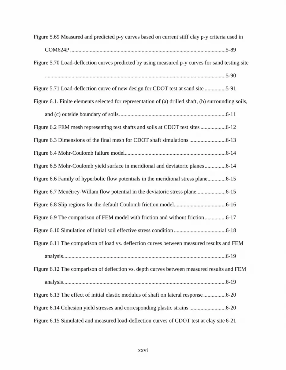
Figure 5.69 Measured and predicted p-y curves based on current stiff clay p-y criteria used in

COM624P ...............................................................................................................5-89

Figure 5.70 Load-deflection curves predicted by using measured p-y curves for sand testing site

.................................................................................................................................5-90

Figure 5.71 Load-deflection curve of new design for CDOT test at sand site ...............5-91

Figure 6.1. Finite elements selected for representation of (a) drilled shaft, (b) surrounding soils,

and (c) outside boundary of soils. ...........................................................................6-11

Figure 6.2 FEM mesh representing test shafts and soils at CDOT test sites ..................6-12

Figure 6.3 Dimensions of the final mesh for CDOT shaft simulations ..........................6-13

Figure 6.4 Mohr-Coulomb failure model........................................................................6-14

Figure 6.5 Mohr-Coulomb yield surface in meridional and deviatoric planes ...............6-14

Figure 6.6 Family of hyperbolic flow potentials in the meridional stress plane.............6-15

Figure 6.7 Menétrey-Willam flow potential in the deviatoric stress plane.....................6-15

Figure 6.8 Slip regions for the default Coulomb friction model.....................................6-16

Figure 6.9 The comparison of FEM model with friction and without friction ...............6-17

Figure 6.10 Simulation of initial soil effective stress condition .....................................6-18

Figure 6.11 The comparison of load vs. deflection curves between measured results and FEM

analysis....................................................................................................................6-19

Figure 6.12 The comparison of deflection vs. depth curves between measured results and FEM

analysis....................................................................................................................6-19

Figure 6.13 The effect of initial elastic modulus of shaft on lateral response ................6-20

Figure 6.14 Cohesion yield stresses and corresponding plastic strains ..........................6-20

Figure 6.15 Simulated and measured load-deflection curves of CDOT test at clay site 6-21

xxvii

Figure 6.16 Comparisons of measured deflection-depth curves and those from FEM simulation

with soil input from triaxial tests for CDOT test at clay site ..................................6-22


with best match soil input for CDOT test at clay site .............................................6-23

Figure 6.18 p-y curves from ABAQUS and COM624P at clay site...............................6-24

Figure 6.19 Simulated and measured load-deflection curves of CDOT test at sand site

6-25


with soil parameters from lab and PM tests for CDOT test at sand site .... 6-26


with best match soil parameters for CDOT test at sand site ...................................6-27

Figure 6.22 P-y curves from ABAQUS and COM624P at sand site ..............................6-28

Figure 7.1 Setup and calibration values for strain gages at test site I clay site...............7-11

Figure 7.2 Setup and calibration values for strain gages at test site II sand site.............7-12

1-1

1 INTRODUCTION

1.1 Background

The close proximity of residential developments to major highway systems in Colorado has

created the need to control the level of noise produced by public motorists. To alleviate this

problem, noise barrier walls are increasingly built next to these highways. Sound barriers, sign

and signal posts are not heavyweight structures and are subjected to predominantly lateral loads

from wind. The Colorado Department of Transportation (CDOT) adopts drilled shafts to support

the noise barrier walls and the large overhead signs and signals placed alongside the highways.

Drilled shafts are routinely subjected to axial, lateral and moment loads. In the case of cantilever

signs and signals, the drilled shafts are also subjected to torsional loads. The geotechnical design

of drilled shafts requires that the shafts have adequate embedment length and dimension to

ensure adequate margin of safety against ultimate failure (ultimate capacity based design).

Furthermore, these shafts should be designed to experience an acceptable level of lateral

displacement (service limit based design). Though some of the induced structure (e.g., cantilever

signs and signals) displacements are permanent due to the weight of the structure, a larger

portion of the induced displacements could be temporary and increase with time due to the

influence of repeated wind load cycles.

The Colorado Department of Transportation’s geotechnical design practice for drilled shafts may

be very conservative and lacking in uniformity. Conservative designs are common when the

engineer lacks confidence in the design theory. Design confidence is gained by evaluating data

obtained from well-documented instrumented full-scale field load tests. Significant savings to

CDOT can be realized if improved and uniform design guidelines and procedures are developed

and implemented for future CDOT projects. The current research project on the “Drilled Shaft

Design for Sound Barrier Walls, Signs, and Signals, Study No. 80.19” was initiated to re-

evaluate and update CDOT design procedures for drilled shafts used to support sound walls,

overhead signs and traffic signals. It is expected that this research will result in findings and

recommendations to improve CDOT design practice with attendant cost savings and improved

safety.

1-2

1.2 Objectives of the Study

The objectives of this research study are as follows:

(1) Determine the needs, benefits, potential cost-effectiveness, and justification of identifying

improved design methodology for Colorado drilled shafts of sound barrier walls, signs, and

signals.

(2) Identify the most accurate approximate design methods to predict the nominal response

(ultimate capacity and deformation) of drilled shafts embedded in Colorado typical

foundation soil conditions and subjected to typical Colorado loads (lateral, moments, and

torsional loads).

(3) Develop a practical procedure to perform instrumented load tests.

1.3 Scope of Work

The research team has carried out the following tasks identified in the research work plan.

a) Identify future candidate construction projects in Colorado for performance of lateral load

tests

b) Review, assimilate, and summarize current CDOT practice, and summarize typical soil and

rock formations in Colorado

c) Document pertinent literature on the design methodology of drilled shafts for noise barrier

walls, overhead signs, and signals

d) Identify and establish the design criteria of drilled shafts for sound barrier walls, overhead

signs, and traffic signals

1-3

e) Identify and establish the availability of drilled shaft database information in existing literature

f) Recommend design methods and design criteria

g) Perform two lateral load tests and verify the recommended design methods and design criteria

with lateral load test results

h) Recommend the appropriate geotechnical test methods for determining soil parameters as

related to drilled shaft capacity and deflection predictions

i) Develop a standard note for performing an instrumented lateral load test

j) Develop 3-D FEM (finite element method) modeling details and perform numerical

simulations for the two Colorado lateral load tests to gain insight on p-y curves.

k) Establish the needs, benefits, potential cost-effectiveness, and justification

1.4 Outline of the Report

Chapter 2 briefly presents existing lateral ultimate capacity estimate methods, such as the Brinch

Hansen method, Broms method, sheet piling method, and caisson program, as well as

serviceability analysis methods, such as COM624P (or LPILE) and NAVFAC method, for sound

barrier walls foundation design. The design methods for drilled shafts supporting overhead signs

and traffic signals are reviewed in Chapter 2 as well. The details of analysis methods are given in

Appendix B and Appendix C for lateral and torsional response, respectively. The typical soils

and bedrock conditions encountered for sound walls, overhead signs, and traffic signals in

Colorado are provided in Chapter 2 as well. More details of the soils and bedrock information of

Colorado are given in Appendix A.

The review of foundation design for sound walls, overhead signs, and signals by Colorado

Department of Transportation and consultants, including foundation design and geotechnical

1-4

investigation, are presented in Chapter 3. Additionally, The AASHTO guidelines and

specifications as well as the practice of the Ohio Department of Transportation are reviewed and

presented in this chapter.

Evaluation of selected analysis methods for lateral and torsional responses of drilled shafts are

documented in Chapter 4. Both hypothetical cases and load test database selected from literature

and Ohio’s test results are used for evaluation and comparison. The evaluation results support the

use of the Broms method with factor of safety of two for sound wall design. The COM624P (or

LPILE) program is considered to be a versatile and reliable tool for predicting drilled shaft

deflections, provided that representative and accurate p-y curves are used. The resistance factors

for LRFD design are also calibrated from the reliability method and fitted to the Allowable

Stress Design method. A tentative recommendation on the torsional design method for overhead

signs and traffic signal foundation design is also made.

Chapter 5 presents the two lateral load tests and analysis results. Two lateral load tests were

conducted on CDOT designed drilled shafts. SPT tests and pressuremeter test results were

obtained from test sites. Direct shear tests and triaxial tests were also performed on samples

retrieved from the load test sites. The Broms method and COM624P program were used to

analyze the lateral load tests with soil parameters determined from these soil testing methods.

The comparison of the analysis results indicated that the triaxial test or direct shear test are

considered to be the most appropriate soil parameter determination methods for drilled shafts in

clay. The pressuremeter test with FHWA (1989) soil strength interpretation equation or SPT

method with Liang (2002) correlation charts provide good predictions as well. For sand sites, the

SPT method with Liang (2002) correlation charts provides the most appropriate capacity

estimate, while direct shear test results provide good match with the measured load-deflection

curve at the shaft top. P-y curves based on the strain gages and inclinometer data were also

derived for both test sites. The re-designed drilled shafts at the test sites for sound barriers were

25% shorter than the original CDOT design length, thus yielding cost savings.

The FEM modeling techniques for simulating lateral loaded drilled shafts in clay and sand by

using ABAQUS were developed in Chapter 6. One lateral load test in Ohio was used to validate

1-5

the FEM modeling techniques. The lateral responses of the two load tests in Colorado were

simulated by using the developed FEM modeling techniques. P-y curves obtained from the FEM

simulation were shown to match with the p-y curves derived from measured strains and

deflections.

Finally, the special note for a lateral load test is provided in Chapter 7. The conclusions and

recommendations are presented in Chapter 8 and 9, respectively.

2-1

2 REVIEW OF ANALYSIS AND DESIGN METHODS, AND SOILS AND

BEDROCK IN COLORADO 2.1 Review of Existing Analysis and Design Methods 2.1.1 Lateral Response of Drilled Shafts

The methods for analysis of laterally loaded drilled shafts can be broadly divided into three

categories: the elastic theory based approach, the discrete and independent spring based approach,

and the finite element based continuum approach. Additional division of various available

analysis methods may be made on the basis of the ability of the analysis to provide a complete

load-deflection solution or only the ultimate capacity solution. For example, the Broms method

is a method that only provides the ultimate capacity solution; whereas, the discrete spring based

approach can offer a complete load-deflection solution. Although it is nearly impossible to

identify and summarize all published analysis methods for laterally loaded drilled shafts, some of

the more prominent and representative analysis methods are briefly reviewed herein and

summarized in Table 2.1. A more in-depth description of those reviewed methods is included in

Appendix B.

2.1.1.1 Ultimate Capacity Estimation Methods

2.1.1.1.1 Brinch Hansen Method

This method is based on earth pressure theory for c-Φ soils. It consists of determining the center

of rotation by taking moment of all forces about the point of load application and equating it to

zero. The ultimate lateral resistance can be calculated by equating the sum of horizontal forces to

zero. The advantages of this method are its applicability to c- Φ soils and layered system.

However, this method is only applicable for short piles (drilled shafts), and a trial-and-error

procedure is needed to locate the point of rotation in the calculation.

2.1.1.1.2 Broms Method

Broms method considers piles or drilled shafts as a beam on an elastic foundation. Simplified

assumptions have been adopted regarding the ultimate soil reactions along the length of a pile.

The rotation point of piles or drilled shafts under lateral load is assumed in different ways for

2-2

cohesive soils and cohesionless soils. The Broms method is capable of considering two boundary

conditions: one is a free pile head, and the other is a restrained shaft head. Also, the Broms

method can handle not only short drilled shafts (piles), but also long drilled shafts (piles). This

method however is only suitable for homogeneous soil, which would be either cohesive soils or

cohesionless soils. In order to apply the method to layered or mixed soil conditions, an

engineers’ judgment is needed to determine average (homogenized) soil properties.

2.1.1.1.3 Sheet Piling Method

The Sheet Piling Method is based on the earth pressure theory. It was initially developed for

sheet piles embedded in cohesionless soils. For cohesive soils, an assumption on equivalent

friction angle has to be made and the cohesion is assumed to be zero. Since it is rather difficult to

make any rational assumption about the equivalent friction angle, the sheet piling is not a

suggested method for drilled shafts embedded in clays.

To some extent, the hand calculations involved in the application of the sheet piling method are

cumbersome. This method is only applicable for short piles embedded in homogenous

cohesionless soils. Also, this method is developed for sheet piles, which may exhibit different

behaviors than drilled shafts.

2.1.1.1.4 Caisson Program

A CDOT engineer, Michael McMullen, developed the Caisson Program. This program is based

on a theory developed by Davidson, et al (1976), which assumes that full plastic strength of the

soil is developed in calculating the ultimate capacity. Davidson’s method assumes rigid-body

motion of the pile and the lateral soil resistance varies linearly with the depth at ultimate load,

but reverses direction at the point of rotation of the shaft. The soil strength is based on Equation

9-7 in “Basic Soils Engineering” by B.K. Hough, which in fact was generated for spread footing

foundations.

The Caisson Program only applies to homogeneous cohesive or cohesionless soil. The research

team encounters some run-time errors when using the Caisson Program to analyze drilled shafts

in cohesive soils. The method cannot provide deflection information.

2-3

2.1.1.2 Load-Deflection Prediction Methods

2.1.1.2.1 COM624P (LPILE)

The COM624P Program, or the equivalent commercial program, LPILE, has been widely used

for decades. The COM624P (LPILE) computer program is based on a numerical solution of a

physical model based on a beam on Winkler foundation. The structural behavior of the drilled

shafts is modeled as a beam, while the soil-shaft interaction is represented by discrete, non-linear

springs. The same concept has been applied to the so-called finite element program, Florida Pier.

The Florida Pier program, however, offers the ability to analyze pile group behavior by

incorporating an empirical group reduction factor.

The adoption of a beam on Winkler foundation as a physical model may introduce a small

amount of inaccuracy because it ignores the interactions between the discrete springs. However,

some studies have shown that this error is minor, if the spring characteristics can be deduced to

represent the true field behavior. Therefore, the representation of the spring has been developed

on the basis of semi-empirical p-y curves, in which p represents the net force acting on the shaft

per unit shaft length and y denotes the lateral displacement of the drilled shafts. Soil mechanics

principles have been evoked to deduce the theoretical ultimate resistance p, and to estimate the

initial stiffness using the subgrade reaction coefficient concept. Nevertheless, the construction of

the p-y curves relies on the curve fitting, using the test results of a limited number of full-scale

lateral load tests. Correlations with soil properties, shaft diameter, and depth were used to give

generality to the recommended p-y curve construction. As a minimum, the friction angle and

undrained shear strength from UU tests are needed to represent soil strength parameters for

cohesionless and cohesive soils, respectively. Correlations between these strength parameters

with the SPT N values have been developed to enable the use of an insitu testing method for

improving COM624P analysis results.

2.1.1.2.2 NAVFAC DM-7 Method

NAVFAC DM-7 method is based on Reese and Matlock’s non-dimensional solutions for

laterally loaded piles with soil modulus assumed proportional to depth (1956). By assuming that

soils behave as a series of separate elements, NAVFAC DM-7 method is an elastic method. The

2-4

ordinary beam theory can be used to develop the differential equation for a laterally loaded pile

(drilled shaft). The differential equation is solved, based upon the development of a

mathematically convenient function for the soil reaction p. The soil reaction p is represented by

the multiple of the modulus of subgrade reaction and soil deflection. For cohesionless soils, the

modulus of subgrade reaction is assumed to be proportional to the depth. The modulus of

subgrade reaction is assumed constant in cohesive soils; however, it will be converted to

equivalent modulus, which is proportional to the depth for calculation purpose. There are three

boundary conditions considered in this method: flexible cap or hinged end condition, rigid cap at

ground surface, and rigid cap at elevated position.

The limitations of this method are that the lateral load cannot exceed approximately one-third of

the ultimate lateral load capacity and only elastic lateral response can be predicted.

2.1.2 Torsional Response of Drilled Shafts The analysis methods for torsional response of drilled shafts can be classified into two categories,

similar to the lateral responses; namely, on the basis of the method’s ability either to provide

only ultimate torsion capacity or a complete torsional loads versus torsional twist at the drilled

shaft head as well as along the depth of the drilled shaft. A brief review of existing analysis

methods for torsional response, including twisting behavior, is given in Table 2.2. A more in-

depth discussion of these methods is provided in the Appendix C.

To predict torsional load vs. torsional twist angle, most of the analytical/numerical methods are

only concerned with the rotational stiffness at the head of the drilled shafts. The exceptions to

this are those developed by O’Neill (1964), Guo and Randolph (1996), who considered the non-

linearity of soil behavior and the torque transfer behavior along the length of the pile.

The existing analytical methods for estimating the ultimate torsion capacity of the drilled shafts

are summarized in Table 2.3. Most of the methods deal with the torsion loads only; however,

Tawfiq (2000) presented a method for combined lateral, overturning, and torsional loads.

Empirical equations were used in Tawfiq’s approach for determining the interface strength

between the soil and the pile.

2-5

2.1.3 Finite Element Method The Florida Pier finite element program is a very powerful software program for analyzing the

three-dimensional behavior of drilled shafts subjected to various load combinations (e.g., axial,

lateral, torsional, and bending). The soil-drilled shaft interactions however, are characterized by

discrete springs, which are similar to the p-y curve concept in the COM624P program for the

lateral load response. While the Florida Pier program can handle three-dimensional loads, the

need remains to have an appropriate methodology to determine the input for the representative

spring behavior. Thus, the Florida Pier program suffers the similar shortcoming as for the

COM624P computer program. This is due to the need for more adequate representation of the

discrete interaction springs.

A true finite element modeling in the continuum framework can be accomplished by the

powerful commercial finite element codes, such as ABAQUS. The drawback of such

undertaking is the need to establish modeling techniques, including the constitutive models for

the soil and the interface, and the mesh representation. Furthermore, the modeling technique

needs to be validated against the actual test data before it can be used for production purposes.

Nevertheless, the true continuum based finite element approach should be used for special cases

in which further insight may be gained and cost saving realized.

2-6

Table 2.1 Summary of Analytical Methods Used to Analyze the Behavior of Laterally Loaded Drilled Shafts

Analytical Method Assumptions Description Advantages Limitations Brinch Hansen Method (1961)

Based on the earth pressure theory

Assuming center of rotation, calculates the ultimate capacity

Applicable for c-φ soils Applicable for layered system

Applicable only for short piles Requires trial-and-error solution to locate point of rotation

Broms Method (1964)

Pile is equivalent to a beam on an elastic foundation

Gives out the maximum moment, its location, and ultimate lateral resistance (charts are provided)

Easy to calculate Applicable to homogeneous soil Gives rough estimation

Sheet piling method (AASHTO 1989)

Based on the earth pressure theory

Uses the sheet piling approach to get the ultimate lateral soil pressure

Requires hand calculations Applicable for short piles

Caissons Program Gives out the ultimate capacity

Cannot provide deflection information Applicable to homogeneous soil Requires computer program

2-7

Analytical Method Assumptions Description Advantages Limitations NAVFAC DM-7, 1971 For coarse grained soil,

Es increases linearly with depth For stiff to hard clays, Es is constant with depth

For coarse grained soil,

Dfzkh = and for stiff to

hard clays constant modulus Es is converted to equivalent modulus Es varying linearly with depth and then the deflection is calculated.

Considers lateral load not exceeding 1/3 of the capacity Gives out only elastic solutions

P-Y Method (1986)

The axial load in the pile is constant.

31

50

5.0 ⎟⎟⎠

⎞⎜⎜⎝

⎛=

yy

pp

ult

Accounts for the nonlinear behavior of most soils

Continuous nature of soil is not clearly modeled The default curves are limited to the soil types of their original development Computer program is required.

Table2.1 Summary of analytical methods used to analyze the behavior of laterally loaded drilled shaft Con.

2-8

Table 2.2 Summary of Analytical Methods for Torsional Response of Piles/Drilled Shafts

Methods Description Equations for Calculation Advantages Limitations

O’Neill (1964-a)

• A closed form differential equation solution.

• Elastic analysis. • Soil is homogeneous,

and it can be cohesive or cohesionless.

βλ−= z0eT)z(T

βλ

=⎟⎠⎞

⎜⎝⎛θ pilehead

T

• Estimate the initial torsional stiffness of pile head by simple hand calculation.

• The torque transfer along the shaft.

• It’s available only for small pile-head loads.

• The estimation is very rough

O’Neill (1964-b)

• A discrete method which can handle the non-linearity of soil response

A program TORQUE1 • Predict the torque-twist curve along the shaft rather than shaft head torsional stiffness.

• Some key parameters are unavailable for application.

Poulos (1975) • Numerical elastic analysis and parametric solutions

• Uniform soil and a soil in which shear modulus and pile-soil adhesion increase linearly with depth.

• Cohesive soils.

φ

φ=φFI

dGT

3s

• Charts are available for

calculation. • Unavailable

for nonlinear soil response analysis.

Randolph (1981)

• Closed-form elastic solutions

• For homogeneous soil and a soil where the stiffness is proportional to depth.

⎟⎟⎠

⎞⎜⎜⎝

⎛µµ

πλ+

⎟⎟⎠

⎞⎜⎜⎝

⎛µµ

π+=

φl

)ltanh(rl

3321

l)ltanh(

rl4

316

GrT

0

0

top30

top

• A simple assumption makes the closed form solution available.

• The governing equation is widely used by other researchers.

• Only suitable for elastic analysis

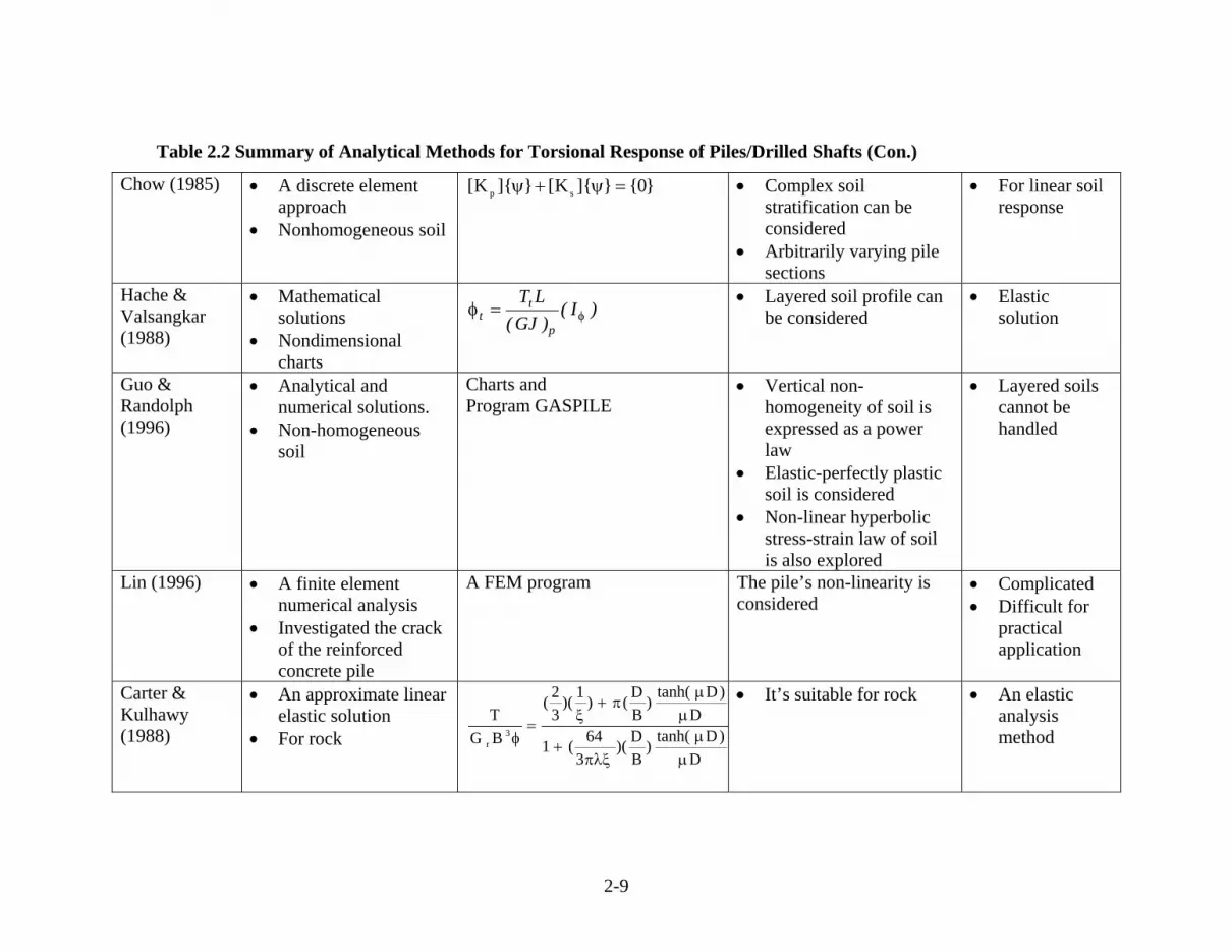
2-9

Table 2.2 Summary of Analytical Methods for Torsional Response of Piles/Drilled Shafts (Con.)

Chow (1985) • A discrete element approach

• Nonhomogeneous soil

}0{}]{K[}]{K[ sp =ψ+ψ • Complex soil stratification can be considered

• Arbitrarily varying pile sections

• For linear soil response

Hache & Valsangkar (1988)

• Mathematical solutions

• Nondimensional charts

)I()GJ(

LT

p

tt φ=φ

• Layered soil profile can be considered

• Elastic solution

Guo & Randolph (1996)

• Analytical and numerical solutions.

• Non-homogeneous soil

Charts and Program GASPILE

• Vertical non-homogeneity of soil is expressed as a power law

• Elastic-perfectly plastic soil is considered

• Non-linear hyperbolic stress-strain law of soil is also explored

• Layered soils cannot be handled

Lin (1996) • A finite element numerical analysis

• Investigated the crack of the reinforced concrete pile

A FEM program The pile’s non-linearity is considered

• Complicated • Difficult for

practical application

Carter & Kulhawy (1988)

• An approximate linear elastic solution

• For rock D

)Dtanh()BD)(

364(1

D)Dtanh()

BD()1)(

32(

BGT

3r

µµ

πλξ+

µµ

π+ξ

=φ

• It’s suitable for rock • An elastic analysis method

2-10

Table 2.3 Summary of Estimation Methods for Torsional Ultimate Capacity of Piles/Drilled Shafts

Methods Description Equations for Calculation Advantages Limitations

FDOT Structural Design Office Method

• Simple torsional load • Soil can be cohesive

or cohesionless • Soil is assumed as a

rigid plastic material

For cohesionless soil ( ) D5.0tanDL5.0KT 2

0s ⋅δ⋅⋅π⋅⋅γ⋅= D33.0tanWTb ⋅δ⋅=

• Stratified soil can be considered

• Simple torsional loads

Florida District 5 Method

• Simple torsional load )2/D()67.0tan()AW(67.0T yb ⋅ϕ⋅+⋅= Program SHAFTUF determines the side friction.

• Needs a program

Modified Florida District 5 Method

• Cohesionless soil • Based on β method

ss fLDQ ⋅⋅⋅π= , )tan()AW(67.0Q yb δ⋅+⋅= )2/D(Q)2/D(QT bs ⋅+⋅=

• Easy calculation

• Difficult to adopt an appropriate value of β

Tawfiq (2000) • Combined torsional and lateral loading conditions

• Cohesionless soil

A Program is necessary. • Combined loads are considered

• Complicated calculation.

Florida District 7 Method

• Cohesive soil • Based on the α

method

∑ ⋅⋅⋅= 2/DfLpT ss )D67.0(QT bb ⋅=

• Over consolidation ratio is considered

• Simple torsional loading.

Colorado DOT • Cohesive soil • Cohesionless soil

)3/D(c)4/D()2/D(c)D5.1L(DT 2clay π+−π=

)3D(w)

2D()D)(

2LK(T

2

sand µ+µπγ=

• Easy calculation

• Simple loads only.

2-11

2.2 Colorado Soils and Bedrock 2.2.1 Introduction Over much of the state, Colorado surficial soils, shallow soils, and bedrock are highly variable

due to repeated episodes of mountain building, subsidence, igneous intrusion and extrusion, and

glaciation. Within many provinces or trends, the character of soil and bedrock vary within

definable limits due to similar geologic history, thus allowing for generalizations of their

geotechnical properties. The emphasis in this report is on soil and bedrock conditions likely to

affect structures rather than total geologic aspects.

This study concentrates on shallow subsurface conditions of soil and bedrock usually

encountered for sound barrier walls, overhead signs, and similar structures along the Urban Front

Range Corridor (the Corridor). For our purposes, the Corridor is defined by a combination of

geologic/geomorphic and population/transportation factors. From west to east, it covers the far

eastern portion of the Rocky Mountains Front Range, the Frontal Hogback, and the valleys and

uplands divisions of the Great Plains Western Piedmont Sub-Province. The Corridor extends

from approximately Fort Collins on the north, including the Greeley area, to Pueblo on the south,

thus capturing the State’s dominant population centers along Interstate 25. An outline of the

statewide geological environment is also presented including a brief overview of soil and

bedrock conditions along other (non-Front Range) important highway corridors.

2.2.2 Summary of Soil and Bedrock Conditions in the Urban Front Range Corridor The soils and bedrock existing along the Urban Front Range Corridor vary considerably as a

result of the geologic processes that formed them. This section provides a brief overview of the

soil and bedrock types often found in the Corridor and discusses engineering properties that may

affect laterally loaded drilled shafts. More detailed geologic descriptions are presented in

Appendix A.

2-12

2.2.2.1 Soil Deposits

2.2.2.1.1 General Soil Types

Soils in the Corridor vary from clean sands and gravels to clays and silts. Sands and gravels are

commonly encountered near existing and historic river channels including the South Platte River,

Cherry Creek, Plum Creek, St. Vrain River, Cache la Poudre River, Arkansas River, and many

others. Remains of previous valley floors or alluvial fans can be seen in gravel capped terraces

in many areas. Alluvial clays and silts are also occasionally present within the river deposits,

although the clay soils are much more common than silt soils. Silt is very often present as a

minor constituent in alluvial sands and gravels. Eolian sands and clays are often located east of

the major historic rivers, coinciding with the prevailing westerly winds. Sometimes these soils

compress upon wetting and may require special design considerations. Significant thicknesses of

the residual surficial soils also exist in some areas, although to a lesser extent than alluvial and

eolian deposits. Even less common are soils of colluvial (slope wash) origin which often contain

the full range of soil types frequently mixed with bedrock fragments. Most sands and gravels

typically encountered are rounded to subangular, and clays possess low to high plasticity. Due to

the many geologic processes that created the soil deposits in the Corridor, significant variations

in material types are common, oftentimes over relatively short distances both horizontally and

vertically.

Man-placed fill soils comprised of the full range of natural soil types, and sometimes bedrock

fragments, are common along the Corridor. Cuts and fills are an inherent part of highway

development and often have significant thicknesses at overpasses and in areas with moderate or

greater topographic relief. Fill soils may also be found in old sanitary landfills, old aggregate

pits, and in low lying areas that were raised for development to reduce the risk of flooding. In

the case of sound barrier walls, berms are sometimes constructed to reduce the height of the wall

so a nominal thickness of fill is typical to most sound barrier projects. Typically, fill soils have

been placed under relatively controlled circumstances in recent decades, but there are exceptions.

It remains the CDOT practice to allow contractors to place construction debris within the right of

way outside of the roadway prism defined by a 1:1 outward slope from the edge of the shoulder.

These fills are typically uncontrolled.

2-13

2.2.2.1.2 Plasticity

The plasticity of fine grained soils in the Front Range Urban Corridor ranges from non-plastic to

low plastic silts to very high plastic clay. Silt soils are not encountered very frequently. Most of

the clay possesses medium plasticity, with plasticity indexes in the range of 15 to 30. Liquid

limits are most often below 50, but higher liquid limits and plasticity indexes are occasionally

observed. Liquid limits greater than approximately 70 are rare. Medium to high plasticity clays

have the potential to be expansive when wetted. The swell potential depends on many factors

including moisture content, dry unit weight, mineral composition, particle size gradation, and

Atterberg Limits. Where swelling soils exist, it is likely that required caisson depths to resist

uplift forces will control the design instead of lateral loading conditions. Of course, both

conditions would need to be checked.

2.2.2.1.3 Moisture Content and Ground Water

The Moisture contents of soils in the Corridor usually range from slightly moist to wet below the

ground water table. Dry soils, defined for our purposes as not having visible moisture, are

encountered occasionally. Saturated soils exist in areas of poor surface drainage, below the

ground water elevation, and sometimes several feet above the ground water table due to capillary

action in fine grained soils. Depths to ground water are highly variable, and localized perched

water conditions frequently exist. Generally, however, the ground water table near permanent

flowing water channels is likely to be at approximately the same level as the water surface.

Ground water elevations rise further away from the river or creek and often correlate with the

ground surface topography, but the ground water surface is sometimes highly variable.

2.2.2.1.4 Consistency or Density

The consistency and density of cohesive and cohesionless soils, respectively, vary considerably.

Cohesive soil consistency runs the gamut of the generally accepted classifications from very soft

to hard, and cohesionless soils also vary over the entire density range from very loose to very

dense. Most cohesive soils encountered in the Corridor typically are medium (UC strength of

0.5 to 1.0 tsf or SPT of 4 to 8) to very stiff (UC of 2.0 to 4.0 tsf or SPT of 15 to 30). The

consistency tends to vary inversely with moisture content; relatively dry cohesive soils are stiffer

2-14

than soils with greater moisture. Most cohesionless soils range from medium dense (SPT of 10

to 30) to dense (SPT of 30 to 50).

2.2.2.1.5 General Distribution of Near Surface Geomaterials

The foregoing discussion categorizes soil types based on whether they are cohesive or

cohesionless. In reality, many soils in Colorado do not conform neatly into one category or the

other; they have cohesive and frictional components. It is assumed that most soils with greater

than 70% passing the #200 sieve in Colorado will behave largely in a cohesive manner, and

those with fewer than 30% fines will behave largely in a frictional manner. The estimated

proportions of geomaterials likely to be encountered near the ground surface in the more

populated areas of the Front Range Urban Corridor at sound barrier wall, overhead sign, or

signal projects are presented in the Table 2.4 to provide a general idea of the typical soil

distribution. Silts are fine grained soils, having little cohesion and are not commonly

encountered in the Urban Corridor.

Table 2.4 Typical Soil Distribution

Material Type USCS Symbols Included

Fines Content

(%<#200)

Estimated

Distribution(%)

Clay, silt CL, CH, ML, MH >65 20a

Sand, gravel SW, SP, GW, GP, SC, SM

SC, etc.

<35 20b

Intermediate soils SC, SM, CL, CH, MH 35-65 60c

a. Silt soils are a minor percentage.

b. Gravel soils are a small percentage.

c. A majority (est. 75%) of these soils are clay.

d. Estimated total distribution of soils based on USCS criteria is 65% clay (and silt) and 35%

sand (and gravel).

The research team was hesitant to provide estimated distributions in the above table because of

the great difficulty in selecting and evaluating an appropriate data set. Consequently, these

2-15

estimates are primarily based on representative values deemed reasonable by several local

consulting and CDOT geotechnical engineers who provided their opinions. USGS maps (see

references) were also reviewed. The values presented in the table should not be considered

absolute, but are presented to provide a relative indication of the frequency of occurrence along

the Corridor and to help identify which soil conditions should be targeted for future lateral load

tests. A review of exploratory boring logs and laboratory data conducted for several CDOT and

Geocal, Inc. projects indicate that the above estimated distributions are reasonable. It is

important to bear in mind that any particular project could have several soil types, or it could

have only one general type of soil. Therefore, it is critical that site specific subsurface

investigations be conducted.

2.2.2.2 Bedrock

2.2.2.2.1 Generalized Distribution

Except for transitional zones where bedrock is very highly weathered, the interface between soil

and bedrock is usually fairly well defined along the Corridor. A major unconformity (period of

non-deposition and/or erosion) which is due to uplift along the mountain front has separated

younger soil from older bedrock. The bedrock units in the Corridor are distributed into four

major settings (arranged as younger to older for the age of their generally included units):

1. Early Tertiary (Paleocene) coarse sandstone and conglomerate units, the youngest

bedrock, are primarily limited to the central part of the Corridor forming major

exposures in the Monument Highlands.

2. For valleys and uplands of the Western Plains Piedmont (the dominant portion of the

Corridor), upper Late Cretaceous sedimentary rocks are intermittently exposed

through soil cover throughout the northern and southern parts and comprise most of

the bedrock likely to be encountered in foundations.

3. The mountain front belt includes a wide age range (Triassic to Pennsylvanian) of

diverse sedimentary rocks that are exposed in a variably wide and locally

intermittent band immediately east of the mountains. Jurassic to lower Late

Cretaceous age shale and sandstone-dominant, tilted strata are intermittently well

exposed along the narrow Frontal Hogback and as flatter lying outcrops in the

Arkansas River valley near Pueblo.

2-16

4. Pre-Cambrian igneous and metamorphic rocks are exposed pervasively in

mountainous areas along the west margin of the Corridor.

2.2.2.2.2 Common Bedrock Types within the Corridor

Most drilled shafts are likely to be constructed where upper Late Cretaceous sedimentary rocks

exist (Item 2 in section 2.2.2.2.1) which includes most of the Denver metro area, Fort Collins,

Greeley, Boulder, Colorado Springs, and Pueblo areas. Major bedrock units include the Denver,

Arapahoe, & Lower Dawson Formations and the Laramie Formation, Fox Hills Sandstone, and

Pierre Shale. Other bedrock types (items 1, 3, and 4 above) are discussed in Appendix A of this

report.

2.2.2.2.2.1 Denver, Arapahoe, and Lower Dawson Formations

The Denver, Arapahoe, & Lower Dawson Formations encompass a broad, arc-shaped band

sweeping from northern Denver around the Monument Highlands with the general arrangement

being Denver Formation dominant to the north (under most of the Denver metropolitan area),

Arapahoe Formation in the center, and Lower Dawson Arkose to the south (around Colorado

Springs). These units, although sometimes separately mapped, are largely age equivalent and

interfinger with each other over long distances.

The Denver Formation predominantly consists of claystone/shale, over most of the Denver area,

with thinner interbeds of siltstone, weakly to well cemented sandstone, and infrequent

conglomerate. Claystone/shale, as well as tuffaceous sandstone, are well noted for having major

vertical and horizontal zones with high to very high swell potential; non-sandy claystone is

frequently highly plastic when saturated. Claystone clays and ash-derived sandstone clays are

montmorillonite rich (frequently termed “bentonitic”) often including seams of nearly pure

bentonite. Where unweathered, the formation includes a blue-green-gray claystone (and

sandstone in some areas) locally known as the “Denver Blue”. The “Denver Blue’s” upper

surface is not a stratigraphic horizon, but rather an irregular weathering/alteration zone that is

often transitional. The bluish color has been observed to change to a predominantly grayish

color after exposure to air.

2-17

The Arapahoe Formation is generally coarser than the Denver Formation. The two are

frequently mapped as Denver-Arapahoe Undifferentiated in the Denver area. The formation is

generally described as well stratified, interbedded claystone/shale, siltstone, sandstone, and

conglomerate. A well-developed lower Arapahoe conglomerate is frequently only weakly

cemented and is a significant aquifer. Conglomerate and sandstone units have variable low to

moderate swell potential; siltstone and claystone/shale have moderate to high swell potential.

Lower Dawson Arkose also tends to be well interbedded with layers of conglomerate, coarse

sandstone, shale, and silty fine sandy shale (termed “mudstone”). The coarser units usually have

moderately well graded quartz and feldspar sands with granitic pebbles (“arkose”); local coal

beds are noted. Clay rich and clay-dominant zones have moderate to very high swell potential

and moderate to high plasticity, particularly in the Austin Bluffs area north of Colorado Springs.

2.2.2.2.2.2 Laramie Formation, Fox Hills Sandstone, and Pierre Shale

Laramie Formation, Fox Hills Sandstone, and Pierre Shale formations occur in two broad

situations: (1) intermittently exposed in moderately dipping beds east of the mountain front

(immediately east of the Frontal Hogback) from Ft. Collins to Denver and (2) with thin soil

mantles in gently dipping and near flat lying units in the Louisville area and along Interstate 25

between Colorado Springs and Pueblo.

The Laramie Formation is dominated by thinly bedded shale and siltstone with common hard to

friable sandstone interbeds, lesser thin hard conglomerate, and lignitic to sub-bituminous coal

beds. The formation is sandier in the lower portion. Most Laramie clays are dominantly

kaolinitic with usually low to moderate swell potential; the middle third tends to be

montmorillonitic with resulting high swell potential. The sandstones vary from weakly to well

cemented.

2-18

Foxhills Sandstone units are cross-bedded and quartz sand-dominant. Relatively thin interbeds

of claystone/shale, mudstone, and coal occur throughout. The sands are generally weakly

cemented and friable; they are important aquifers with medium to high permeability, particularly

north of Denver.

The Pierre Shale is a very thick, claystone/shale-dominant formation with numerous thin

bentonite beds throughout. The bedrock units are almost always suspect for moderate to very

high swell potential, medium to high plasticity, and low slope stability, nearly everywhere they

are encountered along the Corridor. Thin sandstone interbeds occur throughout the formation.

Significantly thick sandstone members are present in several areas at different stratigraphic

positions. Hard limestone masses (butte formers in outcrop) occur in the middle portion to the

south. To the south, the middle portion also contains appreciable gypsum content that may affect

sulfate-susceptible cement.

2.2.2.2.3 Depth to Bedrock

Depths to the most common bedrock units are highly variable and depend on geologic processes

that have occurred in an area and sometimes man’s activities in the form of cut/fill operations.

There is a large area of near surface bedrock in the Monument Highlands between southern

Denver and northern Colorado Springs. Bedrock predominates the near surface geomaterials

closer to the Rocky Mountain Front Range at the western edge of the Urban Front Range

Corridor. In other areas of the Corridor, bedrock may exist near the surface or could be much

deeper beneath alluvial deposits, sometimes in the range of 80 to 100 feet. Generally, however,

bedrock is likely to be encountered within the upper 50 feet of geomaterials at most sites.

Bedrock is intermittently located within the upper few feet in many areas of the overall Corridor.

An estimated percentage of surficial geomaterials likely to be comprised of bedrock at a sound

barrier, sign, or signal project in populated areas along the Corridor is on the order of 10 to 15

percent. Even within the population centers of the Corridor, bedrock is estimated to occur much

more frequently than 15 percent of the projects when the total length of typical sound barrier,

overhead sign, and traffic signal caisson depths is considered. It is important to note that the

upper portion of geomaterials along a caisson provides the greatest resistance to lateral loads,

2-19

although this is a function of pier diameter. Overhead sign foundations have the greatest depths

because of the loading conditions on this type of structure, with typical depths in the range of 17

to 24 feet according to CDOT standard plans. Bedrock is very often encountered within the

upper 25 feet; however, depths to bedrock are highly variable as discussed above.

2.2.2.2.4 Bedrock Hardness

The most common bedrock types in the Corridor, discussed in Section 1.2.2.2.2, are sedimentary

deposits that have been heavily overconsolidated by as much as 1,000 feet of overburden that

subsequently eroded to the present day terrain. The previous overburden pressure, degree of

weathering, and amount of cementation of sandstone or conglomerate, are the key factors that

largely determine the hardness of the bedrock. Unconsolidated, undrained shear strengths in the

Denver Formation range from 3 ksf to 30 ksf, and shear strengths in the Denver Blue range from

8 ksf to more than 30 ksf (Hepworth & Jubenville, 1981). Standard penetration test results

generally range from about 30 to 80 for the non-Denver Blue bedrock, although some highly

weathered areas may have SPT values in the teens. Denver Blue bedrock normally has SPT

blow counts of at least 80. Denver Blue claystone/sandstone bedrock typically has blow count

values in the range of 50/8” to 50/2”, and sometimes this is the first 6 inches of a drive that

would normally not be recorded for a SPT. SPT refusal also occurs. Bedrock hardness varies

from very low strength to moderate strength according to International Society of Rock

Mechanics classification criteria. The weaker bedrock is better described in terms of soil

consistency terminology in the range of very stiff to hard and tends to behave similar to heavily

overconsolidated clay.

Another CDOT study, “Improvement of the Geotechnical Axial Design Methodology for

Colorado’s Drilled Shafts Socketed in Weak Rocks” (July 2003), dealing with axial drilled shaft

capacity has yielded some useful data on the bedrock strength of the metro Denver area. As part

of this study, Osterberg load cell tests (O-cell), pressure meter testing, and coring with

subsequent unconfined compression testing was performed on the weaker brown claystone and

the harder, gray “Denver Blue” claystone/sandstone. O-cell tests at two sites with relatively

weak bedrock (SPT ranging from about 30 to 60) indicated ultimate caisson end bearing values

on the order of 50 ksf, and three O-cell tests in the much harder bedrock indicated ultimate end

2-20

bearing values greater than approximately 250 ksf. Pressure meter tests conducted indicated

unconfined strengths in the general range of 10 ksf to 20 ksf for the weaker bedrock and 50 ksf

to greater than 150 ksf for the harder bedrock. Unconfined compression (UC) tests on the

weaker bedrock generally ranged from 5 ksf to 20 ksf. UC tests on the relatively hard bedrock

indicated strengths ranging from 50 ksf to 300 ksf; the higher values are from well cemented,

clayey sandstone bedrock.

3-1

3 CURRENT DESIGN PRACTICE BY THE COLORADO DOT, AASHTO,

AND THE OHIO DOT Lateral load design procedures for drilled shafts used to support sound barrier walls, overhead

signs, and traffic signals in Colorado are presented in this chapter. It was found that CDOT

engineers and engineering consultants generally do not use the same procedures to design these

foundations. CDOT Staff Bridge engineers prefer to use ultimate strength methods, whereas the

consultants were found to prefer the p-y method of analysis in the form of the commercially

available computer program LPILE, which is an upgraded and more user friendly version of

COM624P. CDOT practice has been to design the various types of structures (sound walls,

overhead signs, and traffic signals) with different design methodologies; whereas, the consultants

apply the p-y method, and sometimes finite element methods, to nearly all laterally loaded

structures. Typically, geotechnical design parameters are provided by geotechnical engineers,

and structural engineers perform the detailed analyses and designs based on the parameters

provided. Consequently, structural engineers usually take the lead role in the design process.

Drilled shafts are nearly always designed to bear in the soils that exist (or will exist in the case of

fill areas) at the structure location; no special effort is made for the shafts to bear in bedrock or

other dense or hard geomaterials.

3.1 Current Sound Barrier Walls Practice in Colorado 3.1.1 Overview 3.1.1.1 CDOT Practice

Several methods have been used by CDOT to design sound barrier wall foundations, and the

method selected largely depends on the designer’s preference. Structural designs are performed

by Staff Bridge engineers based on geotechnical parameters provided by the CDOT geotechnical

group. The level of effort invested by CDOT to design foundations for a sound wall project

depends on the length of wall that will be built. Larger projects would likely have a site specific

design performed, but smaller projects might simply use details from a previous design.

3-2

There are no official CDOT Standard Plans for sound barrier walls, although some designs have

been used at several sites. A design prepared for a sound wall along I-225 between Parker Road

and Iliff Avenue has become somewhat of a pseudo-standard in that most new CDOT sound

barrier projects have borrowed this design. The wall varies in height from 14 to 18 feet. The

drilled shaft foundations have diameters of 2’6” and are 16’8” deep with typical center to center

spacing of 23’4”. Closer spacing of drilled shafts at 7’4” occurs at pilaster locations where the

wall height is increased for aesthetic reasons. These drilled shafts are also 16’8” long below the

bottom of the wall. The design allows for up to 2 feet of unbalanced, unreinforced soil backfill

on a side, and can accommodate permanent ground slopes of 3 (horizontal) to 1 (vertical) from

the wall down. Up to ten feet of unbalanced, geosynthetically reinforced soil is also allowed.

3.1.1.2 Consultants Practice

In the consulting side, several practicing structural engineers employed by consulting firms in

Colorado, ranging from small to very large multi-national companies, were interviewed to gather

the information presented in this section. These consultants have performed design services for

numerous CDOT projects. Engineering consultants practicing in Colorado overwhelmingly use

the computer program LPILE in their analyses of sound barrier wall foundations. Some

engineers perform an ultimate strength analysis (such as Broms Method or Sheet Pile Method) in

addition to the LPILE analysis, and a small number might perform finite element analyses

depending on the magnitude of the sound wall project. Consultants generally perform location

specific foundation designs due to the absence of any formal CDOT standard. As with the

CDOT design practice, the foundation designs are performed by the structural engineers based

on geotechnical parameters provided by geotechnical engineering consultants.

3.1.2 Foundation Design Methods Used By CDOT

CDOT designers have stated that ultimate strength methods are preferred because a traditional

factor of safety can be applied and deflection limits have not been established for deflection (or

serviceability) based methods. Design loads are based on the AASHTO Guide Specifications for

Structural Design of Sound Barriers, 1992, and according to Appendix C of that document, pile

(drilled shaft) design is “to be determined by a structural analysis procedure based upon accepted

3-3

theories.” Procedures used in the past for structural design of sound barrier wall foundations

include the sheet piling method presented in the AASHTO guide and Broms Method. A Fortran

spreadsheet program called “Caisson” developed internally by CDOT Staff Bridge has also been

used. The program is based on Davidson’s work related to subgrade reaction theory.

Deflections are calculated using LPILE Version 1, COM624P, or procedures in NAVFAC

documents, although no limiting deflections have been established. It appears that ¼ inch of

deflection at the ground line is considered to be a non-issue, and deflections of ½ inch have been

considered acceptable.

Methods Used By CDOT Consultants

Many consulting engineers have been using COM624P and LPILE for more than a decade. The

consultants concur with CDOT engineers that there are no well established deflection limits for

drilled shafts; however, each has established their own design criteria. Discussions of the LPILE

program, ultimate strength analysis, and finite element methods are presented.

Drilled shafts for sound walls are typically at least 18 inches in diameter, but are more likely to

be in the 24 to 30 inch range in diameter. Foundation depths vary and are dependent on the

spacing of the shafts. Typical sound wall foundations may be 10 to 15 feet deep and spaced at

15 to 20 feet intervals. One diameter size and one drilled shaft length are typically selected for

an entire project, although differing embedment lengths may be provided for large projects with

a sufficient amount of geotechnical data to adequately identify variations of the subsurface

materials.

3.1.2.1 Loads

3.1.2.1.1 Loading Criteria Used by CDOT Engineers

CDOT structural engineers use the loads provided in Section 2 of the AASHTO Guide

Specifications for Structural Design of Sound Barriers(1992), regardless of which method is used

to design the foundation drilled shafts. The AASHTO document states that sound barrier shall

be designed for wind speeds based on a 50-year mean recurrence interval. For Colorado, this

corresponds to a wind speed of 80 mph for most of the state, but in some areas (near the Front

Range and in Boulder County) wind speeds up to 100 mph are used by CDOT.

3-4

Wind exposure C has typically been used by CDOT for sound barrier design. Exposure C is

prescribed by AASHTO for open terrain with scattered obstructions and for sound barriers

located on bridge structures, retaining walls, or traffic barriers. The corresponding design

pressure for the wall face is usually 27 psf, but may range from 20 psf to 40 psf depending on the

wall height and geographic location. The calculation to determine the wind pressure includes a

gust factor consisting of a 30 percent increase in the wind velocity.

In 2000, CDOT adopted the Load and Resistance Factor Design (LRFD) method for all

structures including sound barrier walls. Working Stress Design (WSD) and Load Factor Design

(LFD) were used in the past. The design is typically controlled by wind loading because the

vertical loads are light and seismic acceleration coefficients are relatively low.

3.1.2.1.2 Loading Criteria Used by Consulting Engineers

Consulting engineers perform their designs based on the same AASHTO loading criteria that

CDOT engineers use. The reader should refer to Section 3.1.2 for the loading criteria.

A main difference between CDOT and consultant design loads appears to exist with the selection

of an appropriate wind exposure level. Consultants are more apt to use exposure B

classifications which are less severe than exposure C that CDOT has typically used. Exposure

B1 is for urban and suburban areas having numerous closely spaced buildings (such as single

family homes) located a distance extending at least 1500 feet in the prevailing upwind direction.

Exposure B2 is defined as more open terrain than exposure B1 and not meeting the requirements

of exposure B1. It appears that exposure B2 is more likely to be selected for sound barrier

design by consultants than exposure B1. Corresponding wind pressures are more likely to be

around 20 psf for exposure B2, but will depend on the wind velocity and wall height. The

typical exposure C wind pressure is 27 psf, but may range from 20 to 40 psf.

3-5

3.1.2.2 Design Methods

3.1.2.2.1 Design Methods Used by CDOT Engineers

3.1.2.2.1.1 Sheet Pile Method

The sheet piling method is included in Appendix C of the AASHTO Guide Specifications for

Structural Design of Sound Barriers (1992), and is based on U.S.S. Steel Sheet Pile Design

analysis. Performing a design using this method involves a trial and error procedure to find an

appropriate shaft embedment length that results in moment equilibrium of the system. Charts are

used to determine active and passive earth pressure coefficients depending on the friction angle

of the soil and slope geometry. Overturning is resisted by the calculated allowable net horizontal

ultimate lateral soil pressure which is equal to the passive pressure on one side of a pile minus

the active pressure on the other side. The upper six inches of supporting soil is neglected in the

analysis.

3.1.2.2.1.2 Broms Method

Broms Method has been used by CDOT engineers to design sound barrier foundations. This

method of lateral analysis and design for drilled shafts is discussed in Appendix B. Broms made

simplifying assumptions about the soil reactions along the length of a pile to estimate the pile’s

lateral response. To perform a design using the Broms Method, soils are classified as either

cohesive or cohesionless. Consequently, a cohesion value for cohesive soils is necessary and a

friction angle is required for cohesionless soils. Appropriate coefficients of lateral subgrade

reaction are also needed to determine whether the piles behave as short (rigid) or long (flexible)

piles. Overall factors of safety (based on load factors divided by resistance factors) in the range

of 2 to 3 are typically applied by CDOT to the design procedure.

3.1.2.2.1.3 Caisson Program

The “Caisson” program was used to design the I-225 sound barrier foundations discussed in

Section 3.1.1.1. The program is based on the theory developed by Davidson, et al (1976),

assuming that full plastic strength of the soil is developed for calculating the ultimate capacity.

The soil strength is based on the Equation 9-7 in “Basic Soils Engineering” by B.K. Hough,

which was generated for footing foundation.

3-6

The program can only apply to homogeneous cohesive or cohesionless soil. The program,

however, cannot be run correctly for cohesive soil conditions. The method cannot provide

deflection information.

3.1.2.2.1.4 LPILE/COM624P

As previously mentioned, CDOT has used LPILE and/or COM624P computer programs to check

the deflections of sound barrier foundations designed using one of the above ultimate strength

methods. CDOT uses LPILE version 1.0 or COM624P. Specific parameters required for the

analysis are discussed in the Section 3.1.2.3.1.2 for geotechnical parameters and a more detailed

description of more recent versions of the LPILE software are discussed in Section 3.1.2.2.2

under the consultant design practices.

3.1.2.2.2 Design Methods Used by Colorado Consulting Engineers

3.1.2.2.2.1 LPILE Computer Program

Nearly all of the engineering consultants interviewed were using a recent version of the LPILE

program, and most were using the latest version, LPILE Plus 4.0. One company prefers a finite

element approach, but occasionally uses COM624P. Ensoft, Inc distributes the LPILE software.

LPILE Plus 4.0 can be used to perform the structural design of the drilled shaft, but many of the

consultants use other software packages for this task. The program is capable of analyzing

scenarios with a number of boundary conditions, loading combinations, sloping ground surface,

layered soils, user input p-y curves, and can generate extensive tabular and graphical outputs. A

particularly useful output graph shows pile length vs. pile-head deflection. Emphasis in this

report is on the soil-structure interaction capabilities of the program.

The program models the soil-structure interaction of laterally loaded piles and drilled shafts

using p-y curves generated by the computer program that are based on published

recommendations for various types of soils. Soil types that can be analyzed by the program are

called 1) Soft Clay, 2) Stiff Clay with Free Water, 3) Stiff Clay without Free Water, 4) Sand, 5)

Linear Interpolation (user specified p-y curve), 6) Vuggy Limestone (strong rock), 7) silt (with

cohesion and internal friction), 8) API Sand, and 9) Weak Rock. Soil types 1, 3, and 4 are most

likely to be used in Colorado for sound barrier walls. Soil Type 2, Stiff Clay with Free Water, is

3-7

intended to be used where stiff clay is the top soil layer with water existing above the ground line

(e.g. lakes, ponds, rivers), so its use may not be appropriate for sound wall foundations in

Colorado. However, it appears that some engineers may have used Soil Type 2 on occasion to

model clay soils at depth below the ground water table, even though this would not be

appropriate. Sedimentary bedrock most likely to be encountered in Colorado at a typical project

is modeled as hard clay using Soil Type 3. As mentioned elsewhere, soft soils of Soil Type 1 are

fairly uncommon, but they may exist at a site. Geotechnical parameters required as input to the

program are discussed in Section 3.1.2.3.2.2.

Deflection limits established by a designer are somewhat arbitrary and are based on the

individual’s engineering judgment. Most designers cited one inch of deflection at the ground

line under service loading conditions as a maximum, and all were comfortable with ½ inch of

deflection at the shaft top. Others stated that deflections greater than one inch may be acceptable

in some situations. Deflection at the bottom of the shaft is normally checked to ensure that it is a

very low number nearly equal to zero.

A deflection limit at the top of sound barrier walls, not the top of caisson, equal to the wall

height divided by 120 (or 0.833% of the height) was established for the T-REX project by the

design build contractor team. (T-REX is a $1.7 billion highway and LRT project currently being

designed and constructed for 19 miles of I-25 and I-225 in metro-Denver). This criterion was

selected based on aesthetic considerations, not structural concerns. Ground line deflections are

typically less than one inch using this criterion, but occasionally are slightly greater than one

inch. Deflection estimates for the T-REX project often include a load caused by retained soil.

A plot of pile head displacement vs. pile length is easily generated by the recent versions of the

LPILE program to identify a shaft length at which greater embedment length results in very

small increases in deflection at the shaft head. This procedure is employed by nearly all of the

consulting engineers in their analysis and design.

Sensitivity studies are sometimes performed to gain additional confidence in the design by

varying the geotechnical parameters. Some designers have applied a global factor of safety to

3-8

the design load to evaluate the deflections. Changing the factor applied to the load can create a

curve of the shaft deflection vs. applied lateral load at the ground line. If the service load plots at

or close to a point on the curve where relatively small increases in the load result in large

increases in deflection, then the foundation design can be modified until acceptable results are

achieved.

3.1.2.2.2.2 Ultimate Strength Methods

As discussed above, most engineering consultants use the LPILE computer program to design

sound barrier wall foundations. Some engineers, however, also check minimum caisson

embedment lengths using the sheet pile method or other moment equilibrium calculations. One

engineer stated that he has used Broms method for ultimate capacity analysis.

3.1.2.2.2.3 Finite Element Methods

Few consulting engineers routinely use finite element methods to analyze laterally loaded

foundations and sometimes use the method to analyze sound wall foundations. It appears that

finite element analysis for sound barrier foundations is performed in a small minority of cases.

One large engineering consulting firm is very comfortable using the Florida Pier program for

larger structures, but they will very likely begin using the newer version of the program called

FB Pier for routine design of all types of structures. Reportedly, FB Pier is much more user

friendly, simpler, and quicker than the previous version. Companies using finite element method

computer programs also have the capability of using LPILE or COM624P.

3.1.2.3 Geotechnical Investigations

3.1.2.3.1 CDOT Geotechnical Investigations

3.1.2.3.1.1 Field Investigation and Laboratory Testing

CDOT uses the AASHTO Standard Specification for Highway Bridges, 1996 with Interims 1997,

1998, and 1999. Section 5.3.3 of the AASHTO standards recommends that wall borings be

spaced at intervals of 100 feet, although the interval may be increased or decreased depending on

geologic conditions. Review of several CDOT engineering geology sheets for sound barrier wall

projects indicated that CDOT’s practice is to space borings at intervals of 100 ft. to 300 ft. with

the most common interval being about 200 ft. along the length of the wall. This coincides with

3-9

the information that the CDOT Geology group provided early in the study. For longer walls, the

spacing of geotechnical bore holes is often increased. In mountainous terrain or other potentially

highly variable geologic regions, borings are sometimes made more frequently than the typical

200 feet intervals. Borehole depths are typically about two times the wall height, which is

consistent with the AASHTO standards. If unusual conditions exist, such as soft soils, boring

depths may be lengthened.

Most of CDOT’s borings for geotechnical investigations are advanced by either solid or hollow

stem auger drilling. CDOT also has capability to core bedrock materials or use a continuous

sampling system for soils; however, these methods are rarely used for sound barrier wall projects.

The typical field sampling and testing procedure used is the SPT method. CDOT has performed

penetration testing using a nominal 2-inch inside diameter California spoon sampler that is

commonly used by local geotechnical consultants, although this procedure is rarely used by

CDOT for sound barrier investigations. CDOT’s drill rigs have automatic hammers via a chain

mechanism that ensures the appropriate drop height for each blow. The split spoon sampler is

used to obtain samples at approximately 5 feet intervals.

Laboratory testing includes soil index properties, gradations and Atterberg Limits. Occasionally,

unconfined compression (UC) tests may be performed on cohesive soil samples as needs arise;

however, it would be rare for UC testing to be performed specifically for sound barrier projects.

Any UC tests would be performed on samples obtained with the continuous sampling system or

Shelby tubes pushed into soft soils.

3.1.2.3.1.2 Geotechnical Design Parameters

Specific recommendations are provided depending on the Staff Bridge designer’s method(s) of

analysis. Recommendations may include the coefficient of lateral subgrade reaction, design

values for cohesion or friction angle, unit weight, and/or specific LPILE input parameters (e.g.

ε50, soil modulus). Lateral design parameters are provided for the entire length of shaft, and

there may or may not be a reduction or elimination of capacity in the upper several feet of the

shaft. One geotechnical memorandum that was reviewed recommended neglecting the upper 5

feet of clay soils for lateral load resistance. There are no rigid procedures established by CDOT

3-10

for determining the geotechnical parameters; rather, geotechnical engineers use their experience

and engineering judgment to select appropriate design values. SPT test results are the primary

parameter used by CDOT Geotechnical Engineers to provide lateral load geotechnical design

criteria.

3.1.2.3.1.2.1 Friction Angle and Cohesion

Empirical correlations between SPT values and friction angle of cohesionless soils or unconfined

compressive strength of cohesive soils are used. There are many references that the geotechnical

engineer might use for this purpose including various FHWA publications, textbooks, or

technical articles. It is necessary for the engineer to make a determination as to whether a soil

will be treated as cohesive or cohesionless.

Angle of internal friction (φ) correlations with SPT results such as those proposed by Peck,

Hanson & Thornburn, Meyerhof, or Sowers are used for cohesionless soils. Relationships

proposed by others are generally very similar to these values. Corrections to the N-value for

overburden pressure are usually not performed. Table 3.1 provides typical values.

Table 3.1 SPT Correlations for Cohesionless Soils

Phi angle

N per ft.

Density

Description

Peck, Hanson

&Thornburn

Meyerhof

Sowers

0-4 Very loose <28 <30 26-30

4-10 Loose 28-30 30-35 28-33

10-30 Medium 30-36 35-40 30-38

30-50 Dense 36-41 40-45 35-44

>50 Very Dense >41 >45 >42

CDOT geotechnical engineers generally use the relationships between unconfined compressive

strength and SPT of cohesive soils shown in Table 3.2.

3-11

Table 3.2 SPT Correlations for Cohesive Soils

N per ft. UC (TSF) Consistency

0-2 0.0-0.25 Very Soft

2-4 0.25-0.5 Soft

4-8 0.5-1.0 Medium

8-16 1.0-2.0 Stiff

16-30 2.0-4.0 Very Stiff

>30 >4.0 Hard

3.1.2.3.1.2.2 Coefficient of Lateral Subgrade Reaction

The coefficient of lateral subgrade reaction, kh, is used in a Broms Method of analysis to

determine if a pile or drilled shaft is short or long. Values for this parameter have typically been

based on procedures developed at the former geotechnical engineering consulting firm of Chen

and Associates. The parameters are summarized in an unpublished, undated draft document by F.

H. Chen that seems to be fairly well circulated in the local geotechnical engineering community.

Other references such as Terzaghi’s published data are sometimes used in the engineer’s

assessment of this parameter. The coefficients of lateral subgrade reaction of cohesive soils are

tabulated in Table 3.3. For cohesive soils kh is constant with depth, but kh increases linearly for

cohesionless soils. The constant of horizontal subgrade reaction, nh, is used for cohesionless

soils to represent the increase of kh with depth. Table 3.4 provides the constants of horizontal

subgrade reaction for cohesionless soils. Note that the values presented are for a one foot

diameter pier and must be corrected by dividing by the diameter for other size shafts. Also note

that Chen did not differentiate between dry or moist cohesionless soils and submerged soils. The

geotechnical engineer must exercise judgment.

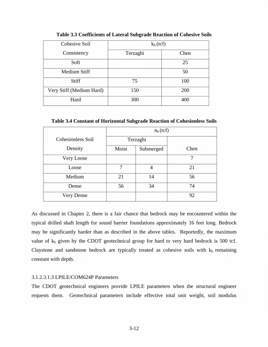
3-12

Table 3.3 Coefficients of Lateral Subgrade Reaction of Cohesive Soils

kh (tcf) Cohesive Soil

Consistency Terzaghi Chen

Soft 25

Medium Stiff 50

Stiff 75 100

Very Stiff (Medium Hard) 150 200

Hard 300 400

Table 3.4 Constant of Horizontal Subgrade Reaction of Cohesionless Soils

nh (tcf)

Terzaghi

Cohesionless Soil

Density Moist Submerged

Chen

Very Loose 7

Loose 7 4 21

Medium 21 14 56

Dense 56 34 74

Very Dense 92

As discussed in Chapter 2, there is a fair chance that bedrock may be encountered within the

typical drilled shaft length for sound barrier foundations approximately 16 feet long. Bedrock

may be significantly harder than as described in the above tables. Reportedly, the maximum

value of kh given by the CDOT geotechnical group for hard to very hard bedrock is 500 tcf.

Claystone and sandstone bedrock are typically treated as cohesive soils with kh remaining

constant with depth.

3.1.2.3.1.3 LPILE/COM624P Parameters

The CDOT geotechnical engineers provide LPILE parameters when the structural engineer

requests them. Geotechnical parameters include effective total unit weight, soil modulus

3-13

constant (k), undrained shear strength (cu), internal friction angle (φ), and the strain at 50% of the

maximum stress (ε50).

Recommendations for cu and φ are based on the previously discussed correlations relating the

parameters to SPT N-values. Unit weight values are also based on SPT results and the

engineer’s experience. The soil modulus parameter, k, has sometimes been assumed to be the

same as the coefficient of lateral subgrade reaction, kh, discussed in the previous section; the

values presented by Chen are typically provided. It must be noted that the soil modulus

parameter required as an input to LPILE is different from the coefficient of lateral subgrade

reaction concept used by Terzaghi, Broms, and others. Values for ε50 are obtained from the

LPILE User’s Manual based on the average undrained shear strength which is taken to be equal

to half of the unconfined compressive strength obtained through correlation with the SPT.

3.1.2.3.1.4 Ground Water

Any ground water that may exist at a site is not specifically factored into the geotechnical

recommendations. Friction angles or cohesion values provided to the structural designer are in

large part based on the SPT values for a given soil layer and the SPTs are generally assumed to

reflect the effects of ground water conditions. Ultimate strength design parameters are therefore

considered not greatly affected by the presence of ground water. LPILE parameters and analyses,

however, are dependent on the location of the ground water table. Logs of exploratory borings

are provided to the structural engineer and they apply the ground water condition when

appropriate. Typically, there is no conservative assumption made that the ground water level

will increase in the future. In summary, it appears that ground water levels are not a major

design factor for the CDOT design procedures.

3.1.2.3.2 Consultant Geotechnical Investigations

Geotechnical engineering consultants nearly always work as subconsultants to the transportation

design firm and structural engineers perform the actual foundation design.

3-14

3.1.2.3.2.1 Field Investigation and Laboratory Testing

Geotechnical engineering consultants generally space borings at intervals similar to those used

by CDOT. The most common interval is about 250 ft. along the length of the wall, but intervals

as great as 500 ft. have been used. Borings are rarely spaced at intervals less than 200 feet,

although boring spacing of 100 feet intervals has been used. The actual spacing may depend on

the anticipated geologic conditions, the proximity of other structure borings, and the needs of the

prime consultant. Borehole depths are typically about 20 feet, but boring depths may be

lengthened if expansive or soft soils exit. If high swelling soils are suspected, drilling depths on

the order of 30 feet are likely. Borings are also lengthened to extend through any proposed cut

areas that would be removed by grading operations.

Bore holes for consultant geotechnical investigations are advanced by either solid or hollow stem

auger drilling. Some drill rigs used by consultants have automatic hammers, but manual

hammers are frequently used as well. Samples are taken at approximately 5 feet intervals.

The typical field sampling and testing procedure is by penetration testing using a nominal 2-inch

inside diameter California spoon sampler. The procedure is very similar to the SPT procedure

(ASTM D1586) except that the blow counts for the different diameter sampler are recorded as

the first 12 inches of the drive. The California sampler is typically seated into the hole with a

few light blows of the hammer prior to recording the blow counts. Penetration testing using the

nominal 1-3/8 inch inside diameter standard split spoon is often used when cohesionless granular

soils are encountered. It is local practice to consider the blow counts achieved with both methods

to be equivalent. A small number of geotechnical consultants, believed to consist of two national

firms, use a Dames & Moore ring sampler having an internal diameter of 2.42 inches and an

outside diameter of 3.25 inches. Because the blow counts achieved with this sampler are much

greater than a standard spoon size, the consultants periodically use a standard spoon to obtain

SPT data. Push tube samples are regularly obtained in overburden materials by one company,

but this type of sampling is not considered to be standard practice for the area. Shelby tubes may

be used if soft soils are encountered, but they are not typically considered for use.

3-15

The predominant local practice of using California samplers was developed primarily to obtain

samples suitable for swell testing. California liner samples are also used to obtain relatively

undisturbed (according to local practice) samples suitable for natural unit weight and unconfined

compression testing. Brass liners 4 inches long fit snugly inside the barrel, and a typical

California barrel can accommodate four liners for a total of 16 inches. Normally, only the liner

near the tip of the barrel is saved, although two liners are saved if a material transition is noted.

A minority of consultants routinely save two liners nearest the tip of the barrel.

Laboratory testing typically includes natural moisture content and unit weight determinations,

gradations, Atterberg Limits, swell tests, and unconfined compression (UC) tests on cohesive

soil samples. Unit weight, swell testing, and UC testing are conducted on California samples

extruded from the brass liners. The Dames & Moore ring sampler can also provide samples for

these tests.

3.1.2.3.2.2 Geotechnical Design Parameters

Specific geotechnical recommendations are provided to the structural engineer depending on his

or her method(s) of analysis. Recommendations may include the coefficient of lateral subgrade

reaction, design values for cohesion or friction angle, unit weight, and/or specific LPILE input

parameters (e.g. ε50, soil modulus). Generally, soil resistance is neglected in the upper three feet

of shafts for sound barrier wall foundations to account for weakening of soils due to frost action

or moisture increases. Consulting geotechnical engineers, like their CDOT counterparts, use

their experience and engineering judgment to select appropriate geotechnical design parameters.

Like CDOT engineers, consultants rely heavily upon SPT results, but laboratory testing plays a

more prominent role in consultant practice.

3.1.2.3.2.2.1 Friction Angle and Cohesion

Empirical correlations between SPT values and friction angle of cohesionless soils or unconfined

compressive strength of cohesive soils discussed in Section 3.1.2.3.1.2 for the CDOT practice are

also used by consultants and are not repeated here. Many consultants use UC test results to aid

in evaluating an appropriate cohesion value, although cohesion may be estimated solely based on

3-16

SPT. Many geotechnical engineers evaluate all of the data available and provide design

parameters based on both SPT data and laboratory data.

It is most common to use half of the laboratory UC strength for cohesion, and this value for

cohesion may be provided as a design parameter. Less frequently, the geotechnical engineer

may provide somewhat lower values than half of the peak UC strength because some of the

observed peak strength may be due to a frictional component of the specimen and to account for

possible loss of strength if the soils become wetted. It is recognized that laboratory UC test

results can be heavily influenced by the moisture content of the sample.

3.1.2.3.2.2.2 Coefficient of Lateral Subgrade Reaction

It appears that geotechnical consultants also widely use values for the coefficient of lateral

subgrade reaction, kh, based on either the Terzaghi typical values or the historic Chen and

Associates parameters. This parameter is discussed in detail in Section 3.1.2.3.1.2 and is not

repeated since the CDOT and consulting geotechnical engineers appear to be providing similar

values. This value may be provided, with some adjustment for geometry, to structural engineers

that will perform finite element analyses.

3.1.2.3.2.3 LPILE Parameters

LPILE parameters are provided by geotechnical engineers when the structural engineer requests

them. Geotechnical parameters include effective total unit weight, soil modulus constant (k),

undrained shear strength (cu), internal friction angle (φ), and the strain at 50% of the maximum

stress (ε50). Values of each parameter may be provided for a particular soil type or values may

be provided for depth intervals below the ground surface if conditions are uniform. It is

normally left to the structural engineer to identify the locations with the most critical subsurface

conditions based on the boring logs and geotechnical parameters provided.

Recommendations for cu and φ are based on the previously discussed correlations relating the

parameters to SPT N-values or unconfined compressive strength. Unit weight values are likely

to be based on results of laboratory testing on California liner samples, SPT results, and the

3-17

engineer’s experience. Laboratory results are likely to be weighted more heavily than SPT data

in the evaluation to determine the unit weight.

The soil modulus constant, k, is provided in accordance with the LPILE User’s Manual based on

estimates of the undrained shear strength which might be based on laboratory UC tests and SPT

data. Like in CDOT practice, the k parameter has sometimes been assumed to be the same as kh

discussed previously, although it appears that most geotechnical engineering consultants

recognize the difference between the parameters.

The LPILE User’s Manual is used along with the results of UC tests and SPT data to establish

appropriate values for ε50. There seem to be two schools of thought on this subject; one school

relies on the laboratory data, and the other bases the recommendation for ε50 on the

recommendations in the user’s manual. Strains observed in samples of Colorado geomaterials

obtained with the California sampler are often higher than those recommended in the software

documentation, particularly for the harder clays and bedrock.

3.1.2.3.2.4 Ground Water

Ground water that may exist at a site is not specifically factored into the geotechnical

recommendations that will be used for an ultimate strength analysis. Values for cohesion and

friction angle are not typically adjusted to reflect any ground water condition. The coefficient of

lateral subgrade reaction may vary for sands as presented in section 3.1.2.3.1.2.

LPILE parameters and analyses, however, are dependent on the location of the ground water

table. Geotechnical recommendations for effective unit weight or submerged soil modulus

parameter k for sands are provided if ground water exists at a site. Some geotechnical engineers

may recommend that the subsurface soils below the water table be modeled as Soil Type 2, stiff

clay with water, although this would only be appropriate if permanent standing water exists

above the ground line. Typically, there is no conservative assumption made that the ground water

level will increase in the future.

3-18

3.2 Overhead Signs Practice in Colorado 3.2.1 CDOT Design Procedure Using Standard Plans CDOT engineers use standard drawings based on AASHTO documents for routine design of

overhead sign structures and their foundations. Standard Plan No. S-614-50, Sheets 1 through 14

provide structural details, as well as foundation dimensions and details. The standard plans are

available for download on CDOT’s web site. The drawings provide a procedure to determine the

required sign post diameter based on the proposed wind loading and geometry of the structure.

Foundation designs shown in the Standard Plans were developed using the Broms Method.

Several documents are referenced as design information on Sheet 1 of drawing S-614-50

including the following:

“Standard Specification for Structural Supports for Highway Signs, Luminaires, and

Traffic Signals” (1994 AASHTO), (Static Signs Only).

“Standard Specification for Structural Supports for Highway Signs, Luminaries, and

Traffic Signals” (2001 AASHTO), (Dynamic Signs Only).

“Fatigue-Resistant Design of Cantilevered Signal, Sign, and Light Supports” (NCHRP

Report 412, 1998) (Static Signs Only).

Subsection 17.4, Signs, in the Staff Bridge Branch Design Manual.

Notes on the standard plans indicate that an 80 mph wind speed is the standard design speed for

Colorado, with a few exceptions. A 90 mph wind design speed is to be used for sign locations

within 4 miles of the base of the foothills along the front range of the eastern slope, and a 100

mph wind speed is used in Boulder County.

Sign geometry inputs required to use the design tables include the sign panel height and length,

height above the base plate to the center of the sign and mast arm, and span distance. For bridge

sign structures, the design is based on a sign height of 15 feet, but sign heights of 10, 12, and 14

3-19

feet may be selected for cantilever signs. The total area of all signs attached to a sign bridge and

the span length are used to find the pipe post diameter. Pipe outside diameters range between

12.75 inches and 24 inches. Infrequently, proposed signage dimensions exceed the limits of the

standard, and specific designs must be performed.

Drilled shaft foundation dimensions tabulated on Sheet No. 14 of Standard Plan S-614-50 are

selected based on the outside pipe diameter of the sign post. Diameters range from 36 to 48

inches, and caisson depths vary from 13 to 24 feet (29 feet for dynamic cantilever sign).

Diameters are dictated by the required anchor bolt patterns. Vertical reinforcement of the

caissons consists of 13 to 24 #8 bars.

Typically, a geotechnical investigation is not performed by CDOT for design of overhead signs.

The design is based on a set of soil parameters as follows (CDOT Standard Plan No. S-614-50):

Soil unit weight = 100 pcf

Soil cohesion = 500 psf

Soil friction angle = 28 degrees

When the following soil conditions (listed in the Standard drawings) are encountered, engineers

need to be contacted for further investigation.

(a) Soils have high organic content or consists of saturated silt and clay

(b) The site won’t support the drilling rig

(c) Foundation soils are not homogeneous

(d) Firm bedrock is encountered.

3.2.2 Consultant Design Practice Consultants also use CDOT Standard Plan S-614-50 to design foundations for overhead signs.

Many consultants consider the standard drawings to be sufficiently conservative to forego

drilling exploratory borings at the sign foundation locations. However, some consultant

designers will perform geotechnical investigations at specific sign locations if it is not near other

3-20

structure borings. If a proposed sign foundation is more than about 100 feet away from another

boring, a soil boring might be made to confirm that the geotechnical conditions meet or exceed

the minimum strength characteristics noted on the standard plans as discussed in the previous

section. Caisson dimensions shown on the standard drawings are typically used even if higher

strength soils are identified.

Design for signs larger than those included in the design standard will typically be done by

consultants using the LPILE program, finite element methods, and/or other procedures discussed

in Section 3.1 for sound barriers. LPILE seems to be the most prevalent design method with

various finite element software programs being the second most common choice.

Geotechnical design parameters are determined in the same manner as for sound barrier walls

discussed in Section 3.1 and are not repeated here. Geotechnical consultants will typically

recommend that the upper 3 to 5 feet of soil be neglected in the structural analysis.

3.3 Traffic Signals Practice in Colorado

3.3.1 AASHTO Design Criteria There are no definite design criteria for foundation in AASHTO Standard Specifications for

Structural Supports for Highway Signs, Luminaries and Traffic Signals (4th Edition, 2001).

Mostly, the design of drilled shafts shall be based on Standard Specifications for Highway

Bridges. In AASHTO LRFD Bridge Design Specifications, the allowable horizontal movement at

drilled shaft head is specified as 1.5 inch for bridge foundations and the drilled shaft head should

be fixed into a foundation cap.

The design loads have been described in chapter 2 of the AASHTO Standard Specifications for

Structural Supports for Highway Signs, Luminaries and Traffic Signals (4th Edition, 2001). The

AASHTO standard specifications also suggest the use of Broms method for the design of drilled

shaft under lateral loads.

3-21

3.3.2 CDOT Design Practice CDOT Standard Plan Nos. S-614-40 (7 sheets) and S-614-40A (5 sheets – Alternate Design) are

used for the routine installation of traffic signal structures and their foundations. Structural

details, as well as foundation dimensions and details are provided in the standard plans available

for download on CDOT’s web site. The drawings prescribe caisson dimensions based on the

signal mast arm length.

Foundation dimensions shown in the Standard Plans were developed based on AASHTO

“Standard Specification for Structural Supports for Highway Signs, Luminaires, and Traffic

Signals” (4th Edition, 2001). A design wind velocity of 100 mph and one 12 ft. lane for truck

induced gust loading were used for the design.

Design parameters appear on the CDOT standard drawings. Overturning analyses were

performed based on Broms procedure as discussed in the AASHTO code. Torsion was also

analyzed using a sliding wedge theory for granular soils and cohesive resistance for clayey soils.

Drilled shaft foundation dimensions are shown on Sheet No. 6 of Standard Plan S-614-40.

Caisson diameters are dictated by the anchor bolt pattern and range from 36 to 54 inches for mast

arm lengths of 30 to 75 feet. Required caisson depths vary from 12 to 20 feet. Vertical

reinforcement of the caissons consists of 11 to 23 #9 bars. For the alternate traffic signal

installation, foundation details are shown on Sheet No. 4 of Standard Plan S-614-40A. 36-inch

diameter caissons are required, and they are 14 feet long for cohesionless soils and 18 feet long

for cohesive soils.

Geotechnical investigations are rarely, if ever, performed by CDOT for design of traffic signals.

The design is based on a set of soil parameters as follows (CDOT Standard Plan No. S-614-40):

Soil unit weight = 110 pcf

Soil cohesion = 750 psf

Soil friction angle = 30 degrees

3-22

Safety factors used by CDOT for flexure and torsion design are:

Flexure Factor of Safety (FS) = 3.0

Torsion FS: FS = 1.5 (Dwg. S-614-40)

FS = 1.25 (Dwg. S-614-40A)

The low safety factors for torsion were chosen by CDOT to prevent torsion from needlessly

controlling drilled shaft depths based on field observations indicating that the vast majority of

traffic signals performed well. The very few unsuccessful foundation installations were due to

installing signal foundations in saturated clay soils with high ground water tables.

When the following soil conditions (listed in the Standard drawings) are encountered, engineers

need to be contacted for further investigation.

a) Signals will not be installed within the roadway prism

b) Soils have high organic content or consists of saturated silt and clay

c) The site won’t support the drilling rig

d) Foundation soils are not homogeneous

e) Firm bedrock is encountered

3.3.3 Consultant Design Practice Consultants also use the CDOT standard drawings for traffic signals. We are not aware of any

situations where site specific designs or geotechnical investigations were conducted for traffic

signals on CDOT projects. Site specific investigations for some cities and counties have been

performed by consultants, and the procedures discussed in Section 3.1 were used for design.

3.4 AASHTO Specification The AASHTO and Ohio DOT design criteria of drilled shaft for supporting sound barrier walls,

overhead signs, and traffic signals are presented in this chapter. Suggested design criteria based

3-23

on this review are then summarized. Specifically, the analysis methods, loads specifications,

tolerable deflection at the drilled shaft top, and factor of safety will be covered.

The AASHTO loads specifications for sound barrier walls were reviewed in section 3.1.2. The

design pressure on wall face could range from 20 psf to 40 psf, with a typical design value of 27

psf. The sound barrier wall height in Colorado typically varies from 14 to 18 feet, while the

typical spacing of drilled shaft ranges from 7’4’’ to 23’4’’. Therefore, the force applied to the

drilled shaft head can be approximated from the multiplication of wind pressure and the tributary

wall area. The maximum, typical, and minimum lateral loads applied to the drilled shaft head are

therefore 16.8 kips, 11.3 kips, and 2 kips, respectively. The moment due to each lateral load is

the load multiplied by half of the wall height.

The design method for lateral response of drilled shaft specified in the AASHTO Guide

Specifications for Structural Design of Sound Barriers (2002) is sheet piling method taken from

the U.S.S. Steel Sheet Piling Design Manual. The sheet piling method is one of several ultimate

strength methods. The details of the sheet piling method are reviewed in Section 3.1.2.2.1.1 and

Appendix B.

As to the tolerable deflection of drilled shaft and Factor of Safety, there are no specifications in

AASHTO Guide Specifications for Structural Design of Sound Barriers (1989, 2002 interim).

However, in the AASHTO LRFD Bridge Design Specifications (2nd Edition, 1998 with 2003

interim), the allowable horizontal movement at drilled shaft head is specified as 1.5 inch for

bridge foundations.

3.5 ODOT Design Practice

In Ohio DOT practice, the standard foundation for sound barrier walls is a single 30 inch

diameter drilled shaft. The design load is calculated based on an 80 mph wind velocity producing

a uniform pressure of 25 psf over the tributary area of the wall.

3-24

The ODOT design criterion is based on the tolerable deflection at the top of the wall to be 1% of

the wall height. The computer program COM624P is usually used as the design method since the

design criterion is based on the serviceability, i.e., tolerable wall deflection.

Liang (1997) developed design charts for both 1% and 1.5% wall height as allowable deflections

at wall top. Table 3.5 to Table 3.8 are reproduced in this report for both cohesive soil and

cohesionless soil deposits. It should be noted that the design tables were based on correlations

between COM624P input parameters and SPT N values. The SPT blow count was assumed to be

corresponding to 60% energy efficiency, hence the subscript 60 shown in the tables. The blow

count number should be adjusted for overburden pressure to standard practice of 1 tsf. Table 3.9

and Table 3.10 provide the updated correlations based on a more extensive sensitivity study on

the enhanced lateral load test database (Liang 2002).

3-25

Table 3.5 Design Chart for Cohesive Soil (Allowable Deflection 1.0% of Wall Height) N60 0-2 2-4 4-8 8-16 16-32

Post Spacing (feet) Su (psi) 0-1.74

1.74-3.47

3.47-6.94

6.94-13.89

13.89-27.78

ε50 >0.02 0.02 0.01 0.007 0.005 ks (pci) <30 30 100 300 1000

8 and under Over 8 Thru 12 Over 12 Thru 16 Over 16 Thru 24

Group

γsat

(pcf) 100-120

110-130

110-130

120-135 130-145

Level 14.0 13.5 7.5 5.5 4.0 5:1 14.5 14.5 8.0 5.5 4.0 4:1 15.0 14.5 8.0 5.5 4.0 3:1 15.5 15.5 8.0 6.0 4.0

12 and less 10 and less 8 and less 6 and less I

2:1 16.0 16.0 8.5 6.0 4.0 Level 19.5 18.0 10.0 8.0 5.5 5:1 20.0 19.5 10.5 8.0 5.5 4:1 20.5 20.0 11.0 8.0 5.5 3:1 21.0 21.0 11.0 8.5 5.5

Greater than 12 thru 16




II

2:1 22.0 21.5 11.5 8.5 5.5 Level 23.0 23.0 14.0 10.0 7.0 5:1 25.0 25.0 15.5 10.0 7.0 4:1 25.0 25.0 15.5 11.0 7.5 3:1 26.0 26.5 16.0 11.5 7.5





III

2:1 27.0 26.5 17.0 11.5 7.5 Level * * 21.0 13.5 9.0 5:1 * * 24.0 14.5 9.0 4:1 * * 28.0 14.5 9.5 3:1 * * 29.0 15.0 9.5

B A R R I E R

H E I G H T

(FT) Greater than 16

thru 20 Greater than 14

thru 20 IV

2:1 * * * 15.0 10.0

3-26

Table 3.6 Design Chart for Cohesive Soil (Allowable Deflection 1.5% of Wall Height) N60 0-2 2-4 4-8 8-16 16-32

Post Spacing (feet) Su (psi) 0-1.74

1.74-3.47

3.47-6.94

6.94-13.89

13.89-27.78

ε50 >0.02 0.02 0.01 0.007 0.005 ks (pci) <30 30 100 300 1000

8 and under Over 8 Thru 12 Over 12 Thru 16 Over 16 Thru 24

Group

γsat

(pcf) 100-120

110-130

110-130

120-135 130-145

Level 12.5 12.5 7.0 5.0 4.0 5:1 13.5 13.5 7.5 5.0 4.0 4:1 13.5 13.5 7.5 5.0 4.0 3:1 14.0 14.0 8.0 5.0 4.0

12 and less 10 and less 8 and less 6 and less I

2:1 14.5 15.0 8.0 5.5 4.0 Level 17.0 17.0 9.5 7.5 5.0 5:1 18.5 18.5 10.0 8.0 5.0 4:1 19.0 18.5 10.5 8.0 5.0 3:1 19.5 19.0 10.5 8.0 5.0





II

2:1 20.0 20.0 11.0 8.5 5.5 Level 21.5 21.0 13.5 9.5 6.5 5:1 23.0 23.0 14.5 10.0 7.0 4:1 23.5 23.0 14.5 10.0 7.0 3:1 25.0 24.0 15.0 10.5 7.0





III

2:1 25.5 24.5 16.0 11.0 7.0 Level * * 19.0 13.0 9.0 5:1 * * 20.5 14.0 9.0 4:1 * * 21.0 14.5 9.0 3:1 * * 22.0 15.0 9.5

B A R R I E R

H E I G H T

(FT) Greater than 16

thru 20 Greater than 14

thru 20 IV

2:1 * * 24.0 15.0 10.0

3-27

Table 3.7 Design Chart for Cohesionless Soil (Allowable Deflection 1.0% of Wall Height) N60 2-4 4-10 10-20 20-30 30-50 50-60

Post Spacing (feet) Φ 25-32 27-35 30-38 32-40 34-43 36-44

AWT <25 25 90 90 225 250 ks (pci)

BWT <20 20 60 60 125 140

L 104 to

108 108 to

112 115 to

120 120 to

125 124 to

128 128 to

130

8 and under

Over 8 Thru 12

Over 12 Thru 16

Over 16 Thru 24

Group

γmoist

(pcf) U

114 to 118

120 to 124

122 to 130

128 to 132

130 to 145

140 to 145

Level 9.0 9.0 7.0 6.0 5.5 5.0 5:1 9.0 9.0 7.5 6.5 6.0 5.5 4:1 9.5 9.5 7.5 7.0 6.5 6.0 3:1 9.5 9.5 8.0 7.5 7.0 6.5

12 and less 10 and

less 8 and less 6 and less I

2:1 10.5 10.5 8.5 8.0 7.5 7.0 Level 10.5 10.5 8.5 8.0 8.0 6.5 5:1 11.0 10.5 9.0 9.0 8.5 7.0 4:1 11.5 11.0 9.5 9.0 8.5 7.5 3:1 12.0 11.5 10.0 9.5 9.0 8.0





II

2:1 13.0 13.0 11.0 10.0 10.0 8.5 Level 12.5 12.0 10.0 9.0 9.0 9.0 5:1 13.5 12.5 11.0 10.5 9.5 9.5 4:1 13.5 13.0 11.5 10.5 10.0 10.0 3:1 14.5 13.5 12.0 10.5 10.0 10.0





III

2:1 15.5 15.5 13.0 11.5 11.0 11.0 Level * * 14.0 13.5 11.5 11.0 5:1 * * 18.0 16.0 13.0 13.0 4:1 * * 20.0 17.5 14.0 14.0 3:1 * * 23.0 21.0 16.0 16.0

B A R R I E R

H E I G H T

(FT) Greater than 16 thru 20


IV

2:1 * * * 23.0 20.0 17.0

3-28

Table 3.8 Design Chart for Cohesionless Soil (Allowable Deflection 1.5% of Wall Height) N60 2-4 4-10 10-20 20-30 30-50 50-60

Post Spacing (feet) Φ 25-32 27-35 30-38 32-40 34-43 36-44

AWT <25 25 90 90 225 250 ks (pci)

BWT <20 20 60 60 125 140

L 104 to

108 108 to

112 115 to

120 120 to

125 124 to

128 128 to

130

8 and under

Over 8 Thru 12

Over 12 Thru 16

Over 16 Thru 24

Group

γmoist

(pcf) U

114 to 118

120 to 124

122 to 130

128 to 132

130 to 145

140 to 145

Level 8.0 8.0 6.5 6.0 5.5 5.0 5:1 8.0 8.0 7.0 6.5 6.0 5.5 4:1 8.5 8.5 7.0 7.0 6.0 6.0 3:1 9.0 8.5 7.5 7.0 6.5 6.5

12 and less 10 and

less 8 and less 6 and less I

2:1 10.0 9.5 8.0 7.5 7.0 6.5 Level 9.5 9.5 8.0 7.5 7.5 6.5 5:1 10.5 10.0 8.5 8.0 8.0 7.0 4:1 11.0 10.5 9.0 8.5 8.0 7.5 3:1 11.5 11.0 9.5 9.0 8.5 7.5





II

2:1 12.5 12.0 10.0 9.5 9.0 8.0 Level 11.5 11.0 9.5 9.0 8.0 8.0 5:1 12.5 11.5 10.0 10.0 8.5 8.5 4:1 13.0 12.0 10.5 10.5 9.0 8.5 3:1 13.5 13.0 11.0 10.5 9.5 9.0





III

2:1 14.5 14.5 12.0 11.5 10.0 9.5 Level 15.5 14.0 12.0 11.0 10.5 10.5 5:1 19 16.0 13.5 12.5 11.0 11.0 4:1 20.5 17.5 14.0 13.0 12.0 11.5 3:1 24.0 19.5 15.0 14.0 12.5 12.0

B A R R I E R

H E I G H T

(FT) Greater than 16 thru 20


IV

2:1 * 30.0 19.0 16.0 14.0 13.0

3-29

Table 3.9 Correlation of Cohesionless Soil for Predicting Lateral Deflection

N60 2 to 4 4 to 10 10 to 20 20 to 30 30 to 50 50 to 60

φ 25 to 35 30 to 38 33 to 41 35 to 43 37 to 45 39 to 48

A.W.T. < 25 25 90 90 225 250 ks

lb/in3 B.W.T. < 20 20 60 60 125 140

Min. 104 to

108

108 to

112

115 to

120

120 to

125

124 to

128

128 to

130 γmoist

pcf Max.

114 to

118

120 to

124

122 to

130

128 to

132

130 to

145

140 to

145

Table 3.10 Correlations of Cohesive Soil for Predicting Lateral Deflection

N60 0 to 2 2 to 4 4 to 8 8 to 16 16 to 32 32 to 64

Su (psi) 0 to 1.88 1.88 to

3.75

3.75 to

7.53

7.53 to

15.00

15.00 to

30.00

30.00 to

55.6

ε50 > 0.02 0.02-0.01 0.01 to

0.007

0.007 to

0.005

0.005 to

0.004

0.004 to

0.002

ks(lb/in3) < 30 30 100 500 1000 2000

γsat (pcf) 100 to

120

110 to

130 110 to 130 120 to 135 130 to 145 140 to 145

4-1

4 COMPARISON AND EVALUATION OF ANALYSIS METHODS Existing analysis methods for drilled shafts under lateral loads were first evaluated on the basis

of several assumed hypothetical conditions involving relatively uniform soil deposits with

typical soil properties and typical shaft dimensions and embedment lengths. This was intended to

provide a basis of comparison of the results of various analysis methods.

In addition to hypothetical cases, a database was established from the review of existing open

literature as well as from numerous lateral load tests previously conducted by the principal

investigators for the ODOT. The compiled database was limited to contain only drilled shafts

with the dimensions of typical drilled shafts currently in use by CDOT. Efforts were also made

to compile a limited database for torsional load tests. Based on comparisons between the results

of existing analysis methods and load test databases complied for this study, appropriate analysis

methods were recommended for analysis and design of drilled shafts subjected to lateral and/or

torsional loads.

The effects of loading rate, cyclic degradation, and ground water on soil stiffness and strength

are also summarized based on pertinent literature review. This discussion is intended to provide

qualitative understanding of the possible implications of transient wind loads.

Calibrations of resistance factors for the Broms method are also presented. The recommended

factor of safety of two seemed to yield a similar resistance factor as determined from reliability

based calibration using a target reliability index of 2.5.

4.1 Hypothetical Cases For the purpose of comparing predictions made by various existing analysis methods, several

hypothetical cases involving uniform soil profile and typical soil properties together with typical

drilled shaft dimensions are assumed. The selected typical properties for clay, sand, and rock are

summarized in Table 4.1, along with the drilled shaft properties.

4-2

Table 4.1 Assumed Properties of Sand, Clay, Rock, and Drilled Shafts in a Comparison

Study for Hypothetical Cases

Properties Sand (Medium Dense) Clay (Medium

Stiff)

Rock

(Limestone)

Drilled

Shaft

γ (pcf) 110 110 156 150

E (ksf) 700 150 1.0E6 5.2E5

ν 0.3 0.5 0.3 0.2

G (ksf) 269 50 3.8E5 2.17E5

φ (Degree) 30 0 40

δ (Degree) 20 0 30

Cu (ksf) 0 0.75 200

ks (pci) 25 100

ε50 0.009

Note: γ=unit weight; E= Young’s Modulus; ν= Poisson’s ratio; G= shear modulus; φ= friction

angle; δ= friction angle between shaft and soils; Cu= undrained shear strength; ks = modulus of

horizontal subgrade reaction; ε50= strain at half of the maximum principal stress difference.

4.1.1 Lateral Response of Drilled Shafts Fig. 4.1 provides a schematic diagram of the hypothetical case of laterally loaded shafts,

depicting the soil profile, the drilled shaft dimensions, and the location of applied lateral loads.

As indicated in the figure, two soil profiles are studied, one is a clay deposit and the second one

is a sand deposit. The methods of analysis investigated include Broms method, sheet piling

method, Caisson program, and the COM624P program. The Brinch Hansen method and the

NAVFAC DM7 method were not evaluated for these hypothetical cases because these two

methods were not considered in the initial course of the study; however, they will be evaluated

with existing lateral load test database.

The calculated results from these analysis methods are tabulated in Table 4.2 which includes

both ultimate lateral capacity and maximum moment. The comparison of capacity estimates is

also presented in Fig. 4.2. It is noted that the methods used by CDOT (i.e., the sheet piling

method and the caisson program) were not applied to the case of cohesive soil deposit due to the

4-3

fact that these methods were not intended for such soil types. For the sandy soil profile studied, it

can be seen that the sheet piling method and COM624P program tend to give relatively lower

estimates of the ultimate capacity compared to the Broms method and Caisson program’s

predictions.

Table 4.2 Summary of Calculated Lateral Capacities and Maximum Moments of Drilled

Shafts in Hypothetical Cases

Methods

Soils Broms Method (Ultimate)

COM624P (At deflection 2.4”)

Sheet piling Method (Isolation Factor = 2)

Caisson program (Ultimate)

Lateral Capacity (kips)

55.7 32 40 55.8

Sand Maximum Moment (kip -ft)

806 549 NA 899


24.8 16 NA NA

Clay Maximum Moment (kip -ft)

360 239 NA NA

4.1.2 Torsional Response of Drilled Shafts For the torsional response of the drilled shaft, four hypothetical soil profiles depicted in Fig. 4.3

are used for comparing five different analysis methods listed in Table 4.3. The calculated

ultimate torsion capacities are summarized in Table 4.3, while the torsional stiffness defined as

torsion divided by twist angle is shown in Table 4.4. The comparison of torsional capacity

estimates in a bar chart is also presented in Fig. 4.4. It can be seen that the CDOT method tends

to predict the highest value of ultimate torsion capacity for all the cases investigated. On the

other hand, the difference of the estimated torsional stiffness among other methods is very small,

roughly within 25% for the simple soil profiles investigated. This is not surprising because most

of these methods are based on similar theoretical basis.

4-4

Table 4.3 Comparison of Ultimate Torsional Capacity Estimated by Various Methods in

Hypothetical Cases

Torsional Capacity (kips-ft)

Soil

Profiles

Florida

Structures

Design

Office

(sand)

Modified

Florida

District 5

Method

(sand)

Florida

District

7

Method

(clay)

Florida

District

5

Method

Colorado

Dept. of

Trans.

(sand &

clay)

Sand 25.4 52 30.32 26.13 91.8

Clay N/A N/A 44.2 44.23 85.9

Sand over

Rock 30.21 60.61 N/A N/A N/A

Note: 1: The method was initially developed for cohesionless soils. 2: The method was initially developed for cohesive soils. 3: The side resistance is the same with Florida District 7 Method.

Table 4.4 Comparison of Calculated Torsional Stiffness at Shaft Head in Hypothetical

Cases

Torsional Stiffness (Tt/φt, 104 kips-ft)

Soil

Profiles Poulos

(1975)

Randolph

(1981)

Chow

(1985)

Hache &

Valsangkar

(1988)

Carter&

Kulhawy

(1988)

Sand 4.9 5.6 5.9 6.2 N/A

Clay 1.3 1.4 1.3 1.1 N/A

Rock only 297 249 N/A N/A 249

4.2 Load Test Database 4.2.1 Selected Lateral Load Test Database There are quite a few lateral load test data available in the literature, such as Florida DOT’s

database compiled by University of Florida. However, only a small part of the existing test data

is related to the shaft diameter between 20 inches and 36 inches and shaft length between 6 feet

4-5

and 30 feet, which are the dimensions commonly found in the CDOT sound wall foundation

practice. After searching the available test data, only 3 lateral load tests with 7 tested drilled

shafts in clay are selected from the ODOT Database, and one test with 5 tested drilled shafts

conducted in sand by Bhushan et al. (1981) is selected. To enlarge the database for drilled shaft

tests in sand, drilled shafts with 42 inch and 48 inch diameters are also included.

Table 4.5 provides a brief summary of the content of the selected database for lateral load tests in

clay. The details of the database for drilled shafts in clay are presented in Appendix D, including

soil profiles, SPT N values, the correlated soil parameters for analysis, and the measured load-

deflection data. The test shafts information and relevant soil properties for the database for sand

are given in Table 4.6 and Table 4.7, respectively.

Table 4.5 Selected Database for Lateral Response of Drilled Shafts in Clay

No. Project Name

Depth of

Shaft

(L) in ft

Diameter of

Shaft

(D) in inches

Predominant

Soil Type

1 I-70 (Columbus, OH), Shaft 1 9.5 30 Clay

2 I-70 (Columbus, OH), Shaft 2 9.5 30 Clay

3 I-90 Sound Barriers, Shaft 2 12 30 Clay

4 I-90 Sound Barriers, Shaft 3 8’-8” 30 Clay

5 I-90 Sound Barriers, Shaft 4 8’-5” 30 Clay

6 I-90 Noise Wall, Shaft 1 (P101) 12 30 Clay

7 I-90 Noise Wall, Shaft 2 (P100) 10 36 Clay

Note: All the tests were conducted in Ohio.

4-6

Table 4.6 Selected Database for Lateral Response of Drilled Shafts in Sand

Pier

Number Diameter(ft)

Embedded

Length(ft)

Test

Site

Concrete

Modulus

(psi) Reinforcement

1 3.51 17 A 3000000 NA

4 2 18 B 4330000 14 #11 bars

5 3 18 B 4330000 14 #11 bars

6 3 18 C 4330000 14 #11 bars

7 4 18 C 4330000 14 #11 bars

Note 1: Piers were constructed with a 5-ft diameter bell near the bottom 2 ft.

Table 4.7 Test Site Information for Drilled Shafts in Sand

Test Site Soil Type

Depth

(ft)

Total Unit

Weight

(pcf)

Friction

Angle

(degree)

Relative

Density

(%)

sand (SP-SM) 0-8 105 38 55 A

sand (SP-SM) 8~15 110 40 67

silty sand (SM) 0-3 105 36 77

B

silty sand (SM)

w/gravelly layers 3~18 105 42 88

silty sand (SM) 0-6 105 36 38

C

silty sand (SM)

w/gravelly layers 6~18 105 42 92

4.2.2 Torsional Load Test Database There is a dearth of torsional load test data available in the open literature. Table 4.8 provides a

brief summary of the existing torsional load test results collected under this research effort. The

most recent torsional load tests on drilled shafts were reported by Tawfiq (2000). It appears that

4-7

the geotechnical community can benefit from more torsional load test results. Pertinent test data,

including soil properties and drilled shaft dimensions are compiled in Table 4.9. It should be

noted that other than Tawfiq (2000b), all other test data are related to small-size model piles.

Thus, one needs to be cautious in interpreting analysis and test results.

Table 4.8 Compilation of Existing Data for Torsional Response of Piles/Drilled Shafts

Investigator Test Description Pile Soil Available Data Stoll (1972) • The first field

torsion load tests.

• 2 piles • Simple loads

• Steel pipe piles filled with concrete.

• Length: 57ft. and 68 ft.

• 10.75 in.-OD, 0.25 in.-wall

Clay • 2 pile head torque-twist curves.

Poulos (1975)

• Model pile tests

• Simple loads

• Solid aluminum piles

• Length: 6 - 20 in. • Diameter: 0.5 - 1.5

in.

Kaolin clay • 4 pile head torque-twist curves.

Dutt (1976) • Model pile tests

• Simple loads

• Soft aluminum pipe piles

• 1.9 in. OD-0.1 in. wall, Circular

• 2.0 in.-0.125 in. wall, Square

• Length: 5 ft.

Sand • 4 pile head torque-twist curves.

• 3 torque distribution along pile curves.

• 3 torque transfer versus twist curves.

Tawfiq (2000a)

1 Scaled model tests

2 Simple loads and combined loads

3 Concrete piles 4 Diameter: 4 in. 5 Length: 20 in.

Sand 6 6 pile head torque-twist curves.

Tawfiq (2000b)

• 3 Full scaled field tests

• Combined lateral, overturning and torsional loads

• Reinforced concrete piles

• Diameter: 4 feet • Length: 20 feet

Sand • 3 pile head torque-twist curves.

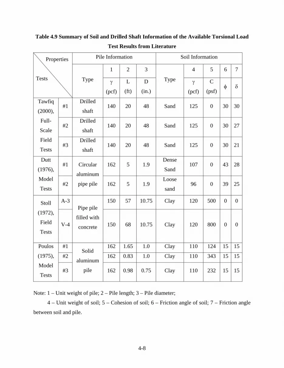
4-8

Table 4.9 Summary of Soil and Drilled Shaft Information of the Available Torsional Load

Test Results from Literature

Pile Information Soil Information

1 2 3 4 5 6 7

Properties

Tests

Type γ

(pcf)

L

(ft)

D

(in.)

Type γ

(pcf)

C

(psf) φ δ

#1 Drilled

shaft 140 20 48 Sand 125 0 30 30

#2 Drilled

shaft 140 20 48 Sand 125 0 30 27

Tawfiq

(2000),

Full-

Scale

Field

Tests #3

Drilled

shaft 140 20 48 Sand 125 0 30 21

#1 162 5 1.9 Dense

Sand 107 0 43 28

Dutt

(1976),

Model

Tests #2

Circular

aluminum

pipe pile 162 5 1.9 Loose

sand 96 0 39 25

A-3 150 57 10.75 Clay 120 500 0 0 Stoll

(1972),

Field

Tests V-4

Pipe pile

filled with

concrete 150 68 10.75 Clay 120 800 0 0

#1 162 1.65 1.0 Clay 110 124 15 15

#2 162 0.83 1.0 Clay 110 343 15 15

Poulos

(1975),

Model

Tests #3

Solid

aluminum

pile 162 0.98 0.75 Clay 110 232 15 15

Note: 1 – Unit weight of pile; 2 – Pile length; 3 – Pile diameter;

4 – Unit weight of soil; 5 – Cohesion of soil; 6 – Friction angle of soil; 7 – Friction angle

between soil and pile.

4-9

4.3 Evaluation of Analysis Methods with Load Test Data 4.3.1 Lateral Load Test Results The database established in section 4.2 is used for evaluating the accuracy of various analysis

methods. A comparison of the results is presented in this section.

4.3.1.1 Hyperbolic Curve Fit

Usually, the lateral load tests do not reach the stage of complete soil failure; therefore, the

ultimate lateral capacity is not directly available from test results. Kulhawy and Chen (1995)

developed a hyperbolic curve fit technique to simulate the non-linear load-deflection behavior

and to predict the ultimate capacity of piles (drilled shafts). The hyperbolic equation in terms of

the lateral load (H) and the lateral deflection (δ) can be expressed as follows:

δ+

δ=

baH (4.1)

where a and b are curve fitting constants. The ultimate lateral load capacity can be calculated as

Hh = 1/b.

4.3.1.2 Ultimate Capacity Estimation - Clay

The analysis methods used to estimate ultimate lateral capacity of drilled shafts in clay include

Broms method and Brinch Hansen method. The Caisson program and Sheet piling method were

not evaluated, since they were intended only for the analysis of drilled shafts embedded in sand.

The undrained shear strength of cohesive soils which were correlated from SPT N values by

using Table 3.6 and then averaged with the weighted average on the basis of the soil layer

thickness, together with lateral loading conditions, are summarized in Table 4.10.

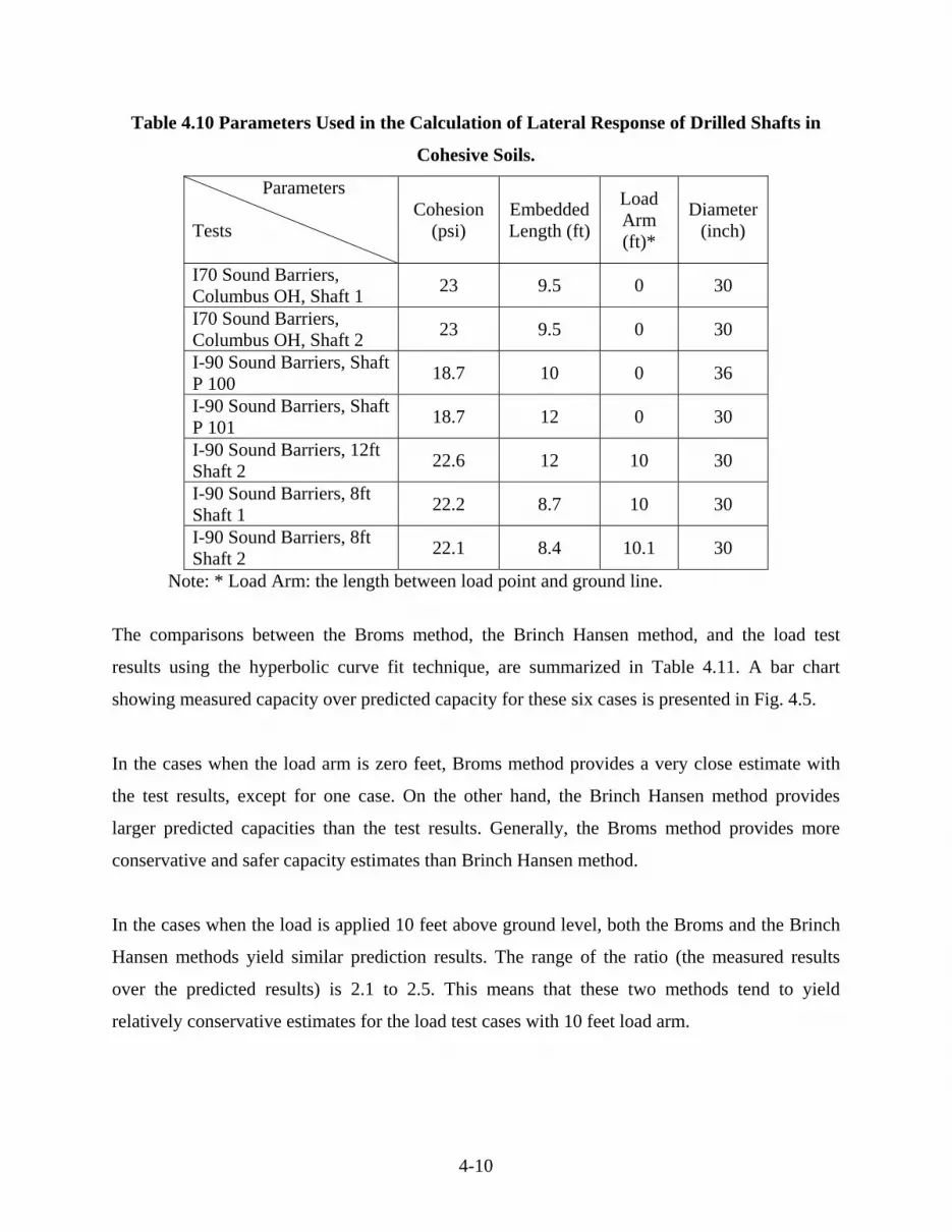
4-10


Cohesive Soils.

Parameters Tests

Cohesion (psi)

Embedded Length (ft)

Load Arm (ft)*

Diameter (inch)

I70 Sound Barriers, Columbus OH, Shaft 1 23 9.5 0 30

I70 Sound Barriers, Columbus OH, Shaft 2 23 9.5 0 30

I-90 Sound Barriers, Shaft P 100 18.7 10 0 36

I-90 Sound Barriers, Shaft P 101 18.7 12 0 30

I-90 Sound Barriers, 12ft Shaft 2 22.6 12 10 30

I-90 Sound Barriers, 8ft Shaft 1 22.2 8.7 10 30

I-90 Sound Barriers, 8ft Shaft 2 22.1 8.4 10.1 30

Note: * Load Arm: the length between load point and ground line.

The comparisons between the Broms method, the Brinch Hansen method, and the load test

results using the hyperbolic curve fit technique, are summarized in Table 4.11. A bar chart

showing measured capacity over predicted capacity for these six cases is presented in Fig. 4.5.

In the cases when the load arm is zero feet, Broms method provides a very close estimate with

the test results, except for one case. On the other hand, the Brinch Hansen method provides

larger predicted capacities than the test results. Generally, the Broms method provides more

conservative and safer capacity estimates than Brinch Hansen method.

In the cases when the load is applied 10 feet above ground level, both the Broms and the Brinch

Hansen methods yield similar prediction results. The range of the ratio (the measured results

over the predicted results) is 2.1 to 2.5. This means that these two methods tend to yield

relatively conservative estimates for the load test cases with 10 feet load arm.

4-11

Table 4.11 Summary of Calculated Lateral Capacity of Drilled Shafts in Cohesive Soils

Col. 1 Col. 2 Col. 3 Methods Soils Load Test

(hyperbolic fit) Hh

Broms Method

Brinch Hansen Method

Col. 1 /Col. 2

Col. 1 /Col. 3

I70 Sound Barriers, Columbus OH, Shaft 1

Lateral Capacity (kips) 92

90

120

1 0.77

I70 Sound Barriers, Columbus OH, Shaft 2

Lateral Capacity (kips) >601 90 120 NA NA

I-90 Sound Barriers, Shaft P 100


78 73 99.8 1.1 0.78

I-90 Sound Barriers, Shaft P 101


85 123 129.6 0.7 0.66

I-90 Sound Barriers, 12ft Shaft 2


161 67 67.6 2.4 2.4



71 34 34.9 2.1 2.0



70 28 32.5 2.5 2.2

1: The measured load-deflection curve does not appear highly nonlinear, hyperbolic fit method

can not make accurate estimation.

4.3.1.3 Ultimate Capacity Estimation - Sand

The analysis methods for estimating the ultimate capacity of drilled shafts in sand include the

Broms method, the Brinch Hansen method, the Caisson program, and the Sheet piling method.

The average soil friction angles, which are weight averaged from the friction angles shown in

Table 4.7, are summarized in Table 4.12

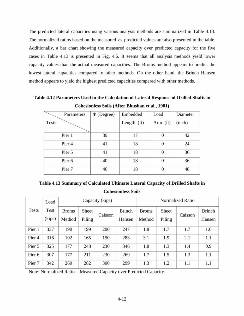
4-12

The predicted lateral capacities using various analysis methods are summarized in Table 4.13.

The normalized ratios based on the measured vs. predicted values are also presented in the table.

Additionally, a bar chart showing the measured capacity over predicted capacity for the five

cases in Table 4.13 is presented in Fig. 4.6. It seems that all analysis methods yield lower

capacity values than the actual measured capacities. The Broms method appears to predict the

lowest lateral capacities compared to other methods. On the other hand, the Brinch Hansen

method appears to yield the highest predicted capacities compared with other methods.


Cohesionless Soils (After Bhushan et al., 1981)

Parameters

Tests

Ф (Degree) Embedded

Length (ft)

Load

Arm (ft)

Diameter

(inch)

Pier 1 39 17 0 42

Pier 4 41 18 0 24

Pier 5 41 18 0 36

Pier 6 40 18 0 36

Pier 7 40 18 0 48

Table 4.13 Summary of Calculated Ultimate Lateral Capacity of Drilled Shafts in

Cohesionless Soils

Capacity (kips) Normalized Ratio

Tests

Load

Test

(kips) Broms

Method

Sheet

Piling Caisson

Brinch

Hansen

Broms

Method

Sheet

Piling Caisson

Brinch

Hansen

Pier 1 337 190 199 200 247 1.8 1.7 1.7 1.6

Pier 4 316 102 165 150 283 3.1 1.9 2.1 1.1

Pier 5 325 177 248 230 346 1.8 1.3 1.4 0.9

Pier 6 307 177 211 230 269 1.7 1.5 1.3 1.1

Pier 7 342 260 282 300 299 1.3 1.2 1.1 1.1

Note: Normalized Ratio = Measured Capacity over Predicted Capacity.

4-13

4.3.1.4 Load-Deflection Prediction - Clay

The ability of COM624P (LPILE) and NAVFAC DM-7 to predict the load-deflection curve for

laterally loaded shafts in clay is evaluated and the comparison plots are shown in Fig. 4.7

through Fig 4.13 for each of seven load tests. The soil parameters used in COM624P are

interpreted from the SPT correlation method and summarized in Appendix D. The subgrade

reaction coefficients used in NAVFAC DM-7 method are correlated from Chen’s correlation

discussed in Section 2.1.1.2.2.

For the cases with a zero foot load arm, the NAVFAC DM-7 predictions tend to either match

with test results or to be larger than measured in the initial linear part of the load-deflection curve.

The COM624P prediction, on the other hand, shows good agreement with the measured load-

deflection curves and yields safer results in the non-linear part of the load-deflection curve.

For the cases where a 10 foot load arm was involved, the NAVFAC DM-7 predictions seem to

agree well with the initial part of the measured load-deflection. The COM624P, on the other

hand, does not seem to be able to provide good matches for these three cases. The predicted

deflection, however, is larger than measured, and therefore, it is on safe side.

In general, it seems that NAVFAC DM-7 can yield a good prediction on the linear part of the

load-deflection response for the drilled shafts in clay, but it cannot capture the non-linear

behavior. The COM624P, however, does provide a fairly reasonable, but somewhat conservative,

prediction of the load-deflection behavior of all seven cases. It is particularly true that COM624P

tends to over predict the deflections for the drilled shafts subjected to combined lateral loads and

moments.

4.3.1.5 Load-Deflection Prediction - Sand

The ability of COM624P (LPILE) and NAVFAC DM-7 to predict the load-deflection behavior

of drilled shafts in sand was investigated and a comparison of the results are plotted in Fig. 4.14

through Fig 4.18. The soil parameters used in COM624P were interpreted from SPT and CPT

test by Bhushan et al. (1981), and they are shown in Table 4.7. The subgrade reaction

coefficients used in the NAVFAC DM-7 method are obtained from Chen’s correlation.

4-14

The NAVFAC DM-7 method yields larger deflections than those predicted by the COM624P

method or those actually measured, particularly in the elastic portion. COM624P prediction

shows good agreement with the initial portion of the measured load-deflection curves. However,

it overestimates the deflections in the nonlinear portion of the curve. The COM624P nevertheless

provides fairly reasonable, but somewhat conservative, predictions of the load-deflection

behavior of all five cases.

4.3.1.6 Permissible Deflection at Drilled Shaft Head - Clay

To establish a sense of linkage between the shaft deflection and shaft capacity, the capacity

values predicted by COM624P according to different permissible deflection criteria (e.g., 0.6

inch, 1 inch, and 1.5 inch), are presented in Table 4.14. The factor of safety calculated on the

basis of the ratio between the deflection based capacity and the actual test capacity is also shown

in the table. Additionally, a chart showing measured capacities over predicted capacities at these

three permissible deflections is presented in Fig. 4.19. From Table 4.14, one can see that the

Factor of Safety ranges from 1.2 to 1.8, for the cases where the load arm equals 0 feet, and from

3.3 to 4.7 for the cases with a 10 foot load arm, respectively. For the 1.5 inch permissible

deflection at the shaft head (ground level), the factor of safety is more than 1.2. It seems that the

1.5 inch permissible deflection is safe from the load capacity point of view. However, if the

relationship between the deflection at shaft top and the deflection at the wall top is assumed to be

linear as shown in Fig. 4.20, then the 1.5 inch deflection at the shaft head would result in the

deflection at wall top to be 3.3 inch for typical drilled shafts with 15 feet of length supporting 18

ft high noise wall. The allowable deflection at wall top should be determined from the input of

structural engineers. Without this input from structural engineers, it seems prudent to adopt a

more conservative criterion of 1 inch permissible deflection at the drilled shaft head (ground

level).

4-15


Different Permissible Deflections in Cohesive Soils

COM624P COM624P COM624P Methods

Soils

Load Test (hyperbolic

fit) Hh 0.6 inch F.S. 1 inch F.S. 1.5 inch F.S.

I70, Columbus OH, Shaft 1

92 52 1.8 59 1.6 66 1.4

I70, Columbus OH, Shaft 2

>60 52 NA 60 NA 66 NA

I-90, Shaft P 100 78 54 1.4 60 1.3 67 1.2

I-90, Shaft P 101 85 57 1.5 66 1.3 72 1.2

I-90, 12ft Shaft 2 161 38 4.2 44 3.7 49 3.3

I-90, 8ft Shaft 1 71 17 4.2 19 3.7 21 3.4

I-90, 8ft Shaft 2 70 15 4.7 18 3.9 20 3.5

Note: F.S. = Ratio of hyperbolic fit capacity over prediction

4.3.1.7 Permissible Deflection at Ground Level - Sand

Following the same path of investigation as in the previous section, the capacity values predicted

by COM624P corresponding to different permissible deflection criteria are summarized in Table

4.15. Also shown are the calculated Factor of Safety based on the ratio between the deflection

based capacities and the actual test data. Additionally, a chart showing measured capacities over

predicted capacity at these three permissible deflections is presented in Fig. 4.21. From Table

4.15, one can see that the F.S. ranges from 3.3 to 7 for 0.6 inch permissible deflection, from 2.7

to 4.5 for 1 inch permissible deflection, and from 2.3 to 3.4 for 1.5 inch permissible deflection,

respectively. For 1.5 inch permissible deflection at the shaft top (ground level), the factor of

safety is more than 2.3. Again, it seems that a permissible deflection of 1.5 inches will

correspond to an adequate factor of safety from the drilled shaft capacity point of view. However,

4-16

based on the same argument as before, it seems prudent to recommend a more conservative

permissible deflection at the drilled shaft head (ground level) to be 1.0 inch.


Different Permissible Deflections at Ground Level in Cohesionless Soils


Soils

Load Test

(hyperbolic

fit) Hh 0.6 inch F.S. 1 inch F.S. 1.5 inch F.S.

Pier 1 337 88 3.8 115 2.9 133 2.5

Pier 4 316 45 7 70 4.5 93 3.4

Pier 5 325 76 4.3 102 3.2 130 2.5

Pier 6 307 72 4.3 95 3.2 120 2.6

Pier 7 342 105 3.3 128 2.7 150 2.3

Note: F.S. = Ratio of hyperbolic fit capacity over predicted

4.3.2 Torsional Load Test Results The database presented in Section 4.2.2 does not contain sufficient information on the torque-

twist relationships; therefore, the evaluation will be focused on ultimate torsional resistance at

the top of the drilled shafts. It is important to note that the dimensions of the drilled shafts or

piles of the torsional load tests in the database are smaller than the dimensions of the drilled

shafts used in CDOT practice.

The comparisons between the estimated torsion capacity from various analysis methods and the

test results for the tests conducted in sand are tabulated in Table 4.16. A bar chart showing the

measured torsional capacity over the predicted torsional capacity is presented in Fig. 4.22.

Similar comparisons for the tests conducted in cohesive soils are summarized in Table 4.17 and

Fig. 4.23. In most cases, Florida DOT’s various methods tend to under-predict the capacity; on

the other hand, the CDOT’s method tends to over-predict the torsion capacity.

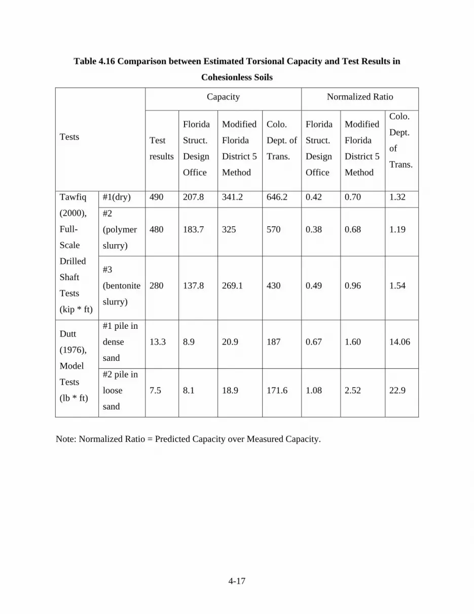
4-17

Table 4.16 Comparison between Estimated Torsional Capacity and Test Results in

Cohesionless Soils

Capacity Normalized Ratio

Tests Test

results

Florida

Struct.

Design

Office

Modified

Florida

District 5

Method

Colo.

Dept. of

Trans.

Florida

Struct.

Design

Office

Modified

Florida

District 5

Method

Colo.

Dept.

of

Trans.

#1(dry) 490 207.8 341.2 646.2 0.42 0.70 1.32

#2

(polymer

slurry)

480 183.7 325 570 0.38 0.68 1.19

Tawfiq

(2000),

Full-

Scale

Drilled

Shaft

Tests

(kip * ft)

#3

(bentonite

slurry)

280 137.8 269.1 430 0.49 0.96 1.54

#1 pile in

dense

sand

13.3 8.9 20.9 187 0.67 1.60 14.06 Dutt

(1976),

Model

Tests

(lb * ft)

#2 pile in

loose

sand

7.5 8.1 18.9 171.6 1.08 2.52 22.9

Note: Normalized Ratio = Predicted Capacity over Measured Capacity.

4-18

Table 4.17 Comparison between Estimated Torsional Capacity and Test Results in

Cohesive Soils

Capacity Normalized Ratio

Tests Test

results

Florida

District 7

Method

Colorado

Dept. of

Trans.

Florida

District

7

Method

Colorado

Dept. of

Trans.

A-3 21.5 14.4 35.2 0.67 1.64 Stoll

(1972),

Field Tests

(kip-ft) V-4 38.5 27.4 67.4 0.71 1.75

#1 1.375 1.2 2.1 0.87 1.53

#2 1.62 1.326 2.68 0.82 1.65

Poulos

(1975),

Model

Tests

(lb-ft) #3 0.67 0.6 1.26 0.90 1.88

Note: Normalized Ratio = Predicted Capacity over Measured Capacity.

4.4 Recommended Methods of Analysis and Design 4.4.1 Lateral Response of Drilled Shafts 4.4.1.1 Ultimate Capacity Based Design - Clay

For the design of drilled shafts in clay, we suggest the use of the Broms method. The Broms

method is considered to provide a more accurate and safer prediction than the Brinch Hansen

method. The calculation steps involved in the Broms method are fairly straight forward as well.

A design Safety Factor of two is recommended based on the discussion in Section 4.3.1. The

lateral loads applied to sound walls, overhead signs, and traffic signals, usually produce the

accompanying moments. For example, the applied wind load on sound walls can be assumed to

concentrate at the mid height of the wall, and then the load arm is 7 to 9 feet for 14 to 18 feet

4-19

high walls. The last three cases in Table 4.11 are very similar to these situations, and the Broms

method prediction is about ½ of the measured ultimate capacity. If a Factor of Safety of two is

applied to Broms method, the actual Factor of Safety will be about 4. Thus, we can adopt a

relatively low factor of safety; however, the value can not be too low, since the first four cases in

Table 4.11 indicate that Broms method may over predict in some cases.

4.4.1.2 Ultimate Capacity Based Design - Sand

The comparisons in section 4.3.1 do not provide conclusive evidence regarding the accuracy of

several capacity estimate methods for laterally loaded drilled shafts in sand. Therefore, for

consistency, the Broms method is suggested. It should be noted that the test data in sand for this

study comes from only one reference. Thus, it warrants the adoption of a safer prediction method

(Broms method) until more extensive database becomes available for further evaluation.

The design Safety Factor of two is recommended based on the discussion in Section 4.3.1. If a

Factor of Safety of two is applied to Broms method, the actual Factor of Safety based on load

test data will range from 2.6 to 6.2, with an average F.S. of 3.9.

4.4.1.3 Service Limit Based Design - Clay

For drilled shafts embedded in clay, COM624P (LPILE) computer program is recommended for

predicting the load-deflection response. The NAVFAC DM-7 method can only predict the initial

linear part of the load-deflection behavior; therefore, it is not recommended.

Without additional input from structural engineers, a permissible deflection of 1.0 inch at the

drilled shaft head is recommended. It should be emphasized that this conclusion was derived

from drilled shaft response, not from structural consideration of sound walls. It is the structure

engineers’ decision according to sound wall structure details.

It is noted that the Broms method may result in larger design length than the COM624P (LPILE)

design value, if a relatively high permissible deflection (say 1.5 inch) is adopted. Therefore, the

design embedment length of drilled shaft should be controlled by the longer length determined

by the Broms method and the COM624P (LPILE) results.

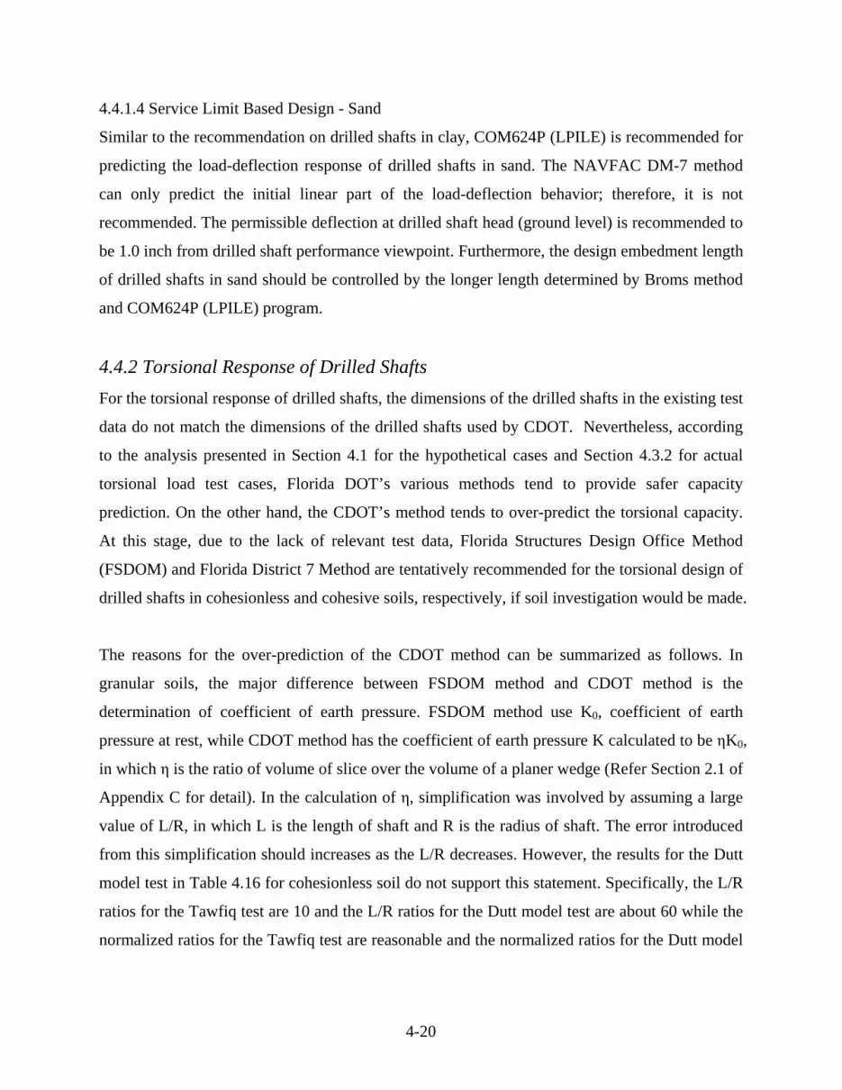
4-20

4.4.1.4 Service Limit Based Design - Sand

Similar to the recommendation on drilled shafts in clay, COM624P (LPILE) is recommended for

predicting the load-deflection response of drilled shafts in sand. The NAVFAC DM-7 method

can only predict the initial linear part of the load-deflection behavior; therefore, it is not

recommended. The permissible deflection at drilled shaft head (ground level) is recommended to

be 1.0 inch from drilled shaft performance viewpoint. Furthermore, the design embedment length

of drilled shafts in sand should be controlled by the longer length determined by Broms method

and COM624P (LPILE) program.

4.4.2 Torsional Response of Drilled Shafts For the torsional response of drilled shafts, the dimensions of the drilled shafts in the existing test

data do not match the dimensions of the drilled shafts used by CDOT. Nevertheless, according

to the analysis presented in Section 4.1 for the hypothetical cases and Section 4.3.2 for actual

torsional load test cases, Florida DOT’s various methods tend to provide safer capacity

prediction. On the other hand, the CDOT’s method tends to over-predict the torsional capacity.

At this stage, due to the lack of relevant test data, Florida Structures Design Office Method

(FSDOM) and Florida District 7 Method are tentatively recommended for the torsional design of

drilled shafts in cohesionless and cohesive soils, respectively, if soil investigation would be made.

The reasons for the over-prediction of the CDOT method can be summarized as follows. In

granular soils, the major difference between FSDOM method and CDOT method is the

determination of coefficient of earth pressure. FSDOM method use K0, coefficient of earth

pressure at rest, while CDOT method has the coefficient of earth pressure K calculated to be ηK0,

in which η is the ratio of volume of slice over the volume of a planer wedge (Refer Section 2.1 of

Appendix C for detail). In the calculation of η, simplification was involved by assuming a large

value of L/R, in which L is the length of shaft and R is the radius of shaft. The error introduced

from this simplification should increases as the L/R decreases. However, the results for the Dutt

model test in Table 4.16 for cohesionless soil do not support this statement. Specifically, the L/R

ratios for the Tawfiq test are 10 and the L/R ratios for the Dutt model test are about 60 while the

normalized ratios for the Tawfiq test are reasonable and the normalized ratios for the Dutt model

4-21

test are unreasonable. Accordingly, the error must come from something other than the L/R ratio;

perhaps from the frictional resistance.

The coefficient of friction between the soil and the concrete was taken as tan(φ) assuming that

the caisson body was rough enough to trap soil along its perimeter to promote the frictional

resistance of soil-on-soil. If this is not the case, such as the reduction of friction due to the use of

drilling mud, then a lesser value such as tan(2/3*φ) could be used. In fact, tan(2/3*φ) was

already utilized for the calculation of the torsional capacity of the bentonite slurry constructed

drilled shaft of Tawfiq’s test, shown in Table 4.16. The over-prediction by CDOT method for

this case, therefore, might imply a need for further investigation on the determination of K since

the coefficient of friction and K are the two most influential factors in the estimation of torsional

capacity. Additionally, the CDOT method will probably over-predict the total torsional

resistance in mixed soils if the torsional resistances from the cohesive and cohesionless

components can be added by superposition.

In cohesive soils, the soil's cohesive value was used as bond strength at the soil-to-concrete

interface for predicting torsional resistance. In fact, the bond strength at this interface may not

be as good as the soil's cohesive value or, as previously stated, the drilling mud may have a

tendency to reduce the friction developed at the pile-to-soil interface and this may warrant

further investigation.

In fact, CDOT’s current design procedure does not require soil strength investigation for signs

and signals. Instead, they rely on a minimum friction angle of 30 degree for granular soils, a

minimum cohesion of 750 psf for cohesive soils, and a minimum unit weight of 110 pcf for all

soils. A factor of safety of 1.25 and the CDOT torsion design method are used. It is not able to

conclude whether or not the selected minimum soil strength parameters are reasonable without a

wide range of investigation on Colorado soil strength in this study. However, according to

CDOT’s current practice, there are no torsional failures reported and the selected soil parameters

are really based on soft clay and loose sand. Therefore, the current practice should be ok, even on

conservative side. It is recommended to perform SPT testing at the location of the major signs

and signals so that a more rational design could be utilized and a cost saving can be expected.

4-22

4.5 Other Considerations 4.5.1 Loading Rate Effect Some literature exists pertaining to the effect of loading rate on the strength of the soils. The

current understanding of the undrained shear strength of cohesive soils as affected by the loading

rate is summarized herein. However, it is important to note that additional research is needed

before any conclusion can be drawn regarding the effect the loading rate has on the lateral

response of drilled shafts.

The standard strain rate of 0.5% to 1% per hour is considered as the strain rate in the laboratory

monotonic tests (Lefebvre and LeBoeurf, 1987). Sheahan et al (1996) found that the strain rate is

insignificant in affecting the undrained shear strength of cohesive soils for the rate ranging from

0.05% to 0.5% per hour. Here, we can assume that typical monotonic load testing in the lab is

about 1% per hour. Sheahan et al (1996) also observed that the average failure strain for the

Boston blue clay is about 3.7%. Thus, it could be assumed that the typical failure strain of

cohesive soils is about 3%. From Lefebvre and LeBoeuf’s study (1987), they observed that there

is a 7% to 14% increase in the undrained shear strength per log cycle of strain rate increase, with

an average of 10% strength increase as a conservative estimate. This increase in shear strength is

linear over five log cycles of strain rate.

Consider that the drilled shafts supporting the noise wall are subjected to 3 seconds of wind gust.

If the soil surrounding the shaft is to fail in three seconds during gust, then the strain rate to

failure is 3600% per hour by assuming a failure strain of 3%, a roughly 3.5 log cycles of strain

rate increase compared to a laboratory shear strain rate. Thus, one can conclude that the

undrained shear strength of cohesive soils determined by standard laboratory tests would be

increased by about 35% for the gust induced failure.

Concerning the loading rate effect on the strength of cohesionless soils, a review of literature is

summarized in Table 4.18. It appears that with exception of Whitman and Healy (1962)

experimental results, other researchers have indicated rather small increase in the apparent

strength increase of cohesionless soils due to increase in loading rate. According to Whitman and

4-23

Healy, the effective friction angle of the cohesionless soils appears to be uninfluenced by the rate

of loading. The undrained shear strength increase in saturated loose sand due to high loading rate

can be attributed to slower pore pressure increase than that during the normal loading rate. Until

more definite experimental findings suggest differently, the research team believes that the

loading rate effect due to a gust may not be an important consideration for dry sand or saturated

dense sand. There might be small benefits if one considers an apparent increase in undrained

shear strength in loose cohesionless soils due to gust loading.

Table 4.18 Test Results of Strain Rate Effect on Strength of Cohesionless Soils

The effect on strength Investigator

Soil Confining pressure

Loading velocity Drained Undrained

Casagrande and Shannon (1948)

Sands 30-90 kPa 0.2

meters/sec. Increased

10%

Seed and Lundgren

(1954)

Dense saturated

sands 200 kPa 1.0 m/s Increased 15-

20%

Increased 10%

Increased 100% Whitman and

Healy (1962)

Dense and

loose sand

70 kPa 0.5 m/s Friction angle is largely

independent of strain rate

Lee et al. (1969)

Loose and

dense dry sand

100-1470 kPa 0.22 m/s

Increased 20% for dense sand at high confining

pressure, 7% for loose sand and low confining pressure

on dense sand

Yamamuro and Lade (1993)

Dense sands 34 MPa

1.33 x 10-7 –2.29 x 10-5

m/s

Increased 2% Increased 7%

4.5.2 Cyclic Loading Degradation Some researchers have looked into the effects of cyclic loading on the drilled shaft lateral

response. It has been found that the repeated loading degrades the clay structure, changes the

pore water pressure, and decreases the stiffness and strength of the soil. In sand and normally

4-24

consolidated clays, the cyclic pore water pressures developed are usually positive and hence it

can be directly linked to the cyclic degradation (Matasovic, et al. 1995). However, in

overconsolidated clays, negative pore water pressure may develop at the beginning of cyclic

loading, despite the fact that degradation of soil stiffness and strength may occur simultaneously

(Matasovic, et al. 1995). For cohesive soils, the undrained strength degradation caused by

undrained cyclic loading can be recovered due to drainage after cyclic loading, combined with

returning to the original effective stress, except for sensitive clay and peat (Yasuhara, 1994).

Poulos (1982) found that the effect of cyclic degradation is more severe for stiff soils than for

soft soils. It is important to note that additional research is necessary before any conclusion can

be drawn.

From the above brief literature review, one can see that strength and stiffness degradation of both

cohesive and cohesionless soils due to cyclic loading may be important; but, currently we lack a

comprehensive understanding, particularly in relation to laterally loaded drilled shafts. Certainly,

more in-depth research in this subject area is warranted. Without further investigation, the

recommended design methods should still work fine. Because the Broms method is conservative,

as discussed in section 4.4.1, the actual factor of safety is larger than the recommended value of

two in the design. Cyclic degradation is expected to occur more in cohesive soils and in the

upper portion of the soil layer. However, the soil resistance in the upper 1.5 diameters of the

shaft was not considered in the Broms method. Thus, this will take care of any degradation.

Furthermore, for sound wall, the main lateral force is wind force which may increase the

cohesive soils’ undrained strength due to high loading rate. The loading rate effect may also

offset the degradation from cyclic loading.

4.5.3 The Effect of Soil Saturation For sand, it is not necessary to consider the effect of saturation since the sand friction angle does

not vary with water content significantly. Bhushan and Askari (1984) observed that an increment

less than 10% of deflection resulted from saturating the sand.

In clay, for capacity estimation, the water content effect can be considered by using the highest

possible elevation of water at the site and then using saturated strength parameter for soil under

4-25

the water table and in-situ strength for water above water table. For serviceability design, the

same soil parameters can be selected as that done in capacity prediction, and then use the

appropriate p-y curve criteria (above or below water table) by using COM624P (LPILE).

4.5.4 The Effect of Moment Arm During the course of this study, it was observed that all the prediction methods, including the

Broms method, the Brinch Hansen method, and the COM624P program, provide very

conservative capacity estimates for shafts with large applied moments, as shown in Table 4.11

and Figs. 4.11 through 4.13. It would be of great savings, if the conservatism can be accounted

for in the design. We believe that the “pull-push” effect on shaft under large applied moment

might result in vertical soil friction on two side of the shaft with opposite direction and thus

providing additional resistance to the applied moment at the shaft head. The scenario is

illustrated in Fig. 4.23. This pull-push effect can be quantified by measuring or analyzing the

moments resulting from vertical soil resistance. Either strain gages at the top portion of shaft or

friction measurement device can be used to measure this effect in future lateral load tests.

4.5.5 Calibration of Resistance Factors for Lateral Design of Drilled Shafts 4.5.5.1 Resistance Factors for Drilled Shafts in Clay

In order to convert from Allowable Stress Design (ASD) to Load Resistance Factor Design

(LRFD) for the lateral design of drilled shafts supporting sound walls, it is required to calibrate

resistance factors either by reliability method or by fitting to the ASD method. The reliability

method is a statistical approach, which requires the statistics on soil strength variations and load

variations. Fitting to the ASD method is an approach to choose resistance factors that will, on

average, result in the same factors of safety as would from ASD.

The calibration of resistance factors for the calculation of the lateral capacity of drilled shafts in

clay will be presented here. First, the reliability method will be used to calibrate the resistance

factors, then, fitting to the ASD method will be used to obtain resistance factors. The resistance

factors from both calibration methods will be compared at the end of this section.

4-26

4.5.5.1.1 Reliability Method

4.5.5.1.1.1 Resistance Statistics

There are at least two kinds of uncertainties on resistance, one is the variation in the capacity

prediction model, and the other one is the uncertainties involved in the soil parameters

determination. For both uncertainties, two variables are required: one is the bias factor (λ) which

is equal to the measured value over predicted value, and the other one is the coefficient of

variance (COV) which is equal to the standard deviation over mean value.

In order to obtain the resistance statistics of the Broms method, a database including the

measured lateral capacity and the predicted capacity by the Broms method is necessary. The

lateral load tests conducted in Ohio for sound wall design is chosen as the database. Table 4.19

shows the lateral load test results for drilled shafts in clay and predicted capacity by the Broms

method. The bias factor, λRB, is also included. The mean of the bias factor, shown in Table 4.19,

is 1.63.

Table 4.19 Database on Measured and Predicted Lateral Capacities in Clay

Shaft Measured Broms’ Method λRB

1 92 90 1

2 78 73 1.1

3 85 123 0.7

4 161 67 2.4

5 71 34 2.1

6 70 28 2.5

The value of the coefficient of variance on the prediction model, COVRB, could be estimated

using a rule-of-thumb, known as the “six sigma” rule. The use of the “six sigma” rule involves

three simple steps. The first step is to estimate the most likely value of the property (Vest), which

usually is the mean value, the lowest conceivable value (Vmin), and the largest conceivable value

(Vmax). Then, in the second step, one could use the “six sigma” rule to estimate the value of the

standard deviation (σ):

4-27

6

VV minmax −=σ (4.2)

The third step is to calculate the coefficient of variance (COV) by:

estV

COV σ= (4.3)

Therefore, the COVRB of the bias factors is 0.18 according to the “six sigma” rule outlined above.

The uncertainties involved in determining the soil parameters lie in the test procedures and

interpretation methods. In this case, SPT test was used to estimate the shear strength of clay. The

study by Orchant et al. (1988) on the variation of SPT test, shown in Table 4.20, is adopted for

determining the COV of the SPT test. The value of 0.45 is chosen for COV of SPT test for

conservative reasons. The bias factor for the SPT test is assumed to be 1.0 since no database is

available. Because of the lack of data for estimating the variation on SPT result interpretation,

the uncertainty in this aspect is ignored for this calibration. Therefore, the bias factor on soil

parameter determination, λRS, is assumed as 1.0 and the coefficient of variance on soil parameter

determination, COVRS, is chosen as 0.45.

Table 4.20 COVs for Various In-Situ Tests (After Orchant et al., 1988)

Test COV

Equipment

COV

Procedure

COV

Random COV Total

COV

Range

SPT 0.05-0.75 0.05-0.075 0.12-0.15 0.14-1.0 0.15-0.45

MCPT 0.05 0.10-0.15 0.10-0.15 0.15-0.22 0.15-0.25

ECPT 0.03 0.05 0.05-0.10 0.07-0.12 0.05-0.15

VST 0.05 0.08 0.10 0.14 0.10-0.20

PMT 0.05 0.12 0.10 0.16 0.10-0.20

After the bias factors and COVs are obtained, they should be combined into one value to

represent the total uncertainties as follows:

RSRBR λ⋅λ=λ (4.4)

2RS

2RBR COVCOVCOV += (4.5)

4-28

in which, λR is the bias factor on resistance side, and COVR is the coefficient of variance on

resistance side. Therefore, for this calibration study, λR = 1.63 and COVR = 0.48.

4.5.5.1.1.2 Load Statistics

For sound wall design, only the wind load is considered as a lateral load. The bias factor for the

wind load (live load), λL, is assumed as 1.0 due to the lack of load information. The COV of

wind load, COVL, is chosen as 0.18 from Nowak (1992)’s study on bridge loads as shown in

Table 4.21. The load factor for wind load, γL, is 1.4 according to AASHTO specification (2003).

Table 4.21 Statistics for Bridge Load Components (After, Nowak, 1992)

Load Component Bias, λ COV

Dead Load

Factory-made

Cast-in-place (CIP)

Asphaltic wearing surface

1.03

1.05

1.00

0.08

0.10

0.25

Live Load (w. dynamic load allowance) 1.1-1.2 0.18

4.5.5.1.1.3 Target Reliability Index

For drilled shaft design, the target reliability index, βT, could range from 2.5 to 3.0 according to

Table 4.22. For this calibration study, both 2.5 and 3.0 will be used for evaluation.

Table 4.22 Values of Target Reliability Index βT (Barker, et al. 1991)

Foundation Type βT

Spread Footings 3.0 to 3.5

Drilled Shafts 2.5 to 3.0

Driven Piles (group) 2.0 to 2.5

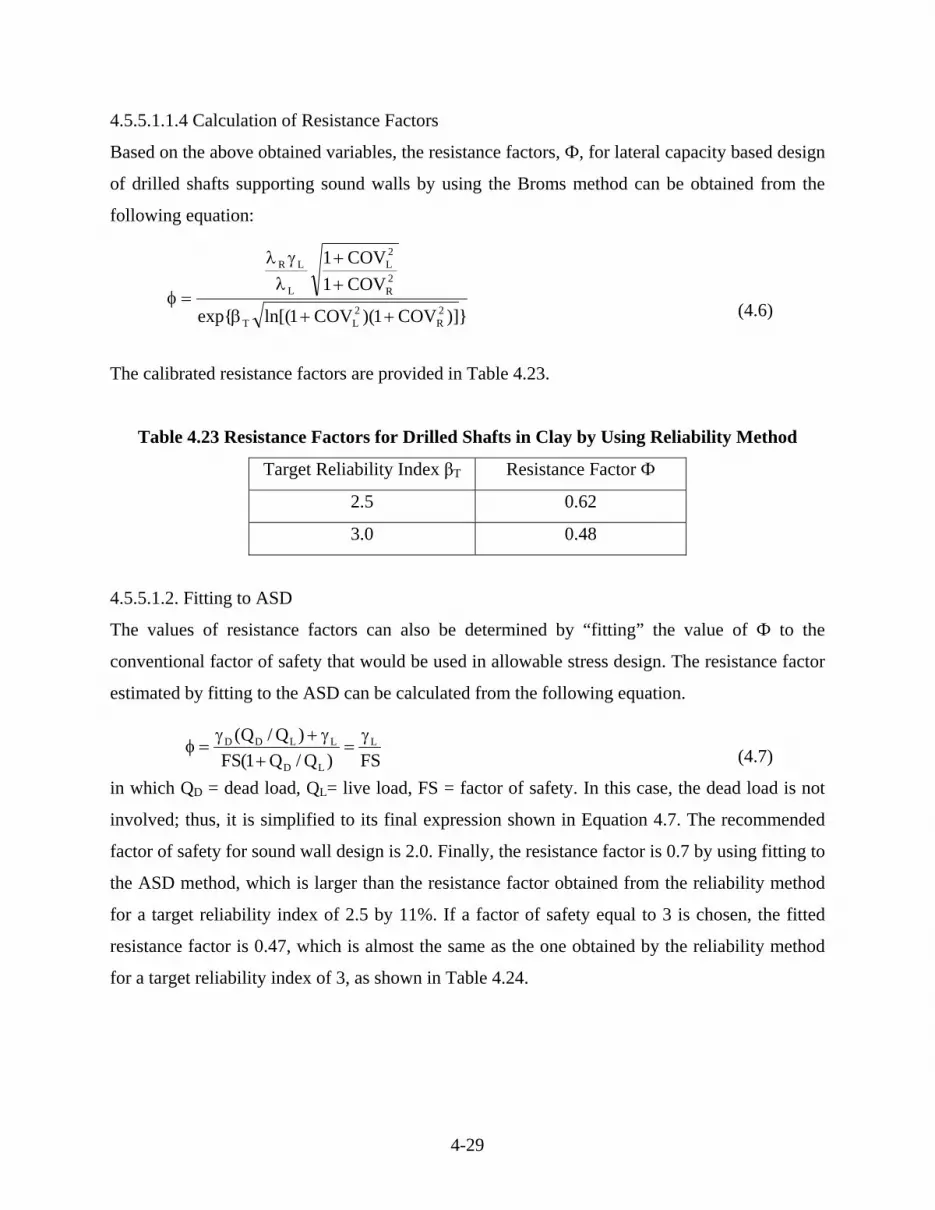
4-29

4.5.5.1.1.4 Calculation of Resistance Factors

Based on the above obtained variables, the resistance factors, Ф, for lateral capacity based design

of drilled shafts supporting sound walls by using the Broms method can be obtained from the

following equation:

(4.6)

The calibrated resistance factors are provided in Table 4.23.

Table 4.23 Resistance Factors for Drilled Shafts in Clay by Using Reliability Method

Target Reliability Index βT Resistance Factor Ф

2.5 0.62

3.0 0.48

4.5.5.1.2. Fitting to ASD

The values of resistance factors can also be determined by “fitting” the value of Ф to the

conventional factor of safety that would be used in allowable stress design. The resistance factor

estimated by fitting to the ASD can be calculated from the following equation.

(4.7)

in which QD = dead load, QL= live load, FS = factor of safety. In this case, the dead load is not

involved; thus, it is simplified to its final expression shown in Equation 4.7. The recommended

factor of safety for sound wall design is 2.0. Finally, the resistance factor is 0.7 by using fitting to

the ASD method, which is larger than the resistance factor obtained from the reliability method

for a target reliability index of 2.5 by 11%. If a factor of safety equal to 3 is chosen, the fitted

resistance factor is 0.47, which is almost the same as the one obtained by the reliability method

for a target reliability index of 3, as shown in Table 4.24.

})]COV1)(COV1ln[(exp{

COV1COV1

2R

2LT

2R

2L

L

LR

++β

++

λγλ

=φ

FS)Q/Q1(FS)Q/Q( L

LD

LLDD γ=

+γ+γ

=φ

4-30

Table 4.24 Values of Ф Calculated Using Fitting to ASD Method

Factor of

Safety

Resistance

Factor, Ф

Compare with

Reliability Method

2.0 0.7 +11%

3.0 0.47 0%

4.5.5.2 Resistance Factors for Drilled Shafts in Sand

Similar to the calibration work done in the previous section for drilled shaft in clay, the same

procedure is followed to calibrate the resistance factors for drilled shafts in sand. Table 4.25

provides calculated bias factors based on Bhushan et al. (1981)’s test data. The mean value of the

bias factor is 1.94.

Table 4.25 Database on Measured and Predicted Lateral Capacities in Sand

Shaft Measured Broms Method λRB

1 337 190 1.8

2 316 102 3.1

3 325 177 1.8

4 307 177 1.7

5 342 260 1.3

The value of the coefficient of variance on the prediction model, COVRB, is 0.15 by using the

“six sigma” rule.

Similar to the previous section, the bias factor on soil parameter determination, λRS, is assumed

as 1.0 and the coefficient of variance on soil parameter determination, COVRS, is chosen as 0.45.

After the bias factors and COVs are obtained, they should be combined into one value to

represent the total resistance uncertainties, resulting in λR = 1.94 and COVR = 0.47.

The values for load statistics are the same as before. The calibrated resistance factors are shown

in Table 4.26 for a target reliability index of 2 and 3. Similar to the procedure used before for

clay, the resistance factors based on fitting to ASD method are shown in Table 4.27.

4-31

Table 4.26 Resistance Factors for Drilled Shaft in Sand by Using Reliability Method

Target Reliability Index βT Resistance Factor Ф

2.5 0.75

3.0 0.59

Table 4.27 Values of Ф Calculated Using Fitting to ASD Method

Factor of

Safety

Resistance

Factor, Ф

Compare with

Reliability Method

2.0 0.7 -7%

3.0 0.47 -20%

The above two calibration examples for drilled shafts in clay and sand presented the procedure to

calibrate the resistance factors for drilled shaft design by using the reliability method and fitting

to the ASD method. Although some assumptions were involved in the determination of

resistance statistics and load statistics, the reliability method provides comparable results with

the fitting to the ASD method. The resistance factor could be chosen from Tables 4.23, 4.24,

4.26, and 4.27 for drilled shafts in clay and sand, respectively.

4-32

Figure 4.1 Schematic representation of soil profile and drilled shaft dimensions for lateral

response in hypothetical cases

P

15 ft

2.5 ft

10 ft

Case 1: 15’ sand Case 2: 15’ clay

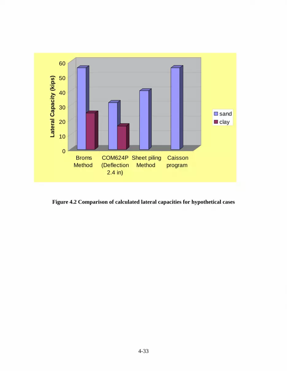
4-33

Figure 4.2 Comparison of calculated lateral capacities for hypothetical cases

0

10

20

30

40

50

60

Late

ral C

apac

ity (k

ips)

BromsMethod

COM624P(Deflection

2.4 in)

Sheet pilingMethod

Caissonprogram

sandclay

4-34

Figure 4.3 Assumed soil profiles and drilled shaft dimensions for torsional responses in

hypothetical cases

2.5’

15’

Mt

Vz

Drilled

shaft

Case 1: 15’Sand Case 2: 15’Clay Case 3: 10’ Sand

Overlying 5’Rock

Case 4: 15’Rock

5’

4-35

Figure 4.4 Comparison of calculated torsional capacity for hypothetical cases

0102030405060708090

100

FloridaStructures

DesignOffice

ModifiedFlorida

District 5Method

FloridaDistrict 7Method

FloridaDistrict 5Method

ColoradoDept. ofTrans.

Tors

iona

l Cap

acity

(kip

s * f

t)

SandClay

4-36

Ultimate Lateral Capacity Prediction

0

0.5

1

1.5

2

2.5

3

I70S1

I70S2

I-90P

100

I-90P

101

I-90S

1

I-90S

2

I-90S

3

Mea

sure

d / P

redi

cted

Broms PredictionBrinch Hansen Prediction

Figure 4.5 Measured over-predicted capacities of drilled shafts in clay based on load test

database

4-37

Figure 4.6 Measured over-predicted capacities of drilled shafts in sand based on load test

database

0

0.5

1

1.5

2

2.5

3

3.5M

easu

red

/ Pre

dict

ed

Pier 1 Pier 4 Pier 5 Pier 6 Pier 7

BromsMethodSheet PilingBrinch HansenCaisson Program

4-38

0

10

20

30

40

50

60

70

80

90

0 0.5 1 1.5 2 2.5 3 3.5 4

Deflection(in.)

Load

(kip

s) Test ResultsHyperbolic FitCom624NAVFAC DM-7

Figure 4.7 I-70 sound barriers, Columbus OH, shaft 1, lateral load-deflection curves

4-39

0

10

20

30

40

50

60

70

80

90

0 0.5 1 1.5 2 2.5 3 3.5 4

Deflection (in.)

Load

(kip

s) Test ResultsHyperbolic FitCOM624NAVFAC DM-7

Figure 4.8 I-70 sound barriers, Columbus OH, shaft 2, lateral load-deflection curves

4-40

0

10

20

30

40

50

60

70

80

90

100

-1 0 1 2 3 4 5 6

Deflection (in.)

Load

(kip

s) Test ResultsHyperbolic FitCOM 624NAVFAC DM-7

Figure 4.9 I-90 sound barriers, shaft 100 lateral load-deflection curves

4-41

0

20

40

60

80

100

120

-1 0 1 2 3 4 5 6 7 8

Deflection (in.)

Load

(kip


Figure 4.10 I-90 sound barriers, shaft 101, lateral load-deflection curves

4-42

0

20

40

60

80

100

120

140

160

-1 0 1 2 3 4 5 6 7 8 9

Deflection (in.)

Load

(kip

s) Test ResultsHyperbolic FitCOM624NAVFAC DM-7

Figure 4.11 I-90 sound barriers, 12 ft depth, shaft 2, lateral load-deflection curves

4-43

0

10

20

30

40

50

60

70

-1 0 1 2 3 4 5 6 7 8

Deflection (in.)

Load

(kip


Figure 4.12 I-90 sound barriers, 8 ft depth, shaft 1 lateral load-deflection curves

4-44

0

10

20

30

40

50

60

70

-1 0 1 2 3 4 5 6 7 8 9

Deflection (in.)

Load

(kip


Figure 4.13 I-90 sound barriers, 8 ft depth, shaft 2 lateral load-deflection curves

4-45

0

50

100

150

200

250

300

0 0.5 1 1.5 2 2.5 3 3.5 4 4.5 5

Deflection (in.)

Load

(kip

s) MeasuredHyperbolic FitCOM624NAVFAC

Figure 4.14 Bhushan et al. (1981), pier 1 lateral load-deflection curve

4-46

0

50

100

150

200

250

0 1 2 3 4 5 6 7 8 9 10

Deflection (in.)

Load

(kip



4-47

0

50

100

150

200

250

300

0 1 2 3 4 5 6

Deflection (in.)

Load

(kip



4-48

0

50

100

150

200

250

300

0 1 2 3 4 5 6 7 8 9 10

Deflection (in.)

Load

(kip



4-49

0

50

100

150

200

250

300

350

0 0.5 1 1.5 2 2.5 3 3.5

Deflection (in.)

Load

(kip



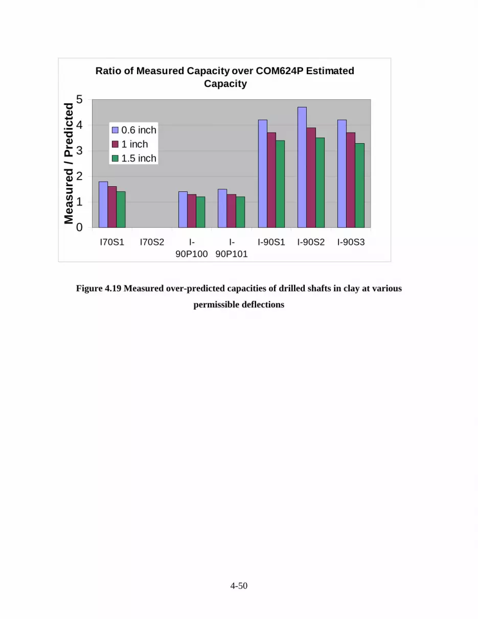
4-50

Figure 4.19 Measured over-predicted capacities of drilled shafts in clay at various

permissible deflections

Ratio of Measured Capacity over COM624P Estimated Capacity

0

1

2

3

4

5

I70S1 I70S2 I-90P100

I-90P101

I-90S1 I-90S2 I-90S3

Mea

sure

d / P

redi

cted

0.6 inch1 inch1.5 inch

4-51

Figure 4.20 The assumed drilled shaft and sound wall deflection under lateral load

∆w

∆p

Hw

L

θ = rotation angle

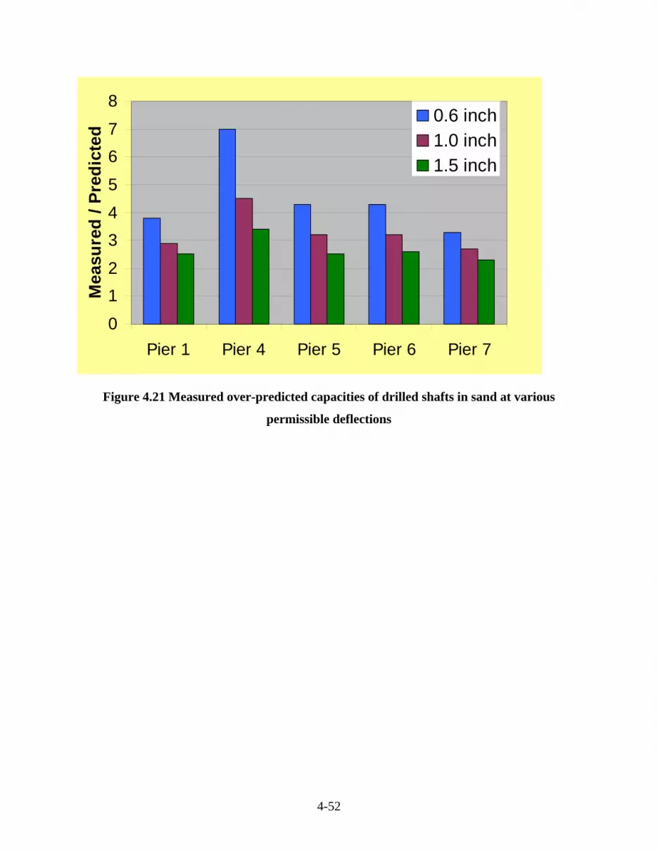
4-52

Figure 4.21 Measured over-predicted capacities of drilled shafts in sand at various

permissible deflections

0

12

34

5

67

8

Pier 1 Pier 4 Pier 5 Pier 6 Pier 7

Mea

sure

d / P

redi

cted

0.6 inch1.0 inch1.5 inch

4-53

Figure 4.22 Measured over-predicted torsional capacities of drilled shafts in sand

0.0

0.5

1.0

1.5

2.0

2.5

3.0

Tawfiq #1 Tawfiq #2 Tawfiq #3 Dutt #1 Dutt #2

Mea

sure

d / P

redi

cted

Florida StructuresDesign Office Modified FloridaDistrict 5 Method Colorado Dept. ofTrans.

4-54

Figure 4.23 Measured over-predicted torsional capacities of drilled shafts in clay

0.0

0.2

0.4

0.6

0.8

1.0

1.2

1.4

1.6

Stoll A3 Stoll V4 Poulos #1 Poulos #2 Poulos#3

Mea

sure

d / P

redi

cted

Florida District 7 MethodColorado Dept. of Trans.

4-55

Figure 4.24 The mechanism of pull-push effect

Lateral Soil

Resistance

MP

Pull Push

Vertical Soil Resistance

5-1

5 LATERAL LOAD TESTS ON DRILLED SHAFTS AND ANALYSIS OF

TEST RESULTS AT SELECTED NOISE WALL SITES NEAR

DENVER, COLORADO

5.1 Project Description

This research project required the research team to perform two lateral load tests on drilled shafts

used to support noise walls. The first lateral load test was conducted on June 11, 2003 near I-225

and 6th Avenue. The second lateral load test was conducted on test shafts drilled near I-225 and

Iliff Avenue. The design consultant used the current CDOT practice to design the drilled shaft

foundations. The load test data allowed an evaluation of the current CDOT design approach as

well as the recommended analysis methods proposed in this research.

5.2 Subsurface Conditions

5.2.1 Introduction This section presents the geotechnical investigation results and geotechnical design parameters

from the four soil borings advanced at the two proposed test sites for the purpose of lateral load

analysis for this research project. The project includes two lateral load test sites; near I-225 and

6th Avenue and near I-225 and Iliff Avenue. The purpose of the geotechnical site investigation

was to determine the geotechnical profile, to characterize the physical properties of the materials

at the site, and to perform pressuremeter testing (this data was utilized to develop geotechnical

recommendations necessary to evaluate the lateral load capacity of the test shafts). The field

investigation was needed to compare design results using the geotechnical data with the lateral

load test results. The plan view of the locations of the soil borings and the summary of the field

and laboratory test results is shown in Figs. 5.1a and 5.1b. The logs of borings are presented in

Figs. 5.2a thru 5.2d.

A total of four borings were drilled using a CME-75 drill rig utilizing 7-½ inch hollow stem

auger (HSA). Borings 1 and 2 were drilled near the I-225/6th Avenue site while Borings 3 and 4

5-2

were drilled near the I-225/Iliff Avenue site. Standard penetration tests (SPT) were performed at

selected intervals in Borings 1 and 3. Shelby tube samples were collected at selected intervals in

Borings 2 and 4. Results of the field investigation and laboratory testing are included in Chapter

7. One-inch diameter PVC piezometers were installed in Borings 1 and 3 in order to monitor

groundwater levels. Gradation analyses and Atterberg limits tests were performed for

classification purposes on representative soil samples retrieved from the borings.

5.2.2 Site Conditions & Geotechnical Profile 5.2.2.1 I-225 near 6th Avenue

At the lateral load test site located near I-225 and 6th Avenue, man-placed fill consisting of stiff

silty clay was encountered to a depth of approximately 6.5 feet below the original ground surface

(OGS). Native materials consisting of soft to medium stiff silty clay and loose silty sand were

encountered below the fill to a depth of approximately 22 feet, where bedrock was encountered.

Bedrock was encountered at an elevation of approximately 5420.5 feet and consisted of firm

claystone. Bedrock was encountered to the maximum depth of investigation of approximately

26.5 feet below OGS, which corresponds to an elevation of approximately 5416 feet.

Groundwater was encountered at an elevation of approximately 5431 feet.

5.2.2.2 I-225 near Iliff Avenue

At the lateral load test site located near I-225 and Iliff Avenue, native materials consisting of

loose to medium dense silty sand were encountered below the OGS to a depth of approximately

19 feet, where bedrock was encountered. Bedrock was encountered at an elevation of

approximately 5618 feet and consisted of firm to medium hard sandstone with interbedded

claystone lenses. Bedrock was encountered to the maximum depth of investigation of

approximately 25 feet below OGS, which corresponds to an elevation of approximately 5612 feet.

Groundwater was encountered at an elevation of approximately 5622.5 feet.

Based on results of the geotechnical site investigation, the CDOT geotechnical engineer

recommended the material properties presented in Table 5.1 to be used in the lateral load

analysis of the drilled shafts using LPILE or similar software. CDOT also recommended that the

lateral resistance for the top five feet of silty clay fill at the 6th Avenue site should be neglected

to account for desiccation cracks in the material for the design of structures.

5-3

Table 5.1: CDOT Recommended Material Properties for Lateral Load Analysis Using

LPILE.

Lateral

Load Test

Site

Elevation

(feet)

Internal

Friction

Angle

(degrees)

Cohesion

c(psf)

Modulus of

Horizontal

Subgrade

Reaction

kh(pci)

Strain at ½ the

Maximum

Principal

Stress

Difference,

ε50 (in/in)

Total

Unit

Weight

γ (pcf)

Below 5442 0 1200 75 0.007 110

Below 5436 0 800 35 0.015 110

Below 5426 30 0 20 -- 115

I-225/6th

Avenue

Below 5420 0 3,000 500 0.005 130

Below 5637 30 0 25 -- 115 I-225/Iliff

Avenue Below 5618 0 4,000 500 0.005 130

5.3 Lateral Load Test and Analysis at I-225 near 6th Avenue

5.3.1 Field Installation of Instruments and Drilled Shafts Construction The planned fieldwork consisted of instrumenting the two test drilled shafts which are to be used

as part of the noise barrier wall foundations at this site, denoted as Test Shafts #1 and #2. The

location of the test shafts is shown on the attached plans in Fig. 5.1a. The instrumentation

consisted of inclinometer tubes to measure the lateral movement with depth during the load

testing, vibrating wire sister bar strain gages, tilt meters, and dial gages as shown in Fig. 5.3a and

5.3b. A complete list of the required instrumentation for the lateral load test is summarized in

Table 5.2, and the detailed plan of instrumentation and instrument elevations are attached in

Chapter 7. The reinforcement details of the test drilled shafts are shown in Fig. 5.3e. E.L.

Robinson Engineering and Geocal, Inc. personnel installed the instrumentation. The test shafts

were instrumented and constructed on June 9, 2003.

5-4

Table 5.2. Table of Instrumentation Used for Lateral Load Test.

Type of Instrument Sister Bar

(each)

Load Cell

(each)

Inclinometer

Tube (ft.)

Tilt

meter

Dial

Gages

Test Shaft # 1

16 ft. Deep 10 1 25 2 2

Test Shaft # 2

16 ft. Deep 10 25 2 2

Total Quantity 20 1 50 4 4

Arrangements were made with the CDOT Project Engineer to facilitate the installation of the

instruments. This included mounting the vibrating wire strain gages to the main steel rebar,

installing the inclinometer tubes in the holes, and supervising the installation of the test shafts.

Pictures showing the installation of the instruments and the drilled shafts construction are shown

in Figs. 5.4 thru 5.9.

5.3.2 Preparation and Setup for the Lateral Load Test Detailed drawings of the testing devices and schematics of the test setup were discussed with all

parties involved. An agreement on the testing setup and methodology was reached as shown in

the attached drawings in Chapter 7. Hamon Contractors built the reference beams and setup the

1.5-inch diameter Dywidag rods and all jacking devices under the supervision of the research

team.

The contractor began constructing the drilled shafts by drilling the hole to the plan bottom

elevation with a 30-inch auger, and then drilled the 6 feet deep 12-inch diameter sub-bottom hole

below the bottom of the drilled shaft. The inclinometer was then lowered into the hole to the

bottom of the 12-inch diameter sub-bottom hole and sand was poured to fill around it in the 6

feet portion below the base of the shaft. The 30-inch diameter, 3-foot long casing was then

installed, followed by the instrumented cage. The 10 feet long W14x109 was then installed in

position as shown in the installation pictures. After installation of all the test shaft elements, the

5-5

concrete was poured in the hole to the top of the steel casing, which was approximately 1 foot

above ground elevation. The same methodology was performed at Test Shaft # 2.

On June 10, 2003, the contractor installed the reference beams and setup the jacking devices as

shown in the pictures in Figures 5.10 and 5.11. The Dywidag rods were assembled and installed

in position.

The loading devices including a 60 Ton jack, a 100 Ton load cell, and special readout devices

were provided by the contractor. The devices were calibrated before shipping to the site. The

jack, load cell, special bearing plates, dial gages, and tilt meters were all installed on the day of

testing (i.e. 6/11/2003). The picture in Fig. 5.12 shows the testing devices and equipment setup.

The strain gages were attached to the data acquisition just before the test started and initial

readings were collected. The calibration factors for the sister bar strain gages and tiltmeters are

shown in Chapter 7. A schematic of the location and serial number of each gage are provided in

Chapter 7. Two sets of initial readings were taken from the inclinometers in Test shafts #1, and

#2 before any load was applied. Pictures showing the preparation and setup for the load test are

shown in Figs. 5.13 and 5.14. Fig. 5.15 shows a general view of the load test.

5.3.3 Lateral Load Test Procedure The lateral load test was performed in increments of loading and unloading as shown below. One

cycle of loading was performed according to the following sequence:

Load cycle 1: (Loads are in Kips)

Loading: 5, 10, 15, 20, 30, 40, 50, 60, 75, and 90.

Unloading: 47, 22, and 0

The strain gages were connected to the CR10X Campbell Scientific Data logger. The strain

readings were taken for each load increment during the time the load was applied, and stored in

the computer for later processing.

The lateral movement (deflection) of the drilled shafts was measured using the SINCO slope

indicator device. The deflection was measured every two feet along the depth of each shaft. The

measurements were taken for the following loads (in Kips):

5-6


Loading: 5, 10, 15, 20, 30, 40, 50, 60, 75, and 90.

Furthermore, the deflection at the top of the drilled shafts was measured using dial gages. The

load applied to the drilled shafts was measured using the load cell. The rotation at the top of the

shafts and at the jacking point was measured using vibrating wire tilt meters. Figs. 5.16 thru 5.18

shows the test being conducted.

The CDOT Project Engineer provided the concrete compressive strength test results on the day

of testing. Two cylinders from each test shaft were tested. The average compressive strength in

test shafts was 4510 psi.

CDOT Engineers supervised the lateral load test, and gave their recommendations on the load

applied. The lateral load applied was stopped at 90 kips because the two shafts were production

shafts and a considerable amount of nonlinear deflection had occurred.

5.3.4 Lateral Load Test Results The measured load-displacement relationships at the top of the shafts, as measured using the dial

gages, are shown in Figs. 5.19 and 5.20 for shafts No. 1 and No. 2, respectively. The deflections

of the drilled shafts, as measured by the inclinometer probe, versus depth of the shaft, are shown

in Figs. 5.21 and 5.22 for shafts No. 1 and No. 2, respectively. Moreover, the deflection of the

drilled shafts at the point of load application, as measured by the inclinometer probe, versus

applied lateral load are shown in Figs. 5.23 and 5.24 for shafts No. 1 and No. 2, respectively.

The measured strains vs. depth (measured from jacking point) in test shaft No. 1 at the tension

side and the compression side are shown in Figs. 5.25 and 5.26, respectively. The measured

angle of tilt in degrees vs. the applied lateral load from the tiltmeters mounted at the jacking

point and at top of concrete is shown in Fig. 5.27.

For test shaft #2, the measured strains vs. depth (measured from jacking point) at the tension side

and the compression side are shown in Figs. 5.28 and 5.29, respectively. The measured angle of

5-7

tilt in degrees vs. the applied lateral load from the tiltmeters mounted at the jacking point and at

top of concrete is shown in Fig. 5.30.

5.3.5 Interpretation of Soil Parameters CDOT has commissioned Knight Piesold, LLC to conduct laboratory tests on soil samples

retrieved from two load test sites. The laboratory test program included soil classification tests,

direct shear tests, and triaxial tests. In addition to index testing, the in-situ water content and in-

place densities of the soils at the test sites were also determined.

The direct shear tests were performed on silty clay samples in an undrained condition, with an

increased shear strain rate. Samples with in-situ water content as well as samples with full

saturation (S = 100%) were tested. The samples were subjected to vertical stresses that are

consistent with in-situ effective overburden stress, thus ensuring close duplication of in-situ

confining stress conditions. The peak shear stress at failure was used to represent the shear

strength under undrained loading. The interpreted shear strength parameters for the cohesive silty

clay are provided in Table 5.3 for both unsaturated (in-situ water content) and fully saturated

conditions. The simplified soil profile at the 6th Avenue test site is shown in Fig. 5.31.

The CU triaxial tests were performed on cohesive silty clays as well. The consolidation pressures

selected in the triaxial tests were consistent with the in-situ effective overburden stresses. During

undrained shearing, the loading rate was increased to about 1% per minute of axial strain rate.

The samples were either tested under the initial water content condition or after being fully

saturated by backpressure saturation. The interpretation of the shear strength under undrained

shear, as reported by the consultant, is based on the total stress based Mohr Circle and the

assumption that the failure plane corresponds to the peak shear stress of the Mohr Circle. For

fully saturated samples, this approximation would result in higher interpreted shear strength than

the Mohr Coulomb’s shear strength. For unsaturated samples, the interpreted shear strength by

the consultant may be conservative, since the effective stress based Mohr Circle may be larger in

size than that the total stress based Mohr Circle. The best estimate of shear strength by the

Knight Piesold’s Laboratory Report is summarized in Table 5.3, in which different tests are not

performed at the same exact depth but in what seems to be the same soil layer.

5-8

Table 5.3 Shear Strength (Undrained Shearing) from Pressuremeter and Lab Tests

Pressuremeter Direct Shear Test Triaxial Shear Test Soil

Layers

(ft)

Sample

ID Su,

G&A

(psi)

Su,

FHWA

(psi)

Unsaturated

(psi)

Saturated

(psi)

Unsaturated

(psi)

Saturated

(psi)

0-2.5 2-A 18.3

2.5-4.5 2-AA 22.2 16.2 15 5.6 18.3 8.6

4.5-6.5 2-B

6.5-10 2-C 12.5 8.8 13.7 8.2 14.7 4.5

10-12.5 2-D 9.4 11.9

12.5-16 2-E 15.3 10.9 11.7

Pressuremeter tests were performed at the 6th Avenue site and the Iliff Avenue site by the URS

in Denver. The report prepared by the URS corporation contains the pressuremeter test results,

along with interpreted soil parameters. For the cohesive silty clay site at the 6th Avenue test site,

the undrained shear strength, interpreted by URS consultant who employing Gibson and

Anderson (1961)’s procedure from pressuremeter tests, are presented in Table 5.3. The

undrained shear strength interpreted by using FHWA (1989)’s equation is also included in Table

5.3. FHWA’s interpretation equation is provided in Equation 5.1.

75.00lu )pp(25.0S −= (5.1)

in which, pl = limit pressure; p0 = in-situ initial horizontal pressure.

From a comparison of the interpreted shear strength in Table 5.3, one may conclude that the

saturation of cohesive soil samples will definitely result in reduction in shear strength, compared

to that obtained from partially saturated samples. The difference between the direct shear and

triaxial test results is unpredictable, due to different stress conditions and strength interpretation

between these two methods. Finally, the interpreted undrained shear strength from the

pressuremeter test by using Gibson and Anderson (1961) method appears to be larger than those

determined from laboratory tests and pressuremeter test interpreted by using FHWA’s equation.

As often is the case, different test methods have resulted in different shear strength parameters. It

5-9

is of interest to compare the elastic modulus of soils obtained from pressuremeter and those from

triaxial test. For pressuremeter test, three types of elastic modulus based on the portion of test

data used for interpretation, Einital based on initial part of test curve, Ereload based on reload

portion of pressure-volume change curve, and Eunload based on using unload portion of pressure-

volume change curve, as shown in Fig. 5.32, can be achieved. Table 5.4 presents the modulus

from the pressuremeter test and the triaxial test. It can be seen that the modulus interpreted from

the initial portion of PM test curve is the smallest one. On the other hand, the unload portion of

PM test curve provides largest estimation of modulus of soils.

Table 5.4 Elastic Modulus (psi) of Soils from Pressuremeter Test and Triaxial Test

Layers (ft) Einitial Ereload Eunload Etriaxial

0-2.5 2919 9174 16680 4140

2.5-4.5 2919 9174 16680 3320

4.5-6.5 2919 9174 16680 3320

6.5-10 723 1529 1946 1614

10-12.5 723 1529 1946 789

12.5-16 1015 2919 5282 3474

5.3.6 Analysis of Load Test Fig. 5.19 and 5.20 show that the two test shafts at the 6th Avenue test site have almost same

lateral response. However, shaft #1 appeared more deflection than shaft #2, which means shaft

#1 can represent a worse situation for these two shafts. Therefore, shaft # 1 is used for analysis.

The analysis is carried out using Broms method and Brinch Hansen method for ultimate capacity

and the COM624P computer program for load-deflection curves. The synthesized shear strength

parameters are summarized in Table 5.5. The strength correlated from the SPT correlation chart

developed by Liang (2002) and the CDOT suggested soil strength in Table 5.1 are also included.

It can be seen that the soil strength suggested by CDOT geotechnical engineer is around half of

that from lab test on soil under in-situ conditions. The averaged soil strength parameters are

presented in Table 5.6 for five analysis cases: SPT Liang Case based on Liang (2002) SPT

correlations, SPT CDOT Case based on CDOT geotechnical engineer recommended soil

parameters, Unsaturated Case based on lab determined strength for unsaturated (in-situ)

5-10

condition, PM (Su,G&A) Case based on pressuremeter determined undrained strength from

Gibson and Anderson method, and PM (Su, FHWA) Case based on pressuremeter determined

undrained strength by using FHWA (1989) equation. It is noted that the unit weight takes into

account the situation of ground water table.

Table 5.5. Interpreted Shear Strength Parameters

SPT Liang Case Unsaturated Case SPT CDOT Case Soil

Layers

(ft)

Sample

ID N

values

Strength

(psi)

Strength (psi) Strength (psi)

0-2.5 2-A 12* 11.3* 18.3 8.3

2.5-4.5 2-AA 12 11.3 15 8.3

4.5-6.5 2-B 15 14 14.4* 8.3

6.5-10 2-C 9 8.5 13.7 5.6

10-12.5 2-D 4 3.75 9.4 5.6

12.5-16 2-E 8 7.53 11.7 5.6

Note *: No direct test results, linear interpolation from adjacent soil layers was used.

Table 5.6. Average Strength in psi for Broms Method

Unsaturated

Case

SPT Liang Case SPT CDOT

Case

PM (Su, G&A)

Case

PM (Su, FHWA)

Case

13.6 9 6.7 17.3 12.3

For COM624p computer analysis, it is necessary to input additional soil parameters other than

just the strength parameters. To this end, the correlation charts developed by Liang (2002) based

on SPT N values were used to create the input parameters as shown in Table 5.7. For the SPT

CDOT Case, the suggested parameters are used for analysis, as shown in Table 5.1.

The calculated lateral capacities using the Broms method and the Brinch Hansen method are

presented in Table 5.8 for five strength cases: SPT Liang case, unsaturated case, SPT CDOT case,

PM (Su, G&A) case, and PM (Su, FHWA) case. It should be noted that the estimated capacities

shown in Table 5.8 are geotechnical capacities. The ratios between the measured capacities and

5-11

the predicted capacities are also tabulated in Table 5.8. It can be seen that, in general, both

Broms method and Brinch Hansen method predict comparable capacities and they are on the

safe side, with the ratio of the measured vs. the predicted ranges from 1.2 to 2.7 for the

unsaturated case, SPT Liang case, SPT CDOT case, and PM (Su, FHWA) case. It can also be

observed that the prediction with the CDOT geotechnical engineer suggested soil parameters

yields most conservative results. On the other hand, the pressuremeter test strength parameters

interpreted from Gibson and Anderson method would result in unsafe prediction of the lateral

capacity of the test shaft. This is not surprising, as the Gibson and Anderson method interpreted

strength parameters are much higher than SPT or laboratory determined strength parameters.

Table 5.7 Other Soil Parameters

Soil

Layers(ft)

Sample ID Φ ε50 γd (pcf) γwet

(pcf)

ks (pci)

0-2.5 2-A 0 0.006 87.9 106 500

2.5-4.5 2-AA 0 0.006 96.8 120 500

4.5-6.5 2-B 0 0.005 NA 119* 500

6.5-10 2-C 0 0.007 95.2 117 500

10-12.5 2-D 0 0.01 97.8 122 100

12.5-16 2-E 0 0.007 100.9 126 500

Note *: No lab test result is available; the average value of the two adjacent layers is adopted. ks

is the static modulus of horizontal subgrade reaction (Kh).

5-12

Table 5.8 Calculated Lateral Capacity of Drilled Shaft #1 in CDOT Test in Clay

Capacity (kips) Measured/Predicted

Strength Case Broms

Method

Brinch

Hansen

Method

Broms

Method

Brinch

Hansen

Method

SPT Liang 71 70 1.9 1.9

Unsaturated 108 101 1.3 1.3

SPT CDOT 53 50 2.5 2.7

PM (Su, FHWA) 98 114 1.4 1.2

PM (Su, G&A) 137 158 0.99 0.85

Note: The ultimate lateral capacity of Shaft #1 is 135 kips.

The COM624P computer analysis was carried out based on different strength cases. The

predicted load-deflection curves at the shaft head are compared with the measured in Fig. 5.33

for SPT and lab strength parameters, and in Fig. 5.34 for pressuremeter tests. For a close-up view

of the accuracy of prediction for the working load condition, the initial portion of the load-

deflection curves in Figs. 5.33 and 5.34 are re-plotted in Figs. 5.35 and 5.36. It can be seen that

at the working load of 20 kips, the COM624P predicted deflection is very close to the measured,

if the laboratory determined strength parameters for unsaturated samples are used. The SPT

correlated soil parameters by using Liang (2002) correlation can still yield a very reasonable

prediction at 20 kips of lateral load. The soil parameters suggested by the CDOT geotechnical

engineer tend to provide a conservative prediction. Also, the NAVFAC method predicts too

much deflection. The pressuremeter method, if undrained strength is interpreted from FHWA

equation, can also provide reasonable prediction of the drilled shaft deflection response. On the

other hand, the pressuremeter method, if the undrained strength is interpreted from Gibson and

Anderson (1961) or from direct conversion into p-y curves, cannot provide a reasonable

prediction.

The loads correspond to three values of drilled shaft deflections (i.e., 0.6 inch, 1 inch, and 1.5

inch) and are extracted from the predicted load-deflection curves for six (6) strength cases, which

are tabulated in Table 5.9. The measured ultimate lateral capacity using the hyperbolic curve fit

5-13

method is used to determine the ratio between the measured ultimate capacity and the predicted

load at different permissible deflection values. These ratios are tabulated in Table 5.9 under the

heading of F.S., as they represent the margin of safety from the measured ultimate capacity.

From this table, one can see that the recommended permissible deflection of 1.0 inch would yield

an equivalent factor of safety between 2.4 to 4.8, for soil parameters interpreted from SPT,

laboratory tests, and pressuremeter test by using FHWA’s interpretation for undrained strength.

On the other hand, the equivalent factor safety based on 1.0 inch permissible deflection is 1.9, if

the soil parameters are interpreted from the pressuremeter tests by using Gibson and Anderson

(1961) method was employed by URS consultant. This equivalent factor of safety is considered

to be unacceptable.

Table 5.9 Calculated Lateral Capacity and Factor of Safety (F.S.) of Drilled Shaft #1 by

COM624P with Different Permissible Deflections at Ground Level in CDOT Test in Clay


Cases 0.6 inch F.S. 1 inch F.S. 1.5 inch F.S.

SPT Liang 35 3.9 41 3.3 46 2.9

Unsaturated 47 2.9 57 2.4 65 2.1

SPT CDOT 24 5.6 28 4.8 31 4.4

PM (Su,FHWA) 45 3.0 54 2.5 57 2.4

PM (Su, G&A) 57 2.4 70 1.9 80 1.7

PM (p-y) 96 1.4 NA NA

Note: The ultimate lateral capacity of Shaft 1 is 135 kips. The PM (p-y) analysis is based on the p-y curves calibrated directly from the p-∆V/V0 curve of pressuremeter test.

A numerical algorithm has been developed by Liu and Liang (2004) for deriving p-y curves

using the strain and deflection data measured during lateral load tests. The p-y curve at the 24-

inch depth derived by this method is shown in Fig. 5.37. The existing stiff clay p-y curve criteria

with strength parameters determined by lab and SPT correlations are used to generate p-y curves

shown in Fig. 5.37(a). Similarly, the pressuremeter test data is used to generate p-y curves shown

in Fig. 5.37(b). The load test data derived p-y curve is much stiffer than other approaches.

5-14

The predicted load-deflection curve is compared with the actual measured for shaft #1 in Fig.

5.38. The match at the working load range is excellent.

Based on the analysis performed in this section, the following observations may be made.

1. The Broms method, when used with SPT correlated in-situ strength or laboratory determined

shear strength for in-situ (unsaturated) samples, yield reasonable F.S. for this load test result.

2. The use of shear strength from the CDOT geotechnical engineer recommendation would yield

high F.S. due to conservative approach to strength interpretation.

3. The COM624P computer program, when used with SPT correlated soil parameters or

laboratory determined strength for in-situ (unsaturated) water content, appears to be capable

of predicting shaft deflection at the working load of 20 kips.

4. The use of the pressuremeter test, if the strength parameters are interpreted by using FHWA

(1989)’s equation, would provide reasonable prediction on capacity and lateral deflection of

the shaft. However, if the strength parameters are interpreted by using Gibson and Anderson

(1961)’s procedure, the pressuremeter method would result in an unsafe prediction of ultimate

lateral capacity for the 6th Avenue test shafts. Furthermore, the drilled shaft deflection cannot

be predicted accurately using soil parameters interpreted from the Gibson and Anderson (1961)

method or the p-y curves directly derived from pressuremeter test.

5.3.7 Re-Design of Drilled Shafts The recommended design methods and design criteria are applied to determine the drilled shaft

length for the 6th Avenue site. The design procedure is as follows. First, the Broms method and a

safety factor of two are used to determine the drilled shaft length. Next, the COM624P computer

program is used to determine if the deflection of the designed drilled shaft under the design load

exceeds the permissible deflection of 1.0 inch. If the deflection is under the permissible

deflection, the design drilled shaft length will be final. Otherwise, if deflection criterion controls,

then COM624P computer program should be run to determine the shaft length such that the

design load would not result in more than 1.0 inch shaft head deflection.

5.3.7.1 Calculation of Design Load and Load Point

The design load on the sound barrier walls in CDOT can be calculated by multiplying the

tributary area (shaft spacing multiplied by the wall height) with design wind pressure. The

5-15

typical shaft length in CDOT is about 16’8’’, and diameter is 2.5 feet. The spacing of drilled

shaft varies from 7 to 24 feet. The sound barrier wall height ranges from 14 to 18 feet. The wind

pressure on sound barrier wall is about 20 to 40 psf, with typical pressure of 27 psf. The load on

a single drilled shaft is therefore calculated as following:

Pmaximum = 24ft * 18ft * 40psf =17.3 kips,

Pminimum = 7ft * 14ft * 20psf = 2 kips,

Ptypical = 18ft * 24ft * 27psf = 12 kips.

The average load point is about 9 feet above the ground, by assuming that the wind pressure is

uniformly distributed on the wall. Thus, the design load of 17.3 kips and the load arm of 9 feet

are used in this design.

5.3.7.2 Selection of Soil Parameters

These parameters were summarized in Section 5.3.6. The unsaturated soil strength parameters

from lab test results are used.

5.3.7.3 Determination of Drilled Shaft Length by the Broms Method

A spreadsheet was created to perform the calculation according to Broms method and the

adopted F.S. of 2. Through several trials, the 12-foot drilled shaft embedment length is selected

for the site. The iterative process for the determination of shaft length can be easily accomplished

in the spreadsheet by changing the ‘Embedded Length L=’ value and the weighted average shear

strength. Although 11 feet of embedded shaft length was calculated to be able to provide 19 kips

resistance load, it was decided to use the 12-foot shaft length to accommodate the possible effect

of ground water fluctuation. The spreadsheet calculation is given in Appendix E.

5.3.7.4 Check the Deflection with COM624P.

COM624P is used to calculate the deflection of the 12-foot drilled shafts under the design load.

The soil parameters used for the COM624P computer analysis is the unsaturated soil strength

case discussed in Section 5.3.6. The 17.3 kips lateral load applied at 9 feet above ground is used

as wind load. The analysis results give the deflection of 0.2 inches at the drilled shaft head

(ground level). This value is less than the permissible 1.0 inch deflection. The predicted load-

deflection curve from COM624 is shown in Fig. 5.39.

5-16

5.3.7.5 The Final Design

Based on above calculations and analysis results, a 12-foot embedment length of drilled shaft

with a 30-inch diameter is recommended. This, when compared to the 15.7-foot original design

drilled shaft length, would yield about 24% length reduction.

5.4 Lateral Load Test and Analysis at I-225 near Iliff Avenue 5.4.1 Field Installation of Instruments and Drilled Shafts Construction The work consisted of building and instrumenting two non-production test shafts with the same

geometry as the shafts tested at I-225 near 6th Avenue. The test shafts were denoted as Test Shaft

North and Test Shaft South. The locations of the test shafts are shown in Fig. 5.1b. The same

instrumentation plan was used as in I-225 near 6th Avenue test shafts. Figs. 5.3c and 5.3d show

the as-built instrumented shafts. The instrumentation used was as per Table 5.2. Additional

details of instrumentation plans and details are shown in Chapter 7. The reinforcement details of

the test shafts are shown in Fig. 5.3e. Instrumentation was installed by E.L. Robinson

Engineering and Geocal, Inc. personnel. The test shafts were instrumented and constructed on

March 29, 2004.

Pictures showing the installation of the instruments and the drilled shafts construction are shown

in Figs. 5.40 thru 5.45.

5.4.2 Preparation and Setup for the Lateral Load Test Detailed drawings of the testing devices and schematics of the test setup were discussed with all

parties involved. An agreement on the testing setup and methodology was reached as shown in

the attached drawings in Figs. 5.3c and 5.3d. Castle Rock Construction Company built the

reference beams and setup the 1.5” diameter Dywidag rods and all jacking devices under the

supervision of the research team.

The contractor began constructing the drilled shafts by drilling the hole to the plan bottom

elevation with a 30” auger, and then drilled the 6 feet deep portion below the bottom of the

5-17

drilled shaft. The inclinometer was then lowered in the hole, and gravel was poured to fill around

it in the 6 feet portion below base of the shaft. The instrumented cage was then lowered in the

hole, followed by the 8 feet long W14x109 which was then installed in position and welded to

several of the #9 bars as shown in the pictures of installation. After installation of all the test

shaft elements, the concrete was poured in the hole to the ground elevation. The same

methodology was performed at Test Shaft North.

On March 31, 2004, the contractor completed the setup of the reference beams and the jacking

devices as shown in the pictures in Figures 5.46 and 5.47. The Dywidag rods were assembled

and installed into position the same day.

The loading devices included a 60-Ton jack with pressure gage rented from VSL, a 100-Ton load

cell, and special readout device rented from Geokon, Inc. The devices were calibrated before

shipping to the site. The jack, load cell, special bearing plates, dial gages, and tilt meters were all

installed on the day of testing (i.e. 4/1/2004). A schematic in Fig. 5.3d shows the testing devices

and equipment setup. The strain gages were attached to the data acquisition just before the test

started and initial readings were collected. The calibration factors for the sister bar strain gages

and tiltmeters are shown in Chapter 7. A schematic of the location and serial number of each

gage are provided in Chapter 7. Two sets of initial readings were taken from the inclinometers in

North and South Test Shafts #1, and #2 before applying any load to the shafts. Pictures showing

the preparation and setup for the load test are shown in Figs. 5.48 through 5.50. Fig. 5.51 shows

a general view of the load test.

5.4.3 Lateral Load Test Procedure The lateral load test was performed in increments of loading and unloading as shown below.

Two cycle of loading were performed according to the following sequence:


Loading: 3, 8, 13, 18, 25, 35, 45, 55, and 65.

Unloading: 0


Loading: 25, and 35.

5-18

Unloading: 0

The strain gages were connected to the CR10X Campbell Scientific Data logger. The strain

readings were taken for each load increment during the time the load was applied and stored in

the computer for later processing.

The lateral movement (deflection) of the drilled shafts was measured using the SINCO slope

indicator device. The deflection was measured every two feet along the depth of each shaft. The

measurements were taken for the following loads (in Kips):


Loading: 3, 5, 8, 13, 25, 35, 45, 55, and 65.


Loading: 25, and 35.

Furthermore, the deflection at the top of the drilled shafts was measured using dial gages. The

load applied to the drilled shafts was measured using the load cell. The rotation at the top of the

shafts and at the jacking point was measured using vibrating wire tiltmeters. Figs. 5.51 thru 5.53

shows the test being conducted.

Geocal, Inc. Engineers provided the concrete compressive strength on the day of testing. Two

cylinders were tested, and the average compressive strength in the test shafts was 4700 psi.

CDOT Engineers supervised the lateral load test, and gave their recommendations on the load

applied. The picture in Fig. 5.54 shows the CDOT Engineers with the researchers.

5.4.4 Lateral Load Test Results The measured load-displacement relationships at the top of the shafts, as measured using the dial

gages, are shown in Figs. 5.55 and 5.56 for the North and South test shafts, respectively. The

deflection of the drilled shafts at the point of load application, as measured by the inclinometer

probe, versus applied lateral load are shown in Figs. 5.57 and 5.58 for the North and South,

respectively. The deflections of the drilled shafts, as measured by the inclinometer probe, versus

depth of the shaft, are shown in Figs. 5.59 and 5.60 for test shafts North and South, respectively.

5-19

The measured strains vs. depth in Test Shaft North at the tension side and the compression side

are shown in Figs. 5.61 and 5.62, respectively. The measured angle of tilt in degrees vs. the

applied lateral load from the tilt meters mounted at the jacking point and at top of concrete is

shown in Fig. 5.63.

For Test Shaft South, the measured strains vs. depth at the tension side and the compression side

are shown in Figs. 5.64 and 5.65, respectively. The measured angle of tilt in degrees vs. the

applied lateral load from the tilt meters mounted at the jacking point and at top of concrete is

shown in Fig. 5.66.

The load-displacement curve for the North Shaft (Fig. 5.56) exhibits excessively large movement

when the applied load exceeded 55 kips. A closer look at the deflection vs. depth plot (Fig. 5.59)

reveals that the breakage of shaft structure had occurred at the bottom of the H-Beam,

contributing to sudden and abnormal movement. A postmortem investigation of the structurally

failed drilled shaft has shown cracking and spalling of concrete at the bottom of the H-Beam due

to insufficient bond between the H-Beam and concrete. The poor bond could be attributed to

small clearance between the H-Beam and reinforcement bars, which prohibited proper

consolidation and compaction of concrete as well as facilitated trapping of water. Since the

current study was to evaluate geotechnical lateral capacity of drilled shafts, the subsequent

analyses in this report focused on the South Shaft.

5.4.5 Interpretation of Soil Parameters CDOT has commissioned Knight Piesold, LLC to conduct laboratory tests on soil samples

retrieved from the I-225 and Iliff Avenue load test site. The laboratory test program includes soil

classification tests and direct shear tests. The in-situ water content and in-place densities of the

soils at the test sites were also determined.

The direct shear tests were performed on silty sand samples under consolidated drained

conditions. Samples with in-situ water content as well as samples with full saturation (S = 100%)

were tested. The interpreted shear strength parameters for the silty sand are provided in Table

5-20

5.10 for both samples 4A which is unsaturated (in-situ water content) and 4B which is fully

saturated. The simplified soil profile at the Iliff Avenue test site is shown in Fig. 5.67.

Table 5.10 Shear Strength (Drained) from Pressuremeter, SPT, and Lab Tests

Pressuremeter SPT Direct Shear Test Soil

Layers

(ft)

Sample

ID C’

(psi)

Ф’ N values C’

(psi)

Φ’

(degree)

0-4 9.7 34 13

4-6 4A 8 2.3 41.1

6-9 4A 5.6 28 10 2.3 41.1

9-15 4B 11 27 7 0.7 39.5

15-15.7 7

Pressuremeter tests were also performed at the Iliff Avenue site by the URS in Denver. The

report prepared by the URS contains the pressuremeter test results, along with interpreted soil

parameters. For the silty sand site at the Iliff Avenue, the drained cohesions and friction angles,

interpreted by the URS consultant from pressuremeter tests, are presented in Table 5.10.

Additionally, SPT N values are provided in Table 5.10. The elastic modulus of sands interpreted

from pressuremeter test are tabulated in Table 5.11.

Table 5.11 Elastic Modulus (psi) of Sands from Pressuremeter Test

Depth (ft) Einitial Ereload Eunload

4 1112 5421 13483

9 1293 4309 7923

14 2224 7645 15290

From a comparison of the interpreted shear strength in Table 5.10, one may conclude that

saturation of cohesionless soil samples (4B) will not result in much reduction in shear strength,

compared to that obtained from unsaturated samples (4A). The interpreted friction angles from

the pressuremeter test appear to be smaller than those determined from laboratory tests. As often

is the case, different test methods have resulted in different shear strength parameters.

5-21

5.4.6 Analysis of Load Test The two test shafts at the Iliff Avenue site, North Shaft and South Shaft, exhibited different

lateral response when the applied lateral load exceeds 18 kips. The test configuration of the two

shafts was the same and they were embedded in the same site. Therefore, the softer response of

the North Shaft may be caused by the defects of the shaft itself. The South Shaft will be selected

for capacity analysis since the main concern in this research is the soil capacity rather than the

shaft capacity.

The analysis of the test shaft at the Iliff Avenue test site is carried out using Broms method for

ultimate capacity and the COM624P computer program for load-deflection curves. The

synthesized shear strength parameters are summarized in Table 5.12, in which the friction angles

correlated from the SPT correlation chart developed by Liang (2002) and suggested by CDOT in

Table 5.1 are also included. The averaged soil strength parameters are presented in Table 5.13

for four analysis cases: SPT correlation by Liang (2002), SPT suggested by CDOT,

pressuremeter determined strength, and direct shear test determined friction. It is noted that the

unit weight takes into account the situation of ground water table. The ground water table was at

15 feet below the ground surface. The averaged effective unit weight based on lab testing on in-

situ density is 0.067 pci.

5-22

Table 5.12 Interpreted Shear Strength Parameters at Sand Site

Pressuremeter SPT Direct Shear Test Soil

Layers

(ft)

C’

(psi)

Ф’ Φ, CDOT

(degree)

Φ, Liang

(degree)

C’

(psi)

Φ’

(degree)

0-4 9.7 34 30 36 2.3 41.1

4-6 9.7 34 30 31 2.3 41.1

6-9 5.6 28 30 33 2.3 41.1

9-15 11 27 30 29 0.7 39.5

15-15.7 11 27 30 29 0.7 39.5

Table 5.13 Average Friction Angle (Degree) for Broms Method

SPT Liang Case SPT CDOT Case PM Case Direct Shear Case

32 30 30 40.4

For COM624p computer analysis, it is necessary to input additional soil parameters other than

just the strength parameters. To this end, the correlation charts developed by Liang (2002) based

on SPT N values were used to create the input parameters as shown in Table 5.14.

Table 5.14 Other Soil Parameters at Sand Site

Soil Layers(ft) γd (pcf) γwet (pcf) ks (pci)

0-4 105.0 120 90

4-6 105.0 120 25

6-9 105.0 120 90

9-15 106.4 116 25

15-15.7 106.4 116 20

The calculated lateral capacities using the Broms method are presented in Table 5.15

representing four strength cases: SPT Liang Case, SPT CDOT Case, Direct Shear Case, and PM

Case. It should be noted that the estimated capacities shown in Table 5.15 are geotechnical

5-23

capacity. The ratios between the measured capacity and the predicted capacities are also

tabulated in Table 5.15. It can be seen that, in general, most of the strength cases provide safe

and good prediction, especially SPT Liang Case which provides the most accurate estimate. On

the other hand, direct shear case over predict capacity by 36%. It may be due to that the sample

during testing was not the same as field condition, resulting in higher friction angle.

Table 5.15 Calculated Lateral Capacity of South Shaft in CDOT Test in Sand

Strength Case Broms Method (kips) Measured/ Predicted

SPT Liang 91 1.05

SPT CDOT 84 1.14

PM 84 1.14

Direct Shear 131 0.73

Note: The ultimate lateral capacity of South Shaft is 96 kips.

The COM624P computer analysis was carried out for different strength cases. The predicted

load-deflection curves at the shaft head are compared with the measured in Fig. 5.68. It can be

seen that at the working load of 20 kips, the COM624P predicted deflection by direct shear case,

SPT Liang case, and PM case is very close to each other. In general, the load-deflection curves

predicted by all the cases are softer than that from the measured.

The loads correspond to three values of drilled shaft deflections (i.e., 0.6 inch, 1 inch, and 1.5

inch) and are extracted from the predicted load-deflection curves for four (4) strength cases

which are tabulated in Table 5.16. The measured ultimate lateral capacity using the hyperbolic

curve fit method is used to determine the ratio between the measured ultimate capacity and the

predicted load at different permissible deflection values. These ratios are tabulated in Table 5.16

under the heading of F.S., as they represent the margin of safety from the measured ultimate

capacity. From this table, one can see that the recommended permissible deflection of 1.0-inch

would yield an equivalent factor of safety between 2.3 to 3.7, for soil parameters interpreted

from SPT, PM or laboratory tests.

5-24

Table 5.16 Calculated Lateral Capacity and Factor of Safety (F.S.) of Drilled Shafts by

COM624P with Different Permissible Deflections at Ground Level in CDOT Test in Sand


Cases 0.6 inch F.S. 1 inch F.S. 1.5 inch F.S.

Direct Shear 30 3.2 42 2.3 54 1.8 SPT Liang 26 3.7 36 2.7 45 2.1

PM 24 4.0 32 3.0 41 2.3 SPT CDOT 18 5.3 26 3.7 34 2.8

Note: The ultimate lateral capacity of South Shaft is 96 kips.

Using the Liu and Liang (2004) methodology, the p-y curve at the 30-inch deep derived from

strain and deflection data of load test is plotted in Fig. 5.69. The p-y curves calculated from

existing p-y curve criteria and soil parameters by various methods are also plotted in Fig. 5.69. It

can be seen that measured p-y curve is stiffer than those from existing p-y criteria. The predicted

load-deflection curve based on the measured p-y curve matches the actual load-deflection curve

well, as shown in Fig. 3.70.

Based on the analysis performed in this section, the following observations can be made.

1. The Broms method, when used with SPT correlated in-situ strength or pressuremeter test

interpreted strength, yield a very good estimate on capacity for this load test result.

2. The use of shear strength from direct shear test results would over predict capacity by 36%

using Broms method.

3. The COM624P computer program, in general, when used with soil parameters determined by

SPT correlations, pressuremeter test interpreted soil strength, or laboratory determined

strength for in-situ condition, appears to provide a conservative prediction.

4. The derived p-y curve from strain and deflection data works well for sand test site. However,

more gages at the top portion of shaft are necessary in order to derive high quality p-y curves.

5-25

5.4.7 Re-Design of Drilled Shafts The recommended design methods and design criteria are applied to determine the drilled shaft

length for the Iliff Avenue site. The design procedure is as follows. First, the Broms method and

a factor safety of two are used for determining the drilled shaft length. Next, the COM624P

computer program is used to determine if the deflection of the designed drilled shaft under the

design load exceeds the permissible deflection of 1.0 inch. If the deflection is under the

permissible deflection, the design drilled shaft length will be final. Otherwise, if deflection

controls, then COM624P computer program should be run to determine the shaft length such that

the design load would not result in more than 1.0 inch shaft head deflection.

5.4.7.1 Calculation of Design Load and Load Point

The design load on the sound barrier walls in CDOT can be calculated by multiplying the

tributary area (shaft spacing multiplied by the wall height) with design wind pressure. Similar to

the calculation done in section 5.3.7.1, the design load of 17.3 kips and the load arm of 9 feet

will be used in this design.

5.4.7.2 Selection of Soil Parameters

The soil parameters were summarized in Section 5.4.6. The soil strength parameters correlated

from the SPT N values using Liang’s (2002) correlation chart were used.

5.4.7.3 Determination of Drilled Shaft Length by the Broms Method

A spreadsheet was created to perform the calculation according to Broms method and the

adopted F.S. of 2. Through several trials, the 12 foot drilled shaft embedment length is selected

for the site. The iterative process for the determination of the shaft length can be easily

accomplished in the spreadsheet by changing the ‘Embedded Length L=’ value and the weighted

average friction angle. The spreadsheet calculation is given in Appendix E.

5.4.7.4 Check the Deflection with COM624P.

COM624P is used to calculate the deflection of the 12 foot drilled shafts under the design load.

The soil parameters used for the COM624P computer analysis is the SPT Liang Case discussed

in Section 5.4.6. The 17.3 kips lateral load applied at 9 feet above ground is used as wind load.

5-26

The analysis results give the deflection of 0.9 inch at the drilled shaft head (ground level). This

value is less than the permissible 1.0-inch deflection. The predicted load-deflection curve from

COM624 is shown in Fig. 5.71.

5.4.7.5 The Final Design

Based on above calculations and analysis results, a 12 foot embedment length of drilled shaft

with 30 inch diameter is recommended. This, when compared to the 15.7 foot original design

drilled shaft length, would yield about 24% in length reduction.

5-27

Figure 5.1a Location of test shafts and test borings

5-28

Figure 5.1b Location of test shafts and test borings

5-29

Figure 5.2a Test borings 1

5-30

Figure 5.2b Test borings 2

5-31

Figure 5.2c Test borings 3

5-32

Figure 5.2d Test borings 4

5-33

Figure 5.3a Location of instruments at test shaft 1

5-34

Figure 5.3b Location of instruments at test shaft 2

5-35

Figure 5.3c Location of instruments at test shaft North (Iliff Ave)

5-36

Figure 5.3d Location of instruments at test shaft South (Iliff Ave.)

5-37

Figure 5.3e Reinforcement of drilled shafts at both test sites

Reinforcement of test drilled shafts at 6th Avenue (clay site)

Reinforcement of test drilled shafts at Iliff Avenue (sand site)

5-38

Figure 5.4 Installation of gage on steel cages

Figure 5.5a Inclinometer assembly

5-39

Figure 5.5b Inclinometer installation in the hole

Figure 5.6 Pouring sand to fill around the bottom 6’ of the inclinometer tube

5-40

Figure 5.7 Instrumented cage transferred to the hole

Figure 5.8 Drilled shafts installed and ready for concrete

5-41

Figure 5.9 Pouring concrete in the hole

Figure 5.10 Picture showing the installation of the testing devices

5-42


Figure 5.12 Picture showing the jacking devices

5-43

Figure 5.13 Setup of measuring devices at shaft 2 (South)

Figure 5.14 Setup of measuring devices at shaft 1 (North)

5-44

Figure 5.15 General view of the load test

Figure 5.16 Running the test and watching the instruments

5-45

Figure 5.17 Picture showing opening behind the shaft during the test

Figure 5.18 Picture showing data collection devices used in the test

5-46

Figure 5.19 Load-deflection curve at the top of test shaft #1 from dial gages

CDOT-Lateral load test Shaft 1 - CLAY

0

10

20

30

40

50

60

70

80

90

100

0 0.2 0.4 0.6 0.8 1 1.2

Lateral Movement (in.)

App

lied

Load

(Kip

s)

Shaft-1 Average

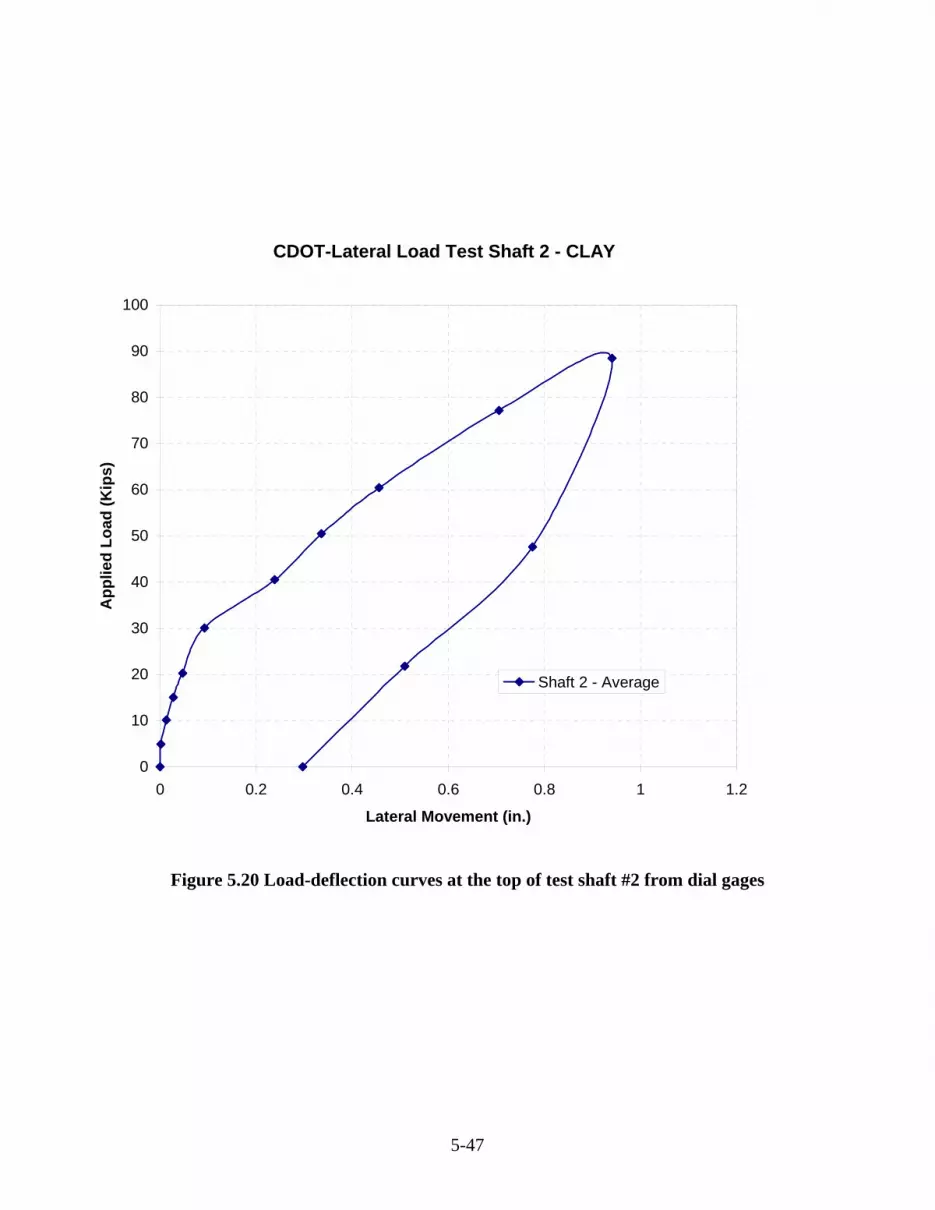
5-47

Figure 5.20 Load-deflection curves at the top of test shaft #2 from dial gages

CDOT-Lateral Load Test Shaft 2 - CLAY

0

10

20

30

40

50

60

70

80

90

100

0 0.2 0.4 0.6 0.8 1 1.2


App

lied

Load

(Kip

s)

Shaft 2 - Average

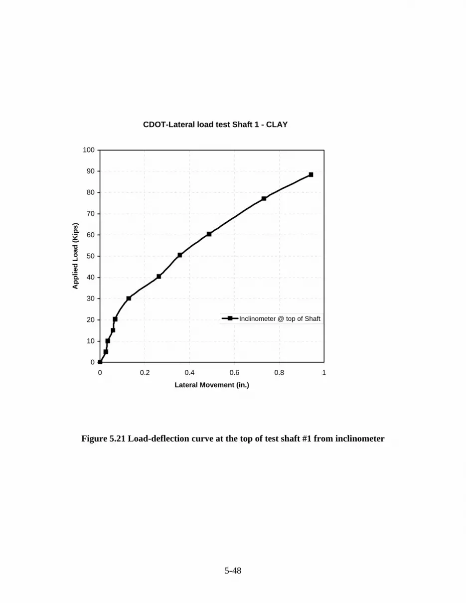
5-48

Figure 5.21 Load-deflection curve at the top of test shaft #1 from inclinometer

CDOT-Lateral load test Shaft 1 - CLAY

0

10

20

30

40

50

60

70

80

90

100

0 0.2 0.4 0.6 0.8 1


App

lied

Load

(Kip

s)

Inclinometer @ top of Shaft

5-49

Figure 5.22 Load-deflection curve at the top of test shaft #2 from inclinometer

CDOT-Lateral load test Shaft 2- CLAY

0

10

20

30

40

50

60

70

80

90

100

0 0.2 0.4 0.6 0.8 1


App

lied

Load

(Kip

s)

Inclinometer @ top of Shaft

5-50

Figure 5.23. Load-deflection curve along the depth of test shaft #1 from inclinometer

CDOT-LATERAL LOAD TEST SHAFT #1 - CLAY

0

5

10

15

20

25

30

-0.5 0 0.5 1 1.5


Dep

th (f

t.)

5 K10 K15 K20 K30 K40 K50 K60 K75 K90 K

Top of Concretedial gages location

Bottom of Shaft

Bottom of Sand

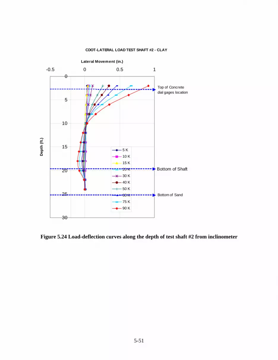
5-51

Figure 5.24 Load-deflection curves along the depth of test shaft #2 from inclinometer

CDOT-LATERAL LOAD TEST SHAFT #2 - CLAY

0

5

10

15

20

25

30

-0.5 0 0.5 1


Dep

th (f

t.)

5 K

10 K

15 K

20 K

30 K

40 K

50 K

60 K

75 K

90 K

Bottom of Shaft


Bottom of Sand

5-52

Figure 5.25. Test shaft #1, strain vs. depth on compression side

CLay Site: Shaft-1

0

2

4

6

8

10

12

14

16

18

20

-350 -300 -250 -200 -150 -100 -50 0

Strain

Dep

th (f

t)

5 K10 K15 K20 K30 K40 K50 K60 K75 K90 K

5-53

Figure 5.26. Test shaft #1, strain vs. depth on tension side

Clay Site: Shaft-1

0

2

4

6

8

10

12

14

16

18

20

0 500 1000 1500 2000

Strain

Dep

th (f

t)

5 K10 K15 K20 K30 K40 K50 K60 K75 K90 K

5-54

Figure 5.27. Test shaft #1, measured angle of tilt

Clay Site - Shaft 1Distance from jacking point to top of concrete is 38"

0

10

20

30

40

50

60

70

80

90

100

0 0.1 0.2 0.3 0.4 0.5 0.6 0.7 0.8 0.9 1

Angle of tilt (Degrees)

Late

ral L

oad

at J

acki

ng P

oint

(Kip

s)

Jacking PointTop of Concrete

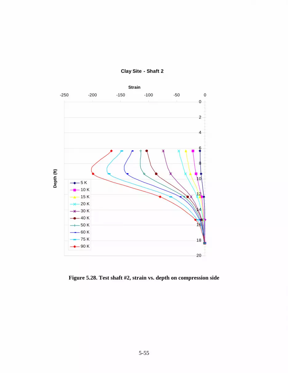
5-55

Figure 5.28. Test shaft #2, strain vs. depth on compression side

Clay Site - Shaft 2

0

2

4

6

8

10

12

14

16

18

20

-250 -200 -150 -100 -50 0

Strain

Dep

th (f

t)

5 K

10 K

15 K

20 K

30 K

40 K

50 K

60 K

75 K

90 K

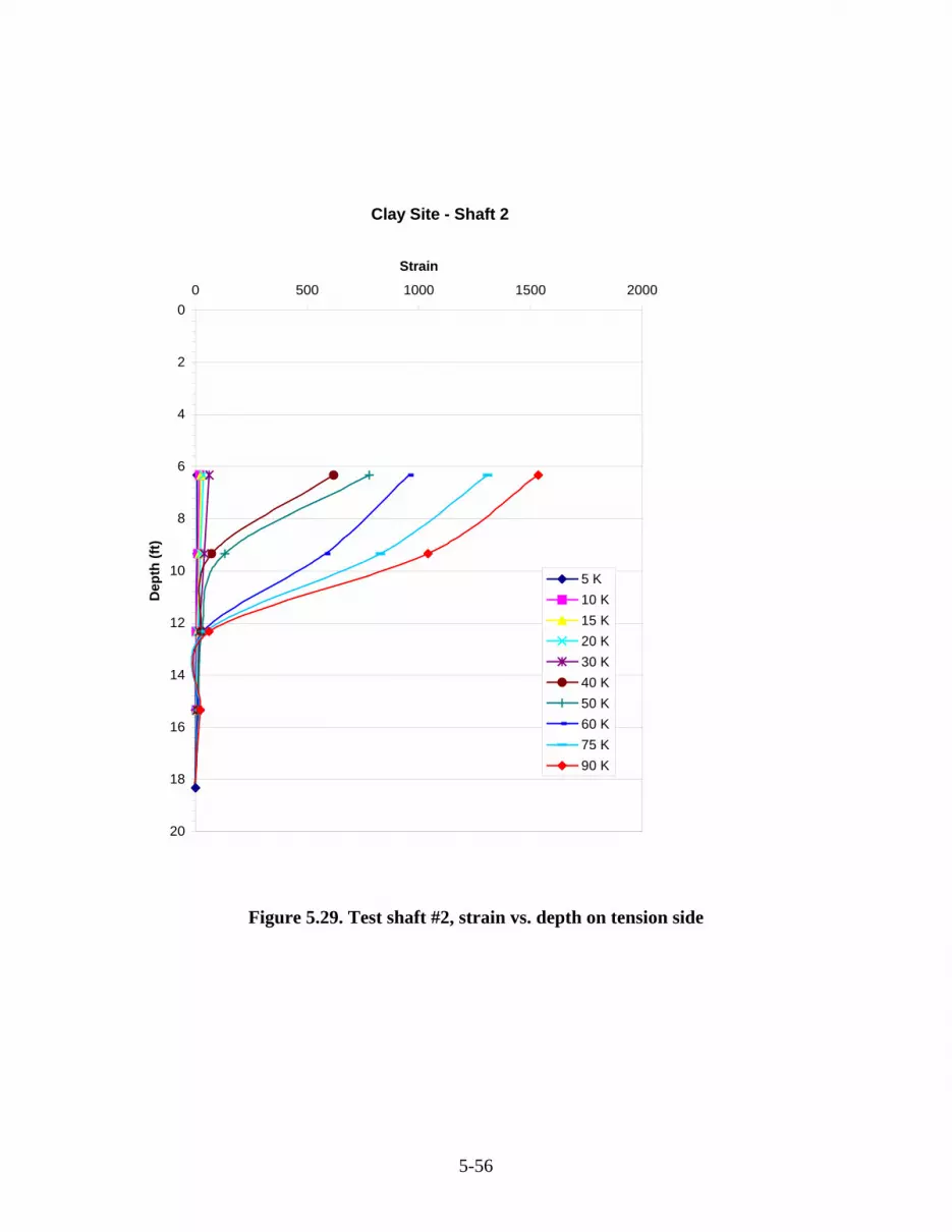
5-56

Figure 5.29. Test shaft #2, strain vs. depth on tension side

Clay Site - Shaft 2

0

2

4

6

8

10

12

14

16

18

20

0 500 1000 1500 2000

Strain

Dep

th (f

t)

5 K10 K15 K20 K30 K40 K50 K60 K75 K90 K

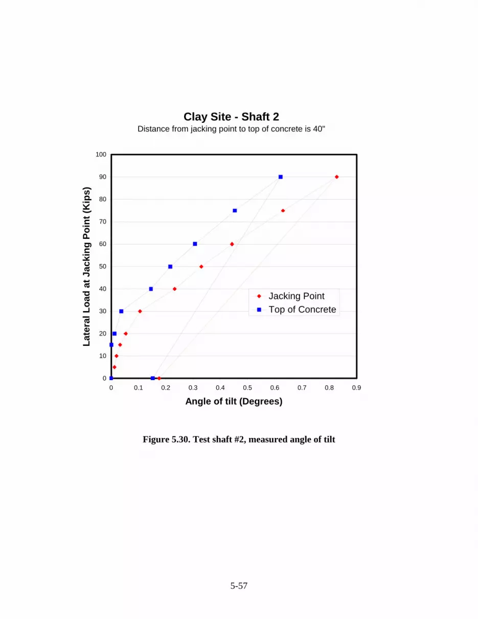
5-57

Figure 5.30. Test shaft #2, measured angle of tilt

Clay Site - Shaft 2Distance from jacking point to top of concrete is 40"

0

10

20

30

40

50

60

70

80

90

100

0 0.1 0.2 0.3 0.4 0.5 0.6 0.7 0.8 0.9


Late

ral L

oad

at J

acki

ng P

oint

(Kip

s)


5-58

Figure 5.31 The shaft setup and soil profile interpreted for analysis at clay site

15.7ft

2.5 ft

1 ft

P

3.25 ft

Shaft 1

2.5 ftSample 2-A; fill, silty clay

4.5 ft

Sample 2-AA; fill, silty clay

6.5 ftSample 2-B; fill, silty clay

10 ft

Sample 2-C; native silty clay

12.5 ftSample 2-D; native silty clay

15.7 ftSample 2-E; native silty clay

5-59

Figure 5.32 Typical pressuremeter test plot

Initial

5-60

0

10

20

30

40

50

60

70

80

90

100

0 0.5 1 1.5 2 2.5 3 3.5 4

Deflection (in.)

Load

(kip

s)

MeasuredCOM624P-SPT, LiangCOM624P-Unsat.COM624P-SPT,CDOTNAVFAC

Figure 5.33. Lateral load-deflection curves based on SPT and lab test results for CDOT test in clay, shaft # 1

5-61

0

20

40

60

80

100

120

140

0 0.2 0.4 0.6 0.8 1 1.2Deflection (in.)

Load

(kip

s)

MeasuredCOM624-PM (Su,URS)COM624-PM (p-y)COM624-PM (Su,FHWA)

Figure 5.34. Lateral load-deflection curves based pressuremeter test results for CDOT test in clay, shaft # 1

5-62

0

5

10

15

20

25

30

35

40

45

50

0 0.05 0.1 0.15 0.2 0.25 0.3 0.35 0.4

Deflection (in.)

Load

(kip

s)

MeasuredCOM624P-SPT, LiangCOM624P-Unsat.COM624P-SPT,CDOTNAVFAC

Figure 5.35. Zoomed load-deflection curves based on SPT and lab test results for CDOT test in clay, shaft # 1

5-63

0

10

20

30

40

50

60

0 0.05 0.1 0.15 0.2 0.25 0.3 0.35 0.4

Deflection (in.)

Load

(kip

s)

MeasuredCOM624-PM (Su,URS)COM624-PM (p-y)COM624-PM (Su,FHWA)

Figure 5.36. Zoomed load-deflection curves based on pressuremeter test results for CDOT test in clay, shaft # 1

5-64

p-y Curves at 24 inch depth, CDOT Clay Site

0

500

1000

1500

2000

2500

3000

0 1 2 3 4

y (in)

p (lb

/in)

MeasuredCOM624P Unsaturated CaseCOM624P SPT Liang CaseCOM624P SPT CDOT Case

(a) p-y curves from SPT and lab test determined soil parameters

p-y Curves at 24 inch depth, CDOT Clay Site

0

500

1000

1500

2000

2500

3000

0 0.5 1 1.5 2 2.5 3

y (in)

p (lb

/in)

MeasuredCOM624P PM (Su, URS)COM624P PM (Su, FHWA)

(b) p-y curves from pressuremeter determined soil parameters

Figure 5.37 P-y curves derived by strain and deflection data versus by (a) Lab and SPT soil

parameters, and (b) pressuremeter data

5-65

Load-Deflection at Shaft Top, CDOT Clay Site

0

10

20

30

40

50

60

70

80

90

0 0.1 0.2 0.3 0.4 0.5 0.6 0.7 0.8 0.9 1

Deflection (in.)

Load

(kip

s)

Measured

COM624P Measured p-y curve

Figure 5.38 Back analysis of load-deflection from measured p-y curves

5-66

0

5

10

15

20

25

30

35

40

0 0.5 1 1.5 2 2.5

Deflection (in.)

Late

ral L

oad

(kip

s)

Figure 5.39 Load-deflection curve of new design for CDOT test at clay site

5-67

Figure 5.40 Installation of gage on steel cages

Figure 5.41a Inclinometer assembly

5-68

Figure 5.41b Inclinometer installation in the hole

Figure 5.42 Pouring sand to fill around the bottom 6’ of the inclinometer tube

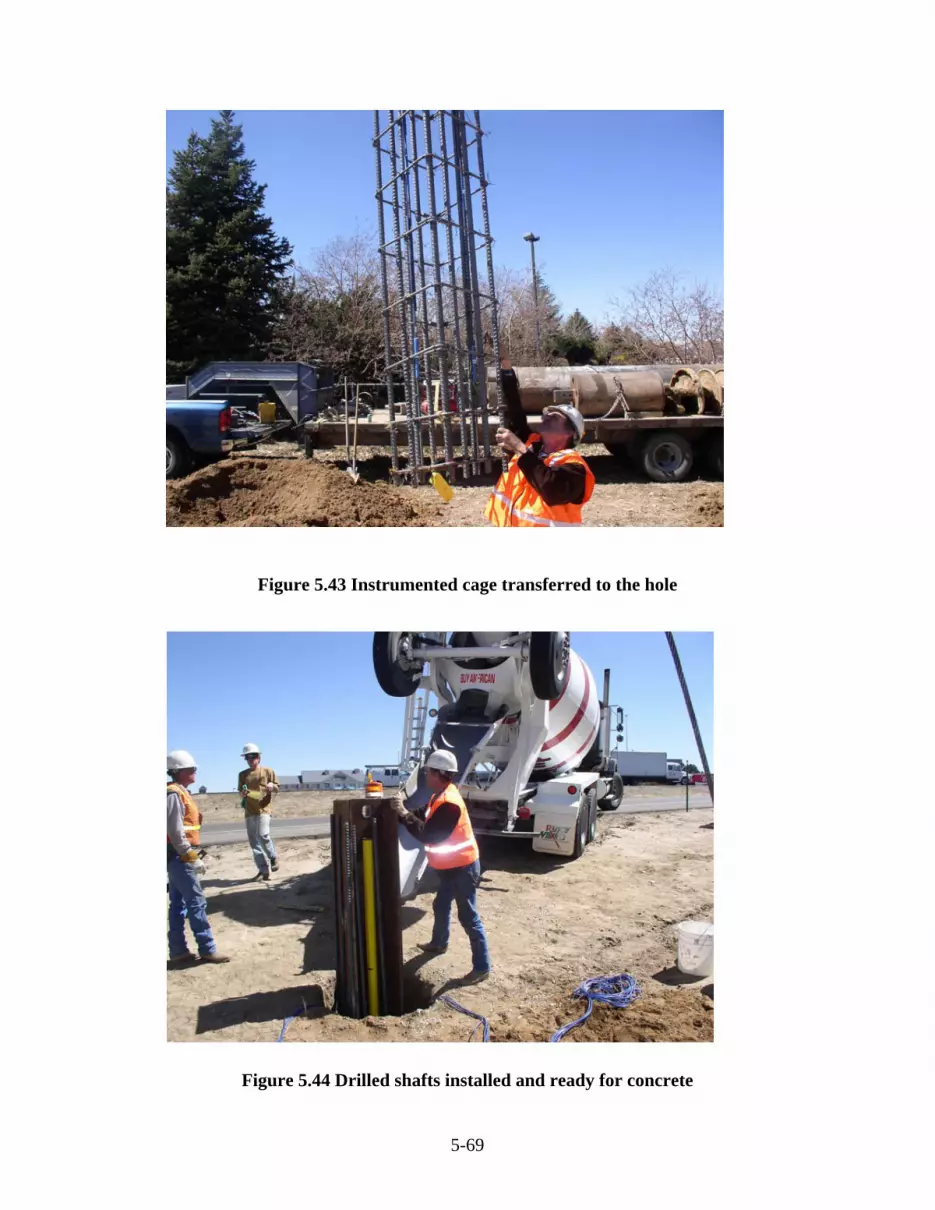
5-69

Figure 5.43 Instrumented cage transferred to the hole

Figure 5.44 Drilled shafts installed and ready for concrete

5-70

Figure 5.45 Pouring concrete in the hole


5-71


Figure 5.48 Picture showing the jacking devices

5-72

Figure 5.49 Setup of measuring devices at shaft 2 (South)

Figure 5.50 Setup of measuring devices at shaft 1 (North)

5-73

Figure 5.51 General view of the load test

Figure 5.52 Running the test and watching the instruments

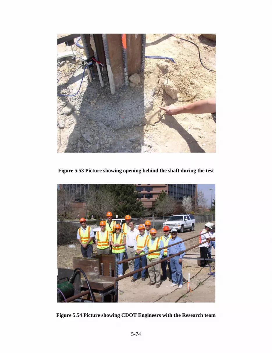
5-74

Figure 5.53 Picture showing opening behind the shaft during the test

Figure 5.54 Picture showing CDOT Engineers with the Research team

5-75

Figure 5.55 Load-deflection curve at the top of test shaft North from dial gages

Northern Shaft (Deflection vs. Applied load)

0

10

20

30

40

50

60

70

0 0.2 0.4 0.6 0.8 1 1.2 1.4 1.6 1.8

Lateral Movement (in)

App

lied

Late

ral L

oad

(K)

Dial Gages

5-76

Figure 5.56 Load-deflection curves at the top of test shaft South from dial gages

Southern Shaft (Deflection vs. Applied load)

0

10

20

30

40

50

60

70

0 0.1 0.2 0.3 0.4 0.5 0.6 0.7 0.8


App

lied

Late

ral L

oad

(K)

Dial Gages

5-77

Figure 5.57 Load-deflection curve at the top of test shaft North from inclinometer

Northern Shaft (Deflection vs. Applied load)

0

10

20

30

40

50

60

70

0 0.5 1 1.5 2 2.5


App

lied

Late

ral L

oad

(K)

Inclinometer

5-78

Figure 5.58 Load-deflection curve at the top of test shaft South from inclinometer

Southern Shaft (Deflection vs. Applied load)

0

10

20

30

40

50

60

70

0 0.1 0.2 0.3 0.4 0.5 0.6 0.7 0.8


App

lied

Late

ral L

oad

(K)

Inclinometer

5-79

Figure 5.59. Load-deflection curve along the depth of test shaft North from inclinometer

CDOT-LATERAL LOAD TEST SHAFT #N - SAND

0

5

10

15

20

25

30

-1 0 1 2 3 4


Dep

th (f

t.)

3 K

8 K

13 K

18 K

25 K

35 K

45 K

55 K

65 K

35 K ReLoad


Bottom of Shaft

Bottom of Sand

5-80

Figure 5.60 Load-deflection curves along the depth of test shaft South from inclinometer

CDOT-LATERAL LOAD TEST SHAFT #S - SAND

0

5

10

15

20

25

30

-0.1 0 0.1 0.2 0.3 0.4 0.5 0.6 0.7 0.8


Dep

th (f

t.)

3 K

8 K

13 K

18 K

25 K

35 K

45 K

55 K

65 K


Bottom of Shaft

Bottom of Sand

5-81

Figure 5.61. Test shaft North, strain vs. depth on compression side

Sandy Site - Northern Shaft

0

2

4

6

8

10

12

14

16

18

20

-200 0 200 400 600 800 1000

Strain

Dep

th (f

t)

3 K8 K13 K18 K25 K35 K45 K55 K65 K0U K

5-82

Figure 5.62 Test shaft North, strain vs. depth on tension side

Sandy Site - Northern Shaft

0

2

4

6

8

10

12

14

16

18

20

0 200 400 600 800 1000 1200 1400 1600

Strain

Dep

th (f

t)

3 K8 K13 K18 K25 K35 K45 K55 K65 K0U K

5-83

Figure 5.63. Test shaft North, measured angle of tilt

Sandy Site - Northern ShaftDistance from jacking point to top of concrete is 54"

0

10

20

30

40

50

60

70

0 0.2 0.4 0.6 0.8 1 1.2


Late

ral L

oad

at J

acki

ng P

oint

(Kip

s)

Top of ConcreteJacking Point

5-84

Figure 5.64. Test shaft South, strain vs. depth on compression side

Sandy Site: Southern Shaft

0

2

4

6

8

10

12

14

16

18

20

-200 -150 -100 -50 0 50 100 150

Strain

Dep

th (f

t)

3 K

8 K

13 K

18 K

25 K

35 K

45 K

55 K

65 K

0U K

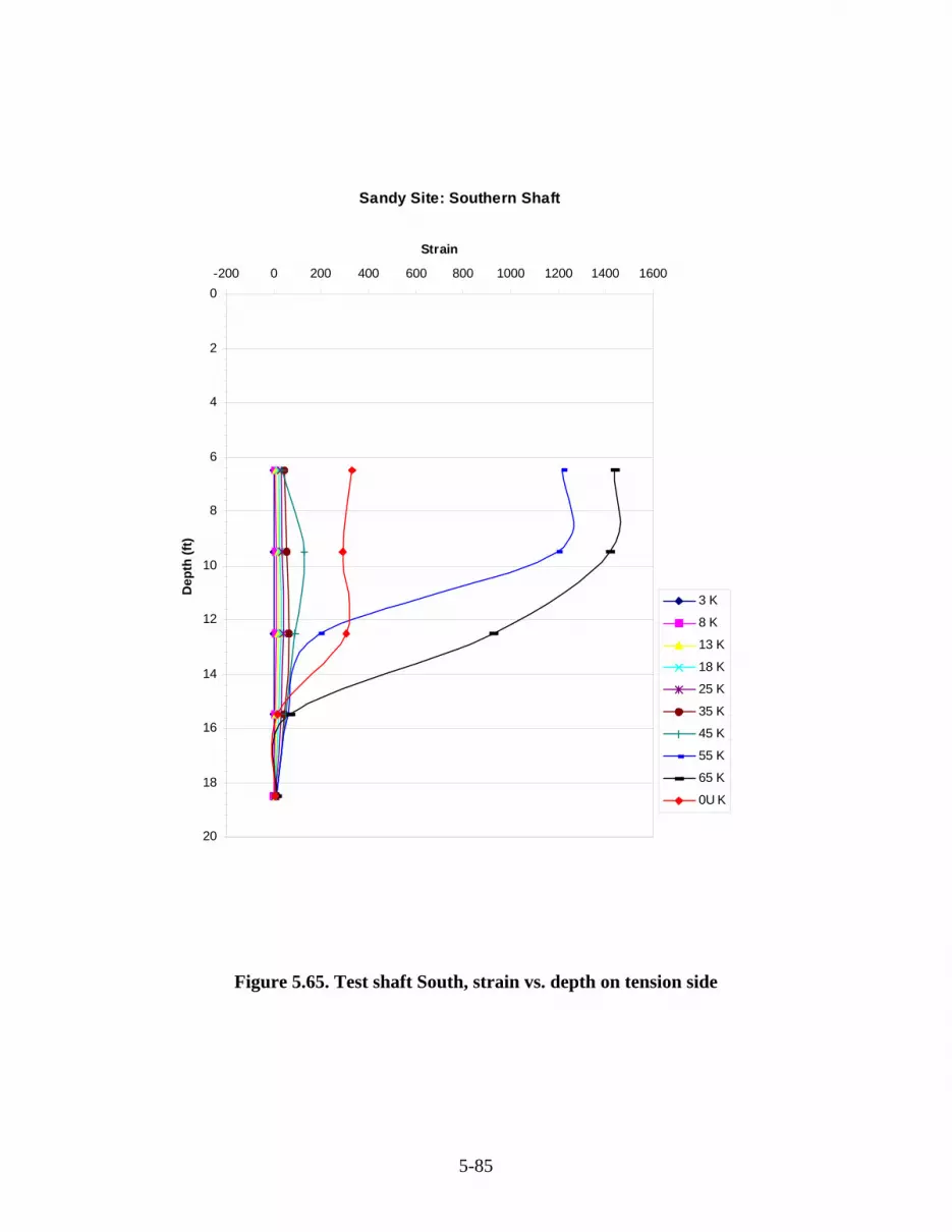
5-85

Figure 5.65. Test shaft South, strain vs. depth on tension side

Sandy Site: Southern Shaft

0

2

4

6

8

10

12

14

16

18

20

-200 0 200 400 600 800 1000 1200 1400 1600

Strain

Dep

th (f

t)

3 K

8 K

13 K

18 K

25 K

35 K

45 K

55 K

65 K

0U K

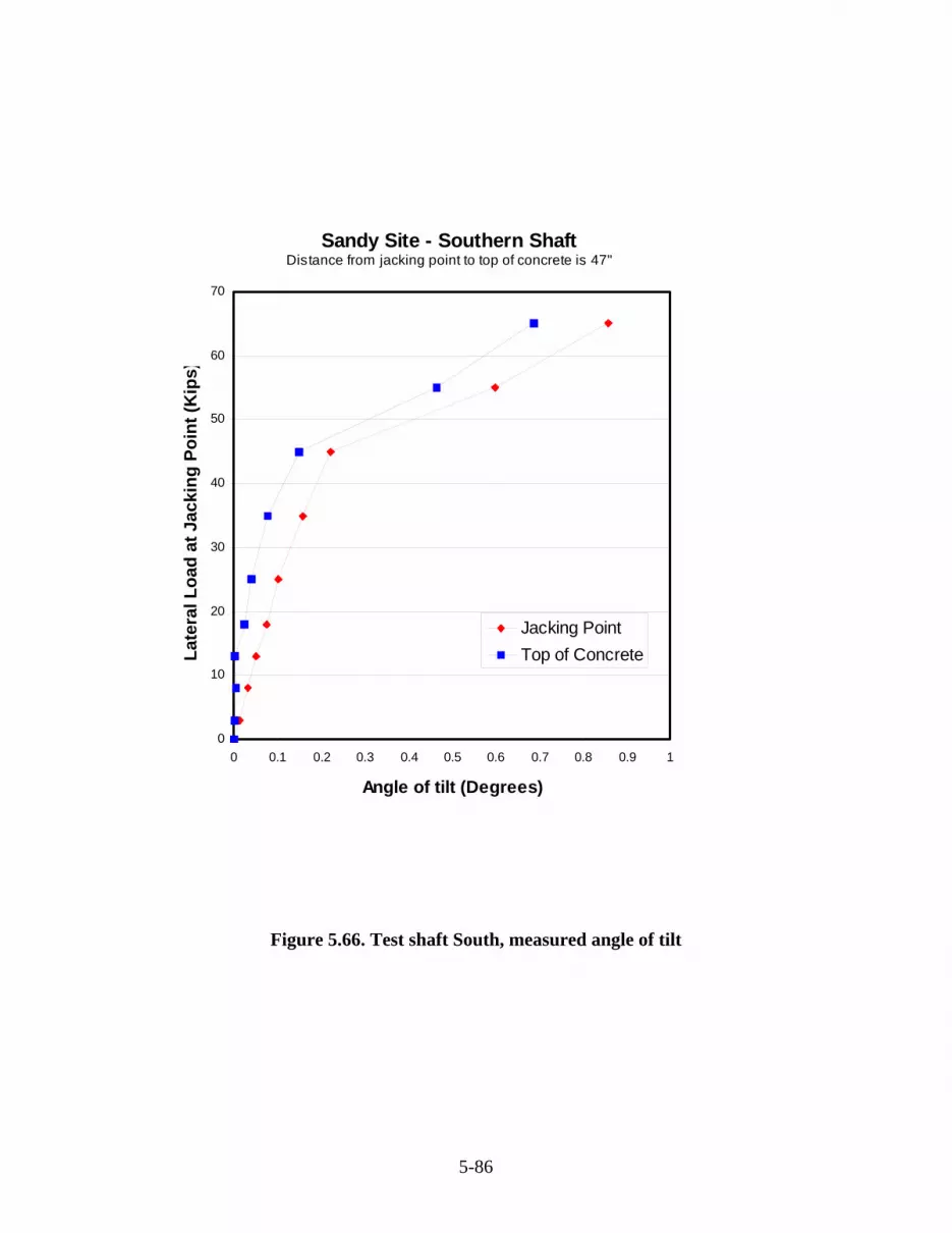
5-86

Figure 5.66. Test shaft South, measured angle of tilt

Sandy Site - Southern ShaftDistance from jacking point to top of concrete is 47"

0

10

20

30

40

50

60

70

0 0.1 0.2 0.3 0.4 0.5 0.6 0.7 0.8 0.9 1


Late

ral L

oad

at J

acki

ng P

oint

(Kip

s)


5-87

Figure 5.67 The shaft setup and soil profile interpreted for CDOT sand site

16 ft

2.5 ft

1 ft

P

4 ft

Shaft

4 ft

SPT N=13

6 ft SPT N= 8

9 ft

SPT N=10

15 ft

SPT N=7

Silt sand for all the layers.

16 ft SPT N=7

Sample 4A

Sample 4B

5-88

Load-Deflection Curves on CDOT Sand Site

0

10

20

30

40

50

60

70

80

0 1 2 3 4 5 6 7 8

Deflection (in.)

Load

(kip

s)

Measured South ShaftSPT Liang CasePM CaseDirect Shear CaseSPT CDOT Case

Figure 5.68. Load-deflection curves for CDOT test in sand, South shaft

5-89

p-y Curves at 30 inch depth, CDOT Sand Site

0

200

400

600

800

1000

1200

0 0.1 0.2 0.3 0.4 0.5 0.6

y (in)

p (lb

/in)

MeasuredCOM624P Direct ShearCOM624P, SPT LiangCOM624P, SPT CDOTCOM624P, PM Case

Figure 5.69 Measured and predicted p-y curves based on current stiff clay p-y criteria used in COM624P

5-90

Load-Deflection Curves on CDOT Sand Site

0

10

20

30

40

50

60

70

80

0 0.5 1 1.5 2 2.5 3

Deflection (in.)

Load

(kip

s)

Measured South Shaft

COM624P, Measured p-y curves

COM624P, Direct Shear

Figure 5.70 Load-deflection curves predicted by using measured p-y curves for sand testing site

5-91

Load-Deflection Curve of CDOT Sand Site, New Design

0

5

10

15

20

25

30

35

0 1 2 3 4 5

Deflection (in.)

Load

(kip

s)

Figure 5.71 Load-deflection curve of new design for CDOT test at sand site

6-1

6 FINITE ELEMENT MODELING TECHNIQUES A true finite element modeling in the continuum framework can be accomplished by the

powerful commercial finite element code ABAQUS. The modeling techniques are discussed

herein, including the constitutive models for the soil and the interface, and the mesh

representation. The modeling technique is validated against one load test result selected from the

lateral load test database in Section 4.2 and the two CDOT tests. The intent of this chapter was to

demonstrate the developed finite element modeling techniques for specialized drilled shafts

projects. It was not the objective of this research to present a design methodology based on FEM

approach.

6.1 FEM Modeling Details 6.1.1 The Finite Elements and the Mesh The finite element chosen for representing the drilled shaft is a 15-node triangular prism element,

C3D15, shown in Fig. 6.1. In the earlier stage of the study, the finite element chosen for

representing the soil surrounding the shaft was a 21-node brick, reduced integration element,

C3D21R. However, it is found that the first order 3-D element C3D8 can also represent the soil

mass very well by comparing with the simulation with C3D21R elements; meanwhile the

simulation will become more efficiently. Therefore, in the simulation study on CDOT’s, C3D8

element is chosen for representing soils; and CIN3D8, a 3-D infinite boundary element, is

selected for the outside boundary of soil mass. Fig. 6.1 (a) to (c) depicts the three types of

elements adopted for representation of drilled shaft, soils, and out side boundary, respectively.

Fig. 6.2 shows both the side view and 3-D view of the final mesh of CDOT test shaft and

surrounding soils. The total depth of the soil mass is 1.5 times the embedment depth of shaft. For

CDOT test cases, the shaft embedment depth is 15.7 ft; and then the total soil mass has the depth

of 23.7 ft. The outer diameter of soil mass is chosen as 10 times the shaft diameter. For CDOT

test cases, the shaft diameter is 3 ft; and then the corresponding soil mass has 30 ft of out

diameter. The dimension of final mesh is depicted in Fig. 6.3. The selection of the mesh size is

based on minimizing the effect of boundary and also using small size to improve the processing

6-2

speed. A coarse mesh is used to simulate the drilled shaft structure to save running time. Initially,

in order to save working space and to speed up the analysis, the symmetric model of the drilled

shaft under lateral loads is used for validation case, which will be introduced in the following

section. However, due to the difficulty of convergence, the full size modeling is used for CDOT

test sites.

6.1.2 Constitutive Models for Soils There are four plasticity models available for modeling soil behavior in the ABAQUS program:

Extended Drucker-Prager model, Modified Drucker-Prager/Cap model, Mohr-Coulomb

Plasticity model, and Critical State (Clay) Plasticity Model. In the present investigation, Mohr-

Coulomb Plasticity model is used since the input parameters are relatively easy to obtain.

6.1.2.1 Overview

The Mohr-Coulomb plasticity model possesses the following capabilities and features.

• It is used to model materials with the classical Mohr-Coulomb yield criterion;

• It allows the material to harden and/or soften isotropically.

• It uses a smooth flow potential that has a hyperbolic shape in the meridional stress plane

and a piecewise elliptic shape in the deviatoric stress plane.

• It is used with the linear elastic material model.

• It can be used for design applications in the geotechnical engineering area to simulate

material response under essentially monotonic loading.

6.1.2.2 Yield Criterion

The Mohr-Coulomb criterion assumes that failure occurs when the shear stress on any point in a

material reaches a value that depends linearly on the normal stress in the same plane. The Mohr-

Coulomb model, depicted in Fig. 6.4, is based on plotting Mohr’s circle for states of stress at

failure in the plane of the maximum and minimum principal stresses. The failure line is the best

straight line that touches these Mohr’s circles.

Therefore, the Mohr-Coulomb model is defined by

φσ−=τ tanc (6.1)

6-3

where σ is negative in compression. For general states of stress the model is more conveniently

written in terms of three stress invariants as

0ctanpqRF mc =−φ−= (6.2)

where

φπ

+Θ+π

+Θφ

=φΘ tan)3

cos(31)

3sin(

cos31),(R mc (6.3)

Φ is the slope of the Mohr-Coulomb yield surface in the p-Rmcq stress plane, shown in

Fig. 6.5, which is commonly referred to as the friction angle of the material and can be

dependent on the temperature and the predefined field variables;

c is the cohesion of the material; and

Θ is the deviatoric polar angle defined as

3

qr)3cos( ⎟⎟⎠

⎞⎜⎜⎝

⎛=Θ (6.4)

and

)(trace31p σ−= is the equivalent pressure stress,

)S:S(23q = is the Mises equivalent pressure stress,

( ) 3/1SSS2/9r ⋅⋅= is the third invariant of deviatoric stress,

pIS +σ= is the deviatoric stress.

6.1.2.3 Flow Potential

The flow potential G is chosen as a hyperbolic function in the meridional stress plane and the

smooth elliptic function proposed by Menétrey and Willam (1995) in the deviatoric stress plane.

A family of hyperbolic potentials in the meridional stress plane is shown in Fig. 6.6, and the flow

potential in the deviatoric stress plane is shown in Fig. 6.7.

6.1.3 Simulation of Interaction between Shaft and Soil The simulation of a contact problem is challenging in the context of finite element analysis. The

Florida Pier finite element program uses the spring element to simulate the interaction between

6-4

the shaft and the soil, thus avoiding the need for contact simulation. The nonlinear stiffness of

the spring element is determined based on semi-empirical p-y relationship commonly used in the

COM624P computer program. Therefore, there is really no difference between Florida Pier and

COM624P analysis. For a truly continuum based FEM approach, the use of contact for

simulating the shaft and soil interaction is necessary. Two kinds of contact simulations are

available in ABAQUS, one is contact element, and the other one is surface-based contact

interface. The surface-based interface is highly recommended in ABAQUS manual for most type

of contact simulations; therefore, the surface-based contact option is chosen in present study.

For the surface-based contact, two surfaces, one is master surface, and the other one is slave

surface, are required for defining a contact. The master surface should be a surface which is more

rigid than slave surface. In present study, the outside of drilled shaft surface is defined as the

master surface; while the inner side of soil surface which is directly surrounding shaft is defined

as slave surface. The nodes of master surface could penetrate into slave surface, but it is not

allowed for nodes of slave surface to penetrate into master surface.

ABAQUS simulates two kinds of contact behavior for surface-based contact, one is the

tangential friction between the two surfaces, and the other one is the load transfer between the

two surfaces in normal direction. The basic coulomb friction model, presented in Fig. 6.8, is used

to simulate the frictional interaction. The constant friction coefficient is required for input. The

effect of contact friction between the shaft and the soil on the lateral behavior of shaft is

relatively small, as illustrated by comparison shown in Fig. 6.9.

For the behavior of the interface in normal direction, the default “hard” contact pressure-

clearance relation option is adopted in the current FEM modeling of the shaft-soil contact. The

“hard” option will provide reasonable contact behavior in normal direction. In this contact

option, any pressure can be transmitted between the surfaces if the two surfaces are under

contact. The contact pressure reduces to zero, if the interface is separated. Conversely, the

separation condition will return back to contact condition, when the clearance between them

reduces to zero.

6-5

6.1.4 Simulation of Initial Condition In order to simulate the in-situ initial condition, two steps of loading will be applied as shown in

Fig. 6.10. The self weight of the soil and shaft is applied in the first step to simulate the initial

effective stress condition. Then, the external lateral load is applied incrementally to allow for

calculation of load vs. deflection response of the drilled shaft.

6.2 Validation of FEM Model

As part of this study, extensive trial of various modeling details has been conducted. Furthermore,

several load test cases were used to validate the proposed modeling details. Since the main

objective of this study is to use the proposed FEM modeling technique to predict the Colorado

load test data, a representation plot of one validation exercise is given in Fig. 6.11. The soil

profile and the associated soil properties used in the FEM simulation are documented in Table

6.1. The match between the FEM predicted and actual measured load-deflection curves is

presented in Fig. 6.11. The comparisons for the deflection vs. depth are shown in Fig. 6.12. It can

be seen that as long as the soil parameters and the interface friction properties are properly

selected, FEM simulation results can have a good agreement with the actual test results.

6-6

Table 6.1 Parameters for Soils

Soil Layers

Depth (ft.-in.)

Cohesion Yield Stress (psi)

Volumetric Plastic Strain

Young’s Modulus

(ksi)

Materials Cohesion

(psi)

6 0 11 0.008 14 0.016 Soil1 0 – 24’’

15 0.024

9.9 22

3 0 5 0.008 7 0.016 Soil2 24’’ –

103’’ 8 0.024

4.95 11

14 0 25 0.008 32 0.016 Soil3 103’’ –

120’’ 35 0.024

22.5 50

15 0 27 0.008 35 0.016 Soil4 120’’ –

144’’ 39 0.024

24.75 55

6.3 Simulation of CDOT Test at Clay Site

Two simulation cases have been conducted to simulate the lateral load test results of Shaft 1 at

CDOT clay site. The input in the first case is mainly based on the triaxial test results. The

equivalent elastic modulus of shaft could range from 3600 ksi to 6000 ksi, depending on the

reinforcement ratio as well as load level. In order to identify the effect of shaft modulus on

lateral response, three try run of FEM analyses by using elastic modulus of shaft of 4000 ksi,

5000 ksi, and 6000 ksi are conducted and the results of the lateral response are plotted in Fig.

6.13. It can be seen that the effect of initial elastic shaft modulus on lateral response is negligible.

Therefore, the initial modulus of drilled shafts is selected as 5000 ksi. The elastic modulus of

soils Es was directly obtained from the triaxial tests results. The cohesion yield stress and

corresponding plastic strains depicted in Fig. 6.14 are obtained from deviatoric stress-strain

curves of triaxial tests. The input parameters for soil materials are given in Table 6.2. The

friction coefficient for clay-shaft interface is assumed as a default value of 0.5 since the effect of

friction on lateral response is minimal.

6-7

Table 6.2 Input of Soil Parameters from Triaxial Test Results

Layers

(ft)

Es(psi) C1(psi) ε1 C2(psi) ε2 C3(psi) ε3 C4(psi) ε4

0-2.5 4140 10.35 0 15.5 0.008 17 0.0155 18.3 0.04

2.5-4.5 3320 7.8 0 12 0.029 17.2 0.07 18.3 0.11

4.5-6.5 3320 7.8 0 12 0.029 17.2 0.07 18.3 0.11

6.5-10 1614 6.9 0 10.41 0.016 13.2 0.09 14.8 0.19

10-12.5 789 3.5 0 6.94 0.029 8.5 0.09 9.2 0.19

12.5-16 3474 3.5 0 9 0.023 11.3 0.098 11.7 0.198

The comparison between the FEM predicted and actual measured load-deflection curves is

presented in Fig. 6.15. An adjustment of input soil parameters in FEM simulation, including

using 30% increased unload modulus from pressuremeter test results to represent soil modulus,

was made as shown in Table 6.3 for achieving better match between the FEM predictions and

actual test data. The deflection vs. shaft depth for FEM simulations at two lateral load levels (20

kips and 90 kips) is shown in Fig. 6.16 and Fig. 6.17, using triaxial test soil parameters and best

match soil parameters, respectively. It is apparent that achieving the matches between the FEM

simulation and actual measurement are much more difficult for the deflection vs. depth plot than

for the load-deflection curve at shaft top.

The FEM simulation results could be used to infer the p-y curves. The comparisons shown in Fig.

18(a) are for p-y curves at 15 inch depth, using actual load test data (only 24 inch depth is

available), ABAQUS FEM simulation with triaxial soil parameters, and ABAQUS FEM

simulation with best match. Similar p-y curve comparison plot is shown in Fig. 6.18 (b) for p-y

curves at 42 inch depth. Based on observations from these two plots, one may conclude that the

ABAQUS derived p-y curves are close to those from measured.

6-8

Table 6.3 Adjusted Soil Parameters for Match Case at Clay Site

Layers

(ft)

Es(psi) C1(psi) ε1 C2(psi) ε2 C3(psi) ε3 C4(psi) ε4

0-2.5 21684 9 0 13 0.008 16 0.016 18.3 0.024

2.5-4.5 21684 7 0 10.5 0.008 13 0.016 15 0.024

4.5-6.5 21684 7 0 10 0.008 12.8 0.016 14.4 0.024

6.5-10 6867 7 0 10 0.008 12 0.016 13.7 0.024

10-12.5 6867 5 0 7 0.008 8.5 0.016 9.4 0.024

12.5-16 6867 6 0 8.5 0.008 10.5 0.016 11.7 0.024

6.4 Simulation of CDOT Test at Sand Site

Two simulation cases have been conducted to simulate the lateral load test at CDOT sand site.

The competent south shaft at sand site is used for simulation. The input parameters of the first

case is mainly based on the friction angles and cohesions from direct shear tests and the modulus

from pressuremeter tests. The initial shaft elastic modulus is chosen as 5000 ksi. The reload

modulus E+ from pressuremeter test is utilized to represent the modulus of sands. The cohesion

yield stress and plastic strains are selected to be close to measured cohesions by direct shear tests

and also make the convergence of the simulation available. The input parameters for soil

materials are presented in Table 6.4. The friction coefficient between shaft and sand is assumed

to be 0.5, e.g. tan27°.

Table 6.4 Input of Soil Parameters from Direct Shear Tests and PM Tests

Depth (ft)

Es(psi) Φ C1(psi) ε1 C2(psi) ε2 C3(psi) ε3 C4(psi) ε4

0 - 4 5421 41.1 1.84 0 3.2 0.01 4 0.03 4.6 0.05 4 - 6 5421 41.1 1.84 0 3.2 0.01 4 0.03 4.6 0.05 6 - 9 4309 41.1 1.84 0 3.2 0.01 4 0.03 4.6 0.05 9 - 15 7645 39.5 1.12 0 2.0 0.01 2.5 0.03 2.8 0.05 15 - 15.7 7645 39.5 1.12 0 2.0 0.01 2.5 0.03 2.8 0.05

The comparison between the FEM predicted and actual measured load-deflection curves is

presented in Fig. 6.19. An adjustment of input soil parameters in FEM simulation, increasing

6-9

modulus by 60%, was made as shown in Table 6.5 for achieving better match between the FEM

predictions and actual test data. The deflection vs. shaft depth for FEM simulations at two lateral

load levels (25 kips and 45 kips) is shown in Fig. 6.20 and Fig. 6.21, using direct shear test and

pressuremeter test soil parameters and best match soil parameters, respectively. It is apparent that

achieving the matches between the FEM simulation and actual measurement are much more

difficult for the deflection vs. depth plot than for the load-deflection curve at shaft top.

The FEM simulation results could be used to infer the p-y curves. The comparisons shown in Fig.

6.22(a) are for p-y curves at 24 inch depth, using actual load test data (only 30 inch depth is

available), ABAQUS FEM simulation with lab and pressuremeter test soil parameters, and

ABAQUS FEM simulation with best match. Similar p-y curve comparison plot is shown in Fig.

6.22 (b) for p-y curves at 60 inch depth. Based on observations from these two plots, one may

conclude that the ABAQUS derived p-y curves are close to those from measured.

Table 6.5 Adjusted Soil Parameters for Match Case at Sand Site

Depth (ft)

Es(psi) Φ C1(psi) ε1 C2(psi) ε2 C3(psi) ε3 C4(psi) ε4

0 - 4 8674 41.1 1.84 0 3.2 0.01 4 0.02 4.6 0.03 4 – 6 8674 41.1 1.84 0 3.2 0.01 4 0.02 4.6 0.03 6 – 9 6894 41.1 1.84 0 3.2 0.01 4 0.02 4.6 0.03 9 – 15 12232 39.5 1.12 0 2.0 0.01 2.5 0.02 2.8 0.03 15 – 15.7 12232 39.5 1.12 0 2.0 0.01 2.5 0.02 2.8 0.03

6.5 Recommended Soil Parameters Determination for FEM Simulation Based on above analyses, the tests required for determination of soil parameters are tabulated in

table 6.6. The friction coefficient between shaft and soils could be chosen as 0.5.

Soils Soil modulus Es C1-C4, ε1- ε4* Friction Angle Φ

Clay Unload modulus of

pressuremeter test

CU triaxial test CU triaxial test

Sand Reload or unload modulus

of pressuremeter test

CU triaxial test or

direct shear test

CU triaxial test or

direct shear test

Note: * C1 to C4 are the cohesion yield stresses; and ε1 to ε4 are corresponding plastic strains.

6-10

6.6 Summary of FEM Simulation

The 3-D finite element simulations by using ABAQUS techniques on CDOT test sites, tells that

the FEM model provides relative conservative prediction on load-deflection curves if the input

parameters are obtained from lab or in-situ tests. Based on the two simulations, it can be seen

that soil modulus obtained from pressuremeter test provides better prediction than those from

triaxial tests. If the shaft modulus is varied with moment and the elastic soil modulus is increased

from measured values by certain amount, such as 30%, then the simulation could provide good

match with measured results.

During the FEM simulation, the p-y curves are also derived and used for COM624P program to

predict the lateral response. Both for clay and sand, the derived p-y curves are very close that

derived from measured strains and deflections. This implies that the p-y curves could be derived

from FEM simulation.

The ability and versatility of the developed FEM simulation technique for laterally loaded drilled

shafts have been demonstrated by means of comparisons with actual load test data. Although the

FEM simulation is a very powerful tool, the complexities and time involvement for performing

such work are quite demanding. Therefore, the FEM simulation is best reserved for the projects

with unusual situations such as extremely large size drilled shafts, exceptional loading conditions,

and highly complex soil types and behavior.

6-11

Figure 6.1. Finite elements selected for representation of (a) drilled shaft, (b) surrounding

soils, and (c) outside boundary of soils.

C3D15

C3D8

(a)

(b) (c)

6-12

(a) Side View

(b) 3-D View

Figure 6.2 FEM mesh representing test shafts and soils at CDOT test sites

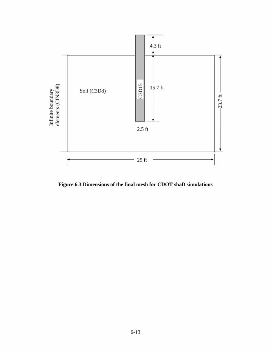
6-13

Figure 6.3 Dimensions of the final mesh for CDOT shaft simulations

25 ft

2.5 ft

15.7 ft

4.3 ft

C3D

15

Soil (C3D8)

Infin

ite b

ound

ary

elem

ents

(CIN

3D8)

23.7

ft

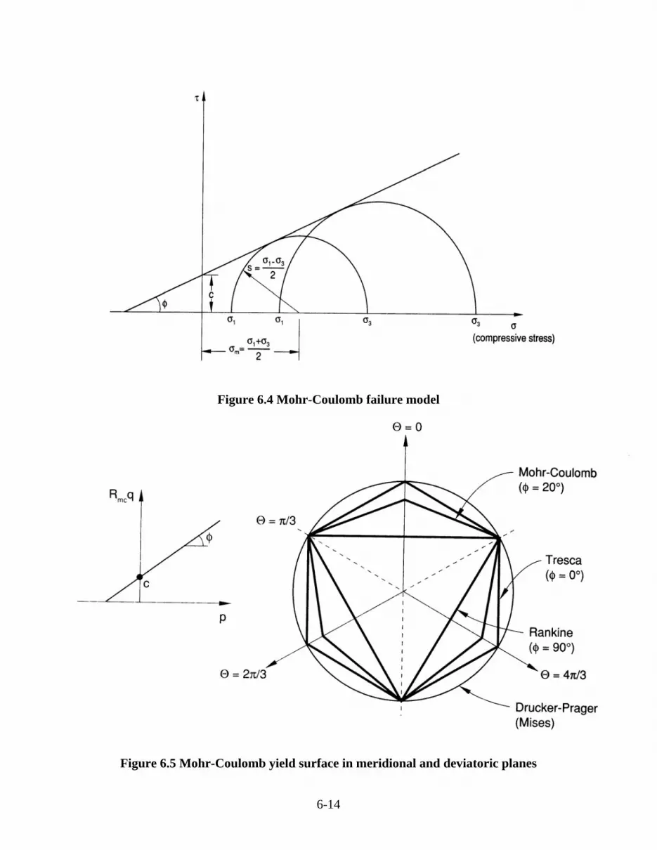
6-14

Figure 6.4 Mohr-Coulomb failure model

Figure 6.5 Mohr-Coulomb yield surface in meridional and deviatoric planes

6-15

Figure 6.6 Family of hyperbolic flow potentials in the meridional stress plane

Figure 6.7 Menétrey-Willam flow potential in the deviatoric stress plane

6-16

Figure 6.8 Slip regions for the default Coulomb friction model

µ, Constant Friction Coefficient

Stick Region

6-17

Load-Deflection Curves Generated By ABAQUS

0

10

20

30

40

50

60

0 0.2 0.4 0.6 0.8

Deflection (in.)

Load

(kip

s)FEM-WithoutFriction

FEM-FrictionTan30

Figure 6.9 The comparison of FEM model with friction and without friction

6-18

Figure 6.10 Simulation of initial soil effective stress condition

Soil with weight

Shaft with weight

Step 1: Gravity Applied

Soil with weight

Shaft with weight

Step 2: Apply Lateral Load

6-19

I-90P101, Comparison of Load-Deflection Curves

0

10

20

30

40

50

60

70

0 0.2 0.4 0.6 0.8 1Deflection (in.)

Load

(kip

s)Measured

ABAQUS

Figure 6.11 The comparison of load vs. deflection curves between measured results and

FEM analysis

I-90P101, Comparison of Defelction-Depth Curves

0

2

4

6

8

10

12

14

-0.5 0 0.5 1 Deflection (in.)

Dep

th (f

t)

Measured at65 kips

ABAQUS at65 kips

Figure 6.12 The comparison of deflection vs. depth curves between measured results and

FEM analysis

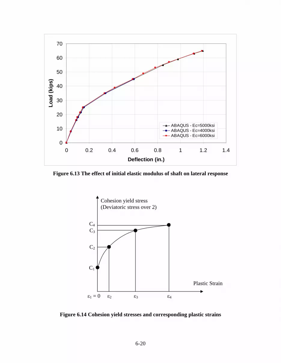
6-20

0

10

20

30

40

50

60

70

0 0.2 0.4 0.6 0.8 1 1.2 1.4

Deflection (in.)

Load

(kip

s)

ABAQUS - Ec=5000ksiABAQUS - Ec=4000ksiABAQUS - Ec=6000ksi

Figure 6.13 The effect of initial elastic modulus of shaft on lateral response

Figure 6.14 Cohesion yield stresses and corresponding plastic strains

Plastic Strain

Cohesion yield stress (Deviatoric stress over 2)

C1

C2

C3

C4

ε1 = 0 ε2 ε3 ε4

6-21

Load-Deflection at Shaft Top, CDOT Clay Site

0

10

20

30

40

50

60

70

80

90

100

0 0.2 0.4 0.6 0.8 1 1.2 1.4

Deflection (in.)

Load

(kip

s)

Measured

ABAQUS-Match Case

ABAQUS-Triaxial

Figure 6.15 Simulated and measured load-deflection curves of CDOT test at clay site

6-22

Deflection-Depth of CDOT Clay Site, ABAQUS-Triaxial Case

-2

0

2

4

6

8

10

12

14

16

18

-0.05 0 0.05 0.1 0.15 0.2 0.25

Deflection (in.)

Dep

th (f

t)

Mea.20 kipsABAQUS 20 kips

(a) Triaxial case with 20 kips of load

Deflection-Depth of CDOT Clay Site, ABAQUS-Triaxial Case

-2

0

2

4

6

8

10

12

14

16

18

-0.5 0 0.5 1 1.5 2

Deflection (in.)

Dep

th (f

t)

Mea. 90 kipsABAQUS 90 kips

(b) Triaxial case with 90 kips of load

Figure 6.16 Comparisons of measured deflection-depth curves and those from FEM

simulation with soil input from triaxial tests for CDOT test at clay site

6-23

Deflection-Depth of CDOT Clay Site, ABAQUS-Match Case

-2

0

2

4

6

8

10

12

14

16

18

-0.04 -0.02 0 0.02 0.04 0.06 0.08

Deflection (in.)

Dep

th (f

t)

Mea.20 kipsABAQUS 20 kips

(a) Match case with 20 kips of load

Deflection-Depth of CDOT Clay Site, ABAQUS-Match Case

-2

0

2

4

6

8

10

12

14

16

18

-0.2 0 0.2 0.4 0.6 0.8 1 1.2

Deflection (in.)

Dep

th (f

t)

Mea. 90 kipsABAQUS 90 kips

(b) Match case with 90 kips of load


simulation with best match soil input for CDOT test at clay site

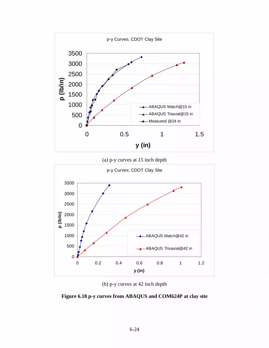
6-24

p-y Curves, CDOT Clay Site

0500

100015002000250030003500

0 0.5 1 1.5

y (in)

p (lb

/in)

ABAQUS Match@15 in

ABAQUS Triaxial@15 in

Measured @24 in

(a) p-y curves at 15 inch depth

p-y Curves, CDOT Clay Site

0

500

1000

1500

2000

2500

3000

3500

0 0.2 0.4 0.6 0.8 1 1.2

y (in)

p (lb

/in)

ABAQUS Match@42 in

ABAQUS Trixaxial@42 in

(b) p-y curves at 42 inch depth

Figure 6.18 p-y curves from ABAQUS and COM624P at clay site

6-25

Load-Deflection Curves on CDOT Sand Site, South Shaft

0

10

20

30

40

50

60

70

0 0.2 0.4 0.6 0.8 1 1.2

Deflection (in.)

Load

(kip

s)

Measured

ABAQUS

ABAQUS - Match Case

Figure 6.19 Simulated and measured load-deflection curves of CDOT test at sand site

6-26

Deflection-Depth of South Shaft of CDOT Sand Site, ABAQUS

0

2

4

6

8

10

12

14

16

18

-0.05 0 0.05 0.1 0.15 0.2 0.25

Deflection (in.)

Dep

th (f

t)

Mea.@25 kips

ABAQUS@25 kips

(a) 25 kips of load


0

2

4

6

8

10

12

14

16

18

-0.1 0 0.1 0.2 0.3 0.4 0.5

Deflection (in.)

Dep

th (f

t)

Mea.@45 kips

ABAQUS@45 kips

(b) 45 kips of load


simulation with soil parameters from lab and PM tests for CDOT test at sand site

6-27


0

2

4

6

8

10

12

14

16

18

-0.05 0 0.05 0.1 0.15

Deflection (in.)

Dep

th (f

t)

Mea.@18 kips

ABAQUS Match@18 kips

(a) 25 kips of load


0

2

4

6

8

10

12

14

16

18

-0.1 0 0.1 0.2 0.3 0.4

Deflection (in.)

Dep

th (f

t)

Mea.@45 kips

ABAQUS Match@45 kips

(b) 45 kips of load


simulation with best match soil parameters for CDOT test at sand site

6-28

p-y Curves, CDOT Sand Site

0

200

400

600

800

1000

1200

1400

1600

1800

2000

0.000 0.200 0.400 0.600 0.800 1.000

y (in)

p (lb

/in)

ABAQUS@24 in

ABAQUS Match@24 in

Measured @30 inch


p-y Curves, CDOT Sand Site

0

200

400

600

800

1000

1200

1400

1600

1800

0.000 0.100 0.200 0.300 0.400 0.500 0.600

y (in)

p (lb

/in)

ABAQUS@60 in

ABAQUS Match@ 60 in


Figure 6.22 P-y curves from ABAQUS and COM624P at sand site

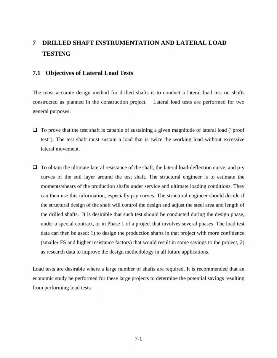
7-1

7 DRILLED SHAFT INSTRUMENTATION AND LATERAL LOAD

TESTING

7.1 Objectives of Lateral Load Tests

The most accurate design method for drilled shafts is to conduct a lateral load test on shafts

constructed as planned in the construction project. Lateral load tests are performed for two

general purposes:

To prove that the test shaft is capable of sustaining a given magnitude of lateral load (“proof

test”). The test shaft must sustain a load that is twice the working load without excessive

lateral movement.

To obtain the ultimate lateral resistance of the shaft, the lateral load-deflection curve, and p-y

curves of the soil layer around the test shaft. The structural engineer is to estimate the

moments/shears of the production shafts under service and ultimate loading conditions. They

can then use this information, especially p-y curves. The structural engineer should decide if

the structural design of the shaft will control the design and adjust the steel area and length of

the drilled shafts. It is desirable that such test should be conducted during the design phase,

under a special contract, or in Phase 1 of a project that involves several phases. The load test

data can then be used: 1) to design the production shafts in that project with more confidence

(smaller FS and higher resistance factors) that would result in some savings to the project, 2)

as research data to improve the design methodology in all future applications.

Load tests are desirable where a large number of shafts are required. It is recommended that an

economic study be performed for these large projects to determine the potential savings resulting

from performing load tests.

7-2

7.2 Description

This item consists of furnishing all materials, equipment, and labor as necessary to instrument

and run a lateral load test on two of the plan production drilled shafts. The plan identification

numbers for the two selected Item Special drilled shafts are numbered X and Y. Conduct the

tests by utilizing the companion load test drilled shaft in each test as the mutual reaction element.

7.3 General Conduct the lateral load tests in accordance with the requirements specified in ASTM-D3966.

Cylinder strengths for the drilled shaft concrete shall indicate a minimum of 4000 psi (f’c), prior

to applying the moment and lateral load force to the shafts to be tested.

7.4 Materials

Low strength mortar (need some specs for these items)

Reinforcing steel

Concrete

Structural steel

7.5 Location of Load Tests

Test locations should be selected after the subsurface geotechnical investigation is performed

following one or more of these criteria:

• At or close to the project site, in a location that represents all of the production shafts on the

project.

• At or close to the weakest soil layer if the design was based on the weakest soil layer (not

relevant if uniform soil layer is encountered at the site)

• In flat areas accessible to heavy equipment (important with sacrificial shafts constructed

before construction is started).

7-3

• At or close to shafts with the highest loads.

7.6 Type of Test Shafts (Production or Sacrificial)

The purpose and type of the load test determine the type of the test shaft. Production test shafts

are often selected for proof load testing. Sacrificial test shafts are used for testing to a higher

deflection or load than in the acceptable criteria. When the exact locations of the production

shafts are not finalized, it is recommended to consider a sacrificial test shaft. Testing of a

production shaft can be risky in some areas (e.g., under water).

7.7 Acquisition of New Geotechnical Data at Sites of New Lateral Load Tests

At the locations of new lateral load tests on drilled shafts, comprehensive subsurface

geotechnical investigation should be performed as described in the previous section. This is

required for the proper design of the load test and to acquire accurate research strength data for

the soil layers that could be correlated with the resistance values measured in the load tests.

Therefore, it is necessary to perform the geotechnical subsurface investigation before performing

the new load test. Three test holes should be drilled at the lateral load test site. Subsurface

geotechnical investigation methods at each test hole should be performed as described in this

study. It will include auger drilling with standard penetration testing, sampling, subsequent

laboratory testing on recovered core specimens, and in-situ pressuremeter testing.

7.8 Drilled Shaft Construction The two drilled shafts to be tested shall be constructed with structural steel members extending a

minimum of half the wall height plus two feet above the top of each drilled shaft, and embedded

a minimum of four feet into the shaft. The lateral load shall be applied at a point located at half

the wall height above the top of each drilled shaft.

A 12 inch diameter hole shall be drilled for a depth of six feet below the bottom of the 16 feet

long production drilled shaft. The 12 inch diameter hole will serve to anchor the bottom six feet

7-4

of the slope inclinometer casing. The hole shall be located appropriately and shall be backfilled

with sand or low strength mortar.

The constructed Item Special pay length of the two drilled shafts to be tested is 16 feet. A one

quarter inch thick (minimum) wall steel drilled shaft casing shall extend from elevation 3 feet

below the top of the shaft up to the top of the drilled shafts that are to be laterally load tested for

the purpose of strengthening the drilled shaft during the application of the lateral test load.

7.9 Testing Engineer

The installation of the drilled shaft instrumentation and the performance of the lateral load tests

shall be performed under the direction of the Testing Engineer. The Testing Engineer shall be a

Professional Engineer who has had experience in conducting at least two similar instrumented

lateral load tests in the past.

7.10 Instrumentation

Instrumentation sensors (strain gages, inclinometer casing, and couplers) are to be purchased by

the contractor. The total quantity of sensors that shall be purchased is summarized in Table 7.1.

The Inclinometer casing and all other sensors, gages, and measuring devices shall be installed

under the direction of CDOT Research team. The locations of the strain gages to be installed on

the drilled shaft reinforcing steel cages shall be as directed by CDOT Research Team.

Inclinometer casings shall be installed in the sand/low strength mortar to a depth at least 6 ft.

below the tip of the plan drilled shafts.

7-5

Table 7.1 Summary of Required Instrumentation and Devices*

Inclinometers** Drilled Shaft #

and depth (ft)

Sister Bar (Each) Tubes

(feet) Couplers

#

V.W. Tiltmeter

Data Acquisition

System

Multi- plexer W14x109

#** – 16 ft. 20 with 50’ cable 25 4 2 pieces

@10’

#** – 16 ft. 24 with 30’ cable 25 4 3 pieces

@10’

Total Quantity 44 115 18 None None None 50’

* Two dial gages and an LVDT shall be used to measure the lateral movement at the jacking point in each

test shaft. A stable reference beam as explained in the testing section shall support the dial gages and

LVDT.

** Inclinometer tubes shall be in 5 feet pieces and shall use 12" long couplers.

7.11 Instrumentation Specifications 1. Inclinometer Tubes: Geokon Model 6501 (or an approved equal) pultruded fiberglass

inclinometer casing with a nominal 2.5 inch inside diameter, bottom plug and top cap.

Inclinometer tubing shall be tied in place prior to placing concrete in the drilled shafts.

The inclinometer casing shall be supported by the reinforcing steel.

2. Sister Bar Strain Gages: Geokon Model 4911 VW#4 rebar strain meter with cable (or an

approved equal).

3. Vibrating Wire Uniaxial Tiltmeter: Geokon Model 6350 vibrating wire Tiltmeter (or an

approved equal). 4. CR10X Data Acquisition System (Geokon Model 8020 MICRO-10 Data logger, or an

approved equal).

5. Muliplexers (Geokon Model 8032, or an approved equal).

6. Enclosure Box (Traffic enclosure manufactured by Southern Manufacturing, 501

Herndon Ave Orlando, Fl 32803, Telephone: 800-866-5699 Fax: 407-894-5373, or an

7-6

approved equal). The size of the box should be a minimum of 4 feet wide by 5 feet high

by 2 feet deep.

All of the instruments and accessories shall be installed according to the manufacturer’s

recommendations and as directed by the Testing Engineer

7.12 Testing

Conduct the lateral load test according to the requirements specified in ASTM-D3966: Standard

Test Method for Piles under Lateral Loads. The standard loading procedure outlined in the

ASTM-D3966 standards should be followed.

The structural design of the load frame system shall be performed by the Testing Engineer and

submitted to CDOT for approval at least 10 working days prior to beginning construction of the

drilled shafts to be tested. The design load for each drilled shaft is based on a 27 psf wind

pressure applied at the mid height of the wall. Based on an assumed 10 feet high wall and a

center-to-center spacing of 23 feet, the resultant force at mid height of the wall is 6.21 Kips

applied at a height of 11 feet above the top of the drilled shaft. The maximum test load, which

includes a factor of safety of three, is 20 kips applied at 11 feet above the top of the drilled shaft.

The maximum design load for the testing device shall be a minimum of 75 Kips to be applied 11

feet above top of shaft. The test will be stopped prior to applying the maximum design load if

CDOT determines that excessive deflection is occurring.

A stable reference beam system for mounting the dial gages and LVTDs to monitor the

movement of the drilled shafts at the points of load application shall be provided. The reference

beam shall be rigid and firmly supported at a minimum distance of at least three shaft diameters

from the center of the test shafts.

The work shall include, but not be limited to:

1. Furnishing the instrumentation, the load application, and testing equipment.

2. Installing the instrumentation, operating load application, and monitoring equipment.

3. Performing structural analysis using the collected data from the lateral load tests.

7-7

4. Furnishing a final report.

7.13 Equipment

The contractor shall furnish all equipment necessary to perform and dismantle the lateral load

tests in compliance with the ASTM-D3966 Standard Test Method for Piles Under Lateral Loads,

and to assist the CDOT Research Team in installing the instruments and data collection devices.

The load shall be applied utilizing an arrangement of components that will provide the required

maximum test load (i.e. load equivalent to 3 times the design load specified in the plans). The

jack and the load cell shall each have a capacity that is 15% greater than the specified maximum

test load. The load cell and the jack shall be accompanied with documentation verifying that they

have been calibrated within the past year.

The contractor shall provide a protective work area, including provisions such as a tent or shed

for protection of the load test equipment and personnel from inclement weather.

7.14 Report

A detailed report containing the lateral load test results shall be prepared and submitted to the

Project Engineer for approval. The report shall include:

(a) Drawings of the instrumentation plans.

(b) Graphs and tables of load vs. lateral deformation.

(c) Horizontal movement along the depth of the shaft determined from inclinometer data.

(d) Angle of tilt of the drilled shaft at the tiltmeter locations.

(e) Strain readings from the strain gages embedded in the drilled shafts and the computed

bending moment and axial forces at each load level.

(f) Back-calculations using the load test results to determine the pertinent parameters for the

soil and bedrock p-y curves.

(g) Recommended design parameters for future drilled shaft projects.

(h) All calibration sheets for the instruments used in the tests.

7-8

(i) All data gathered from the instruments in an electronic format with enough explanation to

make it understandable by the Project Engineer.

7.15 Method of Measurement and Payment

Payment for the instrumentation and lateral load testing of the drilled shafts includes:

1. Furnishing instrumentation and the load application equipment.

2. Drilling and backfilling the 6 feet long, 12 inch diameter hole below the actual

production drilled shafts.

3. Installing and operating the instrumentation and load application equipment.

4. Dismantling of the load test equipment and structural members.

5. Performing analysis by using the collected data from the lateral load tests.

6. Furnishing a final report.

After receiving and approved final report, payment will be made at the contract lump sum price

bid for Item Special Drilled Shafts Instrumentation and Load Testing. Table 7.2 provides the

summary of required materials.

Table 7.2 Summary of Required Material

Drilled Shaft #

and depth (ft)

C10x30 Dywidag Rods 1.5”

Dia.

1.5”x0.5”x0.25” Angles to weld the

gages on

2”x2”x0.25” Angle for Reference

beams

W14x109

#** – 16 ft. 2 pieces 5’ long

65’ 30’ 2 pieces @10’

#** – 16 ft. 2 pieces 5’ long

65’ 30’ 3 pieces @10’

Total Quantity 4 pieces 5’ long

80’ plus 4 couplers

130’ 60’ 50’

The research team will provide the following measuring devices:

1. Data Acquisition.

2. Multiplexers

7-9

3. Dial Gages.

CDOT or the contractor needs to provide an inclinometer device to measure the deflection in the

inclinometers during testing.

The contractor shall provide the required steel to setup the load test as per the drawings prepared

by E.L. Robinson Engineering of Ohio Company. This includes, the W14x109, The C10x30, the

bearing plates, the Dywidag 1.5” diameter rods, the reference beam to support the dial gages, the

L4x4x 3/8, the 1”x.5”x.25” angles, and welding machine to weld the strain gages end blocks.

Prices of Devices and gages:

1. Vibrating wire VSM-4000 Strain gages are $110 each and the cable is $0.41 per foot.

($110x44 + 1960 ft. x $0.41 per foot = $6079)

2. Inclinometer tubes are around $8.00 per foot. ($8x115 + 18 Couplers x $5 = $1010)

3. Steel plates to weld strain gages on (Angle 1x0.5”x0.25”) 130’ costs

4. 50’ of W14x109 (50x109x$1.2 per pound = $6540)

5. Steel angels 2”x2”x0.25 for reference beams 60 feet total

6. C10x30 four pieces 6’ long

7. Steel Plates 12”x12”x1” total of 3.

8. Steel Plates 48”x12”x1” total of 2.

9. Nuts and washers for the Dywidag 1.5” rods. 10 of each.

7.16 Recommendations for Improving the Load Test

1. Use of circular reinforcing cage with stirrups all the way to the bottom of the shaft should be

emphasized in the future load tests.

2. The size of the steel H-Beam should be smaller than the size of the reinforcing cage to provide

for some clearance. More important, there should be a precise method to measure the lateral

load exerted on each test shaft. In addition, the ground elevation and the moment arm for the

two test shafts of the load test should be the same.

3. To extend the H- beam all the way to the bottom of the shaft as in Ohio's load tests.

7-10

4. To design the layout of the load test based on the results of simple geotechnical tests. First, the

diameter should be selected based on the recommended values in the construction project.

However, the length of the shafts should be based on our expectation of the results of the load

test tests, not what will be used in production shafts based on very conservative design. For

example, the Broms method can be used to estimate the length with a factor of safety of 2 and

without neglecting 1.5 d. This is to ensure the full mobilization of the plastic resistance of the

soil around the test shaft.

Additionally, after the geotechnical investigation performed at the load test site, numerical

simulation of the load test, as illustrated in Chapter 6, can be performed for a better design of the

load test.

7-11

Figure 7.1 Setup and calibration values for strain gages at test site I clay site

7-12

Figure 7.2 Setup and calibration values for strain gages at test site II sand site

8-1

8 CONCLUSIONS

Objective 1: Determine the Needs, Benefits, Potential Cost-Effectiveness, and Justification

The research team has reviewed current practice by CDOT engineers and consultants pertaining

to the design and analysis of drilled shafts for supporting sound barrier walls, signs, and signals.

These reviews, together with relevant AASHTO Guidelines and Ohio DOT practice, were

presented in Chapter 3 of this report.

Sound Barrier Walls

It was found that a fundamental discrepancy in the design and analysis philosophy exists

between the CDOT engineers and consultants. CDOT engineers tend to rely mainly on the

strength limit based approach; whereas, consultants prefer the use of the LPILE program for

serviceability based approach. Several methods were used by CDOT engineers to estimate lateral

capacity, while conservative F.S. of 2.5 to 3 was used. Often, CDOT engineers eliminated the

top 5 ft of soils to accommodate concerns with possible soil degradation, moisture infiltration, or

desiccation. The comparison study documented in Chapter 4, based on hypothetical cases and

load test data, has resulted in a recommendation of using the Broms method with a lowered F.S.

of two. Based on the study of two Colorado load test results, performed as part of this research,

a cost saving of 25% could be realized with the proposed design approach.

The accuracy of the Broms method in predicting the ultimate capacities of drilled shafts relies on

the ability to input appropriate soil strength parameters. For clay, as discussed in Chapter 5 of the

report, the most appropriate soil testing method is the triaxial CU test or direct shear test. For

clay, the Broms method using the soil strength parameters interpreted from the pressuremeter test

with FHWA (1989) soil strength interpretation equation or SPT method with Liang (2002)

correlation charts also provides a reasonable capacity estimate. For sand, SPT with Liang (2002)

correlation provides the best soil strength interpretation. The Pressuremeter test would provide

reasonable soil strength interpretation as well.

8-2

The success of the serviceability based design approach requires the establishment of acceptable

performance (deflection) limit and accurate analysis tools such as LPILE or COM624P. This

research has established the acceptable deflection corresponding to the soil’s elastic limit for

repetitive loading at the head of the drilled shaft on the basis of geotechnical consideration of

drilled shaft-soil interaction in order to provide consistency between strength limit and service

limit approaches. One should note that the structural details of the sound barrier walls would

ultimately govern the allowable deflection.

The accuracy of LPILE or COM624P analysis in capturing the load-deflection behavior of

drilled shafts hinges on the ability to input representative p-y curves. For clay, as discussed in

Chapter 5, the most accurate soil parameters determination is the triaxial test or direct shear test.

The pressuremeter test and SPT test with correct interpretation could yield reasonable soil

parameters as well. For sand, direct shear, SPT, and pressuremeter tests yield reasonable and

conservative interpretation on soil parameters required for generating p-y curves.

From the FEM simulations of two Colorado load tests, it was concluded that initial elastic

parameters (Young’s modulus and Poisson’s ratio) of the soil exert the greatest influence on the

predicted initial portion of the load-deflection curve of the drilled shaft subjected to lateral load.

The strength parameters and the yielding/hardening parameters govern the later portion of the

load-deflection curve. Pressuremeter tests in sand and clay have been shown to provide more

accurate soil modulus parameters than the techniques using laboratory tests for FEM analysis.

Overhead Signs and Signals

CDOT engineers have developed standard drawings for foundation design of overhead sign

structures and traffic signals. The foundation design is based on fairly conservative assumed soil

properties. The lateral capacity of the foundation is calculated using the Broms method, while

torsional capacity is estimated by the CDOT in-house method. A factor of safety of 2.5 to 3 is

adopted for lateral load, while 1.25 to 1.5 is adopted for torsional load. CDOT engineers limit the

deformation to be within elastic response (0.1 to 0.2 inch) to avoid accumulation of irrecoverable

8-3

deformation with cyclic wind loads. CDOT engineers have observed no failures or excessive

deformations of the drilled shafts designed according to this approach.

The research has shown that the torsional capacity estimated from the CDOT method gives the

highest capacity among the methods studied in chapter 4. The CDOT method was never verified

by field torsional load testing. The combination of mixed granular and cohesive soil properties,

in conjunction with relatively high F.S. for lateral loads and very low F.S. for torsional load,

perhaps makes the CDOT approach predict the torsional capacity.

Objective 2: Identify Most Accurate Methods to Predict Nominal Response (Ultimate Capacity

and Deformation) of Drilled Shafts

Various existing methods for predicting ultimate lateral and torsional capacity of drilled shafts

have been evaluated using compiled load test data and two Colorado load test results. Both

advantages and limitations of each method were reviewed and summarized in Chapter 2. Among

the methods evaluated, including Broms, Brinch-Hansen, sheet piling, and caisson methods, the

Broms method provided consistent and safe predictions of ultimate capacity, while others

provided either inconsistent or unreliable estimates. CDOT geotechnical engineers seem to

neglect the upper 5 feet of clay soils for lateral load resistance. Design performed by consultants

may or may not eliminate the capacity in the upper several feet of the shaft. The Broms method

eliminates the capacity of 1.5 times the shaft diameter of the clay soil layer for lateral load

resistance.

The torsional capacity of drilled shafts in clay can be estimated more accurately by the Florida

District 7 method. On the other hand, the Florida Structure Design Office method seemed to

provide a more accurate estimate of torsional capacity of drilled shafts in sand.

Structural engineers often establish deflections limits and they are based on individual’s

engineering judgment. It appears that ¼ inch of deflection at the ground line is considered non-

issue and a deflection of ½ inch has been considered acceptable. In Colorado, it appears that ¼

inch of deflection at the ground line is considered insignificant and a deflection of ½ inch is

8-4

considered acceptable. Most engineers cited 1" at the ground under service loading conditions as

a maximum, and some stated that deflections greater than 1" may be acceptable in some

situations. A tilting to the sound barrier walls of 0.833% was established for the T-REX project.

This was selected based on aesthetic, not structural concerns. This resulted in deflections at the

ground level typically less than 1" but occasionally slightly greater than one inch. Liang (1997)

developed design charts for both 1% and 1.5% wall height as allowable deflections at wall top.

In the AASHTO LRFD Bridge Design specifications, the allowable horizontal movement at

drilled shafts head is specified as 1.5" for bridge foundations. Ohio DOT allows either 1" or 1.5”

for design of sound walls. From the drilled shaft performance viewpoint and to be consistent

with the strength limit with F.S of two, the authors of this report recommends a permissible

lateral deflection of 1 inch at the head of the drilled shaft. Mr. Dick Osmun from Staff Bridge

recommends limiting the deformation for signs and signals to the soil’s elastic limit under

repetitive loading estimated with LPILE to avoid accumulation of irrecoverable deformation

with cyclic wind loads.

Deformations of laterally loaded drilled shafts can be accurately predicted by COM624P (or the

equivalent LPILE program) with p-y curves characterized by appropriate soil parameters. This

research indicated that laboratory triaxial CU tests or direct shear test would be desirable tests for

determining accurate soil parameters to generate p-y curves. As an alternative, SPT correlations

could be used for cohesionless soils. The pressuremeter test may be used for determining

strength parameters of cohesive soils. The prediction made by the NAVFAC DM7 method is

very sensitive to the input of the subgrade soil reaction coefficient. NAVFAC DM7 provides a

linear deflection prediction along the initial modulus but does not define the limits for the initial

modulus as does COM624P or the LPILE program. Thus, its use for predicting drilled shaft

deflection is not recommended.

Finite element modeling details have been developed and used to simulate two lateral load tests

performed in Denver, Colorado. The commercial finite element code, ABAQUS, was used for

this purpose. The FEM analysis requires knowledge and training on the part of engineers in order

to successfully model the complex three-dimensional interaction nature of the drilled shaft.

Moreover, since the elasto-plastic constitutive model is used for representing nonlinear, stress

8-5

path dependent, irrecoverable stress-strain behavior, and the computation resource requirement

(in terms of runtime and memory storage) is quite demanding. The FEM simulation technique

could be a useful tool, however, for development of new sets of p-y curves for unique soil types,

unusual size (dimension) of the drilled shaft, or complex loading conditions.

Objective 3: Develop Practical Procedures to Perform Instrumented Load Tests

The research team has developed a standard special note for performing instrumented lateral load

tests, which can be adopted by CDOT engineers or consultants in developing their design plans.

Instrumented lateral load tests should be considered for CDOT projects that involve construction

of a large number of drilled shafts or that have unique soil conditions at the construction site. For

sound barrier wall projects, if the number of the drilled shafts to be constructed is large, then it

would be beneficial to arrange for lateral load tests in an effort to derive site–specific p-y curves

in the COM624P analysis.

9-1

9 RECOMMENDATIONS AND BENEFITS

9.1 Recommendations for CDOT Structural Engineers and Consultants

9.1.1 Sound Barrier Walls: Recommendations The following two simple uniform strength limit state and serviceability limit state design

methods are recommended to determine the required drilled shaft length of sound walls (use the

larger length of the two methods):

1. For the strength limit, use the Broms method and a F.S. of two to determine the required

drilled shaft length. Lateral soil resistance in the upper 1.5 D (D is shaft diameter) of the

shaft is neglected in the Broms method for cohesive soils, so no additional depth should be

neglected as may be recommended in the geotechnical report.

2. For the serviceability limit, use COM624P (LPILE) to estimate the lateral deflection of the

drilled shaft. From the drilled shaft performance viewpoint and to be consistent with the

strength limit with F.S of two, the authors of this report recommends a permissible lateral

deflection of 1 inch at the head of the drilled shaft. Mr. Dick Osmun from Staff Bridge

recommends limiting the deformation for signs and signals to the soil’s elastic limit under

repetitive loading estimated with LPILE to avoid accumulation of irrecoverable deformation

with cyclic wind loads. Other suggestions for the permissible lateral deflection are presented

in Chapter 8.

Note 1: In order to ensure accurate solutions from these design methods, appropriate

geotechnical test methods must be used for obtaining soil parameters as described below.

Note 2: Consideration of possible loading rate effect, cyclic loading effect, ground water table

fluctuations, and effect of lateral load induced moment on the soil resistance are addressed

(Section 4.5).

The most accurate design method for drilled shafts is to conduct a load test on test shafts

constructed as planned in the construction project. Chapter 7 provides a standard special note for

9-2

performing instrumented lateral load tests, which can be adopted by CDOT engineers or

consultants in developing their design plans. Instrumented lateral load tests should be considered

for CDOT projects that involve construction of a large number of drilled shafts or that have

unique soil conditions at the construction site. Lateral load tests are performed for two general

purposes: 1) to design production shafts with more confidence, resulting in large cost savings to

the project, and 2) as research data to improve the accuracy of simple design methods for drilled

shafts supporting sound walls and extract the resistance factor required in the LRFD method.

Finite element modeling should be considered in large or very critical projects with uncommon

field and loading conditions. See Sections 2.1.3 and Chapter 6 for more on these methods

(Florida Pier program and ABAQUS software). Chapter 6 demonstrated the modeling

capabilities and versatility of ABAQUS software for specialized drilled shaft projects. For FEM

based methods, the unload-reload soil moduli (or their average) of the pressuremeter tests should

be used for interpretation of soil modulus.

9.1.2 Sound Barrier Walls: Justifications Various existing methods for predicting ultimate capacity and deflection of drilled shafts

supporting sound walls were evaluated in this study using data of hypothetical cases, a load test

database carefully selected from literature and Ohio’s test results, and two new lateral load tests

performed in Colorado on sand and clayey soil sites as a part of this study. The methods include

the Broms method, COM624P method, sheet piling method, caissons program, Brinch Hansen

method, and NAVFAC DM-7 method. Conclusions and findings were:

1. For the compiled load tests, the Broms method and COM624P method provide safer and

more accurate predictions than other methods, while others provided either inconsistent

or unreliable estimates.

2. For the compiled load tests, the actual FS will be about 4 for test shafts in clays and from

2.6 to 6.2 for sands.

3. LRFD calibration of the compiled load tests suggested that FS of 2 for the Broms method

is appropriate.

4. The Broms method yielded reasonable FS for the two load tests performed in this study.

9-3

5. For the compiled and new load tests, a permissible deflection of 1 inch was also found

appropriate for both sand and clay sites from drilled shaft performance viewpoints, not

from structural consideration of the shaft, which need to be checked to remain within

acceptable design limits. The two new load tests suggest that the equivalent F.S. based on

1.0 inch permissible deflections would range between 2.4 and 4.8 for clayey site and 2.3

to 3.7 for the sand soil site.

6. For the compiled and new load tests, the COM 624P computer program is capable of

predicting shaft deflection at the working load of 20 kips.

Other justification factors are:

The Broms and p-y method are the methods preferred by the FHWA. The Broms method

for cohesive and cohesionless soils is capable of considering several boundary conditions

at the pile head (free and fixed) and can handle short and long piles.

The prediction made by the NAVFAC DM7 method is very sensitive to the input of the

subgrade soil reaction coefficient. At best, NAVFAC DM7 can only provide linear or

elastic deflection predictions for lateral loads up to 1/3 of the ultimate lateral load. Thus,

its use for predicting drilled shaft deflection is not recommended.

Sheet piling method: the hand calculations are cumbersome. Applicable for short piles

embedded in homogeneous cohesionless soils. Developed for sheet piles, which may

exhibit different behavior from drilled shafts.

Caisson program: The program cannot be run correctly for cohesive soil conditions.

9.1.3 Design Methods for Overhead Signs and Signals Current CDOT practice for overhead signs and signals could continue. CDOT engineers have

developed standard drawings for foundation design of overhead sign structures and traffic signals.

The foundation design is based on fairly conservative assumed soil properties. The lateral

capacity of the foundation is calculated using the Broms method, while torsional capacity is

estimated by the CDOT in-house method. A factor of safety of 2.5 to 3 is adopted for the lateral

load, while 1.25 to 1.5 is adopted for the torsional load to prevent torsion from controlling drilled

shaft depths. CDOT engineers limit the deformation to be within elastic response (0.1 to 0.2 inch)

to avoid accumulation of irrecoverable deformation with cyclic wind loads. CDOT engineers

9-4

have observed no failures or excessive deformations of the drilled shafts designed according to

this approach.

Ideally, design of the drilled shaft for overhead signs and signals for lateral load should follow

the same recommendation as the sound barrier walls, provided that CDOT engineers can accept

more accurate method for torsional capacity analysis. This was not possible because of lack of

sufficient quantity of credible torsional load test data. The limited number of torsional load tests

suggests the torsional capacity may be over-estimated by the CDOT method. However, with

overly conservative assumption of soil properties, in conjunction with relatively high F.S. for

lateral loads and very low F.S. for torsional load, the CDOT approach may have a self-

compensating mechanism that minimizes the effect of the overestimate of torsional capacity

mentioned in the above. This could explain the fact that CDOT engineers have not observed any

foundation failure in the past.

However, it is strongly recommended that additional research work be conducted to obtain

reliable torsional load test data in Colorado so that a more accurate analysis method could be

identified.

9.2 Recommendations for CDOT Geotechnical Engineers and Consultants

Ground water table elevation should be carefully identified in field geotechnical exploration

work and the highest possible elevation of GWL should be estimated and used in the design. For

clays, use saturated strength parameters under the water table and in-situ strength parameters for

water above GWL. Appropriate p-y criteria for above and below the ground water table should

be used in COM624P or LPILE analysis. The unit weight required by the Broms method could

be obtained from laboratory test or SPT correlations. Tables 3.9 and 3.10 are recommended to

estimate the k and ε50 for the COM624P (or LPILE) program.

9.2.1 Cohesive Soils The most appropriate soil testing methods to determine the cohesive soil parameters required for

the Broms and COM624P methods are:

9-5

The triaxial CU test or direct shear test as described in Chapter 5 of this report. It is

convenient to use the simpler direct shear test that could easily be performed in CDOT on a

routine basis.

The pressuremeter test with FHWA (1989) soil strength interpretation equation.

The SPT method with Liang (2002) correlation charts, currently adopted by the Ohio DOT.

These are presented in Tables 3.9 and 3.10, which also provide recommendations for all the

other parameters required in the LPILE program.

The CDOT procedure for estimation of strength and LPILE parameters based on SPT could

be used but the results of this study indicates that it is very conservative (i.e., underestimates

strength by 50%).

9.2.2 Cohesionless Soils The most appropriate soil testing methods to determine the cohesionless soil parameters required

for the Broms and COM624P methods are:

The SPT with Liang (2002) correlation provides best soil strength interpretation.

The Pressuremeter test would provide reasonable soil strength interpretation as well.

The SPT with CDOT correlations methods just for strength parameters (Table 3.2) not for the

parameters required in the LPILE program.

The lateral load test on the sandy soil deposit seems to suggest that direct shear test over-predicts

the strength of the soil. In future load tests, a laboratory test using direct shear test apparatus

needs to be conducted on the reconstituted sand specimens to the same density as the in-situ

density.

9.3 Benefits

The research has resulted in the following benefits.

Based on the evaluation of the two Colorado lateral load test results for sound walls, the

proposed design/analysis approach has shown to yield roughly 25% cost saving in both cohesive

9-6

and cohesionless soil deposits. This can be attributed to the recommended Broms method of

analysis together with the reduced factor of safety requirement from 3 to 2.

A more uniform design method was put forward in this research report for designing drilled shaft

foundations for sound barrier walls. This uniformity ensures that less man-hours are needed in

deciding on analysis methods. The approach incorporates both strength limit based design and

the serviceability based analysis, thus ensuring a more consistent design outcome with a

comparable margin of safety from both the ultimate capacity and allowable deflection viewpoint.

The research has provided recommendations for proper geotechnical test methods to characterize

pertinent soil parameters needed for both ultimate capacity prediction and p-y curve generation

in COM624P or LPILE analyses. The recommended geotechnical test methods would allow

CDOT engineers to economize resources in planning out soil testing programs, thus potentially

saving costs as well.

The research has provided a standard instrumented lateral load test note in Chapter 7, which can

be used by CDOT engineers to specify a lateral load test in the design/construction plans. For a

project that involves construction of a large quantity of drilled shafts, or when unique soil

conditions and complex loading combinations exist, the lateral load test prior to final design

decision could potentially offer cost savings to the project.

10-1

10 REFERENCES AASHTO, (1989, 1992) “Guide Specifications for Structural Design of Sound Barriers”,

Washington, D.C.

AASHTO, (1994), LRFD Bridge Design Specifications, “Section-10: Drilled Shafts”, Published

by the American Association of State Highway and Transportation Officials (AASHTO), First

Edition.

AASHTO (1998) LRFD Bridge Design Specifications, Second Edition.

AASHTO (2001), “Standard Specifications for Structural Supports for Highway Signs,

Luminaries and Traffic Signals,” 4th Edition.

AASHTO, (2002) Interim - “Guide Specifications for Structural Design of Sound Barriers”,

Washington, D.C.

AASHTO (2003) Interim - LRFD Bridge Design Specifications, Second Edition.

ABAQUS Standard User’s Manual, Version 5.8, Hibbitt, Karlsson & Sorensen, Inc. 1998.

Barker, R.M., Duncan, J.M., Rojiani, K.B., Ooi, P.S.K., Tan, C.K., and Kim, S.G. (1991)

“Manuals for the Design of Bridge Foundations,” NCHRP Report 343, Transportation Research

Board, National Research Council, Washington, DC.

Bhushan, K., Lee, L.J., and Grime, D.B. (1981) “Lateral Load Tests on Drilled Piers in Sand.”

Drilled Piers and Caissons: Proceedings of a Session at the ASCE National Convention, St

Louis, MO, USA. Conference Code: 00225. P. 114-131.

10-2

Bhushan, K., and Askari, S. (1984) “Lateral-Load Tests on Drilled Pier Foundations for Solar

Plant Heliostats.” Laterally Loaded Deep Foundations: Analysis and Performance, ASTM STP

835, J.A. Langer, E.T. Mosley, and C. D. Thompson, Eds., ASTM, pp. 140-156.

Brinch Hansen, J. (1961). “The ultimate resistance of rigid piles against transversal forces.”

Geoteknisk Institut.Bull., No.12, Copenhagen.

Broms, B.B.(1964a) “Lateral resistance of piles in cohesive soils” Journal of the Soil Mechanics

and Foundation Division, Vol. 90, No. SM2, pp27-63.

Broms, B.B.(1964b) “Lateral resistance of piles in cohesionless soils” Journal of the Soil

Mechanics and Foundation Division, Vol. 90, No. SM3, pp 123-157.

Carter, J.P., and Kulhawy, F.H., (1988) Analysis and Design of Drilled Shaft Foundations

Socketed into Rock, Cornell University, Ithaca, New York.

Casagrande, A., and Shannon, W.L., (1948) “Strength of soils under dynamic loads,”

Proceedings of the American Society of Civil Engineers, ASCE, pp. 591-608.

Chow, Y. K., (1985) “Torsional Response of Piles in Non-Homogeneous Soil,” Journal of

Geotechnical Engineering, ASCE, Vol. 111, pp. 942-947.

Davidson, J.L., Hays, C.O., Jr., and Hagan, E.M., Jr., (1976) “Design of drilled shafts supporting

highway signs”, Transportation Research Record, issue 616, pp 62-66.

Dutt, R. N., (1976) Torsional response of piles in sand, Ph.D. thesis, Univ. of Houston, Texas.

10-3

FHWA (1989). “The Pressuremeter Test for Highway Applications” FHWA Publication No.

FHWA-IP-89-008, Department of Transportation, Federal Highway Administration, McLean,

VA 22101-2296, USA.

Guo, W.D., and Randolph, M.F., (1996) “Torsional Piles in Non-Homogeneous Media,”

Computers and Geotechnics, No. 19, pp. 265-287.

Hache, R.A.G., and Valsangker, A. J., (1988) “Torsional Resistance of Single Pile in Layered

Soil,” Journal of Geotechnical Engineering, ASCE, V. 114, pp. 216-220.

Hepworth and Jubenville, “Drilled Pier Foundations in Shale, Denver Colorado Area”, Drilled

Piers and Caissons, American Society of Civil Engineers, October 28, 1981, p. 68.

Kulhawy, F.H., and Chen. Y.-J., (1995) “A Thirty Year Perspective of Broms’ Lateral Loading

Models, as Applied to Drilled Shafts,” Bengt B. Broms Symposium on Geotechnical Engineering,

Singapore, pp. 225-240.

Lee, K. L., Seed, H. B., and Dunlop, P., (1969) "Effect of Transient Loading on the Strength of

Sand," Proceedings of the 7th International Conference on Soil Mechanics and Foundation

Engineering, Vol. 1, Mexico City, Mexico, pp. 239-247.

Lefebvre, Guy, and LeBoeuf, Denis, (1987) “Rate effects and cyclic loading of sensitive clays,”

Journal of Geotechnical Engineering, ASCE, Vol. 113, No. 5, pp 476-489.

Liang, R.Y. (1997) “Pressuremeter to Predict Lateral Load Capacity of Drilled Shafts on Slope,”

Final Report, FHWA/OH-97/005, ODOT.

Liang, R.Y., (2002) “Drilled Shaft Foundations for Noise Barrier Walls and Slope Stabilization,”

Final Report, FHWA/OH-2002/038, ODOT.

10-4

Lin, S.S., and AlKhaleefi, A.L. (1996) “Torsional Behavior of Cracked Reinforced Concrete

Piles in Sand,” Journal of The Chinese Institute of Engineers, Vol.19: (6), pp. 689-696.

Matasovic, N., and Vucetic, M. (1995) “Generalized cyclic-degradation-pore-pressure generation

model for clays” ASCE Journal of Geotechnical Engineering, Vol. 121(1), pp: 33-42.

Menétrey, Ph. And Willam, K.J. (1995) “Triaxial failure criterion for concrete and its

generalization.” ACI Structural Journal, 92:311-18, May/June.

NAVFAC DM-7 (1971), Department of the Navy, Naval Facilities Engineering Command,

“Design Manual – Soil Mechanics, Foundations and Earth Structures” .

Nowak, A.S., (1992) “Calibration of LRFD Bridge Design Code”, NCHRP 12-33, Report

prepared for National Cooperative Highway Research Program by Department of Civil

Engineering, University of Michigan, Ann Arbor, MI.

O’Neill, Michael Wayne, (1964) “Determination of the Pile-Head, Torque-Twist Relationship

for a Circular Pile Embedded in a Clay Soil,” Master Thesis, The University of Texas at Austin.

Orchant, C. J., Kulhawy, F.H., and Trautmann, C.H. (1988) “Reliability-Based Foundation

Design for Transmission Line Structures Volume 2: Critical Evaluation of In-Situ Test Methods,

EL-5507 Final Report, Report prepared by Cornell University for the Electric Power Research

Institute, Palo Alto, CA.

Poulos, Harry G. (1975) “Torsional Response of Piles,” Journal of the Geotechnical Engineering

Division, V. 101, GT10, pp. 1019-1035.

Poulos, H.G. (1982) “Single pile response to cyclic lateral load” ASCE Journal of Geotechnical

Engineering Div, Vol. 108(GT3), pp: 355-375.

Randolph, M. F. (1981) “Piles Subjected to Torsion,” Journal of the Geotechnical Engineering

Division, American Society of Civil Engineers, Vol.107, issue 8, pp. 1095-1111.

10-5

Reese, L.C., and Matlock, H. (1956). “Non-dimensional solutions for laterally loaded piles with

soil modulus proportional to depth.” Proc., 8th Texas Conf. on soil Mech. and Found. Engrg.,

Austin, Tex.

Seed, H.B., and Lundgren, R., (1954) "Investigation of the Effect of Transient Loadings on the

Strength and Deformation Characteristics of Saturated Sands." Proceedings of the American

Society of Civil Engineers, Vol. 54, pp. 1288-1306.

Sheahan, T.C., Ladd, C.C., and Germaine, J.T., (1996) “Rate-dependent undrained shear

behavior of saturated clay,” Journal of Geotechnical Engineering, ASCE, Vol. 122, No. 2, pp

99-108.

Stoll, U. W. (1972) “Torque Shear Test of Cylindrical Friction Piles,” Civil Engineering, ASCE,

Vol. 42, pp.63-65.

Tawfiq, K. (2000) “Drilled shaft under torsional loading conditions”, Final report Federal

Highway Administration, Florida Department of Transportation.

Whitman, R.V., and Healy, K.A., "Shear Strength of Sands During Rapid Loading," Journal of

the Soil mechanics and Foundations Division, ASCE, Vol. 88, No. SM2, PP. 99-132.

Yamamuro, J. A. and Lade, P. V., (1993) “Effects of strain rate on instability of granular soils,”

Geotechnical Testing Journal, GTJODJ, Vol. 16, No. 3, pp. 304-313..

Yasuhara, K. (1994) “Post cyclic undrained strength for cohesive soils” ASCE Journal of

Geotechnical Engineering, Vol. 120(11), pp:1969-79.

A

APPENDICES

The appendices are only available in electronic format:



drilled shaft design for sound barrier walls, signs, and signals

Documents