viscous effects on penetrating shafts in clays
TRANSCRIPT

VISCOUS EFFECTS ON PENETRATING SHAFTS IN CLAY
by
SANDEEP PRAKASH MAHAJAN
________________________
A Dissertation Submitted to the Faculty of the
DEPARTMENT OF CIVIL ENGINEERING AND ENGINEERING MECHANICS
In Partial Fulfillment of the Requirements For the Degree of
DOCTOR OF PHILOSOPHY
WITH A MAJOR IN CIVIL ENGINEERING
In the Graduate College
THE UNIVERISTY OF ARIZONA
2 0 0 6

2
THE UNIVERSITY OF ARIZONA GRADUATE COLLEGE
As members of the Dissertation Committee, we certify that we have read the dissertation prepared by Sandeep Prakash Mahajan entitled Viscous Effects on Penetrating Shafts in Clay and recommend that it be accepted as fulfilling the dissertation requirement for the Degree of Doctor of Philosophy _________________________________________________________________Date: June 30, 2006
Muniram Budhu _________________________________________________________________Date: June 30, 2006
Achintya Haldar _________________________________________________________________Date: June 30, 2006
Chandrakant .S. Desai _________________________________________________________________Date: June 30, 2006
Dinshaw N. Contractor Final approval and acceptance of this dissertation is contingent upon the candidate’s submission of the final copies of the dissertation to the Graduate College. I hereby certify that I have read this dissertation prepared under my direction and recommend that it be accepted as fulfilling the dissertation requirement. ________________________________________________ Date: June 30, 2006 Dissertation Director: Muniram Budhu

3
STATEMENT BY AUTHOR
This dissertation has been submitted in partial fulfillment of requirements for an advanced degree at the University of Arizona and is deposited in the University Library to be made available to borrowers under rules of the Library.
Brief quotations from this dissertation are allowable without special permission,
provided that accurate acknowledgment of source is made. Requests for permission for extended quotation from or reproduction of this manuscript in whole or in part may be granted by the head of the major department or the Dean of the Graduate College when in his or her judgment the proposed use of the material is in the interests of scholarship. In all other instances, however, permission must be obtained from the author. SIGNED: ______________________ Sandeep Prakash Mahajan

4
ACKNOWLEDGEMENTS I would like to acknowledge many people for helping me during my doctoral work. I have no words to describe my gratitude towards my advisor, Dr. Budhu, for his generous time and commitment. Throughout my doctoral work he encouraged me to develop independent thinking and research skills. He continually stimulated my analytical thinking and greatly assisted me with scientific writing. I am very much grateful to Dr. Budhu for his friendship, counsel and above all for his critical scrutiny and comments of my writing which has immensely improved my technical writing skills. He has modeled a lesson I will gladly carry forward with me in my future work. I am also very grateful for having an exceptional doctoral committee and wish to thank Dr. Haldar, Dr. Desai, Dr. Contractor and Dr. Merry for their support and encouragement. They have generously given their time and I thank them for their contribution and their good-natured support. I am grateful to Dr. Valdes for giving me opportunities to teach undergraduate courses which significantly enhanced my teaching abilities. I extend many thanks to my colleagues and friends, especially Melissa Cox, Pawan Baheti, Juan Lopez and Dustin Agnew for their assistance at various times. Additional thanks to the staff Alice Stilwell, Karen Van Winkle, Lajeana Hall, Olivia Hanson, Tom Demma and Steve Albanese. Finally, I'd like to thank my family, especially my parents for their support and care over the years. I'm grateful to my wife, Anjali, for her continual encouragement and enthusiasm.

5
I dedicate this dissertation to supreme Lord Shree Ganesh for his grace.

6
TABLE OF CONTENTS
LIST OF ILLUSTRATIONS.............................................................................................. 9
LIST OF TABLES............................................................................................................ 11
ABSTRACT...................................................................................................................... 12
CHAPTER 1 : INTRODUCTION................................................................................... 14
1.1 General .................................................................................................................. 14
1.2 Failure strength of soils.......................................................................................... 15
1.3 Post failure strength of soils ................................................................................... 18
1.4 Problem statement................................................................................................. 18
1.5 Hypotheses ............................................................................................................ 21
1.6 Goal and objectives of this research ..................................................................... 21
1.7 Scope of this research ........................................................................................... 22
1.8 Research outcomes................................................................................................ 22
1.9 Organization of dissertation.................................................................................. 22
1.10 Key terms .............................................................................................................. 24
1.11 Notations ............................................................................................................... 25
CHAPTER 2 : LITERATURE REVIEW......................................................................... 28
2.1 Introduction........................................................................................................... 28
2.2 Soil failure due to penetration............................................................................... 29 2.2.1 General.............................................................................................................. 29 2.2.2 Critical State Model (CSM).............................................................................. 29
2.3 Modeling soil penetration ..................................................................................... 34 2.3.1 General.............................................................................................................. 34 2.3.2 Analytical studies.............................................................................................. 35

7
TABLE OF CONTENTS (continued) 2.3.3 Experimental study ........................................................................................... 41 2.3.4 Numerical studies.............................................................................................. 44 2.3.5 Summary ........................................................................................................... 45
2.4 Soil resistance on a penetrating shaft.................................................................... 46 2.4.1 General.............................................................................................................. 46 2.4.2 Skin friction and end bearing resistance ........................................................... 47 2.4.3 Viscous (friction) resistance ............................................................................. 48 2.4.4 Summary ........................................................................................................... 48
2.5 Viscous behavior of soils ...................................................................................... 49 2.5.1 Theory of viscoelastic deformation .................................................................. 49 2.5.2 Creep deformation ............................................................................................ 51 2.5.3 Viscous behavior at critical state ...................................................................... 55 2.5.4 Summary ........................................................................................................... 56
2.6 Viscous shear force ............................................................................................... 57 2.6.1 Shear viscosity .................................................................................................. 57 2.6.2 Viscous drag on shafts in clays......................................................................... 58 2.6.3 Creeping flow.................................................................................................... 59 2.6.4 Viscous drag on bodies in creeping flow.......................................................... 59 2.6.5 Effect of boundaries.......................................................................................... 62
2.7 Soil state around the shaft ..................................................................................... 62
2.8 Summary ............................................................................................................... 66
CHAPTER 3 : MATHEMATICAL FORMULATION AND ANALYSIS ..................... 67
3.1 Introduction........................................................................................................... 67
3.2 Post-failure response of soil as yield stress fluid .................................................. 67
3.3 Analytical method................................................................................................. 70 3.3.1 General.............................................................................................................. 70 3.3.2 Assumptions...................................................................................................... 72 3.3.3 Viscous drag on a penetrating shaft in clay ...................................................... 72
3.4 Results and discussion of analysis ........................................................................ 80 3.4.1 Parameters influencing viscous drag ................................................................ 80 3.4.2 Effects of the size of CS zone ........................................................................... 80 3.4.3 Velocity profile within CS zone ....................................................................... 82 3.4.4 Shear viscosity of clay ...................................................................................... 83

8
TABLE OF CONTENTS (continued)
3.5 Conclusion ............................................................................................................ 86
CHAPTER 4 : SHEAR VISCOSITY OF CLAYS AT CS............................................... 87
4.1 Introduction........................................................................................................... 87
4.2 Current Investigations of soils viscosity ............................................................... 88 4.2.1 General.............................................................................................................. 88 4.2.2 Landslides and earth flows................................................................................ 88 4.2.3 Strain rate effects .............................................................................................. 91
4.3 Modeling of viscous behavior............................................................................... 93
4.4 Shear viscosity using the fall cone test ................................................................ 94 4.4.1 Penetration test.................................................................................................. 94 4.4.2 The fall cone test............................................................................................... 96 4.4.3 Theoretical approach....................................................................................... 101 4.4.4 Experiments .................................................................................................... 105
4.5 Results and discussion of the experimental study............................................... 108
4.6 Application to the CPT ....................................................................................... 118
4.7 Conclusion .......................................................................................................... 119
CHAPTER 5 : SUMMARY, CONCLUSIONS AND RECOMMENDATIONS ......... 121
5.1 Summary and conclusions .................................................................................. 121
5.2 Key Contributions............................................................................................... 123
5.3 Potential applications .......................................................................................... 123
5.4 Recommendations for future research ................................................................ 124
APPENDIX A : MATLAB CODES............................................................................... 125
APPENDIX B : FALL CONE TEST RESULTS .......................................................... 132
APPENDIX C : APPLICATION USING AN ILLUSTRATIVE EXAMPLE .............. 144
REFERENCES ............................................................................................................... 147

9
LIST OF ILLUSTRATIONS
Figure 1.1 Typical stress-strain response of soils at constant normal effective stress and
interpretation of peak and critical state friction angles. ............................................ 16
Figure 1.2 (a) Soil state at the tip of the penetrating shaft (b) soil flow around the penetrating shaft........................................................................................................ 20
Figure 2.1 Three dimensional plot of yield surface in CSM............................................. 30
Figure 2.2 Critical State Model (CSM)…………………………………………………..31
Figure 2.3 (a) Failure patterns under deep foundations (b) Expanding Cavity in an infinite soil mass (Vesic, 1972) ............................................................................................. 36
Figure 2.4 Deep penetration viewed as a steady flow problem (Baligh, 1985)............... 38
Figure 2.5 Plastic soil flow around a spherical penetrometer (Randolph et al. 2000)...... 42
Figure 2.6 Disturbance caused at the conical tip of a penetrometer (Allersma, 1987)..... 43
Figure 2.7 Mechanical models, E = elastic body, V = Viscous, Newtonian body and P = plastic body............................................................................................................ 50
Figure 2.8 Models of viscoelastic bodies (a) Maxwell body (b) Kelvin Body................. 52
Figure 2.9 Creep and viscous flow deformation............................................................... 54
Figure 2.10 Creeping Flow Past (a) a Sphere (b) a circular disk (Van Dyke, 1982)........ 61
Figure 2.11 Soil Disturbance around Penetrating Shafts in Soft Clay (Zeevart, 1948).... 63
Figure 3.1 Typical flow curves for yield stress fluids. ..................................................... 69
Figure 3.2 Analogy of the post-failure response of a soil to a yield stress fluid response.................................................................................................................................... 71
Figure 3.3 Forces acting on a soil element in the CS zone around the shaft .................. 773
Figure 3.4 Velocity profile of the viscous soil in the CS zone ......................................... 77
Figure 3.5 Effect of size of the CS zone on the viscous drag on a cylindrical shaft ........ 81
Figure 3.6 Velocity profiles for different sizes of the CS zone ........................................ 84
Figure 3.7 Upward movement of soil in the CS zone....................................................... 85

10
LIST OF ILLUSTRATIONS (continued)
Figure 4.1 Soil flow of sensitive clay due to heavy rainfall (Reference: Geological Survey of Canada)................................................................................................................. 90
Figure 4.2 The fall cone test apparatus ............................................................................. 95
Figure 4.3 Fall cone and the soil cup ................................................................................ 98
Figure 4.4 Liquid limit from typical fall cone test results ................................................ 99
Figure 4.5 Illustration of the soil state around a fall cone .............................................. 102
Figure 4.6 Modified experimental setup for the fall cone test ........................................ 106
Figure 4.7 LVDT connected to the top of fall cone shaft ............................................... 107
Figure 4.8 Penetration-time relationship of the cone (Test no. 15C1)............................ 110
Figure 4.9 (a) Velocity and (b) acceleration of the cone (Test no. 15C1) ...................... 112
Figure 4.10 Fall cone energy (Ec) ................................................................................... 114
Figure 4.11 PE, KE and Ec with penetration depth (Test no. 15C1) ............................. 115
Figure 4.12 Shear viscosity - LI relationship for kaolin used in this study ................... 117
Figure B1 (a) Penetration-time relationship (b) velocity of the cone for test 15C2 ....... 133
Figure B2 (a) Penetration-time relationship (b) velocity of the cone for test 15C3 ....... 134
Figure B3 (a) Penetration-time relationship (b) velocity of the cone for test 15C4 ....... 135
Figure B4 (a) Penetration-time relationship (b) velocity of the cone for test 15C5 ....... 136
Figure B5 (a) Penetration-time relationship (b) velocity of the cone for test 15C6 ....... 137
Figure B6 (a) Penetration-time relationship (b) velocity of the cone for test 5C1 ......... 138
Figure B7 (a) Penetration-time relationship (b) velocity of the cone for test 5C2 ......... 139
Figure B8 (a) Penetration-time relationship (b) velocity of the cone for test 5C3 ......... 140
Figure B9 (a) Penetration-time relationship (b) velocity of the cone for test C1 ........... 141
Figure B10 (a) Penetration-time relationship (b) velocity of the cone for test C2 ......... 142
Figure B11 (a) Penetration-time relationship (b) velocity of the cone for test C3 ......... 143

11
LIST OF TABLES Table 1 Experimental details .......................................................................................... 109 Table 2 Test data............................................................................................................. 113 Table 3 Estimated shear strength and shear viscosity..................................................... 116

12
ABSTRACT
When a rigid shaft such as a jacked pile or the sleeve of a cone penetrometer penetrates
soil, the soil mass at the shaft tip fails. This failed soil mass flows around the shaft
surface and creates a disturbed soil zone. The soil in this zone, which is at a failure or
critical state (CS), flows and behaves like a viscous fluid. During continuous penetration,
the shaft surface is subjected to an additional viscous shear stress above the static shear
stress (interfacial solid friction). The total resistance on the shaft in motion is due to the
static and viscous shear components. Current methods of calculating the penetration
resistance in soils are based on static interfacial friction, which determine the force
required to cause failure at the shaft-soil interface and not the viscous drag. The main
aim of this research is to understand the viscous soil resistance on penetrating shafts in
clays.
This research consists of two components. First, a theoretical analysis based on creeping
flow hydrodynamics is developed to study the viscous drag on the shaft. The results of
this analysis reveal that the size of the CS zone, the shear viscosity of the soil and
velocity of the shaft influence the viscous drag stress. Large increases in viscous drag
occur when the size of the CS zone is less than four times the shaft radius.

13
Second, a new experimental procedure to estimate the shear viscosity of clays with water
contents less than the liquid limit is developed. Shear viscosity is the desired soil
parameter to estimate viscous drag. However, there is no standard method to determine
shear viscosity of clays with low water contents (or Liquidity Index, LI). Soils can reach
CS for water contents in the plastic range (LI<1) and exhibit viscous behavior. The fall
cone test is widely used to interpret the index (liquid and plastic limit) and strength
properties of clays. In this study the existing analysis of the fall cone test is reexamined
to discern the viscous drag as the cone penetrates the soil. This reexamination shows that
the shear viscosity of clays with low water contents (LI<1.5) can be estimated from time-
penetration data of the fall cone. Fall cone test results on kaolin show that the shear
viscosity decreases exponentially with an increase in LI.
The results of this research can be used to understand practical problems such as jacked
piles in clays, cone penetrometer sleeve resistance and advancement of casings in soil for
drilling or tunneling operations.

14
CHAPTER 1
INTRODUCTION
1.1 General
Several studies exist in geotechnical engineering to predict failure and pre-failure
behavior of soils for calculating their load carrying capacities and settlements at working
loads. In these methods the pre-failure or the failure responses (Figure 1.1) of soil have been
investigated with the help of some ideal material behavior (e.g. elastic, rigid-plastic and
elasto-plastic). To determine failure, the undrained shear strength ( us ) and the effective
friction angle (φ′) are essential strength parameters used for total and effective stress
analyses respectively. The shear strains in these analyses are restricted to the pre-failure state
or until the soil reaches failure strength. In this chapter, the following are presented.
1. A brief understanding on failure and post-failure strength of soils.
2. The problem statement of this research.
3. The hypotheses, objectives and the scope of this research.
4. A guide to the reader on the organization of this dissertation, key terms and
notations.

15
1.2 Failure strength of soils
When a soil is subjected to shearing forces, the soil deforms with changes in stresses
and strains. Under a constant vertical (normal) effective stress, n′σ , all soils tend to reach an
approximately constant shear stress and constant void ratio for continued shearing. Consider
a soil in loose and dense states, sheared at the same vertical effective stress. Loose (non
dilative) soils show a gradual increase in shear stresses as the shear strain increases (strain
hardens) until an approximately constant shear stress, called critical state (CS) shear stress,
csτ , is attained (Figure 1.1 a). Loose soils compress and become denser until a constant void
ratio, called critical void ratio, cse , is reached (Figure 1.1 b). Dense soils show a rapid
increase in shear stress reaching a peak shear stress, pτ , at low shear strains and then show a
decrease in shear stress with increasing shear strain (strain softens), ultimately attaining a CS
shear stress (Figure 1.1 a). The CS shear stress increases with increasing n′σ . Dense soils
compress initially and then expand until a critical void ratio (equal to that of loose soil for
the same n′σ ) is attained. The final state of soil is the CS, a state in which the material
undergoes continuous soil deformation under constant volume and constant shear stress
ratio. Constant shear stress ratio is a ratio of deviatoric stress, q, divided by mean effective
pressure, p′ . Failure and CS are synonymous in this dissertation.
The shear strength of soils is due to friction and interlocking of soil particles.
Coulomb’s frictional law (1776) forms the basis of determining the failure stress in most
.

16
Figure 1.1 Typical stress-strain response of soils at constant normal effective stress and
interpretation of peak and critical state friction angles.
n′σ
τ
(b)
cs'φ p'φ
τ
(c)
Critical shear stress
τp
τcs
γ
Peak Dilative soil
Non-dilative soil
(a)
γ
Dilative soil
Non-dilative soil
e
Shear strain
Shear strain
Shea
r stre
ss
ecs
Normal effective stress
Critical void ratio
C
P
C
P
Critical state
Peak
C
Voi
d ra
tio
Shea
r stre
ss
Crit
ical
stat
e

17
geotechnical engineering applications. The frictional force on the slip plane according to
Coulomb’s law can be written as
sF N= µ [1.1]
where F is the interface frictional force, N is the normal force on the slip plane and sµ is
the coefficient of static friction between two rigid surfaces. The material frictional
behavior is often expressed as 's tanµ = φ , in which 'φ is the frictional property of the
material known as the internal friction angle.
Coulomb’s failure law to compute the failure shear stress for an effective stress
analysis (ESA) can be written as
n tan( )′ ′τ = σ φ [1.2]
where n′σ is the normal effective stress on the slip plane or the interface, τ is the shear
stress acting on the slip plane or the interface. The internal friction angle is the most
important parameter for an ESA in geotechnical engineering.
It is common to identify two values of friction angles for soils (Figure 1.1 c); the peak
friction angle, p'φ and the critical state friction angle, cs′φ . The peak friction angle is
substituted in Equation [1.2] to compute pτ , as observed in dense soils. CS friction angle is
used to compute csτ . The peak friction angle is not a fundamental soil parameter. It depends
on the capacity of the soil to dilate (expand), which is influenced by the arrangement
(packing) of soil particles and the normal effective stress on the failure plane. The CS
friction angle is constant for a given soil and is a fundamental soil parameter.
18
1.3 Post failure strength of soils
Coulomb’s equation gives the information on the soil strength when failure on a slip
plane is initiated. However, there is a certain class of problems in geoengineering which
comprise post-failure soil response. In such response there is no distinct failure plane but the
associated soil mass flows like a fluid after reaching CS (failure). Such problems include
mudslides and soil flow around penetrating rigid bodies such as the shaft surface of a jacked
pile, a sleeve of a cone penetrometer or the installation of spud-can footings for offshore
structures in soft clays. To investigate these problems, it is necessary to model the flow
behavior of soil at CS and beyond.
Soils at CS are similar to yield stress fluids with the yield stress equal to the CS shear
strength. If applied stress on a soil at CS exceeds the yield value the soil will flow like a
viscous fluid in its post-failure response. The viscous soil flow occurs at low Reynolds
number - a flow analogous to creeping flow in hydrodynamics. However, viscous flow has
received scant attention in geomechanics because of the overwhelming need to study the
pre-failure soil behavior.
1.4 Problem statement
Penetration problems such as a cone penetrometer test (CPT) or installation of jacked
piles in clays are common in onshore and offshore geotechnical engineering. When a rigid
shaft penetrates a fine grained soil, the soil mass at and near the tip is subjected to high

19
stresses and fails i.e. reaches CS (Fig. 1.4.1a). The clay at the tip of the shaft then flows
adjacent to the shaft surface during continuous penetration (Fig. 1.4.1b). A zone of
disturbance is created around the surface of the shaft. When the shaft is in motion, the soil
flow offers resistance to the moving shaft. The resistance of a shaft during penetration will
then depend on the stress-strain (solid) relationship and the flow (viscous) properties of the
soil.
The current methods of estimating the shaft resistance in clays utilize the static shear
strength properties of soil. These available methods are inadequate to determine the viscous
drag. A potential approach to analyze viscous drag is to use hydrodynamics principles of
creeping flow.
In a hydrodynamics method, shear viscosity of the soil will be an essential parameter
to compute viscous drag. Shear viscosity has been investigated for soils with higher water
contents (greater than the liquid limit) using viscometers. However, soils can reach CS at
water contents less than their liquid limits. Available tests to determine the viscosity of soils
are not suitable for soils with low water contents. A potential test to determine the shear
viscosity of soil at low water contents is the fall cone test, which is currently used to
measure the index and shear properties of fine grained soils (clays).

20
Figure 1.2 (a) Soil state at the tip of the penetrating shaft (b) soil flow around the
penetrating shaft
Failed soil mass
Undisturbed soil
τ
Critical shear stress τcs
γ Shear strain Sh
ear s
tress
C
(b)
(a)

21
The intention of this study is to apply viscous flow (hydrodynamics) principles to soils
at CS with the main purpose of understanding the effects of viscous soil resistance on
penetrating shafts or objects in clay.
1.5 Hypotheses
The hypotheses for this study are:
1. Viscous drag is a component of the total penetration resistance offered to rigid
bodies (e.g. shaft) during continuous penetration in clay and can be analyzed
using creeping flow hydrodynamics.
2. The fall cone test is a potential tool to determine shear viscosity of clays with
low water contents.
1.6 Goal and objectives of this research
The goal of the research is to understand the viscous drag on penetrating shafts in
clays. To meet this goal, the following objectives were established:
Objective 1: Develop an analytical (theoretical) method based on creeping flow
hydrodynamics to determine the viscous drag on penetrating shafts in clay.

22
Objective 2: Develop an experimental arrangement and procedure to estimate the
shear viscosity of clays.
1.7 Scope of this research
1. An analytical method will be developed for a cylindrical shaft penetrating
in soft clay at a constant rate.
2. Skin friction on the shaft surface will be analyzed. End bearing resistance
is not studied.
1.8 Research outcomes
The contribution of this study is an understanding of the post-failure soil flow in soil
penetration problems. A new analytical approach based on creeping flow principles in
hydrodynamics is developed to investigate such problems. Shear viscosity of soil at failure
(CS) is identified as a key soil parameter, which can be estimated by a new experimental
procedure using a fall cone test.
1.9 Organization of dissertation
This research is described and presented through different chapters. A brief summary
of the topics included in the chapters is as follows:

23
Chapter 1: The introduction, problem statement, hypothesis, objectives and scope of this
research are posed in this chapter to give an overall picture of this study.
Chapter 2: The studies and theories conducted in understanding soil behavior during
penetration process are reviewed. These include:
1. the critical state (CS) model used to predict soil response
2. current approach used to determine the penetrating shaft resistance
3. the modeling of viscous behavior of soil for creep deformation studies
4. the analogy of soil behavior at CS as viscous fluid
5. the differences in viscous behavior at CS and in creep deformation and
6. the theory of computing viscous drag on objects in creeping flow
Chapter 3: The assumptions made for this analytical study are listed. The mathematical
formulations to derive the equation for viscous drag on a cylindrical penetrating shaft are
explained. Based on the derived equation, the parameters influencing the viscous drag on
a shaft are discussed.
Chapter 4: The importance of shear viscosity of soils to determine the viscous drag is
presented and discussed. Viscosities of soil and experimental studies for its measurement
are reviewed. The fall cone test is reviewed and its theory is extended to measure shear
viscosity. The experimental procedure and setup proposed to measure the shear viscosity
by using the extended theory is explained. Experimental measurements, computations

24
and results are presented and discussed. An illustrative example is worked out to describe
the application of this study in measuring viscous drag on the friction sleeve in a CPT
test.
Chapter 5: This dissertation is concluded listing the key results and findings, key
contributions, potential applications of this study. Recommendations for future research
are also listed in this chapter.
1.10 Key terms
Unless otherwise stated, the following definitions apply to some common terms in
this dissertation:
CPT: Cone penetrometer test
CS: Critical state, a state at which continuous soil deformation occurs under constant
volume and constant shear stress ratio.
CS zone: Annular region around the shaft surface in which the soil is at CS
Sleeve: Cylindrical sleeve used to measure friction resistance in a CPT. The sleeve has an
outer diameter equal to the base diameter of the cone and a cross-sectional area of 10 cm2
Soils: Clays
Failure: When soils reach CS
CS shear stress (strength): Constant shear (stress) strength of the soil at CS.
25
Viscous soil: Clay which is at CS and behaves like a viscous fluid.
Creeping flow: Flow of viscous fluids at very low Reynolds number, that is, in general, a
very slow viscous flow.
Post-failure flow (response): Viscous flow of the soil that has attained the CS.
Viscosity: Shear viscosity which offers shear resistance to flow.
Liquid limit: Water content of the soil at which there is a transition of the soil phase from
plastic to liquid state.
Liquidity index (LI): Quantitative measure of the current soil state, value less than 0
signify the solid state and values greater than 1 signifies liquid state. Any value between
0 and 1 indicates that the soil is in plastic range.
Low LI: LI less than 1.5.
Units: The units in this dissertation follow the SI system. 1.11 Notations
a acceleration of cone
C viscous drag force constant
D outer diameter of the CPT friction sleeve
F non-dimensional cone resistance factor fv viscous drag force per unit of shaft
fz total resisting force per unit length of shaft in z direction
fs measured sleeve friction in CPT
26
fss static friction stress on friction sleeve
fsv viscous drag stress on friction sleeve
h penetration depth of cone heq dynamic equilibrium depth of cone
sh penetration depth for static equilibrium of cone
fh final penetration depth of cone L characteristic length of the object moving in viscous fluid
LI liquidity index K fall cone factor (constant) to determine soil shear strength m mass of cone
chN cone bearing capacity factor accounting for the heave around the cone p′ mean effective pressure
q deviatoric stress
Q volume of viscous soil flow at a horizontal cross-section in the CS zone
r radial distance from the center of the shaft
0r radius of the cylindrical shaft
R radius of the sphere
eR Reynolds number
Ro radius of cylindrical annulus of viscous soil (radius of CS zone)
su undrained shear strength
u vertical velocity of the soil flow in the CS zone

27
V velocity moving in viscous fluid
zV velocity of the shaft in z direction
W weight of cone
ρ mass density of viscous fluid
µ dynamic viscosity of a fluid
pµ shear viscosity of (clay) soil
λ cs /τ τ
oλ 0 0R / r
oβ dimensionless parameter representing the size of critical state zone
τ total (dynamic) shear resistance stress
csτ static shear resistance (critical state shear) stress
vτ viscous drag stress
yτ yield stress γ& shear strain rate
′φ internal friction angle of soil
cs′φ critical state friction angle ξ sv sf / f δ inclination angle (in radians) of the heaved soil surface θ half cone apex angle

28
CHAPTER 2
LITERATURE REVIEW
2.1 Introduction
Soil penetration problems are regarded amongst the most challenging problems in
geotechnical engineering. Penetration problems are frequently associated with the
evolution of large deformations and strains, which complicate the analysis procedures. As
a result, there exist disparate ideas for understanding these problems. Studies are
available to understand soil failure and the stress-strain behavior of the soil both at the
shaft tip and adjacent to the shaft surface. Literature on soil penetration analyses and
studies is summarized in this chapter.
The continuous penetration of a shaft is associated with flow of soil adjacent to
the shaft surface. The hypothesis advocated in this dissertation is that the mass of soil
adjacent to the shaft surface will flow like viscous fluid exhibiting creeping (slow
viscous) characteristics. The body in creeping viscous flow is subjected to viscous
resistance (drag). Basic background on creeping flow and computation of viscous drag
force is included this chapter.

29
2.2 Soil failure due to penetration
2.2.1 General
When a rigid shaft penetrates into a soil, the soil mass at the tip of the shaft is
subjected to large stresses and strains. This soil fails and reaches critical state (CS). A
region of soil failure is formed at the shaft tip (Figure 1.2 a). On further penetration of the
shaft, the failed soil mass at the tip flows adjacent to the shaft surface (Figure 1.2 b).
Critical State Model (CSM) is one of the models used to analyze pre-failure or failure
behavior of soils. CSM is described briefly in the following Section 2.2.2.
2.2.2 Critical State Model (CSM)
The CSM is expressed in terms of three variables: the mean effective pressure, 'p ,
the deviatoric (shear) stress, q, and the void ratio, e. A soil is assumed to fail on a unique
failure surface in ( q , 'p , and e) space as shown in Figure 2.1. The three dimensional
figure of CSM can be understood better in two dimensional space by plotting a critical
state line (CSL) separately in (q, 'p ) and ( 'p ,e ) as shown in Figure 2.2. CSM is based on
the concept that all soils under shearing will reach a CS (Figure 2.2), which is attained at
a constant shear stress ratio and constant volume. The constant shear stress
.

30
Yield surface
Critical state line
Yield surface
Normal consolidation line
Reconsolidation line
p′
e
q
Figure 2.1 Three dimensional plot of yield surface in CSM

31
Figure 2.2 Critical State Model (CSM)
cp'
e
'p1
CSL
fp′cse C
op'
'p
q
cp'
Slope,Mfq
Critical state line (CSL)
fp′
C
op'
Yield surface Stress
path
cp'
e
Γe
'p1
CSL
fp′
cse C
(ln scale)
λ
κ
Normal consolidation line (NCL)
The yield surface expands during strain hardening and contracts during strain softening. At critical state the soil undergoes continuous shearing at constant volume and constant stress
ratio Mpq
'f
f =

32
ratio is f'f
qp
⎛ ⎞⎜ ⎟⎝ ⎠
in which fq is the deviatoric stress at failure (CS) and 'fp is the mean
effective stress at failure.
CSM is popular to interpret and predict soil responses subject to various loadings.
Triaxial test data is commonly used in analyses using the CSM. For a triaxial test, mean
effective pressure, 'p , and deviatoric stress, q, are computed as:
' '' 1 32p
3σ + σ
= [2.1]
' '1 3q = σ −σ [2.2]
where '1σ and '
3σ are the major and minor principal effective stresses.
According to CSM, the failure stress state is insufficient to guarantee failure; the
soil structure must also be loose enough. Irrespective of the initial density, a given soil at
a given mean effective stress will reach the same constant density or critical void
ratio, cse , at failure (Figure 1.1 b). In the case of loose soil, the volume decreases
continuously until a critical void ratio is reached. For a dense state of the same soil, the
soil initially compresses and then dilates or increases in volume until it approaches the
same cse as the loose soil. For undrained conditions, the failure occurs under constant
volume and the initial void ratio, e0, is same as the failure (CS) void ratio.
According to CSM, the soil behaves like an elastic material up to certain load
combination and then yields (or behaves) plastically. The Cam-Clay model (Schofield
and Wroth, 1968), which is based on the CS concept, incorporates the volume changes,
elastic strains and plastic yielding to predict soil response. The Cam-Clay model is an

33
incremental hardening/softening elasto-plastic model that is widely used to predict the
stress-strain behavior of soft clays.
The elements of the Cam-Clay models are (1) a yield surface which separates the
elastic and plastic states of the soil (2) a flow rule that governs the hardening or softening
behavior during yielding and (3) a failure law. There is an initial yield surface for all soils
based on the preconsolidation mean effective stress, cp′ . The initial yield surface
represents the loading history of the soil. The yield surface is represented by an ellipse
passing through the origin. The yield surface of the popular Modified Cam-Clay model
(Roscoe and Burland, 1968) takes the form of an ellipsoid (Figure 2.2), which is defined
as follows:
( )22 2 2cM p M p p q 0′ ′ ′− + = [2.3]
where M is the frictional constant and the slope of the CSL in (q, 'p ) space, and cp′ is
preconsolidation mean effective stress. Hardening is modeled through the expansion of
the initial yield surface while softening is modeled by the contraction of the initial yield
surface.
Schofield and Wroth (1968) proposed that a given soil will fail at the CS such
that:
f fq Mp′= [2.4]
and
cs fe e ln pΓ ′= −λ [2.5]

34
where λ is the compression index and Γe is the void ratio corresponding to 'p = 1 kPa on
the failure line of a plot of void ratio versus mean effective stress (Figure 2.2) and
f 1 3 cs
f 1 3 cs
q 3( ) 6sinMp 2 3 sin
′ ′ ′σ −σ φ= = =
′ ′ ′ ′σ + σ − φ [2.6]
Equation [2.6] is an established mathematical relationship between M and cs′φ . However
they are conceptually different. The friction angle, φ′cs, obtained from Coulomb criterion
is sliding friction at the interface of two solid bodies whereas M is an internal friction
between the particles of a failed soil mass at CS. According to Schofield and Wroth
(1968), at CS, a soil “behaves as a frictional fluid rather than yielding as a solid; it is as
though the material had melted under stress.” At CS the soil deforms (or flows) at
constant volume similar to an incompressible viscous fluid.
2.3 Modeling soil penetration
2.3.1 General
Research on soil penetration problems is common in geotechnical engineering.
These studies are intended to understand the soil resistance and deformations linked with
the penetration process. Most of these studies focus on the analyses of cone penetration
test (CPT) and sampling disturbances caused by sampling tubes. Penetration resistance
measured from in-situ penetration tests (e.g. CPT) is utilized to interpret the soil
parameters used in stability analyses. CPT data is commonly used in the design of pile

35
foundations. The measured cone tip resistance and sleeve friction are used to estimate the
end bearing capacity and skin friction stress, respectively.
Large deformations result during soil penetration. Understanding soil deformations
and disturbances is important in order to have an initial perception to predict soil
behavior. Studies have been conducted to understand the soil behavior around penetrating
objects in soils. These studies are based on analytical methods (e.g. Meyerhof, 1951;
Vesic, 1972; Baligh, 1985; Randolph et al., 2000; Sagaseta and Whittle, 2001),
experimental methods (e.g. Allersma, 1987) and numerical methods (e.g. Teh and
Houlsby, 1991; Budhu and Wu, 1992; van den Berg, 1994; Yu et al., 2000). These
analyses are briefly discussed in subsequent sections.
2.3.2 Analytical studies
Initial investigations of penetration problems are founded on bearing capacity and
cavity expansion theories. In a cone penetration analysis, the cone base is analyzed
similar to a pile base assumed as a deep circular footing (e.g. Meyerhof, 1951). A failure
pattern is assumed at the deep footing base (Figure 2.3 a). Equilibrium equations are used
to determine the collapse load, which is the load required to cause an incipient failure
along the failure pattern. The soil is treated as a rigid plastic material. The resulting
vertical pressure is identified as the bearing capacity.

36
Figure 2.3 (a) Failure patterns under deep foundations (b) Expanding Cavity in an infinite
soil mass (Vesic, 1972)
(a)
(b)

37
Vesic (1972) extended the cavity expansion theory, originally used in metal
indentation problems (Hill, 1950), to analyze deep penetration in soils. In this method, a
spherical cavity of zero radius is assumed in the soil located near the cone tip. The
pressure around the tip of a cone to cause penetration is the limit pressure required to
expand the cavity (Figure 2.3 b) to a radius equal to the radius of the cone base. The
required pressure for the expansion of the cavity is a function of the shear strength and
compressibility of the soil.
Baligh (1985) developed an analytical technique called the strain path method
(SPM) in an attempt to understand and predict soil behavior during installation of various
rigid bodies (e.g. piles, cone penetrometers, samplers, etc.) into soils. According to
Baligh (1985), the penetration process resembles a steady flow of soil around the
penetrating object rather than an expansion of a cavity in soil. Hence, the soil
deformations due to penetration should be integrated in the analysis. In the SPM, the
penetration process (Figure 2.4) is viewed as a steady flow of soil around a penetrometer.
Soil flow is assumed to occur along streamlines around the rigid body.
In the first step of this method, an initial estimate of the flow field is made using
classical fluid mechanics approach by modeling the soil as an ideal, incompressible and
inviscid fluid. Approximate velocity fields, which satisfy the conservation of volume (or
.

38
Figure 2.4 Deep penetration viewed as a steady flow problem (Baligh, 1985)

39
mass) are then estimated. Velocity fields are then differentiated with respect to the
directional (spatial) coordinates to determine the strain rates. Integration of these strain
rates along the assumed streamlines defines the strain paths (deformation field) for soil
elements around the cone. Once the strain paths of individual soil elements are known,
the second step of this analysis is to use the material constitutive equations to derive the
effective soil stresses. This process is repeated along a number of stream lines to evaluate
the effective stress field around the cone.
The SPM provides a good framework for elucidating and solving penetration
problems that involve large deformations. Solutions using the SPM provide more realistic
predictions than the initially applied bearing capacity or cavity expansion methods to
estimate penetration effects. This method is valuable in geotechnical engineering
applications for predicting the performance of deep (pile) foundations. The estimated soil
strains in the SPM are approximate and independent of the material properties. However,
in realistic situations, material properties will influence the strain fields. As an effect, the
effective stresses computed in the SPM often result in equilibrium errors. These errors
will be small if the assumed strain field is close to the actual one. It is also not clear
whether this analysis can be applied to frictional materials (e.g. sand).
Teh and Houlsby (1991) presented a finite element analysis for undrained
penetration of clay based on the SPM. The strain field from SPM is introduced into the
finite element model as an initial strain condition. The clay is idealized as a
homogeneous, incompressible and elastic-perfectly plastic (or von Mises) material. The

40
corresponding stress field is computed using the finite element model. This analysis
corrects the equilibrium error encountered in the SPM.
Application of the SPM (Baligh, 1985) is restricted to the conditions of steady deep
penetration and cannot predict ground surface deformations. Sagaseta and Whittle (2001)
extended the SPM and called it the shallow strain path method (SSPM). Shallow
penetration causes heave at the ground surface (in the far field), while settlement occurs
in a thin layer adjacent to the shaft (in the near field). In order to treat this problem, the
SPM was modified to SSPM, which includes a stress free ground surface. The soil mass
in both SPM and SSPM is modeled as an ideal semi-infinite fluid that is laterally
unbounded and moves in a uniform flow field along streamlines around the rigid body.
SSPM is used to analyze the deformations and strains caused by shallow undrained
penetration of shafts in clays. SSPM results show a favorable agreement with the field
measurements of building movements caused by installation of large pile groups. The
comparisons show that the SSPM is capable of reliably predicting the deformations
within the soil mass but generally underestimates the vertical heave measured at the
ground surface.
Randolph et al. (2000) examined the resistance of a spherical penetrometer
penetrating in clay. A solution was developed using upper bound and lower bound
approaches, which was supported by a finite element analysis. The clay was assumed to
be a rigid-plastic material obeying either Tresca or von Mises yield criterion. The
assumed velocity field for soil flow provided for an axisymmetric flow condition around
the penetrometer (Figure 2.5). The soil deformation computations were based on small

41
strain formulation for the plastic flow of the soil. The solutions of this analytical
approach compared well with results from finite element analysis. The computed
penetration resistance is 6-10% lower than the upper bound solution, and within 1% of
the lower bound solution.
2.3.3 Experimental study
Allersma (1987) used photo-elastic measuring technique to visualize stresses that
occur during the penetration of a foundation element (e.g. penetrometer, jacked pile) in
granular material. Random-shaped crushed glass was used as a substitute for sand. The
transmission of forces through the crushed glass was determined using a polariscope - an
instrument for ascertaining, measuring, or exhibiting the properties of polarized light. An
automated device to quantify the optically measurable stress was used to determine stress
distribution at the tip of a penetrometer. The disturbance observed at the conical tip of a
penetrometer is depicted in Figure 2.6. The soil mass at the penetrometer tip is subjected
to high stresses and reaches a failure state.
Lead markers placed below the penetrometer tip were used to monitor the
deformation. It was observed that markers close to the tip initially move in the downward
and horizontal directions. However, at later stages of penetration, an upward motion was
observed. The failed soil at the tip of the penetrometer flows upward and adjacent to the
shaft surface during further advancement.

42
Figure 2.5 Plastic soil flow around a spherical penetrometer (Randolph et al. 2000)

43
Figure 2.6 Disturbance caused at the conical tip of a penetrometer (Allersma, 1987)

44
2.3.4 Numerical studies
The problem of soil penetration has been analyzed by using numerical techniques
such as finite element analysis. Small strain or large strain computations have been
employed to model the penetration process. Large strain analysis allows for the
simulation of large deformations that occur in soil penetration problems such as CPT.
Budhu and Wu (1992) presented a large strain analysis using an updated
Lagrangian finite element formulation for understanding the disturbance in soft clays due
to sampler penetration. Soil disturbances due to sampling operations are of major concern
to a geotechnical engineer attempting to estimate in-situ properties of soil by means of
laboratory tests. They studied the effects of stress increase around the samplers due to
penetration. The results of a parametric study to determine the influence on sampling
disturbances due to the rate of penetration, thickness and tip angle of the sample tube are
also presented. The penetration of the sampler is simulated by splitting a group of nodes
ahead of the penetration route and applying incremental displacements so as to match the
geometric configuration of the sampling tube. Thin-layer interface elements were
included to model the frictional interface of varying roughness between the sampler and
the soil. The degree of disturbance for a frictionless sampler was found to be constant
after a penetration depth of 75 % of the sample tube diameter. On the other hand the
degree of disturbance for a frictional sampler keeps increasing as the penetration
advances.

45
van den Berg (1994) presented a more comprehensive large strain analysis of the
CPT in clay and sand using an Eulerian formulation. In large strain analyses, it is
necessary to decide the new location of boundary nodes and redefine the mesh after each
calculation step, making this procedure more complicated (Budhu and Wu, 1992). To
avoid re-meshing in large strain finite element calculations, van den Berg (1994)
uncoupled the nodal displacements and velocities from the material displacements and
velocities. To validate the results of this analysis, laboratory penetration tests were
conducted in homogeneous clays. The effects observed during the tests were similar to
that reproduced by the numerical analysis.
Yu et al. (2000) presented a finite element procedure based on steady-state
deformation of clay to analyze cone penetration in soils. The proposed procedure can be
applied to both clays and sands. In their analysis they focused on an undrained condition
in clays. The total displacements experienced by soil particles at a particular instant in
time during CPT were computed. This method demands less computational time as
compared to the other large strain finite element methods previously described. The
application of this approach is limited to isotropic and homogeneous soil profiles, and is
not suitable for layered deposits.
2.3.5 Summary
The analyses of soil penetration problems range from simple cavity expansion
theory to numerical methods. The primary focus of existing studies has been in

46
computing the stress-strain behavior of soils during penetration. Finite element models
using small and large strain formulations were implemented to model the soil behavior
during rigid body penetration. Most of the solutions were derived from plasticity models
to predict the pre-failure or failure response of soils. Continuous soil penetration is a
steady flow process. The soil at the tip of the penetrating shaft fails and reaches CS. The
soil mass at CS flows near the shaft surface during continuous penetration of the shaft.
2.4 Soil resistance on a penetrating shaft
2.4.1 General
The total resistance on a penetrating shaft in clay is due skin friction on the shaft
surface and the end bearing resistance at the shaft base or tip. Penetration resistance is
usually computed as the failure (or collapse) load, which is the sudden decrease in soil
strength. The interfacial frictional stress on the soil-shaft interface is usually determined
assuming the soil-shaft interface as a failure plane. An effective stress or a total stress
analysis is used to determine the frictional stress. Interfacial frictional stress multiplied by
the shaft area is the total skin friction resistance.

47
2.4.2 Skin friction and end bearing resistance
Effective stress or total stress analyses are widely used in geotechnical
engineering problems. Effective stress analysis (ESA) is used for long-term
considerations where drained conditions prevail (Budhu, 2000). Internal friction angle
( cs′φ ) is the frictional strength parameter for an ESA. The critical failure shear stress ( csτ )
on the shaft surface for an ESA is
cs n cstan( )′ ′τ = σ φ [2.7]
where n′σ is the normal effective stress on the soil-shaft interface.
For short-term or undrained conditions, total stress analysis (TSA) is used
(Budhu, 2000). The undrained shear strength, su, is the strength parameter in TSA. For
shafts penetrating in soft clays, the interface friction stress for a TSA is calculated on the
basis of a reduced undrained shear strength, αsu,, where α is a skin friction factor
obtained from experiments (Tomlinson, 1957). The factor α is a ‘catch-all’ factor that
includes the disturbance region (zone) created around the due to shaft penetration.
However, the effects of the size of this disturbance zone on the penetration resistance of
the shaft have not been investigated.
The end bearing resistance is calculated using either an ESA or a TSA. The end
bearing capacity equations are usually derived using limit equilibrium approach. Limit
equilibrium methods assume a failure mechanism beneath the shaft base treated as a deep
footing (Figure 2.3 a). One or more equilibrium equations can be used to determine the
ultimate limit load required to initiate failure.

48
2.4.3 Viscous (friction) resistance
The soil mass adjacent to the penetrating shaft surface is at critical state. During
continuous penetration of a shaft, the clay adjacent to the shaft surface will flow like a
viscous fluid rather than sliding like a rigid body along the shaft-soil interface. Along
with interfacial friction, referred as static friction for this study, the shaft will be
subjected to an additional viscous resistance due to the post-failure soil flow. According
to Marsland and Quarterman (1982), the relationship between the resistance of the
continuous penetrating rigid body and the rate of penetration depends on the stress-strain
(solid) relationship and the flow (viscous) properties of the soil. Shear viscosity is a
parameter that resists the motion of material particles with respect to each other, and is
analogous to internal friction. For a post-failure soil flow, shear viscosity of soil is
required to determine the viscous resistance.
2.4.4 Summary
Penetration resistance of a shaft in clay is computed as the static collapse load
causing the failure. The soil mass sliding along the soil-shaft interface is treated as a rigid
body. The shear strength parameters such as 'csφ or su are used to estimate the failure
stress and determine the static frictional resistance. During continuous penetration the
shaft is subjected to an additional viscous resistance above the static resistance, which
can be determined by modeling the soil at CS as a viscous fluid.
49
2.5 Viscous behavior of soils
2.5.1 Theory of viscoelastic deformation
Viscous behavior of soils is considered an integral part of soil rheology. The
theory of linear viscoelastic deformation forms the fundamental basis of rheology and
uses a combination of elastic, plastic and viscous properties of the body. Rheological
equations of viscoelasticity connect stress, strain, strain-rate and time. Mechanical
models (e.g. Maxwell and Kelvin) of viscoelasticity are widely used to simulate the
rheological properties of soil. Elastic properties are simulated by a model in the form of
an elastic element, a spring, denoted by the symbol E (Figure 2.7). The shear behavior
complies with Hooke’s law as
Gτ = γ [2.8]
where τ is the shear stress, G is the shear modulus and γ is the (elastic) shear strain,
which is recoverable with the removal of stress.
The model used for viscous bodies, denoted by the symbol V (Figure 2.7), is a
fluid-filled dashpot with a perforated piston moving down the cylinder and obeying
Newton’s law as:
τ = µγ& [2.9]
where µ is shear viscosity of the fluid and γ& is the shear strain rate.

50
Figure 2.7 Mechanical models, E = elastic body, V = Viscous, Newtonian body and P
= plastic body
P
τ
E V
τ τ
G µ
yτ

51
Plastic properties are simulated by a dry-friction element, denoted by the symbol,
P (Figure 2.7) and obeying Saint-Venant’s law as
ypτ = τ [2.10]
where ypτ is the stress at which the friction slider begins to slide, inducing plastic strains
in the body.
The combination of two or three elements (E, V and P) described above is used to
model the viscoelastic behavior. For example, a Maxwell body can be represented by
linking an elastic element in series with a viscous element (Figure 2.8 a). The Kelvin
body consists of an elastic element connected in parallel with a viscous element (Figure
2.8 b). These simple models are very popular and have the capacity to demonstrate the
properties of a material visually. These models are used to study material responses such
as creep.
2.5.2 Creep deformation
According to the classical theories of elasticity and plasticity, the magnitude of
stress is defined by the magnitude of applied load and how it is applied. If the applied
load remains unchanged, the resulting stresses and strain also remains unchanged. In real
bodies, the stress-strain behavior is observed to change with time. Creep is a long-term
deformation occurring under a constant external load, resulting from changes in the state
of stress and strain of a body as a function of time.

52
Figure 2.8 Models of viscoelastic bodies (a) Maxwell body (b) Kelvin Body
τ
G
µ
τ
G µ
(a) (b)

53
Total strain, γ , in a body is written as:
0 (t)γ = γ + γ [2.11]
where 0γ is the strain induced immediately (or in a very short interval of time) after the
application of load and (t)γ is the strain developing with time without change in the
magnitude of applied load. The rate of strain, ddtγ
γ =& , is observed to decrease (tends to
zero) with time as illustrated in Figure 2.9. The strain (t)γ attains a constant finite value
at large times.
The creep of soils below foundations has led to total and differential settlements
of structures, instability of slopes and tilting of retaining walls, causing considerable
economic losses. The creep behavior of soils has been extensively studied and is
elaborated in many articles and books (e.g. Whitman, 1957; Yong and Japp, 1967;
Mitchell, 1976; Vyalov, 1986; Desai, 2001). Still, there is no clear understanding on the
mechanics of creep in soils.
Whitman (1957) and Yong and Japp (1967) investigated the effects of the rate of
loading on compressive strength of sands and cohesive soils. They investigated the creep
behavior of soils by modeling it as a viscous deformation occurring at slow rate. They
concluded that soil behavior can be modeled like a viscous fluid.
Vyalov (1986) described the rhelogical behavior of soils with respect to the states
of stresses and strains. Viscoelastic models such as Maxwell and Kelvin are employed to
study time-dependent deformation. Vyalov (1986) stated that the qualitative aspect of
.

54
Figure 2.9 Creep and viscous flow deformation
t
γ
0γ
(t)γ
2
1 1- viscous flow 2- creep deformation

55
creep behavior can be represented by these models.
2.5.3 Viscous behavior at critical state
The viscous behavior of soils, discussed in the preceding sections, is associated
with creep - a slow time-dependent deformation. Creep response consists of shear and
volume changes (volumetric strains), which occur at a slow rate. The shear strains in
creep occur before failure and usually prevail in the pre-failure state.
The soil around a penetrating shaft is at CS and will flow adjacent to shaft surface
at constant volume during its continuous motion. The post-failure soil (flow) response is
similar to flow of a viscous fluid, hereafter called viscous flow. The term “plastic flow” is
used in the theory of plasticity. However, it denotes a development of plastic deformation
when the load reaches a certain limit (yield point). Plastic flow of soil is assumed after
yielding and up to failure.
In viscous fluids, application of external shear stresses induces a viscous flow
progressing at a certain velocity of finite magnitude. The stress in a viscous flow is
proportional to the velocity of flow (or the rate of change of deformation). A fluid in
which the stress is directly proportional to the rate of flow is called a Newtonian perfectly
viscous fluid. The magnitude of external shear stress to initiate viscous flow depends on
the type of fluid. For a Newtonian fluid, a shear stress greater than zero induces viscous
flow. In some fluids, the flow is initiated only when the applied shear stress exceeds
certain value, called yield stress. Such fluids are classified as yield stress fluids. Soils at

56
CS are assumed to be similar to yield stress fluids, with CS shear strength analogous to
the yield stress. A soil at CS will flow for applied shear stress greater than the CS shear
stress. CS shear strength is the yield stress required to initiate the flow of a soil at CS.
The behavior of soil as a yield stress fluid is discussed in next chapter.
Strains occurring in a viscous flow are irrecoverable. The manner in which strains
develops with time for a viscous flow is depicted in Figure 2.9. The deformation in a
viscous flow progresses at a constant rate and is characterized by straight line labeled ‘1’.
Creep behavior modeled by a combination of elastic, plastic and viscous behavior is
characterized by curve labeled ‘2’.
The post-failure flow of soil at CS is similar to viscous flow as characterized by
straight line ‘1’ (Figure 2.9). A continuous viscous flow denotes an unceasing and
unconfined change in shape. Typical in this respect is the flow of a perfectly viscous
Newtonian) fluid. Post-failure viscous flow of soil at CS can be thought of a special case
of creep, where flow is similar to that of a purely viscous liquid with no recoverable
deformation.
2.5.4 Summary
Existing studies on viscous behavior of soils is an idealization of solid body as a
plastic fluid to understand the pre-failure plastic flow response after (plastic) yielding and
prior to failure. For applied shear stresses greater than the CS shear stress, post-failure
response of a soil at CS is like viscous flow. This flow response can be modeled as pure

57
viscous fluid rather than a combination of different characteristics such as elastic, plastic
and viscous used to represent creep behavior.
2.6 Viscous shear force
2.6.1 Shear viscosity
Viscosity is a property of liquids (and gases) to resist the motion of elemental
particles with respect to one another. Shear viscosity is associated with internal friction
between two layers of liquid moving relative to each other. Viscous flow offers viscous
resistance due to shear viscosity. Newton (1687) was the first to investigate viscosity. He
found that the shear resistance in a flowing fluid resulted from internal slippage of
particles.
Viscosity is the resistance to distortion or internal friction (Lamb, 1932) that is
exhibited by all real fluids. In viscous fluids, the distortion depends on the rate of change
of shape while in solids the distortion depends on actual changes in the shape. In solids,
the resistance to distortion is termed shearing resistance. Despite this difference the
mathematical methods to describe distortion in both viscous fluid and solid are almost
indistinguishable. For example, the stresses on an infinitesimal element of viscous fluid
are (Lamb, 1932):
xx2 u v w up 23 x y z x
⎛ ⎞∂ ∂ ∂ ∂σ = − − µ + + + µ⎜ ⎟∂ ∂ ∂ ∂⎝ ⎠
[2.12]

58
zz2 u v w up 23 x y z z
⎛ ⎞∂ ∂ ∂ ∂σ = − − µ + + + µ⎜ ⎟∂ ∂ ∂ ∂⎝ ⎠
[2.13]
yzw v y z
⎛ ⎞∂ ∂τ = µ +⎜ ⎟∂ ∂⎝ ⎠
[2.14]
zxu w z x∂ ∂⎛ ⎞τ = µ +⎜ ⎟∂ ∂⎝ ⎠
[2.15]
xyv u x y
⎛ ⎞∂ ∂τ = µ +⎜ ⎟∂ ∂⎝ ⎠
[2.16]
where p is the ambient fluid pressure at rest, σ is the normal stress, τ is the shear stress, µ
is shear viscosity and u, v, and w are the velocities in the x, y, and z Cartesian directions
respectively. The subscripts refer to the planes on which the stresses act. The dimension
of µ is M L-1T–1 where M is mass, T is time and L is length. Equations [2.12] to [2.16] are
similar to the generalized stress-states in a (three-dimensional) solid body stated in most
texts on solid mechanics (e.g. Fung and Tong, 2001).
2.6.2 Viscous drag on shafts in clays
During continuous motion, the shaft surface (e.g. cone friction sleeve) will be
subjected to a viscous drag (resistance) due to the viscous flow of clay adjacent to the
shaft surface. Studies related to the dynamic penetration of clays (Turnage, 1973; Murff
and Coyle, 1973; Berry, 1988) show that viscous resistance is an important component of
59
the total resistance offered by the soil. No analysis is currently available to study or
determine the viscous drag component of the total resistance offered by the soil.
2.6.3 Creeping flow
The main aim of this study is to determine the viscous drag on a shaft penetrating
a clay. The clay flowing around the shaft is assumed as a slow viscous flow at low
Reynolds number [µ
ρVLR e = << 1, eR is the Reynolds number, ρ is density, V is the
velocity and L is the characteristic length). Such flow is called creeping flow (Happel and
Brenner, 1965). Creeping flow involves fluids of high viscosities at slow velocities,
resulting in a low Reynolds number. Soil at CS as a viscous fluid can be presumed to
flow at a low Reynolds number. Materials that exhibit creeping flow behavior include
asphalt (bitumen) at low temperatures, tar, molasses, molten lava, thick slurries and gel.
The following Section 2.6.4 includes a brief background to determine viscous drag on
bodies in creeping flow.
2.6.4 Viscous drag on bodies in creeping flow
In creeping flow, viscous forces resulting due to shearing flow predominate over
inertial forces. McNown et al. (1948) showed that inertia is important only if Re > 70.
The Reynolds number for the creeping flow considered here can be perceived to be much

60
below 70. Neglecting inertia and assuming that any conservative extraneous volume
forces are included in the pressure term, p, the two governing equations that apply to
creeping flow are the Navier-Stokes equation for incompressible fluids (constant volume)
given by:
2v p1∇ = ∇
µ [2.17]
and the continuity equation:
v 0∇⋅ = [2.18]
where ∇ is the divergence operator, v is the local mass average fluid velocity and µ is the
shearing viscosity referred as viscosity in this study. The solutions of Equations [2.17]
and [2.18] using appropriate boundary conditions are used to determine the velocity
distribution and drag on a body in a viscous flow field.
Consider a rigid body moving in a viscous fluid with flow around the body as a
creeping flow. The equation to compute viscous drag on this body is known to be of the
form given by (Lamb, 1932; Ray, 1936; Happel and Brenner, 1965; Panton, 1984):
z zf CµV= [2.19]
where zf is the viscous drag force in the z (vertical) direction, zV is vertical velocity of
the body and C is a constant, which is governed by the geometry of the body with respect
to the flow field and imposed boundary conditions. For an unbounded creeping flow past
a sphere (Figure 2.10 a) of radius, R, C 6πR= (e.g. Lamb, 1932; Panton, 1984). Ray
.

61
Figure 2.10 Creeping Flow Past (a) a Sphere (b) a circular disk (Van Dyke, 1982)
(a)
(b)

62
(1936) obtained solutions for the motion of circular disk (Figure 2.10 b) in an unbounded
viscous fluid. For a disk of radius R the derived value ofC 16R= .
2.6.5 Effect of boundaries
The drag in the presence of finite boundaries or bounded flow conditions is higher
than the drag obtained for semi-infinite unbounded flow conditions (e.g. McNown et al.,
1948). The viscous soil around a penetrating shaft is bounded by finite boundaries
(Figure 1.2 b) beyond which the soil exists at pre-failure states or relatively undisturbed.
Drag on a penetrating body (e.g. shaft) should be analyzed considering the boundary
conditions. The extent of the failure zone around the shaft should be understood to
incorporate the effects of boundary conditions on the viscous drag.
2.7 Soil state around the shaft
When a shaft penetrates into a soil, the soil in its path fails and is displaced
outwards during its advancement. A region of soil near the shaft called the influence zone
is disturbed. The influence zone classified into different sub zones according to the
created intensity of disturbance.
Zeevart (1948) describes three soil zones around driven piles, referred as shaft in
this study. The study was based on the observations of shaft driving (penetration) in the
subsoil of Mexico City (Figure 2.11). Zone I is an annulus of soil that is subjected to

63
Figure 2.11 Soil Disturbance around Penetrating Shafts in Soft Clay (Zeevart, 1948)

64
excessive disturbance (remolding). The soil in this zone reaches CS and is at a post-
failure state. This annulus of soil is referred as the CS zone for this study. If no soil is
squeezed out to the ground surface, the volume of the CS zone is at least equal to the soil
volume displaced by the occupied shaft volume. The extent of this zone according to
Zeevart (1948) is 1.4 times the shaft radius measured from the center of the shaft (Figure
2.11). The soil in this zone flows during the continuous penetration of the shaft.
Zone II is a disturbed zone with a lesser degree of disturbance. The soil in this
zone is usually at a pre-failure state. Soil movement of a point in this zone only occurs
when the shaft tip is along the same depth level and adjacent to it. The movement ceases
when the shaft tip advances further below. This zone, according to Zeevart (1948), has a
radius of about 3 times the radius of the shaft. Zone III, which is present at a distance
beyond zone II, is relatively undisturbed.
Cummins et al. (1948) conducted field and laboratory tests to determine the extent
of disturbance produced by driving shafts in soft clay deposits. They observed that close
to the shaft surface, the natural structure of the clay is excessively disturbed and the
disturbance vanishes at a distance of about 4 times the shaft radius from the center of the
shaft.
Esrig et al. (1977) and Kirby and Wroth (1977) investigated the axial capacity of
driven shafts in clay. Based on displaced volume considerations they suggested that for
driven shafts, the zone of completely remolded soil extends to at least 1.4 times the shaft
radius, measured from the center of the shaft. Kirby and Wroth (1977) stated that the

65
shear property of the soil in this remolded zone is important to understand the shear
resistance on the shaft.
From the observations on driven timber shafts and information available in the
literature, Flaate (1972) concluded that shaft penetration causes strong remolding in a
zone up to 10 to 15 cm from the shaft surface (equivalent to a CS zone radius of 2 to 2.5
times the radius of the shaft studied). Cooke and Price (1973) conducted load tests on
instrumented jacked piles (shafts) in London Clay and observed that movements around
the shaft are greatest within about 4 pile radius of the shaft (possible CS zone).
Randolph and Wroth (1978) discussed the size of influence zone around a driven
shaft by introducing a radius (ri). This radius is the distance from the center of the shaft to
a point away from shaft where the induced shear stress due to penetration becomes
negligible. An approximate value of the radius of influence zone can be computed as:
υ)2.5L(1ri −= [2.20]
where, L is the length of the shaft and υ is the Poisson’s ratio of the soil.
Randolph et al. (1979) assumed that shaft installation (penetration) can be
modeled as the undrained expansion of a cylindrical cavity under plane strain conditions.
It was shown that the radius of the CS zone in case normally consolidated soil is about 5
times the shaft radius from the center of the shaft. For an overconsolidated soil (over
consolidation ratio, OCR = 8) the radius of the CS zone is about 4 times the shaft radius
from the center of the shaft. They assumed that the soil behaves according to the
Modified Cam Clay model and established that, irrespective of consolidation history, the

66
soil adjacent to driven piles ends up as normally consolidated. This is consistent with CS
soil mechanics and the Modified Cam Clay model that embodies it.
From the above cited literature, CS zone exists near the surface of the shafts. The
radius (extent) of the CS zone ranges between 1.4 to 5 times the shaft radius from the
center of the shaft. The minimum value of about 1.4 times the shaft radius is based on
volume considerations (i.e. the zone equivalent to the shaft volume). The effects of the
size of this zone on the viscous resistance on the penetrating shaft are investigated in this
study.
2.8 Summary
Total resistance on a shaft during continuous penetration is due to static and
viscous components. The static component of resistance is studied extensively. However,
the viscous drag is not studied and is still unclear.
It appears from the literature that a CS zone exists near the penetrating shaft
surface. The soil in the CS zone is displaced and flows during the advancement of the
shaft. The penetrating shaft in clay will experience viscous drag due to the soil flow.
Soils at CS can be assumed to be similar to yield stress fluids, which will flow on
exceeding the CS shear stress. Creeping flow equations can be used to determine the
viscous drag on a penetrating shaft.

67
CHAPTER 3
MATHEMATICAL FORMULATION AND ANALYSIS
3.1 Introduction
The penetration of rigid objects such as shafts into soils creates a zone of
disturbance soil around them. The soil in this zone is remolded and has reached critical
state (CS). Soils at CS can be modeled as a viscous yield stress fluids and will flow if
stresses greater than the CS shear (fluid yield) stress are applied. In this chapter a new
theoretical approach is presented using creeping flow hydrodynamics to analyze the
viscous drag on a cylindrical shaft penetrating a clay.
3.2 Post-failure response of soil as yield stress fluid
Viscoplastic or yield stress fluids that do not flow unless they are subjected to a
certain stress are widely used in industrial applications. Well known examples are
toothpaste, gels, clay suspensions, soft glassy materials, fresh concrete and drilling fluids.
For example, when a tube of toothpaste is opened an adequate force is needed before the
toothpaste will start flowing. This force is called the critical force and the induced stress
to initiate flow is called the critical stress or yield stress.
When the applied stress in a yield stress fluid is less than the fluid yield stress, it
deforms plastically like a solid with definite strain recovery upon the removal of stress.
Applied stress exceeding the critical yield stress will cause the fluid to flow and

68
accelerate, leading to avalanches similar to those observed in granular materials (Coussot
et al., 2002). The flow behaviour yield stress fluids can be modeled using Newtonian
(e.g. Bingham) or non-Newtonian flow models.
For simple shear flow, the constitutive equations for yield stress fluids are
expressed as (Nguyen and Boger, 1992):
y0 (noflow)γ = τ <τ& [3.1]
y p yτ = τ +µ γ τ ≥τ& (Bingham fluid) [3.2]
where τ is the total (dynamic) shear stress, yτ is the yield stress, pµ is the shear viscosity
and γ& is the shear strain rate. The CS shear stress ( csτ ) is representative of the fluid yield
stress ( yτ ). When pµ is constant (Newtonian), the flow can be modeled as a Bingham
fluid represented by curve A (Figure 3.1). The constant viscosity is an ideal case for
many visco-plastic fluids at high shear stresses, when there is complete breakdown and
disruption of the material structure that is responsible for yield behavior (Nguyen and
Boger, 1992).
The yield stress definition in plasticity models (e.g. CSM) is not the same as the
fluid yield stress. In solid mechanics, yield stress is the stress at the onset of permanent
strains with some strain recovery after the removal of the applied stress. The yield stress
in a yield stress fluid is the stress at the onset of viscous flow with no strain recovery. In
this study, the yield stress refers to the fluid yield stress.

69
Figure 3.1 Typical flow curves for yield stress fluids.
Shear rate, γ&
Shea
r stre
ss,τ
Yield Stress
B
A
Non-Newtonian
Bingham (Newtonian)
yτ
y0 (noflow)γ = τ <τ&
y p yτ = τ +µ γ τ ≥τ& (Bingham fluid)

70
A soil at CS is a yield stress fluid with the yield stress equal to the critical state
shear stress. An applied external shear stress less than the CS shear stress will cause
elasto-plastic deformation of a soil. An external shear stress equal to CS shear stress will
cause a steady deformation of soil at constant volume. The soil will flow like a viscous
fluid for an applied shear stress greater than the critical shear stress. Viscous drag stress
will then act above the static shear stress. Combining soil behavior before critical state
(Figure 1.1 a) and the soil behavior of soil at critical state as yield stress fluid (Figure 3.1)
the post-failure (flow) response of clays can be represented as illustrated in Figure 3.2.
3.3 Analytical method
3.3.1 General
The current methods of calculating the resistance of shafts penetrating in soils are
based on the assumption that the soil is either a rigid or a deformable solid. These methods
allow for the determination of the static component of the total resistance. For a shaft under
continuous motion in a failed soil mass, viscous resistance is present. No analysis is
available to the knowledge of the author to determine the viscous drag on a penetrating
shaft. The analytical method to determine the viscous resistance to be described later is
based on creeping flow and the analysis requires certain assumptions listed in the next
section.

71
Figure 3.2 Analogy of the post-failure response of a soil to a yield stress fluid response.
Dilative soil
τ
(b)
Critical shear stress
τp
τcs
γ
Peak
Non-dilative soil
(a)
γ
Dilative soil
Non-dilative soil
e
Shear strain
Shea
r stre
ss
ecs
Critical void ratio
P
C
C
τd
(c)
Shea
r stre
ss
γ&
y csτ = τ d cs; 0τ = τ γ =&
Shear (flow) rate
Post-failure

72
3.3.2 Assumptions
The following assumptions are made to develop the analytical method for this
study.
1. The CS zone adjacent to the shaft exists in a concentric annular region.
2. The soil flow occurs at constant volume, consistent with critical state soil
mechanics.
3. The soil mass in the CS zone exhibits steady creeping viscous flow when
subjected to stresses higher than CS shear stress of the soil.
4. A unit length of the shaft surface is analyzed. The CS zone size along the
unit length is constant.
5. Shear viscosity of the soil in the CS zone around the shaft is constant.
3.3.3 Viscous drag on a penetrating shaft in clay
Consider the axial motion of a cylindrical shaft of radius, 0r , in a semi-infinite soil
mass for which an annulus of soil of radius, 0R , adjacent to the shaft has reached critical
state (CS zone) as illustrated in Figure 3.3. The viscous soil within the CS zone is
laterally bounded by soil in a pre-failure state (solid boundary). The total shearing side
resistance ( τ ) on the shaft surface moving at a constant rate is due to static and viscous
components, i.e.
cs vτ = τ + τ [3.3]

73
Figure 3.3 Forces acting on a soil element in the CS zone around the shaft
Undisturbed soil
Elevation
Influence zone
Critical state (CS) zone
Plan
δr
r R0
R0
z
δz
Shaft
r
r0
x
r
p
zdzdpp δ⎟
⎠⎞
⎜⎝⎛+
Stresses acting on the element
cs p pdu d du+ µ µ rdr dr dr
⎡ ⎤⎛ ⎞τ + δ⎜ ⎟⎢ ⎥⎝ ⎠⎣ ⎦ δz
δr
cs pdu+µdr
τ

74
where and vτ is the viscous drag component. The CS shear stress is constant (static) and is
independent of the penetration rate. However, the viscous component will be influenced by
the penetration rate (velocity). For a shaft at rest (penetration rate = 0), the viscous resistance
will not act and the total resistance will be equal to the static component.
Consider a cylindrical element within the CS zone is (1) everywhere parallel to z
(vertical direction), i.e. du =0dz
and (2) a function of r, ( 0 0r r R≤ ≤ ).the drag shear stress on
the shaft surface according to Equation (3.3) is
cs pdudr
⎛ ⎞τ = τ +µ ⎜ ⎟⎝ ⎠
[3.4]
where pdudr
⎛ ⎞µ ⎜ ⎟⎝ ⎠
is the viscous drag component of the shearing resistance and pµ is the
(shear) viscosity of the soil.
The tangential stress on the vertical planes of the cylindrical element at r is
cs pdudr
⎛ ⎞τ = τ +µ ⎜ ⎟⎝ ⎠
and cs p pdu d du+ µ µ rdr dr dr
⎡ ⎤⎛ ⎞τ + δ⎜ ⎟⎢ ⎥⎝ ⎠⎣ ⎦at r r+ δ .
The difference in tangential tractions on the two curved surfaces (Figure 3.3) is
pd dudT= µ 2πrδz δrdr dr⎛ ⎞⎜ ⎟⎝ ⎠
[3.5]
The difference in normal pressures on the ends of the cylindrical element is dp zdz
δ . The
traction from this pressure difference is, dpdP 2 r z rdz
= π δ δ . For vertical equilibrium of the

75
element, the tractions due to the pressure difference must balance the tangential tractions,
i.e. dT = dP
Therefore,
pd du dpdT= µ 2πrδz δr= 2πr.δz.δrdr dr dz⎛ ⎞⎜ ⎟⎝ ⎠
[3.6]
which simplifies to
p
1 d du 1 dprr dr dr µ dz
⎛ ⎞ =⎜ ⎟⎝ ⎠
[3.7]
The solution of Equation (3.7) is
2
1 2p
r dpu= +C lnr+C4µ dz
[3.8]
Applying velocity boundary conditions, zu = V at 0r r= (the shaft radius) and u = 0 at
0r R= , we get
2 20 0
1 zp 0
0
R r dp 1C V4µ dz Rln
r
⎡ ⎤⎛ ⎞−= − +⎢ ⎥⎜ ⎟⎜ ⎟ ⎛ ⎞⎢ ⎥⎝ ⎠⎣ ⎦ ⎜ ⎟
⎝ ⎠
[3.9]
and,
2 2 20 0 0 0
2 zp p 0
0
R R r ln Rdp dpC V4µ dz 4µ dz Rln
r
⎡ ⎤⎛ ⎞−= − + +⎢ ⎥⎜ ⎟⎜ ⎟ ⎛ ⎞⎢ ⎥⎝ ⎠⎣ ⎦ ⎜ ⎟
⎝ ⎠
[3.10]

76
The net flow in the CS zone is zero, i.e. the net flow across a horizontal cross-section at any
depth within the CS zone is zero (constant volume condition consistent with CS). Thus the
volume flow boundary condition is
0
0
R
r
Q 2 urdr 0= π =∫ [3.11]
Substituting Equation (3.8) in Equation (3.11) and solving for dpdz
, we get
2 2 2 2p z 0 0 0 0 0 0
2 2 2 2 2 20 0 0 0 0 0 0 0 0 0
4µ V ( r R 2r ln r 2r ln R )dpdz (r R ){2r ln r 2r ln R (r R )(ln R ln r 1)}
− + + −=
− − + − − − [3.12]
Substituting Equation (3.9) and Equation (3.10) into Equation (3.8) we get
2 2 220 0 0
zp p p0
0
2 20 0 0
zp 0
0
R r Rr dp dp ln r dpu V4µ dz 4µ dz 4µ dzRln
r
R r ln RdpV4µ dz Rln
r
⎡ ⎤⎛ ⎞−= − + −⎢ ⎥⎜ ⎟⎜ ⎟ ⎛ ⎞⎢ ⎥⎝ ⎠⎣ ⎦ ⎜ ⎟
⎝ ⎠⎡ ⎤⎛ ⎞−
+ +⎢ ⎥⎜ ⎟⎜ ⎟ ⎛ ⎞⎢ ⎥⎝ ⎠⎣ ⎦ ⎜ ⎟⎝ ⎠
[3.13]
Substituting Equation (3.12) in Equation (3.13) and simplifying we get
{ }2 2 2 4 4 2 2 2 2 2 2 2 2z 0 0 0 0 0 0 0 0 0 0 0 0
2 2 2 2 2 20 0 0 0 0 0 0 0 0 0
V 2r (r R )lnr (r R 2r r )lnR (r R )(r R (r R )lnr)u
(r R ){2r lnr 2r lnR (r R )(lnR lnr 1)}− + + − − − − + −
=− − + − − −
[3.14]
The velocity profile in the CS zone as given by Equation (3.14) is shown in the
Figure 3.4. The soil adjacent to the shaft is dragged downwards along with it. In the far
field (after point B), the soil moves upwards (heave) as shown in the Figure 3.4. At the
shaft surface, the velocity is Vz, and at the boundary of the CS zone, the velocity is zero,

77
Figure 3.4 Velocity profile of the viscous soil in the CS zone
r
Vz
Vz
A D
r0 Ro
R1
R2
BC
Upward Movement
u
u= 0
CS Zone
Shaft
u = Vz

78
which is consistent with the imposed boundary conditions. However, the net flow across
a horizontal plane at any depth (e.g. plane ABD) is zero as given by Equation (3.11), i.e.,
01
10
RR
Rr
Q 2π urdr urdr 0⎡ ⎤
= ⎢ + ⎥ =⎢ ⎥⎣ ⎦∫ ∫ [3.15]
where R1 is the radial distance of the point of inflexion of the velocity profile (point B in
Figure 3.4)
The viscous drag stress experienced by the penetration shaft is
0
v pr r
duµdr =
⎡ ⎤τ = ⎢ ⎥⎣ ⎦ [3.16]
which, after substituting of the differential of Equation (3.8), gives
( )3 2 4 3 30 0 0 0 0 0 0 0 0
v p z 2 2 2 2 2 20 0 0 0 0 0 0 0 0 0
3r 4r R R / r 4r ln r 4r ln Rµ V
(r R ){2r ln r 2r ln R (r R )(ln R ln r 1)}− + − +
τ =− − + − − −
[3.17]
The viscous drag force (fv) per unit length of the shaft is v 0 vf 2πr= τ , [3.18]
which on substituting Equation (3.17) gives
( )3 2 4 3 30 0 0 0 0 0 0 0 0
v 0 p z 2 2 2 2 2 20 0 0 0 0 0 0 0 0 0
3r 4r R R / r 4r ln r 4r ln Rf 2πr µ V
(r R ){2r ln r 2r ln R (r R )(ln R ln r 1)}− + − +
=− − + − − −
[3.19]
Equation (3.19) is simplified as
4 2v 0 0 0
2 2p z 0 0 0 0
f 4 4 ln 32πµ V (1 ) (1 )(ln 1) 2 ln
λ − λ + λ +=
⎡ ⎤−λ −λ λ − − λ⎣ ⎦ [3.20]
where 00
0
Rλr
=
Putting 4 20 0 0
0 2 20 0 0 0
4 4ln 3β(1 ) (1 )(ln 1) 2ln
λ − λ + λ +=
⎡ ⎤−λ −λ λ − − λ⎣ ⎦, [3.21]

79
we get,
v p z 0f 2πµ V β= [3.22]
Equation (3.22) reveals that the soil’s viscosity, rate of shaft penetration and the
size of the CS zone influence the viscous resistance on the penetrating shaft. The term 0β
or 0λ quantifies the effects of size of the CS zone on the viscous drag.
The total resisting force per unit length of shaft is
z 0 cs p z 0f 2πr 2πµ V β= τ + [3.23]
or ( )p z 0z 0 cs 0 cs v
0
µ V βf 2πr 2πr
r⎛ ⎞
= τ + = τ + τ⎜ ⎟⎝ ⎠
[3.24]
where,
p z 0v
0
µ V βr
τ = [3.25]
is the viscous drag stress.
The total soil resistance on the shaft is
n
z zi ii 1
F = f l=∑ [3.26]
where i indicate the length segment of the shaft in clay and n is the total number of length
segments. If the static and viscous components are constant throughout the length of the
shaft the total resistance on the shaft is
( )n
z zi i 0 cs vi 1
F = f l 2πr L=
= τ + τ∑ [3.27]
where L is the embedment length of the shaft in the clay.

80
3.4 Results and discussion of analysis
3.4.1 Parameters influencing viscous drag
According to the theoretical analysis, size of the CS zone, shear viscosity of the soil
and the rate of penetration (velocity profile) influence the viscous resistance on a
penetrating shaft. For a given shaft radius, the viscous drag stress depends on the
product p z 0µ V β . The effects of these parameters on the viscous drag component and their
relationship with other parameters are discussed.
3.4.2 Effects of the size of CS zone
The size of the CS zone is quantified by 0β or 0λ . Higher values of 0λ result in
lower values of 0β . Consider a shaft penetrating at constant velocity. For values of 0λ less
than about 4, 0β changes rapidly and the viscous resistance increases significantly as
0λ decreases (Figure 3.5). For values of 4λ 0 > , 0β remains virtually constant indicating
that the CS zone with radius greater than about 4 times the radius of the shaft does not
significantly influence the viscous resistance for a given penetration rate. In a study of
shaft installation effects, Randolph et al. (1979) showed that 0λ is about 5 for a normally
consolidated soil and 0λ = 4 for an overconsolidated soil (OCR = 8).

81
Figure 3.5 Effect of size of the CS zone on the viscous drag on a cylindrical shaft
1 1.4 2 3 4 5 6 70
2
4
6
8
10
12
rRo
Pile
Viscous soil (CS zone)
o0
0
Rr
λ =
vo
z
f β2πµV
=

82
The minimum expected value of 0λ is about 1.4 (e.g. Zeevart, 1948; Kirby and
Wroth, 1977; Esrig et al., 1977). Using Equation (3.21), this corresponds to a value of
0β 10= .07 and a viscous shaft resistance per unit length of
v p z 0 p z p zf 2πµ V β 20.14πµ V 20πµ V= = ≅ [3.28]
Equation (3.28) may be regarded as an upper limit of the viscous drag on the shaft.
The theoretical lower limiting drag occurs at larger values of R0 ( 0 0R r>> ). For the lower
limiting drag case, Equation (3.19) reduces to
p zv
0
2πµ Vf
ln 1=
λ − [3.29]
This solution can be used to compute the limiting viscous drag on a penetrating shaft. 3.4.3 Velocity profile within CS zone
The viscous drag stress on the shaft is dependent on the velocity gradient (or strain
rate) at the shaft soil interface (Equation 3.16). The velocity of the shaft and the size of
CS zone affect the velocity profile in the CS zone. The velocity distributions on a
horizontal plane within the CS zone for different sizes of CS zone are shown in Figure
3.6. For small sizes of CS zone, the velocity gradient at the shaft soil interface
significantly influences the viscous drag on the shaft. The rate of change of velocity
gradient at the shaft soil interface decreases significantly with increasing sizes of critical
state zone and for large sizes of the CS zone, the velocity gradient at the soil-shaft
interface reaches an approximately constant value.

83
The velocity distributions shown in Figure 3.6 satisfy the zero volume flow
boundary condition imposed by Equation (3.11). The soil in the near field of the shaft is
dragged downwards, while in the far field the soil movement (velocity) is upwards
(heaving). Both, the radial distance from the center of the shaft at which the upward
movement is initiated (R1 in Figure 3.4) and the position of maximum upward motion (R2
in Figure 3.4), increase with 0λ as shown in Figure 3.7. As the size of the CS zone
decreases, the magnitude of the maximum upward velocity increases.
3.4.4 Shear viscosity of clay
The viscous drag on the penetration shaft is directly proportional to the product
p z 0µ V β (Equation 3.22). The shear viscosity of the clay in the CS zone influences the
viscous drag on the shaft surface. For 6λ o > , the product p z 0µ V β (Figure 3.5) is nearly
constant and, consequently, the viscous drag on the shaft does not change significantly.
For computing the viscous drag, shear viscosity of the soil is essential. However, the
available experimental procedures in the literature are for soils with higher water contents
and are not suitable for the soils with low water contents.

84
Figure 3.6 Velocity profiles for different sizes of the CS zone
6.0 4.0 2.0
λo=1.4
o0
0
Rr
λ =
z
uV

85
Figure 3.7 Upward movement of soil in the CS zone
Maximum upward movement
Initiation of upward movement
(b)
0
rr
oλ

86
3.5 Conclusion
The theoretical analysis of viscous drag on a shaft penetrating in clay shows that
the viscous drag depends on the size of the CS zone around the shaft, the shear viscosity
of the clay in this zone and the penetration velocity of the shaft. The viscous soil mass
close to the shaft surface is dragged downwards along with the shaft. In the far field, the
soil moves upwards (heave). The key soil parameter to estimate the viscous drag in post-
failure analysis is the soil’s shear viscosity.

87
CHAPTER 4
SHEAR VISCOSITY OF CLAYS AT CS
4.1 Introduction
Limited information is available in the literature on viscosities of soil. The
available investigations are applicable to soil flow events such as landslides, mudslides or
earth flows. The soils in such flows contain water contents higher than their liquid limits.
Viscosity of soils with high water contents is measured using viscometers, which are
difficult to operate for soils with low water contents. However, soils can reach CS at
water contents less than liquid limit and flow. The shear viscosity of these soils cannot be
measured using viscometers.
The influences of strain rate on shear behavior of clays have been studied using
shear tests. In these studies, viscous effects are observed in terms of increasing shear
stress with increasing shear strain rate. However, the shear viscosity of clay at CS has not
been specifically addressed. This chapter focuses on the use of the fall cone test to
determine shear viscosity of clays with water contents less than or near the liquid limit.
The fall cone test is widely used to interpret the index properties and the shear
strength of fine grained soils. In this research, the existing theory of the fall cone test is
extended to determine the shear viscosity of clays. It is shown in this chapter that this can
be achieved by a continuous record of the penetration depth-time data in a fall cone test.

88
4.2 Current Investigations of soils viscosity
4.2.1 General
Torrance (1987) stated that it is of geotechnical importance to know the flow
properties of soil such as viscosity for understanding post-failure response. Most
viscosity measurements for soils are done in connection with clay slurry flows, earth
(debris) flows, mudslides or landslides. The soils in these events have water contents
higher than their liquid limit. In a literature search by the author, disparate information on
viscosities of soil is available.
4.2.2 Landslides and earth flows
The solid structure of clay consists of mineral particles, glued together by ionic
bonds. These bonds are broken by ion exchange with or in the absence of external
loading. The exchange can be such that the stronger bonds are substituted by weaker
bonds. With weaker bonds water can now easily cause the soil structure to collapse and
bring the soil mass to a fluid state. Clays often form colloidal suspensions when
immersed in water. Due to this property of clay, landslides and earth flows frequently
occur in regions with heavy rainfall or in clay deposits with high water contents (e.g.
submarine clays). Sensitive clays have large proportions of water present between their
solid particles, which result in high in situ water contents, remarkably higher than their

89
liquid limit. Such clays suffer a large loss of its strength when disturbed leading to rapid
earth flows and landslides. Deposits of sensitive clays normally flow (Figure 4.1) when
disturbed by external influences such as earthquakes or heavy rainfall.
Soil behavior when flow is initiated cannot be predicted using the parameters
measured by conventional shear tests (e.g. direct shear test, triaxial shear test). To
understand the post-failure flow behavior the rheological properties, particularly viscosity
is essential. According to Edgers and Kalrsrud (1982), the shear viscosity of soil plays an
important role in landslides and earth flows. Researchers to study the soil flows in these
events, have examined the viscosities of sensitive clays, which have high water contents
and low shear strength.
Conventionally, viscometers have been used for measuring the shear strength
(Torrance, 1987; Tan et al., 1991; Fakher et al., 1999) and shear viscosity (Komamura
and Huang; 1974; Edgers and Karlsrud, 1985; Locat and Demers, 1988) of soft clays with
high water contents. Komamura and Huang (1974) used a rotational viscometer called the
mini viscometer to study the rhelogical nature of soils in rapid flow landslides. A new
rheological model was proposed based on the proportion of water content. According to
the model, a phase change in the soil occurs at the liquid limit of the soil. For water
contents higher than the liquid limit the visco-plastic soil behavior transforms into a
Newtonian viscous fluid behavior. A sudden drop in the viscosity is observed on the
phase change of the soil.

90
Figure 4.1 Soil flow of sensitive clay due to heavy rainfall (Reference: Geological Survey
of Canada)

91
Edgers and Karlsrud (1985) applied a theoretical viscous flow model to analyze
submarine slides with observed field velocities of about 7m/s to 10m/s. Their analyses of
field data provided estimates for soil viscosities in the range of 2 37 10 to1.4 10× × Pa.s.
Locat and Demers (1988) used a rotational viscometer to investigate viscosity of
sensitive clays. They recommended a relationship between viscosity and LI, which can be
used to compute viscosity of a soil with values of LI between 1.5 and 6. Their study
provided a simplistic initial approximation of the rheological parameters of clayey soils
for applications in landslide studies. They suggested based on field and experimental
observations that, for most sensitive clays the viscosity can be considered constant once
the soil reaches its (fluid) yield stress. The viscosity relationship proposed by Locat and
Demers (1988) for sensitive clays of high LI is
103(Pa.s) 0.00927 (LI)µ = × [4.1]
For soils with LI<1, viscometers are not recommended because of the difficulty of
placing the soil uniformly in the cylinder and removing the entrapped air (Fakher et. al
1999).
4.2.3 Strain rate effects
Strain rates significantly influence the viscous response of soils. The strain rates
equivalent to landslide velocities of about 7 m/s to 10 m/s are represented well in
viscometric measurements (Locat and Demers, 1988). For penetrating shafts such as a
jacked pile or a cone penetrometer sleeve the velocities are much smaller, for example in
92
CPT, the standard penetration rate is about 2 cm/sec, which induces small strain rates
compared to those occurring in landslides.
Ding et al. (2001) studied the viscous behavior of soil and obtained the shear
viscosity of soil using static and cyclic (low shear strain rate) triaxial shear tests. The soil
behavior was modeled like a non-Newtonian fluid. These tests showed a consistent trend
of decreasing viscosity with increasing strain rate. The shear viscosity was expressed as a
power function of strain rate.
Strain rate influences on shear behavior of clays in pre-failure stress conditions
have been studied using shear tests such as the triaxial test (e.g. Mitchell, 1964; Sheahan
et al., 1996) and the simple shear test (e.g. Matesic and Vucetic, 2003). To model the
shear strain rate dependent behavior of saturated clay, Sheahan et al. (1996) presented
experimental results for low strain rates (0.0001 %/s to 10 %/s) using an automated
triaxial device. They concluded that irrespective of the stress history, clays are expected
to behave as viscous materials at very high strain rates. However, the shear viscosity has
not been explicitly determined. Applied stress in these experiments was less than the
failure (CS) stress. Sheahan et al. (1996) suggested examining the behavior of clays at
higher strain rates for applications to in-situ penetration tests, where the soil reaches CS
and exhibits post-failure flow.

93
4.3 Modeling of viscous behavior
Fluids are classified as Newtonian or non-Newtonian based on their relationship
between shear stress and shear (strain) rate while in flow. A fluid with a linear
relationship between shear stress and shear rate is known as a Newtonian fluid. Water is
an example of a Newtonian fluid. Any fluid that does not obey the linear relationship
between shear stress and shear strain rate is a non-Newtonian fluid. High molecular
weight liquids such as slurries or pastes are usually non-Newtonian.
Yield stress fluids are the fluids that flow only when the applied shear stresses
exceed a critical (yield) value. The soil mass at CS is similar to a yield stress fluid which
will flow for applied stress exceeding the CS shear stress. The flow behavior of clays at
CS can be modeled using Newtonian (e.g. Bingham) or non-Newtonian flow models as
discussed in previous chapter. Flow behavior of soft clays and clay slurries has been
studied (e.g. Matsui and Ito, 1977; Inoue et al., 1990; Tan et al., 1990; Fakher et al.,
1999) by adopting various rheological models. It was observed that at low strain rates
( 17%s−< ), the behavior of soft clays can be represented by the Bingham model (Fakher
et al., 1999). In general for soils, pµ is not constant, but varies nonlinearly with the shear
strain rate, similar to curve B (Figure 3.1).
Post-failure flow of clays can be represented as illustrated in Figure 3.2. Non-
Newtonian yield stress fluids are characterized by a yield stress and slowly decreasing
viscosity with strain rate. This type of behavior can be represented by the relationship for

94
plastic flow proposed by Casson (1959). This relationship is expressed, using the notation
of CS shear stress and viscosity in this dissertation, as
1 1 12 2 2
cs p cs( ) ( ) ( ) ; forτ = τ + µ γ τ ≥τ& [4.2]
The above relationship (called Casson fluid) has been successfully applied to a
diverse range of materials similar to soft clays (Nguyen and Boger 1992). Locat and
Demers (1988) suggested that most sensitive clays behave as a Bingham or a Casson
fluid, the latter being more appropriate for less sensitive clays. Assuming Casson’s
relationship is applicable to clays at low LI (less sensitive), the values of total shear
stress, CS shear stress and the shear strain rate need to be known to calculate the shear
viscosity (Equation 4.2).
4.4 Shear viscosity using the fall cone test
4.4.1 Penetration test
Penetration tests using a needle are commonly used to determine the viscosity of
materials such as asphalts (e.g. Puzinaukas, 1967; Tons and Chritz, 1975) and paste-
extrudable explosives (e.g. Picart et al., 1999), which have consistency similar to clays.
The fall cone test (Hansbo 1957) shown in Figure 4.2, is a penetration test widely used in
geotechnical engineering. This test appears to have the potential to measure shear
viscosity of clays and broaden its usage. In this research, the fall cone test is explored to

95
Figure 4.2 The fall cone test apparatus
Soil cup Cup platform
Fall cone
Dial-needle assembly

96
estimate shear viscosity of clays at low liquidity indices. A low LI in the context of this
research refers to LI < 1.5.
4.4.2 The fall cone test
The fall cone test consists of a solid metal cone that freely penetrates a soil mass
placed in a standard size cup (Figure 4.2). The depth of cone (tip) penetration is used to
determine the liquid and plastic limits (Wroth and Wood, 1978; Wood, 1982; Budhu,
1985; Zreik et al., 1995; Feng, 2000) and the undrained shear strength (Hansbo, 1957;
Houlsby, 1982; Wood, 1985; Shimobe, 2000; Koumoto and Houlsby, 2001) of fine-
grained soils. Shear strengths greater than 0.075 kPa and corresponding LI less than 1.7
(Wroth and Wood, 1978) can be effectively measured using the fall cone test.
The conventional fall cone test apparatus is shown in Figure 4.2. The procedure to
conduct a fall cone test is briefly listed below:
1. The fall cone apparatus is stationed on a leveled surface.
2. The given soil to be tested is placed uniformly in a 55mm diameter cylindrical
soil cup. Care should be taken to avoid air voids in the sample. The top soil
surface of a completely filled cup is leveled using a flat spatula. The cup is then
placed centrally on the cup platform below the cone (Figure 4.2).

97
3. The fall cone (Figure 4.3) with an apex angle of 30o and a total mass of 80 grams
is lowered and suspended such that the cone tip is just in contact with the soil
surface.
4. The cone is then released and allowed to fall freely.
5. The final cone penetration depth, fh , into the soil, marked on the dial-needle
assembly (Figure 4.2) is recorded.
The water content corresponding to a penetration depth of 20 mm defines the
liquid limit. Four or more tests on the same soil with different water contents should be
conducted because of the difficulty to achieve a penetration of 20 mm from a single test.
The results of these tests are plotted as water content (ordinate, arithmetic scale) versus
penetration depths (absicca, logarithm scale). A best fit straight line (liquid state line)
linking the data points is drawn (Figure 4.4), and the water content (liquid limit)
corresponding to a penetration depth of 20 mm is calculated.
A recent study by Feng (2000) suggests that the results of the fall cone test for
soils are better represented by a linear relationship between the logarithm of cone
penetration and the logarithm of water content, given by
flog(w) log(c) mlog(h )= + [4.3]
where w is the water content, c is a constant that represents the water content
corresponding to fh 1mm= and m is the slope of the plotted linear relationship. Equation
4.3 can be used to determine the liquid limit ( LLw ), and the plastic limit ( PLw ). For a
.

98
Figure 4.3 Fall cone and the soil cup

99
Figure 4.4 Liquid limit from typical fall cone test results
30
35
40
45
50
55
60
10 100
Penetration of cone (mm) –logarithmic scale 20
Wat
er c
onte
nt, w
(%)
Liquid Limit ( LLw )

100
given soil, c and m can be determined from the results of as few as four fall cone tests.
The plastic limit is computed (Feng, 2000) from
mPLw c(2)= [4.4]
Hansbo (1957) conducted theoretical and experimental investigations of the fall
cone test and showed that the undrained CS shear strength is related to fh and can be
expressed as
cs 2f
KWh
τ = [4.5]
where W is weight of the cone and K is a constant called as the fall cone factor. From the
theoretical and experimental work (Houlsby, 1982; Wood, 1985; Koumoto and Houlsby,
2001) it was shown that K is influenced by the cone geometry, cone roughness, soil
heave around the cone and shear strain rate (dynamic) effects. According to Hansbo
(1957), the resistance to the penetration of the cone during free fall motion depends on
the static shearing resistance (interfacial friction) and viscous resistance (viscous flow).
The dynamic effects due to cone motion during penetration influence the shear
stress in the soil. Koumoto and Houlsby (2001) proposed a reduction factor, λ, to modify
K to be used in Equation (4.5). This modified K accounts for the effects of dynamic
component of shear resistance. The factor, 0.74λ = , was estimated by extrapolating the
published low strain rate (triaxial) test) test results to a higher level strain rate that
approximates the strain rate occurring in the fall cone test.
The depth of static equilibrium, sh , is the depth of cone penetration required so
that the cone weight is balanced by the soil resistance. Static equilibrium of the cone is

101
determined by equilibrium equations in which the cone is assumed at rest (static)
condition and shear stress in the soil is equal to the CS shear strength, csτ . The solution
of the dynamic equation of cone motion (Hansbo, 1957; Houlsby, 1982), neglecting the
inertial forces of soil, shows that, f sh 3h= . Hence the cone is in motion even after sh is
achieved. As the cone is in motion there will be an additional viscous shear stress acting
above csτ of the soil. The total dynamic shear resistance on the cone is the sum of static
shear and viscous components. The approach taken in this study is to separate the static
and viscous shear resistance in order to estimate the shear viscosity of soil.
4.4.3 Theoretical approach
When a fall cone penetrates soil, the soil just below and adjacent to the cone tip
reaches CS and flows around the cone as illustrated in Figure 4.5. The soil mass at CS
behaves like a yield stress fluid as discussed in previous chapters. The equation of motion
of a cone at any penetration depth, h, in the soil is
2ma mg F h= − τ [4.6]
where m is mass of the cone, a is acceleration of the cone at depth, h, g is the acceleration
due to gravity, τ is the (dynamic) shearing resistance and F is the non-dimensional cone
resistance factor (Houlsby, 82; Koumoto and Houlsby, 2001) expressed as
2chF N tan ( )= π θ [4.7]

102
Figure 4.5 Illustration of the soil state around a fall cone
θ
h Post-failure (Critical)
Soil in pre-peak (pre-failure) state
δ

103
where chN is the modified bearing capacity factor of the cone, which accounts for the soil
heave around the cone, and θ is the half cone angle. For a 30o (i.e. 15θ = o ) semi rough
cone, the value of chN is 7.457 (Koumoto and Houlsby, 2001).
When the free fall motion of the cone is initiated, its acceleration decreases from
an initial value, g, due to the soil resistance. At a certain depth of penetration, heq, the
acceleration of the cone becomes zero, i.e. the net force on the cone is zero. In this
investigation, this depth is referred to as the dynamic equilibrium position. The cone
thereafter decelerates further finally coming to rest at hf. The velocity of the cone
increases from the zero (beginning of test) and reaches a maximum value at heq.
Thereafter, the velocity reduces until the cone finally comes to rest. The additional
viscous stress due to cone motion causes the dynamic equilibrium (heq) to be achieved at
penetration depth lesser than the theoretical equilibrium depth, hs. If the dynamic shear
resistance at this point of equilibrium in a fall cone test is estimated, the viscous
component can be extracted by subtracting the static component. From Equation (4.6),
the dynamic equilibrium condition ( a 0= ) is
2eqmg F h= τ [4.8]
from which, we get
2 2eq eq
mg WFh Fh
τ = = [4.9]
From Equations (4.2), (4.5) and (4.9), we can express the term pµ γ& (the viscous
component of shear resistance) as

104
21 121 1 2 22 2
p cs 2 2eq f
W KWFh h
⎡ ⎤⎛ ⎞⎛ ⎞ ⎛ ⎞⎢ ⎥µ γ = τ − τ = −⎜ ⎟⎜ ⎟ ⎜ ⎟⎢ ⎥⎜ ⎟ ⎝ ⎠⎝ ⎠ ⎝ ⎠⎢ ⎥⎣ ⎦
& [4.10]
The static resistance from the fall cone test data (W and hf) can be calculated using the
expression proposed by Komoto and Houlsby (2001). The relationship among K, λ and F
can be written as (Koumoto and Houlsby, 2001)
3KFλ
= [4.11]
Using the above relationship, K = 1.33 for a 30o semi rough cone.
Substituting Equation (4.11) and 0.74λ = in Equation (4.10), and simplifying the
equation further, we get
2
peq f
0.67 1KWh h
⎛ ⎞µ γ = −⎜ ⎟⎜ ⎟
⎝ ⎠& [4.12]
To estimate the viscosity of clay using the fall cone test, γ& and eqh must be determined.
The shear strain pattern around the cone is complex and difficult to determine
accurately. Consequently, γ& during fall cone motion, which varies with h, is also difficult to
measure. However, the approximate γ& at eqh can be estimated from the expression
(Koumoto and Houlsby, 2001) given as
f
2 g 32.44 h
δγ =& [4.13]
where δ the inclination angle (in radians) of heaved soil surface (Figure 4.5). The angle
of heaved soil surface is a function of the cone angle (2θ) and the cone roughness. For a

105
30o semi rough cone, 5.77δ = o (Koumoto and Houlsby, 2001). Substituting in Equation
(4.13), γ& can be estimated as
f
10.34h
γ =& [4.14]
The shear viscosity of a given soil can then be computed using Equations (4.4.10) and (4.14)
as
2
p feq f
0.67 12.94KW hh h
⎛ ⎞µ = −⎜ ⎟⎜ ⎟
⎝ ⎠ [4.15]
4.4.4 Experiments
A standard cone of apex angle, 30o and height, 35 mm, was used for the test. The
procedure used for conducting the tests is similar to the conventional fall cone test explained
previously in the Section 4.4.2. However, to record continuous data of penetration (h) with
time (t), the dial-needle measurement assembly was replaced by a calibrated linear variable
displacement transformer (LVDT) and computer data acquisition system. Photographs of
the modified experimental setup are shown in Figure 4.6 and Figure 4.7. An LVDT
connected to the top of the cone shaft (Figure 4.7) was used to record the depth of
penetration in terms of voltage as a continuous function of time. The voltage data measured
by the LVDT was sent to a data acquisition system

106
Figure 4.6 Modified experimental setup for the fall cone test

107
Figure 4.7 LVDT connected to the top of fall cone shaft
LVDT

108
(DAS). The commercial software, TEST POINT 3.0, was implemented to log, observe
and retrieve the measurements.
Kaolin (clay) of liquid limit ( LLw ) and plastic limit ( PLw ) of 47% and 30%
respectively, was used for the test samples. Dry kaolin was mixed with distilled water to
achieve the desired water content and stored in an air tight container for 24 hours. The
wet soil was then thoroughly mixed and placed in the soil cup for the experiment to be
conducted. Water content of the soil sample placed in the soil cup was measured. Tests
were performed on soil samples with water contents in the range 35.8 % to 65.7 %. The
total mass of the cone assembly (cone, shaft and LVDT) was 93 grams. A computer data
acquisition system recorded the times and penetrations at a frequency of 1 kHz. For soil
states near the plastic limit, additional masses of 50 grams and 150 grams were added to
increase the depth of penetration. Experimental details of water contents and the masses
used for the tests are summarized in Table 1.
4.5 Results and discussion of the experimental study
The data recorded for time versus penetration was filtered to remove noise. A
MATLAB code, written by the author for the curve fitting algorithm to remove noise, is
listed in Appendix A1. It was found that except for a few initial and end points, a 5th
order polynomial was the best fit to define the penetration, h, as a continuous function of
time, t. Measured h versus t data along with the 5th order polynomial fit for Test no. 15C1
is shown in Figure 4.8. This polynomial was differentiated once and twice to obtain

109
Table 1 Experimental details
(a) Using additional mass of 150 gm (total mass 243 gm, W = 2.38 N)
(b) Using additional mass of 50 gm (total mass 143 gm, W = 1.40 N)
(c) Using cone assembly only (total mass 93 gm, W = 0.91 N)
Test No. Water content (%) 15C1 41.93 15C2 35.84 15C3 43.40 15C4 45.51 15C5 43.63 15C6 47.43
Test No. Water content (%) 5C1 54.28 5C2 54.25 5C3 59.89
Test No. Water content (%)
C1 54.25 C2 65.70 C3 58.77

110
Figure 4.8 Penetration-time relationship of the cone (Test no. 15C1)
0 0.01 0.02 0.03 0.04 0.05 0.06 0.07 0.080
0.002
0.004
0.006
0.008
0.01
0.012
0.014
Time, t (s)
Pene
tratio
n, h
(m)
5th order polynomial h f (t)=
heq
hs
o Measured data points
111
velocity and acceleration of the cone, respectively. A MATLAB code for this
computation is listed in Appendix A2.
These results for Test no. 15C1 are shown in Figure 4.9. It was observed that at
heq (point A), the velocity of the cone reaches its maximum value and the acceleration is
zero. Pertinent data of fh and eqh from the tests is summarized in Table 2. The resulting
plots of time-penetration, velocity and acceleration for Tests 15C2 to 15C6, 5C1 to 5C3
and C1 to C3 are given in Appendix B1.Assuming hf as the datum level (Figure 4.10), the
total energy (Ec) of the cone penetrated to a depth h can be written as the sum of potential
energy (PE) and kinetic energy (KE),
2c f
1E mg[h h] mv2
= − + [4.16]
PE, KE and cE as the cone penetrates the soil for Test no. 15C1 are shown in Figure
4.11. The maximum KE occurs at the dynamic equilibrium point A. The total energy
remaining at point A causes the cone to penetrate further until all the available energy is
dissipated in plastic deformation of clay.
The shear viscosity ( pµ ), calculated using Equation (4.15) for different values of
liquidity index (LI) together with csτ and τ , is summarized in Table 3. The relationship
between pµ (Pa.s) and LI for kaolin is depicted in Figure 4.12. The results fit quite well
(regression coefficient = 96%) to an exponential function expressed as
p 817.6exp( 1.43LI)µ = − [4.17]

112
Figure 4.9 (a) Velocity and (b) acceleration of the cone (Test no. 15C1)
0 0.002 0.004 0.006 0.008 0.01 0.012 0.0140
0.05
0.1
0.15
0.2
0.25
0.3
h (m)
Vel
ocity
(m/s
) (a)
0 0.002 0.004 0.006 0.008 0.01 0.012 0.014-15
-10
-5
0
5
10
15
A
Acc
eler
atio
n (m
/s2 )
h (m)
(b)
A
heq
hs

113
Table 2 Test data
Test No.
Water content
(%) LI hf (mm) heq (mm) f
shh
3= (mm)
15C1 41.93 0.70 13.77 7.46 7.95 15C2 35.84 0.34 9.07 5.00 5.24 15C3 43.40 0.79 17.88 9.57 10.33 15C4 45.51 0.80 19.44 10.51 11.22 15C5 43.63 0.91 18.18 9.70 10.49 15C6 47.43 1.02 24.55 13.13 14.17
Test No.
Water content
(%) LI hf (mm) heq (mm) f
shh
3= (mm)
5C1 54.28 1.43 20.40 10.88 11.78 5C2 54.25 1.43 23.55 12.26 13.60 5C3 59.89 1.76 27.59 14.64 15.93
Test No.
Water content
(%) LI hf (mm) heq (mm) f
shh
3= (mm)
C1 54.25 1.43 21.23 10.79 12.26 C2 65.70 2.10 30.19 16.47 17.43 C3 58.77 1.69 18.81 10.52 10.86

114
Figure 4.10 Fall cone energy (Ec)

115
Figure 4.11 PE, KE and Ec with penetration depth (Test no. 15C1)
0 0.002 0.004 0.006 0.008 0.01 0.012 0.0140
0.005
0.01
0.015
0.02
0.025
0.03
0.035
0.04
Kinetic Energy (KE)
Potential Energy (PE) Total Energy, Ec = PE +KE
A
Ener
gy (N
.m)
h (m)

116
Table 3 Estimated shear strength and shear viscosity
Test LI
csτ (kPa)
τ (kPa)
1(sec )−γ&
pµ (Pa.s)
15C1 0.70 16.71 25.64 2.90 328 15C2 0.34 38.49 57.19 3.57 516 15C3 0.79 9.91 15.60 2.54 253 15C4 0.91 8.39 12.93 2.44 200 15C5 0.80 9.59 15.18 2.52 253 15C6 1.03 5.26 8.29 2.17 158 5C1 1.43 4.48 7.10 2.38 125 5C2 1.43 3.36 5.59 2.22 127 5C3 1.76 2.45 3.92 2.05 84 C1 1.43 2.69 4.70 2.34 119 C2 2.10 1.33 2.02 1.96 36 C3 1.69 3.43 4.94 2.48 55

117
Figure 4.12 Shear viscosity - LI relationship for kaolin used in this study
LI
0
100
200
300
400
500
600
0.00 0.50 1.00 1.50 2.00 2.50
p (Pa.s)µ
p
2
817.6exp( 1.43LI)
R 0.96
µ = −
=

118
Locat and Demers (1988) proposed a similar type of relationship for computing the
viscosity of sensitive clays with 1.5 LI 6.0≤ ≤ using viscometers.
4.6 Application to the CPT
Cone penetrometer test (CPT) results have been extensively used in deriving the
static skin friction stress required to compute the axial load capacities of pile foundations.
It is often assumed that the end bearing capacity is related to the cone tip resistance and
the skin friction capacity is related to the sleeve resistance of the CPT. As the cone tip
penetrates, the soil around the cone reaches CS. When the sleeve is pushed after the cone,
viscous flow occurs adjacent to the sleeve. The viscous drag stress on the sleeve can be
computed using Equation (3.22) as
p z osv
2π V βf
Dµ
=π
[4.18]
where fsv is the viscous drag stress and D is the outer diameter of the sleeve.
The measured (dynamic) sleeve friction is a summation of the static frictional
stress and the viscous drag stress, which can be written as
s ss svf f f= + [4.19]
where, fs, is the measured sleeve skin friction and fss is the static friction stress
component.
CPT uses a friction sleeve of diameter, D = 3.57 cm (cross-sectional area of 10
cm2) and a rate of penetration of 2 cm/s. If the diameter of the CS zone is assumed to be 4
119
times the diameter of the sleeve ( o 4λ = ), we get o 1.56β = from Equation (3.21). The
viscous drag stress on the friction sleeve (Equation 4.18) is
sv pf 1.75= µ (Pa.) [4.20]
In the event of a conventional CPT being performed on the kaolin tested in this study,
and has a LI of 0.7, the viscous drag would be about 575 Pa.
The static skin friction stress can be computed from the measured cone sleeve
resistance using
ss sf (1 )f= − ξ [4.21]
where the factor, sv
s
ff
ξ = , is the ratio of viscous drag stress to measured sleeve friction
stress. The viscous drag, according to Equation (3.22), is linearly related to penetration
velocity for a given shear viscosity and the size of the CS zone. CPT results (Marsland
and Quarterman, 1982) indicate that for soft clays, ξ increases linearly with increments of
penetration rate above 2 cm/s ( ξ increases by about 10 % for every increment of 2 cm/s
above its standard penetration rate). A similar application of this research for jacked piles
in clay is illustrated with an example given in Appendix C.
4.7 Conclusion
The theory of the fall cone test, currently used to determine the index and strength
properties of soil, is extended to consider the viscous drag as the cone penetrates the soil
at low liquidity index (or water content). This extended theory shows that the shear

120
viscosity of clays can be determined using continuous record of penetration-time data in a
fall cone test. For the kaolin tested, the shear viscosity decreases exponentially with LI,
This is consistent with the variation of viscosity with LI for clays with higher liquidity
indices, reported in the literature. The shear viscosity of clay can be utilized to determine
the viscous resistance on the sleeve in CPT or jacked piles in clays.

121
CHAPTER 5
SUMMARY, CONCLUSIONS AND RECOMMENDATIONS
5.1 Summary and conclusions
A new approach based on creeping flow hydrodynamics to analyze viscous drag in
post-failure flow of clays has been described assuming the soils at critical state (CS) are
similar to yield stress fluids. This approach can be implemented to analyze the problems
associated with post-failure soil flow. Based on the theoretical solution for viscous drag
on a penetrating shaft in clay, the following conclusions are drawn.
1. Viscous resistance is an additional component above the static interfacial
resistance on a penetrating shaft in clays.
2. Viscous drag on the shaft depends on the size of the CS zone, shear viscosity of
the soil in this zone and velocity of the shaft.
3. Viscous drag on the shaft increases significantly when the size of the CS zone is
less than four times the shaft radius. Limiting viscous drag occurs when the size
of the CS zone exceeds six times the shaft radius.
4. The viscous soil mass close to the shaft surface is dragged downwards and in the
far field, the soil moves upwards (heave). The radial distance from the shaft at
which the upward movement of soil is initiated increases with increases in the
size of the CS zone.

122
5. The shear viscosity of soil at CS is an important parameter to investigate post-
failure soil response and to determine viscous resistance in soil penetration
problems.
Standard methods of defining the viscosity of soil at CS are not presently available.
The shear viscosity has been investigated for clays with higher water contents to study
soil flows in landslides using viscometers. Viscometers are difficult to operate on soils
with low water contents. In this research, it is shown that a fall cone test can be used to
determine the shear viscosity of clays at low water contents (LI < 1.5). Fall cone
experiments were conducted using kaolin samples. Based on the reevaluated theory for
the fall cone test and experimental results, it can be concluded that
1. The fall cone test is a promising tool to estimate the shear viscosity of clays at CS.
2. The shear viscosity decreases exponentially with increases in LI.
3. Casson’s model was used in this study and it is uncertain whether this model
captures the viscous response of soils (in the plastic range) accurately despite
suggestion in the literature of its potential appropriateness to clays.
The results of this research are in agreement with the hypotheses proposed.

123
5.2 Key Contributions
The following are the key contributions of this study.
1. A new theoretical approach based on hydrodynamics to study viscous resistance
in soil penetration problems.
2. Advancement of the theory and experimental procedures of the fall cone test to
estimate shear viscosity of clays at low water contents.
3. Establishment of a relationship between the shear viscosity and LI of clays.
4. Bring attention to the importance of viscous behavior of soils at CS for post-
failure response.
5.3 Potential applications
Potential applications of this research include:
1. Determination of the viscous soil resistance on jacked piles in clays.
2. Extraction of the static friction resistance on the sleeve of a CPT to design pile
foundations.
3. Estimation of the penetration force required in advancing of casing in soil for
drilling or tunneling operations.

124
5.4 Recommendations for future research
For future research, the following is recommended.
1. Comparison of the results of this theoretical solution with field and lab tests.
2. Conducting experimental studies to investigate the influences of shaft cross-
section, penetration velocity and the in situ soil properties on the size of the CS
zone.
3. Investigation of rheological flow models for their applications to the post-failure
flow of clays.
4. Comparison and validation of shear viscosities of clay measured by fall cone test
with other potential measurement techniques.
5. Determination of shear viscosities for different types of clays and examining their
relationships with well known soil parameters for practical applications.

125
APPENDIX A
MATLAB CODES

126
A1. MATLAB CODE TO FILTER THE RAW EXPERIMENT DATA % MATLAB DATA FILTER CODE – FALL CONE EXPERIMENT % INPUT OF RAW DATA input = xlsread('filter.xls'); time_data = input(:,20); time_data = time_data'; voltage_data = input(:,21); voltage_data = voltage_data'; time = time_data; % START AND END POINT OF EXPERIMENT 3. first = 1204; last = 1300; t0=first; t1= last-first +1; %CONSTANTS : 1. LVDT CALIBRATION 2.FILTER LENGTH A= 6.0141052476402200; filterlength =14; repeat = 12; %i= index repeating median filter medrepeat =5; %k=index repeating mean filter meanrepeat =20; output = medfilt1(voltage_data,filterlength); for i= 1:medrepeat; output = medfilt1(output,repeat); end length = size(output,2);

127
%DISCARDING THE FEW INITIAL DATA POINTS WITH ERROR AND NORMALISING THE DATA WITH INITIAL VALUE output = output(filterlength:length); time_data = time_data(filterlength:length); output = output(1) - output; output(1:t0-1)=[]; time_data(1:t0-1)= []; time_data = time_data - time_data(1); output = output - output(1); %DATA AFTER MEDIAN FILTERING final_output = output(1:t1); final_time = time_data(1:t1); %MULTIPLYING BY CALIBRATION CONSTANT TO CONVERT mV to mm medh = A*final_output; medianh = medh; % MEAN FILTER FOR SMOOTH CURVE k=1; while k < meanrepeat for i = 3 : t1-2 medh(i)= mean(medh(i-2 : i+2)); medh(i)= mean(medh(i-2 : i+2)); end k = k + 1; end meanh= medh; %ORIGINAL DATA REQUIRED TO SELECT APPROPRIATE FILTER LENGTH original_data = voltage_data(filterlength:length); original_data(1:t0-1)=[]; original_data=original_data(1:t1);

128
original_data = original_data (1)- original_data; originalh = A*original_data; %PLOTS figure, plot(2,2,3), plot(meanh,final_time); title ('Time vs Penetration ') xlabel('Displacement, h (mm)'); ylabel('Time (sec)'); grid on; %SAVE & WRITE THE DATA IN EXCEL FILE final(:,1) = final_time'; final(:,2) = meanh'; dlmwrite('C:\sandeep\EXPERIMENTS\15C\15C1.xls', final, '\t');

129
A2. MATLAB CODE TO COMPUTE PENETRATION-TIME POLYNOMIAL FIT, VELOCITY ETC. % MATLAB COMPUTATION CODE – FALL CONE EXPERIMENT clear,close all; % INPUT i=1; %coefficient to read data from corresponding excel sheet sheetname = strcat('Sheet',int2str(i)); input = xlsread('15C.xls',sheetname); %Experimental Time-Penetration Data time_data = input(:,1); time = time_data'; penetration_data = input(:,2); penetration = penetration_data'; penetration_m = penetration./1000; %changing h from mm to m index = length(time); %Final penetration depth h_fmm=penetration_data(index); h_fm = penetration_m(index); t_f = time(index); h_s = h_fm/sqrt(3); m = 0.150+0.09295;% mass of cone in kg g = 9.81; W= m*g % cone weight in N % Defining 5th order polynomial order = 5; p = polyfit(time,penetration_m,order); % array dimension is 1 by order+1 % 1st derivative (i.e. velocity) is a 4th order polynomial for i=1:order p_d(i) = (order-i+1)*p(i);

130
end % 2nd derivative (i.e. velocity) is a 4th order polynomial for i=1:order-1 p_d_2(i) = (order-i)*p_d(i); end % Computing values of penetration, velocity and acceleration from % fitted expression h_fit = polyval(p,time); v_exp = polyval(p_d,time); a_exp = polyval(p_d_2,time); % equilibrium point and equlibrium depth [max_velocity,eq_point] = max(v-exp(10:index-10) % equilibrium point h_eq = h_fit(eq_point); % CONE CONSTANTS Koumoto and Houlsby (2001) % 30 Degree Semi-Rough (alpha =0.5) Cone Nch= 7.457; F=(pi*Nch*tan(pi/12)*tan(pi/12)); K=1.33; %K=0.74*(3/F); % total and CS shear stress tau = ((W)/(F* h_eq*h_eq))./1000; % in kPa t_cr = ((K*W)/(h_fm*h_fm))./1000; % in kPa % Average strain rate strain_rate = 0.34*sqrt(1/h_fm); % Shear Viscosity using Casson's Model visc1=2.94*K*W*sqrt(h_fm); visc2=(0.67/h_eq); visc3=(1/h_fm); shear_visc = visc1*((visc2-visc3)^2);

131
% Fall Cone Energy p_e = m*g*(h_fm - h_fit); k_e = 0.5*m*(v_exp).^2; total_energy = p_e + k_e; figure plot(time,h_fit,time,penetration_m,'o'); xlabel('time,t (sec)'); ylabel('h (m)'); title('15C1') grid on; legend('Polynomial Fit','Measured',2) figure plot(h_fit(20:index-20),v_exp(20:index-20)); title('15C1') xlabel('h (m)'); ylabel('v (m/s)'); grid on; filename = strcat('15C1'); save(filename,'penetration_m','h_fit','time','v_exp','a_exp','t_cr','tau','shear_visc');

132
APPENDIX B
FALL CONE TEST RESULTS

133
(a)
(b)
Figure B1 (a) Penetration-time relationship (b) velocity of the cone for test 15C2

134
(a)
(b)
Figure B2 (a) Penetration-time relationship (b) velocity of the cone for test 15C3

135
(a)
(b)
Figure B3 (a) Penetration-time relationship (b) velocity of the cone for test 15C4
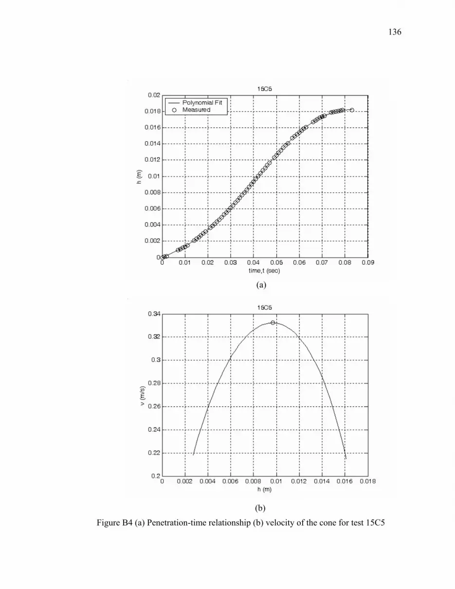
136
(a)
(b)
Figure B4 (a) Penetration-time relationship (b) velocity of the cone for test 15C5

137
(a)
(b)
Figure B5 (a) Penetration-time relationship (b) velocity of the cone for test 15C6

138
(a)
(b)
Figure B6 (a) Penetration-time relationship (b) velocity of the cone for test 5C1

139
(a)
(b)
Figure B7 (a) Penetration-time relationship (b) velocity of the cone for test 5C2

140
(a)
(b)
Figure B8 (a) Penetration-time relationship (b) velocity of the cone for test 5C3

141
(a)
(b)
Figure B9(a) Penetration-time relationship (b) velocity of the cone for test C1

142
(a)
(b)
Figure B10 (a) Penetration-time relationship (b) velocity of the cone for test C2

143
(a)
(b)
Figure B11 (a) Penetration-time relationship (b) velocity of the cone for test C3

144
APPENDIX C
APPLICATION USING AN ILLUSTRATIVE EXAMPLE

145
The example given below is only intended to illustrate the potential application of this
research to practical problems such as a jacked pile in clay.
EXAMPLE :
A cylindrical steel shaft of radius 0.5 m is to be jacked with velocity ( zV ) of 5 cm/sec in
clay layer, which extends upto a depth of 20 m below the ground surface. The undrained
shear strength of this soil is 20 kPa and the LI is 0.6. The relationship between pµ (Pa.s)
and LI determined by using fall cone tests is
p 2000exp( 1.0LI)µ = − [C.1]
If the embedment length of the shaft is 10 m, compute
(a) the static and viscous resistance components on the shaft during penetration. The
jacked pile creates a CS zone of radius equal to 2 times the radius of the pile
(i.e. 0λ 2= ).
(b) The change in total penetration resistance if zV 10cm / sec= and 0λ 1.4= .
SOLUTION:
(a)
1. Static friction resistance:
The static skin frictional stress on a jacked pile in clay under undrained condition (no
volume change) is:
ss uf s= α [C.2]
146
where α is a skin friction factor and su is the undrained shear strength of the clay. For the
given clay with us 25kPa, 1.0≤ α = (Budhu, 2000). The total static skin friction
resistance on the jacked pile is: 0 ss(2 r f )L 628.3kNπ =
2. Viscous friction resistance:
The viscous skin friction resistance per unit length on a penetrating shaft using Equation
(3.22), developed in this study is, v p z 0f 2πµ V β=
For the jacked pile shaft in this example, 2zV 5 10 m / s−= × , 0 4β = (Figure 3.5).
The viscosity of clay using Equation (C.1) is p 1098Pa.sµ ≈
The total viscous resistance on the jacked pile is: p z 0(2πµ V β )L 13.8kN=
The total soil resistance on the jacked pile is: 628.3 13.8 642.1kN+ =
(b)
For this shaft, zV 0.01m / s= and 0 10.56β = (Figure 3.5).
The viscous skin friction resistance per unit length is, v p z 0f 2πµ V β=
The total viscous resistance on the jacked pile is: p z 0(2πµ V β )L 72.6kN= The total soil resistance on the jacked pile is: 628.3 72.6 700.9kN+ =
The total penetration resistance increases by 9.2%.

147
REFERENCES
Allersma, H.G.B. (1997). Optical Analysis of Stress and Strain in Photoelastic Particle
Assemblies. PhD Thesis, Department of Civil Engineering, Delft University of
Technology, Netherlands.
Baligh, M.M. (1985). “Strain path method.” J. Geotech. Eng. Div., ASCE, 111(9), 1108-
1136.
Berry, A.J. (1988) “The dynamic penetration of clays.” Proc. 1st International
Symposium on Penetration Testing ISOPT I, Orlando., A. A. Balkema, Rotterdam,
673-679.
Budhu, M. (1985). “The effect of clay content on liquid limit from fall cone and British
cup device.” Geotech. Testing J., ASTM, 1985, 8(2), 91-95.
Budhu, M. (2000) Soil mechanics and foundations. Wiley, New York.
Budhu, M., and Wu, C. (1992). “Numerical analysis of sampling disturbances in clay
soils.” Int. J. Numeical. Analytical. Methods in Geomechanics, 16, 467-492.

148
Casson W. (1959). “A flow equation for pigment-oil suspensions of printing of the
printing ink type.” Rheology of Dispersed Systems, Pergamon, London.
Cooke, R. W., and Price, G. (1973). “Strains and displacements around friction piles.”
Proc. 8th Int. Conf. on Soil Mechanics and Foundation Engineering, 2 (1), Moscow,
U.S.S.R., 53-60.
Coulomb, C.A. (1776). “Essai sur une application des règles des maximis et minimis à
quelques problèmes de statique relatifs à l’architecture.” Memories de la
Mathematique et de Physique, presentes a l’Academie Royale des Sciences, par
divers savants, et lus dans ces Assemblees., L’Imprimerie Royale, Paris, 3-8.
Coussot, P., Nguyen, Q.D., Huynh, H.T., and Bonn D. (2002). “Avalanche behavior in
yield stress fluids. Phy. Rev. Lett., 88 (17), paper no.175501 (4).
Cummins, A.E., Kerkhoff, G. O., and Peck, R. B. (1948). “Effect of driving piles into
soft clay.” Transactions, ASCE, 115, Paper No. 2400, 275-285.
Desai, C.S. (2001) Mechanics of materials and interfaces: the disturbed state concept.
CRC Press, Boca Raton.

149
Ding, D., Li, J., and Helm, D.C. (2001). “Nonlinear shear viscosity of clayey soils over
different time scales.” Proc. 3rd Int. Conf. on Soft Soil Engineering, Hong Kong, 623
- 627.
Edgers, L., and Karlsrud, K. (1985). “Viscous analysis of submarine flows.” Proceedings
of the 4th International Conference on the Behaviour of Offshore Structures, Delft,
Developments in Marine Technology, 2, 773-784
Esrig, M. I., Kirby, R. C., Bea, R. G., and Murphy, B. S. (1977). “Initial development of
a general effective stress method for prediction of axial capacity for driven piles in
clay.” Proc. of the 9th Annual Offshore Technology Conf., Houston, OTC paper 2943,
495-506.
Fakher, A., Jones, C.F.J.P., and Clarke, B.G. (1999). “Yield stress of super soft clays.” J.
Geotech. Geoenviron. Eng. ASCE, 125 (6), 499-509.
Feng, T.W. (2000). “Fall-cone penetration and water content relationships of clays.”
Geotechnique, 23 (4), 181-187.
Flaate, K. (1972). “Effects of pile driving in clays.” Can. Geotech. J., 9, 81-88.

150
Fung, Y.C., and Tong, P. (2001). Classical and computational solid mechanics. World
Scientific, New Jersey.
Hansbo, S. (1957). “A new approach to the determination of the shear strength of clay by
the fall-cone test.” Proc. of the Royal Swedish Geotechnical Institute, 14, 1-47.
Happel, J., and Brenner, H. (1965). Low Reynolds number hydrodynamics with special
applications to particulate media. Prentice Hall Inc., Eaglewood cliffs, New Jersey.
Hill, R. (1950). The mathematical theory of plasticity. Oxford University Press, London
Houlsby, G.T., (1982). “Theoretical analysis of the fall cone test.” Geotechnique, 32 (2),
111-118.
Inoue, T., Tan, T.S., and Lee, S.L. (1990). “An investigation of shear strength of slurry
clay.” Soils and Foundations, 30(4), 1-10.
Kirby, R. C., and Wroth, C. P. (1977). “Application of critical state soil mechanics to the
prediction of axial capacity for driven piles in clay.” Proc. of the 9th Annual Offshore
Technology Conf., Houston, OTC paper 2942, 483-494.

151
Komamura, F., and Huang, R.J. (1974). “A new rheological model for soil behavior.” J.
Geotech. Eng. Div. ASCE., 100(7), 807-824.
Koumoto, T., and Houlsby, G.T. (2001). “Theory and practice of the fall cone test.”
Geotechnique, 51(8), 701-712.
Lamb, H. (1932). Hydrodynamics (6th edn.). Cambridge University Press, England.
Locat, J., and Demers, D. (1988). “Viscosity, yield stress, remolded strength, and
liquidity index relationships for sensitive clays.” Canadian Geotech. J. 25, 799-806.
Marsland, A. and Quarterman, R.S.T. (1982). “Factors affecting the measurements and
interpretation of quasi static penetration tests in clays.” Proc. 2nd European
Symposium on Penetration Testing ESOPT II, 1982, 2, A. A. Balkema, Amsterdam,
697-702.
Matesic, L., and Vucetic, M. (2003). “Strain-rate effect on soil secant shear modulus at
small cyclic strains.” J. Geotech. Geoenviron. Eng., ASCE, 129(6), 536-549.
Matsui, T., and Ito, T. (1977). “Flow mechanism of clay-layer system and microscopic
meaning on shear parameters on soils.” Proc. 9th Int. Conf. on Soil Mechanics and
Foundation Engineering, Tokyo, Specialty session 9, 143-152.

152
McNown, J.S., Lee, H.M., McPherson, M.B. and Engez, S.M. (1948). “Influence of
boundary proximity on the drag of spheres.” Proc. VII Int. Congress Applied
Mechanics, 2, 17.
Meyerhof, G.G. (1951). “The ultimate bearing capacity of foundations.” Geotechnique, 2
(4), 301-332.
Mitchell, J.K. (1976). Fundamentals of soil behaviour (1st edn.). Wiley, New York.
Mitchell, J.K. (1964). “Shearing resistance of soils as a rate process.” J. Soil Mechanics
and Foundation. Div., ASCE, 90(1), 29-61.
Murff, J.D., and Coyle, H.M. (1973). “Low velocity penetration of kaolin clay.” J.
Geotech. Eng. Div., ASCE, 99 (5), 375-389.
Nguyen, Q.D., and Boger, D.V. (1992). “Measuring the flow properties of yield stress
fluids.” Annual Review Fluid Mechanics, 24, 47-88.
Panton, R.L. (1984). Incompressible flow. Wiley, New York.

153
Picart, D., Manceau, R., and Faure, J. P. (1999). “Characterization of paste-extrudable
explosives using a penetration test.” Propellants, Explosives, Pyrotechnics, 24, 227-
231.
Puzinaukas, V. (1967). “Evaluation of properties of asphalt cements with emphasis on
consistency at low temperatures.” Proc. of the Association of Asphalt Paving
Technologists, 36, 489-540.
Randolph, M. F., and Wroth, C. P. (1978). “Analysis of deformation of vertically loaded
piles.” J. Geotech. Eng. Div., ASCE, 104(12), 1465-1488.
Randolph, M. F., Carter, J. P., and Wroth, C. P. (1979). “Driven piles in clay – the
effects of installation and subsequent consolidation.” Geotechnique, 29 (4), 361-393.
Randolph, M.F., Martin, C., and Hu, Y. (2000). “Limiting resistance of a spherical
penetrometer in cohesive material.” Geotechnique, 2000, 50 (5), 573-582.
Ray, M. (1936). “Application of Bessel functions to the solution of problem of motion of
circular disc in viscous liquid.” Phil Mag. Vol. 21, Series 7, 546-564.
Roscoe, K.H., and Burland, J.B. (1968). “On the generalized stress-strain behaviour of
wet clay.” Engineering Plasticity, Cambridge Univ. Press, 535-609.

154
Sagaseta and Whittle, 2001 Sagaseta, C., and Whittle, A.J. (2001). “Ground movements
due to pile driving in clay.” J. Geotech. Geoenviron. Eng., ASCE, 127 (1), 55-66.
Schofield, A., and Wroth, C.P. (1968). Critical state soil mechanics. McGraw-Hill,
London.
Sheahan, T.C., Ladd, C.C., and Germaine, J.T. (1996). “Rate-dependent undrained shear
behavior of saturated clay.” J. Geotech. Eng., ASCE, 122 (2), 99-108.
Shimobe, S. (2000). “Correlations among liquidity index, undrained shear strength and
fall cone penetration of fine-grained soils.” Coastal Geotech. Eng. in Practice,
Balkema, Rotterdam, 141-146.
Tan, T.S., Goh, T.C., Karunaratne, G.P., Inoue, T. and Lee, S.L. (1991). “Yield stress
measurement by a penetration method.” Canadian Geotech. J., 28(4), 517-522.
Tan, T.S., Yong, K.Y., Leong, E.C., and Lee, S.L. (1990). “Behaviour of clay slurry.”
Soils and Foundations, 30(4), 105-118.
Teh, C.I., and Houlsby, G.T. (1991). “An analytical study of the cone penetration test in
clay.” Geotechnique, 1991, 41(1), 17-34.

155
Tomlinson, M.J. (1957). “The adhesion of driven piles in clay soils.” Proc. 4th
International Conference on Soil Mech. and Found. Eng., Vol. 2, 66-71.
Tons, E., and Chritz, P. (1975). “Grading of asphalt cements by viscosity.” Proc. of the
Association of Asphalt Paving Technologists, 44, 387-415.
Torrance, J.K. (1987). “Shear resistance of remoulded soils by viscometric and fall-cone
methods: A comparison for Canadian sensitive marine clays.” Canadian Geotech. J.,
24(2), 318-322.
Turnage, 1973 Turnage, G.W. (1973). “Influence of viscous-type and inertial forces on
the penetration resistances of saturated fine-grained soils.” J. of Terramechanics, 10,
No. 2, 63-76.
van den Berg, P. (1994). Analysis of soil penetration. PhD thesis, Delft University of
Technology, Netherlands.
Vesic, A.S. (1973). “Analysis of ultimate loads of shallow foundations.” J. Geotech. Eng.
Div. ASCE., 99(1), 45-73.
156
Vyalov, S.S. (1986). Rhelogical fundamentals of soil mechanics. Developments in
Geotechnical Engineering, Vol.36, Elsevier, Amsterdam.
Whitman, R.V. (1957). “The behavior of soils under transient loadings.” Proc. 4th Int.
Conf. on Soil Mechanics and Foundation Engineering, 1, Butterworths Scientific
Publications, London, 207-210.
Wood, D.M. (1982). “Cone penetrometer and liquid limit.” Geotechnique, 32(1), 152-
157.
Wood, D.M. (1985). “Some fall-cone tests.” Geotechnique, 35(1), 64-68.
Wroth, C.P., and Wood, D.M. (1978) “The correlation of index properties with some
basic engineering properties of soils.” Canadian Geotech. J., 15 (2), 137-145.
Yong, R.N., and Japp, R.D. (1967). “A flow law for in dynamic compression.” Proc.
International Symposium on Wave Propagation and Dynamic Properties of Earth
Materials, University of New Mexico Press, Albuquerque, N.M., 183-188.
Yu, H.S., Herrmann, L.R. and Boulanger, R.W. (2000). “Analysis of steady cone
penetration in clay.” J. Geotech. Geoenviron. Eng. ASCE, 126 (7), 594-605.

157
Zeevart, L. (1948). “Discussion on effect of driving piles into soft clay.” Transactions,
ASCE, 115, 286-292.
Zreik, D.A., Ladd, C.C., and Germaine, J.T. (1995). “A new fall cone device for
measuring the undrained strength of very weak cohesive soils.” Geotech. Testing J.,
ASTM, 18(4), 472-482.