measurement of angular vibrations in rotating shafts: effects of the measurement setup nonidealities
TRANSCRIPT
Measurement of Angular Vibrations in Rotating
Shafts: Effects of the Measurement Setup
Non-Idealities
Tommaso Addabbo, Ada Fort, Luca Pancioni,
Mauro Di Marco, Valerio Vignoli
Department of Information Engineering and Mathematical Sciences
University of Siena, 53100 Italy
(e-mail: [email protected])
Roberto Biondi, Stefano Cioncolini
GE Oil & Gas, 50127 Florence, Italy
⋆ RESEARCH MANUSCRIPT ⋆
– PLEASE REFER TO THE PUBLISHED PAPER1 –
Abstract
In this paper the authors discuss a measurement method, based on thezero-crossing demodulation technique of FM signals, to estimate the an-gular velocity vibrations of a rotating shaft. The demodulation algorithmis applied without any filtering to the direct voltage output issued by someprobes sensing the passages of arbitrarily shaped targets installed on therotating shaft. The authors discuss a theoretical approach to analyze themeasurement problem taking into account the chief non-idealities relatedto the measurement set-up, i.e., they have investigated the effects of boththe shaft side vibrations and the irregular shape of the targets. On the ba-sis of the theoretical results the authors propose a measurement methodthat can reject the effects of these mentioned non-idealities, exploitingthe measurements of two or more probes properly positioned around theshaft.
1 Introduction
The measurement of the angular velocity variations of a rotating shaft plays akey role in a broad range of fields and applications, from energy production withturbo-machines to the automotive industry. Among the measurement methods,probably the simplest one is to sense the passing of the teeth of a geared wheel
1Instrumentation and Measurement, IEEE Transactions on, 2013, vol. 62, n. 3, p. 532-543.
1
Research manuscript. Please refer to the published paper ⋆ 2
installed on the shaft, since the time-delay between the teeth is inversely pro-portional to the rotational speed. Exploiting this idea, some papers have beenpublished in literature for specific targeted applications, but an overall theo-retical approach to evaluate the accuracy of the measurement method has notbeen yet discussed exhaustively, even considering the most common measure-ment setup non-idealities [1–7]. The above mentioned papers deal with theproblem of measuring the angular velocity of rotating shafts in specific applica-tions, analyzing different aspects of the measurement task and adopting in mostcases an heuristic and simplified point of view. In [6,7] some theoretical aspectswere investigated, e.g., the estimation of measurement uncertainties.
Differently from the above mentioned works, in this paper the authors letthe shape profile of the geared wheel have an irregular shape: for example,the ‘geared wheel’ can be represented by a bolted joint in the shaft, being thebolts representing ‘teeth’ whose geometrical profiles may differ from each oth-ers. When either fault diagnosis or predictive maintenance have to be performedon scarcely accessible or modifiable machineries, this measurement technique isoften the only one available and a theoretical analysis of the accuracy of thismethod is of some interest, especially when referring to those applications inwhich the measurement precision represents a critical issue (e.g., the measure-ment of torsional vibrations in turbo-machines with extreme-stiff shafts [7–9]).For simplicity, regardless of the actual profile of the sensed profile, in the fol-lowing the authors refer to a generic geared wheel, or cogwheel.
In this paper the authors extend the work presented in [10], providing a deepanalysis of the effects on the measurement due to both the irregular cogwheelshape and the side shaft vibrations. As a result, they show that the well-known zero-crossing demodulation technique can represent a valid solution forretrieving the angular vibrational signal, and propose a method to increase themeasurement accuracy by properly combining two or more probes.
Adopting a presentation organization similar to that one of [10], this paperis structured as in the following. In Sec.2 the authors introduce the notationand a reference probe physical model. In Sec. 3 the analytical representationof the probe voltage signal is discussed, showing that due to the shaft angularvibrations the signal can be written as an infinite summation of frequency-modulated sinusoidal components. In Sec. 4 the authors analyze the frequencyspectrum of the probe output voltage, linking its spectral characteristics to theshape of the sensed geared wheel installed on the shaft, whereas in the Sec. 5 theeffects of the shaft side vibrations are analyzed. In Sec. 6 the authors show howto estimate the vibrational signal using the zero-crossing technique, discussing asensitivity analysis of the proposed measurement method. In Secs. 7 and 8 theauthors propose a method to reject the effects of the irregular cogwheel profileand the shaft side vibrations, respectively. Conclusions and references close thepaper.
All the examples shown in this paper are based on simulations. The useof simulations was necessary to evaluate the correctness of the theoretical ap-proach, since simulations allow for setting up an a-priori known physical condi-tion of the rotating shaft, including angular vibrations, shaft side vibrations andcogwheel shape. The general results presented in this paper were also validatedby means of experimental measurements made at the GE Oil & Gas Facility inFlorence, Italy. Also these results, not reported in this paper for concisenesssake, confirm the theoretical predictions discussed in the following Sections.
Research manuscript. Please refer to the published paper ⋆ 3
C
x
y
VoutMEASUREM.
DEVICE
SensingProbe
Probereception
lobe
Vin
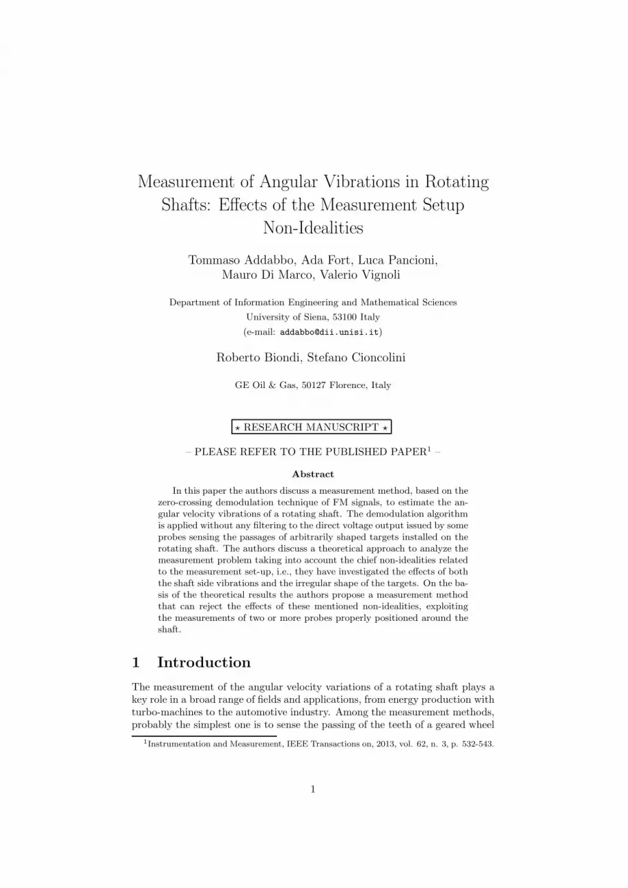
Figure 1: Illustration of a basic reference measurement setup.
2 Notation and Probe Physical model
In this work the authors refer to an arbitrarily shaped cogwheel (Fig. 1) installedon the shaft and positioned in front of a sensing probe. By denoting with ω(t)the instantaneous angular velocity of the cogwheel with respect to its center C(measured in rad/s), the measurement device in Fig. 1 is devised for measuringthe variations of the shaft angular velocity with respect to its average value.The cogwheel center is assumed to be nominally placed in the origin, even ifsmall vibrations (shaft side vibrations) are allowed: in such case, the positioningvector C = (Cx, Cy) is a function of time, i.e., C(t) = (Cx(t), Cy(t)). From apractical point of view, the average angular velocity is calculated referring to afinite time-window of length W , and the angular variations are calculated as
∆ω(t) = ω(t)− 1
W
∫ t
t−W
ω(τ)dτ. (1)
In the following, angular vibrations are managed as small perturbations of aconstant rotating shaft with angular velocity ω0, i.e.,
ω(t) = ω0 + ω(t) = ω0 +∆ωmaxm(t), (2)
where the term ω takes into account the angular vibrations, ∆ωmax is themaximum level of |ω| and m(t) is non-dimensional, with zero mean value and|m(t)| ≤ 1, t ≥ 0.
2.1 Probe modeling
A probe is used to sense the teeth passages of the geared wheel installed onthe shaft. Since the theoretical approach discussed in this paper does not referto specific characteristics of the probe, in the following a generic model for thesensing probes is adopted. Accordingly, referring to Fig. 1, it is assumed thatthe probe has a spatial reception lobe symmetrical with respect to the x axis.Moreover, the probe reception profile is assumed to be described with a genericGaussian single-lobe having normalized amplitude and -3dB half-angle θ0, i.e,
f(θ) =
√
ln 2
πθ20e−
θ2 ln√
2
θ20 , −π ≤ θ ≤ π. (3)
Research manuscript. Please refer to the published paper ⋆ 4
From an electrical point of view, the probe is modeled as a linear time-invariant system with generic band-pass transfer function
H(ω) =jGω
(
1 + j ωωL
)(
1 + j ωωH
) . (4)
In the above transfer function G is a gain factor taking into account the probedistance from the cogwheel, whereas ωL ≪ ωH are the two pulsations associatedwith the high-pass and low-pass cut-off frequencies.
3 Analytical representation of the probe signal
Referring to Fig.1, an analytical representation of the probe voltage signal Vin
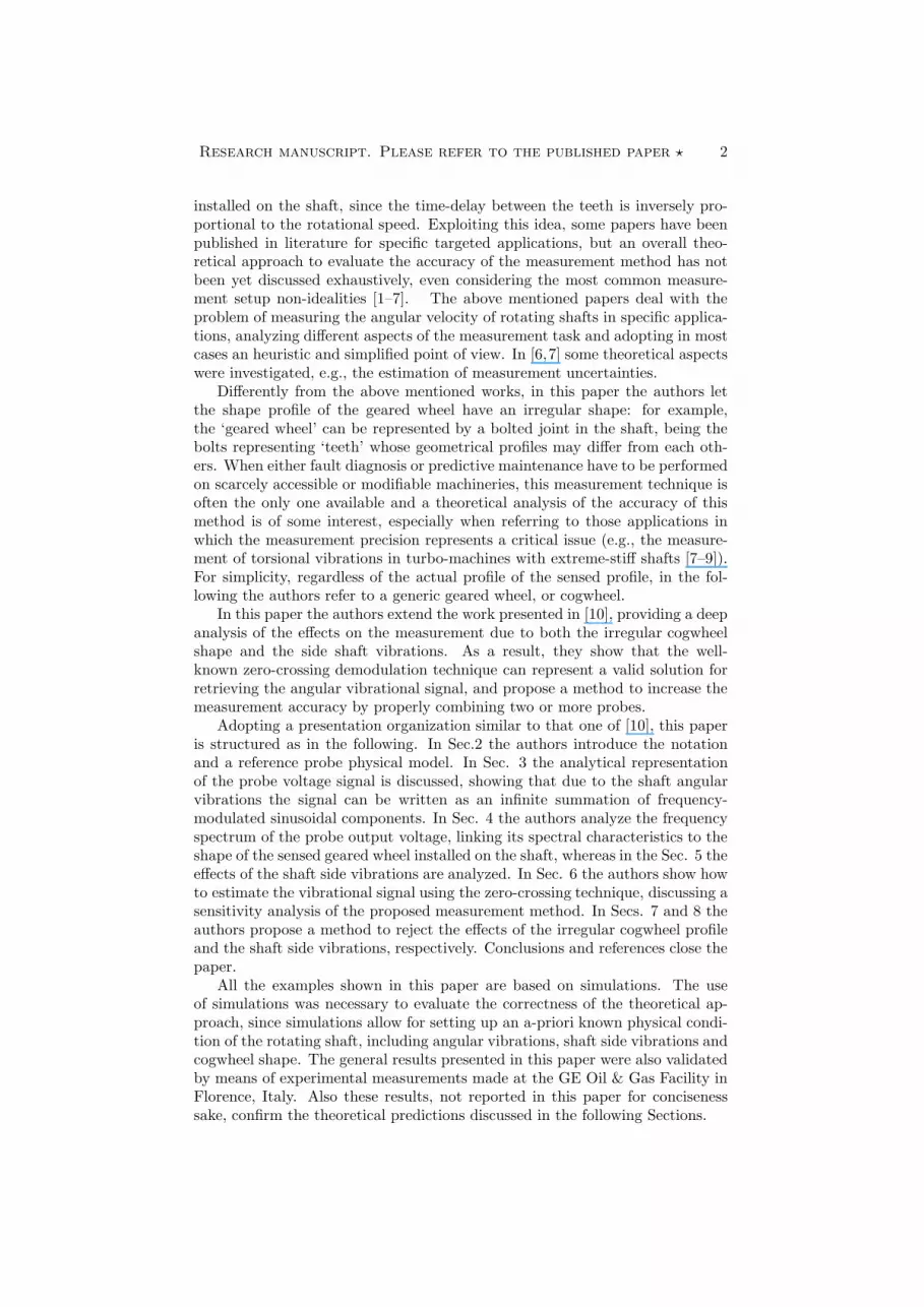
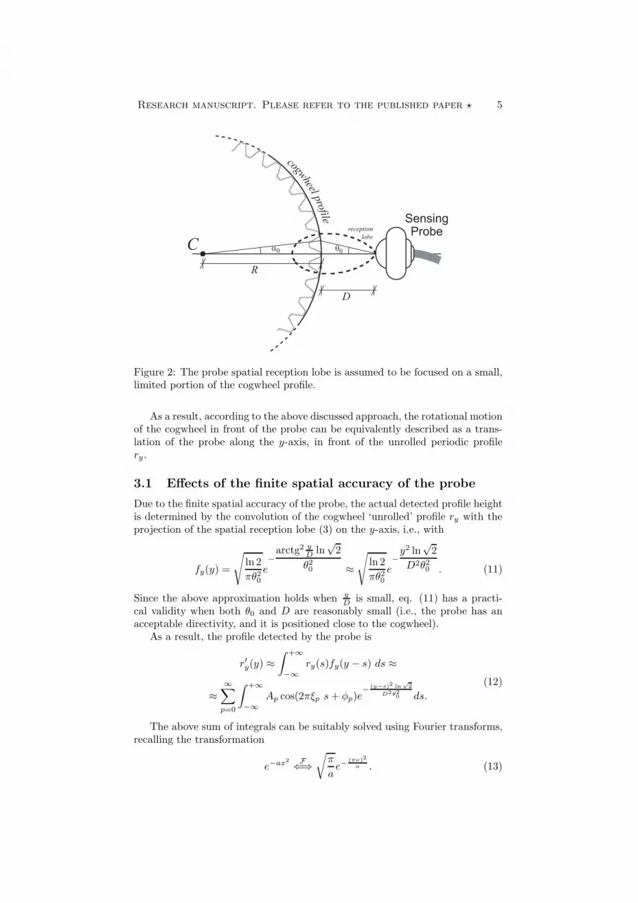
can be obtained following the approach discussed in this Section. The authorsinitially assume to deal with a shaft rotating in absence of side vibrations, thatis, the cogwheel center C is hypothesized to be the fixed point (Cx, Cy) = (0, 0).Moreover, the probe spatial reception lobe is assumed to be focused on a small,limited portion of the cogwheel profile, i.e, referring to Fig. 2,
α0 ≪ θ0 (5)
(the assumption typically makes sense, since D ≪ R). By denoting withr : [0, 2π) → R
+ the polar representation of the cogwheel profile (with respectto the point C), the authors note that under the assumption (5) the cogwheelprofile can be locally approximated by the projection ry : R → R
+ of the po-lar representation r on the y axis, in front of the probe. In other words, therotational motion of the cogwheel in front of the probe can be described as anequivalent relative motion of the probe along the y-axis, in front of the cogwheel‘unrolled’ profile
ry(y) = r( y
Rmod 2π
)
. (6)
Since (6) is a periodic function with period 2πR, it can be expressed as aninfinite Fourier series
ry(y) =a02
+
∞∑
n=1
[
an cos(ny
R
)
+ bn sin(ny
R
)]
. (7)
By reordering the above series, eq. (7) can be rewritten in a more compactanalytical form, as the infinite sum of cosines
ry(y) =
∞∑
p=0
Ap cos(2πξp y + φp), (8)
where
Ap =
a0
2 if p = 0,
a p+12
if p is odd,
b p2
if p is even,
φp =
{
−π2 if p is odd,
0 if p is even,(9)
and
ξp =n(p)
2πR=
{
p+14πR if p is odd,p
4πR if p is even.(10)
Research manuscript. Please refer to the published paper ⋆ 5
C
SensingProbe
cogwheel profile
θ0α0
D
R
reception
lobe
Figure 2: The probe spatial reception lobe is assumed to be focused on a small,limited portion of the cogwheel profile.
As a result, according to the above discussed approach, the rotational motionof the cogwheel in front of the probe can be equivalently described as a trans-lation of the probe along the y-axis, in front of the unrolled periodic profilery.
3.1 Effects of the finite spatial accuracy of the probe
Due to the finite spatial accuracy of the probe, the actual detected profile heightis determined by the convolution of the cogwheel ‘unrolled’ profile ry with theprojection of the spatial reception lobe (3) on the y-axis, i.e., with
fy(y) =
√
ln 2
πθ20e−
arctg2 yDln√2
θ20 ≈√
ln 2
πθ20e−
y2 ln√2
D2θ20 . (11)
Since the above approximation holds when yD
is small, eq. (11) has a practi-cal validity when both θ0 and D are reasonably small (i.e., the probe has anacceptable directivity, and it is positioned close to the cogwheel).
As a result, the profile detected by the probe is
r′y(y) ≈∫ +∞
−∞
ry(s)fy(y − s) ds ≈
≈∞∑
p=0
∫ +∞
−∞
Ap cos(2πξp s+ φp)e−
(y−s)2 ln√
2
D2θ20 ds.
(12)
The above sum of integrals can be suitably solved using Fourier transforms,recalling the transformation
e−ax2 F⇐⇒√
π
ae−
(πν)2
a . (13)
Research manuscript. Please refer to the published paper ⋆ 6
Accordingly, eq. (12) can be rewritten as
r′y(y) ≈∞∑
p=0
A′
p cos(2πξp y + φp), (14)
where
A′
p = Ap e−
(πξpDθ0)2
ln√2 . (15)
3.2 The probe output voltage signal
Using the above results the probe output voltage can be found relating thespatial variable y to the time, by means of the cogwheel angular velocity. Sincethe shaft rotational angle α is linked to the instantaneous angular velocity byan integral relationship, it results
y(t) = Rα(t) = Rα(0) +R
∫ t
0
ω(τ)dτ =
= Rα(0) +Rω0t+R
∫ t
0
ω(τ)dτ.
(16)
Substituting (16) in (14), by properly setting α(0) = 0 without loss of generality,the following expression can be obtained
r′y(t) ≈∞∑
p=0
A′
p cos
[
2πξp
(
Rω0t+R
∫ t
0
ω(τ)dτ
)
+ φp
]
. (17)
The above summation describes the cogwheel profile detected by the probe, as afunction of the time t. In other words, since the cogwheel rotation with respectto the probe is represented as a relative motion of the probe in front of theunrolled cogwheel profile, eq. (17) describes the height of the detected profilesampled in front of the probe, assuming the probe translating along the y-axis,according to (16).
The probe voltage Vin of Fig.1 can be finally determined by filtering thesignal (17) with the probe electric response (4). At a first approximation theprobe transfer function (4) is assumed to be constant over small disjoint band-widths containing the frequency spectrum of each term in the summation (17)(this aspect is made clearer in Sec.4). As a result, the filtering of (17) with (4)changes the amplitudes A′
p and phases φ′p in A′′
p and φ′′p , respectively, obtaining
Vin(t) ≈∞∑
p=0
A′′
p cos
[
2πξp
(
Rω0t+R
∫ t
0
ω(τ)dτ
)
+ φ′′
p
]
. (18)
Recalling def. (10), the authors emphasize that each term in the abovesummation represents the expression of the classical frequency modulation ofsinusoidal carriers [11] with fundamental frequencies
fc,p = Rξpω0 =n(p)ω0
2π, n(p) ∈ N (19)
Research manuscript. Please refer to the published paper ⋆ 7
0 10 20 30 40 50 60 70 80 90100
102
104
106
108
110
0 0.5 1 1.5 2 2.5 3 3.5 4-1.0
-0.5
0
0.5
1.0
[Degrees]
[ms]
r(α
)V
in(t
)
t
[mm]
[volt]
α
(a)
(b)
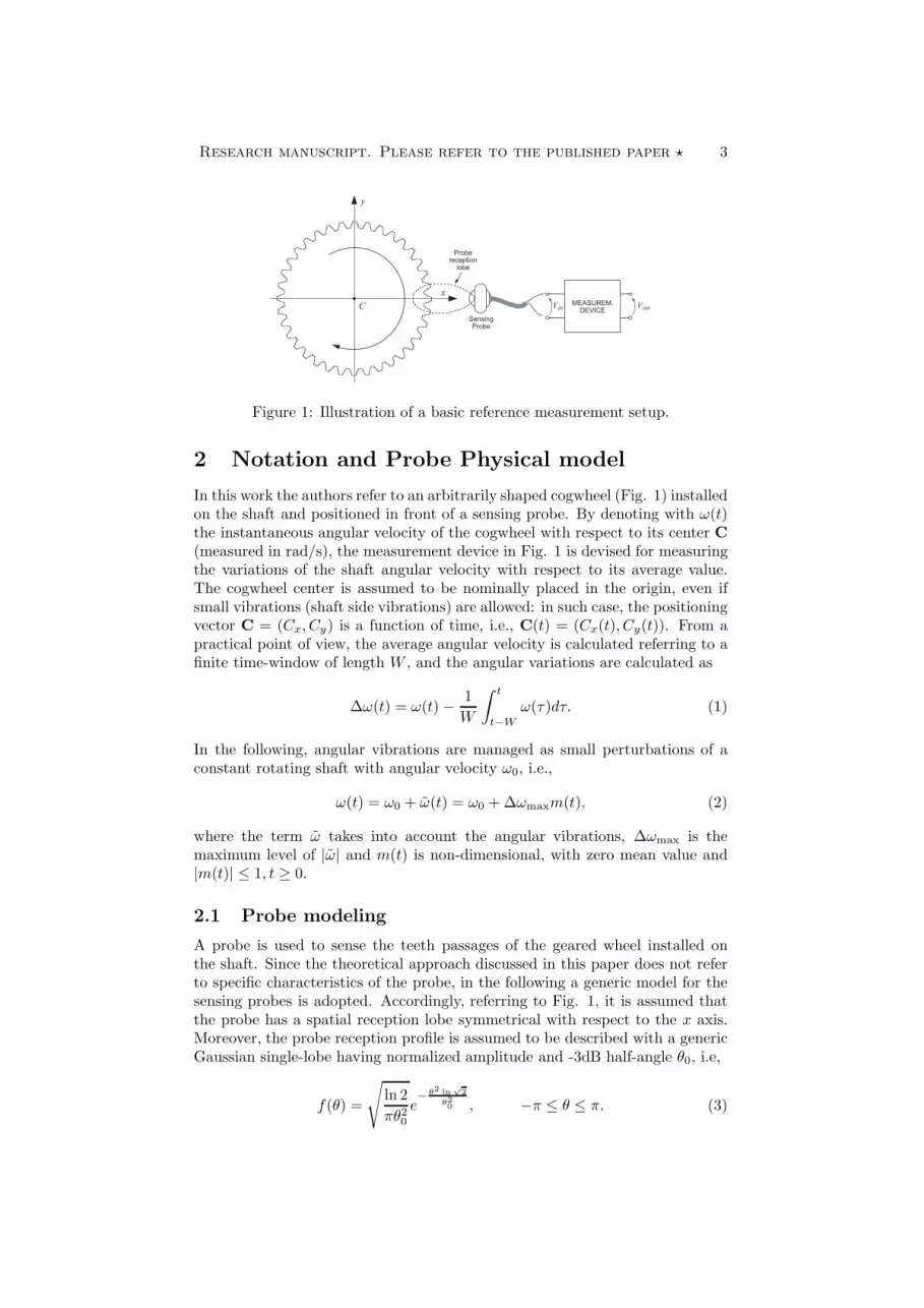
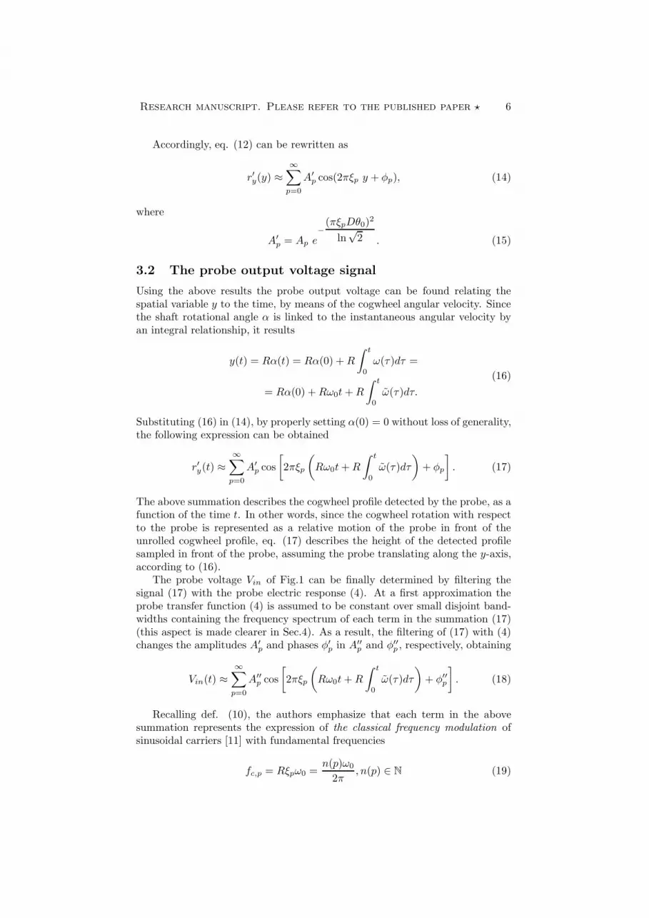
Figure 3: The effect of the finite resolution of the sensing probe on the first90 degrees of the sensed rotating cogwheel profile: (a) cogwheel profile withirregular cogs; (b) correspondent normalized probe output voltage.
Accordingly, each term in the summation can be rewritten in the form
A cos
(
nω0t+ n∆ωmax
∫ t
0
m(τ)dτ + φ
)
. (20)
These latter considerations will be made clearer in the next Sections.
Example 1
Let us consider a shaft rotating at ω0 = 2πf0 = 3600 rpm, i.e., f0 = 60 Hz(no angular vibrations). The used cogwheel has a nominal radius of 10 cm, anirregular profile (N = 36 trapezoidal cogs, with 0.5 mm of standard deviationin the mechanical profile, one broken cog). The nominal distance of the sensingprobe is 10 mm, with 3 dB half-angle equal to 5◦ and pass-band cut-off fre-quencies fL = 2 Hz and fH = 10 kHz. As it can be seen in Fig. 3, due to theprobe finite resolution the output voltage Vin expressed by (18) with ω = 0,normalized to its maximum amplitude, describes a much smoother version ofthe unrolled cogwheel profile.
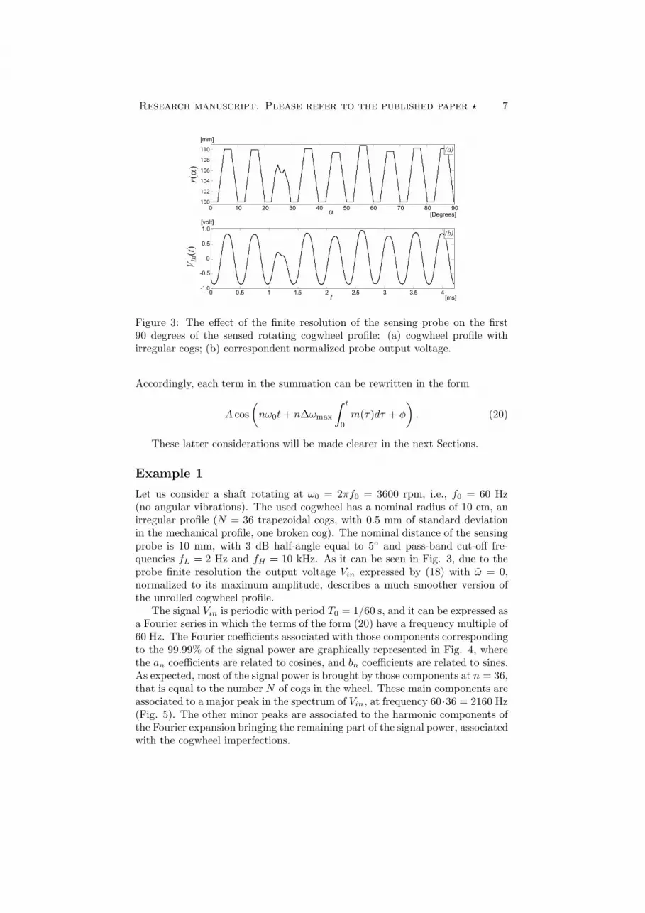
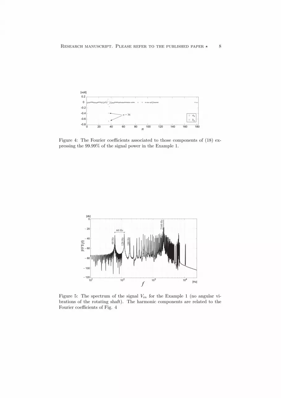
The signal Vin is periodic with period T0 = 1/60 s, and it can be expressed asa Fourier series in which the terms of the form (20) have a frequency multiple of60 Hz. The Fourier coefficients associated with those components correspondingto the 99.99% of the signal power are graphically represented in Fig. 4, wherethe an coefficients are related to cosines, and bn coefficients are related to sines.As expected, most of the signal power is brought by those components at n = 36,that is equal to the number N of cogs in the wheel. These main components areassociated to a major peak in the spectrum of Vin, at frequency 60·36 = 2160 Hz(Fig. 5). The other minor peaks are associated to the harmonic components ofthe Fourier expansion bringing the remaining part of the signal power, associatedwith the cogwheel imperfections.
Research manuscript. Please refer to the published paper ⋆ 8
0 20 40 60 80 100 120 140 160 180-0.8
-0.6
-0.4
-0.2
0
0.2
an
bn
n = 36
[volt]
n
Figure 4: The Fourier coefficients associated to those components of (18) ex-pressing the 99.99% of the signal power in the Example 1.
103 104102101
f[Hz]
60 Hz
60
Hz
12
0 H
z
18
0 H
z
− 120
− 100
− 80
− 60
− 40
− 20
0
|FF
T(f
)|
[db]
21
60
Hz
Figure 5: The spectrum of the signal Vin for the Example 1 (no angular vi-brations of the rotating shaft). The harmonic components are related to theFourier coefficients of Fig. 4
Research manuscript. Please refer to the published paper ⋆ 9
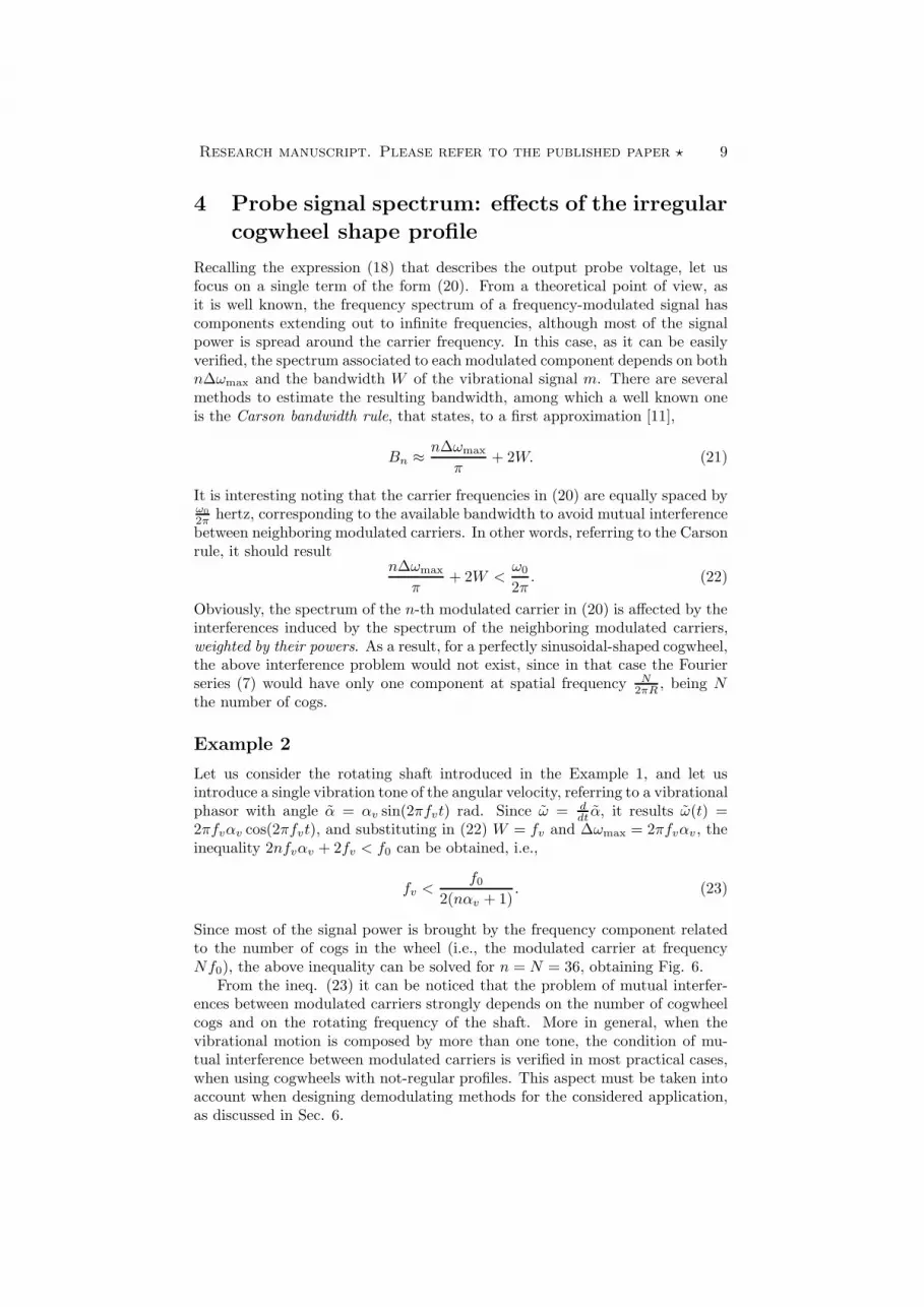
4 Probe signal spectrum: effects of the irregular
cogwheel shape profile
Recalling the expression (18) that describes the output probe voltage, let usfocus on a single term of the form (20). From a theoretical point of view, asit is well known, the frequency spectrum of a frequency-modulated signal hascomponents extending out to infinite frequencies, although most of the signalpower is spread around the carrier frequency. In this case, as it can be easilyverified, the spectrum associated to each modulated component depends on bothn∆ωmax and the bandwidth W of the vibrational signal m. There are severalmethods to estimate the resulting bandwidth, among which a well known oneis the Carson bandwidth rule, that states, to a first approximation [11],
Bn ≈ n∆ωmax
π+ 2W. (21)
It is interesting noting that the carrier frequencies in (20) are equally spaced byω0
2π hertz, corresponding to the available bandwidth to avoid mutual interferencebetween neighboring modulated carriers. In other words, referring to the Carsonrule, it should result
n∆ωmax
π+ 2W <
ω0
2π. (22)
Obviously, the spectrum of the n-th modulated carrier in (20) is affected by theinterferences induced by the spectrum of the neighboring modulated carriers,weighted by their powers. As a result, for a perfectly sinusoidal-shaped cogwheel,the above interference problem would not exist, since in that case the Fourierseries (7) would have only one component at spatial frequency N
2πR , being Nthe number of cogs.
Example 2
Let us consider the rotating shaft introduced in the Example 1, and let usintroduce a single vibration tone of the angular velocity, referring to a vibrationalphasor with angle α = αv sin(2πfvt) rad. Since ω = d
dtα, it results ω(t) =
2πfvαv cos(2πfvt), and substituting in (22) W = fv and ∆ωmax = 2πfvαv, theinequality 2nfvαv + 2fv < f0 can be obtained, i.e.,
fv <f0
2(nαv + 1). (23)
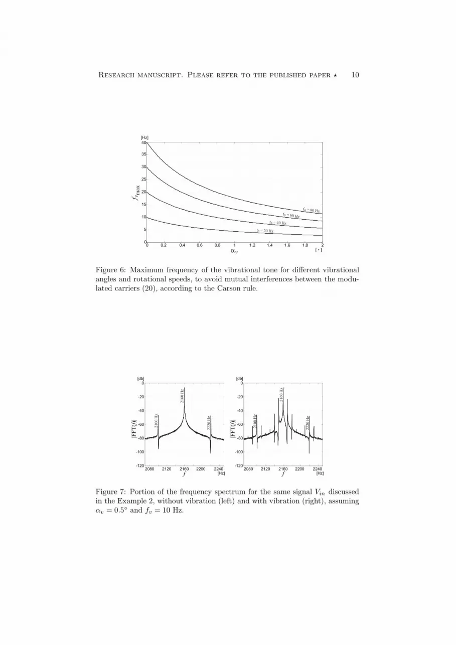
Since most of the signal power is brought by the frequency component relatedto the number of cogs in the wheel (i.e., the modulated carrier at frequencyNf0), the above inequality can be solved for n = N = 36, obtaining Fig. 6.
From the ineq. (23) it can be noticed that the problem of mutual interfer-ences between modulated carriers strongly depends on the number of cogwheelcogs and on the rotating frequency of the shaft. More in general, when thevibrational motion is composed by more than one tone, the condition of mu-tual interference between modulated carriers is verified in most practical cases,when using cogwheels with not-regular profiles. This aspect must be taken intoaccount when designing demodulating methods for the considered application,as discussed in Sec. 6.
Research manuscript. Please refer to the published paper ⋆ 10
0 0.2 0.4 0.6 0.8 1 1.2 1.4 1.6 1.8 20
5
10
15
20
25
30
35
40
f0 = 80 Hzf0 = 60 Hz
f0 = 40 Hz
f0 = 20 Hz
f vm
ax
αv [ ° ]
[Hz]
Figure 6: Maximum frequency of the vibrational tone for different vibrationalangles and rotational speeds, to avoid mutual interferences between the modu-lated carriers (20), according to the Carson rule.
2080 2120 2160 2200 2240-120
-100
-80
-60
-40
-20
0
21
60
Hz
21
60
Hz
21
00
Hz
21
00
Hz
22
20
Hz
22
20
Hz
f
|FF
T(f
)|
[db]
[Hz]2080 2120 2160 2200 2240
-120
-100
-80
-60
-40
-20
0
f
|FF
T(f
)|
[db]
[Hz]
Figure 7: Portion of the frequency spectrum for the same signal Vin discussedin the Example 2, without vibration (left) and with vibration (right), assumingαv = 0.5◦ and fv = 10 Hz.
Research manuscript. Please refer to the published paper ⋆ 11
5 Effects of the shaft side vibrations
The shaft side vibrations are described by the motion of the cogwheel center Con the plane x− y. The effects on the probe signal frequency spectrum can beanalyzed separating the two components along the different axes.
5.1 Side vibrations along the y-axis
In such case the eq. (16) must be rewritten as (the offset angle α(0) is set equalto 0)
y(t) = Rω0t+R
∫ t
0
ω(τ)dτ + Cy(t) =
= Rω0t+R
∫ t
0
(
ω(τ) +1
R
d
dτCy(τ)
)
dτ + Cy(0).
(24)
It is interesting noting that the time derivative of the y-side vibrations deter-mines a direct deterioration of the vibrational signal, inversely proportional tothe cogwheel radius R.
5.2 Side vibrations along the x-axis
The side vibrations of the rotating shaft along the x-axis change the profileheight of the cogwheel detected by the probe. In other words, the signal Cx
must be added directly to the second member of eq. (7). From a qualitativepoint of view, the effect of these side vibrations introduces a factor of the form(1 + Sx(t)) modulating the amplitude of the signal Vin, where the signal Sx
is obtained by taking into account of the probe filtering during each phasediscussed before. The analytical relationship between Sx(t) and Cx can notbe expressed explicitly, in general. Nevertheless, in the following Sections, theauthors will discuss how this aspect influences the estimation of the vibrationalsignal ω.
6 The Vibrational Signal Estimation
In the previous sections it was shown how the frequency spectrum of the outputvoltage probe signal Vin is affected by the main non-idealities of the measuringset-up. At the same time, the authors have shown that the probe signal, besidethe effects of the shaft side vibrations along the x-axis, can be represented by theinfinite sums of frequency-modulated sinusoidal carriers at different frequenciesmultiple of f0. In the case of a cogwheel with an ideal sinusoidal profile, eq.(18) reduces to a single frequency-modulated sinusoidal tone at center frequencyNf0.
From a theoretical point of view, in order to retrieve the vibrational signalω from Vin, classical FM demodulation methods represent good candidates toaccomplish the task [11]. Nevertheless, the authors emphasize that there areseveral impediments to the implementation of most of the traditional methods,as discussed in the following. First of all, the considered application operatesat extremely low frequencies, if compared to the classical FM modulation intelecommunications. Accordingly, the physical realization of band-pass filters to
Research manuscript. Please refer to the published paper ⋆ 12
select only that part of frequency spectrum interested by the main modulatedcarrier at frequency Nf0 is highly critical (also considering that the rotatingshaft f0 is unknown a priori). Moreover, the authors have shown in Sec. 4 thatneighbor modulated carriers can introduce mutual interferences, depending onthe deviation ratio ∆ωmax/2πW .
As discussed in the introduction, in this paper the authors show that a sim-ple variant of the well known zero-crossing frequency demodulation method canrepresent a valid solution to measure the vibrational signal ω, suitable for thekind of considered applications. Differently from the classical approach in whichthe zero-crossing demodulation is applied to a single frequency-modulated sinu-soidal carrier, the method is directly applied to the probe signal Vin, without anypreliminary filtering, proposing measurement methods combining the signals ofmore than one probe to reject the effects of the shaft side vibrations or of thenon-regular cogwheel shape profile.
6.1 The zero-crossing method
The classical zero crossing demodulation method is defined assuming the signalVin to be a single frequency modulated cosine at frequency Nf0, according tothe form (20) [11–13]. Every time the signal Vin is equal to zero the argumentof the cosine function is equal to π
2 + kπ, with k ∈ Z. By simply measuring thetime between two consecutive zeros, i.e., tn and tn+1, it results
2πNf0(tn+1 − tn) +N
∫ tn+1
tn
ω(τ)dτ = π. (25)
Using the integral mean value theorem, assuming ω to be continuous, thereexists τn ∈ [tn, tn+1) such that
∫ tn+1
tnω(τ)dτ = (tn+1 − tn)ω(τn). Accordingly,
by defining ∆tn = tn+1 − tn, eq. (25) becomes
∆tn(Nω0 +Nω(τn)) = π =⇒ ω(τn) =π
N∆tn. (26)
In other words, assuming ω to vary slowly with respect to ∆tn, the above resultprovides a direct estimation of the instantaneous angular velocity ω at the timetn, i.e.,
ω(tn) ≈π
N∆tn. (27)
From the above estimation, one can estimate the mean value ω0 and then thevibrational part ω, using eq. (1).
In this case, the signal Vin (18) is not a simple FM signal and some pre-cautions must be taken into account, as discussed in the following. First ofall, it can be noted that in (27) the angle π/N is equal to half of the averageangle subtended by a cog to the cogwheel center. In other words, since (27) wasderived assuming the signal to be a FM modulated carrier with frequency Nf0,the instantaneous angular velocity is simply estimated dividing half the anglesubtended by a cog by the time the shaft takes to rotate by this angle. As itis known, the cogs can be different from each others, therefore the actual anglesubtended between two zero-crossing times have to be modeled as a randomvariable ϕ.
Research manuscript. Please refer to the published paper ⋆ 13
6.2 Sensitivity analysis
On the basis of (27), the estimation ω of the instantaneous angular velocity canbe written as a function of two random variables ϕ and ∆t, i.e.,
ω =ϕ
∆t. (28)
The random variable ∆t represents the measured value tn+1 − tn, as obtainedfrom the signal processing involved by the zero-crossing technique, and its ran-dom fluctuations account for the measurement errors. On the other hand, ϕrepresents the rotation angle covered by the shaft during the time ∆t. It is arandom variable since in the estimation (27) this angle is assumed to be equalto π
N, whereas its actual value is affected by the irregular cogwheel profile.
By denoting with ϕ0 and ∆t0 the mean values of ϕ and ∆t, in the followingthe authors define ϕ = ϕ0 + δϕ and ∆t = ∆t0 + δt, where δϕ and δt repre-sents the zero-mean fluctuations of ϕ and ∆t around ϕ0 and ∆t0, respectively.Accordingly, the def. (28) can be rewritten referring to its first order Taylorexpansion
ω|ϕ0,∆t0≈
≈ ϕ0
∆t0+
∂ω
∂ϕ(ϕ0,∆t0)δϕ+
∂ω
∂∆t(ϕ0,∆t0)δt =
=ϕ0
∆t0+
1
∆t0δϕ− ϕ0
∆t20δt.
(29)
From a statistical point of view, the random variable ω has mean value
µω = E{ω} ≈ ϕ0
∆t0, (30)
and variance
σ2ω = E{(ω − µω)
2} ≈
≈ 1
∆t20σ2ϕ +
ϕ20
∆t40σ2∆t −
2ϕ0
∆t30E{δϕ δt},
(31)
where σ2∆t and σ2
ϕ are the variances of ∆t and ϕ, respectively.It is worth noting that the third term in the above expression would be zero if
∆t and ϕ were statistically independent: that is not true since the zero-crossingtimes are correlated to the actual angles subtended by the cogs. In the worstcase, by assuming a correlation coefficient ρ = −1 between ∆t and ϕ, the aboveresult can be limited by the upper-bound
σ2ω ≤ 1
∆t20σ2ϕ +
ϕ20
∆t40σ2∆t +
2ϕ0
∆t30σϕσ
2∆t =
=1
∆t20
(
σϕ +ϕ0
∆t0σ∆t
)2
.
(32)
The square root of (31) or, equivalently, the square root of the right sideof (32), describes the uncertainty about the estimation of the instantaneousangular velocity of the rotating shaft. About this point, it can be noted that
Research manuscript. Please refer to the published paper ⋆ 14
as a general trend the variance σ2ω is heavily affected by σ2
∆t as far as ∆t tendsto zero. This may happen, referring to the case considered in this work, if for afixed cogwheel the shaft rotating frequency goes to infinity (ω0 → ∞) or, for ashaft rotating at constant speed, if ϕ → 0 (i.e., the number of cogs N → ∞).
The above theoretical results have general validity if the higher order termsin the Taylor expansion of (28) are negligible, e.g.,
1
10
∣
∣
∣
∣
∂ωϕ
∂ϕδϕ+
∂ω
∂∆tδt
∣
∣
∣
∣
<
1
2
∣
∣
∣
∣
∂2ω
∂ϕ2δϕ2 +
∂2ω
∂∆t2δt2 +
∂2ω
∂ϕ∂∆t2δt δϕ+
∣
∣
∣
∣
,
(33)
that is1
10
∣
∣
∣
∣
1
∆t0δϕ− ϕ0
∆t20δt
∣
∣
∣
∣
<
∣
∣
∣
∣
ϕ0
∆t30δt2 − 1
∆t20δt δϕ
∣
∣
∣
∣
. (34)
6.3 Simplified analysis
It can be easily shown that the random variable ϕ has mean value ϕ0 = πN
andδϕ 6= 0 if and only if the cogwheel does not have N equal cogs.
Nevertheless, from a statistical point of view any uncertainty about theangle ϕ can be expressed as an uncertainty about the time ∆t. This approachis founded on the deterministic integral equation
ϕ =
∫
∆t
ω(τ)dτ, (35)
that links the actual values of ∆t and ϕ. Accordingly, even for a not-idealcogwheel, the quantity ϕ = π
Ncan be assumed constant, being the stochastic
part δt as the sum of two statistically independent quantities
δt = δtϕ + δtm, (36)
where δtϕ is the random fluctuation associated to the (actually random) angle ϕand δtm is the uncertainty related to the measure of ∆t. Referring to the abovetheoretical model, the equations (29)-(34) can be simplified as in the following:
ω|ϕ0,∆t0≈ π
N∆t0
(
1− δt
∆t0
)
, (37)
µω ≈ π
N∆t0, (38)
and variance
σ2ω ≈ π2
N2∆t40σ2∆t. (39)
The variance σ2∆t can be expressed recalling (36) and the statistical indepen-
dence of δtm and δtϕ, obtaining
σ2∆t = E{δt2m}+ E{δt2ϕ}. (40)
Research manuscript. Please refer to the published paper ⋆ 15
Assuming the shaft angular velocity ω to be greater than a minimum valueωmin and, to a first approximation, assuming ω to be constant within the timeinterval ∆t, the second term at the right side of (40) can be written as
E{δt2ϕ} ≈ E
{
(
δϕ
ω
)2}
<σ2ϕ
ω2min
. (41)
Accordingly, by denoting with σ2∆tm
the variance of the error in the measurementof the time-interval ∆t, combining the above results from eq. (39) the followingexpression can be obtained
σ2ω <
π2
N2∆t40
(
σ2∆tm
+σ2ϕ
ω2min
)
. (42)
Finally, by noting that
∆t0 =1
2Nf0, (43)
it is possible to express the uncertainty about the estimation of ω as
u(ω) ≈ π
N∆t20σ∆t = 4πNf2
0σ∆t =
=Nω2
0
πσ∆t <
Nω20
π
√
σ2∆tm
+σ2ϕ
ω2min
.
(44)
The above theoretical results have general validity if the higher order termsin the Taylor expansion of (28) are negligible, e.g., combining (43) with (34),
δt <∆t010
=1
20Nf0. (45)
Summarizing, eq. (44) characterizes the resolution of the measurement set-up, as clarified also by the following example. As a general comment, the authorsemphasize that the higher is (44), and the lower is the quality of the estimatedsignal ω used for retrieving the vibrational signal ω, according to (1).
Example 3
Let us consider the cogwheel of the Example 1, rotating at 3600 rpm, i.e., f0 =60 Hz. Assuming small vibrations of ω around ω0, in order to have a relativerms error lower than 0.5% in the measurement of the instantaneous angularvelocity, from (44) it results
4πNf20σ∆t <
0.5
1002πf0, (46)
that implies, recalling that N = 36, f0 = 60 Hz,
σ∆t <5
1000 2Nf0≈ 1.16 µs. (47)
The upper-bound is meaningful since (45) is satisfied.
Research manuscript. Please refer to the published paper ⋆ 16
It is worth noting that the maximum rms for the measurement of ∆t foundin (47) includes the cumulative effects of the measurement set-up non-idealities,i.e., the induced effects of the shaft side vibrations and of the irregular cogwheelshape profile.
On the other hand, ineq. (44) can be used to estimate an upper-bound forthe uncertainty in the measurement of ω. For example, let us assume for thezero-crossing method a time-measurement accuracy δtm = 1 µs. Moreover, iffor the cogwheel of radius R = 100 mm a mechanical standard deviation of thecogs size of 0.5 mm is assumed, it results σϕ ≈ 0.5
100 = 5 ·10−3 rad. Furthermore,if the lower shaft rotation frequency is assumed to be greater than 55 Hz, fromineq. (44) it can be obtained
u(ω)
2πf0= 2Nf0σ∆t <
2 · 36 · 60 ·√
10−12 +25 · 10−6
4π2552≈ 0.62%,
(48)
that is, a relative rms error in the estimation of the instantaneous angularvelocity not greater than 0.62%.
This example reveals that in order to achieve high measurement resolutions,sophisticated measurement set-up should be mandatory, i.e., a cogwheel with analmost perfect shape profile and negligible shaft side vibrations. Nevertheless,as discussed in the following sections, methods to reject the effects of the non-idealities can increase considerably the resolution of the measurement, evenconsidering badly shaped cogwheels.
7 Rejection of the irregular cogwheel shape
According to the above discussion, the effects of the irregular cogwheel shapeon the measurement can be taken into account assuming the cogwheel to beperfectly shaped and introducing an equivalent error in the estimation of thezero-crossing times. For the moment, let us analyze the case of a shaft rotatingwith no side vibrations and let us assume the uncertainty δtm in (36) to beequal to zero. Since the authors are applying the zero-crossing demodulationmethod to the unfiltered signal Vin, they account for the cogwheel irregularitiesintroducing a phase-error in (25), i.e.,
2πNf0(tn+1 − tn) +N
∫ tn+1
tn
(
ω(τ) +d
dτζ(τ)
)
dτ = π. (49)
Due to the periodicity of the cogwheel shape (each cog is periodic with periodicangle 2π), the signal ζ is strictly linked to ω = ω0 + ω. Nevertheless, oncereferring to small vibrations with vibration frequency quite smaller than Nf0,to a first approximation ζ can be assumed to have period T0 = 1
f0. Under this
hypothesis, the demodulated signal is
ω ≈ ω0 + ω +d
dτζ. (50)
The third term on the right side of (50) is periodic with period T0, and this factintroduces in the frequency spectrum of ω a sequence of spurious harmonics at
Research manuscript. Please refer to the published paper ⋆ 17
multiple frequencies of f0. In the following, the authors theoretically discuss amethod to reject these spurious harmonics.
7.1 Signals with periodic noisy components
Let us consider the periodic signal Z = ddtζ with period T0. It can be easily
proved the following
Proposition 1 The signal
Υ(t) =
M∑
i=1
Z
(
t− (i− 1)T0
M
)
(51)
has period T0
M, for M ∈ N, M > 0.
Proof. It results
Υ
(
t+T0
M
)
=M∑
i=1
Z
(
t− iT0
M
)
=
=
M∑
i=2
Z
(
t− (i− 1)T0
M
)
+ Z(t+ T0) = Υ(t).
(52)
�
It is interesting noting that the frequency spectrum of Υ contains a sequenceof spurious harmonics at frequencies multiple of Mf0. In other words, thefrequency spectrum of Υ is empty between 0 Hz and Mf0.
7.2 A measurement set-up using more than one probe
From the previous discussion, the authors recall that the phase error introducedby the cogwheel irregularities d
dτζ is periodic with period T0. Accordingly, the
above theoretical result can be used to define a measurement set-up based onM > 1 probes: the probes have to be placed at different positions around thecogwheel, such to obtain a phase difference between the noisy electrical compo-nents introduced by the cogwheel irregularities. Indeed, taking as a referencethe first probe at angle position 0◦ (as in Fig. 1), the electric signal issued bythe i-th probe placed at the angle αi is,
Vini(t) ≈
∞∑
p=0
A′′
p cos
(
n(p)ω0t+
+ n(p)
∫ t
0
[
ω(τ) +d
dτζ(
τ − αi
2πT0
)
]
dτ + φ′′
p
)
,
(53)
where (18) and (19) were combined. As a result, averaging the demodulatedsignals obtained applying the zero-crossing method to each probe voltage, itresults
ωM (t) ≈∑M
i=1 ω0 + ω(t) + ddτζ(
τ − αi
2πT0
)
M=
= ω0 + ω(t) +1
M
M∑
i=1
d
dτζ(
τ − αi
2πT0
)
.
(54)
Research manuscript. Please refer to the published paper ⋆ 18
C
x
y
SensingProbe 1
SensingProbe 2
MEASUREM.DEVICE 2
Vin2Vin1
Vout
Vout1Vout2
Vin3
+
LOW-PASSFILTERING
MEASUREM.DEVICE 1
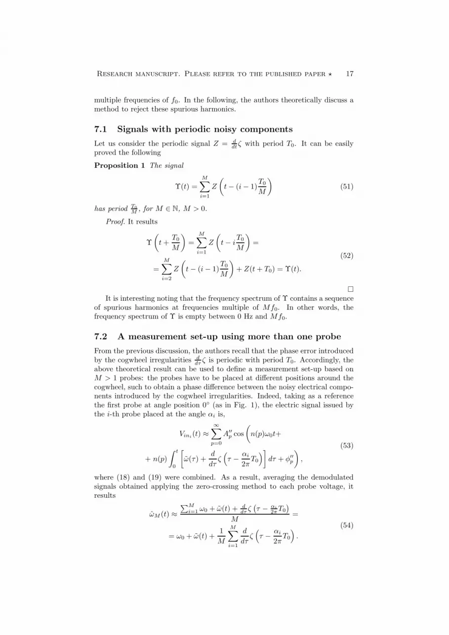
Figure 8: The simplest configuration to reject the effects induced at low-frequencies by the irregular cogwheel shape profile. The configuration can bemade more complicated, e.g., using three probes at 0◦, 120◦, 240◦.
If αi is set equal to2π(i−1)
M, i.e., if the probes are uniformly distributed around
the cogwheel, it results from Proposition 1 that the noisy harmonics introducedby the cogwheel irregular shape are moved to the frequencies multiple of Mf0:by properly choosing the number of probes M , the noisy effects of the cogwheelirregularities can be eliminated by low-pass filtering. The authors underlinethat this result holds regardless of the cogwheel shape profile.
Example 4
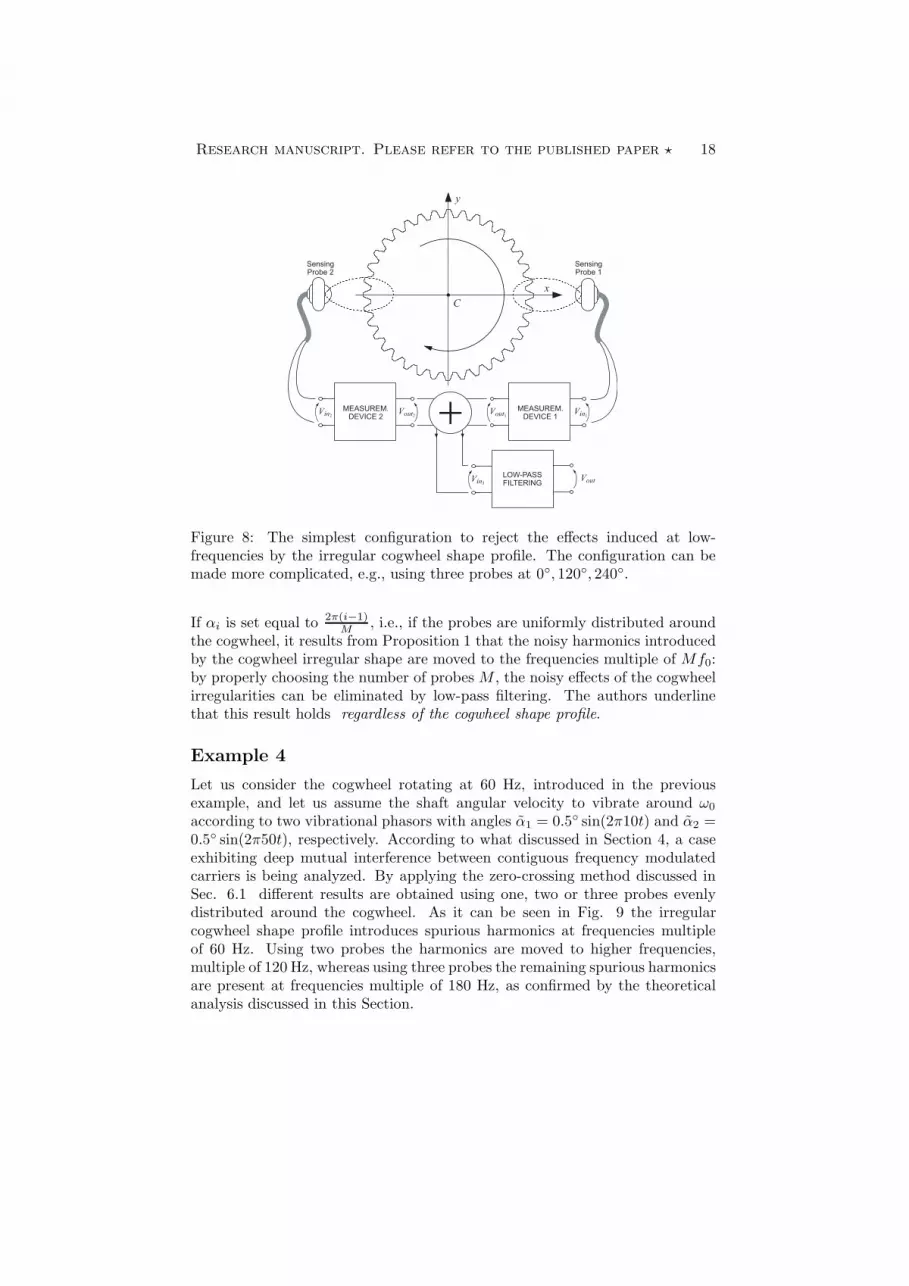
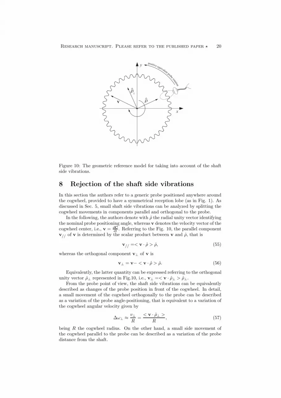
Let us consider the cogwheel rotating at 60 Hz, introduced in the previousexample, and let us assume the shaft angular velocity to vibrate around ω0
according to two vibrational phasors with angles α1 = 0.5◦ sin(2π10t) and α2 =0.5◦ sin(2π50t), respectively. According to what discussed in Section 4, a caseexhibiting deep mutual interference between contiguous frequency modulatedcarriers is being analyzed. By applying the zero-crossing method discussed inSec. 6.1 different results are obtained using one, two or three probes evenlydistributed around the cogwheel. As it can be seen in Fig. 9 the irregularcogwheel shape profile introduces spurious harmonics at frequencies multipleof 60 Hz. Using two probes the harmonics are moved to higher frequencies,multiple of 120 Hz, whereas using three probes the remaining spurious harmonicsare present at frequencies multiple of 180 Hz, as confirmed by the theoreticalanalysis discussed in this Section.
Research manuscript. Please refer to the published paper ⋆ 19
103 104102101100
f[Hz]
10
Hz
10
Hz
10
Hz
50
Hz
50
Hz
50
Hz
− 100
− 60
− 20
0
− 100
− 60
− 20
0
− 100
− 60
− 20
0
|FF
T(f
)||F
FT
(f)|
|FF
T(f
)|
[db]
n x 60 Hz
n x 120 Hz
n x 180 Hz
(a)
(b)
(c)
angular vibration tones
angular vibration tones
angular vibration tones
Figure 9: Frequency spectrum of the estimated angular vibration, obtainedapplying the zero-crossing method to the probe signals. From top to bottom:(a) one probe (0◦), (b) two probes (0◦, 180◦), (c) three probes (0◦, 120◦, 240◦).
Research manuscript. Please refer to the published paper ⋆ 20
x
y
ρ
ρ
v
⊥
positive equivalent probe rotation
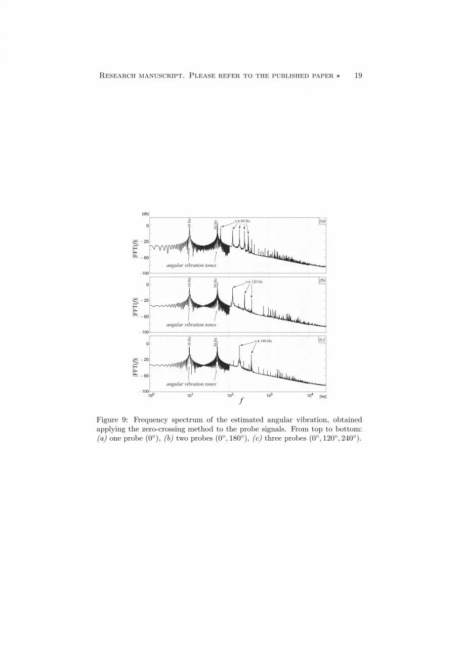
Figure 10: The geometric reference model for taking into account of the shaftside vibrations.
8 Rejection of the shaft side vibrations
In this section the authors refer to a generic probe positioned anywhere aroundthe cogwheel, provided to have a symmetrical reception lobe (as in Fig. 1). Asdiscussed in Sec. 5, small shaft side vibrations can be analyzed by splitting thecogwheel movements in components parallel and orthogonal to the probe.
In the following, the authors denote with ρ the radial unity vector identifyingthe nominal probe positioning angle, whereas v denotes the velocity vector of thecogwheel center, i.e., v = dC
dt. Referring to the Fig. 10, the parallel component
v// of v is determined by the scalar product between v and ρ, that is
v// =< v · ρ > ρ, (55)
whereas the orthogonal component v⊥ of v is
v⊥ = v− < v · ρ > ρ. (56)
Equivalently, the latter quantity can be expressed referring to the orthogonalunity vector ρ⊥ represented in Fig.10, i.e., v⊥ =< v · ρ⊥ > ρ⊥.
From the probe point of view, the shaft side vibrations can be equivalentlydescribed as changes of the probe position in front of the cogwheel. In detail,a small movement of the cogwheel orthogonally to the probe can be describedas a variation of the probe angle-positioning, that is equivalent to a variation ofthe cogwheel angular velocity given by
∆ω⊥ ≈ v⊥R
=< v · ρ⊥ >
R, (57)
being R the cogwheel radius. On the other hand, a small side movement ofthe cogwheel parallel to the probe can be described as a variation of the probedistance from the shaft.
Research manuscript. Please refer to the published paper ⋆ 21
It is of interest to evaluate the overall effect of a cogwheel side movementwhen M measurements obtained using M probes are averaged as in Fig. 8.If M > 1 probes are evenly distributed around the cogwheel according toρ1, . . . , ρM , it is easy to check that due to symmetry
M∑
i=1
ρi =
M∑
i=1
ρi⊥ = 0. (58)
Let us focus on the shaft side vibration components orthogonal to the probes.According to the proposed notation and assumptions (see Fig. 1), the positivedirection of the shaft rotation is clockwise: in other words, if the cogwheel islocked and if the dynamics is described from the probes point of view, the pos-itive direction of the probes rotation is counter-clockwise. Therefore, adoptingthe probe point of view to describe the dynamics, if < v · ρ⊥ > is negative theprobe is rotating faster around the locked cogwheel. Accordingly, exploitingthe symmetry of the setup (58), by averaging the equivalent angular velocityvariations (57) detected by each probe it results
1
M
M∑
i=1
∆ωi⊥ =1
M
M∑
i=1
< v · ρi⊥ >
R=
=1
M
< v ·∑M
i=1 ρi⊥ >
R= 0.
(59)
In Subsec. 5.1 the authors have shown that the orthogonal components of theshaft side vibrations modify directly the angular vibrational signal, i.e., for eachprobe the zero-crossing method reveals the components v⊥ of the shaft sidevibrations. As a result, (59) indicates that when M measurements obtainedusing M probes are averaged as in Fig. 8, the overall effect introduced bythe equivalent angular velocity variations ∆ωi⊥ is canceled, regardless of thedirection and magnitude of v.
On the other hand, let us now focus on the shaft side vibration componentsparallel to the probes. As discussed in the Subsec. 5.2, these side vibrationschange the height of the cogwheel shape detected by the probes, introducing foreach probe a different factor (1+S//(t)) modulating the amplitude of the signalVin. The analytical relationship existing between the amplitude modulatingfactor and the result of the zero-crossing demodulation method depends onseveral parameters, among which the cogwheel shape. Nevertheless, adoptingan heuristic approach and exploiting the symmetry of the setup (58), also inthis case it results
M∑
i=1
< v · ρ >=< v ·M∑
i=1
ρ >= 0, (60)
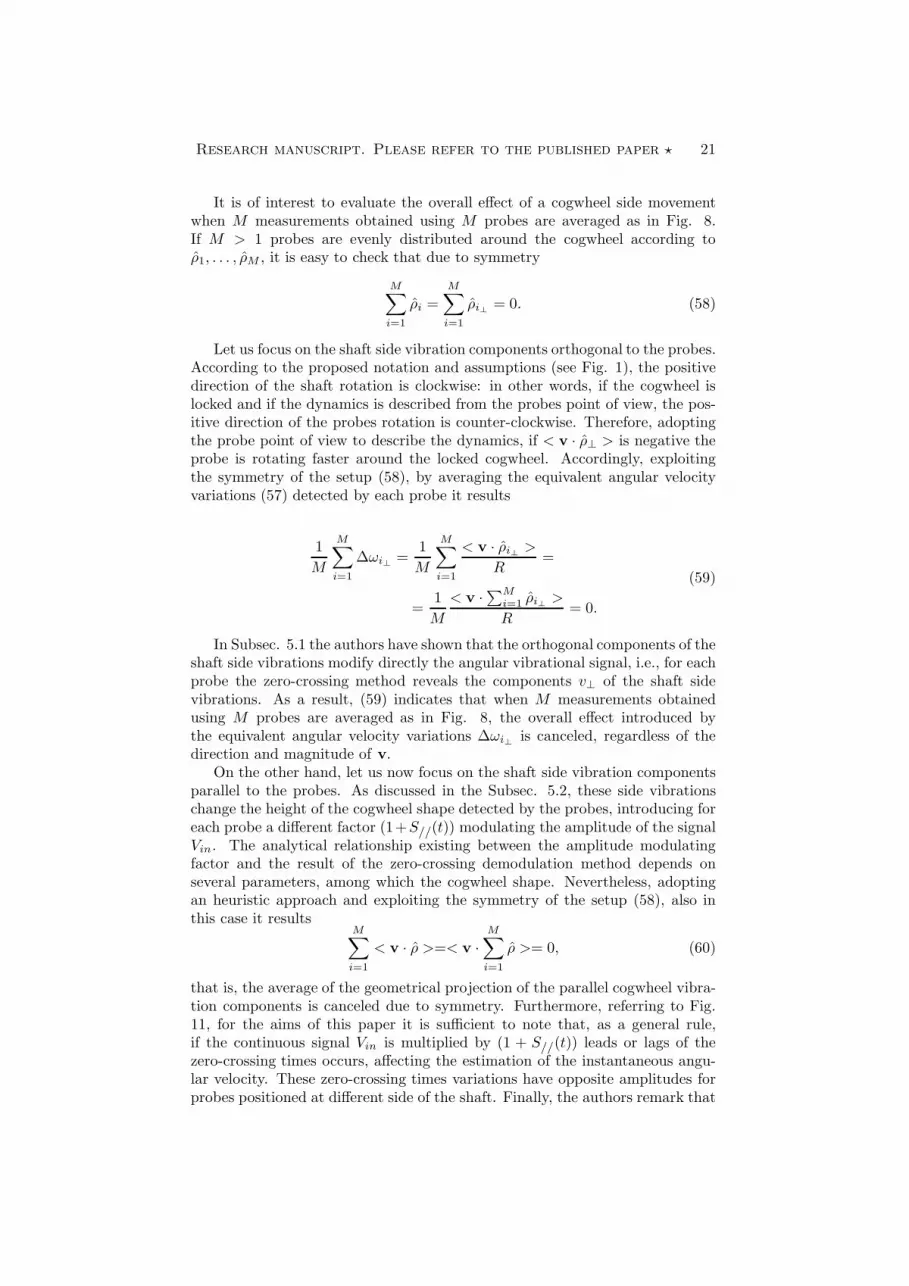
that is, the average of the geometrical projection of the parallel cogwheel vibra-tion components is canceled due to symmetry. Furthermore, referring to Fig.11, for the aims of this paper it is sufficient to note that, as a general rule,if the continuous signal Vin is multiplied by (1 + S//(t)) leads or lags of thezero-crossing times occurs, affecting the estimation of the instantaneous angu-lar velocity. These zero-crossing times variations have opposite amplitudes forprobes positioned at different side of the shaft. Finally, the authors remark that
Research manuscript. Please refer to the published paper ⋆ 22
t
Vin
∆t ∆t
Figure 11: The effects of the amplitude modulation factor (1 + S//(t)) on thezero-crossing times.
the zero-crossing technique is a FM demodulation operation, that is intrinsi-cally robust to amplitude variations of the signal to be demodulated, as it iswell know from telecommunication theory [11, 14].
As a result, as shown in the following example, when M measurementsobtained using M probes are averaged as in Fig. 8, the overall effect of theshaft side vibrations is suitably rejected.
Example 5
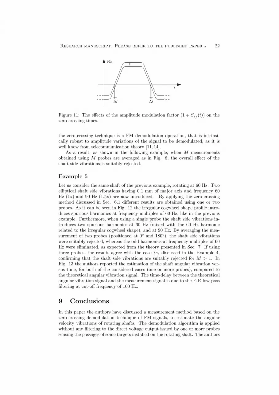
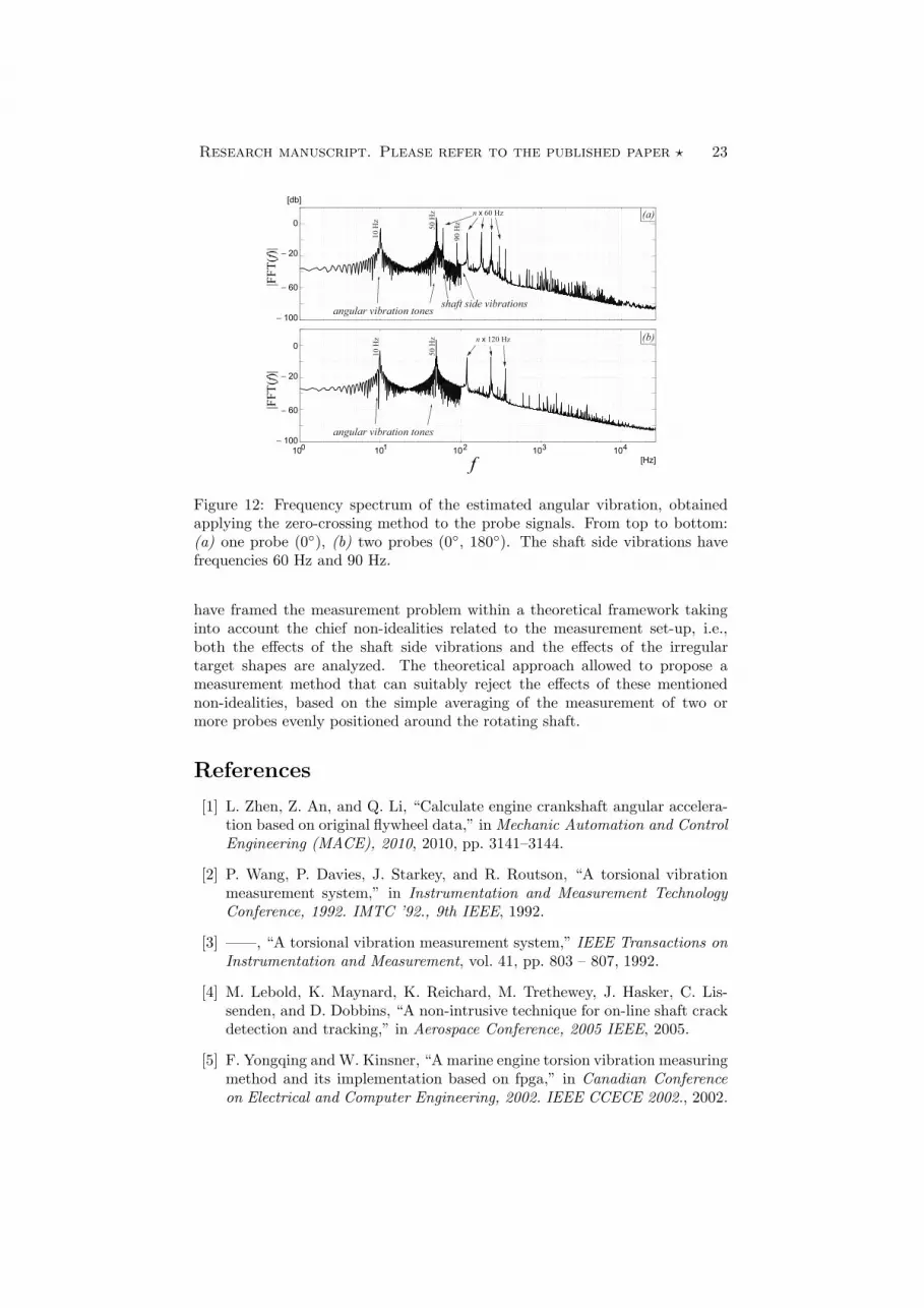
Let us consider the same shaft of the previous example, rotating at 60 Hz. Twoelliptical shaft side vibrations having 0.1 mm of major axis and frequency 60Hz (1x) and 90 Hz (1.5x) are now introduced. By applying the zero-crossingmethod discussed in Sec. 6.1 different results are obtained using one or twoprobes. As it can be seen in Fig. 12 the irregular cogwheel shape profile intro-duces spurious harmonics at frequency multiples of 60 Hz, like in the previousexample. Furthermore, when using a single probe the shaft side vibrations in-troduces two spurious harmonics at 60 Hz (mixed with the 60 Hz harmonicrelated to the irregular cogwheel shape), and at 90 Hz. By averaging the mea-surement of two probes (positioned at 0◦ and 180◦), the shaft side vibrationswere suitably rejected, whereas the odd harmonics at frequency multiples of 60Hz were eliminated, as expected from the theory presented in Sec. 7. If usingthree probes, the results agree with the case (c) discussed in the Example 4,confirming that the shaft side vibrations are suitably rejected for M > 1. InFig. 13 the authors reported the estimation of the shaft angular vibration ver-sus time, for both of the considered cases (one or more probes), compared tothe theoretical angular vibration signal. The time-delay between the theoreticalangular vibration signal and the measurement signal is due to the FIR low-passfiltering at cut-off frequency of 100 Hz.
9 Conclusions
In this paper the authors have discussed a measurement method based on thezero-crossing demodulation technique of FM signals, to estimate the angularvelocity vibrations of rotating shafts. The demodulation algorithm is appliedwithout any filtering to the direct voltage output issued by one or more probessensing the passages of some targets installed on the rotating shaft. The authors
Research manuscript. Please refer to the published paper ⋆ 23
|FF
T(f
)|
[db]
(a)
(b)
10 H
z
50 H
z
10 H
z
50 H
z
90 H
z
angular vibration tonesshaft side vibrations
angular vibration tones
n x 60 Hz
n x 120 Hz
103 104102101100
f [Hz]
− 100
− 60
− 20
0
|FF
T(f
)|
− 100
− 60
− 20
0
Figure 12: Frequency spectrum of the estimated angular vibration, obtainedapplying the zero-crossing method to the probe signals. From top to bottom:(a) one probe (0◦), (b) two probes (0◦, 180◦). The shaft side vibrations havefrequencies 60 Hz and 90 Hz.
have framed the measurement problem within a theoretical framework takinginto account the chief non-idealities related to the measurement set-up, i.e.,both the effects of the shaft side vibrations and the effects of the irregulartarget shapes are analyzed. The theoretical approach allowed to propose ameasurement method that can suitably reject the effects of these mentionednon-idealities, based on the simple averaging of the measurement of two ormore probes evenly positioned around the rotating shaft.
References
[1] L. Zhen, Z. An, and Q. Li, “Calculate engine crankshaft angular accelera-tion based on original flywheel data,” in Mechanic Automation and ControlEngineering (MACE), 2010, 2010, pp. 3141–3144.
[2] P. Wang, P. Davies, J. Starkey, and R. Routson, “A torsional vibrationmeasurement system,” in Instrumentation and Measurement TechnologyConference, 1992. IMTC ’92., 9th IEEE, 1992.
[3] ——, “A torsional vibration measurement system,” IEEE Transactions onInstrumentation and Measurement, vol. 41, pp. 803 – 807, 1992.
[4] M. Lebold, K. Maynard, K. Reichard, M. Trethewey, J. Hasker, C. Lis-senden, and D. Dobbins, “A non-intrusive technique for on-line shaft crackdetection and tracking,” in Aerospace Conference, 2005 IEEE, 2005.
[5] F. Yongqing andW. Kinsner, “A marine engine torsion vibration measuringmethod and its implementation based on fpga,” in Canadian Conferenceon Electrical and Computer Engineering, 2002. IEEE CCECE 2002., 2002.
Research manuscript. Please refer to the published paper ⋆ 24
1 1.02 1.04 1.06 1.08 1.1 1.12 1.14 1.16 1.18 1.23550
3560
3570
3580
3590
3600
3610
3620
3630
3640
3650
[rpm]
[rpm]
[rpm]
[s]
1 1.02 1.04 1.06 1.08 1.1 1.12 1.14 1.16 1.18 1.23550
3560
3570
3580
3590
3600
3610
3620
3630
3640
3650
[s]
1 1.02 1.04 1.06 1.08 1.1 1.12 1.14 1.16 1.18 1.23550
3560
3570
3580
3590
3600
3610
3620
3630
3640
3650
[s]
(a)
(b)
(c)
Figure 13: The estimation of the shaft angular vibration obtained using (a) oneprobe (0◦), (b) two probes (0◦, 180◦) and (c) three probes (0◦, 120◦, 180◦). Thetime-delay between the theoretical and the measurement signals is due to theFIR low-pass filtering at cut-off frequency of 100 Hz.
Research manuscript. Please refer to the published paper ⋆ 25
[6] F. C. Gomez de Leon and P. Merono Perez, “Discrete time interval mea-surement system: fundamentals, resolution and errors in the measurementof angular vibrations,”Measurement Science and Technology, vol. 21, no. 7,July 2010.
[7] P. Sue, D. Wilson, L. Farr, and A. Kretschmar, “High precision torque mea-surement on a rotating load coupling for power generation operations,” inInstrumentation and Measurement Technology Conference (I2MTC), Graz(Austria), 2012, pp. 518–523.
[8] L. Naldi, R. Biondi, and V. Rossi, “Torsional vibrations in rotordynamicsystems, identified by monitoring gearbox behaviour,” in Proceedings of theGT2008, ASME Turbo Expo, 2008.
[9] L. Naldi, M. Golebiovski, and V. Rossi, “New approach to torsional vibra-tion monitoring,” in Proceedings of the Fortieth Turbomachinery Sympo-sium, Houston (Texas), 2011, pp. 60–71.
[10] T. Addabbo, R. Biondi, S. Cioncolini, A. Fort, M. Mugnaini, S. Rocchi, andV. Vignoli, “A multi-probe setup for the measurement of angular vibrationsin a rotating shaft,” in Proceedings of the 2012 IEEE Sensors ApplicationsSymposium, Brescia, Italy, 2012.
[11] S. Haykin and M. Moher, Introduction to analog and digital communica-tions. John Wiley 2007.
[12] R. Wiley, “Approximate FM demodulation using zero crossings,” IEEETrans. on Communications, vol. COM-29, no. 7, pp. 1061–1065, July 1981.
[13] H. Voelcker, “Zero-crossing properties of angle-modulated signals,” IEEETrans. on Communications, vol. COM-20, pp. 307–315, 1972.
[14] G. Kelley, “Choosing the optimum type of modulation–a comparison ofseveral communication systems,” Communications Systems, IRE Transac-tions on, vol. 6, no. 1, pp. 14–21, 1958.