petroleum related rock mechanics
TRANSCRIPT


DEVELOPMENTS IN PETROLEUM SCIENCE 53
PETROLEUM RELATED
ROCK MECHANICS
2nd EDITION

DEVELOPMENTS IN PETROLEUM SCIENCE 53
Volumes 1–7, 9–35, 37–41, 44–45, 48–51 are out of print.
8 Fundamentals of Reservoir Engineering
36 The Practice of Reservoir Engineering (Revised Edition)
42 Casing Design—Theory and Practice
43 Tracers in the Oil Field
46 Hydrocarbon Exploration and Production
47 PVT and Phase Behaviour of Petroleum Reservoir Fluids
52 Geology and Geochemistry of Oil and Gas
53 Petroleum Related Rock Mechanics (2nd Edition)

DEVELOPMENTS IN PETROLEUM SCIENCE 53
PETROLEUM RELATED
ROCK MECHANICS
2nd EDITION
E. FJÆR, R.M. HOLT, P. HORSRUD,
A.M. RAAEN & R. RISNES†
Amsterdam – Boston – Heidelberg – London – New York – OxfordParis – San Diego – San Francisco – Singapore – Sydney – Tokyo

ElsevierRadarweg 29, PO Box 211, 1000 AE Amsterdam, The NetherlandsThe Boulevard, Langford Lane, Kidlington, Oxford OX5 1GB, UK
First edition 1992Second edition 2008
Copyright © 2008 Elsevier B.V. All rights reserved
No part of this publication may be reproduced, stored in a retrieval system or transmitted in any formor by any means electronic, mechanical, photocopying, recording or otherwise without the priorwritten permission of the publisher
Permissions may be sought directly from Elsevier’s Science & Technology Rights Departmentin Oxford, UK: phone (+44) (0) 1865 843830; fax (+44) (0) 1865 853333; email: [email protected]. Alternatively you can submit your request online by visiting the Elsevier website at http://elsevier.com/locate/permissions, and selecting Obtaining permission to use Elseviermaterial
NoticeNo responsibility is assumed by the publisher for any injury and/or damage to persons or property asa matter of products liability, negligence or otherwise, or from any use or operation of any methods,products, instructions or ideas contained in the material herein. Because of rapid advances in themedical sciences, in particular, independent verification of diagnoses and drug dosages should bemade
Library of Congress Cataloging-in-Publication DataA catalog record for this book is available from the Library of Congress
British Library Cataloguing in Publication DataA catalogue record for this book is available from the British Library
ISBN: 978-0-444-50260-5ISSN: 0376-7361
For information on all Elsevier publicationsvisit our website at books.elsevier.com
Printed and bound in Hungary
08 09 10 11 12 10 9 8 7 6 5 4 3 2 1

v
Rasmus Risnes in Memoriam
It is with great regret that we announce the passing of Professor Rasmus Risnes who diedon the 3rd of December 2004 after a prolonged struggle against ill health. He was active inthe field of rock mechanics right up to the end and made a significant contribution to thissecond edition which, regretfully, he will never see. Rasmus was a very pleasant individualwhose vast knowledge and pedagogical expertise was a continual source of inspiration tous all.
He was recognized as one of the pioneers in petroleum-related rock mechanics, bothnationally and internationally, and his early work on sand failure is still regarded as aclassic. In later years he turned his attention to the Chalk and established a highly reputableresearch and teaching laboratory at the University of Stavanger (Norway).
Rasmus will be sorely missed by his many colleagues and friends in the rock mechanicscommunity.
ErlingRunePerArne Marius

This page intentionally left blank

vii
Preface to the second edition
During the years that have passed since the first edition of this book, petroleum related rockmechanics has been well established as a significant supplier of premises and boundaryconditions for the petroleum industry. More than ever, it is now recognised that engineersand geologists in the petroleum industry should possess a certain level of knowledge withinrock mechanics. The need for a textbook like this is therefore even larger now than it was15 years ago.
Although there are still a lot of uncovered areas within petroleum related rock mechan-ics, the topic has in many ways developed significantly over the later years. This is a naturalconsequence of the increased focus this area has gained. We are also proud to admit thatthe general knowledge of petroleum related rock mechanics among the authors of this bookhas increased since the first edition was prepared. Consequently, when the need for a newprinting of the book appeared, we felt the need to revise the manuscript in order to accountfor this development.
The revision has been quite extensive for some parts of the manuscript. The basic struc-ture of the book is however kept as it was, and parts of the text have only been subject tominor revisions. The major guideline for the work has been to update and add informationwhere we felt it was relevant, while maintaining the concept of the book as an introductionto petroleum related rock mechanics as an engineering science. A consequence of this dualobjective has been the introduction of a couple of new appendices, where more advancedmathematics and heavy formulas are presented in a compact form. This way, we hope thatthe main text shall remain easily accessible even for newcomers in the field, while at thesame time the more complete formulas shall be available to the readers who need them.
The revision has been made by the same team of authors that wrote the first edition. Inaddition, several friends and colleagues have generously provided suggestions, advice andencouragement for the work. This support is greatly appreciated.
Trondheim, October 2004
Erling FjærRune M. HoltPer HorsrudArne M. RaaenRasmus Risnes

This page intentionally left blank
ix
Foreword to the 1992 edition
About 10 years ago, petroleum related rock mechanics was mostly confined to a few spe-cific topics like hydraulic fracturing or drilling bit performance. Although a few precursorshad already established the basics of what is now spreading out.
In fact, since that time, the whole petroleum industry has progressively realised thatthe state of underground stresses and its modification due to petroleum related operations,could have a significant impact on performances, in many different aspects of explorationand production. Therefore all those concepts need now to be presented in a simple butcomprehensive way.
An engineering science, “Petroleum related rock mechanics” is also dependent on thevariable and uncertain character of natural geological materials at depth. The limited avail-ability of relevant data is also part of the problem. For that reason, it is essential that anypotential user is aware of the high potential of the technique, together with the actual limi-tations.
This book should totally fulfill these needs. The reader will be provided with fundamen-tals and basics, but also with the techniques used in data acquisition, and eventually with aseries of typical applications like wellbore stability, sand production or subsidence.
The book is mostly for students, geologists or engineers who want to know more aboutrock mechanics, and specifically rock mechanics applied to petroleum industry. It is wellsuited for instance, for drilling or mud engineers wanting to know more on the mechanicalaspect of wellbore stability problems, for reservoir engineers who have to deal with stressrelated problems in their field, like compaction, stress dependent permeability or fractureinjectivity. Operation geologists dealing with drilling in abnormal pressure zones will alsobenefit from this book.
Elf Aquitaine Norge, together with other Norwegian oil companies, has been supportingIKU for several years in their effort to build a strong group in rock mechanics. IKU hasnow a well-established team, whose competence is recognised on the international level.They have mostly been contributing in the field of acoustic wave propagation in rocks andsand production appraisal. They are also very active in research and consulting activitiesin the different fields of petroleum related rock mechanics.
Stavanger, April 1991
Alain Guenot

This page intentionally left blank

xi
Preface to the 1992 edition
Systematic application of rock mechanics is quite new to the petroleum industry. Accord-ingly, the need for an introductory textbook for petroleum engineers and scientists hasrecently emerged. This need was felt by the authors when we started our research in thisarea, and it inspired us to develop the first version of this book as a manuscript for a twoweeks continuing education course for petroleum engineers.
The first 6 chapters deal with the fundamentals of rock mechanics. This includes theoriesof elasticity and failure mechanics, borehole stresses, and acoustic wave propagation. Inaddition, sedimentary rocks are viewed from the geological side as well as from the sideof idealised mathematical modelling based on microstructure. For readers who wants tofurther extend their knowledge on rock mechanics, we suggest the book “Fundamentals ofrock mechanics” by Jaeger and Cook as a continuation. Deeper insight into acoustic wavepropagation in rocks can be achieved from e.g. the book “Acoustics of porous media” byBourbie, Coussy and Zinszner or “Underground Sound” by White.
Chapters 7 and 8 are dedicated to the extremely important task of obtaining parame-ters that are relevant for rock mechanics field application, be it from laboratory tests orfrom analysis of field data like borehole logs. The last 4 chapters discuss applications ofrock mechanics in borehole stability, sand production, hydraulic fracturing and reservoircompaction/surface subsidence analyses.
It has also been our intention to make each chapter more or less selfcontained, especiallythe chapters dealing with applications. Hopefully, this will make the book useful also tothose who are interested only in one particular topic. The other chapters can then be usedas support depending on the reader’s previous knowledge. Notice, however, that the bookis intended to be an introduction to petroleum related rock mechanics as an engineeringscience, rather than a “tool-box” for petroleum engineers.
We wish to thank Elf Aquitaine Norge and Fina Exploration Norway for the financialcontributions which made it possible for us to write this book. In particular, we appreciatethe positive feedback and encouragement provided by Alain Guenot of Elf. The skilfuland patient support from Siri Lyng at IKU in preparing the manuscript for camera-readyquality is greatly appreciated. We also thank Eamonn F. Doyle for advice on our use of theEnglish language.
Trondheim, May 1991
Erling FjærRune M. HoltPer HorsrudArne M. RaaenRasmus Risnes

This page intentionally left blank

xiii
Contents
Rasmus Risnes in Memoriam . . . . . . . . . . . . . . . . . . . . . . . . . . . . . . . . . . . . . . . . . . . . . . . . . . . . . . . . . . . . . v
Preface to the second edition. . . . . . . . . . . . . . . . . . . . . . . . . . . . . . . . . . . . . . . . . . . . . . . . . . . . . . . . . . . . . . vii
Foreword to the 1992 edition . . . . . . . . . . . . . . . . . . . . . . . . . . . . . . . . . . . . . . . . . . . . . . . . . . . . . . . . . . . . . ix
Preface to the 1992 edition . . . . . . . . . . . . . . . . . . . . . . . . . . . . . . . . . . . . . . . . . . . . . . . . . . . . . . . . . . . . . . . . xi
Chapter 1 ELASTICITY . . . . . . . . . . . . . . . . . . . . . . . . . . . . . . . . . . . . . . . . . . . . . . . . . . . . . . . . . . . . . . 11.1. Stress . . . . . . . . . . . . . . . . . . . . . . . . . . . . . . . . . . . . . . . . . . . . . . . . . . . . . . . . . . . . . . . . . . . . . . . . . . . . . . . . . . 1
1.1.1. The stress tensor . . . . . . . . . . . . . . . . . . . . . . . . . . . . . . . . . . . . . . . . . . . . . . . . . . . . . . . . . . . . . 31.1.2. Equations of equilibrium . . . . . . . . . . . . . . . . . . . . . . . . . . . . . . . . . . . . . . . . . . . . . . . . . . . . 51.1.3. Principal stresses in two dimensions . . . . . . . . . . . . . . . . . . . . . . . . . . . . . . . . . . . . . . . . 71.1.4. Mohr’s stress circle . . . . . . . . . . . . . . . . . . . . . . . . . . . . . . . . . . . . . . . . . . . . . . . . . . . . . . . . . . 81.1.5. Principal stresses in three dimensions . . . . . . . . . . . . . . . . . . . . . . . . . . . . . . . . . . . . . . 81.1.6. Mohr’s stress circles in three dimensions . . . . . . . . . . . . . . . . . . . . . . . . . . . . . . . . . . . 101.1.7. Stress invariants . . . . . . . . . . . . . . . . . . . . . . . . . . . . . . . . . . . . . . . . . . . . . . . . . . . . . . . . . . . . . . 111.1.8. Deviatoric stresses . . . . . . . . . . . . . . . . . . . . . . . . . . . . . . . . . . . . . . . . . . . . . . . . . . . . . . . . . . . 11
Geometric interpretation of the deviatoric stress invariants . . . . . . . . . . . . . . . 121.1.9. The octahedral stresses . . . . . . . . . . . . . . . . . . . . . . . . . . . . . . . . . . . . . . . . . . . . . . . . . . . . . . 13
1.2. Strain . . . . . . . . . . . . . . . . . . . . . . . . . . . . . . . . . . . . . . . . . . . . . . . . . . . . . . . . . . . . . . . . . . . . . . . . . . . . . . . . . . 131.2.1. The strain tensor and the strain invariants . . . . . . . . . . . . . . . . . . . . . . . . . . . . . . . . . . 171.2.2. Compatibility conditions . . . . . . . . . . . . . . . . . . . . . . . . . . . . . . . . . . . . . . . . . . . . . . . . . . . . 171.2.3. Principal strains . . . . . . . . . . . . . . . . . . . . . . . . . . . . . . . . . . . . . . . . . . . . . . . . . . . . . . . . . . . . . . 181.2.4. Plane strain and plane stress. . . . . . . . . . . . . . . . . . . . . . . . . . . . . . . . . . . . . . . . . . . . . . . . . 19
1.3. Elastic moduli . . . . . . . . . . . . . . . . . . . . . . . . . . . . . . . . . . . . . . . . . . . . . . . . . . . . . . . . . . . . . . . . . . . . . . . . . 201.4. Strain energy . . . . . . . . . . . . . . . . . . . . . . . . . . . . . . . . . . . . . . . . . . . . . . . . . . . . . . . . . . . . . . . . . . . . . . . . . . 231.5. Thermoelasticity . . . . . . . . . . . . . . . . . . . . . . . . . . . . . . . . . . . . . . . . . . . . . . . . . . . . . . . . . . . . . . . . . . . . . . 24
1.5.1. Thermal strain. . . . . . . . . . . . . . . . . . . . . . . . . . . . . . . . . . . . . . . . . . . . . . . . . . . . . . . . . . . . . . . . 241.5.2. Thermal stress. . . . . . . . . . . . . . . . . . . . . . . . . . . . . . . . . . . . . . . . . . . . . . . . . . . . . . . . . . . . . . . . 241.5.3. Stress strain relation for linear thermoelasticity . . . . . . . . . . . . . . . . . . . . . . . . . . . . 251.5.4. Isothermal and adiabatic moduli . . . . . . . . . . . . . . . . . . . . . . . . . . . . . . . . . . . . . . . . . . . . 251.5.5. Example: Thermal stresses in a constrained square plate . . . . . . . . . . . . . . . . . . 25
1.6. Poroelasticity. . . . . . . . . . . . . . . . . . . . . . . . . . . . . . . . . . . . . . . . . . . . . . . . . . . . . . . . . . . . . . . . . . . . . . . . . . 261.6.1. Suspension of solid particles in a fluid . . . . . . . . . . . . . . . . . . . . . . . . . . . . . . . . . . . . . 261.6.2. Biot’s poroelastic theory for static properties . . . . . . . . . . . . . . . . . . . . . . . . . . . . . . 271.6.3. The effective stress concept . . . . . . . . . . . . . . . . . . . . . . . . . . . . . . . . . . . . . . . . . . . . . . . . . 32

xiv CONTENTS
1.6.4. Pore volume compressibility and related topics . . . . . . . . . . . . . . . . . . . . . . . . . . . . 341.6.5. The Skempton coefficients . . . . . . . . . . . . . . . . . . . . . . . . . . . . . . . . . . . . . . . . . . . . . . . . . . 351.6.6. The correspondence to thermoelasticity . . . . . . . . . . . . . . . . . . . . . . . . . . . . . . . . . . . . 361.6.7. Other notation conventions . . . . . . . . . . . . . . . . . . . . . . . . . . . . . . . . . . . . . . . . . . . . . . . . . . 37
1.7. Anisotropy . . . . . . . . . . . . . . . . . . . . . . . . . . . . . . . . . . . . . . . . . . . . . . . . . . . . . . . . . . . . . . . . . . . . . . . . . . . . 371.7.1. Orthorhombic symmetry . . . . . . . . . . . . . . . . . . . . . . . . . . . . . . . . . . . . . . . . . . . . . . . . . . . . 391.7.2. Transverse isotropy . . . . . . . . . . . . . . . . . . . . . . . . . . . . . . . . . . . . . . . . . . . . . . . . . . . . . . . . . . 41
1.8. Nonlinear elasticity . . . . . . . . . . . . . . . . . . . . . . . . . . . . . . . . . . . . . . . . . . . . . . . . . . . . . . . . . . . . . . . . . . . 421.8.1. Stress–strain relations . . . . . . . . . . . . . . . . . . . . . . . . . . . . . . . . . . . . . . . . . . . . . . . . . . . . . . . 421.8.2. The impact of cracks . . . . . . . . . . . . . . . . . . . . . . . . . . . . . . . . . . . . . . . . . . . . . . . . . . . . . . . . 44
1.9. Time-dependent effects . . . . . . . . . . . . . . . . . . . . . . . . . . . . . . . . . . . . . . . . . . . . . . . . . . . . . . . . . . . . . . . 461.9.1. Consolidation . . . . . . . . . . . . . . . . . . . . . . . . . . . . . . . . . . . . . . . . . . . . . . . . . . . . . . . . . . . . . . . . 461.9.2. Creep . . . . . . . . . . . . . . . . . . . . . . . . . . . . . . . . . . . . . . . . . . . . . . . . . . . . . . . . . . . . . . . . . . . . . . . . . 50
References . . . . . . . . . . . . . . . . . . . . . . . . . . . . . . . . . . . . . . . . . . . . . . . . . . . . . . . . . . . . . . . . . . . . . . . . . . . . 53Further reading. . . . . . . . . . . . . . . . . . . . . . . . . . . . . . . . . . . . . . . . . . . . . . . . . . . . . . . . . . . . . . . . . . . . . . . . 53
Chapter 2 FAILURE MECHANICS . . . . . . . . . . . . . . . . . . . . . . . . . . . . . . . . . . . . . . . . . . . . . . . . . . 552.1. Basic concepts . . . . . . . . . . . . . . . . . . . . . . . . . . . . . . . . . . . . . . . . . . . . . . . . . . . . . . . . . . . . . . . . . . . . . . . . 55
2.1.1. Strength and related concepts . . . . . . . . . . . . . . . . . . . . . . . . . . . . . . . . . . . . . . . . . . . . . . . 552.1.2. The failure surface . . . . . . . . . . . . . . . . . . . . . . . . . . . . . . . . . . . . . . . . . . . . . . . . . . . . . . . . . . . 58
2.2. Tensile failure . . . . . . . . . . . . . . . . . . . . . . . . . . . . . . . . . . . . . . . . . . . . . . . . . . . . . . . . . . . . . . . . . . . . . . . . . 592.3. Shear failure. . . . . . . . . . . . . . . . . . . . . . . . . . . . . . . . . . . . . . . . . . . . . . . . . . . . . . . . . . . . . . . . . . . . . . . . . . . 60
2.3.1. The Mohr–Coulomb criterion . . . . . . . . . . . . . . . . . . . . . . . . . . . . . . . . . . . . . . . . . . . . . . . 612.3.2. The Griffith criterion . . . . . . . . . . . . . . . . . . . . . . . . . . . . . . . . . . . . . . . . . . . . . . . . . . . . . . . . 65
2.4. Compaction failure . . . . . . . . . . . . . . . . . . . . . . . . . . . . . . . . . . . . . . . . . . . . . . . . . . . . . . . . . . . . . . . . . . . 662.5. Failure criteria in three dimensions . . . . . . . . . . . . . . . . . . . . . . . . . . . . . . . . . . . . . . . . . . . . . . . . . . 68
2.5.1. Criteria independent of the intermediate principal stress . . . . . . . . . . . . . . . . . . 692.5.2. Criteria depending on the intermediate principal stress . . . . . . . . . . . . . . . . . . . . 70
π-plane representation. . . . . . . . . . . . . . . . . . . . . . . . . . . . . . . . . . . . . . . . . . . . . . . . . . . . . . . 73Physical explanations . . . . . . . . . . . . . . . . . . . . . . . . . . . . . . . . . . . . . . . . . . . . . . . . . . . . . . . . 74
2.6. Fluid effects . . . . . . . . . . . . . . . . . . . . . . . . . . . . . . . . . . . . . . . . . . . . . . . . . . . . . . . . . . . . . . . . . . . . . . . . . . . 752.6.1. Pore pressure . . . . . . . . . . . . . . . . . . . . . . . . . . . . . . . . . . . . . . . . . . . . . . . . . . . . . . . . . . . . . . . . . 752.6.2. Partial saturation . . . . . . . . . . . . . . . . . . . . . . . . . . . . . . . . . . . . . . . . . . . . . . . . . . . . . . . . . . . . . 762.6.3. Chemical effects . . . . . . . . . . . . . . . . . . . . . . . . . . . . . . . . . . . . . . . . . . . . . . . . . . . . . . . . . . . . . 78
2.7. Presentation and interpretation of data from failure tests . . . . . . . . . . . . . . . . . . . . . . . . . . . 792.8. Beyond the yield point. . . . . . . . . . . . . . . . . . . . . . . . . . . . . . . . . . . . . . . . . . . . . . . . . . . . . . . . . . . . . . . . 80
2.8.1. Plasticity . . . . . . . . . . . . . . . . . . . . . . . . . . . . . . . . . . . . . . . . . . . . . . . . . . . . . . . . . . . . . . . . . . . . . 81Plastic flow . . . . . . . . . . . . . . . . . . . . . . . . . . . . . . . . . . . . . . . . . . . . . . . . . . . . . . . . . . . . . . . . . . . 82Associated flow . . . . . . . . . . . . . . . . . . . . . . . . . . . . . . . . . . . . . . . . . . . . . . . . . . . . . . . . . . . . . . 84Non-associated flow . . . . . . . . . . . . . . . . . . . . . . . . . . . . . . . . . . . . . . . . . . . . . . . . . . . . . . . . . 86Hardening . . . . . . . . . . . . . . . . . . . . . . . . . . . . . . . . . . . . . . . . . . . . . . . . . . . . . . . . . . . . . . . . . . . . 86
2.8.2. Soil mechanics . . . . . . . . . . . . . . . . . . . . . . . . . . . . . . . . . . . . . . . . . . . . . . . . . . . . . . . . . . . . . . . 88Normally consolidated clays . . . . . . . . . . . . . . . . . . . . . . . . . . . . . . . . . . . . . . . . . . . . . . . . 90Overconsolidated clays . . . . . . . . . . . . . . . . . . . . . . . . . . . . . . . . . . . . . . . . . . . . . . . . . . . . . . 92
2.8.3. Localization . . . . . . . . . . . . . . . . . . . . . . . . . . . . . . . . . . . . . . . . . . . . . . . . . . . . . . . . . . . . . . . . . . 93

CONTENTS xv
2.8.4. Liquefaction . . . . . . . . . . . . . . . . . . . . . . . . . . . . . . . . . . . . . . . . . . . . . . . . . . . . . . . . . . . . . . . . . . 942.9. Failure of anisotropic and fractured rocks . . . . . . . . . . . . . . . . . . . . . . . . . . . . . . . . . . . . . . . . . . . 95
2.9.1. Intrinsic anisotropy and the failure surface . . . . . . . . . . . . . . . . . . . . . . . . . . . . . . . . . 952.9.2. The plane of weakness model . . . . . . . . . . . . . . . . . . . . . . . . . . . . . . . . . . . . . . . . . . . . . . . 952.9.3. Fractured rock. . . . . . . . . . . . . . . . . . . . . . . . . . . . . . . . . . . . . . . . . . . . . . . . . . . . . . . . . . . . . . . . 97
2.10. Stress history effects . . . . . . . . . . . . . . . . . . . . . . . . . . . . . . . . . . . . . . . . . . . . . . . . . . . . . . . . . . . . . . . . 992.10.1. Rate effects and delayed failure . . . . . . . . . . . . . . . . . . . . . . . . . . . . . . . . . . . . . . . . . . . 992.10.2. Fatigue . . . . . . . . . . . . . . . . . . . . . . . . . . . . . . . . . . . . . . . . . . . . . . . . . . . . . . . . . . . . . . . . . . . . . . 100
References . . . . . . . . . . . . . . . . . . . . . . . . . . . . . . . . . . . . . . . . . . . . . . . . . . . . . . . . . . . . . . . . . . . . . . . . . . . 100
Chapter 3 GEOLOGICAL ASPECTS OF PETROLEUM RELATED ROCKMECHANICS . . . . . . . . . . . . . . . . . . . . . . . . . . . . . . . . . . . . . . . . . . . . . . . . . . . . . . . . . . . . . . 103
3.1. Underground stresses . . . . . . . . . . . . . . . . . . . . . . . . . . . . . . . . . . . . . . . . . . . . . . . . . . . . . . . . . . . . . . . . . 1033.2. Pore pressure . . . . . . . . . . . . . . . . . . . . . . . . . . . . . . . . . . . . . . . . . . . . . . . . . . . . . . . . . . . . . . . . . . . . . . . . . . 1143.3. Sedimentological aspects . . . . . . . . . . . . . . . . . . . . . . . . . . . . . . . . . . . . . . . . . . . . . . . . . . . . . . . . . . . . . 117
3.3.1. Grains and minerals . . . . . . . . . . . . . . . . . . . . . . . . . . . . . . . . . . . . . . . . . . . . . . . . . . . . . . . . . 1173.3.2. Pre-deposition and deposition . . . . . . . . . . . . . . . . . . . . . . . . . . . . . . . . . . . . . . . . . . . . . . . 1203.3.3. Post-deposition. . . . . . . . . . . . . . . . . . . . . . . . . . . . . . . . . . . . . . . . . . . . . . . . . . . . . . . . . . . . . . . 121
3.4. Mechanical properties of sedimentary rocks . . . . . . . . . . . . . . . . . . . . . . . . . . . . . . . . . . . . . . . . 1233.4.1. Sandstone . . . . . . . . . . . . . . . . . . . . . . . . . . . . . . . . . . . . . . . . . . . . . . . . . . . . . . . . . . . . . . . . . . . . 1243.4.2. Chalk . . . . . . . . . . . . . . . . . . . . . . . . . . . . . . . . . . . . . . . . . . . . . . . . . . . . . . . . . . . . . . . . . . . . . . . . . 1263.4.3. Shale . . . . . . . . . . . . . . . . . . . . . . . . . . . . . . . . . . . . . . . . . . . . . . . . . . . . . . . . . . . . . . . . . . . . . . . . . . 1283.4.4. Rock salt . . . . . . . . . . . . . . . . . . . . . . . . . . . . . . . . . . . . . . . . . . . . . . . . . . . . . . . . . . . . . . . . . . . . . 130
References . . . . . . . . . . . . . . . . . . . . . . . . . . . . . . . . . . . . . . . . . . . . . . . . . . . . . . . . . . . . . . . . . . . . . . . . . . . . 131Further reading. . . . . . . . . . . . . . . . . . . . . . . . . . . . . . . . . . . . . . . . . . . . . . . . . . . . . . . . . . . . . . . . . . . . . . . . 133
Chapter 4 STRESSES AROUND BOREHOLES. BOREHOLE FAILURE CRI-TERIA . . . . . . . . . . . . . . . . . . . . . . . . . . . . . . . . . . . . . . . . . . . . . . . . . . . . . . . . . . . . . . . . . . . . . . 135
4.1. Stresses and strains in cylindrical coordinates . . . . . . . . . . . . . . . . . . . . . . . . . . . . . . . . . . . . . . 1354.2. Stresses in a hollow cylinder . . . . . . . . . . . . . . . . . . . . . . . . . . . . . . . . . . . . . . . . . . . . . . . . . . . . . . . . . 137
4.2.1. The equilibrium equations. . . . . . . . . . . . . . . . . . . . . . . . . . . . . . . . . . . . . . . . . . . . . . . . . . . 1374.2.2. Stress distributions with constant pore pressure. . . . . . . . . . . . . . . . . . . . . . . . . . . . 1384.2.3. Stress distributions with varying pore pressure . . . . . . . . . . . . . . . . . . . . . . . . . . . . 140
The superposition principle . . . . . . . . . . . . . . . . . . . . . . . . . . . . . . . . . . . . . . . . . . . . . . . . . 142Radial flow . . . . . . . . . . . . . . . . . . . . . . . . . . . . . . . . . . . . . . . . . . . . . . . . . . . . . . . . . . . . . . . . . . . 142
4.2.4. Stress distributions with heat flow . . . . . . . . . . . . . . . . . . . . . . . . . . . . . . . . . . . . . . . . . . 1434.2.5. Stress distributions in nonlinear formations . . . . . . . . . . . . . . . . . . . . . . . . . . . . . . . . 144
4.3. Elastic stresses around wells—the general solution. . . . . . . . . . . . . . . . . . . . . . . . . . . . . . . . . 1454.3.1. Transformation formulas . . . . . . . . . . . . . . . . . . . . . . . . . . . . . . . . . . . . . . . . . . . . . . . . . . . . 1464.3.2. The general elastic solution . . . . . . . . . . . . . . . . . . . . . . . . . . . . . . . . . . . . . . . . . . . . . . . . . 1474.3.3. Borehole along a principal stress direction . . . . . . . . . . . . . . . . . . . . . . . . . . . . . . . . . 148
4.4. Poroelastic time dependent effects . . . . . . . . . . . . . . . . . . . . . . . . . . . . . . . . . . . . . . . . . . . . . . . . . . . 1504.4.1. Wellbore pressure invasion . . . . . . . . . . . . . . . . . . . . . . . . . . . . . . . . . . . . . . . . . . . . . . . . . . 1514.4.2. Drillout induced pore pressure changes . . . . . . . . . . . . . . . . . . . . . . . . . . . . . . . . . . . . 153
4.5. Borehole failure criteria . . . . . . . . . . . . . . . . . . . . . . . . . . . . . . . . . . . . . . . . . . . . . . . . . . . . . . . . . . . . . . 154
xvi CONTENTS
4.5.1. Vertical hole, isotropic horizontal stresses and impermeable boreholewall . . . . . . . . . . . . . . . . . . . . . . . . . . . . . . . . . . . . . . . . . . . . . . . . . . . . . . . . . . . . . . . . . . . . . . . 155
4.5.2. Vertical hole, isotropic horizontal stresses and permeable borehole wall . 1574.5.3. Borehole along a principal stress direction . . . . . . . . . . . . . . . . . . . . . . . . . . . . . . . . . 1584.5.4. Borehole in a general direction . . . . . . . . . . . . . . . . . . . . . . . . . . . . . . . . . . . . . . . . . . . . . 159
4.6. Beyond failure initiation. . . . . . . . . . . . . . . . . . . . . . . . . . . . . . . . . . . . . . . . . . . . . . . . . . . . . . . . . . . . . . 1604.6.1. A simple plasticity model . . . . . . . . . . . . . . . . . . . . . . . . . . . . . . . . . . . . . . . . . . . . . . . . . . . 164
The Tresca criterion . . . . . . . . . . . . . . . . . . . . . . . . . . . . . . . . . . . . . . . . . . . . . . . . . . . . . . . . . 164The Mohr–Coulomb criterion . . . . . . . . . . . . . . . . . . . . . . . . . . . . . . . . . . . . . . . . . . . . . . . 165Deformation and plastic strain . . . . . . . . . . . . . . . . . . . . . . . . . . . . . . . . . . . . . . . . . . . . . . 168
4.7. Spherical coordinates . . . . . . . . . . . . . . . . . . . . . . . . . . . . . . . . . . . . . . . . . . . . . . . . . . . . . . . . . . . . . . . . . 1704.7.1. Basic equations . . . . . . . . . . . . . . . . . . . . . . . . . . . . . . . . . . . . . . . . . . . . . . . . . . . . . . . . . . . . . . 1704.7.2. Stress distribution around a spherical cavity with no fluid flow . . . . . . . . . . . 1714.7.3. Stress distribution with fluid flow . . . . . . . . . . . . . . . . . . . . . . . . . . . . . . . . . . . . . . . . . . . 171
References . . . . . . . . . . . . . . . . . . . . . . . . . . . . . . . . . . . . . . . . . . . . . . . . . . . . . . . . . . . . . . . . . . . . . . . . . . . . 172Further reading. . . . . . . . . . . . . . . . . . . . . . . . . . . . . . . . . . . . . . . . . . . . . . . . . . . . . . . . . . . . . . . . . . . . . . . . 173
Chapter 5 ELASTIC WAVE PROPAGATION IN ROCKS. . . . . . . . . . . . . . . . . . . . . . . . . . 1755.1. The wave equation . . . . . . . . . . . . . . . . . . . . . . . . . . . . . . . . . . . . . . . . . . . . . . . . . . . . . . . . . . . . . . . . . . . . 1755.2. P- and S-waves . . . . . . . . . . . . . . . . . . . . . . . . . . . . . . . . . . . . . . . . . . . . . . . . . . . . . . . . . . . . . . . . . . . . . . . . 1775.3. Elastic waves in porous materials . . . . . . . . . . . . . . . . . . . . . . . . . . . . . . . . . . . . . . . . . . . . . . . . . . . . 180
5.3.1. Biot’s theory of elastic wave propagation . . . . . . . . . . . . . . . . . . . . . . . . . . . . . . . . . . 1805.3.2. Dispersion due to local flow. . . . . . . . . . . . . . . . . . . . . . . . . . . . . . . . . . . . . . . . . . . . . . . . . 184
5.4. Attenuation . . . . . . . . . . . . . . . . . . . . . . . . . . . . . . . . . . . . . . . . . . . . . . . . . . . . . . . . . . . . . . . . . . . . . . . . . . . . 1845.5. Anisotropy . . . . . . . . . . . . . . . . . . . . . . . . . . . . . . . . . . . . . . . . . . . . . . . . . . . . . . . . . . . . . . . . . . . . . . . . . . . . 189
5.5.1. The Christoffel equation. . . . . . . . . . . . . . . . . . . . . . . . . . . . . . . . . . . . . . . . . . . . . . . . . . . . . 1895.5.2. Weak anisotropy . . . . . . . . . . . . . . . . . . . . . . . . . . . . . . . . . . . . . . . . . . . . . . . . . . . . . . . . . . . . . 191
5.6. Rock mechanics and rock acoustics . . . . . . . . . . . . . . . . . . . . . . . . . . . . . . . . . . . . . . . . . . . . . . . . . 1925.6.1. Static and dynamic moduli . . . . . . . . . . . . . . . . . . . . . . . . . . . . . . . . . . . . . . . . . . . . . . . . . . 1925.6.2. Stress state and stress history . . . . . . . . . . . . . . . . . . . . . . . . . . . . . . . . . . . . . . . . . . . . . . . 1955.6.3. Additional effects . . . . . . . . . . . . . . . . . . . . . . . . . . . . . . . . . . . . . . . . . . . . . . . . . . . . . . . . . . . . 197
Temperature . . . . . . . . . . . . . . . . . . . . . . . . . . . . . . . . . . . . . . . . . . . . . . . . . . . . . . . . . . . . . . . . . . 197Partial saturation . . . . . . . . . . . . . . . . . . . . . . . . . . . . . . . . . . . . . . . . . . . . . . . . . . . . . . . . . . . . . 197Chemical effects . . . . . . . . . . . . . . . . . . . . . . . . . . . . . . . . . . . . . . . . . . . . . . . . . . . . . . . . . . . . . 199
5.7. Reflections and refractions . . . . . . . . . . . . . . . . . . . . . . . . . . . . . . . . . . . . . . . . . . . . . . . . . . . . . . . . . . . 2005.7.1. Interface waves . . . . . . . . . . . . . . . . . . . . . . . . . . . . . . . . . . . . . . . . . . . . . . . . . . . . . . . . . . . . . . 203
5.8. Borehole acoustics . . . . . . . . . . . . . . . . . . . . . . . . . . . . . . . . . . . . . . . . . . . . . . . . . . . . . . . . . . . . . . . . . . . . 2045.8.1. Borehole modes . . . . . . . . . . . . . . . . . . . . . . . . . . . . . . . . . . . . . . . . . . . . . . . . . . . . . . . . . . . . . . 2065.8.2. Borehole alteration . . . . . . . . . . . . . . . . . . . . . . . . . . . . . . . . . . . . . . . . . . . . . . . . . . . . . . . . . . 212
5.9. Seismics . . . . . . . . . . . . . . . . . . . . . . . . . . . . . . . . . . . . . . . . . . . . . . . . . . . . . . . . . . . . . . . . . . . . . . . . . . . . . . . 214References . . . . . . . . . . . . . . . . . . . . . . . . . . . . . . . . . . . . . . . . . . . . . . . . . . . . . . . . . . . . . . . . . . . . . . . . . . . . 217Further reading. . . . . . . . . . . . . . . . . . . . . . . . . . . . . . . . . . . . . . . . . . . . . . . . . . . . . . . . . . . . . . . . . . . . . . . . 218
Chapter 6 ROCK MODELS. . . . . . . . . . . . . . . . . . . . . . . . . . . . . . . . . . . . . . . . . . . . . . . . . . . . . . . . . . . 2196.1. Layered media . . . . . . . . . . . . . . . . . . . . . . . . . . . . . . . . . . . . . . . . . . . . . . . . . . . . . . . . . . . . . . . . . . . . . . . . 220
CONTENTS xvii
6.2. Models involving porosity only . . . . . . . . . . . . . . . . . . . . . . . . . . . . . . . . . . . . . . . . . . . . . . . . . . . . . . 2226.3. Grain pack models . . . . . . . . . . . . . . . . . . . . . . . . . . . . . . . . . . . . . . . . . . . . . . . . . . . . . . . . . . . . . . . . . . . . 2256.4. Models for cracks and other inclusions . . . . . . . . . . . . . . . . . . . . . . . . . . . . . . . . . . . . . . . . . . . . . . 230
6.4.1. Linear, isotropic models . . . . . . . . . . . . . . . . . . . . . . . . . . . . . . . . . . . . . . . . . . . . . . . . . . . . . 2316.4.2. Anisotropic models . . . . . . . . . . . . . . . . . . . . . . . . . . . . . . . . . . . . . . . . . . . . . . . . . . . . . . . . . . 2336.4.3. Models accounting for interactions . . . . . . . . . . . . . . . . . . . . . . . . . . . . . . . . . . . . . . . . . 2356.4.4. Crack development in stressed rocks . . . . . . . . . . . . . . . . . . . . . . . . . . . . . . . . . . . . . . . 240
6.5. Fractured rocks . . . . . . . . . . . . . . . . . . . . . . . . . . . . . . . . . . . . . . . . . . . . . . . . . . . . . . . . . . . . . . . . . . . . . . . 2436.5.1. Single fractures . . . . . . . . . . . . . . . . . . . . . . . . . . . . . . . . . . . . . . . . . . . . . . . . . . . . . . . . . . . . . . 2436.5.2. Rocks with many fractures . . . . . . . . . . . . . . . . . . . . . . . . . . . . . . . . . . . . . . . . . . . . . . . . . . 246
References . . . . . . . . . . . . . . . . . . . . . . . . . . . . . . . . . . . . . . . . . . . . . . . . . . . . . . . . . . . . . . . . . . . . . . . . . . . . 249
Chapter 7 MECHANICAL PROPERTIES AND STRESS DATA FROM LABO-RATORY ANALYSIS . . . . . . . . . . . . . . . . . . . . . . . . . . . . . . . . . . . . . . . . . . . . . . . . . . . . . 251
7.1. Core samples for rock mechanical laboratory analysis . . . . . . . . . . . . . . . . . . . . . . . . . . . . . 2527.1.1. Core representativeness and size effects . . . . . . . . . . . . . . . . . . . . . . . . . . . . . . . . . . . . 2527.1.2. Core alteration . . . . . . . . . . . . . . . . . . . . . . . . . . . . . . . . . . . . . . . . . . . . . . . . . . . . . . . . . . . . . . . 2527.1.3. Core handling . . . . . . . . . . . . . . . . . . . . . . . . . . . . . . . . . . . . . . . . . . . . . . . . . . . . . . . . . . . . . . . . 2547.1.4. Preparation of test samples . . . . . . . . . . . . . . . . . . . . . . . . . . . . . . . . . . . . . . . . . . . . . . . . . . 255
7.2. Laboratory equipment . . . . . . . . . . . . . . . . . . . . . . . . . . . . . . . . . . . . . . . . . . . . . . . . . . . . . . . . . . . . . . . . 2577.2.1. The load frame . . . . . . . . . . . . . . . . . . . . . . . . . . . . . . . . . . . . . . . . . . . . . . . . . . . . . . . . . . . . . . . 2587.2.2. The triaxial cell . . . . . . . . . . . . . . . . . . . . . . . . . . . . . . . . . . . . . . . . . . . . . . . . . . . . . . . . . . . . . . 2597.2.3. Measurements of stresses and strains . . . . . . . . . . . . . . . . . . . . . . . . . . . . . . . . . . . . . . . 2617.2.4. Acoustic measurements . . . . . . . . . . . . . . . . . . . . . . . . . . . . . . . . . . . . . . . . . . . . . . . . . . . . . 261
7.3. Laboratory tests for rock mechanical property determination . . . . . . . . . . . . . . . . . . . . . . 2637.3.1. Stresses on cylindrical samples . . . . . . . . . . . . . . . . . . . . . . . . . . . . . . . . . . . . . . . . . . . . . 2637.3.2. Drained and undrained test conditions . . . . . . . . . . . . . . . . . . . . . . . . . . . . . . . . . . . . . . 2647.3.3. Standard triaxial compression tests . . . . . . . . . . . . . . . . . . . . . . . . . . . . . . . . . . . . . . . . . 2657.3.4. Interpretation of elastic moduli from triaxial tests . . . . . . . . . . . . . . . . . . . . . . . . . 2667.3.5. Unconfined (uniaxial) compression tests . . . . . . . . . . . . . . . . . . . . . . . . . . . . . . . . . . . 2677.3.6. Hydrostatic tests . . . . . . . . . . . . . . . . . . . . . . . . . . . . . . . . . . . . . . . . . . . . . . . . . . . . . . . . . . . . . 2687.3.7. Triaxial testing of shales. . . . . . . . . . . . . . . . . . . . . . . . . . . . . . . . . . . . . . . . . . . . . . . . . . . . . 2697.3.8. Oedometer (Ko) test . . . . . . . . . . . . . . . . . . . . . . . . . . . . . . . . . . . . . . . . . . . . . . . . . . . . . . . . . 2707.3.9. Stress path tests . . . . . . . . . . . . . . . . . . . . . . . . . . . . . . . . . . . . . . . . . . . . . . . . . . . . . . . . . . . . . . 272
Constant stress ratio tests . . . . . . . . . . . . . . . . . . . . . . . . . . . . . . . . . . . . . . . . . . . . . . . . . . . . 272Constant Mean Stress (CMS) tests . . . . . . . . . . . . . . . . . . . . . . . . . . . . . . . . . . . . . . . . . . 272
7.3.10. Other triaxial failure tests . . . . . . . . . . . . . . . . . . . . . . . . . . . . . . . . . . . . . . . . . . . . . . . . . . 273Extension tests . . . . . . . . . . . . . . . . . . . . . . . . . . . . . . . . . . . . . . . . . . . . . . . . . . . . . . . . . . . . . . 273Multiple and continuous failure state triaxial tests. . . . . . . . . . . . . . . . . . . . . . . . 273True triaxial tests . . . . . . . . . . . . . . . . . . . . . . . . . . . . . . . . . . . . . . . . . . . . . . . . . . . . . . . . . . . 274
7.3.11. Hollow cylinder tests . . . . . . . . . . . . . . . . . . . . . . . . . . . . . . . . . . . . . . . . . . . . . . . . . . . . . . . 2757.3.12. Measurements on small samples . . . . . . . . . . . . . . . . . . . . . . . . . . . . . . . . . . . . . . . . . . 276
7.4. Laboratory tests for stress determination . . . . . . . . . . . . . . . . . . . . . . . . . . . . . . . . . . . . . . . . . . . . 2777.4.1. Differential strain curve analysis . . . . . . . . . . . . . . . . . . . . . . . . . . . . . . . . . . . . . . . . . . . . 2777.4.2. Anelastic strain recovery . . . . . . . . . . . . . . . . . . . . . . . . . . . . . . . . . . . . . . . . . . . . . . . . . . . . 279

xviii CONTENTS
7.4.3. Acoustic techniques . . . . . . . . . . . . . . . . . . . . . . . . . . . . . . . . . . . . . . . . . . . . . . . . . . . . . . . . . 279Differential wave velocity analysis . . . . . . . . . . . . . . . . . . . . . . . . . . . . . . . . . . . . . . . . . 279Acoustic emission . . . . . . . . . . . . . . . . . . . . . . . . . . . . . . . . . . . . . . . . . . . . . . . . . . . . . . . . . . . 280
7.5. Index tests . . . . . . . . . . . . . . . . . . . . . . . . . . . . . . . . . . . . . . . . . . . . . . . . . . . . . . . . . . . . . . . . . . . . . . . . . . . . . 2807.5.1. Tensile strength indicators. . . . . . . . . . . . . . . . . . . . . . . . . . . . . . . . . . . . . . . . . . . . . . . . . . . 2817.5.2. Hardness measurements . . . . . . . . . . . . . . . . . . . . . . . . . . . . . . . . . . . . . . . . . . . . . . . . . . . . . 2827.5.3. Indentation and scratch tests . . . . . . . . . . . . . . . . . . . . . . . . . . . . . . . . . . . . . . . . . . . . . . . . 2837.5.4. Specific shale characterization tests . . . . . . . . . . . . . . . . . . . . . . . . . . . . . . . . . . . . . . . . 283
References . . . . . . . . . . . . . . . . . . . . . . . . . . . . . . . . . . . . . . . . . . . . . . . . . . . . . . . . . . . . . . . . . . . . . . . . . . . . 284
Chapter 8 MECHANICAL PROPERTIES AND IN SITU STRESSES FROMFIELD DATA. . . . . . . . . . . . . . . . . . . . . . . . . . . . . . . . . . . . . . . . . . . . . . . . . . . . . . . . . . . . . . . 289
8.1. Estimation of elastic parameters . . . . . . . . . . . . . . . . . . . . . . . . . . . . . . . . . . . . . . . . . . . . . . . . . . . . . 2898.1.1. Acoustic wireline logs . . . . . . . . . . . . . . . . . . . . . . . . . . . . . . . . . . . . . . . . . . . . . . . . . . . . . . . 290
Full waveform sonic tools . . . . . . . . . . . . . . . . . . . . . . . . . . . . . . . . . . . . . . . . . . . . . . . . . . . 290Multipole sonic tools . . . . . . . . . . . . . . . . . . . . . . . . . . . . . . . . . . . . . . . . . . . . . . . . . . . . . . . . 291
8.1.2. Acoustic logging while drilling . . . . . . . . . . . . . . . . . . . . . . . . . . . . . . . . . . . . . . . . . . . . . 2928.1.3. Acoustic measurements on drill cuttings . . . . . . . . . . . . . . . . . . . . . . . . . . . . . . . . . . . 292
8.2. Estimation of strength parameters . . . . . . . . . . . . . . . . . . . . . . . . . . . . . . . . . . . . . . . . . . . . . . . . . . . 2938.2.1. Log data (wireline and MWD) . . . . . . . . . . . . . . . . . . . . . . . . . . . . . . . . . . . . . . . . . . . . . . 2938.2.2. Drill cuttings measurements. . . . . . . . . . . . . . . . . . . . . . . . . . . . . . . . . . . . . . . . . . . . . . . . . 2938.2.3. Empirical correlations . . . . . . . . . . . . . . . . . . . . . . . . . . . . . . . . . . . . . . . . . . . . . . . . . . . . . . . 2948.2.4. Drilling data . . . . . . . . . . . . . . . . . . . . . . . . . . . . . . . . . . . . . . . . . . . . . . . . . . . . . . . . . . . . . . . . . . 295
8.3. Estimation of in situ stresses . . . . . . . . . . . . . . . . . . . . . . . . . . . . . . . . . . . . . . . . . . . . . . . . . . . . . . . . . 2958.3.1. The density log (overburden stress) . . . . . . . . . . . . . . . . . . . . . . . . . . . . . . . . . . . . . . . . . 2968.3.2. Borehole logs (horizontal stress directions) . . . . . . . . . . . . . . . . . . . . . . . . . . . . . . . . 296
Caliper logs . . . . . . . . . . . . . . . . . . . . . . . . . . . . . . . . . . . . . . . . . . . . . . . . . . . . . . . . . . . . . . . . . . 297Image logs. . . . . . . . . . . . . . . . . . . . . . . . . . . . . . . . . . . . . . . . . . . . . . . . . . . . . . . . . . . . . . . . . . . . 298
8.3.3. Fracture tests (horizontal stress magnitudes) . . . . . . . . . . . . . . . . . . . . . . . . . . . . . . . 298Leak-off tests and extended leak-off tests . . . . . . . . . . . . . . . . . . . . . . . . . . . . . . . . . . 299Mini-frac tests. . . . . . . . . . . . . . . . . . . . . . . . . . . . . . . . . . . . . . . . . . . . . . . . . . . . . . . . . . . . . . . . 304Wireline tools . . . . . . . . . . . . . . . . . . . . . . . . . . . . . . . . . . . . . . . . . . . . . . . . . . . . . . . . . . . . . . . . 305Empirical relations . . . . . . . . . . . . . . . . . . . . . . . . . . . . . . . . . . . . . . . . . . . . . . . . . . . . . . . . . . . 305
8.3.4. Other methods . . . . . . . . . . . . . . . . . . . . . . . . . . . . . . . . . . . . . . . . . . . . . . . . . . . . . . . . . . . . . . . 306References . . . . . . . . . . . . . . . . . . . . . . . . . . . . . . . . . . . . . . . . . . . . . . . . . . . . . . . . . . . . . . . . . . . . . . . . . . . . 306Further reading. . . . . . . . . . . . . . . . . . . . . . . . . . . . . . . . . . . . . . . . . . . . . . . . . . . . . . . . . . . . . . . . . . . . . . . . 308
Chapter 9 STABILITY DURING DRILLING . . . . . . . . . . . . . . . . . . . . . . . . . . . . . . . . . . . . . . . 3099.1. Unstable boreholes: Symptoms, reasons and consequences . . . . . . . . . . . . . . . . . . . . . . . . 310
9.1.1. Tight hole/stuck pipe . . . . . . . . . . . . . . . . . . . . . . . . . . . . . . . . . . . . . . . . . . . . . . . . . . . . . . . . 3119.1.2. Lost circulation . . . . . . . . . . . . . . . . . . . . . . . . . . . . . . . . . . . . . . . . . . . . . . . . . . . . . . . . . . . . . . 312
9.2. Rock mechanics analysis of borehole stability during drilling . . . . . . . . . . . . . . . . . . . . . 3149.3. Time-delayed borehole failure . . . . . . . . . . . . . . . . . . . . . . . . . . . . . . . . . . . . . . . . . . . . . . . . . . . . . . . 320
9.3.1. Establishment of pore pressure equilibrium . . . . . . . . . . . . . . . . . . . . . . . . . . . . . . . . 3209.3.2. Temperature effects . . . . . . . . . . . . . . . . . . . . . . . . . . . . . . . . . . . . . . . . . . . . . . . . . . . . . . . . . . 321
CONTENTS xix
9.3.3. Creep . . . . . . . . . . . . . . . . . . . . . . . . . . . . . . . . . . . . . . . . . . . . . . . . . . . . . . . . . . . . . . . . . . . . . . . . . 3229.4. Interaction between shale and drilling fluid . . . . . . . . . . . . . . . . . . . . . . . . . . . . . . . . . . . . . . . . . 3239.5. Borehole stability analysis for well design . . . . . . . . . . . . . . . . . . . . . . . . . . . . . . . . . . . . . . . . . . 3259.6. Use of pressure gradients . . . . . . . . . . . . . . . . . . . . . . . . . . . . . . . . . . . . . . . . . . . . . . . . . . . . . . . . . . . . . 329
9.6.1. Introduction . . . . . . . . . . . . . . . . . . . . . . . . . . . . . . . . . . . . . . . . . . . . . . . . . . . . . . . . . . . . . . . . . . 3299.6.2. Depth reference and depth corrections. . . . . . . . . . . . . . . . . . . . . . . . . . . . . . . . . . . . . . 330
9.7. Beyond simple stability analysis . . . . . . . . . . . . . . . . . . . . . . . . . . . . . . . . . . . . . . . . . . . . . . . . . . . . . 3319.7.1. Field cases: The borehole stability problem in complex geology . . . . . . . . . 331
Case 1: Drilling-induced lateral shifts along pre-existing fractures(Meillon St. Faust Field, France) . . . . . . . . . . . . . . . . . . . . . . . . . . . . . . . . . . . . . . . 331
Case 2: Drilling in a complex geological setting with high tectonicstresses (Cusiana Field, Colombia) . . . . . . . . . . . . . . . . . . . . . . . . . . . . . . . . . . . . . 331
Case 3: The Heidrun Field, Norwegian Sea . . . . . . . . . . . . . . . . . . . . . . . . . . . . . . . . 3329.7.2. Drilling in depleted reservoirs. . . . . . . . . . . . . . . . . . . . . . . . . . . . . . . . . . . . . . . . . . . . . . . 3339.7.3. Drilling below deep water . . . . . . . . . . . . . . . . . . . . . . . . . . . . . . . . . . . . . . . . . . . . . . . . . . . 3339.7.4. Surge and swab effects . . . . . . . . . . . . . . . . . . . . . . . . . . . . . . . . . . . . . . . . . . . . . . . . . . . . . . 3349.7.5. Hole cleaning . . . . . . . . . . . . . . . . . . . . . . . . . . . . . . . . . . . . . . . . . . . . . . . . . . . . . . . . . . . . . . . . 3359.7.6. Amount and quality of input data . . . . . . . . . . . . . . . . . . . . . . . . . . . . . . . . . . . . . . . . . . . 335
References . . . . . . . . . . . . . . . . . . . . . . . . . . . . . . . . . . . . . . . . . . . . . . . . . . . . . . . . . . . . . . . . . . . . . . . . . . . . 336Further reading. . . . . . . . . . . . . . . . . . . . . . . . . . . . . . . . . . . . . . . . . . . . . . . . . . . . . . . . . . . . . . . . . . . . . . . . 338
Chapter 10 SOLIDS PRODUCTION . . . . . . . . . . . . . . . . . . . . . . . . . . . . . . . . . . . . . . . . . . . . . . . . . . 34110.1. Operational aspects of solids production . . . . . . . . . . . . . . . . . . . . . . . . . . . . . . . . . . . . . . . . . . . 341
10.1.1. Consequences of solids production . . . . . . . . . . . . . . . . . . . . . . . . . . . . . . . . . . . . . . . . 34110.1.2. Well completion and solids control . . . . . . . . . . . . . . . . . . . . . . . . . . . . . . . . . . . . . . . . 342
10.2. Sand . . . . . . . . . . . . . . . . . . . . . . . . . . . . . . . . . . . . . . . . . . . . . . . . . . . . . . . . . . . . . . . . . . . . . . . . . . . . . . . . . . 34310.2.1. Necessary and sufficient conditions for sand production . . . . . . . . . . . . . . . . . 34410.2.2. Forces on a sand grain. . . . . . . . . . . . . . . . . . . . . . . . . . . . . . . . . . . . . . . . . . . . . . . . . . . . . . 34410.2.3. Critical drawdown for cylindrical cavities . . . . . . . . . . . . . . . . . . . . . . . . . . . . . . . . 346
Shear failure . . . . . . . . . . . . . . . . . . . . . . . . . . . . . . . . . . . . . . . . . . . . . . . . . . . . . . . . . . . . . . . . 347Tensile failure. . . . . . . . . . . . . . . . . . . . . . . . . . . . . . . . . . . . . . . . . . . . . . . . . . . . . . . . . . . . . . . 351
10.2.4. Stability and collapse of sand arches . . . . . . . . . . . . . . . . . . . . . . . . . . . . . . . . . . . . . . 354The impact of water . . . . . . . . . . . . . . . . . . . . . . . . . . . . . . . . . . . . . . . . . . . . . . . . . . . . . . . . 357
10.2.5. Rate of produced sand. . . . . . . . . . . . . . . . . . . . . . . . . . . . . . . . . . . . . . . . . . . . . . . . . . . . . . 35710.2.6. Sand transport . . . . . . . . . . . . . . . . . . . . . . . . . . . . . . . . . . . . . . . . . . . . . . . . . . . . . . . . . . . . . . 36210.2.7. Sand prediction . . . . . . . . . . . . . . . . . . . . . . . . . . . . . . . . . . . . . . . . . . . . . . . . . . . . . . . . . . . . . 364
10.3. Chalk . . . . . . . . . . . . . . . . . . . . . . . . . . . . . . . . . . . . . . . . . . . . . . . . . . . . . . . . . . . . . . . . . . . . . . . . . . . . . . . . . 365References . . . . . . . . . . . . . . . . . . . . . . . . . . . . . . . . . . . . . . . . . . . . . . . . . . . . . . . . . . . . . . . . . . . . . . . . . . . 366Further reading . . . . . . . . . . . . . . . . . . . . . . . . . . . . . . . . . . . . . . . . . . . . . . . . . . . . . . . . . . . . . . . . . . . . . . 367
Chapter 11 MECHANICS OF HYDRAULIC FRACTURING. . . . . . . . . . . . . . . . . . . . . . . 36911.1. Conditions for tensile failure. . . . . . . . . . . . . . . . . . . . . . . . . . . . . . . . . . . . . . . . . . . . . . . . . . . . . . . . 37011.2. Fracture initiation and formation breakdown . . . . . . . . . . . . . . . . . . . . . . . . . . . . . . . . . . . . . . 37211.3. Fracture orientation, growth and confinement . . . . . . . . . . . . . . . . . . . . . . . . . . . . . . . . . . . . . 37611.4. Fracture size and shape . . . . . . . . . . . . . . . . . . . . . . . . . . . . . . . . . . . . . . . . . . . . . . . . . . . . . . . . . . . . . 380

xx CONTENTS
11.5. Fracture closure . . . . . . . . . . . . . . . . . . . . . . . . . . . . . . . . . . . . . . . . . . . . . . . . . . . . . . . . . . . . . . . . . . . . . 38211.5.1. Estimation of σ3 from shut-in/decline tests . . . . . . . . . . . . . . . . . . . . . . . . . . . . . . . 38311.5.2. Estimation of σ3 from flowback tests. . . . . . . . . . . . . . . . . . . . . . . . . . . . . . . . . . . . . . 385
11.6. Thermal effects on hydraulic fracturing . . . . . . . . . . . . . . . . . . . . . . . . . . . . . . . . . . . . . . . . . . . . 387References . . . . . . . . . . . . . . . . . . . . . . . . . . . . . . . . . . . . . . . . . . . . . . . . . . . . . . . . . . . . . . . . . . . . . . . . . . . 389Further reading . . . . . . . . . . . . . . . . . . . . . . . . . . . . . . . . . . . . . . . . . . . . . . . . . . . . . . . . . . . . . . . . . . . . . . 390
Chapter 12 RESERVOIR GEOMECHANICS . . . . . . . . . . . . . . . . . . . . . . . . . . . . . . . . . . . . . . . . 39112.1. Compaction and subsidence . . . . . . . . . . . . . . . . . . . . . . . . . . . . . . . . . . . . . . . . . . . . . . . . . . . . . . . . 39112.2. Modelling of reservoir compaction . . . . . . . . . . . . . . . . . . . . . . . . . . . . . . . . . . . . . . . . . . . . . . . . . 392
12.2.1. Uniaxial reservoir compaction . . . . . . . . . . . . . . . . . . . . . . . . . . . . . . . . . . . . . . . . . . . . . 39212.2.2. The depleting sphere . . . . . . . . . . . . . . . . . . . . . . . . . . . . . . . . . . . . . . . . . . . . . . . . . . . . . . . 39412.2.3. Reservoir stress path . . . . . . . . . . . . . . . . . . . . . . . . . . . . . . . . . . . . . . . . . . . . . . . . . . . . . . . 395
The ellipsoidal reservoir . . . . . . . . . . . . . . . . . . . . . . . . . . . . . . . . . . . . . . . . . . . . . . . . . . . 396Elastic contrast . . . . . . . . . . . . . . . . . . . . . . . . . . . . . . . . . . . . . . . . . . . . . . . . . . . . . . . . . . . . . 398Non-ellipsoidal reservoirs . . . . . . . . . . . . . . . . . . . . . . . . . . . . . . . . . . . . . . . . . . . . . . . . . . 399
12.2.4. Beyond simple elastic theory . . . . . . . . . . . . . . . . . . . . . . . . . . . . . . . . . . . . . . . . . . . . . . 39912.2.5. Time delayed reservoir compaction . . . . . . . . . . . . . . . . . . . . . . . . . . . . . . . . . . . . . . . 401
12.3. From compaction to subsidence . . . . . . . . . . . . . . . . . . . . . . . . . . . . . . . . . . . . . . . . . . . . . . . . . . . . 40212.3.1. Geertsma’s nucleus of strain model . . . . . . . . . . . . . . . . . . . . . . . . . . . . . . . . . . . . . . . 402
The effect of the free surface . . . . . . . . . . . . . . . . . . . . . . . . . . . . . . . . . . . . . . . . . . . . . . 403The size of the subsidence bowl . . . . . . . . . . . . . . . . . . . . . . . . . . . . . . . . . . . . . . . . . . . 404Subsidence above a disk shaped reservoir . . . . . . . . . . . . . . . . . . . . . . . . . . . . . . . . 405Some example results . . . . . . . . . . . . . . . . . . . . . . . . . . . . . . . . . . . . . . . . . . . . . . . . . . . . . . 406
12.3.2. Stress alteration in the overburden. . . . . . . . . . . . . . . . . . . . . . . . . . . . . . . . . . . . . . . . . 40912.4. Geomechanical effects on reservoir performance. . . . . . . . . . . . . . . . . . . . . . . . . . . . . . . . . . 414
12.4.1. Compaction drive. . . . . . . . . . . . . . . . . . . . . . . . . . . . . . . . . . . . . . . . . . . . . . . . . . . . . . . . . . . 41412.4.2. Stress effects on porosity. . . . . . . . . . . . . . . . . . . . . . . . . . . . . . . . . . . . . . . . . . . . . . . . . . . 416
Porosity change during depletion . . . . . . . . . . . . . . . . . . . . . . . . . . . . . . . . . . . . . . . . . . 416Overburden correction of laboratory measured porosity . . . . . . . . . . . . . . . . . 417
12.4.3. Stress effects on permeability . . . . . . . . . . . . . . . . . . . . . . . . . . . . . . . . . . . . . . . . . . . . . . 418Flood directionality in the field . . . . . . . . . . . . . . . . . . . . . . . . . . . . . . . . . . . . . . . . . . . . 419Permeability changes under isotropic stress conditions . . . . . . . . . . . . . . . . . . 419Permeability changes under anisotropic stress conditions. . . . . . . . . . . . . . . . 422
12.4.4. Geomechanics in reservoir simulation . . . . . . . . . . . . . . . . . . . . . . . . . . . . . . . . . . . . 424Weakly coupled technique . . . . . . . . . . . . . . . . . . . . . . . . . . . . . . . . . . . . . . . . . . . . . . . . . 424Fully coupled simulation . . . . . . . . . . . . . . . . . . . . . . . . . . . . . . . . . . . . . . . . . . . . . . . . . . . 424
12.4.5. Seismic reservoir monitoring . . . . . . . . . . . . . . . . . . . . . . . . . . . . . . . . . . . . . . . . . . . . . . 425Fluid substitution . . . . . . . . . . . . . . . . . . . . . . . . . . . . . . . . . . . . . . . . . . . . . . . . . . . . . . . . . . . 425Changes in temperature . . . . . . . . . . . . . . . . . . . . . . . . . . . . . . . . . . . . . . . . . . . . . . . . . . . . 426Changes in pore pressure and reservoir stresses . . . . . . . . . . . . . . . . . . . . . . . . . . 426
12.5. Well problems and reservoir geomechanics . . . . . . . . . . . . . . . . . . . . . . . . . . . . . . . . . . . . . . . . 42712.5.1. Casing damage . . . . . . . . . . . . . . . . . . . . . . . . . . . . . . . . . . . . . . . . . . . . . . . . . . . . . . . . . . . . . 42812.5.2. Reservoir geomechanics as a tool to optimize drilling and production
strategies . . . . . . . . . . . . . . . . . . . . . . . . . . . . . . . . . . . . . . . . . . . . . . . . . . . . . . . . . . . . . . . . . 430
CONTENTS xxi
References . . . . . . . . . . . . . . . . . . . . . . . . . . . . . . . . . . . . . . . . . . . . . . . . . . . . . . . . . . . . . . . . . . . . . . . . . . . 430Further reading . . . . . . . . . . . . . . . . . . . . . . . . . . . . . . . . . . . . . . . . . . . . . . . . . . . . . . . . . . . . . . . . . . . . . . 433
Appendix A ROCK PROPERTIES . . . . . . . . . . . . . . . . . . . . . . . . . . . . . . . . . . . . . . . . . . . . . . . . . . . . 435
Appendix B SI METRIC CONVERSION FACTORS . . . . . . . . . . . . . . . . . . . . . . . . . . . . . . . . 443
Appendix C MATHEMATICAL BACKGROUND .. . . . . . . . . . . . . . . . . . . . . . . . . . . . . . . . . . . 445C.1. Introduction . . . . . . . . . . . . . . . . . . . . . . . . . . . . . . . . . . . . . . . . . . . . . . . . . . . . . . . . . . . . . . . . . . . . . . . . . . . 445C.2. Matrices . . . . . . . . . . . . . . . . . . . . . . . . . . . . . . . . . . . . . . . . . . . . . . . . . . . . . . . . . . . . . . . . . . . . . . . . . . . . . . . 445
C.2.1. The transpose of a matrix . . . . . . . . . . . . . . . . . . . . . . . . . . . . . . . . . . . . . . . . . . . . . . . . . . . 445C.2.2. Symmetric matrix . . . . . . . . . . . . . . . . . . . . . . . . . . . . . . . . . . . . . . . . . . . . . . . . . . . . . . . . . . . 445C.2.3. Diagonal matrix . . . . . . . . . . . . . . . . . . . . . . . . . . . . . . . . . . . . . . . . . . . . . . . . . . . . . . . . . . . . . 446C.2.4. Matrix addition . . . . . . . . . . . . . . . . . . . . . . . . . . . . . . . . . . . . . . . . . . . . . . . . . . . . . . . . . . . . . . 446C.2.5. Multiplication by a scalar . . . . . . . . . . . . . . . . . . . . . . . . . . . . . . . . . . . . . . . . . . . . . . . . . . . 446C.2.6. Matrix multiplication. . . . . . . . . . . . . . . . . . . . . . . . . . . . . . . . . . . . . . . . . . . . . . . . . . . . . . . . 446C.2.7. The identity matrix . . . . . . . . . . . . . . . . . . . . . . . . . . . . . . . . . . . . . . . . . . . . . . . . . . . . . . . . . . 447C.2.8. The inverse matrix. . . . . . . . . . . . . . . . . . . . . . . . . . . . . . . . . . . . . . . . . . . . . . . . . . . . . . . . . . . 447C.2.9. The trace of a matrix . . . . . . . . . . . . . . . . . . . . . . . . . . . . . . . . . . . . . . . . . . . . . . . . . . . . . . . . 447C.2.10. Determinants . . . . . . . . . . . . . . . . . . . . . . . . . . . . . . . . . . . . . . . . . . . . . . . . . . . . . . . . . . . . . . . 448C.2.11. Systems of linear equations . . . . . . . . . . . . . . . . . . . . . . . . . . . . . . . . . . . . . . . . . . . . . . . 448
Homogeneous systems . . . . . . . . . . . . . . . . . . . . . . . . . . . . . . . . . . . . . . . . . . . . . . . . . . . . 449C.2.12. Eigenvalues and eigenvectors . . . . . . . . . . . . . . . . . . . . . . . . . . . . . . . . . . . . . . . . . . . . . 449C.2.13. Similarity transforms and orthogonal transforms . . . . . . . . . . . . . . . . . . . . . . . . 450
C.3. Vectors and coordinate transforms . . . . . . . . . . . . . . . . . . . . . . . . . . . . . . . . . . . . . . . . . . . . . . . . . . 451C.4. Tensors and coordinate transforms . . . . . . . . . . . . . . . . . . . . . . . . . . . . . . . . . . . . . . . . . . . . . . . . . . 452C.5. Eigenvalues, eigenvectors and diagonalization . . . . . . . . . . . . . . . . . . . . . . . . . . . . . . . . . . . . . 452C.6. Rotation of the coordinate system: The Euler angles . . . . . . . . . . . . . . . . . . . . . . . . . . . . . . . 453C.7. Examples . . . . . . . . . . . . . . . . . . . . . . . . . . . . . . . . . . . . . . . . . . . . . . . . . . . . . . . . . . . . . . . . . . . . . . . . . . . . . 454
C.7.1. Rotation of the stress tensor . . . . . . . . . . . . . . . . . . . . . . . . . . . . . . . . . . . . . . . . . . . . . . . . 455C.7.2. Inversion of an axis. . . . . . . . . . . . . . . . . . . . . . . . . . . . . . . . . . . . . . . . . . . . . . . . . . . . . . . . . . 455
C.8. Matrix invariants . . . . . . . . . . . . . . . . . . . . . . . . . . . . . . . . . . . . . . . . . . . . . . . . . . . . . . . . . . . . . . . . . . . . . 455C.9. Some trigonometric formulas . . . . . . . . . . . . . . . . . . . . . . . . . . . . . . . . . . . . . . . . . . . . . . . . . . . . . . . . 457C.10. The Voigt notation spelled out . . . . . . . . . . . . . . . . . . . . . . . . . . . . . . . . . . . . . . . . . . . . . . . . . . . . . 457
C.10.1. The Voigt mapping for the stress tensor . . . . . . . . . . . . . . . . . . . . . . . . . . . . . . . . . . 458C.10.2. The Voigt mapping for the strain tensor . . . . . . . . . . . . . . . . . . . . . . . . . . . . . . . . . . 458C.10.3. The Voigt mapping for the stiffness tensor . . . . . . . . . . . . . . . . . . . . . . . . . . . . . . . 458C.10.4. The Voigt mapping for the compliance tensor . . . . . . . . . . . . . . . . . . . . . . . . . . . . 459
C.11. The Einstein summing convention and other notation conventions . . . . . . . . . . . . . . 459C.11.1. The Einstein summing convention . . . . . . . . . . . . . . . . . . . . . . . . . . . . . . . . . . . . . . . . 459C.11.2. Kronecker’s delta . . . . . . . . . . . . . . . . . . . . . . . . . . . . . . . . . . . . . . . . . . . . . . . . . . . . . . . . . . 460C.11.3. Comma notation for partial derivatives . . . . . . . . . . . . . . . . . . . . . . . . . . . . . . . . . . . 460C.11.4. Operator notation for partial derivatives . . . . . . . . . . . . . . . . . . . . . . . . . . . . . . . . . . 460References . . . . . . . . . . . . . . . . . . . . . . . . . . . . . . . . . . . . . . . . . . . . . . . . . . . . . . . . . . . . . . . . . . . . . . . . . . . 461

xxii CONTENTS
Appendix D SOME RELEVANT FORMULAS . . . . . . . . . . . . . . . . . . . . . . . . . . . . . . . . . . . . . . 463D.1. Elasticity . . . . . . . . . . . . . . . . . . . . . . . . . . . . . . . . . . . . . . . . . . . . . . . . . . . . . . . . . . . . . . . . . . . . . . . . . . . . . . 463
D.1.1. Stress invariants . . . . . . . . . . . . . . . . . . . . . . . . . . . . . . . . . . . . . . . . . . . . . . . . . . . . . . . . . . . . . 463D.1.2. Strain in spherical coordinates. . . . . . . . . . . . . . . . . . . . . . . . . . . . . . . . . . . . . . . . . . . . . . 464D.1.3. Isotropic linear elastic stiffness tensor . . . . . . . . . . . . . . . . . . . . . . . . . . . . . . . . . . . . . 464D.1.4. Isotropic linear poro-thermo-elastic stress strain law . . . . . . . . . . . . . . . . . . . . . 464D.1.5. The force balance equation . . . . . . . . . . . . . . . . . . . . . . . . . . . . . . . . . . . . . . . . . . . . . . . . . 465
D.2. Elastic wave propagation in rocks . . . . . . . . . . . . . . . . . . . . . . . . . . . . . . . . . . . . . . . . . . . . . . . . . . . 466D.2.1. Correction for non-laminar flow. . . . . . . . . . . . . . . . . . . . . . . . . . . . . . . . . . . . . . . . . . . . 466D.2.2. Reflection, transmission and conversion coefficients at non-normal in-
cidence . . . . . . . . . . . . . . . . . . . . . . . . . . . . . . . . . . . . . . . . . . . . . . . . . . . . . . . . . . . . . . . . . . . 466D.3. Rock models . . . . . . . . . . . . . . . . . . . . . . . . . . . . . . . . . . . . . . . . . . . . . . . . . . . . . . . . . . . . . . . . . . . . . . . . . . 467
D.3.1. Stresses at a crack tip . . . . . . . . . . . . . . . . . . . . . . . . . . . . . . . . . . . . . . . . . . . . . . . . . . . . . . . 467D.3.2. Self-consistent model for composite media . . . . . . . . . . . . . . . . . . . . . . . . . . . . . . . . 468
D.4. Solids production. . . . . . . . . . . . . . . . . . . . . . . . . . . . . . . . . . . . . . . . . . . . . . . . . . . . . . . . . . . . . . . . . . . . . 469D.4.1. Critical drawdown for turbulent flow . . . . . . . . . . . . . . . . . . . . . . . . . . . . . . . . . . . . . . 469
D.5. Subsidence. . . . . . . . . . . . . . . . . . . . . . . . . . . . . . . . . . . . . . . . . . . . . . . . . . . . . . . . . . . . . . . . . . . . . . . . . . . . 470D.6. Vector operators in cylindrical coordinates . . . . . . . . . . . . . . . . . . . . . . . . . . . . . . . . . . . . . . . . . 471
References . . . . . . . . . . . . . . . . . . . . . . . . . . . . . . . . . . . . . . . . . . . . . . . . . . . . . . . . . . . . . . . . . . . . . . . . . . . . 473
Appendix E LIST OF SYMBOLS. . . . . . . . . . . . . . . . . . . . . . . . . . . . . . . . . . . . . . . . . . . . . . . . . . . . . . 475
Index . . . . . . . . . . . . . . . . . . . . . . . . . . . . . . . . . . . . . . . . . . . . . . . . . . . . . . . . . . . . . . . . . . . . . . . . . . . . . . . . . . . . . . . 483
1
Chapter 1
Elasticity
Most materials have an ability to resist and recover from deformations produced by forces.This ability is called elasticity. It is the foundation for all aspects of rock mechanics. Thesimplest type of response is one where there is a linear relation between the external forcesand the corresponding deformations. When changes in the forces are sufficiently small, theresponse is (nearly) always linear. Thus the theory of linear elasticity is fundamental forall discussions on elasticity.
The theory of elasticity rests on the two concepts stress and strain. These are definedin Sections 1.1 and 1.2. The linear equations relating stresses and strains are discussedin Section 1.3 for isotropic materials, and in Section 1.7 for anisotropic materials. Linearthermoelasticity is discussed in Section 1.5.
The region of validity for linear elasticity is often exceeded in practical situations. Somegeneral features of nonlinear behaviour of rocks are described in Section 1.8.
In petroleum related rock mechanics, much of the interest is furthermore focused onrocks with a significant porosity as well as permeability. The elastic theory for solid ma-terials is not able to fully describe the behaviour of such materials, and the concept ofporoelasticity has therefore to be taken into account. The elastic response of a rock mater-ial may also be time dependent, so that the deformation of the material changes with time,even when the external conditions are constant. The elastic properties of porous materialsand time-dependent effects are described in Sections 1.6 and 1.9, respectively.
1.1. Stress
Consider the situation shown in Fig. 1.1. A weight is resting on the top of a pillar. Due tothe weight, a force is acting on the pillar, while the pillar reacts with an equal, but reverselydirected force. The pillar itself is supported by the ground. Hence the force acting at thetop of the pillar must be acting through any cross-section of the pillar.
The area of the cross-section at a) is A. If the force acting through the cross-section isdenoted F , then the stress σ at the cross-section is defined as:
σ = F
A(1.1)
The SI unit for stress is Pa (= Pascal = N/m2). In the petroleum industry, “oilfield”units like psi (pounds per square inch) are still extensively used, such that one needs to befamiliar with them. See Appendix B for an overview of some conversion factors.
The sign of the stress σ is not uniquely defined by the physics of the situation, and hastherefore to be defined by convention. In rock mechanics the sign convention states thatcompressive stresses are positive. The historical reason for this is that the stresses dealt within rock mechanics are mostly compressive. The sign convention causes no problems when

2 ELASTICITY
Fig. 1.1. Illustration of forces and stress.
consistently used, but it is important to remember that the opposite sign convention is thepreferred choice in some other sciences involving elasticity, and that it is also occasionallyused in rock mechanics.
As Eq. (1.1) shows, the stress is defined by a force and a cross-section (or more generally,a surface), through which the force is acting. Consider the cross-section at b). The forceacting through this cross-section is equal to the force acting through the cross-section at a)(neglecting the weight of the pillar). The area A′ of the cross-section at b) is, however,smaller than A. Hence the stress σ = F/A′ at b) is larger than the stress at a), i.e. the stressdepends on the position within the stressed sample. Going even further, we may divide thecross-section at a) into an infinite number of subsections �A, through which an infinitelysmall part �F of the total force F is acting (Fig. 1.2). The force �F may vary from onesubsection to another. Consider a subsection i which contains a point P. The stress at thepoint P is defined as the limit value of �Fi/�Ai when �Ai goes to zero, i.e.:
σ = lim�Ai→0
�Fi
�Ai(1.2)
Eq. (1.2) defines the local stress at the point P within the cross-section at a), while Eq. (1.1)describes the average stress at the cross-section. When talking about the stress state at apoint, we implicitly mean local stresses.
The orientation of the cross-section relative to the direction of the force is also important.Consider the cross-section at c) in Fig. 1.1, with areaA′′. Here the force is no longer normalto the cross-section. We may then decompose the force into one component Fn that isnormal to the cross-section, and one component Fp that is parallel to the section (Fig. 1.3).The quantity
σ = Fn
A′′ (1.3)

STRESS 3
Fig. 1.2. Local stress.
Fig. 1.3. Decomposition of forces.
is called the normal stress, while the quantity
τ = Fp
A′′ (1.4)
is called the shear stress. Thus, there are two types of stresses which may act through asurface, and the magnitude of each depends on the orientation of the surface.
1.1.1. The stress tensor
To give a complete description of the stress state at a point P within a sample, it is necessaryto identify the stresses related to surfaces oriented in three orthogonal directions.
The stresses related to a surface normal to the x-axis may be denoted σx , τxy and τxz,representing the normal stress, the shear stress related to a force in y-direction, and the
4 ELASTICITY
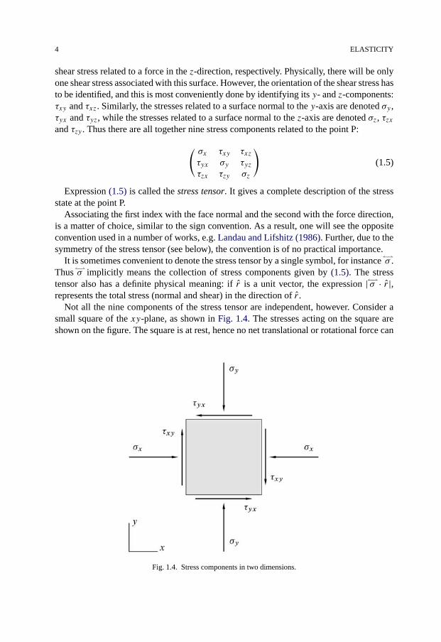
shear stress related to a force in the z-direction, respectively. Physically, there will be onlyone shear stress associated with this surface. However, the orientation of the shear stress hasto be identified, and this is most conveniently done by identifying its y- and z-components:τxy and τxz. Similarly, the stresses related to a surface normal to the y-axis are denoted σy ,τyx and τyz, while the stresses related to a surface normal to the z-axis are denoted σz, τzxand τzy . Thus there are all together nine stress components related to the point P:
(σx τxy τxzτyx σy τyzτzx τzy σz
)(1.5)
Expression (1.5) is called the stress tensor. It gives a complete description of the stressstate at the point P.
Associating the first index with the face normal and the second with the force direction,is a matter of choice, similar to the sign convention. As a result, one will see the oppositeconvention used in a number of works, e.g. Landau and Lifshitz (1986). Further, due to thesymmetry of the stress tensor (see below), the convention is of no practical importance.
It is sometimes convenient to denote the stress tensor by a single symbol, for instance↼⇀σ .Thus↼⇀σ implicitly means the collection of stress components given by (1.5). The stresstensor also has a definite physical meaning: if r is a unit vector, the expression |↼⇀σ · r|,represents the total stress (normal and shear) in the direction of r .
Not all the nine components of the stress tensor are independent, however. Consider asmall square of the xy-plane, as shown in Fig. 1.4. The stresses acting on the square areshown on the figure. The square is at rest, hence no net translational or rotational force can
Fig. 1.4. Stress components in two dimensions.
STRESS 5
act on it. While no translational force is already ensured, no rotational force requires that
τxy = τyx (1.6)
Similarly, it may be shown that
τxz = τzx (1.7)
and
τyz = τzy (1.8)
The relations (1.6) to (1.8) are general, and they reduce the number of independent com-ponents of the stress tensor (1.5) to six.
Although being practical for many purposes, the notation used in (1.5) is not very con-venient for theoretical calculations. For such purposes the following notation is frequentlyused: both types of stresses (normal and shear) are denoted σij . The subscripts i and j maybe any of the numbers 1, 2, 3, which represent the x-, y- and z-axis, respectively. The firstsubscript (i) identifies the axis normal to the actual surface, while the second subscript (j)identifies the direction of the force. Thus, from Fig. 1.4, we see that σ11 = σx , σ13 = τxz,etc. In this notation the stress tensor (1.5) becomes
↼⇀σ =
(σ11 σ12 σ13σ12 σ22 σ23σ13 σ23 σ33
)(1.9)
where we have explicitly used the symmetry of the stress tensor. See Appendices C.4–C.7for a discussion of how the tensor components change as a result of a change of coordinates.
1.1.2. Equations of equilibrium
Apart from forces acting on a surface of a body, there may also be forces acting on everypart of the body itself. Such forces are called body forces. An example of a body force isgravity. We shall denote by fx , fy , and fz the components of the body forces per unit massacting at the point x, y, z of a body. According to the sign convention, fx is positive if it actsin the negative x-direction, and similarly for fy and fz. As an example, consider a smallpart of volume�V of a material with density ρ. If z is the vertical axis, the body force dueto gravity acting on this small volume is ρfz�V = ρg�V , where g is the acceleration ofgravity.
Body forces generally give rise to stress gradients. For instance, an element in a forma-tion is not only subject to the gravity force, it also has to carry the weight of the formationabove. Thus the total stress increases with increasing depth.
For a stressed body to remain at rest, it is required that all forces acting on the bodycancel. This requirement produced a set of symmetry requirements for the stress tensor(Eqs. (1.6) to (1.8)). In addition, it produces a set of equations for the stress gradients.These equations are called the equations of equilibrium.
Consider the parallelepiped shown in Fig. 1.5. The forces acting on this body in thex-direction are
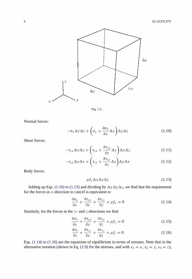
6 ELASTICITY
Fig. 1.5.
Normal forces:
−σx�y�z+(σx + ∂σx
∂x�x
)�y�z (1.10)
Shear forces:
−τyx�x�z+(τyx + ∂τyx
∂y�y
)�x�z (1.11)
−τzx�y�x +(τzx + ∂τzx
∂z�z
)�y�x (1.12)
Body forces:
ρfx�x�y�z (1.13)
Adding up Eqs. (1.10) to (1.13) and dividing by �x�y�z, we find that the requirementfor the forces in x-direction to cancel is equivalent to
∂σx
∂x+ ∂τyx
∂y+ ∂τzx
∂z+ ρfx = 0 (1.14)
Similarly, for the forces in the y- and z-directions we find
∂σy
∂y+ ∂τxy
∂x+ ∂τzy
∂z+ ρfy = 0 (1.15)
∂σz
∂z+ ∂τxz
∂x+ ∂τyz
∂y+ ρfz = 0 (1.16)
Eqs. (1.14) to (1.16) are the equations of equilibrium in terms of stresses. Note that in thealternative notation (shown in Eq. (1.9) for the stresses, and with x1 = x, x2 = y, x3 = z),
STRESS 7
these equations take a particularly simple form:∑j
∂σji
∂xj+ ρfi = 0 (1.17)
1.1.3. Principal stresses in two dimensions
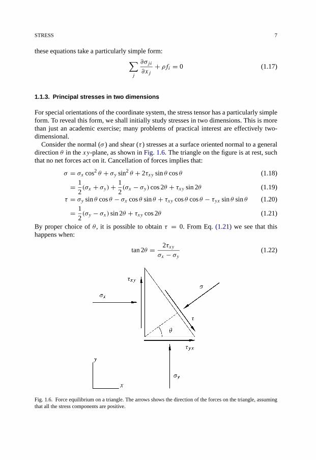
For special orientations of the coordinate system, the stress tensor has a particularly simpleform. To reveal this form, we shall initially study stresses in two dimensions. This is morethan just an academic exercise; many problems of practical interest are effectively two-dimensional.
Consider the normal (σ ) and shear (τ ) stresses at a surface oriented normal to a generaldirection θ in the xy-plane, as shown in Fig. 1.6. The triangle on the figure is at rest, suchthat no net forces act on it. Cancellation of forces implies that:
σ = σx cos2 θ + σy sin2 θ + 2τxy sin θ cos θ (1.18)
= 1
2(σx + σy)+ 1
2(σx − σy) cos 2θ + τxy sin 2θ (1.19)
τ = σy sin θ cos θ − σx cos θ sin θ + τxy cos θ cos θ − τyx sin θ sin θ (1.20)
= 1
2(σy − σx) sin 2θ + τxy cos 2θ (1.21)
By proper choice of θ , it is possible to obtain τ = 0. From Eq. (1.21) we see that thishappens when:
tan 2θ = 2τxyσx − σy (1.22)
Fig. 1.6. Force equilibrium on a triangle. The arrows shows the direction of the forces on the triangle, assumingthat all the stress components are positive.

8 ELASTICITY
Eq. (1.22) has two solutions, θ1 and θ2. The two solutions correspond to two directionsfor which the shear stress τ vanishes. These two directions are called the principal axes ofstress.
The corresponding normal stresses, σ1 and σ2, are called the principal stresses, and arefound by introducing Eq. (1.22) into Eq. (1.19):
σ1 = 1
2(σx + σy)+
√τ 2xy + 1
4(σx − σy)2 (1.23)
σ2 = 1
2(σx + σy)−
√τ 2xy + 1
4(σx − σy)2 (1.24)
It is convenient to choose the notation such that σ1 � σ2. Thus, in the direction θ1,which identifies a principal axis, the normal stress is σ1 and the shear stress is zero. In thedirection θ2, which identifies the other principal axis, the normal stress is σ2 and the shearstress is zero. The principal axes are orthogonal.
1.1.4. Mohr’s stress circle
It is often convenient to reorient the coordinate system such that the x-axis is parallel tothe first principal axis and the y-axis parallel to the other. Then the stresses σ and τ in ageneral direction θ relative to the x-axis become, from Eqs. (1.19) and (1.21):
σ = 1
2(σ1 + σ2)+ 1
2(σ1 − σ2) cos 2θ (1.25)
τ = −1
2(σ1 − σ2) sin 2θ (1.26)
Plotting corresponding values of σ and τ in a diagram (Fig. 1.7a), we obtain a circle calledthe Mohr’s circle. The radius of the circle is (σ1 − σ2)/2 and the centre is at the point(σ1 + σ2)/2 on the σ -axis.
The stresses σ and τ in any direction θ (Fig. 1.7b) correspond to a point on the Mohr’scircle. It is seen from Fig. 1.7a that the largest absolute value for the shear stress is (σ1 −σ2)/2 and occurs for θ = π/4 (= 45°) and θ = 3π/4 (= 135°). The Mohr’s circle is avery useful tool in the analysis of conditions for rock failure, as will be seen in Chapter 2.
1.1.5. Principal stresses in three dimensions
Now moving to three dimensions, we first have to decide how to identify a direction inspace. This can be done by the direction cosines (see also Appendix C.6):
lx = cosαx (1.27)
ly = cosαy (1.28)
lz = cosαz (1.29)

STRESS 9
Fig. 1.7. Mohr’s circle.
Fig. 1.8. Direction cosines.
The angles αx , αy , and αz are the angles between our chosen direction and the x-, y- andz-axes, respectively (Fig. 1.8). The vector r = (lx, ly, lz) is a unit vector in the chosendirection. Note that we always have
l2x + l2y + l2z = 1 (1.30)
The principal stresses can be found by solving for σ the determinant equation (seeAppendix C, in particular Appendix C.2.12 on page 449):∣∣∣∣∣
σx − σ τxy τxzτxy σy − σ τyzτxz τyz σz − σ
∣∣∣∣∣ = 0 (1.31)
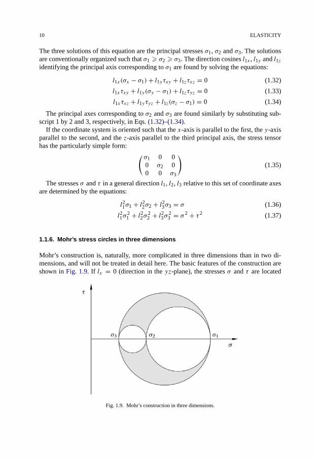
10 ELASTICITY
The three solutions of this equation are the principal stresses σ1, σ2 and σ3. The solutionsare conventionally organized such that σ1 � σ2 � σ3. The direction cosines l1x , l1y and l1zidentifying the principal axis corresponding to σ1 are found by solving the equations:
l1x(σx − σ1)+ l1yτxy + l1zτxz = 0 (1.32)
l1xτxy + l1y(σy − σ1)+ l1zτyz = 0 (1.33)
l1xτxz + l1yτyz + l1z(σz − σ1) = 0 (1.34)
The principal axes corresponding to σ2 and σ3 are found similarly by substituting sub-script 1 by 2 and 3, respectively, in Eqs. (1.32)–(1.34).
If the coordinate system is oriented such that the x-axis is parallel to the first, the y-axisparallel to the second, and the z-axis parallel to the third principal axis, the stress tensorhas the particularly simple form: (
σ1 0 00 σ2 00 0 σ3
)(1.35)
The stresses σ and τ in a general direction l1, l2, l3 relative to this set of coordinate axesare determined by the equations:
l21σ1 + l22σ2 + l23σ3 = σ (1.36)
l21σ21 + l22σ 2
2 + l23σ 23 = σ 2 + τ 2 (1.37)
1.1.6. Mohr’s stress circles in three dimensions
Mohr’s construction is, naturally, more complicated in three dimensions than in two di-mensions, and will not be treated in detail here. The basic features of the construction areshown in Fig. 1.9. If lx = 0 (direction in the yz-plane), the stresses σ and τ are located
Fig. 1.9. Mohr’s construction in three dimensions.

STRESS 11
on the small circle spanning from σ3 to σ2. If lz = 0 (direction in the xy-plane), σ andτ are located on the circle spanning from σ2 to σ1 and, finally, if ly = 0 (direction in thexz-plane), σ and τ are located on the large circle spanning from σ3 to σ1. For all otherdirections, σ and τ are located within the shaded areas.
1.1.7. Stress invariants
The stress tensor is a second order tensor. When changing to a rotated set of coordinateaxes, the components of the stress tensor change. However, as discussed in Appendix C,some properties of the stress tensor remain unchanged. The simplest of these is the meannormal stress
σ = (σx + σy + σz)/3 (1.38)
which equals 1/3 of the trace of the matrix (see page 447). The mean normal stress is thusan invariant of stress.
There also exist other stress combinations that are independent of the coordinate axes.Any combination of stress invariants will of course be a stress invariant as well. The com-monly used stress invariants are:
I1 = σx + σy + σz (1.39)
I2 = −(σxσy + σyσz + σzσx)+ τ 2xy + τ 2
yz + τ 2xz (1.40)
I3 = σxσyσz + 2τxyτyzτxz − σxτ 2yz − σyτ 2
xz − σzτ 2xy (1.41)
(See page 455 for some information about invariants.)
1.1.8. Deviatoric stresses
The mean normal stress σ , defined in Eq. (1.38), essentially causes uniform compressionor extension. Distortions, on the other hand, are essentially caused by the so-called devi-atoric stresses. The deviatoric stress (also called stress deviator or stress deviation—theterminology is not consistent in the literature) is obtained by subtracting the mean normalstress from the normal stress components:(
sx sxy sxzsxy sy syzsxz syz sz
)=(σx − σ τxy τxzτxy σy − σ τyzτxz τyz σz − σ
)(1.42)
Invariants of stress deviation similar to the invariants of stress defined in Eqs. (1.39)–(1.41), are given by:
J1 = sx + sy + sz = 0 (1.43)
J2 = −(sxsy + sysz + szsx)+ s2xy + s2
yz + s2xz (1.44)
J3 = sxsysz + 2sxysyzsxz − sxs2yz − sys2
xz − szs2xy (1.45)

12 ELASTICITY
The invariants J1, J2, J3, and combinations of them, are independent of the choice ofcoordinate axes. Invariants of stress deviation appear e.g. in failure criteria, since thesemust be independent of the choice of coordinate axes (for isotropic materials).
There are many different ways of writing the invariants of stress deviation. See page 463for some useful expressions.
One will often encounter various variants of the stress invariants, in particular the para-meters q and r , which are related to the basic invariants as
q = √3J2 =
√3
2
[(σ1 − σ )2 + (σ2 − σ )2 + (σ3 − σ )2] (1.46)
r = 3
√27
2J3 = 3
√27
2(σ1 − σ )(σ2 − σ )(σ3 − σ ) (1.47)
For a stress state in which two of the principal stresses are equal (σ2 = σ3) the expres-sions simplify to
q = |σ1 − σ3| (1.48)
and
r = σ1 − σ3 (1.49)
q will be used extensively in Chapter 2.
Geometric interpretation of the deviatoric stress invariants
The deviatoric stress invariants have a straightforward geometrical interpretation in prin-cipal stress space, as illustrated in Fig. 1.10. Eq. (1.46) is the equation of a circle centredon σ , with the normal pointing along the hydrostatic axis σ1 = σ2 = σ3. Thus the distancefrom a point (σ1, σ2, σ3) in principal stress space to the hydrostatic axis is√
2
3q = √
2J2 (1.50)
Fig. 1.10. Geometrical interpretation of the deviatoric stress invariants in principal stress space. The dashed linesare the projections of the principal stress axes onto a deviatoric plane (i.e. a plane normal to the hydrostatic axisσ1 = σ2 = σ3, also called the π -plane) passing through the point (σ1, σ2, σ3). The angle ϑ is called the Lodeangle.

STRAIN 13
It can further be shown that the angle ϑ , called the Lode angle, indicated in Fig. 1.10, isgiven by the invariants as
cos(3ϑ) =(r
q
)3
= 3√
3J3
2J 3/22
(1.51)
(Note that since arccos is a multi-valued function, the Lode angle computed from Eq. (1.51)is not unique. If one chooses the principal branch of arccos, the result will be in the range0° to 60° even if the actual stress state corresponds to another value.)
1.1.9. The octahedral stresses
A plane normal to the (1, 1, 1) direction in principal stress space is called an octahedralplane, a π-plane or a deviatoric plane.
The normal stress on and shear stress in this plane are sometimes called the octahedralnormal stress and the octahedral shear stress, and are given by
σoct = 1
3(σ1 + σ2 + σ3) = σ = 1
3I1 (1.52)
τoct = 1
3
√(σ2 − σ3)2 + (σ3 − σ1)2 + (σ1 − σ2)2 =
√2
3J2 =
√2
3q (1.53)
Note that the normal stress in the direction equally inclined to the principal stress axes isthus equal to the mean stress.
1.2. Strain
Consider a sample as shown in Fig. 1.11. The position of a specific particle within thesample is initially x, y, z. After the action of an external force, the position of this particleis shifted. We shall denote the shift in x-direction by u, the shift in y-direction by v, and
Fig. 1.11. Sample deformation.

14 ELASTICITY
the shift in z-direction by w. The quantities u, v and w are called the displacements of theparticle. In order to make the signs of the displacements compatible with the signs of thestresses, as defined in Section 1.1, the displacements are taken to be positive when theyare directed in the negative direction of the axes. Hence, the new position of the particleinitially at x, y, z becomes
x ′ = x − u (1.54)
y′ = y − v (1.55)
z′ = z− w (1.56)
If the displacements u, v and w are constants, i.e. they are the same for every particlewithin the sample, then the displacement is simply a translation of a rigid body. Anothersimple form of displacements is the rotation of a rigid body. For a small rotation specifiedby �ω, where the magnitude | �ω| gives the angle of rotation while the direction of �ω givesthe axis of rotation, the new position of the particle becomes:
�r ′ = �r + �ω × (�r − �r0) (1.57)
where �r = (x, y, z), �r ′ = (x′, y′, z′), and × denotes the vector product. The vector �r0 isthe centre of rotation, through which the axis of rotation goes.
If the relative position of the particles within the sample are changed, so that the newpositions cannot be obtained simply by a rigid translation and/or rotation of the sample,the sample is said to be strained. Fig. 1.12 shows an example of a strained sample. Thedisplacements related to the positions O and P are not equal. The quantity defined as
ε = L− L′
L= −�L
L(1.58)
is called the elongation corresponding to the pointO and the directionOP . To comply withthe sign convention for stresses, we require that the elongation is positive for a contraction.
Fig. 1.12. Deformation

STRAIN 15
Fig. 1.13. Shear deformation.
The elongation is a specific type of quantities known as strains. The other type of strain thatmay occur can be expressed by the change Ψ of the angle between two initially orthogonaldirections (Fig. 1.13). The quantity
Γ = 1
2tanΨ (1.59)
is called the shear strain corresponding to the point O and the direction OP .For many applications one will only be dealing with infinitesimal strains, which implies
that the strains ε and Γ are so small that their products and squares can be ignored, and wewill make this approximation in the following. See Section 1.8 for a discussion of nonlineareffects.
Now consider for a while the strains in two dimensions as shown in Fig. 1.14. Theelongation at x, in the x-direction, is given as
εx = (x +�x)− x − [(x +�x − u(x +�x))− (x − u(x))](x +�x)− x
= u(x +�x)− u(x)�x
(1.60)
In the limit when �x → 0, we have
εx = ∂u
∂x(1.61)
Since the strains are small, we find for the shear strain corresponding to the x-direction
Γxy = 1
2tanΨ ≈ 1
2sinΨ
= −1
2cos
(π
2+ Ψ
)
= −1
2
�P ′1 · �P ′
2
| �P1| · | �P2|(1.62)
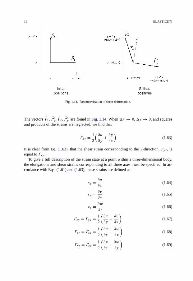
16 ELASTICITY
Fig. 1.14. Parameterization of shear deformation.
The vectors �P1, �P ′1, �P2, �P ′
2, are found in Fig. 1.14. When �x → 0, �y → 0, and squaresand products of the strains are neglected, we find that
Γxy = 1
2
(∂u
∂y+ ∂y
∂x
)(1.63)
It is clear from Eq. (1.63), that the shear strain corresponding to the y-direction, Γyx , isequal to Γxy .
To give a full description of the strain state at a point within a three-dimensional body,the elongations and shear strains corresponding to all three axes must be specified. In ac-cordance with Eqs. (1.61) and (1.63), these strains are defined as:
εx = ∂u
∂x(1.64)
εy = ∂v
∂y(1.65)
εz = ∂w
∂z(1.66)
Γxy = Γyx = 1
2
(∂u
∂y+ ∂v
∂x
)(1.67)
Γxz = Γzx = 1
2
(∂u
∂z+ ∂w
∂x
)(1.68)
Γyz = Γzy = 1
2
(∂v
∂z+ ∂w
∂y
)(1.69)
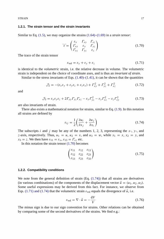
STRAIN 17
1.2.1. The strain tensor and the strain invariants
Similar to Eq. (1.5), we may organize the strains (1.64)–(1.69) in a strain tensor:
↼⇀ε =
(εx Γxy ΓxzΓxy εy ΓyzΓxz Γyz εz
)(1.70)
The trace of the strain tensor
εvol = εx + εy + εz (1.71)
is identical to the volumetric strain, i.e. the relative decrease in volume. The volumetricstrain is independent on the choice of coordinate axes, and is thus an invariant of strain.
Similar to the stress invariants of Eqs. (1.40)–(1.41), it can be shown that the quantities
J2 = −(εxεy + εyεz + εzεx)+ Γ 2xy + Γ 2
yz + Γ 2xz (1.72)
and
J3 = εxεyεz + 2ΓxyΓyzΓxz − εxΓ 2yz − εyΓ 2
xz − εzΓ 2xy (1.73)
are also invariants of strain.There also exists a mathematical notation for strains, similar to Eq. (1.9). In this notation
all strains are defined by
εij = 1
2
(∂ui
∂xj+ ∂uj
∂xi
)(1.74)
The subscripts i and j may be any of the numbers 1, 2, 3, representing the x-, y-, andz-axis, respectively. Thus, u1 = u, u2 = v, and u3 = w, while x1 = x, x2 = y, andx3 = z. We then have ε11 = εx , ε13 = Γxz etc.
In this notation the strain tensor (1.70) becomes(ε11 ε12 ε13ε12 ε22 ε23ε13 ε23 ε33
)(1.75)
1.2.2. Compatibility conditions
We note from the general definition of strain (Eq. (1.74)) that all strains are derivatives(in various combinations) of the components of the displacement vector �u = (u1, u2, u3).Some useful expressions may be derived from this fact. For instance, we observe fromEqs. (1.71) and (1.74) that the volumetric strain εvol equals the divergence of �u, i.e.
εvol = ∇ · �u = −dV
V(1.76)
The minus sign is due to our sign convention for strains. Other relations can be obtainedby comparing some of the second derivatives of the strains. We find e.g.:

18 ELASTICITY
∂2∂εx
∂y2+ ∂2εy
∂x2= 2
∂2Γxy
∂x∂y
(= ∂3u
∂x∂y2+ ∂3v
∂y∂x2
)(1.77)
∂2εx
∂z2+ ∂2εz
∂x2= 2
∂2Γxz
∂x∂z
(= ∂3u
∂x∂z2+ ∂3w
∂z∂x2
)(1.78)
∂2εz
∂y2+ ∂2εy
∂z2= 2
∂2Γzy
∂z∂y
(= ∂3w
∂z∂y2+ ∂3v
∂y∂z2
)(1.79)
These three differential relations, together with three others that express ∂2εx/(∂y∂z),∂2εy/(∂x∂z) and ∂2εz/(∂x∂y) in terms of second derivatives of the shear strains, areknown as the compatibility conditions for strain.
1.2.3. Principal strains
In Section 1.1 we saw that for some specific directions the shear stress vanishes, so that fora specific orientation of the coordinate system (with axis parallel to the principal axes ofstress) the stress tensor becomes particularly simple. The situation is similar for strains.
In two dimensions, it can be shown that the shear strain vanishes in the directions θrelative to the x-axis, which fulfil the equation:
tan 2θ = 2Γxyεx − εy (1.80)
Thus, in two dimensions, there are two orthogonal directions for which the shear strainvanishes. These directions are called the principal axes of strain. The elongations in thedirections of the principal axes of strain, are called the principal strains.
In three dimensions there are three principal axes of strain. The principal strains arefound by solution of the determinant equation
∣∣∣∣∣εx − ε Γxy ΓxzΓxy εy − ε ΓyzΓxz Γyz εz − ε
∣∣∣∣∣ = 0 (1.81)
The solutions are denoted ε1, ε2, ε3. The direction cosines l1x , l1y , l1z identifying theprincipal axis corresponding to ε1 are found by solution of the equations
l1x(εx − ε1)+ l1yΓxy + l1zΓxz = 0 (1.82)
l1xΓxy + l1y(εy − ε1)+ l1zΓyz = 0 (1.83)
l1xΓxz + l1yΓyz + l1z(εz − ε1) = 0 (1.84)
The principal axes corresponding to ε2 and ε3 are found similarly by substituting sub-script 1 by 2 and 3, respectively. Eqs. (1.81) and (1.82)–(1.84) are seen to be equivalentsof Eqs. (1.31) and (1.32)–(1.34) identifying the principal stresses and the principal axes ofstress.

STRAIN 19
1.2.4. Plane strain and plane stress
In several practical applications it is a good approximation to assume that all cross-sectionsalong a given axis are in the same condition, and that there is no displacement along theaxis. This state of strain is called plane strain.
In the following we shall assume the unique axis to be the z-axis. The strain tensor forplane strain is then (
εx(x, y) Γxy(x, y) 0Γxy(x, y) εy(x, y) 0
0 0 0
)(1.85)
where all strain components are independent of z. The term plane of course refers to thefact that the strain is confined to a plane.
If we only have displacement along z, and this displacement is independent of z, thestrain state is referred to as antiplane strain. The strain tensor is then( 0 0 Γxz(x, y)
0 0 Γyz(x, y)
Γxz(x, y) Γyz(x, y) 0
)(1.86)
where again all components are independent of z.A general situation in which the displacement along the z-axis is independent of z can be
decomposed into a sum of plane strain and antiplane strain. This state of strain is referredto as generalized plane strain. The strain tensor is(
εx(x, y) Γxy(x, y) Γxz(x, y)
Γxy(x, y) εy(x, y) Γyz(x, y)
Γxz(x, y) Γyz(x, y) 0
)(1.87)
Note, however, that the concept of generalized plane strain is not uniquely defined inthe literature. Sometimes the term is used when εz rather than the displacement along z isindependent if z. This leads to the strain tensor(
εx(x, y) Γxy(x, y) Γxz(x, y)
Γxy(x, y) εy(x, y) Γyz(x, y)
Γxz(x, y) Γyz(x, y) εz(x, y)
)(1.88)
See Cheng (1998) for a thorough discussion.Analogously, if all stress components are independent of z, and σz = τxz = τyz = 0
(still taking z to be the unique axis), we call the situation plane stress. The stress tensor isthen (
σx(x, y) τxy(x, y) 0τxy(x, y) σy(x, y) 0
0 0 0
)(1.89)
Generalized plane stress is used when all stress components are independent z, leadingto the stress tensor (
σx(x, y) τxy(x, y) τxz(x, y)
τxy(x, y) σy(x, y) τyz(x, y)
τxz(x, y) τyz(x, y) σz(x, y)
)(1.90)

20 ELASTICITY
1.3. Elastic moduli
The theory of linear elasticity deals with situations where there are linear relationships be-tween applied stresses and resulting strains. While most rocks do behave nonlinearly whensubject to large stresses, their behaviour may normally be described by linear relationsfor sufficiently small changes in stress. Consider a sample of length L and cross-sectionalarea A = D2 (Fig. 1.15). When the force F is applied on its end surfaces, the length ofthe sample is reduced to L′. The applied stress is then σx = F/A and the correspondingelongation is εx = (L − L′)/L, according to Eqs. (1.1) and (1.58). If the sample behaveslinearly, there is a linear relation between σx and εz, which we may write
εx = 1
Eσx (1.91)
Eq. (1.91) is known as Hooke’s law, while the coefficientE is called Young’s modulus orsimply the E-modulus. Young’s modulus belongs to a group of coefficients called elasticmoduli. It is a measure of the stiffness of the sample, i.e. the sample’s resistance againstbeing compressed by a uniaxial stress.
Another consequence of the applied stress σx (Fig. 1.15) is an increase in the width Dof the sample. The lateral elongation is εy = εz = (D −D′)/D. In general D′ > D, thusεy and εz become negative. The ratio defined as
ν = −εyεx
(1.92)
is another elastic parameter, known as Poisson’s ratio. It is a measure of lateral expansionrelative to longitudinal contraction.
Eqs. (1.91) and (1.92), which relates one component of stress or strain to another, aredefined by a specific state of stress, namely σx �= 0, σy = σz = 0. In general, eachcomponent of strain is a linear function of all components of stress.
Isotropic materials are materials whose response is independent of the orientation of theapplied stress. For such materials the principal axes of stress and the principal axes of strain
Fig. 1.15. Deformation induced by uniaxial stress.
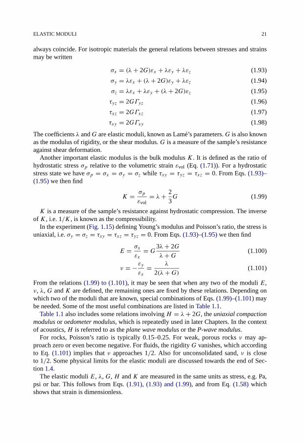
ELASTIC MODULI 21
always coincide. For isotropic materials the general relations between stresses and strainsmay be written
σx = (λ+ 2G)εx + λεy + λεz (1.93)
σy = λεx + (λ+ 2G)εy + λεz (1.94)
σz = λεx + λεy + (λ+ 2G)εz (1.95)
τyz = 2GΓyz (1.96)
τxz = 2GΓxz (1.97)
τxy = 2GΓxy (1.98)
The coefficients λ andG are elastic moduli, known as Lamé’s parameters.G is also knownas the modulus of rigidity, or the shear modulus. G is a measure of the sample’s resistanceagainst shear deformation.
Another important elastic modulus is the bulk modulus K . It is defined as the ratio ofhydrostatic stress σp relative to the volumetric strain εvol (Eq. (1.71)). For a hydrostaticstress state we have σp = σx = σy = σz while τxy = τyz = τxz = 0. From Eqs. (1.93)–(1.95) we then find
K = σp
εvol= λ+ 2
3G (1.99)
K is a measure of the sample’s resistance against hydrostatic compression. The inverseof K , i.e. 1/K , is known as the compressibility.
In the experiment (Fig. 1.15) defining Young’s modulus and Poisson’s ratio, the stress isuniaxial, i.e. σy = σz = τxy = τxz = τyz = 0. From Eqs. (1.93)–(1.95) we then find
E = σx
εx= G3λ+ 2G
λ+G (1.100)
ν = −εyεx
= λ
2(λ+G) (1.101)
From the relations (1.99) to (1.101), it may be seen that when any two of the moduli E,ν, λ, G and K are defined, the remaining ones are fixed by these relations. Depending onwhich two of the moduli that are known, special combinations of Eqs. (1.99)–(1.101) maybe needed. Some of the most useful combinations are listed in Table 1.1.
Table 1.1 also includes some relations involving H = λ+ 2G, the uniaxial compactionmodulus or oedometer modulus, which is repeatedly used in later Chapters. In the contextof acoustics, H is referred to as the plane wave modulus or the P-wave modulus.
For rocks, Poisson’s ratio is typically 0.15–0.25. For weak, porous rocks ν may ap-proach zero or even become negative. For fluids, the rigidity G vanishes, which accordingto Eq. (1.101) implies that ν approaches 1/2. Also for unconsolidated sand, ν is closeto 1/2. Some physical limits for the elastic moduli are discussed towards the end of Sec-tion 1.4.
The elastic moduli E, λ, G, H and K are measured in the same units as stress, e.g. Pa,psi or bar. This follows from Eqs. (1.91), (1.93) and (1.99), and from Eq. (1.58) whichshows that strain is dimensionless.
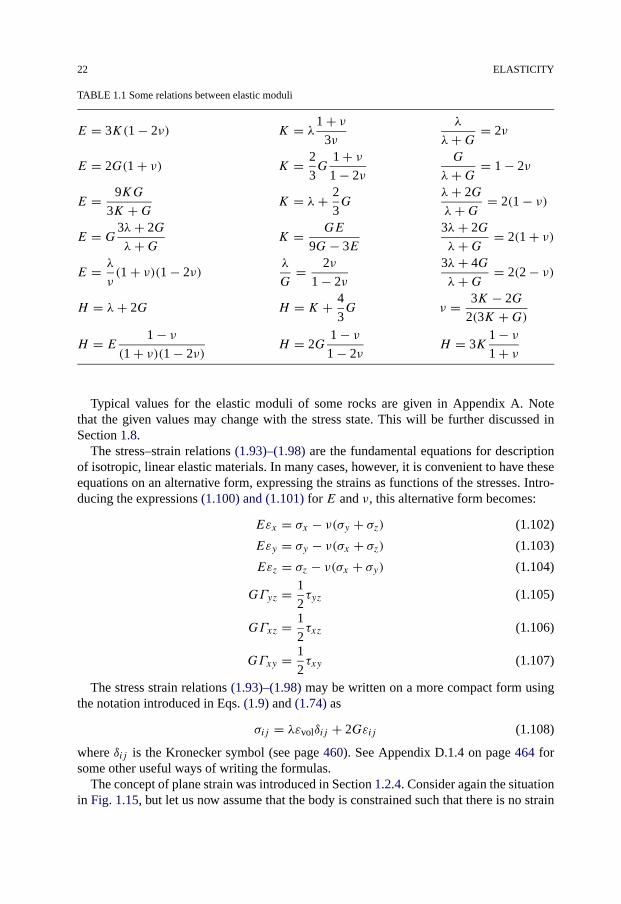
22 ELASTICITY
TABLE 1.1 Some relations between elastic moduli
E = 3K(1 − 2ν) K = λ1 + ν3ν
λ
λ+G = 2ν
E = 2G(1 + ν) K = 2
3G
1 + ν1 − 2ν
G
λ+G = 1 − 2ν
E = 9KG
3K +G K = λ+ 2
3G
λ+ 2G
λ+G = 2(1 − ν)
E = G3λ+ 2G
λ+G K = GE
9G− 3E
3λ+ 2G
λ+G = 2(1 + ν)
E = λ
ν(1 + ν)(1 − 2ν)
λ
G= 2ν
1 − 2ν
3λ+ 4G
λ+G = 2(2 − ν)
H = λ+ 2G H = K + 4
3G ν = 3K − 2G
2(3K +G)H = E 1 − ν
(1 + ν)(1 − 2ν)H = 2G
1 − ν1 − 2ν
H = 3K1 − ν1 + ν
Typical values for the elastic moduli of some rocks are given in Appendix A. Notethat the given values may change with the stress state. This will be further discussed inSection 1.8.
The stress–strain relations (1.93)–(1.98) are the fundamental equations for descriptionof isotropic, linear elastic materials. In many cases, however, it is convenient to have theseequations on an alternative form, expressing the strains as functions of the stresses. Intro-ducing the expressions (1.100) and (1.101) for E and ν, this alternative form becomes:
Eεx = σx − ν(σy + σz) (1.102)
Eεy = σy − ν(σx + σz) (1.103)
Eεz = σz − ν(σx + σy) (1.104)
GΓyz = 1
2τyz (1.105)
GΓxz = 1
2τxz (1.106)
GΓxy = 1
2τxy (1.107)
The stress strain relations (1.93)–(1.98) may be written on a more compact form usingthe notation introduced in Eqs. (1.9) and (1.74) as
σij = λεvolδij + 2Gεij (1.108)
where δij is the Kronecker symbol (see page 460). See Appendix D.1.4 on page 464 forsome other useful ways of writing the formulas.
The concept of plane strain was introduced in Section 1.2.4. Consider again the situationin Fig. 1.15, but let us now assume that the body is constrained such that there is no strain

STRAIN ENERGY 23
in the z-direction, i.e. it is in a state of plane strain. Introducing εz = 0 and σy = 0 inEqs. (1.102)–(1.104) we find an equation corresponding to Eq. (1.91):
E′ = σx
εx= E
1 − ν2= 2G
1 − ν (1.109)
E′ is called the plane strain modulus since it often shows up in plane strain problems. Asan example, see Section 11.4. Note that we have E � E′ � H , which means that thestiffness of the sample increases as it is increasingly confined in the lateral directions.
1.4. Strain energy
A strained body possesses a potential energy which may be released during unloading.Consider a small cube of a material, with sides a, loaded uniaxially with the stress σ . Theresulting elongation is ε = σ/E. The work done by increasing the stress from 0 to σ1 is:
work = force · distance
=∫ σ1
0(a2σ)(a dε) = a3
∫ σ1
0σ
1
Edσ
= 1
2a3 σ
21
E= 1
2a3Eε2
1 = 1
2a3σ1ε1 (1.110)
where ε1 = σ1/E. As the stress state in this case is uniaxial, σ1 is a principal stress whileε1 is a principal strain. When the other two principal stresses are non-zero, correspondingterms will add to the expression for the work. The work per unit volume (= the potentialenergy per unit volume) then becomes:
W = 1
2(σ1ε1 + σ2ε2 + σ3ε3) (1.111)
W is called the strain energy.A variety of expressions for the strain energy can be obtained by suitable substitutions
for the principal stresses and/or the principal strains. Using Eqs. (1.93)–(1.95) to expressthe stresses in terms of the strains, we find that the strain energy (1.111) is equal to:
W = 2[(λ+ 2G)
(ε2
1 + ε22 + ε2
3
)+ 2λ(ε1ε2 + ε1ε3 + ε2ε3)]
(1.112)
Comparing with Eqs. (1.71), (1.72) and (1.73) for the strain invariants, we find that thestrain energy may also be expressed as:
W = 1
2
[(λ+ 2G)ε2
vol + 4GJ2]
= 1
2
[(λ+ 2G)
(ε2x + ε2
y + ε2z
)+ 2λ(εxεy + εyεz + εzεx)+ 4G
(Γ 2xy + Γ 2
yz + Γ 2xz
)](1.113)
Useful relations can be established by analysis of the strain energy. Taking the derivativeof Eq. (1.113) with respect to εx , and using Eq. (1.93), we find that:
∂W
∂εx= 1
2
[2(λ+ 2G)εx + 2λ(εy + εz)
] = σx (1.114)

24 ELASTICITY
Similar expressions connecting σy to εy , etc. can also be established in the same way. Wenow observe, by taking the derivative of Eq. (1.114) with respect to εy , that it is possibleto establish a set of expressions of the type:
∂σx
∂εy= ∂2W
∂εy∂εx= ∂σy
∂εx(1.115)
This equation gives rise to a general symmetry restriction on the elastic moduli, which willbe discussed later. (See page 39.)
Going back to Eq. (1.110), we observe that the Young’s modulusE must be nonnegative,otherwise the system will be unstable (E < 0 implies that ε1 → ∞ will be energeticallyfavourable). By considering other stress geometries, we may similarly show that also theshear modulus G and the bulk modulus K must be nonnegative. It follows from Table 1.1that the Poisson’s ratio ν is then restricted to be in the region −1 < ν < 1/2. (Note thatthese restrictions are derived assuming that the material is isotropic and linearly elastic.)
1.5. Thermoelasticity
1.5.1. Thermal strain
It is well known that (most) materials expand or contract under a temperature change. Letus consider an elastic rod, which is free to expand. The initial temperature is T0, and thetemperature is changed to some other value T . The axial thermal strain resulting from thetemperature change is then given by
εa = −αT (T − T0) (1.116)
where αT is the coefficient of linear thermal expansion. The minus sign ensures that αT ispositive (for the normal cases where a temperature increase gives expansion). Some exam-ples of the numerical values for thermal properties of rocks may be found in Appendix A.
When comparing the thermal expansion for rocks with that of fluids, it is important tobe aware that for fluids one often specifies the coefficient of volumetric thermal expansion,αT,V = 3αT .
1.5.2. Thermal stress
If the rod is constrained at the ends, such that it can not change it’s length, a thermal stresswill build up when the temperature increases. The magnitude of the thermal stress maybe inferred by requiring that the thermal stress should give a strain of opposite sign andequal magnitude to the thermal strain computed from Eq. (1.116). From Eq. (1.91) we seethat the thermal stress resulting from a temperature change T − T0 for a rod which is fullyconstrained in one direction is
σa = −Eεa = EαT (T − T0) (1.117)
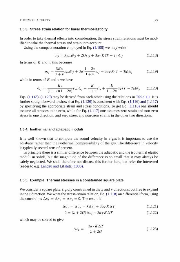
THERMOELASTICITY 25
1.5.3. Stress strain relation for linear thermoelasticity
In order to take thermal effects into consideration, the stress strain relations must be mod-ified to take the thermal stress and strain into account.
Using the compact notation employed in Eq. (1.108) we may write
σij = λεvolδij + 2Gεij + 3αT K(T − T0)δij (1.118)
In terms of K and ν, this becomes
σij = 3Kν
1 + ν εvolδij + 3K1 − 2ν
1 + ν εij + 3αT K(T − T0)δij (1.119)
while in terms of E and ν we have
σij = Eν
(1 + ν)(1 − 2ν)εvolδij + E
1 + ν εij + E
1 − 2ναT (T − T0)δij (1.120)
Eqs. (1.118)–(1.120) may be derived from each other using the relations in Table 1.1. It isfurther straightforward to show that Eq. (1.120) is consistent with Eqs. (1.116) and (1.117)by specifying the appropriate strain and stress conditions. To get Eq. (1.116) one shouldassume all stresses to be zero, while for Eq. (1.117) one assumes zero strain and non-zerostress in one direction, and zero stress and non-zero strains in the other two directions.
1.5.4. Isothermal and adiabatic moduli
It is well known that to compute the sound velocity in a gas it is important to use theadiabatic rather than the isothermal compressibility of the gas. The difference in velocityis typically several tens of percent.
In principle there is a similar difference between the adiabatic and the isothermal elasticmoduli in solids, but the magnitude of the difference is so small that it may always besafely neglected. We shall therefore not discuss this further here, but refer the interestedreader to e.g. Landau and Lifshitz (1986).
1.5.5. Example: Thermal stresses in a constrained square plate
We consider a square plate, rigidly constrained in the x and y directions, but free to expandin the z direction. We write the stress–strain relation, Eq. (1.118) on differential form, usingthe constraints �εx = �εy = �σz = 0. The result is
�σx = �σy = λ�εz + 3αT K�T (1.121)
0 = (λ+ 2G)�εz + 3αT K�T (1.122)
which may be solved to give
�εz = −3αT K�T
λ+ 2G(1.123)
26 ELASTICITY
and
�σx = 2G3λ+ 2G
λ+ 2GαT�T (1.124)
where we have used K = λ+ 2G/3. In terms of E and ν we have
�σx = �σy = αT E
1 − ν�T (1.125)
For αT = 15 · 10−6 K−1, ν = 0.25 and E = 5 GPa (fairly typical values for weaklyconsolidated rock) this becomes
�σx
�T= 0.1 MPa K−1 (1.126)
This shows that thermal stresses may be quite significant, and we shall see in later chaptersthat there are several aspects of petroleum rock mechanics where temperature effects playan important role.
1.6. Poroelasticity
So far, we have treated rocks as if they were homogeneous, solid materials. However, rocksare generally composite materials, and hence inhomogeneous on a microscopic scale. Theway rocks behave, their elastic response, their failure stresses etc., depend, to a large ex-tent, on the non-solid part of the materials. In this section we will take into account the voidspace, which not only is essential for oil to be produced from a reservoir, but also playsan important role in rock mechanical behaviour. We will first consider a macroscopic de-scription of porous and permeable media, which allows us to study both static and dynamicmechanical properties. This approach is based on the theory of Maurice A. Biot.
In this section we will give a brief and practical introduction the theory. We will limitourselves to a description of an idealized porous material which is microscopically homo-geneous and isotropic. This approximation is sometimes referred to as the Gassmann limitof the Biot theory.
For those desiring a more thorough exposition, we refer to the book by Wang (2000), thepapers by Detournay and Cheng (1993), Rice and Cleary (1976) and the book by Coussy(2004). Zimmerman’s (1991) book is also a very useful introduction to the mechanicalproperties of porous media.
1.6.1. Suspension of solid particles in a fluid
Let us first take a look at a very simple porous medium; namely one in which the solidand fluid parts are deformed independently of each other. In practice, we may think ofthis medium as a suspension of solid particles in a fluid, or for instance, a water-saturated,completely unconsolidated sand. If we place this mixture in a container, the volumetricstrain due to an external pressure σp is:
εvol = σp
Keff(1.127)

POROELASTICITY 27
whereKeff is the bulk modulus of the mixture. The total deformation must, however, equalthe sum of the deformations of each component, weighted by the volume portion of eachcomponent.
εvol = Vs
Vtotεvol,s + Vf
Vtotεvol,f (1.128)
where subscripts s and f denote solid and fluid, respectively, and Vtot is the total volume.Now, we define porosity φ as the volume occupied by the fluid relative to the total volume,i.e.:
φ = Vf
Vtot(1.129)
Vs
Vtot= 1 − φ (1.130)
The strains εvol,s and εvol,f are given by the bulk moduli of the solid (Ks) and the fluid(Kf), respectively, according to Eq. (1.99). Then Eq. (1.128) may be written as:
εvol = (1 − φ)σpKs
+ φ σpKf
(1.131)
By combining Eqs. (1.127) and (1.131) we now find that the effective modulus of thesuspension is given by
1
Keff= 1 − φ
Ks+ φ
Kf(1.132)
This is an example of a particularly simple porous material. We shall now generalize bytaking into account the fact that rocks consist of a solid framework and a pore fluid whichcan not be treated independently.
1.6.2. Biot’s poroelastic theory for static properties
We will now consider an isotropic, porous and permeable medium, consisting of two com-ponents: a solid and a fluid part. The displacement of the solid is denoted �us while that ofthe fluid is denoted �uf. For a volume element attached to the solid, the strains are given asthe derivatives of the components of �us. Using Eq. (1.76) we have for the volumetric strain:
εvol = ∇ · �us (1.133)
For the fluid part, we will define a strain parameter ζ , which describes the volumetricdeformation of the fluid relative to that of the solid:
ζ = φ∇ · (�us − �uf) (1.134)
The stress tensor↼⇀σ represents the total external stress on a volume element attachedto the solid framework. The volume element balances this stress partly by stresses in the
28 ELASTICITY
solid framework, and partly by a hydrostatic pressure1 in the fluid, the pore pressure pf.In accordance with the sign convention, all stresses—including the pore pressure—arepositive in compression.
The change in the mass of fluid in a volume element attached to the solid can be dividedinto two parts: the change of the pore volume (due to change in the external stresses and/orthe pore pressure), and the compression/decompression of the fluid as the pore pressurechanges. This means that we may write
ζ = −φ(�Vp
Vp+ pf
Kf
)(1.135)
where Vp is the pore volume, i.e. the volume occupied by the fluid, and Kf is the bulkmodulus of the pore fluid. We see that ζ is positive when the amount of fluid in the volumeelement is decreasing.
The presence of the pore fluid adds extra terms to the strain energy of the material. Hencethe stress–strain relations (Eqs. (1.93)–(1.98)) will also be modified. Biot (1962) showedhow the linear stress–strain relations for this two-phase system can be expressed in termsof the strain parameters εvol and ζ , the stress tensor elements and the pore pressure pf:
σx = λεvol + 2Gεx − Cζ (1.136)
σy = λεvol + 2Gεy − Cζ (1.137)
σz = λεvol + 2Gεz − Cζ (1.138)
τyz = 2GΓyz (1.139)
τxz = 2GΓxz (1.140)
τxy = 2GΓxy (1.141)
pf = Cεvol −Mζ (1.142)
Written on the abbreviated form as Eq. (1.108), Eqs. (1.136)–(1.141) become
σij = λεvolδij + 2Gεij − Cζδij (1.143)
λ and G are the Lamé parameters of the porous material, while C and M are additionalelastic moduli required to describe a two-phase medium. Note that C appears both in thestress and the pore pressure equations. Biot (1941) showed that this is a consequence ofthermodynamic principles.
By letting ζ = 0 in Eq. (1.143) we get Eq. (1.108). ζ = 0 means that there is no fluidmovement in the material, i.e. the material is undrained. Thus the λ in Eq. (1.143) is notthe λ of the dry porous medium, but the λ of the fluid-filled medium when the fluid is notallowed to move. This is discussed further below.
1 The term “hydrostatic pressure” is sometimes used in a restricted sense, meaning the fluid pressure resultingfrom an overlying column of water. In this book we use the term in a broader (and probably more widely used)sense, meaning the pressure in a static fluid irrespective of the source of the pressure. Further, we also use hydro-static for the stress state in a solid when all the principal stresses are equal, i.e. no shear stresses are present (seepage 21).

POROELASTICITY 29
To get some understanding of the physical meaning of M , we may let εvol = 0 inEq. (1.142). Inserting Eq. (1.134) we then find
pf = Mφ∇ · �uf (1.144)
which shows thatMφ is a measure of how much the pore pressure increases as the amountof fluid in a volume element is increased. If the solid was completely rigid, we would thushaveMφ = Kf.
Explicit expressions for C andM in terms of the solid and fluid moduli are given later.Summation of Eqs. (1.136)–(1.138) gives:
σ = Kεvol − Cζ (1.145)
where σ is defined by Eq. (1.38). K = λ + 2G/3 is the bulk modulus of the porous rockin undrained condition, i.e. in a condition where the pore fluid is not allowed to escape.We shall now investigate how the elastic moduli K , C and M relate to the moduli of theconstituents of the rock. First, imagine that we perform a “jacketed” test (see Fig. 1.16a):a porous medium is confined within an impermeable jacket, and subjected to an externalhydrostatic pressure σp.
The pore fluid is allowed to escape during loading, so that the pore pressure is keptconstant, and hence the stress is entirely carried by the solid framework. From Eqs. (1.142)and (1.145), we then obtain
σp
εvol= K − C2
M
def= Kfr (1.146)
Since this test characterizes the stiffness of the solid part of the rock, Kfr is called the bulkmodulus of the framework or the frame modulus. Since there are no shear forces associatedwith the fluid, we can directly identify the shear modulus of the porous system as the shear
Fig. 1.16. “Jacketed” a) and “unjacketed” b) test situations.

30 ELASTICITY
modulus of the framework, i.e.
G = Gfr (1.147)
Next, we proceed to an “unjacketed” test, as illustrated in Fig. 1.16b. The rock sampleunder investigation is here embedded in a fluid in such a way that the hydrostatic pres-sure on the sample is balanced by the pressure in the pores, i.e. pf = σp. CombiningEqs. (1.142) and (1.145) we now find:
σp
εvol= pf
εvol= Kfr
1 − CM
(1.148)
The loading pf = σp means that there is a uniform stress within the sample, whichmeans that the rock framework deforms uniformly. Thus, the volumetric strain of the totalsample, the pore volume and the solid (grain) volume must be equal:
�Vtot
Vtot= �Vp
Vp= �Vs
Vs(1.149)
From pf = σp = −Ks(�Vs/Vs) where Ks is the bulk modulus of the solid grains (1/Ksis often referred to as the grain compressibility) we hence find
�Vs
Vs= �Vp
Vp= �Vtot
Vtot= −εvol = − pf
Ks(1.150)
The stress–strain response is therefore entirely given by the intrinsic elastic properties ofthe solid material. Comparing Eq. (1.150) to Eq. (1.148) we infer that
Ks = Kfr
1 − CM
(1.151)
From Eqs. (1.135) and (1.150) it follows that
ζ = φ(
1
Ks− 1
Kf
)pf (1.152)
On the other hand, the combination of Eqs. (1.142) and (1.145) with pf = σp gives
ζ = C −KMK − C2
pf (1.153)
By combining Eqs. (1.152) and (1.153) we obtain the relation
φ
(1
Ks− 1
Kf
)= C −KMK − C2
(1.154)
Although this equation was derived for a specific loading (“unjacketed test”), it is generallyvalid.
Eqs. (1.151) and (1.154), combined with the definition of Kfr (Eq. (1.146)), allow us toexpress the elastic constants K , C andM in terms of the elastic moduli of the constituentsof the rock (Ks and Kf), plus the porosity φ and the framework modulus Kfr. The results
POROELASTICITY 31
are:
K = Kfr + Kf
φ
(1 − KfrKs)2
1 + KfφKs(1 − φ − Kfr
Ks)
(1.155)
M = Kf
φ
1
1 + KfφKs(1 − φ − Kfr
Ks)
(1.156)
C =(
1 − Kfr
Ks
)M = Kf
φ
1 − KfrKs
1 + KfφKs(1 − φ − Kfr
Ks)
(1.157)
Eq. (1.155), which is called the Gassmann equation or the Biot–Gassmann equation, mayalternatively be written as
K
Ks −K = Kfr
Ks −Kfr+ 1
φ
Kf
Ks −Kf(1.158)
The relations (1.155)–(1.157) do not give a clear physical meaning to each parameter.Better insight may be achieved by looking at a couple of limit cases, where the relationsbecome simpler.
One case is a “hard” rock, where the frame is incompressible compared to the fluid. AsKs Kf in general, we have for this “stiff frame” case:
Kfr,Gfr,Ks Kf (1.159)
For porosities that are not too small (specifically φ (Kf/K2s )(Ks−Kfr)), Eqs. (1.155)–
(1.157) then reduce to:
“Stiffframe”
⎧⎨⎩K ≈ KfrC ≈ Kf
φ(1 − Kfr
Ks)
M ≈ Kfφ
(1.160)
We see that the bulk modulus K is here identified as the bulk modulus of the rock frame-work, while the constantM is entirely given by the properties of the pore fluid and the poresystem.
The opposite limit is that of a “weak frame”. For this case we assume
Kfr,Gfr,Kf � Ks (1.161)
For porosities φ Kf/Ks, Eqs. (1.155)–(1.157) reduce to:
“Weakframe”
{K ≈ Kfr + Kf
φ
C ≈ M ≈ Kfφ
(1.162)
In this case, the bulk modulusK is influenced not only by the rock stiffness, but also by thefluid bulk modulus Kf. In the limiting case when Kfr → 0 (suspension), K = C = M ≈Kf/φ are all given mainly by fluid properties. Disregarding the condition Ks Kf wouldin this case reproduce Eq. (1.132), which was obtained by simple physical arguments.
Note that the “stiff frame” and the “weak frame” limits are rather extreme cases thatare mainly suited for illustrative purposes. For practical calculations the complete expres-sions (1.155)–(1.157) should be used.

32 ELASTICITY
The theory outlined above contains two “unknown” parameters, which are not identifiedin terms of the properties of the rock’s constituents. These are the two elastic moduli of theframework, Kfr, and Gfr. We shall in Chapter 6 see how microscopic theories can be usedto estimate these moduli when further information about the rock structure is available.Empirically, the frame bulk modulus Kfr is found to be significantly smaller than Ks, andto decrease sharply with the porosity.
1.6.3. The effective stress concept
In Section 1.6.2, we discussed an experiment where a rock sample was “jacketed” withthe pore fluid free to escape, so that the pore pressure was kept constant during loading(Fig. 1.16a). Such a test is also called a drained test. The stress–strain response of this testwas given by Eq. (1.146), i.e.
σp = Kfrεvol (1.163)
Imagine now a similar test, but with the pore fluid shut in, so that no fluid flow occurs in orout of the rock sample. This situation is called undrained. Compression of the sample—including the pore space—due to an external hydrostatic load, will in this case cause anincrease in the pore pressure. The sample compression and the pore pressure can be calcu-lated by requiring ζ = 0 in Eqs. (1.142) and (1.145), i.e. no relative displacement betweenpore fluid and solid during the test. The pore pressure is given by Eq. (1.142):
pf = Cεvol (1.164)
while the stress–strain characteristics is given by Eq. (1.145):
σp = Kεvol (1.165)
Using Eqs. (1.146) and (1.164), we can write
K = Kfr + C2
M= Kfr + C
M
pf
εvol(1.166)
By introducing this expression for K into Eq. (1.165) and reorganizing the equation, weobtain:
σp − C
Mpf = Kfrεvol (1.167)
Eq. (1.167) tells us that the deformation is proportional to the effective stress σ ′p, defined
as
σ ′p = σp − αpf (1.168)
rather than the total stress σp, and the corresponding modulus is Kfr, i.e. the same as forthe drained test (Eq. (1.163)). Physically, this means that the solid framework carries thepart σ ′
p of the total external stress σp, while the remaining part, αpf, is carried by the fluid.The remaining pore pressure, (1 − α)pf, is counteracted by internal stresses in the solid.
POROELASTICITY 33
The parameter α is called the Biot coefficient:
α = C
M= 1 − Kfr
Ks(1.169)
with the latter identity from Eq. (1.151). As mentioned above, Kfr is always smaller thanKs. Theoretically, the upper limit for Kfr is (1 − φ)Ks. (See Section 6.2 for more infor-mation on bounds on elastic moduli of composite materials.) The lower limit for Kfr is, ofcourse, zero. Thus, α is restricted to the region φ < α � 1. In unconsolidated or weakrocks, α is close to 1.
In general, the effective stress is defined by
σ ′ij = σij − δijαpf (1.170)
where δij is the Kronecker symbol, see Appendix C.11.2. Observe that only the normaleffective stresses depend on the pore pressure.
One may note that for pf = 0, Eqs. (1.142) and (1.169) give α = ζ/εvol. Then fromEq. (1.135) (with pf = 0), and the definition of εvol we obtain
α = φ �Vp/Vp
�Vtot/Vtot= �Vp
�Vtot(1.171)
which shows that α is a measure of the change in pore volume relative to the change inbulk volume at constant pore pressure.
In addition to the bulk compressibility with respect to confining pressure at constantpore pressure, 1/Kfr, we may define the bulk compressibility with respect to pore pressureat constant confining pressure, 1/Kbp. By letting σp = 0 in Eq. (1.167) we may write
Kbp = − pf
εvol= Kfr
M
C= Kfr
α(1.172)
and thus we have
α = Kfr
Kbp(1.173)
which shows that Biot coefficient α is the ratio of the bulk modulus at constant pore pres-sure to the bulk modulus at constant confining pressure.
It is worth noting that using α, Eqs. (1.155)–(1.157) may be summarized as
1
M= α
C= α2
K −Kfr= φ
Kf+ α − φ
Ks(1.174)
which may be the simplest form to express the equations.The effective stress concept was originally introduced in soil mechanics by Terzaghi in
1923 on an empirical basis. Terzaghi argued that
1. increasing the external hydrostatic pressure produces the same volume change of thematerial as reducing the pore pressure with the same amount,
2. the shear strength depends only on the difference between the normal stress σ andthe pore pressure pf.
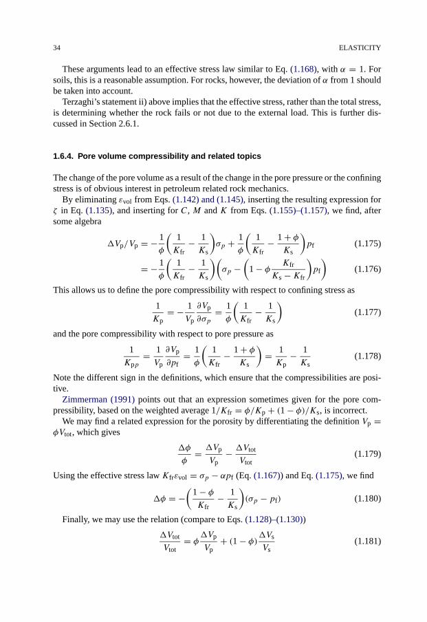
34 ELASTICITY
These arguments lead to an effective stress law similar to Eq. (1.168), with α = 1. Forsoils, this is a reasonable assumption. For rocks, however, the deviation of α from 1 shouldbe taken into account.
Terzaghi’s statement ii) above implies that the effective stress, rather than the total stress,is determining whether the rock fails or not due to the external load. This is further dis-cussed in Section 2.6.1.
1.6.4. Pore volume compressibility and related topics
The change of the pore volume as a result of the change in the pore pressure or the confiningstress is of obvious interest in petroleum related rock mechanics.
By eliminating εvol from Eqs. (1.142) and (1.145), inserting the resulting expression forζ in Eq. (1.135), and inserting for C, M and K from Eqs. (1.155)–(1.157), we find, aftersome algebra
�Vp/Vp = − 1
φ
(1
Kfr− 1
Ks
)σp + 1
φ
(1
Kfr− 1 + φ
Ks
)pf (1.175)
= − 1
φ
(1
Kfr− 1
Ks
)(σp −
(1 − φ Kfr
Ks −Kfr
)pf
)(1.176)
This allows us to define the pore compressibility with respect to confining stress as
1
Kp= − 1
Vp
∂Vp
∂σp= 1
φ
(1
Kfr− 1
Ks
)(1.177)
and the pore compressibility with respect to pore pressure as
1
Kpp= 1
Vp
∂Vp
∂pf= 1
φ
(1
Kfr− 1 + φ
Ks
)= 1
Kp− 1
Ks(1.178)
Note the different sign in the definitions, which ensure that the compressibilities are posi-tive.
Zimmerman (1991) points out that an expression sometimes given for the pore com-pressibility, based on the weighted average 1/Kfr = φ/Kp + (1 − φ)/Ks, is incorrect.
We may find a related expression for the porosity by differentiating the definition Vp =φVtot, which gives
�φ
φ= �Vp
Vp− �Vtot
Vtot(1.179)
Using the effective stress law Kfrεvol = σp − αpf (Eq. (1.167)) and Eq. (1.175), we find
�φ = −(
1 − φKfr
− 1
Ks
)(σp − pf) (1.180)
Finally, we may use the relation (compare to Eqs. (1.128)–(1.130))
�Vtot
Vtot= φ�Vp
Vp+ (1 − φ)�Vs
Vs(1.181)
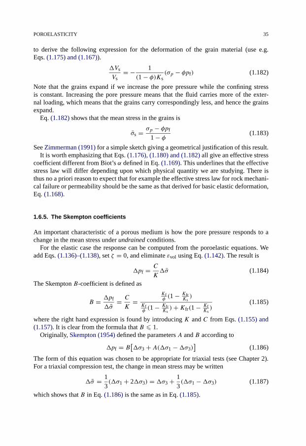
POROELASTICITY 35
to derive the following expression for the deformation of the grain material (use e.g.Eqs. (1.175) and (1.167)).
�Vs
Vs= − 1
(1 − φ)Ks(σp − φpf) (1.182)
Note that the grains expand if we increase the pore pressure while the confining stressis constant. Increasing the pore pressure means that the fluid carries more of the exter-nal loading, which means that the grains carry correspondingly less, and hence the grainsexpand.
Eq. (1.182) shows that the mean stress in the grains is
σs = σp − φpf
1 − φ (1.183)
See Zimmerman (1991) for a simple sketch giving a geometrical justification of this result.It is worth emphasizing that Eqs. (1.176), (1.180) and (1.182) all give an effective stress
coefficient different from Biot’s α defined in Eq. (1.169). This underlines that the effectivestress law will differ depending upon which physical quantity we are studying. There isthus no a priori reason to expect that for example the effective stress law for rock mechani-cal failure or permeability should be the same as that derived for basic elastic deformation,Eq. (1.168).
1.6.5. The Skempton coefficients
An important characteristic of a porous medium is how the pore pressure responds to achange in the mean stress under undrained conditions.
For the elastic case the response can be computed from the poroelastic equations. Weadd Eqs. (1.136)–(1.138), set ζ = 0, and eliminate εvol using Eq. (1.142). The result is
�pf = C
K�σ (1.184)
The Skempton B-coefficient is defined as
B = �pf
�σ= C
K=
Kfφ(1 − Kfr
Ks)
Kfφ(1 − Kfr
Ks)+Kfr(1 − Kf
Ks)
(1.185)
where the right hand expression is found by introducing K and C from Eqs. (1.155) and(1.157). It is clear from the formula that B � 1.
Originally, Skempton (1954) defined the parameters A and B according to
�pf = B[�σ3 + A(�σ1 −�σ3)]
(1.186)
The form of this equation was chosen to be appropriate for triaxial tests (see Chapter 2).For a triaxial compression test, the change in mean stress may be written
�σ = 1
3(�σ1 + 2�σ3) = �σ3 + 1
3(�σ1 −�σ3) (1.187)
which shows that B in Eq. (1.186) is the same as in Eq. (1.185).

36 ELASTICITY
Fig. 1.17. Examples of the variation of B withKfr, for two porosities. The full lines correspond toKf = 2.5 GPa(“water”) and the dashed lines to Kf = 1 GPa (“oil”). In all cases Ks = 37.5 GPa.
Neglecting Kf relative to Ks in Eq. (1.185), and introducing Biot’s α, we have
B = Kf
Kf + φαKfr
(1.188)
In the weak frame limit, where Kfr can be neglected relative to Ks, we have
B = Kf
Kf + φKfr(1.189)
Some examples of the variation of B (as computed from Eq. (1.185)) are shown inFig. 1.17. Note how B decreases with increasing porosity and decreasing fluid bulk modu-lus. Gas as the pore fluid will clearly give a low B except for very unconsolidated rocks.
1.6.6. The correspondence to thermoelasticity
The equations governing poroelasticity are to some extent similar to the equations govern-ing thermoelasticity. This implies that specific solutions to problems in one field may beused to solve corresponding problems in the other.
By eliminating ζ between Eqs. (1.142) and (1.143) we get
σij =(λ− C2
M
)εvolδij + 2Gεij + C
Mpfδij (1.190)
Introducing α from Eq. (1.169) and defining (compare to Eq. (1.146))
λfr = λ− C2
M(1.191)
we obtain
σij = λfrεvolδij + 2Gεij + αpfδij (1.192)
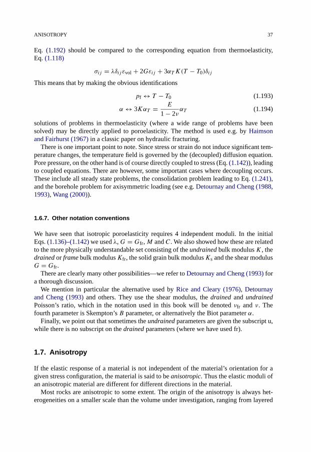
ANISOTROPY 37
Eq. (1.192) should be compared to the corresponding equation from thermoelasticity,Eq. (1.118)
σij = λδij εvol + 2Gεij + 3αT K(T − T0)δij
This means that by making the obvious identifications
pf ↔ T − T0 (1.193)
α ↔ 3KαT = E
1 − 2ναT (1.194)
solutions of problems in thermoelasticity (where a wide range of problems have beensolved) may be directly applied to poroelasticity. The method is used e.g. by Haimsonand Fairhurst (1967) in a classic paper on hydraulic fracturing.
There is one important point to note. Since stress or strain do not induce significant tem-perature changes, the temperature field is governed by the (decoupled) diffusion equation.Pore pressure, on the other hand is of course directly coupled to stress (Eq. (1.142)), leadingto coupled equations. There are however, some important cases where decoupling occurs.These include all steady state problems, the consolidation problem leading to Eq. (1.241),and the borehole problem for axisymmetric loading (see e.g. Detournay and Cheng (1988,1993), Wang (2000)).
1.6.7. Other notation conventions
We have seen that isotropic poroelasticity requires 4 independent moduli. In the initialEqs. (1.136)–(1.142) we used λ,G = Gfr,M and C. We also showed how these are relatedto the more physically understandable set consisting of the undrained bulk modulusK , thedrained or frame bulk modulusKfr, the solid grain bulk modulusKs and the shear modulusG = Gfr.
There are clearly many other possibilities—we refer to Detournay and Cheng (1993) fora thorough discussion.
We mention in particular the alternative used by Rice and Cleary (1976), Detournayand Cheng (1993) and others. They use the shear modulus, the drained and undrainedPoisson’s ratio, which in the notation used in this book will be denoted νfr and ν. Thefourth parameter is Skempton’s B parameter, or alternatively the Biot parameter α.
Finally, we point out that sometimes the undrained parameters are given the subscript u,while there is no subscript on the drained parameters (where we have used fr).
1.7. Anisotropy
If the elastic response of a material is not independent of the material’s orientation for agiven stress configuration, the material is said to be anisotropic. Thus the elastic moduli ofan anisotropic material are different for different directions in the material.
Most rocks are anisotropic to some extent. The origin of the anisotropy is always het-erogeneities on a smaller scale than the volume under investigation, ranging from layered

38 ELASTICITY
Fig. 1.18. Illustration of intrinsic (lithological) and stress induced anisotropy.
sequences of different rock types down to molecular configurations. Sedimentary rocksare created during a deposition process where the grains normally are not deposited ran-domly. For instance, in a river environment, there is a preferred direction (the directionof the streaming water) along which elongated or plane grains will have a tendency to beoriented. Seasonal variations in the fluid flow rates may result in alternating microlayersof fine and coarser grain size distributions. The elastic moduli of rocks created under suchconditions will be dependent on the orientation of the material, i.e. they are anisotropic.Due to its origin, anisotropy of this type is said to be lithological or intrinsic.
Another important type is anisotropy induced by external stresses. The anisotropy isthen normally caused by microcracks, generated by a deviatoric stress and predominantlyoriented normal to the lowest principal stress. The microstructure causing the two types ofanisotropy is illustrated in Fig. 1.18.
In calculations on rock elasticity, anisotropy is often ignored. This simplification maybe necessary rather than just comfortable, because—as we shall see—an anisotropic de-scription requires much more information about the material—information that may notbe available. However, by ignoring anisotropy, one may in some cases introduce large er-rors that invalidate the calculations.
For a general anisotropic material, each stress component is linearly related to everystrain component by independent coefficients. In the mathematical notation used inEqs. (1.9) and (1.75) this may be expressed as
σij =∑k,l
Cijklεkl (1.195)
where Cijkl are elastic constants. Since the indices i, j , k and l may each take the values 1,2 or 3, there are all together 81 of the constants Cijkl . Some of these vanish and others areequal by symmetry, however, so that the number of independent constants is considerablyless. From Eqs. (1.6)–(1.8), (1.74) and (1.195) it may be deduced that
Cijkl = Cjikl = Cijlk = Cjilk (1.196)
i.e. interchanging the first index with the second one, or the third with the fourth, doesnot change the value of the constant. Furthermore, fulfilment of the equations of the type
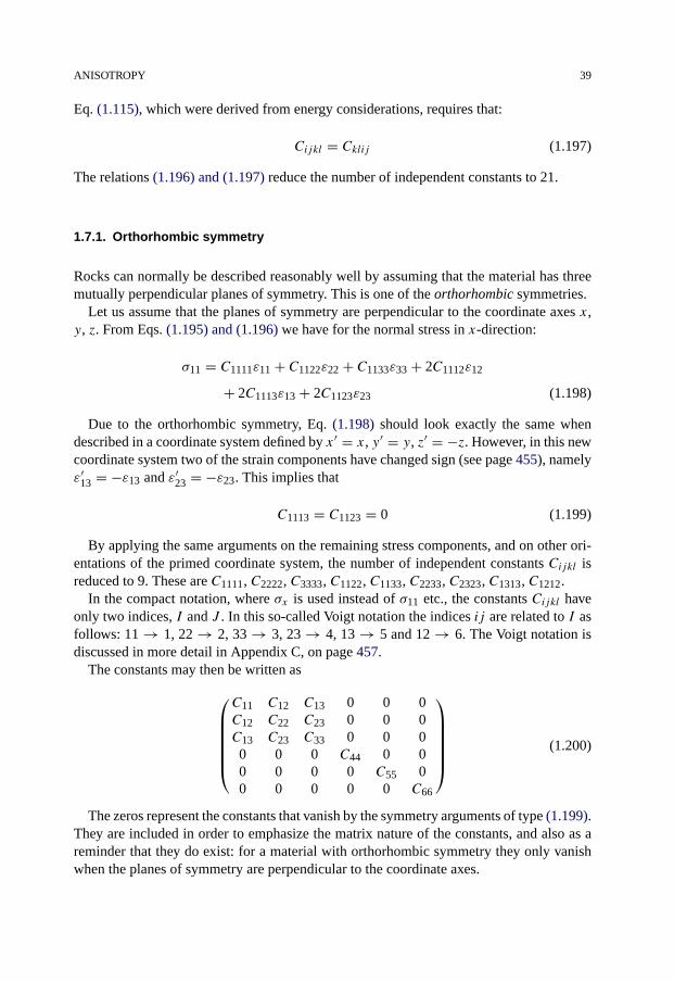
ANISOTROPY 39
Eq. (1.115), which were derived from energy considerations, requires that:
Cijkl = Cklij (1.197)
The relations (1.196) and (1.197) reduce the number of independent constants to 21.
1.7.1. Orthorhombic symmetry
Rocks can normally be described reasonably well by assuming that the material has threemutually perpendicular planes of symmetry. This is one of the orthorhombic symmetries.
Let us assume that the planes of symmetry are perpendicular to the coordinate axes x,y, z. From Eqs. (1.195) and (1.196) we have for the normal stress in x-direction:
σ11 = C1111ε11 + C1122ε22 + C1133ε33 + 2C1112ε12
+ 2C1113ε13 + 2C1123ε23 (1.198)
Due to the orthorhombic symmetry, Eq. (1.198) should look exactly the same whendescribed in a coordinate system defined by x′ = x, y′ = y, z′ = −z. However, in this newcoordinate system two of the strain components have changed sign (see page 455), namelyε′13 = −ε13 and ε′23 = −ε23. This implies that
C1113 = C1123 = 0 (1.199)
By applying the same arguments on the remaining stress components, and on other ori-entations of the primed coordinate system, the number of independent constants Cijkl isreduced to 9. These are C1111, C2222, C3333, C1122, C1133, C2233, C2323, C1313, C1212.
In the compact notation, where σx is used instead of σ11 etc., the constants Cijkl haveonly two indices, I and J . In this so-called Voigt notation the indices ij are related to I asfollows: 11 → 1, 22 → 2, 33 → 3, 23 → 4, 13 → 5 and 12 → 6. The Voigt notation isdiscussed in more detail in Appendix C, on page 457.
The constants may then be written as
⎛⎜⎜⎜⎜⎜⎝
C11 C12 C13 0 0 0C12 C22 C23 0 0 0C13 C23 C33 0 0 0
0 0 0 C44 0 00 0 0 0 C55 00 0 0 0 0 C66
⎞⎟⎟⎟⎟⎟⎠ (1.200)
The zeros represent the constants that vanish by the symmetry arguments of type (1.199).They are included in order to emphasize the matrix nature of the constants, and also as areminder that they do exist: for a material with orthorhombic symmetry they only vanishwhen the planes of symmetry are perpendicular to the coordinate axes.
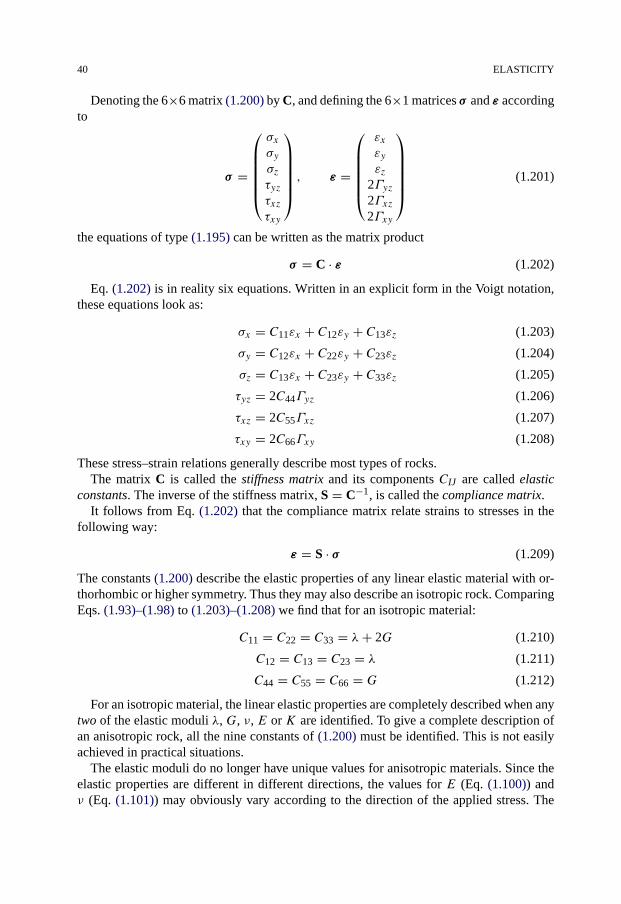
40 ELASTICITY
Denoting the 6×6 matrix (1.200) by C, and defining the 6×1 matrices σ and ε accordingto
σ =
⎛⎜⎜⎜⎜⎜⎝
σxσyσzτyzτxzτxy
⎞⎟⎟⎟⎟⎟⎠ , ε =
⎛⎜⎜⎜⎜⎜⎝
εxεyεz
2Γyz2Γxz2Γxy
⎞⎟⎟⎟⎟⎟⎠ (1.201)
the equations of type (1.195) can be written as the matrix product
σ = C · ε (1.202)
Eq. (1.202) is in reality six equations. Written in an explicit form in the Voigt notation,these equations look as:
σx = C11εx + C12εy + C13εz (1.203)
σy = C12εx + C22εy + C23εz (1.204)
σz = C13εx + C23εy + C33εz (1.205)
τyz = 2C44Γyz (1.206)
τxz = 2C55Γxz (1.207)
τxy = 2C66Γxy (1.208)
These stress–strain relations generally describe most types of rocks.The matrix C is called the stiffness matrix and its components CIJ are called elastic
constants. The inverse of the stiffness matrix, S = C−1, is called the compliance matrix.It follows from Eq. (1.202) that the compliance matrix relate strains to stresses in the
following way:
ε = S · σ (1.209)
The constants (1.200) describe the elastic properties of any linear elastic material with or-thorhombic or higher symmetry. Thus they may also describe an isotropic rock. ComparingEqs. (1.93)–(1.98) to (1.203)–(1.208) we find that for an isotropic material:
C11 = C22 = C33 = λ+ 2G (1.210)
C12 = C13 = C23 = λ (1.211)
C44 = C55 = C66 = G (1.212)
For an isotropic material, the linear elastic properties are completely described when anytwo of the elastic moduli λ, G, ν, E or K are identified. To give a complete description ofan anisotropic rock, all the nine constants of (1.200) must be identified. This is not easilyachieved in practical situations.
The elastic moduli do no longer have unique values for anisotropic materials. Since theelastic properties are different in different directions, the values for E (Eq. (1.100)) andν (Eq. (1.101)) may obviously vary according to the direction of the applied stress. The

ANISOTROPY 41
bulk modulus K is an exception, however: as both the hydrostatic pressure σp and thevolumetric strain εvol are invariant to the orientation of the material, the bulk modulus isalso invariant.
As an example, consider the uniaxial stress state defining Young’s modulus and Pois-son’s ratio (Fig. 1.15). In this example, σy = σz = 0 and τxy = τxz = τyz = 0. Thestress–strain relations (1.203)–(1.208) then become:
σx = C11εx + C12εy + C13εz (1.213)
0 = C12εx + C22εy + C23εz (1.214)
0 = C13εx + C23εy + C33εz (1.215)
0 = 2C44Γyz (1.216)
0 = 2C55Γxz (1.217)
0 = 2C66Γxy (1.218)
Solving Eqs. (1.214) and (1.215) for ν = −εy/εx , we find
ν = −εyεx
= C12C33 − C13C23
C22C33 − C223
(1.219)
while for ν = −εz/εx we find (by interchanging indices 2 and 3):
ν = − εzεx
= C13C22 − C12C23
C22C33 − C223
(1.220)
Thus the value of Poisson’s ratio depends not only on the direction of the applied stress,but also on the direction in which lateral expansion is measured.
1.7.2. Transverse isotropy
A special type of symmetry, which is relevant for many types of rocks, is full rotationalsymmetry around one axis. Rocks possessing such symmetry are said to be transverselyisotropic. It implies that the elastic properties are equal for all directions within a plane,but different in the other directions. This extra element of symmetry reduces the numberof independent elastic constants to 5.
Assuming that the x- and y-directions are equivalent while the z-direction is the differentone, we may rotate the coordinate system any angle around the z-axis without alteringthe elastic constants. For this to be possible it is required that C11 = C22, C13 = C23,C12 = C11 − 2C66, and C44 = C55. The stiffness matrix for a transversely isotropicmaterial having the z-axis as the unique axis is then⎛
⎜⎜⎜⎜⎜⎝
C11 C11 − 2C66 C13 0 0 0C11 − 2C66 C11 C13 0 0 0C13 C13 C33 0 0 00 0 0 C44 0 00 0 0 0 C44 00 0 0 0 0 C66
⎞⎟⎟⎟⎟⎟⎠ (1.221)
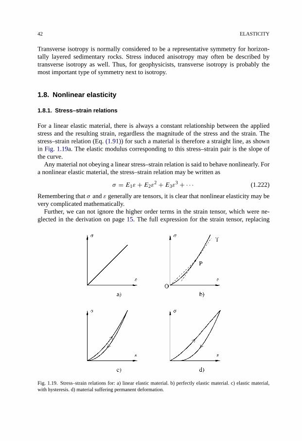
42 ELASTICITY
Transverse isotropy is normally considered to be a representative symmetry for horizon-tally layered sedimentary rocks. Stress induced anisotropy may often be described bytransverse isotropy as well. Thus, for geophysicists, transverse isotropy is probably themost important type of symmetry next to isotropy.
1.8. Nonlinear elasticity
1.8.1. Stress–strain relations
For a linear elastic material, there is always a constant relationship between the appliedstress and the resulting strain, regardless the magnitude of the stress and the strain. Thestress–strain relation (Eq. (1.91)) for such a material is therefore a straight line, as shownin Fig. 1.19a. The elastic modulus corresponding to this stress–strain pair is the slope ofthe curve.
Any material not obeying a linear stress–strain relation is said to behave nonlinearly. Fora nonlinear elastic material, the stress–strain relation may be written as
σ = E1ε + E2ε2 + E3ε
3 + · · · (1.222)
Remembering that σ and ε generally are tensors, it is clear that nonlinear elasticity may bevery complicated mathematically.
Further, we can not ignore the higher order terms in the strain tensor, which were ne-glected in the derivation on page 15. The full expression for the strain tensor, replacing
Fig. 1.19. Stress–strain relations for: a) linear elastic material. b) perfectly elastic material. c) elastic material,with hysteresis. d) material suffering permanent deformation.

NONLINEAR ELASTICITY 43
Eq. (1.74), is (see e.g. Landau and Lifshitz, 1986):
εij = 1
2
(∂ui
∂xj+ ∂uj
∂xi+
3∑l=1
∂ul
∂xi
∂ul
∂xj
)(1.223)
Nonlinear behaviour may have various causes, and appear in many different ways.Fig. 1.19b shows one example. This material has a nonlinear stress–strain relation, sincethe ratio of stress to strain is not the same for all stresses. The relation is, however, identicalfor the loading and unloading process. Such materials are said to be perfectly elastic.
For nonlinear stress–strain relations the elastic modulus is no longer uniquely defined,not even for a specific stress level. As shown in Fig. 1.19b, the modulus related to thepoint P on the curve may either be identified as the slope of the line OP (secant modulus),or it may be identified as the slope of the tangent PT (tangent modulus).
If the correct definition for the moduli is used, the linear form of the stress strain relationsmay be used far beyond the initial linear region. For example, Hooke’s law (Eq. (1.91)) maybe written in its original form:
σ = Esec(ε)ε (1.224)
where Esec(ε) is the secant value of the Young’s modulus. Alternatively, the relation maybe written in a differential form:
�σ = Etan(ε)�ε (1.225)
where �σ and �ε represent differential increments in stress and strain, respectively.Etan(ε) is the tangent value of the Young’s modulus. Note, however, that both Etan(ε) andEsec(ε) depend on the strain ε. This complicates the use of the equations. By comparingEqs. (1.224) and (1.225), we observe that the relation between the secant modulus and thetangent modulus is:
Esec(ε) = 1
ε
∫ ε
0Etan(ε
′) dε′ (1.226)
The stress–strain relation shown in Fig. 1.19c is commonly observed in rocks. The unload-ing path is different from the loading path. This effect is called hysteresis. For materialsbehaving like this, the work done during loading is not entirely released during unload-ing, i.e. a part of the strain energy dissipates in the material. Elastic moduli related to theunloading path are called unloading moduli.
If, as in Fig. 1.19c, the strain vanishes when the stress returns to zero, the material issaid to be elastic. If not, as in Fig. 1.19d, the material has suffered a permanent deformationduring the loading/unloading cycle. For sufficiently large stresses, many rocks enter a phasewhere permanent deformation occurs, yet the material is still able to resist loading (i.e. theslope of the stress–strain curve is still positive). The material is then said to be ductile. Thepoint where the transition from elastic to ductile behaviour occurs is called the yield point.
In Eqs. (1.224)–(1.226) the elastic modulus has been expressed as a function of strain.Since there is a relation between the applied stress and the resulting strain, we might haveexpressed the modulus as a function of stress rather than strain. In general, the elasticmoduli depend on all components of stress (or all components of strain). For example,Young’s modulus may depend on the confining pressure, as shown in Fig. 2.3.

44 ELASTICITY
1.8.2. The impact of cracks
Cracks occur in all types of rocks, and they generally have a large impact on the elasticproperties of the material. For some materials, like poorly consolidated sedimentary rocks,it may be difficult to imagine the presence of cracks. However, weak or failing grain con-tacts have much of the same impact on elastic parameters as cracks have, and may formodelling purposes often be considered as such.
The occurrence of cracks in rocks produce various types of nonlinear behaviour. Weshall here look at a couple of examples. Consider first the situation shown in Fig. 1.20a.The stressed sample contains a crack oriented with its face normal to the stress σx . Sinceno stress can be transferred across the crack itself, the effective Young’s modulus Eeff ofthe sample will be reduced:
σx
εx= Eeff = E(1 − ξQ) (1.227)
Here E is the Young’s modulus of the material without cracks, ξ is called the crack densityand is a function of the size and number of cracks, and Q is a coefficient depending onthe shape and orientation of the crack. (Micromechanical models for calculation of Q andequivalent parameters are described in Section 6.4.) As the stress is increased, the strainεx also increases. A part of the strain increase is due to closure of the crack. At a certainstress level σcx the crack is closed. At stresses above this point ξ will vanish, and Eeff → E
according to Eq. (1.227). The stress strain relation for this sample is then as shown inFig. 1.20b.
For a material containing many cracks of different sizes and closure stresses, the stress–strain relation may look as Fig. 1.19b. Such closure of cracks as stress increases mayexplain the typical feature that elastic constants of rocks normally increase with increasinghydrostatic pressure.
Fig. 1.20. Nonlinear stress–strain relation due to crack closure.
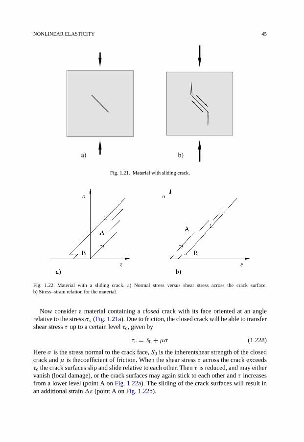
NONLINEAR ELASTICITY 45
Fig. 1.21. Material with sliding crack.
Fig. 1.22. Material with a sliding crack. a) Normal stress versus shear stress across the crack surface.b) Stress–strain relation for the material.
Now consider a material containing a closed crack with its face oriented at an anglerelative to the stress σx (Fig. 1.21a). Due to friction, the closed crack will be able to transfershear stress τ up to a certain level τc, given by
τc = S0 + μσ (1.228)
Here σ is the stress normal to the crack face, S0 is the inherentshear strength of the closedcrack and μ is thecoefficient of friction. When the shear stress τ across the crack exceedsτc the crack surfaces slip and slide relative to each other. Then τ is reduced, and may eithervanish (local damage), or the crack surfaces may again stick to each other and τ increasesfrom a lower level (point A on Fig. 1.22a). The sliding of the crack surfaces will result inan additional strain �ε (point A on Fig. 1.22b).

46 ELASTICITY
Upon unloading, τ is reduced and may eventually become equal to −τc. A reverse slid-ing will then take place (point B on Figs. 1.22a and 1.22b). The stress–strain relation forthe entire sample (Fig. 1.22b) is seen to have a hysteresis. Also, the sample is seen to havesuffered a permanent deformation, since the strain does not go to zero when the stressvanishes.
Real rocks normally contain cracks or crack-like defects of many sizes and differentorientations. The resulting stress–strain relation is typically as shown in Fig. 1.19d.
In Fig. 1.21b the sliding of the crack surfaces is accompanied with the opening of twoother cracks oriented with their faces normal to the direction of the compression stress σ .Opening of cracks with this orientation relative to applied uniaxial stress is a typical fea-ture occurring at high shear stresses. A consequence of such crack opening is an inelasticincrease in the volume of the stressed material. This phenomenon is known as dilatancy.Another consequence is a stress induced mechanical anisotropy, as described in the pre-vious section. The anisotropy may for instance be observed by acoustical techniques (seeSection 5.5).
1.9. Time-dependent effects
So far, we have assumed that any change in applied stress is followed instantaneously bythe corresponding deformation. Quite often, however, it is observed that the deformationof rocks continues for a long time after a change in the applied stress. The time-dependenteffects can be divided into two groups: consolidation and creep. Consolidation is due topore pressure gradients induced by a change in the stress state, and the fact that it takestime to re-establish pore pressure equilibrium. Creep is related to visco-elastic behaviourof the solid framework. In the following, consolidation and creep are discussed separately.In practice, however, it is sometimes difficult to distinguish between genuine creep andconsolidation effects.
1.9.1. Consolidation
Consolidation theory describes the transient process, where pore pressure equilibrium is re-established after a change in the stress state. This process involves a flow of the pore fluidthrough the porous rock. Viscous flow in porous rocks is described by Darcy’s law, whichstates that the fluid flow rate �Q (fluid volume per unit time flowing through a surface), isproportional to the pore pressure gradient ∇pf:
�Q = −A kηf
∇pf (1.229)
Here A is the surface through which the fluid flows, and ηf is the dynamic viscosity of thefluid. k is the permeability of the rock. Normally, k is measured in the unit Darcy, definedas the permeability which gives a flowrate of one centimetre per second of a fluid withviscosity one centipoise for a pressure gradient of one atmosphere per cm. This means that

TIME-DEPENDENT EFFECTS 47
we have 1 D = 0.9869·10−12 m2 since 1 atmosphere is equal to 101325 Pa.2 Permeabilitiesof reservoir rocks may vary from the low milliDarcy region up to several Darcies.
Eq. (1.229) basically describes stationary flow of fluid, in a homogeneous pore pressuregradient field. However, the equation may be further evaluated to make it applicable fordescription of transient processes. The flow rate �Q expresses the difference between thesolid and fluid displacement rates, i.e.
�Q = Aφ(∂ �us
∂t− ∂ �uf
∂t
)(1.230)
By comparing Eq. (1.230) with the definition (Eq. (1.134)) of the strain parameter ζ , wefind that the divergence of �Q is proportional to the time derivative of ζ , i.e.
∇ · �Q = A∂ζ∂t
(1.231)
Or, by introducing Eq. (1.229),
∂ζ
∂t= − k
ηf∇2pf (1.232)
Eq. (1.232) describes transient fluid flow in a porous rock, and also flow in non-homogeneous pore pressure gradient fields.
We may eliminate ζ from Eq. (1.232) by using Eq. (1.142), to find an equation involvingpf and εvol
k
ηf∇2pf = 1
M
∂pf
∂t− α ∂εvol
∂t(1.233)
Alternatively, we may find an equation involving pf and σ by combining Eqs. (1.232),(1.142) and (1.145)
k
ηf∇2pf = α
KfrB
∂pf
∂t− α
Kfr
∂σ
∂t(1.234)
where B was defined in Eq. (1.185).It is clear that the equations in general involve a coupling between the pore pressure and
the strain or stress of the solid material. Only in special cases will the pore pressure obeyan uncoupled equation. For a thorough discussion, see e.g. Wang (2000) or Detournay andCheng (1993).
We shall now consider an example of decoupled consolidation by considering a simpleexperiment: a porous material is confined with no lateral movement (ux = uy = 0) in avertical column with an impermeable bottom (at z = 0) and a highly permeable piston onthe top (at z = h). The bottom of the sample is fixed, i.e. uz (z = 0) = 0. Initially, at t = 0,
2 In some sciences, including soil mechanics and ground water research, an alternative definition for permeabil-ity with unit m/s is used. The relation to our definition is
k(hydrosciences) = k(petroleum sciences)γw/ηw
where γw and ηw are the specific weight and viscosity of water, respectively.
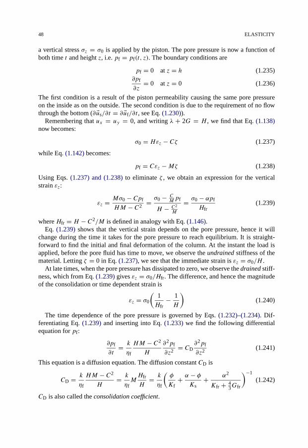
48 ELASTICITY
a vertical stress σz = σ0 is applied by the piston. The pore pressure is now a function ofboth time t and height z, i.e. pf = pf(t, z). The boundary conditions are
pf = 0 at z = h (1.235)∂pf
∂z= 0 at z = 0 (1.236)
The first condition is a result of the piston permeability causing the same pore pressureon the inside as on the outside. The second condition is due to the requirement of no flowthrough the bottom (∂ �us/∂t = ∂ �uf/∂t , see Eq. (1.230)).
Remembering that ux = uy = 0, and writing λ + 2G = H , we find that Eq. (1.138)now becomes:
σ0 = Hεz − Cζ (1.237)
while Eq. (1.142) becomes:
pf = Cεz −Mζ (1.238)
Using Eqs. (1.237) and (1.238) to eliminate ζ , we obtain an expression for the verticalstrain εz:
εz = Mσ0 − Cpf
HM − C2= σ0 − C
Mpf
H − C2
M
= σ0 − αpf
Hfr(1.239)
where Hfr = H − C2/M is defined in analogy with Eq. (1.146).Eq. (1.239) shows that the vertical strain depends on the pore pressure, hence it will
change during the time it takes for the pore pressure to reach equilibrium. It is straight-forward to find the initial and final deformation of the column. At the instant the load isapplied, before the pore fluid has time to move, we observe the undrained stiffness of thematerial. Letting ζ = 0 in Eq. (1.237), we see that the immediate strain is εz = σ0/H .
At late times, when the pore pressure has dissipated to zero, we observe the drained stiff-ness, which from Eq. (1.239) gives εz = σ0/Hfr. The difference, and hence the magnitudeof the consolidation or time dependent strain is
εz = σ0
(1
Hfr− 1
H
)(1.240)
The time dependence of the pore pressure is governed by Eqs. (1.232)–(1.234). Dif-ferentiating Eq. (1.239) and inserting into Eq. (1.233) we find the following differentialequation for pf:
∂pf
∂t= k
ηf
HM − C2
H
∂2pf
∂z2= CD
∂2pf
∂z2(1.241)
This equation is a diffusion equation. The diffusion constant CD is
CD = k
ηf
HM − C2
H= k
ηfMHfr
H= k
ηf
(φ
Kf+ α − φ
Ks+ α2
Kfr + 43Gfr
)−1
(1.242)
CD is also called the consolidation coefficient.

TIME-DEPENDENT EFFECTS 49
Fig. 1.23. Settlement caused by consolidation as a function of time. The solid curve represents the settlement ofa column of finite height, while the dashed curve represents the settlement for an infinitely high column. (AfterBiot, 1941, with permission from AIP.)
Eq. (1.241) and the boundary conditions (1.235) and (1.236) fully determine the porepressure pf(t, z). Biot (1941) discussed the solution of the problem, and found that thesettlement uz can be written in terms of an infinite series. He also provided an approximatesolution, which applies to the settlement of an infinitely high column (h → ∞), or to theinitial settlement (t → 0) of a column of finite height:
uz(t) ≈ 2√πσ0
(1
Hfr− 1
H
)√CDt (1.243)
This result is illustrated in Fig. 1.23.By assuming Kfr,Gfr � Ks, we find that the diffusion constant CD is approximately
given by:
CD ≈ kKf
ηfφ
[1 + Kf
φ(Kfr + 43Gfr)
]−1
(1.244)
In the “stiff frame” limit Kfr,Gfr Kf/φ, and we find that the fluid flow is governed bythe permeability and the elastic properties of the fluid:
CD → k
ηf
Kf
φ(1.245)
On the other hand, if Kfr,Gfr � Kf/φ, the flow is governed more by the elastic propertiesof the framework:
CD → k
ηf
(Kfr + 4
3Gfr
)(1.246)
Physically, CD is a measure of how far (lD) a pore pressure disturbance can propagateduring a given time (τD). The length lD is called the diffusion length and relates to τD andCD as
l2D = CDτD (1.247)
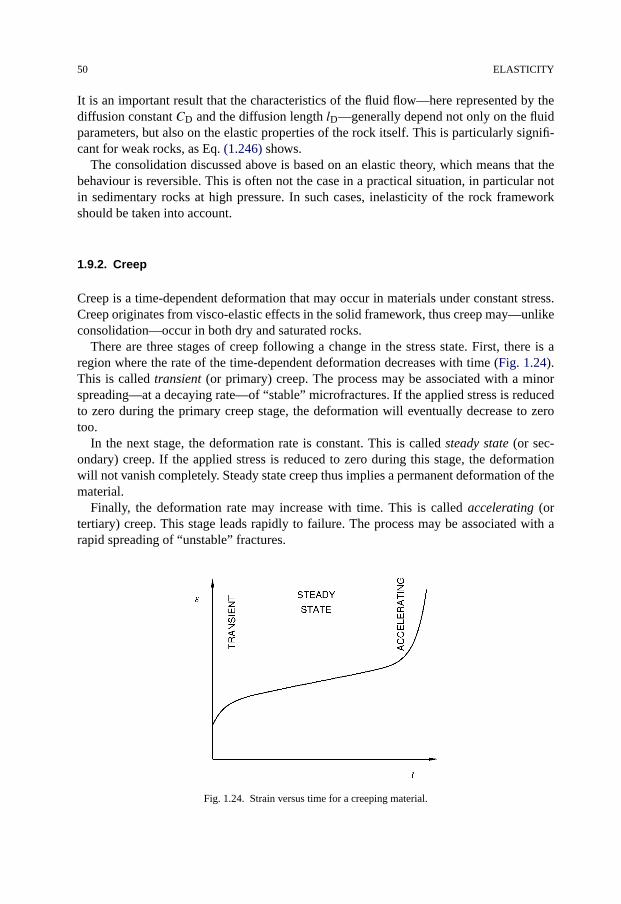
50 ELASTICITY
It is an important result that the characteristics of the fluid flow—here represented by thediffusion constant CD and the diffusion length lD—generally depend not only on the fluidparameters, but also on the elastic properties of the rock itself. This is particularly signifi-cant for weak rocks, as Eq. (1.246) shows.
The consolidation discussed above is based on an elastic theory, which means that thebehaviour is reversible. This is often not the case in a practical situation, in particular notin sedimentary rocks at high pressure. In such cases, inelasticity of the rock frameworkshould be taken into account.
1.9.2. Creep
Creep is a time-dependent deformation that may occur in materials under constant stress.Creep originates from visco-elastic effects in the solid framework, thus creep may—unlikeconsolidation—occur in both dry and saturated rocks.
There are three stages of creep following a change in the stress state. First, there is aregion where the rate of the time-dependent deformation decreases with time (Fig. 1.24).This is called transient (or primary) creep. The process may be associated with a minorspreading—at a decaying rate—of “stable” microfractures. If the applied stress is reducedto zero during the primary creep stage, the deformation will eventually decrease to zerotoo.
In the next stage, the deformation rate is constant. This is called steady state (or sec-ondary) creep. If the applied stress is reduced to zero during this stage, the deformationwill not vanish completely. Steady state creep thus implies a permanent deformation of thematerial.
Finally, the deformation rate may increase with time. This is called accelerating (ortertiary) creep. This stage leads rapidly to failure. The process may be associated with arapid spreading of “unstable” fractures.
Fig. 1.24. Strain versus time for a creeping material.
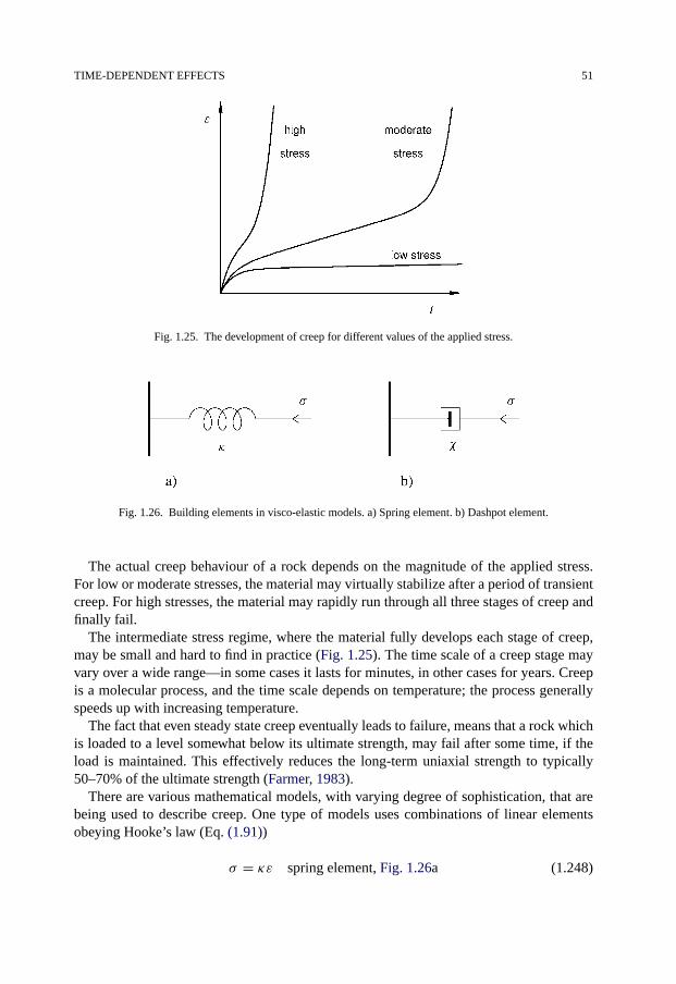
TIME-DEPENDENT EFFECTS 51
Fig. 1.25. The development of creep for different values of the applied stress.
Fig. 1.26. Building elements in visco-elastic models. a) Spring element. b) Dashpot element.
The actual creep behaviour of a rock depends on the magnitude of the applied stress.For low or moderate stresses, the material may virtually stabilize after a period of transientcreep. For high stresses, the material may rapidly run through all three stages of creep andfinally fail.
The intermediate stress regime, where the material fully develops each stage of creep,may be small and hard to find in practice (Fig. 1.25). The time scale of a creep stage mayvary over a wide range—in some cases it lasts for minutes, in other cases for years. Creepis a molecular process, and the time scale depends on temperature; the process generallyspeeds up with increasing temperature.
The fact that even steady state creep eventually leads to failure, means that a rock whichis loaded to a level somewhat below its ultimate strength, may fail after some time, if theload is maintained. This effectively reduces the long-term uniaxial strength to typically50–70% of the ultimate strength (Farmer, 1983).
There are various mathematical models, with varying degree of sophistication, that arebeing used to describe creep. One type of models uses combinations of linear elementsobeying Hooke’s law (Eq. (1.91))
σ = κε spring element, Fig. 1.26a (1.248)

52 ELASTICITY
Fig. 1.27. The Burgers substance. The Burgers substance can be seen as consisting of two simpler substances,the Maxwell substance (a spring and a dashpot in series) and the Kelvin substance (a spring and a dashpot inparallel).
Fig. 1.28. The response of the Burgers substance. a) Applied stress versus time. b) Strain versus time.
and viscous elements obeying the stress–strain relation
σ = χ ∂ε∂t
dashpot element, Fig. 1.26b (1.249)
Here κ is the spring constant, while χ is called the coefficient of viscosity.One of these models (the “Burgers substance”) is shown in Fig. 1.27. This model takes
into account both instantaneous strain, transient creep, and steady state creep. Considerfor instance a stress path as shown in Fig. 1.28a. For t < 0 the system is unstrained. Att = 0 the stress is increased toΣ , while at t = tc the stress is released. The resulting strain(shown in Fig. 1.28b) is found to be
ε =
⎧⎪⎨⎪⎩
0 for t < 0Σκ2
+ Σκ1
(1 − e−t/t1)+ Σ
χ2t for 0 < t < tc
Σκ1
(etc/t1 − 1
)e−t/t1 + Σ
χ2tc for t > tc
(1.250)

REFERENCES 53
Here t1 = χ1/κ1 is the time constant of the transient creep.The instantaneous strain is seen to be: Σ/κ2, the steady state creep velocity: Σ/χ2 and
the permanent strain resulting from the stress path: Σtc/χ2. Thus the permanent strain isseen to arise from the steady state creep. Due to this term, the system has a “memory” ofits stress history.
It is generally assumed that creep is proportional to the deviatoric stresses in a material,while hydrostatic stresses alone will not produce creep effects. Thus creep effectively re-duces the shear modulus and the Young’s modulus of a material, while the bulk modulus isnot affected by it. It follows from Table 1.1 that Poisson’s ratio increases due to creep. Notehowever, that there may be local shear stresses in a sample subject to external hydrostaticloading, due to inhomogeneities in the material. In that case the material may creep underhydrostatic external loads. Such creep has been observed in sandstones.
References
Biot, M.A. (1941). “General theory of three-dimensional consolidation”. J. Appl. Phys. 12, 155–164.Biot, M.A. (1962). “Mechanics of deformation and acoustic propagation in porous media”. J. Appl. Phys. 33,
1482–1498.Cheng, A.H.-D. (1998). “On generalized plain strain poroelasticity”. Int. J. Rock Mech. Min. Sci. 35, 183–193.Coussy, O. (2004). Poromechanics. John Wiley & Sons, Ltd., Chichester, England, ISBN 0-470-84920-7.Detournay, E., Cheng, A.H.-D. (1988). “Poroelastic response of a borehole in a non-hydrostatic stress field”. Int.
J. Rock Mech. Min. Sci. & Geomech. Abstr. 25, 171–182.Detournay, E., Cheng, A.H.-D. (1993). “Fundamentals of poroelasticity”. In: Hudson, J.T. (Ed.), Comprehensive
Rock Engineering. Pergamon Press, Oxford, pp. 113–171.Farmer, T. (1983). Engineering Behaviour of Rocks. Chapman and Hall, London.Haimson, B., Fairhurst, C. (1967). “Initiation and extension of hydraulic fractures in rocks”. Soc. Petr. Eng. J. 7,
310–318.Landau, L.D., Lifshitz, E.M. (1986). Theory of Elasticity, third ed. Pergamon Press.Rice, J.R., Cleary, M.P. (1976). “Some basic stress diffusion solutions for fluid-saturated elastic porous media
with compressible constituents”. Rev. Geophys. Space Phys. 14, 222–241.Skempton, A.W. (1954). “The pore pressure coefficients A and B”. Geotechnique 4, 143–147.Wang, H.F. (2000). Theory of Linear Poroelasticity. Princeton University Press, Princeton.Zimmerman, R.W. (1991). Compressibility of Sandstones. Elsevier Science Publishers, B.V., Amsterdam.
Further reading
Berryman, J.G. (1992). “Effective stress for transport properties of inhomogeneous rock”. J. Geophys. Res. B 97,17409–17424.
Berryman, J.G. (1999). “Origin of Gassmann’s equations”. Geophysics 64, 1627–1629.Biot, M.A. (1955). “Theory of elasticity and consolidation for a porous anisotropic solid”. J. Appl. Phys. 26,
182–185.Biot, M.A. (1956). “General solutions of the equations of elasticity and consolidation for a porous material”.
J. Appl. Mech. 23, 91–96.Biot, M.A., Willis, D.G. (1957). “The elastic coefficients of the theory of consolidation”. J. Appl. Mech. 24,
594–601.de Boer, R. (2000). Theory of Porous Media. Highlights in Historical Development and Current State. Springer,
Berlin, ISBN 3-540-65982-X.
54 ELASTICITY
Brown, R.J.S., Korringa, J. (1975). “On the dependence of the elastic properties of a porous rock on the com-pressibility of the pore fluid”. Geophysics 40, 608–616.
Charlez, P.A. (1991). Rock Mechanics. Volume I. Theoretical Fundamentals. Éditions Technip, Paris.Cheng, A.H.D., Abousleiman, Y., Roegiers, J.-C. (1993). “Review of some poroelastic effects in rock mechanics”.
Int. J. Rock Mech. Min. Sci. & Geomech. Abstr. 30, 1119–1126.Cheng, A.H.-D. (1997). “Material coefficients of anisotropic poroelasticity”. Int. J. Rock Mech. Min. Sci. 34,
199–205.Findley, W.N., Lai, J.S., Onaran, K. (1976). “Creep and Relaxation of Nonlinear Viscoelastic Materials”. Dover
Publications Inc., New York.Gassmann, F. (1951). “Über die Elastizität poröser Medien”. Vierteljahrsschrift der Naturforschenden Gesellshaft
in Zürich 96, 1–23.Hatheway, A.W., Kiersch, G.A. (1982). “Engineering properties of rocks”. In: Carmichael, R.S. (Ed.), Handbook
of Physical Properties of Rocks. Volume II. CRC Press Inc., Florida, pp. 289–331.Jaeger, J.C., Cook, N.G.W. (1979). Fundamentals of Rock Mechanics, third ed. Chapman and Hall, London.Jaeger, J.C., Cook, N.G.W., Zimmerman, R.W. (2007). Fundamentals of Rock Mechanics, fourth ed. Blackwell
Publishing.Nur, A., Byerlee, J.D. (1971). “An Exact effective stress law for elastic deformation of rock with fluids”. J. Geo-
phys. Res. 76, 6414–6419.Terzaghi, K. (1943). Theoretical Soil Mechanic. Wiley, New York.Timoshenko, S.P., Goodier, J.N. (1970). Theory of Elasticity, third ed. McGraw–Hill Kogakusha, Ltd., Tokyo.Zimmerman, R.W. (2000). “Coupling in poroelasticity and thermoelasticity”. Int. J. Rock Mech. & Min. Sci. 37,
79–97.

55
Chapter 2
Failure mechanics
2.1. Basic concepts
When a piece of rock is subject to sufficiently large stresses, a failure of some kind willoccur. This implies that the rock changes its shape permanently, and possibly also fallsapart. The condition is accompanied with a reduced ability to carry loads. Rock failure isan important phenomenon also for petroleum related rock mechanics, as it is the origin ofsevere problems such as borehole instability and solids production. It is therefore useful tobe able to predict under which conditions a rock is likely to fail.
This chapter discusses the most elementary and well known models for rock failure. Oneshould keep in mind however, that these are only simplified descriptions of real rock be-haviour. Rock failure is a complex process which is still not fully understood. Much of theframework used to handle rock failure is therefore based on convenient mathematical de-scriptions of observed behaviour, rather than derivations from basic laws of physics. Someof the concepts used here, including the concept of failure, may thus be poorly defined andsometimes not very relevant, as will be seen below.
For most of the chapter we shall assume that rocks are homogeneous and isotropic.Anisotropy is discussed in Section 2.9, while some consequences of inhomogeneities arebriefly discussed in Sections 2.5 and 2.8.
2.1.1. Strength and related concepts
The stress level at which a rock typically fails is commonly called the strength of the rock.Obviously, as “stress level” is not a uniquely defined parameter, neither is strength. Rockstrength is therefore a meaningful parameter only when the stress geometry—that is: thetype of test, in a laboratory setting—is also specified. We shall soon describe the impactof stress geometry on rock strength. First, we shall however take a look at a couple of themost important tests used to measure rock strength, the uniaxial and triaxial tests, in orderto illustrate the complexity of rock failure, and to introduce some basic concepts. Rockmechanical testing procedures for strength measurements will be described in more detailin Chapter 7.
Fig. 2.1 illustrates a typical test specimen, a cylinder with length to diameter ratio 2:1.A pair of pistons applies (axial) stress to the end faces of the cylinder, while a confining oilbath provides a stress of possibly different magnitude to the circumference. It is normallyassumed that the stress state within the specimen is homogeneous. If the confining stressis zero, we have a uniaxial stress test (also called unconfined compression test). When thetest is performed with a non-zero confining pressure, a so-called triaxial test is performed.

56 FAILURE MECHANICS
Fig. 2.1. Typical test specimen for a uniaxial or triaxial test. A typical sample diameter for petroleum applicationsis 38 mm (1 1/2′′).
Fig. 2.2. Principle sketch of stress versus deformation in a uniaxial compression test. In practise, the ductileregion may be very small.
Fig. 2.2 shows a typical result from a uniaxial test. The applied axial stress (denoted σz)is plotted as a function of the axial strain (εz) of the sample. Several important conceptsare defined in the figure:
Elastic region: The rock deforms elastically. If the stress is released, the specimen willreturn to its original state.
Yield point: The point beyond which permanent changes will occur. The sample will nolonger return to is original state upon stress relief.
Uniaxial compressive strength: The peak stress.Ductile region: A region in which the sample undergoes permanent deformation without
loosing the ability to support load.Brittle region: A region in which the specimen’s ability to withstand stress decreases
rapidly as deformation is increased.

BASIC CONCEPTS 57
Fig. 2.3. Triaxial testing: typical influence of the confining pressure on the shape of the differential stress (axialstress minus confining pressure) versus axial strain curves.
A triaxial test is usually performed by increasing the axial and confining loads simulta-neously, until a prescribed hydrostatic stress level is reached. Then, the confining pressureis kept constant while the axial load is increased until failure occurs. The axial loading isnormally applied such that it gives a constant axial deformation rate.
For a triaxial test, it is customary to plot the difference between the axial stress andthe confining pressure (σr ) versus the axial deformation. One then obtains a curve thatlooks similar to Fig. 2.2. However, the behaviour may be quite different at the higher stresslevels. Fig. 2.3 illustrates results from triaxial tests with various confining pressures. It isseen that for the higher confining pressures the specimen’s ability to support load is notlost, although its stiffness is clearly reduced. This is further discussed in Section 2.8.
So far, we have not given a precise definition of failure, mainly because it is ratherdifficult to give a general definition. For the uniaxial test shown in Fig. 2.2, a seeminglyunambiguous definition of failure may be given, corresponding to the peak stress pointon the curve. For the higher confining pressures in Fig. 2.3, one may on the other handdefine failure at some point where the slope of the stress–strain curve changes. This maynot seem totally appropriate, however, since the specimen still supports increasing loadafter it has failed. Disregarding these problems, we shall in the following sections discussfailure criteria assuming that a consistent definition of failure exists. Later, in Section 2.8,on post-failure behaviour described by the theory of plasticity, we shall be a little moreprecise, at least for problems that can be described within the framework of that theory.
The most common mode of failure observed in uniaxial and triaxial tests is shear fail-ure. This failure mode is caused by excessive shear stress. Another failure mode is tensilefailure, which is caused by excessive tensile stress. Finally, pore collapse is a failure modethat is normally observed in highly porous materials, where the grain skeleton forms a rel-atively open structure. Pore collapse is usually caused by excessive hydrostatic stress. Thevarious failure modes are discussed in Sections 2.2–2.4.
The concept of rock failure is associated with the state of the solid framework. Thus, thestresses that causes failure are the effective stresses felt by the framework. The effectivestress concept was introduced in Section 1.6.3 where we also introduced the notation σ ′
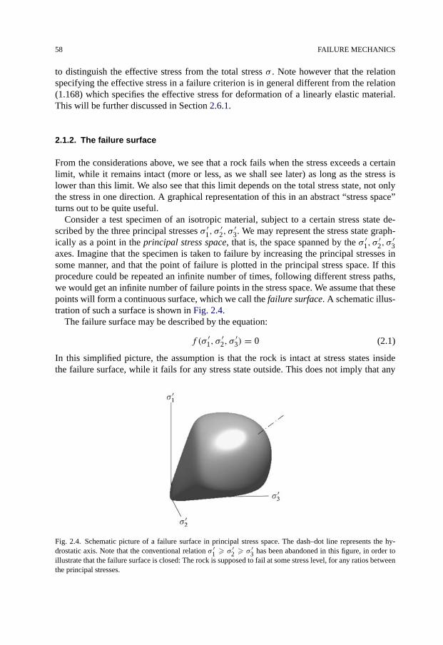
58 FAILURE MECHANICS
to distinguish the effective stress from the total stress σ . Note however that the relationspecifying the effective stress in a failure criterion is in general different from the relation(1.168) which specifies the effective stress for deformation of a linearly elastic material.This will be further discussed in Section 2.6.1.
2.1.2. The failure surface
From the considerations above, we see that a rock fails when the stress exceeds a certainlimit, while it remains intact (more or less, as we shall see later) as long as the stress islower than this limit. We also see that this limit depends on the total stress state, not onlythe stress in one direction. A graphical representation of this in an abstract “stress space”turns out to be quite useful.
Consider a test specimen of an isotropic material, subject to a certain stress state de-scribed by the three principal stresses σ ′
1, σ′2, σ
′3. We may represent the stress state graph-
ically as a point in the principal stress space, that is, the space spanned by the σ ′1, σ
′2, σ
′3
axes. Imagine that the specimen is taken to failure by increasing the principal stresses insome manner, and that the point of failure is plotted in the principal stress space. If thisprocedure could be repeated an infinite number of times, following different stress paths,we would get an infinite number of failure points in the stress space. We assume that thesepoints will form a continuous surface, which we call the failure surface. A schematic illus-tration of such a surface is shown in Fig. 2.4.
The failure surface may be described by the equation:
f (σ ′1, σ
′2, σ
′3) = 0 (2.1)
In this simplified picture, the assumption is that the rock is intact at stress states insidethe failure surface, while it fails for any stress state outside. This does not imply that any
Fig. 2.4. Schematic picture of a failure surface in principal stress space. The dash–dot line represents the hy-drostatic axis. Note that the conventional relation σ ′
1 � σ ′2 � σ ′
3 has been abandoned in this figure, in order toillustrate that the failure surface is closed: The rock is supposed to fail at some stress level, for any ratios betweenthe principal stresses.

TENSILE FAILURE 59
stress state outside the failure surface is inaccessible, since the rock may under suitableconditions be able to support increasing load after failure, as mentioned above.
It is difficult to draw a surface in three dimensions. Therefore, the failure surface isoften presented by cross-sections instead. The most common of such representations arecross-sections in a π-plane. These planes are normal to the hydrostatic axis (also calledhydrostat), that is the axis where σ ′
1 = σ ′2 = σ ′
3. Figs. 2.16 and 2.18 are examples ofπ-plane cross-sections of failure surfaces.
The existence of the failure surface is by no means obvious. For instance, its existenceimplies that failure is independent of stress gradients and of stress history for stress stateson the inner side of the surface. This approximation is not always fulfilled, as we shallsee later in this chapter. Also, we have already seen that failure does not necessarily occurabruptly at the failure point, but may be a gradual process that changes rate at the failuresurface.
In the following, we shall first consider the failure surface in two dimensional stressspace, focusing on the impact of the largest and smallest principal stresses. These config-urations are relatively simple to handle both intuitively and mathematically, and are alsomost commonly used for practical applications. Corresponding failure criteria in three di-mensional stress space is discussed in Section 2.5.
2.2. Tensile failure
Tensile failure occurs when the effective tensile stress across some plane in the sampleexceeds a critical limit. This limit is called the tensile strength, it is given the symbol T0,and has the same unit as stress. The tensile strength is a characteristic property of the rock.Most sedimentary rocks have a rather low tensile strength, typically only a few MPa orless. In fact, it is a standard approximation for several applications that the tensile strengthis zero.
A sample that suffers tensile failure typically splits along one—or very few—fractureplanes, as illustrated in Fig. 2.5. Thus tensile failure is a highly localized and inhomoge-neous process. The fracture planes often originate from preexisting cracks, oriented moreor less normal to the direction of the tensile stress. The highest probability for further dam-age of the rock is at the perimeter of the largest of these cracks, hence the largest crack(s)will grow increasingly faster than the other, and rapidly split the sample. We shall see later(in Section 6.4.4) that the tensile strength is very sensitive to the presence of cracks in thematerial.
The failure criterion, which specifies the stress condition for which tensile failure willoccur, and identifies the location of the failure surface in principal stress space, is given as:
σ ′ = −T0 (2.2)
For isotropic rocks, the conditions for tensile failure will always be fulfilled first for thelowest principal stress, so that the tensile failure criterion becomes
σ ′3 = −T0 (2.3)
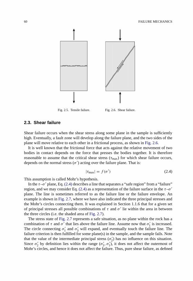
60 FAILURE MECHANICS
Fig. 2.5. Tensile failure. Fig. 2.6. Shear failure.
2.3. Shear failure
Shear failure occurs when the shear stress along some plane in the sample is sufficientlyhigh. Eventually, a fault zone will develop along the failure plane, and the two sides of theplane will move relative to each other in a frictional process, as shown in Fig. 2.6.
It is well known that the frictional force that acts against the relative movement of twobodies in contact depends on the force that presses the bodies together. It is thereforereasonable to assume that the critical shear stress (τmax) for which shear failure occurs,depends on the normal stress (σ ′) acting over the failure plane. That is:
|τmax| = f (σ ′) (2.4)
This assumption is called Mohr’s hypothesis.In the τ–σ ′ plane, Eq. (2.4) describes a line that separates a “safe region” from a “failure”
region, and we may consider Eq. (2.4) as a representation of the failure surface in the τ–σ ′plane. The line is sometimes referred to as the failure line or the failure envelope. Anexample is shown in Fig. 2.7, where we have also indicated the three principal stresses andthe Mohr’s circles connecting them. It was explained in Section 1.1.6 that for a given setof principal stresses all possible combinations of τ and σ ′ lie within the area in betweenthe three circles (i.e. the shaded area of Fig. 2.7).
The stress state of Fig. 2.7 represents a safe situation, as no plane within the rock has acombination of τ and σ ′ that lies above the failure line. Assume now that σ ′
1 is increased.The circle connecting σ ′
1 and σ ′3 will expand, and eventually touch the failure line. The
failure criterion is then fulfilled for some plane(s) in the sample, and the sample fails. Notethat the value of the intermediate principal stress (σ ′
2) has no influence on this situation.Since σ ′
2 by definition lies within the range (σ ′3, σ
′1), it does not affect the outermost of
Mohr’s circles, and hence it does not affect the failure. Thus, pure shear failure, as defined

SHEAR FAILURE 61
Fig. 2.7. Failure line, as specified by Eq. (2.4), in the shear stress–normal stress diagram. Also shown are theMohr circles connecting the principal stresses σ ′
1, σ′2, σ
′3.
by Mohr’s hypothesis, depends only on the minimum and maximum principal stresses andnot on the intermediate stress.
By choosing specific forms of the function f (σ ′) of Eq. (2.4), various criteria for shearfailure are obtained. The simplest possible choice is a constant. The resulting criterion iscalled the Tresca criterion. The criterion simply states that the material will yield when acritical level of shear stress is reached:
τmax = 1
2(σ ′
1 − σ ′3) = S0 (2.5)
S0 is the inherent shear strength (also called cohesion) of the material. In a Mohr τ–σ ′ plotthe Tresca criterion appears simply as a straight horizontal line.
2.3.1. The Mohr–Coulomb criterion
A more general and frequently used criterion is the Mohr–Coulomb criterion, which isbased on the assumption that f (σ ′) is a linear function of σ ′:
|τ | = S0 + μσ ′ (2.6)
Here μ is the coefficient of internal friction. The latter term is clearly chosen by anal-ogy with sliding of a body on a surface, which to the first approximation is described byAmontons’ law:
τ = μσ ′ (2.7)
In Fig. 2.8 we have drawn the Mohr–Coulomb criterion, and a Mohr’s circle that touchesthe failure line. The angle ϕ defined in the Figure is called the angle of internal friction (orfriction angle) and is related to the coefficient of internal friction by
tanϕ = μ (2.8)

62 FAILURE MECHANICS
Fig. 2.8. Mohr–Coulomb criterion in τ–σ ′ space. Also shown is the Mohr’s circle corresponding to a criticalstress state.
Note that the Tresca criterion can be considered as a special case of the Mohr–Coulombcriterion, with ϕ = 0.
The intersection point between the Mohr–Coulomb failure line and the normal stressaxis is of no practical interest in itself, as the point is inaccessible due to tensile failure.However, for some purposes it is convenient to make use of the parameter A defined as thedistance from the intersection point to the origin (see Fig. 2.8). The parameter is called theattraction. The attraction is related to the other Mohr–Coulomb parameters by
A = S0 cotϕ (2.9)
Fig. 2.8 also shows the angle 2β, which gives the position of the point where the Mohr’scircle touches the failure line. It can be seen from the figure that the shear stress at thispoint of contact is
|τ | = 1
2(σ ′
1 − σ ′3) sin 2β (2.10)
while the normal stress is
σ ′ = 1
2(σ ′
1 + σ ′3)+
1
2(σ ′
1 − σ ′3) cos 2β (2.11)
Also, we see that β and ϕ are related by
ϕ + π
2= 2β (2.12)
Since β is the angle for which the failure criterion is fulfilled, β gives the orientation of thefailure plane (see Fig. 1.7). From Eq. (2.12) we have that
β = π
4+ ϕ
2(2.13)
The allowable range for ϕ is from 0° to 90° (in practice the range will be smaller, andcentred around approximately 30°), hence it is clear that β may vary between 45° and 90°.We may conclude that the failure plane is always inclined at an angle smaller that 45° to
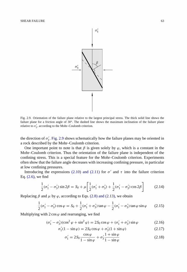
SHEAR FAILURE 63
Fig. 2.9. Orientation of the failure plane relative to the largest principal stress. The thick solid line shows thefailure plane for a friction angle of 30°. The dashed line shows the maximum inclination of the failure planerelative to σ ′
1, according to the Mohr–Coulomb criterion.
the direction of σ ′1. Fig. 2.9 shows schematically how the failure planes may be oriented in
a rock described by the Mohr–Coulomb criterion.One important point to note is that β is given solely by ϕ, which is a constant in the
Mohr–Coulomb criterion. Thus the orientation of the failure plane is independent of theconfining stress. This is a special feature for the Mohr–Coulomb criterion. Experimentsoften show that the failure angle decreases with increasing confining pressure, in particularat low confining pressures.
Introducing the expressions (2.10) and (2.11) for σ ′ and τ into the failure criterionEq. (2.6), we find
1
2(σ ′
1 − σ ′3) sin 2β = S0 + μ
[1
2(σ ′
1 + σ ′3)+
1
2(σ ′
1 − σ ′3) cos 2β
](2.14)
Replacing β and μ by ϕ, according to Eqs. (2.8) and (2.13), we obtain
1
2(σ ′
1 − σ ′3) cosϕ = S0 + 1
2(σ ′
1 + σ ′3) tanϕ − 1
2(σ ′
1 − σ ′3) tanϕ sinϕ (2.15)
Multiplying with 2 cosϕ and rearranging, we find
(σ ′1 − σ ′
3)(cos2 ϕ + sin2 ϕ) = 2S0 cosϕ + (σ ′1 + σ ′
3) sinϕ (2.16)
σ ′1(1 − sinϕ) = 2S0 cosϕ + σ ′
3(1 + sinϕ) (2.17)
σ ′1 = 2S0
cosϕ
1 − sinϕ+ σ ′
31 + sinϕ
1 − sinϕ(2.18)

64 FAILURE MECHANICS
Fig. 2.10. Mohr–Coulomb criterion in the (σ ′1, σ
′3) plane.
Fig. 2.10 is a plot of this relation in the (σ ′1, σ
′3) plane. Again we have a linear relation-
ship, with a positive intercept on the σ ′1-axis, quite similar to the plot in Fig. 2.8. The angle
γ in the (σ ′1, σ
′3) plane is related to ϕ by
tan γ = 1 + sinϕ
1 − sinϕ(2.19)
or
sinϕ = tan γ − 1
tan γ + 1(2.20)
An expression for the uniaxial compressive strength C0 is obtained by putting σ ′3 = 0 in
Eq. (2.18), giving
C0 = 2S0cosϕ
1 − sinϕ= 2S0 tanβ (2.21)
The last equality here is derived from Eq. (2.12). It must be emphasized that the aboveexpression is only valid if the failure mechanism under uniaxial stress is shear failure. Thismay not be the case even when shear failure occurs at rather low confining stresses.
Making use of Eqs. (2.21) and (2.12), we note that Eq. (2.18) may be written in thefollowing simple way:
σ ′1 = C0 + σ ′
3 tan2 β (2.22)
This formulation of the Mohr–Coulomb criterion will be extensively used later in this book.One might perhaps consider computing the tensile strength T0 by putting σ ′
1 = 0 inEq. (2.22). However, this is not a valid approach, since the Mohr–Coulomb criterion de-scribes shear failure while tensile failure is a different failure mode.

SHEAR FAILURE 65
2.3.2. The Griffith criterion
Griffith (1921) developed a failure criterion based on a study of elliptical microcracks ina two dimensional model. When the tensile stress at the tip of the crack exceeds a certainvalue characteristic of the material, the crack will grow and the failure process is initiated.The theory is scaled in terms of the uniaxial tensile strength T0, and the resulting failurecriterion can be written
(σ ′1 − σ ′
3)2 = 8T0(σ
′1 + σ ′
3) if σ ′1 + 3σ ′
3 > 0 (2.23)
σ ′3 = −T0 if σ ′
1 + 3σ ′3 < 0 (2.24)
In a principal stress plot the criterion is represented by a parabola ending in a straight line.This is illustrated in Fig. 2.11a.
The uniaxial compressive strength C0 is given by Eq. (2.23) as
C0 = 8T0 (2.25)
It is seen that the ratio between the uniaxial compressive strength and the tensile strengthis here given as a fixed number. This ratio of 8 appears to be reasonable compared toexperimental values, which often are in the range of 10–15. However, it is clear that fittingthe criterion to experimental data may sometimes be difficult, since the criterion only hasone free parameter.
In τ–σ ′-coordinates, the Griffith criterion is given by only one equation:
τ 2 = 4T0(σ′ + T0) (2.26)
Fig. 2.11. The Griffith criterion. a. Principal stress plot. b. τ–σ ′-plot.

66 FAILURE MECHANICS
(See for instance Jaeger and Cook (1979) for the transition from Eqs. (2.23) and (2.24) toEq. (2.26).)
Eq. (2.26) shows that the criterion is a parabola also in a τ–σ ′-plot, as illustrated inFig. 2.11b. Unlike the Mohr–Coulomb criterion, the Griffith criterion is seen to have asteeper slope at low confining pressures. This feature is typical for experimental observa-tions.
It is often observed that the Griffith criterion may give a reasonably good descriptionof failure at low confining stresses, while a straight line Mohr–Coulomb criterion gives abetter description at higher confining stresses. This has led to the development of a modi-fied Griffith criterion (Brace, 1960; McClintock and Walsh, 1962). This criterion is basedon the idea that the microcracks will close at sufficiently high pressure levels, resulting ina transition towards frictional behaviour corresponding to the Mohr–Coulomb criterion. Ifwe assume that the stress required to close the cracks is so small that it can be neglected,the modified Griffith criterion is simply a Griffith criterion for tensile conditions (σ ′ < 0)coupled to a Mohr–Coulomb criterion for compressive conditions (σ ′ > 0). The criticalshear stress τ = 2T0 predicted by the Griffith criterion at σ ′ = 0 (see Eq. (2.26)) is usedfor the cohesion S0 in the Mohr–Coulomb part of the criterion. A result from this modifiedtheory is that the ratio between uniaxial compressive strength and the tensile strength isgiven by
C0
T0= 4√
μ2 + 1 − μ (2.27)
where μ is the coefficient of internal friction related to the Mohr–Coulomb part of thecriterion.
2.4. Compaction failure
Pore collapse is a failure mode that is normally observed only in high porosity materials,where the grain skeleton forms a relatively open structure. When the material is com-pressed, grains may loosen or break and then be pushed or twisted into the open porespace, resulting in a closer packing of the material. The process is called compaction. Thisdeformation mode is schematically illustrated in Fig. 2.12.
In sandstones where the size of the pores is of the same order of magnitude as the sizeof the grains, pore collapse typically consists in reorientation of the grains to better fillthe void spaces, as indicated in Fig. 2.12. For high porosity chalks, where the size of theindividual grains may be an order of magnitude smaller than the dimensions of the porespace, the pore collapse mechanism becomes very important.
Pore collapse may occur under pure hydrostatic loading. Microscopically, however, fail-ure will be due to local excessive shear forces acting through grains and grain contacts.From this point of view, pore collapse may be regarded as distributed shear failure withinthe material.
Another failure mechanism that may occur under hydrostatic loading is grain crushing.If the stresses are sufficiently high, the grains may be partly crushed at the grain con-tacts, and splitting of the grains may result. Either way, these local failure mechanisms

COMPACTION FAILURE 67
Fig. 2.12. Grain reorientation resulting in a closer packing.
Fig. 2.13. Location of the various failure modes in principal stress space, as defined by Eq. (2.3) for tensilefailure, by Eq. (2.22) for shear failure, and by Eq. (2.29) (assuming σ ′
2 = σ ′3) for compactive yield. For real
rocks, the transition between the various failure modes is smoother than shown here.
represent permanent damage of the rock framework and causes yielding, with associatedreduction in the stiffness of the rock. This type of failure also occurs to some extent undernon-hydrostatic stress conditions, and may be observed in triaxial tests at high confiningpressure (see Fig. 2.3; high confining pressure). The process is then referred to as shear-enhanced compaction.
In principal stress space, this type of failure is represented by an “end cap” that closesthe failure surface at high stresses, as seen on Fig. 2.13. An elliptical form is often used for
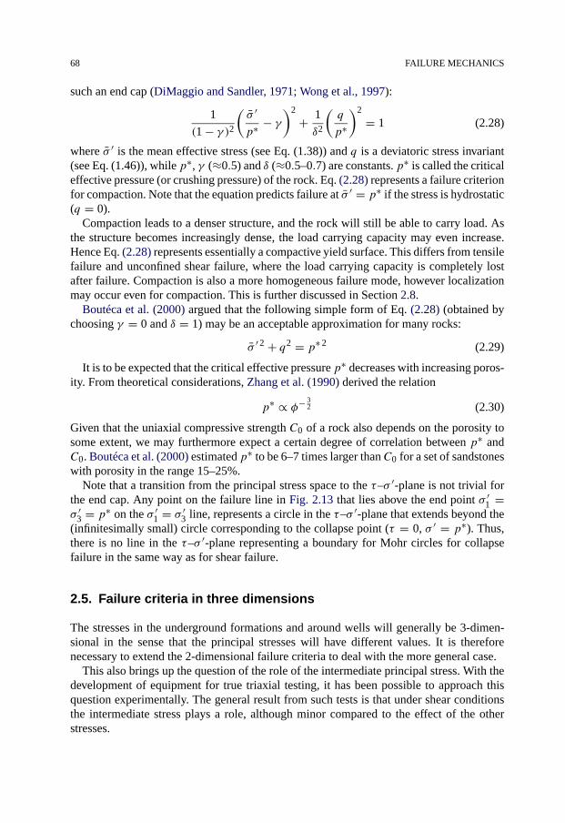
68 FAILURE MECHANICS
such an end cap (DiMaggio and Sandler, 1971; Wong et al., 1997):
1
(1 − γ )2(σ ′
p∗ − γ)2
+ 1
δ2
(q
p∗
)2
= 1 (2.28)
where σ ′ is the mean effective stress (see Eq. (1.38)) and q is a deviatoric stress invariant(see Eq. (1.46)), while p∗, γ (≈0.5) and δ (≈0.5–0.7) are constants. p∗ is called the criticaleffective pressure (or crushing pressure) of the rock. Eq. (2.28) represents a failure criterionfor compaction. Note that the equation predicts failure at σ ′ = p∗ if the stress is hydrostatic(q = 0).
Compaction leads to a denser structure, and the rock will still be able to carry load. Asthe structure becomes increasingly dense, the load carrying capacity may even increase.Hence Eq. (2.28) represents essentially a compactive yield surface. This differs from tensilefailure and unconfined shear failure, where the load carrying capacity is completely lostafter failure. Compaction is also a more homogeneous failure mode, however localizationmay occur even for compaction. This is further discussed in Section 2.8.
Boutéca et al. (2000) argued that the following simple form of Eq. (2.28) (obtained bychoosing γ = 0 and δ = 1) may be an acceptable approximation for many rocks:
σ ′ 2 + q2 = p∗ 2 (2.29)
It is to be expected that the critical effective pressure p∗ decreases with increasing poros-ity. From theoretical considerations, Zhang et al. (1990) derived the relation
p∗ ∝ φ− 32 (2.30)
Given that the uniaxial compressive strength C0 of a rock also depends on the porosity tosome extent, we may furthermore expect a certain degree of correlation between p∗ andC0. Boutéca et al. (2000) estimated p∗ to be 6–7 times larger thanC0 for a set of sandstoneswith porosity in the range 15–25%.
Note that a transition from the principal stress space to the τ–σ ′-plane is not trivial forthe end cap. Any point on the failure line in Fig. 2.13 that lies above the end point σ ′
1 =σ ′
3 = p∗ on the σ ′1 = σ ′
3 line, represents a circle in the τ–σ ′-plane that extends beyond the(infinitesimally small) circle corresponding to the collapse point (τ = 0, σ ′ = p∗). Thus,there is no line in the τ–σ ′-plane representing a boundary for Mohr circles for collapsefailure in the same way as for shear failure.
2.5. Failure criteria in three dimensions
The stresses in the underground formations and around wells will generally be 3-dimen-sional in the sense that the principal stresses will have different values. It is thereforenecessary to extend the 2-dimensional failure criteria to deal with the more general case.
This also brings up the question of the role of the intermediate principal stress. With thedevelopment of equipment for true triaxial testing, it has been possible to approach thisquestion experimentally. The general result from such tests is that under shear conditionsthe intermediate stress plays a role, although minor compared to the effect of the otherstresses.

FAILURE CRITERIA IN THREE DIMENSIONS 69
2.5.1. Criteria independent of the intermediate principal stress
Most of the failure criteria used in rock mechanics were developed before the role of theintermediate principal stress was clear. As the real influence of the intermediate principalstress is relatively small (compared to the significance of the other two) such criteria arestill valuable approximations, and will still be used.
From Fig. 2.10 we are able to infer how the Mohr–Coulomb failure surface looks like inthe three dimensional principal stress space (σ ′
1, σ′2, σ
′3). We shall here temporarily abandon
the conventional relation that σ ′1 � σ ′
2 � σ ′3, in order to illustrate the entire surface.
First, we consider the situation when σ ′2 is the intermediate principal stress. The two cases
σ ′1 > σ
′3 and σ ′
1 < σ′3 can be represented by two lines that are symmetric around the line
σ ′1 = σ ′
3, as shown in Fig. 2.14. The figure shows the projection onto the (σ ′1, σ
′3) plane of
the part of the surface for which σ ′2 is intermediate. Similar projections can be made onto
the (σ ′1, σ
′2) plane for the case where σ ′
3 is intermediate, and onto the (σ ′2, σ
′3) plane for the
case where σ ′1 is intermediate. The complete failure surface is indicated in Fig. 2.15. The
figure shows that opposite pairs of surface sections project onto the (σ ′1, σ
′3), (σ ′
2, σ′3) and
(σ ′1, σ
′2) planes, respectively, along lines as indicated on Fig. 2.14.
The irregular hexagonal pyramid shape of the surface reflects that according to theMohr–Coulomb criterion, failure is independent of the intermediate principal stress. Thesurface is not differentiable at the corners, a fact that may cause problems in numerical cal-culations involving the criterion. The cross-section of the Mohr–Coulomb failure surfacein a π-plane (see Section 2.1.2) is shown in Fig. 2.16. It is seen to be an irregular hexagonwith sharp corners and threefold symmetry.
The Tresca criterion also has a six sided cross-section in the π-plane, but for this crite-rion the section will be a regular hexagon. As the friction angle is zero, the failure surfacewill be parallel to the hydrostatic axis.
Fig. 2.14. Projections onto the (σ ′1, σ
′3) plane, of the
parts of the of the failure surface for which σ ′2 is the in-
termediate principal stress. Note the symmetry about theprojection of the hydrostatic axis (dashed line).
Fig. 2.15. The Mohr–Coulomb failure surface inprincipal stress space.

70 FAILURE MECHANICS
Fig. 2.16. Cross-section of the Mohr–Coulomb criterion in a π -plane. The arrows represent projections of theprincipal stress axes onto the plane. The friction angle ϕ = 30°.
A 3-dimensional failure surface can be obtained for the Griffith criterion in a similarway as for the Mohr–Coulomb criterion. The three pairs of planes ending in a sharp cornerfor the Mohr–Coulomb criterion (Fig. 2.15) is for the Griffith criterion replaced by threepairs of singly curved parabolic surfaces ending in a plane section.
The failure surface constructions presented here demonstrate one basic feature of thefailure surface in 3 dimensions, namely the three-fold symmetry of the π-plane cross-section. However, they suffer from the fact that they ignore the influence of the intermediateprincipal stress. Other extensions to 3 dimensions have therefore been proposed, as dis-cussed below.
2.5.2. Criteria depending on the intermediate principal stress
Mounting experimental evidence has shown that the intermediate principal stress (σ ′2) has
a significant—although moderate—impact on the strength of several rock types (see forinstance Colmenares and Zoback (2002), for an overview). Typically, it is found that rocksare stronger when σ ′
1 > σ′2 > σ
′3 than for the situations where σ ′
2 = σ ′1 or σ ′
2 = σ ′3.
As mentioned in the previous paragraph, the failure surfaces constructed simply on thebasis of two-dimensional criteria also possess sharp corners that causes problems when thecriteria are used for numerical modelling. Various other failure criteria which include theintermediate principal stress have therefore been proposed.
One simple solution is to implement rotational symmetry for the π-plane cross-section.This approach has no physical foundation, however it is mathematically attractive, and isthe basis for some of the most commonly used criteria shown below. (Alternative formula-tions of these criteria, in terms of invariants, are given in Section 2.7.)
One of these criteria is the von Mises criterion, which can be written
(σ ′1 − σ ′
2)2 + (σ ′
1 − σ ′3)
2 + (σ ′2 − σ ′
3)2 = C2 (2.31)
C is a material parameter related to cohesion. In principal stress space this criterion isrepresented by a cylinder centred around the hydrostatic axis, as illustrated in Fig. 2.17.

FAILURE CRITERIA IN THREE DIMENSIONS 71
Fig. 2.17. The von Mises criterion and the Drucker–Prager criterion in principal stress space.
The criterion is seen to be identical to the Tresca criterion for σ ′2 = σ ′
1 or σ ′2 = σ ′
3. Likethe Tresca criterion, the von Mises criterion describes a shear failure mechanism where thefailure condition is independent of the stress level in the material. The von Mises criterionis commonly used to describe yield in metals. It has however very limited applications forrocks.
The corresponding generalization of the Mohr–Coulomb criterion is the Drucker–Pragercriterion. It can be formulated as
(σ ′1 − σ ′
2)2 + (σ ′
1 − σ ′3)
2 + (σ ′2 − σ ′
3)2 = C1(σ
′1 + σ ′
2 + σ ′3 + C2)
2 (2.32)
where C1 and C2 are material parameters, related to internal friction and cohesion. Inprincipal stress space this corresponds to a regular cone, as illustrated in Fig. 2.17.
Murrel (1963) introduced the extended Griffith criterion, which degenerates to the orig-inal Griffith criterion (Eqs. (2.23)–(2.24)) in two dimensions. In principal stress space it isrepresented by a paraboloid terminated by a pyramid, expressed as
(σ ′1 − σ ′
2)2 + (σ ′
1 − σ ′3)
2 + (σ ′2 − σ ′
3)2 = 24T0(σ
′1 + σ ′
2 + σ ′3) (2.33)
ending on the planes
σ ′1 = −T0, σ ′
2 = −T0, σ ′3 = −T0 (2.34)
The extended Griffith criterion predicts that the relation between uniaxial compressivestrength and tensile strength is given by
C0 = 12T0 (2.35)
This value of C0/T0 is typical for many rocks. Also for this criterion the cross-section inthe π-plane is given by a circle, except for the conical part at negative stresses.
An empirical failure criterion based on actual observations of the behaviour of soilswas formulated by Lade (1977). A modified version of this criterion was presented by

72 FAILURE MECHANICS
Ewy (1999):
I ′ 3
I ′3
− 33 = ηL (2.36)
where I ′1 and I ′
3 are modified representations of the first and third stress invariant, definedas
I ′1 = (σ ′
1 + SL)+ (σ ′2 + SL)+ (σ ′
3 + SL) (2.37)
I ′3 = (σ ′
1 + SL)(σ′2 + SL)(σ
′3 + SL) (2.38)
SL is a material parameter related to the cohesion and the friction angle of the rock:
SL = S0
tanϕ(2.39)
while ηL is related only to the internal friction:
ηL = 4 tan2 ϕ9 − 7 sinϕ
1 − sinϕ(2.40)
In principal stress space the criterion has the form of a convex, triangularly shaped cone.The parameter ηL determines the shape of the cross-section in the π-plane. As the value ofηL increases, the cross-sectional shape changes from circular to triangular with smoothlyrounded edges. Fig. 2.18 shows a comparison of the modified Lade criterion to other crite-ria in the π-plane.
The modified Lade criterion is a simple criterion which appears to account for the influ-ence of the intermediate principal stress on shear strength in a realistic way. As such, this is
Fig. 2.18. Characteristic shape of a π -plane cross-section for some failure criteria. The friction angle ϕ = 22.5°.The arrows represent projections of the principal stress axes onto the plane. Note that the criteria have been scaledso that they coincide at the intercepts with the projections of the principal stress axes.

FAILURE CRITERIA IN THREE DIMENSIONS 73
a useful criterion for practical calculations. The formulation based on I ′1 and I ′
3 (Eq. (2.36))may however be somewhat impractical, as it requires solution of a cubic equation. An al-ternative formulation is given in Eqs. (2.41)–(2.44)).
π -plane representation
The Drucker–Prager, von Mises and Murrel criteria are circular in the π-plane, while themodified Lade and Mohr–Coulomb criteria have a 3-fold symmetry. It is clear that for anisotropic material, the yield surface must at least have a 3-fold symmetry in the π-plane.This means that in general, the failure surface in principal stress space may be given byspecifying the mean stress, and the radius in the π-plane as a periodic function of the angle3ϑ (where ϑ is the Lode angle defined in Eq. (1.51) and Fig. 1.10).
The radial distance to a point on the failure surface is given by Eq. (1.50). Defining twogeneral functions f1 and f2 we may thus write a general failure criterion as√
J2 = f1(cos 3ϑ)f2(σ′) (2.41)
where the cosine function ensures the required symmetry in the π-plane, and the factor 2of Eq. (1.50) has been absorbed in f1 and f2. The separation of ϑ and σ ′ means that theshape of the π-plane cross-section is independent of σ ′.
The choice of the cosine in Eq. (2.41) is convenient, since cos 3ϑ can be expressedin terms of invariants (Eq. (1.51)), and does not represent a limitation since any periodicfunction may be expressed by a series in cos 3ϑ .
The function f1 can not be chosen completely arbitrarily, since both empirical evidence(see e.g. Lade, 1993) and theoretical considerations (see e.g. Chen and Han, 1988) indicatethat the failure surface should be convex. If we choose f1 to be a constant, Eq. (2.41)represents the von Mises criterion if f2 is also a constant, the Drucker–Prager criterion iff2 is linear in σ ′, and the extended Griffith criterion if f2 is proportional to the square rootof σ ′.
A representation of the modified Lade criterion can be obtained by expressing I ′1 and I ′
3in terms of σ ′, q and ϑ (see Section 1.1.8), and defining a new variable x = q/(SL + σ ′)(note that
√J2 = x(SL + σ ′)/
√3 ). Introducing these expressions into Eq. (2.36) gives a
cubic equation in x, which can be solved explicitly to give expression (2.42), or iterativelyto give expression (2.43):
f1 = 3
2 cos 3ϑ
(1 − 2 cos
[1
3arccos
(1 − 2ηL cos2 3ϑ
33 + ηL
)± π
3
])(2.42)
=√
3ηL
33 + ηL
[1 + cos 3ϑ
9
√3ηL
33 + ηL+ cos2 3ϑ
27
3ηL
33 + ηL+ · · ·
](2.43)
f2 = 1√3(SL + σ ′) (2.44)
The series expression (2.43) for f1 converges rapidly for low and moderate values of ϕ andmay be the most practical form to use for some purposes, since the two solutions (+ and−) given by Eq. (2.42) have to be patched together to make the solution continuous in ϑ .

74 FAILURE MECHANICS
A general, simple form for f1 may be convenient for practical purposes. We may forinstance choose
f1 = k + (1 − k) cos 3ϑ (2.45)
where k is a number. Choosing k = 1 gives a circular cross-section. Choosing k to makethe uniaxial and biaxial (σ ′
2 = σ ′1) strengths equal, would require
k = 1
2
(1 + 3 − sinϕ
3 + sinϕ
)(2.46)
This relation gives k = 6/7 ≈ 0.857 for ϕ = 30° (note that the convexity criterion requiresk � 10/11 ≈ 0.909). Eqs. (2.45) and (2.46), in combination with
f2 = C01 − sinϕ
3 − sinϕ+ 2
sinϕ
3 − sinϕσ ′ (2.47)
may be used as a rough approximation for the Mohr–Coulomb criterion.By choosing f1 appropriately, it is possible to formulate the Mohr–Coulomb criterion
exactly in terms of the invariants. The expression
f1 = √3
(cosϑ + √
3 sinϑ1 + sinϕ
3 − sinϕ
)−1
(2.48)
in combination with Eq. (2.47) is valid for 0 � ϑ � π/3. By this formulation, we loose theexplicit 3-fold symmetry of Eq. (2.41) (for which we pay by the limited range of validityin ϑ). This is not a major concern, however, since using arccos in Eq. (1.51) maps all stressstates to a ϑ in the correct range.
For papers using the formulation presented here, see e.g. van Eekelen (1980) or Nordalet al. (1989). This representation is convenient for generation of π-plots like Fig. 2.18.
Physical explanations
Wiebols and Cook (1968) proposed a model which offers a physical explanation to theimpact of the intermediate principal stress on rock strength. They considered the shearstrain energy associated with microcracks in the material. Activation of such a crack, interms of sliding between the crack surfaces, will occur when a frictional criterion likethe Mohr–Coulomb criterion (Eq. (2.6)) is fulfilled locally for this crack. The shear andnormal stresses controlling this process are given by the relative orientation of the crack andthe principal stresses (see Eq. (1.36)). The situation is illustrated graphically in Fig. 2.19,showing three different stress states: σ ′
1 > σ′2 = σ ′
3, σ ′1 > σ
′2 > σ
′3, and σ ′
1 = σ ′2 > σ
′3.
We assume that there exists a large number of such cracks with random orientation in thematerial. For simplicity, we also assume that they all have the same activation threshold, sothat the failure line shown in the figure is the same for all cracks. Thus, for every possiblestress state represented by a point on (or within) the Mohr circle(s) in the τ–σ ′-plot thereexist some corresponding cracks that are activated if the point is above the failure line.
The fundamental postulate of Wiebols and Cook is that the material fails when the to-tal strain energy associated with the activated cracks reaches a limit value, which in our

FLUID EFFECTS 75
Fig. 2.19. τ–σ ′-plots with Mohr circles and failure line, for three different stress states.
simplified picture implies that the material fails when a sufficient number of cracks havebeen activated. When σ ′
1 is increased, the cracks with an orientation corresponding to pointP in each diagram will obviously be activated first. For the two cases σ ′
1 > σ′2 = σ ′
3 andσ ′
1 = σ ′2 > σ
′3 there is a large number of cracks corresponding to point P and its vicinity,
due to the rotational symmetry of the stress state in both cases. Hence the total strain energyassociated with these cracks will soon reach the limit value when the σ ′
1–σ ′3-circle crosses
the failure line. For the case σ ′1 > σ
′2 > σ
′3, the stress states are distributed in the shaded
area, and most of these cracks are therefore further away from the failure line. Hence theσ ′
1–σ ′3-circle has to expand further before a sufficient number of cracks is activated so that
the rock fails. As a consequence, the rock is stronger for the case σ ′1 > σ
′2 > σ
′3 than for
the cases σ ′1 > σ
′2 = σ ′
3 and σ ′1 = σ ′
2 > σ′3.
An alternative explanation was proposed by Fjær and Ruistuen (2002). They based theiranalysis on the classical assumption (see Section 2.3) that the rock will fail when the shearstress across a potential failure plane fulfils a failure criterion, like for instance the Mohr–Coulomb criterion. Any imaginary plane through a rock sample is a potential failure plane,hence any point representing a possible stress state in the τ–σ ′-plot (Fig. 2.19) also repre-sents at least one possible failure plane.
Fjær and Ruistuen assumed that there is a variation in the strength of each potentialfailure plane, due to the natural heterogeneity of rocks. This implies that there is a finiteprobability for a plane to fail even if its corresponding point in the Mohr circle diagram liesbelow the failure line, and there is correspondingly a finite probability for the plane not tofail even if its corresponding point lies above the failure line. For the high symmetry casesσ ′
1 > σ′2 = σ ′
3 and σ ′1 = σ ′
2 > σ′3 of Fig. 2.19, there is a large number of planes correspond-
ing to point P which reaches the failure line first, hence there is a high probability that atleast one of these planes will fail early. For the low symmetry case σ ′
1 > σ′2 > σ
′3 nearly
all of the points representing these planes have moved away from the failure line, and theprobability for early failure is correspondingly reduced. The net effect of this is that therock appears as stronger—statistically—for the low stress symmetry case (σ ′
1 > σ′2 > σ
′3)
than for the cases of higher stress symmetry (σ ′1 > σ
′2 = σ ′
3 and σ ′1 = σ ′
2 > σ′3).
2.6. Fluid effects
2.6.1. Pore pressure
In our discussion of failure criteria the pore pressure has so far appeared only indirectlythrough the effective stresses. The effective stresses are thought to represent the forces

76 FAILURE MECHANICS
Fig. 2.20. Mohr circle and failure lines: the effect of increasing pore pressure.
transmitted through the rock skeleton, which in turn causes the deformation of the material,while the remaining parts of the total stresses are carried by the pore fluid. As the porepressure is equal in all directions, it will affect only the normal stresses. The shear stresses,that are due to differences in the principal stresses, will be unaffected. In a τ–σ ′-plot theeffect of increasing the pore pressure while the total stresses are kept constant, is to movethe Mohr circles to the left and closer to the shear and tensile failure lines, as illustrated inFig. 2.20. Thus, increasing pore pressure may destabilize a rock with respect to shear andtensile failure.
The effective stress concept as given by Eq. (1.168) in terms of the Biot constant α, wasderived under the assumption that the rock is linearly elastic, and is not directly applicablefor a rock at failure. It is, however, generally accepted that Terzaghi’s definition of effectivestress (see Section 1.6.3)
σ ′ = σ − pf (2.49)
appears to be the most relevant definition to be used in failure criteria (Detournay andCheng, 1988; Boutéca and Guéguen, 1999).
We may find an argument for this observation by observing that in the vicinity of failure,the rock is softening (that is, the slope of the stress–strain curve is strongly reduced; seeFig. 2.2). It is not obvious however, that Eq. (2.49) is the best definition for the effectiveyield stress, as the rock is supposed to behave elastically until it yields.
2.6.2. Partial saturation
Even unconsolidated sand may have some degree of consolidation. Any child that hasvisited a sandy beach on a sunny day, has experienced the magic of moist sand, whichcan be shaped and reshaped to make all kinds of fantastic figures. When the tide comesand floods the beach, the magic is broken and the figures disintegrate into loose sand. The“magic” is caused by the fact that moist sand is partially water saturated. This means thatthere is a meniscus of water at every grain contact, as shown schematically in Fig. 2.21.
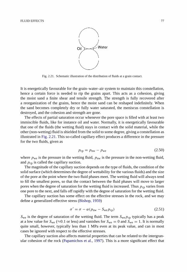
FLUID EFFECTS 77
Fig. 2.21. Schematic illustration of the distribution of fluids at a grain contact.
It is energetically favourable for the grain–water–air system to maintain this constellation,hence a certain force is needed to rip the grains apart. This acts as a cohesion, givingthe moist sand a finite shear and tensile strength. The strength is fully recovered aftera reorganization of the grains, hence the moist sand can be reshaped indefinitely. Whenthe sand becomes completely dry or fully water saturated, the meniscus constellation isdestroyed, and the cohesion and strength are gone.
The effects of partial saturation occur whenever the pore space is filled with at least twoimmiscible fluids, like for instance oil and water. Normally, it is energetically favourablethat one of the fluids (the wetting fluid) stays in contact with the solid material, while theother (non-wetting) fluid is shielded from the solid to some degree, giving a constellation asillustrated in Fig. 2.21. This so-called capillary effect produces a difference in the pressurefor the two fluids, given as
pcp = pnw − pwe (2.50)
where pwe is the pressure in the wetting fluid, pnw is the pressure in the non-wetting fluid,and pcp is called the capillary suction.
The magnitude of the capillary suction depends on the type of fluids, the condition of thesolid surface (which determines the degree of wettability for the various fluids) and the sizeof the pore at the point where the two fluid phases meet. The wetting fluid will always tendto fill the smallest pores, so that the contact between the fluid phases will move to largerpores when the degree of saturation for the wetting fluid is increased. Thus pcp varies fromone pore to the next, and falls off rapidly with the degree of saturation for the wetting fluid.
The capillary suction has some effect on the effective stresses in the rock, and we maydefine a generalized effective stress (Bishop, 1959)
σ ′ = σ − α(pnw − Swepcp) (2.51)
Swe is the degree of saturation of the wetting fluid. The term Swepcp typically has a peakat a low value for Swe (≈0.1 or less) and vanishes for Swe = 0 and Swe = 1. It is normallyquite small, however, typically less than 1 MPa even at its peak value, and can in mostcases be ignored with respect to the effective stresses.
The capillary suction also affects material properties that can be related to the intergran-ular cohesion of the rock (Papamichos et al., 1997). This is a more significant effect that
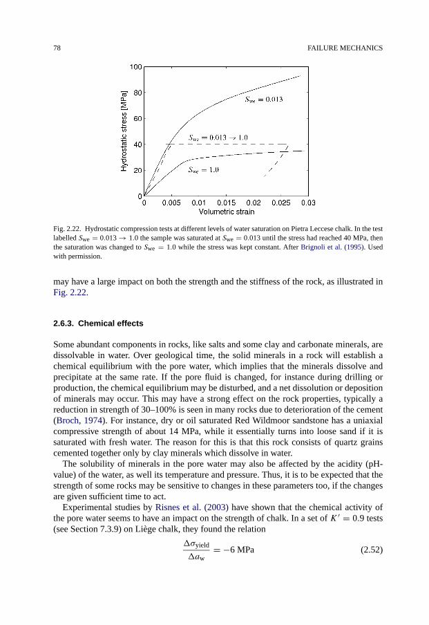
78 FAILURE MECHANICS
Fig. 2.22. Hydrostatic compression tests at different levels of water saturation on Pietra Leccese chalk. In the testlabelled Swe = 0.013 → 1.0 the sample was saturated at Swe = 0.013 until the stress had reached 40 MPa, thenthe saturation was changed to Swe = 1.0 while the stress was kept constant. After Brignoli et al. (1995). Usedwith permission.
may have a large impact on both the strength and the stiffness of the rock, as illustrated inFig. 2.22.
2.6.3. Chemical effects
Some abundant components in rocks, like salts and some clay and carbonate minerals, aredissolvable in water. Over geological time, the solid minerals in a rock will establish achemical equilibrium with the pore water, which implies that the minerals dissolve andprecipitate at the same rate. If the pore fluid is changed, for instance during drilling orproduction, the chemical equilibrium may be disturbed, and a net dissolution or depositionof minerals may occur. This may have a strong effect on the rock properties, typically areduction in strength of 30–100% is seen in many rocks due to deterioration of the cement(Broch, 1974). For instance, dry or oil saturated Red Wildmoor sandstone has a uniaxialcompressive strength of about 14 MPa, while it essentially turns into loose sand if it issaturated with fresh water. The reason for this is that this rock consists of quartz grainscemented together only by clay minerals which dissolve in water.
The solubility of minerals in the pore water may also be affected by the acidity (pH-value) of the water, as well its temperature and pressure. Thus, it is to be expected that thestrength of some rocks may be sensitive to changes in these parameters too, if the changesare given sufficient time to act.
Experimental studies by Risnes et al. (2003) have shown that the chemical activity ofthe pore water seems to have an impact on the strength of chalk. In a set of K ′ = 0.9 tests(see Section 7.3.9) on Liège chalk, they found the relation
�σyield
�aw= −6 MPa (2.52)
PRESENTATION AND INTERPRETATION OF DATA FROM FAILURE TESTS 79
between the yield stress (σyield) and the water activity (aw). Thus, a low salt concentrationin the pore water (which corresponds to a high water activity) makes the chalk weaker.Risnes et al. (2003) concluded that the water activity seems to be the key parameter in thewater weakening effect seen in chalk, and that capillary effects play only a minor role.
2.7. Presentation and interpretation of data from failure tests
To determine the mechanical properties of a rock, normally a series of triaxial compressiontests are performed at different confining pressures. From the stress strain diagrams bothelastic properties and failure or yield data are obtained. The strength data resulting fromsuch a test series will consist of pairs of corresponding yield (or failure) and confiningstresses. This set of failure data can be displayed in different types of diagrams.
It may be confusing that the word failure is often used in a somewhat general sense, notdistinguishing between failure and yield. An argument for this practice is that yield canbe considered as the onset of failure. However, when actual failure data are presented, itshould be checked if the data refer to yield or failure in the strict sense.
Three types of plots are commonly used to present failure data: the principal stress plots(Fig. 2.10), the τ–σ ′ plots (Fig. 2.8), and the q–p′ plots, which will be described below.
In a principal stress plot, the stress path of a given test can be traced as a line, whilefailure is represented by the point where the stress path crosses the failure surface. Theprincipal stress plot is suitable for mapping the entire failure surface, including all types offailure, as demonstrated in Fig. 2.13.
A τ–σ ′ plot displays effectively how the shear stress and the normal stress across a planein a stressed rock varies with the orientation of the plane relative to the orientation of theprincipal stress axes. It is therefore well suited for identifying critical shear stresses, andfor illustrating orientational effects, like Fig. 2.19. As explained in Section 2.4, the τ–σ ′plot is not well suited for displaying collapse.
The q–p′ plot essentially displays the maximum shear stress versus the mean effectivestress. It is based on the parameter q, usually called the generalized shear stress and definedas (see Eq. (1.46))
q = 1√2
√(σ ′
1 − σ ′2)
2 + (σ ′2 − σ ′
3)2 + (σ ′
1 − σ ′3)
2 (2.53)
and the parameter p′ which is identical to the mean effective stress σ ′:
p′ = 1
3(σ ′
1 + σ ′2 + σ ′
3) = σ ′ (2.54)
Both q and p′ are stress invariants (see Sections 1.1.7 and 1.1.8). Under triaxial conditionsσ ′
2 = σ ′3, which implies that q = σ ′
1 − σ ′3.
As for the principal stress plot, the stress path of a given test can be traced as a line in theq–p′ plot, and failure occurs where the stress path crosses the failure line. The q–p′ plotcorresponding to Fig. 2.13 is shown in Fig. 2.23. Note that the transition from Fig. 2.13 toFig. 2.23 is not unique since both q and p′ depend on σ ′
2.

80 FAILURE MECHANICS
Fig. 2.23. Location of the various failure modes in the q–p′ plane, as defined by Eq. (2.3) for tensile failure, byEq. (2.22) for shear failure, and by Eq. (2.29) for compactive yield, assuming σ ′
2 = σ ′3.
Some of the three dimensional failure criteria are simpler to express in terms of q andp′ than in terms of the principal stresses, for instance,
– the von Mises criterion (Eq. (2.31)):
q2 = 1
2C2 (2.55)
– the Drucker–Prager criterion (Eq. (2.32)):
q2 = 1
2C2
1(3p′ + C2)
2 (2.56)
– the modified Lade criterion (Eq. (2.36))—with f1(ϑ, ηL) given by Eq. (2.42); note thesimilarity with Eq. (2.56):
q = f1(ϑ, ηL)(SL + p′) (2.57)
– the extended Griffith criterion (Eq. (2.33)):
q2 = 36T0p′ (2.58)
– and the compactive yield criterion (Eq. (2.29)):
p′ 2 + q2 = p∗ 2 (2.59)
The q–p′ plots are standard for plotting of failure surfaces in soil mechanics (see Sec-tion 2.8.2), and have a growing popularity also in rock mechanics.
2.8. Beyond the yield point
In the previous sections, we have studied various failure criteria and their failure surfacesin principal stress space without clearly expressing what we mean with failure. This is

BEYOND THE YIELD POINT 81
partly due to the fact that failure is not very well defined. Although the failure point canbe defined relatively precisely for the uniaxial test in Fig. 2.2, the situation is much lessclear for the higher confining pressures in Fig. 2.3. Here we have a gradual transition to amaterial with decreased stiffness, but still with an increasing capacity to carry load as thestrain increases. Thus the material can not be considered as completely failed, although ithas been significantly altered at this stage. Whether the alteration is critical or not, dependson the actual situation. For example, the practical criteria for a road tunnel and a wellboremay be quite different. Whereas no change in profile is acceptable for a road tunnel, onemay well live with a borehole with breakouts in many cases (see e.g. Guenot, 1989).
The remarks above illustrate the need for a post-yield description linked to the defin-ition of failure and the failure criterion. To properly describe post-yield behaviour, onewould need a description treating the rock as an inhomogeneous medium, penetrated byinteracting faults and cracks.
Compared to a continuum model, such a description would—of course—be very com-plicated. It is therefore reasonable to look for a continuum theory, that can at least modelsome post-yield behaviour with some precision, although the physical interpretation maybe less precise. One possible candidate is the theory of plasticity, which is widely used inthe description of metals. An introduction to plasticity is given in Section 2.8.1.
Beyond the yield point the solid framework of the rock is gradually destroyed, and itmay become increasingly relevant to compare its behaviour to unconsolidated materials.A model derived for the description of soils is presented in Section 2.8.2.
At some point in the failure process, the description of the rock as homogeneous isclearly not valid, even on a macroscopic scale, as exemplified by the formation of shearplanes in a triaxial test. This calls for other types of modelling. Models addressing local-ization effects at failure are briefly discussed in Section 2.8.3.
2.8.1. Plasticity
Plasticity is a concept describing non-elastic deformation of a material. Unlike elastic de-formation, plastic deformation is not recovered when the load causing the deformation isreleased. Rocks stressed beyond the yield point typically suffer such deformations, and itis often relevant to describe post yield behaviour of rocks by the concepts of plasticity.
The theory of plasticity is designed to model ductile behaviour, that is—behaviour inwhich the material can sustain a load comparable to the failure load well beyond failure,and no attempt should be made to model brittle failure with this theory.
The theory of plasticity is based on four major concepts:
1. Plastic strain. The total strain increment associated with a stress increment is as-sumed to consist of an elastic part and a plastic part:
dεij = dεeij + dεp
ij (2.60)
dεeij is related to the stress increment by conventional elasticity theory, and will vanish
when the stress is released. The plastic strain dεpij is a permanent deformation, and
will remain when the stress is relieved.

82 FAILURE MECHANICS
Fig. 2.24. Stress–strain curve for a linearly elastic – ideally plastic material.
2. A yield criterion. In Section 2.1 we defined yield as the point at which irreversiblechanges occur in the rock. Thus, the yield point represents the onset of plastic defor-mation. Clearly, yield can be defined more precisely than failure. A yield criterion issimilar to the failure criteria defined in Sections 2.2–2.4, and defines the surface instress space where plasticity is initiated.
3. A flow rule. The flow rule describes how the plastic strains develop for a given loadingsituation.
4. A hardening rule. We mentioned in Section 2.1.1 that a rock under certain condi-tions may sustain increasing load after the initial failure. This is described by thehardening rule. The hardening (or, alternatively, the softening) may be interpretedas a change of the yield surface in principal stress space. This can be described bychanging Eq. (2.1) to
f (σ ′1, σ
′2, σ
′3, κ) = 0 (2.61)
where κ is a parameter describing the hardening effects.
An ideally plastic material is a material that can endure infinite plastic strain withoutchange in the stress level. Fig. 2.24 shows schematically the stress–strain diagram for alinearly elastic – ideally plastic material. After the initial elastic phase, the material de-forms at constant stress.
Plastic flow
The function of the flow rule is to describe the development of the plastic strain increments.The basic assumption concerning plastic flow dates back to Saint-Venant in the nineteenthcentury. It states
dεpij = dλhij (σ
′kl) (2.62)
BEYOND THE YIELD POINT 83
where λ is a scalar not specified by the flow rule. It is seen that the hij ’s are functions ofthe stress components. There are two main implications of Eq. (2.62). First, it states thatthe direction of plastic flow is determined by the stress state, and is not influenced by thestress increments or by stress gradients. Second, the magnitude of the plastic strain is notunique. Referring to Fig. 2.24, this is quite trivial for an ideally plastic material, since theyield stress is maintained for any magnitude of the plastic strain.
The assumption that the plastic strains are independent of stress increments, is intuitivelyunderstandable in the following simple example. Consider an object resting on some sur-face, and assume that a force nearly overcoming the rest friction between the object andthe surface is applied. Now, a small force increment is applied at some angle to the pri-mary force. If the increment has a component in the direction of the primary force, the restfriction will be overcome, and the object will start to slide in the direction of the primaryforce, irrespective of the direction of the force increment.
Eq. (2.62) puts some restrictions on the plastic behaviour, however it is far from a com-plete description which requires a specification of the functions hij . Some help is foundfrom the fact that plastic deformation is a dissipative process, which implies that∑
ij
σ ′ijdε
pij � 0 (2.63)
A significant simplification results from the assumption of von Mises (1928), that the hij ’scan be derived as the gradient of a function g in stress space:
dεpij = dλ
∂g
∂σ ′ij
(2.64)
The function g is called plastic potential and must of course be chosen such that Eq. (2.63)is obeyed. Although the assumption of a plastic potential reduces the need for a specifica-tion of six functions hij of six variables to one function g of six variables, it is by no meanssufficient to completely specify plastic flow.
One solution to the problem is Drucker’s (1950) definition of a stable, work hardeningmaterial. Such a material is defined by a more strict version of Eq. (2.63):∑
ij
dσ ′ijdε
pij � 0 (2.65)
Note that while Eq. (2.63) is a thermodynamic law, Eq. (2.65) is not, and thus the con-sequences derived from Eq. (2.65) need not be obeyed by all materials. From Eq. (2.65)Drucker found that the plastic potential g is identical to the function f describing the yieldsurface, that is:
dεpij = dλ
∂f
∂σ ′ij
(2.66)
Thus, once the yield surface is specified, so is plastic flow—a gratifying result indeed.However, we shall see that some of the consequences of Eq. (2.66) are not always fulfilledby rock materials, such that one may need to return to the more general assumption (2.64).
Since, in Eq. (2.66), plastic flow is derived from the yield criterion, it is called an associ-ated flow rule. The flow rule derived from the more general plastic potential g is converselycalled non-associated flow.
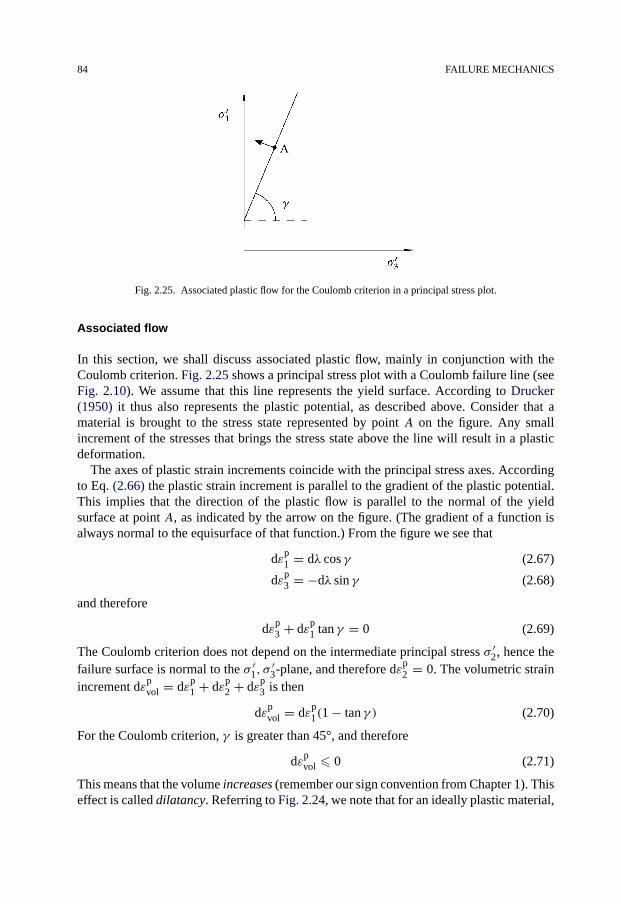
84 FAILURE MECHANICS
Fig. 2.25. Associated plastic flow for the Coulomb criterion in a principal stress plot.
Associated flow
In this section, we shall discuss associated plastic flow, mainly in conjunction with theCoulomb criterion. Fig. 2.25 shows a principal stress plot with a Coulomb failure line (seeFig. 2.10). We assume that this line represents the yield surface. According to Drucker(1950) it thus also represents the plastic potential, as described above. Consider that amaterial is brought to the stress state represented by point A on the figure. Any smallincrement of the stresses that brings the stress state above the line will result in a plasticdeformation.
The axes of plastic strain increments coincide with the principal stress axes. Accordingto Eq. (2.66) the plastic strain increment is parallel to the gradient of the plastic potential.This implies that the direction of the plastic flow is parallel to the normal of the yieldsurface at point A, as indicated by the arrow on the figure. (The gradient of a function isalways normal to the equisurface of that function.) From the figure we see that
dεp1 = dλ cos γ (2.67)
dεp3 = −dλ sin γ (2.68)
and therefore
dεp3 + dεp
1 tan γ = 0 (2.69)
The Coulomb criterion does not depend on the intermediate principal stress σ ′2, hence the
failure surface is normal to the σ ′1, σ
′3-plane, and therefore dεp
2 = 0. The volumetric strainincrement dεp
vol = dεp1 + dεp
2 + dεp3 is then
dεpvol = dεp
1(1 − tan γ ) (2.70)
For the Coulomb criterion, γ is greater than 45°, and therefore
dεpvol � 0 (2.71)
This means that the volume increases (remember our sign convention from Chapter 1). Thiseffect is called dilatancy. Referring to Fig. 2.24, we note that for an ideally plastic material,
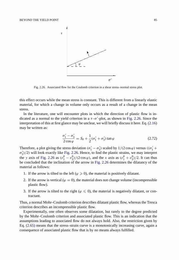
BEYOND THE YIELD POINT 85
Fig. 2.26. Associated flow for the Coulomb criterion in a shear stress–normal stress plot.
this effect occurs while the mean stress is constant. This is different from a linearly elasticmaterial, for which a change in volume only occurs as a result of a change in the meanstress.
In the literature, one will encounter plots in which the direction of plastic flow is in-dicated as a normal to the yield criterion in a τ–σ ′-plot, as shown in Fig. 2.26. Since theinterpretation of this at first glance may be unclear, we will briefly discuss it here. Eq. (2.16)may be written as:
σ ′1 − σ ′
3
2 cosϕ= S0 + 1
2(σ ′
1 + σ ′3) tanϕ (2.72)
Therefore, a plot giving the stress deviation (σ ′1 − σ ′
3) scaled by 1/(2 cosϕ) versus ((σ ′1 +
σ ′3)/2) will look exactly like Fig. 2.26. Hence, to find the plastic strains, we may interpret
the y axis of Fig. 2.26 as (εp1 − εp
3)/(2 cosϕ), and the x axis as (εp1 + εp
3)/2. It can thusbe concluded that the inclination of the arrow in Fig. 2.26 determines the dilatancy of thematerial as follows:
1. If the arrow is tilted to the left (ϕ � 0), the material is positively dilatant.
2. If the arrow is vertical (ϕ = 0), the material does not change volume (incompressibleplastic flow).
3. If the arrow is tilted to the right (ϕ � 0), the material is negatively dilatant, or con-tractant.
Thus, a normal Mohr–Coulomb criterion describes dilatant plastic flow, whereas the Trescacriterion describes an incompressible plastic flow.
Experimentally, one often observes some dilatation, but rarely to the degree predictedby the Mohr–Coulomb criterion and associated plastic flow. This is an indication that theassumptions leading to associated flow do not always hold. Also, the restriction given byEq. (2.65) means that the stress–strain curve is a monotonically increasing curve, again aconsequence of associated plastic flow that is by no means always fulfilled.

86 FAILURE MECHANICS
Non-associated flow
Non-associated plastic flow may occur if the plastic potential is not identical to the yieldsurface. It is a convenient model to use in order to have control on dilatancy without chang-ing the yield criterion.
For plastic flow associated with the Coulomb criterion, the plastic potential can be writ-ten as
f (σ ′1, σ
′3) = σ ′
1 − C0 − σ ′3 tan γ = σ ′
1 − C0 − σ ′3
1 + sinϕ
1 − sinϕ(2.73)
A non-associated yield criterion is found by choosing a different angle in Eq. (2.73), i.e.
g(σ ′1, σ
′3) = σ ′
1 − C0 − σ ′3 tanΨ = σ ′
1 − C0 − σ ′3
1 + sinΨ
1 − sinΨ(2.74)
Ψ is called the dilatancy angle, and from the discussion in the previous section, we knowthat we will have dilatant, incompressible, or contractant flow—depending on whetherΨ islarger than, equal to, or smaller than zero. Note that the allowable range for Ψ is restricted,since Eq. (2.63) has to be fulfilled.
Hardening
According to Eq. (2.61) hardening can be described by a change in the yield surface as afunction of a parameter κ that is, in some way, related to the plastic strains. This is shownschematically in Fig. 2.27. In the figure we define the initial yield surface, and a current
Fig. 2.27. Sketch of hardening in stress space.

BEYOND THE YIELD POINT 87
yield surface, i.e. the yield surface after some plastic straining. Also shown is the failuresurface, which is defined as the surface that separates accessible states from inaccessiblestates. Note that for an ideally plastic material, the initial yield surface and the failuresurface coincide. The use of only one parameter κ to describe hardening is, of course, asimplification, since there are six plastic strain components.
There are two common ways to relate κ to the plastic strain. One way is to assume that κis a function of the total plastic strain. This is called strain hardening, and can be expressedas
κ = κ(∫
Sdεpij
)(2.75)
where∫
S symbolizes integration over the stress path. Another way is to relate κ to the totalplastic work:
κ = κ(∫
Sσ ′ijdε
pij
)(2.76)
This is called work hardening.Hardening is commonly decomposed into two main modes, isotropic hardening and
kinematic hardening. Fig. 2.28 illustrates the difference between these concepts. Isotropichardening means that the yield surface expands (or shrinks) in a uniform way about thehydrostatic axis. Kinematic hardening consists of a translation of the failure surface instress space. In practice, hardening must be described by a combination of the modes or aneven more complicated behaviour, in which different parts of the yield surface deform indifferent ways.
Before concluding, we shall mention one important effect concerning hardening, whichis normally observed experimentally. The Baushinger effect states that if a material issubjected to a given plastic strain in one direction, given a yield stress σ ′
1, the correspond-ing yield stress found when the specimen is later loaded in the opposite direction willbe smaller than σ ′
1. One will see that the Baushinger effect may be obeyed by kinematichardening, but not by isotropic hardening.
Fig. 2.28. Isotropic and kinematic hardening in principal stress space.
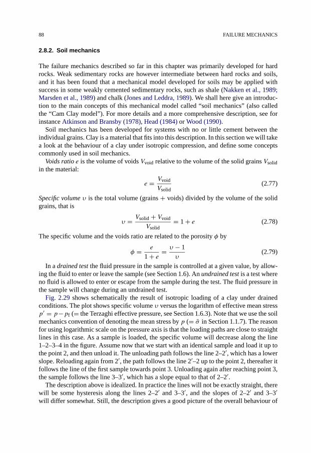
88 FAILURE MECHANICS
2.8.2. Soil mechanics
The failure mechanics described so far in this chapter was primarily developed for hardrocks. Weak sedimentary rocks are however intermediate between hard rocks and soils,and it has been found that a mechanical model developed for soils may be applied withsuccess in some weakly cemented sedimentary rocks, such as shale (Nakken et al., 1989;Marsden et al., 1989) and chalk (Jones and Leddra, 1989). We shall here give an introduc-tion to the main concepts of this mechanical model called “soil mechanics” (also calledthe “Cam Clay model”). For more details and a more comprehensive description, see forinstance Atkinson and Bransby (1978), Head (1984) or Wood (1990).
Soil mechanics has been developed for systems with no or little cement between theindividual grains. Clay is a material that fits into this description. In this section we will takea look at the behaviour of a clay under isotropic compression, and define some conceptscommonly used in soil mechanics.
Voids ratio e is the volume of voids Vvoid relative to the volume of the solid grains Vsolidin the material:
e = Vvoid
Vsolid(2.77)
Specific volume υ is the total volume (grains + voids) divided by the volume of the solidgrains, that is
υ = Vsolid + Vvoid
Vsolid= 1 + e (2.78)
The specific volume and the voids ratio are related to the porosity φ by
φ = e
1 + e = υ − 1
υ(2.79)
In a drained test the fluid pressure in the sample is controlled at a given value, by allow-ing the fluid to enter or leave the sample (see Section 1.6). An undrained test is a test whereno fluid is allowed to enter or escape from the sample during the test. The fluid pressure inthe sample will change during an undrained test.
Fig. 2.29 shows schematically the result of isotropic loading of a clay under drainedconditions. The plot shows specific volume υ versus the logarithm of effective mean stressp′ = p−pf (= the Terzaghi effective pressure, see Section 1.6.3). Note that we use the soilmechanics convention of denoting the mean stress by p (= σ in Section 1.1.7). The reasonfor using logarithmic scale on the pressure axis is that the loading paths are close to straightlines in this case. As a sample is loaded, the specific volume will decrease along the line1–2–3–4 in the figure. Assume now that we start with an identical sample and load it up tothe point 2, and then unload it. The unloading path follows the line 2–2′, which has a lowerslope. Reloading again from 2′, the path follows the line 2′–2 up to the point 2, thereafter itfollows the line of the first sample towards point 3. Unloading again after reaching point 3,the sample follows the line 3–3′, which has a slope equal to that of 2–2′.
The description above is idealized. In practice the lines will not be exactly straight, therewill be some hysteresis along the lines 2–2′ and 3–3′, and the slopes of 2–2′ and 3–3′will differ somewhat. Still, the description gives a good picture of the overall behaviour of

BEYOND THE YIELD POINT 89
Fig. 2.29. Isotropic compression of clay, schematically.
clays. A main point to be learned is the following: the stiffness of a sample which is loadedabove the highest pressure it has been exposed to before, is lower than the stiffness of asample which has seen higher pressures than the present state.
A sample which is at the highest stress it has ever experienced is said to be normallyconsolidated. The sample described above was normally consolidated whenever it wason the line 1–4 (Fig. 2.29). A sample which has been subjected to higher stresses beforeis said to be overconsolidated. The sample above was overconsolidated when it was onone of the lines 2–2′ or 3–3′ (Fig. 2.29). The highest stress a sample has been exposedto is commonly called preconsolidation stress. The overconsolidation ratio of a sample isdefined as the highest stress it has been experienced, divided by the current stress.
Triaxial tests on sandstones are usually run on drained samples, and plots showing stressversus strain (like Figs. 2.2 and 2.3) are used to present the results. Due to the low per-meability, triaxial tests on a material like clay are usually run on undrained samples. It isalso customary to analyse the test results in terms of the effective mean stress p′ and thegeneralized shear stress q, defined in Section 2.7.
Fig. 2.30 shows schematically a typical test on a normally consolidated clay. The loadingpath curves to the left, which means that the mean effective stress is decreasing. Thus thepore pressure increases throughout the test. For strongly overconsolidated samples, oneexpects the path to curve to the right as the sample approaches failure.
Typical behaviour during undrained triaxial testing, for normally consolidated clays andstrongly overconsolidated clays can be summarized as follows:
Normally consolidated clay:
1. No peak stress in the stress–strain diagram, i.e. the shear stress does not fall belowprevious value as the strain increases.
2. The sample contracts throughout the loading.
3. The loading path in a q–p′-plot curves to the left, i.e. the pore pressure increases.

90 FAILURE MECHANICS
Fig. 2.30. Loading path for an undrained test on a normally consolidated clay in the q–p′ domain.
Strongly overconsolidated clay:
1. A peak is normally observable in the stress–strain diagram, i.e. at some point theshear stress falls below previous values as the strain increases.
2. The sample contracts initially, then dilates as failure is approaching.
3. The loading path in a q–p′-plot curves to the right near failure, i.e. the pore pressuredecreases.
The normally consolidated clays and the strongly overconsolidated clays are seen to behavequite differently. We shall now describe each of them in more detail.
Normally consolidated clays
Fig. 2.31 illustrates the stress paths for three undrained tests on samples of a normallyconsolidated clay, starting from three different isotropic compression levels. The arrowsshow the paths of the tests from the start of the triaxial phase to the failure state, that is tothe point where the stress–strain curve flattens out and large shear strains may occur at noincrease in the shear stress. The loading paths in the υ–p′-plot are horizontal, since thereis no change in specific volume during an undrained test. Note that the ends of the pathsseem to fall on continuous “failure” lines in both plots.
Fig. 2.32 shows the corresponding stress paths for drained tests. Again the end pointsare seen to fall on continuous lines. It has been found that the continuous failure linesdefined by the ends of the tests in Figs. 2.31 and 2.32 are indeed the same lines to a fairapproximation. If we plot the test results in a three-dimensional plot, with υ–p′–q as theaxes, we find that the failure lines in the q–p′ and υ–p′ planes are projections of a linein this three-dimensional space, the critical state line (CSL). The critical state line withits projections onto the q–p′ and υ–p′ planes are shown in Fig. 2.33. The critical staterepresents an ultimate state where large shear strains may occur at no change in shearstress.
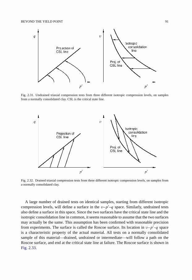
BEYOND THE YIELD POINT 91
Fig. 2.31. Undrained triaxial compression tests from three different isotropic compression levels, on samplesfrom a normally consolidated clay. CSL is the critical state line.
Fig. 2.32. Drained triaxial compression tests from three different isotropic compression levels, on samples froma normally consolidated clay.
A large number of drained tests on identical samples, starting from different isotropiccompression levels, will define a surface in the υ–p′–q space. Similarly, undrained testsalso define a surface in this space. Since the two surfaces have the critical state line and theisotropic consolidation line in common, it seems reasonable to assume that the two surfacesmay actually be the same. This assumption has been confirmed with reasonable precisionfrom experiments. The surface is called the Roscoe surface. Its location in υ–p′–q spaceis a characteristic property of the actual material. All tests on a normally consolidatedsample of this material—drained, undrained or intermediate—will follow a path on theRoscoe surface, and end at the critical state line at failure. The Roscoe surface is shown inFig. 2.33.

92 FAILURE MECHANICS
Fig. 2.33. The Roscoe surface in υ–p′–q space.
Overconsolidated clays
For a normally consolidated clay, there is a unique relationship between the specific vol-ume and the effective stress, defined by the normal consolidation line in the υ–p′ plane.For an overconsolidated clay, there may be a range of voids ratios for a given effectivestress, depending on the preconsolidation stress from which the material was unloaded.This means that whereas an undrained test on a normally consolidated material traversesa unique path in the υ–p′–q space if the starting specific volume is given, there will be arange of possible paths for an overconsolidated material.
We now imagine that we do a series of undrained tests on a clay, for a given specificvolume, but start at different effective hydrostatic stress levels, corresponding to differentoverconsolidation ratios. Fig. 2.34 shows the (idealized) results of these tests, projectedonto the q–p′ plane. A slightly overconsolidated material moves more or less verticallyuntil it reaches the Roscoe surface, and then follows this surface until it reaches the criticalstate. (The curve is initially vertical only to the extent that the Skempton B coefficient isclose to 1, otherwise the curve tilts slightly to the right; see Section 1.6.5.) For stronglyoverconsolidated specimens the movement is again vertical in the initial phases of the ex-periment. The path does not reach the Roscoe surface, but changes direction upon reachinga limiting curve which like the Roscoe surface passes through the critical state. This lim-iting curve is nearly a straight line. In the figure we have assumed that the sample can notsustain tensile stresses, and the change on slope at low p′ reflects this.
If similar tests are done for the same material at various specific volumes, one will findthat they map out a surface in the υ–p′–q space, the Hvorslev surface. This surface playsa similar role for overconsolidated samples as the Roscoe surface does for normally (andslightly over-) consolidated samples. It is a limiting surface for all stress paths, not onlyundrained tests. The Hvorslev surface and the Roscoe surface are shown in Fig. 2.35. Notethat they are joined together at the critical state line.
The behaviour of the material at the Hvorslev surface is less predictable than at theRoscoe surface. If the material behaved uniformly, it would follow the Hvorslev surface up
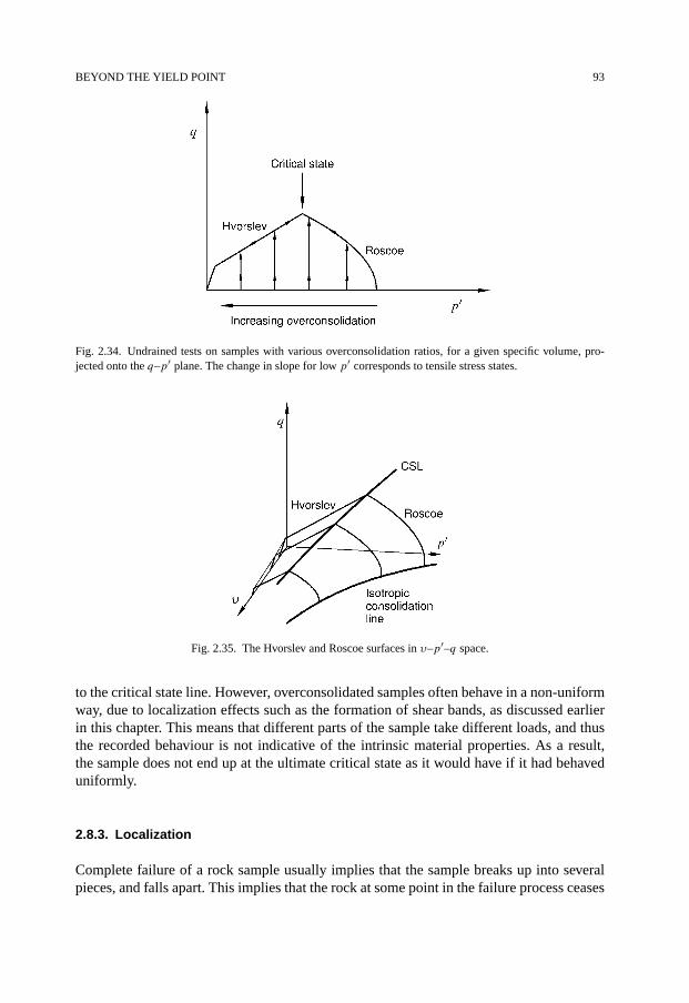
BEYOND THE YIELD POINT 93
Fig. 2.34. Undrained tests on samples with various overconsolidation ratios, for a given specific volume, pro-jected onto the q–p′ plane. The change in slope for low p′ corresponds to tensile stress states.
Fig. 2.35. The Hvorslev and Roscoe surfaces in υ–p′–q space.
to the critical state line. However, overconsolidated samples often behave in a non-uniformway, due to localization effects such as the formation of shear bands, as discussed earlierin this chapter. This means that different parts of the sample take different loads, and thusthe recorded behaviour is not indicative of the intrinsic material properties. As a result,the sample does not end up at the ultimate critical state as it would have if it had behaveduniformly.
2.8.3. Localization
Complete failure of a rock sample usually implies that the sample breaks up into severalpieces, and falls apart. This implies that the rock at some point in the failure process ceases

94 FAILURE MECHANICS
to behave as a homogeneous material even on the macroscopic scale. It also implies thatfailure is complete only within a few restricted areas of the rock sample, like fracture planesdeveloped under tensile failure, and narrow shear bands developed under shear failure.
The formation and growth of localized failure zones occurs when it is energeticallyfavourable for cracks or other (preexisting or randomly induced) defects to grow and in-teract with nearby defects. For tensile failure and unconfined shear failure this is usuallyan unstable situation that rapidly leads to macroscopic failure of the sample. However, forfailure under compressive stresses, the situation may lead to non-uniform deformation in aplanar band within the sample, while the deformation outside the band remains homoge-neous, and the material remains stable.
Rudnicki and Rice (1975) described the conditions for localization of deformation intoplanar bands. The formation of such bands can be considered as a constitutive instability,closely linked to the plastic hardening of the material. It is found that for a material obeyingassociated plastic flow (see Section 2.8.1) the formation of shear bands can only occur afterthe peak stress point. For materials obeying non-associated plastic flow, such bands mayalso be formed prior to the peak stress point, at least for stress configurations close to pureshear.
At lower stress levels, the rock sample is supposed to follow one unique path of uniformdeformation. When the conditions for the formation of a localized deformation band arefulfilled, there are at least two possible orientations of the band. Thus, further deformationof the rock sample will follow one out of several equivalent paths. This spontaneous split-ting of the deformation path is called bifurcation, and the point where the conditions forlocalized deformation are first fulfilled is called the bifurcation point (see Vardoulakis andSulem, 1995).
Other forms of non-uniform deformation are also possible, for instance surface buckling(Biot, 1965; Vardoulakis, 1984) which implies that the material spontaneously changesits shape when the conditions for such deformation are fulfilled. It has been demonstrated(Mollema and Antonellini, 1996; Olsson, 1999; Olsson and Holcomb, 2000) that also com-paction can be localized, in so-called compaction bands. Such bands may act as barriersfor fluid flow, and may therefore be of importance under given conditions, by changingflow paths or altering pore pressure gradients and thereby also the effective stresses. (Seealso Borja and Aydin, 2004; Fossen et al., 2007.)
2.8.4. Liquefaction
Failure of a highly porous rock results in a volume reduction and a corresponding reductionin the pore space. If the rock fails under undrained conditions, the pore space reduction willlead to increasing pore pressure. This implies reduced effective stresses and a correspond-ing reduction in confinement. For a poorly consolidated (or previously damaged) rock, thisis a highly unstable condition that may result in very large deformations driven by the staticshear stresses.
This extreme condition is called liquefaction. It is sometimes observed in connection toearthquakes, and is highly noticeable due to its sudden appearance and quick development,and the large distance the liquefied material may move (see for instance Kramer, 1996).
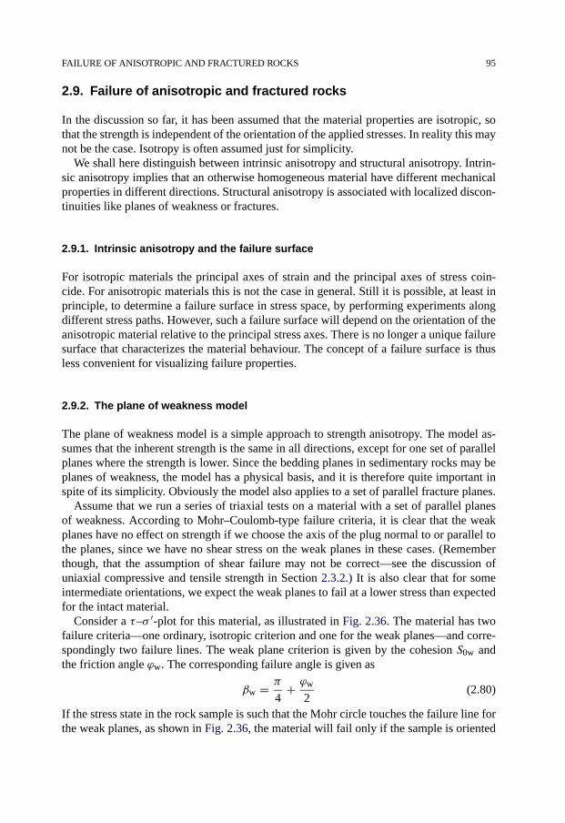
FAILURE OF ANISOTROPIC AND FRACTURED ROCKS 95
2.9. Failure of anisotropic and fractured rocks
In the discussion so far, it has been assumed that the material properties are isotropic, sothat the strength is independent of the orientation of the applied stresses. In reality this maynot be the case. Isotropy is often assumed just for simplicity.
We shall here distinguish between intrinsic anisotropy and structural anisotropy. Intrin-sic anisotropy implies that an otherwise homogeneous material have different mechanicalproperties in different directions. Structural anisotropy is associated with localized discon-tinuities like planes of weakness or fractures.
2.9.1. Intrinsic anisotropy and the failure surface
For isotropic materials the principal axes of strain and the principal axes of stress coin-cide. For anisotropic materials this is not the case in general. Still it is possible, at least inprinciple, to determine a failure surface in stress space, by performing experiments alongdifferent stress paths. However, such a failure surface will depend on the orientation of theanisotropic material relative to the principal stress axes. There is no longer a unique failuresurface that characterizes the material behaviour. The concept of a failure surface is thusless convenient for visualizing failure properties.
2.9.2. The plane of weakness model
The plane of weakness model is a simple approach to strength anisotropy. The model as-sumes that the inherent strength is the same in all directions, except for one set of parallelplanes where the strength is lower. Since the bedding planes in sedimentary rocks may beplanes of weakness, the model has a physical basis, and it is therefore quite important inspite of its simplicity. Obviously the model also applies to a set of parallel fracture planes.
Assume that we run a series of triaxial tests on a material with a set of parallel planesof weakness. According to Mohr–Coulomb-type failure criteria, it is clear that the weakplanes have no effect on strength if we choose the axis of the plug normal to or parallel tothe planes, since we have no shear stress on the weak planes in these cases. (Rememberthough, that the assumption of shear failure may not be correct—see the discussion ofuniaxial compressive and tensile strength in Section 2.3.2.) It is also clear that for someintermediate orientations, we expect the weak planes to fail at a lower stress than expectedfor the intact material.
Consider a τ–σ ′-plot for this material, as illustrated in Fig. 2.36. The material has twofailure criteria—one ordinary, isotropic criterion and one for the weak planes—and corre-spondingly two failure lines. The weak plane criterion is given by the cohesion S0w andthe friction angle ϕw. The corresponding failure angle is given as
βw = π
4+ ϕw
2(2.80)
If the stress state in the rock sample is such that the Mohr circle touches the failure line forthe weak planes, as shown in Fig. 2.36, the material will fail only if the sample is oriented
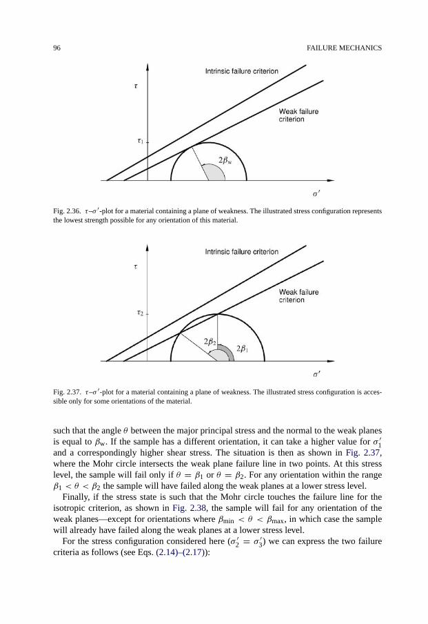
96 FAILURE MECHANICS
Fig. 2.36. τ–σ ′-plot for a material containing a plane of weakness. The illustrated stress configuration representsthe lowest strength possible for any orientation of this material.
Fig. 2.37. τ–σ ′-plot for a material containing a plane of weakness. The illustrated stress configuration is acces-sible only for some orientations of the material.
such that the angle θ between the major principal stress and the normal to the weak planesis equal to βw. If the sample has a different orientation, it can take a higher value for σ ′
1and a correspondingly higher shear stress. The situation is then as shown in Fig. 2.37,where the Mohr circle intersects the weak plane failure line in two points. At this stresslevel, the sample will fail only if θ = β1 or θ = β2. For any orientation within the rangeβ1 < θ < β2 the sample will have failed along the weak planes at a lower stress level.
Finally, if the stress state is such that the Mohr circle touches the failure line for theisotropic criterion, as shown in Fig. 2.38, the sample will fail for any orientation of theweak planes—except for orientations where βmin < θ < βmax, in which case the samplewill already have failed along the weak planes at a lower stress level.
For the stress configuration considered here (σ ′2 = σ ′
3) we can express the two failurecriteria as follows (see Eqs. (2.14)–(2.17)):

FAILURE OF ANISOTROPIC AND FRACTURED ROCKS 97
Fig. 2.38. τ–σ ′-plot for a material containing a plane of weakness. The illustrated stress configuration representsthe highest strength possible for any orientation of this material.
Isotropic failure criterion (cohesion S0, friction angle ϕ)
σ ′1 − σ ′
3 = 2S0 cosϕ + σ ′
3 sinϕ
1 − sinϕ(2.81)
Weak plane failure criterion
σ ′1 − σ ′
3 = 2S0w cosϕw + σ ′
3 sinϕw
sin 2θ cosϕw − (cos 2θ + 1) sinϕw(2.82)
The criterion that predicts the lowest strength for a given orientation θ is always the relevantcriterion. Fig. 2.39 illustrates how the strength varies with the orientation of the sample forsuch a material.
Note that for a general, three dimensional stress state, the shear and normal stressesover the weak planes are given by Eqs. (1.36)–(1.37), and the weak plane failure criterionbecomes much more complicated.
More advanced theories may be developed by allowing cohesion and friction angle tovary as function of orientation. Such theories will predict a smoother dependence on orien-tation. A more empirical approach to the problem was given by Hoek and Brown (1980).
2.9.3. Fractured rock
The behaviour of a fractured rock depends both on the properties of the fractures and onthe properties of the intact rock. Generally, fractured rocks will be much weaker than thecorresponding intact rock, as the resistance against shear failure is considerably less for analready existing fracture.
To predict the behaviour of a fractured rock it may be necessary to apply numericalsimulation methods to the actual fracture system. Alternatively, effective rock propertiesmay be assigned to a representative volume that is much larger than the fracture spacing.
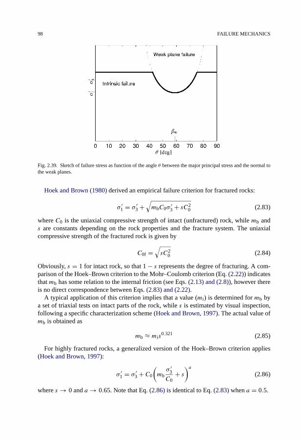
98 FAILURE MECHANICS
Fig. 2.39. Sketch of failure stress as function of the angle θ between the major principal stress and the normal tothe weak planes.
Hoek and Brown (1980) derived an empirical failure criterion for fractured rocks:
σ ′1 = σ ′
3 +√mbC0σ
′3 + sC2
0 (2.83)
where C0 is the uniaxial compressive strength of intact (unfractured) rock, while mb ands are constants depending on the rock properties and the fracture system. The uniaxialcompressive strength of the fractured rock is given by
C0f =√sC2
0 (2.84)
Obviously, s = 1 for intact rock, so that 1 − s represents the degree of fracturing. A com-parison of the Hoek–Brown criterion to the Mohr–Coulomb criterion (Eq. (2.22)) indicatesthat mb has some relation to the internal friction (see Eqs. (2.13) and (2.8)), however thereis no direct correspondence between Eqs. (2.83) and (2.22).
A typical application of this criterion implies that a value (mi) is determined for mb bya set of triaxial tests on intact parts of the rock, while s is estimated by visual inspection,following a specific characterization scheme (Hoek and Brown, 1997). The actual value ofmb is obtained as
mb ≈ mis0.321 (2.85)
For highly fractured rocks, a generalized version of the Hoek–Brown criterion applies(Hoek and Brown, 1997):
σ ′1 = σ ′
3 + C0
(mbσ ′
3
C0+ s
)a(2.86)
where s → 0 and a → 0.65. Note that Eq. (2.86) is identical to Eq. (2.83) when a = 0.5.
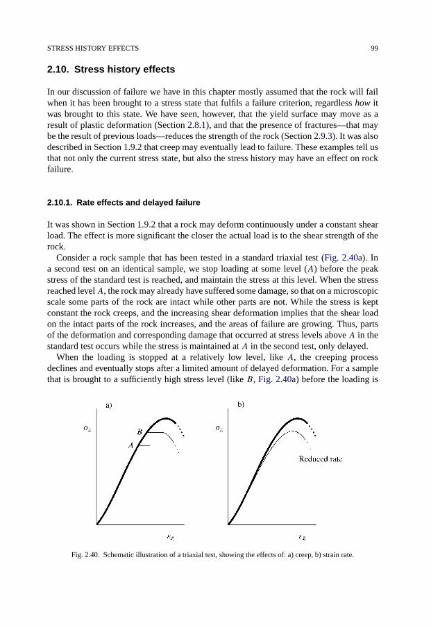
STRESS HISTORY EFFECTS 99
2.10. Stress history effects
In our discussion of failure we have in this chapter mostly assumed that the rock will failwhen it has been brought to a stress state that fulfils a failure criterion, regardless how itwas brought to this state. We have seen, however, that the yield surface may move as aresult of plastic deformation (Section 2.8.1), and that the presence of fractures—that maybe the result of previous loads—reduces the strength of the rock (Section 2.9.3). It was alsodescribed in Section 1.9.2 that creep may eventually lead to failure. These examples tell usthat not only the current stress state, but also the stress history may have an effect on rockfailure.
2.10.1. Rate effects and delayed failure
It was shown in Section 1.9.2 that a rock may deform continuously under a constant shearload. The effect is more significant the closer the actual load is to the shear strength of therock.
Consider a rock sample that has been tested in a standard triaxial test (Fig. 2.40a). Ina second test on an identical sample, we stop loading at some level (A) before the peakstress of the standard test is reached, and maintain the stress at this level. When the stressreached levelA, the rock may already have suffered some damage, so that on a microscopicscale some parts of the rock are intact while other parts are not. While the stress is keptconstant the rock creeps, and the increasing shear deformation implies that the shear loadon the intact parts of the rock increases, and the areas of failure are growing. Thus, partsof the deformation and corresponding damage that occurred at stress levels above A in thestandard test occurs while the stress is maintained at A in the second test, only delayed.
When the loading is stopped at a relatively low level, like A, the creeping processdeclines and eventually stops after a limited amount of delayed deformation. For a samplethat is brought to a sufficiently high stress level (like B, Fig. 2.40a) before the loading is
Fig. 2.40. Schematic illustration of a triaxial test, showing the effects of: a) creep, b) strain rate.

100 FAILURE MECHANICS
stopped, the creeping process is unstable and it will after a while accelerate and result infailure (accelerating creep, see Section 1.9).
The fact that all of the damage that may occur at a given stress level does not occurimmediately, points directly to an effect of loading rate on rock strength. Clearly, if therock is loaded at a lower rate, more damage may occur per unit of stress increase, and therock will essentially be weaker (Fig. 2.40b).
Note that effects of loading rate may also be seen in hydrostatic loading, even if creep isprimarily thought to be related to shear deformation. This can be ascribed to local fluctua-tions in the stresses that will occur in a heterogeneous material like a porous rock.
2.10.2. Fatigue
Excessive deformation at a limited stress level, as described in the previous paragraph, maybe provoked and accelerated if the stress is released and reapplied over and over again. Foreach unloading-reloading cycle a little more damage is added, and the rock sample deformscorrespondingly. Eventually, the rock may be destroyed by fatigue failure. The number ofcycles required to bring a rock to failure increases dramatically if the peak stress level forthe loading cycles is reduced.
If the peak stress of the loading cycles is kept sufficiently low, the rock may not faileven after a very large number of cycles. Still, the cyclic loading may have affected thestrength of the rock, so that in a subsequent failure test the rock will fail at a stress leveldifferent from its normal strength. Typically, cyclic loading will reduce the strength of arock sample, however increased strength due to cyclic loading is also reported (Ray et al.,1999).
References
Atkinson, J.H., Bransby, P.L. (1978). The Mechanics of Soils. An Introduction to Critical State Soil Mechanics.McGraw-Hill, London.
Biot, M.A. (1965). Mechanics of Incremental Deformations. Wiley, New York.Bishop, A.W. (1959). “The principle of effective stress”. Teknisk Ukeblad 39, 859–863.Borja, R.I., Aydin, A. (2004). “Computational modeling of deformation bands in granular media. I. Geological
and mathematical framework”. Comput. Methods Appl. Mech. Engrg. 193, 2667–2698.Boutéca, M., Guéguen, Y. (1999). “Mechanical properties of rocks: Pore pressure and scale effects”. Oil & Gas
Sci. Techn.—Rev. IFP 54, 703–714.Boutéca, M.J., Sarda, J.-P., Vincké, O. (2000). “Constitutive law for permeability evolution of sandstones during
depletion”. SPE58717, presented at the 2000 SPE International Symposium on Formation Damage, Lafayette,LA, 23–24 February.
Brace, W.F. (1960). “An extension of Griffith theory of fracture to rocks”. J. Geophys. Res. 65, 3477–3480.Brignoli, M., Papamichos, E., Santarelli, F.J. (1995). “Capillary effects in sedimentary rocks: application to
reservoir water-flooding”. In: Proc. 35th U.S. Symposium on Rock Mechanics, Lake Tahoe, California,pp. 619–625.
Broch, E. (1974). “The influence of water on some rock properties”. In: Proc. 3rd Congress, ISRM, Denver,Part A, pp. 33–38.
Chen, W.F., Han, D.J. (1988). Plasticity for Structural Engineers. Springer-Verlag, New York.Colmenares, L.B., Zoback, M.D. (2002). “A statistical evaluation of intact rock failure criteria constrained by
polyaxial tests data for five different rocks”. Int. J. Rock Mech. Min. Sci. 39, 695–729.
REFERENCES 101
Detournay, E., Cheng, A.H.-D. (1988). “Poroelastic response of a borehole in a non-hydrostatic stress field”. Int.J. Rock Mech. Min. Sci. & Geomech. Abstr. 25, 171–182.
DiMaggio, F.L., Sandler, I.S. (1971). “Material model for granular soils”. J. Eng. Mech. Div. Am. Soc. Civ.Eng. 97, 935–950.
Drucker, D.C. (1950). “Some implications of work-hardening and ideal plasticity”. Quart. Appl. Math. 7, 411–418.
van Eekelen, H.A.M. (1980). “Isotropic yield surfaces in three dimensions for use in soil mechanics”. Int. J.Numer. Anal. Methods Geomech. 4, 89–101.
Ewy, R.T. (1999). “Wellbore-stability predictions by use of a modified Lade criterion”. SPE Drill. & Comple-tion 14, 85–91.
Fjær, E., Ruistuen, H. (2002). “Impact of the intermediate principal stress on the strength of heterogeneous rock”.J. Geophys. Res. 107 (B2), 2032.
Fossen, H., Schultz, R.A., Shipton, Z.K., Mair, K. (2007). “Deformation bands in sandstone: a review”. J. Geol.Soc. London 164, 755–769.
Griffith, A.A. (1921). “The phenomena of rupture and flow in solids”. Phil. Trans. Roy. Soc. A 221, 163–198.Guenot, A. (1989). “Instability problems at great depth drilling boreholes and wells”. In: Maury, V., Fourmain-
traux, D. (Eds.), Rock at Great Depth. Balkema, Rotterdam, pp. 1199–1208.Head, K.H. (1984). Manual of Soil Laboratory Testing, vols. 1–3. ELE International Ltd.Hoek, E., Brown, E.T. (1980). Underground Excavations In Rocks. The Institution of Mining and Metallurgy,
London.Hoek, E., Brown, E.T. (1997). “Practical estimates of rock strength”. Int. J. Rock Mech. Min. Sci. 34, 1165–1186.Jaeger, J.C., Cook, N.G.W. (1979). Fundamentals of Rock Mechanics, third ed. Chapman and Hall, London.Jones, M.E., Leddra, M.J. (1989). “Compaction and flow of porous rocks at depth”. In: Maury, V., Fourmaintraux,
D. (Eds.), Rock at Great Depth. Balkema, Rotterdam, pp. 891–898.Kramer, S.L. (1996). Geotechnical Earthquake Engineering. Prentice-Hall, New Jersey.Lade, P.V. (1977). “Elasto-plastic stress–strain theory for cohesionless soil with curved yield surfaces”. Int. J.
Solids Struct. 13, 1019–1035.Lade, P.V. (1993). “Rock Strength Criteria: The Theories and the Evidence”. In: Hudson, J.A. (Ed.), Compre-
hensive Rock Engineering. Principles, Practice & Projects. Vol. 1: Fundamentals. Pergamon Press, London,pp. 255–284.
Marsden, J.R., Wu, B., Hudson, J.A., Archer, J.S. (1989). “Investigation of peak rock strength behaviour for well-bore stability prediction”. In: Maury, V., Fourmaintraux, D. (Eds.), Rock at Great Depth. Balkema, Rotterdam,pp. 753–760.
McClintock, F.A., Walsh, J.B. (1962). “Friction on Griffith cracks under pressure”. In: Proc. Fourth U.S. Nat.Congress of Appl. Mech., pp. 1015–1021.
von Mises, R. (1928). “Mechanik der plastichen Formänderung von Kristallen”. Z. Angew. Math. Mech. 8, 161–185.
Mollema, P.N., Antonellini, M.A. (1996). “Compaction bands: A structural analog for anti-mode I cracks inaeolian sandstone”. Tectonophysics 267, 209–228.
Murrel, S.A.F. (1963). “A criterion for brittle fracture of rocks and concrete under triaxial stress and the effect ofpore pressure on the criterion”. In: Fairhurst, C. (Ed.), Rock Mechanics. Pergamon Press, Oxford, pp. 563–577.
Nakken, S.J., Christensen, T.L., Marsden, R., Holt, R.M. (1989). “Mechanical behaviour of clays at high stresslevels for wellbore stability applications”. In: Maury, V., Fourmaintraux, D. (Eds.), Rock at Great Depth.Balkema, Rotterdam, pp. 141–148.
Nordal, S., Jostad, H.P., Kavli, A., Grande, L. (1989). “A Colombian soil model applied to an offshore platform”.In: Proc. 12th Int. Conf. Soil Mechanics and Foundation Engineering, Rio de Janeiro, vol. 4, pp. 471–474.
Olsson, W.A. (1999). “Theoretical and experimental investigation of compaction bands in porous rock”. J. Geo-phys. Res. 104, 7219–7228.
Olsson, W.A., Holcomb, D.J. (2000). “Compaction localization in porous rock”. Geophys. Res. Lett. 27, 3537–3540.
Papamichos, E., Brignoli, M., Santarelli, F.J. (1997). “An experimental and theoretical study of a partially satu-rated collapsible rock”. Mech. Cohes.-Frict. Mater. 2, 251–278.

102 FAILURE MECHANICS
Ray, S.K., Sarkar, M., Singh, T.N. (1999). “The effect of cyclic loading and strain rate on the mechanical behav-iour of sandstone”. Technical note. Int. J. Rock Mech. Min. Sci. 36, 543–549.
Risnes, R., Haghighi, H., Korsnes, R.I., Natvik, O. (2003). “Chalk–fluid interactions with glycol and brines”.Tectonophysics 370, 213–226.
Rudnicki, J.W., Rice, J.R. (1975). “Conditions for the localization of deformation in pressure-sensitive dilatantmaterials”. J. Mech. Phys. Solids 23, 371–394.
Vardoulakis, I. (1984). “Rock bursting as a surface instability problem”. Int. J. Rock Mech. Min. Sci. & Geomech.Abstr. 21, 137–144.
Vardoulakis, I., Sulem, J. (1995). Bifurcation in Geomechanics. Blackie Academic & Professional, Glasgow.Wiebols, G.A., Cook, N.G.W. (1968). “An energy criterion for the strength of rock in polyaxial compression”.
Int. J. Rock Mech. Min. Sci. 5, 529–549.Wong, T.-f., David, C., Zhu, W. (1997). “The transition from brittle faulting to cataclastic flow in porous sand-
stones: Mechanical deformation”. J. Geophys. Res. 102 (B2), 3009–3025.Wood, D.M. (1990). Soil Behaviour and Critical State Soil Mechanics. Cambridge University Press, New York.Zhang, J., Wong, T.-f., Davis, D.M. (1990). “Micromechanics of pressure-induced grain crushing in porous
rocks”. J. Geophys. Res. 95, 341–352.

103
Chapter 3
Geological aspects of petroleum related rock mechanics
From a practical rock mechanics view point, the present state of a rock and its presentmechanical properties are of interest. The long and in many cases complicated processfrom an initial state as a loose sediment to the present state as a rock will however clearlyaffect rock mechanical behaviour.
A sedimentary basin may be exposed to sedimentary subsidence, sea-level changes andtectonic forces creating repeated cycles of elevation and depression, in addition to erosion,changes in sedimentary environment, changes in sedimentation rate, solution and precipita-tion of cementing material etc. All these effects will complicate the geological descriptionof the sedimentary basin. These geological activities and events will affect not only currentrock mechanical properties, but also current boundary conditions in terms of in situ stressesand pore pressure.
Therefore, knowledge of geological processes is valuable in rock engineering. Althoughon a totally different time scale and length scale, geological processes are often comparablewith events in rock mechanics laboratory testing, which means that such tests may be usedto enhance our understanding of geological phenomena.
The purpose of this chapter is to give an introduction to geological aspects which are ofparticular importance in petroleum related rock mechanics.
3.1. Underground stresses
Normally, an underground formation has to carry the weight of the overlying formations.The vertical stress at the bottom of a homogeneous column of height z is σv = ρgz, whereρ is the density of the material and g is the acceleration of gravity. If the density varieswith depth, the vertical stress at depth D becomes
σv =∫ D
0ρ(z)g dz (3.1)
Note that the z-axis is here pointing vertically downwards, with z = 0 correspondingto the Earth surface. The average density of sediments in the overburden is between 1.8and 2.2 g/cm3, so as a rough number, the vertical stress increases downwards with about20 MPa/km (typically 1 psi/ft).
The sedimentary rocks encountered during oil well drilling and production are porousand hence contain fluids. One refers to the pore pressure at depthD as normal if it is givenby the weight of a fluid column above, i.e. in analogy to Eq. (3.1) the normal pore pressurepfn is
pfn =∫ D
0ρf(z)g dz (3.2)
104 GEOLOGICAL ASPECTS OF PETROLEUM RELATED ROCK MECHANICS
The pore fluid density in case of brine with sea water salinity is in the range 1.03–1.07 g/cm3, so the pore pressure increase with depth is roughly 10 MPa/km (0.45 psi/ft).The effective vertical stress, σ ′
v, is then also increasing with approximately 10 MPa/km.In many important cases, however, the pore pressure deviates from the normal value pfn.We will return to these so-called abnormal pore pressures and their possible origins inSection 3.2.
The underground stress state consists of the three mutually orthogonal principal stresses,plus the pore pressure. It is very common (and convenient) in the oil industry to assumethat the vertical stress is a principal stress. This is reasonable at large depth within a homo-geneous Earth, in areas that have not been exposed to tectonic activity or are relaxed in thesense that there are no remnant stresses from previous tectonic activity. The vertical stressis governed by gravity, which has a unique direction, pointing towards the centre of theEarth. So it is not unreasonable to assume that the vertical is a principal stress direction.Let us however be aware that there will be cases when this is not fulfilled, such as nearthe surface: Because the surface is stress free, the principal stress directions at and near itwill be governed by the surface topography. In the case of a strongly sloping surface, evenat depth, the principal stress directions may be far from the vertical-horizontal directions.Also, near heterogeneities such as inclusions or faults, near underground openings such asboreholes (Chapter 4), or near depleting reservoirs (Chapter 12), principal stress directionswill differ from the vertical–horizontal orientation.
Below we will consider the vertical stress as a principal stress. To begin with, assumea relaxed area where the horizontal stress is induced simply as a result of the verticalstress. For simplicity, think of a fluid: The overburden causes a vertical stress (pressure) inthe fluid, but at the same time an equal horizontal stress (pressure). In a rock, the abilityto resist shear stresses causes the horizontal stress σh in general to be different from thevertical stress. We write (in terms of effective stresses):
σ ′h = K ′σ ′
v (3.3)
The ratio K ′ between the effective horizontal and effective vertical stress may vary signifi-cantly. At shallow depths (0–150 m) it may vary from 1 to 10 or even higher, while valuesfrom 0.2 to 1.5 may be found at larger depths. Bjørlykke and Høeg (1997) pointed out thatchemical compaction increases in importance at depths below 2–3 km, and will contributeto horizontal stresses by altering the trend seen from pure mechanical compaction abovethis level.
It has been suggested that, with time, K ′ → 1, so that the stress state becomes hydro-static, with the magnitude given by the weight of the overburden according to Eq. (3.1).This is called Heim’s rule, after work by the Swiss geologist Albert Heim in the nineteenthcentury. Heim suggested that the mechanism causing this development is creep. This stateof stress is referred to as lithostatic.1
1 In the literature, the term lithostatic stress is sometimes defined as the vertical stress being given by Eq. (3.1),without reference to the horizontal stresses. In this book, we follow Jaeger and Cook (1979), Engelder (1993) andothers, and take lithostatic to imply that the stress state is also hydrostatic.
UNDERGROUND STRESSES 105
The transition toward lithostacy is normally a very slow process, and the lithostatic stateof stress is rare in the lithosphere (Engelder, 1993). Some examples of underground stressillustrating non-lithostatic stress states are shown in Figs. 3.1, 3.12 and 9.10.
The idea that creep brings the stress state towards lithostacy is however consideredsound, and it is therefore not likely to find a general rule for predicting horizontal stressat depth, unless very sophisticated models taking long-time stress history into account aredeveloped.
We now consider two very simple models for estimating the in situ stress state. First,assume that the formation under consideration is laterally constrained; i.e. there is nohorizontal strain under the process of rock formation. Furthermore, we assume that therock during this process behaves according to the theory of linear elasticity. Then, fromEqs. (1.102)–(1.103), with εx = εy = 0, one finds:
σ ′h = νfr
1 − νfrσ ′
v (3.4)
In this particular case, the coefficient K ′ is given the name Ko. In a fluid, where Poisson’sratio is 1/2, Ko = 1. For a rock with νfr = 1/3, Ko = 1/2.
There are many reasons to apply the relationship above with great care. We assumedlinear elasticity, and we assumed zero lateral movement. In reality we also assumed thatthe elastic properties of the rock have been constant throughout the whole process of rockformation. This is clearly not true. An approach based on a complete stress history analy-sis was presented by Warpinski (1989), incorporating variations in mechanical propertiesover time. Consolidation, diagenesis, changes in pore pressure due to gas generation, tem-perature gradients, and various tectonic and thermal episodes may be incorporated in thismodel. Viscoelasticity appeared, for the cases studied, to be more relevant for stresses inshale than in sandstone.
Another simple approach is to say that the rock has been, and still is, in a critical statewithin the Earth, i.e. it should obey some kind of a failure criterion. Leaning on ideas ofself-organized criticality (see e.g. the book by Bak, 1996), this may be a reasonable as-sumption, in particular in areas of active tectonics. Choosing the Mohr–Coulomb criterionEqs. (2.18) or (2.22) as criterion for active faulting, the ratio between the minimum andthe maximum effective stress should be (for the case when the unconfined strength C0 isnegligible)
σ ′3 � 1 − sinϕ
1 + sinϕσ ′
1 = 1
tan2 βσ ′
1 (3.5)
If the vertical stress is the maximum principal stress, Eq. (3.5) predicts the following lim-iting value for K ′:
K ′ = 1 − sinϕ
1 + sinϕ(3.6)
If the friction angle is 30°, then K ′ = 1/3. A lower friction angle will result in a highervalue for K ′.
These are very simple examples of models for horizontal stress estimation. In reality,as mentioned above, horizontal stresses are difficult to assess from mathematical models.

106 GEOLOGICAL ASPECTS OF PETROLEUM RELATED ROCK MECHANICS
Fig. 3.1. Stresses versus depth: Vertical stress (from Eq. (3.1) with density 2.1 g/cm3, full line), horizontalstress (from Eqs. (3.7) and (3.8), dashed line), and pore pressure (from Eq. (3.2) with fluid density 1.05 g/cm3,dotted line).
The most direct method of obtaining horizontal stress is to measure it, for instance by afracturing test of the formation (see Sections 8.3 and 11.5).
Breckels and van Eekelen (1982) used fracturing data from whole regions, and derivedrelationships between horizontal stress and depth. They also accounted for possibly ab-normal pore pressures. For the US Gulf Coast, Breckels and van Eekelen presented thefollowing relations:
σh = 0.0053D1.145 + 0.46(pf − pfn) (D < 3500 m) (3.7)
σh = 0.0264D − 31.7 + 0.46(pf − pfn) (D > 3500 m) (3.8)
whereD is depth in metres, pf is the pore pressure in MPa, pfn is the normal pore pressure(corresponding to a gradient of 10.5 MPa/km) and σh is the smallest horizontal stressin MPa. Note that these relations were developed at zero or shallow water depths (see alsoSection 8.3).
The predicted horizontal stress from Breckels and van Eekelen’s relationship is shownin Fig. 3.1 together with trends for vertical stress and normal pore pressure (from Eqs. (3.1)and (3.2), using constant densities for rock and pore fluid).
The Gulf Coast curve (Eqs. (3.7) and (3.8)) may be used with a fair degree of confidencealso in other tectonically relaxed areas such as the North Sea.
The principal horizontal stresses are in general not equal, contrary to what has beenanticipated in Eqs. (3.3)–(3.8). We will in the continuation refer to the maximum horizontalstress as σH and the minimum horizontal stress as σh. The main reason for horizontal stressanisotropy is tectonic stresses. The terms tectonic activity and tectonic stresses relate backto the theory of tectonophysics. The Earth’s crust consists of a number of discrete tectonicplates. These are extensive (a few hundred to thousands of kilometres across) but thin (15–200 km thick) plates that move about the Earth’s surface as rigid bodies. Fig. 3.2 showstwo types of plate boundaries: spreading ridge (two plates moving away from each other)
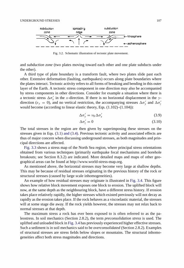
UNDERGROUND STRESSES 107
Fig. 3.2. Schematic illustration of tectonic plate movement.
and subduction zone (two plates moving toward each other and one plate subducts underthe other).
A third type of plate boundary is a transform fault, where two plates slide past eachother. Extensive deformation (faulting, earthquakes) occurs along plate boundaries wherethe plates interact. Tectonic activity refers to all forms of breaking and bending in this outerlayer of the Earth. A tectonic stress component in one direction may also be accompaniedby stress components in other directions. Consider for example a situation where there isa tectonic stress �σ ′
x in the x-direction. If there is no horizontal displacement in the y-direction (εy = 0), and no vertical restriction, the accompanying stresses �σ ′
y and �σ ′z
would become (according to linear elastic theory, Eqs. (1.102)–(1.104)):
�σ ′y = νfr�σ
′x (3.9)
�σ ′z = 0 (3.10)
The total stresses in the region are then given by superimposing these stresses on thestresses given in Eqs. (3.1) and (3.4). Previous tectonic activity and associated effects arethus of major concern when discussing underground stresses, as both magnitudes and prin-cipal directions are affected.
Fig. 3.3 shows a stress map of the North Sea region, where principal stress orientationsobtained from various techniques (primarily earthquake focal mechanisms and boreholebreakouts; see Section 8.3.2) are indicated. More detailed maps and maps of other geo-graphical areas can be found at http://www.world-stress-map.org.
As mentioned above, the horizontal stresses may become very large at shallow depths.This may be because of residual stresses originating in the previous history of the rock orstructural stresses (caused by large scale inhomogeneities).
An example of how residual stresses may originate is illustrated in Fig. 3.4. This figureshows how relative block movement exposes one block to erosion. The uplifted block willnow, at the same depth as the neighbouring block, have a different stress history. If erosiontakes place relatively rapidly, the higher stresses which existed previously will not decay asrapidly as the erosion takes place. If the rock behaves as a viscoelastic material, the stresseswill at some stage die away. If the rock yields however, the stresses may not relax back tonormal stresses at that depth.
The maximum stress a rock has ever been exposed to is often referred to as the pa-leostress. In soil mechanics (Section 2.8.2), the term preconsolidation stress is used. Theuplifted and unloaded block in Fig. 3.4 has previously experienced higher effective stresses.Such a sediment is in soil mechanics said to be overconsolidated (Section 2.8.2). Examplesof structural stresses are stress fields below slopes or mountains. The structural inhomo-geneities affect both stress magnitudes and directions.

108 GEOLOGICAL ASPECTS OF PETROLEUM RELATED ROCK MECHANICS
Fig. 3.3. Stress map of the North Sea, as given by the World Stress Map Project. (Reinecker et al., 2004, availableonline at http://www.world-stress-map.org.)
The Ekofisk field in the North Sea provides a good example of how geological eventscan explain the present state of stress. Ekofisk is the largest of several chalk reservoirs inthe southern part of the Norwegian sector of the North Sea. The chalks are of Maastrichtian(Upper Cretaceous) and Danian (Lower Tertiary) age, and the field has a dome-like struc-ture of elliptical shape. The chalk has a relatively high porosity (around 30% average), but
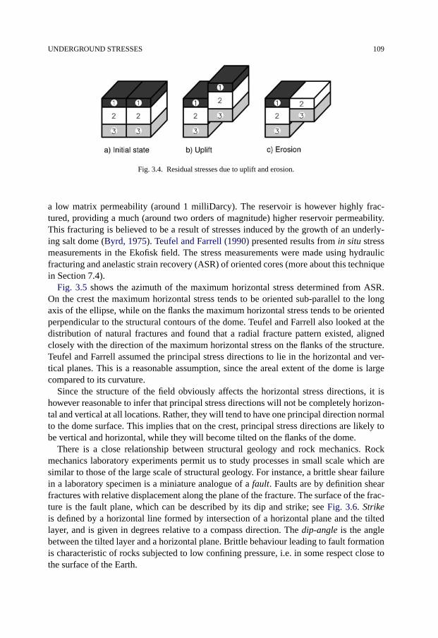
UNDERGROUND STRESSES 109
Fig. 3.4. Residual stresses due to uplift and erosion.
a low matrix permeability (around 1 milliDarcy). The reservoir is however highly frac-tured, providing a much (around two orders of magnitude) higher reservoir permeability.This fracturing is believed to be a result of stresses induced by the growth of an underly-ing salt dome (Byrd, 1975). Teufel and Farrell (1990) presented results from in situ stressmeasurements in the Ekofisk field. The stress measurements were made using hydraulicfracturing and anelastic strain recovery (ASR) of oriented cores (more about this techniquein Section 7.4).
Fig. 3.5 shows the azimuth of the maximum horizontal stress determined from ASR.On the crest the maximum horizontal stress tends to be oriented sub-parallel to the longaxis of the ellipse, while on the flanks the maximum horizontal stress tends to be orientedperpendicular to the structural contours of the dome. Teufel and Farrell also looked at thedistribution of natural fractures and found that a radial fracture pattern existed, alignedclosely with the direction of the maximum horizontal stress on the flanks of the structure.Teufel and Farrell assumed the principal stress directions to lie in the horizontal and ver-tical planes. This is a reasonable assumption, since the areal extent of the dome is largecompared to its curvature.
Since the structure of the field obviously affects the horizontal stress directions, it ishowever reasonable to infer that principal stress directions will not be completely horizon-tal and vertical at all locations. Rather, they will tend to have one principal direction normalto the dome surface. This implies that on the crest, principal stress directions are likely tobe vertical and horizontal, while they will become tilted on the flanks of the dome.
There is a close relationship between structural geology and rock mechanics. Rockmechanics laboratory experiments permit us to study processes in small scale which aresimilar to those of the large scale of structural geology. For instance, a brittle shear failurein a laboratory specimen is a miniature analogue of a fault. Faults are by definition shearfractures with relative displacement along the plane of the fracture. The surface of the frac-ture is the fault plane, which can be described by its dip and strike; see Fig. 3.6. Strikeis defined by a horizontal line formed by intersection of a horizontal plane and the tiltedlayer, and is given in degrees relative to a compass direction. The dip-angle is the anglebetween the tilted layer and a horizontal plane. Brittle behaviour leading to fault formationis characteristic of rocks subjected to low confining pressure, i.e. in some respect close tothe surface of the Earth.
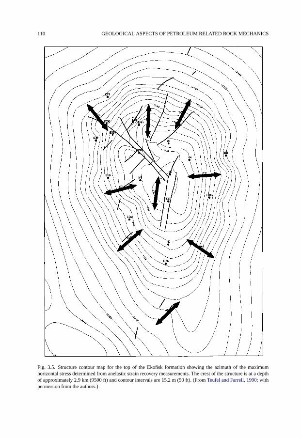
110 GEOLOGICAL ASPECTS OF PETROLEUM RELATED ROCK MECHANICS
Fig. 3.5. Structure contour map for the top of the Ekofisk formation showing the azimuth of the maximumhorizontal stress determined from anelastic strain recovery measurements. The crest of the structure is at a depthof approximately 2.9 km (9500 ft) and contour intervals are 15.2 m (50 ft). (From Teufel and Farrell, 1990; withpermission from the authors.)

UNDERGROUND STRESSES 111
Fig. 3.6. Illustration of dip and strike.
Fig. 3.7. Illustration of fault types.
An extensional, brittle failure in a laboratory test produces a miniature joint. A joint ischaracterized by no displacement along (parallel to) the fracture plane. The rock on eachside of the tensile fracture is moved apart, perpendicular to the failure plane.
The various types of faults can be classified (Anderson, 1951; Twiss and Moores, 1992)according to well-known theories of shear failure (e.g. Mohr–Coulomb). According tothese theories, fracturing will take place in one or both pairs of conjugate planes whichare parallel to the direction of the intermediate principal stress, and are both at equal an-gles of less than 45° to the direction of the maximum principal stress. Some of the mostcommon types of faulting are illustrated in Fig. 3.7, assuming that one principal directionis vertical.
Normal faulting occurs when the maximum principal stress (σ1) is vertical, and the dip ishence larger than 45° (usually around 60°). If the minimum principal stress (σ3) is vertical,the hanging wall is moving upwards, the dip is less than 45° (usually around 30°), and athrust fault is formed. Thrust faults with very shallow dips (less than 10°) are also called

112 GEOLOGICAL ASPECTS OF PETROLEUM RELATED ROCK MECHANICS
Fig. 3.8. Relation between ψ and β.
overthrusts. If the intermediate principal stress (σ2) is vertical, vertical failure planes arecreated. This is referred to as strike-slip faulting.
With reference to Fig. 3.7, ψ is the angle between the maximum principal stress and thefailure plane. This angle is then related to the failure angle, β, such that (see Fig. 3.8):
ψ = π/2 − β (3.11)
Laboratory testing of sand and sandstone commonly yield values of the failure angle in therange 55°–70°, corresponding to ψ values in the range 35°–20°. According to the Mohr–Coulomb failure criterion (see Section 2.3.1), shear fracturing will take place when:
σ ′1 = C0 + σ ′
3 tan2 β (3.12)
where C0 is the unconfined (uniaxial compressive) strength of the rock.The type of fault is dependent on the relative values of the principal stresses. Whether
faulting will take place, and at what angle, is however also dependent on the failure para-meters of the rock.
To illustrate this further, let us consider some simple examples, using the Mohr–Coulomb criterion for shear fracturing.
Consider an unconsolidated sand with zero unconfined strength (typical of shallowsediments). A typical failure angle of the sand is 60°, corresponding to ψ = 30°. TheMohr–Coulomb criterion in this case (note the use of effective stresses) reduces to:
σ ′1 = 3σ ′
3 (3.13)
We assume principal stresses to be vertical and horizontal, with the total vertical stressequal to ρgz. If the vertical stress is the largest principal stress (see Fig. 3.9a), the effectivehorizontal stress must be as low as one third of the effective vertical stress in order fornormal faulting to occur. For thrust faulting, the effective horizontal stress must be 3 timeslarger than the effective vertical stress (see Fig. 3.9b). For strike-slip faulting, the vertical is
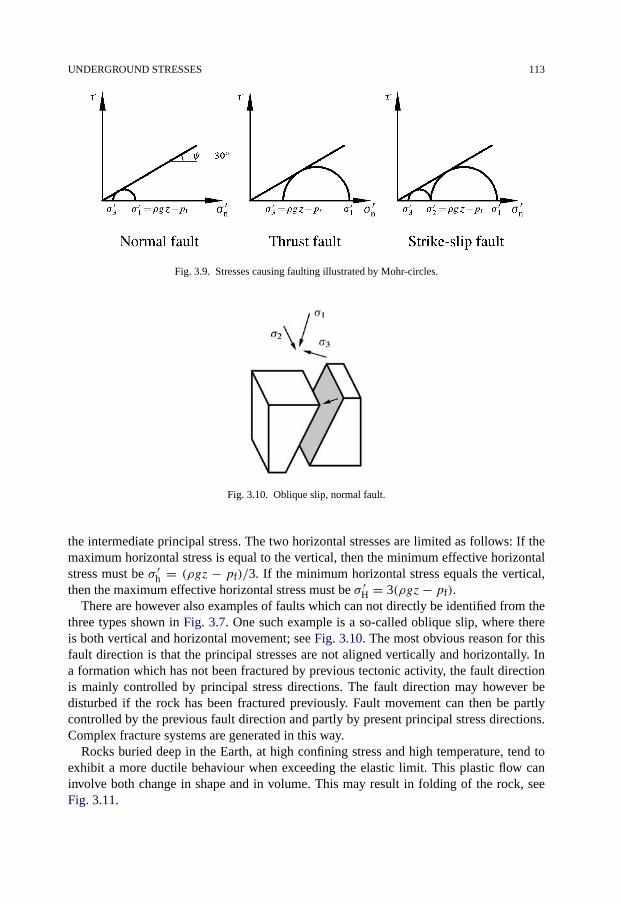
UNDERGROUND STRESSES 113
Fig. 3.9. Stresses causing faulting illustrated by Mohr-circles.
Fig. 3.10. Oblique slip, normal fault.
the intermediate principal stress. The two horizontal stresses are limited as follows: If themaximum horizontal stress is equal to the vertical, then the minimum effective horizontalstress must be σ ′
h = (ρgz − pf)/3. If the minimum horizontal stress equals the vertical,then the maximum effective horizontal stress must be σ ′
H = 3(ρgz− pf).There are however also examples of faults which can not directly be identified from the
three types shown in Fig. 3.7. One such example is a so-called oblique slip, where thereis both vertical and horizontal movement; see Fig. 3.10. The most obvious reason for thisfault direction is that the principal stresses are not aligned vertically and horizontally. Ina formation which has not been fractured by previous tectonic activity, the fault directionis mainly controlled by principal stress directions. The fault direction may however bedisturbed if the rock has been fractured previously. Fault movement can then be partlycontrolled by the previous fault direction and partly by present principal stress directions.Complex fracture systems are generated in this way.
Rocks buried deep in the Earth, at high confining stress and high temperature, tend toexhibit a more ductile behaviour when exceeding the elastic limit. This plastic flow caninvolve both change in shape and in volume. This may result in folding of the rock, seeFig. 3.11.

114 GEOLOGICAL ASPECTS OF PETROLEUM RELATED ROCK MECHANICS
Fig. 3.11. Illustration of compressional folding, cross-section.
Available techniques for measurement and estimation of in situ stress directions andmagnitudes are discussed further in Section 8.3 The most direct measurements are thoseinvolving hydraulic fracturing, where detection of fracture closure pressure yields informa-tion about stress magnitudes. Borehole imaging and/or borehole shape measurements (bye.g. a 4-arm caliper) may reveal information about fracture or drilling-induced breakoutdirections, and hence stress directions (Section 8.3). There is also a number of core basedtechniques (anelastic strain recovery, wave velocity anisotropy, differential strain or wavevelocity analysis, acoustic emission) that can be related to stress magnitudes and direc-tions (Section 7.4). For large scale stress fields, earthquake focal mechanisms represent avaluable source of information.
3.2. Pore pressure
Pore pressure is an important parameter in any rock mechanics study of porous, fluid-filledrock systems. The pore fluid will carry part of the total stresses applied to the system,thus relieving the rock matrix from part of the load. The effective stress as defined byTerzaghi is equal to the total stress minus the pore pressure. This effective stress conceptwas introduced in soil mechanics in 1923 on an empirical basis. It has later been refinedby Biot; see Section 1.6 for further details.
There is overwhelming evidence that porous, saturated and permeable rocks obey aneffective stress law. Both strain, given by the stress–strain relationship (constitutive equa-tion), and yield or failure of the rock is controlled by effective rather than total stresses.
Therefore, when studying borehole stability during drilling, rock stability during produc-tion, and compaction/subsidence, knowledge of the pore pressure in the various formationsis extremely important.
Pore pressure will develop in a saturated formation as sediments are buried. If the porefluid can escape and migrate to the surface at about the same rate as the rate of compaction,a normal pore pressure gradient is maintained, given by the weight of the fluid columnabove (Eq. (3.2)).
There are however several cases where the pore pressure within a zone has a value dif-ferent from the expected normal pore pressure. Usually the pore pressure will in such casesbe higher than the normal, and the zone is referred to as abnormally pressured or overpres-sured. High pore pressures in a reservoir will of course make the field more prolific. On the
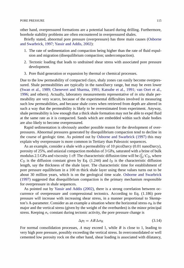
PORE PRESSURE 115
other hand, overpressured formations are a potential hazard during drilling. Furthermore,borehole stability problems are often encountered in overpressured shales.
Briefly stated, abnormal pore pressure (overpressure) has three main causes (Osborneand Swarbrick, 1997; Yassir and Addis, 2002):
1. The rate of sedimentation and compaction being higher than the rate of fluid expul-sion and migration (disequilibrium compaction; undercompaction).
2. Tectonic loading that leads to undrained shear stress with associated pore pressuredevelopment.
3. Pore fluid generation or expansion by thermal or chemical processes.
Due to the low permeability of compacted clays, shaly zones can easily become overpres-sured. Shale permeabilities are typically in the nanoDarcy range, but may be even lower(Swan et al., 1989; Chenevert and Sharma, 1991; Katsube et al., 1991; van Oort et al.,1996; and others). Actually, laboratory measurements representative of in situ shale per-meability are very scarce, because of the experimental difficulties involved in measuringsuch low permeabilities, and because shale cores when retrieved from depth are altered insuch a way that the permeability is likely to be overestimated from experiment. Anyway,shale permeability is low enough that a thick shale formation may not be able to expel fluidat the same rate as it is compacted. Sands which are embedded within such shale bodiesare also likely to become overpressured.
Rapid sedimentation is obviously another possible reason for the development of over-pressures. Abnormal pressures generated by disequilibrium compaction tend to decline inthe course of geologic time. As pointed out by Osborne and Swarbrick (1997) this mayexplain why overpressure is more common in Tertiary than Paleozoic sequences.
As an example, consider a shale with a permeability of 10 picoDarcy (0.01 nanoDarcy),porosity of 25%, and uniaxial compaction modulus of 3 GPa, saturated with a brine of bulkmodulus 2.5 GPa and viscosity 1 cP. The characteristic diffusion time will be l2D/CD, whereCD is the diffusion constant given by Eq. (1.244) and lD is the characteristic diffusionlength, say the thickness of the shale layer. The characteristic time for establishment ofpore pressure equilibrium in a 100 m thick shale layer using these values turns out to beabout 30 million years, which is on the geological time scale. Osborne and Swarbrick(1997) suggested that disequilibrium compaction is the primary mechanism responsiblefor overpressure in shale sequences.
As pointed out by Yassir and Addis (2002), there is a strong correlation between oc-currence of overpressure and compressional tectonics. According to Eq. (1.186) porepressure will increase with increasing shear stress, in a manner proportional to Skemp-ton’s A-parameter. Consider as an example a situation where the horizontal stress σH is themajor and the vertical stress (given by the weight of the overburden) is the minor principalstress. Keeping σv constant during tectonic activity, the pore pressure change is
�pf = AB�σH (3.14)
For normal consolidation processes, A may exceed 1, while B is close to 1, leading tovery high pore pressure, possibly exceeding the vertical stress. In overconsolidated or wellcemented low porosity rock on the other hand, shear loading is associated with dilatancy,

116 GEOLOGICAL ASPECTS OF PETROLEUM RELATED ROCK MECHANICS
leading to pore pressure reduction. This mechanism is therefore expected to cause abnor-mally high pore pressure preferably in young sediments. Note that tectonic activity (e.g.salt tectonics) will result in sustained abnormal pore pressure only if the system remainsclosed and does not fracture.
Another possible source of overpressure is the uplift-erosion process shown in Fig. 3.4.If the rock maintains its pore pressure after the uplift, it will be abnormally pressurizedcompared with its neighbouring formations at the same depth. Often, however, faultingis associated both with tectonic and uplift processes, and in such cases the pore pressurebuild-up would be only transient.
As mentioned above, generation or expansion of pore fluid may lead to overpressure,primarily in shale sections. This may be a result of increase in temperature (aquathermalpressuring). It may be caused by hydrocarbon (kerogen or gas) generation. It may alsobe caused by free water released during transformation of montmorillonite to illite. Thistransition is temperature dependent, requiring temperatures of 70–90°C, corresponding todepths of 2–3 km in areas of average geothermal gradient.
When the pore pressure increases due to fluid expansion/generation, there will be anassociated horizontal stress increase. The relation between horizontal stress and pore pres-sure is hence not unique, but depends on the overpressure mechanism (Yassir and Addis,2002).
Yet another class of mechanisms is associated with fluid movement caused by e.g. den-sity differences between liquids and gases, or possibly by osmotic potentials. There ishowever no evidence that these mechanisms play any significant role in practice.
Fig. 3.12 presents typical pore pressure gradient curves from two North Sea fields, theGullfaks field and the Valhall field. Valhall is a chalk reservoir (Cretaceous) in the Ekofiskarea of the Norwegian sector of the North Sea. Gullfaks is a sandstone reservoir (Jurassic),located further north. Both parts of Fig. 3.12 include the estimated fracture pressure, takenfrom leak-off and mini-frac tests (see Section 8.3). The Valhall field is characterized by ahigh initial pore pressure. Close to the top of the reservoir at 2500 m, the pore pressureis about 44.7 MPa. The overburden gradient is not included for the Valhall field, but atthis depth the total vertical stress is approximately 49 MPa, which makes the differencebetween the overburden stress and the pore pressure quite small. Thus, the effective verticalstress is very low.
In such a situation, the net grain-to-grain stress is small, and unless the strength of thecement between the grains is significant, particles may easily be mobilized. Productionproblems have been experienced in the North Sea chalk fields, materializing both as inflowof solids and casing collapse (see Chapter 10 for analysis of particle production).
Both fields are characterized by a rapid increase of the pore pressure gradient just abovethe reservoir (top of Gullfaks is at approximately 1850 m). This is relatively typical inmany of the North Sea reservoirs. The effective vertical stress in the Gullfaks field is ap-proximately 6 MPa.
Pore pressures above the reservoir, in the low-permeability zones, are normally esti-mated from trendlines and deviations from expected trendlines in wireline log readings.In many cases the accuracy of these methods is not good enough, and stability problemsduring drilling may be a consequence (see also Chapter 9). In the reservoir, where the rock
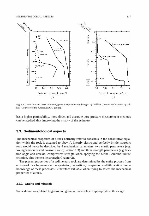
SEDIMENTOLOGICAL ASPECTS 117
Fig. 3.12. Pressure and stress gradients, given as equivalent mudweight: a) Gullfaks (Courtesy of Statoil); b) Val-hall (Courtesy of the Amoco/NOCO-group).
has a higher permeability, more direct and accurate pore pressure measurement methodscan be applied, thus improving the quality of the estimates.
3.3. Sedimentological aspects
The mechanical properties of a rock normally refer to constants in the constitutive equa-tion which the rock is assumed to obey. A linearly elastic and perfectly brittle isotropicrock would hence be described by 4 mechanical parameters: two elastic parameters (e.g.Young’s modulus and Poisson’s ratio; Section 1.3) and three strength parameters (e.g. fric-tion angle and uniaxial compressive strength when applying the Mohr–Coulomb failurecriterion, plus the tensile strength; Chapter 2).
The present properties of a sedimentary rock are determined by the entire process fromerosion of rock fragments to transportation, deposition, compaction and lithification. Someknowledge of these processes is therefore valuable when trying to assess the mechanicalproperties of a rock.
3.3.1. Grains and minerals
Some definitions related to grains and granular materials are appropriate at this stage:

118 GEOLOGICAL ASPECTS OF PETROLEUM RELATED ROCK MECHANICS
TABLE 3.1 Grain-size scale for sediments. In geol-ogy, the so called phi-scale is commonly used. It isdefined by phi = − log2(grain diameter in mm)
Grain diameter range [mm] phi-scale Term
>256 < −8 Boulder64–256 −6– −8 Cobble4–64 −2– −6 Pebble2–4 −1– −2 Granule1/16–2 4– −1 Sand1/256–1/16 8–4 Silt<1/256 >8 Clay
Grain size is a measure of the diameter of the grain, see Table 3.1. According to thisclassification scheme, the grain size determines the classes of sedimentary rocks.
Grain shape involves both the roundness (angularity of corners) and sphericity (proximityto a spherical shape).
Grain sorting is a measure of the range of grain sizes (grain size distribution). A rockcontaining a wide range of grain sizes is said to be poorly sorted, whereas well sortedimplies a narrow distribution.
The packing of grains is important since it affects porosity and permeability. The packingdepends both on grain size, shape and sorting. Round grains will have a smaller frictionangle than the more angular grains at the same porosity. A poorly sorted sand will have ahigher friction angle than a well sorted sand.
There are several rock forming mineral groups: silicates (e.g. feldspar, clay, mica), car-bonates (calcite, dolomite), oxides, sulphides, sulphates and phosphates.
The silicate group is the most important rock forming mineral group, making up morethan 90% of the Earth’s crust. The basic unit of the silicates is the SiO−4
4 silicon tetrahe-dron. The various structures are formed by linking tetrahedral units together by sharingoxygen. Feldspar is the most important single silicate mineral. The three main groups offeldspars are: potassium feldspars (KAlSi3O8), sodium feldspars (NaAlSi3O8) and cal-cium feldspars (CaAl2Si2O8). These are formed by Al substituting for Si, thus allowingadditional or different cations to enter the structure.
Although chemically an oxide, silica (SiO2), is closely related to silicates. Quartz, whichis one of the minerals in the silica group, is the most common mineral in sandstone, rangingfrom 65% to practically 100%. The feldspar content in sandstone is typically 10–15%, andmica and clay minerals may also be found.
The most important minerals in shaly rocks are clay minerals, which are composedof layers of sheet shaped crystals. Two basic structural units exist: One type of sheet isbuilt from silica tetrahedra linked together in a hexagonal structure with chemical formulaSi4O4−
4 . The second type is an octahedral sheet in which silicon is replaced by cations likeAl3+ (this sheet is named gibbsite, with basic formula Al2(OH)6), Mg2+ (named brucite;Mg3(OH)6), Fe3+ or Fe2+, surrounded by six hydroxide groups. Within a given sheet, ionsdifferent from the dominant ones may be present (isomorphic substitution), giving rise to

SEDIMENTOLOGICAL ASPECTS 119
possible charge deficiency. Usually, mainly because of oxygen and hydroxide at the sur-faces, these have negative excess charge, and will therefore attract cations.
The basic sheets are combined to form layered clay minerals. The most common groupsof clay minerals are kaolinite, illite, and smectite. Kaolinite is a two-layer mineral (oftenreferred to as a 1:1 layer silicate), consisting of alternate layers of gibbsite and silicontetrahedron sheet. A basic unit is 0.7 nm thick, while typical composite crystals may be70–100 layers, have six-fold symmetry and are flake shaped, up towards the micrometrerange in lateral extent. The successive layers are strongly bonded to each other with ahydrogen bonding, and therefore water is not permitted to enter in between layers. Mineraldensity is 2.6–2.7 g/cm3.
Smectite is a 2:1 layer mineral, composed of a central gibbsite sheet embedded betweentwo silicon tetrahedron sheet, with a combined thickness of about 1 nm. Isomorphous sub-stitutions are common both within the central octahedral sheet and in the tetrahedral sheet.The bonding between two silica sheet connecting the unit layers is very weak (through vander Waals’ forces). In smectite, this permits water and exchangeable ions to enter betweenthe platelets, leading to a swelling capacity: At surface conditions, smectite minerals mayabsorb up to 10 times their own weight in water (“swelling clays”). Calcium and sodiumare common ions in the interlayer space. Smectite crystals are normally not more than2–5 nm thick in hydrated state, with an average diameter of about 1 µm. Normally, thebasal spacing is found to be near 1.5 nm, indicating that two monolayers of water are ac-commodated within the mineral. The specific surface area associated with the interlayerspace is 500–700 m2/g. Mineral density varies between 2.0 and 2.6 g/cm3.
Montmorillonite is a name often used synonymously with smectite, or as a commonterm for expandable clay minerals. In principle, this is a member of the smectite groupwith geographical origin in Montmorillon, France. Another well-known smectitic clay isBentonite, from Wyoming in the USA. Vermiculite, which is hydrated muscovite (a micamineral), is also classified as smectite, but has much less swelling capacity than the clayminerals mentioned above.
Illite is another 2:1 layer clay mineral, formed by weathering of feldspars, degradationof muscovite, and transformation of smectite to illite at depth. Some of the silicon atomsin smectite are replaced by aluminium, causing a negative charge which is balanced bypotassium ions that provide bonding between the silica tetrahedron sheet. This bond ismuch stronger than in smectite, preventing hydration, but it is considerably weaker than inkaolinite. The basal layer thickness of illite is 1 nm. Mineral density is 2.6–2.9 g/cm3.
The water near the surfaces of clay crystals is different from free water. This was sug-gested by Derjaguin and Churayev (1971). Molecular dynamics simulations (e.g. Skipperet al., 1991; Karaborni et al., 1996; Park and Sposito, 2002) show that bound water in theintralayer space and adsorbed water on surfaces have ordered, crystal-like structures.
Chlorite is often also referred to as a clay mineral. It has a 2:1 sandwich structure, butwith an additional brucite-like (where the dominant ion may be magnesium, iron or nickel)layer embedded between the tetrahedral layers. It has the characteristic flake shape, butdoes not have any swelling capacity. Density may be from 2.6 and up to 3.3 g/cm3.
The basic unit of carbonates is (CO3)2−. Common carbonate minerals are calcite(CaCO3), aragonite (which is a polymorph of calcite) and dolomite (CaMg(CO3)2). Calciteis the main component of carbonate sediments (chalk, limestone).

120 GEOLOGICAL ASPECTS OF PETROLEUM RELATED ROCK MECHANICS
3.3.2. Pre-deposition and deposition
Clastic sedimentary rocks originate from some sort of pre-existing rock. The pre-existingrock is broken into fragments by weathering (mechanical and/or chemical) and erosion.Then it is transported by water (rivers, tides) or wind to another site where it is deposited.This accumulation of fragments from pre-existing rocks form what is called a clastic sedi-ment. The most common types of clastic sediments are conglomerate, sandstone, siltstoneand shale. Other types of sediments are chemical sediments (e.g. precipitation of saltcrystals due to evaporation) and organic sediments (e.g. shells and skeletons from sea or-ganisms forming a chalk or limestone). Note that for instance a limestone can be bothclastic and organic in origin.
Transport, deposition and sediment accumulation may take place in a variety of deposi-tional environments. These various environments will give rise to different distributions ofgrain size, grain shape etc., which may affect the mechanical properties of the rock millionsof years later. Particles may be transported by air (aeolian), water (fluvial) or ice (glacialtransport). Deposition occurs if the particle flow velocity is lower than a settling velocity,being proportional to the square of particle size and the density contrast between particleand suspending fluid, and inversely proportional to fluid viscosity.
When transported by air (aeolian transport), the particles have a very small buoyancy,and the viscosity of the air is low. Particles transported by winds are therefore typicallymore fine-grained than particles transported by water.
In water, such as in a river or a marine environment, particles can be transported in sus-pension (suspended load) or along the bottom (bed load). Sediments deposited in runningwater are termed alluvial (poorly sorted, emerging from a high energy environment) or flu-vial (well sorted, low energy environment). As long as the concentration of particles in thesuspension is low, the water can be regarded as a Newtonian fluid, obeying ordinary hy-drodynamic laws. As the concentration increases, the properties of the suspension (density,viscosity) will start to deviate significantly from those of pure water. Such a suspension canstart to flow as a heavy liquid due to the difference in density between the suspension andthe surrounding water. This is known as a turbidity current. This kind of sediment transportis believed to be an important mechanism when considering transport of sediments fromdeltas and shallow areas, down the continental shelf and into the deep oceans.
Grain flow is another mechanism of sediment transport, resulting from grain collisionsthat contribute to keep the grains from concentrating close to the bottom. Grain flow willhave a low content of clay matrix material. As the contents of silt and clay increases, debrisflow and eventually mudflow develops. Debris flow and mudflow sediments are often verypoorly sorted.
In the shallow beach zone, deposition will often result in well sorted coarse-grainedrocks with high porosity. The grains will tend to be well rounded due to the constant actionof waves, currents and tides. Further down, the grain size decreases and the sorting ispoorer. Clastic deposits of terrestrial origin, resulting from stream transport into the sea,can also be well sorted, but normally contain more clay than the beach deposits. The deltais the zone where fluvial and marine processes meet. If the marine activity is low, thefluvial depositions in the delta will be maintained. If the marine activity is high, however,the deposits will eventually accumulate as a marine sediment. In a delta front deposit,

SEDIMENTOLOGICAL ASPECTS 121
fresh water, sea water and pore water from previous sediments meet. Water from thesedifferent sources will be of completely different composition, and form an environment ofactive precipitation and dissolution. This can lead to cementation (silica, carbonate) of thesediment.
Although carbonate rocks can originate from clastic sediments, the primary source ofcarbonates is from plants and animals which make use of carbonates in some way. Car-bonate sediments will be fine-grained (grain size in the micrometre-range), and the finalproperties of the carbonate rock will depend very much on the post-depositional processes(diagenesis), since the carbonates are strongly influenced by pore fluid chemistry and tem-perature/pressure. Carbonates may also contain larger grains (e.g. fragments of fossils) ofsand particle size or larger. In the same way as for sand deposits, the carbonate is morelikely to be coarse grained and well sorted in high energy, shallow waters.
3.3.3. Post-deposition
After sediment deposition follows a lengthy process of transformation into a rock (sandto sandstone, clay to shale, silt to siltstone). As the sedimentation process continues, anoverburden of younger sediments is deposited. This extra weight on top of a sedimentcauses the sediment to compact. Compaction will result in a closer packing of the grains,thus reducing both porosity and permeability. The friction angle will increase as a result ofcompaction, see Fig. 3.13a. Compaction itself is however not sufficient to create a massive,cemented rock, as closer packing alone does not affect the cohesion. The sediment willhowever act as if it is stronger when the weight of the overburden increases, since thefriction angle is always larger than zero. The increased overburden will result in increasedhorizontal stresses when the sediment is confined horizontally. This will have the sameeffect as a confining pressure in the laboratory, and the sediment can tolerate larger shearstresses before it fails. This is illustrated in Fig. 3.13b.
For the transformation to be complete, processes by which grains are cemented togetherare required. These physical and chemical postdepositional processes are referred to as dia-
Fig. 3.13. Effects of compaction on strength properties: a) Increase of friction angle as a result of compaction;b) Increase of failure stress as a result of confinement.

122 GEOLOGICAL ASPECTS OF PETROLEUM RELATED ROCK MECHANICS
genesis. The parts of the diagenetic processes which contribute to harden the rock, are alsoreferred to as lithification. The term consolidation is often used in a sloppy way by petro-leum engineers, referring to the degree of cementation. For instance, “poorly consolidatedsandstone” is supposed to mean poorly cemented sandstone. Strictly speaking, however,consolidation refers to time dependent deformation due to dissipation of pore pressure (seeBiot’s theory of consolidation in Section 1.6). That means; poorly consolidated basicallymeans poorly compacted. There is however often some correlation between the amount ofdiagenetic cementation and the effective stresses developing in a formation due to com-paction, especially in sand deposits.
Physical changes, in addition to compaction, include changes brought about by tectonicactivity. With respect to diagenetic effects, the chemical changes are however the mostimportant. Cementation is mainly the result of precipitation of a binding agent. When con-sidering chemical processes, the interaction between the solid grain minerals (especiallythe surface minerals) and the pore fluid is the basic process. As only the pore water is freeto move in the sediment (at least as long as porosity and permeability are maintained), theseprocesses are closely linked to changes in pore water chemistry. Precipitation of calciteonto the surface of sand grains is one such example of chemically induced cementation.
Carbonate (especially calcite) and silica are the minerals that account for most of thecementation of sandstones. If the contact stress between quartz grains gets sufficiently high,pressure solution may occur. The idea is that dissolution at the grain contact points liberatesSiO2 to the pore water. The SiO2 is then reprecipitated as quartz overgrowth because thepressure in the pore water is lower, resulting in silica-cementation. Both calcite and quartzcementation lead to strong sandstones. If the grains are held together by clay minerals, thesandstone will be weak.
In carbonate sediments (commonly called carbonates), cementation is mainly precipita-tion of carbonate minerals. Primary cementation will often consist of aragonite or calcitewith a high (up to 30%) magnesium content. These calcium carbonates are metastable, andwill after some thousands of years transform to the more stable form, low-magnesium-calcite, through dissolution and precipitation. Dolomitization involves conversion of cal-cium carbonate and magnesium to dolomite:
2CaCO3 + MgCl2 → CaMg(CO3)2 + CaCl2
This process requires a certain ratio of Mg/Ca in order to take place. This required ratiois reduced as sediments are buried and the temperature increases because the magnesiumions then become less hydrated.
Dolomitization, as most other processes of precipitation and cementation, will often leadto reduced porosity as the void space is fully or partially filled up. This increases the rockstrength in most cases, but also reduces the potential of the rock as a reservoir formation.
Cementation processes will however, as we have seen, require increased pressures orsome throughflow of pore water. If these conditions are not met, cementation will cometo a halt. Some of the North Sea reservoirs can exemplify this. Both the sandstone andchalk reservoirs are characterized by abnormally high pore pressures (see Fig. 3.12). Thishas prevented pressure solution, and an efficient cap rock has prevented further circulationof pore fluid through the reservoir rock. This has helped maintain a very high porosity,30–50% in the most prolific chalk and around 30% in the sandstone reservoirs. This has
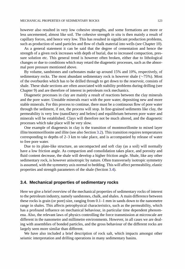
MECHANICAL PROPERTIES OF SEDIMENTARY ROCKS 123
however also resulted in very low cohesive strengths, and some formations are more orless uncemented, almost like soil. The cohesive strength in situ is then mainly a result ofcapillary forces, and hence very low. This has resulted in significant production problems,such as production of sand particles and flow of chalk material into wells (see Chapter 10).
As a general statement it can be said that the degree of cementation and hence thestrength of a given rock increases with depth of burial, due to increased compaction, pres-sure solution etc. This general trend is however often broken, either due to lithologicalchanges or due to conditions which may retard the diagenetic processes, such as the abnor-mal pore pressure mentioned above.
By volume, sandstones and carbonates make up around 15% and 10%, respectively, ofsedimentary rocks. The most abundant sedimentary rock is however shale (∼75%). Mostof the overburden which has to be drilled through to get down to the reservoir, consists ofshale. These shale sections are often associated with stability problems during drilling (seeChapter 9) and are therefore of interest in petroleum rock mechanics.
Diagenetic processes in clay are mainly a result of reactions between the clay mineralsand the pore water. Unstable minerals react with the pore water, depositing new and morestable minerals. For this process to continue, there must be a continuous flow of pore waterthrough the sediment, if not, the process will stop. In fine-grained sediments like clay, thepermeability is very low (nanoDarcy and below) and equilibrium between pore water andminerals will be established. Clays will therefore not be much altered, and the diageneticprocesses which take place will be very slow.
One example of diagenesis in clay is the transition of montmorillonite to mixed layerillite/montmorillonite and illite (see also Section 3.2). This transition requires temperaturescorresponding to depths of 2–3 km to take place, and is accompanied by release of waterto free pore water.
Due to its plate-like structure, an uncompacted and soft clay (as a soil) will normallyhave a low friction angle. As compaction and consolidation takes place, and porosity andfluid content decrease, the shale will develop a higher friction angle. Shale, like any othersedimentary rock, is however anisotropic by nature. Often transversely isotropic symmetryis assumed, with the symmetry axis normal to bedding. This will affect permeability, elasticproperties and strength parameters of the shale (Section 3.4).
3.4. Mechanical properties of sedimentary rocks
Here we give a brief overview of the mechanical properties of sedimentary rocks of interestto the petroleum industry, namely sandstones, chalk, and shales. A main difference betweenthese rocks is grain (or pore) size, ranging from 0.1–1 mm in sands down to the nanometrerange in shales. This affects petrophysical characteristics, such as the permeability, whichhas a profound influence on mechanical behaviour, in particular time dependent phenom-ena. Also, the relevant laws of physics controlling the force transmission at microscale aredifferent in the nanometre and millimetre environments. However, in all cases we are deal-ing with assemblies of bonded particles, and the gross behaviour of the different rocks arelargely seen more similar than different.
We have also included a brief description of rock salt, which impacts amongst otherseismic interpretation and drilling operations in many sedimentary basins.

124 GEOLOGICAL ASPECTS OF PETROLEUM RELATED ROCK MECHANICS
Fig. 3.14. Thin section image of Castlegate sandstone (courtesy of Reidar Bøe, SINTEF Petroleum Research).
3.4.1. Sandstone
A thin section image of a sandstone is shown in Fig. 3.14. The dominant grain sizes ofsandstone are typically 0.01–1 mm. Pore sizes are the same order of magnitude, but slightlysmaller. This gives permeabilities ranging from microDarcy to several Darcies.
The predominant matrix mineral is quartz. The cement may be quartz as well (in the caseof pressure solution), it may be carbonate (especially calcite), or clay minerals. Quartz hasa bulk modulus of 37.5 GPa and a shear modulus of 41 GPa (see Appendix A).
The texture may vary from isotropic to anisotropic. Intrinsic (lithological) anisotropy iscaused by microlamination (bedding), induced for instance by seasonal variations duringdeposition. This typically gives alternating layers of coarse and fine grains. Anisotropymay also be caused by deposition of flat grains with their long axis parallel to each other.
An unconfined test with a sandstone, or a triaxial test at a low confining pressure, typi-cally shows nonlinear stress–strain behaviour during initial loading, with stiffening as thestress is increased. This nonlinearity can be attributed to pre-existing microcracks withinthe core, generated by stress release during coring (for cores from depth; see Section 7.1.2)or caused by weathering (for outcrop or near surface cores). For weak sandstones, wheremany grain contacts are not cemented, the grain contact itself is a nonlinear element(cf. Hertzian contact theory; Chapter 6).
It is not possible to state any number that characterizes the strength or stiffness of a typ-ical sandstone—a “typical” rock does simply not exist. We find sandstones with porositiesranging from less than 5% up to 40%. The strength varies with porosity—as illustrated byFig. 3.15 (from Plumb, 1994).
Plumb found an empirical correlation for the unconfined strength of very clean sand-stones:
C0 = 357(1 − 2.8φ)2 (φ < 0.357) (3.15)
with C0 given in MPa and φ as a fraction.This represents an upper bound to the unconfined strength. For sandstones containing
clay, the strength falls well below the trend suggested by this equation. Note the similaritybetween Eq. (3.15) and the critical porosity model discussed in Section 6.2.
Young’s modulus shows a strong correlation with strength. Deere and Miller (1966)investigated 82 sandstones from 18 different locations in USA. They found the staticYoung’s modulus to be proportional to the unconfined strength (C0), but with significant

MECHANICAL PROPERTIES OF SEDIMENTARY ROCKS 125
Fig. 3.15. Strength of sandstones. After Plumb (1994).
© 1994 Taylor & Francis Group. Used with permission.
scatter. Most data presented by Deere and Miller, and elsewhere, give a proportionalityratio (E/C0) between 100 and 400.
Tensile strength (T0) is not often measured directly on sandstone cores. Values are nor-mally derived from indirect measurements, such as Brazilian tests (see Section 7.5). Thegeneral impression is that (C0/T0) is between 5 and 20 for sandstones. Note however thatunconfined data are often not very reliable, because of pre-existing cracks or flaws in therocks tested.
When a sandstone starts to yield at low confining pressure, the behaviour is often founddilatant. There is a brittle-ductile transition: Above a certain confining pressure, the rockfails in a ductile manner, and plasticity theory is required to describe the constitutive ma-terial behaviour. The failure envelope is often matched to a linear criterion, although it isusually found to be nonlinear, with a decreasing friction angle at high confining stresses.The typical friction angle is near 30°, but may vary typically between 20° and 40°. Thehigher friction angles are found for low porosities and low clay contents.
Sandstones are found to exhibit an end cap in their failure envelope (i.e. material failureunder high isotropic stresses). This is often associated with grain crushing, but may alsoresult from collapse of the pore structure by grain reorganization. Localized “compactionbands” of crushed material have been observed in triaxial tests with high porosity sandstoneat high confining pressure (Olsson and Holcomb, 2000). The stress threshold for graincrushing depends on particle size distribution and particle shape, and on the degree ofcementation. Data on sandstones between 15 and 25% porosity by Wong et al. (1997)show (Boutéca et al., 2000) that the hydrostatic yield stress is 6–7 times the unconfinedstrength.
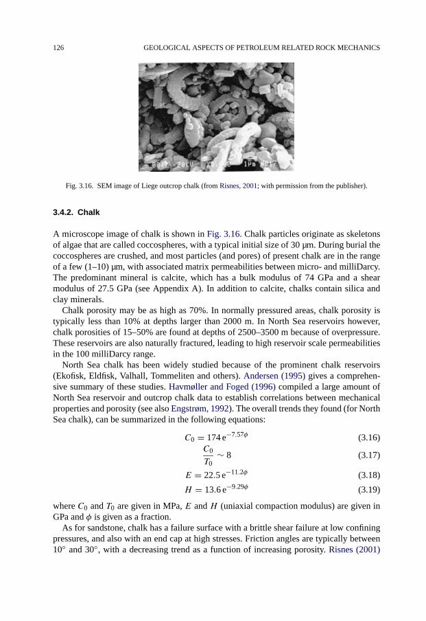
126 GEOLOGICAL ASPECTS OF PETROLEUM RELATED ROCK MECHANICS
Fig. 3.16. SEM image of Liege outcrop chalk (from Risnes, 2001; with permission from the publisher).
3.4.2. Chalk
A microscope image of chalk is shown in Fig. 3.16. Chalk particles originate as skeletonsof algae that are called coccospheres, with a typical initial size of 30 µm. During burial thecoccospheres are crushed, and most particles (and pores) of present chalk are in the rangeof a few (1–10) µm, with associated matrix permeabilities between micro- and milliDarcy.The predominant mineral is calcite, which has a bulk modulus of 74 GPa and a shearmodulus of 27.5 GPa (see Appendix A). In addition to calcite, chalks contain silica andclay minerals.
Chalk porosity may be as high as 70%. In normally pressured areas, chalk porosity istypically less than 10% at depths larger than 2000 m. In North Sea reservoirs however,chalk porosities of 15–50% are found at depths of 2500–3500 m because of overpressure.These reservoirs are also naturally fractured, leading to high reservoir scale permeabilitiesin the 100 milliDarcy range.
North Sea chalk has been widely studied because of the prominent chalk reservoirs(Ekofisk, Eldfisk, Valhall, Tommeliten and others). Andersen (1995) gives a comprehen-sive summary of these studies. Havmøller and Foged (1996) compiled a large amount ofNorth Sea reservoir and outcrop chalk data to establish correlations between mechanicalproperties and porosity (see also Engstrøm, 1992). The overall trends they found (for NorthSea chalk), can be summarized in the following equations:
C0 = 174 e−7.57φ (3.16)C0
T0∼ 8 (3.17)
E = 22.5 e−11.2φ (3.18)
H = 13.6 e−9.29φ (3.19)
where C0 and T0 are given in MPa, E and H (uniaxial compaction modulus) are given inGPa and φ is given as a fraction.
As for sandstone, chalk has a failure surface with a brittle shear failure at low confiningpressures, and also with an end cap at high stresses. Friction angles are typically between10◦ and 30◦, with a decreasing trend as a function of increasing porosity. Risnes (2001)

MECHANICAL PROPERTIES OF SEDIMENTARY ROCKS 127
Fig. 3.17. Typical stress–strain curve for chalk under hydrostatic compression.
pointed out that compressive, tensile and end cap failure modes appear to be governed byone failure surface. The end cap is associated with pore collapse, a phenomenon which maysignificantly reduce the pore space in high porosity chalks. An example of a typical stress–strain curve for chalk under hydrostatic compression (as for example given by Dahou et al.,1995) is shown in Fig. 3.17. The stress reaches a plateau after an initial elastic phase. Thisplateau represents pore collapse. After pore collapse, the material regains some stiffness ifit is continued to be strained.
From Havmøller and Foged (1996) the onset of yielding (pore collapse) in hydrostatictests is given as
σyield = 435 e−8.31φ (3.20)
where σyield is given in MPa and φ is given as a fraction. In uniaxial compaction the yieldstress is
σKoyield = 363 e−7.36φ (3.21)
The uniaxial compaction modulus in the plastic regime is
Hpl = 47.6 e−12.1φ (3.22)
Because of its significance as a reservoir rock in the North Sea, chalk has been widelystudied and characterized. Less comprehensive laboratory studies have been performedwith more competent carbonate rocks (e.g. Yasar and Erdogan, 2004; and referencestherein). Yasar and Erdogan studied limestone, dolomite and (metamorphous) marble, andestablished correlations between P-wave velocity (see Section 5.2) versus strength andYoung’s modulus:
C0 = 31.5vp − 63.7 (3.23)
E = 10.7vp − 18.7 (3.24)
where C0 is given in MPa, E is given in GPa and vp is given in km/s.

128 GEOLOGICAL ASPECTS OF PETROLEUM RELATED ROCK MECHANICS
Fig. 3.18. SEM image of Kimmeridge shale (from Swan et al., 1989; with permission from the publisher).
3.4.3. Shale
A Scanning Electron Image of a shale is shown in Fig. 3.18. Shales consist to a large extentof clay minerals. From the rock mechanical viewpoint, it is natural to define a shale as arock in which clay minerals constitute a load-bearing framework. In practice this meansthat clay content needs to be higher than about 40%. As demonstrated in Fig. 3.18, shaletexture is strongly anisotropic. This is often seen through a plane of weakness along whichthe shale easily splits. It means that all non-scalar physical quantities will be anisotropic, afact which is often neglected in practical rock mechanical analysis, due to lack of data.
Because of the abundance of clay minerals, pore sizes in shale are very small; typicallybetween 5 and 25 nm. In addition, the clay minerals contain structurally bound water. Thismeans that it is difficult to measure as well as to define the elastic properties of the solidmaterial contained in shales.
Various approaches have been used, including theoretical models (Alexandrov andRyzhova, 1961; Katahara, 1996), extrapolation of wave velocity measurements on shales(Tosaya, 1982; Han, 1986; Castagna et al., 1995; and others summarized in Mavko etal., 1998) or clay powders (Vanario et al., 2003) to zero porosity, and theoretical inver-sion of velocity measurements on epoxy impregnated shale samples (Wang et al., 1998).Values scatter widely—the extrapolation techniques give bulk modulus between 5 and25 GPa, and shear modulus ranging from 4 to 10 GPa. These numbers clearly dependon which type of clay mineral (kaolinite, smectite, illite) is dominant, and in particularon the adsorbed or bound water present within minerals and on mineral surfaces. Whensufficiently large crystals are available, such as in the case of muscovite, one may mea-sure directly the stiffness of the solid material in a dry state (no bound water). Suchdata give for this particular mineral (Carmichael, 1984; Alexandrov and Ryzhova, 1961;Katahara, 1996) a bulk modulus of 51 GPa and a shear modulus of 32 GPa. Note howeverthat this mineral is strongly anisotropic, with moduli in the crystal symmetry plane being4–6 times larger than moduli representing normal to plane stiffnesses.
Shales have, because of the narrow pore space, very large specific surface areas. Thesesurfaces are negatively charged, and attract cations from the pore water. Hydrated ions areoften attached to the mineral surfaces. Shale porosity may vary from very small (a few %)
MECHANICAL PROPERTIES OF SEDIMENTARY ROCKS 129
to quite high (up to 70%). Even with the highest porosities, permeability remains verysmall. The nanometre size pores lead to laboratory measured permeabilities in the nano-Darcy range (see references given under Section 3.2). Even lower values may be expectedfor shale under in situ conditions.
The very low permeability makes shale a very special rock material to study. It meansthat rock mechanical tests become extremely time-consuming, since pore pressure equili-bration is slow. It also means that cores when taken out of the Earth, always will have atendency to be damaged by tensile failure occurring during core retrieval: The core wouldhave to be retrieved at an extremely low rate in order to prevent overpressure inside. Thismeans that shale cores may be incompletely saturated. Such a damaged core is clearly notrepresentative of the shale in situ. Resaturation of a shale core can not be done as in stan-dard petrophysics analysis. Capillary forces may lead to further damage of the shale. Theauthors’ experience is that the best results are obtained when a pore pressure is enforced(or measured, as a response to applied stress).
The difficulties in testing and specimen preparation are discussed further in Chapter 7. Itmeans however that good laboratory test results are scarce, and have to be judged carefullyin light of the laboratory procedures applied. Also, because shale is not a reservoir rockand has only indirect economic interest, it has not been studied to the same extent as othersedimentary rocks.
Lashkaripour and Dusseault (1993) collected a large set of shale data from publishedliterature and in-house studies. The majority of shales tested had porosity below 20%. Theyfound unconfined strength to increase with decreasing porosity, and proposed a relation ofthe form
C0 = 193φ−1.14 (3.25)
where C0 is given in MPa and φ is given in %.Their data set also showed strength and stiffness to be related. The ratio between
Young’s modulus and unconfined strength (E/C0) is typically around 200. The compres-sive strength is typically 10–15 times higher than the tensile strength.
Horsrud (2001) studied North Sea shales, most of them with higher porosities (30–55%).He confirmed a proportionality between the Young’s modulus and unconfined strength,with a proportionality constant of ∼150. These data show good correlation of strength withporosity, but the correlations are different from those found for lower porosity shales byLashkaripour and Dusseault. Both works demonstrated that P-wave velocity measurementsshow a good correlation to shale strength, which is a valuable result if one wants to relateshale strength to sonic measurements on drill cuttings or from log/seismic data. Horsrud(2001) found the relation
C0 = 0.77 v2.93p (3.26)
where C0 is given in MPa and vp is given in km/s.Due to its plate-like structure, an uncompacted and soft clay (like soil) will normally
have a low friction angle. As compaction and consolidation takes place, and porosityand fluid content decrease, the shale will develop a higher friction angle. Horsrud alsoshowed that the friction angle in most tests with high porosity shale was very low, typi-cally 10°–20°.
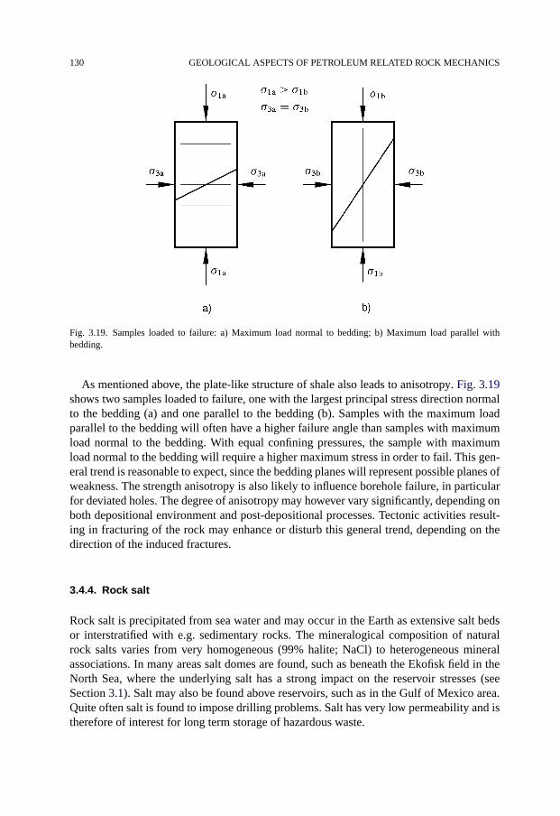
130 GEOLOGICAL ASPECTS OF PETROLEUM RELATED ROCK MECHANICS
Fig. 3.19. Samples loaded to failure: a) Maximum load normal to bedding; b) Maximum load parallel withbedding.
As mentioned above, the plate-like structure of shale also leads to anisotropy. Fig. 3.19shows two samples loaded to failure, one with the largest principal stress direction normalto the bedding (a) and one parallel to the bedding (b). Samples with the maximum loadparallel to the bedding will often have a higher failure angle than samples with maximumload normal to the bedding. With equal confining pressures, the sample with maximumload normal to the bedding will require a higher maximum stress in order to fail. This gen-eral trend is reasonable to expect, since the bedding planes will represent possible planes ofweakness. The strength anisotropy is also likely to influence borehole failure, in particularfor deviated holes. The degree of anisotropy may however vary significantly, depending onboth depositional environment and post-depositional processes. Tectonic activities result-ing in fracturing of the rock may enhance or disturb this general trend, depending on thedirection of the induced fractures.
3.4.4. Rock salt
Rock salt is precipitated from sea water and may occur in the Earth as extensive salt bedsor interstratified with e.g. sedimentary rocks. The mineralogical composition of naturalrock salts varies from very homogeneous (99% halite; NaCl) to heterogeneous mineralassociations. In many areas salt domes are found, such as beneath the Ekofisk field in theNorth Sea, where the underlying salt has a strong impact on the reservoir stresses (seeSection 3.1). Salt may also be found above reservoirs, such as in the Gulf of Mexico area.Quite often salt is found to impose drilling problems. Salt has very low permeability and istherefore of interest for long term storage of hazardous waste.
REFERENCES 131
Salt grains (or crystals) can be between 1 and 50 mm in size. Virgin rock salt is usuallycharacterized by very low porosity (<0.5–1.0%) which in some cases may be less than0.1%. A significant portion of the pore volume may occur as closed voids containing gas,brine or both. Pore sizes are in the nanometre to micrometre range. Permeability of virginrock salt in the Earth is probably in the nanoDarcy range or lower (Cosenza and Ghorey-chi, 1996). Ultra low permeability of natural intact rock salt enables one to hold this rockimpermeable in many practical situations. The negligible permeability of rock salt is alsoattributed to healing processes and creep taking place under in situ conditions (Horseman,1988).
A practical problem of measuring porosity and permeability is the solubility of rock saltin the liquids usually used in laboratory routine work. Therefore, organic fluids or inertgas is often used for permeability tests. Laboratory measured permeabilities and porositiesmay be much larger than those representative for field conditions.
The value of Young’s modulus in rock salt as obtained in a conventional static test is rate-sensitive. To reduce the effect of rate sensitivity, Young’s modulus is usually measuredduring unloading-reloading paths, yielding E-values of 10–30 GPa for various types ofrock salt. Poisson’s ratio ranges between 0.15 and 0.4 being 0.2–0.3 on the average (Hansenet al., 1984).
Some rock salt types have tight cementation and are quite competent while others areloosely cemented and can be crushed by hand pressure. Uniaxial compressive strengthC0 typically ranges from about 15 MPa to 35 MPa. Tensile strength T0 varies from lessthan 1 MPa to 2–3 MPa. Low resistance against tensile stresses is one of the characteristicfeatures of rock salt. The ratio of C0/T0 can be above 20 (Silberschmidt and Silberschmidt,2000). The angle of internal friction ranges from 40° to 65°. Confining pressure remarkablyincreases the ductility of rock salt. Axial strain measured at failure in the confined regimecan reach 10–25% (Lux and Rokahr, 1984).
The plastic behaviour of rock salt is linked to very significant creep behaviour. Thisphenomenon can be explained microscopically by a dislocation glide mechanism (Munsonand Wawersik, 1993; Fokker and Kenter, 1994), and can be modelled macroscopically inanalogy with time dependent metal plasticity. The amount of creep strain increases withincreasing deviatoric stress, and increases strongly with increasing temperature.
References
Alexandrov, K.S., Ryzhova, T.V. (1961). “Elastic properties of rock-forming minerals. II. Layered silicates”. Bull.USSR Acad. Sci. Geophys. Ser. 9, 1165–1168.
Andersen, M.A. (1995). “Petroleum research in North Sea chalk”. RF—Rogaland Research, Stavanger, Norway.Anderson, E.M. (1951). The Dynamics of Faulting and Dyke Formation with Applications to Britain. Oliver and
Boyd, Edinburgh.Bak, P. (1996). How Nature Works. The Science of Self-Organized Criticality. Springer-Verlag, New York.Bjørlykke, K., Høeg, K. (1997). “Effects of burial diagenesis on stresses, compaction and fluid flow in sedimen-
tary basins”. Marine and Petroleum Geology 14, 267–276.Boutéca, M.J., Sarda, J.-P., Vincke, O. (2000). “Constitutive law for permeability evolution of sandstones dur-
ing depletion”. SPE 58717. In: Proc. SPE International Symposium on Formation Damage Control, 23–24February, Lafayette, LA.
132 GEOLOGICAL ASPECTS OF PETROLEUM RELATED ROCK MECHANICS
Breckels, I.M., van Eekelen, H.A.M. (1982). “Relationship between horizontal stress and depth in sedimentarybasins”. J. Petr. Tech. 34, 2191–2199.
Byrd, W.D. (1975). “Geology of the Ekofisk field, Offshore Norway”. In: Petroleum and the Continental Shelf ofNorthwest Europe. John Wiley & Sons, New York, pp. 439–445.
Carmichael, R.S. (1984). Handbook of Physical Properties of Rocks, vol. III. CRC Press.Castagna, J.P., Han, D.-H., Batzle, M.L. (1995). “Issues in rock physics and implications for DHI interpretation”.
The Leading Edge 14, 883–885.Chenevert, M.E., Sharma, A.K. (1991). “Permeability and effective pore pressure of shales”. SPE/IADC 21918.Cosenza, Ph., Ghoreychi, M. (1996). “Coupling between mechanical behavior and transfer phenomena in salt”.
In: Ghoreychi, M., Bérest, P., Hardy Jr., H.R., Langer, M. (Eds.), Proc. 3rd Conference on the MechanicalBehavior of Salt. Trans. Tech. Publications, Clausthal-Zellerfeld, pp. 285–307.
Dahou, A., Shao, J.F., Bederiat, M. (1995). “Experimental and numerical investigations on transient creep ofporous chalk”. Mech. Mater. 21, 147–158.
Deere, D.U., Miller, R.P. (1966). “Engineering classification and index properties for intact rock”. Tech. ReportAFWL-TR-65-116.
Derjaguin, B.V., Churayev, N.V. (1971). “Investigation of the properties of water II”. J. Colloid & InterfaceSci. 36, 415–426.
Engelder, T. (1993). Stress Regimes in the Lithosphere. Princeton University Press, Princeton.Engstrøm, F. (1992). “Rock mechanical properties of Danish North Sea chalk”. In: Proc. 4th North Sea Chalk
Symposium, Deauville, France, 21–23 September.Fokker, P.A., Kenter, C.J. (1994). “The micro mechanical description of rocksalt plasticity”. SPE/ISRM 28117.
In: Proc. Eurock ’94. Delft, Netherlands, 29–31 August. A.A. Balkema, pp. 705–713.Han, D.-H. (1986). “Effects of porosity and clay content on acoustic properties of sandstones and unconsolidated
sediments”. PhD Thesis, Stanford University, USA.Hansen, F.D., Mellegard, K.D., Senseny, P.E. (1984). “Elasticity and strength of ten natural rock salts”. In:
Hardy Jr., H.R., Langer, M. (Eds.), Proc. 1st Conference on the Mechanical Behavior of Salt. Trans. Tech.Publications, Clausthal-Zellerfeld, pp. 71–83.
Havmøller, O., Foged, N. (1996). “Review of rock mechanics data for chalk”. In: Proc. 5th North Sea ChalkSymposium, Reims, France, 7–9 October.
Horseman, S.T. (1988). “Moisture content—a major uncertainty in storage cavity closure prediction”. In:Hardy Jr., H.R., Langer, M. (Eds.), Proc. 2nd Conference on the Mechanical Behavior of Salt. Trans. Tech.Publications, Clausthal-Zellerfeld, pp. 53–68.
Horsrud, P. (2001). “Estimating mechanical properties of shale from empirical correlations”. SPE Drilling &Completion 16, 68–73.
Jaeger, J.C., Cook, N.G.W. (1979). Fundamentals of Rock Mechanics, third ed. Chapman and Hall, London.Katahara, K. (1996). “Clay mineral elastic properties”. SEG Ann. Tech. Conf. Abstracts, pp. 1691–1694.Katsube, T.J., Best, M.E., Mudford, B.S. (1991). “Petrophysical characteristics of shales from the Scotian shelf”.
Geophysics 56, 1681–1689.Karaborni, S., Smit, B., Heidug, W., Urai, J., van Oort, E. (1996). “The swelling of clays: Molecular simulations
of the hydration of montmorillonite”. Science 271, 1102–1104.Lashkaripour, G.R., Dusseault, M.D. (1993). “A statistical study of shale properties: Relationships among prin-
cipal shale properties”. In: Li, K.S., Lo, S.-C.R. (Eds.), Probabilistic Methods in Geotechnical Engineering.Balkema, pp. 195–200.
Lux, K.H., Rokahr, R. (1984). “Laboratory investigations and theoretical statements as a basis for the designof caverns in rock salt formations”. In: Hardy Jr., H.R., Langer, M. (Eds.), Proc. 1st Conference on theMechanical Behavior of Salt. Trans. Tech. Publications, Clausthal-Zellerfeld, pp. 275–310.
Mavko, G., Mukerji, T., Dvorkin, J. (1998). The Rock Physics Handbook. Cambridge University Press.Munson, D.E., Wawersik, W.R. (1993). “Constitutive modelling of salt behavior—state of the technology”. In:
Proc. of the 7th ISMR Congress, vol. 3. Aaachen. Balkema, Rotterdam, pp. 1797–1810.Olsson, W.A., Holcomb, D.J. (2000). “Compaction localization in porous rock”. Geophys. Res. Lett. 27, 3537–
3540.van Oort, E., Hale, A.H., Mody, F.K., Sanjit, R. (1996). “Transport in shales and the design of improved water-
based shale drilling fluids”. SPE Drilling & Completion 11, 137–146.

FURTHER READING 133
Osborne, M.J., Swarbrick, R.E. (1997). “Mechanisms for generating overpressure in sedimentary basins:A reevaluation”. AAPG Bull. 81, 1023–1041.
Park, S.-H., Sposito, G. (2002). “Structure of water adsorbed on a mica surface”. Phys. Rev. Lett. 89, 085501-1–085501-3.
Plumb, R.A. (1994). “Influence of composition and texture on the failure properties of clastic rocks”. SPE/ISRM28022. In: Proc. Eurock ’94. Delft, Netherlands, 29–31 August. A.A. Balkema, pp. 13–20.
Reinecker, J., Heidbach, O., Tingay, M., Connolly, P., Müller, B. (2004). “The 2004 release of the World StressMap”. Available online at www.world-stress-map.org.
Risnes, R. (2001). “Deformation and yield in high porosity outcrop chalk”. Physics and Chemistry of the Earth,Part A: Solid Earth and Geodesy 26, 53–57.
Silberschmidt, V.G., Silberschmidt, V.V. (2000). “Analysis of cracking in rock salt”. Rock Mech. Rock Engrg. 33,53–70.
Skipper, N.T., Refson, K., McConnell, J.D.C. (1991). “Computer simulation of interlayer water in 2:1 clays”.J. Chem. Phys. 94, 7434–7445.
Swan, G., Cook, J., Bruce, S., Meehan, R. (1989). “Strain rate effects in Kimmeridge Bay shale”. Int. J. RockMech. Min. Sci. & Geomech. Abstr. 26, 135–149.
Teufel, L.W., Farrell, H.E. (1990). “In situ stress and natural fracture distribution in the Ekofisk field, North Sea”.In: Third North Sea Chalk Symp., Copenhagen, 11–12 June.
Tosaya, C.A. (1982). “Acoustical properties of clay bearing rocks”. PhD Thesis, Stanford University, USA.Twiss, R.J., Moores, E.M. (1992). Structural Geology. W.H. Freeman & Co.Vanario, T., Prasad, M., Nur, A. (2003). “Elastic properties of dry clay mineral aggregates, suspensions and
sandstones”. Geophys. J. Int. 155, 319–326.Yasar, E., Erdogan, Y. (2004). “Correlating sound velocity with the density, compressive strength and Young’s
modulus of carbonate rocks”. Int. J. Rock Mech. Min. Sci. 41, 871–875.Yassir, N., Addis, M.A. (2002). “Relationships between pore pressure and stress in different tectonic settings”. In:
Huffman, A.R., Bowers, G.L. (Eds.), Pressure Regimes in Sedimentary Basins and their Prediction: AAPGMemoir, pp. 79–88.
Wang, Z., Wang, H., Cates, M.E. (1998). “Elastic properties of solid clays”. In: SEG Ann. Int. Conf.; ExpandedAbstract.
Warpinski, N.R. (1989). “Elastic and viscoelastic calculations of stresses in sedimentary basins”. SPE FormationEvaluation 4, 522–530.
Wong, T.-F., David, C., Zhu, W. (1997). “The transition from brittle to cataclastic flow: Mechanical deformation”.J. Geophys. Res. 102B, 3009–3026.
Further reading
Baar, C.A. (1977). Applied Salt-Rock Mechanics—1: The In-Situ Behavior of Salt Rocks. Elsevier ScientificPublication Company, Amsterdam.
Chilingarian, G.V., Wolf, K.H. (1975). Compaction of Coarse-Grained Sediments. Elsevier.Dikkers, A.J. (1985). Geology in Petroleum Production. Elsevier Science Publishers.Eslinger, E., Pevear, D. (1988). Clay Minerals for Petroleum Geologists and Engineers. Soc. of Economic Pale-
ontologists and Mineralogists, Tulsa, OK.Link, P.K. (1982). Basic Petroleum Geology. Oil & Gas Consultants International Inc., Tulsa, OK, USA.Park, R.G. (1989). Foundations of Structural Geology, second ed. Blackie Academic & Professional.Pettijohn, F.J., Potter, P.E., Siever, R. (1987). Sand and Sandstone, second ed. Springer-Verlag.Pollard, D., Aydin, A. (1988). “Progress in understanding jointing over the past century”. Geol. Soc. Amer.
Bull. 100, 1181–1204.Ramsay, J.G. (1967). Folding and Fracturing of Rocks. McGraw-Hill Inc.Tucker, M.E. (1981). Sedimentary Petrology—An Introduction. Blackwell Scientific Publications.

This page intentionally left blank
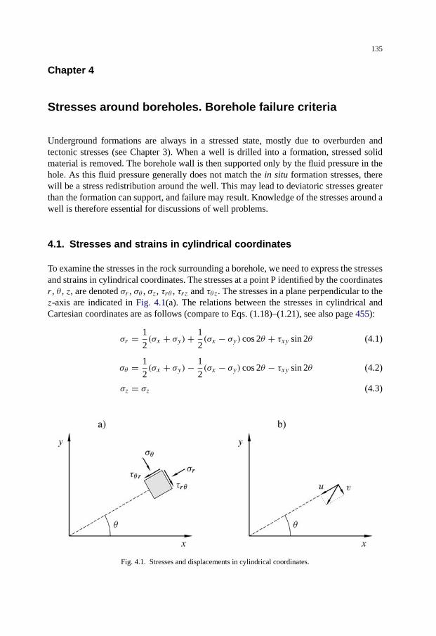
135
Chapter 4
Stresses around boreholes. Borehole failure criteria
Underground formations are always in a stressed state, mostly due to overburden andtectonic stresses (see Chapter 3). When a well is drilled into a formation, stressed solidmaterial is removed. The borehole wall is then supported only by the fluid pressure in thehole. As this fluid pressure generally does not match the in situ formation stresses, therewill be a stress redistribution around the well. This may lead to deviatoric stresses greaterthan the formation can support, and failure may result. Knowledge of the stresses around awell is therefore essential for discussions of well problems.
4.1. Stresses and strains in cylindrical coordinates
To examine the stresses in the rock surrounding a borehole, we need to express the stressesand strains in cylindrical coordinates. The stresses at a point P identified by the coordinatesr , θ , z, are denoted σr , σθ , σz, τrθ , τrz and τθz. The stresses in a plane perpendicular to thez-axis are indicated in Fig. 4.1(a). The relations between the stresses in cylindrical andCartesian coordinates are as follows (compare to Eqs. (1.18)–(1.21), see also page 455):
σr = 1
2(σx + σy)+ 1
2(σx − σy) cos 2θ + τxy sin 2θ (4.1)
σθ = 1
2(σx + σy)− 1
2(σx − σy) cos 2θ − τxy sin 2θ (4.2)
σz = σz (4.3)
Fig. 4.1. Stresses and displacements in cylindrical coordinates.

136 STRESSES AROUND BOREHOLES. BOREHOLE FAILURE CRITERIA
τrθ = 1
2(σy − σx) sin 2θ + τxy cos 2θ (4.4)
τrz = τxz cos θ + τyz sin θ (4.5)
τθz = τyz cos θ − τxz sin θ (4.6)
The corresponding relations between the strains are obtained by replacing the stress para-meters by corresponding strains.
εr = 1
2(εx + εy)+ 1
2(εx − εy) cos 2θ + Γxy sin 2θ (4.7)
εθ = 1
2(εx + εy)− 1
2(εx − εy) cos 2θ − Γxy sin 2θ (4.8)
εz = εz (4.9)
Γrθ = 1
2(εy − εx) sin 2θ + Γxy cos 2θ (4.10)
Γrz = Γxz cos θ + Γyz sin θ (4.11)
Γθz = Γyz cos θ − Γxz sin θ (4.12)
The symbols u, v, w are often used for displacements also in cylindrical coordinates,but now redefined as u being the displacement in the radial direction, v the displacementin the tangential direction and w in the axial direction. This redefinition is illustrated inFig. 4.1(b). The relations between strains and displacements are
εr = ∂u
∂r(4.13)
εθ = u
r+ 1
r
∂v
∂θ(4.14)
εz = ∂w
∂z(4.15)
Γrθ = 1
2r
(∂u
∂θ− v
)+ 1
2
∂v
∂r(4.16)
Γrz = 1
2
(∂w
∂r+ ∂u
∂z
)(4.17)
Γθz = 1
2
(1
r
∂w
∂θ+ ∂v
∂z
)(4.18)
Hooke’s law (see Eqs. (1.93)–(1.98)) has the same form in cylindrical as in Cartesian co-ordinates. For a porous and permeable formation, effective stresses should be used.
σ ′r = (λfr + 2Gfr)εr + λfrεθ + λfrεz (4.19)
σ ′θ = λfrεr + (λfr + 2Gfr)εθ + λfrεz (4.20)
σ ′z = λfrεr + λfrεθ + (λfr + 2Gfr)εz (4.21)
τrθ = 2GfrΓrθ (4.22)
τrz = 2GfrΓrz (4.23)
τθz = 2GfrΓθz (4.24)
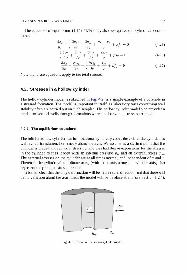
STRESSES IN A HOLLOW CYLINDER 137
The equations of equilibrium (1.14)–(1.16) may also be expressed in cylindrical coordi-nates:
∂σr
∂r+ 1
r
∂τθr
∂θ+ ∂τzr
∂z+ σr − σθ
r+ ρfr = 0 (4.25)
1
r
∂σθ
∂θ+ ∂τrθ
∂r+ ∂τzθ
∂z+ 2τrθ
r+ ρfθ = 0 (4.26)
∂σz
∂z+ ∂τrz
∂r+ 1
r
∂τθz
∂θ+ τrz
r+ ρfz = 0 (4.27)
Note that these equations apply to the total stresses.
4.2. Stresses in a hollow cylinder
The hollow cylinder model, as sketched in Fig. 4.2, is a simple example of a borehole ina stressed formation. The model is important in itself, as laboratory tests concerning wellstability often are carried out on such samples. The hollow cylinder model also provides amodel for vertical wells through formations where the horizontal stresses are equal.
4.2.1. The equilibrium equations
The infinite hollow cylinder has full rotational symmetry about the axis of the cylinder, aswell as full translational symmetry along the axis. We assume as a starting point that thecylinder is loaded with an axial stress σv, and we shall derive expressions for the stressesin the cylinder as it is loaded with an internal pressure pw and an external stress σro.The external stresses on the cylinder are at all times normal, and independent of θ and z.Therefore the cylindrical coordinate axes, (with the z-axis along the cylinder axis) alsorepresent the principal stress directions.
It is then clear that the only deformation will be in the radial direction, and that there willbe no variation along the axis. Thus the model will be in plane strain (see Section 1.2.4),
Fig. 4.2. Section of the hollow cylinder model.
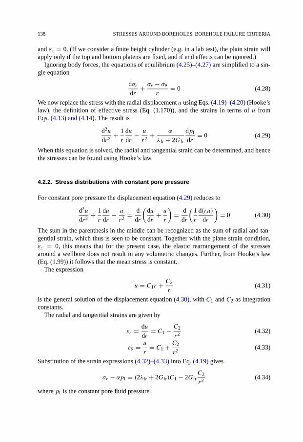
138 STRESSES AROUND BOREHOLES. BOREHOLE FAILURE CRITERIA
and εz = 0. (If we consider a finite height cylinder (e.g. in a lab test), the plain strain willapply only if the top and bottom platens are fixed, and if end effects can be ignored.)
Ignoring body forces, the equations of equilibrium (4.25)–(4.27) are simplified to a sin-gle equation
dσrdr
+ σr − σθr
= 0 (4.28)
We now replace the stress with the radial displacement u using Eqs. (4.19)–(4.20) (Hooke’slaw), the definition of effective stress (Eq. (1.170)), and the strains in terms of u fromEqs. (4.13) and (4.14). The result is
d2u
dr2+ 1
r
du
dr− u
r2+ α
λfr + 2Gfr
dpf
dr= 0 (4.29)
When this equation is solved, the radial and tangential strain can be determined, and hencethe stresses can be found using Hooke’s law.
4.2.2. Stress distributions with constant pore pressure
For constant pore pressure the displacement equation (4.29) reduces to
d2u
dr2+ 1
r
du
dr− u
r2= d
dr
(du
dr+ u
r
)= d
dr
(1
r
d(ru)
dr
)= 0 (4.30)
The sum in the parenthesis in the middle can be recognized as the sum of radial and tan-gential strain, which thus is seen to be constant. Together with the plane strain condition,εz = 0, this means that for the present case, the elastic rearrangement of the stressesaround a wellbore does not result in any volumetric changes. Further, from Hooke’s law(Eq. (1.99)) it follows that the mean stress is constant.
The expression
u = C1r + C2
r(4.31)
is the general solution of the displacement equation (4.30), with C1 and C2 as integrationconstants.
The radial and tangential strains are given by
εr = du
dr= C1 − C2
r2(4.32)
εθ = u
r= C1 + C2
r2(4.33)
Substitution of the strain expressions (4.32)–(4.33) into Eq. (4.19) gives
σr − αpf = (2λfr + 2Gfr)C1 − 2GfrC2
r2(4.34)
where pf is the constant pore fluid pressure.

STRESSES IN A HOLLOW CYLINDER 139
Before matching the boundary conditions, it is convenient to assemble all the r-inde-pendent terms in one constant and the r−2 terms in another:
σr = C′1 + C′
2
r2(4.35)
This small mathematical trick simplifies subsequent calculations, and also makes it imme-diately clear that pf and the elastic constants will not appear in the final answer.
Similarly, we find for the tangential stress
σθ = C′1 − C′
2
r2(4.36)
The two integration constants may now be found from the boundary conditions for theradial stress
σr = pw for r = Rw (4.37)
σr = σro for r = Ro (4.38)
where we write pw and σro for the radial stresses at the inner and outer boundary, respec-tively (see Fig. 4.2).
The result is
C′1 = R2
oσro − R2wpw
R2o − R2
w(4.39)
C′2 = − R2
oR2w
R2o − R2
w(σro − pw) (4.40)
The radial and tangential stresses in a hollow porous cylinder can then be written
σr = R2oσro − R2
wpw
R2o − R2
w− R2
o
R2o − R2
w
R2w
r2(σro − pw) (4.41)
σθ = R2oσro − R2
wpw
R2o − R2
w+ R2
o
R2o − R2
w
R2w
r2(σro − pw) (4.42)
Note that the sum of the radial and tangential stresses is a constant, independent of r . Sincethe mean stress is constant (see the discussion following Eq. (4.30)), this means that theaxial stress is constant.
When these hollow cylinder expressions are applied to well conditions, we may assumethat Ro Rw. Assuming a vertical borehole, we write σh (the horizontal stress) instead ofσro, and find
σr = σh − (σh − pw)R2
w
r2=(
1 − R2w
r2
)σh + R2
w
r2pw (4.43)
σθ = σh + (σh − pw)R2
w
r2=(
1 + R2w
r2
)σh − R2
w
r2pw (4.44)
σz = const (4.45)
Fig. 4.3 shows an illustration of the stress distribution around a borehole as predicted bythe hollow cylinder model. Note that the tangential stress (commonly referred to as the
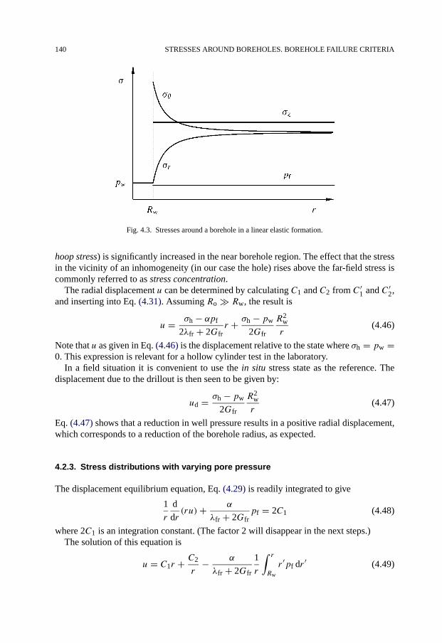
140 STRESSES AROUND BOREHOLES. BOREHOLE FAILURE CRITERIA
Fig. 4.3. Stresses around a borehole in a linear elastic formation.
hoop stress) is significantly increased in the near borehole region. The effect that the stressin the vicinity of an inhomogeneity (in our case the hole) rises above the far-field stress iscommonly referred to as stress concentration.
The radial displacement u can be determined by calculating C1 and C2 from C′1 and C′
2,and inserting into Eq. (4.31). Assuming Ro Rw, the result is
u = σh − αpf
2λfr + 2Gfrr + σh − pw
2Gfr
R2w
r(4.46)
Note that u as given in Eq. (4.46) is the displacement relative to the state where σh = pw =0. This expression is relevant for a hollow cylinder test in the laboratory.
In a field situation it is convenient to use the in situ stress state as the reference. Thedisplacement due to the drillout is then seen to be given by:
ud = σh − pw
2Gfr
R2w
r(4.47)
Eq. (4.47) shows that a reduction in well pressure results in a positive radial displacement,which corresponds to a reduction of the borehole radius, as expected.
4.2.3. Stress distributions with varying pore pressure
The displacement equilibrium equation, Eq. (4.29) is readily integrated to give
1
r
d
dr(ru)+ α
λfr + 2Gfrpf = 2C1 (4.48)
where 2C1 is an integration constant. (The factor 2 will disappear in the next steps.)The solution of this equation is
u = C1r + C2
r− α
λfr + 2Gfr
1
r
∫ r
Rw
r ′pf dr ′ (4.49)

STRESSES IN A HOLLOW CYLINDER 141
where C2 is a second integration constant.The stresses are found by proceeding in the same way as for the constant pressure case,
i.e. by computing the strains, using Hooke’s law and matching boundary conditions.Defining
�pf(r) = pf(r)− pfo (4.50)
the result can be written
σr = R2o(r
2 − R2w)σro + R2
w(R2o − r2)pw
r2(R2o − R2
w)
+ 2η
r2
(∫ r
Rw
r ′�pf(r′) dr ′ − r2 − R2
w
R2o − R2
w
∫ Ro
Rw
r ′�pf(r′) dr ′
)(4.51)
σθ = R2o(r
2 + R2w)σro − R2
w(R2o + r2)pw
r2(R2o − R2
w)
− 2η
r2
(∫ r
Rw
r ′�pf(r′) dr ′ − r2�pf(r)+ r2 + R2
w
R2o − R2
w
∫ Ro
Rw
r ′�pf(r′) dr ′
)(4.52)
σz = σv + 2νfr(σro − pw)R2
w
R2o − R2
w+ 2η�pf(r)
− 4ηνfr
R2o − R2
w
∫ Ro
Rw
r ′�pf(r′) dr ′ (4.53)
where we have introduced the poroelastic stress coefficient η given by
η = Gfr
λfr + 2Gfrα = 1 − 2νfr
2(1 − νfr)α (4.54)
It is clear from the definition that 0 < η < 0.5 (assuming ν > 0).Assuming Ro Rw, and σro = σh, the equations simplify to
σr =(
1 − R2w
r2
)σh + R2
w
r2pw + 2η
r2
∫ r
Rw
r ′�pf(r′) dr ′ (4.55)
σθ =(
1 + R2w
r2
)σh − R2
w
r2pw − 2η
r2
∫ r
Rw
r ′�pf(r′) dr ′ + 2η�pf(r) (4.56)
σz = σv + 2η�pf(r) (4.57)
The stresses at the borehole wall are seen to be
σr = pw (4.58)
σθ = 2σh − pw − 2η(pfo − pf(Rw)
)(4.59)
σz = σv − 2η(pfo − pf(Rw)
)(4.60)
where pf(Rw) is the reservoir fluid pressure at the wellbore wall. If there is open commu-nication between the well fluid and the formation, pf(Rw) is equal to the well pressure pw.If there is a mud cake, pf(Rw) is the fluid pressure behind the mud cake.

142 STRESSES AROUND BOREHOLES. BOREHOLE FAILURE CRITERIA
From a physical point of view this result can be explained as follows: If the well pressureis higher than the reservoir fluid pressure, fluids are injected and the pore fluid pressureis increased around the well. This will give a tendency for the material to expand andthe stresses increase. If on the other hand the well is on production, the well pressure islower than the reservoir pressure. The lower fluid pressure around the well will make theformation shrink, and hence the corresponding reduction in the tangential and axial stress.
Note that the wall stresses are independent of the details of the radial variation in pf(r),only the difference between the farfield value and the value at the borehole wall appears inthe equations.
The superposition principle
Since the governing equations are linear, the final expressions can be seen as a sum ofdifferent basic loads, which are uncoupled. For the hollow cylinder, these basic loads arethe external radial stress, the borehole pressure and the pore pressure.
As an illustration, the well pressure term pwR2w/r
2 is the same in Eqs. (4.43) and (4.55).Further, we expect the well pressure term to be the same if we introduce a more compli-cated far-field stress, e.g. corresponding to a deviated hole in an anisotropic stress field.(See Eq. (4.83).)
Radial flow
A special case is obtained if the pressure variation is given by stationary radial flow intothe well. We will first study the case of a hollow cylinder with outer radius Ro, and lookfor a stationary solution, i.e. we assume that all transients have died away.
The fluid pressure can then be calculated from Darcy’s law (see Section 1.9.1)
Qo
2πrh= k
ηf
dpf
dr(4.61)
whereQo is the constant flow rate, h is the height of the cylinder, k is the permeability andηf is the fluid viscosity. Note that Qo is here defined to be positive for flow in the inwardsdirection.
Solving the equation above, assuming a constant pressure pfo at the outer radius Ro, thepressure is given by the well-known equation
pf = pw + pfo − pw
ln RoRw
lnr
Rw= pfo + pfo − pw
ln RoRw
lnr
Ro(4.62)
Inserting this result into Eqs. (4.51)–(4.53), the equations published by Risnes et al. (1982)are found:
σr = σh + (σh − pw)R2
w
R2o − R2
w
[1 −
(Ro
r
)2]
− (pfo − pw)η
{R2
w
R2o − R2
w
[1 −
(Ro
r
)2]+ ln(Ro/r)
ln(Ro/Rw)
}(4.63)

STRESSES IN A HOLLOW CYLINDER 143
σθ = σh + (σh − pw)R2
w
R2o − R2
w
[1 +
(Ro
r
)2]
− (pfo − pw)η
{R2
w
R2o − R2
w
[1 +
(Ro
r
)2]+ ln(Ro/r)− 1
ln(Ro/Rw)
}(4.64)
σz = σv + 2νfr(σh − pw)R2
w
R2o − R2
w
− (pfo − pw)η
{2νfrR
2w
R2o − R2
w+ 2 ln(Ro/r)− νfr
ln(Ro/Rw)
}(4.65)
A common assumption in reservoir engineering is that the reservoir pressure pfo is constantat all times at a drainage radius Re. (We underline however, that in reality, true stationaryflow will never be reached in an infinite formation.)
If the drainage radius Re can be taken to be much larger than the well radius, the equa-tions are simplified to
σr = σh − (σh − pw)
(Rw
r
)2
+ (pfo − pw)η
[(Rw
r
)2
− ln(Re/r)
ln(Re/Rw)
](4.66)
σθ = σh + (σh − pw)
(Rw
r
)2
− (pfo − pw)η
[(Rw
r
)2
+ ln(Re/r)
ln(Re/Rw)
](4.67)
σz = σv − (pfo − pw)η2 ln(Re/r)− νfr
ln(Re/Rw)(4.68)
These equations can be used as an approximation to a producing well. Eq. (4.68) dependson the plane strain condition, which is valid for an infinitely long borehole. In a real case,the flow will be in a reservoir of limited height, and hence a solution based on generalizedplane stress (see Section 1.2.4) would be valid when the depleted zone extends far into thereservoir, and the full vertical stress is transmitted to the reservoir. In practise, there will besome arching of the overburden preventing the maintenance of the full vertical stress, andhence the true solution will be somewhere in between.
4.2.4. Stress distributions with heat flow
When a well is drilled, the drilling mud will alter the temperature of the surrounding for-mation. When the temperature changes, the formation expands or shrinks, and the stresseswill change. (See Section 1.5 for the basic formulas of thermoelasticity.)
From the correspondence between poroelasticity and thermoelasticity, see Section 1.6.6and Eqs. (4.58)–(4.60), we may immediately write the expressions for the stresses at thewellbore wall:
σr = pw (4.69)
σθ = 2σh − pw + Efr
1 − νfrαT (Tw − To) (4.70)
σz = σv + Efr
1 − νfrαT (Tw − To) (4.71)

144 STRESSES AROUND BOREHOLES. BOREHOLE FAILURE CRITERIA
Tw is the temperature in the well and To is the reservoir temperature. The thermally inducedchanges in stress affect both the tangential and the axial stress. The radial stress is of courseequal to the well pressure regardless of any temperature changes.
4.2.5. Stress distributions in nonlinear formations
The results in Section 4.2.2 as displayed in Fig. 4.3 showed that there is a rapid increase inthe stress deviation towards the borehole wall. These results were based on the assumptionof linear elasticity, i.e. that the elastic moduli of the rock are independent of the stressstate. However, elastic moduli of rocks are normally stress dependent to some extent (seeSection 1.8). Thus, it is reasonable to assume that the elastic moduli close to the wellborewall will differ from those of the virgin formation, due to the stress alteration in the vicinityof the borehole.
Santarelli et al. (1986, 1987) modelled this effect by assuming that Young’s modulusdepends on the minor principal stress σr as E(σr) = E0σ
ar . Here E0 and a are empirical
constants; normally 0 < a < 1, and E0 may be interpreted as the value of Young’s mod-ulus as measured in uniaxial compression tests. Based on this assumption, they found thefollowing expressions for σr and σθ corresponding to Eqs. (4.43)–(4.44).
σr = σh
{[(pw
σh
)1−a− 1
](Rw
r
)N+ 1
} 11−a
(4.72)
σθ = N
1 − a σh
(σr
σh
)a+Mσr (4.73)
where
N = 1
1 − νfr
[(1 − 2νfr)(1 − a)+ 1
](4.74)
M = νfr(1 − a)− 1
(1 − νfr)(1 − a) (4.75)
The implications for the stress distribution around the borehole are significant. Fig. 4.4shows the variation of stresses as functions of radial distance as calculated by Eqs. (4.72)–(4.75) using a = 0.5 and νfr = 0.2. Also the vertical stress is reduced close to the wellbore,as σz is linked to σr and σθ through Hooke’s law (although it is no longer linear).
An important consequence of the nonconstant E-modulus is the relative reduction ofσθ near the wellbore wall. This effect is most pronounced for low borehole pressures forwhich it may even happen that the difference σθ − σr is larger at some distance into theformation than at the borehole wall. Thus, the commonly observed effect that Young’smodulus increases with increasing confining pressure, has the consequence that the stressdeviation near the borehole wall at low borehole pressures is reduced compared to thelinear elastic solution.
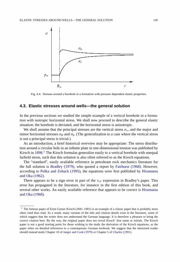
ELASTIC STRESSES AROUND WELLS—THE GENERAL SOLUTION 145
Fig. 4.4. Stresses around a borehole in a formation with pressure dependent elastic properties.
4.3. Elastic stresses around wells—the general solution
In the previous sections we studied the simple example of a vertical borehole in a forma-tion with isotropic horizontal stress. We shall now proceed to describe the general elasticsituation: the borehole is deviated, and the horizontal stress is anisotropic.
We shall assume that the principal stresses are the vertical stress σv, and the major andminor horizontal stresses σH and σh. (The generalization to a case where the vertical stressis not a principal stress is trivial.)
As an introduction, a brief historical overview may be appropriate: The stress distribu-tion around a circular hole in an infinite plate in one-dimensional tension was published byKirsch in 1898.1 The Kirsch formulas generalize easily to a vertical borehole with unequalfarfield stress, such that this solution is also often referred to as the Kirsch equations.
The “standard”, easily available reference in petroleum rock mechanics literature forthe full solution is Bradley (1979), who quoted a report by Fairhurst (1968). However,according to Peška and Zoback (1995), the equations were first published by Hiramatsuand Oka (1962).
There appears to be a sign error in part of the τrθ expression in Bradley’s paper. Thiserror has propagated in the literature, for instance in the first edition of this book, andseveral other works. An easily available reference that appears to be correct is Hiramatsuand Oka (1968).
1 The famous paper of Ernst Gustav Kirsch (1841–1901) is an example of a classic paper that is probably moreoften cited than read. As a result, many variants of the title and citation details exist in the literature, some ofwhich suggest that the writer does not understand the German language. It is therefore a pleasure to bring thecorrect citation here. By the way, the original paper does not reveal Kirsch’ first name or initials. The Kirschpaper is not a good starting point for those wishing to the study the derivation of the Kirsch equations, as thepaper relies on detailed references to a contemporary German textbook. We suggest that the interested readershould instead study Chapter 10 of Jaeger and Cook (1979) or Chapter 5 of Charlez (1991).

146 STRESSES AROUND BOREHOLES. BOREHOLE FAILURE CRITERIA
Fig. 4.5. Coordinate system for a deviated borehole.
4.3.1. Transformation formulas
The in situ principal stresses define a coordinate system which we denote (x′, y′, z′), asindicated in Fig. 4.5. We take σv to be parallel to z′, σH to be parallel to x′ and σh to beparallel to y′.
We introduce a second coordinate system (x, y, z) such that the z-axis points along theaxis of the hole, the x-axis points towards the lowermost radial direction of the hole, andthe y-axis is horizontal (see Fig. 4.5).
A transform from (x′, y′, z′) to (x, y, z) can be obtained in two operations (see Fig. 4.6):
1. a rotation a around the z′-axis,
2. a rotation i around the y-axis.
The transformation can be described mathematically by the direction cosines, where lij ′is the cosine of the angle between the i-axis and the j ′-axis. With reference to Fig. 4.6 it isstraightforward to derive the following expressions
lxx′ = cos a cos i, lxy′ = sin a cos i, lxz′ = − sin ilyx′ = − sin a, lyy′ = cos a, lyz′ = 0lzx′ = cos a sin i, lzy′ = sin a sin i, lzz′ = cos i
(4.76)
(An alternate formulation, using the Euler angles, is discussed in Appendix C, seepage 453.)
Expressed in the (x, y, z) coordinate system, the formation stresses σH, σh and σv be-come:
σ ox = l2xx′σH + l2xy′σh + l2xz′σv (4.77)
σ oy = l2yx′σH + l2yy′σh + l2yz′σv (4.78)
σ oz = l2zx′σH + l2zy′σh + l2zz′σv (4.79)

ELASTIC STRESSES AROUND WELLS—THE GENERAL SOLUTION 147
τ oxy = lxx′ lyx′σH + lxy′ lyy′σh + lxz′ lyz′σv (4.80)
τ oyz = lyx′ lzx′σH + lyy′ lzy′σh + lyz′ lzz′σv (4.81)
τ ozx = lzx′ lxx′σH + lzy′ lxy′σh + lzz′ lxz′σv (4.82)
The superscript o on the stresses denote that these are the virgin formation stresses.
4.3.2. The general elastic solution
The solutions corresponding to Eqs. (4.43)–(4.45) are found assuming plane strain normalto the borehole axis.
Again, it is convenient to express the stresses in terms of cylindrical polar coordinatesr , θ and z, where r represents the distance from the borehole axis, θ the azimuth anglerelative to the x-axis, and z is the position along the borehole axis (see Fig. 4.6). The stresssolutions can be written:
σr = σ ox + σ o
y
2
(1 − R2
w
r2
)+ σ o
x − σ oy
2
(1 + 3
R4w
r4− 4R2
w
r2
)cos 2θ
+ τ oxy
(1 + 3
R4w
r4− 4R2
w
r2
)sin 2θ + pw
R2w
r2(4.83)
Fig. 4.6. The transformation geometry.

148 STRESSES AROUND BOREHOLES. BOREHOLE FAILURE CRITERIA
σθ = σ ox + σ o
y
2
(1 + R2
w
r2
)− σ o
x − σ oy
2
(1 + 3
R4w
r4
)cos 2θ
− τ oxy
(1 + 3
R4w
r4
)sin 2θ − pw
R2w
r2(4.84)
σz = σ oz − νfr
[2(σ o
x − σ oy )R2
w
r2cos 2θ + 4τ o
xy
R2w
r2sin 2θ
](4.85)
τrθ = σ oy − σ o
x
2
(1 − 3
R4w
r4+ 2R2
w
r2
)sin 2θ
+ τ oxy
(1 − 3
R4w
r4+ 2R2
w
r2
)cos 2θ (4.86)
τθz = (−τ oxz sin θ + τ o
yz cos θ)
(1 + R2
w
r2
)(4.87)
τrz = (τ oxz cos θ + τ o
yz sin θ)
(1 − R2
w
r2
)(4.88)
The borehole influence is given by terms in r−2 and r−4, which vanish rapidly with in-creasing r . Thus, for large r the borehole influence vanishes, and the equations degenerateto Eqs. (4.41)–(4.46).
The solutions depend on the angle θ (see Fig. 4.5) indicating that the stresses vary withposition around the wellbore. Generally the shear stresses are non-zero. Thus σr , σθ andσz are not principal stresses for arbitrary orientations of the well.
At the wellbore wall, the equations are simplified to
σr = pw (4.89)
σθ = σ ox + σ o
y − 2(σ ox − σ o
y ) cos 2θ − 4τ oxy sin 2θ − pw (4.90)
σz = σ oz − νfr
[2(σ o
x − σ oy ) cos 2θ + 4τ o
xy sin 2θ]
(4.91)
τrθ = 0 (4.92)
τθz = 2(−τ oxz sin θ + τ o
yz cos θ) (4.93)
τrz = 0 (4.94)
These are the equations which are used in linear elastic analysis of borehole stability.The stress solutions as given by Eqs. (4.83)–(4.88) and Eqs. (4.89)–(4.94) are the stress
solutions for nonporous materials or for porous material with constant pore pressure. Dueto the superposition principle, pore pressure effects may simply be added. Thus, if weassume a radially symmetric pressure distribution around the borehole, the pore pressureterms from Eqs. (4.55)–(4.57) or Eqs. (4.66)–(4.68) may be used directly.
4.3.3. Borehole along a principal stress direction
For a hole along a principal stress direction, the general equations (4.83)–(4.88) simplifyconsiderably. We here give the resulting equations for a vertical borehole, but the expres-
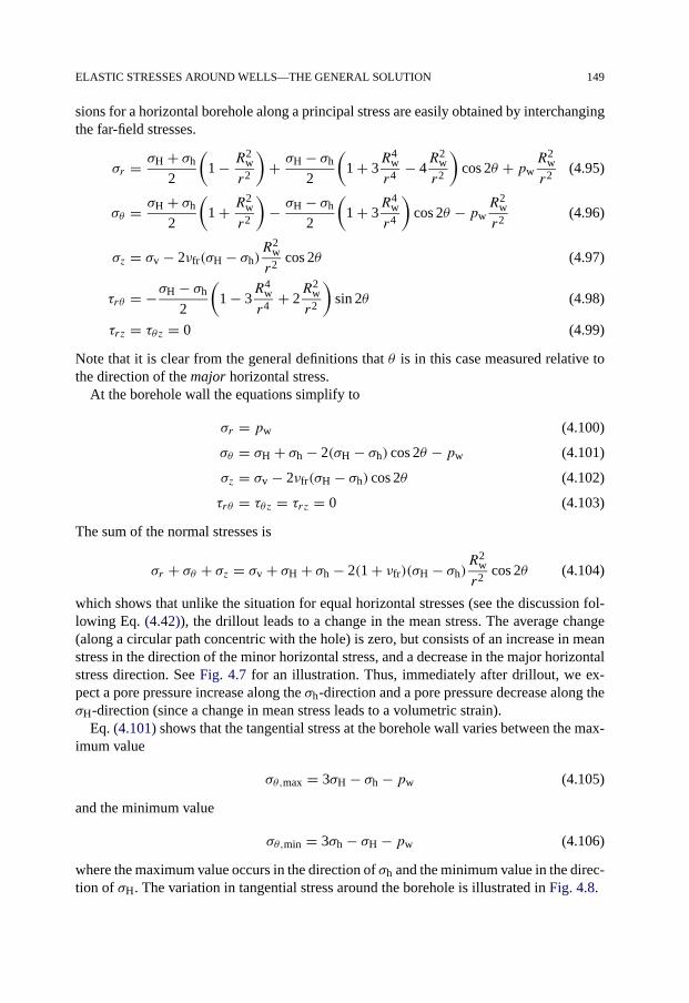
ELASTIC STRESSES AROUND WELLS—THE GENERAL SOLUTION 149
sions for a horizontal borehole along a principal stress are easily obtained by interchangingthe far-field stresses.
σr = σH + σh
2
(1 − R2
w
r2
)+ σH − σh
2
(1 + 3
R4w
r4− 4R2
w
r2
)cos 2θ + pw
R2w
r2(4.95)
σθ = σH + σh
2
(1 + R2
w
r2
)− σH − σh
2
(1 + 3
R4w
r4
)cos 2θ − pw
R2w
r2(4.96)
σz = σv − 2νfr(σH − σh)R2
w
r2cos 2θ (4.97)
τrθ = −σH − σh
2
(1 − 3
R4w
r4+ 2R2
w
r2
)sin 2θ (4.98)
τrz = τθz = 0 (4.99)
Note that it is clear from the general definitions that θ is in this case measured relative tothe direction of the major horizontal stress.
At the borehole wall the equations simplify to
σr = pw (4.100)
σθ = σH + σh − 2(σH − σh) cos 2θ − pw (4.101)
σz = σv − 2νfr(σH − σh) cos 2θ (4.102)
τrθ = τθz = τrz = 0 (4.103)
The sum of the normal stresses is
σr + σθ + σz = σv + σH + σh − 2(1 + νfr)(σH − σh)R2
w
r2cos 2θ (4.104)
which shows that unlike the situation for equal horizontal stresses (see the discussion fol-lowing Eq. (4.42)), the drillout leads to a change in the mean stress. The average change(along a circular path concentric with the hole) is zero, but consists of an increase in meanstress in the direction of the minor horizontal stress, and a decrease in the major horizontalstress direction. See Fig. 4.7 for an illustration. Thus, immediately after drillout, we ex-pect a pore pressure increase along the σh-direction and a pore pressure decrease along theσH-direction (since a change in mean stress leads to a volumetric strain).
Eq. (4.101) shows that the tangential stress at the borehole wall varies between the max-imum value
σθ,max = 3σH − σh − pw (4.105)
and the minimum value
σθ,min = 3σh − σH − pw (4.106)
where the maximum value occurs in the direction of σh and the minimum value in the direc-tion of σH. The variation in tangential stress around the borehole is illustrated in Fig. 4.8.

150 STRESSES AROUND BOREHOLES. BOREHOLE FAILURE CRITERIA
Fig. 4.7. Change in mean stress due to the drillout of a borehole in anisotropic far field stresses. White is increasein mean stress, black is decrease in mean stress. The dotted lines shows the contours of no change.
Fig. 4.8. Change in tangential stress due to the drillout of a borehole in anisotropic far field stresses. White isincrease in tangential stress, black is decrease in tangential stress. The dotted lines shows the contours of nochange.
4.4. Poroelastic time dependent effects
In a nonporous, linear elastic material, the stress redistribution upon drilling or well pres-sure change is immediate. In a porous and permeable medium, however, there are time

POROELASTIC TIME DEPENDENT EFFECTS 151
effects due to the fact that the pore pressure propagates with a limited rate. (See Sec-tion 1.9.1.)
There are two main sources of the poroelastic time effects:
1. Pore pressure change due to production or the invasion of the wellbore fluid.
2. Pore pressure change because the redistribution of the formation stresses gives a vol-umetric strain, see e.g. Eq. (4.104).
While the first mechanism requires a non-sealing wellbore wall, the second will occureven if the wellbore wall is completely sealed.
Detournay and Cheng (1988) discuss in detail the case of a vertical hole with unequalfar-field stresses. We reproduce some of their results here, but strongly recommend theoriginal paper for a complete discussion. See also Chapter 2 of Charlez (1997).
4.4.1. Wellbore pressure invasion
We consider first case 1, in which the pore pressure is changed by communication withthe wellbore pressure. Let us assume that initially pw = pfo, that we have a permeableborehole wall and that at time zero the well pressure is changed by �pw. Assuming anaxisymmetric pressure profile, the pore pressure is decoupled from the deformation, andthe pressure inside the formation will develop according to a decoupled diffusion equationsimilar to Eq. (1.241). The pressure development as a function of time and radial distanceinto the formation is shown in Fig. 4.9. The parameter t ′ labelling the curves is a dimen-sionless time, defined by
t ′ = t CD
R2w
(4.107)
Fig. 4.9. Well pressure penetration. The curves are labelled by the dimensionless time t ′ (see Eq. (4.107)). AfterDetournay and Cheng (1988), with permission from Elsevier Science Publishers.

152 STRESSES AROUND BOREHOLES. BOREHOLE FAILURE CRITERIA
where the diffusion constant CD is given by Eq. (1.242). For an 8′′ hole, t ′ = 1 correspondsto milliseconds or less for a high-permeable sand, and up to several days for a tight shale.
Once the pore pressure profile is known, the tangential stress may be computed byEq. (4.56). If we assume that as time tends to infinity the well pressure change has pen-etrated deeply into the formation, we see from Eq. (4.56) that the contribution to thetangential stress from the pore pressure change is
�σθ(t → ∞) = η�pw
(1 + R2
w
r2
)(4.108)
This is of course in addition to the elastic contribution as given by the first two terms ofEq. (4.56) (or by Eq. (4.44)).
Note that the assumptions leading to Eq. (4.108) are different from those leading toEq. (4.67). The latter assumes a steady flow for large times, while the former assumes thatthe pore pressure far into the formation has become equal to the well pressure for largetime. Both cases are approximations that are not fulfilled in practise.
We also see from Eq. (4.59) that at the borehole wall, the change in tangential stress is
�σθ = 2η�pw (4.109)
at all times.There are no explicit analytical solutions of the diffusion equation for the current prob-
lem, and hence it must be solved by numerical methods.In Fig. 4.10 we show the time development of the pore pressure induced contribution
to the tangential stress. Let us assume that we are considering production, i.e. �pw isnegative. We see that at the borehole wall, the tangential stress is reduced relative to theelastic case at all times. However, for short times, we have an increase in the tangentialstress in the near wellbore region. The region of increased stress propagates outwards withtime.
Fig. 4.10. Tangential stress due to well pressure penetration. The curves are labelled by the dimensionless time t ′.After Detournay and Cheng (1988), with permission from Elsevier Science Publishers.

POROELASTIC TIME DEPENDENT EFFECTS 153
The origin of this increase in tangential stress may be understood by considering thatthe reduced tangential stress near the borehole must be compensated by an increase oftangential stress further away. The position of the region of increased radial stress followsthe position the pressure front. Hence it propagates outwards and broadens with time.
4.4.2. Drillout induced pore pressure changes
We saw (e.g. in Eq. (4.104)) that when the farfield horizontal stresses are unequal, thedrillout leads to a volumetric strain and hence to a change in pressure, which will dissipatewith time due to fluid flow. This will lead to time-dependence of the near wellbore stresses,also when the wellbore wall is completely sealing.
The pore pressure change depends both on the radial position and on the azimuth. Hencethere will be both radial and tangential fluid flow as a result of the drillout. Since thediffusion distance is shortest close to the borehole, pore pressure will reach equilibriumfastest here. A partly or fully open wellbore wall will contribute further to this.
As a result, the near wellbore behaviour will be drained, whereas the response deeperinto the formation will be undrained for short times. Since the drained moduli are smallerthan the undrained, the stress concentration in the near wellbore region will initially beshielded relative to its full elastic value. This is similar to the shielding seen for nonlinearformation, or plastic formations, see Sections 4.2.5 and 4.6. Obviously, the effect will bestrongest when there is a significant difference between drained and undrained parameters,i.e. for soft materials.
As the pore pressure imbalance dissipates, the shielding disappears, and the elastic stressconcentration is reestablished. Detournay and Cheng (1988) suggested that this may be amechanism of delayed failure for boreholes in tight formations.
Fig. 4.11 shows the variation in tangential stress as a function of radius in the minimumstress direction for various dimensionless times (Eq. (4.107)). The plot has been generatedfor ν = 0.4, νfr = 0.2 and Skempton’s B = 0.8. (An example of a set of parametersin our notation that gives these values are φ = 0.15, Kfr = 4 GPa, Gfr = 4 GPa andKs = 37.5 GPa.)
We underline that the figure shows only the tangential stress due to the deviatoric load-ing, i.e. the stress corresponding to the cos 2θ term in Eq. (4.96).
Fig. 4.12 shows the variation in tangential stress at the wellbore wall as a function oftime, again in the direction of the minimum horizontal stress. The initial reduction in stressconcentration is evident.
For a numerical example, assume pw = 20 MPa, σH = 40 MPa, σh = 30 MPa. ThenFig. 4.12 shows that σθ ≈ 15 MPa initially and σθ ≈ 20 MPa at large times. The totaltangential stress is found by adding the contribution from the mean farfield stress, σθ =σH + σh − pw = 50 MPa. Thus, the tangential stress at the borehole wall (in the directionof the minor stress) increases from 65 MPa at early times to 70 MPa at large times.
In addition to the poroelastic time effects, there are also time effects due to temperaturechange and chemical processes. See Chapter 9 for further discussion.
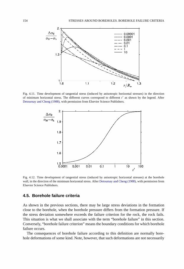
154 STRESSES AROUND BOREHOLES. BOREHOLE FAILURE CRITERIA
Fig. 4.11. Time development of tangential stress (induced by anisotropic horizontal stresses) in the directionof minimum horizontal stress. The different curves correspond to different t ′ as shown by the legend. AfterDetournay and Cheng (1988), with permission from Elsevier Science Publishers.
Fig. 4.12. Time development of tangential stress (induced by anisotropic horizontal stresses) at the boreholewall, in the direction of the minimum horizontal stress. After Detournay and Cheng (1988), with permission fromElsevier Science Publishers.
4.5. Borehole failure criteria
As shown in the previous sections, there may be large stress deviations in the formationclose to the borehole, when the borehole pressure differs from the formation pressure. Ifthe stress deviation somewhere exceeds the failure criterion for the rock, the rock fails.This situation is what we shall associate with the term “borehole failure” in this section.Conversely, “borehole failure criterion” means the boundary conditions for which boreholefailure occurs.
The consequences of borehole failure according to this definition are normally bore-hole deformations of some kind. Note, however, that such deformations are not necessarily

BOREHOLE FAILURE CRITERIA 155
dramatic from an operational point of view (see Chapter 9). Thus, “borehole failure” asdefined here should by no means be taken as a synonym for a lost well. Development ofborehole failure beyond failure initiation is discussed in Section 4.6.
4.5.1. Vertical hole, isotropic horizontal stresses and impermeable borehole wall
For a material that behaves linearly elastic, the largest stress differences occur at the bore-hole wall, hence rock failure is expected to initiate there.
We start with the simplest case, a vertical borehole with constant pore pressure andisotropic farfield horizontal stresses. We assume that the wellbore is lined with a perfectmud cake, which means that the pore pressure is not influenced by the well pressure.
Within this assumptions, the principal stresses at the borehole wall are, according toEqs. (4.43)–(4.45)
σr = pw (4.110)
σθ = 2σh − pw (4.111)
σz = σv (4.112)
There are several conditions for which the borehole may fail, depending on the relativemagnitudes of the principal stresses. Let us first assume that we are lowering pw such thatσr = pw becomes the smallest principal stress. We see from Eqs. (4.111) and (4.112) thatdepending on the relative magnitude of σh and σv, either σθ or σz will become the largestprincipal stress at the borehole wall.
Consider first the situation where σθ > σz > σr at the borehole wall. According to theMohr–Coulomb criterion (Eq. (2.22)), failure will occur when
σ ′θ = C0 + σ ′
r tan2 β (4.113)
Using an effective stress coefficient equal to 1 for failure (see Section 2.6.1) we find thatthe failure criterion for the borehole becomes
pw,min = 2σh + pf(tan2 β − 1)− C0
1 + tan2 β= pf + 2(σh − pf)− C0
1 + tan2 β(4.114)
Thus, if the well pressure falls below the value given by Eq. (4.114), shear failure willoccur at the borehole wall.
Next, assume that σh is smaller relative to σv, such that σv is the largest principal stressat failure. Proceeding as above, the failure criterion becomes
pw = σv + pf(tan2 β − 1)− C0
tan2 β= pf + σv − pf − C0
tan2 β(4.115)
In practice, one needs to calculate both cases, and pick the criterion that gives the largestborehole pressure at failure.
In order to map the region of mechanical stability for a borehole, all six permutationsof the three principal stresses σr , σθ and σz need to be considered. The resulting equations
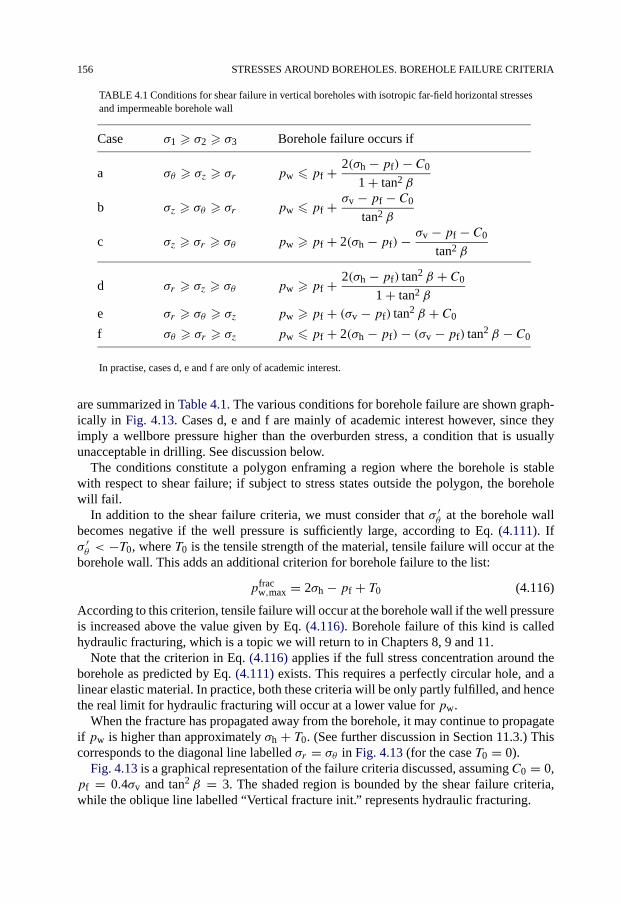
156 STRESSES AROUND BOREHOLES. BOREHOLE FAILURE CRITERIA
TABLE 4.1 Conditions for shear failure in vertical boreholes with isotropic far-field horizontal stressesand impermeable borehole wall
Case σ1 � σ2 � σ3 Borehole failure occurs if
a σθ � σz � σr pw � pf + 2(σh − pf)− C0
1 + tan2 β
b σz � σθ � σr pw � pf + σv − pf − C0
tan2 β
c σz � σr � σθ pw � pf + 2(σh − pf)− σv − pf − C0
tan2 β
d σr � σz � σθ pw � pf + 2(σh − pf) tan2 β + C0
1 + tan2 β
e σr � σθ � σz pw � pf + (σv − pf) tan2 β + C0
f σθ � σr � σz pw � pf + 2(σh − pf)− (σv − pf) tan2 β − C0
In practise, cases d, e and f are only of academic interest.
are summarized in Table 4.1. The various conditions for borehole failure are shown graph-ically in Fig. 4.13. Cases d, e and f are mainly of academic interest however, since theyimply a wellbore pressure higher than the overburden stress, a condition that is usuallyunacceptable in drilling. See discussion below.
The conditions constitute a polygon enframing a region where the borehole is stablewith respect to shear failure; if subject to stress states outside the polygon, the boreholewill fail.
In addition to the shear failure criteria, we must consider that σ ′θ at the borehole wall
becomes negative if the well pressure is sufficiently large, according to Eq. (4.111). Ifσ ′θ < −T0, where T0 is the tensile strength of the material, tensile failure will occur at the
borehole wall. This adds an additional criterion for borehole failure to the list:
pfracw,max = 2σh − pf + T0 (4.116)
According to this criterion, tensile failure will occur at the borehole wall if the well pressureis increased above the value given by Eq. (4.116). Borehole failure of this kind is calledhydraulic fracturing, which is a topic we will return to in Chapters 8, 9 and 11.
Note that the criterion in Eq. (4.116) applies if the full stress concentration around theborehole as predicted by Eq. (4.111) exists. This requires a perfectly circular hole, and alinear elastic material. In practice, both these criteria will be only partly fulfilled, and hencethe real limit for hydraulic fracturing will occur at a lower value for pw.
When the fracture has propagated away from the borehole, it may continue to propagateif pw is higher than approximately σh + T0. (See further discussion in Section 11.3.) Thiscorresponds to the diagonal line labelled σr = σθ in Fig. 4.13 (for the case T0 = 0).
Fig. 4.13 is a graphical representation of the failure criteria discussed, assuming C0 = 0,pf = 0.4σv and tan2 β = 3. The shaded region is bounded by the shear failure criteria,while the oblique line labelled “Vertical fracture init.” represents hydraulic fracturing.

BOREHOLE FAILURE CRITERIA 157
Fig. 4.13. Graphical representation of conditions for borehole failure. The Mohr–Coulomb failure criterion withC0 = 0, pf = 0.4σv and tan2 β = 3 is assumed. The polygon will grow in all directions if C0 is nonzero. Inparticular, if T0 = 0, the line c will coincide with the vertical fracturing line if C0 = σv − pf. (After Guenot,1987; with permission from A.A. Balkema.)
The horizontal line labelled “Horizontal fracturing” represents another failure criterion,which needs to be taken into account: If there is any preexisting fracture or flaw in theborehole wall, the wall pressure will act with a vertical component on the formation there.A horizontal fracture will then grow if σv − pw is less than −T0, i.e. if pw > σv + T0.
4.5.2. Vertical hole, isotropic horizontal stresses and permeable borehole wall
If the borehole wall is permeable, the pore pressure at the borehole wall is equal to the wellpressure. This means that we must use pw rather than pf when computing the effectivestresses. In addition, we must take into account the change in the total stresses induced bythe varying pore pressure, as given by Eqs. (4.58)–(4.60)).
The stresses at the wellbore wall are thus
σr = pw (4.117)
σθ = 2σh − pw + 2η(pw − pfo) (4.118)
σz = σv + 2η(pw − pfo) (4.119)
where η is the poroelastic stress coefficient (see Eq. (4.54)) and pfo is the farfield porepressure. Remember that the last equation follows from the plane strain assumption, and ishence strictly valid only for an infinitely long borehole.

158 STRESSES AROUND BOREHOLES. BOREHOLE FAILURE CRITERIA
Inserting these expressions into the Mohr–Coulomb criterion, using pw when computingthe effective stress, we then find for σθ > σz > σr
pw,min = 2σh − 2ηpfo − C0
2 − 2η= 2σh − α 1−2νfr
1−νfrpfo − C0
2 − α 1−2νfr1−νfr
(4.120)
Note that the equation contains Biot’s α because of the elastic redistribution of the stressesdue to the pore pressure profile, however we still use an effective stress coefficient equal tounity in the failure criterion. Also, observe that since the minor effective stress is zero, thefailure angle does not appear in Eq. (4.120).
Similarly, for σz > σθ > σr we find
pw,min = σv − 2ηpfo − C0
1 − 2η= σv − α 1−2νfr
1−νfrpfo − C0
1 − α 1−2νfr1−νfr
(4.121)
Since σ ′r is always equal to zero, it is of little interest to study the cases corresponding to c,
d, e, f in Table 4.1. The remaining criteria to be considered are thus the hydraulic fracturingcriteria, σ ′
θ = −T0 and σ ′z = −T0. We find for vertical fracturing
pfracw,max = 2σh − 2ηpfo + T0
2 − 2η= 2σh − α 1−2νfr
1−νfrpfo + T0
2 − α 1−2νfr1−νfr
(4.122)
and for horizontal fracturing
pfracw,max = σv − 2ηpfo + T0
1 − 2η= σv − α 1−2νfr
1−νfrpfo + T0
1 − α 1−2νfr1−νfr
(4.123)
Again, this last equation assumes plane strain conditions, and can not be directly applied topressurization of a limited section of a borehole. Hence, the equation has limited practicalapplicability, and is mainly of academic interest.
4.5.3. Borehole along a principal stress direction
The stresses at the wall of a vertical hole with unequal far-field stresses, and constant porepressure, were given in Eqs. (4.100)–(4.103). Since all shear stresses vanish in this case,σr , σθ and σz are the principal stresses and may be used directly in the failure criterion.
From Eq. (4.101) and Fig. 4.8 it is clear that the maximum tangential stress occurs inthe direction of the minimum horizontal stress, and hence shear failure at the borehole wallwill initiate in the direction of the minimum horizontal stress, see Fig. 4.14.
Comparing to Eq. (4.111) we see that the critical well pressure when σθ > σz > σr(case a of Table 4.1) may be found by substituting 2σh with 3σH − σh in Eq. (4.114):
pw,min = pf + 3σH − σh − 2pf − C0
1 + tan2 β(4.124)

BOREHOLE FAILURE CRITERIA 159
Fig. 4.14. Location of shear failure initiation at the wall of a vertical hole with anisotropic horizontal stresses.
Similarly, by comparing Eq. (4.102) to Eq. (4.112) we see that for σz > σθ > σr , (case bof Table 4.1) we have
pw,min = pf + σv + 2|νfr|(σH − σh)− pf − C0
tan2 β(4.125)
Note that we need to take the absolute value of the Poisson’s ratio. This is because thelargest value of σz in Eq. (4.102) occurs for θ = 0° for negative νfr and for θ = 90° forpositive νfr.
The tensile failure criterion Eq. (4.116) is also modified if the horizontal stress isanisotropic. In this case, failure will occur at the positions where σθ is smallest, and hencefracturing will occur in the direction of maximum horizontal stress (see Fig. 4.8). Thecriterion becomes
pfracw,max = 3σh − σH − pf + T0 (4.126)
Here we see that an increase in the largest horizontal stress reduces the upper stabilitylimit for the well pressure. Thus anisotropy in the formation around a borehole reduces theregion where the borehole is stable.
Observe that if σH is sufficiently large, the pressure given by Eq. (4.126) may be smallerthan the criterion for fracture growth outside the influence of the borehole, which is pw ≈σh + T0. Eq. (4.126) may thus be the criterion for initiation of a fracture that does notpropagate beyond the stress concentration around the borehole. See Section 11.2 for amore detailed discussion.
The above equations were derived for a vertical borehole. It is however trivial to adeptthem to a horizontal borehole along a principal stress direction by appropriately inter-changing the far-field stresses. As an example, for a horizontal hole along σH, we mustinterchange σv and σH (assuming σv > σh).
4.5.4. Borehole in a general direction
In the general case it is not possible to obtain closed-form expressions for the critical wellpressure, and one must resort to numerical solution methods.

160 STRESSES AROUND BOREHOLES. BOREHOLE FAILURE CRITERIA
In brief, the procedure for establishing the lowest possible well pressure is as follows:
1. From the known far-field stresses, compute the stresses in the borehole coordinatesystem according to Eqs. (4.77)–(4.82).
2. Compute the stresses at the borehole wall according to Eqs. (4.89)–(4.94).
3. Subdivide the interval 0 < θ < π into a number of sub-intervals (depending on theaccuracy required). For each sub-interval perform the following:
• Diagonalize the stress tensor at the borehole wall to find the principal stresses.
• Find the critical well pressure by inserting the principal stresses into the failurecriterion.
4. The lowest admissible pw is the largest critical well pressure found from the iterationin the step above.
4.6. Beyond failure initiation
Borehole failure is commonly observed as breakouts in the borehole wall. Fig. 4.15 showsa typical example of a failure mode denoted “borehole elongation”, due to the extension ofthe borehole cross-section in one direction. The stress conditions causing this cavity to failcorresponded to case a in Table 4.1. The diagram in Fig. 4.13 is split in various sectors bythe dashed border lines where two principal stresses are equal. Each sector is associatedwith a failure condition in Table 4.1. A typical mode of rupture is associated with eachsector. These are described in Table 4.2 and Figs. 4.16–4.18 for the most relevant cases.
The orientation of breakouts due to failure of type a are related to the orientation of thehorizontal stresses, as discussed in Section 4.5.3. This connection is used in the field fordetermining the direction of the stresses, see further discussion in Section 8.3.2.
Fig. 4.15. Cross-section of a cylindrical cavity after failure.

BEYOND FAILURE INITIATION 161
TABLE 4.2 Rupture modes for the failure of boreholes (Maury and Sauzay, 1987)
Case Rupture mode Figure
Shear, a Rupture occurs in shear surfaces intersecting parallel to the axial stress Fig. 4.16Shear, b Rupture occurs in fragments of toroidal shape Fig. 4.17Shear, c Rupture occurs in multishear surfaces intersecting parallel to the radius Fig. 4.18Tensile Hydraulic fracturing; isolated fractures parallel to the borehole axis Fig. 11.1
Fig. 4.16. Failure planes caused by the tangential (σ ′1) and the radial (σ ′
3) stresses. (a) Stresses on an element atthe wellbore wall. (b) Breakouts.
Fig. 4.17. Failure planes generated by the vertical (σ ′1) and the radial (σ ′
3) stresses. Breakouts will have toroidalshapes. (a) Stresses on an element at the wellbore wall. (b) Breakouts.
Anisotropy in the material parameters of the rock also affects the orientation of break-outs. When the horizontal stress is isotropic, the breakouts tend to be oriented normal to thejoints of bedding in the material (Kaiser et al., 1985). Note, however, that breakouts of the

162 STRESSES AROUND BOREHOLES. BOREHOLE FAILURE CRITERIA
Fig. 4.18. Failure planes generated by the vertical (σ ′1) and the tangential (σ ′
3) stresses. Radial fractures maydevelop following a helical path along the well. (a) Stresses on an element at the wellbore wall. (b) Breakouts.
form shown in Fig. 4.15 may occur even if both the stress field and the material parametersare isotropic.
The criteria for the initiation of borehole failure discussed in Section 4.5 only definethe initiation of borehole failure, and do not reveal the consequences of failure initiation,which is of course of equal interest.
An idea of the development of borehole failure can be obtained by tracing a potentialfailure plane from the borehole wall into the formation. We here choose the simplest caseof a linearly elastic formation and isotropic formation stresses, and assume pw < σh. Theorientation of a potential failure plane at a distance r from the borehole centre is given bythe orientation of the largest and smallest principal stress (σθ and σr , respectively), and thefailure angle β (which is related to the coefficient of internal friction, see Section 2.3.1).The situation is shown schematically in Fig. 4.19. The plane proceeds in the direction
Fig. 4.19.

BEYOND FAILURE INITIATION 163
(π/2 − β) relative to the direction of σθ . According to Fig. 4.19, we have
�r
r�θ→ dr
r dθ= tan
(π
2− β
)(4.127)
Eq. (4.127) is a differential equation, with the solutions
r = C1 e±bθ (4.128)
where b is given by
b = tan
(π
2− β
)=√μ2 + 1 − μ (4.129)
and C1 is a constant. (The coefficient of internal friction μ was defined in Eq. (2.6).) The±-sign in Eq. (4.128) arises because we have an alternate failure plane which is the mirrorimage about the σr -direction of the one indicated in the figure.
Fig. 4.20 shows a set of curves as given by Eq. (4.128). There are clear similarities inthe crack patterns of Figs. 4.15 and 4.20. In Fig. 4.20, the number of failure planes and thepositions of the failure plane initiations (determined by the constant C1) were deliberatelychosen such as to make the figure resemble the observation. In a more extended analysis,Zoback et al. (1985) connect these parameters to horizontal stress anisotropy. They alsosuggest that the formation of such breakouts takes place in successive stages, where newgenerations of failure planes develop outside the initial ones.
This suggestion is founded on an important aspect of the problem: the formation of afailure plane causes a redistribution of the stresses around the borehole. Thus the conditionsfor failure of the still intact parts of the borehole wall are being altered. Unfortunately, thisalteration also implies a reduction in the symmetry of the problem so that calculation ofthe stresses becomes more complicated.
Redistribution of stresses and a reduction of stress state symmetry may even occur priorto the formation of shear failure planes, if the symmetric deformation becomes unstable
Fig. 4.20. Potential failure planes surrounding a borehole.

164 STRESSES AROUND BOREHOLES. BOREHOLE FAILURE CRITERIA
relative to a surface buckling (Vardoulakis et al., 1988). Due to the reduced symmetry, thecomplexity of the problem rises quickly, and numerical techniques are normally neededfor further modelling.
The failure process also involves opening of cracks oriented parallel to the major princi-pal stress (or—more precisely—oriented with their normals parallel to the minor principalstress), as discussed in Section 6.4.4. In a situation corresponding to case a, Table 4.1,these cracks will be oriented parallel to the borehole wall. The opening and growth ofthese cracks is by some authors considered as the fundamental fracture mechanism forbreakout formation in boreholes (Zheng et al., 1988; Ewy and Cook, 1989).
Theoretical simulations based on this consideration also resulted in elongated boreholessimilar to Fig. 4.15. The simulations further gave the important result that the elongatedborehole becomes stable when it has reached a specific shape. This shape depends on theactual combination of stresses and strength, and also on the stress path.
In these simulations, a breakout is initiated as a slab of rock covering a certain angleof the borehole wall is spalled off. This causes further stress concentrations in front of thespalled region, and further spalling takes place within this sector of the borehole. Thus,once a breakout is initiated within a sector, it will not become wider, but will deepen untilit reaches its stable shape.
4.6.1. A simple plasticity model
Stabilization of the borehole after failure initiation can also be described analytically, givensome simplifying assumptions. We shall here discuss a simple model, in which the rock isassumed to behave according to the linear elastic/ideally plastic model described in Sec-tion 2.8.1 (Fig. 2.24). Rock failure is in this model associated with the transition fromelastic to plastic behaviour. This transition does not involve the development of failureplanes, hence the symmetry of the stress state is preserved after failure.
Consider the situation discussed in Section 4.5.1, with a low well pressure. If the stressstate at the borehole wall fulfils the failure criterion, there will be a zone surrounding theborehole where the rock acts as a plastic material. Outside this region the material remainselastic. In the outer, elastic region the general solutions Eqs. (4.35) and (4.36) are stillvalid (although the coefficients of integration will change). In the inner, “plastic zone”, theequation of equilibrium (4.28) is valid, but the principal stresses must also satisfy a yieldcriterion.
The Tresca criterion
To illustrate the main principles with as simple mathematics as possible, we first use theTresca criterion (Eq. (2.5)). We assume that σθ and σr will be the largest and smallestprincipal stresses in the plastic zone. The Tresca criterion then requires
σθ − σr = C0 (4.130)
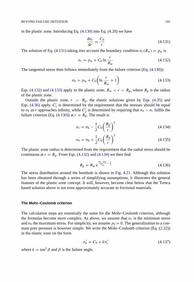
BEYOND FAILURE INITIATION 165
in the plastic zone. Introducing Eq. (4.130) into Eq. (4.28) we have
dσrdr
= C0
r(4.131)
The solution of Eq. (4.131) taking into account the boundary condition σr(Rw) = pw is
σr = pw + C0 lnr
Rw(4.132)
The tangential stress then follows immediately from the failure criterion (Eq. (4.130)):
σθ = pw + C0
(lnr
Rw+ 1
)(4.133)
Eqs. (4.132) and (4.133) apply in the plastic zone, Rw < r < Rp, where Rp is the radiusof the plastic zone.
Outside the plastic zone, r > Rp, the elastic solutions given by Eqs. (4.35) andEqs. (4.36) apply. C′
1 is determined by the requirement that the stresses should be equalto σh as r approaches infinity, while C′
2 is determined by requiring that σθ − σr fulfils thefailure criterion (Eq. (4.130)) at r = Rp. The result is
σr = σh − 1
2C0
(Rp
r
)2
(4.134)
σθ = σh + 1
2C0
(Rp
r
)2
(4.135)
The plastic zone radius is determined from the requirement that the radial stress should becontinuous at r = Rp. From Eqs. (4.132) and (4.134) we then find
Rp = Rw eσh−pwC0
− 12 (4.136)
The stress distribution around the borehole is shown in Fig. 4.21. Although this solutionhas been obtained through a series of simplifying assumptions, it illustrates the generalfeatures of the plastic zone concept. It will, however, become clear below that the Trescabased solution above is not even approximately accurate in frictional materials.
The Mohr–Coulomb criterion
The calculation steps are essentially the same for the Mohr–Coulomb criterion, althoughthe formulas become more complex. As above, we assume that σr is the minimum stressand σθ the maximum stress. For simplicity, we assume pf = 0. The generalization to a con-stant pore pressure is however simple. We write the Mohr–Coulomb criterion (Eq. (2.22))in the elastic zone on the form
σ ′θ = C0 + kσ ′
r (4.137)
where k = tan2 β and β is the failure angle.

166 STRESSES AROUND BOREHOLES. BOREHOLE FAILURE CRITERIA
Fig. 4.21. Stresses around a borehole with a plastic zone, according to the Tresca model. Parameters areC0 = 0.5σh, pw = 0.25σh.
For the plastified zone we allow the possibility of altered parameters
σ ′θ = C′
0 + k′σ ′r (4.138)
Eliminating σθ from the failure criterion in the plastified zone, Eq. (4.138), and insertinginto the force balance equation, Eq. (4.28), we obtain
∂σr
∂r+ σr(1 − k′)
r= C′
0
r(4.139)
Solving Eq. (4.139) using the boundary condition σr(Rw) = pw gives the solution withinthe plastified region
σr =(pw + C′
0
k′ − 1
)(r
Rw
)k′−1
− C′0
k′ − 1(4.140)
The tangential stress follows from the failure criterion, Eq. (4.138):
σθ = C′0 + k′σr = k′
(pw + C′
0
k′ − 1
)(r
Rw
)k′−1
− C′0
k′ − 1(4.141)
From the requirement that σθ = σh as r becomes very large it follows that the elasticzone stresses (Eqs. (4.35) and (4.36)) can be written
σr = σh + C′2
1
r2(4.142)
σθ = σh − C′2
1
r2(4.143)
Adding these equations gives the well-known relation
σθ = 2σh − σr (4.144)

BEYOND FAILURE INITIATION 167
At the radius of the plastic zone, the intact material yield criterion must be fulfilled, henceby inserting Eq. (4.144) into Eq. (4.137) we have:
σr(Rp) = 2σh − C0
k + 1(4.145)
Equating this expression to the inner zone expression for σr , Eq. (4.140), gives an equationto determine the plastic zone radius, which is found to be
Rp
Rw=[
2σh − C0 + (k + 1)C′
0k′−1
(pw + C′0
k′−1 )(k + 1)
] 1k′−1
(4.146)
The coefficient C′2 is determined from Eq. (4.142)
C′2 = R2
p
(σh − σr(Rp)
)(4.147)
which using Eq. (4.145) gives
C′2 = R2
w(k − 1)σh + C0
k + 1
[2σh − C0 + (k + 1)
C′0
k′−1
(pw + C′0
k′−1 )(k + 1)
] 2k′−1
(4.148)
In terms of the attraction, A = C0/(k − 1) (see Eq. (2.9)), Eq. (4.146) may be writtenas
Rp
Rw=[
2σh + (1 − k)A + (1 + k)A′
(pw + A′)(k + 1)
] 1k′−1
(4.149)
If A′ = A this simplifies to
Rp
Rw=[
2(σh + A)(pw + A)(k + 1)
] 1k′−1
(4.150)
The stress distribution around the borehole, assuming a friction angle of 30° is shown inFig. 4.22. Note that the extent of the plastic zone is considerably smaller than for the Trescacase. Fig. 4.23 illustrates how the radius of the plastic zone depends on the well pressure.Observe that the extent of the plastic zone is reduced as the friction angle increases.
The axial stress σz is more tricky to determine. More sophisticated models indicate thatthe plastic region consists of two zones; in the inner zone the axial stress is equal to thetangential stress, while in the outer zone all three principal stresses may differ.
The models presented above are simplifications, since both are based on ideal plas-ticity, and do not take properly into account how the plastic strain changes the yieldcriterion. More realistic models need to incorporate a description of plastic flow and hard-ening/softening, and necessarily become significantly more complicated than the simplemodels sketched here. Although the Mohr–Coulomb based equations above may be usedfor quick overview calculations, more advanced models, normally implemented in FiniteElement codes, are necessary for precise calculations.

168 STRESSES AROUND BOREHOLES. BOREHOLE FAILURE CRITERIA
Fig. 4.22. Stresses around a borehole with a plastic zone, assuming the same failure criterion in the intact andplastic zones. Parameters are C0 = 0.1σh, pw = 0.2σh, ϕ = 30°.
Fig. 4.23. Radius of the plastic zone versus well pressure, for friction angles 10° and 30°. Full lines correspondto C0 = 0.5σh, while dashed lines are for C0 = 0.1σh.
Deformation and plastic strain
The deformation and plastic strain may be computed by the general methods outlined inSection 2.8.1. To simplify equations we restrict ourselves to the Tresca criterion, Eq. (2.5).We rewrite the criterion in the general form of Eq. (2.61)
f (σ ′1, σ
′2, σ
′3) = f (σ ′
r , σ′θ ) = σ ′
θ − σ ′r − C0 = 0 (4.151)

BEYOND FAILURE INITIATION 169
and find the plastic strains according to the associated flow rule, Eq. (2.66)
εpr = dλp
∂f
∂σr= −dλp (4.152)
εpθ = dλp
∂f
∂σθ= dλp (4.153)
εpz = dλp
∂f
∂σz= 0 (4.154)
The total strains are given by the deformations (Eqs. (4.13)–(4.15)), while the plastic strainscan be found from Eq. (2.60). Inserting the resulting expressions into Eq. (4.19) we find
σ ′r = (λfr + 2Gfr)
(∂u
∂r+ dλp
)+ λfr
(u
r− dλp
)(4.155)
Proceeding in the same way for σ ′θ , and using the yield criterion, Eq. (4.151), gives
dλp = 1
2
u
r− 1
2
∂u
∂r− C0
4Gfr(4.156)
Inserting the expression for dλp into Eq. (4.155), and using the force balance equation(4.28) then gives the displacement equation
d2u
dr2+ 1
r
du
dr− u
r2− C0
λfr +Gfr
1
r+ α
λfr +Gfr
dpf
dr= 0 (4.157)
In the following we restrict ourselves to the case where pf is constant, or where the deriva-tive of pf with respect to r is proportional to 1/r . The latter case corresponds to stationaryradial flow, see Eq. (4.62).
The displacement equation can then be rewritten as
d2u
dr2+ 1
r
du
dr− u
r2= P
r(4.158)
where (using Eq. (4.62))
P = C0
λfr +Gfr− α
λfr +Gfr
pfo − pw
ln(Re/Rw)(4.159)
The second term is replaced by zero for the constant pf case.The general solution of Eq. (4.158) is
u = C1r + C2
r+ P
2r ln r (4.160)
Entering this solution into Eq. (4.156) gives
dλp = C2
r2− P
4− C0
4Gfr(4.161)
The integration constant C2 is now determined by requiring that dλp should be zero atr = Rp, giving
dλp = 1
4
(C0
Gfr+ P
)[(Rp
r
)2
− 1
](4.162)

170 STRESSES AROUND BOREHOLES. BOREHOLE FAILURE CRITERIA
We have used the Tresca criterion, because it allows the main points to be demonstratedwith simple mathematics. Using a more realistic criterion, like the Mohr–Coulomb crite-rion, adds significantly to the complexity of the calculations. See Risnes et al. (1982).
4.7. Spherical coordinates
In petroleum related rock mechanics stress and strain solutions in spherical coordinates areof much less importance than solutions in cylindrical coordinates. While the cylindricalgeometry is often a good approximation for a borehole, spherical cavities are to a lessextent a good approximation to real cases.
Still, solutions in spherical coordinates have been employed as a crude approximationto producing cavities (see Section 10.2.3), and are also useful in some methods for theestimation of surface subsidence (see Chapter 12).
We therefore give a short presentation of some basic equations here.
4.7.1. Basic equations
We use the standard convention, and denote the spherical coordinates by (r, θ, φ), and limitourselves to a situation with full spherical symmetry. The only deformation is then in theradial direction, and the non-zero strains are given by (see Appendix D.1.2 for the completeexpressions for strain in spherical coordinates)
εr = ∂u
∂r(4.163)
εφ = εθ = u
r(4.164)
The force equilibrium equation for the r-direction, corresponding to Eq. (4.28), becomes
dσrdr
+ 1
r(2σr − σθ − σφ) = 0 (4.165)
while, due to the symmetry assumed, the force equilibrium equation for the θ -directionrequires
σθ = σφ (4.166)
Eq. (4.165) is then simplified to
dσrdr
+ 2
r(σr − σθ ) = 0 (4.167)
Hooke’s law is reduced to (using εφ = εθ )σr − αpf = (λfr + 2Gfr)εr + 2λfrεθ (4.168)
σθ − αpf = λfrεr + 2(λfr +Gfr)εθ (4.169)

SPHERICAL COORDINATES 171
Inserting the expressions for the strains, Eqs. (4.163) and (4.164), into Hooke’s law, andusing the force equilibrium equation (4.167) gives the displacement equation
d2u
dr2+ 2
r
du
dr− 2
r2u+ α
λfr + 2Gfr
dpf
dr= 0 (4.170)
4.7.2. Stress distribution around a spherical cavity with no fluid flow
With no fluid flow the pore pressure will remain constant, equal to pfo, and the displace-ment equation becomes
d2u
dr2+ 2
r
du
dr− 2
r2u = d
dr
(du
dr+ 2u
r
)= d
dr
(1
r2
d
dr(r2u)
)= 0 (4.171)
The general solution is
u = C1r + C2
r2(4.172)
where the integration constants are to be determined from the boundary conditions
σr = pw for r = Rc (4.173)
σr = σo for r → ∞ (4.174)
Rc is the radius of the spherical cavity.Proceeding as in Section 4.2.2, using Hooke’s law (Eqs. (4.168)–(4.169)), the stress
distribution around a spherical cavity is found to be given by
σr = σo − (σo − pw)
(Rc
r
)3
(4.175)
σθ = σo + 1
2(σo − pw)
(Rc
r
)3
(4.176)
These stress solutions are sketched in Fig. 4.24. The thin dashed lines show the corre-sponding distribution for a cylindrical hole (see Fig. 4.3). If we assume σo to be equal toσh, the stress difference between the tangential and the radial stress at the cavity wall willbe 2(σh − pw) in the cylindrical hole case but only (3/2)(σh − pw) in the spherical cav-ity case. It follows that a spherical cavity tends to be more stable than an open hole withrespect to shear failure.
4.7.3. Stress distribution with fluid flow
Darcy’s law (see Eq. (1.229)) for symmetric spherical flow into a cavity can be written
Q
4πr2= k
ηf
dpf
dr(4.177)

172 STRESSES AROUND BOREHOLES. BOREHOLE FAILURE CRITERIA
Fig. 4.24. Stress distribution around a spherical cavity with no fluid flow. The thin dashed lines show the corre-sponding distribution for a cylinder, see Fig. 4.3.
where 4πr2 is the area of a sphere of radius r . All the other parameters are the same as inEq. (4.61). If we assume that the flow rate is independent of r , the fluid pressure distributionis given by
pf = pfo − (pfo − pw)Rc
r(4.178)
Solving the displacement equation, the steady state solutions for fluid flow into the cavitycan then be written:
σr = σo − [σo − pw − 2η(pfo − pw)
](Rc
r
)3
− 2η(pfo − pw)Rc
r(4.179)
σθ = σo + 1
2
[σo − pw − 2η(pfo − pw)
](Rc
r
)3
− η(pfo − pw)Rc
r(4.180)
At the cavity wall we have
σr = pw (4.181)
σθ = σo + 1
2(σo − pw)− 2η(pfo − pw) (4.182)
As for the cylindrical hole the stresses at the free surface are the same as in the no-flowcase, except that the tangential stress has an additional term due to pressure drawdown.This term is exactly the same as derived for the cylindrical vertical well.
References
Bradley, W.B. (1979). “Failure of inclined boreholes”. J. Energy Resources Tech. 101, 232–239.Charlez, P.A. (1991). Rock Mechanics. Volume 1. Theoretical Fundamentals. Éditions Technip, Paris.Charlez, P.A. (1997). Rock Mechanics. Volume 2. Petroleum Applications. Éditions Technip, Paris.
FURTHER READING 173
Detournay, E., Cheng, A.H.D. (1988). “Poroelastic response of a borehole in a non-hydrostatic stress field”. Int.J. Rock Mech. Min. Sci. & Geomech. Abstr. 25, 171–182.
Ewy, R.T., Cook, N.G.W. (1989). “Fracture processes around highly stressed boreholes”. In: Proc. 12th AnnualEnergy-Sources Technol. Conf. & Exhibition, Drilling Symp. ASME, New York, pp. 63–70.
Fairhurst, C. (1968). “Methods of determining in-situ rock stresses at great depth”. Technical Report no. 1, 1968,prepared for Missouri River Division, U.S. Army Corps of Engineers. School of Mineral and MetallurgicalEngineering, U. of Minnesota, Minneapolis.
Guenot, A. (1987). “Contraintes et ruptures autor des forages pétroliers”. In: Proc. 6th Int. Conf. on Rock Me-chanics, pp. 109–118.
Hiramatsu, Y., Oka, Y. (1962). “Stress around a shaft or level excavated in ground with a three-dimensional stressstate”. Mem. Fac. Eng. Kyotu Univ. 24, 56–76.
Hiramatsu, Y., Oka, Y. (1968). “Determination of the stress in rock unaffected by boreholes or drifts, from mea-sured strains or deformations”. Int. J. Rock Mech. Min. Sci. 5, 337–353.
Jaeger, J.C., Cook, N.G.W. (1979). Fundamentals of Rock Mechanics, third ed. Chapman and Hall, London.Kaiser, P.K., Guenot, A., Morgenstern, N.R. (1985). “Deformation of small tunnels. IV. Behaviour during failure”.
Int. J. Rock Mech. Min. Sci. & Geomech. Abstr. 22, 141–152.Kirsch (1898). “Die Theorie der Elastizität und die Bedürfnisse der Festigkeitslehre”. Zeitschrift des Vereines
deutscher Ingenieure 42, 797–807.Maury, V.M., Sauzay, J.-M. (1987). “Borehole instability: Case histories, rock mechanics approach, and results”.
SPE/IADC 16051. In: SPE/IADC Drilling Conference, New Orleans, LA, March 15–18.Peška, P., Zoback, M.D. (1995). “Compressive and tensile failure of inclined well bores and determination of in
situ stress and rock strength”. J. Geophys. Res. 100B, 12791–12811.Risnes, R., Bratli, R., Horsrud, P. (1982). “Sand stresses around a borehole”. Soc. Petr. Eng. J. 22, 883–898.Santarelli, F.J. (1987). “Theoretical and experimental investigation of the stability of the axisymmetric wellbore”.
PhD thesis, University of London.Santarelli, F.J., Brown, E.T., Maury, V. (1986). “Analysis of borehole stresses using pressure-dependent linear
elasticity”. Int. J. Rock Mech. Min. Sci. & Geomech. Abstr. 23, 445–449.Vardoulakis, I., Sulem, J., Guenot, A. (1988). “Borehole instabilities as bifurcation phenomena”. Int. J. Rock
Mech. Min. Sci. & Geomech. Abstr. 25, 159–170.Zheng, Z., Cook, N.G.W., Myer, L.R. (1988). “Borehole breakout and stress measurements”. In: Cundall, P.A.,
Sterling, R.L., Starfield, A.M. (Eds.), Key Questions in Rock Mechanics. Balkema, Rotterdam, pp. 471–479.Zoback, M.D., Moos, D., Mastin, L., Anderson, R.N. (1985). “Well bore breakouts and in situ stress”. J. Geophys.
Res. 90B, 5523–5555.
Further reading
Aadnoy, B.S., Chenevert, M.E. (1987). “Stability of highly inclined boreholes”. SPE Drilling Engrg. 2, 364–374.Aadnoy, B.S. (1987). “A complete elastic model for fluid-induced and in-situ generated stresses with the presence
of a borehole”. Energy Sources 9, 239–259.Aadnoy, B.S. (1988). “Modeling of the stability of highly inclined boreholes in anisotropic rock formations”.
SPE Drilling Engrg. 3, 259–268.Addis, M.A., Barton, N.R., Bandis, S.C., Aristotellan, U., Henry, J.P. (1990). “Laboratory studies on the stability
of vertical and deviated boreholes”. SPE 20406. In: SPE 65th Annual Technical Conference and Exhibition,New Orleans, LA, September 23–26.
Amadei, B. (1983). Rock Anisotropy and the Theory of Stress Measurements. Springer, Berlin.Bratli, R.K., Horsrud, P., Risnes, R. (1983). “Rock mechanics applied to the region near a wellbore”. In: Proc.
5th International Congress on Rock Mechanics, pp. F1–F17.Brown, E.T., Bray, J.W., Santarelli, F.J. (1989). “Influence of stress-dependent elastic moduli on stresses and
strains around axisymmetric boreholes”. Rock Mech. Rock Engrg. 22, 189–203.Cheatham, J.B. (1984). “Wellbore stability”. J. Petr. Tech. 36, 889–896.Ewy, R.T., Cook, N.G.W. (1990a). “Deformation and fracture around cylindrical openings in rock. I. Observations
and analysis of deformations”. Int. J. Rock Mech. Min. Sci. & Geomech. Abstr. 27, 387–407.

174 STRESSES AROUND BOREHOLES. BOREHOLE FAILURE CRITERIA
Ewy, R.T., Cook, N.G.W. (1990b). “Deformation and fracture around cylindrical openings in rock. II. Initiation,growth and interaction of fractures”. Int. J. Rock Mech. Min. Sci. & Geomech. Abstr. 27, 409–427.
Ewy, R.T. (1999). “Wellbore-stability predictions by use of a modified Lade criterion”. SPE Drilling & Comple-tion 14, 85–91.
Guenot, A., Santarelli, F.J. (1988). “Borehole stability A new challenge for an old problem”. In: Cundall, P.A.,Sterling, R.L., Starfield, A.M. (Eds.), Key Questions in Rock Mechanics. Balkema, Rotterdam, pp. 453–460.
Guenot, A. (1989). “Borehole breakouts and stress fields”. Int. J. Rock Mech. Min. Sci. & Geomech. Abstr. 26,185–195.
Haimson, B., Fairhurst, C. (1967). “Initiation and extension of hydraulic fractures in rocks”. Soc. Petr. Eng. J. 7,310–318.
Haimson, B.C., Herrick, C.G. (1985). “In situ stress evaluation from borehole breakouts. Experimental studies”.In: Ashworth, E. (Ed.), Research & Engineering Applications in Rock Masses, vol. 2. Balkema, Rotterdam,pp. 1207–1218.
Jaeger, J.C., Cook, N.G.W., Zimmerman, R.W. (2007). Fundamentals of Rock Mechanics, fourth ed. BlackwellPublishing.
Maloney, S., Kaiser, P.K. (1989). “Results of borehole breakout simulation tests”. In: Maury, V., Fourmaintraux,D. (Eds.), Rock at Great Depth. Balkema, Rotterdam, pp. 745–752.
Mastin, L. (1988). “Effect of borehole deviation on breakout orientations”. J. Geophys. Res. 93B, 9187–9195.McLean, M.R., Addis, M.A. (1990). “Wellbore stability analysis. A review of current methods of analysis and
their field application”. IADC/SPE 19941. In: SPE/IADC Drilling Conference, Houston, TX, 27 February–2 March.
Périé, P.J., Goodman, R.E., Doe, T.J. (1988). “Simulation of borehole breakouts in a model material”. Int. J. RockMech. Min. Sci. & Geomech. Abstr. 25, 97–98.
Santarelli, F.J., Brown E.T. (1987). “Performance of deep wellbores in rock with a confining pressure-dependentelastic modulus”. In: Proc. 6th Int. Conf. on Rock Mechanics, pp. 1217–1222.
Smart, B.G.D., Somerville, J.M., MacGregor, K.J. (1991). “The prediction of yield zone development arounda borehole and its effect on drilling and production”. In: Rock Mechanics as a Multidisciplinary Science.Balkema.
Sulem, J., Vardoulakis, I. (1989). “Simplified bifurcation analysis of deep boreholes in rocks with microstructure”.In: Maury, V., Fourmaintraux, D. (Eds.), Rock at Great Depth. Balkema, Rotterdam, pp. 845–852.
Veeken, C.A.M., Walters, J.V., Kenter, C.J., Davies, D.R. (1989). “Use of plasticity models for predicting boreholestability”. In: Maury, V., Fourmaintraux, D. (Eds.), Rock at Great Depth. Balkema, Rotterdam, pp. 835–844.

175
Chapter 5
Elastic wave propagation in rocks
Elastic waves are mechanical disturbances that propagate through a material. Such wavesare able to travel over very long distances through the Earth, and thus bring us informationabout parts of the formations that are otherwise inaccessible. In seismic surveys, elasticwaves are generated at the surface, and the echoes from various layers in the formationsbelow are used to map the structure of the underground. Earthquakes are generated byabrupt failure processes and propagate as elastic waves.
Elastic waves in air and water are usually called acoustic waves, or sound waves. Theseterms are often used about elastic waves in rocks too. Elastic waves in rocks propagate witha velocity that is given by elastic stiffnesses and the density of the rock. These parametersdepend on other parameters such as porosity. Thus elastic waves also provide a method bywhich specific formation parameters can be estimated in the field.
As we proceed, we shall see that this evaluation is not straightforward—for example,the stiffness probed by an elastic wave is generally different from the static stiffness. How-ever, the fact that elastic waves are mechanical disturbances means that there has to be afundamental connection between rock acoustics and rock mechanics.
In this chapter we first present the fundamentals of elastic wave propagation in porousmedia (Sections 5.1–5.5). Section 5.6 addresses the main focus of this chapter: the con-nection between rock acoustics and rock mechanics. Finally, we give some background tounderstand sonic wave propagation in boreholes and seismic waves through the subsurface(Sections 5.7–5.9).
5.1. The wave equation
When an elastic wave passes through a material, each part of the material is forced intooscillating motion. Consider a volume element within the material. The element is pushedby the adjacent element behind it, and accelerates. The movement causes the volume el-ement to push on the next element in front of it. This way the movement is propagatingfrom volume element to volume element through the material as a wave.
Wave propagation is described mathematically by the wave equation. This equation fol-lows directly from Newton’s second law of motion: Force = mass · acceleration. The force(per unit volume) acting on a volume element due to the stress the adjacent elements exertwas derived in Chapter 1. The force Fx in the x-direction is given as (see Eq. (1.14)):
Fx = ∂σx
∂x+ ∂τxy
∂y+ ∂τxz
∂z(5.1)
For simplicity, we shall first consider a plane, unidirectional mode of deformation in thex-direction. We shall further assume that the material is a fluid, so that no shear forces canexist, that is τxy = τxz = 0. The mass (per unit volume) is given as the material’s density
176 ELASTIC WAVE PROPAGATION IN ROCKS
ρ, and the acceleration is given as the second derivative (with respect to time t) of thedisplacement u of the volume element. Newton’s second law of motion thus requires that
ρ∂2u
∂t2= ∂σx
∂x(5.2)
The stress σx can be expressed in terms of the displacement u according to Hooke’s law(Eqs. (1.93)–(1.98)), which under the conditions assumed here (plane wave in x-direction,which implies that ∂/∂y = ∂/∂z = 0; and fluid, which implies that G = 0) becomes
σx = λ∂u∂x
(5.3)
Note that for a fluid the Lamé coefficient λ is equal to the bulk modulus. CombiningEqs. (5.2) and (5.3), we obtain
ρ∂2u
∂t2= λ∂
2u
∂x2(5.4)
This is the wave equation for a plane wave propagating in the x-direction in a fluid. Thesolution of the wave equation has the form
u = uo ej(ωt−qx) (5.5)
where j represents the imaginary unit. The real part of this expression describes a periodicdisplacement in the x-direction, with amplitude uo. The complex formulation has beenchosen here because it is mathematically simpler to work with.
The periodic displacement is a wave which propagates in the x-direction, with angularfrequency ω, and wavenumber q. The angular frequency ω is related to the frequency f as
ω = 2πf (5.6)
The wave described by Eq. (5.5) extends from −∞ to +∞ both in space and time. A dis-placement pulse, which is limited in space and time, is described as a sum of waves likeEq. (5.5), each with different angular frequency and different amplitude, such that the netdisplacement vanishes for large values of |x| and |t |.
The displacement u(x, t) represents the displacement of a volume element at position xand time t , as the wave passes by. In this context, the volume element has been consideredas a particle, attached with “springs” to its neighbouring elements. The displacement istherefore often called particle displacement. The displacement wave described by Eq. (5.5)can also be considered as a pressure wave, through the relation between displacement andstress given by Eq. (5.3).
Any two points x1 and x2, which are separated by a distance such that qx2 = qx1 + 2π ,will at all times have equal displacement according to Eq. (5.5). The distance between twosuch points, x2 − x1, is called the wavelength (λw). The wavelength is thus related to thewavenumber as
q = 2π
λw(5.7)
The term (ωt − qx) in the exponent of expression (5.5) is called the phase of the wave. Ifwe follow the wave, locked on to a fixed displacement like a surfer on a sea wave, we move
P- AND S-WAVES 177
with a velocity v = x/t such that the phase (ωt − qx) remains constant. This velocity iscalled the phase velocity, and is related to the angular frequency, the wavenumber and thewavelength as
v = ω
q= λwf (5.8)
Inserting Eq. (5.5) into Eq. (5.4) and solving for ω/q, we find that the phase velocity isgiven by the elastic stiffness and the density as
v =√λ
ρ(5.9)
Thus, we have derived the general result that the phase velocity of an elastic wave is propor-tional to the square root of an elastic modulus, and inversely proportional to the square rootof the density. This result provides our basis for using elastic waves to explore mechanicalproperties of rocks.
The phase velocity is the velocity at which the phase of an elastic wave travels. Elasticwaves in fluids and gases are usually called sound waves, or acoustic waves, and the phasevelocity is usually called the sound velocity. For fresh water, the elastic modulus λ =Kf ≈ 2.25 GPa and the density ρ ≈ 1.0 g/cm3 (where both depend on temperatureand pressure), hence the sound velocity is 1500 m/s, according to Eq. (5.9). For dry airunder normal atmospheric conditions, λ ≈ 0.14 MPa (adiabatic value; see Section 1.5)and ρ ≈ 0.0012 g/cm3, thus the sound velocity is 343 m/s.
As shown above, the definition of the phase velocity is associated with a wave whichextends to infinity in space and time. In practice, we usually work with acoustic signals inthe form of pulses of finite duration. The velocity of a pulse, or equivalently, the velocityof the wave energy, is called the group velocity, and is given as
vgroup = ∂ω
∂q(5.10)
By comparing Eqs. (5.8) and (5.10) we see that if the phase velocity varies with thefrequency—a phenomenon called dispersion—the group and phase velocities will be dif-ferent.
5.2. P- and S-waves
We now proceed to a more general case, and allow the material to possess a shear stiffnessso that shear forces may exist. That is, we shall look at elastic wave propagation in anisotropic solid. Starting with Newton’s second law of motion, and the general expression(5.1) for the force, we find the wave equation for displacement u in the x-direction
ρ∂2u
∂t2= ∂σx
∂x+ ∂τxy
∂y+ ∂τxz
∂z(5.11)

178 ELASTIC WAVE PROPAGATION IN ROCKS
Introducing Hooke’s law (Eqs. (1.93)–(1.98)) we find
ρ∂2u
∂t2= (λ+G)
(∂2u
∂x2+ ∂2v
∂x∂y+ ∂2w
∂x∂z
)+G
(∂2u
∂x2+ ∂2u
∂y2+ ∂2u
∂z2
)(5.12)
(Note that the symbol v here represents displacement in y-direction.) A general solution ofthis equation is
u = uo ej(ωt−ql·�r) (5.13)
The vector �r has the components x, y and z, while l is a unit vector parallel to the di-rection of wave propagation. The components lx , ly and lz will be the direction cosines(see Eqs. (1.27)–(1.29)) of the propagation vector. Equations similar to Eq. (5.12) can bederived for particle displacement in the y- and z-directions. In general, these are coupledequations in u, v and w, however there are two relatively straightforward solutions whichcan be derived from Eq. (5.12). First we search for a solution where the wave propagationis parallel to the displacement u (that is, lx = 1; ly = lz = v = w = 0):
u = uo ej(ωt−qx) (5.14)
Such a wave is called a longitudinal wave, or alternatively a compressional wave, as itinvolves a periodic compression of the material. It is also often termed a primary wave, aname which originates from studies of earthquakes.
Since we are now considering a plane wave propagating parallel to the x-axis, we have∂/∂y = ∂/∂z = 0, and Eq. (5.12) reduces to
ρω2 = q2(λ+ 2G) (5.15)
The phase velocity is
vp = ω
q=√λ+ 2G
ρ(5.16)
The subscript p denotes that this is a primary wave.Eq. (5.12) also has other solutions. For instance, it is possible to establish a mode of
motion in which the particles are displaced only in the x-direction (that is, u �= 0, v =w = 0), while the wave is propagating as a plane wave in the y-direction (which implies∂/∂x = ∂/∂z = 0). The solution is then
u = uo ej(ωt−qy) (5.17)
Inserting this into Eq. (5.12), we find
ρω2 = q2G (5.18)
The phase velocity is
vs = ω
q=√G
ρ(5.19)
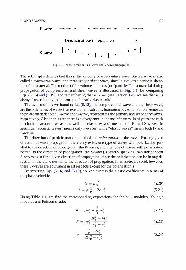
P- AND S-WAVES 179
Fig. 5.1. Particle motion in P-wave and S-wave propagation.
The subscript s denotes that this is the velocity of a secondary wave. Such a wave is alsocalled a transversal wave, or alternatively a shear wave, since it involves a periodic shear-ing of the material. The motion of the volume elements (or “particles”) in a material duringpropagation of compressional and shear waves is illustrated in Fig. 5.1. By comparingEqs. (5.16) and (5.19), and remembering that ν > −1 (see Section 1.4), we see that vp isalways larger than vs in an isotropic, linearly elastic solid.
The two solutions we found to Eq. (5.12), the compressional wave and the shear wave,are the only types of waves that exist for an isotropic, homogeneous solid. For convenience,these are often denoted P-wave and S-wave, representing the primary and secondary waves,respectively. Also in this area there is a divergence in the use of names: In physics and rockmechanics “acoustic waves” as well as “elastic waves” means both P- and S-waves. Inseismics, “acoustic waves” means only P-waves, while “elastic waves” means both P- andS-waves.
The direction of particle motion is called the polarization of the wave. For any givendirection of wave propagation, there only exists one type of waves with polarization par-allel to the direction of propagation (the P-wave), and one type of waves with polarizationnormal to the direction of propagation (the S-wave). (Strictly speaking, two independentS-waves exist for a given direction of propagation, since the polarization can be in any di-rection in the plane normal to the direction of propagation. In an isotropic solid, however,these S-waves are equivalent in all respects except for the polarization.)
By inverting Eqs. (5.16) and (5.19), we can express the elastic coefficients in terms ofthe phase velocities:
G = ρv2s (5.20)
λ = ρv2p − 2ρv2
s (5.21)
Using Table 1.1, we find the corresponding expressions for the bulk modulus, Young’smodulus and Poisson’s ratio:
K = ρv2p − 4
3ρv2
s (5.22)
E = ρv2s
3v2p − 4v2
s
v2p − v2
s(5.23)
ν = v2p − 2v2
s
2(v2p − v2
s )(5.24)
180 ELASTIC WAVE PROPAGATION IN ROCKS
Further relations can be established by use of Table 1.1. Note that
λ+ 2G = H = K + 4
3G = ρv2
p (5.25)
where H is the uniaxial compaction modulus (also referred to as plane wave modulus,or P-wave modulus; see Section 1.3) Eqs. (5.20)–(5.25) were derived for a linearly elas-tic, isotropic and homogeneous material, and show how values for elastic moduli can beobtained from measurements of acoustic velocities in such a material. Rocks are usuallyneither isotropic nor homogeneous, nor are they linearly elastic, and we shall see later(Section 5.6) that this complicates the relations between static elastic moduli and acousticvelocities.
5.3. Elastic waves in porous materials
The elastic response of a porous material may be significantly affected by the presence ofa pore fluid. In poorly consolidated sediments, the P-wave velocity for a water saturatedmaterial can be several times larger than it is when the material is dry. Qualitatively, wecan explain this as a consequence of the added resistance against compression provided bythe pore fluid. For more competent materials, or materials under high confining pressure,the frame stiffness is higher and the contribution of the pore fluid is relatively less, hencethe effect of saturation is much smaller. As saturation also implies an increase in density, itmay even result in a reduction of the P-wave velocity for a stiff rock. Saturation is assumednot to affect the shear modulus for a permeable rock (see Section 1.6.2), hence it usuallyresults in a small decrease in velocity for S-waves.
Clearly, the impact of the pore fluid on the velocities is strongly related to the porosityof the rock. A simple assumption, that has been frequently used for interpretation of welllogs, is that the interval transit time (which is the inverse of the P-wave velocity) is relatedlinearly to the porosity, according to the time average equation (Wyllie et al., 1958):
1
vp= φ
vfluid+ 1 − φvsolid
(5.26)
vfluid and vsolid denote the P-wave velocities of the pore fluid and the solid grain mater-ial, respectively. The equation has an empirical basis (it is theoretically valid in the highfrequency limit for a material consisting of layers of fluid and non-porous solid), and itworks with reasonable accuracy for several practical purposes. If the lithology (and hencevsolid) is known, it can be used to estimate the porosity, or alternatively—it can be used foridentification of the lithology if the porosity can be estimated by other means. The equa-tion is not applicable for predicting the effect of saturation, however, nor can it be used forS-waves.
5.3.1. Biot’s theory of elastic wave propagation
In Chapter 1 we applied Biot’s theory of poroelasticity to describe the effect of the porefluid on the elastic properties of porous materials. The same formalism may also be used

ELASTIC WAVES IN POROUS MATERIALS 181
to describe elastic wave propagation in saturated rocks (Biot, 1962; Stoll, 1974). The pro-cedure for establishing the wave equation and deriving the velocities is analogues to that ofSections 5.1 and 5.2, however we now have to account for the pore pressure pf in additionto the external stress. Also, we have to take into account that the displacement of the fluid(uf) may be different from the displacement of the solid material (us).
Considering longitudinal motion parallel to the x-axis, and following the same approachas in Section 5.1 we find that Newton’s second law of motion requires that
φρf∂2uf
∂t2+ (1 − φ)ρs
∂2us
∂t2= ∂σx
∂x(5.27)
We now differentiate with respect to x on both sides of the equation, introduce the strainparameters εx , ζ (from Eq. (1.134)) and H (from Eq. (1.237)). As we are considering onlywave motion in the x-direction, we have ∂/∂y = ∂/∂z = 0. Expressing the stress σx interms of the strains according to Eq. (1.136) we find that Eq. (5.27) may be written as
∂2
∂t2(−ρfζ + ρεx) = ∂2
∂x2(Hεx − Cζ) (5.28)
Here ρ, defined as
ρ = φρf + (1 − φ)ρs (5.29)
is the bulk density of the porous medium. Eq. (5.28) is a wave equation, similar to Eq. (5.4),although we here use strain rather than displacement as the variable. However, Eq. (5.28)has two variables (ζ and εx), hence we need one more equation. Turning to the movementof the fluid, we find according to Eqs. (1.229) and (1.230) that the net effective force (perunit area) acting on the fluid part of a volume element is
�∇pf − ηf
kφ
(∂ �uf
∂t− ∂ �us
∂t
)(5.30)
Considering only wave motion in the x-direction, and denoting the x-components of �ufand �us as uf and us, respectively, Newton’s second law of motion gives
∂2
∂t2(ρfuf) = ∂pf
∂x− ηf
kφ
(∂uf
∂t− ∂us
∂t
)(5.31)
We now differentiate this equation with respect to x, make use of Eq. (1.142) to eliminatepf and Eq. (1.136) to introduce ζ , and find the second wave equation:
∂2
∂t2
(ρfεx − ρf
φζ
)= ∂2
∂x2(Cεx −Mζ)+ ηf
k
∂ζ
∂t(5.32)
The two wave equations (5.28) and (5.32) have the solutions
εx = εxo ej(ωt−qx) (5.33)
ζ = ζo ej(ωt−qx) (5.34)
Two modifications were introduced by Biot:

182 ELASTIC WAVE PROPAGATION IN ROCKS
1. The pore fluid does not flow strictly in the direction of the pore pressure gradient, butis constrained to follow the pore channel network. To compensate for this, the secondterm on the left hand side of Eq. (5.32) is multiplied by a parameter T , called thetortuosity. The tortuosity is a measure of the twistedness of the pore channels. Givena porous sample with thickness L, the pore fluid has to travel a distance Le > L topenetrate the sample. The tortuosity is defined as T = (Le/L)
2. Thus T � 1. Forsandstone, T is typically in the range 2–3.
2. The fluid flow at higher frequencies is not laminar. This is compensated for by mod-ifying the viscosity ηf → ηfF(κ), where
κ = ap
√ωρf
ηf(5.35)
and ap is equal to the radius of an average pore. F(κ) = 1 at ω = 0, while F(κ) ∝√ω when ω → ∞. A specific expression for F(κ) is given in Appendix D.2.1.
Introducing the expressions (5.33) and (5.34) into the wave equations (5.28) and (5.32),including Biot’s modifications above, and making use of the relation vp = ω/q, we obtainthe two equations for the amplitudes εxo and ζo:
(H − ρv2p)εxo − (C − ρfv
2p)ζo = 0 (5.36)
(C − ρfv2p)εxo −
(M − ρfT
φv2
p + jv2
p
ω
ηfF(κ)
k
)ζo = 0 (5.37)
This homogeneous system of equations has non-trivial solutions if the determinant van-ishes (see Appendix C.2.11), that is if∣∣∣∣∣
(H − ρv2p) −(C − ρfv
2p)
(C − ρfv2p) −(M − ρfT
φv2
p + jv2
pωηfF(κ)k)
∣∣∣∣∣ = 0 (5.38)
Eq. (5.38) is an equation for vp. Since it specifies how the velocity changes with frequency,it is a so called dispersion relation. Attenuation is also implicitly included, through theimaginary parts of the solution (see Section 5.4). In the low frequency limit, the termincluding ω−1 goes to infinity and the only solution to Eq. (5.38) is
vp(ω → 0) =√H
ρ=√
K + 43Gfr
φρf + (1 − φ)ρs(5.39)
Here we have introduced the expression (5.29) for the density ρ, while the modulus H =λ+ 2Gfr = K + 4
3Gfr and K is given by Eq. (1.155).Introducing the velocity given by Eq. (5.39) into Eq. (5.36) we find that ζo = 0 in the
low frequency limit. Thus the solid and the fluid are moving in phase (that is: together)during the oscillatory movements caused by the elastic wave.
An equation similar to Eq. (5.38) can be established for the shear wave velocity:∣∣∣∣ (Gfr − ρv2s ) ρfv
2s
−ρfv2s −(−ρfT
φv2
s + j v2sωηfF(κ)k)
∣∣∣∣ = 0 (5.40)

ELASTIC WAVES IN POROUS MATERIALS 183
Fig. 5.2. P- and S-wave velocities versus porosity for dry and saturated rocks, based on Biot’s theory in the lowfrequency limit. The frame moduli are given by the critical porosity relations (6.16)–(6.17) with a critical porosityof 0.39. Dashed lines: dry rock; Solid lines: saturated rock.
In the low frequency limit, the solution of this equation is
vs(ω → 0) =√Gfr
ρ=√
Gfr
φρf + (1 − φ)ρs(5.41)
Eqs. (5.39) and (5.41) describe the effect of saturation on elastic wave velocities, in the lowfrequency limit.
To illustrate the predictions of the equations, we shall look at an example. In a water-saturated sandstone, we have Kf ≈ 2.2 GPa, ρf ≈ 1.0 g/cm3 and ρs ≈ 2.7 g/cm3, whilefor a dry rock we may assumeKf = ρf = 0. The frame moduliKfr andGfr are not specifiedby the Biot theory, however these will vary with the porosity and the degree of cementation(see Chapter 6). Various empirical relations between the frame moduli and porosity havebeen presented. For this example, we choose to use the critical porosity relations. Fig. 5.2illustrates how fluid saturation affects the elastic velocities in the low frequency limit forsandstones with various porosities, according to Eqs. (5.39), (5.41), (6.16) and (6.17). Wecan see that saturation will lead to an increase in vp for soft (high porosity) rocks, while itmay lead to a slight decrease in vp for stiff rocks. We also see that saturation always leads toa reduction in vs. The effect of saturation depends on the ratio between the frame stiffnessand the fluid modulus, and an increase in vp may thus be seen also for low porosity rocksif the frame stiffness is sufficiently low.
The frequency dependence of vp and vs is controlled by the term jv2
pωηfF(κ)k
in Eqs. (5.38)and (5.40). In the high frequency limit this term vanishes. For the shear wave, this givesthe solution
vs(ω → ∞) =√
Gfr
ρ − φρfT
=√
Gfr
(1 − 1T)φρf + (1 − φ)ρs
(5.42)

184 ELASTIC WAVE PROPAGATION IN ROCKS
By comparing Eq. (5.41) and (5.42) we see that the shear wave velocity will increase withfrequency. The effect is quite small—typically less than 3% from the low frequency limitto the high frequency limit for tortuosity T = 3. The velocity increase is a result of thecoupling to the pore fluid motion. It may be shown that ζo �= 0 in the high frequencylimit, thus the pore fluid is moving out of phase with the solid framework. The actual massinvolved in the wave motion is therefore reduced, and the velocity increases, as Eq. (5.42)shows. This flow of fluid relative to the solid framework is often called “Biot flow”.
For the P-wave, the solution is more complicated for higher frequencies. First of all,Eq. (5.38) is a second degree equation in v2
p for ω > 0, and thus it has two solutions. Thelargest root is the solution (5.39) in the low frequency limit. This is the “normal” P-wavethat is observed in seismic surveys and well logging. The expression for this solution in thehigh frequency limit is somewhat complicated, however it can be shown that there is onlya marginal increase (typically less than 1 per cent) in velocity from the low frequency limitto the high frequency limit in most cases. However, for very soft rocks (in the suspensionlimit), the dispersion can be significantly higher. In general, the dispersion is larger forhigher porosity and lower tortuosity.
The other solution is a so-called “slow wave” which is highly attenuated. At low fre-quencies the wave does not exist as a propagating wave, however it is rather a diffusivemode approaching ordinary (Darcy) flow through the porous rock in the limit ω → 0. Al-though the slow wave is usually not observed as a propagating wave, its existence has beenproven in laboratory experiments (first time by Plona, 1980) which provides justificationof the basis of the Biot theory.
5.3.2. Dispersion due to local flow
In reality, the actual P-wave dispersion is higher than predicted by Biot’s theory. It isassumed that this is related to thin cracks in the solid framework (at grain contacts, forinstance). At low frequencies, the fluid pressure within these thin cracks will be equal tothe pore pressure outside the cracks, and the cracks will thus be a part of the pore space inBiot’s model. At high frequencies, the fluid pressure within the thin cracks will not be ableto follow the rapid oscillations of the pore pressure outside. The cracks will then effectivelybe sealed off and no longer be a part of the pore space in Biot’s model (which requires thatthe entire pore space is connected). As thin, sealed, fluid-filled cracks are almost incom-pliant (see Section 6.4), the effective stiffness of the solid framework will thus increase athigher frequencies.
The thin cracks tend to be closed at high external stresses. Thus, we may expect to finda relation between the bulk and shear moduli of the framework in the high frequency limitand the effective bulk modulus of the dry rock at high external pressure (Mavko and Jizba,1991). The dispersion effect caused by the local flow is usually comparable to or largerthan the effect predicted by the Biot theory alone.
5.4. Attenuation
The waves described in Sections 5.1 and 5.2 are waves propagating with plane wavefrontswithout any loss of energy, so that the amplitude remains constant. In reality, the amplitude

ATTENUATION 185
of an elastic wave that travels through a rock will be reduced as the wave propagates. Wesay that the wave is attenuated. This will partly be due to geometrical spreading causedby a non-planar wavefront, partly due to scattering of wave energy in other directions, andpartly due to transformation of wave energy into other forms of energy (absorption).
The amplitude reduction is a certain fraction of the amplitude itself, hence the amplitudewill fall off exponentially with travelled distance. For a plane wave propagating in thepositive x-direction, the amplitude will thus fall off as
u = u0 e−αx (5.43)
where α is a measure of the attenuation. The unit for α is inverse length [m−1], but it isoften referred to in decibel per metre [dB/m]:
α [dB/m] ≡ (20 log10 e )α [m−1] ≈ 8.686α [m−1] (5.44)
The quality factor Q (often called the Q-factor, for short) is another parameter that isfrequently used as a measure for attenuation. The Q-factor is inversely proportional to α,hence a highQ-factor implies low attenuation and vice versa. It is defined as
Q = ω
2αv(5.45)
Another measure for attenuation is the loss tangent δ, defined as
δ = π
Q(5.46)
While α represents the loss per unit length, the loss tangent is a measure for the loss perwavelength. Measured Q-factors vary strongly with conditions and type of rock. Fig. 5.3shows typical laboratory data (ultrasonic frequencies) for sandstone. Reliable data for at-tenuation is usually hard to obtain, and the amount of data reported in the literature islimited.
Fig. 5.3. Q-factor for P- and S-waves vs. external pressure in dry and fluid-saturated sandstone. (After Johnstonet al., 1979; with permission from SEG.)
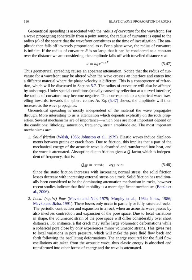
186 ELASTIC WAVE PROPAGATION IN ROCKS
Geometrical spreading is associated with the radius of curvature for the wavefront. Fora wave propagating spherically from a point source, the radius of curvature is equal to theradius (r) of the sphere that the wavefront constitutes at the time of investigation. The am-plitude then falls off inversely proportional to r . For a plane wave, the radius of curvatureis infinite. If the radius of curvature R is so large that it can be considered as a constantover the distance we are considering, the amplitude falls off with travelled distance x as
u = u0 e−x/R (5.47)
Thus geometrical spreading causes an apparent attenuation. Notice that the radius of cur-vature for a wavefront may be altered when the wave crosses an interface and enters intoa different material where the phase velocity is different. This is a consequence of refrac-tion, which will be discussed in Section 5.7. The radius of curvature will also be affectedby anisotropy. Under special conditions (usually caused by reflection at a curved interface)the radius of curvature may become negative. This corresponds to a spherical wave trav-elling inwards, towards the sphere centre. As Eq. (5.47) shows, the amplitude will thenincrease as the wave propagates.
Geometrical spreading is mostly independent of the material the wave propagatesthrough. More interesting to us is attenuation which depends explicitly on the rock prop-erties. Several mechanisms are of importance—which ones are most important depend onthe conditions: lithology, saturation, frequency, strain amplitude etc. The most importantmechanisms are:
1. Solid friction (Walsh, 1966; Johnston et al., 1979). Elastic waves induce displace-ments between grains or crack faces. Due to friction, this implies that a part of themechanical energy of the acoustic wave is absorbed and transformed into heat, andthe wave is attenuated. Absorption due to friction gives aQ-factor which is indepen-dent of frequency, that is:
QSF = const.; αSF ∝ ω (5.48)
Since the static friction increases with increasing normal stress, the solid frictionlosses decrease with increasing external stress on a rock. Solid friction has tradition-ally been considered to be the dominating attenuation mechanism in rocks, howeverrecent studies indicate that fluid mobility is a more significant mechanism (Batzle etal., 2006).
2. Local (squirt) flow (Mavko and Nur, 1979; Murphy et al., 1984; Jones, 1986;Mavko and Jizba, 1991). These losses only occur in partially or fully saturated rocks.The periodic contraction and expansion in a rock when an acoustic wave passes byalso involves contraction and expansion of the pore space. Due to local variationsin shape, the volumetric strain of the pore space will differ considerably over shortdistances. For instance, a flat crack may suffer large volumetric deformations whilea spherical pore close by only experiences minor volumetric strains. This gives riseto local variations in pore pressure, which will make the pore fluid flow back andforth following the oscillating deformations. The energy required for the fluid flowoscillations are taken from the acoustic wave, thus elastic energy is absorbed andtransformed into other forms of energy and the wave is attenuated.
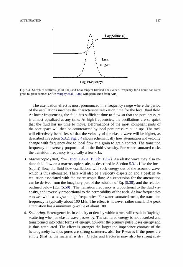
ATTENUATION 187
Fig. 5.4. Sketch of stiffness (solid line) and Loss tangent (dashed line) versus frequency for a liquid saturatedgrain to grain contact. (After Murphy et al., 1984; with permission from AIP.)
The attenuation effect is most pronounced in a frequency range where the periodof the oscillations matches the characteristic relaxation time for the local fluid flow.At lower frequencies, the fluid has sufficient time to flow so that the pore pressureis almost equalized at any time. At high frequencies, the oscillations are so quickthat the fluid has no time to move. Deformations of the most compliant parts ofthe pore space will then be counteracted by local pore pressure build-ups. The rockwill effectively be stiffer, so that the velocity of the elastic wave will be higher, asdescribed in Section 5.3.2. Fig. 5.4 shows schematically how attenuation and velocitychange with frequency due to local flow at a grain to grain contact. The transitionfrequency is inversely proportional to the fluid viscosity. For water-saturated rocksthe transition frequency is typically a few kHz.
3. Macroscopic (Biot) flow (Biot, 1956a, 1956b; 1962). An elastic wave may also in-duce fluid flow on a macroscopic scale, as described in Section 5.3.1. Like the local(squirt) flow, the fluid flow oscillations will suck energy out of the acoustic wave,which is thus attenuated. There will also be a velocity dispersion and a peak in at-tenuation associated with the macroscopic flow. An expression for the attenuationcan be derived from the imaginary part of the solution of Eq. (5.38), and the relationoutlined below (Eq. (5.50)). The transition frequency is proportional to the fluid vis-cosity, and inversely proportional to the permeability of the rock. At low frequenciesα ∝ ω2, while α ∝ √
ω at high frequencies. For water-saturated rocks, the transitionfrequency is typically about 100 kHz. The effect is however rather small: The peakattenuation has a minimumQ-value of about 100.
4. Scattering. Heterogeneities in velocity or density within a rock will result in Rayleighscattering when an elastic wave passes by. The scattered energy is not absorbed andtransformed into other forms of energy, however the primary pulse loses energy andis thus attenuated. The effect is stronger the larger the impedance contrast of theheterogeneity is, thus pores are strong scatterers, also for P-waves if the pores areempty (that is: the material is dry). Cracks and fractures may also be strong scat-

188 ELASTIC WAVE PROPAGATION IN ROCKS
terers, unless both the direction of propagation and the polarization are parallel tothe crack/fracture. Scattering is strong when the wavelength (λw) is comparable orsmaller than the size (a) of the heterogeneity. For longer wavelengths, attenuationfalls off quickly with decreasing frequency:
αscatt. ∝ ω/Qscatt. ∝ a3ω4 for λw > a (5.49)
In sandstones, scattering on grains and pores is dominating in the MHz range, andeffectively prohibits wave propagation over distances longer than a few centimetres atthese (and higher) frequencies. At lower frequencies, scattering on grains and porescan be neglected, however scattering on cracks and fractures may still be significant.Scattering loss usually decreases with increasing external stress, since confinementtends to close cracks and fractures in the rock. Scattering also reduces the velocity.This is further discussed in Chapter 6.
Comparing Eqs. (5.43) and (5.5) we find that the attenuation coefficient α can be asso-ciated with the imaginary part of the wavenumber q, that is:
α = −Im[q] (5.50)
According to the wave equation, the wavenumber is complex if the corresponding elas-tic modulus is complex. Thus the phase velocity is related to the real part of the elasticmodulus and attenuation to the imaginary part. Denoting by C the relevant elastic modulus(which may for instance be (λ + 2G) as in Eq. (5.15), or G as in Eq. (5.18), etc.), thegeneral relations are
ρv2 ≈ Re[C] (5.51)1
Q≈ Im[C]
Re[C] (5.52)
provided that the attenuation is sufficiently small, so that Q−2 � 1. Note that this linkbetween the imaginary part of the elastic modulus and the attenuation is not valid forapparent attenuation due to geometrical spreading.
The real and imaginary parts of the elastic constants are related to each other, accord-ing to the physical principle called causality (the principle that a reaction can never occurbefore its cause). A specific result of this is that—within the frames of linearity—the ve-locity can only be independent of frequency if the corresponding attenuation is zero. Thatis: no velocity dispersion implies no attenuation. Fig. 5.4 shows a typical relation betweenattenuation and velocity dispersion in accordance with causality.
Finally, consider a simple mechanical system consisting of a spring in parallel with aviscous dash pot element coupled in series to another spring (Fig. 1.27, except for theright-hand dash pot element). This could represent a rock which responds to stress changeswith some degree of transient creep. An elastic modulus C of this rock can be expressedas (see Eqs. (1.91), (1.248), (1.249) and (5.33))
C = σ
ε=(
1
κ1 + jωχ+ 1
κ2
)−1
= κ2κ1(κ1 + κ2)+ ω2χ2 + jωχκ2
(κ1 + κ2)2 + ω2χ2(5.53)

ANISOTROPY 189
Thus, the elastic modulus of this rock is complex and the elastic wave corresponding toC will be attenuated. For sufficiently low frequencies, such that ω < (κ1 + κ2)/χ , theimaginary part of C will be proportional to ω and consequently 1/Q ∝ ω according toEq. (5.52). For higher frequencies we find that 1/Q ∝ 1/ω. On the other hand the real partofC is seen to approach κ1κ2/(κ1+κ2)when ω → 0 while it approaches κ2 when ω → ∞.Thus the model describes dispersion and a corresponding peak in attenuation, similar toFig. 5.4. This example also illustrates the relationship between creep and attenuation.
5.5. Anisotropy
Most sedimentary rocks are to some extent anisotropic. This was discussed in Section 1.7,regarding directional dependence of rock stiffness. This directional dependence does ofcourse also affect the acoustic properties of the rock. To account for this, we need to es-tablish a generalized version of the wave equation and its solutions. We shall here presentan outline of the procedure and the results. For a detailed discussion, see for instance Auld(1990).
5.5.1. The Christoffel equation
As described in Section 5.1, the wave equation can be established by looking at the sta-bility of a volume element. For this general case, we choose not to simplify in terms oflongitudinal or transversal wave motion from the start. Using the generalized form for thestress (Eq. (1.195)), we see that Newton’s second law requires:
ρ∂2ui
∂t2=∑j
∂σij
∂xj(5.54)
We assume that the solutions are of the type (ref. Eq. (5.13)):
ui = uoi ej(ωt−q∑k lkxk) (5.55)
Combining Eqs. (5.54) and (5.55) with (1.195), using the expressions (1.74) and (5.8), wefind (after some algebra) the so-called Christoffel equation∑
j,l
(Cijkl lj ll − ρv2δik)uok = 0 (5.56)
δik is Kronecker’s δ (see Appendix C.11.2). Eq. (5.56) is in fact 3 equations with 3 un-knowns: uo1, uo2 and uo3. The equations can be written on matrix form, as
MC
(uo1uo2uo3
)= 0 (5.57)
where MC is called the Christoffel matrix. The elements of the matrix are defined as
MCik =
∑j,l
Cijkl lj ll − ρv2δik (5.58)

190 ELASTIC WAVE PROPAGATION IN ROCKS
Non-trivial solutions of Eq. (5.57) exist if the determinant of the Christoffel matrix is zero,that is if: ∣∣∣∣∑
j,l
Cijkl lj ll − ρv2δik
∣∣∣∣ = 0 (5.59)
This is a compact way of writing a rather lengthy equation. The expanded expression forthe determinant of a 3 × 3 matrix is shown in Appendix C.2.10. It turns out that Eq. (5.59)is a cubic equation for v2. Thus, we shall in general expect to find 3 independent so-lutions for the wave velocity. One of these represents a P-wave (or, in the most generalcase, a quasi-P-wave, meaning a wave with polarization nearly parallel to the directionof propagation). The other two represent S-waves with mutually orthogonal polarizations(or quasi-S-waves, meaning waves with polarizations nearly normal to the direction ofpropagation).
To demonstrate how velocities and polarizations can be found from these equations,we shall consider the special case of transversal isotropy (see Section 1.7.2). Switchingto the Voigt notation (see Appendix C.10), and choosing the z-axis as the unique axis,the stiffness matrix is given by expression (1.221). The Christoffel equation (5.56) thenbecomes, in expanded form:(
C11l21 + C66l
22 + C44l
23 − ρv2 (C11 − C66)l1l2 (C13 + C44)l1l3
(C11 − C66)l1l2 C66l21 + C11l
22 + C44l
23 − ρv2 (C13 + C44)l2l3
(C13 + C44)l1l3 (C13 + C44)l2l3 C44(l21 + l22 )+ C33l
23 − ρv2
)(uo1
uo2
uo3
)= 0
(5.60)The direction cosines l1, l2, and l3 defines the direction of wave propagation, and the par-ticle displacement vector �uo defines the polarization. The next step is to choose a directionof wave propagation that we want to study. For simplicity, we first choose the x-direction,for which l1 = 1, l2 = l3 = 0. The Christoffel equation (5.60) then simplifies to:(
C11 − ρv2 0 00 C66 − ρv2 00 0 C44 − ρv2
)(uo1uo2uo3
)= 0 (5.61)
and the requirement that the determinant of this matrix shall be zero becomes
(C11 − ρv2)(C66 − ρv2)(C44 − ρv2) = 0 (5.62)
This is a cubic equation for v2, as it should be, hence it has three solutions. One solution isv2 = C11/ρ. Introducing this result for v into Eq. (5.61) shows that we have to have uo2 =uo3 = 0, with uo1 �= 0 as the only non-trivial solution for the particle displacement. Thus,for this particular solution, both the direction of wave propagation and the polarization isin the x-direction. This wave is therefore a P-wave.
Another solution of Eq. (5.62) is v2 = C66/ρ. Introducing this result into Eq. (5.61)we find uo1 = uo3 = 0, with uo2 �= 0 as the only non-trivial solution. For this solution, thepolarization is thus in the y-direction, that is normal to the direction of wave propagation,hence this is an S-wave. The last of the three solutions is v2 = C44/ρ. Eq. (5.61) tellsus that this is also an S-wave, polarized in the z-direction. Thus, there are three differentwaves that can travel in the x-direction in this medium, one P-wave and two S-waves.

ANISOTROPY 191
Considering next wave propagation in the z-direction, the Christoffel equation becomes:(C44 − ρv2 0 0
0 C44 − ρv2 00 0 C33 − ρv2
)(uo1uo2uo3
)= 0 (5.63)
Following the same procedure as above, we find one P-wave solution with v2 = C33/ρ
and two S-wave solutions, both with v2 = C44/ρ. Introducing the S-wave solution for v,Eq. (5.63) only tells us that uo3 has to be equal to 0, while both uo1 and uo2 may be non-zero.Thus, for an S-wave travelling parallel to the unique axis, the velocity is independent ofthe polarization.
For wave propagation in a general direction, the off-diagonal terms of the Christoffelmatrix no longer vanish and the solutions become more complicated mathematically. Typ-ical for the transversely isotropic medium is that for any direction of wave propagation,there exists one pure S-wave with polarization normal to the unique axis, plus one P-waveand another S-wave. Except for wave propagation parallel or normal to the unique axis,the last two waves will not have polarization exactly parallel or normal to the direction ofpropagation, hence they will in general be a quasi P-wave and a quasi S-wave, respectively.
A full treatment of wave propagation in anisotropic media is beyond the scope of thisbook. We refer the interested reader to for instance Auld (1990).
5.5.2. Weak anisotropy
Thomsen (1986) simplified the description of anisotropy considering transversely isotropicrocks with weak anisotropy. His description is relevant for oilfield rocks and the data avail-able in field situations, and has become widely applied. Thomsen introduced a new set ofparameters:
εTh = C11 − C33
2C33(5.64)
γTh = C66 − C44
2C44(5.65)
δTh = (C13 + C44)2 − (C33 − C44)
2
2C33(C33 − C44)(5.66)
The wave velocities in a general direction in a transversely anisotropic material can bederived from Eq. (5.59). When linearized in terms of the Thomsen parameters (5.64)–(5.66), the expressions for the velocities take the relatively simple forms:
vp(θ) ≈ αTh(1 + δTh sin2 θ cos2 θ + εTh sin4 θ) (5.67)
vsv(θ) ≈ βTh
(1 + α2
Th
β2Th
(εTh − δTh) sin2 θ cos2 θ
)(5.68)
vsh(θ) ≈ βTh(1 + γTh sin2 θ) (5.69)

192 ELASTIC WAVE PROPAGATION IN ROCKS
where αTh = √C33/ρ, βTh = √
C44/ρ, and θ is the angle between the unique axis andthe direction of wave propagation. vsh is the velocity of the S-wave polarized normal to theunique axis, and vsv is the velocity of the other S-wave (see Section 5.5.1).εTh can be interpreted as the P-wave anisotropy and γTh as the S-wave anisotropy. How-
ever, for P-waves propagating at small angles to the unique axis the anisotropy will bedominated by δTh. The special case where δTh = εTh is known as “elliptical anisotropy”.
It can be shown (Tsvankin, 1997; Mensch and Rasolofosaon, 1997) that, by making theThomsen parameters depend on the azimuth, these equations can also be applied for ma-terials with even lower symmetry than transversely isotropy—provided that the anisotropyis weak.
5.6. Rock mechanics and rock acoustics
At the beginning of this chapter, we argued that elastic waves may provide means to esti-mate mechanical parameters of rocks. We shall here take a closer look at the links betweenthe parameters describing elastic waves, and the parameters describing rock mechanicalproperties.
5.6.1. Static and dynamic moduli
Sound velocities depend explicitly on elastic moduli. This was shown in Section 5.2(Eqs. (5.20)–(5.24). These relations imply that we for instance should obtain the same valuefor E if we measure the acoustic velocities and the density and make use of Eq. (5.23), orwe measure stress and strain in a uniaxial compression test and make use of Eq. (1.91).With knowledge about the P- and S-wave velocities and the density, for instance from welllogs or seismics, it should thus in principle be a simple job to obtain the elastic modulieven if we do not have the possibility to perform rock mechanical tests.
In reality, this is not quite so simple. There is a wide range of experimental evidenceshowing that the elastic moduli obtained from stress and strain measurements in a rockmechanical test (“static moduli”) differ significantly from those obtained from acousticvelocities and density (“dynamic moduli”). Normally, the dynamic moduli are larger thanthe corresponding static ones. The difference is largest for weak rocks, and is reduced withincreasing confinement (King, 1970). In the relatively well cemented Berea sandstone, thedifference at a stress level corresponding to depth in the kilometre range is 20–30%. In aweak sandstone, however, the difference can be an order of magnitude or more, dependingon the stress state. Fig. 5.5 shows as an example how the static and dynamic moduli changeswith the stress state in a relatively weak rock. These measurements were performed on adry sample.
The pore fluid is a potential cause for the difference between static and dynamic mod-uli in rocks. In a velocity measurement the deformation of the rock is undrained, whichimplies that the pore fluid contributes to the velocity (see Section 5.3.1). Thus the moduliderived from velocity measurements on a saturated rock are likely to be higher than the
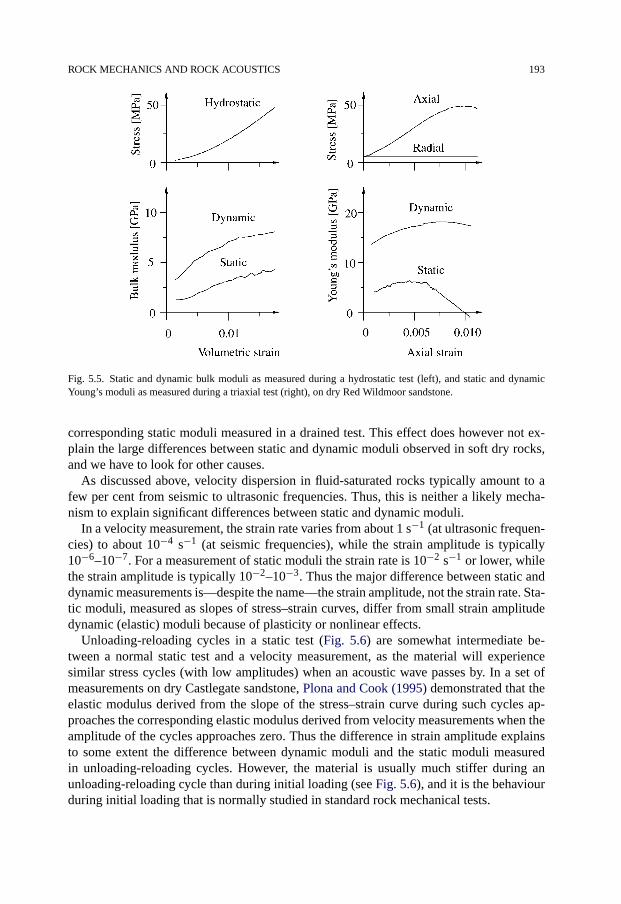
ROCK MECHANICS AND ROCK ACOUSTICS 193
Fig. 5.5. Static and dynamic bulk moduli as measured during a hydrostatic test (left), and static and dynamicYoung’s moduli as measured during a triaxial test (right), on dry Red Wildmoor sandstone.
corresponding static moduli measured in a drained test. This effect does however not ex-plain the large differences between static and dynamic moduli observed in soft dry rocks,and we have to look for other causes.
As discussed above, velocity dispersion in fluid-saturated rocks typically amount to afew per cent from seismic to ultrasonic frequencies. Thus, this is neither a likely mecha-nism to explain significant differences between static and dynamic moduli.
In a velocity measurement, the strain rate varies from about 1 s−1 (at ultrasonic frequen-cies) to about 10−4 s−1 (at seismic frequencies), while the strain amplitude is typically10−6–10−7. For a measurement of static moduli the strain rate is 10−2 s−1 or lower, whilethe strain amplitude is typically 10−2–10−3. Thus the major difference between static anddynamic measurements is—despite the name—the strain amplitude, not the strain rate. Sta-tic moduli, measured as slopes of stress–strain curves, differ from small strain amplitudedynamic (elastic) moduli because of plasticity or nonlinear effects.
Unloading-reloading cycles in a static test (Fig. 5.6) are somewhat intermediate be-tween a normal static test and a velocity measurement, as the material will experiencesimilar stress cycles (with low amplitudes) when an acoustic wave passes by. In a set ofmeasurements on dry Castlegate sandstone, Plona and Cook (1995) demonstrated that theelastic modulus derived from the slope of the stress–strain curve during such cycles ap-proaches the corresponding elastic modulus derived from velocity measurements when theamplitude of the cycles approaches zero. Thus the difference in strain amplitude explainsto some extent the difference between dynamic moduli and the static moduli measuredin unloading-reloading cycles. However, the material is usually much stiffer during anunloading-reloading cycle than during initial loading (see Fig. 5.6), and it is the behaviourduring initial loading that is normally studied in standard rock mechanical tests.
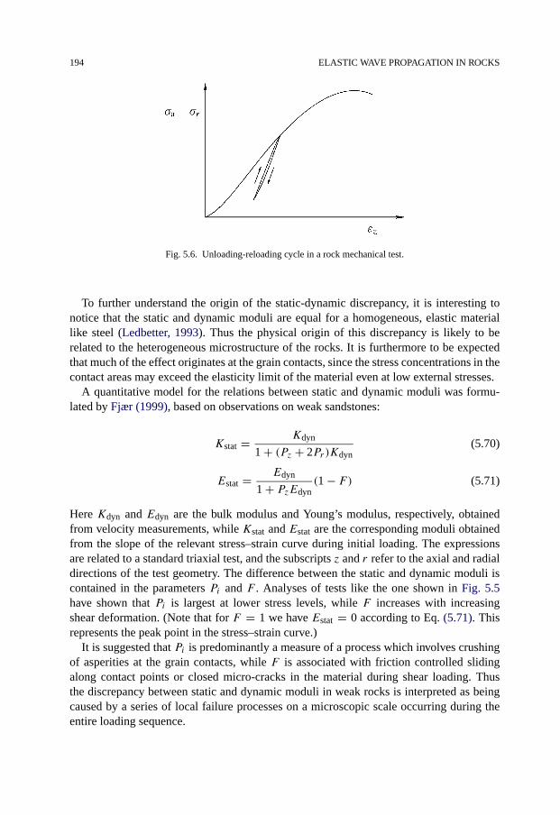
194 ELASTIC WAVE PROPAGATION IN ROCKS
Fig. 5.6. Unloading-reloading cycle in a rock mechanical test.
To further understand the origin of the static-dynamic discrepancy, it is interesting tonotice that the static and dynamic moduli are equal for a homogeneous, elastic materiallike steel (Ledbetter, 1993). Thus the physical origin of this discrepancy is likely to berelated to the heterogeneous microstructure of the rocks. It is furthermore to be expectedthat much of the effect originates at the grain contacts, since the stress concentrations in thecontact areas may exceed the elasticity limit of the material even at low external stresses.
A quantitative model for the relations between static and dynamic moduli was formu-lated by Fjær (1999), based on observations on weak sandstones:
Kstat = Kdyn
1 + (Pz + 2Pr)Kdyn(5.70)
Estat = Edyn
1 + PzEdyn(1 − F) (5.71)
Here Kdyn and Edyn are the bulk modulus and Young’s modulus, respectively, obtainedfrom velocity measurements, while Kstat and Estat are the corresponding moduli obtainedfrom the slope of the relevant stress–strain curve during initial loading. The expressionsare related to a standard triaxial test, and the subscripts z and r refer to the axial and radialdirections of the test geometry. The difference between the static and dynamic moduli iscontained in the parameters Pi and F . Analyses of tests like the one shown in Fig. 5.5have shown that Pi is largest at lower stress levels, while F increases with increasingshear deformation. (Note that for F = 1 we have Estat = 0 according to Eq. (5.71). Thisrepresents the peak point in the stress–strain curve.)
It is suggested that Pi is predominantly a measure of a process which involves crushingof asperities at the grain contacts, while F is associated with friction controlled slidingalong contact points or closed micro-cracks in the material during shear loading. Thusthe discrepancy between static and dynamic moduli in weak rocks is interpreted as beingcaused by a series of local failure processes on a microscopic scale occurring during theentire loading sequence.

ROCK MECHANICS AND ROCK ACOUSTICS 195
Fig. 5.7. Ultrasonic velocities as functions of stress state as measured on dry Red Wildmoor sandstone.
5.6.2. Stress state and stress history
Sound velocities in rocks also depend on the state of stress. To some extent, this effect canbe ascribed to stress induced changes in porosity. However, this is not sufficient to explainthe stress sensitivity of velocities in most rocks. Fig. 5.7 shows the typical behaviour fora sandstone. The behaviour can be understood in terms of micro-cracks (much smallerthan the wavelength) that are opened or closed by the action of the stress. An open crackstrongly reduces the velocity of a wave if the crack is oriented normal to the direction ofpropagation or polarization of the wave, while its effect on the velocity is only marginalotherwise (see Section 6.4).
During hydrostatic loading the velocities increase uniformly, with a gradually diminish-ing rate. This is to be expected due to closure of cracks which make the rock stiffer, orsimilar processes which broadens or multiply grain contacts. These effects are discussed indetail in Sections 6.3 and 6.4. During uniaxial loading, the velocities of waves with polar-ization and/or direction of propagation parallel to the increasing load are seen to increaseinitially, due to the same type of processes that causes increases in velocities during hy-drostatic loading. Upon further loading, the velocities of waves with polarization and/ordirection of propagation normal to the minimum principal stress are seen to be reduced.This is associated with the formation of tensile cracks (often illustrated as “wing cracks”formed during frictional sliding of closed cracks, as shown in Section 6.4.4, Fig. 6.11).Thus stress anisotropy induces acoustic anisotropy. The relevance of interpreting stressinduced velocity changes in sandstones in terms of changes in the occurrence of disconti-nuities such as cracks, has been nicely demonstrated by Sayers (2002).
The impact of micro-cracks on acoustic wave propagation is also reflected in the atten-uation, as the scattering losses due to such cracks can be significant. Thus attenuation istypically reduced with increasing confining pressure, as can be seen from Fig. 5.3.

196 ELASTIC WAVE PROPAGATION IN ROCKS
Using observed acoustic anisotropy as a measure for stress anisotropy is however notstraightforward. This is partly due to the fact that also other effects—like fine layering orgrain orientation—can cause anisotropy, and partly to the fact that rocks are usually formedand cemented under stress. Stress induced anisotropy in uncemented sediments is a conse-quence of static loading making the grain contacts stiffer (see Section 6.3). Different stressin different directions thus induce different stiffness in different directions, which results inacoustic anisotropy. The cementation process provides added stiffness to all grain contacts,so the relative stiffening is largest for the weakly loaded ones. The characteristic signatureof the stress state is thus masked. Subsequent stress induced anisotropy is characteristicfor the stress changes occurring after cementation, rather than the current stress state. Thusthe stress history of a rock may have a significant impact on the stress dependency of thevelocities.
For a core taken from a deep well, the major recent stress history is the unloading processtaking place during and after coring. The cement which was formed free from effectivestress at the grain contacts will be subjected to tensile stress as the grain contacts deformwhen the load disappear. This will generate cracks which reduce the elastic stiffness andthus also the acoustic velocities. When sufficient stress is applied to the core in a laboratorytest, these cracks will close and the velocities will increase correspondingly. A significantpart of the stress dependency of acoustic velocities observed in laboratory tests may there-fore be related to core damage effects, and not be representative for the in situ behaviour.This has been demonstrated through tests on synthetic sandstones cemented under stress(Nes et al., 2002). The effect is illustrated in Fig. 5.8. Note that the velocity is quite insen-sitive to small changes in the stress while the rock is still in the vicinity of its cementationstate, and that it drops significantly upon extensive unloading. Upon reloading, as for a coretested in the laboratory, the velocity increases with a rate that is lower than the decreasing
Fig. 5.8. Schematic illustration of velocity versus stress for a rock, following two different stress paths fromthe cementation state (marked with a circle). The upper right curve could represent in situ loading (caused bydepletion), the upper left curve in situ unloading (caused by injection or coring), and the lower curve a laboratorytest on a core plug.

ROCK MECHANICS AND ROCK ACOUSTICS 197
rate at the end of the unloading path, yet significantly higher than the initial (“in situ”) ratein the vicinity of the cementation stress (see also Chapter 7).
It was shown in Section 1.6.3 that the deformation of a porous, linear elastic rock iscontrolled entirely by an effective stress (Eq. (1.168)) that accounts for the combined actionof the external stress and the pore pressure. It is tempting to assume that this principle isalso valid for acoustic velocities, however this is not the case in general. Often, but notalways, the velocities may depend on an effective stress
σ ′ = σ − npf (5.72)
within a limited range of stress and pore pressure. The coefficient n depends on the type ofwave as well as the type of fluid, and may be larger as well as smaller than 1. In some casesthis principle is not applicable at all. One simple example is a linearly elastic material, forwhich the frame moduli are stress independent (as will be the case for instance for a wellcemented rock not suffering from core damage). Since the P-wave velocity also dependson the bulk modulus and density of the fluid, which in turn depend on the fluid pressure, itis clear that the effects of changes in σ and pf are fundamentally different, and Eq. (5.72)is not valid in this case.
5.6.3. Additional effects
Elastic wave propagation in rocks is also affected by other parameters, which we shall onlymention briefly here.
Temperature
There is normally a slight reduction in velocities with increasing temperature. This ef-fect is usually less than 5% for a 100 °C increase in temperature (Bourbie et al., 1987;Christensen, 1982). The effect may be significantly larger if one or more of the rock con-stituents undergoes a phase transition within the actual temperature range, for instance ifthe pore fluid is freezing or melting. Attenuation is also reduced with increasing tempera-ture. This effect appears to be somewhat larger than the temperature effect on the velocities(Jones and Nur, 1983).
Partial saturation
Partial saturation may have a significant effect on both velocities and attenuation. Considera rock saturated with water and gas. At low frequencies, the pore fluid may be consideredas a suspension of gas bubbles in a liquid (at least if the water saturation Sw is larger thanabout 20%). We may then assume that the gas pressure follows that of the water at any time,and the effective fluid bulk modulusKf is then given by an equation similar to Eq. (1.132):
1
Kf= Sw
Kw+ 1 − Sw
Kg(5.73)

198 ELASTIC WAVE PROPAGATION IN ROCKS
Fig. 5.9. P- and S-wave velocities versus saturation in a gas/water saturated rock, as predicted byEqs. (5.73)–(5.74), (5.39), (5.41) and (1.155) (solid lines), for a dataset representing a relatively weak rock atlow pressures and low frequency. The dashed line indicates the P-wave velocity for patchy saturation, while thegray area indicates the range of possible values for the P-wave velocity for various fluid distributions at higherfrequencies.
Kw and Kg are the bulk moduli of water and gas, respectively. Typically, Kg � Kw, andwe thus have that Kf � Kw unless Sw is very close to 1. The bulk density
ρ = ρs(1 − φ)+ φ(Swρw + (1 − Sw)ρg)
(5.74)
is much less sensitive to Sw, hence the net effect is that the P-wave velocity (Eq. (5.39))drops dramatically when Sw falls below 1, and only picks up slowly as Sw continues todecrease (Fig. 5.9). The S-wave depends only on ρ in addition toGfr (which is not affectedby the degree of saturation, at least not for permeable materials at low frequencies), hencethe S-wave velocity is only marginally dependent on the saturation. For very low satura-tion, capillary forces (see Section 2.6.2) may provide an additional stiffness that makes thevelocities increase.
At higher frequencies, the distribution of the water and gas in the pore space becomessignificant. For instance, water trapped in thin cracks may effectively respond to compres-sion with a stiffness close toKw, and the velocities will be correspondingly higher (see alsoSection 6.4). The distribution of water and gas is a result of the wetting properties of therock and the way the actual saturation was reached. Consequently, there is not a one-to-onerelationship between P-wave velocity and water saturation (Endres and Knight, 1989), butrather a range of possible values for the velocity at each saturation level, as indicated bythe gray area on Fig. 5.9.
The water and the gas may also be separated on a larger scale, such that some areas arefully water saturated while others are not (patchy saturation). The fully saturated areas willbehave as saturated, undrained rock if the pore pressure diffusion length is less than thetypical size (l) of the fully saturated areas, that is—if√
CD
f< l (5.75)
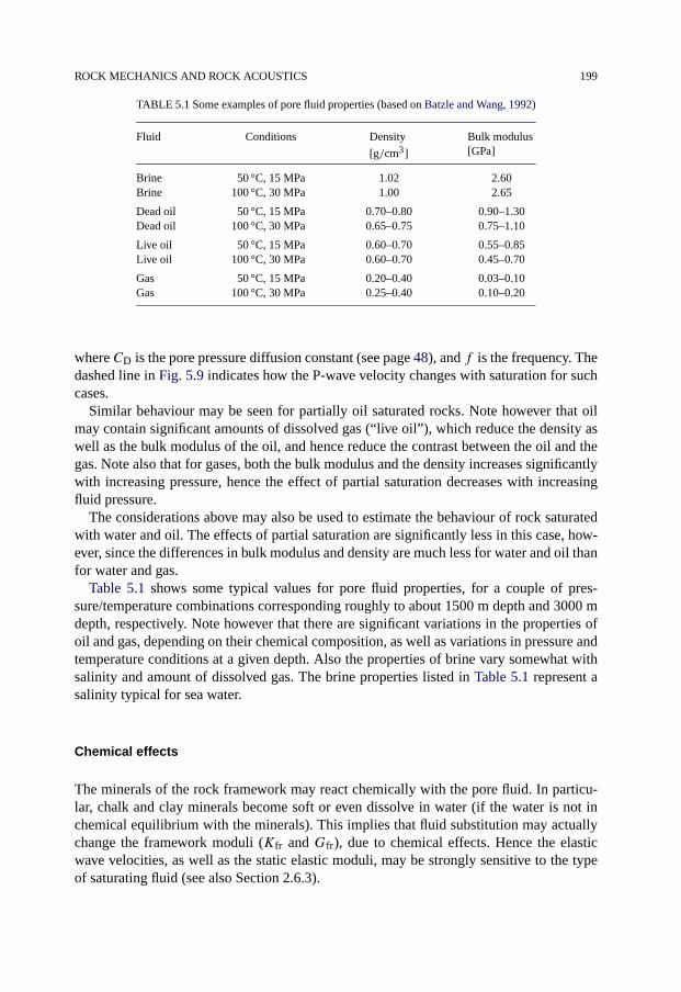
ROCK MECHANICS AND ROCK ACOUSTICS 199
TABLE 5.1 Some examples of pore fluid properties (based on Batzle and Wang, 1992)
Fluid Conditions Density
[g/cm3]
Bulk modulus[GPa]
Brine 50 °C, 15 MPa 1.02 2.60Brine 100 °C, 30 MPa 1.00 2.65
Dead oil 50 °C, 15 MPa 0.70–0.80 0.90–1.30Dead oil 100 °C, 30 MPa 0.65–0.75 0.75–1.10
Live oil 50 °C, 15 MPa 0.60–0.70 0.55–0.85Live oil 100 °C, 30 MPa 0.60–0.70 0.45–0.70
Gas 50 °C, 15 MPa 0.20–0.40 0.03–0.10Gas 100 °C, 30 MPa 0.25–0.40 0.10–0.20
where CD is the pore pressure diffusion constant (see page 48), and f is the frequency. Thedashed line in Fig. 5.9 indicates how the P-wave velocity changes with saturation for suchcases.
Similar behaviour may be seen for partially oil saturated rocks. Note however that oilmay contain significant amounts of dissolved gas (“live oil”), which reduce the density aswell as the bulk modulus of the oil, and hence reduce the contrast between the oil and thegas. Note also that for gases, both the bulk modulus and the density increases significantlywith increasing pressure, hence the effect of partial saturation decreases with increasingfluid pressure.
The considerations above may also be used to estimate the behaviour of rock saturatedwith water and oil. The effects of partial saturation are significantly less in this case, how-ever, since the differences in bulk modulus and density are much less for water and oil thanfor water and gas.
Table 5.1 shows some typical values for pore fluid properties, for a couple of pres-sure/temperature combinations corresponding roughly to about 1500 m depth and 3000 mdepth, respectively. Note however that there are significant variations in the properties ofoil and gas, depending on their chemical composition, as well as variations in pressure andtemperature conditions at a given depth. Also the properties of brine vary somewhat withsalinity and amount of dissolved gas. The brine properties listed in Table 5.1 represent asalinity typical for sea water.
Chemical effects
The minerals of the rock framework may react chemically with the pore fluid. In particu-lar, chalk and clay minerals become soft or even dissolve in water (if the water is not inchemical equilibrium with the minerals). This implies that fluid substitution may actuallychange the framework moduli (Kfr and Gfr), due to chemical effects. Hence the elasticwave velocities, as well as the static elastic moduli, may be strongly sensitive to the typeof saturating fluid (see also Section 2.6.3).

200 ELASTIC WAVE PROPAGATION IN ROCKS
5.7. Reflections and refractions
When an elastic wave hits a boundary of the medium it is travelling through, the wave maybe reflected—like light in a mirror, or refracted—like light at a water surface, or convertedinto other types of elastic waves. Such boundaries, or interfaces between different parts of amedium, are important for most aspects of rock acoustics. In particular, reflections at inter-faces are the foundation of surface seismics, while sonic logging tools rely on refractionsfor obtaining a wave path through the rock along the hole.
Consider first the simple situation where a plane P-wave like (5.14) approaches a bound-ary normal to the direction of propagation. The laws of physics require that
• the displacement normal to the boundary is continuous at the boundary,
• the stress normal to the boundary is continuous at the boundary.
To fulfil these requirements when the wave hits the boundary, two new waves are createdat the boundary: one reflected wave and one transmitted wave. We shall now see how thesephysical continuity requirements can be used to identify the amplitude and phase of boththe reflected wave and the transmitted wave, relative to the amplitude and phase of theinitial wave. We denote by subscript 1 the parameters of the medium through which thewave is initially travelling, and by subscript 2 the parameters of the medium on the otherside of the boundary. The three waves interacting at the boundary are then
ui = uo,i ej(ωt−q1x) Initial wave
ur = uo,r ej(ωt+q1x) Reflected wave
ut = uo,t ej(ωt−q2x) Transmitted wave
The initial wave is travelling in medium 1 towards the boundary, the reflected wave istravelling in medium 1 away from the boundary, and the transmitted wave is travelling inmedium 2 away from the boundary. Note that the frequency ω is the same in both media.The two physical continuity requirements can now be expressed as
ui + ur = ut (5.76)
(λ1 + 2G1)
(∂ui
∂x+ ∂ur
∂x
)= (λ2 + 2G2)
∂ut
∂x(5.77)
Positioning for simplicity the x-axis such that the interface is located at x = 0, introducingthe expressions for ui, ur and ut, and dividing by ejωt , we find
uo,i + uo,r = uo,t (5.78)
(λ1 + 2G1)(−jq1uo,i + jq1uo,r) = (λ2 + 2G2)(−jq2uo,t) (5.79)
These are two equations with two unknowns, namely uo,r and uo,t. These equations arecomplex, thus the equations give us both the amplitude and the phase of the reflected andtransmitted wave. Rather than presenting these expressions explicitly, we now introduce thereflection coefficient rpp, which expresses the stress amplitude of the reflected wave, andthe transmission coefficient tpp, which expresses the stress amplitude of the transmittedwave, both relative to the stress amplitude of the initial wave.

REFLECTIONS AND REFRACTIONS 201
Expressed in terms of particle displacement amplitudes, these coefficients are defined as
rpp = −uo,r
uo,i(5.80)
tpp = ρ2vp2
ρ1vp1
uo,t
uo,i(5.81)
Expressions for rpp and tpp can be found from Eqs. (5.78) and (5.79). Introducing furtherEqs. (5.8) and (5.16) the expressions take the following form:
rpp = ρ2vp2 − ρ1vp1
ρ2vp2 + ρ1vp1(5.82)
tpp = 2ρ2vp2
ρ2vp2 + ρ1vp1(5.83)
The product ρvp is called the acoustic impedance of the medium. Thus the reflection andtransmission coefficients depend on the impedance contrast between the two media. Notethat rpp and tpp may be defined in different ways, depending on the choice of coordinatesystem and wave describing parameters. The definition used here implies that a compres-sion is reflected as a compression if rpp > 0, while for rpp < 0 the reflection involves phaseinversion.
The amplitude of the reflected wave depends on the density and velocity of the sec-ond medium, although the incoming and reflected waves have only propagated throughmedium 1. This may be used in analyses of seismic data, as we shall see in Section 5.9.
This example was particularly simple, since the displacement as well as the stress onlyhad one component, normal to the interface between the two media. Consider next aP-wave which hits an interface at an angle of incidence θi relative to the normal of theinterface. It is now convenient to consider the wave as a ray, as we here wish to focus onthe direction of propagation. A part of the wave will be reflected at an angle θr = θi (seeFig. 5.10). Another part of the wave will be transmitted at an angle θt. The relation between
Fig. 5.10. Reflection and refraction of an acoustic ray at the interface between two media.

202 ELASTIC WAVE PROPAGATION IN ROCKS
the angle of incidence θi and the transmission angle θt is given by Snell’s law:
sin θtvp2
= sin θivp1
(5.84)
Thus the transmitted wave will proceed in a direction somewhat different from the incom-ing wave, provided that vp2 �= vp1. This effect is called refraction.
Note that we may have a situation where (vp2/vp1) sin θi > 1, which would imply thatsin θt > 1 according to Eq. (5.84). This is mathematically and physically unacceptable,hence θt is not defined in this situation. This implies that the refracted wave does not exist,and we have total reflection at the interface. The condition for total reflection of the P-waveis thus
sin θi > sin θcr ≡ vp1
vp2(5.85)
The angle θcr is called the critical angle for total reflection.P- and S-waves are different modes of propagating elastic energy, and are not coupled
in an ordinary medium due to symmetry. When a wave hits an interface at a skew anglerelative to the direction of propagation, the symmetry is broken and the waves may becomecoupled at the interface. In our example here, the incoming P-wave has a particle motionwhich is not fully orthogonal to the particle motion of an S-wave “reflected” from the in-terface at an angle θrs (Fig. 5.11), with polarization in the same plane as the incoming waveand the normal to the interface. Thus such an S-wave may be generated at the interface.The angle θrs is given by the equation
sin θrsvs1
= sin θivp1
(5.86)
Fig. 5.11. Polarization (indicated by double arrows) of reflected, refracted and converted waves at an interface,due to an incoming P-wave.

REFLECTIONS AND REFRACTIONS 203
Fig. 5.12. Reflection coefficient for a P-wave reflected at an interface between two media. Parameter values usedin this example: vp1 = 2500 m/s, vs1 = 1450 m/s, ρ1 = 2.1 g/cm3, vp2 = 3000 m/s, ρ2 = 2.2 g/cm3.
The incoming P-wave will also be coupled to a “refracted” S-wave, propagating in medium2 at an angle θts given by
sin θtsvs2
= sin θivp1
(5.87)
This wave also has its polarization in the same plane as the incoming wave and the normalto the interface. The two S-waves are said to be converted waves, since they originatedfrom a wave of a different type. Similarly, if the incoming wave is an S-wave with polar-ization in this plane, two converted P-waves may be generated at the interface in additionto the reflected and refracted S-waves. Note that an S-wave with polarization parallel to theinterface is not coupled to any P-wave at the interface, hence no such wave is created froman incoming P-wave, nor will such a wave generate converted P-waves.
The degree of coupling between the incoming wave and the reflected, transmitted andconverted waves will vary with the angle θi. The expressions for the reflection, trans-mission and conversion coefficients are rather complicated, and are therefore given inAppendix D.2.2.
Fig. 5.12 shows an example where the reflection coefficient for the incoming P-wavehas been calculated for various angles of incidence. The figure shows that the reflectioncoefficient increases abruptly just below the critical angle (Eq. (5.85)) for total reflection.The reflection coefficient is furthermore seen to depend on the shear wave velocity vs2 ofthe second medium.
5.7.1. Interface waves
In addition to the P- and S-waves, which can propagate through a material, there alsoexist some elastic waves that only propagate along the interface between two media. Onefamiliar example is sea waves, which only exist at the surface of the water. An interface
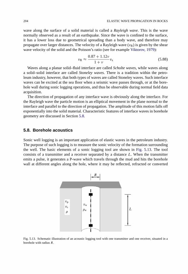
204 ELASTIC WAVE PROPAGATION IN ROCKS
wave along the surface of a solid material is called a Rayleigh wave. This is the wavenormally observed as a result of an earthquake. Since the wave is confined to the surface,it has a lower loss due to geometrical spreading than a body wave, and therefore maypropagate over larger distances. The velocity of a Rayleigh wave (vR) is given by the shearwave velocity of the solid and the Poisson’s ratio (see for example Viktorov, 1979):
vR ≈ 0.87 + 1.12ν
1 + ν vs (5.88)
Waves along a planar solid–fluid interface are called Scholte waves, while waves alonga solid–solid interface are called Stoneley waves. There is a tradition within the petro-leum industry, however, that both types of waves are called Stoneley waves. Such interfacewaves can be excited at the sea floor when a seismic wave passes through, or at the bore-hole wall during sonic logging operations, and thus be observable during normal field dataacquisition.
The direction of propagation of any interface wave is obviously along the interface. Forthe Rayleigh wave the particle motion is an elliptical movement in the plane normal to theinterface and parallel to the direction of propagation. The amplitude of this motion falls offexponentially into the solid material. Characteristic features of interface waves in boreholegeometry are discussed in Section 5.8.
5.8. Borehole acoustics
Sonic well logging is an important application of elastic waves in the petroleum industry.The purpose of such logging is to measure the sonic velocity of the formation surroundingthe well. The basic elements of a sonic logging tool are shown in Fig. 5.13. The toolconsists of a transmitter and a receiver separated by a distance L. When the transmitteremits a pulse, it generates a P-wave which travels through the mud and hits the boreholewall at different angles along the hole, where it may be reflected, refracted or converted
Fig. 5.13. Schematic illustration of an acoustic logging tool with one transmitter and one receiver, situated in aborehole with radius R.

BOREHOLE ACOUSTICS 205
Fig. 5.14. Refractions of waves transmitted from an acoustic logging tool. The dashed line represents a rayincident at sub-critical angle. The solid line is a critical refraction, that continuously emits acoustic energy intothe borehole.
into different modes. Eventually, a series of pulses arrive at the receiver: the direct P-wavetravelling through the mud, a refracted P-wave, a converted S-wave, and a set of boreholeeigenmodes.
Fig. 5.14 illustrates refractions in the borehole geometry. Rays that hit the borehole wallat a sub-critical angle, will be refracted into the formation, and the energy can never returnto the borehole. However, the ray that hits the wall at an angle such that the transmissionangle θt = 90° will propagate parallel to the wall. This wave will continuously radiateenergy into the borehole. We say that this wave is critically refracted. Some of this energywill reach the receiver. Since the critically refracted wave continuously loses energy, it willbe attenuated even in the absence of absorption.
Using the notation of Figs. 5.13 and 5.14, we can find an expression for the expectedarrival time of the critical refraction as a function of transmitter–receiver separation. Thelength travelled in the fluid is
Lw = 2R
cos θcr(5.89)
while the length travelled in the formation is
L′ = L− 2R tan θcr (5.90)
Introducing sin θcr = vw/v (see Eq. (5.85)) where v is the velocity of the refracted waveand vw is the velocity of the borehole fluid, we find the arrival time to be
t = Lw
vw+ L′
v= L
v+ 2R
(1
vw
√1 − ( vw
v)2
− vw
v2√
1 − ( vwv)2
)
= L
v+ 2R
√1
v2w
− 1
v2(5.91)

206 ELASTIC WAVE PROPAGATION IN ROCKS
Fig. 5.15. Arrival time of the critical refraction as a function of transmitter/receiver separation (solid line). Alsoshown is the arrival time of a direct wave with the velocity of the fluid (dashed line). The following parameterswere used: v = 3500 m/s, vw = 1500 m/s, R = 10 cm.
Thus, the arrival time is a constant, plus a term that is equal to the separation betweenthe transmitter and the receiver divided by the velocity of the formation. This means thatthe difference in arrival time between two receivers at different separations from the trans-mitter directly measures the velocity of the formation. Fig. 5.15 illustrates Eq. (5.91), andcompares it with a direct wave travelling with the velocity of the borehole fluid. As can beseen, the refracted wave will be the first arrival, as long as the source-receiver separation isabove a limiting minimum.
In the above discussion, we have not specified whether v is the shear or compressionalvelocity of the formation. The arguments work equally well for both cases, which meansthat we may have both a critically refracted compressional wave and a critically refracted(converted) shear wave. This conclusion is, of course, subject to the condition that theformation velocities are higher than the fluid velocity. For the compressional wave thiswill nearly always be fulfilled, but for the shear wave this is not so. Indeed, formations arecharacterized as slow or soft when the shear wave velocity is slower than the fluid velocity,and as fast or hard otherwise.
5.8.1. Borehole modes
In addition to the refractions, the full wavetrain also consists of borehole modes. Theseare modes that are localized to the borehole, and do not radiate into the formation (at leastfor some parameter ranges). This means that they are often the dominating componentsof the full wavetrain as far as amplitude is concerned. The borehole modes also containinformation about the formation parameters, albeit in a more complicated manner than therefractions.
The most important eigenmode is the Stoneley wave, which is an interface wave. (Thename “Stoneley wave” actually deviates from the strict definition of the type of interface

BOREHOLE ACOUSTICS 207
Fig. 5.16. The low frequency limit of the Stoneley velocity as a function of shear velocity for ρ/ρw = 1.0 andρ/ρw = 2.5.
wave we are considering here; see page 204.) Its velocity is always smaller than that of thefluid in the borehole. The wave has relatively low dispersion. In the low frequency limitthe wave is known as the tube wave and its velocity vSt is
vSt = vw√1 + ρwv2
wρv2
s
(5.92)
where vw and ρw are the velocity and density, respectively, of the fluid in the borehole,while vs and ρ are the shear velocity and density, respectively, of the formation. This rela-tion is plotted in Fig. 5.16 for two different density ratios. Note that for sufficiently smallshear velocities, the Stoneley wave becomes attenuated in the low frequency limit. This isdue to the fact that it will radiate energy in the form of ordinary shear waves when vSt ishigher than the solid’s shear velocity.
Eq. (5.92) indicates the possibility of using the Stoneley velocity to determine the shearwave velocity of a formation. Quite conveniently, the sensitivity to the shear wave veloc-ity is highest when this velocity is small and no shear refraction exists. Some remarks ofcaution are however necessary. The high Stoneley wave attenuation in slow formations, asmentioned above and illustrated in Fig. 5.16, is a main limiting factor. Further, Eq. (5.92)is a low frequency approximation, and should for practical applications be replaced bya numerical inversion in the frequency band of the source. More important, the Stoneleywave velocity is quite sensitive to the formation permeability, especially at low frequencies(see e.g. Schmitt, 1988a). Finally, the Stoneley wave and the refracted (converted) S-waveare sensitive to different components of the stiffness tensor, which may be significant inanisotropic formations. In principle, this offers the possibility of assessing the acousticanisotropy of a fast formation, but in practice this is very difficult since the Stoneley veloc-ity has a low sensitivity to the shear velocity when the shear velocity is high.
The shear eigenmodes or pseudo-Rayleigh waves have phase velocities that are higherthan the fluid velocity, and slower than the shear velocity of the formation. Consequently,

208 ELASTIC WAVE PROPAGATION IN ROCKS
Fig. 5.17. Example of dispersion of the Stoneley mode and the three lowest pseudo-Rayleigh modes in a fastformation. Solid lines are phase velocity, broken lines are group velocity. vp = 3500 m/s, vs = 2000 m/s,
vw = 1500 m/s, ρ = 2.3 g/cm3, ρw = 1.2 g/cm3, R = 10 cm.
they only exist as undamped modes in fast formations. The pseudo-Rayleigh modes have acut-off frequency that increases with mode number (in principle, infinitely many pseudo-Rayleigh modes exist). The cut-off frequency can be roughly estimated by requiring thatan integer number of half wavelengths should fit into the borehole. For a borehole withdiameter of 20 cm, this means that the order of magnitude of the cut-off frequency for thelowest mode is 10 kHz. Note that the presence of the logging tool in the borehole reducesthe effective radius of the hole.
Fig. 5.17 shows examples of dispersion relations for the Stoneley mode and the lowestpseudo-Rayleigh modes. Fig. 5.18 shows examples of (computed) full wavetrains in a fastformation for three different source spectra. All wavetrains are shown in the same scale.In the lower left, the early part of the wavetrains are shown amplified by a factor 10.The figure illustrates that the full waveform depends strongly on the source spectrum. Thearrows indicate the expected arrivals of the P- and S-refractions and the Stoneley wavebased on ray theory.
Considering the high frequency source in the lower frame, the wavetrain is dominated bythe P-refraction and the pseudo-Rayleigh waves. No Stoneley wave is seen. In the middleframe, the onset of the P- and S-refractions coincide well with the expectations from raytheory. The Stoneley overlays the pseudo-Rayleigh waves, and is seen as a marked changein amplitude.
For the low frequency case in the upper frame, there are no pseudo-Rayleigh waves,and the waveform is dominated by the Stoneley wave. Note that the Stoneley wave breaks

BOREHOLE ACOUSTICS 209
Fig. 5.18. Example of (computed) full acoustic wavetrains in a fast formation. Same parameters as in Fig. 5.17.L = 2.44 m. Source centre frequencies are 20 kHz, 10 kHz and 2 kHz for the lower, middle and upper frames,respectively. The early parts of the wavetrains are also shown with 10 times amplification. The amplitude scale isthe same in all three frames.
before the time expected from the low frequency velocity. This is due to dispersion. It isnot possible to determine clear P- and S-refractions in this case.
The wavetrains in a slow formation, as Fig. 5.19 show examples of, are considerablysimpler, due to the absence of the shear refraction and the pseudo-Rayleigh modes. Incertain cases, damped pseudo-Rayleigh modes may however be seen in slow formations.
In the high frequency case in the lower frame of Fig. 5.19, the only clear feature is theP-refraction. Looking at the middle frame of Fig. 5.19, we find two clear events: the P-refraction and the Stoneley wave. Note the relatively low frequency of the Stoneley wave.

210 ELASTIC WAVE PROPAGATION IN ROCKS
Fig. 5.19. Example of (computed) full acoustic wavetrains in a slow formation. vp = 2100 m/s, vs = 1200 m/s,
vw = 1500 m/s, ρ = 2.1 g/cm3, ρw = 1.2 g/cm3, L = 2.44 m. R = 10 cm. Source centre frequencies are20 kHz, 10 kHz and 2 kHz for the lower, middle and upper frames, respectively. The amplitude scale is the samein all three frames. The low frequency wavetrain is also shown with the amplitude reduced by a factor 20 (dashedline).
This is due to the fact that the Stoneley wave is excited most strongly at low frequencies,such that it favours the low frequencies of the excitation pulse. It is also evident that theearly part of the Stoneley wave is lower in frequency than the later part. This is due tothe dispersion of the Stoneley mode in slow formations, where the low frequency partspropagate fastest. (In a fast formation, however, the high frequency parts are the fastest.)The slow onset of the Stoneley mode in a slow formation of course makes picking of
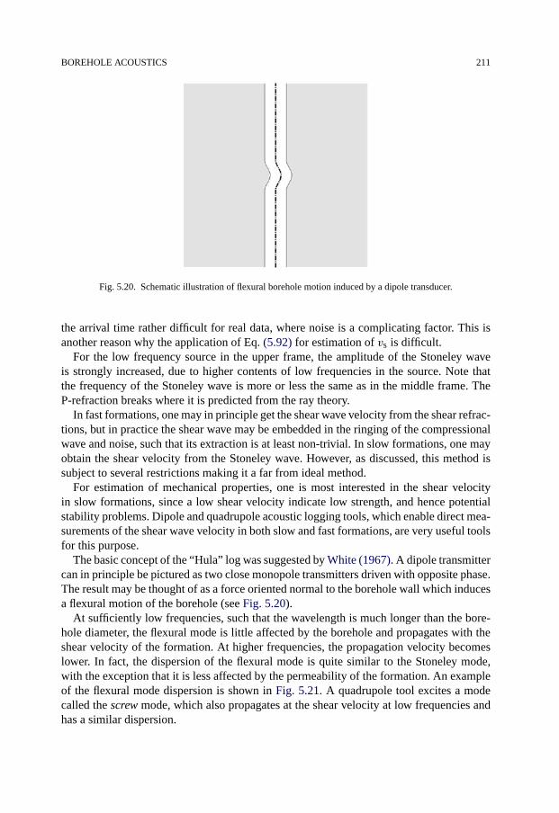
BOREHOLE ACOUSTICS 211
Fig. 5.20. Schematic illustration of flexural borehole motion induced by a dipole transducer.
the arrival time rather difficult for real data, where noise is a complicating factor. This isanother reason why the application of Eq. (5.92) for estimation of vs is difficult.
For the low frequency source in the upper frame, the amplitude of the Stoneley waveis strongly increased, due to higher contents of low frequencies in the source. Note thatthe frequency of the Stoneley wave is more or less the same as in the middle frame. TheP-refraction breaks where it is predicted from the ray theory.
In fast formations, one may in principle get the shear wave velocity from the shear refrac-tions, but in practice the shear wave may be embedded in the ringing of the compressionalwave and noise, such that its extraction is at least non-trivial. In slow formations, one mayobtain the shear velocity from the Stoneley wave. However, as discussed, this method issubject to several restrictions making it a far from ideal method.
For estimation of mechanical properties, one is most interested in the shear velocityin slow formations, since a low shear velocity indicate low strength, and hence potentialstability problems. Dipole and quadrupole acoustic logging tools, which enable direct mea-surements of the shear wave velocity in both slow and fast formations, are very useful toolsfor this purpose.
The basic concept of the “Hula” log was suggested by White (1967). A dipole transmittercan in principle be pictured as two close monopole transmitters driven with opposite phase.The result may be thought of as a force oriented normal to the borehole wall which inducesa flexural motion of the borehole (see Fig. 5.20).
At sufficiently low frequencies, such that the wavelength is much longer than the bore-hole diameter, the flexural mode is little affected by the borehole and propagates with theshear velocity of the formation. At higher frequencies, the propagation velocity becomeslower. In fact, the dispersion of the flexural mode is quite similar to the Stoneley mode,with the exception that it is less affected by the permeability of the formation. An exampleof the flexural mode dispersion is shown in Fig. 5.21. A quadrupole tool excites a modecalled the screw mode, which also propagates at the shear velocity at low frequencies andhas a similar dispersion.

212 ELASTIC WAVE PROPAGATION IN ROCKS
Fig. 5.21. Dispersion of the flexural mode and the screw mode, compared to the Stoneley wave in a slow forma-tion. (After Schmitt, 1988b; with permission from AIP.)
Fig. 5.22. Principle sketch of an axisymmetric altered zone. The index a denotes altered parameter values.
5.8.2. Borehole alteration
We have seen that the full waveform is quite complicated even in the simple model usedabove. We will here discuss briefly a slightly more complicated situation, in which thereis a concentric altered zone around the wellbore. The alteration may be due to mud filtrateinvasion, or stress induced damage (see Section 4.5). We assume that the zone is homoge-neous and isotropic. Fig. 5.22 sketches the situation.
From the ray-theory point of view, it is now clear that we may have refractions both fromthe borehole wall and from the interface between the two formation zones (assuming thatthe velocity of the altered zone is lower than that of the virgin formation).
Fig. 5.23 shows the expected arrival times as a function of distance. The first refractedarrival will be the shallow refraction for short transmitter receiver distances, and the deeprefraction for longer separations. This effect has been used by Hornby and Chang (1985),

BOREHOLE ACOUSTICS 213
Fig. 5.23. Arrival times for the model of Fig. 5.22. Virgin formation as in Fig. 5.15. The altered velocity isreduced by 20%. The altered zone thickness is 20 cm.
Fig. 5.24. Synthetic wavetrains in an altered slow formation. Soft means that the altered layer is 10% slowerthan the virgin zone, hard means that it is 10% faster. The unaltered case is the same as in the middle frame ofFig. 5.19. The altered zone thickness is 10 cm.
who—using data from several runs of an experimental logging tool with variable trans-mitter receiver spacing—computed the altered zone thickness and velocity as a functionof depth. Such calculations should, of course, be considered with some caution, since themodel used is very simple. The assumption of an axisymmetric altered zone is dubious,and the abrupt transition from altered to unaltered formations is only a first approximation.
Fig. 5.24 shows examples of synthetic wavetrains in an altered soft formation. The al-tered zone velocities are 10% higher/lower than those of the virgin formation. It is clear
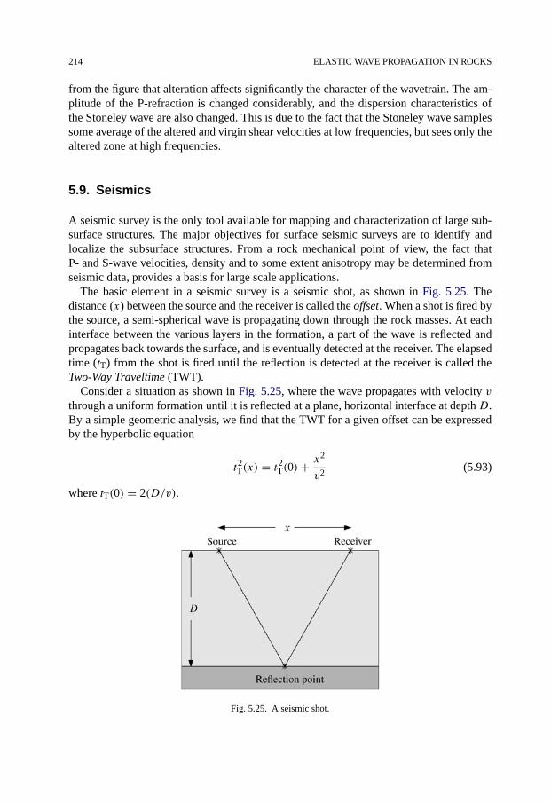
214 ELASTIC WAVE PROPAGATION IN ROCKS
from the figure that alteration affects significantly the character of the wavetrain. The am-plitude of the P-refraction is changed considerably, and the dispersion characteristics ofthe Stoneley wave are also changed. This is due to the fact that the Stoneley wave samplessome average of the altered and virgin shear velocities at low frequencies, but sees only thealtered zone at high frequencies.
5.9. Seismics
A seismic survey is the only tool available for mapping and characterization of large sub-surface structures. The major objectives for surface seismic surveys are to identify andlocalize the subsurface structures. From a rock mechanical point of view, the fact thatP- and S-wave velocities, density and to some extent anisotropy may be determined fromseismic data, provides a basis for large scale applications.
The basic element in a seismic survey is a seismic shot, as shown in Fig. 5.25. Thedistance (x) between the source and the receiver is called the offset. When a shot is fired bythe source, a semi-spherical wave is propagating down through the rock masses. At eachinterface between the various layers in the formation, a part of the wave is reflected andpropagates back towards the surface, and is eventually detected at the receiver. The elapsedtime (tT) from the shot is fired until the reflection is detected at the receiver is called theTwo-Way Traveltime (TWT).
Consider a situation as shown in Fig. 5.25, where the wave propagates with velocity vthrough a uniform formation until it is reflected at a plane, horizontal interface at depth D.By a simple geometric analysis, we find that the TWT for a given offset can be expressedby the hyperbolic equation
t2T(x) = t2T(0)+x2
v2(5.93)
where tT(0) = 2(D/v).
Fig. 5.25. A seismic shot.

SEISMICS 215
Consider now a set of shots with different offsets around the same midpoint. Corre-sponding values of TWT and offset should then fall on a straight line in a plot of t2T(x)versus x2. From this plot it is possible to identify both tT(0) (from the intercept at x = 0)and v (from the slope). Thus it is possible to identify both the depth D and the velocity vfrom the seismic data.
A collection of shots around a common midpoint is called a CMP gather. In order toenhance the useful information (i.e. the reflected pulse) and suppress noise, it is standardprocedure to add up all recorded traces in a CMP gather, after having scaled the time axisof each trace as
tT(x)→√t2T(x)−
x2
v2(5.94)
This scaling ensures that the reflection occurs at the same place for all traces. Such a sumof traces is called a CMP stack. Note that stacking disturbs information about amplitudeand phase in the signals.
If the formation consists of several layers, the wave is refracted at each interface bothbefore it reaches the actual interface we are considering and on its way back to the surface.The expression for TWT is then rather complicated, however in the hyperbolic approxima-tion we have (Dix, 1955)
t2T(x) ≈ t2T(0)+x2
v2RMS
(5.95)
where the so called “root-mean-square velocity” vRMS is given as
v2RMS = 2
tT(0)
N∑j=1
Ljvj (5.96)
Lj and vj are the thickness and velocity of layer j , respectively, and N is the number oflayers, while the TWT at zero offset is given as
tT(0) = 2N∑j=1
Lj
vj(5.97)
As we are able to obtain both vRMS and tT(0) from the CMP gather for the reflection fromeach layer, we have the 2N equations needed to determine the 2N unknowns Lj , vj . Thisprocedure, called Dix inversion, allows us to determine both velocity and thickness of eachlayer.
An alternative form of the traveltime equation (5.95) is found by Taylor expansion ofthe traveltime in x:
tT(x) = tT(0)+ x2
2tT(0)v2NMO
+ · · · (5.98)
The function�tT(x) = tT(x)−tT(0) is called the normal moveout (NMO), and the velocityvNMO is called the normal moveout velocity. In general, vNMO differs from vRMS, howeverfor plane, horizontal, homogeneous layers, we have vNMO = vRMS.

216 ELASTIC WAVE PROPAGATION IN ROCKS
In practice, the processing of seismic data is complicated by several factors, such asdipping layers (which imply that the reflection point differs from the common midpoint),lateral velocity variations and anisotropy (which both implies that the velocity is differentfor different offsets), and spurious reflections originating from refracted waves, convertedwaves, interface waves and multiple reflections. Data derived from seismic processing maythus suffer from large uncertainties.
We have shown earlier that the amplitude of a reflection generated at an interface de-pends on the acoustic impedance. Since the acoustic impedance depends on both velocityand density, the amplitude of a seismic reflection also carries information about the rockdensity. In general, the reflection coefficient depends on the angle of incidence, the P-wavevelocities and densities of both layers, as well as the shear wave velocity vs2 of the lowerlayer (see example in Fig. 5.12). Thus, the variation in amplitude versus offset (correspond-ing to the angle of incidence) for a P-wave reflected at the interface between two layerscarries information about both the P- and S-wave velocity of the layer below the interface.In marine seismic surveys, both the source and the receivers are floating in water, hence allinformation to be extracted about the formations below the sea floor has to be carried byP-waves. Application of the method outlined above is a possible way to extract also shearwave velocities from marine seismic data. The method is known as AVO (Amplitude Ver-sus Offset). In land- or ocean bottom-based seismic surveys, where both P- and S-wavesare generated and detected, an extended method called Multicomponent AVO may be ap-plied to improve the confidence of the estimated shear wave velocity. This method alsoincludes analyses of amplitudes of reflected S-waves, by a similar set of equations as thosedescribed in Appendix D.2.2.
A velocity derived from a seismic data set is a kind of “average” velocity over a distancegiven roughly by the wavelength. If the rock is heterogeneous on a scale shorter than thisdistance, the observed velocity will not be fully representative for the velocity on a shorterlength scale. Examples of how the “average” velocity relates to the short scale velocitiesand the geometrical structure of the heterogeneities are given in Section 6.1.
The resolution of seismic data—that is, the typical size of the smallest objects that canbe seen as reflections—is usually assumed to be about a quarter of the wavelength. As aseismic wave contains a band of frequencies (typically 10–100 Hz), the resolution limit isusually defined as the wavelength of the component that has the highest frequency. The fre-quency content in a seismic signal is mainly given by the attenuation (which is a constant-Qtype withQ in the order of 30–100 for underground formations), the distance travelled bythe wave, and the type of wave. For a P-wave reflected at about 1000 m depth, the typicalwavelength is about 100 m, while the resolution limit is about 20 m, depending of courseon the local conditions. The loss of the highest frequencies with increasing travel-time(which is a consequence of constant-Q attenuation) implies that the resolution is poorer fordeeper reflections. For a P-wave reflected at about 4000 m depth, the typical wavelengthis about 200 m, and the resolution limit about 50 m. Improved recording technology mayimprove the resolution somewhat, maybe as much as a factor of 2. Still the resolution isquite poor, and this limits the applicability of seismic data for determination of formationproperties. Further improvements in the resolution require different processing techniqueswhich may be more sensitive to noise.
REFERENCES 217
References
Auld, B.A. (1990). Acoustic Fields and Waves in Solids. Vol. I, second ed. Robert E. Krieger Publishing Com-pany.
Batzle, M., Han, D.H., Hofmann, R. (2006). “Fluid mobility and frequency-dependent seismic velocity—Directmeasurements”. Geophysics 71, N1–N9.
Batzle, M., Wang, Z. (1992). “Seismic properties of pore fluids”. Geophysics 57, 1396–1408.Biot, M.A. (1956a). “Theory of propagation of elastic waves in a fluid-saturated porous solid. I. Low-frequency
range”. J. Acoust. Soc. Am. 28, 168–178.Biot, M.A. (1956b). “Theory of propagation of elastic waves in a fluid-saturated porous solid. II. Higher frequency
range”. J. Acoust. Soc. Am. 28, 179–191.Biot, M.A. (1962). “Mechanics of deformations and acoustic propagation in porous media”. J. Appl. Phys. 33,
1482–1498.Bourbie, T., Coussy, O., Zinszner, B. (1987). Acoustics of Porous Media. IFP Publications. Editions Technip.Christensen, N.I. (1982). “Seismic velocities”. In: Carmichael, R.S. (Ed.), Handbook of Physical Properties of
Rocks. Vol. II. CRC Press, pp. 2–228.Dix, C.H. (1955). “Seismic velocities from surface measurements”. Geophysics 20, 68–86.Endres, A.L., Knight, R. (1989). “The effect of microscopic fluid distribution on elastic wave velocities”. The
Log Analyst (November–December), 437–445.Fjær, E. (1999). “Static and dynamic moduli of weak sandstones”. In: Amadei, B., Kranz, R.L., Scott, G.A.,
Smeallie, P.H. (Eds.), Rock Mechanics for Industry. Balkema, pp. 675–681.Hornby, B.E., Chang, S.K. (1985). “A case study of shale and sandstone alteration using a digital sonic tool”. In:
SPWLA 26th Ann. Logging Symp.Johnston, D.H., Toksõz, M.N., Timur, A. (1979). “Attenuation of seismic waves in dry and saturated rocks:
II. Mechanisms”. Geophysics 44, 691–711.Jones, T.D. (1986). “Pore fluids and frequency-dependent wave propagation in rocks”. Geophysics 51, 1939–
1953.Jones, T.D., Nur, A. (1983). “Velocity and attenuation in sandstone at elevated temperatures and pressures”.
Geophys. Res. Lett. 10, 140–143.King, M.S. (1970). “Static and dynamic elastic moduli of rocks under pressure”. In: Proc. 11th US Symp. on
Rock Mechanics, pp. 329–351.Ledbetter, H. (1993). “Dynamic vs. static Young’s moduli: a case study”. Mater. Sci. Eng. A165, L9–L10.Mavko, G., Nur, A. (1979). “Wave attenuation in partially saturated rocks”. Geophysics 44, 161–178.Mavko, G., Jizba, D. (1991). “Estimating grain-scale fluid effects on velocity dispersion in rocks”. Geophysics 56,
1940–1949.Mensch, T., Rasolofosaon, P. (1997). “Elastic-wave velocities in elastic media of arbitrary symmetry—generali-
zation of Thomsen’s parameters ε, δ and γ ”. Geophys. J. Internat. 128, 43–64.Murphy III, W.F., Winkler, K.W., Kleinberg, R.L. (1984). “Contact microphysics and viscous relaxation in sand-
stones”. In: Johnson, D.L., Sen, P.N. (Eds.), Physics and Chemistry of Porous Media. Am. Inst. Phys.,pp. 176–190.
Nes, O.-M., Holt, R.M., Fjær, E. (2002). “The reliability of core data as input to seismic reservoir monitoringstudies”. SPE Reservoir Evaluation Eng. (February), 79–86.
Plona, T.J. (1980). “Observation of a second bulk compressional wave in a porous medium at ultrasonic frequen-cies”. App. Phys. Lett. 36, 259–261.
Plona, T.J., Cook, J.M. (1995). “Effects of stress cycles on static and dynamic Young’s moduli in Castlegatesandstone”. In: Proc. of the 35th U.S. Rock Mech. Symp. Balkema, pp. 155–160.
Sayers, C.M. (2002). “Stress-dependent elastic anisotropy of sandstones”. Geophys. Prosp. 50, 85–95.Schmitt, D.P. (1988a). “Shear wave logging in semi-finite saturated porous formations”. J. Acoust. Soc. Am. 84,
2230–2244.Schmitt, D.P. (1988b). “Shear wave logging in elastic formations”. J. Acoust. Soc. Am. 84, 2215–2229.Stoll, R.D. (1974). “Acoustic waves in saturated sediments”. In: Hampton, L. (Ed.), Physics of Sound in Marine
Sediments. Plenum, New York, pp. 19–39.Thomsen, L. (1986). “Weak elastic anisotropy”. Geophysics 51, 1954–1956.
218 ELASTIC WAVE PROPAGATION IN ROCKS
Tsvankin, I. (1997). “Anisotropic parameters and P-wave velocity for orthorhombic media”. Geophysics 62,1292–1309.
Viktorov, I.A. (1979). “Types of acoustic surface waves in solids (review)”. Sov. Phys. Acoust. 25, 1–9.Walsh, J.B. (1966). “Seismic wave attenuation in rock due to friction”. J. Geophys. Res. 71, 2591–2599.White, J.E. (1967). “The Hula log: A proposed acoustic tool”. In: SPWLA 8th Ann. Logging Symp. Trans.,
pp. I1–I25.Wyllie, M.R.J., Gregory, A.R., Gardner, G.H.F. (1958). “An experimental investigation of factors affecting elastic
wave velocities in porous media”. Geophysics 23, 459–493.
Further reading
Aki, K., Richards, P.G. (1980). Quantitative Seismology. W.H. Freeman and Co., New York.Carmichael, R.S. (1984). Handbook of Physical Properties of Rocks. Vol III. CRC Press.Crampin, S. (1985). “Evaluation of anisotropy by shear wave splitting”. Geophysics 50, 142–152.Dvorkin, J., Nolen-Hoeksema, R., Nur, A. (1994). “The squirt flow mechanism: Macroscopic description”. Geo-
physics 59, 428–438.Engelder, T., Plumb, R. (1984). “Changes in in situ ultrasonic properties of rock on strain relaxation”. Int. J. Rock
Min. Sci. & Geomech. Abstr. 21, 75–82.Fjær, E., Holt, R.M., Raaen, A.M. (1989). “Rock mechanics and rock acoustics”. In: Maury, V., Fourmaintraux,
D. (Eds.), Rock at Great Depth. Balkema, Rotterdam, pp. 355–362.Fjær, E., Holt, R.M. (1994). “Rock acoustics and rock mechanics: Their link in petroleum engineering”. The
Leading Edge (April), 255–258.Gregory, A.R. (1976). “Fluid saturation effects on dynamic elastic properties of sedimentary rocks”. Geo-
physics 41, 895–921.Hamilton, E.L. (1971). “Elastic parameters of marine sediments”. J. Geophys. Res. 76, 579–604.Johnson, D.L., Plona, T.J. (1982). “Acoustic slow waves and the consolidation transition”. J. Acoust. Soc. Am. 72,
556–565.Li, X., Zhong, L., Pyrak-Nolte, L.J. (2001). “Physics of partially saturated porous media: Residual saturation and
seismic-wave propagation”. Ann. Rev. Earth Planet. Sci. 29, 419–460.Murphy, W., Reischer, A., Hsu, K. (1993). “Modulus decomposition of compressional and shear velocities in
sand bodies”. Geophysics 58, 227–239.Nur, A., Simmons, G. (1969a). “The effect of saturation on velocity in low porosity rocks”. Earth Planetary Sci.
Lett. 7, 183–193.Nur, A., Simmons, G. (1969b). “Stress-induced velocity anisotropy in rock: an experimental study”. J. Geophys.
Res. 74, 6667–6674.Osif, T.L. (1988). “The effects of salt, gas, temperature, and pressure on the compressibility of water”. SPE
Reservoir Eng. 3, 175–181.Paillet, F.L., Cheng, C.H. (1991). Acoustic Waves in Boreholes. CRC Press.Renlie, L., Raaen, A.M. (1993). “Acoustic wave propagation in a fluid-filled borehole surrounded by a formation
with stress-relief-induced anisotropy”. Geophysics 58, 1257–1269.Sayers, C.M., van Munster, J.G., King, M.S. (1990). “Stress-induced ultrasonic anisotropy in Berea sandstone”.
Int. J. Rock Mech. Min. Sci. & Geomech. Abstr. 27, 429–436.Storvoll, V., Bjørlykke, K. (2004). “Sonic velocity and grain contact properties in reservoir sandstones”. Petro-
leum Geoscience 10, 215–226.Timur, A. (1978). “Rock physics”. Arab. J. Soc. & Eng., 5–30. (Special issue).Tittman, B.R., Bulau, J.R., Abdel-Gawad, M. (1984). “Dissipation of elastic waves in fluid saturated rocks”. In:
Johnson, D.L., Sen, P.N. (Eds.), Physics and Chemistry of Porous Media. Am. Inst. Phys., pp. 131–143.White, J.E. (1983). Underground Sound. Elsevier, New York.Winkler, K.W. (1985). “Dispersion analysis of velocity and attenuation in Berea sandstone”. J. Geophys. Res. 90
(B), 6793–6800.

219
Chapter 6
Rock models
In the previous chapters, we have discussed the mechanical behaviour of rocks in termsof continuum mechanics. That is, we have treated the rocks as homogeneous materials.However, sedimentary rocks are made up of small particles, and are largely heterogeneousmaterials on a length scale comparable to the particle size (Fig. 1.18). Furthermore, inho-mogeneous distribution of particle types and particle sizes in the form of layers or clusters,as well as fractures, produce heterogeneities on larger length scales. The mechanical prop-erties of the rock will differ largely from one part to another if measured on a length scalewhich is small or comparable to the size of the heterogeneities. The continuum approachcan be applied with confidence only as an average, and on a length scale which is largecompared to the size of the heterogeneities.
For many practical applications the continuum approach is valid. However, it is intu-itively clear that the mechanical properties of the rock even on a large scale must depend insome way on the microscopical nature of the rock. We have already touched this problemwhen we introduced the poroelastic formalism (Section 1.6). The theory of poroelasticityis based on the assumption that the rock consists of both a solid part and a fluid part, whichare separated on a microscopic scale, but coexist on a macroscopic scale. One of the state-ments of this theory is that the rock’s framework has its own moduli, separate from thoseof the solid material and the pore fluid.
The poroelastic formalism of Biot introduced earlier (Chapter 1) is capable of predict-ing the elastic properties of a porous material provided that parameters like the frame bulk(Kfr) and the shear (Gfr) moduli are known. These are macroscopic parameters, describingthe properties of the rock on a length scale much larger than the grains and pores. The Biottheory is called a macroscopic theory since it only deals with macroscopic quantities. It isan ultimate goal to be able to express the macroscopic parameters likeKfr andGfr in termsof the properties of the constituents the rock is made of and the microstructure of the rockfabric. Having obtained values for the macroscopic parameters from the microscopic the-ories, we may consider these parameters to represent a material which is homogeneous ona macroscopic scale. This virtual, homogeneous material is commonly called an effectivemedium.
The elastic properties of a composite material like a sedimentary rock depend primarilyon the following three factors:
1. the relative amount of each component present
2. the elastic properties of each component
3. the geometrical distribution of each component.
It is not possible to obtain accurate data for all three factors for a given rock, hence anymodel of the rock will necessarily be based on simplifying assumptions. A model is there-fore valid as a representation for the real rock only to the extent that the features governing
220 ROCK MODELS
the observed behaviour of the rock are accounted for in the model. This also implies that amodel may be a good representation for the rock in a given situation, while it is not at alldescribing the actual behaviour of the rock in other situations.
A large number of rock models have been derived over the years, describing variousproperties of various rocks under various conditions. A comprehensive collection of suchmodels was given by Mavko et al. (1998). Here, we shall first take a look at a model fora simple heterogeneous material, in order to illustrate how the physical properties maydepend on the length scale on which the material is being observed (Section 6.1). Somemodels for porous rocks involve only porosity, with no explicit reference to the shapeof the pore space. Such models are presented in Section 6.2. Other models are based onthe forming process of sedimentary rocks, and describe essentially packs of grains. Suchmodels are described in Section 6.3. Models describing cracked and fractured rocks aredescribed in Sections 6.4 and 6.5.
6.1. Layered media
Consider a material made up of parallel, isotropic layers. This is one of the simplest exam-ples one can find of a non-homogeneous material. We shall use this as an example to seehow a material can be considered as heterogeneous on one scale, and effectively homoge-neous on another.
Given a sample of a layered material. We denote the thickness of layer number i as Li ,so that the total thickness L of the sample is the sum of all Li . If an external load σz isapplied in the direction normal to the layers, all layers have to carry the same load. Thestrain of layer i will be εz,i = σz/Ei , where Ei denotes the Young’s modulus of layer i.The sample will thus deform according to
εz = − 1
L
∑i
�Li = 1
L
∑i
εz,iLi = 1
L
∑i
σz
EiLi = σz 1
L
∑i
Li
Ei≡ σz
⟨1
E
⟩(6.1)
We use 〈x〉 to denote the average of the quantity x weighted by the volumetric proportionof each layer (often called Backus average). The effective Young’s modulus E∗ of thelayered material is according to Eqs. (1.91) and (6.1) given as
E∗ =⟨
1
E
⟩−1
(6.2)
Note that the layered material has transversely isotropic symmetry, so that the effectiveYoung’s modulus will vary with orientation of the applied stress. The total effective stiff-ness tensor of this layered material is given as (Backus, 1962; Helbig, 1994):
C11 = C22 =⟨
4G(λ+G)λ+ 2G
⟩+⟨
1
λ+ 2G
⟩−1⟨λ
λ+ 2G
⟩2
(6.3)
C33 =⟨
1
λ+ 2G
⟩−1
(6.4)
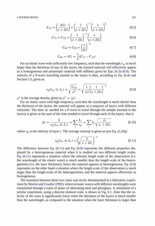
LAYERED MEDIA 221
C12 =⟨
2Gλ
λ+ 2G
⟩+⟨
1
λ+ 2G
⟩−1⟨λ
λ+ 2G
⟩2
(6.5)
C13 = C23 =⟨
1
λ+ 2G
⟩−1⟨λ
λ+ 2G
⟩(6.6)
C44 = C55 =⟨
1
G
⟩−1
(6.7)
C66 = 〈G〉 = 1
2(C11 − C12) (6.8)
For an elastic wave with sufficiently low frequency, such that the wavelength λw is muchlarger than the thickness of any of the layers, the layered material will effectively appearas a homogeneous and anisotropic material with stiffness given by Eqs. (6.3)–(6.8). Thevelocity of a P-wave travelling normal to the layers is then, according to Eq. (6.4) andSection 5.5, given as
vp(λw Li) =√C33
ρ∗ =√
1
〈ρ〉⟨
1
λ+ 2G
⟩−1
(6.9)
ρ∗ is the average density, given as ρ∗ = 〈ρ〉.For an elastic wave with high frequency, such that the wavelength is much shorter than
the thickness of the layers, the material will appear as a sequence of layers with differentvelocities. The time �t needed for a P-wave to travel through the sample (normal to thelayers) is given as the sum of the time needed to travel through each of the layers, that is
�t = L
vp(λw � Li)=∑i
Li
vp=∑i
Li
√ρi
λi + 2Gi(6.10)
where vp is the velocity of layer i. The average velocity is given as (see Eq. (5.26)):
vp(λw � Li) =⟨√
ρ
λ+ 2G
⟩−1
(6.11)
The difference between Eq. (6.11) and Eq. (6.9) represents the different properties dis-played by a heterogeneous material when it is studied on two different length scales.Eq. (6.11) represents a situation where the relevant length scale of the observation (i.e.the wavelength of the elastic wave) is much smaller than the length scale of the hetero-geneities (i.e. the layer thickness), hence the material appears as heterogeneous. Eq. (6.9)represents on the other hand a situation where the length scale of the observation is muchlarger than the length scale of the heterogeneities, and the material appears effectively ashomogeneous.
The transition between these two cases was nicely demonstrated in a laboratory experi-ment by Marion and Coudin (1992), where acoustic waves with different wavelengths weretransmitted through a stack of plates of alternating steel and plexiglass. A simulation of asimilar experiment, using a discrete element code, is shown in Fig. 6.1. Note that the ve-locity of the wave is significantly lower when the thickness of the layers is much smallerthan the wavelength, as compared to the situation when the layer thickness is larger than

222 ROCK MODELS
Fig. 6.1. Recorded signals of P-waves transmitted through 7 different samples, as simulated by a discrete elementcode. The excitation is a one-cycle sine pulse. Each sample is a stack of hard and soft layers of equal thickness.Only the layer thickness L is different for each sample. The hard-layer:soft-layer ratios for stiffness and densityare 20:1 and 8:1, respectively.
the wavelength. Note also the strong attenuation for the intermediate cases, indicating thatthe wave is almost unable to propagate under such conditions. Hovem (1995) showed byanalytical modelling that wave propagation is dispersive with no loss for frequencies belowa critical limit, while waves with higher frequencies are evanescent, suffering loss at eachinterface. The critical frequency limit depends on the periodicity of the layered materialand the impedance contrast between the layers.
This example demonstrates clearly that the properties of a heterogeneous material maybe very different when observed on different length scales. An effective medium repre-senting the material has the properties of the material when it is observed on a length scalemuch larger than that of the heterogeneities.
6.2. Models involving porosity only
For a simple porous rock consisting only of one type of solid material and being saturatedwith only one type of fluid, the relative amount of the components is specified by theporosity φ, while the elastic properties of the components are given by the bulk modulus ofthe fluidKf, and the bulk (Ks) and shear (Gs) moduli of the grain material. Many availableexpressions for the elastic properties of rocks are based only on these parameters, as detailsabout the geometrical distribution of each component is normally not known.
Precise estimates for the elastic moduli of a rock can not be obtained without the vitalinformation about the geometrical distribution of each component, however there are upper
MODELS INVOLVING POROSITY ONLY 223
and lower limits for their values. Such limits—or bounds as they are usually called—canbe established by considering extreme geometrical distributions of the constituents.
Assuming a distribution such that both the grain material and the fluid experiences thesame strain due to an external hydrostatic stress, the bulk modulus (KV) of the rock is givenas
KV = φKf + (1 − φ)Ks (6.12)
KV is an upper bound for the bulk modulus of a real rock, and is called the Voigt bound.Similarly, if we assume that the stress is the same in both the grains and the fluid, we findthat the bulk modulus (KR) of the rock is given as (see Eq. (1.132))
1
KR= φ
Kf+ 1 − φ
Ks(6.13)
KR is a lower bound for the bulk modulus, called the Reuss bound. Similar bounds canbe found for the shear modulus simply by replacing the bulk moduli in Eqs. (6.12) and(6.13) by the corresponding shear moduli. Note that the Reuss bound for the shear modulusGR = 0 for any φ > 0 (since Gf = 0), while the Voigt bound GV > 0 for any φ < 1.
Physically, the Reuss bound represents a suspension, e.g. solid particles in a liquid. Itmay also describe gas bubbles in a liquid (in which case the bulk modulus Kg of the gashas to replace Ks in Eq. (6.13)). The Voigt bound represents an alloy of constituents, andis most appropriate for a rock at low porosity.
The Voigt and Reuss bounds are very wide, and of limited value for modelling of rockproperties. A narrower range is given by the Hashin–Shtrikman bounds. In a general form,these are given as (Hashin and Shtrikman, 1963)
KHS± = K1 + v21
K2−K1+ v1
K1+ 43G1
(6.14)
GHS± = G1 + v21
G2−G1+ 2v1(K1+2G1)
5G1(K1+ 43G1)
(6.15)
Subscripts 1 and 2 denote component 1 and 2, respectively, while v represents the vol-ume fraction of the actual component. The upper (KHS+,GHS+) and lower (KHS−,GHS−)bounds are found by interchanging material 1 and 2 (the upper bound is found when mate-rial 1 is the stiffest one). Physically, the Hashin–Shtrikman bounds represent the moduli ofan assembly of spheres of material 2, each of which is surrounded by a shell of material 1.Note that for the simple grain-fluid model of a rock described above, the lower Hashin–Shtrikman bound is identical to the Reuss bound for both the bulk and the shear modulus.This is also the exact solution for a suspension of grains in a fluid (see Section 1.6).
The arithmetic average of the Voigt and Reuss bounds are sometimes used to ob-tain estimates of the moduli, rather than just the allowable range. These averages, K =(KV + KR)/2 and similar for the shear modulus, are usually called the Voigt–Reuss–Hillaverage moduli (Hill, 1952). The Voigt–Reuss–Hill average moduli represent no well de-fined model of the rock microstructure, however it may be seen as a specific mixture of theextreme structures represented by the Voigt and Reuss bounds.

224 ROCK MODELS
An alternative approach would be to look for the most probable microstructure in aporous rock and try to estimate the moduli for such a structure. Considering for instance acollection of sand grains, it is clear that there exists a maximum porosity, above which thegrains will no longer be in contact with each other and the frame moduli will vanish. Foran ordered simple cubic packing of equally sized spheres, this critical porosity φc is 0.476,for a random packing it is about 0.36, while for a typical clean sand it is about 0.40. Basedon this simple argument, combined with the expectation that the moduli should be equalto the moduli of the grain material if the porosity is zero, we find as the simplest possibleexpression
Kfr = Ks
(1 − φ
φc
)(6.16)
Gfr = Gs
(1 − φ
φc
)(6.17)
The critical porosity concept (Nur et al., 1991, 1995) is not really a micromechanicalmodel, and the critical porosity is an empirical constant which will differ from one rocktype to another, however the concept provides an explanation for the characteristic behav-iour of the frame moduli of sedimentary rocks. Fig. 6.2 shows the undrained bulk modulusversus porosity for a rock, as given by Eq. (6.16) with φc = 0.39. The figure also showsthe Voigt, Reuss and Hashin–Shtrikman bounds for a dry rock, and the Voigt–Reuss–Hillaverage. For comparison, the empirical results of Murphy et al. (1993) for clean sands arealso included.
Fig. 6.2. Undrained bulk modulus versus porosity for water saturated rocks, according to various models. Thedotted line is based on the empirical curve of Murphy et al. (1993) for clean sandstones. The fluid contributionhas been accounted for by use of the Biot–Gassmann equation (1.155) for both the empirical curve and the criticalporosity curve.
GRAIN PACK MODELS 225
The critical porosity concept also provides some understanding of the properties ofsand–clay mixtures (Marion and Nur, 1991). Small amounts of clay in a sandstone usu-ally appear as pore fill, and the mechanical properties of the rock are mainly determined bythe framework of sand grains. The stiffness of the rock is however still largely determinedby the sand grain framework, as the sand grains are stiffer than the clay. On the other hand,clay mixed with only a small amount of sand will behave as a kind of suspension, where themechanical properties will be dominated by those of the clay. The transition between thetwo types of behaviour will occur when the relative volume of sand is about 1 − φc, that iswhen the sand volume is just large enough for the grains to make a continuous framework.
6.3. Grain pack models
Sedimentary rocks are formed by small pieces of solid material that are compacted and tosome extent cemented. Models describing the elastic properties of grain packs may thusprovide interesting information about such materials.
Consider two spherical grains that are pressed together with a normal force F actingalong the line through the centres of the spheres (Fig. 6.3). Due to the force, the grainswill be deformed in the vicinity of the contact spot. The contact area will be a circle withradius b, depending on the force F as
b =[
3(1 − ν2s )aF
4Es
]1/3
(6.18)
This equation was originally derived by Hertz (1882), assuming linearly elastic grainmaterial and that the contact radius is small (b � a). νs and Es are the Poisson’s ratio andYoung’s modulus of the grain material, respectively. The distance between the centres ofthe grains is reduced with s due to the external force:
s =[
9(1 − ν2s )
2F 2
2E2s a
]1/3
(6.19)
The normal stress σ within the grain contact area is given as
σ = 3F
2πb2
(1 − r2
b2
)1/2
(6.20)
where r is the lateral distance from the centre line between the two spheres. A force con-stant Dn relating the longitudinal deformation �s to an increment �F can be derivedfrom Eqs. (6.18) and (6.19), utilizing the relationship between Es and the shear modulusGs (Table 1.1):
Dn = �F
�s=[
3E2s aF
4(1 − ν2s )
2
]1/3
= 2Gsb
1 − νs(6.21)
The response to an incremental shear force �F ′ over a grain contact that is already underthe same external load F as above, can be found by a similar consideration of the forces in

226 ROCK MODELS
Fig. 6.3. Normal stress distribution at the grain contact in a normally loaded contact between two equally sized,spherical grains. (After White, 1983; with permission from Elsevier Science Publishers.)
the grain contact area (see Fig. 6.4). A shear force constant
Dt = �F ′
�s′= [6E2
s aF(1 − ν2s )
2]1/3
(2 − νs)(1 + νs)= 4Gsb
2 − νs(6.22)
relates the shear force between the grains to the lateral displacement (�F ′ and�s′ definedin Fig. 6.4). This theory was first developed by Mindlin (1949), so the grain pack theory asit stands is usually called the “Hertz–Mindlin”-theory.
The relationship between the force F and the external pressure σp causing the force, aswell as the relationship between the displacement s and macroscopic strain εvol, depend onthe packing of the grains.
For a random packing of identical spheres, εvol = 3s/(2a) while
F = 4πa2σp
Nc(1 − φ) (6.23)
Nc is the average number of contacts per sphere, also called the coordination number.Note that the porosity is given essentially by the packing, and is not a free variable in these
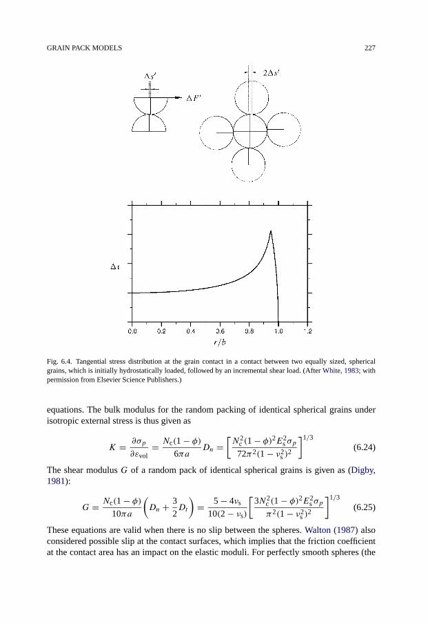
GRAIN PACK MODELS 227
Fig. 6.4. Tangential stress distribution at the grain contact in a contact between two equally sized, sphericalgrains, which is initially hydrostatically loaded, followed by an incremental shear load. (After White, 1983; withpermission from Elsevier Science Publishers.)
equations. The bulk modulus for the random packing of identical spherical grains underisotropic external stress is thus given as
K = ∂σp
∂εvol= Nc(1 − φ)
6πaDn =
[N2
c (1 − φ)2E2s σp
72π2(1 − ν2s )
2
]1/3
(6.24)
The shear modulus G of a random pack of identical spherical grains is given as (Digby,1981):
G = Nc(1 − φ)10πa
(Dn + 3
2Dt
)= 5 − 4νs
10(2 − νs)
[3N2
c (1 − φ)2E2s σp
π2(1 − ν2s )
2
]1/3
(6.25)
These equations are valid when there is no slip between the spheres. Walton (1987) alsoconsidered possible slip at the contact surfaces, which implies that the friction coefficientat the contact area has an impact on the elastic moduli. For perfectly smooth spheres (the
228 ROCK MODELS
friction coefficient is zero; perfect slip), Walton found
K = 1
6
[3N2
c (1 − φ)2σpπ4B2
]1/3
(6.26)
G = 1
10
[3N2
c (1 − φ)2σpπ4B2
]1/3
= 3
5K (6.27)
where
B = 3
2π
(1 − 2νs)(1 − νs)
Es(6.28)
Eqs. (6.24) and (6.25) can be used to estimate how acoustic velocities depend on anexternal hydrostatic stress σp for a dry rock. Since both K and G depend on σ 1/3
p , we
immediately see that both vp and vs depend on the stress as σ 1/6p . Experiments on loose
sands (Domenico, 1977; Bachrach et al., 1998; Han and Batzle, 2006) have shown vp and vsdepending on the stress as σnp , where n is in the range 1/4 to 1/5. There are several possiblereasons for this discrepancy (Makse et al., 2001). The analytical grain pack models do notaccount properly for partial slip and associated grain rotation and rearrangement. The loadis further assumed to be carried equally by all grain contacts, while in reality, it is carried bylocalized force chains through the grain assembly. This may be described by an effective,stress-dependent coordination number. With realistic grain shapes, the surface roughnessof the grains may also lead to grain contact stiffnesses described by an exponent differentfrom 1/3 (as in Eqs. (6.21) and (6.22)). An example of such behaviour is the “bed of nails”model by Carlson and Gangi (1985), which is described under Section 6.5.1. Note that thetheory also predicts that the ratio between vp and vs does not depend on the external stress.
The Hertz–Mindlin contact theory has also been derived for various ordered packingsof grains (see f.i. Wang and Nur, 1992, for a review). Extensions to the model have beenmade to take into account the effects of a saturating fluid (White, 1983; Brandt, 1955),and to describe cemented rather than pressure generated grain contacts (Digby, 1981;Schwartz, 1984; Dvorkin et al., 1991). For cemented contacts the force constants Dn andDt become unknown parameters. and the stress dependency of the acoustic waves tendsto be less pronounced. The Hertz–Mindlin theory is no longer valid at high stress levels,when plastification of the grain contacts may occur. The stiffness will then increase withstress at a rate lower than indicated by the exponent 1/6.
The general case of variously sized, cemented particles in a random dense pack has notbeen solved analytically yet. However, such systems can be studied numerically. Discreteparticle modelling has developed rapidly over the last few years, with the continuous de-velopment of faster and more powerful computers. One such approach is the PFC (ParticleFlow Code1), which is based on the pioneering work of Cundall and Strack (1979).
In PFC, which may be formulated both in 2D and 3D, circular or spherical particles of ar-bitrary size distribution are packed into a granular assembly under a specific applied stress.Each disk or sphere is treated as a rigid body, with translational and rotational degrees of
1 Trademark of Itasca Consulting Group, Minneapolis, USA.

GRAIN PACK MODELS 229
freedom. When two particles come in contact, forces are generated as a result of relative(normal and shear) displacements at the contact. Using a so-called soft contact approach,the particles are permitted numerically to overlap each other, and the degree of overlapcontrols the contact forces through a contact law. The contact law may be Hertzian, or lin-ear, or user-defined. By applying boundaries representative for the problem to be studied(e.g. flat walls to mimic pistons, in case a laboratory test is simulated), the stress conditionscan be changed and the contact forces and associated particle movements calculated, untilequilibrium is reached and a new load increment can be applied. This procedure is cycledover and over again until a numerical experiment is completed.
The particle contacts may be unbonded or bonded. When simulated cement bonds areinserted, they have bond stiffnesses that are in general different from those of the unce-mented contacts. In addition, the bonds have shear and tensile strength. When a shear ortensile failure criterion is exceeded locally, the bond fails, and it then retains the propertiesof the uncemented contact. With the features described above, the discrete model permitscalculation of the complete stress–strain behaviour of an uncemented or cemented granularmedium (Potyondy and Cundall, 2004). It thus serves as a tool for studying rock failuremechanics on the particle scale.
Several features may be added to permit direct comparison between laboratory measure-ments and discrete element computations, such as fluid coupling to simulate stress effectson permeability. For instance, wave propagation may be simulated directly in PFC, sincethe model is inherently dynamic (Li and Holt, 2002). Also, acoustic emissions may besimulated by calculating the energy associated with bond ruptures (Hazzard and Young,2000).
Discrete particle modelling may be used to gain understanding and insight, in particularin comparison with laboratory experiments. It may also be used to solve engineering prob-lems, in competition with continuum methods. The main benefit (Cundall, 2001) is that no
Fig. 6.5. Distribution of contact forces in a 2D specimen created by PFC2D, loaded in the vertical direction. Thewidth of the lines is proportional to the force magnitude, and the direction indicates the orientation. The figureshows only a section of the specimen.

230 ROCK MODELS
Fig. 6.6. Grain contact failures at a given stress level in the 2D specimen shown in Fig. 6.5. The black lines showfailures that are predominantly tensile, while the grey lines show shear failures.
pre-assumed constitutive material law is needed: complex behaviour, including develop-ment of localized fractures and cracks is a natural output of the modelling.
From a fundamental viewpoint, one may ask to what extent the assumptions behind thesimple effective medium theories sketched above are valid. As an illustration of that, adistribution of contact forces in a 2D network is shown in Fig. 6.5. The distribution isclearly heterogeneous, with a small number of contacts carrying a large part of the load(see also Radjai et al., 1996; Williams and Rege, 1997). This allows a.o. for studies ofvarious stress geometries, stress history and degrees of cementation. Note that the networkof force lines is heterogeneous on a larger scale than the grain size.
The numerical calculations also allow for “snap-shots” of grain contact failures at givenpoints in time, as shown in Fig. 6.6. Such figures may help to better understand deformationmechanisms and failure processes in sedimentary rocks.
6.4. Models for cracks and other inclusions
The grain pack models discussed above describe the porous material as a collection ofgrains with varying degree of contact between the grains. This may seem to be a logicalpath to follow when studying sedimentary rocks, since they are indeed formed this way.However, we may also consider a porous material as a solid with lots of holes in it, like a“Swiss cheese”. For some purposes it appears that this approach may be equally relevant,especially for well cemented rocks. More generally, we talk about such models as inclusionmodels, as they consider the effect of including an object in a host material.
To establish a model for such a material, we need descriptions for how holes of variousshapes affect the elastic properties of the solid. In a static approach (Eshelby, 1957; Walsh,1965a, 1965b), it is assumed that a static external load is imposed on a sample consisting ofa host material with embedded inclusions. The elastic properties of the effective medium

MODELS FOR CRACKS AND OTHER INCLUSIONS 231
are obtained by requiring that the effective medium shall suffer the same deformation asthe real sample when subjected to the same external load. In a dynamic approach (Kusterand Toksöz, 1974), it is assumed that a region consisting of inclusions embedded in ahost material is embedded in the effective medium. The elastic properties of the effectivemedium are defined such that the scattering of elastic waves from the embedded region iseliminated. The wavelength of the elastic wave is assumed to be much larger than the sizeof the region.
The two approaches converge when the concentration of inclusions is low. In Sec-tions 6.4.1 and 6.4.2 we shall take a look at models valid for low concentrations ofinclusions. Models intended to account for higher concentrations of inclusions are dis-cussed in Section 6.4.3.
6.4.1. Linear, isotropic models
Assuming that the concentration of inclusions is so low that interactions can be neglected,we may express the impact of the inclusion on the elastic stiffness of the material as aperturbation, proportional to the concentration of the inclusions. Assuming also that thehost material is isotropic, the effective bulk modulus K∗ and the effective shear modulusG∗ of a material containing inclusions, can be written as
K∗ = Ks(1 −QKξincl) (6.29)
G∗ = Gs(1 −QGξincl) (6.30)
Ks and Gs are the bulk modulus and shear modulus, respectively, of the solid materialwithout inclusions. ξincl is an appropriate measure of the concentration of the inclusions,depending on their shape (as will be seen below). QK andQG are measures of the impactthese inclusions have on the respective moduli of the material. QK and QG are functionsof the moduli of the host material and the material within the inclusions. Other moduli canbe represented by similar expressions.
Consider first the case where the inclusions are spherical, fluid-filled holes. The poros-ity φ, which is here given as the sum of the volumes of the holes relative to the total volume,is a suitable measure for the concentration of inclusions, thus ξincl = φ. The expressionsfor the effective moduli can for instance be derived from Eqs. (6.14) and (6.15), by definingKHS+ = K∗, GHS+ = G∗, v2 = 1 − v1 = φ, K1 = Ks, K2 = Kf, G1 = Gs, G2 = 0 (theupper Hashin–Shtrikman bound then represents a solid surrounding a spherical, fluid-filledinclusion), and linearizing the expressions in φ. The results are (see also Mackenzie, 1950;Eshelby, 1957; Walsh, 1965a):
K∗ = Ks
(1 − 3(1 − νs)(1 − Kf
Ks)
2(1 − 2νs)+ (1 + νs)KfKs
φ
)(6.31)
G∗ = Gs
(1 − 15
1 − νs
7 − 5νsφ
)(6.32)
Here νs is the Poisson’s ratio of the solid material, without inclusions. By comparingEq. (6.31) to Eq. (1.155) we find (after some algebra) that K∗ is in agreement with Biot’s

232 ROCK MODELS
theory (Section 1.6.2). Note also that G∗ does not depend on Kf, thus G∗ is the samewhether the material is dry or saturated, again in agreement with Biot’s theory. This is notthe case in general for inclusion models, as we shall see below.
We shall now consider the case where the inclusions are thin, flat cracks. For such inclu-sions, it turns out that the most suitable measure for the concentration of inclusions is thecrack density ξ , defined as
ξ = 2n
π
⟨A2
P
⟩(6.33)
A is the area and P the perimeter of a crack, and n is the number of cracks per unit vol-ume. The brackets 〈 〉 denote an average over all cracks. For circular cracks with radius a,Eq. (6.33) becomes
ξ = n〈a3〉 (6.34)
Assuming that the cracks are randomly oriented, we have (Walsh, 1965a, 1965b; Garbinand Knopoff, 1973, 1975; Budiansky and O’Connell, 1976; see also Watt et al., 1976):
K∗ = Ks
(1 − 16
9
1 − ν2s
1 − 2νsDξ
)(6.35)
G∗ = Gs
(1 − 32
45(1 − νs)
[D + 3
2 − νs
]ξ
)(6.36)
The parameter D is given as
1
D= 1 + 4
3πγ
1 − ν2s
1 − 2νs
Kf
Ks(6.37)
where γ is the aspect (thickness-to-diameter) ratio of the cracks. Note that for a dry mater-ial, for which Kf = 0 and consequently D = 1, the only crack-related parameter affectingthe effective moduli is the crack density ξ . For very thin, fluid-filled cracks, for whichγ � Kf/Ks, we have that D → 0 which implies that the cracks are almost incompliant.Again, only the crack density affects the effective moduli. Thus, details regarding the shapeof thin cracks have no impact on the effective moduli (Budiansky and O’Connell, 1976;Mavko and Nur, 1978).
Eq. (6.36) states that G∗ is affected by saturation, hence it is clear that these equationsare not consistent with Biot’s theory (Section 1.6.2). The reason for this discrepancy is thatsome of the cracks will necessarily have an orientation such that they will be compressed(or opened up) due to an applied shear stress. This change in volume of the crack impliesthat the fluid occupying the crack will be compressed (or expanded), to an extent that ispartly given by Kf. Biot’s theory, which has no assumptions about the shape of the porespace and hence should be valid also for thin, flat (crack-shaped) pores, is based on thefundamental assumption that the material is permeable. Hence the compression of onecrack due to an applied shear stress will only lead to flow of fluid from this crack intoanother crack whose orientation implies that it expands due to the same stress state. Thusthere is no local build-up (or reduction) of fluid pressure, and the fluid bulk modulus doesnot affect the effective shear modulus.

MODELS FOR CRACKS AND OTHER INCLUSIONS 233
It is possible to make an inclusion model consistent with Biot’s theory by defining thatG∗ is not affected by saturation. This is a way of implementing hydraulic connectionsbetween the elements of the pore space (i.e. making the material permeable; see Thomsen,1985). Alternatively, one may use the inclusion model only for the material in a dry state(for which D = 1), thus modelling the frame moduli, and add the effects of saturation byBiot’s theory. The actual situation we are trying to model determines which alternative isthe most representative. For instance, for high frequency elastic waves (see Chapter 5), thefluid may not have time to flow into and out of the cracks, hence the cracks will effectivelybe closed, and expressions like Eqs. (6.35)–(6.37) may give a good representation of themoduli. At low frequencies, the fluid pressure will have time to equalize, and a betterrepresentation of the moduli is found by using the inclusion model to estimate the framemoduli, and the Biot model to add the fluid effects.
6.4.2. Anisotropic models
Cracks in rocks are not always randomly oriented. More typically, cracks grow as a resultof anisotropic changes in the stress state, which leads to a preferred crack orientation withrespect to the stress state (see also Section 1.8). The elastic constants of a material withparallel cracks can be expressed, similar to Eqs. (6.29) and (6.30), as:
C∗ij = Coij (1 −Qij ξ) (6.38)
Co is the stiffness tensor of the host material (without cracks), andQij is the impact of thecracks on C∗
ij (note that the Einstein summing convention, page 459, is not applied here). Ifthe cracks are oriented normal to the z-axis, the coefficientsQij are given as the respectivecomponents of the matrixQ (see for instance Hudson, 1981):
Q = 16
3
⎡⎢⎢⎢⎢⎢⎢⎢⎢⎢⎢⎢⎣
ν2s
1−2νsD
νs(1−νs)1−2νs
D(1−νs)
2
1−2νsD 0 0 0
νs(1−νs)1−2νs
Dν2
s1−2νs
D(1−νs)
2
1−2νsD 0 0 0
(1−νs)2
1−2νsD
(1−νs)2
1−2νsD
(1−νs)2
1−2νsD 0 0 0
0 0 0 1−νs2−νs
0 0
0 0 0 0 1−νs2−νs
00 0 0 0 0 0
⎤⎥⎥⎥⎥⎥⎥⎥⎥⎥⎥⎥⎦
(6.39)
Eqs. (6.38) and (6.39) show thatC∗33 < C
∗11, hence a rock containing a set of parallel cracks
is softer when loaded perpendicular to the cracks than parallel to them. Thus the parallelcracks induce elastic anisotropy in the rock. Stress dependence of acoustic velocities insedimentary rocks, as well as stress induced acoustic anisotropy, can to a large extent bedescribed in terms of cracks. This was also discussed in Chapter 5. This is a consequenceof the fact that shear stresses tend to create cracks with a preferred orientation.
The impact of a crack set with a different orientation can be found by proper rotationof the matrix Q. For a rock that has several crack sets, with densities ξ (1), ξ (2), . . . andcorresponding matricesQ(1),Q(2), . . . , respectively, the effective elastic stiffness tensor is

234 ROCK MODELS
given as
C∗ij = Coij
(1 −Q(1)ij ξ (1) −Q(2)ij ξ (2) . . .
)(6.40)
assuming no mechanical interaction between the cracks.We remember that D → 0 for thin, fluid-filled cracks (Section 6.4.1). This can be ex-
plained as follows: Even a small normal stress tends to impose a very large volumetricstrain on an empty crack. If the crack is filled with a fluid, the volumetric strain will imme-diately be counteracted by a large alteration of the fluid pressure. Consequently, the crackis almost non-deformable due to normal stresses.
These considerations imply that cracks induce only a small P-wave anisotropy in a satu-rated rock, according to Eqs. (6.39) and (5.59). Thomsen (1995) pointed out that this modeldoes not necessarily give a realistic description of a porous rock, since the pore fluid mayflow between the cracks and the pores that deform differently under stress. For a low fre-quency wave, the fluid pressure in the cracks and the pores will be nearly equalized at anytime, which implies that the presence of the pore fluid can not prevent the cracks fromdeforming—at least not to such an extent as for isolated cracks. Assuming perfect porepressure equalization, Thomsen derived a modified expression (Dcp) for the D-parameterthat accounts for the hydraulic interaction between flat cracks and spherical pores.
Assuming that Kf � Ks so that higher order terms of (Kf/Ks) can be neglected, andneglecting mechanical interaction between the inclusions, we find from Thomsen’s workthat the D-parameter can be expressed as
1
Dcp= 1 +
[3
2
1 − νs
1 − 2νs
φp
φ+ 4
3πγ
1 − ν2s
1 − 2νs
(1 − φp
φ
)]Kf
Ks(6.41)
(Note that Eq. (6.41) is slightly different from Thomsen’s definition of Dcp, in order tokeep the expressions (6.41) and (6.37) consistent.) φp is the porosity due to the pores only.The porosity due to the cracks is given as
φ − φp = 4
3πγ ξ (6.42)
hence (1 − (φp/φ))/γ does not depend on γ , and Dpc will not vanish regardless how thinthe cracks are, provided that φp > 0. The realism in Thomsen’s model was confirmed in amodel experiment by Rathore et al. (1995).
The expression (6.41) is valid for static or low frequency oscillations of the externalstress. At high frequencies, the pore fluid will not have time to flow between the cracks andthe pores, and the cracks will effectively appear to be sealed. For this situation, Eq. (6.37)is the relevant expression for the D-parameter.
For completeness, the direct impact of the pores should also be taken into account.Within the approximations used here, this can be done by adding an extra term to theexpression (6.38) for the effective elastic stiffness tensor:
C∗ij = Coij (1 −Qij ξ −QP
ij φp) (6.43)
The matrixQPij can be derived from Eqs. (6.31) and (6.32). Assuming thatKf � Ks it can
be expressed by
QP11 = QP
22 = QP33 = 1
2
(1 + νs
1 − 2νsDp + 10
1 − 2νs
7 − 5νs
)(6.44)

MODELS FOR CRACKS AND OTHER INCLUSIONS 235
QP12 = QP
13 = QP23 = 1 − νs
2νs
(1 + νs
1 − 2νsDp − 10
1 − 2νs
7 − 5νs
)(6.45)
QP44 = QP
55 = QP66 = 15
1 − νs
7 − 5νs(6.46)
At low frequencies Dp = Dcp (given by Eq. (6.41)), while at high frequencies where thepores and the cracks are hydraulically isolated, Dp is given by
1
Dp= 1 + 3
2
1 − νs
1 − 2νs
Kf
Ks(6.47)
Eq. (6.43) in combination with Eqs. (6.39), (6.41), and (6.44)–(6.47) describe a mate-rial with spherical pores and a set of flat, parallel cracks, where the hydraulic connectionbetween the cracks and the pores are accounted for. Mechanical interaction between theinclusions have not been accounted for, however. Such mechanical interactions, and thequestion whether they should be included or not, are discussed in Section 6.4.3.
Sayers and Kachanov (1995) introduced a model where cracks are considered moregenerally as discontinuities, and their impact on the rock properties are described in termsof the displacement discontinuities they induce. In this model, the compliance S∗
ijkl of arock containing a set of cracks is expressed as
S∗ijkl = Soijkl +
1
4(δikαjl + δilαjk + δjkαil + δjlαik)+ βijkl (6.48)
where Soijkl is the compliance of the rock without cracks, and the second rank tensor αijand the fourth-rank tensor βijkl are defined as
αij = 1
V
∑r
BrT nri nrj Sr (6.49)
βijkl = 1
V
∑r
(BrN − BrT )nri nrjnrknrl Sr (6.50)
BrN and BrT are the normal and shear compliances of the rth discontinuity, ni is the ithcomponent of the normal to the discontinuity, Sr is the area of the discontinuity, and V isthe rock volume. For open, penny-shaped cracks BN/BT = 1 − νs/2 which is close to1, hence βijkl is small and can be ignored, while it can be shown that αij is proportionalto the crack density. In general, however, BN and BT may be considered as independent,and the model thus allows for a description of more general discontinuities than opencracks. The fact that this model describes the impact of the discontinuities as additions tothe compliance, rather than deductions from the stiffness (as in Eq. (6.38)), is of minorimportance as long as the concentration of discontinuities is small.
6.4.3. Models accounting for interactions
Eqs. (6.29) and (6.30) are based on the assumption that the concentration of inclusions isso small that interactions between the inclusions can be neglected. When several inclusionsare present, they will interact in the sense that the impact of one inclusion on the material’s

236 ROCK MODELS
stiffness is affected by the presence of the others. This implies that QK and QG to someextent depend on ξincl. Alternatively, we can express this by adding higher order terms inξincl to Eqs. (6.29) and (6.30).
A number of models have been derived, where interactions between the inclusions areaccounted for in one way or another in order to make the model valid also for high densitiesof inclusions. Several of these models are based on the concept of self consistency. Thisimplies that the inclusions are assumed to be surrounded by the effective medium, ratherthan the host material. Thus, we can make Eqs. (6.29) and (6.30) self consistent by redefin-ing the coefficients of the impact terms (KsQK and GsQG, respectively) by replacing theelastic moduli Ks and Gs of the solid host material with the resulting moduli K∗ and G∗of the effective medium.
This approach was used by Budiansky and O’Connell (1976) when they introduced selfconsistent expressions for the elastic moduli of a cracked material, except that they startedby introducing the impact of the cracks as a perturbation to the compliance rather than thestiffness. That is, their initial equations were of the type
1
K∗ = 1
Ks+ QK(νs)
Ksξ (6.51)
1
G∗ = 1
Gs+ QG(νs)
Gsξ (6.52)
rather than Eqs. (6.29) and (6.30). For low concentrations of cracks, this makes no dif-ference since the corresponding expressions converge for small values of ξ . The relevantexpressions for QK and QG can be derived from Eqs. (6.35) and (6.36), respectively.Eqs. (6.51) and (6.52) are made self consistent by making the impact terms functions ofthe effective medium parameters, that is:
1
K∗ → 1
Ks+ QK(ν
∗)K∗ ξ (6.53)
1
G∗ → 1
Gs+ QG(ν
∗)G∗ ξ (6.54)
Making in addition use of the relation betweenK ,G and ν from Table 1.1, we find that fora dry rock (D = 1) containing isotropically distributed flat cracks with crack density ξ theeffective moduli K∗, G∗ and ν∗ may be expressed by the equations
K∗ = Ks
(1 − 16
9
1 − ν∗2
1 − 2ν∗ ξ)
(6.55)
G∗ = Gs
(1 − 32
45
(1 − ν∗)(5 − ν∗)2 − ν∗ ξ
)(6.56)
ξ = 45
16
(νs − ν∗)(2 − ν∗)(1 − ν∗2)(10νs − ν∗ − 3ν∗νs)
(6.57)
The effective Young’s modulus may be derived by combination of these equations, usingsuitable relations from Table 1.1. After linearization in ξ , in order to make the expression
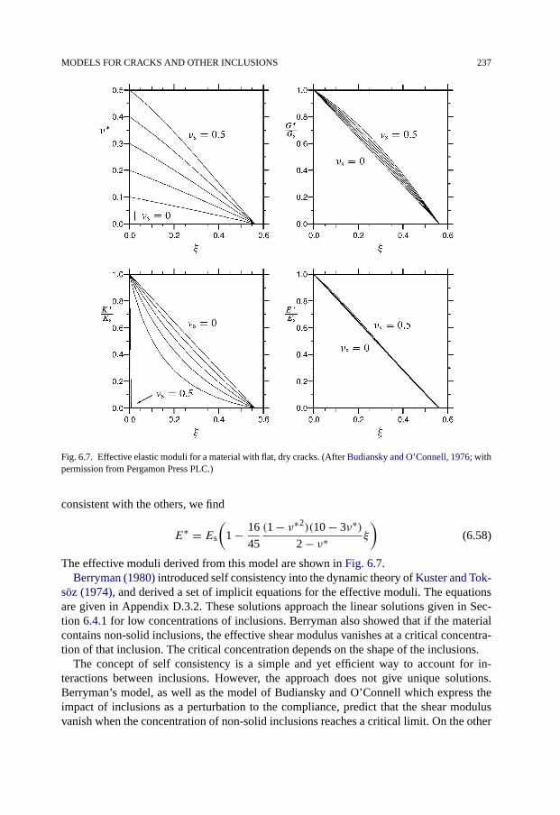
MODELS FOR CRACKS AND OTHER INCLUSIONS 237
Fig. 6.7. Effective elastic moduli for a material with flat, dry cracks. (After Budiansky and O’Connell, 1976; withpermission from Pergamon Press PLC.)
consistent with the others, we find
E∗ = Es
(1 − 16
45
(1 − ν∗2)(10 − 3ν∗)2 − ν∗ ξ
)(6.58)
The effective moduli derived from this model are shown in Fig. 6.7.Berryman (1980) introduced self consistency into the dynamic theory of Kuster and Tok-
söz (1974), and derived a set of implicit equations for the effective moduli. The equationsare given in Appendix D.3.2. These solutions approach the linear solutions given in Sec-tion 6.4.1 for low concentrations of inclusions. Berryman also showed that if the materialcontains non-solid inclusions, the effective shear modulus vanishes at a critical concentra-tion of that inclusion. The critical concentration depends on the shape of the inclusions.
The concept of self consistency is a simple and yet efficient way to account for in-teractions between inclusions. However, the approach does not give unique solutions.Berryman’s model, as well as the model of Budiansky and O’Connell which express theimpact of inclusions as a perturbation to the compliance, predict that the shear modulusvanish when the concentration of non-solid inclusions reaches a critical limit. On the other

238 ROCK MODELS
hand, a self-consistent version of Eqs. (6.29) and (6.30) predicts that the shear modulusnever vanish completely.
One attempt to get around this apparent problem was the Differential Effective Mediumtheory, initially introduced by Salganik (1973), and later studied in detail by Zimmerman(1991). This model considers the effect of introducing an infinitesimal amount of inclu-sions into a material. The equations describing the impact of the inclusions (like Eqs. (6.29)and (6.30)) can then be written on differential form, in which case it does not matterwhether the inclusions are considered as perturbations to the compliance or the stiffness.The effective moduli for a finite concentration of inclusions can be found by integration.
The Differential Effective Medium model appears to eliminate the problem of non-uniqueness, however this does not imply that this model is in general more correct thanthe others. Which of the models that gives the most accurate description of the interactionsbetween inclusions in a material depends on the actual positions of the inclusions relativeto each other. This is closely related to the statement we made at the beginning of thischapter, that the elastic properties of a composite material also depend on the geometricaldistribution of each component.
None of the models described above include any explicit information about the positionsof the inclusions relative to each other, however the fact that the models predict differentresults implies that they represent different configurations. Unfortunately, most papers pre-senting such models do not specify which configuration the model represents. Thus it maybe difficult to decide whether a given model is a suitable representation for a given mate-rial or not. We may get an indication however, by looking at an example that shows howdifferent positions of inclusions affect the interactions between them.
Consider the simple, 2-dimensional sample shown in Fig. 6.8a. By applying a force onthe sample (indicated by the arrows on the figure) and measuring the deformation, weobtain a measure of the stiffness of the material. The thin slit in the middle of the samplerepresents an inclusion similar to a crack. The presence of the crack reduces the stiffnessof the sample, as shown in Fig. 6.9.
The presence of the crack also makes the stress distribution in the sample nonuniform. Inthe areas at the side of the crack the stress level will be larger than it would have been if thecrack was not present. If new cracks are introduced in these areas, as shown in Fig. 6.8b,the stiffness of the sample will be more reduced than a simple linear extrapolation of the
Fig. 6.8. Two-dimensional material with cracks.
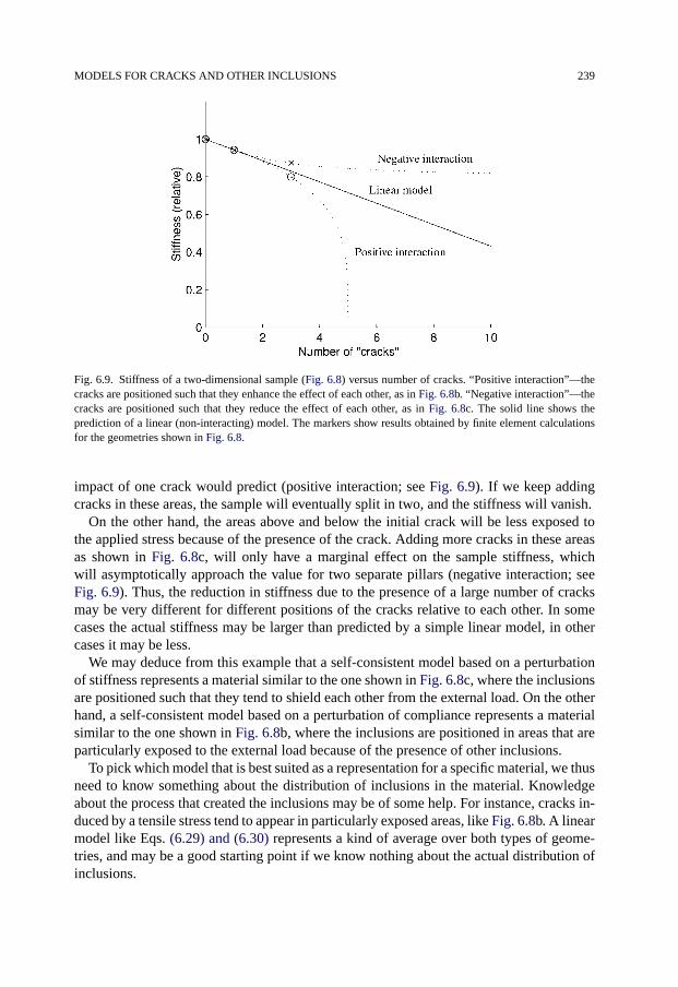
MODELS FOR CRACKS AND OTHER INCLUSIONS 239
Fig. 6.9. Stiffness of a two-dimensional sample (Fig. 6.8) versus number of cracks. “Positive interaction”—thecracks are positioned such that they enhance the effect of each other, as in Fig. 6.8b. “Negative interaction”—thecracks are positioned such that they reduce the effect of each other, as in Fig. 6.8c. The solid line shows theprediction of a linear (non-interacting) model. The markers show results obtained by finite element calculationsfor the geometries shown in Fig. 6.8.
impact of one crack would predict (positive interaction; see Fig. 6.9). If we keep addingcracks in these areas, the sample will eventually split in two, and the stiffness will vanish.
On the other hand, the areas above and below the initial crack will be less exposed tothe applied stress because of the presence of the crack. Adding more cracks in these areasas shown in Fig. 6.8c, will only have a marginal effect on the sample stiffness, whichwill asymptotically approach the value for two separate pillars (negative interaction; seeFig. 6.9). Thus, the reduction in stiffness due to the presence of a large number of cracksmay be very different for different positions of the cracks relative to each other. In somecases the actual stiffness may be larger than predicted by a simple linear model, in othercases it may be less.
We may deduce from this example that a self-consistent model based on a perturbationof stiffness represents a material similar to the one shown in Fig. 6.8c, where the inclusionsare positioned such that they tend to shield each other from the external load. On the otherhand, a self-consistent model based on a perturbation of compliance represents a materialsimilar to the one shown in Fig. 6.8b, where the inclusions are positioned in areas that areparticularly exposed to the external load because of the presence of other inclusions.
To pick which model that is best suited as a representation for a specific material, we thusneed to know something about the distribution of inclusions in the material. Knowledgeabout the process that created the inclusions may be of some help. For instance, cracks in-duced by a tensile stress tend to appear in particularly exposed areas, like Fig. 6.8b. A linearmodel like Eqs. (6.29) and (6.30) represents a kind of average over both types of geome-tries, and may be a good starting point if we know nothing about the actual distribution ofinclusions.

240 ROCK MODELS
6.4.4. Crack development in stressed rocks
Changes in the stress state of a rock may cause cracks to initiate and grow, or maybeto close, depending on the orientation and sign of the principal stresses relative to theorientation of the cracks. Thus, the number, size and predominant orientation of the cracksin a rock specimen largely reflects the stress state and stress history of the specimen.
A compressive stress acting in a direction more or less normal to a crack tends to closethe crack. The closure process depends on the shape of the crack (Mavko and Nur, 1978).Mismatch between the crack faces implies that the closure process extends over a largerange of stress values (see Section 6.5.1).
It is intuitively clear that a crack may grow if the crack faces are pulled apart with asufficiently large force. Following Griffith (1921), we shall consider crack growth inducedby tensile stress in a planar (2-dimensional) system. The specimen under considerationis a plate of thickness t , and the crack is a flat, elliptical slit of length 2a penetratingthe plate. A tensile stress σ (<0) acting normal to the crack causes the plate to deform(Fig. 6.10). The strain energy due to the crack, Wc, defined as the strain energy of thespecimen containing the crack minus the strain energy a similar specimen without a crackwould have if it was exposed to the same stress, is given as
Wc = πa2t
Eσ 2 (6.59)
where E is the Young’s modulus of the material the plate is made of. A free surface issupposed to possess a surface energy ws per unit area (associated with broken atomicbonds), thus the surface energyWs of the crack is
Ws = 4wsat (6.60)
The surface energy required to increase the crack size by a small amount 2�a is(∂Ws/∂a)�a while the strain energy available for this increase is (∂Wc/∂a)�a. Thus,the crack is unstable and will start to grow if
∂Wc
∂a� ∂Ws
∂a(6.61)
By combining Eqs. (6.59)–(6.61), we find that the crack will start to grow if the tensilestress exceeds the threshold value
T0 =√
2wsE
πa(6.62)
Crack growth implies that a increases, and consequently the threshold value decreases, ac-cording to Eq. (6.62). The situation is thus unstable, and the crack will continue to growuntil the specimen fails. Therefore, T0 represents the tensile strength of the specimen con-taining the crack. This demonstrates that pre-existing cracks have a pronounced effect onthe tensile strength of a rock.
Crack growth is often analysed in terms of stress intensity factors, which define thestress state at the tip of a crack. For a crack that is experiencing tensile stress as describedabove (also called Mode I loading) the stress field in the vicinity of the crack tip can beexpressed as

MODELS FOR CRACKS AND OTHER INCLUSIONS 241
Fig. 6.10. Crack tip coordinates.
σij = KI√2πr
f(I)ij (θ) (6.63)
The coordinates r and θ are defined in Fig. 6.10. f (I)ij (θ) are known functions of the angle θ(see for instance Anderson, 1995; see also Appendix D.3.1).KI is called the stress intensityfactor for Mode I loading, and is a measure for the stress singularity at the crack tip. It is afunction of the farfield stress σ and the crack length 2a:
KI = −yσ√πa (6.64)
where y is a dimensionless constant depending on geometry. For a slit in a plate as de-scribed above, y = 1. For a penny-shaped crack (with radius a) in an infinite medium,y = 2/π .
If KI exceeds a critical limit KIC called the fracture toughness, the crack will start togrow.
Crack growth may also occur under compressive stresses. If the stress state isanisotropic, the stress conditions at the tip of a crack oriented at a skew angle relativeto the largest principal stress may become tensile, and the crack will grow if this tensilestress exceeds a critical value. Based on such considerations, Griffith extended his theoryto general stress conditions. The resulting failure criterion is given in Section 2.3.2. As thecrack growth is assumed to be caused by local tensile stress, the tensile strength is a keyparameter also for the compressive failure criterion.
The situation is illustrated in Fig. 6.11a (also discussed in Section 1.8). Even though theinitial crack may be closed because of the compressive stress σ , the crack faces may startto slide relative to each other due to the shear stress τ if the static friction is overcome. Theorientation of the local stresses at the tip of the crack is such that the crack growth willoccur parallel to σ1, and normal to σ3, thus the so-called wing cracks will develop.
The relation between crack growth and global failure of a sample is in general morecomplicated for compressive stresses. In unconfined situations (σ3 = 0), failure typically

242 ROCK MODELS
Fig. 6.11. a. Sliding grain boundary crack thought to be of central importance for rock failure under triaxial stressconditions. b. Local failure (shear: grey lines, and tensile: black lines) caused by external loading on a 2D sample,as simulated by PFC. (This figure is a subset of Fig. 6.6.)
occurs by axial splitting, starting with opening of axial cracks from the tip of the largestpre-existing crack or flaw in the specimen. Under confinement, like in a standard triaxialtest, the wing cracks related to a suitably oriented crack will grow when the conditions arefulfilled, however these cracks will not be able to grow critically and cause macroscopicfailure on their own. Global failure is thus related to interaction and coalescence of severalcracks forming an array along the plane that eventually becomes the global failure plane.
A mathematical model was developed by Horii and Nemat-Nasser (1985), incorporatingboth shear failure and axial splitting. The input parameters to their model were:
1. The length and the orientation of the largest pre-existing crack.
2. The cohesive yield stress and average friction coefficient of the crack interface.
3. Fracture toughness for crack opening in the matrix material.
4. The confining pressure.
Clearly, such detailed knowledge of material properties may be hard to obtain in a generalsituation. The model is however useful in the sense that it can explain from microscopicprinciples the shape of the observed failure envelopes: the nonlinearity of the failure enve-lope, which is often observed in practice, is here explained by the transition from failureinitiated at the largest pre-existing flaws (at low confining pressures) to failure initiated atcritically oriented flaws (at high confining pressures). Horii and Nemat-Nasser obtaineda good fit between model prediction and experimental observations for the variation ofultimate strength with confining pressure in Westerly Granite.
Cracks of the type shown in Fig. 6.11a are not normally observed in rocks. However,local damage induced by shear stress typically involves both shear and tensile failure, asillustrated on Fig. 6.11b. The construction shown in Fig. 6.11a represents a model thatprovides a coupling between shear and tensile failure, and is as such intuitively useful.

FRACTURED ROCKS 243
The fact that the irregular microstructure of a granular material makes this coupling morecomplex is not surprising.
6.5. Fractured rocks
Most rocks that we see in nature appear to be fractured masses rather than intact, solidmaterials. We may also expect fracture systems to penetrate the formations in the under-ground. This may be the case on many length scales, from major faults on a scale largerthan reservoirs, to microfractures seen in a core plug. An example is the fractured chalkreservoir of the Ekofisk field in the North Sea. Here the fractures are responsible for themain part of the permeability. It is therefore of importance to be able to identify as early aspossible the existence of such fracture systems in reservoirs, and to find the directions of thefractures. It may also be important (with reference to e.g. the Ekofisk case and prediction ofreservoir compaction during depletion) to know how much the fractures contribute to theoverall mechanical behaviour of a rock mass. In this section, we shall discuss how fractured(or jointed) rocks behave mechanically, starting with the mechanical behaviour of a singlefracture (or joint). The terms fracture and joint will be used synonymously throughout thissection, although there is a difference from the geological viewpoint (see Chapter 3). Withthe mathematical idealizations presented here, they can however be treated within the sameframework.
6.5.1. Single fractures
Previously in this chapter we considered the effect of cracks on rock mechanical andacoustical properties. By a crack we meant an open void of a given, idealized shape (spher-oid, penny-shaped) which acts as a local discontinuity. In practice however, a crack in aporous rock does not have an ideal geometry. Fracture surfaces are rough, and they maytouch each other at some points.
In general, the complete stress–strain behaviour of a fracture relates normal displace-ment (δwF) to normal stress (δσ ) on the fracture, and shear displacement (δuF) to shearstress (δτ ) along the fracture interface. We may define δwF such that δwF = wF
o − wF,where wF
o is the initial fracture opening and wF the actual fracture opening. The frac-ture is closed when δwF = wF
o − wFmax, where wF
max is the fracture opening at maxi-mum closure. The stress-displacement relation can be written as (see e.g. Bandis, 1990;Saeb and Amadei, 1992): (
δσ
δτ
)=(Knn KntKtn Ktt
)(δwF
δuF
)(6.65)
where the indices in the fracture stiffness tensor (Kij ) denote n for normal and t for tan-gential. Observed deformational behaviour is highly nonlinear for increasing compressiveload, while unloading causes large hysteresis and inelastic behaviour. Under tension, theassociated fracture stiffness is close to zero. Under shearing, the stress–strain relation may

244 ROCK MODELS
exhibit “plastic” as well as “brittle” behaviour, depending on the fracture size. On an empir-ical basis, the following type of expression forKnn has been proposed for joints (Goodman,1974):
Knn = Konn
[Konnw
Fmax + σ
KonnwFmax
]2
(6.66)
Konn is the initial normal stiffness of the joint. The appearance ofKonn andwFmax in Eq. (6.66)
implies that stress history dependence may be accounted for in the joint stiffness.The shear stress dependence of Ktt has been described by a relationship of the type
Ktt = Kott[
1 − τ
τs
]2
(6.67)
Kott is the initial shear stiffness and τs is the asymptotic value for τ at large shear displace-ments. The off-diagonal terms in the stiffness tensor (Eq. (6.65)) account for couplingbetween shear and normal behaviour due to dilatancy. A mathematical model incorporat-ing these terms has been presented by Saeb and Amadei (1992).
Given the fracture stiffness parameters (Eq. (6.65)), one may calculate the frequencydependent time delay, and the sound transmission and reflection coefficients caused by asingle fracture (Pyrak-Nolte et al., 1990). The calculations show an increased damping ofhigh frequencies in a transmitted acoustic signal when the fracture stiffness is reduced. Theeffect of viscosity in a fluid filling the fracture was also analysed, showing increased highfrequency damping with decreasing viscosity.
From a microscopic viewpoint, closure of a fracture can be described mathematicallyby parameters depending on the roughness characteristics of the fracture surfaces. Brownand Scholz (1986) derived a relationship where they accounted for the following fracturesurface parameters: a distribution function for asperity heights, the number of local maximaper unit area, the effective radius of curvature of the asperities, the fracture width at zerostress, and a correction factor for tangential stress contributions. For a particular choice ofthe asperity height distribution function, the strain vs. stress relationship can be written
δεF = A+ B ln δσ (6.68)
where δεF = δwF/wF is the fracture strain. A and B are functions of the fracture surfaceparameters described above. The joint closure is thus a highly nonlinear function of thenormal stress.
Carlson and Gangi (1985) modelled a fracture using a “bed of nails” concept (seeFig. 6.12). A set of cylindrical rods of different lengths Li are attached to the crack walls,simulating a distribution of asperities. The rods are assumed to act as springs. As the nor-mal stress is increased across the fracture, the walls of the fracture move closer and moreand more rods come in contact with the opposite wall. Therefore, the stiffness is increasedas the strain increases, similar to Eq. (6.68). For a through-going fracture, the fracture straincan be expressed as:
δεF =(δσ
σc
)m(6.69)

FRACTURED ROCKS 245
Fig. 6.12. A natural fracture (above) and the mechanically and hydraulically equivalent “bed of nails” fracturemodel, introduced by Carlson and Gangi (1985).
where σc is the stress required to close the crack. The exponent m (�1) is given by thedistribution of rod lengths. The fraction n of rods in contact is:
n = (δεF)(1−m)/m (6.70)
m is thought to be constant throughout a given experiment. The value m = 1 correspondsto a closed crack with perfectly smooth surfaces, while m = 0 corresponds to and opencrack with smooth surfaces.
Carlson and Gangi modified the expression (6.69) for the case of an isolated crack in asolid matrix, giving
δεF =(δσ + σoσc
)m(6.71)
Here σo is equivalent to an initial stress (associated with the tensile strength of the ma-terial). The expressions can be used quantitatively to evaluate the stress dependence ofP-wave velocities in cracked media, leading to a relationship of the following form whichis applicable for high porosity sedimentary rocks:
vp = vop(
1 + σ
σo
)(1−m)/2(6.72)
In Section 6.3 we found for a model consisting of spheres in contact (where the contactsbehave according to Hertzian theory) that the sound velocity would increase with stressaccording to a power law behaviour, with exponent 1/6. This corresponds to m = 2/3(and σo → 0) in Carlson and Gangi’s theory. In many rocks, exponents <1/6 have beenobserved, indicating that m is closer to 1 (Carlson and Gangi, 1985).
246 ROCK MODELS
The shear strength of a joint or fracture is often expressed in terms of a Mohr–Coulombcriterion with zero cohesion (see Section 2.3.1):
τ = σ tanϕ (6.73)
Based on laboratory experiments with more than 200 artificial tensile fractures, Barton andBandis (1990) found that the friction angle ϕ can be expressed as
ϕ = JRC logJCS
σ+ ϕr (6.74)
JRC is called the joint roughness coefficient, while JCS is the wall strength, identified asthe unconfined compressive strength of the intact rock. ϕr is the residual angle of friction(≈30°, see Chapter 2). JRC can be found from simple shear tests, and has typically a valuearound 20 for a rough joint without steps. It is a scale dependent factor, and a scalingrelation has been established (see Barton and Bandis, 1990), giving JRC as a function ofroughness amplitude over profile length.
6.5.2. Rocks with many fractures
A rock mass normally contains a system of fractures. Such a system is specified in termsof fracture orientation, fracture width, length and spacing. While the orientation is mainlydetermined by the stress state at the time the fracture was formed, the remaining parametersare primarily given by the lithology. These parameters are necessary in order to quantify theflow of fluids in a fractured reservoir. In nature, there is of course a distribution of fractureparameters. Many investigators have claimed that fracture size distributions observed inoutcrops tend to be scale invariant (fractal).
Several Finite Element and Finite Difference codes have been developed in order toanalyse the mechanical behaviour of discontinuous media. Standard input parameters area set of fracture stiffnesses and the elastic moduli of the intact material. We shall not de-scribe any of these methods here, but rather discuss one analytical model for the elasticbehaviour of fractured rocks. This theory was developed by White (1983). Consider acube (Fig. 6.13) consisting of fractured blocks. Each block is spot-welded to the neigh-bouring blocks (Fig. 6.14). The average dimensions of a block are Lx , Ly and Lz, andthe number of contact points per unit area Nx , Ny and Nz, respectively. The spot-weldedcontacts are assumed to be circles of average diameters Dx , Dy and Dz. The elastic prop-erties of the fractured cube is derived based on the Hertz–Mindlin approach introducedin Section 6.3. For the effective contact radius b (Eq. (6.18)) we here use the parameterΣxb = (DxNxLyLz)/2 for a surface normal to x, and corresponding expressions for yand z. The compressive strain εx due to a force σx has two contributions:
Firstly, the deformation at the fracture planes normal to x causes a strain (see Eq. (6.21))
εfx = 1 − νs
2GsΣxb
LyLz
Lxσx (6.75)
Secondly, the deformation of the solid blocks gives a strain
εsx = 1
(λs + 2Gs)(1 − ax)σx (6.76)
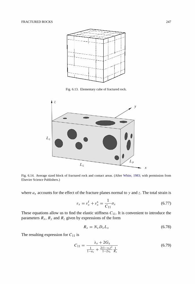
FRACTURED ROCKS 247
Fig. 6.13. Elementary cube of fractured rock.
Fig. 6.14. Average sized block of fractured rock and contact areas. (After White, 1983; with permission fromElsevier Science Publishers.)
where ax accounts for the effect of the fracture planes normal to y and z. The total strain is
εx = εfx + εs
x = 1
C11σx (6.77)
These equations allow us to find the elastic stiffness C11. It is convenient to introduce theparameters Rx , Ry and Rz given by expressions of the form
Rx = NxDxLx (6.78)
The resulting expression for C11 is
C11 = λs + 2Gs
11−ax + 2(1−νs)2
1−2νs
1Rx
(6.79)
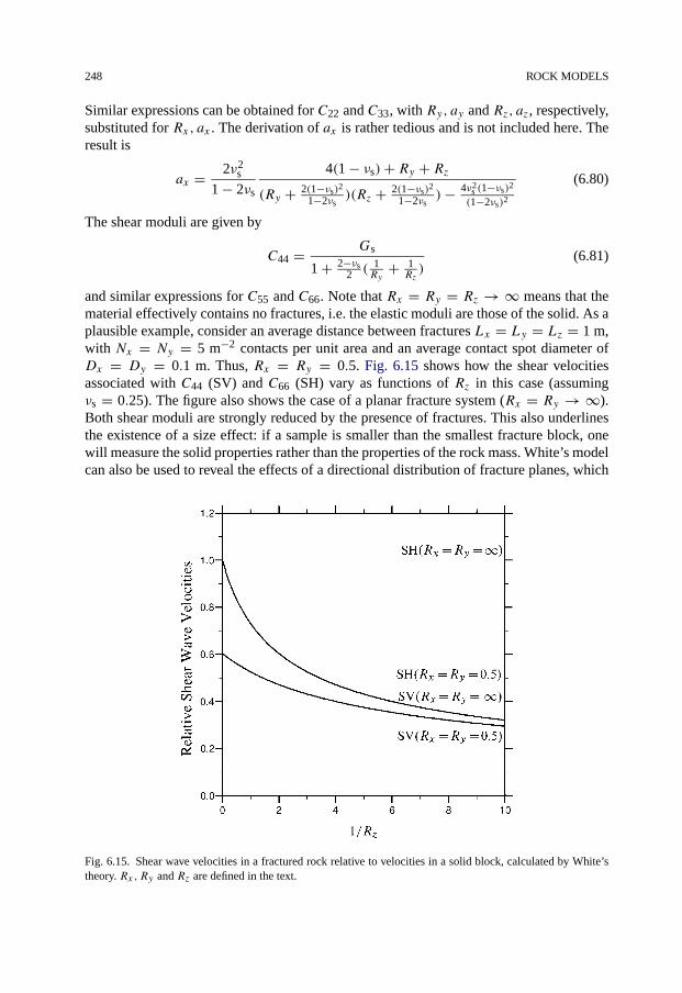
248 ROCK MODELS
Similar expressions can be obtained for C22 and C33, with Ry, ay and Rz, az, respectively,substituted for Rx, ax . The derivation of ax is rather tedious and is not included here. Theresult is
ax = 2ν2s
1 − 2νs
4(1 − νs)+ Ry + Rz(Ry + 2(1−νs)2
1−2νs)(Rz + 2(1−νs)2
1−2νs)− 4ν2
s (1−νs)2
(1−2νs)2
(6.80)
The shear moduli are given by
C44 = Gs
1 + 2−νs2 ( 1
Ry+ 1Rz)
(6.81)
and similar expressions for C55 and C66. Note that Rx = Ry = Rz → ∞ means that thematerial effectively contains no fractures, i.e. the elastic moduli are those of the solid. As aplausible example, consider an average distance between fractures Lx = Ly = Lz = 1 m,with Nx = Ny = 5 m−2 contacts per unit area and an average contact spot diameter ofDx = Dy = 0.1 m. Thus, Rx = Ry = 0.5. Fig. 6.15 shows how the shear velocitiesassociated with C44 (SV) and C66 (SH) vary as functions of Rz in this case (assumingνs = 0.25). The figure also shows the case of a planar fracture system (Rx = Ry → ∞).Both shear moduli are strongly reduced by the presence of fractures. This also underlinesthe existence of a size effect: if a sample is smaller than the smallest fracture block, onewill measure the solid properties rather than the properties of the rock mass. White’s modelcan also be used to reveal the effects of a directional distribution of fracture planes, which
Fig. 6.15. Shear wave velocities in a fractured rock relative to velocities in a solid block, calculated by White’stheory. Rx,Ry and Rz are defined in the text.

REFERENCES 249
give rise to a significant anisotropy. Observations of seismic/VSP anisotropy can thus beused to characterize fractured reservoirs.
References
Anderson, T.L. (1995). Fracture Mechanics. Fundamentals and Applications, second ed. CRC Press, Boca Raton.Bachrach, R., Dvorkin, J., Nur, A. (1998). “High-resolution shallow-seismic experiments in sand, Part II: Veloc-
ities in shallow unconsolidated sand”. Geophysics 63, 1234–1240.Backus, G.E. (1962). “Long-wave elastic anisotropy produced by horizontal layering”. J. Geophys. Res. 67,
4427–4440.Bandis, S.C. (1990). “Mechanical properties of rock joints”. In: Barton, N., Stephansson, O. (Eds.), Rock Joints.
Balkema, Rotterdam, pp. 581–594.Barton, N., Bandis, S.C. (1990). “Review of predictive capabilities of JRC-JCS model in engineering practice”.
In: Barton, N., Stephansson, O. (Eds.), Rock Joints. Balkema, Rotterdam, pp. 603–610.Berryman, J.G. (1980). “Long-wavelength propagation in composite elastic media. II. Ellipsoidal inclusions”.
J. Acoust. Soc. Am. 68, 1820–1831.Brandt, H. (1955). “A Study of the speed of sound in porous granular media”. J. Appl. Mech. 22, 479–486.Brown, S.R., Scholz, C.H. (1986). “Closure of rock joints”. J. Geophys. Res. 90, 8675–8684.Budiansky, B., O’Connell, R.J. (1976). “Elastic moduli of a cracked solid”. Int. J. Solids Structures 12, 81–97.Carlson, R.L., Gangi, A.F. (1985). “Effect of cracks on the pressure dependence of P-wave velocities in crystalline
rocks”. J. Geophys. Res. 90 (B10), 8675–8684.Cundall, P.A., Strack, O.D.L. (1979). “A discrete numerical model for granular assemblies”. Geotechnique 29,
47–65.Cundall, P.A. (2001). “A discontinuous future for numerical modelling in geomechanics?” Proc. Inst. Civil Eng.
Geotec. Eng. 149, 41–47.Digby, P.J. (1981). “The effective elastic moduli of porous granular rocks”. J. Appl. Mech. 48, 803–808.Domenico, S.N. (1977). “Elastic properties of unconsolidated porous sand reservoirs”. Geophysics 42, 1339–
1368.Dvorkin, J., Mavko, G., Nur, A. (1991). “The effect of cementation on the elastic properties of granular materials”.
Mech. Mater. 12, 207–217.Eshelby, J.D. (1957). “The determination of the elastic field of an ellipsoidal inclusion, and related problems”.
Proc. Roy. Soc. London Ser. A 241, 376–396.Garbin, H.D., Knopoff, L. (1973). “The compressional modulus of a material permeated by a random distribution
of circular cracks”. Quart. Appl. Math. 30, 453–464.Garbin, H.D., Knopoff, L. (1975). “Elastic moduli of a medium with liquid-filled cracks”. Quart. Appl. Math. 33,
301–303.Goodman, R.E. (1974). “The mechanical properties of joints”. In: Proc. 3rd Int. Congr. ISRM, Denver Co.,
vol. 1A, pp. 127–140.Griffith, A.A. (1921). “The phenomena of rupture and flow in solids”. Phil. Trans. Roy. Soc. A 221, 163–198.Han, D.-H., Batzle, M. (2006). “Velocities of deepwater reservoir sands”. The Leading Edge 25, 460–466.Hashin, Z., Shtrikman, S. (1963). “A variational approach to the elastic behaviour of multiphase materials”.
J. Mech. Solids 11, 127–140.Hazzard, J.F., Young, R.P. (2000). “Simulating acoustic emissions in bonded-particle models of rock”. Int. J.
Rock Mech. & Min. Sci. 37, 867–872.Helbig, K. (1994). Foundation of Anisotropy for Exploration Geophysicists. Pergamon, Oxford.Hertz, H. (1882). “Über die Berührung fester elastische Körper”. J. reine und angewandte Mathematik 92, 156–
171.Hill, R. (1952). “The elastic behavior of crystalline aggregate”. Proc. Physical Soc. London A65, 349–354.Horii, H., Nemat-Nasser, S. (1985). “Compression-induced microcrack growth in brittle solids: Axial splitting
and shear failure”. J. Geophys. Res. B90, 3105–3125.Hovem, J.M. (1995). “Acoustic waves in finely layered media”. Geophysics 60, 1217–1221.
250 ROCK MODELS
Hudson, J.A. (1981). “Wave speeds and attenuation of elastic waves in material containing cracks”. Geophys.J. R. Astr. Soc. 64, 133–150.
Kuster, G.T., Toksöz, M.N. (1974). “Velocity and attenuation of seismic waves in two-phase media: Part 1. The-oretical formulations”. Geophysics 39, 587–606.
Li, L., Holt, R.M. (2002). “Particle scale reservoir mechanics”. Oil & Gas Sci. Technol. Rev. IFP 57, 525–538.Mackenzie, J.K. (1950). “The elastic constants of a solid containing spherical holes”. Proc. Phys. Soc. B 63, 2–11.Makse, H.A., Gland, N., Johnson, D.L., Schwartz, L. (2001). “The apparent failure of effective medium theory in
granular materials”. Phys. Chem. Earth (A) 26, 107–111.Marion, D.P., Coudin, P. (1992). “From ray to effective medium theories in stratified media: An experimental
study”. SEG Expanded Abstracts 11, 1341–1343.Marion, D., Nur, A. (1991). “Pore-filling material and its effect on velocity in rocks”. Geophysics 56, 225–230.Mavko, G., Mukerji, T., Dvorkin, J. (1998). The Rock Physics Handbook: Tools for Seismic Analysis in Porous
Media. Cambridge University Press, New York.Mavko, G., Nur, A. (1978). “The effect of nonelliptical cracks on the compressibility of rocks”. J. Geophys.
Res. 83, 4459–4468.Mindlin, R.D. (1949). “Compliance of elastic bodies in contact”. J. Appl. Mech. 16, 259–268.Murphy, W., Reischer, A., Hsu, K. (1993). “Modulus decomposition of compressional and shear velocities in
sand bodies”. Geophysics 58, 227–239.Nur, A., Marion, D., Yin, H. (1991). “Wave velocities in sediments”. In: Hovem, J.M., Richardson, M.D., Stoll,
R.D. (Eds.), Shear Waves in Marine Sediments. Kluwer Academic Publishers, Dordrecht, The Netherlands,pp. 131–140.
Nur, A., Mavko, G., Dvorkin, J., Gal, D. (1995). “Critical porosity: The key to relating physical properties toporosity in rocks”. SEG Expanded Abstracts 11, 878–880.
Potyondy, D.O., Cundall, P.A. (2004). “A bonded-particle model for rock”. Int. J. Rock Mech. Min. Sci. 41,1329–1364.
Pyrak-Nolte, L.J., Myer, L.R., Cook, N.G.W. (1990). “Transmission of seismic waves across single natural frac-tures”. J. Geophys. Res. 95 (B6), 8617–8638.
Radjai, F., Jean, M., Moreau, J.-J., Roux, S. (1996). “Force distributions in dense two-dimensional granularsystems”. Phys. Rev. Lett. 77, 274–277.
Rathore, J.S., Fjaer, E., Holt, R.M., Renlie, L. (1995). “P- and S-wave anisotropy of a synthetic sandstone withcontrolled crack geometry”. Geophys. Pros. 43, 711–728.
Saeb, S., Amadei, B. (1992). “Modeling rock joints under shear and normal loading”. Int. J. Rock Mech. Min.Sci. & Geomech. Abstr. 29, 267–278.
Salganik, R.L. (1973). “Mechanics of bodies with many cracks”. Mech. Solids 8, 135–143.Sayers, C.M., Kachanov, M. (1995). “Microcrack-induced elastic wave anisotropy of brittle rocks”. J. Geophys.
Res. 100, 4149–4156.Schwartz, L.M. (1984). “Acoustic properties of porous systems: II. Microscopic description”. In: Johnson, D.L.,
Sen, P.N. (Eds.), Physics and Chemistry of Porous Media. Am. Inst. Phys., New York, pp. 105–118.Thomsen, L. (1985). “Biot-consistent elastic moduli of porous rocks: Low-frequency limit”. Geophysics 50,
2797–2807.Thomsen, L. (1995). “Elastic anisotropy due to aligned cracks in porous rock”. Geophys. Pros. 43, 805–829.Walsh, J.B. (1965a). “The effect of cracks on the compressibility of rock”. J. Geophys. Res. 70, 381–389.Walsh, J.B. (1965b). “The effect of cracks on the uniaxial elastic compression of rocks”. J. Geophys. Res. 70,
399–441.Walton, K. (1987). “The effective elastic moduli of a random packing of spheres”. J. Mech. Phys. Solids 35,
213–226.Wang, Z., Nur, A. (1992). “Elastic wave velocities in porous media: A theoretical recipe”. In: Wang, Z., Nur,
A. (Eds.), Seismic and Acoustic Velocities in Reservoir Rocks. In: SEG Geophysics Reprint Series, vol. 10.Society of Exploration Geophysicists, Tulsa, Oklahoma, pp. 1–35.
Watt, P., Davies, G.F., O’Connell, R. (1976). “The elastic properties of composite materials”. Rev. Geophys.Space Phys. 14, 541–563.
White, J.E. (1983). Underground Sound. Elsevier, New York.Williams, J.R., Rege, N. (1997). “Coherent vortex structures in deforming granular materials”. Mech. Cohesive
Frictional Mater. 2, 223–236.Zimmerman, R.W. (1991). Compressibility of Sandstones. Elsevier Science Publishers, B.V., The Netherlands.
251
Chapter 7
Mechanical properties and stress data from laboratoryanalysis
Evaluation of in situ rock mechanical behaviour requires relevant input data: What is thestress state and the pore pressure at the depth of interest? What are the elastic moduli andthe strength parameters? Can we expect creep or other types of non-elastic behaviour totake place?
Our main data sources in order to answer these questions are core material and datarecorded in the field (measurements while drilling, wireline logs, seismic data and vari-ous well tests). The logs provide data recorded continuously vs. depth, but do not measuredirectly the parameters that are needed for a rock mechanical analysis. For instance, rockstrength can not be measured from wireline logs. Strength estimates may, however, begiven if a proper interpretation procedure is applied. Field measurements of rock mechan-ical parameters are discussed in Chapter 8.
In this chapter we shall discuss rock mechanical core analysis. Cores provide a possibil-ity for direct measurement of e.g. rock strength parameters and static elastic properties. Weshall start by looking at the rocks to be tested: the cores in the laboratory may not be fullyrepresentative of the formation we intend to study. They may also have been altered duringcoring and subsequent handling. Some of these problems can not be solved, others canbe overcome by proper sample preparation methods, test procedures and correction proce-dures. On the other hand, if proper preparation procedures are not applied, severe errorsin the test results may be introduced. These factors will be discussed in more detail below(Section 7.1). We shall then discuss the laboratory equipment and measurement techniques(Section 7.2) applied in rock mechanical testing, including also acoustic measurements.
A rock mechanical core analysis has to be designed according to the purpose of the in-vestigation. If the objective is to predict reservoir compaction, then the tests and testingprocedures may not be the same as for instance in a borehole stability study. Considerationalso has to be given to the rock type which is going to be tested. Shales require both spe-cial preparation procedures and special test procedures. In Section 7.3 we shall describerelevant test procedures which are applied in rock mechanical testing and give some rec-ommendations for test interpretation.
The literature reports numerous attempts to determine in situ stresses from laboratorytesting of core samples. The most relevant test methods will be discussed in Section 7.4.
In some cases it may be useful to perform a set of simpler measurements which canbe used as indicators of rock strength and stiffness. This can provide information at lesscost and at less material consumption. The latter is particularly relevant if the core is ina poor state and larger test plugs can not be prepared. If performed at the rig-site, resultsmay be available closer to real-time. Some of these so-called index tests are described inSection 7.5.

252 MECHANICAL PROPERTIES AND STRESS DATA FROM LABORATORY ANALYSIS
7.1. Core samples for rock mechanical laboratory analysis
7.1.1. Core representativeness and size effects
As we stated above, cores are our only possibility of obtaining direct measurements ofrock strength and static mechanical parameters. Cores are, however, only available fromdiscrete levels, and may only be representative of the formations in or near the boreholeitself. The limited availability of core material may cause large uncertainty in the results.Normally, cores are taken mainly or only in the reservoir, while the mechanical behaviourof the overlying strata may be of large importance for drilling problems, subsidence andrepeated seismic interpretation during reservoir depletion.
A core plug used in standard mechanical testing has a diameter of 1–2.5′′. Only in spe-cial cases will larger (4–5′′) or smaller (0.1–1′′) samples be used. This means that thetested cores may, in case of inhomogeneities, not be representative of the interval underinvestigation. For instance, in a fractured zone, the rocks to be tested are normally takenfrom the intact parts. One has to recall that the elastic behaviour of the fractured rock masscan be very different from that of the intact rock (Chapter 6). This means that if the prop-erties which are important are those of the rock mass, then the analysis will be biased. Thesamples should then, if possible, be taken so that fractures are contained in them. If, on theother hand, the data will be applied in e.g. sand prediction analysis, then the fractures maynot be relevant, and the samples should be taken from the intact parts of the rock.
The discussion above shows that the size of the sample may be important. If the fracturesoccur on a scale of several metres, then it is very unlikely that tests on small samples willprovide reliable data. Fractures and cracks may, however, occur on several length scales,down to and below the sample size. Statistically, a larger sample is expected to containlarger cracks than a small sample. Qualitatively, this would lead to an increased strengthwith decreasing sample size, since the strength decreases with the size of the largest crack.This hypothesis is often valid in experiments (see e.g. Vutukuri et al., 1974), but is notgenerally confirmed. In fact, experiments with sedimentary rocks some times may show anopposite trend (strength increases with sample size). Even though the size effect problemhas been focused since the advent of material property testing in the 18th century (see theinteresting historical overview in Hudson et al., 1972), it still remains unsolved.
Clearly, in granular rocks, there is a lower limit to the sample size given by the require-ment that the sample should contain a large number of grains. In the procedures suggestedby the ISRM (International Society for Rock Mechanics) (Brown (Ed.), 1981), it is statedthat the diameter of a specimen prepared for rock mechanical testing should be at least tentimes the diameter of the largest grain in the rock.
7.1.2. Core alteration
A rock specimen is most likely altered when taken from in situ to laboratory conditions.In situ it may have been at a depth of one or more kilometres, at an ambient temperatureof say 50–150 °C, and in chemical equilibrium with its own pore fluid. When cored, it isbrought to atmospheric conditions in terms of stress, pore pressure and temperature. It is

CORE SAMPLES FOR ROCK MECHANICAL LABORATORY ANALYSIS 253
Fig. 7.1. Schematic illustration of the effective stress field alteration experienced during coring of a vertical corein a normally stressed rock. (After Holt et al., 2000; with permission from Elsevier.)
also in contact with some chemically active/inactive drilling mud, and mud filtrate maypenetrate the core. Thus the main core alteration mechanisms are stress release, pore pres-sure release (especially in low-permeability rocks), thermal effects and chemical effectsdue to fluid exposure. The cores may be further damaged by the action of the drill bit, andby subsequent improper handling and storage (see Section 7.1.3).
Stress release probably has the most severe effect on rock mechanical properties. Fig. 7.1shows schematically the effective stress field alterations experienced by a core during thecoring process. This is under the assumption of a vertical well drilled in an initial stress fieldwith a vertical stress and isotropic horizontal stresses. As the core is drilled, the verticalstress is reduced first, while the horizontal stress is reduced as the core enters the corebarrel. Thus there is a period where the horizontal stress may be significantly larger thanthe vertical stress. This may result in yielding and/or failure of the core. The amount ofcore recovery and the size of the recovered pieces are thus qualitative measures of the rockstrength. The weaker the rock, the less intact core material will be recovered. Macroscopicfailure may also occur as tensile failure (core discing). This has been used to evaluate inparticular the ratio between horizontal and vertical principal stress components (Maury etal., 1988).
Laboratory testing of rock alteration due to stress release has shown an effect on themechanical properties of sandstone (Holt et al., 2000), resulting in a reduced uniaxialcompressive strength, reduced stiffness, reduced acoustic velocities and increased stresssensitivity.
Shale may have nanoDarcy or lower permeability (Section 3.4.3) which means that porepressure equilibrium will not be maintained when the core is retrieved from depth. Thus,tensile failure is very likely to occur, either macroscopically, or on a microscopic level.This process, as well as volumetric expansion during coring and retrieval, causes the shalecore to be incompletely saturated when reaching the surface. As discussed further below
254 MECHANICAL PROPERTIES AND STRESS DATA FROM LABORATORY ANALYSIS
(see Section 7.1.4), this may affect shale properties significantly, and needs to be accountedfor in sample preparation and conditioning.
7.1.3. Core handling
We have seen above that cores may be disturbed by the coring process itself. Further treat-ment on the rig, during transport, during storage and prior to testing in the laboratory mayalso be critically important to the outcome of the rock mechanical analysis. There are twomajor problems which are relevant for sedimentary rocks: one is the fact that they can bemechanically weak, and in some cases completely unconsolidated. The other is that theymay be sensitive to the exposure to or loss of fluids.
For poorly consolidated sandstones, samples may not be kept intact unless they arefrozen immediately after coring, and kept so until mounted in the triaxial cell. Freezingshould, however, be avoided if possible, since it may induce permanent changes in therock. This is in particular the case if water is present. Since clay minerals contain boundwater, freezing may cause disintegration and redistribution of these minerals. If the clayminerals act as cement, this will clearly affect the mechanical properties.
For sandstones (in particular clay-rich sandstones) the rock mechanical properties arealso found to depend on moisture content. The general observation is that (see e.g. Colbackand Wiid, 1965) uniaxial compressive strength decreases with increasing moisture content.Colback and Wiid relate this to a change in the surface energy.
It has been observed by the authors of this book that a sandstone stored in normal labo-ratory atmosphere for one year after sampling increased its strength by a factor of two dueto drying. This was an effect of smectite in the sandstone which contributed significantlyto the cementation when dried.
Shales contain both bound water and free water and should therefore never be frozen.Shales are also extremely sensitive to contact with wetting fluids like water, or to loss ofwater from the pores. This means that the samples should be preserved as soon as the coreis retrieved, so that the natural water content is not reduced. Dehydration may cause themto disintegrate completely within a matter of minutes. In other cases, depending on themicrostructure and the shale composition, dehydration may lead to strengthening of thematerial.
Shale cores intended for rock mechanical tests should be sealed immediately after cor-ing, for instance by wrapping them in a plastic film with further protection like aluminiumand wax on the outside. If this packing process can not be performed immediately after thecore has been landed on the rig, it is still important to ensure that water transport effectsare avoided. One alternative is to cut the core and the core liner in appropriate lengths(typically one metre), wipe the mud from the core surface (especially if water-based mudhas been used), fill the annulus between the core and the liner with an inert fluid like oiland then seal the liner. In all cases it is essential to minimize the period when the core isexposed to air.
Shales should not be contacted with water or any other fluid which wets the shale. Evenif the water is assumed to completely match the chemistry of the pore water, large capillarysuction pressures may be induced because the shale core is no longer 100% saturated when
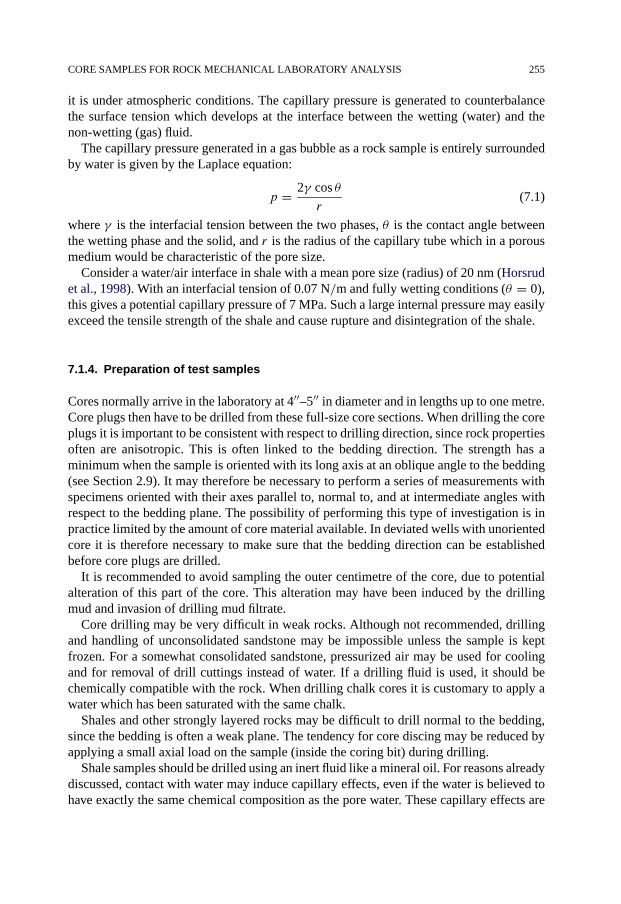
CORE SAMPLES FOR ROCK MECHANICAL LABORATORY ANALYSIS 255
it is under atmospheric conditions. The capillary pressure is generated to counterbalancethe surface tension which develops at the interface between the wetting (water) and thenon-wetting (gas) fluid.
The capillary pressure generated in a gas bubble as a rock sample is entirely surroundedby water is given by the Laplace equation:
p = 2γ cos θ
r(7.1)
where γ is the interfacial tension between the two phases, θ is the contact angle betweenthe wetting phase and the solid, and r is the radius of the capillary tube which in a porousmedium would be characteristic of the pore size.
Consider a water/air interface in shale with a mean pore size (radius) of 20 nm (Horsrudet al., 1998). With an interfacial tension of 0.07 N/m and fully wetting conditions (θ = 0),this gives a potential capillary pressure of 7 MPa. Such a large internal pressure may easilyexceed the tensile strength of the shale and cause rupture and disintegration of the shale.
7.1.4. Preparation of test samples
Cores normally arrive in the laboratory at 4′′–5′′ in diameter and in lengths up to one metre.Core plugs then have to be drilled from these full-size core sections. When drilling the coreplugs it is important to be consistent with respect to drilling direction, since rock propertiesoften are anisotropic. This is often linked to the bedding direction. The strength has aminimum when the sample is oriented with its long axis at an oblique angle to the bedding(see Section 2.9). It may therefore be necessary to perform a series of measurements withspecimens oriented with their axes parallel to, normal to, and at intermediate angles withrespect to the bedding plane. The possibility of performing this type of investigation is inpractice limited by the amount of core material available. In deviated wells with unorientedcore it is therefore necessary to make sure that the bedding direction can be establishedbefore core plugs are drilled.
It is recommended to avoid sampling the outer centimetre of the core, due to potentialalteration of this part of the core. This alteration may have been induced by the drillingmud and invasion of drilling mud filtrate.
Core drilling may be very difficult in weak rocks. Although not recommended, drillingand handling of unconsolidated sandstone may be impossible unless the sample is keptfrozen. For a somewhat consolidated sandstone, pressurized air may be used for coolingand for removal of drill cuttings instead of water. If a drilling fluid is used, it should bechemically compatible with the rock. When drilling chalk cores it is customary to apply awater which has been saturated with the same chalk.
Shales and other strongly layered rocks may be difficult to drill normal to the bedding,since the bedding is often a weak plane. The tendency for core discing may be reduced byapplying a small axial load on the sample (inside the coring bit) during drilling.
Shale samples should be drilled using an inert fluid like a mineral oil. For reasons alreadydiscussed, contact with water may induce capillary effects, even if the water is believed tohave exactly the same chemical composition as the pore water. These capillary effects are

256 MECHANICAL PROPERTIES AND STRESS DATA FROM LABORATORY ANALYSIS
due to incomplete saturation of the shale and the presence of air in the sample. It has beenproposed to remedy this by resaturating the shale (e.g. Schmitt et al., 1994). This is notdone by immersion, but in a controlled humidity atmosphere where water vapour con-denses in the pores. To avoid trapped air it is preferable to have a continuous gas phasebefore starting resaturation. This may require a first stage with drying of the sample. How-ever, it has been strongly argued that such a process may change the structure and propertiesof the shale (Santos et al., 1996). Therefore, attempts to resaturate shale should be avoided.The best approach is to make sure that the shale is well preserved, so that sufficient resat-uration can be obtained by loading the sample prior to or during testing (Horsrud et al.,1998). The water content of the rock should always be measured before rock mechanicaltests are performed.
The significance of sample saturation is well known from soil mechanics. In rocks withsmall pores (shale, chalk), the presence of air may cause significant overestimation of themechanical properties of the rock (Schmitt et al., 1994; Papamichos et al., 1997). As a firstorder approximation one may express this as a generalized effective stress:
σ ′′ = σ − pgas + Sw(pgas − pwater) (7.2)
where Sw is the water saturation and pgas − pwater is the pore-water capillary suction. Thecapillary suction effect may then be compared with the effect of a confining stress. Tosome extent this is consistent with the observations of increased strength and stiffness withreduced saturation.
Reservoir rocks (sandstone, chalk) may also be sensitive to the fluid in the pores. A dryrock is usually stronger than a fluid saturated rock. When measuring petrophysical prop-erties of sandstone it is common procedure to clean the sample and then resaturate it withthe relevant fluid(s). When doing rock mechanical testing of weak sandstone this is notrecommended, since the cleaning process may disturb the cementation of the rock. Weaksandstones should be well preserved and tested with the native fluid content.
Another important observation relates to the high porosity North Sea chalks. Laboratorytesting has shown that oil saturated chalk samples are significantly stronger than water sat-urated samples (Andersen, 1995). It has been suggested that this effect could be explainedbe capillary forces which are caused by the irreducible water still present in oil saturatedchalk. However, it has been shown that the chalk is strengthened (both in compression andtension) also when saturated with methanol which is fully miscible with water (Risnes andFlaageng, 1999). Thus there must be other mechanisms present which have not yet beenexplained.
The ISRM (International Society for Rock Mechanics) standards (Brown (Ed.), 1981,and revision by Kovari et al., 1983) require that specimens intended for standard rock me-chanical tests are right, circular cylinders with a length (L) to diameter (D) ratio between2 and 3. The reason for this is that the sample should be sufficiently long to accommodatea shear plane penetrating through the side walls. If the sample is too short, the shear planewill penetrate through the end faces, and an additional support will be provided. Fig. 7.2 il-lustrates this, and the expected effect of variations inL/D on strength. The chosen criteriontherefore makes sure that the length to diameter ratio is such that the uniaxial compressivestrength is rather insensitive to minor deviations in L/D. This type of relationship has beenconfirmed by experiments (see e.g. Vutukuri et al., 1974).
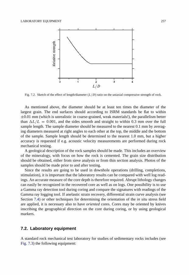
LABORATORY EQUIPMENT 257
Fig. 7.2. Sketch of the effect of length/diameter (L/D) ratio on the uniaxial compressive strength of rock.
As mentioned above, the diameter should be at least ten times the diameter of thelargest grain. The end surfaces should according to ISRM standards be flat to within±0.01 mm (which is unrealistic in coarse-grained, weak materials!), the parallelism betterthan �L/L = 0.001, and the sides smooth and straight to within 0.3 mm over the fullsample length. The sample diameter should be measured to the nearest 0.1 mm by averag-ing diameters measured at right angles to each other at the top, the middle and the bottomof the sample. Sample length should be determined to the nearest 1.0 mm, but a higheraccuracy is requested if e.g. acoustic velocity measurements are performed during rockmechanical testing.
A geological description of the rock samples should be made. This includes an overviewof the mineralogy, with focus on how the rock is cemented. The grain size distributionshould be obtained, either from sieve analysis or from thin section analysis. Photos of thesamples should be made prior to and after testing.
Since the results are going to be used in downhole operations (drilling, completions,stimulation), it is important that the laboratory results can be compared with well log read-ings. An accurate measure of the core depth is therefore required. Abrupt lithology changescan easily be recognized in the recovered core as well as on logs. One possibility is to usea Gamma ray detection tool during coring and compare the signatures with readings of theGamma ray logging tool. If anelastic strain recovery, differential strain curve analysis (seeSection 7.4) or other techniques for determining the orientation of the in situ stress fieldare applied, it is necessary also to have oriented cores. Cores may be oriented by knivesinscribing the geographical direction on the core during coring, or by using geologicalmarkers.
7.2. Laboratory equipment
A standard rock mechanical test laboratory for studies of sedimentary rocks includes (seeFig. 7.3) the following equipment:
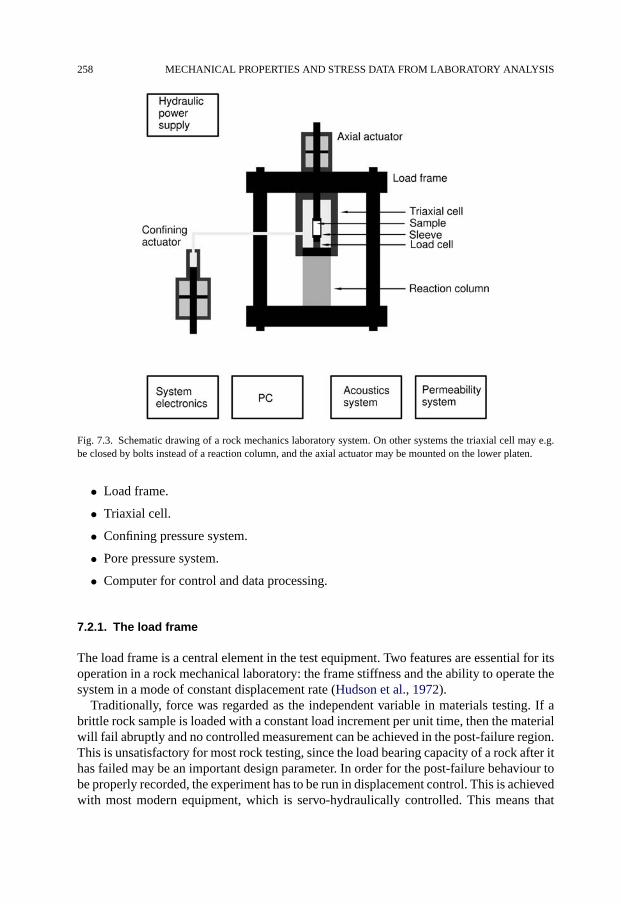
258 MECHANICAL PROPERTIES AND STRESS DATA FROM LABORATORY ANALYSIS
Fig. 7.3. Schematic drawing of a rock mechanics laboratory system. On other systems the triaxial cell may e.g.be closed by bolts instead of a reaction column, and the axial actuator may be mounted on the lower platen.
• Load frame.
• Triaxial cell.
• Confining pressure system.
• Pore pressure system.
• Computer for control and data processing.
7.2.1. The load frame
The load frame is a central element in the test equipment. Two features are essential for itsoperation in a rock mechanical laboratory: the frame stiffness and the ability to operate thesystem in a mode of constant displacement rate (Hudson et al., 1972).
Traditionally, force was regarded as the independent variable in materials testing. If abrittle rock sample is loaded with a constant load increment per unit time, then the materialwill fail abruptly and no controlled measurement can be achieved in the post-failure region.This is unsatisfactory for most rock testing, since the load bearing capacity of a rock after ithas failed may be an important design parameter. In order for the post-failure behaviour tobe properly recorded, the experiment has to be run in displacement control. This is achievedwith most modern equipment, which is servo-hydraulically controlled. This means that
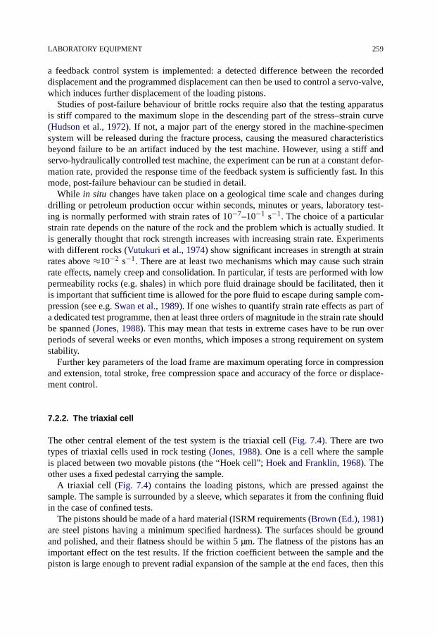
LABORATORY EQUIPMENT 259
a feedback control system is implemented: a detected difference between the recordeddisplacement and the programmed displacement can then be used to control a servo-valve,which induces further displacement of the loading pistons.
Studies of post-failure behaviour of brittle rocks require also that the testing apparatusis stiff compared to the maximum slope in the descending part of the stress–strain curve(Hudson et al., 1972). If not, a major part of the energy stored in the machine-specimensystem will be released during the fracture process, causing the measured characteristicsbeyond failure to be an artifact induced by the test machine. However, using a stiff andservo-hydraulically controlled test machine, the experiment can be run at a constant defor-mation rate, provided the response time of the feedback system is sufficiently fast. In thismode, post-failure behaviour can be studied in detail.
While in situ changes have taken place on a geological time scale and changes duringdrilling or petroleum production occur within seconds, minutes or years, laboratory test-ing is normally performed with strain rates of 10−7–10−1 s−1. The choice of a particularstrain rate depends on the nature of the rock and the problem which is actually studied. Itis generally thought that rock strength increases with increasing strain rate. Experimentswith different rocks (Vutukuri et al., 1974) show significant increases in strength at strainrates above ≈10−2 s−1. There are at least two mechanisms which may cause such strainrate effects, namely creep and consolidation. In particular, if tests are performed with lowpermeability rocks (e.g. shales) in which pore fluid drainage should be facilitated, then itis important that sufficient time is allowed for the pore fluid to escape during sample com-pression (see e.g. Swan et al., 1989). If one wishes to quantify strain rate effects as part ofa dedicated test programme, then at least three orders of magnitude in the strain rate shouldbe spanned (Jones, 1988). This may mean that tests in extreme cases have to be run overperiods of several weeks or even months, which imposes a strong requirement on systemstability.
Further key parameters of the load frame are maximum operating force in compressionand extension, total stroke, free compression space and accuracy of the force or displace-ment control.
7.2.2. The triaxial cell
The other central element of the test system is the triaxial cell (Fig. 7.4). There are twotypes of triaxial cells used in rock testing (Jones, 1988). One is a cell where the sampleis placed between two movable pistons (the “Hoek cell”; Hoek and Franklin, 1968). Theother uses a fixed pedestal carrying the sample.
A triaxial cell (Fig. 7.4) contains the loading pistons, which are pressed against thesample. The sample is surrounded by a sleeve, which separates it from the confining fluidin the case of confined tests.
The pistons should be made of a hard material (ISRM requirements (Brown (Ed.), 1981)are steel pistons having a minimum specified hardness). The surfaces should be groundand polished, and their flatness should be within 5 µm. The flatness of the pistons has animportant effect on the test results. If the friction coefficient between the sample and thepiston is large enough to prevent radial expansion of the sample at the end faces, then this

260 MECHANICAL PROPERTIES AND STRESS DATA FROM LABORATORY ANALYSIS
Fig. 7.4. Principle sketch of the interior of a triaxial cell, showing the loading piston with fluid ports, optionalsintered plates for fluid distribution, a radial strain jig (suspended from the specimen) measuring two orthogonaldiameters, and an axial strain jig measuring change in sample length between the pistons. It is also possible tomeasure axial strain directly on the sample, and to measure radial strain in more than 2 directions, or measure thechange in circumference by a chain around the sample.
is equivalent to providing the material with an additional support. This will manifest itselfas a length:diameter effect, since the support of the end faces will give rise to a highermeasured strength with a short than with a long sample.
In rock testing for petroleum applications one may wish to have fluid inlet and outlet inthe pistons in order to apply and measure pore pressure. This can be done by using sinteredpistons or by introducing flow channels in the piston surfaces.
For acoustic measurements, the piston material should ideally have acoustic propertieswhich provide an acoustic impedance-matching between the acoustic transducers and therock material. The choice of steel as a piston material is in that case not ideal for studiesof soft rock samples. Thus the requirements to piston material, flatness and hardness mayhave to be relaxed in order to combine rock mechanical testing with other petrophysicalmeasurements. When measuring the permeability during loading, it is recommended tohave a system for distribution of the fluid flow at the end surfaces. This can be obtainedby making grooves in the pistons or by inserting a sintered plate between the piston andthe rock sample. This can, however, impose end effects (e.g. sedimentation of fines in thesintered plates). This is a potentially significant error source if the pressure drop along thecore is measured on the outside of the sample.
The sleeve should be soft enough not to provide a significant support to the core. This isnormally not a problem, but should be considered when testing very weak samples at lowconfining pressures. Sleeves are made from rubber, plastic, Teflon or other soft materials.Sleeve wall thicknesses are normally around a few millimetres. To improve the accuracy

LABORATORY EQUIPMENT 261
of radial deformation measurements (and also measurements of acoustic velocities for ra-dially propagating waves) the sleeve should be made as thin as possible.
7.2.3. Measurements of stresses and strains
Stress measurements are performed with strain gauges in the load cell, and fluid pressuretransducers in the confining fluid in the triaxial cell. The load cell may be external orinternal to the pressure vessel. The use of an internal load cell eliminates problems causedby loading ram friction, but makes calibration more difficult (Jones, 1988). Pore pressuresare measured with pressure transducers that are connected to the pistons. By monitoringthe pore pressure drop along a specimen with transducers both in the top and the bottompistons, and in addition measuring the flow rate, it is possible to measure permeability aspart of a rock mechanical test.
The radial deformation of the sample can be measured in several ways. One techniqueis to use LVDTs (Linear Variable Differential Transformers, which operate on a magneticinduction principle) pressed against the sleeve at various points circumferentially aroundthe core. Another widely used method is to have strain gauges glued directly to the sample.A third technique is to use a cantilever system, where the displacement of the arms ismeasured by strain gauges. A fourth technique is to use a chain wrapped around the coreplug, where the change in circumference is monitored with strain gauges. The latter methodis accurate, but does not have the potential to monitor anisotropic deformations. The othertechniques are all essentially point measurements. The accuracy depends on calibration forsleeve deformation. The radial deformation sensors should be mounted on a jig which is notattached to the walls of the triaxial cell. Otherwise, the measurements must be calibratedfor deformation of the entire cell.
Axial deformation can be monitored in several ways. Measurement of stroke (i.e. pistonmovement) is the most common method. This should be done between the pistons insidethe triaxial cell and not between the loading platens on the outside, in order to obtain thetrue sample deformation. If measured outside the cell, corrections for piston deformationhave to be made. Attempts have also been made to measure axial deformation by monitor-ing the relative displacement of two knife-edges pressed against the sleeve at different axialpositions. This technique provides a strain measurement which eliminates end effects, butwill not cover the entire length of the sample.
Measuring devices mounted inside the triaxial cell must always be calibrated for pres-sure effects exerted by the confining fluid.
Volume changes may also be used to monitor deformations. The change in pore volumecan be measured by monitoring the amount of pore fluid entering or leaving a fully satu-rated sample. The change in bulk volume may in principle be measured by monitoring thevolume change of the confining fluid.
7.2.4. Acoustic measurements
The importance of acoustic measurements has been stated several times throughout thisbook. A major motivation for doing acoustic laboratory measurements is to support the

262 MECHANICAL PROPERTIES AND STRESS DATA FROM LABORATORY ANALYSIS
Fig. 7.5. Ultrasonic test apparatus (left) and transducer positions inside the triaxial cell (right).
interpretation of sonic log and seismic measurements. Acoustic laboratory measurementscan provide correlations with rock strength, and may help evaluate the difference betweenstatic and dynamic moduli (Chapter 5). They may also provide information about the insitu stress state.
The range of frequencies where acoustic measurements can be made is limited mainlyby the sample size. The attenuation of sound sets an upper limit, while the requirementthat a sample should contain several wavelengths in order for a propagating wave to beset up, imposes a lower limit to the frequency. With normal sample sizes (say 5–10 cmtransmission length) the frequency will be in the 100 kHz – 1 MHz range.
The ultrasonic sources and detectors used at these frequencies are piezo-electric (nor-mally piezo-ceramic) transducer elements. They are deformed mechanically when an ex-ternal voltage is applied to them, and vice versa: an electric field is generated when theyare deformed by an external force. Differently manufactured piezo-elements are used forgeneration of P- and S-waves. By placing transducers at two opposing faces of a rockspecimen, the sound velocities are measured from transit times of pulsed wavelets throughthe sample. Measurements at various frequencies can be obtained by a spectral analysisof the waveforms (see Winkler and Plona, 1982), but this is only possible if the transduc-ers are broadband in operation. The transducers can be embedded inside the pistons of atriaxial cell, or in the confining fluid for radial transmission. Fig. 7.5 illustrates a set-upused for acoustic laboratory measurements, and particularly shows how transducers can beintegrated into a rock mechanical test system.
For practical purposes, the quality of acoustic signals is extremely sensitive to theacoustic coupling between the transducers and the sample. This coupling is normally ob-tained by a thin layer of grease, a gel or another viscous fluid placed between the face of

LABORATORY TESTS FOR ROCK MECHANICAL PROPERTY DETERMINATION 263
the transducer and the surface of the specimen. It is important that the couplant layer isthin enough not to contribute significantly to the measured transit time.
With shear wave transducers, it is important to make sure that the polarization of thetransmitting and the receiving transducers point in the same direction. The polarization willnormally be marked on the transducers, but should be checked by placing the transducersface to face. Maximum signal is then obtained when the polarizations are parallel, whileminimum signal is obtained when they are at 90° to each other. If lower frequencies thanthe 100 kHz – 1 MHz range are required, one may use the resonant bar technique. Inthis case, the resonance frequency of a vibrating sample is determined. The resonancefrequency is related directly to the wave velocity. Different frequencies can be obtained byusing samples of various size.
In the seismic frequency range (10–100 Hz), velocities may be obtained from stiff-nesses measured in very low strain (<10−6) and stress cycles (Spencer, 1981; Batzle etal., 2006). By measuring strains in various directions and assuming isotropic and homo-geneous specimens, both P- and S-wave moduli are estimated. Monitoring of phase shiftspermits measurements of attenuation. These are however challenging experiments that cannot yet be considered as routine.
Acoustic measurements in the laboratory should be performed with rocks in unconfinedas well as stressed conditions. As discussed later (Section 7.4), unloaded cores are thoughtto contain an orientational distribution of microcracks, reflecting the in situ stress field. Thepossibility of using acoustic velocity measurements on cores to evaluate the in situ stressfield will be discussed further in Section 7.4.3.
Measurements of P- and S-wave velocities on core plugs at atmospheric conditions aresometimes performed and correlated with rock strength or elastic moduli measured in apressure vessel or a triaxial cell. Such correlations are invalid, since the two measurementsrefer to different stress conditions. Therefore, for the purpose of obtaining such correla-tions, acoustic velocities should be measured during the static tests. In order to comparewith log readings, the acoustic velocities should be measured in the same direction, at thesame stress state, and with the same saturating fluid as under downhole conditions. Whenthis is done, experience shows that laboratory measured sound velocities can be differentfrom those measured in the borehole. This may be due to a dispersion effect (Chapter 5),since the frequencies in laboratory studies normally are higher than those used in the field.It may also be due to core alteration, as discussed in Section 7.1.2.
7.3. Laboratory tests for rock mechanical property determination
In this section we will discuss procedures for performing the most common types of rockmechanical tests, including some comments about test interpretation.
7.3.1. Stresses on cylindrical samples
For cylindrical coordinates, r , θ and z, Hooke’s law can be written (with Biot’s coefficientα = 1)

264 MECHANICAL PROPERTIES AND STRESS DATA FROM LABORATORY ANALYSIS
Eεr = σ ′r − ν(σ ′
θ + σ ′z) (7.3)
Eεθ = σ ′θ − ν(σ ′
r + σ ′z) (7.4)
Eεz = σ ′z − ν(σ ′
r + σ ′θ ) (7.5)
The remaining three shear stress equations in Hooke’s law disappear, as the directions r , θand z correspond to the principal stress directions due to the symmetry of the sample andthe set-up. The equations are written with effective stresses to make them applicable bothto porous and non-porous materials.
The confining pressure will generate an isotropic stress field perpendicular to the sampleaxis, as long as the sample can be considered isotropic and homogeneous. (Note that thecase of a hollow cylinder does not comply with these conditions. The material may beisotropic and homogeneous, but the sample is not.) The radial and tangential stresses willbe equal, and so will the radial and tangential strains. If pc is the confining pressure, wemust have
σr = σθ = pc (7.6)
εr = εθ (7.7)
There are thus only two independent stresses, the radial stress σr and the axial stress σz.Hooke’s law can then be reduced to
Eεr = (1 − ν)σ ′r − νσ ′
z (7.8)
Eεz = σ ′z − 2νσ ′
r (7.9)
7.3.2. Drained and undrained test conditions
In drained tests the outlets through the pistons will be open, so that the pore fluid pressurecan be kept at any prescribed value. Most often, the outlets are open to the atmosphere, sothat the pore fluid pressure will be zero. In that case the effective stresses in the sample willbe equal to the total stresses. But sometimes it is of interest to run tests at actual reservoirconditions. The pore pressure must then be kept at the reservoir pressure level.
In testing of low permeability materials, for instance like chalk, drained condition meansthat the test must be run sufficiently slow, in order to avoid unacceptable pressure build-upwhen the sample deforms.
In undrained tests the outlets are in principle closed, so that the pore fluids containedin the sample cannot escape. If the pore fluid pressure is to be measured, there must ofcourse be hydraulic contact through one of the outlets, but the condition of no fluid flowmust be assured. Undrained conditions are commonly used when testing extremely low-permeability rocks like shale (Section 7.3.7).
From a more formal point of view, drained conditions mean that the pore pressure inthe sample is an independent variable. In undrained conditions on the other hand, the porefluid pressure will be a dependent variable.

LABORATORY TESTS FOR ROCK MECHANICAL PROPERTY DETERMINATION 265
7.3.3. Standard triaxial compression tests
Rocks at depth are exposed to an anisotropic stress field. During drilling or petroleumproduction, enhanced shear stresses occur near the borehole or the producing perforations(see Chapter 4). The lowest effective principal stress component is zero at the boreholeor cavity wall if the wall is permeable, and slightly higher if e.g. a mudcake blocks thefluid transport across the boundary (and pw > pf). The unconfined compressive strengthC0 is the most important strength parameter in order to describe stability at the boreholewall. At some distance from the wall, however, the minimum principal stress increases. Inorder to evaluate borehole or cavity stability it is therefore of great value to know how themechanical properties and the strength characteristics depend on external load conditions.
The most commonly adopted experimental procedure for this purpose is the so-calledtriaxial compression test. The axial stress σz and the radial confining pressure σr are keptequal and increased to a preset level, from which σz is increased further until failure hasoccurred, keeping σr constant. Results from a triaxial failure test are shown in Fig. 7.6. Byperforming a series of tests at different confining pressures, it is possible to map the entirefailure envelope (Section 2.7). If the aim of the test programme is a borehole stabilityor sand prediction analysis, then care should be taken that sufficient data is collected atlow confining pressures, representing the stress state near the borehole. The maximumconfining pressure should correspond to the minimum principal effective stress far from theborehole. For a producing reservoir, the value at maximum depletion should be selected.
The test can be run under drained or undrained conditions. Since both the elastic prop-erties and the strength depend on the effective stress, drained tests provide a better experi-mental control because the pore pressure is kept constant at a known value. With extremelylow-permeability shales (nanoDarcy range), however, undrained tests with pore pressuremeasurement performed during the experiment may be advantageous, since undrained testsrequire shorter stabilization times (see Section 7.3.7).
Fig. 7.6. Triaxial test—example of experimental result.

266 MECHANICAL PROPERTIES AND STRESS DATA FROM LABORATORY ANALYSIS
Beyond the brittle-ductile transition it may be very difficult to define the failure point,which may be visible only as a minor change in slope of the stress–strain curve. The post-failure behaviour is important, since it tells us how much the remnant strength of the rockis, i.e. how much load it can sustain after failure has occurred. It is therefore stronglyadvised that triaxial tests are run with the load frame in displacement control mode.
7.3.4. Interpretation of elastic moduli from triaxial tests
Fig. 7.6 illustrates a typical response of a drained triaxial test, including the hydrostaticloading phase. If we simplify the test response, assuming the stress–strain curves to belinear up to failure, it is straightforward to interpret the elastic moduli from such a plot.
In the hydrostatic phase the stresses are equal (see also Section 7.3.1), so the bulk mod-ulus of the framework, is given as Kfr = �σ ′
z/�εvol = �σ ′z/(�εz + 2�εr).
In the triaxial phase �σ ′r = �σ ′
θ = pc = 0. Young’s modulus is then given by the slopeof the axial stress–strain curve in the triaxial phase, i.e. Efr = �σ ′
z/�εz, while Poisson’sratio is given by the ratio between the slopes of both the radial and the axial stress–straincurves in the triaxial phase, i.e. νfr = −�εr/�εz.
The shear modulus can of course now be calculated directly from Young’s modulus andPoisson’s ratio (Table 1.1). Alternatively we have Gfr = 1
2�σ′z/(�εz −�εr).
It is important to realize that if the pore pressure is not kept constant during the test,this interpretation requires that the Biot constant is known. In a general case one shouldconsider the full expression (Eqs. (1.136)–(1.142)) and then only eliminate parameterswhich are kept constant during the test phase of interest.
Another simplification we have made is that the elastic stress–strain response is linear.As illustrated by Fig. 7.6 this is generally not the case, neither in the hydrostatic phasenor in the triaxial phase. When presenting elastic moduli it is therefore essential to definehow the interpretation has been made. For the triaxial phase, the following alternatives arecommonly accepted (see Fig. 7.7):
Fig. 7.7. Illustration of different methods for calculating Young’s modulus from axial stress–strain curves.

LABORATORY TESTS FOR ROCK MECHANICAL PROPERTY DETERMINATION 267
• Initial modulus, given as the initial slope of the stress–strain curve.
• Secant modulus, measured up to a fixed percentage of the peak stress.
• Tangent modulus, given at a specific percentage of the peak stress.
• Average modulus of a linear portion, given within a specific maximum and minimumstress level.
Out of these, the tangent modulus at 50% of the peak stress value is probably the mostused method. However, if the curve is strongly nonlinear, complete information can onlybe given if the entire curve is presented. Comparing moduli from different sources it isthus essential to ensure that the same interpretation method has been used. As illustratedby Fig. 7.7, the moduli can vary significantly with the method used for interpretation.
Such an interpretation is based on several assumptions, where the assumption of anelastic material has already been mentioned. Clearly, this assumption is violated, if thestress–strain curve looks like Fig. 7.7. In such a case, the rock is either nonlinearly elas-tic or elasto-plastic (or both). One should therefore refer to the measured quantities asstatic moduli, and avoid the term “static elastic” moduli. To reduce the problem of non-linearity and variation of the stress–strain slope, it is often recommended to performunloading-reloading cycles at different stress levels and interpret the elastic moduli fromthe stress–strain response of these loading cycles. The stress levels should be chosen suchthat the sample is well within the elastic range. This may result in a much more consistentinterpretation of the elastic moduli.
Another assumption is that the sample is completely isotropic and homogeneous. Givenperfect boundary conditions, this implies that the stress- and strain-field is homogeneousthroughout the sample and throughout the test sequence. Observations of experiments haveshown that this is not always true. Barreling, buckling and shear-band formation are typicalexamples of loss of homogeneity. This can occur significantly below the peak point of aload-displacement curve, and can for instance be identified by loss of uniformity of radialstrain measurements in different directions.
These phenomena have been the subject of extensive investigation using bifurcationtheory, both from an experimental and a more theoretical approach. Examples with appli-cation to failure around boreholes are given by Santarelli and Guenot (1990) and Sulemand Vardoulakis (1989).
7.3.5. Unconfined (uniaxial) compression tests
In an unconfined compression test, a sample is inserted into a load frame and the axial loadis increased with zero confining pressure. This test is hence a simplification of a standardtriaxial compression test. Monitoring the axial stress plus the axial and the radial deforma-tions, one can under drained conditions measure (by definition—see Chapters 1 and 2):
• The unconfined compressive strength C0 (also termed the uniaxial compressivestrength, UCS) as the peak stress.
• Young’s modulus Efr (tangential modulus as the slope of the axial stress versus axialstrain curve).
• Poisson’s ratio νfr as the ratio between radial and axial strain.

268 MECHANICAL PROPERTIES AND STRESS DATA FROM LABORATORY ANALYSIS
Most rocks exhibit brittle failure in unconfined failure tests, so it is straightforward toidentify C0. For interpretation of Young’s modulus and Poisson’s ratio, see Section 7.3.4.
If the rock is anisotropic, Poisson’s ratio and Young’s modulus are not proper para-meters to describe the mechanical behaviour. In Section 1.7, the elastic stiffness tensorwas defined. Eqs. (1.219)–(1.220) illustrate that the value of the measured Poisson’s ratiodepends both on the direction of the applied load and the direction of lateral strain mea-surement. Thus the orientation of the sample’s symmetry with respect to the directions ofapplied and measured stress and strains needs to be specified.
Theoretically, the uniaxial compressive strength depends on the largest crack or flawpresent in the sample. Thus, measurements of C0 are expected to be very sensitive to sam-ple heterogeneity, and to cracks induced by coring and core treatment procedures. Largeexperimental uncertainties may therefore be expected, especially in weak rocks. Since theuniaxial compressive strength is a key parameter in many petroleum related rock mechan-ics applications, it may be worthwhile considering other methods to obtain or estimatethe uniaxial compressive strength. One alternative may be to perform triaxial tests at lowconfining pressures, where some of the cracks not associated with the intrinsic rock be-haviour are closed. Another alternative is a Constant Mean Stress (CMS) test, see alsoSection 7.3.9.
In low-permeability rocks like shale, unconfined tests are normally not run, since thistest mode requires fully drained conditions which are too time-consuming and difficult toobtain in low-permeability rocks.
7.3.6. Hydrostatic tests
Hydrostatic measurements are performed mainly to determine the bulk modulus of therock (or the frame modulus) and of the solid grains. This test represents the first phase of astandard triaxial test. Normally, failure does not occur under hydrostatic loading, althoughpore collapse in chalk and grain crushing in sandstone may induce failure at high stresslevels.
Hydrostatic tests can be performed under drained or undrained conditions. The dif-ference between moduli measured in drained and undrained conditions was outlined inSection 1.6. Let us repeat here the most important results for laboratory testing:
In a drained hydrostatic experiment, the slope of the stress vs. volumetric strain curve isthe bulk frame modulus (Kfr) of the rock (see Section 7.3.4).
In an undrained, hydrostatic experiment, the pore pressure will change during the testand the slope of the stress–strain curve will be equal to the undrained bulk modulus Ku ofthe rock, including the effect of the pore fluid (Eq. (1.155)). The increase of pore pressureduring undrained loading in a poroelastic (Biot) medium is (see also Section 1.6.3):
pf = (C/Ku)σp (7.10)
The constant C is given in Eq. (1.157). The ratio C/Ku is identical to Skempton’sB-parameter (see Section 1.6.5). For fluid and frame bulk moduli (Kf and Kfr) signif-icantly smaller than the bulk modulus of the grain material (Ks), one finds C/Ku →Kf/(φKfr + Kf). It is seen that for a stiff framework, or a situation where gas is present

LABORATORY TESTS FOR ROCK MECHANICAL PROPERTY DETERMINATION 269
in the pore fluid (Kf → 0), the pore pressure development can be neglected. For a weakframe, however, the pore pressure may be almost as high as the external stress. One ex-ample of such behaviour is in soils. In shales, where pore fluid saturation may be hard toachieve, a measured pore pressure response during undrained loading is a useful indica-tion that full saturation is actually reached. Note that in case that the rock also deformsplastically, like in normally consolidated clays or shales (Section 2.8.2), the pore pres-sure response may be larger than predicted by Eq. (7.10). To reduce the problem ofnonlinearity and variation of the stress–strain slope, it is often recommended to performunloading-reloading cycles at different stress levels and interpret the elastic moduli fromthe stress–strain response of these loading cycles. The stress levels should be chosen suchthat the sample is well within the elastic range. This may result in a much more consistentinterpretation of the elastic moduli.
In an “unjacketed” test, i.e. with the pore pressure equal to the confining pressure, theslope of the stress–strain curve gives the bulk modulus Ks of the solid particles (1/Ksis often also termed “grain (or matrix) compressibility”) (Eqs. (1.148) and (1.151)). Thismeasurement can be performed on a core plug in direct contact with a fluid bath. Thevolume change of fluid in the cell is measured as a function of pressure with and withoutthe core present, and the results are subtracted in order to obtain the grain compressibility.Since the volume change is small, the results are very sensitive to changes in temperatureor other factors which may influence the measurement of fluid compressibility.
7.3.7. Triaxial testing of shales
For testing of shales it has been recommended to perform so-called Consolidated-Undrained (CU) tests (Steiger and Leung, 1992; Nakken et al., 1989; Horsrud et al., 1998).The procedure is adopted from soil testing (e.g. Head, 1984). This test consists of threedistinct phases:
1. Loading to the predetermined level of confining pressure and pore pressure.
2. Consolidation, maintaining a constant confining pressure and allowing drainage ofthe pore fluid against a constant pore pressure.
3. Undrained axial loading under a constant axial displacement rate beyond failure ofthe sample.
This test sequence is illustrated schematically in Fig. 7.8. The triaxial phase is performedin undrained conditions to reduce the time required to complete a test. A fully drained testof a low-permeability shale may require weeks or months to complete. In the CU-test, thepore pressure must be monitored throughout the test.
The time required to run such a test depends mainly on the permeability of the shale.Concepts from soil mechanics testing can be applied to assist in determining when con-solidation is completed and also to determine the appropriate displacement rate in theundrained part of the test (Head, 1984). For instance, allowing drainage at the end sur-faces as well as the sides of the core will reduce testing time considerably. As shown inSection 1.9 the consolidation response depends both on the permeability of the rock and
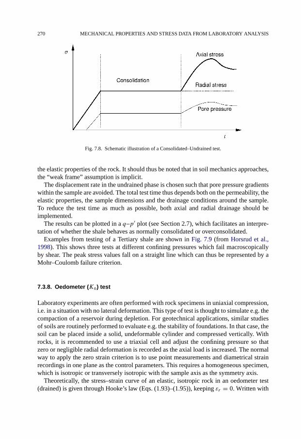
270 MECHANICAL PROPERTIES AND STRESS DATA FROM LABORATORY ANALYSIS
Fig. 7.8. Schematic illustration of a Consolidated–Undrained test.
the elastic properties of the rock. It should thus be noted that in soil mechanics approaches,the “weak frame” assumption is implicit.
The displacement rate in the undrained phase is chosen such that pore pressure gradientswithin the sample are avoided. The total test time thus depends both on the permeability, theelastic properties, the sample dimensions and the drainage conditions around the sample.To reduce the test time as much as possible, both axial and radial drainage should beimplemented.
The results can be plotted in a q–p′ plot (see Section 2.7), which facilitates an interpre-tation of whether the shale behaves as normally consolidated or overconsolidated.
Examples from testing of a Tertiary shale are shown in Fig. 7.9 (from Horsrud et al.,1998). This shows three tests at different confining pressures which fail macroscopicallyby shear. The peak stress values fall on a straight line which can thus be represented by aMohr–Coulomb failure criterion.
7.3.8. Oedometer (Ko) test
Laboratory experiments are often performed with rock specimens in uniaxial compression,i.e. in a situation with no lateral deformation. This type of test is thought to simulate e.g. thecompaction of a reservoir during depletion. For geotechnical applications, similar studiesof soils are routinely performed to evaluate e.g. the stability of foundations. In that case, thesoil can be placed inside a solid, undeformable cylinder and compressed vertically. Withrocks, it is recommended to use a triaxial cell and adjust the confining pressure so thatzero or negligible radial deformation is recorded as the axial load is increased. The normalway to apply the zero strain criterion is to use point measurements and diametrical strainrecordings in one plane as the control parameters. This requires a homogeneous specimen,which is isotropic or transversely isotropic with the sample axis as the symmetry axis.
Theoretically, the stress–strain curve of an elastic, isotropic rock in an oedometer test(drained) is given through Hooke’s law (Eqs. (1.93)–(1.95)), keeping εr = 0. Written with

LABORATORY TESTS FOR ROCK MECHANICAL PROPERTY DETERMINATION 271
Fig. 7.9. CU-tests of Tertiary shale. (After Horsrud et al., 1998; with permission from Int. J. Rock Mech. Min.Sci.)
stress and strain increments we have
�σ ′z = (λfr + 2Gfr)�εz = Efr(1 − νfr)
(1 + νfr)(1 − 2νfr)�εz (7.11)
and
�σ ′r = λfr
λfr + 2Gfr�σ ′
z = νfr
1 − νfr�σ ′
z (7.12)
The modulus dσz/dεz is called the oedometer modulus or uniaxial compaction modulus(Hfr) (see also pages 21 and 394). In the elastic limit it is given by Eq. (7.11).
The oedometer test is most commonly used in geotechnical engineering. The test isthen performed by placing the sample (which normally has an L/D-ratio of ≈1/2) in asteel ring. Drainage may be allowed both through top and bottom pistons, or alternatively,through only one of the pistons. Load is applied incrementally, or in a continuous mode.Axial stress and strain vs. time, plus pore pressure changes are the parameters measuredthroughout these tests.
It has been observed that cyclic loading of sandstones produce moduli that are very dif-ferent from the first loading segment (see for instance Mess, 1978). In a study of syntheticsandstones formed under stress (Holt et al., 2000), the modulus of the second and subse-quent cycle was observed to be at least two times larger than the modulus of the first cycle.The initial modulus of the second cycle was found to be close to the initial modulus ofthe expected behaviour of a virgin rock, i.e. a rock which had not been through the coringprocess.
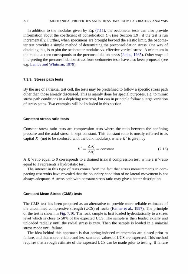
272 MECHANICAL PROPERTIES AND STRESS DATA FROM LABORATORY ANALYSIS
In addition to the modulus given by Eq. (7.11), the oedometer tests can also provideinformation about the coefficient of consolidation CD (see Section 1.9), if the test is runincrementally. Further, when specimens are brought beyond the elastic limit, the oedome-ter test provides a simple method of determining the preconsolidation stress. One way ofobtaining this, is to plot the oedometer modulus vs. effective vertical stress. A minimum inthe modulus then corresponds to the preconsolidation stress (Janbu, 1985). Other ways ofinterpreting the preconsolidation stress from oedometer tests have also been proposed (seee.g. Lambe and Whitman, 1979).
7.3.9. Stress path tests
By the use of a triaxial test cell, the tests may be predefined to follow a specific stress pathother than those already discussed. This is mainly done for special purposes, e.g. to mimicstress path conditions in a depleting reservoir, but can in principle follow a large variationof stress paths. Two examples will be included in this section.
Constant stress ratio tests
Constant stress ratio tests are compression tests where the ratio between the confiningpressure and the axial stress is kept constant. This constant ratio is mostly referred to ascapital K ′ (not to be confused with the bulk modulus), where K ′ is given by
K ′ = �σ ′r
�σ ′z
= constant (7.13)
A K ′-ratio equal to 0 corresponds to a drained triaxial compression test, while a K ′-ratioequal to 1 represents a hydrostatic test.
The interest in this type of tests comes from the fact that stress measurements in com-pacting reservoirs have revealed that the boundary condition of no lateral movement is notalways adequate. A stress path with constant stress ratio may give a better description.
Constant Mean Stress (CMS) tests
The CMS test has been proposed as an alternative to provide more reliable estimates ofthe unconfined compressive strength (UCS) of rocks (Kenter et al., 1997). The principleof the test is shown in Fig. 7.10. The rock sample is first loaded hydrostatically to a stresslevel which is close to 50% of the expected UCS. The sample is then loaded axially andunloaded radially until the radial stress is zero. Then the sample is loaded in a uniaxialstress mode until failure.
The idea behind this approach is that coring-induced microcracks are closed prior tofailure, and thus more reliable and less scattered values of UCS are expected. This methodrequires that a rough estimate of the expected UCS can be made prior to testing. If failure
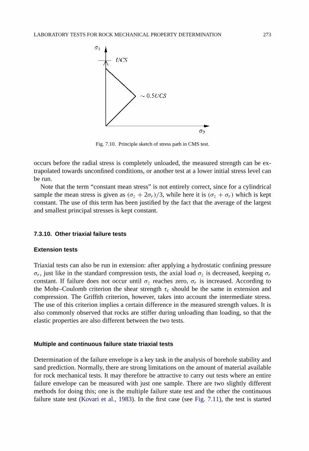
LABORATORY TESTS FOR ROCK MECHANICAL PROPERTY DETERMINATION 273
Fig. 7.10. Principle sketch of stress path in CMS test.
occurs before the radial stress is completely unloaded, the measured strength can be ex-trapolated towards unconfined conditions, or another test at a lower initial stress level canbe run.
Note that the term “constant mean stress” is not entirely correct, since for a cylindricalsample the mean stress is given as (σz + 2σr)/3, while here it is (σz + σr) which is keptconstant. The use of this term has been justified by the fact that the average of the largestand smallest principal stresses is kept constant.
7.3.10. Other triaxial failure tests
Extension tests
Triaxial tests can also be run in extension: after applying a hydrostatic confining pressureσr , just like in the standard compression tests, the axial load σz is decreased, keeping σrconstant. If failure does not occur until σz reaches zero, σr is increased. According tothe Mohr–Coulomb criterion the shear strength τc should be the same in extension andcompression. The Griffith criterion, however, takes into account the intermediate stress.The use of this criterion implies a certain difference in the measured strength values. It isalso commonly observed that rocks are stiffer during unloading than loading, so that theelastic properties are also different between the two tests.
Multiple and continuous failure state triaxial tests
Determination of the failure envelope is a key task in the analysis of borehole stability andsand prediction. Normally, there are strong limitations on the amount of material availablefor rock mechanical tests. It may therefore be attractive to carry out tests where an entirefailure envelope can be measured with just one sample. There are two slightly differentmethods for doing this; one is the multiple failure state test and the other the continuousfailure state test (Kovari et al., 1983). In the first case (see Fig. 7.11), the test is started

274 MECHANICAL PROPERTIES AND STRESS DATA FROM LABORATORY ANALYSIS
Fig. 7.11. Sketch of the stress path followed in a multiple failure state test.
as a normal triaxial test from a given initial confining pressure. When failure is reached(detected manually or automatically as a significant change in the slope of the stress–straincurve), the confining pressure is increased to a higher level. Changes in acoustic velocities(especially the radial velocity) measured during the test may also be used as an indicatorof failure (Holt and Fjær, 1991). Another alternative is to use the Acoustic Emission hitrate as an indicator. The axial stress is then increased further until failure occurs, and inthis way the test continues at a multiple of confining stress levels. This test turns out togive quite reliable results with regards to failure stresses, at least in weak, brittle rocks likesandstones (Holt and Fjær, 1991). Obviously, failure detection in ductile materials is morecomplicated. In addition, in hard rocks, failure in one of the steps may weaken the materialconsiderably. Generally, the elastic moduli are influenced by damage caused in previousload steps, so this test is not recommended for elastic properties evaluation.
The idea behind continuous failure state tests is similar to that of the multiple failurestate tests. In the continuous failure state test (Kovari et al., 1983), both the radial and theaxial stresses are increased in order to monitor the failure envelope continuously ratherthan stepwise.
True triaxial tests
To evaluate further the role of the intermediate stress on the failure envelope, it is possi-ble to perform tests in test machines that can supply a true triaxial (polyaxial) stress, i.e.σ1 �= σ2 �= σ3. These systems normally include three mutually perpendicular pairs ofhydraulic jacks compressed against the faces of a cubically shaped sample. Other applica-tions of polyaxial tests include testing of sand production, fracturing, perforating, injectionand screen integrity. A limitation for the use of such tests within petroleum related rockmechanics is that the tests usually require larger specimens than can be obtained from fieldcores.
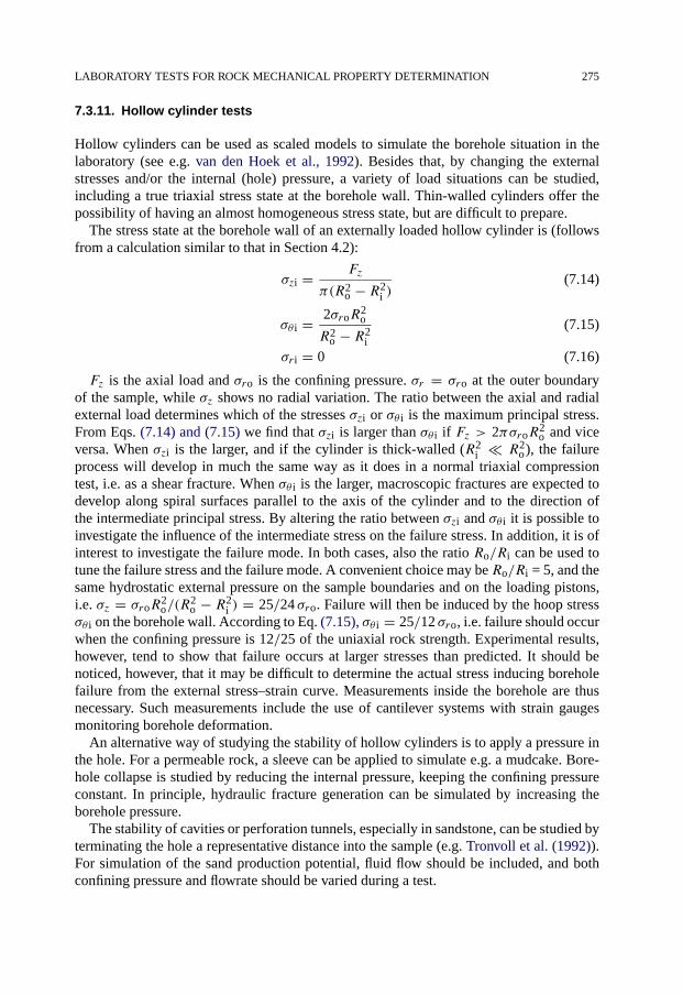
LABORATORY TESTS FOR ROCK MECHANICAL PROPERTY DETERMINATION 275
7.3.11. Hollow cylinder tests
Hollow cylinders can be used as scaled models to simulate the borehole situation in thelaboratory (see e.g. van den Hoek et al., 1992). Besides that, by changing the externalstresses and/or the internal (hole) pressure, a variety of load situations can be studied,including a true triaxial stress state at the borehole wall. Thin-walled cylinders offer thepossibility of having an almost homogeneous stress state, but are difficult to prepare.
The stress state at the borehole wall of an externally loaded hollow cylinder is (followsfrom a calculation similar to that in Section 4.2):
σzi = Fz
π(R2o − R2
i )(7.14)
σθ i = 2σroR2o
R2o − R2
i
(7.15)
σri = 0 (7.16)
Fz is the axial load and σro is the confining pressure. σr = σro at the outer boundaryof the sample, while σz shows no radial variation. The ratio between the axial and radialexternal load determines which of the stresses σzi or σθ i is the maximum principal stress.From Eqs. (7.14) and (7.15) we find that σzi is larger than σθ i if Fz > 2πσroR2
o and viceversa. When σzi is the larger, and if the cylinder is thick-walled (R2
i � R2o), the failure
process will develop in much the same way as it does in a normal triaxial compressiontest, i.e. as a shear fracture. When σθ i is the larger, macroscopic fractures are expected todevelop along spiral surfaces parallel to the axis of the cylinder and to the direction ofthe intermediate principal stress. By altering the ratio between σzi and σθ i it is possible toinvestigate the influence of the intermediate stress on the failure stress. In addition, it is ofinterest to investigate the failure mode. In both cases, also the ratio Ro/Ri can be used totune the failure stress and the failure mode. A convenient choice may beRo/Ri = 5, and thesame hydrostatic external pressure on the sample boundaries and on the loading pistons,i.e. σz = σroR
2o/(R
2o − R2
i ) = 25/24 σro. Failure will then be induced by the hoop stressσθ i on the borehole wall. According to Eq. (7.15), σθ i = 25/12 σro, i.e. failure should occurwhen the confining pressure is 12/25 of the uniaxial rock strength. Experimental results,however, tend to show that failure occurs at larger stresses than predicted. It should benoticed, however, that it may be difficult to determine the actual stress inducing boreholefailure from the external stress–strain curve. Measurements inside the borehole are thusnecessary. Such measurements include the use of cantilever systems with strain gaugesmonitoring borehole deformation.
An alternative way of studying the stability of hollow cylinders is to apply a pressure inthe hole. For a permeable rock, a sleeve can be applied to simulate e.g. a mudcake. Bore-hole collapse is studied by reducing the internal pressure, keeping the confining pressureconstant. In principle, hydraulic fracture generation can be simulated by increasing theborehole pressure.
The stability of cavities or perforation tunnels, especially in sandstone, can be studied byterminating the hole a representative distance into the sample (e.g. Tronvoll et al. (1992)).For simulation of the sand production potential, fluid flow should be included, and bothconfining pressure and flowrate should be varied during a test.

276 MECHANICAL PROPERTIES AND STRESS DATA FROM LABORATORY ANALYSIS
7.3.12. Measurements on small samples
The need for intact core material in laboratory testing in many cases represents a seriousrestriction. Either a core is simply not available, or the core may be in such a state that itis impossible to drill sufficiently large test samples. This has motivated the use of smallersamples (sub-cm) for testing. Especially if drill cuttings can be used, a new source ofinformation is available without any additional cost.
Again acoustic measurements are attractive, because of the close relation to the me-chanical response of the rock. Alternative techniques are available, both a sonic pulsetechnique (Santarelli et al., 1998) and a continuous wave technique (Nes et al., 1998a).The sonic pulse technique is in principle similar to the transmission technique describedin Section 7.2.4. The continuous wave technique (CWT) is well known from solid statephysics and fluid studies. This technique also requires a specimen with smooth and par-allel end surfaces mounted between two acoustic transducers, one used for acoustic wavegeneration and the other for detection. This technique relies on the establishment of ul-trasonic standing wave resonances as the excitation frequency is swept over a frequencyrange containing several resonance frequencies. A typical resonance spectrum is shown inFig. 7.12. Resonances will occur each time the sample length (thickness) equals an integernumber of half wavelengths. The acoustic phase velocity is then given as
v = 2l�f (7.17)
where �f is the frequency difference between resonance peaks, l is the sample thicknessand v is the phase velocity (P or S). CWT is particularly suited for measurements on fine-grained material like shale, where samples of sub-mm thickness may be used.
When used on core material, such measurements may represent a valuable supplementto more time-consuming and expensive tests, or an alternative when larger samples can notbe prepared. Efforts have also been made to simultaneously perform static measurements
Fig. 7.12. CWT test—example of recorded resonance spectrum.
LABORATORY TESTS FOR STRESS DETERMINATION 277
on such small samples (Nes et al., 1998b). However, questions related to sample size inrelation to material heterogeneities should be considered.
These techniques may also be used on drill cuttings, and as such they have a potentialfor field use. This is discussed further in Chapter 8. When drill cuttings are used, addi-tional uncertainties are related to the quality and representativity of the cuttings, i.e. stressunloading effects, drill bit effects, effects of the drilling fluid etc.
7.4. Laboratory tests for stress determination
The stress release experienced by a rock sample during coring causes opening of microc-racks by elastic as well as viscoelastic mechanisms. These cracks are thought to be orientedwith respect to the stress field experienced in situ. It is normally assumed that most cracksopen such that the crack normals are parallel to the direction of maximum in situ stress,which is also the direction of maximum stress release. After the period of crack opening,the cracks remain open. The orientational distribution and the amount of cracks still containinformation about the orientation and the magnitudes of the previously experienced princi-pal stress components. Clearly, influence may be expected from earlier loading-unloadingcycles experienced by the rock throughout geological history. It is not clear to what extentthe entire stress history influences the observations. It is however often assumed that themost recent and the most rapid unloading will dominate the behaviour (de Waal and Smits,1988).
If the crack pattern contains information about the in situ stress field, then any techniqueby which the orientational distribution of microcracks can be measured may provide stressfield data.
This section discusses some methods which are based on core measurements. A require-ment for such testing is of course that the core is oriented, i.e. the geographical orientationof the core must be known (see Section 7.1.4). This is done by orienting the scribe on thecore by the Paleomagnetic orientation method. The described methods have mostly beenused for determination of horizontal stress directions. The measurements thus have to beperformed in the horizontal plane, either using a vertical core, or mounting the measure-ment devices such that they are measuring in the true horizontal plane.
Attempts have also been made to estimate the stress magnitudes from these techniques,but the general experience is that the uncertainty of the results can be considerable.
7.4.1. Differential strain curve analysis
One way of obtaining this orientational information is to measure the anisotropic deforma-tion of the core upon hydrostatic reloading. In the general case this is done by machininga cube from the core and attaching strain gauges. The instrumented (and cleaned/dried)sample is subsequently cast in a compliable medium (e.g. silicone) to prevent confiningfluid from entering the sample during testing. The result is a series of stress–strain curvesfor different directions. They will all exhibit initial nonlinearities related to crack closure.Most strain will occur in the direction of maximum in situ stress.

278 MECHANICAL PROPERTIES AND STRESS DATA FROM LABORATORY ANALYSIS
Fig. 7.13. Geometry of measurement directions in an ASR experiment. Note that here we use ε1 and ε2 torepresent the two principal directions in the horizontal plane.
If one of the principal strain directions is known, four independent strain measurementsare required to determine the complete strain tensor. This will be the case if the verticalstress is a principal stress and the core is vertical. In that case, one measurement is made inthe vertical direction and three in the transverse plane. In the general case, when a principalstress direction can not be assumed to be known, it takes six independent measurements todetermine the complete strain tensor. Note that if one principal direction is assumed verti-cal, only the three measurements in the horizontal plane are strictly required to determinethe directions of the principal horizontal stresses. The horizontal measurements are madeat 45° to each other, as illustrated in Fig. 7.13.
To see how the direction of principal stresses can be determined, we use Eq. (4.7)
εr = εx cos2 θ + εy sin2 θ + 2Γxy sin θ cos θ (7.18)
Referring to Fig. 4.1, εx and εy are the strains in the x- and y-direction, and εr is theradial strain in a direction with an angle θ relative to the x-axis. If we now assume that thex- and y-directions are the principal strain directions, we have
εr = ε1 cos2 θ + ε2 sin2 θ (7.19)
By measuring εr(θ), εr(θ + 45) and εr(θ + 90) we have three equations with threeunknowns (ε1, ε2 and θ ). This yields the following results:
tan 2θ = εr(θ)+ εr(θ + 90)− 2εr(θ + 45)
εr (θ)− εr(θ + 90)(7.20)
ε1 = 1
2
(εr(θ)+ εr(θ + 90)+ εr(θ)
cos 2θ− εr(θ + 90)
cos 2θ
)(7.21)
ε2 = 1
2
(εr(θ)+ εr(θ + 90)− εr(θ)
cos 2θ+ εr(θ + 90)
cos 2θ
)(7.22)
By hypothesis, the total strain associated with crack closure is proportional to the in situstress. The constant of proportionality for stress magnitude estimates can be obtained fromthe vertical strain measurement, assuming that the effective vertical stress is known frome.g. the weight of the overburden, and the pore pressure.

LABORATORY TESTS FOR STRESS DETERMINATION 279
7.4.2. Anelastic strain recovery
This method is based on the anelastic behaviour (creep) occurring after unloading of a rock.In addition to the instantaneous elastic strain that takes place when the stress is relieved,an additional anelastic strain also develops over some time. For a core taken from an un-derground formation, the period of time over which most of the anelastic strain develops istypically 10–50 hours.
A core which is going to be used for ASR measurements should be instrumented as soonas possible after retrieval, since most of the anelastic strain will develop during the first fewhours. It should be noted that the process of bringing the core out of the well takes severalhours, so that the earliest possible start of the measurements is typically 3–5 hours afterdrilling induced stress relief. Once the sample is instrumented, it is vital that it is kept in aconstant temperature and saturated humidity atmosphere during the test.
The principle for determination of principal strain (and stress) directions is the same asthat presented in Section 7.4.1.
Concerning the estimation of stress magnitudes, constitutive models which link thestrains to stresses have to be established. Several methods based on viscoelasticity havebeen presented in the literature Blanton (1983), Warpinski and Teufel (1989) and a gen-eral three-dimensional theory by Matsuki and Takeuchi (1993). For an overview of thesemethods, see e.g. Amadei and Stephansson (1997).
There are, however, still questions which need to be resolved before reliable resultsfrom the ASR-technique can be expected. A study by Yassir et al. (1998) showed that forstress ratios up to 1.5,1 the corresponding strain ratios were very similar, but for stress ra-tios above 2, the corresponding strain ratios showed more scatter. This study was doneunder carefully controlled laboratory conditions, using a synthetic sandstone (see alsoSection 7.1.2) which was formed under stress and isotropically unloaded. Under theseconditions one will avoid the damage effects experienced during coring and core retrieval.Especially under conditions where the shear stress approaches the shear strength of therock, one should expect this to affect the measured relaxation strains.
7.4.3. Acoustic techniques
Differential wave velocity analysis
Since acoustic wave velocities and attenuations are extremely sensitive to cracks (seeChapters 5 and 6), the cracks will also contribute to an acoustic anisotropy. This anisotropyis preserved after the core has entered the laboratory, and measurements of it mayserve as additional information to evaluate in situ principal stress directions (and possi-bly also magnitudes). Engelder and Plumb (1984) demonstrated this effect for a num-ber of rocks sampled at shallow depths. Experiments with reservoir sandstones showa clear minimum of sound velocity in a direction which corresponds to the in situ
1 The stress ratio is here defined as the ratio between the largest and the smallest of the principal stresses.
280 MECHANICAL PROPERTIES AND STRESS DATA FROM LABORATORY ANALYSIS
vertical, i.e. the expected major principal stress direction (see e.g. Holt et al., 1989;Teufel, 1989).
This technique (Differential Wave Velocity Analysis; DWVA) is still not fully developed,and improvements may be expected: it is reasonable to expect a relation between crackdensity and stress magnitude (Ren and Hudson, 1985), and it is reasonable to expect thatreloading the sample to its previous stress state will reduce the crack-induced anisotropy.
Care should however be taken before a directional velocity variation is interpreted asanisotropy. The variation may also be caused by inhomogeneities, since the wave pathswill be slightly different. One way to check that anisotropy is really the source of vari-ation is to measure S-wave velocities in the assumed principal symmetry directions withdifferent polarizations, so that velocities of waves travelling exactly the same path but withdifferent polarizations are measured. Any difference by these velocities can not be due toheterogeneity, and must therefore be caused by anisotropy.
Acoustic emission
In 1950 Kaiser made the experimental observation that when loading a sample, the samplewould start to produce acoustic emissions (AE) when the load exceeded the maximumstress level which the sample had experienced previously. This stress history or stressmemory effect has been the basis for numerous attempts to use this phenomenon for de-termination of in situ stresses. Its application is, however, not straightforward. It has beenshown (Holcomb, 1993) that for triaxial stress states, the maximum stress in a principaldirection can not be retrieved by uniaxial loading in that direction. The onset of acousticemission in the loading direction is dependent also on the stress applied in the two otherorthogonal principal directions.
Acoustic emissions are transient elastic waves generated from localized and suddenchanges of the stresses in a sample. In a porous material like a rock, such sudden changesof local stresses can be the result of growth of microcracks and/or collapse of pores orgrains. This is the basis for the concept of the damage surface of materials, analogous toa yield surface in the theory of plasticity. A damage surface thus defines the limit in stressspace where acoustic emissions are generated when passed (Holcomb, 1993). More recentwork has focused on using this damage surface concept as the basis for studying stressmemory effects.
It has been suggested that the rock will remember the critical stress state during coringand that the in situ horizontal stress state can be determined by mapping the 3D damagesurface of a core (Kenter et al., 1998). This concept has been demonstrated experimentallyon outcrop and field sandstone cores, and it has been supported by analytical and discreteparticle modelling (Pestman et al., 2002).
7.5. Index tests
There is a number of test methods that can be applied to rocks without applying a confiningpressure system. This includes measurements of index properties which can be related in
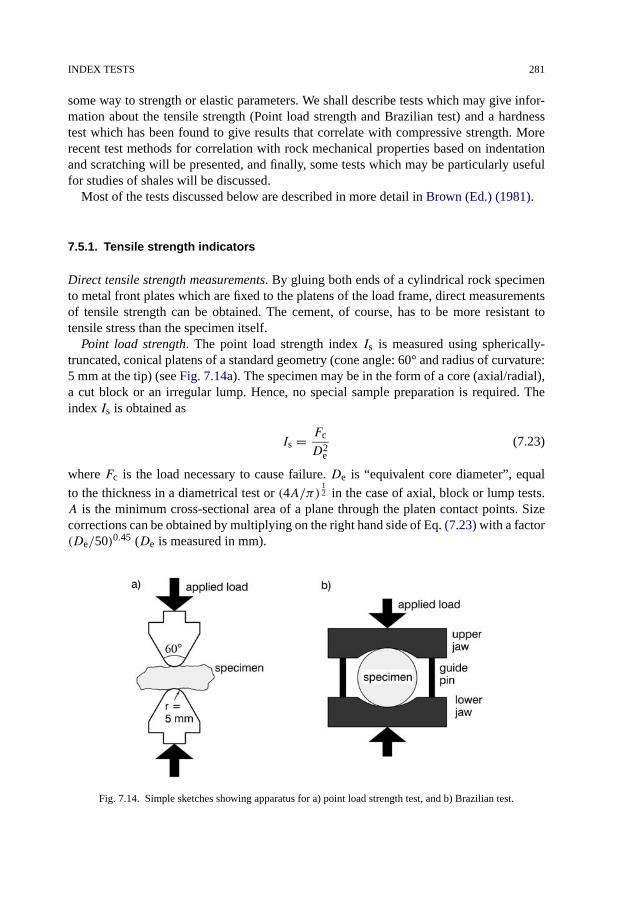
INDEX TESTS 281
some way to strength or elastic parameters. We shall describe tests which may give infor-mation about the tensile strength (Point load strength and Brazilian test) and a hardnesstest which has been found to give results that correlate with compressive strength. Morerecent test methods for correlation with rock mechanical properties based on indentationand scratching will be presented, and finally, some tests which may be particularly usefulfor studies of shales will be discussed.
Most of the tests discussed below are described in more detail in Brown (Ed.) (1981).
7.5.1. Tensile strength indicators
Direct tensile strength measurements. By gluing both ends of a cylindrical rock specimento metal front plates which are fixed to the platens of the load frame, direct measurementsof tensile strength can be obtained. The cement, of course, has to be more resistant totensile stress than the specimen itself.
Point load strength. The point load strength index Is is measured using spherically-truncated, conical platens of a standard geometry (cone angle: 60° and radius of curvature:5 mm at the tip) (see Fig. 7.14a). The specimen may be in the form of a core (axial/radial),a cut block or an irregular lump. Hence, no special sample preparation is required. Theindex Is is obtained as
Is = Fc
D2e
(7.23)
where Fc is the load necessary to cause failure. De is “equivalent core diameter”, equal
to the thickness in a diametrical test or (4A/π)12 in the case of axial, block or lump tests.
A is the minimum cross-sectional area of a plane through the platen contact points. Sizecorrections can be obtained by multiplying on the right hand side of Eq. (7.23) with a factor(De/50)0.45 (De is measured in mm).
Fig. 7.14. Simple sketches showing apparatus for a) point load strength test, and b) Brazilian test.

282 MECHANICAL PROPERTIES AND STRESS DATA FROM LABORATORY ANALYSIS
The point load strength index may be used as an indirect measurement of the uniaxialtensile strength T0:
Is = 0.80T0 (7.24)
The Brazilian test. This test is performed by applying a load with two platens diametri-cally compressed on a rock cylinder, which is normally shorter than or equal in thickness(L) to its diameter (D) (see Fig. 7.14b). Failure occurs by an extension fracture in or closeto the loaded diametrical plane.
A plane stress elastic analysis shows that the stresses close to the centre of the sampleare (Jaeger and Cook, 1979)
σh = − 2F
πDL(7.25)
σv = 6F
πDL(7.26)
The compressional stress is thus always about three times larger than the tensile stress,and since the ratio between the compressive strength and the tensile strength is normallylarger than three, the sample will always fail in tension. The tensile strength (in MPa) isthus given by Eq. (7.25)
T0 = 0.636Fc
DL(7.27)
The peak load Fc is given in N and D and L must be given in mm. The Brazilian testtends to give results which are more reproducible than those obtained by point load strengthmeasurements.
7.5.2. Hardness measurements
Brinell hardness. The Brinell hardness number NBr follows from the ratio of applied loadF on a spherical indenter to the indentation depth D:
NBr = F
2πrD≈ F
πr2s
(7.28)
r is the radius of the sphere and rs is the radius of the indentation surface area. The testis hence non-destructive. For metals and glasses there is a theoretical relationship betweenNBr, the yield stress σyield and Young’s modulus E:
NBr =(a + b ln
E
σyield
)σyield (7.29)
a and b are constants, so that if the yield strength increases in proportion with E, then NBrwill be a measure of σyield.
van der Vlis (1970) and later Geertsma (1985) studied the correlation between NBr,dynamic elastic moduli and the compressive strength of rocks, and for sandstones in par-ticular. Geertsma found a linear relationship between the Brinell hardness and the dynamic
INDEX TESTS 283
Young’s modulus for well consolidated sandstones:
Edyn = 77.25NBr (7.30)
He also presented the approximate result that the Brinell hardness equals the yield strength:
NBr ≈ σyield (7.31)
Other hardness tests. There is a number of other tests whereby material hardness can bequantified. They have in common that they are either indentation tests (like the Brinell hard-ness) or rebound hardness tests (like the Schmidt hammer, for further details, see (Brown(Ed.), 1981)).
7.5.3. Indentation and scratch tests
Indentation tests. The potential access to more information about rock mechanical prop-erties from drill cuttings has motivated work to perform indentation tests on cuttings-sizesamples (Santarelli et al., 1998; Ringstad et al., 1998). These techniques are based oncasting the samples in rapidly curing material (polyester, resin) which can act as a sampleholder and also facilitate grinding and polishing of the sample surface. In these tests the en-tire load-displacement curve is normally recorded, and the slope of the linear regime is usedto correlate with rock mechanical properties such as the uniaxial compressive strength.
Again, uncertainties related to sample size, material heterogeneity, fluid effects etc. needto be considered.
Scratch test. Another technique for determination of mechanical properties is the ScratchTest (Richard et al., 1998; Schei et al., 2000). The principle of this test method is to scratchthe rock surface with a cutter while monitoring the applied force. The cutting depth istypically less than 1 mm. Testing of sandstone and carbonates was found to support asimple force cutting model in the ductile mode
Ft = EA (7.32)
where Ft is the horizontal component of the cutting force averaged over a few cm of scratchlength, E is the intrinsic specific energy and A is the cross-sectional area of the cut.
A strong correlation between specific energy and the uniaxial compressive strength iswell established for several rock types. The possibility to derive information about rockstiffness from scratch measurements has also been demonstrated (Schei et al., 2000). Anobvious advantage with this method is the potential of continuous measurements along acore surface, providing continuous, high resolution data at low cost (Suarez-Rivera et al.,2002).
7.5.4. Specific shale characterization tests
Some rocks, in particular shales or other clay rich materials, are sensitive to water. It isthus essential that characteristic parameters that can be related to the water sensitivity are

284 MECHANICAL PROPERTIES AND STRESS DATA FROM LABORATORY ANALYSIS
measured. Such parameters include the water content, the cation exchange capacity (CEC),specific surface area and the mineralogy.
Water content is measured by weighing a sample before and after heat drying. The heat-ing temperature should be kept lower than 105 °C to ensure that only free water is released.Above this temperature, crystalline water will start to be removed.
CEC can be obtained from several different methods, and since the different methodscan yield quite different results, one should take care when comparing CEC-values fromdifferent sources. A fairly rough and much used method is the so-called methylene blue test(see API, 1968), where a given amount of rock material is transformed into a slurry withde-ionized, distilled water. Strong sulphuric acid is then added to exchange all availablecations in the interlayers of clay minerals with H+ ions. After this, the slurry is diluted, anda solution of methylene blue (C16H18N3SCl·3H2O) is added gradually. H+ ions are thenexchanged with NH+
4 , and the CEC is obtained from the amount of methylene blue requiredto form a blue corona when a suspended drop of the slurry is placed on a filter paper.
Specific surface area is obtained by adsorption of gas or liquid molecules of known sizeonto a surface of a known mass of the rock material (Gregg and Sing, 1967).
Specific surface area has also been used to correlate between wellsite measurements ofthe dielectric constant and the presence of hydratable clays (Leung and Steiger, 1992).A test kit for the dielectric constant measurement technique was developed, using a smallsample of cuttings.
The mineralogy of a rock may be determined from X-ray diffraction. Since the finalnumbers result from interpretation of diffractograms, this is not a completely objectivemethod. Again, comparison of results from different sources should be done with greatcare. Note also that only crystalline minerals will appear on the diffractogram. X-ray amor-phous minerals (e.g. certain opal minerals) will not be detected.
Measuring the activity (the relative humidity) of a shale sample is also frequently usedas an indicator of whether the sample is well preserved and saturated or not. Thesemeasurements are commonly performed under atmospheric conditions. However, underatmospheric conditions the curved interface between the pore water and the air will im-mediately reduce the measured activity below the true value (e.g. Carminati et al., 1997).The amount of this reduction depends on e.g. the pore size distribution of the shale. Thesmaller the pores, the greater the error.
As already discussed, it is important that care is taken in sampling, preservation andhandling of water sensitive rocks like shale. This is particularly important when studyingthe response of these rocks to fluid contact. Tests to measure swelling and disintegration arecommonly used by the drilling mud industry for screening of mud types and mud additives.It is critical that laboratory artifacts are avoided (e.g. due to capillary effects), as they maycompletely dominate the results (see also Section 7.1.4).
References
Amadei, B., Stephansson, O. (1997). Rock Stress and Its Measurement. Chapman & Hall, London.Andersen, M.A. (1995). “Petroleum research in North Sea Chalk”. RF-Rogaland Research.API (American Petroleum Institute) (1968). Supplement 2 to API RP 13B (1st Ed.)—Standard Procedure for
Testing Drilling Fluids: Cation Exchange Capacity. American Petroleum Institute, New York.

REFERENCES 285
Batzle, M.L., Han, D.-H., Hofmann, R. (2006). “Fluid mobility and frequency-dependent seismic velocity—Direct measurements”. Geophysics 71, N1–N9.
Blanton, T.L. (1983). “The relation between recovery deformation and in situ stress magnitudes from anelasticstrain recovery of core”. SPE/DOE 11624. In: SPE/DOE Symp. on Low Permeability, Denver, March 14–16.
Brown, E.T. (Ed.) (1981). Rock Characterization, Testing and Monitoring: ISRM Suggested Methods. PergamonPress, Oxford.
Carminati, S., Brignoli, M., Di Marco, A., Santarelli, F.J. (1997). “The activity concept applied to shales: Conse-quences for oil, tunnelling and civil engineering operations”. Int. J. Rock Mech. & Min. Sci. 34 (3–4). PaperNo. 038.
Colback, P.S.B., Wiid, B.L. (1965). “The influence of moisture content on the compressive strength of rocks”. In:Proc. 3rd Canadian Symp. Rock Mech., Toronto, pp. 65–83.
Engelder, T., Plumb, R. (1984). “Changes in in situ ultrasonic properties of rock on strain relaxation”. Int. J. RockMech. Min. Sci. & Geomech. Abstr. 21, 75–82.
Geertsma, J. (1985). “Some rock mechanical aspects of oil and gas well completions”. Soc. Petr. Eng. J. 25,848–856.
Gregg, S.J., Sing, K.S.W. (1967). Adsorption, Surface Area and Porosity. Academic Press, New York.Head, K.H. (1984). Soil Laboratory Testing, vols. I–III. ELE Intl., London.Hoek, E., Franklin, J.A. (1968). “Simple triaxial cell for field or laboratory testing of rock”. Trans. Inst. Min.
Metall. 77A, 483–489.van den Hoek, P.J., Kooijman, A.P., Kenter, C.J., Khodaverdian, M., Hyland, C.R., McLennan, J.D. (1992). “Size-
dependency of hollow cylinder collapse strength”. SPE 24800. In: Proc. 67th Annual Technical Conferenceand Exhibition, Washington DC, pp. 351–360.
Holcomb, D.J. (1993). “Observations of the Kaiser effect under multiaxial stress states: Implications for its usein determining in situ stress”. Geophys. Res. Lett. 20, 2119–2122.
Holt, R.M., Ingsøy, P., Mikkelsen, M. (1989). “Rock mechanical analysis of north sea reservoir formations”. SPEFormation Evaluation 4 (1), 33–37.
Holt, R.M., Fjær, E. (1991). “Validity of multiple failure state triaxial tests in sandstones”. In: Proc. VII Int.Congress on Rock Mechanics, Aachen.
Holt, R.M., Brignoli, M., Kenter, C.J. (2000). “Core quality: quantification of coring-induced rock alteration”.Int. J. Rock Mech. Min. Sci. 37, 889–907.
Horsrud, P., Sønstebø, E.F., Bøe, R. (1998). “Mechanical and petrophysical properties of North Sea shales”. Int.J. Rock Mech. Min. Sci. 35, 1009–1020.
Hudson, J.A., Crouch, S.L., Fairhurst, C. (1972). “Soft, stiff and servocontrolled testing machines: A review withreference to rock failure”. Engineering Geology 6 (3), 155–189.
Jaeger, J.C., Cook, N.G.W. (1979). Fundamentals of Rock Mechanics, third ed. Chapman and Hall, London.Janbu, N. (1985). “Soil models in offshore engineering. 25th Rankine lecture”. Geotechnique 35, 239–281.Jones, M. (1988). Determination of the Mechanical Properties of Reservoir Rocks Using the Triaxial Test. Ex-
perimental Guidelines. The Norwegian Petroleum Directorate, Stavanger.Kenter, C.J., Brignoli, M., Holt, R.M. (1997). “CMS (Constant Mean Stress) vs. UCS (Unconfined Strength)
tests: A tool to reduce core damage effects”. Int. J. Rock Mech. & Min. Sci. 34 (3–4). Paper No. 129.Kenter, C.J., Pestman, B.J., Van Munster, J.G. (1998). “Determining in situ stress”. Patent EPC 98202284.Kovari, K., Tisa, A., Einstein, H.H., Franklin, J.A. (1983). “Suggested methods for determining the strength of
rock materials in triaxial compression: Revised version”. Int. J. Rock Mech. Min. Sci. & Geomech. Abstr. 20,283–290.
Lambe, T.W., Whitman, R.V. (1979). Soil Mechanics. John Wiley & Sons, New York.Leung, P.K., Steiger, R.P. (1992). “Dielectric constant measurements: A new, rapid method to characterize shale
at the wellsite”. IADC/SPE 23887. In: Proc. 1992 IADC/SPE Drilling Conf., New Orleans, pp. 401–408.Matsuki, K., Takeuchi, K. (1993). “Three-dimensional in situ stress determination by anelastic strain recovery of
a rock core”. Int. J. Rock Mech. Min. Sci. & Geomech. Abstr. 30, 1019–1022.Maury, V.M., Santarelli, F.J., Henry, J.P. (1988). “Core discing: A review”. In: Proc. SANGORM Symp.: Rock
Mechanics in Africa, pp. 221–231.Mess, K.W. (1978). “On the interpretation of core compaction behaviour”. In: Saxena, S.K. (Ed.), Evaluation and
Prediction of Subsidence. ASCE, New York, pp. 76–91.

286 MECHANICAL PROPERTIES AND STRESS DATA FROM LABORATORY ANALYSIS
Nakken, S.J., Christensen, T., Marsden, R., Holt, R.M. (1989). “Mechanical behaviour of clays at high stresslevels for wellbore stability applications”. In: Maury, V., Fourmaintraux, D. (Eds.), Rock at Great Depth.Balkema, Rotterdam, pp. 141–148.
Nes, O.-M., Horsrud, P., Sønstebø, E.F., Holt, R.M., Ese, A.M., Økland, D., Kjørholt, H. (1998a). “Rig site andlaboratory use of CWT acoustic velocity measurements on cuttings”. SPE Reservoir Evaluation & Eng. 1,282–287.
Nes, O.-M., Sønstebø, E.F., Horsrud, P., Holt, R.M. (1998b). “Dynamic and static measurements on mm-sizeshale samples”. SPE/ISRM 47200. In: Proc. Eurock ’98, vol. 2, Trondheim, pp. 23–32.
Papamichos, E., Brignoli, M., Santarelli, F.J. (1997). “An experimental and theoretical study of a partially satu-rated collapsible rock”. Mech. Cohesive-Frictional Mater. 2, 251–278.
Pestman, B.J., Holt, R.M., Kenter, C.J., van Munster, J.G. (2002). “Field application of a novel core-based in-situstress estimation technique”. SPE/ISRM 78158. In: Proc. Oil Rocks, Irving, October 20–23.
Ren, N.K., Hudson, P.J. (1985). “Predicting the in situ state of stress using differential wave velocity analysis”.In: Proc. 26th US Rock Mech. Symp., pp. 1235–1244.
Richard, T., Detournay, E., Drescher, A., Nicodeme, P., Fourmaintraux D. (1998). “The scratch test as a means tomeasure strength of sedimentary rocks”. SPE/ISRM 47196. In: Proc. Eurock ’98, vol. 2, Trondheim, pp. 15–22.
Ringstad, C., Lofthus, E.B., Sønstebø, E.F., Fjær, E. (1998). “Prediction of rock parameters from micro-indentation measurements: The effect of sample size”. SPE/ISRM 47313. In: Proc. Eurock ’98, vol. 2,Trondheim, pp. 487–492.
Risnes, R., Flaageng, O. (1999). “Mechanical properties of chalk with emphasis on chalk–fluid interactions andmicromechanical aspects”. Oil & Gas Sci. Technol. Rev. IFP 54, 751–758.
Santarelli, F.J., Guenot, A. (1990). “Experimental observations of bifurcation phenomena in rocks”. In: Maury,V., Fourmaintraux, D. (Eds.), Rock at Great Depth. Balkema, Rotterdam, pp. 1563–1570.
Santarelli, F.J., Marsala, A.F., Brignoli, M., Rossi, E., Bona, N. (1998). “Formation evaluation from logging oncuttings”. SPE Reservoir Evaluation & Eng. 1, 238–244.
Santos, H., Diek, A., Roegiers, J.C., Fontoura, S. (1996). “Can shale swelling be (easily) controlled?” In: Proc.Eurock ’96, Torino, pp. 99–106.
Schei, G., Fjær, E., Detournay, E., Kenter, C.J., Fuh, G.-F., Zausa F. (2000). “The Scratch Test: An attractivetechnique for determining strength and elastic properties of sedimentary rocks”. SPE 63255. In: 2000 SPEAnnual Technical Conf. and Exhibition, Dallas, 1–4 October.
Schmitt, L., Forsans, T., Santarelli, F.J. (1994). “Shale testing and capillary phenomena”. Int. J. Rock Mech. Min.Sci. & Geomech. Abstr. 31, 411–427.
Spencer Jr., J.W. (1981). “Stress relaxations at low frequencies in fluid saturated rocks: Attenuation and modulusdispersion”. J. Geophys. Res. 86 (B3), 1803–1812.
Steiger, R.P., Leung, P.K. (1992). “Quantitative determination of the mechanical properties of shale”. SPE DrillingEng. 7, 181–185.
Suarez-Rivera, R., Stenebråten, J., Dagrain, F. (2002). “Continuous scratch testing on core allows effective cali-bration of log-derived mechanical properties for use in sanding prediction evaluation”. SPE/ISRM 78157. In:Proc. Oil Rocks, Irving, October, pp. 20–23.
Sulem, J., Vardoulakis, I. (1989). “Simplified bifurcation analysis of deep boreholes in rocks with microstructure”.In: Maury, V., Fourmaintraux, D. (Eds.), Rock at Great Depth. Balkema, Rotterdam, pp. 845–852.
Swan, G., Cook, J., Bruce, S., Meehan, R. (1989). “Strain rate effects in Kimmeridge Bay shales”. Int. J. RockMech. Min. Sci. & Geomech. Abstr. 26, 135–149.
Teufel, L.W. (1989). “Acoustic emissions during anelastic strain recovery from deep boreholes”. In: Khair,A.W. (Ed.), Rock Mechanics as a Guide for Efficient Utilization of Natural Resources. Balkema, Rotterdam,pp. 269–276.
Tronvoll, J., Morita, N., Santarelli, F.J. (1992). “Perforation cavity stability: Comprehensive laboratory experi-ments and numerical analysis”. SPE 24799. In: 1992 SPE Annual Technical Conf. and Exhibition, Washing-ton, DC, 4–7 October.
van der Vlis, A.C. (1970). “Rock classification by a simple hardness test”. In: Proc. 2nd Congress ISRM, pp. 23–30.
Vutukuri, V.S., Lama, R.D., Saluja, S.S. (1974). Mechanical Properties of Rocks, vols. I–IV. Trans Tech. Publ.,Clausthal.

REFERENCES 287
de Waal, J.A., Smits, R.M.M. (1988). “Prediction of reservoir compaction and surface subsidence: Field applica-tion of a new model”. SPE Formation Evaluation 3, 347–356.
Warpinski, N.R., Teufel, L.W. (1989). “A viscoelastic constitutive model for determining in situ stress magnitudesfrom anelastic strain recovery of core”. SPE Production Eng. 4 (3), 272–289.
Winkler, K.W., Plona, T.J. (1982). “Technique for measuring ultrasonic velocity and attenuation spectra in rocksunder pressure”. J. Geophys. Res. 87B, 10776–10780.
Yassir N., Wang, D.-F., Enever, J.R., Davies, P.J. (1998). “An experimental analysis of anelastic strain recovery ofsynthetic sandstone subjected to polyaxial stress”. SPE/ISRM 47238. In: Proc. Eurock ’98, vol. 1, Trondheim,pp. 161–170.

This page intentionally left blank
289
Chapter 8
Mechanical properties and in situ stresses from field data
Knowledge of the mechanical properties and the in situ stresses of the subsurface for-mations is essential in connection with wellbore stability problems, fracturing operations,subsidence problems and sand production evaluation.
In this chapter we will look at methods for estimating mechanical properties and insitu stresses from field tests and field data. The methods can be grouped into three maincategories: measurements while drilling, wireline logging methods and well tests.
We start by recalling the mechanical parameters and in situ stresses of a formation:
Elastic parameters. For an isotropic medium, there are two independent elastic moduli.However, these two parameters have a real and an imaginary part, that both will varywith frequency and with stress level, such that even in the isotropic case the use of twoparameters is clearly a simplification.
Strength parameters. We have seen that the strength of a material is dependent on thestress level, and that failure criteria that describe actual data normally have at least 2–3adjustable parameters.
In situ stresses. The in situ stresses are given by the three principal stresses and threeparameters giving the orientation of the principal stresses. The stress level determineswhether a rock is critically loaded or not. Additionally, the in situ stresses influence boththe elastic parameters and the strength parameters.
8.1. Estimation of elastic parameters
The most important method for estimation of elastic parameters is acoustic logging, and inparticular acoustic wireline logs. Acoustic logging while drilling is now also available, butis still less used.
Acoustic logging tools measure acoustic wave velocities which together with density in-formation and the appropriate formulae discussed in Chapter 5 provide the dynamic elasticparameters (Eqs. (5.20)–(5.24)). We repeat here the equations for dynamic Young’s modu-lus (Edyn) and dynamic Poisson’s ratio (νdyn):
Edyn = ρv2s (3v
2p − 4v2
s )
(v2p − v2
s )(8.1)
νdyn = v2p − 2v2
s
2(v2p − v2
s )(8.2)
Once the dynamic moduli are known, the problem is to relate them to the static parame-ters, which is what is needed for most applications. This problem is a difficult one that hasnot been fully resolved.

290 MECHANICAL PROPERTIES AND IN SITU STRESSES FROM FIELD DATA
The difference between the static Young’s modulus and the dynamic Young’s modulusmay be quite significant, in particular at low stress levels. The dynamic modulus may beseveral times larger than the static modulus e.g. in a weak sandstone. The static–dynamictransition is complicated by the fact that it is not a constant shift, but varies independentlywith loading (Fjær, 1999). The main contribution to the difference is the strain amplitude,which is low in dynamic measurements and large in static measurements. In a porous rockboth pore fluid and cracks can give further contribution to this difference. Empiricallybased static–dynamic transition methods are thus of limited validity, and there is still alsoa lack of theoretically based methods.
One step in the direction of a more fundamental approach was presented by Fjær (1999).This approach was developed primarily for weak sandstone, utilizing a large number ofcarefully designed laboratory tests (mostly on North Sea cores) with simultaneous staticand dynamic measurements. Further description of this quantitative model was given inSection 5.6.
The rest of this section will be devoted to various types of acoustic measurements, pri-marily from downhole measurements, but also from rig measurements. The principles ofacoustic wave propagation around boreholes were described in Section 5.8.
Indirect information which may be useful for evaluation of mechanical parameters canbe obtained from other logging tools, e.g. the gamma, density and neutron logs. These toolscan be used to obtain lithological information.
8.1.1. Acoustic wireline logs
The primary output from acoustic logging tools is the velocities and waveforms of differentwaves, such as the compressional-, shear- and Stoneley waves. Note that acoustic loggingtools may be used to generate information about a number of other characteristics of theformation, such as lithology identification, porosity estimates, gas detection, detection ofnatural fractures, qualitative evaluation of permeability variations and creation of syntheticseismograms for comparison with surface seismics.
Full waveform sonic tools
A principle sketch of a full waveform sonic tool is shown in Fig. 8.1. This consists of anomnidirectional transmitter separated from an array of receivers.
The transmitter creates a pressure pulse in the borehole fluid. This pressure pulse gen-erates compressional and shear waves in the formation, in addition to borehole waves likethe Stoneley wave. These tools will thus ideally provide compressional and shear velocitiesof the formation in addition to the Stoneley wave velocity. However, in slow formations(poorly consolidated) the shear wave velocity is slower than the fluid waves in the borehole.Consequently, the shear velocity can not be measured directly.
From a mechanical properties point of view, one is most interested in the shear velocityin slow formations, since low wave velocities indicate low strength and hence potential

ESTIMATION OF ELASTIC PARAMETERS 291
Fig. 8.1. Principle sketch of a full waveform sonic tool. Typical distance from transmitter to first receiver is 10 ft(3 m), while the distance between each receiver is typically 0.5–1 ft (0.15–0.3 m).
stability problems. Direct measurement of both compressional and shear velocities also inslow formations is possible using dipole or multipole tools.
Typical centre frequency of the transmitter used in full waveform sonic tools is 15 kHz.However, to strongly excite the Stoneley mode, the source spectrum should include fre-quencies below 5 kHz. This can be obtained by increasing the bandwidth of the source andalso by varying the excitation frequency of the source, depending on which waveform isrequested.
Multipole sonic tools
The basic concept of this tool is the dipole source transducer. A dipole transducer can inprinciple be pictured as two closely spaced monopole transducers driven with oppositephases. This piston-like effect creates an increase in pressure on one side of the boreholeand a decrease in pressure on the other side of the borehole. This force oriented normal tothe borehole wall induces a flexural motion of the borehole (see Fig. 5.20).
The dipole source operates at low frequencies, typically with a centre frequency of 1–1.5 kHz. At low frequencies the flexural mode is very little affected by the borehole andtravels at the same speed as the shear wave. Dipole tools can thus provide a direct measure-ment of the shear velocity even in slow formations. At higher frequencies, the propagationvelocity becomes smaller.
Dipole capabilities are often integrated in monopole tools, with the dipole transmitterclose to the monopole source, see Fig. 8.1. By including two dipole transducers orientedperpendicular to each other and two receivers at each receiver station, both in-line andcross-line measurements can be performed. Cross-dipole measurements hence facilitate anevaluation of different types of anisotropy. It is a well known observation that the acousticvelocity is faster along the rock bedding than normal to the bedding. This has commonly

292 MECHANICAL PROPERTIES AND IN SITU STRESSES FROM FIELD DATA
been observed when comparing P-wave velocities measured in vertical holes with mea-surements in highly deviated or horizontal holes in the same formation.
Schlumberger’s Sonic Scanner tool is a combination of 3 monopole and 2 orthogonallyoriented dipole sources, and more than a hundred receivers. The dipole sources may sweepthrough a frequency band from 300 Hz to 8 kHz. The tool enables a fairly detailed charac-terization of the elastic wave velocities in the vicinity of the borehole, as it is sensitive toaxial and azimuthal as well as radial variations.
8.1.2. Acoustic logging while drilling
In recent years, tools for acoustic logging while drilling have also become available. Thetool configuration is similar to that shown in Fig. 8.1, with a transmitter separated a fewfeet (typically 4–7 ft) from an array of receivers. The full waveforms are normally recordedin a downhole memory for later evaluation, but transit times can be transmitted uphole forreal time use: lithology evaluation, porosity determination, pore pressure estimation andcorrelation of drill bit position to seismic maps.
Real time access to good estimates of mechanical properties of the rock is obviously use-ful also for borehole stability evaluation while drilling. By logging while and after drillingone could possibly monitor changes in the rock response during the openhole period. Thismay give an early warning of possible deterioration of rock integrity with time whicheventually results in borehole stability problems. Consistent differences between acousticvelocities recorded while drilling and from wireline logging have been observed in shales(e.g. Boonen et al., 1998). However, time-lapse studies investigating this for borehole sta-bility evaluation have yet not been published.
8.1.3. Acoustic measurements on drill cuttings
Acoustic measurements on drill cuttings may represent a valuable source of informationwhich can supplement the logging techniques. Alternative techniques are available, both asonic pulse technique (Santarelli et al., 1998) and a continuous wave technique (Nes et al.,1998). For further description, see also Section 7.3.12.
Drill cuttings represent a large source of information which is available without any ad-ditional cost. If used on the rig, information will be available close to real time. There are,however, a number of limitations with these techniques, related primarily to the qualityand representativity of the cuttings. How has stress unloading effects, drill bit effects andeffects of the drilling fluid etc. changed the response compared to that of the virgin for-mation? Other uncertainties relate to possible length scale effects (typically mm-size forcuttings while typically 30 cm for an acoustic log) and the accuracy in depth determinationof cuttings origin. A bias in sample selection may also be introduced, promoting measure-ments on the more competent samples in the high-velocity range. The difference in testconditions (atmospheric for cuttings measurements compared to downhole conditions forlogging tools) may also affect the result.
ESTIMATION OF STRENGTH PARAMETERS 293
Despite all these possible uncertainties, reasonable agreement between logged valuesand values derived from cuttings measurements have been reported (Santarelli et al., 1998;Nes et al., 1998), especially with respect to depth trends. Cuttings measurements thusrepresent a promising but not yet fully explored alternative and/or supplement to othermeasurements.
8.2. Estimation of strength parameters
There are no direct methods available for determination of the strength parameters in situ.Hence most of the efforts made to predict strength parameters have been based on empiricalcorrelations, especially relations between acoustic velocities and strength parameters. Thissection will discuss both this and other relations which are being used for estimation ofstrength parameters.
8.2.1. Log data (wireline and MWD)
Log data are attractive for prediction of rock mechanical properties since logging is one ofthe few downhole measurements available. As presented already, there is a direct relationbetween acoustic velocities and dynamic elastic properties. However, rock strength datacan not be inferred directly from logs. The traditional approach has therefore been more orless empirical, using both log derived acoustic velocities (especially the shear velocity) andlog derived porosity. An obvious disadvantage with such an approach is the need for fre-quent calibration and checking of the validity of the empirical correlations when enteringa new field or area.
The model which was briefly discussed in Section 8.1 (Fjær, 1999) can also be used forstrength prediction (Raaen et al., 1996). This model also uses log data (acoustic velocitiesand density), and was developed primarily for prediction of weak sandstone strength. Thefact that this model has a more theoretical basis makes it more robust, and it can thusbe applied in new wells without extensive calibration. This therefore represents a step inthe right direction. However, there is still no universally valid method available whichcan predict the strength of different lithologies directly from logs, without any need ofcalibration.
The methods for predicting rock strength offered by the service companies are all subjectto the limitations discussed above, being more or less empirical and requiring more or lesscalibration.
8.2.2. Drill cuttings measurements
Different types of measurements on drill cuttings have been discussed previously, bothacoustic measurements (Section 7.3.12 and Section 8.1.3) and indentation measurements(Section 7.5.3). To obtain strength values, correlations have to be established (Santarelliet al., 1998; Ringstad et al., 1998). Given the previously discussed uncertainties of using
294 MECHANICAL PROPERTIES AND IN SITU STRESSES FROM FIELD DATA
drill cuttings (Section 8.1.3), these methods must at present be considered quite coarse.However, they should be able to provide at least comparative evaluations, i.e. a “weak”versus “strong” type of classification.
8.2.3. Empirical correlations
The lack of direct downhole strength measurements or other generally applicable theoriesfor relating rock strength to measurable quantities has motivated considerable efforts togenerate empirical correlations for rock strength prediction. Most of this has been basedon log-measured or log-derived properties, such as acoustic velocities or porosities. Someexamples of such work is Edlman et al. (1998), Farquhar et al. (1994), Mason (1987), Onyia(1988). Empirical correlations have been generated very much dependent on the need orthe application. Production related problems deal with weak sandstones while stabilityproblems related to drilling deal with weak shales.
There are some general comments which should be made regarding empirical correla-tions:
• The correlations are normally based on one specific type of rock or lithology. A cor-relation developed in sandstone may not be valid in shale, i.e. empirically basedcorrelations are not universally applicable.
• Rock strength measurements may be very scarce for some lithologies, such as shales,because shales are normally not cored and tested. Shale-specific correlations arescarce (for exceptions, see Lashkaripour and Dusseault, 1993 and Horsrud, 2001).
• Lack of actual core material has promoted use of outcrop material which may not berelevant for downhole sedimentary rocks (differences in sedimentation history, stresshistory, stress environment, diagenesis etc.).
• Laboratory test procedures or data interpretation procedures may vary, yielding resultswhich are not fully compatible.
• Even if the correlation is based on real core material from one area, it may not beapplicable to other geographical areas. It is always recommended to check the validityof correlations when entering new areas and calibrate them if necessary.
• The published correlations are generally biased towards fairly competent rocks, thusreducing their accuracy with respect to weak rocks which is the primary concern inall types of stability evaluations.
For these reasons, no specific correlations will be presented here. These commentsshould also be kept in mind when considering or using empirical correlations for strengthprediction.
In general one will find that the rock strength increases when the rock is densified andcemented, i.e. as depth, age and effective stresses increase. This is further reflected innormal trends of reduced porosity and increased acoustic velocity.
Further discussion of mechanical properties of sedimentary rocks (sandstone, chalk andshale) is given in Section 3.4, including some examples of empirical correlations.

ESTIMATION OF IN SITU STRESSES 295
8.2.4. Drilling data
Intuitively, the response of the drill bit should reflect also the mechanical properties ofthe rock, under true downhole conditions. Bit response is, however, also dependent on anumber of other parameters. Traditionally, the motivation for rock-bit interaction modelshas been to improve bit selection and bit operation procedures. The process of cuttingsgeneration and cuttings removal is fairly complicated, and most ROP (rate of penetration)models are therefore empirical or semi-empirical. Although ROP models are available forseveral bit types, most of the modelling efforts have been directed towards roller cone bits.A representative version of an ROP model is (Warren, 1987):
R =(aS2D3
nW 2+ b
ND+ cDρμ
Fm
)−1
(8.3)
where R is the rate of penetration, W is weight on bit, N is bit rotary speed, S is rockstrength, D is bit diameter, Fm is modified jet impact force, ρ is mud density, μ is plasticviscosity and a, b, c are dimensionless constants.
Additional effects related to bit wear and chip hold down may also be included (e.g.Hareland and Hoberock, 1993).
Thus one can also solve Eq. (8.3) for the rock strength when the rate of penetration andthe other parameters and functions are known (Hareland et al., 1996).
Determination of all the input parameters and model constants may not be trivial, andcalibration against results from tests under controlled conditions or against previous bitruns in the same area may be required. Considerable uncertainty in quantitative predictionsshould therefore be expected. It is also obvious that such models are not easy to use in apredictive manner.
It is quite obvious that the drilling process is a response to the properties of the rockand its state of stress. Information about the rock mechanical properties should thereforebe retrievable from drilling data, but continued efforts to understand and model the drillingprocess are required. Combining all measurements while drilling, both drilling data andlog data, may eventually provide a real-time tool for follow-up of the drilling process. Thiswill be applicable both to borehole stability and drilling efficiency, and eventually the twoaspects may be combined into a fully integrated drilling optimization model.
8.3. Estimation of in situ stresses
This section will present available methods for estimating in situ stresses from field data.Methods based on core measurements were discussed in Chapter 7 and will not be repeatedhere. This section will thus focus on data from well logs and well tests. For a more detaileddescription of all available stress measurement methods, see e.g. Amadei and Stephansson(1997) and Haimson and Cornet (2003). Note that not all these methods are suitable forpetroleum applications.
The presentation given here is based on the common assumption of a vertical-horizontalstress field, i.e. one principal stress is vertical and the two others are horizontal. This is
296 MECHANICAL PROPERTIES AND IN SITU STRESSES FROM FIELD DATA
valid in tectonically inactive areas or areas which have been relaxed from previous tec-tonic activity. In active areas this assumption may not be valid, and the stress field can besignificantly distorted. See also Chapter 3.
8.3.1. The density log (overburden stress)
The density tools are active gamma ray tools that use the Compton scattering of gammarays to measure the electron density of the formation. By appropriate lithology corrections,the electron density is converted to mass density with reasonable accuracy.
The density is useful for determining mechanical properties in two manners: first, thedensity is needed to convert from acoustic velocities to dynamic elastic moduli (see Sec-tion 8.1). Second, the density integrated over the vertical depth of the well is usuallyconsidered to give a good estimate of the vertical stress, at least in areas of low tectonicactivity. In such areas, the vertical stress is also considered to be a principal stress. Whenthe density log is available, the problem of determining the full in situ stress field is thenreduced to determining the magnitude and orientation of the horizontal stresses.
However, the density log is rarely available in the first few hundred metres of a well.Then it is necessary to make estimates of the density to obtain the total vertical stress. Inareas which have not been subjected to tectonic activity it is common to assume a density inthe range 1.8–2.0 g/cm3. This bulk density corresponds to a porosity in the range 50–38%in a rock with a mineral density of 2.6 g/cm3.
Offshore Mid-Norway, bulk densities above 2 g/cm3 have been logged at very shallowdepths. One plausible explanation to this unusually high density is that this area has alsobeen exposed to ice loads. Thus the geological history should be taken into considerationwhen making estimates in non-logged intervals. Geotechnical data from site surveys mayin some cases be available and provide additional information.
8.3.2. Borehole logs (horizontal stress directions)
Determination of horizontal stress directions is based on the possibility of failure at theborehole wall which can be detected by borehole logging tools. To be detectable, the fail-ures must occur in the period after drilling and prior to logging. In a vertical boreholewhich penetrates layers of significantly different horizontal stresses (σH > σh), two dis-tinct failure modes can be detected: compressive and tensile failure. The directions of thesetwo failure modes in an idealized situation are uniquely given by the directions of the twoprincipal horizontal stresses, as illustrated in Fig. 8.2. Compressive failure or shear failurewill be induced in the direction parallel with the smallest horizontal stress (σh) if the wellpressure is low enough to induce shear failure. This is commonly referred to as breakoutsin this context and will lead to an ovalization of the borehole. Tensile failure will occurin the direction parallel with the largest horizontal stress (σH) if the well pressure is largeenough to induce fracturing. See also Chapter 4 for further discussion of stresses aroundboreholes.

ESTIMATION OF IN SITU STRESSES 297
Fig. 8.2. Illustration of directions for compressive and tensile failure around a vertical borehole. Since tensilefailure occurs at high well pressures and compressive failure at low pressures, these failure modes are not normallyobserved at the same depth. A possible exception is if there has been large variations in the well pressure.
Note that in situations with large variations in equivalent circulating density (ECD) ofthe drilling fluid it may be possible to observe both failure modes at the same depth.
Once a failure has occurred on the borehole wall, it is tempting to try to back-calculatealso stress magnitudes, especially the magnitude of the largest horizontal stress by usingelastic theory and appropriate failure criteria. However, a number of assumptions are re-quired for such analyses, rendering the results uncertain. Such estimates can at best beconsidered upper or lower bounds on the stress magnitudes (see also Section 8.3.4). Thelarge amount of information that can be acquired by new tools, such as the Sonic Scan-ner (see Section 8.1.1) may eventually reduce some of the uncertainty, and allow for morereliable estimation of the in situ stresses.
Caliper logs
The caliper log (four-arm) has commonly been used to estimate horizontal stress directionsfrom breakout orientations. This tool provides two diameters of the borehole cross-section.To be able to identify stress induced borehole breakouts, a set of identification criteria hasto be implemented. We quote here the criteria published by Plumb and Hickman (1985):
1. The tool is rotating above and below a borehole breakout.
2. The rotation stops over the breakout zone.
3. The borehole elongation is clearly seen in the log. One pair of pads must show arelatively sharp ascent and descent of the borehole diameter.
4. The smaller of the caliper readings is close to bit size, or if the smaller caliper readingis greater than bit size it should exhibit less variation than the larger caliper.
5. The direction of elongation should not consistently coincide with the high side of theborehole when the hole deviates from vertical.

298 MECHANICAL PROPERTIES AND IN SITU STRESSES FROM FIELD DATA
The last item in this list reflects the problem of differentiating between breakouts andkeyseats.1 This is a major problem, since it is not possible to distinguish between break-outs and keyseats when using four-arm caliper data. Generally, elongations are regardedas keyseats if their direction is within ±10°–15° of the hole azimuth. However, this cancategorize a large portion of the elongations as keyseats, even at deviations less than 6°(Fejerskov and Bratli, 1998). This implies that either a large portion of the data points arewrongly rejected, or much of the previous work on breakout analysis has to be rejected.
This problem with the caliper log is somewhat reduced as six-arm tools are becomingindustry standard. However, the best results are obtained with tools which can provide amore complete image of the borehole.
Image logs
Image logs include both electrical (resistivity) and acoustical borehole imaging logs. Theelectrical image log operates with a large number of electrodes in contact with the forma-tion, usually distributed over several pads on independent arms (four or six). This shallowelectrical investigation is well suited for investigation of fine structures like bedding planes,natural fractures and also drilling induced fractures.
The acoustical imaging tool (often referred to as borehole televiewer, BHTV) is based onreflection of acoustic waves from the borehole wall, recording the travel time and amplitudeof the reflected pulses. The pulses are generated by a rapidly rotating piezo-electric crystal,thus creating a helix-shape logging path with a short distance between each revolution. Thistool is best suited for detection of borehole breakouts, as drilling induced fractures do notcreate significant changes in borehole radius or reflectivity.
Since these tools provide a full image of the borehole wall, it is possible to distinguishbetween stress induced breakouts and keyseats. An example of an electrical borehole imagelog is shown in Fig. 8.3. Examples of the use of image logs for determination of horizontalstress directions and magnitudes is given by Brudy (1998).
If drilling induced fractures are found at an inclination with respect to the borehole axis,this implies that none of the principal stresses are parallel with the borehole axis. This canbe the situation in an inclined borehole, or in a vertical borehole where the vertical stressis not a principal stress, as for instance close to faults (Brudy et al., 1997).
8.3.3. Fracture tests (horizontal stress magnitudes)
The only fully reliable method for determination of the smallest horizontal stress (σh) is tofracture the formation and record the pressure at which the fracture closes. This requiresthat the fracture has penetrated far enough into the formation to feel only the resistance ofthe in situ horizontal stress. In a vertical well this is achieved 2–3 wellbore diameters awayfrom the borehole. In a deviated wellbore, the fracture may have to travel farther away
1 A keyseat is an enlargement of the borehole in one preferred direction, normally created by the mechanicalaction of the drillstring on the borehole wall.

ESTIMATION OF IN SITU STRESSES 299
Fig. 8.3. A resistivity image of a 10 m borehole wall section recorded with 4 arms in a North Sea well. Darkregions represent low resistivity. Intermittent dark traces on arm 1 and 3 indicate drilling induced fractures.Notice that these drilling induced fractures are 180° apart at the borehole wall and are not interconnected aroundthe borehole like traces of natural fractures or bedding planes.
from the borehole, due to the twisting of the fracture and the principal stresses close toa deviated borehole. Basic principles of the different phases of fracture initiation, growthand closure will be discussed in Chapter 11.
Determination of the largest horizontal stress (σH) is not trivial, and there is no straight-forward method available for this. In an idealized linear elastic situation, the largest hori-zontal stress could be determined from a repeated fracture test. However, in practice, thefracture initiation pressure can vary considerably, rendering such an approach highly un-certain (see also Section 11.2). Normally, the fracture initiation pressure is lower than pre-dicted from linear elastic theory. Investigation of Eq. (11.11) shows that if this is the case,the largest horizontal stress is overestimated. This is probably the reason why field studiesutilizing such an approach consistently predict a strike-slip stress regime (σH > σv > σh).
This section will focus on fracturing methods used for determination of the smallesthorizontal stress.
Leak-off tests and extended leak-off tests
Leak-off tests (LOT) are performed during the drilling phase of a well, in the formationimmediately below each casing shoe. The purpose of this test is to determine the maximumwell pressure the new borehole section can sustain without fracturing and loss of drilling

300 MECHANICAL PROPERTIES AND IN SITU STRESSES FROM FIELD DATA
fluid. A traditional leak-off test is therefore not designed to determine the smallest hori-zontal stress, but to obtain a design value for the mud density in the next borehole sectionwhich is going to be drilled.
After a casing string has been cemented, the casing shoe is drilled out and a few me-tres of new formation is penetrated. A leak-off test is then performed by pressurizing thisopen-hole section. The principle of a leak-off test is shown in the first cycle in Fig. 8.4.The pressure in the hole is increased by pumping at a constant volume rate, typically 50–250 l/min. This yields a straight line of pressure versus volume (time), with the slope ofthe line given by the compressibility of the system (primarily the drilling fluid). The pointwhere the pressure response starts to deviate from this straight line is defined as the leak-offpoint. This is actually the point where a fracture is starting to initiate. Normally, a leak-off test is stopped shortly after this, even if the pressure continues to increase above theleak-off pressure.
The slope and the shape of the pressure versus volume line can be affected by a numberof operational aspects (equipment performance, cement channels, pump rate etc.). For adiscussion of how these factors may affect LOT-interpretation, see e.g. Postler (1997).
As discussed in Chapter 11, this leak-off point or fracture initiation point is, however, notnecessarily directly related to the smallest horizontal stress, and is therefore no estimate ofσh. It is also important to note that if the test is stopped shortly after the leak-off point, thegenerated fracture is very short, and even if the shut-in phase is recorded (see Fig. 8.4), thisshut-in pressure may significantly overestimate the smallest horizontal stress. Examplesgiven by Raaen and Brudy (2001) and Raaen et al. (2006) demonstrate that using the leak-
Fig. 8.4. An example of a conventional leak-off test (first cycle) followed by three extended leak-off test cyclesat 9 5/8′′ casing shoe at 2550 m depth. The first cycle is shut in after 14 min of pumping at 75 l/min (1050 lpumped). The following cycles are shut in after 4.8 min of pumping at 250 l/min (1200 l pumped). The verticallines indicate the shut-in point, after which the curves are a function of time, as indicated by the total shut-inperiod of each curve.

ESTIMATION OF IN SITU STRESSES 301
off pressure as an estimate of the smallest horizontal stress can cause significant errors. Atthe very best, the smallest horizontal stress will be a lower bound to a large population ofleak-off pressures (Addis et al., 1998).
To make the leak-off test applicable also to stress determination, modifications have tobe made. This has lead to the so-called extended leak-off test (XLOT, ELOT) (e.g. Kunzeand Steiger, 1992). The main difference from the standard leak-off test is that pumpingcontinues well beyond the leak-off point and also beyond the breakdown pressure. To geta reliable stress estimate, pumping should continue until stable fracture growth is obtained(see third and fourth pump cycle of Fig. 8.4). After shut-in, the shut-in/decline phase shouldbe recorded. As illustrated by Fig. 8.4, it is recommended to pump several cycles to obtainrepeatable test results.
Since these casing shoe tests are normally performed in low-permeability formations likeshale, and with drilling mud in the hole, very little leak-off from the fracture is expected.This implies that fracture closure may be slow in a shut-in/decline test, resulting in analmost flat pressure versus time response. The pressure recorded as the closure pressureis thus still an upper bound estimate of the smallest horizontal stress. Better estimates canthen be obtained by including a flowback phase in the test.
A schematic illustration of an extended leak-off test with flowback is given in Fig. 8.5.This figure illustrates how one can maintain a record of the volumes during the differentphases of the test. This can give information about when and whether the fracture hasactually closed during the test.
The bold, solid line represents the pressure-volume response during pump-in. Vcin repre-sents the volume change due to compression of the fluid volume in the well. Vfrac representsthe volume pumped into the fracture. This volume is spent creating fracture volume, butalso includes any volume lost to the formation. This volume may be used to check the
Fig. 8.5. A schematic illustration of an extended leak-off test with a pump-in phase (bold, solid line) andshut-in/decline and flowback phase (broken line). Volumes during the different phases are indicated, and anestimation of the smallest horizontal stress from the flowback phase is included.

302 MECHANICAL PROPERTIES AND IN SITU STRESSES FROM FIELD DATA
Fig. 8.6. Pressure versus volume for a two-cycle flowback test with mud. The first cycle (dotted line) includeda shut-in phase, while in the second cycle (full line) flowback was started immediately after pumping. The grayhorizontal line shows the stress level inferred. Courtesy of Statoil.
length of the fracture and whether this is sufficient to penetrate the near-well region andinto the virgin stress rock. When pumping stops and the well is shut-in, the pressure dropsfrom pshut to the final shut-in pressure (pfsip). This drop in pressure results from removalof frictional losses, fluid loss to the formation and/or further growth of fracture volume.
The broken line from pfsip to pref represents the flowback phase. If the fracture has notclosed during the shut-in phase, monitoring the flowback phase can provide an estimate ofthe smallest horizontal stress as indicated on the figure. This occurs when the slope of theflowback curve changes, reflecting the large difference in compliance between the systemwith an open fracture and with a closed fracture. The last linear slope of the flowback curveshould thus be close to the initial slope during pump-in, reflecting the compressibility ofthe fluid in the borehole. This volume is denoted as Vcout. If the entire flowback curvehas the same slope as the initial pump-in phase, the fracture has closed during the shut-inphase. Vreturn is thus the actual volume returned from the fracture, whilst Vlost is the volumelost to the formation during the test.
A field example illustrating the principles outlined in Fig. 8.5 is shown in Fig. 8.6(Raaen, 2006). Note that in the first cycle of this test (dotted line) no change in slope is seenbefore formation breakdown. In the second cycle (full line), the slope change takes place ata significantly lower pressure. Thus, the fracture reopening pressure is considerably lowerthan the initial formation breakdown pressure.
The dashed lines show that the same closed-fracture slope is observed during pumpingand flowback in both cycles. In cycle 2, the initial open fracture period during flowback isalso well approximated by a straight line (dash-dot line).
In practice, it is convenient to perform the flowback with a fixed choke, which leadsto a time-varying flowback rate. Since the flow rate through a choke is approximatelyproportional to the square root of the pressure drop, it is readily shown (Raaen and Brudy,2001) that a plot of the square root of pressure versus time should give a straight line ifthe system stiffness is constant. This is confirmed by Fig. 8.7, which shows a plot of data

ESTIMATION OF IN SITU STRESSES 303
Fig. 8.7. Square root of pressure versus time for the second cycle of the test in Fig. 8.6. Courtesy of Statoil.
from cycle 2 of the test in Fig. 8.6. Both the initial open-fracture period and the closedfracture period are approximated well by the dashed straight lines, and the intercept is inaccordance with that inferred from the pressure versus volume data.
For another field example, see Section 11.5, where also other alternatives for improvingthe interpretation of fracture tests are included.
To improve the quality of an extended leak-off test, there are thus several recommenda-tions which should be followed:
• Circulate mud to make sure that the mud column has uniform density and there is noair in the system.
• Calibrate the surface reading of the mud pressure, or preferably use a downhole pres-sure gauge.
• Check that the slope prior to leak-off is in reasonable agreement with the expectedfluid compliance. A slope which is significantly lower can indicate that there is aleakage in the system or poor cement integrity. A direct measurement of the com-pressibility is obtained by performing a casing test (i.e. pressurizing the closed casingbefore drilling out the casing shoe).
• Make sure that the volume pumped into the fracture is large enough to create a fractureof sufficient length (typically 0.5–1 m3). An estimate of the required volume can beobtained with information about the fracture width, the fracture length and the fractureheight (length of the rathole). The fracture width can be estimated from Eq. (11.19).The length of each fracture wing should be long enough to penetrate into virgin for-mation, e.g. 10 wellbore diameters. Note that a longer fracture may be required in adeviated well. The total volume required for a test is thus given by the fracture vol-ume in addition to the volume required to compress the fluid in the borehole prior tofracture initiation.
• Maintain a record of volumes pumped and bled back during flowback, and record thevolumes as a function of time during flowback if possible.
304 MECHANICAL PROPERTIES AND IN SITU STRESSES FROM FIELD DATA
The quality of the test should also be checked against possible operational problems such ascement channels. If the fluid can leak to shallower formations, the test will not be relevantfor the formation below the casing shoe.
The reluctance to perform extended leak-off tests is partly based on the extra time re-quired to run this test compared to a conventional leak-off test. However, this may be theonly possibility to obtain reliable stress data in the development of a field. Stress data whichcan be crucial when designing deviated wells at a later stage.
When using water-based mud, the fractures tend to heal and eventually restore the orig-inal leak-off pressure. When using oil-based mud, it is often claimed that healing does notoccur. However, no published work on this is known to the authors. Such a difference can atleast partly be attributed to differences in filtrate properties of the two mud systems. Water-based mud normally has higher spurt loss and filtrate loss. This creates a filter cake withinthe fracture which seals the fracture tip, thus requiring a higher pressure to propagate thefracture (Onyia, 1991). This difference can be reduced by altering the filtrate properties ofthe oil-based mud (Morita et al., 1996). Note that this argumentation rests on the ability ofthe rock to accept filtrate, hence this can not explain similar differences between the twomud systems in low-permeability rocks like shale.
In practice it is therefore often recommended not to perform extended leak-off tests withoil-based mud if the margin between the leak-off pressure and the smallest horizontal stressis required for a successful operation. This may be critical in wells with a narrow marginbetween the lower and the upper mudweight limit.
When several wells have been drilled in a field, it is not uncommon to run formationintegrity tests (FIT) instead of leak-off tests. This test simply consists of increasing thewell pressure up to a pre-defined level which is considered sufficient for drilling of the nextsection. Pumping is then stopped, and a constant pressure in the shut-in phase is observed.Hence this test is normally stopped in the linear part, before leak-off is reached. An FITcan therefore never be used for stress determination.
Mini-frac tests
As the name suggests, a mini-frac test is a fracture test where a relatively small volumeis injected (typically around 10 m3). Small in this sense relates to conventional fracturestimulation jobs which commonly involve hundreds or even thousands of cubic metres.A mini-frac test is normally run prior to a fracture stimulation job, in order to obtain valuesfor fracturing pressure, closure pressure, fluid loss parameters etc. which are then used inthe design of the fracturing treatment (e.g. Tan et al., 1990). This implies that mini-fractests are normally run in reservoir sections which require stimulation. Since the reservoirsection may already be completed, it is not uncommon to run mini-frac tests in cased andperforated wells.
Again it is recommended to use a downhole pressure gauge to improve the accuracy.A typical fluid used in a mini-frac test is 2% KCl brine. Gel may be added to reduce fluidloss and to make the test more similar to the main treatment.
ESTIMATION OF IN SITU STRESSES 305
Wireline tools
Wireline tools are also available for performing fracture tests in open holes (Kuhlman et al.,1993; Thiercelin et al., 1996; Desroches and Kurkjian, 1999). The basic principle here isto isolate a small section of the hole, typically 1 m, by inflating two rubber packers againstthe formation. A relatively small volume (typically less than 400 l) of fluid is used duringpumping at rates in the range 1 l/min to 100 l/min. Due to the small volume, these testsare often referred to as micro-frac tests. The pressure is measured with a downhole gauge.As with other fracture tests, several cycles are usually performed.
When run in an open hole, good hole quality is essential, i.e. a smooth hole surfaceand close to circular shape. Otherwise it will be problematic to obtain good sealing by thepackers. To provide sealing, the packer pressure should exceed the pressure in the isolatedinterval. This implies that under certain conditions a fracture will be generated first behindthe packer. Referring to Eq. (11.6), this depends on the response of the pore pressure aroundthe borehole. In a formation which is permeable it will be possible to maintain a sealingpressure differential. However, in low permeability formations, a fracture may be generatedfirst behind the packer (sleeve fracturing). An alternative procedure in this situation is to dothis deliberately and subsequently move the packers so that the generated fracture is withinthe isolated zone and then proceed as in a standard test (Desroches and Kurkjian, 1999).
The azimuthal direction of the fracture and hence also the direction of the horizon-tal stresses can also be estimated, provided the test is performed in a vertical well. Themethod used to obtain the fracture direction varies somewhat with the type of tool, eitherusing an imaging tool after fracturing or back calculating from measurements of boreholedeformation during fracturing.
Such tools can of course also be used in cased and perforated holes. Problems with holequality, packer sealing and sleeve fracturing are then no longer of any concern. The use ishowever then limited to producing zones in the reservoir.
Empirical relations
Breckels and van Eekelen (1982) developed empirical correlations for estimation of thesmallest horizontal stress (see also Section 3.1) as a function of depth. These relationshipswere based on hydraulic fracture data from different regions around the world. The rela-tionships for the US Gulf Coast are:
σh = 0.0053D1.145 + 0.46(pf − pfn) (D < 3500 m) (8.4)
σh = 0.0264D − 31.7 + 0.46(pf − pfn) (D > 3500 m) (8.5)
whereD is depth in metres, pf is the pore pressure in MPa, pfn is the normal pore pressureand σh is the total smallest horizontal stress in MPa.
The last term in these relations reflect abnormal pore pressures. The predicted horizontalstress will hence reflect changes in the pore pressure gradient.
Breckels and van Eekelen argue that these relationships can be used with a fair degreeof confidence also in other tectonically relaxed areas of the world such as the North Sea.

306 MECHANICAL PROPERTIES AND IN SITU STRESSES FROM FIELD DATA
Note that these relations were developed at zero or shallow water depths. These authors’experience is that the relation for depths down to 3500 m gives fairly good estimates inmost parts of the North Sea (down to about 2500–3000 m), even at water depths up toapproximately 300 m. As the water depth increases, predictions at shallow formation depthshould be avoided. Thus these relations may provide reasonable estimates, but should onlybe considered as a first estimate and should always be checked and/or calibrated againstproper test data from each field.
8.3.4. Other methods
We will finish this section by briefly mentioning some other methods which have not beendiscussed previously (in this chapter or in Chapter 3).
Inversion of leak-off test data has been suggested for back calculating the horizontalstresses (Aadnøy, 1990). This method uses data from a number of leak-off tests performedin boreholes of different inclination and azimuth. Assuming the vertical stress and thepore pressure are known, the magnitude and direction of the horizontal stresses are backcalculated from linear elastic theory.
Since the method is based on leak-off pressures, it suffers from the same basic weak-nesses as the standard leak-off test, especially the large uncertainty of the leak-off pressurein relation to the fracture breakdown pressure as defined by elastic theory.
Another source of uncertainty is the potential spatial variation in the horizontal stressesin a field. When having to use test data from several wells which can also cover a widedepth range, the tests may include compartments of significantly different stress regimes.Further discussion of these uncertainties can be found in Gjønnes et al. (1998).
Rather than trying to give precise numbers for the stresses, one can try to constrain thestresses (see e.g. Wiprut et al., 1997). This method uses detailed observations of boreholefailures (borehole breakouts, drilling-induced tensile fractures), primarily attempting toconstrain the magnitude and direction of the largest horizontal stress. Especially whenconstraining the stress magnitude, it is essential to have information on both the smallesthorizontal stress and rock strength properties.
Drilling data have also been proposed as a potential source for constraining stresses,especially the smallest horizontal stress (Hareland and Hoberock, 1993). The basis for thismethod is drill bit penetration models of the kind discussed in Section 8.2.4. This is usedto predict rock strength which is further related to the ratio of vertical to horizontal stressin an iterative process.
The stress data predicted from borehole tests and borehole information are point data ina large rock mass. It is therefore often useful to put this into a large-scale framework ofin situ stresses (see also Chapter 3).
References
Amadei, B., Stephansson, O. (1997). Rock Stress and Its Measurement. Chapman & Hall, London.Aadnøy, B.S. (1990). “Inversion technique to determine the in-situ stress field from fracturing data”. J. Petr. Sci.
Eng. 4, 127–141.

REFERENCES 307
Addis, M.A. Hanssen, T.H. Yassir, N., Willoughby, D.R., Enever, J. (1998). “A comparison of leak-off and ex-tended leak-off test data for stress estimation”. SPE/ISRM 47235. In: Proc. Eurock ’98, vol. 1, Trondheim,pp. 131–140.
Boonen, P., Bean, C., Tepper, R., Deady, R. (1998). “Important implications from a comparison of LWD and wire-line acoustic data from a Gulf of Mexico well”. In: Trans. 39th SPWLA Annual Logging Symp., Keystone,CO.
Breckels, I.M., van Eekelen, H.A.M. (1982). “Relationship between horizontal stress and depth in sedimentarybasins”. J. Petr. Tech. 34 (9), 2191–2199.
Brudy, M. (1998). “Determination of the state of stress by analysis of drilling-induced fractures—results from thenorthern North Sea”. SPE/ISRM 47236. In: Proc. Eurock ’98, vol. 1, Trondheim, pp. 141–149.
Brudy, M., Zoback, M.D., Fuchs, K., Rummel, F., Baumgärtner, J. (1997). “Estimation of the complete stresstensor to 8 km depth in the KTB scientific drill holes: Implications for crustal strength”. J. Geophys. Res. 102,18453–18475.
Desroches, J., Kurkjian, A.L. (1999). “Applications of wireline stress measurements”. SPE Reservoir Evaluation 2(5), 451–461.
Edlman, K., Somerville, J.M., Smart, B.G.D., Hamilton, S.A., Crawford, B.R. (1998). “Predicting rock me-chanical properties from wireline porosities”. SPE/ISRM 47344. In: Proc. Eurock ’98, vol. 2, Trondheim,pp. 169–175.
Farquhar, R.A., Somerville, J.M., Smart, B.G.D. (1994). “Porosity as a geomechanical indicator: An applicationof core and log data and rock mechanics”. SPE 28853. In: Proc. European Petr. Conf., London, pp. 481–489.
Fejerskov, M., Bratli, R.K. (1998). “Can dipmeter logs be used to identify in-situ stress directions in the NorthSea”. SPE/ISRM 47236. In: Proc. Eurock ’98, vol. 1, Trondheim, pp. 151–160.
Fjær, E. (1999). “Static and dynamic moduli of weak sandstones”. In: Amadei, B., Kranz, R.L., Scott, G.A.,Smeallie, P.H. (Eds.), Rock Mechanics for Industry. Balkema, pp. 675–681.
Gjønnes, M., Cruz, A.M.G.L., Horsrud, P., Holt, R.M. (1998). “Leak-off tests for horizontal stress determina-tion?” J. Petr. Sci. & Eng. 20, 63–71.
Haimson, B.C., Cornet, F.H. (2003). “ISRM Suggested Methods for rock stress estimation—Part 3: hydraulicfracturing (HF) and/or hydraulic testing of pre-existing fractures (HTPF)”. Int. J. Rock Mech. & Min. Sci. 40,1011–1020.
Hareland, G., Hoberock, L.L. (1993). “Use of drilling parameters to predict in-situ stress bounds”. SPE/IADC25727. In: Proc. 1993 SPE/IADC Drilling Conf., Amsterdam, pp. 457–471.
Hareland, G., Bratli, R.K., Stene, F., Fagereng, S., Jorgensen, T. (1996). “Safe mud weight window predictor—instantaneous, pre-planning and post analysis software”. SPE 36097. In: Proc. Fourth Latin American andCaribbean Petr. Eng. Conf., Port-Of-Spain, pp. 253–260.
Horsrud, P. (2001). “Empirical correlations for determination of shale mechanical properties”. SPE Drilling andCompletion 16, 69–73.
Kuhlman, R.D., Heemstra, T.R., Ray, T.G., Lin, P., Charlez, P.A. (1993). “Field tests of downhole extensome-ter used to obtain formation in-situ stress data”. SPE 25905. In: Proc. SPE Rocky Mountain Regional/LowPermeability Res. Symp., Denver, pp. 625–634.
Kunze, K.R., Steiger, R.P. (1992). “Accurate in-situ stress measurements during drilling operations”. SPE 24593.In: Proc. 67th Ann. Techn. Conf. & Exh., Washington DC, pp. 491–499.
Lashkaripour, G.R., Dusseault, M.D. (1993). “A statistical study on shale properties: Relationships among prin-cipal shale properties”. In: Li, K.S., Lo, S.-C.R. (Eds.), Probabilistic Methods in Geotechnical Engineering.Balkema, Rotterdam, pp. 195–200.
Mason, K.L. (1987). “Three-cone bit selection with sonic logs”. SPE Drilling Engineering 2 (2), 135–142.Morita, N., Black, A.D., Fuh, G.-F. (1996). “Borehole breakdown pressure with drilling fluids—I. Empirical
results”. Int. J. Rock Mech. Min. Sci. & Geomech. Abstr. 33, 39–51.Nes, O.-M., Horsrud, P., Sønstebø, E.F., Holt, R.M., Ese, A.M., Økland, D., Kjørholt, H. (1998). “Rig site and
laboratory use of CWT acoustic velocity measurements on cuttings”. SPE Reservoir Evaluation Eng. 1, 282–287.
Onyia, E.C. (1988). “Relationships between formation strength, drilling strength, and electric log properties”.SPE 18166 In: Proc. 63rd Ann. Techn. Conf. & Exh., Houston, pp. 605–618.
Onyia, E.C. (1991). “An analysis of experimental data on lost circulation problems while drilling with oil-basemud”. SPE 22581. In: Proc. 66th Ann. Techn. Conf. & Exh., Dallas, pp. 425–436.

308 MECHANICAL PROPERTIES AND IN SITU STRESSES FROM FIELD DATA
Plumb, R.A., Hickman, S.H. (1985). “Stress-induced borehole elongation: A comparison between the four-armdipmeter and the borehole televiewer in the Auburn geothermal well”. J. Geophys. Res. 90B, 5513–5521.
Postler, D.P. (1997). “Pressure integrity test interpretation”. SPE/IADC 37589. In: Proc. 1997 SPE/IADC DrillingConf., Amsterdam, pp. 169–183.
Raaen, A.M., Hovem, K.A., Jøranson, H., Fjær, E. (1996). “FORMEL: A step forward in strength logging”. SPE36533. In: Proc. 1996 SPE Ann. Techn. Conf. & Exh., Denver, pp. 439–445.
Raaen, A.M., Brudy, M. (2001). “Pump-in/flowback tests reduce the estimate of horizontal in-situ stress signifi-cantly”. SPE 71367. In: Proc. 2001 SPE Ann. Techn. Conf. & Exh., New Orleans.
Raaen, A.M. (2006). “The pump-in/flowback test improves routine minimum horizontal stress magnitude de-termination in deep wells”. In: International Symposium on In-Situ Rock Stress, Trondheim, Norway, June19–21.
Raaen, A.M., Horsrud, P., Kjørholt, H., Økland, D. (2006). “Improved routine estimation of the minimum hori-zontal stress component from extended leak-off tests”. Int. J. Rock Mech. & Min. Sci. 43, 37–48.
Ringstad, C., Lofthus, E.B., Sønstebø, E.F., Fjær, E. (1998). “Prediction of rock parameters from micro-indentation measurements: The effect of sample size”. SPE/ISRM 47313. In: Proc. Eurock ’98, vol. 1.Trondheim, pp. 487–492.
Santarelli, F.J., Marsala, A.F., Brignoli, M., Rossi, E., Bona, N. (1998). “Formation evaluation from logging oncuttings”. SPE Reservoir Evaluation Eng. 1, 238–244.
Tan, H.C., McGowen, J.M., Soliman, M.Y. (1990). “Field application of minifracture analysis to improve frac-turing treatment design”. SPE Production Eng. 5 (2), 125–132.
Thiercelin, M.J., Plumb, R.A., Desroches, J., Bixenman, P.W., Jonas, J.K., Davie, W.R. (1996). “A new wirelinetool for in-situ stress measurements”. SPE Formation Evaluation 11 (1), 19–25.
Warren, T.M. (1987). “Penetration-rate performance of roller-cone bits”. SPE Drilling Eng. 2 (1), 9–18.Wiprut, D., Zoback, M., Hanssen, T.-H., Peska, P. (1997). “Constraining the full stress tensor from observations
of drilling-induced tensile fractures and leak-off tests: Application to borehole stability and sand productionon the Norwegian margin”. Int. J. Rock Mech. & Min. Sci. 34 (3–4). Paper No. 00365.
Further reading
Brudy, M., Kjørholt, H. (2001). “Stress orientation on the Norwegian continental shelf derived from boreholefailure observed in high-resolution borehole imaging logs”. Tectonophysics 337, 65–84.
Hudson, J.A., Cornet, F.H. (Eds.) (2003). Rock Stress Estimation ISRM Suggested Methods and AssociatedSupporting Papers. Int. J. Rock Mech. & Min. Sci. 40, 955–1276.
Fairhurst, C. (2003). “Stress estimation in rock: a brief history and review”. Int. J. Rock Mech. & Min. Sci. 40,957–973.
Franco, J.L.A., Ortiz, M.A.M., De, G.S., Renlie, L., Williams, S. (2006). “Sonic investigations in and around theborehole”. Oilfield Review (Spring), 14–31.
Haimson, B.C. (1993). “The Hydraulic Fracturing Method of Stress Measurement: Theory and Practice”. In:Hudson, J.T. (Ed.), In: Comprehensive Rock Engineering, vol. 3. Pergamon Press, Oxford, pp. 395–412.
Winkler, K.W., Sinha, B.K., Plona, T.J. (1998). “Effects of borehole stress concentrations on dipole anisotropymeasurements”. Geophysics 63, 11–17.
Zoback, M.D. (2007). Reservoir Geomechanics. Cambridge University Press, Cambridge, ISBN-978-0-521-77069-9.
Zoback, M.D., Barton, C.A., Brudy, M., Castillo, D.A., Finkbeiner, T., Grollimund, B.R., Moos, D.B., Peska, P.,Ward, C.D., Wiprut, D.J. (2003). “Determination of stress orientation and magnitude in deep wells”. Int. J.Rock Mech. & Min. Sci. 40, 1049–1076.
309
Chapter 9
Stability during drilling
Borehole instabilities during drilling cause substantial problems in all areas of the world.A borehole stability problem is an example of what drillers refer to as a “tight hole” or“stuck pipe” incident. There are many possible reasons for being stuck, but in a majorityof the field cases reported, the fundamental reason is mechanical collapse of the borehole(see e.g. Bol et al., 1994; Gazianol et al., 1995). Most instabilities of practical importanceoccur in shale or mudstone; predominantly in the overburden, but sometimes also withinthe reservoir. Often mechanical hole collapse is combined with a lack of hole cleaningability. It is a common opinion in the industry that such stability problems amount to typi-cally 5–10% of drilling costs in exploration and production, incorporating loss of time andsometimes also of equipment. These numbers imply a worldwide cost to the petroleumindustry of hundreds of million dollars per year.
Borehole stability problems have been encountered for as long as wells have beendrilled. Several new challenges have appeared in recent years, making the stability issuemore difficult to handle, but also more important to solve. For example, there has beenan increasing demand by the industry for more sophisticated well trajectories. Highly de-viated, multilateral and horizontal wells are attractive, since a single production platformthen can drain a larger area, which can reduce the number of platforms required to producea given field. Stable drilling is however normally more difficult in deviated than in verticalboreholes. Other situations where borehole stability problems may be expected are duringinfill drilling in depleted reservoirs, when drilling in tectonically active areas, and in deepand geologically complex surroundings. Deep water drilling is a special challenge. Due tothe high costs of drilling in such environments, additional time lost on borehole instabilityhas an extra high price.
As mentioned above, borehole stability is an operational problem primarily in shaleand mudstone. Problems often occur in shales that are rich in swelling clay minerals, andare often associated with high pore pressure. Traditionally, the oil industry has looked atborehole instability as being caused by clay swelling, which can be treated by chemicaladditives (e.g. salt) to the drilling mud. The selection of mud weight has been governedby the pore pressure and the fracture gradient profiles: In order to prevent influx of flu-ids (in particular gas) it has been considered necessary to keep the mud weight abovethe pore pressure gradient. In order to prevent loss of mud into fractures (“lost circula-tion”), it has been found necessary to keep the mud weight below the fracture gradient.We will show in this chapter how the minimum permitted mud weight may be estimatedfrom a rock mechanical perspective. We shall see how mud chemistry may affect the me-chanical integrity of the formation near the well and hence the stability of the borehole.We will also consider the maximum permitted mud weight, associated with mud loss tonew or existing fractures. This analysis leads to the “mud weight window”; i.e. the rangeof permitted mud weights associated with stable drilling. This is key input to well de-sign.
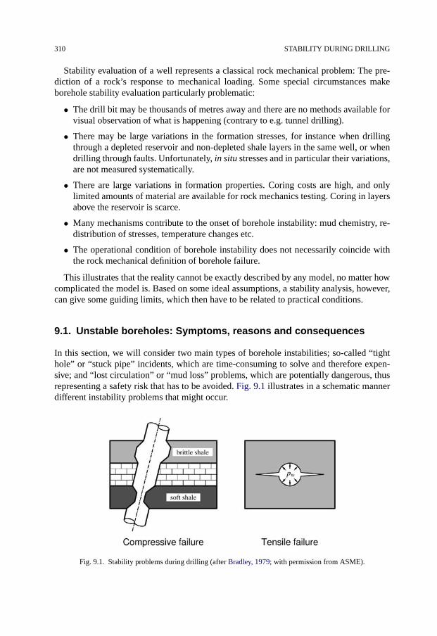
310 STABILITY DURING DRILLING
Stability evaluation of a well represents a classical rock mechanical problem: The pre-diction of a rock’s response to mechanical loading. Some special circumstances makeborehole stability evaluation particularly problematic:
• The drill bit may be thousands of metres away and there are no methods available forvisual observation of what is happening (contrary to e.g. tunnel drilling).
• There may be large variations in the formation stresses, for instance when drillingthrough a depleted reservoir and non-depleted shale layers in the same well, or whendrilling through faults. Unfortunately, in situ stresses and in particular their variations,are not measured systematically.
• There are large variations in formation properties. Coring costs are high, and onlylimited amounts of material are available for rock mechanics testing. Coring in layersabove the reservoir is scarce.
• Many mechanisms contribute to the onset of borehole instability: mud chemistry, re-distribution of stresses, temperature changes etc.
• The operational condition of borehole instability does not necessarily coincide withthe rock mechanical definition of borehole failure.
This illustrates that the reality cannot be exactly described by any model, no matter howcomplicated the model is. Based on some ideal assumptions, a stability analysis, however,can give some guiding limits, which then have to be related to practical conditions.
9.1. Unstable boreholes: Symptoms, reasons and consequences
In this section, we will consider two main types of borehole instabilities; so-called “tighthole” or “stuck pipe” incidents, which are time-consuming to solve and therefore expen-sive; and “lost circulation” or “mud loss” problems, which are potentially dangerous, thusrepresenting a safety risk that has to be avoided. Fig. 9.1 illustrates in a schematic mannerdifferent instability problems that might occur.
Fig. 9.1. Stability problems during drilling (after Bradley, 1979; with permission from ASME).

UNSTABLE BOREHOLES: SYMPTOMS, REASONS AND CONSEQUENCES 311
9.1.1. Tight hole/stuck pipe
The main causes of tight hole/stuck pipe incidents are:
1. Hole collapse (rock mechanical failure).
2. Inappropriate hole cleaning.
3. Differential sticking.
4. Deviation from ideal trajectory.
Cause 1 Hole collapse means that the formation near the borehole fails mechanically,most often by shear failure, but occasionally also by tensile failure. The results of suchfailures can be divided into two main types:
• Increased borehole size due to brittle failure and caving of the wellbore wall. If thecavings are not transported away, this represents a potential source of a stuck pipesituation. This normally takes place in brittle rocks, but the borehole size may alsoincrease by erosion (hydraulic or mechanical) in a weak rock. In driller’s language,“sloughing shale” is often used (although not very well defined) to describe frag-ments or “spallings” generated from the borehole wall. Although often thought tobe of a chemical origin, this is first of all a mechanical problem, which to someextent may be influenced by shale-fluid interactions (see further below). The caseof excessive hole enlargement is sometimes referred to as a “washout”. A washoutis primarily caused by erosion due to high mudflow intensity near the drill bit, orit may be related to softening of the formation by mechanical failure. While a me-chanical hole collapse leads to ovalization of the hole (by formation of a breakout;see Chapter 4), this need not be the case with a washout.
• Reduced borehole diameter may occur in weak (plastic) shales, sandstones and salt.Some chalk formations can also show such behaviour. This phenomenon requiresrepeated reaming, or may even result in a lost drillpipe. The case of very soft (plas-tic) shale is sometimes referred to as “gumbo shale” (gumbo is a Creolian fish soupwith rheology and appearance that may give associations to soft shale). Such shaleis often sticky, contains considerable amounts of swelling minerals (montmoril-lonite), and may cause problems like bit balling and solids accumulation.
• It has traditionally been thought that large hole diameter reductions might be causedby swelling clays. The potential chemical swelling of a shale in downhole stressconditions is however very limited, as was pointed out by Santarelli and Carminati(1995). Large hole deformation is thus a result of primarily plastic shale deforma-tion. The effect of drilling fluid chemistry on borehole stability is explained in moredetail below.
Cause 2 Inappropriate hole cleaning means that drill cuttings, or in the case of a collapsinghole, cavings (rock fragments produced by formation failure) cannot be fully removedby the drilling fluid. Mechanisms 1 and 2 are therefore not independent, but often acttogether. Hole cleaning is less problematic in sand than in shale formations, since thedrilling mud can more easily remove sand particles than shale cavings.
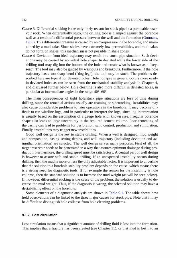
312 STABILITY DURING DRILLING
Cause 3 Differential sticking is the only likely reason for stuck pipe in a permeable reser-voir rock. When differentially stuck, the drilling tool is clamped against the boreholewall as a result of a differential pressure between the well and the formation (Outmans,1958). This differential pressure is caused by an overpressure in the borehole, and main-tained by a mud-cake. Since shales have extremely low permeabilities, and mud-cakesdo not form on shales, this mechanism is not possible in shale zones.
Cause 4 Deviation from ideal trajectory may result in a stuck pipe situation. Such devi-ations may be caused by non-ideal hole shape. In deviated wells the lower side of thedrilling tool may dig into the bottom of the hole and create what is known as a “key-seat”. The tool may also be guided by washouts and breakouts. Furthermore, if the holetrajectory has a too sharp bend (“dog leg”), the tool may be stuck. The problems de-scribed here are typical for deviated holes. Hole collapse in general occurs more easilyin deviated holes as can be seen from the mechanical stability analysis in Chapter 4,and discussed further below. Hole cleaning is also more difficult in deviated holes, inparticular at intermediate angles in the range 40°–60°.
The main consequences of tight hole/stuck pipe situations are loss of time duringdrilling, since the remedial actions usually are reaming or sidetracking. Instabilities mayalso cause considerable problems to later operations in the borehole. It may become dif-ficult to run wireline logs, and in particular to interpret the logs, since log interpretationis usually based on the assumption of a gauge hole with known size. Irregular boreholeshape also leads to large uncertainty in the required cement volume. Poor cementing ofthe casing can lead to problems for perforation, sand control, production and stimulation.Finally, instabilities may trigger new instabilities.
Good well design is the key to stable drilling. When a well is designed, mud weightand composition, casing setting depths, and well trajectory (including deviation and az-imuthal orientation) are selected. The well design serves many purposes: First of all, thetarget reservoir needs to be penetrated in a way that assures optimum drainage during pro-duction. Furthermore, the drilling speed must be satisfactory. A central part of well designis however to assure safe and stable drilling. If an unexpected instability occurs duringdrilling, then the mud is more or less the only adjustable factor. It is important to underlinethat the solution to a borehole stability problem depends on the cause, which means thereis a strong need for diagnostic tools. If for example the reason for the instability is holecollapse, then the standard solution is to increase the mud weight (as will be seen below).If, however, differential sticking is the cause of the problem, the solution is usually to de-crease the mud weight. Thus, if the diagnosis is wrong, the selected solution may have adestabilizing effect on the borehole.
Some elements of a diagnostic analysis are shown in Table 9.1. The table shows howfield observations can be linked to the three major causes for stuck pipe. Note that it maybe difficult to distinguish hole collapse from hole cleaning problems.
9.1.2. Lost circulation
Lost circulation means that a significant amount of drilling fluid is lost into the formation.This implies that a fracture has been created (see Chapter 11), or that mud is lost into an
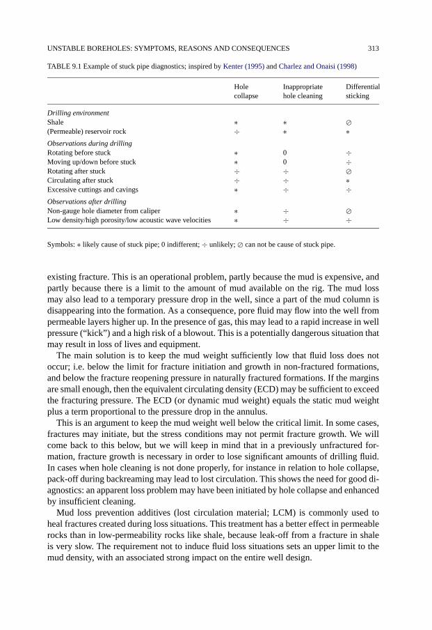
UNSTABLE BOREHOLES: SYMPTOMS, REASONS AND CONSEQUENCES 313
TABLE 9.1 Example of stuck pipe diagnostics; inspired by Kenter (1995) and Charlez and Onaisi (1998)
Holecollapse
Inappropriatehole cleaning
Differentialsticking
Drilling environmentShale ∗ ∗ �(Permeable) reservoir rock ÷ ∗ ∗Observations during drillingRotating before stuck ∗ 0 ÷Moving up/down before stuck ∗ 0 ÷Rotating after stuck ÷ ÷ �Circulating after stuck ÷ ÷ ∗Excessive cuttings and cavings ∗ ÷ ÷Observations after drillingNon-gauge hole diameter from caliper ∗ ÷ �Low density/high porosity/low acoustic wave velocities ∗ ÷ ÷
Symbols: ∗ likely cause of stuck pipe; 0 indifferent; ÷ unlikely; � can not be cause of stuck pipe.
existing fracture. This is an operational problem, partly because the mud is expensive, andpartly because there is a limit to the amount of mud available on the rig. The mud lossmay also lead to a temporary pressure drop in the well, since a part of the mud column isdisappearing into the formation. As a consequence, pore fluid may flow into the well frompermeable layers higher up. In the presence of gas, this may lead to a rapid increase in wellpressure (“kick”) and a high risk of a blowout. This is a potentially dangerous situation thatmay result in loss of lives and equipment.
The main solution is to keep the mud weight sufficiently low that fluid loss does notoccur; i.e. below the limit for fracture initiation and growth in non-fractured formations,and below the fracture reopening pressure in naturally fractured formations. If the marginsare small enough, then the equivalent circulating density (ECD) may be sufficient to exceedthe fracturing pressure. The ECD (or dynamic mud weight) equals the static mud weightplus a term proportional to the pressure drop in the annulus.
This is an argument to keep the mud weight well below the critical limit. In some cases,fractures may initiate, but the stress conditions may not permit fracture growth. We willcome back to this below, but we will keep in mind that in a previously unfractured for-mation, fracture growth is necessary in order to lose significant amounts of drilling fluid.In cases when hole cleaning is not done properly, for instance in relation to hole collapse,pack-off during backreaming may lead to lost circulation. This shows the need for good di-agnostics: an apparent loss problem may have been initiated by hole collapse and enhancedby insufficient cleaning.
Mud loss prevention additives (lost circulation material; LCM) is commonly used toheal fractures created during loss situations. This treatment has a better effect in permeablerocks than in low-permeability rocks like shale, because leak-off from a fracture in shaleis very slow. The requirement not to induce fluid loss situations sets an upper limit to themud density, with an associated strong impact on the entire well design.
314 STABILITY DURING DRILLING
Particles may also be used in a preventive manner, by including a specific concentrationof particles (e.g. graphite and calcium carbonate) in the drilling fluid while drilling. Thepurpose is to arrest drilling-induced fractures at an early stage, before significant lossesoccur. The particles are supposed to bridge off the fracture opening and reduce fluid lossto the fracture, to the extent that the fracture pressure drops and fracture growth stops.Used successfully (Aston et al., 2004; Davison et al., 2004), the fracture pressure canbe increased relative to drilling with a mud without particles. Such an approach may ex-tend drilling in depleting reservoirs, by maintaining a positive mud weight window. Otherpotential applications include deep water drilling, where the window between the porepressure and the fracture gradient is often initially low, and drilling into cooled reservoirsections (due to cold water injection), where cooling has reduced the fracture pressuresignificantly.
9.2. Rock mechanics analysis of borehole stability during drilling
Formations at a given depth in the Earth are exposed to vertical and (generally aniso-tropic) horizontal compressive stresses, as well as a pore pressure (Chapter 3). When ahole is drilled, the surrounding rock must carry the load that previously was carried by theremoved rock. Chapter 4 presents the theoretical basis of stresses around boreholes. In arock that behaves linearly elastic, this leads to a stress concentration near the well as shownin Fig. 9.2. If the rock is sufficiently weak, this stress concentration can lead to failure ofthe borehole.
In drilling of a deep well, such as in petroleum fields, the well is filled with mud. Themud serves two main purposes: One is to prevent flow of pore fluid into the well and holeinstabilities. The other purpose of the mud is to transport drill cuttings from the hole to thesurface. The mud density ρw controls the pressure in the well:
pw = ρwgD (9.1)
g is the acceleration due to gravity, andD is the vertical depth. In oil well drilling language,one usually refers to mud weight (in density units) and gradients of stress or pressure (alsomeasured in equivalent density units) instead of pressures. We shall however perform thetheoretical analysis of borehole stability using the actual stresses and pressures, and thenin the next section translate to oilfield language. Circulation of the mud implies that theeffective (dynamic) mud pressure in the well is higher than the static pressure expressedby Eq. (9.1). As mentioned above, the dynamic well pressure is often referred to as anequivalent circulating density (ECD). The difference may be in the order of 5–10%. Undernormal drilling operations, the pressure will vary between the static and the dynamic values(see Sections 9.7.4 and 9.6).
The mud will carry part of the stress concentration. We shall now use rock mechanicsto analyse how the mud weight controls the mechanical stability of the borehole, buildingmainly on the theory outlined in Chapter 4.
To begin with, we assume linearly elastic rock behaviour and look at the deformation ofthe hole resulting from drill-out. Eq. (4.47) tells us that a vertical borehole will contractproportionally to the difference between the total horizontal stress and the well pressure,
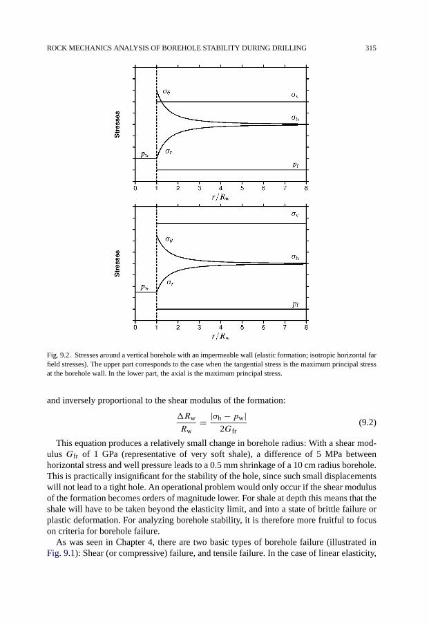
ROCK MECHANICS ANALYSIS OF BOREHOLE STABILITY DURING DRILLING 315
Fig. 9.2. Stresses around a vertical borehole with an impermeable wall (elastic formation; isotropic horizontal farfield stresses). The upper part corresponds to the case when the tangential stress is the maximum principal stressat the borehole wall. In the lower part, the axial is the maximum principal stress.
and inversely proportional to the shear modulus of the formation:
�Rw
Rw= |σh − pw|
2Gfr(9.2)
This equation produces a relatively small change in borehole radius: With a shear mod-ulus Gfr of 1 GPa (representative of very soft shale), a difference of 5 MPa betweenhorizontal stress and well pressure leads to a 0.5 mm shrinkage of a 10 cm radius borehole.This is practically insignificant for the stability of the hole, since such small displacementswill not lead to a tight hole. An operational problem would only occur if the shear modulusof the formation becomes orders of magnitude lower. For shale at depth this means that theshale will have to be taken beyond the elasticity limit, and into a state of brittle failure orplastic deformation. For analyzing borehole stability, it is therefore more fruitful to focuson criteria for borehole failure.
As was seen in Chapter 4, there are two basic types of borehole failure (illustrated inFig. 9.1): Shear (or compressive) failure, and tensile failure. In the case of linear elasticity,
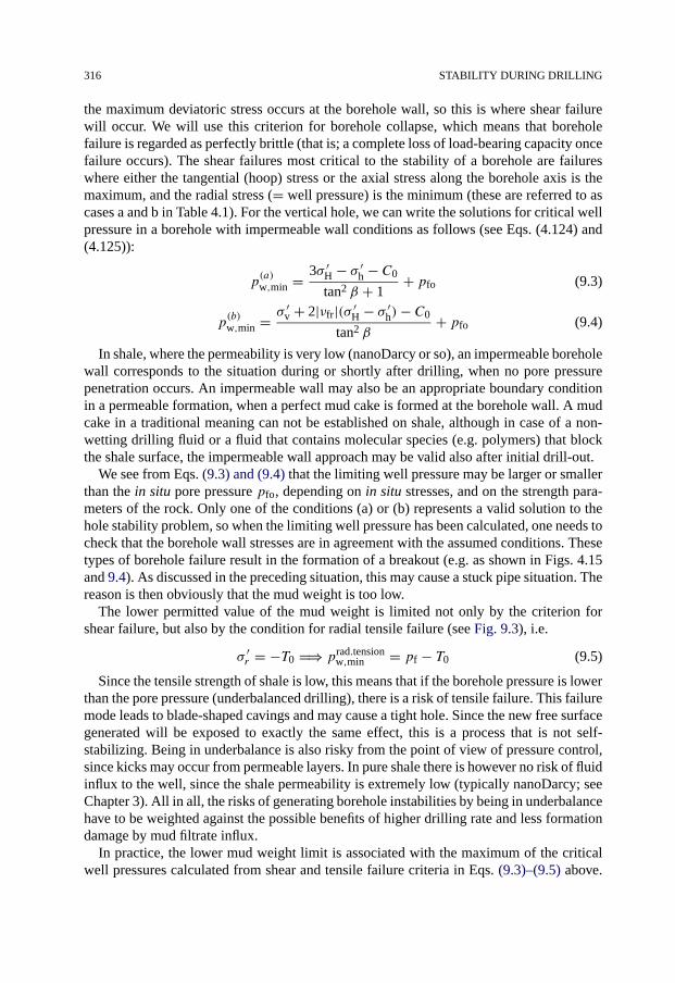
316 STABILITY DURING DRILLING
the maximum deviatoric stress occurs at the borehole wall, so this is where shear failurewill occur. We will use this criterion for borehole collapse, which means that boreholefailure is regarded as perfectly brittle (that is; a complete loss of load-bearing capacity oncefailure occurs). The shear failures most critical to the stability of a borehole are failureswhere either the tangential (hoop) stress or the axial stress along the borehole axis is themaximum, and the radial stress (= well pressure) is the minimum (these are referred to ascases a and b in Table 4.1). For the vertical hole, we can write the solutions for critical wellpressure in a borehole with impermeable wall conditions as follows (see Eqs. (4.124) and(4.125)):
p(a)w,min = 3σ ′
H − σ ′h − C0
tan2 β + 1+ pfo (9.3)
p(b)w,min = σ ′
v + 2|νfr|(σ ′H − σ ′
h)− C0
tan2 β+ pfo (9.4)
In shale, where the permeability is very low (nanoDarcy or so), an impermeable boreholewall corresponds to the situation during or shortly after drilling, when no pore pressurepenetration occurs. An impermeable wall may also be an appropriate boundary conditionin a permeable formation, when a perfect mud cake is formed at the borehole wall. A mudcake in a traditional meaning can not be established on shale, although in case of a non-wetting drilling fluid or a fluid that contains molecular species (e.g. polymers) that blockthe shale surface, the impermeable wall approach may be valid also after initial drill-out.
We see from Eqs. (9.3) and (9.4) that the limiting well pressure may be larger or smallerthan the in situ pore pressure pfo, depending on in situ stresses, and on the strength para-meters of the rock. Only one of the conditions (a) or (b) represents a valid solution to thehole stability problem, so when the limiting well pressure has been calculated, one needs tocheck that the borehole wall stresses are in agreement with the assumed conditions. Thesetypes of borehole failure result in the formation of a breakout (e.g. as shown in Figs. 4.15and 9.4). As discussed in the preceding situation, this may cause a stuck pipe situation. Thereason is then obviously that the mud weight is too low.
The lower permitted value of the mud weight is limited not only by the criterion forshear failure, but also by the condition for radial tensile failure (see Fig. 9.3), i.e.
σ ′r = −T0 �⇒ prad.tension
w,min = pf − T0 (9.5)
Since the tensile strength of shale is low, this means that if the borehole pressure is lowerthan the pore pressure (underbalanced drilling), there is a risk of tensile failure. This failuremode leads to blade-shaped cavings and may cause a tight hole. Since the new free surfacegenerated will be exposed to exactly the same effect, this is a process that is not self-stabilizing. Being in underbalance is also risky from the point of view of pressure control,since kicks may occur from permeable layers. In pure shale there is however no risk of fluidinflux to the well, since the shale permeability is extremely low (typically nanoDarcy; seeChapter 3). All in all, the risks of generating borehole instabilities by being in underbalancehave to be weighted against the possible benefits of higher drilling rate and less formationdamage by mud filtrate influx.
In practice, the lower mud weight limit is associated with the maximum of the criticalwell pressures calculated from shear and tensile failure criteria in Eqs. (9.3)–(9.5) above.
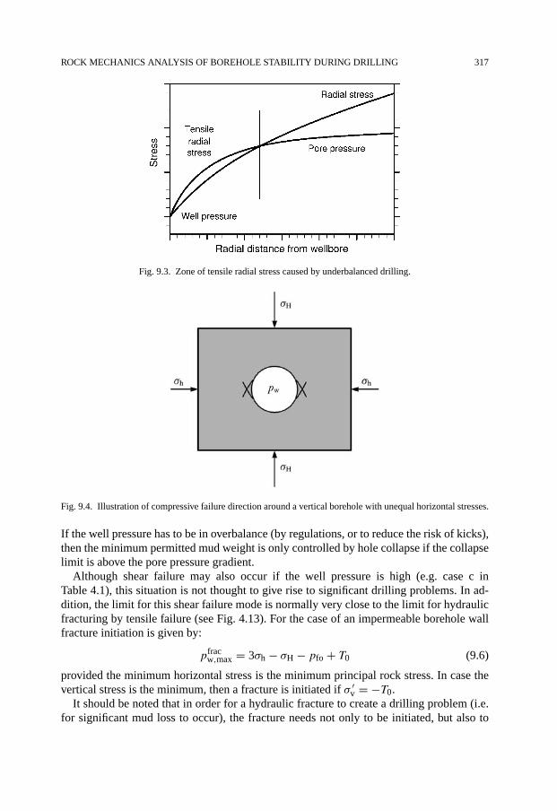
ROCK MECHANICS ANALYSIS OF BOREHOLE STABILITY DURING DRILLING 317
Fig. 9.3. Zone of tensile radial stress caused by underbalanced drilling.
Fig. 9.4. Illustration of compressive failure direction around a vertical borehole with unequal horizontal stresses.
If the well pressure has to be in overbalance (by regulations, or to reduce the risk of kicks),then the minimum permitted mud weight is only controlled by hole collapse if the collapselimit is above the pore pressure gradient.
Although shear failure may also occur if the well pressure is high (e.g. case c inTable 4.1), this situation is not thought to give rise to significant drilling problems. In ad-dition, the limit for this shear failure mode is normally very close to the limit for hydraulicfracturing by tensile failure (see Fig. 4.13). For the case of an impermeable borehole wallfracture initiation is given by:
pfracw,max = 3σh − σH − pfo + T0 (9.6)
provided the minimum horizontal stress is the minimum principal rock stress. In case thevertical stress is the minimum, then a fracture is initiated if σ ′
v = −T0.It should be noted that in order for a hydraulic fracture to create a drilling problem (i.e.
for significant mud loss to occur), the fracture needs not only to be initiated, but also to

318 STABILITY DURING DRILLING
propagate beyond the near well region. A hydraulic fracture will propagate if the pressurein the fracture exceeds the minimum principal stress, plus an additional term depending onthe conditions for fracture growth at the tip, leakage from the fracture to the formation etc.Often mud loss into pre-existing fractures may be a problem. This will occur if the wellpressure is high enough to permit reopening of such a fracture. In practice, therefore, thewell pressure should not exceed the fracture closure pressure (minimum principal (usuallyhorizontal) stress), plus an additional contribution �pexp to be quantified on the basis ofoperational experience; i.e.
pfracpropw,max > σ3 +�pexp (9.7)
The shear failures described by cases d–f in Table 4.1 all imply that the well pressureis higher than the axial stress along the borehole. For a vertical well, this means that thewell pressure exceeds the vertical stress, which is not a common practical situation. Inhorizontal or deviated wells, such a high well pressure would always exceed the fracturinglimit. In borehole stability analysis, these cases are therefore not considered.
The stability of boreholes drilled along horizontal principal stress directions can easilybe analysed using the same mathematical framework as above. One has to remember thatthe far field stresses controlling the tangential stress (and hence the shear failure criterion(a) at the borehole wall) are the stresses acting in the plane perpendicular to the borehole, sothat the term (3σ ′
H − σ ′h) in Eqs. (9.3) and (9.4) in general has to be replaced by (3σ ′
max⊥ −σ ′
min⊥)where σ ′max⊥ and σ ′
min⊥ are the maximum and minimum effective principal stresses,respectively, in the plane perpendicular to the borehole axis:
p(a)w,min = 3σ ′
max⊥ − σ ′min⊥ − C0
tan2 β + 1+ pfo (9.8)
p(b)w,min = σ ′‖ + 2|νfr|(σ ′
max⊥ − σ ′min⊥)− C0
tan2 β+ pfo (9.9)
σ ′‖ is the principal stress parallel to the direction of the hole.Similarly, for fracture initiation in Eq. (9.6), the term (3σ ′
h − σ ′H) is in general written
(3σ ′min⊥ − σ ′
max⊥). This is analogous to what is done in Chapter 10 and in Chapter 11, tobe used for calculation of critical drawdown and fracture initiation pressures.
In summary, the lower mud weight limit in the case of a linearly elastic formation un-dergoing perfectly brittle failure is found from Eqs. (9.1), (9.3), (9.4) and (9.6) and thepossible additional requirement of overbalanced drilling. The upper limit is estimated us-ing Eq. (9.7), and a conservative limit is obtained by assuming �pexp = 0. By furtherinspection of Eqs. (9.3) and (9.4), one finds that the risk of borehole instability with re-spect to mechanical hole collapse becomes high (high critical well pressure) if
• The formation strength is low. This is as one intuitively would expect.
• The failure angle is low. This is usually the case in shale, where β often is 50°–55°,compared to 60° or more in sandstones (see Chapter 3).
• The pore pressure is high. This is often the case in shales above the reservoir (see alsoChapter 3), as well as in some reservoir sections prior to depletion.
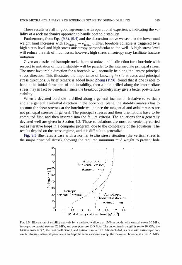
ROCK MECHANICS ANALYSIS OF BOREHOLE STABILITY DURING DRILLING 319
These results are all in good agreement with operational experience, indicating the va-lidity of a rock mechanics approach to handle borehole stability.
Furthermore, from Eqs. (9.3), (9.4) and the discussion above we see that the lower mudweight limit increases with (3σ ′
max⊥ − σ ′min⊥). Thus, borehole collapse is triggered by a
high stress level and high stress anisotropy perpendicular to the well. A high stress levelwill reduce the risk of mud losses, however; high stress anisotropy may facilitate fractureinitiation.
Given an elastic and isotropic rock, the most unfavourable direction for a borehole withrespect to initiation of hole instability will be parallel to the intermediate principal stress.The most favourable direction for a borehole will normally be along the largest principalstress direction. This illustrates the importance of knowing in situ stresses and principalstress directions. A brief remark is added here: Zheng (1998) found that if one is able tohandle the initial formation of the instability, then a hole drilled along the intermediatestress may in fact be beneficial, since the breakout geometry may give a better post-failurestability.
When a deviated borehole is drilled along a general inclination (relative to vertical)and at a general azimuthal direction in the horizontal plane, the stability analysis has toaccount for shear stresses at the borehole wall; since the tangential and axial stresses arenot principal stresses in general. The principal stresses and their orientations have to becomputed first, and then inserted into the failure criteria. The equations for a generallydeviated well are given in Section 4.3. These calculations are most conveniently carriedout as iterative loops in a computer program, due to the complexity of the equations. Theresults depend on the stress regime, and it is difficult to generalize.
Fig. 9.5 illustrates a case with a normal in situ stress situation (the vertical stress isthe major principal stress), showing the required minimum mud weight to prevent hole
Fig. 9.5. Illustration of stability analysis for a deviated wellbore at 1500 m depth, with vertical stress 30 MPa,isotropic horizontal stresses 25 MPa, and pore pressure 15.5 MPa. The unconfined strength is set to 10 MPa, thefriction angle is 30°, the Biot coefficient 1, and Poisson’s ratio 0.25. Also included is a case with anisotropic hor-izontal stresses, where all parameters are kept the same as above, except the maximum horizontal stress 28 MPa.

320 STABILITY DURING DRILLING
collapse as a function of hole deviation. The maximum permitted mud weight may con-servatively be taken as the minimum horizontal stress, in this case 25 MPa correspondingto a mud density of 1.70 g/cm3. For isotropic horizontal stresses, the stable range is nar-rowed continuously as the inclination increases towards horizontal, in particular from 30°until 60°. If the horizontal stresses are anisotropic, the stability of a vertical hole becomessignificantly reduced.
The critical mud weight for a deviated well depends both on inclination and azimuthaldirection. For a horizontal well parallel to the minimum horizontal stress, the collapse limitis improved when compared to the case with horizontal stress isotropy, because the stressanisotropy perpendicular to the hole is reduced.
9.3. Time-delayed borehole failure
9.3.1. Establishment of pore pressure equilibrium
In the field, it is often observed that initial drilling may be stable, but that tight hole/stuckpipe situations occur during tripping or logging runs, typically several days after drill-out.The model we presented in Section 9.2 above does not account for time-dependent bore-hole stability. One limitation of the analysis above was the assumption of an impermeableborehole wall. As pointed out, this is only true if a perfect mud cake is established, or if therock is impermeable. Shale has a very low (nanoDarcy) but still finite permeability, whichmeans that impermeable wall conditions are valid only during drilling. After drilling, thepore pressure close to the borehole wall will gradually approach the well pressure. Eventu-ally, if the formation is exposed to the mud pressure for sufficiently long time, steady statepore pressure equilibrium is reached.
The stress field under permeable wall conditions is given in Chapter 4. Applying Mohr–Coulomb’s failure criterion to a piece of rock at the borehole wall, the minimum permittedwell pressure (analogous to Eqs. (9.3) and (9.4) above) for a vertical borehole is given byone of the two cases (a) and (b) (see Eqs. (4.120) and (4.121)):
p(a)w,min = 3σ ′
H − σ ′h − C0
2 − α 1−2νfr1−νfr
+ pfo (9.10)
p(b)w,min = σ ′
v + 2|νfr|(σ ′H − σ ′
h)− C0
1 − α 1−2νfr1−νfr
+ pfo (9.11)
When the hole is drilled along one of the horizontal principal stress directions, one has toreplace the principal stresses with the appropriate ones, as was done in Eqs. (9.8) and (9.9)above.
The time τD it takes to reach pore pressure equilibrium after a hole is drilled in unbal-anced conditions is based on consolidation theory (Section 1.9), which states that:
τD ≈ l2D
CD(9.12)

TIME-DELAYED BOREHOLE FAILURE 321
Fig. 9.6. Illustration of how the Mohr circle representing the borehole stress field moves from time t = 0 (drillout)to time t → ∞ (pore pressure equilibrium), creating a more unstable situation with respect to shear failure (holecollapse).
Here lD is a characteristic length and CD is the diffusion coefficient defined inEq. (1.242). CD is proportional to the permeability. Taking lD ∼ borehole radius ∼10 cmand the shale permeability ∼1 nanoDarcy, we find that the characteristic time typically is5–10 days. This corresponds to the time period after which instabilities occur in practice.
If the well is kept in overbalance, the pore pressure near the borehole wall will increase,resulting in reduced hole stability with time. This is illustrated in Fig. 9.6, which shows thedisplacement of the Mohr circle in the direction of the shear failure criterion from shorttime (t = 0) to long time (t = ∞). The reason is that the effective confinement (minimumeffective principle stress) approaches zero as pore pressure equilibrium is established. Forthe case described for a vertical well in Fig. 9.5 above, the minimum permitted well pres-sure increases with time to 26 MPa (corresponding to mud density 1.77 g/cm3), whichmeans that the horizontal stress is exceeded, and stable drilling no longer is permitted. Onthe other hand, if the well is drilled in underbalance, the pore pressure will decrease andstability with respect to hole collapse will improve with time.
Two practical implications can be drawn from the above: The likelihood of stabilityproblems (at least during overbalanced drilling) will be reduced the sooner one is able toleave a well section behind by setting casing. Furthermore, maintaining an impermeableboundary condition is a way to stabilize the hole over time. Solutions to this challenge arebeing sought in terms of oil-based or polymer-containing drilling fluids (see Section 9.4).
9.3.2. Temperature effects
Consolidation (or establishment of pore pressure equilibrium) as described in the precedingsection, is not the only possible explanation of time delayed borehole failures. The drillingfluid is usually (at t = 0) colder than the formation to be drilled, since it has surfacetemperature when circulation starts. The fluid and formation temperatures will gradually

322 STABILITY DURING DRILLING
adjust, depending on the circulation rate. After a stop in the circulation, the formation nearthe well will gradually heat up. Maury and Sauzay (1987) found that this could explaindelayed failure. Shortly after drilling the borehole is stable. However, as the temperatureincreases, the tangential and axial stresses at the borehole wall will both increase by thesame amount.
The thermoelastic stresses induced at an impermeable borehole wall are given byEqs. (4.69)–(4.71). If the borehole fluid is colder than the formation, the tangential andaxial stresses are reduced proportionally to the temperature difference between formationand borehole fluid. This acts as a strengthening of the borehole with respect to collapse.Deliberate cooling of the mud can therefore be a practical approach to mitigate stabil-ity problems. This was applied with success in the field (Guenot and Santarelli, 1989;Maury and Guenot, 1995). The thermal effect is proportional to rock stiffness, which meansthat it is more significant in hard than soft rocks. It is also proportional to the thermal ex-pansion coefficient.
There is not a lot of data on thermal expansion on sedimentary rocks, but typically αTis around 10−5 K−1 (see Appendix A). This gives a typical thermal stress contributionof a few MPa, which reduces the lower mud weight limit by 5–10% compared to a situ-ation with no thermal effect. However, since cooling reduces the tangential stress, it notonly reduces the risk of shear failure, but it also promotes fracturing, and may hence be adestabilizing factor with respect to lost circulation problems. The extent of the cold zoneis however limited, and this may limit the growth of the fracture.
Cooling of a low permeability rock like shale will also influence the pore pressure, due toa larger thermal expansion coefficient for the fluid than for the solid parts of the rock. Thus,cooling reduces the pore pressure, which in general improves stability. Rock properties(strength, stiffness) may be altered as a result of temperature changes: Normally strengthand stiffness will increase with decreasing temperature. Finally, mud properties are alsotemperature dependent: Cooling the mud will lead to a slight mud density increase dueto thermal contraction, again resulting in improvement of stability with respect to holecollapse conditions.
Note that if one drills into a reservoir that is cooled by waterflooding, the in situ stressesmay have been altered in a way that makes mud loss and fracturing more likely than un-der initial normal temperature conditions. Field evidence for this phenomenon is given byHettema et al. (2004).
9.3.3. Creep
When discussing time dependent borehole stability, it is obvious that creep may cause aborehole to collapse with time. Since creep tests are complicated and time-consuming,there are very few reliable tests of this kind in the literature. It is however general knowl-edge that a material that is brought above its yield point, may creep to failure. Translatingto the borehole situation, this means that if the mud weight is kept marginally above thelower limit for long enough time, the borehole may collapse as a result of creep. The riskof high (accelerating) creep rates increases with increasing temperature. Although trulyconstant stress conditions over time never occur during drilling, the intrinsic time depen-dent properties of the formation may still have an influence on stability. In practice, this is

INTERACTION BETWEEN SHALE AND DRILLING FLUID 323
difficult to distinguish from other time dependent effects, like consolidation, thermal andchemical effects.
9.4. Interaction between shale and drilling fluid
In the previous section, three sources of time dependent borehole stability were considered:Consolidation, mud cooling, and creep. One more mechanism will be discussed in thissection, namely chemical interaction between the drilling fluid and the formation. This ishowever not just a source of time delayed hole collapse, but may be used to improve shalestability, in particular in cases where instabilities occur in shales with high contents ofswelling clay minerals.
It is often observed that oil-based mud gives better stability than water-based mud. Tostart out, let us consider the (somewhat academic) example of drilling with pure oil (oranother fluid that is completely non-wetting to the shale). The capillary pressure for oil (orother non-wetting fluid) in contact with a water-wet shale is:
pcp = 2γ
r(9.13)
Here γ is the surface tension; γoil–water = 50 · 10−3 N/m. r is the pore size, which inshale typically is 10 nm. From that we find the capillary entry pressure for pure oil to entera water-saturated shale to be ∼10 MPa. Thus, an overbalance of 10 MPa is required foroil (or another non-wetting fluid with similar surface tension) to penetrate into intact shale.This means that for lower mud overbalance, the borehole wall will remain impermeable,and the t = 0 stability will prevail.
Oil-based muds usually give better hole stability than water-based muds, but the latterare preferred for environmental reasons. Oil-based muds are however not pure oils. Theycontain a water phase, and the chemistry of the water phase has an influence on the holestability. Various mud additives have been introduced in water-based systems to help main-tain impermeable borehole wall conditions over time (see Section 9.3.1):
• Sodium silicate (van Oort et al., 1996).
• Long-chained molecules (glycol; polymers etc.) that are thought to build molecularfilter cakes on shale surface (see e.g. Twynam et al. (1994) and Reid et al. (1995)).
The operational experience with such systems is too limited to draw any firm conclusionat this stage.
We shall now discuss chemical mechanisms that may lead to interaction between shaleand drilling fluid. Let us first consider osmosis. The basis for osmosis is the existence of asemi-permeable membrane that permits water molecules to pass but prevents ions to enterthe shale. The membrane may be thought of in two different ways:
1. Oil-based mud may act as a semi-permeable membrane. Ions associated with saltsare prevented to move between the water phase of the mud and the formation.
2. The shale is often regarded as a semi-permeable membrane when contacted by water-based mud. Because the clay minerals have surface charge, the movement of ions isthought to be hampered, giving rise to membrane properties.
324 STABILITY DURING DRILLING
The osmotic potential �Π (from e.g. Marine and Fritz, 1981) is:
�Π = RT
Vwlnaw,df
aw,sh(9.14)
Here R is the molar gas constant (8.31 J/(mol K)), and Vw is the molar volume of water(0.018 l/mol). aw,df is the chemical activity of water in the drilling fluid, and aw,sh is thechemical activity of pore water in the shale. The activity denotes the effective concentrationof water in a solution, so that aw = 1 for fresh water, while aw < 1 for salt water. Forideal solutions, activity is directly given by the salt concentration. For non-ideal solutionswith approximately 0.1 M salt concentration, the difference between activity and waterconcentration may be 10–50%, depending on type of ion (Mahan, 1975).
Mody and Hale (1993) implemented osmotic theory into a rock mechanics model forborehole stability. They added the osmotic potential through a stress term equivalent to theporoelastic contribution seen in Eqs. (4.58)–(4.60):
σr = pw (9.15)
σθ = 2σh − pw + α 1 − 2νfr
1 − νfr�Π (9.16)
σz = σv + α 1 − 2νfr
1 − νfr�Π (9.17)
Adding salt to the drilling fluid so that aw,df < aw,sh sets up an osmotic potential�Π < 0, which will tend to drive water out of the shale and hence acts as an effectivepore pressure reduction. This has an instantaneous stabilizing effect on the borehole.
It is well established that ions do move through shale (e.g. Ballard et al., 1994). Thismeans that the osmotic membrane is leaky, which is handled by introducing a membraneefficiency σ < 1. The membrane efficiency reduces the osmotic potential:
�Π = σ RTVw
lnaw,df
aw,sh(9.18)
The membrane efficiency depends on ionic diffusivity, and will hence in general de-pend both on clay type and on the type of ions present in the drilling fluid (for moreelaborate analysis, see Marine and Fritz, 1981; Bailey et al., 1991; Sherwood, 1994;Heidug and Wong, 1996; Lomba et al., 2000a, 2000b; Sherwood and Craster, 2000). Exper-iments (Chenevert, 1970; van Oort et al., 1996; Ewy and Stankovich, 2002; Schackelfordet al., 2003; and others) seem to indicate that for shales σ is in the range 0.05–0.30. Theosmotic potential may however still be several MPa, which means that reducing drillingfluid activity by adding salt may improve borehole stability significantly, at least duringthe initial phase. The effect will however, due to membrane leakiness, decay with time af-ter drillout. In case of very low activity drilling fluid, one may expect damage as a result ofreduced tangential and/or axial stresses at the borehole wall.
There is also experimental evidence that ionic exchange may occur within the shalewhen it is exposed to brine (Steiger, 1982; Denis et al., 1991; Horsrud et al., 1998). In par-ticular, exposure of smectite-rich shale to KCl causes significant shrinkage (Fig. 9.7), evenwhen the potassium concentration is so small that osmotic swelling would be expected.The rate of exchange depends on the ion concentration, whereas the maximum shrinkage
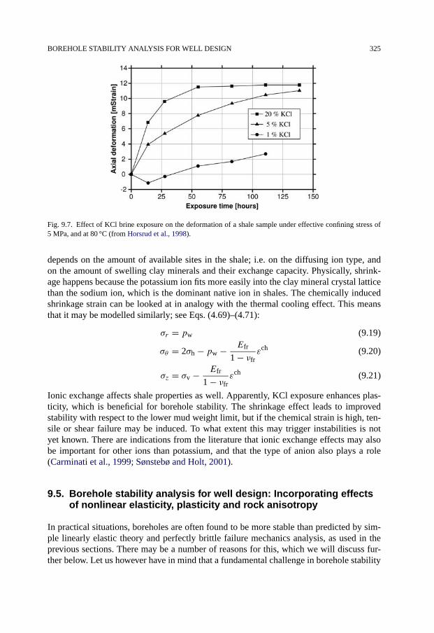
BOREHOLE STABILITY ANALYSIS FOR WELL DESIGN 325
Fig. 9.7. Effect of KCl brine exposure on the deformation of a shale sample under effective confining stress of5 MPa, and at 80 °C (from Horsrud et al., 1998).
depends on the amount of available sites in the shale; i.e. on the diffusing ion type, andon the amount of swelling clay minerals and their exchange capacity. Physically, shrink-age happens because the potassium ion fits more easily into the clay mineral crystal latticethan the sodium ion, which is the dominant native ion in shales. The chemically inducedshrinkage strain can be looked at in analogy with the thermal cooling effect. This meansthat it may be modelled similarly; see Eqs. (4.69)–(4.71):
σr = pw (9.19)
σθ = 2σh − pw − Efr
1 − νfrεch (9.20)
σz = σv − Efr
1 − νfrεch (9.21)
Ionic exchange affects shale properties as well. Apparently, KCl exposure enhances plas-ticity, which is beneficial for borehole stability. The shrinkage effect leads to improvedstability with respect to the lower mud weight limit, but if the chemical strain is high, ten-sile or shear failure may be induced. To what extent this may trigger instabilities is notyet known. There are indications from the literature that ionic exchange effects may alsobe important for other ions than potassium, and that the type of anion also plays a role(Carminati et al., 1999; Sønstebø and Holt, 2001).
9.5. Borehole stability analysis for well design: Incorporating effectsof nonlinear elasticity, plasticity and rock anisotropy
In practical situations, boreholes are often found to be more stable than predicted by sim-ple linearly elastic theory and perfectly brittle failure mechanics analysis, as used in theprevious sections. There may be a number of reasons for this, which we will discuss fur-ther below. Let us however have in mind that a fundamental challenge in borehole stability

326 STABILITY DURING DRILLING
analysis is to define failure in practical terms. The driller is only concerned with stabilityproblems that interfere with the drilling operation. Rock fragments breaking loose fromthe borehole wall, or a minor reduction in the wellbore diameter due to plastic flow, is notnecessarily equivalent to drilling problems. Guenot (1990) pointed out the need for a new“failure criterion” which can account for these practical aspects.
Such a criterion has to bridge field experience with fundamental rock mechanics knowl-edge. The industry learns from previous failures, and may use their experience in futuredrilling operations. The approach may be purely empirical, but in order to have predictivepower, it must at some stage line up with rock mechanics analysis. What we can do, withrock mechanics as our main tool, is to refine the theory to deal in a better way with theshortcomings identified in the field.
As said above, initiation of failure is not necessarily going to lead to a borehole stabil-ity problem. However; the brittle failure theory that we have used, predicts instability assoon as the Mohr–Coulomb criterion is violated at the borehole wall. The calculations ofminimum well pressure (minimum mud weight) thus implicitly assume that the rock losesits entire load bearing capacity once the Mohr–Coulomb limit is reached. The estimatedminimum mud weight is therefore likely to be too low. A simple way to try to compensatefor this is to increase the rock strength with a “fudge factor” > 1 which is calibrated onbasis of field experience, and then use the analytical approach that was presented in thepreceding sections.
Alternatively, which is of course more satisfactory from the theoretical viewpoint, therock mechanics models may be improved to describe the constitutive behaviour of therock in a more correct manner. One obvious modification is to account for the post-failurebehaviour of the rock. Strong rocks tend to be more brittle, with little ability to deformand carry load after the peak stress has been passed. The brittleness tends to decrease withincreasing confining pressure. Weaker rocks are normally more ductile, i.e. they have largerability to deform and carry load beyond their elastic limit. The brittle-ductile transitiondepends on the stress level. Reaching peak stress is of course more critical if the rockis brittle. If the rock is ductile, then the failure limit may be exceeded without dramaticoperational consequences.
To take care of the factors discussed above, models incorporating plasticity and/or non-linear elasticity must be applied. This represents no fundamental problem, but makes thecalculations more cumbersome, especially for deviated holes. When plasticity effects aretaken into consideration, this gives rise to a so-called plastic zone near the borehole wall(as outlined in Chapter 4). This is a weakened zone, but shields the rock beyond and tosome extent improves stability. The stability limit is set either as an upper limit to the plas-tic deformation, or to the extent of the plastic zone. This gives results that are numericallymore realistic for the actual well failure situation than the simple elastic model. Such afailure criterion has however to be specified on the basis of experience; be it from fieldoperations, or controlled hollow cylinder failure tests performed in the laboratory.
Santarelli and Brown (1987) incorporated a pressure-dependent elastic modulus into theanalytical model for borehole failure. Triaxial testing shows that the elastic modulus tendsto increase with the confining pressure (see also Chapter 4). With this model, much of thediscrepancy between a linear elastic model and results from hollow cylinder tests could beaccounted for. It can also explain why failure can occur at some distance behind the wall,

BOREHOLE STABILITY ANALYSIS FOR WELL DESIGN 327
and not at the wellbore wall surface where the stress concentration should be maximumaccording to constant-modulus theory.
We have based our borehole stability analysis on the Mohr–Coulomb criterion for shearfailure. This has many advantages, including the fact that analytical calculations are fa-cilitated. The Mohr–Coulomb criterion does however not account for the experimentallyobserved effect of the intermediate principal stress on rock strength. The stress state in thevicinity of the borehole wall is true triaxial, and this can be accounted for by using failurecriteria that depend on the intermediate principal stress, like the Drucker–Prager criterion;see Chapter 2), or the Mogi–Coulomb approach (Al-Ajmi and Zimmerman, 2006).
When more complex material models are used, more extensive rock characterizationis also required. This is often difficult due to lack of core material. In addition, the rockproperties can change significantly over short distances. One should therefore in each caseconsider whether using more complex models is worthwhile. This should not prevent theuse of such models for studying phenomenological problems and for sensitivity analyses.
One aspect of borehole stability not considered in the analysis presented so far is therole of rock anisotropy. Shale is normally anisotropic due to textural alignment of clayminerals (Chapter 3), and therefore exhibits anisotropic strength, stiffness, and permeabil-ity. Combining the weak plane model for rock strength (Section 2.9) with the boreholefailure criterion, one may incorporate the effect of strength anisotropy in the modelling ofhole collapse.
Fig. 9.8 shows an example of such a calculation, using the same input parameters asin the isotropic stress case displayed in Fig. 9.5, except that the shale strength and frictionangle both are reduced in the horizontal plane. The result is a significantly reduced stabilitywith respect to collapse for inclinations above 30°. For this particular case, stable drillingbecomes impossible with further increase in hole angle, since the mud weight correspond-
Fig. 9.8. Illustration of stability analysis for a deviated wellbore at 1500 m depth. All input parameters are as inFig. 9.5, with isotropic horizontal stresses 25 MPa. The figure shows the effect of horizontal weak planes, withreduced strength (C0/2) and reduced friction angle (ϕ/2).

328 STABILITY DURING DRILLING
Fig. 9.9. Schematic borehole stability analysis.
ing to the collapse limit rapidly exceeds the fracture gradient (given by the minimum insitu stress). By adding plasticity, the stability is significantly improved. One should how-ever be aware that buckling of bedded shale when drilling along or near the symmetryplane (Økland and Cook, 1998) may be an additional cause of instability not caught by theanalysis presented here.
Fig. 9.9 sketches the procedure of complete borehole stability analysis. The input datarequired are rock properties, earth stresses and pore pressure, plus the planned hole trajec-tory. For a simple analysis, only parameters listed in the first row of boxes are required. Fora more advanced level of sophistication, chemical, thermal, plastic, anisotropic and timedependent features are added. In most cases the effects are simply added by superimposingporoelastic, thermoelastic and osmotic contributions to the borehole stresses. This may besatisfactory for most purposes, but implies that coupling between chemical and thermalprocesses are neglected.
The result of the analysis is the mud weight window; i.e. the minimum well pressurepermitted to prevent hole collapse (or fluid influx) and the maximum well pressure per-mitted to prevent loss of fluid to the formation by flow into existing or induced fractures.When these limits are known, the well may be designed.
Well design is of course more than a question of borehole stability. The purpose of thewell is to reach a certain target to ensure optimum drainage of a reservoir or reservoir zone.The suggested hole trajectory required to reach the target then has to be evaluated in orderto see if it is drillable, and then the drilling process has to be optimized to reduce costs bydrilling fast, and by using as few casing strings as possible. At large depths, this is crucial:The number of casing strings has to be kept low, since the casing diameter decreases foreach new string.
Fig. 9.10 illustrates the role of wellbore stability analysis in well design. Because it isnot possible to drill the entire section shown with one mud weight, a casing has to be set

USE OF PRESSURE GRADIENTS 329
Fig. 9.10. Example of a stability chart for a well from the Norwegian Continental Shelf. The full lines are,from left to right, the estimated pore pressure gradient (p), the minimum horizontal stress gradient (h) and theoverburden stress gradient (v), respectively. The dotted lines are the estimated collapse gradient (c) and fracturinggradient (f), while the dashed line is the planned mud weight gradient (m). Casing shoes are indicated by the blacktriangles. Observe how the mud weight is increased below each shoe. Further note that for this particular well,the collapse gradient is larger than the pore pressure gradient for only a limited interval. This may be different inother wells! The airgap is 18 m and the water depth is 370 m. Courtesy of Statoil.
to seal off the upper part of the section before continuing with an increased mud weight inthe lower part. This illustrates the two main tools available to drill stable boreholes: Themud weight and the casing program.
9.6. Use of pressure gradients
9.6.1. Introduction
So far we have largely used pressure in our stability calculations. However, since this has tobe related to a mud weight or mud density, it is customary to convert the different pressuresat a given depth to a density value. This is often referred to as an equivalent mud weightor a pressure gradient. Note that the term gradient is not entirely correct, since it is not theslope of the pressure curve at a given depth, but rather a secant value from surface to the
330 STABILITY DURING DRILLING
given depth, i.e.
ρ = p
gD(9.22)
where p is the pressure at depth D, g is the acceleration of gravity and ρ is the equivalentmud weight or pressure gradient. Common units for ρ is g/cm3 or SG (specific gravityrelative to water).
In SI-units we have
ρ(SG) = p (MPa)
0.00981D (m)(9.23)
Any relevant stress or pressure parameter, e.g. pore pressure, horizontal stress, overburdenstress and fracture pressure may be represented as a gradient, as exemplified in Fig. 9.10.
9.6.2. Depth reference and depth corrections
The use of Eq. (9.22) introduces the need of a depth reference level, i.e. a surface referencelevel. Since the well pressure gradient is related to the mud column, it is natural to use thesame depth when calculating the other pressure gradients. The surface reference level willthen obviously be the drill floor or rotary table (RT), i.e. the top of the mud column. Whendrilling an onshore well it is then quite clear that D is essentially measured from the earthsurface. When drilling an offshore well, D is however made up of several depth elements:
D = Dformation +Dwater +Dairgap (9.24)
where Dairgap is the air gap or the height from the sea to the drill floor, Dwater is the waterdepth andDformation is the formation depth (from the sea floor to the depth of investigation).
When comparing gradients from different wells in a field it is therefore essential to keeptrack of the reference depth. In the exploration phase the variation in Dairgap is normallysmall (typically less than 5 m), as these wells are normally drilled from semisubmersiblerigs with Dairgap typically ranging from 23 to 28 m.Dairgap in production wells depends on how the field is developed. If a fixed platform
is installed, Dairgap may be significantly larger. Thus there is a need to be able to convertfrom one drill floor level to another. The pressure at the same depth underground must bethe same, so that
ρ1gD1 = ρ2gD2 (9.25)
where the subscripts represent different reference levels. This yields
ρ2 = ρ1D1
D2(9.26)
To avoid keeping track of different rig floor elevations, it is convenient to use a moregeneral reference level for the different pressure gradients, e.g. the mean sea level (MSL).This is a convenient approach when collecting and comparing data from different drillingrigs, data that will be the basis of a model that is going to be used for planning of productiondrilling from a platform.
BEYOND SIMPLE STABILITY ANALYSIS 331
Having established the different pressure gradients used as input for a stability analysis,one must always refer back to the same reference level as the mud column (the rotarytable). When planning a specific well one must therefore remember to convert back to adepth that includes the air gap (Dairgap) of that specific well.
9.7. Beyond simple stability analysis
9.7.1. Field cases: The borehole stability problem in complex geology
In this paragraph we will present a few field cases from the literature, which illustrate howrock mechanics analysis can be applied to borehole stability problems.
Case 1: Drilling-induced lateral shifts along pre-existing fractures (Meillon St. FaustField, France)
The Meillon St. Faust is a gas field, located in the southwest of France. For a more de-tailed description, the reader is referred to Maury and Zurdo (1996). Severe casing failuresoccurred in a fault zone above the reservoir during early gas production. These failurescould be interpreted by migration of gas or water from abnormally pressured zones atdepth through damaged cement and into uphole faults or bedding joints. This increasedpore pressure led to reduced effective normal stress on the faults, which triggered sheardisplacement and thus casing collapse.
It is likely that pressure increase in pre-existing fractured rock mass may also causestuck pipe situations during drilling by a similar mechanism (Santarelli et al., 1992). If thewell is drilled with too high overbalance (like in high pressure cycles during surge-swab;see further below), and the mud does not create an efficient cake towards the fracture, thenpressure may build up in the fractures, and the normal effective stress decreases, leadingto shear displacements that may reach a few cm. There are cases where tight hole occurredwith no indication of cavings, and where the problem could not be solved by mud weightincrease. Other symptoms of this failure mode is that tight hole problems occur at the samedepth, together with problems to run in and pull out of hole, abnormal localized torques,deviation of trajectories, and possible drillstring failures. The remedies to solve problemsof this kind are to keep the mud weight low (but still above the collapse criterion for theintact rock), and to increase the sealing capacity of the mud. In the field case reported here,this was done by adding asphalt-type products associated with inert colloidal particles.
Case 2: Drilling in a complex geological setting with high tectonic stresses (CusianaField, Colombia)
The Cusiana field is located in the foothills of the Andes Mountains in Colombia. Majorborehole stability problems (amounting to several millions of dollars per well) have beenencountered (a brief summary was published by Last et al. (1996); see also Willson et al.(1999)). They report hole enlargement as the cause of the majority of problems, resulting

332 STABILITY DURING DRILLING
in large amounts of cavings, hole cleaning and stuck pipe, poor cementing and necessaryside-trackings. The most difficult formation was an alternating sand-shale sequence, wheremud losses and tight hole occurred in the sandy and hole enlargements in the shaly units. Itwas found that increasing the mud weight to limit hole enlargements did not work, becauseit led to significant mud losses.
A borehole stability task force established by the operator acquired a large amount ofdata. Stress measurements were done, downhole borehole images and 4-arm caliper datawere collected, shale core tests were performed in addition to characterization and moni-toring of cavings at surface and MWD surveys. An important result was the determinationof the in situ stress state, which proved the maximum principal stress to be (sub-) horizontaland much larger than the vertical stress, and the minimum principal stress to be horizontal(parallel to the mountains) and much smaller than the vertical stress. In addition, the sand-shale sequence mentioned above turned out to be fractured throughout the entire field. Itwas concluded that borehole mechanical instabilities occurred as a result of shear failurein weak fractured siltstones and shales, and that lost circulation occurred when the mudpressure exceeded the minimum (horizontal) stress. Further, mud invasion contributed toweakening of the fractured rock (by the same mechanism as explained in the precedingparagraph). An important consequence of these mechanisms was that the permitted mudweight window was shrinking to zero, since the minimum mud weight in the shale sectionsexceeded the lost circulation threshold in the sands. The challenge was then not to find away to drill a stable hole, but rather to find a way to drill a hole that is inherently unstable.
Compromises were made by using mud weights that were too high for the sands and toolow for the shales, and then try to manage the instabilities by efficient drilling practices.This included improvement of mud sealing capacity and optimization of hole cleaning,and having lost circulation pills available in case of loss in the sands. The bit was permit-ted to seek its own trajectory where possible, and drilling was performed as smooth andfast (minimizing reaming, back-reaming and vibrations, increasing bit life) as possible. Inaddition, hole conditions (including caving rates) were carefully monitored.
Case 3: The Heidrun Field, Norwegian Sea
The Heidrun field offshore Mid-Norway experienced persistent hole stability problems inTertiary shale formations. A high KCl content drilling fluid was used, in order to handlepossible reactive clay formations above the reservoir. The majority of the wells are ex-tended reach wells with inclination angles in the range 55°–70°. The problems manifestedthemselves mainly as cavings, pack-offs and lost circulation, and were handled by increas-ing the mud weight. This did however in several cases not reduce the caving productionproblem. The details of this case are reported by Stjern et al. (2000).
The operator expected the drilling problems to occur mainly in a low-density and highporosity zone. Extensive data collection was performed, including logging (6-arm caliper,sonic and density, temperature), shale coring and laboratory testing, and sampling andmeasurements of sonic velocities on cuttings. In addition, the stress field was evaluatedusing extended leak-off tests.
As a result of the systematic data collection, it was found that the problem zone wasnot the originally assumed low-density zone, but rather a normal density but fractured
BEYOND SIMPLE STABILITY ANALYSIS 333
zone. This led to the conclusion, like in the preceding cases, that the mud density could bereduced. At the same time, the salt concentration in the mud was reduced, which apparentlyalso improved stability. It was also concluded that hole cleaning had to be optimized byusing low viscosity mud and provide close to turbulent flow. The authors point out that theborehole stability study performed has given a cost reduction of close to 2.5 million dollarsper well in pure saving on flat time during drilling.
9.7.2. Drilling in depleted reservoirs
A particularly difficult situation is infill drilling in depleted reservoirs, where the porepressure may still be the initial one in shale zones, or in the cap rock right above. This is dueto the very low permeability of shales, which means that the time required to establish porepressure equilibrium in a shale zone of tens of metre thickness may be several years, andeasily may exceed reservoir lifetime. In the permeable reservoir zones, the reduced porepressure is established almost instantaneously (except for possible undepleted pockets).Thus, the high pore pressure in the shale requires that the mud weight is kept above theinitial collapse limit to avoid shale instabilities. In neighbouring reservoir sand zones, thismud weight may be too high, since the reduced pore pressure also has caused reducedhorizontal stresses (reduced fracture gradient, see Chapter 12). Thus, drilling with initialmud weight may lead to mud losses. Normally one does not know while drilling whichzones are depleted and which zones are at original pore pressure: This requires a couplingto reservoir management and reservoir monitoring by e.g. time-lapse (4D) seismics.
9.7.3. Drilling below deep water
When drilling below deep water, the water depth contributes to reducing both the hole col-lapse and the fracturing gradients. The well pressure is given by Eq. (9.1), where the totaldepth includes water depth from the top of the mud column (neglecting the air gap). Thismeans that the critical mud density ρw,crit for hole collapse as well as for fracturing will begiven by the corresponding critical mud densities in absence of water (ρ0
w,crit) and by thewater depth (Dwater) and the depth measured from the sea-floor (Dformation) as follows:
ρw,crit = ρ0w,critDformation + ρwaterDwater
Dformation +Dwater(9.27)
As can be seen from this equation and from Fig. 9.11, a main effect of the water is toshrink the mud weight window at shallow depth within the formation. At the sea floor(Dformation = 0) there is no mud weight window, since both the upper and lower limits aregiven by the water density (effective stresses are = 0). At shallow depth below the sea-floor, the effect of water depth still dominates, so that both the upper and lower mud weightlimits are lower than they would have been if drilling took place onshore, or in shallowwater. The consequences of instability in deep water are however much more severe.
A potential solution to the drilling problems is so-called dual gradient or dual densitydrilling. The basic idea is to use only seawater above the seafloor, and the heavier mud

334 STABILITY DURING DRILLING
Fig. 9.11. Illustration of the effect of water depth on the mud weight window. Note the narrow window near thesea-floor in case of deep water.
from the seafloor and down into the formations. This is achieved by using a separate mudlift system to take care of the return mud and cuttings from the borehole.
In some areas, a special drilling problem known as shallow water flow (Alberty etal., 1997; Furlow, 1998) has occurred, with high resulting costs. This problem occurs inuncemented and overpressured sands, so the main cause of the sand collapse is an underbal-anced situation. This problem is as such more related to sand production (see Chapter 10).
9.7.4. Surge and swab effects
When the drill string is pulled out or run into the hole, this will cause cyclic loading ofthe rock near the borehole. The string acts as a piston in the hole because the mud cannotflow without restriction, and hence the well pressure changes. How large this effect willbe, depends on the tripping speed and the mud viscosity. Bourgoyne et al. (1986) havepresented equations needed to calculate this effect.
The effects of cyclic loading on boreholes in shale have not been studied in detail. Onemay foresee the following effects:
1. The failure stress is directly exceeded on a low pressure cycle. The duration andmagnitude of the low pressure cycle will influence the severity of the failure. Thiscould apply both to pressure cycles causing failure in underbalance or shear failurein overbalance.
2. Even when the well pressure oscillates within the failure limits, the delayed porepressure response could lead to an increased failure tendency from cycle to cycle.Although initially within its failure limits, the borehole may fail due to pore pressureincrease near the borehole wall.
3. Stress cycling may also lead to rock fatigue, depending on the amplitude and thenumber of cycles.

BEYOND SIMPLE STABILITY ANALYSIS 335
9.7.5. Hole cleaning
As mentioned in Section 9.1, hole cleaning and borehole stability problems may often bedifficult to distinguish from each other. Hole cleaning problems may be caused by boreholeinstabilities, leading to production of noticeable amounts of cavings. Formation fragments(both cuttings and cavings) will tend to accumulate in hole enlargements, because of re-duced flow rate in such places. These fragments may fall or migrate back into the hole,especially when pumps are stopped. This will cause restrictions in the mud flow and mayalso stick the drill string if the fragments are large enough. The depth where the string getsstuck may thus be in gauge sections below the unstable zone, and not at the depth of fail-ure. We have seen above that although increasing the mud weight appears to be the mostobvious solution, this may in practice not always be recommendable.
High rheology mud (high viscosity; high yield point (YP)) together with high annularvelocities (AV) has in general been accepted as the correct philosophy for cleaning of near-vertical wells. Cleaning high angle wells is, however, not straightforward, and the samephilosophy does not readily apply to this situation. Shaw and Sutherland (1988) reportthe use of low-viscosity sweeps (using sea-water) together with frequent wiper trips ofvarying length as an appropriate approach in deviated wells. Seawater goes into turbulenceat lower velocity than normal mud, thus picking up cuttings at lower annular velocity. Thisalso minimizes hole washouts in weaker formations. In large diameter holes, larger drillpipe has been used, allowing higher flow rate with the same injection pressure. Of course,a problem here may be that low mud weight is detrimental to borehole stability.
Both experimental studies and field experience indicate (e.g. Sewell and Billingsley,2002) that hole cleaning problems are most severe around intermediate inclination angles(40°–60°). It is important to minimize caving production due to borehole instability. If thatproblem can be overcome, hole cleaning can be satisfactorily obtained by using appropri-ate operational procedures. Essentials here are: mud rheology, casing programme, stringrotation, flow rate and general drilling practices. Use of low/high viscosity pills shouldbe considered with respect to the effect on the equivalent circulation density (ECD), theeffects on surge/swab pressures, and eventually the effect on borehole stability.
9.7.6. Amount and quality of input data
There is an increasing number of reported examples of practical application of stabilitypredictions to field cases. In addition to those reported above (Section 9.7.1), some ap-propriate references are Maury and Sauzay (1987), Fuh et al. (1988), McLean and Addis(1990), Fleming et al. (1990) and Woodland (1990). Almost all examples show that in prac-tical use, it is difficult to acquire the data needed to perform an analysis with sophisticatedmodels. This is probably the reason why most analyses are still based on linear elastic the-ory. The user should however be aware of the limitations given by the elastic analysis andbe able to evaluate the importance of these in relation to the rock type, its strain character-istics etc. Given the limitations of the model and the available data, one possible approachis to calibrate the model with field results.
The input data required for borehole stability analysis are shown in Fig. 9.9. Theseinclude earth stresses, pore pressure, and rock properties. When a well is drilled in an un-
336 STABILITY DURING DRILLING
explored area, there is virtually no information available that may permit estimation of therequired parameters. From regional geological knowledge, seismic data, and experiencedtrends of variation in rock parameters and stresses with depth, it may still be possible to es-tablish a first guess of the stability limits. When a few wells are drilled, additional sourcesof information also become available, and one may try to design a field scale mechanicalearth model. Clearly, the more data are collected; the better will be the quality of the stabil-ity prediction. Data collection is however time consuming and expensive, and the possiblegain is often not considered during field planning. Ideally, cores should be taken, and thefailure envelope determined experimentally. For shales, this requires tedious tests, like theCU triaxial tests described in Chapter 7. Furthermore, extended leak off tests (Chapters 8and 11) should be performed so that the horizontal stress field (including orientation) isknown. Finally, pore pressure needs to be estimated, which is very difficult in shale sec-tions. One has to rely on identification of abnormal pressures by studying deviations fromexpected trends in MWD or log data. The accuracy of the existing pore pressure predictionprocedures may be questioned. High pore pressures ahead of the bit may in principle beidentified from seismic or sonic while drilling measurements. This is however currentlyemerging technology.
If less than required data are available, borehole stability analysis needs to be based oneducated parameter guessing. For this purpose, systematic analysis of available core andlog data may be used to establish correlations between mechanical properties and moreeasily measurable index properties. For instance; shale strength shows good correlation toporosity, to sonic wave velocities, and to hardness by indentation (Horsrud, 2001; see alsoChapter 3). To obtain these parameters, one may use drill cuttings or caving fragmentsfor more rapid—possibly rig-site—measurements (Santarelli et al., 1998; Nes et al., 1998)and estimation of shale strength. Held together with drilling parameters and pressure whiledrilling (PWD) measurements, and fed into an appropriate model, better estimates of themud weight limits for borehole stability may be obtained in quasi-real time.
References
Alberty, M.W., Hafle, M.E., Minge, J.C., Byrd, T.M. (1997). “Mechanisms of shallow waterflows and drillingpractices for intervention”. OTC 8301, 7 pp.
Al-Ajmi, A.M., Zimmerman, R.W. (2006). “Stability analysis of vertical boreholes using the Mogi–Coulombfailure criterion”. Int. J. Rock Mechanics & Min. Sci. 43, 1200–1211.
Aston, M.S., Alberty, M.W., McLean, M.R., de Jong, H.J., Amagost, K. (2004). “Drilling fluids for wellborestrengthening”. SPE/IADC 87130. In: IADC/SPE Drilling Conference, Dallas, Texas, 2–4 March 2004.
Bailey, L., Denis, J.H., Maitland, G.C. (1991). “Drilling fluids and wellbore stability—current performance andfuture challenges”. In: Ogden, P.H. (Ed.), Chemicals in the Oil Industry. Roy. Soc. of Chemistry, London,pp. 53–70.
Ballard, T.J., Beare, S.P., Lawless, T.A. (1994). “Fundamentals of shale stabilisation: Water transport throughshales”. SPE Formation Evaluation 9, 129–134.
Bol, G.M., Wong, S.-W., Davidson, C.J., Woodland, D.C. (1994). “Borehole stability in shales”. SPE Drilling &Completion 9, 87–94.
Bourgoyne Jr., A.T., Millheim, K.K., Chenevert, M.E., Young Jr., F.S. (1986). Applied Drilling Engineering. SPETextbook Series, vol. 2.
Bradley, W.B. (1979). “Failure of inclined boreholes”. J. Energy Resources Tech. 101, 232–239.
REFERENCES 337
Carminati, S., Del Gaudio, L., Zausa, F., Brignoli, M. (1999). “How do anions in water-based muds affect shalestability?” SPE 50712. In: SPE Int. Symp. Oilfield Chemistry, Houston, Texas, 16–19 February.
Charlez, P.A., Onaisi, A. (1998). “Three history cases of rock mechanics related stuck pipes while drillingextended reach wells in North Sea”. SPE/ISRM 47287. In: SPE/ISRM Rock Mechanics in Petroleum En-gineering, Trondheim, Norway, 8–10 July 1998.
Chenevert, M.E. (1970). “Shale alteration by water adsorption”. J. Petr. Tech. 22, 1141–1148.Davison, J.M., Leaper, R., Cauley, M.B., Bennett, B., Mackenzie, A., Higgins, C.J., Shuttleworth, N., Wilkin-
son, D. (2004). “Extending the drilling operating window in Brent: Solutions for infill drilling in depletingreservoirs”. SPE/IADC 87174. In: IADC/SPE Drilling Conference, Dallas, Texas, 2–4 March.
Denis, J.H., Keall, M.J., Hall, P.L., Meeten, G.H. (1991). “Influence of potassium concentration on the swellingand compaction of mixed (Na, K) ion-exchanged montmorillonite”. Clay Minerals 26, 255–268.
Ewy, R.T., Stankovich, R.J. (2002). “Shale–fluid interactions measured under simulated downhole conditions”.SPE/ISRM 78160. In: SPE/ISRM Rock Mechanics Conference, Irving, Texas, 20–23 October.
Fleming, N.H., Ronaldi, R., Bruce, S., Haryanto, J. (1990). “The application of “mechanical” borehole stabilitytheory to development well planning”. IADC/SPE 19943. In: IADC/SPE Drill. Conf., 27 February–2 March,Houston, Texas.
Fuh, G.-F., Whitfill, D.L., Schuh, P.R. (1988). “Use of borehole stability analysis for successful drilling of high-angle hole”. IADC/SPE 17235. In: IADC/SPE Drill. Conf., 28 February–2 March, Dallas, Texas.
Furlow, W. (1998). “Shallow water flows: How they develop; what to do about them”. Offshore 58 (9), 70–71& 161.
Gazianol, D., Forsans, T., Boisson, M.J.F., Piau, J.-M. (1995). “Wellbore failure mechanisms in shale: Predictionand prevention”. J. Petr. Tech. 47, 589–595.
Guenot, A. (1990). “Instability problems at great depth, drilling boreholes and wells”. In: Maury, V., Formain-traux, D. (Eds.), Rock at Great Depth. Balkema, Rotterdam, pp. 1199–1208.
Guenot, A., Santarelli, F.J. (1989). “Influence of mud temperature on deep borehole behaviour”. In: Maury, V.,Formaintraux, D. (Eds.), Rock at Great Depth. Balkema, Rotterdam, pp. 809–817.
Heidug, W.K., Wong, S.W. (1996). “Hydration swelling of water-absorbing rocks: a constitutive model”. Int. J.Numer. Anal. Methods Geomech. 20, 403–430.
Hettema, M., Bostrøm, B., Lund, T. (2004). “Analysis of lost circulation during drilling in cooled formations”.SPE 90442. In: SPE Annual Technical Conference and Exhibition, Houston, Texas, 26–29 September.
Horsrud, P., Bostrøm, B., Sønstebø, E.F., Holt, R.M. (1998). “Interaction between shale and water-based drillingfluids: Laboratory exposure tests give new insight into mechanisms and field consequences of KCl contents”.SPE 48986. In: SPE Annual Technical Conference and Exhibition, New Orleans, Louisiana, 27–30 Septem-ber.
Horsrud, P. (2001). “Estimating mechanical properties of shale from empirical correlations”. SPE Drilling &Completion 16, 68–73.
Kenter, C.J. (1995). Unpublished lecture notes, NTNU Norway.Last, N.C., Plumb, R., Harkness, R., Charlez, P., Alsen, J., McLean, M. (1996). “Brief: An integrated approach
to wellbore instability in the Cusiana field”. J. Petr. Tech. 48, 245–246.Lomba, R.F.T., Chenevert, M.E., Sharma, M.M. (2000a). “The ion-selective membrane behavior of native shales”.
J. Petr. Sci. Eng. 25, 9–23.Lomba, R.F.T., Chenevert, M.E., Sharma, M.M. (2000b). “The role of osmotic effects in fluid flow through
shales”. J. Petr. Sci. Eng. 25, 25–35.Mahan, B.H. (1975). University Chemistry. Addison–Wesley Publ. Co. 894 pp.Marine, I.W., Fritz, S.J. (1981). “Osmotic model to explain anomalous hydraulic heads”. Water Resources
Res. 17, 73–82.Maury, V., Sauzay, J.M.G. (1987). “Borehole instability: Case histories, rock mechanics approach and results”.
SPE/IADC 16051. In: SPE/IADC Drilling Conf., New Orleans, Louisiana, 15–18 March.Maury, V., Guenot, A. (1995). “Practical advantages of mud cooling systems for drilling”. SPE Drilling & Com-
pletion 10, 42–48.Maury, V., Zurdo, C. (1996). “Drilling-induced lateral shifts along preexisting fractures: A common cause of
drilling problems”. SPE Drilling & Completion 11, 17–23.McLean, M.R., Addis, M.A. (1990). “Wellbore stability analysis: A review of current methods of analysis and
their field application”. IADC/SPE 19941. In: IADC/SPE Drilling Conference, Houston, Texas, 27 February–2 March.

338 STABILITY DURING DRILLING
Mody, F.K., Hale, A.H. (1993). “Borehole stability model to couple the mechanics and chemistry of drilling fluidshale interaction”. J. Petr. Tech. 45, 1093–1101.
Nes, O.-M., Sønstebø, E.F., Horsrud, P., Holt, R.M. (1998). “Dynamic and static measurements on mm-size shalesamples”. SPE 47200. In: SPE/ISRM Rock Mechanics in Petroleum Engineering, 8–10 July, Trondheim,Norway.
van Oort, E., Hale, A.H., Mody, F.K., Sanjit, R. (1996). “Transport in shales and the design of improved water-based shale drilling fluids”. SPE Drilling & Completion 11, 137–146.
Outmans, H.D. (1958). “Mechanics of differential pressure sticking of drill collars”. Petr. Trans. AIME 213,265–274.
Reid, P.J., Dolan, B., Cliffe, S. (1995). “Mechanism of shale inhibition by polyols in water based drilling fluids”.SPE 28960. In: SPE International Symposium on Oilfield Chemistry, San Antonio, Texas, 14–17 February.
Santarelli, F.J., Brown, E.T. (1987). “Performance of deep wellbores in rock with a confining pressure dependentelastic modulus”. In: Proc. 6th ISRM Congress, Montreal, pp. 1217–1222.
Santarelli, F.J., Dahen, D., Baroud, H., Sliman, K.B. (1992). “Mechanisms of borehole instability in heavilyfractured rock media”. Int. J. Rock Mech. Min. Sci. & Geomech. Abstr. 29, 457–467.
Santarelli, F.J., Carminati, S. (1995). “Do shales swell? A critical review of available evidence”. SPE/IADC29421. In: SPE/IADC Drilling Conference, Amsterdam, Netherlands, 28 February–2 March.
Santarelli, F.J., Marsala, A.F., Brignoli, M.B., Rossi, E., Bona, N. (1998). “Formation evaluation from logging oncuttings”. SPE Reservoir Evaluation Eng. 1, 238–244.
Schackelford, C.D., Malusius, M.A., Olsen, H.W. (2003). “Clay membrane behaviour for geoenvironmental con-tainment”. In: Culligan, P.J., et al. (Eds.), Soil Rock America, vol. I, pp. 767–774.
Shaw, M.N., Sutherland, W.G. (1988). “Innovative approaches to drilling high-angle wells in Bass Strait”.IADC/SPE 17233. In: IADC/SPE Drill. Conf., Dallas, Texas, 28 February–2 March.
Sewell, M., Billingsley, J. (2002). “An effective approach to keeping the hole clean in high-angle wells”. WorldOil 223, 10.
Sherwood, J.D. (1994). “A model of hindered solute transport in a poroelastic shale”. Proc. Roy. Soc. LondonA 445, 679–692.
Sherwood, J.D., Craster, B. (2000). “Transport of water and ions through a clay membrane”. J. Colloid & InterfaceSci. 230, 349–358.
Steiger, R.P. (1982). “Fundamentals and use of potassium/polymer drilling fluids to minimize drilling and com-pletion problems associated with hydratable clays”. J. Petr. Tech. 34, 1661–1669.
Stjern, G., Horsrud, P., Agle, A. (2000). “Improving drilling performance in troublesome clay formations in theHeidrun field”. IADC/SPE 59219. In: IADC/SPE Drill. Conf., New Orleans 23–25 February.
Sønstebø, E.F., Holt, R.M. (2001). “Brine Exposure Effects on a Tertiary North Sea Shale”. In: Proc. DCRocks.Washington DC, 7–10 July. A.A. Balkema.
Twynam, A.J., Cladwell, P.A., Meads, K. (1994). “Glycol-enhanced water-based muds: Case history to demon-strate improved drilling efficiency in tectonically stressed shales”. IADC/SPE 27451. In: SPE/IADC DrillingConference, Dallas, Texas, 15–18 February.
Willson, S., Last, N.C., Zoback, M.D., Moos, D. (1999). “Drilling in South America: A wellbore stabilityapproach for complex geologic conditions”. SPE 53940. In: Latin American and Caribbean Petroleum Engi-neering Conference, Caracas, Venezuela, 21–23 April 1999.
Woodland, D.C. (1990). “Borehole instability in the Western Canadian overthrust belt”. SPE Drilling Eng. 5,23–33.
Zheng, Z. (1998). “Integrated borehole stability analysis—against tradition”. SPE/ISRM 47282. In: SPE/ISRMRock Mechanics in Petroleum Engineering, Trondheim, Norway, 8–10 July 1998.
Økland, D., Cook, J.M. (1998). “Bedding-related borehole instability in high-angle wells”. SPE/ISRM. In: 47285SPE/ISRM Rock Mechanics in Petroleum Engineering, Trondheim, Norway, 8–10 July 1998.
Further reading
Aadnøy, B. (1995). Modern Well Design. A.A. Balkema. 240 pp.Bailey, L., Denis, J.H., Goldsmith, G., Hall, P.L., Sherwood, J.D. (1994). “A wellbore stability simulator for
mud–shale interaction studies”. J. Petr. Sci. Eng. 11, 195–211.
FURTHER READING 339
Bol, G.M. (1986). “The effect of various polymers and salts on borehole and cutting stability in water-base shaledrilling fluids”. IADC/SPE 14802. In: IADC/SPE Drill. Conf., Dallas.
Bradford, I.D.R., Aldred, W.A., Cook, J.M., Elewaut, E.F.M., Fuller, J.A., Kristiansen, T.G., Walsgrove, T.R.(2000). “When rock mechanics met drilling: Effective implementation of real-time wellbore stability control”.IADC/SPE 59121. In: IADC/SPE Drilling Conference, 23–25 February 2000, New Orleans, Louisiana, 13 pp.
Charlez, P.A. (1997). Rock Mechanics. Volume 2. Petroleum Applications. Éditions Technip, Paris.Chen, G., Chenevert, M.E., Sharma, M.M., Yu, M. (2003). “A study of wellbore stability in shales including
poroelastic, chemical, and thermal effects”. J. Petr. Sci. Eng. 38, 167–176.Darley, H.C.H., Gray, G.R. (1988). Composition and Properties of Drilling and Completion Fluids, fifth ed. Gulf
Publ., Co. 643 pp.Fam, M.A., Dusseault, M.B. (1998). “Borehole stability in shales: A physico-chemical perspective”. SPE/ISRM
47301. In: SPE/ISRM Rock Mechanics in Petroleum Engineering, Trondheim, Norway, 8–10 July.Fjær, E., Holt, R.M., Nes, O.-M., Sønstebø, E.F. (2002). “Mud chemistry effects on time-delayed borehole stabil-
ity problems in shales”. SPE/ISRM 78163. In: SPE/ISRM Rock Mechanics Conference, Irving, Texas, 20–23October.
Guenot, A. (1987). “Contraintes et ruptures autour des forages pétroliers”. In: Proc. 6th ISRM Congress, Mon-treal, pp. 109–118.
Hawkes, C.D., Smith, S.P., McLellan, P.J. (2002). “Coupled modelling of borehole instability and multiphase flowfor underbalanced drilling”. SPE 74447. In: IADC/SPE Drilling Conference, Dallas, Texas, 26–28 February.
Horsrud, P., Holt, R.M., Sønstebø, E.F., Svanø, G., Bostrøm, B. (1994). “Time dependent borehole stability: Lab-oratory studies and numerical modelling of different mechanisms in shale”. SPE/ISRM 28060. In: SPE/ISRMRock mechanics in Petroleum Engineering, Delft, Netherlands, 29–31 August.
Jaeger, J.C., Cook, N.G.W. (1979). Fundamentals of Rock Mechanics, third ed. Chapman and Hall, London.Lal, M. (1999). “Shale stability: Drilling fluid interaction and shale strength”. SPE 54356. In: SPE Asia Pacific
Oil and Gas Conference and Exhibition, Jakarta, Indonesia, 20–22 April.Morita, N., Black, A.D., Fuh, G.-F. (1990). “Theory of lost circulation pressure”. SPE 20409. In: SPE Annual
Technical Conference and Exhibition, New Orleans, Louisiana, 23–26 September.van Oort, E., Ripley, D., Ward, I., Chapman, J.W., Williamson, R., Aston, M. (1996). “Silicate-based drilling
fluids: Competent, cost-effective and benign solutions to wellbore stability problems?” IADC/SPE 35059. In:SPE/IADC Drilling Conference, New Orleans, Louisiana, 12–15 March 1996.
Osisanya, S.O., Chenevert, M.E. (1989). “Shale/mud inhibition defined with rig-site methods”. SPE DrillingEng. 4, 261–268.
Santos, H., da Fontoura, S.A.B. (1997). “Concepts and misconceptions of mud selection criteria: How to minimizeborehole stability problems?” SPE 38644. In: SPE Annual Technical Conference and Exhibition, San Antonio,Texas, 5–8 October.
Simpson, J.P., Dearing, H.L. (2000). “Diffusion–osmosis—an unrecognized cause of shale instability”.IADC/SPE 59190. In: IADC/SPE Drilling Conference, New Orleans, Louisiana, 23–25 February.
Steiger, R.P., Leung, P.K. (1992). “Quantitative determination of the mechanical properties of shales”. SPEDrilling Eng. 7, 181–185.
Tare, U.A., Mody, F.K., Tan, C.P. (2002). “Mitigating wellbore stability problems while drilling with water basedmuds in deepwater environments”. OTC 14267.

This page intentionally left blank
341
Chapter 10
Solids production
When hydrocarbons are produced from a reservoir, solid particles sometimes follow thereservoir fluid into the well. This unintended byproduct of the hydrocarbon production iscalled solids production.
The amount of solids produced can vary from a few grams per cubic metre of reservoirfluid, which usually represents a minor problem, to catastrophic amounts possibly leadingto complete filling of the borehole. It is estimated that seventy percent of the world’s hy-drocarbon reserves are contained in reservoirs where solids production is likely to becomea problem at some point in time. The problem is most pronounced in sand reservoirs, hencesand production has attracted most attention. However, it may also be a problem in chalkand coal reservoirs.
There is a large variation in the way solids production has been handled—from not con-sidering it as a problem at all, to not accepting anything but insignificant amounts of solids.The latter attitude has been spurred by the observation that sand production may result inserious accidents. However, methods to control solids production involves additional costsand usually results in reduced production, so that in later years a more relaxed tolerance forsolids production is sometimes considered. When dealing with heavy oil, solids productionis even deliberately provoked in some cases.
We shall here first take a look at some operational aspects related to solids production.Mechanisms that may cause sand production are then described, followed by discussionson how to predict sand production. Chalk production is discussed more briefly—whichreflects that the public literature is rather limited on this subject.
10.1. Operational aspects of solids production
10.1.1. Consequences of solids production
Solids production causes a series of problems to the petroleum production. The main typesof problems are:
1. Erosion of the production equipment. This is primarily a safety problem, as well as aneconomical one. It is also a typical sand production problem, due to the abrasivenessof the quartz grains. The erosion caused by a given amount of sand depends stronglyon the velocity of the fluid in the pipeline; typically the amount of eroded materialis proportional to (velocity)n, where n is a number between 2 and 3 (Haugen et al.,1995). Consequently, the amount of acceptable sand production is much smaller fora gas well—where the fluid velocity is high—than for an oil well.

342 SOLIDS PRODUCTION
2. Instability of the production cavities and the wellbore itself, which may in extremecases result in a complete filling of the borehole (“sand up”) so that the well has tobe abandoned.
3. The necessity to handle large amounts of polluted solids at the rig.
On the other hand, solids production sometimes has the positive effect that it enhancesthe productivity of the well (Geilikman et al., 1994). In a production technique known asCHOPS (Cold Heavy Oil Production with Sand) solids production is actually encouraged,since the heavy oil is otherwise very hard to produce (Geilikman and Dusseault, 1997;Dusseault and El-Sayed, 2000).
10.1.2. Well completion and solids control
After a well has been drilled, it is prepared for hydrocarbon production. This process iscalled completion. Completion methods which do not involve specific equipment to preventor reduce the consequences of solids production are called natural (or barefoot) comple-tions. Instead, the potential for solids production is carefully evaluated prior to completion,and care is taken to stay within the limits of solids free production. Natural completion ischeap and attractive since it does not impair the productivity of the well. However, therequired restrictions on the production in order to avoid solids may prevent economicalproduction. The use of special equipment in order to prevent solids from being releasedfrom the formation, or to prevent produced solids from following the hydrocarbon flow tothe surface, is called active solids control.
Well completion can be done in many different ways. We shall here restrict our attentionto the most common ones.
The hole may be left open, without casing and cement, which allows the hydrocarbonsto flow freely into the well through the wellbore wall. The inflow area is equal to thecircumference of the borehole times the length of the open hole section within the reservoir.This simple completion technique requires that the formation is relatively strong and stable.If not, some support for the borehole wall can be obtained by placing gravel in the hole(gravel packing). The hydrocarbons are then produced through the gravel, which may alsoact as a filter for produced solids. Screens, which are finely meshed metal nets placed in theopen hole, may alternatively be used as filters. The use of screens or gravel packs increasesthe completion costs and reduces the productivity of the well. Clogging of these filtersmay also be a problem. Other methods for solids control include chemical consolidation—where the formation is strengthened by a resin injected into the rock.
In weak formations, casing is usually set and cemented to the formation in order tostabilize the borehole. The casing is then perforated in the reservoir zones, so that thehydrocarbons can flow into the well (Fig. 10.1). Each perforation is created by a chargefired through the casing into the formation. This typically generates a cylindrical hole, 1–2 cm in diameter and 20–50 cm long. The size and shape of the perforations may howevervary considerably with the type of charge used, the formation properties, and the wellpressure relative to the pore pressure in the formation at the time the perforation is created.
It is normally recommended to perforate in underbalance (that is, the well pressure islower than the pore pressure—typically a few MPa) in order to clean up the perforations
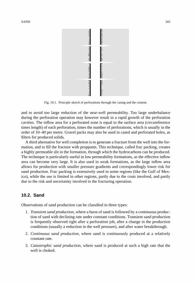
SAND 343
Fig. 10.1. Principle sketch of perforations through the casing and the cement.
and to avoid too large reduction of the near-well permeability. Too large underbalanceduring the perforation operation may however result in a rapid growth of the perforationcavities. The inflow area for a perforated zone is equal to the surface area (circumferencetimes length) of each perforation, times the number of perforations, which is usually in theorder of 10–40 per metre. Gravel packs may also be used in cased and perforated holes, asfilters for produced solids.
A third alternative for well completion is to generate a fracture from the well into the for-mation, and to fill the fracture with proppants. This technique, called frac packing, createsa highly permeable slit in the formation, through which the hydrocarbons can be produced.The technique is particularly useful in low permeability formations, as the effective inflowarea can become very large. It is also used in weak formations, as the large inflow areaallows for production with smaller pressure gradients and correspondingly lower risk forsand production. Frac packing is extensively used in some regions (like the Gulf of Mex-ico), while the use is limited in other regions, partly due to the costs involved, and partlydue to the risk and uncertainty involved in the fracturing operation.
10.2. Sand
Observations of sand production can be classified in three types:
1. Transient sand production, where a burst of sand is followed by a continuous produc-tion of sand with declining rate under constant conditions. Transient sand productionis frequently observed right after a perforation job, after a change in the productionconditions (usually a reduction in the well pressure), and after water breakthrough.
2. Continuous sand production, where sand is continuously produced at a relativelyconstant rate.
3. Catastrophic sand production, where sand is produced at such a high rate that thewell is choked.

344 SOLIDS PRODUCTION
Continuous sand production, even only a few grams per m3, may add up to amounts inthe order of hundreds of kilos per metre of the well after several years of production. Theremoval of such amounts of sand obviously changes the size and shape of the producingcavities. For instance, perforations that are initially formed more or less as separate, cylin-drical holes (Fig. 10.1), may eventually merge and form larger cavities behind the casing.
10.2.1. Necessary and sufficient conditions for sand production
It is generally accepted that sand production can not occur from intact rock, even if it ispoorly consolidated, since a flowing fluid does not normally provide sufficient force topull sand grains out of an intact rock. This is illustrated by a model example in the nextsection. Sand production may thus occur only if the rock in the vicinity of the producingcavity is unconsolidated, or has been damaged. Such damage may be caused by the stressconcentrations that occur around open holes in a stressed rock, as described in Chapter 4.Onset of sand production is therefore closely related to stress induced damage of the rock.Criteria for failure of the rock around production cavities are discussed in Section 10.2.3.
Although unconsolidated or damaged rock is a necessary condition for sand production,it is not necessarily a sufficient condition. Post failure stabilization of a production cavitymay occur after some initial sand production, due to for instance a change in the cavityshape or increased permeability in the damaged region. It has also been shown that dam-aged rock may sometimes form stable sand arches that allow for sand free production atsignificantly higher drawdowns than the rock failure conditions indicate. Criteria describ-ing the stability of sand arches are described in Section 10.2.4. When the conditions exceedthe stability limit for the sand arches, sand will definitively be produced into the well.
Monitoring of sand production is usually based on measurements or observations atthe surface. However, the produced sand will only reach the surface if the well flow issufficiently strong to carry the sand grains all the way up through the well. Thus, sandtransport in the well is also a significant part of the sand production problem, however thatpart will only be discussed briefly here (Section 10.2.6).
Prevention of sand production problems is most effective if it is done or planned duringwell completion. Thus it is essential to be able to predict possible sanding problems beforethe well completion starts. To an increasing extent, this also involves prediction of the rateof produced sand in the cases where sand free production is unachievable or economicallyunfavourable. A model describing sand rate is described in Section 10.2.5, while sandprediction is discussed in Section 10.2.7.
10.2.2. Forces on a sand grain
Consider a sand grain of diameter dg squeezed in between its neighbouring grains at thewall of a cylindrical cavity, as illustrated schematically in Fig. 10.2. The force Fr thatis needed to remove the grain can be estimated as the sum of the shear forces needed toinduce shear failure in the four contact planes at the side of the grain, (given by for instancethe Mohr–Coulomb criterion) plus the force needed to induce tensile failure in the contact

SAND 345
Fig. 10.2. Sand grain at the wall of a cylindrical cavity.
plane behind the grain (given by the tensile failure criterion). On average, this is given as
Fr = π(dg
2
)2[4S0 + μ(2σ ′
z + 2σ ′θ )+ T0
](10.1)
where T0 and S0 are the tensile strength and the cohesion, respectively, μ is the coefficientof internal friction (see Sections 2.2 and 2.3), and σ ′
z and σ ′θ are the effective axial and
tangential stresses, respectively, at the cavity wall.The hydrodynamic forces pulling on the grain are caused by the fluid flowing through
the rock. An estimate of the forces can be obtained as follows: The force F acting on avolume element of the rock due to a fluid flowing through it is F = −A�pf, where A isthe cross-sectional area through which the fluid is flowing, �x is the length of the volumeelement, and �pf is the pore pressure drop over �x. From Darcy’s law (Eq. (1.229)) wederive that F = −A�pf = (ηf/k)Q�x. An expression for the permeability k of a porousrock is given by the Kozeny–Carman equation (Carman, 1956; see also Dullien, 1992; analternative version of this equation is given in Eq. (12.63)):
k = 1
180
φ3
(1 − φ)2 d2g (10.2)
The number N of grains in this volume element is roughly given as the volume of solidmaterial in the element which is (1 −φ)A�x, divided by the volume of one grain which is(1/6)πd3
g . From these considerations we may deduce that the average hydrodynamic forceFh acting on one grain within the volume element is
Fh = F
N= 30πηf
1 − φφ3
Q
Adg (10.3)
(As the grain we are considering is placed at the surface of the rock, we might alternativelyconsider the hydrodynamic forces acting on a free particle. The result, as shown by Charlez(1997), is somewhat different, however the following conclusion is the same. See alsoVardoulakis, 2004.)
Fig. 10.3 compares the forces on a grain in a very weak rock (S0 = 1 MPa). It is assumedthat the grain is only attached by cohesional forces (which is probably the case for someof the grains). The figure shows that the hydrodynamic forces Fh increase with the fluid

346 SOLIDS PRODUCTION
Fig. 10.3. Hydrodynamic force Fh acting on a sand grain, compared to the forces Fr needed to remove the grain.Estimated from Eqs. (10.1) and (10.3); T0 = 0, μ = 0.5, S0 = 1 MPa, σ ′
r = σ ′θ = 0, ηf = 1 cP, φ = 0.2. Solid
lines: dg = 100 µm, dashed lines: dg = 10 µm.
fluxQ/A, however for the typical range shown here, they remain for the most part severalorders of magnitude smaller than the force Fr needed to pull the grain away. Thus, thehydrodynamic forces are not able to destroy a competent rock and induce failure on theirown. The major role for the hydrodynamic forces is to remove grains from unconsolidatedor damaged rock, and to transport loose material into the well.
10.2.3. Critical drawdown for cylindrical cavities
As the fluid flow is normally not able to destroy the rock and induce sand production, a nec-essary condition for sand production is that the rock is unconsolidated or has been damagedby some other mechanism. Such damage is usually caused by the effective stresses in thevicinity of the producing cavity. These depend on several factors, in particular the far-fieldin situ stresses, the pore pressure, and the geometry of the producing cavity. Since the stressfield around a cavity is not homogeneous, the effective stresses in the vicinity of the cavitymay also depend on the rock properties.
We shall in this paragraph take a look at the criteria for sand failure around a producingopening, caused by the in situ stresses. We shall restrict our attention to cylindrical holes—which may be seen as representative for a perforation or an open hole (that is, a well withno casing), and to (semi-)spherical holes—which may represent a perforation after somesand has been produced. A semispherical hole may also represent the tip of a cylindricalperforation.
SAND 347
When working with production, it is often convenient to use drawdown rather than wellpressure to describe the pressure conditions in the well. Drawdown pd is defined as thedifference between the pore pressure pfo far from the well and the well pressure pw, that is
pd = pfo − pw (10.4)
When the well pressure has been reduced so much that the well starts to produce sand, wehave reached the critical drawdown pc
d for sand production in the well. Some expressionsfor the critical drawdown are derived and discussed in this paragraph.
Shear failure
The condition for shear failure at the wall of a cylindrical hole can be derived from ex-pressions for the stresses at the cavity wall combined with a failure criterion, as shown inChapter 4.
Consider first the simple case where the stress (σ ′h) is isotropic. During production, the
pore pressure at the cavity wall is pf(Rc) = pw, the smallest principal stress is σr(Rc) =pw, and the largest principal stress is (see Eq. (4.118))
σθ (Rc) = 2σh − pw − 1 − 2νfr
1 − νfrα(pfo − pf(Rc)
)(10.5)
Failure according to the Mohr–Coulomb failure criterion, Eq. (2.22), requires that
σθ (Rc)− pf(Rc) = C0 − (σr(Rc)− pf(Rc)
)tan2 β (10.6)
Solution of these equations in terms of pw gives us the lower well pressure limit (pw,min)
where failure is initiated.Critical drawdown pc
d for the cavity is defined as
pcd = pfo − pw,min (10.7)
Assuming that the rock is sufficiently soft so that the Biot constant α ≈ 1, the solution ofEqs. (10.5) and (10.6) can be expressed as:
pcd = (1 − νfr)(C0 − 2σ ′
h) (10.8)
Here we have introduced σ ′h = σh − pfo as the effective stress far from the well. Note that
Eq. (10.8) is essentially the same as Eq. (4.120), only that the failure condition is expressedin terms of pc
d rather than pw,min.Fig. 10.4 illustrates the shear failure criterion Eq. (10.8) graphically. Although it is based
on a very simplified model, the picture is qualitatively in agreement with observations. Itshows that a minimum formation strength is required in order to prevent failure of the rockduring production. It also shows that the critical drawdown depends on the effective stressfar from the well, in such a way that pc
d is reduced when the reservoir is depleted, that iswhen pfo is reduced. This implies that the probability for sand production increases as thereservoir is being produced under constant drawdown.
Consider next a situation where the principal in situ stresses are all different. The stabil-ity of the producing cavity (whether it is an open hole or a perforation) now depends on

348 SOLIDS PRODUCTION
Fig. 10.4. Characteristic relationship between critical drawdown pcd and uniaxial compressive strength C0 for a
cylindrical cavity.
the orientation of the cavity relative to the in situ stresses. The stresses at the cavity wallfor a non-flow situation can be obtained from Eqs. (4.76)–(4.88), while Eq. (4.59) tells usto subtract (pfo −pw)((1 − 2νfr)/(1 − νfr))α from the tangential stress in order to accountfor the pore pressure gradient. Introducing these expressions into a failure criterion, forinstance the Mohr–Coulomb criterion (2.22), assuming that α ≈ 1, and following the sameprocedure as described in Chapter 4, we obtain the critical drawdown for any orientationof the cavity.
In general, the result can not be expressed on an explicit form. However, if the cavity isparallel to one of the principal in situ stress directions, the result may be written as:
pcd = (1 − νfr)(C0 − 2σ ′
is) (10.9)
The effective in situ stress σ ′is is given by
2σ ′is = 3σ ′
max⊥ − σ ′min⊥ (10.10)
where σ ′max⊥ and σ ′
min⊥ are the maximum and minimum effective principal stresses, re-spectively, in the plane perpendicular to the cavity axis (see also Section 9.2).
For completeness, we should also consider the possibility that the axial stress is thelargest principal stress at the critical point on the cavity wall (ref. Case b in Table 4.1).This gives the criterion
pcd = 1 − νfr
νfr(C0 − σ ′
is,b) (10.11)
where
σ ′is,b = σ ′‖ + 2νfr(σ
′max⊥ − σ ′
min⊥) (10.12)
and σ ′‖ is the principal stress parallel to the cavity axis (see Section 9.2). The criterionthat gives the lowest critical drawdown, either Eq. (10.9) or Eq. (10.11), is the relevantone to use at any time. Note however that criterion (10.11) is unlikely to be the relevantone except for rather special stress conditions, and that this criterion has no relevance ifνfr � 0 (except for the situation that C0 < σ
′is,b, in which case the cavity is unstable at zero
drawdown).

SAND 349
As a rule of thumb, we can say that stress anisotropy in the plane normal to the cavityaxis reduces the critical drawdown. Consider as an example a vertical well in a formationwhere σv > σH > σh. For a cavity parallel to σH (inclination i = 90°, azimuth a = 0) wehave according to Eq. (10.9)
pcd = (1 − νfr)(C0 − 3σ ′
v + σ ′h) (10.13)
while for a cavity parallel to σh (i = 90°, a = 90°) we have
pcd = (1 − νfr)(C0 − 3σ ′
v + σ ′H) (10.14)
We see that pcd is largest for the cavity parallel to σh, which has the smallest stress
anisotropy in the plane normal to the cavity axis. Thus, from a vertical well it is preferableto orient the perforations parallel to σh in order to obtain the largest critical drawdown.Furthermore, Eqs. (10.9) and (10.10) tell us that from a horizontal well parallel to σh itis preferable to perforate vertically, provided that σv > σH. The examples are plotted inFig. 10.5.
A complicating factor considering the stability of perforations is that the presence of thewell itself disturbs the stress field at the perforation. Note in particular that the perfora-tions we identified as the most preferable ones in order to obtain largest critical drawdownfor the vertical well (Fig. 10.5) are positioned in the parts of the borehole wall where wemay expect to find breakouts around the well, if the conditions for such failure have beenfulfilled at some stage (see Section 4.5.3). If we have reasons to believe that such break-outs have been formed, the perforations should preferably be placed outside the breakoutsectors.
In addition, the presence of other nearby cavities may affect the stress field to someextent and reduce the stability of a perforation. A minimum distance between perforationsis therefore recommended.
In Chapter 4 it was shown that plastic deformation of the rock tends to stabilize a hole,so that it can take larger loads than the purely elastic solutions predict. To see how thisaffects the critical drawdown, we assume that the material behaves according to a linearelastic/perfectly plastic model as described in Chapter 4, and that failure occurs when theplastic strain λ reaches a critical limit λc. Although this model is obviously a simplificationof the true rock behaviour, it captures fairly well the characteristics of soft rocks. Based on
Fig. 10.5. Examples of preferred orientation for perforations, in a formation where σv > σH > σh. Perforationswith highest critical drawdown are drawn as solid lines, perforations with lowest critical drawdown are dotted.

350 SOLIDS PRODUCTION
expression (4.162) for λ, and the assumption that λc is so small that we can ignore higherorder terms, we find that the criterion for failure in an isotropic stress situation becomes
pcd = 1
2(C0 − 2σ ′
h)+ λc!c (10.15)
where
!c = 4C0(λ+G)2C0
λ+GG
− C0−2σ ′h
ln ReRw
≈ 2G (10.16)
Note that Eq. (10.15) does not become exactly equal to Eq. (10.8) when λc = 0. This isbecause Eq. (10.8) is based on the Mohr–Coulomb criterion, while Eq. (10.15) is based onthe Tresca criterion.
We may combine the results obtained above into a generalized equation for critical draw-down
pcd = A1(C0 − 2σ ′
is)+ A2 (10.17)
where A1 is a non-dimensional parameter depending on the Poisson’s ratio and the failurecriterion, while A2 is a parameter with the dimension of stress, depending on the plasticityof the rock. In practice A1 and A2 may be empirical constants. It has been shown (van denHoek et al., 2000a, 2000b, 2000c) that A2 also depends on the size of the cavity. Due tothe increasing difficulty in rotating sand grains at the cavity wall for larger grain diameter-to-cavity diameter ratios, the smaller cavities can take larger plastic strains before failing,and therefore A2 is larger for the smaller cavities.
An alternative approach is to apply strength data from thick-walled cylinder tests (TWC)rather than the unconfined compressive strength (C0) in the critical drawdown criterion.The philosophy of this approach is that nonlinear elasticity and plasticity are implicitlyincluded in the TWC results (Veeken et al., 1991). The critical drawdown can still becomputed from Eq. (10.17), with the modification that
C0 + A2
A1→ sCTWC (10.18)
where CTWC is the collapse pressure of the thick-walled cylinder. By introducingEq. (10.18) into Eq. (10.17) we obtain an expression for the critical drawdown of a cylin-drical cavity, in terms of thick-walled cylinder strength:
pcd = A1(sCTWC − 2σ ′
is) (10.19)
The constant s accounts for the effects of size and the ratio between the outer and innerdiameter of the thick-walled cylinder, as the TWC tests conducted in the laboratory donot exactly match the field conditions on these points. Willson et al. (2002) proposed touse s = 3.1 when CTWC is derived from tests on standard 1 1
2′′
outer diameter, 12′′
innerdiameter, 3′′ long TWC samples.
Although perforations are most conveniently made as cylindrical holes, this is not themost stable shape for a producing cavity. In Chapter 4, the stresses at the wall of a sphericalcavity were given. From these results, in combination with the Mohr–Coulomb failure

SAND 351
Fig. 10.6. Critical drawdown versus rock strength, for cylindrical and spherical cavities.
criterion, we find that the critical drawdown for a semi-spherical cavity in an isotropicstress field is
pcd = 1 − νfr
1 + νfr(2C0 − 3σ ′
h) (10.20)
This expression corresponds to Eq. (10.8) for a cylindrical cavity. Both expressions areillustrated graphically in Fig. 10.6. We see that the spherical cavity is more stable thanthe cylindrical cavity, which tells us that the cylindrical shape typically created by theperforation charge need not be the most stable one. Thus it is possible for a cavity thatstarts to produce sand at a given drawdown, to obtain a more stable shape and eventuallystop producing sand at this drawdown level. This is one possible explanation for a typi-cal observation of transient sand production, where sand production is initiated when thedrawdown is increased, and subsequently stops when the drawdown has been kept constantfor a while.
Tensile failure
Another possible failure mode is tensile failure. At the cavity wall, the radial stress andthe pore pressure are both equal to the well pressure, which implies that the effective ra-dial stress is zero at the cavity wall. If the pore pressure gradient is larger than the radialstress gradient at the cavity wall, the effective radial stress will become negative, and thecondition for tensile failure may be fulfilled at some point inside the wall. Thus, a mini-mum criterion for tensile failure to occur is that the pore pressure gradient is larger thanthe radial stress gradient at the cavity wall, that is
∂pf
∂r
∣∣∣∣r=Rc
>∂σr
∂r
∣∣∣∣r=Rc
(10.21)
If the tensile strength is larger than zero, this criterion may not be sufficient for tensilefailure to occur.
The normalized drawdown pressure gradient (Morita et al., 1989a, 1989b), is defined as
gpn = Rc∂pf
∂r
∣∣∣∣r=Rc
(10.22)
352 SOLIDS PRODUCTION
where Rc is the radius of the cavity. The critical drawdown pressure gradient gcpn, isthe largest possible normalized drawdown pressure gradient without sand failure, thusEq. (10.21) expresses that
gcpn = Rc∂σr
∂r
∣∣∣∣r=Rc
(10.23)
Again we consider the simple case of a cylindrical cavity in a formation where the stressis isotropic. The radial stress is given by Eq. (4.55). Taking the derivative with respect to rwe find that the critical drawdown pressure gradient is given as
gcpn = 2
[σh − pw − (pfo − pw)α
1 − 2νfr
2(1 − νfr)
](10.24)
By combining Eqs. (4.62) and (10.22) we may find an expression for gpn during stableproduction. The results shows that it is highly unlikely that gpn will reach the critical limit(10.23).
Van den Hoek et al. (2000a) concluded—based on modelling accounting for strain lo-calization and grain rotations—that tensile failure may only occur in small holes likeperforations, not in open holes. The reason for this is that shear failure will always pre-cede tensile failure for a large cavity like an open hole. Due to the size effect, a smallcavity like a perforation has a much higher threshold for shear failure, hence tensile fail-ure may occur first, however even for small cavities it will only just precede shear failure.Van den Hoek et al. (2000a) found support for their conclusion in laboratory experimentsshowing no correlation between the (non-)occurrence of sand production and the flow rate(which controls the pore pressure gradient).
However, in a transient period when pw is reduced, the pore pressure gradient at thecavity wall can be much larger. During start-up of the production the well pressure islowered, and the pore pressure gradient at the cavity wall will be significantly larger fora period until stable conditions are established. Thus there may be a critical rate for wellpressure reduction in order to prevent sand production in the start-up period (Santarelli,1994).
To find an expression for the critical well pressure reduction rate, we need to considerthe pore pressure distribution around the cavity, which is given by the pressure diffusionequation
∂pf
∂t= CD∇2pf (10.25)
CD is the diffusion constant (see Eq. (1.241)). The boundary conditions are given by pwand pfo. A complete solution of this equation is somewhat complicated. However, for thesituation where the fluid pressure at the cavity wall is changed abruptly from pfo to pw attime t = 0, a rough approximation for the transient time range 0 < t < R2
c/CD is givenby
pf(r, t) ≈ pw + (pfo − pw)(1 − e−x), t � 0 (10.26)
where
x = r − Rc√πCDt
(10.27)

SAND 353
Consider a situation where the well pressure is reduced from pw = pfo to the productionlevel ppr at a constant rate ro = −dpw/dt over a time to = (pfo − ppr)/ro. The porepressure gradient at the cavity wall at time to (which is the time when the gradient islargest) is then given as
gpn(to)
Rc=[∂pf
∂r
]r=Rct=to
=∫ to
0
∂
∂r
[dpf
dpw
]dpw
dtdt ≈ 2
pfo − ppr√πCDto
(10.28)
Remembering that failure occurs if gpn > gcpn, we find that tensile failure may be triggered
during start-up of the production if the well pressure is reduced so quickly that
to <4R2
c
πCD
[pfo − ppr
gcpn
]2
≈ 4R2cηf
πk(Kfr + 43Gfr)
[pfo − ppr
gcpn
]2
(10.29)
Here we have introduced the approximate expression (1.246) for the diffusion con-stant CD. Note that the critical value for to is proportional to the inverse of the permeability,hence the lower the permeability is, the longer the start-up period should be in order toavoid stability problems. The critical value for to is also proportional to R2
c , hence thisproblem is more of a concern for open holes than for perforations.
We now have two criteria, one related to drawdown (Eqs. (10.8)–(10.15)) and one re-lated to the pore pressure gradient which limit the range for sand free production. Theconditions are illustrated graphically in Fig. 10.7. This figure is an elementary version of asand production stability diagram (Morita et al., 1989a, 1989b).
In addition to the failure mechanisms discussed above, a different mechanism has beenobserved in laboratory tests on sandstones with porosity above 20 per cent. This mecha-nism involves the formation of a slitlike failure zone that grows from the tip of the initialshear failure zone (Fig. 10.8). The growth of such a failure zone may be explained as fol-lows: At the tip of the slit the material fails in compression (see Chapter 2). If the materialis contractant, which may be the case for high porosity rocks, the failed material takes up
Fig. 10.7. Stability diagram for production cavities.

354 SOLIDS PRODUCTION
Fig. 10.8. CT scan showing a slitlike failure zone grown from a cylindrical perforation in a sand production test.Courtesy of SINTEF Petroleum Research.
less space than it did before failure. The failed material is therefore only loosely attachedand may easily be washed away by the flowing fluid. When the failed material is washedaway, the condition for such failure is maintained at the tip of the slit. The slit may there-fore grow rapidly, resulting in significant sand production. The formation of such slitlikefailure zones has been associated with compaction bands, which are zones of localizedcompactive failure (Haimson and Kovacich, 2003). The importance of this mechanism infield situations is however still unclear.
The formation of a stable, yet continuously growing “wormhole”, may take place underspecial conditions, for instance at the interface between soft sand and a shale layer (vanden Hoek et al., 2000c). This mechanism implies improved productivity and reduced sandproduction, however it can only take place in the presence of a stronger, supporting rock.
10.2.4. Stability and collapse of sand arches
Observations have shown that it is possible to maintain stable sand arches while producingfrom unconsolidated sand (Hall and Harrisberger, 1970; Bratli and Risnes, 1981). Sandarches may be formed when damaged rock or loose sand is pushed towards a small openinglike the perforated holes in the casing. Highly damaged rock which is still able to form astable structure around a cavity—possibly assisted by capillary forces—also represents asand arch.
Eventually, even the sand arches may fail, however. Sand production in the form ofcollapse of thin inner shells around cavities in wet, unconsolidated sand was observed byBratli and Risnes (1981). They concluded that the sand production was initiated whenthe criterion for tensile failure, Eq. (10.21), was fulfilled at the cavity wall. We shall hereoutline the derivation of Bratli and Risnes for a spherical cavity. The model they studied isshown schematically in Fig. 10.9.
Although the partial saturation gives the sand a finite cohesion (see Section 2.6.2) thematerial surrounding the cavity can be considered to be in a plastified state. The radialstress gradient can be derived from one of the equations of equilibrium in spherical coor-dinates (Eq. (4.167)) giving
∂σr
∂r= 2
σθ − σrr
(10.30)
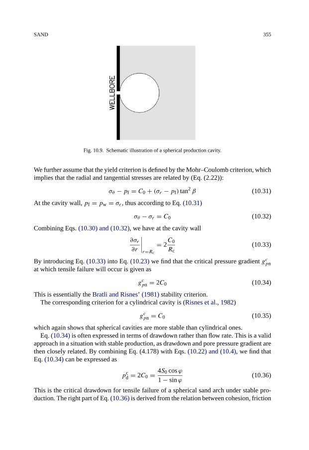
SAND 355
Fig. 10.9. Schematic illustration of a spherical production cavity.
We further assume that the yield criterion is defined by the Mohr–Coulomb criterion, whichimplies that the radial and tangential stresses are related by (Eq. (2.22)):
σθ − pf = C0 + (σr − pf) tan2 β (10.31)
At the cavity wall, pf = pw = σr , thus according to Eq. (10.31)
σθ − σr = C0 (10.32)
Combining Eqs. (10.30) and (10.32), we have at the cavity wall
∂σr
∂r
∣∣∣∣r=Rc
= 2C0
Rc(10.33)
By introducing Eq. (10.33) into Eq. (10.23) we find that the critical pressure gradient gcpnat which tensile failure will occur is given as
gcpn = 2C0 (10.34)
This is essentially the Bratli and Risnes’ (1981) stability criterion.The corresponding criterion for a cylindrical cavity is (Risnes et al., 1982)
gcpn = C0 (10.35)
which again shows that spherical cavities are more stable than cylindrical ones.Eq. (10.34) is often expressed in terms of drawdown rather than flow rate. This is a valid
approach in a situation with stable production, as drawdown and pore pressure gradient arethen closely related. By combining Eq. (4.178) with Eqs. (10.22) and (10.4), we find thatEq. (10.34) can be expressed as
pcd = 2C0 = 4S0 cosϕ
1 − sinϕ(10.36)
This is the critical drawdown for tensile failure of a spherical sand arch under stable pro-duction. The right part of Eq. (10.36) is derived from the relation between cohesion, friction

356 SOLIDS PRODUCTION
angle and unconfined strength (Eq. (2.21)), and has been included since this form of thecriterion is frequently used.
Note the line of arguments used in the derivation of Eq. (10.34) (and Eq. (10.36)): First,the material near the cavity is assumed to be in a plastified state due to shear failure. Next,sand production is provoked by tensile failure of the plastified material at the cavity wall.
Thus, Eq. (10.36) describes the stability limit for a spherical sand arch, formed by plas-tified rock. Beyond this limit, sand will be produced. Note that Eq. (10.20), which predictsa lower critical drawdown than Eq. (10.36), only describes the onset of shear failure fora spherical cavity surrounded by intact rock. Beyond that limit, sand may be producedfrom a cavity of this shape, since rock failure is a necessary, but not necessarily sufficientrequirement for sand production.
For a gas producing cavity, the pore pressure distribution is somewhat different sincegas is a highly compressible fluid. This affects the pore pressure gradient at the cavity wall,and hence it also affects the critical drawdown. Weingarten and Perkins (1995) derived ageneralized version of Eq. (10.36) which includes the effect of fluid compressibility. Thegeneralized equation can only be expressed on implicit form:
1
m+ 1
[pc
d − pfo
(1 −
(pfo
pfo − pcd
)m)]= 2C0 (10.37)
The exponent m specifies the relation between the fluid density and the fluid pressure:
ρf = γpmf (10.38)
where the gas density coefficient γ is a constant. For an incompressible fluid, which wehere can assume for water or oil, m = 0 and Eq. (10.37) reduces to Eq. (10.36). For anideal gas, m = 1 and Eq. (10.37) becomes
pcd = 2C0 + pfo −
√4C2
0 + p2fo (10.39)
We notice that fluid compressibility reduces the critical drawdown.The expressions above are based on the assumption that the fluid flow is following
Darcy’s law (Eq. (1.229)). This assumption do not hold for flow into high rate gas wells,due to the high flow rates. Ong et al. (2000) derived an expression corresponding toEqs. (10.36) and (10.37) for non-Darcy flow. The somewhat complicated expression isshown in Appendix D.4.1. It is found that non-Darcy flow reduces pc
d significantly, henceit can be overly optimistic to neglect the influence of this effect in high rate gas wells.
Note that the in situ stresses do not appear at all in the stability criteria for sand arches(Eqs. (10.34) and following). This is due to the plastified state of the material, which re-laxes the stresses near the cavity wall. Although the in situ stresses are still important forinducing plastification, they obviously play a less important role for the onset of sand pro-duction according to these criteria than shear failure criteria like Eq. (10.17) indicate. Forwells in HPHT reservoirs, this difference could be significant, as the conventional modelsbased on shear failure alone tend to be overly conservative in their estimates of the onsetof sanding under such conditions (Vaziri et al., 2002).
SAND 357
The impact of water
The sand in a hydrocarbon reservoir will normally be partly water saturated and waterwet-ting, while the remaining pore space is filled with hydrocarbons. This implies that the sandwill have an additional cohesion due to capillary forces, as described in Chapter 2. Thus,even unconsolidated sand reservoirs may have sufficient strength to build stable arches andresist the drag forces of the flowing fluid.
Water breakthrough into a well changes the water saturation of the rock near the well.This tends to reduce the capillary forces and thereby also the strength of the partiallywater-saturated reservoir sand. Consequently, the conditions for sand failure may becomefulfilled. This may explain the common observation that sand production accompanies wa-ter breakthrough (Morita et al., 1989b).
It has been claimed, however (Skjærstein et al., 1997), that sand production followingwater breakthrough is typically a temporary problem, and that the well may even producesand free at a larger drawdown some time after water breakthrough than it did before. Pos-sible explanations of such observations could be that the water breakthrough only releasesloose sand that has been trapped in the cavities by capillary forces, or that the cavities mayobtain a more stable shape after the production of some sand.
Other observations (Willson et al., 2002) indicate that sand production increases withwater cut up to about 50%, and declines towards the initial (no water) level when the watercut approaches 100%.
10.2.5. Rate of produced sand
Even when the conditions for sand production are fulfilled, the sand may be produced atsuch a low rate that it is still acceptable from an operational point of view. It is therefore ofinterest to be able to predict not only the conditions for onset of sand production, but alsothe rate of sand production given that it occurs.
Based on a qualitative analysis, Morita (1994) stated that the rate of sand productiondepends on three factors: (1) how much the well pressure is reduced below the criticalsand production pressure, (2) fluid flow rate and viscosity, and (3) cementation.
Since then, various numerical models have been developed for the prediction of sandproduction rate. The topic is still under development, however. We shall here present asimplified, analytical model (Fjær et al., 2004) for continuous sand production, based ona numerical model by Papamichos et al. (2001). The model is describing sand productionfrom the rock around a cavity that has been brought beyond the onset of sand production.
Consider a volume element of the rock in the vicinity of the cavity. If sand is being pro-duced from this element, the porosity increases. Mathematically this relation is describedas
∂msand
∂t= ρs
∂φ
∂t(10.40)
Here msand represents the (cumulative) mass of the sand being produced per unit volumeof rock, and ρs is the density of the sand grains.
358 SOLIDS PRODUCTION
We now assume that the erosion is driven by the flowing fluid in such a way that the rateof produced sand ∂msand/∂t is proportional to the hydrodynamic forces (Eq. (10.3)) actingon the grains. This implies that the rate of produced sand is proportional to ηf(1−φ)φ−3qfl,where qfl = Q/A is the fluid flux. We may also assume that a minimum force is requiredin order to uphold the erosion process, hence no sand is produced if the fluid flux is lowerthan some critical limit qcr
fl . Thus, we have established a general equation for sand erosion:
∂msand
∂t= λsandηf
1 − φφ3
(qfl − qcrfl ) (10.41)
The sand production coefficient λsand has the dimension of s/m3. The combination ofEqs. (10.40) and (10.41) gives us a differential equation for the porosity of the erodingrock. The solution is a little complicated, so we settle here for the approximate solution
φ ≈ φo[
1 + 4λsandηf
ρsφ4o
(qfl − qcrfl )(t − to)
] 14
(10.42)
given the boundary condition that φ = φo (initial porosity) at time t = to. (Note thatthis approximation does not obey the restriction φ � 1 for sufficiently large values oft − to, however the process will be truncated before this becomes a problem, as will beseen below.)
Next, we need to identify the volume of the rock that is in a state where it will producesand. Considering a cylindrical cavity, we assume that the rock can be described by asimple linear elastic/perfectly plastic model as described in Sections 4.6.1 and 10.2.3. Theplastic strain at a point r from the cavity centre can be expressed as (Eq. (4.162)):
λp ∝(Rp
r
)2
− 1 (10.43)
The radius Rp of the plastic zone is given by Eq. (4.136), and can be expressed as
Rp ∝ Rc epdC0 (10.44)
using Eq. (10.4).Sand is produced if a part of the rock has been deformed beyond its critical plastic strain
limit λc (see Section 10.2.3). This is the case for a zone of the rock inside a critical radiusRcr. The situation is illustrated in Fig. 10.10.
Onset of sand production occurs when pd = pcd. At this point, we also have Rcr = Rc.
We may deduce from Eq. (10.43) that Rcr ∝ Rp, hence we find
Rcr = Rc epd−pc
dC0 ≈ Rc
(1 + pd − pc
d
C0
)(10.45)
The approximation is valid if the drawdown exceeds the critical value by a relatively smallamount, such that pd − pc
d � C0. The volume of the sand producing zone, Vsp, can nowbe expressed as
Vsp = πL(R2cr − R2
c ) ≈ 2πLR2cpd − pc
d
C0(10.46)
where L is the length of the cavity.
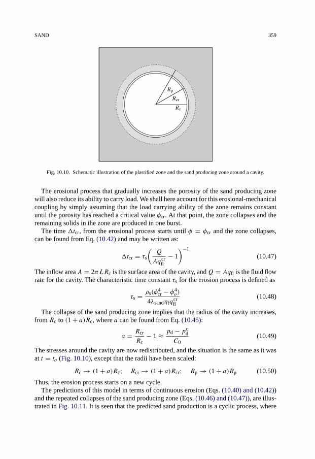
SAND 359
Fig. 10.10. Schematic illustration of the plastified zone and the sand producing zone around a cavity.
The erosional process that gradually increases the porosity of the sand producing zonewill also reduce its ability to carry load. We shall here account for this erosional-mechanicalcoupling by simply assuming that the load carrying ability of the zone remains constantuntil the porosity has reached a critical value φcr. At that point, the zone collapses and theremaining solids in the zone are produced in one burst.
The time �tcr, from the erosional process starts until φ = φcr and the zone collapses,can be found from Eq. (10.42) and may be written as:
�tcr = τs(Q
Aqcrfl
− 1
)−1
(10.47)
The inflow areaA = 2πLRc is the surface area of the cavity, andQ = Aqfl is the fluid flowrate for the cavity. The characteristic time constant τs for the erosion process is defined as
τs = ρs(φ4cr − φ4
o)
4λsandηfqcrfl
(10.48)
The collapse of the sand producing zone implies that the radius of the cavity increases,from Rc to (1 + a)Rc, where a can be found from Eq. (10.45):
a = Rcr
Rc− 1 ≈ pd − pc
d
C0(10.49)
The stresses around the cavity are now redistributed, and the situation is the same as it wasat t = to (Fig. 10.10), except that the radii have been scaled:
Rc → (1 + a)Rc; Rcr → (1 + a)Rcr; Rp → (1 + a)Rp (10.50)
Thus, the erosion process starts on a new cycle.The predictions of this model in terms of continuous erosion (Eqs. (10.40) and (10.42))
and the repeated collapses of the sand producing zone (Eqs. (10.46) and (10.47)), are illus-trated in Fig. 10.11. It is seen that the predicted sand production is a cyclic process, where
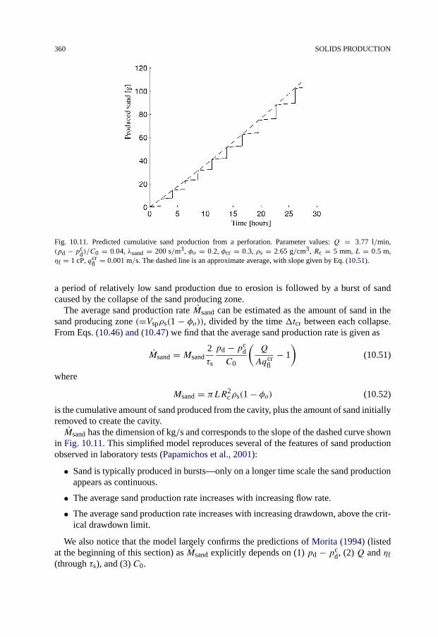
360 SOLIDS PRODUCTION
Fig. 10.11. Predicted cumulative sand production from a perforation. Parameter values: Q = 3.77 l/min,(pd − pc
d)/C0 = 0.04, λsand = 200 s/m3, φo = 0.2, φcr = 0.3, ρs = 2.65 g/cm3, Rc = 5 mm, L = 0.5 m,ηf = 1 cP, qcr
fl = 0.001 m/s. The dashed line is an approximate average, with slope given by Eq. (10.51).
a period of relatively low sand production due to erosion is followed by a burst of sandcaused by the collapse of the sand producing zone.
The average sand production rate Msand can be estimated as the amount of sand in thesand producing zone (=Vspρs(1 − φo)), divided by the time �tcr between each collapse.From Eqs. (10.46) and (10.47) we find that the average sand production rate is given as
Msand = Msand2
τs
pd − pcd
C0
(Q
Aqcrfl
− 1
)(10.51)
where
Msand = πLR2cρs(1 − φo) (10.52)
is the cumulative amount of sand produced from the cavity, plus the amount of sand initiallyremoved to create the cavity.Msand has the dimension of kg/s and corresponds to the slope of the dashed curve shown
in Fig. 10.11. This simplified model reproduces several of the features of sand productionobserved in laboratory tests (Papamichos et al., 2001):
• Sand is typically produced in bursts—only on a longer time scale the sand productionappears as continuous.
• The average sand production rate increases with increasing flow rate.
• The average sand production rate increases with increasing drawdown, above the crit-ical drawdown limit.
We also notice that the model largely confirms the predictions of Morita (1994) (listedat the beginning of this section) as Msand explicitly depends on (1) pd − pc
d, (2) Q and ηf(through τs), and (3) C0.

SAND 361
Note that the sand production rate changes with time, since Rc increases as the cavitywall is eroded away. We may estimate the long term development of Msand by establishingan expression for the development of Rc.
We assume that the drawdown pd is kept constant. Note that the surface area A =2πLRc also increases with time. On the other hand, Q which is proportional to A/Rc(see Eqs. (4.61) and (4.62)) is approximately constant as pd remains constant. By takingthe change in Rc during one erosion cycle—which is�Rc = aRc—and divide by the time�tcr between each collapse, we find that the average rate of change for Rc can be expressedas
dRc
dt= �Rc
�tcr= aRc
τs
(Q
Aqcrfl
− 1
)= a
τs
[(b + 1)Rco − Rc
](10.53)
where Rco is the cavity radius at the onset of sand production, and the dimensionless para-meter b is defined as
b = Q
Aoqcrfl
− 1 (10.54)
Ao = 2πLRco is the surface area of the cavity at the onset of sand production. b is aconstant as long asQ is constant, while a will change with time if pc
d changes—for instanceas a result of depletion.
Integration of Eq. (10.53) gives us an expression for Rc as a function of time
Rc = Rco[1 + b(1 − e−ta/τs)
](10.55)
where
ta =∫ t
0a(t) dt (10.56)
Introducing expression (10.55) into Eq. (10.51), we find that the sand rate as a function oftime can be expressed as:
Msand = Mosand
2ab
τs
[1 + b(1 − e−ta/τs)
]e−ta/τs (10.57)
where
Mosand = Msand(t = 0) = πLR2
coρs(1 − φo) (10.58)
The time development of the sand rate Msand is illustrated in Fig. 10.12. It is here as-sumed that a is constant, so that ta = at . Depending on the time scale and the amount ofsand produced, the model predicts that sand production will appear either as a time lim-ited event (transient sand production), as a stable process with a relatively constant sandproduction rate (continuous sand production), or as an accelerating process reaching dis-astrous proportions (catastrophic sand production). Note that a—which depends on thedrawdown—affects the time scale, while b—which depends on the flow rate—affects thetotal amount of sand produced.
The cumulative amount of sand produced up to a given point in time can be found byintegration of Eq. (10.57). The total amount of sand (MT
sand) produced during one event—i.e. the cumulative amount of sand produced from time t = 0 to some time t τs/a where
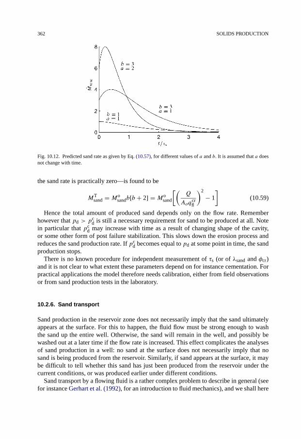
362 SOLIDS PRODUCTION
Fig. 10.12. Predicted sand rate as given by Eq. (10.57), for different values of a and b. It is assumed that a doesnot change with time.
the sand rate is practically zero—is found to be
MTsand = Mo
sandb[b + 2] = Mosand
[(Q
Aoqcrfl
)2
− 1
](10.59)
Hence the total amount of produced sand depends only on the flow rate. Rememberhowever that pd > p
cd is still a necessary requirement for sand to be produced at all. Note
in particular that pcd may increase with time as a result of changing shape of the cavity,
or some other form of post failure stabilization. This slows down the erosion process andreduces the sand production rate. If pc
d becomes equal to pd at some point in time, the sandproduction stops.
There is no known procedure for independent measurement of τs (or of λsand and φcr)and it is not clear to what extent these parameters depend on for instance cementation. Forpractical applications the model therefore needs calibration, either from field observationsor from sand production tests in the laboratory.
10.2.6. Sand transport
Sand production in the reservoir zone does not necessarily imply that the sand ultimatelyappears at the surface. For this to happen, the fluid flow must be strong enough to washthe sand up the entire well. Otherwise, the sand will remain in the well, and possibly bewashed out at a later time if the flow rate is increased. This effect complicates the analysesof sand production in a well: no sand at the surface does not necessarily imply that nosand is being produced from the reservoir. Similarly, if sand appears at the surface, it maybe difficult to tell whether this sand has just been produced from the reservoir under thecurrent conditions, or was produced earlier under different conditions.
Sand transport by a flowing fluid is a rather complex problem to describe in general (seefor instance Gerhart et al. (1992), for an introduction to fluid mechanics), and we shall here
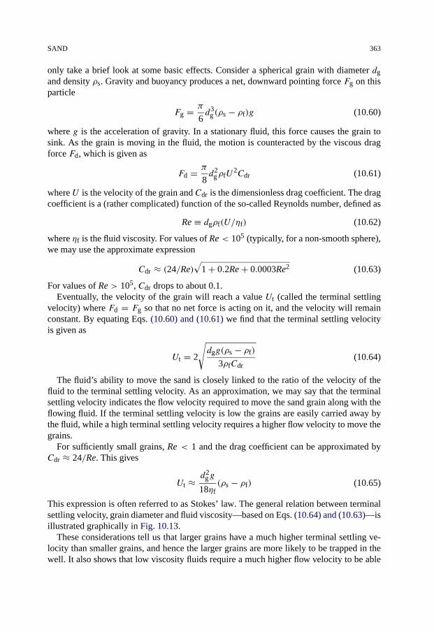
SAND 363
only take a brief look at some basic effects. Consider a spherical grain with diameter dgand density ρs. Gravity and buoyancy produces a net, downward pointing force Fg on thisparticle
Fg = π
6d3
g (ρs − ρf)g (10.60)
where g is the acceleration of gravity. In a stationary fluid, this force causes the grain tosink. As the grain is moving in the fluid, the motion is counteracted by the viscous dragforce Fd, which is given as
Fd = π
8d2
gρfU2Cdr (10.61)
where U is the velocity of the grain and Cdr is the dimensionless drag coefficient. The dragcoefficient is a (rather complicated) function of the so-called Reynolds number, defined as
Re ≡ dgρf(U/ηf) (10.62)
where ηf is the fluid viscosity. For values of Re < 105 (typically, for a non-smooth sphere),we may use the approximate expression
Cdr ≈ (24/Re)√
1 + 0.2Re + 0.0003Re2 (10.63)
For values of Re > 105, Cdr drops to about 0.1.Eventually, the velocity of the grain will reach a value Ut (called the terminal settling
velocity) where Fd = Fg so that no net force is acting on it, and the velocity will remainconstant. By equating Eqs. (10.60) and (10.61) we find that the terminal settling velocityis given as
Ut = 2
√dgg(ρs − ρf)
3ρfCdr(10.64)
The fluid’s ability to move the sand is closely linked to the ratio of the velocity of thefluid to the terminal settling velocity. As an approximation, we may say that the terminalsettling velocity indicates the flow velocity required to move the sand grain along with theflowing fluid. If the terminal settling velocity is low the grains are easily carried away bythe fluid, while a high terminal settling velocity requires a higher flow velocity to move thegrains.
For sufficiently small grains, Re < 1 and the drag coefficient can be approximated byCdr ≈ 24/Re. This gives
Ut ≈ d2gg
18ηf(ρs − ρf) (10.65)
This expression is often referred to as Stokes’ law. The general relation between terminalsettling velocity, grain diameter and fluid viscosity—based on Eqs. (10.64) and (10.63)—isillustrated graphically in Fig. 10.13.
These considerations tell us that larger grains have a much higher terminal settling ve-locity than smaller grains, and hence the larger grains are more likely to be trapped in thewell. It also shows that low viscosity fluids require a much higher flow velocity to be able

364 SOLIDS PRODUCTION
Fig. 10.13. Terminal settling velocity as a function of grain diameter, derived from Eqs. (10.64) and (10.63), forfour different values of the fluid viscosity.
to carry the same amount of sand as compared to high viscosity fluids. As the flow ve-locity may vary along the well, the conditions for sand transport may also vary. Note thatsand may be trapped at the lower end of the production zone, due to the low fluid velocitydown there. Also note that sand that has been trapped in the well while the fluid veloc-ity was relatively low, may be mobilized and washed to the surface if the fluid velocity isincreased.
These results clearly show that there is not necessarily a one-to-one relationship betweenthe amount of sand observed at the surface, and the sand production in the reservoir. Thiseffect obviously makes it difficult to evaluate the validity of sand prediction, and compli-cates sand management. It also illustrates the need for reliable downhole sand detectors.
10.2.7. Sand prediction
Prediction of possible sand production is an important part of the development phase fora sandstone reservoir. Accurate predictions for where and under which conditions sandproduction will occur assist in the design of an optimal development plan and completionstrategy for the wells in the reservoir.
Reliable sand prediction requires good, relevant models for sand production, as well asa complete set of input data for the models. It is a general opinion that the models for sandproduction available today are able to predict the onset of sanding with reasonable accu-racy, while models for predicting the amount of produced sand are still under development.
The relatively simple analytical models for onset of sand production described in Sec-tion 10.2.3 show that two groups of data are required for sand prediction: rock properties(primarily strength) and formation conditions (in situ stresses and pore pressure). A com-
CHALK 365
plete foot-by-foot coverage of such data is rarely available however, and simpler tools forsand prediction are therefore frequently used.
The simplest possible tool is a criterion stating that sand control is not needed below acertain depth. This critical depth is established from field experience, and varies from oneregion to another. The criterion may have a physical bearing in that rock strength usuallyincreases with depth. Other tools relate the critical drawdown directly to the sonic transittime (compressional, shear, or both), which can be argued for as there is some correlationbetween the sonic transit time and rock strength (see Section 8.2.3).
Models based on expressions like Eq. (10.17) may be used once a suitable calibration hasbeen established for the actual formation, and some estimate of C0 (alternatively CTWC;cf. Eq. (10.18)) is available.
Some companies use finite element modelling assuming linear elastic behaviour to ob-tain a better description of the stress state around the cavities. The predictions from suchmodelling may be calibrated with strength data from TWC tests on material from the actualformation. This technique is based on the philosophy that nonlinear elasticity and plastic-ity are implicitly included in the TWC results, and that linear elasticity may therefore beassumed for the finite element modelling of the stress state around the perforation.
Even more advanced numerical models are based on elasto-plastic modelling, like thehighly recognized sand prediction model of Morita (Morita et al., 1989a, 1989b). Thekinematic hardening model describing the rock (see Raaen, 1998) is quite extensive in thiscase, and requires several core tests for calibration.
For prediction of sand volume, additional parameters are needed, and the challenge toobtain relevant data is even larger. The model described in Section 10.2.5 requires forinstance the sand production coefficient λsand, a parameter that so far can only be derivedfrom sand production tests (Papamichos et al., 2001). Also the flow rate per cavity (Q) isseen to be of large importance for the rate of sand production, hence rock permeability andfluid viscosity are implicitly involved and need to be evaluated.
The choice of parameters is somewhat different among other models for prediction ofsand volume, like the semi-empirical model of Willson et al. (2002), and the coupled nu-merical model of Chin and Ramos (2002) which links the amount of produced sand directlyto the plastic deformation of the rock. The basic elements of the models appears to be thesame, however.
10.3. Chalk
Solids production can be a serious problem also in chalk reservoirs. The mechanismscausing chalk production have however not been as well described as those causing sandproduction. Prediction and control of chalk production can therefore be more problematic.
In some cases chalk is produced slowly at a relatively constant rate. Massive chalk pro-duction sometimes occur as sudden, rather unexpected events. In such situations largeamounts of chalk enter into the well, occasionally enough to kill the well. Although themechanisms causing these events are not fully understood, it is known that sudden changesin the well conditions, like quick closure or opening of the fluid flow, may trigger suchinstabilities.

366 SOLIDS PRODUCTION
We may expect that the mechanisms believed to cause sand production also could causechalk production under corresponding conditions. A couple of effects related to the natureof chalk versus that of sandstone make the situation somewhat different however. First, thematrix permeability in chalk is usually quite low, typically of the order 1 milliDarcy. Thismay imply that the conditions for tensile failure are more likely to be fulfilled for chalk.However, reservoir chalks are usually extensively fractured. This enhances the effectivepermeability while at the same time it implies that the fluid pressure distribution may berather complicated on a small scale. It may therefore be questioned whether expressionslike Eqs. (10.24) and (10.29) are valid for chalks. Second, the collapse pressure for highporosity chalks is quite low so that this type of failure has to be considered in addition toshear failure and tensile failure. Collapse of the rock surrounding a producing cavity mayhave a devastating effect on the productivity of the cavity, even if it does not result in solidsproduction.
When a rock collapses, the pore volume is largely reduced (see Section 2.4). This in-duces an abrupt increase in pore pressure which takes some time to dissipate in a lowpermeable material as chalk. The result may be a significant pore pressure build-up lead-ing to tensile effective mean stress and liquefaction conditions. This process may explainobserved chalk production in the field and in laboratory tests where the chalk is seen toflow like toothpaste (Raaen and Renlie, 1990; Andersen, 1995; Kristiansen and Meling,1996).
Papamichos (1998) points out that chalk has a relatively low cohesion, often providedprimarily by capillary forces that exist only when the water saturation is low. Collapse,with subsequent liquefaction and extensive chalk production may thus be induced by wa-ter flooding. A numerical model describing this effect was also presented by Papamichos(1998).
References
Andersen, M.A. (1995). “Petroleum research in North Sea chalk”. RF-Rogaland Research, Stavanger.Bratli, R.K., Risnes, R. (1981). “Stability and failure of sand arches”. Soc. Petr. Eng. J. 21, 236–248.Carman, P.C. (1956). Flow of Gases Through Porous Media. Butterworths, London.Charlez, P.A. (1997). Rock Mechanics. Petroleum Applications. Editions Technip, Paris.Chin, L.Y., Ramos G.G. (2002). “Predicting volumetric sand production in weak reservoirs”. SPE/ISRM 78169.
In: SPE/ISRM Rock Mechanics Conference, Irving, TX, October 20–23.Dullien, F.A.L. (1992). Porous Media. Fluid Transport and Pore Structure, second ed. Academic Press, New York.Dusseault, M.B., El-Sayed, S. (2000). “Heavy-oil production enhancement by encouraging sand production”.
SPE 59276. In: SPE/DOE Improved Oil Recovery Symposium, Tulsa, OK, April 3–5.Fjær, E., Cerasi, P., Li, L., Papamichos, E. (2004). “Modeling the rate of sand production”. ARMA/NARMS
04-588, Gulf Rocks 2004, Houston, June 5–9.Geilikman, M.B., Dusseault, M.B., Dullien, F.A. (1994). “Sand production as a viscoplastic granular flow”. SPE
27343. In: SPE International Symposium on Formation Damage Control, Lafayette, LA, February 9–10.Geilikman, M.B., Dusseault, M.B. (1997). “Fluid-rate enhancement from massive sand production in heavy oil
reservoirs”. J. Petr. Sci. & Eng. 17, 5–18.Gerhart, P.M., Gross, R.J., Hochstein, J.I. (1992). Fundamentals of Fluid Mechanics. Addison-Wesley Publishing
Company.Haimson, B., Kovacich, J. (2003). “Borehole instability in high-porosity Berea sandstone and factors affecting
dimensions and shape of fracture-like breakouts”. Engrg. Geology 69, 219–231.

FURTHER READING 367
Hall, C.D., Harrisberger, W.H. (1970). “Stability of sand arches: A key to sand control”. J. Petr. Tech. 22, 821–829.
Haugen, K., Kvernvold, O., Ronold, A., Sandberg, R. (1995). “Sand erosion of wear-resistant materials: Erosionin choke valves”. Wear 186–187, 179–188.
van den Hoek, P.J., Hertogh, G.M.M., Kooijman, A.P., de Bree, Ph., Kenter, C.J., Papamichos, E. (2000a). “A newconcept of sand production prediction: theory and laboratory experiments”. SPE Drilling & Completion 15,261–273.
van den Hoek, P.J., Kooijman, A.P., de Bree, Ph., Kenter, C.J., Zheng, Z., Kodaverdian, M. (2000b). “Horizontal-wellbore stability and sand production in weakly consolidated sandstones”. SPE Drilling & Completion 15,274–283.
van den Hoek, P.J., Kooijman, A.P., de Bree, Ph., Kenter, C.J., Sellmeyer, H.J., Willson, S.M. (2000c). “Mech-anisms of downhole sand cavity re-stabilisation in weakly consolidated sandstones”. SPE 65183. In: SPEEuropean Petroleum Conference, Paris, October 24–25.
Kristiansen, T.G., Meling, S. (1996). “A production parameter analysis of chalk influxes in the Valhall field”. In:Proc. 5th North Sea Chalk Symposium, Reims.
Morita, N. (1994). “Field and laboratory verification of sand-production prediction models”. SPE Drilling &Completion 9, 227–235.
Morita, N., Whitfill, D.L., Massie, I., Knudsen, T.W. (1989a). “Realistic sand-production prediction: Numericalapproach”. SPE Production Eng. 4, 15–24.
Morita, N., Whitfill, D.L., Fedde, Ø.P., Løvik, T.H. (1989b). “Parametric study of sand production prediction:analytical approach”. SPE Production Eng. 4, 25–33.
Ong, S., Ramos, G.G., Zheng, Z. (2000). “Sand production prediction in high rate, perforated and open-holegas wells”. SPE 58721. In: SPE International Symposium on Formation Damage Control, Lafayette, LA,February 23–24.
Papamichos, E. (1998). “Chalk production and effects of water weakening”. Int. J. Rock Mech. Min. Sci. 35,529–530.
Papamichos, E., Vardoulakis, I., Tronvoll, J., Skjærstein, A. (2001). “Volumetric sand production model andexperiment”. Int. J. Numer. Anal. Meth. Geomech. 25, 789–808.
Raaen, A.M., Renlie, L. (1990). “Relations between acoustic and static mechanical properties of chalk”. In: Proc.3rd North Sea Chalk Symposium, Copenhagen.
Raaen, A.M. (1998). “Efficient determination of the parameters of an elastoplastic model”. SPE/ISRM 47362. In:Eurock ’98, SPE/ISRM Rock Mechanics in Petroleum Engineering, Trondheim, Norway, July 8–10, pp. 277–283.
Risnes, R., Bratli, R.K., Horsrud, P. (1982). “Sand stresses around a wellbore”. Soc. Petr. Eng. J. 22, 883–898.Santarelli, F.J. (1994). “Similarities and differences between wellbore stability and sand production”. In: Aasen,
J.O., et al. (Eds.), North Sea Oil and Gas Reservoirs—III. Kluwer Academic Publishers, pp. 331–338.Skjærstein, A., Tronvoll, J., Santarelli, F.J., Jøranson, H. (1997). “Effect of water breakthrough on sand produc-
tion: experimental and field evidence”. SPE 38806. In: SPE ATCE, San Antonio, TX, October 5–8.Vardoulakis, I. (2004). “Fluidisation in artesian flow conditions: Hydromechanically stable granular media”.
Geotechnique 54, 117–130.Vaziri, H., Xiao, Y., Palmer, I. (2002). “Assessment of several sand prediction models with particular reference to
HPHT wells”. SPE/ISRM 78235. In: SPE/ISRM Rock Mechanics Conference, Irving, TX, October 20–23.Veeken, C.A.M., Davies, D.R., Kenter, C.J., Kooijman, A.P. (1991). “Sand production prediction review: devel-
oping an integrated approach”. SPE 22792. In: SPE 66th ATCE, Dallas, October 6–9.Weingarten, J.S., Perkins, T.K. (1995). “Prediction of sand production in gas wells: Methods and Gulf of Mexico
studies”. J. Petr. Tech. 47, 596–600.Willson, S.M., Moschovidis, Z.A., Cameron, J.R., Palmer, I.D. (2002). “New model for predicting the rate of sand
production”. SPE/ISRM 78168. In: SPE/ISRM Rock Mechanics Conference, Irving, TX, October 20–23.
Further reading
Bratli, R.K., Horsrud, P., Risnes, R. (1983). “Rock mechanics applied to the region near a wellbore”. In: Proc.5th International Congress on Rock Mechanics, Melbourne, Australia, pp. F1–F17.

368 SOLIDS PRODUCTION
Fuh, G.-F., Ramshaw, I., Freedman, K., Abdelmalek, N., Morita, N. (2006). “Use of reservoir formation failureand sanding prediction analysis for viable well-construction and completion-design options”. SPE 103244.In: SPE ATCE San Antonio, TX, September 24–27.
Han, G., Dusseault, M.B. (2002). “Quantitative analysis of mechanisms for water-related sand production”. SPE73737. In: SPE International Symposium on Formation Damage Control, Lafayette, LA, February 20–21.
van den Hoek, P.J., Geilikman, M.B. (2005). “Prediction of sand production rate in oil and gas reservoirs: fieldvalidation and practical use”. SPE 95715. In: SPE ATCE Dallas, TX, October 9–12.
Kristiansen, T.G. (1996). “Geomechanical analysis of the feasibility of openhole completions in weak, plastic Torformation at Valhall based on numerical modeling, analytical analysis and field data”. In: Proc. 5th North SeaChalk Symposium, Reims.
Morita, N., Fuh, G.-F., Burton, B. (2006). “Field and Laboratory observations of post-failure stabilizations duringsand production”. SPE 102802. In: SPE ATCE, Dallas, TX, October 9–12.
Tronvoll, J., Dusseault, M.B., Sanfilippo, F., Santarelli, F.J. (2001). “The tools of sand management”. SPE 71673.In: SPE ATCE, New Orleans, LA, September 30–October 3.
Tronvoll, J., Fjær, E. (1994). “Experimental study of sand production from perforation cavities”. Int. J. RockMech. Min. Sci. Geomech. Abstr. 31, 393–410.

369
Chapter 11
Mechanics of hydraulic fracturing
Hydraulic fracturing in rocks takes place when the fluid pressure within the rock exceedsthe smallest principal stress plus the tensile strength of the rock. This results in tensilefailure or splitting of the rock. A hydraulic fracture may be initiated by natural, geologicalprocesses in the earth whereby the fluid pressure increases and/or the smallest principalstress decreases. Artificial or man-made hydraulic fractures in petroleum activities arenormally initiated by increasing the fluid pressure in the borehole to the point where thesmallest principal stress at the borehole becomes tensile. Continued pumping at an elevatedpressure causes the formation to split and the fracture will grow in the direction of leastresistance. Some distance away from the borehole the fracture will always propagate in thedirection normal to the smallest principal stress in that specific formation.
As the least principal stress often is in a horizontal direction, the resulting fractures willbe vertical. If we consider a vertical open hole, the picture will be as indicated in Fig. 11.1.As the figure shows, two symmetric fracture wings develop perpendicularly to the leastprincipal stress.
Hydraulic fracturing has been used commercially as a stimulation technique in the petro-leum industry since the early fifties. Such fracturing jobs are designed to stimulate produc-tion from reservoirs with low permeability. This often involves pumping large amounts offluid and solids (proppants), thus creating long fractures filled with proppants. A massivehydraulic fracturing (MHF) job may exceed one thousand cubic metres of fluid and onemillion kilograms of proppant. The fracture thus creates a high-permeability flow channeltowards the wellbore which has a large drainage area towards the low-permeability forma-tion. If the fracture was not filled with solid material, it would close when the fluid pressuredrops.
Unintentional fracturing may occur during drilling operations, often referred to as lostcirculation, see also Section 9.1.2. This is a potentially hazardous situation, since the hy-draulic support of the fluid column in the wellbore is reduced. The wellbore pressure maydrop below the pore pressure in the formation and if the formation is permeable, formation
Fig. 11.1. Vertical fracture around a vertical well.

370 MECHANICS OF HYDRAULIC FRACTURING
fluids may start to flow into the wellbore in an uncontrolled manner. In the worst case, ablowout can be the result.
Today, hydraulic fracturing has several applications, such as:
• “Frac and pack” operations in weak sandstone reservoirs. These are relatively shortand wide proppant-filled fractures, designed to penetrate near-well damaged zonesand thus reduce the pressure drop close to the borehole and hence also the sandingpotential of the well.
• Fractures can be created also during water injection in reservoirs. Injectivity may bereduced with time due to partial plugging of the formation around the injector tothe point where the injection rates can only be maintained if the injection pressureis raised above the fracture pressure. Fracturing during injection can occur also atconstant injection pressure. This occurs during water injection when the water is con-sistently colder than the formation. Cooling causes the formation to shrink, thus thestresses are reduced below the initial fracturing pressure.
• Massive hydraulic fracturing jobs are normally preceded by a fracture test with a smallinjection volume (mini-frac) to determine the smallest stress in the formation and thusthe required treating pressure and other design parameters of the fracturing job.
• In drilling operations, leak-off tests are performed to determine the fracture gradientof the formation below a casing shoe and thus the maximum allowable well pressureto prevent lost circulation. If a sufficiently large volume is pumped, this will create asmall fracture around the borehole.
• An extended leak-off test is essentially a standard leak-off test where pumping contin-ues long enough to ensure that a fracture is created. By monitoring the shut-in phaseand the flowback phase, the smallest principal stress can be estimated.
• Hydraulic fracturing can be used for subsurface deposition of waste. In the petroleumindustry, reinjection of contaminated drill cuttings is one example. In this applicationit is important to have a permeable formation at or somewhere above the injectionpoint which can act as a recipient and pressure reducer. If this condition is not present,the pressure will remain high due to very slow leak-off and the fracture created duringinjection may eventually penetrate all the way to the surface.
This chapter will discuss basic processes related to hydraulic fracturing, while hydraulicfracturing applied as a technique for stress determination is discussed further in Chapter 8.Some aspects of hydraulic fracturing related to borehole stability (lost circulation) is treatedin Chapter 9. Details concerning design, operation and interpretation of hydraulic fractur-ing for stimulation has been treated extensively in the literature and will not be discussedfurther here. The reference list includes some key references also in this field.
11.1. Conditions for tensile failure
From a macroscopic point of view, fracturing is related to tensile failure. Generally, whenconsidering a test specimen of solid material, tensile failure will occur when the tractionexceeds the tensile strength T0. Following the usual convention that stresses are positive in

CONDITIONS FOR TENSILE FAILURE 371
Fig. 11.2. Hydraulic fracturing of a porous and permeable rock.
compression, this condition reads:
σ < −T0 (11.1)
For porous materials the total stress should be replaced by the effective stress, and thecondition will then be:
σ − pf < −T0 (11.2)
where pf is the pressure in the pores. Note that the relevant effective stress coefficient hereis equal to 1, because fracturing is a state of failure for the rock (see Section 1.6.3 and2.6.1). This will be used throughout this chapter for all fracturing conditions.
For porous materials it is however worthwhile to consider the condition above more indetail. Assume that we have a plug of porous and permeable material in a triaxial cell assketched in Fig. 11.2. The plug is subjected to an external stress σ . The pore pressure pfcan be varied. A confining pressure may be applied, but this will however not affect theargumentation.
Consider first that the grains are cemented to each other and that the plug is glued tothe pistons. Along the dashed lines the bonds are however broken, thus forming a closedfracture. The force tending to close this fracture will obviously be given by the differencebetween the applied pressure σ and the pore pressure pf in the fracture. The condition foropening of the fracture will thus be:
σ − pf < 0 (11.3)
This condition can of course be reached either by increasing the internal pressure pfor by reducing the external stress σ . In a short plug like the one indicated in Fig. 11.2the internal pressure pf will be constant throughout. But if we consider a long plug withmuch smaller permeability, the same way of reasoning makes it clear that the pressure pfin Eq. (11.3) is the pressure in the fracture, not the average pressure in the plug.
Another way of reasoning to obtain the same result is to assume that the two sides ofthe fracture are covered by an impermeable film, and that a fluid of pressure pf is injected
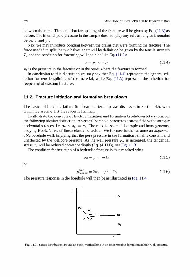
372 MECHANICS OF HYDRAULIC FRACTURING
between the films. The condition for opening of the fracture will be given by Eq. (11.3) asbefore. The internal pore pressure in the sample does not play any role as long as it remainsbelow σ and pf.
Next we may introduce bonding between the grains that were forming the fracture. Theforce needed to split the two halves apart will by definition be given by the tensile strengthT0 and the condition for fracturing will again be like Eq. (11.2):
σ − pf < −T0 (11.4)
pf is the pressure in the fracture or in the pores where the fracture is formed.In conclusion to this discussion we may say that Eq. (11.4) represents the general cri-
terion for tensile splitting of the material, while Eq. (11.3) represents the criterion forreopening of existing fractures.
11.2. Fracture initiation and formation breakdown
The basics of borehole failure (in shear and tension) was discussed in Section 4.5, withwhich we assume that the reader is familiar.
To illustrate the concepts of fracture initiation and formation breakdown let us considerthe following idealized situation: A vertical borehole penetrates a stress field with isotropichorizontal stresses, i.e. σv > σH = σh. The rock is assumed isotropic and homogeneous,obeying Hooke’s law of linear elastic behaviour. We for now further assume an imperme-able borehole wall, implying that the pore pressure in the formation remains constant andunaffected by the wellbore pressure. As the well pressure pw is increased, the tangentialstress σθ will be reduced correspondingly (Eq. (4.111)), see Fig. 11.3.
The condition for initiation of a hydraulic fracture is thus reached when
σθ − pf = −T0 (11.5)
or
pfracw,max = 2σh − pf + T0 (11.6)
The pressure response in the borehole will then be as illustrated in Fig. 11.4.
Fig. 11.3. Stress distribution around an open, vertical hole in an impermeable formation at high well pressure.

FRACTURE INITIATION AND FORMATION BREAKDOWN 373
Fig. 11.4. Idealized borehole pressure response during hydraulic fracturing of a vertical wellbore. Two pressurecycles are included.
The first linear part represents the elastic deformation of the system in and around theborehole, primarily compression of the fluid in the borehole. The peak represents the frac-ture initiation condition, i.e. the creation of a vertical fracture on the borehole wall. Thewell pressure drops instantaneously at this point. This implies a situation of unstable frac-ture growth, whereby the volume of the fracture is growing at a higher rate than the rateof fluid injection. Continued pumping will eventually result in stable fracture growth, rep-resented by the constant well pressure level. In this idealized case the point of fractureinitiation and formation breakdown are thus identical.
The second curve in Fig. 11.4 shows the response which would occur if a second pres-sure cycle was run. Then the only resistance to fracture initiation and formation breakdownwould be the stress concentration around the borehole. The tensile strength is now zero,since the fracture already exists. The difference between the first and the second peakwould thus ideally be a direct measure of the tensile strength of the formation. In practice,however, the presence of the fracture may make the effective stress concentration smallerin the repeat cycle than in the first, meaning that the difference is not only related to thetensile strength.
If the borehole is assumed to be fully permeable, and the pressurization rate was slowenough to ensure steady-state conditions during pumping, the tangential stress at the bore-hole wall is given by Eq. (4.59)
σθ = 2σh − pw − (pfo − pw)1 − 2νfr
1 − νfrα (11.7)
Inserting this expression for the tangential stress into Eq. (11.5) together with the factthat the pore pressure near the borehole and the well pressure now are equal, the fracture

374 MECHANICS OF HYDRAULIC FRACTURING
initiation pressure becomes (Eq. (4.122))
pfracw,max = 2σh − α 1−2νfr
1−νfrpfo + T0
2 − α 1−2νfr1−νfr
(11.8)
If we assume α = 1, the expression can be simplified to
pfracw,max = 2(1 − νfr)σh − (1 − 2νfr)pfo + (1 − νfr)T0 (11.9)
Eq. (11.6) represents the upper limit for the fracture initiation pressure and Eq. (11.8)the lower limit for the fracture initiation pressure. The upper limit is often referred toas the “fast” pressurization limit, and the lower limit as the “slow” pressurization limit(Detournay and Carbonell, 1997). In a real situation the fracture initiation pressure willusually be somewhere between these two limits, depending on several factors:
• There may be cracks and flaws at the borehole wall, so that the effective tensilestrength of the rock is essentially zero, even if the tensile strength of the intact forma-tion may be significant.
• There may be some time-dependent transfer of pressure between the wellbore and theformation. This will depend on the permeability of the formation, the ability of thefracture fluid to build a filter cake prior to fracture initiation and also the pump rate.
Considering the effect of pump rate on pore pressure evolution alone, this effect is onlysignificant for very low rock permeabilities and/or if a low-permeability filter cake is es-tablished. Detournay and Cheng (1992) showed that for a fluid like water, the permeabilityof the rock would have to be lower than 1 µDarcy before any effects of rate would be expe-rienced. Above this value the rock could be assumed fully permeable, and the lower limitof fracture initiation would apply (Eq. (11.8)).
In a real situation, the time-pressure curves may be quite different from that shownin Fig. 11.4. Fig. 11.5 illustrates more general curves. The curve to the left has a distinctbreakdown or initiation pressure, whereas the curve to the right does not. Sometimes a leak-off point (defined in the figures, see also Section 8.3.3) is clearly visible before breakdown,while in other cases there is less difference. The exact reasons for these different featuresare not known, but some probable causes may be listed randomly: filter cake efficiency,plastification, stress dependent elastic properties, temperature effects, leakage behind thecasing shoe, etc. Note that the leak-off point is usually interpreted as the deviation from astraight line. Hence it is difficult to give this point a clear physical meaning, as it may beaffected by all the phenomena listed above.
Let us assume that cracks or fractures exist at the borehole wall such that the inherenttensile strength of the rock is broken. We further assume that the tangential stress is trans-mitted across the fracture, but that the well pressure can penetrate into the fracture withoutprogressing further into the formation. This would require a sealing mud cake around thefracture. Such a scenario is possible when repressurizing a previously fractured boreholein a sandstone. Referring to Eq. (11.6) this would give
pw = σh (11.10)
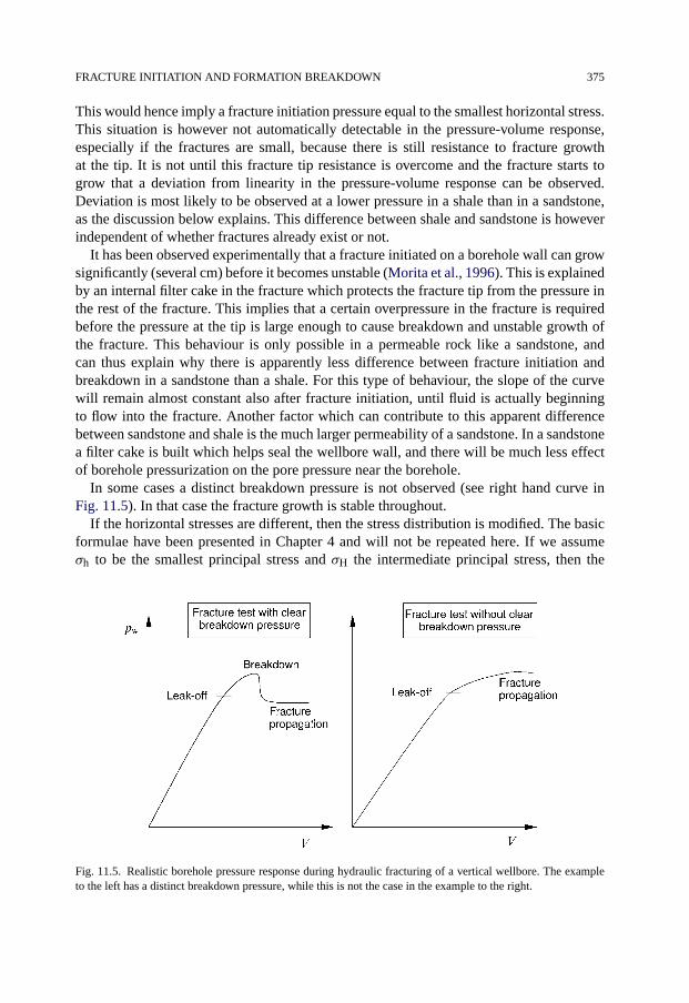
FRACTURE INITIATION AND FORMATION BREAKDOWN 375
This would hence imply a fracture initiation pressure equal to the smallest horizontal stress.This situation is however not automatically detectable in the pressure-volume response,especially if the fractures are small, because there is still resistance to fracture growthat the tip. It is not until this fracture tip resistance is overcome and the fracture starts togrow that a deviation from linearity in the pressure-volume response can be observed.Deviation is most likely to be observed at a lower pressure in a shale than in a sandstone,as the discussion below explains. This difference between shale and sandstone is howeverindependent of whether fractures already exist or not.
It has been observed experimentally that a fracture initiated on a borehole wall can growsignificantly (several cm) before it becomes unstable (Morita et al., 1996). This is explainedby an internal filter cake in the fracture which protects the fracture tip from the pressure inthe rest of the fracture. This implies that a certain overpressure in the fracture is requiredbefore the pressure at the tip is large enough to cause breakdown and unstable growth ofthe fracture. This behaviour is only possible in a permeable rock like a sandstone, andcan thus explain why there is apparently less difference between fracture initiation andbreakdown in a sandstone than a shale. For this type of behaviour, the slope of the curvewill remain almost constant also after fracture initiation, until fluid is actually beginningto flow into the fracture. Another factor which can contribute to this apparent differencebetween sandstone and shale is the much larger permeability of a sandstone. In a sandstonea filter cake is built which helps seal the wellbore wall, and there will be much less effectof borehole pressurization on the pore pressure near the borehole.
In some cases a distinct breakdown pressure is not observed (see right hand curve inFig. 11.5). In that case the fracture growth is stable throughout.
If the horizontal stresses are different, then the stress distribution is modified. The basicformulae have been presented in Chapter 4 and will not be repeated here. If we assumeσh to be the smallest principal stress and σH the intermediate principal stress, then the
Fig. 11.5. Realistic borehole pressure response during hydraulic fracturing of a vertical wellbore. The exampleto the left has a distinct breakdown pressure, while this is not the case in the example to the right.
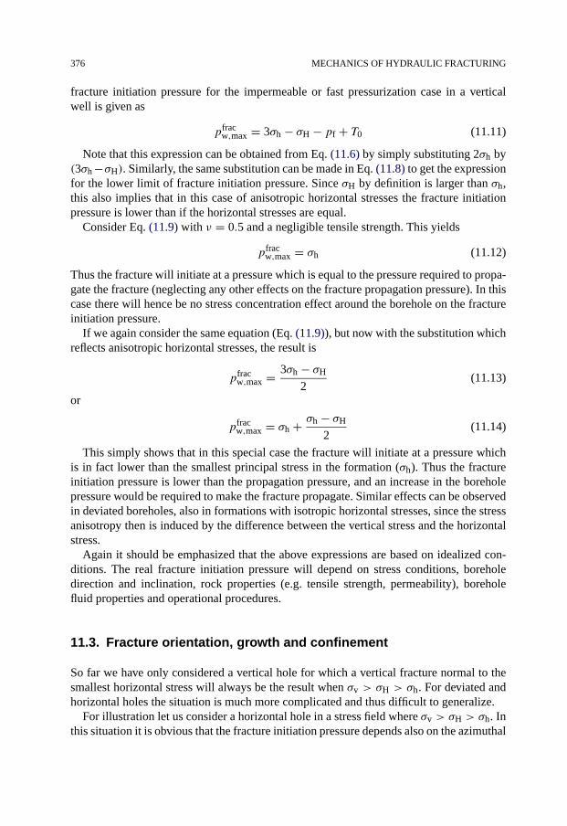
376 MECHANICS OF HYDRAULIC FRACTURING
fracture initiation pressure for the impermeable or fast pressurization case in a verticalwell is given as
pfracw,max = 3σh − σH − pf + T0 (11.11)
Note that this expression can be obtained from Eq. (11.6) by simply substituting 2σh by(3σh −σH). Similarly, the same substitution can be made in Eq. (11.8) to get the expressionfor the lower limit of fracture initiation pressure. Since σH by definition is larger than σh,this also implies that in this case of anisotropic horizontal stresses the fracture initiationpressure is lower than if the horizontal stresses are equal.
Consider Eq. (11.9) with ν = 0.5 and a negligible tensile strength. This yields
pfracw,max = σh (11.12)
Thus the fracture will initiate at a pressure which is equal to the pressure required to propa-gate the fracture (neglecting any other effects on the fracture propagation pressure). In thiscase there will hence be no stress concentration effect around the borehole on the fractureinitiation pressure.
If we again consider the same equation (Eq. (11.9)), but now with the substitution whichreflects anisotropic horizontal stresses, the result is
pfracw,max = 3σh − σH
2(11.13)
or
pfracw,max = σh + σh − σH
2(11.14)
This simply shows that in this special case the fracture will initiate at a pressure whichis in fact lower than the smallest principal stress in the formation (σh). Thus the fractureinitiation pressure is lower than the propagation pressure, and an increase in the boreholepressure would be required to make the fracture propagate. Similar effects can be observedin deviated boreholes, also in formations with isotropic horizontal stresses, since the stressanisotropy then is induced by the difference between the vertical stress and the horizontalstress.
Again it should be emphasized that the above expressions are based on idealized con-ditions. The real fracture initiation pressure will depend on stress conditions, boreholedirection and inclination, rock properties (e.g. tensile strength, permeability), boreholefluid properties and operational procedures.
11.3. Fracture orientation, growth and confinement
So far we have only considered a vertical hole for which a vertical fracture normal to thesmallest horizontal stress will always be the result when σv > σH > σh. For deviated andhorizontal holes the situation is much more complicated and thus difficult to generalize.
For illustration let us consider a horizontal hole in a stress field where σv > σH > σh. Inthis situation it is obvious that the fracture initiation pressure depends also on the azimuthal

FRACTURE ORIENTATION, GROWTH AND CONFINEMENT 377
direction of the borehole. Consider two situations:
1. Borehole parallel with σH: pfracw,max = 3σh − σv − pf + T0 (11.15)
2. Borehole parallel with σh: pfracw,max = 3σH − σv − pf + T0 (11.16)
Obviously, the fracture initiation pressure is larger in case 2 than in case 1. The directionof the fracture relative to the borehole will also be different in the two cases. In case 1the smallest in situ stress is normal to the borehole, and the fracture will be parallel withthe borehole (Fig. 11.6 left). In case 2 the fracture will hence be normal to the borehole(Fig. 11.6 right).
In cases where the borehole is not aligned with any of the principal stress directions thesituation is further complicated. This will always be the situation in a deviated boreholein a vertical/horizontal stress field. The fracture will start to grow in the direction of leastresistance and with some type of nonplanar characteristics. This direction may, however,not coincide with the direction of the smallest principal stress in situ. Hence the fracturemay start to grow in one direction, and then twist to eventually align itself normal to thesmallest in situ principal stress.
In the normal stress regime assumed above, a fracture will always tend to initiate alongthe wellbore at the high and low side of the wellbore, even in deviated wellbores drilledat an angle to the horizontal stresses. Abass et al. (1992) showed experimentally that evenin a horizontal hole along the smallest horizontal stress both a transverse fracture and afracture along the wellbore was created, forming a T-shaped fracture. The longitudinalfracture would however disappear, resulting in propagation of only the transverse fracture.At intermediate angles, Abass et al. (1992) also found that multiple fractures could form atthe wellbore.
In perforated wells the orientation and density of the perforations may complicate thispicture further, resulting in both multiple fractures and nonplanar geometries. Recommen-dations for perforation design to obtain successful hydraulic treatments have been given by
Fig. 11.6. Illustration of different fracture directions, parallel to the borehole (left) and normal to the borehole(right).
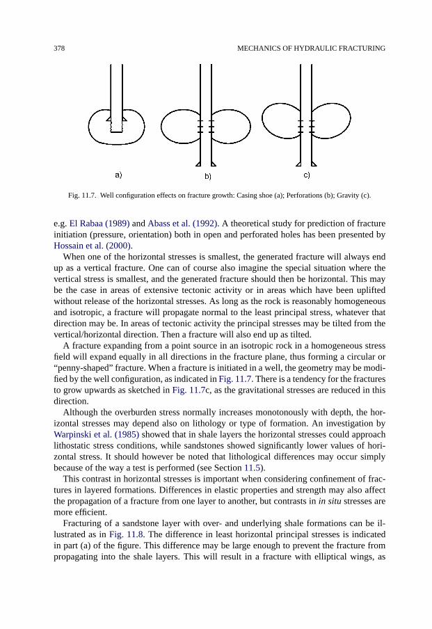
378 MECHANICS OF HYDRAULIC FRACTURING
Fig. 11.7. Well configuration effects on fracture growth: Casing shoe (a); Perforations (b); Gravity (c).
e.g. El Rabaa (1989) and Abass et al. (1992). A theoretical study for prediction of fractureinitiation (pressure, orientation) both in open and perforated holes has been presented byHossain et al. (2000).
When one of the horizontal stresses is smallest, the generated fracture will always endup as a vertical fracture. One can of course also imagine the special situation where thevertical stress is smallest, and the generated fracture should then be horizontal. This maybe the case in areas of extensive tectonic activity or in areas which have been upliftedwithout release of the horizontal stresses. As long as the rock is reasonably homogeneousand isotropic, a fracture will propagate normal to the least principal stress, whatever thatdirection may be. In areas of tectonic activity the principal stresses may be tilted from thevertical/horizontal direction. Then a fracture will also end up as tilted.
A fracture expanding from a point source in an isotropic rock in a homogeneous stressfield will expand equally in all directions in the fracture plane, thus forming a circular or“penny-shaped” fracture. When a fracture is initiated in a well, the geometry may be modi-fied by the well configuration, as indicated in Fig. 11.7. There is a tendency for the fracturesto grow upwards as sketched in Fig. 11.7c, as the gravitational stresses are reduced in thisdirection.
Although the overburden stress normally increases monotonously with depth, the hor-izontal stresses may depend also on lithology or type of formation. An investigation byWarpinski et al. (1985) showed that in shale layers the horizontal stresses could approachlithostatic stress conditions, while sandstones showed significantly lower values of hori-zontal stress. It should however be noted that lithological differences may occur simplybecause of the way a test is performed (see Section 11.5).
This contrast in horizontal stresses is important when considering confinement of frac-tures in layered formations. Differences in elastic properties and strength may also affectthe propagation of a fracture from one layer to another, but contrasts in in situ stresses aremore efficient.
Fracturing of a sandstone layer with over- and underlying shale formations can be il-lustrated as in Fig. 11.8. The difference in least horizontal principal stresses is indicatedin part (a) of the figure. This difference may be large enough to prevent the fracture frompropagating into the shale layers. This will result in a fracture with elliptical wings, as

FRACTURE ORIENTATION, GROWTH AND CONFINEMENT 379
Fig. 11.8. Confinement of a fracture between layers of higher stress.
illustrated in part (b). To extend such a fracture, the walls must be forced outwards, in-creasing the width of the fracture (c). As the fracture is confined at the top and bottom, thiswill result in a more curved fracture wall, and a higher pressure in the fracture is needed toachieve this. It is a characteristic feature of this type of fracture that the fracture propaga-tion pressure will increase with fracture length. The pressure required to extend the fracturecan thus conceptually be divided in three parts:
1. Pressure required to keep the fracture open towards the minimum stress.
2. Pressure required to flow fluid through the fracture.
3. Pressure required to overcome the resistance at the fracture tip and thus create newfracture volume.
or
pe = p(σh)+ p(flow)+ p(tip) (11.17)
The first term thus represents both the minimum in situ stress and the additional pressurerequired to maintain a fracture aperture. For small, narrow fractures with a low viscosityfluid, the extension pressure will remain reasonably constant. For larger fractures usingviscous fluids (or fluids with proppant), especially the fluid resistance will increase andthus also the pressure required to propagate the fracture.
For extension of fractures of circular shape, the extension pressure will remain rela-tively constant. On the other hand, for larger fracturing jobs, the fracture may also becomeconfined in the vertical direction as illustrated in Fig. 11.8, and the extension pressure in-creases with fracture growth. The first term of Eq. (11.17) will then start to increase, sincethe fracture walls are bent outwards and the aperture thus increases. Eventually the exten-sion pressure becomes larger than the horizontal stress in the confining layers. Then thefracture will start to penetrate into these high stress regions. Contrasts in in situ stressesthus represent barriers to fracture propagation, but not in an absolute sense. In the case ofalternate layers of shale and sand, a fracture induced in one layer may break through to an-other sand formation and extend there. This will result in a complicated fracture geometry.
A still more complicated geometry will result if hydraulic fractures are introduced innaturally fractured reservoirs (Warpinski and Teufel, 1987). This will result in combina-
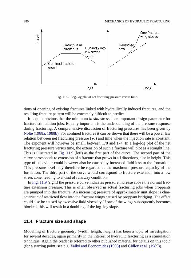
380 MECHANICS OF HYDRAULIC FRACTURING
Fig. 11.9. Log–log plot of net fracturing pressure versus time.
tions of opening of existing fractures linked with hydraulically induced fractures, and theresulting fracture pattern will be extremely difficult to predict.
It is quite obvious that the minimum in situ stress is an important design parameter forfracture stimulation jobs. Equally important is the understanding of the pressure responseduring fracturing. A comprehensive discussion of fracturing pressures has been given byNolte (1988a, 1988b). For confined fractures it can be shown that there will be a power lawrelation between net fracturing pressure (pe) and time when the injection rate is constant.The exponent will however be small, between 1/8 and 1/4. In a log–log plot of the netfracturing pressure versus time, the extension of such a fracture will plot as a straight line.This is illustrated in Fig. 11.9 (left) as the first part of the curve. The second part of thecurve corresponds to extension of a fracture that grows in all directions, also in height. Thistype of behaviour could however also be caused by increased fluid loss to the formation.This pressure level may therefore be regarded as the maximum pressure capacity of theformation. The third part of the curve would correspond to fracture extension into a lowstress zone, leading to a kind of runaway condition.
In Fig. 11.9 (right) the pressure curve indicates pressure increase above the normal frac-ture extension pressure. This is often observed in actual fracturing jobs when proppantsare pumped into the fracture. An increasing pressure of approximately unit slope is char-acteristic of restricted flow into the fracture wings caused by proppant bridging. The effectcould also be caused by excessive fluid viscosity. If one of the wings subsequently becomesblocked, this will result in a doubling of the log–log slope.
11.4. Fracture size and shape
Modelling of fracture geometry (width, length, height) has been a topic of investigationfor several decades, again primarily in the interest of hydraulic fracturing as a stimulationtechnique. Again the reader is referred to other published material for details on this topic(for a starting point, see e.g. Valkó and Economides (1995) and Gidley et al. (1989)).
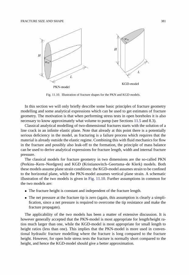
FRACTURE SIZE AND SHAPE 381
Fig. 11.10. Illustration of fracture shapes for the PKN and KGD models.
In this section we will only briefly describe some basic principles of fracture geometrymodelling and some analytical expressions which can be used to get estimates of fracturegeometry. The motivation is that when performing stress tests in open boreholes it is alsonecessary to know approximately what volume to pump (see Sections 11.5 and 8.3).
Classical analytical modelling of two-dimensional fractures starts with the solution of aline crack in an infinite elastic plane. Note that already at this point there is a potentiallyserious deficiency in the model, as fracturing is a failure process which requires that thematerial is already outside the elastic regime. Combining this with fluid mechanics for flowin the fracture and possibly also leak-off to the formation, the principle of mass balancecan be used to derive analytical expressions for fracture length, width and internal fracturepressure.
The classical models for fracture geometry in two dimensions are the so-called PKN(Perkins–Kern–Nordgren) and KGD (Kristianovitch–Geertsma–de Klerk) models. Boththese models assume plane strain conditions: the KGD-model assumes strain to be confinedto the horizontal plane, while the PKN-model assumes vertical plane strain. A schematicillustration of the two models is given in Fig. 11.10. Further assumptions in common forthe two models are:
• The fracture height is constant and independent of the fracture length.
• The net pressure at the fracture tip is zero (again, this assumption is clearly a simpli-fication, since a net pressure is required to overcome the tip resistance and make thefracture propagate).
The applicability of the two models has been a matter of extensive discussion. It ishowever generally accepted that the PKN-model is most appropriate for length/height ra-tios much larger than one, while the KGD-model is most appropriate for small length toheight ratios (less than one). This implies that the PKN-model is more used in conven-tional hydraulic fracture modelling where the fracture is long compared to the fractureheight. However, for open hole stress tests the fracture is normally short compared to theheight, and hence the KGD-model should give a better approximation.

382 MECHANICS OF HYDRAULIC FRACTURING
The maximum width of the fracture (wm) is for both models at the borehole, and for theKGD-model this is given as
wm = 2(1 − ν)Lpe
G= 4(1 − ν2)Lpe
E= 4Lpe
E′ (11.18)
where pe is the net fracture pressure (pressure in the fracture minus the smallest in situstress), L is the fracture half length (see Fig. 11.10), ν is Poisson’s ratio andG is the shearmodulus. E is Young’s modulus, and E′ is the plane strain modulus defined in Eq. (1.109).
Since the net fracture pressure is normally at most a few MPa, while E′ is in the GParange, it is immediately clear from Eq. (11.18) that fracture width is much smaller thanfracture length. The net pressure depends on the flow resistance in the fracture (includingthat caused by leak-off to the surrounding formations) and therefore on viscosity and injec-tion rate. It further depends on the mechanical breakdown processes at the fracture tip. Seee.g. Valkó and Economides (1995) for a comprehensive overview of various approaches tomodel this, analytically and numerically. See also Detournay (2004) for a discussion of therelative importance of fluid (viscous) and fracture tip (mechanical) processes.
The equation for the maximum width in the PKN-model is found by simply substitutingL with H/2.
An average fracture width can be found by assuming an elliptical shape of the fracture.This gives
w = π(1 − ν)Lpe
2G= π(1 − ν2)Lpe
E= πLpe
E′ (11.19)
Eq. (11.19) above may hence be used to design the volume required for stress testing inan open hole below a casing shoe. This principle is explained further in Section 8.3.3.
11.5. Fracture closure
The fracture closure phase is of interest because it provides an opportunity to get an esti-mate of the smallest principal in situ stress (σ3). If the fracture has penetrated beyond theinfluence zone of the wellbore and into virgin formation, it is clear from the discussion inSection 11.1 that the fracture will close when the fluid pressure in the fracture equals thestress acting normal to the fracture (σ3). In most cases it is assumed that this closure stressequals the smallest horizontal stress in the formation (σh).
However, as we shall see in the next two sections, interpretation of the minimum insitu stress from fracture closure is not straightforward. This uncertainty in interpretation ofthe closure pressure is due to the fact that fracture closure is not instantaneous. Fractureclosure is gradual, from the moment of first physical contact between the two fracture faces,until there is no further deformation of the fracture faces. Tests with downhole tiltmeters(Warpinski et al., 1998) have indeed shown that the fracture closure process is characterizedby smoothly decreasing deformation, without evidence of well-defined fracture closure.The minimum in situ stress is of course passed at some point on the pressure decline curve,but it is not obvious that this point can be accurately determined by recording the pressurein the wellbore.

FRACTURE CLOSURE 383
Fig. 11.11. Illustration of well pressure versus volume during a flowback test. After Raaen et al. (2001). An openfracture is indicated to represent the first linear part and a closed fracture to represent the final linear part.
This can be illustrated further by considering the pressure versus volume during a flow-back test in Fig. 11.11. The first linear part represents the stiffness of the open fracture.Then there is a gradual transition towards the final linear part, representing the stiffness ofthe borehole system, i.e. after fracture closure. This transition period is significant, span-ning more than 50 bar. Following the argumentation of Raaen et al. (2001), mechanicalclosure is associated with the pressure where the system stiffness starts to deviate from thefirst linear part. This change in system stiffness must be a result of reduced fracture size,i.e. the pressure is equal to or less than the smallest principal stress in some part of thefracture. The transition period thus represents further fracture closure, and eventually thereis no hydraulic communication between the fracture and the wellbore.
As mechanical closure is considered to represent the in situ stress, the interpretation ofthe smallest principal stress would be in the upper part of this range. However, there isstill considerable uncertainty related to picking of an exact value for the smallest principalstress, as the discussion in the next two sections will demonstrate.
11.5.1. Estimation of σ3 from shut-in/decline tests
When the pumps are stopped and the fracture is shut-in, the pressure required for fractureopening and the pressure required for fluid flow in the fracture immediately drop to zero(Eq. (11.17)). This implies that the pressure in the fracture is equal to the smallest principalstress plus whatever additional pressure is left in the fracture. If the viscosity of the fracturefluid is low (e.g. water) and the fracture is small and unpropped, the additional pressure inthe fracture may be small. This implies that under these conditions the pressure measuredimmediately after shut-in is a reasonable approximation to the smallest in situ principalstress (σ3). This is commonly referred to as the instantaneous shut-in pressure (ISIP).
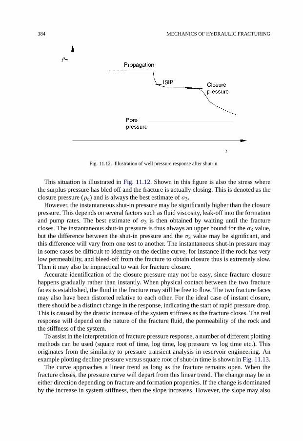
384 MECHANICS OF HYDRAULIC FRACTURING
Fig. 11.12. Illustration of well pressure response after shut-in.
This situation is illustrated in Fig. 11.12. Shown in this figure is also the stress wherethe surplus pressure has bled off and the fracture is actually closing. This is denoted as theclosure pressure (pc) and is always the best estimate of σ3.
However, the instantaneous shut-in pressure may be significantly higher than the closurepressure. This depends on several factors such as fluid viscosity, leak-off into the formationand pump rates. The best estimate of σ3 is then obtained by waiting until the fracturecloses. The instantaneous shut-in pressure is thus always an upper bound for the σ3 value,but the difference between the shut-in pressure and the σ3 value may be significant, andthis difference will vary from one test to another. The instantaneous shut-in pressure mayin some cases be difficult to identify on the decline curve, for instance if the rock has verylow permeability, and bleed-off from the fracture to obtain closure thus is extremely slow.Then it may also be impractical to wait for fracture closure.
Accurate identification of the closure pressure may not be easy, since fracture closurehappens gradually rather than instantly. When physical contact between the two fracturefaces is established, the fluid in the fracture may still be free to flow. The two fracture facesmay also have been distorted relative to each other. For the ideal case of instant closure,there should be a distinct change in the response, indicating the start of rapid pressure drop.This is caused by the drastic increase of the system stiffness as the fracture closes. The realresponse will depend on the nature of the fracture fluid, the permeability of the rock andthe stiffness of the system.
To assist in the interpretation of fracture pressure response, a number of different plottingmethods can be used (square root of time, log time, log pressure vs log time etc.). Thisoriginates from the similarity to pressure transient analysis in reservoir engineering. Anexample plotting decline pressure versus square root of shut-in time is shown in Fig. 11.13.
The curve approaches a linear trend as long as the fracture remains open. When thefracture closes, the pressure curve will depart from this linear trend. The change may be ineither direction depending on fracture and formation properties. If the change is dominatedby the increase in system stiffness, then the slope increases. However, the slope may also

FRACTURE CLOSURE 385
Fig. 11.13. Pressure decline as a function of square root of time.
decrease. This can occur if the fracture pinches off near the wellbore and the leak-off rateto the formation decreases. This implies that the closure pressure may be difficult to detectin certain cases.
A number of more or less elaborate methods have been proposed for interpretation ofshut-in/decline data. See e.g. Guo et al. (1993) for an overview of some methods and Nolte(1989) for an in-depth treatment. Raaen et al. (2001) proposed a method applicable for testswith mud, where a pressure drop across a tight mud cake may dominate leak-off signature.
In formations with very low permeability (e.g. shales), these classical methods for testingand interpretation may not be applicable. Leak-off from the fracture will then be too slowto close the fracture. This implies that the ISIP is poorly defined and/or the time to reachclosure is too long. A pressure decrease may still be observed after shut-in, but this canalso be a result of fracture extension due to energy stored in the fracture. To obtain moreprecise estimates of the smallest principal stress, both in shales and more permeable rocks,a pump-in/flowback test is recommended.
11.5.2. Estimation of σ3 from flowback tests
In a pump-in/flowback test a volume of fluid is injected at fracturing rates. The well is thenallowed to flow back until closure has been detected. A plot of pressure versus time willshow an inflection point at the closure pressure. This is the upper inflection point shownin Fig. 11.14. The physical reason for this change is the increase in system stiffness as thefracture closes.
An alternative interpretation was presented by Shlyapobersky et al. (1988), utilizing thelower inflection point (see Fig. 11.14). This is based on the assumption that mechanicalclosure occurs when the fracture storage equals zero.
Plahn et al. (1997) suggest to use the intersection point between two straight lines drawnthrough the upper and lower inflection points as illustrated in Fig. 11.14. They support

386 MECHANICS OF HYDRAULIC FRACTURING
Fig. 11.14. Well pressure response during flowback.
this procedure with numerical modelling of the flowback and rebound process, using bothKGD (Khristianovitch–Geertsma–de Klerk) and PKN (Perkins–Kern–Nordgren) fracturemodels (Gidley et al., 1989). If the flowback test is idealized to an impermeable rock andinviscid fluid, the closure pressure corresponds to the intersection of two uniquely definedlines. In a more realistic case (viscous fluid), a unique point which corresponds to theclosure pressure can not be found. However, they find that the intersection point is alwayscloser to the closure pressure than either of the two inflection points.
More recently, an alternative approach was presented by Raaen et al. (2001, 2006). Inthis approach the flowed back volume is measured, and the change of system stiffness asthe fracture closures is directly observed. See Section 8.3.3 for further discussion and afield example.
With reference to Fig. 11.14, it is evident that both the methods of Plahn et al. (1997) andRaaen et al. (2001) provide estimates of the closure pressure which are closer in numericalvalue to the upper inflection point.
It has traditionally been assumed that it is necessary to have a constant flowback rate inan appropriate range to be able to get a distinct and interpretable response. However, thedata and interpretations provided by Raaen et al. are based on constant choke setting duringflowback, and they also provide detailed recommendations for the design of such a job.
The pump-in/flowback test may be further extended to include recording of the pressureafter the flowback phase. This phase is sometimes characterized by pressure build-up orrebound, which may be an indication of near-borehole fracture pinch-off.
When withdrawing fluid from the fracture during flowback, the fracture will tend to closenear the wellbore, isolating the remaining part of the fracture which is still open (Plahnet al., 1997), especially if flowback is rapid. After flowback, the fracture will continueto produce back to the wellbore, thus creating this pressure rebound effect. The appear-ance of a rebound effect has been used to confirm the existence of a fracture (Desrochesand Kurkjian, 1999). It has also been proposed to use the maximum pressure during therebound phase as an estimate of the closure stress, especially in impermeable or very

THERMAL EFFECTS ON HYDRAULIC FRACTURING 387
low-permeability formations (Desroches and Kurkjian, 1999). Note, however, that this ex-perience is based on testing with very small volumes, in packer isolated zones. Such anapproach may not be applicable to testing where the entire hole volume is active.
11.6. Thermal effects on hydraulic fracturing
Thermal effects on hydraulic fracturing were briefly mentioned in the introduction to thischapter. Thermally induced fracturing is normally observed during water injection, espe-cially when there is a large temperature difference between the (cold) injection water andthe (hot) reservoir. Typical response is a sudden increase in injectivity after a significantperiod of stable injection (see e.g. Wright et al., 1991). This reflects that the reservoir rockhas been gradually cooled during injection of the cold water. The reservoir rock shrinksdue to cooling, and eventually the smallest in situ stress is reduced to a level below thebottom hole injection pressure. This results in the creation of a fracture which providesa much larger contact area with the formation and hence a dramatic increase in injectiv-ity. The length of the fracture is limited by the extent of the cooled zone. This process isnormally referred to as thermally induced fracturing (TIF).
In the early days of cold water injection this was an unexpected and in some casesunwanted effect. Today, however, this effect is taken into consideration in the planningprocess and is used actively. This possibility has to be designed for with respect to wellplacement, pump capacities, fluid displacement pattern etc.
This process differs from conventional hydraulic fracturing jobs in several ways, pri-marily with respect to the viscosity of the fluid and the time scale of the process. Simul-taneously, the fracturing pressure is also affected by changes in the pore pressure in thereservoir. Modelling injectivity is therefore a relatively complex matter which should alsoinclude a number of other factors (damage due to particles in the water, reservoir hetero-geneities, variation in fluid properties, well interaction etc.). Ideally the modelling of thisprocess requires a fully coupled fracture and reservoir simulation model (e.g. Clifford,1989). Simplified models have however also been introduced, such as the partially de-coupled model of Settari and Warren (1994) and the analytical approach of Detienne et al.(1998).
For further details on injectivity modelling the reader is referred to the above and otherreferences. Here we shall restrict ourselves to a brief look at the purely mechanical aspectof this problem.
Perkins and Gonzalez (1984) gave analytical expressions for the stress change resultingfrom a cylindrical cooled zone of arbitrary height. In the limit of small diameter to heightratio (d/h→ 0), they found
�σr(�T ) = �σθ(�T ) = E
2(1 − ν)αT (Tcool − To) (11.20)
where To represents the initial temperature of the formation, and Tcool is the temperatureof the cooled region.

388 MECHANICS OF HYDRAULIC FRACTURING
For the opposite limiting case (d/h → ∞) which is applicable to the situation aftersome time when the cooled region has grown considerably into the reservoir, the result is
�σr(�T ) = �σθ(�T ) = E
1 − ν αT (Tcool − To) (11.21)
Note that for this case the stress change is a factor 2 larger. For typical sandstone val-ues (E = 5 GPa, ν = 0.3, αT = 1.5 · 10−5/°C) Eq. (11.21) gives a stress change of0.1 MPa/°C.
Perkins and Gonzalez (1985) considered thermal fracturing, where the presence of thefracture leads to a non-circular temperature distribution. They modelled this as an ellipticalcooled zone, and, based on numerical modelling, gave approximate analytical expressionsfor the stress change in cooled regions as a function of height and ellipticity.
As seen above, the stresses reduce considerably as a result of cooling, thereby facilitatingfracture growth. In addition, depending on the aspect ratio of the ellipse, the stress fieldorientation may be altered: The reduction in the initially major horizontal stress will belarger than in the initially minor horizontal stress. Perkins and Gonzalez suggested thatthe directions of the principal stresses may flip, leading to possible generation of fracturesorthogonal to the initial ones.
A pore pressure change also influences the reservoir stresses (see the discussion of thereservoir stress path in Section 12.2.3). From the correspondence between thermoelasticityand poroelasticity (see Section 1.6.6)
�pf ↔ �T (11.22)
(1 − 2ν)α ↔ EαT (11.23)
the general expressions of Perkins and Gonzalez (1985) may also be used for a homoge-neous pressure change within an elliptical region.
Using Eqs. (11.22) and (11.23), and the numbers above, we see that for 5 °C cooling ofthe rock, the thermally induced stress reduction is compensated by approximately 1 MPaincrease in the cooled zone pressure. This implies that for certain cases (low thermal ex-pansion coefficient, low elastic stiffness) the pore pressure induced stress may dominateover the thermally induced stress (Eltvik et al., 1992).
During injection of a hot or cold fluid, heat transport is primarily by convection. Inaddition, thermal conduction to/from over- and underlying formations, and to a smallerextent, thermal conduction in the direction of fluid movement, contributes.
If thermal conduction can be neglected, a sharp temperature front results. Inside thefront, the temperature is that of the injection fluid, while outside it is the original reservoirtemperature. The position of the front can be estimated from energy balance considerations.For a radially symmetric injection pattern one finds
Rcool
Rflood=√
φρwCw
(1 − φ)ρsCs + φρwCw(11.24)
where Rcool is the radius of the cooled zone, and Rflood is the radius of the flooded zone.ρw and Cw are the density and specific heat capacity of the injection fluid, and ρs and Csapply for the rock matrix. Inserting typical numbers, one finds that thermal front moves at30–50% of the speed of the fluid front.

REFERENCES 389
Thermal conduction smoothens the temperature front, more strongly for thin beds. Forsome simple models taking thermal conduction into account, see Lauwerier (1955), Marxand Langenheim (1959) and Platenkamp (1985).
References
Abass, H.H., Hedayati, S., Meadows, D.L. (1992). “Nonplanar fracture propagation from a horizontal wellbore:Experimental study”. SPE 24823. In: SPE Ann. Tech. Conf. & Exh., Washington DC, October 4–7.
Clifford, P.J. (1989). “Simulation of waterflood fracture growth with coupled fluid flow, temperature and rockelasticity”. In: Proc. Second IMA/SPE European Conf. on the Mathemathics of Oil Recovery, Cambridge,July 25–27.
Desroches, J., Kurkjian, A.L. (1999). “Applications of wireline stress measurements”. SPE Reservoir EvaluationEng. 2 (5), 451–461.
Detienne, J.-L., Creusot, M., Kessler, N., Sahuquet, B., Bergerot, J.-L. (1998). “Thermally induced fractures:A field proven analytical model”. SPE Reservoir Evaluation Eng. 1 (1), 30–35.
Detournay, E. (2004). “Propagation regimes of fluid-driven fractures in impermeable rocks”. Int. J. Geomech. 4,35–45.
Detournay, E., Carbonell, R. (1997). “Fracture mechanics analysis of the breakdown process in minifrac or leak-off tests”. SPE Production and Facilities 12 (3), 195–199.
Detournay, E., Cheng, A. (1992). “Influence of pressurization rate on the magnitude of the breakdown pressure”.In: Tillerson, J.R., Wawersik, W.R. (Eds.), Rock Mechanics. Balkema, Rotterdam, pp. 325–333.
El Rabaa, W. (1989). “Experimental study of hydraulic fracture geometry initiated from horizontal wells”. SPE19720. In: SPE Ann. Tech. Conf. & Exh., San Antonio, October 8–11.
Eltvik, P., Skoglunn, T., Settari, A. (1992). “Waterflood-induced fracturing: Water injection above parting pressureat Valhall”. SPE 24912. In: SPE Ann. Tech. Conf. & Exh., Washington DC, October 4–7.
Gidley, J., et al. (Eds.) (1989). Recent Advances in Hydraulic Fracturing. SPE Monograph Series. SPE, Richard-son.
Guo, F., Morgenstern, N.R., Scott, J.D. (1993). “Interpretation of hydraulic fracturing pressure: A comparisonof eight methods used to identify shut-in pressure”. Int. J. Rock Mech. Min. Sci. & Geomech. Abstr. 30,627–631.
Hossain, M.M., Rahman, M.K., Rahman, S.S. (2000). “Hydraulic fracture initiation and propagation: Roles ofwellbore trajectory, perforation and stress regimes”. J. Petroleum Sci. Engrg. 27, 129–149.
Lauwerier, H.A. (1955). “The transport of heat in an oil layer caused by the injection of fluid”. Appl. Sci. Res.A 5, 145–150.
Marx, J.W., Langenheim, R.H. (1959). “Reservoir heating by hot fluid injection”. Petr. Trans., AIME 216, 312–315.
Morita, N., Black, A.D., Fuh, G.-F. (1996). “Borehole breakdown pressure with drilling fluids—I. Empiricalresults”. Int. J. Rock Mech. Min. Sci. & Geomech. Abstr. 33, 39–51.
Nolte, K.G. (1988a). “Principles for fracture design based on pressure analysis”. SPE Production Eng. 3 (1),22–30.
Nolte, K.G. (1988b). “Application of fracture design based on pressure analysis”. SPE Production Eng. 3 (1),31–42.
Nolte, K.G. (1989). “Fracturing-pressure analysis”. In: Gidley, et al. (Eds.), Recent Advances in Hydraulic Frac-turing. In: SPE Monograph Series. SPE, Richardson, pp. 297–318.
Perkins, T.K., Gonzalez, J.A. (1984). “Changes in earth stresses around a wellbore caused by radially symmetricalpressure and temperature gradients”. Soc. Petr. Eng. J. 24 (2), 129–140.
Perkins, T.K., Gonzalez, J.A. (1985). “The effect of thermoelastic stresses on injection well fracturing”. Soc. Petr.Eng. J 25 (1), 78–88.
Plahn, S.V., Nolte, K.G., Miska, S. (1997). “A quantitative investigation of the fracture pump-in/flowback test”.SPE Production and Facilities 12 (1), 20–27.
Platenkamp, R.J. (1985). “Temperature distribution around water injectors: Effects on injection performance”.SPE 13746. In: SPE Middle East Oil Technical Conference and Exhibition, 11–14 March, Bahrain.
390 MECHANICS OF HYDRAULIC FRACTURING
Raaen, A.M., Skomedal, E., Kjørholt, H., Markestad, P., Økland, D. (2001). “Stress determination from hydraulicfracturing tests: The system stiffness approach”. Int. J. Rock Mech. & Min. Sci. 38 (4), 529–541.
Raaen, A.M., Horsrud, P., Kjørholt, H., Økland, D. (2006). “Improved routine estimation of the minimum hori-zontal stress component from extended leak-off tests”. Int. J. Rock Mech. & Min. Sci. 43, 37–48.
Settari, A., Warren, G.M. (1994). “Simulation and field analysis of waterflood induced fracturing”. In: Proc.Eurock ’94, Delft, pp. 435–445.
Shlyapobersky, J., Walhaug, W.W., Sheffield, R.E., Huckabee, P.T. (1988). “Field determination of fracturingparameters for overpressure calibrated design of hydraulic fracturing”. SPE 18195. In: SPE Ann. Tech. Conf.& Exh., Houston, October 2–5.
Valkó, P., Economides, M.J. (1995). Hydraulic fracture mechanics. John Wiley & Sons Ltd, Chichester.Warpinski, N.R., Branagan, P., Wilmer, R. (1985). “In-situ stress measurements at U.S. DOE’s Multiwell Exper-
iment Site, Mesaverde Group, Rifle, Colorado”. J. Petr. Tech. 37 (3), 527–536.Warpinski, N.R., Teufel, L.W. (1987). “Influence of geologic discontinuities on hydraulic fracture propagation”.
J. Petr. Tech. 39 (2), 209–220.Warpinski, N.R., Peterson, R.E., Branagan, P.T., Wolhart, S.L. (1998). “In situ stress and moduli: Comparison of
values derived from multiple techniques”. SPE 49190. In: SPE Ann. Tech. Conf. & Exh., Louisiana, Septem-ber 27–30.
Wright, M.S., Svendsen, A.P., Clifford, P.J. (1991). “Thermally induced fracturing of Ula water injectors(NOCS)”. SPE Production Eng. 6 (4), 384–390.
Further reading
deBree, P., Walters, J.V. (1989). “Micro/Minifrac test procedures and interpretation for in situ stress determina-tion”. Int. J. Rock Mech. Min. Sci. & Geomech. Abstr. 26, 515–521.
Charlez, P.A. (1997). Rock Mechanics. Volume 2. Petroleum Applications. Éditions Technip, Paris.Economides, M.J., Nolte, K.G. (Eds.) (2000). Reservoir Stimulation, third ed. Wiley.Geertsma, J., de Klerk, F. (1969). “A rapid method of predicting width and extent of hydraulically induced frac-
tures”. J. Petr. Tech. 21, 1571–1581.Haimson, B., Fairhurst, C. (1967). “Initiation and extension of hydraulic fractures in rocks”. Soc. Petr. Eng. J. 7,
310–318.Hubbert, M.K., Willis, D.G. (1957). “Mechanics of hydraulic fracturing”. Trans. Amer. Inst. Min. Eng. 210,
153–168.Khristianovitch, S.A., Zeltov, Y.P. (1955). “Formation of vertical fractures by means of highly viscous fluids”. In:
Proc. World Petroleum Congress, Rome, 2, pp. 579–586.Li, X., Cui, L., Roegiers, J.-C. (1998). “Thermoporoelastic modelling of wellbore stability in non-hydrostatic
stress field”. Int. J. Rock Mech. & Min. Sci. 35 (4–5). Paper No. 063.Nolte, K.G., Smith, M.B. (1981). “Interpretation of fracturing pressures”. J. Petr. Tech. 33, 1767–1775.Nolte, K.G. (1991). “Fracturing-pressure analysis for nonideal behavior”. J. Petr. Tech. 43, 210–218.Nordgren, R.P. (1972). “A propagation of a vertical hydraulic fracture”. Soc. Petr. Eng. J. 12, 306–314.Perkins, T.K., Kern, L.R. (1961). “Width of hydraulic fractures”. J. Petr. Tech. 13, 937–949.Yew, C. (1997). Mechanics of Hydraulic Fracturing. Gulf Publ. Co. 182 pp.

391
Chapter 12
Reservoir geomechanics
The probably best-known examples of rock mechanical effects on reservoir scale behaviourare reservoir compaction and associated surface subsidence. Operational problems relatedto subsidence are environmental concerns, like risk of flooding in land operations, or plat-form safety concerns in offshore production. A majority of compaction-induced problemsare associated with casing collapse within or adjacent to the compacting reservoir. It is onthe other hand well established that compaction may be a prominent drive mechanism inrelatively soft oil reservoirs.
Pore pressure depletion leads to changes in Earth stresses—not only in effective stress,but also in the total stresses. These stress changes control not only compaction and sub-sidence, but may also lead to changes in the fluid flow performance of the reservoir.Permeability may change, and the directions of preferred flow may be altered. In somecases, the stress changes within and near the reservoir triggers seismicity during reservoirdepletion. This dynamic nature of petroleum reservoirs also affects the stability of wells tobe drilled and produced during the lifetime of the reservoir. Last but not least, geomechan-ical alteration of the reservoir and its surroundings may be observed in time-lapse (4D)seismic surveys. Reservoir geomechanics is thus becoming an increasingly important partof reservoir management.
12.1. Compaction and subsidence
When oil or gas is produced from a reservoir in the underground, the fluid pressure willgenerally decline. Reduced pore pressure in the reservoir rock will increase the effectivestress and thereby cause the rock itself to shrink, and thus the reservoir will compact. Reser-voir compaction may then in turn cause subsidence at the surface as sketched in Fig. 12.1.
Fig. 12.1. Compaction and subsidence.

392 RESERVOIR GEOMECHANICS
Most oil and gas reservoirs will experience only a small degree of compaction, and thecorresponding subsidence at the surface will be negligible. In order to see a considerabledegree of subsidence, one or several of the following conditions must be present:
• The reservoir pressure drop must be significant. Pressure maintenance by e.g. waterflooding is likely to counteract compaction.
• The reservoir rock must be highly compressible. Compaction is more likely to beimportant in soft rocks.
• The reservoir must have a considerable thickness. However, the whole depleted zonemust be considered. An adjacent aquifer will contribute to compaction, and so maypart of the overburden if drained to the reservoir.
• In order for subsidence to occur, the reservoir compaction must be significant, and inaddition, not shielded by the overburden rock. The degree of shielding depends on thedepth and the geometry of the reservoir, and on the contrast in mechanical propertiesbetween the reservoir and its surroundings.
Considering the conditions above, we would expect only a few reservoirs to cause severesubsidence problems. This is also the case, but the often severe consequences of subsidencemakes it necessary for the industry to predict possible subsidence and compaction upfront,so that platforms and casings are designed properly, and in order to decide on an appropri-ate scheme for infill drilling, placement of injector wells, well completion strategy etc.
The first report on ground subsidence is from the Goose Creek field in Texas, and isdated back in the late 1910s. Later in the 1920s the Bolivar oil field in Venezuela showedthe same behaviour. A well-known case is the Wilmington field in Long Beach, California,where subsidence of almost 9 metres was detected. More recent examples are the Ekofiskand Valhall reservoirs in the Norwegian sector of the North Sea, and the Groningen gasfield onshore and offshore the Netherlands.
In the following, we will present an overview of how we can model compaction andsubsidence. The models presented here are largely analytical, which means that severalsimplifying assumptions need to be made. A key assumption is to consider the reservoir asa homogeneous medium. In reality, the geology is complex, and we are dealing with thebehaviour of a composite and inhomogeneous medium. The modelling needs to accountfor that: The reservoir needs to be divided into compartments with different properties andmaybe also different depletion schemes. This requires numerical modelling, and a detailedknowledge of the geology and associated rock properties. Often, however, simple modelslike those presented below may be sufficient to give an idea of the possible severity ofcompaction and subsidence in a given field case. Based on a simple analysis, one may thendecide whether a further and more refined analysis is necessary.
12.2. Modelling of reservoir compaction
12.2.1. Uniaxial reservoir compaction
In this section we will calculate reservoir compaction in a simple basic case. We assumelinear poroelasticity, and consider a homogeneous reservoir consisting of isotropic rock.

MODELLING OF RESERVOIR COMPACTION 393
The deformation of the reservoir can then be expressed by Hooke’s law from Eqs. (1.102)–(1.104) in terms of changes in effective Earth stresses, using the initial stress state (i.e. startof production) as reference for the strains:
Efrεh = �σ ′h − νfr(�σ
′H +�σ ′
v) (12.1)
EfrεH = �σ ′H − νfr(�σ
′h +�σ ′
v) (12.2)
Efrεv = �σ ′v − νfr(�σ
′H +�σ ′
h) (12.3)
The change in reservoir thickness, �h, is given by the vertical strain εv and the reservoirthickness h, i.e.
�h = −εvh (12.4)
Compaction of the reservoir thus corresponds to a negative �h.In order to compute the compaction, we need to know how the stresses evolve. We
shall here make the most common approach used within the industry, and then in a laterparagraph discuss possible refinements.
Two assumptions are made: First, since the lateral extent of a reservoir normally is muchlarger than its thickness, it is reasonable as a first assumption to neglect the lateral strain:
εh = εH = 0 (12.5)
Thus, the reservoir is assumed to compact only vertically, and we refer to this as uniaxialcompaction. This is the same deformation mode as in an oedometer orKo test as describedin Section 7.3.8.
In order to maintain uniaxial vertical compaction during depletion, the effective hori-zontal stresses have to increase. Inserting Eq. (12.5) into Eqs. (12.1)–(12.2) we find
�σ ′h = �σ ′
H = νfr
1 − νfr�σ ′
v (12.6)
Secondly, we assume that the total vertical stress acting on the reservoir remains constantduring production, which means that the full weight of the overburden is sensed by thereservoir at all times as the pore pressure is reduced (�σv = 0). Thus, stress arching(or shielding of stress by the overburden) is neglected. This gives
�σ ′v = �σv − α�pf = −α�pf (12.7)
We can then insert for all three principal stress changes in Eq. (12.3), and arrive at thefollowing compaction formula:
�h
h= 1
Efr
(1 + νfr)(1 − 2νfr)
1 − νfrα�pf (12.8)
The compaction resulting from a certain pore pressure depletion can now be estimated fromEq. (12.8), provided the elastic properties (Efr and νfr), the poroelastic coefficient (α), andthe reservoir thickness (h) are known.
We may define a compaction coefficient or uniaxial compressibility Cm as
�h
h= Cmα�pf (12.9)
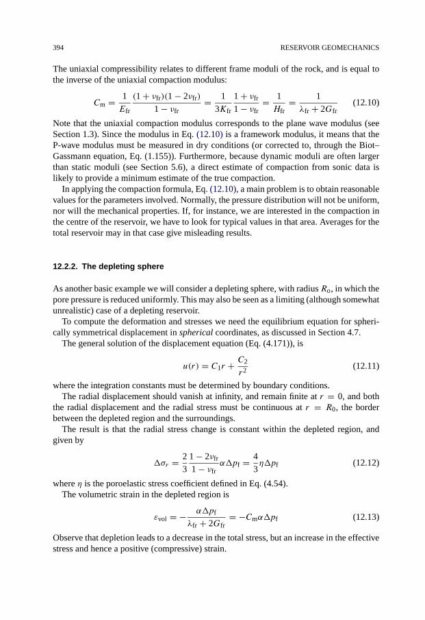
394 RESERVOIR GEOMECHANICS
The uniaxial compressibility relates to different frame moduli of the rock, and is equal tothe inverse of the uniaxial compaction modulus:
Cm = 1
Efr
(1 + νfr)(1 − 2νfr)
1 − νfr= 1
3Kfr
1 + νfr
1 − νfr= 1
Hfr= 1
λfr + 2Gfr(12.10)
Note that the uniaxial compaction modulus corresponds to the plane wave modulus (seeSection 1.3). Since the modulus in Eq. (12.10) is a framework modulus, it means that theP-wave modulus must be measured in dry conditions (or corrected to, through the Biot–Gassmann equation, Eq. (1.155)). Furthermore, because dynamic moduli are often largerthan static moduli (see Section 5.6), a direct estimate of compaction from sonic data islikely to provide a minimum estimate of the true compaction.
In applying the compaction formula, Eq. (12.10), a main problem is to obtain reasonablevalues for the parameters involved. Normally, the pressure distribution will not be uniform,nor will the mechanical properties. If, for instance, we are interested in the compaction inthe centre of the reservoir, we have to look for typical values in that area. Averages for thetotal reservoir may in that case give misleading results.
12.2.2. The depleting sphere
As another basic example we will consider a depleting sphere, with radius Ro, in which thepore pressure is reduced uniformly. This may also be seen as a limiting (although somewhatunrealistic) case of a depleting reservoir.
To compute the deformation and stresses we need the equilibrium equation for spheri-cally symmetrical displacement in spherical coordinates, as discussed in Section 4.7.
The general solution of the displacement equation (Eq. (4.171)), is
u(r) = C1r + C2
r2(12.11)
where the integration constants must be determined by boundary conditions.The radial displacement should vanish at infinity, and remain finite at r = 0, and both
the radial displacement and the radial stress must be continuous at r = R0, the borderbetween the depleted region and the surroundings.
The result is that the radial stress change is constant within the depleted region, andgiven by
�σr = 2
3
1 − 2νfr
1 − νfrα�pf = 4
3η�pf (12.12)
where η is the poroelastic stress coefficient defined in Eq. (4.54).The volumetric strain in the depleted region is
εvol = − α�pf
λfr + 2Gfr= −Cmα�pf (12.13)
Observe that depletion leads to a decrease in the total stress, but an increase in the effectivestress and hence a positive (compressive) strain.

MODELLING OF RESERVOIR COMPACTION 395
Eq. (12.13) may at first glance be slightly surprising, one might be inclined to expectα/Kfr instead of αCm. The reason why this is not so, is the stress concentration whichdevelops around the sphere, which shields it partly from the external stress and makes itappear stiffer than it otherwise would.
12.2.3. Reservoir stress path
During uniaxial reservoir compaction (described in Section 12.2.1), the vertical stressremains constant, while the horizontal stresses change according to Eq. (12.6) during de-pletion. In general, the stress evolution during depletion (the reservoir stress path) may bedefined by the stress path coefficients, as introduced by Hettema et al. (2000):
γv = �σv
�pf(12.14)
γH = �σH
�pf(12.15)
γh = �σh
�pf(12.16)
The coefficient γv is called the arching coefficient, and is zero when the vertical stressremains constant as the pore pressure is changed. The coefficients γh and γH describe thechange in the horizontal stress field. Assuming full rotational symmetry in the horizontalplane, γh = γH. Remember that for a depleting reservoir the pressure drop is negative,so that positive values of the stress path coefficients imply reductions in total vertical andhorizontal stresses.
Stress path coefficients may also be similarly defined in terms of the effective stresses.It is straightforward to show that the relation between the stress path coefficients γ ′ foreffective stresses and the coefficients defined above is
γ ′ = γ − α (12.17)
Since γ < α in practice, the γ ′ values will be negative. This simply implies that effectivestresses increase as a result of depletion, or decrease as a result of inflation.
One may also define another stress path coefficient κ as the ratio between effectivehorizontal and vertical stress changes:
κ = �σ ′h
�σ ′v
(12.18)
This leads to the following relation between γh, γv and κ:
κ = 1 − γhα
1 − γvα
= α − γh
α − γv= γ ′
h
γ ′v
(12.19)
For uniaxial compaction (no arching) as in Section 12.2.1, the stress path coefficients are:
κ = νfr
1 − νfr(12.20)
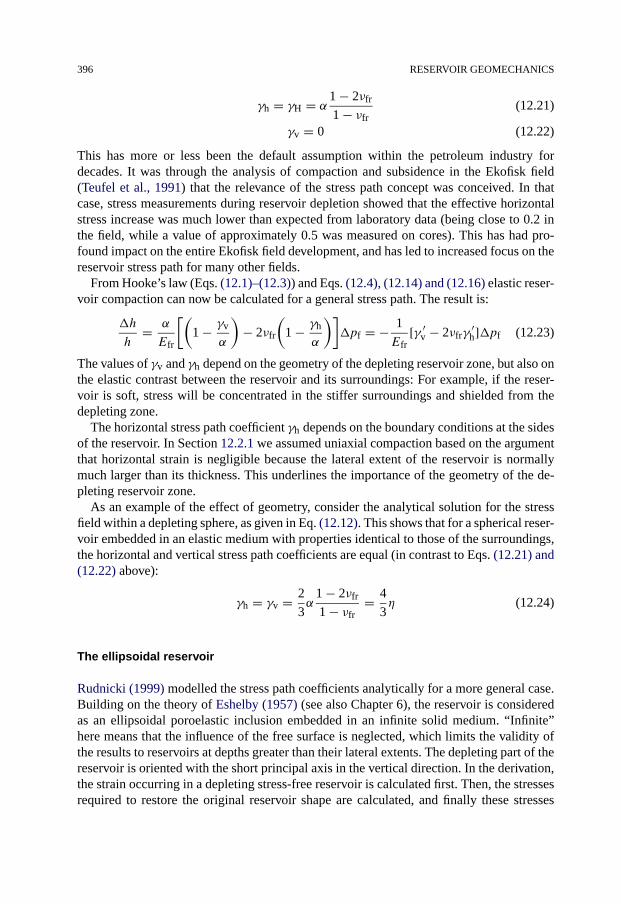
396 RESERVOIR GEOMECHANICS
γh = γH = α 1 − 2νfr
1 − νfr(12.21)
γv = 0 (12.22)
This has more or less been the default assumption within the petroleum industry fordecades. It was through the analysis of compaction and subsidence in the Ekofisk field(Teufel et al., 1991) that the relevance of the stress path concept was conceived. In thatcase, stress measurements during reservoir depletion showed that the effective horizontalstress increase was much lower than expected from laboratory data (being close to 0.2 inthe field, while a value of approximately 0.5 was measured on cores). This has had pro-found impact on the entire Ekofisk field development, and has led to increased focus on thereservoir stress path for many other fields.
From Hooke’s law (Eqs. (12.1)–(12.3)) and Eqs. (12.4), (12.14) and (12.16) elastic reser-voir compaction can now be calculated for a general stress path. The result is:
�h
h= α
Efr
[(1 − γv
α
)− 2νfr
(1 − γh
α
)]�pf = − 1
Efr[γ ′
v − 2νfrγ′h]�pf (12.23)
The values of γv and γh depend on the geometry of the depleting reservoir zone, but also onthe elastic contrast between the reservoir and its surroundings: For example, if the reser-voir is soft, stress will be concentrated in the stiffer surroundings and shielded from thedepleting zone.
The horizontal stress path coefficient γh depends on the boundary conditions at the sidesof the reservoir. In Section 12.2.1 we assumed uniaxial compaction based on the argumentthat horizontal strain is negligible because the lateral extent of the reservoir is normallymuch larger than its thickness. This underlines the importance of the geometry of the de-pleting reservoir zone.
As an example of the effect of geometry, consider the analytical solution for the stressfield within a depleting sphere, as given in Eq. (12.12). This shows that for a spherical reser-voir embedded in an elastic medium with properties identical to those of the surroundings,the horizontal and vertical stress path coefficients are equal (in contrast to Eqs. (12.21) and(12.22) above):
γh = γv = 2
3α
1 − 2νfr
1 − νfr= 4
3η (12.24)
The ellipsoidal reservoir
Rudnicki (1999) modelled the stress path coefficients analytically for a more general case.Building on the theory of Eshelby (1957) (see also Chapter 6), the reservoir is consideredas an ellipsoidal poroelastic inclusion embedded in an infinite solid medium. “Infinite”here means that the influence of the free surface is neglected, which limits the validity ofthe results to reservoirs at depths greater than their lateral extents. The depleting part of thereservoir is oriented with the short principal axis in the vertical direction. In the derivation,the strain occurring in a depleting stress-free reservoir is calculated first. Then, the stressesrequired to restore the original reservoir shape are calculated, and finally these stresses
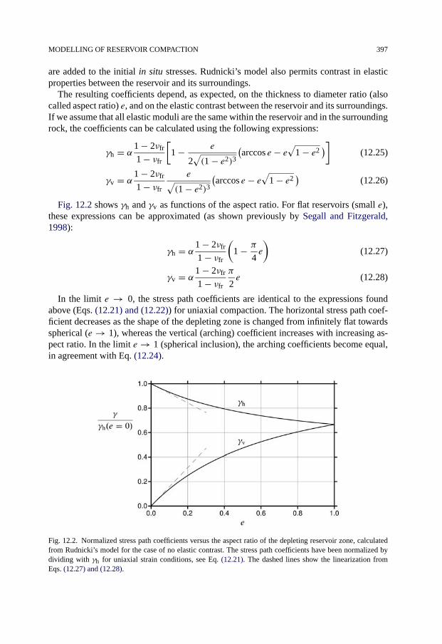
MODELLING OF RESERVOIR COMPACTION 397
are added to the initial in situ stresses. Rudnicki’s model also permits contrast in elasticproperties between the reservoir and its surroundings.
The resulting coefficients depend, as expected, on the thickness to diameter ratio (alsocalled aspect ratio) e, and on the elastic contrast between the reservoir and its surroundings.If we assume that all elastic moduli are the same within the reservoir and in the surroundingrock, the coefficients can be calculated using the following expressions:
γh = α 1 − 2νfr
1 − νfr
[1 − e
2√(1 − e2)3
(arccos e − e
√1 − e2
)](12.25)
γv = α 1 − 2νfr
1 − νfr
e√(1 − e2)3
(arccos e − e
√1 − e2
)(12.26)
Fig. 12.2 shows γh and γv as functions of the aspect ratio. For flat reservoirs (small e),these expressions can be approximated (as shown previously by Segall and Fitzgerald,1998):
γh = α 1 − 2νfr
1 − νfr
(1 − π
4e
)(12.27)
γv = α 1 − 2νfr
1 − νfr
π
2e (12.28)
In the limit e → 0, the stress path coefficients are identical to the expressions foundabove (Eqs. (12.21) and (12.22)) for uniaxial compaction. The horizontal stress path coef-ficient decreases as the shape of the depleting zone is changed from infinitely flat towardsspherical (e → 1), whereas the vertical (arching) coefficient increases with increasing as-pect ratio. In the limit e → 1 (spherical inclusion), the arching coefficients become equal,in agreement with Eq. (12.24).
Fig. 12.2. Normalized stress path coefficients versus the aspect ratio of the depleting reservoir zone, calculatedfrom Rudnicki’s model for the case of no elastic contrast. The stress path coefficients have been normalized bydividing with γh for uniaxial strain conditions, see Eq. (12.21). The dashed lines show the linearization fromEqs. (12.27) and (12.28).

398 RESERVOIR GEOMECHANICS
Note that from Eqs. (12.25) and (12.26) it follows that
γv + 2γh = 2α1 − 2νfr
1 − νfr(12.29)
Thus, for an ellipsoidal reservoir, when the surroundings have the same elastic propertiesas the reservoir, the sum γv + 2γh is independent of the aspect ratio e.
The volumetric compaction of the reservoir can be expressed in terms of the stress pathcoefficients, by introducing the definitions into Hooke’s law. The result is
εvol = −(α − γv + 2γh
3
)�pf
Kfr= γ ′Kfr�pf (12.30)
where γ ′ = (γ ′v + 2γ ′
h)/3.For an ellipsoidal reservoir with no contrast to the elastic properties of the surroundings,
this means (combining Eqs. (12.10) and (12.29)) that the volumetric deformation of thedepleting reservoir is always given by the uniaxial compaction modulus, i.e.
εvol = −αCm�pf (12.31)
This is a direct consequence of stress arching. It also implies that the pore compressibilityis independent of the stress path (but it is different from the basic definition in Eq. (1.178)),see Section 12.4.1.
If we compare the vertical compaction of the reservoir calculated from Eq. (12.23) withthe simple case of uniaxial compaction (e = 0, Eq. (12.8)), we find that the compactionis maximum for uniaxial deformation. The physical explanation of this is that arching (fore > 0) will redistribute the stresses such that the reservoir is partly shielded from theoverburden stress. When the reservoir approaches spherical shape (e = 1), the compactiondrops to 1/3 of the uniaxial compaction case. This also follows directly from the volumetricstrain being independent of the reservoir shape, see Eq. (12.31).
Elastic contrast
The effect of elastic contrast between the reservoir and the surroundings can be studiedusing the full equations in Rudnicki’s article (1999), or based on finite element (FEM)simulations (Morita et al., 1989; Mulders, 2003). In all cases it is found that arching ispromoted if the stiffness of the depleting reservoir is significantly lower than of the sur-rounding rock.
Morita et al. (1989) argued from FEM simulations with a disk shaped reservoir that if theratio between the shear modulus of the reservoir and the overburden rock is between 0.2and 1.5, and if the aspect ratio of the reservoir is less than 0.05, the resulting compactionis essentially uniaxial.
Similar conclusions can be drawn from Rudnicki’s model, which shows an increase bothin γv and also to some extent in γh compared to the elastically matched case (Holt et al.,2004). For a finite aspect ratio, both stress path coefficients approach 1 in the limit of infi-nite elastic contrast. On the other hand, a stiff reservoir in soft surroundings will have lowerstress path coefficients, approaching zero in the case of infinite contrast. Note that the value

MODELLING OF RESERVOIR COMPACTION 399
of γv + 2γh which controls volumetric compaction (see Eq. (12.30)) and also pore com-pressibility (see Section 12.4.1 below) does not remain constant for all aspect ratios, anddecreases with increasing ratio between the stiffness of the reservoir and the surroundings.
Non-ellipsoidal reservoirs
Mulders (2003) compared numerical FEM simulations of stress path coefficients for a diskshaped reservoir with those calculated by Rudnicki’s model. The assumption of ellipsoidalgeometry by Rudnicki causes the stress path coefficients to be homogeneous over the entiredepleted zone.
For a disk shaped reservoir, Mulders found that the stress path coefficients near thecentre of the reservoir agree with the analytical approach. However, γv increases and γhdecreases towards the edge of the reservoir. From FEM simulations one may inspect theeffect of reservoir depth and tilt with respect to the vertical. In particular, tilt is found toenhance arching.
Thermoelastic effects may be added to this model (Rudnicki, 1999; Segall and Fitzger-ald, 1998). This has relevance for recovery of hydrocarbon reserves by injection of coldwater or hot steam.
12.2.4. Beyond simple elastic theory
So far we have considered the reservoir (and its surroundings) to behave linearly elastic.A reservoir may however develop plastic deformation during production, and eventuallyreach a state where faults are generated, or where pre-existing faults are triggered. Faultingmay also occur outside the reservoir, in particular near the edges, where the stress con-centration resulting from stress arching in the surrounding rock is particularly large (seeSection 12.3.2).
For a reservoir rock being intact (non-fractured and in an elastic state) before produc-tion starts, non-elastic processes may occur during depletion, if the stress path brings therock past yield and in the direction of its failure surface. Failure processes may take placefrom the grain scale to the scale of large heterogeneities, and the compaction behaviourgradually becomes plastic. Laboratory experiments, where synthetic sandstone was formedunder stress (Holt et al., 2000) showed that after an initial phase with largely elastic defor-mation, permanent (plastic) deformation gradually takes over as the material compacts. Inuniaxial strain conditions, this led to approximately a doubling of the compaction rate, andit also led to enhanced lateral stress development (corresponding to a reduction of the γhcoefficient) after onset of plasticity.
Plastic behaviour also implies that if water or gas is injected to raise the pore pressureand counteract compaction, one may not expect to recover the compaction that has occurred(Santarelli et al., 1998). Depending on the stress path, and on the constitutive behaviour ofthe reservoir rock, one may also reach a stress state that permits development of localizeddeformation bands, or activation of existing faults.
Fig. 12.3 illustrates schematically how the stress paths will evolve towards the failuresurface in the case of a perfectly linear elastic material. One sees that arching directs the

400 RESERVOIR GEOMECHANICS
Fig. 12.3. Influence of arching on the reservoir stress path. The full arrow shows the stress path in the absence ofarching, while the dashed arrow indicates how arching may redirect the stress path.
path more in direction of the end cap, while lack of arching apparently may lead towards ashear failure (faulting) situation.
The development of plasticity after the rock reaches its yield point may however redirectthe stress path, as shown in Fig. 12.4. These examples are taken from laboratory tests witha high porosity sandstone. They show that, depending on the initial stress state, a uniaxialcompaction path may lead to various scenarios: In one case (curve a; low initial shearstress), the stress path turns parallel to the shear failure limit and eventually reaches failurenear the end cap, while in the other case (curve b; high initial shear stress), strain softeningoccurs after the rock has reached the failure surface.
An initially faulted and fractured reservoir in a tectonically active environment may beassumed to be in a continuous failure state (Addis, 1997). Then, a failure criterion (such asMohr–Coulomb) should apply at all stages during depletion. In a normally faulted stressregime, where the vertical stress is the largest principal stress, this gives (see Eq. (2.22)):
�σ ′v = �σ ′
h tan2 β (12.32)
The stress path coefficient κ is thus
κ = 1
tan2 β= 1 − sinϕ
1 + sinϕ(12.33)
where β is the failure angle and ϕ is the angle of internal friction (see Section 2.3.1).Provided the total vertical stress remains constant (no arching), it follows from Eq. (12.19)that
γh = �σh
�pf= 1 − 1
tan2 β= 2 sinϕ
1 + sinϕ(12.34)
It is assumed that the appropriate effective stress constant is equal to 1, since this situationdescribes rock failure (Eq. (2.49)).
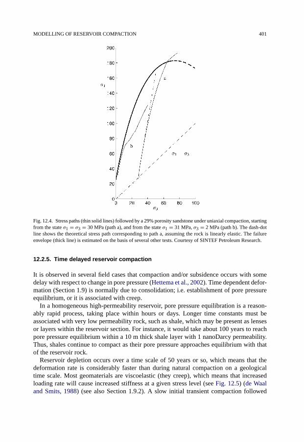
MODELLING OF RESERVOIR COMPACTION 401
Fig. 12.4. Stress paths (thin solid lines) followed by a 29% porosity sandstone under uniaxial compaction, startingfrom the state σ1 = σ3 = 30 MPa (path a), and from the state σ1 = 31 MPa, σ3 = 2 MPa (path b). The dash-dotline shows the theoretical stress path corresponding to path a, assuming the rock is linearly elastic. The failureenvelope (thick line) is estimated on the basis of several other tests. Courtesy of SINTEF Petroleum Research.
12.2.5. Time delayed reservoir compaction
It is observed in several field cases that compaction and/or subsidence occurs with somedelay with respect to change in pore pressure (Hettema et al., 2002). Time dependent defor-mation (Section 1.9) is normally due to consolidation; i.e. establishment of pore pressureequilibrium, or it is associated with creep.
In a homogeneous high-permeability reservoir, pore pressure equilibration is a reason-ably rapid process, taking place within hours or days. Longer time constants must beassociated with very low permeability rock, such as shale, which may be present as lensesor layers within the reservoir section. For instance, it would take about 100 years to reachpore pressure equilibrium within a 10 m thick shale layer with 1 nanoDarcy permeability.Thus, shales continue to compact as their pore pressure approaches equilibrium with thatof the reservoir rock.
Reservoir depletion occurs over a time scale of 50 years or so, which means that thedeformation rate is considerably faster than during natural compaction on a geologicaltime scale. Most geomaterials are viscoelastic (they creep), which means that increasedloading rate will cause increased stiffness at a given stress level (see Fig. 12.5) (de Waaland Smits, 1988) (see also Section 1.9.2). A slow initial transient compaction followed
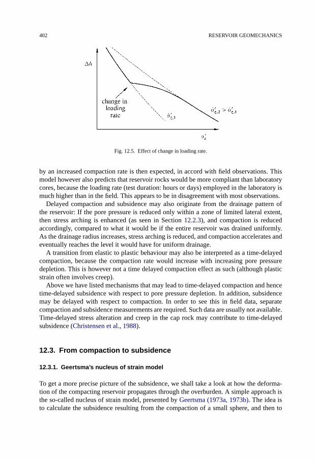
402 RESERVOIR GEOMECHANICS
Fig. 12.5. Effect of change in loading rate.
by an increased compaction rate is then expected, in accord with field observations. Thismodel however also predicts that reservoir rocks would be more compliant than laboratorycores, because the loading rate (test duration: hours or days) employed in the laboratory ismuch higher than in the field. This appears to be in disagreement with most observations.
Delayed compaction and subsidence may also originate from the drainage pattern ofthe reservoir: If the pore pressure is reduced only within a zone of limited lateral extent,then stress arching is enhanced (as seen in Section 12.2.3), and compaction is reducedaccordingly, compared to what it would be if the entire reservoir was drained uniformly.As the drainage radius increases, stress arching is reduced, and compaction accelerates andeventually reaches the level it would have for uniform drainage.
A transition from elastic to plastic behaviour may also be interpreted as a time-delayedcompaction, because the compaction rate would increase with increasing pore pressuredepletion. This is however not a time delayed compaction effect as such (although plasticstrain often involves creep).
Above we have listed mechanisms that may lead to time-delayed compaction and hencetime-delayed subsidence with respect to pore pressure depletion. In addition, subsidencemay be delayed with respect to compaction. In order to see this in field data, separatecompaction and subsidence measurements are required. Such data are usually not available.Time-delayed stress alteration and creep in the cap rock may contribute to time-delayedsubsidence (Christensen et al., 1988).
12.3. From compaction to subsidence
12.3.1. Geertsma’s nucleus of strain model
To get a more precise picture of the subsidence, we shall take a look at how the deforma-tion of the compacting reservoir propagates through the overburden. A simple approach isthe so-called nucleus of strain model, presented by Geertsma (1973a, 1973b). The idea isto calculate the subsidence resulting from the compaction of a small sphere, and then to

FROM COMPACTION TO SUBSIDENCE 403
calculate the total subsidence by adding the influence of many such spheres, assuming thatsuperposition is allowable.
Geertsma’s model is limited to the case where there is no contrast in elastic propertiesbetween the reservoir and the surroundings.
Considering the region outside the depleting sphere (of radius R0), and denoting theradial displacement at the surface of the depleting sphere by u0, the radial displacement ata distance r from the centre of the sphere is (see Eq. (12.11))
u(r) = u0R2
0
r2(12.35)
u0 may be related to the volume change of the depleted region by (remember the signconvention, displacements point in the opposite direction of the coordinate axes, see e.g.Fig. 4.1)
�V = −4πR20u0 (12.36)
Combined with Eq. (12.31) and the definition of volumetric strain, Eq. (1.76), this gives
u0 = −CmV α�pf
4πR20
(12.37)
and hence
u(r) = −Cm
4πV α�pf
1
r2(12.38)
which describes the displacement field outside a depleting sphere in an infinite medium.Note that the magnitude of the displacement field is governed by the product V�pf. This
means that we get the same displacement field outside R0 for a sphere of half the volume ifpf is doubled. This is similar to gravitation theory, in which we get the same gravitationalfield outside the Earth if we assume all the mass to be situated at the centre of the Earth.
This principle is, as we shall see, important for the Geertsma theory.
The effect of the free surface
Eq. (12.38) has one major shortcoming—it does not take the surface properly into account.At the surface, the vertical stress must be zero. This problem was solved by Geertsma,who used known solutions from thermoelasticity (Mindlin and Cheng, 1950a, 1950b; Sen,1951) to arrive at the corrected expression:
�u = Cm
4π
( �R1
R31
+ (3 − 4ν)�R2
R32
− 6z(z+D) �R2
R52
+ 2z
R32
[(3 − 4ν)(z+D)− z])V α�pf (12.39)
The geometry and the symbols are defined in Fig. 12.6. The first term is recognizedas that developed in Eq. (12.38), while the remaining terms are correction terms ensuring
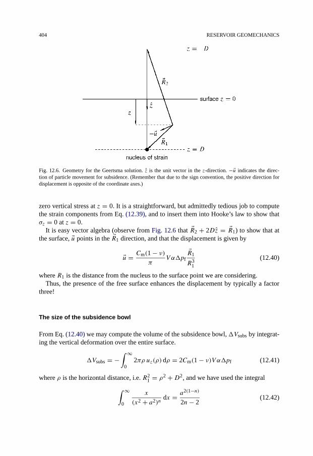
404 RESERVOIR GEOMECHANICS
Fig. 12.6. Geometry for the Geertsma solution. z is the unit vector in the z-direction. −�u indicates the direc-tion of particle movement for subsidence. (Remember that due to the sign convention, the positive direction fordisplacement is opposite of the coordinate axes.)
zero vertical stress at z = 0. It is a straightforward, but admittedly tedious job to computethe strain components from Eq. (12.39), and to insert them into Hooke’s law to show thatσz = 0 at z = 0.
It is easy vector algebra (observe from Fig. 12.6 that �R2 + 2Dz = �R1) to show that atthe surface, �u points in the �R1 direction, and that the displacement is given by
�u = Cm(1 − ν)π
V α�pf
�R1
R31
(12.40)
where R1 is the distance from the nucleus to the surface point we are considering.Thus, the presence of the free surface enhances the displacement by typically a factor
three!
The size of the subsidence bowl
From Eq. (12.40) we may compute the volume of the subsidence bowl,�Vsubs by integrat-ing the vertical deformation over the entire surface.
�Vsubs = −∫ ∞
02πρ uz(ρ) dρ = 2Cm(1 − ν)V α�pf (12.41)
where ρ is the horizontal distance, i.e. R21 = ρ2 +D2, and we have used the integral
∫ ∞
0
x
(x2 + a2)ndx = a2(1−n)
2n− 2(12.42)

FROM COMPACTION TO SUBSIDENCE 405
Eq. (12.41) shows that the volume of the subsidence bowl is related to the volume re-duction of the compacting reservoir (�Vcomp) by
�Vsubs = 2(1 − ν)�Vcomp (12.43)
As an example, for ν = 0.25, the volume of the subsidence bowl is 50% larger than thevolumetric reservoir compaction.
Since the subsidence for an arbitrary shaped reservoir is found by integrating the resultfrom many nuclei, it is clear that this ratio is generally valid (within the assumptions of themodel, i.e. elastic deformation and no contrast between the reservoir and the surroundings).
Subsidence above a disk shaped reservoir
Given Eq. (12.40) it is in principle straightforward to compute the subsidence for an arbi-trarily shaped reservoir by numerical methods. This is however of limited interest, sincethe method is based on constant elastic properties. When one turns to numerical modelling,one should also include a more realistic model of the surrounding formations including thelayers below the reservoir.
There exist, however, analytical solutions for a disk-shaped reservoir which give a gen-eral insight into the subsidence problem, which is useful even though the method is notsuited for precise calculations.
We shall first consider the vertical displacement along the centre line through a disk-shaped reservoir. From Eq. (12.39) we extract the vertical component of the displacement,and integrate over the reservoir. In our calculations, we use a set of strain nuclei situated atz = D, and multiply by the reservoir height h to get the final result. The integrals involvedare similar to Eq. (12.42), and the final result is
uz = −1
2Cmhα�pf
(3 − 4ν + D − z
|D − z| − D − z√R2 + (D − z)2
− (D + z)(3 − 4ν)√R2 + (D + z)2 + 2R2z
(R2 + (D + z)2)3/2)
(12.44)
The surface subsidence at the centre is found by letting z = 0, and is thus
uz = w = 2Cmhα�pf(1 − ν)(
1 − D√D2 + R2
)(12.45)
An important question to resolve is how much error we introduce by assuming the com-paction to be localized at z = D. We remember from the discussion following Eq. (12.38)that for a sphere, we may assume all compaction to take place at the centre, and still getthe correct answer outside the reservoir. Thus, if we modelled a reservoir consisting of adistribution of spheres, we would get correct answer. Now, since a disk can not be fully ap-proximated by spheres, we expect some deviation, but it might seem reasonable to expectthat it will be small.
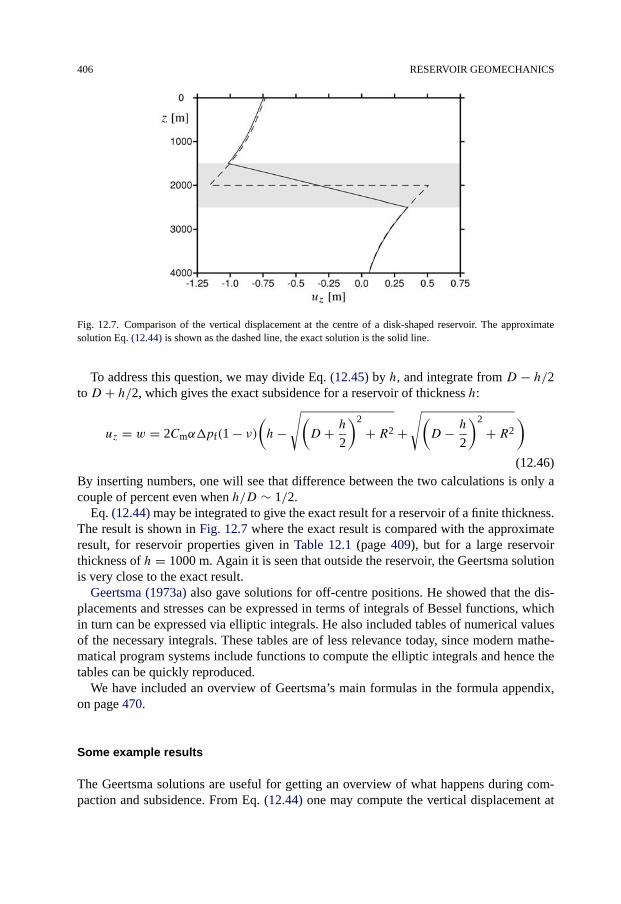
406 RESERVOIR GEOMECHANICS
Fig. 12.7. Comparison of the vertical displacement at the centre of a disk-shaped reservoir. The approximatesolution Eq. (12.44) is shown as the dashed line, the exact solution is the solid line.
To address this question, we may divide Eq. (12.45) by h, and integrate from D − h/2to D + h/2, which gives the exact subsidence for a reservoir of thickness h:
uz = w = 2Cmα�pf(1 − ν)(h−
√(D + h
2
)2
+ R2 +√(D − h
2
)2
+ R2
)(12.46)
By inserting numbers, one will see that difference between the two calculations is only acouple of percent even when h/D ∼ 1/2.
Eq. (12.44) may be integrated to give the exact result for a reservoir of a finite thickness.The result is shown in Fig. 12.7 where the exact result is compared with the approximateresult, for reservoir properties given in Table 12.1 (page 409), but for a large reservoirthickness of h = 1000 m. Again it is seen that outside the reservoir, the Geertsma solutionis very close to the exact result.
Geertsma (1973a) also gave solutions for off-centre positions. He showed that the dis-placements and stresses can be expressed in terms of integrals of Bessel functions, whichin turn can be expressed via elliptic integrals. He also included tables of numerical valuesof the necessary integrals. These tables are of less relevance today, since modern mathe-matical program systems include functions to compute the elliptic integrals and hence thetables can be quickly reproduced.
We have included an overview of Geertsma’s main formulas in the formula appendix,on page 470.
Some example results
The Geertsma solutions are useful for getting an overview of what happens during com-paction and subsidence. From Eq. (12.44) one may compute the vertical displacement at
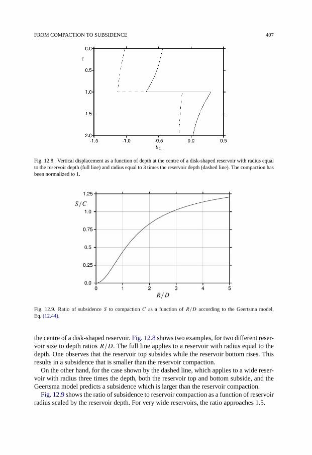
FROM COMPACTION TO SUBSIDENCE 407
Fig. 12.8. Vertical displacement as a function of depth at the centre of a disk-shaped reservoir with radius equalto the reservoir depth (full line) and radius equal to 3 times the reservoir depth (dashed line). The compaction hasbeen normalized to 1.
Fig. 12.9. Ratio of subsidence S to compaction C as a function of R/D according to the Geertsma model,Eq. (12.44).
the centre of a disk-shaped reservoir. Fig. 12.8 shows two examples, for two different reser-voir size to depth ratios R/D. The full line applies to a reservoir with radius equal to thedepth. One observes that the reservoir top subsides while the reservoir bottom rises. Thisresults in a subsidence that is smaller than the reservoir compaction.
On the other hand, for the case shown by the dashed line, which applies to a wide reser-voir with radius three times the depth, both the reservoir top and bottom subside, and theGeertsma model predicts a subsidence which is larger than the reservoir compaction.
Fig. 12.9 shows the ratio of subsidence to reservoir compaction as a function of reservoirradius scaled by the reservoir depth. For very wide reservoirs, the ratio approaches 1.5.
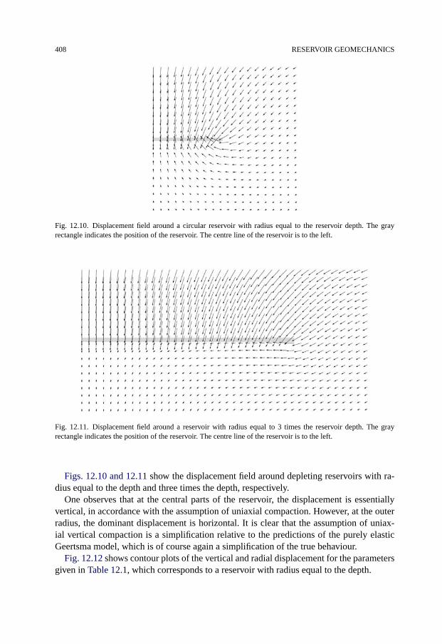
408 RESERVOIR GEOMECHANICS
Fig. 12.10. Displacement field around a circular reservoir with radius equal to the reservoir depth. The grayrectangle indicates the position of the reservoir. The centre line of the reservoir is to the left.
Fig. 12.11. Displacement field around a reservoir with radius equal to 3 times the reservoir depth. The grayrectangle indicates the position of the reservoir. The centre line of the reservoir is to the left.
Figs. 12.10 and 12.11 show the displacement field around depleting reservoirs with ra-dius equal to the depth and three times the depth, respectively.
One observes that at the central parts of the reservoir, the displacement is essentiallyvertical, in accordance with the assumption of uniaxial compaction. However, at the outerradius, the dominant displacement is horizontal. It is clear that the assumption of uniax-ial vertical compaction is a simplification relative to the predictions of the purely elasticGeertsma model, which is of course again a simplification of the true behaviour.
Fig. 12.12 shows contour plots of the vertical and radial displacement for the parametersgiven in Table 12.1, which corresponds to a reservoir with radius equal to the depth.
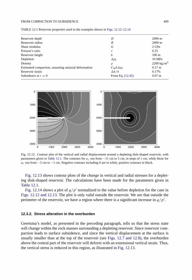
FROM COMPACTION TO SUBSIDENCE 409
TABLE 12.1 Reservoir properties used in the examples shown in Figs. 12.12–12.14
Reservoir depth D 2000 mReservoir radius R 2000 mShear modulus G 2 GPaPoisson’s ratio ν 0.25Reservoir height h 100 mDepletion �pf 10 MPaDensity ρ 2200 kg/m3
Estimated compaction, assuming uniaxial deformation Cmh�pf 0.17 mReservoir strain �h/h 0.17%Subsidence at r = 0 From Eq. (12.45) 0.07 m
Fig. 12.12. Contour plot of the vertical and radial displacement around a depleting disk-shaped reservoir, withparameters given in Table 12.1. The contours for uz run from −11 cm to 5 cm, in steps of 1 cm, while those forur run from −5 cm to −1 cm. Negative contours including 0 are in white, positive contours in black.
Fig. 12.13 shows contour plots of the change in vertical and radial stresses for a deplet-ing disk-shaped reservoir. The calculations have been made for the parameters given inTable 12.1.
Fig. 12.14 shows a plot of q/p′ normalized to the value before depletion for the case inFigs. 12.12 and 12.13. The plot is only valid outside the reservoir. We see that outside theperimeter of the reservoir, we have a region where there is a significant increase in q/p′.
12.3.2. Stress alteration in the overburden
Geertsma’s model, as presented in the preceding paragraph, tells us that the stress statewill change within the rock masses surrounding a depleting reservoir. Since reservoir com-paction leads to surface subsidence, and since the vertical displacement at the surface isusually smaller than at the top of the reservoir (see Figs. 12.7 and 12.8), the overburdenabove the central part of the reservoir will deform with an extensional vertical strain. Thus,the vertical stress is reduced in this region, as illustrated in Fig. 12.13.
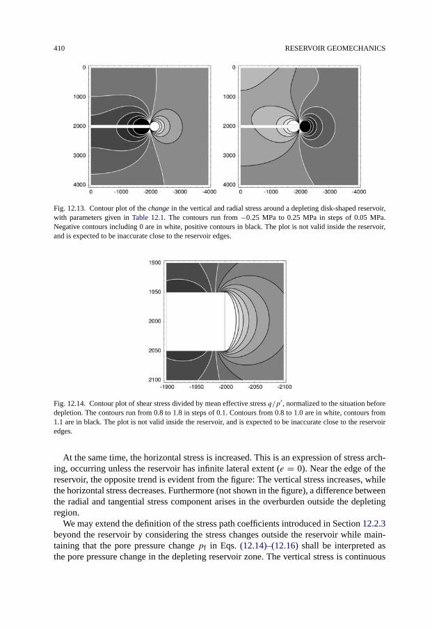
410 RESERVOIR GEOMECHANICS
Fig. 12.13. Contour plot of the change in the vertical and radial stress around a depleting disk-shaped reservoir,with parameters given in Table 12.1. The contours run from −0.25 MPa to 0.25 MPa in steps of 0.05 MPa.Negative contours including 0 are in white, positive contours in black. The plot is not valid inside the reservoir,and is expected to be inaccurate close to the reservoir edges.
Fig. 12.14. Contour plot of shear stress divided by mean effective stress q/p′, normalized to the situation beforedepletion. The contours run from 0.8 to 1.8 in steps of 0.1. Contours from 0.8 to 1.0 are in white, contours from1.1 are in black. The plot is not valid inside the reservoir, and is expected to be inaccurate close to the reservoiredges.
At the same time, the horizontal stress is increased. This is an expression of stress arch-ing, occurring unless the reservoir has infinite lateral extent (e = 0). Near the edge of thereservoir, the opposite trend is evident from the figure: The vertical stress increases, whilethe horizontal stress decreases. Furthermore (not shown in the figure), a difference betweenthe radial and tangential stress component arises in the overburden outside the depletingregion.
We may extend the definition of the stress path coefficients introduced in Section 12.2.3beyond the reservoir by considering the stress changes outside the reservoir while main-taining that the pore pressure change pf in Eqs. (12.14)–(12.16) shall be interpreted asthe pore pressure change in the depleting reservoir zone. The vertical stress is continuous
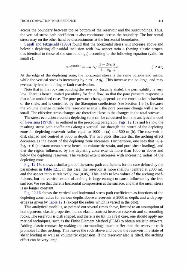
FROM COMPACTION TO SUBSIDENCE 411
across the boundary between top or bottom of the reservoir and the surroundings. Thus,the vertical stress path coefficient is also continuous across the boundary. The horizontalstress may on the other hand be discontinuous at the horizontal boundaries.
Segall and Fitzgerald (1998) found that the horizontal stress will increase above andbelow a depleting ellipsoidal inclusion with low aspect ratio e (having elastic proper-ties identical to those of the surroundings) according to the following equation (valid forsmall e):
�σ exteriorh = −α�pf
1 − 2νfr
1 − νfr
π
4e (12.47)
At the edge of the depleting zone, the horizontal stress is the same outside and inside,while the vertical stress is increasing by ∼α(−�pf). This increase can be large, and mayeventually lead to faulting or fault reactivation.
Note that in the rock surrounding the reservoir (usually shale), the permeability is verylow. There is hence limited possibility for fluid flow, so that the pore pressure response isthat of an undrained case. The pore pressure change depends on the constitutive behaviourof the shale, and is controlled by the Skempton coefficients (see Section 1.6.5). Becausethe volume change outside the reservoir is small, the pore pressure change will also besmall. The effective stress changes are therefore close to the changes in the total stresses.
The stress evolution around a depleting zone can be calculated from the analytical modelof Geertsma (1973b), as outlined in the preceding paragraph. Figs. 12.15a and b show theresulting stress path coefficients along a vertical line through the centre of the depletingzone for depleting reservoir radius equal to 1000 m (a) and 500 m (b). The reservoir isdisk shaped and centred at 3000 m depth. The two plots illustrate that the arching effectdecreases as the extent of the depleting zone increases. Furthermore, one sees that γv +2γh ≈ 0 (constant mean stress; hence no volumetric strain, and pure shear loading), andthat the region influenced by the depleting zone extends more than 1000 m above andbelow the depleting reservoir. The vertical extent increases with increasing radius of thedepleting zone.
Fig. 12.15c shows a similar plot of the stress path coefficients for the case defined by theparameters in Table 12.1. In this case, the reservoir is more shallow (centred at 2000 m),and the aspect ratio is relatively low (0.05). This leads to low values of the arching coef-ficients, but the vertical extent of arching is large enough to cause influence by the freesurface: We see that there is horizontal compression at the surface, and that the mean stressis no longer constant.
Fig. 12.16 shows the vertical and horizontal stress path coefficients as functions of thedepleting zone radius for various depths above a reservoir at 2000 m depth, and with prop-erties as given by Table 12.1 (except the radius which is varied in the plot).
This analytical model is, as pointed out several times above, limited to an assumption ofhomogeneous elastic properties, i.e. no elastic contrast between reservoir and surroundingrocks. The reservoir is disk shaped, and there is no tilt. In a real case, one should apply nu-merical techniques, such as the Finite Element Method (FEM) to obtain realistic answers.Adding elastic contrast by making the surroundings much stiffer than the reservoir rockpromotes further arching. This leaves the rock above and below the reservoir in a state ofshear loading as well as volumetric expansion. If the reservoir also is tilted, the archingeffect can be very large.
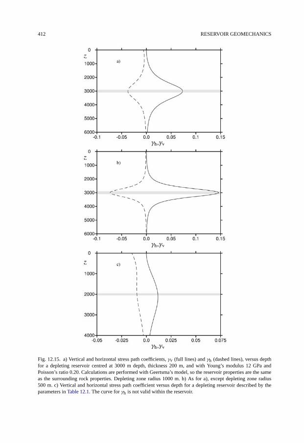
412 RESERVOIR GEOMECHANICS
Fig. 12.15. a) Vertical and horizontal stress path coefficients, γv (full lines) and γh (dashed lines), versus depthfor a depleting reservoir centred at 3000 m depth, thickness 200 m, and with Young’s modulus 12 GPa andPoisson’s ratio 0.20. Calculations are performed with Geertsma’s model, so the reservoir properties are the sameas the surrounding rock properties. Depleting zone radius 1000 m. b) As for a), except depleting zone radius500 m. c) Vertical and horizontal stress path coefficient versus depth for a depleting reservoir described by theparameters in Table 12.1. The curve for γh is not valid within the reservoir.
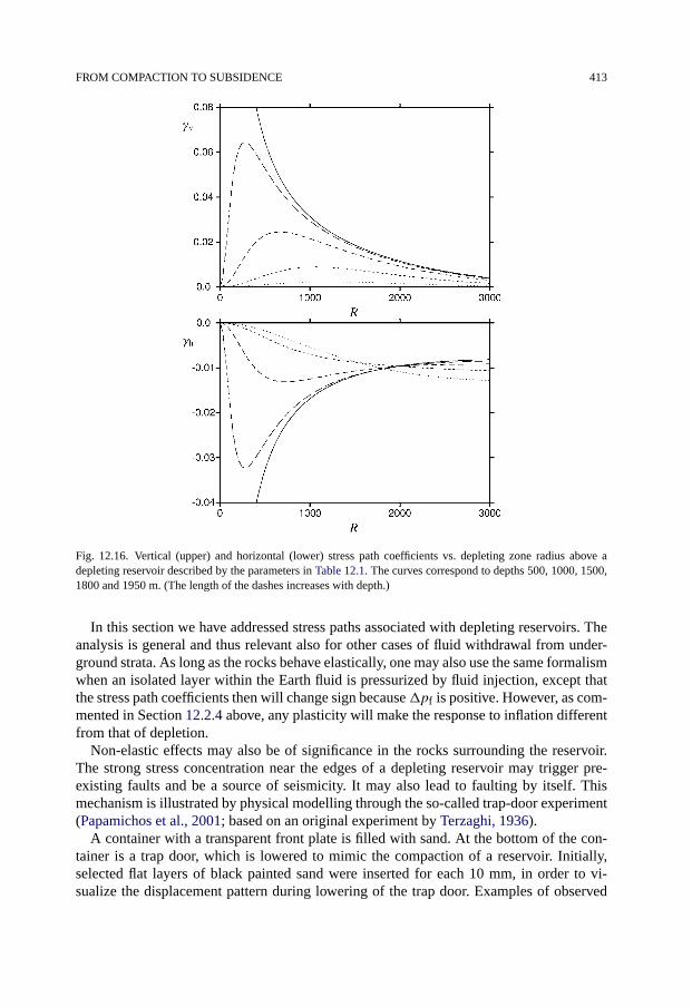
FROM COMPACTION TO SUBSIDENCE 413
Fig. 12.16. Vertical (upper) and horizontal (lower) stress path coefficients vs. depleting zone radius above adepleting reservoir described by the parameters in Table 12.1. The curves correspond to depths 500, 1000, 1500,1800 and 1950 m. (The length of the dashes increases with depth.)
In this section we have addressed stress paths associated with depleting reservoirs. Theanalysis is general and thus relevant also for other cases of fluid withdrawal from under-ground strata. As long as the rocks behave elastically, one may also use the same formalismwhen an isolated layer within the Earth fluid is pressurized by fluid injection, except thatthe stress path coefficients then will change sign because�pf is positive. However, as com-mented in Section 12.2.4 above, any plasticity will make the response to inflation differentfrom that of depletion.
Non-elastic effects may also be of significance in the rocks surrounding the reservoir.The strong stress concentration near the edges of a depleting reservoir may trigger pre-existing faults and be a source of seismicity. It may also lead to faulting by itself. Thismechanism is illustrated by physical modelling through the so-called trap-door experiment(Papamichos et al., 2001; based on an original experiment by Terzaghi, 1936).
A container with a transparent front plate is filled with sand. At the bottom of the con-tainer is a trap door, which is lowered to mimic the compaction of a reservoir. Initially,selected flat layers of black painted sand were inserted for each 10 mm, in order to vi-sualize the displacement pattern during lowering of the trap door. Examples of observed
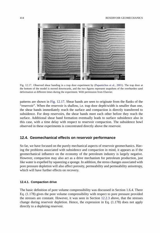
414 RESERVOIR GEOMECHANICS
Fig. 12.17. Observed shear banding in a trap door experiment by (Papamichos et al., 2001). The trap door atthe bottom of the model is moved downwards, and the two figures represent snapshots of the overburden sanddeformation at different times during the experiment. With permission from Elsevier.
patterns are shown in Fig. 12.17. Shear bands are seen to originate from the flanks of the“reservoir”. When the reservoir is shallow, i.e. trap door depth/width is smaller than one,the shear bands immediately reach the surface and compaction is directly transferred tosubsidence. For deep reservoirs, the shear bands meet each other before they reach thesurface. Additional shear band formation eventually leads to surface subsidence also inthis case, with a time delay with respect to reservoir compaction. The subsidence bowlobserved in these experiments is concentrated directly above the reservoir.
12.4. Geomechanical effects on reservoir performance
So far, we have focused on the purely mechanical aspects of reservoir geomechanics. Hav-ing the problems associated with subsidence and compaction in mind, it appears as if thegeomechanical influence on the economy of the petroleum industry is largely negative.However, compaction may also act as a drive mechanism for petroleum production, justlike water is expelled by squeezing a sponge. In addition, the stress changes associated withpore pressure depletion will also affect porosity, permeability and permeability anisotropy,which will have further effects on recovery.
12.4.1. Compaction drive
The basic definition of pore volume compressibility was discussed in Section 1.6.4. ThereEq. (1.178) gives the pore volume compressibility with respect to pore pressure providedthe stresses are constant. However, it was seen in Section 12.2.3 above, that the stresseschange during reservoir depletion. Hence, the expression in Eq. (1.178) does not applydirectly to a depleting reservoir.
GEOMECHANICAL EFFECTS ON RESERVOIR PERFORMANCE 415
To find the appropriate pore volume compressibility, we must take into account how σpin Eq. (1.176) depends on the pore pressure pf.
From the basic definitions of the stress path parameters, Eqs. (12.14)–(12.16) we have(assuming γh = γH)
�σp = 1
3(γv + 2γh)�pf = γ �pf (12.48)
where γ = (γv + 2γh)/3.Entering this expression into Eq. (1.176) we find the pore volume compressibility Cγpp
for a given stress path as
Cγpp = 1
Vp
�Vp
�pf= 1 − γ
φ
(1
Kfr− 1
Ks
)− 1
Ks(12.49)
From the discussion leading to Eq. (12.29), it is clear that for an ellipsoidal reservoir wehave
γ = 2
3
1 − 2νfr
1 − νfrα (12.50)
independent of the ellipticity, as long as there is no elastic contrast between the reservoirand its surroundings. Thus, in this case, which includes the uniaxial compaction case, wehave (Zimmerman, 2000b):
Cγpp = 1 + νfr
3(1 − νfr)
α
φ
1
Kfr+[
2(1 − 2νfr)α
3(1 − νfr)φ− 1
]1
Ks(12.51)
If we may assume Kfr � Ks the equation simplifies to
Cγpp = 1 + νfr
3(1 − νfr)φKfr= Cm
φ(12.52)
which is a frequently used approximation.As a result of a pore pressure decrease the produced fluid volume (at reservoir condi-
tions) is:
�Vprod = −Vp(Cf + Cγpp)�pf (12.53)
The compressibility of the pore fluid is denoted by Cf, and is the inverse of the bulk mod-ulus (Cf = 1/Kf).
This illustrates that in particular for a soft rock which has low stiffness and therefore highpore compressibility, production will be enhanced by compaction of the pores. This is whatwe call compaction drive. In case of high stiffness (low compressibility), the productiondrive will be dominated by the pore fluid compressibility.
As an example, if the pore fluid is oil with bulk modulus of 1 GPa, and the rock is softwith bulk modulus ∼1 GPa, porosity ∼25%, and Poisson’s ratio ∼0.30, the compactionterm in Eq. (12.53) contributes about 2.5 times as much as the fluid compressibility to the
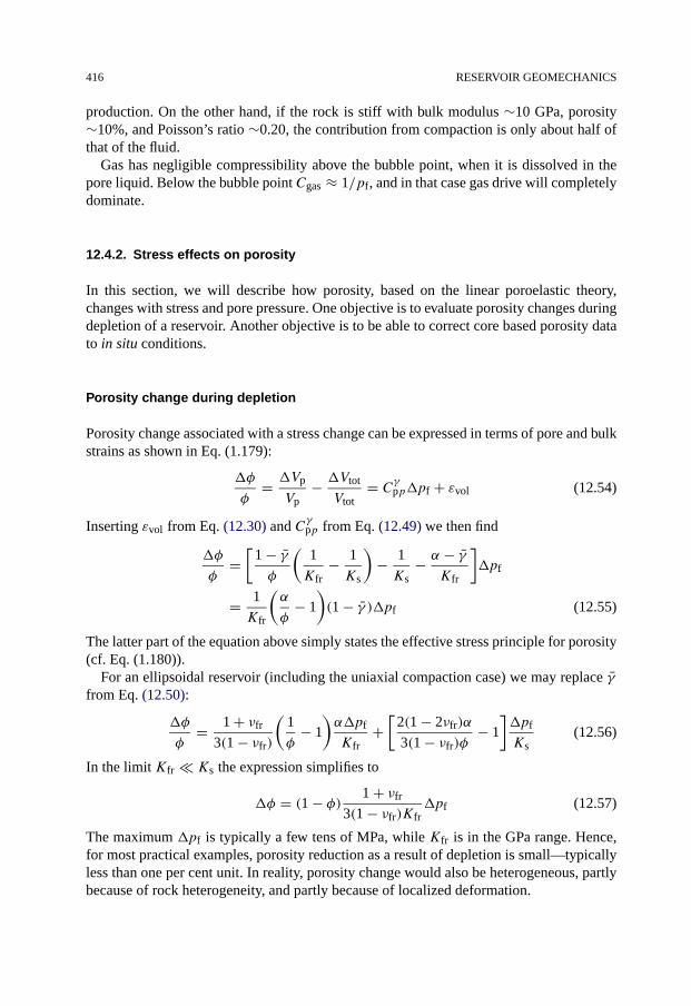
416 RESERVOIR GEOMECHANICS
production. On the other hand, if the rock is stiff with bulk modulus ∼10 GPa, porosity∼10%, and Poisson’s ratio ∼0.20, the contribution from compaction is only about half ofthat of the fluid.
Gas has negligible compressibility above the bubble point, when it is dissolved in thepore liquid. Below the bubble point Cgas ≈ 1/pf, and in that case gas drive will completelydominate.
12.4.2. Stress effects on porosity
In this section, we will describe how porosity, based on the linear poroelastic theory,changes with stress and pore pressure. One objective is to evaluate porosity changes duringdepletion of a reservoir. Another objective is to be able to correct core based porosity datato in situ conditions.
Porosity change during depletion
Porosity change associated with a stress change can be expressed in terms of pore and bulkstrains as shown in Eq. (1.179):
�φ
φ= �Vp
Vp− �Vtot
Vtot= Cγpp�pf + εvol (12.54)
Inserting εvol from Eq. (12.30) and Cγpp from Eq. (12.49) we then find
�φ
φ=[
1 − γφ
(1
Kfr− 1
Ks
)− 1
Ks− α − γ
Kfr
]�pf
= 1
Kfr
(α
φ− 1
)(1 − γ )�pf (12.55)
The latter part of the equation above simply states the effective stress principle for porosity(cf. Eq. (1.180)).
For an ellipsoidal reservoir (including the uniaxial compaction case) we may replace γfrom Eq. (12.50):
�φ
φ= 1 + νfr
3(1 − νfr)
(1
φ− 1
)α�pf
Kfr+[
2(1 − 2νfr)α
3(1 − νfr)φ− 1
]�pf
Ks(12.56)
In the limit Kfr � Ks the expression simplifies to
�φ = (1 − φ) 1 + νfr
3(1 − νfr)Kfr�pf (12.57)
The maximum �pf is typically a few tens of MPa, while Kfr is in the GPa range. Hence,for most practical examples, porosity reduction as a result of depletion is small—typicallyless than one per cent unit. In reality, porosity change would also be heterogeneous, partlybecause of rock heterogeneity, and partly because of localized deformation.
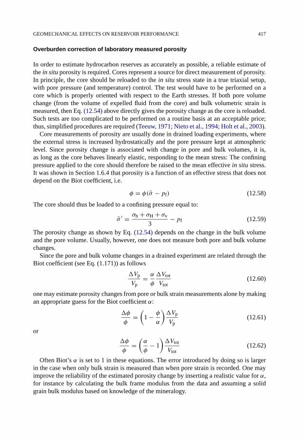
GEOMECHANICAL EFFECTS ON RESERVOIR PERFORMANCE 417
Overburden correction of laboratory measured porosity
In order to estimate hydrocarbon reserves as accurately as possible, a reliable estimate ofthe in situ porosity is required. Cores represent a source for direct measurement of porosity.In principle, the core should be reloaded to the in situ stress state in a true triaxial setup,with pore pressure (and temperature) control. The test would have to be performed on acore which is properly oriented with respect to the Earth stresses. If both pore volumechange (from the volume of expelled fluid from the core) and bulk volumetric strain ismeasured, then Eq. (12.54) above directly gives the porosity change as the core is reloaded.Such tests are too complicated to be performed on a routine basis at an acceptable price;thus, simplified procedures are required (Teeuw, 1971; Nieto et al., 1994; Holt et al., 2003).
Core measurements of porosity are usually done in drained loading experiments, wherethe external stress is increased hydrostatically and the pore pressure kept at atmosphericlevel. Since porosity change is associated with change in pore and bulk volumes, it is,as long as the core behaves linearly elastic, responding to the mean stress: The confiningpressure applied to the core should therefore be raised to the mean effective in situ stress.It was shown in Section 1.6.4 that porosity is a function of an effective stress that does notdepend on the Biot coefficient, i.e.
φ = φ(σ − pf) (12.58)
The core should thus be loaded to a confining pressure equal to:
σ ′ = σh + σH + σv
3− pf (12.59)
The porosity change as shown by Eq. (12.54) depends on the change in the bulk volumeand the pore volume. Usually, however, one does not measure both pore and bulk volumechanges.
Since the pore and bulk volume changes in a drained experiment are related through theBiot coefficient (see Eq. (1.171)) as follows
�Vp
Vp= α
φ
�Vtot
Vtot(12.60)
one may estimate porosity changes from pore or bulk strain measurements alone by makingan appropriate guess for the Biot coefficient α:
�φ
φ=(
1 − φ
α
)�Vp
Vp(12.61)
or
�φ
φ=(α
φ− 1
)�Vtot
Vtot(12.62)
Often Biot’s α is set to 1 in these equations. The error introduced by doing so is largerin the case when only bulk strain is measured than when pore strain is recorded. One mayimprove the reliability of the estimated porosity change by inserting a realistic value for α,for instance by calculating the bulk frame modulus from the data and assuming a solidgrain bulk modulus based on knowledge of the mineralogy.
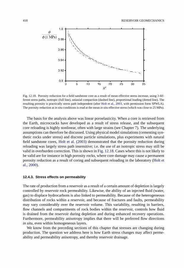
418 RESERVOIR GEOMECHANICS
Fig. 12.18. Porosity reduction for a field sandstone core as a result of mean effective stress increase, using 3 dif-ferent stress paths, isotropic (full line), uniaxial compaction (dashed line), proportional loading (dotted line). Theresulting porosity is practically stress path independent (after Holt et al., 2003, with permission form SPWLA).The porosity reduction at in situ conditions is read at the mean in situ effective stress (which was close to 25 MPa).
The basis for the analysis above was linear poroelasticity. When a core is retrieved fromthe Earth, microcracks have developed as a result of stress release, and the subsequentcore reloading is highly nonlinear, often with large strains (see Chapter 7). The underlyingassumptions can therefore be discussed. Using physical model simulations (cementing syn-thetic rocks under stress) and discrete particle simulations, plus experiments with naturalfield sandstone cores, Holt et al. (2003) demonstrated that the porosity reduction duringreloading was largely stress path insensitive; i.e. the use of an isotropic stress may still bevalid in overburden correction. This is shown in Fig. 12.18. Cases where this is not likely tobe valid are for instance in high porosity rocks, where core damage may cause a permanentporosity reduction as a result of coring and subsequent reloading in the laboratory (Holt etal., 2000).
12.4.3. Stress effects on permeability
The rate of production from a reservoir as a result of a certain amount of depletion is largelycontrolled by reservoir rock permeability. Likewise, the ability of an injected fluid (water,gas) to displace hydrocarbons is also linked to permeability. Because of the heterogeneousdistribution of rocks within a reservoir, and because of fractures and faults, permeabilitymay vary considerably over the reservoir volume. This variability, resulting in barriers,flow channels and compartments of rock bodies within the reservoir, controls how fluidis drained from the reservoir during depletion and during enhanced recovery operations.Furthermore, permeability anisotropy implies that there will be preferred flow directionsin situ, even within homogeneous layers.
We know from the preceding sections of this chapter that stresses are changing duringproduction. The question we address here is how Earth stress changes may affect perme-ability and permeability anisotropy, and thereby reservoir drainage.

GEOMECHANICAL EFFECTS ON RESERVOIR PERFORMANCE 419
Flood directionality in the field
An extensive study of well test data was performed by Heffer and Dowokpor (1990) andHeffer et al. (1994). They showed (as can be seen in Fig. 12.19) that the preferred horizontalflow direction, seen from well tests in a majority of fractured as well as non-fracturedreservoirs, is parallel to the maximum in situ horizontal stress. This implies that stressanisotropy leads to permeability anisotropy. The relevance of this to reservoir engineeringcan be illustrated by considering water injection from a vertical well: If the producingwell is placed in the direction of maximum permeability, early water-breakthrough andlow recovery would be the result. The injector must hence be placed with respect to theproducer by careful consideration of the in situ stress field. Thus; identification of principalin situ stress directions may be of importance for the reservoir drainage strategy.
Permeability changes under isotropic stress conditions
Experimentally one finds that permeability is reduced with increasing isotropic stress. Therelative reduction of permeability is generally larger in low permeability and low porosityrocks, where permeability is mainly due to cracks or narrow pores which are easily closedby an applied stress, than in high permeability and high porosity rocks. As an example,data on sandstones (Yale, 1984; Kilmer et al., 1987; Holt, 1990; Schutjens et al., 2004)show that for milliDarcy or lower permeabilities, a confining pressure increase of 30 MPamay cause a permeability decrease of 50% or more. For porosities above 15–20% andpermeabilities above 1 milliDarcy, the permeability reduction caused by a similar stressincrease is usually of the order 20% or less.
From a microscopic viewpoint, permeability is controlled by the following parameters:
• porosity (φ),
• pore size/grain size (and size distribution),
• pore shape/grain shape,
• tortuosity (T ).
The Kozeny–Carman equation (see e.g. Dullien, 1992) is based on a simple networkmodel, where the pores are considered as pipes:
k = d2g
κ0T 2
φ3
(1 − φ)2 (12.63)
Here dg is the grain diameter (assuming spherical grains), and κ0 is a modifying factorintroduced to account for realistic pore shapes. When stress is increased, as long as therock remains elastic, the main factor changing in the equation above is the porosity. Thisis illustrated in Fig. 12.20, where measured permeability change during hydrostatic load-ing of a sandstone core (24% porosity) from 4 to 35 MPa is compared to permeabilitychange predicted from the Eq. (12.63) above, using strain recordings during the test tocalculate porosity changes according to the theory presented in the preceding section. Inthis case a convincing agreement was obtained. Flornes (2005) found from hydrostatic

420 RESERVOIR GEOMECHANICS
Fig. 12.19. Preferred flow directions with respect to in situ stress directions in 80 petroleum reservoirs worldwide (top), in the subset of non-fractured reservoirs (middle) and in naturally fractured reservoirs (bottom). FromHeffer et al. (1994). With kind permission of Springer Science and Business Media.
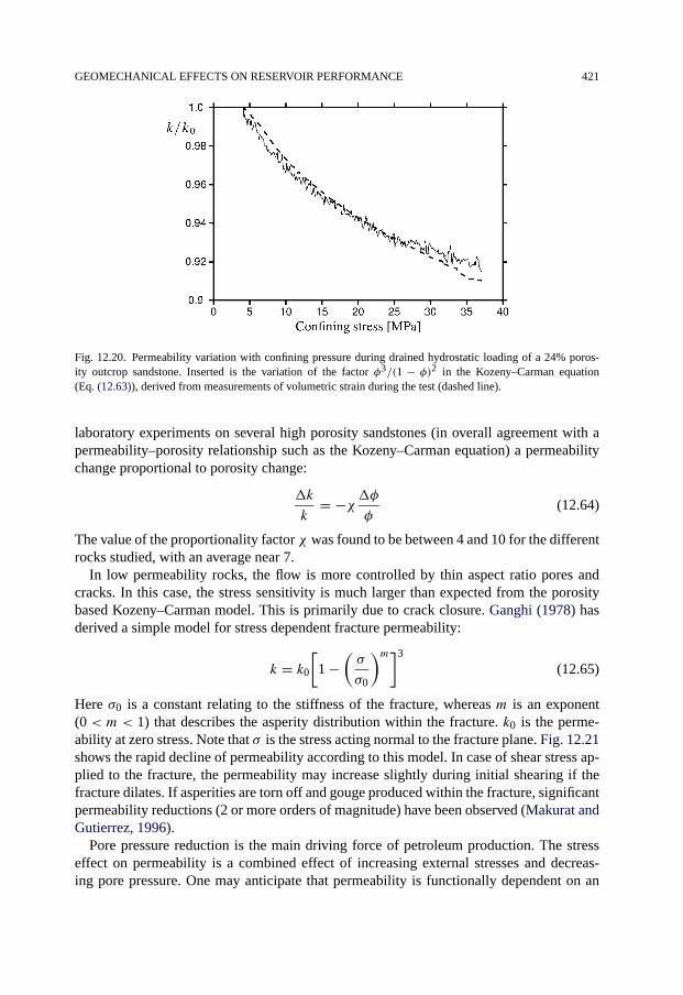
GEOMECHANICAL EFFECTS ON RESERVOIR PERFORMANCE 421
Fig. 12.20. Permeability variation with confining pressure during drained hydrostatic loading of a 24% poros-ity outcrop sandstone. Inserted is the variation of the factor φ3/(1 − φ)2 in the Kozeny–Carman equation(Eq. (12.63)), derived from measurements of volumetric strain during the test (dashed line).
laboratory experiments on several high porosity sandstones (in overall agreement with apermeability–porosity relationship such as the Kozeny–Carman equation) a permeabilitychange proportional to porosity change:
�k
k= −χ �φ
φ(12.64)
The value of the proportionality factor χ was found to be between 4 and 10 for the differentrocks studied, with an average near 7.
In low permeability rocks, the flow is more controlled by thin aspect ratio pores andcracks. In this case, the stress sensitivity is much larger than expected from the porositybased Kozeny–Carman model. This is primarily due to crack closure. Ganghi (1978) hasderived a simple model for stress dependent fracture permeability:
k = k0
[1 −
(σ
σ0
)m]3
(12.65)
Here σ0 is a constant relating to the stiffness of the fracture, whereas m is an exponent(0 < m < 1) that describes the asperity distribution within the fracture. k0 is the perme-ability at zero stress. Note that σ is the stress acting normal to the fracture plane. Fig. 12.21shows the rapid decline of permeability according to this model. In case of shear stress ap-plied to the fracture, the permeability may increase slightly during initial shearing if thefracture dilates. If asperities are torn off and gouge produced within the fracture, significantpermeability reductions (2 or more orders of magnitude) have been observed (Makurat andGutierrez, 1996).
Pore pressure reduction is the main driving force of petroleum production. The stresseffect on permeability is a combined effect of increasing external stresses and decreas-ing pore pressure. One may anticipate that permeability is functionally dependent on an
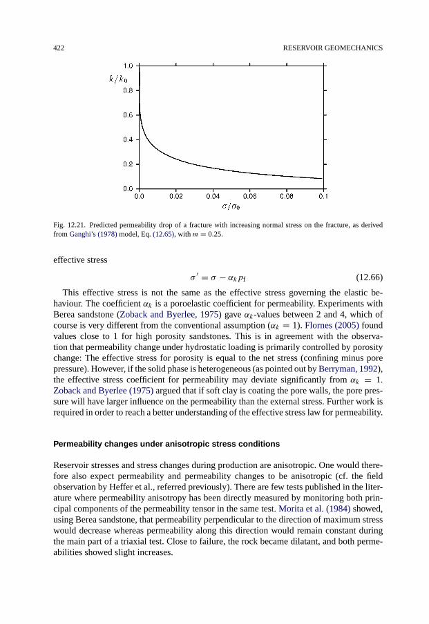
422 RESERVOIR GEOMECHANICS
Fig. 12.21. Predicted permeability drop of a fracture with increasing normal stress on the fracture, as derivedfrom Ganghi’s (1978) model, Eq. (12.65), with m = 0.25.
effective stress
σ ′ = σ − αkpf (12.66)
This effective stress is not the same as the effective stress governing the elastic be-haviour. The coefficient αk is a poroelastic coefficient for permeability. Experiments withBerea sandstone (Zoback and Byerlee, 1975) gave αk-values between 2 and 4, which ofcourse is very different from the conventional assumption (αk = 1). Flornes (2005) foundvalues close to 1 for high porosity sandstones. This is in agreement with the observa-tion that permeability change under hydrostatic loading is primarily controlled by porositychange: The effective stress for porosity is equal to the net stress (confining minus porepressure). However, if the solid phase is heterogeneous (as pointed out by Berryman, 1992),the effective stress coefficient for permeability may deviate significantly from αk = 1.Zoback and Byerlee (1975) argued that if soft clay is coating the pore walls, the pore pres-sure will have larger influence on the permeability than the external stress. Further work isrequired in order to reach a better understanding of the effective stress law for permeability.
Permeability changes under anisotropic stress conditions
Reservoir stresses and stress changes during production are anisotropic. One would there-fore also expect permeability and permeability changes to be anisotropic (cf. the fieldobservation by Heffer et al., referred previously). There are few tests published in the liter-ature where permeability anisotropy has been directly measured by monitoring both prin-cipal components of the permeability tensor in the same test. Morita et al. (1984) showed,using Berea sandstone, that permeability perpendicular to the direction of maximum stresswould decrease whereas permeability along this direction would remain constant duringthe main part of a triaxial test. Close to failure, the rock became dilatant, and both perme-abilities showed slight increases.

GEOMECHANICAL EFFECTS ON RESERVOIR PERFORMANCE 423
Fig. 12.22. Axial permeability (full line) and axial stress (dotted line) vs. axial strain during a triaxial test witha 24% porosity sandstone at 40 MPa confining pressure. Inserted (dashed line) is the variation of the factorφ3/(1 − φ)2 in the Kozeny–Carman equation (Eq. (12.63)), derived from measurements of volumetric strainduring the test (dashed line).
Khan and Teufel (2000) performed experiments where permeability along the core axiswas measured in comparative triaxial compression and extension tests performed on a low(12%) porosity and low (0.1 milliDarcy) permeability sandstone, applying different stresspaths. They conclude that for decreasing stress path coefficient κ (increasing γh), the per-meability anisotropy is increasing. The permeability was always higher in the directionalong the maximum principal stress. Whereas in hydrostatic tests, the permeability evolu-tion was essentially isotropic, the ratio between the maximum and minimum permeabilitywas close to 3 when κ = 0 (uniaxial load increase). The permeability along the maximumprincipal stress was seen (like in the tests of Morita et al.) to increase towards the end ofthe applied loading as a result of dilatancy.
There is evidence from borehole measurements in highly fractured and faulted crys-talline rocks that indicate that the permeability of critically stressed faults can be muchhigher than that of faults being far from failure (Barton et al., 1995).
On the other hand, there are several observations in the literature that permeability dropsduring rock yielding and failure (Holt, 1990; Bruno, 1994; Sarda et al., 1998). This is mostoften seen in high porosity and high permeability materials, and at relatively high confiningpressures. Fig. 12.22 shows an example, where a triaxial test was performed with the same(24% porosity) sandstone used for isotropic loading as shown in Fig. 12.20 at a confiningpressure of 40 MPa. Again the permeability evolution correlates extremely well with theporosity change as determined from the volumetric strain, but only until strain localizationtakes place near rock failure. Then the measured permeability starts to drop at a muchhigher rate than before, while the core is actually dilating. This is probably explained bythe formation of a shear band and associated crushing of grains, creating a barrier to fluidflow. A most dramatic example is the observation by Holcomb and Olsson (2003), whodetected a permeability drop of 3–4 orders of magnitude when a Castlegate sandstone coreat very high confinement was strained axially by 10% in a triaxial test. They interpreted
424 RESERVOIR GEOMECHANICS
the permeability drop by the formation and propagation of a horizontal compaction bandcontaining crushed grains.
Boutéca et al. (2000) and Schutjens et al. (2004) both summarize the behaviour of per-meability in stress space by distinguishing between an elastic or near-elastic regime, wherepermeability changes are small, and probably related mainly to porosity change. Then, asshear stress is increased, inelastic deformation takes over gradually, and the rock eventuallyfails. The permeability may then be enhanced or reduced, depending on the stress path, onthe porosity and initial permeability of the rock, and on its constitutive behaviour.
12.4.4. Geomechanics in reservoir simulation
The evolution of reservoir geomechanics calls for an implementation of geomechanicalconcepts into reservoir simulation. There are two fundamentally different ways of per-forming this:
Weakly coupled technique
A conventional reservoir simulator is used to calculate the pore pressure distribution withinthe reservoir. Such a model needs as input within each cell (105–106 cells in a total simula-tion): rock properties (porosity, the 3 components kx , ky and kz of the permeability tensorplus pore compressibility), fluid properties (saturation of oil, gas and water, viscosities anddensities for the 3 fluid components), and combined rock-fluid parameters (relative perme-abilities, capillary pressure curve). In addition, well information must be included. Usuallythe permeability and mechanical properties are thought to be constant over the lifetime ofthe reservoir.
A large-scale geomechanical (usually finite element) model is then used to calculate thestress changes and mechanical compaction and subsidence as a result of the pore pres-sure reductions found by the reservoir simulation. Permeability and pore compressibilitychanges can be calculated if their stress sensitivities are known, and these data can be fedback to the reservoir simulator, which is then updated, etc. One problem here is that ageomechanical model needs to account for the overburden, plus the rock to the sides andunderneath the reservoir. This in practice usually limits the reservoir to be represented by104–105 elements, i.e. on a much coarser grid than in the reservoir simulation above.
Fully coupled simulation
The coupling between stresses and fluid flow goes back to Biot’s poroelastic theory in Sec-tion 1.6. The idea is to use a single set of coupled governing equations that contain both themechanical and the fluid flow aspects. The benefit is that a fully coupled approach is likelyto be more correct. The problem is that such a simulator is computationally more compli-cated and hence more time-consuming. One should also have in mind that the existing Biottheory might need modification to account correctly for multi-phase fluid saturation andflow.
GEOMECHANICAL EFFECTS ON RESERVOIR PERFORMANCE 425
More detailed descriptions of such models and their development can be found in e.g.Lewis and Schrefler (1998), Osorio et al. (1998), Koutsabeloulis et al. (1994), Gutierrezand Lewis (1998), Settari and Walters (1999), and Stone et al. (2001).
12.4.5. Seismic reservoir monitoring
Seismic reservoir monitoring (time-lapse, or “4D”-seismics) has become a powerful toolto monitor reservoir performance. Results of repeated seismic surveys are compared, anddifferences over time indicate the presence of dynamic processes in the subsurface. Suchalterations may be observed as changes in two-way travel time or as a change in a reflectiv-ity of a certain reflector (e.g. at bottom and/or top of the reservoir). Travel time is associatedwith seismic wave velocities (vp, vs), whereas seismic reflectivity (see Section 5.7) is re-lated to contrast in acoustic impedance (ρvp, ρvs).
The most important sources of observable time lapse effects associated with producingreservoirs are:
• Fluid substitution; i.e. hydrocarbons have been replaced by water due to drainage, orreplaced by an injected fluid.
• Changes in temperature as a result of a cold (water) or hot (steam) injection front.
• Changes in pore pressure and reservoir stresses.
Fluid substitution
The P-wave velocity of a fluid-saturated isotropic rock is given by the Biot theory. Theresult in the low frequency limit, Eq. (5.39), can be written as
vp =
√√√√√Hfr + Kfφ
α2
1+ KfφKs
(α−φ)ρdry + ρfφ
(12.67)
Pore fluid characteristics affect velocity and hence travel time through the fluid bulkmodulus Kf and the fluid density ρf. If oil is replaced by water, both the plane wave mod-ulus in the numerator and the density in the denominator increase. The net effect is notobvious and depend on the other rock parameters involved, such as the plane wave mod-ulus Hfr of the dry frame and the porosity. Typically, brine has a bulk modulus (Kf) of2.5 GPa, while Kf for live oil is near 0.5 GPa. The densities are approximately 1.0 and0.6 g/cm3, respectively. In general, the fluid substitution effect will be more prominent inhigh than in low porosity rock, because a high porosity rock has a low Hfr, making thefluid contribution to the plane wave modulus more significant. In such a case, the P-wavevelocity of the reservoir layer will increase if oil is replaced by water (see Fig. 5.2).
The effect of fluid substitution on the reflection coefficient (Eq. (5.82)) is larger andmore consistent, because the acoustic impedance depends on the product of the modulus

426 RESERVOIR GEOMECHANICS
and the density, which both are increased as a result of water replacing oil:
Zp = ρvp =√√√√(
Hfr + Kf
φ
α2
1 + KfφKs(α − φ)
)(ρdry + ρfφ) (12.68)
Again the effect of fluid substitution is larger in high-porosity than in low-porosity reservoirrocks.
Changes in temperature
The first published example of successful seismic reservoir monitoring was done in con-nection with a steam injection operation (Nur et al., 1984). In this case, the high tempera-ture of the injection fluid compared to the reservoir rock strongly promoted the observedcontrast. Also, when cold water is injected into a reservoir, thermal effects will influencethe observed response.
The effects of a temperature change are two-fold: It affects rock and fluid properties, andit leads to thermal stresses, which may alter the state of stress underground and thereby, thevelocities. These effects may be large: Water-injection often results in thermally inducedfracturing which is beneficial for the EOR operation. Clearly, such changes will lead toprominent changes in seismic behaviour. In most rocks, velocities are found in laboratoryinvestigations to decrease with increasing temperature; typically 5–10% when the rock isheated from room temperature to around 100 °C. Because oil is more temperature sensitivethan brine, the effect is expected to be larger in oil than water saturated regions.
Changes in pore pressure and reservoir stresses
When a reservoir is depleted, the effective stresses are increased, as outlined in Sec-tion 12.2.3 above. One would expect this to cause an increase in wave velocities in thereservoir zone, since velocities in most rocks are found from laboratory experiments toincrease with increasing effective stress.
There is however a number of indications from 4D field data (The Leading Edge, 2005)that this effect is much smaller than anticipated. One probable reason for this is that reser-voir rock in situ is less stress sensitive than it appears from core measurements, becausecores have been altered as a result of the coring process (Section 7.1.2). Stress releaseleads to existence of microcracks in the unloaded cores. These cracks are closing duringreloading, but crack closure is unlikely to be complete and hence perfect re-establishmentof in situ behaviour can not be expected.
Intuitively, one would anticipate that a well-cemented rock in the Earth is relativelystress insensitive. In situ stress dependence is then mainly associated with pre-existing orevolving cracks or fractures within the reservoir. If the rock is poorly cemented so thata number of grain contacts are not welded, stress-dependence occurs as a result of thenonlinear (Hertzian) behaviour of these grain contacts. Also, a soft reservoir rock under-going large depletion may compact with large porosity reduction, causing wave velocitiesto increase.

WELL PROBLEMS AND RESERVOIR GEOMECHANICS 427
One should also remember that pore pressure itself affects the properties of the saturat-ing fluid independent of stress changes. The bulk modulus of oil is reduced typically with0.01 GPa per MPa pore pressure reduction, while the bulk modulus for brine is reducedslightly less, depending on temperature. This effect counteracts the increase in P-wavevelocity caused by effective stress increase. For a stress insensitive frame, the velocityreduction with reducing pore pressure is in the range 0.1–0.3% per MPa, being more sig-nificant for soft rock than for hard rock, and more significant for high than for low gas tooil ratios (GOR).
As was also seen in Section 12.2.3, the stress evolution as a result of pore pressurechange is anisotropic, and may cause non-elastic behaviour of the reservoir rock andeven fault activation/initiation. This would clearly affect wave velocities, leading to stress-induced anisotropy. If the pore pressure is increased (e.g. as a result of water-injection), theeffective stress is decreasing anisotropically, and non-elastic behaviour may occur for rela-tively modest pore pressure changes: Initiation of microcracking by tensile bond breakagesmay happen and lead to velocity reduction, in accord with field observations (Landrø et al.,2005).
We saw in Section 12.3 that stress changes and strains associated with depletion alsooccur in the rock surrounding the reservoir. For the overburden above the centre of thereservoir the vertical stress is reduced and the horizontal stress increased by stress archingas a result of reservoir depletion. This may lead to a reduction of wave velocity for avertically propagating seismic wave, increasing its two-way travel time, and altering thereflectivity associated with top of the reservoir. The influence zone of stress alteration isthick—in Fig. 12.15 close to 1000 m above the reservoir—which magnifies the effect ontwo way travel time compared to that caused by a similar velocity change in the reservoir.There is significant field evidence that depletion-induced stress changes in the overburdencause observable 4D effects (Hatchell and Bourne, 2005). Field data from Valhall (Barkvedand Kristiansen, 2005) demonstrate increased S-wave splitting associated with the stressconcentration above the edges of the reservoir. Thus, seismic observations of stress-archingcan be used to identify depleting reservoir zones and to distinguish between sealing andnon-sealing faults.
Reservoir monitoring can also be done in a passive mode, by detecting seismicity origi-nating from within the reservoir or in the cap rock immediately above or near the reservoiredge (Maxwell et al., 1998; Kristiansen et al., 2000). This type of monitoring is aimed atinterpreting the compaction and subsidence mechanisms and does not directly give infor-mation about fluid movements. Another technique is to monitor surface deformation witha very high resolution using precision laser levelling. The result is inverted mathematically(e.g. using Geertsma model described above) to find reservoir deformation, and relate it tomechanisms responsible for the deformations seen (e.g. thermal recovery, waste or massivefluid injection) (Dusseault and Rothenburg, 2002).
12.5. Well problems and reservoir geomechanics
There is evidence from field operations world wide that the stability of boreholes drilled orwells being produced are affected by stress changes described in the previous paragraphs.
428 RESERVOIR GEOMECHANICS
For example, as was pointed out in Chapter 9, stable drilling of infill wells may becomedifficult as the producing reservoir zones are depleted. This is related to the strong decreaseof horizontal stress (and hence fracture pressure) in permeable layers, at the same timeas the pore pressure (and hence the collapse pressure) remains unchanged in ultra lowpermeability shale layers within or just above the top of the reservoir. The mud weightwindow eventually closes at a critical amount of pore pressure reduction.
Sand failure is also affected by the changing stress field during depletion, as was dis-cussed in Chapter 10. Onset of shear failure in the perforation cavities or in an openproducing hole is controlled by the rock strength and by the far field effective stress(Eq. (10.8)). The increase in far field effective stress caused by pore pressure reductionenhances the risk of sand production. Pressure maintenance by water injection may re-sult in reduction of formation strength and therefore also lead to increased risk of particleproduction as the reservoir is being produced.
12.5.1. Casing damage
A most significant well problem associated with a compacting reservoir is casing damage.Several examples have been documented in the literature, such as from the Ekofisk Fieldand the Valhall Field, North Sea, and from the Belridge Field and the Wilmington Field,California (Schwall et al., 1996; Kristiansen et al., 2000; Fredrich et al., 1998; Dusseault etal., 2001). Casing damage becomes an operational problem when the casing is deformedor bent (by creation of dog-legs) so much that it prevents workovers and recompletions(Cernocky and Scholibo, 1995). This necessitates costly drilling of a side-track well.
The main mechanisms responsible for casing damage are compressional, shear, tensileand bending deformations (Veeken et al., 1994; Cernocky and Scholibo, 1995; Fredrich etal., 1998; Dusseault et al., 2001). The mechanisms are illustrated in Fig. 12.23.
In a compacting zone, the casing strain in a vertical well is assumed to be equal to theformation strain. This is based on an assumption of no axial slip, and uniform reservoircompaction. If the well is deviated, the casing strain equals the component of formationstrain along the well direction. Thus, a deviated well is preferable to a vertical well in orderto reduce compressive casing damage. The risk of casing buckling is highest in unsupportedintervals, for instance near sand producing perforations where the pressure drawdown isalso most severe, wherever the cement gives poor support, or at connections. Based onanalytical and numerical modelling, Cernocky and Scholibo (1995) found that 0.5–0.75%casing strain may be thought of as an upper limit for an unsupported 10 ft section. Bruno(2002) argued that casing compaction of 1% or less is unlikely to impair casing integrity.
Deformation of the casing cross-section due to non-uniform lateral loading is referredto as “crushing” (Cernocky and Scholibo, 1995). This is mainly a problem in reservoirzones with large depletion, and where the formation is very soft. In their finite elementsimulations, Cernocky and Scholibo) chose a “crushing limit” (i.e. the maximum tolerabledecrease of the inner diameter) of 0.3′′ (7.5 mm), based on field experience. They foundthat a low diameter : thickness ratio of the casing (say 10 or thereabout) is a key to reducecrushing risk in highly compactive sands. If a large diameter : thickness ratio is used (say20 or so), the crushing risk is much higher for a horizontal or deviated well than for avertical one. For a low diameter : thickness ratio, the well angle plays a minor role.
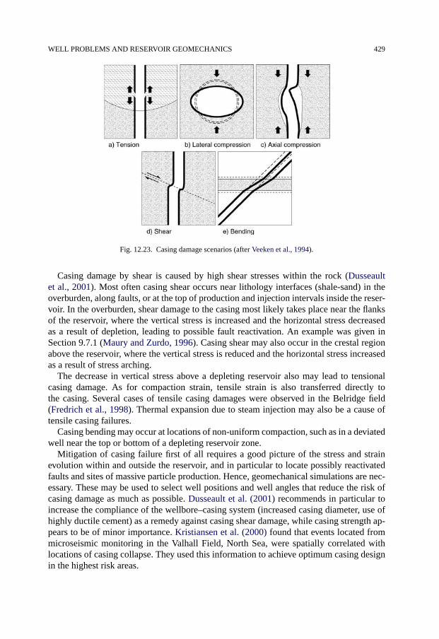
WELL PROBLEMS AND RESERVOIR GEOMECHANICS 429
Fig. 12.23. Casing damage scenarios (after Veeken et al., 1994).
Casing damage by shear is caused by high shear stresses within the rock (Dusseaultet al., 2001). Most often casing shear occurs near lithology interfaces (shale-sand) in theoverburden, along faults, or at the top of production and injection intervals inside the reser-voir. In the overburden, shear damage to the casing most likely takes place near the flanksof the reservoir, where the vertical stress is increased and the horizontal stress decreasedas a result of depletion, leading to possible fault reactivation. An example was given inSection 9.7.1 (Maury and Zurdo, 1996). Casing shear may also occur in the crestal regionabove the reservoir, where the vertical stress is reduced and the horizontal stress increasedas a result of stress arching.
The decrease in vertical stress above a depleting reservoir also may lead to tensionalcasing damage. As for compaction strain, tensile strain is also transferred directly tothe casing. Several cases of tensile casing damages were observed in the Belridge field(Fredrich et al., 1998). Thermal expansion due to steam injection may also be a cause oftensile casing failures.
Casing bending may occur at locations of non-uniform compaction, such as in a deviatedwell near the top or bottom of a depleting reservoir zone.
Mitigation of casing failure first of all requires a good picture of the stress and strainevolution within and outside the reservoir, and in particular to locate possibly reactivatedfaults and sites of massive particle production. Hence, geomechanical simulations are nec-essary. These may be used to select well positions and well angles that reduce the risk ofcasing damage as much as possible. Dusseault et al. (2001) recommends in particular toincrease the compliance of the wellbore–casing system (increased casing diameter, use ofhighly ductile cement) as a remedy against casing shear damage, while casing strength ap-pears to be of minor importance. Kristiansen et al. (2000) found that events located frommicroseismic monitoring in the Valhall Field, North Sea, were spatially correlated withlocations of casing collapse. They used this information to achieve optimum casing designin the highest risk areas.

430 RESERVOIR GEOMECHANICS
12.5.2. Reservoir geomechanics as a tool to optimize drilling and productionstrategies
This section has demonstrated that well problems associated with drilling and productionare strongly linked to the geomechanical response of the reservoir. Drilling instabilities,sand production and casing damage are triggered by depletion. This calls for a geomechani-cal analysis predicting stress changes and strain evolution within and outside the reservoir,based on different production scenarios. Such analyses will provide information like atwhat time and where infill wells have to be drilled in order to minimize stability problems,and where casing damage mitigation is required.
Stress arching in general reduces reservoir compaction and associated well problemswithin the reservoir. On the other hand, the stress changes within and around the reser-voir become more pronounced, which leads to more well failures in the overburden. Stressarching may however to some extent be controlled by the order in which reservoir compart-ments are produced, by pressure maintenance, or by thermal stresses generated as a resultof fluid injection. This opens up possibilities to use geomechanics actively—and through4D and microseismic monitoring—interactively, as a part of reservoir management.
References
Addis, M.A. (1997). “The stress-depletion response of reservoirs”. SPE 38720. In: Proc. SPE ATCE, San Antonio,TX, pp. 55–65.
Barkved, O., Kristiansen, T.G. (2005). “Seismic time-lapse effects and stress changes: Examples from a compact-ing reservoir”. The Leading Edge 24, 1244–1248.
Barton, C.A., Zoback, M.D., Moos, D. (1995). “Fluid flow along potentially active faults in crystalline rock”.Geology 23, 683–686.
Berryman, J.G. (1992). “Effective transport properties for inhomogeneous rock”. J. Geophys. Res. 97B, 17409–17424.
Boutéca, M., Sarda, J.-P., Vincké, O. (2000). “Constitutive law for permeability evolution of sandstones duringdepletion”. SPE 58717. In: Proc. SPE Int. Symp. Formation Damage, Lafayette, LA, USA.
Bruno, M.S. (1994). “Micromechanics of stress-induced permeability anisotropy and damage in sedimentaryrock”. Mech. Mater. 18, 31–48.
Bruno, M.S. (2002). “Geomechanical and decision analyses for mitigating compaction-related casing damage”.SPE Drilling & Completion 17, 179–188.
Cernocky, E.P., Scholibo, F.C. (1995). “Approach to casing design for service in compacting reservoirs”. SPE30522. In: Proc. SPE Annual Technical Conference and Exhibition, 22–25 October, Dallas, Texas.
Christensen, S.O., Janbu, N., Jones, M.E. (1988). “Subsidence due to oil–gas production”. In: Behavior of Off-shore Structures. BOSS ’88. Int. Conf., Trondheim, Norway, June 1988, Proc. vol. 1, pp. 143–157.
Dullien, F.A.L. (1992). Porous Media: Fluid Transport and Pore Structure, second ed. Academic Press. 574 pp.Dusseault, M.B., Bruno, M.S., Barrera, J. (2001). “Casing shear: Causes, cases, cures”. SPE Drilling & Comple-
tion 16, 98–107.Dusseault, M.B., Rothenburg, L. (2002). “Deformation analysis for reservoir management”. Oil & Gas Sci. Tech-
nol. Rev. IFP 57, 539–554.Eshelby, J.D. (1957). “The determination of the elastic field of an ellipsoidal inclusion, and related problems”.
Proc. Royal Soc. London 241, 376–396.Flornes, O. (2005). “Stress dependent fluid flow in porous rock: Experiments and network modelling”. PhD
Thesis NTNU 2005:207, 119 pp.Fredrich, J.T., Deitrick, G.L., Arguello, J.G., DeRouffignac, E.P. (1998). “Reservoir compaction, surface subsi-
dence, and casing damage: A geomechanics approach to mitigation and reservoir management”. SPE/ISRM47284. In: Proc. Eurock ’98, Trondheim, Norway.

REFERENCES 431
Ganghi, A.F. (1978). “Variation of whole and fractured porous rock permeability with confining pressure”. Int. J.Rock Mech. Min. Sci. & Geomech. Abstr. 15, 249–257.
Geertsma, J. (1973a). “A basic theory of subsidence due to reservoir compaction: The homogeneous case”. Ver-handelingen Kon. Ned. Geol. Mijnbouwk. Gen. 28, 43–62.
Geertsma, J. (1973b). “Land subsidence above compacting oil and gas reservoirs”. J. Petr. Tech. 25, 734–744.Gutierrez, M., Lewis, R.W. (1998). “The role of geomechanics in reservoir simulation”. SPE/ISRM Paper 47392.
In: Proc. Eurock ’98, Trondheim, Norway, vol. 2, pp. 439–448.Hatchell, P., Bourne, S. (2005). “Rocks under strain: Strain-induced time-lapse time shifts are observed for de-
pleting reservoirs”. The Leading Edge 24, 1222–1225.Heffer, K.J., Dowokpor, A.B. (1990). “Relationship between azimuths of flood anisotropy and local earth stresses
in oil reservoirs”. In: North Sea Oil and Gas Reservoirs II. Graham & Trotman.Heffer, K.J., Last, N.C., Koutsabeloulis, N.C., Chan, H.C.M., Gutierrez, M., Makurat, A. (1994). “The influence
of natural fractures, faults and earth stresses on reservoir performance—geomechanical analysis by numericalmodelling”. In: North Sea Oil and Gas Reservoirs III. Kluwer Academic Publishers.
Hettema, M.H.H., Schutjens, P.M.T.M., Verboom, B.J.M., Gussinklo, H.J. (2000). “Production-induced com-paction of a sandstone reservoir: The strong influence of stress path”. SPE Reservoir Evaluation Eng. 3,342–347.
Hettema, M., Papamichos, E., Schutjens, P. (2002). “Subsidence delay: Field observations and analysis”. Oil &Gas Sci. Technol. Rev. IFP 57, 443–458.
Holcomb, D.J., Olsson, W.A. (2003). “Compaction localization and fluid flow”. J. Geophys. Res. 108B, 2290.Holt, R.M. (1990). “Permeability reduction induced by a nonhydrostatic stress field”. SPE Formation Evalua-
tion 5, 444–448.Holt, R.M., Brignoli, M., Kenter, C.J. (2000). “Core quality: Quantification of coring induced rock alteration”.
Int. J. Rock Mechanics & Min. Sci. 37, 889–907.Holt, R.M., Lehr, B.C., Kenter, C.J., Spiets, P. (2003). “In-situ porosity from cores: poroelastic correction for
stress relief during coring”. Petrophysics 44, 253–261.Holt, R.M., Flornes, O., Li, L., Fjær, E. (2004). “Consequences of depletion-induced stress changes on reservoir
compaction and recovery”. Paper 04-589 ARMA/NARMS, 10 pp.Khan, M., Teufel, L.W. (2000). “The effect of geological and geomechanical parameters on reservoir stress path
and its importance in studying permeability anisotropy”. SPE Reservoir Evaluation Eng. 3, 394–400.Kilmer, N.H., Morrow, N.R., Pitman, J.K. (1987). “Pressure sensitivity of low permeability sandstones”. J. Petr.
Sci. & Eng. 1, 65–81.Koutsabeloulis, N.C., Heffer, K.J., Wong, S. (1994). “Numerical geomechanics in reservoir engineering”.
In: Siriwardane, H.J., Zaman, M.M. (Eds.), Proc. Computer Methods and Advances in Geomechanics.A.A. Balkema, pp. 2097–2104.
Kristiansen, T.G., Barkved, O., Pattillo, P.D. (2000). “Use of passive seismic monitoring in well and casing designin the compacting and subsiding Valhall Field, North Sea”. SPE 65134. In: Proc. SPE European PetroleumConference, 24–25 October, Paris, France.
Landrø, M., Digranes, P., Strønen, K. (2005). “Pressure depletion measured by time-lapse VSP”. The LeadingEdge 24, 1226–1232.
Lewis, R.W., Schrefler, B.A. (1998). The Finite Element Method in the Static and Dynamic Deformation andConsolidation of Porous Media, second ed. John Wiley & Sons, Chichester, England.
Maury, V., Zurdo, C. (1996). “Drilling-induced lateral shifts along pre-existing fractures: A common cause ofdrilling problems”. SPE Drilling & Completion 11, 17–23.
Maxwell, S.C., Young, R.P., Bossu, R., Jupe, A., Dangerfeld, J. (1998). “Microseismic logging of the Ekofiskreservoir”. SPE/ISRM 47276. In: Proc. Eurock ’98, Trondheim, Norway.
Mindlin, R.D., Cheng, D.H. (1950a). “Nuclei of strain in the semi-infinite solid”. J. Appl. Phys. 21, 926–930.Mindlin, R.D., Cheng, D.H. (1950b). “Thermoelastic stress in the semi-infinite solid”. J. Appl. Phys. 21, 931–933.Makurat, A., Gutierrez, M. (1996). “Fracture flow and fracture cross flow experiments”. SPE 36732. In: SPE
Annual Technical Conference and Exhibition, 6–9 October, Denver, Colorado, 9 pp.Morita, N., Gray, K.E., Srouji, F.A.A., Jogi, P.N. (1984). “Rock property change during reservoir compaction”.
SPE 13099. In: Proc. 59th Conf. SPE, Houston, TX, USA.Morita, N., Whitfill, D.L., Nygaard, O., Bale, A. (1989). “A quick method to determine subsidence, reservoir
compaction and in-situ stress induced by reservoir depletion”. J. Petr. Tech. 41, 71–79.

432 RESERVOIR GEOMECHANICS
Mulders, F.M.M. (2003). “Modelling of stress development and fault slip in and around a producing gas reservoir.PhD Thesis, TU Delft, Netherlands, 2003.
Nieto, J.A., Yale, D.P., Evans, R.J. (1994). “Improved methods for correcting core porosity to reservoir condi-tions”. The Log Analyst 35, 21–30.
Nur, A., Tosaya, C., Vo-Thanh, D. (1984). “Seismic monitoring of thermal enhanced oil recovery processes”. In:Proc. 54th Ann. Internat. Mtg. Soc. Explor. Geophys., pp. 337–340.
Osorio J.G., Chen H.-Y., Teufel L.W., Schaffer S. (1998). “A two-domain, 3D, fully coupled fluid-flow/geomechanical simulation model for reservoirs with stress-sensitive mechanical and fluid-flow prop-erties”. SPE/ISRM Paper 47397. In: Proc. Eurock ’98, Trondheim, Norway, vol. 2, pp. 455–464.
Papamichos, E., Heill, L.K., Vardoulakis, I. (2001). “Overburden modeling above a compacting reservoir using atrap door apparatus”. Phys. Chem. Earth 26A, 69–74.
Rudnicki, J. (1999). “Alteration of regional stress by reservoirs and other inhomogeneities: stabilizing or destabi-lizing?” In: Proceedings of the 9th International Congress on Rock Mechanics 3, pp. 1629–1637.
Santarelli, F.J., Tronvoll, J.T., Svennekjaer, M., Skeie, H., Henriksen, R., Bratli, R.K. (1998). “Reservoir stresspath: The depletion and the rebound”. SPE/ISRM 47350. In: Proc. Eurock ’98, Trondheim, Norway, pp. 203–209.
Sarda, J.-P., Ferfera, F.M.R., Vincké, O., Boutéca, M., Longuemare, P. (1998). “Experimental study of the stresspath influence on monophasic permeability evolution”. SCA Conferences paper SCA 9827.
Schutjens, P.M.T.M., Hanssen, T.H., Hettema, M.H.H., Merour, J., de Bree, P., Coremans, J.W.A., Helliesen, G.(2004). “Compaction-induced porosity/permeability reduction in sandstone reservoirs: Data and model forelasticity-dominated deformation”. SPE Reservoir Evaluation Eng. 7, 202–216.
Schwall, G.H., Slack, M.V., Kaiser, T.M.V. (1996). “Reservoir compaction well design for the Ekofisk Field”.SPE 36621. In: SPE Annual Technical Conference and Exhibition, 6–9 October, Denver, Colorado, 13 pp.
Segall, P., Fitzgerald, S.D. (1998). “A note on induced stress changes in hydrocarbon and geothermal reservoirs”.Tectonophysics 289, 117–128.
Sen, B. (1951). “Note on the stresses produced by nuclei of thermo-elastic strain in a semi-infinite elastic solid”.Quart. Appl. Math. 8, 365–369.
Settari, A., Walters, D.A. (1999). “Advances in coupled geomechanical and reservoir modeling with applicationsto reservoir compaction”. SPE 51927. In: SPE Reservoir Simulation Symposium, 14–17 February, Houston,Texas, USA.
Stone, T., Xian, C., Wan, J. (2001). “Implementation of coupled geomechanics in the eclipse reservoir simulator”.Presented at IFP Research Workshop on Geomechanics in Reservoir Simulation, December 2001.
Teufel, L.W., Rhett, D.W., Farrell, H.E. (1991). “Effect of reservoir depletion and pore pressure drawdown on insitu stress and deformation in the Ekofisk field, North Sea”. In: Proc. 32nd U.S. Symp. on Rock Mechanics,Norman, OK, USA, pp. 62–73.
Teeuw, D. (1971). “Prediction of formation compaction from laboratory and compressibility data”. Soc. Petr.Eng. J. 11, 263–271.
Terzaghi, K. (1936). “Stress distribution in dry and saturated sand above a yielding trap door”. In: Proc. Int.Conference on Soil Mechanics and Foundation Engineering, Cambridge, MA, vol. 1, pp. 307–311.
The Leading Edge (2005). Special section (in the December issue): Rocks under stress, pp. 1213–1286.
Veeken, C.A.M., Wahleitner, J.P., Keedy, C.R. (1994). “Experimental modelling of casing deformation in a com-pacting reservoir”. SPE/ISRM 28090. In: Proc. Eurock’94, Delft, Netherlands, pp. 497–506.
de Waal, J.A., Smits, R.M.M. (1988). “Prediction of reservoir compaction and surface subsidence: field applica-tion of a new model”. SPE Formation Evaluation 3, 347–356.
Yale, D.P. (1984). “Network modelling of flow, storage and deformation in porous rocks”. PhD Thesis, Stan-ford U, 158 pp.
Zimmerman, R.W. (2000b). “Implications of static poroelasticity for reservoir compaction”. In: Girard, J., Lieb-man, M., Breeds, C., Doe, T. (Eds.), Proc. Pacific Rocks 2000. Balkema, Rotterdam, ISBN 90 5809 155 4,pp. 169–172.
Zoback, M.D., Byerlee, J.D. (1975). “Permeability and effective stress”. AAPG Bulletin 59, 154–158.

FURTHER READING 433
Further reading
Andersen, M.A. (1988). “Predicting reservoir-condition PV compressibility from hydrostatic-stress laboratorydata”. SPE Reservoir Eng. 3, 1078–1082.
Barends, F.B.J., Brouwer, F.J.J., Schröder, F.H. (Eds.) (1995a). Land Subsidence. By Fluid Withdrawal. By SolidExtraction. Theory and Modelling. Environmental Effects and Remedial Measures. Proc. FISOLS95, FifthInternational Symposium on Land Subsidence. IAHS Publication No. 234.
Barends, F.B.J., Brouwer, F.J.J., Schröder, F.H. (Eds.) (1995b). Land Subsidence. Natural Causes. MeasuringTechniques. The Groningen Gas Fields. Proc. FISOLS95, Fifth International Symposium on Land Subsi-dence. Balkema, Rotterdam.
Bernabé, Y. (1992). “On the measurement of permeability in anisotropic rocks”. In: Evans, B., Wong, T.-f. (Eds.),Fault Mechanics and Transport Properties of Rocks: a Festschrift in Honor of W.F. Brace. Academic Press,London.
Biot, M.A. (1962). “Mechanics of deformation and acoustic propagation in porous media”. J. Appl. Phys. 33,1482–1498.
Brignoli, M., Pellegrino, A., Santarelli, F.J., Musso, G., Barla, G. (1997). “Continuous and discontinuous defor-mations above a compacting reservoir: Consequences upon the lateral extension of the subsidence bowl”. Int.J. Rock Mech. & Min. Sci. 34. Paper No. 039.
Charlez, P.A. (1997). Rock Mechanics. Volume 2. Petroleum Applications. Éditions Technip, Paris.Chilingarian, G.V., Donaldsen, E.C., Yen, T.F. (Eds.) (1995). Subsidence due to Fluid Withdrawal. Developments
in Petroleum Science, vol. 41. Elsevier Science Publishers B.V., Amsterdam.Chin, L.Y., Nagel, N.B. (2004). “Modeling of subsidence and reservoir compaction under waterflood operations”.
Int. J. Geomech. 4, 28–34.Geertsma, J., van Opstal, G. (1973). “A numerical technique for predicting subsidence above compacting reser-
voirs, based on the nucleus of strain concept”. Verhandelingen Kon. Ned. Geol. Mijnbouwk. Gen. 28, 63–78.Holt, R.M. (1999). “Reservoir stress path: Evaluation of core and field data”. In: Amadei, B., et al. (Eds.), Rock
Mechanics for Industry. A.A. Balkema, pp. 1195–1202.Holzer, T.L. (Ed.) (1984). Man-Induced Land Subsidence. “ Reviews in Engineering Geology, vol. VI. The Geo-
logical Society of America.Ibekwe, I.A., Coker III, O.D., Fuh G.F., Actis S.C. (2003). “Magnolia casing design for compaction”. SPE/IADC
79816. In: SPE/IADC Drilling Conference, 19–21 February, Amsterdam, Netherlands.Kristiansen, T.G. (1998). “Geomechanical characterization of the overburden above the compacting chalk reser-
voir at Valhall”. SPE 47348. In: Proc. Eurock ’98. Trondheim, Norway.Nagel, N.B. (1998). “Ekofisk field overburden modelling”. SPE 47345. In: Proc. Eurock ’98, Trondheim, Norway.Nagel, N. (2001). “Compaction and subsidence issues within the petroleum industry: From Wilmington to Ekofisk
and beyond”. Phys. Chem. Earth 26A, 3–14.Ostensen, R.W. (1986). “The effect of stress-dependent permeability on gas production and well testing”. SPE
Formation Evaluation 1, 227–235.Pattillo, P.D., Smith, M.B. (1985). “The effect of formation flow on the integrity of perforated casing”. Soc. Petr.
Eng. J. 25, 637–651.Pattillo, P.D., Kristiansen, T.G., Sund, G.V., Kjelstadli, R.M. (1998). “Reservoir compaction and seafloor subsi-
dence at Valhall”. SPE 47274. In: Proc. Eurock ’98, Trondheim, Norway.Schutjens, P. (2005). “Reservoir monitoring with seismic timeshifts: Geomechanical modeling for its application
in stacked pay”. In: International Petroleum Technology Conference, 21–23 November, Doha, Qatar.Segall, P. (1992). “Induced stresses due to fluid extraction from axisymmetric reservoirs”. Pure Appl. Geo-
phys. 139, 535–560.Tiab, D., Donaldson, E.C. (1996). Petrophysics—Theory and Practice of measuring Reservoir Rock and Fluid
Transport Properties. Gulf Publ. Co. 706 pp.Zhu, W., Wong, T.-f. (1997). “The transition from brittle faulting to cataclastic flow: Permeability evolution”.
J. Geophys. Res. 102B, 3027–3042.Zimmerman, R.W. (1991). Compressibility of Sandstones. Elsevier Science Publishers B.V., Amsterdam.Zimmerman, R.W. (2000a). “Coupling in poroelasticity and thermoelasticity”. Int. J. Rock Mech. & Min. Sci. 37,
79–97.Zoback, M.D. (2007). Reservoir Geomechanics. Cambridge University Press, Cambridge, ISBN-978-0-521-
77069-9.

This page intentionally left blank

435
Appendix A
Rock properties
The following tables are included in this appendix:
• Table A.1—Static mechanical properties for some common rock types and materials.
• Table A.2—Static mechanical properties for some specific rocks.
• Table A.3—Density, elastic moduli and sound velocities for some common materials.
• Table A.4—Sound velocities for some common rock types.
• Table A.5—Thermal properties for some rocks and materials.
The data are compiled from the sources given in the list below. Elastic moduli are fromtests under unconfined or near unconfined (low confining pressure) conditions.
Note: For most rocks, material properties such as elastic moduli, strength parametersand sound velocities vary from rock sample to rock sample, in addition to being depen-dent on measurement conditions (stress, temperature, saturation). Also, material propertiesare often anisotropic. We have therefore chosen to indicate expected intervals (Tables A.1and A.4) for the properties. In Tables A.2, A.3 and A.5, when some specific materials arereferred to, the values are taken from a specific experiment and need not be representativefor other experiments with the same type of rock.
There may also be slight variations in the numbers given by different sources.

436 ROCK PROPERTIES
Source Used in table
Bourbié, T., Coussy, O., Zinsner, B. (1987). Acoustics of Porous Media. IFP Publications.Editions Technip, Paris, France
A3, A4
Carmichael, R.S. (1982). Handbook of Physical Properties of Rocks (vols. II & III). CRCPress, Boca Raton, Florida
A1, A2, A3,A4
Deere, D.U., Miller, R.P. (1966). “Engineering classification and index properties for intactrock”. Report No. AFWL-TR-65-116, Air Force Weapons Laboratory, Kirtland Air ForceBase, New Mexico.
A1, A2
Gercek, H. (2007). “Poisson’s ratio values for rocks”. Int. J. Rock Mech. Min. Sci. 44, 1–13. A1Green, S.J., Griffin, R.M., Pratt, H.R. (1973). “Stress–strain and failure properties of a porous
shale”. SPE 4242. In: 6th Conf. Drilling and Rock Mechanics.A2
Head, K.H. (1984). Soil Laboratory Testing. Vols. I–III. ELE Intl., London. A1SINTEF Petroleum Research. “Various inhouse tests”. Trondheim. A1, A2, A4Lide, D.R., Frederikse, H.P.R. (Eds.) (1997). Handbook of Chemistry and Physics, 78th ed.,
CRC Press, Boca Raton, Florida.A3, A5
MacGillivray, D.A., Dusseault, M.B. (1998). “Thermal conduction and expansion ofsaturated quartz-illitic and smectitic shales as a function of stress, temperature, andbedding, anisotropy”. Int. J. Rock Mech. & Min. Sci. 35 (4–5). Paper No. 35.
A5
Mavko, G., Mukerji, T., Dvorkin, J. (1998). The Rock Physics Handbook. CambridgeUniversity Press, Cambridge.
A2, A3
Morita, N., Whitfill, D.L., Massie, I., Knudsen, T.W. (1987). “Realistic and productionprediction: Numerical approach”. SPE Production Eng. 4 (1), 15–24.
A2
Nur, A.M., Wang, Z. (1989). Seismic and Acoustic Velocities in Reservoir Rocks, GeophysicsReprint Series. Soc. Expl. Geophysicists, Tulsa, Oklahoma (and references therein).
A3, A4
Somerton, W.H. (1992). Thermal Properties and Temperature-Related Behavior ofRock/Fluid Systems. Elsevier, Amsterdam.
A5
TerraTek (2001). “Properties of Pierre shale”. Personal communication. A2

ROCK PROPERTIES 437
TABLE A.1 Static mechanical properties for some common rock types and materials
Material Density ρ
103 (kg/m3)
Young’s modulusE (GPa)
Poisson’s ratioν
Unconf. compr.strength C0 (MPa)
Tensile strengthT0 (MPa)
Unconsolidatedsands
1.5–1.7 0.01–0.1 ∼0.45
Sandstone 2.0–2.65 0.1–30 0–0.45 1–250Clay 1.9–2.1 0.06–0.15 ∼0.40 0.2–0.5Shale 2.3–2.8 0.4–70 0–0.30 2–250High porositychalk
1.4–1.7 0.5–5 0.05–0.35 4–15
Low porositychalk
1.7–2.0 5–30 0.05–0.30 10–40
Basalt 2.7–2.9 50–100 0.2–0.3 200–350 10–15Granite 2.6–2.8 5–85 0.1–0.34 50–350 5–15Dolomite 2.4–3.2 10–100 0–0.5 40–350Limestone 1.4–2.9 2–100 0–0.3 5–250Gneiss 2.7–3.1 40–100 0.1–0.3 50–250Marble 2.7–3.2 5–90 0–0.3 50–250Ice 0.9 8 0.35Steel 7.9 200 0.28 220–900∗ 350–1200
∗Yield strength.

438 ROCK PROPERTIES
TABLE A.2 Static mechanical properties for some specific rocks
Material Density ρ
103 (kg/m3)
Young’s modulusE (GPa)
Poisson’s ratioν
Unconf. compr.strength C0 (MPa)
Tensile strengthT0 (MPa)
RedWildmoor⊥
1.9–2.0 1.8 14 0.4–0.7
sandstone‖ 1.9–2.0 1.3 7 0.4–0.7Weak reservoirsandstone(North Sea)
1.9 0.4 0.45 1
Berea sandstone 2.18 20 0.38 74St. Petersandstone
2.34 4–10 0.05–0.10 37
Weak shale(North Sea)
2.35 1 6
Pierre shale I 2.37–2.39 0.77–1.12 0.35–0.37 7.5–13.9Shale (El Paso) 2.47 26 0.10 115Bedfordlimestone
2.21 29 0.29 51 1.6
Solenhofenlimestone
2.62 64 0.29 245 4.0
Hackensacksiltstone
2.59 26 0.22 123 3.0
Nevada Tuff 1.61 5.0 0.21 24 1.4Rock salt(Diamondcrystal)
2.16 5 >0.5 21 0.8
Schist⊥ 2.81 21 0.31 55 0.6(Luther Falls)‖ 2.82 58 0.18 83 5.2
⊥Loaded perpendicular to bedding.‖Loaded parallel to bedding.
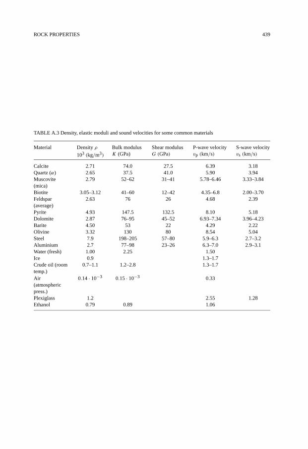
ROCK PROPERTIES 439
TABLE A.3 Density, elastic moduli and sound velocities for some common materials
Material Density ρ
103 (kg/m3)
Bulk modulusK (GPa)
Shear modulusG (GPa)
P-wave velocityvp (km/s)
S-wave velocityvs (km/s)
Calcite 2.71 74.0 27.5 6.39 3.18Quartz (α) 2.65 37.5 41.0 5.90 3.94Muscovite(mica)
2.79 52–62 31–41 5.78–6.46 3.33–3.84
Biotite 3.05–3.12 41–60 12–42 4.35–6.8 2.00–3.70Feldspar(average)
2.63 76 26 4.68 2.39
Pyrite 4.93 147.5 132.5 8.10 5.18Dolomite 2.87 76–95 45–52 6.93–7.34 3.96–4.23Barite 4.50 53 22 4.29 2.22Olivine 3.32 130 80 8.54 5.04Steel 7.9 198–205 57–80 5.9–6.3 2.7–3.2Aluminium 2.7 77–98 23–26 6.3–7.0 2.9–3.1Water (fresh) 1.00 2.25 1.50Ice 0.9 1.3–1.7Crude oil (roomtemp.)
0.7–1.1 1.2–2.8 1.3–1.7
Air(atmosphericpress.)
0.14 · 10−3 0.15 · 10−3 0.33
Plexiglass 1.2 2.55 1.28Ethanol 0.79 0.89 1.06

440 ROCK PROPERTIES
TABLE A.4 Sound velocities for some common rock types
Material Density ρ
103 (kg/m3)
P-wave velocityvp (km/s)
S-wave velocityvs (km/s)
Conditions
Sand, dry, loose 1.5–1.7 0.3–1.0 0.05–0.4 dry, from surface to ≈50 m depthSand, dry 1.6–1.7 1.0–1.7 0.4–0.9 dry, loaded from ≈1 to ≈50 MPaSand, wet, loose 1.8–2.2 1.5–2.0 0.05–0.4 saturated, from surface to ≈50 m
depthSandstone,competent
2.0–2.65 1.8–4.5 1.0–3.0 dry, various porosities
Berea sandstone 2.2 3.8–4.0 2.3–2.4 brine saturated, confinedSandstone,weak
1.7–2.0 1.0–2.0 0.6–1.2 dry, various porosities
Red Wildmoorsst.
2.0 1.7–2.0 1.1–1.3 dry, confined
Clay 1.9–2.1 1.5–1.6 0.1–0.3 saturated, from surface to ≈50 mdepth
London Clay,deep
2.0 1.7–1.8 0.8–1.1 saturated
Shale 2.3–2.8 1.6–4.5 0.7–3.0 saturated, various porositiesWeak shale,North Sea
1.8–2.3 2.4–2.6 1.2–1.3 saturated, unconfined
Chalk, highporosity
1.4–1.7 1.8–2.6 1.0–1.5 saturated, field and lab. data
Chalk, lowporosity
1.7–2.4 2.6–5.0 1.5–3.5 saturated, field and lab. data
Limestone 2.4–2.7 3.5–6.0 2.0–3.5 variousBasalt 2.5–2.9 3.5–5.5 1.7–3.4 dry & saturated; stress 0–100 MPaGranite 2.6–2.7 5.5–6.5 3.0–3.5 dry; stress 0–100 MPa
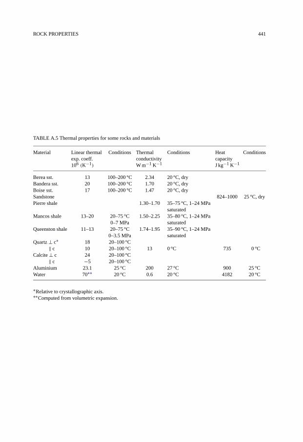
ROCK PROPERTIES 441
TABLE A.5 Thermal properties for some rocks and materials
Material Linear thermalexp. coeff.106 (K−1)
Conditions ThermalconductivityW m−1 K−1
Conditions HeatcapacityJ kg−1 K−1
Conditions
Berea sst. 13 100–200 °C 2.34 20 °C, dryBandera sst. 20 100–200 °C 1.70 20 °C, dryBoise sst. 17 100–200 °C 1.47 20 °C, drySandstone 824–1000 25 °C, dryPierre shale 1.30–1.70 35–75 °C, 1–24 MPa
saturatedMancos shale 13–20 20–75 °C 1.50–2.25 35–80 °C, 1–24 MPa
saturated0–7 MPaQueenston shale 11–13 20–75 °C 1.74–1.95 35–90 °C, 1–24 MPa
saturated0–3.5 MPaQuartz ⊥ c∗ 18 20–100 °C
‖ c 10 20–100 °C 13 0 °C 735 0 °CCalcite ⊥ c 24 20–100 °C
‖ c −5 20–100 °CAluminium 23.1 25 °C 200 27 °C 900 25 °CWater 70∗∗ 20 °C 0.6 20 °C 4182 20 °C
∗Relative to crystallographic axis.∗∗Computed from volumetric expansion.

This page intentionally left blank
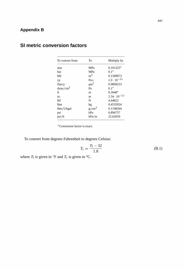
443
Appendix B
SI metric conversion factors
To convert from To Multiply by
atm MPa 0.101325∗bar MPa 0.1∗bbl m3 0.1589873cp Pa s 1.0 · 10−3∗Darcy µm2 0.9869233dyne/cm2 Pa 0.1∗ft m 0.3048∗in. m 2.54 · 10−2∗lbf N 4.44822lbm kg 0.4535924lbm/USgal g/cm3 0.1198264psi kPa 6.894757psi/ft kPa/m 22.62059
∗Conversion factor is exact.
To convert from degrees Fahrenheit to degrees Celsius:
Tc = Tf − 32
1.8(B.1)
where Tf is given in ◦F and Tc is given in °C.

This page intentionally left blank

445
Appendix C
Mathematical background
C.1. Introduction
When using the first edition of this book as a basis for a course in Petroleum Related RockMechanics, we have repeatedly had the request for a refreshment of some mathematicalbackground material, in particular linear algebra. This appendix is an attempt to respondto these requests.
This appendix is not a full tutorial, and we do not attempt to provide full mathematicalrigour in the presentation. Still, we hope that this appendix may be useful for readers thatneed a repetition of some central mathematical methods. We also hope that this appendixmay make it easier to read some of the literature in the field.
C.2. Matrices
A matrix is a rectangular array of numbers or other mathematical objects. The elements ofa matrix are normally referred to by two indices. The first index refers to the rows and thesecond to the columns.
An example of a 3 × 3 matrix is thus
a =(a11 a12 a13a21 a22 a23a31 a32 a33
)(C.1)
C.2.1. The transpose of a matrix
The transpose of a matrix is the matrix found by interchanging the rows and columns of amatrix. The transpose of a is often denoted by aT. The transpose of the matrix in Eq. (C.1)is
aT =(a11 a21 a31a12 a22 a32a13 a23 a33
)(C.2)
C.2.2. Symmetric matrix
A symmetric matrix is equal to its transpose, i.e. it is left unchanged when reflected aboutthe diagonal:
a = aT (C.3)
446 MATHEMATICAL BACKGROUND
In component notation this may be written as
aij = aji (C.4)
C.2.3. Diagonal matrix
A diagonal matrix is a square matrix in which only the diagonal elements are nonzero.Sometimes the following notation is used:
diag(a, b, c) =(a 0 00 b 00 0 c
)(C.5)
C.2.4. Matrix addition
Two matrices of the same size are added by adding corresponding elements. As an example,for two 2 × 2 matrices we have
a + b =(a11 + b11 a12 + b12a21 + b21 a22 + b22
)(C.6)
C.2.5. Multiplication by a scalar
A matrix is multiplied by a scalar by multiplying all elements with the scalar. For example
ka = k(a11 a12a21 a22
)=(ka11 ka12ka21 ka22
)(C.7)
C.2.6. Matrix multiplication
The product of an n× l matrix a and an l×m matrix b is a matrix in which the ij elementis given by ∑
k
aikbkj (C.8)
Thus, for two 2 × 2 matrices we get
ab =(a11b11 + a12b21 a11b12 + a12b22a21b11 + a22b21 a21b12 + a22b22
)(C.9)
Matrix multiplication is non-commutative, i.e. in general we have
ab �= ba (C.10)
MATRICES 447
Matrix multiplication is associative, i.e.
a(bc) = (ab)c = abc (C.11)
Matrix multiplication is distributive, i.e.
a(b + c) = ab + ac (C.12)
C.2.7. The identity matrix
A square matrix with all diagonal elements equal to 1 and all other elements equal to 0 iscalled the identity matrix, and is often denoted by I.
We see that we must have
aI = Ia = a (C.13)
Note that on component form the identity matrix can be written using the Kronecker δ (seepage 460):
Iij = δij (C.14)
C.2.8. The inverse matrix
A square matrix (n × n matrix) a is said to be non-singular if an inverse matrix, denotedby a−1 exists. The inverse matrix is defined by the following relations
aa−1 = a−1a = I (C.15)
The inverse of a 2 × 2 matrix is
a−1 = 1
a11a22 − a12a21
(a22 −a12
−a21 a11
)(C.16)
and that of a 3 × 3 matrix is
a−1 = 1
|a|
(a22a33 − a23a32 a13a32 − a12a33 a12a23 − a13a22a23a31 − a21a33 a11a33 − a13a31 a13a21 − a11a23a21a32 − a22a31 a12a31 − a11a32 a11a22 − a12a21
)(C.17)
where the determinant |a| of the matrix is defined by Eq. (C.21) below.
C.2.9. The trace of a matrix
The trace of a square matrix is defined as the sum of the diagonal elements of the matrix.On component form we thus may write
tr(a) =∑i
aii (C.18)
448 MATHEMATICAL BACKGROUND
The trace of a matrix product is independent of the order of the factors
tr(ab) = tr(ba) (C.19)
Sometimes the trace of a matrix is denoted by Sp(a), from the German word Spur.
C.2.10. Determinants
The determinant is another characteristic number associated with a square matrix a, and isdenoted by |a| or det(a). We shall not discuss determinants in general here, but note thatfor a 2 × 2 matrix the determinant is given by∣∣∣∣ a11 a12
a21 a22
∣∣∣∣ = a11a22 − a21a12 (C.20)
and for a 3 × 3 matrix by(a11 a12 a13a21 a22 a23a31 a32 a33
)= a11a22a33 + a21a32a13 + a31a12a23
−a11a32a23 − a21a12a33 − a31a22a13(C.21)
The determinant of the product of two matrices is equal to the product of the determi-nants, i.e.
|ab| = |a||b| (C.22)
From this equation and Eq. (C.15) it follows that
|a−1| = 1
|a| (C.23)
since |I| = 1.It is clear from Eqs. (C.20) and (C.21) that
|aT| = |a| (C.24)
for 2 × 2 and 3 × 3 matrices. This relation is valid in general.From Eq. (C.17) we see that the 3 × 3 matrix is singular (the inverse does not exist) if
the determinant is zero. This is also a generally valid property.
C.2.11. Systems of linear equations
Matrices form an efficient way of writing a system of linear equations. For instance, wemay write the system
a11x1 + a12x2 = b1 (C.25)
a21x1 + a22x2 = b2 (C.26)
as
ax = b (C.27)

MATRICES 449
where a is the 2 × 2 matrix
a =(a11 a12a21 a22
)(C.28)
while x and b are the column vectors (or 2 × 1 matrices)
x =(x1x2
), b =
(b1b2
)(C.29)
Assuming a to have an inverse, the solution of Eq. (C.27) may be written as
x = a−1b (C.30)
Homogeneous systems
If all bi are zero, we have a homogeneous system:
ax = 0 (C.31)
Then the formal solution (C.30) assuming a to be invertible only allows the trivial solutionx = 0, which is normally not useful.
To get non-trivial solutions for a homogeneous system, the matrix a must thus be singu-lar, i.e. its determinant must be zero:
|a| = 0 (C.32)
C.2.12. Eigenvalues and eigenvectors
The equation
ax = λx (C.33)
where a is an n× n matrix, x is a column vector (or n× 1 matrix) and λ is a scalar (i.e. anumber, in general complex), is called the eigenvalue equation for the matrix a. The valuesof λ for which Eq. (C.33) has non-trivial solutions for x are called the eigenvalues of thematrix.
We see from Eq. (C.32) that we may find the eigenvalues by solving the determinantequation
|a − λI| = 0 (C.34)
Eq. (C.34) is used to determine the principal stresses and strains in Eqs. (1.31) and (1.81).An n × n matrix has n eigenvalues λi , some or all of which may coincide. If we insert
an eigenvalue, e.g. λ1 into (C.33), we get the equation
ax = λ1x (C.35)
450 MATHEMATICAL BACKGROUND
which has a non-trivial solution for x. The solution is called the eigenvector correspondingto λ1. There are n eigenvectors for an n×nmatrix. The eigenvectors are (or can be chosento be) linearly independent (orthogonal). Eqs. (1.32)–(1.34) are an example of the use ofEq. (C.35).
It can be shown that the eigenvalues of a symmetric matrix with real elements are real.
C.2.13. Similarity transforms and orthogonal transforms
If we have a non-singular matrix S, the transform
SaS−1 (C.36)
is called a similarity transform of a.We see that since
|SaS−1 − λI| = |SaS−1 − SλIS−1| = |S||a − λI||S−1| = |a − λI| (C.37)
the eigenvalues are unchanged by a similarity transform. It can also be shown that the traceand the determinant of the matrix are left unchanged by the similarity transform. (We leavethis to the reader as a simple exercise, use Eqs. (C.19) and (C.22).)
A matrix O which fulfils
O−1 = OT (C.38)
is called an orthogonal matrix.It follows from I = OOT that
δik =∑j
Oij (OT)jk =∑j
OijOkj (C.39)
which shows that the row vectors of O (i.e. the vectors formed by the rows of O) areorthogonal, and that their length is 1. From I = OTO one may show that the same appliesto the column vectors (the vectors formed by the columns of O).
It is clear that an orthogonal transform, defined by
OaOT (C.40)
is a subset of the similarity transforms, and thus preserves the trace, the determinant andthe eigenvalues.
Any symmetric matrix with real elements can be diagonalized, i.e. transformed to adiagonal matrix, by an orthogonal transformation.
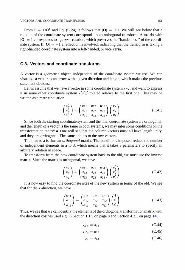
VECTORS AND COORDINATE TRANSFORMS 451
From I = OOT and Eq. (C.24) it follows that |O| = ±1. We will see below that arotation of the coordinate system corresponds to an orthogonal transform. A matrix with|O| = 1 corresponds to a proper rotation, which preserves the “handedness” of the coordi-nate system. If |O| = −1 a reflection is involved, indicating that the transform is taking aright-handed coordinate system into a left-handed, or vice versa.
C.3. Vectors and coordinate transforms
A vector is a geometric object, independent of the coordinate system we use. We canvisualize a vector as an arrow with a given direction and length, which makes the previousstatement obvious.
Let us assume that we have a vector in some coordinate system xyz, and want to expressit in some other coordinate system x′y′z′ rotated relative to the first one. This may bewritten as a matrix equation(
v′x
v′y
v′z
)=(a11 a12 a13a21 a22 a23a31 a32 a33
)(vxvyvz
)(C.41)
Since both the starting coordinate system and the final coordinate system are orthogonal,and the length of a vector is the same in both systems, we may infer some conditions on thetransformation matrix a. One will see that the column vectors must all have length unity,and they are orthogonal. The same applies to the row vectors.
The matrix a is thus an orthogonal matrix. The conditions imposed reduce the numberof independent elements in a to 3, which means that it takes 3 parameters to specify anarbitrary rotation in space.
To transform from the new coordinate system back to the old, we must use the inversematrix. Since the matrix is orthogonal, we have(
vxvyvz
)=(a11 a21 a31a12 a22 a32a13 a23 a33
)(v′x
v′y
v′z
)(C.42)
It is now easy to find the coordinate axes of the new system in terms of the old. We seethat for the x-direction, we have(
a11a12a13
)=(a11 a21 a31a12 a22 a32a13 a23 a33
)( 100
)(C.43)
Thus, we see that we can identify the elements of the orthogonal transformation matrix withthe direction cosines used e.g. in Section 1.1.5 on page 8 and Section 4.3.1 on page 146:
lx′x = a11 (C.44)
lx′y = a12 (C.45)
lx′z = a13 (C.46)
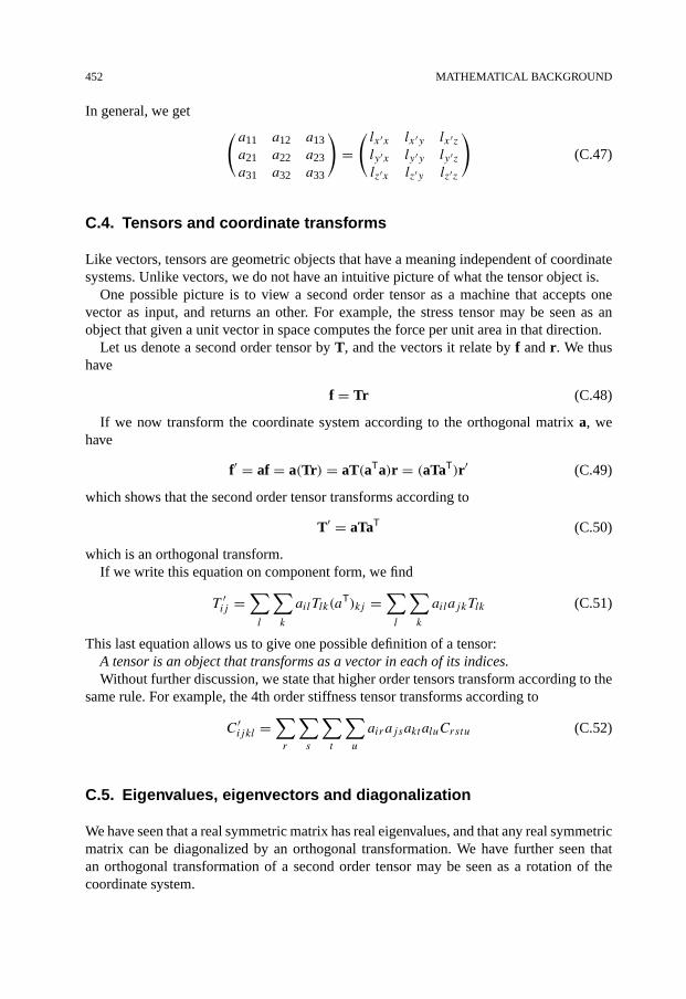
452 MATHEMATICAL BACKGROUND
In general, we get (a11 a12 a13a21 a22 a23a31 a32 a33
)=(lx′x lx′y lx′zly′x ly′y ly′zlz′x lz′y lz′z
)(C.47)
C.4. Tensors and coordinate transforms
Like vectors, tensors are geometric objects that have a meaning independent of coordinatesystems. Unlike vectors, we do not have an intuitive picture of what the tensor object is.
One possible picture is to view a second order tensor as a machine that accepts onevector as input, and returns an other. For example, the stress tensor may be seen as anobject that given a unit vector in space computes the force per unit area in that direction.
Let us denote a second order tensor by T, and the vectors it relate by f and r. We thushave
f = Tr (C.48)
If we now transform the coordinate system according to the orthogonal matrix a, wehave
f′ = af = a(Tr) = aT(aTa)r = (aTaT)r′ (C.49)
which shows that the second order tensor transforms according to
T′ = aTaT (C.50)
which is an orthogonal transform.If we write this equation on component form, we find
T ′ij =
∑l
∑k
ailTlk(aT)kj =
∑l
∑k
ailajkTlk (C.51)
This last equation allows us to give one possible definition of a tensor:A tensor is an object that transforms as a vector in each of its indices.Without further discussion, we state that higher order tensors transform according to the
same rule. For example, the 4th order stiffness tensor transforms according to
C′ijkl =
∑r
∑s
∑t
∑u
airajsaktaluCrstu (C.52)
C.5. Eigenvalues, eigenvectors and diagonalization
We have seen that a real symmetric matrix has real eigenvalues, and that any real symmetricmatrix can be diagonalized by an orthogonal transformation. We have further seen thatan orthogonal transformation of a second order tensor may be seen as a rotation of thecoordinate system.
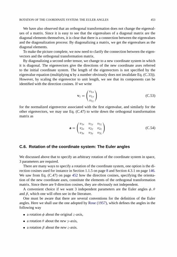
ROTATION OF THE COORDINATE SYSTEM: THE EULER ANGLES 453
We have also observed that an orthogonal transformation does not change the eigenval-ues of a matrix. Since it is easy to see that the eigenvalues of a diagonal matrix are thediagonal elements themselves, it is clear that there is a connection between the eigenvaluesand the diagonalization process: By diagonalizing a matrix, we get the eigenvalues as thediagonal elements.
To make the picture complete, we now need to clarify the connection between the eigen-vectors and the orthogonal transformation matrix.
By diagonalizing a second order tensor, we change to a new coordinate system in whichit is diagonal. The eigenvectors give the directions of the new coordinate axes referredto the initial coordinate system. The length of the eigenvectors is not specified by theeigenvalue equation (multiplying x by a number obviously does not invalidate Eq. (C.33)).However, by scaling the eigenvector to unit length, we see that its components can beidentified with the direction cosines. If we write
v1 =(v1xv1yv1z
)(C.53)
for the normalized eigenvector associated with the first eigenvalue, and similarly for theother eigenvectors, we may use Eq. (C.47) to write down the orthogonal transformationmatrix as
a =(v1x v1y v1zv2x v2y v2zv3x v3y v3z
)(C.54)
C.6. Rotation of the coordinate system: The Euler angles
We discussed above that to specify an arbitrary rotation of the coordinate system in space,3 parameters are required.
There are many ways to specify a rotation of the coordinate system, one option is the di-rection cosines used for instance in Section 1.1.5 on page 8 and Section 4.3.1 on page 146.We saw from Eq. (C.47) on page 452 how the direction cosines, specifying the orienta-tion of the new coordinate axes, constitute the elements of the orthogonal transformationmatrix. Since there are 9 direction cosines, they are obviously not independent.
A convenient choice if we want 3 independent parameters are the Euler angles φ, θand β, which one will often see in the literature.
One must be aware that there are several conventions for the definition of the Eulerangles. Here we shall use the one adopted by Rose (1957), which defines the angles in thefollowing way
• a rotation φ about the original z-axis,
• a rotation θ about the new y-axis,
• a rotation β about the new z-axis.
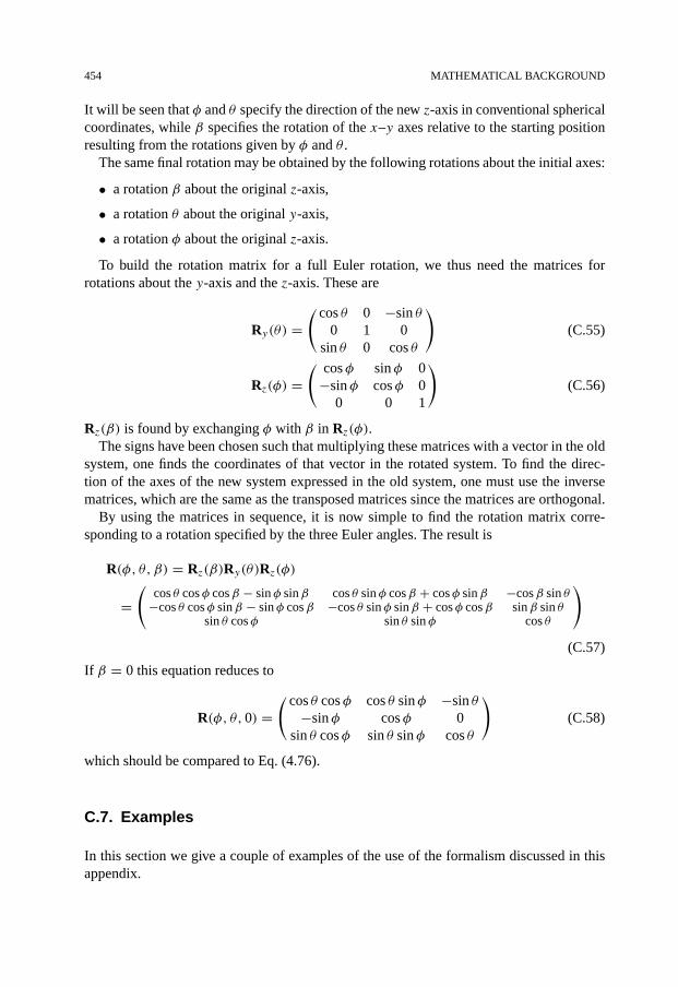
454 MATHEMATICAL BACKGROUND
It will be seen that φ and θ specify the direction of the new z-axis in conventional sphericalcoordinates, while β specifies the rotation of the x–y axes relative to the starting positionresulting from the rotations given by φ and θ .
The same final rotation may be obtained by the following rotations about the initial axes:
• a rotation β about the original z-axis,
• a rotation θ about the original y-axis,
• a rotation φ about the original z-axis.
To build the rotation matrix for a full Euler rotation, we thus need the matrices forrotations about the y-axis and the z-axis. These are
Ry(θ) =( cos θ 0 −sin θ
0 1 0sin θ 0 cos θ
)(C.55)
Rz(φ) =( cosφ sinφ 0
−sinφ cosφ 00 0 1
)(C.56)
Rz(β) is found by exchanging φ with β in Rz(φ).The signs have been chosen such that multiplying these matrices with a vector in the old
system, one finds the coordinates of that vector in the rotated system. To find the direc-tion of the axes of the new system expressed in the old system, one must use the inversematrices, which are the same as the transposed matrices since the matrices are orthogonal.
By using the matrices in sequence, it is now simple to find the rotation matrix corre-sponding to a rotation specified by the three Euler angles. The result is
R(φ, θ, β) = Rz(β)Ry(θ)Rz(φ)
=(
cos θ cosφ cosβ − sinφ sinβ cos θ sinφ cosβ + cosφ sinβ −cosβ sin θ−cos θ cosφ sinβ − sinφ cosβ −cos θ sinφ sinβ + cosφ cosβ sinβ sin θ
sin θ cosφ sin θ sinφ cos θ
)
(C.57)
If β = 0 this equation reduces to
R(φ, θ, 0) =( cos θ cosφ cos θ sinφ −sin θ
−sinφ cosφ 0sin θ cosφ sin θ sinφ cos θ
)(C.58)
which should be compared to Eq. (4.76).
C.7. Examples
In this section we give a couple of examples of the use of the formalism discussed in thisappendix.
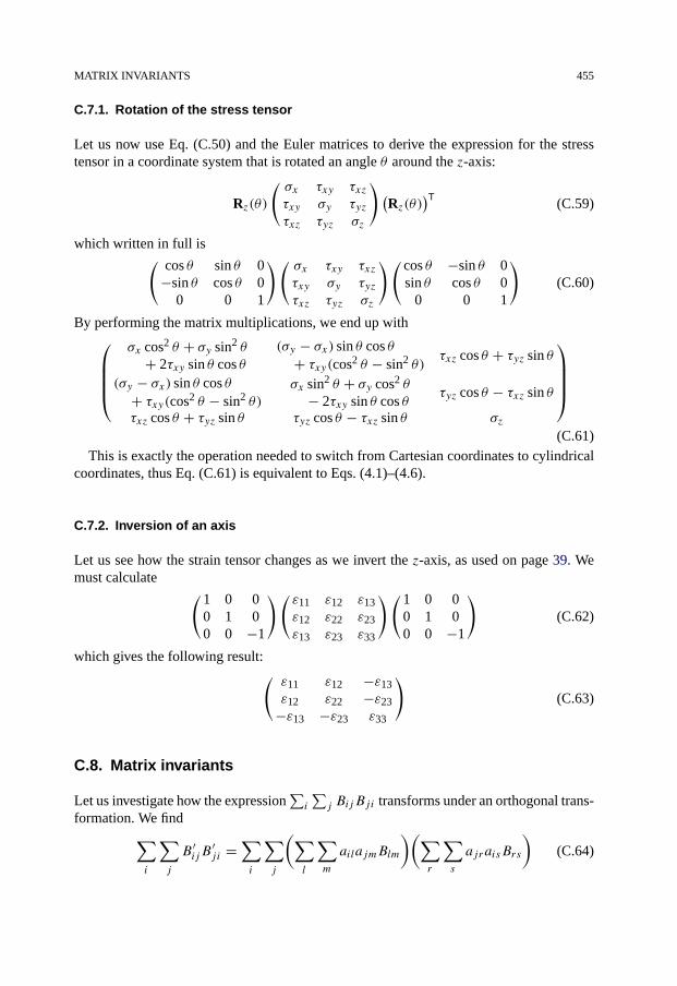
MATRIX INVARIANTS 455
C.7.1. Rotation of the stress tensor
Let us now use Eq. (C.50) and the Euler matrices to derive the expression for the stresstensor in a coordinate system that is rotated an angle θ around the z-axis:
Rz(θ)
(σx τxy τxzτxy σy τyzτxz τyz σz
) (Rz(θ)
)T (C.59)
which written in full is( cos θ sin θ 0−sin θ cos θ 0
0 0 1
)(σx τxy τxzτxy σy τyzτxz τyz σz
)( cos θ −sin θ 0sin θ cos θ 0
0 0 1
)(C.60)
By performing the matrix multiplications, we end up with⎛⎜⎜⎜⎝
σx cos2 θ + σy sin2 θ
+ 2τxy sin θ cos θ(σy − σx) sin θ cos θ
+ τxy(cos2 θ − sin2 θ)τxz cos θ + τyz sin θ
(σy − σx) sin θ cos θ+ τxy(cos2 θ − sin2 θ)
σx sin2 θ + σy cos2 θ
− 2τxy sin θ cos θτyz cos θ − τxz sin θ
τxz cos θ + τyz sin θ τyz cos θ − τxz sin θ σz
⎞⎟⎟⎟⎠(C.61)
This is exactly the operation needed to switch from Cartesian coordinates to cylindricalcoordinates, thus Eq. (C.61) is equivalent to Eqs. (4.1)–(4.6).
C.7.2. Inversion of an axis
Let us see how the strain tensor changes as we invert the z-axis, as used on page 39. Wemust calculate ( 1 0 0
0 1 00 0 −1
)(ε11 ε12 ε13ε12 ε22 ε23ε13 ε23 ε33
)( 1 0 00 1 00 0 −1
)(C.62)
which gives the following result:(ε11 ε12 −ε13ε12 ε22 −ε23
−ε13 −ε23 ε33
)(C.63)
C.8. Matrix invariants
Let us investigate how the expression∑i
∑j BijBji transforms under an orthogonal trans-
formation. We find∑i
∑j
B ′ijB
′ji =
∑i
∑j
(∑l
∑m
ailajmBlm
)(∑r
∑s
ajraisBrs
)(C.64)

456 MATHEMATICAL BACKGROUND
Now, from the relation (see Eq. (C.39))∑i
ailais = δls (C.65)
we derive ∑i
∑j
B ′ijB
′ji =
∑l
∑s
∑r
∑m
δlsδrmBlmBrs =∑s
∑r
BsrBrs (C.66)
This tells us that∑i
∑j BijBji is invariant under an orthogonal transformation.
By similar calculations, it is easy to show that∑k
Bkk (C.67)
∑i
∑j
BijBji (C.68)
∑i
∑j
∑k
BijBjkBki (C.69)
∑i
∑j
∑k
∑l
BijBjkBklBli (C.70)
are invariants of linear, quadratic, cubic and quartic degree. It is obvious how 5th and higherorder invariants are constructed in the same way. It should however be noted that only thefirst three invariants are truly independent, the higher invariants may be expressed as a sumof combinations of the three first.
In rock mechanics, these invariants are not used directly, except for the first. The standardrock mechanical invariants are defined by writing the third degree equation resulting fromEq. (1.31) as
σ 3 − I1σ 2 − I2σ − I3 = 0 (C.71)
Since the solution of the equation are the principal stresses, it is obvious that the coeffi-cients are invariants. (Beware that sometimes Eq. (C.71) is written with a +-sign in frontof the I2-term, leading to the opposite sign for I2.)
By expanding Eq. (1.31), and comparing with Eq. (C.71), the expressions (1.39) to (1.41)follow. The relations between the rock mechanical invariants and those derived in thissection are ∑
k
σkk = I1 (C.72)
∑i
∑j
σij σji = I 21 + 2I2 (C.73)
∑i
∑j
∑k
σij σjkσki = I 31 + 3I2I1 + 3I3 (C.74)
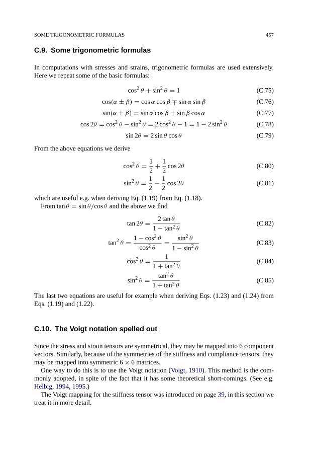
SOME TRIGONOMETRIC FORMULAS 457
C.9. Some trigonometric formulas
In computations with stresses and strains, trigonometric formulas are used extensively.Here we repeat some of the basic formulas:
cos2 θ + sin2 θ = 1 (C.75)
cos(α ± β) = cosα cosβ ∓ sinα sinβ (C.76)
sin(α ± β) = sinα cosβ ± sinβ cosα (C.77)
cos 2θ = cos2 θ − sin2 θ = 2 cos2 θ − 1 = 1 − 2 sin2 θ (C.78)
sin 2θ = 2 sin θ cos θ (C.79)
From the above equations we derive
cos2 θ = 1
2+ 1
2cos 2θ (C.80)
sin2 θ = 1
2− 1
2cos 2θ (C.81)
which are useful e.g. when deriving Eq. (1.19) from Eq. (1.18).From tan θ = sin θ/cos θ and the above we find
tan 2θ = 2 tan θ
1 − tan2 θ(C.82)
tan2 θ = 1 − cos2 θ
cos2 θ= sin2 θ
1 − sin2 θ(C.83)
cos2 θ = 1
1 + tan2 θ(C.84)
sin2 θ = tan2 θ
1 + tan2 θ(C.85)
The last two equations are useful for example when deriving Eqs. (1.23) and (1.24) fromEqs. (1.19) and (1.22).
C.10. The Voigt notation spelled out
Since the stress and strain tensors are symmetrical, they may be mapped into 6 componentvectors. Similarly, because of the symmetries of the stiffness and compliance tensors, theymay be mapped into symmetric 6 × 6 matrices.
One way to do this is to use the Voigt notation (Voigt, 1910). This method is the com-monly adopted, in spite of the fact that it has some theoretical short-comings. (See e.g.Helbig, 1994, 1995.)
The Voigt mapping for the stiffness tensor was introduced on page 39, in this section wetreat it in more detail.
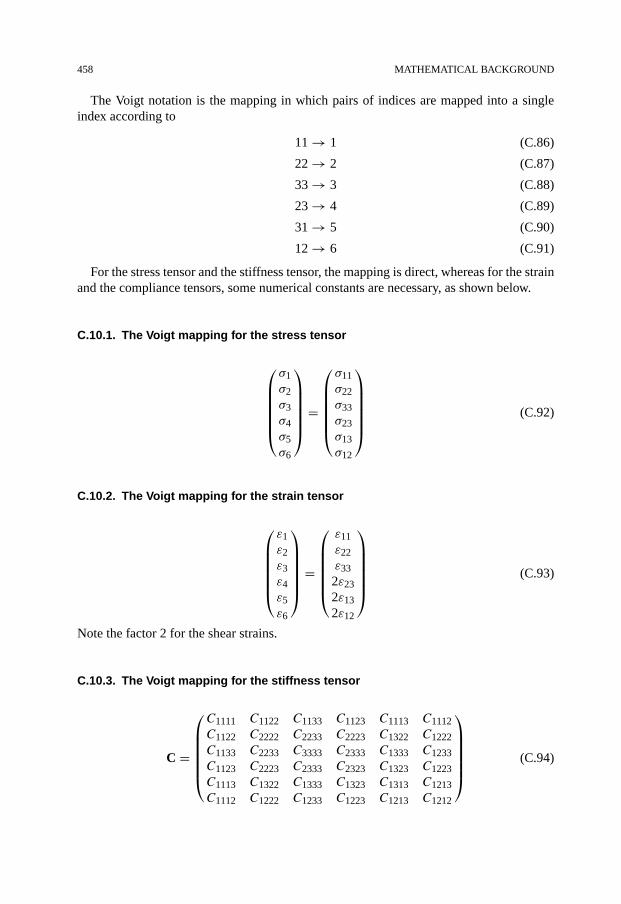
458 MATHEMATICAL BACKGROUND
The Voigt notation is the mapping in which pairs of indices are mapped into a singleindex according to
11 → 1 (C.86)
22 → 2 (C.87)
33 → 3 (C.88)
23 → 4 (C.89)
31 → 5 (C.90)
12 → 6 (C.91)
For the stress tensor and the stiffness tensor, the mapping is direct, whereas for the strainand the compliance tensors, some numerical constants are necessary, as shown below.
C.10.1. The Voigt mapping for the stress tensor
⎛⎜⎜⎜⎜⎜⎝
σ1σ2σ3σ4σ5σ6
⎞⎟⎟⎟⎟⎟⎠ =
⎛⎜⎜⎜⎜⎜⎝
σ11σ22σ33σ23σ13σ12
⎞⎟⎟⎟⎟⎟⎠ (C.92)
C.10.2. The Voigt mapping for the strain tensor
⎛⎜⎜⎜⎜⎜⎝
ε1ε2ε3ε4ε5ε6
⎞⎟⎟⎟⎟⎟⎠ =
⎛⎜⎜⎜⎜⎜⎝
ε11ε22ε332ε232ε132ε12
⎞⎟⎟⎟⎟⎟⎠ (C.93)
Note the factor 2 for the shear strains.
C.10.3. The Voigt mapping for the stiffness tensor
C =
⎛⎜⎜⎜⎜⎜⎝
C1111 C1122 C1133 C1123 C1113 C1112C1122 C2222 C2233 C2223 C1322 C1222C1133 C2233 C3333 C2333 C1333 C1233C1123 C2223 C2333 C2323 C1323 C1223C1113 C1322 C1333 C1323 C1313 C1213C1112 C1222 C1233 C1223 C1213 C1212
⎞⎟⎟⎟⎟⎟⎠ (C.94)
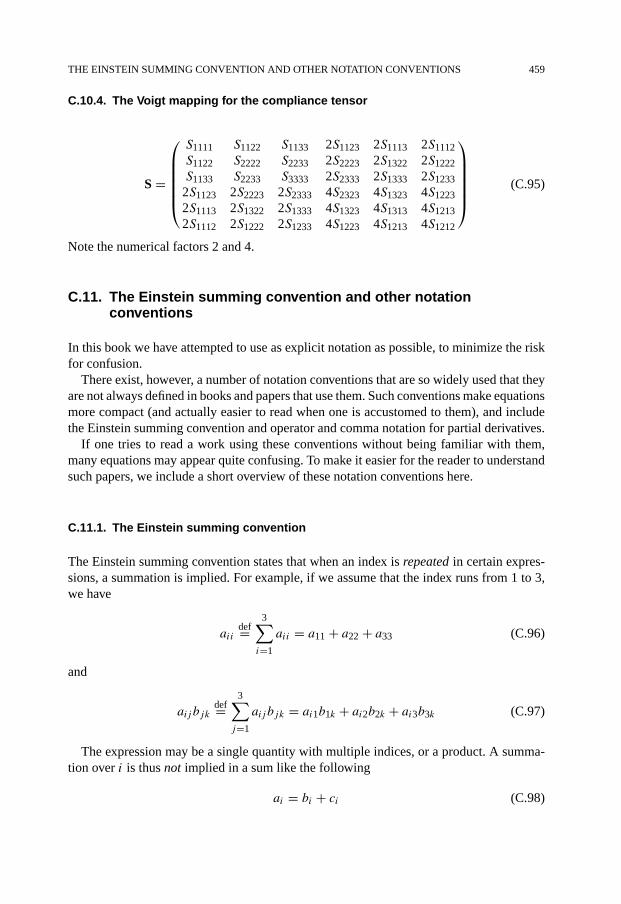
THE EINSTEIN SUMMING CONVENTION AND OTHER NOTATION CONVENTIONS 459
C.10.4. The Voigt mapping for the compliance tensor
S =
⎛⎜⎜⎜⎜⎜⎝
S1111 S1122 S1133 2S1123 2S1113 2S1112S1122 S2222 S2233 2S2223 2S1322 2S1222S1133 S2233 S3333 2S2333 2S1333 2S12332S1123 2S2223 2S2333 4S2323 4S1323 4S12232S1113 2S1322 2S1333 4S1323 4S1313 4S12132S1112 2S1222 2S1233 4S1223 4S1213 4S1212
⎞⎟⎟⎟⎟⎟⎠ (C.95)
Note the numerical factors 2 and 4.
C.11. The Einstein summing convention and other notationconventions
In this book we have attempted to use as explicit notation as possible, to minimize the riskfor confusion.
There exist, however, a number of notation conventions that are so widely used that theyare not always defined in books and papers that use them. Such conventions make equationsmore compact (and actually easier to read when one is accustomed to them), and includethe Einstein summing convention and operator and comma notation for partial derivatives.
If one tries to read a work using these conventions without being familiar with them,many equations may appear quite confusing. To make it easier for the reader to understandsuch papers, we include a short overview of these notation conventions here.
C.11.1. The Einstein summing convention
The Einstein summing convention states that when an index is repeated in certain expres-sions, a summation is implied. For example, if we assume that the index runs from 1 to 3,we have
aiidef=
3∑i=1
aii = a11 + a22 + a33 (C.96)
and
aij bjkdef=
3∑j=1
aij bjk = ai1b1k + ai2b2k + ai3b3k (C.97)
The expression may be a single quantity with multiple indices, or a product. A summa-tion over i is thus not implied in a sum like the following
ai = bi + ci (C.98)
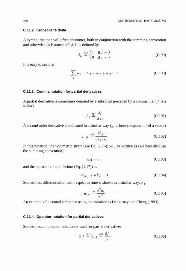
460 MATHEMATICAL BACKGROUND
C.11.2. Kronecker’s delta
A symbol that one will often encounter, both in conjunction with the summing conventionand otherwise, is Kronecker’s δ. It is defined by
δijdef=
{1 if i = j0 if i �= j (C.99)
It is easy to see that ∑i
δii = δ11 + δ22 + δ33 = 3 (C.100)
C.11.3. Comma notation for partial derivatives
A partial derivative is sometimes denoted by a subscript preceded by a comma, i.e. (f is ascalar)
f,jdef= ∂f
∂xj(C.101)
A second order derivative is indicated in a similar way (gi is here component i of a vector)
gi,jkdef= ∂2gi
∂xj ∂xk(C.102)
In this notation, the volumetric strain (see Eq. (1.76)) will be written as (we here also usethe summing convention)
εvol = ui,i (C.103)
and the equation of equilibrium (Eq. (1.17)) as
σji,j + ρXi = 0 (C.104)
Sometimes, differentiation with respect to time is shown in a similar way, e.g.
ui,ttdef= ∂2ui
∂t2(C.105)
An example of a central reference using this notation is Detournay and Cheng (1993).
C.11.4. Operator notation for partial derivatives
Sometimes, an operator notation is used for partial derivatives:
∂ifdef= ∂xi f
def= ∂f
∂xi(C.106)

REFERENCES 461
The volumetric strain becomes
εvol = ∂iui (C.107)
and the equation of equilibrium is
∂jσji + ρXi = 0 (C.108)
References
Detournay, E., Cheng, A.H.-D. (1993). “Fundamentals of poroelasticity”. In: Hudson, J.T. (Ed.), ComprehensiveRock Engineering. Pergamon Press, Oxford, pp. 113–171.
Helbig, K. (1994). Foundations of Anisotropy for Exploration Geophysicists. Pergamon, Oxford.Helbig, K. (1995). “Kelvin and the early history of seismic anisotropy”. In: Fjær, E., Holt, R.M., Rathore, J.S.
(Eds.), Seismic Anisotropy. Society of Exploration Geophysicists, pp. 15–36.Rose, M.E. (1957). Elementary Theory of Angular Momentum. John Wiley & Sons, New York.Voigt, W. (1910). Lehrbuch der Kristallphysik. Teubner, Leipzig.

This page intentionally left blank
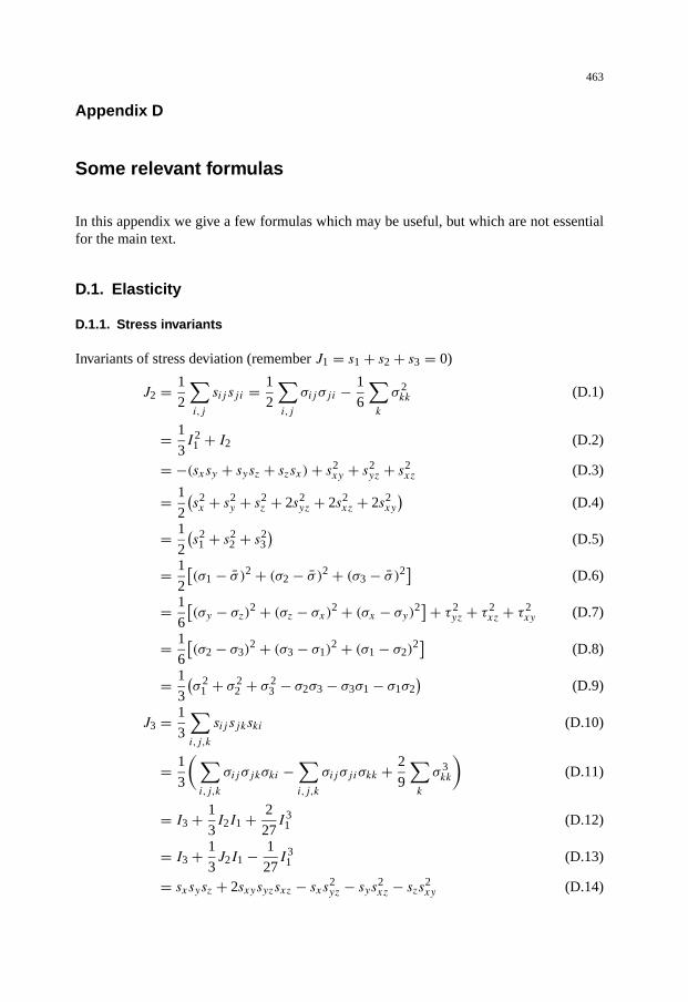
463
Appendix D
Some relevant formulas
In this appendix we give a few formulas which may be useful, but which are not essentialfor the main text.
D.1. Elasticity
D.1.1. Stress invariants
Invariants of stress deviation (remember J1 = s1 + s2 + s3 = 0)
J2 = 1
2
∑i,j
sij sji = 1
2
∑i,j
σij σji − 1
6
∑k
σ 2kk (D.1)
= 1
3I 2
1 + I2 (D.2)
= −(sxsy + sysz + szsx)+ s2xy + s2
yz + s2xz (D.3)
= 1
2
(s2x + s2
y + s2z + 2s2
yz + 2s2xz + 2s2
xy
)(D.4)
= 1
2
(s2
1 + s22 + s2
3
)(D.5)
= 1
2
[(σ1 − σ )2 + (σ2 − σ )2 + (σ3 − σ )2] (D.6)
= 1
6
[(σy − σz)2 + (σz − σx)2 + (σx − σy)2
]+ τ 2yz + τ 2
xz + τ 2xy (D.7)
= 1
6
[(σ2 − σ3)
2 + (σ3 − σ1)2 + (σ1 − σ2)
2] (D.8)
= 1
3
(σ 2
1 + σ 22 + σ 2
3 − σ2σ3 − σ3σ1 − σ1σ2)
(D.9)
J3 = 1
3
∑i,j,k
sij sjkski (D.10)
= 1
3
(∑i,j,k
σij σjkσki −∑i,j,k
σij σjiσkk + 2
9
∑k
σ 3kk
)(D.11)
= I3 + 1
3I2I1 + 2
27I 3
1 (D.12)
= I3 + 1
3J2I1 − 1
27I 3
1 (D.13)
= sxsysz + 2sxysyzsxz − sxs2yz − sys2
xz − szs2xy (D.14)

464 SOME RELEVANT FORMULAS
= 1
27
[54τxyτyzτxz (D.15)
+ 9τ 2xy(σx + σy − 2σz)− 9τ 2
yz(2σx − σy − σz) (D.16)
+ 9τ 2xz(σx − 2σy + σz) (D.17)
+ (σx + σy − 2σz)(2σx − σy − σz)(σx − 2σy + σz)]
(D.18)
= 1
3
(s3
1 + s32 + s3
3
)(D.19)
= s1s2s3 (D.20)
= (σ1 − σ )(σ2 − σ )(σ3 − σ ) (D.21)
= 1
27(σ1 + σ2 − 2σ3)(2σ1 − σ2 − σ3)(σ1 − 2σ2 + σ3) (D.22)
D.1.2. Strain in spherical coordinates
εr = ∂ur
∂r(D.23)
εθ = ur
r+ 1
r
∂uθ
∂θ(D.24)
εφ = 1
r sin θ
∂uφ
∂φ+ uθ
rcot θ + ur
r(D.25)
Γrθ = 1
2r
∂ur
∂θ+ 1
2
∂uθ
∂r− uθ
2r(D.26)
Γθφ = 1
2r
(∂uφ
∂θ− uφ cot θ
)+ 1
2r sin θ
∂uθ
∂φ(D.27)
Γφr = 1
2
(1
r sin θ
∂ur
∂φ+ ∂uφ
∂r− uφ
r
)(D.28)
D.1.3. Isotropic linear elastic stiffness tensor
Cijkl = λδij δkl +G(δikδjl + δilδjk) (D.29)
D.1.4. Isotropic linear poro-thermo-elastic stress strain law
Solved for stresses
σx = (λfr + 2Gfr)εx + λfrεy + λfrεz + αT (3λfr + 2Gfr)(T − T0)+ αpf (D.30)
= λfrεvol + 2Gfrεx + αT (3λfr + 2Gfr)(T − T0)+ αpf (D.31)
σy = λfrεx + (λ+ 2Gfr)εy + λfrεz + αT (3λfr + 2Gfr)(T − T0)+ αpf (D.32)
= λfrεvol + 2Gfrεy + αT (3λfr + 2Gfr)(T − T0)+ αpf (D.33)
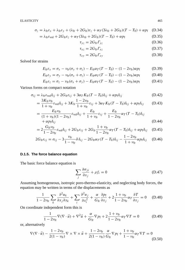
ELASTICITY 465
σz = λfrεx + λfrεy + (λfr + 2Gfr)εz + αT (3λfr + 2Gfr)(T − T0)+ αpf (D.34)
= λfrεvol + 2Gfrεz + αT (3λfr + 2Gfr)(T − T0)+ αpf (D.35)
τyz = 2GfrΓyz (D.36)
τxz = 2GfrΓxz (D.37)
τxy = 2GfrΓxy (D.38)
Solved for strains
Efrεx = σx − νfr(σy + σz)− EfrαT (T − T0)− (1 − 2νfr)αpf (D.39)
Efrεy = σy − νfr(σx + σz)− EfrαT (T − T0)− (1 − 2νfr)αpf (D.40)
Efrεz = σz − νfr(σx + σy)− EfrαT (T − T0)− (1 − 2νfr)αpf (D.41)
Various forms on compact notation
σij = λfrεvolδij + 2Gfrεij + 3αT Kfr(T − T0)δij + αpfδij (D.42)
= 3Kfrνfr
1 + νfrεvolδij + 3Kfr
1 − 2νfr
1 + νfrεij + 3αT Kfr(T − T0)δij + αpfδij (D.43)
= Efrνfr
(1 + νfr)(1 − 2νfr)εvolδij + Efr
1 + νfrεij + Efr
1 − 2νfrαT (T − T0)δij
+ αpfδij (D.44)
= 2Gfrνfr
1 − 2νfrεvolδij + 2Gfrεij + 2Gfr
1 + νfr
1 − 2νfrαT (T − T0)δij + αpfδij (D.45)
2Gfrεij = σij − 3νfr
1 − νfrσ δij − 2GfrαT (T − T0)δij − 1 − 2νfr
1 + νfrαpfδij (D.46)
D.1.5. The force balance equation
The basic force balance equation is∑j
∂σji
∂xj+ ρfi = 0 (D.47)
Assuming homogeneous, isotropic poro-thermo-elasticity, and neglecting body forces, theequation may be written in terms of the displacements as
1
1 − 2νfr
∑k
∂2uk
∂xj ∂xk+∑i
∂2uj
∂x2i
+ α
Gfr
∂pf
∂xj+ 2
1 + νfr
1 − 2νfrαT∂T
∂xj= 0 (D.48)
On coordinate independent form this is
1
1 − 2νfr∇(∇ · �u)+ ∇2 �u+ α
Gfr∇pf + 2
1 + νfr
1 − 2νfrαT∇T = 0 (D.49)
or, alternatively
∇(∇ · �u)− 1 − 2νfr
2(1 − νfr)∇ × ∇ × �u+ 1 − 2νfr
2(1 − νfr)
α
Gfr∇pf + 1 + νfr
1 − νfrαT∇T = 0
(D.50)
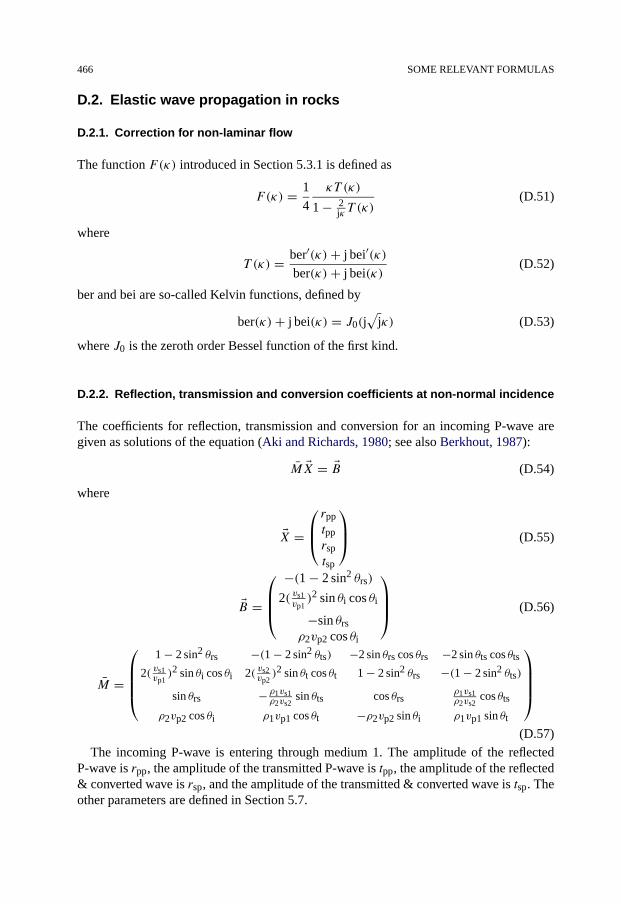
466 SOME RELEVANT FORMULAS
D.2. Elastic wave propagation in rocks
D.2.1. Correction for non-laminar flow
The function F(κ) introduced in Section 5.3.1 is defined as
F(κ) = 1
4
κT (κ)
1 − 2jκ T (κ)
(D.51)
where
T (κ) = ber′(κ)+ j bei′(κ)ber(κ)+ j bei(κ)
(D.52)
ber and bei are so-called Kelvin functions, defined by
ber(κ)+ j bei(κ) = J0(j√
jκ) (D.53)
where J0 is the zeroth order Bessel function of the first kind.
D.2.2. Reflection, transmission and conversion coefficients at non-normal incidence
The coefficients for reflection, transmission and conversion for an incoming P-wave aregiven as solutions of the equation (Aki and Richards, 1980; see also Berkhout, 1987):
M �X = �B (D.54)
where
�X =⎛⎜⎝rpptpprsptsp
⎞⎟⎠ (D.55)
�B =
⎛⎜⎜⎝
−(1 − 2 sin2 θrs)
2( vs1vp1)2 sin θi cos θi
−sin θrsρ2vp2 cos θi
⎞⎟⎟⎠ (D.56)
M =
⎛⎜⎜⎜⎝
1 − 2 sin2 θrs −(1 − 2 sin2 θts) −2 sin θrs cos θrs −2 sin θts cos θts
2( vs1vp1)2 sin θi cos θi 2( vs2
vp2)2 sin θt cos θt 1 − 2 sin2 θrs −(1 − 2 sin2 θts)
sin θrs −ρ1vs1ρ2vs2
sin θts cos θrsρ1vs1ρ2vs2
cos θts
ρ2vp2 cos θi ρ1vp1 cos θt −ρ2vp2 sin θi ρ1vp1 sin θt
⎞⎟⎟⎟⎠
(D.57)
The incoming P-wave is entering through medium 1. The amplitude of the reflectedP-wave is rpp, the amplitude of the transmitted P-wave is tpp, the amplitude of the reflected& converted wave is rsp, and the amplitude of the transmitted & converted wave is tsp. Theother parameters are defined in Section 5.7.

ROCK MODELS 467
Fig. D.1. The three modes of loading for a crack tip.
D.3. Rock models
D.3.1. Stresses at a crack tip
A crack tip may experience three types of loading, commonly denoted Mode I (opening),Mode II (in-plane shear) and Mode III (out-of-plane shear), respectively. The three loadingmodes are illustrated in Fig. D.1.
For an elliptical crack, the stresses at the crack tip can be expressed as
σij = KM√2πr
f(M)ij (θ) (D.58)
where M = I, II or III, and KM represents the stress intensity factor of mode M . KM de-pends on the farfield stress and the crack length (as shown in Eq. (6.64) for KI).
The functions f (M)ij (θ) define the angular dependence of the stress at the crack tip forMode M . The angle θ , the distance r and the coordinate axes are defined in Fig. 6.10.Axis 3 is the out-of-plane axis. The non-zero components of f (M)ij (θ) are:
• Mode I
f(I)11 (θ) = cos
θ
2
[1 − sin
θ
2sin
3θ
2
](D.59)
f(I)22 (θ) = cos
θ
2
[1 + sin
θ
2sin
3θ
2
](D.60)
f(I)12 (θ) = cos
θ
2sinθ
2cos
3θ
2(D.61)
For plane strain conditions f (I)33 (θ) = ν(f(I)11 (θ) + f (I)22 (θ)), while for plane stress
conditions f (I)33 (θ) = 0. (ν is the Poisson ratio.)
• Mode II
f(II)11 (θ) = −sin
θ
2
[2 + cos
θ
2cos
3θ
2
](D.62)
f(II)22 (θ) = sin
θ
2cosθ
2cos
3θ
2(D.63)
f(II)12 (θ) = cos
θ
2
[1 − sin
θ
2sin
3θ
2
](D.64)

468 SOME RELEVANT FORMULAS
For plane strain conditions f (II)33 (θ) = ν(f(II)11 (θ) + f (II)22 (θ)), while for plane stress
conditions f (II)33 (θ) = 0.
• Mode III
f(III)13 (θ) = −sin
θ
2(D.65)
f(III)23 (θ) = cos
θ
2(D.66)
For a more comprehensive description, see for instance Anderson (2005).
D.3.2. Self-consistent model for composite media
Berryman (1980) introduced self consistency into the dynamic theory of Kuster and Toksöz(1974), and derived the following set of implicit equations for the effective moduli:
N∑i=1
ci(Ki −K∗)P ∗i = 0 (D.67)
N∑i=1
ci(Gi −G∗)Q∗i = 0 (D.68)
N∑i=1
ci(ρi − ρ∗) = 0 (D.69)
ci is the volumetric concentration of component i in the material, ρ∗ is the total density,and the coefficients P ∗i andQ∗i are given as follows:
For spherical inclusions
P ∗i = 3K∗ + 4G∗
3Ki + 4G∗ (D.70)
Q∗i = G∗ + F ∗
Gi + F ∗ (D.71)
where
F ∗ = G∗(9K∗ + 8G∗)6(K∗ + 2G∗)
(D.72)
For penny-shaped inclusions (resembling for instance flat cracks)
P ∗i = 3K∗ + 4Gi3Ki + 4Gi + 3πγβ∗ (D.73)
Q∗i = 1
5
[1 + 8G∗
4Gi + πγ (G∗ + 2β∗)+ 2
3Ki + 2Gi + 2G∗
3Ki + 4Gi + 3πγβ∗
](D.74)

SOLIDS PRODUCTION 469
where
β∗ = G∗(3K∗ +G∗)3K∗ + 4G∗ (D.75)
While the solution for ρ∗ is trivial, explicit solutions for K∗ and G∗ are not known, how-ever solutions can be found by numerical iteration.
These solutions approach the linear solutions given in Section 6.4.1 for low concentra-tions of inclusions. Berryman also showed that if the material contains non-solid inclu-sions, the effective shear modulus vanish at a critical concentration of that inclusion. Thecritical concentration depends on the shape of the inclusions.
D.4. Solids production
D.4.1. Critical drawdown for turbulent flow
The critical drawdown for a semispherical sand arch in a non-Darcy flow regime is givenon implicit form as (Ong et al., 2000):
S1 + 3S2
m+ 1(qa)
− mm+1 = 4 sinϕ
1 − sinϕ(D.76)
where
S1 = 2(√
1 + hs(qb − qa)− 1)
hs(1 − RcRe)
(D.77)
S2 = (√
1 + hs(qb − qa)− 1)2
hs(1 − (RcRe)3)
(D.78)
hs = 4k2βγ (1 − (RcRe)3)
3Rc(m+ 1)(ηf(1 − RcRe))2
(S0
tanϕ
)m+1
(D.79)
qa =((pfo − pc
d) tanϕ
S0
)m+1
(D.80)
qb =(pfo tanϕ
S0
)m+1
(D.81)
and Re is the radius of the drainage area. Eq. (D.76) is derived from the assumption thatthe fluid flow follows the Forchheimer equation (Forchheimer, 1901):
−∇pf = ηfQ
kA+ βρf
(Q
A
)2
(D.82)
where the non-Darcy flow coefficient β is a constant of dimension m−1. For β = 0Eq. (D.82) is reduced to the Darcy equation (Eq. (1.229)), and Eq. (D.76) is reduced toEq. (10.37).

470 SOME RELEVANT FORMULAS
D.5. Subsidence
Geertsma’s formulas for the deformation and stress fields outside a disk-shaped reservoir.
ur = CmRh�pf
2
[I1(|z−D|)+ (3 − 4ν)I1(z+D)− 2zI2(z+D)] (D.83)
uz = CmRh�pf
2
[z−D|z−D| I3
(|z−D|)− (3 − 4ν)I3(z+D)− 2zI4(z+D)]
(D.84)
σr = GCmRh�pf
{[I4(|z−D|)+ 3I4(z+D)− 2zI6(z+D)]
− 1
r
[I1(|z−D|)+ (3 − 4ν)I1(z+D)− 2zI2(z+D)]} (D.85)
σθ = GCmRh�pf
{4νI4(z+D)
+ 1
r
[I1(|z−D|)+ (3 − 4ν)I1(z+D)− 2zI2(z+D)]} (D.86)
σz = GCmRh�pf[−I4
(|z−D|)+ I4(z+D)+ 2zI6(z+D)] (D.87)
τrz = GCmRh�pf
[− z−D
|z−D| I2(|z−D|)− I2(z+D)+ zI7(z+D)
](D.88)
where
I1(q) = 2
π√mrR
[(1 − m
2
)K(m)− E(m)
](D.89)
I2(q) = q√m
2π(rR)3/2
[1 − m
2
1 −mE(m)−K(m)]
(D.90)
I3(q) = −q√mK(m)
2π√rRR
+ (U(r − R)− U(R − r))Λ0(β|m)
2R+ 1
RU(R − r) (D.91)
I4(q) = m3/2(R2 − r2 − q2)E(m)
8π(rR)3/2R(1 −m) +√mK(m)
2π√rRR
(D.92)
I6(q) = qm3/2
8πR(1 −m)(rR)3/2
×{
3E(m)+mR2 − r2 − q2
rR
[1 − m
2
1 −mE(m)−1
4K(m)
]}(D.93)
I7(q) = − 1
qI2(q)+ q2m3/2
8π(1 −m)(rR)5/2
×[
1 −m+m2
1 −m E(m)−(
1 − 1
2m
)K(m)
](D.94)
Λ0(β|m) = 2
π
[E(m)F(β|1 −m)+K(m)E(β|1 −m)−K(m)F(β|1 −m)]

VECTOR OPERATORS IN CYLINDRICAL COORDINATES 471
TABLE D.1 Some values for the Geertsma integrals Ii (q)
r , q, R I1 I2 I3 I4 I6 I7
0.2, 0.4, 1.2 0.0595689 0.0461035 0.565282 0.598431 0.477736 −0.05443870.4, 0.4, 1 0.162188 0.197103 0.592418 0.818683 1.15435 −0.0445251
m = 4Rr
q2 + (r + R)2sinβ = q√
q2 + (R − r)2F(α|m) and E(α|m) are elliptic integrals of the first and second kind of parameter m,respectively. K(m) = F(π2 |m) and E(m) = E(π2 |m) are complete elliptic integrals of thefirst and second kind. U is the unit step function, U(x � 0) = 1, U(x < 0) = 0. Λ0(β|m)is called Heuman’s lambda function. Λ0(
π2 |m) = 1.
When working with elliptic integrals, it is important to be aware that there exist manydifferent conventions for the definitions of the arguments, even for the order of the argu-ments. In the convention used here, the integrals are given by
F(α|m) =∫ α
0
1√1 +m sin2 θ
dθ (D.95)
and
E(α|m) =∫ α
0
√1 +m sin2 θ dθ (D.96)
The elliptic integrals are available in modern integrated mathematics computer pro-grams, like Maple or Mathematica and others. Given the availability of such a program,it is an easy and quick task to code and study the consequences of Geertsma’s equations.
In Table D.1 we give some numerical values for the integrals, to make it easy to checkan implementation. Full tables of the integrals are found in Geertsma (1973).
D.6. Vector operators in cylindrical coordinates
The gradient of a scalar
∇f = ∂f
∂r�er + 1
r
∂f
∂θ�eθ + ∂f
∂z�ez (D.97)
The Laplacian of a scalar
∇2f = 1
r
∂f
∂r+ ∂2f
∂r2+ 1
r2
∂2f
∂θ2+ ∂2f
∂z2(D.98)
= 1
r
∂
∂rr∂f
∂r+ 1
r2
∂2f
∂θ2+ ∂2f
∂z2(D.99)
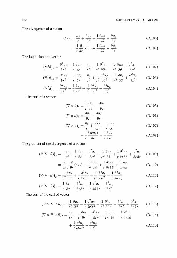
472 SOME RELEVANT FORMULAS
The divergence of a vector
∇ · �u = ur
r+ ∂ur
∂r+ 1
r
∂uθ
∂θ+ ∂uz
∂z(D.100)
= 1
r
∂
∂r(rur)+ 1
r
∂uθ
∂θ+ ∂uz
∂z(D.101)
The Laplacian of a vector
(∇2 �u)r
= ∂2ur
∂r2+ 1
r
∂ur
∂r− ur
r2+ 1
r2
∂2ur
∂θ2− 2
r2
∂uθ
∂θ+ ∂2ur
∂z2(D.102)
(∇2 �u)θ
= ∂2uθ
∂r2+ 1
r
∂uθ
∂r− uθ
r2+ 1
r2
∂2uθ
∂θ2+ 2
r2
∂ur
∂θ+ ∂2uθ
∂z2(D.103)
(∇2 �u)z
= ∂2uz
∂r2+ 1
r
∂uz
∂r+ 1
r2
∂2uz
∂θ2+ ∂2uz
∂z2(D.104)
The curl of a vector
(∇ × �u)r = 1
r
∂uz
∂θ− ∂uθ
∂z(D.105)
(∇ × �u)θ = ∂ur
∂z− ∂uz
∂r(D.106)
(∇ × �u)z = uθ
r+ ∂uθ
∂r− 1
r
∂ur
∂θ(D.107)
= 1
r
∂(ruθ )
∂r− 1
r
∂ur
∂θ(D.108)
The gradient of the divergence of a vector
(∇(∇ · �u))r
= −urr2
+ 1
r
∂ur
∂r+ ∂2ur
∂r2− 1
r2
∂uθ
∂θ+ 1
r
∂2uθ
∂r∂θ+ ∂2uz
∂r∂z(D.109)
= ∂
∂r
1
r
∂
∂r(rur)− 1
r2
∂uθ
∂θ+ 1
r
∂2uθ
∂r∂θ+ ∂2uz
∂r∂z(D.110)
(∇(∇ · �u))θ
= 1
r2
∂ur
∂θ+ 1
r
∂2ur
∂r∂θ+ 1
r2
∂2uθ
∂θ2+ 1
r
∂2uz
∂θ∂z(D.111)
(∇(∇ · �u))z
= 1
r
∂ur
∂z+ ∂2ur
∂r∂z+ 1
r
∂2uθ
∂θ∂z+ ∂2uz
∂z2(D.112)
The curl of the curl of vector
(∇ × ∇ × �u)r = 1
r2
∂uθ
∂θ+ 1
r
∂2uθ
∂r∂θ− 1
r2
∂2ur
∂θ2− ∂2ur
∂z2+ ∂2uz
∂r∂z(D.113)
(∇ × ∇ × �u)θ = uθ
r2− 1
r
∂uθ
∂r− ∂2uθ
∂r2− 1
r2
∂ur
∂θ+ 1
r
∂2ur
∂r∂θ(D.114)
+ 1
r
∂2uz
∂θ∂z− ∂2uθ
∂z2(D.115)

REFERENCES 473
(∇ × ∇ × �u)z = 1
r
∂ur
∂z+ ∂2ur
∂r∂z− 1
r
∂uz
∂r− ∂2uz
∂r2(D.116)
− 1
r2
∂2uz
∂θ2+ 1
r
∂2uθ
∂θ∂z(D.117)
References
Aki, K., Richards, P.G. (1980). Quantitative Seismology. W.H. Freeman and Co., New York.Anderson, T.L. (2005). Fracture Mechanics. Fundamentals and Applications, second ed. CRC Press, Boca Raton.Berkhout, A.J. (1987). Applied Seismic Wave Theory. Elsevier, Amsterdam.Berryman, J.G. (1980). “Long-wavelength propagation in composite elastic media. II. Ellipsoidal inclusions”.
J. Acoust. Soc. Am. 68, 1820–1831.Forchheimer, P. (1901). “Wasserbewegung durch Boden”. Zeit. Ver. Deut. Ing. 45, 1782–1788.Geertsma, J. (1973). “A basic theory of subsidence due to reservoir compaction: The homogeneous case”. Ver-
handelingen Kon. Ned. Geol. Mijnbouwk. Gen. 28, 43–62.Kuster, G.T., Toksöz, M.N. (1974). “Velocity and attenuation of seismic waves in two-phase media: Part I. The-
oretical formulations”. Geophysics 39, 587–606.Ong, S., Ramos, G.G., Zheng, Z. (2000). “Sand production prediction in high rate, perforated and open-hole
gas wells”. SPE 58721. In: SPE International Symposium on Formation Damage Control, Lafayette, LA,February 23–24.

This page intentionally left blank
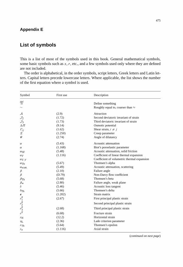
475
Appendix E
List of symbols
This is a list of most of the symbols used in this book. General mathematical symbols,some basic symbols such as x, r , etc., and a few symbols used only where they are definedare not included.
The order is alphabetical, in the order symbols, script letters, Greek letters and Latin let-ters. Capital letters precede lowercase letters. Where applicable, the list shows the numberof the first equation where a symbol is used.
Symbol First use Description
def= Define something∼ Roughly equal to, coarser than ≈A (2.9) AttractionJ2 (1.72) Second deviatoric invariant of strainJ3 (1.73) Third deviatoric invariant of strain�Π (9.14) Osmotic potentialΓij (1.62) Shear strain, i �= jΣ (1.250) Creep parameterΨ (2.74) Angle of dilatancy
α (5.43) Acoustic attenuationα (1.168) Biot’s poroelastic parameterαSF (5.48) Acoustic attenuation, solid frictionαT (1.116) Coefficient of linear thermal expansionαT,V Coefficient of volumetric thermal expansionαTh (5.67) Thomsen’s alphaαscatt. (5.49) Acoustic attenuation, scatteringβ (2.10) Failure angleβ (D.79) Non-Darcy flow coefficientβTh (5.68) Thomsen’s betaβw (2.80) Failure angle, weak planeδ (5.46) Acoustic loss tangentδTh (5.66) Thomsen’s deltaε (1.202) Strain matrixε
p1 (2.67) First principal plastic strain
εp2 Second principal plastic strain
εp3 (2.68) Third principal plastic strain
εF (6.68) Fracture strainεH (12.2) Horizontal strainηL (2.36) Lade criterion parameterεTh (5.64) Thomsen’s epsilonεa (1.116) Axial strain
(continued on next page)
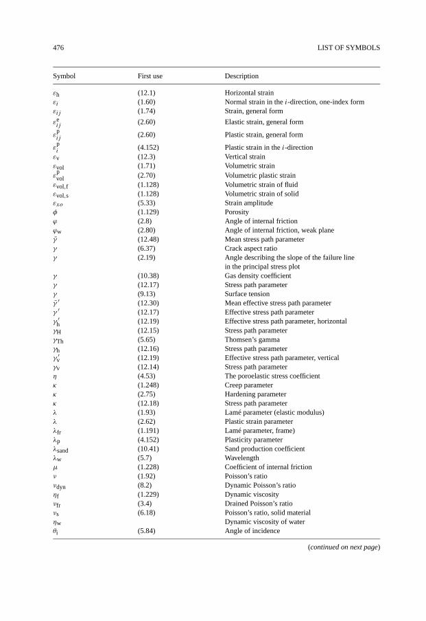
476 LIST OF SYMBOLS
Symbol First use Description
εh (12.1) Horizontal strainεi (1.60) Normal strain in the i-direction, one-index formεij (1.74) Strain, general form
εeij
(2.60) Elastic strain, general form
εpij
(2.60) Plastic strain, general form
εpi
(4.152) Plastic strain in the i-directionεv (12.3) Vertical strainεvol (1.71) Volumetric strainε
pvol (2.70) Volumetric plastic strainεvol,f (1.128) Volumetric strain of fluidεvol,s (1.128) Volumetric strain of solidεxo (5.33) Strain amplitudeφ (1.129) Porosityϕ (2.8) Angle of internal frictionϕw (2.80) Angle of internal friction, weak planeγ (12.48) Mean stress path parameterγ (6.37) Crack aspect ratioγ (2.19) Angle describing the slope of the failure line
in the principal stress plotγ (10.38) Gas density coefficientγ (12.17) Stress path parameterγ (9.13) Surface tensionγ ′ (12.30) Mean effective stress path parameterγ ′ (12.17) Effective stress path parameterγ ′
h (12.19) Effective stress path parameter, horizontalγH (12.15) Stress path parameterγTh (5.65) Thomsen’s gammaγh (12.16) Stress path parameterγ ′
v (12.19) Effective stress path parameter, verticalγv (12.14) Stress path parameterη (4.53) The poroelastic stress coefficientκ (1.248) Creep parameterκ (2.75) Hardening parameterκ (12.18) Stress path parameterλ (1.93) Lamé parameter (elastic modulus)λ (2.62) Plastic strain parameterλfr (1.191) Lamé parameter, frame)λp (4.152) Plasticity parameterλsand (10.41) Sand production coefficientλw (5.7) Wavelengthμ (1.228) Coefficient of internal frictionν (1.92) Poisson’s ratioνdyn (8.2) Dynamic Poisson’s ratioηf (1.229) Dynamic viscosityνfr (3.4) Drained Poisson’s ratioνs (6.18) Poisson’s ratio, solid materialηw Dynamic viscosity of waterθi (5.84) Angle of incidence
(continued on next page)

LIST OF SYMBOLS 477
Symbol First use Description
θr Angle of reflectionθrs (5.86) Angle of “reflected” s-waveθt (5.84) Angle of refracted p-waveθts (5.87) Angle of “refracted” s-waveϑ (1.51) The Lode angleρ (1.13) Densityρdry (12.67) Density of dry rockρf (5.27) Density, fluidρg (5.74) Density of gasρs (5.27) Density, solid materialρw (5.92) Density of borehole fluidρw (5.74) Density of waterσ (1.38) Mean stressσ (9.18) Membrane efficiencyσ (1.3) Normal stressσ (1.202) Stress matrixσ ′ (2.2) Effective stressσi (1.5) Normal stress in i-direction, i = x, y, z, r, θ, φσ ′i
(3.9) Effective normal stress in i-direction,i = x, y, z, r, θ, φ
σij (1.118) Stress in ij -direction
σ ′ij
(1.170) Effective stress in ij -direction
σ ′ (2.28) Mean effective stressσ ′
1 (2.1) Major effective principal stressσ ′
2 (2.1) Intermediate effective principal stress
σ ′3 (2.1) Minor effective principal stress
σ ′v (3.3) Effective vertical stress
σθ i (7.15) Hollow cylinder inner tang. stressσθ,max (4.105) Tangential stress, maxσθ,min (4.106) Tangential stress, minσ1 (1.23) Major principal stressσ2 (1.24) Intermediate principal stressσ3 (1.36) Minor principal stressσH (3.14) Major horizontal principal stressσ ′
H (9.3) Effective major horizontal principal stressσa (1.117) Axial stressσ ′
h (3.3) Effective minor horizontal principal stressσh (3.8) Minor horizontal principal stressσ ′
max⊥ (9.8) Effective maximum stress normal to boreholeσ ′
min⊥ (9.8) Effective minimum stress normal to boreholeσ oi
(4.77) Farfield stress in the i-directionσo (4.174) Hydrostatic far-field stressσoct (1.52) Octahedral normal stressσ ′‖ (9.9) Effective stress parallel to borehole axis
σ ′p (1.168) Effective external hydrostatic stressσp (1.99) External hydrostatic stressσri (7.16) Hollow cylinder inner radial stress
(continued on next page)
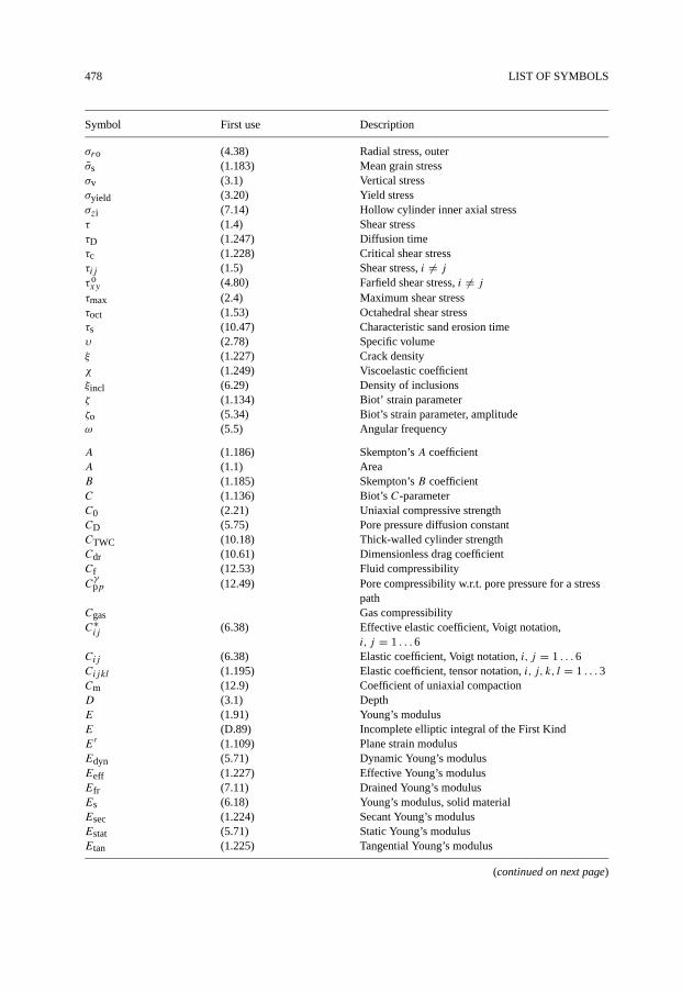
478 LIST OF SYMBOLS
Symbol First use Description
σro (4.38) Radial stress, outerσs (1.183) Mean grain stressσv (3.1) Vertical stressσyield (3.20) Yield stressσzi (7.14) Hollow cylinder inner axial stressτ (1.4) Shear stressτD (1.247) Diffusion timeτc (1.228) Critical shear stressτij (1.5) Shear stress, i �= jτoxy (4.80) Farfield shear stress, i �= jτmax (2.4) Maximum shear stressτoct (1.53) Octahedral shear stressτs (10.47) Characteristic sand erosion timeυ (2.78) Specific volumeξ (1.227) Crack densityχ (1.249) Viscoelastic coefficientξincl (6.29) Density of inclusionsζ (1.134) Biot’ strain parameterζo (5.34) Biot’s strain parameter, amplitudeω (5.5) Angular frequency
A (1.186) Skempton’s A coefficientA (1.1) AreaB (1.185) Skempton’s B coefficientC (1.136) Biot’s C-parameterC0 (2.21) Uniaxial compressive strengthCD (5.75) Pore pressure diffusion constantCTWC (10.18) Thick-walled cylinder strengthCdr (10.61) Dimensionless drag coefficientCf (12.53) Fluid compressibilityCγpp (12.49) Pore compressibility w.r.t. pore pressure for a stress
pathCgas Gas compressibilityC∗ij
(6.38) Effective elastic coefficient, Voigt notation,i, j = 1 . . . 6
Cij (6.38) Elastic coefficient, Voigt notation, i, j = 1 . . . 6Cijkl (1.195) Elastic coefficient, tensor notation, i, j, k, l = 1 . . . 3Cm (12.9) Coefficient of uniaxial compactionD (3.1) DepthE (1.91) Young’s modulusE (D.89) Incomplete elliptic integral of the First KindE′ (1.109) Plane strain modulusEdyn (5.71) Dynamic Young’s modulusEeff (1.227) Effective Young’s modulusEfr (7.11) Drained Young’s modulusEs (6.18) Young’s modulus, solid materialEsec (1.224) Secant Young’s modulusEstat (5.71) Static Young’s modulusEtan (1.225) Tangential Young’s modulus
(continued on next page)

LIST OF SYMBOLS 479
Symbol First use Description
F (D.95) Elliptic integral of the Second KindF (1.1) ForceFd (10.61) Drag forceFg (10.60) Net gravity forceFh (10.3) Hydrodynamic force on a grainFn (1.3) Normal forceFp (1.4) Parallel forceFr (10.1) Force needed to remove a grain from the rockG (1.93) Shear modulusGfr (1.147) Shear modulus of the frameGs (6.17) Shear modulus, solid materialH (3.19) Uniaxial compaction modulusHfr (1.239) Drained uniaxial compaction modulusI1 (1.39) 1. invariant of stressI ′1 (2.36) 1. invariant of effective stressI2 (1.41) 2. invariant of stressI3 (1.41) 3. invariant of stressI ′3 (2.36) 3. invariant of effective stressJ1 (1.43) 1. deviatoric invariant of stressJ2 (1.45) 2. deviatoric invariant of stressJ3 (1.45) 3. deviatoric invariant of stressJCS (6.74) Wall strengthJRC (6.74) Joint roughness coefficientK (1.99) Bulk modulusK (D.89) Elliptic integral of the First KindK ′ (3.3) Principal stress ratioKI (6.63) Stress intensity factor, mode IKIC Fracture toughnessKbp (1.172) Bulk modulus with respect to pore pressureKdyn (5.70) Dynamic bulk modulusKeff (1.127) Effective bulk modulusKf (1.131) Bulk modulus, fluidKfr (1.146) Drained bulk modulusKg (5.73) Bulk modulus of gasKo (3.21) Compaction modulusKp (1.177) Inverse pore compressibility w.r.t. confining pressureKpp (1.178) Inverse pore compressibility w.r.t. pore pressureKs (1.131) Bulk modulus, solid materialKstat (5.70) Static bulk modulusKu (7.10) Undrained bulk modulusKw (5.73) Bulk modulus of waterM (1.142) Biot’sM-parameterMT
sand (10.59) Total mass of produced sand in one eventMo
sand (10.57) Initial mass of removed sandMsand (10.51) Sand production rateMsand (10.51) Total mass of produced sandNc (6.23) Coordination numberpc
d (10.7) Critical drawdown pressureQ (4.177) Flow rate (scalar)
(continued on next page)
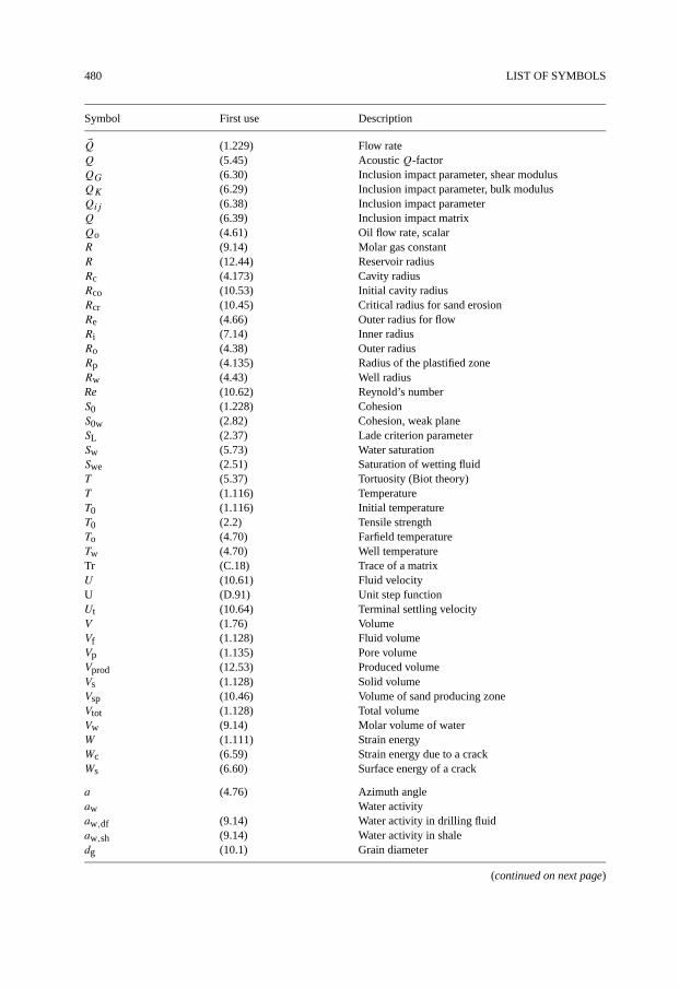
480 LIST OF SYMBOLS
Symbol First use Description
�Q (1.229) Flow rateQ (5.45) AcousticQ-factorQG (6.30) Inclusion impact parameter, shear modulusQK (6.29) Inclusion impact parameter, bulk modulusQij (6.38) Inclusion impact parameterQ (6.39) Inclusion impact matrixQo (4.61) Oil flow rate, scalarR (9.14) Molar gas constantR (12.44) Reservoir radiusRc (4.173) Cavity radiusRco (10.53) Initial cavity radiusRcr (10.45) Critical radius for sand erosionRe (4.66) Outer radius for flowRi (7.14) Inner radiusRo (4.38) Outer radiusRp (4.135) Radius of the plastified zoneRw (4.43) Well radiusRe (10.62) Reynold’s numberS0 (1.228) CohesionS0w (2.82) Cohesion, weak planeSL (2.37) Lade criterion parameterSw (5.73) Water saturationSwe (2.51) Saturation of wetting fluidT (5.37) Tortuosity (Biot theory)T (1.116) TemperatureT0 (1.116) Initial temperatureT0 (2.2) Tensile strengthTo (4.70) Farfield temperatureTw (4.70) Well temperatureTr (C.18) Trace of a matrixU (10.61) Fluid velocityU (D.91) Unit step functionUt (10.64) Terminal settling velocityV (1.76) VolumeVf (1.128) Fluid volumeVp (1.135) Pore volumeVprod (12.53) Produced volumeVs (1.128) Solid volumeVsp (10.46) Volume of sand producing zoneVtot (1.128) Total volumeVw (9.14) Molar volume of waterW (1.111) Strain energyWc (6.59) Strain energy due to a crackWs (6.60) Surface energy of a crack
a (4.76) Azimuth angleaw Water activityaw,df (9.14) Water activity in drilling fluidaw,sh (9.14) Water activity in shaledg (10.1) Grain diameter
(continued on next page)
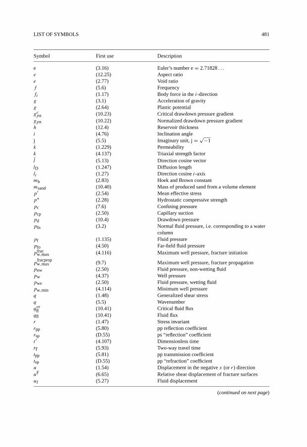
LIST OF SYMBOLS 481
Symbol First use Description
e (3.16) Euler’s number e = 2.71828 . . .e (12.25) Aspect ratioe (2.77) Void ratiof (5.6) Frequencyfi (1.17) Body force in the i-directiong (3.1) Acceleration of gravityg (2.64) Plastic potentialgcpn (10.23) Critical drawdown pressure gradientgpn (10.22) Normalized drawdown pressure gradienth (12.4) Reservoir thicknessi (4.76) Inclination anglej (5.5) Imaginary unit, j = √−1k (1.229) Permeabilityk (4.137) Triaxial strength factorl (5.13) Direction cosine vectorlD (1.247) Diffusion lengthli (1.27) Direction cosine i-axismb (2.83) Hoek and Brown constantmsand (10.40) Mass of produced sand from a volume elementp′ (2.54) Mean effective stressp∗ (2.28) Hydrostatic compressive strengthpc (7.6) Confining pressurepcp (2.50) Capillary suctionpd (10.4) Drawdown pressurepfn (3.2) Normal fluid pressure, i.e. corresponding to a water
columnpf (1.135) Fluid pressurepfo (4.50) Far-field fluid pressurepfrac
w,max (4.116) Maximum well pressure, fracture initiation
pfracpropw,max (9.7) Maximum well pressure, fracture propagationpnw (2.50) Fluid pressure, non-wetting fluidpw (4.37) Well pressurepwe (2.50) Fluid pressure, wetting fluidpw,min (4.114) Minimum well pressureq (1.48) Generalized shear stressq (5.5) Wavenumberqcr
fl (10.41) Critical fluid fluxqfl (10.41) Fluid fluxr (1.47) Stress invariantrpp (5.80) pp reflection coefficientrsp (D.55) ps “reflection” coefficientt ′ (4.107) Dimensionless timetT (5.93) Two-way travel timetpp (5.81) pp transmission coefficienttsp (D.55) pp “refraction” coefficientu (1.54) Displacement in the negative x (or r) directionuF (6.65) Relative shear displacement of fracture surfacesuf (5.27) Fluid displacement
(continued on next page)
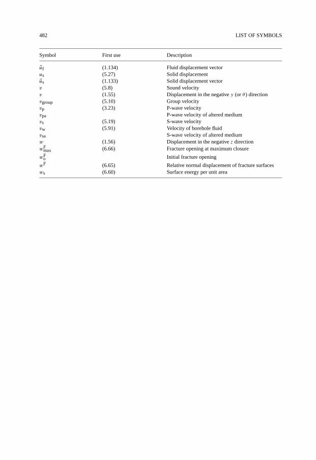
482 LIST OF SYMBOLS
Symbol First use Description
�uf (1.134) Fluid displacement vectorus (5.27) Solid displacement�us (1.133) Solid displacement vectorv (5.8) Sound velocityv (1.55) Displacement in the negative y (or θ ) directionvgroup (5.10) Group velocityvp (3.23) P-wave velocityvpa P-wave velocity of altered mediumvs (5.19) S-wave velocityvw (5.91) Velocity of borehole fluidvsa S-wave velocity of altered mediumw (1.56) Displacement in the negative z directionwF
max (6.66) Fracture opening at maximum closure
wFo Initial fracture opening
wF (6.65) Relative normal displacement of fracture surfacesws (6.60) Surface energy per unit area

483
Index
π -plane, 12, 13, 59, 73
absorption, 185accelerating creep, 50acoustic
emission, 280impedance, 201logging, 289
while drilling, 292measurements, 261
drill cuttings, 292small samples, 276
transducer, 262wave, 179
activity, see chemical activityAmontons’ law, 61anelastic strain recovery, 109, 279angle of incidence, 201angle of internal friction, 61angular frequency, 176anisotropy, 37, 123, 124, 128, 130, 189, 255
intrinsic, 38, 95lithological, 38stress induced, 38, 46structural, 95
arching, 393, 395, 398coefficient, 395, 397
aspect ratio, 232associated flow, 83attenuation, 185attraction, 62average modulus
definition of, 267AVO, 216axial stress, 265
Backus average, 220barefoot completion, 342Baushinger effect, 87bifurcation, 94, 267
point, 94Biot coefficient
definition of, 33Biot flow, 187Biot theory, 27
stiff frame limit (def.), 31
wave equation, see wave equation Biot theoryweak frame limit (def.), 31
Biot–Gassmann equation, 31, 224, 394blowout, 370body force, 5Bolivar, 392borehole
collapse, 275, 311failure criteria, 154stability, 265, 309televiewer (BHTV), 298
bounds, 223Hashin–Shtrikman, 223Reuss, 223Voigt, 223
Brazilian test, 282breakout, 160, 161, 163, 164, 296Breckels van Eekelen correlation, 106, 305Brinell hardness, 282brittle deformation, 56buckling, 94bulk modulus, 266, 268
definition of, 21Burgers substance, 52
caliper log, 297cantilever, 261capillary
forces, 198pressure, 255suction, 256
capillary effect, 77carbonate, 118, 122, 123casing, 328
collapse, 331damage, 428
cation exchange capacity, 284causality, 188chalk, 120, 126, 365
fluid effects, 256preparation, 255production, 365
chemicalactivity, 78, 284, 324consolidation, 342effects, 199

484 INDEX
CHOPS (Cold Heavy Oil Production with Sand),342
Christoffelequation, 189matrix, 189
clastic sediment, 120clay, 118
minerals, 254closure pressure, 382CMP gather, 215coefficient of consolidation, 272coefficient of internal friction, 61cohesion, 61common midpoint, 215compaction, 66, 121, 391
band, 94, 125, 354criterion, 68delayed, 402drive, 414ellipsoidal reservoir, 396uniaxial, 392well problems, 427
compatibility conditions, 18complex moduli, 188compliance
matrix, 40compressibility
definition, 21pore volume, 34uniaxial, 393
compressional wave, 178, 290Compton scattering, 296confining fluid, 259confining pressure, 265consolidated-undrained test, 269consolidation, 46, 122, 259, 320, 401
coefficient of, 48Constant Mean Stress test, 272contact angle, 255continuous failure state test, 273continuous wave technique, 276, 292converted waves, 203coordination number, 226core
alteration, 252depth, 257discing, 253freezing, 254handling, 254orientation, 257preparation, 255representativeness, 252sandstone, 254shale, 254
size, 252wrapping, 254
crack density, 44, 232crack growth, 240cracks, 252creep, 46, 50, 104, 188, 259, 322
accelerating, 50and temperature, 51primary, 50secondary, 50steady state, 50tertiary, 50transient, 50
critical angle, 202critical drawdown, 347
pressure gradient, 352critical effective pressure, 68critical porosity, 224critical state line, 90cross-dipole, 291crushing pressure, 68Cusiana, 331cuttings, 336
damage surface, 280Darcy, definition of unit, 47Darcy’s law, 46, 142deep water drilling, 333dehydration, 254density log, 296depleting sphere, 394depletion, 347depth correction, 330depth reference, 330determinant, 448diagenesis, 122differential effective medium theory, 238differential sticking, 311differential strain curve analysis, 277differential wave velocity analysis, 280diffusion
constant, 48equation, 48length, 49
dilatancy, 46, 84dilatancy angle, 86dip-angle, 109dipole log, 211dipole transducer, 291direction cosines, 8, 146discrete particle modelling, 228dispersion, 177
acoustic, 263

INDEX 485
dispersion relation, 182displacement, 14
control, 258discontinuity, 235
Dix inversion, 215dog leg, 312drag coefficient, 363drained test, 32, 88, 268drawdown, 347drill cuttings, 276, 283, 293drilling, 309drilling induced fractures, 298Drucker–Prager criterion, 71
in the p′q-plane, 80ductile, 43, 81ductile deformation, 56dynamic moduli, 192dynamic well pressure, 314
ECD (equivalent circulating density), 297, 313effective medium, 219
self consistent, 236effective stress, 57, 114
coefficients, 35generalized, 256principle
acoustic velocities, 197effective stress (def.), 32eigenvalue, 449Einstein summing convention, 459Ekofisk, 108, 109, 116, 126, 130, 392, 396, 428elastic moduli, 289
anisotropy, 38definition, 20frame modulus, 29relations between, 22secant modulus, 43suspension, 27tangent modulus, 43unloading, 43
elastic wave, 175, 179elasticity, 1
linear, 1, 20nonlinear, 42perfect, 43
elliptical anisotropy, 192elongation
definition of, 14ELOT, see extended leak-off testend cap, 67
in the p′q-plane, 80equation of equilibrium
Cartesian coordinates, 6
cylindrical coordinates, 137Euler angles, 146, 453
many different conventions, 453extended Griffith criterion, 71
in the p′q-plane, 80extended leak-off test, 301, 370extension test, 273
failure, 55envelope, 60, 265, 273line, 60surface, 58
failure criteriacompaction, see compaction criterionDrucker–Prager, see Drucker–Prager criterionextended Griffith, see extended Griffith criterionGriffith, see Griffith criterionHoek–Brown, see Hoek–Brown criterionmodified Griffith, see modified Griffith criterionmodified Lade, see modified Lade criterionMogi–Coulomb, see Mogi–Coulomb criterionMohr–Coulomb, see Mohr–Coulomb criterionTresca, see Tresca criterionvon Mises, see von Mises criterion
fault, 109faulting, 399filter cake, 375FIT, see formation integrity testflexural wave, 211flood directionality, 419flow rule, 82fluid properties, 199Forchheimer equation, 469formation breakdown, 372formation integrity test, 304frac pack, 343, 370fracture, 243, 252
aperture, 379closure, 382closure pressure, 318confinement, 376, 378extension pressure, 379geometry, 380gradient, 309, 370growth, 376initiation, 372initiation pressure, 299orientation, 376pressure, 380tip, 379toughness, 241width, 382
fracture test, 298wireline tools, 305

486 INDEX
fractured reservoirs, 379frame modulus, 219
definition of, 29friction
angle, 118, 121, 123, 125, 126definition of, 61
coefficient of, 45
gamma ray, 257, 296gas density coefficient, 356Gassmann equation, see Biot–Gassmann equationGeertsma nucleus of strain model, 402generalized shear stress, 79Goose Creek, 392grain
compressibility, 30, 269mean stress, 35shape, 118size, 118
distribution, 257sorting, 118
gravel packing, 342Griffith crack, 240Griffith criterion, 65, 273Groningen, 392group velocity, 177Gullfaks, 116gumbo shale, 311
hardening rule, 82hardness tests, 282Heidrun, 332Heim’s rule, 104Hertz–Mindlin theory, 226Hertzian contact, 225Hoek cell, 259Hoek–Brown criterion, 98hole cleaning, 311hollow cylinder, 137hollow cylinder test, 275Hooke’s law, 20, 393
cylindrical coordinates, 136hoop stress, 140horizontal stress, 104, 106, 277
direction, 296empirical relations, 305magnitude, 298
HPHT (high pressure, high temperature), 356Hvorslev surface, 92hydraulic fracturing, 156, 369
massive, 369hydrodynamic forces, 345hydrostat, 59
hydrostatic pressure, 28hydrostatic test, 268hysteresis, 43
identity matrix, 447image log
acoustical, 298electrical, 298
impermeable borehole wall, 316in situ stress, see stress in situindentation tests, 283index tests, 280inherent shear strength, 61initial modulus
definition of, 267injection, 399instantaneous shut-in pressure (ISIP), 383interface wave, 204interfacial tension, 255intermediate principal stress, 60, 68–70, 274interval transit time, 180invariant
strain, 17stress, 11stress deviation, 11
isotropichardening, 87materials
definition of, 20ISRM
requirements, 259standards, 256
jacketed test, 29joint, 111, 243
Kelvin substance, 52keyseat, 298, 312KGD (Khristianovitch–Geertsma–de Klerk)
model, 381, 386kinematic hardening, 87Kirsch equations, 145Kozeny–Carman equation, 419Kronecker’s delta, 460
laboratory testing, 251Lamé parameter, 21, 28Laplace equation, 255leak-off point, 300, 374leak-off test, 299, 370limestone, 120liquefaction, 94, 366lithification, 122

INDEX 487
lithostatic stress, 104, 378load cell, 261load frame, 258loading pistons, 259local flow, 184, 186localization, 93Lode angle, 13longitudinal wave, 178loss tangent, 185lost circulation, 309, 312, 369LOT, see leak-off testLVDT, 261
matrixaddition, 446definition, 445diagonal, 446diagonalization, 450eigenvalue, 449identity, 447invariants
general, 455inverse, 447multiplication, 446orthogonal, 450similarity transform, 450singular, 447spur, 448symmetric, 445trace, 447transpose, 445
matrix compressibility, 269Maxwell substance, 52mechanical properties
drilling data, 295empirical correlations, 294
methylene blue test, 284micro-frac test, 305microcracks, 277mineralogy, 257, 284mini-frac test, 304, 370Mode I loading, 240, 467Mode II loading, 467Mode III loading, 468modified Griffith criterion, 66modified Lade criterion, 72
in the p′q-plane, 80Mogi–Coulomb criterion, 327Mohr–Coulomb criterion, 61, 155, 273Mohr’s circle, 8
3D, 10Mohr’s hypothesis, 60monopole transducer, 291
mudfiltrate, 253loss, 310weight, 309
multiple failure state test, 273
natural completion, 342non-associated plastic flow, 83non-Darcy flow coefficient, 469non-laminar flow, 182normal fault, 111normal moveout, 215
velocity, 215normal pore pressure, 106normalized drawdown pressure gradient, 351normally consolidated, 89, 270nucleus of strain model, 402
octahedral plane, 13octahedral stresses, 13oedometer
modulus, 21, 271test, 270
offset, 214oil-based mud, 304, 323open hole completion, 342oriented core, 277orthogonal matrix, 450orthogonal transform, 450osmosis, 116, 323overconsolidated, 89, 107, 270overconsolidation ratio, 89
P-wave, 179modulus, 21, 180velocity, 262
paleostress, 107partial saturation, 197patchy saturation, 198perforation, 342
oriented, 349permeability, 46
effective stress for, 422stress effects on, 418
permeable borehole wall, 320phase
of elastic wave, 176phase velocity, 177PKN (Perkins–Kern–Nordgren) model, 381, 386plane of weakness model, 95plane strain, 19, 137plane strain modulus, 23, 382plane stress, 19plane wave modulus, 21, 180

488 INDEX
plasticpotential, 83strain, 81, 168
plasticitytheory, 81
point load strength, 281Poisson’s ratio, 266
definition of, 20dynamic, 289
polarization, 179pore collapse, 57, 127, 268pore pressure, 28, 103, 106, 114, 391
drillout-induced, 149normal, 103
pore volume compressibility, 34stress path, 415uniaxial, 415
poroelastic stress coefficient, 141, 157poroelasticity, 26
analogy to thermoelasticity, 37porosity, 27
change during depletion, 416effective stress for, 34, 417overburden correction, 417stress dependent, 416
post failure, 259preconsolidation
stress, 89, 107, 272pressure
gradient, 329rebound, 386solution, 122
pressurization rate, 373primary creep, 50primary wave, 178principal axes
of strain, 18of stress, 8, 10
principal strain, 18principal stress space, 58proper rotation, 451proppants, 343pseudo-Rayleigh wave, 207pump rate, 374pump-in/flowback test, 302, 385
quality factor (Q-factor), 185quartz, 124quasi-waves, 190
radial flowstationary, 142
Rayleigh scattering, 187
Rayleigh wave, 204reflection coefficient, 200refraction, 202reservoir
compaction, 391fractured, 400monitoring
4D seismic, 425simulation
geomechanics, 424stress path, see stress path
Reuss bound, 223Reynolds number, 363rock mechanical tests, 263ROP (rate of penetration), 295Roscoe surface, 91rotation matrix
Euler angles, 454
S-wave, 179velocity, 262
salt, 130sample
diameter, 256length, 256size, 256surface, 257
sand, 118prediction, 265production, 343
catastrophic, 343coefficient, 358continuous, 343rate, 360transient, 343, 351
sandstone, 120, 121, 123, 124fluid effects, 256fracturing, 375preparation, 255synthetic, 399
scattering loss, 187Scholte wave, 204scratch test, 283screens, 342secant modulus
definition of, 267secondary creep, 50secondary wave, 179seismic resolution, 216self consistent, 236shale, 120, 121, 123, 128, 294, 309
fracturing, 375, 385permeability, 269preparation, 255

INDEX 489
saturation, 256testing of, 265, 269
shallow water flow, 334shear band, 94shear failure, 57, 60shear modulus, 266
definition of, 21shear wave, 179, 290shear-enhanced compaction, 67shut-in/decline test, 301, 383sign convention
strain, 14stress, 1
Skempton coefficients, 92, 268definition of, 35
sleeve, 259sloughing shale, 311slow formations, 290smallest horizontal stress
estimation of, 300, 305, 382solid friction loss, 186solids production, 341sonic pulse technique, 276, 292Sonic Scanner, 292, 297sonic tool
full waveform, 290long-spaced, 291multipole, 291
sound velocity, 177, 262effect of temperature, 197
specific surface area, 284specific volume, 88spreading ridge, 106squirt flow, 186stacking, 215static moduli, 192static vs. dynamic moduli, 192, 193, 262, 290, 394static well pressure, 314steady state creep, 50stiff frame limit (def.), 31stiffness matrix, 40stimulation, 369Stokes’ law, 363Stoneley wave, 204, 206, 290strain
amplitude, 290antiplane, 19cylindrical coordinates, 136definition of, 15elongation
definition of, 14energy, 23, 240from displacements
cylindrical coordinates, 136
gauge, 261generalized plane (def.), 19hardening, 87invariant, 17plane, 19, 137plastic, 168principal, 18rate, 259tensor, 17, 278
nonlinear, 42volumetric, 17
strength, 55and creep, 51anisotropy, 95inherent shear, 45parameters, 289, 293
stressaround borehole, 139, 314
general orientation, 147in principal stress direction, 149nonlinear, 144plastic, 165time effects, 150varying pore pressure, 141
at borehole walltemperature effects, 143varying pore pressure, 141
concentration, 140, 153, 156, 194, 314, 344,373, 395, 399, 413, 427
cylindrical coordinates, 135, 455definition of, 1deviatoric (def.), 11effective (def.), 32generalized plane (def.), 19history, 53, 59, 99, 105, 107, 196, 240, 244, 280hydrostatic, 28
definition of, 21in situ, 103, 277, 289, 295, 382
field tests, 295from laboratory tests, 277
intensity factor, 240, 467invariant, 11, 463normal
definition of, 3path, 58, 79, 90, 272
coefficient, 395overburden, 410, 411reservoir, 395
plane (def.), 19principal (def.), 8residual, 107shear (def.), 3structural, 107

490 INDEX
tectonic, 106, 331tensor, 4, 455thermal, see thermoelastic stresstransformation formulas, 146, 455
stress–strain relationanisotropic, 38Biot theory, 28isotropic, 22isotropic linear elasticity, 21linear thermoelasticity, 25
strike, 109strike-slip
fault, 112stress regime, 299
stuck pipe, 309, 312, 320, 331subduction zone, 107subsidence, 391
bowl, 404delayed, 402disk shaped reservoir, 405nucleus of strain model, 402some examples, 406
summing convention, 459superposition principle, 142surface energy, 240, 254surge and swab, 334suspension, 26, 184, 197, 223swelling, 119, 284, 309, 323system stiffness, 302, 386
tangent modulusdefinition of, 267
tectonic forces, 103tectonic plates, 106tectonic stress, see stress, tectonictensile failure, 57, 59, 369, 370tensile strength, 59, 125, 129, 131, 156, 281, 372
chalk, 126tensor, 452terminal settling velocity, 363tertiary creep, 50thermal expansion
coefficient, 24, 388volumetric, 24
thermally induced fracturing (TIF), 387thermoelastic stress, 24, 144, 322, 388thermoelasticity, 24
analogy to poroelasticity, 37thick-walled cylinder
strength, 350test, 350
Thomsen parameters, 191thrust fault, 111tight hole, 309, 315, 320, 331time average equation, 180time-delayed borehole failure, 153, 320tortuosity, 182, 184, 419total reflection, 202transient creep, 50transmission coefficient, 200transversal wave, 179transverse isotropy, 41, 123, 220Tresca criterion, 61, 69, 85, 164, 350triaxial
cell, 259test, 55, 265
trigonometric identities, 457true triaxial test, 274tube wave, 207turbidity current, 120two-way traveltime (TWT), 214
unconfinedcompression test, see uniaxial teststrength, see uniaxial compr. strength
unconfined strength, 131underbalance, 342underbalanced drilling, 316, 321undrained (def.), 28undrained test, 32, 88, 268uniaxial
compaction, 392, 393compressibility, 393compression, 270
uniaxial compaction modulus, 21, 180, 271, 394chalk, 126
uniaxial compressive strength, 56, 64, 272chalk, 126sandstone, 124shale, 129
uniaxial test, 55, 267unjacked test, 30
Valhall, 116, 126, 392, 427, 428velocity
group, 177phase, 177root-mean-square, 215
vertical stress, 103, 296void ratio, 88Voigt bound, 223Voigt notation, 39, 190, 457von Mises criterion, 70
in the p′q-plane, 80

INDEX 491
washout, 311, 335waste disposal, 370water
bound, 254content, 284free, 254weakening, 79
water injection, 370, 387water-based mud, 254, 304, 323wave equation, 175, 176
Biot theory, 181wavelength, 176wavenumber, 176weak frame limit (def.), 31well completion, 342wellbore, see boreholeWilmington, 392, 428wing cracks, 195, 241
work hardening, 87wormhole, 354
X-ray diffraction, 284XLOT, see extended leak-off test
yieldcriterion, 82point, 43, 56
Young’s moduluschalk, 126correlation with strength, 124definition of, 20dynamic, 289
and Brinell hardness, 283lab. test, 266salt, 131stress dependent, 144

This page intentionally left blank