analytical mechanics
TRANSCRIPT
Analytical Mechanics
Shinichi Hirai
Dept. Robotics, Ritsumeikan Univ.
Shinichi Hirai (Dept. Robotics, Ritsumeikan Univ.) Analytical Mechanics 1 / 22
Agenda
1 Schedule
2 Introduction to Analytical Mechanics
3 Illustrative ExamplesFree fall of a massOpen/Closed link mechanismsWatt’s governorBeam deformation
4 MATLAB environment
5 Summary
Shinichi Hirai (Dept. Robotics, Ritsumeikan Univ.) Analytical Mechanics 2 / 22
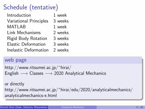
Schedule (tentative)Introduction 1 weekVariational Principles 3 weeksMATLAB 1 weekLink Mechanisms 2 weeksRigid Body Rotation 3 weeksElastic Deformation 3 weeksInelastic Deformation 2 weeks
web page
http://www.ritsumei.ac.jp/~hirai/English −→ Classes −→ 2020 Analytical Mechanics
or directlyhttp://www.ritsumei.ac.jp/~hirai/edu/2020/analyticalmechanics/analyticalmechanics-e.html
Shinichi Hirai (Dept. Robotics, Ritsumeikan Univ.) Analytical Mechanics 3 / 22
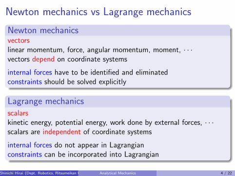
Newton mechanics vs Lagrange mechanics
Newton mechanicsvectorslinear momentum, force, angular momentum, moment, · · ·vectors depend on coordinate systems
internal forces have to be identified and eliminatedconstraints should be solved explicitly
Lagrange mechanicsscalarskinetic energy, potential energy, work done by external forces, · · ·scalars are independent of coordinate systems
internal forces do not appear in Lagrangianconstraints can be incorporated into Lagrangian
Shinichi Hirai (Dept. Robotics, Ritsumeikan Univ.) Analytical Mechanics 4 / 22

Free fall of a mass (Newton mechanics)x
m
mggravitational force
Newton mechanics
linear momentum p = mv
Newton’s eq. of motiondp
dt= −mg
dp
dt=
d
dt(mv) = mv
differential equation mv = −mg
Shinichi Hirai (Dept. Robotics, Ritsumeikan Univ.) Analytical Mechanics 5 / 22
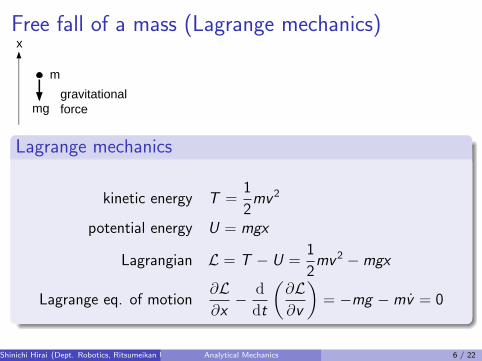
Free fall of a mass (Lagrange mechanics)x
m
mggravitational force
Lagrange mechanics
kinetic energy T =1
2mv 2
potential energy U = mgx
Lagrangian L = T − U =1
2mv 2 −mgx
Lagrange eq. of motion∂L∂x
− d
dt
(∂L∂v
)= −mg −mv = 0
Shinichi Hirai (Dept. Robotics, Ritsumeikan Univ.) Analytical Mechanics 6 / 22
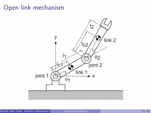
Open link mechanism
θ1
θ2l1
l2
link 1
link 2
joint 1
joint 2
lc2
lc1
x
y
Shinichi Hirai (Dept. Robotics, Ritsumeikan Univ.) Analytical Mechanics 7 / 22
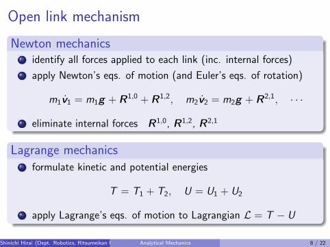
Open link mechanism
Newton mechanics1 identify all forces applied to each link (inc. internal forces)
2 apply Newton’s eqs. of motion (and Euler’s eqs. of rotation)
m1v1 = m1g + R1,0 + R1,2, m2v2 = m2g + R2,1, · · ·
3 eliminate internal forces R1,0, R1,2, R2,1
Lagrange mechanics1 formulate kinetic and potential energies
T = T1 + T2, U = U1 + U2
2 apply Lagrange’s eqs. of motion to Lagrangian L = T − U
Shinichi Hirai (Dept. Robotics, Ritsumeikan Univ.) Analytical Mechanics 8 / 22
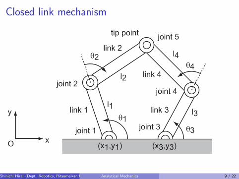
Closed link mechanism
x
y
O
link 1
link 2
link 3
link 4
θ1
θ3
θ2θ4
tip point
l1
l2
l3
l4
(x1,y1) (x3,y3)
joint 1
joint 2
joint 3
joint 4
joint 5
Shinichi Hirai (Dept. Robotics, Ritsumeikan Univ.) Analytical Mechanics 9 / 22
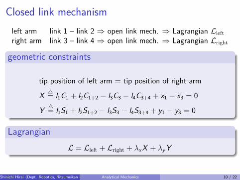
Closed link mechanism
left arm link 1 – link 2 ⇒ open link mech. ⇒ Lagrangian Lleft
right arm link 3 – link 4 ⇒ open link mech. ⇒ Lagrangian Lright
geometric constraints
tip position of left arm = tip position of right arm
X△= l1C1 + l2C1+2 − l3C3 − l4C3+4 + x1 − x3 = 0
Y△= l1S1 + l2S1+2 − l3S3 − l4S3+4 + y1 − y3 = 0
Lagrangian
L = Lleft + Lright + λxX + λyY
Shinichi Hirai (Dept. Robotics, Ritsumeikan Univ.) Analytical Mechanics 10 / 22

Watt’s governor (Newton mechanics)
θ1
τ
free joint
m
θ2
l
rotation around driving axis
I1 = m(l cos θ2)2 = ml2 cos2 θ2
τ =d
dt(I1θ1) = I1θ1 + I1θ1
τ ={ml2 · 2 cos θ2(− sin θ2)θ2
}θ1 +
{ml2 cos2 θ2
}θ1
Shinichi Hirai (Dept. Robotics, Ritsumeikan Univ.) Analytical Mechanics 11 / 22
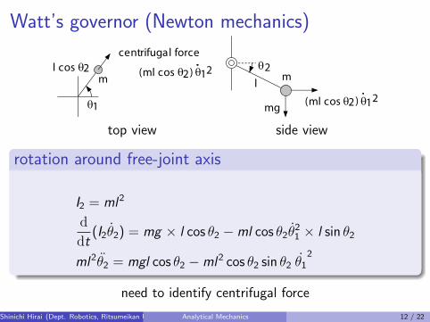
Watt’s governor (Newton mechanics)
θ1
m
centrifugal force
(ml cos θ2) 2θ1l cos θ2
mθ2
l
mg(ml cos θ2) 2θ1
top view side view
rotation around free-joint axis
I2 = ml2
d
dt(I2θ2) = mg × l cos θ2 −ml cos θ2θ
21 × l sin θ2
ml2θ2 = mgl cos θ2 −ml2 cos θ2 sin θ2 θ12
need to identify centrifugal force
Shinichi Hirai (Dept. Robotics, Ritsumeikan Univ.) Analytical Mechanics 12 / 22

Watt’s governor (Lagrange mechanics)
θ1
m
θ2x
y
z
l
position of mass
x =
l cos θ1 cos θ2l sin θ1 cos θ2−l sin θ2
= l
cos θ1 cos θ2sin θ1 cos θ2− sin θ2
Shinichi Hirai (Dept. Robotics, Ritsumeikan Univ.) Analytical Mechanics 13 / 22
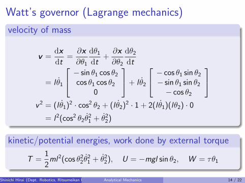
Watt’s governor (Lagrange mechanics)
velocity of mass
v =dxdt
=∂x∂θ1
dθ1dt
+∂x∂θ2
dθ2dt
= l θ1
− sin θ1 cos θ2cos θ1 cos θ2
0
+ l θ2
− cos θ1 sin θ2− sin θ1 sin θ2
− cos θ2
v 2 = (l θ1)
2 · cos2 θ2 + (l θ2)2 · 1 + 2(l θ1)(lθ2) · 0
= l2(cos2 θ2θ21 + θ22)
kinetic/potential energies, work done by external torque
T =1
2ml2(cos θ22 θ
21 + θ22), U = −mgl sin θ2, W = τθ1
Shinichi Hirai (Dept. Robotics, Ritsumeikan Univ.) Analytical Mechanics 14 / 22
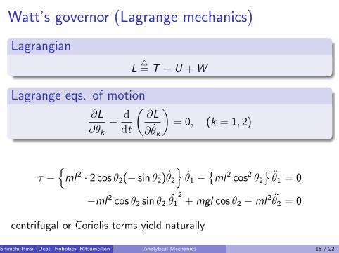
Watt’s governor (Lagrange mechanics)
Lagrangian
L△= T − U +W
Lagrange eqs. of motion
∂L
∂θk− d
dt
(∂L
∂θk
)= 0, (k = 1, 2)
τ −{ml2 · 2 cos θ2(− sin θ2)θ2
}θ1 −
{ml2 cos2 θ2
}θ1 = 0
−ml2 cos θ2 sin θ2 θ12+mgl cos θ2 −ml2θ2 = 0
centrifugal or Coriolis terms yield naturally
Shinichi Hirai (Dept. Robotics, Ritsumeikan Univ.) Analytical Mechanics 15 / 22
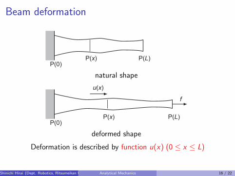
Beam deformation
P(0)P(x) P(L)
natural shape
P(0)P(x) P(L)
f
u(x)
deformed shape
Deformation is described by function u(x) (0 ≤ x ≤ L)
Shinichi Hirai (Dept. Robotics, Ritsumeikan Univ.) Analytical Mechanics 16 / 22
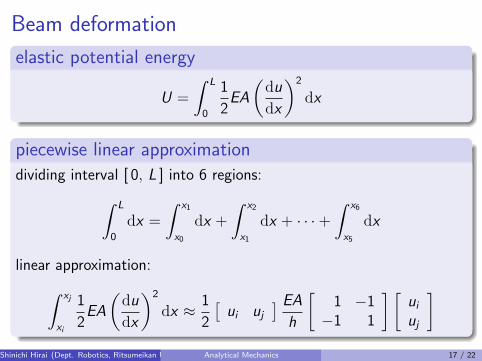
Beam deformation
elastic potential energy
U =
∫ L
0
1
2EA
(du
dx
)2
dx
piecewise linear approximation
dividing interval [ 0, L ] into 6 regions:∫ L
0
dx =
∫ x1
x0
dx +
∫ x2
x1
dx + · · ·+∫ x6
x5
dx
linear approximation:∫ xj
xi
1
2EA
(du
dx
)2
dx ≈ 1
2
[ui uj
] EAh
[1 −1
−1 1
] [uiuj
]Shinichi Hirai (Dept. Robotics, Ritsumeikan Univ.) Analytical Mechanics 17 / 22
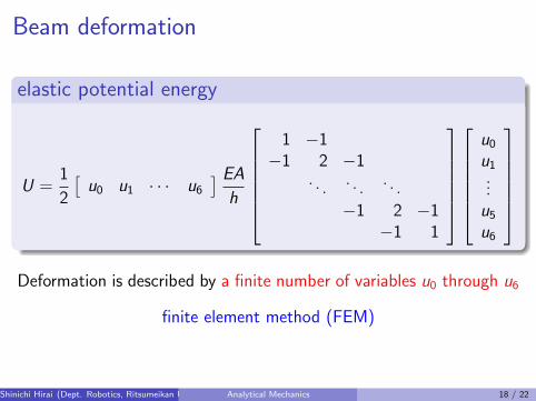
Beam deformation
elastic potential energy
U =1
2
[u0 u1 · · · u6
] EAh
1 −1
−1 2 −1. . . . . . . . .
−1 2 −1−1 1
u0u1...u5u6
Deformation is described by a finite number of variables u0 through u6
finite element method (FEM)
Shinichi Hirai (Dept. Robotics, Ritsumeikan Univ.) Analytical Mechanics 18 / 22
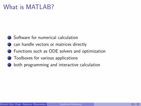
What is MATLAB?
1 Software for numerical calculation
2 can handle vectors or matrices directly
3 Functions such as ODE solvers and optimization
4 Toolboxes for various applications
5 both programming and interactive calculation
Shinichi Hirai (Dept. Robotics, Ritsumeikan Univ.) Analytical Mechanics 19 / 22
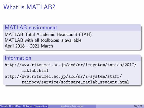
What is MATLAB?
MATLAB environmentMATLAB Total Academic Headcount (TAH)MATLAB with all toolboxes is availableApril 2018 – 2021 March
Informationhttp://www.ritsumei.ac.jp/acd/mr/i-system/topics/2017/
matlab.html
http://www.ritsumei.ac.jp/acd/mr/i-system/staff/
rainbow/service/software_matlab_student.html
Shinichi Hirai (Dept. Robotics, Ritsumeikan Univ.) Analytical Mechanics 20 / 22
What is MATLAB?
Install MATLAB into your own PC or mobile
Sample programs are on the web of the class
You can use your own PC or mobile in class
Shinichi Hirai (Dept. Robotics, Ritsumeikan Univ.) Analytical Mechanics 21 / 22
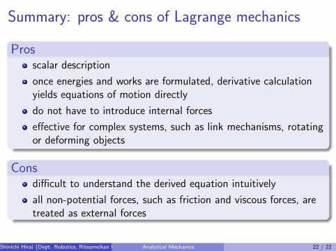
Summary: pros & cons of Lagrange mechanics
Prosscalar description
once energies and works are formulated, derivative calculationyields equations of motion directly
do not have to introduce internal forces
effective for complex systems, such as link mechanisms, rotatingor deforming objects
Consdifficult to understand the derived equation intuitively
all non-potential forces, such as friction and viscous forces, aretreated as external forces
Shinichi Hirai (Dept. Robotics, Ritsumeikan Univ.) Analytical Mechanics 22 / 22