applied biofluid mechanics
TRANSCRIPT

This page intentionally left blank

Applied BiofluidMechanics
Lee Waite, Ph.D., P.E.
Jerry Fine, Ph.D.
New York Chicago San Francisco Lisbon London Madrid Mexico City Milan New Delhi San Juan Seoul
Singapore Sydney Toronto

Copyright © 2007 by The McGraw-Hill Companies, Inc. All rights reserved. Manufactured in the UnitedStates of America. Except as permitted under the United States Copyright Act of 1976, no part of this pub-lication may be reproduced or distributed in any form or by any means, or stored in a database or retrievalsystem, without the prior written permission of the publisher.
0-07-150951-8
The material in this eBook also appears in the print version of this title: 0-07-147217-7.
All trademarks are trademarks of their respective owners. Rather than put a trademark symbol after everyoccurrence of a trademarked name, we use names in an editorial fashion only, and to the benefit of the trade-mark owner, with no intention of infringement of the trademark. Where such designations appear in thisbook, they have been printed with initial caps.
McGraw-Hill eBooks are available at special quantity discounts to use as premiums and sales promotions,or for use in corporate training programs. For more information, please contact George Hoare, Special Sales,at [email protected] or (212) 904-4069.
TERMS OF USE
This is a copyrighted work and The McGraw-Hill Companies, Inc. (“McGraw-Hill”) and its licensors reserveall rights in and to the work. Use of this work is subject to these terms. Except as permitted under theCopyright Act of 1976 and the right to store and retrieve one copy of the work, you may not decompile, dis-assemble, reverse engineer, reproduce, modify, create derivative works based upon, transmit, distribute, dis-seminate, sell, publish or sublicense the work or any part of it without McGraw-Hill’s prior consent. You mayuse the work for your own noncommercial and personal use; any other use of the work is strictly prohibited.Your right to use the work may be terminated if you fail to comply with these terms.
THE WORK IS PROVIDED “AS IS.” McGRAW-HILL AND ITS LICENSORS MAKE NO GUARAN-TEES OR WARRANTIES AS TO THE ACCURACY, ADEQUACY OR COMPLETENESS OF ORRESULTS TO BE OBTAINED FROM USING THE WORK, INCLUDING ANY INFORMATION THATCAN BE ACCESSED THROUGH THE WORK VIA HYPERLINK OR OTHERWISE, AND EXPRESSLYDISCLAIM ANY WARRANTY, EXPRESS OR IMPLIED, INCLUDING BUT NOT LIMITED TOIMPLIED WARRANTIES OF MERCHANTABILITY OR FITNESS FOR A PARTICULAR PURPOSE.McGraw-Hill and its licensors do not warrant or guarantee that the functions contained in the work will meetyour requirements or that its operation will be uninterrupted or error free. Neither McGraw-Hill nor its licen-sors shall be liable to you or anyone else for any inaccuracy, error or omission, regardless of cause, in thework or for any damages resulting therefrom. McGraw-Hill has no responsibility for the content of any infor-mation accessed through the work. Under no circumstances shall McGraw-Hill and/or its licensors be liablefor any indirect, incidental, special, punitive, consequential or similar damages that result from the use of orinability to use the work, even if any of them has been advised of the possibility of such damages. This lim-itation of liability shall apply to any claim or cause whatsoever whether such claim or cause arises in con-tract, tort or otherwise.
DOI: 10.1036/0071472177

ABOUT THE AUTHORS
LEE WAITE, PH.D., P.E., is Head of the Department ofApplied Biology and Biomedical Engineering, and Directorof the Guidant/Eli Lilly and Co. Applied Life SciencesResearch Center, at Rose-Hulman Institute of Technology inTerre Haute, Indiana. He is also the author of BiofluidMechanics in Cardiovascular Systems, published byMcGraw-Hill.
JERRY FINE, PH.D., is Associate Professor of MechanicalEngineering at Rose-Hulman Institute of Technology.Before he joined the faculty at Rose, Dr. Fine served as a patrol plane pilot in the U.S. Navy and taught at the U.S. Naval Academy.
Copyright © 2007 by The McGraw-Hill Companies, Inc. Click here for terms of use.

This page intentionally left blank
vii
Contents
Preface xiiiAcknowledgments xv
Chapter 1. Review of Basic Fluid Mechanics Concepts 1
1.1 A Brief History of Biomedical Fluid Mechanics 11.2 Fluid Characteristics and Viscosity 6
1.2.1 Displacement and velocity 71.2.2 Shear stress and viscosity 81.2.3 Example problem: shear stress 101.2.4 Viscosity 111.2.5 Clinical feature: polycythemia 13
1.3 Fundamental Method for Measuring Viscosity 141.3.1 Example problem: viscosity measurement 16
1.4 Introduction to Pipe Flow 161.4.1 Reynolds number 171.4.2 Example problem: Reynolds number 191.4.3 Poiseuille’s law 191.4.4 Flow rate 23
1.5 Bernoulli Equation 241.6 Conservation of Mass 24
1.6.1 Venturi meter example 261.7 Fluid Statics 27
1.7.1 Example problem: fluid statics 281.8 The Womersley Number α: A Frequency Parameter for Pulsatile Flow 29
1.8.1 Example problem: Womersley number 30Problems 31Bibliography 33
Chapter 2. Cardiovascular Structure and Function 35
2.1 Introduction 352.2 Clinical Features 362.3 Functional Anatomy 372.4 The Heart as a Pump 382.5 Cardiac Muscle 39
2.5.1 Biopotential in myocardium 40
For more information about this title, click here
2.5.2 Excitability 412.5.3 Automaticity 43
2.6 Electrocardiograms 432.6.1 Electrocardiogram leads 442.6.2 Mean electrical axis 452.6.3 Example problem: mean electrical axis 472.6.4 Unipolar versus bipolar and augmented leads 482.6.5 Electrocardiogram interpretations 492.6.6 Clinical feature: near maximal exercise stress test 50
2.7 Heart Valves 512.7.1 Clinical features 52
2.8 Cardiac Cycle 522.8.1 Pressure-volume diagrams 552.8.2 Changes in contractility 572.8.3 Ventricular performance 582.8.4 Clinical feature: congestive heart failure 582.8.5 Pulsatility index 592.8.6 Example problem: pulsatility index 59
2.9 Heart Sounds 602.9.1 Clinical features 612.9.2 Factors influencing flow and pressure 61
2.10 Coronary Circulation 632.10.1 Control of the coronary circulation 642.10.2 Clinical features 65
2.11 Microcirculation 652.11.1 Capillary structure 652.11.2 Capillary wall structure 662.11.3 Pressure control in the microvasculature 672.11.4 Diffusion in capillaries 682.11.5 Venules 68
2.12 Lymphatic Circulation 69Problems 69Bibliography 75
Chapter 3. Pulmonary Anatomy, Pulmonary Physiology,and Respiration 77
3.1 Introduction 773.1.1 Clinical features: hyperventilation 78
3.2 Alveolar Ventilation 793.2.1 Tidal volume 793.2.2 Residual volume 793.2.3 Expiratory reserve volume 803.2.4 Inspiratory reserve volume 803.2.5 Functional residual capacity 803.2.6 Inspiratory capacity 803.2.7 Total lung capacity 803.2.8 Vital capacity 81
3.3 Ventilation-Perfusion Relationships 813.4 Mechanics of Breathing 81
3.4.1 Muscles of inspiration 823.4.2 Muscles of expiration 833.4.3 Compliance of the lung and chest wall 83
viii Contents
3.4.4 Elasticity, elastance, and elastic recoil 833.4.5 Example problem: compliance 84
3.5 Work of Breathing 853.5.1 Clinical features: respiratory failure 87
3.6 Airway Resistance 883.6.1 Example problem: Reynolds number 91
3.7 Gas Exchange and Transport 913.7.1 Diffusion 923.7.2 Diffusing capacity 923.7.3 Oxygen dissociation curve 943.7.4 Example problem: oxygen content 953.7.5 Clinical feature 96
3.8 Pulmonary Pathophysiology 963.8.1 Bronchitis 963.8.2 Emphysema 963.8.3 Asthma 973.8.4 Pulmonary fibrosis 983.8.5 Chronics obstructive pulmonary disease (COPD) 983.8.6 Heart disease 983.8.7 Comparison of pulmonary pathologies 98
3.9 Respiration in Extreme Environments 993.9.1 Barometric pressure 1003.9.2 Partial pressure of oxygen 1013.9.3 Hyperventilation and the alveolar gas equation 1023.9.4 Alkalosis 1033.9.5 Acute mountain sickness 1033.9.6 High-altitude pulmonary edema 1043.9.7 High-altitude cerebral edema 1043.9.8 Acclimatization 1043.9.9 Drugs stimulating red blood cell production 105
3.9.10 Example problem: alveolar gas equation 106Review Problems 106Bibliography 109
Chapter 4. Hematology and Blood Rheology 111
4.1 Introduction 1114.2 Elements of Blood 1114.3 Blood Characteristics 111
4.3.1 Types of fluids 1124.3.2 Viscosity of blood 1134.3.3 Fåhræus-Lindqvist effect 1144.3.4 Einstein’s equation 116
4.4 Viscosity Measurement 1164.4.1 Rotating cylinder viscometer 1164.4.2 Measuring viscosity using Poiseuille’s law 1184.4.3 Viscosity measurement by a cone and plate viscometer 119
4.5 Erythrocytes 1214.5.1 Hemoglobin 1234.5.2 Clinical features—sickle cell anemia 1254.5.3 Erythrocyte indices 1254.5.4 Abnormalities of the blood 1264.5.5 Clinical feature—thalassemia 127
Contents ix
4.6 Leukocytes 1274.6.1 Neutrophils 1284.6.2 Lymphocytes 1294.6.3 Monocytes 1314.6.4 Eosinophils 1314.6.5 Basophils 1314.6.6 Leukemia 1314.6.7 Thrombocytes 132
4.7 Blood Types 1324.7.1 Rh blood groups 1344.7.2 M and N blood group system 135
4.8 Plasma 1354.8.1 Plasma viscosity 1364.8.2 Electrolyte composition of plasma 1364.8.3 Blood pH 1374.8.4 Clinical features—acid–base imbalance 137
Review Problems 138Bibliography 139
Chapter 5. Anatomy and Physiology of Blood Vessels 141
5.1 Introduction 1415.2 General Structure of Arteries 141
5.2.1 Tunica intima 1425.2.2 Tunica media 1425.2.3 Tunica externa 143
5.3 Types of Arteries 1445.3.1 Elastic arteries 1445.3.2 Muscular arteries 1445.3.3 Arterioles 144
5.4 Mechanics of Arterial Walls 1445.5 Compliance 147
5.5.1 Compliance example 1515.5.2 Clinical feature—arterial compliance and hypertension 152
5.6 Pulse Wave Velocity and the Moens–Korteweg Equation 1535.6.1 Applications box—fabrication of arterial models 1535.6.2 Pressure–strain modulus 1535.6.3 Example problem—modulus of elasticity 154
5.7 Vascular Pathologies 1555.7.1 Atherosclerosis 1555.7.2 Stenosis 1555.7.3 Aneurysm 1565.7.4 Clinical feature—endovascular aneurysm repair 1565.7.5 Thrombosis 157
5.8 Stents 1575.8.1 Clinical feature—“Stent Wars” 158
5.9 Coronary Artery Bypass Grafting 1595.9.1 Arterial grafts 160
Review Problems 161Bibliography 162
x Contents
Contents xi
Chapter 6. Mechanics of Heart Valves 165
6.1 Introduction 1656.2 Aortic and Pulmonic Valves 165
6.2.1 Clinical feature—percutaneous aortic valve implantation 1696.3 Mitral and Tricuspid Valves 1716.4 Pressure Gradients across a Stenotic Heart Valve 172
6.4.1 The Gorlin equation 1736.4.2 Example problem—Gorlin equation 1756.4.3 Energy loss across a stenotic valve 1756.4.4 Example problem—energy loss method 1786.4.5 Clinical features 178
6.5 Prosthetic Mechanical Valves 1786.5.1 Clinical feature—performance of the On-X valve 1806.5.2 Case study—the Björk-Shiley convexo-concave heart valve 180
6.6 Prosthetic Tissue Valves 184Review Problems 184Bibliography 185
Chapter 7. Pulsatile Flow in Large Arteries 187
7.1 Introduction 1877.2 Fluid Kinematics 1887.3 Continuity 1897.4 Complex Numbers 1907.5 Fourier Series Representation 1927.6 Navier–Stokes Equations 1987.7 Pulsatile Flow in Rigid Tubes—Womersley Solution 2027.8 Pulsatile Flow in Rigid Tubes—Fry Solution 2147.9 Instability in Pulsatile Flow 221Review Problems 222Bibliography 227
Chapter 8. Flow and Pressure Measurement 229
8.1 Introduction 2298.2 Indirect Pressure Measurements 229
8.2.1 Indirect pressure gradient measurements usingDoppler ultrasound 230
8.3 Direct Pressure Measurement 2318.3.1 Intravascular—strain gauge tipped pressure transducer 2318.3.2 Extravascular—catheter-transducer measuring system 2378.3.3 Electrical analog of the catheter measuring system 2388.3.4 Characteristics for an extravascular pressure
measuring system 2408.3.5 Example problem—characteristics of an extravascular
measuring system 2418.3.6 Case 1: the undamped catheter measurement system 2438.3.7 Case 2: the undriven, damped catheter measurement system 2448.3.8 Pop test—measurement of transient step response 248
8.4 Flow Measurement 2498.4.1 Indicator dilution method 2498.4.2 Fick technique for measuring cardiac output 2508.4.3 Fick technique example 2508.4.4 Rapid injection indicator-dilution method—
dye dilution technique 2508.4.5 Thermodilution 2518.4.6 Electromagnetic flowmeters 2528.4.7 Continuous wave ultrasonic flowmeters 2538.4.8 Example problem—continuous wave Doppler ultrasound 254
8.5 Summary and Clinical Applications 255Review Problems 256Bibliography 258
Chapter 9. Modeling 259
9.1 Introduction 2599.2 Theory of Models 260
9.2.1 Dimensional analysis and the Buckingham Pi theorem 2609.2.2 Synthesizing Pi terms 262
9.3 Geometric Similarity 2649.4 Dynamic Similarity 2659.5 Kinematic Similarity 2659.6 Common Dimensionless Parameters in Fluid Mechanics 2669.7 Modeling Example 1—Does the Flea Model the Man? 2669.8 Modeling Example 2 2689.9 Modeling Example 3 269Review Problems 271Bibliography 273
Chapter 10. Lumped Parameter Mathematical Models 275
10.1 Introduction 27510.2 Electrical Analog Model of Flow in a Tube 276
10.2.1 Nodes and the equations at each node 27710.2.2 Terminal load 27810.2.3 Summary of the lumped parameter electrical analog model 288
10.3 Modeling of Flow through the Mitral Valve 28810.3.1 Model description 28910.3.2 Active ventricular relaxation 29210.3.3 Meaning of convective resistance 29210.3.4 Variable area mitral valve model description 29210.3.5 Variable area mitral valve model parameters 29310.3.6 Solving the system of differential equations 29410.3.7 Model trials 29410.3.8 Results 294
10.4 Summary 296Review Problems 297Bibliography 297
Index 299
xii Contents
xiii
Preface
Biomedical engineering is a discipline that is multidisciplinary bydefinition. The days when medicine was left to the physicians, andengineering was left to the engineers, seem to have passed us by. Ihave searched for an undergraduate/graduate level biomedical fluidmechanics textbook since I began teaching at Rose-Hulman in 1987. Ilooked for, but never found, a book that combined the physiology of thecardiovascular and pulmonary systems with engineering of fluidmechanics and hematology to my satisfaction, so I agreed to write a mono-graph. Ken McCombs at McGraw-Hill was satisfied well enough withthat work that he asked me to write the textbook version that you seehere. Applied Biofluid Mechanics includes problem sets and a solutionsmanual that traditionally accompany engineering textbooks.
Applied Biofluid Mechanics begins in Chapter 1 with a review of someof the basics of fluid mechanics, which all mechanical or chemical engi-neers would learn. It continues with two chapters on cardiovascular andpulmonary physiology followed by a chapter describing hematology andblood rheology. These five chapters provide the foundation for the remain-der of the book, which focuses on more advanced engineering concepts.Dr. Fine has added some particularly nice improvements in Chapters 7and 10 concerning solutions for, and modeling of, pulsatile flow.
My 10-week, graduate-level, biofluid mechanics course forms the basisfor the book. The course consists of 40 lectures and covers most, but notall, of the material contained in the book. The course is intended to pre-pare students for work in the health care device industry and others forgraduate work in biomedical engineering.
In spite of great effort on the part of many proofreaders, I expect thatmistakes will appear in this book. I welcome suggestions for improvementfrom all readers, with intent to improve subsequent printings and editions.
LEE WAITE, PH.D., P.E.
Copyright © 2007 by The McGraw-Hill Companies, Inc. Click here for terms of use.

This page intentionally left blank

Acknowledgments
I would like to thank my BE525 students from fall term of 2006, whothrough their proofreading helped to improve this book, Applied BiofluidMechanics. I wish to thank Steve Chapman and the editorial and pro-duction staff at McGraw-Hill for their assistance.
Special thanks go to my friend and co-author Dr. Jerry Fine, withoutwhom it would have been extremely difficult to meet the agreed-upondeadlines for this book. Dr. Fine is especially responsible for significantimprovements in Chapters 7 and 10.
Jerry would like to give a special acknowledgment to his father, Dr. Neil C. Fine, for his encouragement over the years, and for being asuperb example of a life-long learner.
Thanks once again to the faculty in the Applied Biology and BiomedicalEngineering Department at Rose-Hulman for their counsel and for put-ting up with a department head who wrote a book instead of giving fullconcentration to departmental issues.
In writing this book I have been keenly aware of the debt I owe to DonYoung, my dissertation advisor at Iowa State, who taught me much ofwhat I know about biomedical fluid mechanics.
Most of all I would like to thank my colleague, wife, and best friendGabi Nindl Waite, who put up with me during the long evening hoursand long weekends that it took to write this book. Thanks especially foreverything you taught me about physiology.
LEE WAITE, PH.D., P.E.
xv
Copyright © 2007 by The McGraw-Hill Companies, Inc. Click here for terms of use.

This page intentionally left blank

Applied BiofluidMechanics

This page intentionally left blank
Chapter
1Review of Basic Fluid Mechanics Concepts
1.1 A Brief History of Biomedical Fluid Mechanics
People have written about the circulation of blood for thousands of years.I include here a short history of biomedical fluid mechanics, because Ibelieve it is important to recognize that, in all of science and engineer-ing, we “stand on the shoulders of giants.”1 In addition, it is interestinginformation in its own right. Let us begin the story in ancient times.
The Yellow Emperor, Huang Ti, lived in China from about 2700 to2600 BC and, according to legend, wrote one of the first works dealingwith circulation. Huang Ti is credited with writing Internal Classics,in which fundamental theories of Chinese medicine were addressed,although most Chinese scholars believe it was written by anonymousauthors in the Warring Period (475–221 BC). Among other topics,Internal Classics includes the Yin-Yang doctrine and the theory ofcirculation.
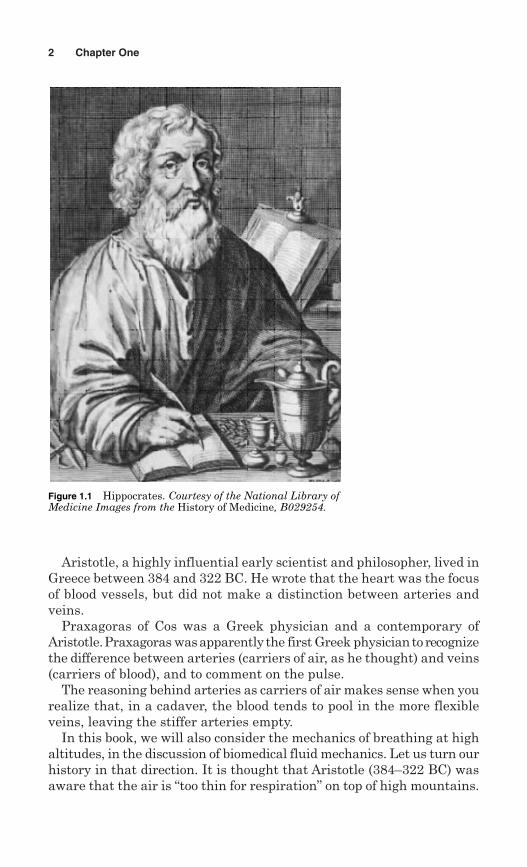
Hippocrates (Fig. 1.1), who lived in Greece around 400 BC, is consid-ered by many to be the father of science-based medicine and was the firstto separate medicine from magic. Hippocrates declared that the humanbody was integral to nature and was something that should be under-stood. He founded a medical school on the island of Cos, Greece, anddeveloped the Oath of Medical Ethics.
1
1 “If I have seen further (than others), it is by standing on the shoulders of giants.” Thiswas written by Isaac Newton in a letter to Robert Hooke, 1675.
Copyright © 2007 by The McGraw-Hill Companies, Inc. Click here for terms of use.
Aristotle, a highly influential early scientist and philosopher, lived inGreece between 384 and 322 BC. He wrote that the heart was the focusof blood vessels, but did not make a distinction between arteries andveins.
Praxagoras of Cos was a Greek physician and a contemporary ofAristotle. Praxagoras wasapparently the first Greek physiciantorecognizethe difference between arteries (carriers of air, as he thought) and veins(carriers of blood), and to comment on the pulse.
The reasoning behind arteries as carriers of air makes sense when yourealize that, in a cadaver, the blood tends to pool in the more flexibleveins, leaving the stiffer arteries empty.
In this book, we will also consider the mechanics of breathing at highaltitudes, in the discussion of biomedical fluid mechanics. Let us turn ourhistory in that direction. It is thought that Aristotle (384–322 BC) wasaware that the air is “too thin for respiration” on top of high mountains.
2 Chapter One
Figure 1.1 Hippocrates. Courtesy of the National Library ofMedicine Images from the History of Medicine, B029254.
Francis Bacon (1561–1626) in his Novum Organun, which appeared in1620, includes the following statement (Bacon, 1620, pp. 358–360) froman English translation of the Latin text. “The ancients also observed,that the rarity of the air on the summit of Olympus was such that thosewho ascended it were obliged to carry sponges moistened with vinegarand water, and to apply them now and then to their nostrils, as the airwas not dense enough for their respiration.”
There is much evidence that the ancients seem to have known some-thing about the mechanics of respiration at high altitudes. The followingcolorful description of mountain sickness comes from a classical Chinesehistory of the period preceding the Han dynasty, the Ch’ien Han Shu. TheChinese text is from Pan Ku (AD 32–92), and the English translation isfrom Alexander Wylie (1881) as appears in John West’s High Life (1998).Speaking of a journey through the mountains, the text comments:
Again, on passing the Great Headache Mountain, the Little HeadacheMountain, the Red Land, and the Fever Slope, men’s bodies become fever-ish, they lose color, and are attached with headache and vomiting; theasses and cattle being all in like condition. Moreover there are three poolswith rocky banks along which the pathway is only 16 or 17 inches wide fora length of some 30 le, over an abyss...
The first description of high-altitude pulmonary edema appearedsome 400 years later. Fa-hien was a Chinese Buddhist monk who under-took an amazing trip through western China, Sinkiang, Kashmir,Afghanistan, Pakistan, and northern India to Calcutta by foot. He con-tinued the trip by boat to Sri Lanka and then on to Indonesia and finallyto the China Sea ending in Nanjing. The journey took 15 years fromAD 399 to 414. While crossing the “Little Snowy Mountains” inAfghanistan, his companion became ill.
Having stayed there till the third month of winter, Fa-hien and twoothers, proceeding southward, crossed the Little Snowy Mountains, onwhich the snow lies accumulated both in winter and in summer. On thenorthern side of the mountains, in the shade, they suddenly encountereda cold wind which made them shiver and become unable to speak. Hwuy-king could not go any further. White froth came down from his mouth,and he said to Fa-hien, “I cannot live any longer. Do you immediatelygo away, that we do not all die here.” With these words, he died. Fa-hienstroked the corpse and cried out piteously, “Our original plan has failed;it is fate. What can we do?”
Father Joseph de Acosta (1540–1600) was a Spanish Jesuit priest wholeft Spain and traveled to Peru in about 1570. He wrote the book HistoriaNatural y Moral de las Indias, which was first published in Seville inSpanish in 1590. Acosta had become a Jesuit priest at the age of 13. Ashe left Spain, he traveled across the Atlantic to Nombre de Dios, a townon the Atlantic coast of Panama, near the mouth of the Río Chagres, near
Review of Basic Fluid Mechanics Concepts 3
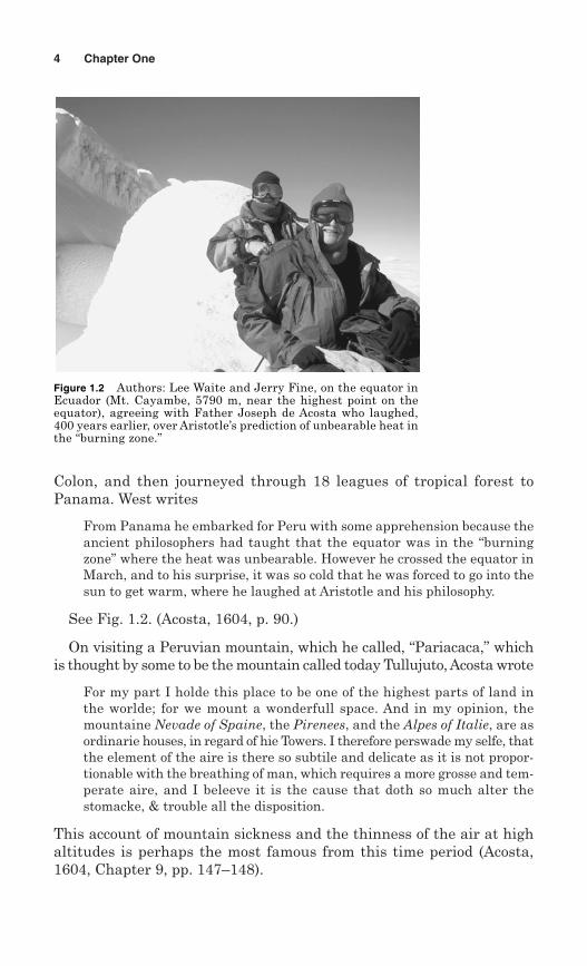
Colon, and then journeyed through 18 leagues of tropical forest toPanama. West writes
From Panama he embarked for Peru with some apprehension because theancient philosophers had taught that the equator was in the “burningzone” where the heat was unbearable. However he crossed the equator inMarch, and to his surprise, it was so cold that he was forced to go into thesun to get warm, where he laughed at Aristotle and his philosophy.
See Fig. 1.2. (Acosta, 1604, p. 90.)
On visiting a Peruvian mountain, which he called, “Pariacaca,” whichis thought by some to be the mountain called today Tullujuto, Acosta wrote
For my part I holde this place to be one of the highest parts of land inthe worlde; for we mount a wonderfull space. And in my opinion, themountaine Nevade of Spaine, the Pirenees, and the Alpes of Italie, are asordinarie houses, in regard of hie Towers. I therefore perswade my selfe, thatthe element of the aire is there so subtile and delicate as it is not propor-tionable with the breathing of man, which requires a more grosse and tem-perate aire, and I beleeve it is the cause that doth so much alter thestomacke, & trouble all the disposition.
This account of mountain sickness and the thinness of the air at highaltitudes is perhaps the most famous from this time period (Acosta,1604, Chapter 9, pp. 147–148).
4 Chapter One
Figure 1.2 Authors: Lee Waite and Jerry Fine, on the equator inEcuador (Mt. Cayambe, 5790 m, near the highest point on theequator), agreeing with Father Joseph de Acosta who laughed,400 years earlier, over Aristotle’s prediction of unbearable heat inthe “burning zone.”
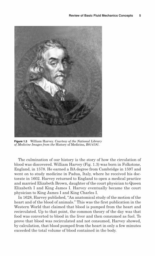
The culmination of our history is the story of how the circulation ofblood was discovered. William Harvey (Fig. 1.3) was born in Folkstone,England, in 1578. He earned a BA degree from Cambridge in 1597 andwent on to study medicine in Padua, Italy, where he received his doc-torate in 1602. Harvey returned to England to open a medical practiceand married Elizabeth Brown, daughter of the court physician to QueenElizabeth I and King James I. Harvey eventually became the courtphysician to King James I and King Charles I.
In 1628, Harvey published, “An anatomical study of the motion of theheart and of the blood of animals.” This was the first publication in theWestern World that claimed that blood is pumped from the heart andrecirculated. Up to that point, the common theory of the day was thatfood was converted to blood in the liver and then consumed as fuel. Toprove that blood was recirculated and not consumed, Harvey showed,by calculation, that blood pumped from the heart in only a few minutesexceeded the total volume of blood contained in the body.
Review of Basic Fluid Mechanics Concepts 5
Figure 1.3 William Harvey. Courtesy of the National Libraryof Medicine Images from the History of Medicine, B014191.
Jean Louis Marie Poiseuille was a French physician and physiologist,born in 1797. Poiseuille studied physics and mathematics in Paris.Later, he became interested in the flow of human blood in narrow tubes.In 1838, he experimentally derived and later published Poiseuille’s law.Poiseuille’s law describes the relationship between flow and pressuregradient in long tubes with constant cross section. Poiseuille died inParis in 1869.
Otto Frank was born in Germany in 1865, and he died in 1944. Hewas educated in Munich, Kiel, Heidelberg, Glasgow, and Strasburg. In1890, Frank published, “Fundamental form of the arterial pulse,” whichcontained his “Windkessel theory” of circulation. He became a physicianin 1892 in Leipzig and became a professor in Munich in 1895. Frank per-fected optical manometers and capsules for the precise measurement ofintracardiac pressures and volumes.
1.2 Fluid Characteristics and Viscosity
A fluid is defined as a substance that deforms continuously under appli-cation of a shearing stress, regardless of how small the stress is. Bloodis a primary example of a biological fluid. To study the behavior of mate-rials that act as fluids, it is useful to define a number of important fluidproperties, which include density, specific weight, specific gravity, andviscosity.
Density is defined as the mass per unit volume of a substance andis denoted by the Greek character r (rho). The SI units for r are kg/m3,and the approximate density of blood is 1060 kg/m3. Blood is slightlydenser than water, and red blood cells in plasma2 will settle to thebottom of a test tube, over time, due to gravity.
Specific weight is defined as the weight per unit volume of a sub-stance. The SI units for specific weight are N/m3. Specific gravity s is theratio of the weight of a liquid at a standard reference temperature to theweight of water. For example, the specific weight of mercury SHg � 13.6at 20�C. Specific gravity is a unitless parameter.
Density and specific weight are measures of the “heaviness” of a fluid,but two fluids with identical densities and specific weights can flow quitedifferently when subjected to the same forces. You might ask, “What isthe additional property that determines the difference in behavior?”That property is viscosity.
6 Chapter One
2 Plasma has a density very close to that of water.
1.2.1 Displacement and velocity
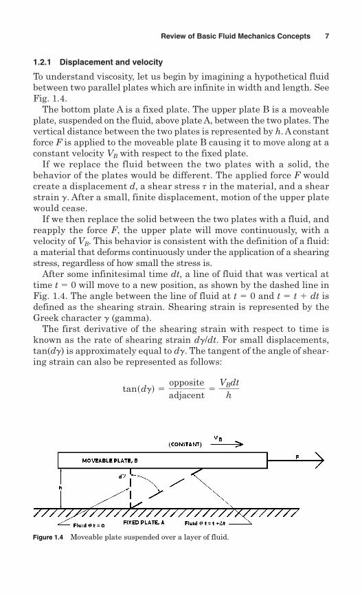
To understand viscosity, let us begin by imagining a hypothetical fluidbetween two parallel plates which are infinite in width and length. SeeFig. 1.4.
The bottom plate A is a fixed plate. The upper plate B is a moveableplate, suspended on the fluid, above plate A, between the two plates. Thevertical distance between the two plates is represented by h. A constantforce F is applied to the moveable plate B causing it to move along at aconstant velocity VB with respect to the fixed plate.
If we replace the fluid between the two plates with a solid, thebehavior of the plates would be different. The applied force F wouldcreate a displacement d, a shear stress t in the material, and a shearstrain g. After a small, finite displacement, motion of the upper platewould cease.
If we then replace the solid between the two plates with a fluid, andreapply the force F, the upper plate will move continuously, with avelocity of VB. This behavior is consistent with the definition of a fluid:a material that deforms continuously under the application of a shearingstress, regardless of how small the stress is.
After some infinitesimal time dt, a line of fluid that was vertical attime t � 0 will move to a new position, as shown by the dashed line inFig. 1.4. The angle between the line of fluid at t � 0 and t � t � dt isdefined as the shearing strain. Shearing strain is represented by theGreek character g (gamma).
The first derivative of the shearing strain with respect to time isknown as the rate of shearing strain dg/dt. For small displacements,tan(dg) is approximately equal to dg. The tangent of the angle of shear-ing strain can also be represented as follows:
tansdgd 5oppositeadjacent
5VBdt
h
Review of Basic Fluid Mechanics Concepts 7
Figure 1.4 Moveable plate suspended over a layer of fluid.
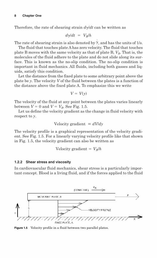
Therefore, the rate of shearing strain dg/dt can be written as
The rate of shearing strain is also denoted by , and has the units of 1/s.The fluid that touches plate A has zero velocity. The fluid that touches
plate B moves with the same velocity as that of plate B, VB. That is, themolecules of the fluid adhere to the plate and do not slide along its sur-face. This is known as the no-slip condition. The no-slip condition isimportant in fluid mechanics. All fluids, including both gasses and liq-uids, satisfy this condition.
Let the distance from the fixed plate to some arbitrary point above theplate be y. The velocity V of the fluid between the plates is a function ofthe distance above the fixed plate A. To emphasize this we write
The velocity of the fluid at any point between the plates varies linearlybetween V � 0 and V � VB. See Fig. 1.5.
Let us define the velocity gradient as the change in fluid velocity withrespect to y.
The velocity profile is a graphical representation of the velocity gradi-ent. See Fig. 1.5. For a linearly varying velocity profile like that shownin Fig. 1.5, the velocity gradient can also be written as
1.2.2 Shear stress and viscosity
In cardiovascular fluid mechanics, shear stress is a particularly impor-tant concept. Blood is a living fluid, and if the forces applied to the fluid
Velocity gradient 5 VB/h
Velocity gradient ; dV/dy
V 5 Vsyd
g.
dg/dt 5 VB/h
8 Chapter One
Figure 1.5 Velocity profile in a fluid between two parallel plates.
are sufficient, the resulting shearing stress can cause red blood cells tobe destroyed. On the other hand, studies indicate a role for shear stressin modulating atherosclerotic plaques. The relationship between shearstress and arterial disease has been studied much, but is not yet verywell understood.
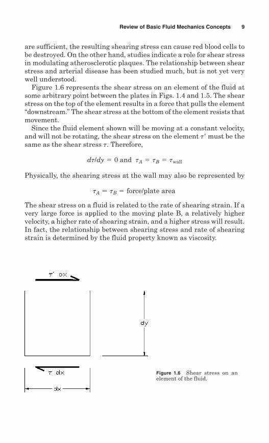
Figure 1.6 represents the shear stress on an element of the fluid atsome arbitrary point between the plates in Figs. 1.4 and 1.5. The shearstress on the top of the element results in a force that pulls the element“downstream.” The shear stress at the bottom of the element resists thatmovement.
Since the fluid element shown will be moving at a constant velocity,and will not be rotating, the shear stress on the element t� must be thesame as the shear stress t. Therefore,
Physically, the shearing stress at the wall may also be represented by
The shear stress on a fluid is related to the rate of shearing strain. If avery large force is applied to the moving plate B, a relatively highervelocity, a higher rate of shearing strain, and a higher stress will result.In fact, the relationship between shearing stress and rate of shearingstrain is determined by the fluid property known as viscosity.
tA 5 tB 5 force/plate area
dt/dy 5 0 and tA 5 tB 5 twall
Review of Basic Fluid Mechanics Concepts 9
Figure 1.6 Shear stress on anelement of the fluid.
10 Chapter One
1.2.3 Example problem: shear stress
Wall shear stress may be important in the development of various vas-cular disorders. For example, the shear stress of circulating blood onendothelial cells has been hypothesized to play a role in elevating vasculartransport in ocular diseases such as diabetic retinopathy.
In this example problem, we are asked to estimate the wall shear stress inan arteriole in the retinal circulation. Gilmore et al. have published a relatedpaper in the American Journal of Physiology: Heart and Circulatory Physiology,volume 288, in February 2005. In that article, the authors published the meas-ured values of retinal arteriolar diameter and blood velocity in arterioles. Forthis problem, we will use their published values: 80 µm for a vessel diameterand 30 mm/s for mean retinal blood flow velocity. Later in Sec. 1.4.4, we willsee that, for a parabolic flow profile, a good estimate of the shearing rate is
where Vm is the mean velocity across the vessel cross section and D is thevessel inside diameter.
We will also see in the next section that the shear stress is equal to theviscosity multiplied by the rate of shearing strain, that is,
Therefore, to estimate the shear stress on the wall of a retinal arteriole, withthe data from Gilmore’s paper, we can calculate
Although 10.5 Pa seems like a low shear stress when compared to thestrength of aluminum or steel, it is a relatively high shear stress when com-pared to a similar estimate in the aorta, 0.5 Pa. See Table 1.1.
t 5m 8Vm
D5
0.0035 Nsm2 8s3d
cms
0.008 cm5 10.5
Nm2
t 5 mg.
g.5
8Vm
D
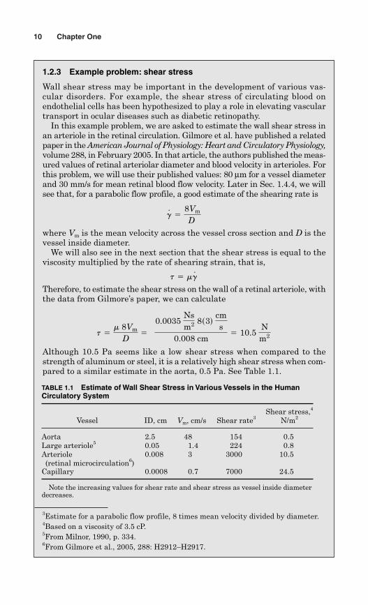
3Estimate for a parabolic flow profile, 8 times mean velocity divided by diameter.4Based on a viscosity of 3.5 cP.5From Milnor, 1990, p. 334.6From Gilmore et al., 2005, 288: H2912–H2917.
TABLE 1.1 Estimate of Wall Shear Stress in Various Vessels in the HumanCirculatory System
Shear stress,4
Vessel ID, cm Vm, cm/s Shear rate3 N/m2
Aorta 2.5 48 154 0.5Large arteriole5 0.05 1.4 224 0.8Arteriole 0.008 3 3000 10.5(retinal microcirculation6)
Capillary 0.0008 0.7 7000 24.5
Note the increasing values for shear rate and shear stress as vessel inside diameterdecreases.
1.2.4 Viscosity
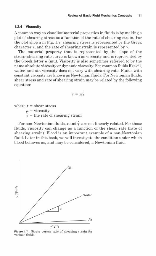
A common way to visualize material properties in fluids is by making aplot of shearing stress as a function of the rate of shearing strain. Forthe plot shown in Fig. 1.7, shearing stress is represented by the Greekcharacter t, and the rate of shearing strain is represented by .
The material property that is represented by the slope of thestress–shearing rate curve is known as viscosity and is represented bythe Greek letter m (mu). Viscosity is also sometimes referred to by thename absolute viscosity or dynamic viscosity. For common fluids like oil,water, and air, viscosity does not vary with shearing rate. Fluids withconstant viscosity are known as Newtonian fluids. For Newtonian fluids,shear stress and rate of shearing strain may be related by the followingequation:
where t � shear stress m� viscosity
� the rate of shearing strain
For non-Newtonian fluids, t and are not linearly related. For thosefluids, viscosity can change as a function of the shear rate (rate ofshearing strain). Blood is an important example of a non-Newtonianfluid. Later in this book, we will investigate the condition under whichblood behaves as, and may be considered, a Newtonian fluid.
g.
g.
t 5 mg.
g.
Review of Basic Fluid Mechanics Concepts 11
Figure 1.7 Stress versus rate of shearing strain forvarious fluids.
Air
Water
Oil
m
τ (N
/m2 )
g (s–1)⋅
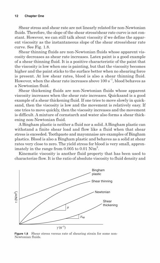
Shear stress and shear rate are not linearly related for non-Newtonianfluids. Therefore, the slope of the shear stress/shear rate curve is not con-stant. However, we can still talk about viscosity if we define the appar-ent viscosity as the instantaneous slope of the shear stress/shear ratecurve. See Fig. 1.8.
Shear thinning fluids are non-Newtonian fluids whose apparent vis-cosity decreases as shear rate increases. Latex paint is a good exampleof a shear thinning fluid. It is a positive characteristic of the paint thatthe viscosity is low when one is painting, but that the viscosity becomeshigher and the paint sticks to the surface better when no shearing forceis present. At low shear rates, blood is also a shear thinning fluid.However, when the shear rate increases above 100 s–1, blood behaves asa Newtonian fluid.
Shear thickening fluids are non-Newtonian fluids whose apparentviscosity increases when the shear rate increases. Quicksand is a goodexample of a shear thickening fluid. If one tries to move slowly in quick-sand, then the viscosity is low and the movement is relatively easy. Ifone tries to move quickly, then the viscosity increases and the movementis difficult. A mixture of cornstarch and water also forms a shear thick-ening non-Newtonian fluid.
A Bingham plastic is neither a fluid nor a solid. A Bingham plastic canwithstand a finite shear load and flow like a fluid when that shearstress is exceeded. Toothpaste and mayonnaise are examples of Binghamplastics. Blood is also a Bingham plastic and behaves as a solid at shearrates very close to zero. The yield stress for blood is very small, approx-imately in the range from 0.005 to 0.01 N/m2.
Kinematic viscosity is another fluid property that has been used tocharacterize flow. It is the ratio of absolute viscosity to fluid density and
12 Chapter One
Figure 1.8 Shear stress versus rate of shearing strain for some non-Newtonian fluids.
Newtonian
Shearthickening
Shear thinning
Binghamplastic
m
map
τ (N
/m2 )
g (s–1)⋅
is represented by the Greek character � (nu). Kinematic viscosity canbe defined by the equation:
where m is the absolute viscosity and r is the fluid density.
The SI units for absolute viscosity are Ns/m2. The SI units for kinematicviscosity are m2/s.
n 5m
r
Review of Basic Fluid Mechanics Concepts 13
1.2.5 Clinical feature: polycythemia
Polycythemia refers to a condition in which there is an increase in hemo-globin above 17.5 g/dL in adult males or above 15.5 g/dL in females(Hoffbrand and Pettit, 1984). There is usually an icrease in the number ofred blood cells above 6 � 1012 L–1 in males and 5.5 � 1012 L–1 in females.That is, a sufferer from this condition has a much higher blood viscosity dueto this elevated red blood cell count.
Symptoms of polycythemia are typically related to an increase in bloodviscosity and clotting. The symptoms include headache, dizziness, itchiness,shortness of breath, enlarged spleen, and redness in the face.
Polycythemia vera is an acquired disorder of the bone marrow thatresults in an increase in the number of blood cells resulting from exces-sive production of all three blood cell types: erythrocytes, or red blood cells;leukocytes, or white blood cells; and thrombocytes, or platelets.
The cause of polycythemia vera is not well-known. It rarely occurs inpatients under 40 years. Polycythemia usually develops slowly, and apatient might not experience any problems related to the disease evenafter being diagnosed. In some cases, however, the abnormal bone marrowcells grow uncontrollably resulting in a type of leukemia.
In patients with polycythemia vera, there is also an increased tendencyto form blood clots that can result in strokes or heart attacks. Some patientsmay experience abnormal bleeding because their platelets are abnormal.
The objective of the treatment is to reduce the high blood viscosity (thick-ness of the blood) due to the increased red blood cell mass, and to preventhemorrhage and thrombosis.
Phlebotomy is one method used to reduce the high blood viscosity. Inphlebotomy, one unit (pint) of blood is removed, weekly, until the hema-tocrit is less than 45; then, phlebotomy is continued as necessary.Occasionally, chemotherapy may be given to suppress the bone marrow.Other agents such as interferon may be given to lower the blood count.
A condition similar to polycythemia may be experienced by high-altitudemountaineers. Due to a combination of dehydration and excess red blood cellproduction brought about by extended stays at high altitudes, the climber’sblood thickens dangerously. A good description of what this is like is foundin the later chapters of Annapurna, by Maurice Herzog.
14 Chapter One
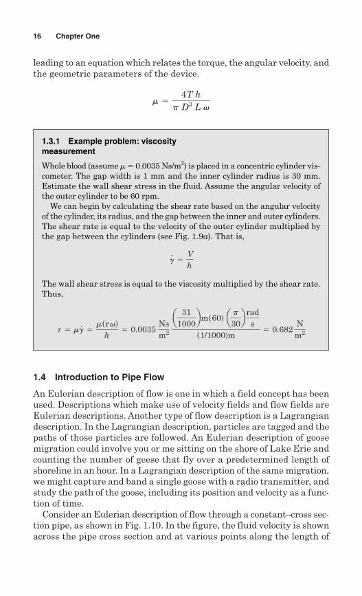
Figure 1.9a Cross section of a rotating cylinder viscometer.
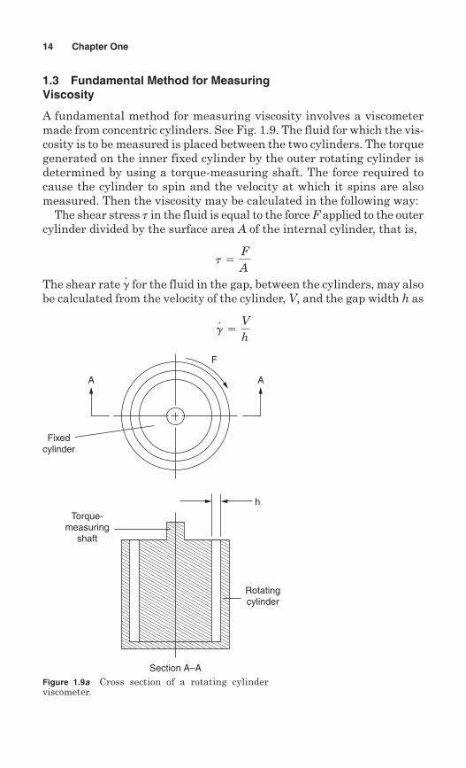
1.3 Fundamental Method for MeasuringViscosity
A fundamental method for measuring viscosity involves a viscometermade from concentric cylinders. See Fig. 1.9. The fluid for which the vis-cosity is to be measured is placed between the two cylinders. The torquegenerated on the inner fixed cylinder by the outer rotating cylinder isdetermined by using a torque-measuring shaft. The force required tocause the cylinder to spin and the velocity at which it spins are alsomeasured. Then the viscosity may be calculated in the following way:
The shear stress t in the fluid is equal to the force F applied to the outercylinder divided by the surface area A of the internal cylinder, that is,
The shear rate for the fluid in the gap, between the cylinders, may alsobe calculated from the velocity of the cylinder, V, and the gap width h as
g.5
Vh
g.
t 5FA
AA
F
Fixed cylinder
Torque-measuring
shaft
h
Rotatingcylinder
Section A–A
Review of Basic Fluid Mechanics Concepts 15
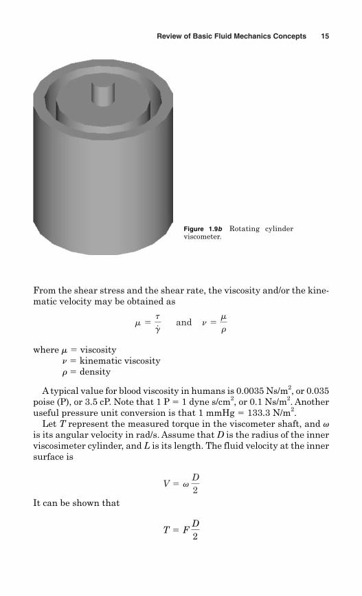
Figure 1.9b Rotating cylinderviscometer.
From the shear stress and the shear rate, the viscosity and/or the kine-matic velocity may be obtained as
where m � viscosityn � kinematic viscosity r� density
A typical value for blood viscosity in humans is 0.0035 Ns/m2, or 0.035poise (P), or 3.5 cP. Note that 1 P � 1 dyne s/cm2, or 0.1 Ns/m2. Anotheruseful pressure unit conversion is that 1 mmHg � 133.3 N/m2.
Let T represent the measured torque in the viscometer shaft, and vis its angular velocity in rad/s. Assume that D is the radius of the innerviscosimeter cylinder, and L is its length. The fluid velocity at the innersurface is
It can be shown that
T 5 F D2
V 5 v D2
m 5t
g. � � � and� � n 5
m
r
leading to an equation which relates the torque, the angular velocity, andthe geometric parameters of the device.
m 54T hp D3 L v
16 Chapter One
1.3.1 Example problem: viscositymeasurement
Whole blood (assume m� 0.0035 Ns/m2) is placed in a concentric cylinder vis-cometer. The gap width is 1 mm and the inner cylinder radius is 30 mm.Estimate the wall shear stress in the fluid. Assume the angular velocity ofthe outer cylinder to be 60 rpm.
We can begin by calculating the shear rate based on the angular velocityof the cylinder, its radius, and the gap between the inner and outer cylinders.The shear rate is equal to the velocity of the outer cylinder multiplied bythe gap between the cylinders (see Fig. 1.9a). That is,
The wall shear stress is equal to the viscosity multiplied by the shear rate.Thus,
t 5 mg.5msrvd
h5 0.0035
Nsm2 a 311000
bms60d a p30brad
ss1/1000dm
5 0.682 Nm2
g.5
Vh
1.4 Introduction to Pipe Flow
An Eulerian description of flow is one in which a field concept has beenused. Descriptions which make use of velocity fields and flow fields areEulerian descriptions. Another type of flow description is a Lagrangiandescription. In the Lagrangian description, particles are tagged and thepaths of those particles are followed. An Eulerian description of goosemigration could involve you or me sitting on the shore of Lake Erie andcounting the number of geese that fly over a predetermined length ofshoreline in an hour. In a Lagrangian description of the same migration,we might capture and band a single goose with a radio transmitter, andstudy the path of the goose, including its position and velocity as a func-tion of time.
Consider an Eulerian description of flow through a constant–cross sec-tion pipe, as shown in Fig. 1.10. In the figure, the fluid velocity is shownacross the pipe cross section and at various points along the length of
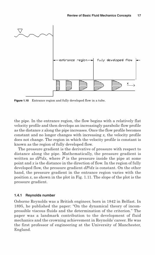
the pipe. In the entrance region, the flow begins with a relatively flatvelocity profile and then develops an increasingly parabolic flow profileas the distance x along the pipe increases. Once the flow profile becomesconstant and no longer changes with increasing x, the velocity profiledoes not change. The region in which the velocity profile is constant isknown as the region of fully developed flow.
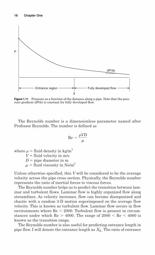
The pressure gradient is the derivative of pressure with respect todistance along the pipe. Mathematically, the pressure gradient iswritten as dP/dx, where P is the pressure inside the pipe at somepoint and x is the distance in the direction of flow. In the region of fullydeveloped flow, the pressure gradient dP/dx is constant. On the otherhand, the pressure gradient in the entrance region varies with theposition x, as shown in the plot in Fig. 1.11. The slope of the plot is thepressure gradient.
1.4.1 Reynolds number
Osborne Reynolds was a British engineer, born in 1842 in Belfast. In1895, he published the paper: “On the dynamical theory of incom-pressible viscous fluids and the determination of the criterion.” Thepaper was a landmark contribution to the development of fluidmechanics and the crowning achievement in Reynolds’ career. He wasthe first professor of engineering at the University of Manchester,England.
Review of Basic Fluid Mechanics Concepts 17
Figure 1.10 Entrance region and fully developed flow in a tube.
The Reynolds number is a dimensionless parameter named afterProfessor Reynolds. The number is defined as
where r � fluid density in kg/m3
V � fluid velocity in m/s D � pipe diameter in mm � fluid viscosity in Ns/m2
Unless otherwise specified, this V will be considered to be the averagevelocity across the pipe cross section. Physically, the Reynolds numberrepresents the ratio of inertial forces to viscous forces.
The Reynolds number helps us to predict the transition between lam-inar and turbulent flows. Laminar flow is highly organized flow alongstreamlines. As velocity increases, flow can become disorganized andchaotic with a random 3-D motion superimposed on the average flowvelocity. This is known as turbulent flow. Laminar flow occurs in flowenvironments where Re � 2000. Turbulent flow is present in circum-stances under which Re � 4000. The range of 2000 � Re � 4000 isknown as the transition range.
The Reynolds number is also useful for predicting entrance length inpipe flow. I will denote the entrance length as . The ratio of entranceXE
Re 5rVDm
18 Chapter One
X
P
dP/dx
Fully developed flowEntrance region
Figure 1.11 Pressure as a function of the distance along a pipe. Note that the pres-sure gradient dP/dx is constant for fully developed flow.
length to pipe diameter for laminar pipe flow is given asngth as Xven as
Consider the following example: If Re � 300, then XE � 18 D, and anentrance length equal to 18 pipe diameters is required for fully developedflow. In the human cardiovascular system, it is not common to see fullydeveloped flow in arteries. Typically, the vessels continually branch, withthe distance between branches not often being greater than 18 pipediameters.
Although most blood flow in humans is laminar, having a Re of 300or less, it is possible for turbulence to occur at very high flow rates inthe descending aorta, for example, in highly conditioned athletes.Turbulence is also common in pathological conditions such as heartmurmurs and stenotic heart valves.
Stenotic comes from the Greek word “stenos,” meaning narrow.Stenotic means narrowed, and a stenotic heart valve is one in which thenarrowing of the valve is a result of the plaque formation on the valve.
XE
D > 0.06 Re
Review of Basic Fluid Mechanics Concepts 19
1.4.2 Example problem:Reynolds number
Estimate the Reynolds number for blood flow in a retinal arteriole, usingthe published values from Gilmore et al. Assume that the blood density is1060 kg/m3. Is there any concern that blood flow in the human retina willbecome turbulent?
From Table 1.1, we see that the inside diameter of the arteriole is 0.008 cm,the mean velocity in the vessel is 3 cm/s, and the viscosity measured as 0.0035Ns/m2. The Reynolds number can be calculated as
For this flow condition, the Reynolds number is far, far less than 2000, andthere is no danger of the flow becoming turbulent.
Re 5rVDm
5
1060 kgm3
3100
ms
0.008100
m
0.0035 Nsm2
5 0.73
1.4.3 Poiseuille’s law
Velocity as a function of radius. In 1838, Jean-Marie Poiseuille empir-ically derived this law, which is also known as the Hagen-Poiseuillelaw, due to the additional experimental contribution by GotthilfHeinrich Ludwig Hagen in 1839. This law describes steady, laminar,
20 Chapter One
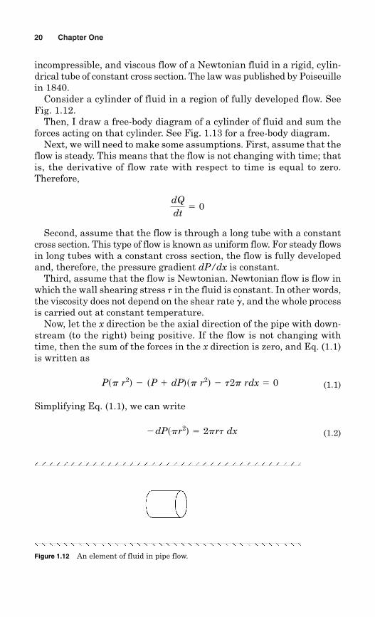
Figure 1.12 An element of fluid in pipe flow.
incompressible, and viscous flow of a Newtonian fluid in a rigid, cylin-drical tube of constant cross section. The law was published by Poiseuillein 1840.
Consider a cylinder of fluid in a region of fully developed flow. SeeFig. 1.12.
Then, I draw a free-body diagram of a cylinder of fluid and sum theforces acting on that cylinder. See Fig. 1.13 for a free-body diagram.
Next, we will need to make some assumptions. First, assume that theflow is steady. This means that the flow is not changing with time; thatis, the derivative of flow rate with respect to time is equal to zero.Therefore,
Second, assume that the flow is through a long tube with a constantcross section. This type of flow is known as uniform flow. For steady flowsin long tubes with a constant cross section, the flow is fully developedand, therefore, the pressure gradient dP/dx is constant.
Third, assume that the flow is Newtonian. Newtonian flow is flow inwhich the wall shearing stress t in the fluid is constant. In other words,the viscosity does not depend on the shear rate , and the whole processis carried out at constant temperature.
Now, let the x direction be the axial direction of the pipe with down-stream (to the right) being positive. If the flow is not changing withtime, then the sum of the forces in the x direction is zero, and Eq. (1.1)is written as
(1.1)
Simplifying Eq. (1.1), we can write
(1.2)2dPspr2d 5 2prt dx
Psp r2d 2 sP 1 dPdsp r2d 2 t2p rdx 5 0
g.
dQdt
5 0
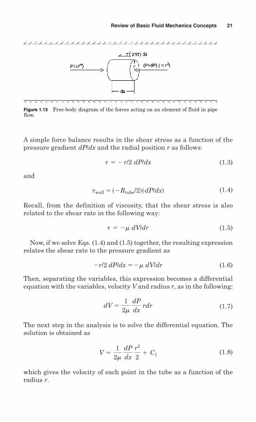
A simple force balance results in the shear stress as a function of thepressure gradient dP/dx and the radial position r as follows:
(1.3)
and
(1.4)
Recall, from the definition of viscosity, that the shear stress is alsorelated to the shear rate in the following way:
(1.5)
Now, if we solve Eqs. (1.4) and (1.5) together, the resulting expressionrelates the shear rate to the pressure gradient as
(1.6)
Then, separating the variables, this expression becomes a differentialequation with the variables, velocity V and radius r, as in the following:
(1.7)
The next step in the analysis is to solve the differential equation. Thesolution is obtained as
(1.8)
which gives the velocity of each point in the tube as a function of theradius r.
V 51
2m dPdx
r2
21 C1
dV 51
2m dPdx
rdr
2r/2 dP/dx 52m dV/dr
t 5 2m dV/dr
twall5 s2Rtube/2dsdP/dxd
t 5 2r/2 dP/dx
Review of Basic Fluid Mechanics Concepts 21
Figure 1.13 Free-body diagram of the forces acting on an element of fluid in pipeflow.
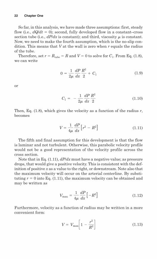
So far, in this analysis, we have made three assumptions: first, steadyflow (i.e., dQ/dt � 0); second, fully developed flow in a constant–crosssection tube (i.e., dP/dx is constant); and third, viscosity m is constant.Now, we need to make the fourth assumption, which is the no-slip con-dition. This means that V at the wall is zero when r equals the radiusof the tube.
Therefore, set r � Rtube � R and V � 0 to solve for C1. From Eq. (1.8),we can write
(1.9)
or
(1.10)
Then, Eq. (1.8), which gives the velocity as a function of the radius r,becomes
(1.11)
The fifth and final assumption for this development is that the flowis laminar and not turbulent. Otherwise, this parabolic velocity profilewould not be a good representation of the velocity profile across thecross section.
Note that in Eq. (1.11), dP/dx must have a negative value; as pressuredrops, that would give a positive velocity. This is consistent with the def-inition of positive x as a value to the right, or downstream. Note also thatthe maximum velocity will occur on the arterial centerline. By substi-tuting r � 0 into Eq. (1.11), the maximum velocity can be obtained andmay be written as
(1.12)
Furthermore, velocity as a function of radius may be written in a moreconvenient form:
(1.13)V 5 Vmax c1 2 r2
R2 d
Vmax 514m
dPdx
[2R2]
V 51
4m dPdx
[r2 2 R2]
C1 5 21
2m dPdx
R2
2
0 51
2m dPdx
R2
21 C1
22 Chapter One
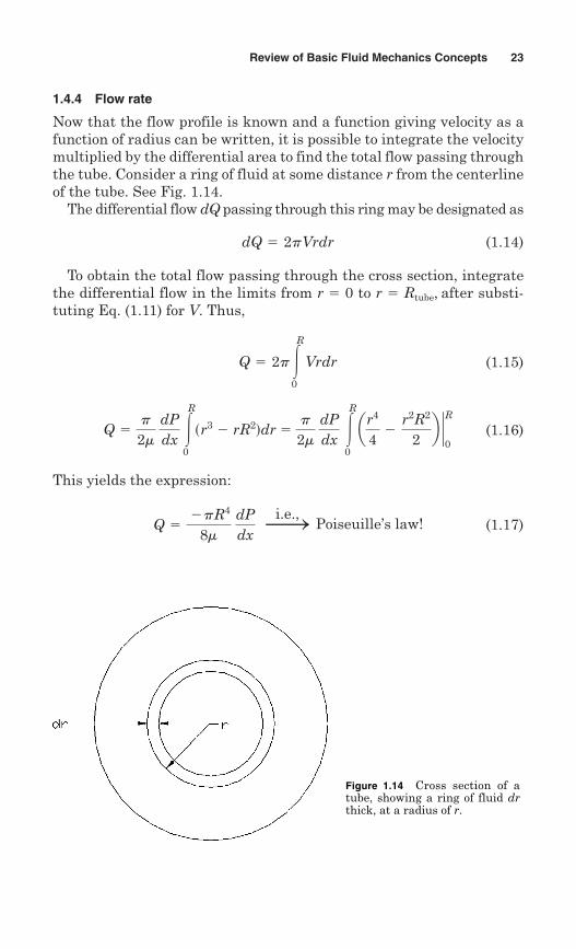
1.4.4 Flow rate
Now that the flow profile is known and a function giving velocity as afunction of radius can be written, it is possible to integrate the velocitymultiplied by the differential area to find the total flow passing throughthe tube. Consider a ring of fluid at some distance r from the centerlineof the tube. See Fig. 1.14.
The differential flow dQ passing through this ring may be designated as
(1.14)
To obtain the total flow passing through the cross section, integratethe differential flow in the limits from r � 0 to r � Rtube, after substi-tuting Eq. (1.11) for V. Thus,
(1.15)
(1.16)
This yields the expression:
(1.17)Q 52pR4
8m dPdx
hi.e.,
Poiseuille’s law!
Q 5p
2m dPdx
3R
0
sr3 2 rR2ddr 5p
2m dPdx
3R
0
ar4
42
r2R2
2b `R
0
Q 5 2p 3R
0
Vrdr
dQ 5 2pVrdr
Review of Basic Fluid Mechanics Concepts 23
Figure 1.14 Cross section of atube, showing a ring of fluid drthick, at a radius of r.
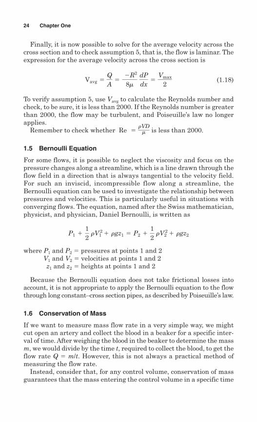
Finally, it is now possible to solve for the average velocity across thecross section and to check assumption 5, that is, the flow is laminar. Theexpression for the average velocity across the cross section is
(1.18)
To verify assumption 5, use Vavg to calculate the Reynolds number andcheck, to be sure, it is less than 2000. If the Reynolds number is greaterthan 2000, the flow may be turbulent, and Poiseuille’s law no longerapplies.
Remember to check whether is less than 2000.
1.5 Bernoulli Equation
For some flows, it is possible to neglect the viscosity and focus on thepressure changes along a streamline, which is a line drawn through theflow field in a direction that is always tangential to the velocity field.For such an inviscid, incompressible flow along a streamline, theBernoulli equation can be used to investigate the relationship betweenpressures and velocities. This is particularly useful in situations withconverging flows. The equation, named after the Swiss mathematician,physicist, and physician, Daniel Bernoulli, is written as
where P1 and P2 � pressures at points 1 and 2 V1 and V2 � velocities at points 1 and 2 z1 and z2 � heights at points 1 and 2
Because the Bernoulli equation does not take frictional losses intoaccount, it is not appropriate to apply the Bernoulli equation to the flowthrough long constant–cross section pipes, as described by Poiseuille’s law.
1.6 Conservation of Mass
If we want to measure mass flow rate in a very simple way, we mightcut open an artery and collect the blood in a beaker for a specific inter-val of time. After weighing the blood in the beaker to determine the massm, we would divide by the time t, required to collect the blood, to get theflow rate Q � m/t. However, this is not always a practical method ofmeasuring the flow rate.
Instead, consider that, for any control volume, conservation of massguarantees that the mass entering the control volume in a specific time
P1 112
rV121 rgz1 5 P2 1
12
rV221 rgz2
Re 5rVDm
Vavg 5QA5
2R2
8m dPdx
5Vmax
2
24 Chapter One
is equal to the sum of the mass leaving that same control volume overthe same time interval plus the increase in mass inside the controlvolume, that is,
The continuity equation presents conservation of mass in a slightly dif-ferent form for cases where the mass inside the control volume does notincrease or decrease, and it is written as
where r1 � the fluid density at point 1A1 � the area across which the fluid enters the control volume V1 � the average velocity of the fluid across A1
The variables r2, A2, and V2 are density, area, and average velocity atpoint 2.
For incompressible flows under circumstances where the mass insidethe control volume does not increase or decrease, the density of the fluidis constant (i.e., r1 � r2) and the continuity equation can be written inits more usual form:
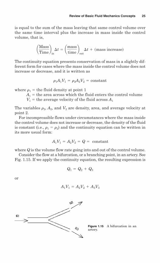
where Q is the volume flow rate going into and out of the control volume.Consider the flow at a bifurcation, or a branching point, in an artery. See
Fig. 1.15. If we apply the continuity equation, the resulting expression is
or
A1V1 5 A2V2 1 A3V3
Q1 5 Q2 1 Q3
A1V1 5 A2V2 5 Q 5 constant
r1A1V1 5 r2A2V2 5 constant
aMassTime
bin
t 5 amasstime
bout
t 1 smass increased
Review of Basic Fluid Mechanics Concepts 25
Figure 1.15 A bifurcation in anartery.
26 Chapter One
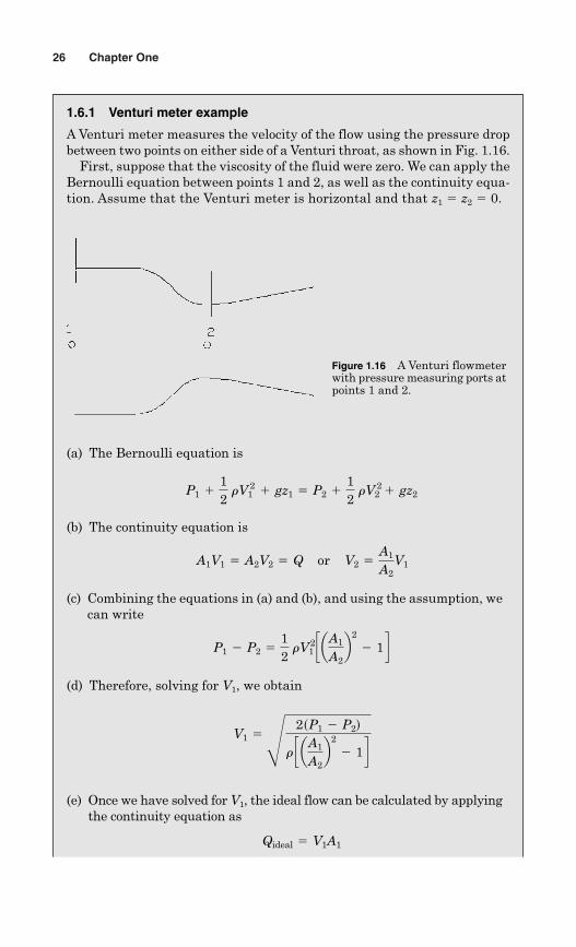
1.6.1 Venturi meter example
A Venturi meter measures the velocity of the flow using the pressure dropbetween two points on either side of a Venturi throat, as shown in Fig. 1.16.
First, suppose that the viscosity of the fluid were zero. We can apply theBernoulli equation between points 1 and 2, as well as the continuity equa-tion. Assume that the Venturi meter is horizontal and that z1 � z2 � 0.
Figure 1.16 A Venturi flowmeterwith pressure measuring ports atpoints 1 and 2.
(a) The Bernoulli equation is
(b) The continuity equation is
(c) Combining the equations in (a) and (b), and using the assumption, wecan write
(d) Therefore, solving for V1, we obtain
(e) Once we have solved for V1, the ideal flow can be calculated by applyingthe continuity equation as
Qideal 5 V1A1
V1 5ã 2sP1 2 P2d
r c aA1
A2b2
2 1 d
P1 2 P2 512
rV12 c aA1
A2b2
2 1 d
A1V1 5 A2V2 5 Q� � or� � V2 5A1
A2V1
P1 112
rV1 2 1 gz1 5 P2 1
12
rV221 gz2
1.7 Fluid Statics
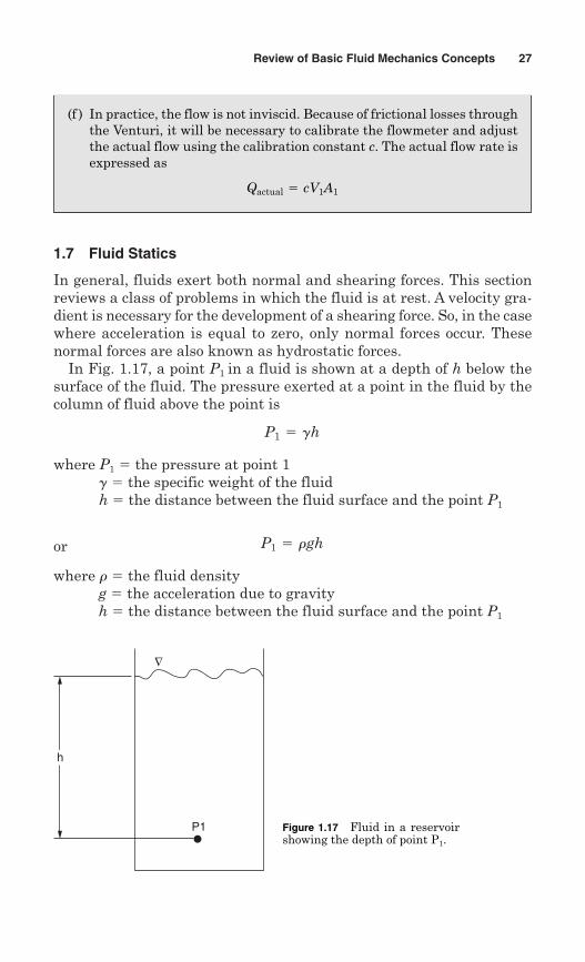
In general, fluids exert both normal and shearing forces. This sectionreviews a class of problems in which the fluid is at rest. A velocity gra-dient is necessary for the development of a shearing force. So, in the casewhere acceleration is equal to zero, only normal forces occur. Thesenormal forces are also known as hydrostatic forces.
In Fig. 1.17, a point P1 in a fluid is shown at a depth of h below thesurface of the fluid. The pressure exerted at a point in the fluid by thecolumn of fluid above the point is
where P1 � the pressure at point 1 g � the specific weight of the fluidh � the distance between the fluid surface and the point P1
or
where r � the fluid density g � the acceleration due to gravity h � the distance between the fluid surface and the point P1
P1 5 rgh
P1 5 gh
Review of Basic Fluid Mechanics Concepts 27
h
P1
∇
Figure 1.17 Fluid in a reservoirshowing the depth of point P1.
(f ) In practice, the flow is not inviscid. Because of frictional losses throughthe Venturi, it will be necessary to calibrate the flowmeter and adjustthe actual flow using the calibration constant c. The actual flow rate isexpressed as
Qactual 5 cV1A1
28 Chapter One
1.7.1 Example problem: fluid statics
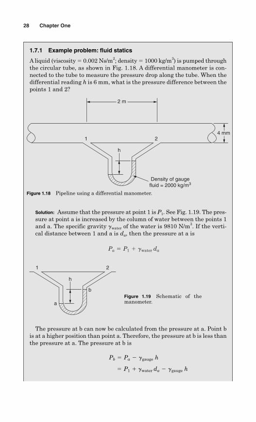
A liquid (viscosity � 0.002 Ns/m2; density � 1000 kg/m3) is pumped throughthe circular tube, as shown in Fig. 1.18. A differential manometer is con-nected to the tube to measure the pressure drop along the tube. When thedifferential reading h is 6 mm, what is the pressure difference between thepoints 1 and 2?
Solution: Assume that the pressure at point 1 is P1. See Fig. 1.19. The pres-sure at point a is increased by the column of water between the points 1and a. The specific gravity gwater of the water is 9810 N/m3. If the verti-cal distance between 1 and a is da, then the pressure at a is
Pa 5 P1 1 gwater da
Density of gaugefluid = 2000 kg/m3
h
4 mm
2 m
1 2
Figure 1.18 Pipeline using a differential manometer.
h
1 2
a
bFigure 1.19 Schematic of themanometer.
The pressure at b can now be calculated from the pressure at a. Point bis at a higher position than point a. Therefore, the pressure at b is less thanthe pressure at a. The pressure at b is
5 P1 1 gwater da 2 ggauge h
Pb 5 Pa 2 ggauge h
Review of Basic Fluid Mechanics Concepts 29
1.8 The Womersley Number �: a FrequencyParameter for Pulsatile Flow
The Womersley number, or alpha parameter, is another dimensionlessparameter that has been used in the study of fluid mechanics. Thisparameter represents a ratio of transient to viscous forces, just as theReynolds number represented a ratio of inertial to viscous forces. Acharacteristic frequency represents the time dependence of the param-eter. The Womersley number may be written as
where r � the vessel radius v � the fundamental frequency7
r � the density of the fluid m � the viscosity of the fluid � � the kinematic viscosity
In higher-frequency flows, the flow profile is blunter near the centerlineof the vessel since the inertia becomes more important than viscousforces. Near the wall, where V is close to zero, viscous forces are stillimportant.
a 5 rÅ v
n or a 5 rÅ
vr
m
where ggauge is the specific weight of the gauge fluid and h is the height ofpoint b with respect to point a.
The pressure at 2 is also lower than the pressure at b and is calculated from
Finally, the pressure difference between 1 and 2 is written as
or
P 5 a2000s9.81d Nm3 2 1000s9.81d
N m3b 6
1000 m 5 58.9
Nm2
P1 2 P2 5 sggauge 2 gwaterdh
5 P1 1 gwater da 2 ggauge h 2 sda 2 hdgwater
P2 5 Pb 2 sda 2 hdgwater
7 The fundamental frequency is typically the heart rate. The units must be rad/s fordimensional consistency.
30 Chapter One
Some typical values of the parameter a for various species are
human aorta a � 20
canine aorta a � 14
feline aorta a � 8
rat aorta a � 3
1.8.1 Example problem:Womersley number
The heart rate of a 400-kg horse is approximately 36 beats per minute (bpm),while the heart rate of a 3-kg rabbit is approximately 210 bpm (Li, 1996).Compare the Womersley number in the horse aorta to that in the rabbit aorta.
Li also points out that the size of red blood cells from various mammalsdoes not vary much in diameter. No mammal has a red blood cell larger than10 mm in diameter. Windberger et al. also published the values of viscosityfor nine different animals, including horse and rabbit. For this exampleproblem, we will assume that the blood density is approximately the sameacross the species. The published values of viscosity were 0.0052 Ns/m2 forthe horse and 0.0040 Ns/m2 for the rabbit.
Allometric studies of mammals show that various characteristics, likeaortic diameter, grow in a certain relationship with the size of the animal.From Li, we can use the published allometric relationship for the aorta sizeof various mammals to estimate the diameter of the aorta. Thus, we have(Li, 1996, Equation 3.7, p. 27)
where D is the aortic diameter, given in centimeters, and W is the animalweight, given in kilograms. Therefore, for this problem, we will use anaortic diameter of approximately 3.7 cm for the horse, 2.0 cm for the man,and 0.7 cm for the rabbit. Then,
From the results, one can see that transient forces become relativelymore important than viscous forces as the animal size increases.
arabbit 5 rÅvrm 50.7100
mã210a p30brad/s 1060 kg/m3
0.004 Ns/m2 5 17
ahorse 5 rÅvrm 53.7100
mã36a p30brad/s 1060 kg/m3
0.0052 Ns/m2 5 32
D 5 0.48 W 0.34
a 5 r Åvn � or� a 5 r Åvrm
Review Problems
1. Show that for the Poiseuille flow in a tube of radius R, the wall shearingstress can be obtained from the relationship:
for a Newtonian fluid of viscosity m. The volume rate of flow is Q.
2. Determine the wall shearing stress for a fluid, having a viscosity of 3.5 cP,flowing with an average velocity of 9 cm/s in a 3-mm-diameter tube. Whatis the corresponding Reynolds number? (The fluid density r� 1.06 g/cm3.)
3. In a 5-mm-diameter vessel, what is the value of the flow rate that causesa wall shear stress of 0.84 N/m2? Would the corresponding flow be lami-nar or turbulent?
4. It has been suggested that a power law:
be used to characterize the relationship between the shear stress and thevelocity gradient for blood. The quantity b is a constant, and the expo-nent n is an odd integer. Use this relationship, and derive the corre-sponding velocity distribution for flow in a tube. Use all assumptionsmade in deriving Poiseuille’s law (except for the shear stress relationship).
Plot several velocity distributions (�/�max versus r/R) for n � 1, 3, 5, . . .,to show how the profile changes with n.
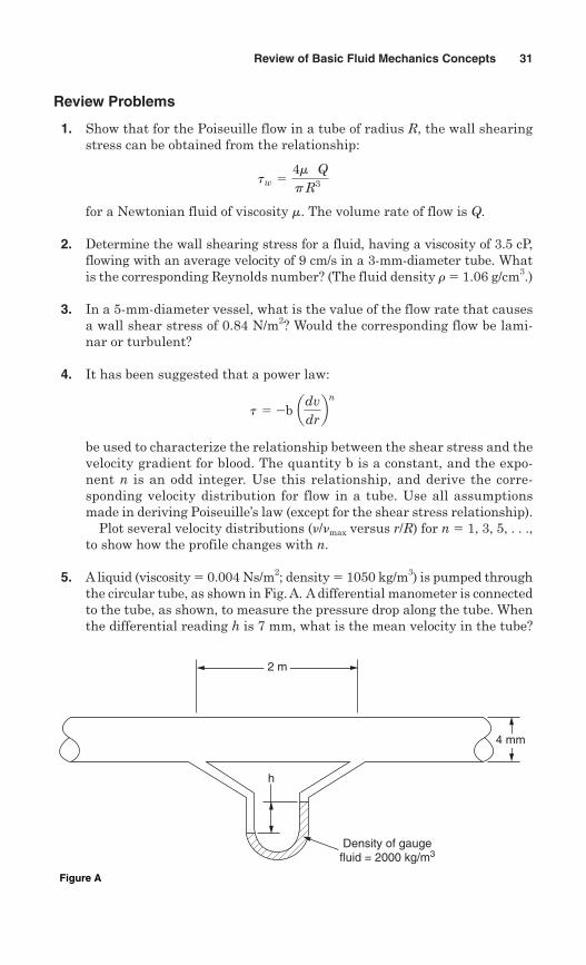
5. A liquid (viscosity � 0.004 Ns/m2; density � 1050 kg/m3) is pumped throughthe circular tube, as shown in Fig. A. A differential manometer is connectedto the tube, as shown, to measure the pressure drop along the tube. Whenthe differential reading h is 7 mm, what is the mean velocity in the tube?
t 52b advdrbn
tw 54m QpR3
Review of Basic Fluid Mechanics Concepts 31
Density of gaugefluid = 2000 kg/m3
h
4 mm
2 m
Figure A
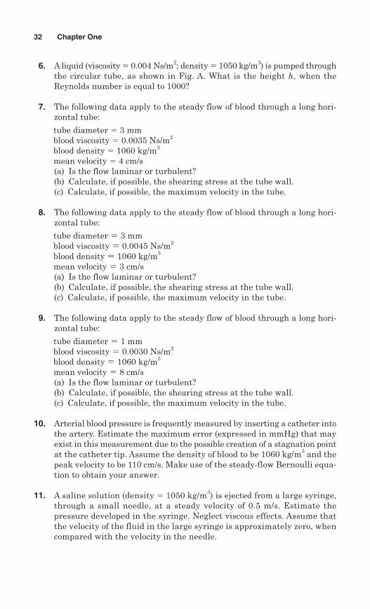
32 Chapter One
6. A liquid (viscosity � 0.004 Ns/m2; density � 1050 kg/m3) is pumped throughthe circular tube, as shown in Fig. A. What is the height h, when theReynolds number is equal to 1000?
7. The following data apply to the steady flow of blood through a long hori-zontal tube:
tube diameter � 3 mmblood viscosity � 0.0035 Ns/m2
blood density � 1060 kg/m3
mean velocity � 4 cm/s(a) Is the flow laminar or turbulent?(b) Calculate, if possible, the shearing stress at the tube wall.(c) Calculate, if possible, the maximum velocity in the tube.
8. The following data apply to the steady flow of blood through a long hori-zontal tube:
tube diameter � 3 mmblood viscosity � 0.0045 Ns/m2
blood density � 1060 kg/m3
mean velocity � 3 cm/s(a) Is the flow laminar or turbulent?(b) Calculate, if possible, the shearing stress at the tube wall.(c) Calculate, if possible, the maximum velocity in the tube.
9. The following data apply to the steady flow of blood through a long hori-zontal tube:
tube diameter � 1 mmblood viscosity � 0.0030 Ns/m2
blood density � 1060 kg/m3
mean velocity � 8 cm/s(a) Is the flow laminar or turbulent?(b) Calculate, if possible, the shearing stress at the tube wall.(c) Calculate, if possible, the maximum velocity in the tube.
10. Arterial blood pressure is frequently measured by inserting a catheter intothe artery. Estimate the maximum error (expressed in mmHg) that mayexist in this measurement due to the possible creation of a stagnation pointat the catheter tip. Assume the density of blood to be 1060 kg/m3 and thepeak velocity to be 110 cm/s. Make use of the steady-flow Bernoulli equa-tion to obtain your answer.
11. A saline solution (density � 1050 kg/m3) is ejected from a large syringe,through a small needle, at a steady velocity of 0.5 m/s. Estimate thepressure developed in the syringe. Neglect viscous effects. Assume thatthe velocity of the fluid in the large syringe is approximately zero, whencompared with the velocity in the needle.
12. A saline solution (density � 1050 kg/m3) is ejected from a 20-mm-diametersyringe, through a 2-mm-diameter needle, at a steady velocity of 0.5 m/s.Estimate the pressure developed in the syringe. Neglect viscous effects.
13. Estimate the value of velocity at which the saline solution in problem12 would be turbulent in the 2-mm-diameter needle. At that velocity, whatis the pressure developed in the syringe?
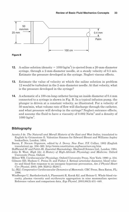
14. A schematic of a 100-cm-long catheter having an inside diameter of 0.4 mmconnected to a syringe is shown in Fig. B. In a typical infusion pump, theplunger is driven at a constant velocity, as illustrated. For a velocity of50 mm/min, what volume rate of flow will discharge through the catheter,and what pressure will develop in the syringe? Neglect entrance effects,and assume the fluid to have a viscosity of 0.002 Ns/m2 and a density of1000 kg/m3.
Bibliography
Acosta J de. The Naturall and Morall Historie of the East and West Indies, translated toEnglish by Grimestone E. Valentine Simmes for Edward Blount and Williams Aspleybooksellers, London; 1604.
Bacon, F. Novum Organum, edited by J. Devey. New Four, P.F. Collier, 1902 (Englishtranslation) pp. 356–360. http://www.constitution.org/bacon/nov.org.htm
Hoffbrand AV and Pettit JE. Essential Haematology. Blackwell Science Ltd., London; 1984.John B. West. High life; A History of High-Altitude Physiology and Medicine. Oxford
University Press, Oxford.Milnor WR. Cardiovascular Physiology. Oxford University Press, New York; 1990: p. 334.Gilmore ED, Hudson C, Preiss D, and Fisher J. Retinal arteriolar diameter, blood veloc-
ity and blood flow response to an isocapnic hyperoxic provocation, Am J Physiol HeartCirc Physiol, 2005; 288: H2912–H2917.
Li, JKJ, Comparative Cardiovascular Dynamics of Mammals. CRC Press, Boca Raton, FL;1996.
Windberger U, Bartholovitsch A, Plasenzotti R, Korak KJ, and Heinze G. Whole blood vis-cosity, plasma viscosity and erythrocyte aggregation in nine mammalian species:Reference values and comparison data, Exp Physiol, 2003;88(3):431–440.
Review of Basic Fluid Mechanics Concepts 33
100 cm
25 mm
50mm/min
Patm
0.4 mm
Figure B

This page intentionally left blank
Chapter
2Cardiovascular Structure
and Function
2.1 Introduction
One may question why it is important for a biomedical engineer to studyphysiology. To answer this question, we can begin by recognizing thatcardiovascular disorders are now the leading cause of death in developednations. Furthermore, to understand the pathologies or dysfunctions ofthe cardiovascular system, engineers must first begin to understand thephysiology or proper functioning of that system. If an engineer wouldlike to design devices and procedures to remedy those cardiovascularpathologies, then she or he must be well acquainted with physiology.
The cardiovascular system consists of the heart, arteries, veins,capillaries, and lymphatic vessels. Lymphatic vessels are vesselswhich collect extracellular fluid and return it to circulation. The mostbasic functions of the cardiovascular system are to deliver oxygenand nutrients, to remove waste, and to regulate temperature.
The heart is actually two pumps: the left heart and the right heart.The amount of blood coming from the heart (cardiac output) is depend-ent on arterial pressure. This chapter deals with the heart and its abil-ity to generate arterial pressure in order to pump blood.
The adult human heart has a mass of approximately 300 g. If it beats70 times per minute, then it will beat ~100,000 times per day, ~35 milliontimes per year, and ~3 billion times (3 � 109) during your lifetime. If eachbeat ejects 70 mL of blood, your heart pumps over 7000 L, or the equiva-lent of 1800 gal/day. That is the same as 30 barrels of blood each andevery day of your life! The lifetime equivalent work done by the heart isthe equivalent of lifting a 30-ton weight to the top of Mount Everest. Allof this work is done by a very hardworking 300-g muscle that does not rest!
35
Copyright © 2007 by The McGraw-Hill Companies, Inc. Click here for terms of use.
36 Chapter Two
2.2 Clinical Features
A 58-year-old German woman had undergone surgery in 1974 to fix amitral stenosis.1 She later developed a restenosis, which caused themitral valve to leak. She underwent surgery in November 1982 to replaceher natural mitral valve with a Björk-Shiley convexo-concave mitralprosthesis.2
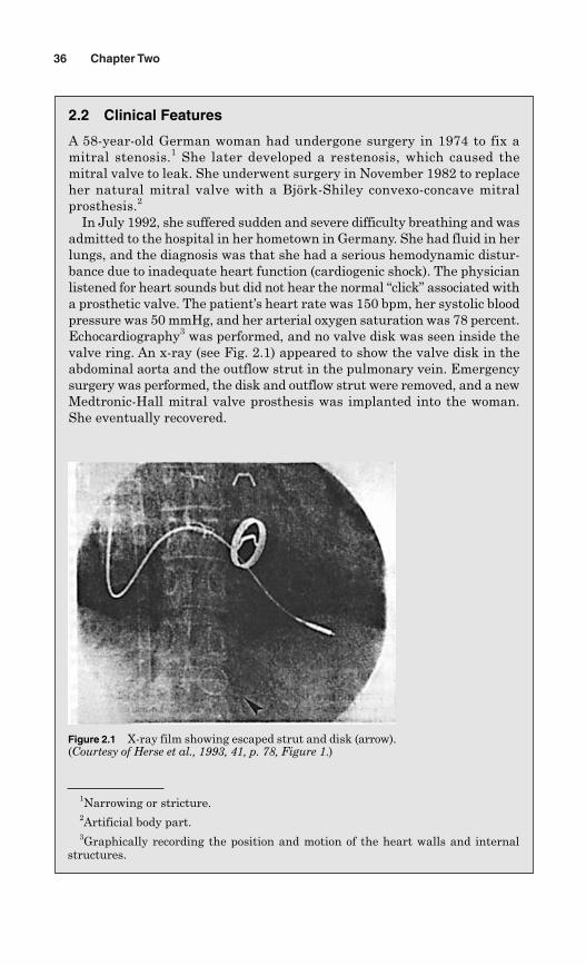
In July 1992, she suffered sudden and severe difficulty breathing and wasadmitted to the hospital in her hometown in Germany. She had fluid in herlungs, and the diagnosis was that she had a serious hemodynamic distur-bance due to inadequate heart function (cardiogenic shock). The physicianlistened for heart sounds but did not hear the normal “click” associated witha prosthetic valve. The patient’s heart rate was 150 bpm, her systolic bloodpressure was 50 mmHg, and her arterial oxygen saturation was 78 percent.Echocardiography3 was performed, and no valve disk was seen inside thevalve ring. An x-ray (see Fig. 2.1) appeared to show the valve disk in theabdominal aorta and the outflow strut in the pulmonary vein. Emergencysurgery was performed, the disk and outflow strut were removed, and a newMedtronic-Hall mitral valve prosthesis was implanted into the woman.She eventually recovered.
Figure 2.1 X-ray film showing escaped strut and disk (arrow).(Courtesy of Herse et al., 1993, 41, p. 78, Figure 1.)
1Narrowing or stricture.2Artificial body part.3Graphically recording the position and motion of the heart walls and internal
structures.
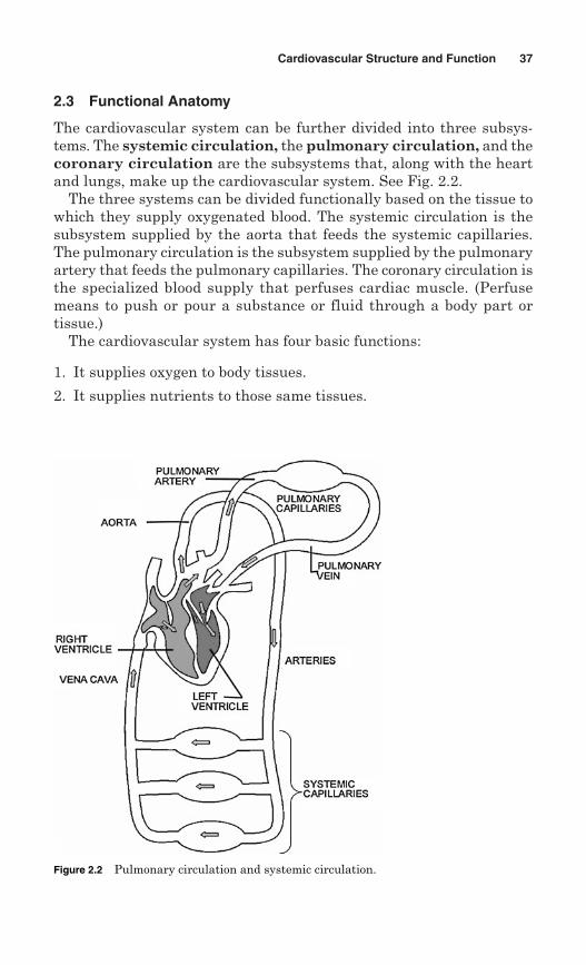
2.3 Functional Anatomy
The cardiovascular system can be further divided into three subsys-tems. The systemic circulation, the pulmonary circulation, and thecoronary circulation are the subsystems that, along with the heartand lungs, make up the cardiovascular system. See Fig. 2.2.
The three systems can be divided functionally based on the tissue towhich they supply oxygenated blood. The systemic circulation is thesubsystem supplied by the aorta that feeds the systemic capillaries.The pulmonary circulation is the subsystem supplied by the pulmonaryartery that feeds the pulmonary capillaries. The coronary circulation isthe specialized blood supply that perfuses cardiac muscle. (Perfusemeans to push or pour a substance or fluid through a body part ortissue.)
The cardiovascular system has four basic functions:
1. It supplies oxygen to body tissues.
2. It supplies nutrients to those same tissues.
Cardiovascular Structure and Function 37
Figure 2.2 Pulmonary circulation and systemic circulation.
3. It removes carbon dioxide and other wastes from the body.
4. It regulates temperature.
The path of blood flowing through the circulatory system and thepressures of the blood at various points along the path tell us much abouthow tissue is perfused with oxygen. The left heart supplies oxygenatedblood to the aorta at a relatively high pressure.
Blood continues to flow along the path through the circulatory system,and its path may be described as follows: Blood flows into smaller arter-ies and finally into systemic capillaries where oxygen is supplied to thesurrounding tissues. At the same time, it picks up waste carbon diox-ide from that same tissue and continues flowing into the veins.Eventually, the blood returns to the vena cava. From the vena cava,deoxygenated blood flows into the right heart. From the right heart, thestill deoxygenated blood flows into the pulmonary artery. The pulmonaryartery supplies blood to the lungs where carbon dioxide is exchangedwith oxygen. The blood, which has been enriched with oxygen, flows fromthe lungs through the pulmonary veins and back to the left heart.
It is interesting to note that blood flowing through the pulmonaryartery is deoxygenated and blood flowing through the pulmonary veinis oxygenated. Although systemic arteries carry oxygenated blood, it isa mistake to think of arteries only as vessels that carry oxygenatedblood. A more appropriate distinction between arteries and veins is thatarteries carry blood at a relatively higher pressure than the pressurewithin the corresponding veins.
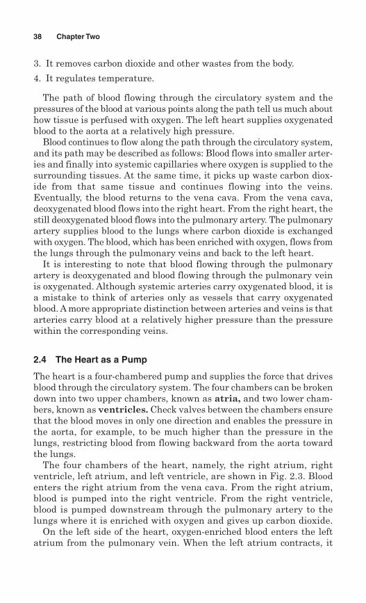
2.4 The Heart as a Pump
The heart is a four-chambered pump and supplies the force that drivesblood through the circulatory system. The four chambers can be brokendown into two upper chambers, known as atria, and two lower cham-bers, known as ventricles. Check valves between the chambers ensurethat the blood moves in only one direction and enables the pressure inthe aorta, for example, to be much higher than the pressure in thelungs, restricting blood from flowing backward from the aorta towardthe lungs.
The four chambers of the heart, namely, the right atrium, rightventricle, left atrium, and left ventricle, are shown in Fig. 2.3. Bloodenters the right atrium from the vena cava. From the right atrium,blood is pumped into the right ventricle. From the right ventricle,blood is pumped downstream through the pulmonary artery to thelungs where it is enriched with oxygen and gives up carbon dioxide.
On the left side of the heart, oxygen-enriched blood enters the leftatrium from the pulmonary vein. When the left atrium contracts, it
38 Chapter Two
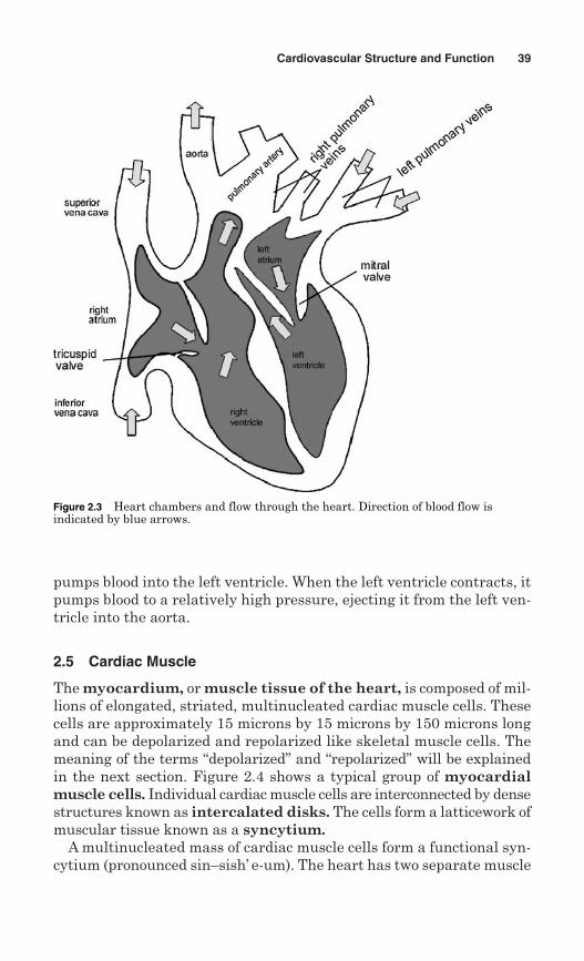
pumps blood into the left ventricle. When the left ventricle contracts, itpumps blood to a relatively high pressure, ejecting it from the left ven-tricle into the aorta.
2.5 Cardiac Muscle
The myocardium, or muscle tissue of the heart, is composed of mil-lions of elongated, striated, multinucleated cardiac muscle cells. Thesecells are approximately 15 microns by 15 microns by 150 microns longand can be depolarized and repolarized like skeletal muscle cells. Themeaning of the terms “depolarized” and “repolarized” will be explainedin the next section. Figure 2.4 shows a typical group of myocardialmuscle cells. Individual cardiac muscle cells are interconnected by densestructures known as intercalated disks. The cells form a latticework ofmuscular tissue known as a syncytium.
A multinucleated mass of cardiac muscle cells form a functional syn-cytium (pronounced sin–sish’ e-um). The heart has two separate muscle
Cardiovascular Structure and Function 39
Figure 2.3 Heart chambers and flow through the heart. Direction of blood flow isindicated by blue arrows.
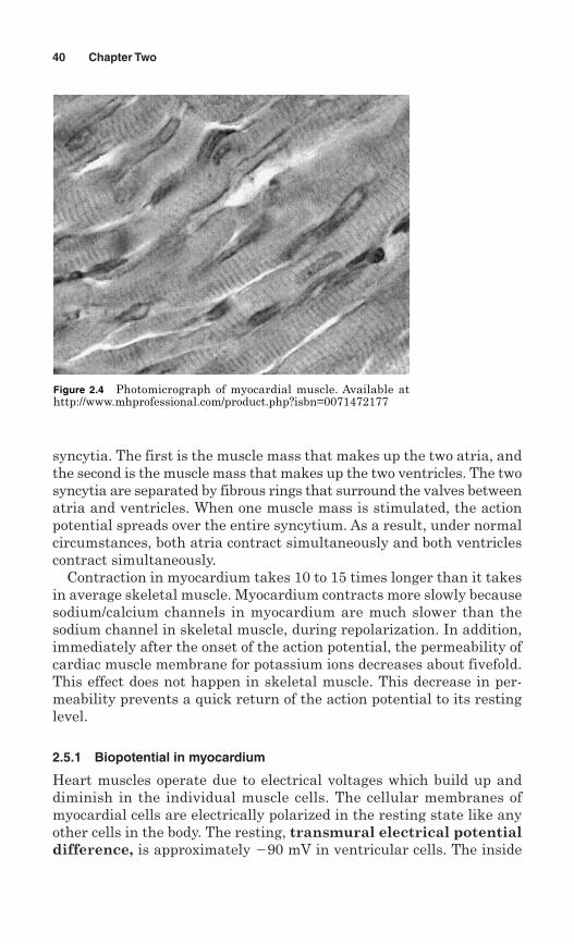
syncytia. The first is the muscle mass that makes up the two atria, andthe second is the muscle mass that makes up the two ventricles. The twosyncytia are separated by fibrous rings that surround the valves betweenatria and ventricles. When one muscle mass is stimulated, the actionpotential spreads over the entire syncytium. As a result, under normalcircumstances, both atria contract simultaneously and both ventriclescontract simultaneously.
Contraction in myocardium takes 10 to 15 times longer than it takesin average skeletal muscle. Myocardium contracts more slowly becausesodium/calcium channels in myocardium are much slower than thesodium channel in skeletal muscle, during repolarization. In addition,immediately after the onset of the action potential, the permeability ofcardiac muscle membrane for potassium ions decreases about fivefold.This effect does not happen in skeletal muscle. This decrease in per-meability prevents a quick return of the action potential to its restinglevel.
2.5.1 Biopotential in myocardium
Heart muscles operate due to electrical voltages which build up anddiminish in the individual muscle cells. The cellular membranes ofmyocardial cells are electrically polarized in the resting state like anyother cells in the body. The resting, transmural electrical potentialdifference, is approximately 90 mV in ventricular cells. The inside
40 Chapter Two
Figure 2.4 Photomicrograph of myocardial muscle. Available athttp://www.mhprofessional.com/product.php?isbn=0071472177
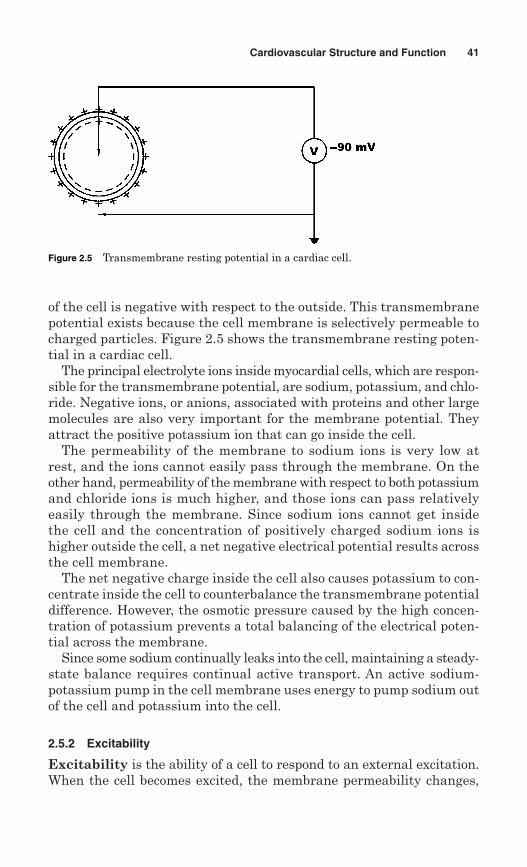
of the cell is negative with respect to the outside. This transmembranepotential exists because the cell membrane is selectively permeable tocharged particles. Figure 2.5 shows the transmembrane resting poten-tial in a cardiac cell.
The principal electrolyte ions inside myocardial cells, which are respon-sible for the transmembrane potential, are sodium, potassium, and chlo-ride. Negative ions, or anions, associated with proteins and other largemolecules are also very important for the membrane potential. Theyattract the positive potassium ion that can go inside the cell.
The permeability of the membrane to sodium ions is very low atrest, and the ions cannot easily pass through the membrane. On theother hand, permeability of the membrane with respect to both potassiumand chloride ions is much higher, and those ions can pass relativelyeasily through the membrane. Since sodium ions cannot get insidethe cell and the concentration of positively charged sodium ions ishigher outside the cell, a net negative electrical potential results acrossthe cell membrane.
The net negative charge inside the cell also causes potassium to con-centrate inside the cell to counterbalance the transmembrane potentialdifference. However, the osmotic pressure caused by the high concen-tration of potassium prevents a total balancing of the electrical poten-tial across the membrane.
Since some sodium continually leaks into the cell, maintaining a steady-state balance requires continual active transport. An active sodium-potassium pump in the cell membrane uses energy to pump sodium outof the cell and potassium into the cell.
2.5.2 Excitability
Excitability is the ability of a cell to respond to an external excitation.When the cell becomes excited, the membrane permeability changes,
Cardiovascular Structure and Function 41
Figure 2.5 Transmembrane resting potential in a cardiac cell.
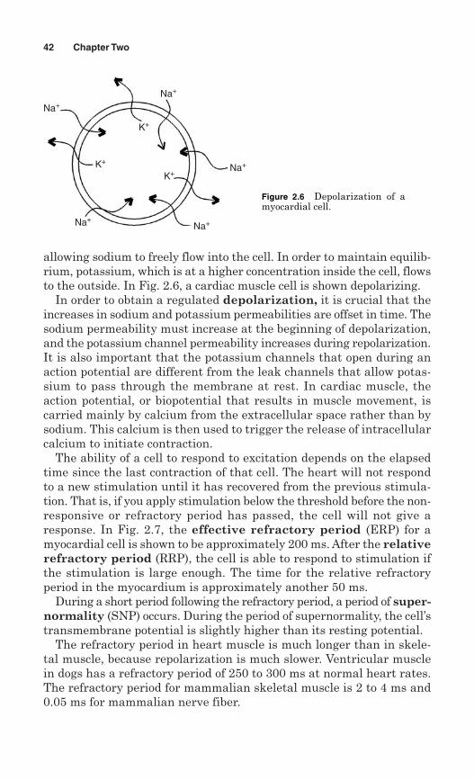
allowing sodium to freely flow into the cell. In order to maintain equilib-rium, potassium, which is at a higher concentration inside the cell, flowsto the outside. In Fig. 2.6, a cardiac muscle cell is shown depolarizing.
In order to obtain a regulated depolarization, it is crucial that theincreases in sodium and potassium permeabilities are offset in time. Thesodium permeability must increase at the beginning of depolarization,and the potassium channel permeability increases during repolarization.It is also important that the potassium channels that open during anaction potential are different from the leak channels that allow potas-sium to pass through the membrane at rest. In cardiac muscle, theaction potential, or biopotential that results in muscle movement, iscarried mainly by calcium from the extracellular space rather than bysodium. This calcium is then used to trigger the release of intracellularcalcium to initiate contraction.
The ability of a cell to respond to excitation depends on the elapsedtime since the last contraction of that cell. The heart will not respondto a new stimulation until it has recovered from the previous stimula-tion. That is, if you apply stimulation below the threshold before the non-responsive or refractory period has passed, the cell will not give aresponse. In Fig. 2.7, the effective refractory period (ERP) for amyocardial cell is shown to be approximately 200 ms. After the relativerefractory period (RRP), the cell is able to respond to stimulation ifthe stimulation is large enough. The time for the relative refractoryperiod in the myocardium is approximately another 50 ms.
During a short period following the refractory period, a period of super-normality (SNP) occurs. During the period of supernormality, the cell’stransmembrane potential is slightly higher than its resting potential.
The refractory period in heart muscle is much longer than in skele-tal muscle, because repolarization is much slower. Ventricular musclein dogs has a refractory period of 250 to 300 ms at normal heart rates.The refractory period for mammalian skeletal muscle is 2 to 4 ms and0.05 ms for mammalian nerve fiber.
42 Chapter Two
Na+
Na+
Na+
K+
K+
K+
Na+
Na+
Figure 2.6 Depolarization of amyocardial cell.
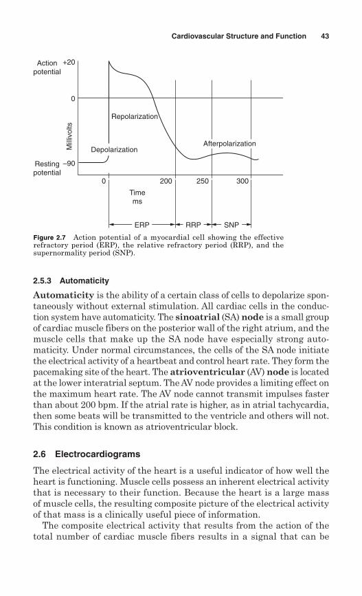
2.5.3 Automaticity
Automaticity is the ability of a certain class of cells to depolarize spon-taneously without external stimulation. All cardiac cells in the conduc-tion system have automaticity. The sinoatrial (SA) node is a small groupof cardiac muscle fibers on the posterior wall of the right atrium, and themuscle cells that make up the SA node have especially strong auto-maticity. Under normal circumstances, the cells of the SA node initiatethe electrical activity of a heartbeat and control heart rate. They form thepacemaking site of the heart. The atrioventricular (AV) node is locatedat the lower interatrial septum. The AV node provides a limiting effect onthe maximum heart rate. The AV node cannot transmit impulses fasterthan about 200 bpm. If the atrial rate is higher, as in atrial tachycardia,then some beats will be transmitted to the ventricle and others will not.This condition is known as atrioventricular block.
2.6 Electrocardiograms
The electrical activity of the heart is a useful indicator of how well theheart is functioning. Muscle cells possess an inherent electrical activitythat is necessary to their function. Because the heart is a large massof muscle cells, the resulting composite picture of the electrical activityof that mass is a clinically useful piece of information.
The composite electrical activity that results from the action of thetotal number of cardiac muscle fibers results in a signal that can be
Cardiovascular Structure and Function 43
200 250 300
Time ms
ERP RRP SNP
0
Repolarization
Mill
ivol
ts
0
+20
–90
Actionpotential
Restingpotential
AfterpolarizationDepolarization
Figure 2.7 Action potential of a myocardial cell showing the effectiverefractory period (ERP), the relative refractory period (RRP), and thesupernormality period (SNP).
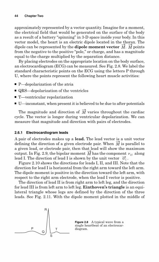
approximately represented by a vector quantity. Imagine for a moment,the electrical field that would be generated on the surface of the bodyas a result of a battery “spinning” in 3-D space inside your body. In thisvector model, the heart is an electric dipole located in the thorax. Thedipole can be represented by the dipole moment vector . pointsfrom the negative to the positive “pole,” or charge, and has a magnitudeequal to the charge multiplied by the separation distance.
By placing electrodes on the appropriate location on the body surface,an electrocardiogram (ECG) can be measured. See Fig. 2.8. We label thestandard characteristic points on the ECG using the letters P throughU, where the points represent the following heart muscle activities:
■ P—depolarization of the atria■ QRS—depolarization of the ventricles■ T—ventricular repolarization■ U—inconstant, when present it is believed to be due to after potentials
The magnitude and direction of varies throughout the cardiaccycle. The vector is longer during ventricular depolarization. We canmeasure that magnitude and direction with pairs of electrodes.
2.6.1 Electrocardiogram leads
A pair of electrodes makes up a lead. The lead vector is a unit vectordefining the direction of a given electrode pair. When is parallel toa given lead, or electrode pair, then that lead will show the maximumoutput. In Fig. 2.9, the bipolar moment has the component alonglead I. The direction of lead I is shown by the unit vector .
Figure 2.10 shows the directions for leads I, II, and III. Note that thedirection for lead I is horizontal from the right arm toward the left arm.The dipole moment is positive in the direction toward the left arm, withrespect to the right arm electrode, when the lead I vector is positive.
The direction of lead II is from right arm to left leg, and the directionfor lead III is from left arm to left leg. Einthoven’s triangle is an equi-lateral triangle whose legs are defined by the direction of the threeleads. See Fig. 2.11. With the dipole moment plotted in the middle of
aS1
na1MS
MS
MS
MS
MS
44 Chapter Two
P
R
QS
T
Figure 2.8 A typical wave from asingle heartbeat of an electrocar-diogram.
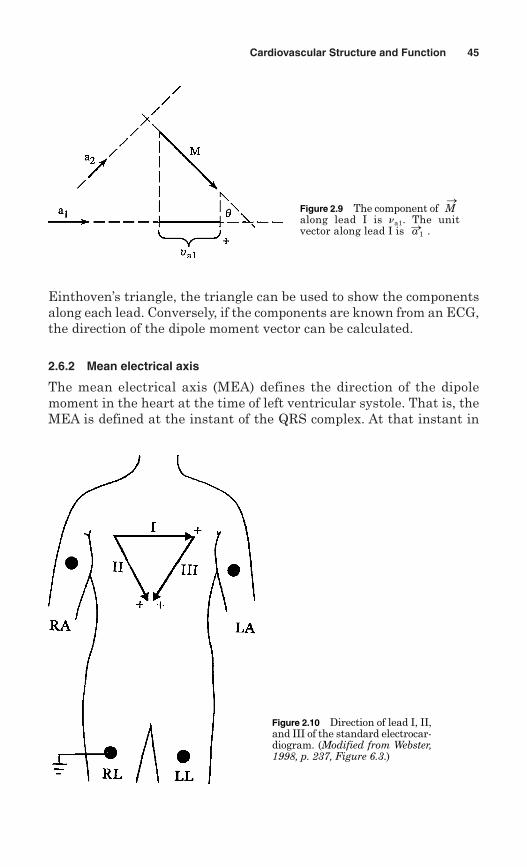
Einthoven’s triangle, the triangle can be used to show the componentsalong each lead. Conversely, if the components are known from an ECG,the direction of the dipole moment vector can be calculated.
2.6.2 Mean electrical axis
The mean electrical axis (MEA) defines the direction of the dipolemoment in the heart at the time of left ventricular systole. That is, theMEA is defined at the instant of the QRS complex. At that instant in
Cardiovascular Structure and Function 45
Figure 2.10 Direction of lead I, II,and III of the standard electrocar-diogram. (Modified from Webster,1998, p. 237, Figure 6.3.)
Figure 2.9 The component of along lead I is na1. The unitvector along lead I is .aS1
MS
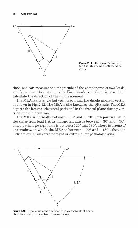
time, one can measure the magnitude of the components of two leads,and from this information, using Einthoven’s triangle, it is possible tocalculate the direction of the dipole moment.
The MEA is the angle between lead I and the dipole moment vector,as shown in Fig. 2.12. The MEA is also known as the QRS axis. The MEAdepicts the heart’s “electrical position” in the frontal plane during ven-tricular depolarization.
The MEA is normally between 30° and �120° with positive beingclockwise from lead I. A pathologic left axis is between 30° and 90°,and a pathologic right axis is between 120° and 180°. There is a zone ofuncertainty, in which the MEA is between 90° and 180°, that canindicate either an extreme right or extreme left pathologic axis.
46 Chapter Two
++
LL
–
+LARA –
–
I
II
III
Figure 2.11 Einthoven’s trianglefor the standard electrocardio-gram.
++
LL
–
+LARA –
–
I
II
III
MEA
Figure 2.12 Dipole moment and the three components it gener-ates along the three electrocardiogram axes.
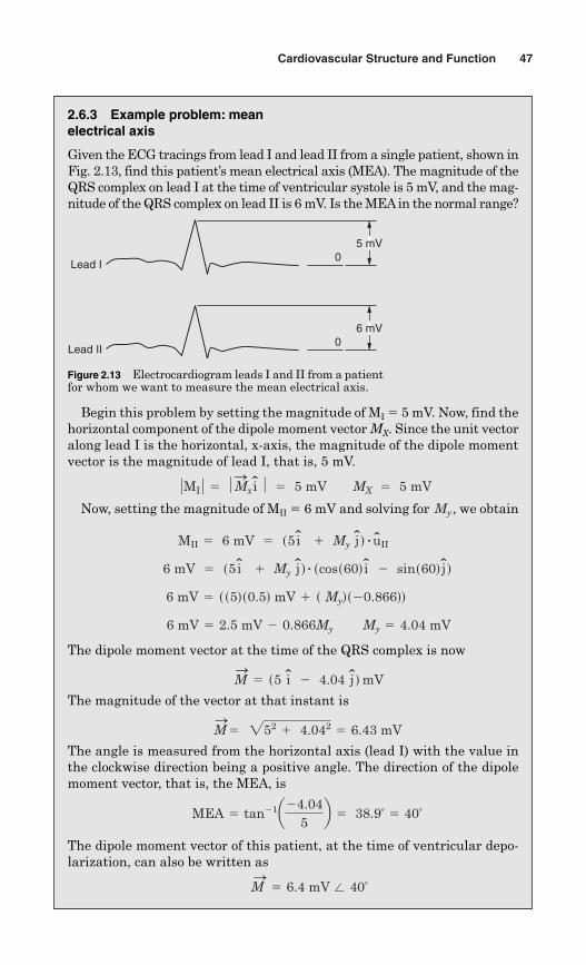
Cardiovascular Structure and Function 47
2.6.3 Example problem: meanelectrical axis
Given the ECG tracings from lead I and lead II from a single patient, shown inFig. 2.13, find this patient’s mean electrical axis (MEA). The magnitude of theQRS complex on lead I at the time of ventricular systole is 5 mV, and the mag-nitude of the QRS complex on lead II is 6 mV. Is the MEAin the normal range?
Lead I0
5 mV
Lead II0
6 mV
Figure 2.13 Electrocardiogram leads I and II from a patientfor whom we want to measure the mean electrical axis.
Begin this problem by setting the magnitude of MI � 5 mV. Now, find thehorizontal component of the dipole moment vector MX. Since the unit vectoralong lead I is the horizontal, x-axis, the magnitude of the dipole momentvector is the magnitude of lead I, that is, 5 mV.
Now, setting the magnitude of MII � 6 mV and solving for , we obtain
The dipole moment vector at the time of the QRS complex is now
The magnitude of the vector at that instant is
The angle is measured from the horizontal axis (lead I) with the value inthe clockwise direction being a positive angle. The direction of the dipolemoment vector, that is, the MEA, is
The dipole moment vector of this patient, at the time of ventricular depo-larization, can also be written as
M S5 6.4 mV / 40+
MEA 5 tan21a24.045b 5 38.9+ 5 40+
MS 5 252 1 4.042 5 6.43 mV
MS5 s5 i 2 4.04 j d mV
6 mV 5 2.5 mV 2 0.866My� � � � My 5 4.04 mV
6 mV 5 ss5ds0.5d mV 1 s Myds20.866dd
6 mV 5 s5i 1 My j d ? scoss60d i 2 sins60d j d
MII 5 6 mV 5 s5i 1 My j d ? uII
My
ZMI Z 5 ZMSx i Z 5 5 mV MX 5 5 mV
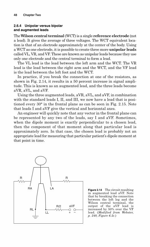
48 Chapter Two
R/2 aVF
LARA
RR
RLLL + –
Figure 2.14 The circuit resultingin augmented lead aVF. Notethat by breaking the connectionbetween the left leg and theWilson central terminal, theoutput of the aVF lead isincreased by 50% over the VFlead. (Modified from Webster, p. 240, Figure 6.5c.)
2.6.4 Unipolar versus bipolar and augmented leads
The Wilson central terminal (WCT) is a single reference electrode (nota lead). It gives the average of three voltages. The WCT equivalent loca-tion is that of an electrode approximately at the center of the body. Usinga WCT as one electrode, it is possible to create three more unipolar leadscalled VL, VR, and VF. These are known as unipolar leads because they useonly one electrode and the central terminal to form a lead.
The VL lead is the lead between the left arm and the WCT. The VRlead is the lead between the right arm and the WCT, and the VF leadis the lead between the left foot and the WCT.
In practice, if you break the connection at one of the resistors, asshown in Fig. 2.14, it results in a 50 percent increase in signal ampli-tude. This is known as an augmented lead, and the three leads becomeaVR, aVL, and aVF.
Using the three augmented leads, aVR, aVL, and aVF, in combinationwith the standard leads I, II, and III, we now have a lead that is posi-tioned every 30° in the frontal plane as can be seen in Fig. 2.15. Notethat leads I and aVF give the vertical and horizontal axes.
An engineer will quickly note that any vector in the frontal plane canbe represented by any two of the leads, say I and aVF. Sometimes,when the dipole moment is exactly perpendicular to a chosen lead,then the component of that moment along that particular lead isapproximately zero. In that case, the chosen lead is probably not anappropriate lead for measuring that particular patient’s dipole moment atthat point in time.
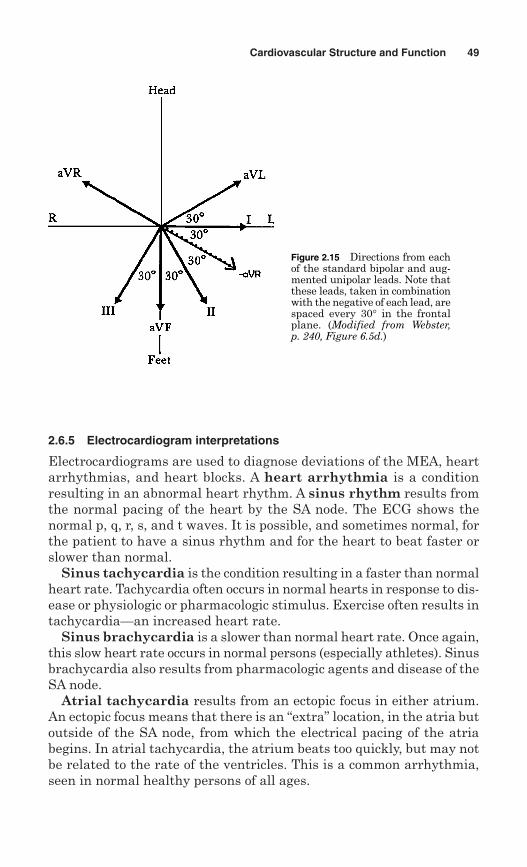
Cardiovascular Structure and Function 49
2.6.5 Electrocardiogram interpretations
Electrocardiograms are used to diagnose deviations of the MEA, heartarrhythmias, and heart blocks. A heart arrhythmia is a conditionresulting in an abnormal heart rhythm. A sinus rhythm results fromthe normal pacing of the heart by the SA node. The ECG shows thenormal p, q, r, s, and t waves. It is possible, and sometimes normal, forthe patient to have a sinus rhythm and for the heart to beat faster orslower than normal.
Sinus tachycardia is the condition resulting in a faster than normalheart rate. Tachycardia often occurs in normal hearts in response to dis-ease or physiologic or pharmacologic stimulus. Exercise often results intachycardia—an increased heart rate.
Sinus brachycardia is a slower than normal heart rate. Once again,this slow heart rate occurs in normal persons (especially athletes). Sinusbrachycardia also results from pharmacologic agents and disease of theSA node.
Atrial tachycardia results from an ectopic focus in either atrium.An ectopic focus means that there is an “extra” location, in the atria butoutside of the SA node, from which the electrical pacing of the atriabegins. In atrial tachycardia, the atrium beats too quickly, but may notbe related to the rate of the ventricles. This is a common arrhythmia,seen in normal healthy persons of all ages.
Figure 2.15 Directions from eachof the standard bipolar and aug-mented unipolar leads. Note thatthese leads, taken in combinationwith the negative of each lead, arespaced every 30° in the frontalplane. (Modified from Webster, p. 240, Figure 6.5d.)
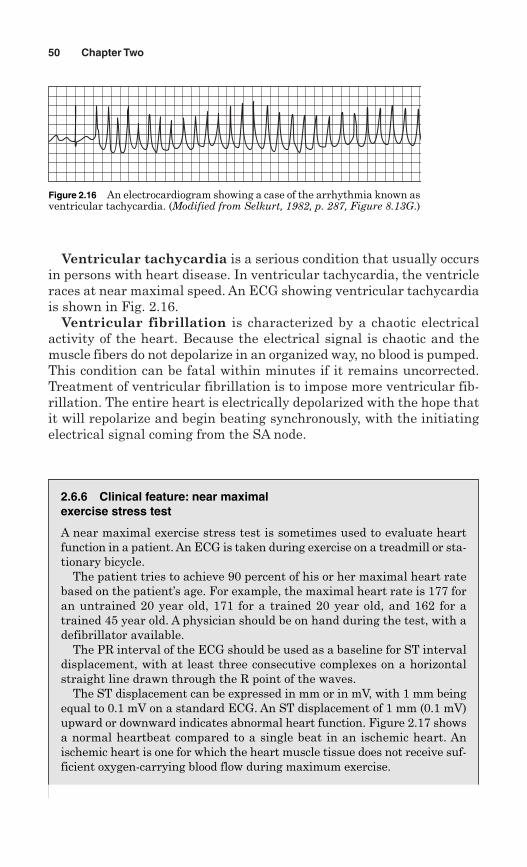
Ventricular tachycardia is a serious condition that usually occursin persons with heart disease. In ventricular tachycardia, the ventricleraces at near maximal speed. An ECG showing ventricular tachycardiais shown in Fig. 2.16.
Ventricular fibrillation is characterized by a chaotic electricalactivity of the heart. Because the electrical signal is chaotic and themuscle fibers do not depolarize in an organized way, no blood is pumped.This condition can be fatal within minutes if it remains uncorrected.Treatment of ventricular fibrillation is to impose more ventricular fib-rillation. The entire heart is electrically depolarized with the hope thatit will repolarize and begin beating synchronously, with the initiatingelectrical signal coming from the SA node.
50 Chapter Two
Figure 2.16 An electrocardiogram showing a case of the arrhythmia known asventricular tachycardia. (Modified from Selkurt, 1982, p. 287, Figure 8.13G.)
2.6.6 Clinical feature: near maximalexercise stress test
A near maximal exercise stress test is sometimes used to evaluate heartfunction in a patient. An ECG is taken during exercise on a treadmill or sta-tionary bicycle.
The patient tries to achieve 90 percent of his or her maximal heart ratebased on the patient’s age. For example, the maximal heart rate is 177 foran untrained 20 year old, 171 for a trained 20 year old, and 162 for atrained 45 year old. A physician should be on hand during the test, with adefibrillator available.
The PR interval of the ECG should be used as a baseline for ST intervaldisplacement, with at least three consecutive complexes on a horizontalstraight line drawn through the R point of the waves.
The ST displacement can be expressed in mm or in mV, with 1 mm beingequal to 0.1 mV on a standard ECG. An ST displacement of 1 mm (0.1 mV)upward or downward indicates abnormal heart function. Figure 2.17 showsa normal heartbeat compared to a single beat in an ischemic heart. Anischemic heart is one for which the heart muscle tissue does not receive suf-ficient oxygen-carrying blood flow during maximum exercise.
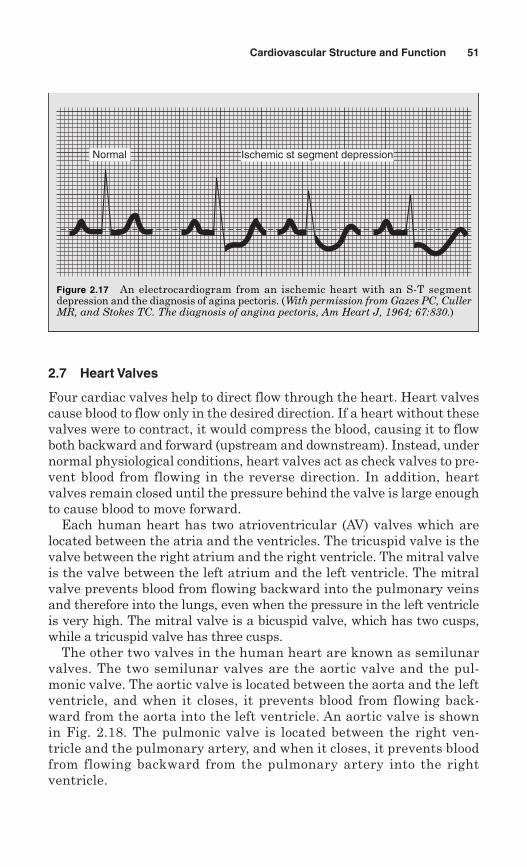
Cardiovascular Structure and Function 51
2.7 Heart Valves
Four cardiac valves help to direct flow through the heart. Heart valvescause blood to flow only in the desired direction. If a heart without thesevalves were to contract, it would compress the blood, causing it to flowboth backward and forward (upstream and downstream). Instead, undernormal physiological conditions, heart valves act as check valves to pre-vent blood from flowing in the reverse direction. In addition, heartvalves remain closed until the pressure behind the valve is large enoughto cause blood to move forward.
Each human heart has two atrioventricular (AV) valves which arelocated between the atria and the ventricles. The tricuspid valve is thevalve between the right atrium and the right ventricle. The mitral valveis the valve between the left atrium and the left ventricle. The mitralvalve prevents blood from flowing backward into the pulmonary veinsand therefore into the lungs, even when the pressure in the left ventricleis very high. The mitral valve is a bicuspid valve, which has two cusps,while a tricuspid valve has three cusps.
The other two valves in the human heart are known as semilunarvalves. The two semilunar valves are the aortic valve and the pul-monic valve. The aortic valve is located between the aorta and the leftventricle, and when it closes, it prevents blood from flowing back-ward from the aorta into the left ventricle. An aortic valve is shownin Fig. 2.18. The pulmonic valve is located between the right ven-tricle and the pulmonary artery, and when it closes, it prevents bloodfrom flowing backward from the pulmonary artery into the right ventricle.
Figure 2.17 An electrocardiogram from an ischemic heart with an S-T segmentdepression and the diagnosis of agina pectoris. (With permission from Gazes PC, CullerMR, and Stokes TC. The diagnosis of angina pectoris, Am Heart J, 1964; 67:830.)
Normal Ischemic st segment depression
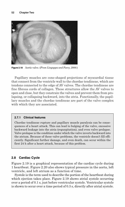
Papillary muscles are cone-shaped projections of myocardial tissuethat connect from the ventricle wall to the chordae tendineae, which aretendons connected to the edge of AV valves. The chordae tendineae arefine fibrous cords of collagen. These structures allow the AV valves toopen and close, but they constrain the valves and prevent them from pro-lapsing, or collapsing backward, into the atria. Functionally, the papil-lary muscles and the chordae tendineae are part of the valve complexwith which they are associated.
52 Chapter Two
Figure 2.18 Aortic valve. (From Lingappa and Farey, 2000.)
2.7.1 Clinical features
Chordae tendineae rupture and papillary muscle paralysis can be conse-quences of a heart attack. This can lead to bulging of the valve, excessivebackward leakage into the atria (regurgitation), and even valve prolapse.Valve prolapse is the condition under which the valve inverts backward intothe atrium. Because of these valve problems, the ventricle doesn’t fill effi-ciently. Significant further damage, and even death, can occur within thefirst 24 h after a heart attack, because of this problem.
2.8 Cardiac Cycle
Figure 2.19 is a graphical representation of the cardiac cycle during1 heartbeat. Figure 2.20 also shows typical pressure in the aorta, leftventricle, and left atrium as a function of time.
Systole is the term used to describe the portion of the heartbeat duringwhich ejection takes place. Figure 2.19 shows atrial systole occurringover a period of 0.1 s, just before ventricular systole. Ventricular systoleis shown to occur over a time period of 0.3 s, directly after atrial systole.
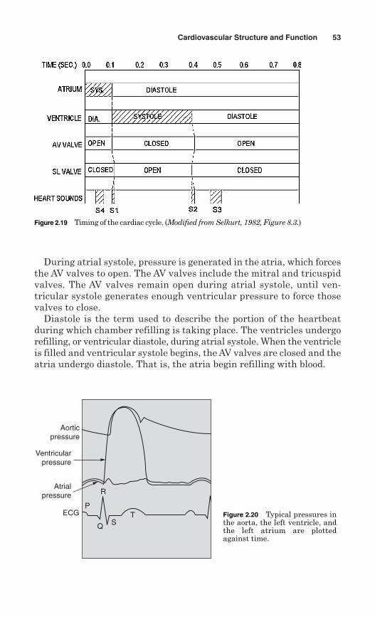
Cardiovascular Structure and Function 53
During atrial systole, pressure is generated in the atria, which forcesthe AV valves to open. The AV valves include the mitral and tricuspidvalves. The AV valves remain open during atrial systole, until ven-tricular systole generates enough ventricular pressure to force thosevalves to close.
Diastole is the term used to describe the portion of the heartbeatduring which chamber refilling is taking place. The ventricles undergorefilling, or ventricular diastole, during atrial systole. When the ventricleis filled and ventricular systole begins, the AV valves are closed and theatria undergo diastole. That is, the atria begin refilling with blood.
Figure 2.19 Timing of the cardiac cycle. (Modified from Selkurt, 1982, Figure 8.3.)
Q ST
P
R
ECG
Atrialpressure
Ventricularpressure
Aorticpressure
Figure 2.20 Typical pressures inthe aorta, the left ventricle, andthe left atrium are plottedagainst time.
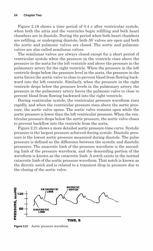
Figure 2.19 shows a time period of 0.4 s after ventricular systole,when both the atria and the ventricles begin refilling and both heartchambers are in diastole. During the period when both heart chambersare refilling, or undergoing diastole, both AV valves are open and boththe aortic and pulmonic valves are closed. The aortic and pulmonicvalves are also called semilunar valves.
The semilunar valves are always closed except for a short period ofventricular systole when the pressure in the ventricle rises above thepressure in the aorta for the left ventricle and above the pressure in thepulmonary artery for the right ventricle. When the pressure in the leftventricle drops below the pressure level in the aorta, the pressure in theaorta forces the aortic valve to close to prevent blood from flowing back-ward into the left ventricle. Similarly, when the pressure in the rightventricle drops below the pressure levels in the pulmonary artery, thepressure in the pulmonary artery forces the pulmonic valve to close toprevent blood from flowing backward into the right ventricle.
During ventricular systole, the ventricular pressure waveform risesrapidly, and when the ventricular pressure rises above the aortic pres-sure, the aortic valve opens. The aortic valve remains open while theaortic pressure is lower than the left ventricular pressure. When the ven-tricular pressure drops below the aortic pressure, the aortic valve closesto prevent backflow into the ventricle from the aorta.
Figure 2.21 shows a more detailed aortic pressure-time curve. Systolicpressure is the largest pressure achieved during systole. Diastolic pres-sure is the lowest aortic pressure measured during diastole. The pulsepressure is defined as the difference between the systolic and diastolicpressures. The anacrotic limb of the pressure waveform is the ascend-ing limb of the pressure waveform, and the descending portion of thewaveform is known as the catacrotic limb. A notch exists in the normalcatacrotic limb of the aortic pressure waveform. That notch is known asthe dicrotic notch and is related to a transient drop in pressure due tothe closing of the aortic valve.
54 Chapter Two
Figure 2.21 Aortic pressure waveform.
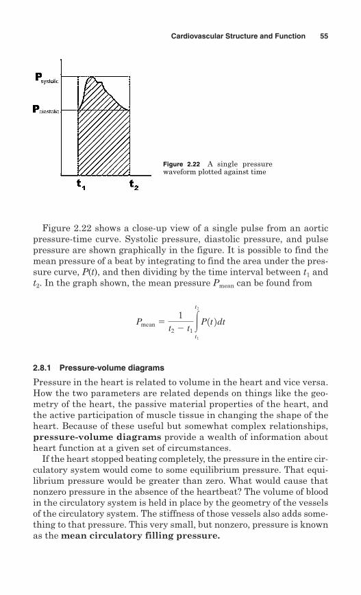
Figure 2.22 shows a close-up view of a single pulse from an aorticpressure-time curve. Systolic pressure, diastolic pressure, and pulsepressure are shown graphically in the figure. It is possible to find themean pressure of a beat by integrating to find the area under the pres-sure curve, P(t), and then dividing by the time interval between t1 andt2. In the graph shown, the mean pressure Pmean can be found from
2.8.1 Pressure-volume diagrams
Pressure in the heart is related to volume in the heart and vice versa.How the two parameters are related depends on things like the geo-metry of the heart, the passive material properties of the heart, andthe active participation of muscle tissue in changing the shape of theheart. Because of these useful but somewhat complex relationships,pressure-volume diagrams provide a wealth of information aboutheart function at a given set of circumstances.
If the heart stopped beating completely, the pressure in the entire cir-culatory system would come to some equilibrium pressure. That equi-librium pressure would be greater than zero. What would cause thatnonzero pressure in the absence of the heartbeat? The volume of bloodin the circulatory system is held in place by the geometry of the vesselsof the circulatory system. The stiffness of those vessels also adds some-thing to that pressure. This very small, but nonzero, pressure is knownas the mean circulatory filling pressure.
Pmean �1
t2 t1�t2
t1
P1t 2dt
Cardiovascular Structure and Function 55
Figure 2.22 A single pressurewaveform plotted against time
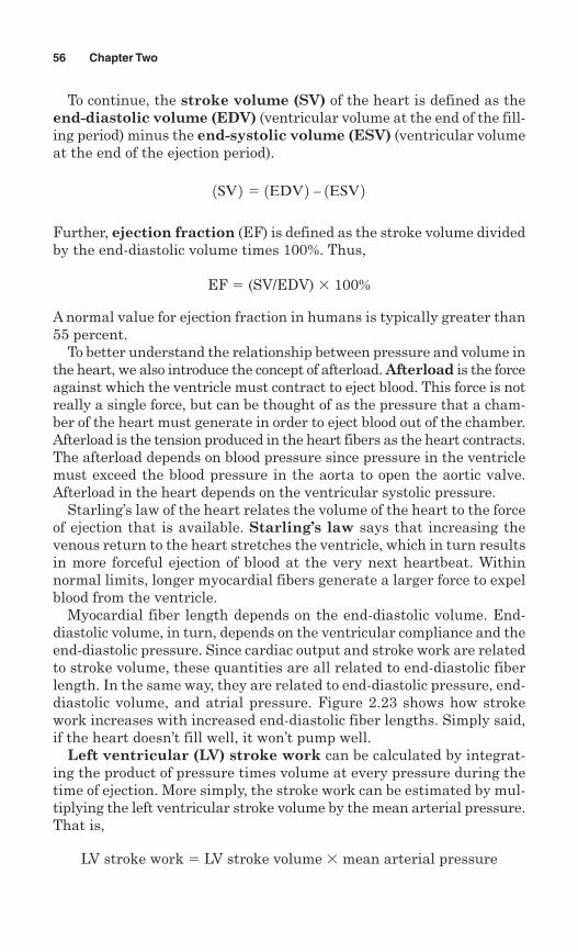
To continue, the stroke volume (SV) of the heart is defined as theend-diastolic volume (EDV) (ventricular volume at the end of the fill-ing period) minus the end-systolic volume (ESV) (ventricular volumeat the end of the ejection period).
Further, ejection fraction (EF) is defined as the stroke volume dividedby the end-diastolic volume times 100%. Thus,
EF � (SV/EDV) � 100%
A normal value for ejection fraction in humans is typically greater than55 percent.
To better understand the relationship between pressure and volume inthe heart, we also introduce the concept of afterload. Afterload is the forceagainst which the ventricle must contract to eject blood. This force is notreally a single force, but can be thought of as the pressure that a cham-ber of the heart must generate in order to eject blood out of the chamber.Afterload is the tension produced in the heart fibers as the heart contracts.The afterload depends on blood pressure since pressure in the ventriclemust exceed the blood pressure in the aorta to open the aortic valve.Afterload in the heart depends on the ventricular systolic pressure.
Starling’s law of the heart relates the volume of the heart to the forceof ejection that is available. Starling’s law says that increasing thevenous return to the heart stretches the ventricle, which in turn resultsin more forceful ejection of blood at the very next heartbeat. Withinnormal limits, longer myocardial fibers generate a larger force to expelblood from the ventricle.
Myocardial fiber length depends on the end-diastolic volume. End-diastolic volume, in turn, depends on the ventricular compliance and theend-diastolic pressure. Since cardiac output and stroke work are relatedto stroke volume, these quantities are all related to end-diastolic fiberlength. In the same way, they are related to end-diastolic pressure, end-diastolic volume, and atrial pressure. Figure 2.23 shows how strokework increases with increased end-diastolic fiber lengths. Simply said,if the heart doesn’t fill well, it won’t pump well.
Left ventricular (LV) stroke work can be calculated by integrat-ing the product of pressure times volume at every pressure during thetime of ejection. More simply, the stroke work can be estimated by mul-tiplying the left ventricular stroke volume by the mean arterial pressure.That is,
LV stroke work � LV stroke volume � mean arterial pressure
1SV 2 � 1EDV 2 – 1ESV 2
56 Chapter Two
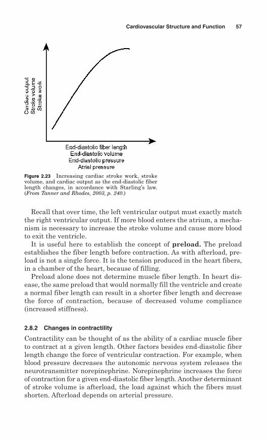
Recall that over time, the left ventricular output must exactly matchthe right ventricular output. If more blood enters the atrium, a mecha-nism is necessary to increase the stroke volume and cause more bloodto exit the ventricle.
It is useful here to establish the concept of preload. The preloadestablishes the fiber length before contraction. As with afterload, pre-load is not a single force. It is the tension produced in the heart fibers,in a chamber of the heart, because of filling.
Preload alone does not determine muscle fiber length. In heart dis-ease, the same preload that would normally fill the ventricle and createa normal fiber length can result in a shorter fiber length and decreasethe force of contraction, because of decreased volume compliance(increased stiffness).
2.8.2 Changes in contractility
Contractility can be thought of as the ability of a cardiac muscle fiberto contract at a given length. Other factors besides end-diastolic fiberlength change the force of ventricular contraction. For example, whenblood pressure decreases the autonomic nervous system releases theneurotransmitter norepinephrine. Norepinephrine increases the forceof contraction for a given end-diastolic fiber length. Another determinantof stroke volume is afterload, the load against which the fibers mustshorten. Afterload depends on arterial pressure.
Cardiovascular Structure and Function 57
Figure 2.23 Increasing cardiac stroke work, strokevolume, and cardiac output as the end-diastolic fiberlength changes, in accordance with Starling’s law.(From Tanner and Rhodes, 2003, p. 240.)
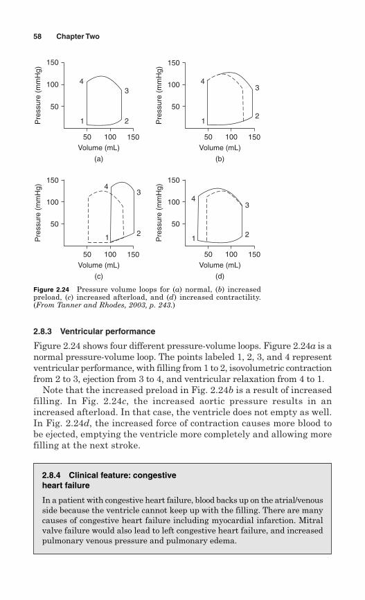
2.8.3 Ventricular performance
Figure 2.24 shows four different pressure-volume loops. Figure 2.24a is anormal pressure-volume loop. The points labeled 1, 2, 3, and 4 representventricular performance, with filling from 1 to 2, isovolumetric contractionfrom 2 to 3, ejection from 3 to 4, and ventricular relaxation from 4 to 1.
Note that the increased preload in Fig. 2.24b is a result of increasedfilling. In Fig. 2.24c, the increased aortic pressure results in anincreased afterload. In that case, the ventricle does not empty as well.In Fig. 2.24d, the increased force of contraction causes more blood tobe ejected, emptying the ventricle more completely and allowing morefilling at the next stroke.
58 Chapter Two
50 100 150
Volume (mL)
(a)
50
100
150
Pre
ssur
e (m
mH
g)
4
1
3
2
50 100 150
Volume (mL)
(b)
50
100
150
Pre
ssur
e (m
mH
g)
4
1
3
2
50 100 150
Volume (mL)
(c)
50
100
150
Pre
ssur
e (m
mH
g) 4
1
3
2
50 100 150
Volume (mL)
(d)
50
100
150
Pre
ssur
e (m
mH
g)
4
1
3
2
Figure 2.24 Pressure volume loops for (a) normal, (b) increasedpreload, (c) increased afterload, and (d) increased contractility.(From Tanner and Rhodes, 2003, p. 243.)
2.8.4 Clinical feature: congestive heart failure
In a patient with congestive heart failure, blood backs up on the atrial/venousside because the ventricle cannot keep up with the filling. There are manycauses of congestive heart failure including myocardial infarction. Mitralvalve failure would also lead to left congestive heart failure, and increasedpulmonary venous pressure and pulmonary edema.
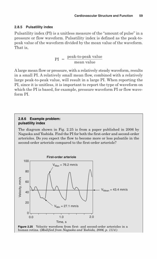
Cardiovascular Structure and Function 59
2.8.5 Pulsatility index
Pulsatility index (PI) is a unitless measure of the “amount of pulse” in apressure or flow waveform. Pulsatility index is defined as the peak-to-peak value of the waveform divided by the mean value of the waveform.That is,
A large mean flow or pressure, with a relatively steady waveform, resultsin a small PI. A relatively small mean flow, combined with a relativelylarge peak-to-peak value, will result in a large PI. When reporting thePI, since it is unitless, it is important to report the type of waveform onwhich the PI is based, for example, pressure waveform PI or flow wave-form PI.
PI 5 peak-to-peak value
mean value
2.8.6 Example problem:pulsatility index
The diagram shown in Fig. 2.25 is from a paper published in 2006 byNagaoka and Yoshida. Find the PI for both the first-order and second-orderarterioles. Do you expect the flow to become more or less pulsatile in thesecond-order arteriole compared to the first-order arteriole?
Figure 2.25 Velocity waveform from first- and second-order arterioles in ahuman retina. (Modified from Nagaoka and Yoshida, 2006, p. 1114.)
Time, s
Vel
ocity
, mm
/s
First-order arteriole
VMax = 76.2 mm/s
VMin = 27.1 mm/s
VMean = 43.4 mm/s
2.01.00.00
20
40
60
80
100
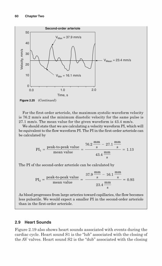
2.9 Heart Sounds
Figure 2.19 also shows heart sounds associated with events during thecardiac cycle. Heart sound S1 is the “lub” associated with the closing ofthe AV valves. Heart sound S2 is the “dub” associated with the closing
60 Chapter Two
Time, s
Vel
ocity
, mm
/s
Second-order arteriole
VMax = 37.9 mm/s
VMin = 16.1 mm/s
VMean = 23.4 mm/s
2.01.00.00
10
20
30
40
50
Figure 2.25 (Continued)
For the first-order arteriole, the maximum systolic-waveform velocityis 76.2 mm/s and the minimum diastolic velocity for the same pulse is27.1 mm/s. The mean value for the given waveform is 43.4 mm/s.
We should state that we are calculating a velocity waveform PI, which willbe equivalent to the flow waveform PI. The PI in the first-order arteriole canbe calculated by
The PI of the second-order arteriole can be calculated by
As blood progresses from large arteries toward capillaries, the flow becomesless pulsatile. We would expect a smaller PI in the second-order arteriolethan in the first-order arteriole.
PI2 5peak-to-peak value
mean value5
37.9 mm
s2 16.1
mms
23.4 mm
s
5 0.93
PI1 5peak-to-peak value
mean value5
76.2 mm
s2 27.1
mms
43.4 mm
s
5 1.13
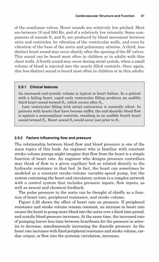
Cardiovascular Structure and Function 61
of the semilunar valves. Heart sounds are relatively low pitched. Mostare between 10 and 500 Hz, and of a relatively low intensity. Some com-ponents of sounds S1 and S2 are produced by blood movement betweenatria and ventricles, by vibration of the ventricular walls, and even byvibration of the base of the aorta and pulmonary arteries. A third, lessdistinct heart sound may occur shortly after the opening of the AV valves.This sound can be heard most often in children or in adults with thinchest walls. A fourth sound may occur during atrial systole, when a smallvolume of blood is injected into the nearly filled ventricle. Once again,this less distinct sound is heard most often in children or in thin adults.
2.9.1 Clinical features
An increased end-systolic volume is typical in heart failure. In a patientwith a failing heart, rapid early ventricular filling produces an audiblethird heart sound termed S3, which occurs after S2.
Late ventricular filling with atrial contraction is normally silent. Inpatients with hearts that have become stiffer, the end-diastolic blood flowis against a noncompliant ventricle, resulting in an audible fourth heartsound termed S4. Heart sound S4 would occur just prior to S1.
2.9.2 Factors influencing flow and pressure
The relationship between blood flow and blood pressure is one of themain topics of this book. An engineer who is familiar with constantstroke-volume pumps might imagine that flow from the heart is a simplefunction of heart rate. An engineer who designs pressure controllersmay think of flow to a given capillary bed as related directly to thehydraulic resistance in that bed. In fact, the heart can sometimes bemodeled as a constant stroke-volume variable-speed pump, but thesystem containing the heart and circulatory system is a complex networkwith a control system that includes pressure inputs, flow inputs, aswell as neural and chemical feedback.
The pulse pressure in the aorta can be thought of chiefly as a func-tion of heart rate, peripheral resistance, and stroke volume.
Figure 2.26 shows the effect of heart rate on pressure. If peripheralresistance and stroke volume remain constant, an increase in heart ratecauses the heart to pump more blood into the aorta over a fixed time period,and systolic blood pressure increases. At the same time, the increased rateof pumping leaves less time between heartbeats for the pressure in arter-ies to decrease, simultaneously increasing the diastolic pressure. As theheart rate increases with fixed peripheral resistance and stroke volume, car-diac output, or flow into the systemic circulation, increases.
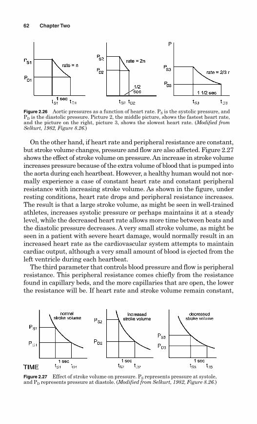
62 Chapter Two
Figure 2.27 Effect of stroke volume on pressure. PS represents pressure at systole,and PD represents pressure at diastole. (Modified from Selkurt, 1982, Figure 8.26.)
Figure 2.26 Aortic pressures as a function of heart rate. PS is the systolic pressure, andPD is the diastolic pressure. Picture 2, the middle picture, shows the fastest heart rate,and the picture on the right, picture 3, shows the slowest heart rate. (Modified fromSelkurt, 1982, Figure 8.26.)
On the other hand, if heart rate and peripheral resistance are constant,but stroke volume changes, pressure and flow are also affected. Figure 2.27shows the effect of stroke volume on pressure. An increase in stroke volumeincreases pressure because of the extra volume of blood that is pumped intothe aorta during each heartbeat. However, a healthy human would not nor-mally experience a case of constant heart rate and constant peripheralresistance with increasing stroke volume. As shown in the figure, underresting conditions, heart rate drops and peripheral resistance increases.The result is that a large stroke volume, as might be seen in well-trainedathletes, increases systolic pressure or perhaps maintains it at a steadylevel, while the decreased heart rate allows more time between beats andthe diastolic pressure decreases. A very small stroke volume, as might beseen in a patient with severe heart damage, would normally result in anincreased heart rate as the cardiovascular system attempts to maintaincardiac output, although a very small amount of blood is ejected from theleft ventricle during each heartbeat.
The third parameter that controls blood pressure and flow is peripheralresistance. This peripheral resistance comes chiefly from the resistancefound in capillary beds, and the more capillaries that are open, the lowerthe resistance will be. If heart rate and stroke volume remain constant,
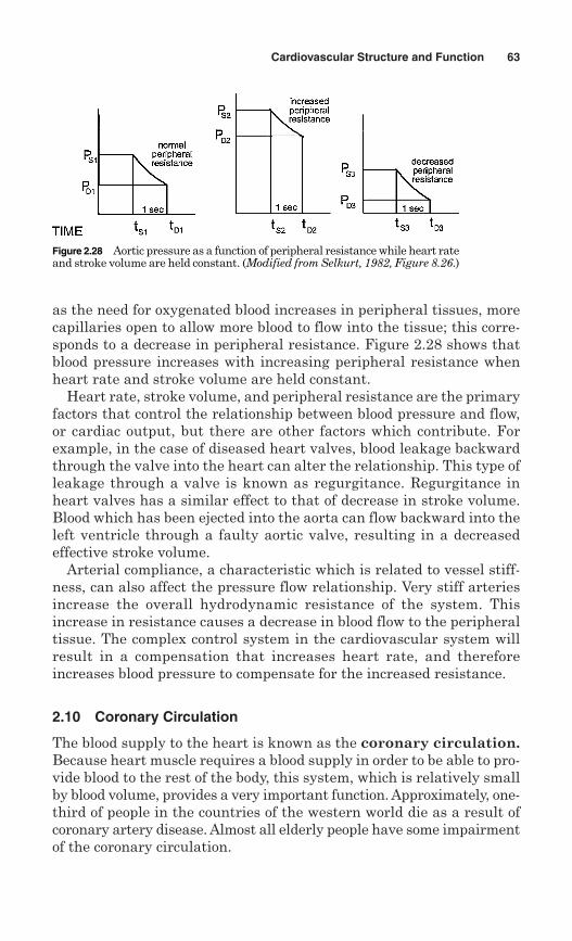
as the need for oxygenated blood increases in peripheral tissues, morecapillaries open to allow more blood to flow into the tissue; this corre-sponds to a decrease in peripheral resistance. Figure 2.28 shows thatblood pressure increases with increasing peripheral resistance whenheart rate and stroke volume are held constant.
Heart rate, stroke volume, and peripheral resistance are the primaryfactors that control the relationship between blood pressure and flow,or cardiac output, but there are other factors which contribute. Forexample, in the case of diseased heart valves, blood leakage backwardthrough the valve into the heart can alter the relationship. This type ofleakage through a valve is known as regurgitance. Regurgitance inheart valves has a similar effect to that of decrease in stroke volume.Blood which has been ejected into the aorta can flow backward into theleft ventricle through a faulty aortic valve, resulting in a decreasedeffective stroke volume.
Arterial compliance, a characteristic which is related to vessel stiff-ness, can also affect the pressure flow relationship. Very stiff arteriesincrease the overall hydrodynamic resistance of the system. Thisincrease in resistance causes a decrease in blood flow to the peripheraltissue. The complex control system in the cardiovascular system willresult in a compensation that increases heart rate, and thereforeincreases blood pressure to compensate for the increased resistance.
2.10 Coronary Circulation
The blood supply to the heart is known as the coronary circulation.Because heart muscle requires a blood supply in order to be able to pro-vide blood to the rest of the body, this system, which is relatively smallby blood volume, provides a very important function. Approximately, one-third of people in the countries of the western world die as a result ofcoronary artery disease. Almost all elderly people have some impairmentof the coronary circulation.
Cardiovascular Structure and Function 63
Figure 2.28 Aortic pressure as a function of peripheral resistance while heart rateand stroke volume are held constant. (Modified from Selkurt, 1982, Figure 8.26.)
The resting coronary blood flow in humans is around 225 mL/min,which is a bit less than 5 percent of cardiac output. During strenuousexercise, cardiac output in young healthy people increases four- to sev-enfold. Because the heart also provides this increased flow at a higherarterial pressure, the work of the heart is increased six to nine timesover the resting work output. The coronary blood flow increases only six-to ninefold to supply oxygen and nutrients needed by the cardiac muscle,during this increased workload.
The main coronary artery arises from the root of the aorta. It thenbranches into the left and right coronary arteries. Seventy-five percentof the coronary blood supply goes through the left coronary artery and25 percent through the right coronary artery.
The left coronary artery supplies blood to the left lateral portion of theleft ventricle and the anterior (front) portion of the ventricular septum.The ventricular septum is the wall between the left and right ventricles.The left coronary artery then branches into the anterior descend-ing coronary artery and the circumflex coronary artery. Those twobranches provide blood supply to the left ventricle.
The right coronary artery supplies the right ventricle and the pos-terior (back) portion of the ventricular septum. The right coronary arteryalso supplies blood to the specialized muscle fibers of the sinoatrial (SA)node, which is located at the top-rear-right of the right atrium and isthe primary electrical pacemaking site of the heart.
Blood flows through the capillaries of the heart and returns throughthe cardiac veins to the coronary sinus. The coronary sinus is the maindrainage channel of venous blood from the heart muscle. It has theappearance of a groove on the back surface of the heart, between the leftatrium and ventricle, and drains into the right atrium. Most of the coro-nary blood flow from the left ventricle returns to the coronary circula-tion through the coronary sinus. Most coronary blood flow to the rightventricle returns through the small anterior cardiac veins that flowdirectly into the right atrium.
2.10.1 Control of the coronary circulation
Control of the coronary circulation is almost entirely local. The coronaryarteries and arterioles vasodilate (increase in diameter) in response tothe cardiac muscle’s need for oxygen. Whenever muscular activity of theheart increases, blood flow to the heart increases. Decreased activity alsocauses a decrease in coronary blood flow. After blood flows through thecoronary arteries, about 70 percent of the oxygen in the arterial bloodis removed as it passes through the heart muscle. This means that thereis not much oxygen left in the coronary venous blood that could havebeen removed in more strenuous activity. Therefore, it is necessary thatcoronary flow increase as heart work increases.
64 Chapter Two
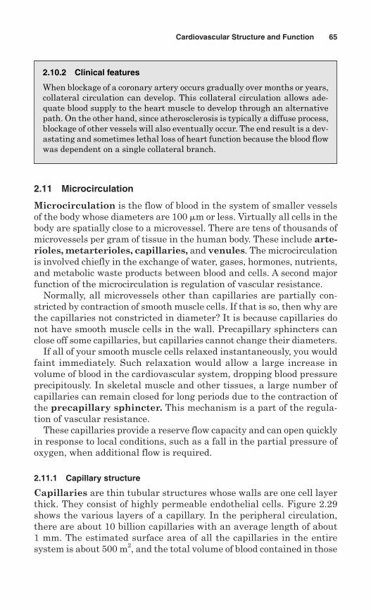
2.11 Microcirculation
Microcirculation is the flow of blood in the system of smaller vesselsof the body whose diameters are 100 �m or less. Virtually all cells in thebody are spatially close to a microvessel. There are tens of thousands ofmicrovessels per gram of tissue in the human body. These include arte-rioles, metarterioles, capillaries, and venules. The microcirculationis involved chiefly in the exchange of water, gases, hormones, nutrients,and metabolic waste products between blood and cells. A second majorfunction of the microcirculation is regulation of vascular resistance.
Normally, all microvessels other than capillaries are partially con-stricted by contraction of smooth muscle cells. If that is so, then why arethe capillaries not constricted in diameter? It is because capillaries donot have smooth muscle cells in the wall. Precapillary sphincters canclose off some capillaries, but capillaries cannot change their diameters.
If all of your smooth muscle cells relaxed instantaneously, you wouldfaint immediately. Such relaxation would allow a large increase involume of blood in the cardiovascular system, dropping blood pressureprecipitously. In skeletal muscle and other tissues, a large number ofcapillaries can remain closed for long periods due to the contraction ofthe precapillary sphincter. This mechanism is a part of the regula-tion of vascular resistance.
These capillaries provide a reserve flow capacity and can open quicklyin response to local conditions, such as a fall in the partial pressure ofoxygen, when additional flow is required.
2.11.1 Capillary structure
Capillaries are thin tubular structures whose walls are one cell layerthick. They consist of highly permeable endothelial cells. Figure 2.29shows the various layers of a capillary. In the peripheral circulation,there are about 10 billion capillaries with an average length of about1 mm. The estimated surface area of all the capillaries in the entiresystem is about 500 m2, and the total volume of blood contained in those
Cardiovascular Structure and Function 65
2.10.2 Clinical features
When blockage of a coronary artery occurs gradually over months or years,collateral circulation can develop. This collateral circulation allows ade-quate blood supply to the heart muscle to develop through an alternativepath. On the other hand, since atherosclerosis is typically a diffuse process,blockage of other vessels will also eventually occur. The end result is a dev-astating and sometimes lethal loss of heart function because the blood flowwas dependent on a single collateral branch.
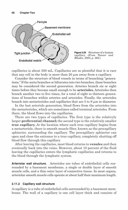
capillaries is about 500 mL. Capillaries are so plentiful that it is rarethat any cell in the body is more than 20 �m away from a capillary.
Consider the structure of blood vessels in terms of branching “genera-tions.” If the aorta branches or bifurcates into two branches, those branchesmay be considered the second generation. Arteries branch six or eighttimes before they become small enough to be arterioles. Arterioles thenbranch another two to five times, for a total of eight to thirteen genera-tions of branches within arteries and arterioles. Finally, the arteriolesbranch into metarterioles and capillaries that are 5 to 9 �m in diameter.
In the last arteriole generation, blood flows from the arterioles intothe metarterioles, which are sometimes called terminal arterioles. Fromthere, the blood flows into the capillaries.
There are two types of capillaries. The first type is the relativelylarger preferential channel; the second type is the relatively smallertrue capillary. At the location where each true capillary begins froma metarteriole, there is smooth muscle fiber, known as the precapillarysphincter, surrounding the capillary. The precapillary sphincter canopen and close the entrance to a true capillary, completely shutting offblood flow through this capillary.
After leaving the capillaries, most blood returns to venules and theneventually back into the veins. However, about 10 percent of the fluidleaving the capillaries enters the lymphatic capillaries and returns tothe blood through the lymphatic system.
Arteriolar wall structure. Arterioles are tubes of endothelial cells sur-rounded by a basement membrane, a single or double layer of smoothmuscle cells, and a thin outer layer of connective tissue. In most organs,arteriolar smooth muscle cells operate at about half their maximum length.
2.11.2 Capillary wall structure
A capillary is a tube of endothelial cells surrounded by a basement mem-brane. The wall of a capillary is one cell layer thick and consists of
66 Chapter Two
Figure 2.29 Structure of a humancapillary. (From Tanner andRhodes, 2003, p. 264.)
endothelial cells surrounded on the outside by a basement membrane.Pericytes (Rouget cells) are connective tissue and may be a primitiveform of vascular smooth muscle cells, and add structural integrity to thecapillary. Precapillary sphincters are small helical twists of smoothmuscle around the smallest arterioles (metarterioles). These sphinctersare very responsive to the local or intrinsic effects like the concentrationof oxygen or carbon dioxide.
The wall thickness of a capillary is about 0.5 �m. The inside diame-ter is approximately 4 to 9 �m which is barely large enough for an ery-throcyte, or red blood cell, to squeeze through. In fact, erythrocytes,which are approximately 8 �m in diameter, must often fold in order tosqueeze through the capillary.
Capillary walls have intercellular clefts, which are thin slits betweenadjacent endothelial cells. The width of these slits is only about 6 to 7 nm(6 to 7 � 109 m) on the average. Water molecules and most water-solubleions diffuse easily through these pores.
The pores in capillaries are of different sizes for different organs. Forexample, intercellular clefts in the brain are known as “tight junctions.”These pores allow only extremely small molecules like water, oxygen, andcarbon dioxide to pass through the capillary wall. In the liver, the oppo-site is true. The intercellular clefts in the liver are wide open and almostanything that is dissolved in the plasma also goes through these pores.
Because a single capillary has such a small diameter, each capillarytaken alone has a very high hydraulic resistance. However, when youadd together many capillaries in parallel, the capillaries account foronly about 15 percent of the total resistance in each organ.
2.11.3 Pressure control in themicrovasculature
Arterioles regulate vascular pressures and microvascular resistance. Aconstant “conflict” exists between preserving arterial pressure byincreasing arteriolar resistance and allowing all regions to receive suf-ficient perfusion to provide oxygen to the tissue. By decreasing resist-ance in small vessels, more blood flows and oxygen perfusion increases.By decreasing resistance in arterioles and capillaries, however, systemblood pressure falls.
The normal pressure in an arteriole is typically 30 to 70 mmHg,while the pressure in a venule is 10 to 16 mmHg. Large arteries aresimply conduits to allow blood transfer between locations. These largevessels have very low resistance and do not play a significant role inpressure regulation. Small arteries (0.5 to 1 mm in diameter) control 30to 40 percent of total vascular resistance, and arterioles (�500 �m indiameter) combined with those small arteries make up 70 to 80 percentof total vascular resistance. Nearly all of the rest of the resistance(20 to 30 percent) comes from capillaries and venules.
Cardiovascular Structure and Function 67
Constriction of smooth muscle cells maintains the resistance in theseresistance vessels. Release of norepinephrine from the sympatheticnervous system contributes to smooth muscle constriction. When fullyrelaxed, the diameter of the vessel surrounded by smooth muscle cannearly double. If the vessel diameter doubles, the resistance over a fixedlength of vessel increases by 24
� 16 times.Arterioles possess significant smooth muscle cells and can dilate 60
to 100 percent from their resting diameter. Arterioles can also constrict40 to 50 percent from their resting diameter for long periods.
Only approximately 10 percent of muscle capillaries are open at rest.Therefore, muscle is capable of increasing its rate of bulk flow tenfold asthe need for oxygen increases. Since humans are not capable of increasingtheir cardiac output tenfold (the human heart can achieve a maximal five-fold increase), shutting down other capillary beds is a necessary pressurecontrol mechanism. That is, you can increase the blood flow to some muscletenfold so long as not all muscles in the body try to do that simultaneously.
2.11.4 Diffusion in capillaries
Lipid-soluble molecules like O2 and CO2 easily pass through the lipidcomponents of endothelial cell membranes. Water-soluble moleculeslike glucose must diffuse through water-filled pathways in the capillarywall between adjacent endothelial cells. The water-filled pathwaysare known as pores. In humans, adjacent endothelial cells are heldtogether by tight junctions, which have occasional gaps.
Capillaries of the brain and spinal cord allow only the smallest water-soluble molecules to pass through. Pores are partially filled with sub-micron fibers (fiber matrix) that act as a filter.
Most pores allow passage of 3- to 6-nm molecules. This pore sizeallows the passage of water, inorganic ions, glucose, and amino acids.Pores exclude passage of large molecules like serum albumin andglobular proteins. A limited number of large pores exist. It is possi-ble that these larger pores are actually defects in the cell wall. Largepores allow passage of virtually all large molecules. Because of theselarge pores and their associated leakage, nearly all serum albumin mol-ecules leak out of the cardiovascular system each day.
2.11.5 Venules
Venules are endothelial tubes that are usually surrounded by a mono-layer of vascular smooth muscle cells. Smooth muscle cells in venulesare much smaller in diameter, but longer than those of arterioles.
The smallest venules are more permeable than capillaries. A signifi-cant amount of the diffusion that occurs in the microcirculation, there-fore, occurs in the venules.
68 Chapter Two
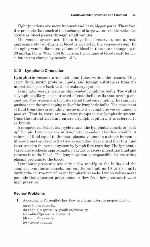
Tight junctions are more frequent and have bigger pores. Therefore,it is probable that much of the exchange of large water-soluble moleculesoccurs as blood passes through small venules.
The venous system acts like a huge blood reservoir, and at rest,approximately two-thirds of blood is located in the venous system. Bychanging venule diameter, volume of blood in tissue can change up to20 mL/kg. For a 70-kg (154 lb) person, the volume of blood ready for cir-culation can change by nearly 1.5 L.
2.12 Lymphatic Circulation
Lymphatic vessels are endothelial tubes within the tissues. Theycarry fluid, serum proteins, lipids, and foreign substances from theinterstitial spaces back to the circulatory system.
Lymphatic vessels begin as blind-ended lymphatic bulbs. The wall ofa lymph capillary is constructed of endothelial cells that overlap oneanother. The pressure in the interstitial fluid surrounding the capillarypushes open the overlapping cells of the lymphatic bulbs. The movementof fluid from the surrounding tissue into the lymphatic vessel lumen ispassive. That is, there are no active pumps in the lymphatic system.Once the interstitial fluid enters a lymph capillary, it is referred toas lymph.
A compression/relaxation cycle causes the lymphatic vessels to “suckup” lymph. Lymph valves in lymphatic vessels make this possible. Avolume of fluid equal to the total plasma volume in a single human isfiltered from the blood to the tissues each day. It is critical that this fluidis returned to the venous system by lymph flow each day. The lymphaticvasculature collects approximately 3 L/day of excess interstitial fluid andreturns it to the blood. The lymph system is responsible for returningplasma proteins to the blood.
Lymphatic pressures are only a few mmHg in the bulbs and thesmallest lymphatic vessels, but can be as high as 10 to 20 mmHgduring the contraction of larger lymphatic vessels. Lymph valves makepossible this apparent progression or flow from low pressure towardhigh pressure.
Review Problems
1. According to Poiseuille’s law, flow in a large artery is proportional to
(a) radius × viscosity(b) radius4 × (pressure gradient)/viscosity(c) radius4/(pressure gradient)(d) radius2/viscosity(e) viscosity/radius
Cardiovascular Structure and Function 69
2. According to the Reynolds number, turbulence is more likely with
(a) increasing viscosity(b) decreasing tube diameter(c) decreasing velocity(d) increasing velocity(e) increasing pressure
3. Decreased aortic compliance means
(a) decreased stiffness, resulting in increased resistance(b) increased change in cross-sectional area for a given pressure increase(c) increased stiffness, resulting in increased mean aortic pressure for the
same cardiac output(d) increased stiffness, resulting in a decrease in mean aortic pressure for
same cardiac output(e) decreased stiffness, resulting in a decrease in mean aortic pressure
4. Cardiac output is approximately proportional to
(a) aortic pressure divided by systemic vascular resistance(b) systemic vascular resistance times aortic pressure(c) systemic vascular resistance times right atrial pressure(d) right ventricular pressure divided by systemic vascular resistance(e) aortic pressure times stroke volume
5. If the heart were stopped, after due time, the pressure in the entire systemcirculation would come to equilibrium at some pressure greater than 0.This equilibrium pressure is known as
(a) mean aortic pressure(b) diastolic pressure(c) mean circulatory filling pressure(d) vena cava pressure(e) central venous pressure
6. For the following ECG, find the mean electrical axis.
70 Chapter Two
0Lead aVF
Lead II
Lead I
5 mV
0 3 mV
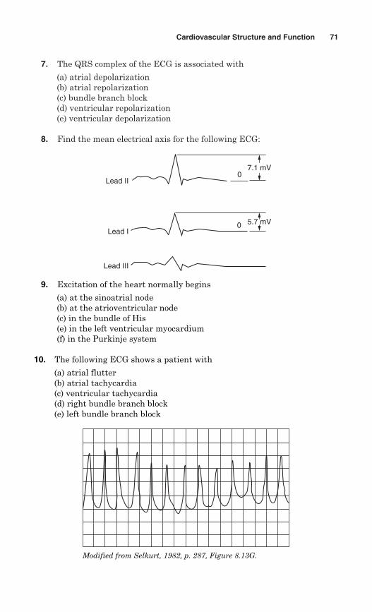
7. The QRS complex of the ECG is associated with
(a) atrial depolarization(b) atrial repolarization(c) bundle branch block(d) ventricular repolarization(e) ventricular depolarization
8. Find the mean electrical axis for the following ECG:
Cardiovascular Structure and Function 71
0Lead II
Lead I
Lead III
7.1 mV
0 5.7 mV
9. Excitation of the heart normally begins
(a) at the sinoatrial node(b) at the atrioventricular node(c) in the bundle of His(e) in the left ventricular myocardium(f) in the Purkinje system
10. The following ECG shows a patient with
(a) atrial flutter(b) atrial tachycardia(c) ventricular tachycardia(d) right bundle branch block(e) left bundle branch block
Modified from Selkurt, 1982, p. 287, Figure 8.13G.
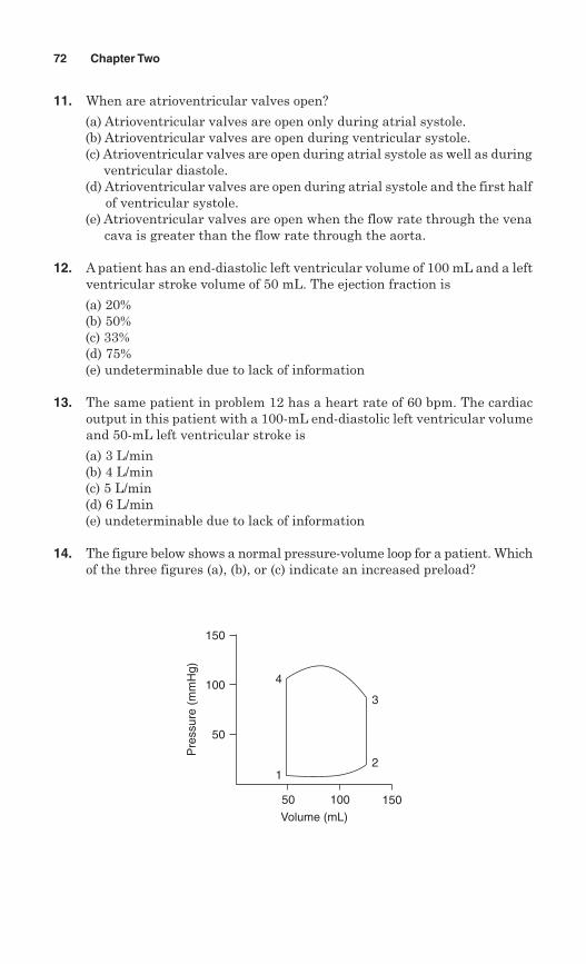
11. When are atrioventricular valves open?
(a) Atrioventricular valves are open only during atrial systole.(b) Atrioventricular valves are open during ventricular systole.(c) Atrioventricular valves are open during atrial systole as well as during
ventricular diastole.(d) Atrioventricular valves are open during atrial systole and the first half
of ventricular systole.(e) Atrioventricular valves are open when the flow rate through the vena
cava is greater than the flow rate through the aorta.
12. A patient has an end-diastolic left ventricular volume of 100 mL and a leftventricular stroke volume of 50 mL. The ejection fraction is
(a) 20%(b) 50%(c) 33%(d) 75%(e) undeterminable due to lack of information
13. The same patient in problem 12 has a heart rate of 60 bpm. The cardiacoutput in this patient with a 100-mL end-diastolic left ventricular volumeand 50-mL left ventricular stroke is
(a) 3 L/min(b) 4 L/min(c) 5 L/min(d) 6 L/min(e) undeterminable due to lack of information
14. The figure below shows a normal pressure-volume loop for a patient. Whichof the three figures (a), (b), or (c) indicate an increased preload?
72 Chapter Two
50 100 150Volume (mL)
50
100
150
Pre
ssur
e (m
mH
g)
4
1
3
2
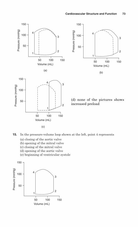
15. In the pressure-volume loop shown at the left, point 4 represents
(a) closing of the aortic valve(b) opening of the mitral valve(c) closing of the mitral valve(d) opening of the aortic valve(e) beginning of ventricular systole
Cardiovascular Structure and Function 73
50 100 150
Volume (mL)
(b)
50
100
150
Pre
ssur
e (m
mH
g)
4
1
3
2
50 100 150
Volume (mL)
(c)
50
100
150
Pre
ssur
e (m
mH
g)
4
1
3
2
(d) none of the pictures showsincreased preload
50 100 150
Volume (mL)
50
100
150
Pre
ssur
e (m
mH
g)
4
1
3
2
50 100 150
Volume (mL)
(a)
50
100
150
Pre
ssur
e (m
mH
g)
4
1
3
2
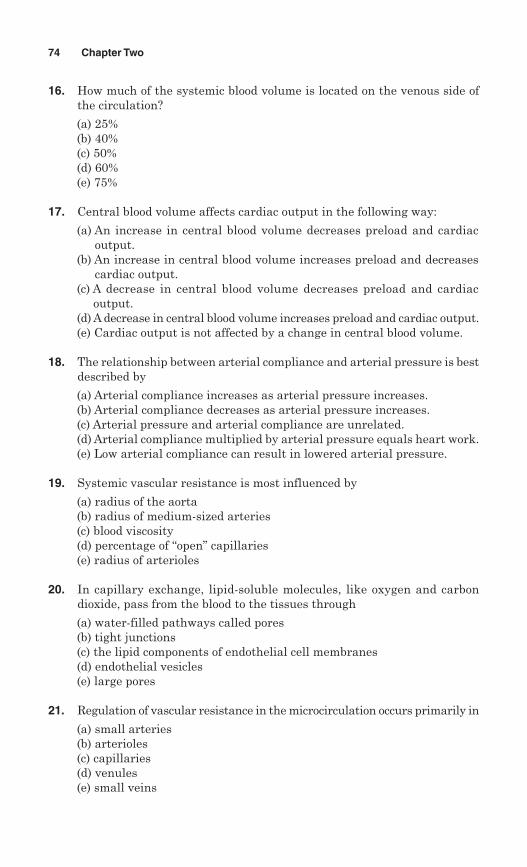
74 Chapter Two
16. How much of the systemic blood volume is located on the venous side ofthe circulation?
(a) 25%(b) 40%(c) 50%(d) 60%(e) 75%
17. Central blood volume affects cardiac output in the following way:
(a) An increase in central blood volume decreases preload and cardiacoutput.
(b) An increase in central blood volume increases preload and decreasescardiac output.
(c) A decrease in central blood volume decreases preload and cardiacoutput.
(d) A decrease in central blood volume increases preload and cardiac output.(e) Cardiac output is not affected by a change in central blood volume.
18. The relationship between arterial compliance and arterial pressure is bestdescribed by
(a) Arterial compliance increases as arterial pressure increases.(b) Arterial compliance decreases as arterial pressure increases.(c) Arterial pressure and arterial compliance are unrelated.(d) Arterial compliance multiplied by arterial pressure equals heart work.(e) Low arterial compliance can result in lowered arterial pressure.
19. Systemic vascular resistance is most influenced by
(a) radius of the aorta(b) radius of medium-sized arteries(c) blood viscosity(d) percentage of “open” capillaries(e) radius of arterioles
20. In capillary exchange, lipid-soluble molecules, like oxygen and carbondioxide, pass from the blood to the tissues through
(a) water-filled pathways called pores(b) tight junctions(c) the lipid components of endothelial cell membranes(d) endothelial vesicles(e) large pores
21. Regulation of vascular resistance in the microcirculation occurs primarily in
(a) small arteries(b) arterioles(c) capillaries(d) venules(e) small veins
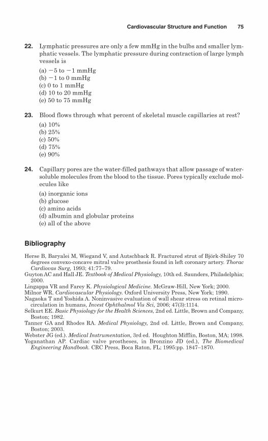
22. Lymphatic pressures are only a few mmHg in the bulbs and smaller lym-phatic vessels. The lymphatic pressure during contraction of large lymphvessels is
(a) 5 to 1 mmHg(b) 1 to 0 mmHg(c) 0 to 1 mmHg(d) 10 to 20 mmHg(e) 50 to 75 mmHg
23. Blood flows through what percent of skeletal muscle capillaries at rest?
(a) 10%(b) 25%(c) 50%(d) 75%(e) 90%
24. Capillary pores are the water-filled pathways that allow passage of water-soluble molecules from the blood to the tissue. Pores typically exclude mol-ecules like
(a) inorganic ions(b) glucose(c) amino acids(d) albumin and globular proteins(e) all of the above
Bibliography
Herse B, Baryalei M, Wiegand V, and Autschback R. Fractured strut of Björk-Shiley 70degrees convexo-concave mitral valve prosthesis found in left coronary artery. ThoracCardiovas Surg, 1993; 41:77–79.
Guyton AC and Hall JE. Textbook of Medical Physiology, 10th ed. Saunders, Philadelphia;2000.
Lingappa VR and Farey K. Physiological Medicine. McGraw-Hill, New York; 2000.Milnor WR. Cardiovascular Physiology. Oxford University Press, New York; 1990.Nagaoka T and Yoshida A. Noninvasive evaluation of wall shear stress on retinal micro-
circulation in humans, Invest Ophthalmol Vis Sci, 2006; 47(3):1114.Selkurt EE. Basic Physiology for the Health Sciences, 2nd ed. Little, Brown and Company,
Boston; 1982.Tanner GA and Rhodes RA. Medical Physiology, 2nd ed. Little, Brown and Company,
Boston; 2003.Webster JG (ed.). Medical Instrumentation, 3rd ed. Houghton Mifflin, Boston, MA; 1998.Yoganathan AP. Cardiac valve prostheses, in Bronzino JD (ed.), The Biomedical
Engineering Handbook. CRC Press, Boca Raton, FL; 1995:pp. 1847–1870.
Cardiovascular Structure and Function 75

This page intentionally left blank
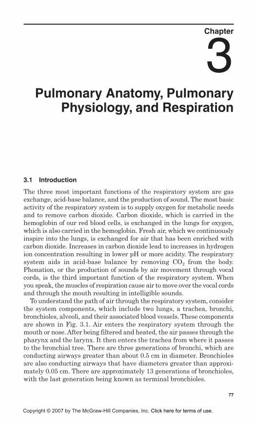
Chapter
3Pulmonary Anatomy, Pulmonary
Physiology, and Respiration
3.1 Introduction
The three most important functions of the respiratory system are gasexchange, acid-base balance, and the production of sound. The most basicactivity of the respiratory system is to supply oxygen for metabolic needsand to remove carbon dioxide. Carbon dioxide, which is carried in thehemoglobin of our red blood cells, is exchanged in the lungs for oxygen,which is also carried in the hemoglobin. Fresh air, which we continuouslyinspire into the lungs, is exchanged for air that has been enriched withcarbon dioxide. Increases in carbon dioxide lead to increases in hydrogenion concentration resulting in lower pH or more acidity. The respiratorysystem aids in acid-base balance by removing CO2 from the body.Phonation, or the production of sounds by air movement through vocalcords, is the third important function of the respiratory system. Whenyou speak, the muscles of respiration cause air to move over the vocal cordsand through the mouth resulting in intelligible sounds.
To understand the path of air through the respiratory system, considerthe system components, which include two lungs, a trachea, bronchi,bronchioles, alveoli, and their associated blood vessels. These componentsare shown in Fig. 3.1. Air enters the respiratory system through themouth or nose. After being filtered and heated, the air passes through thepharynx and the larynx. It then enters the trachea from where it passesto the bronchial tree. There are three generations of bronchi, which areconducting airways greater than about 0.5 cm in diameter. Bronchiolesare also conducting airways that have diameters greater than approxi-mately 0.05 cm. There are approximately 13 generations of bronchioles,with the last generation being known as terminal bronchioles.
77
Copyright © 2007 by The McGraw-Hill Companies, Inc. Click here for terms of use.
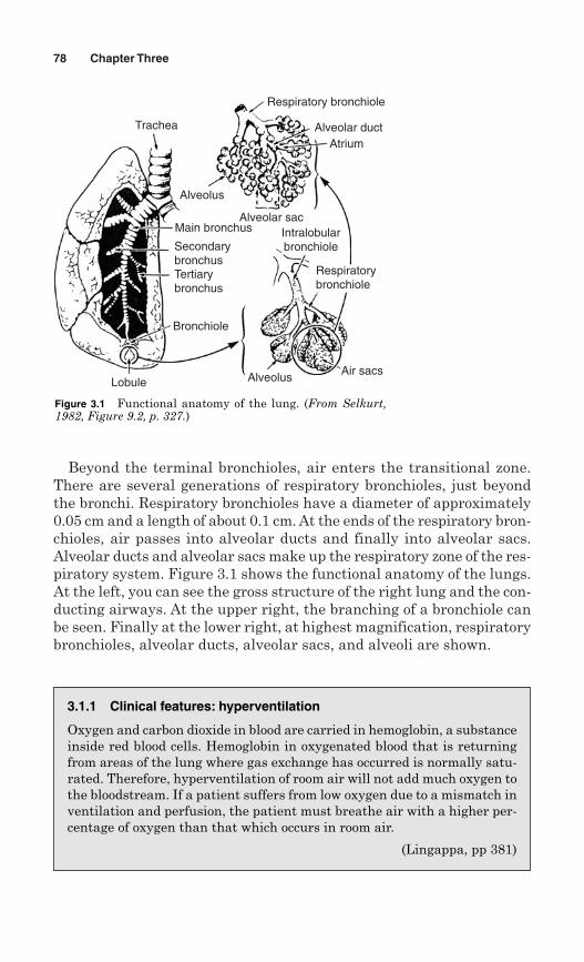
Beyond the terminal bronchioles, air enters the transitional zone.There are several generations of respiratory bronchioles, just beyondthe bronchi. Respiratory bronchioles have a diameter of approximately0.05 cm and a length of about 0.1 cm. At the ends of the respiratory bron-chioles, air passes into alveolar ducts and finally into alveolar sacs.Alveolar ducts and alveolar sacs make up the respiratory zone of the res-piratory system. Figure 3.1 shows the functional anatomy of the lungs.At the left, you can see the gross structure of the right lung and the con-ducting airways. At the upper right, the branching of a bronchiole canbe seen. Finally at the lower right, at highest magnification, respiratorybronchioles, alveolar ducts, alveolar sacs, and alveoli are shown.
78 Chapter Three
Lobule
Bronchiole
Alveolus Air sacs
Respiratorybronchiole
Intralobularbronchiole
Alveolar sacMain bronchus
SecondarybronchusTertiarybronchus
Alveolus
AtriumAlveolar duct
Respiratory bronchiole
Trachea
Figure 3.1 Functional anatomy of the lung. (From Selkurt,1982, Figure 9.2, p. 327.)
3.1.1 Clinical features: hyperventilation
Oxygen and carbon dioxide in blood are carried in hemoglobin, a substanceinside red blood cells. Hemoglobin in oxygenated blood that is returningfrom areas of the lung where gas exchange has occurred is normally satu-rated. Therefore, hyperventilation of room air will not add much oxygen tothe bloodstream. If a patient suffers from low oxygen due to a mismatch inventilation and perfusion, the patient must breathe air with a higher per-centage of oxygen than that which occurs in room air.
(Lingappa, pp 381)
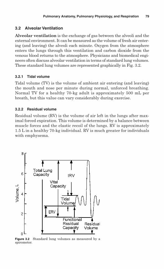
3.2 Alveolar Ventilation
Alveolar ventilation is the exchange of gas between the alveoli and theexternal environment. It can be measured as the volume of fresh air enter-ing (and leaving) the alveoli each minute. Oxygen from the atmosphereenters the lungs through this ventilation and carbon dioxide from thevenous blood returns to the atmosphere. Physicians and biomedical engi-neers often discuss alveolar ventilation in terms of standard lung volumes.These standard lung volumes are represented graphically in Fig. 3.2.
3.2.1 Tidal volume
Tidal volume (TV) is the volume of ambient air entering (and leaving)the mouth and nose per minute during normal, unforced breathing.Normal TV for a healthy 70-kg adult is approximately 500 mL perbreath, but this value can vary considerably during exercise.
3.2.2 Residual volume
Residual volume (RV) is the volume of air left in the lungs after max-imal forced expiration. This volume is determined by a balance betweenmuscle forces and the elastic recoil of the lungs. RV is approximately1.5 L in a healthy 70-kg individual. RV is much greater for individualswith emphysema.
Pulmonary Anatomy, Pulmonary Physiology, and Respiration 79
Figure 3.2 Standard lung volumes as measured by aspirometer.
3.2.3 Expiratory reserve volume
Expiratory reserve volume (ERV) is the volume of air expelled from thelungs during a maximal forced expiration that begins at the end ofnormal tidal expiration. The ERV plus the RV combine to make up thefunctional residual capacity. Normal ERV for our standard 70-kg indi-vidual is approximately 1.5 L.
3.2.4 Inspiratory reserve volume
Inspiratory reserve volume (IRV) is the volume of air that is inhaledduring forced maximal inspiration beginning at the end of normal tidalinspiration. This volume depends on muscle forces and also on the elas-tic recoil of the chest wall and the elastic recoil of the lungs. The IRV ofa healthy 70-kg individual is approximately 2.5 L.
3.2.5 Functional residual capacity
Functional residual capacity (FRC) is the volume in the lungs at the endof normal tidal expiration. FRC depends on the equilibrium point atwhich the elastic inward recoil of the lungs balances the elastic outwardrecoil of the chest wall. FRC consists of the sum of the RV and the ERVand can be represented by Eq. (3.1). The FRC of a healthy 70-kg adultis approximately 3 L.
(3.1)
3.2.6 Inspiratory capacity
Inspiratory capacity (IC) is the volume of air taken into the lungsduring a maximal inspiratory effort that starts at the end of a normalTV expiration. IC is the sum of TV and IRV and can be representedby Eq. (3.2). The IC of our healthy 70-kg adult is about 3 L.
(3.2)
3.2.7 Total lung capacity
Total lung capacity (TLC) is the volume of air in the lungs after amaximal inspiratory effort. The strength of contraction of inspira-tory muscles and the inward elastic recoil of the lungs and the chestwall determine the TLC. The TLC is also equal to the sum of the IRV,the TV, the ERV, and the RV. A typical value for TLC of a healthy
IC 5 IRV 1 TV
FRC 5 RV 1 ERV
80 Chapter Three
70-kg male is about 6 L. An equation representing the TLC may bewritten by:
(3.3)
3.2.8 Vital capacity
Vital Capacity (VC) is the volume of air expelled from the lung duringa maximal expiratory effort after a maximum forced inspiration. TheVC is the difference between the TLC and the RV. VC in a normalhealthy 70-kg adult is about 4.5 L. Equation 3.4 shows an equationfor VC.
(3.4)
3.3 Ventilation-Perfusion Relationships
Ventilation is the act of supplying air into the lungs and perfusion isthe pumping of blood into the lungs. In this book we will use to rep-resent the airflow rate associated with ventilation and to representthe blood flow rate associated with perfusion. The ratio of ventilationto perfusion is important for lung function and is represented as theventilation/perfusion ratio as shown in Eq. (3.5).
(3.5)
Pulmonary artery smooth muscle constricts the vessels of the pulmonarycapillary beds in response to hypoxia or low oxygen. This type of vaso-constriction is one of the most important parameters that determine pul-monary blood flow. In other capillary beds within the body, smooth musclevasodilates in response to tissue hypoxia, improving perfusion.
Resting ventilation is about 4 to 6 L/min. Resting pulmonary arteryblood flow is about 5 L/min. At rest, therefore, the ventilation/perfusionratio is about 0.8 to 1.2. Figure 3.3 shows a schematic representing aventilation/perfusion ratio of 1 with a ventilation rate and perfusion rateboth equal to 5 L/min.
3.4 Mechanics of Breathing
For the normal physiological case of breathing, air flows into the lungswhen the alveolar pressure drops below the pressure of the surround-ing ambient air. This is known as “negative pressure breathing”
ventilation-perfusion ratio 5V.
Q.
Q. V
.
VC 5 TV 1 IRV 1 ERV
TLC 5 IRV 1 TV 1 ERV 1 RV
Pulmonary Anatomy, Pulmonary Physiology, and Respiration 81
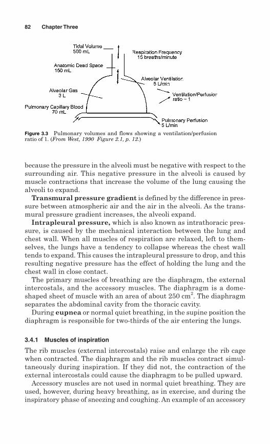
because the pressure in the alveoli must be negative with respect to thesurrounding air. This negative pressure in the alveoli is caused bymuscle contractions that increase the volume of the lung causing thealveoli to expand.
Transmural pressure gradient is defined by the difference in pres-sure between atmospheric air and the air in the alveoli. As the trans-mural pressure gradient increases, the alveoli expand.
Intrapleural pressure, which is also known as intrathoracic pres-sure, is caused by the mechanical interaction between the lung andchest wall. When all muscles of respiration are relaxed, left to them-selves, the lungs have a tendency to collapse whereas the chest walltends to expand. This causes the intrapleural pressure to drop, and thisresulting negative pressure has the effect of holding the lung and thechest wall in close contact.
The primary muscles of breathing are the diaphragm, the externalintercostals, and the accessory muscles. The diaphragm is a dome-shaped sheet of muscle with an area of about 250 cm2. The diaphragmseparates the abdominal cavity from the thoracic cavity.
During eupnea or normal quiet breathing, in the supine position thediaphragm is responsible for two-thirds of the air entering the lungs.
3.4.1 Muscles of inspiration
The rib muscles (external intercostals) raise and enlarge the rib cagewhen contracted. The diaphragm and the rib muscles contract simul-taneously during inspiration. If they did not, the contraction of theexternal intercostals could cause the diaphragm to be pulled upward.
Accessory muscles are not used in normal quiet breathing. They areused, however, during heavy breathing, as in exercise, and during theinspiratory phase of sneezing and coughing. An example of an accessory
82 Chapter Three
Figure 3.3 Pulmonary volumes and flows showing a ventilation/perfusionratio of 1. (From West, 1990 Figure 2.1, p. 12.)
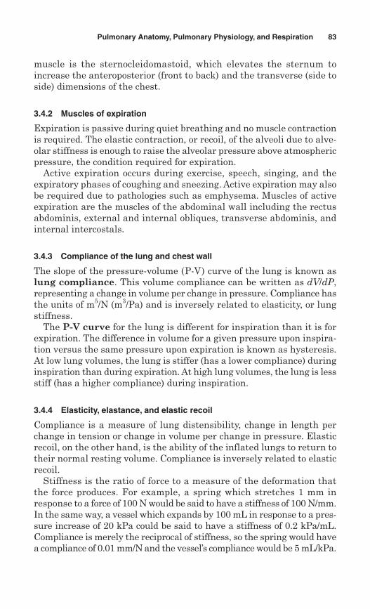
muscle is the sternocleidomastoid, which elevates the sternum toincrease the anteroposterior (front to back) and the transverse (side toside) dimensions of the chest.
3.4.2 Muscles of expiration
Expiration is passive during quiet breathing and no muscle contractionis required. The elastic contraction, or recoil, of the alveoli due to alve-olar stiffness is enough to raise the alveolar pressure above atmosphericpressure, the condition required for expiration.
Active expiration occurs during exercise, speech, singing, and theexpiratory phases of coughing and sneezing. Active expiration may alsobe required due to pathologies such as emphysema. Muscles of activeexpiration are the muscles of the abdominal wall including the rectusabdominis, external and internal obliques, transverse abdominis, andinternal intercostals.
3.4.3 Compliance of the lung and chest wall
The slope of the pressure-volume (P-V) curve of the lung is known aslung compliance. This volume compliance can be written as dV/dP,representing a change in volume per change in pressure. Compliance hasthe units of m5/N (m3/Pa) and is inversely related to elasticity, or lungstiffness.
The P-V curve for the lung is different for inspiration than it is forexpiration. The difference in volume for a given pressure upon inspira-tion versus the same pressure upon expiration is known as hysteresis.At low lung volumes, the lung is stiffer (has a lower compliance) duringinspiration than during expiration. At high lung volumes, the lung is lessstiff (has a higher compliance) during inspiration.
3.4.4 Elasticity, elastance, and elastic recoil
Compliance is a measure of lung distensibility, change in length perchange in tension or change in volume per change in pressure. Elasticrecoil, on the other hand, is the ability of the inflated lungs to return totheir normal resting volume. Compliance is inversely related to elasticrecoil.
Stiffness is the ratio of force to a measure of the deformation thatthe force produces. For example, a spring which stretches 1 mm inresponse to a force of 100 N would be said to have a stiffness of 100 N/mm.In the same way, a vessel which expands by 100 mL in response to a pres-sure increase of 20 kPa could be said to have a stiffness of 0.2 kPa/mL.Compliance is merely the reciprocal of stiffness, so the spring would havea compliance of 0.01 mm/N and the vessel’s compliance would be 5 mL/kPa.
Pulmonary Anatomy, Pulmonary Physiology, and Respiration 83
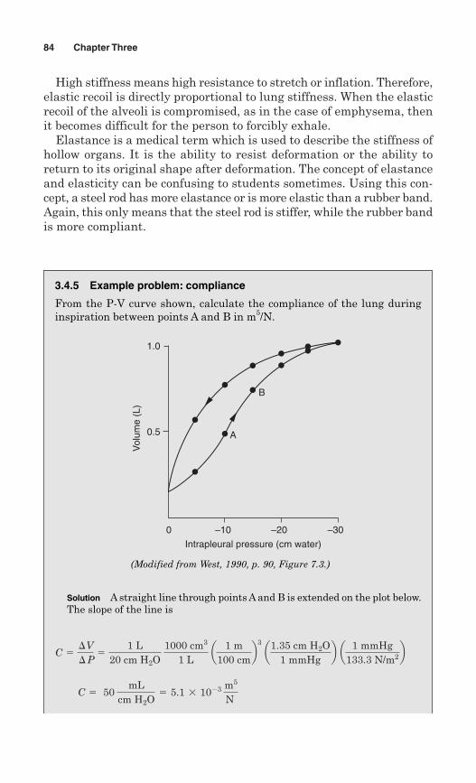
High stiffness means high resistance to stretch or inflation. Therefore,elastic recoil is directly proportional to lung stiffness. When the elasticrecoil of the alveoli is compromised, as in the case of emphysema, thenit becomes difficult for the person to forcibly exhale.
Elastance is a medical term which is used to describe the stiffness ofhollow organs. It is the ability to resist deformation or the ability toreturn to its original shape after deformation. The concept of elastanceand elasticity can be confusing to students sometimes. Using this con-cept, a steel rod has more elastance or is more elastic than a rubber band.Again, this only means that the steel rod is stiffer, while the rubber bandis more compliant.
84 Chapter Three
3.4.5 Example problem: compliance
From the P-V curve shown, calculate the compliance of the lung duringinspiration between points A and B in m5/N.
Solution A straight line through points A and B is extended on the plot below.The slope of the line is
C 5 50 mL
cm H2O5 5.1 3 1023 m
5
N
C 5V P
51 L
20 cm H2O 1000 cm3
1 L a 1 m
100 cmb3
a1.35 cm H2O1 mmHg
b a 1 mmHg133.3 N/m2b
Intrapleural pressure (cm water)
Vol
ume
(L)
–30–20–100
A
B
0.5
1.0
(Modified from West, 1990, p. 90, Figure 7.3.)
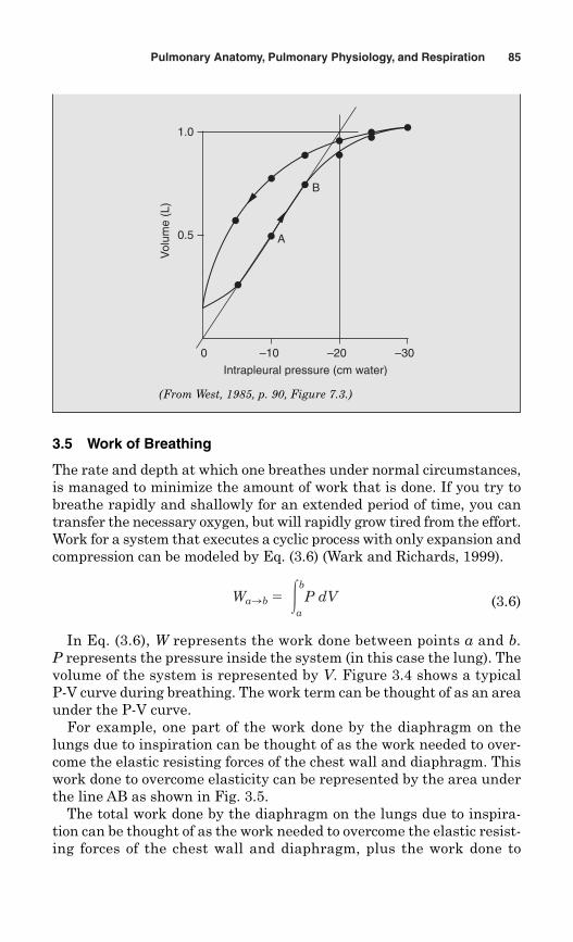
3.5 Work of Breathing
The rate and depth at which one breathes under normal circumstances,is managed to minimize the amount of work that is done. If you try tobreathe rapidly and shallowly for an extended period of time, you cantransfer the necessary oxygen, but will rapidly grow tired from the effort.Work for a system that executes a cyclic process with only expansion andcompression can be modeled by Eq. (3.6) (Wark and Richards, 1999).
(3.6)
In Eq. (3.6), W represents the work done between points a and b.P represents the pressure inside the system (in this case the lung). Thevolume of the system is represented by V. Figure 3.4 shows a typicalP-V curve during breathing. The work term can be thought of as an areaunder the P-V curve.
For example, one part of the work done by the diaphragm on thelungs due to inspiration can be thought of as the work needed to over-come the elastic resisting forces of the chest wall and diaphragm. Thiswork done to overcome elasticity can be represented by the area underthe line AB as shown in Fig. 3.5.
The total work done by the diaphragm on the lungs due to inspira-tion can be thought of as the work needed to overcome the elastic resist-ing forces of the chest wall and diaphragm, plus the work done to
WaSb5 3b
aP dV
Pulmonary Anatomy, Pulmonary Physiology, and Respiration 85
Intrapleural pressure (cm water)
Vol
ume
(L)
–30–20–100
A
B
0.5
1.0
(From West, 1985, p. 90, Figure 7.3.)
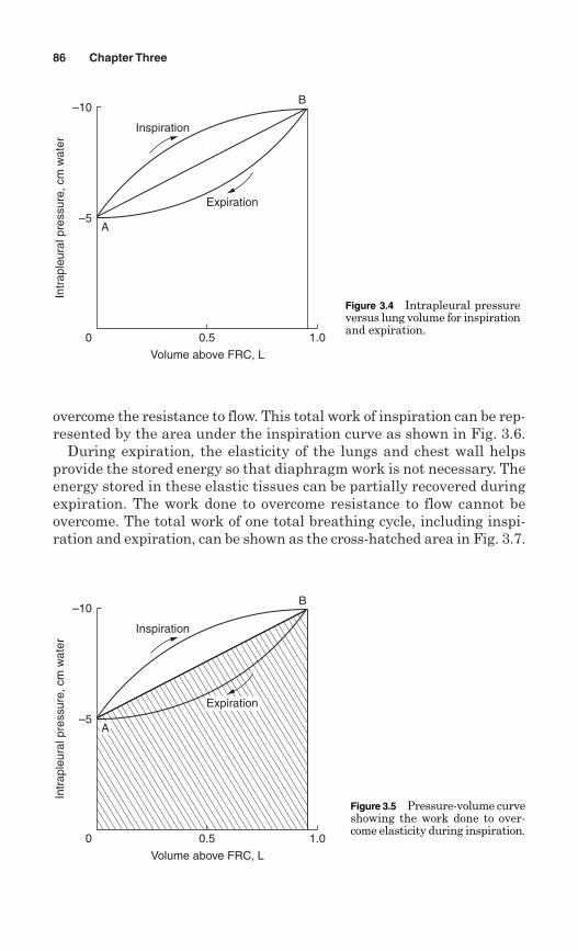
overcome the resistance to flow. This total work of inspiration can be rep-resented by the area under the inspiration curve as shown in Fig. 3.6.
During expiration, the elasticity of the lungs and chest wall helpsprovide the stored energy so that diaphragm work is not necessary. Theenergy stored in these elastic tissues can be partially recovered duringexpiration. The work done to overcome resistance to flow cannot beovercome. The total work of one total breathing cycle, including inspi-ration and expiration, can be shown as the cross-hatched area in Fig. 3.7.
86 Chapter Three
0.5 1.00
–5
–10
Volume above FRC, L
Expiration
Inspiration
B
A
Intr
aple
ural
pre
ssur
e, c
m w
ater
0.5 1.00
–5
–10
Volume above FRC, L
Expiration
Inspiration
B
A
Intr
aple
ural
pre
ssur
e, c
m w
ater
Figure 3.4 Intrapleural pressureversus lung volume for inspirationand expiration.
Figure 3.5 Pressure-volume curveshowing the work done to over-come elasticity during inspiration.
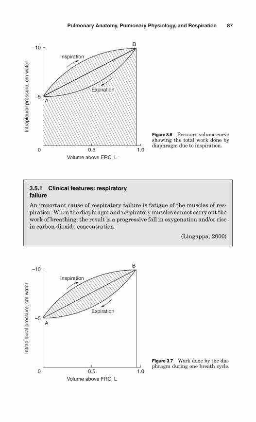
Pulmonary Anatomy, Pulmonary Physiology, and Respiration 87
0.5 1.00
–5
–10
Volume above FRC, L
Expiration
Inspiration
B
A
Intr
aple
ural
pre
ssur
e, c
m w
ater
0.5 1.00
–5
–10
Volume above FRC, L
Expiration
Inspiration
B
A
Intr
aple
ural
pre
ssur
e, c
m w
ater
3.5.1 Clinical features: respiratoryfailure
An important cause of respiratory failure is fatigue of the muscles of res-piration. When the diaphragm and respiratory muscles cannot carry out thework of breathing, the result is a progressive fall in oxygenation and/or risein carbon dioxide concentration.
(Lingappa, 2000)
Figure 3.7 Work done by the dia-phragm during one breath cycle.
Figure 3.6 Pressure-volume curveshowing the total work done bydiaphragm due to inspiration.
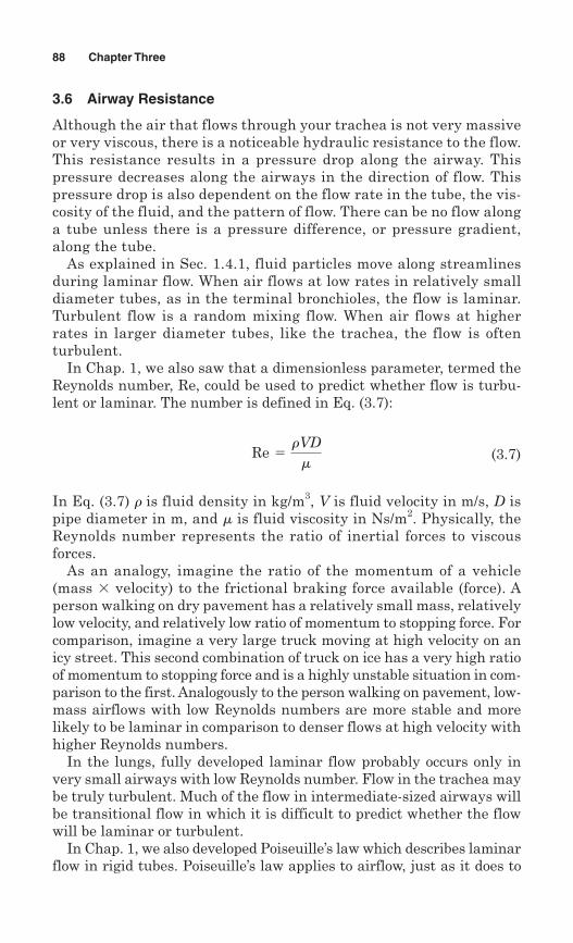
88 Chapter Three
3.6 Airway Resistance
Although the air that flows through your trachea is not very massiveor very viscous, there is a noticeable hydraulic resistance to the flow.This resistance results in a pressure drop along the airway. Thispressure decreases along the airways in the direction of flow. Thispressure drop is also dependent on the flow rate in the tube, the vis-cosity of the fluid, and the pattern of flow. There can be no flow alonga tube unless there is a pressure difference, or pressure gradient,along the tube.
As explained in Sec. 1.4.1, fluid particles move along streamlinesduring laminar flow. When air flows at low rates in relatively smalldiameter tubes, as in the terminal bronchioles, the flow is laminar.Turbulent flow is a random mixing flow. When air flows at higherrates in larger diameter tubes, like the trachea, the flow is often turbulent.
In Chap. 1, we also saw that a dimensionless parameter, termed theReynolds number, Re, could be used to predict whether flow is turbu-lent or laminar. The number is defined in Eq. (3.7):
(3.7)
In Eq. (3.7) � is fluid density in kg/m3, V is fluid velocity in m/s, D ispipe diameter in m, and � is fluid viscosity in Ns/m2. Physically, theReynolds number represents the ratio of inertial forces to viscousforces.
As an analogy, imagine the ratio of the momentum of a vehicle(mass � velocity) to the frictional braking force available (force). Aperson walking on dry pavement has a relatively small mass, relativelylow velocity, and relatively low ratio of momentum to stopping force. Forcomparison, imagine a very large truck moving at high velocity on anicy street. This second combination of truck on ice has a very high ratioof momentum to stopping force and is a highly unstable situation in com-parison to the first. Analogously to the person walking on pavement, low-mass airflows with low Reynolds numbers are more stable and morelikely to be laminar in comparison to denser flows at high velocity withhigher Reynolds numbers.
In the lungs, fully developed laminar flow probably occurs only invery small airways with low Reynolds number. Flow in the trachea maybe truly turbulent. Much of the flow in intermediate-sized airways willbe transitional flow in which it is difficult to predict whether the flowwill be laminar or turbulent.
In Chap. 1, we also developed Poiseuille’s law which describes laminarflow in rigid tubes. Poiseuille’s law applies to airflow, just as it does to
Re 5rVDm
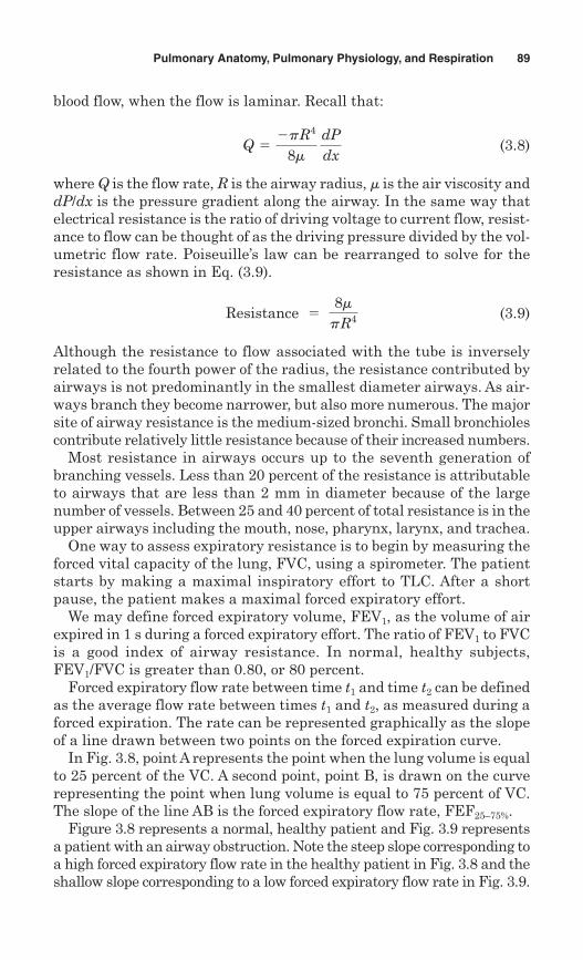
blood flow, when the flow is laminar. Recall that:
(3.8)
where Q is the flow rate, R is the airway radius, � is the air viscosity anddP/dx is the pressure gradient along the airway. In the same way thatelectrical resistance is the ratio of driving voltage to current flow, resist-ance to flow can be thought of as the driving pressure divided by the vol-umetric flow rate. Poiseuille’s law can be rearranged to solve for theresistance as shown in Eq. (3.9).
(3.9)
Although the resistance to flow associated with the tube is inverselyrelated to the fourth power of the radius, the resistance contributed byairways is not predominantly in the smallest diameter airways. As air-ways branch they become narrower, but also more numerous. The majorsite of airway resistance is the medium-sized bronchi. Small bronchiolescontribute relatively little resistance because of their increased numbers.
Most resistance in airways occurs up to the seventh generation ofbranching vessels. Less than 20 percent of the resistance is attributableto airways that are less than 2 mm in diameter because of the largenumber of vessels. Between 25 and 40 percent of total resistance is in theupper airways including the mouth, nose, pharynx, larynx, and trachea.
One way to assess expiratory resistance is to begin by measuring theforced vital capacity of the lung, FVC, using a spirometer. The patientstarts by making a maximal inspiratory effort to TLC. After a shortpause, the patient makes a maximal forced expiratory effort.
We may define forced expiratory volume, FEV1, as the volume of airexpired in 1 s during a forced expiratory effort. The ratio of FEV1 to FVCis a good index of airway resistance. In normal, healthy subjects,FEV1/FVC is greater than 0.80, or 80 percent.
Forced expiratory flow rate between time t1 and time t2 can be definedas the average flow rate between times t1 and t2, as measured during aforced expiration. The rate can be represented graphically as the slopeof a line drawn between two points on the forced expiration curve.
In Fig. 3.8, point A represents the point when the lung volume is equalto 25 percent of the VC. A second point, point B, is drawn on the curverepresenting the point when lung volume is equal to 75 percent of VC.The slope of the line AB is the forced expiratory flow rate, FEF25–75%.
Figure 3.8 represents a normal, healthy patient and Fig. 3.9 representsa patient with an airway obstruction. Note the steep slope corresponding toa high forced expiratory flow rate in the healthy patient in Fig. 3.8 and theshallow slope corresponding to a low forced expiratory flow rate in Fig. 3.9.
Resistance 5 8mpR4
Q 52pR4
8m dPdx
Pulmonary Anatomy, Pulmonary Physiology, and Respiration 89
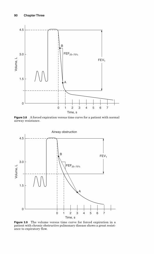
90 Chapter Three
0 1 2 3 4 5 6 7Time, s
A
B
FEF25–75%
Vol
ume,
L
0
1.5
3.0
4.5
FEV1
Airway obstruction
Figure 3.9 The volume versus time curve for forced expiration in apatient with chronic obstructive pulmonary disease shows a great resist-ance to expiratory flow.
0 1 2 3 4 5 6 7
Time, s
A
B
FEF25–75%
Vol
ume,
L
0
1.5
3.0
4.5
FEV1
Figure 3.8 A forced expiration versus time curve for a patient with normalairway resistance.
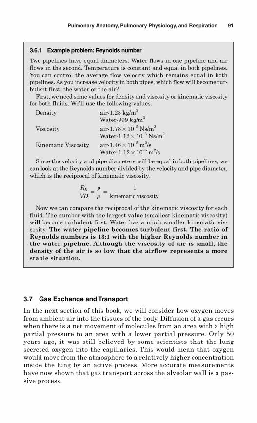
Pulmonary Anatomy, Pulmonary Physiology, and Respiration 91
3.6.1 Example problem: Reynolds number
Two pipelines have equal diameters. Water flows in one pipeline and airflows in the second. Temperature is constant and equal in both pipelines.You can control the average flow velocity which remains equal in bothpipelines. As you increase velocity in both pipes, which flow will become tur-bulent first, the water or the air?
First, we need some values for density and viscosity or kinematic viscosityfor both fluids. We’ll use the following values.
Density air-1.23 kg/m3
Water-999 kg/m3
Viscosity air-1.78 × 10⁻⁵ Ns/m2
Water-1.12 × 10⁻³ Ns/m2
Kinematic Viscosity air-1.46 × 10⁻⁵ m2/sWater-1.12 × 10−6 m2/s
Since the velocity and pipe diameters will be equal in both pipelines, wecan look at the Reynolds number divided by the velocity and pipe diameter,which is the reciprocal of kinematic viscosity.
Now we can compare the reciprocal of the kinematic viscosity for eachfluid. The number with the largest value (smallest kinematic viscosity)will become turbulent first. Water has a much smaller kinematic vis-cosity. The water pipeline becomes turbulent first. The ratio ofReynolds numbers is 13:1 with the higher Reynolds number inthe water pipeline. Although the viscosity of air is small, thedensity of the air is so low that the airflow represents a morestable situation.
RE
VD5r
m5
1kinematic viscosity
3.7 Gas Exchange and Transport
In the next section of this book, we will consider how oxygen movesfrom ambient air into the tissues of the body. Diffusion of a gas occurswhen there is a net movement of molecules from an area with a highpartial pressure to an area with a lower partial pressure. Only 50years ago, it was still believed by some scientists that the lungsecreted oxygen into the capillaries. This would mean that oxygenwould move from the atmosphere to a relatively higher concentrationinside the lung by an active process. More accurate measurementshave now shown that gas transport across the alveolar wall is a pas-sive process.
92 Chapter Three
3.7.1 Diffusion
Gases like oxygen and carbon dioxide move across the blood-gas barrierof the alveolar wall by diffusion. You might ask, “what parameters affectthe rate of transfer?” The rate of gas movement across the alveolar wallis dependent on the diffusion area, the driving pressure, and the wallthickness.
The diffusion area is the surface area of the alveolar wall or blood-gas barrier. That surface area is proportional to the rate of diffusion.The driving pressure which pushes gases across the alveolar wall is thepartial pressure of the gas in question. The driving force that pushesoxygen into the bloodstream is the difference between the partial pres-sure of oxygen in the alveoli and the partial pressure of oxygen in theblood, . The rate of diffusion of oxygen into bloodstream is propor-tional to .
The rate of diffusion of oxygen into the bloodstream is inversely pro-portional to the thickness of the alveolar wall. A thicker wall causes theoxygen diffusion to decrease and a thinner wall makes it easier foroxygen to flow into the bloodstream.
The blood-gas barrier in the lung has a surface area of about 50 to100 m2 shared by over 750 million alveoli. This huge diffusion area isavailable to a relatively small volume of blood. Pulmonary capillaryblood volume is only about 60 mL during resting and about 95 mLduring exercise.
Carbon dioxide diffuses about 20 times more rapidly than oxygenthrough the alveolar wall. The much higher solubility of carbon dioxideis responsible for this increased diffusion rate.
3.7.2 Diffusing capacity
One might wonder if oxygen transfer into the blood is limited by howfast the blood can flow through the lungs, or by how fast oxygen candiffuse through the blood-gas barrier. It turns out that under normalphysiological circumstances, oxygen diffusion through the alveolar wallis sufficient to provide oxygen to all red blood cells flowing through thepulmonary capillaries, and the limiting factor for oxygen uptake is per-fusion or the rate of blood flow through those capillaries. A red bloodcell, also referred to as an erythrocyte, spends an average of about 0.75to 1.2 s passing through a pulmonary capillary under normal restingconditions.
Under some circumstances oxygen diffusion rates through the wallmay also limit the oxygen transfer rate. During extreme exercise, theerythrocyte may stay in the capillary as little as 0.25 s. Even thisvery short time would be enough time for oxygen to diffuse into the
PO2
PO2
capillaries at normal atmospheric oxygen partial pressures. However,during extreme exercise at high altitude, or in a patient with thick-ening of the alveolar wall due to pulmonary fibrosis, oxygen flowrate may switch from a perfusion-limited to a diffusion-limitedprocess.
Resistance to diffusion So far, we have considered the blood-gas bar-rier as the only source of resistance to diffusion of gases from thealveoli into the bloodstream. In fact, there is a second important com-ponent. The uptake of oxygen occurs in two stages. The first is diffu-sion through the alveolar wall and the second is the reaction of oxygenwith hemoglobin.
The diffusing capacity through the alveolar wall is defined by theflow rate of the gas divided by the partial pressure difference that isdriving the flow. Diffusing capacity of a gas can be written as Da inEq. (3.10).
(3.10)
In Eq. (3.10), represents the flow rate of some gas from the alve-oli into the capillary. Pa represents the partial pressure of that gas inthe alveoli and Pc represents the partial pressure of the same gas in thecapillary.
If we think of the electrical analogy in which resistance is equal tovoltage divided by current, we can see that it is possible to think of 1/Da
as a resistance to diffusion.
(3.11)
The rate of reaction of oxygen with hemoglobin can be representedby the symbol . The units on are per mL blood per mmHgpartial pressure of O2. If Vc represents the volume of pulmonary capil-lary blood, then the product of and Vc will have the units of mLO2/min/mmHg or flow divided by pressure. Once again, the inverse,pressure/flow is analogous to resistance.
(3.12)
The total resistance to the flow of oxygen into the bloodstream is thecombination of the resistance to diffusion caused by the blood-gas bar-rier plus the resistance to flow due to the oxygen-hemoglobin reaction.
ResistanceO2-Hgb 5 1uVc
mL O2min
1
Da5
Pa 2 Pc
V.
gas
V.
gas
Da 5V.
gas
sPa 2 Pcd
Pulmonary Anatomy, Pulmonary Physiology, and Respiration 93
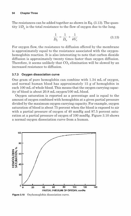
The resistances can be added together as shown in Eq. (3.13). The quan-tity 1/D
Lis the total resistance to the flow of oxygen due to the lung.
(3.13)
For oxygen flow, the resistance to diffusion offered by the membraneis approximately equal to the resistance associated with the oxygen-hemoglobin reaction. It is also interesting to note that carbon dioxidediffusion is approximately twenty times faster than oxygen diffusion.Therefore, it seems unlikely that CO2 elimination will be slowed by anincreased resistance to diffusion.
3.7.3 Oxygen dissociation curve
One gram of pure hemoglobin can combine with 1.34 mL of oxygen,and normal human blood has approximately 15 g of hemoglobin ineach 100 mL of whole blood. This means that the oxygen-carrying capac-ity of blood is about 20.8 mL oxygen/100 mL blood.
Oxygen saturation is reported as a percentage and is equal to theamount of oxygen combined with hemoglobin at a given partial pressuredivided by the maximum oxygen-carrying capacity. For example, oxygensaturation of blood is about 75 percent when the blood is exposed to airwith a partial pressure of oxygen of 40 mmHg and 97.5 percent satu-ration at a partial pressure of oxygen of 100 mmHg. Figure 3.10 showsa normal oxygen dissociation curve from a human.
1DL
51
Da1
1uVc
94 Chapter Three
Figure 3.10 Oxyhemoglobin dissociation curve.
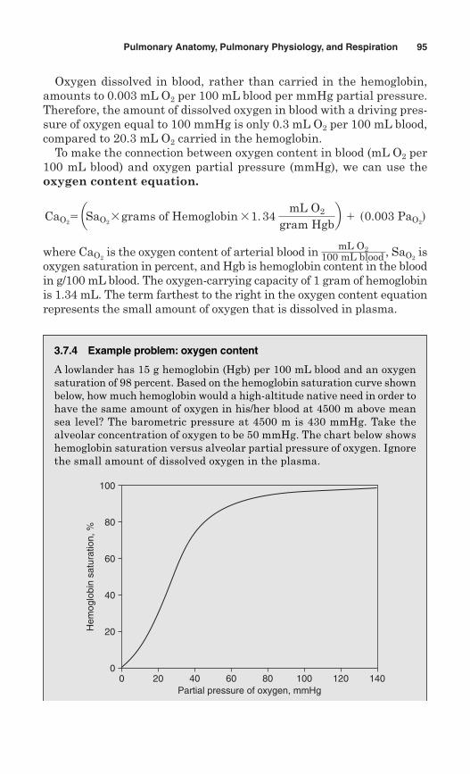
Oxygen dissolved in blood, rather than carried in the hemoglobin,amounts to 0.003 mL O2 per 100 mL blood per mmHg partial pressure.Therefore, the amount of dissolved oxygen in blood with a driving pres-sure of oxygen equal to 100 mmHg is only 0.3 mL O2 per 100 mL blood,compared to 20.3 mL O2 carried in the hemoglobin.
To make the connection between oxygen content in blood (mL O2 per100 mL blood) and oxygen partial pressure (mmHg), we can use theoxygen content equation.
where is the oxygen content of arterial blood in , isoxygen saturation in percent, and Hgb is hemoglobin content in the bloodin g/100 mL blood. The oxygen-carrying capacity of 1 gram of hemoglobinis 1.34 mL. The term farthest to the right in the oxygen content equationrepresents the small amount of oxygen that is dissolved in plasma.
SaO2
mL O2100 mL bloodCaO2
CaO25 aSaO2
3grams of Hemoglobin31. 34 mL O2
gram Hgbb 1 s0.003 PaO2
d
Pulmonary Anatomy, Pulmonary Physiology, and Respiration 95
3.7.4 Example problem: oxygen content
A lowlander has 15 g hemoglobin (Hgb) per 100 mL blood and an oxygensaturation of 98 percent. Based on the hemoglobin saturation curve shownbelow, how much hemoglobin would a high-altitude native need in order tohave the same amount of oxygen in his/her blood at 4500 m above meansea level? The barometric pressure at 4500 m is 430 mmHg. Take thealveolar concentration of oxygen to be 50 mmHg. The chart below showshemoglobin saturation versus alveolar partial pressure of oxygen. Ignorethe small amount of dissolved oxygen in the plasma.
00
20
40
60
80
100
20 40 60 80 100 120 140Partial pressure of oxygen, mmHg
Hem
oglo
bin
satu
ratio
n, %
96 Chapter Three
Solution The oxygen saturation in the lowlander is 85 percent from theabove chart.
The lowlander with 98 percent hemoglobin saturation will have an oxygencontent of his/her blood of:
To find the oxygen content of the blood in the high-altitude native solve forthe hgb content that will give the same total oxygen content at 85 percentsaturation:
corresponding to about a 19 percent increase in hematocrit or an increaseof hematocrit from 0.42 to 0.50. Richalet et al. did a study on Chileanminers who commute from sea level to 4500 m and found that after a yearof chronic intermittent hypoxia (7 days at high altitude followed by 7 daysat sea level), the mean hematocrit for the miners increased to 52 percent(Richalet et al., 2002).
3.7.5 Clinical feature
A 54-year-old man was admitted to the emergency room complaining ofheadache and shortness of breath. On room air, his partial pressure ofarterial oxygen ( ) was 89 mmHg, partial pressure of CO2 ( ) was38 mmHg, and hematocrit was 44 percent. His oxygen saturation was notdirectly measured but instead calculated at 98 percent from the oxy-hemoglobin dissociation curve shown in the example problem in Sec. 3.7.4.After some improvement, he was scheduled for a brain CAT scan and dis-charged from the hospital.
The patient was brought back to the emergency room the next evening,unconscious. This time carbon monoxide and oxygen were measured alongwith the routine blood gases. The results were oxygen saturation �53 percent and carboxyhemoglobin 46 percent.
Carbon dioxide does not affect but it does affect oxygen saturationand the oxygen content of the blood. This patient was suffering fromcarbon monoxide poisoning due to a faulty heater in his home. The oxy-hemoglobin saturation curve is based on the partial pressure of oxygenin the alveoli, and use of that curve assumes that the hemoglobin in thearteries comes to equilibrium with the air in the alveoli (adapted fromMartin).
PaO2
sSaO2d
PaCO2 PaO2
X 5 17.9 gm Hgb
100 mL blood
20.4 mL O2
100 mL blood5 1.34
mL O2
gm Hgb aX
gm Hgb100 mL blood
b s0.85 d
1.34 mL O2
gm Hgb a15
gm Hgb100 mL blood
b s0.98 d 5 19.7 mL O2
100 mL blood
3.8 Pulmonary Pathophysiology
3.8.1 Bronchitis
Bronchitis is an inflammation of the airways resulting in excessivemucus production in the bronchial tree. Bronchitis occurs when theinner walls of the bronchi become inflamed. It often follows a cold orother respiratory infection and happens in virtually all people, just asthe common cold. When the bronchitis does not go away quickly but per-sists, then it is termed chronic bronchitis.
3.8.2 Emphysema
Emphysema is a chronic disease in which air spaces beyond bronchiolesare increased. The stiffness of the alveoli is decreased, (static complianceis increased), and airways collapse more easily. Because of the decreasedstiffness of the lung, exhalation requires active work and the work ofbreathing is significantly increased. The surface area of the alveoli becomesmaller, and the air sacs become less elastic. As carbon dioxide accumu-lates in the lungs, there becomes less and less room available for oxygento be inhaled, thereby decreasing the partial pressure of oxygen in thelungs. See Fig. 3.11 which shows a picture of an emphysematous lung.
Emphysema is most often caused by cigarette smoking, althoughsome genetic diseases can cause similar damage to the alveoli. Once thisdamage has occurred, it is not reversible.
3.8.3 Asthma
Asthma is a chronic disease which affects 5 million children in theUnited States. In asthma, the airways become overreactive withincreased mucus production, swelling, and muscle contraction. Becauseof the decreased size of the bronchi and bronchioles, flow of air isrestricted and both inspiration and expiration become more difficult.
3.8.4 Pulmonary fibrosis
Pulmonary fibrosis affects 5 million people worldwide and 200,000 inthe United States. Pulmonary fibrosis is caused by a thickening or scar-ring of pulmonary membrane. The result is that the alveoli are graduallyreplaced by fibrotic tissue becoming thicker, with a decreased compliance(increased stiffness) and a decrease in diffusing capacity. Symptoms of pul-monary fibrosis include a shortness of breath, chronic dry, hacking cough,fatigue and weakness, chest discomfort, loss of appetite, and rapid weightloss. Traditionally, it was thought that pulmonary fibrosis might be anautoimmune disorder or the result of a viral infection. There is growingevidence that there is a genetic link to pulmonary fibrosis.
Pulmonary Anatomy, Pulmonary Physiology, and Respiration 97
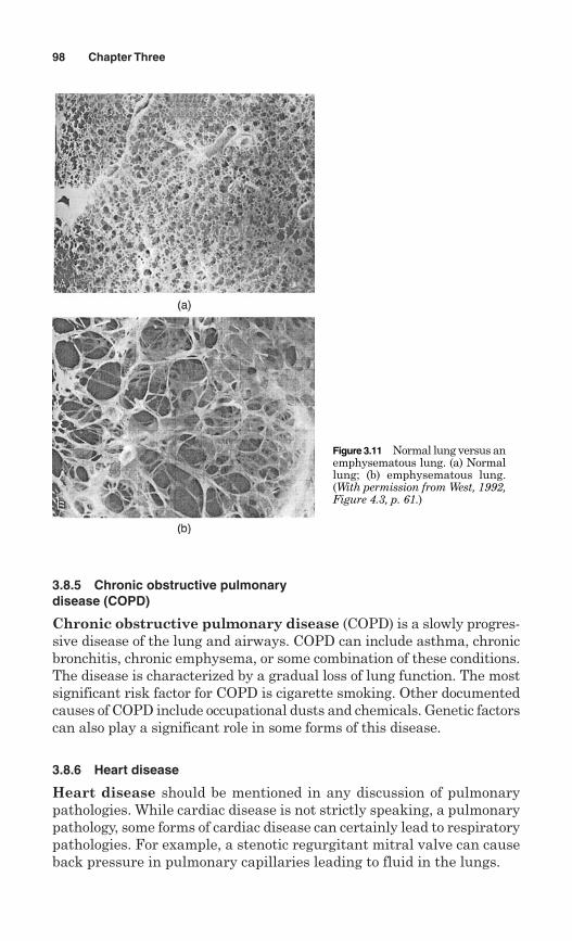
3.8.5 Chronic obstructive pulmonarydisease (COPD)
Chronic obstructive pulmonary disease (COPD) is a slowly progres-sive disease of the lung and airways. COPD can include asthma, chronicbronchitis, chronic emphysema, or some combination of these conditions.The disease is characterized by a gradual loss of lung function. The mostsignificant risk factor for COPD is cigarette smoking. Other documentedcauses of COPD include occupational dusts and chemicals. Genetic factorscan also play a significant role in some forms of this disease.
3.8.6 Heart disease
Heart disease should be mentioned in any discussion of pulmonarypathologies. While cardiac disease is not strictly speaking, a pulmonarypathology, some forms of cardiac disease can certainly lead to respiratorypathologies. For example, a stenotic regurgitant mitral valve can causeback pressure in pulmonary capillaries leading to fluid in the lungs.
98 Chapter Three
Figure 3.11 Normal lung versus anemphysematous lung. (a) Normallung; (b) emphysematous lung.(With permission from West, 1992,Figure 4.3, p. 61.)
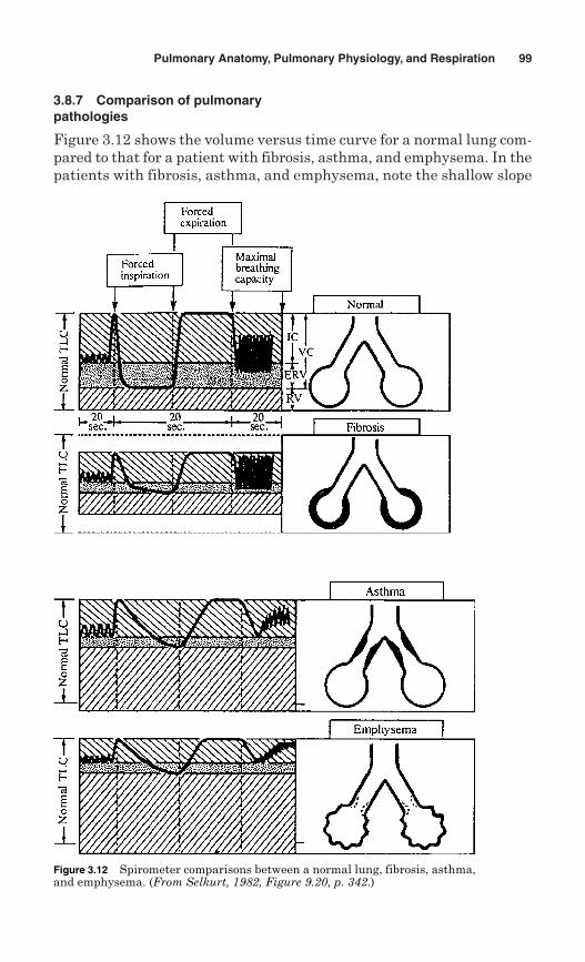
3.8.7 Comparison of pulmonarypathologies
Figure 3.12 shows the volume versus time curve for a normal lung com-pared to that for a patient with fibrosis, asthma, and emphysema. In thepatients with fibrosis, asthma, and emphysema, note the shallow slope
Pulmonary Anatomy, Pulmonary Physiology, and Respiration 99
Figure 3.12 Spirometer comparisons between a normal lung, fibrosis, asthma,and emphysema. (From Selkurt, 1982, Figure 9.20, p. 342.)
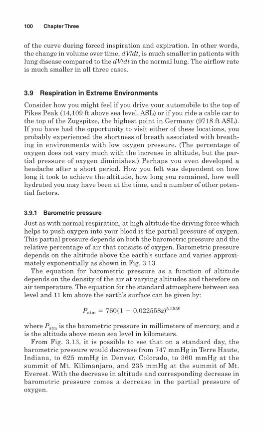
of the curve during forced inspiration and expiration. In other words,the change in volume over time, dV/dt, is much smaller in patients withlung disease compared to the dV/dt in the normal lung. The airflow rateis much smaller in all three cases.
3.9 Respiration in Extreme Environments
Consider how you might feel if you drive your automobile to the top ofPikes Peak (14,109 ft above sea level, ASL) or if you ride a cable car tothe top of the Zugspitze, the highest point in Germany (9718 ft ASL).If you have had the opportunity to visit either of these locations, youprobably experienced the shortness of breath associated with breath-ing in environments with low oxygen pressure. (The percentage ofoxygen does not vary much with the increase in altitude, but the par-tial pressure of oxygen diminishes.) Perhaps you even developed aheadache after a short period. How you felt was dependent on howlong it took to achieve the altitude, how long you remained, how wellhydrated you may have been at the time, and a number of other poten-tial factors.
3.9.1 Barometric pressure
Just as with normal respiration, at high altitude the driving force whichhelps to push oxygen into your blood is the partial pressure of oxygen.This partial pressure depends on both the barometric pressure and therelative percentage of air that consists of oxygen. Barometric pressuredepends on the altitude above the earth’s surface and varies approxi-mately exponentially as shown in Fig. 3.13.
The equation for barometric pressure as a function of altitudedepends on the density of the air at varying altitudes and therefore onair temperature. The equation for the standard atmosphere between sealevel and 11 km above the earth’s surface can be given by:
where Patm is the barometric pressure in millimeters of mercury, and zis the altitude above mean sea level in kilometers.
From Fig. 3.13, it is possible to see that on a standard day, thebarometric pressure would decrease from 747 mmHg in Terre Haute,Indiana, to 625 mmHg in Denver, Colorado, to 360 mmHg at thesummit of Mt. Kilimanjaro, and 235 mmHg at the summit of Mt.Everest. With the decrease in altitude and corresponding decrease inbarometric pressure comes a decrease in the partial pressure ofoxygen.
Patm 5 760s1 2 0.022558zd5.2559
100 Chapter Three
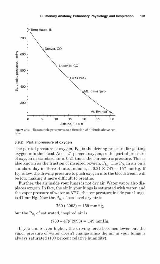
3.9.2 Partial pressure of oxygen
The partial pressure of oxygen, is the driving pressure for gettingoxygen into the blood. Air is 21 percent oxygen, so the partial pressureof oxygen in standard air is 0.21 times the barometric pressure. This isalso known as the fraction of inspired oxygen, . The in air on astandard day in Terre Haute, Indiana, is 0.21 � 747 � 157 mmHg. If
is low, the driving pressure to push oxygen into the bloodstream willbe low, making it more difficult to breathe.
Further, the air inside your lungs is not dry air. Water vapor also dis-places oxygen. In fact, the air in your lungs is saturated with water, andthe vapor pressure of water at 37°C, the temperature inside your lungs,is 47 mmHg. Now the of sea-level dry air is
760 (.2093) � 159 mmHg,
but the of saturated, inspired air is
(760 – 47)(.2093) � 149 mmHg.
If you climb even higher, the driving force becomes lower but thevapor pressure of water doesn’t change since the air in your lungs isalways saturated (100 percent relative humidity).
PO2
PO2
PO2
PO2FIO2
PO2
Pulmonary Anatomy, Pulmonary Physiology, and Respiration 101
Figure 3.13 Barometric pressures as a function of altitude above sealevel.
302520151050
Altitude, 1000 ft
300
400
500
600
700
Bar
omet
ric p
ress
ure,
mm
Hg
Terre Haute, IN
Denver, CO
Leadville, CO
Pikes Peak
Mt. Kilimanjaro
Mt. Everest
Let’s climb to 14,000 ft above sea level (ASL). Now the of inspiredair at 14,000 ft ASL is (446 mmHg – 47)(.2093) � 82 mmHg or abouthalf of the for inspired air at sea level.
Now if we continue to climb to 18,000 ft ASL, the in dry air is halfthat of sea-level dry air and the inspired partial pressure of oxygen isonly 70 mmHg.
(380 – 47) (.2093) � 70 mmHg
Finally, at the top of Mt. Everest the is one-third of sea-level dry airand the of inspired air at 29,000 ft ASL is only 43 mmHg.
(250 – 47) (.2093) � 43 mmHg
What would happen if a high performance jet lost cabin pressure atan altitude of 63,000 ft ASL? The barometric pressure at this extremealtitude is less than the vapor pressure of water at 37°C. In this casethe partial pressure of oxygen would be zero and, in fact, your blood (andall other water in your tissues) would boil.
3.9.3 Hyperventilation and the alveolar gas equation
Inspired oxygen is not the complete story. What about the CO2 in yourlungs? Doesn’t it also displace air, making the even lower? Theamount of oxygen in the alveoli depends on the production of carbondioxide and the rate of transfer of oxygen from the lungs to the blood inthe pulmonary capillaries.
To understand what is happening with the person’s arterial oxygenconcentration, begin with the alveolar gas equation (Levitzky, 2003)which takes into account the patient’s arterial CO2 partial pressure
, fraction of inspired oxygen ( ), and the barometric pressure(PB). Take care with the symbols since “a” in represents “arterial”while “A” in stands for “alveolar.”
where P is partial pressure, A is alveolar, is fraction of inspiredoxygen, PB is barometric pressure, is the vapor pressure of waterat 37�C, and R is the respiratory quotient.
The respiratory quotient or respiratory exchange ratio is:
R 5 V.
CO2
V.
O2
5 rate of CO2 production
rate of O2 usage
PH2O
FIO2
PAO25 FIO2
sPB 2 PH20d 2 PACO2aFIO2
11 2 FIO2
Rb
PACO2
PaCO2
FIO2sPaCO2
d
PO2
PO2
PO2
PO2
PO2
PO2
102 Chapter Three
This alveolar gas equation is valid if there is no CO2 in inspired gas. Ifwe assume a typical value for R of 0.8, the following abbreviated alve-olar gas equation is often used for clinical purposes.
This equation uses a water vapor pressure of 47 mmHg, which is thevapor pressure of water at body temperature, 37°C. Ambient is thesame at all altitudes, 0.21.
The partial pressure of carbon dioxide in your lungs can approach40 mmHg. Since the partial pressure of inspired oxygen at an altitudeof 18,000 ft ASL was calculated as 70 mmHg without considering CO2,the of air in the alveoli could be as low as 70 1.2(40) � 22 mmHg. At the top of Mt. Everest it could be as low as 43 1.2(40) � 5 mmHg.If that is true, how can so many people climb above 14,000 ft so easily anda few people even reach the summit of Mt. Everest without oxygen? Theshort answer is hyperventilation. By breathing faster, climbers are ableto lower the partial pressure of carbon dioxide in their alveoli. If youincrease ventilation rate by four, you can lower the PCO2 to about 10 mmHg.
By hyperventilation, the of alveolar oxygen at the top of Mt.Everest can be calculated as follows.
of inspired air at 29,000 ft is (250 47)(.2093) � 43 mmHg. ThePCO2 of the air in the alveoli is 10 mmHg. The partial pressure of theoxygen in the alveoli is 43 1.2(10) � 30 mmHg.
3.9.4 Alkalosis
One might wonder whether there are any difficulties or side effectsresulting from hyperventilation and the associated drop in the partialpressure of carbon dioxide. In fact, the result is respiratory alkalosis.The pH of the blood increases above normal. You feel bad and you can’tsleep well. One result could be acute mountain sickness.
Your body’s solution to respiratory alkalosis is that your kidneys willexcrete bicarbonate over the next few days. At the same time, theincrease in pH puts a kind of “brake” on ventilation and causes yourbreathing to slow down. The excretion of bicarbonate causes the pH inthe blood to decrease and the “brakes” on ventilation are reduced. Aftertwo or three days at altitude, blood pH returns to normal.
3.9.5 Acute mountain sickness
The feeling of nausea and headache, resulting from low oxygen environ-ments, hyperventilation, and the associated respiratory alkalosis, is knownas acute mountain sickness (AMS). Sleeping at altitude is also troublesome.When your breathing slows, oxygen saturation in your blood drops.
PO2
PO2
PO2
FIO2
PAO25 FIO2
sPB 2 47d 2 PaCO2s1.2d
Pulmonary Anatomy, Pulmonary Physiology, and Respiration 103
This drop in causes you to wake up with a feeling of breathlessness.Diamox is a trademark name for acetazolamide, a well-known carbonicanhydrase inhibitor which is used in the treatment of seizures and glau-coma and is also a diuretic. Diamox does not prevent mountain sickness,but it speeds up acclimatization by increasing urinary excretion of bicar-bonate. People taking Diamox have been shown to have a more consis-tent level of blood oxygen saturation, enabling more restful sleep. AMScan also result in nocturnal periodic breathing, weird dreams, and fre-quent awakening at night.
3.9.6 High-altitude pulmonary edema
High-altitude pulmonary edema (HAPE) is a life-threatening noncar-diogenic (not caused by heart disease) lung edema. The mechanismthat causes HAPE is not completely known, but the disease is thoughtto be caused by patchy, low-oxygen, pulmonary vasoconstriction (con-striction of blood vessels). That constriction results in localized over-perfusion and increased permeability of pulmonary capillary walls.These changes result in high pulmonary artery pressure, high per-meability, and fluid leakage into the alveoli. The result of HAPE is thatthe lungs fill with fluid, decreasing ventilation. Symptoms of HAPEcan include cough, shortness of breath on exercise, progressive short-ness of breath, and eventually suffocation, if left untreated. The con-dition is unstable and the only effective treatment for HAPE is descentto a lower altitude and respiration in a more oxygen-rich environment.
3.9.7 High-altitude cerebral edema
High-altitude cerebral edema (HACE) is a less common, but equallylife-threatening condition in which cerebral edema is the result ofbreathing in a depleted oxygen environment. HACE is theoreticallylinked to brain swelling. Symptoms of HACE can include severe throb-bing headache, confusion, difficulty walking, difficulty speaking, drowsi-ness, nausea, vomiting, seizures, hallucinations, and coma. A personsuffering from HACE is often gray or pale in appearance. A victim cansuffer from HAPE and HACE simultaneously. Both HAPE and HACEnormally occur at altitudes above 15,000 ft ASL but can occur at highski areas above 8000 ft ASL.
3.9.8 Acclimatization
If you ascend to a high altitude and remain for a long period of time, yourbody can begin to acclimatize. By increasing the number of red bloodcells in your blood, you are able to increase the amount of hemoglobinand hence the oxygen carrying capacity of your blood. There are people
PO2
104 Chapter Three
who live permanently above 16,000 ft in the Peruvian Andes. Theirinspired is only about 45 mmHg, but those people have more oxygenin their blood than do normal sea-level residents!
The volume percent of red blood cells in blood is known as hematocrit.Hematocrit in normal healthy males is about 42 to 45 percent. If aperson’s hematocrit falls below 25 percent, then he or she is consideredanemic. Hematocrit values can also be greater than normal and a hema-tocrit above 70 percent is known as polycythemia.
During acclimatization to low oxygen environments, it is possibleto replace approximately 1 percent of your erythrocytes per day. Atthe same time, erythrocytes continue to die after their approximately125-day life span. Therefore, it takes 2 or 3 weeks to increase yourhematocrit significantly.
In a study done in Potosi, Bolivia, which is located in southern Boliviaon a high plane at approximately 13,000 ft ASL, the average hematocritin males was found to be 52.7 percent. Early observations of humanadaptation to high altitude were made in Potosi by de la Calancha inthe late 1600s. The Spanish historian writes that “more than one gen-eration was required” for a Spanish child to thrive in Potosi. It’s not clearwhether being born and raised at high altitude or whether interbreed-ing with the Andean population was required.
3.9.9 Drugs stimulating red blood cell production
Erythropoietin (EPO) is a naturally occurring hormone which stimulatesred blood cell production. Low oxygen stimulates EPO production inhumans, which in turn stimulates a higher production of red blood cells.Recombinant EPO (rEPO) is a synthetic version of this hormone.
The difficulty with taking rEPO to increase hematocrit is that an increasein hematocrit also increases blood viscosity, and therefore increases thework of the heart required to pump blood. At the 1984 Los Angeles Olympicsbefore rEPO was available, some American bicycle racers received bloodtransfusions to raise their red blood cell counts (they also received hepa-titis).After rEPO became readily available, athletes began taking injectionsof rEPO. Anumber of Belgian and Dutch professional cyclists died of strokesin 1987–88, presumably from EPO-induced clots in arteries.
Recombinant human erythropoietin (rEPO) has become the standardof care for renal anemia. rEPO has a relatively short half-life and is gen-erally administered two or three times a week.
Darbepoetin is a synthetic hormone that increases red blood cell pro-duction, and is used to treat anemia and related conditions. It is in thesame class of drugs as rEPO and competes for the same market. Its brandname is Aranesp, and it is marketed by Amgen. It was approved inSeptember 2001 by the U.S. Food and Drug Administration for treatment
PO2
Pulmonary Anatomy, Pulmonary Physiology, and Respiration 105
of patients with chronic renal failure by intravenous or subcutaneousinjection. Darbepoetin alpha is a longer lasting agent with a half-lifeapproximately three times that of rEPO.
Like rEPO, Darbepoetin’s use increases the risk of cardiovascularproblems, including cardiac arrest, seizures, arrhythmia or strokes,hypertension, congestive heart failure, vascular thrombosis, myocardialinfarction, and edema. Also like rEPO, Darbepoetin has the potential tobe abused by athletes seeking an advantage. Its use during the 2002Winter Olympic Games to improve performance led to the disqualifica-tion of several cross-country skiers from their final races.
106 Chapter Three
3.9.10 Example problem: alveolar gasequation
A high-altitude native living in the Andes in Potosi, Bolivia, at 13,000 ft(~4000 m) above sea level has a hematocrit 53 percent. If the partial pres-sure of alveolar oxygen in this man’s lungs is 50 mmHg, calculate the par-tial pressure of arterial carbon dioxide using the abbreviated form of thealveolar gas equation.
Solution The abbreviated form of the alveolar gas equation is:
Solving for the partial pressure of CO2 yields:
To solve for the barometric pressure at altitude, from Sec. 3.9.1, we use theequation:
Therefore,
The partial pressure of carbon dioxide in the arterial blood is 31 mmHg.
PaCO25 0.21s462 2 47d 2 50
1.2 5 31 mmHg
Patm 5 760s1 2 0.022558s4dd5.2559 5 462 mmHg
Patm 5 760s1 2 0.022558zd5.2559
PaCO25
FIO2sPB 2 47d 2 PaO2
1.2
PAO25 FIO2
sPB 2 47d 2 1.2sPaCO2d
Review Problems
1. Determine the total lung capacity of a patient with vital capacity of 4.6 L,functional residual capacity of 2.6 L, and residual volume of 1.3 L.
2. Determine the expiratory reserve capacity of a patient with functionalresidual capacity of 2.9 L and a residual volume of 1.3 L.
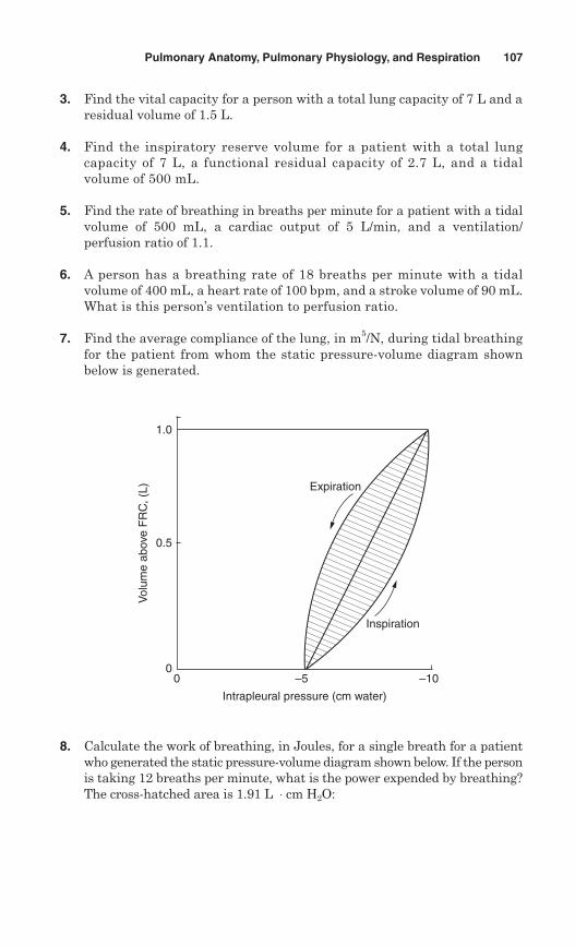
3. Find the vital capacity for a person with a total lung capacity of 7 L and aresidual volume of 1.5 L.
4. Find the inspiratory reserve volume for a patient with a total lungcapacity of 7 L, a functional residual capacity of 2.7 L, and a tidalvolume of 500 mL.
5. Find the rate of breathing in breaths per minute for a patient with a tidalvolume of 500 mL, a cardiac output of 5 L/min, and a ventilation/perfusion ratio of 1.1.
6. A person has a breathing rate of 18 breaths per minute with a tidalvolume of 400 mL, a heart rate of 100 bpm, and a stroke volume of 90 mL.What is this person’s ventilation to perfusion ratio.
7. Find the average compliance of the lung, in m5/N, during tidal breathingfor the patient from whom the static pressure-volume diagram shownbelow is generated.
Pulmonary Anatomy, Pulmonary Physiology, and Respiration 107
8. Calculate the work of breathing, in Joules, for a single breath for a patientwho generated the static pressure-volume diagram shown below. If the personis taking 12 breaths per minute, what is the power expended by breathing?The cross-hatched area is 1.91 L ⋅ cm H2O:
Intrapleural pressure (cm water)
–5 –1000
0.5
1.0
Inspiration
Expiration
Vol
ume
abov
e F
RC
, (L)
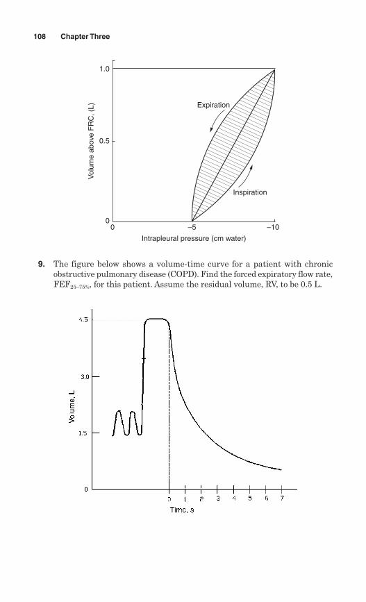
9. The figure below shows a volume-time curve for a patient with chronicobstructive pulmonary disease (COPD). Find the forced expiratory flow rate,FEF25–75%, for this patient. Assume the residual volume, RV, to be 0.5 L.
108 Chapter Three
Intrapleural pressure (cm water)
–5 –1000
0.5
1.0
Inspiration
Expiration
Vol
ume
abov
e F
RC
, (L)
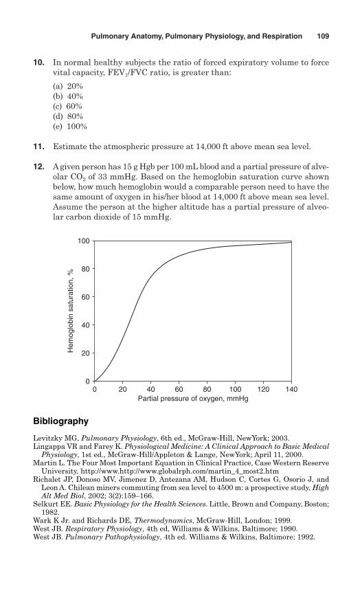
10. In normal healthy subjects the ratio of forced expiratory volume to forcevital capacity, FEV1/FVC ratio, is greater than:
(a) 20%(b) 40%(c) 60%(d) 80%(e) 100%
11. Estimate the atmospheric pressure at 14,000 ft above mean sea level.
12. A given person has 15 g Hgb per 100 mL blood and a partial pressure of alve-olar CO2 of 33 mmHg. Based on the hemoglobin saturation curve shownbelow, how much hemoglobin would a comparable person need to have thesame amount of oxygen in his/her blood at 14,000 ft above mean sea level.Assume the person at the higher altitude has a partial pressure of alveo-lar carbon dioxide of 15 mmHg.
Pulmonary Anatomy, Pulmonary Physiology, and Respiration 109
00
20
40
60
80
100
20 40 60 80 100 120 140Partial pressure of oxygen, mmHg
Hem
oglo
bin
satu
ratio
n, %
Bibliography
Levitzky MG, Pulmonary Physiology, 6th ed., McGraw-Hill, NewYork; 2003.Lingappa VR and Farey K. Physiological Medicine: A Clinical Approach to Basic Medical
Physiology, 1st ed., McGraw-Hill/Appleton & Lange, NewYork; April 11, 2000.Martin L. The Four Most Important Equation in Clinical Practice, Case Western Reserve
University, http://www.http://www.globalrph.com/martin_4_most2.htmRichalet JP, Donoso MV, Jimenez D, Antezana AM, Hudson C, Cortes G, Osorio J, and
Leon A. Chilean miners commuting from sea level to 4500 m: a prospective study, HighAlt Med Biol, 2002; 3(2):159–166.
Selkurt EE. Basic Physiology for the Health Sciences. Little, Brown and Company, Boston;1982.
Wark K Jr. and Richards DE, Thermodynamics, McGraw-Hill, London; 1999.West JB. Respiratory Physiology, 4th ed, Williams & Wilkins, Baltimore; 1990.West JB. Pulmonary Pathophysiology, 4th ed. Williams & Wilkins, Baltimore; 1992.

This page intentionally left blank
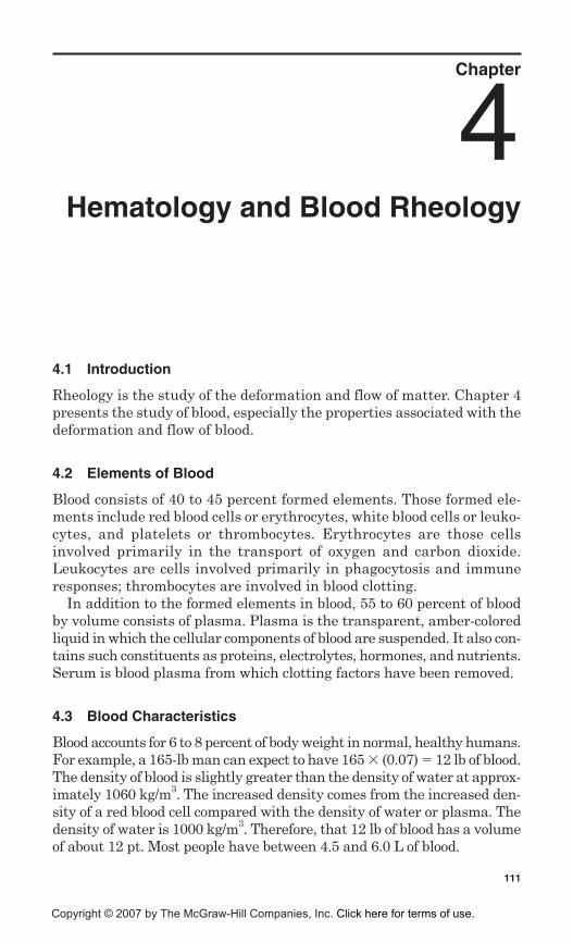
Chapter
4Hematology and Blood Rheology
4.1 Introduction
Rheology is the study of the deformation and flow of matter. Chapter 4presents the study of blood, especially the properties associated with thedeformation and flow of blood.
4.2 Elements of Blood
Blood consists of 40 to 45 percent formed elements. Those formed ele-ments include red blood cells or erythrocytes, white blood cells or leuko-cytes, and platelets or thrombocytes. Erythrocytes are those cellsinvolved primarily in the transport of oxygen and carbon dioxide.Leukocytes are cells involved primarily in phagocytosis and immuneresponses; thrombocytes are involved in blood clotting.
In addition to the formed elements in blood, 55 to 60 percent of bloodby volume consists of plasma. Plasma is the transparent, amber-coloredliquid in which the cellular components of blood are suspended. It also con-tains such constituents as proteins, electrolytes, hormones, and nutrients.Serum is blood plasma from which clotting factors have been removed.
4.3 Blood Characteristics
Blood accounts for 6 to 8 percent of body weight in normal, healthy humans.For example, a 165-lb man can expect to have 165 � (0.07) � 12 lb of blood.The density of blood is slightly greater than the density of water at approx-imately 1060 kg/m3. The increased density comes from the increased den-sity of a red blood cell compared with the density of water or plasma. Thedensity of water is 1000 kg/m3. Therefore, that 12 lb of blood has a volumeof about 12 pt. Most people have between 4.5 and 6.0 L of blood.
111
Copyright © 2007 by The McGraw-Hill Companies, Inc. Click here for terms of use.
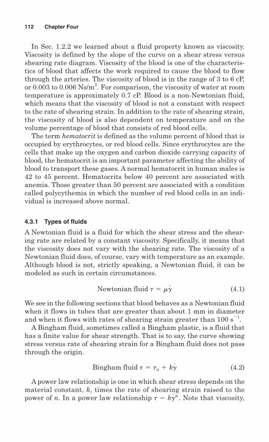
In Sec. 1.2.2 we learned about a fluid property known as viscosity.Viscosity is defined by the slope of the curve on a shear stress versusshearing rate diagram. Viscosity of the blood is one of the characteris-tics of blood that affects the work required to cause the blood to flowthrough the arteries. The viscosity of blood is in the range of 3 to 6 cP,or 0.003 to 0.006 Ns/m2. For comparison, the viscosity of water at roomtemperature is approximately 0.7 cP. Blood is a non-Newtonian fluid,which means that the viscosity of blood is not a constant with respectto the rate of shearing strain. In addition to the rate of shearing strain,the viscosity of blood is also dependent on temperature and on thevolume percentage of blood that consists of red blood cells.
The term hematocrit is defined as the volume percent of blood that isoccupied by erythrocytes, or red blood cells. Since erythrocytes are thecells that make up the oxygen and carbon dioxide carrying capacity ofblood, the hematocrit is an important parameter affecting the ability ofblood to transport these gases. A normal hematocrit in human males is42 to 45 percent. Hematocrits below 40 percent are associated withanemia. Those greater than 50 percent are associated with a conditioncalled polycythemia in which the number of red blood cells in an indi-vidual is increased above normal.
4.3.1 Types of fluids
A Newtonian fluid is a fluid for which the shear stress and the shear-ing rate are related by a constant viscosity. Specifically, it means thatthe viscosity does not vary with the shearing rate. The viscosity of aNewtonian fluid does, of course, vary with temperature as an example.Although blood is not, strictly speaking, a Newtonian fluid, it can bemodeled as such in certain circumstances.
(4.1)
We see in the following sections that blood behaves as a Newtonian fluidwhen it flows in tubes that are greater than about 1 mm in diameterand when it flows with rates of shearing strain greater than 100 s1.
A Bingham fluid, sometimes called a Bingham plastic, is a fluid thathas a finite value for shear strength. That is to say, the curve showingstress versus rate of shearing strain for a Bingham fluid does not passthrough the origin.
(4.2)
A power law relationship is one in which shear stress depends on thematerial constant, k, times the rate of shearing strain raised to thepower of n. In a power law relationship . Note that viscosity,t 5 kg
. n
Bingham fluid t 5 to 1 kg.
Newtonian fluid t 5 mg.
112 Chapter Four
m, is replaced by k in the power law relationship. A Casson fluid is onewith some of the characteristics of a Bingham fluid but also one thatfollows a power law relationship.
(4.3)
Pseudoplastic fluids have no yield stress and are those defined by. Note that n � 1 defines a Newtonian fluid. If n � 1, then the
fluid is known as a shear-thinning fluid; if n � 1, it is known as a shear-thickening fluid.
4.3.2 Viscosity of blood
Viscosity is strongly dependent on temperature, but since humans aremaintained at a constant 37�C, the issue of viscosity change with tem-perature is not significant. On the other hand, blood viscosity varies withsuch parameters as hematocrit, shear rate, and even vessel diameter.Figure 4.1 shows the shear stress of blood plotted versus the shear ratefor blood at a fixed hematocrit. Note that for shear rates above 100 s1,viscosity becomes constant.
t 5 ksg.dn
Casson fluid���t 5 to 1 k2g.1 2k2to2g
.
Hematology and Blood Rheology 113
3 5
Bingham fluid power law relation
Shear rate100/s
τ yield
She
ar s
tres
s
µ = constant
Figure 4.1 Shear stress as a function of the rate of shearingstrain (shear rate) for blood.
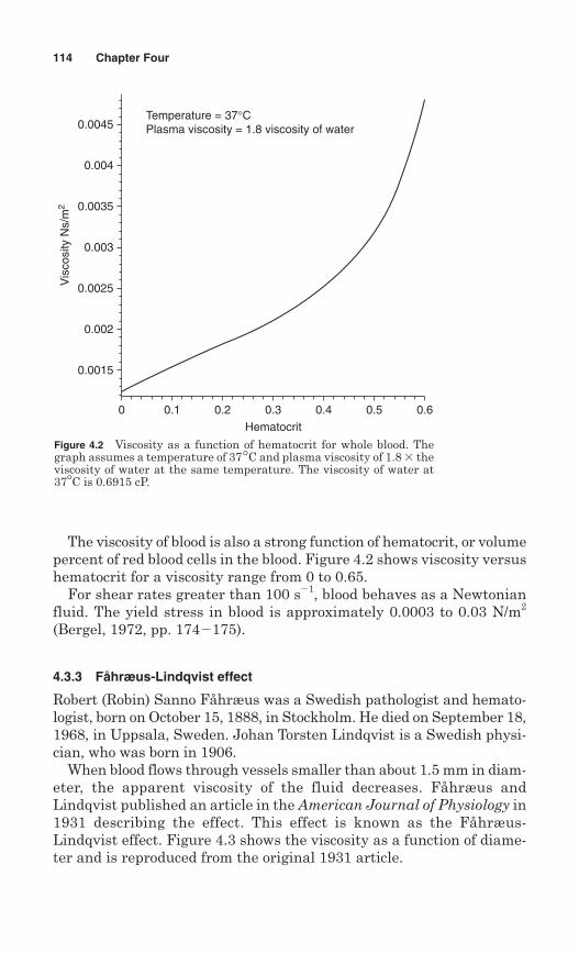
The viscosity of blood is also a strong function of hematocrit, or volumepercent of red blood cells in the blood. Figure 4.2 shows viscosity versushematocrit for a viscosity range from 0 to 0.65.
For shear rates greater than 100 s1, blood behaves as a Newtonianfluid. The yield stress in blood is approximately 0.0003 to 0.03 N/m2
(Bergel, 1972, pp. 174175).
4.3.3 Fåhræus-Lindqvist effect
Robert (Robin) Sanno Fåhræus was a Swedish pathologist and hemato-logist, born on October 15, 1888, in Stockholm. He died on September 18,1968, in Uppsala, Sweden. Johan Torsten Lindqvist is a Swedish physi-cian, who was born in 1906.
When blood flows through vessels smaller than about 1.5 mm in diam-eter, the apparent viscosity of the fluid decreases. Fåhræus andLindqvist published an article in the American Journal of Physiology in1931 describing the effect. This effect is known as the Fåhræus-Lindqvist effect. Figure 4.3 shows the viscosity as a function of diame-ter and is reproduced from the original 1931 article.
114 Chapter Four
Figure 4.2 Viscosity as a function of hematocrit for whole blood. Thegraph assumes a temperature of 37°C and plasma viscosity of 1.8 � theviscosity of water at the same temperature. The viscosity of water at37�C is 0.6915 cP.
0 0.1 0.2 0.3 0.4 0.5 0.6
Hematocrit
Temperature = 37°CPlasma viscosity = 1.8 viscosity of water
Vis
cosi
ty N
s/m
2
0.0015
0.002
0.0025
0.003
0.0035
0.004
0.0045
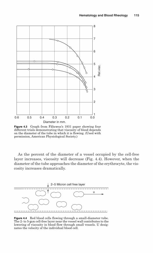
As the percent of the diameter of a vessel occupied by the cell-freelayer increases, viscosity will decrease (Fig. 4.4). However, when thediameter of the tube approaches the diameter of the erythrocyte, the vis-cosity increases dramatically.
Hematology and Blood Rheology 115
8
7
6
5
4
3
2
1
Rel
.vis
c.
0.6 0.5 0.4 0.3 0.2 0.1 0.0
Diameter in mm.
Figure 4.3 Graph from Fåhræus’s 1931 paper showing fourdifferent trials demonstrating that viscosity of blood dependson the diameter of the tube in which it is flowing. (Used withpermission, American Physiological Society.)
2–5 Micron cell free layer
u
Figure 4.4 Red blood cells flowing through a small-diameter tube.The 2- to 5-�m cell-free layer near the vessel wall contributes to thelowering of viscosity in blood flow through small vessels. U desig-nates the velocity of the individual blood cell.
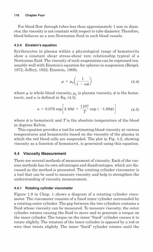
For blood flow through tubes less than approximately 1 mm in diam-eter, the viscosity is not constant with respect to tube diameter. Therefore,blood behaves as a non-Newtonian fluid in such blood vessels.
4.3.4 Einstein’s equation
Erythrocytes in plasma within a physiological range of hematocritsshow a constant shear stress-shear rate relationship typical of aNewtonian fluid. The viscosity of such suspensions can be expressed rea-sonably well with Einstein’s equation for spheres in suspension (Bergel,1972; Jeffery, 1922; Einstein, 1906).
(4.4)
where m is whole blood viscosity, mp is plasma viscosity, is the hema-tocrit, and � is defined in Eq. (4.5).
(4.5)
where is hematocrit and T is the absolute temperature of the bloodin degrees Kelvin.
This equation provides a tool for estimating blood viscosity at varioustemperatures and hematocrits based on the viscosity of the plasma inwhich the red blood cells are suspended. The plot in Fig. 4.2, showingviscosity as a function of hematocrit, is generated using this equation.
4.4 Viscosity Measurement
There are several methods of measurement of viscosity. Each of the var-ious methods has its own advantages and disadvantages, which are dis-cussed as the method is presented. The rotating cylinder viscometer isa tool that can be used to measure viscosity and help to strengthen theunderstanding of viscosity measurement.
4.4.1 Rotating cylinder viscometer
Figure 1.9 in Chap. 1 shows a diagram of a rotating cylinder visco-meter. The viscometer consists of a fixed inner cylinder surrounded bya rotating outer cylinder. The gap between the two cylinders contains afluid whose viscosity can be measured. To measure viscosity, the outercylinder rotates causing the fluid to move and to generate a torque onthe inner cylinder. The torque on the inner “fixed” cylinder causes it torotate slightly. The rotation of the inner cylinder is opposed by a rod orwire that twists slightly. The inner “fixed” cylinder rotates until the
f
a 5 0.076 exp c2.49f 11107
T exp s 21.69fd d
f
m 5 mpa 11 2 af
b
116 Chapter Four
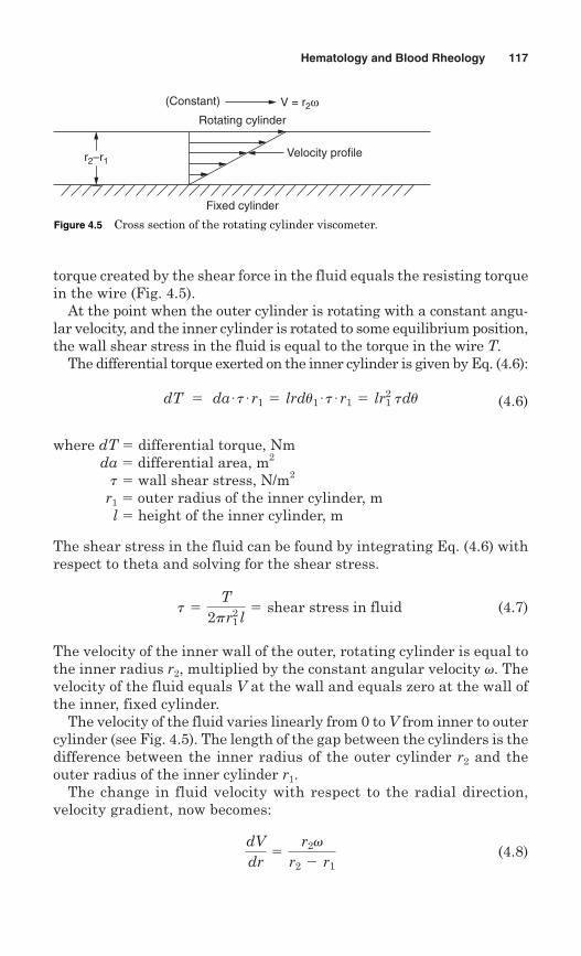
torque created by the shear force in the fluid equals the resisting torquein the wire (Fig. 4.5).
At the point when the outer cylinder is rotating with a constant angu-lar velocity, and the inner cylinder is rotated to some equilibrium position,the wall shear stress in the fluid is equal to the torque in the wire T.
The differential torque exerted on the inner cylinder is given by Eq. (4.6):
(4.6)
where dT � differential torque, Nmda � differential area, m2
t � wall shear stress, N/m2
r1 � outer radius of the inner cylinder, ml � height of the inner cylinder, m
The shear stress in the fluid can be found by integrating Eq. (4.6) withrespect to theta and solving for the shear stress.
(4.7)
The velocity of the inner wall of the outer, rotating cylinder is equal tothe inner radius r2, multiplied by the constant angular velocity v. Thevelocity of the fluid equals V at the wall and equals zero at the wall ofthe inner, fixed cylinder.
The velocity of the fluid varies linearly from 0 to V from inner to outercylinder (see Fig. 4.5). The length of the gap between the cylinders is thedifference between the inner radius of the outer cylinder r2 and theouter radius of the inner cylinder r1.
The change in fluid velocity with respect to the radial direction,velocity gradient, now becomes:
(4.8)dVdr
5r2v
r2 2 r1
t 5T
2pr12 l5 shear stress in fluid
dT 5 da # t # r1 5 lrdu1 # t # r1 5 lr12 tdu
Hematology and Blood Rheology 117
Rotating cylinder
(Constant) V = r2ω
Velocity profile
Fixed cylinder
r2–r1
Figure 4.5 Cross section of the rotating cylinder viscometer.
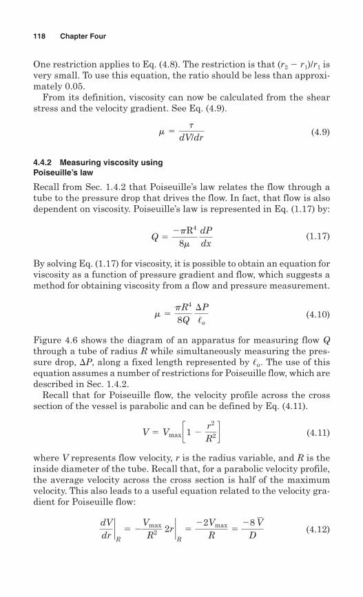
One restriction applies to Eq. (4.8). The restriction is that (r2 r1)/r1 isvery small. To use this equation, the ratio should be less than approxi-mately 0.05.
From its definition, viscosity can now be calculated from the shearstress and the velocity gradient. See Eq. (4.9).
(4.9)
4.4.2 Measuring viscosity usingPoiseuille’s law
Recall from Sec. 1.4.2 that Poiseuille’s law relates the flow through atube to the pressure drop that drives the flow. In fact, that flow is alsodependent on viscosity. Poiseuille’s law is represented in Eq. (1.17) by:
(1.17)
By solving Eq. (1.17) for viscosity, it is possible to obtain an equation forviscosity as a function of pressure gradient and flow, which suggests amethod for obtaining viscosity from a flow and pressure measurement.
(4.10)
Figure 4.6 shows the diagram of an apparatus for measuring flow Qthrough a tube of radius R while simultaneously measuring the pres-sure drop, P, along a fixed length represented by . The use of thisequation assumes a number of restrictions for Poiseuille flow, which aredescribed in Sec. 1.4.2.
Recall that for Poiseuille flow, the velocity profile across the crosssection of the vessel is parabolic and can be defined by Eq. (4.11).
(4.11)
where V represents flow velocity, r is the radius variable, and R is theinside diameter of the tube. Recall that, for a parabolic velocity profile,the average velocity across the cross section is half of the maximumvelocity. This also leads to a useful equation related to the velocity gra-dient for Poiseuille flow:
(4.12)dVdr`R
5 2Vmax
R2 2r `R
522Vmax
R528 V
D
V 5 Vmax c1 2 r2
R2 d
/o
m 5pR4
8Q P/o
Q 52pR4
8m dPdx
m 5t
dV/dr
118 Chapter Four
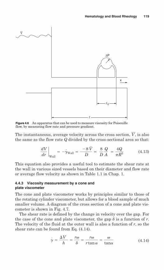
The instantaneous, average velocity across the cross section, , is alsothe same as the flow rate Q divided by the cross-sectional area so that:
(4.13)
This equation also provides a useful tool to estimate the shear rate atthe wall in various sized vessels based on their diameter and flow rateor average flow velocity as shown in Table 1.1 in Chap. 1.
4.4.3 Viscosity measurement by a cone andplate viscometer
The cone and plate viscometer works by principles similar to those ofthe rotating cylinder viscometer, but allows for a blood sample of muchsmaller volume. A diagram of the cross section of a cone and plate vis-cometer is shown in Fig. 4.7.
The shear rate is defined by the change in velocity over the gap. Forthe case of the cone and plate viscometer, the gap d is a function of r.The velocity of the fluid at the outer wall is also a function of r, so theshear rate can be found from Eq. (4.14).
(4.14)g.5
V h
5rvd5
rvr tan a
5v
tana
dVdr
`Wall
5 2g.
Wall 528 V
D5
8D
QA
54QpR3
V
Hematology and Blood Rheology 119
x
∆P
�0
�
∇
Figure 4.6 An apparatus that can be used to measure viscosity for Poiseuilleflow, by measuring flow rate and pressure gradient.
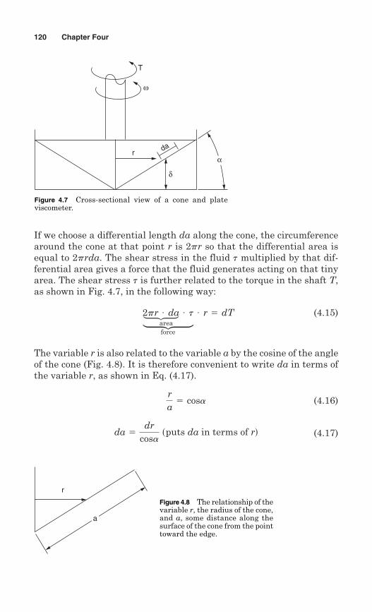
If we choose a differential length da along the cone, the circumferencearound the cone at that point r is 2pr so that the differential area isequal to 2prda. The shear stress in the fluid t multiplied by that dif-ferential area gives a force that the fluid generates acting on that tinyarea. The shear stress t is further related to the torque in the shaft T,as shown in Fig. 4.7, in the following way:
(4.15)
The variable r is also related to the variable a by the cosine of the angleof the cone (Fig. 4.8). It is therefore convenient to write da in terms ofthe variable r, as shown in Eq. (4.17).
(4.16)
(4.17)da 5dr
cosa sputs da in terms of rd
ra5 cosa
2pr # da # t # r 5 dT
120 Chapter Four
3
area3
force
ω
T
r da
δ
α
Figure 4.7 Cross-sectional view of a cone and plate viscometer.
a
r
Figure 4.8 The relationship of thevariable r, the radius of the cone,and a, some distance along thesurface of the cone from the pointtoward the edge.
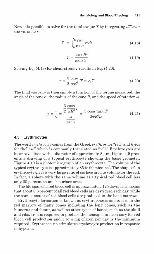
Hematology and Blood Rheology 121
Now it is possible to solve for the total torque T by integrating dT overthe variable r.
(4.18)
(4.19)
Solving Eq. (4.19) for shear stress t results in Eq. (4.20):
(4.20)
The final viscosity is then simply a function of the torque measured, theangle of the cone a, the radius of the cone R, and the speed of rotation v.
(4.21)
4.5 Erythrocytes
The word erythrocyte comes from the Greek erythros for “red” and kytosfor “hollow,” which is commonly translated as “cell.” Erythrocytes arebiconcave discs with a diameter of approximate 8 �m. Figure 4.9 pres-ents a drawing of a typical erythrocyte showing the basic geometry.Figure 4.10 is a photomicrograph of an erythrocyte. The volume of thetypical erythrocyte is approximately 85 to 90 microns3. The shape of anerythrocyte gives a very large ratio of surface area to volume for the cell.In fact, a sphere with the same volume as a typical red blood cell hasonly 60 percent as much surface area.
The life span of a red blood cell is approximately 125 days. This meansthat about 0.8 percent of all red blood cells are destroyed each day, whilethe same amount of red blood cells are produced in the bone marrow.
Erythrocyte formation is known as erythropoiesis and occurs in thered marrow of many bones including the long bones, such as thehumerus and femur, as well as other types of bones, such as the skulland ribs. Iron is required to produce the hemoglobin necessary for redblood cell production and 1 to 4 mg of iron per day is the minimumrequired. Erythropoeitin stimulates erythrocyte production in responseto hypoxia.
m 5t
g. 5
32
cosapR3 T
v
tana
53 cosa tanaT
2pR3v
t 532
cosapR3 T 5 c1T
T 52ptcosa
R3
3
T 5 3R
0
2ptcosa
r2dr
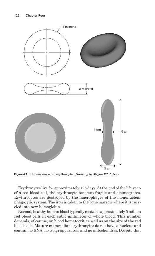
122 Chapter Four
Erythrocytes live for approximately 125 days. At the end of the life spanof a red blood cell, the erythrocyte becomes fragile and disintegrates.Erythrocytes are destroyed by the macrophages of the mononuclearphagocytic system. The iron is taken to the bone marrow where it is recy-cled into new hemoglobin.
Normal, healthy human blood typically contains approximately 5 millionred blood cells in each cubic millimeter of whole blood. This numberdepends, of course, on blood hematocrit as well as on the size of the redblood cells. Mature mammalian erythrocytes do not have a nucleus andcontain no RNA, no Golgi apparatus, and no mitochondria. Despite that
8 microns
2 microns
1 µm
2 µm
8 µm
Figure 4.9 Dimensions of an erythrocyte. (Drawing by Megan Whitaker.)
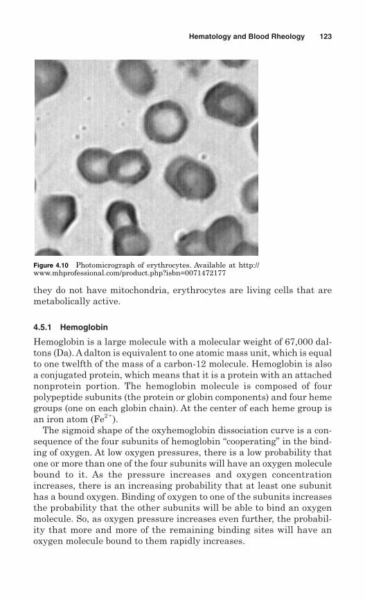
they do not have mitochondria, erythrocytes are living cells that aremetabolically active.
4.5.1 Hemoglobin
Hemoglobin is a large molecule with a molecular weight of 67,000 dal-tons (Da). A dalton is equivalent to one atomic mass unit, which is equalto one twelfth of the mass of a carbon-12 molecule. Hemoglobin is alsoa conjugated protein, which means that it is a protein with an attachednonprotein portion. The hemoglobin molecule is composed of fourpolypeptide subunits (the protein or globin components) and four hemegroups (one on each globin chain). At the center of each heme group isan iron atom (Fe2�).
The sigmoid shape of the oxyhemoglobin dissociation curve is a con-sequence of the four subunits of hemoglobin “cooperating” in the bind-ing of oxygen. At low oxygen pressures, there is a low probability thatone or more than one of the four subunits will have an oxygen moleculebound to it. As the pressure increases and oxygen concentrationincreases, there is an increasing probability that at least one subunithas a bound oxygen. Binding of oxygen to one of the subunits increasesthe probability that the other subunits will be able to bind an oxygenmolecule. So, as oxygen pressure increases even further, the probabil-ity that more and more of the remaining binding sites will have anoxygen molecule bound to them rapidly increases.
Hematology and Blood Rheology 123
Figure 4.10 Photomicrograph of erythrocytes. Available at http://www.mhprofessional.com/product.php?isbn=0071472177
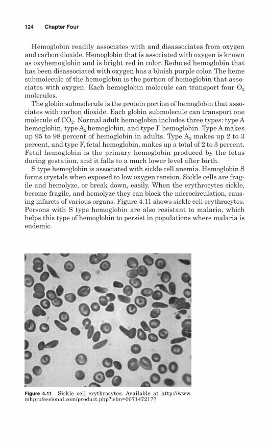
Hemoglobin readily associates with and disassociates from oxygenand carbon dioxide. Hemoglobin that is associated with oxygen is knownas oxyhemoglobin and is bright red in color. Reduced hemoglobin thathas been disassociated with oxygen has a bluish purple color. The hemesubmolecule of the hemoglobin is the portion of hemoglobin that asso-ciates with oxygen. Each hemoglobin molecule can transport four O2
molecules.The globin submolecule is the protein portion of hemoglobin that asso-
ciates with carbon dioxide. Each globin submolecule can transport onemolecule of CO2. Normal adult hemoglobin includes three types: type Ahemoglobin, type A2 hemoglobin, and type F hemoglobin. Type A makesup 95 to 98 percent of hemoglobin in adults. Type A2 makes up 2 to 3percent, and type F, fetal hemoglobin, makes up a total of 2 to 3 percent.Fetal hemoglobin is the primary hemoglobin produced by the fetusduring gestation, and it falls to a much lower level after birth.
S type hemoglobin is associated with sickle cell anemia. Hemoglobin Sforms crystals when exposed to low oxygen tension. Sickle cells are frag-ile and hemolyze, or break down, easily. When the erythrocytes sickle,become fragile, and hemolyze they can block the microcirculation, caus-ing infarcts of various organs. Figure 4.11 shows sickle cell erythrocytes.Persons with S type hemoglobin are also resistant to malaria, whichhelps this type of hemoglobin to persist in populations where malaria isendemic.
124 Chapter Four
Figure 4.11 Sickle cell erythrocytes. Available at http://www.mhprofessional.com/product.php?isbn=0071472177

Example A patient has a hematocrit of 45 percent red blood cells and has5 million red blood cells in each cubic millimeter of blood. Estimate the MCV.
1 micron 5 1026 meters
5 90 3 10218 m3 5 90 micron3
MCV 50.45
5 3 106 RBCmm3 3
10003mm3
m3
4.5.3 Erythrocyte indices
There can be a number of reasons to cause a person to have a lower thannormal quantity of hemoglobin. It could be that the person has a normalnumber of erythrocytes but lower than normal hemoglobin in each ery-throcyte. It could be that the person has a normal amount of hemoglo-bin in each erythrocyte, but a very low hematocrit. These parametersare quantified and those values are known as erythrocyte indices.
One index measures the average volume of an erythrocyte: mean cor-puscular volume (MCV). The MCV can be calculated from the hemat-ocrit of whole blood and the concentration of red blood cells per unitvolume as in Eq. (4.22).
(4.22)MCV 5 HCT
# RBC/volume
Hematology and Blood Rheology 125
4.5.2 Clinical features—sickle cell anemia
Sickle cell anemia presents as severe anemia caused by hemolysis (breakingup of red blood cells). This anemia is punctuated by crises. The symptoms ofthe anemia are mild in comparison with the severity of the crises becauseS type hemoglobin gives up oxygen relatively easily compared with hemo-globin A. Some patients have an almost normal life, with few crises. Otherpatients develop severe crises and may die in early childhood. Sickle cellcrises are sometimes very painful. They can be precipitated by such factorsas infection, acidosis, dehydration, or deoxygenation (associated with alti-tude, for example). The most serious vascular occlusive crisis occurs in thebrain. Of all patients with sickle cell anemia, 7 percent experience a stroke.
A second index measures the amount of hemoglobin in a red blood cell.That index is known as the mean corpuscular hemoglobin (MCH) index.MCH may be calculated as shown in Eq. (4.23).
(4.23) MCH 5 Hgb /volume
# RBCs/volume

A third erythrocyte index is mean corpuscular hemoglobin concentra-tion (MCHC). This index is a measure of the concentration of hemoglo-bin in whole blood (mass/volume). The MCHC may be calculated asshown in Eq. (4.24):
(4.24)MCHC 5 Hgb/volumeHematocrit
126 Chapter Four
Example If a patient has a hemoglobin concentration of 15 g/100 mL of wholeblood and also has 5 million red blood cells in each cubic millimeterof blood, thenthe MCH can be calculated in the following manner:
5 30 3 10212 gm
RBC
MCH 515 g/100 mL
5 3 106 RBC’s/mm3 5
15 g/100 mL 31 mLcm3 3
cm3
103mm3
5 3 106 RBC’s/mm3
Example For a patient with a hemoglobin concentration of 15 g/100 mL ofwhole blood and a hematocrit of 0.45, the MCHC can be calculated as shownbelow:
MCHC 5 15 gm/100 mL
.455
0.33 gm of hemoglobin100 mL blood
4.5.4 Abnormalities of the blood
Anemia is defined as a reduction below normal in the oxygen-carryingcapacity of blood. This reduction in oxygen-carrying capacity could be aresult of a decrease in the number of red blood cells in the blood, or itcould be a result of a decrease in hemoglobin in each red blood cell, orit could be caused by both.
Macrocytic hyperchromic anemia is an anemia in which a greatlyreduced number of red blood cells are too large (macrocytic), contain toomuch hemoglobin, and are therefore too red (hyperchromic). These large,red erythrocytes lack erythrocyte maturation factor. This lack can some-times be related to a vitamin B12 deficiency.
Polycythemia is defined as an increase in the total red cell mass of theblood. It is commonly thought of as an increase in the number of ery-throcytes per cubic millimeter of whole blood above 6 million. Relativepolycythemia can be a result of increased concentration of red blood
cells due to decreased blood volume, for example, as a result of dehydra-tion. Polycythemia vera, however, results from hyperactivity of the bonemarrow. In polycythemia vera there is an abnormal proliferation of allhematopoietic bone marrow elements, often associated with leukocytosis(increase in white blood cells) and thrombocythemia (increase in platelets).It is often difficult to determine the cause of polycythemia vera, but itmay be symptomatic of tumors in the bone marrow, kidney, or brain.
Hematology and Blood Rheology 127
4.5.5 Clinical feature—thalassemia
Hemoglobin is a protein carried by erythrocytes. It consists of about 6 per-cent heme and the rest globin, a colorless protein obtained by removingheme from hemoglobin, the oxygen-carrying compound in red blood cells. Ahemoglobin molecule consists of four polypeptide chains: two alpha chains,each with 141 amino acids, and two beta chains, each with 146 amino acids.Thalassemia is a genetic disorder that results from a reduced rate of syn-thesis of alpha or beta chains in the hemoglobin. In thalassemia the MCVand MCH are low. Traits of alpha thalassemia, failure of genes that producethe alpha chains, are usually not associated with anemia, but the MCV andMCH are low and the red blood cell count is greater than 5.5 � 1012 ery-throcytes per liter. The synthesis ratio of alpha:beta chains is reduced below1:1 in alpha thalassemia.
In beta thalassemia few or no beta chains are produced. Excess alphachains cause severe ineffective production of red blood cells (erythropoiesis)and hemolysis. The more alpha chains, the more severe the anemia.
Beta thalassemia minor (trait) is common and usually symptomless. MCVand MCH are very low but the red blood cell count is high. Mild or no anemia,with hemoglobin 10 to 15 g/dL, is associated with beta thalassemia minor.
From February 2004 to November 2004, a research project was carriedout in Saudi Arabia investigating the occurrence of thalassemia (Al-Suliman,2006). Healthy subjects coming to six marriage consultation centers inthe Al-Hasa area in Saudi Arabia underwent routine mandatory tests.Subjects were considered to have beta-thalassemia trait if they had anMCV � 80 femtoliters (80 � 10–15 L) and/or an MCH) � 27 g/dL. The studyfound that in 3.4 percent of married couples, both partners had the beta-thalassemia trait. The conclusion of the study was that a premaritalscreening program is helpful in countries with a high incidence of hemo-globin pathologies, for identification and prevention of high-risk mar-riages. More comprehensive programs were suggested to learn the actualrate of occurrence of beta-thalassemia in that specific region.
4.6 Leukocytes
Leukocytes, also known as white blood cells, can be broadly definedinto two groups, arranged by function—phagocytes and immunocytes.They can also be classified into two groups by appearance—granulocytes
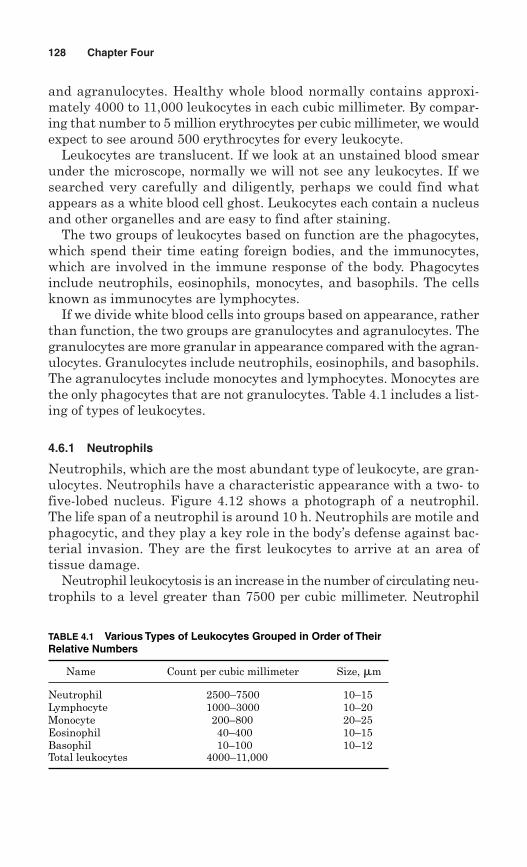
and agranulocytes. Healthy whole blood normally contains approxi-mately 4000 to 11,000 leukocytes in each cubic millimeter. By compar-ing that number to 5 million erythrocytes per cubic millimeter, we wouldexpect to see around 500 erythrocytes for every leukocyte.
Leukocytes are translucent. If we look at an unstained blood smearunder the microscope, normally we will not see any leukocytes. If wesearched very carefully and diligently, perhaps we could find whatappears as a white blood cell ghost. Leukocytes each contain a nucleusand other organelles and are easy to find after staining.
The two groups of leukocytes based on function are the phagocytes,which spend their time eating foreign bodies, and the immunocytes,which are involved in the immune response of the body. Phagocytesinclude neutrophils, eosinophils, monocytes, and basophils. The cellsknown as immunocytes are lymphocytes.
If we divide white blood cells into groups based on appearance, ratherthan function, the two groups are granulocytes and agranulocytes. Thegranulocytes are more granular in appearance compared with the agran-ulocytes. Granulocytes include neutrophils, eosinophils, and basophils.The agranulocytes include monocytes and lymphocytes. Monocytes arethe only phagocytes that are not granulocytes. Table 4.1 includes a list-ing of types of leukocytes.
4.6.1 Neutrophils
Neutrophils, which are the most abundant type of leukocyte, are gran-ulocytes. Neutrophils have a characteristic appearance with a two- tofive-lobed nucleus. Figure 4.12 shows a photograph of a neutrophil.The life span of a neutrophil is around 10 h. Neutrophils are motile andphagocytic, and they play a key role in the body’s defense against bac-terial invasion. They are the first leukocytes to arrive at an area oftissue damage.
Neutrophil leukocytosis is an increase in the number of circulating neu-trophils to a level greater than 7500 per cubic millimeter. Neutrophil
128 Chapter Four
TABLE 4.1 Various Types of Leukocytes Grouped in Order of TheirRelative Numbers
Name Count per cubic millimeter Size, �m
Neutrophil 2500–7500 10–15Lymphocyte 1000–3000 10–20Monocyte 200–800 20–25Eosinophil 40–400 10–15Basophil 10–100 10–12Total leukocytes 4000–11,000

leukocytosis is the most frequently observed change in the blood count. Afew causes of this include inflammation and tissue necrosis, for example,as a result of a myocardial infarction, acute hemorrhage, or bacterialinfection. Acute infections such as appendicitis, smallpox, or rheumaticfever can result in leukocytosis. If the neutrophil count becomes con-siderably less than normal, it can also be due to a viral infection suchas influenza, hepatitis, or rubella.
Physiologic leukocytosis occurs in newborn infants, pregnancy, andafter strenuous exercise, when the number of circulating neutrophilscan increase to about 7500 per cubic millimeter with no associatedpathology.
4.6.2 Lymphocytes
Lymphocytes are the immunological component of our defense againstforeign invasion of the body. Lymphocytes make up about a fourth of thecirculating leukocytes. Lymphocytes are nonphagocytic, and a primary
Hematology and Blood Rheology 129
Figure 4.12 Photomicrograph of a neutrophil. (Note the four-lobednucleus.) Available at http://www.mhprofessional.com/product.php?isbn=0071472177

function of these cells is the release of antibody molecules and the dis-posal of antigens.
B lymphocytes originate in the bone marrow and make up about20 percent of lymphocytes. These cells synthesize antibody molecules.The type of immunity that involves B lymphocytes is known as humoralimmunity. The B cells fight against bacteria.
T lymphocytes, on the other hand, originate in the thymus gland andmake up about 80 percent of lymphocytes. These T cells are precondi-tioned to attack antigens either directly or by releasing chemicals toattract neutrophils and B lymphocytes. T lymphocytes do not produceantibodies directly. On the other hand, T cells multiply and clone moreT cells, which are also responsive to some antigen. This is known as cell-mediated immunity. T cells fight against bacteria, viruses, protozoa,and fungi, as well as such things as transplanted organs. Patients withacquired immune deficiency syndrome (AIDS) monitor T-cell level, anindicator of the activity of the AIDS virus. Figure 4.13 shows a pho-tomicrograph of a lymphocyte.
Lymphocytosis is defined as an increase in the number of circulatinglymphocytes above normal. There are normally 1000 to 3000 lympho-cytes in a cubic millimeter of blood. When the number of circulating lym-phocytes becomes 10,000 per cubic millimeter, for example, this is knownas lymphocytosis. Some causes of acute lymphocytosis include infec-tious mononucleosis, rubella, mumps, and human immunodeficiencyvirus (HIV). Causes of chronic lymphocytosis include tuberculosis andsyphilis.
130 Chapter Four
Figure 4.13 Photomicrograph of blood showing a lymphocyte atthe right and a neutrophil at the left. Available at http://www.mhprofessional.com/product.php? isbn=0071472177

The life span of a lymphocyte is weeks to months. A large number ofinherited or acquired deficiencies in any of the components of theimmune system may cause an impaired immune system response. A pri-mary lack of T lymphocytes, as in AIDS, leads not only to bacterialinfections, but also to viral, protozoal, and fungal infections.
4.6.3 Monocytes
Monocytes are mobile and actively phagocytic and are larger than otherleukocytes. They have a large central oval or indented nucleus. Theycirculate in the bloodstream for 20 to 40 h and then leave the blood-stream to enter the body’s tissues and mature and differentiate intomacrophages. Macrophages carry out a function similar to that of aneutrophil. Macrophages may live for several months or even years!
Of all circulating leukocytes, 3 to 9 percent are monocytes. Theyincrease in number in patients with malaria, mononucleosis, typhoidfever, and Rocky Mountain spotted fever.
4.6.4 Eosinophils
Eosinophils are granulocytes that play a special role in allergic responseor defense against parasites and in the removal of fibrin formed duringinflammation. The primary function of an eosinophil is detoxification offoreign proteins. The number of eosinophils in whole blood is normally0 to 3 percent of leukocytes. However, in allergic reactions this per-centage increases. Eosinophils increase in numbers due to bronchitis,bronchial asthma, or hay fever.
4.6.5 Basophils
Basophils are seen only occasionally in normal peripheral blood.1 Onefunction of a basophil is to release histamine in an area of tissue damagein order to increase blood flow and to attract other leukocytes to the areaof damage. Basophils increase in number in response to hemolyticanemia or chicken pox.
4.6.6 Leukemia
Leukemia is a group of disorders characterized by the accumulation ofabnormal white cells in the bone marrow. In other words, there is a pur-poseless malignant proliferation of leukopoietic tissue, which is the tissuethat forms leukocytes. This type of leukopoietic tissue is found in bone
Hematology and Blood Rheology 131
1Peripheral blood cells are the cellular components of circulating blood, as opposed tothe cells kept in the lymphatic system, spleen, liver, bone marrow, or in tissues in case ofinflammation.
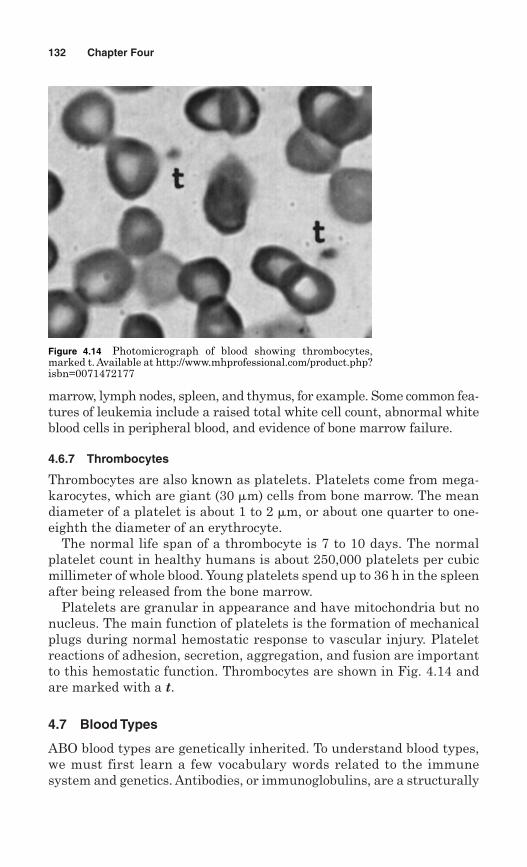
marrow, lymph nodes, spleen, and thymus, for example. Some common fea-tures of leukemia include a raised total white cell count, abnormal whiteblood cells in peripheral blood, and evidence of bone marrow failure.
4.6.7 Thrombocytes
Thrombocytes are also known as platelets. Platelets come from mega-karocytes, which are giant (30 �m) cells from bone marrow. The meandiameter of a platelet is about 1 to 2 �m, or about one quarter to one-eighth the diameter of an erythrocyte.
The normal life span of a thrombocyte is 7 to 10 days. The normalplatelet count in healthy humans is about 250,000 platelets per cubicmillimeter of whole blood. Young platelets spend up to 36 h in the spleenafter being released from the bone marrow.
Platelets are granular in appearance and have mitochondria but nonucleus. The main function of platelets is the formation of mechanicalplugs during normal hemostatic response to vascular injury. Plateletreactions of adhesion, secretion, aggregation, and fusion are importantto this hemostatic function. Thrombocytes are shown in Fig. 4.14 andare marked with a t.
4.7 Blood Types
ABO blood types are genetically inherited. To understand blood types,we must first learn a few vocabulary words related to the immunesystem and genetics. Antibodies, or immunoglobulins, are a structurally
132 Chapter Four
Figure 4.14 Photomicrograph of blood showing thrombocytes,marked t. Available at http://www.mhprofessional.com/product.php?isbn=0071472177

Hematology and Blood Rheology 133
related class of glycoproteins that are produced in response to a specificantigen. Antigens, on the other hand, are any substance that attractsantibodies. Antigens include foreign proteins, toxins, bacteria, andviruses.
An allele is any alternative form of a gene that can occupy a par-ticular chromosomal locus. A genotype is the genetic makeup of anindividual, or the alleles present at one or more specific loci. A phe-notype is the entire physical, biochemical, and physiological makeupof an individual (as opposed to genotype).
The three alleles associated with the ABO blood groups are IA, IB,and i. Alleles IA and IB are dominant to i, but show no dominance withrespect to one another. Each person has two alleles, one inheritedfrom each parent. For example, if a person inherits the IA allele fromeach parent, he or she will have the IA/IA genotype and blood type A(phenotype).
Agglutination is the term for the aggregation of erythrocytes intoclumps. Severe agglutination can lead to death. Agglutinogens (or anti-gens) are substances on the membranes of erythrocytes. Agglutininsare antibodies in the plasma that try to attack specific agglutinogens.This is known as an antibody–antigen reaction.
Persons with type A blood have the IA/IA genotype and their erythro-cytes have the A antigen (agglutinogen) and the b or anti-B antibody(agglutinin). If such people receive a transfusion of type B blood, theirantibodies would attack the antigens on the donor erythrocytes andcause agglutination.
Persons with type B blood have the B antigen. Persons with type ABblood have both the A and the B antigens on their erythrocytes. Finally,people with type O blood have no A or B antigens on their erythro-cytes.
Table 4.2 shows phenotypes and genotypes of the four blood groupsalong with their respective antigens and antibodies. Note that personswith A blood have the b antibody, persons with type B blood have the aantibody, and persons with O blood have both the a and b antibodies.
TABLE 4.2 Blood Types, Distributions, and Their Associated Antigens and Antibodies
Erythrocyte Plasma Population distri-Blood type Blood group antigen antibody bution whites, lowa phenotype genotype (agglutinogens) (agglutinins) (for example)
A IA/IA or IA/i A Anti-B (b) 42%B IB/IB or IB/i B Anti-A (�) 9%AB IA/IB A and B Neither 4%O i/i Neither Anti-A and 46%
Anti-B (� & b)
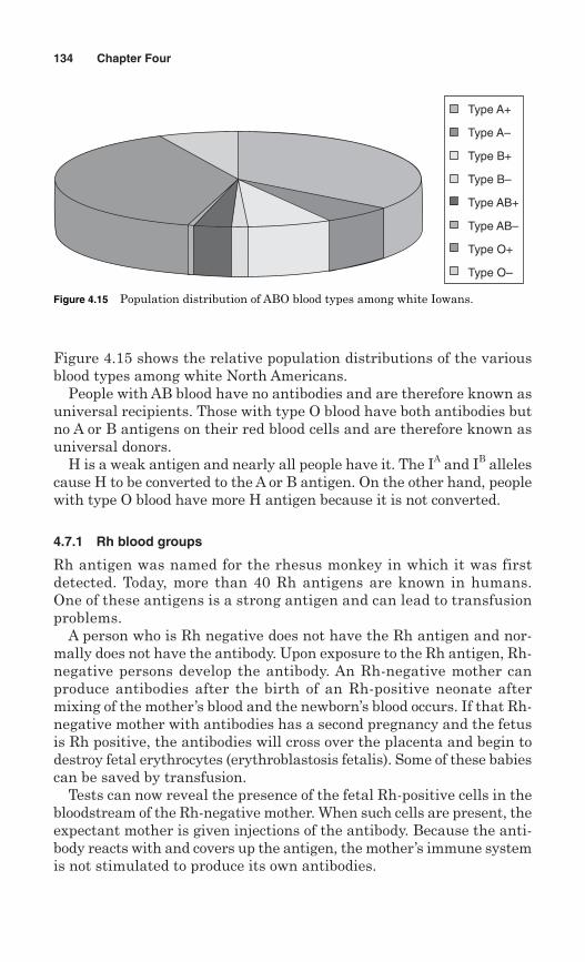
Figure 4.15 shows the relative population distributions of the variousblood types among white North Americans.
People with AB blood have no antibodies and are therefore known asuniversal recipients. Those with type O blood have both antibodies butno A or B antigens on their red blood cells and are therefore known asuniversal donors.
H is a weak antigen and nearly all people have it. The IA and IB allelescause H to be converted to the A or B antigen. On the other hand, peoplewith type O blood have more H antigen because it is not converted.
4.7.1 Rh blood groups
Rh antigen was named for the rhesus monkey in which it was firstdetected. Today, more than 40 Rh antigens are known in humans.One of these antigens is a strong antigen and can lead to transfusionproblems.
A person who is Rh negative does not have the Rh antigen and nor-mally does not have the antibody. Upon exposure to the Rh antigen, Rh-negative persons develop the antibody. An Rh-negative mother canproduce antibodies after the birth of an Rh-positive neonate aftermixing of the mother’s blood and the newborn’s blood occurs. If that Rh-negative mother with antibodies has a second pregnancy and the fetusis Rh positive, the antibodies will cross over the placenta and begin todestroy fetal erythrocytes (erythroblastosis fetalis). Some of these babiescan be saved by transfusion.
Tests can now reveal the presence of the fetal Rh-positive cells in thebloodstream of the Rh-negative mother. When such cells are present, theexpectant mother is given injections of the antibody. Because the anti-body reacts with and covers up the antigen, the mother’s immune systemis not stimulated to produce its own antibodies.
134 Chapter Four
Type A+
Type A–
Type B+
Type B–
Type AB+
Type AB–
Type O+
Type O–
Figure 4.15 Population distribution of ABO blood types among white Iowans.
4.7.2 M and N blood group system
Many other antigens exist, and although they may not be medicallyimportant in transfusions, they can be used to study genetics and areused in tests involving disputed parenthood.
Two antigens, M and N, exist and the alleles for production of theseantigens show no dominance to each other. There are therefore three cor-responding genotypes: M, MN, and N. The M phenotype is the blood typewith the M antigen located on the erythrocyte and is associated with theM/M genotype. Table 4.3 shows a list of MN phenotypes along withtheir respective genotypes and antigens.
4.8 Plasma
Plasma is a transparent amber fluid and is 90 percent water by volume.The 10 percent that is not water adds some very important character-istics to the function of blood.
Plasma contains inorganic substances like sodium ions, potassium ions,chloride ions, bicarbonate ions, calcium ions, and those chemicals makeup about 1 percent of the plasma by volume. Plasma proteins make upabout 7 percent of plasma by volume. Those proteins include albumins,globulins, and fibrinogens. In plasma there is a further ~1 percent byvolume of nonprotein organics and also varying amounts of hormones,enzymes, vitamins, and dissolved gases.
Plasma proteins are large molecules with high molecular weight thatdo not pass through the capillary wall. They remain in the blood vesseland establish an osmotic gradient.
Albumin accounts for most of the plasma protein osmotic pressure.Human plasma contains about 4 to 5 g albumin/100 mL plasma.Albumin is important in binding certain substances that are trans-ported in plasma, such as barbiturates and bilirubin.
Globulins are present in human plasma at the rate of approximately2 to 3 g/100 mL plasma. The normal albumin-to-globulin ratio is approx-imately 2. Fibrinogen is a plasma protein that is involved in hemostasis,which is the process by which loss of blood from the vascular system isreduced (blood clotting).
Hematology and Blood Rheology 135
TABLE 4.3 MN Phenotypes and Their AssociatedGenotypes and Antigens
Phenotype Genotype Erythrocyte antigen
M M/M MMN M/N M and NN N/N N
4.8.1 Plasma viscosity
Plasma viscosity is a function of the concentration of plasma proteinsof large molecular size. This is particularly true of the proteins with pro-nounced axial asymmetry. Fibrinogen and some of the immunoglobulinsfall in this category. Normal values of viscosity at room temperature arein the range of 1.5 to 1.7 cP (1.5 to 1.7 � 10–3 Ns/m2).
4.8.2 Electrolyte composition of plasma
One equivalent (eq) contains Avogadro’s number of � or charges(6 � 1023 charges). Therefore, for singly charged (univalent ions) 1equivalent of ions is equal to 1 mole and therefore 1 meq � 1 mmol.
Table 4.4 shows the electrolyte composition of plasma. Note thatsodium is an important ion in plasma, which contains 142 meq/L.This is the same as 142 mol/L. Plasma also contains 5 meq/L of calciumion, which is the same as 2.5 mmol/L because calcium is a doublycharged ion.
Osmotic pressure is defined as the pressure that builds up as a resultof the tendency of water to diffuse down the concentration gradient. Onthe other hand, oncotic pressure is osmotic pressure due to plasmaproteins.
Osmolarity, in units of Osm/L, is the measure of the concentration ofa solute that would cause an osmotic pressure. Osmolarity is equal tomolar concentration multiplied by the number of ionized particles in thesolution. When a solute has the concentration of 1 Osmole (Osm), itwould have an osmotic pressure of 22.4 atm compared with pure water.Human plasma has the same osmotic pressure as 0.9 percent NaClsolution (physiologic or isotonic saline).
The 0.9 percent NaCl is a solution that contains 9 g of NaCl in 1000 gof water or 9 g NaCl/L water; 1 mol of NaCl contains 23 g of sodium and35 g of chlorine for a total of 58 g of sodium chloride. The molar con-centration of isotonic saline is 9 g of sodium chloride in 1 L of water or9/58 � 155 mmolar. The osmolarity of isotonic saline is 155 mmolarmultiplied by 2 ionized particles (sodium and chloride) or 310 mOsm.
136 Chapter Four
TABLE 4.4 Electrolyte Composition of Plasma
Substance Symbol meq/L Substance Symbol meq/L
Sodium Na� 142 Chloride Cl– 103Potassium K� 4 Bicarbonate HCO3
– 28Calcium Ca�� 5 Proteins 17Magnesium Mg� 2 Others 5Total 153 153
When erythrocytes are placed in an isotonic solution, they do notchange size. When they are placed in a hypertonic solution, water passesout of the cell and they shrink. When the erythrocytes are placed in ahypotonic solution (0.35 percent NaCl, for example), they swell to anearly spherical shape and in some cases undergo hemolysis.
4.8.2 Blood pH
The pH of normal healthy blood is in the range of 7.35 to 7.45. Whenthe pH is less than 7.35, this condition is defined as acidosis. When thepH is greater than 7.45, this condition is defined as alkalosis. CO2 dis-solved in water in plasma produces carbonic acid, which lowers bloodpH. Bicarbonate and carbonic acid form an acid–base buffer pair, whichhelps to keep the arterial pH near 7.4. When PCO2 decreases, then thepH increases.
The ratio of bicarbonate concentration to partial pressure of CO2 inblood is a ratio of metabolic compensation to respiratory compensation.The Henderson–Hasselbalch equation can be used to calculate the pHof arterial blood based on that ratio.
(4.25)
where the bicarbonate concentration is given in milliequivalents per literand the partial pressure of carbon dioxide is given in millimeters ofmercury. The normal ratio of metabolic compensation to respiratorycompensation can be estimated as follows:
Normal ratio 5 sHCO2
3 d 0.03 sPCO2
d 5
240.03s40d
5 20
pH 5 6.1 1 log [HCO2
3 ]0.03sPCO2
d
Hematology and Blood Rheology 137
4.8.3 Clinical features—acid–baseimbalance
An imbalance of acid generation or removal due to either lungs or kidneysis usually compensated for by a nearly equal and opposite change in theother organ. For example, diarrhea with a loss of bicarbonate-containingfluids will trigger hyperventilation and respiratory compensation to elim-inate enough CO2 to compensate for the bicarbonate loss in the stool.Conversely, vomiting with loss of stomach hydrochloric acid results in meta-bolic alkalosis for which hypoventilation and an increase in blood CO2 isthe compensation.
138 Chapter Four
Review Problems
1. Whole blood (assume m� 0.004 Ns/m2) is placed in a concentric cylinder vis-cometer. The gap width is 1 mm and the inner cylinder radius is 30 mm.Estimate the torque exerted on the 10-cm-long inner cylinder. Assume theangular velocity of the outer cylinder to be 30 rad/min.
2. Whole blood is forced from a large reservoir through a small rigid tube(diameter � 2 mm; length � 500 mm) and discharges into the atmosphere.If the gauge pressure in the reservoir is 4 � 104 N/m2, estimate the dis-charge from the tube in m3/s. The blood hematocrit is 55 percent and theblood temperature is 30�C. Assume the relative viscosity of plasma to be1.24 � 10–3 Ns/m2.
3. For a certain cone and plate viscometer the cone angle is 1.5�. A fluid isplaced in the device and the following data are obtained. Is the fluidNewtonian? Explain. Determine the viscosity at the lowest speed in Ns/m2.
4. Blood flowing through the descending aorta can become turbulent in somehighly trained athletes. Does blood act as a Newtonian fluid in this case?Why or why not?
5. Using the Einstein equation to predict viscosity as a function of hematocritand temperature, calculate the viscosity of blood at 37�C using a hematocritof 42 percent and a plasma viscosity of 1.24 � 10–3 Ns/m2.
6. Using the Einstein equation to predict viscosity as a function of hematocritand temperature, calculate the viscosity of blood at 37�C using a hematocritof 50 and a plasma viscosity of 1.24 � 10–3 Ns/m2. What is the percentincrease in viscosity compared to the value in Prob. 5?
7. In looking in a microscope field at whole blood, how many erythrocytes doyou expect to see for each leukocyte? How many for every thrombocyte?How many for every neutrophil?
8. A patient with thalassemia trait has a blood test that shows a hematocritof 40 percent and a red blood cell concentration of 5.5 � 106 RBC/mm3.Determine the mean corpuscular volume for this patient.
9. If the same patient in Prob. 8 has a measured hemoglobin of 10 g/100mL, calculate the mean corpuscular hemoglobin and the mean corpuscu-lar hemoglobin concentration.
Shear stress Speed of rotationdyn/cm2 rad/min
19.18 609.59 303.84 12
10. Calculate the ratio of metabolic compensation to respiratory compensa-tion for a person with a bicarbonate concentration of 24 meq/L and a PCO2of 25 mmHg. Does this person have acidosis or alkalosis? Respiratory ormetabolic?
11. List the components of blood.
12. Describe the Fåhræus–Lindqvist effect.
13. Blood is forced from a large reservoir through a small rigid tube (diame-ter � 2 mm, length � 500 mm) and discharges into the atmosphere. If thegauge pressure in the reservoir is 2 � 104 N/m2, estimate the dischargefrom the tube in m3/s. Given:
blood hematocrit � 45 percentblood temperature � 37�Cviscosity of plasma � 0.00125 Ns/m2
blood density � 1060 kg/m3
14. Blood is forced from a large reservoir through a small rigid tube (diame-ter � 2 mm, length � 500 mm) and discharges into the atmosphere. If thegauge pressure in the reservoir is 2 � 104 N/m2, estimate the dischargefrom the tube in m3/s. Given:
blood hematocrit � 50 percentblood temperature � 37�Cviscosity of plasma � 0.00126 Ns/m2
blood density � 1060 kg/m3
15. Estimate the rate of shearing strain for a capillary with a diameter of100 �m and a mean velocity of 40 mm/s.
Bibliography
Bergel, DH, Cardiovascular Fluid Mechanics, Vol. 2, Academic Press, London, 1972,Chap. 15, p. 166.
Einstein, A, Eine neue Bestimmung der Molekueldimensionen, Ann Phys, 19:289–306,1906; with a correction in 34:591, 1911.
Fåhræus, R and Lindqvist, R, Viscosity of blood in narrow capillary tubes, Am J Physiol,96:562–568, 1931.
Hoffbrand, AV and Pettit, JE, Essential Haematology, 3rd ed., Blackwell Scientific, Oxford,1998.
Jeffery, GB, The motion of ellipsoidal particles immersed in a viscous fluid, Proceedingsof the Royal Society of London. Series A, Containing Papers of a Mathematical andPhysical Character, Vol. 102, No. 715. (Nov. 1, 1922), pp. 161–179.
Selkurt, EE, Basic Physiology for the Health Sciences, Little, Brown and company, Boston,1982.
Al-Suliman A, Prevalence of beta-thalassemia trait in premarital screening in Al-Hasa,Saudi Arabia, Ann Saudi Med, 26(1):14–16, 2006.
Tassiopoulos, S, Deftereos, S, Konstantopoulos, K, Farmakis, D, Tsironi, M, Kyriakidis,M, and Aessopos, A, Does heterozygous b-thalassemia confer a protection against coro-nary artery disease? Ann NY Acad Sci, 1054:467–470, 2005.
Hematology and Blood Rheology 139

This page intentionally left blank
Chapter
5Anatomy and Physiology
of Blood Vessels
5.1 Introduction
Arteries are the high-pressure blood vessels that transport blood fromthe heart, through increasingly smaller arteries, to arterioles, and fur-ther to the level of capillaries. Veins conduct the blood from the capillariesback to the heart on the lower-pressure side of the cardiovascular system.The structure of arteries and veins as well as their mechanical proper-ties are discussed in this chapter. At any given time about 13 percent ofthe total blood volume resides in the arteries, and about 7 percent residesin the capillaries.
Veins, arteries, and capillaries differ in structure because they are spe-cialized to perform their respective perfusion, exchange, and capaci-tance function. However, the inner layer of all blood vessels is linedwith a single layer of endothelial cells.
5.2 General Structure of Arteries
There are three types of arteries which can be classified according to theirstructure and size. Elastic arteries, which include the aorta, have arelatively greater diameter and a greater number of elastic fibers.Muscular arteries are smaller in diameter than elastic arteries, butlarger than arterioles, and they have a relatively larger proportion ofmuscle compared to connective tissue. Arterioles are the smallest-diameter arteries and have a few layers of smooth muscle tissue andalmost no connective tissue.
In general, arteries are composed of three layers: the tunica intimaor the innermost layer, the tunica medica or middle layer, and the
141
Copyright © 2007 by The McGraw-Hill Companies, Inc. Click here for terms of use.
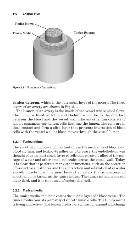
tunica externa, which is the outermost layer of the artery. The threelayers of an artery are shown in Fig. 5.1.
The lumen of an artery is the inside of the vessel where blood flows.The lumen is lined with the endothelium which forms the interfacebetween the blood and the vessel wall. The endothelium consists ofsimple squamous epithelium cells that line the lumen. The cells are inclose contact and form a slick layer that prevents interaction of bloodcells with the vessel wall as blood moves through the vessel lumen.
5.2.1 Tunica intima
The endothelium plays an important role in the mechanics of blood flow,blood clotting, and leukocyte adhesion. For years, the endothelium wasthought of as an inert single layer of cells that passively allowed the pas-sage of water and other small molecules across the vessel wall. Today,it is clear that it performs many other functions, such as the secretionof vasoactive substances and the contraction and relaxation of vascularsmooth muscle. The innermost layer of an artery that is composed ofendothelium is known as the tunica intima. The tunica intima is one celllayer thick and it is composed of endothelial cells.
5.2.2 Tunica media
The tunica media or middle coat is the middle layer of a blood vessel. Thetunica media consists primarily of smooth muscle cells. The tunica mediais living and active. The tunica media can contract or expand and change
142 Chapter Five
Figure 5.1 Structure of an artery.
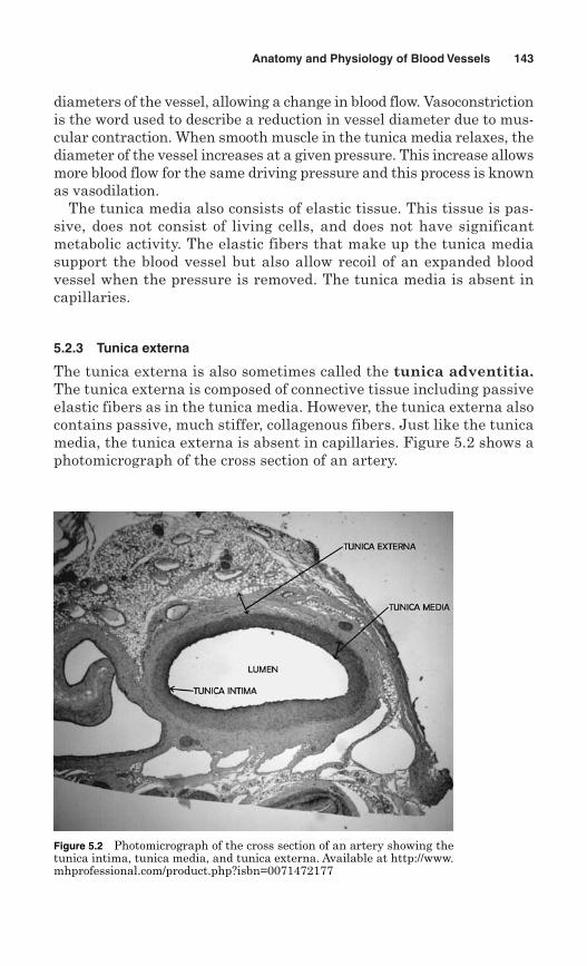
diameters of the vessel, allowing a change in blood flow. Vasoconstrictionis the word used to describe a reduction in vessel diameter due to mus-cular contraction. When smooth muscle in the tunica media relaxes, thediameter of the vessel increases at a given pressure. This increase allowsmore blood flow for the same driving pressure and this process is knownas vasodilation.
The tunica media also consists of elastic tissue. This tissue is pas-sive, does not consist of living cells, and does not have significantmetabolic activity. The elastic fibers that make up the tunica mediasupport the blood vessel but also allow recoil of an expanded bloodvessel when the pressure is removed. The tunica media is absent incapillaries.
5.2.3 Tunica externa
The tunica externa is also sometimes called the tunica adventitia.The tunica externa is composed of connective tissue including passiveelastic fibers as in the tunica media. However, the tunica externa alsocontains passive, much stiffer, collagenous fibers. Just like the tunicamedia, the tunica externa is absent in capillaries. Figure 5.2 shows aphotomicrograph of the cross section of an artery.
Anatomy and Physiology of Blood Vessels 143
Figure 5.2 Photomicrograph of the cross section of an artery showing thetunica intima, tunica media, and tunica externa. Available at http://www.mhprofessional.com/product.php?isbn=0071472177
5.3 Types of Arteries
Although arteries have the same general structure, they can be dividedinto groups by their specific functional characteristics. The three typesof arteries discussed in this chapter are elastic arteries, musculararteries, and arterioles.
5.3.1 Elastic arteries
Elastic arteries have the largest diameter of the three groups of arter-ies. The aorta is a good example of an elastic artery. One of the chief char-acteristics of elastic arteries is their ability to stretch and hold additionalvolume, thus performing the function of a “capacitance” vessel. Just asan electrical capacitor stores charge when given an increased voltage,an elastic vessel can store additional volume when subjected to anincreased pressure. Elastic arteries have very thick tunica medias whencompared with other arteries and contain a large amount of the elasticfiber elastin.
5.3.2 Muscular arteries
Muscular arteries are intermediate-sized arteries. In these vessels thetunica media is composed almost entirely of smooth muscle. The tunicamedia of a muscular artery can be as many as 40 cell layers thick.Functionally, muscular arteries can change diameter to influence flowthrough vasoconstriction and vasodilation. Most arteries are musculararteries.
5.3.3 Arterioles
Arterioles are defined as those arteries which have a diameter of lessthan 0.5 mm. Arterioles have a muscular tunica media which is one tofive layers thick. These layers are composed entirely of smooth musclecells. Arterioles also do not possess much of a tunica externa.
Approximately 70 percent of the pressure drop between the heartand the veins occurs in the small arteries and the arterioles. Very littlepressure drop occurs in the large arteries, and about 20 percent of thepressure drop occurs in the capillaries.
5.4 Mechanics of Arterial Walls
To understand the mechanics of arterial walls, begin by imagining a longtube of constant cross section and constant wall thickness. This imagi-nary tube is homogeneous and isotropic (the material properties areidentical in all directions). The typical blood vessel is branched and
144 Chapter Five
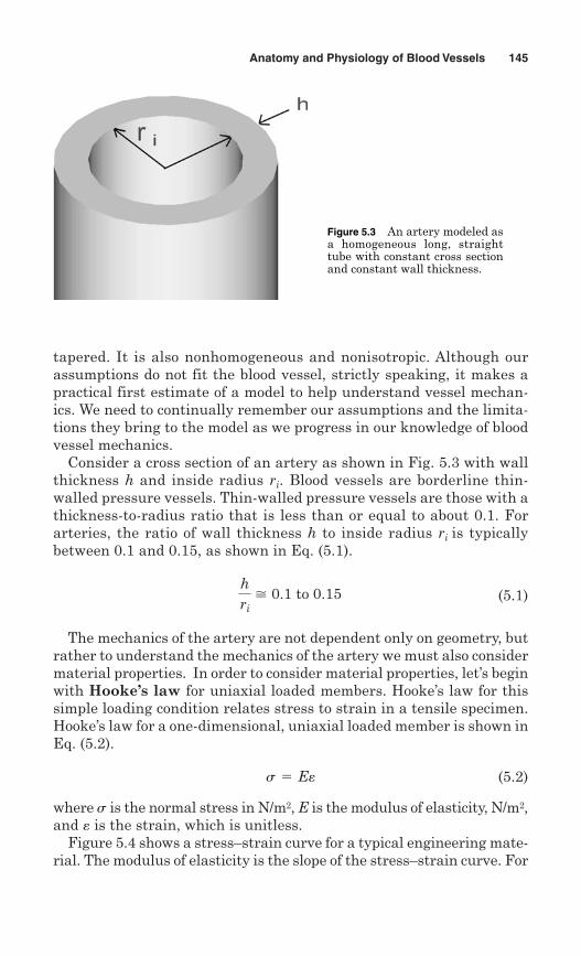
tapered. It is also nonhomogeneous and nonisotropic. Although ourassumptions do not fit the blood vessel, strictly speaking, it makes apractical first estimate of a model to help understand vessel mechan-ics. We need to continually remember our assumptions and the limita-tions they bring to the model as we progress in our knowledge of bloodvessel mechanics.
Consider a cross section of an artery as shown in Fig. 5.3 with wallthickness h and inside radius ri. Blood vessels are borderline thin-walled pressure vessels. Thin-walled pressure vessels are those with athickness-to-radius ratio that is less than or equal to about 0.1. Forarteries, the ratio of wall thickness h to inside radius ri is typicallybetween 0.1 and 0.15, as shown in Eq. (5.1).
(5.1)
The mechanics of the artery are not dependent only on geometry, butrather to understand the mechanics of the artery we must also considermaterial properties. In order to consider material properties, let’s beginwith Hooke’s law for uniaxial loaded members. Hooke’s law for thissimple loading condition relates stress to strain in a tensile specimen.Hooke’s law for a one-dimensional, uniaxial loaded member is shown inEq. (5.2).
(5.2)
where s is the normal stress in N/m2, E is the modulus of elasticity, N/m2,and � is the strain, which is unitless.
Figure 5.4 shows a stress–strain curve for a typical engineering mate-rial. The modulus of elasticity is the slope of the stress–strain curve. For
s 5 Ee
hri> 0.1 to 0.15
Anatomy and Physiology of Blood Vessels 145
Figure 5.3 An artery modeled asa homogeneous long, straighttube with constant cross sectionand constant wall thickness.
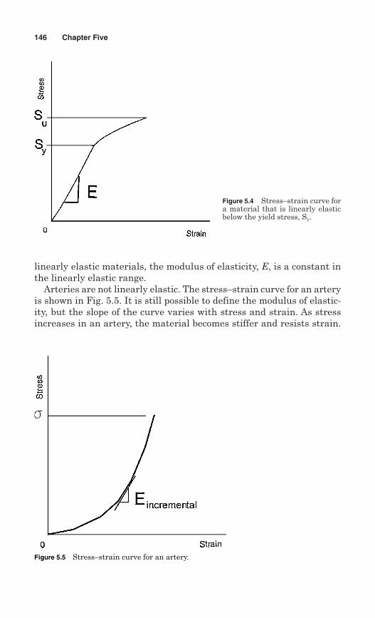
linearly elastic materials, the modulus of elasticity, E, is a constant inthe linearly elastic range.
Arteries are not linearly elastic. The stress–strain curve for an arteryis shown in Fig. 5.5. It is still possible to define the modulus of elastic-ity, but the slope of the curve varies with stress and strain. As stressincreases in an artery, the material becomes stiffer and resists strain.
146 Chapter Five
Figure 5.4 Stress–strain curve fora material that is linearly elasticbelow the yield stress, Sy.
Figure 5.5 Stress–strain curve for an artery.
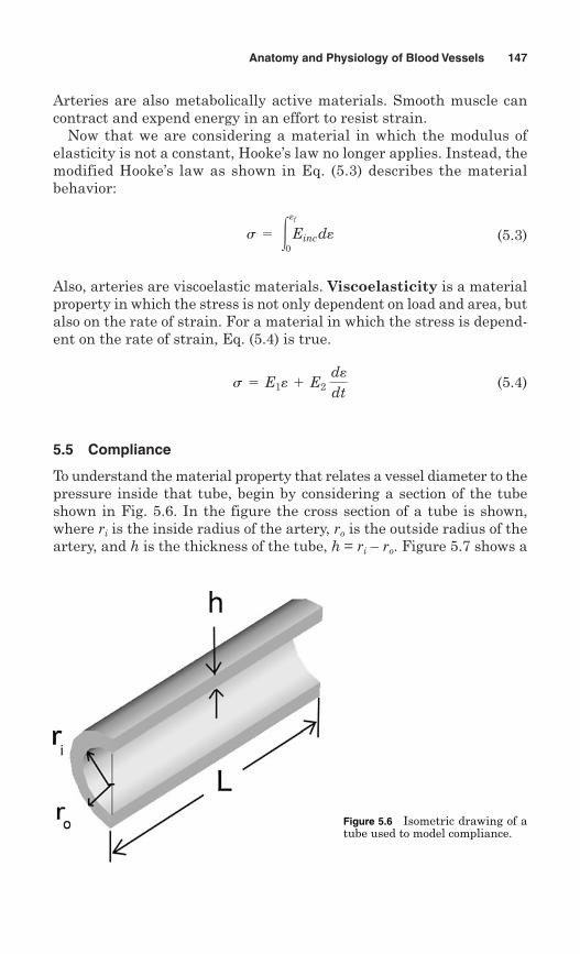
Arteries are also metabolically active materials. Smooth muscle cancontract and expend energy in an effort to resist strain.
Now that we are considering a material in which the modulus ofelasticity is not a constant, Hooke’s law no longer applies. Instead, themodified Hooke’s law as shown in Eq. (5.3) describes the materialbehavior:
(5.3)
Also, arteries are viscoelastic materials. Viscoelasticity is a materialproperty in which the stress is not only dependent on load and area, butalso on the rate of strain. For a material in which the stress is depend-ent on the rate of strain, Eq. (5.4) is true.
(5.4)
5.5 Compliance
To understand the material property that relates a vessel diameter to thepressure inside that tube, begin by considering a section of the tubeshown in Fig. 5.6. In the figure the cross section of a tube is shown,where ri is the inside radius of the artery, ro is the outside radius of theartery, and h is the thickness of the tube, h = ri – ro. Figure 5.7 shows a
s 5 E1e 1 E2 dedt
s 5 3ef
0Einc
de
Anatomy and Physiology of Blood Vessels 147
Figure 5.6 Isometric drawing of atube used to model compliance.
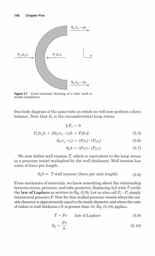
free-body diagram of the same tube on which we will now perform a forcebalance. Note that Sh is the circumferential hoop stress.
(5.5)
(5.6)
(5.7)
We now define wall tension T, which is equivalent to the hoop stressin a pressure vessel multiplied by the wall thickness. Wall tension hasunits of force per length.
(5.8)
From mechanics of materials, we know something about the relationshipbetween stress, pressure, and tube geometry. Replacing Shh with T yieldsthe law of Laplace as written in Eq. (5.9). Let us also call Pi – Po simplytransmural pressure P. Now for thin-walled pressure vessels where the out-side diameter is approximately equal to the inside diameter, and where the ratioof radius to wall thickness r/h is greater than 10, Eq. (5.10) applies.
T � Pr law of Laplace (5.9)
(5.10)Sh 5Prh
Shh ; T wall tension sforce per unit lengthd
Shh 5 sPirid2sPorod
Shsro2rid 5 sPirid2sPorod
Po2roL 1 2Shsro2ridL 5 Pi2riL
� Fx 5 0
148 Chapter Five
Sh (ro – ri)L
Sh (ro – ri)L
Pi 2ri LPo 2ro L x
Figure 5.7 Cross-sectional drawing of a tube used tomodel compliance.
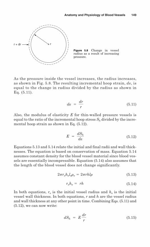
As the pressure inside the vessel increases, the radius increases,as shown in Fig. 5.8. The resulting incremental hoop strain, d�, isequal to the change in radius divided by the radius as shown inEq. (5.11).
(5.11)
Also, the modulus of elasticity E for thin-walled pressure vessels isequal to the ratio of the incremental hoop stress Sh divided by the incre-mental hoop strain as shown in Eq. (5.12).
(5.12)
Equations 5.13 and 5.14 relate the initial and final radii and wall thick-nesses. The equation is based on conservation of mass. Equation 5.14assumes constant density for the blood vessel material since blood ves-sels are essentially incompressible. Equation (5.14) also assumes thatthe length of the blood vessel does not change significantly.
(5.13)
(5.14)
In both equations, ro is the initial vessel radius and ho is the initialvessel wall thickness. In both equations, r and h are the vessel radiusand wall thickness at any other point in time. Combining Eqs. (5.11) and(5.12), we can now write:
(5.15)dSh 5 E drr
roho 5 rh
2proholoro 5 2prhlr
E 5 dSh
de
de 5 drr
Anatomy and Physiology of Blood Vessels 149
+ rr + dr
Figure 5.8 Change in vesselradius as a result of increasingpressure.
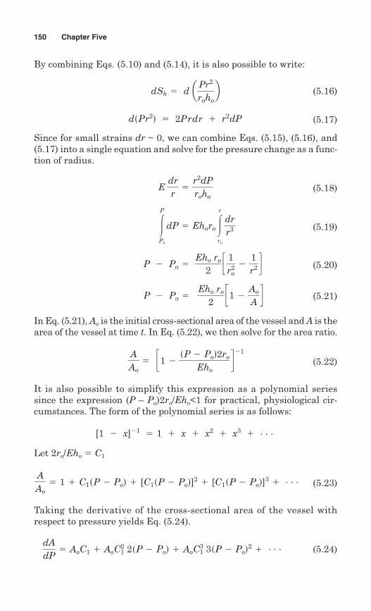
By combining Eqs. (5.10) and (5.14), it is also possible to write:
(5.16)
(5.17)
Since for small strains dr ~ 0, we can combine Eqs. (5.15), (5.16), and(5.17) into a single equation and solve for the pressure change as a func-tion of radius.
(5.18)
(5.19)
(5.20)
(5.21)
In Eq. (5.21), Ao is the initial cross-sectional area of the vessel and A is thearea of the vessel at time t. In Eq. (5.22), we then solve for the area ratio.
(5.22)
It is also possible to simplify this expression as a polynomial seriessince the expression (P – Po)2ro/Eho<1 for practical, physiological cir-cumstances. The form of the polynomial series is as follows:
Let 2ro/Eho � C1
(5.23)
Taking the derivative of the cross-sectional area of the vessel withrespect to pressure yields Eq. (5.24).
(5.24)dAdP
5 AoC1 1 AoC21 2sP 2 Pod 1 AoC
31 3sP 2 Pod2 1 . . .
AAo5 1 1 C1sP 2 Pod 1 [C1sP 2 Pod]2 1 [C1sP 2 Pod]3 1 . . .
[1 2 x]21 5 1 1 x 1 x2 1 x3 1 . . .
AAo5 c1 2 sP 2 Pod2ro
Ehod21
P 2 Po 5 Eho ro
2c1 2 Ao
Ad
P 2 Po 5 Eho ro
2c 1r2
o2
1r2 d
3P
Po
dP 5 Ehoro 3r
ro
drr3
E drr5
r2dProho
dsPr2d 5 2Prdr 1 r2dP
dSh 5 d aPr2
rohob
150 Chapter Five
Practically speaking, C12, C1
3, . . . are so small that we can now estimatethe compliance of the vessel by Eq. (5.25).
(5.25)
Finally, it is also possible to estimate modulus of elasticity if the complianceis known. In Eq. (5.26), the modulus of elasticity is derived from Eq. (5.25).
(5.26)E 52pro
3
Cho
C 5 dAdP
< AoC1 5 p ro3
Eho
Anatomy and Physiology of Blood Vessels 151
5.5.1 Compliance example
In Fig. 5.9 a tube with modulus of elasticity, E, is anchored between twostationary ports and injected with a known volume of water. For the pres-sure increase (Pf Po), fixed length Lo, tube diameter D, and volume ofinjected fluid V, calculate the compliance and estimate the modulus of elas-ticity. The wall thickness of the tube is 1 mm.
Initial pressure, Po � 10 kPaPressure increase, Pf Po � 6 kPaInitial tube diameter, D � 20 mmInitial length, Lo � 25 cmVolume injected, V � 10 mL
The change in cross-sectional area resulting from an injection of 10 mLinto the tube is the change in volume divided by the fixed tube length.
The compliance of the tube can then be calculated as the change in areadivided by the change in pressure.
Compliance 5dAdP
50.4 cm2
6000 Pa3
1 m2
s100d2 cm2 5 6.7 3 1029 m2
Pa
A 5VLo
510 cm3
25 cm5 0.4 cm2
Figure 5.9 Measuring compliance and estimating modulus of elasticity.
152 Chapter Five
Once the compliance has been determined, the incremental modulus ofelasticity for the tube can be estimated from the compliance.
0.94 MPa
5.5.2 Clinical feature—arterial complianceand hypertension
Physicians are interested in vascular stiffness because a number of stud-ies have shown that vascular stiffness is related to hypertension. It isthought, for example, that isolated systolic hypertension, one of the mostcommon types of hypertension among older persons, results from age-associated vascular stiffening and reduced compliance (Schiffrin, 2004).
It is possible to understand and quantify vascular compliance by nonin-vasive measurements and by analysis of pressure waveforms. From theMoens–Korteweg equation (Sec. 5.6), one can see that pulse wave velocityis directly related to the vessel’s modulus of elasticity and hence compliance.Evaluation of pulse wave velocities shows that arterial stiffness increaseswith advancing age. Arterial stiffness is significantly and independentlyassociated with increased risk for cardiovascular morbidity and mortality.
For example, Laurent et al. (2001) performed a study at BroussaisUniversity Hospital in Paris, France, from 1980 to 1996, in which theymeasured aortic stiffness of a large group of patients regularly over time.When patients entered the study, aortic stiffness was assessed from themeasurement of carotid-femoral pulse wave velocity.
Pulse wave velocity was measured along the descending aorta using thefoot-to-foot velocity method. Waveforms were obtained transcutaneouslyover the common carotid artery and the right femoral artery, and the timedelay t was measured between the feet of the two waveforms. The distanced covered by the waves was assimilated to the distance measured betweenthe two recording sites. Pulse wave velocity was calculated as the distancetraveled by the wave d divided by the transit time t.
The study showed an increased risk of mortality in patients with anincreased pulse wave velocity, hence an increased value of modulus of elas-ticity and increased compliance and that arterial stiffness may help in theevaluation of individual risk in patients with hypertension.
The independent predictability of aortic stiffness could be quantified inthe study population: the odds ratio for an increase in pulse wave velocityof 5 m/s above the patient’s pulse wave velocity at the time of entering thestudy was 1.51 for cardiovascular mortality. An odds ratio of 1 means thatthere is no increased risk. An odds ratio of 1.5 means that 1.5 patientswith the increase died for every 1 patient in the control group.
The authors wrote that the increased mortality risk because of a 5 m/sincrease in pulse wave velocity was equivalent to that of aging 10 years.
Modulus of elasticity5E52pro
3
Cho5
2ps0.01d3m3
6.731029 m2
Pa30.001 m
5
5.6 Pulse Wave Velocity and theMoens–Korteweg Equation
Some years before Otto Frank’s attack on the Windkessel problem, therelation between wave velocity and elasticity in a tube of fluid was estab-lished theoretically by Korteweg in 1878. Dutch mathematician DiederikKorteweg studied at the Polytechnical School at Delft. He attended theUniversity of Amsterdam, receiving a doctorate in 1878. He remained atAmsterdam and became professor there in 1881 until he retired in 1918.For larger arteries the Moens–Korteweg equation relates the mate-rial properties of the vessel wall to the speed of wave propagation. Thesimplified version of the equation ignores the modulus of fluid elasticitybecause it is four orders of magnitude greater than the modulus of elas-ticity of the vessel wall. The simplified Moens–Korteweg equationbecomes:
where c is the pulse wave velocity, E is the modulus of elasticity of thevessel wall material, h is the wall thickness of the vessel, ri is the insideradius of the vessel, and r is the density of the blood.
c > Å Eh2ri r
Anatomy and Physiology of Blood Vessels 153
5.6.1 Application box—fabrication of arterial models
Stevanov et al. (2000) reported that they fabricated elastomer arterialmodels with specific compliance. They made elastic tubes from a two-component silicon elastomer using a lathe for precise control of the wallthickness. The authors measured compliance from quasi-static area–pressurecurves and compared those measurements to values of predicted compliancebased on the Moens–Korteweg equation. The values of the compliance meas-urements agreed with the calculated values with an error of 5.5 percentor less.
5.6.2 Pressure–strain modulus
It is difficult to measure the thickness of arteries in vivo, so sometimesscientists also report the pressure–strain modulus. The pressurestrain modulus is defined by the ratio of pressure change to normalizeddiameter change resulting from that pressure change. Equations (5.27)
through (5.30) designate the pressure–strain modulus, Ep.
(5.27)
(5.28)
(5.29)
(5.30)
In 1972 in their paper titled, “Transcutaneous Measurement of the ElasticProperties of the Human Femoral Artery,” Mozersky et al. reported thepressure–strain modulus in humans and how it varies with age. Table 5.1shows how the stiffness of the blood vessels increases with age.
E 5ro
ho Ep
E 5 2ro2 aPmax 2 Pmin
dmax 2 dminb
E 52pro
32hopdm
aPmax 2 Pmin
dmax 2 dminb
Ep ;Pmax2Pmin
sdmax 2 dmind/dmean
154 Chapter Five
5.6.3 Example problem—modulusof elasticity
Laurent et al. (2001) performed a study at Broussais University Hospital inParis, France, from 1980 to 1996, in which they measured the aortic stiffnessof a large group of patients regularly over time. When patients entered thestudy, aortic stiffness was assessed from measurement of carotid-femoralpulse wave velocity.
In the study, the independent predictability of aortic stiffness could bequantified in the study population: the odds ratio for an increase in pulsewave velocity of 5 m/s above the patients’ pulse wave velocity at the timeof entering the study was 1.51 for cardiovascular mortality.
Problem Estimate the increase in modulus of elasticity of the aorta associ-ated with a 5 m/s increase in the pulse wave velocity. Take the diameter ofthe aorta to be 2.5 cm and the wall thickness to be 0.25 cm. Use a densityof blood of 1060 kg/m3.
Solution From the Moens–Korteweg equation:
c > Å Eh2rir
TABLE 5.1 Pressure–Strain Modulus of Arteriesin Humans
�35 years old 2.64 � 105 N/m2
35–60 years old 3.88 � 105 N/m2
�60 years old 6.28 � 105 N/m2
Anatomy and Physiology of Blood Vessels 155
5.7 Vascular Pathologies
5.7.1 Atherosclerosis
Atherosclerosis is a vascular pathology that has become a prominent dis-ease in Western society. The term comes from the Greek words athero(gruel or paste) and sclerosis (hardness), and the disorder is character-ized by progressive narrowing and occlusion of blood vessels. Whenfatty substances, cholesterol, cellular waste products, calcium, and fibrinbuild up in the inner lining of an artery, this causes a narrowing of thelumen of the vessel and also an increase in the wall stiffness or adecrease in compliance of the vessel. The buildup that results is calledplaque. Some level of stiffening of the arteries and narrowing is a normalresult of aging. Eventually, the plaque can block an artery and restrictflow through that vessel, resulting in a heart attack if the vessel beingblocked is one that supplies blood to the heart. Atherosclerosis can alsoproduce blood clot formation, sometimes resulting in a stroke. When apiece of plaque breaks away from the arterial wall and flows down-stream, it can also become lodged in smaller vessels and block flow, alsoresulting in stroke.
Atherosclerosis usually affects medium-sized or large arteries. Three riskfactors associated with atherosclerosis are elevated levels of cholesterol andtriglycerides in the blood, high blood pressure, and cigarette smoking.
5.7.2 Stenosis
Stenosis refers to an obstruction of flow through a vessel. When a local-ized plaque forms inside a vessel, this is called a stenosis. An aorticstenosis, for example, refers to an obstruction at the level of the aorticvalve. An aortic stenosis is typically seen as a restricted systolic open-ing of the valve with an increased pressure drop across the valve.Doppler echocardiography can be used to identify and quantify theseverity of a valvular stenosis.
where c is the pulse wave velocity, E is the modulus of elasticity of the vesselwall material, h is the wall thickness of the vessel, ri is the inside radiusof the vessel, and r is the density of the blood.
The predicted increase in modulus of elasticity becomes:
E > 2rirc
2
h5
2 2.5100
1060s5d2
0.25100
5 530,000 Nm2
5.7.3 Aneurysm
Aneurysm is the term that refers to the abnormal enlargement orbulging of an artery wall. This condition is the result of a weakness orthinning of the blood vessel wall. Aneurysms can occur in any type ofblood vessel, but they usually occur in arteries. Aneurysms commonlyoccur in the abdomen or the brain. These are known as abdominal aorticaneurysms (AAA) or cerebral aneurysms (CA).
An AAA is an enlargement of the lower part of the aorta. AAAs areknown as silent killers because in most cases, there are no symptomsassociated with the pathology. When an AAA ruptures, it will result inlife-threatening blood loss. Most AAAs are diagnosed during a physical examwhen the person is undergoing a checkup for some other health concern.
AAAs that are less than 2 in. in diameter are usually monitored andtreated with blood pressure–lowering drugs. AAAs that are greater than2 in. in diameter are typically surgically replaced with a flexible graftwhen they are discovered.
A CA is a weak, bulging spot in an artery of the brain. These oftenresult from a weakness in the tunica media (muscle layer) of the vesselthat is present from birth. A CA may cause symptoms ranging fromheadache, drowsiness, neck stiffness, nausea, and vomiting to moresevere symptoms such as mental confusion, vertigo (dizziness), and lossof consciousness. A ruptured aneurysm most often results in a severeheadache demanding immediate medical attention. A CA can be diag-nosed by imaging tests like x-rays, ultrasound, computed axial tomog-raphy (CAT), and magnetic resonance imaging (MRI). When detected,brain aneurysms can be treated by microsurgery.
156 Chapter Five
5.7.4 Clinical feature—endovascularaneurysm repair
AAAs are a serious health care issue in the United States with a mortalityrate from ruptures of 15,000 patients per year. One common therapy usedin conjunction with an AAA is the endovascular stent graft. The endovas-cular stent graft is a tube composed of fabric supported by a metal meshcalled a stent. A minimally invasive technique is used to place the vascularstent graft inside the bulging aneurysm and the stent graft forms the newwall on the aorta, suspended inside of the original aorta. In most cases thestent can be placed using a minimally invasive technique whereby the graftsare inserted through the femoral artery using fluoroscopic control. The graftis released at the appropriate location and expanded with a balloon. Thegraft is then embedded into the wall of the original aorta using wire barbs.
Some complications of this procedure include endoleaks, graft displace-ment, and graft migration. Type I leaks occur at the connection between thestent graft and the aorta, with proximal being designated IA and the distal
Anatomy and Physiology of Blood Vessels 157
connection being designated IB. Type II leaks occur at a branch of theaorta, outside of the stent graft. Type III leaks are those leaks in which astructural failure of the graft occurs, such as component separation, orthose resulting from material fatigue. This type failure can include stent-graft fractures and holes in the fabric of the device.
Some typical endovascular grafts that are or have recently become com-mercially available include the Medtronic Vascular–AneuRx, which as of2006 is one of the most commonly implanted. The Gore Exclude from W. L.Gore & Associates is an expanded polytetrafluoroethylene (PTFE) bifur-cated graft with an outer self-expanding Nitinol support wire. The ZenithAAA endovascular graft from Cook Vascular, Inc., has woven polyestergraft material over stainless steel stents.
The shape of the neck of an aneurysm is an important parameter when con-sidering who is a candidate for an endovascular graft. Hostile neck anatomyis one of the most common reasons that patients are denied endovascularaneurysm repairs (EVAR) (Cox et al., 2006).
Cox et al. report using prophylactic adjunctive proximal balloon-expand-able stents in patients with hostile neck anatomy or with type I endoleaks.The neck of an aortic aneurysm describes the point in the aorta at whichthe vessel begins to balloon. There is a proximal neck and a distal neck.“Adjunctive” describes a secondary therapy which is used in combinationwith a primary treatment to improve the success of the primary treatment.
Cox’s group treated 19 patients with balloon-expandable stents toimprove the neck anatomy of the aneurysm. Hostile neck anatomy includeda neck length of less than 15 mm and a neck diameter greater than 26 mm.Primary success was achieved in all 19 patients. Based on their experience,the authors recommended that EVAR may be offered to an expandedpatient population with hostile neck anatomy with use of prophylacticballoon-expandable stents.
5.7.5 Thrombosis
Thrombosis refers to the formation or development of an aggregation ofblood substances, including platelets, fibrin, and cellular elements. Simplyput, a thrombus is a blood clot. Thrombosis often results in vascularobstruction at the point of formation. For comparison, an embolism is ageneral clot or plug that could refer to a blood clot, or an air bubble, oreven a mass of cancer cells that is brought by flowing blood from onevessel into a smaller-diameter vessel, where it is eventually lodged.
5.8 Stents
A stent is a metal mesh tube that is inserted into an artery on a ballooncatheter and inflated to expand and hold open an artery, so that bloodcan flow more easily through the artery. The stent remains permanently
in place to hold the artery open. Drug-eluting stents are stents thatcontain drugs that are eluted into the bloodstream and help prevent thearteries from becoming reclogged.
Stents often become necessary when an artery has narrowed due toatherosclerosis. During this vascular disease, plaque builds up on theendothelium. When the vessel becomes 85 to 90 percent blocked, bloodflow becomes restricted and the patient may experience symptoms indi-cating a decrease in blood flow.
Typically, stents are inserted on a balloon catheter through the femoralartery or brachial artery and guided up to the narrowed section of asmaller artery. The balloon catheter allows the stent to be expanded intoplace, by the inflation of the balloon after the stent has reached the cor-rect location.
158 Chapter Five
5.8.1 Clinical feature—“Stent Wars”
At the time of the writing of this textbook in 2006, drug-eluting stentsare the subject of many legal disputes and discussion, which some havereferred to as “Stent Wars.” Because drug-eluting stents have been so suc-cessful in reducing the rate of coronary stent restenosis, marketing ana-lysts have predicted that drug-eluting stents will double the world marketfor stents to $5 billion annually.
In early 2006 there are two drug-eluting stents which have received Foodand Drug Administration (FDA) approval for sale in the United States:the Cordis Cypher™ sirolimus-eluting stent and the Boston-ScientificTaxus™ paclitaxel-eluting stent. The CYPHER received approval in April2003 and the TAXUS received approval in March 2004.
Sirolimus (rapamycin) is an immunosuppressant drug that is also usedto prevent organ rejection after organ transplantation. It is an antibioticthat was first discovered as a by-product of a bacterium found in a soilsample from Easter Island. Rapamycin was originally intended as an anti-fungal drug, but was abandoned when it was discovered that it had potentimmunosuppressive properties in mammals.
Paclitaxel (Taxol) is a drug that has been used in cancer treatment sinceits discovery in 1967. It was isolated from the bark of the Pacific yew tree,Taxus brevifolia. When it was first isolated, paclitaxel was noted for its anti-tumor activity in rodents.
One might ask, “which of the two drug-eluting stents is safer or moreeffective?” A February 2006 study was done to compare the two stents. Ithad already been necessary to demonstrate the safety and efficacy of bothstents for them to receive their initial FDA approval. However, prior to the2006 study, there had been no large studies done to evaluate which of thetwo worked best.
The study (Morice et al., 2006) was conducted in Europe, Latin America,and Asia. It involved 1386 patients at 90 hospitals. Each patient randomly
Anatomy and Physiology of Blood Vessels 159
received either the Cypher or the Taxus. Follow-up evaluations were per-formed after 8 and 12 months.
After a year of stent placement, the rate of adverse cardiac events wassimilarly low in both groups. The restenosis rates were 9.6 percent forpatients who received the Cypher stents and 11.1 percent for the patientswho received the Taxus stents. There was not a statistically significantdifference in major clinical events including myocardial infarction andtarget lesion revascularization, a repeat procedure to revascularize thestent location.
With these very good results in both cases, compared to much higherrestenosis rates in non-drug-eluting stents, one might think that life issmooth sailing for the two manufacturers. However, there have been diffi-culties along the way.
In October 2003, the FDA issued a Public Health Notification concerningthe Cypher stent. In the notice the FDA wrote:
Cordis Corporation issued a letter to inform healthcare professionals of a rarebut potential risk of thrombosis associated with the use of the CYPHERSirolimus-Eluting Coronary Stent. The letter provides clarification on the safeuse of the product in accordance with the scientific evidence that led to prod-uct approval.
The CYPHER stent was approved in April 2003 for patients undergoingangioplasty procedures. Since the product’s introduction it is estimatedthat over 50,000 patients have received a CYPHER stent. To date, FDA hasreceived 47 Medical Device Reports (MDRs) of stent thrombosis occurringat the time of implantation or within a few days of implantation.
In the case of Taxus, in July 2004 the FDA announced a recall of Taxusstent systems as a result of “characteristics in the design of these two lotsthat resulted in failure of the balloon to deflate and impeded removal of theballoon after stent placement.”
5.9 Coronary Artery Bypass Grafting
Coronary arteries are the blood vessels that deliver blood to heart muscletissue. When atherosclerotic plaque builds up on the wall of the coronaryarteries, the result is coronary artery disease. Plaque accumulations canbe accelerated by smoking, high blood pressure, elevated cholesterol,and diabetes. In some cases, patients with coronary artery disease canbe treated with a minimally invasive procedure called an angioplasty.During an angioplasty, a stent is placed inside the vessel to increase thelumen diameter and to hold the vessel open. When that procedure is notpossible, the patient may be a candidate for a coronary artery bypassgraft (CABG) surgery. CABG surgery is performed about 350,000 timeseach year in the United States. When a patient undergoes a bypass
graft, the surgeon makes an incision in the middle of the chest and sawsthrough the sternum. The heart is cooled with iced saline while a solu-tion is injected into the arteries to minimize damage.
Veins are typically harvested from the legs to be used as the bypassvessels. It is also possible to use chest arteries, like the internalmammary artery. During the surgery, the bypass vessels are sewedonto the coronary arteries beyond the narrowing or blockage. Theother end of the bypass vessel is then attached to the aorta to pro-vide a strong blood supply to the coronary circulation that is unim-peded by blockages.
The entire CABG procedure takes about 4 h to complete. Duringthose 4 h, the aorta is clamped for about 60 min and the blood supplyto the body is furnished by cardiopulmonary bypass for about 90 min.At the end of surgery, the sternum is wired together with stainlesssteel wire and the chest incision is sutured closed.
5.9.1 Arterial grafts
Currently, there are about 700,000 coronary and 70,000 peripheral arte-rial grafts each year in the United States. Autologous grafts are graftsthat are harvested from a patient and grafted to an artery of the samepatient. Typical autologous vessels include the greater saphenous veinand the internal mammary artery.
In 1912, Carrel won the Nobel Prize in Medicine for his work on thevascular suture and the transplantation of blood vessels. Then in 1948,Kunlin developed the heart bypass using autologous veins. In 1952,Arthur Voorhees at Columbia University postulated that diseasedarteries might be replaced by synthetic fabric. Voorhees and colleaguesdeveloped Vinyon-N cloth tubes to substitute for diseased arterial seg-ments. The concept was confirmed and soon synthetic vessels thatwere larger than 5 mm in diameter were used and often remainedpatent (unoccluded) for more than 10 years. However, for vessels lessthan 5 mm in diameter, the prosthetic vessels occlude rapidly uponimplantation.
The next advance in vascular grafts came in 1957 when DeBakeyand colleagues introduced polyethylene-terephthalate (PET), also knownas Dacron®. In 1959, W. S. Edwards introduced the polytetrafluoroeth-ylene (PTFE) graft, also known as Teflon®. Then, 10 years later, in 1969R. W. Gore invented the expanded polytetrafluoroethylene graft (ePTFE),also known as Gore-Tex®.
The search for a viable, small-diameter vascular graft that is lessthan 5 mm in diameter continues. By 1978, Herring had describedendothelial seeding of synthetic grafts, and by 1987 Cryolife, Inc., began
160 Chapter Five
recovering human greater saphenous veins and cryopreserving them foruse as vascular grafts. Grafts in which blood vessels come from ahuman donor and are matched by blood type between the donor andrecipient are known as allografts. In 1988 clinical trials of endothe-lial sodding on ePTFE grafts took place. Sodding is a high-densityendothelial seeding in which more than 0.2 million cells per squarecentimeter are seeded.
One exciting direction for the future of vascular grafts is the area oftissue engineered vessels. L’Heureux et al. (1998) used separately cul-tured smooth muscle cells and fibroblasts to construct a living bloodvessel. The smooth muscle was wrapped around a tube to produce thetunica media. A fibroblast sheet was wrapped around that constructto produce the tunica adventitia. After maturation, the tube wasremoved and endothelial cells were seeded onto the lumen. Viabilitywas demonstrated.
Review Problems
1. The following values of arterial compliance are reported in the literature:
Simon et al., 1982 2.2 � 10210 m4/N
Mergerman et al., 1986 0.05 to 0.20 percent diameter change/mmHg
Both studies reported values for 5-mm-diameter arteries. Compare thesevalues by converting to m2/Pa.
2. For the data in Prob. 4, assume a wall thickness of 0.25 mm and estimatethe incremental modulus of elasticity.
3. For the data in Prob. 4, assume a wall thickness of 0.25 mm and calculatea pressure–strain modulus for these arteries. Compare these results to Ep
as reported by Mozersky et al. (1972). (See Table 5.1)
4. Draw and label the three layers of a blood vessel. Describe the components.
5. The arterial compliance of a vessel is 3.0 � 1010 m2/Pa; the artery dia-meter is 5 mm; the wall thickness is 0.2 mm. Estimate the modulus ofelasticity.
6. The modulus of elasticity of a vessel is 2.0 MPa; the artery diameter is 5 mm;the wall thickness is 0.2 mm.
(a) Estimate the compliance.(b) For this vessel, what increase in pressure, in mmHg, would be required
to increase the vessel radius by 10 percent?
7. Describe the tunica media. Of what does it typically consist?
Anatomy and Physiology of Blood Vessels 161
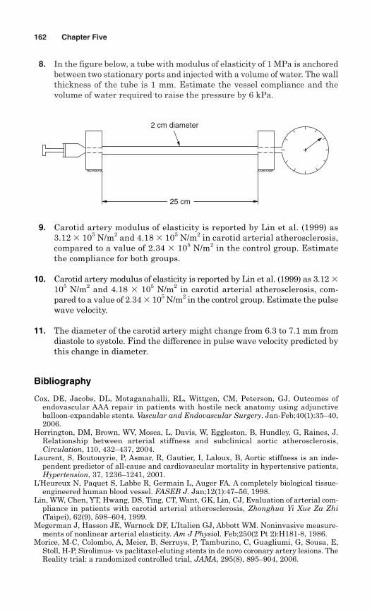
8. In the figure below, a tube with modulus of elasticity of 1 MPa is anchoredbetween two stationary ports and injected with a volume of water. The wallthickness of the tube is 1 mm. Estimate the vessel compliance and thevolume of water required to raise the pressure by 6 kPa.
162 Chapter Five
2 cm diameter
+
25 cm
9. Carotid artery modulus of elasticity is reported by Lin et al. (1999) as3.12 � 105 N/m2 and 4.18 � 105 N/m2 in carotid arterial atherosclerosis,compared to a value of 2.34 � 105 N/m2 in the control group. Estimatethe compliance for both groups.
10. Carotid artery modulus of elasticity is reported by Lin et al. (1999) as 3.12 �105 N/m2 and 4.18 � 105 N/m2 in carotid arterial atherosclerosis, com-pared to a value of 2.34 � 105 N/m2 in the control group. Estimate the pulsewave velocity.
11. The diameter of the carotid artery might change from 6.3 to 7.1 mm fromdiastole to systole. Find the difference in pulse wave velocity predicted bythis change in diameter.
Bibliography
Cox, DE, Jacobs, DL, Motaganahalli, RL, Wittgen, CM, Peterson, GJ, Outcomes ofendovascular AAA repair in patients with hostile neck anatomy using adjunctive balloon-expandable stents. Vascular and Endovascular Surgery. Jan-Feb;40(1):35–40,2006.
Herrington, DM, Brown, WV, Mosca, L, Davis, W, Eggleston, B, Hundley, G, Raines, J.Relationship between arterial stiffness and subclinical aortic atherosclerosis,Circulation, 110, 432–437, 2004.
Laurent, S, Boutouyrie, P, Asmar, R, Gautier, I, Laloux, B, Aortic stiffness is an inde-pendent predictor of all-cause and cardiovascular mortality in hypertensive patients,Hypertension, 37, 1236–1241, 2001.
L’Heureux N, Paquet S, Labbe R, Germain L, Auger FA. A completely biological tissue-engineered human blood vessel. FASEB J. Jan;12(1):47–56, 1998.
Lin, WW, Chen, YT, Hwang, DS, Ting, CT, Want, GK, Lin, CJ, Evaluation of arterial com-pliance in patients with carotid arterial atherosclerosis, Zhonghua Yi Xue Za Zhi(Taipei), 62(9), 598–604, 1999.
Megerman J, Hasson JE, Warnock DF, L’Italien GJ, Abbott WM. Noninvasive measure-ments of nonlinear arterial elasticity. Am J Physiol. Feb;250(2 Pt 2):H181-8, 1986.
Morice, M-C, Colombo, A, Meier, B, Serruys, P, Tamburino, C, Guagliumi, G, Sousa, E,Stoll, H-P, Sirolimus- vs paclitaxel-eluting stents in de novo coronary artery lesions. TheReality trial: a randomized controlled trial, JAMA, 295(8), 895–904, 2006.

Moses, JW, Leon, MB, Popma, JJ, et al., SIRIUS Investigators, Sirolimus-eluting stentsversus standard stents in patients with stenosis in a native coronary artery, N EnglJ Med, 349, 1315–1323, 2003.
Mozersky, DJ, Sumner, DS, Hokanson, DE, Strandness, DE, Transcutaneous measurementof the elastic properties of the human femoral artery, Circulation, 46, 948–955, 1972.
Schiffrin, E, Vascular stiffening and arterial compliance, implications for systolic bloodpressure, Am J Hypertens, 17, 39S–48S, 2004.
Selkurt, EE, Basic Physiology for the Health Sciences, Little, Brown and company, Boston,1982.
Simon AC, Levenson JA, Levy BY, Bouthier JE, Peronneau PP, Safar ME, Effect of nitro-glycerin on peripheral large arteries in hypertension, Br J Clin Pharmacol.Aug;14(2):241–6, 1982.
Stevanov, M, Baruthio, J, and Eclancher, B, Fabrication of elastomer arterial modelswith specified compliance. J Appl Physiol, Vol. 88, Issue 4, 1291–1294, April 2000.
Stoyioglou, A, Jaff, MR, Department of Cardiology, Lenox Hill Hospital, New York, NewYork, USA, Medical treatment of peripheral arterial disease: a comprehensive review,J Vasc Interv Radiol, 15(11), 1197–1207, 2004.
Voorhees, AB, Jr., Janetzky, A, III, Blakemore, AH, The use of tubes constructed fromvinyon ‘N’ cloth in bridging defects, Ann Surg, 135, 332, 1952.
Anatomy and Physiology of Blood Vessels 163

This page intentionally left blank
165
Chapter
6Mechanics of Heart Valves
6.1 Introduction
Four cardiac valves help to direct flow through the heart. Heart valvescause blood to flow only in the desired direction. If a heart without heartvalves were to contract, it would simply squeeze the blood, causing it toflow both backward and forward (upstream and downstream). Instead,under normal physiological conditions, heart valves act as check valvesto prevent blood from flowing in the reverse direction. Also, heart valvesremain closed until the pressure behind the valve is large enough tocause blood to move forward.
Each human heart has two atrioventricular valves, which arelocated between the atria and the ventricles. The tricuspid valve is thevalve between the right atrium and the right ventricle. The mitralvalve is the valve between the left atrium and the left ventricle. Themitral valve prevents blood from flowing backward into the pulmonaryveins and therefore into the lungs, even when the pressure in the leftventricle is very high. The mitral valve is a bicuspid valve having twocusps and the tricuspid valve has three cusps.
The two semilunar valves are the aortic valve and the pulmonicvalve. The aortic valve is located between the aorta and the left ven-tricle and when it closes it prevents blood from flowing backward fromthe aorta into the left ventricle. An aortic valve is shown in Fig. 6.1. Thepulmonic valve is located between the right ventricle and the pulmonaryartery, and when it closes it prevents blood from flowing backward,from the pulmonary artery into the right ventricle.
6.2 Aortic and Pulmonic Valves
The aortic and pulmonic valves consist of three semilunar cusps thatare embedded within connective tissue. The cusps are attached to a
Copyright © 2007 by The McGraw-Hill Companies, Inc. Click here for terms of use.
fibrous ring that is embedded in the ventricular septum. The leaflets ofthe three cusps are lined with endothelial cells and have a dense col-lagenous core that is adjacent to the aortic side of the leaflets.
A leaflet of an aortic valve is shown in Fig. 6.2. Note the different shapeof the leaflets of the mitral valve as shown in Fig. 6.3. The side of the valveleaflet that is adjacent to the aorta is a fibrous layer within the leaflet, andis called the fibrosa. The side of the leaflet that is adjacent to the ven-tricle is composed of collagen and elastin and is called the ventricularis.The ventricularis is thinner than the fibrosa and presents a very smoothand slippery surface to blood flow through the valve. The central portionof the valve, known as the spongiosa, contains connective tissue and pro-teins and is normally not vascularized. The corpus arantii (or nodulusof Arantus) is a large collagenous mass in the coaptation region which isthought to aid in valve closure and reduce regurgitation. Coapt literallymeans to approximate, as at the edge of a wound. Acoaption surface is onethat is formed by two overlapping surfaces that approximate one another.
166 Chapter Six
Figure 6.1 Aortic valve. (Reprinted with permission from LingappaVR, Farey K. Physiological Medicine, McGraw-Hill, New York, 2000.
Figure 6.2 Sketch of an aortic valve leaflet.
Fibrosa only
Corpus aranti CommissureFree edge
Connected to aorta
Flow direction
Ventricularis
Collagen fibers in the fibrosa and ventricularis are unorganized in theunstressed or unloaded condition. When the valve is loaded, however,the fibers become oriented in a circumferential direction. A fibrous annu-lar ring separates the aorta from the left ventricle.
Three bulges exist at the root of the aorta, immediately superior tothe annular ring of the aortic valve. Those three bulges are known as thesinus of valsalva or the aortic sinus. Two of the sinuses give rise tothe coronary arteries that branch off the aorta. The right coronary arterycomes from the right anterior sinus. The left coronary artery arisesfrom the left posterior sinus. The third sinus is known as the non coro-nary sinus or the right posterior sinus.
When the aortic or the pulmonic valve is closed there is a small over-lap of tissue from each leaflet that protrudes from the valve and formsa surface within the aorta. This overlapping surface is once again knownas a coaption surface. This overlapping tissue or coaption surface in theaortic or pulmonic valve is known as the lunula. The lunula is impor-tant in ensuring that the valve seals to prevent leakage.
The anatomy of the pulmonic valve is similar to that of the aortic valve.The chief difference is that the sinuses are smaller and the annulus islarger in the pulmonic valve. The anatomical dimensions of pulmonicand aortic valves are reported by Yoganathan et al. in the BiomedicalEngineering Handbook. The authors reference a study by Westaby et al.in 1984 in which 160 pathologic specimens from cadavers were examined.The mean aortic valve diameter was reported as 23.2 � 3.3 mm and themean pulmonic valve diameter was reported as 24.3 � 3.0 mm. Anotherstudy that was referenced in the same resource was carried out byGramiak and Shah in 1970 and used M-mode echocardiography to meas-ure the aortic root diameter. The aortic root diameter at end systole was
Mechanics of Heart Valves 167
Posteromedialpapillarymuscle
Anterolateralpapillarymuscle
Chordaetendineae
Mural leaflet
Anterolateral commisure
Aortic leaflet
Posteromedialcommisure
Figure 6.3 Medial view of the dissected mitral valve, cut through the antero-lateral commissure.
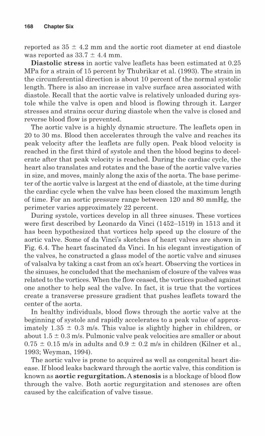
reported as 35 � 4.2 mm and the aortic root diameter at end diastolewas reported as 33.7 � 4.4 mm.
Diastolic stress in aortic valve leaflets has been estimated at 0.25MPa for a strain of 15 percent by Thubrikar et al. (1993). The strain inthe circumferential direction is about 10 percent of the normal systoliclength. There is also an increase in valve surface area associated withdiastole. Recall that the aortic valve is relatively unloaded during sys-tole while the valve is open and blood is flowing through it. Largerstresses and strains occur during diastole when the valve is closed andreverse blood flow is prevented.
The aortic valve is a highly dynamic structure. The leaflets open in20 to 30 ms. Blood then accelerates through the valve and reaches itspeak velocity after the leaflets are fully open. Peak blood velocity isreached in the first third of systole and then the blood begins to decel-erate after that peak velocity is reached. During the cardiac cycle, theheart also translates and rotates and the base of the aortic valve variesin size, and moves, mainly along the axis of the aorta. The base perime-ter of the aortic valve is largest at the end of diastole, at the time duringthe cardiac cycle when the valve has been closed the maximum lengthof time. For an aortic pressure range between 120 and 80 mmHg, theperimeter varies approximately 22 percent.
During systole, vortices develop in all three sinuses. These vorticeswere first described by Leonardo da Vinci (1452–1519) in 1513 and ithas been hypothesized that vortices help speed up the closure of theaortic valve. Some of da Vinci’s sketches of heart valves are shown inFig. 6.4. The heart fascinated da Vinci. In his elegant investigation ofthe valves, he constructed a glass model of the aortic valve and sinusesof valsalva by taking a cast from an ox’s heart. Observing the vortices inthe sinuses, he concluded that the mechanism of closure of the valves wasrelated to the vortices. When the flow ceased, the vortices pushed againstone another to help seal the valve. In fact, it is true that the vorticescreate a transverse pressure gradient that pushes leaflets toward thecenter of the aorta.
In healthy individuals, blood flows through the aortic valve at thebeginning of systole and rapidly accelerates to a peak value of approx-imately 1.35 � 0.3 m/s. This value is slightly higher in children, orabout 1.5 � 0.3 m/s. Pulmonic valve peak velocities are smaller or about0.75 � 0.15 m/s in adults and 0.9 � 0.2 m/s in children (Kilner et al.,1993; Weyman, 1994).
The aortic valve is prone to acquired as well as congenital heart dis-ease. If blood leaks backward through the aortic valve, this condition isknown as aortic regurgitation. A stenosis is a blockage of blood flowthrough the valve. Both aortic regurgitation and stenoses are oftencaused by the calcification of valve tissue.
168 Chapter Six
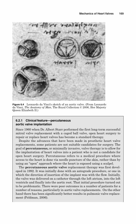
Mechanics of Heart Valves 169
Figure 6.4 Leonardo da Vinci’s sketch of an aortic valve. (From Leonardoda Vinci, The Anatomy of Man, The Royal Collection © 2006, Her MajestyQueen Elizabeth II.)
6.2.1 Clinical feature—percutaneousaortic valve implantation
Since 1960 when Dr. Albert Starr performed the first long-term successfulmitral valve replacement with a caged ball valve, open heart surgery torepair or replace heart valves has become a standard therapy.
Despite the advances that have been made in prosthetic heart valvereplacements, some patients are not suitable candidates for surgery. Thegoal of percutaneous, or minimally invasive, valve therapy is to allow forthe implantation of heart valves into a patient who is not a candidate foropen heart surgery. Percutaneous refers to a medical procedure whereaccess to the heart is done via needle puncture of the skin, rather than byusing an “open” approach where the heart is exposed using a scalpel.
The percutaneous aortic valve replacement therapy was first devel-oped in 1992. It was initially done with an antegrade procedure, or one inwhich the direction of insertion of the implant was with the flow. Initially,the valve was delivered on a catheter through the left atrium, into the leftventricle and finally into the aortic root. That initial procedure turned outto be problematic. There were poor outcomes in a number of patients for anumber of reasons, particularly in aortic valve replacements. On the otherhand there has been significantly better results in pulmonic valve replace-ment (Feldman, 2006).
170 Chapter Six
At this writing in 2006, the most modern approach to percutaneous aorticvalve implantation is a retrograde, or “against the flow” procedure. Webb’sgroup (Webb et al., 2006) describes a new retrograde procedure in whichthe prosthesis is inserted into the aorta via the femoral artery.
The prosthesis described is a Cribier-Edwards Percutaneous Valvefrom Edwards Lifesciences, Inc. The prosthesis is shown in Fig. 6.5. It ismade from a stainless steel stent with an attached trileaflet equine peri-cardial valve, attached to a fabric cuff. The valve is inserted through thefemoral artery to the aorta on a 22F (7.3 mm) or 24F (8 mm) catheter. Thecatheter is steerable and deflectable allowing manipulation of the prosthe-sis through the native aortic valve. To reduce cardiac output during deploy-ment of the valve, rapid ventricular pacing was used.
Webb et al. describe the deployment of the percutaneous aortic valveprosthesis in 18 patients with an age of 75 to 87 years for whom surgerywas not an option. The implantation was reported to be successful in 14patients. The aortic valve area increased from an average of 0.6 cm2 beforethe procedure to 1.6 cm2 after the procedure. The authors concluded, “Thisinitial experience suggests that percutaneous transarterial aortic valveimplantation is feasible in selected high-risk patients with satisfactoryshort-term outcomes” (Webb et al., 2006).
Figure 6.5 Cribier-Edwards Percutaneous Valve. (From EdwardsLifesciences, Inc. AHA Circulation, Lippincott, Williams & Wilkins.)
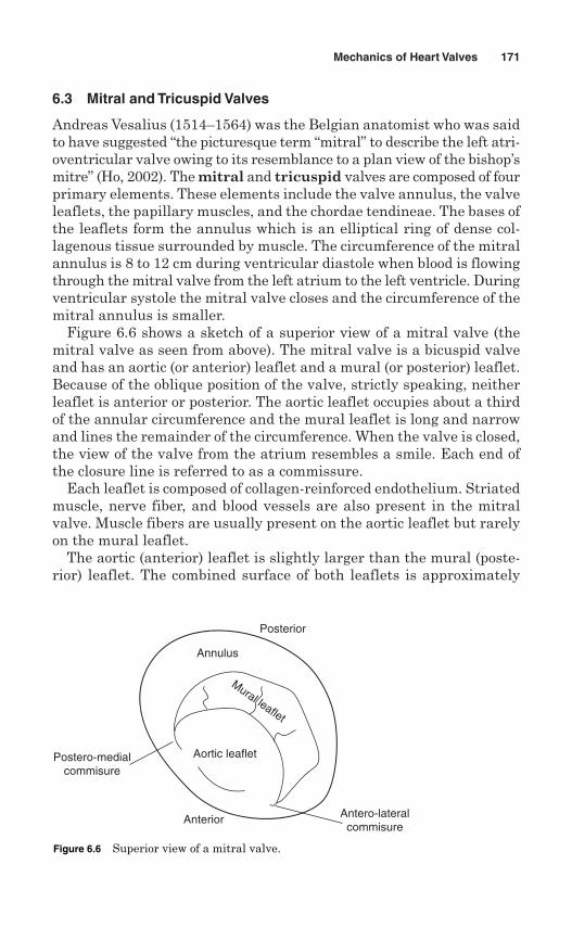
6.3 Mitral and Tricuspid Valves
Andreas Vesalius (1514–1564) was the Belgian anatomist who was saidto have suggested “the picturesque term “mitral” to describe the left atri-oventricular valve owing to its resemblance to a plan view of the bishop’smitre” (Ho, 2002). The mitral and tricuspid valves are composed of fourprimary elements. These elements include the valve annulus, the valveleaflets, the papillary muscles, and the chordae tendineae. The bases ofthe leaflets form the annulus which is an elliptical ring of dense col-lagenous tissue surrounded by muscle. The circumference of the mitralannulus is 8 to 12 cm during ventricular diastole when blood is flowingthrough the mitral valve from the left atrium to the left ventricle. Duringventricular systole the mitral valve closes and the circumference of themitral annulus is smaller.
Figure 6.6 shows a sketch of a superior view of a mitral valve (themitral valve as seen from above). The mitral valve is a bicuspid valveand has an aortic (or anterior) leaflet and a mural (or posterior) leaflet.Because of the oblique position of the valve, strictly speaking, neitherleaflet is anterior or posterior. The aortic leaflet occupies about a thirdof the annular circumference and the mural leaflet is long and narrowand lines the remainder of the circumference. When the valve is closed,the view of the valve from the atrium resembles a smile. Each end ofthe closure line is referred to as a commissure.
Each leaflet is composed of collagen-reinforced endothelium. Striatedmuscle, nerve fiber, and blood vessels are also present in the mitralvalve. Muscle fibers are usually present on the aortic leaflet but rarelyon the mural leaflet.
The aortic (anterior) leaflet is slightly larger than the mural (poste-rior) leaflet. The combined surface of both leaflets is approximately
Mechanics of Heart Valves 171
Annulus
Posterior
Antero-lateralcommisure
Postero-medialcommisure
Anterior
Mural leaflet
Aortic leaflet
Figure 6.6 Superior view of a mitral valve.
twice the area of the mitral orifice, allowing for a large area of coapta-tion permitting effective valve sealing.
The mitral valve is shown in a medial view in Fig. 6.3. The valve hasbeen dissected through the anterolateral commissure and laid open. Inthis view it can be seen that the anterior and posterior leaflets are notseparate entities, but rather one continuous piece of tissue.
The chordae tendineae for both leaflets attach to the papillarymuscle. Chordae tendineae consist of an inner core of collagen sur-rounded by loosely meshed elastin and collagen fibers with an outerlayer of endothelial cells. There is an average of about 12 primarychordae tendineae attached to each papillary muscle. The anterolat-eral and the posteromedial papillary muscle attach to the ventricularwall and tether the mitral valve into place. The chordae tendineae pre-vent the mitral valve from inverting through the annular ring and intothe atrium. That is, in normal physiologic situations they preventmitral valve prolapse. Improper tethering results in prolapse and mitralregurgitation.
Stresses in mitral valve leaflets of up to 0.22 MPa have been estimatedwhen the left ventricular pressure reaches up to 150 mmHg during ven-tricular systole. Mitral velocity flow curves show a peak in the curveduring early filling. This is known as an E wave. Peak velocities aretypically 50 to 80 cm/s at the mitral annulus. A second velocity peakoccurs during atrial systole and is known as an A wave.
In healthy individuals, velocities in the A waves are lower than thevelocities during the E wave. Diastolic filling of the ventricle shows apeak in flow during diastolic filling followed by a second peak duringatrial systole.
6.4 Pressure Gradients across a StenoticHeart Valve
To assess the seriousness of a heart valve stenosis, it would be helpfulto know the area of the stenosed valve when open, or how much of thevalve opening is being blocked by the stenosis. Gorlin and Gorlin (1951)developed an equation to empirically predict valve area based on thepressure drop across the valve and the flow rate through the valve. Thepublished equations that were useful for the prediction of area in mitraland aortic valves are still used in cardiology today.
Harris and Robiolio (1999) write, “Although the ‘gold standard’ forassessment of the severity of mitral stenosis has long been the Gorlinformula derived from data obtained from cardiac catheterization,advances in echocardiography have largely supplanted this procedure.Nonetheless, cardiac catheterization remains a mainstay in the man-agement of mitral stenosis.”
172 Chapter Six
6.4.1 The Gorlin equation
We will begin by writing the Gorlin equation in terms of variables thatare consistent with the other fluid mechanics notations in this text-book. The volume of flow passing through the aortic valve per beat Q isthe cardiac output CO divided by the heart rate HR.
(6.1)
The average flow rate through the aortic valve is the same amountdivided by the ejection time per beat, TE.
(6.2)
Next, remember that the mean velocity of the flow V (average flow veloc-ity across the flow cross section, through the valve) multiplied by thecross-sectional area AV is equal to the flow rate.
(6.3)
The Bernoulli equation is an equation based on the principle of conser-vation of energy, in the absence of viscous losses. In fact, there will be sig-nificant viscous losses through the heart valve, but the Gorlin equation isan empirical equation intended to account for those losses with an empir-ically derived valve coefficient. The Bernoulli equation is as follows:
(6.4)
If point 1 referred to in the equation is a reservoir with a very smallvelocity compared to the jet through the valve, the equation could berewritten:
(6.5)
or, in terms of the volume flow rate:
(6.6)
The above equation relates flow rate, pressure drop, and valve area in theideal case, but in the case of a real valve, two nonideal characteristics have
Q 5 AV Å2Pr
V2 5 Å2Pr
P1 112
r V 21 5 P2 1
12
r V 22
Q 5 V AV
Q 5 flow rate per beat 5CO
sHRdsTEd
Flow rate per beat 5COHR
Mechanics of Heart Valves 173
to be considered. Real blood flow is viscous flow and therefore Eq. (6.5) usesa valve constant, CV, to represent the actual velocity through the valve.
(6.7)
In the second nonideal condition, a jet of blood flowing through the valvewill contract to a smaller area than the total cross-sectional valve area.The area of contraction A depends on the valve design and can be des-ignated here using the valve coefficient CC.
(6.8)
Combining Eqs. (6.3), (6.7), and (6.8), the Gorlin equation becomes:
(6.9)
The coefficients are measured for various orifices and it should be care-fully noted that both the valve coefficient and the contraction coefficientare empirically derived coefficients which may not be constant under vary-ing pressure and flow conditions as well as varying Reynolds numbers.
In fact, this equation or a modified form of the equation is often usedclinically to estimate the effective area of a stenotic heart valve. To fur-ther simply its use clinically, the equation is often written in the fol-lowing form:
(6.10)
where AV is the area of the stenotic valve, CO is the cardiac output incc/min, TE is the ejection time or the time per beat during which bloodflows through the valve. HR is the heart rate in beats per minute, Pis the mean pressure gradient over the ejection period in mmHg, and Kis the Gorlin constant.
The Gorlin constant is proportional to CC, CV, and and containsall the conversion factors necessary to account for a mathematicallyconsistent set of units. The flow rate is equal to:
(6.11)
If the cardiac output is given in cubic centimeters per minute, the ejectionperiod in seconds per beat, and the heart rate in beats per minute, then
Q 5CO
TE HR
1/2r
AV 5 COsTE HR K 2Pd
Q 5 CC CV AV Å2Pr
A 5 CC AV
V2 5 CV Å2Pr
174 Chapter Six
Mechanics of Heart Valves 175
Eq. (6.11) yields a flow rate in cubic centimeters per second. It is impor-tant once again to note that the Gorlin equation is a useful concept, butthat the Gorlin “constant” is not a constant but depends on the flow rate.
Therefore, the Gorlin value of the Gorlin constant K is sometimesgiven as 44.3 in aortic valves and 37.7 in mitral valves. The units asso-ciated with the Gorlin constant are as follows:
cms2mmHg
6.4.2 Example problem—Gorlin equation
A patient has a cardiac output of 5 L/min. The systolic ejection period is358 ms with a heart rate of 70 beats per minute. The mean aortic gradientas measured by echocardiography is 81 mmHg. Find the aortic valve areaas estimated by the Gorlin equation. What is the average flow rate acrossthe aortic valve during ejection?
Answer
where AV � aortic valve area, cm2
CO � cardiac output, mL/minTE � time of ejection per beat, s
HR � heart rate, beats/min
mean pressure gradient � left ventricular pressure aortic pressure,mmHg
The average flow rate across the valve is 5000 mL/25 s � 200 mL/s.
AV 55,000
s0.358d s70d s44.3d 2815 0.50 cm2
AV 5 CO
TE HR s44.3d2P
6.4.3 Energy loss across a stenotic valve
Energy loss across a stenotic valve is influenced by more than theeffective valve area predicted by the Gorlin equation. Garcia et al. (2000)suggest an approach that uses an energy method to more accurately esti-mate the severity of an aortic stenosis. The authors suggest an indexthat they refer to as the energy loss index. Although it is a measureof energy loss, the energy loss index yields a value with pressure units.
The Gorlin equation uses transvalvular pressure gradients topredict effective orifice areas. These parameters are commonly used
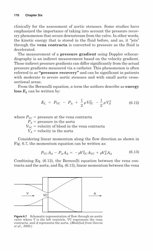
176 Chapter Six
clinically for the assessment of aortic stenoses. Some studies haveemphasized the importance of taking into account the pressure recov-ery phenomenon that occurs downstream from the valve. In other words,the kinetic energy that is stored in the fluid before, and as, it “jets”through the vena contracta is converted to pressure as the fluid isdecelerated.
The measurement of a pressure gradient using Doppler echocar-diography is an indirect measurement based on the velocity gradient.Those indirect pressure gradients can differ significantly from the actualpressure gradients measured via a catheter. This phenomenon is oftenreferred to as “pressure recovery” and can be significant in patientswith moderate to severe aortic stenoses and with small aortic cross-sectional areas.
From the Bernoulli equation, a term the authors describe as energyloss EL can be written by:
(6.12)
where PVC � pressure at the vena contractaPA � pressure in the aorta
VVC � velocity of blood in the vena contractaVA � velocity in the aorta
Considering linear momentum along the flow direction as shown inFig. 6.7, the momentum equation can be written as:
(6.13)
Combining Eq. (6.12), the Bernoulli equation between the vena con-tracta and the aorta, and Eq. (6.13), linear momentum between the vena
PVC AA 2 PA AA 5 2rV 2VC AVC 1 rV
2A AA
EL 5 PVC 2 PA 1 12
rV 2VC 2 1
2 rV 2
A
Figure 6.7 Schematic representation of flow through an aorticvalve where V is the left ventricle, VC represents the venacontracta, and A represents the aorta. (Modified from Garciaet al., 2000.)
VCV A
contracta and the aorta, to eliminate pressures in the equation yields:
(6.14)
The continuity equation yields:
and alternatively (6.15)
Because measuring the area at the vena contracta is problematic, andbecause it will be convenient to use VV AV multiplied together as car-diac output, the energy loss equation can be rewritten as:
(6.16)
Now the energy loss can be calculated in terms of variables that arereadily measurable through transthoracic echocardiography, as shownin Eq. (6.17).
(6.17)
where r � densityVVC � blood velocity at the vena contractaCO � cardiac outputAA � cross-sectional area of the aortaEL � energy loss expressed in units of pressure
The unitless energy loss coefficient associated with this energy lossis defined by the term:
(6.18)
An energy loss index that is less that 0.5 cm2/m2 should probably be con-sidered a critical value. A value less than 0.5 indicates a serious stenosis.
Recall that the effective orifice area EOA is the area at the venacontracta which is derived from the continuity equation, and is shownin Eq. (6.19).
(6.19)EOA 5 VVAV
VVC
Energy loss coefficient 5 sEOAdsAAdsAA 2 EOAd
EL 5r
2 aVVC 2
COAAb2
EL 5r
2 aVVC 2 VV AV
AAb2
V 2A 5
V 2VC A2
VC
A2A
AVC 5AV VV
VVC
EL 5 2 ar V 2VC AVC
AAb 1 ar
2 V 2
Ab 1 ar2 V 2VCb
Mechanics of Heart Valves 177
6.5 Prosthetic Mechanical Valves
Early mechanical prosthetic heart valves were ball valves. In 1952,Dr. Charles Hufnagel implanted the first ball and cage valve intoa patient with aortic valve insufficiency. Although the design of
178 Chapter Six
6.4.4 Example problem—energy lossmethod
The same patient from the previous example problem using the Gorlinequation has a cardiac output of 5 L/min. Aortic area � 4.9 cm2. Density �1060 kg/m3. Velocity at the vena contracta � 1.66 m/s. The mean aortic gra-dient as measured by echocardiography is 81 mmHg.
Find the “energy loss” in mmHg and the energy loss coefficient.
From Eq. (6.19) the effective orifice area is
Finally, from Eq. (6.18) the energy loss coefficient is:
6.4.5 Clinical features
(Lingappa and Farey, 2000)Chordae tendineae rupture and papillary muscle paralysis can
be consequences of a heart attack. This can lead to bulging of the valve,excessive backward leakage into the atria (regurgitation), and evenvalve prolapse. Valve prolapse is the condition under which the valveinverts backward into the atrium. Because of these valve problems, theventricle does not fill efficiently. Significant further damage, and evendeath, can occur within the first 24 hours after a heart attack becauseof this problem.
Energy loss coefficient 5 sEOAdsAAdsAA 2 EOAd
5 s0.5ds4.9ds4.9 2 0.5d
5 0.46
EOA 5 VVAV
VVC5 CO
VVC5 5000/60 cm3
s1.66/100 cm/s
5 0.50 cm2
3mmHg
133.3 Nm2
5 EL 5 13 mmHg
EL 5r
2 aVVC 2
COAAb2
51060 kgm3
N s2
kg m°1.66
ms 2
5000/60 cm3
sAA cm2 m
100 cm¢2
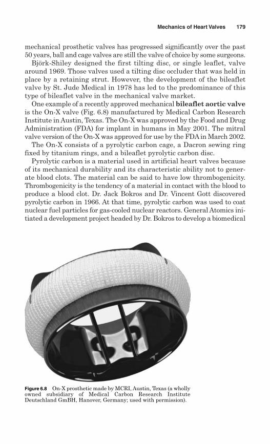
mechanical prosthetic valves has progressed significantly over the past50 years, ball and cage valves are still the valve of choice by some surgeons.
Björk-Shiley designed the first tilting disc, or single leaflet, valvearound 1969. Those valves used a tilting disc occluder that was held inplace by a retaining strut. However, the development of the bileafletvalve by St. Jude Medical in 1978 has led to the predominance of thistype of bileaflet valve in the mechanical valve market.
One example of a recently approved mechanical bileaflet aortic valveis the On-X valve (Fig. 6.8) manufactured by Medical Carbon ResearchInstitute in Austin, Texas. The On-X was approved by the Food and DrugAdministration (FDA) for implant in humans in May 2001. The mitralvalve version of the On-X was approved for use by the FDAin March 2002.
The On-X consists of a pyrolytic carbon cage, a Dacron sewing ringfixed by titanium rings, and a bileaflet pyrolytic carbon disc.
Pyrolytic carbon is a material used in artificial heart valves becauseof its mechanical durability and its characteristic ability not to gener-ate blood clots. The material can be said to have low thrombogenicity.Thrombogenicity is the tendency of a material in contact with the blood toproduce a blood clot. Dr. Jack Bokros and Dr. Vincent Gott discoveredpyrolytic carbon in 1966. At that time, pyrolytic carbon was used to coatnuclear fuel particles for gas-cooled nuclear reactors. General Atomics ini-tiated a development project headed by Dr. Bokros to develop a biomedical
Mechanics of Heart Valves 179
Figure 6.8 On-X prosthetic made by MCRI, Austin, Texas (a whollyowned subsidiary of Medical Carbon Research InstituteDeutschland GmBH, Hanover, Germany; used with permission).
grade of pyrolytic carbon. The result was Pyrolite, which was incorporatedinto heart valve designs and remains the most widely used material forheart valves today.
180 Chapter Six
6.5.1 Clinical feature—performanceof the On-X valve
Between December 2000 and January 2003, Özyurda et al. conducted astudy in Turkey to assess the performance of the On-X valve (Medical CarbonResearch Institute, Austin, TX). The authors wrote, “Few data are availableon the clinical outcome of patients undergoing valve replacement with theOn-X valve. Therefore, the aim of this study was to evaluate the early andmidterm performance of this new generation bileaflet prosthesis.”
On-X valves were implanted into 400 patients. Of these 400, 120 had anaortic valve replacement (AVR), 258 had a mitral valve replacement (MVR),and 22 had a combined aortic and mitral valve replacement (DVR).
Patients were followed up prospectively at 3- to 6-month intervals. Theoverall hospital mortality in the study was 3.5 percent. When examiningthe patients 4 years after the initial surgery, the overall survival rate was92 � 1 percent. Freedom from thromboembolism and thrombosis events at4 years in the study were as follows:■ Thromboembolism
▫ 99.1 percent for aortic valve replacement▫ 98.3 percent for mitral valve replacement▫ 94.7 percent for dual valve replacement patients
■ Thrombosis▫ 100 percent for aortic valve replacements▫ 99.2 percent for mitral valve replacements▫ 94.7 percent for dual valve replacements
The authors also wanted to establish data concerning pressure drops acrossthe On-X. They performed an echocardiograph within 1 year of the aorticvalve replacement and found that the mean aortic valve gradient was 12.8� 6, 10.3 � 3, 9.0 � 4, 8.3 � 3, and 6.2 � 3 mmHg for 19, 21, 23, 25, 27/29mm valve sizes, respectively. The mitral valve replacement mean gradientwas 4.9 � 2, 4.5 � 1.2, and 4.0 � 0.8 mmHg for 25, 27/29, 31/33 mm valvesizes, respectively.
The conclusion of the authors after this study was that the “On-X valveis a highly effective mechanical valve substitute with low morbidity andmortality and good functional results.”
6.5.2 Case study—the Björk-Shileyconvexo-concave heart valve
The design and development of the Björk-Shiley convexo-concave (BSCC)heart valve is interesting from a biomedical engineering design as well asfrom an ethical standpoint. In the early 1960s the earliest human prosthetic
heart valves were developed. In 1976, Dr. Viking Björk and ShileyIncorporated developed the 60� convexo-concave BSCC-60 heart valve.The 60� designation indicates that the valve was designed to have a max-imum 60� opening. The valve had improved flow characteristics overother valves that were on the market at the time. In 1979, Shiley cameout with a valve that opened even farther. It was the BSCC-70 heartvalve. The valve had a cobalt chrome alloy housing with a pyrolyticcarbon disc, a Teflon sewing ring, and a cobalt chrome retaining strutwhich retained the disc in the valve.
During clinical trials of the valve, the first valve failure occurred whenthe outlet strut fractured. Shiley Inc. reported that failure as an anom-aly and the FDA approved the valve for use in the United States. Afterthe BSCC-60 went on the market, outlet strut fractures began to occur.Most of the reported fractures were fatal and between 1980 and 1983Shiley implemented three voluntary recalls of the valve. During thattime, Shiley’s share of the prosthetic valve market was up to 60 percent.
In the early 1980s the FDA began an investigation of the Björk-Shileyvalve. Evidence later surfaced that Shiley Inc. attempted to delay andconceal damaging information about its product. For example, the FDArequested sets of randomly selected, recalled valves for testing. Insteadof sending randomly selected valves, Shiley handpicked the valves thatwere sent to the FDA for testing.
■ Case report 1: 53-year-old German woman in 1992 in Göttingen. SeeChap. 2, Sec. 2.2 for a complete description of this case report.
■ Case report 2: 49-year-old Japanese businessman in San Francisco in1990. See below.
Mechanics of Heart Valves 181
Clinical feature—case report. In 1990, a 49-year-old Japanese businessmanwho was attending a conference in San Francisco was brought to the emer-gency room of a local hospital (Chen et al., 1992). The patient was sufferingfrom sudden onset severe difficulty breathing with anterior (front) chest painradiating to his back. The doctors noted that he had a healed, midlinesternal scar indicating previous chest surgery. The patient lacked awarenessof his surroundings and he was blue around the lips. When the physicians lis-tened to his heart and lung sounds, he had diffuse rales over both lungs andan S3 gallop. There were no murmurs. High doses of dopamine were requiredto raise his systolic blood pressure to 70 mmHg. An electrocardiogram showedatrial fibrillation with a 130 beats per minute ventricular rate.
An emergency echocardiogram showed vigorous left ventricular con-traction and a bulging atrium. It also showed a prosthetic heart valve butno evidence of prosthetic disc motion. It was subsequently learned thatthe patient, years earlier, had been implanted with a 60°-opening BSCCprosthetic heart valve.
In the end, 89,000 people worldwide received BSCC valves. ByNovember 1991, 466 outlet strut fractures had been reported. A largefollow-up study of 2,303 60� or 70� convexo-concave valves implanted inthe Netherlands was published in 1992 (van der Graaf et al., 1992). Itwas determined that most patients who died with a BSCC valve had diedoutside the hospital. Only 24 percent of the patients who had died withthe BSCC valves implanted had been examined for strut failure. In thestudy it was determined that the cumulative failure rate for BSCC60valves was 4.2 percent over 8 years. The cumulative failure rate forBSCC70 valves was 17.4 percent over 8 years. When a strut fractureoccurs in a BSCC heart valve, the mortality rate is very high. For aorticvalve with strut failure, 85 percent of the patients die. The overall mor-tality rate for strut fractures is 75 percent. Shiley Inc. voluntarily with-drew the BSCC heart valve from the market in 1986.
In a January 1994 study published in Lancet (de Mol et al., 1994), 24valves were replaced in 22 patients who were considered to be at highrisk with respect to failure of a BSCC heart valve. Of the 24 valves, 7had experienced a single leg fracture of the strut. The authors wrote,“This finding supports our hypothesis that, owing to the lethal charac-ter of the failing aortic-valve strut, fractures remain under-reported, fewsuch patients reach hospital and necropsy is rarely done.”
In a January 2000 report (Steyerberg et al., 2000), it was estimatedthat 35,000 patients were still alive with one or more implanted BSCCvalves. Pfizer purchased Shiley in 1979 at the onset of its convexo-con-cave valve ordeal. In 1992, after years of litigation, Pfizer sold Shiley’sbusinesses to Italy’s Sorin Biomedical. Sorin opted not to purchaserights to the convexo-concave valve. Later, a firm by the name of AllianceMedical Technologies, comprising former Shiley and Pfizer employees,purchased the rights to Shiley’s Monostrut heart valve line from Sorin.The Monostrut is still available outside the United States. It has devel-oped a good reputation for reliability and good hemodynamics. There areno welded struts on the Monostrut valve as both the inlet and outletstruts are part of the same piece of metal as the valve ring.
182 Chapter Six
The man was immediately transferred to St. Mary’s Medical Center foremergency cardiopulmonary bypass. A chest x-ray showed the prostheticvalve disc in the patient’s descending thoracic aorta. The valve strut waslater found in the left ventricle. The damaged prosthesis was explanted andreplaced with a 29-mm St. Jude Medical mitral valve.
Three days later the man underwent another surgery for the removal ofthe prosthetic disc. He recovered fully without complications and was dis-charged from the hospital 2 weeks later.
Patients with an implanted BSCC heart valve seem to be limited toonly a few options:
1. They can elect to keep the valve and hope it does not fail. So far thepublished failure rates are in the 2 to 17 percent range. The risk offailure is thought to be dependent on fatigue and therefore cumu-lative with time. In the long run, the failure rates may be muchhigher.
2. Patients may elect preventive valve replacement surgery. The risk ofdeath for a 50-year-old man from valve replacement surgery is about5 percent. The cost of such a replacement surgery is conservativelyin excess of $25,000 in the United States.
In January 1988, the following letter from the FDA was sent to physi-cians to provide information about the risk of outlet strut fractures.
January 1998Dear Doctor:This letter provides new information about the risk of outlet strut fracturefor 60 degree Björk-Shiley Convexo-Concave (BSCC) heart valves and newrecommendations from an independent expert panel regarding prophy-lactic valve replacement. The recommendations are described in detail inthe enclosed attachments.
Under the Settlement Agreement that was entered into by a world-wide class of BSCC valve patients and Shiley Incorporated and approvedby the U.S. District Court in Cincinnati, Ohio in Bowling v. Pfizer, anindependent expert medical and scientific panel consisting of cardio-thoracic surgeons, cardiologists, and epidemiologists was created called theSupervisory Panel. Under the terms of the Settlement Agreement, theSupervisory Panel is charged with the responsibilities of conducting studiesand research, and of making recommendations regarding which BSCC heartvalve patients should be considered for prophylactic valve replacement. TheSupervisory Panel’s recommendations also serve to determine which classmembers qualify for explantation benefits under the Settlement Agreement.The Panel’s work has enabled it to develop these present guidelines for valvereplacement surgery. The Panel’s guidelines represent a departure frompast reliance upon the valve replacement surgery guidelines developed by aMedical Advisory Panel created by Shiley Incorporated. (Letter from theFDA website: http:// www.fda.gov/medwatch/safety/1998/bjork.htm)
In 2004, van Gorp published another study in which he investigated all2263 Dutch BS convexo-concave patients (van Gorp et al., 2004). For thesurviving patients in 1992 (n � 1330), they calculated the expected dif-ferences in life expectancy with and without valve replacement. Of 1330patients, 96 (10 percent) had undergone valve replacement. The inves-tigators concluded that 117 patients (9 percent) had an estimated gainin life expectancy after valve replacement.
Mechanics of Heart Valves 183
6.6 Prosthetic Tissue Valves
One disadvantage to a mechanical prosthetic valve is that the patientis required to undergo lifelong anticoagulation therapy. Althoughpyrolytic carbon has low thrombogenicity, valves made from this mate-rial still generate enough blood clots to warrant this type of therapy.Naturally occurring heart valves avoid the blood clotting problem as wellas having better hemodynamic properties.
Homografts are valves that come from a different member of thesame species. These allografts typically come from cadavers and there-fore consist of nonliving tissue. The advantage to containing no livingcells is that the valves will not be rejected by the immune system of thehost. The disadvantage is that they do not have cellular regenerationassociated with living tissue and therefore are susceptible to long-termmechanical wear and damage. Human allografts are also available inonly very limited supplies. One interesting alternative approach tocadaveric allografts that is sometimes used is to transplant a patient’sown pulmonary valve into the aortic position.
One alternative approach to an allograft is a xenograft. A xenograftis an implant derived from another species. In 1969, Kaiser and co-workers described a tissue valve substitute that consisted of a gluter-aldehyde-treated, explanted porcine valve. This porcine valve becamecommercially available in 1970 as the Hancock porcine xenograft.
Tissue valves are rarely used in young children and young adultsbecause of valve leaflet calcification and a relatively shorter valve lifewhen compared to mechanical valves.
Review Problems
1. Name four heart valves and describe their location.
2. Describe the composition of a heart valve. Of what materials are they con-structed? Do they contain living cells?
3. What driving forces cause the opening and closing of heart valves?
4. In the Özyurda study (2005), the mean pressure gradient across the mitralvalve when it was open was 4.0 mmHg for a 31-mm-diameter mitral valvewith an effective orifice area of 2.6 cm2. Estimate the average flow ratethrough the valve. Is the flow laminar?
5. A patient has a cardiac output of 5.5 L/min. The systolic ejection period is350 ms with a heart rate of 65 beats per minute. The mean aortic gradientas measured by echocardiography is 75 mmHg. Find the aortic valve areaas estimated by the Gorlin equation. What is the average flow rate acrossthe aortic valve during ejection?
184 Chapter Six
6. A particular patient with a stenotic mitral valve has a reduced effectiveorifice area of the valve: 1.0 cm2. The systolic ejection period is 330 mswith a heart rate of 70 beats per minute. The mean aortic gradient asmeasured by echocardiography is 25 mmHg. Using the Gorlin equation,estimate the pressure gradient required to maintain a cardiac output of4500 mL/min.
7. For an aortic valve with a 0.55 energy loss coefficient, find the effective ori-fice area based on an aortic cross-sectional area of 5 cm2.
8. Find a general expression for effective orifice area as a function of loss coef-ficient.
9. Find the maximum velocity through the vena contracta of the aortic valvefor a cardiac output of 6 L/min and an effective orifice area of 0.7 cm2.
10. The patient from Prob. 5 has a cardiac output of 5.5 L/min. The aortic cross-sectional area is 5 cm2, blood density is 1060 kg/m3, and the patient has aneffective orifice area of 0.63 cm2 and a mean aortic gradient of75 mmHg. Find the energy loss in mmHg and the energy loss coefficient.
11. In general, given the same effective valve area, is a larger aorta associatedwith a larger or smaller energy loss coefficient? Does that correlate to moreor less energy loss?
12. Find the energy loss coefficient for the On-X mitral valve from Prob. 4described by the Özyurda study (2005). The valve was a 31-mm-diametermitral valve with an effective orifice area of 2.6 cm2.
Bibliography
Cannon, SR, Richards, KL, Crawford, M, “Hydraulic Estimation of Stenotic Orifice Area:A Correction of the Gorlin Formula,” Circulation, 71, 1170–1178, 1985.
Chen, M, Baladi, N, Walji, S, Lam, D, Hanna, E, Lee, G, and Mason, D, EmergencyRecognition and Treatment of Strut Fracture and Disc Embolization in Patients withBjörk-Shiley Valve Prosthesis. Am. Heart J., December 124(6), 1648–1650, 1992.
de Mol, BA, Kallewaard, M, McLellan, RB, van Herwerden, LA, Defauw, JJ, van derGraaf, Y, “Single-Leg Strut Fractures in Explanted Björk-Shiley Valves,” Lancet,343(8888), 9–12, 1994.
Feldman, T, “Percutaneous Valve Repair and Replacement Challenges Encountered,Challenges Met, Challenges Ahead,” Circulation, 113, 771–773, 2006.
Garcia, D, Pibarot, P, Dumesnil, J. G., Sakr, F., Durand, L-G, “Assessment of Aortic ValveStenosis Severity: A New Index Based on the Energy Loss Concept,” Circulation, 101,765–771, 2000.
Gorlin R, Gorlin SG, “Hydraulic Formula for Calculation of the Area of the StenoticMitral Valve, Other Cardiac Valves, and Central Circulatory Shunts,” Am. Heart J.,41, 1, 1951.
Hajar, R, “Art and Medicine, Da Vinci’s Anatomical Drawings,” Heart, 3(2), 2002.Harris, KM, Robiolio, P, “Valvular Heart Disease: Identifying and Managing Mitral
and Aortic Lesions,” Post Graduate Medicine On-line, 106(7), December 1999,http://www.postgradmed.com/issues/1999/12_99/harris.htm.
Mechanics of Heart Valves 185
Ho, S, “Anatomy of the Mitral Valve,” Heart, 88(Suppl 4), iv5-10, 2002.Kilner PJ, Yang GZ, Mohiaddin RH, et al., “Helical and Retrograde Secondary Flow
Patterns in the Aortic Arch Studied by Three-Directional Magnetic Resonance VelocityMapping,” Circulation, 88(I), 2235, 1993.
Kaiser GA, Hancock WD, Lukban SB, Litwak RS. Clinical use of a new design stentedxenograft heart valve prosthesis. Surg. Forum., 20, 137–138, 1969.
Lingappa VR and Farey K, Physiological Medicine, McGraw-Hill, New York, 2000.Özyurda, U, Ruchan Akar, A, Uymaz, O, Oguz, M, Ozkan, M, Yildirim, C, Aslan, A, Tasoz,
R, “Early Clinical Experience with the On-X Prosthetic Heart Valve,” Interact.Cardiovasc. Thorac. Surg., 4, 588–594, 2005; originally published online Sep 16, 2005.
Steyerberg, EW, Kallewaard, M, van der Graaf, Y, van Herwerden, LA, Habbema, JD,“Decision Analyses for Prophylactic Replacement of the Bjork-Shiley Convexo-ConcaveHeart Valve: An Evaluation of Assumptions and Estimates,” Med. Decis. Making, 20(1),20–32, 2000.
Thubrikar, M, Heckman, JL, Nolan, SP, “High Speed Cine-Radiographic Study of AorticValve Motion,” J. Heart Valve Dis., 2, 653, 1993.
van der Graaf, Y, de Waard, F, van Herwerden, LA, Defauw, J, “Risk of Strut Fracture ofBjork-Shiley Valves,” Lancet, 339(8788), 257–261, 1992.
van Gorp, MJ, Steyerberg, EW, Van der Graaf, Y, “Decision Guidelines for ProphylacticReplacement of Bjork-Shiley Convexo-Concave Heart Valves: Impact on ClinicalPractice,” Circulation, 109(17), 2092–2096, 2004.
Webb, JG, Chandavimol, M, Thompson, CR, Ricci, DR, Carere, RG, Munt, BI, Buller, CE,Pasupati, S, Lichtenstein, S, “Percutaneous Aortic Valve Implantation Retrograde fromthe Femoral Artery,” Circulation, 113, 842–850, 2006; originally published onlineFebruary 6, 2006.
Westaby, S, Karp, RB, Blackstone, EH, et al., “Adult Human Valve Dimensions and TheirSurgical Significance,” Am. J. Cardiol., 53, 552, 1984.
Weyman, AE, Principles and Practices of Echocardiography, Lea & Febiger, Philadelphia,1994.
Yoganathan, AP, Hopmeyer, J, Heinrich, RS, in Biomedical Engineering Handbook,Bronzino, JD, ed., CRC Press/IEEE Press, Boca Raton, FL, 1995.
186 Chapter Six
Chapter
7Pulsatile Flow in Large Arteries
7.1 Introduction
We now turn our attention to the creation of mathematical modelswhich can be used to simulate the flow of blood in the circulatorysystem. A good place to start is with the study of flow in large blood ves-sels. This flow is pulsatile in nature, so our concern is the relationshipbetween the periodically varying pressure gradient driving the flowand the instantaneous blood velocity and flow rate. An understandingof the mathematical description of pulsatile flow will then lead to betterexperimental procedures as laid out in Chap. 8. This understanding isalso the starting point for the more in-depth models of the circulatorysystem described in Chap. 10.
This chapter is designed as an introduction to two basic modelingtechniques. The first of these, due to J. R. Womersley, a physiologistat St. Bart’s Hospital in London, is based on an analogy with the flow ofelectricity in a conductor of finite size. You will learn how the spatial dis-tribution of the blood velocity through the artery cross section is describedby special mathematical functions called Bessel functions. The period-ically varying nature of the phenomenon will be captured with the morefamiliar sines and cosines, which we will refer to as harmonic functions.
The second modeling technique is due to Joseph C. Greenfield andDonald L. Fry, medical doctors working at the National Heart Instituteand Duke University Medical Center in the United States. This approachdraws an analog between the blood flow rate and the current flow in alumped parameter electrical circuit having a resistor and an induc-tor driven with a voltage source. The voltage source is analogous to thepressure gradient driving the pulsatile flow.
In both cases, we will find that the flow rate is harmonic in nature,composed of phase-shifted and scaled sines and cosines. Calculation of
187
Copyright © 2007 by The McGraw-Hill Companies, Inc. Click here for terms of use.
the shifting and scaling factors is the key to the solution of the problem.A number of mathematical techniques are required. But, to aid you ingetting the big picture, we will try to make this chapter as self-containedas possible, meaning that you should be able to read it without havingto use outside reference materials.
So, we ask for your patience and persistence while we take you on areview tour of fluid mechanics notation, the equation of continuity whichdescribes mass conservation in our flow, the use of complex numbers,the practice of representing periodic functions such as pressure gradi-ents with Fourier series of sines and cosines, the basic Navier–Stokesequation describing the dynamics of a flowing fluid, and finally con-cluding with the special solutions by Womersley and Fry and Greenfield.
7.2 Fluid Kinematics
Let’s begin with the mathematical description of the motion of the fluidmoving in a flow field. It will be convenient to express the velocity interms of three Cartesian components so that velocity becomes a func-tion of x, y, and z spatial coordinates, as well as a function of time. Wealso use u, v, and w to stand for the velocity components in the x, y, andz directions, respectively. Written in a concise form:
(7.1)
In fluid dynamics, a concern is the acceleration of a fluid particle. The cor-responding expressions for acceleration are shown in Eqs. (7.2) through(7.5). The chain rule is used in calculating the time derivatives since posi-tions x, y, and z are themselves functions of time. Note that Eq. (7.2) isthe vector representation of the acceleration and Eqs. (7.3) through (7.5)show the three scalar Cartesian components of the acceleration.
(7.2)
(7.3)
(7.4)
(7.5) aw 5'w't1 u'w'x 1 v'w'y 1 w'w'z
ay 5'v't1 u'v'x 1 v'v'y 1 w'v'z
ax 5'u't1 u'u'x 1 v'u'y 1 w'u'z
aS 5'VS
't1 u
'VS
'x 1 v'VS
'y 1 w' VS
'z
Acceleration 5 aSsx,y,z,td
VS5 ui 1 vj1wk5usx,y,z,td i 1vsx,y,z,td j 1wsx,y,z,tdk
Velocity 5 VSsx,y,z,td
188 Chapter Seven
It is also possible to more concisely express the acceleration using the oper-ator D( )/Dt, which is known as the material derivative or substantialderivative. The parenthesis in this notation encloses a vector or scalar tobe named later, for example, the velocity vector in Eq. (7.6) below.
(7.6)
The operator D( )/Dt is defined in Eq. (7.7).
(7.7)
It is valuable here to point out that the total material derivative hastwo parts. One part is the local time derivative and the other comes fromthe fact that our fluid particle “convects” or moves into a region of differentvelocity. Therefore, a particle in steady flow can accelerate. This conceptionis fundamental to an Eulerian formulation. The derivative is essentially theacceleration of an infinitesimally small chunk of fluid which happens to belocated at a point with coordinates (x,y,z) at time denoted by “t.”
It is also useful here to define the gradient operator, , and rewritethe material derivative more concisely.
(7.8)
(7.9)
Equation (7.10) below also introduces the Laplacian operator. TheLaplacian yields a scalar, by taking the dot product of the vector gra-dient operator, , with itself as shown in Eq. (7.11).
Laplacian operator (a scalar)
(7.10)
(7.11)
7.3 Continuity
The continuity equation, or conservation of mass, was introduced inChap. 1 of this book. It was written as � constant,where is fluid density, A is the cross-sectional area of the blood vessel,and V is the average blood velocity across the cross section.
r
r1A1V1 5 r2A2V2
=2sd 5'2sd
'x21'2sd
'y21'2sd
'z2
=2sd 5 =Ssd ? =
Ssd
=S
Ds dDt
5's d't
1 VS?=Ss d
=Ssd 5
's d'x
i 1's d'y
j 1's d'z
k
=s d
DsVSd
Dt
DsdDt
5'sd't1 u
'sd'x 1 v
'sd'y 1 w
'sd'z
aS 5 DVS
Dt
VS
Pulsatile Flow in Large Arteries 189
Since we are now dealing with the flow at a point the more generalversion of the conservation of mass equation, which is also commonlyreferred to as the continuity equation can be written by:
(7.12)
The continuity equation is one of the basic governing equations of fluidmechanics and is valid for compressible and incompressible flows inthe form written above. It is also valid for steady as well as pulsatileflows in that form.
For the case of incompressible flows, like blood, the continuity equa-tion can also be simplified to:
(7.13)
7.4 Complex Numbers
If one uses harmonic functions to model blood flow, then complex num-bers are useful. Complex numbers use a number called j (or i in somedisciplines), with the definition that j2
� 1. These numbers are writ-ten in the form of a vector where , where a and b are realnumbers. The part a is designated the real part of the complex number,
, and b is the imaginary part, . Leonhard Euler(17071783) made the observation that:
(7.14)
Euler’s formula became very useful in the solution to differential equa-tions since it allows one to interpret the exponential of a complexnumber in terms of sines and cosines.
The modern convention is to place the real part of the number on thehorizontal x-axis and to display the imaginary part on the y-axis. In thisway numbers like are displayed in the complex plane. SeeFig. 7.1, which shows a vector represented in the complex plane.
In this presentation, we will use Euler’s identity in the following form:
(7.15)
where j2 � 1, j3�j, t � time, v� fundamental frequency of the signal,cos(vt) � Re[e jvt] or the real part, and sin (vt) � Im[e jvt] or the imagi-nary part
e jvt 5 cos svtd 1 j sin svtd
zSzS 5 a 1 j b
e j x 5 cos sxd 1 j sin sxd
b 5 Ims zSda 5 Res zSd
zS 5 a 1 jb
'sud'x 1
'svd'y 1
'swd'z 5 0
'r't1'srud'x 1
'srvd'y 1
'srwd'z 5 0
190 Chapter Seven
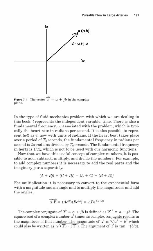
In the type of fluid mechanics problem with which we are dealing inthis book, t represents the independent variable, time. There is also afundamental frequency, v, associated with the problem, which is typi-cally the heart rate in radians per second. It is also possible to repre-sent (vt) as u, now with units of radians. If the heart beat takes placeover a period of T0 seconds, the fundamental frequency in radians persecond is 2� radians divided by T0 seconds. The fundamental frequencyin hertz is 1/T0, which is not to be used with our harmonic functions.
Now that we have this useful concept of complex numbers, it is pos-sible to add, subtract, multiply, and divide the numbers. For example,to add complex numbers it is necessary to add the real parts and theimaginary parts separately.
(A � Bj) � (C � Dj) � (A � C) � (B � D)j
For multiplication it is necessary to convert to the exponential formwith a magnitude and an angle and to multiply the magnitudes and addthe angles.
The complex conjugate of is defined as . Thesquare root of a complex number times its complex conjugate results inthe magnitude of that number. The magnitude of is whichcould also be written as . The argument of is . tan 21sb/adzS2s zSd ? s zS*d
2a2 1 b2zSzS
zS * 5 a 2 jbzS 5 a 1 jb
AS
BS5 sAejudsBejfd 5 ABe jsu1fd
Pulsatile Flow in Large Arteries 191
Figure 7.1 The vector in the complexplane.
zS 5 a 1 jb
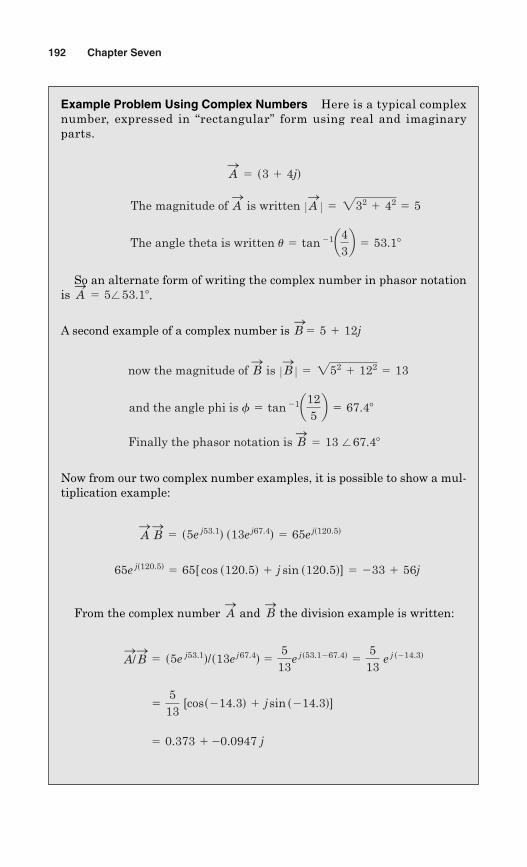
192 Chapter Seven
Example Problem Using Complex Numbers Here is a typical complexnumber, expressed in “rectangular” form using real and imaginaryparts.
So an alternate form of writing the complex number in phasor notationis .
A second example of a complex number is
Now from our two complex number examples, it is possible to show a mul-tiplication example:
From the complex number and the division example is written:
5 0.373 120.0947 j
55
13 [coss214.3d 1 j sin s214.3d]
A/S
BS5 s5e j53.1d/s13e j67.4d 5
513
e js53.1267.4d 55
13 e j s214.3d
BS
AS
65e js120.5d 5 65[ cos s120.5d 1 j sin s120.5d] 5 233 1 56j
AS
BS5 s5e j53.1d s13e j67.4d 5 65e js120.5d
Finally the phasor notation is BS5 13 /67.48
and the angle phi is f 5 tan 21a125b 5 67.48
now the magnitude of BS
is ZBSZ 5 252 1 122 5 13
BS5 5 1 12j
AS5 5/53.18
The angle theta is written u 5 tan 21a43b 5 53.18
The magnitude of AS is written ZA
SZ 5 232 1 42 5 5
AS5 s3 1 4jd
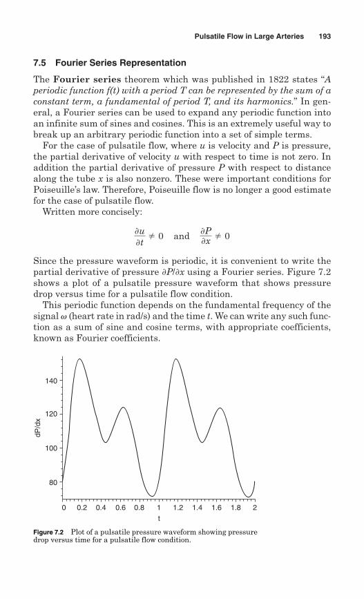
7.5 Fourier Series Representation
The Fourier series theorem which was published in 1822 states “Aperiodic function f(t) with a period T can be represented by the sum of aconstant term, a fundamental of period T, and its harmonics.” In gen-eral, a Fourier series can be used to expand any periodic function intoan infinite sum of sines and cosines. This is an extremely useful way tobreak up an arbitrary periodic function into a set of simple terms.
For the case of pulsatile flow, where u is velocity and P is pressure,the partial derivative of velocity u with respect to time is not zero. Inaddition the partial derivative of pressure P with respect to distancealong the tube x is also nonzero. These were important conditions forPoiseuille’s law. Therefore, Poiseuille flow is no longer a good estimatefor the case of pulsatile flow.
Written more concisely:
Since the pressure waveform is periodic, it is convenient to write thepartial derivative of pressure using a Fourier series. Figure 7.2shows a plot of a pulsatile pressure waveform that shows pressuredrop versus time for a pulsatile flow condition.
This periodic function depends on the fundamental frequency of thesignal v (heart rate in rad/s) and the time t. We can write any such func-tion as a sum of sine and cosine terms, with appropriate coefficients,known as Fourier coefficients.
'P/'x
'u't2 0� � and� � 'P'x 2 0
Pulsatile Flow in Large Arteries 193
0
80
100
120
140
0.2 0.4 0.6 0.8 1 1.2 1.4 1.6 1.8 2
t
dP/d
x
Figure 7.2 Plot of a pulsatile pressure waveform showing pressuredrop versus time for a pulsatile flow condition.
Since is periodic, it may be written:
This is a Fourier series representation of the pressure gradient. If wehave a periodic pressure waveform, it is possible to obtain the Fouriercoefficients, A1, A2, A3, . . . B1, B2, B3, . . . by a number of common meth-ods. The formal approach taught in most courses in differential equa-tions involves the evaluation of a series of integrals. Let f be a periodicfunction with period T0. Then
(7.17)
(7.18)
(7.19)
Doing the integrals formally using the principles of integral calculuscan be very laborious if f is other than a fairly simple function. It maybe convenient to evaluate the integrals numerically. Or, if a set of dig-itized data exists, for example, a fast Fourier transform implementedin many types of software may be used to approximate the neededFourier coefficients.
It is also possible to write the Fourier series using complex numbersby using Euler’s identity to convert the sines and cosines to exponen-tials. The equivalent expression would be:
(7.20)
where an � An Bn j, n is the number of the harmonic, v is the fun-damental frequency (rad/s), and Ao is the mean pressure gradient(nonpulsatile).
an � (An Bn j)
or
an � conjugate (An � Bn j)
Note:
'P'x5 Re c �
`
n50ane j v n td
Bn 52T03
T0
0fstd sin sn v td dt
An 52T03
T0
0fstd cos sn v td dt
A0 51T03
T0
0fstd dt
1 B1 sin svtd 1 B2 sin s2vtd 1 B3 sin s3vtd 1 c
'P'x 5 Ao 1 A1 cos svtd 1 A2 cos s2vtd 1 A3 cos s3vtd 1 c
'P'x
194 Chapter Seven
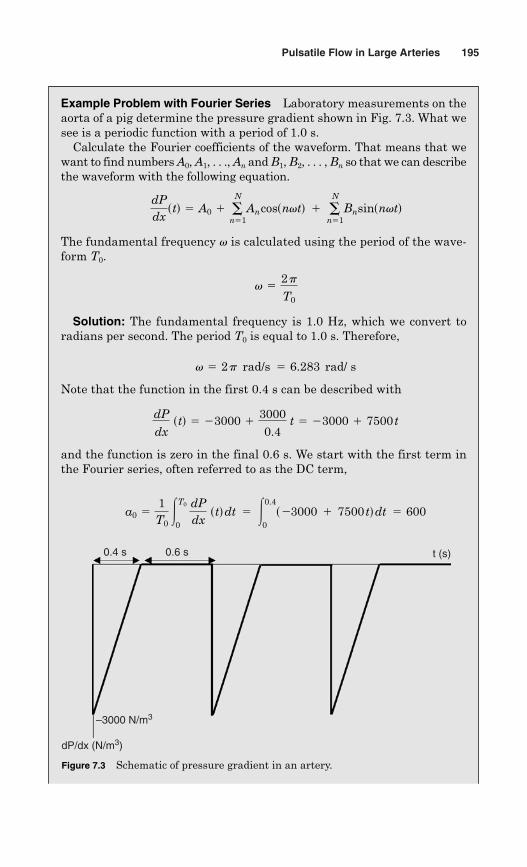
Pulsatile Flow in Large Arteries 195
Example Problem with Fourier Series Laboratory measurements on theaorta of a pig determine the pressure gradient shown in Fig. 7.3. What wesee is a periodic function with a period of 1.0 s.
Calculate the Fourier coefficients of the waveform. That means that wewant to find numbers A0, A1, . . ., An and B1, B2, . . . , Bn so that we can describethe waveform with the following equation.
The fundamental frequency v is calculated using the period of the wave-form T0.
Solution: The fundamental frequency is 1.0 Hz, which we convert toradians per second. The period T0 is equal to 1.0 s. Therefore,
Note that the function in the first 0.4 s can be described with
and the function is zero in the final 0.6 s. We start with the first term inthe Fourier series, often referred to as the DC term,
a0 51T03
T0
0 dPdx
std dt 5 30.4
0s23000 1 7500 td dt 5 600
dPdx
std 5 23000 1 30000.4
t 5 23000 1 7500 t
v 5 2 p rad/s 5 6.283 rad/ s
v 52 p
T0
dPdxstd 5 A0 1 �
N
n51An cos snvtd 1 �
N
n51Bn sin snvtd
0.4 s 0.6 s t (s)
–3000 N/m3
dP/dx (N/m3)
Figure 7.3 Schematic of pressure gradient in an artery.
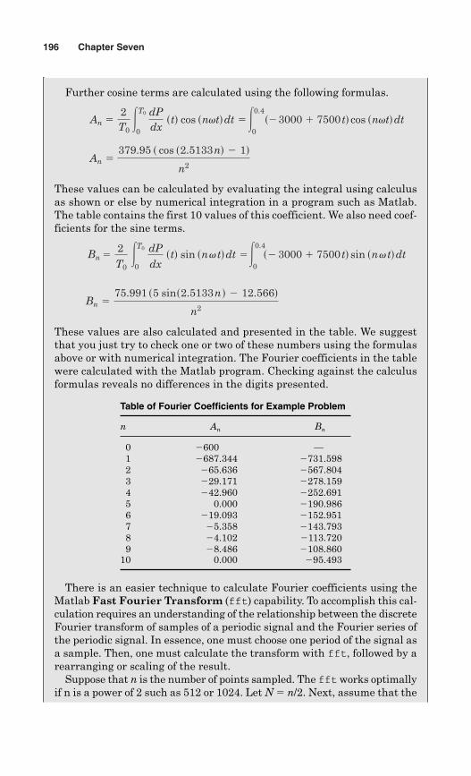
196 Chapter Seven
Further cosine terms are calculated using the following formulas.
These values can be calculated by evaluating the integral using calculusas shown or else by numerical integration in a program such as Matlab.The table contains the first 10 values of this coefficient. We also need coef-ficients for the sine terms.
These values are also calculated and presented in the table. We suggestthat you just try to check one or two of these numbers using the formulasabove or with numerical integration. The Fourier coefficients in the tablewere calculated with the Matlab program. Checking against the calculusformulas reveals no differences in the digits presented.
There is an easier technique to calculate Fourier coefficients using theMatlab Fast Fourier Transform (fft) capability. To accomplish this cal-culation requires an understanding of the relationship between the discreteFourier transform of samples of a periodic signal and the Fourier series ofthe periodic signal. In essence, one must choose one period of the signal asa sample. Then, one must calculate the transform with fft, followed by arearranging or scaling of the result.
Suppose that n is the number of points sampled. The fftworks optimallyif n is a power of 2 such as 512 or 1024. Let N � n/2. Next, assume that the
Bn 575.991 s5 sin s2.5133 n d 2 12.566d
n2
Bn52T0
3T0
0
dPdx
std sin sn v td dt 530.4
0s23000 1 7500 td sin sn v td dt
An 5379.95 s cos s2.5133 nd 2 1d
n2
An 52T03
T0
0 dPdx
std cos snvtd dt 530.4
0s23000 1 7500 td cos snvtd dt
Table of Fourier Coefficients for Example Problem
n An Bn
0 600 —1 687.344 731.5982 65.636 567.8043 29.171 278.1594 42.960 252.6915 0.000 190.9866 19.093 152.9517 5.358 143.7938 4.102 113.7209 8.486 108.860
10 0.000 95.493
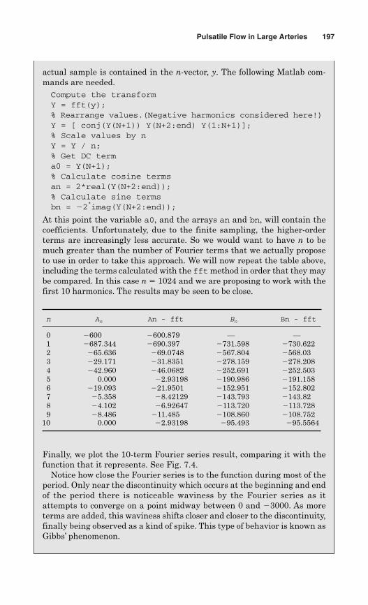
Pulsatile Flow in Large Arteries 197
actual sample is contained in the n-vector, y. The following Matlab com-mands are needed.Compute the transformY = fft(y);% Rearrange values.(Negative harmonics considered here!)Y = [ conj(Y(N+1)) Y(N+2:end) Y(1:N+1)];% Scale values by nY = Y / n;% Get DC terma0 = Y(N+1);% Calculate cosine termsan = 2*real(Y(N+2:end));% Calculate sine termsbn = 2*imag(Y(N+2:end));
At this point the variable a0, and the arrays an and bn, will contain thecoefficients. Unfortunately, due to the finite sampling, the higher-orderterms are increasingly less accurate. So we would want to have n to bemuch greater than the number of Fourier terms that we actually proposeto use in order to take this approach. We will now repeat the table above,including the terms calculated with the fft method in order that they maybe compared. In this case n � 1024 and we are proposing to work with thefirst 10 harmonics. The results may be seen to be close.
Finally, we plot the 10-term Fourier series result, comparing it with thefunction that it represents. See Fig. 7.4.
Notice how close the Fourier series is to the function during most of theperiod. Only near the discontinuity which occurs at the beginning and endof the period there is noticeable waviness by the Fourier series as itattempts to converge on a point midway between 0 and 3000. As moreterms are added, this waviness shifts closer and closer to the discontinuity,finally being observed as a kind of spike. This type of behavior is known asGibbs’ phenomenon.
n An An - fft Bn Bn - fft
0 600 600.879 — —1 687.344 690.397 731.598 730.6222 65.636 69.0748 567.804 568.033 29.171 31.8351 278.159 278.2084 42.960 46.0682 252.691 252.5035 0.000 2.93198 190.986 191.1586 19.093 21.9501 152.951 152.8027 5.358 8.42129 143.793 143.828 4.102 6.92647 113.720 113.7289 8.486 11.485 108.860 108.752
10 0.000 2.93198 95.493 95.5564
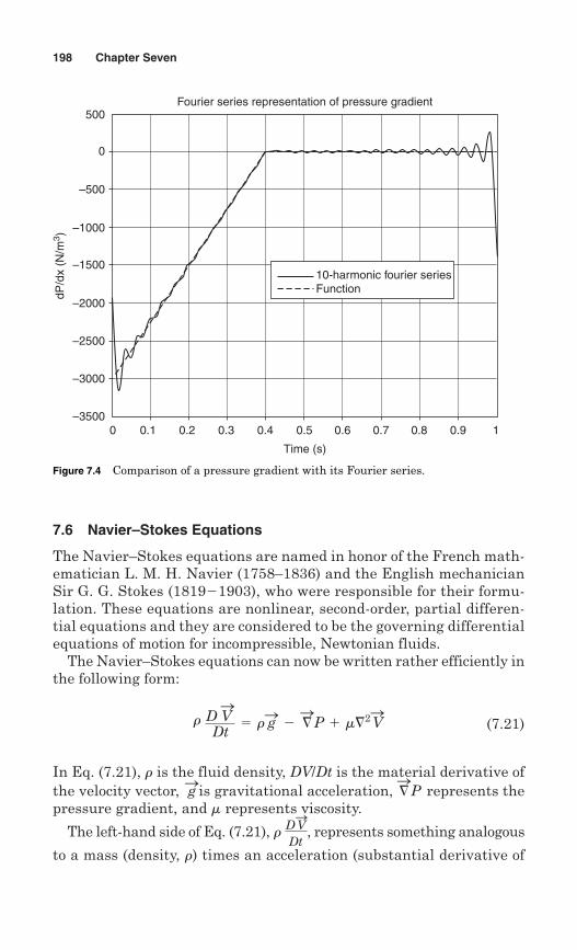
198 Chapter Seven
7.6 Navier–Stokes Equations
The Navier–Stokes equations are named in honor of the French math-ematician L. M. H. Navier (1758–1836) and the English mechanicianSir G. G. Stokes (18191903), who were responsible for their formu-lation. These equations are nonlinear, second-order, partial differen-tial equations and they are considered to be the governing differentialequations of motion for incompressible, Newtonian fluids.
The Navier–Stokes equations can now be written rather efficiently inthe following form:
(7.21)
In Eq. (7.21), is the fluid density, DV/Dt is the material derivative of the velocity vector, is gravitational acceleration, represents thepressure gradient, and represents viscosity.
The left-hand side of Eq. (7.21), , represents something analogous
to a mass (density, ) times an acceleration (substantial derivative ofr
r D VS
Dt
m
=S
PgSr
r D VS
Dt5 r gS 2 =
SP 1 m=2 V
S
0 0.1 0.2 0.3 0.4 0.5 0.6 0.7 0.8 0.9 1
Time (s)
–3500
–3000
–2500
–2000
–1500
–1000
–500
0
500
dP/d
x (N
/m3 )
Fourier series representation of pressure gradient
10-harmonic fourier series Function
Figure 7.4 Comparison of a pressure gradient with its Fourier series.
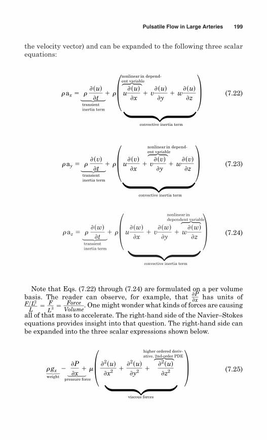
the velocity vector) and can be expanded to the following three scalarequations:
Pulsatile Flow in Large Arteries 199
(7.24)r az 5 r 'swd't
1 r ± u'swd'x
1 v'swd'y
1 w'swd'z
≤5
transientinertia term
3nonlinear in dependent variable
3 convective inertia term
(7.25)r gx 2 'P'x1 m ± '2sud
'x2 1'2sud'y2 1
'2sud'z2 �≤
5
pressure force
3
3 viscous forces
5
weight
higher ordered deriv-ative, 2nd-order PDE
(7.23)r ay 5 r 'svd't
1 r ± u'svd'x
1 v'svd'y
1 w'svd'z
≤5
transientinertia term
3
nonlinear in depend-ent variable
3 convective inertia term
(7.22)r ax 5 r 'sud't
1 r ± u'sud'x
1 v'sud'y
1 w'sud'z
≤5
transientinertia term
3
nonlinear in depend-ent variable
3 convective inertia term
Note that Eqs. (7.22) through (7.24) are formulated on a per volumebasis. The reader can observe, for example, that has units of
. One might wonder what kinds of forces are causingall of that mass to accelerate. The right-hand side of the Navier–Stokesequations provides insight into that question. The right-hand side canbe expanded into the three scalar expressions shown below.
F>L2
L5
FL3 5
ForceVolume
'P'x
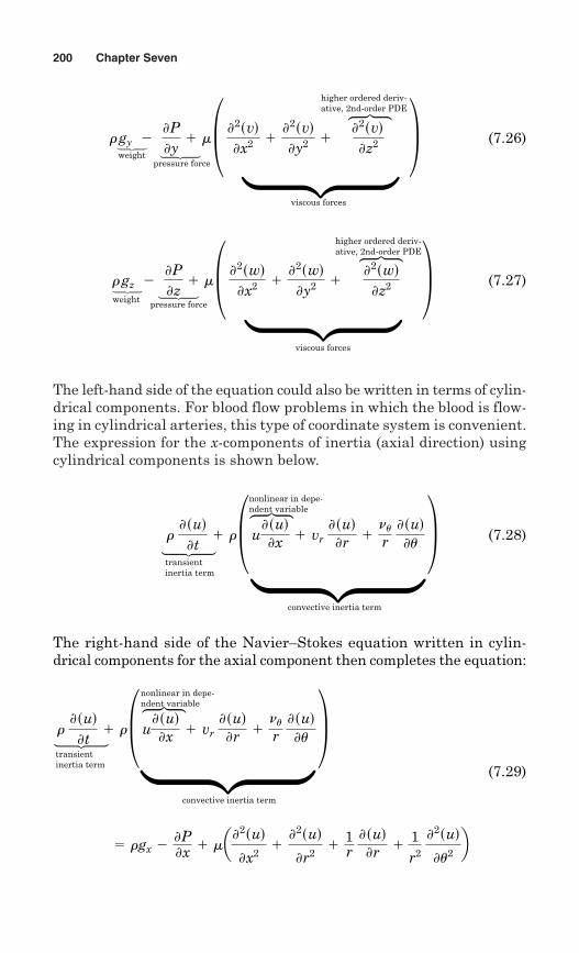
The left-hand side of the equation could also be written in terms of cylin-drical components. For blood flow problems in which the blood is flow-ing in cylindrical arteries, this type of coordinate system is convenient.The expression for the x-components of inertia (axial direction) usingcylindrical components is shown below.
200 Chapter Seven
(7.26)r gy 2 'P'y1 m ± '2svd
'x2 1'2svd'y2 1
'2svd'z2 ≤
3 viscous forces
5
5
pressure force
3
higher ordered deriv-ative, 2nd-order PDE
(7.27)r gz 2 'P'z1 m ± '2swd
'x2 1'2swd'y2 1
'2swd'z2 ≤
5
pressure force
3
3 viscous forces
5
weight
higher ordered deriv-ative, 2nd-order PDE
weight
(7.28) r 'sud't
1 r ± u'sud'x 1 vr
'sud'r 1
nur 'sud'u ≤
3convective inertia term
3
nonlinear in depe-ndent variable
5
transientinertia term
The right-hand side of the Navier–Stokes equation written in cylin-drical components for the axial component then completes the equation:
(7.29)
r 'sud't
1 r ± u'sud'x 1 vr
'sud'r 1
nur 'sud'u ≤
3convective inertia term
3
nonlinear in depe-ndent variable
5
transientinertia term
5 rgx 2'P'x 1 ma
'2sud
'x21'2sud
'r21
1r 'sud'r 1 1
r2 '2sud
'u2b
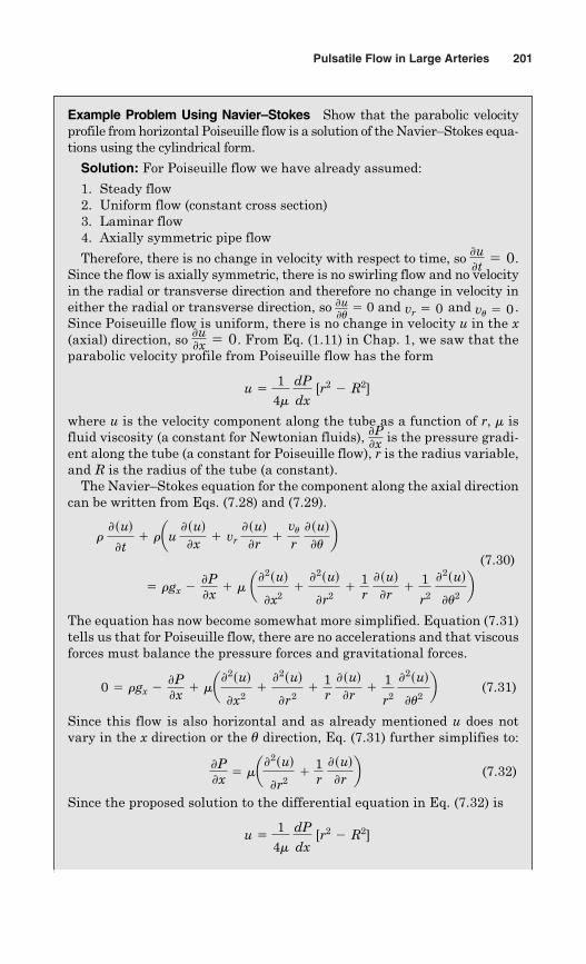
Pulsatile Flow in Large Arteries 201
Example Problem Using Navier–Stokes Show that the parabolic velocityprofile from horizontal Poiseuille flow is a solution of the Navier–Stokes equa-tions using the cylindrical form.
Solution: For Poiseuille flow we have already assumed:
1. Steady flow2. Uniform flow (constant cross section)3. Laminar flow4. Axially symmetric pipe flow
Therefore, there is no change in velocity with respect to time, so .Since the flow is axially symmetric, there is no swirling flow and no velocityin the radial or transverse direction and therefore no change in velocity ineither the radial or transverse direction, so � 0 and and .Since Poiseuille flow is uniform, there is no change in velocity u in the x(axial) direction, so . From Eq. (1.11) in Chap. 1, we saw that theparabolic velocity profile from Poiseuille flow has the form
where u is the velocity component along the tube as a function of r, m isfluid viscosity (a constant for Newtonian fluids), is the pressure gradi-ent along the tube (a constant for Poiseuille flow), r is the radius variable,and R is the radius of the tube (a constant).
The Navier–Stokes equation for the component along the axial directioncan be written from Eqs. (7.28) and (7.29).
(7.30)
The equation has now become somewhat more simplified. Equation (7.31)tells us that for Poiseuille flow, there are no accelerations and that viscousforces must balance the pressure forces and gravitational forces.
(7.31)
Since this flow is also horizontal and as already mentioned u does notvary in the x direction or the direction, Eq. (7.31) further simplifies to:
(7.32)
Since the proposed solution to the differential equation in Eq. (7.32) is
u 5 14m
dPdx
[r2 2 R2]
'P'x 5 ma
'2sud
'r21
1r 'sud'r b
u
0 5 rgx 2'P'x 1 ma
'2sud
'x21'2sud
'r21
1r 'sud'r 1
1
r2 '2sud
'u2b
5 rgx 2'P'x 1 m a'2sud
'x21'2sud
'r21
1r 'sud'r 1
1
r2 '2sud
'u2b
r 'sud't
1 rau 'sud'x 1 vr
'sud'r 1
vur 'sud'u b
'P'x
u 5 14m
dPdx
[r2 2 R2]
'u'x 5 0
vu 5 0vr 5 0'u'u
'u't5 0
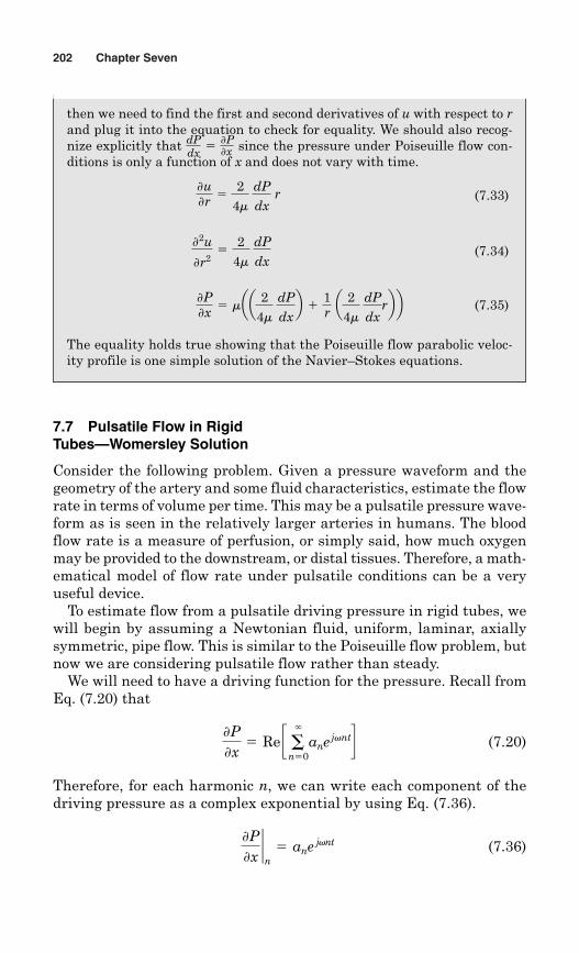
202 Chapter Seven
then we need to find the first and second derivatives of u with respect to rand plug it into the equation to check for equality. We should also recog-nize explicitly that since the pressure under Poiseuille flow con-ditions is only a function of x and does not vary with time.
(7.33)
(7.34)
(7.35)
The equality holds true showing that the Poiseuille flow parabolic veloc-ity profile is one simple solution of the Navier–Stokes equations.
'P'x 5 maa 2
4m dPdxb 1 1
r a 24m
dPdx
rbb
'2u
'r25
24m
dPdx
'u'r 5
24m
dPdx
r
dPdx 5
'P'x
7.7 Pulsatile Flow in Rigid Tubes—Womersley Solution
Consider the following problem. Given a pressure waveform and thegeometry of the artery and some fluid characteristics, estimate the flowrate in terms of volume per time. This may be a pulsatile pressure wave-form as is seen in the relatively larger arteries in humans. The bloodflow rate is a measure of perfusion, or simply said, how much oxygenmay be provided to the downstream, or distal tissues. Therefore, a math-ematical model of flow rate under pulsatile conditions can be a veryuseful device.
To estimate flow from a pulsatile driving pressure in rigid tubes, wewill begin by assuming a Newtonian fluid, uniform, laminar, axiallysymmetric, pipe flow. This is similar to the Poiseuille flow problem, butnow we are considering pulsatile flow rather than steady.
We will need to have a driving function for the pressure. Recall fromEq. (7.20) that
(7.20)
Therefore, for each harmonic n, we can write each component of thedriving pressure as a complex exponential by using Eq. (7.36).
(7.36)'P'x`n5 ane j v n t
'P'x5 Re c �
`
n50anejvntd
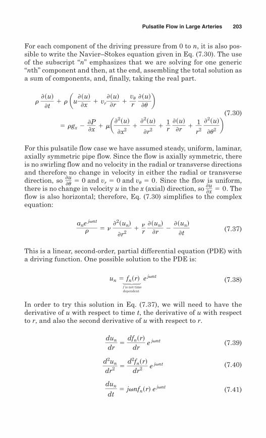
Pulsatile Flow in Large Arteries 203
For each component of the driving pressure from 0 to n, it is also pos-sible to write the Navier–Stokes equation given in Eq. (7.30). The useof the subscript “n” emphasizes that we are solving for one generic“nth” component and then, at the end, assembling the total solution asa sum of components, and, finally, taking the real part.
(7.30)
For this pulsatile flow case we have assumed steady, uniform, laminar,axially symmetric pipe flow. Since the flow is axially symmetric, thereis no swirling flow and no velocity in the radial or transverse directionsand therefore no change in velocity in either the radial or transversedirection, so . Since the flow is uniform,there is no change in velocity u in the x (axial) direction, so . Theflow is also horizontal; therefore, Eq. (7.30) simplifies to the complexequation:
(7.37)
This is a linear, second-order, partial differential equation (PDE) witha driving function. One possible solution to the PDE is:
(7.38)
In order to try this solution in Eq. (7.37), we will need to have thederivative of u with respect to time t, the derivative of u with respectto r, and also the second derivative of u with respect to r.
(7.39)
(7.40)
(7.41)dun
dt5 jvnfnsrd e jvnt
d2un
dr2 5d2fnsrd
dr2 e jvnt
dun
dr5
dfnsrddr
e jvnt
un 5 fnsrd e jvnt
ane jvnt
r 5 n '2sund
'r21nr 'sund'r 2
'sund't
'u'x 5 0
'u'u 5 0 and vr 5 0 and vu 5 0
5 rgx 2'P'x 1 ma
'2sud
'x21'2sud
'r21
1r 'sud'r 1
1r2
'2sud
'u2b
r 'sud't
1 r au'sud'x 1 vr'sud'r 1
vur 'sud'u b
5
f is not timedependent
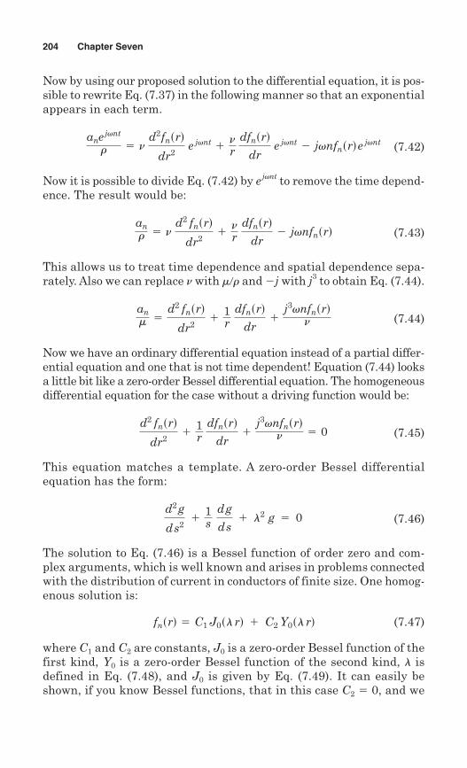
Now by using our proposed solution to the differential equation, it is pos-sible to rewrite Eq. (7.37) in the following manner so that an exponentialappears in each term.
(7.42)
Now it is possible to divide Eq. (7.42) by ejvnt to remove the time depend-ence. The result would be:
(7.43)
This allows us to treat time dependence and spatial dependence sepa-rately. Also we can replace nwith m�r and j with j3 to obtain Eq. (7.44).
(7.44)
Now we have an ordinary differential equation instead of a partial differ-ential equation and one that is not time dependent! Equation (7.44) looksa little bit like a zero-order Bessel differential equation. The homogeneousdifferential equation for the case without a driving function would be:
(7.45)
This equation matches a template. A zero-order Bessel differentialequation has the form:
(7.46)
The solution to Eq. (7.46) is a Bessel function of order zero and com-plex arguments, which is well known and arises in problems connectedwith the distribution of current in conductors of finite size. One homog-enous solution is:
(7.47)
where C1 and C2 are constants, J0 is a zero-order Bessel function of thefirst kind, Y0 is a zero-order Bessel function of the second kind, l isdefined in Eq. (7.48), and J0 is given by Eq. (7.49). It can easily beshown, if you know Bessel functions, that in this case C2 � 0, and we
fnsrd 5 C1 J0sl rd 1 C2 Y0sl rd
d2 g
d s2 1
1s
d g
d s 1 l2
g 5 0
d2 fnsrd
dr21
1r
dfnsrddr
1j3vnfnsrdn 5 0
anm 5
d2 fnsrd
dr21
1r
dfnsrddr
1j3vnfnsrdn
anr 5 n
d2 fnsrd
dr21nr
dfnsrddr
2 jvnfnsrd
anejvnt
r 5 n d2fnsrd
dr2 e jvnt 1
nr
dfnsrddr
e jvnt 2 jvnfnsrde jvnt
204 Chapter Seven
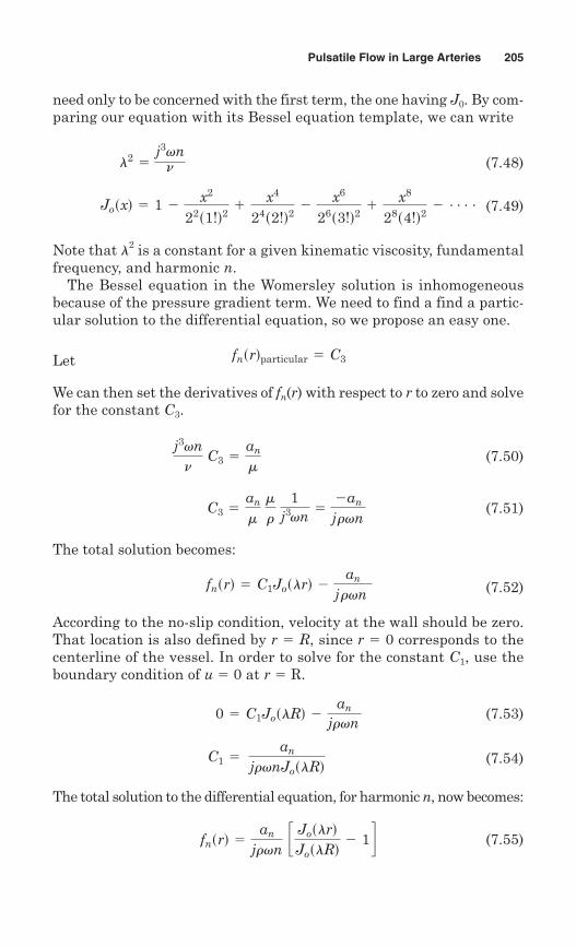
Pulsatile Flow in Large Arteries 205
need only to be concerned with the first term, the one having J0. By com-paring our equation with its Bessel equation template, we can write
(7.48)
(7.49)
Note that l2 is a constant for a given kinematic viscosity, fundamentalfrequency, and harmonic n.
The Bessel equation in the Womersley solution is inhomogeneousbecause of the pressure gradient term. We need to find a find a partic-ular solution to the differential equation, so we propose an easy one.
Let
We can then set the derivatives of fn(r) with respect to r to zero and solvefor the constant C3.
(7.50)
(7.51)
The total solution becomes:
(7.52)
According to the no-slip condition, velocity at the wall should be zero.That location is also defined by r � R, since r � 0 corresponds to thecenterline of the vessel. In order to solve for the constant C1, use theboundary condition of u � 0 at r � R.
(7.53)
(7.54)
The total solution to the differential equation, for harmonic n, now becomes:
(7.55)fnsrd 5an
jrvn c Joslrd
JoslRd2 1 d
C1 5 an
jrvnJoslRd
0 5 C1JoslRd 2an
jrvn
fnsrd 5 C1Joslrd 2an
j rvn
C3 5an
m m
r
1j3
vn52an
j rvn
j3vnn
C3 5an
m
fnsrdparticular 5 C3
Josxd 5 1 2 x2
22s1!d21
x4
24s2!d22
x6
26s3!d21
x8
28s4!d22 c.
l2 5j3vnn
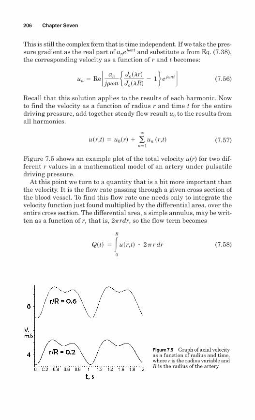
This is still the complex form that is time independent. If we take the pres-sure gradient as the real part of and substitute u from Eq. (7.38),the corresponding velocity as a function of r and t becomes:
(7.56)
Recall that this solution applies to the results of each harmonic. Nowto find the velocity as a function of radius r and time t for the entiredriving pressure, add together steady flow result u0 to the results fromall harmonics.
(7.57)
Figure 7.5 shows an example plot of the total velocity u(r) for two dif-ferent r values in a mathematical model of an artery under pulsatiledriving pressure.
At this point we turn to a quantity that is a bit more important thanthe velocity. It is the flow rate passing through a given cross section ofthe blood vessel. To find this flow rate one needs only to integrate thevelocity function just found multiplied by the differential area, over theentire cross section. The differential area, a simple annulus, may be writ-ten as a function of r, that is, 2prdr, so the flow term becomes
(7.58)Qstd 5 3R
0
usr,td ? 2 p r dr
usr,td 5 u0srd 1 �`
n51un sr,td
un 5 Re c an
jrvne Joslrd
JoslRd2 1 f e jvnt d
anejvnt
206 Chapter Seven
Figure 7.5 Graph of axial velocityas a function of radius and time,where r is the radius variable andR is the radius of the artery.
We can perform this integral after looking up integral identities for Bessel functions in a mathematical reference. The one we need touse is
The symbol J1 denotes a Bessel function of the first kind and of the firstorder. After a number of steps of calculus style derivations which neednot be explained here, we reach a solution for the flow rate producedby harmonic n of the pressure gradient.
(7.59)
These must be summed and added to
(7.60)
which is the average flow rate produced by the constant term in thepressure gradient’s Fourier series. Finally, we have
(7.61)
Womersley published his solution in 1955 when it wasn’t so easy tomake up a computer model of the flow. Bessel functions were not easilyaccessible then as they are now in all scientific software. So he inte-grated the velocity terms, solved for flow, and published the followingequation for the flow component resulting from each of the drivingpressure gradient harmonics:
(7.62)
where the pressure gradient associated with each harmonic is:
(7.63)
The magnitude of the driving pressure is given by:
(7.64)Mn 52An2 1 Bn
2
'P'x
`n5 Mn cos svnt 1 fnd
Qn 5pR4
m Mn aM10
a2b
n sin svnt 1 fn 1 e10n
d
Qstd 5 Q0 1 �N
n51Qnstd
Q0 5 a0 8 m
p R4
Qn 5 ssp R2ddRe c an
jvnre 2 J1sl Rdl R J0sl Rd
2 1 f e jvnt d
3x J0sxd dx 5 x J1sxd
Pulsatile Flow in Large Arteries 207
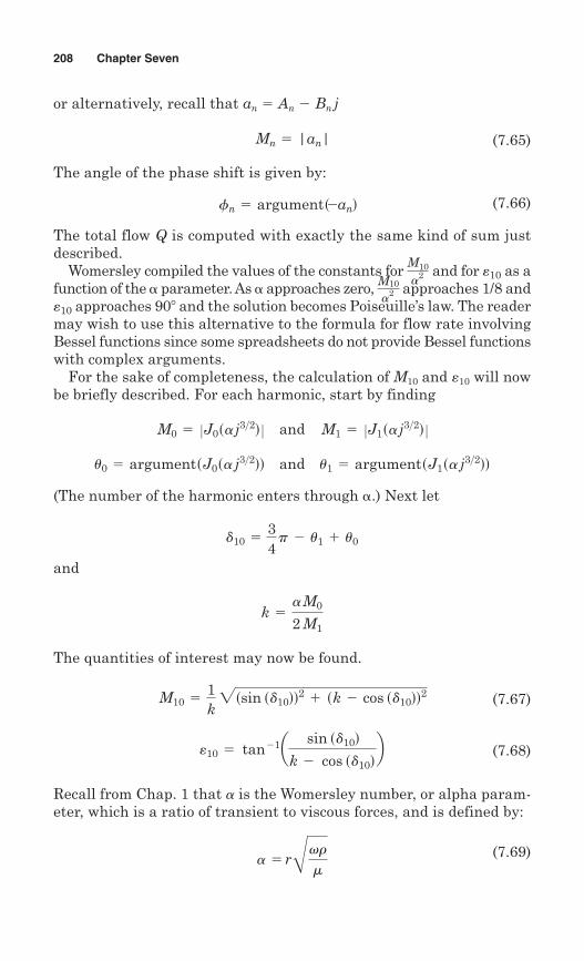
or alternatively, recall that an � An Bn j
(7.65)
The angle of the phase shift is given by:
(7.66)
The total flow Q is computed with exactly the same kind of sum justdescribed.
Womersley compiled the values of the constants for and for as afunction of the � parameter. As � approaches zero, approaches 1/8 and
approaches 90� and the solution becomes Poiseuille’s law. The readermay wish to use this alternative to the formula for flow rate involvingBessel functions since some spreadsheets do not provide Bessel functionswith complex arguments.
For the sake of completeness, the calculation of M10 and �10 will nowbe briefly described. For each harmonic, start by finding
and
and
(The number of the harmonic enters through �.) Next let
and
The quantities of interest may now be found.
(7.67)
(7.68)
Recall from Chap. 1 that a is the Womersley number, or alpha param-eter, which is a ratio of transient to viscous forces, and is defined by:
(7.69)a 5r Åvrm
e10 5 tan 21a sin sd10dk 2 cos sd10d
b
M10 51k
2s sin sd10dd2 1 sk 2 cos sd10dd2
k 5a M0
2 M1
d10 534
p 2 u1 1 u0
u1 5 argumentsJ1sa j3>2ddu0 5 argumentsJ0sa j3>2ddM1 5 ZJ1sa j3>2d ZM0 5 ZJ0sa j3>2d Z
e10
M10
a2
e10M10
a2
fn 5 arguments2and
Mn 5 |an|
208 Chapter Seven
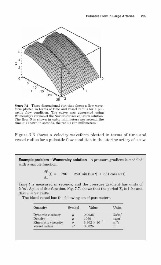
Figure 7.6 shows a velocity waveform plotted in terms of time andvessel radius for a pulsatile flow condition in the uterine artery of a cow.
Pulsatile Flow in Large Arteries 209
22520
1510
5
0
1
0
tr
2
4
6
Q
Figure 7.6 Three-dimensional plot that shows a flow wave-form plotted in terms of time and vessel radius for a pul-satile flow condition. The curve was generated usingWomersley’s version of the Navier–Stokes equation solution.The flow Q is shown in cubic millimeters per second, thetime t is shown in seconds, the radius r in millimeters.
Example problem—Womersley solution A pressure gradient is modeledwith a simple function,
Time t is measured in seconds, and the pressure gradient has units ofN/m3. A plot of this function, Fig. 7.7, shows that the period T0 is 1.0 s andthat v � 2p rad/s.
The blood vessel has the following set of parameters.
dPdxstd 5 2796 2 1250 sin s2 p td 1 531 cos s4 p td
Quantity Symbol Value Units
Dynamic viscosity m 0.0035 Ns/m2
Density r 1060 kg/m3
Kinematic viscosity � 3.302 � 106 m2/sVessel radius R 0.0025 m
210 Chapter Seven
Calculate the Womersley solution for pulsatile flow. In addition to thevelocity through the pipe cross section at any time, calculate the flowrate through the vessel as a function of time. Present the results withplots.
Solution:1. We organize the input data. The pressure gradient is already in
Fourier series form. It may also be written as
so that a0 � 796, a1 � 1250 j, and a2 � 531.2. Using the Eq. (1.11) which describes the velocity profile in Poiseuille
flow, we write down the steady state (DC analog) solution.
3. We compute the parameters needed for Womersley which depend on thevessel geometry and fluid properties. We utilize Eq. (7.48) and write
ln 5 Å j3 v nn
u0 51
4 m a0sr2 2 R2d 5256840 r2 1 0.35525
dPdxstd 5 Res2796 1 1250j e2p j t 1 531 e4 p j td
0 0.1 0.2 0.3 0.4 0.5 0.6 0.7 0.8 0.9 1
Time (s)
–3000
–2500
–2000
–1500
–1000
–500
0
500
dP/d
x (P
a/m
)
Pressure gradient driving the flow
Figure 7.7 Womersley solution example problem: pressure gradient.
Pulsatile Flow in Large Arteries 211
Pieces of the solution are displayed in the following table.
4. We calculate and add the pulsatile terms for the velocity solution.Using Eq. (7.56),
Hence, our solution may be constructed as
The infinity sign ( ) over the sum in Eq. (7.57) indicates that in themost general case a converging series with an infinity of terms wouldbe needed to represent the arbitrary pressure gradient exactly. In thiscase, with a simple representation of the pressure gradient using threeterms, our solution terminates quickly with just three parts. Two plotsillustrate the results. Figure 7.8 shows the three-dimensional por-trayal of axial velocity as a function of time and radial position, andFig. 7.9 shows the velocity versus time for center and midradius.
5. We calculate the flow rate as a function of time by integrating over thecross section, as indicated in Eq. (7.58). As an alternative we could usethe formula in Eq. (7.59)
To assist a reader who desires to implement this formula, we tabulatethe inner term in braces for each harmonic.
Qn 5 ssp R2dd Re c an
j v n re 2 J1sl Rdl R J0sl Rd
2 1 f e j v n t d
`
usr,td 5 u0 1 u1 1 u2
1 0.03983d e12.566 j t]
u2 5 Re[ss20.0007274 1 0.006844jd J0ss1379 2 1379 jd rd
2 0.1877d e6.283 j t]
u1 5 Re[ss20.03225 2 0.06772jd J0ss975.4 2 975.4 jd rd
Term n � 1 n � 2
975.4 975.4 j 1379 1379 j
0.1877 0.03983 j
1.0758 � 2.259 j 5.754 � 0.6115 jJ0sl Rd
an
j r v n
ln
n
1 0.5783 0.3292 j2 0.7088 0.2467 j
e 2 J1sl Rdl R J0sl Rd
2 1 f
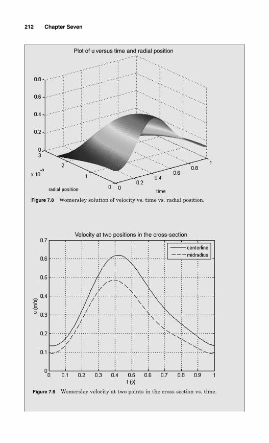
212 Chapter Seven
Figure 7.9 Womersley velocity at two points in the cross section vs. time.
Figure 7.8 Womersley solution of velocity vs. time vs. radial position.
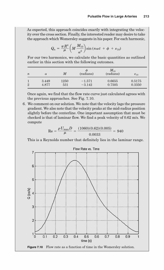
Pulsatile Flow in Large Arteries 213
As expected, this approach coincides exactly with integrating the veloc-ity over the cross section. Finally, the interested reader may desire to takethe approach which Womersley suggests in his paper. For each harmonic,
For our two harmonics, we calculate the basic quantities as outlinedearlier in this section with the following outcomes.
Once again, we find that the flow rate curve just calculated agrees withthe previous approaches. See Fig. 7.10.
6. We comment on our solution. We note that the velocity lags the pressuregradient. We also note that the velocity peaks at the mid-radius positionslightly before the centerline. One important assumption that must bechecked is that of laminar flow. We find a peak velocity of 0.62 m/s. Wecompute
This is a Reynolds number that definitely lies in the laminar range.
Re 5 r Umax Dm 5
s1060ds0.62ds0.005d
0.00335 940
Qn 5p R4
m aM
M10
a2b sin sn v t 1 f 1 e10d
f M10n a M (radians) (radians) �10
1 3.449 1250 1.571 0.6655 0.51752 4.877 531 3.142 0.7505 0.3350
Figure 7.10 Flow rate as a function of time in the Womersley solution.
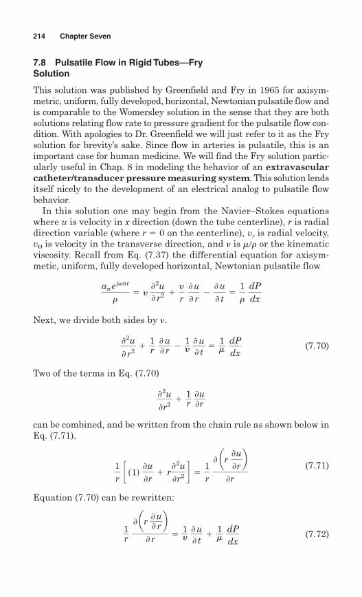
7.8 Pulsatile Flow in Rigid Tubes—FrySolution
This solution was published by Greenfield and Fry in 1965 for axisym-metric, uniform, fully developed, horizontal, Newtonian pulsatile flow andis comparable to the Womersley solution in the sense that they are bothsolutions relating flow rate to pressure gradient for the pulsatile flow con-dition. With apologies to Dr. Greenfield we will just refer to it as the Frysolution for brevity’s sake. Since flow in arteries is pulsatile, this is animportant case for human medicine. We will find the Fry solution partic-ularly useful in Chap. 8 in modeling the behavior of an extravascularcatheter/transducer pressure measuring system. This solution lendsitself nicely to the development of an electrical analog to pulsatile flowbehavior.
In this solution one may begin from the Navier–Stokes equationswhere u is velocity in x direction (down the tube centerline), r is radialdirection variable (where r � 0 on the centerline), vr is radial velocity,v� is velocity in the transverse direction, and � is m�r or the kinematicviscosity. Recall from Eq. (7.37) the differential equation for axisym-metic, uniform, fully developed horizontal, Newtonian pulsatile flow
Next, we divide both sides by �.
(7.70)
Two of the terms in Eq. (7.70)
can be combined, and be written from the chain rule as shown below inEq. (7.71).
(7.71)
Equation (7.70) can be rewritten:
(7.72)1r ' ar ' u
' r b' r 5
1y ' u' t1
1m dP
dx
1r c s1d 'u
'r1 r
'2u'r2 d 5 1
r ' ar
'u'rb
'r
'2u'r2
11r 'u'r
'2u' r2
11r ' u' r 2
1y ' u' t5
1m dP
dx
an e j v n t
r5 y
'2u' r2 1
y
r ' u' r
2' u' t5
1r
dPdx
214 Chapter Seven
If we multiply both sides of Eq. (7.72) by 2prdr and integrate fromr � 0 to R where R is the tube radius we obtain Eq. (7.73).
(7.73)
The integral of the derivative in the left-hand side of Eq. (7.73)returns the term , so we can rewrite Eq. (7.73) as shown below inEq. (7.74).
(7.74)
Notice that the integral from zero to R of u(2pr)dr is the integral of thevelocity multiplied by the differential area so that the term is simplythe flow through the tube.
It is possible now to replace the first term on the right-hand side ofthe equation with the symbol Q, representing flow. After evaluating thelast term between 0 and the vessel radius R we arrive at Eq. (7.75).
(7.75)
By dividing both sides of Eq. (7.63) by pR2 we obtain Eq. (7.76).
(7.76)
Recall that for a Newtonian fluid, the shear stress at the wall is equalto the viscosity times the velocity gradient as shown in Eq. (7.77).
(7.77)
Substitute Eq. (7.77) into Eq. (7.76) to obtain Eq. (7.78)
(7.78)
If we rearrange the equation as follows, and multiply it by m, it will beeasier to see what develops.
(7.79)2dPdx
5r
p R2 ' Q' t
1 a2 twall
Rb
2R
a2twall
mb 5
1y p R2
' Q' t
11m
dPdx
twall 5 2m 'u'r`R
2R
' u' r `R 5
1y p R2
' Q' t 1
1m dP
dx
2 p R ' u' r `R5 1
y ' Q' t 1
1m dP
dx p R2
2 p r ' u' r `R0 5
1y '' t
3R
0u s2 p r drd 1
1m dP
dx 2 p r
2
2`R0
r 'u'r
2 p 3R
0
' ar' u' r b' r dr 5 1
y 3R
0a' u' tb s2 p r drd 1
1m dP
dx 3R
0 s2 p r drd
Pulsatile Flow in Large Arteries 215
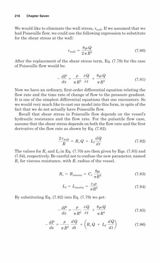
We would like to eliminate the wall stress, �wall. If we assumed that wehad Poiseuille flow, we could use the following expression to substitutefor the shear stress at the wall:
(7.80)
After the replacement of the shear stress term, Eq. (7.79) for the caseof Poiseuille flow would be:
(7.81)
Now we have an ordinary, first-order differential equation relating theflow rate and the time rate of change of flow to the pressure gradient.It is one of the simplest differential equations that one encounters. Sowe would very much like to cast our model into this form, in spite of thefact that we do not actually have Poiseuille flow.
Recall that shear stress in Poiseuille flow depends on the vessel’shydraulic resistance and the flow rate. For the pulsatile flow case,assume that the shear stress depends on both the flow rate and the firstderivative of the flow rate as shown by Eq. (7.82).
(7.82)
The values for Rv and LI in Eq. (7.70) are then given by Eqs. (7.83) and(7.84), respectively. Be careful not to confuse the new parameter, namedRv for viscous resistance, with R, radius of the vessel.
(7.83)
(7.84)
By substituting Eq. (7.82) into Eq. (7.79) we get:
(7.85)
(7.86) 2dPdx
5r
p R2 d Q
dt 1 aRv Q 1 LI
d Q
d tb
2dPdx
5r
p R2 ' Q' t
18 m Q
p R4
LI 5 Linertia 5c1r
pR2
Rv 5 Rviscous 5 Cv 8mpR4
2 twall
R5 Rv Q 1 LI
d Qd t
2dPdx
5r
p R2 ' Q' t
18 m Q
p R4
twall 58 m Q2 p R3
216 Chapter Seven
Next, substituting the expressions for the viscous resistance term Rv
and the inertia term LI yields the following equation. To further sim-plify, let .
(7.87)
(7.88)
Finally, it is possible to simplify the Fry solution to the following first-order ordinary differential equation with terms that represent fluidinertance and fluid resistance as shown below in Eq. (7.89).
(7.89)
where
(7.90)
(7.91)
The problem with this approach is an acceptable determination of cu andcv. This process will be addressed later. For now, we want you to rec-ognize that the Fry solution is very important since it is an analogwith a simple electrical circuit, one having an inductor in series witha resistor and a voltage source. This allows very useful modeling analo-gies to be established. The solutions of these equations will now beaddressed.
Differential equations of the kind called for by Fry and Greenfield rep-resent each of the harmonics used in modeling the pressure gradient.They are written as follows:
(7.92)
What we need is the steady state solution to this problem, which takesplace after the transient (start-up) portions of the solution have beendamped out. As a result, the initial conditions are not needed in this
Lu dQdt
1 Rv Q 5 2dPdx`n5 2Re[an e j v n t]
Rv 5cv8mp R4
Lu 5s1 1 c1drpR2 5
cur
pR2
2dPdx
5 Lu dQ
dt1 RvQ
2dPdx
5 cva rpR2b dQ
dt1 cu a 8m
pR4bQ
2dPdx
5r
pR2 dQ
dt1
c1r
pR2 dQ
dt1
cv8m
pR4 Q
cu 5 1 1 c1
Pulsatile Flow in Large Arteries 217
case. It can easily be shown that the steady state solution to the problemlooks like
(7.93)
Here the harmonic’s amplification factor Mn is given by
(7.94)
while the phase shift fn is given by
(7.95)
For a solution using N harmonics, the solution for flow rate will be thePoiseuille flow rate Q0, coming from the constant term in the pressuregradient added to the sum of the harmonics.
(7.96)
The Fry solution requires two coefficients, cu and cv. Several options arepossible, including matching the solution to experimentally observedflow rates. There is also a formal procedure which causes the Fry solu-tion to match that of Womersley, harmonic by harmonic.
We identify the phase shift term in the Womersley solution, e10, ascomplementary to f.
Let
(7.97)
It can be shown that if we stipulate that
(7.98)
and
(7.99)
then the harmonic solution to the Fry equation will coincide with thecorresponding Womersley solution. Since M10 and �10 are functions of
cu 5 2z
M10 2z2 1 1
cv 5a2
8 M10 2z2 1 1
z 5 tan ae10 2 p
2b
Qstd 5 Q0std 1 �N
n51Qnstd
fn 5 tan 21a2v n Lu
Rvb
Mn 5 1
2sv n Lud2 1 R2v
Qnstd 52Re[Mn an e jsvnt1fnd]
218 Chapter Seven
Pulsatile Flow in Large Arteries 219
Figure 7.11 The coefficients cu and cv used to calculate the Fry parameters.
the number �, we can plot them. See Fig. 7.11. An example problem willnow be used to illustrate the construction of a Fry solution whichmatches the previous Womersley example.
Example problem illustrating the Fry method This is a continuation ofour previous example which uses the pressure gradient,
Time t is measured in seconds, and the pressure gradient has units ofN/m3. A plot of this function with period T0 � 1.0 s and v � 2p rad/s isshown in Fig. 7.7. The blood and the artery data are the same as for theprevious example.
dPdxstd 5 2796 2 1250 sin s2 p td 1 531 cos s4 p td
Quantity Symbol Value Units
Dynamic viscosity m 0.0035 Ns/m2
Density r 1060 kg/m3
Kinematic viscosity n 3.302 � 106 m2/sVessel radius R 0.0025 m
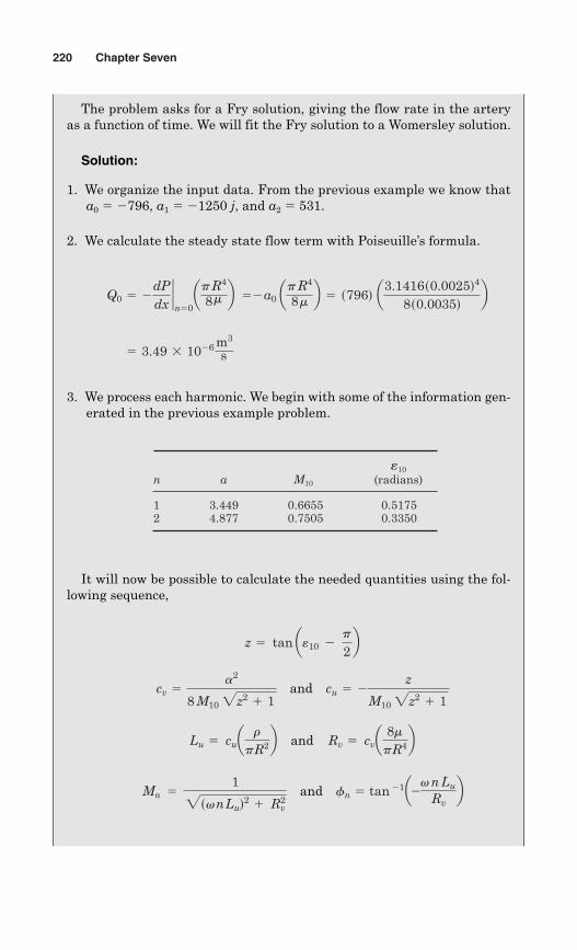
The problem asks for a Fry solution, giving the flow rate in the arteryas a function of time. We will fit the Fry solution to a Womersley solution.
Solution:
1. We organize the input data. From the previous example we know thata0 � 796, a1 � 1250 j, and a2 � 531.
2. We calculate the steady state flow term with Poiseuille’s formula.
3. We process each harmonic. We begin with some of the information gen-erated in the previous example problem.
It will now be possible to calculate the needed quantities using the fol-lowing sequence,
and
and
and fn 5 tan 21a2v n Lu
RvbMn 5
1
2sv n Lud2 1 R2v
Rv 5 cva 8mpR4bLu 5 cua r
pR2b
cu 5 2z
M10 2z2 1 1cv 5
a2
8 M10 2z2 1 1
z 5 tan ae10 2 p
2b
5 3.49 3 1026 m3
s
Q0 5 2dPdx`n50ap R4
8 m b 5 2a0 ap R4
8 mb 5 s796d a3.1416s0.0025d4
8s0.0035db
220 Chapter Seven
�10
n a M10 (radians)
1 3.449 0.6655 0.51752 4.877 0.7505 0.3350
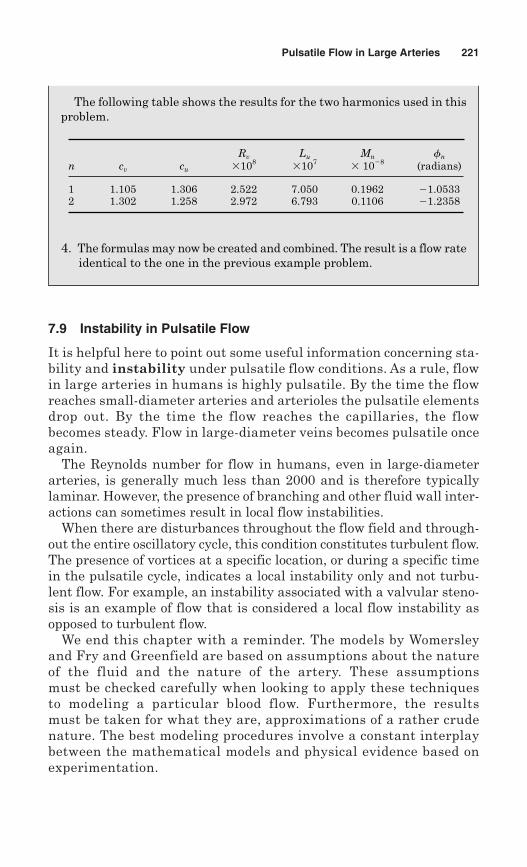
7.9 Instability in Pulsatile Flow
It is helpful here to point out some useful information concerning sta-bility and instability under pulsatile flow conditions. As a rule, flowin large arteries in humans is highly pulsatile. By the time the flowreaches small-diameter arteries and arterioles the pulsatile elementsdrop out. By the time the flow reaches the capillaries, the flowbecomes steady. Flow in large-diameter veins becomes pulsatile onceagain.
The Reynolds number for flow in humans, even in large-diameterarteries, is generally much less than 2000 and is therefore typicallylaminar. However, the presence of branching and other fluid wall inter-actions can sometimes result in local flow instabilities.
When there are disturbances throughout the flow field and through-out the entire oscillatory cycle, this condition constitutes turbulent flow.The presence of vortices at a specific location, or during a specific timein the pulsatile cycle, indicates a local instability only and not turbu-lent flow. For example, an instability associated with a valvular steno-sis is an example of flow that is considered a local flow instability asopposed to turbulent flow.
We end this chapter with a reminder. The models by Womersleyand Fry and Greenfield are based on assumptions about the natureof the fluid and the nature of the artery. These assumptions must be checked carefully when looking to apply these techniquesto modeling a particular blood flow. Furthermore, the results must be taken for what they are, approximations of a rather crudenature. The best modeling procedures involve a constant interplaybetween the mathematical models and physical evidence based onexperimentation.
Pulsatile Flow in Large Arteries 221
The following table shows the results for the two harmonics used in thisproblem.
4. The formulas may now be created and combined. The result is a flow rateidentical to the one in the previous example problem.
Rv Lu Mn fn
n cv cu �108�107
� 108 (radians)
1 1.105 1.306 2.522 7.050 0.1962 1.05332 1.302 1.258 2.972 6.793 0.1106 1.2358
Review Problems
1. You are given a pulsatile flow field which is symmetric about the x-axis.The driving force is a pressure gradient,
Assume this axis is horizontal. You may assume that the flow is incom-pressible.
What form do the Navier–Stokes equations take?
2. Take the complex number, z � 50 16 j. Calculate the following quan-tities:(a) The magnitude of z(b) The argument of z in radians and in degrees(c) The complex conjugate of z
3. You are given two complex numbers z1 � 3 6 j and z2 � 5 � 2 j. Calculate:(a) The sum z1 � z2. Express your answer in both rectangular (a � bj) and
polar (Meju) forms.(b) The difference z2 z1. Express your answer in both forms.(c) The product z1z2. Express your answer in both forms.(d) The quotient z1/z2. Express your answer in both forms.
(The use of a computer is strongly suggested for the remaining problems.)
4. Bessel functions of the kind discussed in this chapter can take complexnumbers as arguments. Say you are given a number z0 � 50 20 j. Usingyour favorite software (Matlab is suggested), calculate:(a) J0(z0)(b) The magnitude of the above number(c) The argument of the above number
5. Take a look at the following triangular pulse function. See Fig. 7.12. Itsmathematical specification over one period, T0 � 1.6, is
fstd 5 • 2.5 t t # 0.42 2 2.5 t 0.4 , t # 0.8
0 otherwise
wsr,td 5 0
vsr,td 5 0
usr,td 5 Re[ fsrd e j v t]
dPdx
5 Re[A e jvt]
222 Chapter Seven
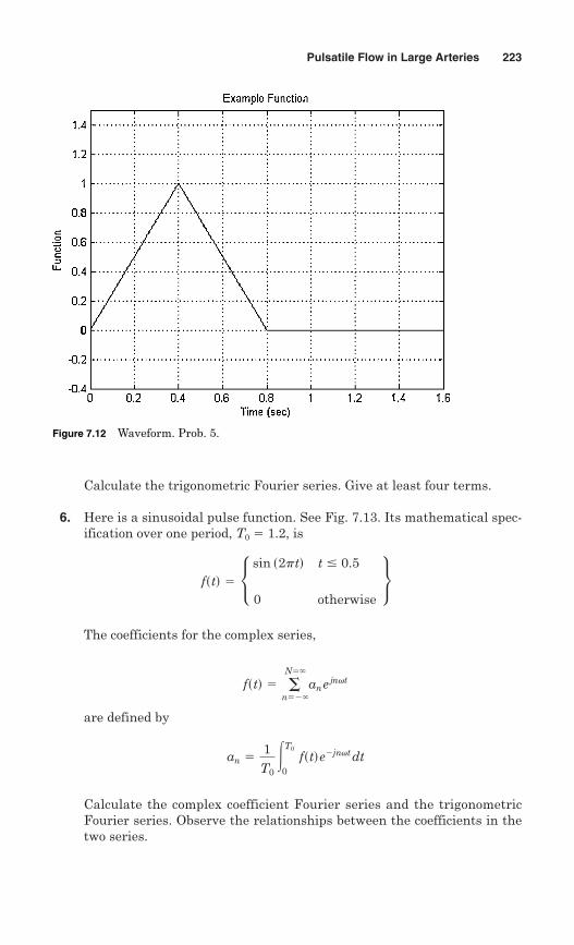
Calculate the trigonometric Fourier series. Give at least four terms.
6. Here is a sinusoidal pulse function. See Fig. 7.13. Its mathematical spec-ification over one period, T0 � 1.2, is
The coefficients for the complex series,
are defined by
Calculate the complex coefficient Fourier series and the trigonometricFourier series. Observe the relationships between the coefficients in thetwo series.
an 51T03
T0
0fstd e2jnvt
dt
fstd 5 �N5`
n52`an e j n v t
fstd 5 • sin s2ptd t # 0.5
0 otherwise
Pulsatile Flow in Large Arteries 223
Figure 7.12 Waveform. Prob. 5.
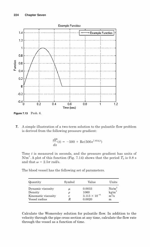
7. A simple illustration of a two-term solution to the pulsatile flow problemis derived from the following pressure gradient:
Time t is measured in seconds, and the pressure gradient has units ofN/m3. A plot of this function (Fig. 7.14) shows that the period T0 is 0.8 sand that v � 2.5p rad/s.
The blood vessel has the following set of parameters.
dPdxstd 5 2500 1 Res500 e7.854 j td
224 Chapter Seven
Figure 7.13 Prob. 6.
Quantity Symbol Value Units
Dynamic viscosity m 0.0033 Ns/m2
Density r 1060 kg/m3
Kinematic viscosity n 3.113 � 106 m2/sVessel radius R 0.0020 m
Calculate the Womersley solution for pulsatile flow. In addition to thevelocity through the pipe cross section at any time, calculate the flow ratethrough the vessel as a function of time.
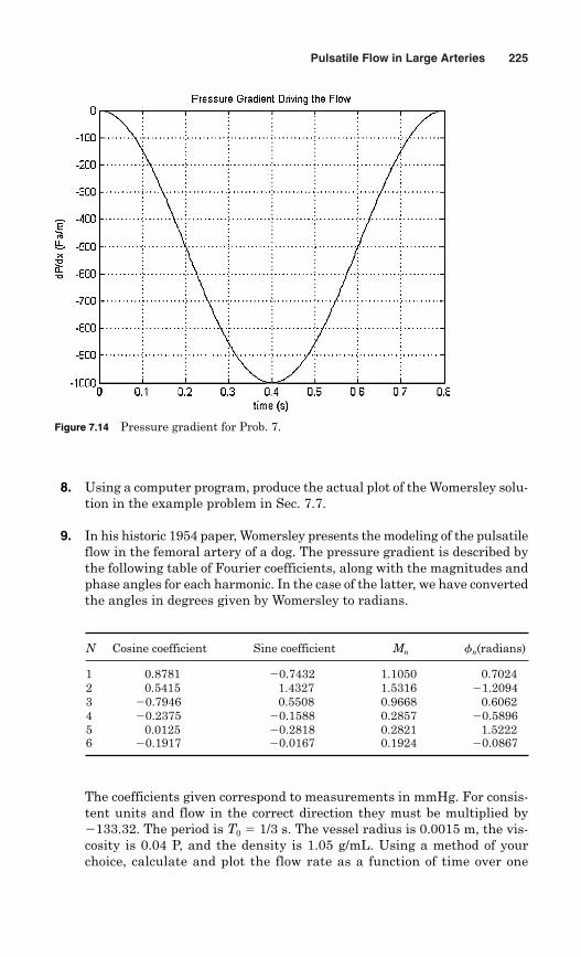
Pulsatile Flow in Large Arteries 225
N Cosine coefficient Sine coefficient Mn fn(radians)
1 0.8781 0.7432 1.1050 0.70242 0.5415 1.4327 1.5316 1.20943 0.7946 0.5508 0.9668 0.60624 0.2375 0.1588 0.2857 0.58965 0.0125 0.2818 0.2821 1.52226 0.1917 0.0167 0.1924 0.0867
8. Using a computer program, produce the actual plot of the Womersley solu-tion in the example problem in Sec. 7.7.
9. In his historic 1954 paper, Womersley presents the modeling of the pulsatileflow in the femoral artery of a dog. The pressure gradient is described bythe following table of Fourier coefficients, along with the magnitudes andphase angles for each harmonic. In the case of the latter, we have convertedthe angles in degrees given by Womersley to radians.
The coefficients given correspond to measurements in mmHg. For consis-tent units and flow in the correct direction they must be multiplied by133.32. The period is T0 � 1/3 s. The vessel radius is 0.0015 m, the vis-cosity is 0.04 P, and the density is 1.05 g/mL. Using a method of yourchoice, calculate and plot the flow rate as a function of time over one
Figure 7.14 Pressure gradient for Prob. 7.
period. You may wish to compare your results with the plots on page 559of Womersley’s paper. (Your plotting software is probably much better thanWomersley’s, so don’t expect perfect agreement.) If you wish to avoid theuse of Bessel functions, you can employ the table below which lists thequantities a, M10, and e10. The latter angles are presented in radians.
226 Chapter Seven
n a �10
1 3.34 0.6651 1.08152 4.72 0.7436 0.69643 5.78 0.7839 0.55214 6.67 0.8096 0.47125 7.46 0.8278 0.41716 8.17 0.8416 0.3752
Mr10
10. A previous problem specifies pressure gradient:
where time t is measured in seconds, and the pressure gradient has unitsof N/m3. The blood vessel has the following set of parameters:
dPdxstd 5 2500 1 Res500 e7.854 j td 5 2500 1 500 cos s7.854 td
Quantity Symbol Value Units
Dynamic viscosity m 0.0033 Ns/m2
Density r 1060 kg/m3
Kinematic viscosity n 3.113 � 106 m2/sVessel radius R 0.0020 m
Calculate the Fry solution to the problem. Use the Womersley solution tocalibrate your Fry solution. Present the results with plots.
11. The pressure gradient in the artery of a pig has been measured and digi-tized. The sampling rate was 512/s. Figure 7.15 is a plot of that data. Thedata are accessible at the text website at http://www.mhprofessional.com/product.php?isbn=0071472177. Represent theses data with a 10-termFourier series. Use the Fast Fourier Transform to calculate the Fouriercoefficients.
12. Given the vessel data from prob. 10 and pressure gradient data fromprob. 11, construct a 10-term Womersley solution to the previous problem.
13. Continue the previous problem by constructing a Fry solution whichmatches the Womersley solution.
14. Using a software tool of your choice, create a computer program whichinputs the Fourier coefficients and fundamental frequency of the pressure
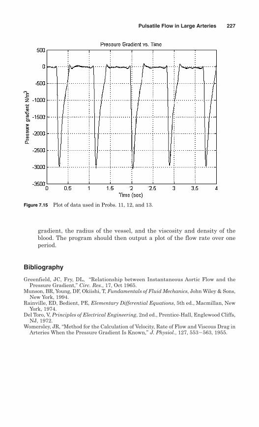
gradient, the radius of the vessel, and the viscosity and density of theblood. The program should then output a plot of the flow rate over oneperiod.
Bibliography
Greenfield, JC, Fry, DL, “Relationship between Instantaneous Aortic Flow and thePressure Gradient,” Circ. Res., 17, Oct 1965.
Munson, BR, Young, DF, Okiishi, T, Fundamentals of Fluid Mechanics, John Wiley & Sons,New York, 1994.
Rainville, ED, Bedient, PE, Elementary Differential Equations, 5th ed., Macmillan, NewYork, 1974.
Del Toro, V, Principles of Electrical Engineering, 2nd ed., Prentice-Hall, Englewood Cliffs,NJ, 1972.
Womersley, JR, “Method for the Calculation of Velocity, Rate of Flow and Viscous Drag inArteries When the Pressure Gradient Is Known,” J. Physiol., 127, 553563, 1955.
Pulsatile Flow in Large Arteries 227
Figure 7.15 Plot of data used in Probs. 11, 12, and 13.

This page intentionally left blank
Chapter
8Flow and Pressure Measurement
8.1 Introduction
From the measurement system for measuring hypertension in humanswith an indirect method, to the system for measurement of flow andpressure waveforms in the uterine artery of cows, flow and pressuremeasurement systems have wide-ranging applications in biology andmedicine. A few of the varied methods for making these measurementsare discussed below.
Measurements of flow and pressure are two of the most importantmeasurements in biological and medical applications. Because there isa complex control system in the human body controlling pressure andflow, the interactions of the measuring system with the physiologicalcontrol system increase the complexity of the measurement. The inva-sive nature of flow and pressure measurement also makes it difficult toobtain accurate measurements in some cases. Sometimes, a noninvasiveor indirect measurement is possible.
According to the American Heart Association Council on High BloodPressure Research, accurate measurement of blood pressure is critical to thediagnosis and management of individuals with hypertension. Dr. ThomasPickering et al. (2005) write, “The ausculatory (indirect measurement) tech-nique with a trained observer and mercury sphygmomanometer continuesto be the method of choice for measurement in the office.”
8.2 Indirect Pressure Measurements
An important example of a noninvasive, indirect measurement is themeasurement of blood pressure using a sphygmomanometer. This typeof measurement is routinely used in clinical practice because of its rel-ative ease and low cost.
229
Copyright © 2007 by The McGraw-Hill Companies, Inc. Click here for terms of use.
A sphygmomanometer has a cuff that can be wrapped around apatient’s arm and inflated with air. The device includes a means for pres-surizing the cuff, and a gauge for monitoring the pressure inside the cuff.When the pressure inside the cuff is increased above the patient’s sys-tolic pressure, the cuff squeezes the arm, and blood flow through the ves-sels directly under the cuff is completely blocked. The pressure insidethe cuff is released slowly, and when the cuff pressure falls below thepatient’s systolic pressure, blood can spurt through arteries in the armbeneath the cuff. The operator measuring blood pressure typically placesa stethoscope distal to the cuff and just over the brachial artery.Turbulent flow of blood through the compressed artery makes audiblesounds, known as Korotkoff sounds. At the time these Korotkoffsounds are initially detected, the blood pressure is noted, and this valuebecomes the measurement of the systolic pressure.
The nature of the sound heard through the stethoscope changes as thesphygmomanometer pressure continues to drop. The sounds change froma repetitive tapping sound to a muffled rumble and then the sound finallydisappears. The pressure is once again noted at the instant that thesounds completely disappear. This value is the diastolic blood pressure.
Indirect measurement of blood pressure using a sphygmomanometerhas the advantage of being noninvasive, inexpensive, and reliable. Onedisadvantage of the system is the relative inaccuracy of the systemassociated with operator error, relatively low resolution, and the diffi-culty of measuring the diastolic pressure. Since the measurement ofdiastolic pressure depends on the detection of the absence of sound, themethod is inherently dependent on the ability of the operator to clearlyhear very quiet sounds and to judge the point in time at which thosesounds disappear.
8.2.1 Indirect pressure gradientmeasurements using Doppler ultrasound
By using echocardiography, it is possible to make an indirect meas-urement of pressure gradients at specific locations in the cardiovascu-lar system that are estimated from changing blood velocities. Özyurdaet al. (2005) used echocardiography to indirectly measure pressure gra-dients in 400 patients with aortic or mitral valve replacement withprosthetic heart valves. The Bernoulli equation (see also Sec. 6.4.3) wasused to calculate pressure gradient across the prosthesis.
where P was the pressure gradient, or pressure drop across the valve,V2 represents blood velocity through the valve, V1 represents the left
P 5r
2 AV 2
2 2 V 21 B
230 Chapter Eight
ventricular outflow tract velocity (the velocity leaving the ventricle), andr is blood density.
The authors of the study calculated pressure gradients in mmHgusing multiple instantaneous velocities through the valve, throughoutthe velocity profile. The average of all such instantaneous pressure gra-dients was reported as the mean pressure gradient. While the applica-tion of the Bernoulli equation ignores frictional losses across the valve,this method provides a noninvasive, clinically meaningful estimate ofpressure gradient across the valve. The authors of the study reportedthe equation they used as the “modified Bernoulli equation,” which wasreported as:
where velocities are reported in m/s and pressure gradients are reportedin mmHg.
8.3 Direct Pressure Measurement
When more accurate pressure measurements are required, it becomesnecessary to make a direct measurement of blood pressure. Two meth-ods that are described below involve using either an intravascularcatheter with a strain gauge measuring transducer on its tip or anextravascular transducer connected to the patient by a saline-filled tube.
8.3.1 Intravascular—strain gauge tippedpressure transducer
Transducers are devices that convert energy from one form to another.It is often desirable to have electrical output represent a parameter likeblood pressure or blood flow. Typically, these devices convert some typeof mechanical energy to electrical energy. For example, most pressure-measuring transducers convert stored energy in the form of pressure intoelectrical energy, perhaps measured as a voltage.
A pressure transducer very often uses a strain gauge to measurepressure. We can begin the topic of strain gauge-tipped pressure trans-ducers by considering strain. Figure 8.1 shows a member under asimple uniaxial load in order to demonstrate the concept of strain. Asthe load causes the member to stretch some amount L, strain can bemeasured as L/L. A strain gauge could be bonded onto a diaphragmon a catheter tip.
Two advantages of a strain gauge pressure transducer, compared toan extravascular pressure transducer described in Sec. 8.3.2, are goodfrequency response, and fewer problems associated with blood clots.
P 5 r
2AV
22 2 V
21 B 5
1060 kg/m3
2s133dPa/mmHgAV
22 2 V
21 Bms 5 4 AV
22 2 V
21 B
Flow and Pressure Measurement 231
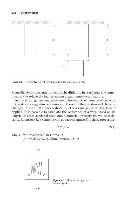
Some disadvantages might include the difficulty in sterilizing the trans-ducers, the relatively higher expense, and transducer fragility.
As the strain gauge lengthens due to the load, the diameter of the wirein the strain gauge also decreases and therefore the resistance of the wirechanges. Figure 8.2 shows a drawing of a strain gauge with a load Fapplied. It is possible to calculate the resistance of a wire based on itslength, its cross-sectional area, and a material property known as resis-tivity. Equation (8.1) relates strain gauge resistance R to those properties.
(8.1)
where R � resistance, in Ohms, �r� resistivity, in Ohm ⋅ meters, � ⋅ m
R 5 rL/A
232 Chapter Eight
Figure 8.1 Demonstration of strain in a tensile specimen, L/L.
F
F
Figure 8.2 Strain gauge withforce F applied.
L L
∆L
P
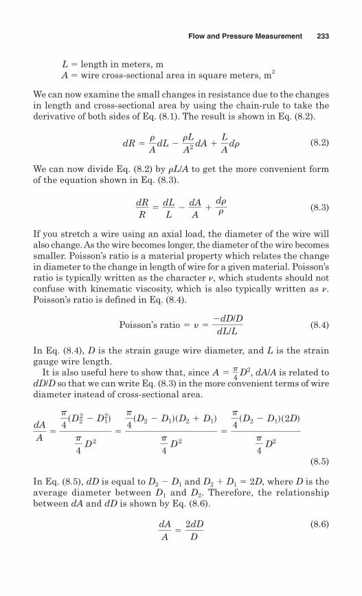
L � length in meters, mA � wire cross-sectional area in square meters, m2
We can now examine the small changes in resistance due to the changesin length and cross-sectional area by using the chain-rule to take thederivative of both sides of Eq. (8.1). The result is shown in Eq. (8.2).
(8.2)
We can now divide Eq. (8.2) by rL/A to get the more convenient formof the equation shown in Eq. (8.3).
(8.3)
If you stretch a wire using an axial load, the diameter of the wire willalso change. As the wire becomes longer, the diameter of the wire becomessmaller. Poisson’s ratio is a material property which relates the changein diameter to the change in length of wire for a given material. Poisson’sratio is typically written as the character n, which students should notconfuse with kinematic viscosity, which is also typically written as n.Poisson’s ratio is defined in Eq. (8.4).
(8.4)
In Eq. (8.4), D is the strain gauge wire diameter, and L is the straingauge wire length.
It is also useful here to show that, since , dA/A is related todD/D so that we can write Eq. (8.3) in the more convenient terms of wirediameter instead of cross-sectional area.
(8.5)
In Eq. (8.5), dD is equal to D2 D1 and D2 � D1 � 2D, where D is theaverage diameter between D1 and D2. Therefore, the relationshipbetween dA and dD is shown by Eq. (8.6).
(8.6)dAA5
2dDD
dAA5
p
4sD2
2 2 D21d
p
4 D2
5
p
4sD2 2 D1dsD2 1 D1d
p
4 D2
5
p
4sD2 2 D1ds2Dd
p
4 D2
A 5p
4 D2
Poisson’s ratio 5 y 52dD/DdL/L
dRR5
dLL2
dAA1
drr
dR 5r
A dL 2
rLA2 dA 1
LA
dr
Flow and Pressure Measurement 233
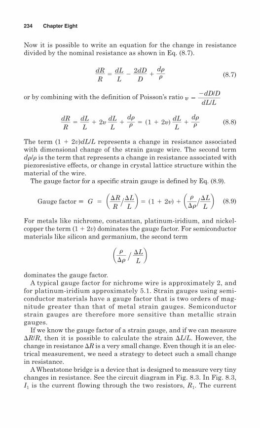
Now it is possible to write an equation for the change in resistancedivided by the nominal resistance as shown in Eq. (8.7).
(8.7)
or by combining with the definition of Poisson’s ratio
(8.8)
The term (1 � 2v)dL/L represents a change in resistance associatedwith dimensional change of the strain gauge wire. The second term dr/r is the term that represents a change in resistance associated withpiezoresistive effects, or change in crystal lattice structure within thematerial of the wire.
The gauge factor for a specific strain gauge is defined by Eq. (8.9).
(8.9)
For metals like nichrome, constantan, platinum-iridium, and nickel-copper the term (1 � 2v) dominates the gauge factor. For semiconductormaterials like silicon and germanium, the second term
dominates the gauge factor.A typical gauge factor for nichrome wire is approximately 2, and
for platinum-iridium approximately 5.1. Strain gauges using semi-conductor materials have a gauge factor that is two orders of mag-nitude greater than that of metal strain gauges. Semiconductorstrain gauges are therefore more sensitive than metallic straingauges.
If we know the gauge factor of a strain gauge, and if we can measureR/R, then it is possible to calculate the strain L/L. However, thechange in resistance R is a very small change. Even though it is an elec-trical measurement, we need a strategy to detect such a small changein resistance.
A Wheatstone bridge is a device that is designed to measure very tinychanges in resistance. See the circuit diagram in Fig. 8.3. In Fig. 8.3,I1 is the current flowing through the two resistors, R1. The current
a rr
> LLb
Gauge factor ; G 5 aRR>L
Lb 5 s1 1 2yd 1 a r
r>LLb
dRR5
dLL1 2y dL
L1
drr 5 s1 1 2yd dL
L1
drr
y 52dD/DdL/L
dRR5
dLL2
2dDD
1drr
234 Chapter Eight
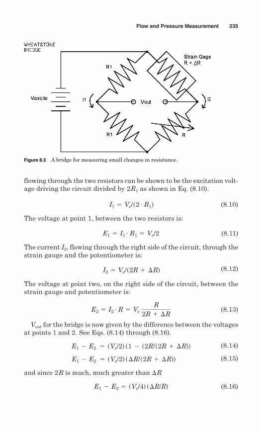
flowing through the two resistors can be shown to be the excitation volt-age driving the circuit divided by 2R1 as shown in Eq. (8.10).
(8.10)
The voltage at point 1, between the two resistors is:
(8.11)
The current I2, flowing through the right side of the circuit, through thestrain gauge and the potentiometer is:
(8.12)
The voltage at point two, on the right side of the circuit, between thestrain gauge and potentiometer is:
(8.13)
Vout for the bridge is now given by the difference between the voltagesat points 1 and 2. See Eqs. (8.14) through (8.16).
(8.14)
(8.15)
and since 2R is much, much greater than
(8.16)E1 2 E2 5 sVe/4d sR/Rd
R
E1 2 E2 5 sVe/2d sR/s2R 1 Rdd
E1 2 E2 5 sVe/2d s1 2 s2R/s2R 1 Rdd
E2 5 I2 # R 5 Ve R
2R 1 R
I2 5 Ve/s2R 1 Rd
E1 5 I1 # R1 5 Ve/2
I1 5 Ve/s2 # R1d
Flow and Pressure Measurement 235
Figure 8.3 A bridge for measuring small changes in resistance.
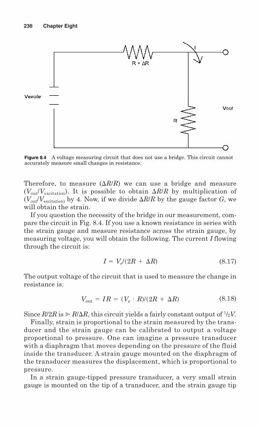
Therefore, to measure (R/R) we can use a bridge and measure(Vout/Vexcitation). It is possible to obtain R/R by multiplication of(Vout/Vexcitation) by 4. Now, if we divide R/R by the gauge factor G, wewill obtain the strain.
If you question the necessity of the bridge in our measurement, com-pare the circuit in Fig. 8.4. If you use a known resistance in series withthe strain gauge and measure resistance across the strain gauge, bymeasuring voltage, you will obtain the following. The current I flowingthrough the circuit is:
(8.17)
The output voltage of the circuit that is used to measure the change inresistance is:
(8.18)
Since R/2R is � R/R, this circuit yields a fairly constant output of 1/2V.Finally, strain is proportional to the strain measured by the trans-
ducer and the strain gauge can be calibrated to output a voltageproportional to pressure. One can imagine a pressure transducerwith a diaphragm that moves depending on the pressure of the fluidinside the transducer. A strain gauge mounted on the diaphragm ofthe transducer measures the displacement, which is proportional topressure.
In a strain gauge-tipped pressure transducer, a very small straingauge is mounted on the tip of a transducer, and the strain gauge tip
Vout 5 I R 5 sVe # Rd/s2R 1 Rd
I 5 Ve/s2R 1 Rd
236 Chapter Eight
Figure 8.4 A voltage measuring circuit that does not use a bridge. This circuit cannotaccurately measure small changes in resistance.
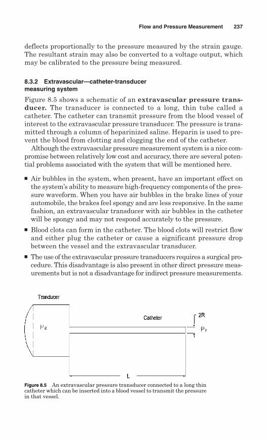
Flow and Pressure Measurement 237
deflects proportionally to the pressure measured by the strain gauge.The resultant strain may also be converted to a voltage output, whichmay be calibrated to the pressure being measured.
8.3.2 Extravascular—catheter-transducermeasuring system
Figure 8.5 shows a schematic of an extravascular pressure trans-ducer. The transducer is connected to a long, thin tube called acatheter. The catheter can transmit pressure from the blood vessel ofinterest to the extravascular pressure transducer. The pressure is trans-mitted through a column of heparinized saline. Heparin is used to pre-vent the blood from clotting and clogging the end of the catheter.
Although the extravascular pressure measurement system is a nice com-promise between relatively low cost and accuracy, there are several poten-tial problems associated with the system that will be mentioned here.
■ Air bubbles in the system, when present, have an important effect onthe system’s ability to measure high-frequency components of the pres-sure waveform. When you have air bubbles in the brake lines of yourautomobile, the brakes feel spongy and are less responsive. In the samefashion, an extravascular transducer with air bubbles in the catheterwill be spongy and may not respond accurately to the pressure.
■ Blood clots can form in the catheter. The blood clots will restrict flowand either plug the catheter or cause a significant pressure dropbetween the vessel and the extravascular transducer.
■ The use of the extravascular pressure transducers requires a surgical pro-cedure. This disadvantage is also present in other direct pressure meas-urements but is not a disadvantage for indirect pressure measurements.
Figure 8.5 An extravascular pressure transducer connected to a long thincatheter which can be inserted into a blood vessel to transmit the pressurein that vessel.
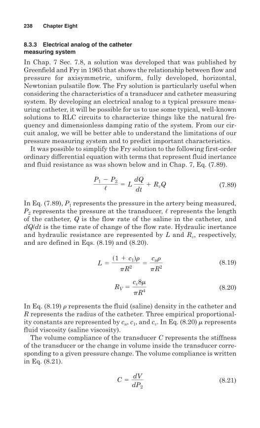
238 Chapter Eight
8.3.3 Electrical analog of the cathetermeasuring system
In Chap. 7 Sec. 7.8, a solution was developed that was published byGreenfield and Fry in 1965 that shows the relationship between flow andpressure for axisymmetric, uniform, fully developed, horizontal,Newtonian pulsatile flow. The Fry solution is particularly useful whenconsidering the characteristics of a transducer and catheter measuringsystem. By developing an electrical analog to a typical pressure meas-uring catheter, it will be possible for us to use some typical, well-knownsolutions to RLC circuits to characterize things like the natural fre-quency and dimensionless damping ratio of the system. From our cir-cuit analog, we will be better able to understand the limitations of ourpressure measuring system and to predict important characteristics.
It was possible to simplify the Fry solution to the following first-orderordinary differential equation with terms that represent fluid inertanceand fluid resistance as was shown below and in Chap. 7, Eq. (7.89).
(7.89)
In Eq. (7.89), P1 represents the pressure in the artery being measured,P2 represents the pressure at the transducer, represents the lengthof the catheter, Q is the flow rate of the saline in the catheter, anddQ/dt is the time rate of change of the flow rate. Hydraulic inertanceand hydraulic resistance are represented by L and Rv, respectively,and are defined in Eqs. (8.19) and (8.20).
(8.19)
(8.20)
In Eq. (8.19) r represents the fluid (saline) density in the catheter andR represents the radius of the catheter. Three empirical proportional-ity constants are represented by cu, c1, and cv. In Eq. (8.20) representsfluid viscosity (saline viscosity).
The volume compliance of the transducer C represents the stiffnessof the transducer or the change in volume inside the transducer corre-sponding to a given pressure change. The volume compliance is writtenin Eq. (8.21).
(8.21)C 5dVdP2
m
RV 5cv8m
pR4
L 5s1 1 c1dr
pR25
cur
pR2
/
P1 2 P2
/ 5 L dQ
dt1 RvQ
Flow and Pressure Measurement 239
By separating variables and integrating with respect to time, it is pos-sible to solve for flow rate Q as a function of the change in the pressurein the transducer as shown in Eqs. (8.22) and (8.23).
(8.22)
(8.23)
The time rate of change of Q, as a function of compliance and P2, cannow be written:
(8.24)
Now it becomes possible to substitute Eqs. (8.23) and (8.24) intoEq. (7.89) above.
(8.25)
L and Rv are defined by Eqs. (8.19) and (8.20), respectively. C is thevolume compliance of the transducer. The length of the catheter is rep-resented by , and the pressures in the blood vessel and the transducerare P1 and P2, respectively.
Next rewrite the derivative terms in the somewhat simplified formwhere and we arrive at Eq. (8.26).
(8.26)
Now we can define a term, E, that is equal to 1/C or the inverse of thevolume compliance of the transducer. The term E is known as the volumemodulus of elasticity of the transducer. Then, by multiplying both sidesof the equation by the catheter length, , we arrive at Eq. (8.27). Noticethat Eq. (8.27) is a second-order, linear, ordinary, differential equationwith driving function EP1. This type of equation is typical in many,many types of electrical and mechanical applications and one that wewill use several times.
(8.27)
For the mechanical analog system shown in Fig. 8.6, the equation definesa typical spring, mass, damper system where the spring constant is
/
/LCP$
2 1 /RvCP.
2 1 P2 5 P1
dPdt is written as P
. and d
2Pdt2 5 P
$
/
LC d2P2
dt2 1 RvC
dP2
dt 5
P1 2 P2
/
dQ
dt 5 C
d2P2
dt2
Q 5dVdt
5 C dP2
dt
dV 5 C dP2
/LP$
2 1 /RvP.
2 1 E P2 5 EP1{k
{m
{b
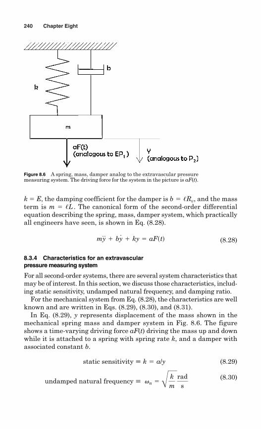
240 Chapter Eight
Figure 8.6 A spring, mass, damper analog to the extravascular pressuremeasuring system. The driving force for the system in the picture is aF(t).
k � E, the damping coefficient for the damper is , and the massterm is m � . The canonical form of the second-order differentialequation describing the spring, mass, damper system, which practicallyall engineers have seen, is shown in Eq. (8.28).
(8.28)
8.3.4 Characteristics for an extravascularpressure measuring system
For all second-order systems, there are several system characteristics thatmay be of interest. In this section, we discuss those characteristics, includ-ing static sensitivity, undamped natural frequency, and damping ratio.
For the mechanical system from Eq. (8.28), the characteristics are wellknown and are written in Eqs. (8.29), (8.30), and (8.31).
In Eq. (8.29), y represents displacement of the mass shown in themechanical spring mass and damper system in Fig. 8.6. The figureshows a time-varying driving force aF(t) driving the mass up and downwhile it is attached to a spring with spring rate k, and a damper withassociated constant b.
(8.29)
(8.30)undamped natural frequency ; vn 5 Å km
rads
static sensitivity ; k 5 a/y
my$1 by
.1 ky 5 aFstd
/Lb 5 /Rv
Flow and Pressure Measurement 241
8.3.5 Example problem—characteristicsof an extravascular measuring system
A liquid-filled catheter, 100 cm long, with an internal radius of 0.92 mm, isconnected to a strain gauge pressure sensor. The curve in Fig. 8.7 shows a
(8.31)
By making the appropriate substitutions from Eq. (8.27), we can nowsolve for the specific characteristics associated with our extravascularpressure measurement system.
(8.27)
For the static system, displacement y does not change. In the pressuremeasuring system, the pressure does not change. All of the higher-order terms like are now zero. For the pressure meas-uring system, it is desirable that for every pressure input an equivalentpressure output occurs, so let us design the static gain to be unity.Equation (8.28) for the static system is:
(8.28)
For the analogous pressure measuring system k � E and a � E so thestatic sensitivity is one, or E/E.
Again, this means simply that the measurement system is designedto measure the input value and repeat it as the output value.
The undamped natural frequency and dimensionless damping ratioof the system are given by Eqs. (8.32) and (8.33).
(8.32)
(8.33)
Sections 8.3.6 and 8.3.7 describe two examples of second-order, pressuremeasuring systems. Case 1 is an undamped catheter measuring system,and Case 2 is the undriven, damped system.
Damping ratio ; z 5/Rv
22E/L5
/cv8mp R4
2ÅE/cur
pR2
Undamped natural frequency ; vn 5 Å E/L
rads5 ÅEpR2
/cur rads
my$1 b y
.1 ky 5 aFstd� � � � or� � � � ky 5 aFstd
y., y$, P
.2 and P
$2
/L P$
2 1 /Rv P.
2 1 E P2 5 E P1
damping ratio ; z 5 b
22km5
bbcr
{m
{
{k
{a
0{0
{b
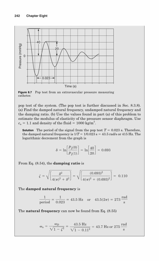
242 Chapter Eight
pop test of the system. (The pop test is further discussed in Sec. 8.3.8). (a) Find the damped natural frequency, undamped natural frequency andthe damping ratio. (b) Use the values found in part (a) of this problem toestimate the modulus of elasticity of the pressure sensor diaphragm. Usecu � 1.1 and density of the fluid � 1000 kg/m3.
Solution The period of the signal from the pop test T � 0.023 s. Therefore,the damped natural frequency is 1/T � 1/0.023 s � 43.5 rad/s or 415 Hz. Thelogarithmic decrement from the graph is
From Eq. (8.54), the damping ratio is
The damped natural frequency is
The natural frequency can now be found from Eq. (8.55)
vn 5vD
21 2 z2 543.5 Hz
21 2 0.1125 43.7 Hz or 275
rads
1period
51
0.0235 43.5 Hz� � or� � 43.5s2pd 5 273
rads
z 5 Å c d2
4spd2 1 d2d 5 Å c s0.693d2
4spd2 1 s0.693d2d 5 0.110
d 5 ln cP2s0d
P2s1dd 5 ln c40
20d 5 0.693
Time (s)
Pre
ssur
e (m
mH
g)
0.023
20
40
0
Figure 8.7 Pop test from an extravascular pressure measuringcatheter.
Flow and Pressure Measurement 243
8.3.6 Case 1: the undamped cathetermeasurement system
For the special case of a driven, undamped catheter measuring system wecan now estimate some of the characteristics of the system. An undampedsystem would be one in which the viscosity of the fluid in the catheter, andtherefore the corresponding hydraulic resistance in the catheter, are verysmall; therefore close to zero. A practical example of an undamped meas-uring system is one in which the viscosity is very small compared to themass of the system. A relatively large diameter catheter, with no air bub-bles and with a relatively low viscosity fluid like water, and relatively lowtotal volume displacement would behave in this way. A system like thiscould have a very fast response time but would be susceptible to “catheterwhip,” or noise associated with accelerations at the catheter tip.
For this case recognize that viscosity m, viscous resistance Rv, and thedamping coefficient b are all approximately equal to zero. Then recallthe expression for undamped natural frequency in Eq. (8.32). We canalready see that the damping ratio is zero for this undamped system,and we could predict the natural frequency from Eq. (8.32).
(8.32)
(8.33)
Going a step further, we would also like to predict the output of the pres-sure measuring system for every input. If P1 is the input pressure to thesystem, then we would like the pressure output P2 to be equal to P1 forany input frequency. Let’s set the input, or driving pressure, to be P1 cos(vt). The output of the system or the pressure at the transducer isnow P2 cos(vt). Recall the governing differential equation from Eq. (8.27).
(8.27)
Now after solving for the first and second derivative of P2, the expres-sions below can be substituted into Eq. (8.27).
(8.34)
(8.35)
(8.36)P$
2 5 2v2P2 cos svtd
P.
2 5 2vP2 sin svtd
P2 5 P2 cos svtd
/LP$
2 1 /RvP.
2 1 EP2 5 EP1
damping ratio ; z 5/Rv
22E/L5 0
undamped natural frequency ; vn 5 Å E/L
rads5 ÅEpR2
/cur rads
m > 0 Rv > 0 b > 0
244 Chapter Eight
Equation (8.27) now becomes Eq. (8.37). Note that P2 now representsa constant.
(8.37)
Since Rv is equal to zero for this case, the second term drops out andwe can divide through by cos(vt). The result is Eq. (8.38).
(8.38)
Solving for P2 yields Eq. (8.39).
(8.39)
Now using the definition of vn from Eq. (8.32) we can finally solve forthe transfer function, P2/P1 as shown in Eq. (8.41).
(8.40)
(8.41)
Finally, Fig. 8.8 shows the response of the second-order, undamped,catheter pressure measuring system. Note that there is significantamplification of the signal as the input frequency approaches the nat-ural frequency of the system.
8.3.7 Case 2: the undriven, damped catheter measurement system
A damped system would be one in which the viscosity of the fluid in thecatheter, and therefore the corresponding hydraulic resistance in thecatheter, are relatively large; therefore significant. A practical exampleof a damped measuring system, is one in which the viscosity is relativelylarge compared to the mass of the system. A relatively small diametercatheter, with air bubbles or perhaps with a crimp in the tubing, andwith a relatively high viscosity fluid like blood, might behave in this way.A system like this could have a relatively low response time but might
P2
P15
1
c1 2 v2
vn2d
1vn
2 5/LE
P2 5EP1
sE 2 /Lv2d5
P1
a1 2 /Lv2
Eb
/Ls2v2dP2 1 EP2 5 EP1
5 EP1 cos svtd
/Ls2v2dP2 cossvtd1 /Rvs2vdP2 sinsvtd 1 EP2 cossvtd
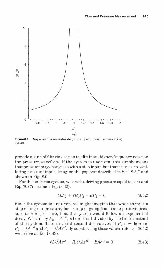
Flow and Pressure Measurement 245
provide a kind of filtering action to eliminate higher-frequency noise onthe pressure waveform. If the system is undriven, this simply meansthat pressure may change, as with a step input, but that there is no oscil-lating pressure input. Imagine the pop test described in Sec. 8.3.7 andshown in Fig. 8.9.
For the undriven system, we set the driving pressure equal to zero andEq. (8.27) becomes Eq. (8.42).
(8.42)
Since the system is undriven, we might imagine that when there is astep change in pressure, for example, going from some positive pres-sure to zero pressure, that the system would follow an exponentialdecay. We can try , where l is 1 divided by the time constantof the system. The first and second derivatives of P2 now become
and . By substituting those values into Eq. (8.42)we arrive at Eq. (8.43).
(8.43)/Ll2Aelt 1 Rv/lAelt 1 EAelt 5 0
P$
2 5 l2AeltP
.2 5 lAelt
P2 5 Aelt
/LP$
2 1 /RvP.
2 1 EP2 5 0
0.2 0.4 0.6 0.8 1 1.2 1.4 1.6 1.8 20
2
4
6
8
10
P2
P1
ω2
ωn2
Figure 8.8 Response of a second-order, undamped, pressure measuringsystem.
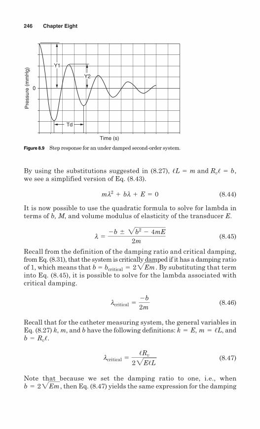
By using the substitutions suggested in (8.27), ,we see a simplified version of Eq. (8.43).
(8.44)
It is now possible to use the quadratic formula to solve for lambda interms of b, M, and volume modulus of elasticity of the transducer E.
(8.45)
Recall from the definition of the damping ratio and critical damping,from Eq. (8.31), that the system is critically damped if it has a damping ratioof 1, which means that b � . By substituting that terminto Eq. (8.45), it is possible to solve for the lambda associated withcritical damping.
(8.46)
Recall that for the catheter measuring system, the general variables inEq. (8.27) k, m, and b have the following definitions: and
.
(8.47)
Note that because we set the damping ratio to one, i.e., when, then Eq. (8.47) yields the same expression for the dampingb 5 22Em
lcritical 5/Rv
22E/L
b 5 Rv/k 5 E, m 5 /L,
lcritical 52b2m
bcritical 5 22Em
l 52b 6 2b2 2 4mE
2m
ml2 1 bl 1 E 5 0
/L 5 m and Rv/ 5 b
246 Chapter Eight
Time (s)
Pre
ssur
e (m
mH
g)
Td
Y2
Y1
0
Figure 8.9 Step response for an under damped second-order system.
Flow and Pressure Measurement 247
ratio in Eq. (8.33). Again, l is one over the time constant of the systemand z is the dimensionless damping ratio.
(8.33)
The output of our system is therefore defined by the expression shownin Eq. (8.48).
(8.48)
where and . Substituting into Eq. (8.48)also yields
(8.49)
Comparing the definition for the natural frequency from Eq. (8.32), wefind that we now have an expression for critically damped catheters thatrelates the output of the measuring system to the natural frequency ofthe catheter.
(8.50)
Critically damped systems are a very important case. This kind ofsystem is on the borderline, but does not oscillate as it returns to equi-librium after perturbation. This disturbance is damped out as quicklyas possible, as in the case of a door closer designed to close a screen dooras quickly as possible with no back and forth motion.
The critical time constant for the system is 1/lcritical as shown inEq. (8.51).
(8.51)
It is useful to point out that Eqs. (8.52) and (8.53) are general expres-sions for the catheter measuring system and not a special case for thecritically damped system.
(8.52)
(8.53)vn 5 Å km5 Å E
/L
z 5b
22EM5
Rv/22E/L
critical time constant 52mb5
2/LRv/
52LRv
5curo
2
cv4y
P2 5 Ae2vnt 1 B t e2vnt
P2 5 Ae22E
mt1 B t e
22Em
t
b 5 22Emm 5 /Lb 5 Rv/
P2 5 Aelt 1 Btelt 5 Ae2 A b
2m Bt 1 Bte2 A b
2m Bt
damping ratio ; z 5/Rv
22E/L
8.3.8 Pop test—measurement of transientstep response
One way to determine some characteristics of a second-order system isto create a step input to the system and measure the response. Onestraightforward and simple method of measuring the system responseis to input a step change into the system by popping a balloon or surgi-cal glove and measuring the response. Imagine a catheter with one endconnected to a pressure transducer and the other end inserted into a con-tainer covered with a balloon or surgical glove. If the system is pres-surized and the balloon or glove is popped, the resulting pressure outputfrom the system looks like that shown in Fig. 8.9. The original steadystate pressure was Y1 and the pressure output of the transducer oscil-lates back and forth around zero, depending on the characteristics of thepressure measuring system.
The period of the oscillation is labeled TD in Fig. 8.9. The damped nat-ural frequency of the system, measured in radians per second, is givenby the equation . The logarithmic decrement is given as d and
is defined by the equation
The damping ratio of the pressure measuring system can now be cal-culated from the logarithmic decrement as shown in Eq. (8.54).
(8.54)
The relationship between the natural frequency, the damped naturalfrequency, and the damping ratio is shown in Eq. (8.55).
(8.55)
By measuring the amplitude ratio of successive positive peaks, it is pos-sible to determine the logarithmic decrement of the system. From thelogarithmic decrement it then becomes straightforward to measure thedamped natural frequency, the damping ratio, and the undamped nat-ural frequency.
If the natural frequency of the catheter measuring system is verylow, some relatively low frequency harmonics of the pressure waveformcan be amplified, distorting the pressure waveform significantly. If pos-sible, choose a catheter-transducer measuring system with a natural fre-quency that is 10 times greater than the highest harmonic frequency ofinterest in the pressure waveform.
vD
vn5 21 2 z2
z 5 Å c d2
4spd2 1 d2 d
d 5 ln cP2s0dP2s1d
d
vD 52pTD
248 Chapter Eight
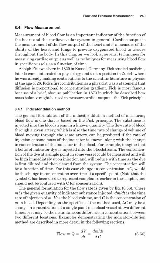
8.4 Flow Measurement
Measurement of blood flow is an important indicator of the function ofthe heart and the cardiovascular system in general. Cardiac output isthe measurement of the flow output of the heart and is a measure of theability of the heart and lungs to provide oxygenated blood to tissuesthroughout the body. In this chapter we look at several techniques formeasuring cardiac output as well as techniques for measuring blood flowin specific vessels as a function of time.
Adolph Fick was born in 1829 in Kassel, Germany. Fick studied medicine,later became interested in physiology, and took a position in Zurich wherehe was already making contributions to the scientific literature in physicsat the age of 26. Fick’s first contribution as a physicist was a statement thatdiffusion is proportional to concentration gradient. Fick is most famousbecause of a brief, obscure publication in 1870 in which he described howmass balance might be used to measure cardiac output—the Fick principle.
8.4.1 Indicator dilution method
The general formulation of the indicator dilution method of measuringblood flow is one that is based on the Fick principle. The substance isinjected into the bloodstream in a known quantity. The flow rate of bloodthrough a given artery, which is also the time rate of change of volume ofblood moving through the same artery, can be predicted if the rate ofinjection of some mass of the indicator is known, along with the changein concentration of the indicator in the blood. For example, imagine thata bolus of indicator dye is injected into the bloodstream. The concentra-tion of the dye at a single point in some vessel could be measured and willbe high immediately upon injection and will reduce with time as the dyeis first diluted and then cleared from the system. The concentration willbe a function of time. For this case change in concentration, ∆C, wouldbe the change in concentration over time at a specific point. (Note that thesymbol C has been used to represent compliance earlier in the chapter, andshould not be confused with C for concentration).
The general formulation for the flow rate is given by Eq. (8.56), wherem is the given quantity of indicator substance injected, dm/dt is the timerate of injection of m, V is the blood volume, and C is the concentration ofm in blood. Depending on the specifics of the method used, C may be achange in concentration at a single point in a blood vessel at two differenttimes, or it may be the instantaneous difference in concentration betweentwo different locations. Examples demonstrating the indicator-dilutionmethod are described in more detail in the following sections.
(8.56)Flow ; Q 5dVdt
5dm/dt
C
Flow and Pressure Measurement 249
8.4.2 Fick technique for measuring cardiac output
The Fick principle relates the cardiac output Q to oxygen consump-tion and to the arterial and venous concentration of oxygen as shownin Eq. (8.57).
(8.57)
For Eq. (8.57), Q is the cardiac output in liters per min, dm/dt is the con-sumption of O2 in liters per min, Ca is the arterial concentration of O2 inliters per liter, and Cv is the venous concentration of O2 in liters per liter.Using a device called a spirometer, it is possible to measure a patient’soxygen consumption. It is also possible to measure both arterial and venousoxygen concentration from a blood sample collected through a catheter.
Oxygen is the indicator used in this method which enters the blood-stream through the pulmonary capillaries. Cardiac output is calculatedbased on the oxygen consumption rate and the oxygen concentration inarterial and venous blood.
Q 5dVdt
5dm/dt
C5 dm/dt
Ca 2 Cv
250 Chapter Seven
8.4.3 Fick technique example
A patient’s spirometer oxygen consumption is 250 mL/min while her arte-rial oxygen concentration is 0.2 mL/mL and her venous oxygen concentra-tion 0.15 mL/mL. Cardiac output is calculated by dividing the oxygenconsumption rate by the change in concentration (0.220.15) L/L. Thepatient’s cardiac output is 5 L/min.
Q 5dVdt
5dm/dt
C5
0.25 liter/min0.20 liter/liter 2 0.15 liter/liter
5 5 litersmin
Q 5dVdt
5dm/dt
C
8.4.4 Rapid injection indicator-dilutionmethod—dye dilution technique
Indocyanine green is used clinically as an indicator to measure bloodflow. This method could be used to measure cardiac output but is alsoapplicable to local flow measurements like cerebral blood flow or femoralarterial flow. A curve is generated using a constant flow pump and bloodis continuously drawn from the vessel of interest into a colorimetercuvette to measure color (dye concentration).
Figure 8.10 shows a dye concentration curve that is generated by thismethod. A bolus of dye is rapidly injected into the vessel of interest. Thesolid line in the figure represents the fluctuation in concentration of the dye,in the blood, after injection. The variable m represents the amount of dyeinjected. Q represents the flow rate and C represents the dye concentra-tion. The area under the curve in Fig. 8.10 represents the amount of dyeinjected. The flow rate can be calculated as shown in Eq. (8.58).
(8.58)
In Eq. (8.58) Q is approximately constant and C is a function of time.
8.4.5 Thermodilution
The technique of thermodilution uses heat as an indicator for measur-ing blood flow thereby avoiding the use of dyes like indocyanine green.Cooled saline can be injected into the right atrium while a thermistorplaced in the pulmonary artery measures temperature. Temperature isused as a measure of the concentration of the indicator substance; in thiscase heat. Flow can then be calculated using Eq. (8.59).
(8.59)Q 5q
rb cb 3t1
0Tbstddt
m3
s
Q 5m
3t1
0Cstddt
Pulsatile Flow in Large Arteries 251
Time0 t1
Recirculation of dye
Curve if recirculation were not possible
Con
cent
ratio
n
Figure 8.10 Recirculation curve used for measuring blood flow with indocyanine-greendye dilution method. (Reprinted from Webster, JG, ed, Medical Instrumentation:Application and Design, 1998, Fig. 8.2, p. 335. With permission from John Wiley & Sons.)
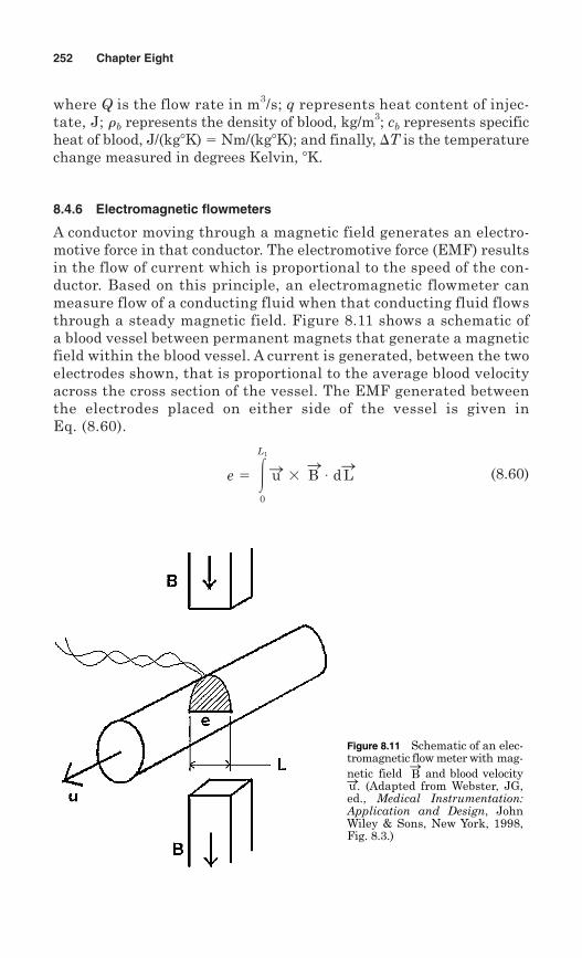
252 Chapter Eight
where Q is the flow rate in m3/s; q represents heat content of injec-tate, J; rb represents the density of blood, kg/m3; cb represents specificheat of blood, J/(kg�K) � Nm/(kg�K); and finally, T is the temperaturechange measured in degrees Kelvin, �K.
8.4.6 Electromagnetic flowmeters
A conductor moving through a magnetic field generates an electro-motive force in that conductor. The electromotive force (EMF) resultsin the flow of current which is proportional to the speed of the con-ductor. Based on this principle, an electromagnetic flowmeter canmeasure flow of a conducting fluid when that conducting fluid flowsthrough a steady magnetic field. Figure 8.11 shows a schematic ofa blood vessel between permanent magnets that generate a magneticfield within the blood vessel. A current is generated, between the twoelectrodes shown, that is proportional to the average blood velocityacross the cross section of the vessel. The EMF generated betweenthe electrodes placed on either side of the vessel is given in Eq. (8.60).
(8.60)e 5 3L1
0
uS 3 BS # dLS
Figure 8.11 Schematic of an elec-tromagnetic flow meter with mag-netic field and blood velocity
. (Adapted from Webster, JG,ed., Medical Instrumentation:Application and Design, JohnWiley & Sons, New York, 1998,Fig. 8.3.)
uSBS
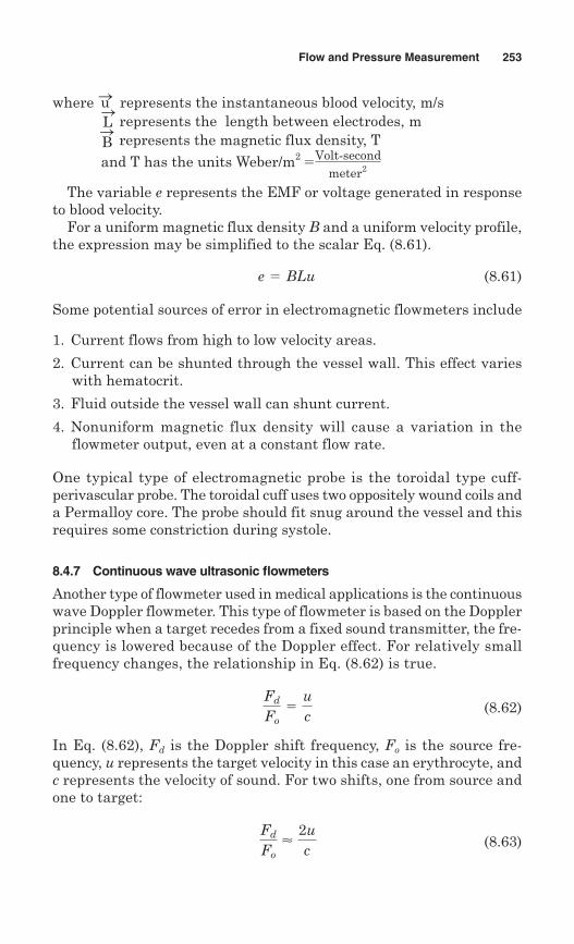
Flow and Pressure Measurement 253
where represents the instantaneous blood velocity, m/srepresents the length between electrodes, mrepresents the magnetic flux density, T
and T has the units Weber/m2 �
The variable e represents the EMF or voltage generated in responseto blood velocity.
For a uniform magnetic flux density B and a uniform velocity profile,the expression may be simplified to the scalar Eq. (8.61).
(8.61)
Some potential sources of error in electromagnetic flowmeters include
1. Current flows from high to low velocity areas.
2. Current can be shunted through the vessel wall. This effect varieswith hematocrit.
3. Fluid outside the vessel wall can shunt current.
4. Nonuniform magnetic flux density will cause a variation in theflowmeter output, even at a constant flow rate.
One typical type of electromagnetic probe is the toroidal type cuff-perivascular probe. The toroidal cuff uses two oppositely wound coils anda Permalloy core. The probe should fit snug around the vessel and thisrequires some constriction during systole.
8.4.7 Continuous wave ultrasonic flowmeters
Another type of flowmeter used in medical applications is the continuouswave Doppler flowmeter. This type of flowmeter is based on the Dopplerprinciple when a target recedes from a fixed sound transmitter, the fre-quency is lowered because of the Doppler effect. For relatively smallfrequency changes, the relationship in Eq. (8.62) is true.
(8.62)
In Eq. (8.62), Fd is the Doppler shift frequency, Fo is the source fre-quency, u represents the target velocity in this case an erythrocyte, andc represents the velocity of sound. For two shifts, one from source andone to target:
(8.63)Fd
Fo<
2uc
Fd
Fo5
uc
e 5 BLu
Volt-secondmeter2
BSLSuS
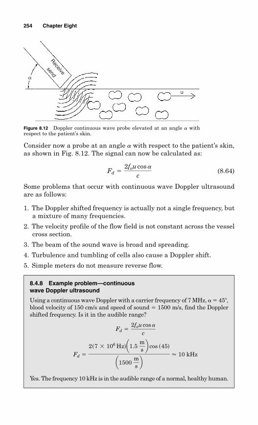
8.4.8 Example problem—continuouswave Doppler ultrasound
Using a continuous wave Doppler with a carrier frequency of 7 MHz, � � 45�,blood velocity of 150 cm/s and speed of sound � 1500 m/s, find the Dopplershifted frequency. Is it in the audible range?
Yes. The frequency 10 kHz is in the audible range of a normal, healthy human.
Fd 5
2s7 3 106 Hzda1.5 ms b cos s45d
a1500 ms b
< 10 kHz
Fd 52fou cos a
c
Consider now a probe at an angle a with respect to the patient’s skin,as shown in Fig. 8.12. The signal can now be calculated as:
(8.64)
Some problems that occur with continuous wave Doppler ultrasoundare as follows:
1. The Doppler shifted frequency is actually not a single frequency, buta mixture of many frequencies.
2. The velocity profile of the flow field is not constant across the vesselcross section.
3. The beam of the sound wave is broad and spreading.
4. Turbulence and tumbling of cells also cause a Doppler shift.
5. Simple meters do not measure reverse flow.
Fd 52fou cos a
c
254 Chapter Eight
u
Receive
send
α
Figure 8.12 Doppler continuous wave probe elevated at an angle a withrespect to the patient’s skin.
8.5 Summary and Clinical Applications
Chapter 8 introduces flow and pressure measurement schemes. A veryquick review to remind the reader of the important clinical applicationsof those measurements is given below.
Indirect pressure measurements According to the American HeartAssociation, high blood pressure is listed as a primary or contributing causeof death in more than a quarter of a million Americans each year. Nearlyone in three U.S. adults has high blood pressure and 30 percent of thosepeople do not know it. Indirect blood pressure measurement using a sphyg-momanometer is the method of choice for measuring blood pressure in thedoctor’s office and is critical to the management regimen of this disease.
Intravascular pressure measurement Cardiologists sometimes insert astrain-gauge-tipped pressure catheter into an artery to determinewhether a specific stenosis is the cause of decreased blood flow. If thepressure is much lower downstream from the blockage than the pres-sure immediately upstream, this indicates that the lesion is the cause.This procedure can also be used to evaluate the effectiveness of catheter-ization and stenting. This use of intravascular pressure measurementis an important aspect of the diagnosis of coronary arterial disease.
Extravascular pressure measurement Pulmonary capillary wedge pres-sure is the pressure measured by inserting a balloon-tipped catheterfrom a peripheral vein into the right atrium, through the right ventri-cle, and then positioned within a branch of the pulmonary artery.Measurement of pulmonary capillary wedge pressure (PCWP) gives anindirect measure of left atrial pressure and is particularly useful in thediagnosis of left ventricular failure and mitral valve disease.
The catheter used for this procedure has one opening (port) at the tipof the catheter and a second port several centimeters proximal to theballoon. These ports are connected to extravascular pressure transducersallowing the pressure measurement.
Cardiac output measurement Cardiac output is one of the main determi-nants of organ perfusion. During a coronary artery bypass, dislocationof the heart changes the cardiac output and so it is important for theanesthesiologist to have a reliable tool for assessing hemodynamic statusto avoid situations with disastrously low cardiac output. There are anumber of methods used to assess cardiac output, including the Ficktechnique, rapid injection dye dilution, and thermodilution.
Electromagnetic and continuous wave Doppler flowmeters These two devices aretwo tools in the physicians’ arsenal that can be used to measure blood flowin a variety of arteries. For example, physicians use Doppler flowmetersto diagnose peripheral arterial disease. The physician measures flow
Flow and Pressure Measurement 255
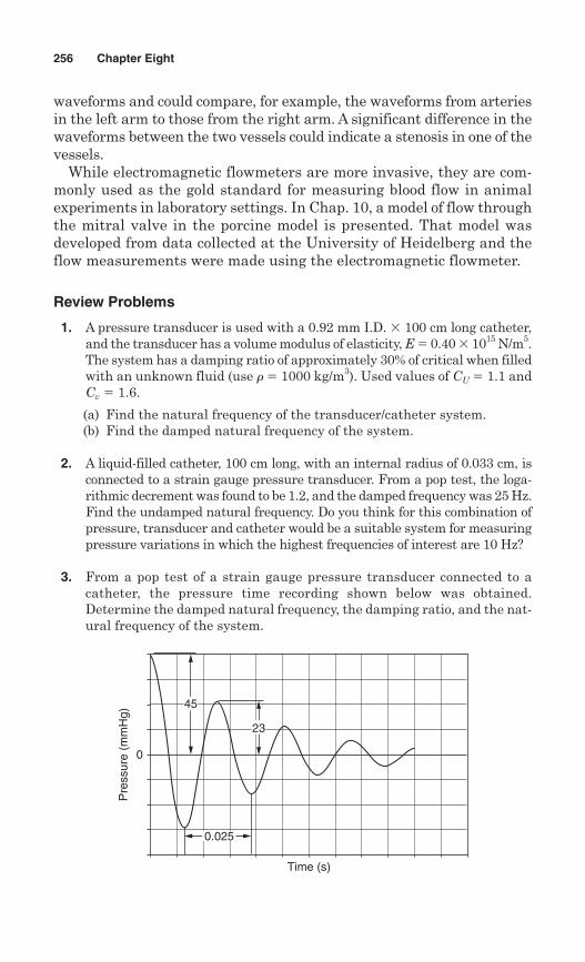
waveforms and could compare, for example, the waveforms from arteriesin the left arm to those from the right arm. A significant difference in thewaveforms between the two vessels could indicate a stenosis in one of thevessels.
While electromagnetic flowmeters are more invasive, they are com-monly used as the gold standard for measuring blood flow in animalexperiments in laboratory settings. In Chap. 10, a model of flow throughthe mitral valve in the porcine model is presented. That model wasdeveloped from data collected at the University of Heidelberg and theflow measurements were made using the electromagnetic flowmeter.
Review Problems
1. A pressure transducer is used with a 0.92 mm I.D. � 100 cm long catheter,and the transducer has a volume modulus of elasticity, E � 0.40 � 1015 N/m5.The system has a damping ratio of approximately 30% of critical when filledwith an unknown fluid (use r� 1000 kg/m3). Used values of CU � 1.1 andCv � 1.6.
(a) Find the natural frequency of the transducer/catheter system.(b) Find the damped natural frequency of the system.
2. A liquid-filled catheter, 100 cm long, with an internal radius of 0.033 cm, isconnected to a strain gauge pressure transducer. From a pop test, the loga-rithmic decrement was found to be 1.2, and the damped frequency was 25 Hz.Find the undamped natural frequency. Do you think for this combination ofpressure, transducer and catheter would be a suitable system for measuringpressure variations in which the highest frequencies of interest are 10 Hz?
3. From a pop test of a strain gauge pressure transducer connected to acatheter, the pressure time recording shown below was obtained.Determine the damped natural frequency, the damping ratio, and the nat-ural frequency of the system.
256 Chapter Eight
Time (s)
Pre
ssur
e (m
mH
g)
0.025
23
45
0
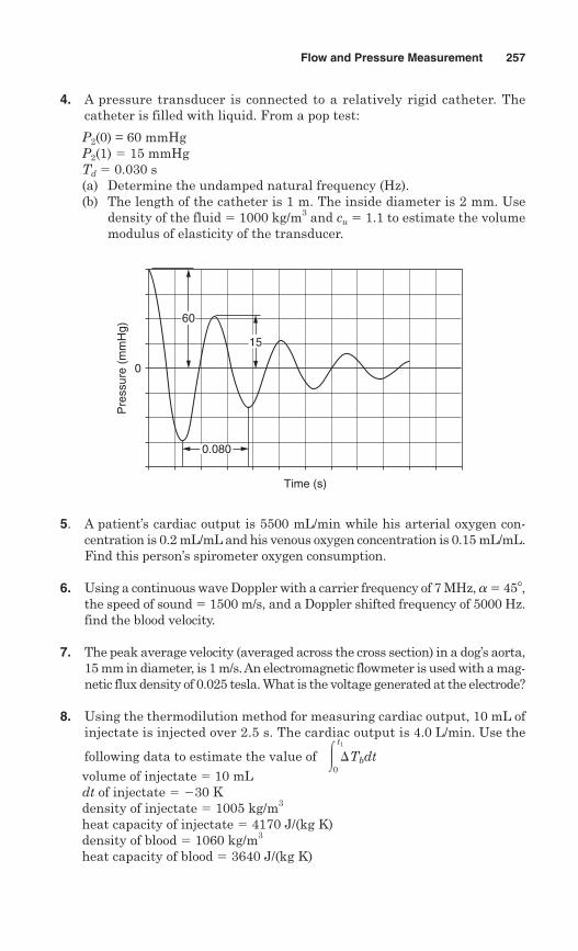
4. A pressure transducer is connected to a relatively rigid catheter. Thecatheter is filled with liquid. From a pop test:
P2(0) = 60 mmHgP2(1) � 15 mmHgTd � 0.030 s(a) Determine the undamped natural frequency (Hz).(b) The length of the catheter is 1 m. The inside diameter is 2 mm. Use
density of the fluid � 1000 kg/m3 and cu � 1.1 to estimate the volumemodulus of elasticity of the transducer.
Flow and Pressure Measurement 257
5. A patient’s cardiac output is 5500 mL/min while his arterial oxygen con-centration is 0.2 mL/mL and his venous oxygen concentration is 0.15 mL/mL.Find this person’s spirometer oxygen consumption.
6. Using a continuous wave Doppler with a carrier frequency of 7 MHz, a� 45�,the speed of sound � 1500 m/s, and a Doppler shifted frequency of 5000 Hz.find the blood velocity.
7. The peak average velocity (averaged across the cross section) in a dog’s aorta,15 mm in diameter, is 1 m/s. An electromagnetic flowmeter is used with a mag-netic flux density of 0.025 tesla. What is the voltage generated at the electrode?
8. Using the thermodilution method for measuring cardiac output, 10 mL ofinjectate is injected over 2.5 s. The cardiac output is 4.0 L/min. Use the
following data to estimate the value ofvolume of injectate � 10 mLdt of injectate � 30 Kdensity of injectate � 1005 kg/m3
heat capacity of injectate � 4170 J/(kg K)density of blood � 1060 kg/m3
heat capacity of blood � 3640 J/(kg K)
3t1
0Tbdt
Time (s)
Pre
ssur
e (m
mH
g)
0.080
15
60
0
9. Consider the indirect measurement of blood pressure in an obese patientusing a sphygmomanometer. Does indirect measurement of blood tend tooverestimate or underestimate the actual blood pressure in the obesepatient? Is there an inaccuracy in the measurement associated with“hardened arteries” in elderly patients?
10. A rigid-walled catheter is connected to a pressure sensor. The catheter is1 m long, with an inside diameter of 1.1 mm and filled with water at20�C. The volume modulus of elasticity of the pressure sensor diaphragmis 0.49 � 1015 N/m5. Find the natural frequency of the catheter, thedamped natural frequency of the catheter, and the damping ratio. Use vis-cosity of the water � 0.89 cP and cv � 1.8.
11. For the same pressure measuring catheter from Prob. 8.10, add an airbubble to the system. Use an isothermal for air of per liter
of air volume. The catheter is 1 m long, with an inside diameter of 1.1 mmand filled with water at 20�C. The volume modulus of elasticity of the pres-sure sensor diaphragm is 0.49 � 1015 N/m5. Find the length of air bubblein the catheter required for a damping ratio, , of 0.14.
12. For the same pressure measuring catheter from Prob. 8.10 without the airbubble a 15-cm-long pinch reduces the inside diameter of the catheter to0.3 mm. Find the damped natural frequency of the catheter with the pinch.Use a cu of 1.1 and cv of 1.8.
Bibliography
Cromwell, L, Weibell, FJ, Pfeiffer, EA. Biomedical Instrumentation and Measurements,2nd ed, Prentice-Hall, Englewood Cliffs, NJ, 1980.
Khandpur, RS. Biomedical Instrumentation. Technology and Applications, McGraw-Hill,New York, 2005.
Kothari, N, Amaria, T, Hegde, A, Mandke, A, Mandke, NV. “Measurement of CardiacOutput: Comparison of Four Different Methods,” IJTCVS, 19, 163168, 2003.
Özyurda, U, Akar, R, Uymaz, O, Oguz, M, Ozkan, M, Yildirim, C, Aslan, A, RTasoz, R.“Early Clinical Experience with the On-X Prosthetic Heart Valve,” Interact. Cardiovasc.Thorac. Surg., 4, 588–594, 2005; originally published online Sep 16, 2005.
Pickering, TG, Hall, JE, Appel, LJ, Falkner, BE, Graves, J, Hill, MN, Jones, DW, Kurtz,T, Sheps, SG, Roccella, EJ. “Recommendations for Blood Pressure Measurement inHumans and Experimental Animals,” Hypertension, 45, 142, 2005.
Szabo, G, Soans, D, Graf, A, Beller, C, Waite, L, Hagl, S. “A New Computer Model ofMitral Valve Hemodynamics during Ventricular Filling,” Eur. J. Cardiothoracic Surg.,26, 239247, 2004.
Togawa, T, Tamura, T, and Öberg, P. Biomedical Transducers and Instruments, CRC Press,Boca Raton, FL, 1997.
Webster, JG, ed. Medical Instrumentation Application and Design, 3rd ed, John Wiley &Sons, New York, 1998.
z
0.010 mLPa
VP
258 Chapter Eight
Chapter
9Modeling
9.1 Introduction
Models are used widely in all types of engineering, and especially influid mechanics. The term model has many uses, but in the engineer-ing context, it usually involves a representation of a physical system, aprototype, that may be used to predict the behavior of the system insome desired respect. These models can include physical models thatappear physically similar to the prototype or mathematical models, whichhelp to predict the behavior of the system, but do not have a similar phys-ical embodiment. In this chapter, we develop procedures for designingmodels in a way to ensure that the model and prototype will behavesimilarly.
Consider the question: “Why can a 1.5-mm-long flea fall a meterwithout injury but a 1.5-m-tall man can’t fall 1 km unhurt?” A modelis a representation of a physical system that may be used to predictthe behavior of the system in some desired respect. The impliedquestion in the stated question above is, “Can the flea be used tomodel the man?”
It is true that a 1.5-mm-long flea can jump about 1 m. If we use geo-metric scaling, we might predict that a 1.5-m-long person would jumpabout 1 km. Since that is clearly not true, then what is wrong with thispicture? A careful look at the theory of models will help answer ourquestion.
In Sec. 9.7, we attempt to use a flea to model a man (or vice versa) tomodel the terminal velocity of the prototype using the model. We willlearn, by using the theory of models and dimensional analysis, why thismodel does not work very well.
259
Copyright © 2007 by The McGraw-Hill Companies, Inc. Click here for terms of use.
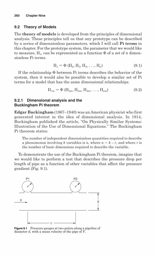
9.2 Theory of Models
The theory of models is developed from the principles of dimensionalanalysis. These principles tell us that any prototype can be describedby a series of dimensionless parameters, which I will call Pi terms inthis chapter. For the prototype system, the parameter that we would liketo measure, �1, can be represented as a function � of a set of n dimen-sionless Pi terms.
�1 � � (�2, �3, �4, . . ., �n) (9.1)
If the relationship � between Pi terms describes the behavior of thesystem, then it would also be possible to develop a similar set of Piterms for a model that has the same dimensional relationships.
�1m � � (�2m, �3m, �4m, . . ., �nm) (9.2)
9.2.1 Dimensional analysis and theBuckingham Pi theorem
Edgar Buckingham (1867–1940) was an American physicist who firstgenerated interest in the idea of dimensional analysis. In 1914,Buckingham published the article, “On Physically Similar Systems:Illustration of the Use of Dimensional Equations.” The BuckinghamPi theorem states:
The number of independent dimensionless quantities required to describea phenomenon involving k variables is n, where n � k – r, and where r isthe number of basic dimensions required to describe the variable.
To demonstrate the use of the Buckingham Pi theorem, imagine thatwe would like to perform a test that describes the pressure drop perlength of pipe as a function of other variables that affect the pressuregradient (Fig. 9.1).
260 Chapter Nine
+
P1
+
P2
d
L
V
Figure 9.1 Pressure gauges at two points along a pipeline ofdiameter d, with a mean velocity of the pipe of V.
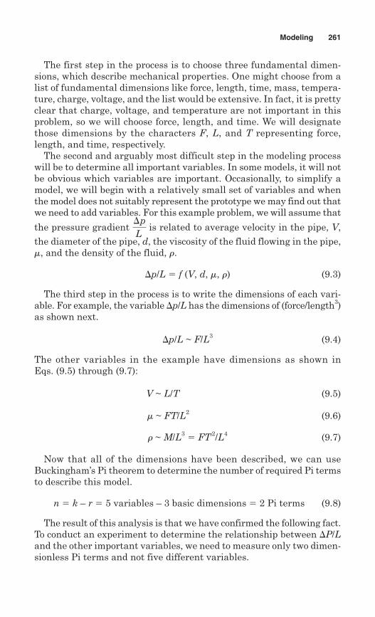
The first step in the process is to choose three fundamental dimen-sions, which describe mechanical properties. One might choose from alist of fundamental dimensions like force, length, time, mass, tempera-ture, charge, voltage, and the list would be extensive. In fact, it is prettyclear that charge, voltage, and temperature are not important in thisproblem, so we will choose force, length, and time. We will designatethose dimensions by the characters F, L, and T representing force,length, and time, respectively.
The second and arguably most difficult step in the modeling processwill be to determine all important variables. In some models, it will notbe obvious which variables are important. Occasionally, to simplify amodel, we will begin with a relatively small set of variables and whenthe model does not suitably represent the prototype we may find out thatwe need to add variables. For this example problem, we will assume that
the pressure gradient is related to average velocity in the pipe, V,the diameter of the pipe, d, the viscosity of the fluid flowing in the pipe, m, and the density of the fluid, r.
p/L � f (V, d, m, r) (9.3)
The third step in the process is to write the dimensions of each vari-able. For example, the variable p/L has the dimensions of (force/length3)as shown next.
p/L ~ F/L3 (9.4)
The other variables in the example have dimensions as shown inEqs. (9.5) through (9.7):
V ~ L/T (9.5)
m ~ FT/L2 (9.6)
r ~ M/L3� FT2/L4 (9.7)
Now that all of the dimensions have been described, we can useBuckingham’s Pi theorem to determine the number of required Pi termsto describe this model.
n � k – r � 5 variables – 3 basic dimensions � 2 Pi terms (9.8)
The result of this analysis is that we have confirmed the following fact.To conduct an experiment to determine the relationship between P/Land the other important variables, we need to measure only two dimen-sionless Pi terms and not five different variables.
pL
Modeling 261
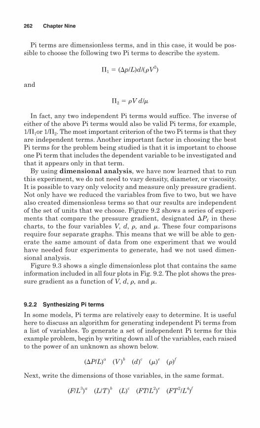
Pi terms are dimensionless terms, and in this case, it would be pos-sible to choose the following two Pi terms to describe the system.
�1 � (p/L)d/(rV2)
and
�2 � rV d/m
In fact, any two independent Pi terms would suffice. The inverse ofeither of the above Pi terms would also be valid Pi terms, for example,1/�1or 1/�2. The most important criterion of the two Pi terms is that theyare independent terms. Another important factor in choosing the bestPi terms for the problem being studied is that it is important to chooseone Pi term that includes the dependent variable to be investigated andthat it appears only in that term.
By using dimensional analysis, we have now learned that to runthis experiment, we do not need to vary density, diameter, or viscosity.It is possible to vary only velocity and measure only pressure gradient.Not only have we reduced the variables from five to two, but we havealso created dimensionless terms so that our results are independentof the set of units that we choose. Figure 9.2 shows a series of experi-ments that compare the pressure gradient, designated in thesecharts, to the four variables V, d, r, and m. These four comparisonsrequire four separate graphs. This means that we will be able to gen-erate the same amount of data from one experiment that we wouldhave needed four experiments to generate, had we not used dimen-sional analysis.
Figure 9.3 shows a single dimensionless plot that contains the sameinformation included in all four plots in Fig. 9.2. The plot shows the pres-sure gradient as a function of V, d, r, and m.
9.2.2 Synthesizing Pi terms
In some models, Pi terms are relatively easy to determine. It is usefulhere to discuss an algorithm for generating independent Pi terms froma list of variables. To generate a set of independent Pi terms for thisexample problem, begin by writing down all of the variables, each raisedto the power of an unknown as shown below.
(P/L)a (V )b (d)c (m)e (r)f
Next, write the dimensions of those variables, in the same format.
(F/L3)a (L/T )b (L)c (FT/L2)e (FT2/L4)f
P/
262 Chapter Nine
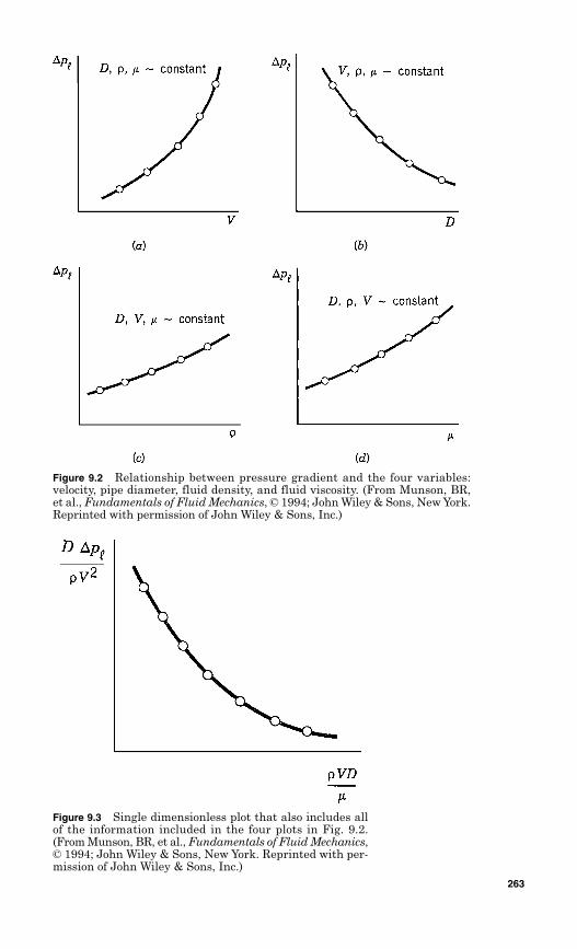
Figure 9.2 Relationship between pressure gradient and the four variables:velocity, pipe diameter, fluid density, and fluid viscosity. (From Munson, BR,et al., Fundamentals of Fluid Mechanics, © 1994; John Wiley & Sons, New York.Reprinted with permission of John Wiley & Sons, Inc.)
Figure 9.3 Single dimensionless plot that also includes allof the information included in the four plots in Fig. 9.2.(From Munson, BR, et al., Fundamentals of Fluid Mechanics,© 1994; John Wiley & Sons, New York. Reprinted with per-mission of John Wiley & Sons, Inc.)
263
Now it is possible to write a set of three equations, one for each basicdimension, and to solve them simultaneously for three values. Since wehave five unknowns and only three equations, it is necessary to assumethe values of two convenient variables.
F: a � 0 � 0 � e � f � 0
L: 3a � b � c 2e 4f � 0
T: 0 b 0 � e � 2f � 0
For our example, we will assume a � 1 and e � 0 to produce two inde-pendent Pi terms. That will ensure that P/L will appear in only onePi term. Solving the three equations yields the following:
1 � f � 0 f � 1
3 � b � c 4f � 0 c � 1
b � 2f � 0 b � 2
Therefore, by using the values of a � 1 and e � 0, one possible Pi termfollows:
�1 � (P/L)1 V2d1r
1
To generate the second independent Pi term, let e � 1 and a � 0. Thiswill ensure that every variable appears in one of the Pi terms and thatP/L does not appear in �2.
1 � f � 0 f � 1
b � c 2 4f � 0 c � 1
b � 1 � 2f � 0 b � 1
�2 � V1d1mr
1� m/rVd
Note that �2 is the reciprocal of the Reynolds number, a well-knowndimensionless parameter used in many fluid mechanics applications.
Therefore, if we make �2 for the model equal to �2 for the prototype,then �1 for the model will predict meaningful values for �1 of theprototype.
9.3 Geometric Similarity
When we equate Pi terms involving length ratios only, the model satis-fies the condition of geometric similarity. Scale models in which allthree dimensions of the model (height, width, and length) have the
264 Chapter Nine
same scale have geometric similarity. A common dimensionless Pi terminvolving geometry is the ratio of length to width or the ratio of twolengths.
L1/L2 � L1m/L2m
If a model is a 1/10 scale model, this means that the ratio of lengthsbetween the model and the prototype is 1/10. The flea in our exampleintroduced above might be considered a 1/1000 scale model of a human,if it were similarly proportioned to the human. If we only know theflea’s length and the man’s height, we can consider the flea geometri-cally similar. We will call the flea a 1/1000 scale model for a firstapproximation.
But if we consider the overall effectiveness of the model, what aboutthe other Pi terms that have forces and time in them? For a completemodel, we also need some other types of similarity.
9.4 Dynamic Similarity
For a perfect model, we must be sure that we have included all impor-tant variables. Further, all Pi terms in the model must be equal to eachPi terms in the prototype. When we achieve geometric similarity bymatching the geometric Pi terms, as with a scale model airplane, themodel will look like a smaller version of the prototype but will not nec-essarily behave like the prototype. When we equate Pi terms involvingforce ratios we achieve dynamic similarity.
For example, density is a variable that contains force as one of itsdimensions. A Pi term in some fluid mechanics problems that includesdrag force and density could be the term that follows. For this Pi termthe variable D represent drag force, r represents fluid density, V rep-resents fluid velocity, and t1 and t2 are geometric dimensions.
To achieve dynamics similarity, �1 in the prototype must equal �1
in the model.
[D/(rVmax2 t1t2)]p � [D/(rVmax
2 t1t2)]m
9.5 Kinematic Similarity
When we equate Pi terms involving velocity or acceleration ratios weobtain kinematic similarity. Many Pi terms that have a force dimensionwill also have a velocity or acceleration dimension. For example, theReynolds number is a common Pi term in fluid mechanics that has both
�1 5 [D/srV2t1t2d]
Modeling 265
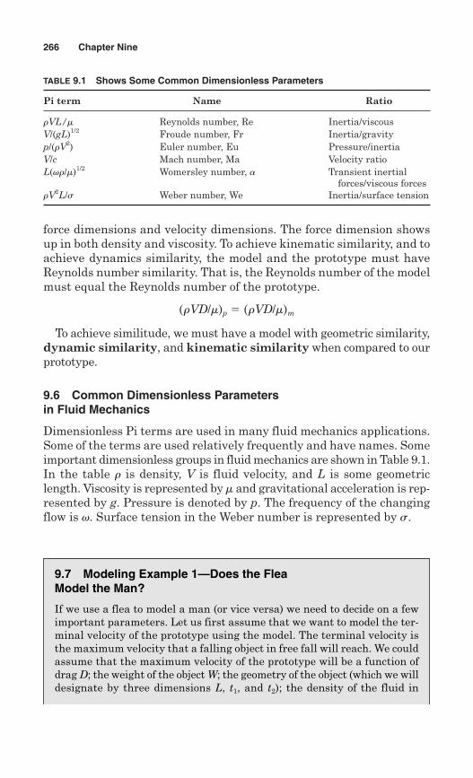
force dimensions and velocity dimensions. The force dimension showsup in both density and viscosity. To achieve kinematic similarity, and toachieve dynamics similarity, the model and the prototype must haveReynolds number similarity. That is, the Reynolds number of the modelmust equal the Reynolds number of the prototype.
(rVD/m)p � (rVD/m)m
To achieve similitude, we must have a model with geometric similarity,dynamic similarity, and kinematic similarity when compared to ourprototype.
9.6 Common Dimensionless Parameters in Fluid Mechanics
Dimensionless Pi terms are used in many fluid mechanics applications.Some of the terms are used relatively frequently and have names. Someimportant dimensionless groups in fluid mechanics are shown in Table 9.1.In the table r is density, V is fluid velocity, and L is some geometriclength. Viscosity is represented by m and gravitational acceleration is rep-resented by g. Pressure is denoted by p. The frequency of the changingflow is v. Surface tension in the Weber number is represented by s.
266 Chapter Nine
TABLE 9.1 Shows Some Common Dimensionless Parameters
Pi term Name Ratio
rVL/m Reynolds number, Re Inertia/viscousV/(gL)1/2 Froude number, Fr Inertia/gravityp/(rV2) Euler number, Eu Pressure/inertiaV/c Mach number, Ma Velocity ratioL(vr/m)1/2 Womersley number, a Transient inertial
forces/viscous forcesrV2L/s Weber number, We Inertia/surface tension
9.7 Modeling Example 1—Does the FleaModel the Man?
If we use a flea to model a man (or vice versa) we need to decide on a fewimportant parameters. Let us first assume that we want to model the ter-minal velocity of the prototype using the model. The terminal velocity isthe maximum velocity that a falling object in free fall will reach. We couldassume that the maximum velocity of the prototype will be a function ofdrag D; the weight of the object W; the geometry of the object (which we willdesignate by three dimensions L, t1, and t2); the density of the fluid in
which the object is falling r; and the viscosity of the fluid in which theobject is falling m. Mathematically, we can write the relationship as follows:
Vmax � f (D, W, L, t1, t2, r, m)
Therefore, for this modeling problem, there are eight variables and threebasic dimensions that are required to describe the units on those variables. Thethree basic dimensions are time, length, and force. If our assumptions arevalid, then the required number of Pi terms is n � 5.
n � k – r � 8 3
I will choose the following five independent Pi terms:
�1 � rVmaxL/m Reynolds number
�2 � D/(rVmax2 t1t2) Coefficient of drag
�3 � D/W Drag Force to Weight ratio
�4 � t1/L Geometrical scale
�5 � t2/L Geometrical scale
For a first approximation for our model, we will take the flea weight to be10–4 g. The flea length will be 1.5 mm and we will consider the flea and theman to have the same aspect ratio. That means that we will assume �4 and�5 to be identical in the model and prototype a priori. The man’s length willbe 1.5 m and the weight will be 100 kg.
Starting from this data, our geometric scale is 1000:1. The man is 1000times longer and 1000 times wider than the flea. Because we are looking tomodel the terminal velocity of the falling man and/or the flea, the drag forcewill be equal to weight for �3 � 1.
For kinematic and dynamic similarity let �1man � �1flea and let �2man ��2flea. The resulting equations are shown below.
�2 � [W/(rVmax2 t1t2)]man � [W/(rVmax
2 t1t2)]flea
(Vman/Vflea)2 � (Wman/Wflea)(t1∗t2)flea/(t1∗t2)man
(Vman/Vflea)2 � (105/104)(1/1000)2�1000
If the second Pi term is identical in the flea and the man, the terminalvelocity of the man will be ~30 times that of the flea.
�1 � (rVmaxL/m)man � (rVmaxL/m)flea
(Vman/Vflea) � Lflea/Lman � 1/1000
Modeling 267
If the first Pi term, the Reynolds number, is identical in the flea and theman, then the velocity of the man will be 1000 times that of the flea. Wecan see that these two conditions are mutually exclusive and the man andthe flea, falling through the same fluid, are not a good model for eachother. For Reynolds similarity, the man must fall 1000 times slower. Fordrag similarity, the man needs to fall 30 times faster.
If you want to allow the man and flea to fall at the same velocity andhave Reynolds number similarity, it would also be theoretically possibleto change fluids so that we have a different kinematic viscosity, v. Wemight ask ourselves whether it is practical. The kinematic viscosity ofstandard air is vair � 1.46 � 105 m2/s. Now if we set the velocity of theman and the flea equal, with the constraint of maintaining Reynoldsnumber similarity, the equation is shown below.
Since viscosity divided by density is equivalent to kinematic viscosity;m/r� v, and if the flea is falling through air and the man is falling throughan alternate fluid, it is also possible to write the equation as:
For Reynolds number similarity the man needs to fall through a fluidthat has a kinematic viscosity 1000 times greater than that of standardair or ~1.5 � 102 m2/s. Glycerine at 20�C has a kinematic viscosity of1.2 � 103 m2/s, so we would need to use glycerine at a much cooler tem-perature to achieve that kinematic viscosity! Because of glycerine’s verylarge density compared to air, now buoyancy would become a significantfactor and we realize that the flea just is not a good model for the man(and vice versa).
Our original question was, “Why can a 1.5 mm flea can fall a meterwithout injury but a 1.5 m man can’t fall 1 km unhurt?” The answer isthat the model and prototype are geometrically similar (1/1000 scale)but not dynamically and kinematically similar. The low Reynoldsnumber and relatively high drag effect predict that the flea falls veryslowly!
yair
yalternate5
11000
armbman
armbflea
5lflea
lman5
11000
268 Chapter Nine
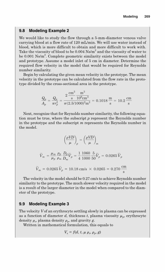
Modeling 269
9.8 Modeling Example 2
We would like to study the flow through a 5-mm-diameter venous valvecarrying blood at a flow rate of 120 mL/min. We will use water instead ofblood, which is more difficult to obtain and more difficult to work with.Take the viscosity of blood to be 0.004 Ns/m2 and the viscosity of water tobe 0.001 Ns/m2. Complete geometric similarity exists between the modeland prototype. Assume a model inlet of 5 cm in diameter. Determine therequired flow velocity in the model that would be required for Reynoldsnumber similarity.
Begin by calculating the given mean velocity in the prototype. The meanvelocity in the prototype can be calculated from the flow rate in the proto-type divided by the cross-sectional area in the prototype.
Next, recognize that for Reynolds number similarity, the following equa-tion must be true, where the subscript p represent the Reynolds numberin the prototype and the subscript m represents the Reynolds number inthe model.
The velocity in the model should be 0.27 cm/s to achieve Reynolds numbersimilarity to the prototype. The much slower velocity required in the modelis a result of the larger diameter in the model when compared to the diam-eter of the prototype.
9.9 Modeling Example 3
The velocity V of an erythrocyte settling slowly in plasma can be expressedas a function of diameter d, thickness t, plasma viscosity mp, erythrocytedensity re, plasma density rp, and gravity g.
Written in mathematical formulation, this equals to
Vs � f(d, t, m re, rp, g)
Vm 5 0.0265 Vp 5 10.18 cm/s 3 0.0265 5 0.270 cms
Vm 5mmmp
rp
rm Dp
DmVp 5
14
10601000
5
50Vp 5 0.0265 Vp
arVDmb
p5 arVD
mb
m
Qp
Ap5
Qp
pr2p5
2 cm3
s
m3
106cm3
ps2.5/1000d2m2 5 0.1018 ms5 10.2
cms
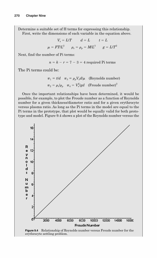
270 Chapter Nine
Determine a suitable set of � terms for expressing this relationship.First, write the dimensions of each variable in the equation above.
Vs � L/T d � L t � L
m � FT/L2re � rp � M/L3 g � L/T2
Next, find the number of Pi terms:
n � k r � 7 3 � 4 required Pi terms
The Pi terms could be:
p1 � t/d p3 � rpVsd/m (Reynolds number)
p2 � re/rp p4 � Vs2/gd (Froude number)2
Once the important relationships have been determined, it would bepossible, for example, to plot the Froude number as a function of Reynoldsnumber for a given thickness/diameter ratio and for a given erythrocyteversus plasma ratio. As long as the Pi terms in the model are equal to thePi terms in the prototype, that plot would be equally valid for both proto-type and model. Figure 9.4 shows a plot of the Reynolds number versus the
Figure 9.4 Relationship of Reynolds number versus Froude number for theerythrocyte settling problem.
Modeling 271
Figure 9.5 Plot of particle sedimentation versus diameter.
Froude number for a density of plasma of 1000 kg/m3 and a density of ery-throcytes of 1200 kg/m3, a viscosity of 0.0035 Ns/m2, g � 9.81 m/s2, and fora thickness-to-diameter ratio of 25. Note that this plot has no units, andas long as the Pi terms are equal in the model and the prototype, the plotis valid.
Figure 9.5 shows the erythrocyte settling rate as a function of cell diam-eter for a density of plasma of 1000 kg/m3 and a density of erythrocytes of1200 kg/m3, a viscosity of 0.0035 Ns/m2, g � 9.81 m/s2, and for a thickness-to-diameter ratio of 25. Note that this plot has units associated and is thusvalid only for this set of parameters.
Review Problems
1. Consider a 1/32 scale model airplane which “looks” very similar to theprototype airplane being modeled. What type of similarity does thismodel have? Would you expect it to fly? If not, describe the other typesof similarity you would need for the airplane model to behave similarlyto the prototype.
2. To achieve Reynolds number similarity for the 1/32 scale model above,keeping the velocity in the model equal to that in the prototype, whatshould be the kinematic viscosity of the model fluid. What is the nearestfluid you can find to that kinematic viscosity. Use a kinematic viscosity forwater of 1.0 centistoke and a kinematic viscosity for air of 17 centistokes.
3. A 5� scale model of a heart valve is to be tested in a flow loop using a clearpolycarbonate pipeline flowing water to visualize flow patterns. Use a den-sity of 1060 kg/m3 and a viscosity of 0.0045 Ns/m2 and calculate the ratioof the flow velocity of the model to the flow velocity of the prototype nec-essary to achieve Reynolds number similarity between the model and theprototype.
4. If the 5� scale model of the heart valve described above has Reynoldsnumber similarity to the prototype, would it then be a good model of theprototype for studying pressure drop across the valve? Why or why not?
5. Wall shear stress tw, in a vessel depends on the radius of the vessel r, thedensity of the fluid r, the viscosity of the fluid m, the pressure gradient inthe vessel dP/dx. Find the minimum number of Pi terms required todescribe this relationship and suggest some suitable Pi terms.
6. Imagine that you do not know the Moens–Korteweg equation, but you realizethat the velocity c at which a pressure pulse travels through an artery is afunction of vessel diameter d, vessel wall thickness t, blood density r, andvessel wall modulus of elasticity E. Determine a set of dimensionlessparameters that could be used to study the relationship between pulsewave velocity and the wall thickness of the vessel.
7. When Poiseuille first developed Poiseuille’s law relating flow in a pipe Qto pressure drop along a pipe P/l he developed the law empirically. Usingdimensional analysis, generate a set of Pi terms and suggest an experimentto determine Poiseuille’s law for flow through a rectangular channel.
8. You are designing an experimental system to model pressure drops inPoiseuille flow in a 1-mm-diameter artery. You would like to use water inyour model through a tube that has a diameter of 1 cm. What velocity andflow rate should be used in the model? Pressure drop in the artery is rep-resented by P/L, blood density by r, blood velocity by V, vessel diameterby D, and blood viscosity by m. The velocity you would like to test in theprototype artery is 5 cm/s. Use a blood viscosity of 3.5 centipoise andblood density of 1060 kg/m3. Use a viscosity of water of 0.7 centipoise anddensity of 1000 kg/m3.
9. For the solution in Prob. 9.8, write the names of the Pi terms using thenames of dimensionless parameters from Table 9.1.
10. Two pipelines have equal diameters. Water flows in one pipeline and airflows in the second. Temperature is constant and equal in both pipelines.
272 Chapter Nine
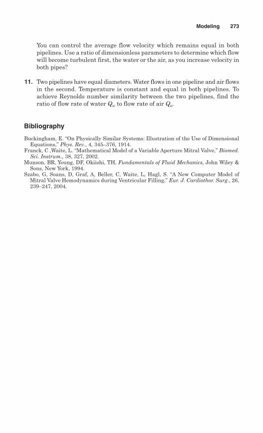
You can control the average flow velocity which remains equal in bothpipelines. Use a ratio of dimensionless parameters to determine which flowwill become turbulent first, the water or the air, as you increase velocity inboth pipes?
11. Two pipelines have equal diameters. Water flows in one pipeline and air flowsin the second. Temperature is constant and equal in both pipelines. Toachieve Reynolds number similarity between the two pipelines, find theratio of flow rate of water Qw to flow rate of air Qa.
Bibliography
Buckingham, E. “On Physically Similar Systems: Illustration of the Use of DimensionalEquations,” Phys. Rev., 4, 345–376, 1914.
Franck, C ,Waite, L. “Mathematical Model of a Variable Aperture Mitral Valve,” Biomed.Sci. Instrum., 38, 327, 2002.
Munson, BR, Young, DF, Okiishi, TH, Fundamentals of Fluid Mechanics, John Wiley &Sons, New York, 1994.
Szabo, G, Soans, D, Graf, A, Beller, C, Waite, L, Hagl, S. “A New Computer Model ofMitral Valve Hemodynamics during Ventricular Filling,” Eur. J. Cardiothor. Surg., 26,239–247, 2004.
Modeling 273

This page intentionally left blank
275
Chapter
10Lumped Parameter
Mathematical Models
10.1 Introduction
Since the pioneering work of Otto Frank in 1899, there have been manytypes of mathematical models of blood flow. The aim of these models is abetter understanding of the biofluid mechanics in cardiovascular sys-tems. Mathematical computer models aim to facilitate the understand-ing of the cardiovascular system in an inexpensive and noninvasive way.One example of the motivation for such a model occurred when Raineset al. in 1974 observed that patients with severe vascular disease havepressure waveforms that are markedly different from those in healthy per-sons. By developing a model that would predict which changes in param-eters affect those pressure waveforms in what way, the scientists mightprovide a means for diagnosing vascular disease before it becomes severe.
Lumped parameter models are in common use for studying the fac-tors that affect pressure and flow waveforms. A lumped parameter modelis one in which the continuous variation of the system’s state vari-ables in space is represented by a finite number of variables, definedat special points called nodes. The model would be less computation-ally expensive, with a correspondingly lower spatial resolution, whilestill providing useful information at important points within the model.Lumped parameter models are good for helping to study the relation-ship of cardiac output to peripheral loads, for example, but because ofthe finite number of lumped elements, they cannot model the higherspatial-resolution aspects of the system without adding many, manymore elements.
Chapter 10 begins by addressing the general electrical analog modelof blood flow, based on electrical transmission line equations. Later
Copyright © 2007 by The McGraw-Hill Companies, Inc. Click here for terms of use.
in Chap.10 a specific model of flow through a human mitral valve ispresented in some detail.
10.2 Electrical Analog Model of Flow in a Tube
In Chap. 7, Sec. 7.7, a solution was developed, which was published byGreenfield and Fry in 1965, that shows the relationship between flowand pressure for axisymmetric, uniform, fully developed, horizontal,Newtonian, pulsatile flow. The Fry solution is particularly useful whenmodeling the relationship of the pressure gradient in a tube or bloodvessel to the instantaneous blood velocity. In Chap. 8, we used the Frysolution to develop an electrical analog of a typical pressure-measuringcatheter. Using well-known solutions to RLC circuits, it became pos-sible to characterize parameters like the natural frequency and dimen-sionless damping ratio of the system.
I describe, here in Chap. 10, an alternative development of the mod-eling of flow through any vessel or tube based on that analog. Let thesubscript V represent properties of the blood vessel that we are model-ing and the subscript L represent properties of the terminating load. InChap. 8, the terminating load was a transducer, but in the more gen-eral case of the isolated blood vessel within a cardiovascular system, theterminating load represents the effects of a group of distal blood vessels,usually arterioles and capillaries.
Figure 10.1 shows the electrical schematic of a circuit representing alength of artery, terminating in a capillary bed. The values for resist-ance, capacitance, and inductance for each resistor, capacitor, and induc-tor, respectively, are calculated from the blood vessel properties on a perunit length basis.
Recall that the hydrodynamic resistance of a blood vessel depends onits radius and length as well as the viscosity of the fluid flowing in the
276 Chapter Ten
LV RV LV RV LV RV
RL1
RL2CL
CVCVCV
q1
qc1
n
1 2 3
PIN
Figure 10.1 Electrical schematic of a model of blood flowing through a vesselor tube, with the V transcript representing the characteristics of the vessel andL representing the terminal load.
tube. For this type of discretized model, the resistance in each discreteresistor can be written as
(10.1)
Using the SI system of units, the dimension of RV is Ns/m5. The induc-tance in the vessel for each discrete inductor element becomes
(10.2)
The inductance will have units of Ns2/m5. The capacitance of the vesselis the compliance of the vessel, or dA/dP, and depends on the pressureat the point where the capacitor is located.
(10.3)
Its units in SI are m5/N. Note that the resistance, inductance, and capac-itance of each vessel segment can vary, for example, in a tapering vessel.
10.2.1 Nodes and the equations at each node
In electrical circuit analysis, a node is defined as a point in a circuitwhere two or more circuit elements join. In Fig. 10.1, we will take thecombination of a resistor, inductor, and capacitor as being a singleelement of our model, and number the nodes at the center of each ele-ment at the points where the resistor, capacitor, and inductor are joined.The nodes in Fig. 10.1 are labeled 1, 2, 3, . . . , n.
In the model, the input flow to the first element is labeled q1. The inputpressure is labeled Pin. The flow leaving node 1 toward the capacitor islabeled qc1. The pressure at node 1 is P1. Note that the model does notcontain any information about the pressure at points between the inputpoint and node 1.
Considering node 1, we can now write an equation for the pressuredrop across the first resistor and inductor as shown in Eq. (10.4) as thefirst-order differential equation
(10.4)
In Eq. 10.4, Pin represents the input pressure to the vessel. P1 is the pres-sure at node 1 and q is the flow through the vessel. The time rate ofchange of flow is designated dq/dt. Note that LV1 and RV1 can vary from
Pin 2 P1 5 q1 RV1 1 LV1 dq1
dt
CV 5q
dP/dt
LV 5 /L 5 cu r/pr2
RV 5 /Rviscous 5 cv 8m/pr4
Lumped Parameter Mathematical Models 277
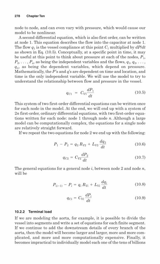
node to node, and can even vary with pressure, which would cause ourmodel to be nonlinear.
A second differential equation, which is also first order, can be writtenat node 1. This equation describes the flow into the capacitor at node 1.The flow q1 is the vessel compliance at this point C1 multiplied by dP/dtas shown in Eq. (10.5). Conceptually, at a specific point in time, it maybe useful at this point to think about pressure at each of the nodes, P1,P2, . . . , Pn, as being the independent variables and the flows, q1, q2, . . . ,qn, as being the dependent variables, which depend on pressure.Mathematically, the P ’s and q’s are dependent on time and location, andtime is the only independent variable. We will use the model to try tounderstand the relationship between flow and pressure in the vessel.
(10.5)
This system of two first-order differential equations can be written oncefor each node in the model. At the end, we will end up with a system of2n first-order, ordinary differential equations, with two first-order equa-tions written for each node: node 1 through node n. Although a largemodel can be computationally complex, the equations for a single nodeare relatively straight forward.
If we repeat the two equations for node 2 we end up with the following:
(10.6)
(10.7)
The general equations for a general node i, between node 2 and node n,will be
(10.8)
(10.9)
10.2.2 Terminal load
If we are modeling the aorta, for example, it is possible to divide thevessel into segments and write a set of equations for each finite segment.If we continue to add the downstream details of every branch of theaorta, then the model will become larger and larger, more and more com-plicated, and more and more computationally expensive. Finally, itbecomes impractical to individually model each one of the tens of billions
qCi 5 CVi dPi
dt
Psi21d 2 Pi 5 qi RVi 1 LVi dqi
dt
qC2 5 CV2dP2
dt
P1 2 P2 5 q2 RV2 1 LV2 dq2
dt
qC1 5 CV1dP1
dt
278 Chapter Ten
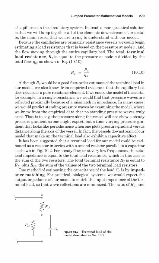
of capillaries in the circulatory system. Instead, a more practical solutionis that we will lump together all of the elements downstream of, or distalto, the main vessel that we are trying to understand with our model.
Because the capillaries are primarily resistance vessels we could beginestimating a load resistance that is based on the pressure at node n, andthe flow moving through the entire capillary bed. The total, terminalload resistance, RT is equal to the pressure at node n divided by thetotal flow qn, as shown in Eq. (10.10).
(10.10)
Although RT would be a good first-order estimate of the terminal load inour model, we also know, from empirical evidence, that the capillary beddoes not act as a pure resistance element. If we ended the model of the aorta,for example, in a single resistance, we would find that pressure waves arereflected proximally because of a mismatch in impedance. In many cases,we would predict standing pressure waves by examining the model, wherewe know from the empirical data that no standing pressure waves trulyexist. That is to say, the pressure along the vessel will not show a steadypressure gradient as one might expect, but a time-varying pressure gra-dient that looks like periodic noise when one plots pressure gradient versusdistance along the axis of the vessel. In fact, the vessels downstream of ourmodel that make up the terminal load also exhibit a capacitive effect.
It has been suggested that a terminal load for our model could be esti-mated as a resistor in series with a second resistor parallel to a capacitoras shown in Fig. 10.2. For steady flow, or at very low frequencies, the totalload impedance is equal to the total load resistance, which in this case isthe sum of the two resistors. The total terminal resistance RT is equal toRL1 plus RL2, the sum of the values of the two terminal load resistors.
One method of estimating the capacitance of the load CL is by imped-ance matching. For practical, biological systems, we would expect theoutput impedance of our model to match the input impedance of the ter-minal load, so that wave reflections are minimized. The ratio of RL1 and
RT 5 Pnqn
Lumped Parameter Mathematical Models 279
CL
RL1
RL2
n
Figure 10.2 Terminal load of themodel described in Sec.10.2.
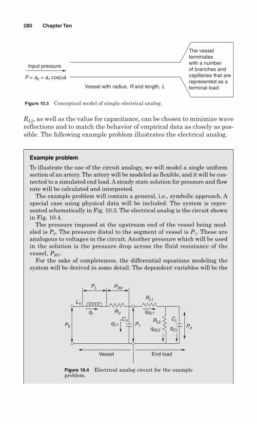
RL2, as well as the value for capacitance, can be chosen to minimize wavereflections and to match the behavior of empirical data as closely as pos-sible. The following example problem illustrates the electrical analog.
280 Chapter Ten
Figure 10.3 Conceptual model of simple electrical analog.
Example problem
To illustrate the use of the circuit analogy, we will model a single uniformsection of an artery. The artery will be modeled as flexible, and it will be con-nected to a simulated end load. A steady state solution for pressure and flowrate will be calculated and interpreted.
The example problem will contain a general, i.e., symbolic approach. Aspecial case using physical data will be included. The system is repre-sented schematically in Fig. 10.3. The electrical analog is the circuit shownin Fig. 10.4.
The pressure imposed at the upstream end of the vessel being mod-eled is P0. The pressure distal to the segment of vessel is P1. These areanalogous to voltages in the circuit. Another pressure which will be usedin the solution is the pressure drop across the fluid resistance of thevessel, PRV.
For the sake of completeness, the differential equations modeling thesystem will be derived in some detail. The dependent variables will be the
Input pressure
P = a0 + a1 cos(w)
Vessel with radius, R and length, L
The vessel terminateswith a numberof branches and capillaries that are represented as a terminal load.
Figure 10.4 Electrical analog circuit for the exampleproblem.
Vessel End load
q1
qC1qCL
CV CL
RL1
RL2
qRL1
qRL2P0
LV
RV
PL PRV
PeP1
pressures just named. We will find a steady state solution for these pres-sures, and use it to further calculate the set of flow rates.
The solution will be expressed in the terminology of the electrical analog.The development uses the Kirchhoff voltage (KVL) and current laws (KCL).These are fundamental laws of circuit behavior. We supplement them withthe equations describing the behavior of the circuit components, resistor,capacitor, and inductor. We begin with the first stage, giving the relationshipspertaining to the components.
the capacitor relationship (A)
where PL is the voltage drop across the inductor, LV (B)
(C)
Next, we apply the KVL to the circuit, looping around the circuit ele-ments and voltage drops in the stage.
It is convenient at this point to substitute Eq. (C) into this equation.
Next, solve for the derivative.
In this initial equation, P0 is taken as an input, and we interpret PRV andP1 as two state variables. Another differential equation is needed to com-plete the description of the first stage.
We apply the KCL at the junction of the two stages.
The currents are expressed in terms of voltages where PRL1 is the pressuredrop across the load resistance RL1
PRV
RV2 CV
d P1
d t2
PRL1
RL15 0
q1 2 qC1 2 qRL1 5 0
d PRV
d t5 2
RV
LV PRV 2
RV
LV P1 1
RV
LV P0
P0 2LV
RV d PRV
d t2 PRV 2 P1 5 0
P0 2 LV d q1
d t2 PRV 2 P1 5 0
q1 5 PRV
RV
PL5LV d q1
d t
qC1 5 CV d P1
d t
Lumped Parameter Mathematical Models 281
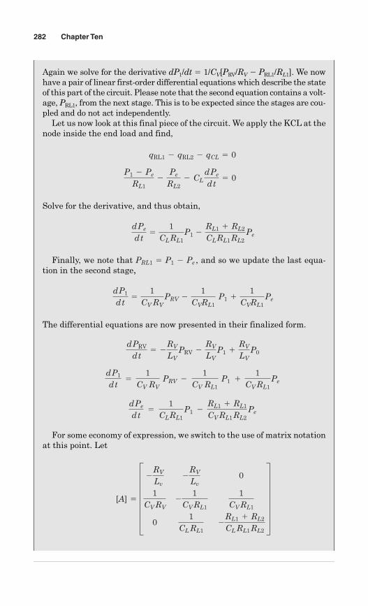
Again we solve for the derivative dP1/dt � 1/CV[PRV/RV PRL1/RL1]. We nowhave a pair of linear first-order differential equations which describe the stateof this part of the circuit. Please note that the second equation contains a volt-age, PRL1, from the next stage. This is to be expected since the stages are cou-pled and do not act independently.
Let us now look at this final piece of the circuit. We apply the KCL at thenode inside the end load and find,
Solve for the derivative, and thus obtain,
Finally, we note that , and so we update the last equa-tion in the second stage,
The differential equations are now presented in their finalized form.
For some economy of expression, we switch to the use of matrix notationat this point. Let
[A] 5 G2
RV
Lv2
RV
Lv0
1CV RV
21
CV RL1
1CV RL1
01
CL RL12
RL1 1 RL2
CL RL1 RL2
W
d Pe
d t 5
1CL
RL1 P1 2
RL1 1 RL1
CV RL1 RL2 Pe
d P1
d t 5
1CV RV
PRV 2 1
CV RL1 P1 1
1CV RL1
Pe
d PRV
d t5 2
RV
LV PRV 2
RV
LV P1 1
RV
LV P0
d P1
d t5
1CV RV
PRV 21
CVRL1 P1 1
1CVRL1
Pe
PRL1 5 P1 2 Pe
d Pe
d t5
1CL RL1
P1 2RL1 1 RL2
CL RL1 RL2 Pe
P1 2 Pe
RL12
Pe
RL22 CL
d Pe
d t5 0
qRL1 2 qRL2 2 qCL 5 0
282 Chapter Ten
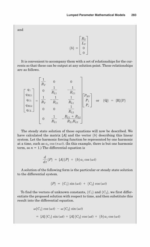
and
It is convenient to accompany them with a set of relationships for the cur-rents so that these can be output at any solution point. These relationshipsare as follows.
The steady state solution of these equations will now be described. Wehave calculated the matrix [A] and the vector describing this linearsystem. Let the harmonic forcing function be represented by one harmonicat a time, such as . (In this example, there is but one harmonicterm, so n � 1.) The differential equation is
A solution of the following form is the particular or steady state solutionto the differential system.
To find the vectors of unknown constants, and , we first differ-entiate the proposed solution with respect to time, and then substitute thisresult into the differential equation.
5 [A] 5C16 sin svtd 1 [A] 5C26 cos svtd 1 5b6 a1 cos sv td
v5C16 cos sv td 2 v 5C26 sin sv td
5C265C165P6 5 5C16 sin sv td 1 5C26 cos sv td
dd t
5P6 5 [A] 5P6 1 5b6 a1 cos sv td
an cos sn v td
5b6
Eq1
qRL1
qC1
qRL2
qCL
U 5 I1
RV0 0
01
RL12
1RL1
1RV
21
RL1
1RL1
0 01
RL2
01
RL12
RL1 1 RL2
RL1RL2
Y CPRV
P1
Pe
S � � or� � 5Q6 5 [R]5P6
5b6 5 DRV
LV
00
T
Lumped Parameter Mathematical Models 283
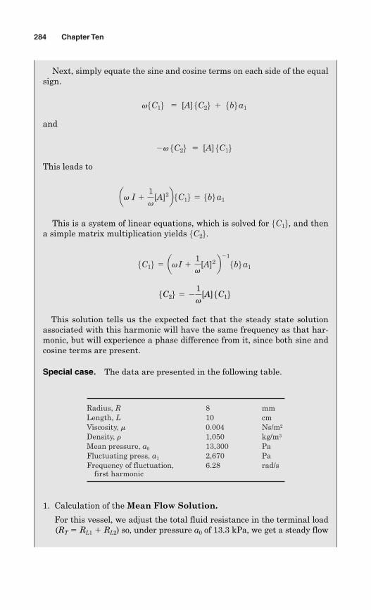
Next, simply equate the sine and cosine terms on each side of the equalsign.
and
This leads to
This is a system of linear equations, which is solved for , and thena simple matrix multiplication yields .
This solution tells us the expected fact that the steady state solutionassociated with this harmonic will have the same frequency as that har-monic, but will experience a phase difference from it, since both sine andcosine terms are present.
Special case. The data are presented in the following table.
1. Calculation of the Mean Flow Solution.
For this vessel, we adjust the total fluid resistance in the terminal load(RT � RL1 � RL2) so, under pressure a0 of 13.3 kPa, we get a steady flow
5C26 5 21v
[A] 5C16
5C16 5 av I 11v
[A]2 b215b6 a1
5C26 5C16av I 1
1v
[A]2b 5C16 5 5b6 a1
2v 5C26 5 [A] 5C16
v5C16 5 [A] 5C26 1 5b6 a1
284 Chapter Ten
Radius, R 8 mmLength, L 10 cmViscosity, m 0.004 Ns/m2
Density, r 1,050 kg/m3
Mean pressure, a0 13,300 PaFluctuating press, a1 2,670 PaFrequency of fluctuation, 6.28 rad/s
first harmonic
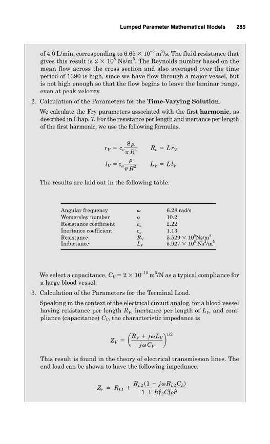
of 4.0 L/min, corresponding to 6.65 � 10–5 m3/s. The fluid resistance thatgives this result is 2 � 108 Ns/m5. The Reynolds number based on themean flow across the cross section and also averaged over the timeperiod of 1390 is high, since we have flow through a major vessel, butis not high enough so that the flow begins to leave the laminar range,even at peak velocity.
2. Calculation of the Parameters for the Time-Varying Solution.
We calculate the Fry parameters associated with the first harmonic, asdescribed in Chap. 7. For the resistance per length and inertance per lengthof the first harmonic, we use the following formulas.
The results are laid out in the following table.
We select a capacitance, CV � 2 � 10–10 m5/N as a typical compliance fora large blood vessel.
3. Calculation of the Parameters for the Terminal Load.
Speaking in the context of the electrical circuit analog, for a blood vesselhaving resistance per length RV, inertance per length of LV, and com-pliance (capacitance) CV, the characteristic impedance is
This result is found in the theory of electrical transmission lines. Theend load can be shown to have the following impedance.
Ze 5 RL1 1RL2 s1 2 j v RL2 CLd
1 1 R2L2C
2Lv
2
ZV 5 aRV 1 j v LV
j v CVb1/2
LV 5 L lVlV 5 cur
p R2
Rv 5 L rVrV 5 cv8 m
p R4
Lumped Parameter Mathematical Models 285
Angular frequency � 6.28 rad/sWomersley number � 10.2Resistance coefficient cv 2.22Inertance coefficient cu 1.13Resistance RV 5.529 � 105Ns/m5
Inductance LV 5.927 � 105 Ns2/m5
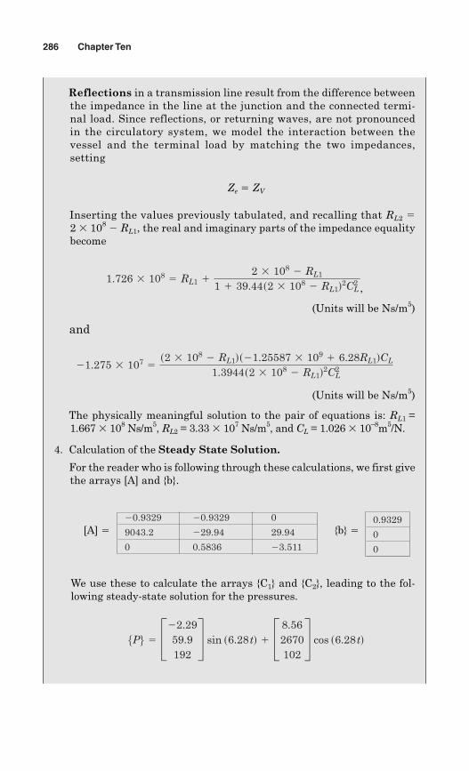
Reflections in a transmission line result from the difference betweenthe impedance in the line at the junction and the connected termi-nal load. Since reflections, or returning waves, are not pronouncedin the circulatory system, we model the interaction between thevessel and the terminal load by matching the two impedances,setting
Ze � ZV
Inserting the values previously tabulated, and recalling that RL2 �2 � 108
RL1, the real and imaginary parts of the impedance equalitybecome
,
(Units will be Ns/m5)
and
(Units will be Ns/m5)
The physically meaningful solution to the pair of equations is: RL1 =1.667 � 108 Ns/m5, RL2 = 3.33 � 107 Ns/m5, and CL = 1.026 � 10–8m5/N.
4. Calculation of the Steady State Solution.
For the reader who is following through these calculations, we first givethe arrays [A] and {b}.
[A] � {b} �
We use these to calculate the arrays {C1} and {C2}, leading to the fol-lowing steady-state solution for the pressures.
5P6 5 C22.2959.9192
S sin s6.28 td 1 C 8.562670102
S cos s6.28 td
21.275 3 107 5s2 3 108 2 RL1ds21.25587 3 109 1 6.28RL1dCL
1.3944s2 3 108 2 RL1d2C2L
1.726 3 108 5 RL1 12 3 108 2 RL1
1 1 39.44s2 3 108 2 RL1d2C2L
286 Chapter Ten
0.9329 0.9329 0
9043.2 29.94 29.94
0 0.5836 3.511
0.9329
0
0
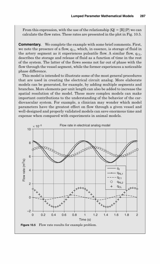
From this expression, with the use of the relationship {Q} � [R]{P} we cancalculate the flow rates. These rates are presented in the plot in Fig. 10.5.
Commentary. We complete the example with some brief comments. First,we note the presence of a flow, qC1, which, in essence, is storage of fluid inthe artery segment as it experiences pulsatile flow. A similar flow, qCL,describes the storage and release of fluid as a function of time in the restof the system. The latter of the flows seems not far out of phase with theflow through the vessel segment, while the former experiences a noticeablephase difference.
This model is intended to illustrate some of the most general proceduresthat are used in creating the electrical circuit analog. More elaboratemodels can be generated, for example, by adding multiple segments andbranches. More elements per unit length can also be added to increase thespatial resolution of the model. These more complex models can makeimportant contributions to the understanding of the behavior of the car-diovascular system. For example, a clinician may wonder which modelparameters have the greatest effect on flow through a given vessel andwell-designed and properly validated models can save enormous time andexpense when compared with experiments in animal models.
Lumped Parameter Mathematical Models 287
Figure 10.5 Flow rate results for example problem.
0–2
0
2
4
6
8
10
0.2 0.4 0.6 0.8 1 1.2 1.4 1.6 1.8 2
Time (s)
Flow rate in electrical analog model
Flo
w r
ate
(m3 /
s)
× 10–5
q1
qRL1
qC1
qRL2
qCL
10.2.3 Summary of the lumped parameterelectrical analog model
Many scientists have used similar models to mimic blood flow and pres-sure conditions in animal circulation as well as in the human circula-tory system, with the goal of better understanding of the relationshipbetween the two.
For example, Bauernschmidt et al. (1999a) simulated flow hemody-namics during pulsatile extracorporeal perfusion. Control of perfu-sion is achieved by surgeons, anesthesiologists, and perfusionistsmaking real-time decisions. This leads to variations of the perfusion reg-imens between different hospitals and between different surgical teamsin the same hospital. To develop a computer-controlled scheme for theintegrated control of extracorporeal circulation, they developed a math-ematical model for simulating hemodynamics during pulsatile perfusion.The model was constructed in Matlab using Simulink. They divided thehuman arterial tree into a 128-segment multibranch structure. Peri-pheral branches were terminated by resistance terms representingsmaller arterioles and capillary beds. Bauernschmidt studied the effectsof different perfusion regimens with differing amounts of flow and pul-satility and found the model to be useful for a realistic simulation of dif-ferent perfusion regimens.
In 2004, L. R. John developed a mathematical model of the humanarterial system, based on an electrical transmission line analogy. Theauthors concluded that quantitative variations of blood pressure andflow waveforms along the arterial tree from their model followed clinicaltrends.
10.3 Modeling of Flow through the Mitral Valve
Assessment of ventricular function and quantification of valve stenosisand mitral regurgitation are important in clinical practice as well as inphysiological research (Thomas and Weyman, 1989, 1991; Takeuchi et al.,1991; Thomas et al., 1997; Scalia et al., 1997; Rich et al., 1999; Firstenberget al., 2001; DeMey et al., 2001; Garcia et al., 2001). Approximately400,000 patients are diagnosed with congestive heart failure in theUnited States each year. Elevated diastolic filling pressure in thesepatients leads to the development of congestive heart failure symptoms(Jae et al., 1997). Noninvasive assessment of diastolic function that doesnot require the use of intracardiac pressure has been an important goal,and in recent years, Doppler electrocardiography has become the “diag-nostic modality of choice” (Garcia et al., 2001) to assess diastolic function.
The goal of the research that created this model was development andvalidation of a mathematical model of flow through the mitral valve
288 Chapter Ten
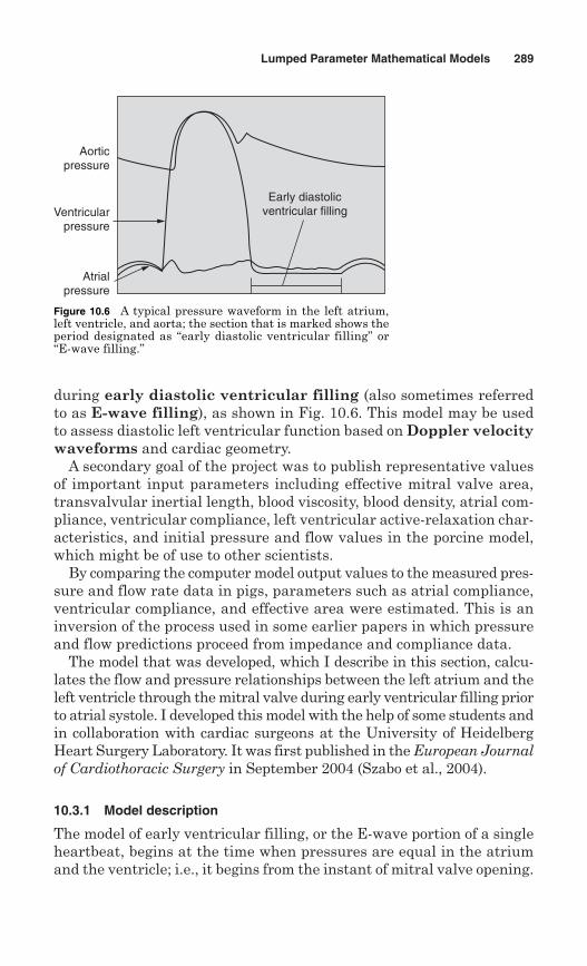
during early diastolic ventricular filling (also sometimes referredto as E-wave filling), as shown in Fig. 10.6. This model may be usedto assess diastolic left ventricular function based on Doppler velocitywaveforms and cardiac geometry.
A secondary goal of the project was to publish representative valuesof important input parameters including effective mitral valve area,transvalvular inertial length, blood viscosity, blood density, atrial com-pliance, ventricular compliance, left ventricular active-relaxation char-acteristics, and initial pressure and flow values in the porcine model,which might be of use to other scientists.
By comparing the computer model output values to the measured pres-sure and flow rate data in pigs, parameters such as atrial compliance,ventricular compliance, and effective area were estimated. This is aninversion of the process used in some earlier papers in which pressureand flow predictions proceed from impedance and compliance data.
The model that was developed, which I describe in this section, calcu-lates the flow and pressure relationships between the left atrium and theleft ventricle through the mitral valve during early ventricular filling priorto atrial systole. I developed this model with the help of some students andin collaboration with cardiac surgeons at the University of HeidelbergHeart Surgery Laboratory. It was first published in the European Journalof Cardiothoracic Surgery in September 2004 (Szabo et al., 2004).
10.3.1 Model description
The model of early ventricular filling, or the E-wave portion of a singleheartbeat, begins at the time when pressures are equal in the atriumand the ventricle; i.e., it begins from the instant of mitral valve opening.
Lumped Parameter Mathematical Models 289
Atrialpressure
Ventricularpressure
Aorticpressure
Early diastolicventricular filling
Figure 10.6 A typical pressure waveform in the left atrium,left ventricle, and aorta; the section that is marked shows theperiod designated as “early diastolic ventricular filling” or“E-wave filling.”
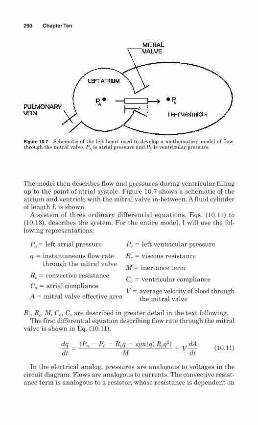
The model then describes flow and pressures during ventricular fillingup to the point of atrial systole. Figure 10.7 shows a schematic of theatrium and ventricle with the mitral valve in-between. A fluid cylinderof length L is shown.
A system of three ordinary differential equations, Eqs. (10.11) to(10.13), describes the system. For the entire model, I will use the fol-lowing representations:
Pa � left atrial pressure Pv � left ventricular pressure
q � instantaneous flow rate Rv � viscous resistancethrough the mitral valve
Rc � convective resistanceM � inertance term
Ca � atrial complianceCv � ventricular compliance
A � mitral valve effective areaV � average velocity of blood through
the mitral valve
Rv, Rc, M, Ca, Cv are described in greater detail in the text following.The first differential equation describing flow rate through the mitral
valve is shown in Eq. (10.11).
(10.11)
In the electrical analog, pressures are analogous to voltages in thecircuit diagram. Flows are analogous to currents. The convective resist-ance term is analogous to a resistor, whose resistance is dependent on
dqdt5sPa 2 Pv 2 Rvq 2 sgnsqd Rcq
2dM
1 V dAdt
290 Chapter Ten
Figure 10.7 Schematic of the left heart used to develop a mathematical model of flowthrough the mitral valve. PA is atrial pressure and PV is ventricular pressure.
the current, which flows through it. Convective resistance will be dis-cussed in more detail in Sec. 10.3.3. The term represents the timerate of change of flow rate due to the closing or opening of the mitralvalve. If the valve were held completely open, this term would be zero.Section 10.3.4 describes, in greater detail, the variable-area mitralvalve that is used in this model.
The second differential equation is written as follows:
(10.12)
where Ca represents atrial compliance in m5/N . The pressure insidethe atrium is related to its volume through atrial compliance, Ca �d(volume)/dt. The volume is also related to flow rate. In one sense, theflow into the atrium determines its final volume and therefore thefinal atrial pressure.
Similarly, the third equation describing the system is the equation forchange in ventricular pressure with time. The ventricular pressure issimilarly related to the ventricular volume and the ventricular compli-ance, Cv. The change in pressure of the ventricle is also related to “activerelaxation.” The active relaxation term, resulting from ventricular geom-etry, is described in more detail in Sec. 10.3.2.
(10.13)
In all three equations, q represents flow rate in m3/s, dq/dt representsthe time rate of change of flow rate in m3/s2, Pa represents left atrialpressure in N/m2, Pv represents left ventricular pressure in N/m2, andM represents the inertance term, which is analogous to inductance inthe electrical circuit and has the units of kg/m4.
M in Eq. (10.14) can be calculated as
(10.14)
where represents blood density in kg/m3, l represents the blood columnlength through the mitral valve with units of meters, and A representsthe mitral valve effective area in m2.
Rv in Eq. (10.15) represents viscous resistance, which is analogous toresistance in the electrical circuit and has the units kg/m4s. Rv can becalculated as
(10.15)
where represents viscosity with units of Ns/m2.m
Rv 5 8 rlm/A2
r
M 5 rl/A
dPv
dt5
qCv2 active relaxation term
Q m3
N/m2RdPa
dt52qCa
V dAdt
Lumped Parameter Mathematical Models 291
Rc represents convective resistance, which, in an electrical circuitmodel, would be analogous to a resistor whose variable resistance isdependent on current through the resistor, and has the units kg/m7.Rc can be calculated as
(10.16)
10.3.2 Active ventricular relaxation
Another parameter affecting the final ventricular pressure during fill-ing is active relaxation. To imagine active relaxation think of an emptyplastic 1-L soft drink bottle. If you squeeze the bottle, the volumedecreases, forcing air out of the bottle. Now when you release the bottlebecause of its geometry the bottle will expand, and if air is not allowedto flow back into the bottle (place your hand over the entrance) the pres-sure inside it will decrease below atmospheric. At the beginning of dias-tole, the left ventricle expands in a similar way and we say that activeventricular relaxation is present.
For the purpose of the model, active relaxation can be measuredempirically and included in the model as a term, which decreases thepressure in the ventricle. When active relaxation occurs, it looks like astep change of pressure in a near critically damped system. Active relax-ation parameters include a time constant for the pressure drop off andalso a ratio of the maximum atrial pressure (pressure just prior to activerelaxation) to minimum atrial pressure.
10.3.3 Meaning of convective resistance
To help understand the meaning of convective resistance, consider theBernoulli equation while neglecting viscous resistance. The transmitralpressure drop, P, is equal to 1/2 V2 where V is the transmitral veloc-ity. Rc represents the convective resistance or resistance to flow associ-ated with acceleration due to spatial changes rather than temporalchanges. Blood must speed up as it passes through the mitral valve,because the valve acts like a nozzle on a garden hose. By using a nozzleon a garden hose, you can increase the velocity of the water as it exitsthe hose without increasing the pressure driving the water. In the sameway that water is speeded up when leaving a garden hose using a nozzle,blood must be accelerated as it moves through the mitral valve. Thatacceleration is the explanation for convective resistance.
10.3.4 Variable area mitral valve modeldescription
Previous lumped parameter models of diastolic filling modeled the mitralvalve as a cylinder of a fixed cross-sectional area and length (Thomasand Weyman, 1989, 1992; Flachskampf et al., 1992; Waite et al., 2000).
r
Rc 5 rl/A2
292 Chapter Ten
Although the valve opening is clearly not constant since the valve bynature must open and close, it was possible to make a reasonable firstestimate of the flow through the valve by modeling it as instantaneously100 percent open or 100 percent closed.
In the current version of the model, the valve is modeled with a time-varying mitral opening area. One piece of the lumped parameter modeldescribed earlier is a model of the intrinsic and extrinsic characteristicsof the valve itself, disregarding the heart chambers. We will call this por-tion of the model the “variable-area mitral valve model.” A completedescription of the variable area mitral valve model that was used as apart of this model can be seen in Franck and Waite (2002).
By using a systems approach, the mitral valve aperture can be viewedabstractly as a mechanical system whose behavior is governed by intrin-sic dynamics and the forces acting on it. The intrinsic dynamics of thevalve aperture are modeled by a second-order linear differential equation.This way of modeling takes into account the mass of the valve cusps, theelasticity of the tissue, and the damping experienced by the valve cuspswhile it also helps to keep the valve model simple. The equation alreadycontains two of the six parameters the valve model uses: the damping coef-ficient D and the natural frequency of the mitral valve . D describes theamount of damping the valve cusps experience, which mainly depends onblood viscosity and the size of the cusps. The natural frequency takesinto account the mass of the valve cusps and the elasticity of the tissue.
(10.17)
The intrinsic dynamics of the forces acting on the valve, F(t), are rep-resented by the following equation with the parameters explained laterin Sec. 10.3.5.
(10.18)
Equation (10.17) is a second-order, nonlinear differential equation. Thevariable area A replaces all occurrences of the constant effective mitralvalve area in the earlier model.
10.3.5 Variable area mitral valve modelparameters
The equation for the variable area introduced six new parameters intothe model. (1) Amax is the cross-sectional aperture of the mitral valvewhen fully opened. (2) The Greek character represents the naturalfrequency of the mitral valve in s–1. It is influenced by the mass of thevalve cusps and the modulus of elasticity of the tissue. (3) D represents
v
Fstd 5 sAmax 2 Ad cKssPa 2 Pvd 1 KdsgnsV dV 21 KadVdtd
1v2 A
??1
2Dv
A?1 A 5 Fstd
v
v
Lumped Parameter Mathematical Models 293
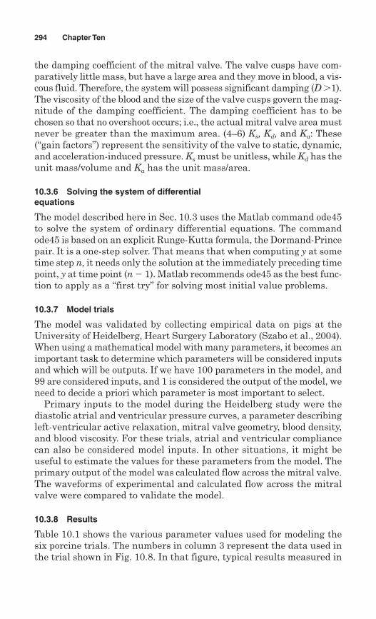
the damping coefficient of the mitral valve. The valve cusps have com-paratively little mass, but have a large area and they move in blood, a vis-cous fluid. Therefore, the system will possess significant damping (D �1).The viscosity of the blood and the size of the valve cusps govern the mag-nitude of the damping coefficient. The damping coefficient has to bechosen so that no overshoot occurs; i.e., the actual mitral valve area mustnever be greater than the maximum area. (4–6) Ks, Kd, and Ka: These(“gain factors”) represent the sensitivity of the valve to static, dynamic,and acceleration-induced pressure. Ks must be unitless, while Kd has theunit mass/volume and Ka has the unit mass/area.
10.3.6 Solving the system of differentialequations
The model described here in Sec. 10.3 uses the Matlab command ode45to solve the system of ordinary differential equations. The commandode45 is based on an explicit Runge-Kutta formula, the Dormand-Princepair. It is a one-step solver. That means that when computing y at sometime step n, it needs only the solution at the immediately preceding timepoint, y at time point (n � 1). Matlab recommends ode45 as the best func-tion to apply as a “first try” for solving most initial value problems.
10.3.7 Model trials
The model was validated by collecting empirical data on pigs at theUniversity of Heidelberg, Heart Surgery Laboratory (Szabo et al., 2004).When using a mathematical model with many parameters, it becomes animportant task to determine which parameters will be considered inputsand which will be outputs. If we have 100 parameters in the model, and99 are considered inputs, and 1 is considered the output of the model, weneed to decide a priori which parameter is most important to select.
Primary inputs to the model during the Heidelberg study were thediastolic atrial and ventricular pressure curves, a parameter describingleft-ventricular active relaxation, mitral valve geometry, blood density,and blood viscosity. For these trials, atrial and ventricular compliancecan also be considered model inputs. In other situations, it might beuseful to estimate the values for these parameters from the model. Theprimary output of the model was calculated flow across the mitral valve.The waveforms of experimental and calculated flow across the mitralvalve were compared to validate the model.
10.3.8 Results
Table 10.1 shows the various parameter values used for modeling thesix porcine trials. The numbers in column 3 represent the data used inthe trial shown in Fig. 10.8. In that figure, typical results measured in
294 Chapter Ten
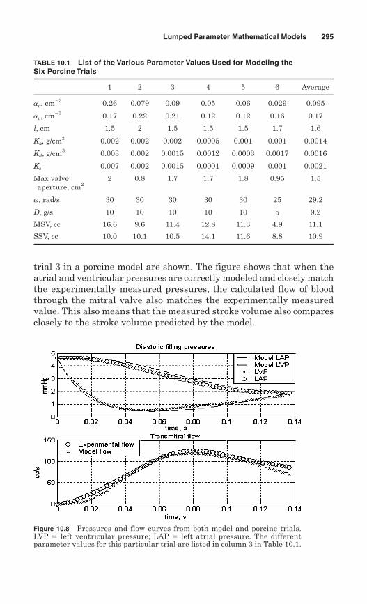
trial 3 in a porcine model are shown. The figure shows that when theatrial and ventricular pressures are correctly modeled and closely matchthe experimentally measured pressures, the calculated flow of bloodthrough the mitral valve also matches the experimentally measuredvalue. This also means that the measured stroke volume also comparesclosely to the stroke volume predicted by the model.
Lumped Parameter Mathematical Models 295
TABLE 10.1 List of the Various Parameter Values Used for Modeling theSix Porcine Trials
1 2 3 4 5 6 Average
�a, cm3 0.26 0.079 0.09 0.05 0.06 0.029 0.095
�v, cm3 0.17 0.22 0.21 0.12 0.12 0.16 0.17
l, cm 1.5 2 1.5 1.5 1.5 1.7 1.6
Ka, g/cm2 0.002 0.002 0.002 0.0005 0.001 0.001 0.0014
Kd, g/cm3 0.003 0.002 0.0015 0.0012 0.0003 0.0017 0.0016
Ks 0.007 0.002 0.0015 0.0001 0.0009 0.001 0.0021
Max valve 2 0.8 1.7 1.7 1.8 0.95 1.5aperture, cm2
�, rad/s 30 30 30 30 30 25 29.2
D, g/s 10 10 10 10 10 5 9.2
MSV, cc 16.6 9.6 11.4 12.8 11.3 4.9 11.1
SSV, cc 10.0 10.1 10.5 14.1 11.6 8.8 10.9
Figure 10.8 Pressures and flow curves from both model and porcine trials.LVP � left ventricular pressure; LAP � left atrial pressure. The differentparameter values for this particular trial are listed in column 3 in Table 10.1.
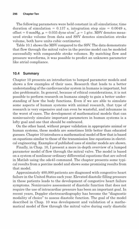
The following parameters were held constant in all simulations; timeduration of simulation � 0.137 s, integration step size � 0.0049 s,offset � 0 mmHg, m� 0.035 dyne s/cm2, � 1 g/cc. MSV denotes meas-ured stroke volume from data and SSV denotes simulation strokevolume, both have units cubic centimeter.
Table 10.1 shows the MSV compared to the SSV. The data demonstratethat flow through the mitral valve in the porcine model can be modeledsuccessfully with comparable stroke volumes. By matching flow andpressure waveforms, it was possible to predict an unknown parameterlike atrial compliance.
10.4 Summary
Chapter 10 presents an introduction to lumped parameter models andshows a few examples of their uses. Research that leads to a betterunderstanding of the cardiovascular system in humans is important, butalso problematic. In general, because of ethical considerations, it is notpossible to perform research on humans simply to gain a better under-standing of how the body functions. Even if we are able to simulatesome aspects of human systems with animal research, that type ofresearch is very expensive and can even be wasteful, and inhumane inthe worst of cases. The development of mathematical models that cannoninvasively simulate important parameters in human systems is alofty goal and one that should be embraced.
On the other hand, without proper validation in appropriate animal orhuman systems, these models are sometimes little better than educatedguesses. Chapter 10 introduces a mathematical model of flow that is basedon equations similar to those of the transmission line equations in electri-cal engineering. Examples of published uses of similar models are shown.
Finally, in Chap. 10, I present a more in-depth overview of a lumpedparameter model of flow through the mitral valve. The model is basedon a system of nonlinear ordinary differential equations that are solvedin Matlab using the ode45 command. The chapter presents some typi-cal results from a porcine model and shows some promising results fromthat model.
Approximately 400,000 patients are diagnosed with congestive heartfailure in the United States each year. Elevated diastolic filling pressurein these patients leads to the development of congestive heart failuresymptoms. Noninvasive assessment of diastolic function that does notrequire the use of intracardiac pressure has been an important goal. Inrecent years, Doppler electrocardiography has become the “diagnosticmodality of choice” to assess diastolic function. The goal of the modeldescribed in Chap. 10 was development and validation of a mathe-matical model of flow through the mitral valve during early diastolic
r
296 Chapter Ten
ventricular filling (also sometimes referred to as E-wave filling), whichpromises assessment of diastolic left ventricular function using non-invasively collected Doppler waveforms.
Review Problems
1. Using Matlab or a computer algebra system, set up and repeat the calcula-tions of the example problem following Sec. 10.2.2.
2. Try a new version of the example problem above with a different set of data.See the table.
Lumped Parameter Mathematical Models 297
Radius, R 8.5 mmLength, L 15 cmViscosity, m 0.0042 Ns/m2
Density, r 1,050 kg/m3
Mean pressure, a0 12,500 PaPulse press, a1 2,500 PaFrequency of fluctuation, 7.5 rad/sfirst harmonic
3. Extend the example by adding two additional stages. Derive the matrices [A],{b}, and [R]. Solve the example problem, but with an artery that has taper.Let the segments have radii of 8.0, 7.5, and 7.0 mm. Assume that the lengthis still 10 cm. Keep the “capacitance” constant.
Bibliography
Bauernschmitt R, Naujokat E, Mehmanesh H, Schulz S, Vahl CF, Hagl S, Lange R.“Mathematical Modelling of Extracorporeal Circulation: Simulation of DifferentPerfusion Regimens,” Perfusion, 14(5), 321–330, 1999a.
Bauernschmitt R, Schulz S, Schwarzhaupt A, Kiencke U, Vahl CF, Lange R, Hagl S.“Simulation of Arterial Hemodynamics after Partial Prosthetic Replacement of theAorta,” Ann. Thorac. Surg., 68(4), 1441–1442, 1999b.
De Mey S, De Sutter J, Vierendeels J, Verdonck P. “Diastolic Filling and Pressure Imaging:Taking Advantage of the Information in a Colour M-mode Doppler Image.” Eur JEchocardiogr. Review. 2(4):219–233, 2001.
Firstenberg MS, Greenberg NL, Smedira NG, McCarthy PM, Garcia MJ, Thomas JD.“Relationship between Systolic and Diastolic Function with Improvements in ForwardStroke Volume Following Reduction in Mitral Regurgitation.” Comput. Cardiol. 28:177–180, 2001.
Fisher J. “Comparative Study of the Hydrodynamic Function of Six Size 19 mm BileafletHeart Valves,” Eur. J. Cardiothorac. Surg., 9(12), 692–695, 1995; discussion 695–696.
Flachskampf F, Weyman A, Guerrero JL, Thomas JD. “Calculation of AtrioventricularCompliance from the Mitral Flow Profile: Analytic and in-Vitro Study,” J. Am. Coll.Cardiol., 19, 998–1004, 1992.
Franck C. A Lumped Variable Model for Mitral Valve Aperture during Diastolic Filling[M.S. thesis], Rose-Hulman Institute of Technology, Terre Haute, IN, 2001.
Franck C, Waite, L. “Mathematical Model of a Variable Aperture Mitral Valve,” Biomed.Sci. Instrum., 38, 327–331, 2002.
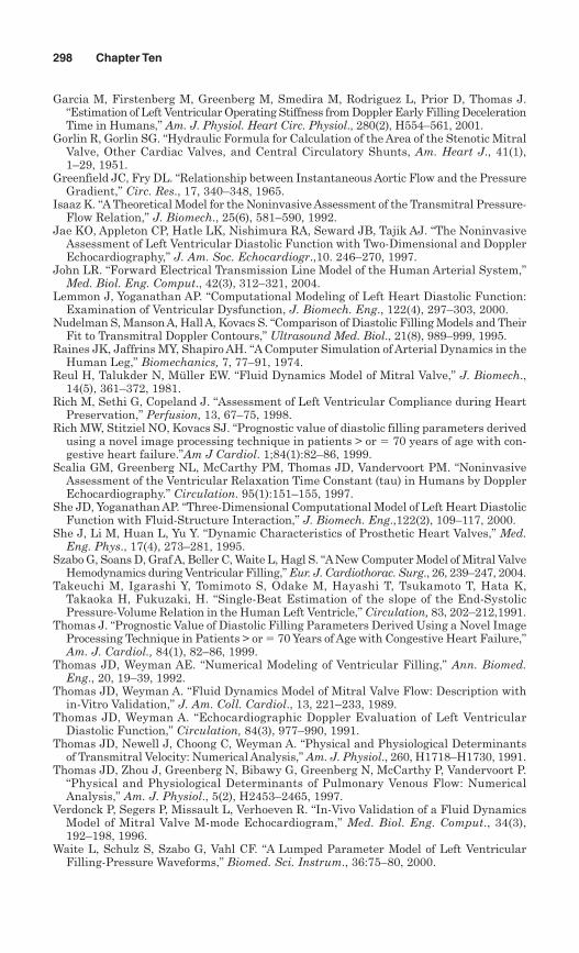
Garcia M, Firstenberg M, Greenberg M, Smedira M, Rodriguez L, Prior D, Thomas J.“Estimation of Left Ventricular Operating Stiffness from Doppler Early Filling DecelerationTime in Humans,” Am. J. Physiol. Heart Circ. Physiol., 280(2), H554–561, 2001.
Gorlin R, Gorlin SG. “Hydraulic Formula for Calculation of the Area of the Stenotic MitralValve, Other Cardiac Valves, and Central Circulatory Shunts, Am. Heart J., 41(1),1–29, 1951.
Greenfield JC, Fry DL. “Relationship between Instantaneous Aortic Flow and the PressureGradient,” Circ. Res., 17, 340–348, 1965.
Isaaz K. “A Theoretical Model for the Noninvasive Assessment of the Transmitral Pressure-Flow Relation,” J. Biomech., 25(6), 581–590, 1992.
Jae KO, Appleton CP, Hatle LK, Nishimura RA, Seward JB, Tajik AJ. “The NoninvasiveAssessment of Left Ventricular Diastolic Function with Two-Dimensional and DopplerEchocardiography,” J. Am. Soc. Echocardiogr.,10. 246–270, 1997.
John LR. “Forward Electrical Transmission Line Model of the Human Arterial System,”Med. Biol. Eng. Comput., 42(3), 312–321, 2004.
Lemmon J, Yoganathan AP. “Computational Modeling of Left Heart Diastolic Function:Examination of Ventricular Dysfunction, J. Biomech. Eng., 122(4), 297–303, 2000.
Nudelman S, Manson A, Hall A, Kovacs S. “Comparison of Diastolic Filling Models and TheirFit to Transmitral Doppler Contours,” Ultrasound Med. Biol., 21(8), 989–999, 1995.
Raines JK, Jaffrins MY, Shapiro AH. “A Computer Simulation of Arterial Dynamics in theHuman Leg,” Biomechanics, 7, 77–91, 1974.
Reul H, Talukder N, Müller EW. “Fluid Dynamics Model of Mitral Valve,” J. Biomech.,14(5), 361–372, 1981.
Rich M, Sethi G, Copeland J. “Assessment of Left Ventricular Compliance during HeartPreservation,” Perfusion, 13, 67–75, 1998.
Rich MW, Stitziel NO, Kovacs SJ. “Prognostic value of diastolic filling parameters derivedusing a novel image processing technique in patients > or � 70 years of age with con-gestive heart failure.”Am J Cardiol. 1;84(1):82–86, 1999.
Scalia GM, Greenberg NL, McCarthy PM, Thomas JD, Vandervoort PM. “NoninvasiveAssessment of the Ventricular Relaxation Time Constant (tau) in Humans by DopplerEchocardiography.” Circulation. 95(1):151–155, 1997.
She JD, Yoganathan AP. “Three-Dimensional Computational Model of Left Heart DiastolicFunction with Fluid-Structure Interaction,” J. Biomech. Eng.,122(2), 109–117, 2000.
She J, Li M, Huan L, Yu Y. “Dynamic Characteristics of Prosthetic Heart Valves,” Med.Eng. Phys., 17(4), 273–281, 1995.
Szabo G, Soans D, Graf A, Beller C, Waite L, Hagl S. “ANew Computer Model of Mitral ValveHemodynamics during Ventricular Filling,” Eur. J. Cardiothorac. Surg., 26, 239–247, 2004.
Takeuchi M, Igarashi Y, Tomimoto S, Odake M, Hayashi T, Tsukamoto T, Hata K,Takaoka H, Fukuzaki, H. “Single-Beat Estimation of the slope of the End-SystolicPressure-Volume Relation in the Human Left Ventricle,” Circulation, 83, 202–212,1991.
Thomas J. “Prognostic Value of Diastolic Filling Parameters Derived Using a Novel ImageProcessing Technique in Patients > or � 70 Years of Age with Congestive Heart Failure,”Am. J. Cardiol., 84(1), 82–86, 1999.
Thomas JD, Weyman AE. “Numerical Modeling of Ventricular Filling,” Ann. Biomed.Eng., 20, 19–39, 1992.
Thomas JD, Weyman A. “Fluid Dynamics Model of Mitral Valve Flow: Description within-Vitro Validation,” J. Am. Coll. Cardiol., 13, 221–233, 1989.
Thomas JD, Weyman A. “Echocardiographic Doppler Evaluation of Left VentricularDiastolic Function,” Circulation, 84(3), 977–990, 1991.
Thomas JD, Newell J, Choong C, Weyman A. “Physical and Physiological Determinantsof Transmitral Velocity: Numerical Analysis,” Am. J. Physiol., 260, H1718–H1730, 1991.
Thomas JD, Zhou J, Greenberg N, Bibawy G, Greenberg N, McCarthy P, Vandervoort P.“Physical and Physiological Determinants of Pulmonary Venous Flow: NumericalAnalysis,” Am. J. Physiol., 5(2), H2453–2465, 1997.
Verdonck P, Segers P, Missault L, Verhoeven R. “In-Vivo Validation of a Fluid DynamicsModel of Mitral Valve M-mode Echocardiogram,” Med. Biol. Eng. Comput., 34(3),192–198, 1996.
Waite L, Schulz S, Szabo G, Vahl CF. “A Lumped Parameter Model of Left VentricularFilling-Pressure Waveforms,” Biomed. Sci. Instrum., 36:75–80, 2000.
298 Chapter Ten

Index
Copyright © 2007 by The McGraw-Hill Companies, Inc. Click here for terms of use.

This page intentionally left blank

A wave, 172AAA. See abdominal aortic aneurysmsabdominal aortic aneurysms (AAA),
156–157absolute viscosity, 11, 13acclimatization, 103–105acetazolamide, 103. See also Diamoxacid-base balance, 77, 137acidosis, 137de Acosta, Joseph, 3–4acquired immune deficiency syndrome
(AIDS), 130–131action potential, 40, 42, 43factive relaxation, 292acute mountain sickness (AMS), 4, 103–104afterload, 56, 57agglutination, 133agranulocytes, 128AIDS. See acquired immune deficiency
syndromeairway resistance, 88–91albumin, 135
serum, 68alkalosis, 137
respiratory, 103allele, 133Alliance Medical Technologies, 182allografts, 161, 184alpha parameter, 29–30, 208, 218, 219f,
266t. See also Womersley numberaltitude, high, 2–4, 13, 93, 99–105alveolar gas equation, 102–103, 106alveoli, 77–78, 78f
emphysema and, 96–97gas transport in, 91–93oxygen in, 102pressure in, 82–83ventilation of, 79wall of, 92
amplification factor, 218AMS. See acute mountain sicknessanacrotic limb, 54, 54f“An anatomical study of the motion of the
heart and of the blood of animals”(Harvey), 5
anemia, 105, 112general, 126hemolytic, 131macrocytic hyperchromic, 126sickle cell, 124–125
aneurysm, 156–157angina pectoris, 51fangioplasty, 159Annapurna (Herzog), 13anterior descending coronary artery, 64antibodies, 132–134antigens, 133–135aorta, 36, 37f, 39, 39f, 51, 61
alpha parameter for, 30aneurysm of, 156–157CABG surgery and, 160modeling, 278–279pressure in, 52, 53f, 54, 54f, 61stenosis of, 155stiffness of, 152, 154systemic circulation and, 37wall shear stress in, 10
aortic sinus, 167aortic valve, 51, 52f, 165–170, 166f,
169f, 230diastolic stress on, 168flow rate through, 173, 175implantation of replacement, 169–170leaflets of, 166, 166f, 168peak velocity through, 168pressure gradient across, 178regurgitation through, 63, 168replacement of, 169–170, 178–184stenosis of, 168
appendicitis, 129Aranesp, 105Aristotle, 2, 4arrhythmia, 49–50, 50f, 106arterial tree, modeling, 288arteries, 2, 6, 37f. See also aorta;
coronary arteriescirculation and, 37–38compliance of, 63, 147–154coronary, 64–65disease of, 9, 255
301
Page numbers followed by t, f, or n indicate tables, figures, or notes, respectively.
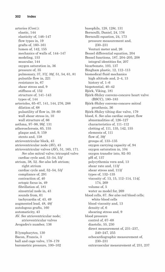
arteries (Cont.):elastic, 144elasticity of, 146–147flow types in, 19grafts of, 160–161lumen of, 142, 155mechanics of walls of, 144–147modeling, 153muscular, 144oxygen saturation in, 36pressure of, 35pulmonary, 37, 37f, 39f, 51, 54, 61, 81pulsatile flow in, 221resistance in, 67shear stress and, 9stiffness of, 152structure of, 141–143types of, 144
arterioles, 65–67, 141, 144, 276, 288dilation of, 68pulsatility of flow in, 59–60wall shear stress in, 10wall structure of, 66
asthma, 97–98, 99f, 131atherosclerosis, 65, 155
plaque and, 9, 159stents and, 158
atrioventricular block, 43atrioventricular node (AV), 43atrioventricular valves (AV), 51, 165, 171.
See also mitral valve; tricuspid valvecardiac cycle and, 53–54, 53f
atrium, 38, 52. See also left atrium; right atrium
cardiac cycle and, 52–54, 53fcompliance of, 291contraction of, 40ectopic focus in, 49fibrillation of, 181sinoatrial node in, 43sounds from, 61tachycardia of, 43, 49
augmented lead, 48, 48fautologous grafts, 160automaticity, 43AV. See atrioventricular node;
atrioventricular valvesAvogadro’s number, 136
B lymphocytes, 130Bacon, Francis, 3ball and cage valve, 178–179barometric pressure, 100–102
basophils, 128, 128t, 131Bernoulli, Daniel, 24, 176Bernoulli equation, 24, 173
pressure measurement and, 230–231
Venturi meter and, 26Bessel differential equation, 204Bessel functions, 187, 204–205, 208
integral identities for, 207bicarbonate, 103, 137Bingham plastic, 12, 112–113biomedical fluid mechanics
high altitude and, 2–4, 13history of, 1–6
biopotential, 40–42Björk, Viking, 181Björk-Shiley convexo-concave heart valve
(BSCC), 180–183Björk-Shiley convexo-concave mitral
prosthesis, 36Björk-Shiley tilting disc valve, 179blood, 6. See also cardiac output; flow
abnormalities of, 126–127characteristics of, 111–112clotting of, 111, 135, 142, 155elements of, 111flow of, 39fgroups of, 133–135oxygen carrying capacity of, 94oxygen saturation in, 104oxygen transfer into, 92–93pH of, 137polycythemia vera and, 13shear rate and, 113fshear stress and, 113ftypes of, 132–135viscosity of, 13, 15, 112–114, 114f,
174, 269volume of, 5water as model for, 269
blood cells, 67. See also red blood cells;white blood cells
blood viscosity and, 13density of, 6shearing stress and, 9
blood pressurecontrol of, 67–68diastolic, 55, 230direct measurement of, 231–237,
240–247, 255echocardiographic measurement of,
230–231extravascular measurement of, 231, 237
302 Index
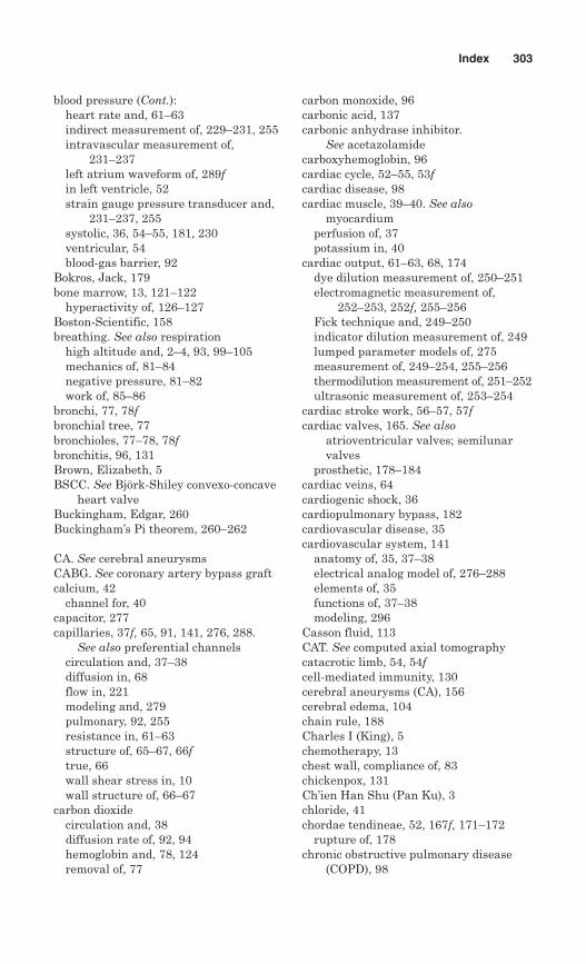
blood pressure (Cont.):heart rate and, 61–63indirect measurement of, 229–231, 255intravascular measurement of,
231–237left atrium waveform of, 289fin left ventricle, 52strain gauge pressure transducer and,
231–237, 255systolic, 36, 54–55, 181, 230ventricular, 54blood-gas barrier, 92
Bokros, Jack, 179bone marrow, 13, 121–122
hyperactivity of, 126–127Boston-Scientific, 158breathing. See also respiration
high altitude and, 2–4, 93, 99–105mechanics of, 81–84negative pressure, 81–82work of, 85–86
bronchi, 77, 78fbronchial tree, 77bronchioles, 77–78, 78fbronchitis, 96, 131Brown, Elizabeth, 5BSCC. See Björk-Shiley convexo-concave
heart valveBuckingham, Edgar, 260Buckingham’s Pi theorem, 260–262
CA. See cerebral aneurysmsCABG. See coronary artery bypass graftcalcium, 42
channel for, 40capacitor, 277capillaries, 37f, 65, 91, 141, 276, 288.
See also preferential channelscirculation and, 37–38diffusion in, 68flow in, 221modeling and, 279pulmonary, 92, 255resistance in, 61–63structure of, 65–67, 66ftrue, 66wall shear stress in, 10wall structure of, 66–67
carbon dioxidecirculation and, 38diffusion rate of, 92, 94hemoglobin and, 78, 124removal of, 77
carbon monoxide, 96carbonic acid, 137carbonic anhydrase inhibitor.
See acetazolamidecarboxyhemoglobin, 96cardiac cycle, 52–55, 53fcardiac disease, 98cardiac muscle, 39–40. See also
myocardiumperfusion of, 37potassium in, 40
cardiac output, 61–63, 68, 174dye dilution measurement of, 250–251electromagnetic measurement of,
252–253, 252f, 255–256Fick technique and, 249–250indicator dilution measurement of, 249lumped parameter models of, 275measurement of, 249–254, 255–256thermodilution measurement of, 251–252ultrasonic measurement of, 253–254
cardiac stroke work, 56–57, 57fcardiac valves, 165. See also
atrioventricular valves; semilunarvalves
prosthetic, 178–184cardiac veins, 64cardiogenic shock, 36cardiopulmonary bypass, 182cardiovascular disease, 35cardiovascular system, 141
anatomy of, 35, 37–38electrical analog model of, 276–288elements of, 35functions of, 37–38modeling, 296
Casson fluid, 113CAT. See computed axial tomographycatacrotic limb, 54, 54fcell-mediated immunity, 130cerebral aneurysms (CA), 156cerebral edema, 104chain rule, 188Charles I (King), 5chemotherapy, 13chest wall, compliance of, 83chickenpox, 131Ch’ien Han Shu (Pan Ku), 3chloride, 41chordae tendineae, 52, 167f, 171–172
rupture of, 178chronic obstructive pulmonary disease
(COPD), 98
Index 303
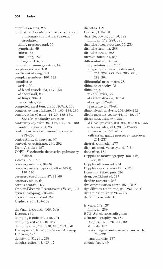
circuit elements, 277circulation. See also coronary circulation;
pulmonary circulation; systemiccirculation
filling pressure and, 55lymphatic, 69micro-, 65modelling, 187theory of, 1, 5, 6
circumflex coronary artery, 64coaption surface, 166coefficient of drag, 267complex numbers, 190–192compliance
atrial, 291of blood vessels, 63, 147–152of chest wall, 83of lungs, 83–84ventricular, 290
computed axial tomography (CAT), 156congestive heart failure, 58, 106, 288, 296conservation of mass, 24–25, 188–190.
See also continuity equationcontinuity equation, 25, 177, 188, 189–190
Venturi meter and, 26continuous wave ultrasonic flowmeter,
253–256contractility, changes in, 57convective resistance, 290, 292Cook Vascular, 157COPD. See chronic obstructive pulmonary
diseaseCordis, 158–159coronary arteries, 64–65coronary artery bypass graft (CABG),
159–160coronary circulation, 37, 63–65coronary sinus, 64corpus arantii, 166Cribier-Edwards Percutaneous Valve, 170critical damping, 246–247critical time constant, 247Cypher stent, 158–159
da Vinci, Leonardo, 168, 169fDacron, 160damping coefficient, 240, 294damping, critical, 246–247damping ratio, 241–243, 246, 248, 276Darbepoetin, 105–106. See also AranespDC term, 195density, 6, 91, 261, 269depolarization, 42, 42f, 47
diabetes, 159Diamox, 103–104diastole, 53–54, 53f, 56, 292
filling in, 172, 288, 296diastolic blood pressure, 55, 230diastolic function, 288diastolic stress, 168dicrotic notch, 54, 54fdifferential equations
Fry solution and, 217lumped parameter models and,
277–278, 282–283, 290–291,293–294
differential manometer, 28diffusing capacity, 93diffusion, 91
in capillaries, 68of carbon dioxide, 92, 94of oxygen, 92–94resistance to, 93–94
dimensional analysis, 259, 260–262dipole moment vector, 44, 45–48, 46fdirect measurement, 255
of blood pressure, 231–237, 240–247, 255extravascular, 214, 231, 237–247intravascular, 231–237with strain gauge pressure transducer,
231–237discretized model, 277displacement, velocity and, 7–8dopamine, 181Doppler echocardiography, 155, 176,
288, 296Doppler ultrasound, 254Doppler velocity waveforms, 289Dormand-Prince pair, 294drag, coefficient of, 267driving pressure, 243dye concentration curve, 251, 251fdye dilution technique, 250–251, 251fdynamic similarity, 265–267dynamic viscosity, 11
E wave, 172, 297filling in, 289
ECG. See electrocardiogramechocardiography, 36, 180
Doppler, 155, 176, 288, 296M-mode, 167pressure gradient measurement with,
230–231transthoracic, 177
ectopic focus, 49
304 Index
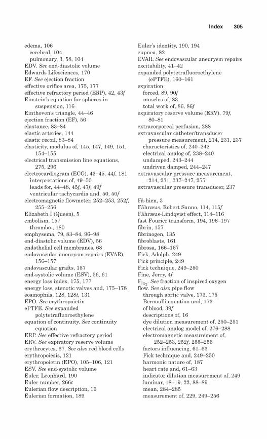
edema, 106cerebral, 104pulmonary, 3, 58, 104
EDV. See end-diastolic volumeEdwards Lifesciences, 170EF. See ejection fractioneffective orifice area, 175, 177effective refractory period (ERP), 42, 43fEinstein’s equation for spheres in
suspension, 116Einthoven’s triangle, 44–46ejection fraction (EF), 56elastance, 83–84elastic arteries, 144elastic recoil, 83–84elasticity, modulus of, 145, 147, 149, 151,
154–155electrical transmission line equations,
275, 296electrocardiogram (ECG), 43–45, 44f, 181
interpretations of, 49–50leads for, 44–48, 45f, 47f, 49fventricular tachycardia and, 50, 50f
electromagnetic flowmeter, 252–253, 252f,255–256
Elizabeth I (Queen), 5embolism, 157
thrombo-, 180emphysema, 79, 83–84, 96–98end-diastolic volume (EDV), 56endothelial cell membranes, 68endovascular aneurysm repairs (EVAR),
156–157endovascular grafts, 157end-systolic volume (ESV), 56, 61energy loss index, 175, 177energy loss, stenotic valves and, 175–178eosinophils, 128, 128t, 131EPO. See erythropoietinePTFE. See expanded
polytetrafluoroethyleneequation of continuity. See continuity
equationERP. See effective refractory periodERV. See expiratory reserve volumeerythrocytes, 67. See also red blood cellserythropoiesis, 121erythropoietin (EPO), 105–106, 121ESV. See end-systolic volumeEuler, Leonhard, 190Euler number, 266tEulerian flow description, 16Eulerian formation, 189
Euler’s identity, 190, 194eupnea, 82EVAR. See endovascular aneurysm repairsexcitability, 41–42expanded polytetrafluoroethylene
(ePTFE), 160–161expiration
forced, 89, 90fmuscles of, 83total work of, 86, 86f
expiratory reserve volume (ERV), 79f,80–81
extracorporeal perfusion, 288extravascular catheter/transducer
pressure measurement, 214, 231, 237characteristics of, 240–242electrical analog of, 238–240undamped, 243–244undriven damped, 244–247
extravascular pressure measurement,214, 231, 237–247, 255
extravascular pressure transducer, 237
Fa-hien, 3Fåhræus, Robert Sanno, 114, 115fFåhræus-Lindqvist effect, 114–116fast Fourier transform, 194, 196–197fibrin, 157fibrinogen, 135fibroblasts, 161fibrosa, 166–167Fick, Adolph, 249Fick principle, 249Fick technique, 249–250Fine, Jerry, 4fFIO2
. See fraction of inspired oxygenflow. See also pipe flow
through aortic valve, 173, 175Bernoulli equation and, 173of blood, 39fdescriptions of, 16dye dilution measurement of, 250–251electrical analog model of, 276–288electromagnetic measurement of,
252–253, 252f, 255–256factors influencing, 61–63Fick technique and, 249–250harmonic nature of, 187heart rate and, 61–63indicator dilution measurement of, 249laminar, 18–19, 22, 88–89mean, 284–285measurement of, 229, 249–256
Index 305
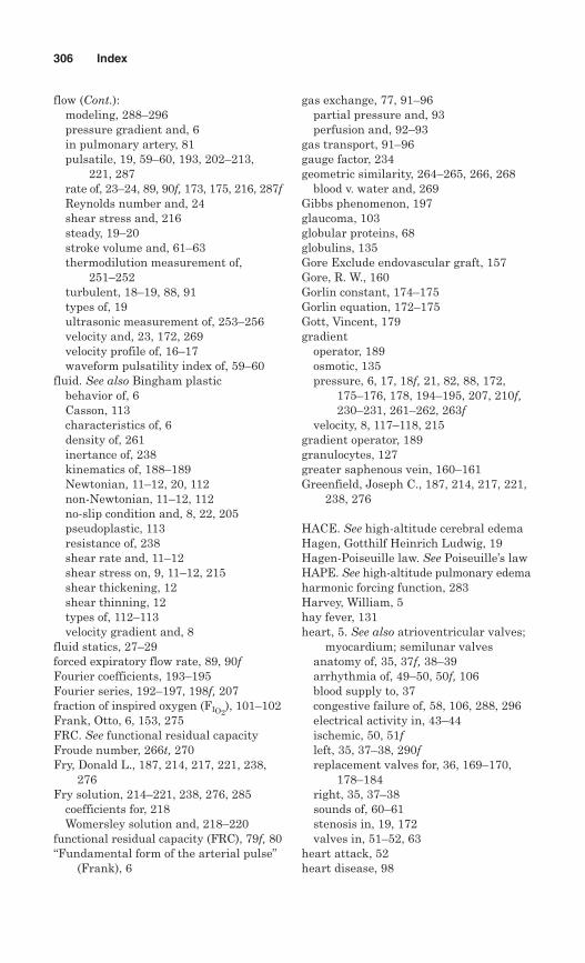
flow (Cont.):modeling, 288–296pressure gradient and, 6in pulmonary artery, 81pulsatile, 19, 59–60, 193, 202–213,
221, 287rate of, 23–24, 89, 90f, 173, 175, 216, 287fReynolds number and, 24shear stress and, 216steady, 19–20stroke volume and, 61–63thermodilution measurement of,
251–252turbulent, 18–19, 88, 91types of, 19ultrasonic measurement of, 253–256velocity and, 23, 172, 269velocity profile of, 16–17waveform pulsatility index of, 59–60
fluid. See also Bingham plasticbehavior of, 6Casson, 113characteristics of, 6density of, 261inertance of, 238kinematics of, 188–189Newtonian, 11–12, 20, 112non-Newtonian, 11–12, 112no-slip condition and, 8, 22, 205pseudoplastic, 113resistance of, 238shear rate and, 11–12shear stress on, 9, 11–12, 215shear thickening, 12shear thinning, 12types of, 112–113velocity gradient and, 8
fluid statics, 27–29forced expiratory flow rate, 89, 90fFourier coefficients, 193–195Fourier series, 192–197, 198f, 207fraction of inspired oxygen (FIO2
), 101–102Frank, Otto, 6, 153, 275FRC. See functional residual capacityFroude number, 266t, 270Fry, Donald L., 187, 214, 217, 221, 238,
276Fry solution, 214–221, 238, 276, 285
coefficients for, 218Womersley solution and, 218–220
functional residual capacity (FRC), 79f, 80“Fundamental form of the arterial pulse”
(Frank), 6
gas exchange, 77, 91–96partial pressure and, 93perfusion and, 92–93
gas transport, 91–96gauge factor, 234geometric similarity, 264–265, 266, 268
blood v. water and, 269Gibbs phenomenon, 197glaucoma, 103globular proteins, 68globulins, 135Gore Exclude endovascular graft, 157Gore, R. W., 160Gorlin constant, 174–175Gorlin equation, 172–175Gott, Vincent, 179gradient
operator, 189osmotic, 135pressure, 6, 17, 18f, 21, 82, 88, 172,
175–176, 178, 194–195, 207, 210f,230–231, 261–262, 263f
velocity, 8, 117–118, 215gradient operator, 189granulocytes, 127greater saphenous vein, 160–161Greenfield, Joseph C., 187, 214, 217, 221,
238, 276
HACE. See high-altitude cerebral edemaHagen, Gotthilf Heinrich Ludwig, 19Hagen-Poiseuille law. See Poiseuille’s lawHAPE. See high-altitude pulmonary edemaharmonic forcing function, 283Harvey, William, 5hay fever, 131heart, 5. See also atrioventricular valves;
myocardium; semilunar valvesanatomy of, 35, 37f, 38–39arrhythmia of, 49–50, 50f, 106blood supply to, 37congestive failure of, 58, 106, 288, 296electrical activity in, 43–44ischemic, 50, 51fleft, 35, 37–38, 290freplacement valves for, 36, 169–170,
178–184right, 35, 37–38sounds of, 60–61stenosis in, 19, 172valves in, 51–52, 63
heart attack, 52heart disease, 98
306 Index
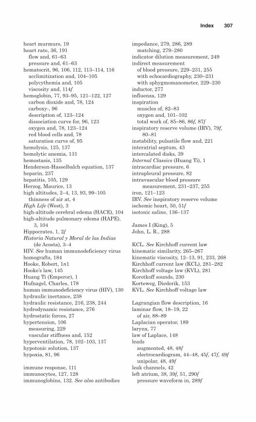
heart murmurs, 19heart rate, 36, 191
flow and, 61–63pressure and, 61–63
hematocrit, 96, 106, 112, 113–114, 116acclimitization and, 104–105polycythemia and, 105viscosity and, 114f
hemoglobin, 77, 93–95, 121–122, 127carbon dioxide and, 78, 124carboxy-, 96description of, 123–124dissociation curve for, 96, 123oxygen and, 78, 123–124red blood cells and, 78saturation curve of, 95
hemolysis, 125, 137hemolytic anemia, 131hemostasis, 135Henderson-Hasselbalch equation, 137heparin, 237hepatitis, 105, 129Herzog, Maurice, 13high altitudes, 2–4, 13, 93, 99–105
thinness of air at, 4High Life (West), 3high-altitude cerebral edema (HACE), 104high-altitude pulmonary edema (HAPE),
3, 104Hippocrates, 1, 2fHistoria Natural y Moral de las Indias
(de Acosta), 3–4HIV. See human immunodeficiency virushomografts, 184Hooke, Robert, 1n1Hooke’s law, 145Huang Ti (Emperor), 1Hufnagel, Charles, 178human immunodeficiency virus (HIV), 130hydraulic inertance, 238hydraulic resistance, 216, 238, 244hydrodynamic resistance, 276hydrostatic forces, 27hypertension, 106
measuring, 229vascular stiffness and, 152
hyperventilation, 78, 102–103, 137hypotonic solution, 137hypoxia, 81, 96
immune response, 111immunocytes, 127, 128immunoglobins, 132. See also antibodies
impedance, 279, 286, 289matching, 279–280
indicator dilution measurement, 249indirect measurement
of blood pressure, 229–231, 255with echocardiography, 230–231with sphygmomanometer, 229–230
inductor, 277influenza, 129inspiration
muscles of, 82–83oxygen and, 101–102total work of, 85–86, 86f, 87f
inspiratory reserve volume (IRV), 79f,80–81
instability, pulsatile flow and, 221interatrial septum, 43intercalated disks, 39Internal Classics (Huang Ti), 1intracardiac pressure, 6intrapleural pressure, 82intravascular blood pressure
measurement, 231–237, 255iron, 121–123IRV. See inspiratory reserve volumeischemic heart, 50, 51fisotonic saline, 136–137
James I (King), 5John, L. R., 288
KCL. See Kirchhoff current lawkinematic similarity, 265–267kinematic viscosity, 12–13, 91, 233, 268Kirchhoff current law (KCL), 281–282Kirchhoff voltage law (KVL), 281Korotkoff sounds, 230Korteweg, Diederik, 153KVL. See Kirchhoff voltage law
Lagrangian flow description, 16laminar flow, 18–19, 22
of air, 88–89Laplacian operator, 189larynx, 77law of Laplace, 148leads
augmented, 48, 48felectrocardiogram, 44–48, 45f, 47f, 49funipolar, 48, 49f
leak channels, 42left atrium, 38, 39f, 51, 290f
pressure waveform in, 289f
Index 307
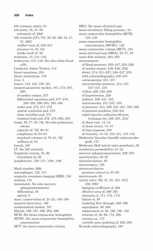
left coronary artery, 64left heart, 35, 37–38
schematic of, 290fleft ventricle (LV), 37f, 38–39, 39f, 45, 47,
51, 290foutflow tract of, 230–231pressure in, 52, 53fstroke work of, 56
leukemia, 13, 131–132leukocytes, 127–132. See also white blood
cellsLindqvist, Johan Torsten, 114linear equations, 284linear momentum, 176liver, 5lumen, 132, 155, 159, 161lumped parameter models, 187, 275–297,
296of cardiac output, 275differential equations and, 277–278,
282–283, 290–291, 293–294nodes and, 275, 277–278spatial resolution and, 275state variables and, 275terminal load and, 276, 278–280, 285
lungs, 38, 77–78, 78f. See also pulmonaryedema
capacity of, 79f, 80–81compliance of, 83–84standard volumes of, 79–81, 79fstiffness of, 84
lunula, 167LV. See left ventriclelymphatic system, 35, 66
circulation in, 69lymphocytes, 128–131, 128t, 130f
Mach number, 266tmacrophages, 122, 131magnetic resonance imaging (MRI), 156malaria, 131manometer. See also mercury
sphygmomanometerdifferential, 28optical, 6
mass, conservation of, 24–25, 188–190material derivative, 189mathematical models, 187Matlab, 196–197, 288, 294, 296MCH. See mean corpuscular hemoglobinMCHC. See mean corpuscular hemoglobin
concentrationMCV. See mean corpuscular volume
MEA. See mean electrical axismean circulatory filling pressure, 55mean corpuscular hemoglobin (MCH),
125–126mean corpuscular hemoglobin
concentration (MCHC), 126mean corpuscular volume (MCV), 125mean electrical axis (MEA), 45–47, 49mean flow solution, 284–285measurement
of blood pressure, 229–247, 255–256of cardiac output, 249–256, 252fdirect, 214, 231–237, 240–247, 255with echocardiography, 230–231extravascular, 231, 237extravascular pressure, 214, 231,
237–247, 255of flow, 229, 249–256of hypertension, 229indirect, 229–231, 255intravascular, 231–237, 255of pressure, 214, 229, 231–247, 255–256of pressure gradient, 230–231rapid injection indicator-dilution
technique for, 250–251, 251fof shear rate, 14–15of shear stress, 14–15of step response, 248of viscosity, 14–16, 116–121, 118–119
Medtronic Vascular-AneuRx endovasculargraft, 157
Medtronic-Hall mitral valve prosthesis, 36membrane permeability, 41–42mercury sphygmomanometer, 229–230metarterioles, 65–67microcirculation, 65microsurgery, 156microvasculature
pressure control in, 67–68microvessels, 65mitral valve, 39f, 51, 53, 165, 167f,
230, 290fdamping coefficient of, 294effective area of, 290–291elements of, 171–172, 171ffailure of, 58modeling flow through, 288–296regurgitant, 98, 288replacement of, 36, 169, 180, 182stenosis of, 36, 98, 172, 288stresses on, 172variable area modeling of, 292–294
M-mode echocardiography, 167
308 Index
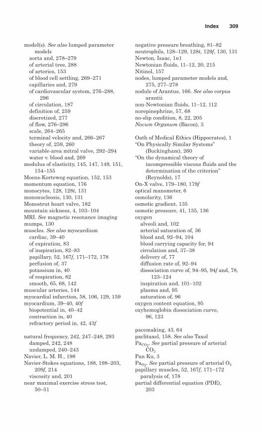
model(s). See also lumped parametermodels
aorta and, 278–279of arterial tree, 288of arteries, 153of blood cell settling, 269–271capillaries and, 279of cardiovascular system, 276–288,
296of circulation, 187definition of, 259discretized, 277of flow, 276–296scale, 264–265terminal velocity and, 266–267theory of, 259, 260variable-area mitral valve, 292–294water v. blood and, 269
modulus of elasticity, 145, 147, 149, 151,154–155
Moens-Korteweg equation, 152, 153momentum equation, 176monocytes, 128, 128t, 131mononucleosis, 130, 131Monostrut heart valve, 182mountain sickness, 4, 103–104MRI. See magnetic resonance imagingmumps, 130muscles. See also myocardium
cardiac, 39–40of expiration, 83of inspiration, 82–83papillary, 52, 167f, 171–172, 178perfusion of, 37potassium in, 40of respiration, 82smooth, 65, 68, 142
muscular arteries, 144myocardial infarction, 58, 106, 129, 159myocardium, 39–40, 40f
biopotential in, 40–42contraction in, 40refractory period in, 42, 43f
natural frequency, 242, 247–248, 293damped, 242, 248undamped, 240–243
Navier, L. M. H., 198Navier-Stokes equations, 188, 198–203,
209f, 214viscosity and, 201
near maximal exercise stress test, 50–51
negative pressure breathing, 81–82neutrophils, 128–129, 128t, 129f, 130, 131Newton, Isaac, 1n1Newtonian fluids, 11–12, 20, 215Nitinol, 157nodes, lumped parameter models and,
275, 277–278nodule of Arantus, 166. See also corpus
arantiinon-Newtonian fluids, 11–12, 112norepinephrine, 57, 68no-slip condition, 8, 22, 205Novum Organum (Bacon), 3
Oath of Medical Ethics (Hippocrates), 1“On Physically Similar Systems”
(Buckingham), 260“On the dynamical theory of
incompressible viscous fluids and thedetermination of the criterion”(Reynolds), 17
On-X valve, 179–180, 179foptical manometer, 6osmolarity, 136osmotic gradient, 135osmotic pressure, 41, 135, 136oxygen
alveoli and, 102arterial saturation of, 36blood and, 92–94, 104blood carrying capacity for, 94circulation and, 37–38delivery of, 77diffusion rate of, 92–94dissociation curve of, 94–95, 94f and, 78,
123–124inspiration and, 101–102plasma and, 95saturation of, 96
oxygen content equation, 95oxyhemoglobin dissociation curve,
96, 123
pacemaking, 43, 64paclitaxel, 158. See also TaxolPaCO2. See partial pressure of arterial
CO2
Pan Ku, 3PaO2. See partial pressure of arterial O2
papillary muscles, 52, 167f, 171–172paralysis of, 178
partial differential equation (PDE), 203
Index 309
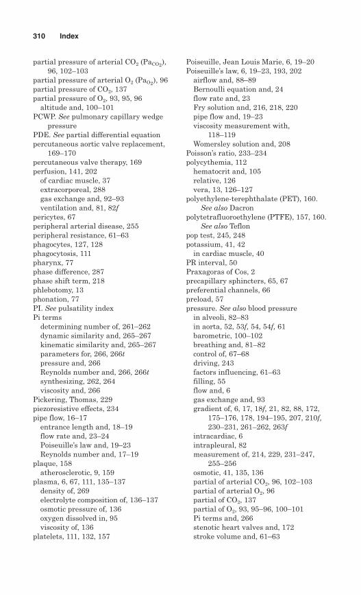
partial pressure of arterial CO2 (PaCO2),96, 102–103
partial pressure of arterial O2 (PaO2), 96partial pressure of CO2, 137partial pressure of O2, 93, 95, 96
altitude and, 100–101PCWP. See pulmonary capillary wedge
pressurePDE. See partial differential equationpercutaneous aortic valve replacement,
169–170percutaneous valve therapy, 169perfusion, 141, 202
of cardiac muscle, 37extracorporeal, 288gas exchange and, 92–93ventilation and, 81, 82f
pericytes, 67peripheral arterial disease, 255peripheral resistance, 61–63phagocytes, 127, 128phagocytosis, 111pharynx, 77phase difference, 287phase shift term, 218phlebotomy, 13phonation, 77PI. See pulsatility indexPi terms
determining number of, 261–262dynamic similarity and, 265–267kinematic similarity and, 265–267parameters for, 266, 266tpressure and, 266Reynolds number and, 266, 266tsynthesizing, 262, 264viscosity and, 266
Pickering, Thomas, 229piezoresistive effects, 234pipe flow, 16–17
entrance length and, 18–19flow rate and, 23–24Poiseuille’s law and, 19–23Reynolds number and, 17–19
plaque, 158atherosclerotic, 9, 159
plasma, 6, 67, 111, 135–137density of, 269electrolyte composition of, 136–137osmotic pressure of, 136oxygen dissolved in, 95viscosity of, 136
platelets, 111, 132, 157
Poiseuille, Jean Louis Marie, 6, 19–20Poiseuille’s law, 6, 19–23, 193, 202
airflow and, 88–89Bernoulli equation and, 24flow rate and, 23Fry solution and, 216, 218, 220pipe flow and, 19–23viscosity measurement with,
118–119Womersley solution and, 208
Poisson’s ratio, 233–234polycythemia, 112
hematocrit and, 105relative, 126vera, 13, 126–127
polyethylene-terephthalate (PET), 160.See also Dacron
polytetrafluoroethylene (PTFE), 157, 160.See also Teflon
pop test, 245, 248potassium, 41, 42
in cardiac muscle, 40PR interval, 50Praxagoras of Cos, 2precapillary sphincters, 65, 67preferential channels, 66preload, 57pressure. See also blood pressure
in alveoli, 82–83in aorta, 52, 53f, 54, 54f, 61barometric, 100–102breathing and, 81–82control of, 67–68driving, 243factors influencing, 61–63filling, 55flow and, 6gas exchange and, 93gradient of, 6, 17, 18f, 21, 82, 88, 172,
175–176, 178, 194–195, 207, 210f,230–231, 261–262, 263f
intracardiac, 6intrapleural, 82measurement of, 214, 229, 231–247,
255–256osmotic, 41, 135, 136partial of arterial CO2, 96, 102–103partial of arterial O2, 96partial of CO2, 137partial of O2, 93, 95–96, 100–101Pi terms and, 266stenotic heart valves and, 172stroke volume and, 61–63
310 Index
pressure (Cont.):vapor of water, 102–103ventricular, 52, 54volume loops for, 58, 58f
pressure drop, 260in airways, 88Bernoulli equation and, 173stenosis and, 172
pressure recovery, 176pressure waveform, 55f, 193f, 248
aortic, 54fin left atrium, 289fpulsatility index for, 59vascular disease and, 275
pressure-strain modulus, 153–154pressure-volume curve (P-V), 83, 86f,
87fpressure-volume diagrams, 55–57prolapse, 52prosthetic tissue valves, 184prototype, 259pseudoplastic fluids, 113PTFE. See polytetrafluoroethylenepulmonary artery, 37, 37f, 39f, 51, 61
blood flow in, 81pressure in, 54
pulmonary capillaries, 92, 255pulmonary capillary wedge pressure
(PCWP), 255pulmonary circulation, 37, 37f
carbon dioxide and, 38oxygen and, 37–38
pulmonary edema, 58, 104high-altitude, 3, 104
pulmonary fibrosis, 93, 98, 99fpulmonary pathophysiology, 96–98,
99fpulmonary vein, 36, 37f, 38, 39f, 290fpulmonic valve, 51, 165–170
peak velocity through, 168replacement of, 169
pulsatile flow, 193, 287Fry solution for, 214–221instability in, 221Womersley solution and, 202–213
pulsatility index (PI), 59–60pulse, 2
pressure of, 55wave velocity of, 152–153
P-V curve. See pressure-volume curvePyrolite, 180pyrolytic carbon, 179–180, 184. See also
Pyrolite
rapid injection indicator-dilutionmeasurement, 250–251, 251f. See also dye dilution technique
rate of shearing strain. See shear raterecombinant erythropoietin (rEPO),
105–106red blood cells, 67, 77, 111. See also
erythrocytesacclimatization and, 104–105continuous wave ultrasound and, 253description of, 121–123drugs stimulating production of,
105–106hemoglobin and, 78indices for, 125–126settling rate of, 269–271shear stress-shear rate relationship of,
116sickle cell anemia and, 124
reference electrode, 48reflections, 286regurgitance, 63
aortic, 63, 168in mitral valve, 98, 288
relative refractory period (RRP), 42, 43f
rEPO. See recombinant erythropoietinrepolarization, 40, 42residual volume (RV), 79–81resistance to diffusion, 93–94resistor, 277respiration
acid-base balance and, 137in extreme environments, 99–106high altitude and, 2–4, 93, 99–105muscles of, 82
respiratory alkalosis, 103respiratory system
components of, 77–78, 78ffailure of, 87functions of, 77
restenosis, 36stents and, 159
returning waves, 286Reynolds number, 17–19, 29, 174, 213,
221, 267–270, 285airway resistance and, 88flow rate and, 24Pi terms and, 266, 266tsimilarity in, 268–269
Reynolds, Osborne, 17–18Rh antigen, 134rheology, 111
Index 311
rheumatic fever, 129right atrium, 38, 39f, 51right coronary artery, 64right heart, 35, 37–38right ventricle, 37f, 38, 39f, 51
valves in, 51RLC circuits, 276Rocky Mountain spotted fever, 131Rouget cells, 67RRP. See relative refractory periodrubella, 129, 130Runge-Kutta formula, 294RV. See residual volume
SA. See sinoatrial nodesaphenous vein, 160–161scale model, 264–265semilunar cusps, 165–166semilunar valves, 54, 61. See also aortic
valve; pulmonic valveserum, 111serum albumin, 68shear rate, 7–8
blood and, 113fmeasurement of, 14–15Newtonian fluids and, 11non-Newtonian fluids and, 11–12shear stress and, 9, 10, 11–12,
21, 116viscosity and, 9, 10, 21wall shear stress and, 16
shear strain, 7shear stress, 6, 7, 112. See also wall shear
stressarterial disease and, 9atherosclerotic plaques and, 9blood and, 113fblood cells and, 9cone and plate viscometer and,
120–121flow and, 216on fluids, 9, 11–12, 215measurement of, 14–15Newtonian fluids and, 11, 215non-Newtonian fluids and, 11–12Pouiseuille flow and, 216pressure gradient and, 21rate of shearing strain and, 9, 10,
11–12, 116rotating cylinder viscometer and,
117–118viscosity and, 8–10, 21, 215
shear thickening fluids, 12
shear thinning fluids, 12Shiley Incorporated, 181–183sickle cell anemia, 124–125similarity
dynamic, 265–267geometric, 264–266, 268–269kinematic, 265–267Pi terms and, 265–267Reynolds number and, 268–269
Simulink, 288sinoatrial node (SA), 43, 49, 50, 64sinus brachycardia, 49sinus of Valsalva, 167sinus rhythm, 49sinus tachycardia, 49sirolimus, 158–159smallpox, 129smooth muscles cells, 65, 68, 142SNP. See supernormalitysodium, 41, 42sodium channel, 40sodium-potassium pump, 41Sorin Biomedical, 182sound production, 77spatial resolution, 275specific gravity, 6specific weight, 6sphygmomanometer, mercury,
229–230spirometer, 99f, 250ST interval, 50, 50fSt. Jude Medical, 179
replacement mitral valve by, 182standard lung volumes, 79–81, 79fStarling’s law, 56Starr, Albert, 169state variables, 275static sensitivity, 240–241steady state solution, 286stenosis, 256. See also restenosis
of aorta, 155of aortic valve, 168energy loss and, 175–178heart and, 19, 172of mitral valve, 36, 98, 172, 288pressure drop and, 172valvular, 155
stenotic heart valves, 19stents, 157–159
aneurysms and, 156–157drug-eluting, 158–159
step response, 245, 246fmeasurement of, 248
312 Index
stiffness, 83–84aortic, 152, 154arterial, 152of lungs, 84vascular, 152
Stokes, G. G., 198strain gauge tipped pressure transducer,
231–237, 255streamline, 24stress. See also shear stress; wall shear
stresson aortic valve, 168diastolic, 168on mitral valve, 172test, 50–51
stress-strain curve, 145–146, 146fstroke, 106, 155stroke volume (SV), 56, 57, 295
constant, 61–62flow and, 61–63pressure and, 61–63
substantial derivative, 189supernormality (SNP), 42, 43fSV. See stroke volumesyncytium, 39–40syphilis, 130systemic circulation, 37, 37fsystole, 52–54, 53f, 289
sounds in, 61systolic blood pressure, 36, 54–55, 181, 230systolic-waveform velocity, 60
T lymphocytes, 130–131tachycardia
atrial, 43, 49sinus, 49ventricular, 50, 50f
Taxol, 158Taxus stent, 158–159Teflon, 160, 181terminal arterioles. See metarteriolesterminal bronchioles, 77–78terminal load, 276, 278–280, 285terminal velocity, 259, 266–267terminating load, 276thalassemia, 127theory of models, 259, 260thermodilution, 251–252thrombocytes, 111, 132fthromboembolism, 180thrombosis, 106, 157, 180
stents and, 159thrombus, 157
tidal volume (TV), 79–81tight junctions, 67, 69time constant, critical, 247time-varying solution, 285total lung capacity (TLC), 79f, 80–81trachea, 77, 78f
airflow in, 88transmembrane resting potential,
41, 41ftransmission line equations, 275, 296transmural electrical potential difference,
40–41transmural pressure gradient, 82transthoracic echocardiography, 177transvalvular pressure gradients, 175tricuspid valve, 39f, 51, 53, 165
elements of, 171–172, 171ftrue capillary, 66tuberculosis, 130tunica adventitia, 143, 161. See also
tunica externatunica externa, 142–143, 142f, 143ftunica intima, 141–142, 142f, 143ftunica media, 141–143, 142f, 143f, 156turbulent flow, 18–19
of air, 88, 91TV. See tidal volumetyphoid fever, 131
ultrasound, 156. See also echocardiographycontinuous wave, 253–256Doppler, 254
undamped natural frequency, 240–243unipolar leads, 48, 49f
valve area, Bernoulli equation and, 173valve prolapse, 52valves. See specific valvesvalvular stenosis, 155variable-area mitral valve model,
292–294vascular pathologies, 155–157
pressure waveforms and, 275vascular resistance, 65, 67–68vascular stiffness, 152vasoconstriction, 143vasodilation, 64VC. See vital capacityveins, 2, 141
CABG surgery and, 160cardiac, 64pulmonary, 36, 37f, 38, 39f, 290fsaphenous, 160–161
Index 313
velocitythrough aortic valve, 168displacement and, 7–8flow and, 23, 172, 269flow curves of, 172flow profile of, 16–17flow rate and, 23gradient of, 8, 117–118, 215kinematic similarity and, 265–266profile of, 8, 8f, 22through pulmonic valve, 168pulse wave, 152–153terminal, 259, 266–267
velocity waveformsDoppler, 289pulsatility index of, 60systolic, 60
vena cava, 37f, 38, 39fvena contracta, 176, 178ventilation. See also hyperventilation
of alveoli, 79perfusion and, 81, 82f
ventilation-perfusion ratio, 81, 82fventricles, 38. See also left ventricle; right
ventricleblood pressure in, 52, 54cardiac cycle and, 52–54, 53fcompliance of, 290contraction of, 40performance of, 58refractory period in, 42, 43frelaxation of, 58, 292sounds from, 61
ventricular fibrillation, 50ventricular filling, 61ventricular pressure, 54ventricular septum, 64ventricular tachycardia, 50, 50fventricularis, 166–167Venturi meter, 26–27venules, 65, 66
structure of, 68–69Vesalius, Andreas, 171viscoelasticity, 147viscometer
cone and plate, 119–121rotating cylinder, 14–15, 14f, 15f,
116–118, 119
viscosity, 6, 11–13, 91absolute, 11, 13of blood, 13, 15, 112–114, 114f, 174, 269dynamic, 11hematocrit and, 114fkinematic, 12–13, 91, 233, 268measuring, 14–16, 116–121, 118–119Navier-Stokes equations and, 201Pi terms and, 266of plasma, 136resistance and, 216shear rate and, 9, 10, 21shear stress and, 8–10, 21, 215vessel diameter and, 114–116, 115fwall shear stress and, 16
vital capacity (VC), 79f, 81vocal cords, 77Voorhees, Arthur, 160
W. L. Gore & Associates, 157Waite, Lee, 4fwall shear stress
blood vessels and, 10shear rate and, 16viscosity and, 16
watervapor pressure of, 102–103
water-filled pathways, 68WCT. See Wilson central terminalWeber number, 266, 266tWest, John, 3Wheatstone bridge, 234, 235fwhite blood cells, 111, 127–132Wilson central terminal (WCT), 48, 48fWindkessel theory, 6, 153Womersley, J. R., 187, 207, 208, 213, 221Womersley number, 29–30, 208, 218,
219f, 266tWomersley solution, 202–213, 209f, 214,
218Fry solution and, 218–220Poiseuille’s law and, 208pulsatile flow and, 202–213
Wylie, Alexander, 3
xenografts, 184
Zenith AAA endovascular graft, 157
314 Index