advanced soil mechanics
TRANSCRIPT

Foundation Engineering
Draft Version April 2012
S. van Baars

2
PREFACE
This book is just a help for the students fort the old course Grundbau 2.
Luxembourg, April 2012 Stefan Van Baars
3
CONTENT
I SHALLOW FOUNDATIONS ................................................ 5
1 Elastic stresses and deformations ................................................................................. 6
2 Boussinesq ..................................................................................................................... 8
3 Flamant........................................................................................................................ 12
4 Deformation of layered soil ......................................................................................... 16
5 Strip footing ................................................................................................................. 19 5.1 Lower bound ........................................................................................................ 19 5.2 Upper bound ......................................................................................................... 22
6 Prandtl ......................................................................................................................... 24
7 Brinch Hansen ............................................................................................................. 25 7.1 Bearing capacity of strip foundation ..................................................................... 25 7.2 Inclination factors ................................................................................................. 28
7.3 Shape factors ........................................................................................................ 28 7.4 Brinch Hansen and codes ...................................................................................... 30
7.5 CPT and undrained shear strength ........................................................................ 33
II PILE FOUNDATIONS........................................................ 35
8 Cone Penetration Test (CPT)...................................................................................... 36
9 Compression piles ....................................................................................................... 39 9.1 Pile types .............................................................................................................. 39 9.2 Bearing capacity ................................................................................................... 44
9.3 Tip resistance using Brinch Hansen (Prandtl or Meyerhof) ................................... 45 9.4 Tip resistance using Koppejan .............................................................................. 46
9.5 Shaft resistance..................................................................................................... 49
10 Tension piles ................................................................................................................ 53 10.1 Differences between tension and compression piles .............................................. 53 10.2 Reduction of the cone value qc due to excavation.................................................. 53
10.3 Reduction of cone resistance due to tensile pile force ........................................... 54 10.4 Clump criterion .................................................................................................... 55
10.5 Edge Piles ............................................................................................................ 56

4

5
I Shallow foundations
6
1 Elastic stresses and deformations Very important in the calculation of the shallow foundations are the stresses and
deformations. As long as we assume that we have non failing soils, behaving rather linea
elastic, we can make simple design calculations by hand.
Because of equilibrium of moments the stress tensor must be symmetric,
,
,
.
xy yx
yz zy
zx xz
(1.1)
The equations of equilibrium constitute a set of six equations involving nine stress
components. In itself this can never be sufficient for a mathematical solution. The
deformations must also be considered before a solution can be contemplated.
For a linear elastic material the relation between stresses and strains is given by Hooke’s law,
1[ ( )],
1[ ( )],
1[ ( )],
xx xx yy zz
yy yy zz xx
zz zz xx yy
E
E
E
(1.2)
1,
1,
1.
xy xy
yz yz
zx zx
E
E
E
(1.3)
where E is the modulus of elasticity (Young’s modulus), and is Poisson’s ratio. The
equations (1.2) and (1.3) add six equations to the system, at the same time introducing six
additional variables.
The six strains can be related to the three components of the displacement vector,
,
,
,
xxx
y
yy
zzz
u
x
u
y
u
z
(1.4)
12
12
12
( ),
( ),
( ).
yxxy
y zyz
xzzx
uu
y x
u u
z y
uu
x z
(1.5)
7
These are the compatibility equations. In total there are now just as many equations as there
are variables, so that the system may be solvable, at least if there are a sufficient number of
boundary conditions.
The minus sign in the equations has been introduced in geotechnical engineering because a
volume decrease leads to a positive strain and a volume increase to a negative strain.
For a number of problems solutions of the system of equations can be found in the literature
on the theory of elasticity. In soil mechanics the solutions for a half space or a half plane,
with a horizontal upper surface, are of special interest. In the next chapters some of the most
important solutions for soil mechanics are further discussed.
For the solved elastic problems the strains and effective stresses can be calculated for drained
or consolidated loads, with the help of two stiffness parameters ( , or , )E K G . If these
parameters are replaced by two undrained parameters ( , )u uE the strains and total stresses
can be calculated for undrained problems (short loads on clay or peat). When calculating
these two parameters, one should realize that an undrained load, because of the
incompressibility of water, causes no volume change, so
0.5.u (1.6)
The undrained compression modulus becomes infinite:
.3(1 2 )
uu
u
EK
(1.7)
Besides this the water has no shear stresses, both in the drained as in the undrained state.
From this it follows that
.2(1 ) 2(1 )
uu
u
EEG G
(1.8)
From which can be derived that
(1 ).
(1 )
uuE E
(1.9)
Replacing the drained stiffness parameters ( , )E from the previous chapters by the
undrained stiffness parameters ( , )u uE and calculating these values in the way demonstrated
above, the solutions can be used not only for the drained, but also for the undrained case.
8
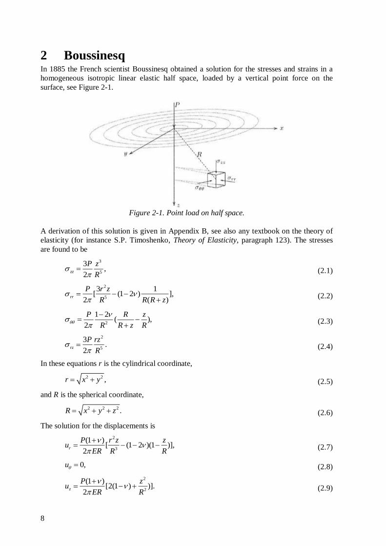
2 Boussinesq In 1885 the French scientist Boussinesq obtained a solution for the stresses and strains in a
homogeneous isotropic linear elastic half space, loaded by a vertical point force on the
surface, see Figure 2-1.
A derivation of this solution is given in Appendix B, see also any textbook on the theory of
elasticity (for instance S.P. Timoshenko, Theory of Elasticity, paragraph 123). The stresses
are found to be
3
5
3,
2zz
P z
R
(2.1)
2
5
3 1[ (1 2 ) ],
2 ( )rr
P r z
R R R z
(2.2)
2
1 2( ),
2
P R z
R R z R
(2.3)
2
5
3.
2rz
P rz
R
(2.4)
In these equations r is the cylindrical coordinate,
2 2 ,r x y (2.5)
and R is the spherical coordinate,
2 2 2 .R x y z (2.6)
The solution for the displacements is
2
3
(1 )[ (1 2 )(1 )],
2r
P r z zu
ER R R
(2.7)
0,u (2.8)
2
2
(1 )[2(1 ) )].
2z
P zu
ER R
(2.9)
Figure 2-1. Point load on half space.
9
The vertical displacement of the surface is particularly interesting. This is
2(1 )0 : .z
Pz u
Er
(2.10)
For 0r this tends to infinity. At the point of application of the point load the displacement
is infinitely large. This singular behaviour is a consequence of the singularity in the surface
load, as in the origin the stress is infinitely large. That the displacement in that point is also
infinitely large may not be so surprising.
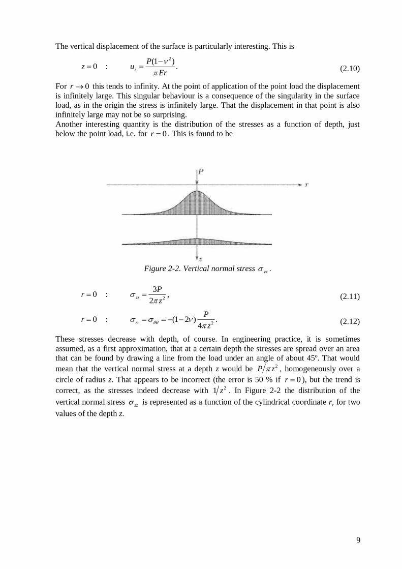
Another interesting quantity is the distribution of the stresses as a function of depth, just
below the point load, i.e. for 0r . This is found to be
2
30 : ,
2zz
Pr
z
(2.11)
20 : (1 2 ) .
4rr
Pr
z
(2.12)
These stresses decrease with depth, of course. In engineering practice, it is sometimes
assumed, as a first approximation, that at a certain depth the stresses are spread over an area
that can be found by drawing a line from the load under an angle of about 45º. That would
mean that the vertical normal stress at a depth z would be 2P z , homogeneously over a
circle of radius z. That appears to be incorrect (the error is 50 % if 0r ), but the trend is
correct, as the stresses indeed decrease with 21 z . In Figure 2-2 the distribution of the
vertical normal stress zz is represented as a function of the cylindrical coordinate r, for two
values of the depth z.
Figure 2-2. Vertical normal stress zz .
10
The assumption of linear elastic material behaviour means that the entire problem is linear, as
the equations of equilibrium and compatibility are also linear. This implies that the principle
of superposition of solutions can be applied. Boussinesq’s solution can be used as the starting
point of more general types of loading, such as a system of point loads, or a uniform load
over a certain given area.
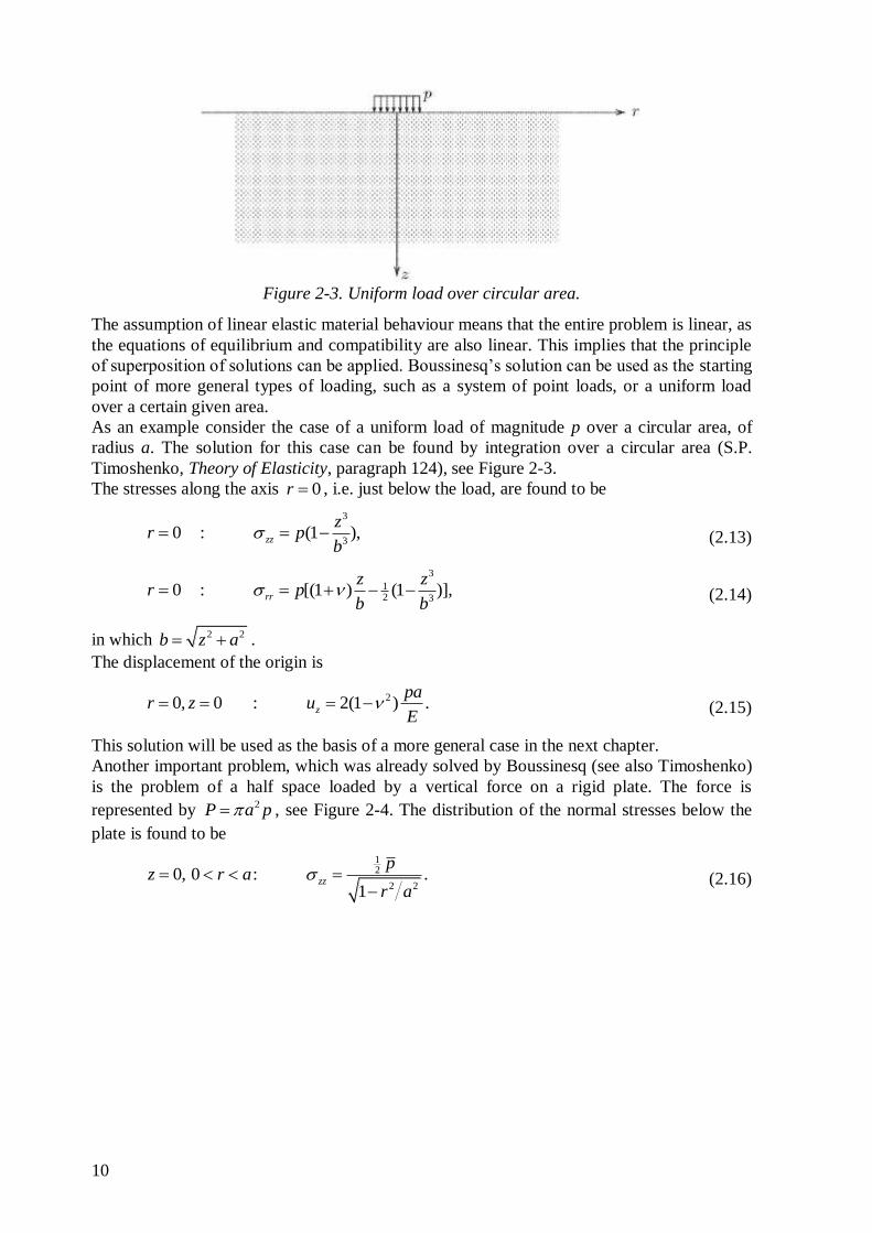
As an example consider the case of a uniform load of magnitude p over a circular area, of
radius a. The solution for this case can be found by integration over a circular area (S.P.
Timoshenko, Theory of Elasticity, paragraph 124), see Figure 2-3.
The stresses along the axis 0r , i.e. just below the load, are found to be
3
30 : (1 ),zz
zr p
b (2.13)
3
12 3
0 : [(1 ) (1 )],rr
z zr p
b b (2.14)
in which 2 2b z a .
The displacement of the origin is
20, 0 : 2(1 ) .z
par z u
E (2.15)
This solution will be used as the basis of a more general case in the next chapter.
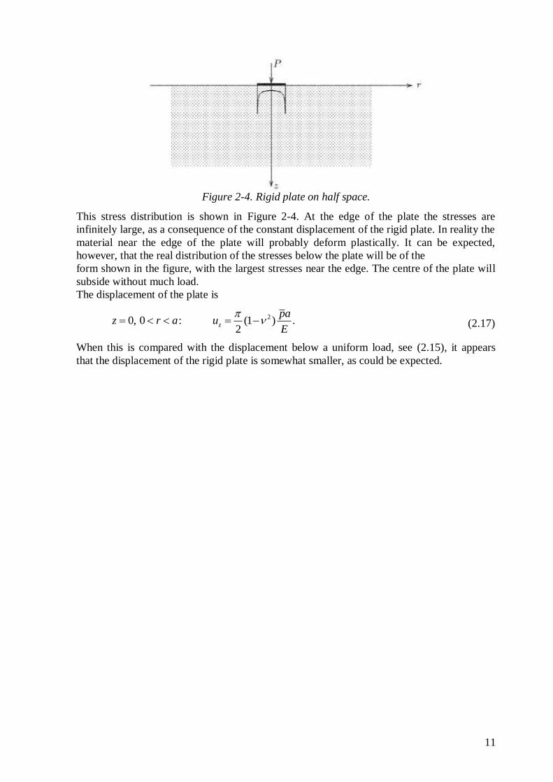
Another important problem, which was already solved by Boussinesq (see also Timoshenko)
is the problem of a half space loaded by a vertical force on a rigid plate. The force is
represented by 2P a p , see Figure 2-4. The distribution of the normal stresses below the
plate is found to be
12
2 20, 0 : .
1zz
pz r a
r a
(2.16)
Figure 2-3. Uniform load over circular area.
11
This stress distribution is shown in Figure 2-4. At the edge of the plate the stresses are
infinitely large, as a consequence of the constant displacement of the rigid plate. In reality the
material near the edge of the plate will probably deform plastically. It can be expected,
however, that the real distribution of the stresses below the plate will be of the
form shown in the figure, with the largest stresses near the edge. The centre of the plate will
subside without much load.
The displacement of the plate is
20, 0 : (1 ) .2
z
paz r a u
E
(2.17)
When this is compared with the displacement below a uniform load, see (2.15), it appears
that the displacement of the rigid plate is somewhat smaller, as could be expected.
Figure 2-4. Rigid plate on half space.
12
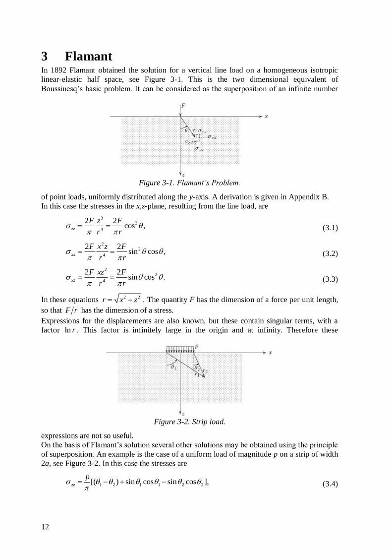
3 Flamant In 1892 Flamant obtained the solution for a vertical line load on a homogeneous isotropic
linear-elastic half space, see Figure 3-1. This is the two dimensional equivalent of
Boussinesq’s basic problem. It can be considered as the superposition of an infinite number
of point loads, uniformly distributed along the y-axis. A derivation is given in Appendix B.
In this case the stresses in the x,z-plane, resulting from the line load, are
33
4
2 2cos ,zz
F z F
r r
(3.1)
22
4
2 2sin cos ,xx
F x z F
r r
(3.2)
22
4
2 2sin cos .xz
F xz F
r r
(3.3)
In these equations 2 2r x z . The quantity F has the dimension of a force per unit length,
so that F r has the dimension of a stress.
Expressions for the displacements are also known, but these contain singular terms, with a
factor ln r . This factor is infinitely large in the origin and at infinity. Therefore these
expressions are not so useful.
On the basis of Flamant’s solution several other solutions may be obtained using the principle
of superposition. An example is the case of a uniform load of magnitude p on a strip of width
2a, see Figure 3-2. In this case the stresses are
1 2 1 1 2 2[( ) sin cos sin cos ],zz
p
(3.4)
Figure 3-1. Flamant’s Problem.
Figure 3-2. Strip load.
13
1 2 1 1 2 2[( ) sin cos sin cos ],xx
p
(3.5)
2 2
2 1[cos cos ].xz
p
(3.6)
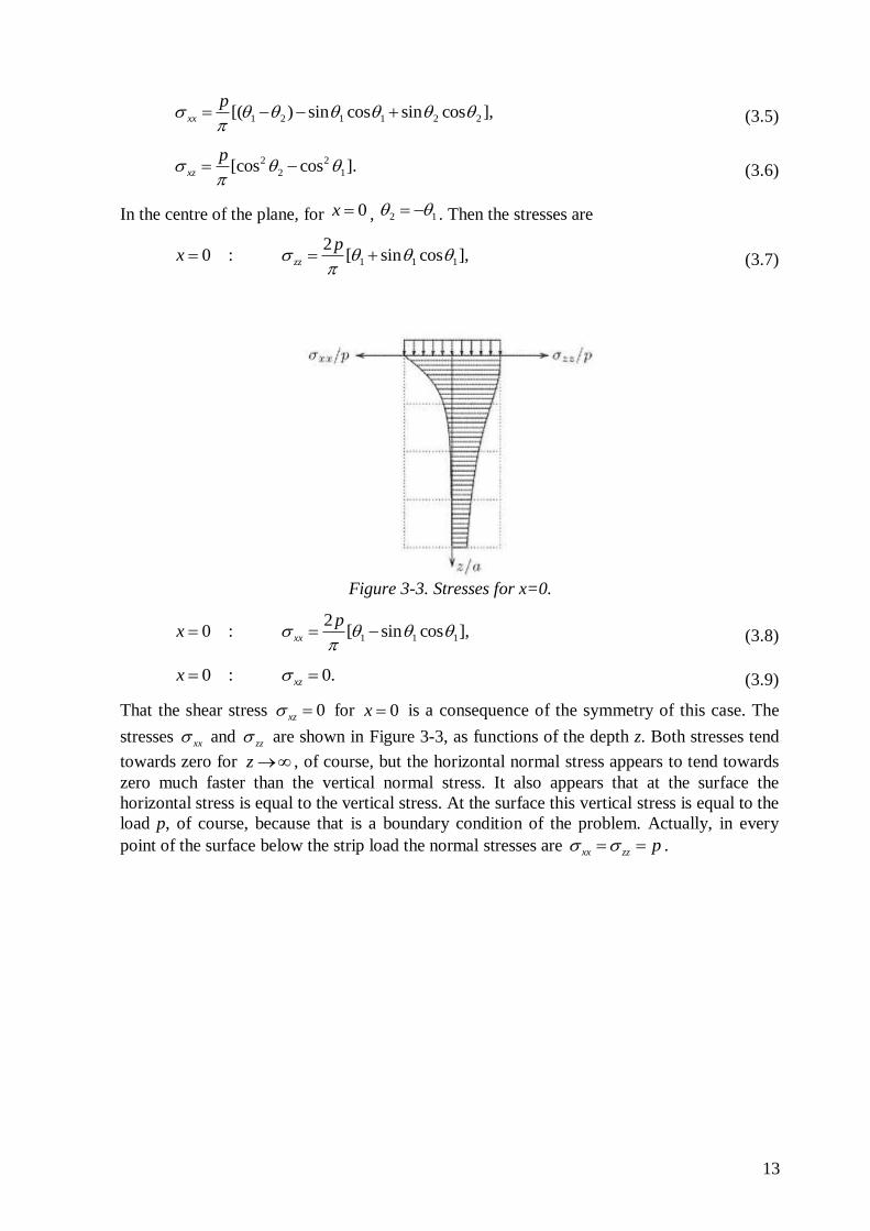
In the centre of the plane, for 0x , 2 1 . Then the stresses are
1 1 1
20 : [ sin cos ],zz
px
(3.7)
1 1 1
20 : [ sin cos ],xx
px
(3.8)
0 : 0.xzx (3.9)
That the shear stress 0xz for 0x is a consequence of the symmetry of this case. The
stresses xx and zz are shown in Figure 3-3, as functions of the depth z. Both stresses tend
towards zero for z , of course, but the horizontal normal stress appears to tend towards
zero much faster than the vertical normal stress. It also appears that at the surface the
horizontal stress is equal to the vertical stress. At the surface this vertical stress is equal to the
load p, of course, because that is a boundary condition of the problem. Actually, in every
point of the surface below the strip load the normal stresses are xx zz p .
Figure 3-3. Stresses for x=0.
14
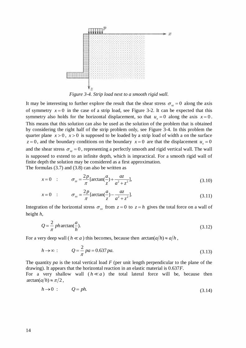
It may be interesting to further explore the result that the shear stress 0xz along the axis
of symmetry 0x in the case of a strip load, see Figure 3-2. It can be expected that this
symmetry also holds for the horizontal displacement, so that 0xu along the axis 0x .
This means that this solution can also be used as the solution of the problem that is obtained
by considering the right half of the strip problem only, see Figure 3-4. In this problem the
quarter plane 0x , 0x is supposed to be loaded by a strip load of width a on the surface
0z , and the boundary conditions on the boundary 0x are that the displacement 0xu
and the shear stress 0xz , representing a perfectly smooth and rigid vertical wall. The wall
is supposed to extend to an infinite depth, which is impractical. For a smooth rigid wall of
finite depth the solution may be considered as a first approximation.
The formulas (3.7) and (3.8) can also be written as
2 2
20 : [arctan( ) ],zz
p a azx
z a z
(3.10)
2 2
20 : [arctan( ) ].xx
p a azx
z a z
(3.11)
Integration of the horizontal stress xx from 0z to z h gives the total force on a wall of
height h,
2arctan( ).
aQ ph
h (3.12)
For a very deep wall ( h a ) this becomes, because then arctan( )a h a h ,
2: 0.637 .h Q pa pa
(3.13)
The quantity pa is the total vertical load F (per unit length perpendicular to the plane of the
drawing). It appears that the horizontal reaction in an elastic material is 0.637F.
For a very shallow wall ( h a ) the total lateral force will be, because then
arctan( ) 2a h ,
0 : .h Q ph (3.14)
Figure 3-4. Strip load next to a smooth rigid wall.
15
This is in agreement with the observation made earlier that the value of the horizontal stress
at the surface, just below the load, is xx p . For a very short wall the horizontal force will
be that horizontal stress, multiplied by the length of the wall.
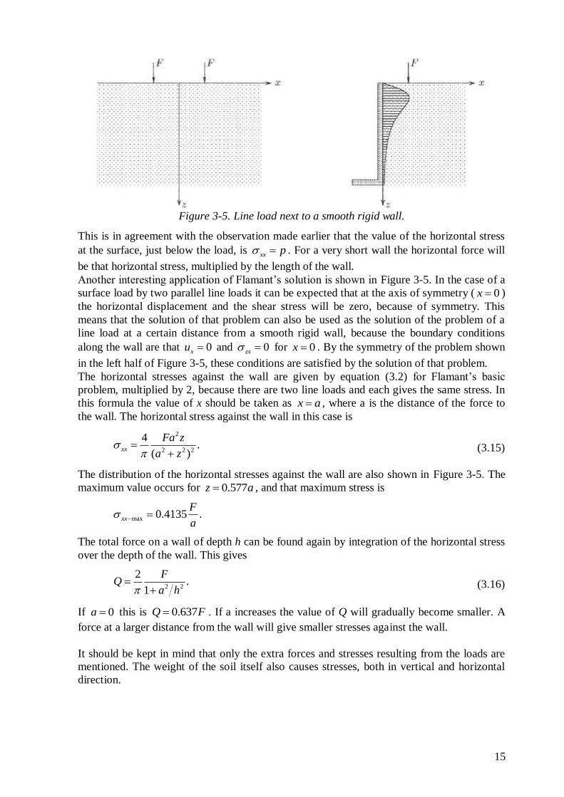
Another interesting application of Flamant’s solution is shown in Figure 3-5. In the case of a
surface load by two parallel line loads it can be expected that at the axis of symmetry ( 0x )
the horizontal displacement and the shear stress will be zero, because of symmetry. This
means that the solution of that problem can also be used as the solution of the problem of a
line load at a certain distance from a smooth rigid wall, because the boundary conditions
along the wall are that 0xu and 0zx for 0x . By the symmetry of the problem shown
in the left half of Figure 3-5, these conditions are satisfied by the solution of that problem.
The horizontal stresses against the wall are given by equation (3.2) for Flamant’s basic
problem, multiplied by 2, because there are two line loads and each gives the same stress. In
this formula the value of x should be taken as x a , where a is the distance of the force to
the wall. The horizontal stress against the wall in this case is
2
2 2 2
4.
( )xx
Fa z
a z
(3.15)
The distribution of the horizontal stresses against the wall are also shown in Figure 3-5. The
maximum value occurs for 0.577z a , and that maximum stress is
max 0.4135 .xx
F
a
The total force on a wall of depth h can be found again by integration of the horizontal stress
over the depth of the wall. This gives
2 2
2.
1
FQ
a h
(3.16)
If 0a this is 0.637Q F . If a increases the value of Q will gradually become smaller. A
force at a larger distance from the wall will give smaller stresses against the wall.
It should be kept in mind that only the extra forces and stresses resulting from the loads are
mentioned. The weight of the soil itself also causes stresses, both in vertical and horizontal
direction.
Figure 3-5. Line load next to a smooth rigid wall.
16
4 Deformation of layered soil An important problem of soil mechanics practice is the prediction of the settlements of a
structure built on the soil. For a homogeneous isotropic linear elastic material the
deformations could be calculated using the theory of elasticity. That is a completely
consistent theory, leading to expressions for the stresses and the displacements. However,
solutions are available only for a half space and a half plane, not for a layered material (at
least not in closed form). Moreover, soils exhibit non-linear properties (such as a stiffness
increasing with the actual stress), often have anisotropic properties, and in many cases the
soil consists of layers of different properties. For such materials the description of the
material properties is already a complex problem, let alone the analysis of stresses and
deformations.
For these reasons an approximation is often used, based on a semi-elastic analysis. In this
approximation it is first postulated that the vertical stresses in the soil, whatever it true
properties are, can be approximated by the stresses that can be calculated from linear elastic
theory. On the basis of these stresses the deformations are then determined, using the best
available description of the relation between stress and strain, which may be non-linear. If the
soil is layered, the deformations of each layer are calculated using its own properties, and
then the surface displacements are determined by a summation of the deformations of all
layers. In this way the different properties of the layers can be taken into account, including a
possible increase of the stiffness with depth.
The procedure is not completely consistent, because in a soil consisting of layers of different
stiffness, the stress distribution will not be the same as in a homogeneous linear elastic
material. A partial justification may be that the stresses following from an elastic
computation at least satisfy the equilibrium conditions. Also it has been found, by
comparison of solutions for layered materials with the solution for a homogeneous material,
that the distribution of the vertical stress zz is not very sensitive to the material properties,
provided that the differences in material properties are not very large, i.e. excepting extreme
cases such as a very stiff layer on a very soft subsoil.
Example
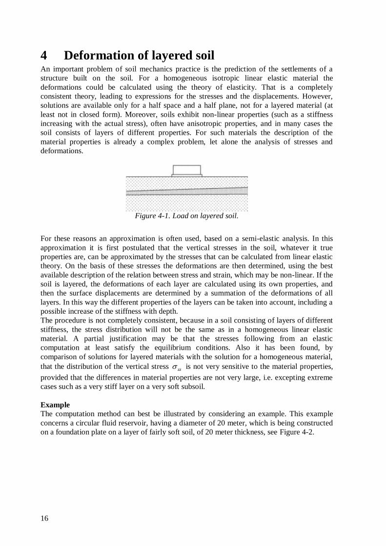
The computation method can best be illustrated by considering an example. This example
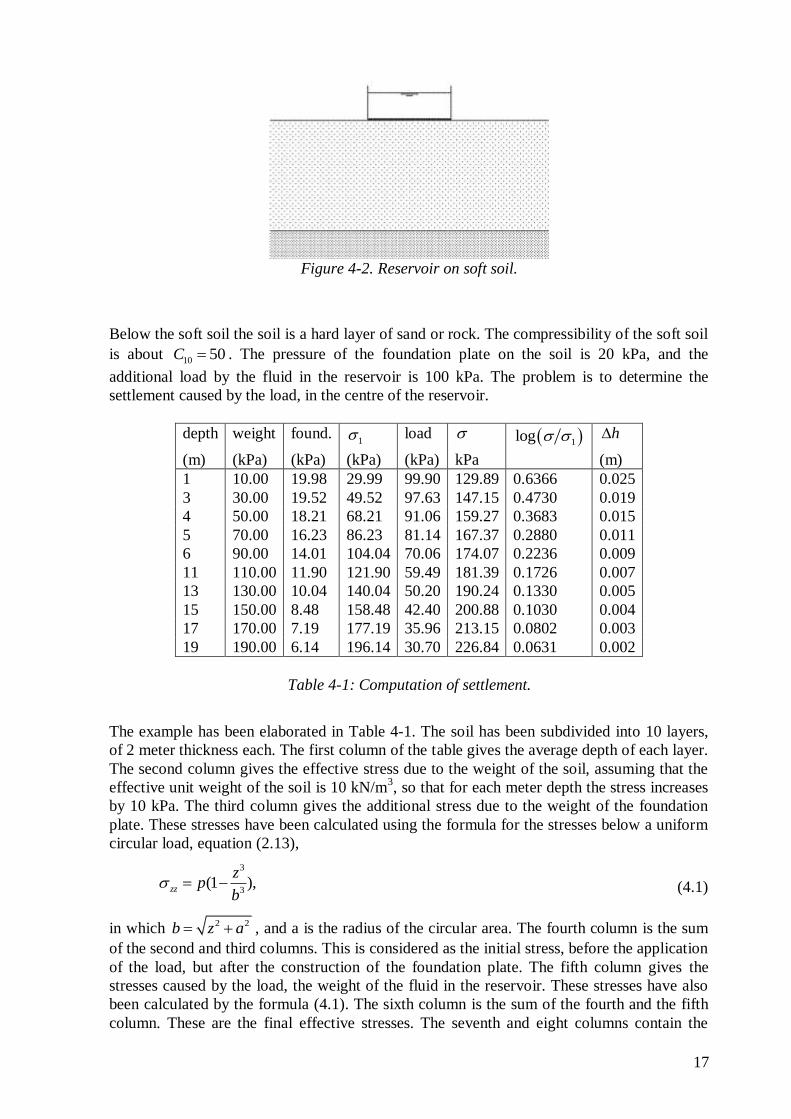
concerns a circular fluid reservoir, having a diameter of 20 meter, which is being constructed
on a foundation plate on a layer of fairly soft soil, of 20 meter thickness, see Figure 4-2.
Figure 4-1. Load on layered soil.
17
Below the soft soil the soil is a hard layer of sand or rock. The compressibility of the soft soil
is about 10 50C . The pressure of the foundation plate on the soil is 20 kPa, and the
additional load by the fluid in the reservoir is 100 kPa. The problem is to determine the
settlement caused by the load, in the centre of the reservoir.
depth weight found. 1 load 1log h
(m) (kPa) (kPa) (kPa) (kPa) kPa (m)
1 10.00 19.98 29.99 99.90 129.89 0.6366 0.025
3 30.00 19.52 49.52 97.63 147.15 0.4730 0.019
4 50.00 18.21 68.21 91.06 159.27 0.3683 0.015
5 70.00 16.23 86.23 81.14 167.37 0.2880 0.011
6 90.00 14.01 104.04 70.06 174.07 0.2236 0.009
11 110.00 11.90 121.90 59.49 181.39 0.1726 0.007
13 130.00 10.04 140.04 50.20 190.24 0.1330 0.005
15 150.00 8.48 158.48 42.40 200.88 0.1030 0.004
17 170.00 7.19 177.19 35.96 213.15 0.0802 0.003
19 190.00 6.14 196.14 30.70 226.84 0.0631 0.002
The example has been elaborated in Table 4-1. The soil has been subdivided into 10 layers,
of 2 meter thickness each. The first column of the table gives the average depth of each layer.
The second column gives the effective stress due to the weight of the soil, assuming that the
effective unit weight of the soil is 10 kN/m3, so that for each meter depth the stress increases
by 10 kPa. The third column gives the additional stress due to the weight of the foundation
plate. These stresses have been calculated using the formula for the stresses below a uniform
circular load, equation (2.13),
3
3(1 ),zz
zp
b (4.1)
in which 2 2b z a , and a is the radius of the circular area. The fourth column is the sum
of the second and third columns. This is considered as the initial stress, before the application
of the load, but after the construction of the foundation plate. The fifth column gives the
stresses caused by the load, the weight of the fluid in the reservoir. These stresses have also
been calculated by the formula (4.1). The sixth column is the sum of the fourth and the fifth
column. These are the final effective stresses. The seventh and eight columns contain the
Figure 4-2. Reservoir on soft soil.
Table 4-1: Computation of settlement.
18
actual computation of the deformations of each layer, using Terzaghi’s logarithmic formula,
and the value 10 50C . By adding the deformations of the layers the total settlement of the
reservoir is obtained, which is found to be 0.10 m. That is not very small, and it might mean
that the construction of the reservoir on such a soft soil is not feasible.
The procedure described above can easily be extended. It is, for instance, simple to account
for different properties in each layer, by using a variable compressibility. The method is also
not restricted to circular loads. The method can easily be combined with Newmark’s method
to calculate the stresses below a load of arbitrary magnitude on an area of arbitrary shape. It
is also possible to incorporate creep by adding the formula of Koppejan in the calculation.
The method can also be elaborated with little difficulty to a computer program. Such a
program may use a numerical form of Newmark’s method to determine the stresses, and then
calculate the settlements of the loaded area by the method illustrated above. The formula to
compute the deformation of each layer may be Terzaghi’s formula, but it may also include a
time dependent term, to account for creep and consolidation.
19
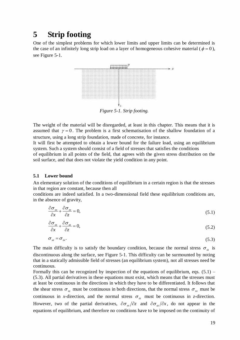
5 Strip footing One of the simplest problems for which lower limits and upper limits can be determined is
the case of an infinitely long strip load on a layer of homogeneous cohesive material ( 0 ),
see Figure 5-1.
The weight of the material will be disregarded, at least in this chapter. This means that it is
assumed that 0 . The problem is a first schematisation of the shallow foundation of a
structure, using a long strip foundation, made of concrete, for instance.
It will first be attempted to obtain a lower bound for the failure load, using an equilibrium
system. Such a system should consist of a field of stresses that satisfies the conditions
of equilibrium in all points of the field, that agrees with the given stress distribution on the
soil surface, and that does not violate the yield condition in any point.
5.1 Lower bound
An elementary solution of the conditions of equilibrium in a certain region is that the stresses
in that region are constant, because then all
conditions are indeed satisfied. In a two-dimensional field these equilibrium conditions are,
in the absence of gravity,
0,xx zx
x z
(5.1)
0,xz zz
x z
(5.2)
.xz zx (5.3)
The main difficulty is to satisfy the boundary condition, because the normal stress zz is
discontinuous along the surface, see Figure 5-1. This difficulty can be surmounted by noting
that in a statically admissible field of stresses (an equilibrium system), not all stresses need be
continuous.
Formally this can be recognized by inspection of the equations of equilibrium, eqs. (5.1) –
(5.3). All partial derivatives in these equations must exist, which means that the stresses must
at least be continuous in the directions in which they have to be differentiated. It follows that
the shear stress xz must be continuous in both directions, that the normal stress xx must be
continuous in x-direction, and the normal stress zz must be continuous in z-direction.
However, two of the partial derivatives, xx z and zz x , do not appear in the
equations of equilibrium, and therefore no conditions have to be imposed on the continuity of
Figure 5-1. Strip footing.
20
these two normal stresses in these directions. This means that xx may be discontinuous in z-
direction, and that zz may be discontinuous in x-direction. Such a discontinuity is shown,
for the vertical direction, in Figure 5-2.
This figure shows a small element, with all the stresses acting upon its boundaries. The
normal stress xx must be continuous in x-direction, because of equilibrium, as can most
easily be seen by letting the width of the element approach zero. Then the continuity of the
stress xx can be seen as a consequence of Newton’s principle that the reaction must be equal
to the action. The normal stress zz , however, may jump across the vertical line, without
disturbing equilibrium.
In Figure 5-2 the stress zz is discontinuous in x-direction. The partial derivative zz x is
infinitely large at the location of the vertical axis, but the element, and all of its parts, are
perfectly well in equilibrium.
This property of equilibrium systems has been applied by Drucker, one of the originators of
the theory of plasticity, to construct equilibrium fields for practical problems. In this method
the field is subdivided into regions of simple form, in each of which the stress is constant, so
that the equations of equilibrium are automatically satisfied. The various subregions then are
connected by requiring that all the stresses transferred on the boundary surfaces are
continuous, allowing the normal stresses in the direction of these boundaries to be
discontinuous.
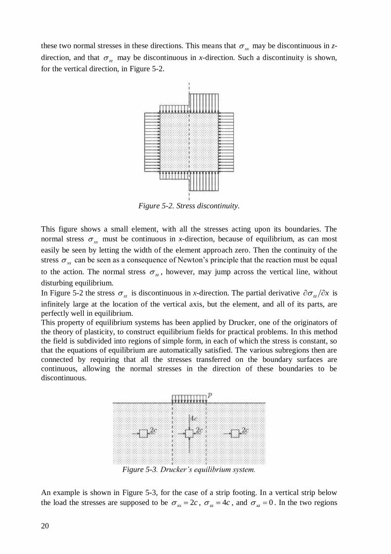
An example is shown in Figure 5-3, for the case of a strip footing. In a vertical strip below
the load the stresses are supposed to be 2xx c , 4zz c , and 0xz . In the two regions
Figure 5-2. Stress discontinuity.
Figure 5-3. Drucker’s equilibrium system.
21
to the left and right of this strip the stresses are 2xx c , 0zz , and 0xz . On the two
vertical discontinuity lines only the vertical normal stress zz is discontinuous. The other
stresses are continuous, as required by equilibrium. This field of stresses satisfies all the
conditions of equilibrium, and satisfies the boundary conditions on the upper surface. The
shear stress 0zx , and the normal stress 0zz if | |x a , and zz p if | |x a , where
2a is the width of the loaded strip. The stress distribution should also satisfy the condition
that the yield condition is never violated. This can be checked most conveniently by
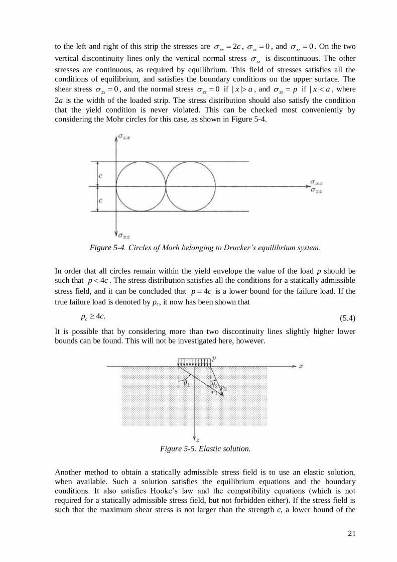
considering the Mohr circles for this case, as shown in Figure 5-4.
In order that all circles remain within the yield envelope the value of the load p should be
such that 4p c . The stress distribution satisfies all the conditions for a statically admissible
stress field, and it can be concluded that 4p c is a lower bound for the failure load. If the
true failure load is denoted by pc, it now has been shown that
4 .cp c (5.4)
It is possible that by considering more than two discontinuity lines slightly higher lower
bounds can be found. This will not be investigated here, however.
Another method to obtain a statically admissible stress field is to use an elastic solution,
when available. Such a solution satisfies the equilibrium equations and the boundary
conditions. It also satisfies Hooke’s law and the compatibility equations (which is not
required for a statically admissible stress field, but not forbidden either). If the stress field is
such that the maximum shear stress is not larger than the strength c, a lower bound of the
Figure 5-4. Circles of Morh belonging to Drucker’s equilibrium system.
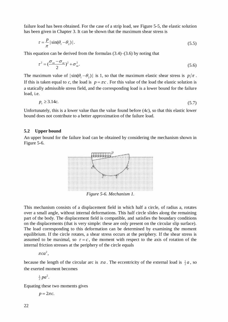
Figure 5-5. Elastic solution.
22
failure load has been obtained. For the case of a strip load, see Figure 5-5, the elastic solution
has been given in Chapter 3. It can be shown that the maximum shear stress is
1 2| sin( ) | .p
(5.5)
This equation can be derived from the formulas (3.4)–(3.6) by noting that
2 2 2( ) .2
xx zzxz
(5.6)
The maximum value of 1 2| sin( ) | is 1, so that the maximum elastic shear stress is p .
If this is taken equal to c, the load is p c . For this value of the load the elastic solution is
a statically admissible stress field, and the corresponding load is a lower bound for the failure
load, i.e.
3.14 .cp c (5.7)
Unfortunately, this is a lower value than the value found before (4c), so that this elastic lower
bound does not contribute to a better approximation of the failure load.
5.2 Upper bound
An upper bound for the failure load can be obtained by considering the mechanism shown in
Figure 5-6.
This mechanism consists of a displacement field in which half a circle, of radius a, rotates
over a small angle, without internal deformations. This half circle slides along the remaining
part of the body. The displacement field is compatible, and satisfies the boundary conditions
on the displacements (that is very simple: these are only present on the circular slip surface).
The load corresponding to this deformation can be determined by examining the moment
equilibrium. If the circle rotates, a shear stress occurs at the periphery. If the shear stress is
assumed to be maximal, so c , the moment with respect to the axis of rotation of the
internal friction stresses at the periphery of the circle equals
2 ,ca
because the length of the circular arc is a . The eccentricity of the external load is 12
a , so
the exerted moment becomes
212
.pa
Equating these two moments gives
2 .p c
Figure 5-6. Mechanism 1.
23
This is an upper bound for the failure load pc,
6.28 .cp c (5.8)
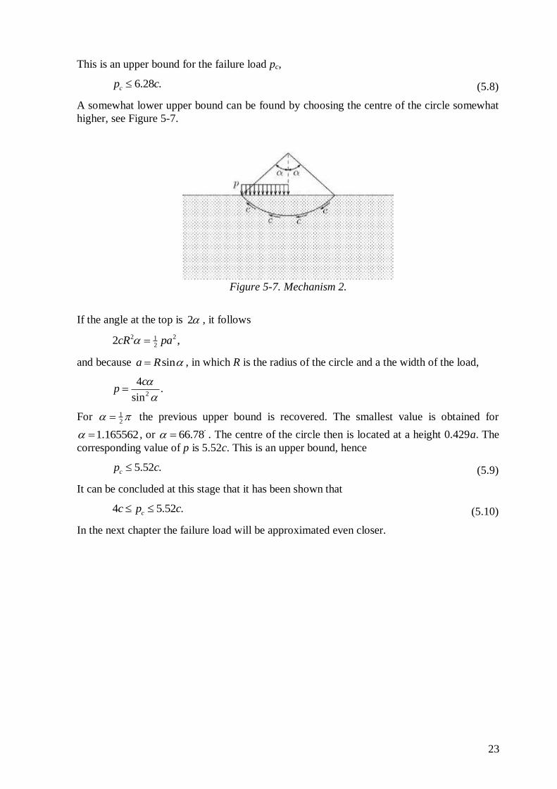
A somewhat lower upper bound can be found by choosing the centre of the circle somewhat
higher, see Figure 5-7.
If the angle at the top is 2 , it follows
2 212
2 ,cR pa
and because sina R , in which R is the radius of the circle and a the width of the load,
2
4.
sin
cp
For 12
the previous upper bound is recovered. The smallest value is obtained for
1.165562 , or 66.78 . The centre of the circle then is located at a height 0.429a. The
corresponding value of p is 5.52c. This is an upper bound, hence
5.52 .cp c (5.9)
It can be concluded at this stage that it has been shown that
4 5.52 .cc p c (5.10)
In the next chapter the failure load will be approximated even closer.
Figure 5-7. Mechanism 2.
24
6 Prandtl In 1920 Prandtl succeeded in finding a solution for the problem of a strip load on a half plane
that is both statically admissible and kinematically admissible. This solution must therefore
give the true failure load. The lower bound part of Prandtl’s solution, with an equilibrium
system of stresses, will be presented in this chapter. The proof that this solution is also
kinematically admissible, which is much more difficult, will be omitted here. A complete
proof can be found in textbooks on the theory of plasticity. The material is considered to be
weightless ( 0 ), and frictionless ( 0 ), so that its only relevant property is the cohesive
strength c. That is a great restriction, but it will be relaxed in later chapters.
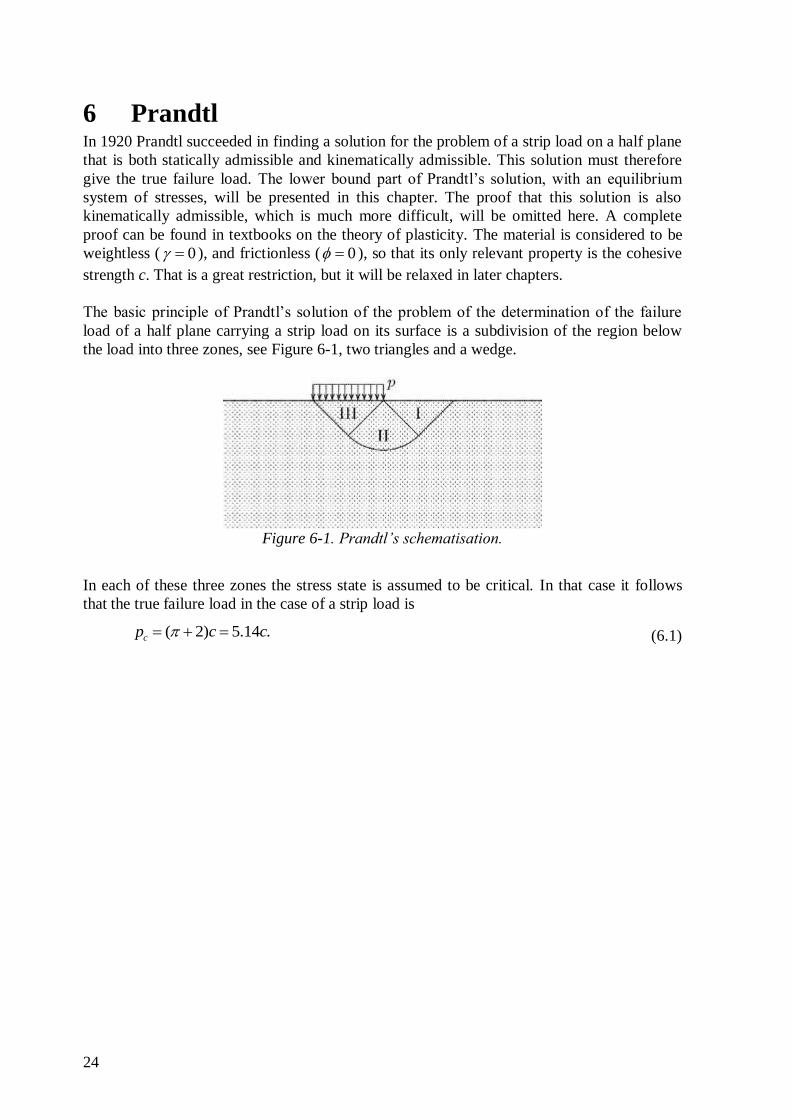
The basic principle of Prandtl’s solution of the problem of the determination of the failure
load of a half plane carrying a strip load on its surface is a subdivision of the region below
the load into three zones, see Figure 6-1, two triangles and a wedge.
In each of these three zones the stress state is assumed to be critical. In that case it follows
that the true failure load in the case of a strip load is
( 2) 5.14 .cp c c (6.1)
Figure 6-1. Prandtl’s schematisation.
25
7 Brinch Hansen Although the computation of limit states for materials with internal friction does not lead to
results that are certainly on the safe side or on the unsafe side of the failure load (as they are
for cohesive materials), these computations can still be very valuable, because it can be
expected that the results will at least give an approximation of the failure load. Engineering
calculations are always based upon a number of assumptions and approximations, and
engineers have to accept that their results at best are an approximation of reality. The
circumstance that it cannot be stated with certainty that a given load is above or below the
failure load does not make the results useless. As long as the computations are based upon
reasonable assumptions regarding the stresses and deformations, and if they incorporate
certain experiences from the field or the laboratory, the results may be considered as giving a
useful approximation of the real world. In this process there is also room for engineering
judgement, which is a combination of intuition, experience and common sense. Finally, it
may be mentioned that the applicability of a certain methodology may be enhanced by its
possible agreement with known results for special cases.
In this chapter the case of a strip footing on cohesive material, considered in chapters 5 and 6,
is extended to a general type of shallow foundation, on a soil characterized by its cohesion c,
friction angle and volumetric weight . The soil is assumed to be completely
homogeneous. Although the formulas were originally intended to be applied to foundation
strips of buildings, at a shallow depth below the soil surface, they are also applied to large
caisson foundations used in offshore engineering for the foundation of huge oil production
platforms.
7.1 Bearing capacity of strip foundation
An important problem of foundation engineering is the computation of the maximum load
(the bearing capacity) of a strip foundation, i.e. a very long foundation, of constant width, at
a certain depth below the soil surface. The influence of the depth of the foundation is
accounted for by considering a surcharge at the foundation level, to the left and the right of
the applied load. For the simplest case, of a strip of infinite length, on weightless soil, the
first computations were made by Prandtl, see Figure 7-2, on the basis of the assumption that
in a certain region at the soil surface the stresses satisfy the equilibrium conditions and the
Mohr-Coulomb failure criterion. In this entire region the soil then is on the verge of yielding.
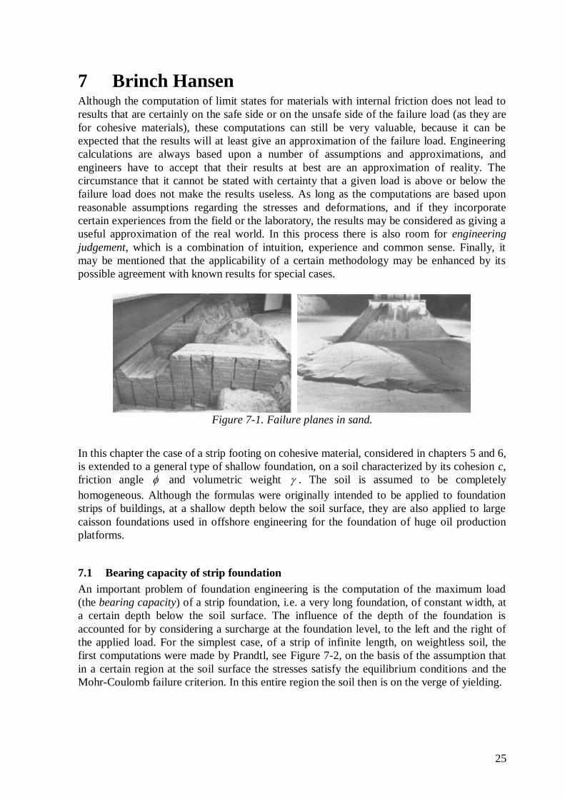
Figure 7-1. Failure planes in sand.
26
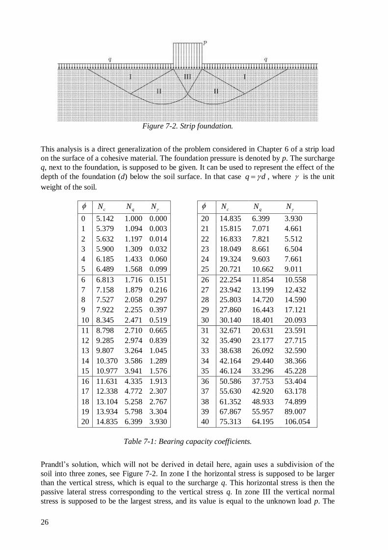
This analysis is a direct generalization of the problem considered in Chapter 6 of a strip load
on the surface of a cohesive material. The foundation pressure is denoted by p. The surcharge
q, next to the foundation, is supposed to be given. It can be used to represent the effect of the
depth of the foundation (d) below the soil surface. In that case q d , where is the unit
weight of the soil.
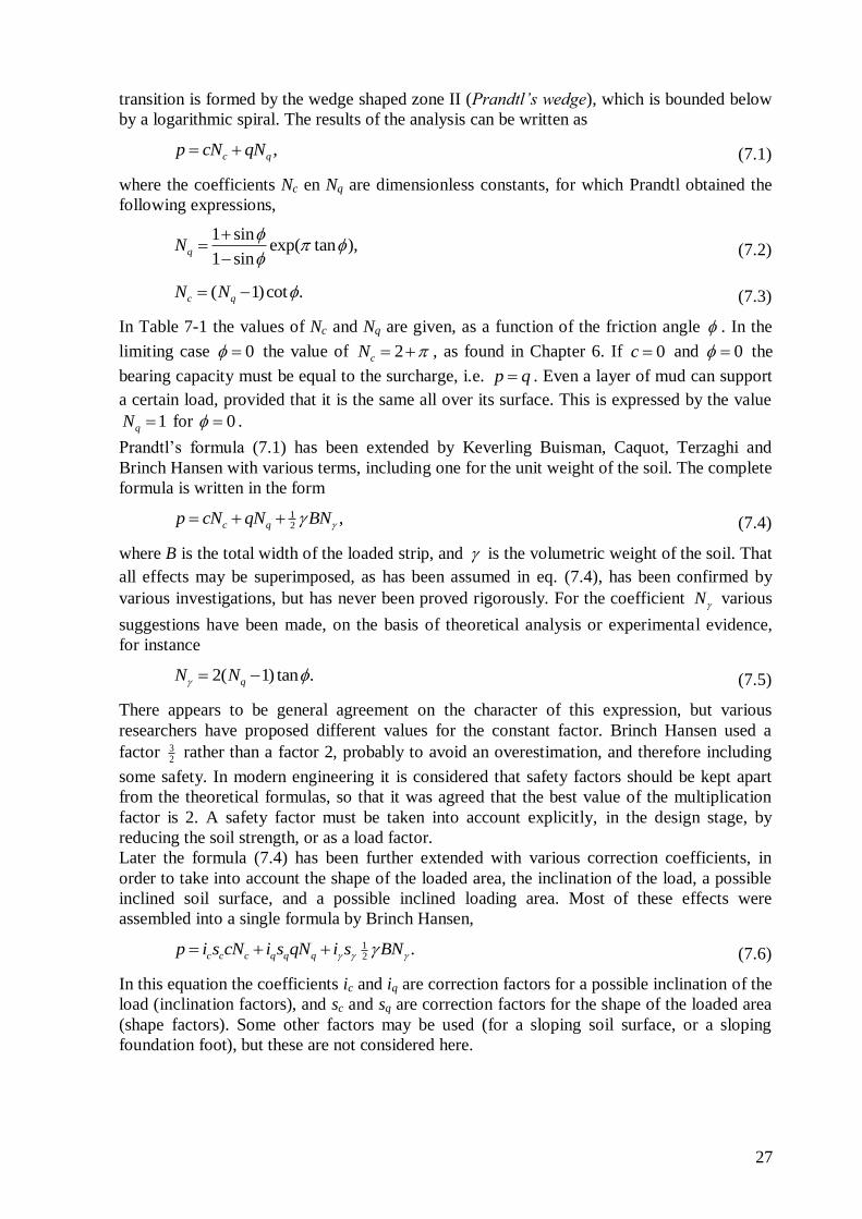
cN qN N
cN qN N
0 5.142 1.000 0.000 20 14.835 6.399 3.930
1 5.379 1.094 0.003 21 15.815 7.071 4.661
2 5.632 1.197 0.014 22 16.833 7.821 5.512
3 5.900 1.309 0.032 23 18.049 8.661 6.504
4 6.185 1.433 0.060 24 19.324 9.603 7.661
5 6.489 1.568 0.099 25 20.721 10.662 9.011
6 6.813 1.716 0.151 26 22.254 11.854 10.558
7 7.158 1.879 0.216 27 23.942 13.199 12.432
8 7.527 2.058 0.297 28 25.803 14.720 14.590
9 7.922 2.255 0.397 29 27.860 16.443 17.121
10 8.345 2.471 0.519 30 30.140 18.401 20.093
11 8.798 2.710 0.665 31 32.671 20.631 23.591
12 9.285 2.974 0.839 32 35.490 23.177 27.715
13 9.807 3.264 1.045 33 38.638 26.092 32.590
14 10.370 3.586 1.289 34 42.164 29.440 38.366
15 10.977 3.941 1.576 35 46.124 33.296 45.228
16 11.631 4.335 1.913 36 50.586 37.753 53.404
17 12.338 4.772 2.307 37 55.630 42.920 63.178
18 13.104 5.258 2.767 38 61.352 48.933 74.899
19 13.934 5.798 3.304 39 67.867 55.957 89.007
20 14.835 6.399 3.930 40 75.313 64.195 106.054
Prandtl’s solution, which will not be derived in detail here, again uses a subdivision of the
soil into three zones, see Figure 7-2. In zone I the horizontal stress is supposed to be larger
than the vertical stress, which is equal to the surcharge q. This horizontal stress is then the
passive lateral stress corresponding to the vertical stress q. In zone III the vertical normal
stress is supposed to be the largest stress, and its value is equal to the unknown load p. The
Figure 7-2. Strip foundation.
Table 7-1: Bearing capacity coefficients.
27
transition is formed by the wedge shaped zone II (Prandtl’s wedge), which is bounded below
by a logarithmic spiral. The results of the analysis can be written as
,c qp cN qN (7.1)
where the coefficients Nc en Nq are dimensionless constants, for which Prandtl obtained the
following expressions,
1 sinexp( tan ),
1 sinqN
(7.2)
( 1)cot .c qN N (7.3)
In Table 7-1 the values of Nc and Nq are given, as a function of the friction angle . In the
limiting case 0 the value of 2cN , as found in Chapter 6. If 0c and 0 the
bearing capacity must be equal to the surcharge, i.e. p q . Even a layer of mud can support
a certain load, provided that it is the same all over its surface. This is expressed by the value
1qN for 0 .
Prandtl’s formula (7.1) has been extended by Keverling Buisman, Caquot, Terzaghi and
Brinch Hansen with various terms, including one for the unit weight of the soil. The complete
formula is written in the form
12
,c qp cN qN BN (7.4)
where B is the total width of the loaded strip, and is the volumetric weight of the soil. That
all effects may be superimposed, as has been assumed in eq. (7.4), has been confirmed by
various investigations, but has never been proved rigorously. For the coefficient N various
suggestions have been made, on the basis of theoretical analysis or experimental evidence,
for instance
2( 1) tan .qN N (7.5)
There appears to be general agreement on the character of this expression, but various
researchers have proposed different values for the constant factor. Brinch Hansen used a
factor 32
rather than a factor 2, probably to avoid an overestimation, and therefore including
some safety. In modern engineering it is considered that safety factors should be kept apart
from the theoretical formulas, so that it was agreed that the best value of the multiplication
factor is 2. A safety factor must be taken into account explicitly, in the design stage, by
reducing the soil strength, or as a load factor.
Later the formula (7.4) has been further extended with various correction coefficients, in
order to take into account the shape of the loaded area, the inclination of the load, a possible
inclined soil surface, and a possible inclined loading area. Most of these effects were
assembled into a single formula by Brinch Hansen,
12
.c c c q q qp i s cN i s qN i s BN (7.6)
In this equation the coefficients ic and iq are correction factors for a possible inclination of the
load (inclination factors), and sc and sq are correction factors for the shape of the loaded area
(shape factors). Some other factors may be used (for a sloping soil surface, or a sloping
foundation foot), but these are not considered here.
28
7.2 Inclination factors
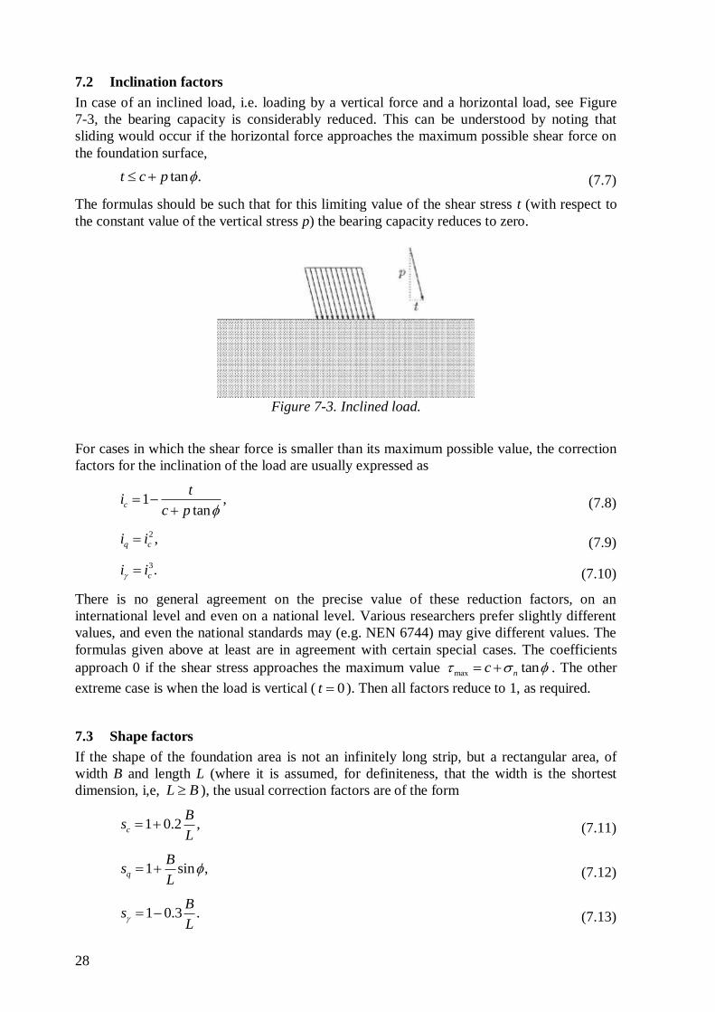
In case of an inclined load, i.e. loading by a vertical force and a horizontal load, see Figure
7-3, the bearing capacity is considerably reduced. This can be understood by noting that
sliding would occur if the horizontal force approaches the maximum possible shear force on
the foundation surface,
tan .t c p (7.7)
The formulas should be such that for this limiting value of the shear stress t (with respect to
the constant value of the vertical stress p) the bearing capacity reduces to zero.
For cases in which the shear force is smaller than its maximum possible value, the correction
factors for the inclination of the load are usually expressed as
1 ,tan
c
ti
c p
(7.8)
2 ,q ci i (7.9)
3.ci i (7.10)
There is no general agreement on the precise value of these reduction factors, on an
international level and even on a national level. Various researchers prefer slightly different
values, and even the national standards may (e.g. NEN 6744) may give different values. The
formulas given above at least are in agreement with certain special cases. The coefficients
approach 0 if the shear stress approaches the maximum value max tannc . The other
extreme case is when the load is vertical ( 0t ). Then all factors reduce to 1, as required.
7.3 Shape factors
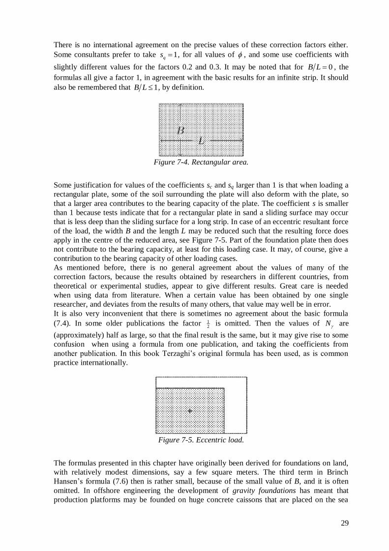
If the shape of the foundation area is not an infinitely long strip, but a rectangular area, of
width B and length L (where it is assumed, for definiteness, that the width is the shortest
dimension, i,e, L B ), the usual correction factors are of the form
1 0.2 ,c
Bs
L (7.11)
1 sin ,q
Bs
L (7.12)
1 0.3 .B
sL
(7.13)
Figure 7-3. Inclined load.
29
There is no international agreement on the precise values of these correction factors either.
Some consultants prefer to take 1qs , for all values of , and some use coefficients with
slightly different values for the factors 0.2 and 0.3. It may be noted that for 0B L , the
formulas all give a factor 1, in agreement with the basic results for an infinite strip. It should
also be remembered that 1B L , by definition.
Some justification for values of the coefficients sc and sq larger than 1 is that when loading a
rectangular plate, some of the soil surrounding the plate will also deform with the plate, so
that a larger area contributes to the bearing capacity of the plate. The coefficient s is smaller
than 1 because tests indicate that for a rectangular plate in sand a sliding surface may occur
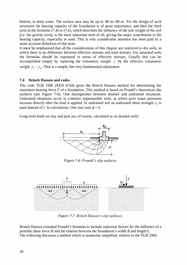
that is less deep than the sliding surface for a long strip. In case of an eccentric resultant force
of the load, the width B and the length L may be reduced such that the resulting force does
apply in the centre of the reduced area, see Figure 7-5. Part of the foundation plate then does
not contribute to the bearing capacity, at least for this loading case. It may, of course, give a
contribution to the bearing capacity of other loading cases.
As mentioned before, there is no general agreement about the values of many of the
correction factors, because the results obtained by researchers in different countries, from
theoretical or experimental studies, appear to give different results. Great care is needed
when using data from literature. When a certain value has been obtained by one single
researcher, and deviates from the results of many others, that value may well be in error.
It is also very inconvenient that there is sometimes no agreement about the basic formula
(7.4). In some older publications the factor 12
is omitted. Then the values of N are
(approximately) half as large, so that the final result is the same, but it may give rise to some
confusion when using a formula from one publication, and taking the coefficients from
another publication. In this book Terzaghi’s original formula has been used, as is common
practice internationally.
The formulas presented in this chapter have originally been derived for foundations on land,
with relatively modest dimensions, say a few square meters. The third term in Brinch
Hansen’s formula (7.6) then is rather small, because of the small value of B, and it is often
omitted. In offshore engineering the development of gravity foundations has meant that
production platforms may be founded on huge concrete caissons that are placed on the sea
Figure 7-4. Rectangular area.
Figure 7-5. Eccentric load.
30
bottom, in deep water. The surface area may be up to 80 m 80 m . For the design of such
structures the bearing capacity of the foundation is of great importance, and then the third
term in the formulas (7.4) or (7.6), which describes the influence of the unit weight of the soil
(i.e. the gravity term), is the most important term of all, giving the major contribution to the
bearing capacity, especially in sand. This is why considerable attention has been paid to a
more accurate definition of this term.
It must be emphasized that all the considerations of this chapter are restricted to dry soils, in
which there is no difference between effective stresses and total stresses. For saturated soils
the formulas should be expressed in terms of effective stresses. Usually this can be
accomplished simply by replacing the volumetric weight by the effective volumetric
weight s w . That is a simple, but very fundamental adjustment.
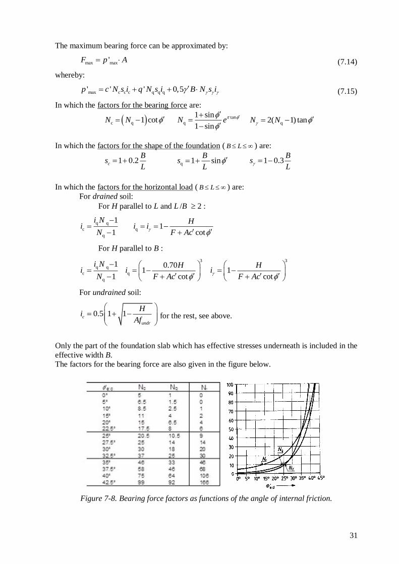
7.4 Brinch Hansen and codes
The code TGB 1990 (NEN 6744) gives the Brinch Hansen method for determining the
maximum bearing force F of a foundation. This method is based on Prandtl’s theoretical slip
surfaces (see Figure 7-6). One distinguishes between drained and undrained situations.
Undrained situations occur in cohesive impermeable soils, in which pore water pressures
increase directly after the load is applied. In undrained soil an undrained shear strength cu is
used instead of c' in calculations. One also uses = 0.
Long-term loads on clay and peat are, of course, calculated as on drained soils!
Brinch Hansen extended Prandtl’s formulas to include reduction factors for the influence of a
possible shear force H and the relation between the foundation’s width B and length L.
The following discusses a method which is somewhat simplified, relative to the TGB 1990.
Figure 7-6. Prandtl’s slip surfaces.
p
q HF
Figure 7-7. Brinch Hansen’s slip surfaces.
31
The maximum bearing force can be approximated by:
max max'F p A (7.14)
whereby:
max c c c q q q' ' ' 0,5p c N s i q N s i B N s i (7.15)
In which the factors for the bearing force are:
c q 1 cotN N tan
q
1 sin
1 sinN e
q2( 1) tanN N
In which the factors for the shape of the foundation ( B L ) are:
1 0.2c
Bs
L
q 1 sinB
sL
1 0.3B
sL
In which the factors for the horizontal load ( B L ) are:
For drained soil:
For H parallel to L and L /B 2 :
q q
c q
q
11
1 cot
i N Hi i i
N F Ac
For H parallel to B :
3 3
q q
c q
q
1 0.701 1
1 cot cot
i N H Hi i i
N F Ac F Ac
For undrained soil:
0.5 1 1c
undr
Hi
Af
for the rest, see above.
Only the part of the foundation slab which has effective stresses underneath is included in the
effective width B.
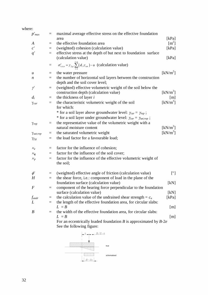
The factors for the bearing force are also given in the figure below.
Figure 7-8. Bearing force factors as functions of the angle of internal friction.
32
where:
p'max = maximal average effective stress on the effective foundation
area [kPa]
A = the effective foundation area [m2]
c' = (weighted) cohesion (calculation value) [kPa]
q' = effective stress at the depth of but next to foundation surface
(calculation value) [kPa]
= 1
i n
v;z;o f;g i car
i
. d . u
(calculation value)
u = the water pressure [kN/m2]
n = the number of horizontal soil layers between the construction
depth and the soil cover level;
' = (weighted) effective volumetric weight of the soil below the
construction depth (calculation value) [kN/m3]
di = the thickness of layer i [m]
car = the characteristic volumetric weight of the soil [kN/m3]
for which:
* for a soil layer above groundwater level: car = rep ;
* for a soil layer under groundwater level: car = sat;rep ;
rep = the representative value of the volumetric weight with a
natural moisture content [kN/m3]
sat;rep = the saturated volumetric weight [kN/m3]
f;g = the load factor for a favourable load;
c = factor for the influence of cohesion;
q = factor for the influence of the soil cover;
= factor for the influence of the effective volumetric weight of
the soil;
' = (weighted) effective angle of friction (calculation value) []
H = the shear force, i.e.: component of load in the plane of the
foundation surface (calculation value) [kN]
F = component of the bearing force perpendicular to the foundation
surface (calculation value) [kN]
fundr = the calculation value of the undrained shear strength = cu [kPa]
L = the length of the effective foundation area, for circular slabs:
L = B [m]
B = the width of the effective foundation area, for circular slabs:
L = B [m]
For an eccentrically loaded foundation B is approximated by B-2e
See the following figure:
true
schematised
33
Note: The factors for the bearing force are too conservative. This is because it is assumed that the factors do not
influence each other, which is incorrect.
The factors for the shape of the foundation and particularly for the horizontal load are not substantiated scientifically but they are based on empirical relations, experiments, calculations, etc.
For a horizontal load H one not only has to apply a reduction in the calculation of the vertical bearing force F, but one also has to check if sliding can occur (e.g. using Coulomb).
The reduction of the vertical bearing force F as a result of the horizontal load H is considerable. Assuming H/F = 0.30 results in iq = 0.50!!
7.5 CPT and undrained shear strength
In the Netherlands the cone penetration test is mainly used as a model test for pile
foundations. In the Western parts of the Netherlands the soil usually consists of 10 – 20
meters of very soft soil layers (clay and peat), on a rather stiff sand layer. This soil structure
is very well suited for a pile foundation, of wooden or concrete piles of about 20 cm – 40 cm
diameter, reaching just into the sand. The weight of the soft soil acts as a surcharge on the
sand, which has a considerable cone resistance. The allowable stress on the sand depends
upon its friction angle , its cohesion c (usually very small, or zero), and the surcharge q.
The dimensions of the foundation pile have very little influence, because this parameter
appears only in the third term of Brinch Hansen’s formula, which is a small term if the width
is less than, say, 1 meter. This means that the maximum pressure for a large pile and the thin
pile of a cone penetrometer will be practically the same, so that the allowable pressure on a
pile can be determined by simply measuring the cone resistance. This will be elaborated in
Chapter 8.
The cone penetration test can also be used to determine physical parameters of the soil,
especially the shear strength. It can be postulated, for instance, that in clays the cone
resistance will be determined mainly by the undrained shear strength of the soil (su). In
agreement with the analysis of Brinch Hansen the relation will be of the form
,c v c uq N s (7.16)
where v is the local vertical stress caused by the surcharge, and Nc is a dimensionless
factor. For a circular cone in a cohesive material a cone factor Nc of the order of magnitude
15 – 18 is usually assumed, on the basis of plasticity calculations for the insertion of a cone
into a cohesive material of infinite extent. By measuring the cone resistance qc the undrained
shear strength su can be determined. The results are not very accurate, because of theoretical
shortcomings and practical difficulties, but the measurement has the great advantage of being
done in situ, on the least disturbed soil. The alternative would be taking a sample, bringing it
to a laboratory, and then doing a laboratory test. This process includes many possible sources
of disturbance, which can be avoided by doing a test in situ.

34
35
II Pile foundations
36
8 Cone Penetration Test (CPT) The cone penetration test (CPT) is a testing method used to determine the geotechnical
engineering properties of soils and the soil stratigraphy. It was initially developed in the
1950s at the Dutch Laboratory for Soil Mechanics in Delft (now Deltares) to investigate soft
soils. Based on this history it has also been called the "Dutch cone test". Today, the CPT is
one of the most used and accepted in soil methods for soil investigation worldwide.
The test is used to determine:
soil types,
(stratigraphic) soil layering,
soil stiffnesses and strengths (empirical)
bearing capacities of pile foundations
permeability and consolidation parameters,
groundwater pressure
environmental data (pollution)
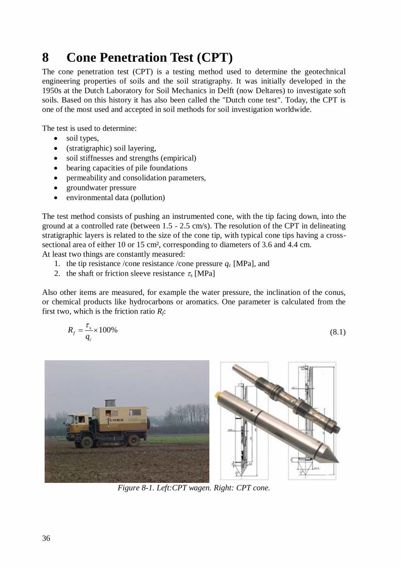
The test method consists of pushing an instrumented cone, with the tip facing down, into the
ground at a controlled rate (between 1.5 - 2.5 cm/s). The resolution of the CPT in delineating
stratigraphic layers is related to the size of the cone tip, with typical cone tips having a cross-
sectional area of either 10 or 15 cm², corresponding to diameters of 3.6 and 4.4 cm.
At least two things are constantly measured:
1. the tip resistance /cone resistance /cone pressure qc [MPa], and
2. the shaft or friction sleeve resistance s [MPa]
Also other items are measured, for example the water pressure, the inclination of the conus,
or chemical products like hydrocarbons or aromatics. One parameter is calculated from the
first two, which is the friction ratio Rf:
100%sf
c
Rq
(8.1)
Figure 8-1. Left:CPT wagen. Right: CPT cone.
37
The friction number is quite helpful in determining the soil type, see Table 8-1, but a
checking with a few additional borings remains very important.
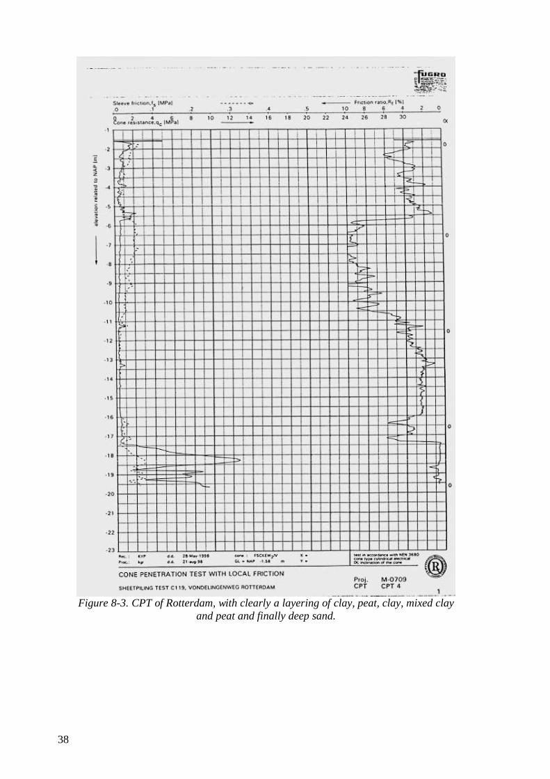
For example in the sounding (CPT) of Rotterdam in Figure 8-3, the soil types and layering
are very clear. There are very soft layers until -17.5 m: a clear clay layer until -5,5 m; peat
until -11,5 m; clay until -16,0 m; clayey peat until -17,5 and first then soft sand.
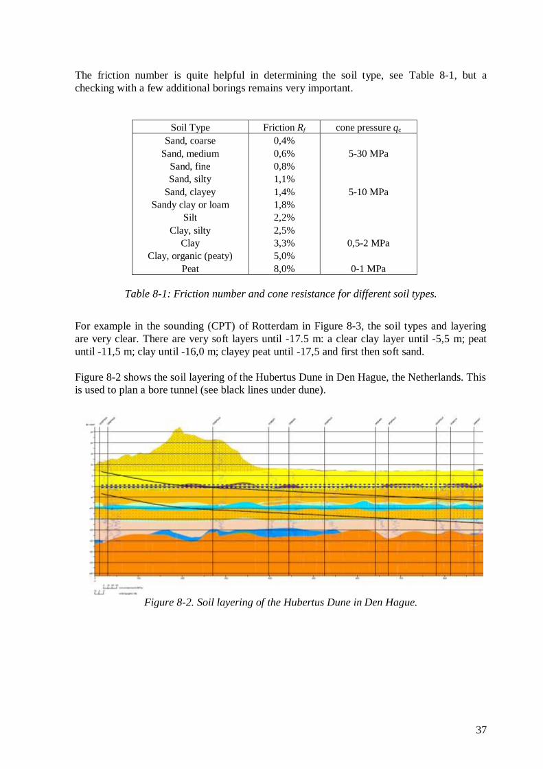
Figure 8-2 shows the soil layering of the Hubertus Dune in Den Hague, the Netherlands. This
is used to plan a bore tunnel (see black lines under dune).
Soil Type Friction Rf cone pressure qc
Sand, coarse
Sand, medium
Sand, fine
Sand, silty
Sand, clayey
Sandy clay or loam
Silt
Clay, silty
Clay
Clay, organic (peaty)
Peat
0,4%
0,6%
0,8%
1,1%
1,4%
1,8%
2,2%
2,5%
3,3%
5,0%
8,0%
5-30 MPa
5-10 MPa
0,5-2 MPa
0-1 MPa
Table 8-1: Friction number and cone resistance for different soil types.
Figure 8-2. Soil layering of the Hubertus Dune in Den Hague.
38
Figure 8-3. CPT of Rotterdam, with clearly a layering of clay, peat, clay, mixed clay
and peat and finally deep sand.
39
9 Compression piles In many river delta areas, for example the Western part of the Netherlands, the soil consists
of layers of soft soil (clay and peat), of 10 20 meter thickness, on a stiff sand layer, of
pleistocene origin. The bearing capacity of this sand layer is derived for a large part from its
deep location, with the soft layers acting as a surcharge. The properties of the sand itself, a
relatively high density, and a high friction angle, also help to give this sand layer a good
bearing capacity, of course. The system of soft soils and a deeper stiff sand layer is very
suitable for a pile foundation. In this chapter a number of important soil mechanics aspects of
such pile foundations is briefly discussed.
9.1 Pile types
Piles can be made from wood, steel, (partially) reinforced concrete or prestressed concrete.
The installation can be done by driving, vibrating, boring or pressing, but not all installation
techniques can be applied to the different pile types.
The following distinction can be made between the piles, but it is a strong simplification:
Wooden piles (driven or pressed)
Steel piles (driven, vibrated or bored)
Precast concrete piles (driven)
In situ concrete, piles (driven with steel pipe)
In situ concrete, piles (bored with steel pipe support)
In situ concrete, piles (bored with slurry support)
Wooden piles
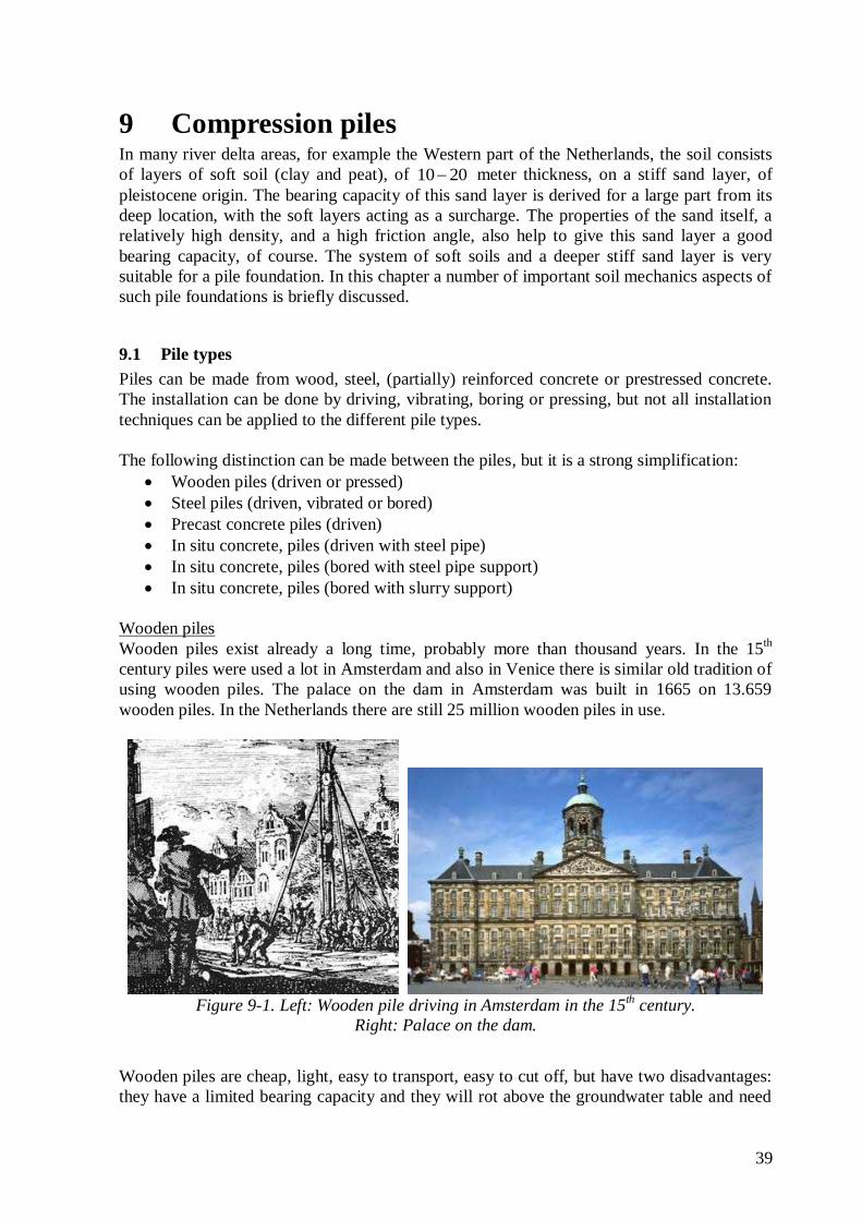
Wooden piles exist already a long time, probably more than thousand years. In the 15th
century piles were used a lot in Amsterdam and also in Venice there is similar old tradition of
using wooden piles. The palace on the dam in Amsterdam was built in 1665 on 13.659
wooden piles. In the Netherlands there are still 25 million wooden piles in use.
Wooden piles are cheap, light, easy to transport, easy to cut off, but have two disadvantages:
they have a limited bearing capacity and they will rot above the groundwater table and need
Figure 9-1. Left: Wooden pile driving in Amsterdam in the 15
th century.
Right: Palace on the dam.
40
therefore a concrete extension or something similar and should never face a sinking
groundwater (not even a leak draining sewage system nearby).
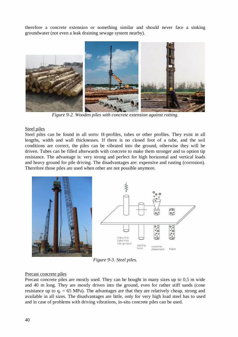
Steel piles
Steel piles can be found in all sorts: H-profiles, tubes or other profiles. They exist in all
lengths, width and wall thicknesses. If there is no closed foot of a tube, and the soil
conditions are correct, the piles can be vibrated into the ground, otherwise they will be
driven. Tubes can be filled afterwards with concrete to make them stronger and to option tip
resistance. The advantage is: very strong and perfect for high horizontal and vertical loads
and heavy ground for pile driving. The disadvantages are: expensive and rusting (corrosion).
Therefore those piles are used when other are not possible anymore.
Precast concrete piles
Precast concrete piles are mostly used. They can be bought in many sizes up to 0,5 m wide
and 40 m long. They are mostly driven into the ground, even for rather stiff sands (cone
resistance up to qc = 65 MPa). The advantages are that they are relatively cheap, strong and
available in all sizes. The disadvantages are little, only for very high load steel has to used
and in case of problems with driving vibrations, in-situ concrete piles can be used.
Figure 9-2. Wooden piles with concrete extension against rotting.
Figure 9-3. Steel piles.
41
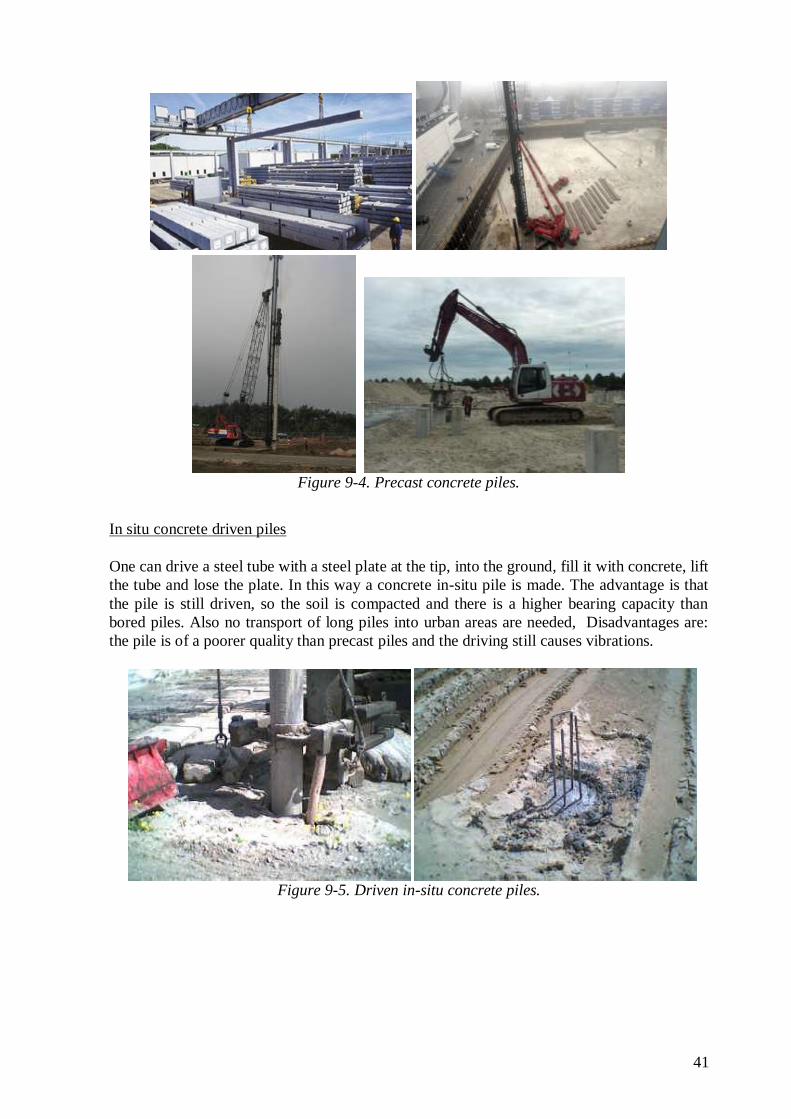
In situ concrete driven piles
One can drive a steel tube with a steel plate at the tip, into the ground, fill it with concrete, lift
the tube and lose the plate. In this way a concrete in-situ pile is made. The advantage is that
the pile is still driven, so the soil is compacted and there is a higher bearing capacity than
bored piles. Also no transport of long piles into urban areas are needed, Disadvantages are:
the pile is of a poorer quality than precast piles and the driving still causes vibrations.
Figure 9-4. Precast concrete piles.
Figure 9-5. Driven in-situ concrete piles.
42
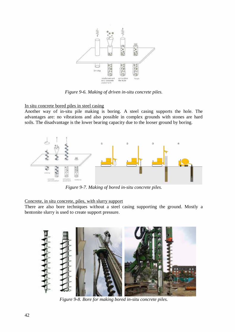
In situ concrete bored piles in steel casing
Another way of in-situ pile making is boring. A steel casing supports the hole. The
advantages are: no vibrations and also possible in complex grounds with stones are hard
soils. The disadvantage is the lower bearing capacity due to the looser ground by boring.
Concrete, in situ concrete, piles, with slurry support
There are also bore techniques without a steel casing supporting the ground. Mostly a
bentonite slurry is used to create support pressure.
Figure 9-6. Making of driven in-situ concrete piles.
Figure 9-7. Making of bored in-situ concrete piles.
Figure 9-8. Bore for making bored in-situ concrete piles.
43
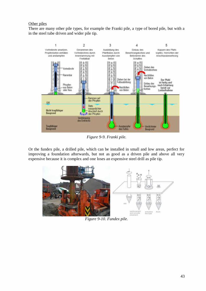
Other piles
There are many other pile types, for example the Franki pile, a type of bored pile, but with a
in the steel tube driven and wider pile tip.
Or the fundex pile, a drilled pile, which can be installed in small and low areas, perfect for
improving a foundation afterwards, but not as good as a driven pile and above all very
expensive because it is complex and one loses an expensive steel drill as pile tip.
Figure 9-9. Franki pile.
Figure 9-10. Fundex pile.
44
9.2 Bearing capacity
A pile may also have a bearing capacity due to friction along the length of the pile. This is
very important for piles in sand layers. In applications in very soft soil (clay layers), the
contribution of friction is generally very unreliable, because the soil may be subject to
settlements, whereas the pile may be rigid, if it has been installed into a deep sand layer. It
may even happen that the subsiding soil exerts a downward friction force on the pile,
negative skin friction, which reduces the effective bearing capacity of the pile. Friction is of
course very important for tension piles, for which it is the only contributing mechanism.
The maximum value of the skin friction can be determined very well using a friction cone,
which is a penetration test in which the sleeve friction is also measured. The local values are
often very small, however, so that the measured data are not very accurate. For sandy soils
the friction therefore is often correlated to the cone resistance.
The ultimate bearing capacity of a compression pile is determined by both the tip bearing
capacity and the shaft bearing capacity:
;max ;max: ;max:r r tip r schaftF F F (9.1)
whereby:
;max: ;max;r tip tip r tipF A p (9.2)
;max: ;;max;
L
r shaft p avgo r shaft
F O p
(9.3)
in which:
Fr;max = maximum bearing force
Fr;max;tip = maximum tip resistance force
Fr;max;shaft = maximum shaft friction force
Apoint = surface area of the tip of the pile
pr;max;tip = maximum tip resistance according to the sounding ( = qc )
Op;avg = circumference of the pile shaft
L = length of the pile
pr;max;shaft = maximum pile shaft friction according to the sounding ( = s cq )
Notes In case prefab piles with enlarged feet are used, L may not be larger than the height of the enlarged foot H
(see Figure 9-15).
A reduced value of maximum tip resistance of 15 MPa is valid (see Figure 9-16).
One must not forget to reduce the net bearing capacity of the pile by the value of negative shaft friction.
For s see Table 9-2 in Chapter 9.5
In areas with soft soils, mostly methods based on the Cone Penetretation Tests are used (for
example method Koppejan). Another way is to calculate the bearing capacity of the pile with
Brinch-Hansen, this is done when there are no Cone Penetretation Tests to use for the
previous method.
45
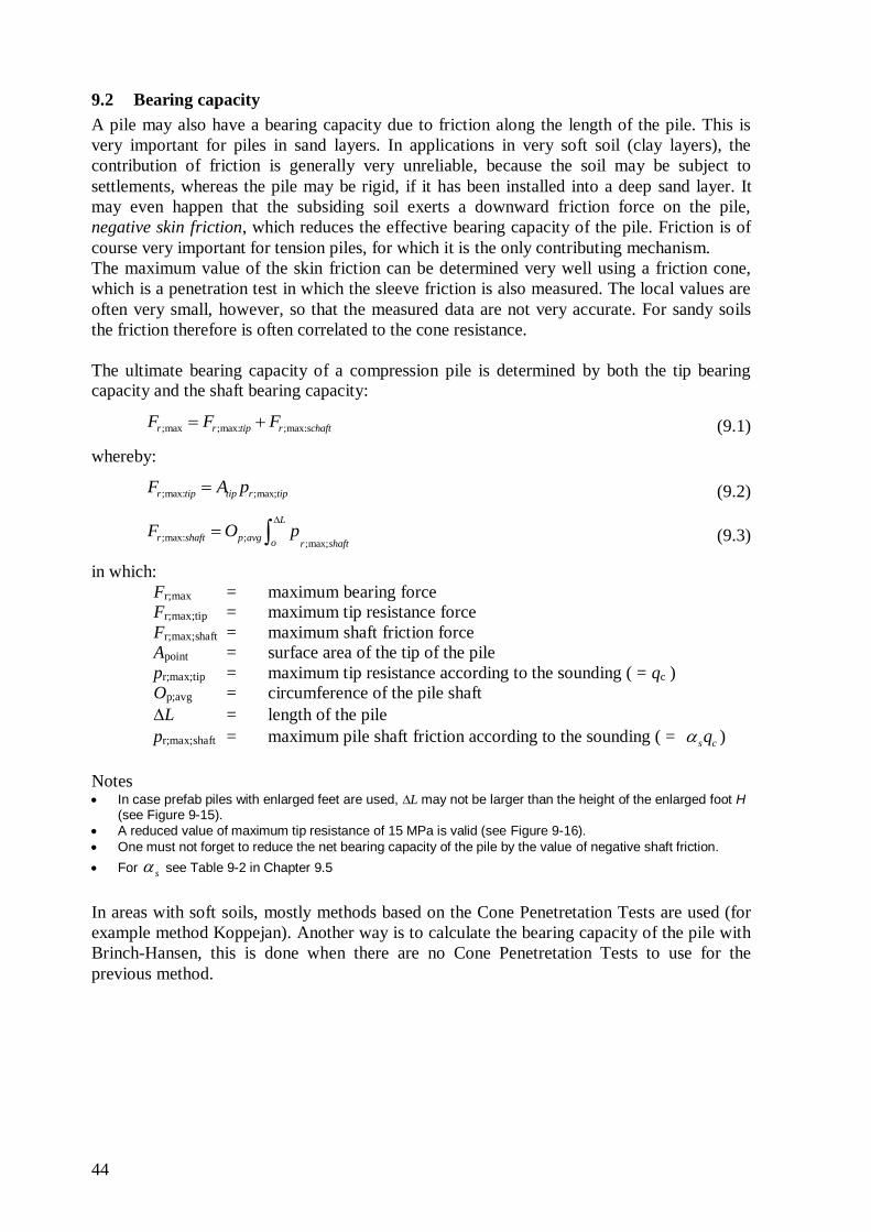
9.3 Tip resistance using Brinch Hansen (Prandtl or Meyerhof)
For the determination of the bearing capacity of a foundation pile it is possible to use a
theoretical analysis, on the basis of Brinch Hansen’s general bearing capacity formula. In this
analysis the basic parameters are the shear strength of the sand layer (characterized by its
cohesion c and its friction angle ), and the weight of the soft layers, which can be taken into
account as a surcharge q.
The maximum tip resistance can be determined analogously to the bearing capacity of a
shallow foundation, which is based on a slide plain according to Prandtl. This entails simply
using the 2-dimensional solution for 3-dimensional collapse (conservative) and simply
disregarding the shear strength, not the weight, of the soil above the foundation plane
(conservative).
The following example shows that the term e;d0.5 efB N s is negligible relative
to v;z;o;d q qN s . Therefore the tip resistance can be calculated most simply according to:
p N sr;max;tip v;z;o;d q q
Example Given is a pile that is driven 11 metres into the ground according to Figure 9-11. The pile is in approximately 1 metre of sand; above the sand layer is 10 metres of clay. Groundwater level is 1 metre below ground level. The following data is given:
Sand: = 40 c = 0
w,d = 20 kN/m3
Clay: w,d = 15 kN/m3
Pile dimensions: 0.4 x 0.4 m2
According to Prandtl, because the cohesion is zero the maximum pressure below the tip of the pile will be:
r;max;tip v;z;o;d q q q e;d0.5 efp N s i B N s i
According to Table 7-1 in Chapter 7: Nq = 64 and N = 106
The pile is only subjected to axial loads, so: iq = i =1 The shape factors can be derived from (Bef = Lef):
sq = 1+sin 40 = 1.64 s = 1-0.3 = 0.7 The initial effective ground pressure is:
2
v;z;o;d 10 15 1 20 10 10 70 kN/m
The maximum acceptable tip stress is:
r;max;tip
3 3 3 2
70 64 1.64 0.5 10 0.4 106 0.7
7.35 10 0.15 10 7.5 10 kN/m
p
So: e;d0.5 efB N s << v;z;o;d q qN s
Figure 9-11. Slide plains under a pile according to Prandtl.
46
9.4 Tip resistance using Koppejan
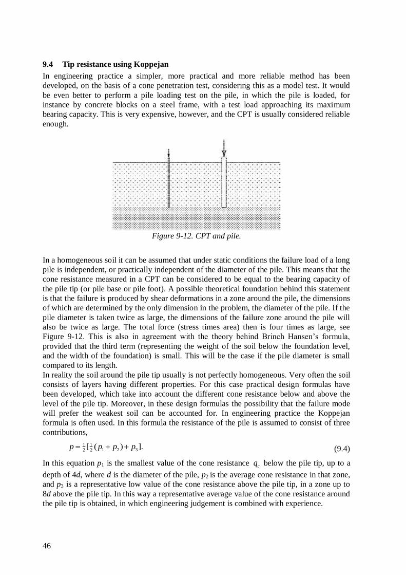
In engineering practice a simpler, more practical and more reliable method has been
developed, on the basis of a cone penetration test, considering this as a model test. It would
be even better to perform a pile loading test on the pile, in which the pile is loaded, for
instance by concrete blocks on a steel frame, with a test load approaching its maximum
bearing capacity. This is very expensive, however, and the CPT is usually considered reliable
enough.
In a homogeneous soil it can be assumed that under static conditions the failure load of a long
pile is independent, or practically independent of the diameter of the pile. This means that the
cone resistance measured in a CPT can be considered to be equal to the bearing capacity of
the pile tip (or pile base or pile foot). A possible theoretical foundation behind this statement
is that the failure is produced by shear deformations in a zone around the pile, the dimensions
of which are determined by the only dimension in the problem, the diameter of the pile. If the
pile diameter is taken twice as large, the dimensions of the failure zone around the pile will
also be twice as large. The total force (stress times area) then is four times as large, see
Figure 9-12. This is also in agreement with the theory behind Brinch Hansen’s formula,
provided that the third term (representing the weight of the soil below the foundation level,
and the width of the foundation) is small. This will be the case if the pile diameter is small
compared to its length.
In reality the soil around the pile tip usually is not perfectly homogeneous. Very often the soil
consists of layers having different properties. For this case practical design formulas have
been developed, which take into account the different cone resistance below and above the
level of the pile tip. Moreover, in these design formulas the possibility that the failure mode
will prefer the weakest soil can be accounted for. In engineering practice the Koppejan
formula is often used. In this formula the resistance of the pile is assumed to consist of three
contributions,
1 11 2 32 2
[ ( ) ].p p p p (9.4)
In this equation p1 is the smallest value of the cone resistance cq below the pile tip, up to a
depth of 4d, where d is the diameter of the pile, p2 is the average cone resistance in that zone,
and p3 is a representative low value of the cone resistance above the pile tip, in a zone up to
8d above the pile tip. In this way a representative average value of the cone resistance around
the pile tip is obtained, in which engineering judgement is combined with experience.
Figure 9-12. CPT and pile.
47
In the Netherlands, the bearing capacity of a pile is usually determined with soundings (Cone
Penetration Tests). A sounding can be perceived as a model test, loading a compression pile
beyond the state of collapse. Theoretically sounding entails determining the maximum tip
resistance at every level in the ground. Because the size of the slide plain below and beside
the pile or sounding cone depends on the dimensions of the foundation area, the cone
resistance cannot be directly interpreted as the maximum tip resistance of a pile. Generally
one assumes the slide plane continues to some 0.7 times the pile diameter below the pile and
up to approximately 8 times the diameter above the foundation.
In this case the maximum tip resistance can be derived from the sounding using:
c;l;avg c;ll;avg
r;max;tip p c;lll;avg1/ 22
q qp s q
in which:
qc;l;avg = the average value of the cone resistances qc;z;corr’ along section I,
from the level of the tip of the pile to a level at least 0.7 times the equivalent
centre line (Deq) and at most 4 times Deq deeper. The bottom of section I must
be selected between these boundaries so that pr;max;tip is minimal;
qc;ll;avg = the average value of the cone resistances qc;z;corr’ along section II,
from the bottom of section I to the level of the tip of the pile; the value of the
cone resistance to be used in calculations may never exceed that of a lower
level;
qc;lll;avg = the average value of the cone resistances qc;z;corr’ along section III,
which runs up from the pile tip level to a level 8 times the equivalent centre
line (Deq) above; as for section II the value used for the cone resistance may
never exceed that of a lower level, starting with the value of cone resistance at
the end of section II.
In the case of auger piles, this section must start with a cone resistance equal
to or less than 2 NM/m2, unless the sounding took place within 1 metre of the
side of the pile after the pile was placed in the ground;
Deq = equivalent pile tip diameter:
Round pile: eqD D
Square/rectangular pile: 4
/eqD a b a
a = width of pile, shortest side
b = width of pile, longest side (with 1.5a b a )
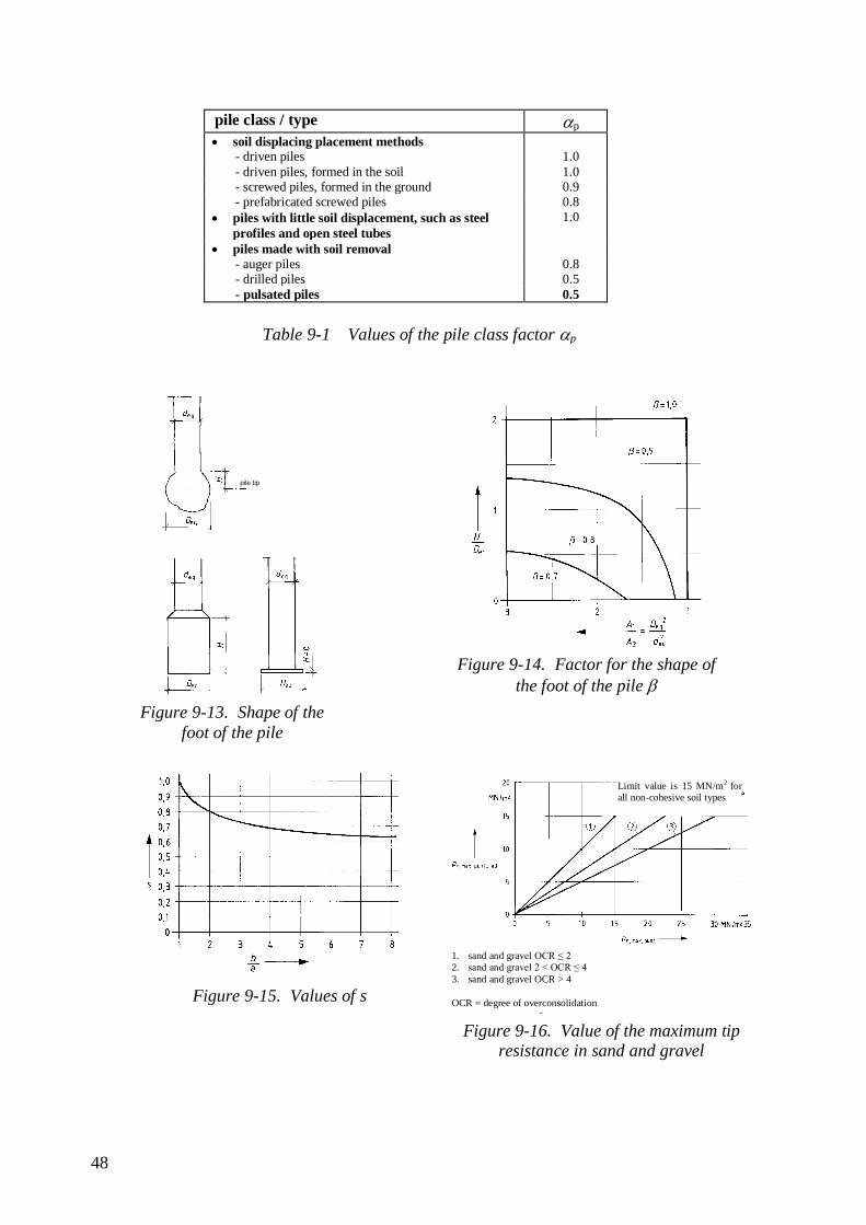
p = the pile class factor according to Table 9-1
= the factor that takes into account the influence of the shape of the foot
of the pile, determined using Figure 9-13 and Figure 9-14;
s = the factor that takes into account the influence of the shape of the
cross section of the foot of the pile, determined using Figure 9-15.
48
pile class / type p soil displacing placement methods
- driven piles 1.0
- driven piles, formed in the soil 1.0 - screwed piles, formed in the ground 0.9 - prefabricated screwed piles 0.8
piles with little soil displacement, such as steel
profiles and open steel tubes
1.0
piles made with soil removal
- auger piles 0.8 - drilled piles 0.5
- pulsated piles 0.5
Table 9-1 Values of the pile class factor p
pile tip
Figure 9-13. Shape of the
foot of the pile
Figure 9-14. Factor for the shape of
the foot of the pile
Figure 9-15. Values of s
Figure 9-16. Value of the maximum tip
resistance in sand and gravel
Limit value is 15 MN/m2 for
all non-cohesive soil types
1. sand and gravel OCR ≤ 2
2. sand and gravel 2 < OCR ≤ 4
3. sand and gravel OCR > 4
OCR = degree of overconsolidation
49
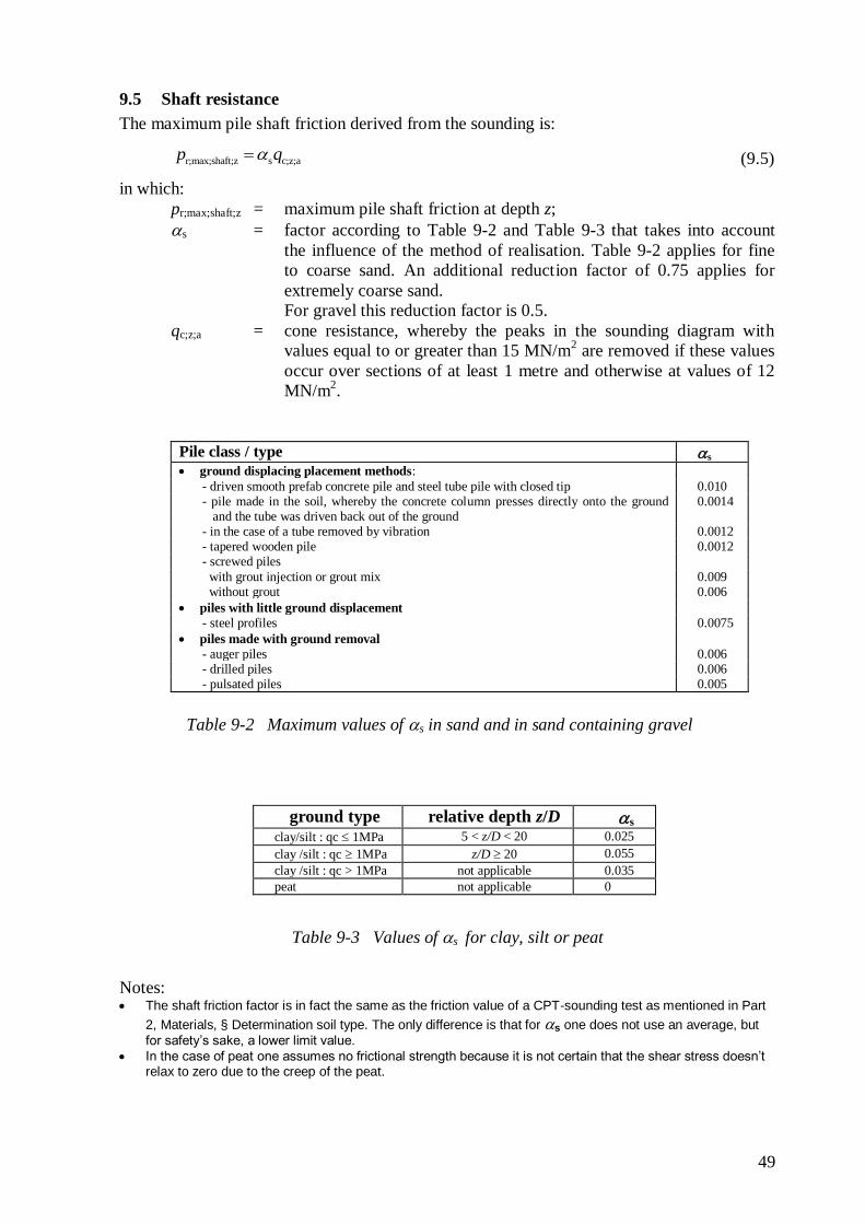
9.5 Shaft resistance
The maximum pile shaft friction derived from the sounding is:
r;max;shaft;z s c;z;ap q (9.5)
in which:
pr;max;shaft;z = maximum pile shaft friction at depth z;
s = factor according to Table 9-2 and Table 9-3 that takes into account
the influence of the method of realisation. Table 9-2 applies for fine
to coarse sand. An additional reduction factor of 0.75 applies for
extremely coarse sand.
For gravel this reduction factor is 0.5.
qc;z;a = cone resistance, whereby the peaks in the sounding diagram with
values equal to or greater than 15 MN/m2 are removed if these values
occur over sections of at least 1 metre and otherwise at values of 12
MN/m2.
Pile class / type s ground displacing placement methods:
- driven smooth prefab concrete pile and steel tube pile with closed tip 0.010 - pile made in the soil, whereby the concrete column presses directly onto the ground
and the tube was driven back out of the ground 0.0014
- in the case of a tube removed by vibration 0.0012 - tapered wooden pile 0.0012 - screwed piles
with grout injection or grout mix 0.009 without grout 0.006
piles with little ground displacement
- steel profiles 0.0075
piles made with ground removal
- auger piles 0.006 - drilled piles 0.006 - pulsated piles 0.005
ground type relative depth z/D s clay/silt : qc 1MPa 5 < z/D < 20 0.025
clay /silt : qc 1MPa z/D 20 0.055
clay /silt : qc > 1MPa not applicable 0.035
peat not applicable 0
Notes: The shaft friction factor is in fact the same as the friction value of a CPT-sounding test as mentioned in Part
2, Materials, § Determination soil type. The only difference is that for s one does not use an average, but
for safety’s sake, a lower limit value.
In the case of peat one assumes no frictional strength because it is not certain that the shear stress doesn’t relax to zero due to the creep of the peat.
Table 9-2 Maximum values of s in sand and in sand containing gravel
Table 9-3 Values of s for clay, silt or peat
50
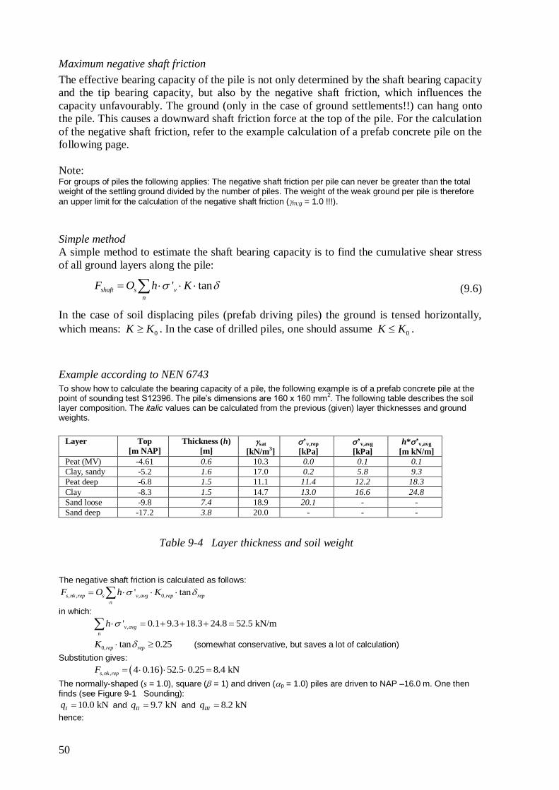
Maximum negative shaft friction
The effective bearing capacity of the pile is not only determined by the shaft bearing capacity
and the tip bearing capacity, but also by the negative shaft friction, which influences the
capacity unfavourably. The ground (only in the case of ground settlements!!) can hang onto
the pile. This causes a downward shaft friction force at the top of the pile. For the calculation
of the negative shaft friction, refer to the example calculation of a prefab concrete pile on the
following page.
Note: For groups of piles the following applies: The negative shaft friction per pile can never be greater than the total weight of the settling ground divided by the number of piles. The weight of the weak ground per pile is therefore
an upper limit for the calculation of the negative shaft friction (m;g = 1.0 !!!).
Simple method
A simple method to estimate the shaft bearing capacity is to find the cumulative shear stress
of all ground layers along the pile:
' tanshaft s v
n
F O h K (9.6)
In the case of soil displacing piles (prefab driving piles) the ground is tensed horizontally,
which means: 0K K . In the case of drilled piles, one should assume 0K K .
Example according to NEN 6743
To show how to calculate the bearing capacity of a pile, the following example is of a prefab concrete pile at the point of sounding test S12396. The pile’s dimensions are 160 x 160 mm
2. The following table describes the soil
layer composition. The italic values can be calculated from the previous (given) layer thicknesses and ground weights.
Layer Top
[m NAP]
Thickness (h)
[m] sat
[kN/m3]
’v,rep
[kPa]
’v,avg
[kPa]
h*’v,avg
[m kN/m]
Peat (MV) -4.61 0.6 10.3 0.0 0.1 0.1
Clay, sandy -5.2 1.6 17.0 0.2 5.8 9.3
Peat deep -6.8 1.5 11.1 11.4 12.2 18.3
Clay -8.3 1.5 14.7 13.0 16.6 24.8
Sand loose -9.8 7.4 18.9 20.1 - -
Sand deep -17.2 3.8 20.0 - - -
The negative shaft friction is calculated as follows:
, , , 0,' tans nk rep s v avg rep rep
n
F O h K
in which:
,' 0.1 9.3 18.3 24.8 52.5 kN/mv avg
n
h
0, tan 0.25rep repK (somewhat conservative, but saves a lot of calculation)
Substitution gives:
, , 4 0.16 52.5 0.25 8.4 kNs nk repF
The normally-shaped (s = 1.0), square ( = 1) and driven (p = 1.0) piles are driven to NAP –16.0 m. One then finds (see Figure 9-1 Sounding):
10.0 kNIq and 9.7 kNIIq and 8.2 kNIIIq
hence:
Table 9-4 Layer thickness and soil weight
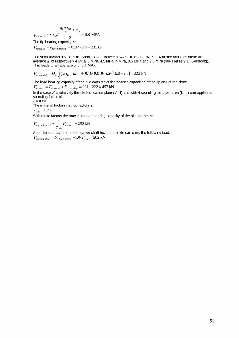
51
;max;2 9.0 MPA
2
I IIIII
r tip p
q qq
p s
The tip bearing capacity is: 2
;max; ;max; 0.16 9.0 231 kNr tip tip r tipF A F
The shaft friction develops in "Sand, loose". Between NAP –10 m and NAP – 16 m one finds per metre an average qc of respectively 4 MPa, 3 MPa, 4.5 MPa, 4 MPa, 8.5 MPa and 9.5 MPa (see Figure 9-1 Sounding). This leads to an average qc of 5.6 MPa.
;max;
0
4 0.16 0.010 5.6 16.0 9.8 222 kN
L
r shaft tip s cF O q dz
The load bearing capacity of the pile consists of the bearing capacities of the tip and of the shaft:
;max; ;max; ;max; 231 222 453 kNr d r tip r shaftF F F
In the case of a relatively flexible foundation plate (M=1) and with 4 sounding tests per area (N=4) one applies a sounding factor of:
= 0.80. The material factor (method factor) is:
m;b 1.25
With these factors the maximum load bearing capacity of the pile becomes:
; ;max; ;max;
;
290 kNr found d r d
m b
F F
After the subtraction of the negative shaft friction, the pile can carry the following load:
; ; ; ; ;max; ;1.0 282 kNr found all d r found d s nkF F F
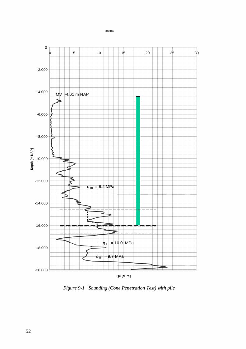
52
S12396
-20.000
-18.000
-16.000
-14.000
-12.000
-10.000
-8.000
-6.000
-4.000
-2.000
0
0 5 10 15 20 25 30
Qc [MPa]
De
pth
[m
NA
P]
MV -4.61 m NAP
q = 8.2 MPaIII
q = 10.0 MPaI
q = 9.7 MPaII
Figure 9-1 Sounding (Cone Penetration Test) with pile
53
10 Tension piles
10.1 Differences between tension and compression piles
The calculation of tension piles is theoretically the same as for compression piles, but there
are a number of differences:
1. Tension piles are only subject to shaft friction, not to tip resistance.
2. Tension piles have smaller coefficients of shaft friction than compression piles.
3. Tension piles are most commonly used in excavated building sites. Due to the
excavation of the building site, the ground pressure and thus the value of qc and the
friction force on the pile are reduced. This correction has to be taken into account for
tension piles.
4. Due to the tensile force of the tension piles the vertical effective ground pressure and
with it the value of qc are reduced. This correction has to be taken into account for
tension piles.
5. Not only the single pile should be tested for possible slip, the clump weight should
also be verified. The pile could emerge with the soil around it.
6. The safety factors for tension piles are greater than for compression piles, firstly
because inaccuracies are greater for shaft friction than for tip resistance and secondly
because this is increased further by statement 4.
7. The self-weight of the pile (usually under water) affects the system positively.
Due to statements 1-6 the tensile capacity of a pile is many times smaller than the
compression capacity of a pile.
There are no norms for the calculation of tension piles. Usually the rules according to the
CUR-report 98-9 are assumed, but they are disputable.
Particularly for very large tensile forces grout anchors are used instead of tension piles.
Calculation of the bearing capacity of a tension pile is not easy. One must take a lot of factors
into account. For instance, the tensile force in a pile reduces the surrounding effective ground
pressure and thereby reduces the pile’s tensile force. This leads to a complex method of
calculation. Hence, in general, tension piles are calculated using a computer programme. For
the sake of completeness, the theory of such computer programmes is explained below.
10.2 Reduction of the cone value qc due to excavation
Most calculations assume piles are driven into the ground after the building sites have been
excavated. As a consequence of the reduced effective ground pressure, the cone resistance
has to be reduced. The following relationship can be used for this reduction:
0.71
;
,
;
'
'
v new
c corr c
v old
q q
(10.1)
in which:
,c corrq = corrected cone resistance at depth z [MPa]
;'v new = vertical effective ground pressure after excavation at depth z [kPa]
;'v old = vertical effective ground pressure before excavation at depth z [kPa]
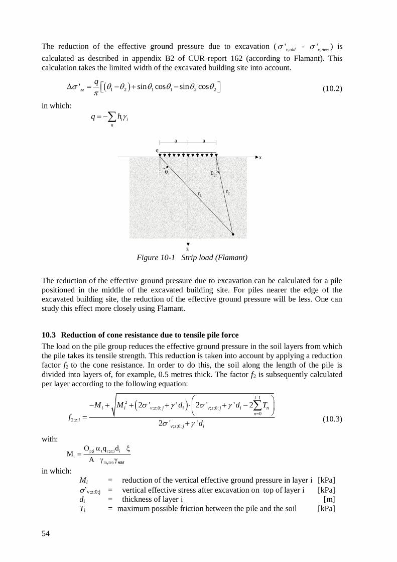
54
The reduction of the effective ground pressure due to excavation (;'v old -
;'v new ) is
calculated as described in appendix B2 of CUR-report 162 (according to Flamant). This
calculation takes the limited width of the excavated building site into account.
1 2 1 1 2 2' sin cos sin coszz
q
(10.2)
in which:
i i
n
q h
The reduction of the effective ground pressure due to excavation can be calculated for a pile
positioned in the middle of the excavated building site. For piles nearer the edge of the
excavated building site, the reduction of the effective ground pressure will be less. One can
study this effect more closely using Flamant.
10.3 Reduction of cone resistance due to tensile pile force
The load on the pile group reduces the effective ground pressure in the soil layers from which
the pile takes its tensile strength. This reduction is taken into account by applying a reduction
factor f2 to the cone resistance. In order to do this, the soil along the length of the pile is
divided into layers of, for example, 0.5 metres thick. The factor f2 is subsequently calculated
per layer according to the following equation:
1
2
; ;0; ; ;0;
0
2; ;
; ;0;
2 ' ' 2 ' ' 2
2 ' '
i
i i v z j i v z j i n
n
z i
v z j i
M M d d T
fd
(10.3)
with:
p i t c z i i
i
m ten
O q dM
A
; ; ;
, var
in which:
Mi = reduction of the vertical effective ground pressure in layer i [kPa]
’v;z;0;j = vertical effective stress after excavation on top of layer i [kPa]
di = thickness of layer i [m]
Ti = maximum possible friction between the pile and the soil [kPa]
a a
x
z
21
r1r2
q
Figure 10-1 Strip load (Flamant)
55
Op = average circumference of the pile in layer i [m]
t = friction factor as indicated in table 24 of CUR-report 98-9
qc;z;i = average cone resistance in layer i after reduction due to
excavation [kPa]
A = surface area taken up by the pile [m2]
m,ten = material factor for piles with tensile loads (=1.4)
var = material factor for variable loads (=1.0)
= factor, dependent on the number of soundings. See table 1
of NEN 6743 ( 0.8 )
Notes. 1. In many cases the load on the tension piles is normative during implementation. In this phase the variation of
the load is negligible. Consequently one uses var = 1.0 in this phase. 2. An underwater concrete floor is considered a flexible structure according to the definition in NEN 6743,
hence, when determining the factor according to table 1 of NEN 6743, the number of piles is set as 1.
10.4 Clump criterion
An important form of global translation is the vertical uplift (heave) of a building pit
including the tension piles and ground in between, due to the groundwater pressure.
Therefore not only should one check whether the pile will fail due to sliding and whether it
can be pulled “clean” out of the soil, one should also verify whether all piles, including the
soil, can be pulled out as a “clump”. The weight of the clump Fclump per pile is often
calculated as follows:
2 13 2
· ' 3
· ' / 3
clumpF A L A
A L A
in which:
A = surface area per tension element [m2]
’ = effective volumetric weight of the soil [kN/m3]
L = distance between the bottom of the underwater
concrete floor and the bottom of the tension element [m]
This formula shows that the length L is reduced because a cone-shaped fracture surface at 45
degrees is taken into account at the centre point of the tension element (pile).
The maximum acceptable tensile force is then:
,a clump m clumpF F
in which:
m,clump = material factor for the weight of the clump (=1.1)
Of course, the weight of the underwater concrete and of the tension element (pile) may also
be included (m = 1.1).
The problem with the method above is that it is not correct to take the pore water pressure
only at a constant level of the pile tip (pile base), while the bottom of the “soil clump” has a
far more complex shape. Therefore an easier way for a quick design check of the clump
criterion can be found in Chapter Error! Reference source not found. “Global translation”.
56
10.5 Edge Piles
Particularly around an open access road to a tunnel, edge piles sometimes have greater tensile
loads than the other piles. In this case, to determine the tensile load capacity, one must take
into account:
limited (Flamant-) reduction of the sounding resistance along the edge of the excavated
building site due to the excavations.
group action based on the average pile tensile forces in a cross section and thus not based
on the tension in the edge piles themselves.
possible horizontal forces in sheet piling next to the pile.