STATISTICAL MECHANICS

Daniel F. StyerOberlin College

Oberlin College

Statistical Mechanics

Daniel F. Styer

This text is disseminated via the Open Education Resource (OER) LibreTexts Project (https://LibreTexts.org) and like thehundreds of other texts available within this powerful platform, it is freely available for reading, printing and"consuming." Most, but not all, pages in the library have licenses that may allow individuals to make changes, save, andprint this book. Carefully consult the applicable license(s) before pursuing such effects.

Instructors can adopt existing LibreTexts texts or Remix them to quickly build course-specific resources to meet the needsof their students. Unlike traditional textbooks, LibreTexts’ web based origins allow powerful integration of advancedfeatures and new technologies to support learning.

The LibreTexts mission is to unite students, faculty and scholars in a cooperative effort to develop an easy-to-use onlineplatform for the construction, customization, and dissemination of OER content to reduce the burdens of unreasonabletextbook costs to our students and society. The LibreTexts project is a multi-institutional collaborative venture to developthe next generation of open-access texts to improve postsecondary education at all levels of higher learning by developingan Open Access Resource environment. The project currently consists of 14 independently operating and interconnectedlibraries that are constantly being optimized by students, faculty, and outside experts to supplant conventional paper-basedbooks. These free textbook alternatives are organized within a central environment that is both vertically (from advance tobasic level) and horizontally (across different fields) integrated.

The LibreTexts libraries are Powered by MindTouch and are supported by the Department of Education Open TextbookPilot Project, the UC Davis Office of the Provost, the UC Davis Library, the California State University AffordableLearning Solutions Program, and Merlot. This material is based upon work supported by the National Science Foundationunder Grant No. 1246120, 1525057, and 1413739. Unless otherwise noted, LibreTexts content is licensed by CC BY-NC-SA 3.0.

Any opinions, findings, and conclusions or recommendations expressed in this material are those of the author(s) and donot necessarily reflect the views of the National Science Foundation nor the US Department of Education.

Have questions or comments? For information about adoptions or adaptions contact info@LibreTexts.org. Moreinformation on our activities can be found via Facebook (https://facebook.com/Libretexts), Twitter(https://twitter.com/libretexts), or our blog (http://Blog.Libretexts.org).

This text was compiled on 01/27/2022

®

1 1/27/2022

TABLE OF CONTENTSThis is a book about statistical mechanics at the advanced undergraduate level. It assumes a background in classical mechanics throughthe concept of phase space, in quantum mechanics through the Pauli exclusion principle, and in mathematics through multivariatecalculus.

1: THE PROPERTIES OF MATTER IN BULK1.1: WHAT IS STATISTICAL MECHANICS ABOUT?1.2: OUTLINE OF BOOK1.3: FLUID STATICS1.4: PHASE DIAGRAMS1.5: ADDITIONAL PROBLEMS

2: PRINCIPLES OF STATISTICAL MECHANICS2.1: MICROSCOPIC DESCRIPTION OF A CLASSICAL SYSTEM2.2: MACROSCOPIC DESCRIPTION OF A LARGE EQUILIBRIUM SYSTEM2.3: FUNDAMENTAL ASSUMPTION2.4: STATISTICAL DEFINITION OF ENTROPY2.5: ENTROPY OF A MONATOMIC IDEAL GAS2.6: QUALITATIVE FEATURES OF ENTROPY2.7: USING ENTROPY TO FIND (DEFINE) TEMPERATURE AND PRESSURE2.8: ADDITIONAL PROBLEMS

3: THERMODYNAMICS3.1: HEAT AND WORK3.2: ENTROPY3.3: HEAT ENGINES3.4: MULTIVARIATE CALCULUS3.5: THERMODYNAMIC QUANTITIES3.6: THE THERMODYNAMIC DANCE3.7: NON-FLUID SYSTEMS3.8: THERMODYNAMICS APPLIED TO FLUIDS3.9: THERMODYNAMICS APPLIED TO PHASE TRANSITIONS3.10: THERMODYNAMICS APPLIED TO CHEMICAL REACTIONS3.11: THERMODYNAMICS APPLIED TO LIGHT3.12: ADDITIONAL PROBLEMS

4: ENSEMBLES4.1: THE CANONICAL ENSEMBLE4.2: MEANING OF THE TERM “ENSEMBLE”4.3: CLASSICAL MONATOMIC IDEAL GAS4.4: ENERGY DISPERSION IN THE CANONICAL ENSEMBLE4.5: TEMPERATURE AS A CONTROL VARIABLE FOR ENERGY (CANONICAL ENSEMBLE)4.6: THE EQUIVALENCE OF CANONICAL AND MICROCANONICAL ENSEMBLES4.7: THE GRAND CANONICAL ENSEMBLE4.8: THE GRAND CANONICAL ENSEMBLE IN THE THERMODYNAMIC LIMIT4.9: SUMMARY OF MAJOR ENSEMBLES4.10: QUANTAL STATISTICAL MECHANICS4.11: ENSEMBLE PROBLEMS I4.12: ENSEMBLE PROBLEMS II

5: CLASSICAL IDEAL GASESThis chapter considers ideal (i.e. non-interacting) gases made up of atoms or molecules that may have internal structure (i.e. not pointparticles). The internal degrees of freedom will be treated either classically or quantally, but the translational degrees of freedom willalways be treated classically.

2 1/27/2022

5.1: CLASSICAL MONATOMIC IDEAL GASES5.2: CLASSICAL DIATOMIC IDEAL GASES5.3: HEAT CAPACITY OF AN IDEAL GAS5.4: SPECIFIC HEAT OF A HETERO-NUCLEAR DIATOMIC IDEAL GAS5.5: CHEMICAL REACTIONS BETWEEN GASES5.6: PROBLEMS

6: QUANTAL IDEAL GASES6.1: INTRODUCTION6.2: THE INTERCHANGE RULE6.3: QUANTUM MECHANICS OF INDEPENDENT IDENTICAL PARTICLES6.4: STATISTICAL MECHANICS OF INDEPENDENT IDENTICAL PARTICLES6.5: QUANTUM MECHANICS OF FREE PARTICLES6.6: FERMI-DIRAC STATISTICS6.7: BOSE-EINSTEIN STATISTICS6.8: SPECIFIC HEAT OF THE IDEAL FERMION GAS6.9: ADDITIONAL PROBLEMS6.10: APPENDIX

7: HARMONIC LATTICE VIBRATIONS7.1: THE PROBLEM7.2: STATISTICAL MECHANICS OF THE PROBLEM7.3: NORMAL MODES FOR A ONE-DIMENSIONAL CHAIN7.4: NORMAL MODES IN THREE DIMENSIONS7.5: LOW-TEMPERATURE HEAT CAPACITY7.6: MORE REALISTIC MODELS7.7: WHAT IS A PHONON?7.8: ADDITIONAL PROBLEMS

8: INTERACTING CLASSICAL FLUIDS8.1: INTRODUCTION8.2: PERTURBATION THEORY8.3: VARIATIONAL METHODS8.4: DISTRIBUTION FUNCTIONS8.5: CORRELATIONS AND SCATTERING8.6: THE HARD SPHERE FLUID

9: STRONGLY INTERACTING SYSTEMS AND PHASE TRANSITIONS9.1: INTRODUCTION TO MAGNETIC SYSTEMS AND MODELS9.2: FREE ENERGY OF THE ONE-DIMENSIONAL ISING MODEL9.3: THE MEAN-FIELD APPROXIMATION9.4: CORRELATION FUNCTIONS IN THE ISING MODEL9.5: COMPUTER SIMULATION9.6: ADDITIONAL PROBLEMS

10: APPENDICES10.1: A- SERIES AND INTEGRALS10.2: B- EVALUATING THE GAUSSIAN INTEGRAL10.3: C- CLINIC ON THE GAMMA FUNCTION10.4: D- VOLUME OF A SPHERE IN D DIMENSIONS10.5: E- STIRLING'S APPROXIMATION10.6: F- THE EULER-MACLAURIN FORMULA AND ASYMPTOTIC SERIES10.7: G- RAMBLINGS ON THE RIEMANN ZETA FUNCTION10.8: H- TUTORIAL ON MATRIX DIAGONALIZATION10.9: I- CATALOG OF MISCONCEPTIONS10.10: J- THERMODYNAMIC MASTER EQUATIONS10.11: K- USEFUL FORMULAS

3 1/27/2022

BACK MATTERINDEXGLOSSARY

1 1/27/2022

CHAPTER OVERVIEW1: THE PROPERTIES OF MATTER IN BULK

1.1: WHAT IS STATISTICAL MECHANICS ABOUT?1.2: OUTLINE OF BOOK1.3: FLUID STATICS1.4: PHASE DIAGRAMSStatistical mechanics applies to all sorts of materials: fluids, crystals, magnets, metals, polymers, starstuff, even light. I want to showyou some of the enormous variety of behaviors exhibited by matter in bulk, and that can (at least in principle) be explained throughstatistical mechanics.

1.5: ADDITIONAL PROBLEMS

Daniel F. Styer 1.1.1 12/30/2021 https://phys.libretexts.org/@go/page/6329

1.1: What is Statistical Mechanics About?Statistical mechanics treats matter in bulk. While most branches of physics. . . classical mechanics, atomic physics,quantum mechanics, nuclear physics. . . deal with one or two or a few dozen particles, statistical mechanics deals with,typically, about a mole of particles at one time. A mole is , considerably larger than a few dozen. Let’scompare this to a number often considered large, namely the U.S. national debt. This debt is (2014) about 18 trilliondollars, so the national debt is about thirty trillionth of a mole of dollars. Even so, a mole of water molecules occupiesonly 18 ml or about half a fluid ounce. . . it’s just a sip.

The huge number of particles present in the systems studied by statistical mechanics means that the traditional questions ofphysics are impossible to answer. For example, the traditional question of classical mechanics is the time-developmentproblem: Given the positions and velocities of all the particles now, find out what they will be at some future time. Thisproblem has has not been completely solved for three gravitating bodies. . . clearly we will get nowhere asking the samequestion for bodies! But in fact, a solution of the time-development problem for a mole of water moleculeswould be useless even if it could be obtained. Who cares where each molecule is located? No experiment will ever be ableto find out. To make progress, we have to ask different questions, question like “How does the pressure change withvolume?”, “How does the temperature change upon adding particles?”, “What is the mean distance between atoms?”, or“What is the probability for finding two atoms separated by a given distance?”. Thus the challenge of statistical mechanicsis two-fold: first find the questions, and only then find the answers.

In contrast, the Milky Way galaxy contains about 0.3 or 0.6 trillionth of a mole of stars. The entire universe probablycontains fewer than a mole of stars.

6.02 ×1023

1

6.02 ×1023

1

Daniel F. Styer 1.2.1 12/30/2021 https://phys.libretexts.org/@go/page/6330

1.2: Outline of BookThis book begins with a chapter, the properties of matter in bulk, that introduces statistical mechanics and shows why it isso fascinating.

It proceeds to discuss the principles of statistical mechanics. The goal of this chapter is to motivate and then produce aconceptual definition for that quantity of central importance: entropy. In contrast to, say, quantum mechanics, it is notuseful to cast the foundations of statistical mechanics into a mathematically rigorous “postulate, theorem, proof” mold. Ourarguments in this chapter are often heuristic and suggestive; “plausibility arguments” rather than proofs.

Once we have defined entropy and know a few of its properties, what can we do with it? The subject of thermodynamicsasks what can be discovered about substance by just knowing that entropy exists, without knowing a formula for it. It isone of the most fascinating fields in all of science, because it produces a large number of dramatic and unexpected resultsbased on this single modest assumption. This book’s chapter on thermodynamics begins begins by developing a concreteoperational definition for entropy, in terms of heat and work, to complement the conceptual definition produced in theprevious chapter. It goes on to apply entropy to situations as diverse as fluids, phase transitions, and light.

The chapter on ensembles returns to issues of principle, and it produces formulas for the entropy that are considerablyeasier to apply than the one produced in chapter 2. Armed with these easier formulas, the rest of the book uses them invarious applications.

The first three applications are to the classic topics of classical ideal gases, quantal ideal gases, including Fermi-Dirac andBose-Einstein statistics, and harmonic lattice vibrations or phonons.

The subject of ideal gases (i.e. gases of non-interacting particles) is interesting and often useful, but it clearly does not tellthe full story. . . for example, the classical ideal gas can never condense into a liquid, so it cannot show any of thefascinating and practical phenomena of phase transitions. The next chapter treats weakly interacting fluids, using the toolsof perturbation theory and the variational method. The correlation function is introduced as a valuable tool. This is the firsttime in the book that we ask questions more detailed than the questions of thermodynamics.

Finally we treat strongly interacting systems and phase transitions. Here our emphasis is on magnetic systems. Toolsinclude mean field theory, transfer matrices, correlation functions, and computer simulations. Under this heading fall someof the most interesting questions in all of science. . . some answered, many still open.

The first five chapters (up to and including the chapter on classical ideal gases) are essential background to the rest of thebook, and they must be treated in the sequence presented. The last four chapters are independent and can be treated in anyorder.

Daniel F. Styer 1.3.1 1/4/2022 https://phys.libretexts.org/@go/page/6331

1.3: Fluid StaticsI mentioned above that statistical mechanics asks questions like “How does the pressure change with volume?”. But whatis pressure? Most people will answer by saying that pressure is force per area:

But force is a vector and pressure is a scalar, so how can this formula be correct? The aim of this section is to investigatewhat this formula means and find out when it is correct.

1.3.1 Problems

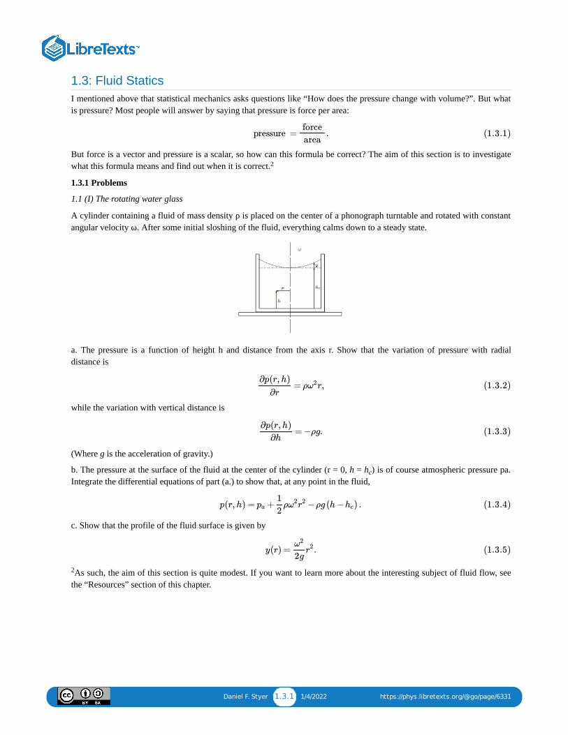
1.1 (I) The rotating water glass

A cylinder containing a fluid of mass density ρ is placed on the center of a phonograph turntable and rotated with constantangular velocity ω. After some initial sloshing of the fluid, everything calms down to a steady state.

a. The pressure is a function of height h and distance from the axis r. Show that the variation of pressure with radialdistance is

while the variation with vertical distance is

(Where g is the acceleration of gravity.)

b. The pressure at the surface of the fluid at the center of the cylinder (r = 0, h = h ) is of course atmospheric pressure pa.Integrate the differential equations of part (a.) to show that, at any point in the fluid,

c. Show that the profile of the fluid surface is given by

As such, the aim of this section is quite modest. If you want to learn more about the interesting subject of fluid flow, seethe “Resources” section of this chapter.

pressure = . force

area (1.3.1)

2

= ρ r,∂p(r, h)

∂rω2 (1.3.2)

= −ρg.∂p(r, h)

∂h(1.3.3)

c

p(r, h) = + ρ −ρg (h − ) .pa

1

2ω2r2 hc (1.3.4)

y(r) = .ω2

2gr2 (1.3.5)

2

Daniel F. Styer 1.4.1 1/6/2022 https://phys.libretexts.org/@go/page/6332

1.4: Phase DiagramsToo often, books such as this one degenerate into a study of gases. . . or even into a study of the ideal gas! Statisticalmechanics in fact applies to all sorts of materials: fluids, crystals, magnets, metals, polymers, starstuff, even light. I want toshow you some of the enormous variety of behaviors exhibited by matter in bulk, and that can (at least in principle) beexplained through statistical mechanics.

Because the axes of a phase diagram are pressure and temperature, the misconception arises that phase diagrams plotpressure as a function of temperature. No. Pressure and temperature are independent variables. For example, volume is afunction of pressure and temperature, V(T, p). Instead, the lines on a phase diagram mark the places where there are cliffsin the function V(T, p).

End with the high Tc phase diagram of Amnon Aharony discussed by MEF at Gibbs Symposium. Birgeneau.

Resources

The problems of fluid flow are neglected in the typical American undergraduate physics curriculum. An introduction tothese fascinating problems can be found in the chapters on elasticity and fluids in any introductory physics book, such as

F.W. Sears, M.W. Zemansky, and H.D. Young, University Physics, fifth edition (Addison-Wesley, Reading,Massachusetts, 1976), chapters 10, 12, and 13, or

D. Halliday, R. Resnick, and J. Walker, Fundamentals of Physics, fourth edition (John Wiley, New York, 1993),sections 16–1 to 16–7.

More idiosyncratic treatments are given by

R.P. Feynman, R.B. Leighton, and M. Sands, The Feynman Lectures on Physics (Addison-Wesley, Reading,Massachusetts, 1964), chapters II-40 and II-41, and

Jearl Walker The Flying Circus of Physics (John Wiley, New York, 1975), chapter 4.

Hansen and McDonald

An excellent description of various states of matter (including liquid crystals, antiferromagnets, superfluids, spatiallymodulated phases, and more) extending our section on “Phase Diagrams” is

Michael E. Fisher, “The States of Matter—A Theoretical Perspective” in W.O. Milligan, ed., Modern StructuralMethods (The Robert A. Welch Foundation, Houston, Texas, 1980) pp. 74–175.

Daniel F. Styer 1.5.1 12/16/2021 https://phys.libretexts.org/@go/page/6333

1.5: Additional Problems1.2 (I*) Compressibility, expansion coefficient

The “isothermal compressibility” of a substance is defined as

where the volume V(p, T) is treated as a function of pressure and temperature.

a. Justify the name “compressibility”. If a substance has a large κ is it hard or soft? Since “squeeze” is a synonymfor “compress”, is “squeezeabilty” a synonym for “compressibility”? Why were the negative sign and the factor of1/V included in the definition?

b. The “expansion coefficient” is

In most situations β is positive, but it can be negative. Give one such circumstance.

c. What are κ and β in a region of two-phase coexistence (for example, a liquid in equilibrium with its vapor)?

d. Find κ and β for an ideal gas, V(p, T) = Nk T/p.

e. Show that

for all substances.

f. Verify this relation for the ideal gas. (Clue: The two expressions are not both equal to −Nk /p V.)

1.3 (I*) Heat capacity as a susceptibility

Later in this book we will find that the “heat capacity” of a fluid is

where the energy E(T, V, N) is considered as a function of temperature, volume, and number of particles. The heat capacityis easy to measure experimentally and is often the first quantity observed when new regimes of temperature or pressure areexplored. (For example, the first sign of superfluid He was an anomalous dip in the measured heat capacity of thatsubstance.)

a. Explain how to measure the heat capacity of a gas given a strong, insulated bottle, a thermometer, a resistor, avoltmeter, an ammeter, and a clock.

b. Near the superfluid transition temperature T , the heat capacity of Helium is given by

Sketch the heat capacity and the energy as a function of temperature in this region.

c. The heat capacity is one member of a class of thermodynamic quantities called “susceptibilities”. Why does ithave that name? (Clues: A change in temperature causes a change in energy, but how much of a change? If the heatcapacity is relatively high, is the system relatively sensitive or insensitive (i.e. susceptible or insusceptible) to suchtemperature changes?)

d. Interpret the isothermal compressibility (1.6) as a susceptibility. (Clue: A change in pressure causes a change involume.)

1.4 (I) The meaning of “never”

(p, T ) = − ,κT

1

V (p, T )

∂V (p, T )

∂p(1.5.1)

T

β(p, T ) =1

V (p, T )

∂V (p, T )

∂T(1.5.2)

T

T B

= −∂ (p, T )κT

∂T

∂β(p, T )

∂p(1.5.3)

B2

3

(T , V , N) = ,CV

∂E(T , V , N)

∂T(1.5.4)

3

c

(T ) = −A ln(|T − | / ).CV Tc Tc (1.5.5)

Daniel F. Styer 1.5.2 12/16/2021 https://phys.libretexts.org/@go/page/6333

(This problem is modified from Kittel and Kroemer, Thermal Physics, second edition, page 53.) It has been said that “sixmonkeys, set to strum unintelligently on typewriters for millions of years, would be bound in time to write all the books inthe British Museum”. This assertion gives a misleading impression concerning very large numbers. Consider thefollowing situation:

The quote considers six monkeys. Let’s be generous and allow 10 monkeys to work. (About twice the present humanpopulation.)The quote vaguely mentions “millions of years”. The age of the universe is about 14 billion years, so let’s allow all ofthat time, about 10 seconds.The quote wants to write out all the books in a very large library. Let’s be modest and demand only the production ofShakespeare’s Hamlet, a work of about 105 characters.Finally, assume that a monkey can type ten characters per second, and for definiteness, assume a keyboard of 29characters (letters, comma, period, space. . . ignore caPitALIzaTion).

a. Show that the probability that a given sequence of 10 characters comes out through a random striking of 10 keysis

How did you perform the arithmetic?

b. Show that the probability of producing Hamlet through the “unintelligent strumming” of 10 monkeys over 10seconds is about 10 , which is small enough to be considered zero for most purposes.

1.5 Human genetics

There are about 21,000 genes in the human genome. Suppose that each gene could have any of three possible states (called“alleles”). (For example, if there were a single gene for hair color, the three alleles might be black, brown, and blond.)Then how many genetically distinct possible people would there be? Compare to the current worldwide human population.Estimate how long it would take for every possible genetically distinct individual to be realized. Compare to the age of theuniverse.

Technically, the “heat capacity at constant volume”.

J. Jeans, Mysterious Universe (Cambridge University Press, Cambridge, 1930) p. 4.

An insightful discussion of the “monkeys at typewriters” problem, and its implications for biological evolution, is givenby Richard Dawkins in his book The Blind Watchmaker (Norton, New York, 1987) pp. 43–49.

4

5

10

18

5 5

≈ .1

2910000010−146240 (1.5.6)

10 18

−146 211

3

4

5

1 1/27/2022

CHAPTER OVERVIEW2: PRINCIPLES OF STATISTICAL MECHANICS

In a book on classical or quantum mechanics, the chapter corresponding to this one would be titled “Foundations of Classical (orQuantum) Mechanics”. Here, I am careful to use the term “principles” rather than “foundations”. The term “foundations” suggests rocksolid, logically rigorous, hard and fast rules, such as the experimental evidence that undergirds quantum theory. Statistical mechanicslacks such a rigorous undergirding. Remember that our first job in statistical mechanics is to find the questions. Of course, we can askany question we wish, but we need to find profitable questions. Such a task is not and cannot be one of rigor.

Our treatment here is based on classical mechanics, not quantum mechanics. This approach is easier and more straightforward than theapproach through quantum mechanics, and—as you will soon see—there are quite enough difficulties and subtleties in the classicalapproach! After we investigate the principles of statistical mechanics from a classical perspective, we will outline (in section 4.10) thegeneralization to quantum mechanics.

2.1: MICROSCOPIC DESCRIPTION OF A CLASSICAL SYSTEM2.2: MACROSCOPIC DESCRIPTION OF A LARGE EQUILIBRIUM SYSTEM2.3: FUNDAMENTAL ASSUMPTION2.4: STATISTICAL DEFINITION OF ENTROPY2.5: ENTROPY OF A MONATOMIC IDEAL GAS2.6: QUALITATIVE FEATURES OF ENTROPY2.7: USING ENTROPY TO FIND (DEFINE) TEMPERATURE AND PRESSURE2.8: ADDITIONAL PROBLEMS

Daniel F. Styer 2.1.1 1/13/2022 https://phys.libretexts.org/@go/page/6336

2.1: Microscopic Description of a Classical SystemThis section deals with classical mechanics, not statistical mechanics. But any work that attempts to build macroscopicknowledge from microscopic knowledge—as statistical mechanics does—must begin with a clear and precise statement ofwhat that microscopic knowledge is.

The microscopic description of a physical system has two components: First, “What are the parts of the system? How dothey affect each other?”, second, “How are those parts arranged?”. The first question is answered by giving the mechanicalparameters of the system. The second is answered by giving its dynamical variables. Rather than give formal definitionsof these terms, we give two examples.

The earth-moon system. In this system, the mechanical parameters are the mass of the earth, the mass of the moon, and(because the earth and moon interact gravitationally), the gravitational constant G. The dynamical variables are theposition and velocity (or momentum) of each body. (Alternative dynamical variables are the position of the center of massand the separation between the bodies, plus the total momentum of the system and the angular momentum of the twobodies about the center of mass.) You can see from this example that the mechanical parameters give you the knowledge towrite down the Hamiltonian for the system, while the dynamical variables are the quantities that change according to thelaws governed through that Hamiltonian. The mechanical parameters do not depend upon the initial condition of thesystem—the dynamical variables do. Often (although not always) the mechanical parameters are timeconstant while thedynamical variables are time-varying.

Helium atoms in a box. It is natural to begin the description by saying that there are N atoms, each of mass m. But thisinnocent beginning is neither obvious nor precisely correct. By saying that the only thing we need to know about eachatom is its mass, we are modeling the atoms as point particles. A more precise model would describe the system as Nnuclei and 2N electrons, but then our treatment would necessarily involve quantum mechanics rather than classicalmechanics. Furthermore we would not gain anything by this more precise and more difficult description. . . we know fromexperience that under ordinary conditions the nuclei and electrons do bind themselves together as atoms. Even the moreprecise description would not result in unassailable rigor, because the nuclei themselves are made up of nucleons and thenucleons of quarks. In fact, a model-building process similar to this one went on unmentioned even in our treatment of theearth-moon system: When we said that we needed to know only the masses of the two bodies, we were assuming (a goodbut not perfect assumption) that the distribution of matter through the earth and moon was irrelevant to their motion. Wewill adopt the model that replaces helium atoms by point particles, but you should keep in mind that it is a model.

To continue in our microscopic description, we need to know how the atoms interact with each other. A common model isthat atoms interact in a pairwise fashion through some sort of atom-atom interaction potential such as the “Lennard-Jones6–12 potential”:

Here the quantities and are mechanical parameters.

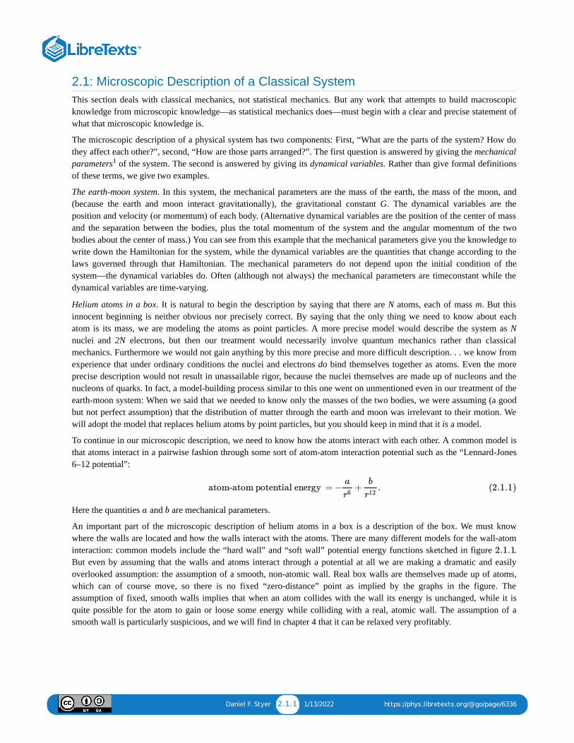
An important part of the microscopic description of helium atoms in a box is a description of the box. We must knowwhere the walls are located and how the walls interact with the atoms. There are many different models for the wall-atominteraction: common models include the “hard wall” and “soft wall” potential energy functions sketched in figure .But even by assuming that the walls and atoms interact through a potential at all we are making a dramatic and easilyoverlooked assumption: the assumption of a smooth, non-atomic wall. Real box walls are themselves made up of atoms,which can of course move, so there is no fixed “zero-distance” point as implied by the graphs in the figure. Theassumption of fixed, smooth walls implies that when an atom collides with the wall its energy is unchanged, while it isquite possible for the atom to gain or loose some energy while colliding with a real, atomic wall. The assumption of asmooth wall is particularly suspicious, and we will find in chapter 4 that it can be relaxed very profitably.

1

atom-atom potential energy = − + .a

r6

b

r12(2.1.1)

a b

2.1.1

Daniel F. Styer 2.1.2 1/13/2022 https://phys.libretexts.org/@go/page/6336

Figure

The final step is to recognize that there might be externally electric, magnetic, or gravitational fields that affect the system.If these external fields are present and relevant they will have to be added to the list of mechanical parameters.

At last we are ready to turn to the dynamical variables for the helium-atoms-in-a-box system. These are (mercifully) easyto describe: they are just the position and momentum of each particle, a total of 2N 3-dimensional vectors. A shorthandname for this information is “point in phase space”. Phase space is an abstract space with one coordinate corresponding toeach dynamical variable. Thus in our example the coordinates are the positions and momenta for particle number 1,number 2,. . . number 9,. . . and number N:

For a system of N particles, phase space is 6N-dimensional. A single point in phase space gives the position andmomentum of every particle in the system.

The mechanical parameters are sometimes called “parameters in the Hamiltonian”, or “external parameters”, or “fields”.

Time development of a classical systemGiven a microscopic description such as either of the two above, what can we do with it? The time development of thesystem is represented by the motion of a point in phase space. That point will snake through many points in the phasespace but all of the points visited will have the same energy. Because many points of the given energy will be visited, it isnatural to ask whether, in fact, all phase space points corresponding to a given energy will eventually be visited by asystem started at any one of those points.

It is easy to find systems for which this statement is false, but all such examples seem to be in one way or another atypical.For example, consider two or three or even many millions of non-interacting particles in a hard-walled box, and start themall traveling straight up and down. They will travel straight up and down forever. The points in phase space with identicalenergy, but with the particles traveling left and right, will never be visited. This example is atypical because if the particlesinteracted, even slightly, then they would fall out of the “straight up and down” regions of phase space.

Problems

2.1 (Q) Three-body interactions: microscopic

Make up a problem involving two charged point particles and a polarizable atom.

2.2 Mechanical parameters and dynamical variables

Here is a classical mechanics problem: “A pendulum bob of mass m swings at the end of a cord which runs through asmall hole in the ceiling. The cord is being pulled up through the hole so that its length is . At time t = 0the bob is at rest and at angle . Find the subsequent motion of the bob.” Do not solve this problem. Instead, list themechanical parameters and the dynamical variables that appear in it.

2.3 A Hamiltonian

Write down the total Hamiltonian of a neutral plasma of N protons and N electrons moving in a rectangular box withinterior dimensions of L × L × L , assuming that i) any proton or electron interacts with the wall material through apotential energy function

2.1.1

( , , , , , , , , , … , , , , , … , , , , , ) .x1 y1 z1 px,1 py,1 x2 y2 z2 pz,2 x9 y9 z9 px,9 py,9 xN yN zN px,N py,N pz,N (2.1.2)

1

2

ell(t) = −αtℓ0

θ0

x y z

W (d) = ( − )W0

1

d21a2

0

for d < a

otherwise (2.1.3)

Daniel F. Styer 2.1.3 1/13/2022 https://phys.libretexts.org/@go/page/6336

where d is the (perpendicular) distance of the particle in question from the wall, and ii) the system is subject to a uniformelectric field in the ˆx direction of magnitude E. List the mechanical parameters that appear in this Hamiltonian, anddistinguish them from the dynamical variables.

2.4 (Q) For discussion: Mechanical parameters, dynamical variables, and modeling

List the mechanical parameters and dynamical variables of these systems:

a. Hydrogen molecules enclosed in a sphere.

b. Water molecules in a box.

c. A mixture of hydrogen molecules and helium atoms in a box.

To what extent are you making models as you generate descriptions? To what extent are you making assumptions? (Forexample, by using non-relativistic classical mechanics.)

For the earth-moon model, all the points visited will also have the same total momentum and angular momentum, but thisis not the case for the helium-in-a-smooth-box model.

2

Daniel F. Styer 2.2.1 1/6/2022 https://phys.libretexts.org/@go/page/6337

2.2: Macroscopic Description of a Large Equilibrium SystemThe title of this section introduces two new terms. . . large and equilibrium. A system is large if it contains many particles,but just how large is “large enough”? A few decades ago, physicists dealt with systems of one or two or a dozen particles,or else they dealt with systems with about 10 particles, and the distinction was clear enough. Now that computer chipshave such small lines, systems of intermediate size are coming under investigation. (This field carries the romantic nameof “mesoscopic physics”.) In practical terms, it is usually easy enough to see when the term “large” applies, but there is norigorous criterion and there have been some surprises in this regard.

A similar situation holds for the term equilibrium. A system is said to be in equilibrium if its macroscopic properties arenot changing with time. Thus a cup of tea, recently stirred and with churning, swirling flow, is not at equilibrium, whereassome time later the same cup, sedate and calm, is at equilibrium. But some of the properties of the latter cup are changingwith time: for example, the height of water molecule number 173 changes rapidly. Of course this is not a macroscopicproperty, but then there is no rigorous definition of macroscopic vs. microscopic properties. Once again there is littledifficulty in practice, but a rigorous criterion is wanting and some excellent physicists have been fooled. (For example, amixture of hydrogen gas and oxygen gas can behave like a gas in equilibrium. But if a spark is introduced, these chemicalswill react to form water. The gas mixture is in equilibrium as far as its physical properties are concerned, but not as far asits chemical properties are concerned.)

With these warnings past, we move on to the macroscopic description. As with the microscopic description, it has twoparts: the first saying what the system is and the second saying what condition the system is in. For definiteness, weconsider the helium-in-a-smooth-box model already introduced.

To say what this system is, we again list mechanical parameters. At first these are the same as for the microscopicdescription: the number of particles , the mass of each particle , and a description of the atom-atom interactionpotential (e.g. the Lennard-Jones parameters and ). But we usually don’t need to specify the atom-wall interaction oreven the location of the walls. . . instead we specify only the volume of the container . The reason for this is not hard tosee. If we deal with a large system with typical wall-atom interactions (short range) and typical walls (without intricateprojections and recesses) then very few particles will be interacting with the walls at any one instant, so we expect that thedetails of wall-atom interaction and container shape will be affect only a tiny minority of atoms and hence be irrelevant tomacroscopic properties. There are of course exceptions: for example, in a layered substance such as graphite or mica, orone of the high-temperature superconductors, the shape of the container might well be relevant. But in this book we willnot often deal with such materials.

Finally, what condition is the system in? (In other words, what corresponds to the dynamical variables in a microscopicdescription?) Clearly the “point in phase space”, giving the positions and momenta of each and every particle in thesystem, is far too precise to be an acceptable macroscopic description. But at the same time it is not acceptable to say wedon’t care anything about microscopic quantities, because the energy of this system is conserved, so energy will be afeature of both the microscopic and macroscopic descriptions. In fact, for the helium-in-a-smooth-box model, energy is theonly quantity that is conserved, so it is the only item in the list of macroscopic descriptors. (Other systems, such as theearth-moon system, will have additional conserved quantities, and hence additional items in that list.)

What equilibrium is not

There’s a common misconception that at equilibrium, the sample is uniform. This might not be true: A mixture of ice andwater at atmospheric pressure and temperature 0 C is at equilibrium but is not uniform. Or, consider a container of air 50kilometers tall with its base on Earth at sea level: most of the molecules huddle at the bottom of the container, and the topis near-vacuum.

2.5 (Q) Three-body interactions: macroscopic

Even though three-body interactions do exist, they can usually be ignored in a macroscopic description. (Just as the wall-atom interaction does exist, but it can usually be ignored in a macroscopic description.) Why?

2.6 (Q,E) Lost in space

23

N m

a b

V

3

Daniel F. Styer 2.2.2 1/6/2022 https://phys.libretexts.org/@go/page/6337

A collection of N asteroids floats in space far from other gravitating bodies. Model each asteroid as a hard sphere of radiusR and mass m. What quantities are required for a microscopic description of this system? For a macroscopic description?

The momentum and angular momentum of the helium atoms is not conserved, because there are external forces due to thebox.

3

Daniel F. Styer 2.3.1 1/27/2022 https://phys.libretexts.org/@go/page/6338

2.3: Fundamental AssumptionDefine microstate and macrostate.

There are many microstates corresponding to any given macrostate. The collection of all such microstates is called an“ensemble”. (Just as a musical ensemble is a collection of performers.)

Note: An ensemble is a (conceptual) collection of macroscopic systems. It is not the collection of atoms that makes up amacroscopic system.

(Terminology: A microstate is also called a “configuration” or a “complexion”. . . both poor terms. A macrostate is alsocalled a “thermodynamic state”. A “corresponding” microstate is sometimes called an “accessible” or a “consistent”microstate.)

A system is said to be “isolated” if no energy goes in or out, and if the mechanical parameters ( , , etc.) are also fixed.Most of the systems you deal with in classical mechanics classes, for example, are isolated.

The fundamental assumption of statistical mechanics is:

An isolated system in an equilibrium macrostate has equal probability of being in any of the microstates corresponding tothat macrostate.

Conceptual difficulties:

1. What is equilibrium?2. What is probability? (Any experiment is done on one system.)3. May be false! (Can be motivated by the ergodic hypothesis, but this is just suggestive, and the ergodic hypothesis itself

has not been proven and may be false. Cellular automata may violate this assumption. . . but do physical/biologicalsystems? See for example Andrew I. Adamatzky, Identification of Cellular Automata (Taylor and Francis, 1995) andthe essay review by Normand Mousseau, in Contemporary Physics, 37 (1996) 321–323; Stephen Wolfram, A New Kindof Science (Wolfram Media, 2002).)

Practical difficulties.

1. Gives way to find average values of microscopic quantities, such as

but not things like temperature and pressure.

2. Based on model. (In particular, infinitely hard smooth walls.)

3. For point particle model, requires infinitely thin sheet in phase space. Work instead with the volume of phase spacecorresponding to energies from to , and at the end of the calculation take the limit .

To examine these practical difficulties in more detail, consider again the helium-in-a-smooth-box model. Suppose we wantto find the number of microstates with energy ranging from to , in a system with identical particles in a boxof volume .

Your first answer might be that there are an infinite number of points in phase space satisfying this criterion. This is truebut it misses the point: A thimble and a Mack truck both contain an infinite number of points, but the Mack truck carriesmore because it has more volume. Clearly the microstate count we desire is some sort of measure of phase-space volume.I’ll call the region of phase space with energy ranging from to by the name , and call its volume

However, this volume isn’t precisely what we want. Permutation argument for N identical particles. (For a system with Nidentical particles, there are N! points in phase space corresponding to the same microstate.) A better measure of themicrostate count is thus

N V

⟨kinetic energy⟩, ⟨potential energy⟩, ⟨height⟩,

E E+ΔE ΔE → 0

E E+ΔE N

V

E E+ΔE σ(E, ΔE)

dΓ. ( Volume in phase space. )∫σ(E,ΔE)

(2.3.1)

dΓ. (Delabeled volume in phase space.) 1

N !∫σ(E,ΔE)

(2.3.2)

Daniel F. Styer 2.3.2 1/27/2022 https://phys.libretexts.org/@go/page/6338

There remains one more problem. We desire a count, which is dimensionless, and the above expression gives a phase-space volume, which has the dimensions of

The solution to this problem is straightforward if clunky. Pick a quantity with the dimensions of angular momentum. Anyquantity will do, so make an arbitrary choice. Call the quantity . (Clearly, by the time we produce a measurable physicalresult at the end of a calculation, it had better be independent of our choice of , just as the value of any measurable resultin a classical mechanics problem has to be independent of choice of the potential energy zero.) Then define the microstatecount as the dimensionless quantity

In poker, there are 52 cards in a deck, so the probability of drawing any given card from a shuffled deck is 1/52. Thenumber 52 plays a fundamental role in answering any question concerning probability in poker.

In statistical mechanics, there are microstates corresponding to a macrostate, so the probability of encountering anygiven microstate is (if the fundamental assumption is correct) . The number plays the same fundamental role instatistical mechanics that 52 does in poker.

2.7 Microstate count for a mixtureWhat expression corresponds to for a collection of Helium atoms and Argon atoms?

(angular momentum .)3N

h0

h0

Ω(E, ΔE,V ,N) = dΓ. (Dimensionless, delabeled volume in phase space. )1

h3N0

1

N !∫σ(E,ΔE)

(2.3.3)

Ω

1/Ω Ω

2.3.3 NHe NAr

Daniel F. Styer 2.4.1 1/27/2022 https://phys.libretexts.org/@go/page/6339

2.4: Statistical Definition of Entropy

You cannot take the logarithm of a number with dimensions. Perhaps you have heard this rule phrased as “you can’ttake the logarithm of 3.5 meters” or “you can’t take the logarithm of five oranges”. Why not? A simple argument is“Well, what would be the units of ?” A more elaborate argument follows. The logarithm function is theinverse of the exponential function:

But remember that

If had the dimensions of length, then the expression above would be a meaningless sum of 1 plus a length plus anarea plus a volume plus so forth.

You cannot exponentiate a number with dimensions, and you cannot take the logarithm of a number with dimensions.

Additivity (see problem 2.10) . . . don’t physically mix.

The constant k in this definition is called the “Boltzmann constant”. It is clear from the argument that the Boltzmannconstant could have been chosen to have any value: 1, , whatever. For historical reasons, it was chosen to have the value

There is no particular physical significance to this number: its logical role is analogous to 2.54 cm/inch or 4.186joule/calorie. In other words, the origin of this number is not to be sought in nature, but in the history of the definition ofthe joule and the kelvin. It is a conversion factor.

Problems

2.8 (E) Accessible regions of phase space

Suppose that N non-interacting particles, each of mass , move freely in a one-dimensional box (i.e. an infinite squarewell). Denote the position coordinates by and the momentum coordinates by . The boxrestricts all the positions to fall between and . The energy of the system lies between and .

a. If only one particle is present, draw the system’s phase space and shade the regions of phase space that areaccessible.

b. If two particles are present then phase space is four dimensional, which makes it difficult to draw. Draw separatelythe part of phase space involving positions and the part involving momenta. Shade the accessible regions of phasespace.

c. Suppose two particles are present, and consider the slice of phase space for which and equalssome constant called . Draw a (carefully labeled) sketch of this slice with the accessible regions shaded.

d. Describe the accessible regions of phase space if particles are present.

2.9 Accessible configurations of a spin system

Consider an isolated system of spin- atoms in a magnetic field . The atoms are fixed at their lattice sites and thespins do not interact. Each atom has a magnetic moment m that can point either “up” (parallel to the field ) or “down”(antiparallel to ). A microstate (or configuration) of this system is specified by giving the direction of every spin. An upspin has energy , a down spin has energy , so a configuration with up spins and down spins has energy

This system is called the “ideal paramagnet”.

Logarithms and dimensions

ln(3.5meters)

y = ln(x) means the same as x = .ey

x = = 1 +y + + +⋯ .ey 12!

y2 13!

y3

y

S(E, ΔE, V , N) = lnΩ(E, ΔE, V , N)kB (2.4.1)

Bπ

= 1.38 × joule / kelvin. kB 10−23 (2.4.2)

m

, , . . . ,x1 x2 xN , , . . . ,p1 p2 pN

= 0xi = Lxi E E +ΔE

= (2/3)Lx1 p2

p2

N

N 12

H

H

H

−mH +mH n↑ n↓

E = −( − ) mH.n↑ n↓ (2.4.3)

Daniel F. Styer 2.4.2 1/27/2022 https://phys.libretexts.org/@go/page/6339

a. Not every energy is possible for this model. What is the maximum possible energy? The minimum? What is theminimum possible non-zero energy difference between configurations?

b. Suppose we know that the system has up spins and down spins, but we do not know how these spins arearranged. How many microstates are consistent with this knowledge?

c. The variables and cannot be determined directly from macroscopic measurements. Find expressions for and in terms of , , and . (Hand a paramagnet sample to an experimentalist and ask her to find the numberof up spins. She will just look at you quizzically. But ask her to find the number, the energy, and the magnetic fieldand she’ll be happy to.)

d. Consider the energy range from to where is small compared to but large compared to . What is the approximate number of states lying in this energy range? Express your answer

in a form that does not include the quantities or .

2.10 Microstates for a combined system

System #1 is in a macrostate with three corresponding microstates, labeled , , and . System #2 is in a macrostate withfour corresponding microstates, labeled α, β, γ, and δ. How many microstates are accessible to the combined systemconsisting of system #1 and system #2? List all such microstates.

2.11 (E) The logarithm

Suppose that a differentiable function satisfies

for all positive x and y. Show that

[Clues: 1) Take derivative with respect to , then set ) Set in Equation .]

n↑ n↓

n↑ n↓ n↑

n↓ N E H

E E +ΔE ΔE NmH

mH Ω(E, ΔE, H, N)

n↑ n↓

A B C

f(xy) = f(x) +f(y) (2.4.4)

f(x) = k ln(x). (2.4.5)

x x = 1.2 y = 1 2.4.4

Daniel F. Styer 2.5.1 12/30/2021 https://phys.libretexts.org/@go/page/6340

2.5: Entropy of a Monatomic Ideal GasSo far in this chapter, we have been dealing very abstractly with a very general class of physical systems. We have made anumber of assumptions that are reasonable but that we have not tested in practice. It is time to put some flesh on theseformal bones. We do so by using our statistical definition of entropy to calculate the entropy of a monatomic ideal gas.(Here “monatomic” means that we approximate the atoms by point particles, and “ideal” means that those particles do notinteract with each other. In addition, we assume that the gas contains only one chemical species and that classicalmechanics provides an adequate description. Thus a more precise name for our system would be the “pure classicalmonatomic idea gas”, but in this case we wisely prefer brevity to precision.) Working with this concrete example will showus that what we have said is sensible (at least for this system), and guide us in further general developments.

The previous pages have been remarkably free of equations for a physics book. Now is the time to remedy that situation.Before studying this section, you need to know that the volume of a -dimensional sphere is

If you don’t already know this, then read appendix D, “Volume of a Sphere in Dimensions”, before reading this section.And if you don’t know the meaning of , where is a half-integer, then you should read appendix C, “Clinic on theGamma Function”, before reading appendix D. Finally, if you don’t know Stirling’s approximation for the factorialfunction, namely

then you should also read appendix E, “Stirling’s Approximation”, before reading further. (Do not be discouraged by thislong list of prerequisites. This mathematical material is quite interesting in its own right and will be valuable throughoutthis book.)

We consider a system of identical, classical, non-interacting point particles, each of mass . The kinetic energy of thissystem is

and the potential energy is

(One sometimes hears that the ideal gas has “no potential energy”. It is true that there is no potential energy due to atom-atom interaction, but, as the above expression makes clear, there is indeed a potential energy term due to atom-wallinteraction. Because of the character we assume for that term, however, the numerical value of the potential energy isalways zero. Note also that the ideal gas is not the same as the “hard-sphere gas”. In the hard-sphere model two atoms haveinfinite potential energy if they are separated by a distance of twice the hard-sphere radius or less. In the ideal gas modeltwo atoms do not interact. It is permissible even for two atoms to occupy the same location. . . only in the model, ofcourse!)

Now that the system is completely specified, it is time to begin the problem. We wish to calculate the entropy

where the function represents the volume in phase space corresponding to energies from to (i.e. the volumeof the region ). Before jumping into this (or any other) problem, it is a good idea to list a few properties that weexpect the solution will have. . . this list might guide us in performing the calculation; it will certainly allow us to check theanswer against the list to see if either our mathematics or our expectations need revision. We expect that:

We will be able to take the limit as and get sensible results.The entropy will depend on only the volume of the container and not on its shape.

d

(r) =Vdπd/2

(d/2)!rd (2.5.1)

d

x! x

lnn! ≈ n lnn−n for n ≫ 1, (2.5.2)

N m

( + +⋯ + )1

2mp2

1 p22 p2

N (2.5.3)

0

∞

if all particles are inside container

otherwise. (2.5.4)

S(E, ΔE,V ,N) = ln ,kBW (E, ΔE,V ,N)

N !h3N0

(2.5.5)

W E E+ΔE

σ(E, ΔE)

ΔE → 0S

Daniel F. Styer 2.5.2 12/30/2021 https://phys.libretexts.org/@go/page/6340

If we double the size of the system, by doubling and , then we will double . (Additivity.) will depend on in a trivial, “sea-level” fashion.

The formal expression for the volume of the accessible region of phase space is

The complexity of this integral rests entirely in the complexity of the shape of rather than in the complexity ofthe integrand, which is just 1. Fortunately the integral factorizes easily into a position part and a momentum part, and theposition part factorizes into a product of integrals for each particle (see problem 2.8). For, say, particle number 5, if theparticle is inside the container it contributes 0 to the energy, so the total energy might fall between and (depending on other factors). But if it is outside the container, then it contributes to the energy, which always exceedsthe limit . Thus the integral is just the volume of the container:

This integral depends on the volume but is independent of the shape of the container. We will soon see that, as aconsequence, the entropy depends on volume but not shape (which is in accord with our expectations).

The integrals over momentum space do not factorize, so we must consider the entire -dimensional momentum spacerather than separate 3-dimensional spaces. We know that the total potential energy is zero (unless it is infinite), so theenergy restriction is taken up entirely by the kinetic energy. Equation tells us that the momentum space points withenergy E fall on the surface of a sphere of radius . Thus the accessible region in momentum space is a shell withinner radius and with outer radius . (Notice that we are counting all the microstates within theaccessible region of phase space, not just “typical” microstates there. For example, one microstate to be counted has all ofthe particles at rest, except for one particle that has all the energy of the system and is heading due west. This is to becounted just as seriously as is the microstate in which the energy is divided up with precise equality among the severalparticles, and they are traveling in diverse specified directions. Indeed, the system has exactly the same probability ofbeing in either of these two microstates.) Using Equation for the volume of a -dimensional sphere, the volume ofthat shell is

I prefer to write this result in a form with all the dimensionfull quantities lumped together, namely as

The quantity in square brackets is dimensionless. To find the accessible volume of the entire phase space, we multiply theabove result by , the result of performing separate position integrals. Thus

As promised, W depends upon the variables E, ∆E, V, and N. It also depends upon the “unmentioned” mechanicalparameter m. The arguments on page 15 have been vindicated. . . the phase space volume W depends only upon V and notupon the detailed shape of the container. At last we can find the entropy! It is

E,V , N S

S h0

W (E, ΔE,V ,N) = accessible volume in phase space (2.5.6)

.

= dΓ∫σ(E,ΔE)

= ∫ d ∫ d ∫ d ⋯ ∫ d ∫ d ∫ d ⋯x1 y1 z1 xN yN zN

∫ d ∫ d ∫ d … ∫ d ∫ d ∫ dpx,1 py,1 pz,1 pz,N py,N pz,N

(2.5.7)

σ(E, ΔE)

E E+ΔE

∞E+ΔE

∫ d ∫ d ∫ d = V .x5 y5 z5 (2.5.8)

V

3NN

2.5.32mE− −−−

√

2mE− −−−

√ 2m(E+ΔE)− −−−−−−−−−−

√

2.5.1 3N

[(2m(E+ΔE) −(2mE ] .π3N/2

(3N/2)!)3N/2 )3N/2 (2.5.9)

(2mE [ −1] .π3N/2

(3N/2)!)3N/2 (1 + )

ΔE

E

3N/2

(2.5.10)

V N N

W (E, ΔE,V ,N) = [ −1] .(2πmE )V 2/3 3N/2

(3N/2)!(1 + )

ΔE

E

3N/2

(2.5.11)

S = ln = ln [ −1]kBW

N !h3N0

kB

⎧

⎩⎨( )

2πmEV 2/3

h20

3N/21

N !(3N/2)!(1 + )

ΔE

E

3N/2 ⎫

⎭⎬ (2.5.12)

Daniel F. Styer 2.5.3 12/30/2021 https://phys.libretexts.org/@go/page/6340

or

How does this expression compare to our list of expectations on page 22?

If we take the limit , the entropy approaches , contrary to expectations.The entropy depends on the volume of the container but not on its shape, in accord with expectations.If we double , and , then will not exactly double, contrary to expectations.The entropy does depend on in a “sea-level” fashion, in accord with expectations.

Only two of our four expectations have been satisfied. (And it was obvious even from Equation that the fourthexpectation would be correct.) How could we have gone so far wrong?

The trouble with expression for the entropy of a monatomic ideal gas is that it attempts to hold for systems of anysize. In justifying the definition of entropy (2.7) (and in writing the list of expectations on page 22) we relied upon theassumption of a “large” system, but in deriving expression we never made use of that assumption. On the strengthof this revised analysis we realize that our expectations will hold only approximately for finite systems: they will hold tohigher and higher accuracy for larger and larger systems, but they will hold exactly only for infinite systems.

There is, of course, a real problem in examining an infinite system. The number of particles is infinite, as is the volume,the energy, and of course the entropy too. Why do we need an equation for the entropy when we already know that it’sinfinite? Once the problem is stated, the solution is clear: We need an expression not for the total entropy , but for theentropy per particle . More formally, we want to examine the system in the “thermodynamic limit”, in which

In this limit we expect that the entropy will grow linearly with system size, i.e. that

The quantities written in lower case, such as e, the energy per particle, and , the volume per particle, play the same role instatistical mechanics as “per capita” quantities do in demographics. (The gross national product of the United States ismuch larger than the gross national product of Kuwait, but that is just because the United States is much larger thanKuwait. The GNP per capita is higher in Kuwait than in the United States.)

Let’s take the thermodynamic limit of expression (the entropy of a finite system) to find the entropy per particle ofan infinite monatomic ideal gas. The first thing to do, in preparing to take the thermodynamic limit, is to write as as , and as so that the only size-dependent variable is . This results in

Next we use Stirling’s approximation,

to simplify the expressions like \(\ln( \frac32N)!\) above. Thus for large values of we have approximately (anapproximation that becomes exact as )

The first term on the right increases linearly with . The next bunch of terms is

= N ln( )−lnN ! − ln( N)! + ln[ −1].S

kB

3

2

2πmEV 2/3

h20

3

2(1 + )

ΔE

E

3N/2

(2.5.13)

ΔE → 0 −∞S

E,V N S

S h0

2.5.5

2.5.13

2.5.13

S

s = S/N

N → ∞ in such a way that → e, → v, and → δe.E

N

V

N

ΔE

N(2.5.14)

S(E, ΔE,V ,N) → Ns(e, v, δe). (2.5.15)

v

2.5.13V vN ,E

eN ΔE δeN N

= N ln( )−lnN ! − ln( N)! + ln[ −1].S

kB

3

2

2πmev2/3N 5/3

h20

3

2(1 + )

δe

e

3N/2

(2.5.16)

lnn! ≈ n lnn−n for n ≫ 1, (2.5.17)

N

N → ∞

.

S

kB≈ N ln( )−N lnN +N −( N) ln( N)+ N +ln[ −1]

3

2

2πmev2/3N 5/3

h20

3

2

3

2

3

2(1 + )

δe

e

3N/2

= N ln( )+ N ln −N lnN +N − N ln( N)+ N +ln[ −1]3

2

2πmev2/3

h20

3

2N 5/3 3

2

3

2

3

2(1 + )

δe

e

3N/2

N

Daniel F. Styer 2.5.4 12/30/2021 https://phys.libretexts.org/@go/page/6340

which again increases linearly with . The final term is, as grows

This term not only increases linearly with in the thermodynamic limit, it also vanishes as (This is a generalprinciple: One must first take the thermodynamic limit , and only then take the “thin phase space limit”

.)

Our expectation that in the thermodynamic limit the entropy would be proportional to the system size has beenfully vindicated. So has the expectation that we could let , although we have seen that we must do so carefully.The end result is that the entropy per particle of the pure classical monatomic ideal gas is

This is called the “Sackur-Tetrode formula”. It is often written as

with the understanding that it should be applied only to very large systems, i.e. to systems effectively at thethermodynamic limit.

Problems2.12 Entropy of a spin system

Consider again the ideal paramagnet of problem 2.9.

a. Write down an expression for as a function of . Simplify it using Stirling’s approximation forlarge values of . (Clue: Be careful to never take the logarithm of a number with dimensions.)

b. Find an expression for the entropy per spin as a function of the energy per spin e and magnetic field in thethermodynamic limit.

c. Sketch the resulting entropy as a function of the dimensionless quantity . Does it take on the proper limits as ? (In your sketch pay special attention to endpoints of the domain, and to any places where the function or its

derivative suffers a discontinuity, or a kink, or goes to zero or infinity. In general, it is important that the sketch convey acorrect impression of the qualitative character of the function, and less important that it be quantitatively accurate.)

2.13 The approach to the thermodynamic limit

For the classical monatomic ideal gas, plot entropy as a function of particle number using both the “finite size” form and the Sackur-Tetrode form . We will see in problem 4.11 that for a gas at room temperature and

atmospheric pressure, it is appropriate to use

.=

=

N ln −N lnN +N − N ln( N)+ N3

2N 5/3 3

2

3

2

3

2

N lnN −N lnN +N − N ln( )− N ln(N) + N5

2

3

2

3

2

3

2

3

2

N [ − ln( )]5

2

3

2

3

2

N N

ln[ −1] ≈ ln(1 + )δe

e

3N/2

(1 + )δe

e

3N/2

(2.5.18)

= N ln(1 + ).3

2

δe

e(2.5.19)

N δe → 0!N → ∞

δe ≡ ΔE/N → 0

2.5.15 N

ΔE → 0

s(e, v) = [ ln( )+ ] .kB3

2

4πmev2/3

3h20

5

2(2.5.20)

4

S(E,V ,N) = N [ ln( )+ ] ,kB3

2

4πmEV 2/3

3h20N

5/3

5

2(2.5.21)

lnΩ(E, ΔE,H,N) E

N

s(e,H) H

u ≡ e/mH

e → ±mH

2.5.13 2.5.21

E / = (1.66 × ) .V 2/3 h20 1029kg−1 N 5/3 (2.5.22)

Daniel F. Styer 2.5.5 12/30/2021 https://phys.libretexts.org/@go/page/6340

Use the masses of argon and krypton. All other things being equal, is the thermodynamic limit approached more rapidlyfor atoms of high mass or for atoms of low mass?

2.14 Other energy conventions

In the text we found the entropy of a monatomic ideal gas by assuming that the potential energy of an atom was zero if theatom were inside the box and infinite if it were outside the box. What happens if we choose a different conventional zeroof potential energy so that the potential energy is U for an atom inside the box and infinite for an atom outside the box?

2.15 Other worlds

Find the entropy as a function of , and in the thermodynamic limit for a monatomic ideal gas in a world witharbitrary5 spatial dimensionality .

2.16 Ideal gas mixtures

Consider a large sample of classical monatomic ideal gas that is a mixture of two components: particles of mass and particles of mass . If , show that the entropy is

Otto Sackur (1880–1914) was a German physical chemist. Hugo Tetrode (1895–1931) was a Dutch theoretical physicist.Each independently uncovered this equation in 1912.

Why, you wonder, should anyone care about a world that is not three-dimensional? For three reasons: (1) There areimportant physical approximations of two-dimensional worlds (namely surfaces) and of one-dimensional worlds (namelypolymers). (2) The more general formulation might help you in unexpected ways. For example, Ken Wilson and MichaelFisher were trying to understand an important problem concerning critical points. They found that their technique couldnot solve the problem in three dimensions, but it could solve the problem in four dimensions. Then they figured out how touse perturbation theory to slide carefully from four dimensions to three dimensions, thus making their solution relevant toreal physical problems. Wilson was awarded the Nobel Prize for this work. This illustrates the third reason, namely younever can tell what will be important and hence: (3) Knowledge is better than ignorance.

(Clue: Use the result of problem D.2.)

E,V N

d

NA mA

NB mB N ≡ +NA NB

S (E,V , , ) = + [ ln( )+ ]NA NB kBNA

3

2

4π EmA V 2/3

3h20N

5/3

5

2(2.5.23)

4

5

+ [ ln( )+ ]kBNB32

4π EmB V 2/3

3h20N

5/3

52

− N [( ) ln( )+( ) ln( )]kBNA

N

NA

N

NB

N

NB

N

(2.5.24)

Daniel F. Styer 2.6.1 11/11/2021 https://phys.libretexts.org/@go/page/6341

2.6: Qualitative Features of EntropyThe concept of entropy is notoriously difficult to grasp. Even the consummate mathematician and physicist Johnny vonNeumann claimed that “nobody really knows what entropy is anyway.” Although we have an exact and remarkably simpleformula for the entropy of a macrostate in terms of the number of corresponding microstates, this simplicity merely hidesthe subtle characterization needed for a real understanding of the entropy concept. To gain that understanding, we mustexamine the truly wonderful (in the original meaning of that overused word) surprises that this simple formula presentswhen applied to real physical systems.

Surprises

The monatomic ideal gas

Let us examine the Sackur-Tetrode formula (2.32) qualitatively to see whether it agrees with our understanding of entropyas proportional to the number of microstates corresponding to a given macrostate. If the volume is increased, then theformula states that the entropy increases, which certainly seems reasonable: If the volume goes up, then each particle hasmore places where it can be, so the entropy ought to increase. If the energy is increased, then increases, which againseems reasonable: If there is more energy around, then there will be more different ways to split it up and share it amongthe particles, so we expect the entropy to increase. (Just as there are many more ways to distribute a large booty among acertain number of pirates than there are to distribute a small booty.) But what if the mass m of each particle increases?(Experimentally, one could compare the entropy of, say, argon and krypton under identical conditions. See problem 2.27.)Our formula shows that entropy increases with mass, but is there any way to understand this qualitatively?

In fact, I can produce not just one but two qualitative arguments concerning the dependence of on . Unfortunately thetwo arguments give opposite results! The first relies upon the fact that

so for a given energy , any individual particle may have a momentum ranging from 0 to . A larger mass implies awider range of possible momenta, which suggests more microstates and a greater entropy. The second argument reliesupon the fact that

so for a given energy , any individual particle may have a speed ranging from 0 to . A larger mass implies anarrowed range of possible speeds, which suggests fewer microstates and a smaller entropy. The moral is simple:Qualitative arguments can backfire!

That’s the moral of the paradox. The resolution of the paradox is both deeper and more subtle: It hinges on the fact that theproper home of statistical mechanics is phase space, not configuration space, because Liouville’s theorem impliesconservation of volume in phase space, not in configuration space. This issue deeply worried the founders of statisticalmechanics. See Ludwig Boltzmann, Vorlesungen über Gastheorie (J.A. Barth, Leipzig, 1896–98), part II, chapters III andVII [translated into English by Stephen G. Brush: Lectures on Gas Theory (University of California Press, Berkeley,1964)]; J. Willard Gibbs, Elementary Principles in Statistical Mechanics (C. Scribner’s Sons, New York, 1902), page 3;and Richard C. Tolman, The Principles of Statistical Mechanics (Oxford University Press, Oxford, U.K., 1938), pages 45,51–52.

Freezing water

It is common to hear entropy associated with “disorder,” “smoothness,” or “homogeneity.” How do these associationsstand up to the simple situation of a bowl of liquid water placed into a freezer? Initially the water is smooth andhomogeneous. As its temperature falls, the sample remains homogeneous until the freezing point is reached. At thefreezing temperature the sample is an inhomogeneous mixture of ice and liquid water until all the liquid freezes. Then thesample is homogeneous again as the temperature continues to fall. Thus the sample has passed from homogeneous to

V

S

E S

S m

E = ,1

2m∑

i

p2i (2.6.1)

E 2mE− −−−

√

E = ,m

2∑

i

v2i (2.6.2)

E E/m− −−−

√

Daniel F. Styer 2.6.2 11/11/2021 https://phys.libretexts.org/@go/page/6341

inhomogeneous to homogeneous, yet all the while its entropy has decreased. (We will see later that the entropy of a samplealways decreases as its temperature falls.)

Suppose the ice is then cracked out of its bowl to make slivers, which are placed back into the bowl and allowed to rest atroom temperature until they melt. The jumble of irregular ice slivers certainly seems disordered relative to thehomogeneous bowl of meltwater, yet it is the ice slivers that have the lower entropy. The moral here is that the hugenumber of microscopic degrees of freedom in the meltwater completely overshadow the minute number of macroscopicdegrees of freedom in the jumbled ice slivers. But the analogies of entropy to “disorder” or “smoothness” invite us toignore this moral and concentrate on the system’s gross appearance and nearly irrelevant macroscopic features.

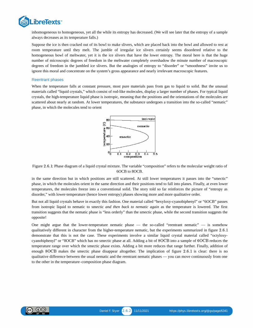
Reentrant phases

When the temperature falls at constant pressure, most pure materials pass from gas to liquid to solid. But the unusualmaterials called “liquid crystals,” which consist of rod-like molecules, display a larger number of phases. For typical liquidcrystals, the high-temperature liquid phase is isotropic, meaning that the positions and the orientations of the molecules arescattered about nearly at random. At lower temperatures, the substance undergoes a transition into the so-called “nematic”phase, in which the molecules tend to orient

Figure : Phase diagram of a liquid crystal mixture. The variable “composition” refers to the molecular weight ratio of6OCB to 8OCB.

in the same direction but in which positions are still scattered. At still lower temperatures it passes into the “smectic”phase, in which the molecules orient in the same direction and their positions tend to fall into planes. Finally, at even lowertemperatures, the molecules freeze into a conventional solid. The story told so far reinforces the picture of “entropy asdisorder,” with lower-temperature (hence lower entropy) phases showing more and more qualitative order.

But not all liquid crystals behave in exactly this fashion. One material called “hexyloxy-cyanobiphenyl” or “6OCB” passesfrom isotropic liquid to nematic to smectic and then back to nematic again as the temperature is lowered. The firsttransition suggests that the nematic phase is “less orderly” than the smectic phase, while the second transition suggests theopposite!

One might argue that the lower-temperature nematic phase — the so-called “reentrant nematic” — is somehowqualitatively different in character from the higher-temperature nematic, but the experiments summarized in figure demonstrate that this is not the case. These experiments involve a similar liquid crystal material called “octyloxy-cyanobiphenyl” or “8OCB” which has no smectic phase at all. Adding a bit of into a sample of reduces thetemperature range over which the smectic phase exists. Adding a bit more reduces that range further. Finally, addition ofenough makes the smectic phase disappear altogether. The implication of figure is clear: there is noqualitative difference between the usual nematic and the reentrant nematic phases — you can move continuously from oneto the other in the temperature–composition phase diagram.

2.6.1

2.6.1

8OCB 6OCB

8OCB 2.6.1

Daniel F. Styer 2.6.3 11/11/2021 https://phys.libretexts.org/@go/page/6341

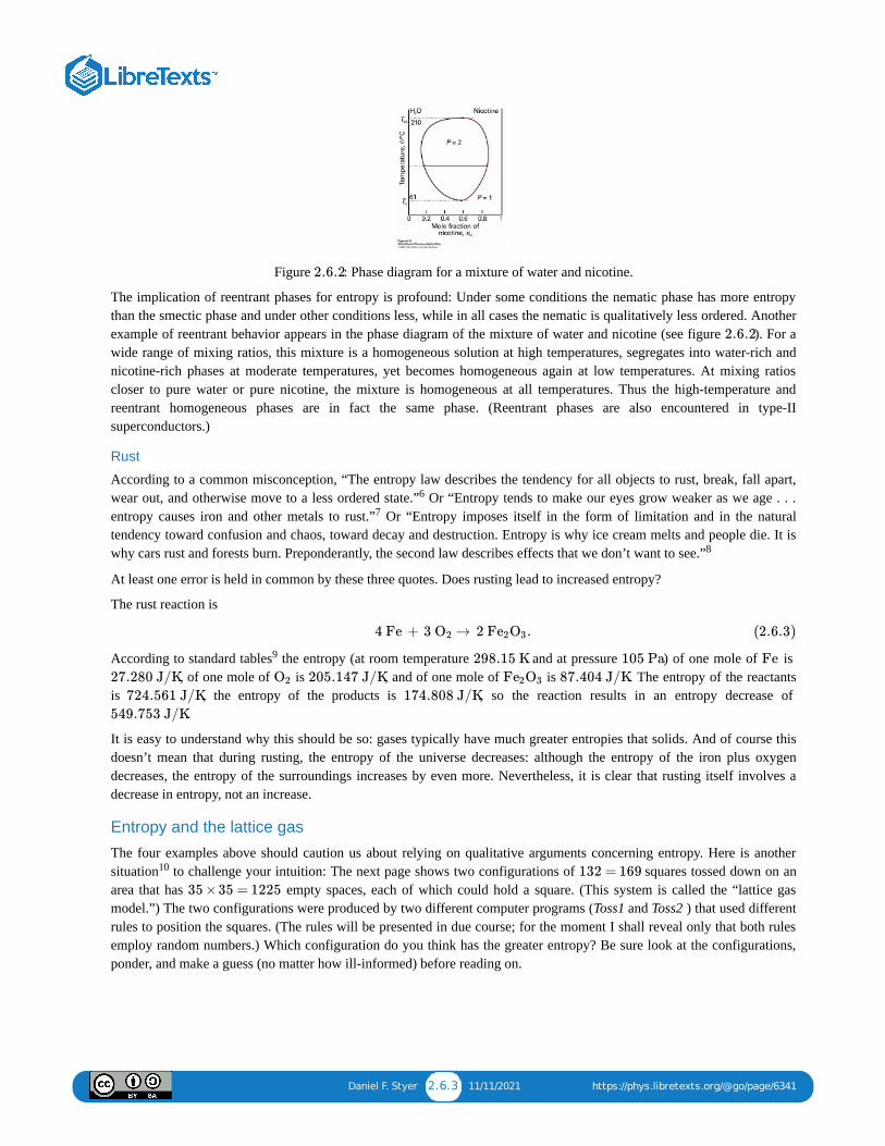
Figure : Phase diagram for a mixture of water and nicotine.

The implication of reentrant phases for entropy is profound: Under some conditions the nematic phase has more entropythan the smectic phase and under other conditions less, while in all cases the nematic is qualitatively less ordered. Anotherexample of reentrant behavior appears in the phase diagram of the mixture of water and nicotine (see figure ). For awide range of mixing ratios, this mixture is a homogeneous solution at high temperatures, segregates into water-rich andnicotine-rich phases at moderate temperatures, yet becomes homogeneous again at low temperatures. At mixing ratioscloser to pure water or pure nicotine, the mixture is homogeneous at all temperatures. Thus the high-temperature andreentrant homogeneous phases are in fact the same phase. (Reentrant phases are also encountered in type-IIsuperconductors.)

Rust

According to a common misconception, “The entropy law describes the tendency for all objects to rust, break, fall apart,wear out, and otherwise move to a less ordered state.” Or “Entropy tends to make our eyes grow weaker as we age . . .entropy causes iron and other metals to rust.” Or “Entropy imposes itself in the form of limitation and in the naturaltendency toward confusion and chaos, toward decay and destruction. Entropy is why ice cream melts and people die. It iswhy cars rust and forests burn. Preponderantly, the second law describes effects that we don’t want to see.”

At least one error is held in common by these three quotes. Does rusting lead to increased entropy?

The rust reaction is

According to standard tables the entropy (at room temperature and at pressure ) of one mole of is , of one mole of is , and of one mole of is . The entropy of the reactants

is , the entropy of the products is , so the reaction results in an entropy decrease of .

It is easy to understand why this should be so: gases typically have much greater entropies that solids. And of course thisdoesn’t mean that during rusting, the entropy of the universe decreases: although the entropy of the iron plus oxygendecreases, the entropy of the surroundings increases by even more. Nevertheless, it is clear that rusting itself involves adecrease in entropy, not an increase.

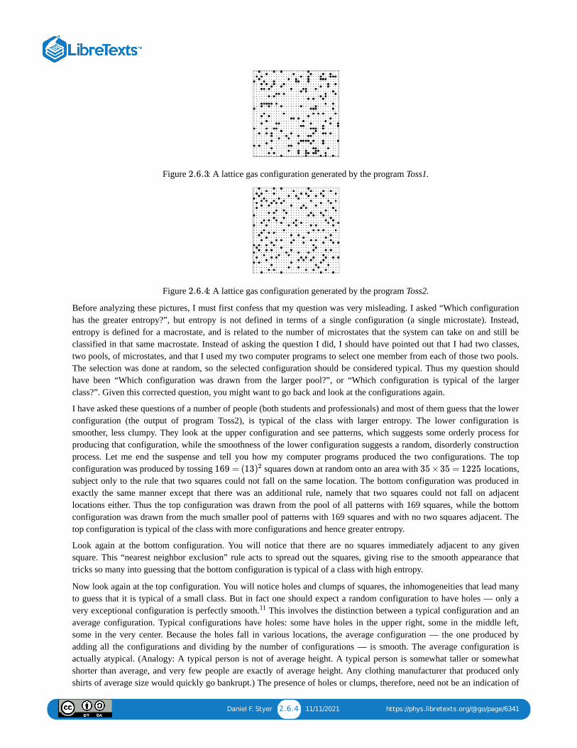
Entropy and the lattice gas

The four examples above should caution us about relying on qualitative arguments concerning entropy. Here is anothersituation to challenge your intuition: The next page shows two configurations of squares tossed down on anarea that has empty spaces, each of which could hold a square. (This system is called the “lattice gasmodel.”) The two configurations were produced by two different computer programs (Toss1 and Toss2 ) that used differentrules to position the squares. (The rules will be presented in due course; for the moment I shall reveal only that both rulesemploy random numbers.) Which configuration do you think has the greater entropy? Be sure look at the configurations,ponder, and make a guess (no matter how ill-informed) before reading on.

2.6.2

2.6.2

6

7

8

4 Fe + → . 3 O2 2 Fe2O3 (2.6.3)

9 298.15 K 105 Pa Fe27.280 J/K O2 205.147 J/K Fe2O3 87.404 J/K

724.561 J/K 174.808 J/K549.753 J/K

10 132 = 16935 ×35 = 1225

Daniel F. Styer 2.6.4 11/11/2021 https://phys.libretexts.org/@go/page/6341

Figure : A lattice gas configuration generated by the program Toss1.

Figure : A lattice gas configuration generated by the program Toss2.

Before analyzing these pictures, I must first confess that my question was very misleading. I asked “Which configurationhas the greater entropy?”, but entropy is not defined in terms of a single configuration (a single microstate). Instead,entropy is defined for a macrostate, and is related to the number of microstates that the system can take on and still beclassified in that same macrostate. Instead of asking the question I did, I should have pointed out that I had two classes,two pools, of microstates, and that I used my two computer programs to select one member from each of those two pools.The selection was done at random, so the selected configuration should be considered typical. Thus my question shouldhave been “Which configuration was drawn from the larger pool?”, or “Which configuration is typical of the largerclass?”. Given this corrected question, you might want to go back and look at the configurations again.

I have asked these questions of a number of people (both students and professionals) and most of them guess that the lowerconfiguration (the output of program Toss2), is typical of the class with larger entropy. The lower configuration issmoother, less clumpy. They look at the upper configuration and see patterns, which suggests some orderly process forproducing that configuration, while the smoothness of the lower configuration suggests a random, disorderly constructionprocess. Let me end the suspense and tell you how my computer programs produced the two configurations. The topconfiguration was produced by tossing squares down at random onto an area with locations,subject only to the rule that two squares could not fall on the same location. The bottom configuration was produced inexactly the same manner except that there was an additional rule, namely that two squares could not fall on adjacentlocations either. Thus the top configuration was drawn from the pool of all patterns with 169 squares, while the bottomconfiguration was drawn from the much smaller pool of patterns with 169 squares and with no two squares adjacent. Thetop configuration is typical of the class with more configurations and hence greater entropy.

Look again at the bottom configuration. You will notice that there are no squares immediately adjacent to any givensquare. This “nearest neighbor exclusion” rule acts to spread out the squares, giving rise to the smooth appearance thattricks so many into guessing that the bottom configuration is typical of a class with high entropy.

Now look again at the top configuration. You will notice holes and clumps of squares, the inhomogeneities that lead manyto guess that it is typical of a small class. But in fact one should expect a random configuration to have holes — only avery exceptional configuration is perfectly smooth. This involves the distinction between a typical configuration and anaverage configuration. Typical configurations have holes: some have holes in the upper right, some in the middle left,some in the very center. Because the holes fall in various locations, the average configuration — the one produced byadding all the configurations and dividing by the number of configurations — is smooth. The average configuration isactually atypical. (Analogy: A typical person is not of average height. A typical person is somewhat taller or somewhatshorter than average, and very few people are exactly of average height. Any clothing manufacturer that produced onlyshirts of average size would quickly go bankrupt.) The presence of holes or clumps, therefore, need not be an indication of

2.6.3

2.6.4

169 = (13)2 35 ×35 = 1225

11

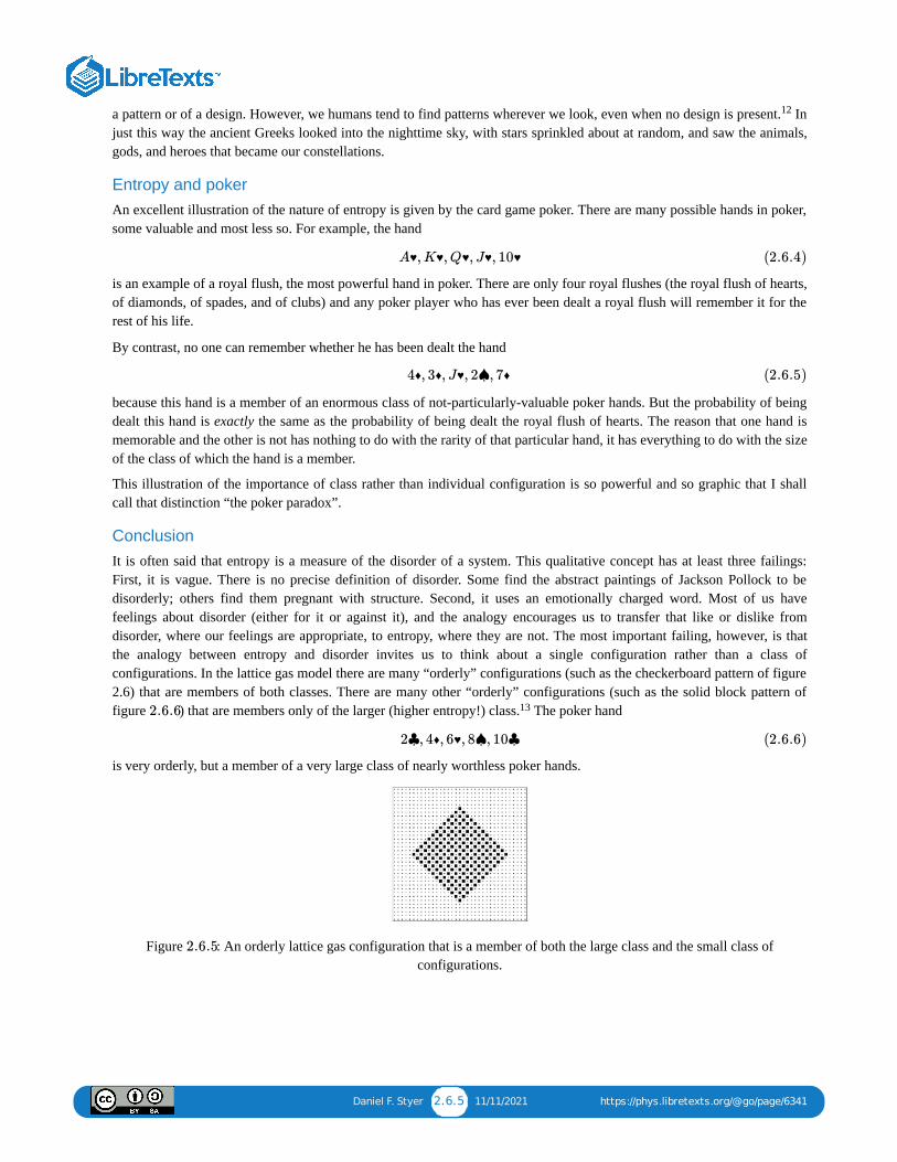
Daniel F. Styer 2.6.5 11/11/2021 https://phys.libretexts.org/@go/page/6341

a pattern or of a design. However, we humans tend to find patterns wherever we look, even when no design is present. Injust this way the ancient Greeks looked into the nighttime sky, with stars sprinkled about at random, and saw the animals,gods, and heroes that became our constellations.

Entropy and pokerAn excellent illustration of the nature of entropy is given by the card game poker. There are many possible hands in poker,some valuable and most less so. For example, the hand

is an example of a royal flush, the most powerful hand in poker. There are only four royal flushes (the royal flush of hearts,of diamonds, of spades, and of clubs) and any poker player who has ever been dealt a royal flush will remember it for therest of his life.

By contrast, no one can remember whether he has been dealt the hand

because this hand is a member of an enormous class of not-particularly-valuable poker hands. But the probability of beingdealt this hand is exactly the same as the probability of being dealt the royal flush of hearts. The reason that one hand ismemorable and the other is not has nothing to do with the rarity of that particular hand, it has everything to do with the sizeof the class of which the hand is a member.

This illustration of the importance of class rather than individual configuration is so powerful and so graphic that I shallcall that distinction “the poker paradox”.

ConclusionIt is often said that entropy is a measure of the disorder of a system. This qualitative concept has at least three failings:First, it is vague. There is no precise definition of disorder. Some find the abstract paintings of Jackson Pollock to bedisorderly; others find them pregnant with structure. Second, it uses an emotionally charged word. Most of us havefeelings about disorder (either for it or against it), and the analogy encourages us to transfer that like or dislike fromdisorder, where our feelings are appropriate, to entropy, where they are not. The most important failing, however, is thatthe analogy between entropy and disorder invites us to think about a single configuration rather than a class ofconfigurations. In the lattice gas model there are many “orderly” configurations (such as the checkerboard pattern of figure2.6) that are members of both classes. There are many other “orderly” configurations (such as the solid block pattern offigure ) that are members only of the larger (higher entropy!) class. The poker hand

is very orderly, but a member of a very large class of nearly worthless poker hands.

Figure : An orderly lattice gas configuration that is a member of both the large class and the small class ofconfigurations.

12

A♥, K♥, Q♥, J♥, 10♥ (2.6.4)

4♦, 3♦, J♥, 2♠, 7♦ (2.6.5)

2.6.6 13

2♣, 4♦, 6♥, 8♠, 10♣ (2.6.6)

2.6.5

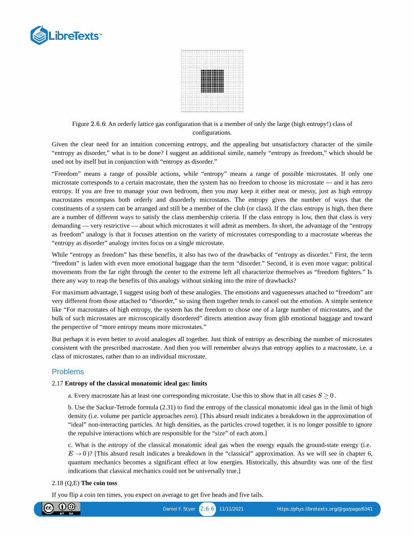
Daniel F. Styer 2.6.6 11/11/2021 https://phys.libretexts.org/@go/page/6341

Figure : An orderly lattice gas configuration that is a member of only the large (high entropy!) class ofconfigurations.

Given the clear need for an intuition concerning entropy, and the appealing but unsatisfactory character of the simile“entropy as disorder,” what is to be done? I suggest an additional simile, namely “entropy as freedom,” which should beused not by itself but in conjunction with “entropy as disorder.”

“Freedom” means a range of possible actions, while “entropy” means a range of possible microstates. If only onemicrostate corresponds to a certain macrostate, then the system has no freedom to choose its microstate — and it has zeroentropy. If you are free to manage your own bedroom, then you may keep it either neat or messy, just as high entropymacrostates encompass both orderly and disorderly microstates. The entropy gives the number of ways that theconstituents of a system can be arranged and still be a member of the club (or class). If the class entropy is high, then thereare a number of different ways to satisfy the class membership criteria. If the class entropy is low, then that class is verydemanding — very restrictive — about which microstates it will admit as members. In short, the advantage of the “entropyas freedom” analogy is that it focuses attention on the variety of microstates corresponding to a macrostate whereas the“entropy as disorder” analogy invites focus on a single microstate.

While “entropy as freedom” has these benefits, it also has two of the drawbacks of “entropy as disorder.” First, the term“freedom” is laden with even more emotional baggage than the term “disorder.” Second, it is even more vague: politicalmovements from the far right through the center to the extreme left all characterize themselves as “freedom fighters.” Isthere any way to reap the benefits of this analogy without sinking into the mire of drawbacks?

For maximum advantage, I suggest using both of these analogies. The emotions and vaguenesses attached to “freedom” arevery different from those attached to “disorder,” so using them together tends to cancel out the emotion. A simple sentencelike “For macrostates of high entropy, the system has the freedom to chose one of a large number of microstates, and thebulk of such microstates are microscopically disordered” directs attention away from glib emotional baggage and towardthe perspective of “more entropy means more microstates.”

But perhaps it is even better to avoid analogies all together. Just think of entropy as describing the number of microstatesconsistent with the prescribed macrostate. And then you will remember always that entropy applies to a macrostate, i.e. aclass of microstates, rather than to an individual microstate.

Problems2.17 Entropy of the classical monatomic ideal gas: limits

a. Every macrostate has at least one corresponding microstate. Use this to show that in all cases .

b. Use the Sackur-Tetrode formula (2.31) to find the entropy of the classical monatomic ideal gas in the limit of highdensity (i.e. volume per particle approaches zero). [This absurd result indicates a breakdown in the approximation of“ideal” non-interacting particles. At high densities, as the particles crowd together, it is no longer possible to ignorethe repulsive interactions which are responsible for the “size” of each atom.]

c. What is the entropy of the classical monatomic ideal gas when the energy equals the ground-state energy (i.e. )? [This absurd result indicates a breakdown in the “classical” approximation. As we will see in chapter 6,

quantum mechanics becomes a significant effect at low energies. Historically, this absurdity was one of the firstindications that classical mechanics could not be universally true.]

2.18 (Q,E) The coin toss

If you flip a coin ten times, you expect on average to get five heads and five tails.

2.6.6

S ≥ 0

E → 0

Daniel F. Styer 2.6.7 11/11/2021 https://phys.libretexts.org/@go/page/6341

a. The pattern HHHHHHHHHH violates this expectation dramatically. What is the probability of obtaining thispattern?

b. The pattern HTHTHTHTHT matches this expectation exactly. What is the probability of obtaining this pattern?

c. What is the probability of obtaining the pattern HTTTHHTTHT?

d. What is the probability of obtaining a pattern with one tail and nine heads?

2.19 (Q) Random walks

You are presented with two pictures that supposedly sketch the progress of a random walker as it moves through space.One was drawn by a computer using a random number generator, the other by a human being. One picture is more or lessuniform, the other has some spaces dark with lines and other spaces hardly touched. Which picture was drawn in whichway?

2.20 Poker

In the game of poker, a hand consists of five cards drawn from a deck of 52 cards. The cards are evenly divided into foursuits (hearts, diamonds, clubs, spades).

a. How many hands are there in poker? Explain your reasoning.

b. How many hands are flushes? (That is, all five cards of the same suit.)

c. Harry plays poker every evening, and each evening he is dealt 100 hands. How long must Harry play, on average,before being dealt the hand

Cutler J. Cleveland and Robert Kaufmann “Fundamental principles of energy,” in Encyclopedia of Earth, last updated 29August 2008, http://www.eoearth.org/article/Fundamental-principles-of-energy.

Louis M. Savary, Teilhard de Chardin: The Divine Milieu Explained (Paulist Press, Mahwah, NJ, 2007) page 163.

Gilbert L. Wedekind, Spiritual Entropy (Xulon Press, Fairfax, VA, 2003) page 68.

Ihsan Barin, Thermochemical Data of Pure Substances (VCH Publishers, Weinheim, Germany, 1995) pages 675, 1239,and 702.

The argument of this section was invented by Edward M. Purcell and is summarized in Stephen Jay Gould, Bully forBrontosaurus (W.W. Norton, New York, 1991), pages 265–268, 260–261. The computer programs mentioned, which workunder MS-DOS, are available for free downloading through http://www.oberlin.edu/physics/dstyer/.

In his book The Second Law (Scientific American Books, New York, 1984), P.W. Atkins promotes the idea that entropyis a measure of homogeneity. (This despite the everyday observation of two-phase coexistence.) To buttress this argument,the book presents six illustrations (on pages 54, 72, 74, 75, and 77) of “equilibrium lattice gas configurations.” Eachconfiguration has 100 occupied sites on a grid. If the occupied sites had been selected at random, then theprobability of any site being occupied would be , and the probability of any given pair of sites both beingoccupied would be . The array contains adjacent site pairs, so the expected number of occupiedadjacent pairs would be . The actual numbers of occupied nearest-neighbor pairs in the six illustrationsare , and . A similar calculation shows that the expected number of empty rows or columns in a randomlyoccupied array is . The actual numbers for the six illustrations are , and . I amconfident that the sites in these illustrations were not occupied at random, but rather to give the impression of uniformity.

Look again at figure . Do you see the dog catching a ball in the middle left? Do you see the starship Enterprise inthe bottom right?

Someone might raise the objection: “Yes, but how many configurations would you have to draw from the pool, onaverage, before you obtained exactly the special configuration of figure ?” The answer is, “Precisely the samenumber that you would need to draw, on average, before you obtained exactly the special configuration of figure .”These two configurations are equally special and equally rare.

4♦, 3♦, J♥, 2♠, 7♦ (2.6.7)

6

7

8

9

10

11

40 ×40100/1600

1/(16)2 2 ×39 ×392(39/16 11.88)=

0, 7, 3, 7, 4 3(15/16)10 ×2 ×40 = 41.96 28, 5, 5, 4, 4 0

12 2.6.3

13

2.6.62.6.3

Daniel F. Styer 2.7.1 1/27/2022 https://phys.libretexts.org/@go/page/18538

2.7: Using Entropy to Find (Define) Temperature and PressureReferences: Schroeder sections 3.1, 3.4, and 3.5. Reif section 3.3. Kittel and Kroemer pages 30–41.

You will remember that one of the problems with our ensemble approach to statistical mechanics is that, while one readilysees how to calculate ensemble average values of microscopic (mechanical) quantities like the kinetic energy, the potentialenergy, or the mean particle height, it is hard to see how to calculate the sort of macroscopic (thermodynamic) quantity thatwe’re really more interested in anyway, such as the temperature or pressure. In fact, it is not even clear how we shoulddefine these important quantities. Our task in this lecture is to motivate such definitions. Because our arguments aremotivations rather than deductions, they will be suggestive rather than definitive. The arguments can be made substantiallymore solid, but only at the cost of dramatic increase in mathematical complexity. (See David Ruelle’s StatisticalMechanics: Rigorous Results [Physics QC174.8.R84 1989].) At this stage in your education, you should just accept thearguments and the definitions, realizing that they are not definitive, and go on to learn how to use them. If you’re stillworried about them a year from now, then that would be a good time to read the more complex arguments in Ruelle’sbook.

An analogy will help explain the mathematical level of this lecture. Why is the period of the simple harmonic oscillatorindependent of amplitude? I can give two answers: 1) At larger amplitudes, the particle has more distance to move, but italso moves faster, and these two effects exactly cancel. 2) Solve the problem mathematically, and you’ll see that

which is clearly unaffected by amplitude. The first answer gives more insight into what is going onphysically, but it is not definitive. (It does not explain why the two effects cancel exactly rather that have one dominate theother, which is the case for non-parabolic oscillators.) The second argument is bulletproof, but it gives little insight. It isbest to use both types of argument in tandem. Unfortunately, the bulletproof arguments for this section are really tooelaborate and formal to present here. (In a few weeks I will give you a sample of a rigorous statistical mechanicalargument: “The Grand Canonical Ensemble in the Thermodynamic Limit”, section 4.8. It is the easiest such argument thatI know of, and you will see that it’s not very easy at all!)

Rapidly increasing character of the Ω(E) functionFor a monatomic ideal gas (“in the thermodynamic limit”) the entropy is

Thus Ω(E, V, N), the number of microstates consistent with the macrostate (or thermodynamic state) specified by E, V, andN, is

In particular, as a function of energy,

This is a very rapidly increasing function of . (The function increases more rapidly than . Thefunction increases more rapidly than . The function increases very rapidly indeed!)Although we have proven this result only for the ideal gas, it is plausible for interacting systems as well: If you throwmore energy into a system, there are more ways for the energy to be arranged. (There is an argument to this effect in Reif’ssection 2.5. The result is not, however, always true. . . check out the ideal paramagnet.)

As the particle number grows larger and larger (approaching the “thermodynamic limit”) this increase of with becomes more and more rapid.

Two isolated systemsConsider two systems, and , enclosed in our perfectly reflecting no-skid walls. System has energy , volume ,and particle number ; similarly for system B.

ω = k/m− −−−

√

S(E,V ,N) ≡ lnΩ(E,V ,N) = N [ ln( ) + ] .kB kB3

2

4πmEV 2/3

3h20N

5/3

5

2(2.7.1)

Ω(E,V ,N) = .e(5/2)N( )4πmEV 2/3

3h20N

5/3

(3/2)N

(2.7.2)

Ω(E) = ( constant ) .E (3/2)N (2.7.3)

E f(x) = x2 f(x) = x

f(x) = x3 f(x) = x2 f(x) = x1023

14

N Ω E

A B A EA VANA

Daniel F. Styer 2.7.2 1/27/2022 https://phys.libretexts.org/@go/page/18538

I have drawn the two systems adjacent, but they might as well be miles apart because they can’t affect each other throughthe no-skid walls. No energy can flow from one system to the other because no energy can move from the atoms in thesystem into the walls. The formal name for such walls is “insulating” or “adiabatic”. As we have discussed previously,such perfectly insulating walls do not exist in nature (if nothing else, system A affects system B through the gravitationalinteraction), but good experimental realizations exist and they are certainly handy conceptually.

The total system consisting of plus is characterized by the macroscopic quantities , , , , , and .The number of microstates corresponding to this macrostate is

Two systems in thermal contactConsider the same two systems, and , as before, but now allow the wall between them to be an ordinary, energy-permeable wall. Such a wall is called “diathermal”. (The walls between the systems and the outside world are stillinsulating.)

Now the mechanical parameters , and still remain constant when the two systems are brought together, butthe energies and change. (Of course the total energy remains constant as individual energieschange.) Such contact between two systems, where energy can flow between the systems but where the mechanicalparameters don’t change, is called “thermal contact”. Once they are in contact, I don’t know what the distribution ofenergy between and is: It could be that is in its ground state and all the excess energy is in , or vice versa, and itcould change rapidly from one such extreme to the other. But while I no longer have knowledge of the distribution, I dohave an expectation. My expectation, drawn from daily experience, is that energy will flow from one system to anotheruntil and take on some pretty well-defined final equilibrium values. The exact energies will then fluctuate aboutthose equilibrium values, but those fluctuations will be small. And what characterizes this final equilibrium situation? Yourfirst guess might be that the energy on each side should be equal. But no, if a big system were in contact with a smallsystem, then you’d expect more energy to end up in the big system. Then you might think that the energy per particle oneach side should be equal, but that’s not right either. (Ice and liquid water are in equilibrium at the freezing point, despitethe fact that the energy per particle of liquid water is much greater than than of ice.) The correct expectation (known to anycook) is that:

When two systems and are brought into thermal contact, and will change until they reach equilibriumvalues and , with negligible fluctuations, and at equilibrium both systems and will have the same“temperature”.

This is the qualitative property of temperature that will allow us, in a few moments, to produce a rigorous, quantitativedefinition. To do so we now look at the process microscopically instead of through our macroscopic expectations.

Once the two systems are in thermal contact the energy of system A could be anything from 0 to the total energy Forany given , the number of accessible microstates of the combined system, plus , is . Thusthe total number of microstates of the combined system is

(Please don’t tell me the obvious. . . that is a continuous quantity so you have to integrate rather than sum. This is aseat-of-the-pants argument. If you want attention to fine points, look them up in Ruelle’s book.) Let us examine the

A B EA EB VA VB NA NB

( , , , , , ) = ( , , ) ( , , ).ΩT EA EB VA VB NA NB ΩA EA VA NA ΩB EB VB NB (2.7.4)

A B

, ,VA VB NA NB

EA EB ≡ +ET EA EB

A B A B

EA EB

A B EA EB

E(e)

AE

(e)

BA B

ET15

EA A B ( ) ( − )ΩA EA ΩB ET EA

( ) = ( ) ( − ) .ΩT ET ∑=0EA

ET

ΩA EA ΩB ET EA (2.7.5)

EA

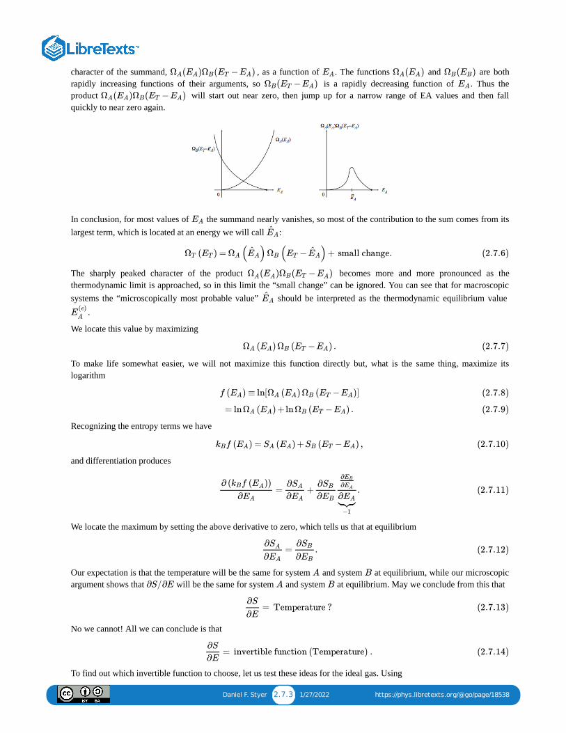
Daniel F. Styer 2.7.3 1/27/2022 https://phys.libretexts.org/@go/page/18538

character of the summand, , as a function of . The functions and are bothrapidly increasing functions of their arguments, so is a rapidly decreasing function of . Thus theproduct will start out near zero, then jump up for a narrow range of EA values and then fallquickly to near zero again.

In conclusion, for most values of the summand nearly vanishes, so most of the contribution to the sum comes from itslargest term, which is located at an energy we will call :

The sharply peaked character of the product becomes more and more pronounced as thethermodynamic limit is approached, so in this limit the “small change” can be ignored. You can see that for macroscopicsystems the “microscopically most probable value” should be interpreted as the thermodynamic equilibrium value

.

We locate this value by maximizing

To make life somewhat easier, we will not maximize this function directly but, what is the same thing, maximize itslogarithm

Recognizing the entropy terms we have

and differentiation produces

We locate the maximum by setting the above derivative to zero, which tells us that at equilibrium

Our expectation is that the temperature will be the same for system and system at equilibrium, while our microscopicargument shows that will be the same for system and system at equilibrium. May we conclude from this that

No we cannot! All we can conclude is that

To find out which invertible function to choose, let us test these ideas for the ideal gas. Using

( ) ( − )ΩA EA ΩB ET EA EA ( )ΩA EA ( )ΩB EB

( − )ΩB ET EA EA

( ) ( − )ΩA EA ΩB ET EA

EA

EA

( ) = ( ) ( − )+ small change. ΩT ET ΩA EA ΩB ET EA (2.7.6)

( ) ( − )ΩA EA ΩB ET EA

EA

E(e)

A

( ) ( − ) .ΩA EA ΩB ET EA (2.7.7)

f ( ) ≡ ln[ ( ) ( − )]EA ΩA EA ΩB ET EA (2.7.8)

= ln ( ) +ln ( − ) .ΩA EA ΩB ET EA (2.7.9)

f ( ) = ( ) + ( − ) ,kB EA SA EA SB ET EA (2.7.10)

= + .∂ ( f ( ))kB EA

∂EA

∂SA

∂EA

∂SB

∂EB

∂EB

∂EA

∂EA −1

(2.7.11)

= .∂SA

∂EA

∂SB

∂EB

(2.7.12)

A B

∂S/∂E A B

= Temperature ? ∂S

∂E(2.7.13)

= invertible function (Temperature) .∂S

∂E(2.7.14)

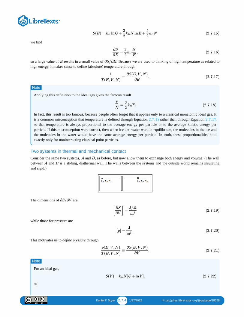
Daniel F. Styer 2.7.4 1/27/2022 https://phys.libretexts.org/@go/page/18538

we find

so a large value of results in a small value of . Because we are used to thinking of high temperature as related tohigh energy, it makes sense to define (absolute) temperature through

Applying this definition to the ideal gas gives the famous result

In fact, this result is too famous, because people often forget that it applies only to a classical monatomic ideal gas. Itis a common misconception that temperature is defined through Equation rather than through Equation ,so that temperature is always proportional to the average energy per particle or to the average kinetic energy perparticle. If this misconception were correct, then when ice and water were in equilibrium, the molecules in the ice andthe molecules in the water would have the same average energy per particle! In truth, these proportionalities holdexactly only for noninteracting classical point particles.

Two systems in thermal and mechanical contactConsider the same two systems, and , as before, but now allow them to exchange both energy and volume. (The wallbetween and is a sliding, diathermal wall. The walls between the systems and the outside world remains insulatingand rigid.)

The dimensions of are

while those for pressure are

This motivates us to define pressure through

For an ideal gas,

so

S(E) = lnC + N lnE+ NkB3

2kB

5

2kB (2.7.15)

= ,∂S

∂E

3

2kB

N

E(2.7.16)

E ∂S/∂E

≡ .1

T (E,V ,N)

∂S(E,V ,N)

∂E(2.7.17)

Note

= T .E

N

3

2kB (2.7.18)

2.7.18 2.7.17

A B

A B

∂S/∂V

[ ] =∂S

∂V

J/K

m3(2.7.19)

[p] = .J

m3(2.7.20)

≡ .p(E,V ,N)

T (E,V ,N)

∂S(E,V ,N)

∂V(2.7.21)

Note

S(V ) = N [C +lnV ].kB (2.7.22)

Daniel F. Styer 2.7.5 1/27/2022 https://phys.libretexts.org/@go/page/18538

leading to

the ideal gas equation of state! (Which is again too famous for its own good. Too many statistical mechanics coursesdegenerate into “an intensive study of the ideal gas”, and it is a shame to waste such a beautiful, powerful, and diversesubject on the study of only one substance, especially since that substance doesn’t even exist in nature!)

Two systems that can exchange energy, volume, and particles

We return to the same situation as before, but now the wall between and is not only diathermal and sliding, but alsoallows particles to flow. (Imagine piercing a few tiny holes in the wall.)

The reasoning in this case exactly parallels the reasoning already given two above, so I will not belabor it. I will merelypoint out that we can now define a new quantity, the chemical potential , which governs the flow of particles just astemperature governs the flow of energy or pressure governs the flow of volume. It is

The meaning of chemical potential

The upshot of all our definitions is that

What do these definitions mean physically? The first term says that if two systems are brought together so that they canexchange energy but not volume or particle number, then in the system with high temperature the energy will decreasewhile in the system with low temperature the energy will increase. The second term says that if two systems with the sametemperature are brought together so that they can exchange volume but not particle number, then in the system with highpressure the volume will increase while in the system with low pressure the volume will decrease. The third term says thatif two systems with the same temperature and pressure are brought together so that they can exchange particles, then in thesystem with high chemical potential the number will decrease while in the system with low chemical potential the numberwill increase. In summary:

Exchange of energy? Exchange of volume? Exchange of particles? Result:

YesPermitted, but .Permitted, but .

Prohibited.Yes.

Permitted, but .

Prohibited.Prohibited.

Yes.

System with high decreases in .

System with high increases in .

System with high decreases in .

Chemists have a great name for chemical potential. . . they call it “escaping tendency”, because particles tend to movefrom a region of high to a region of low just as energy tend to move from a region of high to a region of low .(G.W. Castellan, Physical Chemistry, 2nd edition, Addison-Wesley, Reading, Mass., 1971, section 11–2.) You can see thatchemical potential is closely related to density, and indeed for an ideal gas

= = ,∂S

∂V

NkB

V

p

T(2.7.23)

pV = N T ,kB (2.7.24)

A B

μ

− ≡ .μ(E,V ,N)

T (E,V ,N)

∂S(E,V ,N)

∂N(2.7.25)

dS = dE+ dV − dN .1

T

p

T

μ

T(2.7.26)

ΔT = 0

ΔT = 0 Δp = 0

T

E

p

V

μ

N

μ μ T T

μ = T ln( (T )ρ),kB λ3 (2.7.27)

Daniel F. Styer 2.7.6 1/27/2022 https://phys.libretexts.org/@go/page/18538

where is the number density and is a certain length, dependent upon the temperature, that we will seeagain (in equation (5.4)).

Once again, remember that this relation holds only for the ideal gas. At the freezing point of water, when ice and liquidwater are in equilibrium, the chemical potential is the same for both the solid and the liquid, but the densities clearlyare not!

Problems

2.21 (Q) The location of

In the figure on page 41, does the equilibrium value fall where the two curves and cross? Ifnot, is there a geometrical interpretation, in terms of that figure, that does characterize the crossing?

2.22 (Q) Meaning of temperature and chemical potential

The energy of a microscopic system can be dissected into its components: the energy due to motion, the energy dueto gravitational interaction, the energy due to electromagnetic interaction. Can the temperature be dissected intocomponents in this way? The chemical potential? (Clue: Because the temperature and chemical potential arederivatives of the entropy, ask yourself first whether the entropy can be dissected into components.)

2.23 (E) Chemical potential of an ideal gas

a. Show that the chemical potential of a pure classical monatomic ideal gas is

b. Show that when the temperature is sufficiently high and the density sufficiently low (and these are, after all, theconditions under which the ideal gas approximation is valid) the chemical potential is negative.

c. Show that

At a fixed, low density, does increase or decrease with temperature?

2.24 Ideal paramagnet, take three

Find the chemical potential of the ideal paramagnet. (Your answer must not be a function of .) (Towork this problem you must have already worked problems 2.9 and 2.12.)

Resources

Percival as CM for chaos and SM. Hilborn on chaos.

PAS chaos programs, public domain stadium and wedge. CUPS stadium.

Tolman, Ruelle.

Through the booty argument of page 27.

Here and in the rest of this section, we assume that the ground state energy of both system and system has been setby convention to zero.

ρ = N/V λ(T )

Note

E(e)

A

E (e)A

( )ΩA EA ( − )ΩB ET EA

μ = − T ln( )3

2kB

4πmEV 2/3

3h20N

5/3(2.7.28)

= − T ln .kB⎡

⎣( )

2πm TkB

h20

3/2V

N

⎤

⎦(2.7.29)

= − .∂μ(T ,V ,N)

∂T

μ(T ,V ,N)

T

3

2kB (2.7.30)

μ

μ(E,H,N) T

14

15 A B

2.8.1 12/2/2021 https://phys.libretexts.org/@go/page/18714

2.8: Additional Problems2.25 Accessible configurations in another spin system

The Ising model for a ferromagnetic material such as nickel is different from the “ideal paramagnet” discussed inproblem 2.9. In this model the spins reside at lattice sites and may point either up or down, but in contrast to theideal paramagnet model, two adjacent spins do interact. Specifically, if two adjacent spins point in the samedirection, the pair has energy . If they point in different directions, the pair has energy . (In the ferromagneticsituation considered here, .) We consider here a one-dimensional Ising model of sites with zero externalmagnetic field.

a. Not every energy is possible for this model. What is the maximum possible energy? The minimum? What isthe smallest possible energy spacing between configurations?

b. Consider the energy range from to where is small compared to but large compared to . What is the approximate number of states lying within this energy range?

c. Write down an expression for the entropy as a function of . (Clue: Be careful to nevertake the logarithm of a number with dimensions.)

d. Take the thermodynamic limit to find the entropy per atom as a function of the energy per atom: .(Clue: Use Stirling’s approximation.)

e. Check your work by comparing the Ising entropy per spin when the interactions vanish tothe ideal paramagnet entropy per spin in zero field. (See problem 2.12. Clue: If , then also. Why?)

General clues: It helps to concentrate not on the status of the spins (up or down) but on the status of the pairs (alikeor different). How many nearest neighbor pairs are there? For each given configuration of pairs, how manycorresponding configurations of spins are there?

2.26 Shake and spin

Make up a problem involving an ideal paramagnet with atoms free to move around.

2.27 Entropy as a function of mass

Use the Sackur-Tetrode formula to find the difference between the entropy of a sample of argon gas and a samplekrypton gas under identical conditions. Use the data in Ihsan Barin, Thermochemical Data of Pure Substances, thirdedition (VCH Publishers, New York, 1995) to test this prediction at the temperatures 300 K and 2000 K.

2.28 (Q,D) For discussion: “The icy cold of outer space”

Is outer space at a high temperature or a low temperature? Before answering, consider these points:

a. The environment of outer space consists of protons and photons streaming away from the sun. The twosystems are virtually uncoupled (do not interact with each other). I’m asking for the temperature of theprotons.

b. It was implicitly (perhaps illicitly) assumed in section 2.7.3 that the centers of mass of the two systems inthermal contact were in the same reference frame. This is a general principle: When referring to thetemperature of a moving body, we mean the temperature as measured by a thermometer moving along withthat body.

c. Remember that in the arguments of section 2.7.3 the two systems could exchange energy but not particles.

d. What if we approximated the protons by an ideal gas?

e. Look at the Handbook of Chemistry and Physics under index entry “Temperature, Earth’s atmosphere”.

−J +J

J > 0 N

E E +ΔE ΔE NJ

J Ω(E, ΔE, J, N)

S(E, ΔE, J, N) E

s(e, J)

s(e, J) (J = 0)

s(e, H) J = 0 e = 0

2.8.2 12/2/2021 https://phys.libretexts.org/@go/page/18714

2.29 (Q,D) Errors in Reif

Scan Reif pages 47–61, but don’t read them in detail as they are rife with errors. Point out the major error inquantum mechanics made in each of the following passages. (Use a maximum of three sentences per passage.)

a. The examples on pages 48 and 49.

b. The second paragraph on page 57.

c. The first paragraph on page 60.

2.30 Polymers

I’d like to think up some problem concerning polymers of fixed length vs. polymers of fixed “activity for length”.The activity is analogous to chemical potential in that it is a control knob for polymer length. It might render thewhole concept more concrete.

1 1/27/2022

CHAPTER OVERVIEW3: THERMODYNAMICS

3.1: HEAT AND WORK3.2: ENTROPY3.3: HEAT ENGINES3.4: MULTIVARIATE CALCULUS3.5: THERMODYNAMIC QUANTITIES3.6: THE THERMODYNAMIC DANCE3.7: NON-FLUID SYSTEMS3.8: THERMODYNAMICS APPLIED TO FLUIDS3.9: THERMODYNAMICS APPLIED TO PHASE TRANSITIONS3.10: THERMODYNAMICS APPLIED TO CHEMICAL REACTIONS3.11: THERMODYNAMICS APPLIED TO LIGHT3.12: ADDITIONAL PROBLEMS

Daniel F. Styer 3.1.1 1/13/2022 https://phys.libretexts.org/@go/page/6343

3.1: Heat and WorkWe’ve seen how to calculate—at least in principle, although our techniques were primitive and difficult to use—theentropy S(E, V, N). We’ve also argued (“the booty argument”, section 2.7.1) that for most systems entropy will increasemonotonically with energy when V and N are fixed. Thus we (can)/(will always be able to) invert the function to findenergy as a function of entropy, volume, and number:

Recall that V and N are just stand-ins as representative mechanical parameters.

But how can we measure entropy? Walk into any laboratory and the experimentalist there will say “I have thermometersfor measuring temperature. I have resistors, ammeters, and voltmeters, and a I have a procedure for using these instrumentsto measure the heat flowing into a sample. I have calibers for measuring volume and manometers for measuring pressure.But I have no instrument to measure the number of microstates consistent with a given macrostate.” Although we haveproduced a conceptual definition of entropy, we need also an operational definition of entropy.

An “operational definition” defines the target word, not in terms of other words, but in terms of a procedure that producesa decision or a numerical value concerning that target word. For example, an operational definition for the wordtuberculosis is “a disease marked by wasting, cough, fever, and formation of small cheesy lumps in the lungs”. In contrast,a conceptual definition is “a disease caused by the bacillus bacterium Mycobacterium tuberculosis”. The operationaldefinition tells you how to diagnose the disease; the conceptual definition tells you what’s going on and suggests a cure.We need to produce an operational definition to go along with our conceptual definition of entropy, and that’s the startingpoint of this chapter.

Heat:

Change in energy with no change in mechanical parameters =

Change in energy due to temperature difference between system and surroundings =

Heat (absorbed by system) = Q

Configuration work.

Change in energy due to change in mechanical parameters =

Change in energy when system is wrapped in insulating (“no-skid”) walls =

Configuration work (done by system) = W

Dissipative work.

Change in energy due to non-equilibrium effects =

Change in energy due to, e.g., shaking, stirring, or running current through the system =

Dissipative work (done by system) = W

It is an empirical fact (sometimes called “the second law of thermodynamics”), that dissipative work always increases theenergy of the system. Joule the brewer; story about honeymoon at Cascade de Sallanches.

Caution: Heat and work refer to mechanisms for energy change, not to types of energy. Do not think that heat goes into achange of kinetic energy (or into “mixed up energy”) whereas work goes into a change of potential energy (or into“ordered energy”).

Any change due to heating could also be done via dissipative work, and there’s no way you could tell the difference. Joulecalled this “the conversion of work to heat”, although that’s not correct using the modern definitions of “work” and “heat”.

Analogy: You can put money into your bank account through depositing cash or checks, or through an electronic fundstransfer. You can take money out of your bank account through these three mechanisms too. But once the money is insideyour bank account, you cannot say “This dollar was deposited through cash, while that dollar was deposited throughelectronic funds transfer.” Once they’re in your account, you can’t distinguish the dollars through the mechanism ofentrance. Similarly with energy. You can increase the temperature and energy of a cup of water by putting it near a flame,

E(S,V ,N). (3.1.1)

conf

diss

Daniel F. Styer 3.1.2 1/13/2022 https://phys.libretexts.org/@go/page/6343

or by putting it near a high-temperature resistor, or by stirring it rigorously. Given a high-temperature cup of water, there’sno way to tell which of these mechanisms was used.

Problems3.1 What is heat?

Below is an excerpt from a sixth-grade science textbook. Find at least six errors in the excerpt.

What is heat?

You have learned that all matter is made up of atoms. Most of these atoms combine to form molecules. Thesemolecules are always moving—they have kinetic energy. Heat is the energy of motion (kinetic energy) of theparticles that make up any piece of matter.

The amount of heat a material has depends on how many molecules it has and how fast the molecules aremoving. The greater the number of molecules and the faster they move, the greater the number of collisionsbetween them. These collisions produce a large amount of heat.

How is heat measured? Scientists measure heat by using a unit called a calorie. A calorie is the amount of heatneeded to raise the temperature of 1 gram of 1 water 1 degree centigrade (Celsius). A gram is a unit used formeasuring mass. There are about 454 grams in 1 pound.

What is temperature?

The amount of hotness in an object is called its temperature. A thermometer is used to measure temperature inunits called degrees. Most thermometers contain a liquid.

ΔE =Q+ +Wconf Wdiss (3.1.2)

Daniel F. Styer 3.2.1 11/4/2021 https://phys.libretexts.org/@go/page/6344

3.2: Entropy

but

so

where the equality holds for quasistatic changes.

The operational definition of entropy is that, for a quasistatic change,

If we walk into a laboratory with this definition of entropy, the experimentalist will say “Sure I can find this quantity. I’vegot thermometers; and I’ve got resistors, ammeters, and voltmeters, plus a procedure for using them to calculate heatflow.”

For any change (perhaps quasistatic, perhaps not)

(The entropy change might be due to heat, might be due to dissipative work, might be due to a combination of the two.)

Configurational entropy vs. thermal entropy

The operational, thermodynamic definition for entropy, Equation , was in fact discovered before the morefundamental, conceptual, statistical definition (2.7) was. Because of this dual definition some people get the misconceptionthat there are two kinds of entropy: the statistical kind (“configurational entropy”) and the operational kind (“thermalentropy”). That’s false. These are two different ways of looking at the same thing.

3.2 (I) Ideal gas with variables S and V.

a. Use equation (2.32) to show that for a sample of monatomic ideal gas with a fixed number of particles, the energyfunction is

where E , V , and S are constants with the dimensions of energy, volume, and entropy.

b. Use the formulas

to find the temperature and pressure functions for this sample.

3.3 (I) Dependence of heat and work on path

Suppose the ideal gas sample mentioned in the previous problem undergoes a change from an initial state with volume Vand entropy S to a final state with volume 8V and entropy (1+ 5 ln 2)S . There are an infinite number of quasistatic pathsthat execute this change. For example:

A First increase the entropy from S = S to S = (1 + 5 ln 2)S , keeping the volume fixed at V = V , then expand fromV = V to V = 8V , keeping the entropy fixed at S = (1 + 5 ln 2)S .

B Increase the volume and entropy simultaneously along the path

.

dE = TdS−pdV +μdN

= dQ+d +dWconf Wdiss

≥ dQ+dWconf

d = −pdV +μdNWconf

TdS > dQ

dS = .dQ

T(3.2.1)

dS ≥ .dQ

T(3.2.2)

3.2.1

E(S,V ) = ,E0( )V0

V

2/3

eS/S0 (3.2.3)

0 0 0

T (S,V ) = and p(S,V ) = −∂E(S,V )

∂S

∂E(S,V )

∂V(3.2.4)

0

0 0 0

0 0 0

0 0 0

Daniel F. Styer 3.2.2 11/4/2021 https://phys.libretexts.org/@go/page/6344

C First expand from V = V to V = 8V , keeping the entropy fixed at S = S , then increase the entropy from S = S toS = (1 + 5 ln 2)S , keeping the volume fixed at V = 8V .

Each path has the same change in volume, entropy, and energy, but each will have a different heat and work. (Rememberthat each path is quasistatic.)

a. Calculate the heat absorbed by the sample and the work done on the sample for each of these three paths.

b. Find the difference Q + W for each of these three paths.

c. A fourth path from the initial to the final state involves a non-quasistatic change and the absorption of heat Q =3E . What work is done on the sample during this change?

(In making up this problem I choose somewhat peculiar initial and final states, and connecting paths, so that the abovequantities could be calculated analytically. Despite these peculiarities the principle illustrated by the problem should beclear: heat and work depend upon path, but their difference the energy change does not.)

3.4 (I*) Work in terms of p and V

We have so far considered work and heat in a fluid system specified by the variables S, V, and N, and have oftenassumed that N is constant. Another way of specifying such a system is through the variables p (pressure) and V.This problem considers quasistatic processes described as paths in the (p, V) plane.

a. Show that the work done on the system in changing quasistatically from the initial state (V , p ) to the finalstate (V , p ) along the path shown in the figure below is the negative of the area under the curve. What is thework done if the path is traversed in the opposite direction?

b. What is the work done on the system through the same change along the path below?

c. Finally, what is the work done on the system if it comes back to its starting point as in the cycle shownbelow? What if the cycle is instead executed in a counterclockwise fashion?

3.5 (I) Fluid work

In a quasistatic, adiabatic process, a sample of gas expands from V = 1 m to V = 8 m , while the pressure drops from p =32 Pa to p = 1 Pa. It is observed that during this process the pressure and volume are related by

S(V ) = [ ln( )+1] .S05

3

V

V0(3.2.5)

0 0 0 0

0 0

0

i i

f f

i3

f3

i

f

Daniel F. Styer 3.2.3 11/4/2021 https://phys.libretexts.org/@go/page/6344

where the constant γ is . Of course, this is not the only process leading from this particular initial state to that particularfinal state. Find the total work done on the system and heat absorbed by the system in each of the following quasistaticprocesses, all of which connect the same two thermodynamic states.

a. The adiabatic process described above.

b. At constant pressure, the gas expands from V to V . (Heat must be added to the system during this expansion inorder to keep the pressure constant.) Then at constant volume, the the pressure is reduced from p to p . (Heat mustbe extracted from the system during this stage of the process.)

c. The volume is increased and heat is supplied at just the right rate to make the pressure decrease linearly withvolume.

d. As in part (b.) but with the two steps performed in opposite order.

p = constant ,V γ (3.2.6)

53

i f

i f

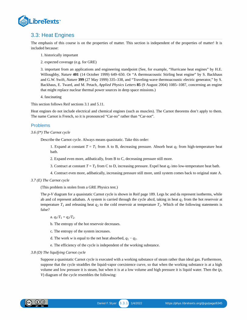
Daniel F. Styer 3.3.1 1/4/2022 https://phys.libretexts.org/@go/page/6345

3.3: Heat EnginesThe emphasis of this course is on the properties of matter. This section is independent of the properties of matter! It isincluded because:

1. historically important

2. expected coverage (e.g. for GRE)

3. important from an applications and engineering standpoint (See, for example, “Hurricane heat engines” by H.E.Willoughby, Nature 401 (14 October 1999) 649–650. Or “A thermoacoustic Stirling heat engine” by S. Backhausand G.W. Swift, Nature 399 (27 May 1999) 335–338, and “Traveling-wave thermoacoustic electric generator,” by S.Backhaus, E. Tward, and M. Petach, Applied Physics Letters 85 (9 August 2004) 1085–1087, concerning an enginethat might replace nuclear thermal power sources in deep space missions.)

4. fascinating

This section follows Reif sections 3.1 and 5.11.

Heat engines do not include electrical and chemical engines (such as muscles). The Carnot theorems don’t apply to them.The name Carnot is French, so it is pronounced “Car-no” rather than “Car-not”.

Problems3.6 (I*) The Carnot cycle

Describe the Carnot cycle. Always means quasistatic. Take this order:

1. Expand at constant T = T from A to B, decreasing pressure. Absorb heat q from high-temperature heatbath.

2. Expand even more, adibatically, from B to C, decreasing pressure still more.

3. Contract at constant T = T from C to D, increasing pressure. Expel heat q into low-temperature heat bath.

4. Contract even more, adibatically, increasing pressure still more, until system comes back to original state A.

3.7 (E) The Carnot cycle

(This problem is stolen from a GRE Physics test.)

The p-V diagram for a quasistatic Carnot cycle is shown in Reif page 189. Legs bc and da represent isotherms, whileab and cd represent adiabats. A system is carried through the cycle abcd, taking in heat q from the hot reservoir attemperature T and releasing heat q to the cold reservoir at temperature T . Which of the following statements isfalse?

a. q /T = q /T .

b. The entropy of the hot reservoir decreases.

c. The entropy of the system increases.

d. The work w is equal to the net heat absorbed, q − q .

e. The efficiency of the cycle is independent of the working substance.

3.8 (D) The liquifying Carnot cycle

Suppose a quasistatic Carnot cycle is executed with a working substance of steam rather than ideal gas. Furthermore,suppose that the cycle straddles the liquid-vapor coexistence curve, so that when the working substance is at a highvolume and low pressure it is steam, but when it is at a low volume and high pressure it is liquid water. Then the (p,V) diagram of the cycle resembles the following:

1 1

2 2

1

1 2 2

1 1 2 2

1 2

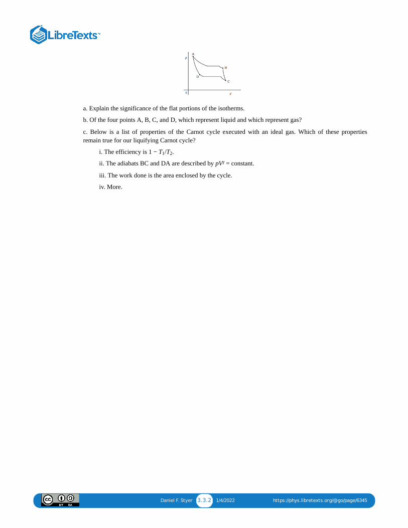
Daniel F. Styer 3.3.2 1/4/2022 https://phys.libretexts.org/@go/page/6345

a. Explain the significance of the flat portions of the isotherms.

b. Of the four points A, B, C, and D, which represent liquid and which represent gas?

c. Below is a list of properties of the Carnot cycle executed with an ideal gas. Which of these propertiesremain true for our liquifying Carnot cycle?

i. The efficiency is 1 − T /T .

ii. The adiabats BC and DA are described by pV = constant.

iii. The work done is the area enclosed by the cycle.

iv. More.

1 2

γ

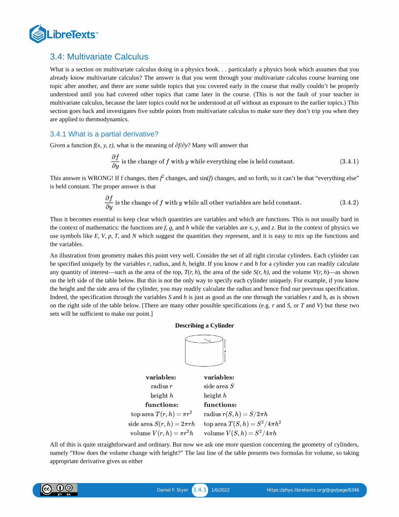
Daniel F. Styer 3.4.1 1/6/2022 https://phys.libretexts.org/@go/page/6346

3.4: Multivariate CalculusWhat is a section on multivariate calculus doing in a physics book. . . particularly a physics book which assumes that youalready know multivariate calculus? The answer is that you went through your multivariate calculus course learning onetopic after another, and there are some subtle topics that you covered early in the course that really couldn’t be properlyunderstood until you had covered other topics that came later in the course. (This is not the fault of your teacher inmultivariate calculus, because the later topics could not be understood at all without an exposure to the earlier topics.) Thissection goes back and investigates five subtle points from multivariate calculus to make sure they don’t trip you when theyare applied to thermodynamics.

3.4.1 What is a partial derivative?Given a function f(x, y, z), what is the meaning of ∂f/∂y? Many will answer that

This answer is WRONG! If f changes, then f changes, and sin(f) changes, and so forth, so it can’t be that “everything else”is held constant. The proper answer is that

Thus it becomes essential to keep clear which quantities are variables and which are functions. This is not usually hard inthe context of mathematics: the functions are f, g, and h while the variables are x, y, and z. But in the context of physics weuse symbols like E, V, p, T, and N which suggest the quantities they represent, and it is easy to mix up the functions andthe variables.

An illustration from geometry makes this point very well. Consider the set of all right circular cylinders. Each cylinder canbe specified uniquely by the variables r, radius, and h, height. If you know r and h for a cylinder you can readily calculateany quantity of interest—such as the area of the top, T(r, h), the area of the side S(r, h), and the volume V(r, h)—as shownon the left side of the table below. But this is not the only way to specify each cylinder uniquely. For example, if you knowthe height and the side area of the cylinder, you may readily calculate the radius and hence find our previous specification.Indeed, the specification through the variables S and h is just as good as the one through the variables r and h, as is shownon the right side of the table below. [There are many other possible specifications (e.g. r and S, or T and V) but these twosets will be sufficient to make our point.]

Describing a Cylinder

All of this is quite straightforward and ordinary. But now we ask one more question concerning the geometry of cylinders,namely “How does the volume change with height?” The last line of the table presents two formulas for volume, so takingappropriate derivative gives us either

is the change of f with y while everything else is held constant. ∂f

∂y(3.4.1)

2

is the change of f with y while all other variables are held constant. ∂f

∂y(3.4.2)

variables:

radius r

height h

functions:

top area T (r,h) = πr2

side area S(r,h) = 2πrh

volume V (r,h) = π hr2

variables:

side area S

height h

functions:

radius r(S,h) = S/2πh

top area T (S,h) = /4πS2 h2

volume V (S,h) = /4πhS2

Daniel F. Styer 3.4.2 1/6/2022 https://phys.libretexts.org/@go/page/6346

What? Is ∂V/∂h equal to T or to −T? It can’t be equal to both! The problem with equation (3.11) is that we were carelessabout specifying the variables. The two expressions for volume,

are in fact two completely different functions, with completely different variables, so we should expect completelydifferent derivatives. If we increase the height h keeping the radius r fixed, the figure on the left below makes it clear thatthe volume increases. But if we increase the height and keep the side area S fixed, the radius will have to decrease asshown on the right below. The change on the right adds to the volume at the top of the cylinder but subtracts from thevolume all along the sides. It would be most remarkable if the two volume changes were equal and, as our derivatives haveshown, they are not.

A mathematician would say that we got ourselves in trouble in equation (3.11) because we gave two different functions thesame name. A physicist would reply that they both represent the volume, so they deserve the same name. Rather than getinto an argument, it is best to write out the variables of all functions explicitly, thus rewriting (3.11) as

(Physicists often neglect to write out the full list of variables, which saves some time and some ink but which invites error.R.H. Price and J.D. Romano (Am. J. Phys. 66 (1998) 114) expose a situation in which a physicist published a deep error,which he made by neglecting to write out an explicit variable list.)

It becomes tiresome to write out the entire argument list for every function, so a shorthand notation has been developed. Aright hand parenthesis is written after the partial derivative, and the functional arguments that are not being differentiatedare listed as subscripts to that parenthesis. Thus the derivatives above are written as

The expression on the left is read “the partial derivative of V with respect to h while r is held constant”.

3.4.2 The Legendre transformation

Let us return to a description of cylinders in terms of the variables r and h. Clearly, one of the functions of interest is thevolume

A glance at the table on page 58 (or a moment’s thought about geometry) shows that the total differential of V as afunction of r and h is

whence

Thus knowledge of the function V(r, h) gives us a bonus. . . if we know V(r, h), then we can take simple derivatives to findthe other quantities of interest concerning cylinders, namely S(r, h) and T(r, h). Because of the central importance of V (r,h), it is called a “master function” and the total differential (3.16) is called a “master equation”.

= π = T or = − /4π = −T .∂V

∂hr2 ∂V

∂hS2 h2 (3.4.3)

V (r,h) = π h and V (S,h) = /4πh,r2 S2 (3.4.4)

= π = T (r,h) or = − /4π = −T (S,h).∂V (r,h)

∂hr2 ∂V (S,h)

∂hS2 h2 (3.4.5)

= and = .∂V (r,h)

∂h

∂V

∂h)r

∂V (S,h)

∂h

∂V

∂h)S (3.4.6)

V (r,h). (3.4.7)

dV = S(r,h)dr+T (r,h)dh, (3.4.8)

S(r,h) = and T (r,h) = .∂V

∂r)h

∂V

∂h)r (3.4.9)

Daniel F. Styer 3.4.3 1/6/2022 https://phys.libretexts.org/@go/page/6346

Is there any way to find a similarly convenient “master description” in terms of the variables S and h? Indeed there is, andit is given by the “Legendre transformation”. In the Legendre transformation from the variables r and h to the variables Sand h, we change the focus of our attention from the master function V(r, h) to the function

(The above equation is written out in full with all arguments shown. It is more usually seen as

although this form raises the possibility that variables and functions will become mixed up.) The total differential of Φ is

We have found a new master function! It is

and the new master equation is

giving rise immediately to

This description has all the characteristics of a master description: once the master function is known, all the otherinteresting functions can be found by taking straightforward derivatives.

3.4.3 Maxwell relations

Suppose

Then

But because

it follows that

This is called a "Maxwell relation".

Applied to equation (3.16), this tells us at a glance that

We know that these two derivatives are equal without needing to find either one of them! Applied to equation (3.24), ittells us with equal ease that

Φ(S,h) = V (r(S,h),h) −Sr(S,h). (3.4.10)

Φ = V −Sr, (3.4.11)

dΦ = dV −Sdr−rdS (3.4.12)

= Sdr+Tdh−Sdr−rdS (3.4.13)

= −rdS+Tdh (3.4.14)

Φ(S,h), (3.4.15)

dΦ = −r(S,h)dS+T (S,h)dh, (3.4.16)

r(S,h) = − and T (S,h) = .∂Φ

∂S)h

∂Φ

∂h)S (3.4.17)

df = A(x, y)dx+B(x, y)dy. (3.26) (3.4.18)

A(x, y) = and B(x, y) = .∂f

∂x)y

∂f

∂y)x

=f(x,y)∂ 2

∂x∂y

f(x,y)∂ 2

∂y∂x

= .∂A

∂y)x

∂B

∂x)y (3.4.19)

= .∂S

∂h)r

∂T

∂r)h (3.4.20)

= − .∂r

∂h)S

∂T

∂S)h (3.4.21)

Daniel F. Styer 3.4.4 1/6/2022 https://phys.libretexts.org/@go/page/6346

3.4.4 Implicit function theoremSuppose f(x, y) is a function of the variables x and y. What is

the slope of a contour of constant f?

Start with

which holds for any differential change dx and dy. But we’re not interested in any differential change: to evaluate the slope(3.30), we need a change in which df = 0 so

Thus

and, writing the restriction “with dx, dy on contour of f” into the symbols of the equation,

Note that you get the wrong answer if you “cancel the small quantity ∂f from numerator and denominator of the ratio.”That’s because “the small quantity ∂f with constant y” is different from “the small quantity ∂f with constant x”. I need towrite a few words and a figure concerning why.

3.4.5 Multivariate chain ruleSuppose f(x, y) and g(x, y) are two function of the variables x and y. Then again we have

for any differential change dx and dy.

What if we are interested, not in any change, but in a change along a contour of constant g? Specifically, what if we needto find the change of f with x while moving on a contour of constant g? Then just take the exact differential above andapply it to a change dx, dy along the contour with constant g. Divide by the differential quantity dx:

Now write the restriction “with dx, dy on contour of g” into the symbols of the equation to find

the multivariate chain rule.

Problems

3.9 Partial derivatives in space

A point on the plane can be specified either by the variables (x, y) or by the variables (x', y') where

∂y

∂x)f (3.4.22)

df = dx+ dy.∂f

∂x)y

∂f

∂y)x (3.4.23)

0 = dx+ dy with dx, dy on contour of f .∂f

∂x)y

∂f

∂y)x

= − with dx, dy on contour of fdy

dx

∂f

∂x)y

∂f

∂y)x

= − .∂y

∂x)f

∂f

∂x)y

∂f

∂y)x

(3.4.24)

df = dx+ dy∂f

∂x)y

∂f

∂y)x (3.4.25)

= + = + with dx, dy on contour of gdf

dx

∂f

∂x)y

dx

dx

∂f

∂y)x

dy

dx

∂f

∂x)y

∂f

∂y)x

dy

dx

= + ,∂f

∂x)g

∂f

∂x)y

∂f

∂y)x

∂y

∂x)g (3.4.26)

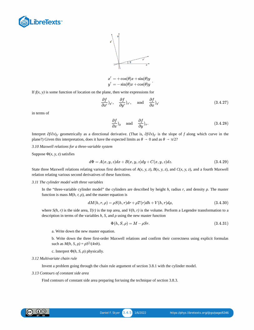
Daniel F. Styer 3.4.5 1/6/2022 https://phys.libretexts.org/@go/page/6346

If f(x, y) is some function of location on the plane, then write expressions for

in terms of

Interpret ∂f/∂x) geometrically as a directional derivative. (That is, ∂f/∂x) is the slope of f along which curve in theplane?) Given this interpretation, does it have the expected limits as θ → 0 and as θ → π/2?

3.10 Maxwell relations for a three-variable system

Suppose Φ(x, y, z) satisfies

State three Maxwell relations relating various first derivatives of A(x, y, z), B(x, y, z), and C(x, y, z), and a fourth Maxwellrelation relating various second derivatives of these functions.

3.11 The cylinder model with three variables

In the “three-variable cylinder model” the cylinders are described by height h, radius r, and density ρ. The masterfunction is mass M(h, r, ρ), and the master equation is

where S(h, r) is the side area, T(r) is the top area, and V(h, r) is the volume. Perform a Legendre transformation to adescription in terms of the variables h, S, and ρ using the new master function

a. Write down the new master equation.

b. Write down the three first-order Maxwell relations and confirm their correctness using explicit formulassuch as M(h, S, ρ) = ρS /(4πh).

c. Interpret Φ(h, S, ρ) physically.

3.12 Multivariate chain rule

Invent a problem going through the chain rule argument of section 3.8.1 with the cylinder model.

3.13 Contours of constant side area

Find contours of constant side area preparing for/using the technique of section 3.8.3.

.x′

y′

= +cos(θ)x+sin(θ)y

= −sin(θ)x+cos(θ)y

, , and ∂f

∂x′)y ′

∂f

∂y′)x′

∂f

∂x)y ′ (3.4.27)

and .∂f

∂x)y

∂f

∂y)x (3.4.28)

y' y'

dΦ = A(x, y, z)dx+B(x, y, z)dy+C(x, y, z)dz. (3.4.29)

dM(h, r, ρ) = ρS(h, r)dr+ρT (r)dh+V (h, r)dρ, (3.4.30)

Φ(h,S, ρ) = M −ρSr. (3.4.31)

2

Daniel F. Styer 3.5.1 12/30/2021 https://phys.libretexts.org/@go/page/6347

3.5: Thermodynamic QuantitiesBy a thermodynamic “quantity” I mean either a variable or a function. We have already seen that for fluids we may regardthe entropy as a function of energy, volume, and number, S(E, V, N), or the energy as a function of entropy, volume, andnumber, E(S, V, N): using the term “quantity” avoids prejudging the issue of whether entropy, for example, is to be treatedas a variable or a function.

It is traditional to divide thermodynamic quantities into two classes: “extensive” and “intensive”. Extensive quantitiesincrease linearly with system size while intensive quantities are independent of system size. (You might ask, “Why can’t aquantity depend on system size in some other fashion, such as quadratically?” The answer is that this is not impossible—for example, the radius of a spherical sample increses as the cube root of the system size—but it rarely happens in practicefor quantities that concern us—see problem 3.18.) Thus extensive quantities are characteristic of the sample whileintensive quantities are characteristic of the substance.

Examples of extensive quantities are energy, volume, number, entropy, and the magnetization M (i.e. the magnetic dipolemoment of the entire sample):

.

Examples of intensive quantities are temperature, pressure, chemical potential, and the applied magnetic field H:

If one extensive quantities is divided by another extensive quantity, the quotent is an intensive quantity. The mostfrequently used quantities of this type are the number densities, such as

There are also volume densities like

Quantities such as E/S are also intensive, but they are rarely used and don’t have special names.

Note that in defining densities such as above, we are not making any assumptions about how the matter in the sample isarranged. For liquid water in equilibrium with ice (e.g. at atmospheric pressure and a temperature of 273 K) the water has agreater number density (and a greater entropy density) than the ice, but the number density of the system is still just thetotal number divided by the total volume.

Here is a valuable problem solving tip. You know from previous courses that it is important to keep track of thedimensions of physical quantities: if you derive an equation for which the left side has the dimensions of meters and theright side has the dimensions of meters/second, your derivation must be wrong. In thermodynamics there is the equallyimportant check of extensivity: if the left side is extensive and the right side is intensive, then the equation must be wrong.You should keep a running check of these properties as you solve problems. The first time you produce an equation that isincorrect in its dimensions or its extensivity, go back immediately and correct your error.

Problem 1.2 has already introduced the “isothermal compressibility”

and the “expansion coefficient”

Both of these quantities are defined so as to be intensive.

E, V , N , S, M (3.5.1)

T , p, μ, H. (3.5.2)

e = , s = , and v = .E

N

S

N

V

N(3.5.3)

u = , S = , and ρ = .E

V

S

V

N

V(3.5.4)

(p, T ) = −κT

1

V

∂V (p, T )

∂p(3.5.5)

β(p, T ) = .1

V

∂V (p, T )

∂T(3.5.6)

Daniel F. Styer 3.5.2 12/30/2021 https://phys.libretexts.org/@go/page/6347

Another quantity of interest is the “heat capacity”, defined informally as “the amount of heat required to quasistaticallyraise the temperature of a sample by one kelvin”. (The heat capacity was introduced briefly in problem 1.3.) Because thisdefinition refers to a sample, heat capacity is an extensive quantity. The definition is incomplete because it doesn’t saywhat path is taken while the heat is added, and we know that heat is a path-dependent quantity. For fluids, the two mostfrequently used heat capacities are the heat capacity at constant volume and at constant pressure, denoted by

Thus C (which will in general be a function of temperature, pressure, and number) is the amount of heat required toincrease the temperature of a sample by one kelvin while the sample is under a constant pressure (often, in earth-boundlaboratories, a pressure of one atmosphere). In contrast C (which will in general be a function of temperature, volume,and number) is the amount of heat required to increase the temperature of a sample by one kelvin while holding it in astrong box to prevent it from expanding. Because liquids expand little upon heating, C and C are nearly equal for liquids.But the two quantities differ dramatically for gases.

For small quasistatic changes, we know that

whence

This gives us the formal definitions of heat capacity,

and from these equations it is again clear that heat capacity is an extensive quantity.

The intensive quantities analogous to heat capacities are called “specific heats”:

The specific heat is readily measured experimentally and we will come back to it again and again.

Problems

3.14 (E) Which one was it?

For a system with a fixed number of particles, the reciprocal of the absolute (kelvin) temperature T is given by whichof the following derivatives? Explain your reasoning. Do not look up the answer or, if you have memorized it, don’tuse that piece of your memory. (Clue: Dimensional analysis will work, but there’s an even easier way.)

3.15 (I) Acceptable forms for the entropy

Below are seven equations purporting to be equations for S(E, V, N) for various thermodynamic systems. However,four of them are not physically acceptable. Find the four inpermissible equations and for each indicate why it cannotbe correct. The quantities T and v are in all cases positive, intensive quantities with the dimensions of temperatureand volume, respectively.

1

and .CV Cp (3.5.7)

p

V

V p

ΔS =Q

T(3.5.8)

C = .limΔT →0

T ΔS

ΔT(3.5.9)

= T and = T ,CV

∂S(T , V , N)

∂TCp

∂S(T , p, N)

∂T(3.5.10)

= and = .cV

CV

Ncp

Cp

N(3.5.11)

∂p(S, V )

∂V

∂p(S, V )

∂S

∂S(E, p)

∂p

∂V (E, p)

∂p

∂S(E, V )

∂E(3.5.12)

0 0

S(E, V , N) = (EV N( )k2

B

v0T0

1/3

)1/3 (3.5.13)

Daniel F. Styer 3.5.3 12/30/2021 https://phys.libretexts.org/@go/page/6347

3.16 (I) Heat capacities for the ideal gas

Use equation (2.32) to find the heat capacities

for the pure classical monatomic ideal gas.

3.17 (I) Heat capacity at a phase transition

What is C for a fluid when the liquid and gas coexist?

3.18 (D) Gravitational potential energy

Consider a uniform sphere of mass M and radius R.

a. Use dimensional analysis to show that the gravitational potential energy of the sphere is of the form

where c is a dimensionless constant independent of M and R.

b. Is U intensive, extensive, or neither?

c. Is the total energy E (which is equal to U plus contributions from other forms of energy) intensive,extensive, or neither?

d. Estimate the value of U for a glass of water.

You should conclude from this problem that the total energy E is in principle non-extensive, but that the deviationsfrom being extensive are negligible for everyday thermodynamic systems.

e. (Optional and quite time consuming.) Use ideas from classical mechanics to show that the dimensionlessconstant in equation (3.60) is c = 3/5.

In truth, it’s worse than this, because it doesn’t even specify the end point of the process. If we are describing the fluidsample by V and T, for example, and the starting point were (V , T ), then the end point must have T = T + 1 K, but as faras our informal definition goes, the final volume could be anything.

S(E, V , N) =( )kBv2

0

T 20

1/3

( )EN

V

2/3

(3.5.14)

S(E, V , N) =( )kBv2

0

T 20

1/3EN

V(3.5.15)

S(E, V , N) =( )kB

T0

1/2

(NE + )kBT0V 2

v20

1/2

(3.5.16)

S(E, V , N) = N ln(EV / )kB N 2kBT0v0 (3.5.17)

S(E, V , N) = N exp(−EV / )kB N 2kBv0 (3.5.18)

S(E, V , N) = N exp(−E / )kB V 2 N 2kBT0v20 (3.5.19)

(T , V , N) = T and (T , p, N) = TCV∂S

∂T)V,N Cp

∂S

∂T)p,N

p

= −cG ,UG

M 2

R(3.5.20)

G

G

G

1

i i f i

Daniel F. Styer 3.6.1 12/30/2021 https://phys.libretexts.org/@go/page/6348

3.6: The Thermodynamic DanceA more conventional name for this section would be “Changes of Variable in Thermodynamics”, but the changes ofvariable involved always remind me of an elaborate dance where partners are exchanged and where patterns seem todissolve and then reappear, but in fact are always present, even if hidden.

3.6.1 Description in terms of variables (S, V, N)We know that in many circumstances (e.g. pure, non-magnetic fluids) the thermodynamic state of a system is uniquelyspecified by giving the entropy S, the volume V, and the particle number N. The master function for this description is theenergy

whose total differential is

Remember that a “master function” is one from which all functions of interest can be obtained by simple differentiation. . .the equation above, for example, shows directly that

Remember also that the variables V and N are just representative mechanical parameters. Other mechanical parameterssuch as particle mass m, particle radius r , or the numbers of two different species, N and N , will be relevant in othercircumstances.

3.6.2 Description in terms of variables (T, V, N)For many purposes the description in terms of S, V, and N is awkward. (Entropy, for example, can be difficult to measureand to understand.) In these situations a more natural set of variables might be temperature T, volume V, and number N.We can change to this set through a Legendre transformation (a process sometimes called “trading in an S for a T”)obtaining the new master function

which is called the “Helmholtz potential” (or the “Helmholtz free energy” ). and which has the associated master equation

(In some books, the Helmholtz potential is denoted by A rather than F.)

Lots of information can be read directly from the master equation. For example, the entropy can be found through

It is less obvious how to find the energy, but a little thought shows that

This equation is frequently used and carries the name “Gibbs-Helmholtz equation”.

One sometimes hears that “energy must be regarded as a function of (S, V, N) while Helmholtz potential must be regardedas a function of (T, V, N)”. This is false. The energy E(T, V, N) above is a perfectly good function but it is not a masterfunction. The energy is the master function for the description in terms of (S, V, N) but not for the description in terms of(T, V, N). Similarly, one could find the Helmholtz potential as a function of (S, V, N), but it would not be a master function.

Another immediate consequence of the master equation is that

E(S,V ,N) (3.6.1)

dE = TdS−pdV +μdN . (3.6.2)

p(S,V ,N) = − .∂E

∂V)S,N (3.6.3)

HS H2 He

2

F (T ,V ,N) = E−TS, (3.6.4)

3

dF = −SdT −pdV +μdN . (3.6.5)

S(T ,V ,N) = − .∂F

∂T)V,N (3.6.6)

E(T ,V ,N) = F +TS = F −T = .∂F

∂T)V,N

∂(F/T )

∂(1/T ))V,N (3.6.7)

p(T ,V ,N) = − .∂F

∂V)T ,N (3.6.8)

Daniel F. Styer 3.6.2 12/30/2021 https://phys.libretexts.org/@go/page/6348

This equation is extremely well know. . . it is just the “equation of state”, relating pressure, temperature, volume, andnumber. Examples are the famous ideal gas equation of state

and the only slightly less famous van der Waals equation of state for non-ideal gases

where v and e are positive empirical constants with the dimensions of volume and energy respectively.

Notice that S(T, V, N), E(T, V, N), and p(T, V, N) are all interesting quantities, but none of them are master functions, that is,none of them contain all the thermodynamic information. It is a common misconception that the equation of state containseverything one could want to know about a substance. In fact, for example, helium and nitrogen are both nearly ideal gasesat room temperature (so they obey nearly the same equation of state) but the specific heat of nitrogen is about 67% greaterthan that of helium (so they differ dramatically in some thermodynamic properties).

Yet another immediate consequence of the master equation is the Maxwell relation

Each of the derivatives above is not only a mathematical expression, but also an invitation to perform an experiment. Thederivative on the left is measured through an experiment like the following: A sample in a container of variable volume(such as a piston) is placed within a thermostatically controlled bath (so that the temperature doesn’t change) and is heatedin a slow and carefully monitored way (so that the heat absorbed quasistatically can be divided by the temperature to findthe entropy change). As the substance is heated at constant temperature, the volume of the piston must change. Dividingthe heat absorbed by the temperature and the volume change gives (for small volume changes) the derivative on the left.This experiment is not impossible, but clearly it is difficult and expensive.

Consider in turn the experiment on the right. The sample is in a “strong box” container of fixed volume and its pressureand temperature are measured as the temperature is changed. The change doesn’t need to be controlled carefully and theheat absorbed doesn’t need to be monitored: you can just blast your sample with a propane torch. Dividing the measuredchange in pressure by the measured change in temperature gives (for small temperature changes) the derivative on theright. It is remarkable that the results of these two very different experiments is always the same. . . and it shows howthermodynamics can save a lot of experimental labor! But it is still more remarkable—nearly unbelievable—that we knowthese two experiments give the same results because we know that the entropy function S(E, V, N) exists, even though wemight not know what that function is. (This Maxwell relation is discussed further in problem 3.23.)

3.6.3 Description in terms of variables (S, p, N)I don’t need to stop with this second description. Both of the descriptions above used volume as a variable. Mostexperiments executed here on Earth’s surface are actually performed with a constant pressure (namely one atmosphere)rather than with a constant volume, suggesting that pressure should be one of our variables. We may start with thedescription in terms of (S, V, N) and then trade in a V for a p, obtaining a master function

called the “enthalpy”, and the related master equation

We could pause here to write down derivatives of H(S, p, N), Maxwell relations, and so forth, but this would merely berepetitive of what we did in the last section. Instead, we ask for yet another description with the advantages of using bothtemperature instead of entropy and pressure instead of volume.

p(T ,V ,N) =N TkB

V(3.6.9)

p(T ,V ,N) = − ,TkB

V /N −v0

e0v0

(V /N)2(3.6.10)

0 0

= .∂S

∂V)T ,N

∂p

∂T)V,N (3.6.11)

4

H(S, p,N) = E+pV , (3.6.12)

dH = TdS+V dp+ µdN . (3.6.13)

Daniel F. Styer 3.6.3 12/30/2021 https://phys.libretexts.org/@go/page/6348

3.6.4 Description in terms of variables (T, p, N)In this description, the master function

is called the “Gibbs potential” (or the “Gibbs free energy” ) and the master equation is

(It is most unfortunate that in some books the Gibbs potential is denoted F, the symbol that most books reserve for theHelmholtz potential.)

It is immediately obvious that

It is also true that G is an extensive quantity, and that it is a function of only one extensive quantity, namely N. It followsthat G must increase linearly with N, whence

Notice that µ, which appeared from equation (3.76) to depend upon N, is actually independent of N.

The chemical potential has so far been a wallflower in the thermodynamic dance. But there is no reason why we cannottrade in an N for a µ in the same way that we traded in a V for a p.

3.6.5 Description in terms of variables (T, V, µ)Here the master function is

with master equation

You might wonder why Π doesn’t have a name. This is because

or, to put it more formally,

so Π already has the name of “negative pressure times volume”.

3.6.6 Intensive description in terms of variables (T, µ)Putting equations (3.79) and (3.81) together gives

whence

In other words, we have produced a new master function, the pressure

with master equation

where we have used the volume densities

G(T , p,N) = F +pV (3.6.14)

5

dG= −SdT +V dp+μdN . (3.6.15)

μ(T , p,N) = .∂G

∂N)T ,p (3.6.16)

μ(T , p) = .G(T , p,N)

N(3.6.17)

Π(T ,V , µ) = F −μN (3.6.18)

dΠ = −SdT −pdV −Ndμ. (3.6.19)

Π = F −μN = F −G= −pV (3.6.20)

Π(T ,V ,μ) = −p(T ,μ)V , (3.6.21)

−pdV −V dp = −SdT −pdV −Ndμ (3.6.22)

dp = dT + dμ.S

V

N

V(3.6.23)

p(T ,μ) (3.6.24)

dp = SdT +ρdμ (3.6.25)

Daniel F. Styer 3.6.4 12/30/2021 https://phys.libretexts.org/@go/page/6348

The master function p(T, µ) differs in important ways from the others that we have seen. First, it is intensive rather thanextensive. Second, it is a function of two rather than three variables, and the two variables are both intensive. It is clear thatwe cannot get any information about the system size out of p(T, µ). . . thus it fails the usual test of a master function,namely that it must provide all thermodynamic information. On the other hand, p(T, µ) provides all the information aboutintensive quantities. The problems in this chapter demonstrate that p(T, µ) is a surprisingly useful master function.

This entire section is summarized in appendix J.

Problems

3.19 Stumbling in the thermodynamic dance

a. From the thermodynamic assembly with variables T, p, and N, with master equation

one is tempted to produce an assembly with variables T, p, and µ, using master function

Why does this fail?

b. Show that what is really desired is an intensive-only description in terms of the variables T and p, for which themaster equation is

where s = S/N and v = V/N. (This result is called the “Gibbs-Duhem equation”.)

3.20 Not a master function

The function E(S, V, N) is a master function: all thermodynamic quantities of interest can be obtained by takingsuitable derivatives of E(S, V, N). For the variables (T, V, N) the master function is the Helmholtz potential F(T, V, N).While the energy E(T, V, N) of course remains a function, it is no longer a master function. Prove this to yourself byconsidering two different substances, A and B, with Helmholtz potentials F (T, V, N) and F (T, V, N) = F (T, V, N) +aTV /N. Show that these two substances have identical energies E(T, V, N) but different equations of state p(T, V, N).

3.21 Thermodynamics of a new substance

The entropy of a newly discovered gas is determined to be

where the constants T and v are positive, intensive quantities with the dimensions of temperature and volume,respectively.

a. Verify that this equation is acceptable in its dimensions and in its extensivity.

b. Find T(S, V, N) and p(S, V, N) for this gas.

c. Find C (T, V, N) for this gas.

3.22 Energy from the Gibbs potential

The text claims that “any thermodynamic function can be obtained from a master function by taking derivatives.” To backup this claim, show that

S = S/V and ρ = N/V . (3.6.26)

dG= −SdT +V dp+μdN (3.6.27)

Φ = G−μN . (3.6.28)

dμ = −sdT +vdp, (3.6.29)

A B A2

S(E,V ,N) = ,( )kB

T0

1/2

(NE+ )kBT0V

2

v20

1/2

(3.6.30)

0 0

V

E(T , p,N) = G(T , p,N) −T −p∂G

∂T)p,N

∂G

∂p)T ,N (3.6.31)

= −T∂(G/p)

∂(1/p))T ,N

∂G

∂T)p,N (3.6.32)

Daniel F. Styer 3.6.5 12/30/2021 https://phys.libretexts.org/@go/page/6348

Find an expression for F(T, p, N) in terms of G(T, p, N).

3.23 A Maxwell relation: special cases

a. Apply the Maxwell relation (3.71) to the the special case of an ideal gas (equation of state pV = Nk T) to showthat

where V (T) is an undetermined function of integration that differs from one ideal gas to another. (The remarkablecharacter of our Maxwell relation comes into sharp focus when applied to this special case: The “mechanical-type”experiments which uncover the equation of state enable us to determine much about the entropy function even in theabsence of any “heat-type” experiments.)

b. Another special case worth examination is two-phase coexistence of liquid and gas. Verify the Maxwell relationboth for “typical” two-phase coexistence—in which the low-temperature phase has higher density than the high-temperature phase—and for the unusual cases—such as the coexistence of water and ice—where the low-temperature phase has a higher density.

3.24 Chemical potential for mixtures

If a system contains a mixture of two chemical substances, say N molecules of substance A and N molecules ofsubstance B, then the list of mechanical parameters must be expanded, and the entropy is a function

In this case the chemical potential of substance A is

and similarly for B. Notice that the chemical potential of substance A depends upon the number of molecules of Bpresent.

a. Perform the thermodynamic dance down to the function F(T, V, NA, NB) to show that

µA(T, V, NA, NB) = ∂F ∂NA T ,V,NB (3.96)

and similarly for B.

b. Argue that, because µ and µ are intensive, their functional dependence on V, N , and N , must be throughthe number densities ρ = N /V and ρ = N /V, i.e. that

c. Consider the Gibbs potential G(T, p, NA, NB) and modify the extensivity argument that produced equation(3.77) to show that

where the chemical potentials are independent of the overall numbers NA and NB but may depend on theirratio.

3.25 More parameters

What is the generalization of

for systems that can be lifted and tossed? (That is, for systems in which height h and velocity v are mechanicalparameters.)

3.26 Another mechanical parameter

= −p∂(G/T )

∂(1/T ))p,N

∂G

∂p)T ,N (3.6.33)

B

S(T ,V ,N) = N ln(V / (T )),kB V0 (3.6.34)

0

A B

S(E,V , , ).NA NB (3.6.35)

(E,V , , ) = −T (E,V , , )μA NA NB NA NB

∂S

∂NA

)E,V,NB(3.6.36)

A B A B

A A B B

(T ,V , , ) = (T , , ) .μA NA NB μA ρA ρB (3.6.37)

G(T , p, , ) = (T , p, / ) + (T , p, / ) ,NA NB μA NA NB NA μB NA NB NB (3.6.38)

dE = TdS−pdV +μdN (3.6.39)

Daniel F. Styer 3.6.6 12/30/2021 https://phys.libretexts.org/@go/page/6348

Recall expression (2.32) for the entropy of a monatomic ideal gas, and recall that . Find expressionsfor the change in entropy and in volume if the masses of the particles are varied at constant p, T, and N. Suggestexperiments that could verify these relations.

3.27 Which variables to exchange?

In carrying out the thermodynamic dance, we have exchanged the variable S for the function T(S, V, N), and we haveexchanged the variable V for the function p(T, V, N), and more. Why would it never be appropriate to exchange thevolume for the temperature? (Clue: Consider the volume of water at temperatures just above and below freezing.)

When we changed variable from (S, V, N) to (E, V, N) (equation 3.1), I argued that this inversion was mathematicallylegitimate. Here I will not be so formal and just assume that everything will come out all right. (See, however, problem3.27.) Clifford Truesdell has called this “the principle of thoughtless invertibility”.

The term “free” in this name is of only historical significance. Its origin lies in the fact that F is related to the maximumamount of energy that is available (“free”) for conversion into work through an isothermal process.

If a material existed for which these two experiments did not give identical results, then we could use that substance tobuild a perpetual motion machine.

I prefer the name “Gibbs potential” because it is like electrostatic potential — the quantity itself is not of intrinsic interest,but one can find many interesting things by taking its derivatives. The name “free energy” is particularly inappropriate:What do you buy from a power company? You’ve been told “Turn off the lamps to conserve energy”, but this is silly:energy is conserved whether the lamps are on or off. There’s plenty of thermal energy in any room, but you can’t get workout of that energy because the room has uniform temperature. So you don’t buy energy from a power company, you in factbuy Gibbs potential. For this reason it should be called “Gibbs expensive energy”. I am trying to get the federalgovernment to change the name of the Department of Energy to the Department of Gibbs Potential, but so far I’ve had nosuccess.

E = N T32

kB

2

3

4

5

3.7.1 12/2/2021 https://phys.libretexts.org/@go/page/18786

3.7: Non-fluid SystemsAll the results of the previous section relied on the underlying assumption that the system was a pure fluid and thus couldbe described by specifying, for example, the temperature T, the volume V, and the particle number N. Recall that the lattertwo were simply examples of many possible mechanical parameters that could be listed, such as the molecular mass, themolecular moment of inertia, or pair interaction parameters such as the hard-sphere radius or the Lennard-Jonesparameters.

But of course nature presents us with many materials that are not pure fluids! One obvious example is a fluid mixture, thespecification of which requires the number of molecules of each constituent. Another example is a crystal of a layeredmaterial such as graphite. To find the energy, for example, it is not sufficient to specify only the volume. You must knowthe area of the layers and the height to which these layers are stacked.

In this book we will focus instead on a third example, namely magnets. The fundamental thermodynamic relation formagnetic systems is

where H, the applied magnetic field, is an intensive mechanical parameter and M, the magnetization (total magnetic dipolemoment of the sample), is extensive. Just as the thermodynamic equations for fluids presented in the previous sectionimplicitly assume that the magnetic properties of the sample can be ignored (either because the substance is non-magneticor because the magnetic field does not change), so the equation above implicitly assumes that the volume and numberspecification of the sample can be ignored.

In another course, you may have learned a mnemonic for remembering the thermodynamic differentials and Maxwellrelations of a pure fluid systems with a constant particle number. Such mnemonics encourage the very worst problemsolving strategy, namely “poke around until you discover an equation that fits”. Anyone who uses this strategy finds itimpossible to investigate mixtures, crystals, magnets, or any other member of the rich array of materials that nature has sogenerously spread before us. Instead of memorizing equations and hoping that the right one will present itself, you shouldthink about what sort of equation you will need to solve a problem and then derive it. Appendix J will remind you of thestrategy of the thermodynamic dance and will help you keep your signs straight.

3.28 Magnetic systems

Show that for magnetic systems (see equation (3.100)),

and

dE = TdS−MdH, (3.7.1)

=∂M

∂T)H

∂S

∂H)T (3.7.2)

= − .∂H

∂T)M

∂S

∂M)T (3.7.3)

3.8.1 11/25/2021 https://phys.libretexts.org/@go/page/18787

3.8: Thermodynamics Applied to FluidsIn the rest of this chapter we apply the general results of section 3.6, “The Thermodynamic Dance”, to particular concretesituations. We begin with fluids, that is, systems whose thermodynamic states are adequately described by giving thevariables temperature T, volume V, and particle number N. Furthermore, in this section we will not allow particles to enteror leave our system, so only two variables, T and V, are needed.

3.8.1 Heat capacities

Is there any relation between

the heat capacity at constant pressure, and

the heat capacity at constant volume? Remembering that entirely different experiments are used to measure the twoquantities, you might guess that there is not. But mathematically, the difference between C and C is related to a change invariable from (T, V) to (T, p), so you might begin to suspect a relation. [You might want to prepare for this section byworking problem 3.12.]

Begin with the mathematical definition of the total differential of entropy,

The above holds for any infinitesimal change. We restrict ourselves to infinitesimal changes at constant pressure, anddivide by dT, to find

Multiplying both sides by T gives a heat capacity relation

This relationship is correct but not yet written in its most convenient form. For example, reference books providetabulations of C and C , but not of ∂S/∂V) or ∂V/∂T) .

The first step in changing the heat capacity relation into “standard form” is an easy one. Recall from problem 1.2 that theexpansion coefficient (an intensive tabulated quantity ) is defined by

whence

The second step is less obvious. At equation (3.71) I discussed the Maxwell relation

and mentioned that the right hand side was much easier to measure. Thus we have the preferable expression

(T , p) = T ,Cp

∂S

∂T)p (3.8.1)

(T ,V ) = T ,CV

∂S

∂T)V (3.8.2)

p V

dS = dT + dV .∂S

∂T)V

∂S

∂V)T (3.8.3)

= + .∂S

∂T)p

∂S

∂T)V

∂S

∂V)T

∂V

∂T)p (3.8.4)

= +T .Cp CV

∂S

∂V)T

∂V

∂T)p (3.8.5)

p V T p

6

β(T , p) =1

V

∂V

∂T)p (3.8.6)

= +TV β .Cp CV

∂S

∂V)T (3.8.7)

= ,∂S

∂V)T

∂p

∂T)V (3.8.8)

= +TV β .Cp CV

∂p

∂T)V (3.8.9)

3.8.2 11/25/2021 https://phys.libretexts.org/@go/page/18787

This expression is still not very convenient, however, because the quantity ∂p/∂T) is neither named nor tabulated.Although easier to measure than ∂S/∂V) is, its measurement still requires a constant-volume strong box. Measurements atconstant pressure are easier to perform and hence more frequently tabulated. We now write ∂p/∂T) in terms of suchquantities.

The total differential of V(T, p) is

or, in terms of named quantities,

(The isothermal compressibility

was defined in problem 1.2.) Restricting the above total differential to changes at constant V gives

or

This immediately gives us the final form for our relationship between heat capacities,

This is a far from obvious result that is true for all fluids and, I emphasize, was derived assuming only that entropy existsand without the use of any explicit formula for the entropy.

Note that T, V, and κ are all positive quantities. The expansion coefficient β may be either positive or negative, but itenters the relationship as β . Thus

Can we understand these results physically? Heat capacity is the amount of heat required to raise the temperature of asample by one kelvin. If the sample is heated at constant volume, all of the heat absorbed goes into increasing thetemperature. But if the sample is heated at constant pressure, then generally the substance will expand as well as increaseits temperature, so some of the heat absorbed goes into increasing the temperature and some is converted into expansionwork. Thus we expect that more heat will be needed for a given change of temperature at constant pressure than at constantvolume, i.e. that C ≥ C . We also expect that the relation between C and C will depend upon the expansion coefficientβ. It is hard, however, to turn these qualitative observations into the precise formula (3.117) without recourse to the formalmathematics that we have used. It is surprising, for example, that β enters into the formula as β , so that materials whichcontract with increasing temperature still have C ≥ C .

For solids and liquids, there is little expansion and thus little expansion work, whence C ≈ C . But for gases, .What happens at two-phase coexistence?

So far we have discussed only the difference between the two heat capacities. It is conventional to also define the “heatcapacity ratio”

which can be regarded as a function of T and V or as a function of T and p. But the result above shows that for all values ofT and V,

V

T

V

dV = dT + dp∂V

∂T)p

∂V

∂p)T (3.8.10)

dV = V βdT −V dp.κT (3.8.11)

(T ,V ) ≡ −κT1

V

∂V

∂p)T (3.8.12)

V βdT = V dpκT (3.8.13)

= .β

κT

∂p

∂T)V (3.8.14)

= +TV .Cp CV

β2

κT(3.8.15)

T2

≥ .Cp CV (3.8.16)

p V p V

2

p V

p V ≫Cp CV

γ ≡ ,Cp

CV

(3.8.17)

3.8.3 11/25/2021 https://phys.libretexts.org/@go/page/18787

We can apply these results to the ideal gas with equation of state

Problem 1.2 used this equation to show that for an ideal gas,

Thus the heat capacity relation (3.117) becomes

and we have

3.8.2 Energy as a function of temperature and volume

You know that E(S, V) is a master function with the famous master equation

For the variables T and V the master function is the Helmholtz potential F(T, V) with master equation

Thus in terms of the variables T and V the energy in no longer a master function, but that doesn’t mean that it’s not afunction at all. It is possible to consider the energy as a function of T and V, and in this subsection we will find the totaldifferential of E(T, V). We begin by finding the total differential of S(E, V) and finish off by substituting that expression fordS into the master equation (3.125). The mathematical expression for that total differential is

but we showed in the previous subsection that this is more conveniently written as

Thus

and, finally,

The most interesting consequence of this exercise is that the heat capacity C , which was defined in terms of an entropyderivative, is also equal to an energy derivative:

For an ideal gas

whence

γ(T ,V ) ≥ 1. (3.8.18)

pV = N T .kB (3.8.19)

β = and = .1

TκT

1

p(3.8.20)

= +TV = + = + N ,Cp CV

p

T 2CV

pV

TCV kB (3.8.21)

γ = = 1 + .Cp

CV

NkB

CV

(3.8.22)

dE = TdS−pdV . (3.8.23)

dF = −SdT −pdV . (3.8.24)

dS = dT + dV ,∂S

∂T)V

∂S

∂V)T (3.8.25)

dS = dT + dV .CV

T

β

κT(3.8.26)

dE = TdS−pdV = T [ dT + dV ]−pdVCV

T

β

κT(3.8.27)

dE = dT +[T −p]dV .CV

β

κT(3.8.28)

V

(T ,V ) ≡ T = .CV

∂S

∂T)V

∂E

∂T)V (3.8.29)

[T −p] = 0,β

κT(3.8.30)

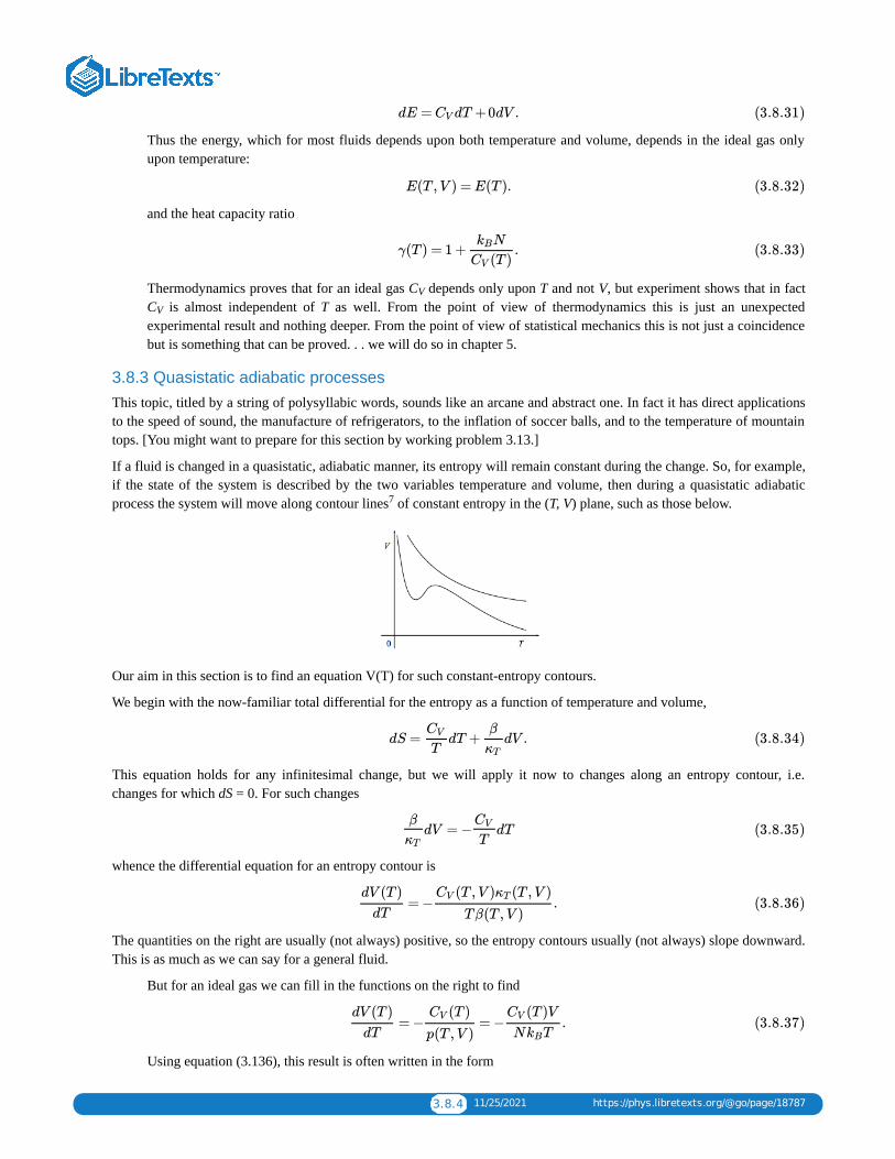
3.8.4 11/25/2021 https://phys.libretexts.org/@go/page/18787

Thus the energy, which for most fluids depends upon both temperature and volume, depends in the ideal gas onlyupon temperature:

and the heat capacity ratio

Thermodynamics proves that for an ideal gas C depends only upon T and not V, but experiment shows that in factC is almost independent of T as well. From the point of view of thermodynamics this is just an unexpectedexperimental result and nothing deeper. From the point of view of statistical mechanics this is not just a coincidencebut is something that can be proved. . . we will do so in chapter 5.

3.8.3 Quasistatic adiabatic processesThis topic, titled by a string of polysyllabic words, sounds like an arcane and abstract one. In fact it has direct applicationsto the speed of sound, the manufacture of refrigerators, to the inflation of soccer balls, and to the temperature of mountaintops. [You might want to prepare for this section by working problem 3.13.]

If a fluid is changed in a quasistatic, adiabatic manner, its entropy will remain constant during the change. So, for example,if the state of the system is described by the two variables temperature and volume, then during a quasistatic adiabaticprocess the system will move along contour lines of constant entropy in the (T, V) plane, such as those below.

Our aim in this section is to find an equation V(T) for such constant-entropy contours.

We begin with the now-familiar total differential for the entropy as a function of temperature and volume,

This equation holds for any infinitesimal change, but we will apply it now to changes along an entropy contour, i.e.changes for which dS = 0. For such changes

whence the differential equation for an entropy contour is

The quantities on the right are usually (not always) positive, so the entropy contours usually (not always) slope downward.This is as much as we can say for a general fluid.

But for an ideal gas we can fill in the functions on the right to find

Using equation (3.136), this result is often written in the form

dE = dT +0dV .CV (3.8.31)

E(T ,V ) = E(T ). (3.8.32)

γ(T ) = 1 + .NkB

(T )CV

(3.8.33)

V

V

7

dS = dT + dV .CV

T

β

κT(3.8.34)

dV = − dTβ

κT

CV

T(3.8.35)

= − .dV (T )

dT

(T ,V ) (T ,V )CV κT

Tβ(T ,V )(3.8.36)

= − = − .dV (T )

dT

(T )CV

p(T ,V )

(T )VCV

N TkB(3.8.37)

3.8.5 11/25/2021 https://phys.libretexts.org/@go/page/18787

This is as far as we can go for an arbitrary ideal gas.

But for an ideal gas with constant heat capacity, and hence with constant γ, this differential equation is readily solvedusing separation of variables. We write

with the immediate solution

giving

Remembering that γ ≥ 1, this confirms the downward slope of the entropy contours on the (V, T) plane. This result ismost frequently used with the variables p and T, rather than V and T:

The above equation holds only for quasistatic, adiabatic processes in ideal gases that have heat capacitiesindependent of temperature. You might think that it is such a restricted result that it holds little interest. Thisequation is used frequently in applications, in the graduate record examination, and in physics oral examinations!You should memorize it and know how to work with it.

Problems3.29 Intensive vs. extensive variables

Equation (3.134), E(T, V) = E(T), states that for an ideal gas the energy is a function of temperature alone. How is itpossible for E, an extensive quantity, to be a function of only T, an intensive quantity?

3.30 Heat capacity at constant pressure

Equation (3.131) shows that the heat capacity at constant volume, which is defined in terms of an entropy derivative,is also equal to an energy derivative. You might suspect a similar relation between C (T, p, N) and

Show that such a suspicion is not correct, and instead find an expression for C in terms of a derivative of enthalpy.

3.31 Qualitative heat capacity relations

(This problem is stolen from a GRE Physics test.)

For an ideal gas, C is greater than C because:

a. The gas does work on its surroundings when its pressure remains constant while its temperature isincreased.

b. The heat input per unit increase in temperature is the same for processes at constant pressure and at constantvolume.

c. The pressure of the gas remains constant when its temperature remains constant.

d. The increase in the gas’s internal energy is greater when the pressure remains constant than when thevolume remains constant.

e. The heat needed is greater when the volume remains constant than when the pressure remains constant.

3.32 Heat capacities in a magnetic system

For a magnetic system (see equation (3.100)), show that

= .dV (T )

dT

1

1 −γ(T )

V

T(3.8.38)

(1 −γ) =dV

V

dT

T(3.8.39)

(1 −γ) lnV = lnT + constant, (3.8.40)

= constant T or T = constant. V 1−γ V γ−1 (3.8.41)

p = constant .V γ (3.8.42)

p

.∂E(T ,p,N)

∂T)p,N

p

p V

3.8.6 11/25/2021 https://phys.libretexts.org/@go/page/18787

are related through

3.33 Isothermal compressibility

a. Show that the isothermal compressibility, defined in problem 1.2 as

is also given by

where ρ is the number density N/V. Clue:

b. What does this result tell you about the relation between density and chemical potential?

c. In part (a.) we began with a description in terms of the three variables T, p, N and then reduced it to an intensive-only description, which requires just two variables, such as µ and T. Reverse this process to show that

3.34 Pressure differential

By regarding pressure as a function of temperature T and number density ρ, show that

3.35 Isothermal vs. adiabatic compressibility

In class we derived a remarkable relation between the heat capacities C and C . This problem uncovers a similarrelation between the isothermal and adiabatic compressibilities,

The adiabatic compressibility κ is the compressibility measured when the fluid is thermally insulated. (It is relatedto the speed of sound: see problem 3.44.)

a. Use

to show that

Sketch an experiment to measure this quantity directly.

b. From the mathematical relation

= T , = T , β = , and =CH

∂S

∂T)H CM

∂S

∂T)M

∂M

∂T)H χT

∂M

∂H)T (3.8.43)

= −T /CM CH β2 χT (3.8.44)

= −κT1

V

∂V

∂p)T ,N (3.8.45)

= = = ,κT1

ρ

∂ρ

∂p)T

1

ρ2

∂ρ

∂μ)T

1

ρ2

p∂2

∂μ2)T (3.8.46)

= .∂ρ

∂p)T

∂ρ

∂μ)T

∂μ

∂p)T (3.8.47)

= = − .κTV

N 2

∂N

∂μ)T ,V

1

N

∂V

∂μ)T ,N (3.8.48)

dp = dT + dρ.β

κT

1

ρκT(3.8.49)

p V

= − and = − .κT1

V

∂V

∂p)T κS

1

V

∂V

∂p)S (3.8.50)

S

dS = dT + dp∂S

∂T)p

∂S

∂p)T (3.8.51)

= .∂T

∂p)S

βT

/VCp

(3.8.52)

dV = dp+ dT∂V

∂p)T

∂V

∂T)p (3.8.53)

3.8.7 11/25/2021 https://phys.libretexts.org/@go/page/18787

derive the multivariate chain rule

whence

c. Finally, show that

3.36 Change of chemical potential with temperature

Prove that

and that

How's that for weird?

It is easy to see why ∂V/∂T) itself is not tabulated. Instead of requiring a tabulation for iron, you would need a tabulationfor a five gram sample of iron, for a six gram sample of iron, for a seven gram sample of iron, etc.

Such contours are sometimes called isoentropic curves or, even worse, adiabats. The latter name is not just a linguistichorror, it also omits the essential qualifier that only quasistatic adiabatic processes move along curves of constant entropy

= + ,∂V

∂p)S

∂V

∂p)T

∂V

∂T)p

∂T

∂p)S (3.8.54)

= − .κS κTTβ2

/VCp

(3.8.55)

γ ≡ = .Cp

CV

κT

κS(3.8.56)

= −∂μ

∂T)p,N

S

N(3.8.57)

= − = − + .∂μ

∂T)V,N

∂S

∂N)T ,V

S

N

β

ρκT(3.8.58)

6p

7

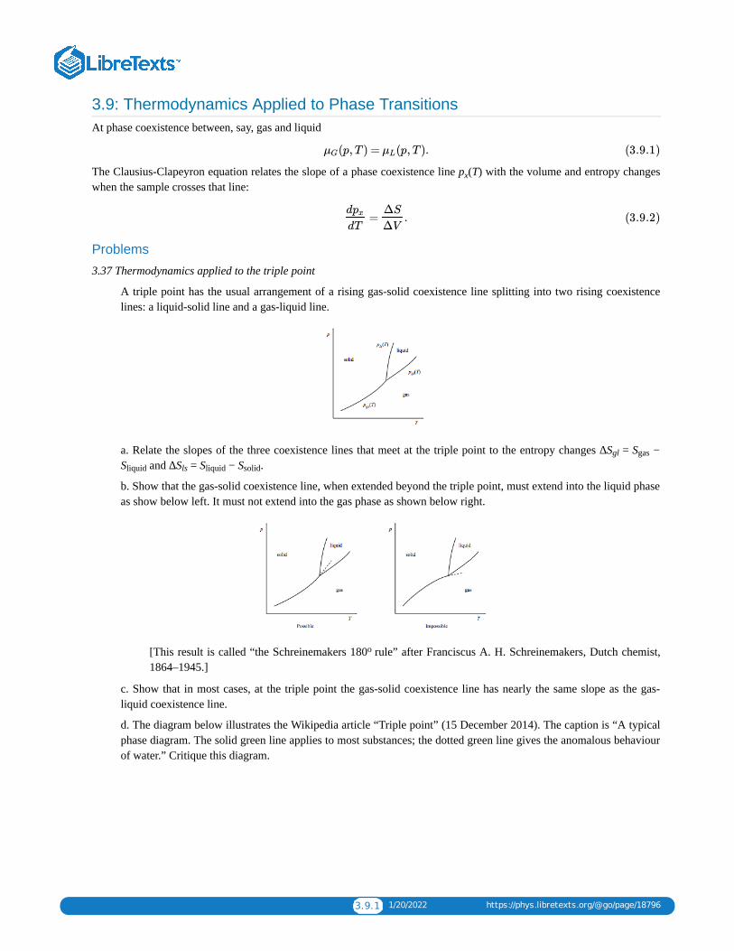
3.9.1 1/20/2022 https://phys.libretexts.org/@go/page/18796

3.9: Thermodynamics Applied to Phase TransitionsAt phase coexistence between, say, gas and liquid

The Clausius-Clapeyron equation relates the slope of a phase coexistence line p (T) with the volume and entropy changeswhen the sample crosses that line:

Problems

3.37 Thermodynamics applied to the triple point

A triple point has the usual arrangement of a rising gas-solid coexistence line splitting into two rising coexistencelines: a liquid-solid line and a gas-liquid line.

a. Relate the slopes of the three coexistence lines that meet at the triple point to the entropy changes ∆S = S −S and ∆S = S − S .

b. Show that the gas-solid coexistence line, when extended beyond the triple point, must extend into the liquid phaseas show below left. It must not extend into the gas phase as shown below right.

[This result is called “the Schreinemakers 180 rule” after Franciscus A. H. Schreinemakers, Dutch chemist,1864–1945.]

c. Show that in most cases, at the triple point the gas-solid coexistence line has nearly the same slope as the gas-liquid coexistence line.

d. The diagram below illustrates the Wikipedia article “Triple point” (15 December 2014). The caption is “A typicalphase diagram. The solid green line applies to most substances; the dotted green line gives the anomalous behaviourof water.” Critique this diagram.

(p,T ) = (p,T ).μG μL (3.9.1)

x

= .dpx

dT

ΔS

ΔV(3.9.2)

gl gas

liquid ls liquid solid

o

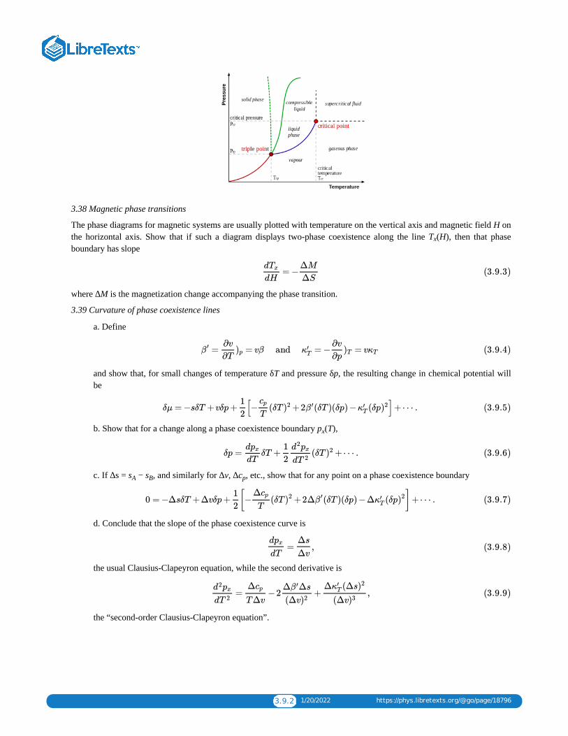
3.9.2 1/20/2022 https://phys.libretexts.org/@go/page/18796

3.38 Magnetic phase transitions

The phase diagrams for magnetic systems are usually plotted with temperature on the vertical axis and magnetic field H onthe horizontal axis. Show that if such a diagram displays two-phase coexistence along the line T (H), then that phaseboundary has slope

where ∆M is the magnetization change accompanying the phase transition.

3.39 Curvature of phase coexistence lines

a. Define

and show that, for small changes of temperature δT and pressure δp, the resulting change in chemical potential willbe

b. Show that for a change along a phase coexistence boundary p (T),

c. If ∆s = s − s , and similarly for ∆v, ∆c , etc., show that for any point on a phase coexistence boundary

d. Conclude that the slope of the phase coexistence curve is

the usual Clausius-Clapeyron equation, while the second derivative is

the “second-order Clausius-Clapeyron equation”.

x

= −dTx

dH

ΔM

ΔS(3.9.3)

= = vβ and = − = vβ ′ ∂v

∂T)p κ′

T

∂v

∂p)T κT (3.9.4)

δμ = −sδT +vδp+ [− (δT +2 (δT )(δp) − (δp ]+⋯ .1

2

cp

T)2 β ′ κ′

T )2 (3.9.5)

x

δp = δT + (δT +⋯ .dpx

dT

1

2

d2px

dT 2)2 (3.9.6)

A B p

0 = −ΔsδT +Δvδp+ [− (δT +2Δ (δT )(δp) −Δ (δp ]+⋯ .1

2

Δcp

T)2 β ′ κ′

T )2 (3.9.7)

= ,dpx

dT

Δs

Δv(3.9.8)

= −2 + ,d2px

dT 2

Δcp

TΔv

Δ Δsβ ′

(Δv)2

Δ (Δsκ′T )2

(Δv)3(3.9.9)

3.10.1 1/13/2022 https://phys.libretexts.org/@go/page/18888

3.10: Thermodynamics Applied to Chemical Reactions

3.10.1 Thermodynamics of mixtures

So far in this book we have considered mostly pure substances. What happens if we have a mixture of several chemicalspecies, say the four substances A, B, C, and D? In this case the mechanical parameters will include the numbers N , N ,N , and N , and the entropy

will have the total differential

The differential above defines the quantity

Notice that the chemical potential of substance A can depend upon the number of molecules of B, C, and D present, so it isnot necessarily the same as the chemical potential of pure A. (For example, the chemical potential of sugar dissolved in acup of water is not equal to the chemical potential of pure sugar, unless the solution is saturated and there is undissolvedsugar at the bottom of the cup.)

It is convenient to define the total number of molecules

and the (intensive) fractional amounts

The thermodynamic dance can be followed for mixtures just as well as it can be for pure substances. One noteworthy resultis

3.10.2 Equilibrium condition for a chemical reaction

Suppose that α molecules of substance A can combine with β molecules of substance B to produce γ molecules ofsubstance C and δ molecules of substance D. If this can happen, then of course the reverse can also occur: γ molecules ofsubstance C may combine with δ molecules of substance D to produce α molecules of substance A and β molecules ofsubstance B. The first action is called a “forward step” of the chemical reaction, and the second is called a “backwardstep”. This chemical reaction is symbolized by

Thus if we mix together a certain number of molecules each of A, B, C, and D, there can be a reaction and we might notend up with the same distribution of molecules that we started off with. It is possible that there will be more forward thanbackwards steps, in which case we will end up with more C’s and D’s and fewer A’s and B’s than we had at the start, or itcould go predominantly the other way. It is allowable for the system to exist in a wide range of conditions, varying from“mostly reactants” to “mostly products”, but experience teaches us that the overwhelmingly likely condition is one withsome of each are present. In this condition reactions still proceed, in both the forward and backward directions, but steps inboth directions proceed at the same rate so there is no net change in the number of molecules of any species. Thiscondition is called “chemical equilibrium”.

A B

C D

S(E,V , , , , )NA NB NC ND (3.10.1)

dS = dE+ dV − d .1

T

p

T∑i=A

D μi

TNi (3.10.2)

(E,V , , , , ) = −T (E,V , , , , ) .μA NA NB NC ND NA NB NC ND

∂S

∂NA

)E,V, , ,NB NC ND (3.10.3)

N = + + +NA NB NC ND (3.10.4)

= , etc.fANA

N(3.10.5)

G(T , p, , , , )NA NB NC ND ≡ E−TS+pV

= (T , p, , , , )∑i=A

D

μi fA fB fC fD Ni

αA +βB⟺ γC +δD. (3.10.6)

3.10.2 1/13/2022 https://phys.libretexts.org/@go/page/18888

The above paragraph precisely parallels the discussion in section 2.7, “Using entropy to find (define) temperature andpressure”. In that section we saw that if, for example, two systems could exchange volume, it was possible for all thevolume to go to one system or for all of it to go to the other system, but that the overwhelmingly likely possibility was the“equilibrium condition” in which the two systems shared volume in such a way that each had the same pressure. Theequilibrium condition was the one with a maximum number of microstates (or, equivalently, a maximum entropy) withrespect to the distribution of volume.

Precisely the same effect is at work in chemical equilibrium. The equilibrium state is characterized by a maximum in theentropy with respect to the number of number of reaction steps taken. At this equilibrium point the entropy doesn’t changewhen the chemical reaction proceeds by one step in either direction. The change in entropy through a forward step is ofcourse

and the change in entropy through a backward step is the negative of this. In either case, the equilibrium condition is thatthis change in entropy vanish, i.e. that

Interpretation in terms of “escaping tendency”.

If we specialize to the case of liquid-gas phase equilibrium, this equation is just equation (3.162).

We cannot go further without formulas for the chemical potentials µ. Complete formulas are not available within the realmof thermodynamics, but the next section shows that thermodynamics can put severe constraints on the permissiblefunctional forms for µ.

3.10.3 Chemical potential of an ideal gasI emphasized on page 69 that the equation of state did not contain full thermodynamic information. Thus, for example,knowledge of the equation of state V(T, p, N) is not sufficient to uncover the master function G(T, p, N). On the other hand,that knowledge is sufficient to restrict the functional form of the Gibbs potential, which in turn restricts the possiblefunctional forms of the chemical potential. In this subsection we uncover that restriction.

Our strategy is to recognize that volume is the derivative of G(T, p, N) with respect to p, and chemical potential is thederivative of G(T, p, N) with respect to N. Given V(T, p, N), we can integrate with respect to p to find G(T, p, N), and thendifferentiate with respect to N to find µ(T, p). This process does not completely determine the Gibbs potential or thechemical potential, because a constant of integration is involved. But it does restrict the permissible functional forms ofG(T, p, N) and µ(T, p). The master thermodynamic equation for variables (T, p, N) is

whence

Thus for a substance obeying the ideal gas equation of state, we have

Integrating both sides with respect to p gives

or

−α −β +γ +δ ,∂S

∂NA

∂S

∂NB

∂S

∂NC

∂S

∂ND

(3.10.7)

α +β = γ +δ .μA μB μC μD (3.10.8)

dG= −SdT +V dp+μdN (3.10.9)

V (T , p,N) = .∂G

∂p)T ,N (3.10.10)

= .N TkB

p

∂G

∂p)T ,N (3.10.11)

N T ∫ = ∫ dpkBdp

p

∂G

∂p)T ,N (3.10.12)

N T ln( ) = G(T , p,N)kBp

(T ,N)p(3.10.13)

3.10.3 1/13/2022 https://phys.libretexts.org/@go/page/18888

The role of “constant of integration” is played by , which must be constant with respect to p but which may varywith T and N.

In fact, careful examination of the above equation shows what the dependence of on N must be. The quantities Gand N above are extensive, while T and p are intensive, so must be intensive so that both sides will depend linearly onsystem size. Thus is independent of N, and we have

whence

This is the form of the Gibbs potential and of the chemical potential for any ideal gas. The function isundetermined, and it is through differences in (T)\) that one ideal gas differs from another. But the dependence on pand on N are completely pinned down by the above results.

This result is frequently written in terms of the number density ρ = N/V. For an ideal gas p = k Tρ, and we can define thefunction through . Then we can write

What if the ideal gas is a mixture of, say, the four chemical species A, B, C, and D? Exactly the same result applies foreach species:

where the function ˜ρA(T) is the same for a pure ideal gas of A and for an ideal gas mixture. The chemical potential µ isindependent of the densities ρ , ρ , and ρ . I am looking for a purely thermodynamic argument to proved this result, butuntil I find it you’ll have to accept this statistical argument: In an ideal gas the molecules of A don’t interact with themolecules of B, C, and D, so they don’t know whether or not such molecules are even present. The behavior of A thuscan’t depend upon the number of B, C, and D molecules present, and it will be the same even if there are 0 molecules of B,C, and D, that is if the gas is pure.

3.10.4 The equilibrium condition for idea gas reactions

[Before plunging in, I want to point out that there’s a contradiction embodied in the term “ideal gas chemical reaction”. Inan ideal gas, molecules do not interact. . . when two molecules approach, they just pass right through each other. But achemical reaction is a form of interaction! Clearly, in this section we are thinking of molecules that interact weakly unlessthey are very close to each other, but once they approach they interact strongly and react quickly.]

Putting together the general equilibrium condition for chemical reactions

with expression (3.183) for the chemical potential of an ideal gas gives the equilibrium condition

Using the properties of logarithms, this can be rewritten as

or, after minor rearrangement, as

(T ,N)p~

(T ,N)p~

p~

p~

G(T , p,N) = N T ln( )kBp

(T )p~(3.10.14)

μ(T , p) = = T ln( ).G(T , p,N)

NkB

p

(T )p~(3.10.15)

\( (T )p~

\(p~

B(T )ρ~ \( (T ) = T (T )ρ~ kB ρ~

μ(T , ρ) = T ln( ).kBρ

(T )ρ(3.10.16)

(T , ) = T ln( )μA ρA kBρA

(T )ρ~A(3.10.17)

A

B C D

α +β = γ +δμA μB μC μD (3.10.18)

α T ln( )+β T ln( ) = γ T ln( )+δ T ln( )kBρA

(T )ρAkB

ρB

(T )ρBkB

ρC

(T )ρCkB

ρD

(T )ρD(3.10.19)

= ,( )ρA

(T )ρA

α

( )ρB

(T )ρB

β

( )ρC

(T )ρC

γ

( )ρD

(T )ρD

δ

(3.10.20)

3.10.4 1/13/2022 https://phys.libretexts.org/@go/page/18888

Chemists like to write this equation in terms of “the concentration of A”, written as [A], namely as

where K(T) is called the “equilibrium constant” (despite the fact that it is a function of temperature). This result is calledthe “law of mass action” despite the fact that it is not a fundamental law (we have just derived it) and even despite the factthat (because it holds only for ideal gases) it’s not precisely true for any real substance! (And also, I might add, despite thefact that the “law” has nothing to do with “mass” or with “action”.) Even though the result is poorly named, it shows justhow valuable thermodynamics is in connecting disparate areas of research. Who would have guessed that the law of massaction follows from only thermodynamics and the ideal gas equation of state? We have proven the result without oncedoing a chemical experiment!

Problems3.40 Chemical potential for ideal gas mixtures

The entropy S(E, V, N , N ) of a classical monatomic ideal gas mixture was uncovered using statistical mechanics inproblem 2.16. Invert the result of that problem to find E(S, V, N , N ), then show that the temperature and pressureof an ideal gas mixture obey familiar results for pure ideal gases. Show that

and relate this expression to the form (3.183). Verify relation (3.172). 3.41 Relations between equilibrium constantsYou measure the equilibrium constants for these three chemical reactions:

(Call those constants K , K , and K .) Find an expression for the equilibrium constant for the reaction

= .ργ

CρδD

ραAρβ

B

(T ) (T )ρ~γ

C ρ~δD

(T ) (T )ρ~αA ρβ

B

(3.10.21)

= K(T ),[C [D]γ ]δ

[A [B]α ]β(3.10.22)

A B

A B

(T , p, , ) = T ln p ,μA fA fB kB⎡

⎣( )

h20

2πmA( T )kB5/3

3/2

fA⎤

⎦(3.10.23)

2 +H2 O2

+H2 Cl2+2Cl2 O2

⟺ 2 OH2

⟺ 2HCl

⟺ 2ClO2

A B C

4 +2 O⟺ 4HCl +5ClO2 H2 O2

3.11.1 12/23/2021 https://phys.libretexts.org/@go/page/18889

3.11: Thermodynamics Applied to LightAnother non-fluid system (see section 3.7).

See Robert E. Kelly, “Thermodynamics of blackbody radiation,” Am. J. Phys. 49 (1981) 714–719, and Max Planck, TheTheory of Heat Radiation, part II.

How do you get a “box of light?” This is blackbody (cavity) radiation: meaning radiation in thermal equilibrium. (Usuallyit’s also in equilibrium with the cavity walls, but you could imagine a container with mirror walls. . . )

3.11.1 Fundamentals

The fundamental thermodynamic equation for this system involves the master function E(S, V). It is

This equation differs from previously encountered master equations in that there is no term for µ dN. From the classicalperspective, this is because radiation is made up of fields, not particles. From the quantal perspective, this is becausephoton number is not conserved.

Thermodynamics binds one quantity to another, but it must use experiment (or statistical mechanics) to find the valuesbeing bound. For example, thermodynamics tells us that

but it cannot calculate either C , or C , or β, or κ : these quantities must be found by experiment (or through a statisticalmechanical calculation). The empirical result that we will employ is that for blackbody radiation,

This equation of state is the parallel for blackbody radiation to pV = Nk T for ideal gases. It was discovered by experiment,but it can be derived from electrodynamics as well.

3.11.2 Energy density as a function of temperatureConsider the energy as a function of volume and temperature. Because E(V, T) is extensive, but in the argument list only Vis extensive (recall that N doesn’t appear in the argument list), we must have

That is, the energy density u depends only upon temperature. What is this dependence?

We seek a differential equation for u(T). Compare

with

Together these give us a formula for dS:

The Maxwell relation associated with this differential is

or

dE = TdS−pdV . (3.11.1)

= +TV ,Cp CV

β2

κT(3.11.2)

p V T

p = = u.1

3

E

V

1

3(3.11.3)

B

E(V ,T ) = V u(T ). (3.11.4)

dE = d(V u) = V du+udV = V dT +udVdu

dT(3.11.5)

dE = TdS−pdV = TdS− udV .1

3(3.11.6)

dS =( ) dT +[ ]dV .V

T

du

dT

4

3

u

T(3.11.7)

=∂( )

∂V)T

∂[ ]

∂T)V (3.11.8)

3.11.2 12/23/2021 https://phys.libretexts.org/@go/page/18889

A rearrangement gives

The solution is

whence

The Stefan-Boltzmann law!

3.11.3 Quasistatic adiabatic expansion of radiationConsider a sample of radiation undergoing quasistatic adiabatic change of volume. The entropy is a constant during thisprocess, although the value of that constant will of course depend on the particular sample that’s expanding.

but dS = 0, E = uV, and p = u/3 so

Recognizing that this constant will depend upon which adiabat is taken, i.e. that it will depend on the entropy, we write

Using the Stefan-Boltzmann result u = σT we find that

This explains the cooling of the universe as it expands from the initial “hot big bang” to the current “3 K microwavebackground.”

3.11.4 Thermodynamics of the energy spectrum

What if we consider not just the energy density per volume, but the energy density per volume and wavelength? Let

represent the energy per volume due to that radiation with wavelength between λ and λ + dλ. As you know, quantummechanics was discovered through Planck’s efforts to find a theoretical explanation for the measured function .This is not the place to describe Planck’s work. Instead I want to focus on a purely thermodynamic result that was knownlong before Planck started his investigations.

This is Wien’s law , which states that the function , which you’d think could have any old form, must be of theform

An immediate consequence of Wien’s law is the Wien displacement theorem: The wavelength λˆ which maximizes is inversely proportional to temperature:

= = [ − u] .1

T

du

dT

4

3

d[u/T ]

dT

4

3

1

T

du

dT

1

T 2(3.11.9)

= 4du

dT

u

T(3.11.10)

4 lnT = lnu+ const (3.11.11)

u(T ) = σ .T 4 (3.11.12)

dE = TdS−pdV (3.11.13)

udV +V du

V du

lnu

u

= − udV1

3

= − udV4

3

= − lnV +const4

3

= KV −4/3

u(S,V ) = K(S) .V −4/3 (3.11.14)

4

T (S,V ) = .C(S)

V 1/3(3.11.15)

o

(T ,λ)dλu (3.11.16)

(T ,λ)u

8 (T ,λ)u

(T ,λ) = f(λT ).u T 5 (3.11.17)

(T ,λ)u

3.11.3 12/23/2021 https://phys.libretexts.org/@go/page/18889

where the constant is the value of x that maximizes f(x). The consequences of the Wien displacement theorem are familiarfrom daily life: low temperature objects (such as people) radiate largely in the infrared, moderate temperature objects (suchas horseshoes in the forge) radiate largely in the red, while high temperature objects (such as the star Sirius) radiate largelyin the blue.

I stated earlier that Wien’s law is a purely thermodynamic result. That’s almost true, but it also relies on one more factfrom electrodynamics, a result called “no mode hoping”:

If the volume makes a quasistatic, adiabatic change from V to V , then the light of wavelength in the range λ to λ+ dλ shifts into the range λ to λ + dλ where

(This result may be derived rigorously from Maxwell’s equations, but it’s reasonable through this analogy: A string oflength L vibrating in, say, its third mode, has wavelength . If the length of the string is slowly changed, then thewave remains in its third mode, so λ/L is constant.)

Now we’re ready to begin the derivation. Consider the quasistatic adiabatic expansion of light, and while that expansion isgoing on focus your attention on the light in wavelength range λ to λ + dλ. According to the “no mode hopping” result,during this expansion the quantity

remains constant during the expansion. Furthermore, according to equation (3.203) the quantity

also remains constant. Multiplying these two equations, we find that the volume-independent quantity

remains constant during the expansion: this number characterizes the expansion.

Another such volume-independent constant can be found by repeating the reasoning of subsection 3.11.3, Quasistaticadiabatic expansion of radiation, but considering not the energy of all the radiation, but the energy of the radiation withwavelengths from λ to λ+ ∆λ. This energy is , and the pressure due to this segment of the radiation is

. During a quasistatic adiabatic expansion, dE = −pdV, so

During the expansion the volume and wavelengths are changing through (see equation 3.207)

so we have

Thus

(T ) = ,λ constant

T(3.11.18)

1 2 1 1

1 2 2 2

= .λ1

V1/3

1

λ2

V1/3

2

(3.11.19)

λ = L32

λ/V 1/3 (3.11.20)

TV 1/3 (3.11.21)

Tλ (3.11.22)

E = V Δλu

p = Δλ13u

(V Δλ)d +( Δλ)dV +( V )d[Δλ] = − ΔλdV .u u u1

3u (3.11.23)

λ

dλ

d[Δλ]

= cV 1/3

= c dV = dV1

3V −2/3 1

3

λ

V

= dV1

3

Δλ

V

(V Δλ)d = − ΔλdV .u5

3u (3.11.24)

3.11.4 12/23/2021 https://phys.libretexts.org/@go/page/18889

But equation (3.203) shows how a larger volume is related to a lower temperature, so the quantity

remains constant during the expansion.

Thus we have two volume-independent ways to characterize the particular curve taken by this expansion. In thethermodynamics of light, a state is specified by two variables, so a curve is specified by only one parameter. Hence thesetwo characterizations cannot be independent: one must be a function of the other. Thus

or

Wein's law.

Wien is pronounced like the English “veen”.

Problems3.42 Heat capacity of light

Show that, for blackbody radiation, C = 4E/T.

Resources

Thermodynamic tables. (G.N. Lewis and M. Randall) Zemansky. Practical heat engines. Callen. Fermi.

Math book. e.g. Taylor and Mann?

Picture of Smithsonian crystal on www?

Thermodynamic data (e.g. steam tables) on www?

V du

ln u

u

= − dV5

3u

= − lnV +const5

3

= KV −5/3

(T ,λ)u

T 5(3.11.25)

= f(λT )(T ,λ)u

T 5(3.11.26)

(T ,λ) = f(λT ).u T 5 (3.11.27)

8

V

3.12.1 1/6/2022 https://phys.libretexts.org/@go/page/18890

3.12: Additional Problems3.43 Cool mountain air

Model the earth’s atmosphere as an ideal gas (nitrogen) in a uniform gravitational field. Ignore all winds. Let mdenote the mass of a gas molecule, g the acceleration of gravity, and z the height above sea level.

a. Use ideas from Newtonian mechanics to show that the change of atmospheric pressure p with height z is

b. If the atmosphere is a poor conductor of heat, then the decrease in pressure with height is due to anadiabatic expansion. (Clue: In other words: At the bottom of the mountain, fill an insulated balloon with air atthe local density, pressure, and temperature. Transport that balloon to the top of the mountain. During thejourney the balloon will expand, so the density, pressure, and temperature will change. According to ourassumption, during this journey the balloon’s density, pressure, and temperature will match those of theatmosphere outside.) Show that under this assumption

and hence that

Evaluate this expression in kelvin per kilometer for nitrogen, which has γ = 1.4.

c. In contrast, if the atmosphere were a good conductor of heat, then temperature would be uniform. Find p(z)under such circumstances. Denote the sea-level pressure and temperature by p and T .

d. Similarly find p(z) for an adiabatic atmosphere. 3.44 The speed of sound When a sound wave passesthrough a fluid (liquid or gas), the period of vibration is short compared to the time necessary for significantheat flow, so the compressions may be considered adiabatic. Analyze the compressions and rarefactions offluid in a tube. The equilibrium mass density is ρ . Apply F = ma to a slug of fluid of thickness ∆x, and showthat if the variations in pressure p(x, t) are small then pressure satisfies the wave equation

where c, the speed of sound, is given by

Optional: Use the results of problems 1.2 and 3.35 to show that, for an ideal gas,

3.45 Thermodynamics of a plastic rod

(This problem is based on Reif problem 5.14.)

For a restricted range of lengths L and temperatures T, the tension force in a stretched plastic rod is

where a is a positive constant and L is the relaxed (unstretched) length of the rod. When L = L , the heat capacityC of the rod (measured at constant length) is given by C (T, L ) = bT, where b is independent of temperature.

a. Write down the fundamental thermodynamic relation for this rod, expressing dE in terms of dS and dL.

= − p(z).dp

dz

mg

T (z)kB(3.12.1)

=dp

dT

γ

γ−1

p(T )

T(3.12.2)

= − .dT

dz

γ−1

γ

mg

kB(3.12.3)

0 0

0

=p∂2

∂t2c2 p∂2

∂x2(3.12.4)

c = .1

ρ0κS− −−−√

(3.12.5)

c = .γTkB

m

− −−−−√ (3.12.6)

F (T ,L) = a (L− ),T 2 L0 (3.12.7)

0 0

L L 0

3.12.2 1/6/2022 https://phys.libretexts.org/@go/page/18890

b. Compute (∂S/∂L)T. (Clue: Derive an appropriate Maxwell relation for the assembly with variables T and L.)

c. Knowing S(T , L ), integrate along an appropriate path to find S(T, L) at any temperature and length withinthe range of applicability of the equation for F(T, L).

d. If you start at T = T and L = L and then quasi-statically stretch a thermally insulated rod until it reacheslength L , what is the final temperature T ? Show than when L ≤ L < L , the rod is cooled by this process.

e. Find the heat capacity C (L, T) of the rod when its length is not necessarily L .

f. Find (∂T/∂L)S for arbitrary T and L. Can insulated stretches warm as well as cool the rod?

3.46 Magnetic cooling

At low temperatures, paramagnetic salts obey the Curie law

where c is a positive constant (see equation (3.100)). Assume that the heat capacity C is a constant independent oftemperature and field. Suppose a sample at magnetic field H and temperature T is wrapped in insulation, and thenthe magnetic field is slowly reduced to zero. Find the final temperature, and show that it is less than T . Thistechnique, known as “adiabatic demagnetization” is the refrigeration method used to produce the temperatures fromabout 1 kelvin to 1 microkelvin.

3.47 Thermodynamics of an electrochemical cell

Reif 5.16.

3.48 Thermodynamics and evolution

Read the essay “Thermodynamics and Evolution” by John W. Patterson, in Scientists Confront Creationism, LaurieR. Godfrey, ed. (Norton, New York, 1983), pages 99–116, on reserve in the science library.

a. When a snowflake forms, its surroundings increase in entropy (“become more disordered”). What is thename of the heat flow associated with this entropy change?

b. Patterson argues that ∆S < 0 on Earth, due to biological evolution, and that ∆S > 0 somewhere else in theuniverse in order to make up for it. Where is that entropy increase taking place?

c. Patterson feels the need to invoke “self-organization” and Prigogine (pages 110–111) to explain how his rampumps could be made. Is this necessary? List two or more situations from nature in which water does flowuphill.

3.49 Entropy and evolution

Creationists sometimes claim that the second law of thermodynamics prohibits biological evolution.

a. The surface of the Sun (mean temperature 5778 K) heats the surface of the Earth (mean temperature 288 K)through visible and near-infrared radiation. The solar energy absorbed by the Earth each second is 1.732 ×10 J. What is the entropy change per second (due to this process) of the Sun? The Earth? Does the entropy of“Sun plus Earth” increase or decrease?

b. Yet the mean temperature of the Earth changes slowly, if at all. This is because almost all of the solar energyabsorbed by the Earth is then emitted through far-infrared radiation which in turn heats “outer space” — thecosmic microwave background (CMB; temperature 2.728 K). What is the entropy change per second (due tothis process) of the Earth? The CMB? Does the entropy of “Earth plus CMB” increase or decrease?

c. Now refine the model by supposing that, due to evolution, the entropy of the Earth is not exactly constant,but is decreasing. (In this case the entropy of the CMB would have to be increasing faster than rate predictedin part (b).) Suppose that, due to evolution, each individual organism is 1000 times “more improbable” thanthe corresponding individual was 100 years ago. In other words, if Ω is the number of microstates consistentwith the specification of an organism 100 years ago, and if Ωf is the number of microstates consistent with the

0 0

i i

f f 0 i f

L 0

M = c ,H

T(3.12.8)

H

i i

i

17

i

3.12.3 1/6/2022 https://phys.libretexts.org/@go/page/18890

specification of today’s “improved and less probable” organism, then Ω = 10−3Ω . What is the correspondingchange in entropy per organism?

d. The population of Earth is about 1018 eukaryotic individuals and 1032 prokaryotic individuals. If theestimate of part (c) holds for each one of them, what is the change in entropy due to evolution each second?

e. How accurately would you have to measure the entropy flux of part (b) in order to notice the diversion ofentropy flux calculated in part (d)? Has any scientific quantity ever been measured to this accuracy?

f. It is generally agreed that the greatest rate of evolution fell during the Cambrian period, from 542 millionyears ago to 488 million years ago. During this so-called “Cambrian explosion” multicellular organisms firstformed and then radiated into remarkable variety. Suppose that during the Cambrian period entropy wasdiverted into the evolution of living things at the rate calculated in part (d). And suppose that at the end of theCambrian there were 10 multicellular individuals. How much “improved and less probable” would eachorganism be, relative to its single-celled ancestor at the beginning of the Cambrian period?

The moral of the story? There’s plenty of entropy to go around.

f i

18

1 1/27/2022

CHAPTER OVERVIEW4: ENSEMBLES

After the last chapter’s dip into thermodynamics, we return to the discussion of the principles of statistical mechanics begun in chapter2.

4.1: THE CANONICAL ENSEMBLE4.2: MEANING OF THE TERM “ENSEMBLE”4.3: CLASSICAL MONATOMIC IDEAL GASI’ve told you that it’s easier to do calculations in the canonical ensemble than in the microcanonical ensemble. Today I’m going todemonstrate the truth of this assertion.

4.4: ENERGY DISPERSION IN THE CANONICAL ENSEMBLE4.5: TEMPERATURE AS A CONTROL VARIABLE FOR ENERGY (CANONICAL ENSEMBLE)4.6: THE EQUIVALENCE OF CANONICAL AND MICROCANONICAL ENSEMBLES4.7: THE GRAND CANONICAL ENSEMBLE4.8: THE GRAND CANONICAL ENSEMBLE IN THE THERMODYNAMIC LIMIT4.9: SUMMARY OF MAJOR ENSEMBLES4.10: QUANTAL STATISTICAL MECHANICS4.11: ENSEMBLE PROBLEMS I4.12: ENSEMBLE PROBLEMS II

Daniel F. Styer 4.1.1 1/27/2022 https://phys.libretexts.org/@go/page/6350

4.1: The Canonical EnsembleExamples of “systems” and “baths”:

Bottle of wine/a swimming pool.Sample of gas/laboratory temperature control apparatus.One ideal gas molecule/sample of gas.But not one interacting gas molecule/sample of gas. (The Boltzmann distribution is for systems within ensembles, notfor molecules within systems.)

We denote a microstate by x. Exactly what is meant by a microstate will depend upon circumstances. For a system of pointparticles it means specifying all the positions and momenta. For a spin system it means specifying the “up” or “down” stateof each spin. We’ll see other examples later.

I’ll try to use different letters for microscopic and macroscopic (thermodynamic) quantities. For example H(x) versus E(the thermodynamic energy is ; versus .

SummaryThe canonical ensemble in general:

The probability that the system is in the microstate x is proportional to the “Boltzmann factor”

The normalization factor is called the “partition function” or “sum over all states” (German “Zustandsumme”):

(Note that Z is independent of x.) Thus the probability that the system is in microstate x is

The connection to thermodynamics is that the Helmholtz free energy is

Note that in finding Z we sum over all microstates: the low-energy ones, the high-energy ones, the “orderly” ones (e.g. allatoms heading west, or all atoms heading east), the “disorderly” ones (e.g. atoms heading in scattered directions).

The canonical ensemble for a pure classical monatomic fluid:

The probability that the system is in the microstate Γ is proportional to the “Boltzmann factor”

Writing out all the normalizations correctly gives: the probability that the system is in some microstate within the phasespace volume element dΓ about Γ is

where the partition function is

(The integral runs over all of phase space.) This is an example of “partition function”, namely the partition function for apure classical monatomic fluid. It does not apply to mixtures, to crystals, to the ideal paramagnet. In contrast, the definitionof “partition function” is equation (4.2), the “sum over all states” of the Boltzmann factor.

E = ⟨H(x)⟩ M(x) M = ⟨M(x)⟩

.e−H(x)/ TkB (4.1.1)

Z(T ,V ,N) = .∑ microstates x

e−H(x)/ TkB (4.1.2)

.e

−H(x)/ TkB

Z(T ,V ,N)(4.1.3)

F (T ,V ,N) = − T lnZ(T ,V ,N).kB (4.1.4)

.e−H(Γ)/ TkB (4.1.5)

dΓ,e−H(Γ)/ TkB

N ! Z(T ,V ,N)h3N0

(4.1.6)

Z(T ,V ,N) = ∫ dΓ.1

N !h3N0

e−H(Γ)/ TkB (4.1.7)

Daniel F. Styer 4.2.1 1/4/2022 https://phys.libretexts.org/@go/page/6351

4.2: Meaning of the Term “Ensemble”An ensemble is just a collection. For example, a musical group is an ensemble. Think of a bunch of systems filling up ahuge gymnasium.

Microcanonical ensemble: A collection of many systems, all with the same volume, particle number, particle mass,chemical composition, etc., and each with energy E < H(x) ≤ E + ∆E.Canonical ensemble: A collection of many systems, all with the same volume, particle number, particle mass, chemicalcomposition, etc., and each connected to the same heat bath (whence each with the same temperature T).

The names (selected by J. Willard Gibbs) are pretty poor.

Daniel F. Styer 4.3.1 12/30/2021 https://phys.libretexts.org/@go/page/6352

4.3: Classical Monatomic Ideal GasI’ve told you that it’s easier to do calculations in the canonical ensemble than in the microcanonical ensemble. Today I’mgoing to demonstrate the truth of this assertion.

Remember how we found the entropy S(E, V, N) for a classical monatomic ideal gas? The hard part involved finding thevolume of a shell in 3N-dimensional space. It took us three or four hours to derive the Sackur-Tetrode formula (equation(2.32)), namely

It took us another hour or so to show that the energy of this system is (equation (2.57))

whence

In this section, we’ll derive this same equation using the canonical ensemble. While the derivation is no stroll in the park,most people find it considerably easier than the microcanonical derivation.

Our strategy will be: (1) Integrate the Boltzmann factor over all phase space to find the partition function Z(T, V, N). (2)Find the Helmholtz free energy using

And finally (3) use the thermodynamic result

to find the entropy.

The Hamiltonian for this model system is

where the potential energy function for each individual atom as a function of its location x is

This has been background. Now we’re ready to roll up our sleeves and plunge into the work. Any questions? Okay, let’sgo.

The canonical partition function is

There are N triplets of integrals over positions and N triplets of integrals over momenta. . . in total, a 6N-dimensionalintegral. Because the Hamiltonian consists of a sum of terms, the Boltzmann factor consists of a product of quantities:

S(E,V ,N) = N [ ln( )+ ] .kB3

2

4πmEV 2/3

3h20N

5/3

5

2(4.3.1)

E = N T3

2kB (4.3.2)

S(T ,V ,N) = N [ ln( )+ ] .kB3

2

2πm TkB V 2/3

h20N

2/3

5

2(4.3.3)

F (T ,V ,N) = − T ln(Z(T ,V ,N)).kB (4.3.4)

S(T ,V ,N) = −∂F

∂T)V,N (4.3.5)

H(Γ) = ( + + + +⋯ + )+U ( ) +U ( ) +⋯ +U ( ) ,1

2mp2x,1 p2

y,1 p2z,1 p2

x,2 p2z,N x1 x2 xN (4.3.6)

U(x) = 0

∞

if x is inside the container

if outside (4.3.7)

Z(T ,V ,N) =

=

∫ dΓ1

N !h3N0

e−βH(Γ)

d d d ⋯ d d d1

N !h3N0

∫+∞

−∞x1 ∫

+∞

−∞y1 ∫

+∞

−∞z1 ∫

+∞

−∞xN ∫

+∞

−∞yN ∫

+∞

−∞zN

× d d d ⋯ d d d∫+∞

−∞px,1 ∫

+∞

−∞py,1 ∫

+∞

−∞pz,1 ∫

+∞

−∞px,N ∫

+∞

−∞py,N ∫

+∞

−∞pz,Ne

−βH(r)

Daniel F. Styer 4.3.2 12/30/2021 https://phys.libretexts.org/@go/page/6352

More importantly, however, each of these quantities depends on a different set of variables. Therefore the partitionfunction also breaks up into a product of quantities:

The partition function, which in general is a 6N-dimensional integral, has been reduced in this case to a product of N three-dimensional integrals over position and 3N one-dimensional integrals over momentum. (This near-miraculoussimplification comes about because all of the limits of integration are constants. . . if the limits of integration of p werefunctions of p —as they are in the microcanonical ensemble—then it wouldn’t happen.)

Moreover, the N position integrals differ only in the dummy variable of integration: they all have the same value. The sameholds for the 3N integrals over momentum. The partition function is nothing more than

It is not difficult to evaluate the two integrals remaining. The position integral ranges over all space, but for any point inspace outside of the container, its integrand is

Meanwhile, for any point in space within the container, the integrand is

Thus

Meanwhile, the momentum integral is a clear cousin to the Gaussian integral (equation B.5)

Use of the substitution in the momentum integral gives

Putting all this together gives us

We’ve completed the first step of our three-step plan. Now we must find the free energy

Something’s a bit funny here. If we double V and N, we should double F, but this doesn’t exactly happen: that factor of N!is sure to mess things up. What’s gone wrong? We ran into the same problem in when we used the microcanonical

= ×⋯ × ×⋯ × .e−βH(Γ) e−β( /2m)p2

x,1 e−β( /2m)p2

y,1 e−β( /2m)p2

z,N e−βU( )x1 e−βU( )x2 e−βU( )xN (4.3.8)

Z(T ,V ,N) = [ d d d ]×⋯ ×[ d d d ]1

N !h3N0

∫+∞

−∞x1 ∫

+∞

−∞y1 ∫

+∞

−∞z1e

−βU( )x1 ∫+∞

−∞xN ∫

+∞

−∞yN ∫

+∞

−∞zNe

−βU( )xN

×[ d ]×⋯ ×[ d ]∫+∞

−∞px,1e

−β( /2m)p2z,1 ∫

+∞

−∞pz,Ne

−β( /2m)p2s,N

y,1

x,1

.

Z(T ,V ,N) =

×

1

N !h3N0

[ dx dy dz ]∫+∞

−∞∫

+∞

−∞∫

+∞

−∞e−βU(x)

N

[ dp ]∫+∞

−∞e−β( /2m)p2

3N

= = 0.e−βU(x) e−β(∞) (4.3.9)

= = 1.e−βU(x) e−β(0) (4.3.10)

dx dy dz = d d d 1 = V .∫+∞

−∞∫

+∞

−∞∫

+∞

−∞e−βU(x) ∭

container x1 y1 z1 (4.3.11)

du = .∫+∞

−∞e−u2

π−−√ (4.3.12)

u = pβ/2m− −−−−

√

dp = du = .∫+∞

−∞e−β( /2m)p2

2m/β− −−−−

√ ∫+∞

−∞e−u2

2πm TkB− −−−−−−

√ (4.3.13)

Z(T ,V ,N) = = .V N

N !h3N0

( )2πm TkB− −−−−−−

√3N 1

N !( )

2πm TkB V 2/3

h20

3N/2

(4.3.14)

F (T ,V ,N) = − T lnZ = − T ln .kB kB⎡

⎣

1

N !( )

2πm TkB V 2/3

h20

3N/2⎤

⎦(4.3.15)

Daniel F. Styer 4.3.3 12/30/2021 https://phys.libretexts.org/@go/page/6352

ensemble (at equation (2.24)) and it has the same solution: we must take the thermodynamic limit. For large values of N,

But

so

This feels a lot healthier: If we double both V and N, then the ratio (V 2/3/N2/3 ) is unchanged, so the free energy exactlydoubles. Now the final step: Take the derivative with respect to temperature to find the entropy. To do this, recognize thatwithin the square brackets we have

With this realization the derivative becomes straightforward:

or

Wow. This is exactly the same as expression (4.10), which came from a (considerably longer) microcanonical derivation.

We’ve come a long way and it is certainly appropriate to take a moment here to bask in our triumph. But while doing so, asmall but troubling question might arise: Why should we get the same answer from a canonical and a microcanonicalcalculation? After all, the ensembles in question are quite distinct: In a microcanonical ensemble each system has the sameenergy. In a canonical ensemble the individual systems can have any energy they’d like, as reflected by states that rangefrom crystalline to plasma. Why should we get identical entropies from such very different collections?

Loose remark: One often hears that for a gas at temperature T, the probability of an atom having energy E is proportionalto the “Boltzman factor” e . This is true only for non-interacting atoms. If the atoms interact then the kinetic energybelongs to atoms but the potential energy belongs to atom pairs, so it’s impossible to define “the energy of an atom”. Whatis always true is that in the canonical ensemble at temperature T, the probability of a system having energy E isproportional to e .

.

F (T ,V ,N) = − T lnkB⎡

⎣

1

N !( )

2πm TkB V 2/3

h20

3N/2⎤

⎦

= − T ln −lnN !kB⎡

⎣( )

2πm TkB V 2/3

h20

3N/2⎤

⎦

≈ − T [ N ln( )−N lnN +N]kB3

2

2πm TkB V 2/3

h20

−N lnN = N (− lnN) = N ln( )32

23

32

N−2/3

F (T ,V ,N) = − TN [ ln( )+1] .kB3

2

2πm TkB V 2/3

h20N

2/3(4.3.16)

[ ln(T ) + a lot of things independent of T ]32

S(T ,V ,N) = − = N [ ln( )+1]+ TN [ ]∂F

∂T)V,N kB

3

2

2πm TkB V 2/3

h20N

2/3kB

3

2

1

T(4.3.17)

S(T ,V ,N) = N [ ln( )+ ] .kB3

2

2πm TkB V 2/3

h20N

2/3

5

2(4.3.18)

−E/k TB

−E/k TB

Daniel F. Styer 4.4.1 1/20/2022 https://phys.libretexts.org/@go/page/6353

4.4: Energy Dispersion in the Canonical EnsembleThe systems in the canonical ensemble are not restricted to having just one particular energy or falling within a given rangeof energies. Instead, systems with any energy from the ground state energy to infinity are present in the ensemble, butsystems with higher energies are less probable. In this circumstance, it is important to ask not only for the mean energy, butalso for the dispersion (uncertainty, fluctuation, spread, standard deviation) in energy.

Terminology: “Uncertainty” suggests that there’s one correct value, but measurement errors prevent your knowing it. (Forexample: “You are 183.3 ± 0.3 cm tall.”) “Dispersion” suggests that there are several values, each one correct. (Forexample: “The mean height of people in this room is 172 cm, with a dispersion (as measured by the standard deviation) of8 cm.”) “Fluctuation” is similar to “dispersion,” but suggests that the value changes with time. (For example: My heightfluctuates between when I slouch and when I stretch.) This book will use the term “dispersion” or, when tradition dictates,“fluctuation.” Other books use the term “uncertainty.”

The energy of an individual member of the ensemble we call H(x), whereas the average energy of the ensemble memberswe call E:

The dispersion in energy ∆E is given through

This relation, which holds for the dispersion of any quantity under any type of average, is worth memorizing. Furthermoreit’s easy to memorize: The only thing that might trip you up is whether the result is or , butthe result must be positive (it is equal to ∆E ) and it’s easy to see that the average of the squares must exceed the square ofthe averages (consider a list of data containing both positive and negative numbers).

Now it remains to find . Recall that we evaluated h through a slick trick (“parametric differentiation”)involving the derivative

namely

The essential part of the trick was that the derivative with respect to β pulls down an H(x) from the exponent in theBoltzmann factor. In order to pull down two factors of H(x), we will need to take two derivatives. Thus the average

must be related to the second-order derivative

To see precisely how this works out, we take

H(x) = microscopic energy of an individual system (4.4.1)

E = ⟨H(x)⟩ = thermodynamic energy for the ensemble. (4.4.2)

Δ = ⟨(H(x) −E ⟩E2 )2 (4.4.3)

= ⟨ (x) −2H(x)E + ⟩H2

E2

= ⟨ (x)⟩ −2 +H 2 E2 E2

= ⟨ (x)⟩ −H 2 E2

= ⟨ (x)⟩ − ⟨H(x)H 2 ⟩2 (4.4.4)

⟨ ⟩ − ⟨HH 2 ⟩2 ⟨H −⟨ ⟩⟩2 H 2

2

⟨ (x)⟩H 2 ⟨H(x)⟩

,∂ lnZ

∂β) parameters (4.4.5)

= = ( ) = − = −E∂ lnZ

∂β

1

Z

∂Z

∂β

1

Z

∂

∂β∑

x

e−βH(x) H(x)∑

xe−βH(x)

∑x

e−βH(x)(4.4.6)

⟨ (x)⟩H 2

.lnZ∂2

∂β2) parameters (4.4.7)

Daniel F. Styer 4.4.2 1/20/2022 https://phys.libretexts.org/@go/page/6353

For our purposes, this result is better than we could ever possibly have hoped. It tells us that

To simplify the rightmost expression, note that

whence

or

This result is called a “fluctuation-susceptibility theorem”.

Analogy: “susceptibility” means “herd instinct”. A herd of goats is highly susceptible to external influence, because asmall influence (such as a waving handkerchief) will cause the whole herd to stampede. On the other hand a herd of cowsis insusceptible to external influence. . . indeed, cowherds often talk about how hard it is to get the herd into motion. Apolitician is susceptible if he or she is readily swayed by the winds of public opinion. The opposite of “susceptible” is“steadfast” or “stalwart”. If a herd (or politician) is highly susceptible, you expect to see large fluctuations. A herd of goatsruns all over its pasture, whereas a herd of cows stays pretty much in the same place.

How does ∆E behave for large systems, that is “in the thermodynamic limit”? Because C is intensive, ∆E goes up like as the thermodynamic limit is approached. But of course, we expect things to go to infinity in the thermodynamic

limit! There will be infinite number, volume, energy, entropy, free energy, etc. The question is what happens to the relativedispersion in energy, ∆E/E. This quantity goes to zero in the thermodynamic limit.

This resolves the question raised at the end of the previous section. A system in a canonical ensemble is allowed to haveany energy from ground state to infinity. But most of the systems will not make use of that option: they will in fact haveenergies falling within a very narrow band about the mean energy. For larger and larger systems, this energy band becomesmore and more narrow. This is why the canonical entropy is the same as the microcanonical entropy.

lnZ∂2

∂β2= −

( ) (− (x) ) −( H(x) ) (− H(x) )∑x e−βH(x) ∑x

H 2 e−βH(x) ∑x

e−βH(x) ∑x

e−βH(x)

( )∑x

e−βH(x) 2

= −(x)∑

xH 2 e−βH(x)

∑x

e−βH(x)( )

H(x)∑x

e−βH(x)

∑x

e−βH(x)

2

= ⟨ (x)⟩ − ⟨H(x)H 2 ⟩2

Δ = = − = − .E2 lnZ∂2

∂β2

∂E

∂β

∂E

∂T

∂T

∂β(4.4.8)

= and = = − ,∂E

∂TCV

∂β

∂T

∂ (1/ T )kB

∂T

1

kBT 2(4.4.9)

Δ =E2 kBT 2CV (4.4.10)

ΔE = T .kBCV− −−−−

√ (4.4.11)

VN−−

√

Daniel F. Styer 4.5.1 1/6/2022 https://phys.libretexts.org/@go/page/6354

4.5: Temperature as a Control Variable for Energy (Canonical Ensemble)Note distinction!

is the probability of falling in a particular microstate x. This happens to be a function only of the energy of themicrostate, whence this function is often called . (For a continuous system, corresponds to p(Γ)dΓ. . . theprobability of the system falling in some phase space point within the volume dΓ about point Γ.)

P(H) is the probability of having a particular energy. It is equal to . (Ω(H): the number of microstates withenergy H.)

Temperature as persuasion.

Temperature as an energy control parameter.

Analogy: “The Jim Smith effect.” A man asks a statistician “What is the probability that a man named Milton Abramowitzwill win the lottery?” The questioner, whose name is Milton Abramowitz, is disappointed when the statistician’s answer isso tiny. So he tries again: “What is the probability that a man named Jim Smith will win the lottery?” The statisticianreplies with a number that is still small, but not quite so small as the first reply. In response, the man changes his name toJim Smith.

Because P(H(Γ)) decreases rapidly with H, and Ω(H) increases rapidly with H, we expect P(H) to be pretty sharply peakednear some (recall the arguments of section 2.7.3). We also expect this peak to become sharper and sharper as thesystem becomes larger and larger (approaching “the thermodynamic limit”).

Even at high temperature, the most probable microstate is the ground state. However the most probable energy increaseswith temperature.

In the canonical ensemble (where all microstates are “accessible”) the microstate most likely to be occupied is the groundstate, and this is true at any positive temperature, no matter how high. The ground state energy is not the most probableenergy, nor is the ground state typical, yet the ground state is the most probable microstate. In specific, even at atemperature of 1 000 000 K, a sample of helium is more likely to be in a particular crystalline microstate than in anyparticular plasma microstate. However, there are so many more plasma than crystalline microstates that (in thethermodynamic limit) the sample occupies a plasma macrostate with probability 1.

Economic analogy for temperature as an energy control parameter: strict regulation versus incentives. “Market-basedapproaches work more efficiently than clumsy command-and-control techniques”—Alan S. Blinder, “Needed: PlanetInsurance”, New York Times, 22 October 1997, page A23.

4.1 Probability of microstate vs. probability of energy

is the probability of being in a particular microstate with energy H, whereas is the probability ofbeing in any microstate whose energy falls within the range H to H + dH. The number of microstates with energyfrom H to H + dH is Ω(H)dH. Following the arguments of section 2.7.1 (“Rapidly increasing character of the Ω(H)function”), assume that Ω(H) = cH . (For a classical monatomic ideal gas of N atoms, ν = (3/2)N.) Show that underthis assumption

Does Z have the correct dimensions? Show that

Sketch Ω(H), , and P(H).

Only the most ardent students of American history know that Jim Smith signed the Declaration of Independence.

P(x)

P(H(x)) P(x)

P(H(Γ))Ω(H)

1

⟨H⟩

P(H) P(H)dH

ν

Z(T ,V ,N) = c Γ(ν +1).( T )kBν+1 (4.5.1)

P(H) = while P (H) = .e−H/ TkB

c Γ(ν +1)( T )kBν+1

H νe−H/ TkB

Γ(ν +1)( T )kBν+1

(4.5.2)

P(H)

1

Daniel F. Styer 4.6.1 12/2/2021 https://phys.libretexts.org/@go/page/6355

4.6: The Equivalence of Canonical and Microcanonical EnsemblesIn a microcanonical ensemble the individual systems are all restricted, by definition, to have a given energy. In a canonicalensemble the individual systems are allowed to have any energy, from that of the ground state to that of an ionized plasma,but we have seen that (for large systems) they tend not to use this permission and instead they cluster within a narrow bandof energies. We might expect, therefore, that a calculation performed in the microcanonical ensemble for systems at agiven energy value, say 5 Joules, would give the same results as a calculation performed in the canonical ensemble forsystems at whatever temperature corresponds to an average energy of 5 Joules.

If the canonical and microcanonical ensembles give the same results, why bother with the canonical ensemble? We will seesoon (section 5.1) that calculations are much easier to perform in the canonical ensemble.

4.7.1 1/27/2022 https://phys.libretexts.org/@go/page/18898

4.7: The Grand Canonical EnsembleGrand as in the French “big” rather than as in the English “magnificent”. This ensemble is “bigger” than the canonicalensemble in that there are more possible microstates.

SummaryThe grand canonical ensemble for a pure classical monatomic fluid:

The probability that the system has N particles and is in the microstate Γ is proportional to

where

Writing out all the normalizations correctly gives: the probability that the system has N particles and is in some microstatewithin the phase space volume element dΓ about Γ is

where the "grand canonical partition function" is

This sum is expected to converge when µ is negative.

The connection to thermodynamics is that

N

,e−β(H( )−μN)ΓN (4.7.1)

β = .1

TkB(4.7.2)

N N

d ,e−β(H( )−μN)ΓN

N ! Ξ(β,V ,μ)h3N0

ΓN (4.7.3)

Ξ(β,V ,μ) = ∫ d∑N=0

∞1

N !h3N0

e−β(H( )−μN)ΓN ΓN (4.7.4)

= Z(β,V ,N).∑N=0

∞

eβμN (4.7.5)

Π(T ,V ,μ) = −p(T ,μ)V = − T lnΞ(T ,V ,μ).kB (4.7.6)

4.8.1 1/6/2022 https://phys.libretexts.org/@go/page/18899

4.8: The Grand Canonical Ensemble in the Thermodynamic LimitThis section uncovers results that are of interest in their own right, but it also serves as an example of a mathematicallyrigorous argument in statistical mechanics.

Definitions. The grand partition function is

the Helmholtz free energy is

and the chemical potential is

Theorem. Consider a grand canonical ensemble of hard-core particles at equilibrium with a bath of temperature T and“number control parameter” α. There is a “most probable value of N”, called (a function of T, V , and α), satisfying

such that, in the thermodynamic limit,

Strategy. The theorem assumes hard-core particles so that there will be a maximum number of particles in any givenvolume, whence the sum (4.45) is finite rather than infinite, and convergence questions do not arise. (Less restrictiveconditions—e.g. that the repulsion between two nearby particles increases rapidly enough as they are brought together—may be used instead of the hard-core condition, but then the proof becomes more technical and less insightful.) The proofworks by establishing both upper and lower bounds on sum (4.45), and then showing that, in the thermodynamic limit,these two bounds are equal.

Proof. Assume that each hard-core particle has volume v . Then the maximum number of particles that can fit into acontainer of volume V is N ≤ V/v . Thus the sum in equation (4.45) does not go to ∞, but stops at N .

We will need a trivial mathematical result, called “the method of the maximum term”: If f is a sequence of positive terms,N = 0, 1, . . . N , and if the maximum element of the sequence is maxf , then

Applying this result to the sum (4.45), we obtain

where Z is shorthand for Z(T, V, N). Taking the logarithm of each side, and realizing that ln maxf = maxln f, gives

To prepare for taking the thermodynamic limit, we divide both sides by V and employ the definition F = −k T lnZ ,resulting in

Consider the difference between these upper and lower bounds. It is clear that

Ξ(T ,V ,α) = Z(T ,V ,N),∑N=0

∞

e−αN (4.8.1)

F (T ,V ,N) = − T lnZ(T ,V ,N),kB (4.8.2)

μ(T ,V ,N) = .∂F (T ,V ,N)

∂N)T ,V (4.8.3)

N

α = − ,μ(T ,V , )N

TkB(4.8.4)

− T lnΞ(T ,V ,α) → −μ(T ,V , ) +F (T ,V , ).kB N N N (4.8.5)

0∗

0∗

N∗

N

max ≤ ≤ ( +1) max .fN ∑N=0

N ∗

fN N ∗ fN (4.8.6)

max ≤ Ξ ≤ ( +1) max ,e−αNZN N ∗ e−αNZN (4.8.7)

N

max −αN +ln ≤ lnΞ ≤ ln( +1) +max −αN +ln .ZN N ∗ ZN (4.8.8)

N B N

max−α − ≤ ≤ +max−α − .N

V

FN

TVkB

lnΞ

V

ln( +1)N ∗

V

N

V

FN

TVkB(4.8.9)

4.8.2 1/6/2022 https://phys.libretexts.org/@go/page/18899

In the limit as V → ∞, the right hand side above approaches 0, so

Thus in the thermodynamic limit the lower bound approaches the upper bound, and

Now we need to find the maximum of the quantity in curly brackets above. The maximum is located at , which wefind by taking the partial derivative with respect to N and setting it equal to zero:

Using the definition (4.47), the equation for becomes

Returning to equation (4.56), this location of implies that, for sufficiently large values of V,

from which the final result (4.49) follows immediately.

Resume. The system under study can exchange energy and particles with a heat bath that has “energy control parameter” β= 1/k T and “number control parameter” α. The probability that the system contains exactly N particles is

The proof shows that, in the thermodynamic limit, there is one particular value of N, namely \(\hatN\, for which Papproaches 1. All the other P ’s, of course, approach 0. The condition for locating \(\hatN\ is just that it gives themaximum value of P . . . this condition gives rise to equation (4.48). Once → 1 becomesequation (4.49).

0 ≤ ≤ .ln( +1)N ∗

V

ln(V / +1)v0

V(4.8.10)

→ 0.ln( +1)N ∗

V(4.8.11)

→ max−α − .lnΞ

V

N

V

FN

TVkB(4.8.12)

N = N

= − .α

V

1

TVkB

∂FN

∂N]N=N

(4.8.13)

N

α = − .μ(T ,V , )N

TkB(4.8.14)

N

= − − ,lnΞ

V

μ(T ,V , )N

TkB

N

V

FN

TVkB(4.8.15)

B

= .PN

Z(β,V ,N)e−αN

Ξ(β,V ,α)(4.8.16)

N

N

N islocated, theresult\(N PN

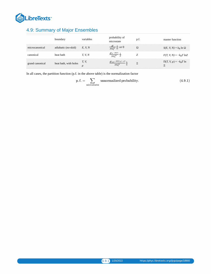
4.9.1 1/20/2022 https://phys.libretexts.org/@go/page/18900

4.9: Summary of Major Ensembles

boundary variables probability ofmicrostate

p.f. master function

microcanonical adiabatic (no-skid) E, V, N Ω S(E, V, N) = k ln Ω

canonical heat bath T, V, N Z F(T, V, N) = −k T lnZ

grand canonical heat bath, with holes T, V,μ

Ξ Π(T, V, µ) = −k T lnΞ

In all cases, the partition function (p.f. in the above table) is the normalization factor

or 0dΓ

N!h3N0

1Ω B

dΓe−βH(Γ)

N!h3N0

1Z B

dΓNe−βH( )−αNΓN

N!h3N0

1Ξ

B

p. f. = unnormalized probability. ∑ microstates

(4.9.1)

4.10.1 1/6/2022 https://phys.libretexts.org/@go/page/18901

4.10: Quantal Statistical MechanicsHow shall we define a partition function for quantal systems? A reasonable first guess is that

This guess runs into problems immediately. Most quantal states are not energy eigenstates, so it’s not clear how to interpret“E” for such states. Another difficulty—harder to see—arises because there are many more quantal states than classicalstates, so the guess above is in some sense counting too many states. It’s hard to see how it could have the correct classicallimit. (Indeed, a mathematical investigation of the above guess would reveal that it doesn’t even have the correctthermodynamic limit—if you were to calculate the Helmholtz free energy from the above guess, the resulting F(T, V, N)would increase far faster than linearly with system size.) A second guess might be

This avoids the problem of how to interpret E for non-energy eigenstates, but there still seems to be an over-counting ofstates in the case of an energy degeneracy: If two energy eigenstates are separate in energy by any amount, no matter howsmall, those two energy eigenstates will contribute two terms to the above sum. But if the energy separation vanishes, thenall linear combinations of the two states are also energy eigenstates, and each of this infinite number of combinations willenter into the sum.

Finally we arrive at a workable definition for quantal partition function, namely

Note that this is a sum over an energy eigenbasis, not over energy eigenvalues. These two sums differ through degeneracy:If E = E , then two equal terms enter into the sum. More formally: if N(m) is the degeneracy of eigenvalue m, that is, thenumber of linearly independent states with energy E , then

The above argument has a strange, ex post facto character: We define the quantal partition function not from firstprinciples, but to insure that it has properties that we consider desirable (namely, that it avoids subtle interpretation issues,it posses the expected classical limit, and it has desirable behavior at level crossings). Linear combinations of energyeigenstates are quantal states just as legitimate as energy eigenstates, so why do we ignore them in the sum? The argumentreminds me of politics at its worst: “I’m going to pass this law because I want it, even though I can’t support it with anyrationale.” The resulting definition of partition function is strange in that it seems to select the energy eigenbasis as somesort of God-given basis, “better” than any other basis. In fact, the result is not as bad as it seems. It turns out (see problem4.2) that our definition can be rephrased in a basis-independent manner as

If you don’t know what it means to exponentiate the Hamiltonian operator , don’t worry. For this book—and for mostpractical calculations—the most effective definition is the form on the left. The point is simply that the definition ofpartition function can be cast into the basis-independent form on the right. The energy eigenbasis is not special.

In this chapter we have often found, first, results about probabilities, and second, connections to thermodynamics. Thissection has so far dealt with only the second element. What do these results imply for probabilities? I will often say thingslike “The probability of having energy E is

On the face of it, this statement is absurd, because most of the microstates aren’t energy eigenstates so they don’t have anyenergy at all. What I mean is “If the energy is measured, the probability of finding energy E is

Z(T , parameters ) = . [first guess ∑ all quantal states e−βE

Z(T , parameters ) = . [ second guess ]∑ all energy eigenstates e−βE

Z(T , parameters ) = .∑ energy eigenbasis n

e−βEn (4.10.1)

6 5

m

Z(T , parameters ) = N(m) .∑ energy eigenvalues m

e−βEm (4.10.2)

Z(T , parameters ) = = ⟨j j⟩ .∑ energy eigenbasis n

e−βEn ∑ any basis j

∣∣e

−βH ∣∣ (4.10.3)

H

m

. "N(m)e−βEm

Z

m

. "N(m)e−βEm

Z

4.10.2 1/6/2022 https://phys.libretexts.org/@go/page/18901

I will often use the first statement rather than the long and formal second statement. I do so, however, fully realizing thatthe first statement is wrong and that I use it just as convenient shorthand for the second statement. You may use thisshorthand too, as long as you don’t mean it.

The ultimate source of such problems is that the English language was invented by people who did not understandquantum mechanics, hence they never produced concise, accurate phrases to describe quantal phenomena. In thesame way, the ancient phrase “Search the four corners of the Earth” is still colorful and practical, and is used todayeven by those who know that the Earth isn’t flat.

Similarly, I will often say “The probability of being in the energy eigenstate η (x , . . . , x ) with energy E is

But what I really mean is “If the microstate is projected onto a basis which includes the energy eigenstate η (x , . . . , x ),then the probability of projecting onto that state is

4.2 The trace

Show that for any operator , the “trace” of , defined as

is independent of basis. What is the trace in terms of the matrix representation of the operator?

4.3 Entropy in the canonical ensemble

From the partition function (4.61), one can find the free energy F and hence the entropy S. Show that the entropyobtained in this manner equals

where

is the probability that the system is in its nth energy eigenstate (using the shorthand mentioned above). Thisexpression for the entropy is particularly useful in information theory. (Clue: Work forward from S = −∂F/∂T andbackwards from equation (4.65) to meet at the middle.)

4.4 Entropy in the microcanonical ensemble

[You must work the previous problem before working this one.] What are the state probabilities pn, analogous to(4.66), for an system in the microcanonical ensemble? Devise a suitable quantal replacement for the microcanonicaldefinition of entropy (2.7). Cast your replacement into the form of a function of the microcanonical probabilities p .Is formula (4.65) correct in the microcanonical ensemble?

n 1 N n

. "e−βEn

Z

n 1 N

. "e−βEn

Z

A A

trace ≡ ⟨j| |j⟩,A ∑ any basis j

A (4.10.4)

S(T ) = − ln ,kB ∑n

pn pn (4.10.5)

=pn

e−βEn

Z(T )(4.10.6)

n

4.11.1 1/1/2022 https://phys.libretexts.org/@go/page/18902

4.11: Ensemble Problems I4.5 Classical monatomic ideal gas in the canonical ensemble

In section 5.1 we will show that the canonical partition function of a classical monatomic ideal gas is

where

a. Show that in the thermodynamic limit, the Helmholtz free energy per particle is

b. Differentiate with respect to T to find S(T, V, N).

c. Change variables to S(E, V, N) using E = N k T, and compare the resulting expression to the entropy derived inclass through the microcanonical ensemble.

4.6 Number fluctuations in the grand canonical ensemble

Calculate ∆N, the root mean square fluctuations in the particle number, for a system in the grand canonicalensemble. (Clue: Take derivatives with respect to µ.) Show that this result is related to the isothermal compressibilityκT through

(Clue: Use the results of problem 3.33.)

4.7 Classical monatomic ideal gas in the grand canonical ensemble

a. Use the fact that

to find Ξ(T, V, µ) for the classical monatomic ideal gas.

b. Use the connection to thermodynamics for the grand canonical ensemble, namely

to show that for any substance

c. Derive the ideal gas equation of state in the grand canonical ensemble.

4.8 Isobaric ensemble

This problem encourages you to think about an ensemble with a specified temperature, pressure, and particlenumber. A physical model to keep in mind is a collection of systems each with the same number of particles and allconnected to the same heat bath but enclosed in balloons rather than in rigid boxes. I want you to guess the answersto the following questions rather than produce mathematical or verbal arguments. If you are uncomfortable makingguesses in a physics problem assignment then do only the first two parts.

a. Given that T, p, and N are fixed, what quantities fluctuate?

Z(T ,V ,N) = ,1

N ![ ]

V

(T )λ3

N

(4.11.1)

λ(T ) ≡ .h0

2πm TkB− −−−−−−

√(4.11.2)

= − T [ln( )+1] .F (T ,V ,N)

NkB

V /N

(T )λ3(4.11.3)

32 B

= .ΔN

N

TkB κT

V

− −−−−−√ (4.11.4)

Z(T ,V ,N) = ,1

N ![ ]

V

(T )λ3

N

(4.11.5)

p(T ,μ)V = T lnΞ(T ,V ,μ),kB (4.11.6)

N(T ,V ,μ) = T .kB∂ lnΞ

∂μ)T ,V (4.11.7)

4.11.2 1/1/2022 https://phys.libretexts.org/@go/page/18902

b. In going from the canonical to the isobaric ensemble, what control parameter (comparable to β = 1/k T or α= −µ/k T) must be introduced, and how is it related to the pressure?

c. What is the (unnormalized) probability of finding the system in microstate x with energy H(x) and volumeV(x)?

d. What is the relevant state sum (comparable to Z or Ξ), and how is it related to the thermodynamic masterfunction G(T, p, N)?

e. The relevant fluctuation-susceptibility relation connects the fluctuations in volume to what susceptibility?

f. Write out the fluctuation-susceptibility relation, using B to represent a product of several unguessableintensive quantities but writing out the extensive quantities explicitly.

g. What are the dimensions of B? Can you use this knowledge to guess at the unguessable?

4.9 Fluctuation-susceptibility relation for a magnetic system

In the Ising model for a magnet, the spins are located at fixed sites (labeled by i), and can point either up or down (s= ±1). The Ising Hamiltonian is

where m is the magnetic moment of each spin, H is the applied magnetic field, and H represents some spin-spininteraction energy, the details of which are not important here except for the fact that it is independent of H. Themicroscopic magnetization, which varies from configuration to configuration, is

while the macroscopic (or thermodynamic) magnetization is the canonical average over all such microscopicmagnetizations:

The magnetic susceptibility—easily measured experimentally—is

Show that in the canonical ensemble the fluctuations in magnetization are related to the susceptibility by

4.10 Two definitions of magnetization

The previous problem gave a statistical mechanical definition of magnetization:

while equation (3.100) gave a thermodynamic definition:

Show that these two definitions give equivalent results.

4.11 Values for the approach to the thermodynamic limit

In problem 2.13, “The approach to the thermodynamic limit,” you were given a value of EV /h and told that itwas appropriate “for a gas at room temperature and atmospheric pressure.” Justify this value as

B

B

i

H= ( , … , ) −mH ,H0 s1 sN ∑i=1

N

si (4.11.8)

H0

M ( , … , ) = ms1 sN ∑i

si (4.11.9)

M(T ,H) = ⟨M⟩. (4.11.10)

(T ,H) = .χT

∂M

∂H)T (4.11.11)

ΔM = .TkB χT− −−−−−√ (4.11.12)

M(T ,H) = ⟨M⟩, (4.11.13)

M(S,H) = − .∂E

∂H)S (4.11.14)

2/3 20

E / = [ /( )]V 2/3 h20

3

2( T )kB

5/3 p2/3h2 N 5/3 (4.11.15)

4.11.3 1/1/2022 https://phys.libretexts.org/@go/page/18902

4.12 Integrals by parametric differentiation

To find the mean energy or energy dispersion in the canonical ensemble, we introduced the “slick trick” ofdifferentiating with respect to β. This trick, called parametric differentiation, is in fact useful in a number ofcircumstances. For example, in a graduate electrodynamics class I was once assigned a problem (Jackson, ClassicalElectrodynamics, problem 14.5(b)) for which I needed to evaluate

where b is a constant with |b| < 1. My classmates and I tried everything: substitutions, partial fractions, conversion toa contour integral in the complex plane, and, most popular of all, “look it up in reference books”. I puzzled over itfor a dozen hours before giving up. When the solutions were handed out, I expected to find many pages devoted toevaluating the integral. Instead I found a two-line argument that began with the known integral (see Dwight 858.546or Gradshteyn and Ryzhik 3.644.4)

and then took a fourth derivative. What was the argument, and what is the value of the integral?

4.13 Parametric differentiation in quantum mechanics

The previous problem showed how parametric differentiation could be useful in electrodynamics. This one showshow it can be useful in quantum mechanics. In quantum mechanics, an infinite square well of width π has energyeigenfunctions

One frequently needs to evaluate matrix elements such as

Show how this integral—as well as a host of other useful matrix elements—can be obtained easily from the wellknown result

4.14 Polymers

A primitive model for a polymer is a random walk on a simple cubic lattice. A random walk consists of n steps (or“links”) starting at (“anchored to”) the origin. (In this model a polymer unit can step back onto a lattice site alreadyoccupied by a different polymer unit. This unrealistic feature is corrected in a more sophisticated model, the so-called “self avoiding walk.”)

a. Show that the number of distinct walks consisting of n links is Nn = 6n. Does this formula hold when n = 0?

For many purposes it is valuable to consider the ensemble of all random walks, regardless of their size. In thisensemble there is a “size control parameter” α such that the probability of finding a walk x consisting of n(x) links isproportional to e . (Thus longer walks are less probable in this ensemble, but there are more of them.) Thepartition function associated with this model is

b. Show that the mean walk size in this ensemble is a function of α given through

dθ∫2π

0

θcos2

(1 +b sinθ)5(4.11.16)

dθ =∫2π

0

θcos2

a+b sinθ

2π

a+ −a2 b2− −−−−−

√(4.11.17)

(x) = sin(nx) n = 1, 2, 3, …ηn2

π

−−√ (4.11.18)

⟨n m⟩ = sin(nx) sin(mx)dx.∣∣x2∣∣

2

π∫

π

0x2 (4.11.19)

sin(ax) sin(bx)dx = [ − ] a ≠ ±b.∫π

0

1

2

sin(a−b)π

a−b

sin(a+b)π

a+b(4.11.20)

−αn(x)

Ξ(α) = .∑ walks ×

e−αn(x) (4.11.21)

⟨n⟩ = − .∂ lnΞ(α)

∂α(4.11.22)

4.11.4 1/1/2022 https://phys.libretexts.org/@go/page/18902

c. Show that

Clue: the geometric series sums to

d. What is the smallest possible value of the control parameter α? Does large α correspond to long polymers orshort polymers?

e. Show that the dispersion in n is given through

whence

Thus the relative dispersion decreases for longer polymers.

(See also loops: S. Leibler, R.R.P. Singh, and M.E. Fisher, “Thermodynamic behavior of two-dimensional vesicles,”Phys. Rev. Lett. 59 (1987) 1989–1992; C. Richard, A.J. Guttmann, and I. Jensen, “Scaling function and universalamplitude combinations for self-avoiding polygons,” J. Phys. A 34 (2001) L495– 501.)

4.15 A class of new ensembles

Any mechanical parameter in the Hamiltonian can be “traded in” for a control parameter. This problem details theprocedure if the mechanical parameter is intensive and an intrinsically positive quantity. Examples to keep in mindare 1) the particle mass, 2) the spacing between planes of a high temperature superconductor, or 3) the naturalfrequency of vibration for a diatomic molecule modeled as a simple harmonic oscillator. In honor of this lastexample I will call the parameter ω. In the “micro-ω” ensemble, all of the systems in the ensemble have a particularvalue of the parameter. In the “grand-ω” ensemble, the systems in the ensemble have a variety of values for theparameter, but larger values are less probable. In fact, the probability is proportional to e −γNω, where γ is a “controlparameter” which can be adjusted to set the mean value of ω to any desired positive value. We suspect that, in thethermodynamic limit, the results of the two ensembles will be identical when the mean value of ω in the grand-ωensemble is the same as the fixed value of ω in the micro-ω ensemble.

a. The thermodynamic assembly corresponding to the micro-ω ensemble has as master function the Helmholtzfree energy F(T, V, N, ω). Using the definition

write out the differential equation for dF. b. Execute a Legendre transformation to an assembly with masterfunction

and show that in this assembly, the function (not variable!) ω is

In the grand-ω ensemble, the probability that a system has a parameter falling within dω about ω is

Ξ(α) = and that (n) = .1

1 −6e−α

6

−6eα(4.11.23)

1 +x+ + +⋯ = when |x| < 1.x2 x3 1

1 −x(4.11.24)

(Δn = ,)2 lnΞ∂2

∂α2(4.11.25)

= = .Δn

⟨n⟩

eα

6

−−−√ +1

1

⟨n⟩

− −−−−−−

√ (4.11.26)

B(T ,V ,N ,ω) = − ,∂F

∂ω)T ,V,N (4.11.27)

K(T ,V ,N ,B) = F +Bω, (4.11.28)

ω(T ,V ,N ,B) = .∂K

∂B)T ,V,N (4.11.29)

.Z(T ,V ,N ,ω)dωe−γNω

Z (T ,V ,N , )d∫ ∞0 e−γNω′

ω′ ω′(4.11.30)

4.11.5 1/1/2022 https://phys.libretexts.org/@go/page/18902

Define the partition function

where ω is an arbitrary constant with the dimensions of ω whose only purpose is to make Y dimensionless.Presumably, the relationship between thermodynamics and statistical mechanics in the grand-ω ensemble is

by analogy to the similar relation in the canonical ensemble. We will assume this relationship and use it, firstto find the relationship between the statistical mechanical γ and the thermodynamic B and second to show thatthe statistical mechanical equation (4.96) is consistent with the thermodynamic equation (4.93).

c. Show that, in the grand-ω ensemble,

and

Note that and ∆ω are functions of T, V , N, and γ.

d. Compare equations (4.94) and (4.98) and conclude that, if (4.97) is to hold, then

e. Show that

f. We suspect that, in the thermodynamic limit N, V → ∞, ln Y ∼ N. If true, show that is intensive(independent of N) whereas ∆ω falls like .

g. To evaluate Y (γ) in the thermodynamic limit, write

Take logarithms to show that

and argue that in the thermodynamic limit the last term becomes negligible. Finally conclude that

or, in light of relationship (4.100),

which should be compared to equation (4.93).

We have shown only that this ensemble scheme is “not inconsistent”. It is not obviously wrong, but of course thisdoes not prove that it is right. A flawless general proof would require detailed mathematical reasoning, but proofsfor particular situations are outlined in the next problem and in problem 4.18.

4.16 The grand-ω ensemble for the classical monatomic ideal gas

Apply the concepts of the previous problem to the classical monatomic ideal gas where the mechanical parameter ωis the particle mass. In particular, find expressions

Y (T ,V ,N , γ) = Z(T ,V ,N ,ω)dω,1

ω0∫

∞

0e−γNω (4.11.31)

0

K = − T lnY ,kB (4.11.32)

⟨ω⟩ = −1

N

∂ lnY

∂γ(4.11.33)

Δ = .ω2 1

N 2

Y∂2

∂γ2(4.11.34)

⟨ω⟩

B = N γ.kBT′ (4.11.35)

Δω = .T )kB∂ω

∂B

− −−−−−−√

T ,V,N

(4.11.36)

⟨ω⟩

1/ N−−

√

Y (T ,V ,N , γ) = Z(T ,V ,N ,ω)dω ≈ Z(T ,V ,N , ⟨ω⟩) .1

ω0∫

∞

0e−γNω e−γN⟨ω⟩ Δω

ω0(4.11.37)

lnY ≈ −γN⟨ω⟩+lnZ+ln(Δω/ ),ω0 (4.11.38)

K = TγN⟨ω⟩+FkB (4.11.39)

K = F +B⟨ω⟩ (4.11.40)

4.11.6 1/1/2022 https://phys.libretexts.org/@go/page/18902

a. for B(T, V, N, m),

b. for m(T, V, N, B),

c. and for and ∆m as functions of T, V , N, and γ.

4.17 An ensemble of your own

Any mechanical parameter in the Hamiltonian can be traded in for a control parameter. Can you think up a goodproblem using this fact where the parameter is, say, an applied magnetic field? Or the spring constant (or relaxedlength) between two atoms in a diatomic molecule (or in the Einstein model)? Or the moment of inertia of adiatomic molecule modeled as a dumbbell? Or a parameter in the Lennard-Jones potential? Or the size of hard-sphere atoms? Or the spacing between atoms in a crystal?

⟨m⟩

4.12.1 1/20/2022 https://phys.libretexts.org/@go/page/18903

4.12: Ensemble Problems IIThe remaining problems in this chapter deal with the same “principles” issues that the others do, but they assume somefamiliarity with physical and mathematical topics that we have not yet treated. I place them here because of their character,but I do not expect you to do them at this moment. Instead I list their prerequisites and I hope you will come back to themlater.

4.18 The grand-ω ensemble for the simple harmonic oscillator

(Prerequisite: Problems 4.15 and 5.7.) Problem 4.15 introduced a class of ensembles in which mechanicalparameters in the Hamiltonian were not fixed but rather allowed to fluctuate under the control of some parameters γ.Apply this concept to the diatomic molecules of problem 5.7, using the natural frequency of vibration as themechanical parameter. Develop the suggestive arguments of problem 4.15 into a mathematically rigorous proof.

4.19 Particles in a bowl

(Prerequisite: Chapter 5.) I can’t count how many times I’ve waved my hands and told you that the precise characterof the boundaries should be irrelevant to the bulk properties found by statistical mechanics. Now you have a chanceto prove it (for a restricted situation of course).

a. Consider N non-interacting, classical point particles moving subject to the potential energy function U(r) =Kr /2. Evaluate the classical partition function Z (T, K, N) and compare it to the partition function Z (T, V, N)for N particles in a hard-walled container of volume V.

b. For what V (as a function of K) will the two partition functions in part (a.) be the same?

c. The “bowl” container has no stiff walls, so it is possible for a particle to be located at any distance from theorigin. But is it not likely that a particle will get too far away. Calculate the rms radius . (Useequipartition?)

d. Suppose the hard-walled container is spherical with radius R. Place the origin at the center of the sphere andfind the rms radius .

e. For the V corresponding to K in the sense of part (b.), compare the two rms radii.

Extra: Do this problem quantum mechanically. (Clue: Notice the mathematical similarity between this problem andthe Einstein model of lattice vibrations.)

4.20 Quantal monatomic ideal gas

(Prerequisite: Chapter 6.) We have many times considered the problem of N non-interacting classical point particlesin a box of edge length L = V . Now we will solve the problem for quantum mechanical particles.

The partition function is , where the sum is taken over the many-particle energy eigenstates Ψ(r , . . . ,r ). Ignore symmetry-under-interchange requirements so that such states are specified by a simple listing of thecomponent one-particle levels (or orbitals) η (r). Thus Ψ can be specified by simply listing the relevant k values ofits component levels. Show then that

where and the sum is over all k permitted by periodic boundary conditions. Evaluate the sum (inthe thermodynamic limit) by turning it into an integral. Compare the resulting partition function with that of aclassical monatomic ideal gas.

4.21 Quantal monatomic ideal gas in the microcanonical ensemble

Consider the situation of the above problem but calculate the microcanonical partition function Ω(E, V, N). Comparewith the classical result.

2b h

⟨ ⟩r2− −−√

⟨ ⟩r2− −−√

1/3

Z =∑ e−βE1

N

k

Z =1

N !( )∑

k

e−βEk

N

(4.12.1)

= /2mEk ℏ2k2

1 1/27/2022

CHAPTER OVERVIEW5: CLASSICAL IDEAL GASESThis chapter considers ideal (i.e. non-interacting) gases made up of atoms or molecules that may have internal structure (i.e. not pointparticles). The internal degrees of freedom will be treated either classically or quantally, but the translational degrees of freedom willalways be treated classically.

5.1: CLASSICAL MONATOMIC IDEAL GASES5.2: CLASSICAL DIATOMIC IDEAL GASES5.3: HEAT CAPACITY OF AN IDEAL GAS5.4: SPECIFIC HEAT OF A HETERO-NUCLEAR DIATOMIC IDEAL GAS5.5: CHEMICAL REACTIONS BETWEEN GASES5.6: PROBLEMS

Daniel F. Styer 5.1.1 12/23/2021 https://phys.libretexts.org/@go/page/6357

5.1: Classical Monatomic Ideal GasesWe have already found the Helmholtz free energy of the classical monatomic ideal gas (section 4.3). I think you will agreethat the canonical calculation is considerably easier than the corresponding microcanonical calculation. Here we willreview the calculation, then go back and investigate just what caused the solution to be so much easier, and thisinvestigation will lead to an important theorem.

5.1.1 Solving the problemThe energy

is a sum of terms, each involving different variables, so the Boltzmann factor

is a product of factors, each involving different variables. Thus the partition function, which in general is an integral in a6N-dimensional space, factors into 3- and 1-dimensional integrals

This doesn’t happen in the microcanonical calculation!

Moreover, we found it easy to evaluate the N three-dimensional position integrals and the 3N one-dimensional momentumintegrals. The result was

The result above is correct, but it is not the most convenient form for the partition function. There are lots of variables andconstants floating around, many of them with hard-to-remember dimensions. The quantity Z is in fact dimensionless, butthat’s not obvious from the expression. For this reason is customary to define the quantity

called the “thermal de Broglie wavelength”. Like any wavelength, it has the dimensions of length, and the notation λ(T)suggests this. It is, of course, an intensive quantity. In terms of the thermal de Broglie wavelength, the partition functionfor the classical monatomic ideal gas is

If a particle of mass m has kinetic energy kBT, then it has momentum √ 2mkBT and thus a quantum-mechanical deBroglie wavelength of

The definition (5.4) above slips in an extra dimensionless factor of = 1.77 just to make the result (5.5) easier toremember and to work with. Physically, the thermal de Broglie wavelength represents the quantal smearing of eachindividual point particle. Thus if the mean separation between atoms is much greater than λ(T), we expect that theclassical approximation will be a good one. If the mean separation is less than or about equal to λ(T), we expect thata quantal treatment will be required.

H(Γ) = ( + + + +⋯ + )+U ( ) +U ( ) +⋯ +U ( )1

2mp2x,1 p2

y,1 p2z,1 p2

x,2 p2z,N x1 x2 xN (5.1.1)

= ×⋯ × ×⋯ ×e−βH(Γ) e−β( /2m)p2

z,1 e−β( /2m)p2

ν,1 e−β( /2m)p2

z,N e−βU( )x1 e−βU( )x2 e−βU( )xN (5.1.2)

Z(T ,V ,N) = [ d d d ]×⋯ ×[ d d d ]1

N !h3N∫

+∞

−∞x1 ∫

+∞

−∞y1 ∫

+∞

−∞z1e

−βU( )x1 ∫+∞

−∞xN ∫

+∞

−∞yN ∫

+∞

−∞zNe

−βU( )xN

×[ d ]×⋯ ×[ d ] .∫+∞

−∞px,1e

−β( /2m)p2x,1 ∫

+∞

−∞pz,Ne

−β( /2m)p2z,N

Z(T ,V ,N) = .V N

N !h3N[ ]2πm TkB

− −−−−−−√

3N(5.1.3)

λ(T ) = ,h

2πm TkB− −−−−−−

√(5.1.4)

Z(T ,V ,N) = .1

N !( )

V

(T )λ3

N

(5.1.5)

λ = = .h

p

h

2m TkB− −−−−−

√(5.1.6)

π−−√

Daniel F. Styer 5.1.2 12/23/2021 https://phys.libretexts.org/@go/page/6357

After doing any calculation is it useful to perform a “debriefing” to figure out why—in general rather than technical terms—the calculation went the way it did. Almost everyone agrees that this canonical calculation is a lot easier than thecorresponding microcanonical calculation to find Ω(E, V, N) for the classical monatomic ideal gas. But what was theparticular feature that made it so much easier? Surely it was the factorization of the Boltzmann factor and the subsequentfactorization of the partition function. This enabled us to perform one- and three-dimensional integrals rather than the 3N-dimensional integral required (see appendix D) for the microcanonical calculation. Is there anything that can be said moregenerally about this feature?

5.1.2 Theorem on decoupling HamiltoniansIndeed there is. Suppose a Hamiltonian is a sum of two pieces

where Γ and Γ are exclusive. (That is, the phase space variables in the list Γ and the phase space variables in the list Γtogether make up the whole list Γ, and no variable appears in both lists.) The Hamiltonian H(Γ) is then said to “decouple”into the two parts H (Γ ) and H (Γ ). Then it is easy to see that the partition function will factor into two parts:

If the Hamiltonian decouples into three parts, then this reasoning can be used to show that the partition function breaks intothree factors. And so forth.

For example, the Hamiltonian of the classical monatomic ideal gas that we have just investigated decouples into 4N pieces,

Each term of the form p /2m in the Hamiltonian leads to a factor of h/λ(T) in the partition function. . . each term of theform U(x) leads to a factor of V. Thus our theorem on decoupling Hamiltonians shows that the partition function is

If the particles do interact, then the potential energy part of the Hamiltonian does not break up into exclusive pieces, butthe kinetic energy part still does. Thus for an interacting gas with potential energy of interaction

the partition function is

Although the potential energy part of the problem is now excruciatingly difficult, our theorem on decoupling Hamiltoniansassures us that the kinetic energy part is just as easy to handle for an interacting as for a non-interacting gas.

5.1 Gas with pair interactions

For a pure classical monatomic gas that interacts only through pair interactions (i.e. for which there are no three-body or higher interactions) the Hamiltonian is

where U (x) is the potential energy due to the interaction between a particle at point x and the container, and U (x,y) is the potential energy due to the interaction between a particle at point x and a particle at point y. The potentialenergy thus breaks up into a sum of N + N(N − 1)/2 pieces. Does the decoupling theorem apply?

H(Γ) = ( ) + ( ) ,H1 Γ1 H2 Γ2 (5.1.7)

1 2 1 2

1 1 2 21

Z(T ,V ,N) = ∫ dΓ = ∫ d ∫ d .1

N !h3Ne−βH(Γ) 1

N !h3NΓ1e

−βH( )Γ1 Γ2e−βH( )Γ2 (5.1.8)

H(Γ) = + +⋯ + +U ( ) +U ( ) +⋯ +U ( ) .p2x,1

2m

p2y,1

2m

p2z,N

2mx1 x2 xN (5.1.9)

2

Z(T ,V ,N) = .1

N !h3N( )

h

λ(T )

3N

V N (5.1.10)

( , , … , )UN x1 x2 xN (5.1.11)

Z(T ,V ,N) = d ⋯ d .1

N ! (T )λ3N∫

+∞

−∞x1 ∫

+∞

−∞zNe

−βUN (5.1.12)

H(Γ) = + ( ) + ( , ) ,∑i=1

Np2i

2m∑i=1

N

UA xi ∑i=1

N−1

∑j=i+1

N

UB xi xj (5.1.13)

A B

Daniel F. Styer 5.1.3 12/23/2021 https://phys.libretexts.org/@go/page/6357

Alternatively, the two parts of the Hamiltonian are called “uncoupled”. These terms derive from the ordinary Englishword “to couple”, meaning to join or to connect.

1

Daniel F. Styer 5.2.1 12/9/2021 https://phys.libretexts.org/@go/page/6358

5.2: Classical Diatomic Ideal GasesRigid linear model. The partition function is

General results for separation of Z into translational (center of mass) and internal degrees of freedom. Term “internalspecific heat”.

Z(T , V , N) =1

N ![ ( )]

V

(T )λ3

4 I Tπ3

kB

h2

N

(5.2.1)

Daniel F. Styer 5.3.1 1/27/2022 https://phys.libretexts.org/@go/page/6359

5.3: Heat Capacity of an Ideal Gas

5.3.1 The equipartition theorem

Equipartition theorem. (For classical systems.) Suppose the Hamiltonian H(Γ) decouples into one piece involving asingle phase space variable—call it H1, plus another piece which involves all the other phase space variables—call itH (Γ ). Suppose further that the energy depends quadratically upon this single phase space variable, and that this variablemay take on values from −∞ to +∞. Then, in classical statistical mechanics, the mean contribution to the energy due to thatsingle variable is

Notice how general this theorem is. The remaining piece of the Hamiltonian, H (Γ ), might decouple further or it mightnot. The phase space variable entering H might be a momentum,

or an angular momentum,

or even a position coordinate, as in the simple harmonic oscillator energy

Furthermore, in all these circumstances, the mean energy is independent of the particular parameters m or I or k. . . itdepends only upon the temperature. This explains the origin of the name “equipartition”: the mean translational energy dueto motion in the x direction is equal to the mean rotational energy due to the change of θ, and this holds true even if the gasis a mixture of molecules with different masses and different moments of inertia. The energy is equally partitioned amongall these different ways of holding energy.

Proof. We will write

although the variable might not be a linear momentum. Then the average of H is

Clearly, the integrals over Γ cancel in this last expression. (This explains why the form of H is irrelevant to the theorem.)We are left with

These two integrals could be evaluated in terms of Gamma functions (see appendix C), but they don’t need to be evaluatedyet. Think for a moment about our “slick trick” of parametric differentiation. . . using it we can write

The integral that remains is of Gaussian character and we could evaluate it using the results of Appendix B. But beforerushing in to integrate, let’s employ the substitution to find

2 2

⟨ ⟩ = T .H11

2kB (5.3.1)

2 2

1

(p) = ,H1p2

2m(5.3.2)

(ℓ) = ,H1ℓ2

2I(5.3.3)

(x) = k .H11

2x2 (5.3.4)

(p) = a ,H1 p2 (5.3.5)

1

⟨ ⟩ = = .H1∫ dΓH1e

−βH(Γ)

∫ dΓe−βH(Γ)

dp ∫ d∫ +∞−∞ H1e

−βH1 Γ2e−β ( )H2 Γ2

dp ∫ d∫ +∞−∞ e−βH1 Γ2e−β ( )H2 Γ2

(5.3.6)

2 2

⟨ ⟩ = .H1

dpa∫ +∞−∞ p2e−βap2

dp∫ +∞−∞ e−βap2

(5.3.7)

⟨ ⟩ = − ln[ dp ].H1d

dβ∫

+∞

−∞e−βap2

(5.3.8)

u = pβa−−√

Daniel F. Styer 5.3.2 1/27/2022 https://phys.libretexts.org/@go/page/6359

This last expression shows that there’s no need to evaluate the integral. Whatever its value is, it is some number, not afunction of β, so when we take the derivative with respect to β the term involving that number will differentiate to zero.Similarly for the constant a, which explains why the equipartition result is independent of that prefactor. We are left with

or, finally, the desired equipartition result

5.3.2 Applications of equipartition; Comparison with experiment

5.3.3 Crossover between classical and quantal behavior; Freeze outAt high temperatures, typical thermal energies are much greater than level spacings. Transitions from one level to anotherare very easy to do and the granular character of the quantized energies can be ignored. This is the classical limit, andequipartition holds!

At low temperatures, typical thermal energies are less that the level spacing between the ground state and the first excitedstate. There is so little thermal energy around that the molecule cannot even be excited out of its ground state. Virtually allthe molecules are in their ground states, and the excited states might as well just not exist.

In classical mechanics, a diatomic molecule offered a small amount of rotational energy will accept that energy and rotateslowly. But in quantum mechanics, a diatomic molecule offered a small amount of rotational energy will reject that energyand remain in the ground state, because the energy offered is not enough to lift it into the first excited state. The quantaldiatomic molecule does not rotate at all at low temperatures, so it behaves exactly like a monatomic molecule with onlycenter-of-mass degrees of freedom.

In short, we explain the high-temperature rotational specific heat (c = k ) through equipartition. We explain the low-temperature rotational specific heat (c vanishes) through difficulty of promotion to the first quantal excited state. Thisfall-off of specific heat as the temperature is reduced is called “freeze out”.

The crossover between the high-temperature and low-temperature regimes occurs in the vicinity of a characteristictemperature θ at which the typical thermal energy is equal to energy separation between the ground state and the firstexcited state. If the energies of these two states are ε and ε respectively, then we define the characteristic crossovertemperature through

5.2 Generalized equipartition theorem and the ultra-relativistic gas

a. Suppose the Hamiltonian H(Γ) decouples into two pieces

where p is some phase space variable that may take on values from −∞ to +∞, and where Γ represents all the phasespace variables except for p. (Note that the absolute value |p| is needed in order to avoid, for example, taking thesquare root of a negative number in the case n = 1/2.) Show that, in classical statistical mechanics, the meancontribution to the energy due to that single variable is

b. In special relativity, the energy of a free (i.e. non-interacting) particle is given by

⟨ ⟩ = − ln[ du ] = − ln[ ]+ln[ du ] .H1d

dβ

1

βa−−

√∫

+∞

−∞e−u2 d

dβ

1

β−−

√

1

a−−√∫

+∞

−∞e−u2

(5.3.9)

⟨ ⟩ = − ln = lnβ =H1d

dβ

1

β−−

√

1

2

d

dβ

1

2

1

β(5.3.10)

⟨ ⟩ = T .H11

2kB (5.3.11)

2

rotV B

rotV

0 1

θ ≡ −kB ϵ1 ϵ0 (5.3.12)

H(Γ) = a|p + ( )|n H2 Γ2 (5.3.13)

2

⟨a|p ⟩ = T|n1

nkB (5.3.14)

+(pc(m )c2 2)2

− −−−−−−−−−−−√ (5.3.15)

Daniel F. Styer 5.3.3 1/27/2022 https://phys.libretexts.org/@go/page/6359

where c is the speed of light. As you know, when this gives the non-relativistic kinetic energy KE ≈ mc +p /2m. In the “ultra-relativistic” limit, where v is close to c, the energy is approximately pc. What is the heat capacityof a gas of non-interacting ultra-relativistic particles?

c. Estimate the crossover temperature between the non-relativistic and ultra-relativistic regimes.

5.3 Another generalization of equipartition

Consider the same situation as the equipartition theorem in the text, but now suppose the single phase space variabletakes on values from 0 to +∞. What is the corresponding result for ?

5.4 Equipartition and the virial theorem

Look up the term “virial theorem” in a classical mechanics textbook. Is there any relation between the virial theoremof classical mechanics and the equipartition theorem of classical statistical mechanics?

This paragraph is written in the “shorthand” language discussed on page 113, as if energy eigenstates were the onlyallowed quantal states.

Approximations are an important part of physics, and an important part of approximation is to ensure their reliabilityand consistency. The notation (pronounced “the big-oh notation”) is an important and practical tool for makingapproximations reliable and consistent. The technique is best illustrated through an example. Suppose you desire anapproximation for

valid for small values of x, that is, . You know that

and that

so it seems that reasonable approximations are

and

whence

Let’s try out this approximation at x = 0.01. A calculator shows that

while the value for the approximation is

This is a very poor approximation indeed. . . the deviation from f(0) = 1 is even of the wrong sign!

Let’s do the problem over again, but this time keeping track of exactly how much we’ve thrown away while makingeach approximation. We write

v≪ c 2

2

⟨ ⟩H1

2

The NotationO

O

f(x) =e−x

1 −x(5.3.16)

x ≪ 1

= 1 −x+ − +⋯e−x 1

2x2 1

6x3 (5.3.17)

= 1 +x+ + +⋯1

1 −xx2 x3 (5.3.18)

≈ 1 −xe−x (5.3.19)

≈ 1 +x1

1 −x(5.3.20)

≈ (1 −x)(1 +x) = 1 − .e−x

1 −xx2 (5.3.21)

0

= 1.0000503 …e−x0

1 −x0(5.3.22)

1 − = 0.9999000.x20 (5.3.23)

Daniel F. Styer 5.3.4 1/27/2022 https://phys.libretexts.org/@go/page/6359

as

where the notation (x ) stands for the small terms that we haven’t bothered to write out explicitly. The symbol (x )means “terms that are about the magnitude of x , or smaller” and is pronounced “terms of order x ”. The notationwill allow us to make controlled approximations in which we keep track of exactly how good the approximation is.

Similarly, we write

and find the product

Note, however, that , and that , and so forth, whence

Thus we have the approximation

Furthermore, we know that this approximation is accurate to terms of order (x ) (i.e. that the first neglected terms areof order (x )). Evaluating this approximation at x = 0.01 gives

far superior to our old approximation (5.35).

What went wrong on our first try? The −x in approximation (5.35) is the same as the −x on line (5.47). However,lines (5.46) and (5.48) demonstrate that there were other terms of about the same size (that is, other “terms of orderx ”) that we neglected in our first attempt.

= 1 −x+ − +⋯e−x 1

2x2 1

6x3 (5.3.24)

= 1 −x+ +O ( ) ,e−x 1

2x2 x3 (5.3.25)

O3

O3

3 3O

= 1 +x+ +O ( ) ,1

1 −xx2 x3 (5.3.26)

f(x) = [1 −x+ +O ( )]×[1 +x+ +O ( )]1

2x2 x3 x2 x3 (5.3.27)

= [1 −x+ +O ( )]1

2x2 x3 (5.3.28)

+[1 −x+ +O ( )]x1

2x2 x3 (5.3.29)

+[1 −x+ +O ( )]1

2x2 x3 x2 (5.3.30)

+[1 −x+ +O ( )]O ( )1

2x2 x3 x3 (5.3.31)

x× = O ( )12x2 x3 ×O ( ) = O ( )x2 x3 x3

f(x) = [1 −x+ +O ( )]1

2x2 x3 (5.3.32)

+[x− +O ( )]x2 x3 (5.3.33)

+[ +O ( )]x2 x3 (5.3.34)

+O ( )x3 (5.3.35)

= 1 + +O ( )1

2x2 x3 (5.3.36)

f(x) ≈ 1 +1

2x2 (5.3.37)

O2

O3

0

1 + = 1.0000500,1

2x2

0 (5.3.38)

2 2

2

Daniel F. Styer 5.3.5 1/27/2022 https://phys.libretexts.org/@go/page/6359

The notation is superior to the “dot notation” (such as · · ·) in that dots stand for “a bunch of small terms”, but thedots don’t tell you just how small they are. The symbol (x ) also stands for “a bunch of small terms”, but in additionit tells you precisely how small those terms are. The notation allows us to approximate in a consistent manner,unlike the uncontrolled approximations where we ignore a “small term” without knowing whether we have alreadyretained terms that are even smaller.

O

O3

O

Daniel F. Styer 5.4.1 1/13/2022 https://phys.libretexts.org/@go/page/6360

5.4: Specific Heat of a Hetero-nuclear Diatomic Ideal GasThe classical partition function is

Let’s make sure we have the quantum mechanics of one molecule straight before we jump into treating 6.02 × 10molecules: First of all, we consider hetero-nuclear rather than homo-nuclear diatomic molecules (such as CO or HCl ratherthan H or N ) because in the latter there are additional issues due to the Pauli principle. Let’s just avoid these issues onour first encounter. The quantal energy eigenvalues are

with

Thus the quantal “characteristic temperature” θ (or Θ ) is

And, finally, the quantal partition function is

It saves a lot of writing to define the “rotational partition function”

The expression on the far right is the one that I like to use. . . instead of having a lot of variables like T, , and I floatingaround just waiting to get misplaced, everything is neatly packaged into the ratio θ/T, which is obviously dimensionless.

Now, for any partition function of the form

We have

and

Because the rotational partition function depends on temperature only through the combination θ/T, it makes sense to usethat variable for derivatives:

and

Z = .1

N ![ dθ dφ d d ]

V

(T )λ3

1

h2∫

π

0

∫2π

0

∫+∞

−∞

ℓθ ∫+∞

−∞

ℓφe−β( + )/2Iℓ2

s ℓ2ϵ

N

(5.4.1)

23

2 2

= ℓ(ℓ +1) ℓ = 0, 1, 2, …ϵrotℏ2

2I(5.4.2)

= 2ℓ +1. degeneracy ℓ (5.4.3)

rot

θ ≡ − = .kB ϵ1 ϵ0ℏ2

I(5.4.4)

Z = .1

N ![ (2ℓ +1) ]

V

(T )λ3∑ℓ=0

∞

e−βℓ(ℓ+1) /2Iℏ2

N

(5.4.5)

ζ(T ) ≡ (T ) ≡ (2ℓ +1) = (2ℓ +1) .ζ rot ∑ℓ=0

∞

e−βℓ(ℓ+1) /2Iℏ2

∑ℓ=0

∞

e−ℓ(ℓ+1)θ/2T (5.4.6)

ℏ

Z = = (T ).1

N ![ ζ(T )]

V

(T )λ3

N

ZmonoζN (5.4.7)

F = − T lnZ =kB − T lnkB Zmono Fmono

− TN lnζkB Nf rot

(5.4.8)

= = − = .erot ∂ ( /T )f rot

∂(1/T )

∂ lnζ

∂βcrotV

∂erot

∂T(5.4.9)

= = = − = − θerot∂ ( /T )f rot

∂(1/T )

∂ (− T lnζ/T )kB

∂(1/T )kB

∂ lnζ

∂(1/T )kB

∂ lnζ

∂(θ/T )(5.4.10)

Daniel F. Styer 5.4.2 1/13/2022 https://phys.libretexts.org/@go/page/6360

Now back to the evaluation of ζ(T). It is quite easy to prove that the infinite sum for ζ(T) converges. You will then betempted to find an expression for ζ(T) in terms of well-known functions like polynomials or exponentials. If you try this,you will not find any simple expression. Instead of manipulating ζ(T) into some combination of familiar functions, we willhave to become familiar with it on our own. It can be evaluated and plotted on a computer just by adding up a finitenumber of terms in the defining infinite sum. But doing so is not the most productive way to approach an understanding ofthis function. . . given a plot of ζ(T), how would you find the specific heat due to rotation? A better way to approach theproblem is to find how the partition function ζ(T) (and hence the specific heat c (T)) behaves at low and hightemperatures.

At low temperatures, we expand in terms of the small variable e to find

The notation is read “terms of order x ”. (See the box on page 129.) Now for small variablesε the logarithm is

whence

Note that in going from equation (5.67) to equation (5.68) it would have been impossible to make sure that all of theseveral expansions were kept to equivalent orders of accuracy had we used + · · · rather than the notation.

Now it is easy to use equations (5.62) and (5.63) to find

and

(Note that if we had used equations (5.61) instead, it would have been a lot more work.) The specific heat vanishes at zerotemperature, and it increases exponentially slowly with increasing temperature. This is a very slow growth indeed. . . notonly is the slope zero, but the second derivative is zero, the third derivative is zero, indeed all orders of derivative vanish atthe origin.

= = = − .crotV

∂erot

∂T

∂erot

∂(θ/T )

∂(θ/T )

∂T

θ

T 2

∂erot

∂(θ/T )(5.4.11)

rotV

−θ/T

.ζ(T ) = 1 +3 +5 +7 +⋯e−θ/T e−3θ/T e−6θ/T

= 1 +3 +5 +O ( )e−θ/T e−3θ/T e−6θ/T

O ( )xN N

ln(1 + ϵ) = ϵ− + − +O ( )1

2ϵ2 1

3ϵ3 1

4ϵ4 ϵ5 (5.4.12)

lnζ(T ) = 3 +5 +O ( )e−θ/T e−3θ/T e−6θ/T

−1

2[3 +5 +O ( )]e−θ/T e−3θ/T e−6θ/T

2

+1

3[3 +5 +O ( )]e−θ/T e−3θ/T e−6θ/T

3

+O ( )e−4θ/T

= 3 +5 +O ( )e−θ/T e−3θ/T e−6θ/T

− [9 +30 +O ( )]1

2e−2θ/T e−4θ/T e−6θ/T

+ [27 +135 +O ( )]1

3e−3θ/T e−5θ/T e−6θ/T

+O ( )e−4θ/T

= 3 − +14 +O ( )e−θ/T 9

2e−2θ/T e−3θ/T e−4θ/T (5.4.13)

\matcalO

= − θ[−3 −9 −42 +O ( )]erot kB e−θ/T e−2θ/T e−3θ/T e−4θ/T (5.4.14)

= [3 −18 +126 +O ( )]crot kB( )θ

T

2

e−θ/T e−2θ/T e−3θ/T e−4θ/T (5.4.15)

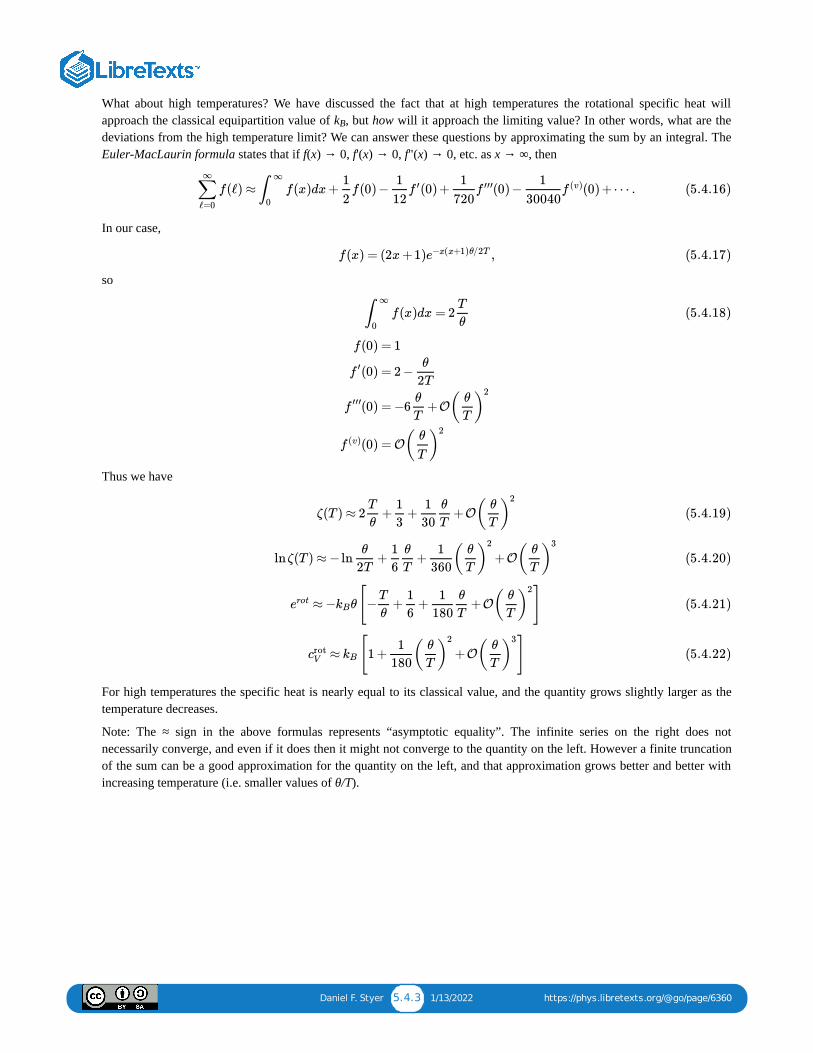
Daniel F. Styer 5.4.3 1/13/2022 https://phys.libretexts.org/@go/page/6360

What about high temperatures? We have discussed the fact that at high temperatures the rotational specific heat willapproach the classical equipartition value of k , but how will it approach the limiting value? In other words, what are thedeviations from the high temperature limit? We can answer these questions by approximating the sum by an integral. TheEuler-MacLaurin formula states that if f(x) → 0, f'(x) → 0, f"(x) → 0, etc. as x → ∞, then

In our case,

so

Thus we have

For high temperatures the specific heat is nearly equal to its classical value, and the quantity grows slightly larger as thetemperature decreases.

Note: The ≈ sign in the above formulas represents “asymptotic equality”. The infinite series on the right does notnecessarily converge, and even if it does then it might not converge to the quantity on the left. However a finite truncationof the sum can be a good approximation for the quantity on the left, and that approximation grows better and better withincreasing temperature (i.e. smaller values of θ/T).

B

f(ℓ) ≈ f(x)dx+ f(0) − (0) + (0) − (0) +⋯ .∑ℓ=0

∞

∫∞

0

1

2

1

12f ′ 1

720f ′′′ 1

30040f (v) (5.4.16)

f(x) = (2x+1) ,e−x(x+1)θ/2T (5.4.17)

f(x)dx = 2∫∞

0

T

θ(5.4.18)

f(0)

(0)f ′

(0)f ′′′

(0)f (v)

= 1

= 2 −θ

2T

= −6 +Oθ

T( )

θ

T

2

= O( )θ

T

2

ζ(T ) ≈ 2 + + +OT

θ

1

3

1

30

θ

T( )

θ

T

2

(5.4.19)

lnζ(T ) ≈ −ln + + +Oθ

2T

1

6

θ

T

1

360( )

θ

T

2

( )θ

T

3

(5.4.20)

≈ − θ[− + + +O ]erot kBT

θ

1

6

1

180

θ

T( )

θ

T

2

(5.4.21)

≈ [1 + +O ]crotV kB

1

180( )

θ

T

2

( )θ

T

3

(5.4.22)

Daniel F. Styer 1 1/4/2022 https://phys.libretexts.org/@go/page/6361

Welcome to the Physics Library. This Living Library is a principal hub of the LibreTexts project, which is a multi-institutional collaborative venture to develop the next generation of open-access texts to improve postsecondary educationat all levels of higher learning. The LibreTexts approach is highly collaborative where an Open Access textbookenvironment is under constant revision by students, faculty, and outside experts to supplant conventional paper-basedbooks.

Campus Bookshelves Bookshelves

Learning Objects

Daniel F. Styer 5.6.1 1/13/2022 https://phys.libretexts.org/@go/page/6362

5.6: Problems5.5 Decoupling quantal Hamiltonians

Prove the “decoupling Hamilton implies factoring partition function” theorem of section 5.1.2 for quantal systems.

5.6 Schottky anomaly

A molecule can be accurately modeled by a quantal two-state system with ground state energy 0 and excited stateenergy . Show that the internal specific heat is

Sketch this specific heat as a function of . How does the function behave when and ?

5.7 Simple harmonic oscillator

Suppose a molecule can be accurately modeled as a harmonic oscillator of natural frequency ω.

a. Find the expected internal energy of one such molecule, written as a sum of the ground state energy plus atemperature-dependent part.

b. Show that the internal specific heat is

c. Show that at low temperatures ,

whereas at high temperatures ,

d. (Optional.) Show that the leading quantal correction to the high-temperature specific heat is

e. Sketch the internal specific heat as a function of .

5.8 Simple harmonic oscillator — entropy

I was speaking with someone who claimed that thermodynamics didn’t apply to systems of interacting atoms, or toliving things, or to anything other than the ideal gas. He challenged me “What’s the entropy of a pendulum? Theanswer is that entropy doesn’t apply to a pendulum!” Answer his question for a pendulum in the simple harmonicoscillator approximation, with natural frequency ω and temperature T.

5.9 Kinetic energy in air

What is the kinetic energy is a cubic liter of air (mostly nitrogen and oxygen) at one atmosphere pressure and roomtemperature? At one atmosphere pressure and temperature 600 K? Use classical mechanics, and express your answerboth in Joules and in the commercial unit kilowatt-hours. (Clue: If you calculate the average kinetic energy of onemolecule, you’re working way too hard.) Why doesn’t anyone exploit all this valuable energy lying around in everycubic meter of air?

5.10 Conceptual comparison

a. Explain qualitatively why the results of the two previous problems are parallel at low temperatures.

ϵ

(T ) =cintV

kB( )ϵ

TkB

2e−ϵ/ TkB

(1 + )e−ϵ/ TkL

2(5.6.1)

/ϵkB T ≪ ϵkB T ≫ ϵkB

(T ) = .cintV

kB( )ℏω

TkB

2e

−ℏω/ TkB

(1 − )e−ℏω/ TkH2

(5.6.2)

( T ≪ ℏω)kB

(T ) ≈cintV

kB( )ℏω

TkB

2

e−ℏω/ TkB (5.6.3)

( T \rrℏω)kB

(T ) ≈ .cintV

kB (5.6.4)

(T ) = [1 − +O ( )] , where x = .cintV

kB

1

12x

2x

3 ℏω

TkB

(5.6.5)

T /ℏωkB

Daniel F. Styer 5.6.2 1/13/2022 https://phys.libretexts.org/@go/page/6362

b. (Harder.) Explain qualitatively both high temperature results. (Clue: At high temperatures, the average energy perparticle in the Schottky case approaches /2. Why?)

5.11 Compressibility of a diatomic gas

Find the isothermal compressibility κ for an ideal diatomic gas, where each molecule is modeled as a dumbbellwith moment of inertia I.

5.12 Systems with a small number of states

(This problem requires no calculation! All the answers can be found in your head.) A collection of non-interactingparticles is in thermal equilibrium. Each particle has only three energy eigenvalues, namely 0, , and .

a. What is the criterion for “high temperature” in this situation?

b. Suppose there are three non-degenerate energy eigenstates. At high temperatures, what is the averageenergy of each particle? (Clue: The answer is not .)

c. Now suppose that the lower two energy eigenstates are non-degenerate, but that there are two independentstates with energy . What is the average energy per particle at high temperatures in this case?

5.13 Anharmonic oscillator

The energy eigenvalues of a simple harmonic oscillator are equally spaced, and we have explored the consequencesof this for the heat capacity of a collection of harmonic oscillators. Suppose an anharmonic oscillator isapproximately harmonic (with natural frequency ω ) for small energies, but that for large energies (greater than, say,E ) the eigenvalues become more closely spaced as energy increases. At temperatures greater than E /k , will theheat capacity of a collection of such anharmonic oscillators be greater than or less than that of a collection ofharmonic oscillators with the same natural frequency ω ? Why?

5.14 Descriptive features of models

(This problem is stolen from a GRE Physics test.)

Two possible models for a diatomic ideal gas are the rigid dumbbell (model R; two point particles connected by arigid rod) and the springy dumbbell (model S; two point particles connected by a spring). In classical statisticalmechanics, which of the following statements is true?

a. Model R has a specific heat .

b. Model S has a smaller specific heat than model R.

c. Model S is always correct.

d. Model R is always correct.

e. The choice between models R and S depends on the temperature.

5.15 An n-state system, qualitatively

A model molecule has n equally-spaced energy levels, all of them non-degenerate, with energy spacing . Thus as nvaries from 2 to ∞ this model interpolates between the Schottky system of problem 5.6 and the simple harmonicoscillator of problem 5.7.

a. Find a low-temperature approximation for the specific heat that is independent of n.

b. At high temperatures, the specific heat approaches zero. What is the criterion for “high temperature”?

c. At high temperatures, what is the expected energy of this model?

d. There is a theorem stating that at any fixed positive temperature, the specific heat must increase withincreasing n. Assume this theorem and use it to prove that as n increases, the maximum in the specific heatversus temperature curve becomes higher.

5.16 An n-state system, quantitatively

Show that the system of the previous problem has internal specific heat

ϵ

T

ϵ 4ϵ

4ϵ

4ϵ

0

x x B

0

=cV32

kB

ϵ

Daniel F. Styer 5.6.3 1/13/2022 https://phys.libretexts.org/@go/page/6362

Does this expression have the proper limits when n = 2 and when n → ∞?

(T ) = [ − ] .cintV

kB ( )ϵ

TkB

2e

−ϵ/ TkB

(1 − )e−ϵ/ TkB2

( )nϵ

TkB

2e

−nϵ/ TkB

(1 − )e−nϵ/ TkB2

(5.6.6)

1 1/27/2022

CHAPTER OVERVIEW6: QUANTAL IDEAL GASES

In the previous chapter, we found that at high temperatures, an ideal gas of diatomic molecules with spring interactions has a heatcapacity of per molecule: from the translational degrees of freedom, kB from the rotational degrees of freedom, and kB fromthe spring degrees of freedom. If the temperature is decreased, the spring degrees of freedom become governed by quantum mechanicsrather than classical mechanics, the equipartition theorem no longer holds, and eventually these degrees of freedom “freeze out” andcontribute nothing to the heat capacity: the total heat capacity per molecule becomes . If the temperature is decreased still further,the story is repeated for the rotational degrees of freedom and eventually they freeze out. What happens if the temperature is decreasedyet again? Do the translational degrees of freedom then freeze out as well? The answer is “sort of”, but the crossover from the classicalto the quantal regime is complicated in this case by the quantal requirement of interchange symmetry. This requirement gives rise to amuch richer and more interesting crossover behavior than is provided by simple freeze out.

6.1: INTRODUCTION6.2: THE INTERCHANGE RULE6.3: QUANTUM MECHANICS OF INDEPENDENT IDENTICAL PARTICLES6.4: STATISTICAL MECHANICS OF INDEPENDENT IDENTICAL PARTICLES6.5: QUANTUM MECHANICS OF FREE PARTICLES6.6: FERMI-DIRAC STATISTICS6.7: BOSE-EINSTEIN STATISTICS6.8: SPECIFIC HEAT OF THE IDEAL FERMION GAS6.9: ADDITIONAL PROBLEMS6.10: APPENDIX

kB

7

2kB

3

2

kB

5

2

Daniel F. Styer 6.1.1 12/9/2021 https://phys.libretexts.org/@go/page/6364

6.1: IntroductionIn the previous chapter, we found that at high temperatures, an ideal gas of diatomic molecules with spring interactions hasa heat capacity of per molecule: from the translational degrees of freedom, k from the rotational degrees offreedom, and k from the spring degrees of freedom. If the temperature is decreased, the spring degrees of freedombecome governed by quantum mechanics rather than classical mechanics, the equipartition theorem no longer holds, andeventually these degrees of freedom “freeze out” and contribute nothing to the heat capacity: the total heat capacity permolecule becomes . If the temperature is decreased still further, the story is repeated for the rotational degrees offreedom and eventually they freeze out. What happens if the temperature is decreased yet again? Do the translationaldegrees of freedom then freeze out as well? The answer is “sort of”, but the crossover from the classical to the quantalregime is complicated in this case by the quantal requirement of interchange symmetry. This requirement gives rise to amuch richer and more interesting crossover behavior than is provided by simple freeze out.

7

2kB

3

2kB B

B

5

2kB

Daniel F. Styer 6.2.1 12/16/2021 https://phys.libretexts.org/@go/page/6365

6.2: The Interchange RuleBefore turning to statistical mechanics, let us review the quantal “interchange rule”. The wavefunction for a system ofthree particles is a function of three variables: ψ(x , x , x ). [The symbol x represents whatever is needed to specify thestate: For a spinless particle in one dimension x represents the coordinate x or, if you are working in momentum space, thecoordinate p. For a particle with spin moving in three dimensions, x represents (x, y, z, m ), or perhaps (p , p , p , m ).] Ifthe three particles are identical, then the wavefunction must be either symmetric under the interchange of any pair ofvariables

or else antisymmetric under the interchange of any pair of variables,

The foregoing assertion is an empirical rule that cannot be derived from any of the other principles of quantum mechanics.(Indeed there is currently considerable interest in anyons, hypothetical particles that obey all the principles of quantummechanics except the interchange rule.) The rule holds for all quantal states, not just energy eigenstates. It holds forinteracting as well as for non-interacting particles. And the rule has a number of surprising consequences, both within thedomain of quantum mechanics and atomic physics, and, as well shall soon see in detail, within the domain of statisticalmechanics.

The sign of the interchange symmetry, either + or −, is governed only by the type of particle involved: for pions it isalways +, for electrons it is always −. Particles for which the sign is always + are called bosons, and those for which it isalways − are called fermions. It is an experimental fact that particles with integral spin s are bosons and those with halfintegral spin s are fermions.

6.2.1 Problems6.1 The interchange rule in another representation

Full information about the state of three identical spinless particles is contained not only in the configurational wavefunction ψ(x , x , x ) but also in the momentum space wave function

Show that if one representation is symmetric (or antisymmetric), then the other one is as well.

6.2 Symmetrization

Show that for any function f(x, y, z), the function

is symmetric under the interchange of any pair of variables. How many such pairs are there? Is there a similaralgorithm for building up an antisymmetric function from any garden-variety function?

A B C

z x y z x

ψ ( , , ) = +ψ ( , , ) = +ψ ( , , ) , etc. ,xA xB xC xB xA xC xB xC xA (6.2.1)

ψ ( , , ) = −ψ ( , , ) = +ψ ( , , ) , etc. xA xB xC xB xA xC xB xC xA (6.2.2)

A B C

( , , ) = ∫ ∫ ψ ( , , ) .ψ~

pA pB pC

1

(2πℏ)9/2d3xA d3xC xA xB xC e−i( ⋅ + ⋅ + ⋅ )/ℏpA xA pB xB pC xC (6.2.3)

(x, y, z) = f(x, y, z) +f(x, z, y) +f(z, x, y) +f(z, y, x) +f(y, z, x) +f(y, x, z)fS (6.2.4)

Daniel F. Styer 6.3.1 12/23/2021 https://phys.libretexts.org/@go/page/6366

6.3: Quantum Mechanics of Independent Identical ParticlesThis chapter considers collections of independent (i.e. non-interacting) identical monatomic particles. It does not treat mixtures ordiatomic molecules. Notice that “independent” means only that the particles do not interact with each other. In contrast, each particleindividually may interact with some background potential, such as a square well or harmonic oscillator potential. Later on (in section6.5) we will restrict our consideration to particles that interact only with the walls of their container (“free particles”), but for now wetreat the more general case.

Doing quantal statistical mechanics requires a basis of states to sum over. In this section we consider the only the quantum mechanicsof our situation in order to produce an energy eigenbasis. . . we defer all questions of statistical mechanics to the next section.

Most of our discussion in this section is phrased in terms of the three-particle problem rather than the N-particle problem. The use of aspecific number lends the advantage of concreteness, and three is the smallest number that generalizes readily to the N-particle case.

6.3.1 A basis for non-identical particles

Consider first a single particle moving in the background potential. Elementary quantum mechanics deals with this situation, and it tellsus that there will be a certain number M of (possibly degenerate) energy eigenstates. (Usually M will be infinite, but there areadvantages to calling it M and maintaining the ability to take the limit M → ∞.) The rth energy eigenstate has energy and isrepresented by the wavefunction η (x), where x denotes the arguments of the wavefunction: Thus for a spinless particle, x could standfor x, y, z or p , p , p or even p , y, p . For a particle with spin s, x could stand for expressions like x, y, z, s or p , p , p , s .

We will soon use these one-particle energy eigenstates as building blocks to construct energy eigenstates for the N-particle situation,i.e. energy eigenstates for the entire system. Thus we will frequently be talking about both “one-particle energy eigenstates” and “N-particle energy eigenstates” in the same sentence, and both phrases are mouthfulls. To make our sentences shorter and clearer—and toemphasize the dramatic distinction between these two entities—we will adopt the common convention of referring to the one-particleenergy eigenstates as “levels” and to the N-particle energy eigenstates as “states”. (Some books use the term “orbitals” rather than“levels”.) Thus we have for the one-particle energy eigenproblem:

Now consider more than one particle—let’s say three particles—moving independently and all subject to the same backgroundpotential. If the particles are not identical (say one helium, one argon, and one neon atom), then the three-body energy eigenbasis willcontain elements (“states”) such as

(If the particles interacted, then this would still be a state of the system, but it would not be an energy eigenstate.) We will represent thisstate by the notation :

Of course, degeneracies now must exist: the energy of is the same as the energy of . The entire basis consists of M suchstates (more generally, for the case of N independent particles, M ), namely:

Out of these M states we can build up (by addition and scalar multiplication) any wavefunction, i.e. any normalized function of (x ,x , x ). This is exactly what we want for non-identical particles. But for identical particles we don’t want to be able to build any

ϵr

r

x y z x z z x y z x

levels: energies:

(x)η1

ϵ1

(x)η2

ϵ2

⋯⋯

(x)ηr

ϵr

⋯⋯

(x)ηM

ϵM

( ) ( ) ( ) with energy + + .ηr xA ηs xB ηt xC ϵr ϵs ϵl (6.3.1)

|r, s, t⟩

( ) ( ) ( ) ⟺ |r, s, t⟩.ηr xA ηs xB ηℓ xC (6.3.2)

|r, s, t⟩ |s, r, t⟩ 3

N

|1, 1, 1⟩

|2, 1, 1⟩|1, 2, 1⟩|1, 1, 2⟩|3, 1, 1⟩

⋮|3, 2, 1⟩|3, 1, 2⟩

⋮|4, 2, 1⟩

⋮|M, M, M⟩

(6.3.3)

3A

B C

Daniel F. Styer 6.3.2 12/23/2021 https://phys.libretexts.org/@go/page/6366

wavefunction. Because of the interchange rule, the only relevant wavefunctions are those symmetric (or antisymmetric) under theinterchange of any pair of coordinates, for example

and hence these are the only kind of wavefunctions we want to be able to build. In other words, we need an energy eigenbasisconsisting only of symmetric (or antisymmetric) wavefunctions.

6.3.2 A basis for identical particles

Fortunately, there exists a general procedure for constructing symmetric (or antisymmetric) functions out of garden-variety (or “non-symmetrized”) functions, and this procedure will enable us to build the two desired basis sets. For functions of three variables theprocedure (which is readily generalized to N variables) works like this: Given a function f(x , x , x ), the new function

is surely symmetric under the interchange of any pair of variables, and the new function

is surely antisymmetric. These two procedures are called “symmetrization” and “antisymmetrization” (or sometimes “alternation”)respectively. It is of course possible that the resulting function vanishes, but this does not invalidate the procedure, because zerofunctions are both symmetric and antisymmetric!

When applied to a quantal wavefunction ψ(x , x , x ), these processes result in the symmetric wavefunction

and in the antisymmetric wavefunction

where the constants A and A are inserted simply to insure normalization. Note that the operators and defined above are linear,whence a basis for symmetric wavefunctions may be obtained by symmetrizing every element of an ordinary, non-symmetrized, basis,and similarly for antisymmetric wavefunctions.

For functions of three variables that factorize into three functions of one variable, i.e. functions of the form (6.5), these definitions canbe expressed even more simply because, for example, swapping η and η is the same as swapping x and x . Thus, if is anenergy eigenstate, then

is a symmetric state with the same energy, while

in an antisymmetric state with the same energy.

It is easy to see that the symmetrization process is unaffected by the order of the letters, i.e. that

whence, for example, the states all symmetrize to the same state. Similarly in antisymmetrization theorder of the letters affects only the sign of the result,

but this result is considerably more profound: It shows not only that, for example, is the same state as , but also that

whence , and, in general, that antisymmetrizes to zero unless r, s, and t are all distinct.

Now we construct a basis for symmetric wavefunctions by applying the operator to every element of our non-symmetrized basis onpage 141. We obtain

ψ ( , , ) = ±ψ ( , , ) ,xA xB xC xC xB xA (6.3.4)

A B C

f ( , , ) +f ( , , ) +f ( , , ) +f ( , , ) +f ( , , ) +f ( , , )xA xB xC xA xC xB xC xA xB xC xB xA xB xC xA xB xA xC (6.3.5)

f ( , , ) −f ( , , ) +f ( , , ) −f ( , , ) +f ( , , ) −f ( , , )xA xB xC xA xC xB xC xA xB xC xB xA xB xC xA xB xA xC (6.3.6)

A B C

ψ ( , , ) ≡ [ψ ( , , ) +ψ ( , , ) +ψ ( , , ) +ψ ( , , ) +ψ ( , , )]S x4 xB xC As xA xB xC xA xC xB xC xA xA xB xC xA xB xA xC (6.3.7)

ψ ( , , ) ≡ [ψ ( , , ) −ψ ( , , ) +ψ ( , , ) +ψ ( , , ) −ψ ( , , )]A xA xB xC Aa xA xB xC xA xC xB xC xB xA xB xC xA xB xA xC (6.3.8)

s a S A

s t B C |r, s, t⟩

|r, s, t⟩≡ [|r, s, t⟩+|t, r, s⟩+|t, r, s⟩+|t, s, r⟩+|s, t, r⟩+|s, r, t⟩]S As (6.3.9)

|r, s, t⟩≡ [|r, s, t⟩−|r, t, s⟩+|t, r, s⟩−|t, s, r⟩+|s, t, r⟩−|s, r, t⟩]A Aa (6.3.10)

|r, s, t⟩= |r, t, s⟩ etc. S S (6.3.11)

|1, 1, 2⟩, |1, 2, 1⟩, and|2, 1, 1⟩

|r, s, t⟩= − |r, t, s⟩= |t, r, s⟩ etc., A A A (6.3.12)

|1, 2, 3⟩A |3, 2, 1⟩A

|3, 1, 1⟩= − |3, 1, 1⟩A A (6.3.13)

|3, 1, 1⟩= 0A |r, s, t⟩

S

Daniel F. Styer 6.3.3 12/23/2021 https://phys.libretexts.org/@go/page/6366

where the crossed out elements are those that have already appeared earlier in the list. It is clear that there are fewer elements in thisbasis than there are in the non-symmetrized basis, although it is a challenge to count them exactly. The number of elements turns out tobe

or, for the N-particle ratherthan the three-particle case,

where the binomial coefficient symbol is define through

We construct a basis for antisymmetric wavefunctions in the same way. The result is

where now the crossed out elements have either appeared earlier in the list or else are equal to zero. There are even fewer elements inthis basis than there were in the symmetrized basis. In fact there are exactly

such elements, or for the case of N particles,

|1, 1, 1⟩

|2, 1, 1⟩

|1, 2, 1⟩

|1, 1, 2⟩

|3, 1, 1⟩

⋮|3, 2, 1⟩|3, 1, 2⟩

⋮

|4, 2, 1⟩

⋮|M, M, M⟩

,(M)(M +1)(M +2)

3!(6.3.14)

( ) .M +N −1

N(6.3.15)

( ) ≡ .m

n

m!n!(m −n)!

(6.3.16)

|1, 1, 1⟩

|2, 1, 1⟩

|1, 2, 1⟩

|1, 1, 2⟩

|3, 1, 1⟩

⋮|3, 2, 1⟩

|3, 1, 2⟩

⋮

|4, 2, 1⟩

⋮

| M, M, M⟩

,(M)(M −1)(M −2)

3!(6.3.17)

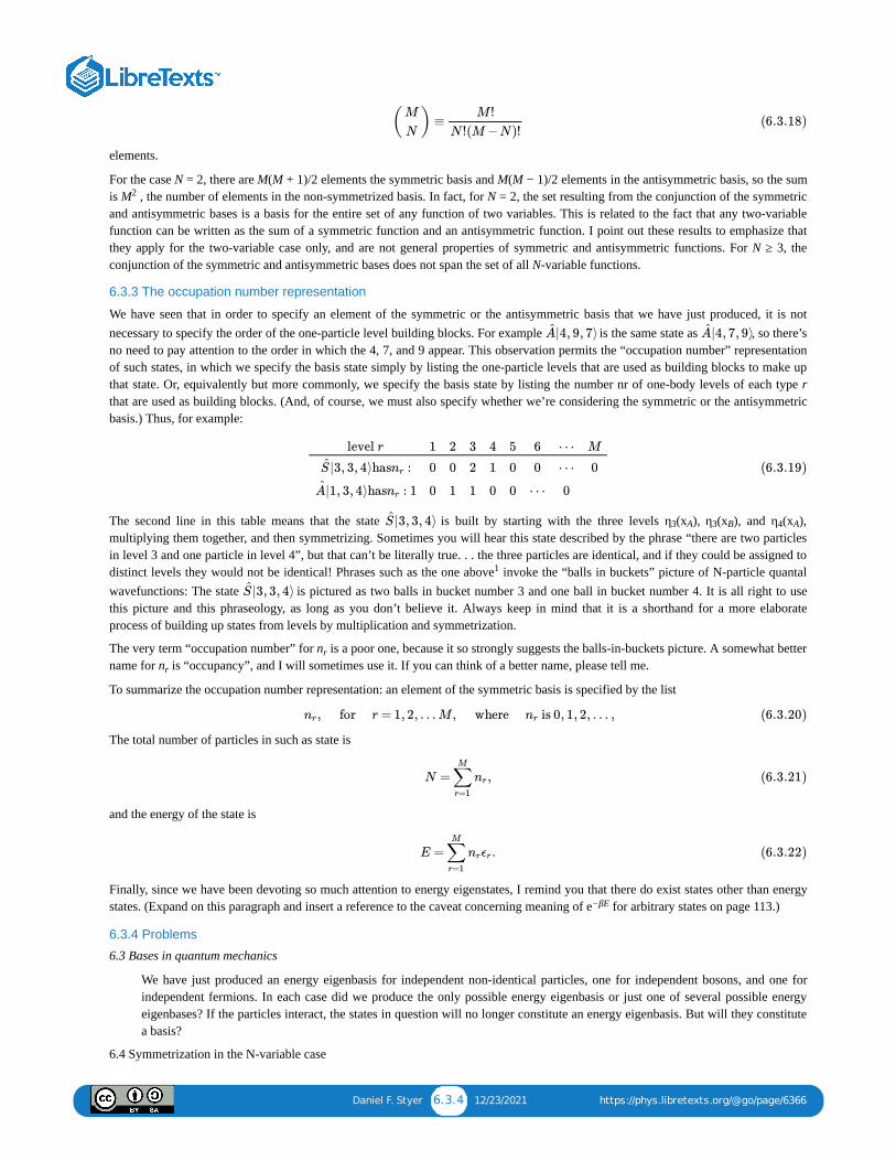
Daniel F. Styer 6.3.4 12/23/2021 https://phys.libretexts.org/@go/page/6366

elements.

For the case N = 2, there are M(M + 1)/2 elements the symmetric basis and M(M − 1)/2 elements in the antisymmetric basis, so the sumis M , the number of elements in the non-symmetrized basis. In fact, for N = 2, the set resulting from the conjunction of the symmetricand antisymmetric bases is a basis for the entire set of any function of two variables. This is related to the fact that any two-variablefunction can be written as the sum of a symmetric function and an antisymmetric function. I point out these results to emphasize thatthey apply for the two-variable case only, and are not general properties of symmetric and antisymmetric functions. For N ≥ 3, theconjunction of the symmetric and antisymmetric bases does not span the set of all N-variable functions.

6.3.3 The occupation number representation

We have seen that in order to specify an element of the symmetric or the antisymmetric basis that we have just produced, it is notnecessary to specify the order of the one-particle level building blocks. For example is the same state as , so there’sno need to pay attention to the order in which the 4, 7, and 9 appear. This observation permits the “occupation number” representationof such states, in which we specify the basis state simply by listing the one-particle levels that are used as building blocks to make upthat state. Or, equivalently but more commonly, we specify the basis state by listing the number nr of one-body levels of each type rthat are used as building blocks. (And, of course, we must also specify whether we’re considering the symmetric or the antisymmetricbasis.) Thus, for example:

The second line in this table means that the state is built by starting with the three levels η (x ), η (x ), and η (x ),multiplying them together, and then symmetrizing. Sometimes you will hear this state described by the phrase “there are two particlesin level 3 and one particle in level 4”, but that can’t be literally true. . . the three particles are identical, and if they could be assigned todistinct levels they would not be identical! Phrases such as the one above invoke the “balls in buckets” picture of N-particle quantalwavefunctions: The state is pictured as two balls in bucket number 3 and one ball in bucket number 4. It is all right to usethis picture and this phraseology, as long as you don’t believe it. Always keep in mind that it is a shorthand for a more elaborateprocess of building up states from levels by multiplication and symmetrization.

The very term “occupation number” for n is a poor one, because it so strongly suggests the balls-in-buckets picture. A somewhat bettername for n is “occupancy”, and I will sometimes use it. If you can think of a better name, please tell me.

To summarize the occupation number representation: an element of the symmetric basis is specified by the list

The total number of particles in such as state is

and the energy of the state is

Finally, since we have been devoting so much attention to energy eigenstates, I remind you that there do exist states other than energystates. (Expand on this paragraph and insert a reference to the caveat concerning meaning of e for arbitrary states on page 113.)

6.3.4 Problems

6.3 Bases in quantum mechanics

We have just produced an energy eigenbasis for independent non-identical particles, one for independent bosons, and one forindependent fermions. In each case did we produce the only possible energy eigenbasis or just one of several possible energyeigenbases? If the particles interact, the states in question will no longer constitute an energy eigenbasis. But will they constitutea basis?

6.4 Symmetrization in the N-variable case

( ) ≡M

N

M !N !(M −N)!

(6.3.18)

2

|4, 9, 7⟩A |4, 7, 9⟩A

level r

|3, 3, 4⟩has :S nr

|1, 3, 4⟩has : 1A nr

1

0

0

2

0

1

3

2

1

4

1

0

5

0

0

6

0

⋯

⋯

⋯

0

M

0 (6.3.19)

|3, 3, 4⟩S 3 A 3 B 4 A

1

|3, 3, 4⟩S

r

r

, for r = 1, 2, … M , where is 0, 1, 2, … ,nr nr (6.3.20)

N = ,∑r=1

M

nr (6.3.21)

E = .∑r=1

M

nrϵr (6.3.22)

−βE

Daniel F. Styer 6.3.5 12/23/2021 https://phys.libretexts.org/@go/page/6366

Equations (6.8) and (6.9) contain algorithms for constructing (anti)symmetric functions of three variables by summing up sixterms. How do these equations generalize to functions of N variables and, in particular, how many terms appear in each sum?

6.5 Symmetrizing the symmetric

The non-symmetrized state is already symmetric in the case that r = s = t. What happens if you attempt to symmetrizethis already symmetric state through the procedure (6.12)? What if you attempt to antisymmetrize it through the procedure(6.13)?

6.6 Normalization constants

Find the normalization constants A and A in equations (6.12) and (6.13). Be sure your formula works for the case of and . Generalize your result to the N-particle case, where the answer is a function of n , n , . . . , nM as well as N.

6.7 Algorithms for permutations

Invent some problem concerning the Heap algorithm for generating permutations. Better just give a reference to Sedgwick’spaper.

6.8 Algorithms to list basis states

Come up with some algorithm for producing the three sets of basis states that we have discussed, preferably in some useful order(where “useful” is to be defined by you). Your algorithm should generalize readily to the N-particle case.

6.9 Number of basis elements

Perform the counts (6.18) and (6.21). (Clue: Do it first for N = 3, then for N arbitrary.)

For example, phrases like “the level is filled” or “the level is empty” or “the level is half-filled”.

|r, s, t⟩

s a |3, 3, 5⟩S

|4, 4, 4⟩S 1 2

1

Daniel F. Styer 6.4.1 12/2/2021 https://phys.libretexts.org/@go/page/6367

6.4: Statistical Mechanics of Independent Identical Particles

6.4.1 Partition function

Now that we have an energy eigenbasis, the obvious thing to do is to calculate the canonical partition function

where for fermions and bosons, respectively, the term “state” implies the occupation number lists:

fermions (n , n , · · · , n ), n = 0, 1, subject to n = N

bosons (n , n , · · · , n ), subject to n = N

As we have seen, it is difficult to even count these lists, much less enumerate them and perform the relevant sum! It can bedone, but there is a trick that renders it unnecessary. (Don’t be ashamed if you don’t see the trick. . . neither did Einstein orFermi. They both did it the hard, canonical way.)

The trick here, as in so many places in statistical mechanics, is to use the grand canonical ensemble. In this ensemble, thepartition function is

where the term “state” now implies the occupation number lists without any restriction on total particle number:

fermions (n , n , · · · , n ), n = 0, 1

bosons (n , n , · · · , n )

Writing out the sum over states explicitly, we have for fermions

A typical factor in the product is

so for fermions

Meanwhile, for bosons, the explicit state sum is

and a typical factor in the product is

Z(β) = ,∑ states

e−βE (6.4.1)

1 2 M r ∑r r

1 2 M ∑r r

Ξ(β, μ) = = =∑ states

e−βE+βμN ∑ states

e−β ( −μ )∑r nrϵr nτ ∑ states

∏r=1

M

e−β ( −μ)nr ϵr (6.4.2)

1 2 M r

1 2 M

.

Ξ(β, μ) = …∑=0n1

1

∑=0n2

1

∑=0nM

1

∏r=1

M

e−β ( −μ)nr ϵr

= [ ][ ]⋯ [ ]∑=0n1

1

e−β ( −μ)n1 ϵ1 ∑=0n2

1

e−β ( −μ)n2 ϵ1 ∑n=0

1

e−β ( −μ)nM ϵ1

[ ] = 1 + ,∑=0nr

1

e−β ( −μ)nr ϵr e−β( −μ)ϵr (6.4.3)

Ξ(β, μ) = 1 + .∏r=1

M

e−β( −μ)ϵr (6.4.4)

.

Ξ(β, μ) = …∑=0n1

∞

∑=0n2

∞

∑nM=0

∞

∏r=1

M

e−β ( −μ)nr ϵr

= [ ][ ]⋯ [ ]∑=0n1

∞

e−β ( −μ)n1 ϵ1 ∑=0n2

∞

e−β ( −μ)n2 ϵ1 ∑=0nM

∞

e−β ( −μ)nM ϵ1

Daniel F. Styer 6.4.2 12/2/2021 https://phys.libretexts.org/@go/page/6367

where in the last line we have summed the geometric series under the assumption that > µ. Thus for bosons

The two results are compactly written together as

where the + sign refers to fermions and the − sign to bosons.

6.4.2 Mean occupation numbers

In our previous work, we have always found the partition function and worked from there. Surprisingly, however, for thesituation of quantal ideal gases it is more useful to find the mean occupation numbers, such as

Note that the averages are functions of β and µ (as well as of r) but it is notationally clumsy to show that dependence.

How can such averages be evaluated? A slick trick would be helpful here! Consider the derivative

Using the explicit expression (6.37) for Ξ (where the + sign refers to fermions and the − sign to bosons), this gives

leaving us with the final result.

As before, the + sign refers to fermions and the − sign to bosons.

The mean occupation numbers play such an important role that it is easy to forget that they are only averages, that therewill be fluctuations, that for a given T and µ not all states will have exactly building blocks of level 5 (see problem6.13). Keep this in mind if you ever find yourself saying “occupation number” rather than “mean occupation number”.

,

[ ]∑=0nr

∞

e−β ( −μ)nr ϵr = 1 +[ ]+ + +⋯e−β( −μ)ϵr [ ]e−β( −μ)ϵr

2

[ ]e−β( −μ)ϵr

3

=1

1 −e−β( −μ)ϵr

ϵr

Ξ(β, μ) = .∏r=1

M 1

1 −e−β( −μ)ϵr

(6.4.5)

Ξ(β, μ) = ,∏r=1

M

[1 ± ]e−β( −μ)ϵr±1

(6.4.6)

⟨ ⟩ = = .n5

∑ states n5e−β(E−μN)

∑ states e−β(E−μN)

∑ states n5e−β ( − μ)∑r nrϵr nr

Ξ(β, μ)(6.4.7)

⟨ ⟩nr

= = (−β ) = −β ⟨ ⟩ .∂ lnΞ

∂ϵ5

1

Ξ

∂Ξ

∂ϵ5

1

Ξ∑

states

n5 e−β ( − μ)∑r nrϵr nr n5 (6.4.8)

⟨ ⟩ = −n51

β

∂ lnΞ

∂ϵ5(6.4.9)

= − ln 1

β

∂

∂ϵ5∑r=1

M

[1 ± ]e−β( −μ)ϵr

±1

(6.4.10)

= − ln 1

β

∂

∂ϵ5[1 ± ]e−β( −μ)ϵS

±1

(6.4.11)

= − ± 1

β

±(−β)e−β( −μ)ϵ5

[1 ± ]e−β( −μ)e5(6.4.12)

= ,1

±1eβ( −μ)ϵS

(6.4.13)

⟨ ⟩ = .nr

1

±1eβ( −μ)ϵr

(6.4.14)

⟨ ⟩n5

Daniel F. Styer 6.4.3 12/2/2021 https://phys.libretexts.org/@go/page/6367

In practice, these results from the grand canonical ensemble are used as follows: One uses these results to find quantities ofinterest as functions of temperature, volume, and chemical potential, such as the pressure p(T, V, µ). But most experimentsare done with a fixed number of particles N, so at the very end of your calculation you will want to find µ(T, V, N) in orderto express your final answer as p(T, V, N). You can find µ(T, V, N) by demanding that

In other words, the quantity µ serves as a parameter to insure normalization, very much as the quantity Z serves to insurenormalization in the canonical ensemble through

You might wonder, in fact, about the relation between the canonical probability

which we have seen many times before, and the recently derived occupancy probability

The first result applies to both interacting and non-interacting systems, both classical and quantal. The second applies onlyto non-interacting quantal systems. Why do we need a new probability? What was wrong with our derivation (in section4.1) of the canonical probability that requires us to replace it with an occupancy probability? The answer is that nothingwas wrong and that the occupancy probability doesn’t replace the canonical probability. The canonical probability and theoccupancy probability answer different questions. The first finds the probability that the entire system is in the many-bodystate n. The second finds the probability that the one-body level r is used as a building block in constructing the many-body state. Indeed, although we derived the occupancy probability result through a grand canonical argument, it is alsopossible to derive the occupancy probabilities from strict canonically arguments, proof that these two probabilities cancoexist peacefully.

6.4.3 The Boltzmann limitThis is the limit where particles are far enough apart that overlap of wavefunction is minimal, so we needn’t worry aboutsymmetrization or antisymmetrization. Equivalently, it is the limit where for all r.

6.4.4 Problems6.10 Evaluation of the grand canonical partition function

Can you find a simple expression for Ξ(β, µ) for non-interacting particles in a one-dimensional harmonic well? Fornon-interacting particles in a one-dimensional infinite square well? For any other potential? Can you do anythingvaluable with such an expression once you’ve found it?

6.11 Entropy of quantal ideal gases

This problem derives an expression for the entropy of a quantal ideal gas in terms of the mean occupation numbershnri. (Compare problem 4.3.) Throughout the problem, in the symbols ± and ∓, the top sign refers to fermions andthe bottom sign refers to bosons.

a. Use the connection between thermodynamics and statistical mechanics to show that, for any system,

b. Show that for the quantal ideal gas,

N = ⟨ ⟩ = .∑r=1

M

nr ∑r=1

M1

±1eβ( −μ)er

(6.4.15)

1 = .∑n

e−βEn

Z(6.4.16)

,e−βEn

Z(6.4.17)

.1

N

1

±1eβ( −μ)ϵr

(6.4.18)

⟨ ⟩ ≪nr

= lnΞ −β .S(T , V , μ)

kB

∂ lnΞ

∂β(6.4.19)

Daniel F. Styer 6.4.4 12/2/2021 https://phys.libretexts.org/@go/page/6367

c. The mean occupation numbers are functions of T, V, and µ (although it is notationally clumsy to showthis dependence). Show that

d. Finally, show that

e. Find a good approximation for this expression in the Boltzmann limit, .

f. (Optional.) Find an expression for C in terms of the quantities .

6.12 Isothermal compressibility of quantal ideal gases

a. Show that in a quantal ideal gas, the isothermal compressibility is

where as usual the top sign refers to fermions and the bottom sign to bosons. (Clue: Choose the most appropriateexpression for κ from those uncovered in problem 3.33.)

b. Compare this expression to that for a classical (“Maxwell-Boltzmann”) ideal gas.

c. The negative sign in the expression for fermions opens the possibility that κT could be negative. Prove that thispotential horror never happens. d. Do the relative sizes of the three compressibilites (fermion, classical, boson)adhere to your qualitative expectations? (Compare problem 6.29.)

6.13 Dispersion in occupation number

Find an expression analogous to (6.45) giving the dispersion in the occupation numbers. (Clue: A slick trick wouldbe helpful here.) Answer:

lnΞ(T , V , μ) = ∓ ln(1 ∓ ⟨ ⟩).∑r

nr (6.4.20)

⟨ ⟩nr

.β

∂ ⟨ ⟩nr

∂β)V,μ = −β ( −μ) ⟨ ⟩ (1 ∓ ⟨ ⟩)ϵr nr nr

= −[ln(1 ∓ ⟨ ⟩) −ln⟨ ⟩| ⟨ ⟩ (1 ∓ ⟨ ⟩)nr nr nr nr

S(T , V , μ) = − [⟨ ⟩ ln⟨ ⟩±(1 ∓ ⟨ ⟩) ln(1 ∓ ⟨ ⟩)] .kB∑r

nr nr nr nr (6.4.21)

⟨ ⟩ ≪ 1nr

V ⟨ ⟩nr

= [1 ∓ ] ,κT

1

ρ TkB

∑r ( )nr2

⟨ ⟩∑r nr

(6.4.22)

T

Δ = =nr

1

±eβ( −μ)/2ϵr e−β( −μ)/2ϵr

⟨ ⟩ (1 ∓ ⟨ ⟩)nr nr

− −−−−−−−−−−−√ (6.4.23)

Daniel F. Styer 6.5.1 1/20/2022 https://phys.libretexts.org/@go/page/6368

6.5: Quantum Mechanics of Free Particles“Particle in a box.” Periodic boundary conditions. k-space. In the thermodynamic limit, the dots in k-space become denselypacked, and it seems appropriate to replace sums over levels with integrals over k-space volumes. (In fact, there is at leastone situation (see equation 6.83) in which this replacement is not correct.)

Density of levels in k-space:

Energy density of levels:

How to use energy density of levels:

and this approximation (usually) becomes exact in the thermodynamic limit.

6.5.1 Problems6.14 Free particles in a box

We argued that, for a big box, periodic boundary conditions would give the same results as “clamped boundaryconditions”. Demonstrate this by finding the density of levels for three-dimensional particle in a box problem.

6.15 Density of levels for bound particles

What is the density of levels for a one-dimensional harmonic oscillator with spring constant K? For a three-dimensional isotropic harmonic oscillator?

6.16 Density of levels in d dimensions

What is the density of levels for free particles subject to periodic boundary conditions in a world of ddimensions?

( worth memorizing. )V

8π3(6.5.1)

number of one-body levels with from E to E +dE ≡ G(E)dE = V dEϵr2–

√ m3

2π2ℏ3E−−

√ (6.5.2)

f ( ) ≈ G(E)f(E)dE∑r

ϵr ∫∞

0(6.5.3)

G(E)

G(E)

Daniel F. Styer 6.6.1 12/16/2021 https://phys.libretexts.org/@go/page/6369

6.6: Fermi-Dirac StatisticsIn three dimensions, the chemical potential µ decreases with temperature. Why? It is clear that at T = 0, µ = > 0. But asthe temperature rises the gas approaches the classical limit, for which µ < 0 (see problem 2.23). This is not proof, but itmakes sense that µ should decrease with increasing temperature. A proof is available but surprisingly difficult.

6.6.1 Problems6.17 Qualitative origin of

(This problem is stolen from a GRE Physics test.)

The mean kinetic energy of electrons in metals at room temperature is usually many times the thermal energy k T.Which of the following can best be used to explain this fact?

a. The time-energy uncertainty relation.

b. The Pauli exclusion principle.

c. The degeneracy of the energy levels.

d. The Born approximation.

e. The wave-particle duality.

6.18 Fermion gas in two dimensions

(This problem is based on one in Ashcroft and Mermin, page 53.)

Consider a gas of free, independent, spin- fermions in two dimensions. The gas is contained within an area (or twodimensional volume) of A.

a. What is the density of one-particle levels in k-space?

b. How does the Fermi energy depend upon the density N/A?

c. Use = N to show that

Notice that the chemical potential µ decreases with temperature.

6.19 Dependence of chemical potential on temperature

Show that for independent (not necessarily free) fermions, the µ(T) curve has slope (when N and V are constant)

Can you use this result to show that the chemical potential must decrease with temperature? I can’t.

6.20 Thermodynamics of the fermion gas

Consider a collection of free and independent spin- fermions. Do not assume that the temperature vanishes.

a. Use the fundamental grand canonical result Π = −k T ln Ξ to show that

b. Use the expression for and the change of variable to find

c. Integrate by parts to obtain

EF

EF

B

12

EF

⟨ ⟩∑r nr

μ+ T ln(1 + ) = .kB e−μ/kBTEF (6.6.1)

= − .dμ

dT

1

T

G(E) (β(E −μ)/2)(E −μ)dE∫∞

0 sech2

G(E) (β(E −μ)/2)dE∫ ∞0

sech2(6.6.2)

12

B

p(T ,μ)V = T G(E) ln(1 + )dE.kB ∫∞

0eβ(μ−E) (6.6.3)

G(E) x = βE

p(T ,μ) = [ ] ln(1 + )dx.( T )kB5/2 2m3− −−−

√

π2ℏ3∫

∞

0x−−√ eβμe−x (6.6.4)

Daniel F. Styer 6.6.2 12/16/2021 https://phys.libretexts.org/@go/page/6369

(Do not attempt to evaluate the integral that remains.)

d. Meanwhile, show that the total energy

is given by

Thus the pressure and energy are related by

which is exactly the same relationship they have in the classical monatomic ideal gas! (See problem 6.28.)

6.21 Pressure at zero temperature

Use the result of the previous problem to show that at absolute zero the pressure of a gas of free and independentspin- fermions does not vanish (as it does for a classical ideal gas). Instead, the zero-temperature pressure is \(\frac25 \rho \mathcalE_F).

6.22 Mass-radius relation for white dwarf stars

(This problem is modified from Kittel and Kroemer, Thermal Physics, second edition, page 216.)

A white dwarf star (see Kittel and Kroemer, pp. 196–198) consists of highly compressed hydrogen in which theatoms have ionized into independent protons and electrons. In most cases it is a good model to assume that theelectrons are free and independent non-relativistic fermions at zero temperature. Consider a white dwarf of mass Mand radius R, containing N electrons.

a. Show that to a very good approximation, N = M/m , where m is the mass of a proton.

b. Show that the gravitational potential energy of a uniform sphere of mass M and radius R is −cGM /R, whereG is the gravitational constant and c is a dimensionless constant. (In fact but this is tedious to show.)

c. Show that the kinetic energy of the electrons is

where m is the mass of an electron.

d. If the potential and kinetic energies satisfy

as required by the virial theorem of mechanics, show that

Evaluate the constant assuming that . Note that the radius decreases as the mass increases.

e. If the white dwarf has the mass of the sun (2 × 10 kg), what is its radius (in km)? Compare this to theradius of our sun.

f. Neutron stars (observed as pulsars) are also zero temperature fermion gases, but in this case the fermions areneutrons rather than electrons. Derive the mass-radius relation for a neutron star, and use it to find the radius

p(T ,μ) = [ ] dx2

3( T )kB

5/2 2m3− −−−

√

π2ℏ3∫

∞

0

x3/2

+1exe−βμ(6.6.5)

E(T ,V ,μ) = G(E)f(E)EdE∫∞

0(6.6.6)

E(T ,V ,μ) = V [ ] dx( T )kB5/2 2m3− −−−

√

π2ℏ3∫

∞

0

x3/2

+1exe−βμ(6.6.7)

pV = E,2

3(6.6.8)

12

p p

2

c = 35

KE =9

20( )

3π2

2

1/3ℏ2

mem5/3p

M 5/3

R2(6.6.9)

e

KE = − PE,1

2(6.6.10)

R = a constant of approximate value m .M 1/3 1017 kg1/3 (6.6.11)

c = 35

30

Daniel F. Styer 6.6.3 12/16/2021 https://phys.libretexts.org/@go/page/6369

of a neutron star with the mass of the sun.

6.7.1 11/25/2021 https://phys.libretexts.org/@go/page/18918

6.7: Bose-Einstein StatisticsPerhaps you thought the Fermi-Dirac results were strange: Non-interacting particles forming a collection as hard as steel. .. room temperature being effectively zero. Wait until you see the Bose-Einstein results.

6.7.1 TheoryFor independent bosons, whether free or subject to an external potential, the mean occupation number function is

To begin to understand this function, note that

Thus this function has the general character sketched below:

Although we have written as a function of the continuous variable , we will in fact have occasion to evaluate it onlyat the energy eigenvalues , eigenvalues which of course differ for different external potentials. Itseems bizarre that b(E) can be negative, and indeed this is only a mathematical artifact: Recall that in our derivation of theBose function we needed to assume that µ < in order to insure convergence (see equation 6.35). Evaluating at anyeigenvalue r will always result in a positive mean occupation number.

The character of the Bose function is dominated by the singularity at = µ, so in trying to understand the function and itsphysical implications one must first locate the chemical potential. This section will provide a tour of Bose-Einsteinbehavior with decreasing temperature, throughout which the chemical potential shifts to the right. (When we investigatedFermi-Dirac behavior, we started at T = 0 and toured with increasing temperature, so the chemical potential shifted left.)This rightward shift presents a potential problem, because as the temperature decreases µ might shift right all the way to

, and we know that µ < 1. We will just have to go ahead and take the tour, being wary because we know that a µ = 1 roadblock might pop up right in front of us as we view the countryside. With any luck µ will not yet have reached when ourtour halts at T = 0.

For the case of free and independent bosons (subject to periodic boundary conditions), the ground level energy is = 0.The natural first step is to find µ(T, V, N) by demanding that

Natural though this may be, caution is in order. Remember that the integral above is an approximation to the sum overdiscrete energy levels

b(E) = .1

−1eβ(E−μ)(6.7.1)

when:

E < μ

E = μ

E > μ

we have:

b(E) negative

b(E) = ∞

b(E) positive

(6.7.2)

b(E) E

, , , . . . , , . . .ϵ1 ϵ2 ϵ3 ϵr

ε1 b(E)

E

ϵ1

ϵ1

ϵ1

N = G(E)b(E)dE.∫∞

0(6.7.3)

N = b ( ) .∑r

ϵr (6.7.4)

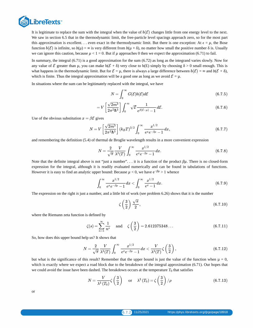
6.7.2 11/25/2021 https://phys.libretexts.org/@go/page/18918

It is legitimate to replace the sum with the integral when the value of changes little from one energy level to the next.We saw in section 6.5 that in the thermodynamic limit, the free-particle level spacings approach zero, so for the most partthis approximation is excellent. . . even exact in the thermodynamic limit. But there is one exception: At = µ, the Bosefunction is infinite, so b(µ) = ∞ is very different from b(µ + δ), no matter how small the positive number δ is. Usuallywe can ignore this caution, because µ < 1 = 0. But if µ approaches 0 then we expect the approximation (6.71) to fail.

In summary, the integral (6.71) is a good approximation for the sum (6.72) as long as the integrand varies slowly. Now forany value of greater than µ, you can make b( + δ) very close to b(E) simply by choosing δ > 0 small enough. This iswhat happens in the thermodynamic limit. But for = µ, there is always a large difference between = ∞ and b( + δ),which is finite. Thus the integral approximation will be a good one as long as we avoid = µ.

In situations where the sum can be legitimately replaced with the integral, we have

Use of the obvious substitution gives

and remembering the definition (5.4) of thermal de Broglie wavelength results in a more convenient expression

Note that the definite integral above is not “just a number”. . . it is a function of the product βµ. There is no closed-formexpression for the integral, although it is readily evaluated numerically and can be found in tabulations of functions.However it is easy to find an analytic upper bound: Because µ < 0, we have e > 1 whence

The expression on the right is just a number, and a little bit of work (see problem 6.26) shows that it is the number

where the Riemann zeta function is defined by

So, how does this upper bound help us? It shows that

but what is the significance of this result? Remember that the upper bound is just the value of the function when µ = 0,which is exactly where we expect a road block due to the breakdown of the integral approximation (6.71). Our hopes thatwe could avoid the issue have been dashed. The breakdown occurs at the temperature T that satisfies

or

b(E)

ϵ

b(E)

E E

E b(E) E

E

N = G(E)b(E)dE∫∞

0(6.7.5)

= V [ ] dE.2m3− −−−

√

2π2ℏ3∫

∞

0E−−

√1

−1eβ(E−μ)(6.7.6)

x = βE

N = V [ ] dx,2m3− −−−

√

2π2ℏ3( T )kB

3/2 ∫∞

0

x1/2

−1exe−βμ(6.7.7)

N = dx.2

π−−√

V

(T )λ3∫

∞

0

x1/2

−1exe−βμ(6.7.8)

−βµ

dx < dx.∫∞

0

x1/2

−1exe−βμ∫

∞

0

x1/2

−1ex(6.7.9)

ζ( ) ,3

2

π−−√

2(6.7.10)

ζ(s) = and ζ( ) = 2.612375348 …∑n=1

∞1

ns

3

2(6.7.11)

N = dx < ζ( ) ,2

π−−√

V

(T )λ3∫

∞

0

x1/2

−1exe−βμ

V

(T )λ3

3

2(6.7.12)

0

N = ζ( ) or ( ) = ζ( ) /ρV

( )λ3 T0

3

2λ3 T0

3

2(6.7.13)

6.7.3 11/25/2021 https://phys.libretexts.org/@go/page/18918

For temperatures above T , the chemical potential shifts right as the temperature falls, and the integral approximation(6.71) is legitimate (indeed, exact in the thermodynamic limit). But as the temperature decreases below T , the chemicalpotential sticks at µ = 0 and the integral approximation (6.71) must be modified.

What is the proper modification? The function is slowly varying for all values of except = µ, so the integralapproximation is legitimate for all the energy levels except the ground level at 1 = 0 = µ. Only for the ground level is someother result needed, so we just add in the ground level occupancy by hand:

Now, we have already seen that when µ = 0—the condition for validity of this equation—the integral can be evaluatedexactly and we have

Note that here is not given by its traditional formula (6.45), because

Instead, equation (6.84) is the formula for when T < T . The mean ground level occupancy is an intensivequantity when T > T but an extensive quantity when T < T .

In summary, the correct normalization equation breaks into two parts, namely

We should expect that each part will behave quite differently, i.e. we expect a sudden change of behavior as thetemperature drops through T .

What does all this mean physically? A naive reading of equation (6.80) suggests an upper bound on the number of particlesthat can be placed into the volume V. This would be sensible if the particles were marbles with hard-core repulsions. Butthese are non-interacting particles! Surely we can add more particles just by throwing them into the container. Indeed wecan do so, and the associated excess mean occupation number is due to the level that particles like best at lowtemperatures, namely the ground level. The ground level thus has a much higher mean occupancy than the first excitedlevel, and this rapid variation of mean occupancy with energy renders the approximation of sum by integral invalid. Theinequality (6.80) does not limit the number of particles in the system: instead it shows the domain within which it islegitimate to approximate the sum (6.72) by the integral (6.71).

The abrupt transition at T (ρ) is called Bose-Einstein condensation and the material at temperatures below T (ρ) is calledthe Bose condensate. These terms are unfortunate: they conjure images of a gas condensing into a liquid, in whichcircumstance the atoms separate into two different classes: those in the liquid and those remaining in the vapor. Thissuggests that in Bose-Einstein condensation too there are two classes of particles: those in the ground level and those in theexcited levels. This picture is totally false. It is incorrect to say “one particle is in the ground level, another is in the fourthexcited level”. In truth the individual particles are not in individual levels at all: instead the whole system is in a stateproduced by multiplying together the individual level wavefunctions (“building blocks”) and then symmetrizing them. Theliterature of Bose-Einstein statistics is full of statements like “at temperatures below T , any particle added to the systemgoes into the ground level.” Such statements are wrong. They should be replaced with statements like “at temperaturesbelow T , any increase in particle number occurs through an increase in , the mean occupancy of the ground level.” Oralternatively, “at temperatures below T , it is very likely that many of the building blocks from which the systemwavefunction is built are the ground level.” Or again, to be absolutely precise, “at temperatures below T , if the energy is

(ρ) = .T0h2

2πm ( )kBζ2/3 32

ρ2/3 (6.7.14)

0

0

b(E) E E

N = ⟨ ⟩+ G(E)b(E)dE.n1 ∫∞

0(6.7.15)

N = ⟨ ⟩+ ζ( ) .n1V

(T )λ3

3

2(6.7.16)

⟨ ⟩n1

= = ∞.1

−1eβ(E−μ)

1

−1e0(6.7.17)

⟨ ⟩n1 0 ⟨ ⟩n1

0 0

N =⎧

⎩⎨⎪

⎪

dx2π√

V

(T )λ3 ∫ ∞0

x1/2

−1exe−βμ

⟨ ⟩+ ζ ( )n1V

(T )λ3

32

for T > (ρ)T0

for T < (ρ)T0

(6.7.18)

0

0 0

0

0 ⟨ ⟩n1

0

0

6.7.4 11/25/2021 https://phys.libretexts.org/@go/page/18918

measured then it is very likely that many of the building blocks from which the resulting energy eigenfunction is built arethe ground level.” Read again the previous paragraph—the one that begins “What does all this mean physically?”. Noticethat I never need to say that a particle “is in” or “goes into” a given level.

6.7.2 ExperimentReferences: M.H. Anderson, J.R. Ensher, M.R. Matthews, C.E. Wieman, E.A. Cornell, “Observation of Bose-Einsteincondensation in a dilute atomic vapor”, Science, 269 (14 July 1995) 198–201; Randall G. Hullet at Rice; Malcolm W.Browne, “Two groups of physicists produce matter that Einstein postulated”, New York Times, 14 July 1995, page 1.

6.7.3 Problems

6.23 Character of the Bose function

What are the limits of the Bose function (equation 6.70) as → ±∞? Is the curvature of the function greaterwhen the temperature is high or when it is low?

6.24 Thermodynamics of the Bose condensate

For temperatures less than the Bose condensation temperature T , find the energy, heat capacity, and entropy of anideal gas of spin-zero bosons confined to a volume V. Write your answers in terms of the dimensionless integral

but don't bother to evaluate it. Show that

6.25 More thermodynamics of the Bose condensate

For the system of the previous problem, show that

From this show that at low temperatures, the pressure of a collection of free and independent bosons goes like p ∼T . (This is always less than the classical pressure p ∼ T.)

6.26 An integral important for Bose condensation

Show that

where

Clue:

b(E) E

0

I = dx∫∞

0

x3/2

−1ex(6.7.19)

= and S = .CV

5

2

E

T

5

3

E

T(6.7.20)

F = − E and p = .2

3

2

3

E

V(6.7.21)

5/2

dx = ζ( )∫∞

0

x1/2

−1ex3

2

π−−√

2(6.7.22)

ζ(s) = .∑n=1

∞ 1

ns(6.7.23)

= = for x > 0.1

−1ex1

(1 − )ex e−xe−x∑

n=0

∞

e−nx (6.7.24)

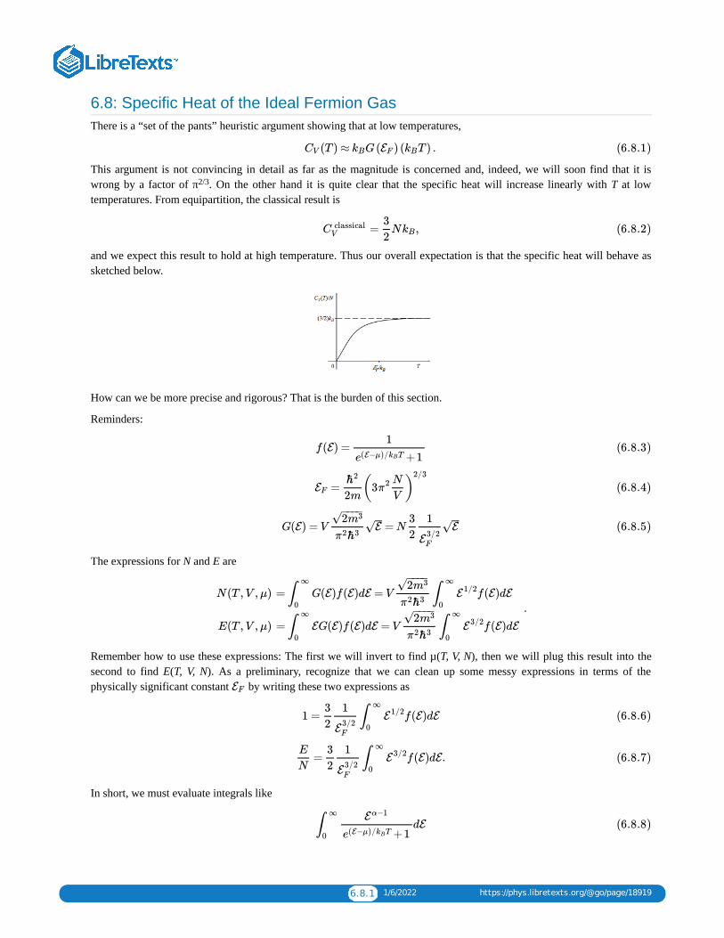
6.8.1 1/6/2022 https://phys.libretexts.org/@go/page/18919

6.8: Specific Heat of the Ideal Fermion GasThere is a “set of the pants” heuristic argument showing that at low temperatures,

This argument is not convincing in detail as far as the magnitude is concerned and, indeed, we will soon find that it iswrong by a factor of π . On the other hand it is quite clear that the specific heat will increase linearly with T at lowtemperatures. From equipartition, the classical result is

and we expect this result to hold at high temperature. Thus our overall expectation is that the specific heat will behave assketched below.

How can we be more precise and rigorous? That is the burden of this section.

Reminders:

The expressions for N and E are

Remember how to use these expressions: The first we will invert to find µ(T, V, N), then we will plug this result into thesecond to find E(T, V, N). As a preliminary, recognize that we can clean up some messy expressions in terms of thephysically significant constant by writing these two expressions as

In short, we must evaluate integrals like

(T ) ≈ G( ) ( T ) .CV kB EF kB (6.8.1)

2/3

= N ,C classical V

3

2kB (6.8.2)

f(E) =1

+1e(E−μ)/ TkB(6.8.3)

=EFℏ2

2m(3 )π2 N

V

2/3

(6.8.4)

G(E) = V = N2m3− −−−

√

π2ℏ3E−−

√3

2

1

E3/2F

E−−

√ (6.8.5)

.N(T ,V ,μ)

E(T ,V ,μ)

= G(E)f(E)dE = V f(E)dE∫∞

0

2m3− −−−√

π2ℏ3∫

∞

0E

1/2

= EG(E)f(E)dE = V f(E)dE∫∞

0

2m3− −−−√

π2ℏ3∫

∞

0E

3/2

EF

1 = f(E)dE3

2

1

E3/2F

∫∞

0E

1/2 (6.8.6)

= f(E)dE.E

N

3

2

1

E3/2F

∫∞

0E

3/2 (6.8.7)

dE∫∞

0

Eα−1

+1e(E−μ)/ TkB(6.8.8)

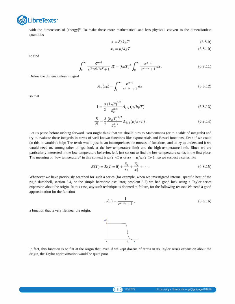
6.8.2 1/6/2022 https://phys.libretexts.org/@go/page/18919

with the dimensions of [energy] . To make these more mathematical and less physical, convert to the dimensionlessquantities

to find

Define the dimensionless integral

so that

Let us pause before rushing forward. You might think that we should turn to Mathematica (or to a table of integrals) andtry to evaluate these integrals in terms of well-known functions like exponentials and Bessel functions. Even if we coulddo this, it wouldn’t help: The result would just be an incomprehensible morass of functions, and to try to understand it wewould need to, among other things, look at the low-temperature limit and the high-temperature limit. Since we areparticularly interested in the low-temperature behavior, let’s just set out to find the low-temperature series in the first place.The meaning of “low temperature” in this context is or , so we suspect a series like

Whenever we have previously searched for such a series (for example, when we investigated internal specific heat of therigid dumbbell, section 5.4, or the simple harmonic oscillator, problem 5.7) we had good luck using a Taylor seriesexpansion about the origin. In this case, any such technique is doomed to failure, for the following reason: We need a goodapproximation for the function

a function that is very flat near the origin.

In fact, this function is so flat at the origin that, even if we kept dozens of terms in its Taylor series expansion about theorigin, the Taylor approximation would be quite poor.

α

x = E/ TkB (6.8.9)

= μ/ Tx0 kB (6.8.10)

dE = dx.∫∞

0

Eα−1

+1e(E−μ)/ TkB( T )kB

α ∫∞

0

xα−1

+1ex−x0(6.8.11)

( ) = dx.Aα x0 ∫∞

0

xα−1

+1ex−x0(6.8.12)

1 = (μ/ T )3

2

( T )kB3/2

E3/2F

A3/2 kB (6.8.13)

= (μ/ T ) .E

N

3

2

( T )kB5/2

E3/2F

A5/2 kB (6.8.14)

T ≪ μkB = μ/ T ≫ 1x0 kB

E(T ) = E(T = 0) + + +⋯ .E1

x0

E2

x20

(6.8.15)

g(x) = ,1

+1ex−x0(6.8.16)

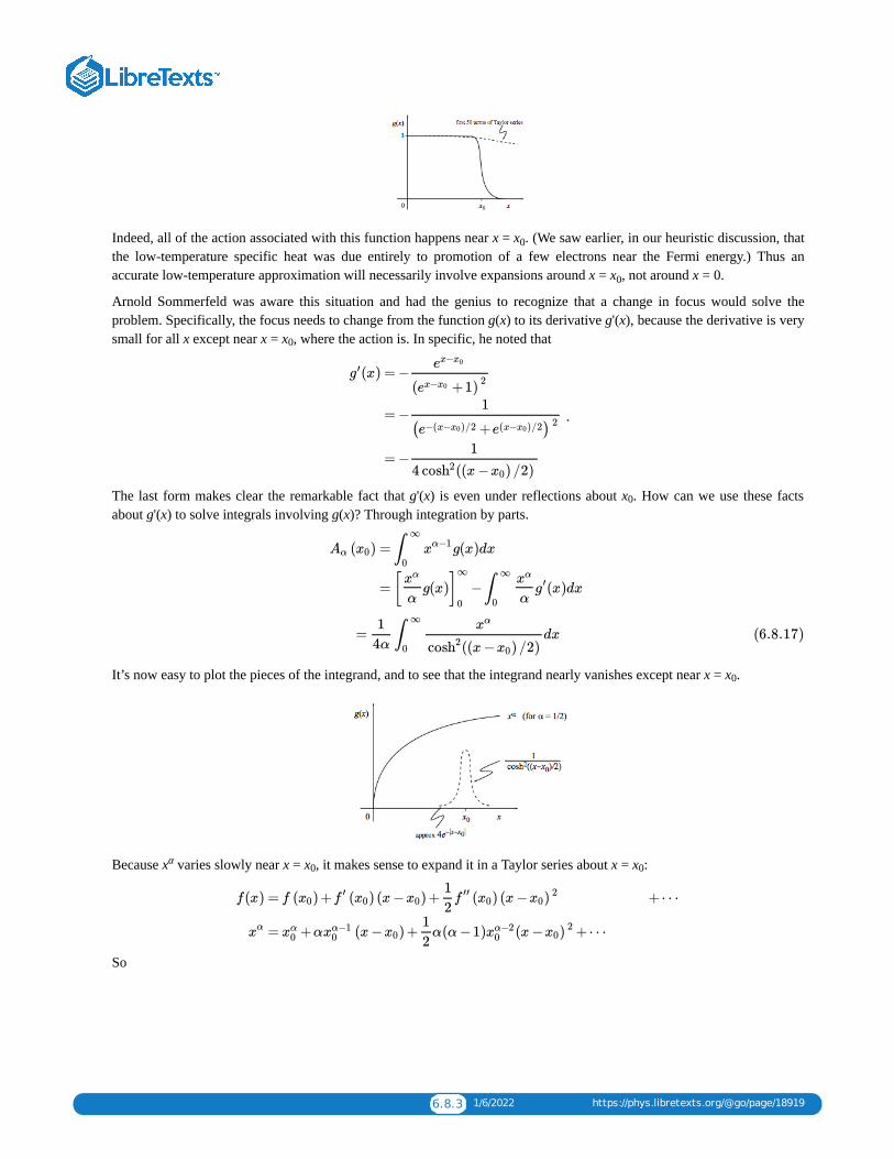
6.8.3 1/6/2022 https://phys.libretexts.org/@go/page/18919

Indeed, all of the action associated with this function happens near x = x . (We saw earlier, in our heuristic discussion, thatthe low-temperature specific heat was due entirely to promotion of a few electrons near the Fermi energy.) Thus anaccurate low-temperature approximation will necessarily involve expansions around x = x , not around x = 0.

Arnold Sommerfeld was aware this situation and had the genius to recognize that a change in focus would solve theproblem. Specifically, the focus needs to change from the function g(x) to its derivative g'(x), because the derivative is verysmall for all x except near x = x , where the action is. In specific, he noted that

The last form makes clear the remarkable fact that g'(x) is even under reflections about x . How can we use these factsabout g'(x) to solve integrals involving g(x)? Through integration by parts.

It’s now easy to plot the pieces of the integrand, and to see that the integrand nearly vanishes except near x = x .

Because x varies slowly near x = x , it makes sense to expand it in a Taylor series about x = x :

So

0

0

0

.

(x)g′ = −ex−x0

( +1)ex−x02

= −1

( + )e−(x− )/2x0 e(x− )/2x02

= −1

4 ((x− ) /2)cosh2 x0

0

( )Aα x0 = g(x)dx∫∞

0xα−1

= − (x)dx[ g(x)]xα

α

∞

0

∫∞

0

xα

αg′

= dx1

4α∫

∞

0

xα

((x− ) /2)cosh2 x0

(6.8.17)

0

α0 0

f(x)

xα

= f ( ) + ( ) (x− ) + ( )x0 f ′ x0 x01

2f ′′ x0 (x− )x0

2

= +α (x− ) + α(α−1) +⋯xα0 xα−10 x0

1

2xα−2

0 (x− )x02

+⋯

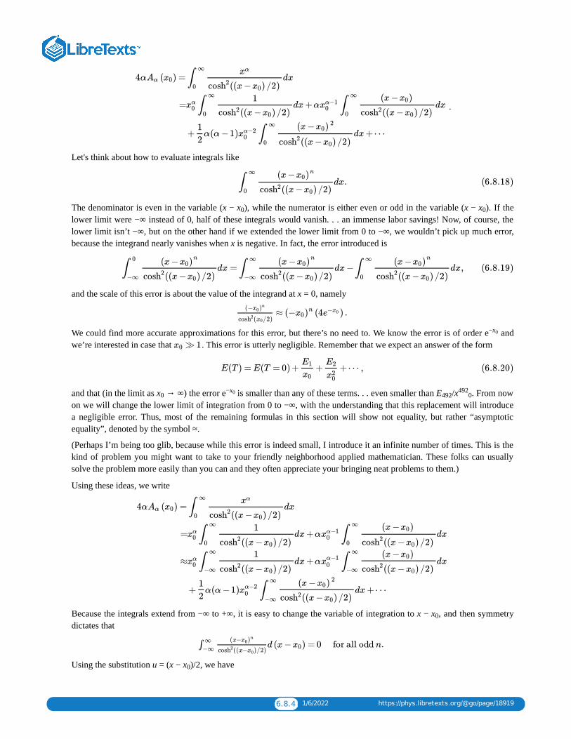
6.8.4 1/6/2022 https://phys.libretexts.org/@go/page/18919

Let's think about how to evaluate integrals like

The denominator is even in the variable (x − x ), while the numerator is either even or odd in the variable (x − x ). If thelower limit were −∞ instead of 0, half of these integrals would vanish. . . an immense labor savings! Now, of course, thelower limit isn’t −∞, but on the other hand if we extended the lower limit from 0 to −∞, we wouldn’t pick up much error,because the integrand nearly vanishes when x is negative. In fact, the error introduced is

and the scale of this error is about the value of the integrand at x = 0, namely

We could find more accurate approximations for this error, but there’s no need to. We know the error is of order e andwe’re interested in case that . This error is utterly negligible. Remember that we expect an answer of the form

and that (in the limit as x → ∞) the error e is smaller than any of these terms. . . even smaller than E /x . From nowon we will change the lower limit of integration from 0 to −∞, with the understanding that this replacement will introducea negligible error. Thus, most of the remaining formulas in this section will show not equality, but rather “asymptoticequality”, denoted by the symbol ≈.

(Perhaps I’m being too glib, because while this error is indeed small, I introduce it an infinite number of times. This is thekind of problem you might want to take to your friendly neighborhood applied mathematician. These folks can usuallysolve the problem more easily than you can and they often appreciate your bringing neat problems to them.)

Using these ideas, we write

Because the integrals extend from −∞ to +∞, it is easy to change the variable of integration to x − x , and then symmetrydictates that

Using the substitution u = (x − x )/2, we have

.

4α ( ) =Aα x0

=

dx∫∞

0

xα

((x− ) /2)cosh2 x0

dx+α dxxα0 ∫∞

0

1

((x− ) /2)cosh2 x0

xα−10 ∫

∞

0

(x− )x0

((x− ) /2)cosh2 x0

+ α(α−1) dx+⋯1

2xα−2

0 ∫∞

0

(x− )x02

((x− ) /2)cosh2 x0

dx.∫∞

0

(x− )x0n

((x− ) /2)cosh2 x0

(6.8.18)

0 0

dx = dx− dx,∫0

−∞

(x− )x0n

((x− ) /2)cosh2 x0

∫∞

−∞

(x− )x0n

((x− ) /2)cosh2 x0

∫∞

0

(x− )x0n

((x− ) /2)cosh2 x0

(6.8.19)

≈ (4 ) .(− )x0

n

( /2)cosh2 x0

(− )x0n e−x0

−x0

≫ 1x0

E(T ) = E(T = 0) + + +⋯ ,E1

x0

E2

x20

(6.8.20)

0−x0 492

4920

4α ( ) =Aα x0

=

≈

dx∫∞

0

xα

((x− ) /2)cosh2 x0

dx+α dxxα0 ∫∞

0

1

((x− ) /2)cosh2 x0

xα−10 ∫

∞

0

(x− )x0

((x− ) /2)cosh2 x0

dx+α dxxα0 ∫∞

−∞

1

((x− ) /2)cosh2 x0

xα−10 ∫

∞

−∞

(x− )x0

((x− ) /2)cosh2 x0

+ α(α−1) dx+⋯1

2xα−2

0 ∫∞

−∞

(x− )x02

((x− ) /2)cosh2 x0

0

d (x− ) = 0 for all odd n.∫ ∞−∞

(x− )x0n

((x− )/2)cosh2 x0

x0

0

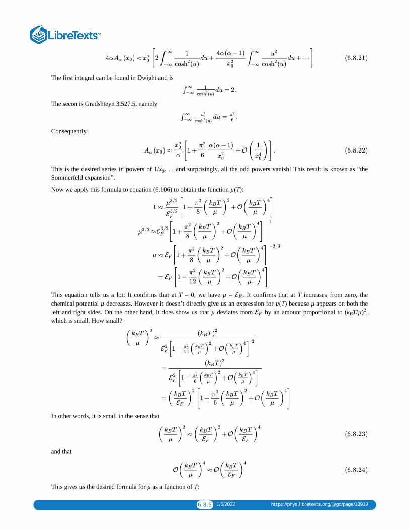
6.8.5 1/6/2022 https://phys.libretexts.org/@go/page/18919

The first integral can be found in Dwight and is

The secon is Gradshteyn 3.527.5, namely

Consequently

This is the desired series in powers of 1/x . . . and surprisingly, all the odd powers vanish! This result is known as “theSommerfeld expansion”.

Now we apply this formula to equation (6.106) to obtain the function µ(T):

This equation tells us a lot: It confirms that at T = 0, we have µ = . It confirms that at T increases from zero, thechemical potential µ decreases. However it doesn’t directly give us an expression for µ(T) because µ appears on both theleft and right sides. On the other hand, it does show us that µ deviates from by an amount proportional to (k T/µ) ,which is small. How small?

In other words, it is small in the sense that

and that

This gives us the desired formula for µ as a function of T:

4α ( ) ≈ [2 du+ du+⋯]Aα x0 xα0 ∫∞

−∞

1

(u)cosh2

4α(α−1)

x20

∫∞

−∞

u2

(u)cosh2(6.8.21)

du = 2.∫∞

−∞1

(u)cosh2

du = .∫ ∞−∞

u2

(u)cosh2

π2

6

( ) ≈ [1 + +O( )] .Aα x0

xα0

α

π2

6

α(α−1)

x20

1

x40

(6.8.22)

0

1

≈μ3/2

μ

≈ [1 + +O ]μ3/2

E3/2F

π2

8( )

TkB

μ

2

( )TkB

μ

4

E3/2F [1 + +O ]

π2

8( )

TkB

μ

2

( )TkB

μ

4 −1

≈ EF[1 + +O ]π2

8( )

TkB

μ

2

( )TkB

μ

4 −2/3

= [1 − +O ]EFπ2

12( )

TkB

μ

2

( )TkB

μ

4

EF

EF B2

≈( )TkB

μ

2 ( T )kB2

E2F[1 − +O ]π2

12( )TkB

μ

2( )TkB

μ

4 2

=( T )kB

2

[1 − +O ]E2F

π2

6( )TkB

μ

2( )TkB

μ

4

= [1 + +O ]( )TkB

EF

2π2

6( )

TkB

μ

2

( )TkB

μ

4

≈ +O( )TkB

μ

2

( )TkB

EF

2

( )TkB

EF

4

(6.8.23)

O ≈ O( )TkB

μ

4

( )TkB

EF

4

(6.8.24)

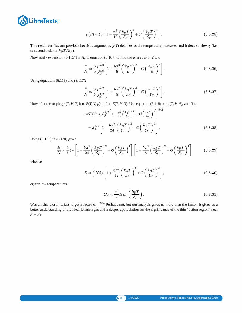
6.8.6 1/6/2022 https://phys.libretexts.org/@go/page/18919

This result verifies our previous heuristic arguments: µ(T) declines as the temperature increases, and it does so slowly (i.e.to second order in ).

Now apply expansion (6.115) for A to equation (6.107) to find the energy E(T, V, µ):

Using equations (6.116) and (6.117):

Now it’s time to plug µ(T, V, N) into E(T, V, µ) to find E(T, V, N): Use equation (6.118) for µ(T, V, N), and find

Using (6.121) in (6.120) gives

whence

or, for low temperatures.

Was all this worth it, just to get a factor of π ? Perhaps not, but our analysis gives us more than the factor. It gives us abetter understanding of the ideal fermion gas and a deeper appreciation for the significance of the thin “action region” near

.

μ(T ) ≈ [1 − +O ] .EFπ2

12( )

TkB

EF

2

( )TkB

EF

4

(6.8.25)

T/kB EF

α

≈ [1 + +O ] .E

N

3

5

μ5/2

ε3/2F

5π2

8( )

TkB

μ

2

( )TkB

μ

4

(6.8.26)

≈ [1 + +O ] .E

N

3

5

μ5/2

E3/2F

5π2

8( )

TkB

EF

2

( )TkB

EF

4

(6.8.27)

μ(T ≈)5/2E

5/2F [1 − +O ]π2

12( )TkB

EF

2( )TkB

EF

4 5/2

= [1 − +O ] .E5/2F

5π2

24( )

TkB

EF

2

( )TkB

EF

4

(6.8.28)

≈ [1 − +O ][1 + +O ]E

N

3

5EF

5π2

24( )

TkB

EF

2

( )TkB

EF

4 5π2

8( )

TkB

EF

2

( )TkB

EF

4

(6.8.29)

E ≈ N [1 + +O ] ,3

5EF

5π2

12( )

TkB

EF

2

( )TkB

EF

4

(6.8.30)

≈ N ( ) .CV

π2

2kB

TkB

EF(6.8.31)

2/3

E = EF

6.9.1 12/9/2021 https://phys.libretexts.org/@go/page/18920

6.9: Additional Problems6.27 What if there were no interchange rule?

Suppose that the interchange rule did not apply, so that the basis on page 141 were the correct one for three identicalparticles. (Alternatively, consider a gas of N non-identical particles.) Find and sketch the heat capacity as a functionof temperature.

6.28 Pressure and energy density

(This problem was inspired by Reif problem 9.5.) Any non-relativistic monatomic ideal gas, whether classical orquantal, satisfies

This remarkable fact can be demonstrated most easily in the canonical ensemble. (Throughout this problem theparticle number is fixed so the N dependence of functions is never mentioned explicitly.)

a. Use to demonstrate the relation for the classical monatomic ideal gas.

b. From thermodynamics, show that

c. Argue that temperature and energy eigenvalues enter into the canonical partition function as quotients:

d. Show that in non-relativistic quantum mechanics the free particle energy eigenvalues depend on boxvolume through

e. Use the last three items together to prove the pressure-energy density relation.

f. How are the pressure and energy density related for blackbody radiation? At what stage does the aboveproof break down in this case?

6.29 Pressure comparison

(This problem is modified from one in a GRE Physics test.)

Consider three systems of non-interacting identical particles, each with the same T, V, and N. In one system theparticles are fermions, in another they are bosons, and in a third they behave classically. Which system has thegreatest pressure? Which has the smallest?

6.30 Challenge

For many years I suspected that the chemical potential µ of an ideal gas would have to decrease or at least remainconstant when the temperature increased (with V and N constant). I tried proving this in a number of ways, and inmy attempts I came across several interesting facts (such as the results of problem 3.36 and part (f.) of problem 6.11)but I was never been able to prove the desired result. That’s because the result is false! The chemical potentialincreases with temperature for ideal fermions in one dimension. Can you show this?

p = .2

3

E

V(6.9.1)

E = N T32

kB

E(T , V ) = − and p(T , V ) = .∂ lnZ

∂β)V

1

β

∂ lnZ

∂V)T (6.9.2)

lnZ(T , V ) = F (β , β , … , β )ϵ1 ϵ2 ϵM (6.9.3)

= − .∂ϵr

∂V

2

3

ϵr

V(6.9.4)

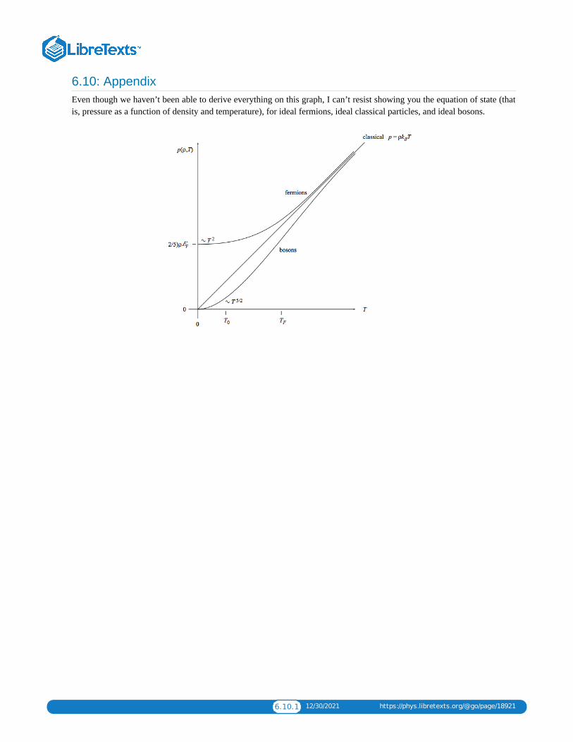
6.10.1 12/30/2021 https://phys.libretexts.org/@go/page/18921

6.10: AppendixEven though we haven’t been able to derive everything on this graph, I can’t resist showing you the equation of state (thatis, pressure as a function of density and temperature), for ideal fermions, ideal classical particles, and ideal bosons.

1 1/27/2022

CHAPTER OVERVIEW7: HARMONIC LATTICE VIBRATIONS

7.1: THE PROBLEM7.2: STATISTICAL MECHANICS OF THE PROBLEM7.3: NORMAL MODES FOR A ONE-DIMENSIONAL CHAIN7.4: NORMAL MODES IN THREE DIMENSIONS7.5: LOW-TEMPERATURE HEAT CAPACITY7.6: MORE REALISTIC MODELS7.7: WHAT IS A PHONON?7.8: ADDITIONAL PROBLEMS

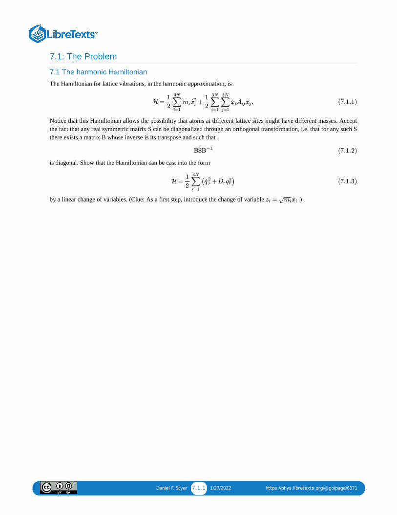
Daniel F. Styer 7.1.1 1/27/2022 https://phys.libretexts.org/@go/page/6371

7.1: The Problem

7.1 The harmonic Hamiltonian

The Hamiltonian for lattice vibrations, in the harmonic approximation, is

Notice that this Hamiltonian allows the possibility that atoms at different lattice sites might have different masses. Acceptthe fact that any real symmetric matrix S can be diagonalized through an orthogonal transformation, i.e. that for any such Sthere exists a matrix B whose inverse is its transpose and such that

is diagonal. Show that the Hamiltonian can be cast into the form

by a linear change of variables. (Clue: As a first step, introduce the change of variable .)

H = + .1

2∑i=1

3N

mix2i

1

2∑i=1

3N

∑j=1

3N

xiAijxj (7.1.1)

BSB−1 (7.1.2)

H = ( + )1

2∑r=1

3N

q 2r Drq2

r (7.1.3)

=zi mi−−−

√ xi

Daniel F. Styer 7.2.1 12/16/2021 https://phys.libretexts.org/@go/page/6372

7.2: Statistical Mechanics of the Problem

7.2 Thermal energy versus kinetic energy

According to the Fall 2001 Review Draft of Ohio’s Academic Content Standards for Science (page 48), eight-gradestudents should understand that thermal energy “is in the disorderly motion of molecules.” Explain how position as well asmotion (i.e. potential energy as well as kinetic energy) contribute to thermal energy.

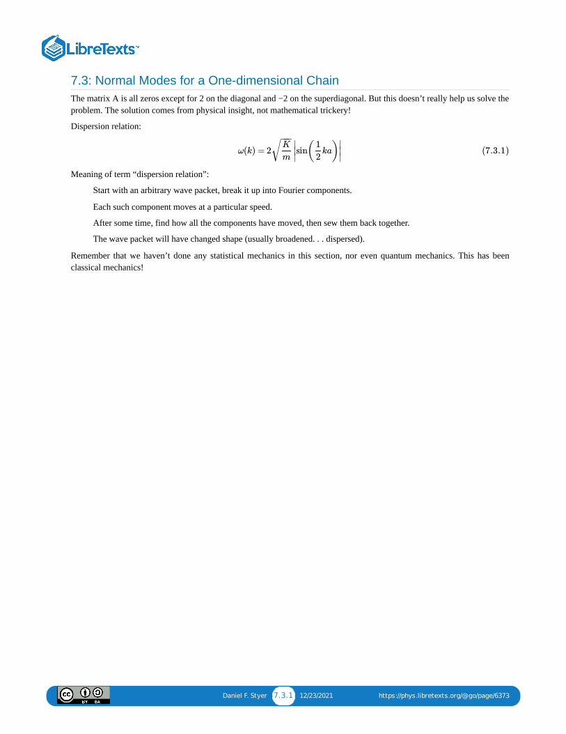
Daniel F. Styer 7.3.1 12/23/2021 https://phys.libretexts.org/@go/page/6373

7.3: Normal Modes for a One-dimensional ChainThe matrix A is all zeros except for 2 on the diagonal and −2 on the superdiagonal. But this doesn’t really help us solve theproblem. The solution comes from physical insight, not mathematical trickery!

Dispersion relation:

Meaning of term “dispersion relation”:

Start with an arbitrary wave packet, break it up into Fourier components.

Each such component moves at a particular speed.

After some time, find how all the components have moved, then sew them back together.

The wave packet will have changed shape (usually broadened. . . dispersed).

Remember that we haven’t done any statistical mechanics in this section, nor even quantum mechanics. This has beenclassical mechanics!

ω(k) = 2 sin( ka)K

m

−−−√

∣

∣∣

1

2

∣

∣∣ (7.3.1)

Daniel F. Styer 7.4.1 1/13/2022 https://phys.libretexts.org/@go/page/6374

7.4: Normal Modes in Three DimensionsIf you wanted to study heat flow, or how sound warms up a crystal, or how light warms up a crystal, you’d have to studythese time-dependent dispersion effects. This is hard: the classical mechanics is hard (normal modes) and the quantummechanics is hard. For the purposes of this book we need only examine static effects, and in particular we need only findthe heat capacity at low temperatures.

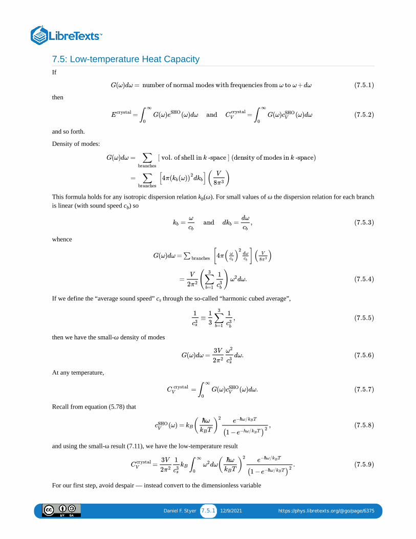
Daniel F. Styer 7.5.1 12/9/2021 https://phys.libretexts.org/@go/page/6375

7.5: Low-temperature Heat CapacityIf

then

and so forth.

Density of modes:

This formula holds for any isotropic dispersion relation k (ω). For small values of ω the dispersion relation for each branchis linear (with sound speed c ) so

whence

If we define the “average sound speed” c through the so-called “harmonic cubed average”,

then we have the small-ω density of modes

At any temperature,

Recall from equation (5.78) that

and using the small-ω result (7.11), we have the low-temperature result

For our first step, avoid despair — instead convert to the dimensionless variable

G(ω)dω = number of normal modes with frequencies from ω to ω+dω (7.5.1)

= G(ω) (ω)dω and = G(ω) (ω)dωEcrystal ∫∞

0

eSHO CcrystalV ∫

∞

0

cSHOV (7.5.2)

G(ω)dω = [ vol. of shell in k -space ] (density of modes in k -space) ∑ branches

= [4π d ]( )∑ branches

( (ω))kb2kb

V

8π3

b

b

= and d = ,kbω

cbkb

dω

cb(7.5.3)

G(ω)dω = [4π ]( )∑ branches ( )ωcb

2dωcb

V

8π3

= ( ) dω.V

2π2∑b=1

3 1

c3b

ω2 (7.5.4)

s

≡ ,1

c3s

1

3∑b=1

31

c3b

(7.5.5)

G(ω)dω = dω.3V

2π2

ω2

c3s

(7.5.6)

= G(ω) (ω)dω.C crystal V ∫

∞

0

cSHOV (7.5.7)

(ω) = ,cSHOV

kB( )ℏω

TkB

2 e−ℏω/ TkB

(1 − )e−hω/ TkB2

(7.5.8)

= dω .C crystalV

3V

2π2

1

c3s

kB ∫∞

0

ω2 ( )ℏω

TkB

2 e−ℏω/ TkB

(1 − )e−ℏω/ TkB2

(7.5.9)

Daniel F. Styer 7.5.2 12/9/2021 https://phys.libretexts.org/@go/page/6375

and find

The integral is rather hard to do, but we don’t need to do it — the integral is just a number. We have achieved our aim,namely to show that at low temperatures, C ∼ T .

However, if you want to chase down the right numbers, after some fiddling you’ll find that

Thus, the low-temperature specific-heat of a solid due to a lattice vibration is

7.3 How far do the atoms vibrate?

Consider a simplified classical Einstein model in which N atoms, each of mass m, move classically on a simple cubiclattice with nearest neighbor separation of a. Each atom is bound to its lattice site by a spring of spring constant K,and all the values of K are the same. At temperature T, what is the root mean square average distance of each atomfrom its equilibrium site? (Note: I am asking for an ensemble average, not a time average.)

x =ℏω

TkB(7.5.10)

= dxC crystal V

3V

2π2

1

c3s

kB( )TkB

ℏ

3

∫∞

0

x4e−x

(1 − )e−x 2(7.5.11)

V3

dx = 4Γ(4)ζ(4) = .∫∞

0

x4e−x

(1 − )e−x 2

4

15π4 (7.5.12)

= V .C crystalV kB

2π2

5( )

TkB

ℏcs

3

(7.5.13)

Daniel F. Styer 7.6.1 1/27/2022 https://phys.libretexts.org/@go/page/6376

7.6: More Realistic Models7.4 Debye frequency

In the Debye model, a solid with average sound speed c has density of normal-mode frequencies

Find a formula for ω (N, V, c ), and write G(ω) in terms of ω .

7.5 Debye model energy and heat capacity

Find E(T, V, N) and C (T, V, N) for a harmonic solid in the Debye model, in terms of ω and the function

s

G(ω) = .3V

2π2c3s

ω2

0

for ω < ωD

for ω > ωD

(7.6.1)

D s D

V D

7.7.1 12/16/2021 https://phys.libretexts.org/@go/page/18929

7.7: What is a Phonon?

7.8.1 1/4/2022 https://phys.libretexts.org/@go/page/18930

7.8: Additional Problems7.6 Spin waves

For harmonic lattice vibrations at low frequencies, ω = c k. There are analogous excitations of ferromagnets called“spin waves” which, at low frequencies, satisfy ω = Ak . Find the temperature dependence of the heat capacity of aferromagnet at low temperatures. (Do not bother to evaluate constants. . . I am only looking for the functional formof the temperature dependence.)

7.7 Comparison of models

(This problem is stolen from a GRE Physics test.)

One feature common to both the Debye and Einstein models for the specific heat of a crystal composed of Nidentical atoms is that

a. The average energy of each atom is 3k T.

b. The vibrational energy of the crystal is equivalent to the energy of 3N independent harmonic oscillators.

c. The crystal is assumed to be continuous for all elastic waves.

d. The speed of longitudinal elastic waves is less than the speed of transverse elastic waves.

e. The upper cutoff frequency of elastic waves is the same.

s2

B

1 1/27/2022

CHAPTER OVERVIEW8: INTERACTING CLASSICAL FLUIDS

8.1: INTRODUCTION8.2: PERTURBATION THEORY8.3: VARIATIONAL METHODS8.4: DISTRIBUTION FUNCTIONS8.5: CORRELATIONS AND SCATTERING8.6: THE HARD SPHERE FLUID

Daniel F. Styer 8.1.1 12/16/2021 https://phys.libretexts.org/@go/page/6378

8.1: IntroductionThe subject of this chapter is also called “real gases”, or “dense gases”, or “non-ideal gases”, or “imperfect gases”, or“liquids and dense gases”. The many names are a clue that the same problem has been approached by many differentscientists from many different points of view, which in turn is a hint that the problem is one of enormous importance. Andin this case the hints are correct. We have treated non-interacting classical atoms for long enough in this book. We knowthat this treatment leads to results in which all substances have the same equation of state (although they can sometimes bedistinguished through their heat capacities) and in which there are no phase transitions, no crystals, no life, and very littleof interest. It galls me that anyone ever called such a situation “ideal”. The problem of interacting atoms is important forindustrial and military applications, but it is just as important from the point of view of pure science. We are now going tosee what happens when we allow the atoms to interact. Some call the methods and results “messy”. I call them fascinating.I would not want to live in the “ideal” world.

To be specific, we will consider the model problem of:

Monatomic atoms with no internal structure, interacting through spherically symmetric pair potentials.Classical mechanics.

Many undergraduate books state that this is an “important outstanding problem”. That is no longer correct. In fact, theproblem was solved (except near phase transitions) in the years 1980–85 by Lado, Ashcroft, Foiles, and Rosenfeld (seeTalbot, Lebowitz, et al. “A comparison of MHNC and MC at high pressures”, J. Chem. Phys. 85 (1986) 2187–2192, Y.Rosenfeld, “Variational MHNC”, J. Stat. Phys. 42 (1986) 437–457). The solution is a technique called “modified hyper-netted chain”. Unfortunately, I will not have time to tell you what the solution is or even what the words in the name mean.But I can tell you that it is an ingenious combination of perturbation and variational methods, and I will be telling youabout these two techniques in this chapter. (The best references for this chapter are the books by Donald McQuarrie,Statistical Mechanics, and by J.P. Hansen and I.R. McDonald, Theory of Simple Liquids.)

Problems8.1 The Lennard-Jones potential

The general Lennard-Jones potential is

a. Given a and b, find , the minimum energy, and r , the distance of separation at that minimum. Write u(r)in terms of the parameters and r rather than the parameters a and b.

b. If σ is the separation at which u(σ) = 0, find σ in terms of r . Why is irrelevant here?

c. Note the simplifications in the above results if n = 12. For this case, write u(r) using the parameters andσ.

8.2 Negative compressibilities

Look at figure 8.6.1 on page 307 of Reif. Notice that for temperatures below the critical temperature (T in thefigure), the van der Waals fluid can have negative values of κ . Suppose a fluid with negative compressibilityexisted, and I had a bottle of it on the table in front of me. What would happen if the volume of the bottle decreasedslightly. . . say if I rapped my fingers on it? (This impossibility is a warning that the van der Waals equation issimply not applicable at temperatures in the vicinity of the critical temperature or below.)

8.3 Entropy of a real gas

A real gas obeys the equation of state

where B is a positive constant.

u(r) = − +a

r6

b

rn(8.1.1)

ϵm 0ϵm 0

0 ϵm

ϵm

4

T

pV = N T [1 +B ] ,kB

N

V(8.1.2)

Daniel F. Styer 8.1.2 12/16/2021 https://phys.libretexts.org/@go/page/6378

a. In one sentence, describe the behavior of this gas in the limit that T and N are constant but V → ∞.(Answers containing mathematical symbols are automatically disqualified.)

b. Using an appropriate Maxwell relation, calculate the difference in entropy between an ideal gas and this realgas when both have the same T, V, and N.

c. At a given T, V, and N, which entropy is larger? Is this consistent with “the entropy inequality”? Can youjustify it with a qualitative argument? Is it possible for the constant B to be negative or zero?

Daniel F. Styer 8.2.1 1/4/2022 https://phys.libretexts.org/@go/page/6379

8.2: Perturbation Theory8.2.1 Fluids in the canonical ensemble

The partition function for a fluid is

where

The momentum integrals can be performed precisely as they were for the ideal gas, giving

where λ(T) is the thermal de Broglie wavelength. It is useful to define the “configurational partition function”

For example, in a three-particle system with spherically symmetric pair potential u(r), the configurational partition function is

Every other time in this book that we have encountered a complicated partition function, like the one above, it has factorized into theproduct of many similar terms. (This happened even in our treatment of harmonic lattice vibrations, through the use of normalcoordinates.) The expression above does not factorize in this neat way. With considerable diligence and patience, it is possible to evaluateQ (T, V) for N = 3. But you can see that doing it for cases of interest, such as N = 6.02 × 10 , is simply out of the question. Instead weattempt to use perturbation theory by expanding about an already solved problem, namely the ideal gas. Such an approximation will be agood one at low densities, where the gas is “nearly ideal”. The obvious thing to do is to expand Q (T, V) in the small parameter ρ = N/V,the number density. But how can we do that? The quantity ρ doesn’t appear in these formulas!

8.2.2 The search for a small parameterWe cannot expand Q (T, V) in terms of ρ, but we do know that at low densities all fluids behave like an ideal gas, and that for an ideal gasthe chemical potential is

so that as ρ → 0, µ → −∞ and e → 0. So here is a second small parameter. You might object that e doesn’t appear in the partitionfunction any more than ρ does, but it does appear in the grand canonical partition function!

8.2.3 Fluids in the grand canonical ensembleThe grand canonical partition function is

where we have the activity

Z(T ,V ,N) = ∫ dΓ1

N !h3Ne−βH(Γ) (8.2.1)

H(Γ) = + ( , … , ) .1

2m∑i=1

N

p2i UN r1 rN (8.2.2)

Z(T ,V ,N) = ∫ d ⋯ d ,1

(T )N !λ3Nr1 rNe

−β ( ,…, )UN r1 rN (8.2.3)

(T ,V ) = ∫ d ⋯ d .QN

1

N !r1 rNe

−β ( ,…, )UN r1 rN (8.2.4)

(T ,V ) = d d d .Q31

6∫V

r1 ∫V

r2 ∫V

r3e−β[u(| − |)+u(| − |)+u(| − |)]r1 r2 r1 r3 r2 r3 (8.2.5)

N23

N

N

μ = T ln( ),kBρ

1/ (T )λ3(8.2.6)

βµ βµ

Ξ(T ,V ,μ) = Z(T ,V ,N)∑N=0

∞

eβμN (8.2.7)

= (T ,V )∑N=0

∞

( )eβμ

(T )λ3

N

QN (8.2.8)

= (T ,V )∑N=0

∞

zNQN (8.2.9)

= 1 + (T ,V )z+ (T ,V ) + (T ,V ) +O ( ) ,Q1 Q2 z2 Q3 z3 z4 (8.2.10)

z ≡ .eβμ

(T )λ3(8.2.11)

Daniel F. Styer 8.2.2 1/4/2022 https://phys.libretexts.org/@go/page/6379

The activity is the small parameter upon which perturbation theory relies. (For an ideal gas, it is equal to the number density ρ.)

Note that in this approach we still have to calculate Q coefficients, but we will probably stop at N = 4 or 5 rather than N = 6.02 × 10 . Iwill write down the first two coefficients:

Because the interactions are short-ranged, most of the time u(|r −r |) nearly vanishes, so Q is pretty close to V /2. It is neither intensivenor extensive.

8.2.4 The Mayer expansion

Now we go from the partition function to an experimentally measurable master function, namely pressure:

Employing

we obtain

The last line above defines the “Mayer expansion”. The expansion coefficients b = b (T) are intensive functions of temperature (incontrast to the coefficients Q (T, V)). Using equations (8.14) it is easy to show that b = 1 and that

In contrast to the situation with equation (8.14), the integrand above is nearly always zero, which makes it much easier to work with. (Thesame is true for all the the Mayer coefficients.) Indeed, a little more work will show that

Specialists in the statistical mechanics of fluids spend a lot of time calculating b coefficients for a given potential energy of interactionu(r). We will instead emphasize what to do with the b s once they are calculated.

8.2.5 Expansion for the density

To obtain the number density ρ = N/V from the Mayer expansion, use the thermodynamic connection between ρ and p:

Thus

N23

(T ,V ) = d = VQ1 ∫V

r1e−β0

(T ,V ) = d d .Q21

2∫V

r1 ∫V

r2e−βu([ − |)r1 r2 (8.2.12)

1 2 22

= lnΞp(T , z)

TkB

1

V(8.2.13)

= ln[1 + z+ + +O ( )]1

VQ1 Q2z

2 Q3z3 z4 (8.2.14)

ln(1 + ϵ) = ϵ− + +O ( )1

2ϵ2 1

3ϵ3 ϵ4 (8.2.15)

= [ z+ + − + +O ( )]p(T , z)

TkB

1

VQ1 Q2z

2 Q3z3 1

2( z+ )Q1 Q2z

2 2 1

3( z)Q1

3z4 (8.2.16)

= z+ ( − ) + ( − + ) +O ( )1

VQ1

1

VQ2

1

2Q2

1z2 1

VQ3 Q1Q2

1

3Q3

1z3 z4 (8.2.17)

= .∑ℓ=1

∞

bℓzℓ (8.2.18)

ℓ ℓ

N 1

= ( d d − d d 1)b21

2V∫V

r1 ∫V

r2e−βu(| − |)r1 r2 ∫V

r1 ∫V

r2

= d d ( −1) .1

2V∫V

r1 ∫V

r2 e−βu(| − |)r1 r2 (8.2.19)

= 2π dr ( −1) .b2 ∫∞

0

r2 e−u(r)/ TkB (8.2.20)

ℓ

ℓ

ρ = = = z .∂p

∂μ)T

∂z

∂μ)T

∂p

∂z)T

∂(βp)

∂z)T (8.2.21)

ρ(T , z) = ℓ .∑ℓ=1

∞

bℓzℓ (8.2.22)

Daniel F. Styer 8.2.3 1/4/2022 https://phys.libretexts.org/@go/page/6379

8.2.6 Eliminating the activity: the virial expansionNow we have two expansions, (8.20) and (8.24), in terms of the activity:

(The temperature dependence of p, ρ, and the b s is not shown explicitly.) What we would really like, however, would be the traditional(and experimentally accessible) equation of state, p(ρ). In other words, we want to eliminate the z between the two expansions above. Tothis end we will invert the expansion for ρ(z) to find z(ρ), and plug that expression into the expansion (8.25) for p(z). In the appendix weperform the inversion to find, correct to third order,

Plugging into (8.25) gives

This last expression is called the “virial expansion”, and it is usually written (with the temperature dependence put back in) as

8.2.7 Appendix: Inverting ρ(z) to find z(ρ)Begin with

then use

to find

Problems8.4 Virial expansion for the ideal gas

Find Q , Q , Q , etc. for an ideal gas. Hence show that the virial equation of state for an ideal gas is pV = Nk T.

8.5 General properties of expansion coefficients

a. Show that Q = V, whence b = 1.

b. Show (informally) that the b Mayer coefficients, as well as the B (T) virial coefficients, are intensive.

βp(z) = z+ + +O ( )b2z2 b3z

3 z4 (8.2.23)

ρ(z) = z+2 +3 +O ( )b2z2 b3z

3 z4 (8.2.24)

ℓ

s

z(ρ) = ρ−2 +(8 −3 ) +O ( ) .b2ρ2 b2

2 b3 ρ3 ρ4 (8.2.25)

βp(ρ) = z+ + +O ( )b2z2 b3z

3 z4 (8.2.26)

= [ρ−2 +(8 −3 ) ] + + [ρ +O ( )b2ρ2 b2

2 b3 ρ3 b2 [ρ−2 ]b2ρ2 2

b3 ]3 ρ4 (8.2.27)

= [ρ−2 +(8 −3 ) ] + [ −4 ] + [ρ +O ( )b2ρ2 b2

2 b3 ρ3 b2 ρ2 b2ρ3 b3 ]3 ρ4 (8.2.28)

= ρ− +(4 −2 ) +O ( ) .b2ρ2 b2

2 b3 ρ3 ρ4 (8.2.29)

= ρ+ (T ) + (T ) +O ( ) .p(T , ρ)

TkBB2 ρ2 B3 ρ3 ρ4 (8.2.30)

ρ(z) = z+2 +3 +O ( ) ,b2z2 b3z

3 z4 (8.2.31)

z = ρ+O ( )z2

= +2ρO ( )+O ( )ρ2 z2 z4

= +O ( )ρ2 z3

= (ρ+O ( )) (ρ+O ( ))z2 z2 z2 z3

= +O ( )ρ3 z4

= +O ( )ρ3 z4

= ( +O ( )) (ρ+O ( ))ρ2 z3 z2

z = ρ−2 +O ( )b2z2 z3

z = ρ−2 +O ( )b2ρ2 z3 = (ρ−2 +O ( )) (ρ−2 +O ( ))b2ρ

2 z3 b2ρ2 z3

= −4 +4 +ρO ( )ρ2 b2ρ3 b2

2ρ4 z3

= −4 +O ( )ρ2 b2ρ3 z4

z = ρ−2 −3 +O ( )b2z2 b3z

3 z4

z = ρ−2 [ −4 +O ( )] −3 [ +O ( )] +O ( )b2 ρ2 b2ρ3 z4 b3 ρ3 z4 z4

z(ρ) = ρ−2 +(8 −3 ) +O ( ) .b2ρ2 b2

2 b3 ρ3 ρ4 (8.2.32)

1 2 3 B

1 1

ℓ n

Daniel F. Styer 8.3.1 1/27/2022 https://phys.libretexts.org/@go/page/6380

8.3: Variational Methods8.6 Bogoliubov’s contribution to the Gibbs-Bogoliubov inequality

Show that the Gibbs-Bogoliubov inequality, which we derived in class for classical systems, also holds for quantalsystems.

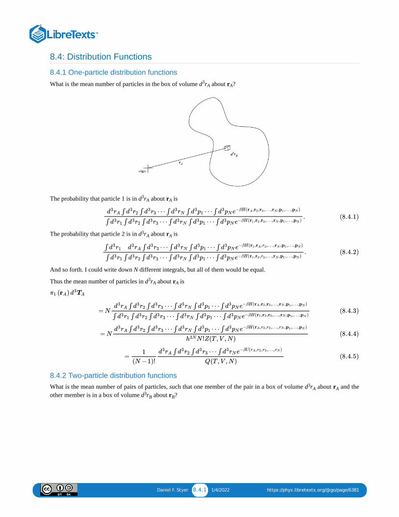
Daniel F. Styer 8.4.1 1/4/2022 https://phys.libretexts.org/@go/page/6381

8.4: Distribution Functions

8.4.1 One-particle distribution functions

What is the mean number of particles in the box of volume d r about r ?

The probability that particle 1 is in d r about r is

The probability that particle 2 is in d r about r is

And so forth. I could write down N different integrals, but all of them would be equal.

Thus the mean number of particles in d r about r is

8.4.2 Two-particle distribution functionsWhat is the mean number of pairs of particles, such that one member of the pair in a box of volume d r about r and theother member is in a box of volume d r about r ?

3A A

3A A

.∫ ∫ ⋯ ∫ ∫ ⋯ ∫d3rA d3r2 d3r3 d3rN d3p1 d3pNe

−βH( , , ,…, , ,…, )rA r2 r3 rN p1 pN

∫ ∫ ∫ ⋯ ∫ ∫ ⋯ ∫d3r1 d3r2 d3r3 d3rN d3p1 d3pNe−βH( , , ,…, , ,…, )r1 r2 r3 rN p1 pN

(8.4.1)

3A A

.∫ ∫ ⋯ ∫ ∫ ⋯ ∫d3r1 d3rA d3r3 d3rN d3p1 d3pNe

−βH( , , ,…, , ,…, )r1 rA r3 rN p1 pN

∫ ∫ ∫ ⋯ ∫ ∫ ⋯ ∫d3r1 d3r2 d3r3 d3rN d3p1 d3pNe−βH( , , ,…, , ,…, )r1 r2 r3 rN p1 pN

(8.4.2)

3A A

( )π1 rA d3TA

= N∫ ∫ ⋯ ∫ ∫ ⋯ ∫d3rA d3r2 d3r3 d3rN d3p1 d3pNe

−βH( , , ,…, , ,…, )rA r2 r3 rN p1 pN

∫ ∫ ∫ ⋯ ∫ ∫ ⋯ ∫d3r1 d3r2 d3r3 d3rN d3p1 d3pNe−βH( , , ,…, , ,…, )r1 r2 r3 rN p1 pN

(8.4.3)

= N∫ ∫ ⋯ ∫ ∫ ⋯ ∫d3rA d3r2 d3r3 d3rN d3p1 d3pNe

−βH( , , ,…, , ,…, )rA r2 r3 rN p1 pN

N !Z(T ,V ,N)h3N(8.4.4)

=1

(N −1)!

∫ ∫ ⋯ ∫d3rA d3r2 d3r3 d3rNe−βU( , , ,…, )rA r2 r3 rN

Q(T ,V ,N)(8.4.5)

3A A

3B B

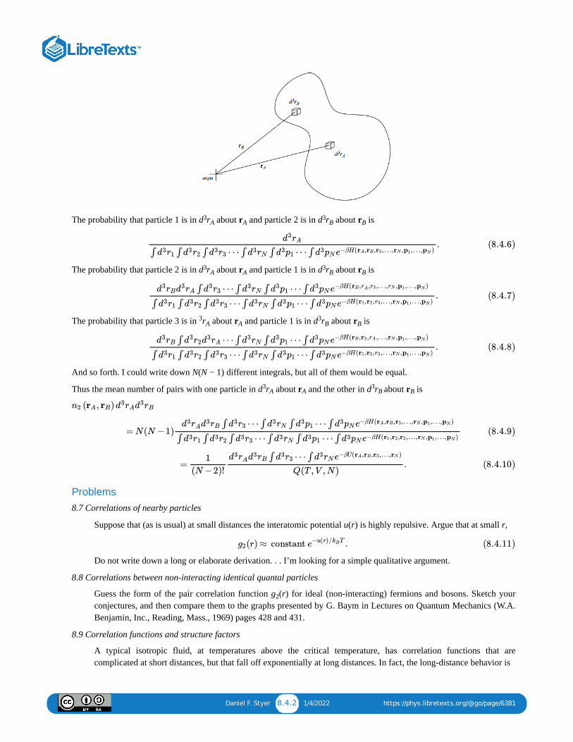
Daniel F. Styer 8.4.2 1/4/2022 https://phys.libretexts.org/@go/page/6381

The probability that particle 1 is in d r about r and particle 2 is in d r about r is

The probability that particle 2 is in d r about r and particle 1 is in d r about r is

The probability that particle 3 is in r about r and particle 1 is in d r about r is

And so forth. I could write down N(N − 1) different integrals, but all of them would be equal.

Thus the mean number of pairs with one particle in d r about r and the other in d r about r is

Problems8.7 Correlations of nearby particles

Suppose that (as is usual) at small distances the interatomic potential u(r) is highly repulsive. Argue that at small r,

Do not write down a long or elaborate derivation. . . I’m looking for a simple qualitative argument.

8.8 Correlations between non-interacting identical quantal particles

Guess the form of the pair correlation function g (r) for ideal (non-interacting) fermions and bosons. Sketch yourconjectures, and then compare them to the graphs presented by G. Baym in Lectures on Quantum Mechanics (W.A.Benjamin, Inc., Reading, Mass., 1969) pages 428 and 431.

8.9 Correlation functions and structure factors

A typical isotropic fluid, at temperatures above the critical temperature, has correlation functions that arecomplicated at short distances, but that fall off exponentially at long distances. In fact, the long-distance behavior is

3A A

3B B

.d3rA

∫ ∫ ∫ ⋯ ∫ ∫ ⋯ ∫d3r1 d3r2 d3r3 d3rN d3p1 d3pNe−βH( , , ,…, , ,…, )rA rB r3 rN p1 pN

(8.4.6)

3A A

3B B

.∫ ⋯ ∫ ∫ ⋯ ∫d3rBd

3rA d3r3 d3rN d3p1 d3pNe−βH( , , ,…, , ,…, )rB rA r3 rN p1 pN

∫ ∫ ∫ ⋯ ∫ ∫ ⋯ ∫d3r1 d3r2 d3r3 d3rN d3p1 d3pNe−βH( , , ,…, , ,…, )r1 r2 r3 rN p1 pN

(8.4.7)

3A A

3B B

.∫ ⋯ ∫ ∫ ⋯ ∫d3rB d3r2d

3rA d3rN d3p1 d3pNe−βH( , , ,…, , ,…, )rB r2 rA rN p1 pN

∫ ∫ ∫ ⋯ ∫ ∫ ⋯ ∫d3r1 d3r2 d3r3 d3rN d3p1 d3pNe−βH( , , ,…, , ,…, )r1 r2 r3 rN p1 pN

(8.4.8)

3A A

3B B

( , )n2 rA rB d3rAd3rB

= N(N −1)∫ ⋯ ∫ ∫ ⋯ ∫d3rAd

3rB d3r3 d3rN d3p1 d3pNe−βH( , , ,…, , ,…, )rA rB r3 rN p1 pN

∫ ∫ ∫ ⋯ ∫ ∫ ⋯ ∫d3r1 d3r2 d3r3 d3rN d3p1 d3pNe−βH( , , ,…, , ,…, )r1 r2 r3 rN p1 pN

(8.4.9)

= .1

(N −2)!

∫ ⋯ ∫d3rAd3rB d3r3 d3rNe−βU( , , ,…, )rA rB r3 rN

Q(T ,V ,N)(8.4.10)

(r) ≈ constant .g2 e−u(r)/ TkB (8.4.11)

2

Daniel F. Styer 8.4.3 1/4/2022 https://phys.libretexts.org/@go/page/6381

where ξ, the so-called correlation length, depends on temperature and density. In contrast, at the critical temperaturethe correlation function falls off much more slowly, as

Find the structure factor

associated with each of these correlation functions. Will your results match those of experiments at small values of kor at large values (i.e. at long or short wavelengths)?

8.10 Long wavelength structure factor

Show that, for an isotropic fluid, vanishes at k = 0. Here S(k) is the structure factor

8.11 Correlations in a magnetic system

In the Ising model for a magnet, described in problem 4.9, the (net) correlation function is defined by

where the site j = 0 is some arbitrary “central spin”. Using the results of problem 4.9, show that for a lattice of Nsites,

(r) = 1 +g2Ae−r/ξ

r(8.4.12)

(r) = 1 +g2A

r1+η(8.4.13)

S(k) = ∫ r [ (r) −1]d3 g2 e−ik⋅r (8.4.14)

dS(k)

dk

S(k) = 1 +ρ∫ r [ (r) −1] .d3 g2 eik⋅r (8.4.15)

≡ ⟨ ⟩− ,Gi s0si ⟨ ⟩s02 (8.4.16)

(T ,H) = N .χT

m2

TkB∑i

Gi (8.4.17)

Daniel F. Styer 1 12/30/2021 https://phys.libretexts.org/@go/page/6382

Welcome to the Physics Library. This Living Library is a principal hub of the LibreTexts project, which is a multi-institutional collaborative venture to develop the next generation of open-access texts to improve postsecondary educationat all levels of higher learning. The LibreTexts approach is highly collaborative where an Open Access textbookenvironment is under constant revision by students, faculty, and outside experts to supplant conventional paper-basedbooks.

Campus Bookshelves Bookshelves

Learning Objects

Daniel F. Styer 8.6.1 1/13/2022 https://phys.libretexts.org/@go/page/6383

8.6: The Hard Sphere FluidConsider a fluid in which each atom is modeled by a “hard sphere” of volume v . In this system the potential energyvanishes unless two spheres overlap, while if they do overlap it is infinite. The criterion for overlap is that the centers ofthe two spheres are separated by a distance of 2r or less, where . This model is certainly oversimplified in thatit ignores the attractive part of the interatomic force, but it is an excellent starting point for perturbation theory, and it alsohas certain features of interest in its own right, as the problems below demonstrate. (The first problem below is requiredbackground for all of the others.)

8.12 Scaling in the hard sphere fluid

The canonical partition function for a fluid is

For an ideal gas, the integral over configuration space gives just V , so it makes sense to write

where the last line has defined W, the ratio of interacting to non-interacting (“ideal”) configurational partitionfunctions.

a. Argue that in the case of hard spheres W is independent of temperature. It does, however, depend on themechanical parameter v , so we will write the ratio as W(V, N, v ).

b. Argue that W(V, N, v ) ≤ 1, where the equality holds only when v = 0.

c. Show that the Helmholtz free energy for any fluid satisfies

where we have defined f , the excess free energy per atom. Is the free energy of a hard sphere fluid greaterthan or less than the free energy of an ideal gas at the same T, V, and N?

d. Because f is intensive, it cannot depend upon V and N separately, but only through their intensive quotient,the number density ρ = N/V. Use a similar argument to show that

where w is a dimensionless, intensive quantity.

e. Use dimensional analysis to show that the hard sphere w (and hence f ) cannot depend upon ρ and vseparately, but only through their product: w(ρv ).

This last result is of enormous importance. It implies that there is no need to perform elaborate computer simulationsfor a variety of densities and a variety of radii. It suffices to either simulate for a variety of densities at one fixedradius or vice versa. It also demonstrates that the quantity of importance in the statistical mechanics of hard spheresis the “scaled density” η ≡ ρv .

f. Use thermodynamics to show that

8.13 The hard sphere phase transition

a. Interpret the scaled density η ≡ ρv geometrically. Why is is sometimes called the “packing fraction”?

b. Is it possible to have a fluid with η ≥ 1?

0

0 = πv043

r30

Z(T ,V ,N) = ∫ ⋯ ∫ .1

(T )N !λ3Nd3r1 d3rNe

−β ( ,…, )UN r1 rN (8.6.1)

N

Z(T ,V ,N) = ( )( ∫ ⋯ ∫ )/N !V N

(T )λ3N

1V N

d3r1 d3rNe−β ( ,…, )UN r1 rN

≡ (T ,V ,N)W (T ,V ,N),Z ideal (8.6.2)

0 0

0 0

(T ,V ,N , ) = (T ,V ,N) − T lnW (V ,N , )FHS v0 F ideal kB v0

≡ +N ,F ideal f ex (8.6.3)

ex

ex

W (V ,N , ) = w ,v0 (ρ, )v0N (8.6.4)

ex 0

0

0

(T , ρ, ) = (T , ρ) +ρ .pHS v0 pideal [η ]∂ (η)fex

∂η η=ρv0

(8.6.5)

0

Daniel F. Styer 8.6.2 1/13/2022 https://phys.libretexts.org/@go/page/6383

c. Show that if hard spheres are packed into a face-centered cubic lattice (which is probably the densest possiblepacking spheres, although no one has been able to prove it), .

In fact, at scaled densities η well below the limits mentioned above, the system undergoes a phase transition from afluid to a solid. Computer simulations show that the transition occurs when the scaled density is η ≈ 0.496. Theconjecture η = is tempting, but apparently not correct. (On the other hand it is hard to do computer simulationsnear phase transitions, so the question is not completely closed!)

8.14 The hard sphere fluid equation of state

Many long and difficult hours of analytic calculation and computer simulation have gone into studying the hardsphere fluid. In 1964 Ree and Hoover codified much of this work into the following empirical formula which is agood approximation for the hard sphere fluid equation of state:

Only five years later, Carnahan and Starling hit upon a much simpler yet still remarkably accurate equation of state,namely

Both of these formulas apply only to the fluid phase (see the previous problem) and neither one is exact. Answer thefollowing questions for the Carnahan-Starling formula.

a. As the density increases from zero, at what point does the formula become nonsense?

b. On which regions of the (T, ρ) plane does the hard sphere fluid exert a greater pressure than the ideal gas?Can you explain your answer through a simple physical argument?

c. Integrate equation (8.56) to show that for the hard sphere fluid,

Does this formula satisfy the inequality established in part (c.) of problem 8.12?

d. Find the difference between the entropy of the hard sphere fluid and that of an ideal gas. At a given T, V,and N, which entropy is larger? Can you justify this result with a qualitative argument?

8.15 The hard sphere free energy

Use the Gibbs-Bogoliubov inequality to show that

Reason that E (T, V, N) = E (T, V, N), and conclude with a relation between entropies.

8.16 Virial expansion for hard spheres

Using the notation of problem 8.12, show that for a hard sphere fluid:

a. Q = V(V − 8v ).

b. b = −4v .

c. B (T) = 4v .

d. Show that both the Ree-Hover and the Carnahan-Starling equations of state, introduced in problem 8.14,expand to give the correct first virial coefficient B (T).

F.H. Ree and W.G. Hoover, J. Chem. Phys., 40 (1964) 939–950.

N.F. Carnahan and K.E. Starling, J. Chem. Phys., 51 (1969) 635–636.

η = π /6 = 0.74052–

√

t

t12

1

(T , ρ, ) = Tρ [1 +4η ] where η = ρ .pHS v0 kB1 +0.25403η+0.27726η2

1 −2.2460η+1.3010η2v0 (8.6.6)

2

(T , ρ, ) = Tρ where η = ρ .pHS v0 kB1 +η+ −η2 η3

(1 −η)3v0 (8.6.7)

(T , η) = Tη .fex kB4 −3η

(1 −η)2(8.6.8)

(T ,V ,N) ≥ (T ,V ,N).FHS F ideal (8.6.9)

HS ideal

212 0

2 0

2 0

2

1

2

1 1/27/2022

CHAPTER OVERVIEW9: STRONGLY INTERACTING SYSTEMS AND PHASE TRANSITIONS

9.1: INTRODUCTION TO MAGNETIC SYSTEMS AND MODELS9.2: FREE ENERGY OF THE ONE-DIMENSIONAL ISING MODEL9.3: THE MEAN-FIELD APPROXIMATION9.4: CORRELATION FUNCTIONS IN THE ISING MODEL9.5: COMPUTER SIMULATION9.6: ADDITIONAL PROBLEMS

Daniel F. Styer 1 12/9/2021 https://phys.libretexts.org/@go/page/6385

Welcome to the Physics Library. This Living Library is a principal hub of the LibreTexts project, which is a multi-institutional collaborative venture to develop the next generation of open-access texts to improve postsecondary educationat all levels of higher learning. The LibreTexts approach is highly collaborative where an Open Access textbookenvironment is under constant revision by students, faculty, and outside experts to supplant conventional paper-basedbooks.

Campus Bookshelves Bookshelves

Learning Objects

Daniel F. Styer 9.2.1 12/30/2021 https://phys.libretexts.org/@go/page/6386

9.2: Free Energy of the One-Dimensional Ising ModelThe N-spin one-dimensional Ising model consists of a horizontal chain of spins, s , s , . . . , s , where s = ±1.

A vertical magnetic field H is applied, and only nearest neighbor spins interact, so the Hamiltonian is

For this system the partition function is

where

If J = 0, (the ideal paramagnet) the partition function factorizes, and the problem is easily solved using the “summingHamiltonian yields factorizing partition function” theorem. If H = 0, the partition function nearly factorizes, and theproblem is not too difficult. (See problem 9.3.) But in general, there is no factorization.

We will solve the problem using induction on the size of the system. If we add one more spin (spin number N + 1), then thechange in the system’s energy depends only upon the state of the new spin and of the previous spin (spin number N).Define Z as, not the sum over all states, but the sum over all states in which the last (i.e. Nth) spin is up, and define Zas the sum over all states in which the last spin is down, so that

Now, if one more spin is added, the extra term in e results in a factor of

From this, it is very easy to see that

This is really the end of the physics of this derivation. The rest is mathematics.

So put on your mathematical hats and look at the pair of equations above. What do you see? A matrix equation!

We introduce the notation

for the matrix equation. The 2 × 2 matrix T, which acts to add one more spin to the chain, is called the transfer matrix. Ofcourse, the entire chain can be built by applying T repeatedly to an initial chain of one site, i.e. that

where

1 2 N i

= −J −mH .HN ∑i=1

N−1

sisi+1 ∑i=1

N

si (9.2.1)

= = ⋯ ,ZN ∑ states

e−βHN ∑=±1s1

∑=±1s2

∑=±1sN

eK +L∑N−1i=1 sisi+1 ∑N

i=1 si (9.2.2)

K ≡ and L ≡ .J

TkB

mH

TkB

(9.2.3)

↑N

↓N

= + .ZN Z↑N Z

↓N (9.2.4)

−βH

.eK +LsN sN+1 sN+1 (9.2.5)

= +Z↑N+1 Z

↑N eK+L Z

↓N e−K+L (9.2.6)

= + .Z↓N+1 Z

↑N e−K−L Z

↓N eK−L (9.2.7)

( ) =( )( ) .Z↑

N+1

Z↓N+1

eK+L

e−K−L

e−K+L

eK−L

Z↑N

Z↓N

(9.2.8)

= TwN+1 wN (9.2.9)

= ,wN+1 TN

w1 (9.2.10)

Daniel F. Styer 9.2.2 12/30/2021 https://phys.libretexts.org/@go/page/6386

The fact that we are raising a matrix to a power suggests that we should diagonalize it. The transfer matrix T haseigenvalues λ and λ (labeled so that |λ | > |λ |) and corresponding eigenvectors x and x . Like any other vector, w canbe expanded in terms of the eigenvectors

and in this form it is very easy to see what happens when w is multiplied by T N times:

So the partition function is

By diagonalizing matrix T (that is, by finding both its eigenvalues and its eigenvectors) we could find every element in theright hand side of the above equation, and hence we could find the partition function Z for any N. But of course we arereally interested only in the thermodynamic limit N → ∞. Because |λ | > |λ |, λ dominates λ in the thermodynamiclimit, and

provided that . Now,

and this approximation becomes exact in the thermodynamic limit. Thus the free energy per spin is

So to find the free energy we only need to find the larger eigenvalue of T: we don’t need to find the smaller eigenvalue,and we don’t need to find the eigenvectors!

It is a simple matter to find the eigenvalues of our transfer matrix T. They are the two roots of

which are

It is clear that both eigenvalues are real, and that the larger one is positive, so

Finally, using equation (9.17), we find the free energy per spin

=( ) .w1eL

e−L(9.2.11)

A B A B A B 1

= +w1 cAxA cBxB (9.2.12)

1

= = +wN+1 TN

w1 cA⊤NxA cBT

NxB

= + .cAλNA

xA cBλNB

xB (9.2.13)

= + = ( + )+ ( + ) .ZN+1 Z↑N+1 Z

↓N+1 cAλN

A x↑A x

↓A cBλN

B x↑B x

↓B (9.2.14)

N

A BN

AN

B

≈ ( + )ZN+1 cAλNA x

↑A x

↓A (9.2.15)

( + ) ≠ 0cA x↑A x

↓A

= − T ln ≈ − T N ln − T ln[ ( + )],FN+1 kB ZN+1 kB λA kB cA x↑A x

↓A (9.2.16)

f(K, L) = = − T ln .limN→∞

(K, L)FN+1

N +1kB λA (9.2.17)

det( ) = 0−λeK+L

e−K−L

e−K+L

−λeK−L(9.2.18)

(λ − ) (λ − )− = 0eK+L eK−L e−2K (9.2.19)

−2 coshLλ + − = 0,λ2 eK e2K e−2K (9.2.20)

λ = [coshL ± ] .eK L −1 +cosh2 e−4K− −−−−−−−−−−−−−−

√ (9.2.21)

= [coshL + ] .λA eK L +sinh2 e−4K− −−−−−−−−−−−

√ (9.2.22)

f(T , H) = −J − T ln[cosh + ].kB

mH

TkB

+sinh2 mH

TkB

e−4J/ TkB

− −−−−−−−−−−−−−−−−

√ (9.2.23)

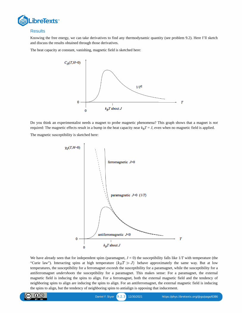
Daniel F. Styer 9.2.3 12/30/2021 https://phys.libretexts.org/@go/page/6386

ResultsKnowing the free energy, we can take derivatives to find any thermodynamic quantity (see problem 9.2). Here I’ll sketchand discuss the results obtained through those derivatives.

The heat capacity at constant, vanishing, magnetic field is sketched here:

Do you think an experimentalist needs a magnet to probe magnetic phenomena? This graph shows that a magnet is notrequired: The magnetic effects result in a bump in the heat capacity near k T = J, even when no magnetic field is applied.

The magnetic susceptibility is sketched here:

We have already seen that for independent spins (paramagnet, J = 0) the susceptibility falls like 1/T with temperature (the“Curie law”). Interacting spins at high temperature behave approximately the same way. But at lowtemperatures, the susceptibility for a ferromagnet exceeds the susceptibility for a paramagnet, while the susceptibility for aantiferromagnet undershoots the susceptibility for a paramagnet. This makes sense: For a paramagnet, the externalmagnetic field is inducing the spins to align. For a ferromagnet, both the external magnetic field and the tendency ofneighboring spins to align are inducing the spins to align. For an antiferromagnet, the external magnetic field is inducingthe spins to align, but the tendency of neighboring spins to antialign is opposing that inducement.

B

( T ≫ J)kB

Daniel F. Styer 9.2.4 12/30/2021 https://phys.libretexts.org/@go/page/6386

Aligning the spins in a paramagnet is like herding cats: the individual spins are independent and don’t naturally take topointing all in the same direction. Aligning the spins in a ferromagnet is like herding cows: the individual spins want to allgo in the same direction and don’t care which direction it is. Aligning the spins in an antiferromagnet is like herdingsiblings in a dysfunctional family, where each sibling says “I want to go to the opposite of wherever my brother/sisterwants to go.”

Daniel F. Styer 9.3.1 1/20/2022 https://phys.libretexts.org/@go/page/6387

9.3: The Mean-Field ApproximationMany times, in this book, I have had occasion to make an approximation, but then I argued (sometimes rigorously andsometimes less rigorously) that this approximation would become “exact in the thermodynamic limit.” So let meemphasize that the mean-field approximation is not exact in the thermodynamic limit. It is usually accurate at hightemperatures. It is rarely accurate near phase transitions.

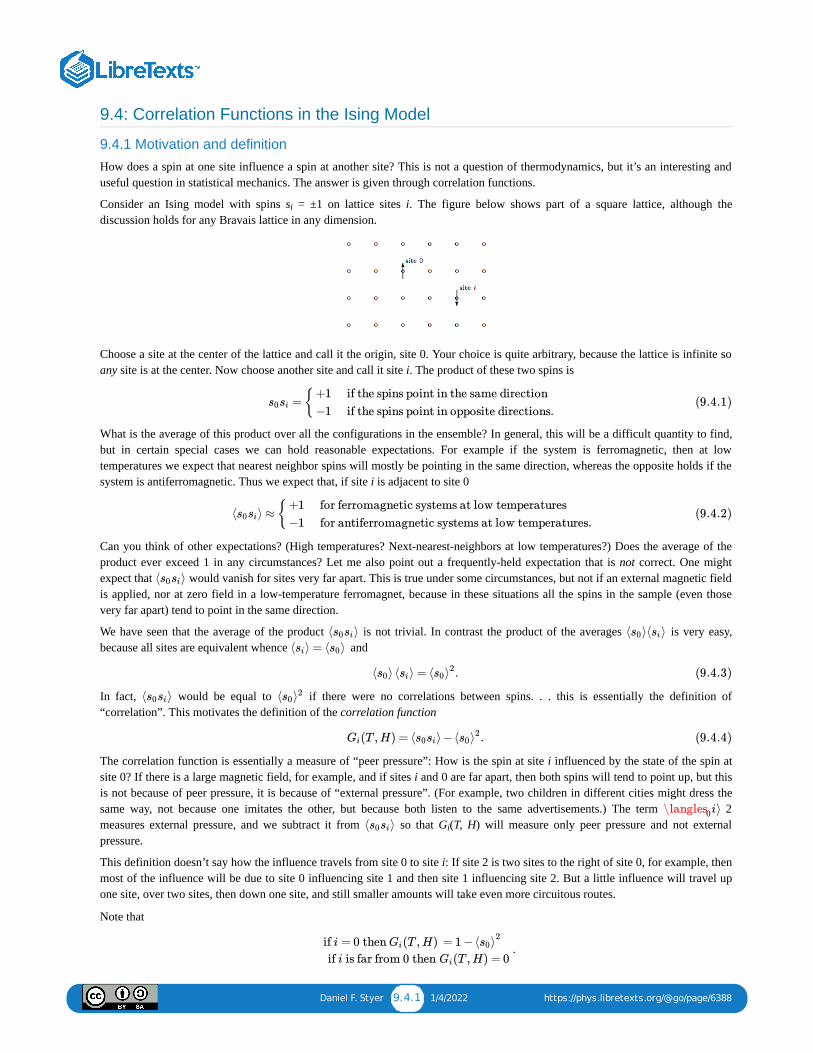
Daniel F. Styer 9.4.1 1/4/2022 https://phys.libretexts.org/@go/page/6388

9.4: Correlation Functions in the Ising Model

9.4.1 Motivation and definition

How does a spin at one site influence a spin at another site? This is not a question of thermodynamics, but it’s an interesting anduseful question in statistical mechanics. The answer is given through correlation functions.

Consider an Ising model with spins s = ±1 on lattice sites i. The figure below shows part of a square lattice, although thediscussion holds for any Bravais lattice in any dimension.

Choose a site at the center of the lattice and call it the origin, site 0. Your choice is quite arbitrary, because the lattice is infinite soany site is at the center. Now choose another site and call it site i. The product of these two spins is

What is the average of this product over all the configurations in the ensemble? In general, this will be a difficult quantity to find,but in certain special cases we can hold reasonable expectations. For example if the system is ferromagnetic, then at lowtemperatures we expect that nearest neighbor spins will mostly be pointing in the same direction, whereas the opposite holds if thesystem is antiferromagnetic. Thus we expect that, if site i is adjacent to site 0

Can you think of other expectations? (High temperatures? Next-nearest-neighbors at low temperatures?) Does the average of theproduct ever exceed 1 in any circumstances? Let me also point out a frequently-held expectation that is not correct. One mightexpect that would vanish for sites very far apart. This is true under some circumstances, but not if an external magnetic fieldis applied, nor at zero field in a low-temperature ferromagnet, because in these situations all the spins in the sample (even thosevery far apart) tend to point in the same direction.

We have seen that the average of the product is not trivial. In contrast the product of the averages is very easy,because all sites are equivalent whence and

In fact, would be equal to if there were no correlations between spins. . . this is essentially the definition of“correlation”. This motivates the definition of the correlation function

The correlation function is essentially a measure of “peer pressure”: How is the spin at site i influenced by the state of the spin atsite 0? If there is a large magnetic field, for example, and if sites i and 0 are far apart, then both spins will tend to point up, but thisis not because of peer pressure, it is because of “external pressure”. (For example, two children in different cities might dress thesame way, not because one imitates the other, but because both listen to the same advertisements.) The term 2measures external pressure, and we subtract it from so that G (T, H) will measure only peer pressure and not externalpressure.

This definition doesn’t say how the influence travels from site 0 to site i: If site 2 is two sites to the right of site 0, for example, thenmost of the influence will be due to site 0 influencing site 1 and then site 1 influencing site 2. But a little influence will travel upone site, over two sites, then down one site, and still smaller amounts will take even more circuitous routes.

Note that

i

=s0si+1

−1

if the spins point in the same direction

if the spins point in opposite directions. (9.4.1)

⟨ ⟩ ≈s0si+1

−1

for ferromagnetic systems at low temperatures

for antiferromagnetic systems at low temperatures. (9.4.2)

⟨ ⟩s0si

⟨ ⟩s0si ⟨ ⟩⟨ ⟩s0 si⟨ ⟩ = ⟨ ⟩si s0

⟨ ⟩ ⟨ ⟩ = .s0 si ⟨ ⟩s02 (9.4.3)

⟨ ⟩s0si ⟨s0⟩2

(T ,H) = ⟨ ⟩− .Gi s0si ⟨ ⟩s02 (9.4.4)

i⟩\langles0

⟨ ⟩s0si i

. if i = 0 then (T ,H)Gi

if i is far from 0 then

= 1 − ⟨ ⟩s02

(T ,H) = 0Gi

Daniel F. Styer 9.4.2 1/4/2022 https://phys.libretexts.org/@go/page/6388

I have three comments to make concerning the correlation function. First, realize that the correlation function gives informationabout the system beyond thermodynamic information. For most of this book we have been using microscopic information tocalculate a partition function and then to find macroscopic (thermodynamic) information about the system. We did not use thepartition function to ask any question that involved the distance between two spins (or two atoms). The correlation function enablesus to probe more deeply into statistical mechanics and ask such important microscopic questions.

Second, the correlation function is a measurable quantity. I have produced the definition through conceptual motivations that makeit seem impossible to find except by examining individual spins. . . a conceptual nicety but experimental impossibility. But in factthe correlation function can be found experimentally through neutron scattering. This technique relies upon interference in the deBroglie waves of neutron waves scattered from nearby spins. It is not trivial: indeed two of the inventors of the technique wereawarded the Nobel prize in physics for 1994. (It is also worth noting that the work of one of these two was based upon theoreticalwork done by Bob Weinstock in his Ph.D. thesis.) I will not have enough time to treat this interesting topic, but you should realizethat what follows in this section is not mere theoretical fluff. . . it has been subjected to, and passed, the cold harsh probe ofexperimental test.

Third, although the definition given here applies only to Ising models on Bravais lattices, analogous definitions can be producedfor other magnetic systems, for fluids, and for solids.

9.4.2 Susceptibility from the correlation functionI have emphasized above that the correlation function gives information beyond that given by thermodynamics. But the correlationfunction contains thermodynamic information as well. In this subsection we will prove that if the correlation function G (T, H) isknown for all sites in the lattice, then the susceptibility, a purely thermodynamic quantity, can be found through

where the sum is over all sites in the lattice (including the origin).

We begin with a few reminders. The microscopic magnetization for a single configuration is

and the macroscopic (thermodynamic) magnetization is its ensemble average

The Ising Hamiltonian breaks into two pieces,

where is independent of magnetic field. In the nearest-neighbor Ising model the field-independent part of the Hamiltonian is

but we will not use this formula. . . the results of this section are true for spin-spin interactions of arbitrary complexity. Finally, theBoltzmann factor is

Now we can start the argument by examining the sum of the correlation function over all sites. In what follows, the notation means the “sum over states”.

1

i

χ(T ,H) = N (T ,H),m2

TkB∑i

Gi (9.4.5)

M ( , … , ) = ms1 sN ∑i

si (9.4.6)

M = ⟨M⟩ = mN ⟨ ⟩ .s0 (9.4.7)

H= ( , … , ) −mHH0 s1 sN ∑i

si (9.4.8)

= ( , … , ) −HM ( , … , ) ,H0 s1 sN s1 sN (9.4.9)

H0

( , … , ) = −J ,H0 s1 sN ∑<i,j>

sisj (9.4.10)

= .e−βH e−β +βHMH0 (9.4.11)

∑s

= ⟨ ⟩−∑i

Gi ∑i

s0si ⟨ ⟩s02 (9.4.12)

= [ − ]∑i

∑ss0sie−βH

Z

( )∑s s0e−βH 2

Z2(9.4.13)

= −N(M/m)∑

ss0 e−βH

Z

( )∑s s0e−βH 2

Z2(9.4.14)

Daniel F. Styer 9.4.3 1/4/2022 https://phys.libretexts.org/@go/page/6388

Look at this last equation carefully. What do you see? The quotient rule! Do you remember our slick trick for finding dispersions?The appearing in the leftmost summand can be gotten there by taking a derivative of equation (9.35) with respect to H:

Watch carefully:

But the quantity in square brackets is nothing more than m times equation (9.39),

But we also know that

whence, finally

Whew!

Now we can stop running and do our cool-down stretches. Does the above equation, procured at such expense, make sense? Theleft hand side is extensive. The right hand side has a factor of N and also sum over all sites, and usually a sum over all sites isextensive. So at first glance the left hand side scales linearly with N while the right hand side scales with N , a sure sign of error! Infact, there is no error. The correlation function G vanishes except for sites very close to the origin. (“Distant sites areuncorrelated”, see equation (9.28).) Thus the sum over all sites above has a summand that vanishes for most sites, and it isintensive rather than extensive.

9.4.3 All of thermodynamics from the susceptibility

The previous subsection shows us how to find one thermodynamic quantity, χ(T, H) at some particular values for temperature andfield, by knowing the correlation function G (T, H) for all sites i, at those same fixed values for temperature and field. In thissubsection we will find how to calculate any thermodynamic quantity at all, at any value of T and H at all, by knowing χ(T, H) forall values of T and H. Thus knowing the correlation G (T, H) as a function of all its arguments—i, T, and H—enables us to find anythermodynamic quantity at all.

To find any thermodynamic quantity it suffices to find the free energy F(T, H), so the claim above reduces to saying that we canfind F(T, H) given χ(T, H). Now we can find χ(T, H) from F(T, H) by simple differentiation, but going backwards requires somevery careful integration. We will do so by looking at the difference between quantities for the Ising model and for the idealparamagnet.

Remember that the thermodynamic state of an Ising magnet is specified by the two variables T and H, as indicated in the figure.

=Z (M/m) −N∑S s0 e−βH ∑S s0e

−βH∑S s0e−βN

Z2(9.4.15)

M

= βM .∂e−βH

∂He−βH (9.4.16)

( ) =∂

∂H

∑S s0e−βH

Z

Z βM − βM∑S s0 e−βH ∑S e−βH∑S s0e−βH

Z2(9.4.17)

= β [ ]Z M −mN∑S s0 e−βH ∑S s0e−βH∑S s0e−βH

Z2(9.4.18)

( ) = βm∂

∂H

∑s s0e−βH

Z∑i

Gi (9.4.19)

( ) = = = χ∂

∂H

∑s s0e−βH

Z

∂ ⟨ ⟩s0

∂H

∂M/mN

∂H

1

mN(9.4.20)

χ(T ,H) = N (T ,H).m2

TkB∑i

Gi (9.4.21)

2

i

i

i

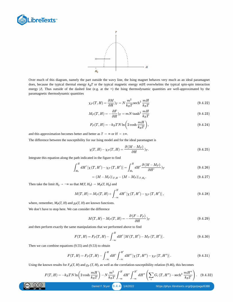
Daniel F. Styer 9.4.4 1/4/2022 https://phys.libretexts.org/@go/page/6388

Over much of this diagram, namely the part outside the wavy line, the Ising magnet behaves very much as an ideal paramagnetdoes, because the typical thermal energy k T or the typical magnetic energy m|H| overwhelms the typical spin-spin interactionenergy |J|. Thus outside of the dashed line (e.g. at the ×) the Ising thermodynamic quantities are well-approximated by theparamagnetic thermodynamic quantities

and this approximation becomes better and better as T → ∞ or H → ±∞.

The difference between the susceptibility for our Ising model and for the ideal paramagnet is

Integrate this equation along the path indicated in the figure to find

Then take the limit H → −∞ so that M(T, H ) → M (T, H ) and

where, remember, M (T, H) and χ (T, H) are known functions.

We don’t have to stop here. We can consider the difference

and then perform exactly the same manipulations that we performed above to find

Then we can combine equations (9.55) and (9.53) to obtain

Using the known results for F (T, H) and χ (T, H), as well as the correlation-susceptibility relation (9.46), this becomes

B

(T ,H) = = NχP

∂M

∂H)T

m2

TkBsech2 mH

TkB(9.4.22)

(T ,H) = − = mNMP

∂F

∂H)T tanh2 mH

TkB(9.4.23)

(T ,H) = − TN ln(2 cosh ),FP kBmH

TkB(9.4.24)

χ(T ,H) − (T ,H) = .χP

∂ (M − )MP

∂H)T (9.4.25)

d [χ (T , ) − (T , )] = d∫H

H0

H ′ H ′ χP H ′ ∫H

H0

H ′ ∂ (M − )MP

∂H ′)T (9.4.26)

= − .(M − )|MP T ,H (M − )|MP T ,H0(9.4.27)

0 0 P 0

M(T ,H) = (T ,H) + d [χ (T , ) − (T , )] ,MP ∫H

−∞

H ′ H ′ χP H ′ (9.4.28)

P P

M(T ,H) − (T ,H) = −MP

∂ (F − )FP

∂H)T (9.4.29)

F (T ,H) = (T ,H) − d [M (T , ) − (T , )] .FP ∫H

−∞

H ′ H ′ MP H ′ (9.4.30)

F (T ,H) = (T ,H) − d d [χ (T , ) − (T , )] .FP ∫H

−∞

H ′ ∫H ′

−∞

H ′′ H ′′ χP H ′′ (9.4.31)

P P

F (T ,H) = − TN ln(2 cosh )−N d d ( (T , ) − ) .kBmH

TkB

m2

TkB∫

H

−∞

H ′ ∫H ′

−∞

H ′′ ∑i

Gi H ′′ sech2 mH ′′

TkB(9.4.32)

Daniel F. Styer 9.4.5 1/4/2022 https://phys.libretexts.org/@go/page/6388

Let me stress how remarkable this result is. You would think that to find the thermodynamic energy E(T, H) of the Ising model youwould need to know the spin-spin coupling constant J. But you don’t: You can find E(T, H) without knowing J, indeed withoutknowing the exact form of the spin-spin interaction Hamiltonian at all, if you do know the purely geometrical informationcontained within the correlation function. This is one of the most amazing and useful facts in all of physics.

9.4.4 Parallel results for fluidsI cannot resist telling you how the results of this section change when applied to fluid rather than magnetic systems. In that case thecorrelation function g (r; T, V, N) depends upon the position r rather than the site index i. Just as the sum of G over all sites isrelated to the susceptibility χ, so the integral of g (r) over all space is related to the compressibility κ . And just as the susceptibilitycan be integrated twice (carefully, through comparison to the ideal paramagnet) to give the magnetic free energy F(T, H), so thecompressibility can be integrated twice (carefully, through comparison to the ideal gas) to give the fluid free energy F(T, V, N). Andjust as the magnetic thermodynamic quantities can be found from the correlation function without knowing the details of the spin-spin interaction Hamiltonian, so the fluid thermodynamic quantities can be found from the correlation function without knowingthe details of the particle interaction forces. A question for you: How is it possible to get all this information knowing only thecorrelation function in space rather than the correlation function in phase space? In other words, why don’t you need informationabout the velocities?

I should put in some references to experimental tests and to say who thought this up. Are these available in Joel’s review article?

Namely, by asking “Wouldn’t it be nice to know how one spin is influenced by its neighbors?”

This does not mean that the thermodynamic energy is independent of the spin-spin Hamiltonian, because the Hamiltonianinfluences the correlation function.

2

2 i

2 T

1

2

Daniel F. Styer 9.5.1 12/30/2021 https://phys.libretexts.org/@go/page/6389

9.5: Computer Simulation

9.5.1 Basic strategy

If we’re going to use a computer to solve problems in statistical mechanics, there are three basic strategies that we could take.I illustrate them here by showing how they would be applied to the Ising model.

1. Exhaustive enumeration. Just do it! List all the states (microstates, configurations), their associated probabilities, andaverage over them! Admittedly, there are a lot of states, but computers are fast, right? Let’s see how many states there are.Consider a pretty small problem: a three dimensional Ising model on an 8 × 8 × 8 cube. This system has 512 spins that can beoriented either “up” or “down”, so there are 2 ≈ 10 configurations. Suppose that our computer could generate andexamine a million configurations per second. . . this is about as fast as is currently possible. Then an exhaustive enumerationwould require 10 seconds to do the job. By contrast, the universe is about 10 seconds old. So for one computer to do theproblem it would take 10 times the age of the universe. Now this is impractical, but maybe we could do it by arrangingcomputers in parallel. Well, there are about 10 protons in the universe, and if every one were to turn into a spiffy Unixworkstation, it would still require 10 times the age of the universe to complete the list. And this is for a small problem!Sorry, computers aren’t fast, and they never will be fast enough to solve the complete enumeration problem. It is not fornothing that this technique is called exhaustive enumeration.

2. Random sampling. Instead of trying to list the entire pool of possible configurations, we will dip into it at random andsample the configurations. This can be implemented by scanning through the lattice and orienting spins up with probability and down with probability . The problem in this strategy is that all configurations are equally likely to be sampled, butbecause there are many more high energy configurations than low energy configurations, it is very unlikely to sample a lowenergy configuration (the “poker paradox” again). But in the Boltzmann distribution e the low energy configurationsare in fact more likely to occur. So you could sample for a long time before encountering even one configuration with non-negligible probability. This strategy is considerably better than the first one, but it would still take about the age of theuniverse to implement.

3. Importance sampling. This strategy is to sample the pool of possible configurations not completely at random, but in such away that the most likely configurations are most likely to be sampled. An enormously successful algorithm to performimportance sampling was developed by Nick Metropolis and his coworkers Arianna Rosenbluth, Marshall Rosenbluth,Augusta Teller, and Edward Teller (of hydrogen bomb fame) in 1953. (“Equation of state calculations by fast computingmachines”, J. Chem. Phys. 21 1087–1092.) It is called “the Metropolis algorithm”, or “the M(RT) algorithm”, or simply “theMonte Carlo algorithm”. The next section treats this algorithm in detail.

An analogy to political polling is worth making here. Exhaustive enumeration corresponds to an election, random samplingcorresponds to a random poll, and importance sampling corresponds to a poll which selects respondents according to thelikelihood that they will vote.

9.5.2 The Metropolis algorithmThis algorithm builds a chain of configurations, each one modified (usually only slightly) from the one before. For example, ifwe number the configurations (say, for the 8 ×8×8 Ising model, from 1 to 2 ) such a chain of configurations might be

Note that it is possible for two successive configurations in the chain to be identical.

To build any such chain, we need some transition probability rule W(C → C ) giving the probability that configuration Cwill follow configuration C . And to be useful for importance sampling, the rule will have to build the chain in such a waythat the probability of C appearing in the chain is e .

So we need to produce a result of the form: if “rule” then “Boltzmann probability distribution”. It is, however, very difficult tocome up with such results. Instead we go the other way to produce a pool of plausible transition rules. . . plausible in that theyare not obviously inconsistent with a Boltzmann probability distribution.

Consider a long chain of N configurations, in which the probability of a configuration appearing is given by theBoltzmann distribution. The chain must be “at equilibrium” in that

512 154

148 18

130

80

50

12

12

−energy/k TB

2

512

→ → → → → → ⋯C171 C49 C1294 C1294 C171 C190 (9.5.1)

a b b

a

n−βE /Zn

configs

number of transitions ( → ) = number of transitions ( → ) .Ca Cb Cb Ca (9.5.2)

Daniel F. Styer 9.5.2 12/30/2021 https://phys.libretexts.org/@go/page/6389

But the number of Cas in the chain is Nconfigse −βEa /Z, and similarly for the number of Cbs, so the equation above is

whence

This condition, called “detailed balance”, defines our pool of plausible transition probability rules. It is possible that a rulecould satisfy detailed balance and still not sample according to the Boltzmann distribution, but any rule that does not satisfydetailed balance certainly cannot sample according to the Boltzmann distribution. In practice, all the rules that satisfy detailedbalance seem to work.

Two transitions probability rules that do satisfy detailed balance, and the two rules most commonly used in practice, are

where we have taken

and where the normalization constant is fixed so that

If we had to calculate the normalization constant, then we would be back to performing an exhaustive enumeration, so wemust find a way to work with unnormalized transition probabilities. To this end we define w as the factor for the transitionprobability aside from the normalization constant, i.e. the part in curly brackets in equations (9.61) and (9.62). Note that it is apositive number less than or equal to one:

Notice that for any rule satisfying detailed balance the transition probability must increase as the change in energy decreases,suggesting a simple physical interpretation: The chain of configurations is like a walker stepping from configuration toconfiguration on a “configuration landscape”. If a step would decrease the walker’s energy, he is likely to take it, whereas if itwould increase his energy, he is likely to reject it. Thus the walker tends to go downhill on the configuration landscape, but itis not impossible for him to go uphill. This seems like a recipe for a constantly decreasing energy, but it is not, because moreuphill steps than downhill steps are available to be taken.

This paragraph constitutes the most densely packed observation in this book. It looks backward to the poker paradox, to thedefinition of temperature, and to the “cash incentives” interpretation of the canonical ensemble. It looks forward toequilibration and to optimization by Monte Carlo simulated annealing. Why not read it again?

From these ingredients, Metropolis brews his algorithm:

Generate initial configuration [at random or otherwise]

Gather data concerning configuration [e.g. find M :=n − n ; M :=M]

DO Iconfig = 2, Nconfigs

Generate candidate configuration [e.g. select a spin to flip]

Compute w for transition to candidate

With probability w , make the transition

Gather data concerning configuration [e.g. find M:=n − n ; M :=M + M]

END DO

W ( → ) = W ( → ) ,N configs e−βEa

ZCa Cb N configs

e−βEb

ZCb Ca (9.5.3)

=W ( → )Ca Cb

W ( → )Cb Ca

e−β( − )Eb Ea (9.5.4)

W ( → ) = [ normalization constant ] Ca Cb

e−βΔE

1 +e−βΔE(9.5.5)

W ( → ) = [ normalization constant ] Ca Cb

1

e−βΔE

if ΔE ≤ 0

if ΔE > 0

ΔE = −Eb Ea (9.5.6)

W ( → ) = 1.∑Cb

Ca Cb (9.5.7)

a→b

0 < ≡ ≤ 1.wa→b (9.5.8)

3

3

↑ ↓ sum

a→b

a→b

↑ ↓ sum sum

Daniel F. Styer 9.5.3 12/30/2021 https://phys.libretexts.org/@go/page/6389

Summarize and print data [e.g. M :=M /Nconfigs]

I’ll make three comments concerning this algorithm. First of all, note that the step “With probability w , make thetransition” implies that sometimes the transition is not made, in which case two configurations adjacent in the chain will beidentical. It is a common misconception that in this case the repeated configuration should be counted only once, but that’s notcorrect: you must execute the “Gather data concerning configuration” step whether the previous candidate was acceptedor rejected.

Secondly, I wish to detail how the step

With probability w , make the transition

is implemented. It is done by expanding the step into the two substeps

Produce a random number z [0 ≤ z < 1]

IF z < w THEN switch to candidate

[i.e. configuration := candidate configuration]

Finally, I need to point out that this algorithm does not precisely implement either of the transition probability rules (9.61) or(9.62). For example, if the step “Generate candidate configuration” is done by selecting a single spin to flip, thenthe algorithm will never step from one configuration to a configuration three spin-flips away, regardless of the value of ∆E.Indeed, under such circumstances (and if there are N spins in the system), the transition probability rule is

It is easy to see that this transition probability rule satisfies detailed balance.

9.5.3 Implementing the Metropolis algorithmIt is not atypical to run a Monte Carlo program for about 10,000 Monte Carlo steps per site. As such, the program might runfor hours or even days. This is considerably less than the age of the universe, but probably far longer than you are used torunning programs. The following tips are useful for speeding up or otherwise improving programs implementing theMetropolis algorithm.

1. Use scaled quantities. The parameters J, m, H, and T do not enter in any possible combination, but only through twoindependent products. These are usually taken to be

Thus the Boltzmann exponent for a given configuration is

where s is +1 if the spin at site i is up, −1 if it is down, and where denotes a nearest neighbor pair.

2. Don’t find total energies. To calculate w you must first know ∆E, and the obvious way to find ∆E is to find E and E(through equation (9.68)) and subtract. This way is obvious but terribly inefficient. Because the change in configuration issmall (usually a single spin flip) the change in energy can be found from purely local considerations without finding the totalenergy of the entire system being simulated. Similarly, if you are finding the average (scaled) magnetization

(as suggested by the square brackets in the algorithm on page 202) you don’t need to scan the entire lattice to find it. Instead,just realize that it changes by ±2 with each spin flip.

3. Precompute Boltzmann factors. It is computationally expensive to find evaluate a exponential, yet we must know the valueof e . However, usually there are only a few possible values of ∆E. (For example in the square lattice Ising model with

ave sum

a→b

a→b

a→b

W ( → ) = .Ca Cb

⎧

⎩⎨⎪⎪

⎪⎪

1N

wa→b

0

1 − W ( → )∑ ≠Cb CaCa Cb

if and differ by a single spin flip Ca Cb

if and differ by more than a single spin flip Ca Cb

if =Ca Cb

(9.5.9)

= and = .T~ TkB

JH~ mH

J(9.5.10)

− = + ,E

TkB

1

T~⎛

⎝∑⟨i,j⟩

sisj H~∑

i

si

⎞

⎠(9.5.11)

i ⟨i, j⟩

a→b b a

M = = =n↑ n↓ ∑i

si (9.5.12)

−β∆E

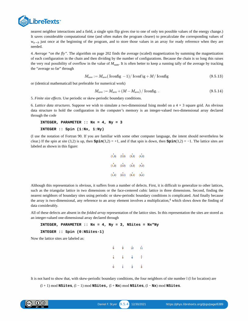
Daniel F. Styer 9.5.4 12/30/2021 https://phys.libretexts.org/@go/page/6389

nearest neighbor interactions and a field, a single spin flip gives rise to one of only ten possible values of the energy change.)It saves considerable computational time (and often makes the program clearer) to precalculate the corresponding values ofw just once at the beginning of the program, and to store those values in an array for ready reference when they areneeded.

4. Average “on the fly”. The algorithm on page 202 finds the average (scaled) magnetization by summing the magnetizationof each configuration in the chain and then dividing by the number of configurations. Because the chain is so long this raisesthe very real possibility of overflow in the value of M . It is often better to keep a running tally of the average by trackingthe “average so far” through

or (identical mathematicall but preferable for numerical work)

5. Finite size effects. Use periodic or skew-periodic boundary conditions.

6. Lattice data structures. Suppose we wish to simulate a two-dimensional Ising model on a 4 × 3 square grid. An obviousdata structure to hold the configuration in the computer’s memory is an integer-valued two-dimensional array declaredthrough the code

INTEGER, PARAMETER :: Nx = 4, Ny = 3

INTEGER :: Spin (1:Nx, 1:Ny)

(I use the notation of Fortran 90. If you are familiar with some other computer language, the intent should nevertheless beclear.) If the spin at site (3,2) is up, then Spin(3,2) = +1, and if that spin is down, then Spin(3,2) = −1. The lattice sites arelabeled as shown in this figure:

Although this representation is obvious, it suffers from a number of defects. First, it is difficult to generalize to other lattices,such as the triangular lattice in two dimensions or the face-centered cubic lattice in three dimensions. Second, finding thenearest neighbors of boundary sites using periodic or skew-periodic boundary conditions is complicated. And finally becausethe array is two-dimensional, any reference to an array element involves a multiplication, which slows down the finding ofdata considerably.

All of these defects are absent in the folded array representation of the lattice sites. In this representation the sites are stored asan integer-valued one-dimensional array declared through

INTEGER, PARAMETER :: Nx = 4, Ny = 3, NSites = Nx*Ny

INTEGER :: Spin (0:NSites-1)

Now the lattice sites are labeled as:

It is not hard to show that, with skew-periodic boundary conditions, the four neighbors of site number l (l for location) are

(l + 1) mod NSites, (l − 1) mod NSites, (l + Nx) mod NSites, (l − Nx) mod NSites.

a→b

sum

:= ( Iconfig −1)/ Iconf ig +M/ Iconfig Mave Mave (9.5.13)

:= +(M − ) / Iconfig. .Mave Mave Mave (9.5.14)

4

Daniel F. Styer 9.5.5 12/30/2021 https://phys.libretexts.org/@go/page/6389

Unfortunately, the Fortran Mod function was inanely chosen to differ from the mathematical mod function, so this arithmeticmust be implemented through

Mod(l + 1, NSites)

Mod(l + (NSites - 1), NSites)

Mod(l + Nx, NSites)

Mod(l + (NSites - Nx), NSites)

7. Random number generators. It is hard to find an easy source of high-quality random numbers: this is a problem for physics,also for government and industry.

In Fortran, the datum Site(i,j) is stored at memory location number i + j*(Nx-1), whence the data are stored in the sequence(1,1), (2,1), (3,1), (4,1), (1,2), (2,2),. . . . In other computer languages the formula for finding the memory location is different,but in all languages it involves an integer multiply

D.E. Knuth, Seminumerical Algorithms (Addison–Wesley, Reading, Massachusetts, 1981) chapter 3.

W.H. Press, S.A. Teukolsky, W.T. Vettering, and B.P. Flannery, Numerical Recipes chapter 7. (For a confession and aprize announcement, see also W.H. Press and S.A. Teukolsky, “Portable random number generators”, Computers inPhysics 6 (1992) 522–524.)

T.-W. Chiu and T.-S. Guu, “A shift-register sequence random number generator,” Computer Physics Communications47 (1987) 129–137. (See particularly figures 1 and 2.)

A.M. Ferrenberg, D.P. Landau, and Y.J. Wong, “Monte Carlo simulations: Hidden errors from ‘good’ random numbergenerators,” Phys. Rev. Lett. 69 (1992) 3382.

S.K. Park and K.W. Miller, “Random number generators: Good ones are hard to find,” Communications of the ACM 31(1988) 1192–1201.

8. Initial configurations and equilibration. The Metropolis algorithm does not specify how to come up with the firstconfiguration in the chain. Indeed, selecting this configuration is something of an art. If you are simulating at hightemperatures, it is usually appropriate to begin with a configuration chosen at random, so that about half the spins will be upand half down. But if you are simulating at low temperatures (or at high fields) it might be better to start at the configurationwith all spins up. Other possibilities are also possible. But however you select the initial configuration, it is highly unlikelythat the one you pick will be “typical” of the configurations for the temperature and magnetic field at which you aresimulating.

9. Low temperatures. At low temperatures, most candidate transitions are rejected. BLK algorithm. (A.B. Bortz, J.L.Lebowitz, and M.H. Kalos, “A new algorithm for Monte Carlo simulation of Ising spin systems,” J. Comput. Phys. 17 (1975)10–18.)

10. Critical temperatures. “Critical slowing down,” response is cluster flipping. (U. Wolff, “Collective Monte Carlo updatingfor spin systems,” Phys. Rev. Lett. 62 (1989) 361–364. See also Jian-Sheng Wang and R.H. Swendsen, “Cluster Monte Carloalgorithms,” Physica A 167 (1990) 565–579.)

11. First-order transitions.

12. Molecular dynamics.

9.5.4 The Wolff algorithm

In 1989 Ulli Wolff proposed an algorithm for Monte Carlo simulation that is particularly effective near critical points. (U.Wolff, Phys. Rev. Lett., 62 (1989) 361–364.) The next page presents the Wolff algorithm as applied to the zero-fieldferromagnetic nearest-neighbor Ising model,

on a square lattice or a simple cubic lattice.

Generate initial configuration

Gather data concerning this configuration

4

H = −J∑ with = ±1,sisj si (9.5.15)

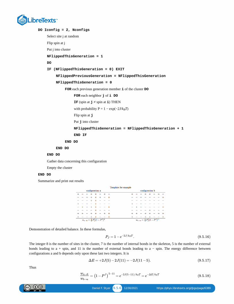
Daniel F. Styer 9.5.6 12/30/2021 https://phys.libretexts.org/@go/page/6389

DO Iconfig = 2, Nconfigs

Select site j at random

Flip spin at j

Put j into cluster

NFlippedThisGeneration = 1

DO

IF (NFlippedThisGeneration = 0) EXIT

NFlippedPreviousGeneration = NFlippedThisGeneration

NFlippedThisGeneration = 0

FOR each previous generation member i of the cluster DO

FOR each neighbor j of i DO

IF (spin at j ≠ spin at i) THEN

with probability P = 1 − exp(−2J/k T)

Flip spin at j

Put j into cluster

NFlippedThisGeneration = NFlippedThisGeneration + 1

END IF

END DO

END DO

END DO

Gather data concerning this configuration

Empty the cluster

END DO

Summarize and print out results

Demonstration of detailed balance. In these formulas,

The integer 8 is the number of sites in the cluster, 7 is the number of internal bonds in the skeleton, 5 is the number of externalbonds leading to a + spin, and 11 is the number of external bonds leading to a − spin. The energy difference betweenconfigurations a and b depends only upon these last two integers. It is

Thus

B

= 1 − .PJ e−2J/ TkB (9.5.16)

ΔE = +2J(5) −2J(11) = −2J(11 −5). (9.5.17)

= = =wa→b

wb→a

(1 − )P J 5−11e−2J(5−11)/ TkB e−ΔE/ TkB (9.5.18)

Daniel F. Styer 9.5.7 12/30/2021 https://phys.libretexts.org/@go/page/6389

and detailed balance is insured.

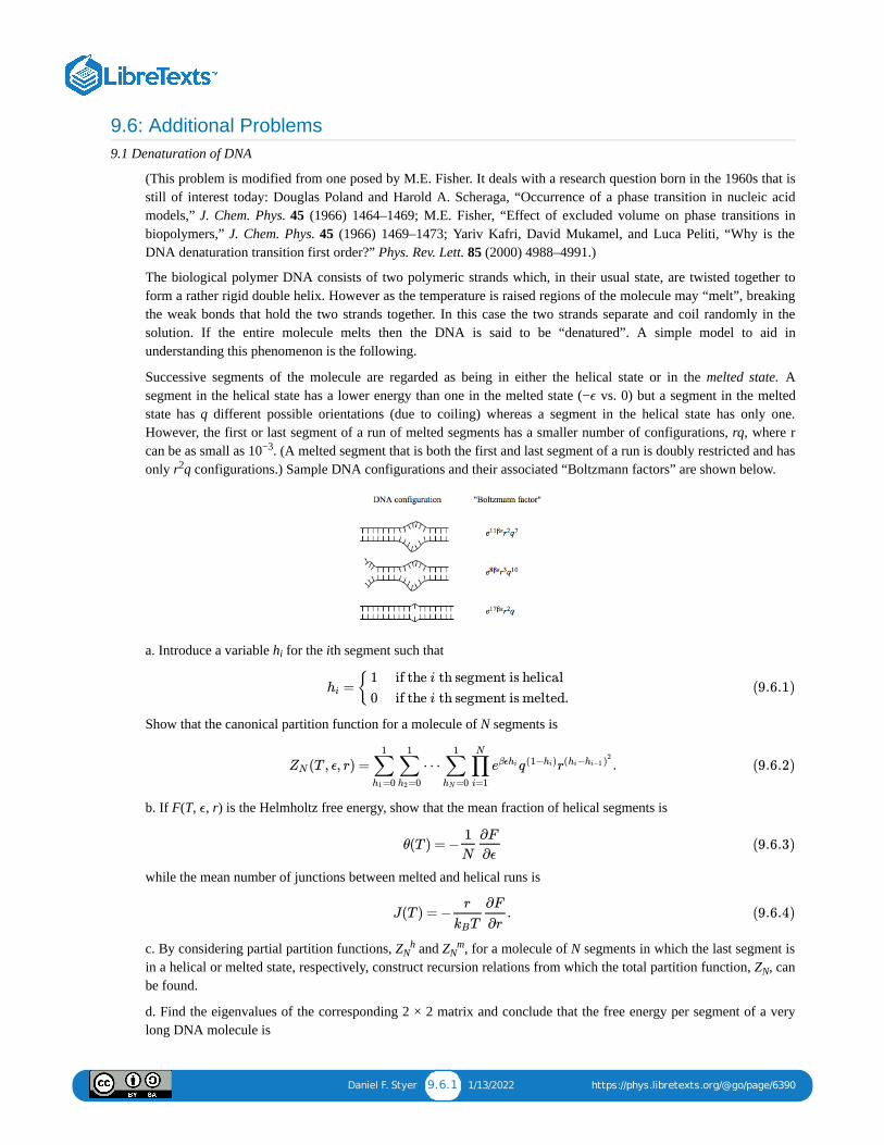
Daniel F. Styer 9.6.1 1/13/2022 https://phys.libretexts.org/@go/page/6390

9.6: Additional Problems9.1 Denaturation of DNA

(This problem is modified from one posed by M.E. Fisher. It deals with a research question born in the 1960s that isstill of interest today: Douglas Poland and Harold A. Scheraga, “Occurrence of a phase transition in nucleic acidmodels,” J. Chem. Phys. 45 (1966) 1464–1469; M.E. Fisher, “Effect of excluded volume on phase transitions inbiopolymers,” J. Chem. Phys. 45 (1966) 1469–1473; Yariv Kafri, David Mukamel, and Luca Peliti, “Why is theDNA denaturation transition first order?” Phys. Rev. Lett. 85 (2000) 4988–4991.)

The biological polymer DNA consists of two polymeric strands which, in their usual state, are twisted together toform a rather rigid double helix. However as the temperature is raised regions of the molecule may “melt”, breakingthe weak bonds that hold the two strands together. In this case the two strands separate and coil randomly in thesolution. If the entire molecule melts then the DNA is said to be “denatured”. A simple model to aid inunderstanding this phenomenon is the following.

Successive segments of the molecule are regarded as being in either the helical state or in the melted state. Asegment in the helical state has a lower energy than one in the melted state (− vs. 0) but a segment in the meltedstate has q different possible orientations (due to coiling) whereas a segment in the helical state has only one.However, the first or last segment of a run of melted segments has a smaller number of configurations, rq, where rcan be as small as 10 . (A melted segment that is both the first and last segment of a run is doubly restricted and hasonly r q configurations.) Sample DNA configurations and their associated “Boltzmann factors” are shown below.

a. Introduce a variable h for the ith segment such that

Show that the canonical partition function for a molecule of N segments is

b. If F(T, , r) is the Helmholtz free energy, show that the mean fraction of helical segments is

while the mean number of junctions between melted and helical runs is

c. By considering partial partition functions, Z and Z , for a molecule of N segments in which the last segment isin a helical or melted state, respectively, construct recursion relations from which the total partition function, Z , canbe found.

d. Find the eigenvalues of the corresponding 2 × 2 matrix and conclude that the free energy per segment of a verylong DNA molecule is

ϵ

−3

2

i

=hi

1

0

if the i th segment is helical

if the i th segment is melted. (9.6.1)

(T , ϵ, r) = ⋯ .ZN ∑=0h1

1

∑=0h2

1

∑=0hN

1

∏i=1

N

eβϵhi q(1− )hi r( − )hi hi−12

(9.6.2)

ϵ

θ(T ) = −1

N

∂F

∂ϵ(9.6.3)

J(T ) = − .r

TkB

∂F

∂r(9.6.4)

Nh

Nm

N

Daniel F. Styer 9.6.2 1/13/2022 https://phys.libretexts.org/@go/page/6390

where w = qe . Does this result take on the correct value at zero temperature?

e. In the limit that r vanishes show that the molecule undergoes a sharp melting transition at temperature

Sketch the energy, entropy, and helical fraction θ(T) as a function of temperature and discuss the character of thetransition.

f. If r is small but nonzero, sketch the behavior you expect for θ(T).

g. (Optional.) Show that when r is small but nonzero the sharp transition is “smeared out” over a temperature rangeof approximate width

h. (Optional.) Show that the number of junctions J(T) defined in (b.) varies as Ar both at T = T and at lowtemperatures. Find the values of A and α in each case.

9.2 Thermodynamics of the one-dimensional Ising model

The Helmholtz free energy of the one-dimensional, nearest-neighbor Ising magnet is

where

Use this result to show that

9.3 Zero-field one-dimensional Ising model

In class we found the free energy of a one-dimensional, nearest-neighbor Ising magnet with arbitrary magnetic fieldusing the transfer matrix method. This problem finds the free energy in a much simpler way, which unfortunatelyworks only in zero magnetic field.

a. Show that the partition function can be written as

b. Show that the last sum is

regardless of the value of s .

f(T , ϵ, r) = − T ln [1 +w + ]− ϵ,kB

1

2(1 −w +4w)2 r2− −−−−−−−−−−−−

√ (9.6.5)

−βϵ

= .Tm

ϵ

lnqkB

(9.6.6)

ΔT ≈ .4ϵr

qkB ln2(9.6.7)

αm

F (T , H) = −N J + T ln[coshL + ] ,kB L +sinh2 e−4K− −−−−−−−−−−−

√ (9.6.8)

L = and K = .mH

TkB

J

TkB

(9.6.9)

E(T , H = 0) = −JN tanhK, (9.6.10)

(T , H = 0) = N ,CH kB

K2

Kcosh2(9.6.11)

M(T , H) = mN ,sinhL

L +sinh2 e−4K− −−−−−−−−−−−

√(9.6.12)

(T , H = 0) = N .χT

m2

TkB

e2K (9.6.13)

= ⋯ .ZN ∑=±1s1

∑=±1s2

eKs1s2 ∑=±1s3

eKs2s3 ∑=±1sN−1

eKsN−2 sN−1 ∑=±1sN

eKsN−1 sN (9.6.14)

= 2 coshK,∑=±1sN

eKsN−1 sN (9.6.15)

N−1

Daniel F. Styer 9.6.3 1/13/2022 https://phys.libretexts.org/@go/page/6390

c. Conclude that

and that the zero-field Helmholtz free energy per site is

d. Find the zero-field heat capacity, and show that it gives the expected behavior at very low temperatures.

9.4 Magnetization near the critical point: mean field approximation

Analyze the Ising model in the mean field approximation to show that the zero-field magnetization near the criticaltemperature is

Be sure to specify the value of the numerical constant a. (Hint: .) (Remark:Experiment shows that the magnetization is not precisely of the character predicted by mean field theory: While itdoes approach zero like (T − T) , the exponent β is not 1/2 — for two-dimensional systems β = 1/8, while for three-dimensional systems β ≈ 0.326.)

9.5 Correlation functions for paramagnets

In a paramagnet (see problem 2.9) the spins are uncorrelated, i.e. the correlation function is

Use this fact to verify the correlation sum rule

derived in problem 8.11.

9.6 Lattice gas—Ising magnet

In class we showed that for a lattice gas

whereas for an Ising magnet

and we concluded that the lattice gas and Ising magnet were more-or-less equivalent, with chemical potential andmagnetic field playing sort of analogous roles. These conclusions are indeed correct, but this problem renders themprecise.

a. Show that an up spin is associated with an occupied site, and a down spin with a vacant site, through

b. Write out the sum for Ξ(T, µ) in terms of the variables s , and show that the correspondence

= KZN 2N coshN−1 (9.6.16)

f(T ) = − T ln(2 cosh ).kB

J

TkB

(9.6.17)

M(T ) =⎧

⎩⎨mNa( )−TTc

Tc

1/2

0

for T < Tc

for T > Tc

(9.6.18)

tanhx = x − + +⋯13

x3 215

x5

cβ

(T , H) = 0 for i ≠ 0.Gi (9.6.19)

(T , H) = N ,χT

m2

TkB

∑i

Gi (9.6.20)

Ξ(T , μ) = ⋯ ,∑=0n1

1

∑=0n2

1

∑=0nN

1

( )v0

(T )λ3

N

eβμ +βϵ∑i ni ∑nn ninj (9.6.21)

Z(T , H) = ⋯ +βJ∑=±1s1

∑=±1s2

∑=±1sN

eβmH ∑i

si ∑nn

sisj (9.6.22)

= ( +1) .ni

1

2si (9.6.23)

i

ϵ = 4J (9.6.24)

μ = 2mH − T ln( / (T ))−4qJkB v0 λ3 (9.6.25)

Daniel F. Styer 9.6.4 1/13/2022 https://phys.libretexts.org/@go/page/6390

(where q is the number of nearest neighbors for each site on the lattice) leads to

where p(T, µ) is the pressure of the gas and f(T, H) is the free energy per spin of the magnet.

c. Interpret equation (9.100) using the phrase “escaping tendency”. (Is this a sensible question?)

d. (Hard.) Take derivatives of equation (9.101) to show that

9.7 Estimates concerning exhaustive enumeration

Consider an Ising model with 6.02 × 10 sites. How many distinct configurations can this system take on? Estimatethe mass of paper and ink required to write out a single character. What mass would be required to write out thisnumber of configurations in decimal notation? Compare your estimate to the mass of the earth.

9.8 Fluctuations in Monte Carlo simulation

When the mean energy of a system is determined through Monte Carlo simulation, the result will necessarily havean uncertainty due to the statistical character of the simulation. (The same is true of any other measured quantity.) Soif mean energy is plotted as a function of temperature, the data points will not fall on a sharp line but instead within abroad band. Using a fluctuation-susceptibility relation, show that the width of the band depends on its slope. Willsteep bands be wide or narrow?

9.9 The folded array representation

Implement the folded array representation of a triangular lattice subject to skew-periodic boundary conditions. Clue:The piece of lattice under study will be a parallelogram.

9.10 Monte Carlo project

Perform a Monte Carlo simulation on the Ising model. The precise form and direction of the simulation is up to you:here are some suggestions that you are free to use, combine, extend, or ignore.

a. Draw movies showing the spin configuration of a two-dimensional Ising model as the simulation proceeds.Discuss the qualitative character of the model at high temperatures, low temperatures, and near the criticaltemperature (which is known, from Onsager’s exact solution, to be k T /J = −2/ ln( − 1)).

b. Simulate the one-dimensional Ising model and compare your results to the analytic solution obtained inclass. Consider using the BKL algorithm at low temperatures.

c. Simulate the DNA denaturation model of problem 9.1, and compare your results to the analytic results ofthat problem. You will need to modify the Metropolis algorithm.

d. Simulate a two- or three-dimensional Ising ferromagnet at zero field, using an initial configuration of allspins up. Monitor the magnetization for a number of temperatures ranging from k T ≈ 5J down to k T = 0.Record both the equilibrium magnetization and the number of steps required to reach equilibrium, and plotthese as a function of temperature. Can you locate the critical temperature?

e. Monitor both the mean energy (or magnetization) and the fluctuations in energy (or magnetization). Use afluctuation-susceptibility relation to find the heat capacity (or susceptibility). In particular, show how asimulation at zero magnetic field can still give information about the magnetic susceptibility.

f. Verify the relation discussed in problem 9.8.

p(T , μ) = mH − qJ −f(T , H),v03

2(9.6.26)

ρ(T , μ) = [1 +M(T , H)/mN ],v01

2(9.6.27)

4 (T , μ) = χ(T , H)/ N ,ρ2κT v0 m2 (9.6.28)

− N [ln( / (T ))+ ] = ,Sgas kB v0 λ3 3

2Smag (9.6.29)

− N = .CV

3

2kB CM (9.6.30)

23

B c 2–

√

5

B B

Daniel F. Styer 9.6.5 1/13/2022 https://phys.libretexts.org/@go/page/6390

g. Implement the Wolff algorithm for improved simulation near the critical point.

h. Use finite size scaling to obtain accurate results near the critical point.

i. Compare the BKL and Wolff algorithms at low temperature.

j. Find the correlation function

for a few values of T and H. How does it behave as the critical point is approached? k. (Very ambitious.)Verify the correlation-susceptibility relation (9.46).

A.B. Bortz, J.L. Lebowitz, and M.H. Kalos, J. Comput. Phys., 17 (1975) 10–18.

U. Wolff, Phys. Rev. Lett. 62 (1989) 361–364. J.-S. Wang and R.H. Swendsen, Physica A 167 (1990) 565–579.

H. Gould and J. Tobochnik, An Introduction to Computer Simulation Methods: Applications to Physical Systems, part I(Addison-Wesley, Reading, Mass., 1988) sections 12.4 and 16.5

6

7

= ⟨ ⟩−Gi s0si ⟨ ⟩s02 (9.6.31)

5

6

7

1 1/27/2022

CHAPTER OVERVIEW10: APPENDICES

10.1: A- SERIES AND INTEGRALS10.2: B- EVALUATING THE GAUSSIAN INTEGRAL10.3: C- CLINIC ON THE GAMMA FUNCTION10.4: D- VOLUME OF A SPHERE IN D DIMENSIONS10.5: E- STIRLING'S APPROXIMATION10.6: F- THE EULER-MACLAURIN FORMULA AND ASYMPTOTIC SERIES10.7: G- RAMBLINGS ON THE RIEMANN ZETA FUNCTION10.8: H- TUTORIAL ON MATRIX DIAGONALIZATION10.9: I- CATALOG OF MISCONCEPTIONS10.10: J- THERMODYNAMIC MASTER EQUATIONS10.11: K- USEFUL FORMULAS

Daniel F. Styer 10.1.1 1/20/2022 https://phys.libretexts.org/@go/page/6392

10.1: A- Series and Integrals

= 1 +x+ + + +⋯ for |x| < 1 (the "geometric series") 1

1 −xx

2x

3x

4 (10.1.1)

= 1 +x+ + + +⋯ex 1

2!x

2 1

3!x

3 1

4!x

4 (10.1.2)

ln(1 +x) = x− + − +⋯ for |x| < 11

2x

2 1

3x

3 1

4x

4 (10.1.3)

dx = for a > 0 (the "Gaussian integral") ∫+∞

−∞

e−a +bxx2 π

a

−−√ e

/4ab2

(10.1.4)

Daniel F. Styer 10.2.1 1/27/2022 https://phys.libretexts.org/@go/page/6393

10.2: B- Evaluating the Gaussian IntegralThe integral

called the Gaussian integral, does not fall to any of the methods of attack that you learned in elementary calculus. But itcan be evaluated quite simply using the following trick.

Define the value of the integral to be A. Then

At the last step we have written A as a two-variable integral over the entire plane. This seems perverse, because most ofthe times we work hard to reduce two-dimensional integrals to one-dimensional integrals, whereas here we are going inreverse. But look at the integrand again. When regarded as an integral on the plane, it is clear that we can regard x + y asjust r , and this suggests we should convert the integral from Cartesian (x, y) to polar (r, θ) coordinates:

The last integral immediately suggests the substitution u = r , giving

We conclude that

B.1 (I) Problem: Another integral

Show that

(Clue: Use the substitution .

dx∫+∞

−∞e−x2

(10.2.1)

= dx dy = dxdy .A2 ∫+∞

−∞e−x2

∫+∞

−∞e−y2

∫+∞

−∞∫

+∞

−∞e−( + )x2 y2

(10.2.2)

2

2 2

2

= dr rdθ = 2π r drA2 ∫∞

0∫

2π

0e−r2

∫∞

0e−r2

(10.2.3)

2

= π du = −π = π.A2 ∫∞

0e−u e−u ∣∣

∞0

(10.2.4)

dx = .∫+∞

−∞e−x2

π−−√ (10.2.5)

dx = .∫∞

0

e−x

x−−√π−−√ (10.2.6)

y = x−−√

Daniel F. Styer 10.3.1 12/30/2021 https://phys.libretexts.org/@go/page/6394

10.3: C- Clinic on the Gamma FunctionThe gamma function Γ(s) is defined, for s > 0, by

Upon seeing any integral, your first thought is to evaluate it. Stay calm. . . first make sure that the integral exists. A quickcheck shows that the integral above converges when s > 0.

There is no simple formula for the gamma function for arbitrary s. But for s = 1,

For s > 1 we may integrate by parts,

giving

Apply equation (C.4) repeatedly for n a positive integer,

to find a relation between the gamma function and the factorial function. Thus the gamma function generalizes the factorialfunction to non-integer values, and can be used to define the factorial function through

In particular,

(It is a deep and non-obvious result that the gamma function is in fact the simplest generalization of the factorial function.)

The gamma function can be simplified for half-integral arguments. For example

where we used the substitution . Thus

and so forth.

Γ(s) = dx.∫∞

0xs−1

e−x (10.3.1)

Γ(1) = dx = − = 1.∫∞

0e−x e−x ∣∣

∞0

(10.3.2)

dx = − +(s−1) dx,∫∞

0xs−1e−x xs−1e−x ∣∣

∞0

∫∞

0xs−2e−x (10.3.3)

Γ(s) = (s−1)Γ(s−1) for s > 1. (10.3.4)

Γ(n) = (n−1)Γ(n−1) = (n−1)(n−2)Γ(n−2) = (n−1)(n−2) ⋯ 2 ⋅ 1 ⋅ Γ(1) = (n−1)!, (10.3.5)

x! = Γ(x+1) for any x > −1. (10.3.6)

0! = Γ(1) = 1. (10.3.7)

Γ( ) = dx = (2ydy) = dy =1

2∫

∞

0x

−1/2e

−x ∫∞

0y

−1e

−y2

∫∞

−∞e

−y2

π−−

√ (10.3.8)

y = x−−

√

Γ( ) = Γ( ) = =( )!,3

2

1

2

1

2

π−−

√

2

1

2(10.3.9)

Γ( ) = Γ( ) = ,5

2

3

2

3

2

3

4π−−

√ (10.3.10)

Daniel F. Styer 10.4.1 11/25/2021 https://phys.libretexts.org/@go/page/6395

10.4: D- Volume of a Sphere in d DimensionsI will call the volume of a d-dimensional sphere, as a function of radius, V (r). You know, of course, that

(two-dimensional volume is commonly called “area”) and that

But what is the formula for arbitrary d? There are a number of ways to find it. I will use induction on dimensionality d.That is, I will use the formula for d = 2 to find the formula for d = 3, the formula for d = 3 to find the formula for d = 4,and in general use the formula for d to find the formula for d + 1. This is not the most rigorous formal method to derive theformula, but it is very appealing and has much to recommend it.

To illustrate the process, I will begin with a well-known and easily visualized stage, namely deriving V (r) from V (r).Think of a 3-dimensional sphere (of radius r) as a stack of pancakes of various radii, but each with infinitesimal thicknessdz. The pancake on the very bottom of the stack (z = −r) has zero radius. The one above it is slightly broader. They getbroader and broader until we get to the middle of the stack (z = 0), where the pancake has radius r. The pancakes stackedstill higher become smaller and smaller, until they vanish again at the top of the stack (z = +r). Because the equation for thesphere is

the radius of the pancake at height z is

This whole process shows that

It is easy to check this integral against the known result for V (r):

So we haven’t gone wrong yet.

Now, how to derive V (r) from V (r)? This requires a more vivid imagination. Last time we started with a two-dimensionaldisk of radius r in (x, y) space and thickened it a bit into the third dimension (z) to form a pancake of three-dimensionalvolume dz V (r ). Stacking an infinite number of such pancakes in the z direction, from z = −r to z = +r, gave us a three-dimensional sphere. Now we begin with a three-dimensional sphere of radius r in (w, x, y) space and thicken it a bit intothe fourth dimension (z) to form a thin four-dimensional pancake of four-dimensional volume dz V (r ). Stacking aninfinite number of such pancakes in the z direction, from z = −r to z = +r, gives a four-dimensional sphere. Because theequation for the four-sphere is

the radius of the three-dimensional sphere at height z is

d

(r) = πV2 r2 (10.4.1)

(r) = π .V34

3r3 (10.4.2)

3 2

+ + = ,x2 y2 z2 r2 (10.4.3)

0

.−r2 z20

− −−−−−√ (10.4.4)

(r) = dz ( ) .V3 ∫+r

−r

V2 −r2 z2− −−−−−√ (10.4.5)

3

(r) = dzπ ( − )V3 ∫+r

−r

r2 z2 (10.4.6)

= π[ z− ]r2 1

3z3

+r

−r

(10.4.7)

= π [2 − ]r3 2

3r3 (10.4.8)

= π .4

3r3 (10.4.9)

4 3

0

2 0

0

3 0

+ + + = ,w2 x2 y2 z2 r2 (10.4.10)

0

Daniel F. Styer 10.4.2 11/25/2021 https://phys.libretexts.org/@go/page/6395

and the volume of the four-sphere is

In general, the volume of a (d + 1)-sphere is

If we guess that the formula for V (r) takes the form

(which is certainly true for two and three dimensions, and which is reasonable from dimensional analysis), then

This proves our guess and gives us a recursive formula for C :

The problem below shows how to build this recursive chain up from C = π to

Thus the volume of a d-dimensional sphere of radius r is

D.1 (I) Problem: Volume of a d-dimensional sphere

Before attempting this problem, you should read the material concerning beta functions in an applied mathematicstextbook, such as George Arfken’s Mathematical Methods for Physicists or Mary Boas’s Mathematical Methods inthe Physical Sciences. (Or in the Digital Library of Mathematical Functions.)

a. Show that

b. Use

and C = π to conclude that

,−r2 z20

− −−−−−√ (10.4.11)

(r) = dz ( ) .V4 ∫+r

−r

V3 −r2 z2− −−−−−√ (10.4.12)

(r) = dz ( ) .Vd+1 ∫+r

−r

Vd −r2 z2− −−−−−√ (10.4.13)

d

(r) =Vd Cdrd (10.4.14)

(r) = dzVd+1 ∫+r

−r

Cd ( − )r2 z2 d/2(10.4.15)

= rdu∫+1

−1

Cd ( − )r2 r2u2 d/2(10.4.16)

= du .rd+1Cd ∫+1

−1

(1 − )u2 d/2(10.4.17)

d

= du .Cd+1 Cd ∫+1

−1

(1 − )u2 d/2(10.4.18)

2

= = .Cd

πd/2

Γ( +1)d

2

πd/2

(d/2)!(10.4.19)

(r) = .Vdπd/2

(d/2)!rd (10.4.20)

du = B( , +1) .∫+1

−1

(1 − )u2 d/2 1

2

d

2(10.4.21)

B(p, q) =Γ(p)Γ(q)

Γ(p+q)(10.4.22)

2

= .Cd

πd/2

Γ( +1)d2

(10.4.23)

Daniel F. Styer 10.4.3 11/25/2021 https://phys.libretexts.org/@go/page/6395

D.2 (I) Problem: Volume of a d-dimensional ellipse

Show that the volume of the d-dimensional ellipse described by the equation

is

+ + +⋯ + = 1( )x1

a1

2

( )x2

a2

2

( )x3

a3

2

( )xd

ad

2

(10.4.24)

(r) = ⋯ .Vdπd/2

(d/2)!a1a2a3 ad (10.4.25)

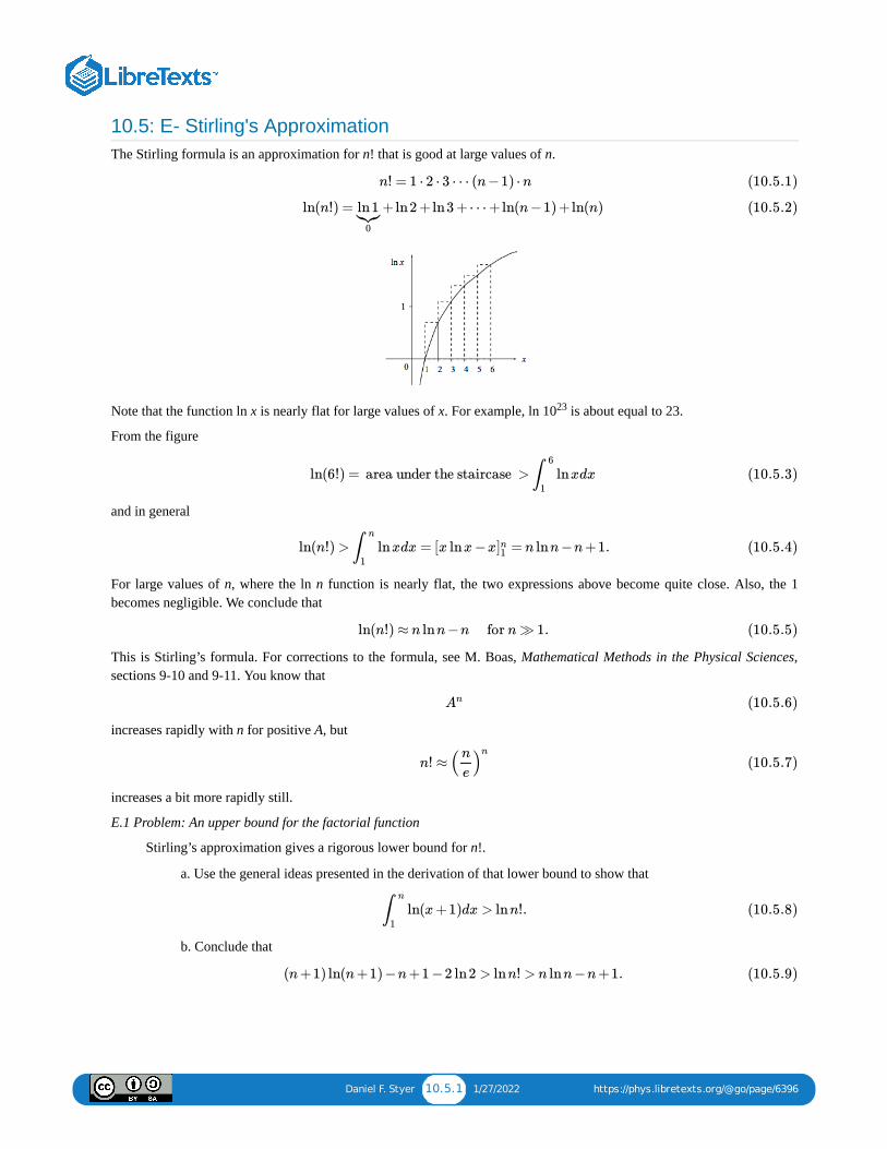
Daniel F. Styer 10.5.1 1/27/2022 https://phys.libretexts.org/@go/page/6396

10.5: E- Stirling's ApproximationThe Stirling formula is an approximation for n! that is good at large values of n.

Note that the function ln x is nearly flat for large values of x. For example, ln 10 is about equal to 23.

From the figure

and in general

For large values of n, where the ln n function is nearly flat, the two expressions above become quite close. Also, the 1becomes negligible. We conclude that

This is Stirling’s formula. For corrections to the formula, see M. Boas, Mathematical Methods in the Physical Sciences,sections 9-10 and 9-11. You know that

increases rapidly with n for positive A, but

increases a bit more rapidly still.

E.1 Problem: An upper bound for the factorial function

Stirling’s approximation gives a rigorous lower bound for n!.

a. Use the general ideas presented in the derivation of that lower bound to show that

b. Conclude that

n! = 1 ⋅ 2 ⋅ 3 ⋯ (n−1) ⋅n (10.5.1)

ln(n!) = +ln2 +ln3 +⋯ +ln(n−1) +ln(n)ln1

0

(10.5.2)

23

ln(6!) = area under the staircase > lnxdx∫6

1

(10.5.3)

ln(n!) > lnxdx = [x lnx−x = n lnn−n+1.∫n

1

]n1 (10.5.4)

ln(n!) ≈ n lnn−n for n ≫ 1. (10.5.5)

An (10.5.6)

n! ≈ ( )n

e

n

(10.5.7)

ln(x+1)dx > lnn!.∫n

1

(10.5.8)

(n+1) ln(n+1) −n+1 −2 ln2 > lnn! > n lnn−n+1. (10.5.9)

Daniel F. Styer 10.6.1 12/16/2021 https://phys.libretexts.org/@go/page/6397

10.6: F- The Euler-MacLaurin Formula and Asymptotic SeriesYou know that a sum can be approximated by an integral. How accurate is that approximation? The Euler-MacLaurinformula gives the corrections.

This series is asymptotic. If the series is truncated at any point, it can give a highly accurate approximation. But the seriesmay be either convergent or divergent, so adding additional terms to the truncated series might give rise to a poorerapproximation. The Stirling approximation is a truncation of an asymptotic series.

References

C.M. Bender and S.A. Orszag, Advanced Mathematical Methods for Scientists and Engineers, (McGraw-Hill, New York,1978).

M. Abramowitz and I. Stegum, Handbook of Mathematical Functions, (National Bureau of Standards, Washington, D.C.,1964).

f(k) ≈ f(x)dx∑n−1k=0 ∫ n

0

− [f(n) −f(0)] + [ (n) − (0)] − [ (n) − (0)] + [ (n) − (0)]− [ (n)12

112

f ′ f ′ 1720

f ′′′ f ′′′ 130240

f (v) f (v) 11209600

f (vii)

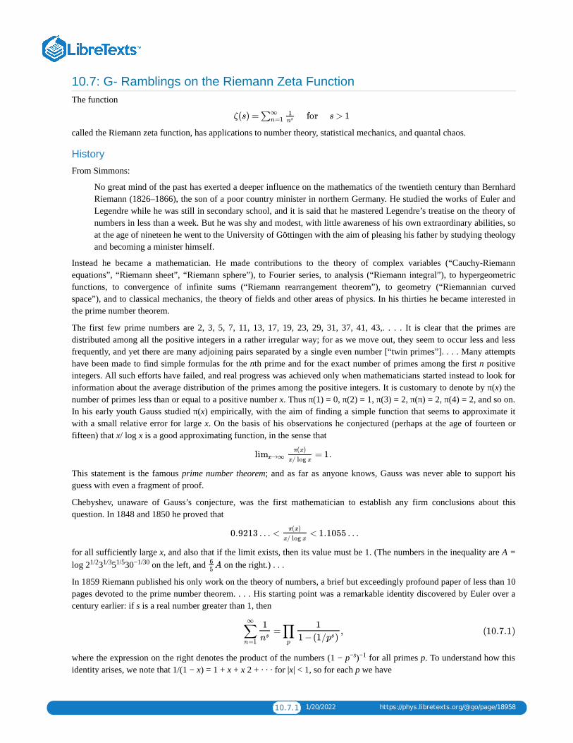
10.7.1 1/20/2022 https://phys.libretexts.org/@go/page/18958

10.7: G- Ramblings on the Riemann Zeta FunctionThe function

called the Riemann zeta function, has applications to number theory, statistical mechanics, and quantal chaos.

History

From Simmons:

No great mind of the past has exerted a deeper influence on the mathematics of the twentieth century than BernhardRiemann (1826–1866), the son of a poor country minister in northern Germany. He studied the works of Euler andLegendre while he was still in secondary school, and it is said that he mastered Legendre’s treatise on the theory ofnumbers in less than a week. But he was shy and modest, with little awareness of his own extraordinary abilities, soat the age of nineteen he went to the University of Göttingen with the aim of pleasing his father by studying theologyand becoming a minister himself.

Instead he became a mathematician. He made contributions to the theory of complex variables (“Cauchy-Riemannequations”, “Riemann sheet”, “Riemann sphere”), to Fourier series, to analysis (“Riemann integral”), to hypergeometricfunctions, to convergence of infinite sums (“Riemann rearrangement theorem”), to geometry (“Riemannian curvedspace”), and to classical mechanics, the theory of fields and other areas of physics. In his thirties he became interested inthe prime number theorem.

The first few prime numbers are 2, 3, 5, 7, 11, 13, 17, 19, 23, 29, 31, 37, 41, 43,. . . . It is clear that the primes aredistributed among all the positive integers in a rather irregular way; for as we move out, they seem to occur less and lessfrequently, and yet there are many adjoining pairs separated by a single even number [“twin primes”]. . . . Many attemptshave been made to find simple formulas for the nth prime and for the exact number of primes among the first n positiveintegers. All such efforts have failed, and real progress was achieved only when mathematicians started instead to look forinformation about the average distribution of the primes among the positive integers. It is customary to denote by π(x) thenumber of primes less than or equal to a positive number x. Thus π(1) = 0, π(2) = 1, π(3) = 2, π(π) = 2, π(4) = 2, and so on.In his early youth Gauss studied π(x) empirically, with the aim of finding a simple function that seems to approximate itwith a small relative error for large x. On the basis of his observations he conjectured (perhaps at the age of fourteen orfifteen) that x/ log x is a good approximating function, in the sense that

This statement is the famous prime number theorem; and as far as anyone knows, Gauss was never able to support hisguess with even a fragment of proof.

Chebyshev, unaware of Gauss’s conjecture, was the first mathematician to establish any firm conclusions about thisquestion. In 1848 and 1850 he proved that

for all sufficiently large x, and also that if the limit exists, then its value must be 1. (The numbers in the inequality are A =log 2 3 5 30 on the left, and on the right.) . . .

In 1859 Riemann published his only work on the theory of numbers, a brief but exceedingly profound paper of less than 10pages devoted to the prime number theorem. . . . His starting point was a remarkable identity discovered by Euler over acentury earlier: if s is a real number greater than 1, then

where the expression on the right denotes the product of the numbers (1 − p ) for all primes p. To understand how thisidentity arises, we note that 1/(1 − x) = 1 + x + x 2 + · · · for |x| < 1, so for each p we have

ζ(s) = for s > 1∑∞n=1

1ns

= 1.limx→∞π(x)

x/ log x

0.9213 … < < 1.1055 …π(x)

x/ log x

1/2 1/3 1/5 −1/30 A65

= ,∑n=1

∞1

ns∏p

1

1 −(1/ )ps(10.7.1)

−s −1

10.7.2 1/20/2022 https://phys.libretexts.org/@go/page/18958

On multiplying these series for all primes p and recalling that each integer n > 1 is uniquely expressible as a product ofpowers of different primes, we see that

which is the desired identity. The sum of this series is evidently a function of the real variable s > 1, and the identityestablishes a connection between the behavior of this function and properties of the primes. Euler himself exploited thisconnection in several ways, but Riemann perceived that access to the deeper features of the distribution of primes can onlybe gained by allowing s to be a complex variable. . . . In his paper he proved several important properties of this function,and in a sovereign way simply stated a number of others without proof. During the century since his death, many of thefinest mathematicians in the world have exerted their strongest efforts and created rich new branches of analysis inattempts to prove these statements. The first success was achieved in 1893 by J. Hadamard, and with one exception everystatement has since been settled in the sense Riemann expected. (Hadamard’s work led him to his 1896 proof of the primenumber theorem.) The one exception is the famous Riemann hypothesis: that all the zeros of ζ(s) in the strip 0 ≤ ≤ 1 lieon the central line . It stands today as the most important unsolved problem in mathematics, and is probably themost difficult problem that the mind of man has ever conceived. In a fragmentary note found among his posthumouspapers, Riemann wrote that these theorems “follow from an expression for the function ζ(s) which I have not yet simplifiedenough to publish”. . . .

At the age of thirty-nine Riemann died of tuberculosis in Italy, on the last of several trips he undertook in order to avoidthe cold, wet climate of northern Germany.

General character of the zeta function

It is easy to see that ζ(s) diverges at s = 1 and that it decreases monotonically to 1 as s increases from 1. As the historicalnote suggests, its behavior for complex values of s is much more elaborate.

= 1 + + +⋯ .11−(1/ )ps

1ps

1p2s

∏p

1

1 −(1/ )ps= (1 + + +⋯)∏

p

1

ps1

p2s

= 1 + + +⋯ + +⋯1

2s1

3s1

ns

=∑n=1

∞ 1

ns

Re

Res = 12

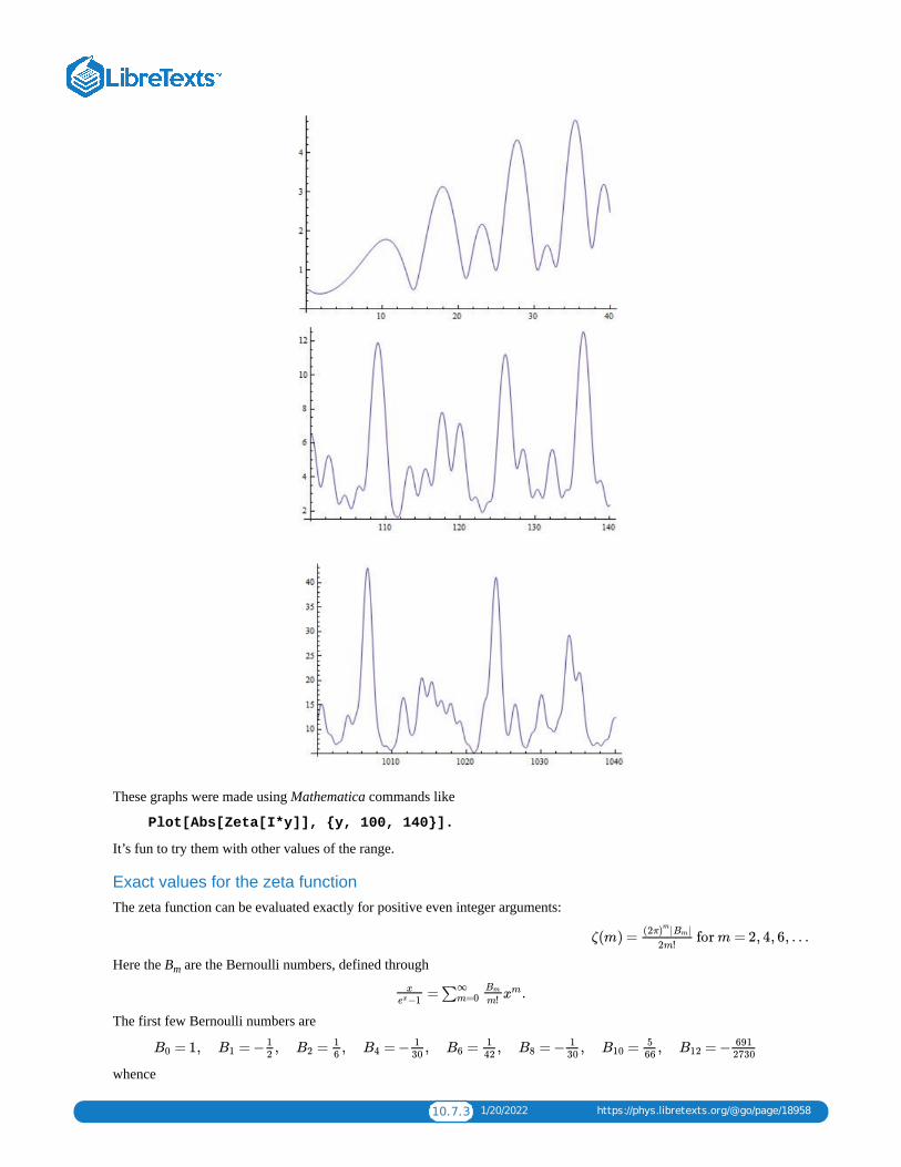
10.7.3 1/20/2022 https://phys.libretexts.org/@go/page/18958

These graphs were made using Mathematica commands like

Plot[Abs[Zeta[I*y]], y, 100, 140].

It’s fun to try them with other values of the range.

Exact values for the zeta functionThe zeta function can be evaluated exactly for positive even integer arguments:

Here the B are the Bernoulli numbers, defined through

The first few Bernoulli numbers are

whence

ζ(m) = for m = 2, 4, 6, …(2π | |)

mBm

2m!

m

= .x

−1ex∑∞

m=0Bm

m!xm

= 1, = − , = , = − , = , = − , = , = −B0 B112

B216

B41

30B6

142

B81

30B10

566

B12691

2730

10.7.4 1/20/2022 https://phys.libretexts.org/@go/page/18958

The zeta function near s = 1

The zeta function diverges with a simple pole at s = 1. In the vicinity of the divergence it is approximately equal to

where C is Euler’s constant, 0.5772. . . . (The rest of this section is stolen from Bender and Orszag.) When s is near 1, thedefining series

is very slowly converging. About 10 terms are needed to compute ζ(1.1) accurate to 1 percent!

Fortunately, there is an expression for the difference between ζ(s) and the Nth partial sum:

The integral cannot be evaluated analytically but it can be expanded in an asymptotic series, giving

where the B are again the Bernoulli numbers.

Truncating this formula can give extremely accurate results. For example, using N = 9, only 38 terms of the series areneeded to find ζ(1.1) accurate to 26 decimal places.

ReferencesG.F. Simmons, Differential Equations with Applications and Historical Notes, (McGraw-Hill, New York, 1972) pp. 210–211, 214–218.

C.M. Bender and S.A. Orszag, Advanced Mathematical Methods for Scientists and Engineers, (McGraw-Hill, New York,1978) p. 379.

Jahnke, Emde, and Lösch, Tables of Higher Functions, 6th ed. (McGraw-Hill, New York, 1960) chap. IV. (Noteparticularly the beautiful relief plot of |ζ(s)| for complex values of s.)

J. Spanier and K. Oldham, An Atlas of Functions, (Hemisphere Publishing, Washington, D.C., 1987) chap. 3. (Presents analgorithm purporting to find ζ(s) accurately for any real s.)

M. Abramowitz and I. Stegum, Handbook of Mathematical Functions, (National Bureau of Standards, Washington, D.C.,1964) chap. 23.

M.C. Gutzwiller, Chaos in Classical and Quantum Mechanics, (Springer-Verlag, New York, 1990) section 17.9.

ζ(2) = , ζ(4) = , ζ(6) = , ζ(8) = .π2

6π4

90π6

945π8

9450

ζ(s) ≈ C + 1s−1

ζ(s) =∑∞n=1

1ns

20

ζ(s) = + du.∑Nn=0

1sn

1Γ(s)

∫ ∞

0us−1e−Nu

−1eu

ζ(s) ≈ + − + + +⋯∑n=0

N 1

sn1

(s−1)N s−1

1

2N s

sB2

N s+1

s(s+1)(s+2)B4

2N s+3(10.7.2)

m

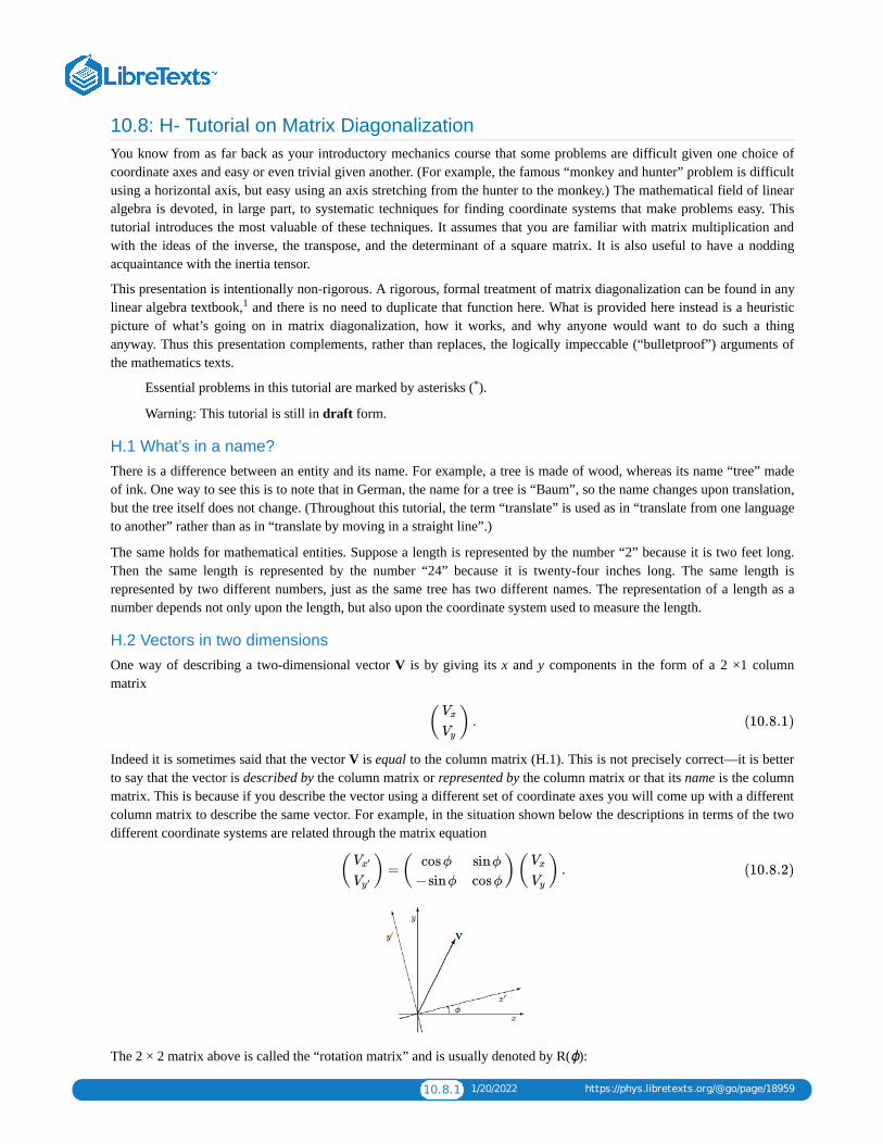
10.8.1 1/20/2022 https://phys.libretexts.org/@go/page/18959

10.8: H- Tutorial on Matrix DiagonalizationYou know from as far back as your introductory mechanics course that some problems are difficult given one choice ofcoordinate axes and easy or even trivial given another. (For example, the famous “monkey and hunter” problem is difficultusing a horizontal axis, but easy using an axis stretching from the hunter to the monkey.) The mathematical field of linearalgebra is devoted, in large part, to systematic techniques for finding coordinate systems that make problems easy. Thistutorial introduces the most valuable of these techniques. It assumes that you are familiar with matrix multiplication andwith the ideas of the inverse, the transpose, and the determinant of a square matrix. It is also useful to have a noddingacquaintance with the inertia tensor.

This presentation is intentionally non-rigorous. A rigorous, formal treatment of matrix diagonalization can be found in anylinear algebra textbook, and there is no need to duplicate that function here. What is provided here instead is a heuristicpicture of what’s going on in matrix diagonalization, how it works, and why anyone would want to do such a thinganyway. Thus this presentation complements, rather than replaces, the logically impeccable (“bulletproof”) arguments ofthe mathematics texts.

Essential problems in this tutorial are marked by asterisks ( ).

Warning: This tutorial is still in draft form.

H.1 What’s in a name?There is a difference between an entity and its name. For example, a tree is made of wood, whereas its name “tree” madeof ink. One way to see this is to note that in German, the name for a tree is “Baum”, so the name changes upon translation,but the tree itself does not change. (Throughout this tutorial, the term “translate” is used as in “translate from one languageto another” rather than as in “translate by moving in a straight line”.)

The same holds for mathematical entities. Suppose a length is represented by the number “2” because it is two feet long.Then the same length is represented by the number “24” because it is twenty-four inches long. The same length isrepresented by two different numbers, just as the same tree has two different names. The representation of a length as anumber depends not only upon the length, but also upon the coordinate system used to measure the length.

H.2 Vectors in two dimensionsOne way of describing a two-dimensional vector V is by giving its x and y components in the form of a 2 ×1 columnmatrix

Indeed it is sometimes said that the vector V is equal to the column matrix (H.1). This is not precisely correct—it is betterto say that the vector is described by the column matrix or represented by the column matrix or that its name is the columnmatrix. This is because if you describe the vector using a different set of coordinate axes you will come up with a differentcolumn matrix to describe the same vector. For example, in the situation shown below the descriptions in terms of the twodifferent coordinate systems are related through the matrix equation

The 2 × 2 matrix above is called the “rotation matrix” and is usually denoted by R(ϕ):

1

*

( ) .Vx

Vy(10.8.1)

( ) =( )( ) .Vx′

Vy ′

cosϕ

−sinϕ

sinϕ

cosϕ

Vx

Vy(10.8.2)

10.8.2 1/20/2022 https://phys.libretexts.org/@go/page/18959

One interesting property of the rotation matrix is that it is always invertible, and that its inverse is equal to its transpose.Such matrices are called orthogonal. You could prove this by working a matrix multiplication, but it is easier to simplyrealize that the inverse of a rotation by ϕ is simply a rotation by −ϕ, and noting that

(The dagger represents matrix transposition.)

There are, of course, an infinite number of column matrix representations for any vector, corresponding to the infinitenumber of coordinate axis rotations with ϕ from 0 to 2π. But one of these representations is special: It is the one in whichthe x'-axis lines up with the vector, so the column matrix representation is just

where is the magnitude of the vector. This set of coordinates is the preferred (or “canonical”) set

for dealing with this vector: one of the two components is zero, the easiest number to deal with, and the other component isa physically important number. You might wonder how I can claim that this representation has full information about thevector: The initial representation (H.1) contains two independent numbers, whereas the preferred representation (H.5)contains only one. The answer is that the preferred representation contains one number (the magnitude of the vector)explicitly while another number (the polar angle of the vector relative to the initial x-axis) is contained implicitly in therotation needed to produce the preferred coordinate system.

H.1 Problem: Right angle rotations

Verify equation (H.2) in the special cases ϕ = 90 , ϕ= 180 , ϕ = 270 , and ϕ = 360 .

H.2 Problem: The rotation matrix

a. Derive equation (H.2) through purely geometrical arguments.

b. Express and , the unit vectors of the (x', y') coordinate system, as linear combinations of and . Then use

to derive equation (H.2).

c. Which derivation do you find easier?

H.3 Problem: Rotation to the preferred coordinate system*

In the preferred coordinate system, V = 0. Use this requirement to show that the preferred system is rotated from theinitial system by an angle ϕ with

For any value of V /V , there are two angles that satisfy this equation. What is the representation of V in each ofthese two coordinate systems?

H.4 Problem: A non-rotation orthogonal transformation

In one coordinate system the y-axis is vertical and the x-axis points to the right. In another the y'-axis is vertical andthe x'-axis points to the left. Find the matrix that translates vector coordinates from one system to the other. Showthat this matrix is orthogonal but not a rotation matrix.

H.5 Problem: Other changes of coordinate*

Suppose vertical distances (distances in the y direction) are measured in feet while horizontal distances (distances inthe x direction) are measured in miles. (This system is not perverse. It is used in nearly all American road maps.)

R(ϕ) ≡( )cosϕ

−sinϕ

sinϕ

cosϕ(10.8.3)

1

(ϕ) = R(−ϕ) = (ϕ).R−1 R† (10.8.4)

( ) ,V

0(10.8.5)

V = |V| = +V 2x V 2

y

− −−−−−−√

o o o o

i′

j′

i′

j′

= V ⋅ and = V ⋅Vx′ i′

Vy ′ j′

(10.8.6)

y'

tanϕ = .Vy

Vx(10.8.7)

y x

10.8.3 1/20/2022 https://phys.libretexts.org/@go/page/18959

Find the matrix that changes the representation of a vector in this coordinate system to the representation of a vectorin a system where all distances are measured in feet. Find the matrix that translates back. Are these matricesorthogonal?

H.6 Problem: Other special representations

At equation (H.5) we mentioned one “special” (or “canonical”) representation of a vector. There are three others,namely

If coordinate-system rotation angle ϕ brings the vector representation into the form (H.5), then what rotation anglewill result in these three representations?

H.3 Tensors in two dimensionsA tensor, like a vector, is a geometrical entity that may be described (“named”) through components, but a d-dimensionaltensor requires d rather than d components. Tensors are less familiar and more difficult to visualize than vectors, but theyare neither less important nor “less physical”. We will introduce tensors through the concrete example of the inertia tensorof classical mechanics (see, for example, reference [2]), but the results we present will be perfectly general.

Just as the two components of a two-dimensional vector are most easily kept track of through a 2 × 1 matrix, so the fourcomponents of two-dimensional tensor are most conveniently written in the form of a 2×2 matrix. For example, the inertiatensor T of a point particle with mass m located at (x, y) has components

(Note the distinction between the tensor T and its matrix of components, its “name”, T.) As with vector components, thetensor components are different in different coordinate systems, although the tensor itself does not change. For example, inthe primed coordinate system of the figure on page 231, the tensor components are of course

A little calculation shows that the components of the inertia tensor in two different coordinate systems are related through

This relation holds for any tensor, not just the inertia tensor. (In fact, one way to define “tensor” is as an entity with fourcomponents that satisfy the above relation under rotation.) If the matrix representing a tensor is symmetric (i.e. the matrixis equal to its transpose) in one coordinate system, then it is symmetric in all coordinate systems (see problem H.7).Therefore the symmetry is a property of the tensor, not of its matrix representation, and we may speak of “a symmetrictensor” rather than just “a tensor represented by a symmetric matrix”.

As with vectors, one of the many matrix representations of a given tensor is considered special (or “canonical”): It is theone in which the lower left component is zero. Furthermore if the tensor is symmetric (as the inertia tensor is) then in thispreferred coordinate system the upper right component will be zero also, so the matrix will be all zeros except for thediagonal elements. Such a matrix is called a “diagonal matrix” and the process of finding the rotation that renders thematrix representation of a symmetric tensor diagonal is called “diagonalization”. We may do an “accounting ofinformation” for this preferred coordinate system just as we did with vectors. In the initial coordinate system, thesymmetric tensor had three independent components. In the preferred system, it has two independent componentsmanifestly visible in the diagonal matrix representation, and one number hidden through the specification of the rotation.

H.7 Problem: Representations of symmetric tensors*

Show that if the matrix S representing a tensor is symmetric, and if B is any orthogonal matrix, then all of therepresentations

are symmetric. (Clue: If you try to solve this problem for rotations in two dimensions using the explicit rotationmatrix (H.3), you will find it solvable but messy. The clue is that this problem asks you do prove the result in any

( ) , ( ) , ( ) .0

−V

−V

0

0

V(10.8.8)

2

2

=( ) .T′ my′2

−mx′y′

−mx′y′

mx′2(10.8.9)

= R(ϕ)T (ϕ).T′ R−1 (10.8.10)

3

BSB† (10.8.11)

10.8.4 1/20/2022 https://phys.libretexts.org/@go/page/18959

number of dimensions, and for any orthogonal matrix B, not just rotation matrices. This more general problem isconsiderably easier to solve.)

H.8 Problem: Diagonal inertia tensor

The matrix (H.9) represents the inertia tensor of a point particle with mass m located a distance r from the origin.Show that the matrix is diagonal in four different coordinate systems: one in which the x'-axis points directly towardthe particle, one in which the y'-axis points directly away from the particle, one in which the x'-axis points directlyaway from the particle, and one in which the y'-axis points directly toward the particle. Find the matrixrepresentation in each of these four coordinate systems.

H.9 Problem: Representations of a certain tensor

Show that a tensor represented in one coordinate system by a diagonal matrix with equal elements, namely

has the same representation in all orthogonal coordinate systems.

H.10 Problem: Rotation to the preferred coordinate system*

A tensor is represented in the initial coordinate system by

Show that the tensor is diagonal in a preferred coordinate system which is rotated from the initial system by an angleϕ with

This equation has four solutions. Find the rotation matrix for ϕ = 90 , then show how the four different diagonalrepresentations are related. You do not need to find any of the diagonal representations in terms of a, b and c. . . justshow what the other three are given that one of them is

H.11 Problem: Inertia tensor in outer product notation

The discussion in this section has emphasized the tensor’s matrix representation (“name”) T rather than the tensor Titself.

a. Define the “identity tensor” 1 as the tensor represented in some coordinate system by

Show that this tensor has the same representation in any coordinate system.

b. Show that the inner product between two vectors results in a scalar: Namely

if vector bfa is represented by and vector bfb is represented by

then the inner product a·b is given through

and this inner product is a scalar. (A 1×2 matrix times a 2×1 matrix is a 1×1 matrix.) That is, the vector a isrepresented by different coordinates in different coordinate systems, and the vector b is represented by differentcoordinates in different coordinate systems, but the inner product a·b is the same in all coordinate systems.

( ) ,d0

0

0

d0(10.8.12)

( ) .a

b

b

c(10.8.13)

tan(2ϕ) = .2b

a−c(10.8.14)

o

( ) .d1

0

0

d2(10.8.15)

1 =( ) .1

0

0

1(10.8.16)

( )ax

ay( )bx

by

( )( ) = +ax aybx

byaxbx ayby

10.8.5 1/20/2022 https://phys.libretexts.org/@go/page/18959

c. In contrast, show that the outer product of two vectors is a tensor: Namely

(A 2 × 1 matrix times a 1 × 2 matrix is a 2 × 2 matrix.) That is, show that the representation of ab transforms fromone coordinate system to another as specified through (H.11).

d. Show that the inertia tensor for a single particle of mass m located at position r can be written in coordinate-independent fashion as

H.4 Tensors in three dimensionsA three-dimensional tensor is represented in component form by a 3 × 3 matrix with nine entries. If the tensor issymmetric, there are six independent elements. . . three on the diagonal and three off-diagonal. The components of a tensorin three dimensions change with coordinate system according to

where R is the 3 × 3 rotation matrix.

A rotation in two dimension is described completely by giving a single angle. In three dimensions more information isrequired. Specifically, we need not only the amount of the rotation, but we must also know the plane in which the rotationtakes place. We can specify the plane by giving the unit vector perpendicular to that plane. Specifying an arbitrary vectorin three dimensions requires three numbers, but specifying a unit vector in three dimensions requires only two numbersbecause the magnitude is already fixed at unity. Thus three numbers are required to specify a rotation in three dimensions:two to specify the rotation’s plane, one to specify the rotation’s size. (One particularly convenient way to specify a three-dimensional rotation is through the three Euler angles. Reference [3] defines these angles and shows how to write the 3 × 3rotation matrix in terms of these variables. For the purposes of this tutorial, however, we will not need an explicit rotationmatrix. . . all we need is to know is the number of angles required to specify a rotation.)

In two dimensions, any symmetric tensor (which has three independent elements), could be represented by a diagonaltensor (with two independent elements) plus a rotation (one angle). We were able to back up this claim with an explicitexpression for the angle.

In three dimensions it seems reasonable that any symmetric tensor (six independent elements) can be represented by adiagonal tensor (three independent elements) plus a rotation (three angles). The three angles just have to be selectedcarefully enough to make sure that they cause the off-diagonal elements to vanish. This supposition is indeed correct,although we will not pause for long enough to prove it by producing explicit formulas for the three angles.

H.5 Tensors in d dimensionsA d-dimensional tensor is represented by a d×d matrix with d entries. If the tensor is symmetric, there are d independenton-diagonal elements and d(d−1)/2 independent off-diagonal elements. The tensor components will change withcoordinate system in the now-familiar form

where R is the d × d rotation matrix.

How many angles does it take to specify a rotation in d dimensions? Remember how we went from two dimensions tothree: The three dimensional rotation took place “in a plane”, i.e. in a two-dimensional subspace. It required two (i.e. d −1) angles to specify the orientation of the plane plus one to specify the rotation within the plane. . . a total of three angles.

A rotation in four dimensions takes place within a three-dimensional subspace. It requires 3 = d − 1 angles to specify theorientation of the three-dimensional subspace, plus, as we found above, three angles to specify the rotation within thethree-dimensional subspace. . . a total of six angles.

ab ≐( ) ( ) =( )ax

aybx by

axbx

aybx

axby

ayby

T = m1 −mrr.r2 (10.8.17)

= ,T′ RTR† (10.8.18)

2

= ,T′ RTR† (10.8.19)

10.8.6 1/20/2022 https://phys.libretexts.org/@go/page/18959

A rotation in five dimensions requires 4 = d − 1 angles to specify the four-dimensional subspace in which the rotationoccurs, plus the six angles that we have just found specify a rotation within that subspace. . . a total of ten angles.

In general, the number of angles needed to specify a rotation in d dimensions is

This is exactly the number of independent off-diagonal elements in a symmetric tensor. It seems reasonable that we canchoose the angles to ensure that, in the resulting coordinate system, all the off-diagonal elements vanish. The proof of thisresult is difficult and proceeds in a very different manner from the plausibility argument sketched here. (The proof involvesconcepts like eigenvectors and eigenvalues, and it gives an explicit recipe for constructing the rotation matrix. It has theadvantage of rigor and the disadvantage of being so technical that it’s easy to lose track of the fact that that all you’re doingis choosing a coordinate system.)

H.12 Problem: Non-symmetric tensors*

Argue that a non-symmetric tensor can be brought into a “triangular” representation in which all the elements belowthe diagonal are equal to zero and all the elements on and above the diagonal are independent. (This is indeed thecase, although in general some of the non-zero elements remaining will be complex-valued, and some of the angleswill involve rotations into complex-valued vectors.)

H.6 Linear transformations in two dimensionsSection H.3 considered 2 × 2 matrices as representations of tensors. This section gains additional insight by considering 2× 2 matrices as representations of linear transformations. It demonstrates how diagonalization can be useful and gives aclue to an efficient algorithm for diagonalization.

A linear transformation is a function from vectors to vectors that can be represented in any given coordinate system as

If the equation above represents (“names”) the transformation in one coordinate system, what is its representation in someother coordinate system? We assume that the two coordinate systems are related through an orthogonal matrix B such that

(For example, if the new coordinate system is the primed coordinate system of the figure on page 231, then the matrix Bthat translates from the original to the new coordinates is the rotation matrix R(ϕ).) Given this “translation dictionary”, wehave

But B is invertible, so

whence

Thus the representation of the transformation in the primed coordinate system is

(compare equation H.11). This equation has a very direct physical meaning. Remember that the matrix B translates fromthe old (x, y) coordinates to the new (x', y') coordinates, while the matrix B translates in the opposite direction. Thus the

= d−1 + = d(d−1)/2.Ad Ad−1 (10.8.20)

( ) =( )( ) .u

v

a11

a21

a12

a22

x

y(10.8.21)

( ) = B( ) and ( ) = B( ) .u′

v′

u

v

x′

y′

x

y(10.8.22)

( ) = B( )( ) .u′

v′

a11

a21

a12

a22

x

y(10.8.23)

( ) = ( )x

yB−1 x′

y′(10.8.24)

( ) = B( ) ( ) .u′

v′

a11

a21

a12

a22B−1 x′

y′(10.8.25)

B( )a11

a21

a12

a22B−1 (10.8.26)

−1

10.8.7 1/20/2022 https://phys.libretexts.org/@go/page/18959

equation above says that the representation of a transformation in the new coordinates is given by translating from new toold coordinates (through the matrix B ), then applying the old representation (the “a matrix”) to those old coordinates,and finally translating back from old to new coordinates (through the matrix B).

The rest of this section considers only transformations represented by symmetric matrices, which we will denote by

Let’s try to understand this transformation as something more than a jumble of symbols awaiting a plunge into thecalculator. First of all, suppose the vector V maps to the vector W. Then the vector 5V will be mapped to vector 5W. Inshort, if we know how the transformation acts on vectors with magnitude unity, we will be able to see immediately how itacts on vectors with other magnitudes. Thus we focus our attention on vectors on the unit circle:

A brief calculation shows that the length of the output vector is then

which isn’t very helpful. Another brief calculation shows that if the input vector has polar angle θ, then the output vectorhas polar angle φ with

which is similarly opaque and messy.

Instead of trying to understand the transformation in its initial coordinate system, let’s instead convert (rotate) to thespecial coordinate system in which the transformation is represented by a diagonal matrix. In this system,

The unit circle is still

so the image of the unit circle is

namely an ellipse! This result is transparent in the special coordinate system, but almost impossible to see in the originalone.

Note particularly what happens to a vector pointing along the x' coordinate axis. For example, the unit vector in thisdirection transforms to

In other words, the when the vector is transformed it changes in magnitude, but not in direction. Vectors with this propertyare called eigenvectors. It is easy to see that any vector on either the x' or y' coordinate axes are eigenvectors.

H.7 What does “eigen” mean?

If a vector x is acted upon by a linear transformation B, then the output vector

will usually be skew to the original vector x. However, for some very special vectors it might just happen that x 0 isparallel to x. Such vectors are called “eigenvectors”. (This is a terrible name because (1) it gives no idea of what

−1

( ) =( )( ) .u

v

a

b

b

c

x

y(10.8.27)

+ = 1.x2 y2 (10.8.28)

= ,+u2 v2− −−−−−√ + + +2b(a+c)xya2x2 b2 c2y2

− −−−−−−−−−−−−−−−−−−−−−−−√ (10.8.29)

tanφ = ,b+c tanθ

a+b tanθ(10.8.30)

( ) =( )( ) =( ) .u′

v′

d1

0

0

d2

x′

y′

d1x′

d2y′(10.8.31)

+ = 1,x′2 y′2 (10.8.32)

+ = 1,( )u′

d1

2

( )v′

d2

2

(10.8.33)

( ) =( )( ) .d1

0

d1

0

0

d2

1

0(10.8.34)

= Bxx′ (10.8.35)

10.8.8 1/20/2022 https://phys.libretexts.org/@go/page/18959

eigenvectors are or why they’re so important and (2) it sounds gross. However, that’s what they’re called.) We havealready seen, in the previous section, that eigenvectors are related to coordinate systems in which the transformation isparticularly easy to understand. If x is an eigenvector, then

where λ is a scalar called “the eigenvalue associated with eigenvector x”. If x is an eigenvector, then any vector parallel tox is also an eigenvector with the same eigenvalue. (That is, any vector of the form cx, where c is any scalar, is also aneigenvector with the same eigenvalue.) Sometimes we speak of a “line of eigenvectors”.

The vector x = 0 is never considered an eigenvector, because

for any value of λ for any linear transformation. On the other hand, if

for some non-zero vector x, then x is an eigenvector with eigenvalue λ = 0.

H.13 Problem: Plane of eigenvectors

Suppose x and y are two non-parallel vectors with the same eigenvalue. (In this case the eigenvalue is said to be“degenerate”, which sounds like an aspersion cast upon the morals of the eigenvalue but which is really just poorchoice of terminology again.) Show that any vector of the form c x + c y is an eigenvector with the sameeigenvalue.

H.8 How to diagonalize a symmetric matrixWe saw in section H.3 that for any 2 × 2 symmetric matrix, represented in its initial basis by, say,

a simple rotation of axes would produce a new coordinate system in which the matrix representation is diagonal:

These two matrices are related through

where R(ϕ) is the rotation matrix (H.3). Problem H.10 gave a direct way to find the desired rotation. However this directtechnique is cumbersome and doesn’t generalize readily to higher dimensions. This section presents a different technique,which relies on eigenvalues and eigenvectors, that is more efficient and that generalizes readily to complex-valuedmatrices and to matrices in any dimension, but that is somewhat sneaky and conceptually roundabout.

We begin by noting that any vector lying along the x'-axis (of the preferred coordinate system) is an eigenvector. For

example, the vector is represented (in the preferred coordinate system) by

Multiplying this vector by the matrix in question gives

so is an eigenvector with eigenvalue d . The same holds for any scalar multiple of , whether positive or negative.Similarly, any scalar multiple of is an eigenvector with eigenvalue d . In short, the two elements on the diagonal in thepreferred (diagonal) representation are the two eigenvalues, and the two unit vectors and of the preferred coordinate

Bx = λx, (10.8.36)

B0 = λ0, (10.8.37)

Bx = 0x = 0 (10.8.38)

1 2

( ) ,a

b

b

c(10.8.39)

( ) .d1

0

0

d2(10.8.40)

( ) = R(ϕ)( ) (ϕ),d1

0

0

d2

a

b

b

cR−1 (10.8.41)

5 i′

( ) .5

0(10.8.42)

( )( ) = ( ) ,d1

0

0

d2

5

0d1

5

0(10.8.43)

5 i′

1 i′

j′

2

i′

j′

10.8.9 1/20/2022 https://phys.libretexts.org/@go/page/18959

system are two of the eigenvectors. Thus finding the eigenvectors and eigenvalues of a matrix gives you the informationneeded to diagonalize that matrix. The unit vectors and constitute an “orthonormal basis of eigenvectors”. Theeigenvectors even give the rotation matrix directly, as described in the next paragraph.

Let’s call the rotation matrix

so that the inverse (transpose) matrix is

The representation of in the preferred basis is

so its representation in the initial basis is (see equation H.2)

Similarly, the representation of in the initial basis is

Thus the rotation matrix is

Example

Suppose we need to find a diagonal representation for the matrix

First we search for the special vectors—the eigenvectors—such that

At the moment, we don’t know either the eigenvalue λ or the associated eigenvector (x, y). Thus it seems that (bad news)we are trying to solve two equations for three unknowns:

Remember, however, that there is not one single eigenvector: any multiple of an eigenvector is also an eigenvector.(Alternatively, any vector on the line that extends the eigenvector is another eigenvector.) We only need one of theseeigenvectors, so let’s take the one that has x = 1 (i.e. the vector on the extension line where it intersects the vertical line x =1). (This technique will fail if we have the bad luck that our actual eigenvector is vertical and hence never passes throughthe line x = 1.) So we really have two equations in two unknowns:

i′

j′

B =( )b11

b21

b12

b22(10.8.44)

= =( ) .B−1 B† b11

b12

b21

b22(10.8.45)

i′

( ) ,1

0(10.8.46)

( ) =( )( ) =( ) .B† 1

0

b11

b12

b21

b22

1

0

b11

b12(10.8.47)

j′

( ) =( )( ) =( ) .B† 0

1

b11

b12

b21

b22

0

1

b21

b22(10.8.48)

B =( ) . initial rep. of , on its side i

′

initial rep. of , on its side j′ (10.8.49)

T =( ) .7

3

3

7(10.8.50)

( )( ) = λ( ) .7

3

3

7

x

y

x

y(10.8.51)

7x+3y = λx

3x+7y = λy(10.8.52)

7 +3y = λ

3 +7y = λy

10.8.10 1/20/2022 https://phys.libretexts.org/@go/page/18959

but note that they are not linear equations. . . the damnable product λy in the lower right corner means that all ourtechniques for solving linear equations go right out the window. We can solve these two equations for λ and y, but there’san easier, if somewhat roundabout, approach.

Finding eigenvalues

Let’s go back to equation (H.52) and write it as

Then

or

Let’s think about this. It says that for some matrix M = T − λ1, we have

You know right away one vector (x, y) that satisfies this equation, namely (x, y) = (0, 0). And most of the time, this is theonly vector that satisfies the equation, because

We appear to have reached a dead end. The solution is (x, y) = (0, 0), but the zero vector is not, by definition, considered aneigenvector of any transformation. (Because it always gives eigenvalue zero for any transformation.)

However, if the matrix M is not invertible, then there will be other solutions to

in addition to the trivial solution (x, y) = (0, 0). Thus we must look for those special values of λ such that the so-calledcharacteristic matrix M is not invertible. These values come if and only if the determinant of M vanishes. For thisexample, we have to find values of λ such that

This is a quadratic equation in λ

called the characteristic equation. Its two solutions are

or

We have found the two eigenvalues of our matrix!

Finding eigenvectors

Let’s look now for the eigenvector associated with λ = 4. Equation (H.53)

( )( )−λ( ) =( ) .7

3

3

7

x

y

x

y

0

0(10.8.53)

( )( )−λ( )( ) =( )7

3

3

7

x

y

1

0

0

1

x

y

0

0(10.8.54)

( )( ) =( ) .7 −λ

3

3

7 −λ

x

y

0

0(10.8.55)

M ( ) =( ) .x

y

0

0(10.8.56)

( ) = ( ) =( ) .x

yM−1 0

0

0

0(10.8.57)

M ( ) =( ) .x

y

0

0(10.8.58)

det( ) = 0.7 −λ

3

3

7 −λ(10.8.59)

(7 −λ − = 0)2 32 (10.8.60)

7 −λ = ±3 (10.8.61)

λ = 7 ±3 = 10 or 4 (10.8.62)

10.8.11 1/20/2022 https://phys.libretexts.org/@go/page/18959

still holds, but no longer does it look like two equations in three unknowns, because we are now interested in the case λ =4:

Following our nose gives

and when we see this our heart skips a beat or two. . . a degenerate system of equations! Relax and rest your heart. Thissystem has an infinite number of solutions and it’s supposed to have an infinite number of solutions, because any multipleof an eigenvector is also an eigenvector. The eigenvectors associated with λ = 4 are any multiple of

An entirely analogous search for the eigenvectors associated with λ = 10 finds any multiple of

Tidying up

We have the two sets of eigenvectors, but which shall we call and which ? This is a matter of individual choice, butmy choice is usually to make the transformation be a rotation (without reflection) through a small positive angle. Our new,preferred coordinate system is related to the original coordinates by a simple rotation of 45 if we choose

(Note that we have also “normalized the basis”, i.e. selected the basis vectors to have magnitude unity.) Given this choice,the orthogonal rotation matrix that changes coordinates from the original to the preferred system is (see equation H.50)

and the diagonalized matrix (or, more properly, the representation of the matrix in the preferred coordinate system) is

You don’t believe me? Then multiply out

and see for yourself.

Problems

H.14 Problem: Diagonalize a 2 × 2 matrix

Diagonalize the matrix

a. Find its eigenvalues.

b. Find its eigenvectors, and verify that they are orthogonal.

7x+3y = λx

3x+7y = λy

7x+3y = 4x

3x+7y = 4y

3x+3y = 0

3x+3y = 0

( ) .1

−1(10.8.63)

( ) .1

1(10.8.64)

i′

i′

o

= ( ) and = ( ) .i′ 1

2–

√

1

1j

′ 1

2–

√

−1

1(10.8.65)

B = ( )1

2–

√

1

−1

1

1(10.8.66)

( ) .10

0

0

4(10.8.67)

B( )7

3

3

7B† (10.8.68)

∗

( ) .26

12

12

19(10.8.69)

10.8.12 1/20/2022 https://phys.libretexts.org/@go/page/18959

c. Sketch the eigenvectors, and determine the signs and sequence most convenient for assigning axes. (That is,

should the first eigenvector you found be called , , or ?)

d. Find the matrix that translates from the initial basis to the basis of eigenvectors produced in part (c.).

e. Verify that the matrix produced in part (d.) is orthogonal.

f. Verify that the representation of the matrix above in the basis of eigenvectors is diagonal.

g. (Optional.) What is the rotation angle?

H.15 Problem: Eigenvalues of a 2 × 2 matrix

Show that the eigenvalues of

are

Under what circumstances is an eigenvalue complex valued? Under what circumstances are the two eigenvalues thesame?

H.16 Problem: Diagonalize a 3 × 3 matrix

Diagonalize the matrix

a. Find its eigenvalues by showing that the characteristic equation is

b. Find its eigenvectors, and verify that they are orthogonal.

c. Show that the translation matrix can be chosen to be

Why did I use the phrase “the translation matrix can be chosen to be” rather then “the translation matrix is”?

H.17 Problem: A 3 × 3 matrix eigenproblem

Find the eigenvalues and associated eigenvectors for the matrix

H.9 A glance at computer algorithms

Anyone who has worked even one of the problems in section H.8 knows that diagonalizing a matrix is no picnic: there’s alot of mundane arithmetic involved and it’s very easy to make mistakes. This is a problem ripe for computer solution.One’s first thought is to program a computer to solve the problem using the same technique that we used to solve it onpaper: first find the eigenvalues through the characteristic equation, then find the eigenvectors through a degenerate set oflinear equations.

i′

− i′

j′

( )a

b

b

c(10.8.70)

λ = [(a+c) ± ]1

2(a−c +4)2 b2− −−−−−−−−−−

√ (10.8.71)

1

625

⎛

⎝⎜

1182

−924

540

−924

643

720

540

720

−575

⎞

⎠⎟ (10.8.72)

−2 −5λ+6 = (λ−3)(λ+2)(λ−1) = 0λ3 λ2 (10.8.73)

B =1

25

⎛

⎝⎜

20

9

12

−15

12

16

0

−20

15

⎞

⎠⎟ (10.8.74)

.⎛

⎝⎜

1

2

3

2

3

4

3

4

5

⎞

⎠⎟ (10.8.75)

10.8.13 1/20/2022 https://phys.libretexts.org/@go/page/18959

This turns out to be a very poor algorithm for automatic computation. The effective algorithm is to choose a matrix B suchthat the off-diagonal elements of

are smaller than the off-diagonal elements of A. Then choose another, and another. Go through this process again andagain until the off-diagonal elements have been ground down to machine zero. There are many strategies for choosing theseries of B matrices. These are well-described in any edition of Numerical Recipes.

When you need to diagonalize matrices numerically, I urge you to look at Numerical Recipes to see what’s going on, but Iurge you not to code these algorithms yourself. These algorithms rely in an essential way on the fact that computerarithmetic is approximate rather than exact, and hence they are quite tricky to implement. Instead of coding the algorithmsyourself, I recommend that you use the implementations in either LAPACK (the Linear Algebra PACKage) or EISPACK.These packages are probably the finest computer software ever written, and they are free. They can be obtained throughthe “Guide to Available Mathematical Software” (GAMS) at http://gams.nist.gov.

H.10 A glance at non-symmetric matrices and the Jordan form

Many of the matrices that arise in applications are symmetric and hence the results of the previous sections are the onlyones needed. But every once in a while you do encounter a non-symmetric matrix and this section gives you a guide totreating them. It is just an introduction and treats only 2 × 2 matrices.

Given a non-symmetric matrix, the first thing to do is rotate the axes to make the matrix representation triangular, asdiscussed in problem H.12:

Note that b 0 because otherwise the matrix would be symmetric and we would already be done. In this case vectors onthe x-axis are eigenvectors because

Are there any other eigenvectors? The equation

tells us that

whence and the eigenvector has polar angle θ where

Note that if c = a (the “degenerate” case: both eigenvalues are the same) then θ = 0 or θ = π. In this case all of theeigenvectors are on the x-axis.

Diagonal form

We already know that that a rotation of orthogonal (Cartesian) coordinates will not diagonalize this matrix. We mustinstead transform to a skew coordinate system in which the axes are not perpendicular.

BAB−1 (10.8.76)

4

5 6

( ) .a

0

b

c(10.8.77)

≠

( )( ) = a( ) .a

0

b

c

1

0

1

0(10.8.78)

( )( ) = a( )a

0

b

c

1

0

1

0(10.8.79)

ax+by

cy

= λx

= λy

\lamba ≠ c

tanθ = .c−a

b(10.8.80)

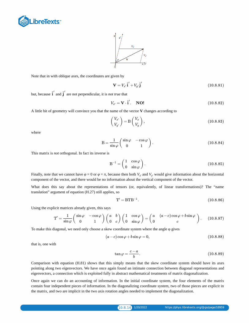
10.8.14 1/20/2022 https://phys.libretexts.org/@go/page/18959

Note that in with oblique axes, the coordinates are given by

but, because and are not perpendicular, it is not true that

A little bit of geometry will convince you that the name of the vector V changes according to

where

This matrix is not orthogonal. In fact its inverse is

Finally, note that we cannot have φ = 0 or φ = π, because then both V and V would give information about the horizontalcomponent of the vector, and there would be no information about the vertical component of the vector.

What does this say about the representations of tensors (or, equivalently, of linear transformations)? The “nametranslation” argument of equation (H.27) still applies, so

Using the explicit matrices already given, this says

To make this diagonal, we need only choose a skew coordinate system where the angle φ gives

that is, one with

Comparison with equation (H.81) shows that this simply means that the skew coordinate system should have its axespointing along two eigenvectors. We have once again found an intimate connection between diagonal representations andeigenvectors, a connection which is exploited fully in abstract mathematical treatments of matrix diagonalization.

Once again we can do an accounting of information. In the initial coordinate system, the four elements of the matrixcontain four independent pieces of information. In the diagonalizing coordinate system, two of those pieces are explicit inthe matrix, and two are implicit in the two axis rotation angles needed to implement the diagonalization.

V = +Vx′ i′

Vy ′ j′

(10.8.81)

i′

j′

= V ⋅ . NO!Vx′ i′

(10.8.82)

( ) = B( ) ,Vx′

Vy ′

Vx

Vy(10.8.83)

B = ( ) .1

sinφ

sinφ

0

−cosφ

1(10.8.84)

=( ) .B−1 1

0

cosφ

sinφ(10.8.85)

x' y'

= .T′ BTB−1 (10.8.86)

= ( )( )( ) =( ) .T′ 1

sinφ

sinφ

0

−cosφ

1

a

0

b

c

1

0

cosφ

sinφ

a

0

(a−c) cosφ+b sinφ

c(10.8.87)

(a−c) cosφ+b sinφ = 0, (10.8.88)

tanφ = .c−a

b(10.8.89)

10.8.15 1/20/2022 https://phys.libretexts.org/@go/page/18959

This procedure works almost all the time. But, if a = c, then it would involve φ = 0 or φ = π, and we have already seen thatthis is not an acceptable change of coordinates.

Degenerate case

Suppose our matrix has equal eigenvalues, a = c, so that it reads

If b = 0, then the matrix is already diagonal. (Indeed, in this case all vectors are eigenvectors with eigenvalue a, and thelinear transformation is simply multiplication of each vector by a).

But if , then, as we have seen, the only eigenvectors are on the x-axis, and it is impossible to make a basis ofeigenvectors. Only one thing can be done to make the matrix representation simpler than it stands in equation (H.91), andthat is a shift in the scale used to measure the y-axis.

For example, suppose that in the (x, y) coordinate system, the y-axis is calibrated in inches. We wish to switch to the (x', y')system in which the y'-axis is calibrated in feet. There is no change in axis orientation or in the x-axis. It is easy to see thatthe two sets of coordinates are related through

This process is sometimes called a “stretching” or a “scaling” of the y-axis.

The transformation represented by matrix (H.91) in the initial coordinate system is represented in the new coordinatesystem by

The choice of what to do now is clear. Instead of scaling the y-axis by a factor of 12, we can scale it by a factor of 1/b, andproduce a new matrix representation of the form

Where is the information in this case? In the initial coordinate system, the four elements of the matrix contain fourindependent pieces of information. In the new coordinate system, two of those pieces are explicit in the matrix, one isimplicit in the rotation angle needed to implement the initial triangularization, and one is implicit in the y-axis scaletransformation.

The Jordan form

Remarkably, the situation discussed above for 2 × 2 matrices covers all the possible cases for n × n matrices. That is, in ndimensional space, the proper combination of rotations, skews, and stretches of coordinate axes will bring the matrixrepresentation (the “name”) of any tensor or linear transformation into a form where every element is zero except on thediagonal and on the superdiagonal. The elements on the diagonal are eigenvalues, and each element on the superdiagonalis either zero or one: zero if the two adjacent eigenvalues differ, either zero or one if they are the same. The warning ofproblem H.12 applies here as well: The eigenvalues on the diagonal may well be complex valued, and the same applies forthe elements of the new basis vectors.

References

For example, Kenneth Hoffman and Ray Kunze, Linear Algebra, second edition (Prentice-Hall, Englewood Cliffs, NewJersey, 1971).

For example, Jerry Marion and Stephen Thorton, Classical Dynamics of Particles and Systems, fourth edition (SaundersCollege Publishing, Fort Worth, Texas, 1995) section 11.2.

( ) .a

0

b

a(10.8.90)

b ≠ 0

( ) =( )( ) and ( ) =( )( )x′

y′

1

0

0

1/12

x

y

x

y

1

0

0

12

x′

y′(10.8.91)

( )( )( ) =( ) .1

0

0

1/12

a

0

b

a

1

0

0

12

a

0

12b

a(10.8.92)

( ) .a

0

1

a(10.8.93)

1

2

10.8.16 1/20/2022 https://phys.libretexts.org/@go/page/18959

For example, Jerry Marion and Stephen Thorton, Classical Dynamics of Particles and Systems, fourth edition (SaundersCollege Publishing, Fort Worth, Texas, 1995) section 11.7.

W.H. Press, S.A. Teukolsky, W.T. Vetterling, B.P. Flannery, Numerical Recipes (Cambridge University Press, Cambridge,U.K., 1992).

E. Anderson, et al., LAPACK Users’ Guide (SIAM, Philadelphia, 1992).

B.T. Smith, et al., Matrix Eigensystem Routines—EISPACK Guide (Springer-Verlag, Berlin, 1976).

Although all rotation matrices are orthogonal, there are orthogonal matrices that are not rotation matrices: see problemH.4.

Or, to be absolutely precise, the particle located at the point represented by the vector with components (x, y).

An efficient algorithm for diagonalization is discussed in section H.8. For the moment, we are more interested in knowingthat a diagonal matrix representation must exist than in knowing how to most easily find that preferred coordinate system.

3

4

5

6

1

2

3

10.9.1 12/30/2021 https://phys.libretexts.org/@go/page/19082

10.9: I- Catalog of MisconceptionsEffective teaching does not simply teach students what is correct—it also insures that students do not believe what isincorrect. There are a number of prevalent misconceptions in statistical mechanics. For example, an excellent history ofstatistical mechanics is titled The Kind of Motion We Call Heat. This title is wonderfully memorable and historicallyjustifiable, but it embodies no fewer than three different physics misconceptions: heat is confused with thermal energy;thermal energy is confused with kinetic energy; and kinetic energy is confused with motion. Below is a list ofmisconceptions that are explicitly mentioned in this book, together with the page number where that misconception ispointed out and corrected.

a microstate (a configuration) has an entropy, 32

all gases are ideal, 44

at high temperature, the most probable microstate has high energy, 107

balls-in-buckets picture of quantal states, 145, 158

Boltzmann distribution is for molecules within systems, 99, 104

Bose-Einstein “condensation”, 158

canonical probability for a quantal state that doesn’t have a definite energy, 113, 128

chemical potential increases with temperature, 46, 152, 153, 155, 168

computers are fast, 199

concerning (anti)symmetric functions, 144

concerning Monte Carlo simulation, 202

concerning multivariate calculus, 57

concerning quantum mechanics, 48

configurational entropy differs from thermal entropy, 52

C is ∂E/∂T) , 81

definition of partition function, 100

density is uniform at equilibrium, 7, 16, 45, 64

energy must be a function of (S, V, N), 68, 78

ensemble is a collection of atoms, 16

entropy as (moral?) decay, 30

entropy as disorder, 34

entropy doesn’t apply to a pendulum, 135

equation of state contains all thermodynamic information, 69, 88

heat is thermal energy, 50, 51

highest temperature implies maximum energy, 135, 136

ideal gas is hard-sphere gas, 21

ideal gas potential energy, 21, 102

in Reif, 48

occupancy probability vs. canonical probability, 149

one molecule is an ensemble element, 99, 104

phase diagram plots pressure as a function of temperature, 7

p p

10.9.2 12/30/2021 https://phys.libretexts.org/@go/page/19082

probability of atom having energy E is proportional to e , 104

sum over typical microstates, not over all microstates, 23, 100

temperature is energy per particle, 42

the most probable energy is the energy of the most probable microstate, 107

thermal energy is kinetic energy, 50, 51, 107

−E/k TB

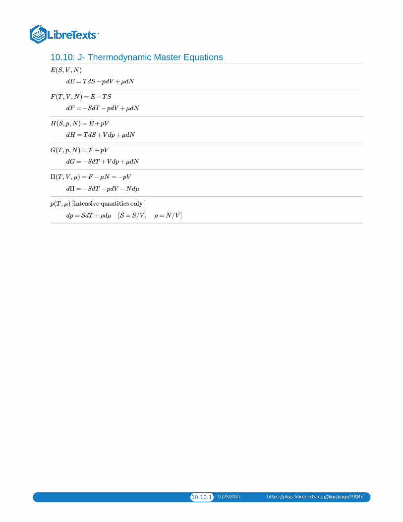
10.10.1 11/25/2021 https://phys.libretexts.org/@go/page/19083

10.10: J- Thermodynamic Master EquationsE(S,V ,N)

dE = TdS−pdV +μdN

F (T ,V ,N) = E−TS

dF = −SdT −pdV +μdN

H(S, p,N) = E+pV

dH = TdS+V dp+μdN

G(T , p,N) = F +pV

dG= −SdT +V dp+μdN

Π(T ,V ,μ) = F −μN = −pV

dΠ = −SdT −pdV −Ndμ

p(T ,μ) [intensive quantities only ]

dp = SdT +ρdμ [S = S/V , ρ = N/V ]

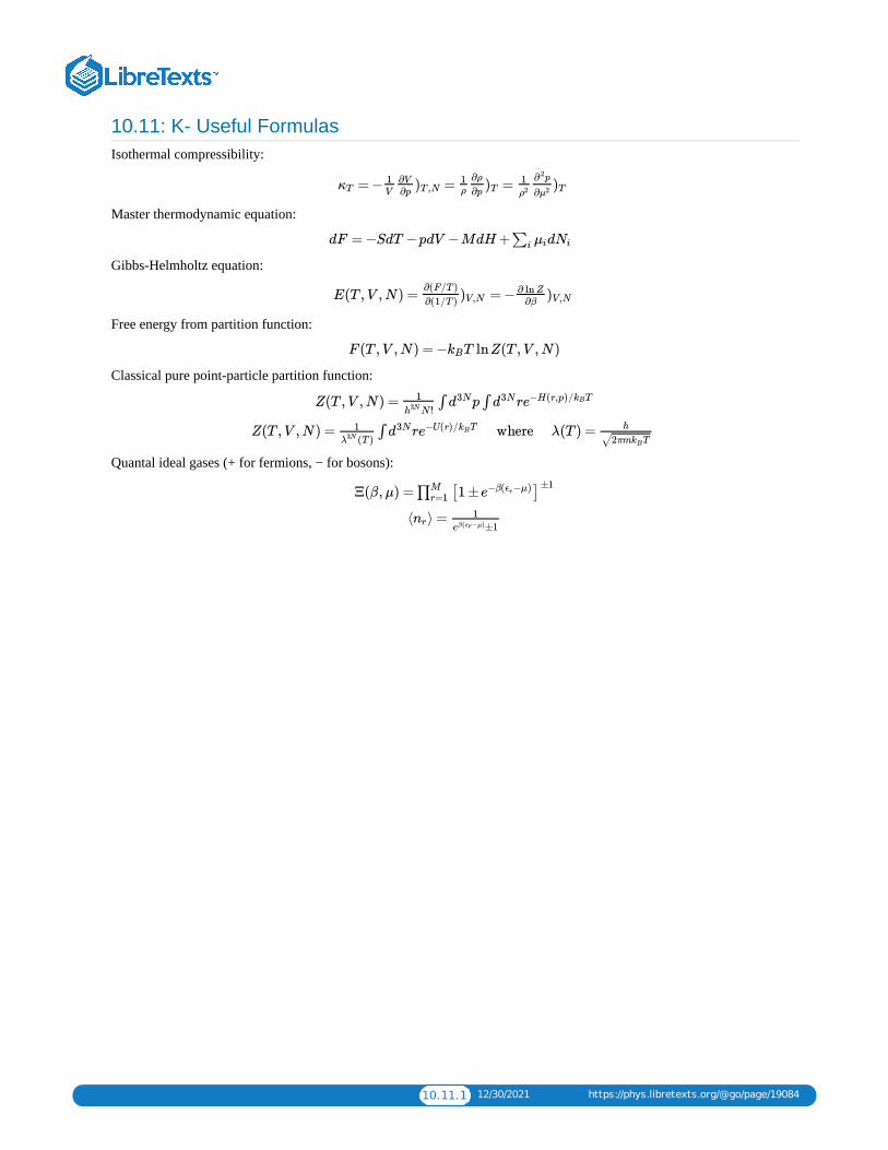
10.11.1 12/30/2021 https://phys.libretexts.org/@go/page/19084

10.11: K- Useful FormulasIsothermal compressibility:

Master thermodynamic equation:

Gibbs-Helmholtz equation:

Free energy from partition function:

Classical pure point-particle partition function:

Quantal ideal gases (+ for fermions, − for bosons):

= − = =κT1V

∂V∂p

)T ,N1ρ

∂ρ

∂p)T

1

ρ2

p∂ 2

∂μ2 )T

dF = −SdT −pdV −MdH + d∑i μi Ni

E(T ,V ,N) = = −∂(F/T )

∂(1/T ))V,N

∂ lnZ

∂β)V,N

F (T ,V ,N) = − T lnZ(T ,V ,N)kB

Z(T ,V ,N) = ∫ p ∫ r1

N !h3N d3N d3N e−H(r,p)/ TkB

Z(T ,V ,N) = ∫ r where λ(T ) =1

(T )λ3N d3N e−U(r)/ TkB h

2πm TkB√

Ξ(β,μ) =∏Mr=1 [1 ± ]e−β( −μ)ϵr

±1

⟨ ⟩ =nr1

±1eβ( −μ)ϵr

Index

Cconfigurational entropy

3.2: Entropy

Eentropy

3.2: Entropy

FFluid Statics

1.3: Fluid Statics

Hheat engine

3.3: Heat Engines

IIsing Model

9.4: Correlation Functions in the Ising Model

MMetropolis algorithm

9.5: Computer Simulation

PPerturbation theory

8.2: Perturbation Theory phase diagram

1.4: Phase Diagrams

Tthermal entropy

3.2: Entropy

VVariational Method

8.3: Variational Methods

Glossary

Sample Word 1 | Sample Definition 1