Fluid Mechanics

David Tong

Department of Applied Mathematics and Theoretical Physics,

Centre for Mathematical Sciences,

Wilberforce Road,

Cambridge, CB3 OBA, UK

http://www.damtp.cam.ac.uk/user/tong/fluids.html

d.tong@damtp.cam.ac.uk

Recommended Books and Resources

There are many books on fluid mechanics, ranging from the eminently accessible

to the dauntingly comprehensive. Here are a collection that I found useful.

• Van Dyke, An Album of Fluid Motion

If you’re going to look at one book on fluid mechanics then it should be this one. It’s

a book of pictures, many of them very pretty, While this likely sounds lightweight, in

this case a picture really does paint 20 equations and helps build intuition for fluid

flow. It’s di�cult to buy at a reasonable price (at the time of writing, Amazon o↵er a

paperback version for £833.82) but you can find versions on the internet.

• Acheson, Elementary Fluid Dynamics

• Childress, An Introduction to Theoretical Fluid Mechanics

If you’re going to look at a second book on fluid dynamics, it should probably be one

of these, or something similar. Both are aimed at the beginner. They are clear and

easygoing. I have a slight preference for Acheson which focuses more on the physics.

• George Batchelor, An Introduction to Fluid Dynamics

This is considered the bible of fluid mechanics by many practitioners. It’s not partic-

ularly cuddly, but the explanations are clear enough and it is certainly comprehensive

(unless you care about turbulence).

• Landau and Lifshitz, Fluid Mechanics

An astonishing amount of physics is packed into this book, but it’s not the easiest read.

Like Batchelor, it puts thermodynamics front and centre which is useful in making

contact with other areas of physics which can otherwise feel hidden. (In these lectures,

we only bring thermodynamics into the game when we describe sound waves.)

• Drazin and Reid, Hydrodynamic Stability

For all your instability needs.

• Frisch, Turbulence

A look at symmetries and scaling in turbulent flow.

Contents

1 Introduction 3

1.1 The Basics 5

1.1.1 Path Lines and Steamlines 6

1.1.2 The Material Time Derivative 8

1.1.3 Conservation of Mass 9

1.1.4 The Stream Function 10

2 Inviscid Flows 12

2.1 The Euler Equation 12

2.1.1 Under Pressure 13

2.1.2 The Euler Equation is Just Momentum Conservation 16

2.1.3 Archimedes’ Principle 17

2.1.4 Energy Conservation and Bernoulli’s Principle 18

2.2 Vorticity 21

2.2.1 The Vorticity Equation 26

2.2.2 Kelvin’s Circulation Theorem 29

2.3 Potential Flows in 3d 32

2.3.1 Boundary Conditions 33

2.3.2 Flow Around a Sphere 34

2.3.3 D’Alembert’s Paradox 38

2.3.4 A Bubble Rising 39

2.4 Potential Flows in 2d 42

2.4.1 Circulation Around a Cylinder 43

2.4.2 Lift and the Magnus Force 45

2.5 A Variational Principle 46

2.5.1 The Principle of Least Action 47

2.5.2 An Action Principle for Fluids 50

3 The Navier-Stokes Equation 55

3.1 Stress, Strain and Viscosity 58

3.1.1 Newtonian Fluids 60

3.1.2 Momentum and Energy Conservation Revisited 62

3.2 Some Simple Viscous Flows 64

3.2.1 The No-Slip Boundary Condition 64

3.2.2 Couette Flow 65

– i –

3.2.3 Poiseuille Flow 68

3.2.4 Vorticity Revisited and the Burgers Vortex 69

3.3 Dimensional Analysis 71

3.3.1 The Reynolds Number 73

3.3.2 Scaling 75

3.4 Stokes Flow 77

3.4.1 Flow Around a Sphere 78

3.4.2 Uniqueness and the Minimum Dissipation Theorem 83

3.4.3 Eddies in the Corner 85

3.4.4 Hele-Shaw Flow 89

3.4.5 Swimming at Low Reynolds Number 90

3.5 The Boundary Layer 94

3.5.1 Prandtl’s Boundary Layer Equation 96

3.5.2 An Infinite Flat Plate 98

3.5.3 Boundary Layers with Pressure Gradients 101

3.5.4 Separation 105

4 Waves 111

4.1 Surface Waves 111

4.1.1 Free Boundary Conditions 112

4.1.2 The Equations for Surface Waves 113

4.1.3 Surface Tension 121

4.2 Internal Gravity Waves 123

4.3 Because the Earth Spins 126

4.3.1 The Shallow Water Approximation 127

4.3.2 Geostrophic Balance 129

4.3.3 Poincare Waves 132

4.3.4 We Need to Talk About Kelvin Waves 134

4.3.5 Equatorial Waves 135

4.3.6 Chiral Waves are Topologically Protected 139

4.4 Sound Waves 142

4.4.1 Compressible Fluids and the Equation of State 143

4.4.2 Some Thermodynamics 144

4.4.3 Briefly, Heat Transport 148

4.4.4 The Equations for Sound Waves 149

4.4.5 Viscosity and Damping 153

4.5 Non-Linear Sound Waves 156

4.5.1 The Method of Characteristics 157

– ii –

4.5.2 Soundcones 160

4.5.3 Wave Steepening and a Hint of Shock 162

4.5.4 Burgers’ Equation 165

4.6 Shocks 167

4.6.1 Jump Conditions 169

4.6.2 Shocks Start Supersonic 174

4.6.3 On Singularities and Physics 176

5 Instabilities 179

5.1 Kelvin-Helmholtz Instability 181

5.1.1 The Simplest Instability 183

5.1.2 Rolling Up The Vortex Sheet 185

5.1.3 Gravity Helps. Surface Tension Helps Too. 187

5.1.4 The Rayleigh-Taylor Instability 188

5.2 A Piece of Piss 189

5.2.1 Gravity Makes the Flow Thinner 193

5.3 Rayleigh-Benard Convection 194

5.3.1 The Boussinesq Approximation 195

5.3.2 Perturbation Analysis 198

5.4 Instabilities of Inviscid Shear Flows 203

5.4.1 Rayleigh’s Criterion 205

5.4.2 Fjortoft’s Criterion 207

5.4.3 Howard’s Semi-circle Theorem 209

5.4.4 Couette Flow Revisited 211

5.5 Instabilities of Viscous Shear Flows 212

5.5.1 Poiseuille Flow Revisited 215

6 Turbulence 217

6.1 Mean Flow 218

6.1.1 The Reynolds Averaged Navier-Stokes Equation 219

6.2 Some Dimensional Analysis 222

6.2.1 Scale Invariance 225

6.3 Velocity Correlations 228

6.3.1 Navier-Stokes for Correlation Functions 231

6.3.2 The Structure of the Three-Point Function 234

6.3.3 The von Karman-Howarth Equation 236

6.3.4 Kolmogorov’s 4/5 238

– 1 –

Acknowledgements

I’m no expert on fluid mechanics. I wrote these notes primarily to teach myself

the basics of the subject and I hope that others may find them useful. If, however, you

would prefer to learn from someone who actually knows what they’re talking about

then I put together a collection of resources that I found helpful on this webpage.

My thanks to Matt Davison, Mihalis Dafermos, Sean Hartnoll and Jorge Santos for

helpful discussions on some of the topics included in these notes. I am supported by a

Simons Investigator award.

– 2 –

1 Introduction

Take anything in the universe, throw a bunch of it in a box, and turn up the heat.

Then it doesn’t matter what you started with, the motion of this substance will be

governed by the equations of fluid dynamics.

This is a remarkable statement. There are lots of di↵erent things in the universe and

we go to great lengths to understand their properties. Yet if you heat them, most of

the di↵erences disappear. When things get hot, everything looks the same.

Here are some examples. Take any element in the periodic table and heat it until it

melts, so that it is either a liquid or a gas. The motion of every element is governed by

the same set of equations. The only reminder of what you started with is to be found

in a handful of parameters of these equations which describe, among other things, the

density and viscosity of the fluid. These will di↵er from element to element. But the

basic set of equations are the same, regardless of whether you started with an alkaline

earth metal or an inert gas.

This same story holds if we turn our attention to more exotic substances. For exam-

ple, inside every proton and neutron sit three quarks. They have been trapped there

since the Big Bang, held in place by the grip of the strong nuclear force. However, ear-

lier this century, experimenters succeeded in colliding nuclei together with energies that

were so high that the protons and neutrons themselves melted, freeing their imprisoned

quarks and forming a novel state of matter known as a the quark-gluon plasma. This

plasma only lasts for a fraction of a second before it cools and once again forms protons

and neutrons. But during that fraction of a second it moves. And the movement is

described by the laws of fluid mechanics.

Here is an even more extreme example. Take spacetime itself. It is possible for

spacetime to collapse in on itself to form a black and, due to the work of Hawking, we

know that these black holes are hot objects. So a black hole can be viewed as a way to

heat spacetime. Surprisingly, if you look at the equations that govern the event horizon

of a black hole, you will once again find the laws of fluid mechanics.

All of which is to say that there is a wonderful universality to the laws that govern

fluids. In certain circumstances, these laws describe literally everything. And this

makes them interesting.

The reasons underlying this universality are well understood. At the microscopic

level, fluids are ridiculously complicated objects, consisting of, say, 1023 atoms, each

– 3 –

following its own path, while acting through various forces on the atoms around it.

But much of this motion is fleeting and we lose little if we ignore it. Instead, we care

only about patterns in the collective motion of the atoms that survive over long time

scales. It turns out that these long-lived modes are all related to familiar conservation

laws – conservation of mass, momentum and energy – and these conservation laws are

universal and obeyed by all substances. This, ultimately, is why all fluids look the

same: the equations of fluid dynamics are essentially the equations that govern how

conserved quantities evolve in time. (This is a theme that will rear its head at various

places in this course, but is not something that we dwell upon. In contrast, the idea

that conservation laws underlie fluid mechanics will be the focal point of the lectures

on Kinetic Theory which derive the Navier-Stokes equation starting point from 1023

atoms, each obeying Newton’s laws.)

In addition to the universal aspect of fluid mechanics, the subject also has enormous

practical applications. It explains, for example, why planes fly. (As we will recount later

in these lectures, one of the more embarrassing episodes in the history of theoretical

physics occurred in 1903 when the Wright brothers took to the air before physicists

were able to adequately explain either lift or drag!) Fluid mechanics explains how

oil flows through pipes and how the motion of the atmosphere manifests itself in the

climate, and how many decades of focussing on the former has resulted in an urgent

and desperate need to better understand the latter.

In this course we explore the basics of fluid mechanics. Our focus will not be on

quarks and black holes, but nor will it be any particular application of fluid mechanics.

Instead our goal is simply to understand the di↵erent things that fluids can do. Fluids

are everywhere and they have a tendency to move. The purpose of these lectures is

simply to construct and explore the equation governing this motion.

As we’ve stressed above, the motion of all fluids is described by the same basic set

of equations. Prominent among these is the Navier-Stokes equation, accompanied by

one or two of further equations describing the conservation of mass and, in some cases,

the flow of heat. One of the themes of fluid mechanics is that a wonderful diversity of

di↵erent behaviour emerges from these equations. As these lectures progress, we will

find ourselves falling into a routine. Like Monet and his haystacks, we will return to

these same theme over and over again, not because we did anything wrong the first time

but because there is always something new to see. Attacking the same set of equations,

but with slight change to the boundary condition, or a novel approximation scheme,

will often yield something new and surprising. One of the delights of the subject lies

in finding such riches sitting inside such simple equations.

– 4 –

1.1 The Basics

When we were kids, we are told that there are three phases of matter: solid, liquid

and gas. As we grow older, we learn that this is a hopelessly naive view of the world.

Nonetheless, it is the one that we will adopt in this course which is concerned only

with the latter two. Liquids and gases are both examples of fluids. Roughly speaking,

a fluid is a substance that flows when pushed. More rigorously, fluids are objects that

are well described by the equations of these lectures.

The subject of fluid mechanics starts with a lie. (Applied mathematicians prefer

the term “approximation”.) The lie, sometimes dubbed the continuum hypothesis, is

that fluids are indivisible continuous objects. The fluid can be then described by two

smooth, continuous fields,

• The density ⇢(x, t)

• The velocity u(x, t).

Of course, we know that in reality fluids are made of molecules and this approximation

must break down on atomic scales. But we also know from experience that if we look

on suitably large scales, where we are coarse graining over a many many molecules,

then the continuum description is remarkably good.

It is appropriate to start these lectures by stressing that we are dealing with an

approximation. It will not be our last. The study of fluids is all about the art of

approximation. The equations of fluid mechanics, simple as they are, cannot be solved

in full generality and we will make progress only by simplifying. The skill is in learning

what to keep and what to ignore. And we start by ignoring the existence of atoms.

It’s not just the discreteness of matter than is swept under the rug in the continuous

description. We also ignore the vast majority of the motion of the constituent atoms

and molecules that make up the fluid. At room temperature, these constituents are

flying around at speeds of 100 ms�1 or so. (This is certainly true of gases. For liquids,

the molecules are more closely bound to their neighbours and we have to think more

carefully about what the velocity of a single molecule really means.) But most of

this underlying atomic motion is neglected in our coarse-grained description. Instead,

the velocity field u(x, t) describes the average, macroscopic motion of the fluid. In

particular, there is a state of the fluid in which u(x, t) = 0 and we pretend that the

fluid is completely still, even though the underlying particles are still flying around,

just with no direction preferred over any other.

– 5 –

(As an aside: the internal motion of the constituents doesn’t show up in the velocity

field u(x, t), but it does manifest itself in the temperature of the fluid which is another

field T (x, t). We’ll elaborate on the role that temperature plays as these lectures

progress but for now, and indeed for much of the lectures, we will be able to ignore it.)

It is also worth elaborating on how to think about the position x that appears in the

argument of the fields ⇢(x, t) and u(x, t). This is some fixed position in space. This

means, in particular, that u(x, t) is the velocity that would be measured by some fixed

array of sensors embedded in the fluid, as opposed to sensors that drift along with the

fluid. The use of fields ⇢(x, t) and u(x, t) is called the Eulerian description.

We will also have use for a slightly di↵erent viewpoint, in which we think of individual

“parcels of fluid”, each initially sitting at some position x and then following the flow by

travelling at speed u(x, t). It’s not so easy to define what we mean by these“parcels of

fluid” given that the underlying atoms are, as we described above, wandering o↵ in all

sorts of directions, often at high speed, with only the most scant regard for the velocity

field u(x, t). But the concept of a fluid parcel that keeps its identify as the fluid moves

is an extremely useful pretence. We will sometimes talk about a “particle” of fluid and

we have in mind these parcels rather than the underlying atoms. The perspective in

which we follow the trajectories of these parcels, and study the forces that act on them

as if they were particles in classical mechanics, is called the Lagrangian description.

Throughout these lectures, all our equations will be written in the Eulerian de-

scription, using the velocity field u(x, t), but some intuition will come from a more

Lagrangian way of thinking. Moreover, we will certainly have a need to understand the

trajectories of particles that are embedded within the fluid. Indeed, we kick o↵ with

some simple observations.

1.1.1 Path Lines and Steamlines

There are a number of ways to visualise the flow u(x, t) of a fluid. Here are the two

most useful:

• A pathline is the trajectory followed by a particle embedded within the fluid.

• A streamline is a tangent to u(x, t) at every point x for fixed time t. In general,

the tangents to a vector field F(x) are said to be integral curves for F. So the

streamlines are integral curves for the velocity field at a fixed time.

If the flow is steady, meaning that @u/@t = 0, then the pathlines and streamlines

coincide. But, for time dependent flows, they di↵er. To see this, let’s drape some

equations around the definitions above.

– 6 –

Figure 1. The pathlines for particles in the flow u = (yt, 1) are shown on the the left.

These are a history of the flow. The middle and right hand figures show streamlines, with

the right-hand figure at a later time.

First consider the pathline. A particle within the fluid will follow some trajectory

x(t). At any time t, the velocity of this particle is given by the velocity field u evaluated

at the position of the particle, meaning

dx

dt(t) = u(x(t), t) (1.1)

Given some initial starting point x(t = 0) = x0, we can solve this equation to find the

pathline.

In contrast, a streamline is a trajectory x(s) such that the tangents of x(s) coincide

with the velocity field at a fixed time t,

dx

ds(s) = u(x(s), t)

In words, the streamline is a snapshot of the flow at some fixed time, while the pathline

tells us about the actual history of the particle.

An Example

Consider the two-dimensional flow given by

u(x, t) =

↵yt

�

!

for some fixed coe�cients ↵ and �. The pathline obeys

dx

dt=

x

y

!=

↵yt

�

!

– 7 –

The y component is solved by y = y0 + �t, while the equation for the x component

becomes x = ↵yt = ↵(y0t + �t2), which gives x = x0 +12↵y0t

2 + 13↵�t

3. To get the

pathline, we eliminate t to get the family of curves in the (x, y) plane

x = x0 +↵

2�2y0(y � y0)

2 +↵

3�2(y � y0)

3

These are plotted on the left-hand plot of Figure 1 for various values of the starting

point (x0, y0).

In contrast, to find the streamlines we instead solve

dx

ds=

x0

y0

!=

↵yt

�

!

where the prime means d/ds. These now have the solutions y = y0 + �s and x =

x0 + ↵y0ts +12↵�ts

2 where t is now some fixed parameter. These are shown in the

middle and right-hand plots of Figures 1 for t > 0. Note that the pathlines and

streamlines are not similar in this example: the former is a cubic curve, the latter a

parabola. (Or, in the special case of t = 0, straight lines.) Moreover, the streamlines

are time-dependent: the right-hand figure is a snapshot of the flow at a later time than

the middle figure.

1.1.2 The Material Time Derivative

As we stressed above, the density ⇢(x, t) and velocity field u(x, t) are measured in the

Eulerian sense at some fixed point x. But this leaves us with the question: how do we

see things change in time if we’re drifting along with the fluid?

Specifically, suppose that there is some field �(x, t) that we would like to measure.

This might be the density of the fluid itself, or something else. The explicit time

dependence in �(x, t) tells us how this quantity changes with time if we’re sitting at

some fixed position x. But if we’re drifting with the fluid, then we follow a pathline

x(t) defined by (1.1). The value of field along this trajectory is given by �(x(t), t) and

the total time derivative is

d

dt�(x(t), t) =

@�

@t+ x ·r� =

@�

@t+ u ·r�

The additional u ·r� term captures the change in � because of the way we’re swept

along by the fluid. The transport of some object as it’s carried along by a fluid is known

as advection and, correspondingly, u ·r� is called the advective rate of change. This

idea of a total time derivative will be important, so much so that we introduce some

– 8 –

new notation for it (even though we already have perfectly good notation in d�/dt!).

We write

D�

Dt=

@�

@t+ u ·r�

and call this the material derivative. It can be thought of as a bridge between the

Eulerian description in terms of a fixed point x and the Lagrangian description which

moves with the fluid.

1.1.3 Conservation of Mass

Our first equation of fluid mechanics is the simplest: it captures the fact that mass is

conserved. Moreover, like all conservation laws in physics, mass is conserved locally.

This means that if the mass of the fluid decreases at some point in space then it must

have moved to a neighbouring point.

This fact is captured by the conservation equation, relating the density ⇢ and the

velocity u,

@⇢

@t+r · (⇢u) = 0 (1.2)

Equations of this kind are commonplace in physics because they appear whenever we

have a conservation law. In particular, an identical equation appears in Electromag-

netism where, in that context, ⇢ is the electric charge density and J = ⇢u is the electric

current density. For us, ⇢ is the mass density and ⇢u is the mass flux density.

To see why (1.2) captures the conservation of mass, consider the mass M of fluid in

some fixed region V ,

M =

Z

V

⇢ dV

The change of this mass is given by

dM

dt=

Z

V

@⇢

@tdV = �

Z

V

r · (⇢u) dV = �

Z

S

⇢u · dS

where we have used the divergence theorem and S = @V is the boundary of the region

V . This tells us that if there is no net flow of mass flux through the boundary S

then the total mass M inside the region V remains constant. In other words, mass is

conserved.

– 9 –

We can also write the mass conservation equation (1.2) using our new material deriva-

tive notation. It becomes

D⇢

Dt+ ⇢r · u = 0 (1.3)

Incompressible Fluids

Throughout much of these lectures notes we will make one further approximation: we

will assume that fluids are incompressible, meaning that ⇢(x, t) is a constant. In this

case, ⇢ = r⇢ = 0 and the continuity equation (1.2) becomes simply

r · u = 0 (1.4)

In the language of our Vector Calculus lectures, we say that the fluid flow is solenoidal

or divergence free. The vast majority of these lectures will be devoted to finding the

wonderfully diverse solutions to the equation (1.4).

In the fact, the requirement that ⇢ = r⇢ = 0 can be loosened slightly. We see from

(1.3) that we only really require D⇢/Dt = 0 for the incompressible condition (1.4) to be

enforced. This means that any individual parcel of fluid should not change its density

as it’s swept along, but di↵erent parts of the larger fluid may have di↵erent densities.

Such a situation is said to be stratified and arises, for example, in the ocean where the

water is more dense at the bottom than the top. We’ll meet situations like these when

we discuss some aspects of waves in Section 4.

The assumption that fluid flow is incompressible is not totally innocent. In fact,

the phenomenon of fluids compressing and expanding as their density changes is so

common that we give it a special name. This name is “sound”! It turns out that that

assumption of incompressibility is good when the speed of the fluid |u| is much less

than the speed of sound. For air at atmospheric pressure, the speed of sound is 340

ms�1; for water at room (or ocean) temperature it is around 1500 ms�1. For much of

these lectures, we will restrict ourselves to flows much below these speeds and assume

that r ·u = 0. But, in Section 4.4, we will discuss the propagation of sound waves and

then we will be forced to look more closely at the equations that govern compressible

fluids.

1.1.4 The Stream Function

For incompressible fluids, satisfying r · u = 0, we can write the velocity field as

u = r⇥A

– 10 –

For many fluid flows, this isn’t particularly helpful since we have just swapped one

vector field u for anotherA. However, when the flow is two-dimensional (in some sense)

this provides a very useful simplification because it means that we get to exchange the

vector field u for a scalar field called the stream function.

For example, suppose that the flow is independent of the z-direction, so that the

velocity field takes the form

u = (u1(x, y, t), u2(x, y, t), 0)

Then the vector potential A can be written as

A = (0, 0, (x, y, t)) ) u1 =@

@yand u2 = �

@

@x

and the degrees of freedom are captured by the stream function (x, y, t). It has the

nice property that lines of constant are streamlines of the flow. To see this, note

that lines of constant have a normal n given by

n = r =

✓@

@x,@

@y, 0

◆

and so u · n = 0. This is telling us that vectors that are normal to lines of constant

are also normal to streamlines. But in 2d, the enemy of an enemy is necessarily a

friend. So lines of constant are streamlines.

The idea of a stream function can be fruitfully applied in other coordinate systems.

For example, in spherical polar coordinates we could take a stream function that de-

pends only on (r, ✓, t). The associated velocity field is then

u =1

r sin ✓

@(sin ✓ )

@✓r�

1

r

@(r )

@r✓ (1.5)

We’ll make good use of this in a number of places throughout this course, starting when

we discuss potential flows in Section 2.3.

– 11 –

2 Inviscid Flows

Fluids have a property known as viscosity. This is an internal, friction force acting

within the fluid as di↵erent layers rub together. It is crucially important in many

applications.

Nonetheless, we will start our journey into the world of fluids by ignoring viscosity

altogether. Such flows are called inviscid. This will allow us to build intuition for the

equations of fluid mechanics without the complications that viscosity brings. Moreover,

the flows that we find in this section will not be wasted work. As we will see later in

Section 3, they give a good approximation to viscous flows in certain regimes where

the more general equations reduce to those studied here.

2.1 The Euler Equation

We have already met the mass conservation equation (1.2)

@⇢

@t+r · (⇢u) = 0 (2.1)

We will assume that the fluid is incompressible, so that this becomes

r · u = 0 (2.2)

But we need one more equation to describe the motion of fluids. This second equation

comes from what fluid dynamicists sometimes call “momentum balance”. It is what

everyone else calls “F = ma”.

Consider some fixed region in space that we call V . The momentum in this volume

isRV⇢u dV and Newton’s second law tells us that the rate of change of momentum

is equal to the force. The novelty here is that the momentum inside V might change

simply because the fluid leaves (or enters) the region V . To write down the equation

of motion, we need to take this into account.

Claim: The momentum flux across the boundary in some time �t is

Momentum Flux = �t⇥

Z

S

(⇢u)u · dS (2.3)

with S = @V is the boundary of the volume V .

– 12 –

Proof: Consider some small area of fluid �S

lying on the surface S and watch it evolve. In

some small time interval �t it sweeps out a vol-

ume �(Vol) = u · n �t �S where n is the nor-

mal to the surface as shown in following fig-

ure. As usual we write the vector area element

�S = n �S, so we have �(Vol) = u · �S �t. This means that the momentum departing

through the surface is ⇢u �(Vol). This gives the claimed result. ⇤

Including this extra term for the momentum that leaks through the sides, the “F=ma”

equation of motion for the fluid is

d

dt

Z

V

⇢u dV = �

Z

S

(⇢u)u · dS+ Force

The additional term from the leaking momentum flux (2.3) sits on the right-hand side

with the minus sign there, as always, to signify loss.

We’ll get to the force shortly. Before we do, we can use the divergence theorem to

convert the surface integral over momentum flux into a volume integral. Taking this

term over to the other side, and resorting to index notation for the vectors u, we haveZ

V

⇢@ui

@tdV +

Z

V

⇢@

@xj(uiuj) dV = Force

Here we’ve used the fact that we’re working with an incompressible fluid, both in

the fact that ⇢ is constant and also in the derivative in the second term which reads

@j(uiuj) = ui@juj+uj@jui. But the first of these vanishes because incompressible fluids

obey r · u = 0. We we’re left withZ

V

⇢

✓@u

@t+ (u ·r)u

◆dV =

Z

V

⇢Du

DtdV = Force (2.4)

In other words, the “ma” part of our equation involves the material derivative of the

velocity. In hindsight, this is not surprising. The material derivative is the rate of

change when you follow a parcel of fluid through the flow. This is the appropriate

meaning of ”rate of change” in Newton’s second law.

2.1.1 Under Pressure

Next we come to the question of forces that the fluid experiences. As we’ve already

mentioned, we’ll postpone any discussion of friction forces to Section 3. The fluid may

be exposed to some external force, with gravity the most obvious, and we’ll come to

these shortly. But the most important force comes from within: this is pressure.

– 13 –

From a microscopic perspective, the pressure in a fluid comes from the motion of the

underlying atoms or molecules. But, as we’ve already stressed, in these notes we shy

away from the fundamentals and focus on the macroscopic. Here pressure manifests

itself as a force acting on the surface of any fluid element.

The pressure is defined as the force per unit

area. Consider a small parcel of fluid, con-

tained within a fixed volume V . The pressure

P (x, t) acts on the surface S = @V of this vol-

ume1. It’s an isotropic force, meaning that it

is the same in all directions. The force exerted

by the fluid outside V on some small region �S

on the surface is

Fpressure = �Pn �S

where n is the outward-pointing normal as shown in the figure.

The pressure P (x, t) should be viewed as a dynamical field that must be solved,

subject to certain boundary conditions, at the same time as the velocity field u(x, t).

Indeed, for certain simple flows we’ll see that there’s a direct relationship between the

pressure and velocity.

Including the pressure, the equation of motion for the fluid (2.4) becomes

Z

V

⇢Du

DtdV = �

Z

S

P dS+Other Forces (2.5)

We will assume that these other forces act on the volume of the fluid rather than the

surface (this is true for external forces like gravity) and so take the integral form

Other Forces =

Z

V

f dV

The pressure acts on the surface of the volume V but we can massage it into a volume-

type force through use of the divergence theorem. This givesZ

V

⇢Du

DtdV =

Z

V

(�rP + f) dV

1I am apparently alone in the world in thinking that the lower case p for pressure looks way toomuch like the density ⇢ for them to happily cohabit in the same equation.

– 14 –

The final step is to recall that this whole derivation holds for an arbitrary volume V

within the fluid. Since it holds for all such V , the integrand itself must vanish. So

we’re left with the di↵erential equation of motion for the fluid

⇢Du

Dt= �rP + f (2.6)

This is the Euler equation. Finding solutions to this simple equation will occupy us

for the rest of this section although we will, ultimately, replace it in Section 3 by the

Navier-Stokes equation which includes the e↵ects of viscosity. Fluids that obey the

Euler equation are said to be ideal.

Importantly, the Euler equation is non-linear in the velocity field, although this is

somewhat hidden in the notation above since the non-linearity sits in the material

derivative: Du/Dt = @u/@t+ (u ·r)u.

Note that a constant pressure P throughout the fluid does nothing. This is because

the pressure is isotropic: if one piece of fluid pushes on a neighbour, the neighbour

pushes back with equal force. Interesting dynamics only arises when we have pressure

di↵erences across the fluid, as captured by rP .

The Euler equation is a vector equation. Combined with the requirement of incom-

pressibility, r · u = 0, we have four equations in total. We will use these to solve for

the four dynamical variables: P and u.

Looking Forwards: the Equation of State

If you know one thing about gases, then it will be the ideal gas law. This relates the

pressure P , volume V and temperature T of a gas by

PV = NkBT

where N is the number of molecules in the gas and kB a universal constant of nature

called Boltzmann’s constant that relates energy to temperature. (For what it’s worth,

kB ⇡ 1.4 ⇥ 10�23 JK�1.) For our purposes, it’s more useful to think of the ideal gas

law in terms of the density ⇢ = Nm/V rather than volume, where m is the mass of the

constituent molecule,

P =kB⇢T

mThe ideal gas law is an example of an equation of state. It holds for strictly non-

interacting gases. If we take into account interactions, either in gases or in liquids, it

will be replaced by some other equation of state that again relates pressure P , density

⇢ and temperature T . (You can learn more about how to calculate the equation of

state from first principles in the lectures on Statistical Physics.)

– 15 –

When we first meet the ideal gas law, we think of P , ⇢ and T as constants that

characterise the whole system. But it also holds if they are promoted to the kind of local

fields P (x, t), ⇢(x, t) and T (x, t) that we work with in these lectures. For incompressible

fluids, with ⇢ constant, the equation of state tells us that the temperature T (x, t) simply

tracks the pressure P (x, t). For this reason we won’t need to consider it separately.

Things are more interesting if we have compressible fluids, in which ⇢(x, t) is another

dynamical variable. In this case the mass conservation equation (1.2) and Euler equa-

tion aren’t enough information to tell us what happens and we need another equation.

It turns out that in this situation the right way forward is to use the equation of state

to replace ⇢(x, t) with the temperature field T (x, t) and then write down a separate

equation for how heat flows in the system. (Roughly speaking, it is a version of the

heat equation, with the material derivative replacing the usual time derivative.) We’ll

explain this further in Section 4.4 when we discuss sound waves and we will be forced

to think more carefully about the thermodynamics of fluids. (A fuller derivation can

be found in the lectures on Kinetic Theory.)

2.1.2 The Euler Equation is Just Momentum Conservation

Suppose that there is no external force on our fluid, so f = 0. Then the Euler equation

can be written in the characteristic form of a conservation law

⇢@u

@t+ ⇢(u ·r)u+rP = 0 )

@⇢ui

@t+

@

@xj(⇢uiuj + P �ij) = 0 (2.7)

where we’ve used the assumption that the fluid is incompressible, both in taking ⇢

inside the derivatives and in using @juj = 0.

It’s clear what is conserved here: it is simply the momentum in each of the three

directions:RV⇢ui dV . Associated to each conserved quantity is a current. The novelty

here is that because the conserved quantity is itself a vector, the associated current is

a tensor ⇧ij. This tells us how the momentum in the ith direction is transported in the

jth direction. The form of the momentum current can be read o↵ from the equation

above,

⇧ij = ⇢uiuj + P �ij

The first, advective contribution describes the momentum due to the motion of the

fluid. The pressure contribution to momentum is perhaps more surprising. It is a hint,

even at this macroscopic level, that pressure is associated to something moving around.

This something is, of course, the constituent atoms of molecules of the fluid that we

have declared irrelevant for fluid mechanics.

– 16 –

There is a simple way of seeing why pressure is related to momentum. Take a box

with some fluid inside and make a little hole in it. The pressure inside the box will

force the fluid out of the hole. The rate at which momentum escapes from the box is

equal to the pressure. (Or, more strictly, the pressure di↵erence between the inside and

outside of the box.)

2.1.3 Archimedes’ Principle

Before exploring the full content of the Euler equation, we can extract some familiar

and long-known results. To kick o↵, suppose that the fluid sits in a gravitational field.

(Which, let’s face it, most do.) This means that we have an external force density

f = ⇢g

where g = �gz is the gravitational acceleration and points downwards.

We can now look for the trivial solution to the Euler equation (2.6) in which the fluid

is at rest, so u = 0. We see that the fluid must have a pressure gradient to counteract

the gravitational field

rP = ⇢g ) P = P0 � ⇢gz (2.8)

This is known as hydrostatic pressure. It is the pressure that pushes against the weight

of the fluid above. (If you’re worried about the minus sign and the possibility of the

pressure becoming negative, think of the surface of the fluid as sitting at z = 0, so that

pressure only increases as we move down to z < 0.)

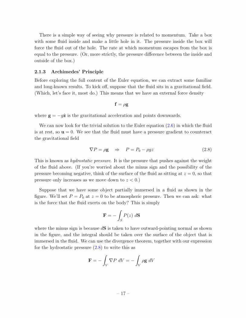
Suppose that we have some object partially immersed in a fluid as shown in the

figure. We’ll set P = P0 at z = 0 to be atmospheric pressure. Then we can ask: what

is the force that the fluid exerts on the body? This is simply

F = �

Z

S

P (z) dS

where the minus sign is because dS is taken to have outward-pointing normal as shown

in the figure, and the integral should be taken over the surface of the object that is

immersed in the fluid. We can use the divergence theorem, together with our expression

for the hydrostatic pressure (2.8) to write this as

F = �

Z

V

rP dV = �

Z

V

⇢g dV

– 17 –

where the integral is now over the volume of displaced

fluid. This is telling us that the force exerted by the

fluid on the object is equal to the weight of the displaced

fluid. Eureka! This, of course, is Archimedes principle.

In equilibrium, the force F must balance the weight of

the object itself. This can be achieved if the object is

less dense than water, in which case it floats. Otherwise

it sinks. This discussion hasn’t brought anything new

to Archimedes idea. It’s really just the old argument wrapped in the language of vector

calculus.

The results above also give us a reason to ignore gravity for much of this course. In

the presence of a gravitational field, the pressure simply adapts as in (2.8) to cancel it.

Therefore, in the presence of gravity, we can think of the pressure as

P = P0 � ⇢gz + P 0

and Euler’s equation becomes

⇢D⇢

Dt= �rP 0

and we proceed from there.

2.1.4 Energy Conservation and Bernoulli’s Principle

In classical mechanics, it’s often useful to identify conserved quantities. The same is

true in fluid mechanics and there is a way to rewrite the Euler equation that highlights

one such conserved quantity. We start with the vector identity

u⇥ (r⇥ u) =1

2r(u · u)� (u ·r)u

We use this to substitute for the non-linear (u ·r)u term in the Euler equation to get

⇢

✓@u

@t+

1

2r|u|2 � u⇥ (r⇥ u)

◆= �rP + f (2.9)

So far this doesn’t look any more useful. But now we dot with u to make the curly

term disappear. We have

⇢u ·@u

@t+ u ·r

✓1

2⇢|u|2 + P

◆= u · f

– 18 –

At this stage, we make one further assumption: we take the force to be conservative,

meaning that we can write it in terms of a potential energy �(x, t),

f = �r� (2.10)

For example, the gravitational force can be written in this way. We then have

1

2⇢@|u|2

@t+ u ·r

✓1

2⇢|u|2 + P + �

◆= 0

This is again of the form of a conservation equation. To see this, we again pull the u

inside the r using the fact that the fluid is incompressible so r · u = 0. (This is the

same step that we did for the momentum conservation equation in (2.7).) We get the

final form

1

2⇢@|u|2

@t+r · (uH) = 0 (2.11)

where

H =1

2⇢|u|2 + P + � (2.12)

There’s no mystery in what is being conserved here: the time derivative is acting on12⇢|u|

2 which we recognise as the kinetic energy density of the fluid. The equation (2.11)

is simply capturing energy conservation of the continuous fluid, with uH the energy

flux.

For a steady fluid, satisfying @u/@t = 0, we have

u ·rH = 0 (2.13)

This is Bernoulli’s Theorem. It states that the quantityH is constant along streamlines.

Roughly speaking, the fluid flows quickly in places where the pressure is low, and more

slowly when the pressure builds.

An Example: Drinking from a Firehose

Consider water flowing down a pipe which, at some point, narrows as shown in Figure

2. This might, for example, be the nozzle on a firehose. We’ll take the narrowing to be

gradual so that the streamlines are smooth and follow the pipe.

– 19 –

Figure 2. As a pipe narrows, the velocity must increase and Bernoulli’s theorem tells us

that, for steady flows, the pressure also increases.

Initially, the pipe has area A and the fluid has speed U . By the end the area has

reduced to a < A and the speed to u. For incompressible fluids, the speed is dictated

by the conservation of mass which tells us that the volume of fluid passing through any

given slice of the pipe must remain the same, so

UA = ua

This immediately tells us that the speed of the flow in the narrow section is faster than

in the initial section: u = UA/a. Meanwhile, Bernoulli’s theorem tells us that

⇢

2U2 + P =

⇢

2u2 + p

where P and p are the initial and final pressure respectively and we are ignoring any

external forces. Rearranging, we have

p = P +⇢

2U2

✓1�

A2

a2

◆

We see that because A > a, the pressure actually decreases as the pipe narrows. This

makes sense: the decrease in pressure in the narrow section means that there is a

pressure di↵erence and this is precisely what causes the fluid to accelerate from speed

U to speed u.

More Qualitative Applications

There are other situations where Bernoulli’s principle gives us some useful intuition.

For example, it’s possible to levitate a ping pong ball on a fast jet of air. You can

achieve this by blowing through a straw or by using a hairdryer. The question is: why

is the ball stable? Why doesn’t it fall o↵ to one side? In this situation, the airflow is

turbulent and it’s not entirely clear that Bernoulli’s principle, which requires a steady

flow, can be invoked. Nonetheless, it does provide an answer. Suppose that the ball

– 20 –

did move slightly o↵ to one side and out of the main flow. Then the air will be moving

faster in the middle of the flow, resulting in a lower pressure and the ball gets pushed

back into the middle.

The most famous application of Bernoulli’s principle is to explain the lift experienced

by an aerofoil. The air travels faster over the top of the wing than the bottom and the

pressure di↵erence results in a net upwards force. But this begs the question: why does

the air travel faster over the top of the wing? One popular explanation (and one that I

was told in school) is that the flow must reach the trailing edge of the wing at the same

time, regardless of whether it goes up or down. But that doesn’t sound right! There’s

no principle in physics that says you must reach your goal at the same time regardless

of the path you take. (If there were, we wouldn’t need maps.) We will revisit this later

in the course when we study flows around objects in some detail.

2.2 Vorticity

To characterise the shape of a velocity field u, we look at its derivatives. In general

there are nine such derivatives, @iuj, with i, j = 1, 2, 3. But, for incompressible flows,

we know that one linear combination vanishes: r · u = 0. The remaining derivatives

can be decomposed as a symmetric and anti-symmetric tensor. The symmetric one is

known as the rate of strain tensor,

Eij =1

2

✓@ui

@xj+

@uj

@xi

◆(2.14)

The anti-symmetric tensor is

⌦ij =1

2

✓@ui

@xj�

@uj

@xi

◆

It contains the same information as vector field, !i = ✏ijk⌦jk, which is more familiarly

written as

! = r⇥ u

This is the vorticity. It tells us how the fluid swirls at each point in space. The integral

curves associated to ! (i.e. the lines that are tangent to ! at each point x) are called

vortex lines. Because ! = r⇥ u, the vortex lines are perpendicular to streamlines.

Examples of Flows

To get a feel for what the vorticity ! and rate of strain E are telling us, we can look

at a couple of examples.

– 21 –

Figure 3. On the left, a flow with strain and no vorticity. On the right, a flow with vorticity

and no strain.

First consider the 2d flow

u = ↵(�x, y, 0)

with ↵ a constant. This is plotted on the left of Figure 3. The velocity field hasr·u = 0

and also ! = 0, while the rate of strain tensor is

E = ↵

0

BB@

�1 0 0

0 +1 0

0 0 0

1

CCA

From the figure, you can see that the fluid is squeezed in one direction (the x-direction

in this case) and stretched in the other (the y-direction). This is the characteristic

feature of flows with a rate of strain. To see this, note that the rate of strain tensor is

symmetric and so can always be diagonalised so that it takes the form

E =

0

BB@

E1 0 0

0 E2 0

0 0 E3

1

CCA

But, for incompressible fluids with r · u = 0, we must have E1 + E2 + E3 = 0. So

one eigenvalue is necessarily positive and another necessarily negative. These are the

directions in which the flow is, respectively, stretched and squeezed.

– 22 –

Figure 4. On the left, a flow with vorticity. On the right, a flow that rotates around the

origin but with vanishing vorticity.

Next consider the flow

u = ↵(�y, x, 0) (2.15)

This has r ·u = E = 0 and a constant vorticity everywhere in the fluid, ! = (0, 0, 2↵).

It is depicted on the right of Figure 3. Unsurprisingly, it exhibits a rotation.

However, one should be wary of simply eyeballing a flow to decide on vorticity. To

illustrate this, consider the example

u = f(r)(�y, x, 0)

where f(r) is any function of r2 = x2 + y2. (Note that we’re keeping the flow essen-

tially two dimensional.) This is a generalisation of our previous flow (2.15) and the

streamlines look identical for any choice f(r). The vorticity is ! = (0, 0,!(r)), with

! =1

r

d

dr(r2f) (2.16)

Now the vorticity !(r) varies in the radial direction. This means that if we take the

specific choice of f = 1/r2, then the vorticity vanishes, ! = 0, even though the flow

is clearly rotating around the origin. This is because a non-zero vorticity !(x) 6= 0 at

some point x means that the fluid is rotating locally around x, not just around the

origin.

To build a more physical understanding for what vorticity means, suppose that we

drop some propellers in the fluid, like those plastic windspinners that you can buy at

the seaside. If you drop them in the fluid, they will move around the origin with the

flow. But if the fluid has a vorticity then their orientation will also rotate as the move,

– 23 –

as shown on the left-hand side of Figure 4. If the fluid has no vorticity, as is the case

for f = 1/r2, then they will remain in the same orientation as they move around, as

shown in the right-hand figure.

In fact, things are a little more subtle than this. The specific choice u = (�y/r2, x/r2, 0)

has the property that the integral of the velocity field around any circle C that sur-

rounds the origin always givesI

C

u · dx = 2⇡

This is because the velocity field drops o↵ as 1/r, while the perimeter of the circle

grows as r. But, by Stokes’ theorem, we haveI

C

u · dx =

Z

S

! · dS = 2⇡

where S is a surface with boundary @S = C. So it can’t quite be true that the vorticity

! vanishes everywhere! Indeed, the flow is singular at the origin x = y = 0 (which,

in three dimensions, means that it is singular along the entire z-axis.) For the above

calculation to be consistent, the vorticity must be non-zero along this axis, with

! = 2⇡�2(r)z

This is su�cient for the flow to have rotation around the origin, even though it doesn’t

have vorticity at any other point. This slightly subtle example will arise in some later

applications. In fact, it’s not a bad approximation for what happens when you empty

the bath, with the (admittedly finite size) plughole taking the place of r = 0.

The Biot-Savart Law

We can invert the equation ! = r ⇥ u to get an expression for the velocity in terms

of the vorticity. In fact, this is a calculation that we’ve done elsewhere and it’s worth

taking the opportunity to remind ourselves of this.

In Electromagnetism, the magnetic field obeys r ·B = 0 which means that it can be

written in terms of a vector potential B = r⇥A. In the case of magnetostatics, the

magnetic field is given by Ampere’s law

r⇥B = µ0J ) r2A = �µ0J

with J the current density. This is just the Poisson equation for each component of A

and can be solved using the Green’s function,

A(x) =µ0

4⇡

Z

V

d3x0 J(x0)

|x� x0|

– 24 –

If we subsequently take the curl of this equation, then we get an expression for the

magnetic field B in terms of the current density

B(x) =µ0

4⇡

Z

V

d3x0 J(x0)⇥ (x� x0)

|x� x0|(2.17)

This is the Biot-Savart law.

But we can now repeat each of these steps for the fluid velocity. If the fluid is

incompressible, so r · u = 0, then we can introduce a vector potential A such that

u = r ⇥ A. This way of writing the velocity is at the heart of the idea of a stream

function, as we saw in Section 1.1.4. The curl of the velocity is the vorticity, so we have

r⇥ u = ! ) r2A = �!

Following the same steps that we took above, the vector potential can then be expressed

as

A(x, t) =1

4⇡

Z

V

d3x0 !(x0, t)

|x� x0|

Again taking the curl gives the fluid analog of the Biot-Savart law

u(x, t) =1

4⇡

Z

V

d3x0 !(x0, t)⇥ (x� x0)

|x� x0|

In fact, there’s an additional subtlety that’s important for fluids. While the expression

above is true if the vorticity field !(x, t) is defined everywhere in R3, often that’s not

the case for fluids. We may have boundaries, or obstacles in the fluid, that require us

to impose certain boundary conditions. The most general form of the velocity is then

u(x, t) = r�(x, t) +1

4⇡

Z

V

d3x0 !(x0, t)⇥ (x� x0)

|x� x0|(2.18)

where the u ⇠ r� piece doesn’t contribute to the vorticity because r ⇥ r� = 0.

We can only reconstruct the velocity field from the vorticity up to this subtlety. In

particular, there are situations – such as those we will meet in Sections 2.3 and 2.4 –

where all the physics is sitting in the u ⇠ r� term.

While the mathematics leading to the electromagnetic and fluidic versions of the

Biot-Savart law is identical, there are some di↵erences. The first is conceptual. In

electromagnetism, one thinks of the current J as something fixed and external, which

determines the magnetic field B. In contrast, in fluid mechanics the vorticity ! is

thought of as an object derived from the velocity field u. Nonetheless, there will be

times in these lectures when it’s useful to think of vorticity as an object in its own

right.

– 25 –

The second di↵erence is more technical. The electromagnetic Biot-Savart law (2.17)

holds only for static currents. There is a generalisation to time-dependent currents,

but it requires us to take into account the time that it takes light to travel from the

current to the place where the magnetic field is measured. (See Section 6 of the lectures

on Electromagnetism.) In contrast, as shown, the fluid version (2.18) holds for time

dependent flows, with the velocity and vorticity fields evaluated at the same time.

2.2.1 The Vorticity Equation

It is interesting to ask how the vorticity ! evolves. We return to the equation (2.9)

that we previously used on the way to deriving Bernoulli’s formula, again restricted to

a conservative force f = �r�,

⇢@u

@t+

1

2⇢r|u|2 = u⇥ ! �rP �r� (2.19)

If we take the curl of this, and use the fact that r⇥ (r anything) = 0, we have

⇢@!

@t= r⇥ (u⇥ !)

We now use the vector identity

r⇥ (u⇥ !) = (r · !)u+ (! ·r)u� (r · u)! � (u ·r)!

We have r ·! = 0 because the vorticity ! is itself a curl. And r ·u = 0 because we’re

dealing with an incompressible fluid. Rearranging the remaining terms, we have

D!

Dt= (! ·r)u (2.20)

This is the vorticity equation. It tells us how the vortex lines stretch and twist as the

fluid evolves.

Using r · u = r · ! = 0, the vorticity equation can be rewritten as

@!i

@t+

@

@xj

�uj!i

� ui!j�= 0

This is the standard form of a continuity equation, telling us that vorticity is conserved.

To try to get a feel for what the vorticity equation (2.20) is telling us, first suppose

that the right-hand side vanished. Then the vorticity would simply drift with the fluid.

We can get a sense for what the right-hand side means by considering two nearby points

x1(t) and x2(t) at some time t, separated by a small distance

L(t) = x2(t)� x1(t)

– 26 –

We’ll think about how this material line seg-

ment evolves with the flow. At a later time

t+ �t, each of these end points has been swept

along and now sit at

xi(t+ �t) ⇡ xi(t) + �xi ⇡ xi(t) + u(xi(t))�t

So the line segment L has evolved as

L(t+ �t) ⇡ x2(t+ �t)� x1(t+ �t)

⇡ L(t) +�u(x2(t))� u(x1(t))

��t

We now Taylor expand u(x2) = u(x1 + L) ⇡ u(x1) + L ·ru(x1) to write this as

L(t+ �t) ⇡ L(t) + (L ·r)u(x(t)) �t

where we have evaluated the gradient of the velocity field at x, which could be either x1

or x2 or anywhere in between: it doesn’t matter as they are close. In the limit �t ! 0,

all the ⇡ signs become = signs. We see that a small line segment of the fluid evolves

as

dL

dt= (L ·r)u

But the right-hand-side is the same form as we find in the vorticity equation (2.20).

This is telling us that the lines of vorticity are stretched and twisted like the material

lines of the fluid itself. We usually say that the vortex lines “move with the fluid”.

We can get a more direct expression for the change in the magnitude of the vorticity.

First take the dot product of (2.20) with !. This tells us how the magnitude (squared)

of the vorticity |!|2 changes,

1

2

D|!|2

Dt= ! · (! ·r)u = !i!j

@ui

@xj

where, in the second term, we’ve resorted to index notation to clarify what is inner-

producted with what. Note, however, that !i!j is symmetric in i and j so this picks

out the strain of the flow defined in (2.14). We have

1

2

D|!|2

Dt= ! · E! (2.21)

We learn that vorticity is increased or decreased by the rate of strain in the flow.

– 27 –

Note that if, at some time, the vorticity vanishes everywhere, say !(x, t = 0) = 0,

then it will vanish everywhere at all subsequent times. This holds regardless of any

conservative forces that might be at play. This prompts the question: where does

vorticity come from in the first place? The answer is that it comes from non-conservative

forces. These includes friction forces, as captured through the viscosity of the fluid, and

the Coriolis force. We will devote Section 3 to understanding the e↵ects of viscosity

and see in a number of explicit examples how it gives rise to vorticity.

An Example

To illustrate how vortex lines stretch and twist, consider the flow

u(x, t) = ustrain(x) + urot(x, t) with

(ustrain = ↵(�x,�y, 2z)

urot = f(r, t)(�y, x, 0)

Both of these flows are similar to the examples given above. The strain flow stretches

the fluid in the z direction, while squeezing in the (x, y)-plane; the rotational flow

clearly rotates in the (x, y)-plane, with an angular velocity determined by the function

f(r, t) where r2 = x2 + y2.

The vorticity lies on z-direction, with ! = (0, 0,!) and ! given by (2.16),

! =1

r

d

dr(r2f)

The vorticity equation (2.20) is then a partial di↵erential equation for !(r, t),

@!

@t� ↵r

@!

@r= 2↵!

This is solved by

!(r, t) = e2↵t W (re↵t) (2.22)

for an arbitrary function W (r), which is the initial vorticity at time t = 0. We see

that the strain indeed increases the vorticity, with an exponential growth in time. But

the time dependence in the function W (re↵t) gives a corresponding squeezing of the

vorticity in the (x, y) plane. This e↵ect is known as vortex stretching.

In this example, the vorticity is aligned with one of the principal axes of the rate of

strain tensor. When this isn’t the case, the vortex lines get twisted by the strain.

– 28 –

Bernoulli’s Theorem Revisited

There is a version of Bernoulli’s theorem for the vortex lines, tangent to !. To see

this, we take the inner product of (2.19) with ! to find that, in a steady flow with

@u/@t = 0, we have

! ·rH = 0

We learn that the Bernoulli functionH, defined in (2.12), is constant both along stream-

lines (as in (2.13)) and along vortex lines.

If the vorticity vanishes everywhere, then the fluid is said to be irrotational. In this

case, we can say more. For a steady, irrotational flow, the equation (2.9) tells us that

Bernoulli’s function

H =1

2⇢u2 + P + �

is actually constant everywhere in the fluid, not just along streamlines and vortex lines.

We will explore these flows further in Section 2.3.

2.2.2 Kelvin’s Circulation Theorem

The circulation of a flow around a closed curve C is defined by

� =

I

C

u · dx

Now consider a material curve C(t), meaning that it follows the flow of the underlying

fluid elements. We want to understand how the associated circulation �(t) changes.

We have

D�

Dt=

I

C(t)

✓Du

Dt· dx+ u ·

D(dx)

Dt

◆(2.23)

We can replace Du/Dt in the first term using the Euler equation (2.6). Assuming a

conservative force f = �r�, this givesI

C(t)

Du

Dt· dx =

1

⇢

I

C(t)

(�rP �r�) · dx = 0

which vanishes because it is the integral of a gradient around a closed path. That leaves

us with the second term in (2.23). The notation D(dx)/Dt is a little formal because

the material derivative D/Dt was defined to act on fields, while here it’s acting on a

line element. But the meaning is straightforward: it captures the way that the line

element dx changes under the flow.

– 29 –

To see what this means in practice, we can return to the fundamentals. Consider a

small, moving line element �x(t), with end points x1(t) and x2(t), so �x ⇡ x2�x1. We

want to know how this line segment evolves. But this is the calculation that we just saw

when building intuition for the meaning of the vorticity equation: there we called the

material line segment L(t), but it is the same thing as �x in the present context. This

tells us how the line element changes and gives meaning to the expression D(dx)/Dt:

it is

D(dx)

Dt= (dx ·r)u

Using this in (2.23), we have

D�

Dt=

I

C(t)

u · (dx ·r)u =

I

C(t)

ui

@ui

@xjdxj

where we’ve again resorted to index notation to clarify which objects are dotted to-

gether. This can be written as

D�

Dt=

1

2

I

C(t)

r(u · u) · dx = 0

which again vanishes because it is the integral of a gradient around a closed path. The

upshot is that the circulation around any closed loop C(t) does not change when we

follow this loop with the flow,

D�

Dt= 0

This is Kelvin’s Circulation Theorem.

To see the consequences of this result, first note that the circulation is related to the

vorticity by Stokes theorem

� =

Z

S

! · dS (2.24)

where S is any surface with boundary @S = C. (It’s worth remembering at this point

that Stokes learned about Stokes’ theorem from his friend William Thomson, later

known as Lord Kelvin!) So the circulation theorem again tells us that a fluid that

starts o↵ as irrotational, with ! = 0, will remain irrotational.

– 30 –

More intuition comes if we focus on flows in

which vorticity is localised. To this end, sup-

pose that ! is non-vanishing only in some re-

gion of the fluid. Find a surface S such that the

circulation defined in (2.24) is non-vanishing.

As we vary the surface S, � can’t change. This

means that the vorticity can’t be localised in a

co-dimension three region of space: it must be extended along a tube-like region. This

tube might extend to infinity, which is the case in the example of vorticity that we saw

earlier in this section. Or it might form a vortex loop, as shown in the figure to the

right. In either case, it can’t just end.

We learned previously that the magnitude of the vorticity can change due to the strain

in the fluid (2.21). Now we see that, in a certain sense, vorticity must be conserved.

There’s no contradiction here. As the magnitude of the vorticity increases, the area of

the flux tube must decrease so that the vortex flux (2.24) remains unchanged. Indeed,

we saw precisely this e↵ect at play in the vortex (2.22). At heart, this is just the

conservation of angular momentum: it is the fluid version of an ice skater who spins

faster when they pull in their arms.

An Historical Aside

I think it’s fair to say that Kelvin got a little carried away with his results on vortices.

He was so taken with the stability of vortices, and smoke rings in particular, that he

proposed that they may form the basis of all matter, with di↵erent atoms arising as

di↵erent knots of vortices. Some pictures from one of Kelvin’s original papers are shown

in Figure 5.

With hindsight, Kelvin’s idea looks overly optimistic. Nonetheless, modern ideas

in physics suggest that they may contain a grain of truth. In quantum field theories,

certain particles arise as so-called “solitons” in which the fields wrap themselves in

some stable configuration, not unlike vortices in fluids. From a certain perspective, the

proton and neutron can be viewed as solitons of an underlying pion field, known as a

Skyrmion. (Admittedly, the more familiar story of the proton and neutron as made

from three quarks is a more fundamental perspective.) Magnetic monopoles, if they

exist, would be examples of solitons.

– 31 –

Figure 5. Taken from the 1867 paper “On Vortex Motion” by Sir William Thomson, better

known by his later name Lord Kelvin.

2.3 Potential Flows in 3d

In this section we restrict ourselves to flows that are steady, so @u/@t = 0, incompress-

ible and irrotational. These latter two properties mean that

r · u = 0 and r⇥ u = 0

This suggest two di↵erent vector calculus routes to attack the problem. We could use

the first condition to write u = r⇥A. This was our previous stream function approach.

However, it turns out to be more useful to use the irrotational property. If the domain

of the flow is simply connected, then a vector field that obeys r⇥u = 0 can be written

in terms of a potential � such that

u = r�

The requirement that the flow is incompressible, r · u = 0, then tells us that

r2� = 0

This is a very familiar: it is just the Laplace equation. A flow that is steady, incom-

pressible and irrotational is called, for obvious reasons, a potential flow. Importantly,

the Laplace equation is linear. That means that if we have two solutions then we

can simply superpose them to get a third. The non-linearity of the Euler equation

disappeared by virtue of the irrotational assumption.

To understand potential flows, all we have to do is solve the Laplace equation. The

devil in the details is, as we shall see, is largely in the boundary conditions imposed on

the flow.

– 32 –

2.3.1 Boundary Conditions

In many courses in theoretical physics, boundary conditions are relatively unimportant

beyond the usual requirement that things fall o↵ asymptotically. (There are, of course,

counterexamples such as the study of electromagnetic waves in materials.) For fluids,

however, many of the most important results come from imposing the right boundary

conditions.

We’ll meet various kinds of boundary conditions in this course. For example, later

when we come to discuss waves we’ll think about dynamical interfaces between two

fluids. But, for now, we will restrict to the simplest kind: a solid boundary.

Suppose that the fluid comes into contact with a solid object. Maybe there’s a wall

at the edge of the container. Or maybe there’s some object, like the wing of an aircraft,

sitting in the fluid flow. What boundary condition should we impose?

Our first condition is completely obvious. The fluid can’t flow into the solid. To

describe this mathematically, we introduce a normal vector n(x) at each point x on the

boundary. If the boundary is flat, then n is constant. If the boundary curves in some

way, then n changes accordingly. Provided that the boundary itself does not move, we

must have

n · u = 0

at each point of the boundary. This is the statement that nothing seeps into the solid.

It is also the statement that the boundary of a fluid is a streamline.

We will also be interesting in situations in which the boundary does move, with some

velocity U. In this case, we place ourselves in the frame of the moving boundary, where

the fluid velocity is u0 = u�U and the boundary condition is n · u0 = 0. Back in the

original frame, we have

n · u = n ·U (2.25)

This simple statement that the solid is impermeable is sometimes called the kinematic

boundary condition. It fixes the component of the fluid velocity perpendicular to the

boundary.

We haven’t yet said anything about the component of the velocity that is tangential to

the boundary. For example, we might think that a “no-slip” boundary condition should

be imposed, which says that the layer of fluid right next to the boundary is stationary.

Indeed, this will be important in certain fluid flows (actually, very important!) but

– 33 –

these kinds of boundary conditions arise only when take the viscosity of the fluid into

account. For that reason we postpone their discussion to Section 3.

2.3.2 Flow Around a Sphere

Perhaps the most familiar solution to the Laplace equation (and certainly the one most

useful for Electromagnetism), is the spherically symmetric potential

�(r) = �q

r(2.26)

for some constant q. This corresponds to a radial, three-dimensional flow

u =q

r2r

Strictly speaking, this doesn’t satisfy the Laplace equation everywhere. Instead, it is

the Green’s function, obeying

r2� = 4⇡q�3(x)

The delta-function should be thought of as a source (for q > 0) or a sink (for q < 0)

for the fluid.

This radially symmetric solution is simple, but of little immediate utility in the

context of fluid dynamics because it’s hard to think of a situation in which a fluid spews

out radially in 3d from some source. Instead we turn to (slightly) more complicated

solutions. Our strategy is going to be a little bit cheap: rather than trying to solve

a particular problem, we’ll instead write down some simple potentials and then try to

interpret the results in terms of some fluid flow that might be of interest. We then

declare success at having solved something important!

To make progress, we work with spherical polar coordinates

x = r sin ✓ cos' , y = r sin ✓ sin' , z = r cos ✓

In these coordinates, the Laplacian takes the form

r2 =

1

r2@

@r

✓r2

@

@r

◆+

1

r2 sin ✓

@

@✓

✓sin ✓

@

@✓

◆+

1

r2 sin2 ✓

@2

@'2

We’ll look for solutions that are independent of the coordinate '. The most general

such solution can be written in terms of Legendre polynomials Pn(cos ✓),

�(r, ✓) =1X

n=0

✓Anr

n +Bn

rn+1

◆Pn(cos ✓)

– 34 –

Figure 6. On the left, the constant flow with A 6= 0 and B = 0. On the right, the dipole

flow with A = 0 and B 6= 0.

The radial solution that we saw above corresponds to the n = 0 term (with P0(cos ✓) =

1). The next simplest is the n = 1 term. Recalling that P1(cos ✓) = cos ✓, this solution

depends on two constants A and B,

�(r, ✓) =

✓Ar +

B

r2

◆cos ✓ (2.27)

Both of these terms have a natural interpretation in terms of fluid flow. The first term

can be rewritten as � = Az, which tells us that it’s simply a straight, constant flow

in the z-direction. This is shown in the left-hand side of Figure 6. The flow runs left

to right in the figure, which means that I’ve made the slightly disorienting choice of

the taking the z-axis to lie horizontally. At large distances, this term dominates so we

identify

A = U

as the asymptotic velocity.

The second term can be viewed, in the language of electromagnetism, as a dipole.

To see this, consider a source and sink of the form (2.26) displaced slightly in some

direction d. The potential is

� =q

r�

q

|r+ d|(2.28)

We then look at this at distances r � |d|. We Taylor expand the second term as

1

|r+ d|⇡

1

r+ d ·r

1

r+ . . . =

1

r�

d · r

r2+ . . .

– 35 –

The potential (2.28) then becomes

� ⇡ qd · r

r3+ . . .

If we take the displacement to be aligned with the z-direction, so d = dz and d · r =

dr cos ✓, and subsequently take the limit |d| ! 0 keeping the product qd fixed, then

we get the second term in (2.27) with B = qd. The velocity field can be computed in

spherical polar coordinates,

u =@�

@rr+

1

r

@�

@✓✓

The resulting fluid flow is shown on the right in Figure 6.

Because the Laplace equation is linear, we can simply add these two flows together

for any choice of A = U and B. The result is shown on the left-hand side of Figure 7. So

far it’s not immediately obvious that we’ve constructed something useful. However, if

we look at the velocity, we find something interesting. The radial and angular velocity

are given by

ur =@�

@r=

✓U �

2B

r3

◆cos ✓ and u✓ =

1

r

@�

@✓= �

✓U +

B

r3

◆sin ✓ (2.29)

Crucially, the radial velocity vanishes at a radius R where

R3 =2B

U

This means that the flow has the appropriate boundary conditions to hold if there is

a solid sphere of radius R at the at the origin. Nothing is flowing into the sphere! We

then just ignore the previous flow inside the sphere at r < R completely. It is only

what sits outside that matters. This is shown in the right-hand side of Figure 7. The

upshot is that the potential

� = U

✓1 +

R3

2r3

◆cos ✓ (2.30)

describes a flow of asymptotic velocity U past a solid sphere of radius R. Standard

uniqueness theorems then tell us that it is the flow with these properties.

We’ve chosen to describe a flow with asymptotic velocity U and a stationary sphere.

Alternatively, we could boost by U . This means that we remove the constant U term

in (2.30) to describe a fluid that is asymptotically stationary, but with a sphere moving

through it at speed U .

– 36 –

Figure 7. One the left, the constant flow superposed with the dipole flow. On the right, a

well-placed solid sphere, hiding the messy bit.

This flow (2.30) has a stream function of the kind that we defined in section 1.1.4.

It is given by

(r, ✓) = �U

2

✓1�

R3

r3

◆r sin ✓ (2.31)

Lines of constant are the streamlines depicted in Figure 7. They are perpendicular

to the equipotentials of �. In these coordinates, the point ✓ = 0 sits on the right of the

sphere, and the point ✓ = ⇡ sits on the left, where the fluid comes from.

The velocity perpendicular to the sphere vanishes, but the velocity u✓ tangent to the

surface of the sphere does not vanish when r = R. We may wonder how realistic this

is for actual fluids and the answer, in many situations, is not very! We’ll revisit this

when we come to discuss viscosity.

There are a number of interesting features of the flow (2.30). First, there are two

points where the flow stops completely and u = 0. This happens on the surface of the

sphere, r = R, at ✓ = 0 (on the right) and ✓ = ⇡ (on the left) as depicted by orange

dots in Figure 7. This occurs when the fluid comes in with vanishing impact parameter

and, on symmetry grounds, can’t tell whether to go up or down. So instead it stops.

Points where the local fluid velocity vanishes are called stagnation points.

Next, we can look at the top and bottom of the sphere with ✓ = ±⇡/2. From (2.29),

we see that the velocity on the boundary of the sphere is

|utop| =3

2U

– 37 –

In other words, the fluid speeds up as it moves past the sphere. In fact, this follows from

Bernoulli’s principle as we explain below. Relatedly, you can see that the streamlines

get squeezed together at the top and bottom of the sphere. This is familiar in other

situations: stand at the top of a hill and it’s windier than it was at the bottom.

2.3.3 D’Alembert’s Paradox

Next we calculate the pressure that the fluid exerts on the sphere. For this we use

Bernoulli’s principle which says that the function H defined in (2.12) remains con-

stant along streamlines (and, because the flow is irrotational, throughout the fluid).

Asymptotically,

H =1

2⇢U2 + P1

where P1 is the asymptotic pressure of the flow. Meanwhile, on the surface of the

sphere

H =9

8⇢U2 sin2 ✓ + P (✓)

So the pressure on the surface of the sphere is

P (✓) = P1 +1

2⇢U2

✓1�

9

4sin2 ✓

◆(2.32)

Here’s the weird thing: the pressure depends only on sin2 ✓. This means that the

pressure exerted on the sphere at the front, where ⇡/2 < ✓ ⇡ (this is on the left in

the figure) is identical to the pressure exerted behind, where 0 ✓ < ⇡/2 (on the right

in the figure). And that doesn’t sound right at all! We know from experience that an

object placed in a stream will su↵er a drag force which, in this case, should serve to

carry the sphere along with the flow. But that’s not what we find! Instead the flow

finds a way to move seamlessly around the object, exerting no force.

Said di↵erently, we can always boost our solution by speed U so that the fluid is

stationary and the sphere is moving through it with speed U . The result above says

that the sphere experiences no friction. It just glides through the fluid unimpeded.

Tantalising as this sounds, it’s simply not right. The fact that the maths di↵ers so

wildly from observation is known as the D’Alembert paradox, after the mathematician

Jean le Rond d’Alembert who first uncovered this puzzle in 1752.

– 38 –

Another Historical Aside

D’Alembert concluded his paper with:

“It seems to me that the theory, developed in all possible rigour, gives,

at least in several cases, a strictly vanishing resistance, a singular paradox

which I leave to future Geometers to elucidate”

Future geometers (and physicists) took their time. Even though the Euler equation

was replaced by the Navier-Stokes equation, which includes the e↵ects of viscosity, there

are arguments that suggest that, at least for fast fluid flows, the e↵ects of viscosity are

negligible. Which, if true, would mean that the solution we’ve described here provides

a good approximation for fast moving fluids and the drag force should be close to zero.

Needless to say, that’s not what’s observed.

As the years wore on, this curious mathematical puzzle turned into something of

an embarrassment. And this embarrassment, in turn, grew into a sense of genuine

shame as controlled, powered flight became a reality. The Wright brothers made their

famous first flight in December 1903, a century and a half after D’Alembert’s work, yet

the basic resolution of his paradox was still not fully understood, leaving theoretical

physicists at something of a disadvantage in explaining the most important technology

of the day. The breakthrough came only in 1905 (a good year for physics) and the work

of Prandtl on boundary layers. We will describe this in Section 3.5.

Yet Pradtl’s discovery was far from a proof and its full importance took some time

to seep in. Even as late as 1915, the great Rayleigh finished a review of a book on

hydrodynamics with

“‘We may hope that before long [artificial flight] may be co-ordinated and

brought into closer relation with theoretical hydrodynamics. In the mean-

time one can scarcely deny that much of the latter science is out of touch

with reality”

Part of the goal of these lectures is to explain that, happily, theoretical hydrody-

namics is very much in touch with reality. It’s just a little more subtle than the simple

approach we’ve taken here.

2.3.4 A Bubble Rising

A small variation on the calculation allows us to understand how bubbles rise to the

surface in a fluid, at least in the inviscid approximation that underlies this section.

– 39 –

Consider a sphere of radius R and mass M

moving through the a stationary fluid with

speed U . At the time when the bubble is cen-

tred at the origin, the flow is described by the

potential

� = �UR3

2r3cos ✓

To see that this is the appropriate flow func-

tion, note that u ! 0 as r ! 1, so the fluid is indeed asymptotically stationary.

Moreover, on the surface of the sphere u = U cos ✓ r so u · r = U cos ✓ which is indeed

the relevant boundary condition (2.25) for a sphere moving with speed U . The flow is

shown in the figure to the right.

We can calculate the kinetic energy of the fluid,

Tfluid =1

2⇢

Z

r>R

(r�)2 dV =1

2⇢

Z

r>R

�r · (�r�)� �r2�

�dV

The second term vanishes because the potential obeys r2� = 0. The first term can be

evaluated by the divergence theorem and gives

Tfluid =1

2⇢

Z�u · dS =

1

4⇢R3U2

Z 2⇡

0

d'

Z⇡

0

d✓ cos2 ✓ sin ✓ =⇡

3⇢R3U2

To this we should add the kinetic energy 12MU2 of the sphere itself, so that the total

kinetic energy of the sphere and the fluid is

Ttotal =1

2MU2 + Tfluid =

1

2Me↵U

2

Here we’ve introduced the e↵ective mass Me↵ is the combined mass of the sphere,

together with the surrounding fluid,

Me↵ = M +2⇡

3⇢R3

Note that the additional contribution 2⇡3 ⇢R

3 is precisely half the mass of the fluid

displaced by the sphere.

Now consider the case of a bubble, with M = 0. The e↵ective mass is just Me↵ =2⇡3 ⇢R

3. But this bubble is an absence of water. This means that if we raise it by some

height z then we lose potential energy! This is most easily seen because moving a

– 40 –

bubble upwards is the same as moving the displaced water downwards. The potential

energy is then

V = �

✓4⇡

3⇢R3

◆gz

where the factor of 4⇡3 ⇢R

3 = 2Me↵ is the mass of the displaced water. The total energy

of the bubble is then

E =1

2Me↵U

2� 2Me↵gz

The minus sign means that the bubble rises, rather than falls, due to gravity. Of

course, we knew that anyway. The factor of 2 is perhaps more surprising: it says that

the bubble accelerates upwards at twice the usual gravitational acceleration,

U = 2g

The idea that the absence of something can itself be viewed as a new object – the

bubble – is rather intuitive in this context. A more quantum version of the same idea

also arises in the theory of solids where the absence of an electron acts very much like

a particle with positive electric charge, known as a “hole”.

Looking (Far) Forwards: Renormalisation

Before we go on, it’s worth pausing to point out that, hidden inside this simple cal-

culation, is an idea that will later blossom into something rather deep. This is the

observation that, when immersed in a fluid, an object acts as if it has an e↵ective mass

Me↵ , which is a combination of its original mass M together with the mass of the fluid

that it drags along with it.

This same phenomena occurs at a much more fundamental level for elementary par-

ticles such as electrons, quarks, and the Higgs boson. This arises because our universe

is filled with di↵erent fields, each of which acts in many ways like a fluid. These fields

include the familiar electric and magnetic fields as well as many others. When a particle

moves through space, these fields become excited and get dragged along with the parti-

cle, much like a ball moving through water. The upshot is that mass of an elementary

particle has two contributions: an inherent mass, analogous to M that in this context

is called the “bare mass”, and an additional contribution from the other fields. These

combine to give the mass Me↵ which is what we measure in experiment.

– 41 –

The calculations that give rise to this shift in the mass go by the name of renormali-

sation. They can be rather challenging and you will have the pleasure of meeting them

in later courses on Quantum Field Theory. While the underlying mathematics can

seem daunting, it’s worth keeping in mind that what’s really going on is little di↵erent

from the e↵ective mass of a ball moving through water.

2.4 Potential Flows in 2d

In this section, we again look at potential flows with u = r� and r2� = 0, but this

time in two dimensions. You might think that things are simpler for 2d flows. However,

as we will explain, there is a novelty that doesn’t arise in the 3d case.

We work in 2d polar coordinates (r, ✓) so Laplace’s equation takes the form

r2� =

1

r

@

@r

✓r@�

@r

◆+

1

r2@2�

@✓2= 0

We will explore the di↵erent solutions to this equation.

Radial and Angular Flows

Once again, the simplest rotationally invariant solution is not particularly useful: it is

the radial, planar flow

� = q log

✓r

r0

◆) u =

q

rr

This is again the Green’s function, now obeying the 2d Poisson equation

r2� = 2⇡q �2(x)

However, this time there is a second, rotationally invariant flow. It arises from the

potential

� =�

2⇡✓ (2.33)

with � a constant. First note that this is not a single-valued potential because �(✓ +

2⇡) 6= �(✓) and you may wonder about the validity of such potentials. To see the

consequence, we can simply compute the velocity field

u = r� =�

2⇡r✓

We’ve met this velocity field before! It was given in (2.15) (where you should substitute

f(r) = �/2⇡r2 in (2.15)). This is the flow that has the property that it swirls around

– 42 –

the origin, even though it is irrotational, with r ⇥ u = 0, at least away from r = 0.

The parameter � measures the circulation of the flow

� =

I

C

u · dx

where the integral is taken around any curve that surrounds the origin. Usually the

integral of any conservative vector field like u = r� around a closed curve is necessarily

vanishing. The reason that it’s not the case here is because � is not single-valued. It is

the ability to have circulation in 2d flows that adds some extra spice to the proceedings.

We’ll now see how this manifests itself in a simple example.

2.4.1 Circulation Around a Cylinder

We consider the flow around an infinite cylinder, aligned along the y direction. This

ensures that the flow is e↵ectively two-dimensional: we care only about the velocity in

the (x, z)-plane.

The start of our story is the same as the flow around a sphere that we saw in the

previous section. The most general solution to the 2d Laplace equation is

�(r, ✓) = (A0 +B0 log r)(C0 +D0✓) +1X

n=1

⇣Anr

n cos(n✓ + ↵n) +Bn

rncos(n✓ + �n)

⌘

Here we focus on the flows with n = 1. The integration constants ↵1 and �1 will play

no role so we set them to zero and look at:

� = U

✓r +

R2

r

◆cos ✓ (2.34)

This is very similar to the 3d potential (2.27). Again, the first term describes a constant

flow with asymptotic velocity U , a fact that we’ve anticipated in labelling the overall

coe�cient. The second term is now a two-dimensional dipole. Combined, they give

rise to the velocity field

u =@�

@rr+

1

r

@�

@✓✓ = U

✓1�

R2

r2

◆cos ✓r� U

✓1 +

R2

r2

◆sin ✓ ✓ (2.35)

We see that the radial component has the property that

ur = U

✓1�

R2

r2

◆cos ✓ = 0 when r = R

– 43 –

This means that this potential describes the

flow past a solid cylinder of radius R. The

velocity field u is shown on the right, with the

two stagnation points shown in orange. The

details are slightly di↵erent, but the qualitative

features are the same as for the sphere.

Adding Circulation

Things get more interesting if we add some cir-

culation. Because the Laplace equation in lin-

ear, we can superpose the flow around the cylinder (2.34) with the rotation (2.33),

� = U

✓r +

R2

r

◆cos ✓ +

�

2⇡✓ (2.36)

The extra term a↵ects only the angular part of the velocity, which now takes the form

u = U

✓1�

R2

r2

◆cos ✓ r+

�

2⇡r� U

✓1 +

R2

r2

◆sin ✓

�✓

You can check that the associated stream function is

= Ur

✓1�

R2

r2

◆sin ✓ �

�

2⇡log

✓r

r0

◆(2.37)

To understand the e↵ect on the flow, we can search for the stagnation points at which

|u| = 0. Clearly ur = 0 provided that we sit at radius r = R. The angular velocity

then vanishes at the angle ✓ such that

� = 4⇡UR sin ✓

But this has a solution only when |�| < 4⇡UR (where we’re taking U > 0). This

suggests that the flow will be di↵erent for small and large circulation �.

We start by looking at small |�| < 4⇡UR so that there are two stagnation points on

the surface of the cylinder at sin ✓ = �/4⇡UR. The corresponding flow is shown on the

left hand side of Figure 8. (I’ve taken � < 0 in this figure for reasons that will become

apparent below.) Note that the stagnation point plays an important role: this is where

the fluid separates, with stream lines on either side taking di↵erent paths, one above

the cylinder and the other below.

– 44 –

Figure 8. On the left: the flow around a cylinder when the circulation is small; on the right,

when the circulation is big.

Meanwhile, when |�| > 4⇡UR, there is no stagnation point on the surface of the

cylinder. Instead it now occurs at ✓ = ⇡/2 (which ensures that ur = 0) and a distance

r from the centre, given by the solution to the quadratic

r2 ��

2⇡U+R2 = 0

This ensures that u✓ = 0. The quadratic is guaranteed to have one positive root sitting

outside the sphere provided that |�| > 4⇡UR. The flow is shown on the right-hand

side of Figure 8, again with the stagnation point shown in orange.

2.4.2 Lift and the Magnus Force

Now we can repeat the calculation that we performed for the sphere to answer the

quesion: what’s the pressure that the fluid exerts on the cylinder? We use Bernoulli’s

principle and the conservation of H throughout the flow. At infinity we have

H =1

2⇢U2 + P1

while, on the surface of the sphere, it is

H =1

2⇢

✓�

2⇡R� 2U sin ✓

◆2

+ P (✓)

So the pressure on the surface of the sphere is

P (✓) = P1 +1

2⇢U2

�1� 4 sin2 ✓

�+

U�⇢

⇡Rsin ✓ �

�2⇢

8⇡2R2(2.38)

– 45 –

The pressure acts radially on the sphere. We want

to decompose this force to compute the component

forces Fz in the z-direction (horizontal in the flow

diagrams in Figure 8) and the x-direction (verti-

cally in Figure 8). From the diagram on the right,

we see that

Fz =

Z 2⇡

0

P (✓)R cos ✓ d✓ = 0

So there is no force in the direction of the flow. Or, said di↵erently, there is no drag

force. This is the same result that we saw for the sphere and leads to D’Alembert’s

paradox. The novelty is that the force perpendicular to the asymptotic flow is non-

vanishing: it receives a contribution from the sin ✓ term in (2.38),

Fx = �

Z 2⇡

0

P (✓)R sin ✓ d✓ = �U�⇢

⇡

Z 2⇡

0

sin2 ✓ = �U�⇢

The minus sign means that, for � < 0 as shown in Figure 8, the force is upwards. This

makes sense: if you look at the figure, you see that the streamlines are closer together

at the top of the cylinder. This means that the fluid is travelling faster at the top and,

correspondingly, there is a lower pressure. Hence the upwards force. This force is called

lift. (We took � < 0 in Figure 8 to save ourselves the embarrassment of having a force

called “lift” that acts downwards.)

In the calculation above, we took the fluid to be circulating and the cylinder to be

stationary. However, the same e↵ect occurs if the cylinder rotates while the fluid has

no circulation. In this situation, the lift force is referred to as the Magnus force. It is

the same force that makes a ball swerve when you put spin on it.

2.5 A Variational Principle

All laws of physics can be expressed using the principle of least action. What about

the laws of fluid mechanics?

The action principle is best suited to fundamental laws of physics where there is no

friction at play. The full Navier-Stokes equation for fluids (that we will meet in Section

3) includes a friction term and so isn’t immediately amenable to a formulation using an

action. But the Euler equation that we’ve studied in this section has no such friction

term which suggests that it should be possible to write down an action that gives rise

to the Euler equation. The question is: how?

– 46 –

This, it turns out, is not quite as straightforward as one might think. But it is

possible and, moreover, gives some insight into the mathematical structure of the Euler

equation. The purpose of this section is to describe this.

This section is something of a tangent to the rest of these notes and we won’t be

returning to the action principle later in these lectures, not least because we’ll be em-

bracing the full Navier-Stokes equation. Also, the terminology in this section can be a

little confusing simply because Euler and Lagrange were rather impressive mathemati-

cians. To give you a sense of this, our goal is to work in the Eulerian framework of fluid

mechanics, rather than the Lagrangian framework, and then write down a Lagragian

and derive the Euler-Lagrange equations to reproduce the Euler equation. All clear?

Good.

2.5.1 The Principle of Least Action

We start by giving a review of the principle of least action, both in the framework of

classical mechanics and also in classical field theory. You can read more about this in

the lectures on Classical Dynamics and in the first section of the lectures on Quantum

Field Theory.

First, Newtonian mechanics. We’ll consider a single particle with a position given

by x 2 R3. The position changes with time, so the trajectory of a particle traces out

a curve x(t). Of all these possible trajectories, there is a typically one that obeys the

laws of physics. We want to know which one.

If the particle has mass m then its kinetic energy is T = 12mx2. We’ll assume that

the particle experiences a potential energy V (x). We then define the Lagrangian

L(x, x) = T � V (2.39)

and, from this, the action

S[x(t)] =

Zdt L(x, x) =

Zdt

1

2mx2

� V (x)

�(2.40)

The action assigns a number S to each trajectory x(t). (Strictly speaking, we should

consider the action for all trajectories with certain boundary conditions specified, such

as x(t0) = x0 and x(t1) = x1. This is important, but we’ll sweep it under the rug in

what follows.)

– 47 –

The principle of least action states that the true trajectory x(t) followed by the par-

ticle is the one that extremises the action S. Mathematically, this means the following.

Suppose that you have a putative trajectory x(t) with some action S. We look at all

neighbouring trajectories x(t) + �x(t) and compute their action S + �S. The original

trajectory is the one taken by the particle if �S = 0 for all variations �x(t).

For our action (2.40), we have

S[x(t) + �x(t)] =

Zdt

1

2m(x+ �x)2 � V (x+ �x)

�

⇡

Zdt

1

2m(x2 + 2x · �x)� V (x)�rV · �x

�= S + �S

where, in going to the second line, we’ve ignored all terms of order �x2 and higher.

This gives us an expression for the variation of the action �S which we can now play

with

�S =

Zdt [mx · �x�rV · �x] =

Zdt [�mx�rV ] · �x

In the second equality we’ve integrated by parts and thrown away the boundary terms.

(We’ve been careless about why one can throw away boundary terms after integration

by parts; that’s the bit we’re sweeping under the rug.) The principle of least action

states that the true trajectory has �S = 0 for all possible variations �x. This can only

be true if the expression in square brackets vanishes, meaning

mx = �rV (2.41)

This, of course, is the Newtonian equation of motion. The principle of least action is

just a recasting of this familiar result.

The action for a given equation of motion is not necessarily unique. Here, for example,

is a di↵erent action that yields the same equation of motion (2.41). We will initially

think of the position x(t) and velocity v(t) of the particle as independent quantities.

We’ll then enforce the requirement v = x through the use of a Lagrange multiplier.

The upshot is that we can write down the action

S[x(t),v(t),�(t)] =

Zdt

1

2mv2

� V (x)� � · (v � x)

�(2.42)

The equation of motion for � reproduces the constraint v = x, while the equation of

motion of motion for v tells us that we should identify the Lagrange multiplier with

the velocity: mv = �. Finally, the equation of motion for x is � = �rV . Combining

these reproduces (2.41).

– 48 –

For the Newtonian particle, there’s clearly no advantage to writing the action (2.42)

over (2.40). Indeed, it seems a little perverse to do so. But these kind of tricks can

prove useful in other contexts and one of these turns out to be fluid dynamics.

An Action for Fields

The next conceptual step is to move from particles to fields. We will consider a scalar

field '(x, t) which associates a number to each point in space and time. Note, in

particular, that the role of the spatial coordinate x has changed. In the context of

Newtonian mechanics, x was the dynamical degree of freedom, something that evolves

over time. But in field theory that’s no longer the case. Now x is just a label, like time

t, and the field ' is the dynamical degree of freedom whose values depends on both

space and time.

We would like to write down an action for this field. This means that we want to

associate a number S to each possible field configuration '(x, t). We start by defining

the Lagrangian density L (although everyone simple refers to it as the “Lagrangian”).

A natural choice, which is the analog of (2.39), is

L(', ',r') =1

2'2

�1

2c2(r')2 � V (')

We have a kinetic energy type term, '2, but now we have two di↵erent kinds of potential

energy. The first, proportional to r'2, is an energy arising from spatial gradients of

the field. It comes with a constant coe�cient c which has dimension [c] = LT�1. In

many situations, this is the speed of ripples of the field. In addition, we have a second

potential energy V (') which depends only on ' and not on its derivatives. We pick

di↵erent potentials V (') to model the situation that we’re interested in, just like V (x)

in Newtonian mechanics. Typically one picks V (') so that it penalises large values of

', e,g. V (') ⇠ '2. Here we’ll keep V (') general.

We associate an action S to a given field configuration '(x, t) by integrating the

Lagrangian over both space and time,

S =

Zdt d3x L =

Zdt d3x

1

2'2

�1

2c2(r')2 � V (')

�(2.43)

It’s worth stressing, for the second time, the di↵erent roles that the spatial coordinate

plays in (2.40) and (2.43). It has been demoted from its role as a dynamical degree of

freedom in the former to a mere integration variable in the latter.

– 49 –

At this point, we proceed in much the same way as for the Newtonian particle. We

take a reference field configuration '(x, t) and compute its action S. Then we look at

all nearby field configurations '(x, t) + �'(x, t) and compute their action S + �S. The

original field configuration obeys the classical equations of motion if and only if �S = 0

for all �'. In equations, we have

S['+ �'] =

Zdt d3x

1

2('+ �')2 �

1

2c2(r'+r�')2 � V ('+ �')

�

⇡

Zdt d3x

1

2('2 + 2' �')�

1

2c2(r'2 +r' ·r�')� V (')�

@V

@'�'

�

where, as before, we’ve truncated our expansion at leading order in �' in the second

line. From this we can extract the variation of the action

�S =

Zdt d3x

' �'� c2r' ·r�'�

@V

@'�'

�

=

Zdt d3x

�'+ c2r2'�

@V

@�

��'

Here we’ve again integrated by parts, now with respect to both temporal and spatial

derivatives, so that all terms are proportional to �'. Requiring that �S = 0 for all

possible �' tells us that the expression in square brackets must vanish, so

@2'

@t2� c2r2' = �

@V

@'(2.44)

This is the simplest equation of motion for a classical scalar field.

The equation of motion (2.44) doesn’t play a particularly prominent role in classical

physics, where our heads are more likely to be turned by more sophisticated theories

such as Electromagnetism or General Relativity. It does however, arise in various

cameos and we’ll meet it briefly in Section 4.3.3 when discussing a certain kind of wave

that is driven by the Coriolis force. The equation only really comes to the fore when

we turn to Quantum Field Theory, where it plays more of a starring role.

2.5.2 An Action Principle for Fluids

Now we are in a position to construct an action principle for fluids. Our goal is to write

down an action which reproduces the Euler equation for an incompressible fluid

⇢Du

Dt= �rP and r · u = 0 (2.45)

We could also include further forces, such as gravity, but since this doesn’t add extra

conceptual issues we will just ignore it and focus on the simplest equations above.

– 50 –

The first question that we should ask is: what are the dynamical degrees of freedom

for a fluid? Until now, we have viewed (2.45) as four equations for four variables, u

and P . But we might suspect that these aren’t quite the right variables to construct

an action. After all, when writing down an action for the Newtonian particle, it’s

important that we vary with respect to the position x rather than the velocity x. And

the same is true for a fluid. To build an action, we need to start thinking about the

“position” of the fluid.

To this end, we will think of the configuration of the fluid as a map from R37! R3

x 7! ↵i(x, t) i = 1, 2, 3

Here x label the fixed positions in space, while ↵i(x, t) label parcels of the fluid. This

is the Eulerian (as opposed to Lagrangian) description of a fluid. We will refer to ↵i as

the embedding coordinate of the fluid.

We will think of ↵i(x, t) as the fields of our Lagrangian although, as we will see,

they will need to be augmented by several more. But even before we get going, it’s

worth pointing out that ↵i(x, t) aren’t quite like other fields. This is because the

map from R37! R3 that describes our fluid must be invertible. For example, there’s

no configuration of the fluid with, say, ↵i(x, t) = 0. That would describe the entire

fluid as sitting at a single point and that’s not allowed. In fact, because our fluid is

incompressible, we should require that the map from R3! R3 is volume preserving.

This is assured if

det

✓@↵i

@xj

◆= 1 (2.46)

We will have to find a way to impose a constraint like this on our map.

(As an aside: these kind of constraints are not entirely unfamiliar. In general rela-

tivity, the dynamical degree of freedom is a metric gµ⌫(x, t) but, as with a fluid, we’re

not allowed to set gµ⌫ = 0. Instead, we must have det(gµ⌫) 6= 0.)

We describe the fluid by the maps ↵i. How do we define the velocity? You might

naively think that it’s just ↵i, but that’s not right. Instead, we need to think more

physically. Suppose that you focus on one particular parcel of fluid, say the one labelled

by ↵i = (3, 7, 4). Then we can follow this parcel through the fluid. If ↵i(x, t) changes

then the parcel of fluid must have moved to a some neighbouring point, which means

that the velocity u is non-zero. This velocity is defined implicitly as

@↵i

@t+ u ·r↵i = 0 (2.47)

– 51 –

Because the map from R37! R3 is invertible, we can get an explicit expression for u

in terms of ↵i. Using the fact that the map preserves volumes (2.46), this is given by

ui(x, t) = �1

2✏ijk✏lmn

@↵l

@t

@↵m

@xj

@↵n

@xk

To see this, you just need to use the definition of the determinant in terms of ✏ijk.

It’s also straightforward to show that the condition (2.46) ensures that r · u = 0 as

expected.

Note that for these incompressible flows, with r · u = 0, the equation (2.47) takes

the form of a conservation law ↵i +r · (u↵i) = 0. There is a simple physical intuition

for this: it is just the statement that you can trace the evolution of a given parcel of

fluid, a kind of “conservation of particle identity” if you like.

Now we’ve set-up the basic kinematical structure for fluids, our next job is to write

down the action. Here a number of choices await us. It is possible to write down an

action just for the embedding coordinates ↵i(x, t), with the constraint (2.46) imposed

by a Lagrange multiplier. While it’s possible, it’s also a little messy. It turns out to be

more straightforward to write down an action for ↵i and ui, together with a collection

of Lagrange multipliers. This is analogous to the slightly daft action (2.42) that we

introduced for the Newtonian particle.

We take as our action

S[↵,u,�,�] =

Zdt d3x

1

2⇢u2 + �r · u� �i

✓@↵i

@t+ u ·r↵i

◆�(2.48)

The equations of motion arise from varying the action with respect to ↵i(x, t), ui(x, t)

and the Lagrange multipliers �(x, t) and �i(x, t).

The Lagrange multipliers are easiest to deal with. Varying with respect to � gives the

incompressibility condition r ·u = 0, now directly in terms of velocity rather than the

more abstract (2.46). Meanwhile, varying with respect to �i gives us the relation (2.47)

between the embedding coordinate and velocity. That leaves us with the equations of

motion that come from varying the action with respect to ↵i and ui. If we vary with

respect to ↵i, we have

@�i

@t+ u ·r�i = 0 (2.49)

So we see that the Lagrange multiplier �i obey the same equation (2.47) as the embed-

ding coordinates. Meanwhile, varying with respect to the components of the velocity

– 52 –

u gives the expression

⇢u = r�+ �ir↵i (2.50)

This is a curious equation, relating the velocity to �, ↵ and �. Note that the first term

is familiar: it is just the kind of potential flow that we met in Sections 2.3 and 2.4, with

the Lagrange multiplier playing the role of the potential. But the the second term is

less familiar and it’s not immediately obvious how this is related to the Euler equation.

In particular, we haven’t yet seen how the pressure emerges in this framework.

To make progress, we compute Du/Dt using the expression (2.50). There’s a little

bit of algebra involved, but it’s not too hard to show that

⇢Dui

Dt⌘ ⇢

✓@ui

@t+ uj

@ui

@xj

◆=

@

@xi

✓@�

@t+ �j

@↵j

@t+

1

2⇢u2

◆+

D�j

Dt

@↵j

@xi�

D↵j

Dt

@�j

@xi

But the last two terms vanish by virtue of (2.47) and (2.49). We’re left,

⇢Du

Dt= �rP where P = �

@�

@t� �j

@↵j

@t�

1

2⇢u2 + constant

with the pressure given, as shown, by a combination of the velocity and Lagrange

multipliers. This is the promised Euler equation, now derived from an action principle.

A Slightly Simpler Action

As we mentioned above, there are slightly simpler versions of the fluid action. Here

we describe one that succeeds in eliminating the need for embedding coordinates com-

pletely. Instead, it uses the fact that a general velocity field u(x, t) in R3 can be written

as

u = r�+ �r↵ (2.51)

for some functions �, � and ↵. (These functions are not unique.) This is sometimes

known as the Clebsch representation. Note that it’s very similar to the form of the

velocity (2.50) that arose from our previous variational principle, except now there is

just a single ↵ and � function rather than a triplet.

There is a nice way of visualising the form of the velocity field (2.51). The first term

is clearly the irrotational, potential flow that we met previously. The second term gives

vorticity

! = r⇥ u = r� ⇥r↵

There’s a nice way to think about this. This is telling us that vortex lines (i.e. integral

curves of !) lie on the intersection of surfaces of constant ↵ and constant �.

– 53 –

Now consider the action

S =

Zdt d3x

��

@↵

@t�

1

2(r�+ �r↵)2

�(2.52)

This is closely related to our previous action (2.48): it’s what you get if you substitute

the expression (2.50) for u into the action and drop the i = 1, 2, 3 indices on ↵i and �i.

Now when varying the action, we must remember that the velocity u is defined by

(2.51). The equation of motion for � then tells us that r · u = 0. Meanwhile, the

equations of motions for ↵ and � are, respectively,

D�

Dt= 0 and

D↵

Dt= 0

We can now repeat our previous calculation to once again find the Euler equation

⇢Du

Dt= �rP with P = ⇢

✓�@�

@t� �

@↵

@t�

1

2(r�+ �r↵)2

◆

There is one rather pretty consequence of this: the Lagrangian that appears in (2.52)

is recognised as the pressure,

S[�,↵, �] =1

⇢

Zdt d3x P [�,↵, �]

If you’re thermodynamically inclined, this makes sense. In an appropriate ensemble,

the pressure is equal to the free energy and there are situations where the action and

free energy sit on the same footing.

– 54 –