PREPRINT

1

Image segmentation of cross-country scenes capturedin IR spectrum

Artem LenskiyKorea University of Technology and Education

1600, Chungjeol-ro, Byeongcheon-myeon, Dongnam-gu, Cheonan-si, Chungcheongnam-do 31253,Republic of Korea

email: a.a.lensky@gmail.com

Abstract—Computer vision has become a major source ofinformation for autonomous navigation of robots of varioustypes, self-driving cars, military robots and mars/lunar roversare some examples. Nevertheless, the majority of methods fo-cus on analysing images captured in visible spectrum. In thismanuscript we elaborate on the problem of segmenting cross-country scenes captured in IR spectrum. For this purpose weproposed employing salient features. Salient features are robustto variations in scale, brightness and view angle. We suggestthe Speeded-Up Robust Features as a basis for our salientfeatures for a number of reasons discussed in the paper. We alsoprovide a comparison of two SURF implementations. The SURFfeatures are extracted from images of different terrain types. Forevery feature we estimate a terrain class membership function.The membership values are obtained by means of either themulti-layer perceptron or nearest neighbors. The features classmembership values and their spatial positions are then appliedto estimate class membership values for all pixels in the image.To decrease the effect of segmentation blinking that is causedby rapid switching between different terrain types and to speedup segmentation, we are tracking camera position and predictfeatures’ positions. The comparison of the multi-layer perceptionand the nearest neighbor classifiers is presented in the paper. Theerror rate of terrain segmentation using the nearest neighboursobtained on the testing set is 16.6±9.17%.

Keywords—autonomous ground vehicle, visual navigation, tex-ture segmentation.

I. INTRODUCTION

Autonomouse navigation systems designed for autonomousdriving in outdoor, non-urban environment is more compli-cated than a system designed for traversing in urban environ-ment with plenty straight lines. A variety of perception sys-tems have been proposed for aiding off-road navigation. Suchsystems process data obtained from varies sensors includinglaser-range finders, color and grayscale cameras. Each type ofsensors provides its own advantages and disadvantages.

In this chapter we elaborate on the problem of segmentingcross-country scene images using texture information. Ourapproach takes an advantage of salient features that are robustto variations in scale, brightness and view angle. The discussedtexture segmentation algorithm can be easily incorporated intonavigation systems with laser range scanners and other types ofsensors. Moreover, using salient features the computer vision

system can be easily extended to object recognition simply byadding new types of objects into the training set.

The rest of the chapter is organized as follows. Section2 overviews current perception algorithms employed in thefield of autonomous navigation of unnamed ground vehicles incross-country environment. At the end of section 2, a flowchartof the proposed segmentation system is given. Section 3compares two popular implementations of the speeded uprobust features (SURF) algorithms. Section 4 describes featuredetection part of the terrain segmentation. The proposed texturemodel is described in section 5 and the segmentation procedureis proposed in section 6. In section 7 we elaborate on 3D re-construction for SURF features tracking. Experimental resultsand conclusions are given in sections 8 and 9 respectively.

II. LITERATURE OVERVIEW

The majority of systems for unmanned ground vehiclesgenerally relay on the two types of sensors: cameras and laser-range scanners. The data obtained by the laser-range scan-ners is applied for precise 3D reconstruction of surroundingenvironment. From the reconstructed 3D scene it is possibleto distinguish flat regions, tree trunks and tree crowns [1].Moreover, lase-range scanners are capable of operating at anytime of the day. On the other hand one disadvantage of laserscanners is an inability to distinguish some types of terrain.For instance it is impossible to distinguish gravel, mud andasphalt as these terrains have similar point-cloud distributions.It is also hard to recognize either a reconstructed object is atall patch of grass, a rock or a low shrub. Another possibledisadvantage of 3D laser-range scanners is still a high price.

One of the sources of information that is commonly usedfor terrain segmentation and road detection is color. Colorcarries information that simplify discrimination of gravel andmud, or grass and rocks. The recognition accuracy in thiscase depends on a surrounding illumination. To minimizethe influence of variations in illumination, a representativetraining data set should be collected, that covers all expectedenvironmental conditions. Additionally, the classifier should beable to adequately represent variabilities of perceived colorswithin each single class. Manduchi et al. [2], [3] proposed aclassifier that estimates color density functions of each classby employing Gaussian Mixture Models. The motivation ofthis method comes from the fact that, for the same terrain

PREPRINT

2

type, color distributions under direct and diffuse light oftencorrespond to different Gaussians modes. To improve colorbased terrain type classification Jansen et al. [4] proposeda Greedy expectation maximization algorithm. The authorsfirstly clustered training images into environmental states, thenbefore an input image is segmented its environmental state isdetermined. Color distributions vary from one environmentalstate to another even within the same terrain class. Overall,the authors were able to classify sky, foliage, grass, sand andgravel with the lowest probability of correct classification of80%. Nevertheless, such classes as grass, trees and bushesare still indistinguishable have similar colors, moreover colorinformation is not available at night.

Texture is another characteristic employed for terrain seg-mentation. Texture features extracted from grayscale or colorimages makes it easy to separate grass, trees, mud, gravel,and asphalt. A number of computer vision algorithms havebeen successfully applied for terrain segmentation using var-ious texture features. To classify texture features into sixterrain classes, Sung et al. [5] applied a two-layer perceptronwith 18 and 12 neurons in first and second hidden layersrespectively. The feature vector was composed of the meanand energy values computed for selected sub-bands of two-level Daubechies wavelet transform, resulting in 8 dimensionalvector. These values were calculated for each of the three colorchannels. Thus, each texture feature contained 24 components.The experiments were conducted in the following manner.Firstly, 100 random video frames were selected for extractingtraining patches. Then, among them ten were selected fortesting purposes. The wavelet mean and energy were calculatedfor fixed 16x16 pixel sub-blocks. Considering a resolution ofinput images of 720x480 pixels, the sub-block of 16x16 pixelsis too small to capture texture characteristics, especially atlarger scales, which therefore leads to a poor texture scaleinvariance. They achieved the average segmentation rate of75.1%. Considering that color information was not explicitlyused and only texture features were taken into account, thesegmentation rate is promising, although there is still roomfor improvement.

Castano et al. [6] experimented with two types of texturefeatures. The first type of features is based on the Gabortransform, particularly the authors applied the Gabor transformwith 3 scales and 4 orientations as described in [7]. The secondtype is relays on the histogram approach, where amplitudesof the complex Gabor transform is partitioned into windowsand histograms are calcualted from the Gabor features foreach window. The classifier for the first type of featuresmodeled the probability distribution function using a mixtureof Gaussians and performed a Maximum Likelihood classi-fication. The second classifier represents local statistics bymarginal histograms. Comparable performances were reachedwith the both models. Particularly, in the case when halfof the hand segmented images were used for training andthe other half for testing, the classification performance onthe cross-country scene images was 70% for mixtures ofGaussian and 66% for histogram based classification. Visualanalysis of the presented segmentation results suggests thatthe wrong classification happens due to a short range of scale

independence of Gabor features, and rotational invariance thatmake texture less distinguishable.

Scenes captures in IR appear quite different compare toimages captures in visible spectrum. The terrain appearancein IR spectrum is less affected by shadows and illuminationchanges. Furthermore, the reflection in visible light range(0.4 − 0.7µm) for grass and trees (birch, pine and fir) isindistinguishable. On the other hand there is a substantialdifference in reflectance in infrared range. By segmentingthe surrounding environment outdoors, the robot is able toavoid trees and adjust the speed for traversal depending ofthe terrain types. Kang et al. [8] proposed a new type oftexture features extracted from multiband images includingcolor and near-infrared bands. Prior texture segmentation theyreconstructed 3D scene using structure from motion module.The reconstructed scene was divided into four depth levels.Depending on the level the appropriate mask size is selected.Overall they used 33 masks for each band constituting of132 dimensional feature vectors. For each mask a product iscalculated by multiplying pixels in the mask together accordingto their patterns. The obtained features are coined as higher-order local autocorrelation (HLAC) features [9], [10]. Theauthors presented segmentation results for four urban scenes,with the best segmentation recognition rates of 84.4%, 76.1%,84.5% and 76.1%. We tend to believe that the training seteven with millions of features, i.e. a thousand features perimage and thousands of images in the training set, will bevery sparsely distributed in such a high dimensional featurespace (132 dimensions). Therefore, classifiers will have hardtime learning and generalizing from comparably small trainingsets in such high dimensional spaces.

The best segmentation accuracy is achieved then varioustypes of sensor data and uncorrelated features are combined forsegmentation. An interesting work has been performed by Blaset al. [11], [12]. They combined color and texture descriptorsfor online, unsupervised cross-country road segmentation. The27-dimensional descriptors were clustered to define 16 textons.Then each pixel is classified as belonging to one of them.During the segmentation process, a histogram for a 32x32window is estimated. The histogram represents a number ofoccurred textons. The obtained histograms are clustered into8 clusters. A histogram from each window is then assignedto one of the clusters. Unfortunately, the authors did notpresent quantitative segmentation results for cross-countryterrain segmentation due to probably unsupervised nature ofthe algorithm. Lenskiy et al. [13] also applied texton basedapproach for terrain recognition, however instead of featuresextracted from fixed size windows, they employed the SIFTfeatures [14]. The SIFT features relay on scale-space extremadetection for automatically detecting scales and location ofinterest points.

Rasmussen [16] provided a comparison of color, texture,distance features measured by the laser range scanners, and acombination of them for the purpose of cross-country scenesegmentation. The segmentation was the worst when texturefeatures were used alone. In the case when 25% of thewhole feature set was used in training, only 52.3% of thewhole feature set was correctly classified. One explanation

PREPRINT

3

of this poor segmentation quality is in the feature extractionapproach. The feature vector consisted of 48 values repre-senting responses of the Gabor filter bank. Specifically, itconsisted of 2 phases with 3 wavelengths and 8 equally-spaced orientations. The 48-dimensional vector appears to haveenough dimensions to accommodate a wide variety of textures,however as we mentioned above it is still high, considering thattraining set consisted of 17120 features. Besides the featuredimensionality, the size of texture patches also influencedthe segmentation quality. The size of the patch was set ablock of 15x15 pixels that is relatively small, which led toa poor scale invariance. Furthermore, features locations werecalculated on the grid without considering an image content.Another reason of the problematic segmentation accuracy is inthe low classifiers capacity. The author chose a neural networkwith only one hidden layer with 20 neurons as a classifier.One layer feed-forward neural network is usually taking moreiterations for partitioning concave clusters and often end up ina local minima. Considering terrain texture features are veryirregular, neural networks with a higher number of layers isappropriate.

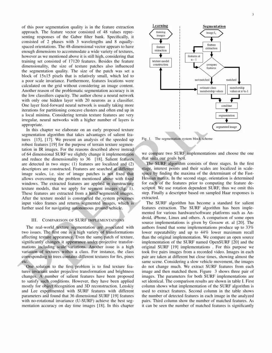
In this chapter we elaborate on an early proposed texturesegmentation algorithm that takes advantages of salient fea-tures [15], [17]. We present an analysis of the speeded uprobust features [19] for the purpose of terrain texture segmen-tation in IR images. For the reasons described above insteadof 64 dimensional SURF we slightly change it implementationand reduce the dimensionality to 36 [18]. Salient featuresare detected in two steps: (1) features are localized and (2)descriptors are constructed. Features are searched at differentimage scales, i.e. size of image patches is not fixed thatallows overcoming the problem mentioned above with fixedwindows. The extracted features are applied in constructingtexture models, that we apply for segment images (fig. 1).These features are extracted from a hand segmented images.After the texture model is constructed the system processesinput video frames and returns segmented images, which isfurther used for navigating autonomous ground vehicle.

III. COMPARISON OF SURF IMPLEMENTATIONS

The real-world texture segmentation are associated withtwo issues. The first one is a high variety of transformationsaffecting texture appearance. Even the same patch of texture,significantly changes it appearance under projective transfor-mations including scale variations. Another issue is a highvariation of textures within a class. For instance, the classcorresponding to trees contains different textures for firs, pinesetc.

One solution to the first problem is to find texture fea-tures invariant under projective transformation and brightnesschanges. A number of salient features have been proposedto satisfy such conditions. However, they have been appliedmostly for object recognition and 3D reconstruction. Lenskiyand Lee experimented with SURF features with differentparameters and found that 36 dimensional SURF [19] featureswith no-rotational invariance (U-SURF) achieve the best seg-mentation accuracy on day time images [18]. In this chapter

Fig. 1. The segmentation system block scheme

we compare two SURF implementations and choose the onethat suits our goals best.

The SURF algorithm consists of three stages. In the firststage, interest points and their scales are localized in scale-space by finding the maxima of the determinant of the Fast-Hessian matrix. In the second stage, orientation is determinedfor each of the features prior to computing the feature de-scriptor. We use rotation dependent SURF, thus we omit thisstep. Finally a descriptor based on sampled Haar responses isextracted.

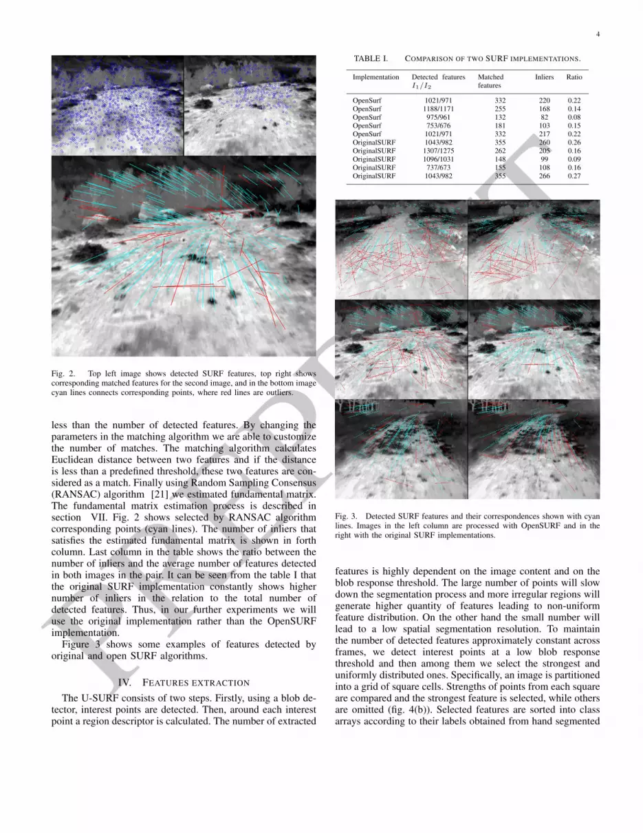
The SURF algorithm has become a standard for salientfeatures extraction. The SURF algorithm has been imple-mented for various hardware/software platforms such as An-droid, iPhone, Linux and others. A comparison of some opensource implementations is given by Gossow et. al [20]. Theauthors found that some implementations produce up to 33%lower repeatability and up to 44% lower maximum recallthan the original implementation. We compare an open sourceimplementation of the SURF named OpenSURF [20] and theoriginal SURF [19] implementations . For this purpose wetook five pairs images from a recorded video. Images in eachpair are taken at different but close times, showing almost thesame scene. Considering a slow vehicle movement, the imagesdo not change much. We extract SURF features from eachimage and then matched them. Figure 3 shows three pair ofimages. The parameters for both SURF implementations areset identical. The comparison results are shown in table I. Firstcolumn shows what implementation of the SURF algorithm isused to extract features. Second column in the table showsthe number of detected features in each image in the analyzedpairs. Third column show the number of matched features. Asit can be seen the number of matched features is significantly

PREPRINT

4

Fig. 2. Top left image shows detected SURF features, top right showscorresponding matched features for the second image, and in the bottom imagecyan lines connects corresponding points, where red lines are outliers.

less than the number of detected features. By changing theparameters in the matching algorithm we are able to customizethe number of matches. The matching algorithm calculatesEuclidean distance between two features and if the distanceis less than a predefined threshold, these two features are con-sidered as a match. Finally using Random Sampling Consensus(RANSAC) algorithm [21] we estimated fundamental matrix.The fundamental matrix estimation process is described insection VII. Fig. 2 shows selected by RANSAC algorithmcorresponding points (cyan lines). The number of inliers thatsatisfies the estimated fundamental matrix is shown in forthcolumn. Last column in the table shows the ratio between thenumber of inliers and the average number of features detectedin both images in the pair. It can be seen from the table I thatthe original SURF implementation constantly shows highernumber of inliers in the relation to the total number ofdetected features. Thus, in our further experiments we willuse the original implementation rather than the OpenSURFimplementation.

Figure 3 shows some examples of features detected byoriginal and open SURF algorithms.

IV. FEATURES EXTRACTION

The U-SURF consists of two steps. Firstly, using a blob de-tector, interest points are detected. Then, around each interestpoint a region descriptor is calculated. The number of extracted

TABLE I. COMPARISON OF TWO SURF IMPLEMENTATIONS.

Implementation Detected featuresI1/I2

Matchedfeatures

Inliers Ratio

OpenSurf 1021/971 332 220 0.22OpenSurf 1188/1171 255 168 0.14OpenSurf 975/961 132 82 0.08OpenSurf 753/676 181 103 0.15OpenSurf 1021/971 332 217 0.22OriginalSURF 1043/982 355 260 0.26OriginalSURF 1307/1275 262 205 0.16OriginalSURF 1096/1031 148 99 0.09OriginalSURF 737/673 155 108 0.16OriginalSURF 1043/982 355 266 0.27

Fig. 3. Detected SURF features and their correspondences shown with cyanlines. Images in the left column are processed with OpenSURF and in theright with the original SURF implementations.

features is highly dependent on the image content and on theblob response threshold. The large number of points will slowdown the segmentation process and more irregular regions willgenerate higher quantity of features leading to non-uniformfeature distribution. On the other hand the small number willlead to a low spatial segmentation resolution. To maintainthe number of detected features approximately constant acrossframes, we detect interest points at a low blob responsethreshold and then among them we select the strongest anduniformly distributed ones. Specifically, an image is partitionedinto a grid of square cells. Strengths of points from each squareare compared and the strongest feature is selected, while othersare omitted (fig. 4(b)). Selected features are sorted into classarrays according to their labels obtained from hand segmented

PREPRINT

5

Fig. 4. a) Hand segmented image, b) Detected features, selected featuresare circled. Blue, green and dark red features represent trees, grass and roadcorrespondingly.

maps (fig. 4(a)). We considered three terrain classes: a) grassand small shrubs, b) trees and c) road including gravel andsoil. Among 3506 video frames, we selected 70 frames fortraining purposes and 10 for testing. Overall 45361 featureswere extracted from the training images.

Lenskiy and Lee [18] analyzed a number of classifiersfor the purpose of SURF features classification. A classifierbased on the multilayer perceptron(MLP) was found to be themost suitable in terms of classification accuracy, memory andprocessing time requirements. Although, the MLP is able togeneralize and classify complex domains of data, some datapreprocessing must be performed. The necessity comes fromthe fact that terrains of different classes are often mixing upmaking it impossible to separate one terrain region from theothers even by a human. Therefore, a hand segmented regionoften contains fragments of a few types. To exclude featuresrepresenting such fragments as well as non-informative fea-tures we omit those of them which reside far apart from thefeatures of its own class [18]. After excluding such featureswe are left with 41887 features, specifically 9080, 5852 and26955 features in grass, trees and road classes correspondingly.

For the purpose of analyzing how good terrain classes areseparated in the SURF features space we divided the wholetraining set into two subsets. The first subset consists offeatures surrounded by at least three/five neighbors of thesame class. We call this subset a dense subset. The secondsubset contains all the remaining features. The number offeatures when at least three neighbors are of the same classis equal to 16705 (40%), the number of remaining features is25182 (60%). When at least five neighbors are of the sameclass, there are 16494 (40%) features in the dense subset and25393 (60%) features in the non-dense subsets. To check howwell features from different terrain classes are separated wecalculated interclass and intraclass variability as follows:

ν(x, y) =1

N1N2

N1∑i=1

N2∑j=1

√√√√ 36∑k=1

(xi,k − yj,k)2 (1)

where x, y are feature sets, N1 and N2 are number offeatures in feature sets x and y respectively.

Tables II show estimated variability for the whole trainingset, for the non-dense and dense subsets respectively. Valueson the main diagonal represent interclass variabilities, and the

TABLE II. INTER- AND INTRACLASS VARIANCE FOR THE WHOLETRAINING FEATURE SET.

grass trees road

grass 0.79 0.85 0.77trees 0.85 0.83 0.79road 0.77 0.79 0.69

TABLE III. INTER- AND INTRACLASS VARIANCE FOR THE NON-DENSEFEATURE SUBSET.

grass trees road

grass 0.78 0.83 0.77trees 0.83 0.82 0.79road 0.77 0.79 0.74

remaining values represent variabilities between correspondingclasses. As it can be seen in the cases of grass and road fea-tures, values of interclass variabilities are smaller than valuesfor intraclass variability. However, in the case of features fromthe class associated with trees, the interclass variability is notsmaller than the variability calculated between trees and roadclasses even for features from the dense-subset. This althoughdoes not necessary mean that the class is not separable at all,it could be due to non-normal feature distribution. To checkif this is the case we visualize features distribution. We applythe principal component analysis(PCA) to each of two subsetsand select among 36 components two main components. Byplotting two main components of each subset we are able tovisualize the features’ distributions. A solid structure is clearlyrecognizable, that supports the assumption that SURF featuresare suitable for texture classification. Secondly, as it can beseen from the plots(fig 5, b,d), features from the tree classare split up into two clusters. Therefor a nonlinear classifiersuch as the MLP is needed to separate classes.

V. TEXTURE MODEL CONSTRUCTION

As it was mentioned, the number of features in eachclass is relatively large. To generalize and transform the datainto a compact form we applied the MLP . Following thisway, features are transformed into synaptic weights of theMLP, the quantity of synaptic weights is considerably lessthan the number of features multiplied by dimension of theSURF descriptor. Therefore, significant memory reduction andreduction of processing time is achieved.

Moreover, it has been proven that a neural network withone hidden layer with sigmoid activation functions is capableof approximating any function to arbitrarily accuracy [22].However, there is no precise answer on the number of neuronsnecessary for approximation. It was numerically shown [23]

TABLE IV. INTER- AND INTRACLASS VARIATIONS FOR THE DENSEFEATURE SUBSET.

grass trees road

grass 0.81 0.97 0.83trees 0.97 0.87 0.84road 0.83 0.83 0.65

PREPRINT

6

Fig. 5. Dimensionally reduced feature spaces. a) and c) show non-densefeature subset, where for each feature among 5 (a) or 3 (c) its neighbors, oneor more features belong to a different class. b) and d) show dense featuressubset, where among each feature all 5 (b) or 3 (d) neighbors belong to thesame class.

that the MLP with two hidden layers often achieves betterapproximation and requires fewer weights. Fewer weightsmean less likeliness to get caught in local minima, whilesolving the optimization problem that is required in the trainingprocess. Thus, we experimented with the MLP with two hiddenlayers.

The training process is associated with solving a nonlinearoptimization problem. Due to the fact that the error function isnot convex, the training procedure is very likely to end-up ina local minimum. The error function is presented as follows:

ε(w) =∑x

(f(w, x)− class(x))2 −→ min (2)

where f(w, x) is the output of the MLP, x is a trainingset consisted of feature descriptors, and class(x) desired classlabel obtained by hand segmentation. class(x) returns a threedimensional vector, where only one component set to one, andthe others are zeros.

To overcome the problem associated with the trainingprocess a number of minimization algorithms have beensuggested. We experimented with ”resilient propagation”(RPROP) and the ”Levenberg-Marquardt” (LM) training al-gorithms [18]. The former one requires less memory, butneeds a large number of iterations to converge. The latterone converges in less iteration, and usually finds a bettersolution, however it requires a larger amount of memory. Weexperimented with the MLP of the following architecture: 36-40-20-3, where 36 the SURF descriptor dimension, 40 and 20are the numbers of neurons in the first and the second hiddenlayers, and 3 is the number of classes. The decision functionof the MLP with two hidden layer is as follows:

Fig. 6. The structure of a MLP with two hidden layers. m = 3, N1 = 40,N2 = 20, N3 = 3

f(d) =

3∑i=0

w(3)m,i σ

20∑j=0

w(2)i,j σ

(40∑k=0

w(1)j,k dk

) (3)

where σ is a sigmoid activation function, w(m) are interlayerweight matrices. The total number of interlayer weighs is equalto Nw = (36+1)× 40+ (40+1)× 20+ (20+1)× 3 = 2363which is considerably less than the total number of featurecomponents Nc = 41887× 36 = 1507932.

VI. SEGMENTATION PROCEDURE

The segmentation procedure consists of two steps . Firstly,SURF features are extracted from the input images. The outputcomponents can be thought as class membership values. Thesevalues along with features’ spatial positions lk = (xk, yk)are utilized by the segmentation algorithm. The algorithm issummarized in the following list of steps:

VII. FEATURE TRACKING

To decrease the effect of segmentation blinking that iscaused by rapid switching between different terrain types andto speed up segmentation, we match features in the currentframe with features extracted in the previous frame . If acorresponding point is found, the membership values calcu-lated in the previous frame are transferred to correspondingpoints in the current frame. The correspondence is found bycalculating Euclidean distance between feature descriptors incurrent and previous frames. To optimize the calculation time,the searching area in the current frame is restricted by a circledefined by a feature coordinates in the previous frame and aradius r. The feature with a minimum Euclidean distance in the36-dimensional space is considered as a match if the distanceis less than a predefined threshold. Based on the found matchesa fundamental matrix F is estimated. A fundamental matrix Fis the unique 3×3 rank 2 homogeneous matrix which satisfies:

m′TFm = 0 (4)

PREPRINT

7

Algorithm 1 Segmentation algorithmInput: I - image, d - feature descriptor, l - feature position,

t - threshold.1: m = {1, 2, 3}2: for i = 1 to width(I)× height(I) do

Select features located within r around pixel (xi, yi)3: T (xi, yi) =

{l|∥∥(xi, yi)T − lj∥∥ < r, j = 1 . . . N

}Estimate the membership value of a pixel I(xi, yi)

4: Vm((xi, yi)) = 1#(T ((xi,yi)))

∑#(T (xi,yi))k=1 dk ·

1σ√2πe−‖(xi,yi)T−lk‖2

2σ

Assign a class index to the pixel I(xi, yi)5: if t < max (Vm(xi, yi)) then6: S(xi, yi) = argmaxm (Vm(xi, yi))7: else8: S(xi, yi) = 09: end if

10: end forOutput:S

for all corresponding points (m,m′). Another definition of thefundamental matrix is l′ = Fm for the epipolar line l′. Sincem′ belong to l′, m′T l′ = 0→ m′TFm = 0 . We only need 8points to solve equation (4) and find F . However, this solutionwould not be robust due to a large number of outliers. To filterthem out and find fundamental matrix the RANSAC algorithmis applied [21]. As soon as a fundamental matrix is estimatedan essential matrix E is calculated in the following manner:

E =WTFW, (5)

where W is a matrix of intrinsic parameters. Then E isdecomposed [24] into P = A[I|0], P ′ = A[R|t]. P andP ′ are calibrated perspective projection matrices (PPM). Usingreconstructed PPMs and feature coordinates we can triangulatethem and obtain 3D coordinates M (fig. 7).

After the metric 3D reconstruction of a current cameraposition and orientation is provided, the prediction of thenext position and orientation can be performed [25]. Then,predicted PPM is applied to previously reconstructed 3D pointsM to obtain a projection onto an image plane. To predictthe cameras position and orientation we use two separatetrackers. For tracking the camera position we use the regularKalman filter [26] and to predict camera orientation we appliedExtended Kalman Filter, where orientation is represented usingquaternion notation [27].

VIII. EXPERIMENTAL RESULTS

To test the segmentation algorithm we run experiments ontwo image sets: the training set and the testing set. The trainingimage set consists of 70 images, and the testing set contains10 images. We experimented with he MLP trained with theRPROP and LM algorithms. The mean, standard deviation,minimum and maximum segmentation error rates are shownin table V.

The lowest error rate is achieved with the nearest neighborclassifier (NN). The NN classifier looks for a nearest feature

Fig. 7. a) Detected SURF features from a first image in the image pair, b)Reconstructed points from a pair of frames, green squares represent positionsof the cameras, and the blue circle shows predicted position of the camera

TABLE V. ERROR RATES USING DIFFERENT CLASSIFIERS AND DATASETS

Classifier mean std min max

NN (training set) 5.03 1.66 2.89 10.7MLP 40-20 LM(training set) 15.25 5.26 7.27 29.31MLP 40-20 RPROP(training set) 18.90 6.42 8.95 37.30NN (test set) 16.67 9.17 9.86 32.1MLP 40-20 LM (test set) 19.1 10.39 12.5 37.52MLP 40-20 RPROP(test set) 21.51 9.72 13.14 38.29

and classifies a feature of interest to the nearest feature′s class.The distance to the nearest feature is used to calculate thestrength associated with the assigned class [18]. The NNclassifier uses during classification all training samples, asa result the segmentation error on the training set is thelowest compared to the MLP classifier. On the other handMLP converts the training set into a compact set of interlayerweights that considerably reduce memory requirements anddecreases calculation time. The MLP trained by the LMalgorithm shows comparably lower segmentation error ratesfollowed by the MLP trained by RPROP . In [17] a networkwith 40 neurons in each hidden layer was trained with theLM algorithm. Here we reduced the number of neurons inthe second hidden layer to 20. We noticed that each timethe network is retrained different segmentation accuracy isobtained. Moreover the increase of number of neurons upto 60 neurons in each hidden layer (experiments not shown)did not lead to better quality of segmentation. On reason, isthat the learning algorithms gets stuck in a local minimum asmore variable/weights makes the optimization problem morecomplex. Another reason is poorer generalization of a networkwith larger number of weights. In this case the networkmemorizes noisy data. The segmentation results obtained withthe NN and MLP trained by the LM and RPROP algorithmsare shown in figures 8, 9 and 10.

The lowest error rate is achieved with the nearest neighborclassifier (NN). The MLP trained by LM algorithm showscomparably low segmentation error rate followed by the MLPtrained by RPROP. In [17] a network with 40 neurons in eachhidden layer was employed. Here we reduced the number ofneurons in the second hidden layer to 20. We noticed that eachtime the network is retrained different segmentation accuracyis obtained.

PREPRINT

8

Fig. 8. The first and second rows show segmentation results obtained forthe test and training images respectively, when nearest neighbor classifier wasapplied.

Fig. 9. The first and second rows show segmentation results obtained forthe test and training images respectively, when MLP classifier trained by LMalgorithm was applied.

IX. CONCLUSIONS

Besides comparing the original and the open SURF imple-mentations, we found that the ratio of the number of extractedfeatures to the number of correctly detected correspondingpoints is higher for upright version of the original implementa-tion than for the OpenSURF implementation. We demonstratedthat 36 dimensional SURF features indeed carries meaningfulinformation applicable for terrain segmentation. We appliedsegmentation algorithm that extracts 36 dimensional SURFfeatures and estimates class membership values for each pixel.Three terrain classes: grass, bushes and trees have been con-sidered. The proposed segmentation approach effectively sup-

Fig. 10. The first and second rows show segmentation results obtained forthe test and training images respectively, when MLP classifier trained by RPalgorithm was applied.

plements those vision systems that use salient features for 3Dreconstruction and object recognition. Among classification al-gorithms we tested the MLP trained by the LM and RPROPtraining algorithms, and the nearest neighbour algorithm. Thesegmentation system based on the network estimator showsslightly higher segmentation error rates compared to the esti-mator based on nearest neighbor algorithm. Nevertheless, thenumber of interconnecting weights is significantly lower thanthe number of training samples, which results in considerablememory and computational savings.

REFERENCES

[1] Lalonde, J.-F., et al., Natural terrain classification using three-dimensional lidar data for ground robot mobility. Journal of FieldRobotics, 2006. 23: p. 839 - 861.

[2] Manduchi, R., Learning Outdoor Color Classification. IEEE Transac-tions on pattern analysis and machine intelligence, 2006. 28(11): p.1713-1723.

[3] Manduchi, R., et al., Obstacle detection and terrain classifcation forautonomous off-road navigation. Autonomous Robot, 2005. 18: p.81102.

[4] Jansen, P., et al. Colour based Off-Road Environment and TerrainType Classification. in 8th International IEEE Conference on IntelligentTransportation Systems. 2005.

[5] Sung, G.-Y., D.-M. Kwak, and J. Lyou, Neural Network Based Ter-rain Classification Using Wavelet Features. Journal of Intelligent andRobotic Systems, 2010.

[6] Castano, R., R. Manduchi, and J. Fox. Classification experimentson real-world texture. in Third Workshop on Empirical EvaluationMethods in Computer Vision. 2001. Kauai, Hawaii.

[7] Lee, T.S., Image Representation Using 2D Gabor Wavelets. IEEETransactions on pattern analysis and machine intelligence, 1996. 18.

[8] Kang, Y., et al., Texture Segmentation of Road Environment SceneUsing SfM Module and HLAC Features. IPSJ Transaction on ComputerVision and Applications, 2009. 1: p. 220-230.

PREPRINT

9

[9] Kurita, T. and N. Otsu. Texture Classification by Higher Order LocalAutocorrelation Features. in Asian Conference on Computer Vision.1993.

[10] Otsu, N. and T. Kurita. A New Scheme for Practical Flexible andIntelligent Vision Systems. in IAPR Workshop on Computer Vision.1988.

[11] Blas, M.R., et al. Fast color/texture segmentation for outdoor robots.in International Conference on Intelligent Robots and Systems. 2008.Nice, France.

[12] Konolige, K., et al., Mapping, Navigation, and Learning for Off-RoadTraversal. Journal of Field Robotics, 2009. 26(1): p. 88-113.

[13] Lensky, A.A., et al. Terrain images segmentation and recognition usingSIFT feature histogram. in 3rd Workshop on military robots. 2008.KAIST: Adgency for Defence Development.

[14] Lowe, D.G., Object recognition from local scale-invariant features.Proceedings of the International Conference on Computer Vision, 1999.1: p. 1150-1157.

[15] Lenskiy, A.A. and J.-S. Lee. Rugged terrain segmentation based onsalient features in International Conference on Control, Automationand Systems 2010 2010. Gyeonggi-do, Korea

[16] Rasmussen, C. Combining Laser Range, Color, and Texture Cues forAutonomous Road Following. in International Conference on Robotics& Automation. 2002. Washington, DC.

[17] Lenskiy, A.A. and J.-S. Lee. Terrain images segmentation in infra-red spectrum for autonomous robot navigation in IFOST 2010. 2010.Ulsan, Korea.

[18] Lenskiy, A.A. and J.-S. Lee, Machine learning algorithms for visualnavigation of unmanned ground vehicles, in Computational Modelingand Simulation of Intellect: Current State and Future Perspectives, B.Igelnik, Editor 2011, IGI Global.

[19] Bay, H., et al., Speeded-Up Robust Features (SURF). Computer Visionand Image Understanding, 2008. 110(3): p. 346-359.

[20] Gossow, D., D. Paulus, and P. Decker. An Evaluation of Open SourceSURF Implementations. in RoboCup 2010: Robot Soccer World CupXIV. 2010.

[21] Fischler, M.A. and R.C. Bolles, Random Sample Consensus: AParadigm for Model Fitting with Applications to Image Analysis andAutomated Cartography. Comm. Of the ACM 1981. 24: p. 381-395.

[22] Cybenko, G., Approximation by superposition of a sigmoidal function.Math. Control. Signals, Syst., 1989. 2: p. 303-314.

[23] Chester, D.L. Why Two Hidden Layers are Better than One. in Proc.Int. Joint Conf. Neural Networks. 1990. Washington, DC.

[24] Hartley, R. and A. Zisseman, Multiple View Geometry in ComputerVision, Second Edition 2003: Cambridge University Press.

[25] Lensky, A.A., , and J.S. Lee. Tracking feature points in static environ-ment. in Conference on Ground Weapons 2009. Daejon, South Korea.

[26] Brown, R.G. and P.Y.C. Hwang, Introduction to Random Signals andApplied Kalman Filtering with MATLAB Exercises and Solutions1997:John Wiley & Sons. 496.

[27] Goddard, J.S., Pose and Motion Estimation From Vision Using DualQuaternion-based extended Kalman Filtering, 1997, The University ofTennessee: Knoxville.