dynamosaicing: mosaicing of dynamic scenes

Dynamosaicing: Mosaicing of Dynamic ScenesAlex Rav-Acha, Student Member, IEEE, Yael Pritch,

Dani Lischinski, and Shmuel Peleg, Member, IEEE

Abstract—This paper explores the manipulation of time in video editing, which allows us to control the chronological time of events.

These time manipulations include slowing down (or postponing) some dynamic events while speeding up (or advancing) others. When a

video camera scans a scene, aligning all the events to a single time interval will result in a panoramic movie. Time manipulations are

obtained by first constructing an aligned space-time volume from the input video, and then sweeping a continuous 2D slice (time front)

through that volume, generating a new sequence of images. For dynamic scenes, aligning the input video frames poses an important

challenge. We propose to align dynamic scenes using a new notion of “dynamics constancy,” which is more appropriate for this task than

the traditional assumption of “brightness constancy.” Another challenge is to avoid visual seams inside moving objects and other visual

artifacts resulting from sweeping the space-time volumes with time fronts of arbitrary geometry. To avoid such artifacts, we formulate the

problem of finding optimal time front geometry as one of finding a minimal cut in a 4D graph, and solve it using max-flow methods.

Index Terms—Video mosaicing, dynamic scene, video editing, graph cuts, panoramic mosaicing, time manipulations, space-time

volume.

Ç

1 INTRODUCTION

IN traditional video mosaicing, a panoramic still image iscreated from video captured by a camera scanning a

scene. The resulting panoramic image shows simulta-neously objects that were photographed at different times.The observation that traditional mosaicing does not keepthe original time of events helps us to generate richerrepresentations of scenes.

Imagine a person standing in the middle of a crowdedsquare looking around. When requested to describe hisdynamic surroundings, he will usually describe ongoingactions. For example, “some people are talking in thesouthern corner, others are eating in the north,” etc. Thiskind of description ignores the chronological order in whicheach activity was observed, focusing on the activitiesthemselves instead.

The same principle of manipulating the progression oftime while relaxing the chronological constrains may be usedto obtain a flexible representation of dynamic scenes. It allowsus not only to postpone or advance some activities, but also tomanipulate their speed. Dynamic panoramas are indeed themost natural extension of panoramic mosaicing. But, dy-namic mosaicing can be used also with a video taken from astatic camera where we present a scheme to control the timeprogress for individual objects. We will start the descriptionof temporal video manipulations in the case of a static camera,before we will continue to the case of dynamic panorama.

In our framework, the input video is represented as analigned space-time volume. The time manipulations weexplore are those that can be obtained by sweeping a 2D slice

(time front) through the space-time volume, generating a newsequence of images.

In order to analyze and manipulate videos of dynamicscenes, several challenging problems must be addressed:The first one is the stabilization of the input video sequence.In many cases, the field of view of the camera includesmostly dynamic regions, when even robust alignmentmethods fail. The second problem is that time slices in thespace-time volume may pass through moving objects. As aresult, visual seams and other visual artifacts may occur inthe resulting movie. To reduce such artifacts, we use image-based optimization of the time fronts which favors seamlessstitching. This optimization problem is formulated as one offinding the minimal cut in a 4D graph.

1.1 Related Work

The most popular approach for the mosaicing of dynamicscenes is to compress all the scene information into a singlestatic mosaic image. There are numerous methods fordealing with scene dynamics in the static mosaic. Someapproaches eliminate all dynamic information from thescene, as dynamic changes between images are undesired[25]. Other methods encapsulate the dynamics of the sceneby overlaying several snapshots of the moving objects intothe static mosaic, resulting in a “stroboscopic” effect [15],[12], [1]. In contrast to these methods that generate a singlestill mosaic image, we use mosaicing to generate a dynamicvideo sequence having a desired time manipulation.

The mechanism of slicing through a stack of images (whichis essentially the space-time volume) is similar to video-cubes[16], which produces composite still images, and to panora-mic stereo [20], [30]. Unlike these methods, dynamosaics aregenerated by coupling the scene dynamics, the motion of thecamera, and the shape and the motion of the time front.

In [18], [9], two videos of dynamic textures (or the samevideo with two different temporal shifts) are being stitchedseamlessly side by side, yielding a movie with a larger fieldof view. In this work we are interested in more general time

IEEE TRANSACTIONS ON PATTERN ANALYSIS AND MACHINE INTELLIGENCE, VOL. 29, NO. 10, OCTOBER 2007 1789

. The authors are with the School of Computer Science and Engineering, TheHebrew University of Jerusalem, Ross Building, Giva Ram, 91904Jerusalem, Israel. E-mail: {alexis, yaelpri, danix, peleg}@cs.huji.ac.il.

Manuscript received 21 May 2006; revised 6 Oct. 2006; accepted 7 Dec. 2006;published online 18 Jan. 2007.Recommended for acceptance by M. Pollefeys.For information on obtaining reprints of this article, please send e-mail to:[email protected], and reference IEEECS Log Number TPAMI-0389-0506.Digital Object Identifier no. 10.1109/TPAMI.2007.1091.

0162-8828/07/$25.00 � 2007 IEEE Published by the IEEE Computer Society

manipulations, in which the edited movies combineinformation from many frames of the input sequence.

The basic idea of dynamosaicing was presented in anearlier paper [22]. Since dynamosaicing is concerned withdynamic scenes and since dynamic scenes present chal-lenges both in alignment and in stitching, these topics areexpanded substantially in this paper. A different approachtoward seamless stitching in the case of dynamic textures(with the ability to produce infinite loops) was suggested in[2]. A discussion on the differences between the twoapproaches appears in Section 4.

1.2 An Overview of Dynamosaicing

Given a sequence of input video frames I1; . . . ; IN , they arefirst registered and aligned to a global spatial coordinatesystem. A specialized alignment scheme for sequences ofdynamic scenes is described in Section 2, but otherstabilization methods can sometimes be used (e.g., [5], [24]).

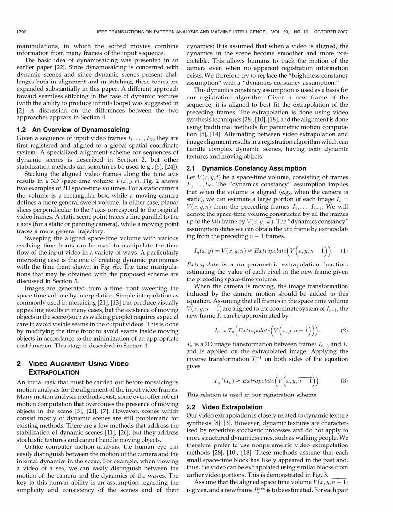
Stacking the aligned video frames along the time axisresults in a 3D space-time volume V ðx; y; tÞ. Fig. 2 showstwo examples of 2D space-time volumes. For a static camerathe volume is a rectangular box, while a moving cameradefines a more general swept volume. In either case, planarslices perpendicular to the t axis correspond to the originalvideo frames. A static scene point traces a line parallel to thet axis (for a static or panning camera), while a moving pointtraces a more general trajectory.

Sweeping the aligned space-time volume with variousevolving time fronts can be used to manipulate the timeflow of the input video in a variety of ways. A particularlyinteresting case is the one of creating dynamic panoramaswith the time front shown in Fig. 6b. The time manipula-tions that may be obtained with the proposed scheme arediscussed in Section 3.

Images are generated from a time front sweeping thespace-time volume by interpolation. Simple interpolation ascommonly used in mosaicing [21], [13] can produce visuallyappealing results in many cases, but the existence of movingobjects in the scene (such as walking people) requires a specialcare to avoid visible seams in the output videos. This is doneby modifying the time front to avoid seams inside movingobjects in accordance to the minimization of an appropriatecost function. This stage is described in Section 4.

2 VIDEO ALIGNMENT USING VIDEO

EXTRAPOLATION

An initial task that must be carried out before mosaicing ismotion analysis for the alignment of the input video frames.Many motion analysis methods exist, some even offer robustmotion computation that overcomes the presence of movingobjects in the scene [5], [24], [7]. However, scenes whichconsist mostly of dynamic scenes are still problematic forexisting methods. There are a few methods that address thestabilization of dynamic scenes [11], [26], but they addressstochastic textures and cannot handle moving objects.

Unlike computer motion analysis, the human eye caneasily distinguish between the motion of the camera and theinternal dynamics in the scene. For example, when viewinga video of a sea, we can easily distinguish between themotion of the camera and the dynamics of the waves. Thekey to this human ability is an assumption regarding thesimplicity and consistency of the scenes and of their

dynamics: It is assumed that when a video is aligned, thedynamics in the scene become smoother and more pre-dictable. This allows humans to track the motion of thecamera even when no apparent registration informationexists. We therefore try to replace the “brightness constancyassumption” with a “dynamics constancy assumption.”

This dynamics constancy assumption is used as a basis forour registration algorithm: Given a new frame of thesequence, it is aligned to best fit the extrapolation of thepreceding frames. The extrapolation is done using videosynthesis techniques [28], [10], [18], and the alignment is doneusing traditional methods for parametric motion computa-tion [5], [14]. Alternating between video extrapolation andimage alignment results in a registration algorithm which canhandle complex dynamic scenes, having both dynamictextures and moving objects.

2.1 Dynamics Constancy Assumption

Let V ðx; y; tÞ be a space-time volume, consisting of framesI1; . . . ; IN . The “dynamics constancy” assumption impliesthat when the volume is aligned (e.g., when the camera isstatic), we can estimate a large portion of each image In ¼V ðx; y; nÞ from the preceding frames I1; . . . ; In�1. We willdenote the space-time volume constructed by all the framesup to the kth frame by V ðx; y; k!Þ. The “dynamics constancy”assumption states we can obtain the nth frame by extrapolat-ing from the preceding n� 1 frames,

Inðx; yÞ ¼ V ðx; y; nÞ � Extrapolate V x; y; n� 1��!� ��

: ð1Þ

Extrapolate is a nonparametric extrapolation function,estimating the value of each pixel in the new frame giventhe preceding space-time volume.

When the camera is moving, the image transformationinduced by the camera motion should be added to thisequation. Assuming that all frames in the space time volumeV ðx; y; n� 1

��!Þ are aligned to the coordinate system of In�1, thenew frame In can be approximated by

In � Tn Extrapolate V x; y; n� 1��!� ��

: ð2Þ

Tn is a 2D image transformation between frames In�1 and Inand is applied on the extrapolated image. Applying theinverse transformation T�1

n on both sides of the equationgives

T�1n ðInÞ � Extrapolate V x; y; n� 1

��!� �� : ð3Þ

This relation is used in our registration scheme.

2.2 Video Extrapolation

Our video extrapolation is closely related to dynamic texturesynthesis [8], [3]. However, dynamic textures are character-ized by repetitive stochastic processes and do not apply tomore structured dynamic scenes, such as walking people. Wetherefore prefer to use nonparametric video extrapolationmethods [28], [10], [18]. These methods assume that eachsmall space-time block has likely appeared in the past and,thus, the video can be extrapolated using similar blocks fromearlier video portions. This is demonstrated in Fig. 3.

Assume that the aligned space time volume V ðx; y; n� 1��!Þ

is given, and a new frame Ipredn is to be estimated. For each pair

1790 IEEE TRANSACTIONS ON PATTERN ANALYSIS AND MACHINE INTELLIGENCE, VOL. 29, NO. 10, OCTOBER 2007

of space-time blocks Wp and Wq, we define the SSD (sum ofsquare differences) to be:

dðWp;WqÞ ¼Xðx;y;tÞðWpðx; y; tÞ �Wqðx; y; tÞÞ2: ð4Þ

As shown in Fig. 3, for each pixel ðx; yÞ in frame In�1 wedefine a 3D space-time block Wx;y;n�1 whose spatial center isat pixel ðx; yÞ and whose temporal boundary is at time n� 1(frames which were not aligned yet can not be used). Wethen search in the space time volume V ðx; y; n� 2

��!Þ for aspace-time block with the minimal SSD to block Wx;y;n�1.Let Wp ¼W ðxp; yp; tpÞ be the most similar block, spatiallycentered at pixel ðxp; ypÞ and temporally bounded by tp. Thevalue of the extrapolated pixel Ipredn ðx; yÞ will be taken fromV ðxp; yp; tp þ 1Þ, the pixel that appeared immediately afterthe most similar block. This scheme follows the “dynamicsconstancy” assumption: Given that two different space timeblocks are similar, we assume that their continuations arealso similar. While a naive search for each pixel may beexhaustive, the scheme can be significantly accelerated byfocusing on a smaller set of image features. Additionalmodifications can further accelerate the process [23].

We used the SSD (sum of squared differences) as adistance measure between two space-time blocks, but otherdistance measures can be used such as the sum of absolutedifferences or more sophisticated measures [28]. We did notnotice a substantial difference in registration results whenchanging the distance measure.

2.3 Alignment with Video Extrapolation

Alignment with video extrapolation can be described by thefollowing steps:

1. Assume that the motion of the first K frames hasalready been computed, and let n ¼ K þ 1.

2. Align all frames in the space time volume

V ðx; y; ðn� 1Þ��!

Þ to the coordinate system of Frame In�1.3. Estimate the next new frame by extrapolation from

the previous frames

Ipredn ¼ Extrapolate V x; y; ðn� 1Þ��!� ��

:

4. Compute the motion parameters (the global2D image transformation T�1

n ) by aligning thenew input frame In to the extrapolated frame Ipredn .

5. Increase n by 1 and return to Step 2. Repeat untilreaching the last frame of the sequence.

The global 2D image alignment in Step 2, as well as theinitialization step, are performed using direct methods forparametric motion computation [5], [14]. We usually used amotion model having image rotation and translation, whichgave good results in the case of rotating cameras. Objectswith depth parallax can be treated as moving objects whenthe camera motion varies slowly.

The initialization, in which the motion of the firstK framesis computed, is done as follows: The entire video sequence isscanned to find K consecutive frames which are best suitedfor traditional alignment methods, e.g., frames where motioncomputation converges and having the smallest residualerror. We used Lucas-Kanade alignment on blurred frames[5]. From theseK frames, video extrapolation continues in thepositive and negative time directions.

2.4 Masking Unpredictable Regions

Real scenes always have a few regions that can not bepredicted. For example, people walking in the street oftenchange their behavior in an unpredictable way, e.g., raisingtheir hands or changing their direction. In these cases, thevideo extrapolation will fail, resulting in outliers. Thealignment can be improved by masking out unpredictableregions.

This is done as follows: After the new input image In isaligned with the extrapolated image Ipredn which estimated it,the color difference between the two images is computed.Each pixel ðx; yÞ is masked out if the color difference in itsneighborhood is higher than some threshold r (We usuallyused r ¼ 1.) P

ðIn � Ipredn Þ2PI2x þ I2

y

> r: ð5Þ

The predictability mask is used in the alignment of frameInþ1 to frame Iprednþ1 .

2.5 Fuzzy Estimation

The alignment may be further improved by using fuzzyestimation.This isdonebykeepingnotonly thebestcandidatefor extrapolating each pixel, but the best S candidates (weused up to five candidates for each pixel). The multipleestimations for extrapolating each pixel can be combinedusing a summation of the error terms

Tn ¼ arg minT

Xx;y;s

�x;y;sðT�1n ðInÞðx; yÞ � Ipredn ðx; y; sÞÞ2

( ); ð6Þ

where Ipredn ðx; y; sÞ is the sth candidate for the value of thepixel Inðx; yÞ. The weight �x;y;s of each candidate is based onthe difference of its corresponding space-time cube from thecurrent one as defined in (4) and is given by

�x;y;s ¼ e�dðWp;Wq Þ2

2�2 :

We almost always used 7� 7� 7 space-time cubes and � ¼1=255 to reflect the noise in the image gray levels. Note thatthe weights for each pixel do not necessarily sum to one and,therefore, the registration mostly relies on the predictableregions. Also, other ways to combine different predictions arealso possible.

2.6 Handling Alignment Drift

Alignment based on video extrapolation follows Newton’sFirst Law: An object in uniform motion tends to remain in thatstate. If we initialize our registration algorithm with a smallmotion relative to the real camera motion, our method willcontinue this motion for the entire video. In this case, thebackground will be handled as a slowly moving object. This isnot a bug in the algorithm, but rather a degree of freedomresulting from the “dynamics constancy” assumption.

This degree of freedom can be eliminated by incorporatinga prior bias, assuming that part of the scene is static. This isdone by adding a new predictive static candidate S þ 1 atevery pixel (by simply copying the value of the previousframe). In our experiments, we gave a small weight of 0.1 tothe static candidate relative to the total weight of the pixel. Inthis way, we have prevented the drift without effecting theaccuracy of the motion computations.

RAV-ACHA ET AL.: DYNAMOSAICING: MOSAICING OF DYNAMIC SCENES 1791

2.7 Examples

The sequence shown in Fig. 4 was used by [26] and by [11]as an example for their registration of dynamic textures.The global motion in this sequence is a horizontaltranslation and the true displacement can be computedfrom the motion of one of the flowers. The displacementerror reported by [26] was 29.4 percent of the totaldisplacement between the first and last frames, while theerror of our methods was only 1.7 percent.

Fig. 5 shows an examples of video registration usingextrapolation in a challenging scene. In this scene, maskingout the unpredictable regions (parts of the falls and thefumes), as described in Section 2.4, was important forobtaining a good registration.

3 EVOLVING TIME FRONTS

3.1 Mosaicing by an Evolving Time Front

Image mosaicing is the process of creating novel images byselecting patches from the frames of the input sequence andcombining them to form a new image ([21], [13], [1] are just afew examples of the wide literature on mosaicing). It can bedescribed by a functionMðx; yÞ that maps each pixel ðx; yÞ inthe output imageS to the input frame from which this pixel istaken and its location in that frame. In this work, we focusonly on temporal warping, that is Sðx; yÞ ¼ V ðx; y;Mðx; yÞÞ,

where V ðx; y; tÞ is the aligned space-time volume. Thisfunction can be represented by a continuous slice (time slice)in the space-time volume as illustrated in Fig. 6. A time slicedetermines the mosaic patches by its intersection with theframes of the original sequence at the original discrete timevalues (shown as dashed lines in Fig. 6).

To get a desired time manipulation we specify anevolving time front: A free-form surface that deforms as itsweeps through the space-time volume. Taking snapshotsof this surface at different times results in a sequence oftime slices that are represented by temporal-shift functionsSkðx; yÞ ¼ V ðx; y;Mkðx; yÞÞ.

3.2 What Time Manipulations Can Be Obtained?

In this section, we describe the manipulation of chronologicaltime versus local time using dynamosaicing. We first describethe dynamic panoramas, where the chronological time iseliminated. This application inspired this work. We thenshow other applications where a video should be edited in away that changes the chronological order of events in thescene. The realistic appearance of the movie is kept bypreserving the time flow locally, even when the globalchronological time is being changed.

3.2.1 Panoramic Dynamosaicing

Panoramic dynamosaics may be generated using theapproach described above with the time slices shown inFig. 6b. Assuming that the camera is scanning the scene fromleft to right, the first mosaic in the sequence will beconstructed from strips taken from the right side of eachinput frame, showing regions as they first appear in the fieldof view (see Fig. 7). The last mosaic in the resulting sequencewill be the mosaic image generated from the strips on the left,just before a region disappears from the field of view.Between these two marginal slices of the space-time volume,we take intermediate slices, smoothly showing regions fromtheir appearance to their disappearance. Each of the mosaicimages is a panoramic image and the resulting movie is adynamic panorama in which local time is preserved. Fig. 1shows a single panorama from such a movie.

Panoramic dynamosaics represent the elimination of thechronological time of the scanning camera. Instead, allregions appear simultaneously according to the local timeof their visibility period: From their first appearance to theirdisappearance. But, there is more to time manipulation thaneliminating the chronological time.


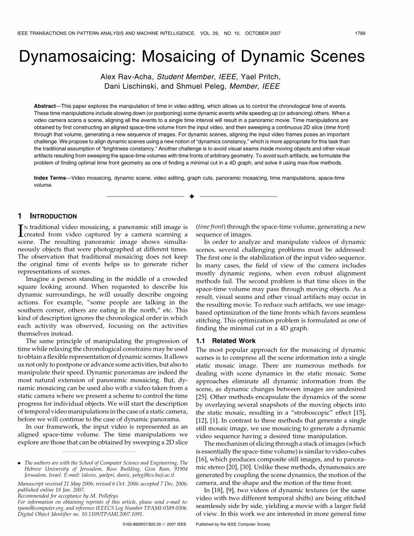
Fig. 1. Dynamosaicing can create dynamic panoramic movies of a scene. This figure shows a single frame in a panoramic movie, generated from a

video taken by a panning camera (420 frames). When the movie is played (see www.vision.huji.ac.il/dynmos), the entire scene comes to life, and all

water flows down simultaneously.

Fig. 2. Two-dimensional space-time volumes: Each frame is repre-

sented by a 1D row and the frames are aligned along the global x axis.

(a) A static camera defines a rectangular space-time region, while (b) a

moving camera defines a more general swept volume.

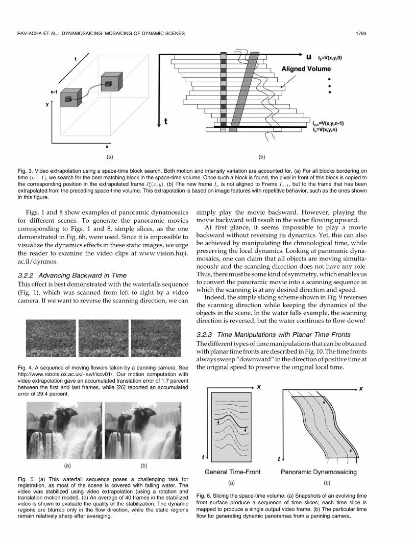
Figs. 1 and 8 show examples of panoramic dynamosaics

for different scenes. To generate the panoramic movies

corresponding to Figs. 1 and 8, simple slices, as the one

demonstrated in Fig. 6b, were used. Since it is impossible to

visualize the dynamics effects in these static images, we urge

the reader to examine the video clips at www.vision.huji.

ac.il/dynmos.

3.2.2 Advancing Backward in Time

This effect is best demonstrated with the waterfalls sequence

(Fig. 1), which was scanned from left to right by a video

camera. If we want to reverse the scanning direction, we can

simply play the movie backward. However, playing themovie backward will result in the water flowing upward.

At first glance, it seems impossible to play a moviebackward without reversing its dynamics. Yet, this can alsobe achieved by manipulating the chronological time, whilepreserving the local dynamics. Looking at panoramic dyna-mosaics, one can claim that all objects are moving simulta-neously and the scanning direction does not have any role.Thus, there must be some kind of symmetry, which enables usto convert the panoramic movie into a scanning sequence inwhich the scanning is at any desired direction and speed.

Indeed, the simple slicing scheme shown in Fig. 9 reversesthe scanning direction while keeping the dynamics of theobjects in the scene. In the water falls example, the scanningdirection is reversed, but the water continues to flow down!

3.2.3 Time Manipulations with Planar Time Fronts

The different types of time manipulations that can be obtainedwithplanar timefrontsaredescribedin Fig.10.Thetimefrontsalways sweep “downward” in the direction of positive time atthe original speed to preserve the original local time.


Fig. 3. Video extrapolation using a space-time block search. Both motion and intensity variation are accounted for. (a) For all blocks bordering ontime ðn� 1Þ, we search for the best matching block in the space-time volume. Once such a block is found, the pixel in front of this block is copied tothe corresponding position in the extrapolated frame Ipnðx; yÞ. (b) The new frame In is not aligned to Frame In�1, but to the frame that has beenextrapolated from the preceding space-time volume. This extrapolation is based on image features with repetitive behavior, such as the ones shownin this figure.

Fig. 4. A sequence of moving flowers taken by a panning camera. Seehttp://www.robots.ox.ac.uk/~awf/iccv01/. Our motion computation withvideo extrapolation gave an accumulated translation error of 1.7 percentbetween the first and last frames, while [26] reported an accumulatederror of 29.4 percent.

Fig. 5. (a) This waterfall sequence poses a challenging task forregistration, as most of the scene is covered with falling water. Thevideo was stabilized using video extrapolation (using a rotation andtranslation motion model). (b) An average of 40 frames in the stabilizedvideo is shown to evaluate the quality of the stabilization. The dynamicregions are blurred only in the flow direction, while the static regionsremain relatively sharp after averaging.

Fig. 6. Slicing the space-time volume: (a) Snapshots of an evolving time

front surface produce a sequence of time slices; each time slice is

mapped to produce a single output video frame. (b) The particular time

flow for generating dynamic panoramas from a panning camera.

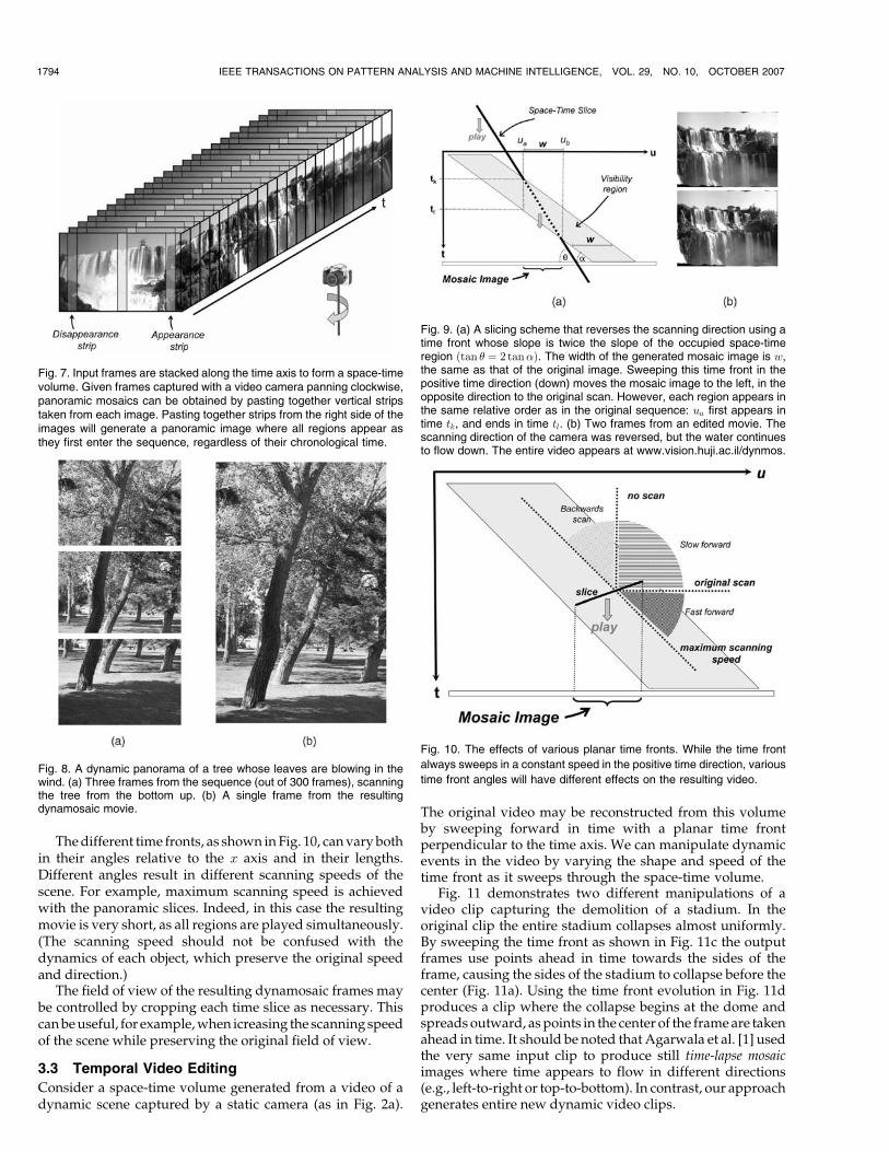
The different time fronts, as shown in Fig. 10, can vary bothin their angles relative to the x axis and in their lengths.Different angles result in different scanning speeds of thescene. For example, maximum scanning speed is achievedwith the panoramic slices. Indeed, in this case the resultingmovie is very short, as all regions are played simultaneously.(The scanning speed should not be confused with thedynamics of each object, which preserve the original speedand direction.)

The field of view of the resulting dynamosaic frames maybe controlled by cropping each time slice as necessary. Thiscan be useful, for example, when icreasing the scanning speedof the scene while preserving the original field of view.

3.3 Temporal Video Editing

Consider a space-time volume generated from a video of adynamic scene captured by a static camera (as in Fig. 2a).

The original video may be reconstructed from this volumeby sweeping forward in time with a planar time frontperpendicular to the time axis. We can manipulate dynamicevents in the video by varying the shape and speed of thetime front as it sweeps through the space-time volume.

Fig. 11 demonstrates two different manipulations of avideo clip capturing the demolition of a stadium. In theoriginal clip the entire stadium collapses almost uniformly.By sweeping the time front as shown in Fig. 11c the outputframes use points ahead in time towards the sides of theframe, causing the sides of the stadium to collapse before thecenter (Fig. 11a). Using the time front evolution in Fig. 11dproduces a clip where the collapse begins at the dome andspreads outward, as points in the center of the frame are takenahead in time. It should be noted that Agarwala et al. [1] usedthe very same input clip to produce still time-lapse mosaicimages where time appears to flow in different directions(e.g., left-to-right or top-to-bottom). In contrast, our approachgenerates entire new dynamic video clips.


Fig. 7. Input frames are stacked along the time axis to form a space-timevolume. Given frames captured with a video camera panning clockwise,panoramic mosaics can be obtained by pasting together vertical stripstaken from each image. Pasting together strips from the right side of theimages will generate a panoramic image where all regions appear asthey first enter the sequence, regardless of their chronological time.

Fig. 8. A dynamic panorama of a tree whose leaves are blowing in thewind. (a) Three frames from the sequence (out of 300 frames), scanningthe tree from the bottom up. (b) A single frame from the resultingdynamosaic movie.

Fig. 9. (a) A slicing scheme that reverses the scanning direction using atime front whose slope is twice the slope of the occupied space-timeregion ðtan � ¼ 2 tan�Þ. The width of the generated mosaic image is w,the same as that of the original image. Sweeping this time front in thepositive time direction (down) moves the mosaic image to the left, in theopposite direction to the original scan. However, each region appears inthe same relative order as in the original sequence: ua first appears intime tk, and ends in time tl. (b) Two frames from an edited movie. Thescanning direction of the camera was reversed, but the water continuesto flow down. The entire video appears at www.vision.huji.ac.il/dynmos.

Fig. 10. The effects of various planar time fronts. While the time front

always sweeps in a constant speed in the positive time direction, various

time front angles will have different effects on the resulting video.

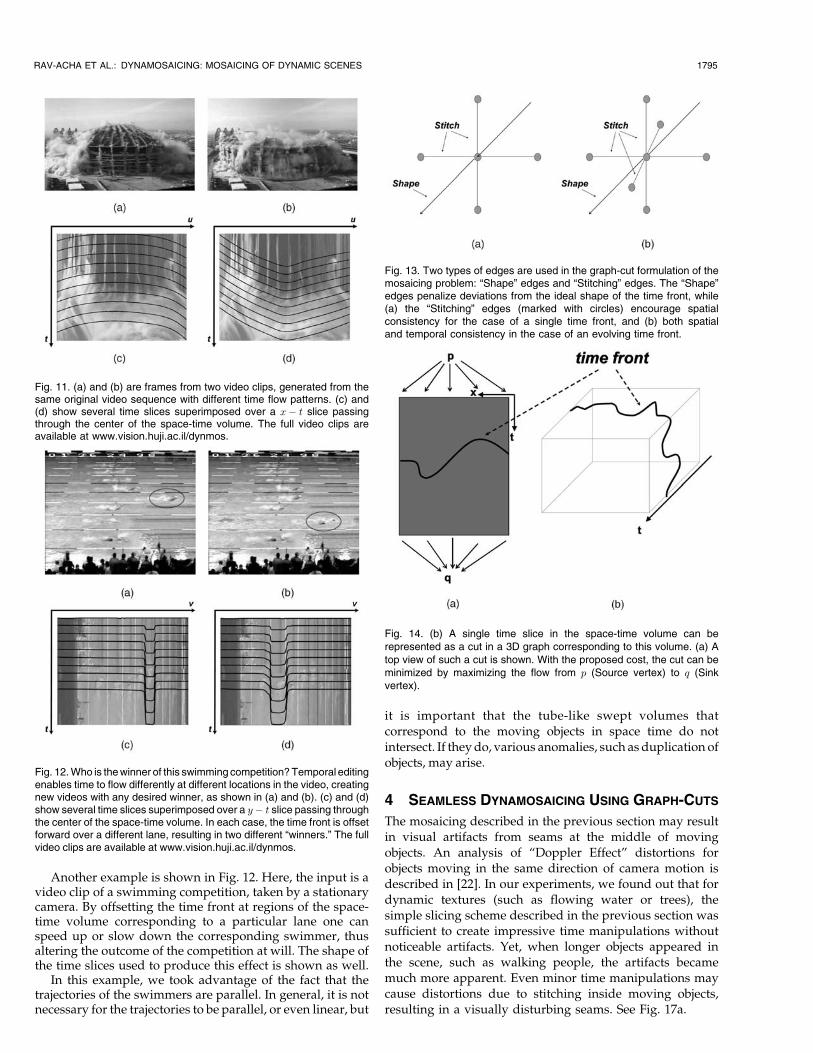
Another example is shown in Fig. 12. Here, the input is avideo clip of a swimming competition, taken by a stationarycamera. By offsetting the time front at regions of the space-time volume corresponding to a particular lane one canspeed up or slow down the corresponding swimmer, thusaltering the outcome of the competition at will. The shape ofthe time slices used to produce this effect is shown as well.

In this example, we took advantage of the fact that thetrajectories of the swimmers are parallel. In general, it is notnecessary for the trajectories to be parallel, or even linear, but

it is important that the tube-like swept volumes thatcorrespond to the moving objects in space time do notintersect. If they do, various anomalies, such as duplication ofobjects, may arise.

4 SEAMLESS DYNAMOSAICING USING GRAPH-CUTS

The mosaicing described in the previous section may resultin visual artifacts from seams at the middle of movingobjects. An analysis of “Doppler Effect” distortions forobjects moving in the same direction of camera motion isdescribed in [22]. In our experiments, we found out that fordynamic textures (such as flowing water or trees), thesimple slicing scheme described in the previous section wassufficient to create impressive time manipulations withoutnoticeable artifacts. Yet, when longer objects appeared inthe scene, such as walking people, the artifacts becamemuch more apparent. Even minor time manipulations maycause distortions due to stitching inside moving objects,resulting in a visually disturbing seams. See Fig. 17a.


Fig. 11. (a) and (b) are frames from two video clips, generated from thesame original video sequence with different time flow patterns. (c) and(d) show several time slices superimposed over a x� t slice passingthrough the center of the space-time volume. The full video clips areavailable at www.vision.huji.ac.il/dynmos.

Fig. 12. Who is the winner of this swimming competition? Temporal editingenables time to flow differently at different locations in the video, creatingnew videos with any desired winner, as shown in (a) and (b). (c) and (d)show several time slices superimposed over a y� t slice passing throughthe center of the space-time volume. In each case, the time front is offsetforward over a different lane, resulting in two different “winners.” The fullvideo clips are available at www.vision.huji.ac.il/dynmos.

Fig. 13. Two types of edges are used in the graph-cut formulation of themosaicing problem: “Shape” edges and “Stitching” edges. The “Shape”edges penalize deviations from the ideal shape of the time front, while(a) the “Stitching” edges (marked with circles) encourage spatialconsistency for the case of a single time front, and (b) both spatialand temporal consistency in the case of an evolving time front.

Fig. 14. (b) A single time slice in the space-time volume can berepresented as a cut in a 3D graph corresponding to this volume. (a) Atop view of such a cut is shown. With the proposed cost, the cut can beminimized by maximizing the flow from p (Source vertex) to q (Sinkvertex).

The distortions of objects and the visual seams can besignificantly reduced by taking into consideration thatstitching inside dynamic regions should be avoided. Inorder to do so, we define a cost function whose minimiza-tion determines the optimal time slice surface. This costfunction balances between the minimization of a “stitching”cost and the maximization of the similarity of the time frontto its desired ideal shape.

A common way to represent and solve such problems isby multilabel graphs, where the labels of each vertex denoteall possible time shifts for that pixel [1], [2]. Unfortunately,the general formulation results in an NP-hard problem,whose approximation requires intensive computations, suchas using loopy belief propagation [27] or iterative graph-cuts[6]. This becomes prohibitive for the case of video editing,where the cost is minimized over a 3D graph. In [2], [29], thecomputational time was reduced by assuming that all thetime fronts and all the pixels in a single column have thesame time-shift, resulting in a 1D problem which can besolved using dynamic programming. In [2], the solution wasfurther enhanced by passing several candidates for eachpixel and applying the full optimization to those candidates.This approach can handle dynamic textures or objects thatmove horizontally but may fail for objects having a moregeneral motion.

We take a different approach which can be implementedwithout reducing the dimensionality of the problem. In ourmethod, we assume that the desired time front is continuousin the space-time volume, i.e., neighboring pixels have similartemporal shifts. Based on this assumption, we formulate theproblem as the one of minimizing a cost function defined on a4D graph. With this formulation, the problem can be solved inpolynomial time as shown in the next section.

It is interesting to compare dynamosaicing with the PVTapproach [2]. The PVT approach, with its ability to havediscrete jumps in time, is most effective with repetitivestochastic textures and with its ability to generate infinitedynamics. When the scene has moving objects each havinga given structure, e.g., moving people, discrete time jumpsmay result in unacceptable distortions and discontinuities.In this case, dynamosaicing with the continuous time frontsis more applicable. Continuous time fronts are also morerobust in cases of error in camera motion. In addition, whilethe PVT approach perform best with camera that jumpsfrom one stable position to another stable position,dynamosaicing works best with smooth camera motion.

4.1 A Single Time Front

In this section, we will examine the creation of a singleseamless image, while keeping the general shape of theideal time front that corresponds to the desired time-manipulation. Movie generation will be addressed later.

We assume that the input sequence has already beenaligned to a single reference frame and stacked together alongthe time axis to form an aligned space-time volume V ðx; y; tÞ.For simplicity, we will also assume that all the frames afteralignment are of the same size. Pixels outside the field of viewof the camera will be marked as impossible.

The output image S is created from the input movieaccording to a time front which is represented by a functionMðx; yÞ. The value of each pixel Sðx; yÞ is taken fromV ðx; y;Mðx; yÞÞ in the aligned space-time volume. Toproduce a seamless mosaic, we modify its ideal shape (e.g.,

as computed in Section 3) qaccording to the moving objects inthe scene. We define a cost function on the time shiftsMðx; yÞ.The general form of this cost function is

EðMÞ ¼ EshapeðMÞ þ �EstitchðMÞ: ð7Þ

The term Eshape attracts the time front to follow itspredefined shape, the term Estitch works to minimize thestitching artifacts, and � balances between the two. (Weused � ¼ 0:3 when gray values were between 0-255.) Whenthe image dynamics is only a dynamic texture, such aswater or smoke, � should be small.

To create panoramas, Eshape can constrain the time frontto pass through the entire sequence, yielding a panoramicimage. For more general time manipulations, we can use thetime fronts described in Section 3.2 as shape priors. Let M 0

be the ideal time front (for example, a time front determinedby the user) then Eshape may be defined as

EshapeðMÞ ¼Xx;y

kMðx; yÞ �M 0ðx; yÞkr; ð8Þ

where r � 1 can be any norm. We usually used the l1 normand not the l2 norm in order to obtain a robust behavior ofthe time front, making it follow the original time frontunless it cuts off parts of a moving object.

The second term, Estitch addresses the minimization ofthe stitching artifacts. It is based on the cost between eachpair of neighboring output pixels ðx; yÞ and ðx0; y0Þ. Withoutloss of generality, we assume that Mðx; yÞ �Mðx0; y0Þ

Espatialðx; y; x0; y0Þ ¼XMðx0;y0Þ�1

k¼Mðx;yÞ

1

2kV ðx; y; kÞ � V ðx; y; kþ 1Þk2

þ 1

2kV ðx0; y0; kÞ � V ðx0; y0; kþ 1Þk2:

ð9Þ

This cost is zero when the two adjacent points ðx; yÞ andðx0; y0Þ come from the same frame ðMðx; yÞ ¼Mðx0; y0ÞÞ.When Mðx; yÞ 6¼Mðx0; y0Þ, this cost is zero when the colorsof ðx; yÞ and ðx0; y0Þ do not change and it increases based onthe dynamics at those pixels.

The global stitching cost for the time front M is given by

EstitchðMÞ ¼Xðx;yÞ

Xðx0;y0Þ2Nðx;yÞ

Espatialðx; y; x0; y0Þ; ð10Þ

where:

. Nðx; yÞ are the pixels in the neighborhood of ðx; yÞ.

. Espatialðx; y; x0; y0Þ is the stitching cost for each pair ofspatially neighboring pixels ðx; yÞ and ðx0; y0Þ, asdescribed in (9).

Note that the cost in (9) differs from traditional stitchingcosts (for example, [1]) where there is no summation, butonly the two time-shifts Mðx; yÞ and Mðx0; y0Þ are used. Thecost in (9) is reasonable when the time front is continuous,which means that if ðx; yÞ and ðx0; y0Þ are neighboring pixels,their source frames Mðx; yÞ and Mðx0; y0Þ are close in time.The main advantage of the cost in (9) is that its globalminimum can be found in polynomial time using a min-cutas will be described below.

When the camera is moving, some pixels in the space-time volume vðx; y; tÞmay not be in the field of view. We do


not assign vertices to such pixels, therefore, only pixels inthe field of view are used in the panoramic image.

4.2 A Single Time Front as 3D Min-Cut

A 3D directed graph G is constructed from the alignedspace-time volume, such that each location ðx; yÞ at frame kis represented by a vertex ðx; y; kÞ. A cut in this graph is apartitioning of the nodes into two sets P and Q. Further,assume that two vertices, the source p 2 P and the sinkq 2 Q, have been distinguished. Given a time front Mðx; yÞ,the corresponding cut in G is defined as follows:

ðx; y; kÞ 2 P ifMðx; yÞ � kðx; y; kÞ 2 Q otherwise:

�ð11Þ

In the other direction, given a cut fP;Qg, we define Mðx; yÞas mink ðx; y; kÞ 2 Qf g. A cost of a cut fP;Qg is defined to beP

u2P;v2Q wðu; vÞ, where wðu; vÞ is the weight of the edgeu! v. We will assign weights to edges between neighbor-ing vertices in G such that the cost of each cut in G will beequal to the cost of the corresponding time front Mðx; yÞ.

Before we turn to describing the edge weights reflectingEstitch and Eshape, we need to ensure that there is a1:1 correspondence between cuts in G and assignmentof M. To do so, we set infinite weights to the edgesðx; y; kþ 1Þ ! ðx; y; kÞ, and to the edges ðx; y;NÞ ! q.These edges prevents cuts in which ðx; y; kþ 1Þ 2 Q butðx; y; kÞ 2 P , which are the only cuts that do not corre-spond to assignments of M.

4.2.1 Assigning Weights to the Graph Edges

The cost term Eshape measures the distance to the ideal shapeof the time front. As seen in (8), this cost consists of termswhich depend on the assignment of single variablesðMðx; yÞÞ. To reflect this cost term, we add directed edgesfrom ðx; y; kÞ to ðx; y; kþ 1Þ with the weights kkþ 1�M 0ðx; yÞkr (M 0 corresponds to the prior time front, r � 1 is a

norm). We also add edges from the Source p to ðx; y; 1Þ withthe weights k1�M 0ðx; yÞkr. The sum of weights in the eachcut givesEshape for the corresponds assignment of time front.

To take into account the stitching costEstitch, we add edges(in both directions) between each adjacent pair of pixels ðx; yÞand ðx0; y0Þ and each k with the following weight:

1


þ 1

2kV ðx0; y0; kÞ � V ðx0; y0; kþ 1Þk2:

These edges are shown in Fig. 13. It can be seen that thegiven a cut, the sum of weights of these edges equals to thestitching cost given in (9). Note, however, that thisequivalence is not true for traditional stitching costs (used,for example, in [2], [1]) but only for our cost function.

4.2.2 Computing the Best Assignment M

The minimal cut in G can be computed in polynomial timeusing min-cut [17]. From the construction of the graph, thecost of a cut in G equals to the corresponding cost definedon the original 2D graph. Therefore, the best assignment oftime slice M can be found efficiently using a min-cut, asshown in Fig. 14.

It should be noted that although it seems as if thecomplexity of the problem was increased by the conversionfrom a 2D problem to a 3D one, the total number of labels in theoriginal 2D formulation equals to the number of vertices inG.

4.3 Evolving Time Front as a 4D Min-Cut

To create a new movie (of length L), we have to sweep thespace-time volume with an evolving time front, defining asequence of time-slices M1; . . . ;ML. This is shown in Fig. 15.Onewaytocontrol thetimeslices isusingtheidealshapeof thetime front as a shape prior. In this case, each time slice Ml iscomputed independently according to the ideal shape of the


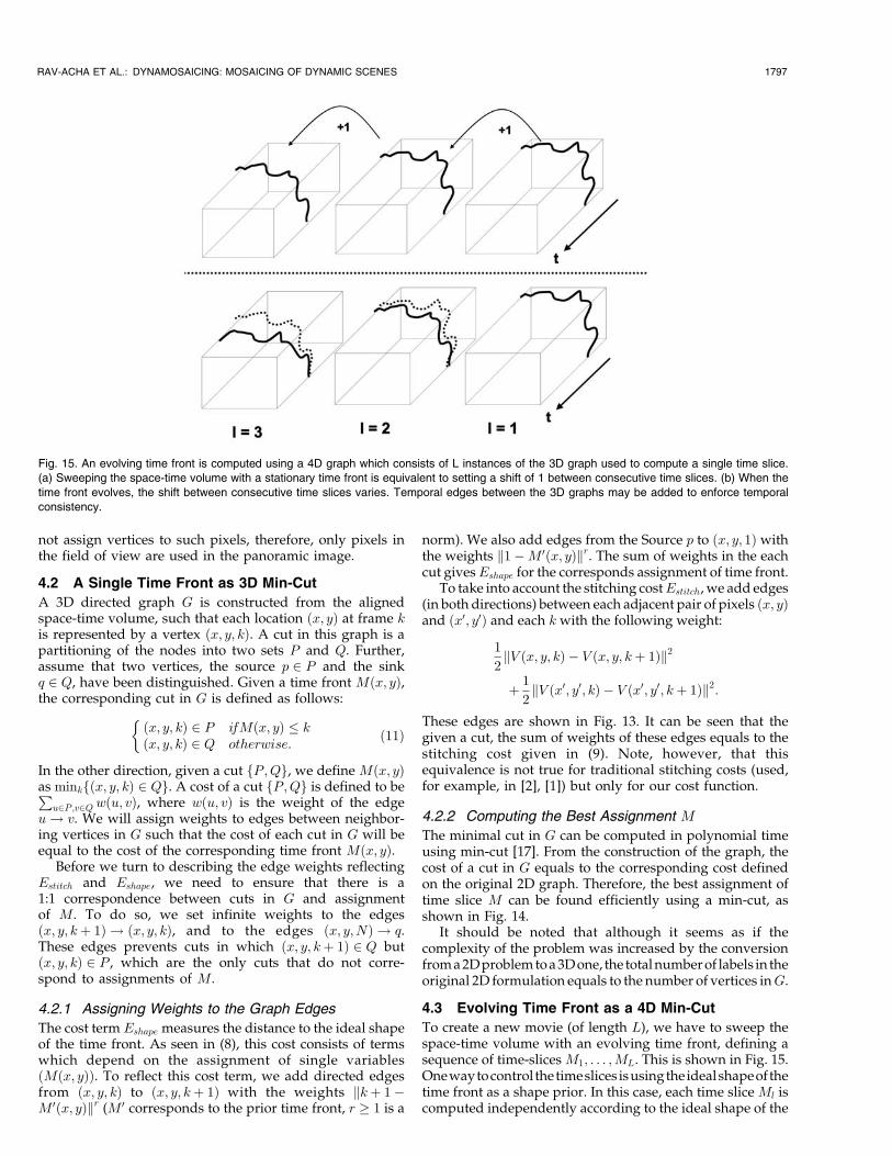
Fig. 15. An evolving time front is computed using a 4D graph which consists of L instances of the 3D graph used to compute a single time slice.

(a) Sweeping the space-time volume with a stationary time front is equivalent to setting a shift of 1 between consecutive time slices. (b) When the

time front evolves, the shift between consecutive time slices varies. Temporal edges between the 3D graphs may be added to enforce temporal

consistency.

corresponding time slice and according to the stitchingconstraints, as was described in the previous section. Anexample for a time manipulation that can be obtained in thisway is shown in Fig. 16. The ideal time front evolved in a waythatmadenearbyregions movefaster,while theexact shapeofthe each time slice was determined using a min-cut to avoidvisible seams.

When the time manipulation aims to preserve thedynamics of the original movie (as is the case in producingpanoramic movies), a better control can be obtained byadding temporal consistency constraints that avoids“jumps” in the output sequence, and minimizing the costfor all the time-slices at once. We first describe the modifiedstitching cost that involves also temporal consistency andlater show how it may be solved using min-cut.

4.3.1 Preserving Temporal Consistency

Temporal consistency can be encouraged by setting for each

pair of temporally neighboring pixels ðx; y; tÞ and ðx; y; tþ1Þ the following cost (assuming that Mtðx; yÞ �Mtþ1ðx; yÞ):

Etemporalðx; y; tÞ¼XMtþ1ðx;yÞ�1

k¼Mtðx;yÞþ1

1

2kV ðx; y; kÞ�V ðx; y; kþ1Þk2

þ 1

2kV ðx; y; kþ 1Þ � V ðx; y; kþ 2Þk2:

ð12Þ

This formulation reflects temporal consistency in both past

and future. This cost is zero for Mtþ1ðx; yÞ ¼Mtðx; yÞ þ 1, an

assignment which preserves the temporal relations of the


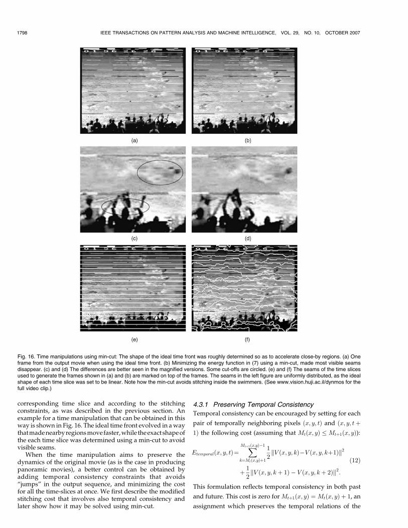
Fig. 16. Time manipulations using min-cut: The shape of the ideal time front was roughly determined so as to accelerate close-by regions. (a) Oneframe from the output movie when using the ideal time front. (b) Minimizing the energy function in (7) using a min-cut, made most visible seamsdisappear. (c) and (d) The differences are better seen in the magnified versions. Some cut-offs are circled. (e) and (f) The seams of the time slicesused to generate the frames shown in (a) and (b) are marked on top of the frames. The seams in the left figure are uniformly distributed, as the idealshape of each time slice was set to be linear. Note how the min-cut avoids stitching inside the swimmers. (See www.vision.huji.ac.il/dynmos for thefull video clip.)

original movie. The global stitching cost for the time frontM isnow given by

EstitchðMÞ ¼Xl

EstitchðMlÞ þXðx;y;tÞ

Etemporalðx; y; tÞ; ð13Þ

where EstitchðMlÞ is the global spatial stitching cost definedin (10).

4.3.2 Computing the Evolving Time Front Using Min-Cut

As was done for the case of a single time front, the costdefined for the evolving time front can be formulated as a cutin a directed graph G0. The 4D graph G0ðx; y; k; lÞ isconstructed from the aligned space-time volume, such thateach location ðx; yÞ at input frame k and output frame l isrepresented by a vertex. A cut fP;Qg that corresponds to theset of time slices M1ðx; yÞ; . . . ;MLðx; yÞ is defined as follows:

ðx; y; k; lÞ 2 P ifMlðx; yÞ � kðx; y; k; lÞ 2 Q otherwise:

�ð14Þ

As the 4D graph G0 is very similar to L instances of the

3D graph G (described in the previous section), we describe

only the modifications that should be done to obtain G0. To

reflect the modified stitching cost given in (13), the edges (in

both directions) between each pair of temporal neighbors

ðx; y; k; lÞ and ðx; y; kþ 1; lþ 1Þ are assigned with the follow-

ing weights:

1


þ 1

2kV ðx; y; kþ 1Þ � V ðx; y; kþ 2Þk2:

ð15Þ

The minimal cut of this graph corresponds to a set of

time-slices M1; . . . ;ML which implement the desired time

manipulation while keeping a seamless movie.

4.3.3 Flow-Based Temporal Consistency

A variant of this algorithm is to enforce temporal consistency

by assigning weights to edges between pixels according to

the optical flow at that pixels, instead of using temporal

consecutive pixels. (See [4] regarding methods to compute

optical flow).Let ðx; yÞ be a pixel at the kth frame. Let ðx0; y0Þ be the

corresponding location at frame k� 1 according to the flow

from frame k to frame k� 1, and let ðx00; y00Þ be the

corresponding location at frame kþ 1 according to the flow

from frame k to frame kþ 1.


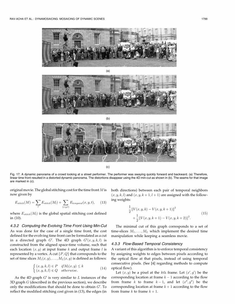
Fig. 17. A dynamic panorama of a crowd looking at a street performer. The performer was swaying quickly forward and backward. (a) Therefore,linear time front resulted in a distorted dynamic panorama. The distortions disappear using the 4D min-cut as shown in (b). The seams for that imageare marked in (c).

To enforce temporal consistency we do the following:

. Edges ðx; y; k; lÞ ! ðx0; y0; k� 1; l� 1Þ are assignedwith the weights:

1

2kV ðx0; y0; kþ 1Þ � V ðx0; y0; kÞk2:

. Edges ðx; y; k; lÞ ! ðx00; y00; kþ 1; lþ 1Þ are assignedwith the weights:

1

2kV ðx00; y00; kþ 2Þ � V ðx00; y00; kþ 1Þk2:

The reason we had to separate between the two directions(“past” edges versus “future” edges) is that the forwardflow and the inverse flow are not necessarily the same.

The advantage of the flow-based temporal consistencyover the simpler approach is that the older one encouragesthe time fronts to remain static unless necessary, while theoptical-flow-based approach encourages the time fronts toevolve in a more natural way according to the flow in thescene.

4.4 Accelerations

The memory required for saving the 4D graph may be toolarge. For example, the input movie that was used tocreate the panoramic movie shown in Fig. 18 consists of1,000 frames, each of size 320� 240. Constructing thegraph would require prohibitive computer resources. Wetherefore suggest several modifications that reduce boththe memory requirements and the runtime of thealgorithm:

. We solve only for a sampled set of time slices, givinga sparser output movie, and interpolate the stitchingfunction between them. (This acceleration is possiblewhen the motion in the scene is not very large.)

. We can constrain each pixel to come only from apartial set of input frames. This is very reasonablefor sequences taken from a video, where their is a lotof redundancy between consecutive frames. (It isimportant though to sample the source-frames in aconsistent way. For example, if the frame k is acandidate source for pixel ðx; yÞ in the one outputframe, then the frame kþ 1 should be a candidate forpixel ðx; yÞ in the successive output frame.)

. We use an hierarchical framework, where a coarsesolution is found for low resolution images, and thesolution is refined at higher resolution levels onlyalong the boundaries. Similar accelerations were alsoused in [2], and are discussed in [19].

5 CONCLUDING REMARKS

It was shown that by relaxing the chronological constraintsof time, a flexible representation of dynamic videos can beobtained. Specifically, when the chronological order ofevents is no longer considered a hard restriction, a widerange of time manipulations can be applied. An interestingexample is creating dynamic panoramas where all eventsoccur simultaneously and the same principles hold even forvideos taken by a static camera.

Manipulating the time in movies is performed by sweep-ing an evolving time front through the aligned space-timevolume. The strength of this approach is that accuratesegmentation and recognition of objects are not needed. Thisfact significantly simplifies and increases the robustness ofthe method. This robustness comes at a cost of limiting thetime manipulations that can be applied on a given video.Assume that one moving object occludes another movingobject. With our method, the concurrency of the occlusionmust be preserved for both objects.

In order to overcome this limitation and allow indepen-dent time manipulations even for objects that occlude eachother, very good object segmentation and tracking is needed.In addition, methods for video completion should be used.

It is interesting to compare dynamosaicing with the PVTapproach [2]. The PVT approach, with its ability to havediscrete jumps in time, is most effective with repetitivestochastic textures and with its ability to generate infinitedynamics. When the scene has moving objects each having agiven structure, e.g., moving people, dynamosaicing withthe continuous time fronts is more applicable. Continuoustime fronts are also more robust in cases of error in cameramotion. In addition, while the PVT approach perform bestwith camera that jumps from one stable position to anotherstable position, dynamosaicing works best with smoothcamera motion.

ACKNOWLEDGMENTS

This research was supported (in part) by the EU throughcontract IST-2001-39184 BENOGO, and by a grant from theIsrael Science Foundation.


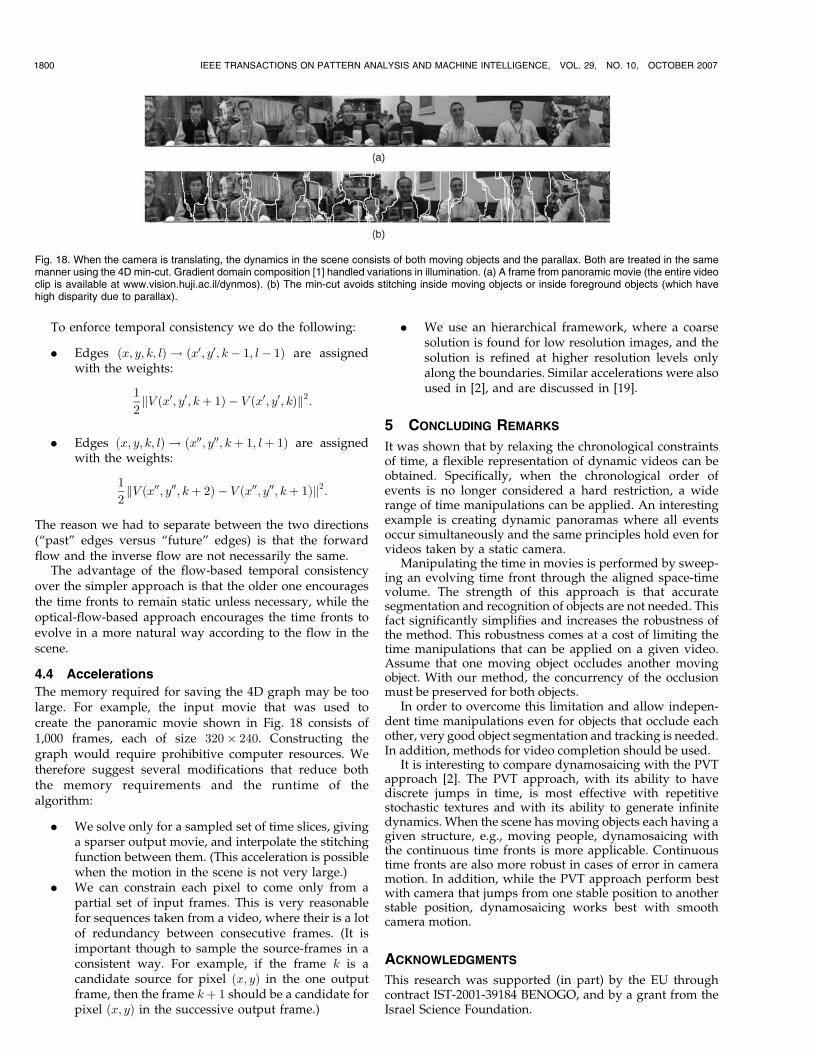
Fig. 18. When the camera is translating, the dynamics in the scene consists of both moving objects and the parallax. Both are treated in the samemanner using the 4D min-cut. Gradient domain composition [1] handled variations in illumination. (a) A frame from panoramic movie (the entire videoclip is available at www.vision.huji.ac.il/dynmos). (b) The min-cut avoids stitching inside moving objects or inside foreground objects (which havehigh disparity due to parallax).

REFERENCES

[1] A. Agarwala, M. Dontcheva, M. Agrawala, S. Drucker, A. Colburn,B. Curless, D. Salesin, and M. Cohen, “Interactive Digital Photo-montage,” Proc. ACM SIGGRAPH ’04, pp. 294-302, Aug. 2004.

[2] A. Agarwala, C. Zheng, C. Pal, M. Agrawala, M. Cohen, B.Curless, D. Salesin, and R. Szeliski, “Panoramic Video Textures,”Proc. ACM SIGGRAPH ’05, pp. 821-827, July 2005.

[3] Z. Bar-Joseph, R. El-Yaniv, D. Lischinski, and M. Werman,“Texture Mixing and Texture Movie Synthesis Using StatisticalLearning,” IEEE Trans. Visualization and Computer Graphics, vol. 7,no. 2, pp. 120-135, Apr.-June 2001.

[4] J.L. Barron, D.J. Fleet, S.S. Beauchemin, and T.A. Burkitt,“Performance of Optical Flow Techniques,” Proc. Computer Visionand Pattern Recognition, pp. 236-242, 1992.

[5] J.R. Bergen, P. Anandan, K.J. Hanna, and R. Hingorani,“Hierarchical Model-Based Motion Estimation,” Proc. EuropeanConf. Computer Vision, pp. 237-252, May 1992.

[6] Y. Boykov, O. Veksler, and R. Zabih, “Fast Approximate EnergyMinimization via Graph Cuts,” IEEE Trans. Pattern Analysis andMachine Intelligence, vol. 23, no. 11, pp. 1222-1239, Nov. 2001.

[7] L.G. Brown, “Survey of Image Registration Techniques,” ACMComputing Surveys, vol. 24, no. 4, pp. 325-376, Dec. 1992.

[8] G. Doretto, A. Chiuso, S. Soatto, and Y.N. Wu, “Dynamic Textures,”Int’l J. Computer Vision, vol. 51, no. 2, pp. 91-109, Feb. 2003.

[9] G. Doretto and S. Soatto, “Towards Plenoptic Dynamic Textures,”Proc. Workshop Textures, pp. 25-30, Oct. 2003.

[10] A. Efros and T. Leung, “Texture Synthesis by Non-ParametricSampling,” Proc. Int’l Conf. Computer Vision, vol. 2, pp. 1033-1038,Sept. 1999.

[11] A.W. Fitzgibbon, “Stochastic Rigidity: Image Registration forNowhere-Static Scenes,” Proc. Int’l Conf. Computer Vision, pp. 662-669, July 2001.

[12] W.T. Freeman and H. Zhang, “Shape-Time Photography,” Proc.Conf. Computer Vision and Pattern Recognition, vol. 2, pp. 151-157,2003.

[13] S. Hsu, H.S. Sawhney, and R. Kumar, “Automated Mosaics viaTopology Inference,” IEEE Trans. Computer Graphics and Applica-tions, vol. 22, no. 2, pp. 44-54, 2002.

[14] M. Irani and P. Anandan, “Robust Multi-Sensor Image Align-ment,” Proc. Int’l Conf. Computer Vision, pp. 959-966, Jan. 1998.

[15] M. Irani, P. Anandan, J. Bergen, R. Kumar, and S. Hsu, “MosaicRepresentations of Video Sequences and Their Applications,”Signal Processing: Image Comm., vol. 8, no. 4, pp. 327-351, May 1996.

[16] A. Klein, P. Sloan, A. Colburn, A. Finkelstein, and M. Cohen,“Video Cubism,” Technical Report MSR-TR-2001-45, MicrosoftResearch, 2001.

[17] V. Kolmogorov and R. Zabih, “What Energy Functions can beMinimized via Graph Cuts?” Proc. European Conf. Computer Vision,pp. 65-81, May 2002.

[18] V. Kwatra, A. Schodl, I. Essa, G. Turk, and A. Bobick, “GraphcutTextures: Image and Video Synthesis using Graph Cuts,” ACMTrans. Graphics, SIGGRAPH ’03, vol. 22, no. 3, pp. 277-286, July2003.

[19] H. Lombaert, Y. Sun, L. Grady, and C. Xu, “A Multilevel BandedGraph Cuts Method for Fast Image Segmentation,” Proc. Int’l Conf.Computer Vision, pp. 259-265, Oct. 2005.

[20] S. Peleg, M. Ben-Ezra, and Y. Pritch, “Omnistereo: PanoramicStereo Imaging,” IEEE Trans. Pattern Analysis and MachineIntelligence, vol. 23, no. 3, pp. 279-290, Mar. 2001.

[21] S. Peleg, B. Rousso, A. Rav-Acha, and A. Zomet, “Mosaicing onAdaptive Manifolds,” IEEE Trans. Pattern Analysis and MachineIntelligence, vol. 22, no. 10, pp. 1144-1154, Oct. 2000.

[22] A. Rav-Acha, Y. Pritch, D. Lischinski, and S. Peleg, “Dynamosai-cing: Video Mosaics with Non-Chronological Time,” Proc. Conf.Computer Vision and Pattern Recognition, June 2005.

[23] A. Rav-Acha, Y. Pritch, and S. Peleg, “Online Registration ofDynamic Scenes Using Video Extrapolation,” Proc. WorkshopDynamical Vision at ICCV ’05, Oct. 2005.

[24] P.H.S. Torr and A. Zisserman, “MLESAC: A New RobustEstimator with Application to Estimating Image Geometry,”J. Computer Vision and Image Understanding, vol. 78, no. 1,pp. 138-156, 2000.

[25] M. Uyttendaele, A. Eden, and R. Szeliski, “Eliminating Ghostingand Exposure Artifacts in Image Mosaics,” Proc. Conf. ComputerVision and Pattern Recognition, vol. II, pp. 509-516, Dec. 2001.

[26] R. Vidal and A. Ravichandran, “Optical Flow Estimation andSegmentation of Multiple Moving Dynamic Textures,” Proc.Computer Vision and Pattern Recognition, pp. 516-521, 2005.

[27] Y. Weiss and W.T. Freeman, “On the Optimality of Solutions ofthe Max-Product Belief Propagation Algorithm in ArbitraryGraphs,” IEEE Trans. Information Theory, vol. 47, no. 2, pp. 723-735, 2001.

[28] Y. Wexler, E. Shechtman, and M. Irani, “Space-Time VideoCompletion,” Proc. Conf. Computer Vision and Pattern Recognition,vol. 1, pp. 120-127, June 2004.

[29] Y. Wexler and D. Simakov, “Space-Time Scene Manifolds,” Proc.Int’l Conf. Computer Vision, Oct. 2005.

[30] A. Zomet, D. Feldman, S. Peleg, and D. Weinshall, “MosaicingNew Views: The Crossed-Slits Projection,” IEEE Trans. PatternAnalysis and Machine Intelligence, vol. 25, no. 6, pp. 741-754, June2003.

Alex Rav-Acha received the BSc and MScdegrees in computer science from the HebrewUniversity of Jerusalem, Israel, in 1997 and2001, respectively. He is currently a PhD studentin computer science at the Hebrew University ofJerusalem. His research interests include videosummary, video editing, image deblurring, andmotion analysis. He is a student member of theIEEE.

Yael Pritch received the BSc and MSc degreesin computer science from the Hebrew Universityof Jerusalem, Israel, in 1998 and 2000, respec-tively. For the last several years, she has beenworking at HumanEyes Technologies. She isnow a PhD student in computer science at theHebrew University of Jerusalem. Her researchinterests are in computer vision with emphasison motion analysis and video manipulations.

Dani Lischinski received the BSc and MScdegrees in computer science from the HebrewUniversity of Jerusalem in 1987 and 1989 and thePhD degree in computer science from CornellUniversity in 1994. He is currently on the facultyof the School of Engineering and ComputerScience at the Hebrew University of Jerusalem.Professor Lischinski’s areas of interest includecomputer graphics and image and video proces-sing. In particular, he has worked on algorithms

for photorealistic image synthesis, image-based modeling and rendering,texture synthesis, and editing and manipulation of images and video. Formore information see http://www.cs.huji.ac.il/~danix.

Shmuel Peleg received the BSc degree inmathematics from The Hebrew University ofJerusalem, Israel, in 1976 and the MSc and PhDdegrees in computer science from the Universityof Maryland, College Park, in 1978 and 1979,respectively. He has been a faculty member at theHebrew University of Jerusalem since 1980 andhas held visiting positions at the University ofMaryland, New York University, and the SarnoffCorporation. He is a member of the IEEE.

. For more information on this or any other computing topic,please visit our Digital Library at www.computer.org/publications/dlib.


dynamosaicing: mosaicing of dynamic scenes

Documents