generative modeling of dynamic visual scenes - core
TRANSCRIPT
Generative Modeling of Dynamic Visual Scenes
by
Dahua Lin
Submitted to the Department of Electrical Engineering and ComputerScience
in partial fulfillment of the requirements for the degree of
Doctor of Philosophy in Computer Science and Engineering
at the
MASSACHUSETTS INSTITUTE OF TECHNOLOGY
September 2012
© Massachusetts Institute of Technology 2012. All rights reserved.
A u th or . .... ...... ............... ...........................Department of Electrical Engineering and Computer Science
August 30, 2012
A, '
Certified by. (/4John Fisher
Senior Research ScientistThesis Supervisor
I)
Accepted byPrdfessore(4 ie A. Kolodziejski
Chairman, Department Committee on Graduate Students
~1
2
Generative Modeling of Dynamic Visual Scenes
by
Dahua Lin
Submitted to the Department of Electrical Engineering and Computer Scienceon August 30, 2012, in partial fulfillment of the
requirements for the degree ofDoctor of Philosophy in Computer Science and Engineering
Abstract
Modeling visual scenes is one of the fundamental tasks of computer vision. Whereastremendous efforts have been devoted to video analysis in past decades, most priorwork focuses on specific tasks, leading to dedicated methods to solve them. ThisPhD thesis instead aims to derive a probabilistic generative model that coherentlyintegrates different aspects, notably appearance, motion, and the interaction betweenthem. Specifically, this model considers each video as a composite of dynamic layers,each associated with a covering domain, an appearance template, and a flow describ-ing its motion. These layers change dynamically following the associated flows, andare combined into video frames according to a Z-order that specifies their relativedepth-order.
To describe these layers and their dynamic changes, three major components areincorporated: (1) An appearance model describes the generative process of the pixelvalues of a video layer. This model, via the combination of a probabilistic patchmanifold and a conditional Markov random field, is able to express rich local detailswhile maintaining global coherence. (2) A motion model captures the motion patternof a layer through a new concept called geometric flow that originates from differentialgeometric analysis. A geometric flow unifies the trajectory-based representation andthe notion of geometric transformation to represent the collective dynamic behaviorspersisting over time. (3) A partial Z-order specifies the relative depth order betweenlayers. Here, through the unique correspondence between equivalent classes of partialorders and consistent choice functions, a distribution over the spaces of partial ordersis established, and inference can thus be performed thereon.
The development of these models leads to significant challenges in probabilisticmodeling and inference that need new techniques to address. We studied two im-portant problems: (1) Both the appearance model and the motion model rely onmixture modeling to capture complex distributions. In a dynamic setting, the com-ponents parameters and the number of components in a mixture model can changeover time. While the use of Dirichlet processes (DPs) as priors allows indefinitenumber of components, incorporating temporal dependencies between DPs remains anontrivial issue, theoretically and practically. Our research on this problem leads to a
3
new construction of dependent DPs, enabling various forms of dynamic variations fornonparametric mixture models by harnessing the connections between Poisson andDirichlet processes. (2) The inference of partial Z-order from a video needs a methodto sample from the posterior distribution of partial orders. A key challenge here isthat the underlying space of partial orders is disconnected, meaning that one maynot be able to make local updates without violating the combinatorial constraints forpartial orders. We developed a novel sampling method to tackle this problem, whichdynamically introduces virtual states as bridges to connect between different parts ofthe space, implicitly resulting in an ergodic Markov chain over an augmented space.
With this generative model of visual scenes, many vision problems can be readilysolved through inference performed on the model. Empirical experiments demon-strate that this framework yields promising results on a series of practical tasks,including video denoising and inpainting, collective motion analysis, and semanticscene understanding.
Thesis Supervisor: John FisherTitle: Senior Research Scientist
4
Acknowledgments
Upon the completion of this thesis, it is time to deliver my gratitude to all who have
given me the encouragement, support, and love that I need to pursue a PhD at MIT
- a journey filled with challenges unprecedented in my life.
First and foremost, I owe my sincere gratitude to my thesis supervisor John Fisher.
He led me to a fascinating realm where the beautiful theory of probabilistic modeling
and the interesting applications in computer vision meet each other. As my advisor,
he gave me total freedom to explore what I was interested in, while providing a lot
of valuable suggestions in model formulation, experiment design, and paper revision.
I appreciate all his contributions of time and energy to make my academic pursuit
productive and rewarding. It was definitely a great pleasure working with him.
I want to express my thanks to Professor Eric Grimson. Eric was the department
head of EECS and is now the Chancellor of MIT. In spite of his administrative
commitment, he met with me on a regular basis and was always supportive of my
research and career development. Instead of offering detailed advices, Eric usually
presented questions at a high level, which have been proved to be crucial in keeping
me on the right track.
My thanks also go to Professor Alan Willsky. In each semester, Alan held weekly
group-lets for both his and John's students. I was fortunate to attend such group-lets
and learned a lot from him. His insightful views of various research topics have not
only helped me through a number of technical difficulties, but also led me to new
perspectives of the problems that I was working on.
I felt honored to be a member of John's research group in CSAIL. The great help
from other members of the group has made my professional time at MIT efficient and
enjoyable. This group is also the source of discussion and collaboration. Particularly,
I would like to thank Jason Chang for his help in resolving technical issues, Donglai
Wei for the inspiring discussion aIld the ECCV paper that we collaborated on, and
Randi Cabezas for the preparation of all those wonderful lunches. I am also thankful
of other members of both John and Eric's groups: Xiaogang Wang, Xiaoxu Ma,
Chaowei Niu, Gerald Dalley, Biswajit Bose, Zoran Dzunic, Giorgos Papachristoudis,
Katie Bouman, and Sue Zheng.
The life at MIT means much more than research. It was my great honor to know
many new friends on this campus, who are a constant source of hope and courage.
Among these friends, I would like to express my gratitude in particular to Jing Chen,
who was always willing to lend her hands to her friends, Jingqing Zhang, a lovely and
kind-hearted girl who published the first chemical engineering paper with my name
on the author list, Yaodong Zhang, who was able to turn any conversation into a fun,
Xiaoqian Jiang, a good friend who helped me a lot in my personal affairs and shared
with me a lot of interesting things both inside and outside academia, and Jianxiong
Xiao, whose lovely kid brought lots of joy to the lab. I am also indebted to Jingjing
Liu, Mengdi Wang, Fei Liang, Ying Liu, Yuan Luo, Yuan Shen, Xi Wang, Yang Cai,
Yu Xin, Maokai Lin, and Ce Liu.
Tremendous thanks should be delivered to my family, for my parents who brought
me from an infant to a PhD with immense love and support, and for my loving,
encouraging, and understanding wife - Leimi, who was always standing by me when
I was facing challenges and difficulties, and have sacrificed a lot in support of my
academic pursuit. A thousand thanks, my beloved!
Finally, I acknowledge the funding sources that supported my PhD work: (1) Het-
erogeneous Sensor Networks (HSN), which is supported by the Army Research Office
(ARO) Multidisciplinary Research Initiative (MURI) program (Award W911NF-06-
1-0076), (2) Stratigraphic Pattern Recognition, which is sponsored by Shell, (3) Non-
parametric Representations for Integrated Inference, Control, and Sensing, which is
supported by the Defense Advance Research Projects Agency (Award FA8650-11-1-
7154), and (4) Nonparametric Bayesian Models to Represent Knowledge and Uncer-
tainty in Decentralized Planning, which is supported by the Office of Naval Research
Multidisciplinary Research Initiative (MURI) program (Award N000141110688).
6
Contents
1 Introduction
1.1 Questions to be Answered . . . . . . . . . . . . .
1.2 The Overall Scene Modeling Framework . . . . .
1.2.1 Three Approaches to Scene Composition
1.2.2 A Layered Model of Dynamic Scenes .
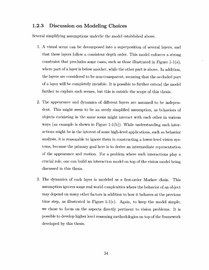
1.2.3 Discussion on Modeling Choices . . . . . .
1.2.4 M ain Aspects . . . . . . . . . . . . . . . .
1.3 The Organization of the Thesis . . . . . . . . . .
2 Theoretical Background
2.1 Probabilistic Graphical Models . . . . . . . . . .
2.1.1 Basic Concepts of Graphical Models . . .
2.1.2 Conditional Independence . . . . . . . . .
2.1.3 Example Applications in Computer Vision
2.1.4 Exact Inference . . . . . . . . . . . . . . .
2.2 Exponential Family Distributions . . . . . . . . .
2.2.1 Basics of Exponential Families . . . . . . .
2.2.2 Useful Examples . . . . . . . . . . . . . .
2.2.3 The Log-partition Function . . . . . . . .
2.2.4 Conjugate Duality . . . . . . . . . . . . .
2.3 Model Estimation and Variational Inference . . .
2.3.1 Maximum Likelihood Estimation . . . . .
2.3.2 Expectation Maximization . . . . . . . . .
7
25
. . . . . . . . . . . 26
. . . . . . . . . . . 28
. . . . . . . . . . . 29
. . . . . . . . . . . 30
. . . . . . . . . . . 34
. . . . . . . . . . . 35
. . . . . . . . . . . 36
40
. . . . . . . . . . . 41
. . . . . . . . . . . 41
. . . . . . . . . . . 44
. . . . . . . . . . . 47
. . . . . . . . . . . 50
. . . . . . . . . . . 54
. . . . . . . . . . . 54
. . . . . . . . . . . 56
. . . . . . . . . . . 58
. . . . . . . . . . . 59
. . . . . . . . . . . 60
. . . . . . . . . . . 60
. . . . . . . . . . . 63
2.3.3 Mean Field and Variational Inference . . . . . . . . . . . . . . 66
2.4 Monte Carlo Sampling . . . . . . . . . . . . . . . . . . . . . . . . . . 70
2.4.1 Monte Carlo Integration . . . . . . . . . . . . . . . . . . . . . 70
2.4.2 Importance Sampling . . . . . . . . . . . . . . . . . . . . . . . 71
2.4.3 Markov Chain Monte Carlo . . . . . . . . . . . . . . . . . . . 72
2.4.4 Gibbs Sampling . . . . . . . . . . . . . . . . . . . . . . . . . . 75
3 The Appearance Model 76
3.1 Probabilistic Image Models . . . . . . . . . . . . . . . . . . . . . . . . 77
3.1.1 Manifold-based Image Modeling . . . . . . . . . . . . . . . . . 79
3.1.2 MRF-based Image Modeling . . . . . . . . . . . . . . . . . . . 81
3.2 A New Image Prior . . . . . . . . . . . . . . . . . . . . . . . . . . . . 85
3.2.1 Modeling Base Images . . . . . . . . . . . . . . . . . . . . . . 86
3.2.2 The Patch Manifold Model . . . . . . . . . . . . . . . . . . . . 86
3.2.3 Patch Coherence via Markov Random Fields . . . . . . . . . . 92
3.2.4 The Joint Likelihood . . . . . . . . . . . . . . . . . . . . . . . 95
3.3 Learning the Image Model . . . . . . . . . . . . . . . . . . . . . . . . 97
3.3.1 Learning the Gaussian Process Prior . . . . . . . . . . . . . . 98
3.3.2 Learning the Probabilistic Patch Manifold . . . . . . . . . . . 99
3.4 Application to Image Recovery . . . . . . . . . . . . . . . . . . . . . 104
3.4.1 Image Denoising . . . . . . . . . . . . . . . . . . . . . . . . . 105
3.4.2 Image Inpainting . . . . . . . . . . . . . . . . . . . . . . . . . 111
3.5 Sum m ary . . . . . . . . . . . . . . . . . . . . . . . . . . . . . . . . . 115
4 The Motion Model 116
4.1 Overview of Motion Models . . . . . . . . . . . . . . . . . . . . . . . 117
4.1.1 Review of Related Work . . . . . . . . . . . . . . . . . . . . . 118
4.1.2 Motivation: Problems with Existing Methods . . . . . . . . . 122
4.1.3 A New Approach based on Geometric Flows . . . . . . . . . . 123
4.2 Geometric Flows . . . . . . . . . . . . . . . . . . . . . . . . . . . . . 125
4.2.1 The Concept of Geometric Flow . . . . . . . . . . . . . . . . . 125
8
4.2.2 Lie Group and Lie Algebra . . . . . . . . . . . . . . . . . . . . 127
4.2.3 Lie Algebraic Representation . . . . . . . . . . . . . . . . . . . 131
4.2.4 Lie Algebra of Affine Transforms . . . . . . . . . . . . . . . . 132
4.3 The Vector Space of Flows . . . . . . . . . . . . . . . . . . . . . . . . 134
4.3.1 Infinitesimal Generators of Flows . . . . . . . . . . . . . . . . 134
4.3.2 Flow Actions . . . . . . . . . . . . . . . . . . . . . . . . . . . 138
4.3.3 Multi-scale Extensions . . . . . . . . . . . . . . . . . . . . . . 141
4.4 Stochastic Flow Model . . . . . . . . . . . . . . . . . . . . . . . . . . 145
4.4.1 The Stochastic Flow Formulation . . . . . . . . . . . . . . . . 145
4.4.2 The Action of Stochastic Flow on Images . . . . . . . . . . . . 147
4.4.3 Integration of Observations . . . . . . . . . . . . . . . . . . . 149
4.4.4 Gaussian Process Prior over Complex Flows . . . . . . . . . . 149
4.4.5 Multiple Concurrent Flows . . . . . . . . . . . . . . . . . . . . 150
4.5 Experim ents . . . . . . . . . . . . . . . . . . . . . . . . . . . . . . . . 152
4.5.1 Analyzing Crowd Motion Patterns . . . . . . . . . . . . . . . 153
4.5.2 Modeling Flows in General Dynamic Scenes . . . . . . . . . . 156
4.6 Sum m ary . . . . . . . . . . . . . . . . . . . . . . . . . . . . . . . . . 162
5 Dynamic Bayesian Nonparametrics 164
5.1 Finite Mixture Models . . . . . . . . . . . . . . . . . . . . . . . . . . 165
5.1.1 Generic Formulation . . . . . . . . . . . . . . . . . . . . . . . 165
5.1.2 Specific Examples: GMM and Topic Models . . . . . . . . . . 167
5.1.3 Estimation of Finite Mixture Models . . . . . . . . . . . . . . 169
5.2 Dirichlet Process Mixture Models . . . . . . . . . . . . . . . . . . . . 170
5.2.1 Dirichlet Processes . . . . . . . . . . . . . . . . . . . . . . . . 170
5.2.2 P6lya Urn and Chinese Restaurant Process . . . . . . . . . . . 171
5.2.3 Stick-breaking Construction . . . . . . . . . . . . . . . . . . . 174
5.2.4 DP Mixture Models . . . . . . . . . . . . . . . . . . . . . . . . 175
5.3 Dependent Dirichlet Processes . . . . . . . . . . . . . . . . . . . . . . 176
5.3.1 A Brief Review . . . . . . . . . . . . . . . . . . . . . . . . . . 178
9
5.3.2 Poisson, Gamma, and Dirichlet Processes .
5.3.3 Poisson-based Construction of DDP . . . .
5.3.4 A Markov Chain of Dirichlet Processes . .
5.4 Gibbs Sampling Algorithm . . . . . . . . . . . . .
5.4.1 Posterior and Predictive Distributions . .
5.4.2 Sampling from a Dependent DP . . . . . .
5.4.3 Gibbs Sampling for Inference over Dynamic
5.5 Empirical Results . . . . . . . . . . . . . . . . . .
5.5.1 Simulations on Synthetic Data . . . . . . .
5.5.2 Modeling People Flows . . . . . . . . . . .
5.5.3 Analyzing Paper Topics . . . . . . . . . .
5.6 Sum m ary . . . . . . . . . . . . . . . . . . . . . .
DPMM
6 The Order of Layers
6.1 Modeling the Depth Order of Layers . . . . . . . . . . . . .
6.1.1 Revisiting Layered Video Models . . . . . . . . . . .
6.1.2 The Generic Formulation for Partial Order Inference
6.2 Minimally Sufficient Partial Orders . . . . . . . . . . . . . .
6.2.1 Basic Concepts of Partial Orders . . . . . . . . . . .
6.2.2 Sufficiency, Identifiability, and Minimality . . . . . .
6.2.3 Representation based on Directed Acyclic Graph . . .
6.3 A New Approach to Sampling Partial Orders . . . . . . . . .
6.3.1 Review of Sampling Methods . . . . . . . . . . . . .
6.3.2 Bridging Markov Chains . . . . . . . . . . . . . . . .
6.3.3 Mixing Time Analysis . . . . . . . . . . . . . . . . .
6.3.4 Hierarchical Bridging Markov Chain . . . . . . . . .
6.3.5 Dynamic Construction . . . . . . . . . . . . . . . . .
6.4 Experim ents . . . . . . . . . . . . . . . . . . . . . . . . . . .
6.4.1 Constrained Binary Labeling . . . . . . . . . . . . . .
6.4.2 Inferring Layer Orders from Synthetic Images . . . .
10
183
187
194
. . 195
196
201
202
205
205
. . 208
209
210
211
. . . . 212
. . . . 212
. . . . 213
214
. . . . 214
. . . . 217
. . . . 223
. . . . 230
. . . . 230
. . . . 232
. . . . 237
. . . . 245
. . . . 252
. . . . 253
. . . . 254
. . . . 257
6.4.3 Inferring Layer Orders from Real Videos . . . . . . . . . . .
6.5 Sum m ary . . . . . . . . . . . . . . . . . . . . . . . . . . . . . . . .
7 Conclusions
7.1 Summary of Contributions . . . . . . . . . . . . . . . . . . . . . . .
7.2 Future Directions . . . . . . . . . . . . . . . . . . . . . . . . . . . .
A Basics of Group Theory
A.1 Basic Concepts of Group . . . . . . . . . . . .
A.2 Group Homomorphisms and Kernels.....
A.3 Normal Subgroups and Quotient Groups .
A.4 Semidirect Product . . . . . . . . . . . . . . .
B Basics of Differential Geometry
B.1 Basic Concepts of Manifolds . . . . . . . . . .
B.2 Smooth M aps . . . . . . . . . . . . . . . . . .
B.3 Tangent Vectors and Tangent Space . . . . . .
B.4 Vector Fields . . . . . . . . . . . . . . . . . .
B.5 Embedding and Submanifolds . . . . . . . . .
C Affine Transformation Group
C.1 The Affine Transformation Group . . . . . . .
C.2 Factorization of the Affine Group . . . . . . .
C.3 Two-dimensional Affine Transforms . . . . . .
C.4 Entries of the Lie algebraic representation . .
C.5 Important Subgroups of the 2D Affine Group
268
. . . . . . . . . . . . . 268
. . . . . . . . . . . . . 270
. . . . . . . . . . . . . 271
. . . . . . . . . . . . . 274
276
. . . . . . . . . . . . . 276
. . . . . . . . . . . . . 277
. . . . . . . . . . . . . 278
. . . . . . . . . . . . . 281
. . . . . . . . . . . . . 282
285
285
288
293
295
297
11
260
261
262
263
265
List of Figures
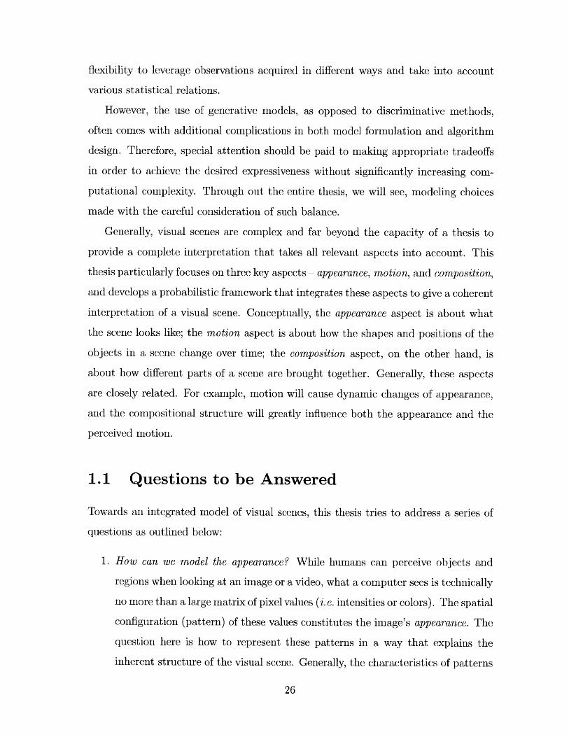
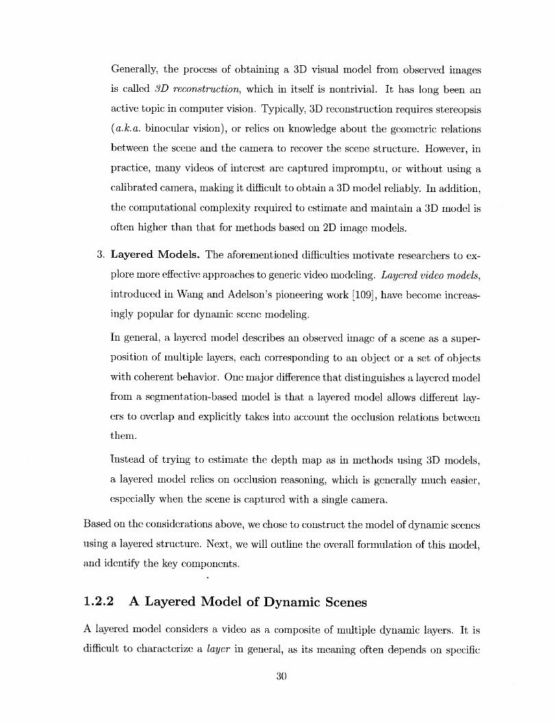
1-1 This figure shows several cases where the simplified assumptions un-
derlying the layered model are violated. (a) shows a girl behind a boy,
while her hands are in front of him. If we model them as two layers,
then there is no definite depth order between them. (b) shows two kids
playing basketball. While they can be modeled as two dynamic layers,
their behavior are not independent. (c) show a soldier in a battlefield.
His behavior may be influenced by many factors, and simply modeling
it as a Markov chain may overly simplify the real world complication. 31
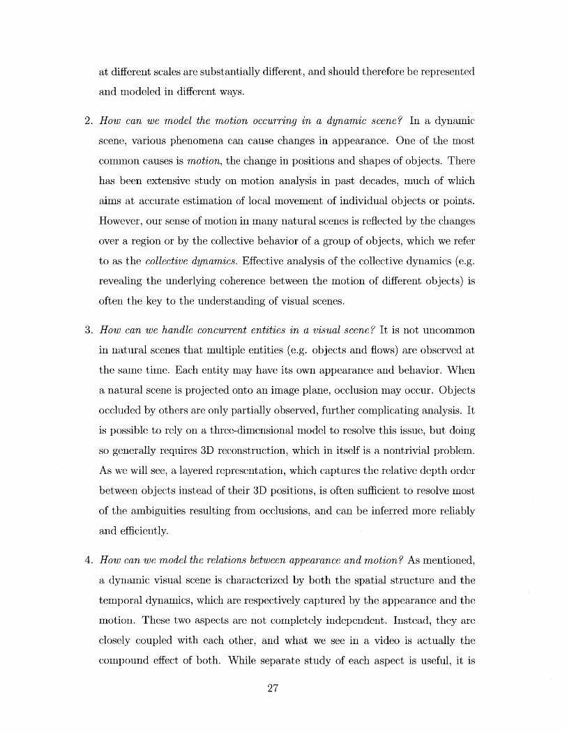
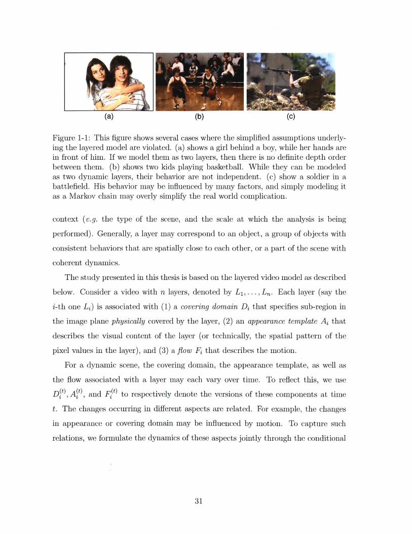
1-2 The graphical representation of the layered visual model. As shown
in this figure, the framework is comprised of m layers, each associated
with a motion model, a domain model, and an appearance model.
These aspects are assumed to be independent a priori, and dynamic
evolution of each aspect is assumed to follow a Markov chain. Given the
characterizations of these aspects, a video frame I() can be generated
according to the relative depth order between layers, which is denoted
by Z(t). The arrows in blue color highlight the factor that formalizes
the generation of video frames conditioned on latent states of these
asp ects. . . . . . . . . . . . . . . . . . . . . . . . . . . . . . . . . . . 32
12
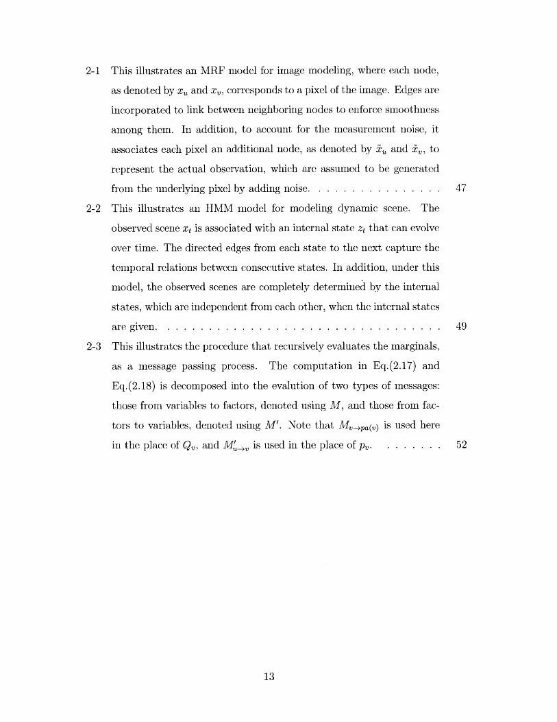
2-1 This illustrates an MRF model for image modeling, where each node,
as denoted by x, and x, corresponds to a pixel of the image. Edges are
incorporated to link between neighboring nodes to enforce smoothness
among them. In addition, to account for the measurement noise, it
associates each pixel an additional node, as denoted by ze and zr-, to
represent the actual observation, which are assumed to be generated
from the underlying pixel by adding noise. . . . . . . . . . . . . . . . 47
2-2 This illustrates an HMM model for modeling dynamic scene. The
observed scene xt is associated with an internal state zt that can evolve
over time. The directed edges from each state to the next capture the
temporal relations between consecutive states. In addition, under this
model, the observed scenes are completely determined by the internal
states, which are independent from each other, when the internal states
are given . . . . . . . . . . . . . . . . . . . . . . . . . . . . . . . . . . 49
2-3 This illustrates the procedure that recursively evaluates the marginals,
as a message passing process. The computation in Eq.(2.17) and
Eq.(2.18) is decomposed into the evalution of two types of messages:
those from variables to factors, denoted using M, and those from fac-
tors to variables, denoted using M'. Note that Mvopa(v) is used here
in the place of Qv, and M', is used in the place of p.. . . . . . . . 52
13
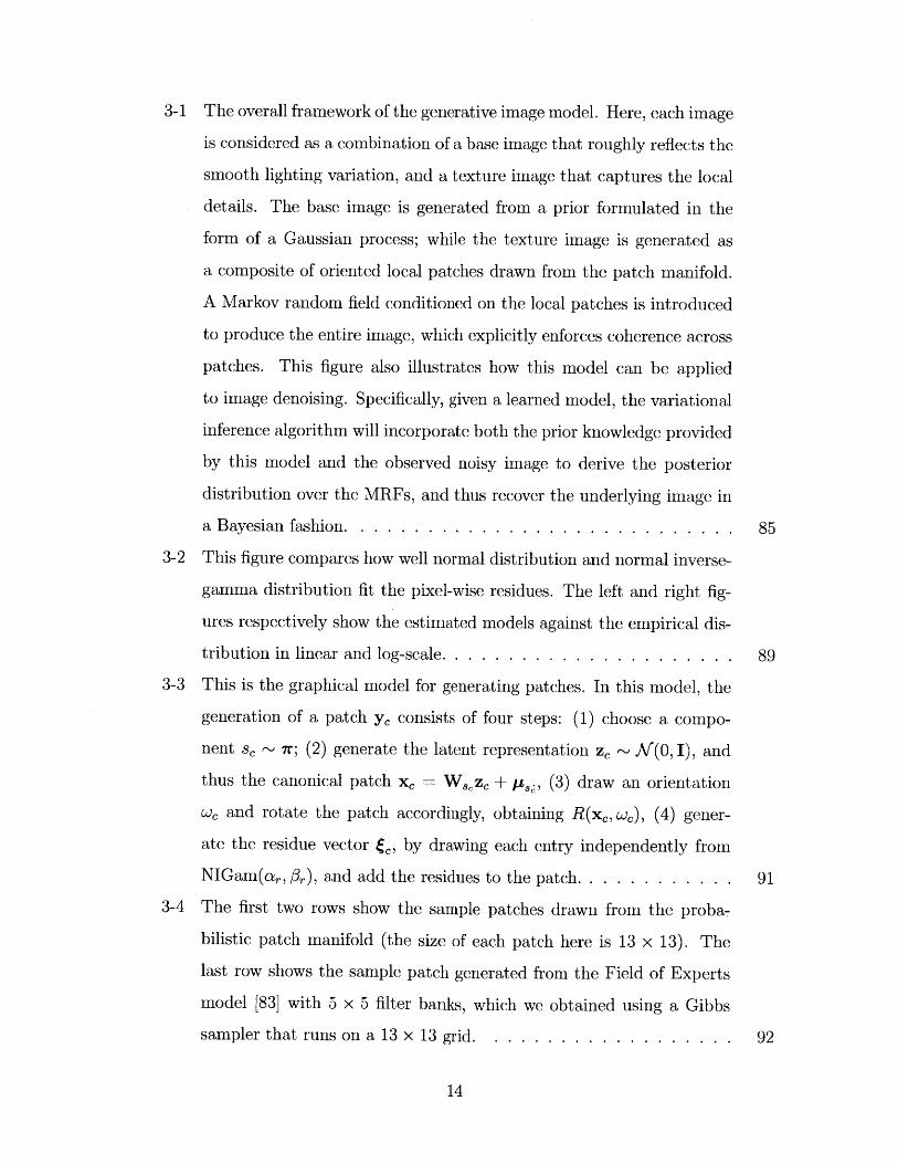
3-1 The overall framework of the generative image model. Here, each image
is considered as a combination of a base image that roughly reflects the
smooth lighting variation, and a texture image that captures the local
details. The base image is generated from a prior formulated in the
form of a Gaussian process; while the texture image is generated as
a composite of oriented local patches drawn from the patch manifold.
A Markov random field conditioned on the local patches is introduced
to produce the entire image, which explicitly enforces coherence across
patches. This figure also illustrates how this model can be applied
to image denoising. Specifically, given a learned model, the variational
inference algorithm will incorporate both the prior knowledge provided
by this model and the observed noisy image to derive the posterior
distribution over the MRFs, and thus recover the underlying image in
a Bayesian fashion. . . . . . . . . . . . . . . . . . . . . . . . . . . . . 85
3-2 This figure compares how well normal distribution and normal inverse-
gamma distribution fit the pixel-wise residues. The left and right fig-
ures respectively show the estimated models against the empirical dis-
tribution in linear and log-scale. . . . . . . . . . . . . . . . . . . . . . 89
3-3 This is the graphical model for generating patches. In this model, the
generation of a patch ye consists of four steps: (1) choose a compo-
nent sc ~ 7r; (2) generate the latent representation zc - NJ(O, I), and
thus the canonical patch xc = z + p,., (3) draw an orientation
we and rotate the patch accordingly, obtaining R(xc, wc), (4) gener-
ate the residue vector c, by drawing each entry independently from
NIGam(ar, /,), and add the residues to the patch. . . . . . . . . . . . 91
3-4 The first two rows show the sample patches drawn from the proba-
bilistic patch manifold (the size of each patch here is 13 x 13). The
last row shows the sample patch generated from the Field of Experts
model [83] with 5 x 5 filter banks, which we obtained using a Gibbs
sampler that runs on a 13 x 13 grid. . . . . . . . . . . . . . . . . . . 92
14
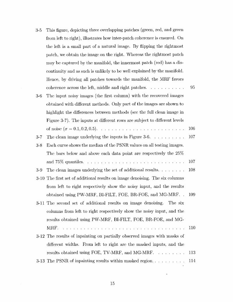
3-5 This figure, depicting three overlapping patches (green, red, and green
from left to right), illustrates how inter-patch coherence is ensured. On
the left is a small part of a natural image. By flipping the rightmost
patch, we obtain the image on the right. Whereas the rightmost patch
may be captured by the manifold, the innermost patch (red) has a dis-
continuity and as such is unlikely to be well explained by the manifold.
Hence, by driving all patches towards the manifold, the MRF favors
coherence across the left, middle and right patches. . . . . . . . . . . 95
3-6 The input noisy images (the first column) with the recovered images
obtained with different methods. Only part of the images are shown to
highlight the differences between methods (see the full clean image in
Figure 3-7). The inputs at different rows are subject to different levels
of noise (o- 0.1,0.2,0.5). . . . . . . . . . . . . . . . . . . . . . . . . 106
3-7 The clean image underlying the inputs in Figure 3-6. . . . . . . . . . 107
3-8 Each curve shows the median of the PSNR values on all testing images.
The bars below and above each data point are respectively the 25%
and 75% quantiles. . . . . . . . . . . . . . . . . . . . . . . . . . . . . 107
3-9 The clean images underlying the set of additional results. . . . . . . . 108
3-10 The first set of additional results on image denoising. The six columns
from left to right respectively show the noisy input, and the results
obtained using PW-MRF, BI-FILT, FOE, BR-FOE, and MG-MRF. . 109
3-11 The second set of additional results on image denoising. The six
columns from left to right respectively show the noisy input, and the
results obtained using PW-MRF, BI-FILT, FOE, BR-FOE, and MG-
M R F . . . . . . . . . . . . . . . . . . . . . . . . . . . . . . . . . . . . 110
3-12 The results of inpainting on partially observed images with masks of
different widths. From left to right are the masked inputs, and the
results obtained using FOE, TV-MRF, and MG-MRF. . . . . . . . . 113
3-13 The PSNR of inpainting results within masked region . . . . . . . . . 114
15
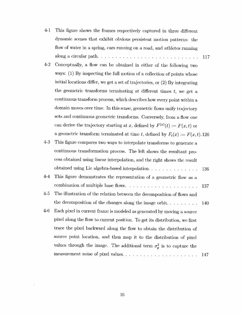
4-1 This figure shows the frames respectively captured in three different
dynamic scenes that exhibit obvious persistent motion patterns: the
flow of water in a spring, cars running on a road, and athletes running
along a circular path. . . . . . . . . . . . . . . . . . . . . . . . . . . . 117
4-2 Conceptually, a flow can be obtained in either of the following two
ways: (1) By inspecting the full motion of a collection of points whose
initial locations differ, we get a set of trajectories, or (2) By integrating
the geometric transforms terminating at different times t, we get a
continuous transform process, which describes how every point within a
domain moves over time. In this sense, geometric flows unify trajectory
sets and continuous geometric transforms. Conversely, from a flow one
can derive the trajectory starting at x, defined by F(x)(t) := F(x, t) or
a geometric transform terminated at time t, defined by Ft(x) := F(x, t). 126
4-3 This figure compares two ways to interpolate transforms to generate a
continuous transformation process. The left shows the resultant pro-
cess obtained using linear interpolation, and the right shows the result
obtained using Lie algebra-based interpolation. . . . . . . . . . . . . . 136
4-4 This figure demonstrates the representation of a geometric flow as a
combination of multiple base flows. . . . . . . . . . . . . . . . . . . . 137
4-5 The illustration of the relation between the decomposition of flows and
the decomposition of the changes along the image orbit . . . . . . . . 140
4-6 Each pixel in current frame is modeled as generated by moving a source
pixel along the flow to current position. To get its distribution, we first
trace the pixel backward along the flow to obtain the distribution of
source point location, and then map it to the distribution of pixel
values through the image. The additional term o is to capture the
measurement noise of pixel values. . . . . . . . . . . . . . . . . . . . . 147
16
4-7 Here show the flows sampled from two prior models. The left one is
sampled from the GP-prior with O-GP = 0. In this case, essentially
no spatial coherence is enforced. The right one is sampled from the
GP-prior with og = 300 pixels. For each sample, 400 trajectories are
simulated and shown as red curves. . . . . . . . . . . . . . . . . . . . 150
4-8 This graphical model incorporates the generative observation model
and the GP-prior of the flows. Here, each observation entry is associ-
ated with a label variable zi that indicates which flow it is generated
from and a binary variable gi that indicates whether it is a valid ob-
servation. The label variables are connected to each other through an
MRF, while the distribution of gi is independent, characterized by a
prior confidence ci, i.e. the prior probability of gi = 1. . . . . . . . . . 152
4-9 The plot of all extracted local motions from the New York Grand
Central station. . . . . . . . . . . . . . . . . . . . . . . . . . . . . . . 153
4-10 Three are three representative flows discovered by the Lie algebra based
flow model. The region that is not covered by the flow is masked. The
blue arrows indicate the flow field, and a subset of persons governed
by the flow is highlighted with red boxes. . . . . . . . . . . . . . . . . 153
4-11 This figure compares the motion prediction performance of LAB-FM
and JLV-GM on testing samples. The x-axis here is the number of
mixture components, and the y-axis quantity here is the fraction of
observations within given errors from the model prediction. . . . . . . 154
4-12 An example of outlier detected by the flow model. Here, the trajectory
of the person (highlighted with red color) is clearly different from what
the flow model may predict at his location. . . . . . . . . . . . . . . . 154
17
4-13 This figure shows the motion analysis results obtained from a scene
with cars moving on a road. The first row shows the results respectively
obtained using optical flow (left) and geometric flow (right), which are
visualized in form of velocity fields. The left picture of the second row
shows a subset of predicted trajectories (the blue curves are yielded
by geometric flows, the red ones are yielded by optical flows, while the
green ones are ground-truth derived by manual labeling. The fourth
picture compares the trajectory-prediction error quantitatively. . . . . 158
4-14 This figure shows the motion analysis results obtained from a scene
with a large group of athletes running on tracks. The first row shows
the results respectively obtained using optical flow (left) and geometric
flow (right), which are visualized in form of velocity fields. The left
picture of the second row shows a subset of predicted trajectories (the
blue curves are yielded by geometric flows, the red ones are yielded by
optical flows, while the green ones are ground-truth derived by manual
labeling. The fourth picture compares the trajectory-prediction error
quantitatively. . . . . . . . . . . . . . . . . . . . . . . . . . . . . . . . 159
4-15 In this figure, the first column shows the results obtained on modeling
the flowing water in a mountain spring. The second column shows
that on a rotating disc. The bottom row shows two charts, giving
the average fitting errors and generalization errors obtained from the
corresponding example. . . . . . . . . . . . . . . . . . . . . . . . . . . 160
4-16 The trajectory prediction errors with different types of observations.
The left and right charts are respectively obtained from the scene with
moving cars and that with running athletes. . . . . . . . . . . . . . . 161
4-17 The figure shows the motion patterns of the bottom-right part of the
mountain spring estimated under different settings. From left to right,
the results are obtained by optical flow, geometric flows with o-g, set
to 0, 100, 10000 respectively. . . . . . . . . . . . . . . . . . . . . . . . 161
18
5-1 The graphical representation of a finite mixture model. The mix-
ture comprises K component models, respectively with parameters
01, .. . , OK- Data samples are generated independently from this model.
In particular, to generate the i-th sample, zi is first drawn from ir, and
then the corresponding component 9(O,) is used to generate xi. . . . 165
5-2 The graphical representation of a Gaussian mixture model, which con-
sists of K Gaussian components. Each Gaussian component (say the
k-th one) is characterized by a mean vector pk and a covariance matrix
Ek. With this model, each data point is drawn independently from a
particular Gaussian distribution, chosen from a discrete distribution 7r. 165
5-3 This figure shows two examples of using Gaussian mixtures to ap-
proximate other distributions: (a) a distribution with three modes is
approximated by a mixture model comprised of three Gaussian com-
ponents. (b) a heavy-tailed distribution is approximated by a mixture
of four Gaussian components with zero mean and different variances
(this is also called a Gaussian scale mixture). . . . . . . . . . . . . . 166
5-4 This figures show the graphical representation of two topic models un-
der different formulations: (a) is probabilistic latent semantic indexing,
where each document is associated with a document-specific mixture
of topics Oj. (b) is latent Dirichlet allocation, which extends PLSI by
introducing a Dirichlet prior over the topic distributions. In addition
to this, a Dirichlet prior is often incorporated as the prior of the word
distributions. . . . . . . . . . . . . . . . . . . . . . . . . . . . . . . . 167
5-5 This figure shows the graphical representations of the DP mixture
model. (a) Basic formulation: each sample is associated with a pa-
rameter, which is generated from an underlying DP sample D. (b)
An equivalent formulation derived based on the Chinese restaurant
process. Here, an infinitely pool of atoms is independently generated,
and each sample is attached a label drawn from a CRP. This labels
associates the sample with an atom chosen from the pool. . . . . . . 175
19
5-6 This figure shows an extended DP mixture model, which incorporates
temporal dependency between DPs at consecutive time. In this model,
there is a DP mixture model at each time step. Based on the tem-
poral dependency between them, the DPs together form a Markov
chain. Conditioned on the DP prior at time t, the model parameters
0t:1, ... .t:nt and thus the observations Xt:1, ... , Xt:nt are independently
generated. ....... ................................. 177
5-7 This figure shows a realization of a Poisson process whose base measure
p is inhomogeneous over the underlying space, which is a collection of
points. Let A and B denote the two regions marked by red ellipses.
Then Nr(A) and Nr(B) are respectively the numbers of points therein,
which are are independent variables. . . . . . . . . . . . . . . . . . . 183
5-8 This figure illustrates how a Gamma process can be constructed from a
Poisson process over a product space. On the left shows a realization of
a Point process II* over the product space Q x R+, where each point is a
pair (0, wo). Converting each such point to a term w960 and combining
them to form a series, we obtain a random measure as in Eq.(5.34).
In particular, when I* ~ PP(p x -y), E* is a Gamma process that has
E * ~ I'P (p ). . . . . . . . . . . . . . . . . . . . . . . . . . . . . . . . 185
5-9 This diagram shows the high-level idea behind our approach. Rather
than directly working with the DPs directly, we do the construction in
the Poisson domain, obtaining a new Poisson process via the operations
that preserve complete randomness. Then, we can derive a DP from
the resultant Poisson process, based on their intrinsic connections. . . 187
20
5-10 This figure compares the performance between D-DPMM and D-FMM
with differing numbers of components. The upper graph shows the
median of distance between the resulting clusters and the ground truth
at each phase. The lower graph shows the actual number of clusters
as a function of time. Clearly, the performance of dynamic FMM is
inferior to that of dynamic DPMM, when the pre-set number of clusters
does not match the true number. . . . . . . . . . . . . . . . . . . . . 206
5-11 The simulation results under different settings: (a) shows the perfor-
mance of D-DPMM with different values of acceptance probability,
under different data sizes. (b) shows the performance of D-DPMM
with different values of diffusion variance, under different data sizes. 207
5-12 The experimental results on people flow modeling. This figure shows
the timelines of the top 20 flows. On the right is the snapshot of two
such flows, with the velocity fields overlain on the images. (Only the
parts covered by the flow domain are visible). . . . . . . . . . . . . . 208
5-13 The experimental results on PAMI topic analysis. On the left are
the timelines of the top 10 topics. On the right are the two leading
keywords for these topics. . . . . . . . . . . . . . . . . . . . . . . . . 209
6-1 This illustrates how two Markov chains are bridged. In the joint chain over
X U Y, each x E X has a probability bQB(x, y) to transit to y E Y, and
each y has a probability fQF(Y, X) to transit to x . . . . . . . . . . . . . 233
21
6-2 (a) shows the hierarchically bridging Markov chain on a simple problem:
X1 , X2 E {0, 1} with constraint xi 1 X2. We use red color for the backward
transitions from children to parents, and green for the transitions from par-
ents to children. (b) illustrates a typical transition path. We use numbered
circles to indicate the transition order. In this process, the bridges (0, -)
and (-, -) are constructed upon the backward transition from a child state.
When (-, -) is instantiated, the right branch has not been visited, and the
forward probability value for that branch is set with an optimistic estimate,
encouraging the chain to visit that branch. Upon seeing (1, 0), the forward
probabilities of its parents will be updated accordingly. . . . . . . . . . . 246
6-3 Each curve shows the mean energy values (- log p(x)) as a function of
elapsed iterations. Since Relaxed-GS and HBMC may yield states that
are not in Q, we use the energy of the last valid state as the energy value
for an iteration. This also shows bars at 10% and 90% quantiles for 100
repeated runs. . . . . . . . . . . . . . . . . . . . . . . . . . . . . . . . 255
6-4 The energy auto-correlation function. . . . . . . . . . . . . . . . . . . . 256
6-5 The correlations between the empirical distributions of the collected samples
and the true distribution. Note that the y-axis is at log-scale. . . . . . . . 257
6-6 An illustrative example: (a) synthetic image with markups (this image +
noise of o- = 0.2 is the input), (b) ground-truth (HBMC obtains this in most
cases), (c) a result via MRF, (d) a result via BLK. . . . . . . . . . . . . 258
6-7 The average ratios of error labels on both test regions and hard regions over
all 200 synthetic images, obtained using four methods under different levels
of noise and model bias. . . . . . . . . . . . . . . . . . . . . . . . . . . 258
6-8 The inferred partial orders of vehicles in 4 frames of a video (interval = 3
sec). Vehicles are marked with transparent rectangles in different colors.
Below them are opaque blocks that illustrate their Z-orders . . . . . . . . 261
22
C-1 This graph illustrates the relations of subgroups of the Affine group. In
this graph, Af f represents Aff(n), Af f+ represents Aff+(n), GL repre-
sents GL(n, R), GL+ represents GL+(n, R), 0 represents 0(n), SO repre-
sents SO(n), D represents the diagonal group, D+ represents the positive
diagonal group, U. S. represents the uniform scaling group, T represents
the translation group, E represents E(n), E+ represents E+(n). The ar-
rows represent the sub-group relationship, while the symbol x in the
formulas represents the semidirect product factorization. . . . . . . . 292
23

List of Tables
24
Chapter 1
Introduction
One of the fundamental goals of computer vision is to derive intelligent systems that
can reason about visual scenes, typically captured in the form of images and videos.
The past decades have witnessed tremendous efforts towards this goal, resulting in
great advancement in a wide range of computer vision topics. However, a substantive
amount of prior work is dedicated to specific vision problems, such as object recog-
nition, image segmentation, and motion analysis, leading to substantially different
models for describing different aspects of a scene.
This thesis pursues a different approach. Instead of seeking solutions dedicated to
particular problems, the primary goal of this thesis is to develop a generative model
of dynamic visual scenes that integrates models of different aspects (e.g. appearance
and motion) into a probabilistic framework. This work is driven by our strong desire
to understand the fundamental structures of visual scenes. As Kurt Lewin said,
There is nothing more practical than a good theory.
Whereas problem-oriented approaches can be very successful in accomplishing specific
tasks, our view is the advancement of computer vision ultimately relies on deep un-
derstanding of the visual scenes, as well as effective means to capture their structures.
From a practical standpoint, many applied problems can be readily solved through
the inference performed on an integrated generative model. Moreover, as opposed
to descriptive and discriminative methods, a generative model also provides greater
25
flexibility to leverage observations acquired in different ways and take into account
various statistical relations.
However, the use of generative models, as opposed to discriminative methods,
often comes with additional complications in both model formulation and algorithm
design. Therefore, special attention should be paid to making appropriate tradeoffs
in order to achieve the desired expressiveness without significantly increasing com-
putational complexity. Through out the entire thesis, we will see, modeling choices
made with the careful consideration of such balance.
Generally, visual scenes are complex and far beyond the capacity of a thesis to
provide a complete interpretation that takes all relevant aspects into account. This
thesis particularly focuses on three key aspects - appearance, motion, and composition,
and develops a probabilistic framework that integrates these aspects to give a coherent
interpretation of a visual scene. Conceptually, the appearance aspect is about what
the scene looks like; the motion aspect is about how the shapes and positions of the
objects in a scene change over time; the composition aspect, on the other hand, is
about how different parts of a scene are brought together. Generally, these aspects
are closely related. For example, motion will cause dynamic changes of appearance,
and the compositional structure will greatly influence both the appearance and the
perceived motion.
1.1 Questions to be Answered
Towards an integrated model of visual scenes, this thesis tries to address a series of
questions as outlined below:
1. How can we model the appearance? While humans can perceive objects and
regions when looking at an image or a video, what a computer sees is technically
no more than a large matrix of pixel values (i. e. intensities or colors). The spatial
configuration (pattern) of these values constitutes the image's appearance. The
question here is how to represent these patterns in a way that explains the
inherent structure of the visual scene. Generally, the characteristics of patterns
26
at different scales are substantially different, and should therefore be represented
and modeled in different ways.
2. How can we model the motion occurring in a dynamic scene? In a dynamic
scene, various phenomena can cause changes in appearance. One of the most
common causes is motion, the change in positions and shapes of objects. There
has been extensive study on motion analysis in past decades, much of which
aims at accurate estimation of local movement of individual objects or points.
However, our sense of motion in many natural scenes is reflected by the changes
over a region or by the collective behavior of a group of objects, which we refer
to as the collective dynamics. Effective analysis of the collective dynamics (e.g.
revealing the underlying coherence between the motion of different objects) is
often the key to the understanding of visual scenes.
3. How can we handle concurrent entities in a visual scene? It is not uncommon
in natural scenes that multiple entities (e.g. objects and flows) are observed at
the same time. Each entity may have its own appearance and behavior. When
a natural scene is projected onto an image plane, occlusion may occur. Objects
occluded by others are only partially observed, further complicating analysis. It
is possible to rely on a three-dimensional model to resolve this issue, but doing
so generally requires 3D reconstruction, which in itself is a nontrivial problem.
As we will see, a layered representation, which captures the relative depth order
between objects instead of their 3D positions, is often sufficient to resolve most
of the ambiguities resulting from occlusions, and can be inferred more reliably
and efficiently.
4. How can we model the relations between appearance and motion? As mentioned,
a dynamic visual scene is characterized by both the spatial structure and the
temporal dynamics, which are respectively captured by the appearance and the
motion. These two aspects are not completely independent. Instead, they are
closely coupled with each other, and what we see in a video is actually the
compound effect of both. While separate study of each aspect is useful, it is
27
also very important to understand how they relate to each other. Such spatial-
temporal relations can be exploited to improve the analysis of videos and help
other video-related tasks.
5. How can we handle model complexity? Tradeoffs between expressiveness and
complexity has been one of the central themes of machine learning and related
fields such as computer vision. Mixture models, which are often used to capture
complex distributions, are employed in many vision models. An important issue
here is how to determine the number of components in a mixture model (i.e. the
model order). In a dynamic setting (e.g. video analysis), the phenomena of
interest may evolve over time. Modeling such phenomena generally requires a
model which is able to change its order adaptively. Formulating and estimating
models with dynamic complexity is a challenging problem.
1.2 The Overall Scene Modeling Framework
The first step of visual scene modeling is to choose a specific way to construct the
model. In general, dynamic scenes can be very complex. To effectively model such
scenes, we have to make simplified assumptions, emphasizing key aspects, while de-
liberately neglecting the others. First of all, we have to decide the basic structure of
the model. Here, several questions arise:
" What are the basic components?
" How do the components interact?
" How do they evolve over time?
Generally, there are three approaches to scene modeling, with different answers to
these questions, which we will briefly review below.
28
1.2.1 Three Approaches to Scene Composition
Existing approaches to scene modeling can be roughly classified into three categories,
according to the ways they model the compositional structure of a scene.
1. Segmentation-based Models. Segmentation is widely used in analyzing im-
ages comprised of multiple regions. Models in this category describe an image as
composed of multiple disjoint regions called segments. The appearance within
each segment has relatively consistent characteristics, while such characteristics
in neighboring regions may be remarkably different.
A segmentation-based model typically comprises a set of appearance models,
each for a particular region, and a model that incorporates prior knowledge
about the segmentation itself (e.g. spatial continuity and the smoothness of the
segment boundaries). Such approaches aim to capture common visual char-
acteristics within each region while allowing substantial variation across the
boundaries.
Despite its utility in image analysis, several fundamental problems limit the
use of segmentation-based approaches in dynamic contexts, especially when
occlusion occurs. First, an object can be divided into disconnected segments in
different ways, sometimes complicating the correspondence between segments
across video frames. Second, segments moving towards each other and then
overlapping would lead to a "conflict of explanation", while segments moving
away may leave part of the image covered by no region. These problems stem
from the occlusion occurring when a three dimensional scene is projected onto
a two dimensional view.
2. Three Dimensional Models. A three-dimensional (3D) model describes a
visual scene within a 3D coordinate system, and observed images of the scene as
projections onto 2D image planes. By maintaining the 3D positions of objects,
the ambiguities encountered by segmentation-based models can be effectively
addressed.
29
Generally, the process of obtaining a 3D visual model from observed images
is called 3D reconstruction, which in itself is nontrivial. It has long been an
active topic in computer vision. Typically, 3D reconstruction requires stereopsis
(a.k.a. binocular vision), or relies on knowledge about the geometric relations
between the scene and the camera to recover the scene structure. However, in
practice, many videos of interest are captured impromptu, or without using a
calibrated camera, making it difficult to obtain a 3D model reliably. In addition,
the computational complexity required to estimate and maintain a 3D model is
often higher than that for methods based on 2D image models.
3. Layered Models. The aforementioned difficulties motivate researchers to ex-
plore more effective approaches to generic video modeling. Layered video models,
introduced in Wang and Adelson's pioneering work [109], have become increas-
ingly popular for dynamic scene modeling.
In general, a layered model describes an observed image of a scene as a super-
position of multiple layers, each corresponding to an object or a set of objects
with coherent behavior. One major difference that distinguishes a layered model
from a segmentation-based model is that a layered model allows different lay-
ers to overlap and explicitly takes into account the occlusion relations between
them.
Instead of trying to estimate the depth map as in methods using 3D models,
a layered model relies on occlusion reasoning, which is generally much easier,
especially when the scene is captured with a single camera.
Based on the considerations above, we chose to construct the model of dynamic scenes
using a layered structure. Next, we will outline the overall formulation of this model,
and identify the key components.
1.2.2 A Layered Model of Dynamic Scenes
A layered model considers a video as a composite of multiple dynamic layers. It is
difficult to characterize a layer in general, as its meaning often depends on specific
30
(a) (b) (c)
Figure 1-1: This figure shows several cases where the simplified assumptions underly-ing the layered model are violated. (a) shows a girl behind a boy, while her hands arein front of him. If we model them as two layers, then there is no definite depth orderbetween them. (b) shows two kids playing basketball. While they can be modeledas two dynamic layers, their behavior are not independent. (c) show a soldier in abattlefield. His behavior may be influenced by many factors, and simply modeling itas a Markov chain may overly simplify the real world complication.
context (e.g. the type of the scene, and the scale at which the analysis is being
performed). Generally, a layer may correspond to an object, a group of objects with
consistent behaviors that are spatially close to each other, or a part of the scene with
coherent dynamics.
The study presented in this thesis is based on the layered video model as described
below. Consider a video with n layers, denoted by L 1, . . . , L,. Each layer (say the
i-th one Li) is associated with (1) a covering domain Di that specifies sub-region in
the image plane physically covered by the layer, (2) an appearance template Ai that
describes the visual content of the layer (or technically, the spatial pattern of the
pixel values in the layer), and (3) a flow F that describes the motion.
For a dynamic scene, the covering domain, the appearance template, as well as
the flow associated with a layer may each vary over time. To reflect this, we use
D *), Aft), and Ft) to respectively denote the versions of these components at time
t. The changes occurring in different aspects are related. For example, the changes
in appearance or covering domain may be influenced by motion. To capture such
relations, we formulate the dynamics of these aspects jointly through the conditional
31
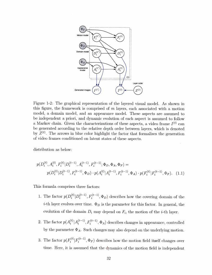
Figure 1-2: The graphical representation of the layered visual model. As shown inthis figure, the framework is comprised of m layers, each associated with a motionmodel, a domain model, and an appearance model. These aspects are assumed tobe independent a priori, and dynamic evolution of each aspect is assumed to followa Markov chain. Given the characterizations of these aspects, a video frame (t) canbe generated according to the relative depth order between layers, which is denotedby Z(t). The arrows in blue color highlight the factor that formalizes the generationof video frames conditioned on latent states of these aspects.
distribution as below:
p(D1t), A1 IE0, F |D t-1, At-1, F.t-' ;D D, A(F ~
p(Dt)|D t-l) Fjt~ 1 D)- p(A|t)A F - ,A) p( FFt1-, ,F). (1.1)
This formula comprises three factors:
1. The factor p(DIt|D/~l, F~4l, @D) describes how the covering domain of the
i-th layer evolves over time. ( D is the parameter for this factor. In general, the
evolution of the domain Di may depend on F, the motion of the i-th layer.
2. The factor p(At) A-, FW1 , cJIA) describes changes in appearance, controlled
by the parameter (DA. Such changes may also depend on the underlying motion.
3. The factor p( p (FD, IF) describes how the motion field itself changes over
time. Here, it is assumed that the dynamics of the motion field is independent
32
of the appearance a priori.
To establish a complete probabilistic formulation, we also need a prior distribution
over these components for the initial frame, as
p(D( , A(O) , F 03|<b0(Do (D0A 4)g0 p(D(0)|<DD 0pA) I 0D pk) OF 'Dp(DD) Ai0 F iJ,4 DpD0 i uA F (1.2)
As the motion only affects what we may observe in the next frame, the initial prior
of the covering domain and the appearance does not depend on the motion.
Given all the layers, each observed video frame can be generated through super-
position. Note that the covering domains of different layers can overlap, some regions
may be covered by more than one layer. In such a region, only the layer at the top
is visible, while others are occluded. This model uses a partial order to capture the
relative depth order between layers such that the top layer of each region can be
readily determined. Let Z denote this partial order and x be a pixel location, then
the visible pixel value at x is given by
IP)(x) = L' )(x), t(x) = max{i : x E D t)}. (1.3)
Here, t(x) denotes the index of the layer that is visible at x, which is set to be
the maximum among all the layers that cover x. Note that the maximum here is
with respect to the depth order Z, implying that it corresponds to the top layer. In
addition, we use Lit) (x) to denote the pixel value at x of the layer Li at time t. Hence,
following a (partial) depth order, all layers can be combined in a consistent way into
video frames.
We obtain a joint model, as shown in Figure 1-2, by integrating the priors for
individual layers with the factor above that describes how layers combined to produce
observe images. Note that a probabilistic model expressed in form of a graph is often
referred to as a graphical model, for which Chapter 2 provides a detailed treatment.
33
1.2.3 Discussion on Modeling Choices
Several simplifying assumptions underlie the model established above.
1. A visual scene can be decomposed into a superposition of several layers, and
that these layers follow a consistent depth order. This model enforces a strong
constraint that precludes some cases, such as those illustrated in Figure 1-1(a),
where part of a layer is below another, while the other part is above. In addition,
the layers are considered to be non-transparent, meaning that the occluded part
of a layer will be completely invisible. It is possible to further extend the model
further to explain such scenes, but this is outside the scope of this thesis.
2. The appearance and dynamics of different layers are assumed to be indepen-
dent. This might seem to be an overly simplified assumption, as behaviors of
objects coexisting in the same scene might interact with each other in various
ways (an example is shown in Figure 1-1(b)). While understanding such inter-
actions might be in the interest of some high-level applications, such as behavior
analysis, it is reasonable to ignore them in constructing a lower-level vision sys-
tems, because the primary goal here is to derive an intermediate representation
of the appearance and motion. For a problem where such interactions play a
crucial role, one can build an interaction model on top of the vision model being
discussed in this thesis.
3. The dynamics of each layer is modeled as a first-order Markov chain. This
assumption ignores some real world complexities where the behavior of an object
may depend on many other factors in addition to how it behaves at the previous
time step, as illustrated in Figure 1-1(c). Again, to keep the model simple,
we chose to focus on the aspects directly pertinent to vision problems. It is
possible to develop higher level reasoning methodologies on top of the framework
developed by this thesis.
34
1.2.4 Main Aspects
In the visual modeling formulation outlined above, we can identify several key aspects
and how they relate to each other. These aspects are summarized as follows.
1. Appearance. The appearance model specifies the spatial structure of the vi-
sual scene. In particular, the pixel values in each layer Li are captured by
an appearance template Aj. The associated appearance model (with parame-
ter <DA) provides a generative prior p(Ail DA) over such appearance templates,
specifying how the pixels are distributed, how their values relate to each other,
and what the spatial structures are.
2. Motion. The dynamics of a visual scene is mainly captured by the motion
model. At the heart of the motion model is an intermediate representation of
the motion, called flows. Particularly, each layer Li is associated with a flow,
denoted by F. In addition, the motion model also specifies the prior distribution
of the flows p(F) 14)0) and how flows evolve over time p(Ft<DF)-
3. Layer Order. The composition of layers into video frames depends on the
relative depth order between layers. A layer can be occluded by the one above
it when they overlap. This relation between layers can be formalized as a partial
order, over which we can define a prior distribution for Bayesian inference.
Whereas we do not develop a complete interpretation of visual scenes in this
thesis, we view the framework and methodology presented in this thesis as part of an
overall effort towards that ultimate goal. Putting this thesis in a broader perspective
of computer vision research, we acknowledge that some important problems are not
covered by the three aspects above (e.g. the modeling of layer domains, the relations
between layers from different views, and semantic implications of the characterizations
for appearance and motion). Still, this thesis contributes to the advancement of
computer vision in several important ways:
* It demonstrates the utility of generative models in computer vision, and illus-
trates how they can be formulated to solve vision problems through the devel-
35
opment of specific models to describe appearance, motion, and layer order.
" The models studied in. this thesis can be extended, modified, or adapted to solve
other problems that we do not explicitly consider. For example, the appearance
model can be generalized to describe color images or textures on 3D surfaces,
and the motion model can be adapted by incorporating additional structure
when applied to a specific context. Furthermore, these models can be used in
combination with other vision models to derive more sophisticated frameworks
or to address more complex issues.
" A series of methods, such as dynamic nonparametric models and methods to
sample from combinatorial spaces, has been developed to address specific chal-
lenges in vision problems. The use of these methods, however, is by no means
restricted to the applications discussed in this thesis. They can be applied,
sometimes with modification, to solve other problems, including many outside
the realm of computer vision.
1.3 The Organization of the Thesis
Thus far, a high-level structure of the scene model has been specified. However, many
interesting but challenging questions are yet to be answered: e.g. how to represent
appearance and motion, how to define the prior distribution and conditional distri-
bution, how to estimate the model parameters, and how to perform inference over
this model. Most of the work presented in this thesis tries to answer these questions,
as we shall see in the following chapters.
The remaining part of this thesis is organized as follows. Chapter 2 briefly re-
views the advancement of visual modeling in past decades with an aim to provide a
retrospective view of of ways in which recent progress of this field is influenced by
the prevalent use of probabilistic models. This chapter also covers the basic concepts
for probabilistic modeling, such as Bayesian networks and Markov random fields, as
well as the basic tools for learning and inference, including mean field approximation,
36
belief propagation, and Monte Carlo sampling. The materials in this chapter lay the
theoretical foundation for later discussions.
Starting from Chapter 3, we present the vision models in detail. Particularly, this
chapter describes a new image prior for appearance modeling. The development of the
new image model is motivated by the key insight that the effectiveness of an image
model, to a large extent, hinges on its capability of capturing local pixel patterns
and maintaining the coherence of local structures. To improve on these aspects,
we develop a new generative model of images, which integrates a patch manifold to
capture local patterns and a conditional Markov random field to enforce coherence
across patches. We also derive algorithms to estimate the model parameters from a
set of training images. It is important to note that with this model, a set of low-
level vision problems, including image denoising and inpainting, can be readily solved
via the inference performed based on a joint model that combines this prior with a
specific measurement process.
The results obtained by applying this model to image recovery are also be pre-
sented and analyzed.
Chapter 4 discusses motion models. As an important area of computer vision,
motion estimation has been extensively studied. Prior work on motion modeling and
estimation has focused on tracking and optical flow. However, in many scenes, the
overall sense of dynamics is reflected by the collective movement of large groups of
objects/people, or by the motion over a region, which we refer to as the collective
dynamics. The primary goal here is to develop an effective framework to character-
ize and estimate such collective dynamics. In this chapter, we introduce the notion
of geometric flow, a concept originating from differential geometry, which is able to
capture motion patterns that persist (or smoothly evolve) over time. Subsequently,
we derive a vector space of flows by exploiting the intrinsic connection between Lie
groups and Lie algebras. A stochastic flow model is then developed on top of this,
with which flow parameters can be efficiently inferred from different types of obser-
vations, including tracks of key points and continuous changes in image appearance.
Application of the new motion model in several different contexts is also presented in
37
this chapter.
In both appearance and motion modeling, mixture models, which bring together
a set of component models to approximate complex distributions, play a crucial role.
Traditional study of mixture models focuses mainly on the task of fitting a mixture to
a given set of data. However, for video analysis, mixture models may need to evolve
over time so as to adapt to the changes of the observed scene. This motivates the
development of tools to construct dynamic mixture models in Chapter 5. Specifically,
this chapter first reviews finite mixture models, which are widely used in practice, and
Dirichlet process mixture models (DPMM) - a new way to construct mixture models
that allow an indefinite number of mixture components. The key challenge of using
DPMMs in a dynamic context is to allow the mixtures to evolve while maintaining
strong dependencies between them. To solve this problem, we develop a new ap-
proach to constructing dependent Dirichlet processes, which, unlike classic methods
such as the Chinese Restaurant Processes and Stick Breaking Processes, explicitly
exploits the intrinsic connection between Dirichlet and Poisson process and the con-
cept of complete randomness. Upon this construction, several primitive operations
are derived, allowing the mixture model to change in various ways. In addition to
theoretical analysis, this chapter also demonstrates the utility of this new construc-
tion in flow modeling and video interpretation, as well as applications outside the
vision domain.
Chapter 6 considers the layered structure of the model. As mentioned, layers can
overlap and thus a partial order is needed to keep track of the relative depth order
between them. This chapter studies various properties of a partial order, such as
sufficiency, minimality, and identifiability, and how they relate to visual modeling.
Based on this analysis, we establish an efficient representation using directed graphs.
In this chapter, we also discuss the methods for inferring partial depth order from
observed scenes. Generally, MAP estimation of the optimal partial order is NP-hard,
and the combinatorial constraints on partial orders also lead to great difficulties in
devising sampling schemes (e.g. the underlying space can be disconnected due to the
constraints). To address this problem, we develop a novel method to efficiently sample
38

from a constrained combinatorial space by constructing an augmented Markov chain
with improved mixing performance through the introduction of bridging nodes.
Finally, Chapter 7 concludes the entire thesis, summarizing the key aspects of the
dynamic scene model and the probabilistic modeling techniques developed to address
some of the challenges arising therefrom. In this chapter, we discuss several directions
that merit further study.
39
Chapter 2
Theoretical Background
The visual scene model developed in this thesis is a Bayesian probabilistic model,
which integrates the models of different aspects, notably the appearance model, the
motion model, and the model of layer orders, into a joint formulation.
The development of these models heavily relies on various tools of probabilistic
modeling and inference, which, in particular, includes graphical models, exponential
family distributions, variational inference, and Monte Carlo sampling.
In this chapter, we first review the basic concepts graphical models, a graphical
representation of joint distributions that indicates dependencies between variables
through edges (or arrows). With a probabilistic graphical model, one can estimate
the most probable value of the variables of interest (or the posterior distributions over
them) through inference, conditioned on the variables whose values are known.
However, performing exact inference over a graphical model can be computation-
ally intractable in practice. In such case, one can resort to techniques that can per-
form the inference approximately with reasonable complexity. This chapter also gives
a brief exposition of these approximate inference techniques, including variational
inference and Monte Carlo sampling.
Note that the contents covered by this chapter are not the contribution of this the-
sis. They are mostly from existing work. Nonetheless, this chapter is indispensable,
as it lays the theoretical foundation for the development in other chapters.
40
2.1 Probabilistic Graphical Models
Graphical models, through the combination of graph theory and probability theory,
provides a powerful and elegant means to formulate probabilistic models. The key
idea underlying graphical models is factorization: a joint distribution represented
by a graphical model can generally be factorized according to the structure of the
underlying graph. Through such factorization, model estimation and inference can
often be greatly simplified.
2.1.1 Basic Concepts of Graphical Models
A graphical model defines a family of probabilistic distributions based on graph, of
which each vertex is associated with a random variable and edges are used to indicate
the statistical dependencies between variables.
First of all, we set up the notations. Consider a graph G = (V, E). The random
variable associated with a vertex v E V is denoted by Xv, which can take values in
some space Xv. A lower-case letter (say x, E Xv) denotes a particular value assigned
to Xv. For a subset of vertices A, XA denotes the collection of random variables as
XA :- (xv, v c A), and XA denotes a particular assignment to XA.
Bayesian Networks
The graphical models associated with an acyclic directed graph (DAG) is often called
a Bayesian network. For such a graph, if there is an edge s -+ t, then s is called
a parent of t, while t is called a child of s. Generally, a vertex may have multiple
parents and multiple children. For a vertex v, the set of its parents is denoted by
ir(v), and the set of its children ch(v). A graphical model where each node (except
for the root node) has exactly one parent is called a tree model.
A Bayesian network defines a family of conditional distributions for each vertex
v, as pV(Xvlzr(V)), which describes the distribution of X, conditioned on the values
assigned to its parents. When v is the root, ir(v) = 0, this conditional distribution
reduces to a prior distribution as pv(Xv).
41
Along the graph, the joint likelihood of all variables associated with the graph can
be factorized into the product of these conditional factors, as
p(xv) = H P(Xv IX(,()). (2.1)vEV
It can be easily verified that with this joint formulation, the conditional likelihood
p(xvIx,(v)) is exactly equal to the value given by p(XvIx,(v)).
Markov Random Fields
The graphical models associated with an undirected graph is often called a Markov
random field (MRF), which factorizes according to cliques. Here, a clique C is
defined to be a fully connected subset of vertices.
Generally, an MRF considers a set of cliques C (C may be a proper subset of all
cliques) and defines a (potential function for each clique C E C, as 4'c : @vec X, -+
R+, which maps each particular value assignment of clique C to a nonnegative real
number, which reflects how compatible the assignment is with the model.
With the clique potentials, the joint likelihood of all variables can be written as
p(xv) = Z ?c(xc), (2.2)CC
where Z is a normalization constant, given by
Z = c(xc)po(dxv). (2.3)
Here, yo denotes the base measure of the joint space. For continuous variables, it is
the Lebesgue measure; while for discrete variables, it is the counting measure.
For a general MRF, the potential functions #c need not be pertinent to any
marginal or conditional distributions over the cliques. The only restrictions to 4c is
that they should be non-negative and their product is integrable (i.e. Z is finite).The maximum cardinality of a clique is called the order of the MRF. It is easy
42
to see that in a first-order MRF, all variables are independent, which is not very
interesting. Second-order MRFs have been widely used in practice, due to its sim-
plicity. A second-order MRF consists of two types of potentials, the ones over single
variables and those over pairs of connected variables. Generally, the formulation of a
second-order MRF can be written in the following form:
P(XV) = 1flv(Xv) 17 (P(Xu,Xv). (2.4)vEV {u,v}EE
From Bayesian networks to Markov random fields
It is useful to note that a Bayesian network can be considered as a special case of a
Markov random field.
Specifically, a Bayesian network as formulated in Eq.(2.1) can be treated as a
Markov random field defined on a set of cliques as
C = {Co := {v} U ir(v) V E V}.
Here, the potential function associated with the clique Cv is simply the conditional
pdf of Xv, as
and the normalization constant Z equals 1. However, in general, MR.F cannot be
converted to a Bayesian network (except for some special cases).
From a graph theoretical perspective, this re-formulation turns a directed graph
into an undirected graph, by (1) converting all directed edges to undirected edges,
and (2) adding undirected edges between pairs of parents of each vertex (if they are
not connected). This process is called moralization.
Factor graph
Both Bayesian networks and Markov random fields can be represented uniformly as
factor graphs. Different from a graphical model introduced above, a factor graph is a
43
bipartite graph consisting of two types of nodes: variable nodes, each associated with
a random variable, and factor nodes, each associated with a factor (e.g. conditional
pdfs and clique potentials). Each edge in this graph connects between a factor and a
variable involved in that factor.
With a factor graph, the joint distribution over all variables can be written in
form of a product of factors, as
P(Xv) =1 ffj(s,).j=1
Here, V denotes the set of all variable nodes, j is used as the index of factors, and Sj
denotes the subset of variables involved in the j-th factor.
As we shall see later, the notion of factor graph will greatly simplify the description
of belief propagation, a general message passing algorithm for computing marginals
over a graphical model.
2.1.2 Conditional Independence
Probabilistic graphical models can also be characterized through conditional indepen-
dence between random variables, also known as the Markov properties.
Here, we briefly review the notion of conditional independence.
Definition 2.1 (Conditionally independent variables). Let X, Y, Z be random vari-
ables, with a joint distribution p(X, Y, Z). If for any assignment x, y, z,
p(x, y z) - p(xz)p(yIz),
we call X and Y are conditionally independent given Z (or X and Y are inde-
pendent conditioned on Z), denoted as X I Y|Z.
For a general graphical model defined on a graph G, the conditional independence
is determined by the structure of G. However, the way to determine conditional
independence for Bayesian networks is different from that for Markov random fields.
44
Conditional independence between variables of a Bayesian network can be deter-
mined by examining the d-separation.
Definition 2.2 (D-separation). Let G be a directed graph and A, B, C be disjoint
subsets of vertices, any trail p satisfying either of the following conditions is said to
be d-separated by C:
1. p contains a chain u - m -+ v with m E C;
2. p contains a chain u +- m +- v with m E C;
3. p contains a fork u +- m -+ v with m E C;
4. p contains an inverted fork u -+ m +- v, where m is neither in C nor a descen-
dant of any vertex in C.
A and B are said to be d-separated by C is any trails between a vertex in A and a
vertex in B is d-separated.
Proposition 2.1. Given a Bayesian network defined on an acyclic directed graph
G. Let A, B, C be disjoint subsets of vertices. Then XA L XB|Xc if A and B are
d-separated by C.
Conditional independence between variables of an MRF can be determined much
more easily, by examining normal graph separation.
Proposition 2.2. Given a Markov random field defined on an undirected graph G.
Let A, B, C be disjoint subsets of vertices. Then XA L XB XC if any paths between
a vertex in A and a vertex in B passes through some vertex in C.
Enumerating all possible choices of subsets A, B, and C results in a list of asser-
tions of conditional independence. It can be shown that the collection of conditional
independence obtained by d-separation analysis on a Bayesian network is equal to
that obtained through the analysis on the MRF derived by moralization.
45
Equivalence of characterization
We have discussed two characterizations of probabilistic graphical models: factoriza-
tion and conditional independence. The Hammersley- Clifford theorem below, which
is a fundamental result of graphical model theory, establishes the equivalence of these
two characterizations.
Theorem 2.1 (Hammersley-Clifford theorem). Let G = (V, E) be an undirected
graph, of which each vertex v is associated with a random variable X, taking value in
X,. Suppose p(xv) > 0 for every xv E @vev v (positivity condition), then the
following statements are equivalent:
1. p satisfies local Markov property: for each vertex v E V, X, is independent
of all other variables conditioned on its neighbors, as
Xv I Xv\({}ug(r v)) Xg(v), (2.5)
where A(v) denotes the set of neighbors of v (excluding v itself).
2. p satisfies global Markov property: let A, B, and C be disjoint subsets of
vertices, such that A and B are separated by C (i.e. every path between A and
B passes through some vertex in C, or there is no path between A and B), then
XA I XB|XC.
3. p can be factorized according to the cliques of the graph. Particularly, let C be
the set of all maximal cliques of G, then p can be written as
p(xy) = 1 1 c (xc).- (2.6)ceC
A similar result holds for Bayesian networks, where the only modification is using
d-separation instead of graph separation in describing the Markov properties.
46
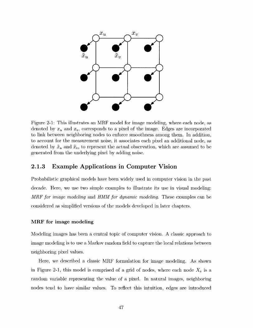
Figure 2-1: This illustrates an MRF model for image modeling, where each node, asdenoted by x, and x, corresponds to a pixel of the image. Edges are incorporatedto link between neighboring nodes to enforce smoothness among them. In addition,to account for the measurement noise, it associates each pixel an additional node, asdenoted by zu and ze, to represent the actual observation, which are assumed to begenerated from the underlying pixel by adding noise.
2.1.3 Example Applications in Computer Vision
Probabilistic graphical models have been widely used in computer vision in the past
decade. Here, we use two simple examples to illustrate its use in visual modeling:
MRF for image modeling and HMM for dynamic modeling. These examples can be
considered as simplified versions of the models developed in later chapters.
MRF for image modeling
Modeling images has been a central topic of computer vision. A classic approach to
image modeling is to use a Markov random field to capture the local relations between
neighboring pixel values.
Here, we described a classic MRF formulation for image modeling. As shown
in Figure 2-1, this model is comprised of a grid of nodes, where each node X, is a
random variable representing the value of a pixel. In natural images, neighboring
nodes tend to have similar values. To reflect this intuition, edges are introduced
47
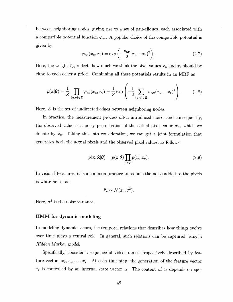
between neighboring nodes, giving rise to a set of pair-cliques, each associated with
a compatible potential function ou,. A popular choice of the compatible potential is
given by
SOuv (XuXV) = exp - (xu - X) . (2.7)
Here, the weight Ouv reflects how much we think the pixel values xu and xv should be
close to each other a priori. Combining all these potentials results in an MRF as
p(x|6) = 1 pOv(xu, z) = exp - I w{v (x - X))2 (2.8){u,v}EE {u,v}EE
Here, E is the set of undirected edges between neighboring nodes.
In practice, the measurement process often introduced noise, and consequently,
the observed value is a noisy perturbation of the actual pixel value xu, which we
denote by zu. Taking this into consideration, we can get a joint formulation that
generates both the actual pixels and the observed pixel values, as follows
p(x, x|6) = p(x|6)71 QP(z lz). (2.9)vEV
In vision literatures, it is a common practice to assume the noise added to the pixels
is white noise, as
zX NV(xV,o a).
Here, u2 is the noise variance.
HMM for dynamic modeling
In modeling dynamic scenes, the temporal relations that describes how things evolve
over time plays a central role. In general, such relations can be captured using a
Hidden Markov model.
Specifically, consider a sequence of video frames, respectively described by fea-
ture vectors XO, x 1, ... , XT. At each time step, the generation of the feature vector
xt is controlled by an internal state vector zt. The content of zt depends on spe-
48
Figure 2-2: This illustrates an HMM model for modeling dynamic scene. The observedscene xt is associated with an internal state zt that can evolve over time. The directededges from each state to the next capture the temporal relations between consecutivestates. In addition, under this model, the observed scenes are completely determinedby the internal states, which are independent from each other, when the internalstates are given.
cific problems, which, for example, may contain shape parameters, kinematic status,
and object locations, etc. A Hidden Markov Model is established based on two
assumptions:
1. The internal states constitute a Markov chain as
T
p(z..., ZT) = p(zO) fp(zt Zt-1). (2.10)t=1
2. The observed features are conditionally independent of each other given the
internal states, as
T
p(xo,. ... ,)XT |zo, . .,ZT ) = JJ(xt Izt ). (2.11)t=o
Together, the joint formulation that generates both internal states and the observed
features can be written as
T T
pxo,..-- , xT; zo, ... , ZT) p(zo) ]7p(zt zti) 11 p(xt zt). (2.12)t=1 t=O
The graphical representation is shown in Figure 2-2, which is a Bayesian network
with tree-structure.
49
2.1.4 Exact Inference
Given a probability distribution p defined as a graphical model, one can solve the
following problems:
1. Evaluate the likelihood of observed data;
2. Compute the conditional distribution p(XUyxo). Here, 0 denotes the set of
vertices whose values xo are known (or observed), and U denotes the set of
vertices of interest.
3. Compute the most probable value of XU conditioned on xo, i.e. solve u =
argmax, p(xU xo).
The process of solving one or more of these problems is often referred to as prob-
abilistic inference (or simply inference).
Performing exact inference upon a generic graphical model is challenging, and in
most cases, computationally intractable. However, for tree models, including MRFs
on graphs without loops or Bayesian networks of which each vertex has at most one
parent, the inference of marginal distribution of each variable can be solved efficiently
through an algorithm with recursive message passing, which is also known as the sum-
product algorithm.
Sum-product algorithm
Consider an MRF defined on a tree T = (V, E). Clearly, it is a second-order model.
Designating any one vertex s E V as the root results in a rooted tree, where each of
other vertices (say v) have one parent, denoted by pa(v). Then the joint distribution
can be written as
p(xv) = 1 7 @/(x) (Pv(Xpa(v), Xv). (2.13)veV veV\{s}
To simplify the following discussion, we focus on discrete variables here. For each
50
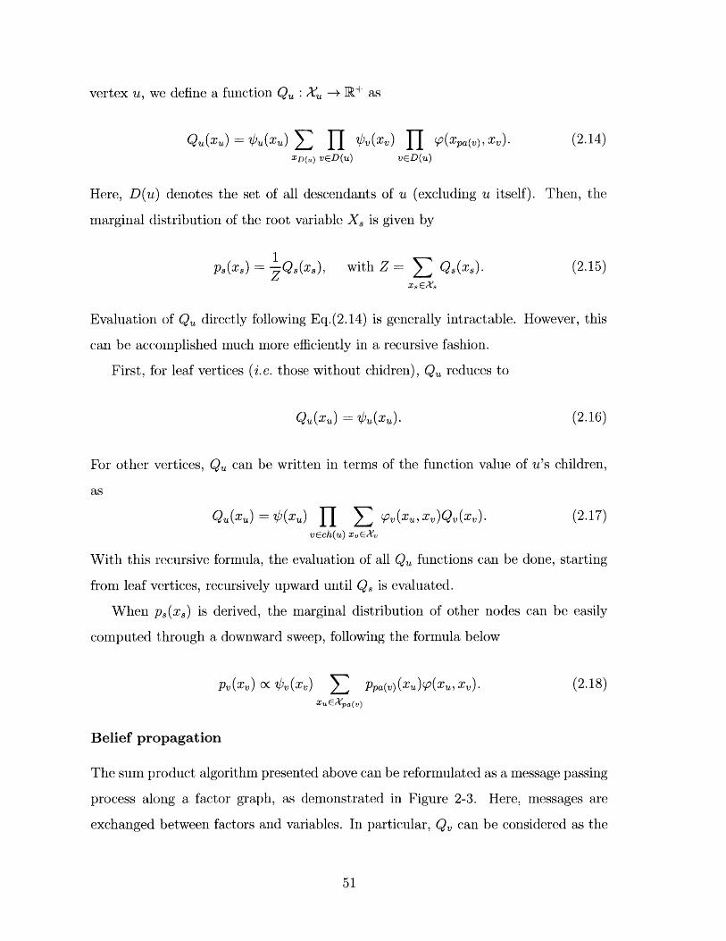
vertex u, we define a function Qu : Xu - R+ as
Qu(xu) = @u (xu) 1 171 @'v(xv) 11 (P(Xpa(v), Xv). (2.14)XD(u) vcD(u) vED(u)
Here, D(u) denotes the set of all descendants of u (excluding u itself). Then, the
marginal distribution of the root variable X, is given by
Ps(Xs) + Q,(x,), with Z = Q,(x8). (2.15)
Evaluation of Qu directly following Eq.(2.14) is generally intractable. However, this
can be accomplished much more efficiently in a recursive fashion.
First, for leaf vertices (i.e. those without chidren), Qu reduces to
QU(xU) - @/9(xu). (2.16)
For other vertices, Qu can be written in terms of the function value of u's children,
as
QU (XU) = @b(XU) ( PV (XU, X') QV(x,). (2.17)vEch(u) xveXv
With this recursive formula, the evaluation of all Qu functions can be done, starting
from leaf vertices, recursively upward until Q, is evaluated.
When p,(x,) is derived, the marginal distribution of other nodes can be easily
computed through a downward sweep, following the formula below
Pv(Xv) Oc V(xV) Z Ppa(v)(Xu)(P(Xu,Xv). (2.18)xuEXpa(v)
Belief propagation
The sum product algorithm presented above can be reformulated as a message passing
process along a factor graph, as demonstrated in Figure 2-3. Here, messages are
exchanged between factors and variables. In particular, Qv can be considered as the
51
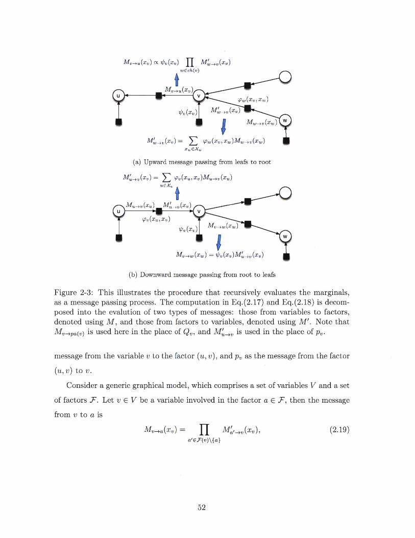
M (x') Oc V4, (x') II M ,_,..(x)wrzch(v)
M',(xv)E= J W(xV'xw)MW_,,(xW)
(a) Upward message passing from leafs to root
M'_,,V(xv) = : [ P(xU, xV)MU-_,(zU)UEX
MI-4.(x.) =0,(x-)M',,(x)
(b) Downward message passing from root to leafs
Figure 2-3: This illustrates the procedure that recursively evaluates the marginals,as a message passing process. The computation in Eq. (2.17) and Eq.(2.18) is decom-posed into the evalution of two types of messages: those from variables to factors,denoted using M, and those from factors to variables, denoted using M'. Note thatM,_,pa() is used here in the place of Q, and M',, is used in the place of p,.
message from the variable v to the factor (U, v), and P, as the message from the factor
(u,v) to v.
Consider a generic graphical model, which comprises a set of variables V and a set
of factors F. Let v E V be a variable involved in the factor a E F, then the message
from v to a is
Mv-+a(xv) = 1Ia'.F(v)\{a}
Ma',V(XV),
52
(2.19)
where F(v) denotes the set of all factors that involve v. The message from a to v is
Mav(xv) S fa(XSa) f Mw-a(X'). (2.20)x'S :x/ =xV WSa\{V}
Here, Sa is the set of variables involved in the factor fa.
For a tree-structured graphical model, after an upward sweep with messages passed
from leafs to the root, and then a downward sweep with messages passed from the
root to leafs, exact marginals can then be computed as
pV(xV) oc r M' _v(xv). (2.21)ae.(v)
The algorithm described above is called belief propagation. Note that belief
propagation are often applied to graphical models with loops, which is often referred
to as loopy belief propagation. In a loopy belief propagation algorithm, the mes-
sage passing process may run many cycles. Note that unlike the belief propagation
algorithm on trees, which is guaranteed to converge within a finite number of iter-
ations, loopy belief propagation converges only under certain conditions, and even
when it converges, the results may not be the exact marginals. Therefore, it is an
approximate inference technique.
Junction Trees
Given a graph with cycles, exact inference can be performed based on the junction tree
representation, where vertices are clustered to form a tree of cliques. A generalized
message passing algorithm can be applied to perform exact inference over a junction
tree. The computational complexity of this algorithm grows exponentially in the
tree-width, i. e. the size of the maximal clique over all possible triangulations of the
underlying graph.
For many graphical models arising in practice, the tree-width may grow with the
problem scale, rendering the junction tree algorithm intractable even for a problem
of moderate size. In such cases, one may resort to approximate inference techniques.
53
2.2 Exponential Family Distributions
The notion of exponential family distributions subsume a board range of probabilis-
tic models, which include many classic distributions (e.g. Gaussian distributions,
multinomial distributions, and Dirichlet distributions, etc) and complex probabilistic
models integrating multiple components. In particular, most models developed in
this thesis, including the patch-based MRF to describe appearance (see Chapter 3)
and the stochastic flow model (see Chapter 4), belong to exponential families.
2.2.1 Basics of Exponential Families
Given a real-valued random vector X taking values in X, and a collection of real
valued functions defined on X as # (#j)-j. Then for each x E X, O(x) =
( 5j(x))q-j is an d-dimensional real vector.
With this notation, the exponential family associated with # is defined to be
a family of parametric distributions, as
p(x) = exp (0T#(x) - A(9)) . (2.22)
Here, p(x) is the probability density function when X is a continuous variable, or
the probability mass function when X is discrete. In addition, # is called the suffi-
cient statistics, 6 is called the natural parameter (also known as the canonical
parameter, and A is called the log partition function, which is given by
A(6) = f exp(OT#(x))v(dx). (2.23)
Here, v is the base measure (Lebesgue measure for continuous variables and counting
measure for discrete variables).
When there exists a vector 6 E Rd and a real number C such that
6T#(x) = C, a.e.(w.r.t. v),
54
then the formulation above is called a overcomplete representation. In this case,
there exists an entire affine subset of parameters associated with the same distribution.
These parameters are unidentifiable from a statistical standpoint.
If the representation is not overcomplete, it is called a minimal representation.
If a minimal representation is used, there is a unique parameter associated with each
distribution in the family. For each exponential family, one can always find a minimal
representation through reparameterization.
Using minimal representation often simplifies theoretical analysis. However, over-
complete representation can be useful and convenient in some practical cases.
Mean Parameterization
The definition above characterizes a exponential family using canonical parameter-
ization. Actually, any exponential family has a dual parameterization, called mean
parameterization, which describes a distribution in terms of the mean of sufficient
statistics. Many statistical computation problems, including marginalization and
maximum likelihood estimation, can be considered as converting parameters from
one form to the other.
Consider an exponential family distribution p associated with the sufficient statis-
tics 4 (#j)Ti. The mean parameter associated with 5j is defined to be
p- = E, [#5(X)] = #5(x)p(x)v(dx).
Together, we get a vector of mean parameters y = (pj)l. It turns out that un-
der certain conditions, this vector provides an alternative parameterization of the
exponential family.
We let M be the set of all realizable mean vectors, as
M - d 1 3p s.t. E,[#(X)]
Proposition 2.3. For any exponential family, M, the set of all realizable mean
55
vectors of sufficient statistics, is convex.
2.2.2 Useful Examples
Next, we consider several probability distributions that will be used in this thesis,
and see how they can be analyzed as exponential family distributions.
Gaussian distribution
A multivariate Gaussian distribution over Rd has a pdf as below
1p(xlp, E) = (2r)d/2 IE 1/2 eXP p) TE
1 (x (2.24)
With some algebraic manipulation, this can be rewritten as
p(xlp, E) = exp (E-L)Tx- tr (-XXT) - -(TE-1 p + d log(27r) +
Clearly, this is a exponential family distribution, of which the sufficient statistics,
canonical parameters, and log-partition function are respectively given by
(2.26)
(2.27)
(2.28)
<O(x) = x, - xx T
0 (E-1/p,E-),
A(6) =1 (p1TE~1 p + d log(27r) + log |EI) .
Discrete distribution
A discrete distribution over a finite set X is characterized by the probability mass
function f : X -+ [0, 1]. Let f = (f(x))xaxst be an IX -dimensional vector comprised
of all the probability mass values. Then the pmf can be written as
p(xlf) = f(x) = fTI1 (2.29)
56
log |E|)
(2.25)
12 (
Here, the sufficient statistics is given by the indicator vector Is, the natural parameter
is f, and the log-partition is always equal to zero. Note that this is an overcomplete
formulation, as 1TI - 1 always holds.
Dirichlet distribution
A Dirichiet distribution, denoted by Dir(a), is a distribution over the probability
simplex (i.e. the set of all non-negative vectors that sum to 1). The pdf of Dir(a) is
given byn n
p(xa) =( ) X 1. (2.30)
This can be rewritten in an exponential form as
p(xl a) = (a - 1)T log(x) - log F(ai) - log F ae (2.31)
Here, the sufficient statistics is log(x), the vector formed by entry-wise logarithm, the
canonical parameter is a - 1, and the log-partition is given by
log F(ai) - log F a i.
Ising model
The Ising model, which originates from statistical physics, has been widely used in
computer vision for enforcing smoothness over an indicator map. An Ising model is
typically defined on a grid G = (V, E), where each vertex is associated with a binary
variable taking values in {-1, +1}. The joint formulation is defined as an MRF:
p(x O) = I )v (xv) fJ &n,(1(x =xV)). (2.32)vGV (u,v)EE
Here, Z is a normalization constant.
57
This can be rewritten in an exponential form as follows. Let
6v =(logv(1) -- log Ve(-1))/2, and O, = (log4(1) - log4(0))/2,
then
p(x|O)ccexp E vxv+ > OUl(xU=xV) (2.33)( vEV (u,v)cE
The re-parameterized formulation above clearly suggests that the Ising model is an
exponential family distribution.
2.2.3 The Log-partition Function
The log-partition function A(6) in itself is an object of particular interest. As stated
by the following proposition, the derivatives of A w.r.t. the canonical parameter are
closely related to the mean parameters.
Proposition 2.4. Consider an exponential family as given in Eq.(2.22), the log-
partition function A has
VoA(6) - EO[#(X)], (2.34)
and
VOA(6) = Cove[q(X)] Eo[q5(X)#(X)'] - Eo[#(X)]Eo[#(X)]T . (2.35)
Here, Eo [.] indicates the expectation w.r.t. the distribution in this family with canonical
parameter 6.
As covariance matrix is always semi-definite, Eq.(2.35) immediately leads to the
following corollary.
Corollary 2.1. The log-partition function A is a convex function for any exponential
family. Moreover, if A is associated with a minimal representation, then A is strictly
convex.
58

From Eq.(2.34), we can see that VA defines a mapping from the set of all valid
canonical parameters, denoted by (, to M, the set of realizable mean vectors. For
this mapping, we have the following theorem
Theorem 2.2. For an exponential family with minimal representation, the gradient
mapping VA : 8 -+ M is one-to-one, and onto the interior of M. Conversely, if
V A is one-to-one, then the associated exponential representation if minimal.
2.2.4 Conjugate Duality
The conjugate dual of the log-partition function A, denoted by A*, is defined to be
A*(t) "- sup {pu6 - A(6)}.9EE)
(2.36)
Here, p is called the dual variable. The dual function is closely related to the entropy,
as formally stated by the theorem below.
Theorem 2.3. Given an exponential family as in Eq. (2.22).
parameter satisfying the dual matching condition as
E [#(X)] = VA(6)
Then the conjugate dual function A* has
A*( -H(po)
+oo
(P E M),
(otherwise).
Here, H(po) is the entropy of a distribution p in this family, with parameter 0.
Note that whereas there can be multiple canonical parameters 0 satisfying the dual
matching condition when the exponential representation is overcomplete, Eq. (2.38) is
well-defined, as all 0 corresponding to the same pi gives rise to the same distribution,
and thus the same entropy value.
59
Let 6 be a canonical
(2.37)
(2.38)
Taking advantage of the duality, we further have
Theorem 2.4. Let A* be the dual function of a log-partition function A, then
A(6) =sup {0Ty - A*(p)}. (2.39)
For all 0 E 8, the supremum is attained uniquely at y that satisfies the dual matching
condition.
2.3 Model Estimation and Variational Inference
This section considers the problem of estimating the parameters of an exponential
family model from observed data. Two approaches are discussed here: the frequentist
approach, which pursues the maximum likelihood estimate (MLE) of the parame-
ters, and the Bayesian approach, which considers the parameters as random variables
generated from a prior distribution.
Generally, in the simplest cases where variables generated from a model is com-
pletely observed, the maximum likelihood estimation reduces to the problem of mo-
ment matching. However, when variables are partially observed, one may resort
to Expectation-Maximization (EM) algorithm, which provides a general approach
to solving MLE. The E-steps in an EM algorithm requires evaluation of the mean
parameters, which, for some complex model, can be computationally intractable.
Variational inference based on mean field approximation is a generic methodology to
address this difficulty.
2.3.1 Maximum Likelihood Estimation
Consider a probability distribution p(x6), whose parameter 6 is unknown and to
be estimated. Let X 1,..., X, be n independent and identically distributed (i.i.d.)
variables, each generated from p.
60
Estimation of completely observed models
We first consider the simplest situation, where the values of X 1, . . . , X, are com-
pletely observed (or known), which are denoted by xi, . . . , x,. Then the maximum
likelihood estimate (MLE), denoted by 6, is defined to be
0 = argmax fp(x i6).
Taking the logarithm of the likelihood values turns the product into sum, which,
in most cases, would greatly simplify the evaluation. Thus, 0 can be reformulated
equivalently as
0 - argmax log p(xi 6). (2.40)0
Let p(x6) be an exponential family, as
p(x|0) = exp(6T#(x) - A(O)), (2.41)
where 6 is the vector canonical parameters. Then Eq.(2.40) further reduces to
0 = argmax OTfI - A(6), (2.42)
where - is the empirical mean of the sufficient statistics over the observed data, which
is given by
n(x) (2.43)
i=1
According to Theorem 2.3, the optimum of Eq.(2.42) is attained, when
Eo [#(x)] = A. (2.44)
Hence, the problem of maximum likelihood estimation for an exponential family re-
duces to a moment matching problem, which pursues a parameter with which the
expectation of sufficient statistics matches the empirical mean.
61
Except for some simple distributions, where analytic solution exists, solving MLE
generally requires the use of numerical optimization methods (e.g. gradient descend).
Note that since A(O) is convex, the optimization problem in Eq.(2.42) is convex.
Estimation of Models with Latent Variables
A more challenging problem arises when parts of the variables are not observed di-
rectly. For convenience of discussion, for a partially observed model, we denote the
vector of variables generated from the model as (X, Y), which is comprised of an ob-
served part X and a latent part Y. In addition, each assignment to (X, Y) is denoted
by (x,y) with x E X and y E Y.
Suppose the model is an exponential family. The joint formulation can then be
written as
p(x, y 16) = exp (6T#0(x, y) - A(6)) . (2.45)
Given an observation X = x, the posterior distribution of Y is
p(y1x; 0) = exp (OTO(X Y)) (2.46)fy exp (OT4(x, y)) v(dy)
Clearly, this remains an exponential family distribution, of which the associated suf-
ficient statistics is #x(y) A #(x, y). For this distribution, the log partition function
Ax(6) is given by
Ax(O) jexp (6TO(XI Y)) v(dy). (2.47)
Note here that the integration is over Y, and Ax depends on x.
Given partial observations x 1 , ... , xa, the maximum likelihood estimate 0 is de-
fined to ben
8 argmax log p(xi 6). (2.48)
Here, p(Xi0) is the marginal likelihood of xi, given by
p(xi 6) j p(xi, y l6)v(dy). (2.49)
62
Under the exponential family formulation in Eq.(2.45), it can be rewritten as
p(Xjl&) exp (OT#(xi, y) - A(6)) v(dy)
= exp(-A(6)) exp (6Tq(xi,y)) v(dy).JV
Combining this with Eq.(2.47) results in
log p(xi 6) = A,(6) - A(6). (2.51)
We can see that the partial log-likelihood can be characterized as the difference be-
tween the log partition of p(ylxi; 6) and that of p(x, y16).
2.3.2 Expectation Maximization
Consider the partially observed model as formulated above. Generally, evaluation of
Ax(6) requires integration over Y, which is often intractable. This difficulty can be
addressed using an variational lower bound to approximate Ax.
Variational Lower Bound
Let Mx denote the set of all realizable mean vectors for the exponential family
p(ylx; 6), as
(2.52)
Then, according to Theorem 2.4, we obtain the variational representation of Ax as
Ax(6) = sup {Ty - A*(p)}, (2.53)
with
A* (px) = sup {6Ty, - Ax(6)}. (2.54)ose
63
(2.50)
M. =f{3p : p E Rd I p = E, [#(x, Y)]} .
Then the partial log-likelihood in Eq.(2.51) can be bounded from below, as
log p(xi 6) > 0y -- A* (pt) - A(6). (2.55)
This inequality holds for any p,, E M,. If and only if the dual matching condition is
satisfied, as
yX = Ee[(x, Y)] = VeAx(6), (2.56)
the inequality becomes an equality.
Expectation Maximization Algorithm
With the analysis above, we can derive a variational formulation, where the objective
function is given by
6) Z(Tpi - A* (pi) - A(6))
According to Eq.(2.56), this objective function provides a lower bound of n log p(x, 6).
The Expectation-Maximization (EM) algorithm is a coordinate ascent scheme
to optimize this variational lower-bound, which alternates between two updating
steps, as below.
1. E-step: update each dual vector pi with the model parameter 6 fixed, as
(2.58)
This problem can be further reduced to
p +) +- argmax (6 (t))Ty1 - A* (p) (2.59)
The optimum is attained when t = Ee(t) [<(xi, Y)]. Hence this step is to solve
64
L(pi, . . 1.p , 0)= (2.57)
yA0 - argmax Li(pA, 06').
the mean of $(xi, Y) w.r.t. 6 (t), as
(2.60)
2. M-step: update the parameter 0 with all dual vectors pi, . . . , yn fixed, as
-argmax Li(p, t+')OcE
0 (t+1) (2.61)
This can be further written as
n
0(t+) +-argmx (OA~t+) - (Oi (2.62)
Clearly, this is equivalent to the maximum likelihood estimate over a fully ob-
served model, with the sufficient statistics of the observation data given by(t+) +. In particular, the optimum is attained when
Al1 .. nt'.I atclr teotmmi tandwe
Eo [#(X, Y)] = I yt+)ni=
(2.63)
It is worth noting that at the end of each E-step, the gap between the sum of
partial log likelihood and the variational lower bound will be closed, as
(2.64)
Hence, as the algorithm proceeds, the variational lower bound increases, and thus the
joint partial likelihood also increases.
A key computational challenge of the E-M algorithm is the evaluation of E6 [#(xi, Y)]
in E-steps. Specifically, this mean is given by
J (xi, y)p(yIxi; 0)v(dy).(2.65)
Except for some special models, computation of this integral (or sum) is usually in-
65
<- Eo [#(X), Y)] .
Li (t+')0() =mo ~ 0 ).
Ee [#(xi, Y)] =
tractable. Variational inference, as we shall see next, provides a generic methodology
to address this difficulty.
2.3.3 Mean Field and Variational Inference
Evaluation of the mean of sufficient statistics arises not only in uvarious inference
problems but also in model estimation (e.g. EM algorithm requires evaluation of con-
ditional mean vectors in E-steps). In general, such evaluation involves integration (or
sum) over some space, which can be intractable in complex models. In what follows,
we describe a generic approach - variational inference - to address this problem,
which relies on mean field approximation, a tool originating from statistical physics.
Tractable family
We begin the exposition by introducing the notion of tractable family. Given a graph-
ical model based on a graph G = (V, E), a tractable subgraph is a subgraph F of
G over which it is feasible to perform exact inference. For example, F can be a com-
pletely disconnected graph (i.e. a graph without edges), a chain, or a tree. Then the
family of probabilistic distributions that can factorize according to F is a sub-family
of those defined on G.
Consider an exponential family with a set of sufficient statistics < = (#j)Tj, each
associated with a clique of G. Only a subset of them is associated with the cliques of
the subgraph F, which we denote by IF C {1, ... m}. Then, the canonical parameters
of the distribution in the sub-family defined on F is a subset of 8, as
1(F) A {0 E 8 | O6= 0, Vj E {1, ... , m}\F}. (2.66)
A simple example may help to illustrate these notations. Consider an Ising model
defined on a graph G = (V, E), as below
p(x|0) = exp E 0,x, + 0 aJ(x, = x,) - A(O)) . (2.67)v EV {u,v}E E
66
Here, the parameter space 8 is a subset of RIVI+IEI. Given a disconnected subgraph
F = (V, 0). The pairwise sufficient statistics E(x,, x ) is no longer associated with
the cliques of F, and therefore IF only contains the indices of the single-variable
potentials. As a result, the restricted parameter space for F is
O(F) = { E - o = 0, V{u, v} c E}. (2.68)
Let M be the set of all realizable mean vectors for the graphical model defined
on G. For the sub-family defined on F, the set is realizable mean vectors is denoted
by MF, as
M(F) {p E R m |-6 E Q(F): - Ee[#(x)]}. (2.69)
Clearly, M (F) is a convex subset of M.
Mean field approximation
The following proposition is the theoretical basis for mean field methods.
Proposition 2.5. Let A be a log-partition function associated with an exponential
family, then for each 0 E 8,
A(6) ;> 6ty - A*(p), Vpt E M. (2.70)
Here, the dual function A* is defined by
A*(p) sup {Ty - A(6)}. (2.71)ee
The equality holds if and only if 6 and t satisfy the tt Eo [O(x)].
Here, Eq.(2.70) provides a lower bound of A(O). However, A* is often intractable
to evaluate general. In such cases, it is infeasible to compute this lower bound. The
mean field method approxmiates this lower bound by restricting pI to the tractable
subset M(F)'.
'As we assume it is feasible to perform exact inference on F, evaluating y E M(F) is feasible.
67
Let A* be the restriction of A* to M(F), which is tractable to compute. Then
Ty t- A*(tt) for each t E M(F) provides a tractable lower bound of A(O). Among
all these tractable lower bounds, the best one (i.e. the tightest one) is
sup {6TI - A*(I)}. (2.72)pEM(F)
This is called the mean field approximation of A(6). Solving this optimization
problem, we get
IAF= argmax - F (2.73)pCM(F)
Here, AF is called the mean field approximation of Eo[#(x)].
The mean field approximation can also be derived and interpreted in a different way,
in terms of minimizing the Kullback-Leibler divergence.
Recall that an exponential family distribution can be characterized using either
the canonical parameters or the mean parameters. Hence, a mean vector t E M
uniquely corresponds to a distribution in the family. Consider a distribution po with
canonical parameter 0, and a distribution q,, with mean vector p. The Kullback-
Leibler divergence between them is
DKL(qI Jpo) = E% g P(X)J
= Eq, ((0T#(x) - A(Q/)) - (0T#(x) - A(6))
- (6, - 6 )T L + A(0) - A(6t). (2.74)
Here, OA denotes a canonical parameter dually coupled with p (i.e. satisfying the
dual matching condition) and we utilize the fact Eq, [#(x)] t. Moreover, as 6 is
dually coupled with p, we have
y- A(QL) = A*(p,). (2.75)
68
This immediately follows that
DKL(qp I P6) =A() + A*Qu) - 6 t (2.76)
Restricting yt to the tractable subset M(F), we have
DKL(q, Pe) = A(6) +A(p) - OT, Vt E M(F). (2.77)
Thus,
argmax (6 Ty - A* (p)) = argmin DKL(qI 1p). (2.78)PEGM(F) pEM(F)
This result suggests that the mean field approximation to Eo[<p(x)] is the mean vector
p in M(F) that minimizes the Kullback-Leibler divergence between qp and po.
Variational E-M
Come back to the E-M algorithm for maximum likelihood estimation. When the
mean vectors in E-steps are difficult or even intractable to evaluate, one may resort
to variational inference techiques to approximate them. This variant of the EM
algorithm is often referred to as variational EM.
In variational EM, the objective function remains the same as Eq.(2.57), except
that the mean vectors p, ... , y, are restricted to a tractable subset M(F). Then,
the problem in E-steps is given by
p,+0 <- argmax ((6(*))Ty - A*,() argmin D(279pEMx; (F) pEGMx(F)
As the optimum is attained, the objective value Li(pt+), 0 (t), has
Li(pf+), 0 (t)) = logp(xil6(t)) - DKL(qp(t+1) p0 (t)). (2.80)
When MF = M, the variational EM algorithm degenerates to the standard EM,
where DKL(qp1 (t+1) pO(t)) = 0, and the variational lower bound is tight.
69
2.4 Monte Carlo Sampling
Evaluation of expectation often arises as central steps in probabilistic inference and
model estimation, which is often a very challenging task as it requires integration over
a huge space in many practical cases. There are many approaches to address this
problem, typically relying on approximations. A representative method is variational
inference based on mean field approximation. This section describes another category
of methods, namely Monte Carlo sampling, which performs inference by drawing
samples from the desired distribution.
2.4.1 Monte Carlo Integration
Consider the problem of evaluating the expectation of a real-valued random vector
X ~p, as
E,[X] = xp(x)v(x). (2.81)
When this integration is difficult to compute, we can approximate it by independently
drawing a large number of samples x1, . . . , x, from p and computing the sample mean,
as
E,[X] ~ - xi. (2.82)n
More generally, we can approximate h(X) as
E,[h(X)] h ± h(xi) (2.83)n 1
Here, h : X -* R is an arbitrary real-valued function. The estimator h is unbiased,
meaning
E,[h] = E,[h(x)).
Moreover, according to the Law of Large Numbers, h almost surely converges to the
expectation E,[h(x)], as n -+ oc. The variance of h is given by
1]2Var(h) = -E, (h - E,[h]) . (2.84)
70
2.4.2 Importance Sampling
In the cases where p is difficult to sample from, one can draw samples from another
distribution q and reweight the samples. Specifically, given X - p and a real-valued
function h defined on X, we have
h(x) p(x)dx = Eqq(x)
[P(x) h]q(x)
(2.85)
Thus, we can draw independent samples xi, .. ., x, from q, and approximate E,[h] as
(2.86)E,[h(x)] ~ I, =h(xi)
This way of doing Monte Carlo integration is called importance sampling. Here,
q can be arbitrary distribution that satisfies
q(x) = 0 =- p(x) = 0. (2.87)
Generally, it is desirable to choose q such that q(x) is roughly proportional to p(x)h(x),
which would lead to small variance of the estimator.
In practice, p and q are often formulated in the following form
1p(x) = gp(x),zp
(2.88)and q(x) = gq(x).Zq
Here, Z, and Zq are normalization constants, which may be difficult to compute. In
such cases, one can approximate Ep [h] using x 1 , .. . , xn ~ q as follows
'i1 wwith wi = gp (xi)
gq(Xi)(2.89)
Here, wi is often called the importance weight of xi.
71
E,[h(x)] =
2.4.3 Markov Chain Monte Carlo
Direct sampling from a high dimensional space is usually very difficult. Markov
Chain Monte Carlo (MCMC) provides a very general and powerful methodology to
address this problem, which makes it feasible to sample from a broad class of complex
distributions.
Ergodic Markov chain
Markov Chain Monte Carlo is developed based on the ergodicity of Markov chains.
A Markov chain is defined to be a sequence of random variables X 1, X 2 ,..., such
that
p(Xt+i lXt, xt_, ... , x1) = p(Xt+ixt), t = 1, 2, .. . (2.90)
If the transition probability p(xt+1|xt) is time invariant, the Markov chain is said to
be homogeneous. A homogeneous Markov chain is completely characterized by a
transition probability matrix T, with which, we have p(xt+i Xt) = T(xt, xt+1).
A distribution p over X is called a stationary distribution (or invariance dis-
tribution) w.r.t. the Markov chain with transition probability matrix T, if
p (x) = 7,p(z')T(z', x). (2.91)
Proposition 2.6. Given a Markov chain with transition probability matrix T, let p
be a distribution over X, then p is a stationary distribution w.r.t. the given Markov
chain, if
p(x)T(x, x') = p(x')T(x', x). (2.92)
Here, the condition given in Eq.(2.92) is called detailed balance, which is a
sufficient condition that ensures p is a stationary distribution w.r.t. T.
The primary goal here is to sample from a given distribution by constructing a
Markov chain. This is related to an important property of a Markov chain - ergodicity.
Definition 2.3 (Ergodicity). A Markov chain over a finite state space is said to be
ergodic, if the following conditions holds:
72
1. The Markov chain is irreducible, meaning every state is accessible from every
other state.
2. Every state s is positive recurrent, meaning that starting from s, the chain
will return to s almost surely, and the expected time to return to s is finite.
3. Every state s is aperiodic, meaning that there exists a time t8, such that a
chain starting from s may return to s at any time step after t.
The following theorem is a fundamental result of Markov chain theory, which also
serves as the theoretical basis of MCMC.
Theorem 2.5. There exists a unique stationary distribution 7r for an ergodic Markov
chain, which is called the equilibrium distribution. Moreover, in spite of the initial
distribution of X 1, the sequence X1, X 2,... converges in distribution to r.
While the introduction above focues on Markov chains over finite state space,
similar analysis can be applied to Markov processes over other measurable spaces.
The Metropolis-Hastings algorithm
The basic idea of Markov Chain Monte Carlo (MCMC) is to simulate an ergodic
Markov chain whose equilibrium distribution p is the distribution one wants to draw
samples from. After running the chain for a sufficiently long time, the distribution of
the samples generated from the chain matches the desired distribution p.
The famous Metropolis-Hastings algorithm (M-H) is a sampling method that fol-
lows this idea, which is a generalization of the basic Metropolis algorithm. The M-H
algorithm requires a proposal distribution q, which is used to generate a new sample
conditioned on the current one. The detailed procedure of this algorithm is given in
Algorithm 1.
This algorithm is actually simulating a Markov chain whose equilibrium distri-
bution is p. This can be easily shown by proving the detailed balance condition as
follows
p(x)q(xlx') A(x', x) =min~p(x)q(xlx'), p(x)q(xlx')} =p(x')q(x'|x) A(x, x'). (2.94)
73
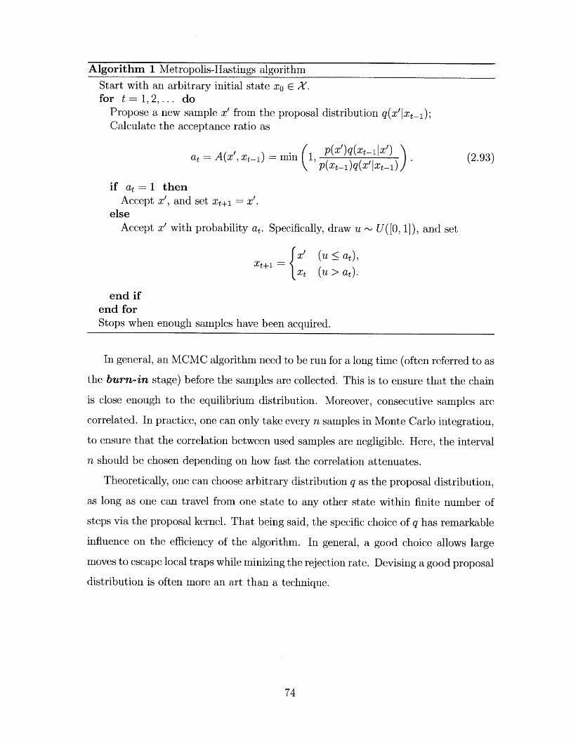
Algorithm 1 Metropolis-Hastings algorithm
Start with an arbitrary initial state xo E X.for t = 1, 2, ... do
Propose a new sample x' from the proposal distribution q(x'|xt_1);Calculate the acceptance ratio as
p(t')q(zx_1|x')at = A(x', xt_1) min 1, p(x)q(xtx) . (2.93)
(p(xt_1)q(x'Izt_1))
if at = 1 thenAccept x', and set xt+1= x'.
elseAccept x' with probability at. Specifically, draw u U([O, 1]), and set
z' (u <at),z+ (u > at).
end ifend forStops when enough samples have been acquired.
In general, an MCMC algorithm need to be run for a long time (often referred to as
the burn-in stage) before the samples are collected. This is to ensure that the chain
is close enough to the equilibrium distribution. Moreover, consecutive samples are
correlated. In practice, one can only take every n samples in Monte Carlo integration,
to ensure that the correlation between used samples are negligible. Here, the interval
n should be chosen depending on how fast the correlation attenuates.
Theoretically, one can choose arbitrary distribution q as the proposal distribution,
as long as one can travel from one state to any other state within finite number of
steps via the proposal kernel. That being said, the specific choice of q has remarkable
influence on the efficiency of the algorithm. In general, a good choice allows large
moves to escape local traps while minizing the rejection rate. Devising a good proposal
distribution is often more an art than a technique.
74
2.4.4 Gibbs Sampling
Gibbs sampling is a simple and widely used MCMC algorithm and can be considered
as a special case of the Metropolis-Hastings algorithm.
Suppose we are to sample from a joint distribution p(x) = p(x 1, . . . , xm). Starting
from an atrbitrary vector, the Gibbs sampling algorithm updates one component
of the vector at a step as follows: (1) choose a particular component (say xi), and (2)
re-draw the value of xi from the conditional distribution p(xilx\i). At each cycle, the
algorithm updates all variables following a prescribed or random order.
The Gibbs sampling procedure gives rise to a Markov chain, as the distribution of
the state produced by each step is solely determined by the previous state. Moreover,
it is not difficult to see that p is invariant w.r.t. this Markov chain. This can be
shown by the following argument. Suppose the joint distribution over all variables at
current step is p. At next step, we redraw xi from p(xi x\i). Note that the marginal
distribution of x\i remains the same. Hence, the joint distribution remains p.
The Gibbs sampling algorithm can also be viewed as a special case of the Metropolis-
Hastings algorithm, where the proposal distribution for the step to update xi is
q((x', xxi)|I(xi, xxi)) = p(x'lxxi). (2.95)
It is not difficult to verify with such a proposal, the acceptance ratio is always 1,
implying that the proposed transition is always accepted.
The standard Gibbs sampler, though simple, is usually very inefficient, as con-
secutive samples generated from the chain is highly correlated, especially for high-
dimensional sample spaces. To improve the performance of the Gibbs sampler, two
widely used strategies are
1. Blocked Gibbs sampling: group variables into blocks, and update an entire
block at a step, conditioned on other blocks.
2. Collapsed Gibbs sampling: integrates out one or more variables when sam-
pling from other variables.
75
Chapter 3
The Appearance Model
One important module of the scene modeling framework is the appearance model.
Technically, an image is a two dimensional matrix of numbers, also known as pixel
values. In a natural image, there are certain structures (patterns) among these pixels,
and it is such structures that constitute the appearance of the image.
In this work, a new image model is developed to characterize such structures. The
development here focuses on the modeling of local structures, which we consider as
a key aspect that characterizes images. Particularly, by integrating a probabilistic
manifold to capture local pixel patterns and a Markov random field to bring them
together into a joint formulation, this model is able to express rich local structures
while maintaining the coherence between them.
We derive a variational EM algorithm to estimate the model from training images,
as well as inference algorithms for inferring underlying images from partially corrupted
observations. These inference algorithms are applied to solve various low-level vision
problems, which particularly include image denoising and image inpainting. Experi-
mental results will be presented on both tasks, with comparison to other MRF-based
methods.
76
3.1 Probabilistic Image Models
Image modeling, which describes the structure and content of an image through a
mathematical formalism, lies at the heart of computer vision and provides important
basis for many vision tasks. In digital image processing and computer vision, a visual
scene is typically represented as an image or a video, which, from a mathematical
standpoint, can be considered as a function that maps each physical point (often
called a pixel) on the image plane to an intensity or color value. In this thesis, we
focus on intensity images, and thus each image can be represented as a real valued
function as I : D - R, where D is the image domain, i.e. the set of visible pixel
coordinates. However, it would be straightforward to extend the work presented in
this chapter to color images.
Generally, the pixel values of an image at different locations are strongly corre-
lated with each other and often exhibit certain structures, which distinguish an image
of natural scenes from arbitrary two-dimensional signals. Therefore, one key to im-
age modeling is to capture such structures. With different motivations, researchers
have developed various approaches to image modeling, among which many can be
formulated as a parametric distribution over images, as p(I; 0), where 0 denotes the
parameters. This distribution is often called an image prior.
Given an image prior, many low-level vision tasks can be readily solved via
Bayesian inference. Take image denoising for example. Suppose the observed im-
age I is generated from an underlying natural image I through a noisy measurement
process as p(III; q), where q denotes the parameter that characterizes the measure-
ment (e.g. the variance of noise). Then, the task of recovering the underlying image
can be formulated to be a Maximuin-a-Posteriori optimization problem as below
Z argmaxp(Ij; 0,Oq) = argmaxp(I; )p(III;q). (3.1)
Here, I denotes the optimal solution to this problem. Instead of pursuing the single
optimum, one may also choose to characterize the inherent uncertainty, e.g. sampling
from the posterior distribution p(Il1; 0, TI).
77
The task of image modeling and that of using an image model to accomplish vision
tasks, as in Eq.(3.1), consists of three aspects:
1. Establish an image prior p(I; 0). This has been one of the central topics in com-
puter vision for years. Consider the image recovery problem, prior knowledge
about the structure or characteristics is generally needed to infer the missing
or corrupted parts of an image. In previous work, two families of approaches
are widely used to formulate image priors, namely the manifold-based models
and the MRF-based models. As we shall see, they are complementary, and can
potentially be integrated to derive a more effective model.
2. Formulate the measurement process, which various across different applications.
In image denoising, it is a common practice to assume the observed images are
corrupted by additive white noise, as
I(x) = I(x) + EX, EX ~ -(O, a2 ), VX G D. (3.2)
Whereas this formulation may tend to oversimplify the actual measurement
process, which, in many practical cases, produces results comparable with those
produced using more sophisticated measurement models, with lower computa-
tional complexity.
3. Develop algorithms to solve the optimization problem in Eq.(3.1), or to sample
from the posterior distribution. We will elaborate on this part later in this
chapter, when the image model is established.
The primary goal of this chapter is to develop a new image prior to model natural
images. Before introducing the new model, we first briefly review previous approaches
to this problem, which, as mentioned, roughly fall into two categories: manifold-based
and MRF-based. As we shall see later, these two types of approaches have their
respective strength and weakness, and our new approach is motivated by combining
the strengths of both.
78
3.1.1 Manifold-based Image Modeling
An important family of approaches to image modeling is based on manifolds. Specif-
ically, an image with N pixels can be treated as a vector in RN. Here, to simplify the
discussion, we suppose all images to be modeled are of the same size, and thus their
vector representations are in the same space.
It has long been observed that natural images mostly concentrate around a low-
dimensional manifold. Motivated by this, different methods have been developed
to estimate such a manifold from training images. Among these methods, there is
an important family - subspace modeling, which is based on a further simplified
assumption, that is, images lie on a low-dimensional subspace. In a subspace model,
an image can be expressed as a linear combination of base images, as
I = Bc + E. (3.3)
Suppose the dimension of the subspace is q, then B is a matrix of size N x q, of which
each column corresponds to a base image. c E Rq is a coefficient vector.
Many methods have been proposed to learn B, the image bases, from a set of
training images. Representative methods include Principal Component Analysis
(PCA) [104, 105], Independent Component Analysis (ICA) [10], as well as others
that rely on information theoretical criteria.
The linear assumption underlying the subspace models tends to be too strong
for many practical problems, even for those only involving a restricted class of im-
ages. In later work, more sophisticated methods that allow the modeling of nonlinear
manifolds are developed. These methods extend the classic linear models in different
ways:
1. Locally linear approximation. An important way to construct a manifold is
through locally linear approximation, that is, to use a set of linear spaces, each
covering a small region on the manifold. Different methods use different ways to
characterize the locally linear spaces. A well-known method in this family is the
one proposed by Roweis and Saul, called Locally linear embedding (LLE) [86].
79
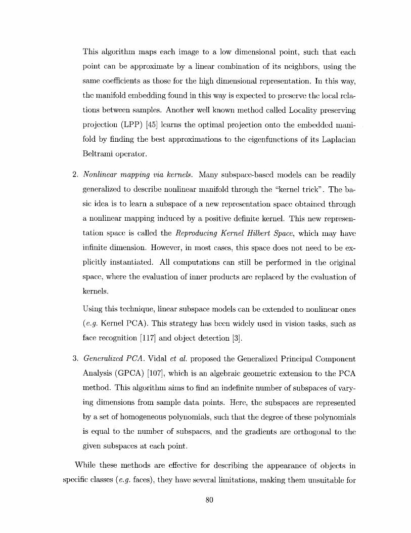
This algorithm maps each image to a low dimensional point, such that each
point can be approximate by a linear combination of its neighbors, using the
same coefficients as those for the high dimensional representation. In this way,
the manifold embedding found in this way is expected to preserve the local rela-
tions between samples. Another well known method called Locality preserving
projection (LPP) [45] learns the optimal projection onto the embedded mani-
fold by finding the best approximations to the eigenfunctions of its Laplacian
Beltrami operator.
2. Nonlinear mapping via kernels. Many subspace-based models can be readily
generalized to describe nonlinear manifold through the "kernel trick". The ba-
sic idea is to learn a subspace of a new representation space obtained through
a nonlinear mapping induced by a positive definite kernel. This new represen-
tation space is called the Reproducing Kernel Hilbert Space, which may have
infinite dimension. However, in most cases, this space does not need to be ex-
plicitly instantiated. All computations can still be performed in the original
space, where the evaluation of inner products are replaced by the evaluation of
kernels.
Using this technique, linear subspace models can be extended to nonlinear ones
(e.g. Kernel PCA). This strategy has been widely used in vision tasks, such as
face recognition [117] and object detection [3].
3. Generalized PCA. Vidal et al. proposed the Generalized Principal Component
Analysis (GPCA) [107], which is an algebraic geometric extension to the PCA
method. This algorithm aims to find an indefinite number of subspaces of vary-
ing dimensions from sample data points. Here, the subspaces are represented
by a set of homogeneous polynomials, such that the degree of these polynomials
is equal to the number of subspaces, and the gradients are orthogonal to the
given subspaces at each point.
While these methods are effective for describing the appearance of objects in
specific classes (e.g. faces), they have several limitations, making them unsuitable for
80
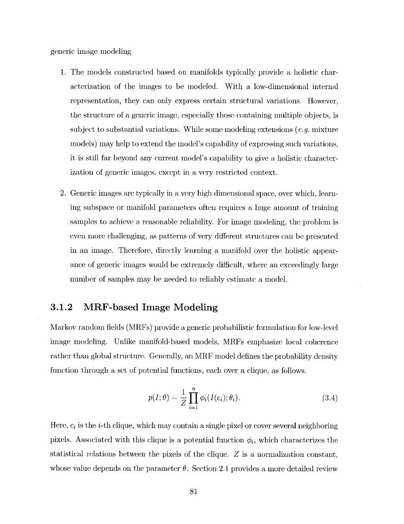
generic image modeling
1. The models constructed based on manifolds typically provide a holistic char-
acterization of the images to be modeled. With a low-dimensional internal
representation, they can only express certain structural variations. However,
the structure of a generic image, especially those containing multiple objects, is
subject to substantial variations. While some modeling extensions (e.g. mixture
models) may help to extend the model's capability of expressing such variations,
it is still far beyond any current model's capability to give a holistic character-
ization of generic images, except in a very restricted context.
2. Generic images are typically in a very high dimensional space, over which, learn-
ing subspace or manifold parameters often requires a huge amount of training
samples to achieve a reasonable reliability. For image modeling, the problem is
even more challenging, as patterns of very different structures can be presented
in an image. Therefore, directly learning a manifold over the holistic appear-
ance of generic images would be extremely difficult, where an exceedingly large
number of samples may be needed to reliably estimate a model.
3.1.2 MRF-based Image Modeling
Markov random fields (MRFs) provide a generic probabilistic formulation for low-level
image modeling. Unlike manifold-based models, MRFs emphasize local coherence
rather than global structure. Generally, an MRF model defines the probability density
function through a set of potential functions, each over a clique, as follows.
p(I; 6) = #i (I (ci); 64). (3.4)i=1
Here, ci is the i-th clique, which may contain a single pixel or cover several neighboring
pixels. Associated with this clique is a potential function 4i, which characterizes the
statistical relations between the pixels of the clique. Z is a normalization constant,
whose value depends on the parameter 0. Section 2.1 provides a more detailed review
81
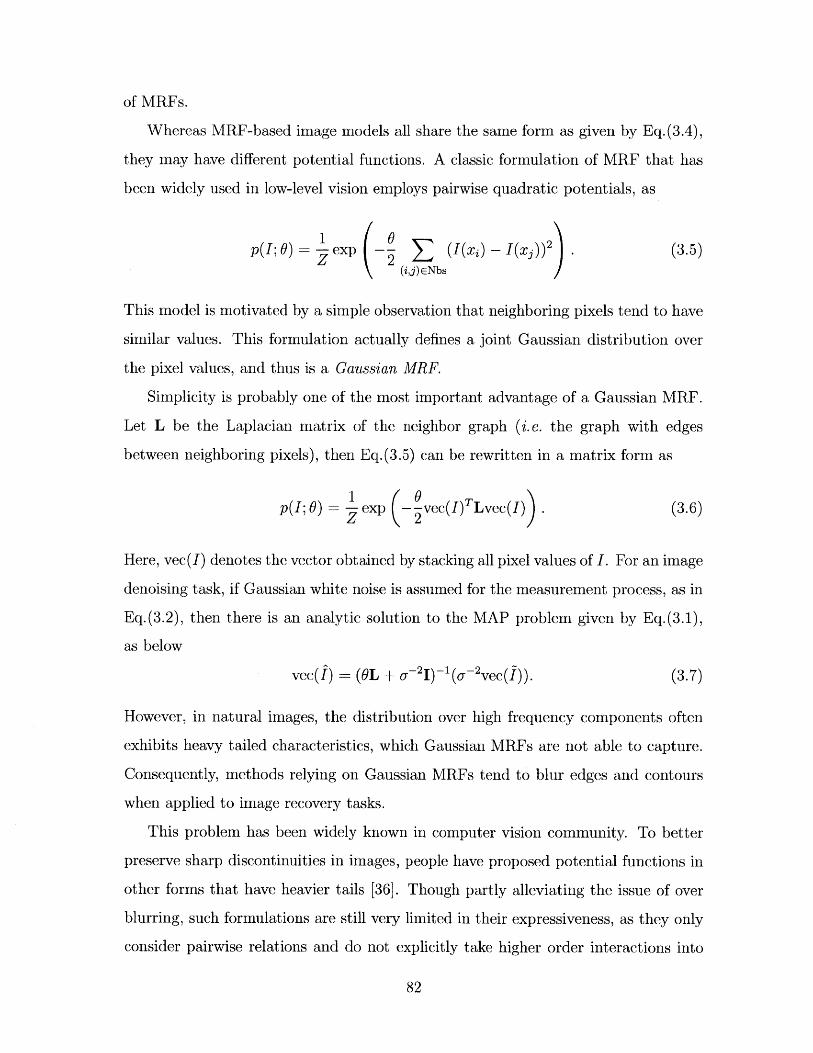
of MRFs.
Whereas MRF-based image models all share the same form as given by Eq.(3.4),
they may have different potential functions. A classic formulation of MRF that has
been widely used in low-level vision employs pairwise quadratic potentials, as
p(I; 0) = exp 2 (I(i) - I(x3 ))2) (3.5)(ij)ENbs
This model is motivated by a simple observation that neighboring pixels tend to have
similar values. This formulation actually defines a joint Gaussian distribution over
the pixel values, and thus is a Gaussian MRF.
Simplicity is probably one of the most important advantage of a Gaussian MRF.
Let L be the Laplacian matrix of the neighbor graph (i.e. the graph with edges
between neighboring pixels), then Eq.(3.5) can be rewritten in a matrix form as
p(I; 8) =- 1exp ( vec(I)TLvec(I) . (3.6)
Here, vec(I) denotes the vector obtained by stacking all pixel values of I. For an image
denoising task, if Gaussian white noise is assumed for the measurement process, as in
Eq.(3.2), then there is an analytic solution to the MAP problem given by Eq.(3.1),
as below
vec(f) = (OL + oU-21)1(Uf- 2vec(I)). (3.7)
However, in natural images, the distribution over high frequency components often
exhibits heavy tailed characteristics, which Gaussian MRFs are not able to capture.
Consequently, methods relying on Gaussian MRFs tend to blur edges and contours
when applied to image recovery tasks.
This problem has been widely known in computer vision community. To better
preserve sharp discontinuities in images, people have proposed potential functions in
other forms that have heavier tails [36]. Though partly alleviating the issue of over
blurring, such formulations are still very limited in their expressiveness, as they only
consider pairwise relations and do not explicitly take higher order interactions into
82
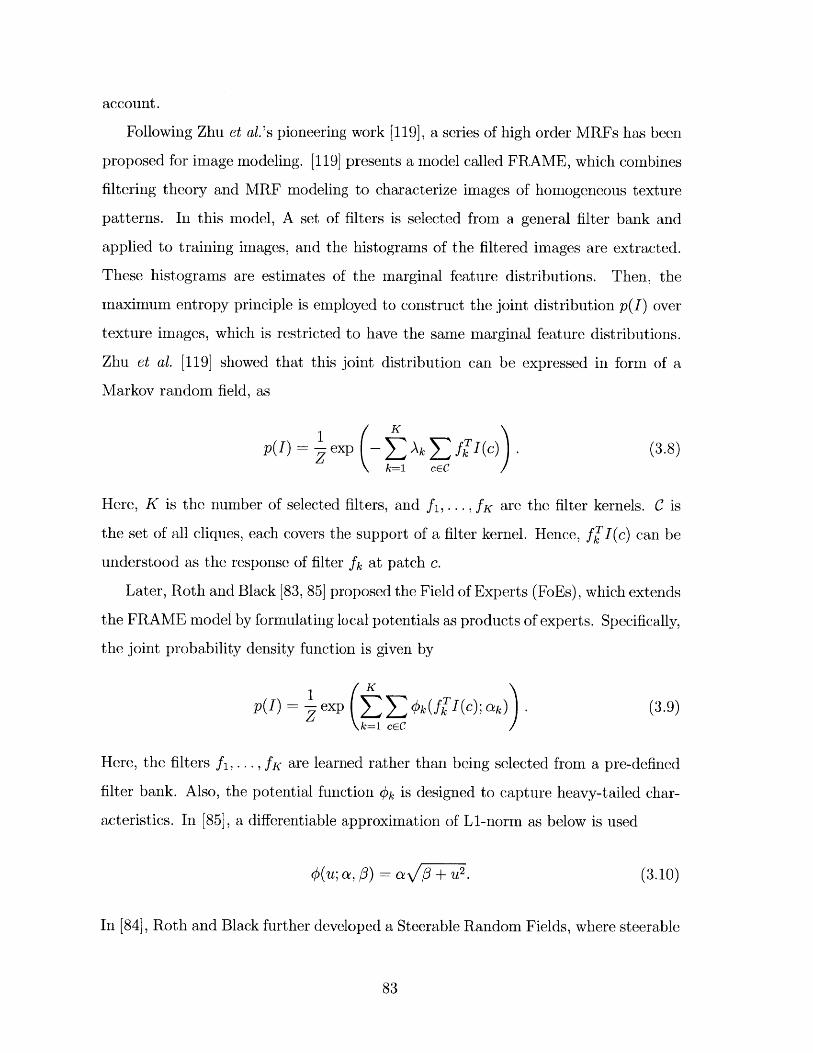
account.
Following Zhu et al.'s pioneering work [119], a series of high order MRFs has been
proposed for image modeling. [119] presents a model called FRAME, which combines
filtering theory and MRF modeling to characterize images of homogeneous texture
patterns. In this model, A set of filters is selected from a general filter bank and
applied to training images, and the histograms of the filtered images are extracted.
These histograms are estimates of the marginal feature distributions. Then, the
maximum entropy principle is employed to construct the joint distribution p(I) over
texture images, which is restricted to have the same marginal feature distributions.
Zhu et al. [119] showed that this joint distribution can be expressed in form of a
Markov random field, as
p(I) (3.8)(k=1 cC
Here, K is the number of selected filters, and fi, . . . , fK are the filter kernels. C is
the set of all cliques, each covers the support of a filter kernel. Hence, fkjJ(c) can be
understood as the response of filter fk at patch c.
Later, Roth and Black [83, 85] proposed the Field of Experts (FoEs), which extends
the FRAME model by formulating local potentials as products of experts. Specifically,
the joint probability density function is given by
1p() = exp #if T Ic;a).(3.9)
(k=1 c EC
Here, the filters fi, ... , fK are learned rather than being selected from a pre-defined
filter bank. Also, the potential function #k is designed to capture heavy-tailed char-
acteristics. In [85], a differentiable approximation of Li-norm as below is used
n(U; a, R) = a/ + I. (3.10)
In [84], Roth and Black further developed a Steerable Random Fields, where steerable
83
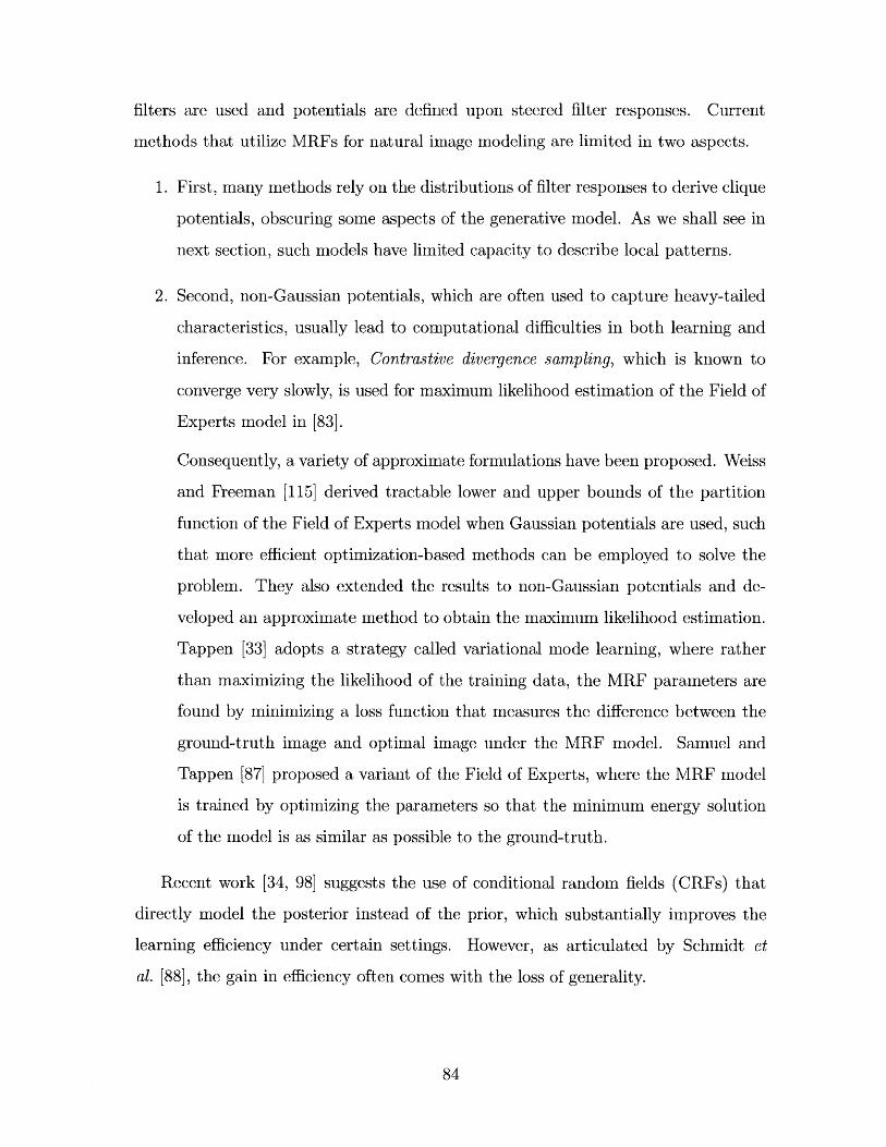
filters are used and potentials are defined upon steered filter responses. Current
methods that utilize MRFs for natural image modeling are limited in two aspects.
1. First, many methods rely on the distributions of filter responses to derive clique
potentials, obscuring some aspects of the generative model. As we shall see in
next section, such models have limited capacity to describe local patterns.
2. Second, non-Gaussian potentials, which are often used to capture heavy-tailed
characteristics, usually lead to computational difficulties in both learning and
inference. For example, Contrastive divergence sampling, which is known to
converge very slowly, is used for maximum likelihood estimation of the Field of
Experts model in [83].
Consequently, a variety of approximate formulations have been proposed. Weiss
and Freeman [115] derived tractable lower and upper bounds of the partition
function of the Field of Experts model when Gaussian potentials are used, such
that more efficient optimization-based methods can be employed to solve the
problem. They also extended the results to non-Gaussian potentials and de-
veloped an approximate method to obtain the maximum likelihood estimation.
Tappen [33] adopts a strategy called variational mode learning, where rather
than maximizing the likelihood of the training data, the MRF parameters are
found by minimizing a loss function that measures the difference between the
ground-truth image and optimal image under the MRF model. Samuel and
Tappen [87] proposed a variant of the Field of Experts, where the MRF model
is trained by optimizing the parameters so that the minimum energy solution
of the model is as similar as possible to the ground-truth.
Recent work [34, 98] suggests the use of conditional random fields (CRFs) that
directly model the posterior instead of the prior, which substantially improves the
learning efficiency under certain settings. However, as articulated by Schmidt et
al. [88], the gain in efficiency often comes with the loss of generality.
84
"1--.. .. InferenceTexture patch manifold Infere, ce
G rMRFs underlying image observed Image
base Image texture image
Figure 3-1: The overall framework of the generative image model. Here, each imageis considered as a combination of a base image that roughly reflects the smoothlighting variation, and a texture image that captures the local details. The baseimage is generated from a prior formulated in the form of a Gaussian process; whilethe texture image is generated as a composite of oriented local patches drawn from thepatch manifold. A Markov random field conditioned on the local patches is introducedto produce the entire image, which explicitly enforces coherence across patches. Thisfigure also illustrates how this model can be applied to image denoising. Specifically,given a learned model, the variational inference algorithm will incorporate both theprior knowledge provided by this model and the observed noisy image to derive theposterior distribution over the MRFs, and thus recover the underlying image in aBayesian fashion.
3.2 A New Image Prior
In this work, we develop a new image prior, motivated by the following observation.
The global appearance structure of natural images varies dramatically from image
to image and from scene to scene. One key aspect shared by natural images that
distinguish them from other two-dimensional signals is the structures of the local
patterns.
The new image model is a probabilistic generative model, which comprises a patch
model that leverages the expressive power of manifold modeling to capture the vari-
ations of local patterns, and a family of Markov random fields to enforce coherence
across patches. Specifically, to produce an image, local components from the patch
manifold are selected to generate individual patches, and thereon a conditional MRF
is constructed to generate an image coherently.
Figure 3-1 shows the overall framework of the proposed image prior. Here, an
image I is considered as the superposition of two components: (1) a low-frequency
component B, called the base image, which roughly reflects smooth lighting variation
85
over the entire image (e.g. which region is dark and which is lighter); and (2) a high-
frequency component Y, called the texture image, which captures the local details
and is modeled as a coherent composite of local texture patterns. Through such a
decomposition, the effect of overall illumination variation can be roughly separated
from the modeling of local patterns (e.g. textures).
3.2.1 Modeling Base Images
Intuitively, a base image is simply an excessively blurred version of the original image.
We formulate the prior distribution of the base images as a Gaussian process, which,
with a proper choice of covariance function, is effective in modeling smooth signals.
Particularly, the covariance function that we use here is defined to be
Cov(B(x), B(x')) = aBexp (- 2 1 . (3.11)
Here, x and x' are the coordinates of two pixels, and Cov(B(x), B(x')) is the prior
covariance between the corresponding pixel values. The parameter aB and o can
be learned from training images. In particular, u controls the range of correlation.
Generally, a model with larger value of o- would enforce longer range of coupling,
thus generating more blurry images.
While more sophisticated models might be used to describe the base image, we
did not choose to pursue this direction further. The reason is that for many low-level
vision tasks that this work is targeting, the key is to recover the local structures,
and thus this simple Gaussian process model is sufficient. That being said, it would
be interesting, as a future work, to study the modeling of global image structures
(e.g. spatial configurations of regions) and see how it might contribute to vision
applications.
3.2.2 The Patch Manifold Model
The generative model of texture images is comprised of two main components: (1)
a probabilistic patch manifold model that aims to capture the structures of local
86
patterns, and (2) a conditional MRF that enforces coherence across patches.
First of all, a generative patch model is introduced, which characterizes local
patterns at the level of patches. The construction of this model is motivated by two
observations:
1. In natural images, intensity values of neighboring pixels are highly correlated.
Let d, be the dimension of a patch vector (i.e. the number of pixels in a patch),
then most patches may lie around a manifold of dimension much lower than dp.
Hence, the task of modeling the distribution of patches can be partly reduced
to the estimation of such a patch manifold.
2. A patch and its rotated versions are equally likely for a natural image. This
might not be necessarily true in practice. However, based on this assumption,
we may substantially reduce the complexity of the manifold by mapping all
rotated versions to a single point on the manifold.
The generation of a patch based on this model consists of three steps:
1. Generate a canonical patch from a component of the manifold. Here, a canonical
patch is a patch with standard orientation.
2. Generate a rotated version of the canonical patch.
3. Generate the residues. This step allows deviation from the manifold.
Next, I will discuss these steps in detail.
Generation of canonical patches
Patches that are rotated versions of each other are considered to be equivalent. Given
an equivalence class of patches, we designate the patch with horizontal orientation
as the canonical patch of this class. Here, the orientation of a patch is determined
by the leading eigenvector of the structure tensor [11]. In particular, the structure
87
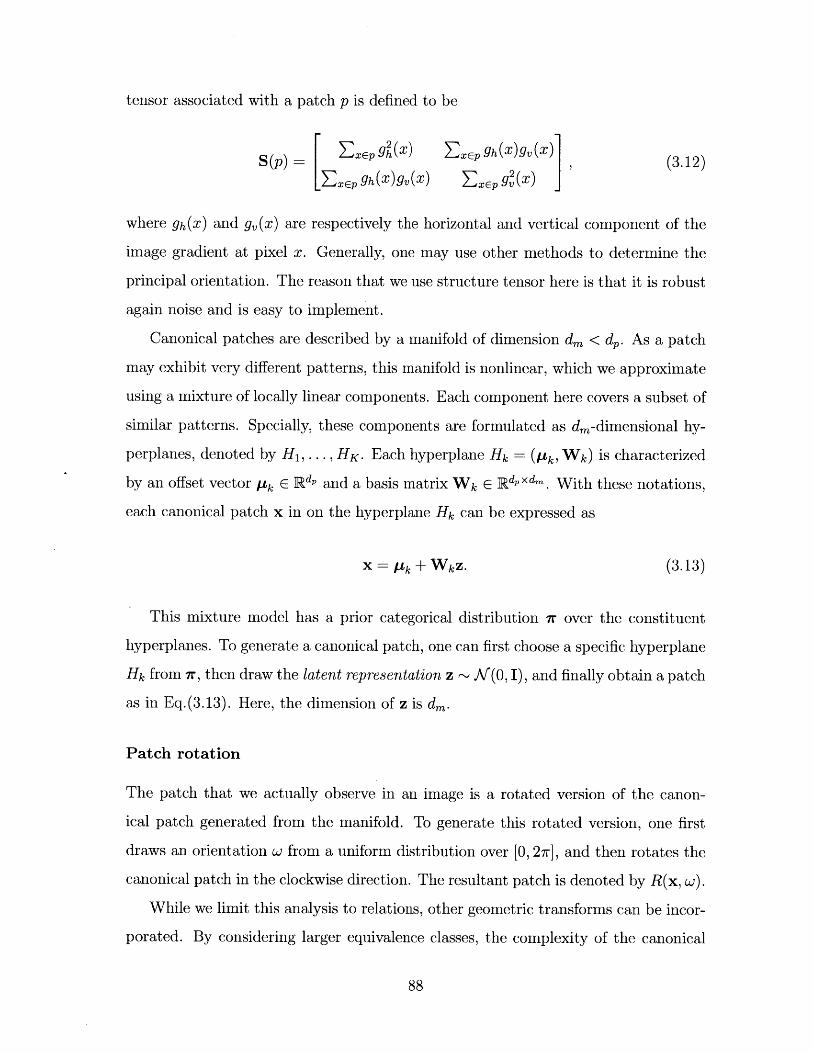
tensor associated with a patch p is defined to be
S(p) = x~pgh(X) Zx~pgA(X)9,(X) (3.12)
where gh(x) and gv(x) are respectively the horizontal and vertical component of the
image gradient at pixel x. Generally, one may use other methods to determine the
principal orientation. The reason that we use structure tensor here is that it is robust
again noise and is easy to implement.
Canonical patches are described by a manifold of dimension dm < dp. As a patch
may exhibit very different patterns, this manifold is nonlinear, which we approximate
using a mixture of locally linear components. Each component here covers a subset of
similar patterns. Specially, these components are formulated as dm-dimensional hy-
perplanes, denoted by H 1, . . . , HK. Each hyperplane Hk = (pk, W) is characterized
by an offset vector pk E RdP and a basis matrix Wk E RdPXd. With these notations,
each canonical patch x in on the hyperplane Hk can be expressed as
X = pk + WkZ. (3.13)
This mixture model has a prior categorical distribution -r over the constituent
hyperplanes. To generate a canonical patch, one can first choose a specific hyperplane
Hk from ir, then draw the latent representation z - Ni(O, I), and finally obtain a patch
as in Eq.(3.13). Here, the dimension of z is dm.
Patch rotation
The patch that we actually observe in an image is a rotated version of the canon-
ical patch generated from the manifold. To generate this rotated version, one first
draws an orientation w from a uniform distribution over [0, 27r], and then rotates the
canonical patch in the clockwise direction. The resultant patch is denoted by R(x, w).
While we limit this analysis to relations, other geometric transforms can be incor-
porated. By considering larger equivalence classes, the complexity of the canonical
88
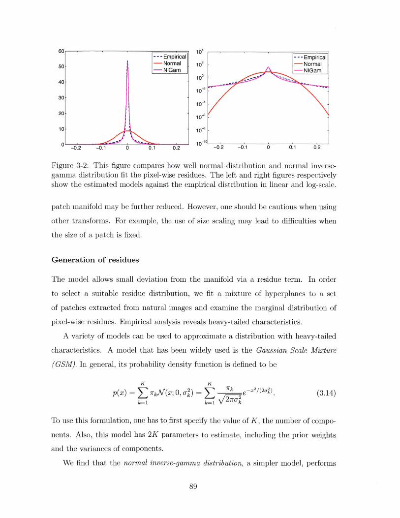
-0.2 -0.1 0 0.1 0.2
Figure 3-2: This figure compares how well normal distribution and normal inverse-gamma distribution fit the pixel-wise residues. The left and right figures respectivelyshow the estimated models against the empirical distribution in linear and log-scale.
patch manifold may be further reduced. However, one should be cautious when using
other transforms. For example, the use of size scaling may lead to difficulties when
the size of a patch is fixed.
Generation of residues
The model allows small deviation from the manifold via a residue term. In order
to select a suitable residue distribution, we fit a mixture of hyperplanes to a set
of patches extracted from natural images and examine the marginal distribution of
pixel-wise residues. Empirical analysis reveals heavy-tailed characteristics.
A variety of models can be used to approximate a distribution with heavy-tailed
characteristics. A model that has been widely used is the Gaussian Scale Mixture
(GSM). In general, its probability density function is defined to be
K K
p(x) E kA (x; 0, o) - 1F" 2x 2 /(2o2> (3.14)k=1 k=1 k
To use this formulation, one has to first specify the value of K, the number of compo-
nents. Also, this model has 2K parameters to estimate, including the prior weights
and the variances of components.
We find that the normal inverse-gamma distribution, a simpler model, performs
89
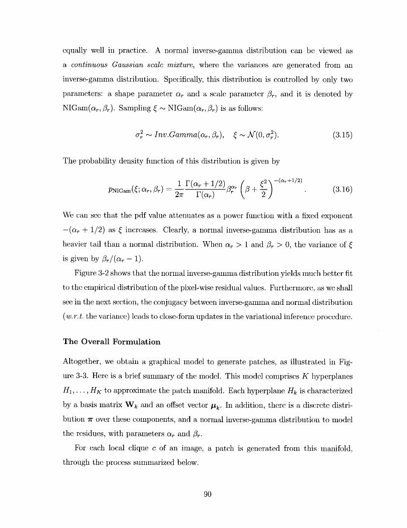
equally well in practice. A normal inverse-gamma distribution can be viewed as
a continuous Gaussian scale mixture, where the variances are generated from an
inverse-gamma distribution. Specifically, this distribution is controlled by only two
parameters: a shape parameter a, and a scale parameter /,, and it is denoted by
NIGam(ar, /3,). Sampling ( - NIGam(a,, 1,) is as follows:
of ~ Inv.Gamma(ar, ,), ~ N(O, of). (3.15)
The probability density function of this distribution is given by
1 F (a, + 1/2) + 2-(+12PNIGam( ar,,3 r) - ,r(3.16)27 F(ar) 2
We can see that the pdf value attenuates as a power function with a fixed exponent
-(ar + 1/2) as ( increases. Clearly, a normal inverse-gamma distribution has as a
heavier tail than a normal distribution. When ar > 1 and /3r > 0, the variance of (
is given by X,/(ar - 1).
Figure 3-2 shows that the normal inverse-gamma distribution yields much better fit
to the empirical distribution of the pixel-wise residual values. Furthermore, as we shall
see in the next section, the conjugacy between inverse-gamma and normal distribution
(w.r.t. the variance) leads to close-form updates in the variational inference procedure.
The Overall Formulation
Altogether, we obtain a graphical model to generate patches, as illustrated in Fig-
ure 3-3. Here is a brief summary of the model. This model comprises K hyperplanes
H 1, . . . , HK to approximate the patch manifold. Each hyperplane Hk is characterized
by a basis matrix Wk and an offset vector pk. In addition, there is a discrete distri-
bution 7r over these components, and a normal inverse-gamma distribution to model
the residues, with parameters a, and 3 r.
For each local clique c of an image, a patch is generated from this manifold,
through the process summarized below.
90

Figure 3-3: This is the graphical model for generating patches. In this model, thegeneration of a patch ye consists of four steps: (1) choose a component se - 7r; (2)generate the latent representation zc ~ NV(O, I), and thus the canonical patch xc =W8czc + y',, (3) draw an orientation we and rotate the patch accordingly, obtainingR(xc, wc), (4) generate the residue vector c, by drawing each entry independentlyfrom NIGam(ar, ,), and add the residues to the patch.
1. Choose a particular component of the manifold, by drawing its indicator sc - -7r.
2. Generate the latent representation zc ~ N(O, I). Then, the canonical patch is
given by xc = Wc zc + ys.
3. Draw an orientation we ~ U([O, 27r]), and generate the rotated version R(xc, Wc).
4. Generate the residue (c = ( (1) , .,(d). Each entry ( 0 here is independently
sampled from the normal inverse gamma distribution, as ( -~ NIGam(ar, #,).
With all these variables, we can obtain a patch as
yc = R(xc, oc) + c = R(Wgczc + ti,)+ c. (3.17)
As an empirical comparison, we collect 100,000 patches of size 13 x 13, and esti-
mate both a probabilistic manifold and a Field of Experts model over this set. Fig-
ure 3-4 shows the samples respectively generated from both models. Qualitatively,
the patch manifold model developed here yields more structured patterns.
91
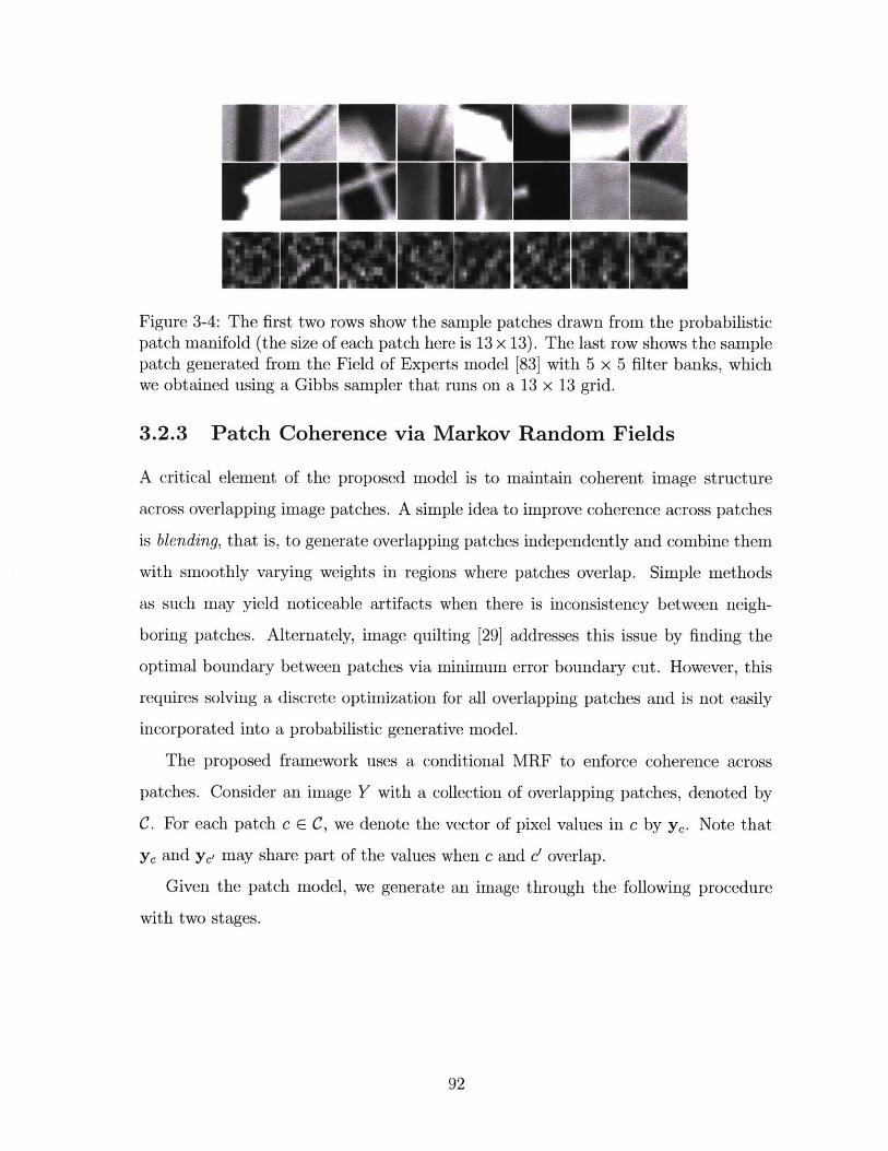
Figure 3-4: The first two rows show the sample patches drawn from the probabilisticpatch manifold (the size of each patch here is 13 x 13). The last row shows the samplepatch generated from the Field of Experts model [83] with 5 x 5 filter banks, whichwe obtained using a Gibbs sampler that runs on a 13 x 13 grid.
3.2.3 Patch Coherence via Markov Random Fields
A critical element of the proposed model is to maintain coherent image structure
across overlapping image patches. A simple idea to improve coherence across patches
is blending, that is, to generate overlapping patches independently and combine them
with smoothly varying weights in regions where patches overlap. Simple methods
as such may yield noticeable artifacts when there is inconsistency between neigh-
boring patches. Alternately, image quilting [29] addresses this issue by finding the
optimal boundary between patches via minimum error boundary cut. However, this
requires solving a discrete optimization for all overlapping patches and is not easily
incorporated into a probabilistic generative model.
The proposed framework uses a conditional MRF to enforce coherence across
patches. Consider an image Y with a collection of overlapping patches, denoted by
C. For each patch c E C, we denote the vector of pixel values in c by yc. Note that
ye and yc, may share part of the values when c and c' overlap.
Given the patch model, we generate an image through the following procedure
with two stages.
92
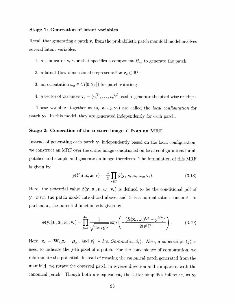
Stage 1: Generation of latent variables
Recall that generating a patch ye from the probabilistic patch manifold model involves
several latent variables:
1. an indicator sc - 7r that specifies a component Hc to generate the patch;
2. a latent (low-dimensional) representation ze E Rq;
3. an orientation w E U([O, 27]) for patch rotation;
4. a vector of variances v, = (v (1), ... ,o)used to generate the pixel-wise residues.
These variables together as (se, ze, we, vc) are called the local configuration for
patch yc. In this model, they are generated independently for each patch.
Stage 2: Generation of the texture image Y from an MRF
Instead of generating each patch ye independently based on the local configuration,
we construct an MR.F over the entire image conditioned on local configurations for all
patches and sample and generate an image therefrom. The formulation of this MRF
is given by
p(Y s, z, w, v) = f (ycSC zc we, vc). (3.18)cEC
Here, the potential value #(yc~sc, zc, wc, ve) is defined to be the conditional pdf of
yc w.r.t. the patch model introduced above, and Z is a normalization constant. In
particular, the potential function # is given by
dm 1W)2"'1 (R (xe, oc) ()- y )#(YcIsc, ze We, VC) = J7 exp -). (3.19)
j=1 2 7_() 2 (vC)
Here, xc = WSczc + y,, and v ~ Inv.Gamma(ar, B,). Also, a superscript (j) is
used to indicate the j-th pixel of a patch. For the convenience of computation, we
reformulate the potential. Instead of rotating the canonical patch generated from the
manifold, we rotate the observed patch in reverse direction and compare it with the
canonical patch. Though both are equivalent, the latter simplifies inference, as xc
93
involves a latent representation z, that needs to be inferred. The resultant potential
is thus given by
dm 1 X (R(yc, -oc)() - )2(Yc se, zc, Wc) = I exp - .W .)2 (3.20)
j=1 27r(vc)2 2/(V)2
It is important to note:
1. This MRF, including the parameters of the potential functions and the value of
the normalization constant, depends on local configurations. That's the reason
we call it a conditional MRF.
2. With this MRF formulation, the texture image Y is generated as a whole by
sampling from the MRF model, which is different from sampling individual
patches and combining them through a post-processing procedure. Intuitively,
one may see this as a process that couples the generation of all patches.
Substituting this potential function given by Eq.(3.20) into Eq.(3.18), we can
rewrite the likelihood of Y conditioned on local configurations as
p(Yjs, z, w, v) oc exp - Ec(yc sc, zc, oc) . (3.21)
Here, the energy term associated with patch c is given by
1 dUEc = (v )-1 (R(yc, -c -
j=1
(v)- 1 (R(yc, -oc)(j) - (Wczc + yL8 )(j))2. (3.22)j=1
As the energy term is quadratic, the MRF constructed above is a Gaussian MRF.
It is worth emphasizing again that this MRF is conditioned on local configurations.
Integrating out the variances V, we will end up with a continuous mixture of MRFs
with heavy-tailed marginals on the residues.
94
Figure 3-5: This figure, depicting three overlapping patches (green, red, and greenfrom left to right), illustrates how inter-patch coherence is ensured. On the left is asmall part of a natural image. By flipping the rightmost patch, we obtain the imageon the right. Whereas the rightmost patch may be captured by the manifold, theinnermost patch (red) has a discontinuity and as such is unlikely to be well explainedby the manifold. Hence, by driving all patches towards the manifold, the MRF favorscoherence across the left, middle and right patches.
Based on the MRF derived above, the maximum-a-posterior inference will drive
each patch towards the patch manifold. As patches overlap with each other, if two
adjacent patches are inconsistent, the patch overlap with both would be unlikely to
be generated from the patch manifold. Hence, this process, via patch overlapping,
also encourages coherence across patches (see Figure 3-5).
3.2.4 The Joint Likelihood
Overall, the model has the following parameters: (1) the hyperplanes of the manifold:
H 1,... , HK with Hk = (, , Wk), (2) the prior 7r over these hyperplanes, and (3) the
parameters of the residue distribution a, and 0,. These parameters together are
denoted by 0. In addition, each texture image Y is associated with several hidden
variables: the hyperplane selectors s, the latent representations z, the orientations
W, and the residue variances v. Given 6, the joint likelihood of Y and these hidden
variables is
p(YIGy) JJ p(scl ir)p(zc)p(wc)p(velar, z,). (3.23)cEC
Here, p(se17r) is a categorical distribution, p(ze) is a standard Gaussian distribu-
tion, P(Oc) is a uniform distribution over [0,27r], and p(velar,, 3r) is a multivariate
inverse-gamma distribution. Gy denotes the conditional MRF to generate Y, given
95
by Eq.(3.21) and Eq.(3.22).
Discussions
We discuss some issues with respect to the image prior presented above.
1. This model focuses on local characteristics. This is sufficient for low level vision
tasks where recovery of local patterns is the main objective. Consider an im-
age corrupted by white noise, its overall appearance structure is largely intact.
Denoising such an image mainly requires prior knowledges on local textures.
2. In the generative model described above, we actually establish a prior over a
space of Gaussian MRFs, in which each MRF is conditioned on a configuration
of local patch models. This contrasts with previous work utilizing a single MRF
or CRF (either hand-crafted or learned) for low-level vision tasks [83, 84, 115].
Formulating the image prior as a distribution over MRFs brings forth several
benefits: (1) a probabilistically consistent generative model; (2) the capacity to
model heavy tailed characteristics or other statistical properties that are not well
described by Gaussian models; and (3) the availability of efficient algorithms
for learning and inference.
3. Though assumed independent a priori, the local configurations of different
patches will be coupled given the observations1 , provided that the patches are
overlapping. The inference procedure will take the information from the ob-
served image to guide the choices of latent values, encouraging the generation
of locally coherent images that have similar appearance structure as the obser-
vation.
That being said, we believe that there is interesting dependence among these
local configurations, which is worth further investigation as future work.
'Section 2.1 discusses conditional independence of graphical models, which contains an importantresult for Bayesian networks: parent nodes of an observed node are mutually dependent in theposterior distribution.
96
4. The local model of each patch is similar to a mixture of PPCA that has been
employed for digit recognition and image compression [101]. The novelty here
consists in the maintenance of coherence across patches via conditional MRFs,
and the use of dominant orientations and heavy-tailed residue distribution.
5. Using manifold model to derive clique potentials distinguishes it from previous
work on natural image modeling, where the use of derivative filters in defining
potentials is a common practice.
3.3 Learning the Image Model
In practice, we can learn the model parameters from a given set of training images.
Before describing the details of the learning algorithm, we first introduce our experi-
ment settings. Specifically, our experiments are performed on the Berkeley Segmen-
tation Data Set and Benchmarks 500 (BSDS500) [5], which has been widely used to
assess denoising and inpainting methods[83, 84, 115]. Note that we use BSDS500[5],
a recently released extension including 200 new test images.
This data set specifies a subset of 200 images for model training, which we denote
by I1, . . . , I. Here, n = 200. The algorithm first decomposes each image i into two
components: a base image Bi and a texture image Y via simple image processing.
In particular, for an image I, a low-pass filter 2 is used to produce an excessively
smoothed version, which is treated as the base image Bi, then the texture image is
set to be Y = i - Bi. In this way, a set of base images B 1, . . . , B" and a set of texture
images Y1, . . . , Y are derived, which are then respectively used to learn the Gaussian
process prior and the patch manifold model. Below, we will respectively describe the
detailed procedures.
2 A filter with a Gaussian kernel of large radius (o- = 25 pixels) is used in our experiments toobtain the base image.
97
3.3.1 Learning the Gaussian Process Prior
The estimation of the GP prior is based on all base images derived as above. These
base images are assumed to be independently generated from a Gaussian process, as
Bi ~ GP(pB, KB), i = 1,. ... , n. (3.24)
Here, yB is a constant mean value, and rcB is a covariance function defined by
IB(X, Y aB -eXP(- .) (3.25)
Then, for an image I with h rows and w columns, this covariance function gives rise
to a covariance matrix Ci of size (hw) x (hw), as
C(u, v) = I(e, ze) aB- exp (- LU - V 2 (3.26)
Here, xu and xz are the coordinates of the u-th and v-th pixels. Let bi = vec(Bi) be
the vector comprised of all pixel values in Bi. Then under this model, the probability
density at Bi is given by
11p(Bi; AB, r'B) = exp (bi - pB)'C;-'(bi - pB) (3.27)
(27r)hw/2|Cl1/2 2
Let N be the number of pixels in an image. The complexity of evaluating this pdf is
O(N 3), which is prohibitive for a typical image, where N is often over 10'.
Here, we only have to estimate three parameters pB, aB, and o-B. Hence, it is not
necessary to use the entire image to obtain reliable estimates. In our experiment, a
simplified method is used instead. We first estimate pB, for which, the maximum
likelihood estimate is simply the mean of all pixel values in all base images.
The estimation of aB and UB can be found using numerical gradient ascent.
To make the computation tractable, rather than using the whole image, we ran-
domly draw a set of pixel pairs from the base images. Each pair is denoted by
((ui, xi), (vi, yi)). Here, ui and vi are the pixel values minus pAB, and x and yj are
98
the pixel coordinates. Note that the two pixels in each pair must be from the same
image. The marginal distribution of (ui, vi) remains a Gaussian distribution, as
1 1J .p((Ui, Vi); KB) = -2rh/1i/ exp 2((Ui, IVi)) , ,((Ui, Vi)) .
/( 2 r)hw/2 1/ s2
Here, Ej is the marginal covariance of (us, vi), which is given by
(3.28)
aB
aBe d /(20B)
-d/ (2a2aB C,
aB Jwith di = ||xi - y|.
Hence, we have
Eil =aa(1 - pi(9B)2 ), with pi(oB) = exp(-d'/(2o-)).
1( - (u? + v? - 2pi(uB)uivi). (3.31)
Then aB and aB can be solved by maximizing the following objective function
(3.32)
Here, N, is the number of pixel pairs. The derivatives of this objective function
w.r.t. the parameters can be easily derived based on the formulas above.
3.3.2 Learning the Probabilistic Patch Manifold
The model of texture images consists of two modules: the patch manifold and the
MRF. As the potential functions of the MRF to enforce coherence across patches
are simply the likelihood with respect to the patch manifold model, we only have to
estimate the parameters for the patch manifold in the stage of model training.
The patch manifold, as shown in Figure 3-3, involves the following parameters to
99
(3.29)
and
(3.30)
lo 19p((Ui, Vi); KB).
be estimated: the prior distribution over components ir, the component parameters
{(Wk, p'k)} Iki, and the parameters of the residue distribution a, and 3,. These pa-
rameters together are denoted by 6. This model also involves several latent variables
for each patch yc: the indicator sc E {1, ... , K} that associates it with a component,
the latent representation zc, the orientation we, and the vector of residue variance vc.
These hidden variables together are denoted by (c
Variational approximation
Direct maximum likelihood estimation of the model parameters 6 is intractable, as
it requires integration over all hidden variables. Here, variational EM3 is employed,
which infers the expectation of the hidden variables while optimizing the model pa-
rameters. Particularly, we factorize the posterior distribution of these hidden variables
into a product as
J7 qc(sc, zc, we, vc), (3.33)ceC
where we approximate qc as
dp K
qc(sc, ze,w, vc) = oe (wc) fl qe(vi I|d ,3) Z ~rc(k)6k(sc) k (Z). (3.34)j=1 k=1
Here, we briefly explain the rationale underlying the choice of this variational approx-
imate:
1. The orientation wc has a complex and nonlinear relation with the patch vector
Yc. Here, 6c is a delta-distribution that assigns probability 1 to Oc. Thus,
in E-steps, the estimation of the variational parameter for we reduces to an
optimization problem to find the optimal orientation, which is generally easier
to solve. In addition, E6 7 [R(yc, -wc)] simply degenerates to R(yc, -c), which
also makes the M-steps easier.
2. For the residue variance vi, we assume the variational distribution to be an
3 Section 2.3 provides a brief introduction of the generic variational EM algorithm
100
inverse gamma distribution q, (vI &, a). This is a natural choice. Recall that
the prior of vi is an inverse gamma distribution, due to conjugacy, the posterior
distribution of v remains in the same family.
3. The choice of the variational distribution for the variables se and ze is based
on the consideration below. The value of ze is largely determined by sc which
chooses a specific linear component to explain the patch. Conditioned on yc
as well as w, and ve, the joint posterior distribution over both se and ze is
a mixture of Gaussian, of which the marginal distribution of ze may be multi-
modal. Approximating this joint distribution using a product form as q(sc)q(zc)
can not properly capture this multi-modal characteristics. The most appropriate
form here would be
K
q(sc, zc) = -rc(sc)N((zclA8., tsc). =E -rc(k)6k(sc)NV(zclAk, tk). (3.35)k=1
In our original implementation, this formulation was used, which requires esti-
mating and maintaining K mean vectors and K covariance matrices for each
patch during inference. And the inference takes exceedingly long time to run,
mostly devoted to the update of ik. To reduce both time and space com-
plexity, we decided to use a simplified form, which simply replaces the normal
distribution with a delta distribution, as
K
q(sc, ze) - Z rc(k)6k (sc)4, (zc). (3.36)k=1
This simplification still preserves the multi-modal characteristics of the marginal
of zc, while substantially reducing the computational cost.
The variational EM steps
With this approximation, the joint objective function of variational EM is
J(O, {'c}) = (Eq. [log P(Yc, sc, ze, WC, ve 6) + H(qc)])c (3.37)
101
Here, (-)c denotes the sample mean over all patches extracted from the training im-
ages, asZj~ Ecc fC
(fc = 1 c
Moreover, based on the patch manifold model, we have
P(Yc,SeZc,WeV eO) =P(Yc sc, ze, cW, vc)p(sc|7r)P(zc)p(Wc)p(vc lar,,).
(3.38)
(3.39)
The factors in this formula are respectively explained as follows:
1. p(yc sc, zc, we, vc) is the conditional pdf of a patch yc given the value of latent
variables, which is given by
UM 1H expj=1 V27r (v )2
(R(ye, -) - x2)
2(v )2
where xc = W'C Zc + ps,.
2. p(sc 7r) is the prior probability of choosing the component sC.
3. p(zc) follows the standard normal distribution, as given by
p(zc) = (27r)~ 11 2 exp(-lzc|2/2).
4. p(Wc) = 1/(27r), as we ~ U([0, 27r]).
5. p(vclar,#, ) follows the inverse gamma distribution with shape parameter a,
and scale parameter 3,. In particular, it has
dp dpr
P(Vcklr, /r) - fJp(VjC &rA 3) = 11 F r (vJ)-(ar+l) exp1 F(ar) c
j-~L(-3 (3.41)
Based on the results above, we derive the updating formulas for both E-steps and
M-steps. Specifically, the E-steps update the parameters of qc given the model
102
(3.40)
J=
p(ycsc zc we, IZIWC VC) =
parameters, as follows
rc(k) CC Fk - re,kA - zc,k 2); (3.42)
zek = (i + (WT) cW) ((W)TAc(R(yc -wc) - plk)); (3.43)
1i = a, + ; (3.44)
3c = X, + rc: ,(k) (r, . (3.45)k=1
The M-steps update the model parameters given qc. The updating formulas are:
^r(k) = (i(k)e; (3.46)
Ak- Ac)- c( y - NWkze,k))c; (3.47)
iN_ = ( ck)(ye -- A)zc,k(k) cZcZT)-1. (3.48)
In addition, the scalar parameters ar and /3r of the inverse gamma distribution can
be obtained via MLE over the approximate distribution given by q,. Specifically, we
can minimize the objective below numerically
de
((ar + 1)3 +flI) - d(ar log,r - log F(ar)). (3.49)j=1
Here, i& d/#3)c and Ai = (log(/3) - @(&i)), where V' is the digamma function.
Initialization
Using variational EM requires all model parameters to be properly initialized. Here,
we describe the specific way that we chose to perform initialization in our experiments.
First, we group all patches from all images by K-means into K clusters, where K is
empirically set. For each cluster, we apply probabilistic PCA [102] to estimate pk and
Wk. After that, we set -r to be the relative weights of these clusters, and obtain a, and
#, by performing MLE on the residues. This completes the initialization. Generally,
there can be alternative approaches to accomplish this. However, exploring different
103
initialization schemes is not in the scope of this thesis.
Separate training strategy
The patch manifold is a mixture model. In practice, a divide-and-conquer strategy
can be used to estimate the model, that is, learn different sets of components from
different data sets, and then put them together into a unified mixture model. This
separate training strategy parallelizes the training procedure and reduces memory
demands.
We applied this strategy in our experiment. In particular, we group all images in
the training set into five categories: nature, animals, people, buildings, and shore, and
respectively learn a patch manifold model for each.
The design parameters are set empirically to balance accuracy and model com-
plexity. In particular, we set the number of mixture hyperplanes to K = 160 for
each category, and fix their dimension to be q = 12. After category-specific models
are learned, we combine them into a unified model by simply putting all components
together and re-normalizing their prior weights. The unified model is then used to
solve the image recovery problems, which we will discuss in next section.
3.4 Application to Image Recovery
We apply the image model to solve low level vision problems, including image denois-
ing and inpainting. Generally, an observed image 0 is given, which is assumed to be
generated from an underlying image I by a measurement process. Inference of I can
be formulated as MAP estimation:
I = argmax p(Il6)p(OII; r). (3.50)I
Here, 0 is the parameter of the image prior, and q is the parameter of the measure-
ment model. Different low level vision tasks have different measurement processes,
which, nonetheless, can be solved with the same image model. This is one significant
104
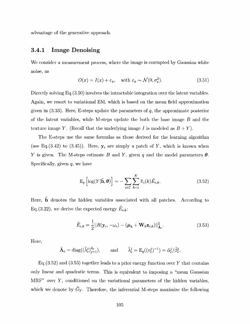
advantage of the generative approach.
3.4.1 Image Denoising
We consider a measurement process, where the image is corrupted by Gaussian white
noise, as
O(x) = I(x) + Ex, with Ex ~ A(0, of). (3.51)
Directly solving Eq. (3.50) involves the intractable integration over the latent variables.
Again, we resort to variational EM, which is based on the mean field approximation
given in (3.33). Here, E-steps update the parameters of q, the approximate posterior
of the latent variables, while M-steps update the both the base image B and the
texture image Y. (Recall that the underlying image I is modeled as B + Y).
The E-steps use the same formulas as those derived for the learning algorithm
(see Eq.(3.42) to (3.45)). Here, ye are simply a patch of Y, which is known when
Y is given. The M-steps estimate B and Y, given q and the model parameters 0.
Specifically, given q, we have
K
Eq [log(Ylf, 6)] = 7rc(k)5c,k. (3.52)cEC k=1
Here, h denotes the hidden variables associated with all patches. According to
Eq.(3.22), we derive the expected energy ck:
1Ec,k = IIR(yc, -Wc) - (sk + wkZc,k) j (3.53)2 A
Here,
Ac = diag((1 ) ), and 1j = Eq((v ) 1) = 5 /C3 .
Eq. (3.52) and (3.53) together leads to a prior energy function over Y that contains
only linear and quadratic terms. This is equivalent to imposing a "mean Gaussian
MRF" over Y, conditioned on the variational parameters of the hidden variables,
which we denote by Oy. Therefore, the inferential M-steps maximize the following
105
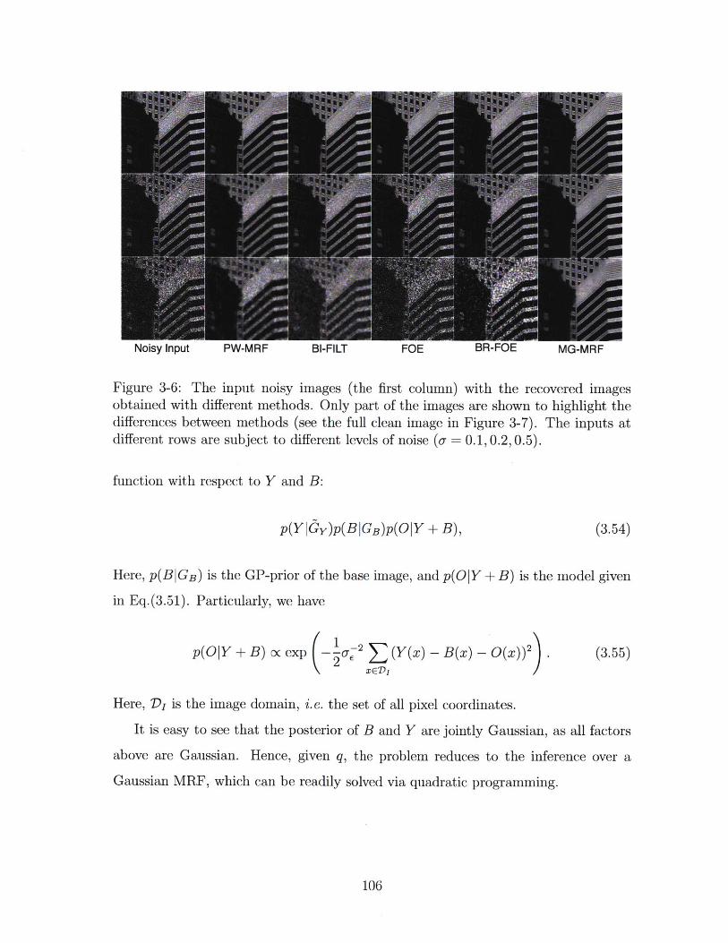
Noisy Input PW-MRF BI-FILT FOE BR-FOE MG-MRF
Figure 3-6: The input noisy images (the first column) with the recovered imagesobtained with different methods. Only part of the images are shown to highlight thedifferences between methods (see the full clean image in Figure 3-7). The inputs atdifferent rows are subject to different levels of noise (or-= 0.1, 0.2, 0.5).
function with respect to Y and B:
p(YI Gy)p(BIGB)p(O Y + B), (3.54)
Here, p(BIGB) is the GP-prior of the base image, and p(O Y + B) is the model given
in Eq.(3.51). Particularly, we have
p(OY + B) oc exp - Z6r-2 (Y(x) - B(x) - O(x))2. (3.55)
Here, D, is the image domain, i.e. the set of all pixel coordinates.
It is easy to see that the posterior of B and Y are jointly Gaussian, as all factors
above are Gaussian. Hence, given q, the problem reduces to the inference over a
Gaussian MRF, which can be readily solved via quadratic programming.
106
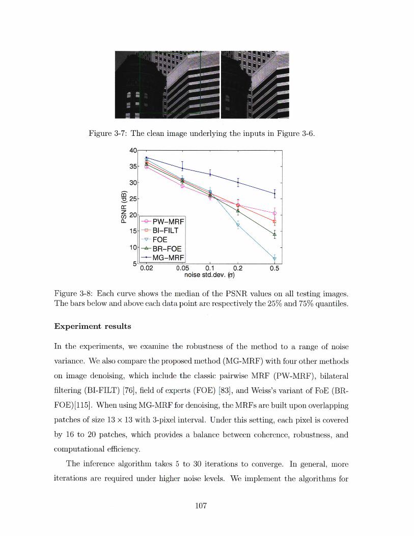
Figure 3-7: The clean image underlying the inputs in Figure 3-6.
40
35 --
30--
a25 -
zU) 20 -o -e- PW-MRF
15- -B BI-FILTv FOE
10- -BR-FOE-
-MG-MRF10.02 0.05 0.1 0.2 0.5
noise std.dev. (a)
Figure 3-8: Each curve shows the median of the PSNR values on all testing images.The bars below and above each data point are respectively the 25% and 75% quantiles.
Experiment results
In the experiments, we examine the robustness of the method to a range of noise
variance. We also compare the proposed method (MG-MRF) with four other methods
on image denoising, which include the classic pairwise MRF (PW-MRF), bilateral
filtering (BI-FILT) [76], field of experts (FOE) [83], and Weiss's variant of FoE (BR-
FOE) [115]. When using MG-MRF for denoising, the MRFs are built upon overlapping
patches of size 13 x 13 with 3-pixel interval. Under this setting, each pixel is covered
by 16 to 20 patches, which provides a balance between coherence, robustness, and
computational efficiency.
The inference algorithm takes 5 to 30 iterations to converge. In general, more
iterations are required under higher noise levels. We implement the algorithms for
107
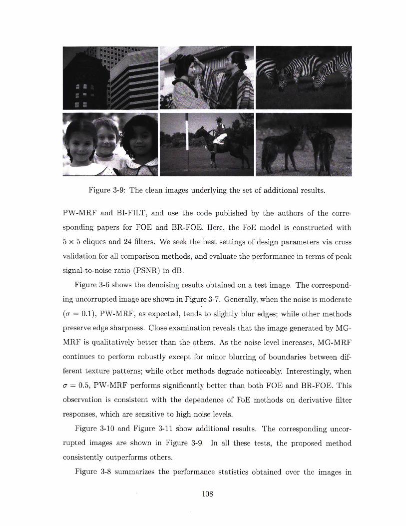
Figure 3-9: The clean images underlying the set of additional results.
PW-MRF and BI-FILT, and use the code published by the authors of the corre-
sponding papers for FOE and BR-FOE. Here, the FoE model is constructed with
5 x 5 cliques and 24 filters. We seek the best settings of design parameters via cross
validation for all comparison methods, and evaluate the performance in terms of peak
signal-to-noise ratio (PSNR) in dB.
Figure 3-6 shows the denoising results obtained on a test image. The correspond-
ing uncorrupted image are shown in Figure 3-7. Generally, when the noise is moderate
(o- = 0.1), PW-MRF, as expected, tends to slightly blur edges; while other methods
preserve edge sharpness. Close examination reveals that the image generated by MG-
MRF is qualitatively better than the others. As the noise level increases, MG-MRF
continues to perform robustly except for minor blurring of boundaries between dif-
ferent texture patterns; while other methods degrade noticeably. Interestingly, when
o- = 0.5, PW-MRF performs significantly better than both FOE and BR-FOE. This
observation is consistent with the dependence of FoE methods on derivative filter
responses, which are sensitive to high noise levels.
Figure 3-10 and Figure 3-11 show additional results. The corresponding uncor-
rupted images are shown in Figure 3-9. In all these tests, the proposed method
consistently outperforms others.
Figure 3-8 summarizes the performance statistics obtained over the images in
108
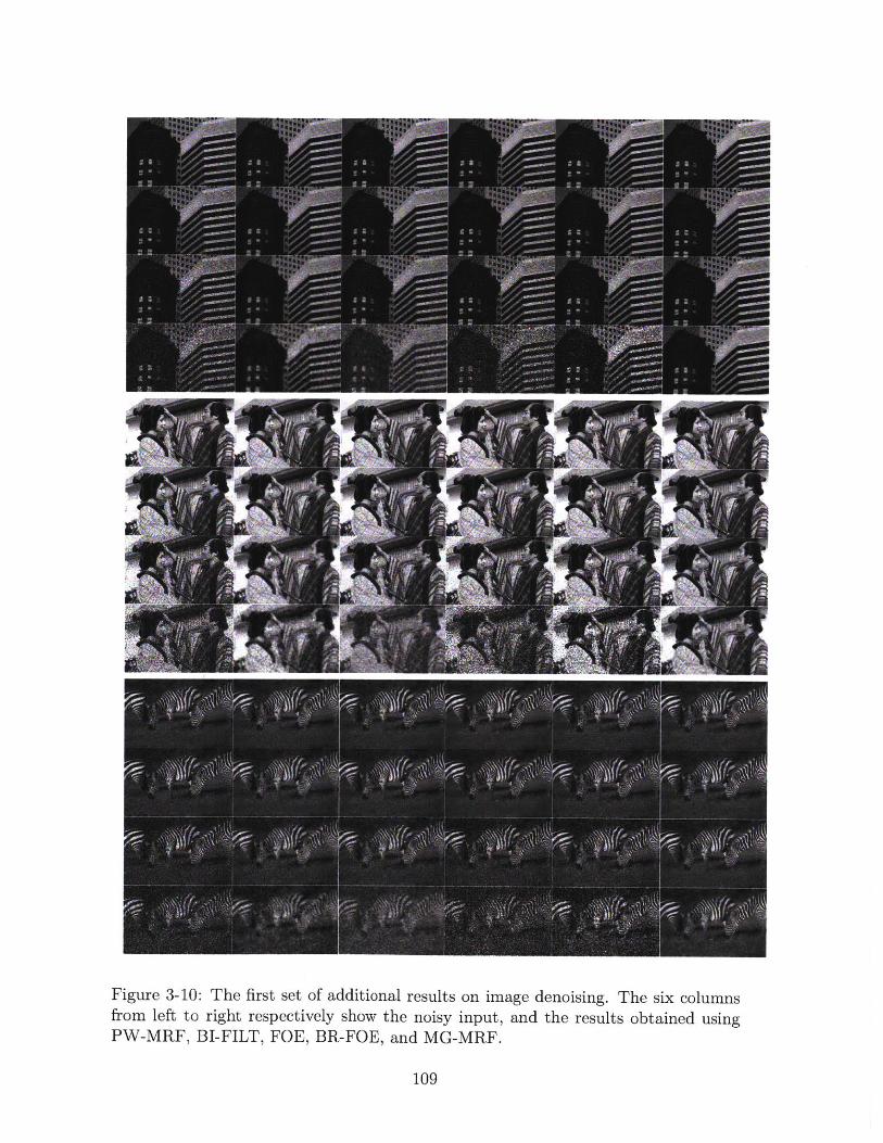
Figure 3-10: The first set of additional results on image denoising. The six columnsfrom left to right respectively show the noisy input, and the results obtained usingPW-MRF, BI-FILT, FOE, BR-FOE, and MG-MRF.
109
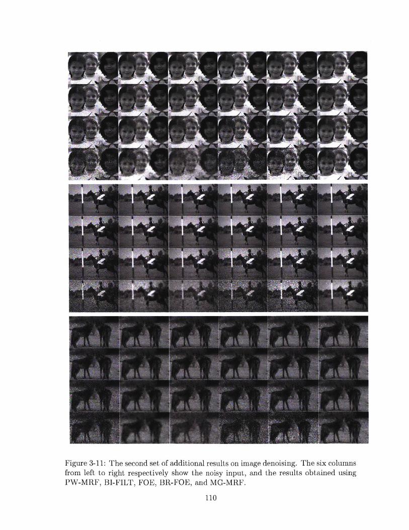
Figure 3-11: The second set of additional results on image denoising. The six columnsfrom left to right respectively show the noisy input, and the results obtained usingPW-MRF, BI-FILT, FOE, BR-FOE, and MG-MRF.
110
the test set, under different noise conditions (i.e. o, = 0.02, 0.05, 0.1, 0.2 and 0.5).
In general, the methods based on pairwise links (PW-MRF and BI-FILT) degrade
more gracefully than the FoE-based methods (FOE and BR-FOE) as the noise level
increases. MG-MRF consistently outperforms other methods.
The experimental results demonstrate that MG-MRF is superior to other methods
in two aspects: preservation of texture details and robustness to high noise levels.
This is a consequence of its distinctive mechanism in which the oriented templates
derived from the learned patch manifold generate local patterns, and are combined
with an MRF to ensure coherence between them. This is in contrast to prior methods
using MRFs which impose coherence at the pixel level. When the noise variance is
large, the direct influence of the observed pixel values becomes insignificant. The
inference algorithm uses the observed image mainly for choosing templates from the
manifold. Note that each choice is conditioned on all 169 pixels in a patch, making it
much more robust than the methods that rely on a much smaller neighborhood. The
Bayesian formulation utilizing a distribution of models instead of a single model also
contributes to the reliability.
3.4.2 Image Inpainting
The task of inpainting is to recover missing portions of a partially observed image.
Suppose we are to recover an image I. Let 0 and U respectively denote the set of
observed and missing pixels, and 1(0) denote the observed pixel values. The problem
here is to infer the value of 1(U).
Similarly, we can apply variational E-M to solve this problem, with E-steps up-
dating q, the approximate posterior of the associated latent variables, and M-steps
updating the base image B and the texture image Y. Here, the E-steps follow the
same formulas as in image denoising, while the M-steps are different. As discussed
above, given q, there is a Gaussian Markov random field over Y, denoted by ay. The
M-steps maximize the following function with respect to Y and B:
p(Y|Gy)p(B|GB) (3.56)
111
under the following constraint
Y(O) + B(O) = 1(0). (3.57)
Instead of solving this constrained optimization problem, we reformulate it as an
equivalent unconstrained problem that involves three variables Y(U), B(U), Y(0),
by replacing B(0) with 1(0) - Y(0). The resultant problem remains a quadratic
programming problem (but without constraints), which can be readily solved.
Initialization
Special care should be taken to bootstrap the E-M algorithm. Here, I describe an
effective procedure to initialize the variable values.
First, we obtain B(0) by excessively blurring the observed region, and solve B(U)
purely based on the prior Gaussian process. This has a close-form solution. Let b,
and b, respectively denote the vector of pixel values in B(0) and B(U), then the
optimal value of b, is given by
= pB + C C o(b0 - AB)- (3.58)
Here, Cao is the prior covariance matrix between bu and bo and Coo is the prior
covariance of bo. Both can be directly derived from the Gaussian process.
Next, we initialize the texture image Y. Here, Y(0) can be easily determined,
as Y(0) = 1(0) - B(O). The part Y(U) can be derived by greedily filling in the
missing pixels, from boundary towards the center.
At each iteration, we pick a partially observed patch with the least missing pixels,
and evaluate the marginal likelihood of the observed part w.r.t. all components of the
patch manifold, choosing the one that yield highest value to explain the patch. Then,
we infer the optimal values of the missing pixels in this patch using the chosen compo-
nent (recall that each component is a Gaussian distribution). This process continues
until all missing pixels are filled, which provides a reasonably good initialization.
112
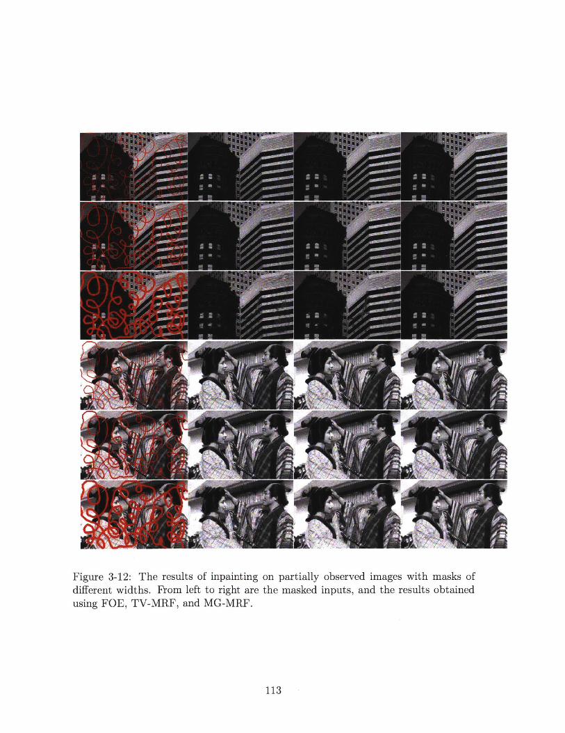
Figure 3-12: The results of inpainting on partially observed images with masks ofdifferent widths. From left to right are the masked inputs, and the results obtainedusing FOE, TV-MRF, and MG-MRF.
113
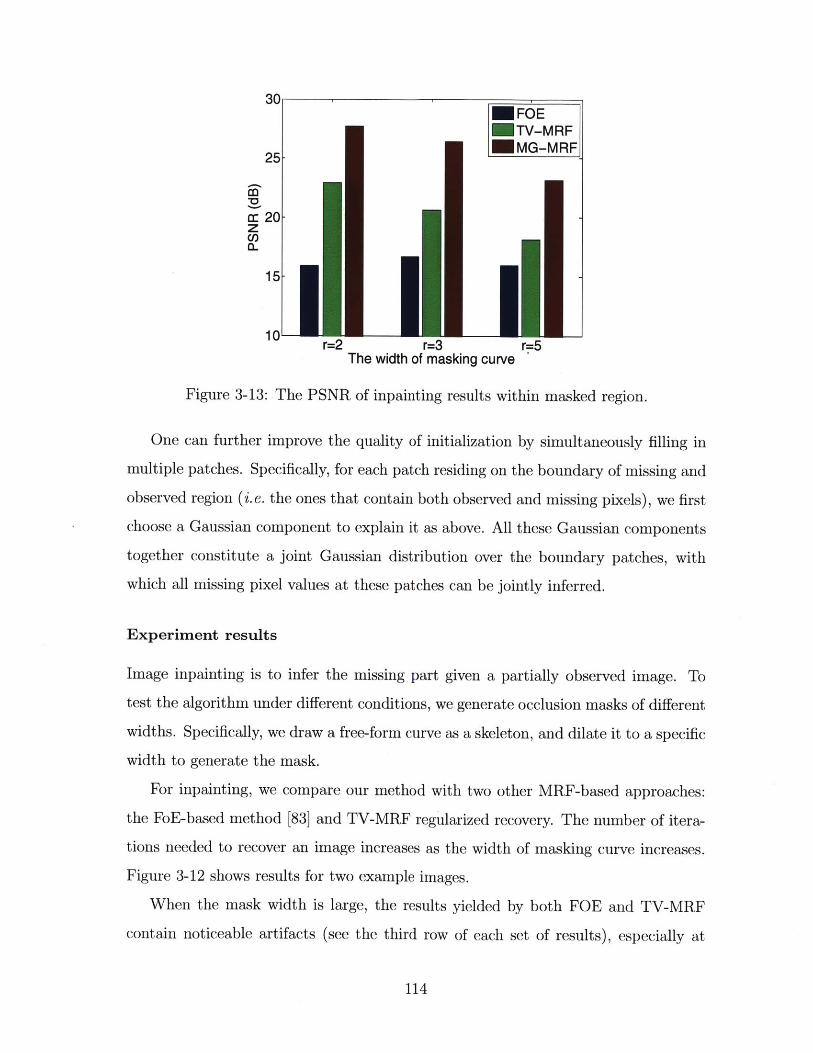
cc20-zC')
15-
r=2 r=3 r=5The width of masking curve '
Figure 3-13: The PSNR of inpainting results within masked region.
One can further improve the quality of initialization by simultaneously filling in
multiple patches. Specifically, for each patch residing on the boundary of missing and
observed region (i.e. the ones that contain both observed and missing pixels), we first
choose a Gaussian component to explain it as above. All these Gaussian components
together constitute a joint Gaussian distribution over the boundary patches, with
which all missing pixel values at these patches can be jointly inferred.
Experiment results
Image inpainting is to infer the missing part given a partially observed image. To
test the algorithm under different conditions, we generate occlusion masks of different
widths. Specifically, we draw a free-form curve as a skeleton, and dilate it to a specific
width to generate the mask.
For inpainting, we compare our method with two other MRF-based approaches:
the FoE-based method [83] and TV-MRF regularized recovery. The number of itera-
tions needed to recover an image increases as the width of masking curve increases.
Figure 3-12 shows results for two example images.
When the mask width is large, the results yielded by both FOE and TV-MRF
contain noticeable artifacts (see the third row of each set of results), especially at
114
places the masking curve passes through complex patterns. While MG-MR.F performs
better in recovering such patterns, as they are effectively captured by the texture
manifold. We also perform quantitative evaluation, in terms of PSNR within the
masked region. The results shown in Figure 3-13 show that MG-MRF works better
than the comparison methods for all three different mask widths.
3.5 Summary
We developed a generative image model for low level vision, which incorporates a
patch manifold to model the local texture patterns, and a conditional MRF to ensure
coherence between patches. With a mean field approximation, we derived efficient
algorithms for both learning and inference, which we apply to image denoising and
inpainting.
The experimental results demonstrate that our method performs substantially
better than other methods in recovering complex texture patterns, and shows superior
robustness against severe noise corruption. Such improvement is ascribed to the patch
model that is more effective than an MRF based on derivative filters in capturing
local structures, as well as the Bayesian approach that adaptively combines the MRF
predictions in posterior inference.
115
Chapter 4
The Motion Model
As a key aspect in dynamic scene modeling, motion plays a crucial role in a wide
variety of vision tasks, such as surveillance, even detection, and video analysis.
While the research on motion analysis has a long history, much of existing work
focuses on developing techniques to estimate local velocity, such as object tracking
and optical flow. The reliance on local observations (i.e. those within a small region
and at a particular time step) restricts their capability of resolving many ambiguities
arising in practice. Moreover, with the results produced by such methods (e.g. pixel-
wise velocities or tracks of individual objects), it remains a nontrivial problem to
derive a coherent interpretation of the observed motion.
To address these issues, I introduced the notion of geometric flow to motion model-
ing, which provides a higher level formulation that is able to capture common motion
patterns over both space and time. On top of geometric flows, a linear representation
based on Lie algebra is derived, with which a family of flows can be mapped to a
vector space with each flow characterized by a coefficient vector. The Lie algebraic
representation greatly simplifies probabilistic modeling of flows. Taking advantage of
this, we further formulate a stochastic flow model and apply it to analyze motion in
real world videos.
116
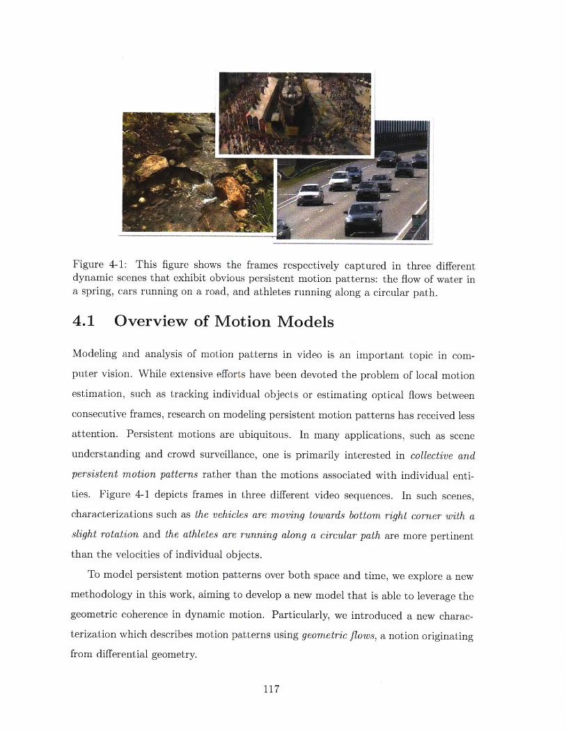
Figure 4-1: This figure shows the frames respectively captured in three differentdynamic scenes that exhibit obvious persistent motion patterns: the flow of water ina spring, cars running on a road, and athletes running along a circular path.
4.1 Overview of Motion Models
Modeling and analysis of motion patterns in video is an important topic in com-
puter vision. While extensive efforts have been devoted the problem of local motion
estimation, such as tracking individual objects or estimating optical flows between
consecutive frames, research on modeling persistent motion patterns has received less
attention. Persistent motions are ubiquitous. In many applications, such as scene
understanding and crowd surveillance, one is primarily interested in collective and
persistent motion patterns rather than the motions associated with individual enti-
ties. Figure 4-1 depicts frames in three different video sequences. In such scenes,
characterizations such as the vehicles are moving towards bottom right corner with a
slight rotation and the athletes are running along a circular path are more pertinent
than the velocities of individual objects.
To model persistent motion patterns over both space and time, we explore a new
methodology in this work, aiming to develop a new model that is able to leverage the
geometric coherence in dynamic motion. Particularly, we introduced a new charac-
terization which describes motion patterns using geometric flows, a notion originating
from differential geometry.
117
4.1.1 Review of Related Work
Research on motion analysis has a long history, and numerous algorithms and models
have been proposed, which mostly fall into four categories: tracking, optical flows,
deformable models, and space-time features.
Tracking
A tracking algorithm is employed to keep track of the locations and other states of
the interested objects across frames. At each frame, the location of each object is
determined via local search around a predicted center. This is often formalized as a
Bayesian filtering problem[18][61] [71].
Kalman filtering[116] and Particle filtering[18] [6] are two most widely used filtering
techniques in dynamic analysis. Both incorporate a hidden markov chain to model the
transition of object states (such as locations) based on temporal continuity or other
kinematic assumptions. An appearance model (e.g. a template) is used to connect
the internal states to observed image sequences.
In particular, Kalman filtering[116] assumes linear dependencies (in form of con-
ditional Gaussian distribution) between temporally consecutive frames. Taking ad-
vantage of the mathematical properties of Gaussian distributions, the inference can
be done efficiently using analytic formulas. Particle filtering[18] [6] is based on sequen-
tial importance sampling. It uses a collection of weighted particles to represent the
posterior distribution of states, which evolve over time via resampling or reweighting.
Particle filtering is much more flexible than Kalman filtering in handling non-Gaussian
cases, however, it tends to be much slower in practice.
In addition to object locations, other features are often incorporated as states
during the tracking process. Typical features that are utilized in tracking include
statistics of the intensity or colors[20][92], edges[25][26], or their hybrids[71][42].
Efforts devoted to improving the efficiency, robustness, and accuracy of track-
ing have substantially advanced the the state-of-the-art in the past decade. Latest
tracking systems can achieve satisfactory performance in controlled environments.
118
However, reliable tracking remains a significant challenge under general conditions,
where occlusions may occur frequently and objects distant from cameras may be
severely blurred.
Optical flow
Optical flow methods use a dense map of local velocities to represent the motion
between two consecutive frames. There are two families of optical flow algorithms,
respectively originating from the Horn-Schunk method [47] and the Lucas-Kanade
method [65].
The Horn-Schunk method [47] is based on the assumption of constant intensity.
Through first-order approximation, this results in a linear relation between image
gradients and the local velocity. This relation can be used to determine the velocity
component along the gradient direction, but not the orthogonal one, leading to the
aperture problem. To address this issue, smoothness is often enforced to regularize the
estimation. The Lucas-Kanade method [65] takes a block-wise approach, where each
block is associated with a velocity (or an affine transform) that can be determined
through iterative regression. The aperture problem is effectively mitigated by using
blocks instead of individual pixels.
Numerous optical flow estimation methods have been developed to make improve-
ments upon the standard algorithms in different aspects. Baker and Anandan [12]
proposed to use Markov random fields to enforce smoothness and use a robust en-
ergy function instead of the squared error in order to suppress the effect of outliers.
Bruhn et al. [15] developed a method that combines the Horn-Schunk's smoothness
regularizer and Lucas-Kanade's shared estimation strategy to give a smooth and re-
liable estimation. Weickert et al. [112] studies different types of convex regularizers
of the flow fields. Ince and Konrad [49] proposed a methodology that simultaneously
determines the optical flow and the occlusion, and breaks the smoothness constraint
at the places where occlusion occurs. Sun et al. [95] introduced a probabilistic model
of optical flows, which casts the optical flow estimation problem to a maximum-a-
posteriori inference problem. Lefevre et al. [60] extended the optical flow formulation
119
to generic Riemann manifolds. A comprehensive review of these algorithms is beyond
the scope of this thesis. Interested readers can refer to Mitiche's review [70] or Baker's
comparative study [7].
One drawback that suffered by many optical flow estimation methods is the aper-
ture problem mentioned above, which is rooted in the optical flow equation that
serves as the basis of these methods. While smoothness via regularization alleviates
this problem, it introduces another issue - blurring across motion boundary. More-
over, the underlying constant-intensity assumption makes the algorithms vulnerable
to illumination changes.
Deformable models
This family of models is used to track the dynamic movement and deformation of
specific classes of objects. These models keep track of the location and shape of
objects, and actively update them over time. Models in this family can be roughly
classified into several types as follows.
1. Contour-based models. A representative model of this type is Active contour[52].
Typically, it represents a contour as a string of points, and seeks the best con-
tour by minimizing an energy function that balances the tendency of placing the
contour near edges and the smoothness of the contour. Shape priors are some-
times incorporated to regularize the solution. The active contour algorithm has
been improved by a lot of work[81] [75] [68] since it is proposed.
2. Level-set methods. The level set method[67] is a different technique for tracking
curves, which are represented as the zero level set of an auxiliary function. One
important advantage of level set representation over explicit contour representa-
tion consists in its inherent capability of handling the variation of curve length
and change of topology.
3. deformable templates. The methods that rely only on boundaries, including
active contour and level set methods, neglect the interior contents which would
also contain significant information for motion estimation. Actually, models
120
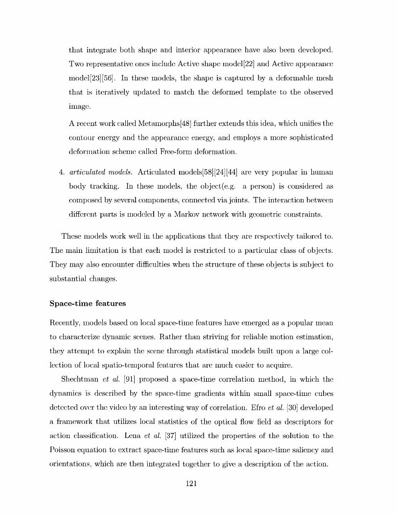
that integrate both shape and interior appearance have also been developed.
Two representative ones include Active shape model[22] and Active appearance
model[23][56]. In these models, the shape is captured by a deformable mesh
that is iteratively updated to match the deformed template to the observed
image.
A recent work called Metamorphs[48] further extends this idea, which unifies the
contour energy and the appearance energy, and employs a more sophisticated
deformation scheme called Free-form deformation.
4. articulated models. Articulated models[58][24][44] are very popular in human
body tracking. In these models, the object(e.g. a person) is considered as
composed by several components, connected via joints. The interaction between
different parts is modeled by a Markov network with geometric constraints.
These models work well in the applications that they are respectively tailored to.
The main limitation is that each model is restricted to a particular class of objects.
They may also encounter difficulties when the structure of these objects is subject to
substantial changes.
Space-time features
Recently, models based on local space-time features have emerged as a popular mean
to characterize dynamic scenes. Rather than striving for reliable motion estimation,
they attempt to explain the scene through statistical models built upon a large col-
lection of local spatio-temporal features that are much easier to acquire.
Shechtmnan et al. [91] proposed a space-time correlation method, in which the
dynamics is described by the space-time gradients within small space-time cubes
detected over the video by an interesting way of correlation. Efro et al. [30] developed
a framework that utilizes local statistics of the optical flow field as descriptors for
action classification. Lena et al. [37] utilized the properties of the solution to the
Poisson equation to extract space-time features such as local space-time saliency and
orientations, which are then integrated together to give a description of the action.
121

An important advantage for these methods is that they circumvent the difficulty
of reliable motion estimation. Instead of focusing on the accuracy of individual de-
scriptors, these methods treat the entire set of descriptors as a bag of visual terms,
using their statistics to characterize a scene. A drawback of this approach is that
spatial relations between features at different parts, which often convey significant
information, are not utilized.
4.1.2 Motivation: Problems with Existing Methods
As we can see from the review in previous section that many existing methods are
local by nature, which are reflected in two aspects:
1. They characterize the dynamics of a scene using velocities or short-time tracks
of individual points or objects, and focus on accurate estimation of these local
velocities. Generally, they do not pursue higher level representation that brings
together such local observations, or consider it as a separate modeling problem.
2. They estimate the velocity of an object or a point only based on spatially
and temporally local information. The utilization of the relations between the
motions of different objects or points is merely restricted to smoothing and
regularization.
Such methodologies may be sufficient when one is dealing with a simple scene
where the appearance of the moving objects can be clearly seen, and their trajec-
tories can be easily identified. However, the local nature of these methods severely
limits their capability of modeling complex dynamic scenes or the scenes captured
under adverse conditions. A typical example, in which conventional approaches may
encounter difficulties, is the video surveillance of a public area where the people are
monitored by a far-field camera with low resolution and low signal-to-noise ratio, and
occlusion occurs frequently. Under such circumstance, it is very difficult to accomplish
persistent and robust estimation relying only on local information.
In order to address this issue, we should extend our perspective to a broader
scope. In a real scene, the dynamic behaviors often exhibit strong coherence within
122
a region and during a period, which, we believe, can be captured jointly with a
unified formulation. Such coherence, if leveraged properly, may lead to two significant
advantages:
1. The inherent coherence of a dynamic model connects objects or points at differ-
ent locations, thus offering a mechanism to share statistical strength and help
to tackle ambiguities that would otherwise be difficult to resolve.
2. As common motion patterns are often reflected via a large collection of obser-
vations over space and time, they can be estimated more reliably than local
descriptions such as the velocities of individual objects.
3. The common behaviors or relations shared by a group of objects or reflected
over a large region often convey significant information for higher level analysis,
such as interpreting observed phenomena and predicting future evolution.
4.1.3 A New Approach based on Geometric Flows
In this work, our primary goal is to characterize coherent motion patterns with a
unified formulation while preserving flexibility to express natural variations. Direct
application of existing techniques to accomplish this task is challenging. With a nar-
row focus on temporally and spatially local motion (e.g. the velocities of a particular
object or at a particular time), current methods do not provide a natural mechanism
to aggregate potentially sparse observations over space and time into a unified model.
While regularization techniques, such as enforcing smoothness via a Markov random
fields, may help to improve the robustness of local estimates, they do not change the
way that most exiting methods characterize motion - using local velocities.
Achieving the goal above requires a new representation - a representation devised
with broader perspective. Before introducing our new approach, we first review two
conventional ways to describe motion. The first is to represent the motion of an
object by its trajectory, i.e. the position of an object or a point as a function of time.
Alternately, one might use a geometric transform to describe how a region evolves.
123
While this captures the common behavior of an entire region, it only does so within
a small temporal window.
Trajectories characterize motion over time while geometric transforms over space.
This motivates the idea to establish a temporally and spatially global representation
that unifies trajectories and geometric transforms. Consequently, we introduce the
notion of geometric flow, which characterizes motion over both space and time, as a
unification of a collection of trajectories driven by common rules and a continuous
geometric transformation process. Note here that the term geometric flow has a
precise meaning in differential geometry and that our use is consistent with it.
Analysis later will reveal that a geometric flow can be represented using a velocity
field. Nonetheless, it is fundamentally different from an optical flow. Geometric
flows describe motion by a continuous geometric transform process, while optical flow
represents motion as a dense velocity map where each velocity is estimated locally.
Each family of geometric flows is associated with a Lie algebra, i.e. a vector space
comprised of infinitesimal generators, with each flow represented by a vector in this
space. A Lie algebraic representation makes it possible to decompose a flow into a
linear combination of base flows, thus greatly simplifying statistical modeling and
estimation.
In reality, the trajectory of an object can deviate from the path predicted by the
driving flow for a variety of reasons. To account for such uncertainties, a generative
stochastic model of flows is formulated, which incorporate a Gaussian process as
a prior on the flow parameters so as to capture global coherence more effectively.
The stochastic formulation is then generalized to admit multiple concurrent flows by
introducing an MRF for flow association. The estimation under this model can be
done efficiently using variational EM.
The main contributions of this work are summarized as follows:
1. Introduce the notion of geometric flows to model persistent motion patterns,
which unifies trajectories and geometric transforms through their intrinsic con-
nections.
124

2. Derive a Lie algebraic representation, such that each family of flows can be
characterized by a set of basis and thus each flow by a coefficient vector. This
greatly simplifies the modeling of flows.
3. Develop specific constructions of parametric family of affine flows, which include
affine flows and multi-scale extensions that combine multiple locally affine flows
to express complex motion patterns while maintaining global consistency.
4. Formulate a stochastic flow model, which provides a uniform mechanism to
integrate different types of observations for robust motion estimation. Standard
inference techniques such as variational E-M can then be applied to estimate
flow coefficients from noisy observations.
4.2 Geometric Flows
As discussed in previous section, to derive a motion model that can effectively capture
coherent motion patterns over space and time, we propose to use geometric flows.
4.2.1 The Concept of Geometric Flow
The concept of flow that we are going to discuss in this chapter originates from the
theory of differential geometry. To distinguish it from other flows in computer vision
(e.g. optical flow), we call it geometric flow. Rather than describing the dynamics as
the velocities of individual objects or points, each flow characterizes the motion over
a spatial region and a time range. Here, we first review two primary representations
used for motion description in previous work:
1. Trajectory-based descriptions, often used in person or vehicle tracking systems,
collect the kinematic state of an individual object over time, typically indepen-
dent of other objects in the scene.
2. Geometric transforms, often used in object alignment and image registration
applications, describe the transformation of points over an entire region.
125
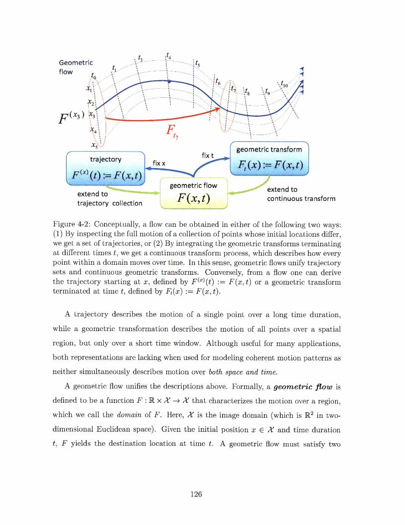
Geometric t5flow
tt
tt
2'
\ t7
X 5 )fix t geometnic transformtrajectorx ti
F0. F (x):= Fx, t)
geometric flowexted toextend to
teetoy cFlx, t) continuous transformtrajectory collection
Figure 4-2: Conceptually, a flow can be obtained in either of the following two ways:
(1) By inspecting the full motion of a collection of points whose initial locations differ,we get a set of trajectories, or (2) By integrating the geometric transforms terminatingat different times t, we get a continuous transform process, which describes how everypoint within a domain moves over time. In this sense, geometric flows unify trajectory
sets and continuous geometric transforms. Conversely, from a flow one can derivethe trajectory starting at x, defined by FWx(t) := F(x, t) or a geometric transformterminated at time t, defined by F(x) := F(x, t).
A trajectory describes the motion of a single point over a long time duration,
while a geometric transformation describes the motion of all points over a spatial
region, but only over a short time window. Although useful for many applications,
both representations are lacking when used for modeling coherent motion patterns as
neither simultaneously describes motion over both space and time.
A geometric flow unifies the descriptions above. Formally, a geometric flow is
defined to be a function F : R x X -+ X that characterizes the motion over a region,
which we call the domain of F. Here, X is the image domain (which is R 2 in two-
dimensional Euclidean space). Given the initial position x e X and time duration
t, F yields the destination location at time t. A geometric flow must satisfy two
126
identities:
F(x, 0) = x, Vx E X, (4.1)
F(F(x, t1 ), t2 )= F(x, ti + t 2 ), Vx E X, ti, t 2 E R. (4.2)
Consider a physical point driven by a flow F. Eq.(4.1) simply states that at time
t = 0 the point is at its initial position while Eq.(4.2) states that geometric flows
are associative, i.e. a point moving along the flow for time ti and then for time t2 is
equivalent to moving for time t1 +t 2. Note that t can be negative, allowing "backward
tracing". Figure 4-2 illustrates a geometric flow and its relations with trajectories and
geometric transforms.
Varying time t over R yields a family of geometric transforms {Ft lt (E R}. It can be
shown from Eq.(4.1) and (4.2) that they constitute a one-parameter transformation
group isomorphic to the addition group (R, +), which is the algebraic characterization
of a flow. The action of this group on a particular point x leads to the orbit {Ft(x) t E
R}, which is exactly the trajectory that the point would traverse. This analysis makes
the intrinsic link between the trajectories and geometric transforms induced by the
same flow explicitly.
4.2.2 Lie Group and Lie Algebra
The notion of geometric flow is closely related to the theory of Lie group and Lie
algebra. We will see later that by exploiting the intrinsic connections between Lie
group and Lie algebra, geometric flows can be mapped to vectors in a linear space,
thus leading to a vector representation of flows. To lay the theoretical basis of later
discussion, the remaining part of this section will temporarily digress from the main
theme of motion modeling and provide a brief and abstract review of the concepts of
Lie group and Lie algebra.
The exposition of the Lie group and Lie algebra theory rests on the basic concepts
of group theory and differential geometry (One may refer to Appendix A and B for a
brief summary).
127
Lie Groups
Lie group theory is a beautiful theory where the group theory and manifold theory
meet each other. In this theory, the key concept is Lie group, which is formally defined
below.
Definition 4.1 (Lie Group). A Lie group is a smooth manifold G together with a
product operation, such that it is also a group, in which the product operation and the
inverse operation are smooth maps, (it is equivalent to that (g, h) -+ gh-' is smooth).
The notion of Lie group subsumes a variety of mathematical entities. For example,
non-zero real numbers R* with multiplication, positive real numbers R+ with mul-
tiplication, and invertible matrices with matrix multiplication (general linear group
GL(n, R), are all Lie groups. In addition, any direct product (in algebraic sense) of
Lie groups remains a Lie group.
A Lie group can have sub-structures, called Lie subgroups, as defined below.
Definition 4.2 (Lie Subgroup). A Lie subgroup of a Lie group G is a subgroup of G
together with a smooth structure that makes it an immersed sub-manifold of G.
One can define functions that map from a Lie group to another. If such a function
preserves group structure, it is called a group homomorphism. In addition, we have
Definition 4.3 (Lie group Homomorphism). Let G and H be Lie groups, a smooth
map F : G -+ H which is also a group homomorphism is called a Lie group homo-
morphism.
Definition 4.4 (Lie group isomorphism). A diffeomorphism that is also a group iso-
morphism is called a Lie group isomorphism. Any bijective Lie group homomorphism
is a Lie group isomorphism.
Lie Algebra
Each Lie group is associated with a vector space with special algebraic structure,
called a Lie algebra. This is an important concept, which we rely on to establish
128
vector space representation of geometric flows. Formally, a Lie algebra is defined as
follows.
Definition 4.5 (Lie Algebra). A Lie algebra is a real vector space g with a binary
operation, notated as [x, y], called bracket operation, which satisfies the following
properties:
1. (Bilinearity): for all x, y, z c g and a, b E R,
[ax + by, z] = a[x, z] + b[y, z], (4.3)
[z, ax + by] = a[z, x] + b[z, y]. (4.4)
2. (Alternating property): for all x E g,
[x,x] = 0. (4.5)
Combination of this with the bilinearity immediately leads to anti-commutativity
as
[x,y] -[y, x]. (4.6)
3. (The Jacobi identity): for all x, y, z E g,
[x, [y, z]] + [y, [z, x]] + [z, [x, y]] - 0. (4.7)
Similar to other algebraic structures, an Lie algebra may has its own sub structure,
called Lie subalgebra, as defined below.
Definition 4.6 (Lie subalgebra). A subspace ( of a Lie algebra g is called a Lie
subalgebra, if is closed under bracket operation.
Definition 4.7 (Lie algebra homomorphism). Let g and j be Lie algebras, a linear
map F : g -+ j is called a Lie algebra homomorphism if it also preserves bracket
operations
F([X,Y]) = [F(X), F(Y)].
129
An invertible (or equivalently bijective) Lie algebra homomorphism is called a Lie
algebra isomorphism.
It is easy to see that the kernel and range of Lie algebra homomorphism are Lie
algebras. In addition, the space of n x n matrices with commutator bracket defined
by
[A, B = AB - BA
is also a Lie algebra, called the matrix Lie algebra.
Relations between Lie Group and Lie Algebra
Lie group and Lie algebra are closely related. In general, the relations between them
can be established through left-invariant vector fields, i.e. vector fields that are in-
variant to left translation:
Definition 4.8 (Left translation). Let
Lg : G -+ G called left translation as
G be a Lie group, any g C G defines a map
Vx E G, L(h) = g - x.
For any g E G, left translation is a diffeomorphism, whose inverse map is given
by L9_1.
Definition 4.9 (Left-invariant Vector Field). A vector field V of a Lie group G is
called left-invariant if it is invariant under all left-translations.
Vg, x E G, (Lg)*V(x) = V(gx).
Let G be a Lie group, it can be proved that the set of all left-invariant vector
fields with bracket operations defined by
[X,Y] =XoY-YoX
130
constitutes a Lie algebra, which we called the Lie algebra associated with G, denoted
by Lie(G). Note the Lie algebra associated with a Lie group is unique.
The Lie algebra associated with a Lie group G is isomorphic to the tangent space
of G at the identity element, as stated by the following theorem.
Theorem 4.1. Let G be a Lie group. The evaluation map E : Lie(G) -+ TeG, given
by E(X) = X(e) is a vector space isomorphism. Hence,
dim Lie(G) = dim G. (4.8)
In addition to the relations between Lie group and its associated Lie algebra, there
also exists close relations between their sub structures, as stated by the following
theorem.
Theorem 4.2. Let G be a Lie group, g be its associated Lie algebra. H be a Lie
subgroup of G, then the Lie algebra associated with H is isomorphic to a Lie subalgebra
of g.
4.2.3 Lie Algebraic Representation
Traditionally, a given geometric transform can be represented as an element in a Lie
group. From the standpoint of statistical modeling, this Lie group-based representa-
tion is difficult to work with. The main problem stems from the multiplicative nature
of the group structure, which does not support linear operations (addition and scalar
multiplication) and thus complicates the application of many statistical learning and
inference techniques formulated based on vector spaces.
This issue can be addressed by exploiting the intrinsic connections between the
Lie group and the Lie algebra, as follows:
1. Every Lie group G is uniquely associated with a Lie algebra, denoted by Lie(G),
which is a vector space isomorphic to the tangent space at the identity of the
Lie group.
131
2. Each vector in the Lie algebra Lie(G) corresponds uniquely to an element in G
via the exponentiation mapping: exp : Lie(G) -+ G.
3. There exists a neighborhood of the identity element of G, within which every
element is uniquely associated with a corresponding element in Lie(G), called
the Lie algebraic representation.
In general, a Lie algebraic representation has two advantages:
1. The functional form F of a geometric flow is in general nonlinear. As many sta-
tistical models presume an underlying vector space, this complicates a statistical
model of flows. Exploiting the linear nature of the infinitesimal generator, the
Lie algebraic representation largely overcomes such difficulties.
2. Geometric constraints of a flow, which typically restrict the induced transforms
to a particular subgroup, are often nonlinear in functional form. Such con-
straints become linear with the Lie algebraic representation as each subgroup
of transforms is described by a linear subspace of the Lie algebra.
4.2.4 Lie Algebra of Affine Transforms
To illustrate the use of Lie algebra in practice, we take the group of affine transfor-
mations as an example and show how the Lie algebraic representation benefits the
modeling and analysis of geometric transforms. Affine transforms, parameterized by
A and b, have the following form:
x' = Ax + b. (4.9)
and can be expressed in homogeneous coordinates as
_, x' A b x _x Tx. (4.10)
1 0 1 1
While this augmented matrix representation widely used in many vision applications,
its use in statistical methods presents some difficulties. First, a group of affine ma-
132
trices is not a vector space, and thus is not closed under vector addition nor scalar
multiplication, complicating the use of statistical learning methods with implicit vec-
tor space assumptions. Moreover, it is often the case that one would like to impose
geometric constraints upon the transformation. For example, restriction to volume-
preserving deformations corresponds to a determinant constraint, i.e. det(T) = 1.
This and a variety of geometric constraints are nonlinear and can be difficult to in-
corporate into statistical models. The difficulty essentially arises from the fact that
the affine group has a multiplicative rather than additive structure. It is desirable to
establish a mapping from the multiplicative structure to an equivalent vector space
representation. This is precisely what the Lie algebra accomplishes in a local sense.
The Lie algebraic representation of a 2D affine transform is a 3 x 3 matrix with
all zeroes on the bottom row. It is related to the homogeneous matrix representation
through matrix exponentiation and the matrix logarithm. If X denotes the Lie algebra
representation of T, then
T = exp(X) AI + Z X, (4.11)k!k=1
X =log (T) k (T - I)k. (4.12)k=1
One advantage of the Lie algebraic representation is that transformation sub-
groups are mapped to linear subspaces. Within the 2D affine group, there are many
subgroups that correspond to particular families of transforms. This gives rise to
a linear parameterization of them. Consider rotations by an angle 0 of which the
transform matrix TR(o) and the corresponding Lie algebraic representation XR(o) are
cos0 -sin 0 0 - 0
TR(O) = sin 0 COS XR(O) .1 (4.13)
0 0 1 0 0 0
It can be easily seen that the Lie algebraic representation of all rotations lies in a one
dimensional subspace. Similarly, the Lie algebraic representations of many other im-
133
portant transforms such as scaling, shearing, and translation, correspond to subspaces
of the Lie algebra, as well. This property in turn allows for linear characterization
of a variety of geometric constraints. Consider the volume-preserving constraint dis-
cussed above. Since the composition of two volume-preserving transforms is also
volume-preserving. All volume-preserving transformations constitute a subgroup of
the affine group. Consequently, their Lie algebraic representations form a subspace.
The associated constraint is captured by the simple expression
tr(X) = 0 <-> X11 + X22 = 0. (4.14)
Here, we just briefly discuss the Lie algebraic representation of affine transforms.
Appendix C provides a more detailed study of the affine transformation group and
its subgroups, as well as the Lie algebraic characterization of the affine group.
4.3 The Vector Space of Flows
We have discussed the connection between geometric transforms and Lie algebraic
representations above. Next, we leverage this connection to derive the Lie algebraic
representation of a geometric flow, which is a continuous transformation process in-
stead of a single transformation. As a consequence of this development, we also
establish a vector space of flows.
4.3.1 Infinitesimal Generators of Flows
Consider a point driven by a geometric flow F that starts at y and suppose it passes
x at time t, i.e. F(y)(t) = x. The velocity of the point at t can be obtained by taking
the derivative of F(v). A geometric flow has an important property with regards to
velocity: Given any x in the flow domain, any point driven by the flow passes through
x with the same velocity independent of its initial location. The property implies that
each geometric flow F induces a time-invariant velocity field, denoted by VF, which
134
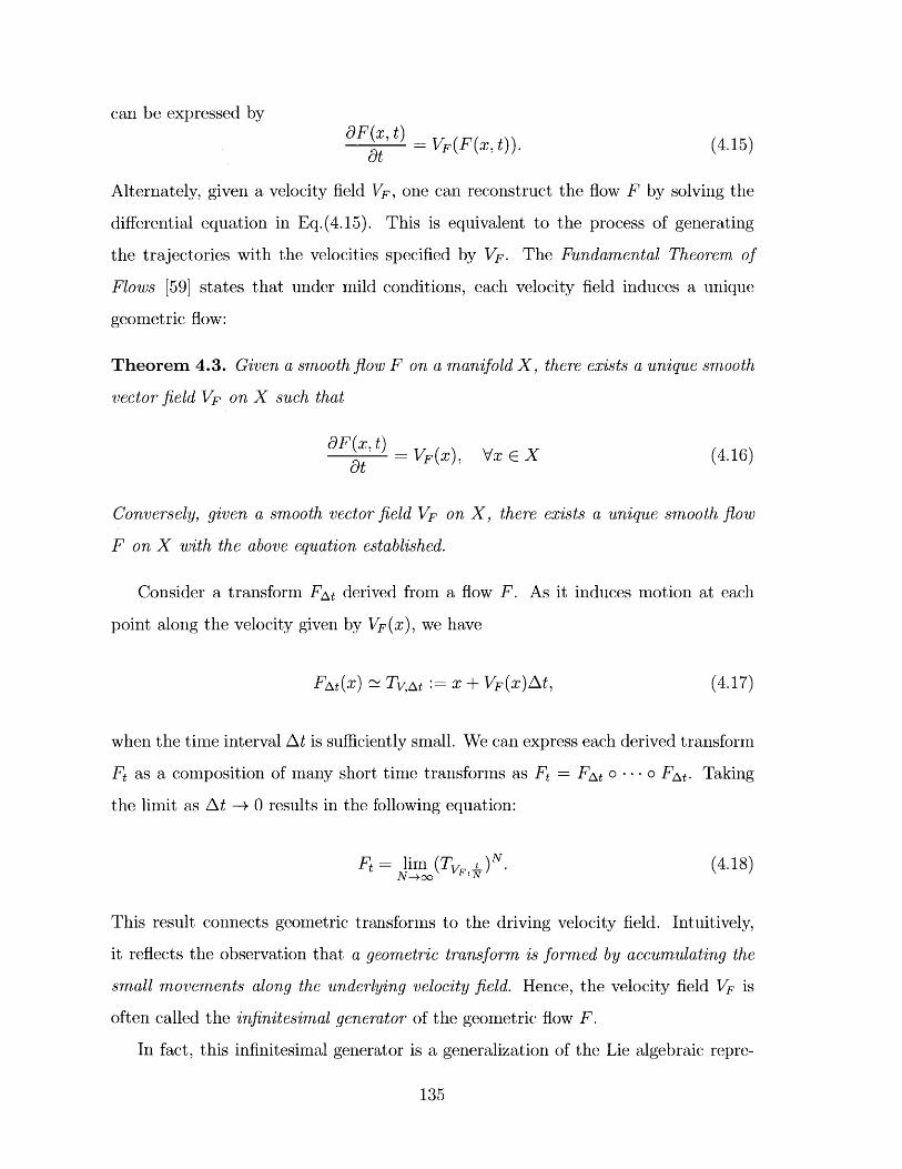
can be expressed by8F(x, t)t VF(F(x, t)). (4.15)at
Alternately, given a velocity field VF, one can reconstruct the flow F by solving the
differential equation in Eq.(4.15). This is equivalent to the process of generating
the trajectories with the velocities specified by VF. The Fundamental Theorem of
Flows [59] states that under mild conditions, each velocity field induces a unique
geometric flow:
Theorem 4.3. Given a smooth flow F on a manifold X, there exists a unique smooth
vector field VF on X such that
aF(x, t)at VF(X), V E X (4.16)
Conversely, given a smooth vector field VF on X, there exists a unique smooth flow
F on X with the above equation established.
Consider a transform FAt derived from a flow F. As it induces motion at each
point along the velocity given by VF(x), we have
FAt(x) ~ Tv,,Nt := x + VF(x)At, (4.17)
when the time interval At is sufficiently small. We can express each derived transform
Ft as a composition of many short time transforms as Ft = FAt o ... o FAt. Taking
the limit as At -+ 0 results in the following equation:
F = lim (TV, t )N. (4.18)N-*oo 'N
This result connects geometric transforms to the driving velocity field. Intuitively,
it reflects the observation that a geometric transform is formed by accumulating the
small movements along the underlying velocity field. Hence, the velocity field VF is
often called the infinitesimal generator of the geometric flow F.
In fact, this infinitesimal generator is a generalization of the Lie algebraic repre-
135
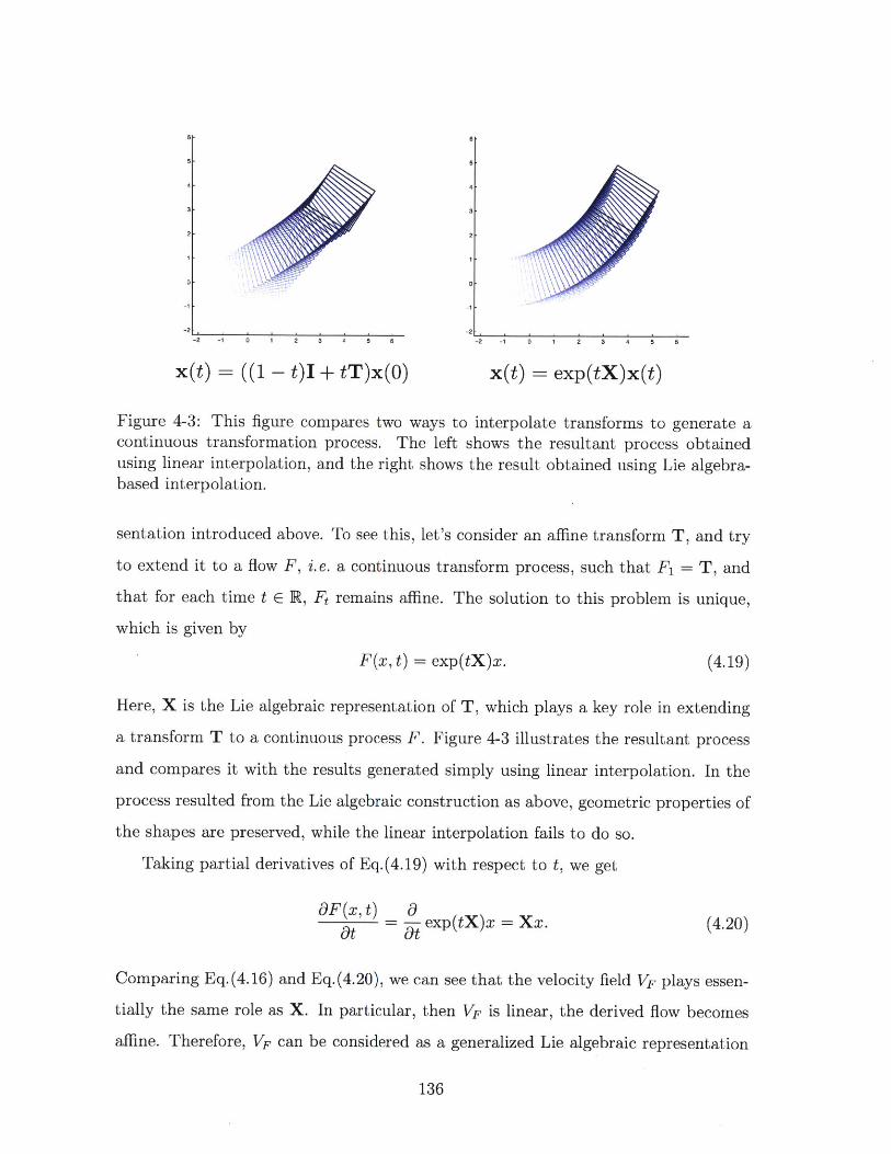
6B a
5- 5
4 -4
3 ' 3 -
-2 -1 0 1 2 3 4 5 B -2 -1 0 1 2 3 4 5 B
x(t) = ((1 - t)I + tT)x(O) x(t) exp(tX)x(t)
Figure 4-3: This figure compares two ways to interpolate transforms to generate acontinuous transformation process. The left shows the resultant process obtainedusing linear interpolation, and the right shows the result obtained using Lie algebra-based interpolation.
sentation introduced above. To see this, let's consider an affine transform T, and try
to extend it to a flow F, i.e. a continuous transform process, such that F1 = T, and
that for each time t E R, F remains affine. The solution to this problem is unique,
which is given by
F(x, t) = exp(tX)x. (4.19)
Here, X is the Lie algebraic representation of T, which plays a key role in extending
a transform T to a continuous process F. Figure 4-3 illustrates the resultant process
and compares it with the results generated simply using linear interpolation. In the
process resulted from the Lie algebraic construction as above, geometric properties of
the shapes are preserved, while the linear interpolation fails to do so.
Taking partial derivatives of Eq.(4.19) with respect to t, we get
OF(x,t) _8
- exp(tX)x = Xx. (4.20)at at
Comparing Eq. (4.16) and Eq. (4.20), we can see that the velocity field VF plays essen-
tially the same role as X. In particular, then VF is linear, the derived flow becomes
affine. Therefore, VF can be considered as a generalized Lie algebraic representation
136
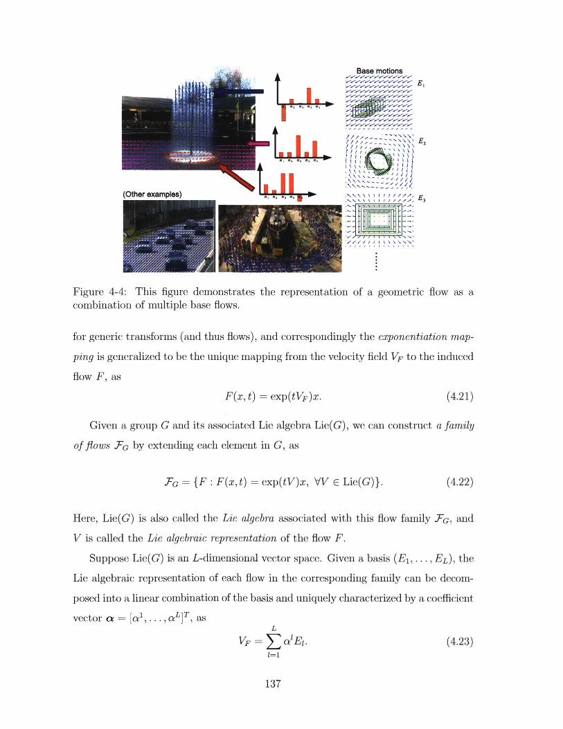
(Other examples)I.
Y-k~ Base motions
a, a,' a, 5 i
a, a, 1, --E3
Figure 4-4: This figure demonstrates the representation of a geometric flow as acombination of multiple base flows.
for generic transforms (and thus flows), and correspondingly the exponentiation map-
ping is generalized to be the unique mapping from the velocity field VF to the induced
flow F, as
F(x, t) = exp(tVF) x. (4.21)
Given a group G and its associated Lie algebra Lie(G), we can construct a family
of flows FG by extending each element in G, as
G_ ={F : F(x,t) = exp(tV)x, VV E Lie(G)}. (4.22)
Here, Lie(G) is also called the Lie algebra associated with this flow family FG, and
V is called the Lie algebraic representation of the flow F.
Suppose Lie(G) is an L-dimensional vector space. Given a basis (Ei, . .. , EL), the
Lie algebraic representation of each flow in the corresponding family can be decom-
posed into a linear combination of the basis and uniquely characterized by a coefficient
vector a = [al,.. .,aL]T, asL
VF -'E. (4.23)
137
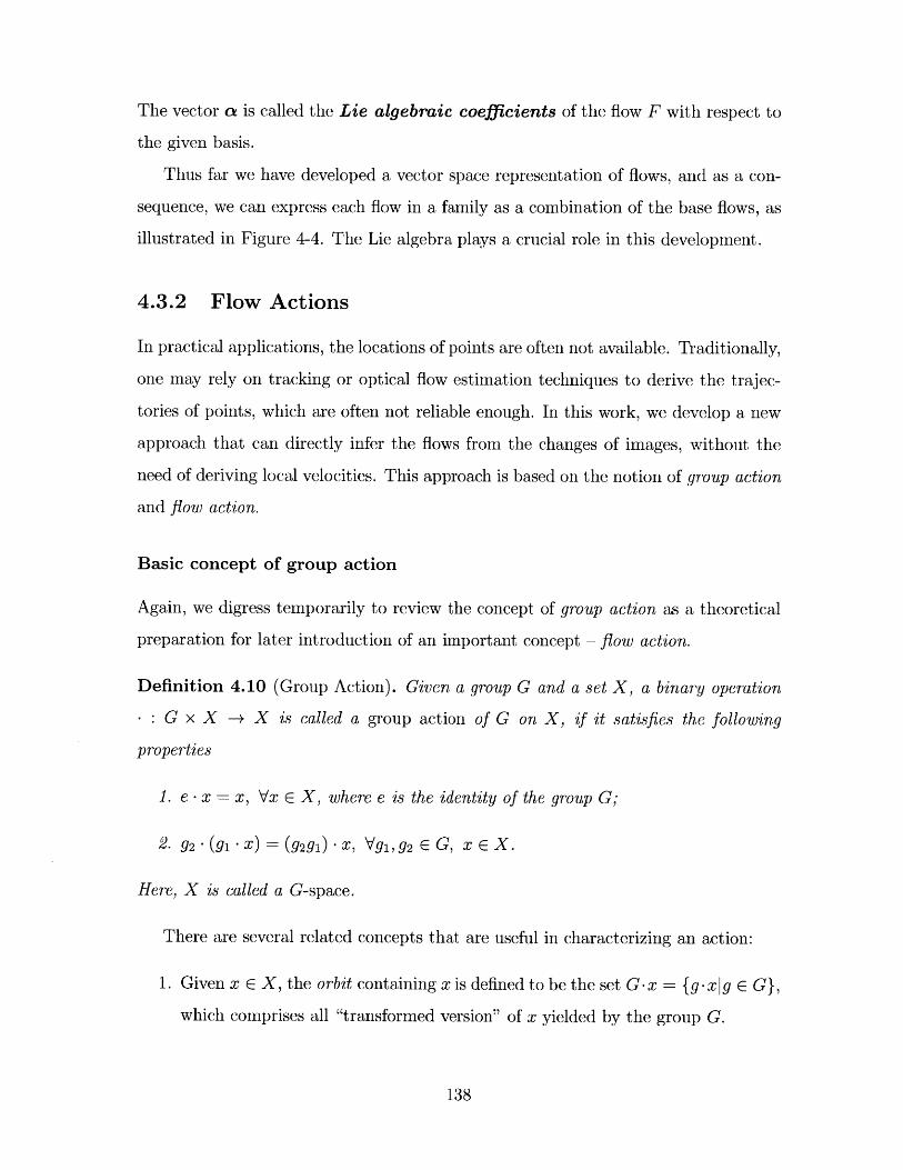
The vector a is called the Lie algebraic coefficients of the flow F with respect to
the given basis.
Thus far we have developed a vector space representation of flows, and as a con-
sequence, we can express each flow in a family as a combination of the base flows, as
illustrated in Figure 4-4. The Lie algebra plays a crucial role in this development.
4.3.2 Flow Actions
In practical applications, the locations of points are often not available. Traditionally,
one may rely on tracking or optical flow estimation techniques to derive the trajec-
tories of points, which are often not reliable enough. In this work, we develop a new
approach that can directly infer the flows from the changes of images, without the
need of deriving local velocities. This approach is based on the notion of group action
and flow action.
Basic concept of group action
Again, we digress temporarily to review the concept of group action as a theoretical
preparation for later introduction of an important concept - flow action.
Definition 4.10 (Group Action). Given a group G and a set X, a binary operation
- : G x X -+ X is called a group action of G on X, if it satisfies the following
properties
1. e - x = x, Vx E X, where e is the identity of the group G;
2. g2 - (gi x) = (929 1) -x, Vgi, 92 E G, x E X.
Here, X is called a G-space.
There are several related concepts that are useful in characterizing an action:
1. Given x E X, the orbit containing x is defined to be the set G -x = {g -xIg E G},
which comprises all "transformed version" of x yielded by the group G.
138
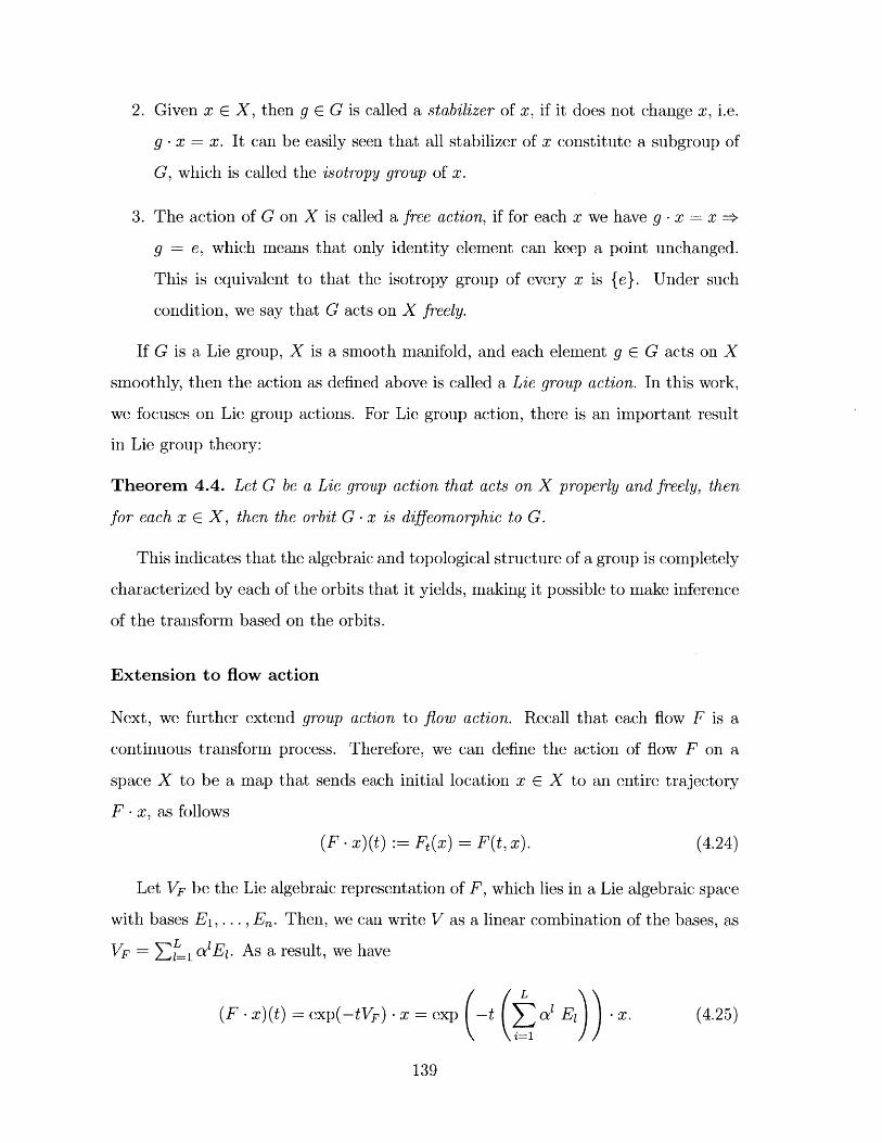
2. Given x E X, then g c G is called a stabilizer of x, if it does not change x, i.e.
g -x = x. It can be easily seen that all stabilizer of x constitute a subgroup of
G, which is called the isotropy group of x.
3. The action of G on X is called a free action, if for each x we have g -x x ->
g = e, which means that only identity element can keep a point unchanged.
This is equivalent to that the isotropy group of every x is {e}. Under such
condition, we say that G acts on X freely.
If G is a Lie group, X is a smooth manifold, and each element g c G acts on X
smoothly, then the action as defined above is called a Lie group action. In this work,
we focuses on Lie group actions. For Lie group action, there is an important result
in Lie group theory:
Theorem 4.4. Let G be a Lie group action that acts on X properly and freely, then
for each x e X, then the orbit G -x is diffeomorphic to G.
This indicates that the algebraic and topological structure of a group is completely
characterized by each of the orbits that it yields, making it possible to make inference
of the transform based on the orbits.
Extension to flow action
Next, we further extend group action to flow action. Recall that each flow F is a
continuous transform process. Therefore, we can define the action of flow F on a
space X to be a map that sends each initial location x E X to an entire trajectory
F -x, as follows
(F -x)(t) := Ft(x) = F(t, x). (4.24)
Let VF be the Lie algebraic representation of F, which lies in a Lie algebraic space
with bases E1, . . . , En. Then, we can write V as a linear combination of the bases, as
VF i a'E. As a result, we have
L(F -x)(t) =- exp(-tVF) - x = exp -t a' El - . (4.25)
139
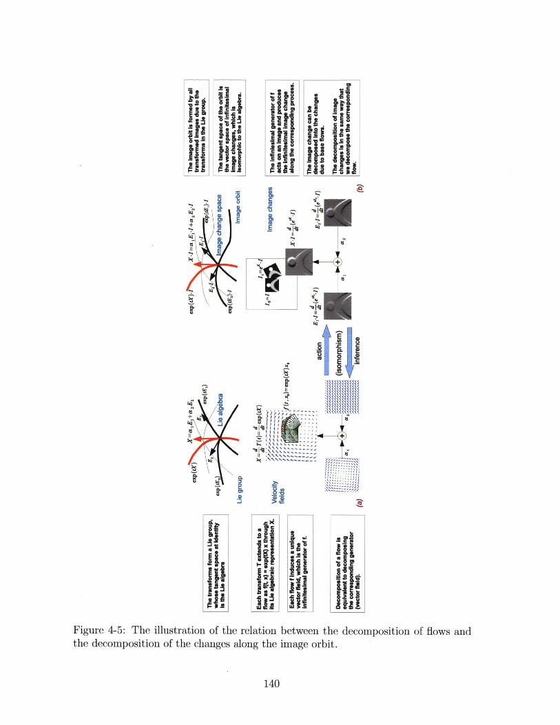
IL 14 j i2 8 'lt . e
Its
eE a 101
CJC
CMi. E UD
Figure 4-5: The illustration of the relation between the decomposition of flows and
the decomposition of the changes along the image orbit.
140
This equation is in a nonlinear form that is difficult to work with. To address this
issue, we first introduce the action of infinitesimal generator VF on x, which is defined
to be
a a(V - X) =- (F . x) (t) = - (x, t). (4.26)
Based on this definition and the representation of V as a linear combination, we
further obtain
L L
(V - x) = a'(Ei -x) a exp(tE) -x. (4.27)1= = t=O
This result establishes the isomorphism between the Lie algebraic representations and
the results of their action on X, which is the theoretical foundation of our inference
approach. Intuitively, the infinitesimal change generated by the flow F can be de-
composed as a linear combination of the "base changes" (El -x) in the same way as
the decomposition of the flow itself into combination of base flows. Therefore, the
inference problem reduces to a regression problem on the the space of infinitesimal
changes.
The space X to be acted on can be a space of any available observations, such
as point locations, images, and contour curves, etc. The linear relation established
in Eq.(4.27) can be utilized to directly connect the flow coefficients to the dynamic
changes of observations. Figure 4-5 gives an illustration of this notion, when the flow
is considered as directly acting on the image space.
4.3.3 Multi-scale Extensions
The dynamics in a real scene may exhibit different characteristics in different scales.
In a complex scene, while there exist common patterns that can be captured by a
global flow, different local parts may have different local characteristics respectively.
Hence, complete modeling of such dynamic scenes calls for a multi-scale framework
that integrates the flow models in different granularities.
A hierarchical structure is a natural structure for implementing the multi-scale
141
modeling. The underlying idea is to use a global flow model to capture the com-
monalities over a large domain, and this model is refined within each local domain
to yield local models that describe the local characteristics more accurately. These
local models can be further refined recursively if necessary, which will give rise to a
hierarchy of models. Let B 1 , ... , B, are local models that are generated by refining
the model A, then A is called the parent model of B 1,..., Bm; while B 1 ,..., Bm are
called A's children models.
The construction of a multi-scale model hierarchy involves three stages:
1. Domain subdivision. Given a flow F defined on a spatial domain Do, when we
intend to refine FO, we first divide Da into several smaller regions D 1,1, ... , D1,m
with Do U Jl 1 D1,k, on which the local models are based.
2. Flow refinement. After the local domains D1 ,1, ... , Di,m are determined, we can
generate m local flows F1,1,... , Fi,m for these local domains, which can then be
refined respectively.
3. Flow Assembling. Combine the refined local flows into a coherent global flow
F1 . This process may involve the enforcement of some consistency constraints.
There are different methods for domain division and local flow assembling. In the
following, I will discuss two methods that we may consider to adopt in our framework.
Disjoint division into polygonal cells
The first way is to divide each domain into polygonal sub-domains with a polygonal
mesh. Different sub-domains do not overlap with each other except at the boundary,
and each local flow is strictly confined within the given sub-domains. To ensure that
the integrated flow is well-defined at the boundary, we need to enforce the consistency
constraints at the boundary, which are in the following form
VFa (x)=Z VF (x), Vx E Da n Db. (4.28)
142
Let Ei,... , EL be the basis of the Lie algebra associated with the flow family, such
that VFa i1 alE, and VF, -1 #3E1 , then the consistency constraints can be
written in terms of flow coefficients as
L L
S a1E1(x) = 1E 1(x), Vx E Da n Db. (4.29)1=1 1=1
We can see that they are linear constraints. Enforcing these consistency constraints
results in a space of consistent flows, denoted by CF1 , which is a subspace of F1 , the
joint space of local flows.
The dimensionality of the space of consistent flows in general depends on the
graphical topology of the mesh, as well as the choice of the flow class.
Triangle mesh and consistent subspace
When a triangular mesh is employed (i.e. dividing the image plane into disjoint trian-
gular cells) and the affine flows are used as local flows, we have more specific results.
Specifically, we partition the scene using a triangle mesh with m cells and n
vertices, and attach each cell with an affine flow. Let E, ... , EL denote the basis of
the associated Lie algebraic representation (base velocity fields). Then the local flow
of the i-th cell can be represented by an L-dimensional Lie algebraic coefficient vector
Local flows may generate different velocities at shared vertices. Consider a vertex
x shared by the i-th and j-th cells. In general, VFi (x) may not equal VFj (x), leading
to discontinuities at a cell boundary.
To avoid such inconsistencies, we require that the local flows yield the same veloc-
ities at shared vertices, i.e. VF(x) = VFj (x), resulting in the consistency constraints
of the local coefficients asL
- )Ei(x) = 0. (4.30)
If all triangles are non-degenerated, i.e. three vertices do lie on a line, then there
are in total (6m - 2n) independent consistency constraints, which give rise to a 2n-
143
dimensional space of consistent flows.
The strategy of dividing domains into non-overlapping polygonal sub-domains is
straightforward and simple to implement, however, it has two drawbacks:
1. The refined flow formed by stitching local affine flows is in general not smooth.
In particular, F1 (x, t) is not continuously differentiable at cell boundaries.
2. The space of consistent flows varies as the sub-domains change. This means
that when a local modification is made to the triangle mesh, all consistency
constraints need to be re-computed, making it difficult to apply it to the context
with evolving domains.
Partition of unity
To overcome these difficulties, we also explore another method that is based on par-
tition of unity, which is a concept originating from topology for constructing global
continuous functions from locally defined functions. The basic idea is to combine
local functions with overlapped smooth "window functions" that sum to unity.
Let D 1 ,1 ,..., D1,m be open sub-domains that covers Do, i.e. Do U ( 1 D1 ,,
then the set of non-negative functions {Wk : Do - R} is called a partition of unity
subordinate to the cover if it satisfies
wk (x) = 1, Vx E Do, and wk(X) =0, Vx ( D1,k, Vk = 1 .. (4.31)k=1
Back to the multi-scale flow modeling problem. Let F 1,1 ... , Fi,m be the local flows
defined respectively on the overlapping over-domains D 1 ,1, ... , Di,m, then we can
construct the complete flow F1 over Do in terms of its infinitesimal generator as
m
VF1 (X) ZWk(X) VF1,k(X) (4.32)k=1
The flows constructed in this way are well-defined without the need to enforcing
additional consistency constraints. In addition, if both fi,k and wk are smooth, then
144
the derived flow must be smooth. Furthermore, we have the following property that
makes it suitable in the context with evolving domains:
Proposition 4.1. Let {Wk : Do -+ R} be a partition of unity subordinate to a given
cover D 1,1 , ... , D1,,, then if the domains are transformed by a diffeomorphism T, i.e.
D1,k F TD1,k, then {Twk : TD1,k -+ R} is a partition of unity subordinate to the
new cover, i.e. the sum-to-unity condition continues to hold, where Twk is defined by
Twk(x) - Wk(T-lx).
It means that domain evolution will not affect the validity of the flow if the
weighting functions are transformed accordingly. In summary, using partition of
unity method may incur more computation cost as multiple flows are involved in the
overlapping area, which, however, brings forth a series of benefits, which, for exam-
ple, include modeling flexibility, smoothness, and adaptivity to evolving environment
where the domain of flow can change dynamically.
4.4 Stochastic Flow Model
To model real scenes, we are facing a complicated situation with a series of practical
challenges. These challenges include noisy measurement, missing data, and errors
arising in the feature extraction processes. To cope with these difficulties, we extended
the algebraic formulation developed above to a stochastic model that allows objects
to deviate from the ideal trajectories.
4.4.1 The Stochastic Flow Formulation
The stochastic model of a dynamic flow is formulated as a diffusion process charac-
terized as follows:
x(t) - F(xo, t) + oB(t) (4.33)
Here, F(xo, t) is a deterministic geometric flow as given by
dx(t) = VF(x(t)), (4-34)dt
145
and B(t) is the Brownian motion that accounts for the residual part due to deviation
or measurement noise. This equation can be written equivalently, as
dxt =VF(x) + -dBt. (4.35)
Let At be the time interval between two measurements of x(t), then if At is sufficiently
small, we have
x(t + At) - x(t) ~ VF(x) + At, At ~ AP(0, 0'At).
In practice, we will restrict F to a finite dimensional family, whose associated Lie
algebraic space has basis (E1, ... , EL), and express VF as the linear combination of
these bases. Then, we have
L
x(t + At) - x(t) ~ acEl(x) + (At.1=1
(4.37)
If x is observed, and a Gaussian prior is assumed for the Lie algebraic coefficients
a ~ V(0, Zo). (4.38)
Then, the maximum a posterior estimation of the flow, formulated as
a
maximize logp(a) + logp(x a),i=1
w.r.t. a, (4.39)
will reduce to a regularized linear regression problem, as below
n n iminimize 2a EO a + 2(0at) Xi(ty) -
i=o j=1 (
L
zi(tj_1) - a;Ej(zb(ty_
2
1)) .)
(4.40)
Here, nt is the number of time steps, and tj = jAt is the j-th time step. This is a
quadratic optimization problem and can be readily solved.
146
(4.36)
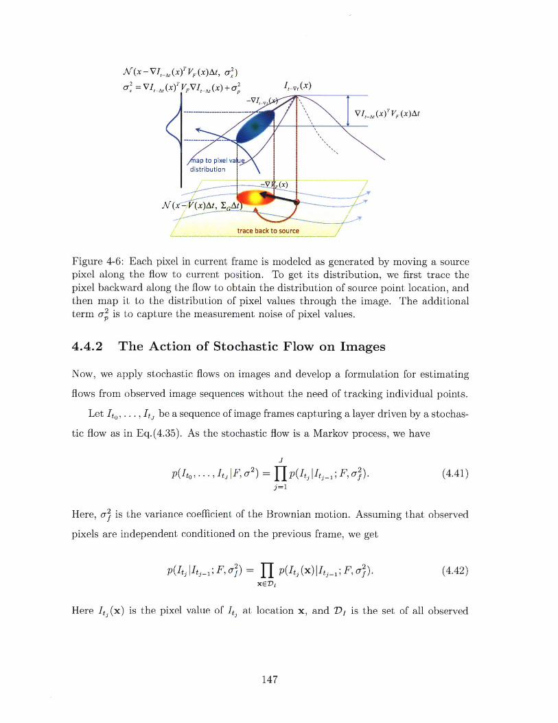
A((x - VI, (x)T VF (X)At, x2)
= -At (x)T V t + x-Vt()
-VI-
rX)FVII-Al T F (x)At
ap to pixel vaLdistribution
AF(X-(x)AZt, .At
trace back to source
Figure 4-6: Each pixel in current frame is modeled as generated by moving a sourcepixel along the flow to current position. To get its distribution, we first trace thepixel backward along the flow to obtain the distribution of source point location, andthen map it to the distribution of pixel values through the image. The additionalterm ou is to capture the measurement noise of pixel values.
4.4.2 The Action of Stochastic Flow on Images
Now, we apply stochastic flows on images and develop a formulation for estimating
flows from observed image sequences without the need of tracking individual points.
Let It., . .. , I be a sequence of image frames capturing a layer driven by a stochas-
tic flow as in Eq.(4.35). As the stochastic flow is a Markov process, we have
J
p(Ito,. . . I F, a2 ) = Jp(Itj|Itj_,; F, U2). (4.41)j=1
Here, Ou is the variance coefficient of the Brownian motion. Assuming that observed
pixels are independent conditioned on the previous frame, we get
p(Itj Itj_; F, O-) = [ p(Itj (x)IIt,; F, O). (4.42)
Here It, (x) is the pixel value of It, at location x, and D, is the set of all observed
147
pixel locations in the flow domain. Through back tracing (see Figure 4-6), we obtain
p(It, (x)|IIt,_- ; F, u') = NV(It _(x) - px , a 2). (4.43)
with
px = VIEt_(x)TVF(X)At, (4.44)
a = ajVje (x)TVItI (x) At. (4.45)
Here, we use a locally linear approximation as below in deriving the normal distribu-
tion above:
I(x + Ax) ~ I(x) + VxAx. (4.46)
Note here that Eq.(4.45) suppresses the influence of the pixels with high contrast
neighborhood. With Lie algebraic representation, we can further expand each factor
in Eq.(4.42) as
L
p(It (x) j;F,( x) - It,_1 (x) - Ea/p4 , p2) . (4.47)
Here, p4 VI ,_ (x)TEl(x)At. Therefore, we can model the changes of image
pixels using pixel-wise normal distributions. At a particular pixel, the mean of its
corresponding normal distribution depends on the flow coefficients, while the variance
depends on the image gradient at the same location.
Again, the estimation of flow coefficients from a sequence of images can be formu-
lated as an MAP problem, as follows
flt
maximize log p(a) + loge log P(It It,_; a). (4.48)j=1
Here, we exploit the fact a sequence of images generated according to a given stochas-
tic flow model constitutes a Markov chain. When p(a) is a Gaussian prior, this
problem reduces to a quadratic programming problem, which we can readily solve.
148
4.4.3 Integration of Observations
From the discussion above, it can be seen that under a stochastic flow formulation,
the likelihood has a similar form when different types of observations are utilized
(e.g. tracks of individual objects and image frames), in spite of their different gener-
ation processes. Specifically, we have
1. When point tracks are used, the likelihood of each track t can be written as
nt L
p(ta) = A t (j) - t(j - 1) cx aEi(t(j)), oAt . (4.49)j=1 =
2. When image frames are directly worked on, the likelihood of each image frame,
conditioned on the previous one, can be written as
L
p(I|Ig_1,a) j= , A Ij(x) - I_1 (x) l ap, ) . (4.50)
Here, px and ox are respectively the model-predicted mean and variance of the
pixel change at x.
For both cases, the likelihood terms can be written uniformly as products of
Af(yil Ea, Ei). Here, vyj denotes the observed change, Ei denotes the matrix where
each column represents the "base change" induced by a particular base flow. Thus,
Eia is the model-predicted change, as a linear combination of the base changes. Here,
we call the triplet (yi, Ei, Ei) an observation entry.
With the generic form of likelihood terms discussed above, one can integrate dif-
ferent types of observations whenever they are available from the scene. This would
lead to a unified model with multiple Gaussian likelihood factors. As a result, flow
estimation based on this model can be casted as a joint Gaussian inference problem.
4.4.4 Gaussian Process Prior over Complex Flows
Flows in natural scenes exhibit complex yet spatially coherent variations. Effective
modeling of such flows requires a fine-grained mesh that may compromise the spatial
149
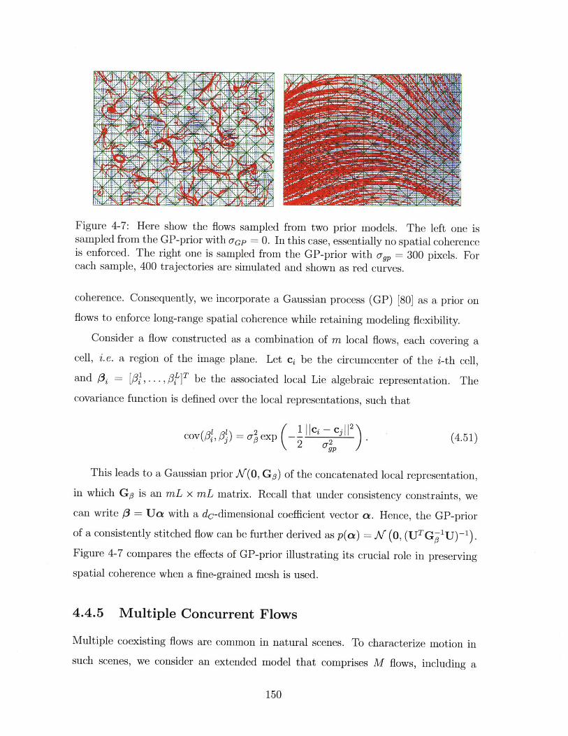
Figure 4-7: Here show the flows sampled from two prior models. The left one issampled from the GP-prior with UGP = 0. In this case, essentially no spatial coherenceis enforced. The right one is sampled from the GP-prior with ogp = 300 pixels. Foreach sample, 400 trajectories are simulated and shown as red curves.
coherence. Consequently, we incorporate a Gaussian process (GP) [80] as a prior on
flows to enforce long-range spatial coherence while retaining modeling flexibility.
Consider a flow constructed as a combination of m local flows, each covering a
cell, i.e. a region of the image plane. Let ci be the circumcenter of the i-th cell,
and i3= f,...,#/]T be the associated local Lie algebraic representation. The
covariance function is defined over the local representations, such that
cov(# ,f# ) = o.exp - Ici -. C1 2 (4.51)
This leads to a Gaussian prior K(O, GO) of the concatenated local representation,
in which G,3 is an mL x mL matrix. Recall that under consistency constraints, we
can write # = Ua with a dc-dimensional coefficient vector a. Hence, the GP-prior
of a consistently stitched flow can be further derived as p(a) = K (0, (UTGf U)-).
Figure 4-7 compares the effects of GP-prior illustrating its crucial role in preserving
spatial coherence when a fine-grained mesh is used.
4.4.5 Multiple Concurrent Flows
Multiple coexisting flows are common in natural scenes. To characterize motion in
such scenes, we consider an extended model that comprises M flows, including a
150
Ni
X_
NX-lil
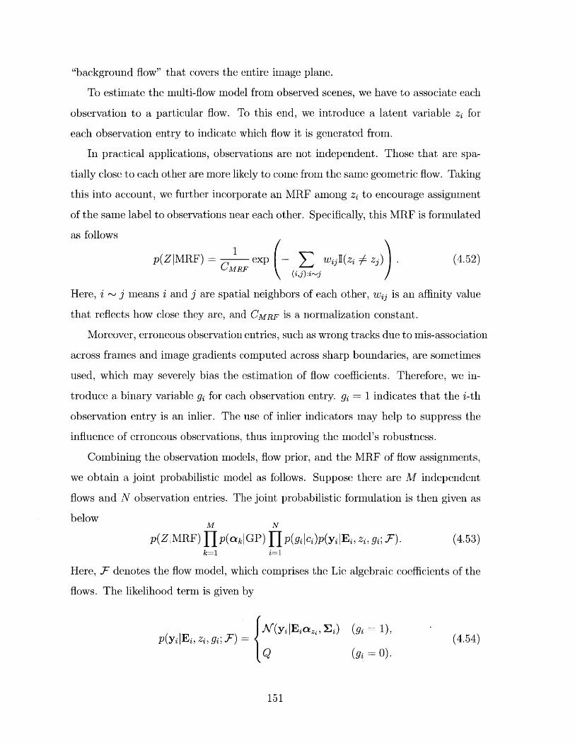
"background flow" that covers the entire image plane.
To estimate the multi-flow model from observed scenes, we have to associate each
observation to a particular flow. To this end, we introduce a latent variable zi for
each observation entry to indicate which flow it is generated from.
In practical applications, observations are not independent. Those that are spa-
tially close to each other are more likely to come from the same geometric flow. Taking
this into account, we further incorporate an MRF among zi to encourage assignment
of the same label to observations near each other. Specifically, this MRF is formulated
as follows
p(ZIMRF)= exp wiyL(zi f zj) . (4.52)CMRF Ai-
Here, i - j means i and j are spatial neighbors of each other, wij is an affinity value
that reflects how close they are, and CMRF is a normalization constant.
Moreover, erroneous observation entries, such as wrong tracks due to mis-association
across frames and image gradients computed across sharp boundaries, are sometimes
used, which may severely bias the estimation of flow coefficients. Therefore, we in-
troduce a binary variable gi for each observation entry. gi 1 indicates that the i-th
observation entry is an inlier. The use of inlier indicators may help to suppress the
influence of erroneous observations, thus improving the model's robustness.
Combining the observation models, flow prior, and the MRF of flow assignments,
we obtain a joint probabilistic model as follows. Suppose there are M independent
flows and N observation entries. The joint probabilistic formulation is then given as
belowM N
p(Z IMRF) fp(Ak GP) f p(gi cj)p(yi lEi, zi, gi; F). (4.53)k=1 i=1
Here, F denotes the flow model, which comprises the Lie algebraic coefficients of the
flows. The likelihood term is given by
p (yi I Ei, zi, gi; T) = NV(yilIEi a z, E i) (gi = 1), (4.54)
151
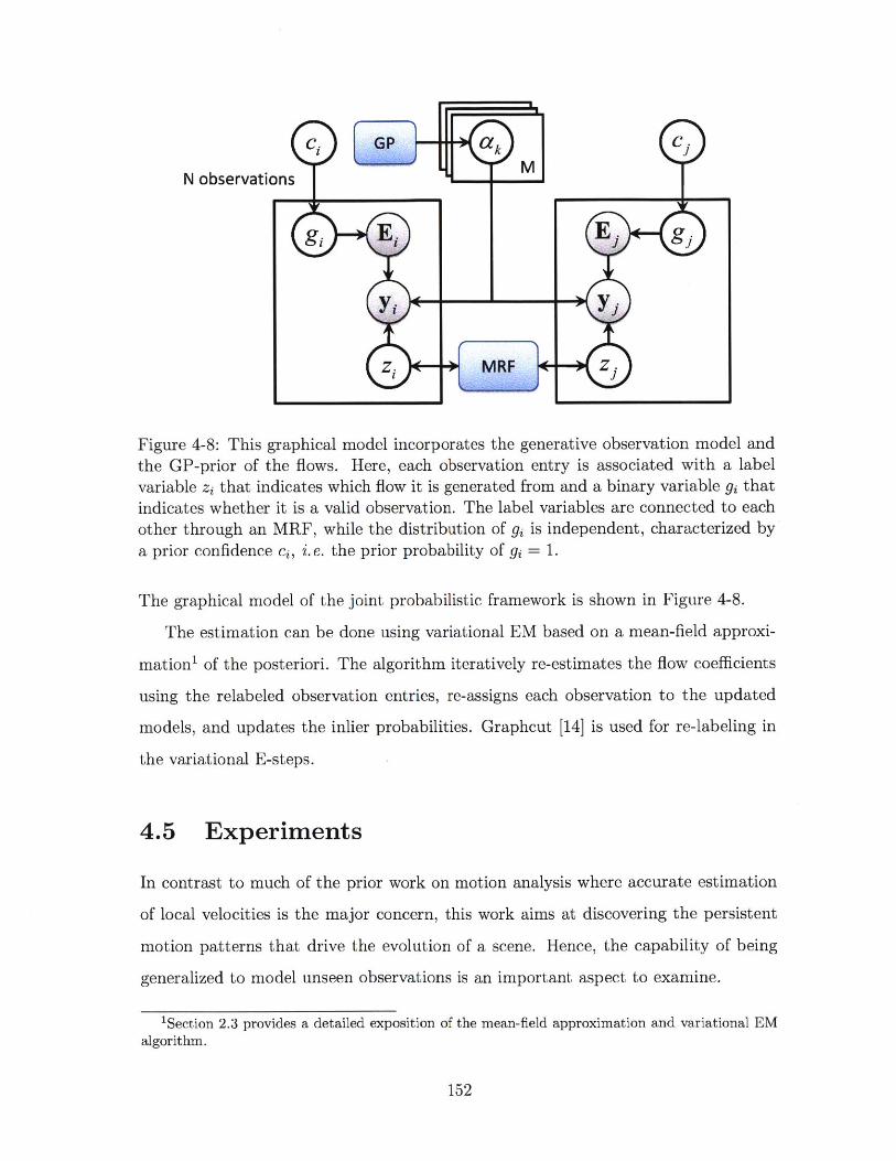
N
Figure 4-8: This graphical model incorporates the generative observation model andthe GP-prior of the flows. Here, each observation entry is associated with a labelvariable zi that indicates which flow it is generated from and a binary variable gi thatindicates whether it is a valid observation. The label variables are connected to eachother through an MRF, while the distribution of gi is independent, characterized bya prior confidence ci, i. e. the prior probability of gi = 1.
The graphical model of the joint probabilistic framework is shown in Figure 4-8.
The estimation can be done using variational EM based on a mean-field approxi-
mationi of the posteriori. The algorithm iteratively re-estimates the flow coefficients
using the relabeled observation entries, re-assigns each observation to the updated
models, and updates the inlier probabilities. Graphcut [14] is used for re-labeling in
the variational E-steps.
4.5 Experiments
In contrast to much of the prior work on motion analysis where accurate estimation
of local velocities is the major concern, this work aims at discovering the persistent
motion patterns that drive the evolution of a scene. Hence, the capability of being
generalized to model unseen observations is an important aspect to examine.
'Section 2.3 provides a detailed exposition of the mean-field approximation and variational EMalgorithm.
152
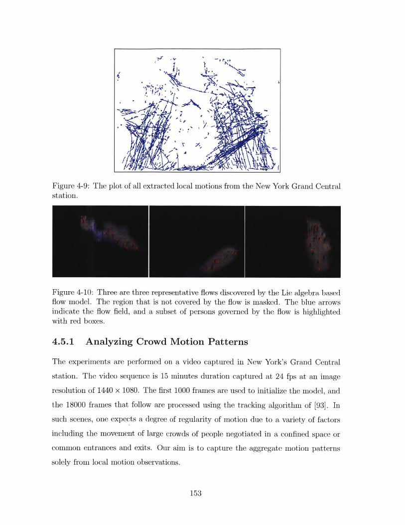
d
Figure 4-9: The plot of all extracted local motions from the New York Grand Centralstation.
Figure 4-10: Three are three representative flows discovered by the Lie algebra basedflow model. The region that is not covered by the flow is masked. The blue arrowsindicate the flow field, and a subset of persons governed by the flow is highlightedwith red boxes.
4.5.1 Analyzing Crowd Motion Patterns
The experiments are performed on a video captured in New York's Grand Central
station. The video sequence is 15 minutes duration captured at 24 fps at an image
resolution of 1440 x 1080. The first 1000 frames are used to initialize the model, and
the 18000 frames that follow are processed using the tracking algorithm of [93]. In
such scenes, one expects a degree of regularity of motion due to a variety of factors
including the movement of large crowds of people negotiated in a confined space or
common entrances and exits. Our aim is to capture the aggregate motion patterns
solely from local motion observations.
153
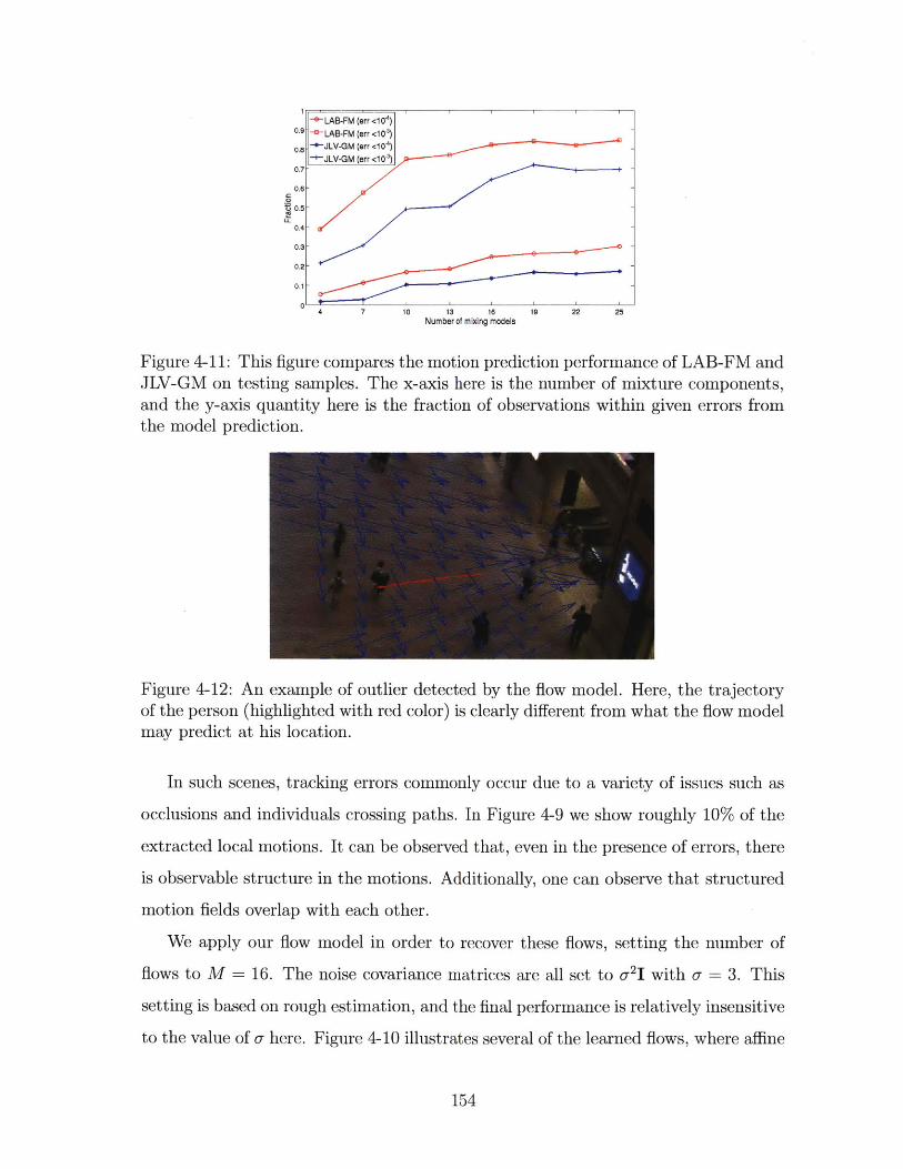
0.7
0.6
t 0.5
0.4
0.3
0.2-
10 13 16 s19 22 25Number of mixing models
Figure 4-11: This figure compares the motion prediction performance of LAB-FM andJLV-GM on testing samples. The x-axis here is the number of mixture components,and the y-axis quantity here is the fraction of observations within given errors fromthe model prediction.
Figure 4-12: An example of outlier detected by the flow model. Here, the trajectoryof the person (highlighted with red color) is clearly different from what the flow modelmay predict at his location.
In such scenes, tracking errors commonly occur due to a variety of issues such as
occlusions and individuals crossing paths. In Figure 4-9 we show roughly 10% of the
extracted local motions. It can be observed that, even in the presence of errors, there
is observable structure in the motions. Additionally, one can observe that structured
motion fields overlap with each other.
We apply our flow model in order to recover these flows, setting the number of
flows to M = 16. The noise covariance matrices are all set to U2 1 with a-= 3. This
setting is based on rough estimation, and the final performance is relatively insensitive
to the value of -here. Figure 4-10 illustrates several of the learned flows, where affine
154
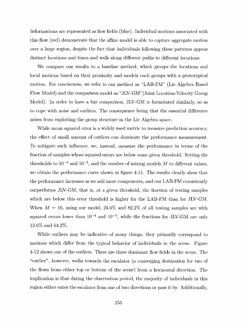
deformations are represented as flow fields (blue). Individual motions associated with
this flow (red) demonstrate that the affine model is able to capture aggregate motion
over a large region, despite the fact that individuals following these patterns appear
distinct locations and times and walk along different paths to different locations.
We compare our results to a baseline method, which groups the locations and
local motions based on their proximity and models each groups with a prototypical
motion. For conciseness, we refer to our method as "LAB-FM" (Lie Algebra Based
Flow Model) and the comparison model as "JLV-GM" (Joint Location-Velocity Group
Model). In order to have a fair comparison, JLV-GM is formulated similarly, so as
to cope with noise and outliers. The consequence being that the essential difference
arises from exploiting the group structure in the Lie Algebra space.
While mean squared error is a widely used metric to measure prediction accuracy,
the effect of small amount of outliers can dominate the performance measurement.
To mitigate such influence, we, instead, measure the performance in terms of the
fraction of samples whose squared errors are below some given threshold. Setting the
thresholds to 10-4 and 10-, and the number of mixing models M to different values,
we obtain the performance curve shown in figure 4-11. The results clearly show that
the performance increases as we add more components, and our LAB-FM consistently
outperforms JLV-GM, that is, at a given threshold, the fraction of testing samples
which are below this error threshold is higher for the LAB-FM than for JLV-GM.
When M = 16, using our model, 24.6% and 82.2% of all testing samples are with
squared errors lower than 10-4 and 10-3, while the fractions for JLV-GM are only
13.6% and 64.2%.
While outliers may be indicative of many things, they primarily correspond to
motions which differ from the typical behavior of individuals in the scene. Figure
4-12 shows one of the outliers. There are three dominant flow fields in the scene. The
"outlier", however, walks towards the escalator (a converging destination for two of
the flows from either top or bottom of the scene) from a horizontal direction. The
implication is that during the observation period, the majority of individuals in this
region either enter the escalator from one of two directions or pass it by. Additionally,
155
the analysis indicates that during this period, very few people entered the scene from
the escalator or from the bottom of the scene.
4.5.2 Modeling Flows in General Dynamic Scenes
Next, we test the geometric flows on more complex scenes, where each flow is com-
posed of multiple local flows. In particular, we conducted experiments on videos from
DynTex database [4] and UCF Crowd Analysis database [2]. These videos represent
a wide spectrum of dynamic scenes.
Experiment Settings
We use consistently stitched flows to model the motion patterns in each video. Each
flow is established on a triangle mesh that covers the entire scene and parameterized
by the Lie algebraic representation. To generate the triangle mesh, we first make a
rectangle mesh with 5 rows and 6 columns, and divide each rectangle cell into two
triangles.
Affine flow family is chosen to be the basic flow family for describing the motion
within each cell. This family is associated with a 6-dimensional Lie algebra. While we
found that this setting suffices to obtain good results on the testing videos, generally
there is no restriction to the choice of basic flow family and mesh topology. One
can also use other flow families with our framework to model more complex motion.
The representation dimension (the dimension of the consistent subspace) is L = 84,
which is much smaller than that of the dense velocity map. In addition, we use a GP
prior to enforce long-range spatial coherence, where ogp, which controls the range of
correlation, is set to 100.
We use multiple concurrent flows to model a dynamic scene, including one that
corresponds to the static background. The number of flows in each scene is given.
To initialize the algorithm, we manually specify a "seed area" for each flow, and the
observations in these areas are used to estimate the initial flow models. Besides, we
set the prior confidence of inlier to 0.9 for each observation entry. Flow segmentation,
156
inlier probabilities, and flow models are then iteratively updated until convergence.
To compare our approach with traditional local motion estimation methods, we
implement an optical flow estimation algorithm with multi-scale search and local
smoothness. Moreover, we adapt the algorithm to incorporate multiple frames in
estimation for fair comparison. This is accomplished by assuming a time-invariant
velocity v at each location, and integrating the term ||I- + vTV 12 for every pair of
consecutive frames into the objective function. The design parameters of the optical
flow, including the local search range and the coefficients in the smoothness terms,
are optimized by cross validation.
Collective Behavior of Moving Objects
The algorithms are first evaluated on the scenes that comprise groups of moving
objects, such as people, and vehicles. To test the generalization performance, for
each video, we first manually trace 20 trajectories, whose nominal duration is 100
frames, as ground truth, and then use the first 20 frames to estimate the motion
models. These models are then used to simulate the trajectories starting from the
initial positions as those in the manually traced ones. The performance is measured
by the deviation of the simulated trajectories from the ground truth.
Figure 4-13 and Figure 4-14 shows the results. The results shown in the first row
are obtained on a scene with cars moving along a high way. We see that the optical
flow is over-fitted to the short-time behavior of individual cars: (1) it only extracts
motion in the places where cars are passing by during first 20 frames; (2) the velocity
map lacks spatial coherence. For the same example, the geometric flow accurately
captures the collective behavior of the cars, while preserving spatial coherence. Note
that the subtle variation of the moving direction of the cars is precisely captured in
the flow model.
We also evaluate the trajectory prediction performance, observing that the pre-
dicted trajectories simulated on the optical flow field quickly deviate from the ground
truth; while the ones yielded by geometric flow are much more accurate. The plotted
error curves indicate that the average deviation due to the optical flow is more than
157
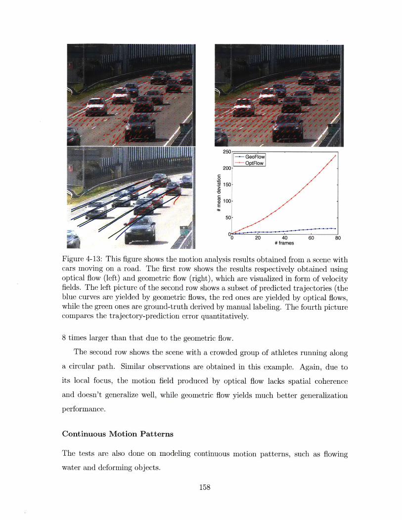
# frames
Figure 4-13: This figure shows the motion analysis results obtained from a scene withcars moving on a road. The first row shows the results respectively obtained usingoptical flow (left) and geometric flow (right), which are visualized in form of velocityfields. The left picture of the second row shows a subset of predicted trajectories (theblue curves are yielded by geometric flows, the red ones are yielded by optical flows,while the green ones are ground-truth derived by manual labeling. The fourth picturecompares the trajectory-prediction error quantitatively.
8 times larger than that due to the geometric flow.
The second row shows the scene with a crowded group of athletes running along
a circular path. Similar observations are obtained in this example. Again, due to
its local focus, the motion field produced by optical flow lacks spatial coherence
and doesn't generalize well, while geometric flow yields much better generalization
performance.
Continuous Motion Patterns
The tests are also done on modeling continuous motion patterns, such as flowing
water and deforming objects.
158
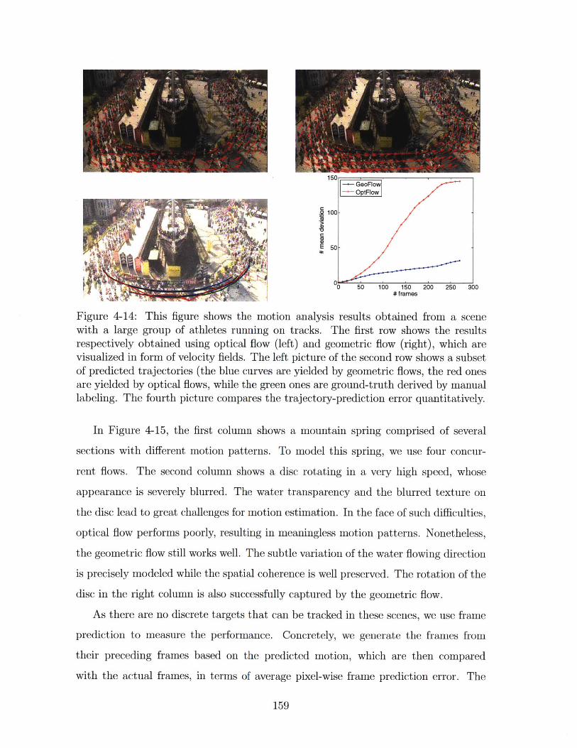
0 50 100 150 200 250 300* # frames
Figure 4-14: This figure shows the motion analysis results obtained from a scenewith a large group of athletes running on tracks. The first row shows the resultsrespectively obtained using optical flow (left) and geometric flow (right), which arevisualized in form of velocity fields. The left picture of the second row shows a subsetof predicted trajectories (the blue curves are yielded by geometric flows, the red onesare yielded by optical flows, while the green ones are ground-truth derived by manuallabeling. The fourth picture compares the trajectory-prediction error quantitatively.
In Figure 4-15, the first column shows a mountain spring comprised of several
sections with different motion patterns. To model this spring, we use four concur-
rent flows. The second column shows a disc rotating in a very high speed, whose
appearance is severely blurred. The water transparency and the blurred texture on
the disc lead to great challenges for motion estimation. In the face of such difficulties,
optical flow performs poorly, resulting in meaningless motion patterns. Nonetheless,
the geometric flow still works well. The subtle variation of the water flowing direction
is precisely modeled while the spatial coherence is well preserved. The rotation of the
disc in the right column is also successfully captured by the geometric flow.
As there are no discrete targets that can be tracked in these scenes, we use frame
prediction to measure the performance. Concretely, we generate the frames from
their preceding frames based on the predicted motion, which are then compared
with the actual frames, in terms of average pixel-wise frame prediction error. The
159
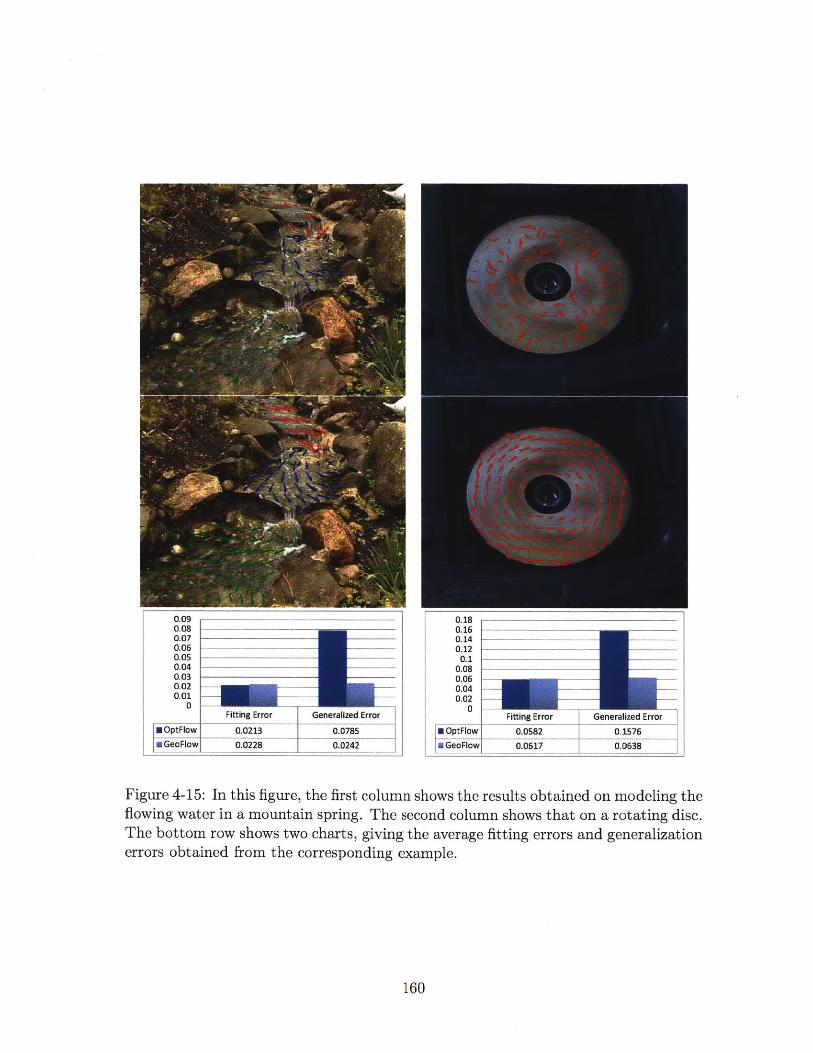
Figure 4-15: In this figure, the first column shows the results obtained on modeling theflowing water in a mountain spring. The second column shows that on a rotating disc.The bottom row shows two charts, giving the average fitting errors and generalizationerrors obtained from the corresponding example.
160
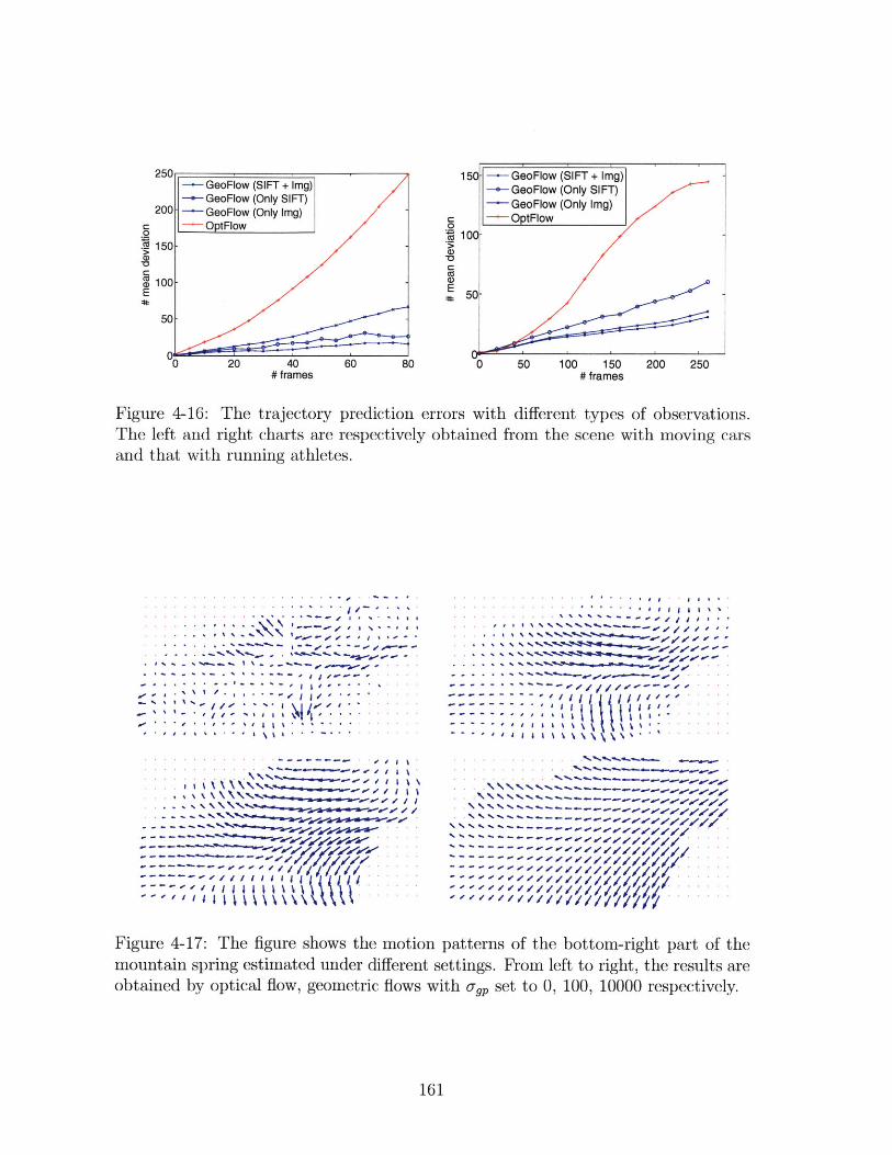
250
200
150(D
(100E
C0
E
# frames100 150
# frames
Figure 4-16: The trajectory prediction errors with different types of observations.
The left and right charts are respectively obtained from the scene with moving cars
and that with running athletes.
I -
- - - .q.....~ *~ ~ -
I - - - -
-. 9------ II.............
4,.
4 \9/p.~~~ I..
tI 4
. ..- '.-..-.-..-... I.4.
;gel . . .
.. %'
%L *
Vt...
Figure 4-17: The figure shows the motion patterns of the bottom-right part of the
mountain spring estimated under different settings. From left to right, the results are
obtained by optical flow, geometric flows with ogp set to 0, 100, 10000 respectively.
161
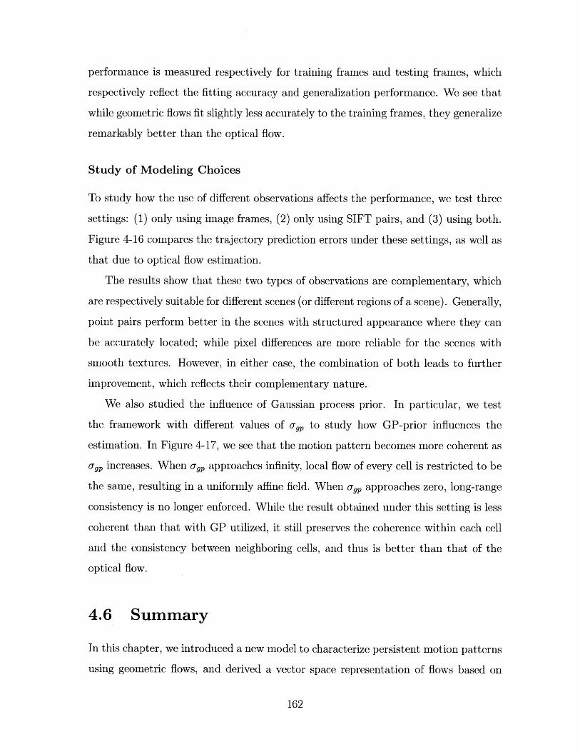
performance is measured respectively for training frames and testing frames, which
respectively reflect the fitting accuracy and generalization performance. We see that
while geometric flows fit slightly less accurately to the training frames, they generalize
remarkably better than the optical flow.
Study of Modeling Choices
To study how the use of different observations affects the performance, we test three
settings: (1) only using image frames, (2) only using SIFT pairs, and (3) using both.
Figure 4-16 compares the trajectory prediction errors under these settings, as well as
that due to optical flow estimation.
The results show that these two types of observations are complementary, which
are respectively suitable for different scenes (or different regions of a scene). Generally,
point pairs perform better in the scenes with structured appearance where they can
be accurately located; while pixel differences are more reliable for the scenes with
smooth textures. However, in either case, the combination of both leads to further
improvement, which reflects their complementary nature.
We also studied the influence of Gaussian process prior. In particular, we test
the framework with different values of o-p to study how GP-prior influences the
estimation. In Figure 4-17, we see that the motion pattern becomes more coherent as
o-gp increases. When ogp approaches infinity, local flow of every cell is restricted to be
the same, resulting in a uniformly affine field. When -gp approaches zero, long-range
consistency is no longer enforced. While the result obtained under this setting is less
coherent than that with GP utilized, it still preserves the coherence within each cell
and the consistency between neighboring cells, and thus is better than that of the
optical flow.
4.6 Summary
In this chapter, we introduced a new model to characterize persistent motion patterns
using geometric flows, and derived a vector space representation of flows based on
162

Lie algebraic analysis. This representation greatly simplifies the use of probabilistic
modeling and inference on flows. We also developed a stochastic flow model and
extended it through domain sub-division.
We conducted experiments to test this new approach on real videos, and compare
it with optical flow estimation. The results clearly demonstrate that geometric flows,
formulated with the goal of capturing coherent patterns over both space and time,
perform substantially better than optical flows, and thus they are more effective in
persistent motion modeling.
163
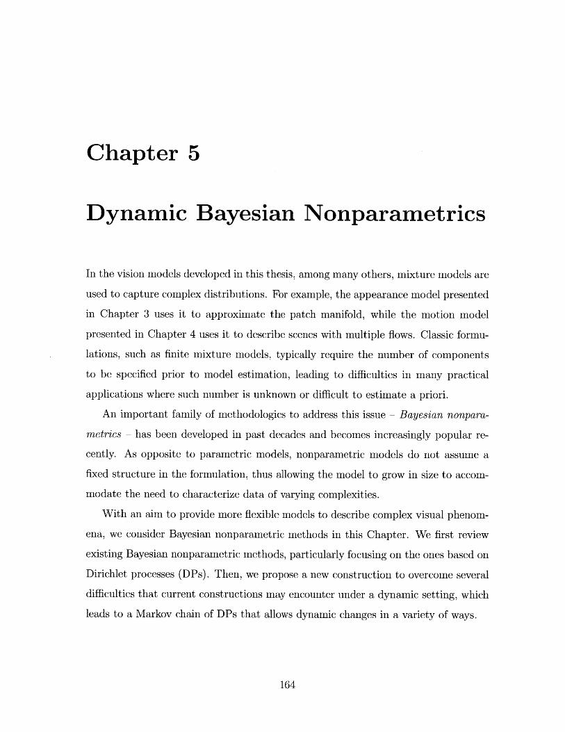
Chapter 5
Dynamic Bayesian Nonparametrics
In the vision models developed in this thesis, among many others, mixture models are
used to capture complex distributions. For example, the appearance model presented
in Chapter 3 uses it to approximate the patch manifold, while the motion model
presented in Chapter 4 uses it to describe scenes with multiple flows. Classic formu-
lations, such as finite mixture models, typically require the number of components
to be specified prior to model estimation, leading to difficulties in many practical
applications where such number is unknown or difficult to estimate a priori.
An important family of methodologies to address this issue - Bayesian nonpara-
metrics - has been developed in past decades and becomes increasingly popular re-
cently. As opposite to parametric models, nonparametric models do not assume a
fixed structure in the formulation, thus allowing the model to grow in size to accom-
modate the need to characterize data of varying complexities.
With an aim to provide more flexible models to describe complex visual phenom-
ena, we consider Bayesian nonparametric methods in this Chapter. We first review
existing Bayesian nonparametric methods, particularly focusing on the ones based on
Dirichlet processes (DPs). Then, we propose a new construction to overcome several
difficulties that current constructions may encounter under a dynamic setting, which
leads to a Markov chain of DPs that allows dynamic changes in a variety of ways.
164
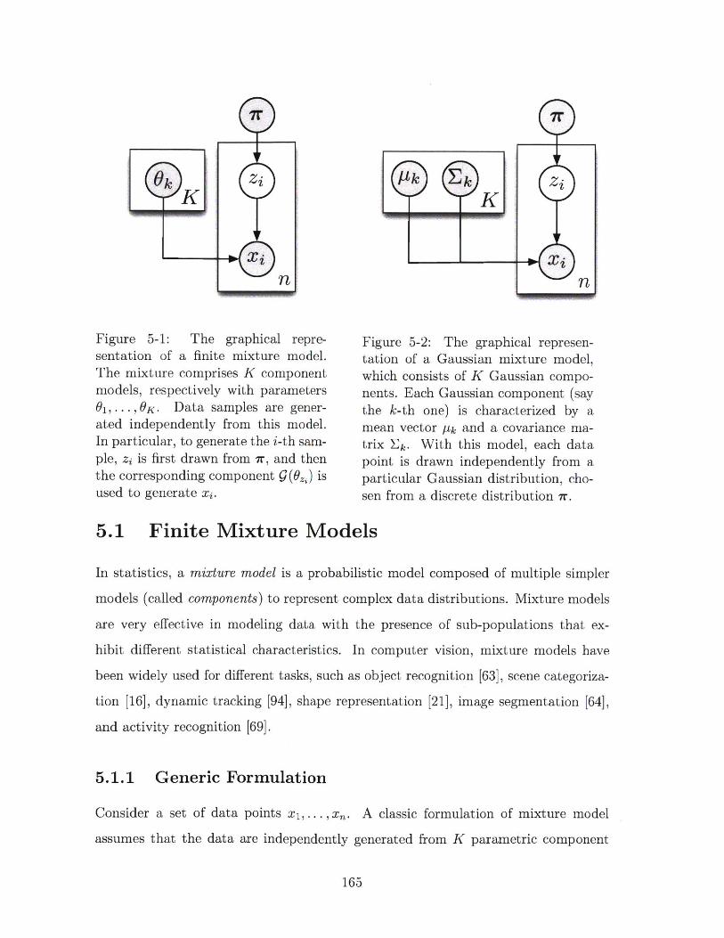
Figure 5-1: The graphical repre-sentation of a finite mixture model.The mixture comprises K componentmodels, respectively with parameters01, .. . , OK. Data samples are gener-ated independently from this model.In particular, to generate the i-th sam-ple, zi is first drawn from 7r, and thenthe corresponding component g(,) isused to generate xi.
Figure 5-2: The graphical represen-tation of a Gaussian mixture model,which consists of K Gaussian compo-nents. Each Gaussian component (saythe k-th one) is characterized by amean vector pk and a covariance ma-trix L'4. With this model, each datapoint is drawn independently from aparticular Gaussian distribution, cho-sen from a discrete distribution 7r.
5.1 Finite Mixture Models
In statistics, a mixture model is a probabilistic model composed of multiple simpler
models (called components) to represent complex data distributions. Mixture models
are very effective in modeling data with the presence of sub-populations that ex-
hibit different statistical characteristics. In computer vision, mixture models have
been widely used for different tasks, such as object recognition [63], scene categoriza-
tion [16], dynamic tracking [94], shape representation [21], image segmentation [64],
and activity recognition [69].
5.1.1 Generic Formulation
Consider a set of data points x1 ,... , x,. A classic formulation of mixture model
assumes that the data are independently generated from K parametric component
165
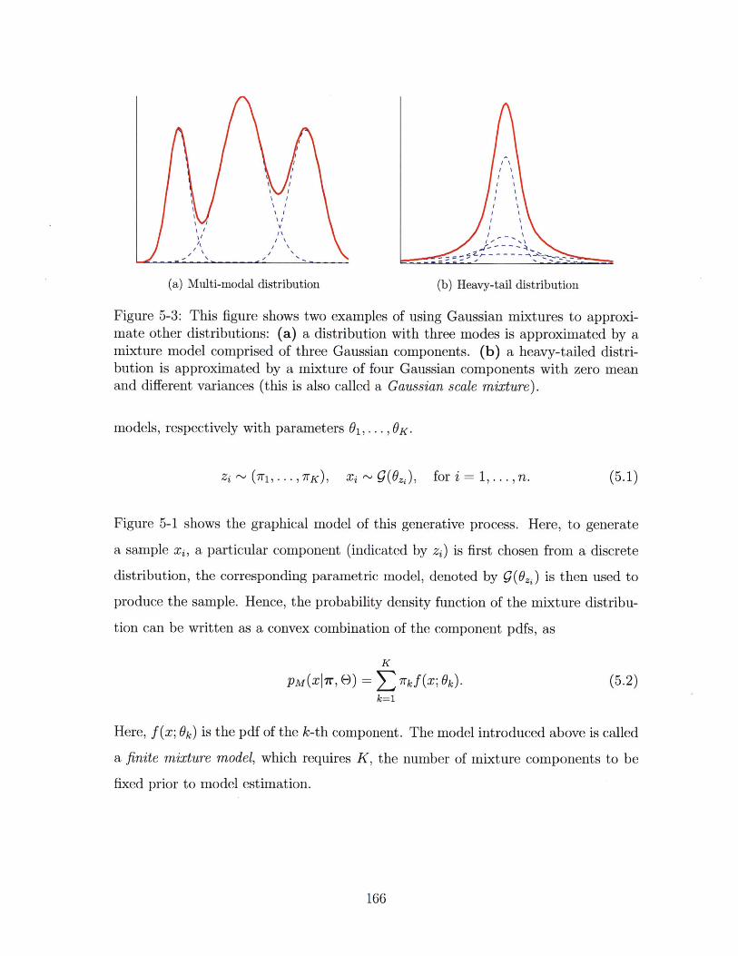
~I /// /'%
(a) Multi-modal distribution (b) Heavy-tail distribution
Figure 5-3: This figure shows two examples of using Gaussian mixtures to approxi-mate other distributions: (a) a distribution with three modes is approximated by amixture model comprised of three Gaussian components. (b) a heavy-tailed distri-bution is approximated by a mixture of four Gaussian components with zero meanand different variances (this is also called a Gaussian scale mixture).
models, respectively with parameters 01, . . ., OK -
z ~ (7 1 , ... 7, K), xi . g(OzQ), for i = 1, ... , n. (5.1)
Figure 5-1 shows the graphical model of this generative process. Here, to generate
a sample xi, a particular component (indicated by zi) is first chosen from a discrete
distribution, the corresponding parametric model, denoted by 9(0,) is then used to
produce the sample. Hence, the probability density function of the mixture distribu-
tion can be written as a convex combination of the component pdfs, as
K
PM(x7r, 8) Z lrkf( Ok). (5.2)k=1
Here, f(x; Ok) is the pdf of the k-th component. The model introduced above is called
a finite mixture model, which requires K, the number of mixture components to be
fixed prior to model estimation.
166
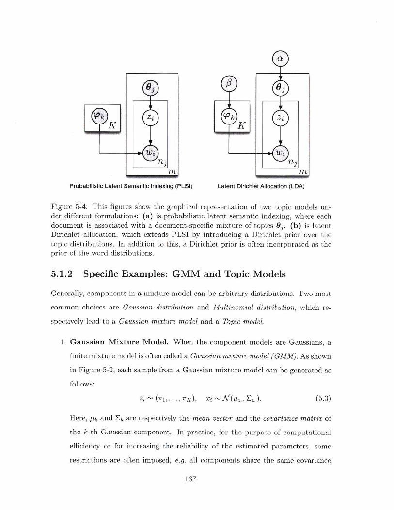
Probabilistic Latent Semantic Indexing (PLSI) Latent Dirichlet Allocation (LDA)
Figure 5-4: This figures show the graphical representation of two topic models un-der different formulations: (a) is probabilistic latent semantic indexing, where eachdocument is associated with a document-specific mixture of topics 0,. (b) is latentDirichlet allocation, which extends PLSI by introducing a Dirichlet prior over thetopic distributions. In addition to this, a Dirichlet prior is often incorporated as theprior of the word distributions.
5.1.2 Specific Examples: GMM and Topic Models
Generally, components in a mixture model can be arbitrary distributions. Two most
common choices are Gaussian distribution and Multinomial distribution, which re-
spectively lead to a Gaussian mixture model and a Topic model.
1. Gaussian Mixture Model. When the component models are Gaussians, a
finite mixture model is often called a Gaussian mixture model (GMM). As shown
in Figure 5-2, each sample from a Gaussian mixture model can be generated as
follows:
zi ~ (7i-, . rK ), xji ~ NJ(922,Ezi). (5.3)
Here, pk and Ek are respectively the mean vector and the covariance matrix of
the k-th Gaussian component. In practice, for the purpose of computational
efficiency or for increasing the reliability of the estimated parameters, some
restrictions are often imposed, e.g. all components share the same covariance
167
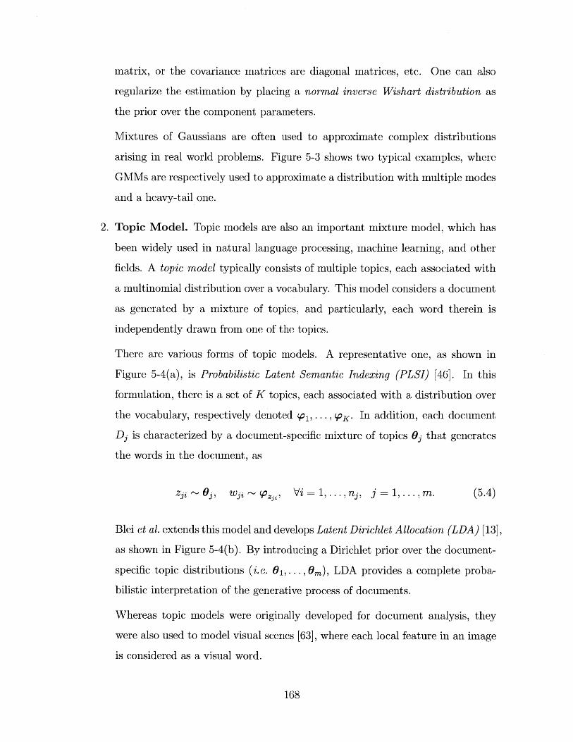
matrix, or the covariance matrices are diagonal matrices, etc. One can also
regularize the estimation by placing a normal inverse Wishart distribution as
the prior over the component parameters.
Mixtures of Gaussians are often used to approximate complex distributions
arising in real world problems. Figure 5-3 shows two typical examples, where
GMMs are respectively used to approximate a distribution with multiple modes
and a heavy-tail one.
2. Topic Model. Topic models are also an important mixture model, which has
been widely used in natural language processing, machine learning, and other
fields. A topic model typically consists of multiple topics, each associated with
a multinomial distribution over a vocabulary. This model considers a document
as generated by a mixture of topics, and particularly, each word therein is
independently drawn from one of the topics.
There are various forms of topic models. A representative one, as shown in
Figure 5-4(a), is Probabilistic Latent Semantic Indexing (PLSI) [46]. In this
formulation, there is a set of K topics, each associated with a distribution over
the vocabulary, respectively denoted 1, ... , . In addition, each document
Dj is characterized by a document-specific mixture of topics 6j that generates
the words in the document, as
zji ~ 6j, wji ~ pzj,7 Vi = 1, -. - n j, j = 1, . .. , m. (5.4)
Blei et al. extends this model and develops Latent Dirichlet Allocation (LDA) [13],
as shown in Figure 5-4(b). By introducing a Dirichlet prior over the document-
specific topic distributions (i.e. 0 1,...,0m), LDA provides a complete proba-
bilistic interpretation of the generative process of documents.
Whereas topic models were originally developed for document analysis, they
were also used to model visual scenes [63], where each local feature in an image
is considered as a visual word.
168
5.1.3 Estimation of Finite Mixture Models
Given a set of data x1, ... , x, one can estimate the parameters of a finite mixture
model using maximum likelihood estimation (MLE), that is, to solve the following
optimization problem:
n
( ) = argmax log pM(xi7r, (). (5.5)
Generally, there is no analytic solution to this problem. One can find the optimal
solution using expectation-maximization, an iterative algorithm for finding maximum
likelihood solutions for models with latent variables (see Chapter 2 for more details).
In a finite mixture model, each data sample xi is associated with a latent variable
zj E {1,... , K}. Given the model parameters (7r, 0) and the observation x, the
posterior probabilities of zi are given by
Pr(zi = k lx; 7r, (9) = rk f(X; . (5.6)F1_1 rif (xi; 01)
The E-M algorithm involves a K-dimensional vector qj for each sample xi to represent
these posterior probabilities. Then the E-steps and M-steps are respectively given as
follows.
1. E-step. Update the values of qj for each i = 1, ... , n, as
7r(-If ( i; 0 (t-1))q (k) +- , k = 1, 1 K. (5.7)
7, rg ( 1f (zi; 0(- ))
2. M-step. Update the model parameters, including both 7r and 9, as
7r' +- g q(k), k = 1, . .. , K, (5.8)
j=1
andn
0(t) <- argmax q(')(k)f(x;0), k=1, . . . , K. (5.9)i=
169
The specific form of formulas to update component parameters 01, ... , OK de-
pends on the specific form of the component models. Take Gaussian mixture
model for example, Eq.(5.9) reduces to the update of the mean vectors and the
covariance matrices:
p +- qt)(k)xi (5.10)Wk i=1
Ef <-) 1 q ' (k) (xi - p M ) (zi - p-t ) T. (5.11)k i=1
It is important to note that the E-M algorithm described above is a coordinate ascent
algorithm that would converge to a local optima. A simple strategy that may lead to
better solutions is to run the procedure many times with random initialization and
choose the result that yields the highest joint likelihood.
5.2 Dirichlet Process Mixture Models
A major problem with finite mixture models is that they require the number of
components to be specified before the models are estimated on data. This may lead
to difficulties in the application where this number is unknown or difficult to estimate.
To address this issue, nonparametric mixture models have been developed, notably
the Dirichlet Process Mixture Model, also known as DPMM [73, 99]. As a DP mixture
model may contain infinitely many components, it is also called an infinite mixture
model in some early work [79].
5.2.1 Dirichlet Processes
First of all, we briefly review the concept of Dirichlet process (DP) and how a mixture
model can be constructed based on a DP. Formally, a DP is defined as follows.
Definition 5.1 (Dirichlet Process). Let (Q, F) be a measurable space, and y be a
finite measure over Q. A Dirichlet process with base measure pa, denoted by DP(p),
is defined to be a distribution of random probability measure D over Q, such that for
170
any finite measurable partition (A1, ... , An), the random vector (D(A1 ), ... , D(An))
has a Dirichlet distribution:
(D(A1),. . ., D(A,)) ~ Dir(p(A1),. . ., p(An)). (5.12)
Note that in other literatures, y is often factorized into a base distribution p,
p/p(Q), and a concentration parameter cz, A p(Q). For the convenience of later
discussion, we use the base measure [t as a whole to characterize a DP in this thesis.
According to Kolmogorov's extension theorem [55], there exists a unique stochastic
process that satisfies the property above, meaning that a base measure y corresponds
uniquely to a Dirichlet Process. The definition above is a descriptive definition.
Actually, we can also explicitly construct a DP through an interesting process called
stick breaking, which will be presented later.
From a DP, each sample path D itself is a probability measure over Q, and there-
fore DP(pI) is essentially a distribution over distributions. Such a stochastic process
- one of which every sample is a probability measure - is called a random probabil-
ity measure. There is a very important property that distinguishes DP from other
random probability measures - neutrality, which is defined by the proposition below.
Proposition 5.1. Let p be a measure over Q, D - DP(p) and A, B, C be disjoint
measurable subsets of Q. Then, (D(A), D(B), D(C)) is a neutral vector, meaning that
the ratio D(A)/D(B) is independent of the value of D(C).
There are other important properties about a DP. We will show later that D is
almost surely a discrete distribution over a countably infinite subset of Q, which can
be established via the stick breaking construction. Previous work mostly uses two
methods to construct DPs: the Polya urn scheme and the stick-breaking construction,
which we will describe in what follows.
5.2.2 P6lya Urn and Chinese Restaurant Process
Consider a generative model: D ~ DP(pl) and 01,... , O2|D - D. The P6lya urn
scheme is a sequential procedure to directly draw 01,... , 0, from this generative
171
model, without making D explicit. Given 01,... , O6_1, by integrating out D, we
have
hZ[6 1,.. ., I_1 ~ + a- 1 p . (5 .13 )j=1
We can see that O6 has a positive probability repeating a value that was seen earlier.
The more often that an atom value has been sampled, the more likely that it is to
be repeated in successive draws. As the number of samples n increases, the number
of distinct values also increases, but at a much slower rate (about O(log(n))). This
is known as the clustering property. To make this clear we introduce the terminology
atoms to refer to such distinct values, denoted by #, 42,..., and thus rewrite Eq.(5.13)
intoKi- 1 (k)
0 0l1, ... , Oi-1 ~ -i 64k + A Pi. (5.14)k=1 c) i-1 e i-1
Here, Kj_1 is the number of distinct atoms in the first i - 1 samples, and m k) is the
number of appearances of the atom #k. Moreover, we don't actually have to explicitly
maintain the samples 01, ... , 0,; instead, we can use a label zi to indicate which atom
the i-th sample takes value from, i.e. 64 = #2,. Using atoms and labels, each with its
own distinctive meaning, we can sample O as follows
1. Draw zi 1, . . . , K -1 + 1} conditioned on zi, . . . , zi_ 1 with
Pr~zi k Iz, . . , zri) = /(a, + (i - 1)) (k E {1, . .. , Ki_1}), (.5
a,/( + (i - 1)) k = Ki-1 + 1.
2. If z < Ki_1, we are done, and it simply means that 64 = ; otherwise, we
draw a new atom #K,-,l from the base distribution p,, and set z = Ki 1 + 1.
Chinese Restaurant Process
This procedure is closely related to the Chinese restaurant process, as described be-
low. Consider a Chinese restaurant with an infinite number of circular tables, each
of infinite capacity. When a new customer enters, he chooses a table to sit at. The
172
probability that a particular table is chosen is proportional to the number of people
already seated there. There is also a positive probability proportional to a that a
new table is selected. Using zi to indicate the index of the table that the i-th cus-
tomer chooses, we will get a sequence z1,... , zn, when n customers have been seated.
Comparison of this process with the P61ya urn scheme suggests that the generation
model of such sequence can be exactly characterized by Eq. (5.15). Consequently, the
sampling procedure can be reformulated equivalently as
(zi, ... ,zn) ~ C RP(a,);
k - P,; for k = 1, ... , Kn. (5.16)
Here, we first draw the labels from the Chinese restaurant process as described above,
which we denote by CRP(c). This labeling process results in clusters of data, each
corresponding to a label. Then, an atom #k, the parameter of the component to
explain the samples classified to the k-th table, can be independently drawn from p,
for each cluster.
Exchangeability
The sequential dependency as in Eq.(5.13) might seem to indicate that the joint
probability of 01, ... O, depends on the their order. However, this is not really the
case.
Consider the Chinese Restaurant Process, it is not difficult to derive the joint
probability of the labels as
PCRP(z1,- , zna,) p(zi z 1 ,. - -- , zi-1) -- H_ mk) - 1)! (5.17)f is eb i (a + i)
The right hand side of this equation can be obtained by rearranging the factors.
173
Moreover, with the atom parameters taken into account, we further get
P(01, ... ,Onl/p) =p(Zi, . Zn; 0i, . .. , OK. JP)
K.
=PCRP (Z1, - Zn Ias)r Py (Ok)- (5.18)k=1
It is clear from Eq.(5.17) that PCRP(ZI,- , Zn) only depends on the number of times
each label occurs, but not on their order. As a result, the joint probability of 01,... , O
does not depend on the order either, implying that 01,. .. , O, is an exchangeable
sequence.
De Finetti's theorem [55] states that exchangeable samples are conditionally in-
dependent given some latent variable. Here, the latent variable is D, a DP sample
path that serves as the prior of atoms.
5.2.3 Stick-breaking Construction
The stick breaking construction proposed by Sethuraman [90] provides a direct con-
struction of DP. Let {#3 k} i be a sequence of independent random variables from a
beta distribution, as
3 k - Beta(1, a), for k = 1, 2, ... , (5.19)
and {#k}k'1 be a sequence of independent variables from the base distribution p., as
Ok - Py, fork= 1, 2- . (5.20)
Then, we can construct a random series D as
k-1 oo
lrk = k (1 -), and D = 1 x1p7 . (5.21)1=1 k=1
Intuitively, this sampling procedure is analogous to a stick breaking process. Starting
from a stick of unit length, we first draw a random fraction #1 ~ Beta(1, ao), and let
174
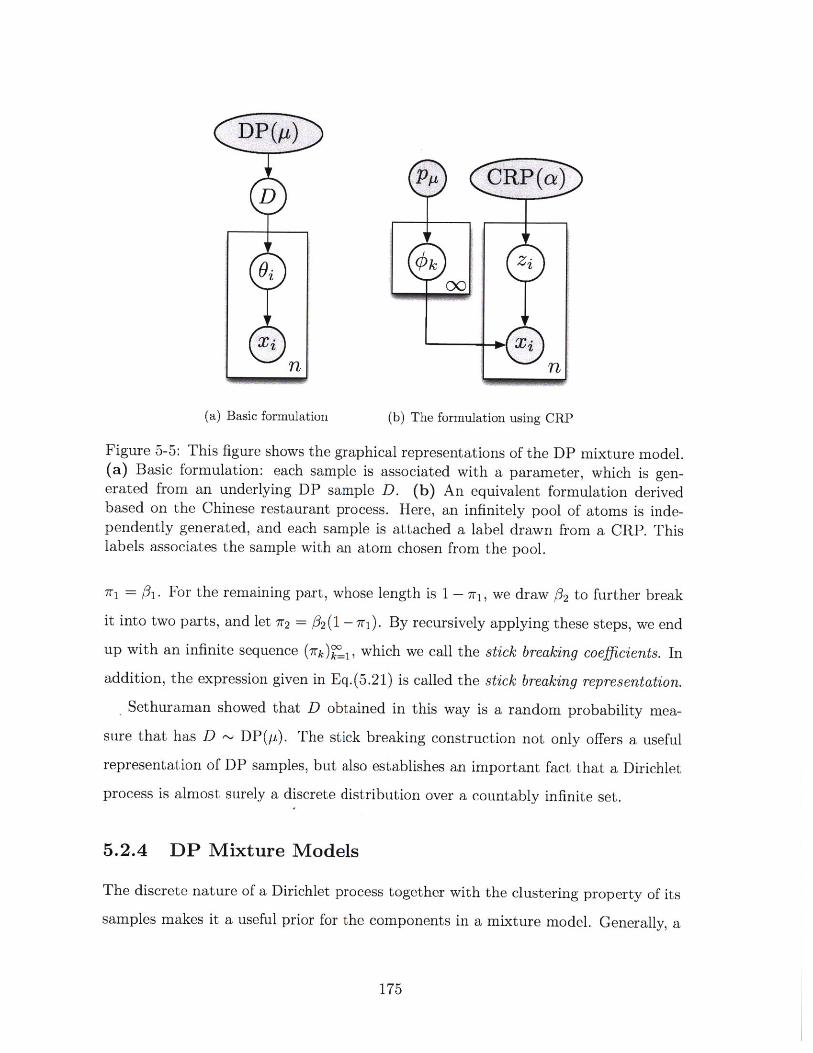
(a) Basic formulation (b) The formulation using CRP
Figure 5-5: This figure shows the graphical representations of the DP mixture model.(a) Basic formulation: each sample is associated with a parameter, which is gen-erated from an underlying DP sample D. (b) An equivalent formulation derivedbased on the Chinese restaurant process. Here, an infinitely pool of atoms is inde-pendently generated, and each sample is attached a label drawn from a CRP. Thislabels associates the sample with an atom chosen from the pool.
7r1 = #31. For the remaining part, whose length is 1 - 7ri, we draw #2 to further break
it into two parts, and let 7r2 = /2(1 - 7i). By recursively applying these steps, we end
up with an infinite sequence (7rk)%' 1 , which we call the stick breaking coefficients. In
addition, the expression given in Eq.(5.21) is called the stick breaking representation.
Sethuraman showed that D obtained in this way is a random probability mea-
sure that has D ~ DP(pi). The stick breaking construction not only offers a useful
representation of DP samples, but also establishes an important fact that a Dirichlet
process is almost surely a discrete distribution over a countably infinite set.
5.2.4 DP Mixture Models
The discrete nature of a Dirichlet process together with the clustering property of its
samples makes it a useful prior for the components in a mixture model. Generally, a
175
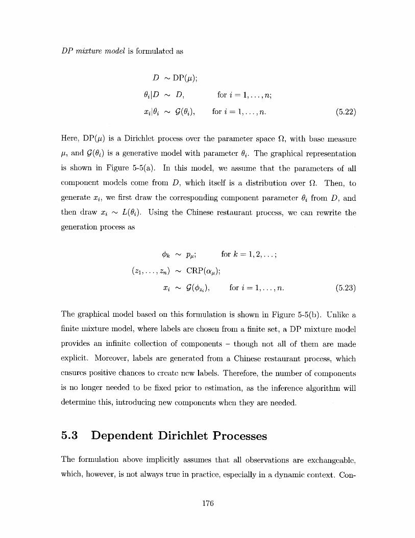
DP mixture model is formulated as
D ~DP(p);
Bi lD ~D, for i = 1, ... , n;
xilI O ~ g(0j), for i - 1, ... , n. (5.22)
Here, DP(p) is a Dirichlet process over the parameter space Q, with base measure
p, and 9(0) is a generative model with parameter O6. The graphical representation
is shown in Figure 5-5(a). In this model, we assume that the parameters of all
component models come from D, which itself is a distribution over Q. Then, to
generate xi, we first draw the corresponding component parameter O from D, and
then draw x ~ L(9j). Using the Chinese restaurant process, we can rewrite the
generation process as
4k ~ P,; for k = 1, 2, ...
(zi, .,z) ~ CRP(a,);
Xi ~% (Ozi),I for i = 1, ... , n. (5.23)
The graphical model based on this formulation is shown in Figure 5-5(b). Unlike a
finite mixture model, where labels are chosen from a finite set, a DP mixture model
provides an infinite collection of components - though not all of them are made
explicit. Moreover, labels are generated from a Chinese restaurant process, which
ensures positive chances to create new labels. Therefore, the number of components
is no longer needed to be fixed prior to estimation, as the inference algorithm will
determine this, introducing new components when they are needed.
5.3 Dependent Dirichlet Processes
The formulation above implicitly assumes that all observations are exchangeable,
which, however, is not always true in practice, especially in a dynamic context. Con-
176
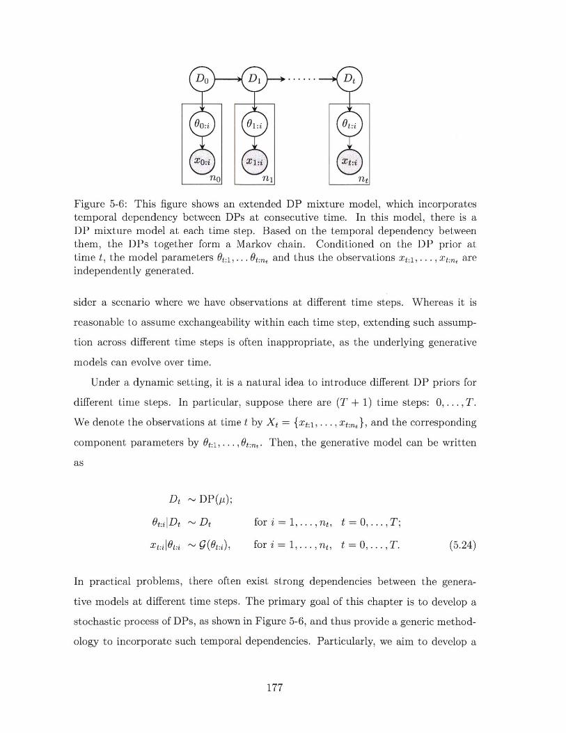
Figure 5-6: This figure shows an extended DP mixture model, which incorporatestemporal dependency between DPs at consecutive time. In this model, there is aDP mixture model at each time step. Based on the temporal dependency betweenthem, the DPs together form a Markov chain. Conditioned on the DP prior attime t, the model parameters 6 t:1,... Ot:n, and thus the observations Tt:1,... , X:n areindependently generated.
sider a scenario where we have observations at different time steps. Whereas it is
reasonable to assume exchangeability within each time step, extending such assump-
tion across different time steps is often inappropriate, as the underlying generative
models can evolve over time.
Under a dynamic setting, it is a natural idea to introduce different DP priors for
different time steps. In particular, suppose there are (T + 1) time steps: 0,... , T.
We denote the observations at time t by Xt = {Xt:1, ... , Xt:n}, and the corresponding
component parameters by Ot:1,...,6t:n,. Then, the generative model can be written
as
Dt ~ DP(p);
6t:j |Dt ~ Dt for i= 1, .. ., n, t= 0, ... , T;
ot:il6t:i ~ g (6t:j), for i= 1, .. . ,n , t = 0, .. . ,T. (5.24)
In practical problems, there often exist strong dependencies between the genera-
tive models at different time steps. The primary goal of this chapter is to develop a
stochastic process of DPs, as shown in Figure 5-6, and thus provide a generic method-
ology to incorporate such temporal dependencies. Particularly, we aim to develop a
177
process that supports dynamic creation and removal of components, as well as vari-
ation of component parameters, while maintaining the desirable property that the
marginal distribution of Dt remains a DP.
In the parametric world, one may often easily find a way to transform a parame-
ter that preserves its original form of distribution, e.g. a noisy linear transform of a
Gaussian distributed variable remains Gaussian. However, this becomes a challeng-
ing issue when we are working with Dirichlet processes. As we shall see, whereas
there have been a lot of efforts devoted to the incorporation of statistical dependency
between DPs, previous methods are limited both theoretically and practically.
Later in this chapter, we will introduce a new perspective of Dirichlet processes
by examining their connections with Poisson processes, and thereon derive a new
construction of dependent DPs that allows a variety of transformations on DPs while
retaining the marginal distributions as DPs.
5.3.1 A Brief Review
We first briefly review previous work on dependent Dirichlet processes. The notion
of dependent Dirichlet process (DDP) was coined by MacEachern in his pioneering
work [66]. In particular, he discussed a special form of DDP, called single-p DDP,
where each component distribution is extended to a stochastic process that describes
how the component parameter evolves with the covariate. Whereas several exten-
sions were also discussed, such as the use of non-stationary stochastic processes for
describing atom evolution, this work did not other forms of variations, e.g. dynamic
incorporation of new atoms.
Following this work, a variety of DDP constructions have been developed, which
mainly fall into three categories.
Convex Combinations
A straightforward way to extend the Dirichlet processs is to generate Dt, the non-
parametric mixture with covariate t, as a convex combination of an existing DP and
178
a new one. M6ller et al. [72] proposed a method that combines the inference across
related nonparametric mixture models through a convex combination as below
Dt =F 0 + (1 - e)Ft. (5.25)
Here, FO and Ft are independent sample paths from a DP, which respectively capture
the common atoms across all groups and the atoms only used by the t-th group.
Zhu et al. [120] proposed a time sensitive DP mixture model, which assigns each
atom a time-dependent weight, defined as follows
w(t,j) = k(t - ti). (5.26)ilt <t,sg=j
This is a variant of the standard Chinese restaurant process, where the contribution
of each occurrence of an atom attenuates over time. Such a weighting strategy is
actually equivalent to introducing a sequence of latent DPs, each for a time step, and
considering the mixture at each time step as their moving average.
Caron et al. [17] directly generalized the P6lya urn scheme, where a subset of
balls from the urn is randomly chosen and deleted. With an appropriate choice of
deletion probability, this would result in a stationary process, where existing atoms
have geometrically distributed life spans, and new atoms constantly come up. The
generalized P6lya urn model was later applied for spike sorting [35].
Ahmed and Xing [1] developed a temporal DP mixture model called Recurrent
Chinese restaurant process. Here, each atom occurring at previous time step can be
chosen with the following probability
7 2 k,t-1 + n. ' (5.27)N_ 1 + (i - 1) + a(
Here, nt-1 is the number of occurrences of atom k at t - 1, n(j) is the number of
occurrences at t up to the (i - 1)-th sample, Nt-I is the number of data samples at
t - 1. Whereas this generalization was motivated from an algorithmic standpoint,
it can be considered to be resulted from a convex combination of the previous DP
179
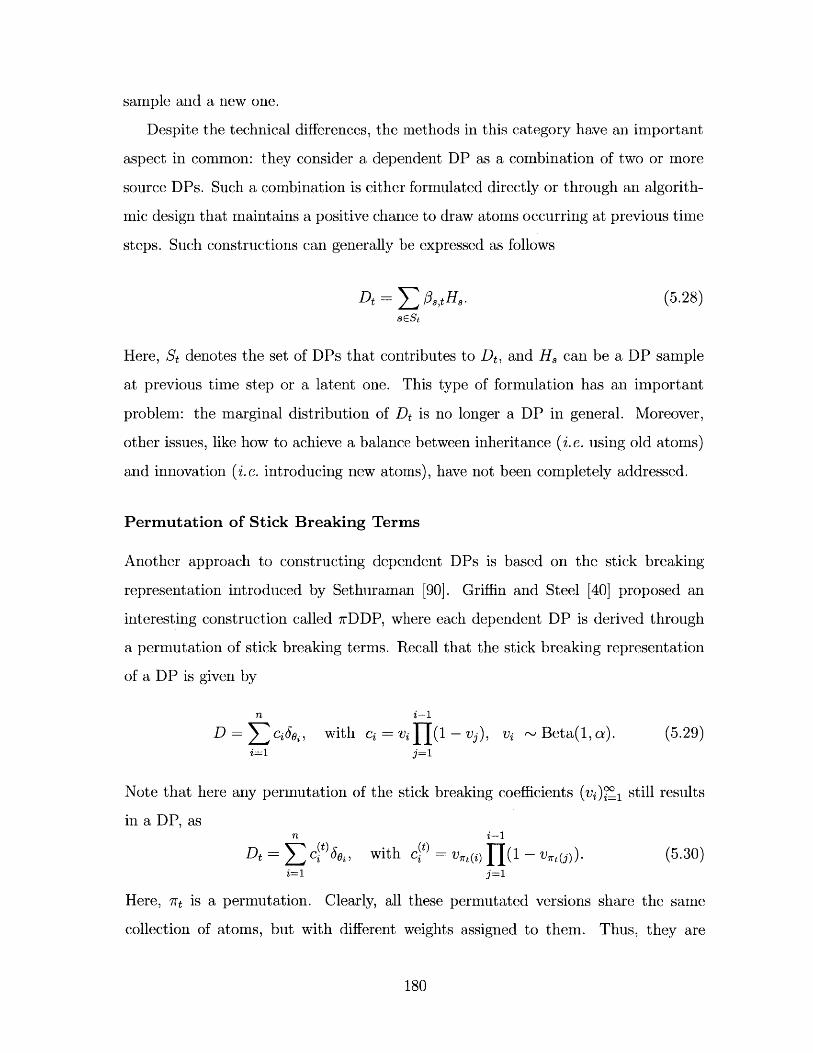
sample and a new one.
Despite the technical differences, the methods in this category have an important
aspect in common: they consider a dependent DP as a combination of two or more
source DPs. Such a combination is either formulated directly or through an algorith-
mic design that maintains a positive chance to draw atoms occurring at previous time
steps. Such constructions can generally be expressed as follows
Dt =- E ,SHA. (5.28)sE St
Here, St denotes the set of DPs that contributes to Dt, and H, can be a DP sample
at previous time step or a latent one. This type of formulation has an important
problem: the marginal distribution of Dt is no longer a DP in general. Moreover,
other issues, like how to achieve a balance between inheritance (i.e. using old atoms)
and innovation (i.e. introducing new atoms), have not been completely addressed.
Permutation of Stick Breaking Terms
Another approach to constructing dependent DPs is based on the stick breaking
representation introduced by Sethuraman [90]. Griffin and Steel [40] proposed an
interesting construction called rDDP, where each dependent DP is derived through
a permutation of stick breaking terms. Recall that the stick breaking representation
of a DP is given by
n i-1
D = ciks, with ci = vi f(1 - v), vi ~ Beta(1, a). (5.29)i=1 j=1
Note that here any permutation of the stick breaking coefficients (vj) 1 still results
in a DP, asn i-1
D = c()6o, with ct) v(i) 7(i - V, y)). (5.30)i=1 j=1
Here, 7rt is a permutation. Clearly, all these permutated versions share the same
collection of atoms, but with different weights assigned to them. Thus, they are
180
related to each other. This paper also proposed a useful way to generate the ordering.
The basic idea is to sample the arrival order from a point process.
Building upon this idea, Chung and Dunson [19 proposed the local DP model
(lDP). This work aims to formulate a joint distribution over a collection of DPs,
and, for this purpose, introduces a universal pool of atoms. Each DP under this
joint formulation contains a subset of atoms in the pool, and is associated with a
covariate-dependent permutation.
These methods guarantees that the marginal distribution of each resultant pro-
cess remains a DP. However, they bring about another nontrivial question: how to
devise the process that generate the permutation such that it can express the desired
dependency structure. Also, as such formulations involve random permutations, the
sampling schemes tend to be very complicated, often leading to considerably increased
demand of computational costs.
Hierarchical Dirichlet Process
Hierarchical Dirichlet Process (HDP) was proposed by Teh et al. [100], which has
become one of the most widely used approaches to constructing dependent nonpara-
metric mixture models. Taking advantage of the fact that each sample of a DP is a
distribution over the underlying space, this model organizes DP samples into a tree,
where parents serve as the base probability measure of their children. The generative
formulation is given below
Do ~ DP(a, B), Dt ~ DP(7, DO), for t = 1, 2, .... (5.31)
This way ensures that the atoms in a child DP are from its parent, thus offering a
way for atoms to be shared across different children.
Ren et al. [82] applied this idea to a dynamic context, and developed the dynamic
HDP (dHDP) to model sequential data. The generative formulation of dHDP is
D =(1 - w)Dti + wH, Ht =DP(a, Do), Do DP(y, B). (5.32)
181
This model adopts the convex combination formula to evolve a DP over time, where
the innovative process is generated from an HDP.
In [100], Teh et al. discussed an extension called HDP-HMM, which is based on a
Markov chain with infinitely many states. In this model, the distribution of the next
state conditioned on any current state is a child DP. All such DPs share the same
parent. Hence, the transition is between the atoms from a common parent DP. Fox et
al. [31] further extends this formulation by introducing an additional sticky variable
to control the self-transition bias.
Kim and Smyth [53] extended HDP along a different direction. They introduced
a random perturbation for each group, called random effects, which allows the pa-
rameters to each atom to vary when inherited by child DPs.
HDP is very useful in many applications that involve groups of data. However,
HDP and its variants are subject to a fundamental limitation, that is, the DPs must
be organized into a tree-structure.
Spatially Normalized Gamma Process
Recently, Rao and Teh [78] proposed a new way for dependent DP construction, called
spatially normalized gamma process, which allows more flexible configuration of the
dependency structure. This formulation leverages an important relation between
Gamma and Dirichlet process, that is, normalizing a Gamma process results in a DP.
In particular, it defines a gamma process G over an extended space. For each group
t, a DP Dt is derived through normalized restriction of G to a measurable subset.
The DPs derived on overlapping subsets are thus dependent. This construction can
be reduced to the following form:
D =- ctjHj, with (ctj)jCR, - Dir((aj)jER,). (5.33)jERt
Here, Rt is the subset of latent DPs used for Dt, and the coefficients ctj are random
variables from a Dirichlet distribution.
It is worth noting that under this formulation, the relative weights of two latent
182
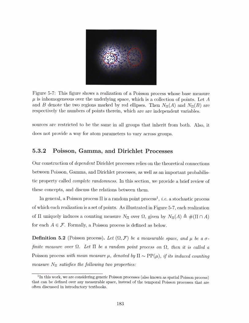
Figure 5-7: This figure shows a realization of a Poisson process whose base measurep is inhomogeneous over the underlying space, which is a collection of points. Let Aand B denote the two regions marked by red ellipses. Then Nn(A) and Nn(B) arerespectively the numbers of points therein, which are are independent variables.
sources are restricted to be the same in all groups that inherit from both. Also, it
does not provide a way for atom parameters to vary across groups.
5.3.2 Poisson, Gamma, and Dirichlet Processes
Our construction of dependent Dirichlet processes relies on the theoretical connections
between Poisson, Gamma, and Dirichlet processes, as well as an important probabilis-
tic property called complete randomness. In this section, we provide a brief review of
these concepts, and discuss the relations between them.
In general, a Poisson process H is a random point process', i. e. a stochastic process
of which each realization is a set of points. As illustrated in Figure 5-7, each realization
of H uniquely induces a counting measure Nr over Q, given by Nn(A) A #(1I n A)
for each A E F. Formally, a Poisson process is defined as below.
Definition 5.2 (Poisson process). Let (Q, F) be a measurable space, and yt be a a-
finite measure over Q. Let H be a random point process on Q, then it is called a
Poisson process with mean measure p, denoted by H ~ PP([p), if its induced counting
measure Nn satisfies the following two properties:
'In this work, we are considering generic Poisson processes (also known as spatial Poisson process)that can be defined over any measurable space, instead of the temporal Poisson processes that areoften discussed in introductory textbooks.
183
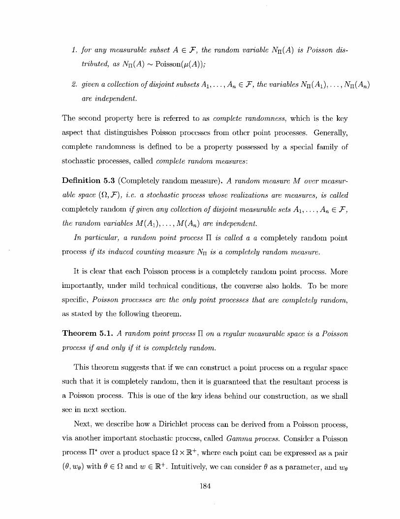
1. for any measurable subset A E T, the random variable NrI(A) is Poisson dis-
tributed, as Nn(A) - Poisson(p(A));
2. given a collection of disjoint subsets A 1,... , An E T, the variables Nn(A1), ... , Nn(An)
are independent.
The second property here is referred to as complete randomness, which is the key
aspect that distinguishes Poisson processes from other point processes. Generally,
complete randomness is defined to be a property possessed by a special family of
stochastic processes, called complete random measures:
Definition 5.3 (Completely random measure). A random measure M over measur-
able space (Q, F), i.e. a stochastic process whose realizations are measures, is called
completely random if given any collection of disjoint measurable sets A 1, ... , An E F,
the random variables M(A 1 ), ... , M(An) are independent.
In particular, a random point process 17 is called a a completely random point
process if its induced counting measure Nn is a completely random measure.
It is clear that each Poisson process is a completely random point process. More
importantly, under mild technical conditions, the converse also holds. To be more
specific, Poisson processes are the only point processes that are completely random,
as stated by the following theorem.
Theorem 5.1. A random point process H on a regular measurable space is a Poisson
process if and only if it is completely random.
This theorem suggests that if we can construct a point process on a regular space
such that it is completely random, then it is guaranteed that the resultant process is
a Poisson process. This is one of the key ideas behind our construction, as we shall
see in next section.
Next, we describe how a Dirichlet process can be derived from a Poisson process,
via another important stochastic process, called Gamma process. Consider a Poisson
process W* over a product space Q x R+, where each point can be expressed as a pair
(0, wo) with 0 E Q and w E R+. Intuitively, we can consider 0 as a parameter, and wo
184
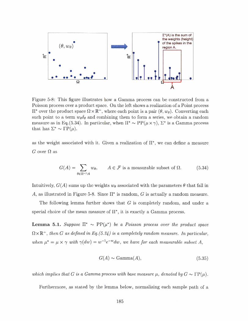
E*(A) is the sum ofthe weights (height)
0 Wof the spikes in the(O, E) region A.
0
* S lA-i* 00.00 0000 T.T 9
A
Figure 5-8: This figure illustrates how a Gamma process can be constructed from aPoisson process over a product space. On the left shows a realization of a Point processH* over the product space Q x R+, where each point is a pair (6, wo). Converting eachsuch point to a term wo5o and combining them to form a series, we obtain a randommeasure as in Eq.(5.34). In particular, when H* ~ PP(I x -y), E* is a Gamma processthat has E* ~ PP(p).
as the weight associated with it. Given a realization of H*, we can define a measure
G over Q as
G(A) = wo, A E F is a measurable subset of Q. (5.34)OcU*nA
Intuitively, G(A) sums up the weights wo associated with the parameters 0 that fall in
A, as illustrated in Figure 5-8. Since HI* is random, G is actually a random measure.
The following lemma further shows that G is completely random, and under a
special choice of the mean measure of 11*, it is exactly a Gamma process.
Lemma 5.1. Suppose fl* ~ PP(p*) be a Poisson process over the product space
Q x R+, then G as defined in Eq. (5.34) is a completely random measure. In particular,
when p* = p x y with y(dw) = w-le-wdw, we have for each measurable subset A,
G(A) ~ Gamma(A), (5.35)
which implies that G is a Gamma process with base measure p, denoted by G ~ FP(kL).
Furthermore, as stated by the lemma below, normalizing each sample path of a
185
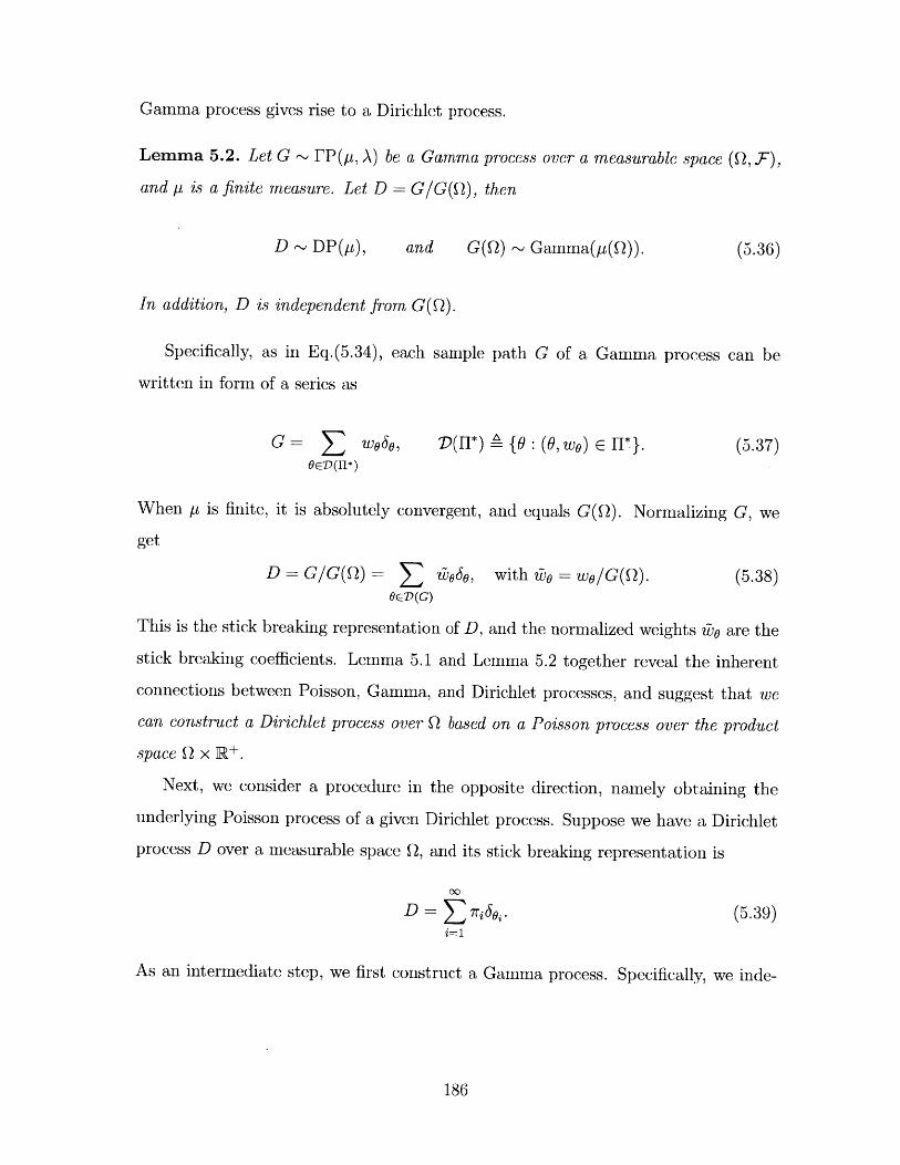
Gamma process gives rise to a Dirichlet process.
Lemma 5.2. Let G ~ IP(p, A) be a Gamma process over a measurable space (Q, F),
and t is a finite measure. Let D = G|G(Q), then
D ~ DP(p), and G(Q) - Gamma(p(Q)). (5.36)
In addition, D is independent from G(Q).
Specifically, as in Eq.(5.34), each sample path G of a Gamma process can be
written in form of a series as
G S wo6o, D(H*) A {O: (O,wo) E l*}. (5.37)OED(rJ*)
When y is finite, it is absolutely convergent, and equals G(Q). Normalizing G, we
get
D = G/G(Q) = zodo, with vo = wO/G(Q). (5.38)OED(G)
This is the stick breaking representation of D, and the normalized weights tZe0 are the
stick breaking coefficients. Lemma 5.1 and Lemma 5.2 together reveal the inherent
connections between Poisson, Gamma, and Dirichlet processes, and suggest that we
can construct a Dirichlet process over Q based on a Poisson process over the product
space Q x R+.
Next, we consider a procedure in the opposite direction, namely obtaining the
underlying Poisson process of a given Dirichlet process. Suppose we have a Dirichlet
process D over a measurable space Q, and its stick breaking representation is
00
D = ro.. (5.39)i=1
As an intermediate step, we first construct a Gamma process. Specifically, we inde-
186
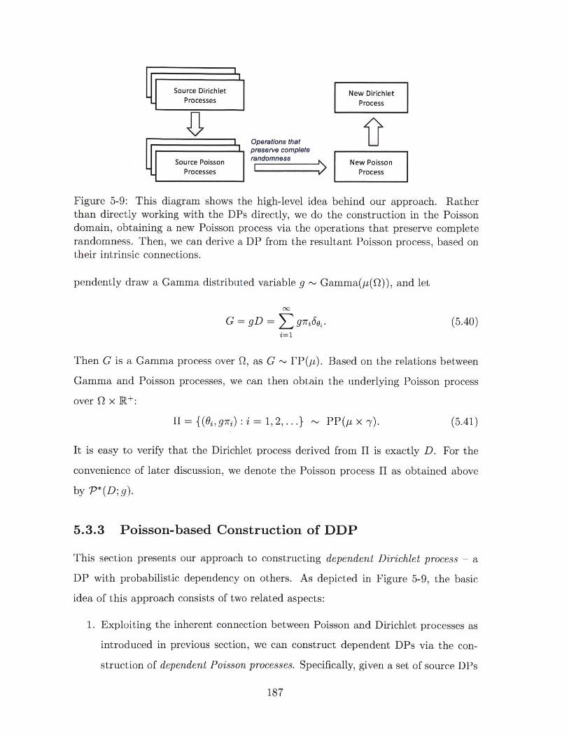
Source Dirichlet New DirichletProcesses Process
Operations that|preserve complete
Source Poisson randomness New PoisProcesses Proces
Figure 5-9: This diagram shows the high-level idea behind our approach. Ratherthan directly working with the DPs directly, we do the construction in the Poissondomain, obtaining a new Poisson process via the operations that preserve completerandomness. Then, we can derive a DP from the resultant Poisson process, based ontheir intrinsic connections.
pendently draw a Gamma distributed variable g ~ Gamma(p(Q)), and let
00
G = gD = g7rijo. (5.40)i=1
Then G is a Gamma process over Q, as G ~ FP(p). Based on the relations between
Gamma and Poisson processes, we can then obtain the underlying Poisson process
over Q x R+:
H = {(O, g7r) : i = 1, 2,.. .} ~ PP(p x -y). (5.41)
It is easy to verify that the Dirichlet process derived from II is exactly D. For the
convenience of later discussion, we denote the Poisson process H as obtained above
by P*(D;g).
5.3.3 Poisson-based Construction of DDP
This section presents our approach to constructing dependent Dirichlet process - a
DP with probabilistic dependency on others. As depicted in Figure 5-9, the basic
idea of this approach consists of two related aspects:
1. Exploiting the inherent connection between Poisson and Dirichlet processes as
introduced in previous section, we can construct dependent DPs via the con-
struction of dependent Poisson processes. Specifically, given a set of source DPs
187
over a space Q, we first obtain their underlying Poisson processes over Q x R+,
and thereon construct a dependent Poisson process, from which a new DP can
be derived based on the Poisson-Dirichlet relations.
2. This strategy reduces the problem to the one of constructing dependent Pois-
son processes. To solve this problem, we develop a generic methodology that
rests upon the notion of complete randomness. The idea is that by applying
operations that can preserve complete randomness to a set of Poisson processes,
we get a new point process that is completely random, which, by Theorem 5.1,
remains a Poisson process.
In what follows, we consider three such operations: superposition, subsampling,
and point transition. When applied to the underlying Poisson processes, they produce
new Poisson processes and thus new Dirichlet processes. These operations together
offer great flexibility for evolving a DP dynamically.
Superposition
An important way to create dependent Dirichlet process is to combine existing ones.
Whereas it is a natural idea to simply combine them through convex combination,
the resultant process is, however, no longer a DP in general. In this work, we take a
new approach - combine DPs through the union of the underlying Poisson processes.
Given a collection of independent DPs D 1,... , D,. Following the procedure de-
scribed in previous section, we independently draw m Gamma distributed coefficients:
gi, ... , gm, with gk Gamma(pk (Q)), and obtain their underlying Poisson processes,
as
lk = P*(Dk; gk) PP(pt x 7). (5.42)
The union of these Poisson processes is rl* Y =I U ... U fl*. The following theorem
establishes the fact that n* remains a Poisson process.
Theorem 5.2 (Superposition Theorem of Poisson Processes). Let 11, .. m be in-
188
dependent Poisson processes on Q with Uk ~ PP(pk), then their union has
IiU U m ~ PP(1+---+ym). (5.43)
This irmediately follows that
gro.S, ~ PP((p1 + -- -+ ym) x 7.(5.44)
According to the relations between Poisson and Gamma processes, *, corresponds
to a Gamma process, denoted by Gms,, which equals the sum 2 of the ones associated
with 11* .. *:
m m m
Gs,= w6o = ( woos = Gk= gkDk. (5.45)(O,wo)EUl*U..-U* k=1 (0,wO)Eflk k=1 k=1
Normalizing GP,, we finally get a Dirichlet process D, as follows.
m mG8 n,/G8 n,(Q) = D = a kDk ~ DP(p1 + -- -+ tm). (5.46)
k=1um k=1
Here, gsum = gi + - + gm, and ak = gk/gsum. We note that the coefficients here
are Dirichlet distributed random variables, as (ai, . . . , am) ~ Dir(pi(Q), . . . , pm(Q)).
Consequently, one can construct a Dirichlet process through a random convex combi-
nation of independent Dirichlet processes, as
Dsup = D1 G -- -E Dm A clDi + --- + cmDm ~ DP(pi + + pm). (5.47)
For convenience, we use D1 E ... E Dm to denote the DP resulted from the superposi-
tion of D 1, ... , Dm. The procedure described above illustrates in detail how one can
construct a dependent Dirichlet process via the operations on Poisson processes that
preserve complete randomness. In regard to this procedure, we have the following
2 Here, we utilize a fact that the realizations of independent Poisson processes are almost surelydisjoint, and consequently the sum of the terms in the union is almost surely equal to the sum ofindividual series.
189
discussions.
1. Although playing a crucial role in this theoretical derivation, the underlying
Poisson processes, however, do not need to be explicitly instantiated in the
actual construction as given by Eq.(5.47).
2. That the coefficients ci, ... , cm are drawn from a Dirichlet distribution distin-
guishes our construction from the simple convex combinations that use deter-
ministic coefficients. This is the key to make DeU a Dirichlet process.
Subsampling
We can also construct a dependent DP by extracting a portion of a given DP. This is
done by a complete randomness preserving operation called random subsampling - a
special case of random coloring, which is described below.
Theorem 5.3 (Coloring Theorem of Poisson Processes). Let H PP(p) be a Poisson
process over a measurable space Q, C be a finite subset. Each c E C is associated with
a measurable function q : Q -4 [0,1], such that for each 0 c Q, Eccc qc(O) = 1. For
each 0 E H, we draw a discrete variable zo E C, with Pr(zo = c) = qc(0). Let Hc =
{ 0 H :zo c} for each c E C, then Hc is a Poisson process as Uc ~ PP(pc) with
pc = qcy, i.e. tc(d0) = qc(0)p(d0), and Uc for different values of c are independent.
The procedure in this theorem can be intuitively interpreted as follows. Given a
realization of a Poisson process H, we randomly assign a color c E C to each point,
according to the distribution over C given by (qc(0))cec. Then we divide the entire
set of points into |CI subsets depending on the color associated with each point. In
this way, we get |CI point processes. Theorem 5.3 suggests that they are independent
Poisson processes, and particularly, Hc ~ PP(qcy) for each c E C. Restricting C to be
{0, 1}, we have:
Corollary 5.1. Let H ~ PP(p) be a Poisson process Q, and q : Q - [0, 1] be a
measurable function. If we independently draw bo E {0, 1} for each 0 E H with Pr(bo =
1) = q(0), and let Hsub {0 E H : b0 = 1}, Then H8 ub and UH/bub are independent
Poisson processes over Q, with Hub ~ PP(qp), and H/Hsub ~ PP((1 - q)p).
190
The procedure described above is essentially a random subsampling process, where
we determines whether to retain each particular point via independent Bernoulli trial,
namely draw bo - Bernoulli(q(0)), and accept it if bo = 1. The Corollary 5.1 implies
that the resultant point process remains a Poisson process, with mean measure qp.
This operation can be utilized for dependent DP construction. Let D be a Dirichlet
process over Q as D ~ DP(p), with the stick breaking representation given by
00
D Z io60. (5.48)i=1
Again, we can get the underlying Poisson process as 1* = P*(D; g) {(0j, gri)
i = 1,2, .. .} with g ~Gamma(pL(Q)), which has 1* ~ DP(qp x -y). Now we apply
the subsampling procedure to l*, independently drawing bi ~ Bernoulli(q( 2 )) for
each i, and accepting only those with bi = 1. This results in a subset given by
sub ( , gri) : bi = 1}. Here, 1sub corresponds to a Gamma process, as
Gsb - gI ri'o, ~ FP(qp) (5.49)i:bi=1
Normalizing G5 ub yields a Dirichlet process D8sb:
Dsub Sq(D) 7 x o, ~ DP(qp), with 7 =r. (5.50)i:bi=1 j:bj=1 7
Here, we use Sq to denote the subsampling operation applied to a DP with acceptance
function q. We can see that the construction of Dub does not actually require explicit
instantiation of the underlying Poisson and Gamma processes. This can be done by
randomly choosing a subset of the terms in D via independent Bernoulli trial, and
re-normalizing the coefficients of the selected terms. For this process, we note:
1. The sub-sampling via independent Bernoulli trial fundamentally differs from
choosing a random subset of fixed size. That the acceptance of each term
is independently determined is the key in our method to preserve complete
randomness.
191
2. In general, the acceptance function q can be any measurable function with values
in [0, 1]. This provides the flexibility for one to incorporate application-specific
knowledge that favors some subset of Q. However, in many practical cases, it
is sufficient to just use a constant q, which would make the computation easier.
Point Transition
The third way to construct a dependent DP is point transition. A point transition
operation moves each term independently following a probabilistic transition function,
which is formally defined below.
Definition 5.4 (Probabilistic transition function). A probabilistic transition function
over a measurable space (Q, F) is a function T : Q x F -+ [0,1] such that
1. for each 0 Q Q, T(0, -) is a probability measure over Q;
2. for each A E F, p(., A) is integrable.
The probabilistic transition function describes, in a probabilistic manner, how a
point in Q would move at each time step. In particular, T(0, -) is the conditional
distribution of where a point will be, given that its current location is 6. With slight
abuse of notation, we use T as a transform that can act on a point, a set, or a
probability measure. Specifically, given 0 E Q, T(0) is a random variable representing
the destination of 0. Given a set S C , T(S) represents a random point process,
of which each realization is a set of transformed points, as T(S) {T() : 0 E S}.
Given a probability measure p over Q, Tp is a transformed measure over Q, given by
(Tp)(A) A JT(, A)p(d). (5.51)
Intuitively, if p is a probability distribution of the initial positions, then Ty is the
distribution of the destinations.
Point transition is an operation on a point process that moves each point according
to a given transition function T. According to the following theorem, it also preserves
192
complete randomness, and thus, when applied to a Poisson process, yields a new
Poisson process.
Theorem 5.4 (Transition Theorem of Poisson Processes). Let H ~ PP(p) be a
Poisson process over Q and T be a probabilistic transition. Then
T(f) {T(O) : 0 E H} PP(Tpa). (5.52)
Like other complete randomness preserving operations, point transition can be
used to construct dependent DPs. Let D ~ DP(p) be a DP over Q, with stick
breaking representation D = E 07rio,, and its underlying Poisson process is J* =
{(0, g7ri) : i = 1, 2,. . .}, where g Gamma(p(Q)). Given a transition function T over
, we define a transition T* over the product space Q x R+ to be T*(0, w) e (T(O), w).
According to Theorem 5.4, applying T* to HU* results in a new Poisson process, as
T* (U*) = (T(64), grri) : i = 1, 2, .... } ~ P(T* (p- x 7).(5.53)
In addition, we have
Lemma 5.3. Let T be a probabilistic transition over Q, T* be a probabilistic transition
over Q x R+ given by T*((0,w)) -+ (T(6),w). Then given a measure y over Q, and
a measure v over R+, then
T*(y x v) = Ty x v. (5.54)
Combining Eq.(5.53) and Eq.(5.54), we immediately get
T*(UI*) ~ PP(Ty x 7). (5.55)
Then, using the relations between Poisson and Dirichlet processes, we can derive the
corresponding Dirichlet process, denoted by T(D), as
T(D) A 7ri 6 T(o,) ~ DP(Tp). (5.56)
193
This operation randomly moves the location of each term, without changing the
coefficients, and therefore, we don't have to re-normalize them.
5.3.4 A Markov Chain of Dirichlet Processes
Integrating these three operations, we develop a Markov chain of Dirichlet processes.
In this model, given Dt_1, the DP at time t - 1, the generation of Dt is formulated as
Dt = T(Sq(Dt_1)) E Ht, with Ht ~ DP(v). (5.57)
Starting with Dt- 1, we first choose a subset of terms according to a given acceptance
function q, via independently Bernoulli trial. Then the selected terms will be moved
around following a probabilistic transition T, which are then combined with some
new terms from Ht to form Dt. Here, we call Ht the innovative process, as it brings
in new terms that were not existent before. By this construction, creating new terms,
removing existing terms, and varying term locations are all allowed during the evo-
lution, respective via superposition, subsampling, and point transition. Let pt be the
base measure of Dt, then we have
pt = T(qpt) +v. (5.58)
In particular, if the acceptance probability q is a constant over the entire space Q,
then
at = qat_1+a.. (5.59)
Here, at A st(Q) and a, A v(Q) are respectively the concentration parameters of pit
and v. According to this relation, one may hold the concentration parameter at fixed
at a. over time, by setting a, - (1 - q)ac. Intuitively, the value of q controls the
prior preference of inheriting existing terms to creating new ones.
In addition, we derive the following result that quantifies the statistical depen-
dencies between DPs at different time steps. Given a measurable subset A E F, and
194
s, t C R we have
Cov(D,(A), D,+t(A)) < sup q(O) Var(Dt(A)). (5.60)
This shows that the covariance between two DPs decays exponentially as the temporal
distance between them increases, provided that q is upper bounded by some q,,,p < 1.
This is often a desirable property in practice.
In this work, we use this Markov chain of DPs as a prior of dynamic mixture
models. This provides a temporal evolution mechanism that inherently supports
creation of new components, removal of existing components, and variation of com-
ponent parameters, while maintaining the complete randomness of the underlying
Poisson processes, such that Dt at each time t is marginally a Dirichlet process.
5.4 Gibbs Sampling Algorithm
This section presents the sampling algorithm to perform inference over the dynamic
mixture model with the Markov chain of DPs as the prior. The key idea here is
to derive the sampling steps by exploiting the fact that our construction maintains
the property of being marginally DP. Specifically, in section 5.4.1, we first study
the posterior distribution of a DP given a finite set of its samples, and derive a
construction of DPs that is equivalent to sampling from this posterior distribution.
In section 5.4.2, we then develop a sequential sampling procedure to draw samples
from a Markov chain of DPs. In section 5.4.3, we further incorporate the generative
model of observations into the framework, and adapt the aforementioned algorithm
to sample from the posterior distribution of mixture model parameters.
195
5.4.1 Posterior and Predictive Distributions
Consider the first two steps of the Markov chain in Eq.(5.57), as
Do ~DP(po),
H DP(v),
D1 T(Sq(Do)) 9 H. (5.61)
At time t = 0, we can draw samples from Do following the P6lya urn scheme that has
Do marginalized out. Then, given a collection of samples observed at t = 0, which we
denote by (o, to draw samples at t = 1, we have to first marginalize out both Do and
D1, as their realizations are infinite series that cannot be completely represented by a
computer. In particular, this procedure comprises four steps: (1) derive the posterior
distribution of Do, conditioned on (o; (2) derive the distribution of D 1 , conditioned
on (o, by marginalizing out Do; (3) derive the predictive distribution of the first
sample at t = 1, conditioned on (Do, by further marginalizing out D1 ; and (4) update
the predictive distribution of next sample, as we see more samples at t = 1.
The derivation in these steps is nontrivial. However, as we shall see, the theoret-
ical connections between Poisson, Gamma, and Dirichlet processes provide a useful
perspective to study these distributions and greatly simplify the derivation.
The Posterior Distribution: Dol(o
The first question is what's the posterior distribution of D, given the observed sam-
ples therefrom? To answering this question, we establish the following theorem, which
gives a construction of D that is equivalent to sampling D from the posterior distri-
bution.
Theorem 5.5. Given the generative model as above, and a set of samples 4, which
are independently drawn from D. Suppose 1 comprises K distinct atoms: $1,... ,#K
196
and #k appears m(k) times, then we have
K -1K
Dos (g + 1Wk gDr+ ( Wkr0k) D4@. (5.62)k=1 k=1
Here, g - Gamma(p(Q)), Wk - Gamma(m(k)) for k - 1,..., K are independent
Gamma variables, and D,~ DP(p) is an independent DP.
The representation of the posterior samples given in Eq.(5.62) has two parts: the
one comprised of observed atoms, and the remaining part that is based on D,. As
more samples are observed, the former part would gradually become dominant, and
DpO4 would recover the underlying D exactly as 1<D1 approaches infinity.
The Distribution: D1 bo
Before continuing the derivation, we first clarify some notations. Instead of explicitly
instantiating every sample, we maintain a set of atoms, and use a label for each sample
to associate it with the corresponding atom. Each atom in the collection is bound to
an index that uniquely identifies it throughout the entire process. The value of an
atom may change over time.
In particular, we use Kt to denote the total number of atoms ever observed up
to time t, and #' to denote the value of the k-th atom at time t. At each time step
(say t), we draw nt samples, denoted by t:1, ... , t:,t, and their labels are denoted
by zts, ... , i.n,, such that t:i = #.t:i In the actual problem, we only store the atom
values and labels, and as such the value of each sample can be easily determined
through the references to atoms via the labels. In addition, we use IP to denote
the set of samples at time t, and mt(k) to denote the number of times the atom #kappears in 4)t.
Given a set of samples (o drawn from Do, which has KO distinct atoms: 0,. . . , #0and the atom #0 was seen mo(k) times. Then according to Theorem 5.5, the posterior
197
distribution Dol Do is given by
1 Ko Ko 0Do = gD + E og , with Zo go w . (5.63)0 k=1 k=1
Here, D' ~ DP(po), g' ~ Gamma(to(Q)), and w ~ Gamma(mo(k)) for k =
1, ... , K' are all independent. The Poisson process underlying Do is
U j* = i*' U {(4 , w )} , with i*' ~ PP(o x 7). (5.64)
Applying the operations in Eq.(5.61) to Hl*, which involve subsampling and moving
the points in UT*, and as well incorporating those from the underlying Poisson process
of H, denoted by fls, we get a new Poisson process that can be written as
0io = H*1 U T(Sq(H*' U {(40, wo) : k = 1,... Ko}))
- HI1 U T(Sq(J1*')) U {(T(40), wo) : b = 1}
= H* 1|o U {(T(42), wo) : b' = 1}, with r*'o =fl* U T(Sq(H*')). (5.65)
Here, bl ~ Bernoulli(q(00)) for k - 1,...,Ko are independently drawn for each
observed atom, which indicates whether to retain the k-th atom at time t = 1.
Besides, by Theorem 5.2, U*'o also a Poisson process, as U*'Io ~ PP(v + qpo). From
Eq.(5.65), the DP corresponding to ll* is given by
Ko Ko
D 1o = D'+ biologQ , with ZE go + bio . (5.66)ZI0 k=1 / k=1
Here, g'1D'01 0 FP(pi) with pi = qpuo + v is an independent Gamma process.
Eq.(5.66) provides a construction of Di that is equivalent to directly sampling it
from the conditional distribution D 1 <bo, where Do is marginalized out.
198
The Predictive Distribution of the Samples from D1
We are going to sequentially sample 01 1,... , O1,i from D 1. Particularly, to draw
the first sample 0 1:1, with D1 marginalized out, we have to study the predictive
distribution 01:1|<Do. From Eq.(5.66), which gives a construction of samples from
D1 lb, we derive 0 1.1|<Do, as
1 ( Ko1:1|<bo ~- a~ppI + qk (#0)mo(k)T(#, (5.67)
1 k=1
Here, a., = Pi(Q) and p,, are respectively the concentration parameter and base
distribution of p, and ao is a constant given by ac = aI- + qk(#)mo(k). It can
be seen that 01:1 can be drawn from either the base distribution p,,,, or the transition
distributions due to the inherited atoms T(#k). Specifically, we can draw 01:1 as
follows.
1. Draw the label z1:1 E {1, ... , Ko, Ko + 1} with
Pr~i.1= k = q(#2)mo(k)/ae0 (k < Ko), 5.8Pr(zi~i =k) k1(5.68)
/ (k Ko + 1).
2. If z1:1 = k < K0 , we draw #0' T(#0, .); otherwise k Ko +1, we draw #1 ~ p,.
In both cases, we have 0 1:1 =1
Depending on the value of zi:, and conditional distribution of 02 can be in different
form. Particularly, if z1: 1 = 0, 01:1 is a new atom from p, 1. In this case, we have
Ko 1 0)m k
01:2|11:,U U = 0; <1o ~ 11 + q(2)k ) T(#0,-) + 6 . (5.69)E1 1~ k0 1 K0 +1
Here, a = a + 1. If zi:1 = E [1, KO], then 01:1 is an instance of the atom #, which
immediately follows that (1) the term #1 is retained at time t = 1, implying b, = 1,
and (2) the value of #1 = T(# 1) is actually seen. As a consequence, the distribution
199
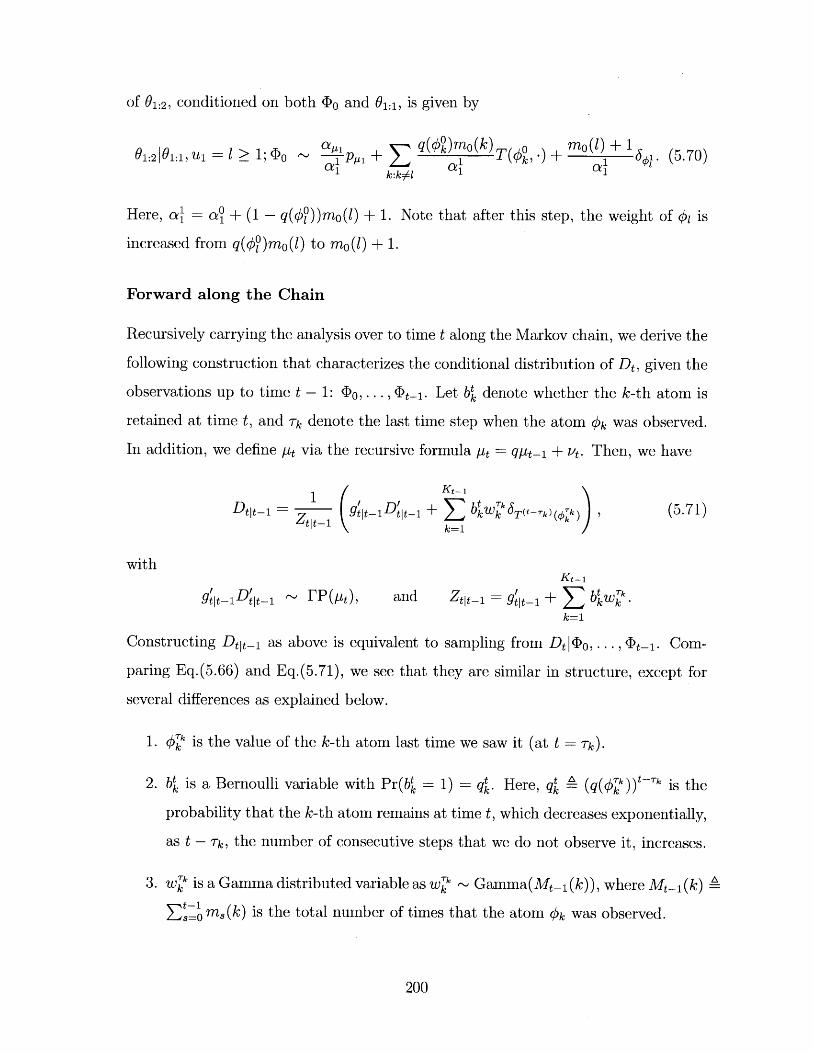
of 01:2, conditioned on both 4o and 01:1, is given by
a. q(4%)mno(k), mo (1) + 101: 2 |01:1,i 1 > 1; o ~ -iPpi + k 1 T( m) + 1 o. (5.70)
1 k:kol a, al
Here, aI a + (1- q(4i))mo(l) + 1. Note that after this step, the weight of 41 is
increased from q(4)mo(l) to mo(l) + 1.
Forward along the Chain
Recursively carrying the analysis over to time t along the Markov chain, we derive the
following construction that characterizes the conditional distribution of Dt, given the
observations up to time t - 1: (Do,..., 4t-1. Let b' denote whether the k-th atom is
retained at time t, and rk denote the last time step when the atom 4k was observed.
In addition, we define pt via the recursive formula pt = qpt_ 1 + vt. Then, we have
D _1 1 ( _D' _r -'\ (5.71)9t DI +S btkk 6 Tct--k)(07k'Dt~t 1 - tit- ( I -I tt-1 k=1 k kk
withKt-1
9ti tjt 1 ~ PP(pt), and Zit_1 1 = gIt1 + E btwk.k=1
Constructing DtI- 1 as above is equivalent to sampling from D IlO, ... , 4t-1. Com-
paring Eq.(5.66) and Eq.(5.71), we see that they are similar in structure, except for
several differences as explained below.
1. 40' is the value of the k-th atom last time we saw it (at t = rk).
2. bt is a Bernoulli variable with Pr(bt = 1) qt. Here, qt A (q('k))t%-' is the
probability that the k-th atom remains at time t, which decreases exponentially,
as t - rk, the number of consecutive steps that we do not observe it, increases.
3. wj' is a Gamma distributed variable as wk Gamma(Mt_1 (k)), where Mt 1 (k) A
t-i m,(k) is the total number of times that the atom 4k was observed.
200
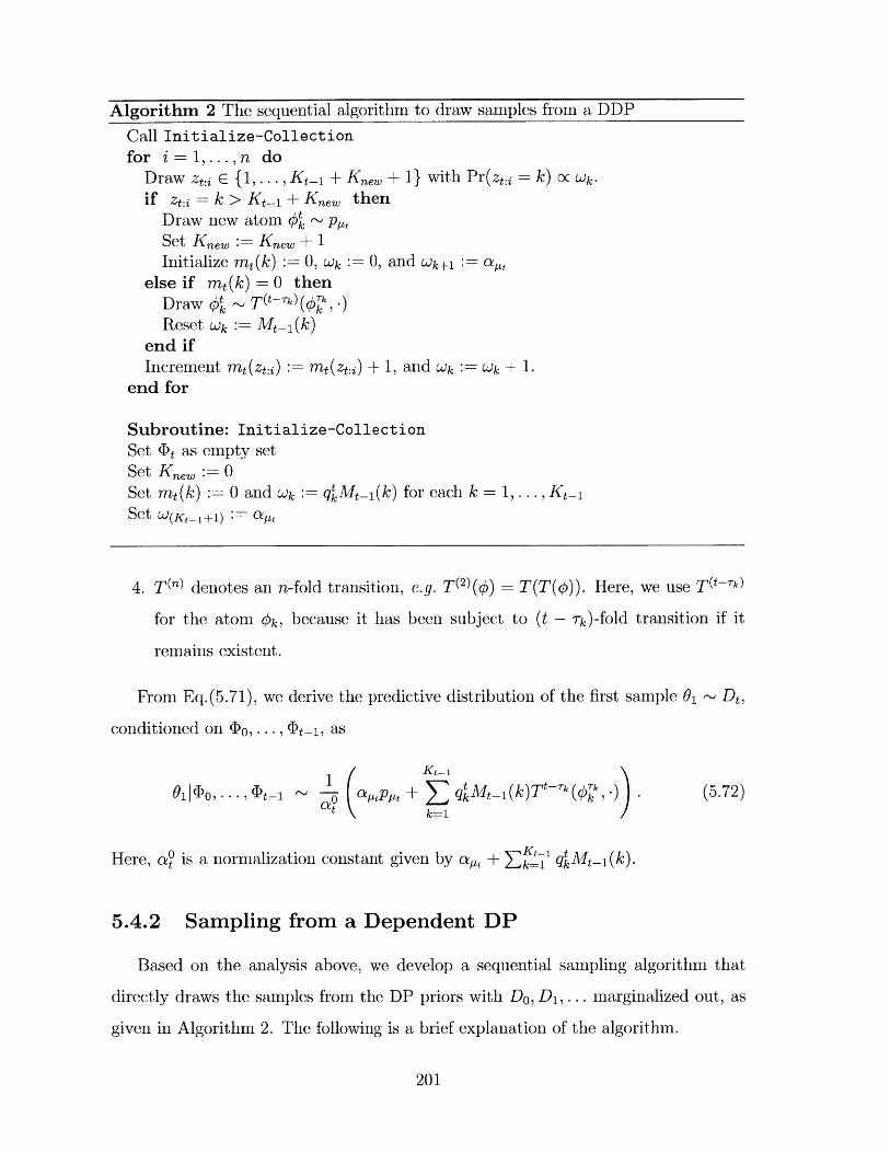
Algorithm 2 The sequential algorithm to draw samples from a DDP
Call Initialize-Collectionfor i = 1, ... , n do
Draw ZteC:i {1, .... , Kt- 1 + Knew + 1} with Pr(zt.i = k) Oc Wk.if zt.i = k > Kt- 1 + Knew then
Draw new atom # ~ p,,Set Knew := Knew + 1Initialize mt(k) := 0, Wk := 0, and Wk+1 := a,
else if mt(k) = 0 thenDraw $~ T(t-k)(k, -)
Reset Wk Mt_ 1(k)end ifIncrement mt(zt:i) mt (zt:i) + 1, and Wk Wk + 1.
end for
Subroutine: Initialize-CollectionSet <bt as empty setSet Knew :=0Set mt(k) 0 and Wk := qtMt_1(k) for each k = 1,...,Kt_1Set w(K, t+1) :y=LLf
4. T() denotes an n-fold transition, e.g. T(2 )() = T(T(#)). Here, we use T(t-rk)
for the atom #k, because it has been subject to (t - rk)-fold transition if it
remains existent.
From Eq.(5.71), we derive the predictive distribution of the first sample 01 - Dt,
conditioned on 4o, ... , 4 _1, as
01|<bo,~~Kt . . 'b_ yp ,+ q M t_1 (k)T -7-(0, -) .(5.72)Cet k=1
Here, ct is a normalization constant given by at, + Zk1 qkMt 1 (k).
5.4.2 Sampling from a Dependent DP
Based on the analysis above, we develop a sequential sampling algorithm that
directly draws the samples from the DP priors with Do, D1, ... marginalized out, as
given in Algorithm 2. The following is a brief explanation of the algorithm.
201
1. First of all, we have to initialize <bt as an empty set, and set Knew, the number
of new atoms created at time t, to zero.
2. For convenience, we introduce a weight Wk for each atom, and initially set
Wk - qtMt_1(k) for k = 1, ... , Kt_1. Additionally, we set ogt-i) = a, which
represents the weight of creating an new atom.
3. We draw a new sample at each step. Specifically, at the i-th step, we draw the
label zt:j from a finite set {1, .. , Kt1 + Knew + 1}, with the probability values
proportional to the weights, i.e. Pr(z:i = k) C Wk.
4. If zt:j = K-i-+Knew+l, we have to draw a new atom # from the base distribution
p., increment Knew by 1, and initialize both Wk and mt(k) to zeros. (Note that
Wk and mt(k) will be immediately incremented to one, before drawing the next
sample.)
5. If zt:j = k < Kt- 1 + Knew, there are two possible cases: (1) mt(k) > 0, which
implies that the atom #k has been seen in previous samples, and its value #'has been determined; (2) mt(k) = 0, which implies that this atom is inherited
from the previous time step t - 1, and it is the first sample associated with it at
time t. In this case, we have to draw #' ~ T(#t- 1, .), and accordingly we have
to change the weight Wk from qktMt_1(k) to Mt_1 (k), as we are assured that this
atom is retained.
6. In all cases, we will increment both the counter mt(zt:i) and the weight Wzt.i by
one.
5.4.3 Gibbs Sampling for Inference over Dynamic DPMM
We use the Markov chain of Dirichlet processes as the prior of dynamic mixture
models in our framework. The generative process is formulated as follows: for each
202
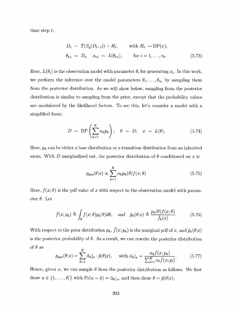
time step t,
Dt = T(Sq(Dt_1)) + Ht, with Ht ~ DP(v);
Ot:i Dt, Xt:j ~ L(Ot:), for i = 1, .. . , nt. (5.73)
Here, L(O6) is the observation model with parameter O6 for generating xi. In this work,
we perform the inference over the model parameters 01,..., 0f, by sampling them
from the posterior distribution. As we will show below, sampling from the posterior
distribution is similar to sampling from the prior, except that the probability values
are modulated by the likelihood factors. To see this, let's consider a model with a
simplified form:
'K
D DP ( akPk) ; D; x ~ L(0). (5.74)k=1
Here, Pk can be either a base distribution or a transition distribution from an inherited
atom. With D marginalized out, the posterior distribution of 0 conditioned on x is
K
Ppos(0 x) oC z akpk(0)f(x; 0) (5.75)k=1
Here, f(x; 0) is the pdf value of x with respect to the observation model with param-
eter 0. Let
(x; pk) A f (X; o)pk (0)dO, and P( (x) (5.76)1Jk ,fk(x) (576
With respect to the prior distribution Pk, f(x; pk) is the marginal pdf of x, and ik(0 x)
is the posterior probability of 0. As a result, we can rewrite the posterior distribution
of 0 asK K cakf (X; Pk)
pros (|x) Z dklx - (|x), with k = c ) (5.77)k=1 l=1
Hence, given x, we can sample 0 from the posterior distribution as follows. We first
draw u E {1, ... , K} with Pr(u = k) = dklx, and then draw 0 ~ p(Ox).
203
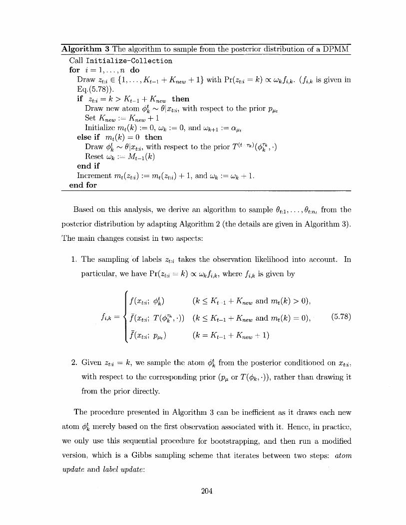
Algorithm 3 The algorithm to sample from the posterior distribution of a DPMM
Call Initialize-Collectionfor i = 1, ... , n do
Draw zt:j E {,.... , Kt_1 + Knew + 1} with Pr(zt = k) Oc wkfi,k. (fi,k is given inEq. (5.78)).if z:i = k > Kt_1 + Knew then
Draw new atom #t , 0 1|xt.j, with respect to the prior p,Set Knew := Knew + 1Initialize mt(k) := 0, ok := 0, and Wk+1 := a,
else if mt(k) = 0 thenDraw di 0 xt:i, with respect to the prior T(t Tk)(4, -)Reset Wk Mt_1 (k)
end ifIncrement mt(zt:i) mt (zt:i) + 1, and Wk := ok + 1.
end for
Based on this analysis, we derive an algorithm to sample 6t:1,.. ., t:nt from the
posterior distribution by adapting Algorithm 2 (the details are given in Algorithm 3).
The main changes consist in two aspects:
1. The sampling of labels zt:j takes the observation likelihood into account. In
particular, we have Pr(zt:i = k) c Wkfi,k, where fi,k is given by
f(xti; #0) (k < Kt- 1 + Knew and mt(k) > 0),
fi,k f(xt:i; T(#1, )) (k < Ki1 + Kne, and mt(k) 0), (5.78)
f (xt:i; ppt) (k =Kt_1 + Knew + 1)
2. Given zt:i = k, we sample the atom #' from the posterior conditioned on xt:j,
with respect to the corresponding prior (p,, or T(#k, -)), rather than drawing it
from the prior directly.
The procedure presented in Algorithm 3 can be inefficient as it draws each new
atom #t merely based on the first observation associated with it. Hence, in practice,
we only use this sequential procedure for bootstrapping, and then run a modified
version, which is a Gibbs sampling scheme that iterates between two steps: atom
update and label update:
204
1. Atom update: We resample each atom 4k conditioned on all the observa-
tions with label k, denoted by Xk, with respect to the corresponding prior Pk.
Particularly, if k < Kt-1, 4k is an inherited atom, and thus P= T(t=k-) (g);
otherwise, 4k is a new atom that were drawn from p,, and thus P p,,.
2. Label update: This is similar to the steps in Algorithm 3. Specifically, for
each i = 1,... , n, except that after bootstrapping, mt have actually counted all
the samples observed at time t. Therefore, we have to first decrement mt(zt:i)
by 1, and after zt:j is updated, we increment mt(zt:i) according to its new value.
5.5 Empirical Results
This section presents experimental results on both synthetic and real data. Firsta set
of simulations are done on synthetic data to compare the proposed DDP model with
dynamic FMM in describing Gaussian clusters that may change over time. Then, the
DDP model is applied to two real world tasks, modeling people flows and analyzing
the trends of research topics. These experiments demonstrate the model's practical
utility.
5.5.1 Simulations on Synthetic Data
The data for simulations were synthesized as follows. We initialized the model with
two Gaussian components, and added new components following a temporal Poisson
process (one per 20 phases on average). For each component, the life span has a
geometric distribution with mean 40, the mean of each Gaussian component evolves
independently as a Brownian motion, and the variance is fixed to 1. We performed
the simulation for 80 phases, and at each phase, we drew 1000 samples for each active
component.
At each phase, we sample for 5000 iterations, discarding the first 2000 for burn-
in, and collecting a sample every 100 iterations for performance evaluation. The
particles of the last iteration at each phase were incorporated into the model as a
205
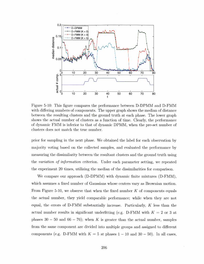
U)0
CuCo
~0
CU
00)E
o 10 20 30 40 50 60 70 80
E
0
a 0 10 20 30 40 50 60 70 80t
Figure 5-10: This figure compares the performance between D-DPMM and D-FMMwith differing numbers of components. The upper graph shows the median of distancebetween the resulting clusters and the ground truth at each phase. The lower graphshows the actual number of clusters as a function of time. Clearly, the performanceof dynamic FMM is inferior to that of dynamic DPMM, when the pre-set number ofclusters does not match the true number.
prior for sampling in the next phase. We obtained the label for each observation by
majority voting based on the collected samples, and evaluated the performance by
measuring the dissimilarity between the resultant clusters and the ground truth using
the variation of information criterion. Under each parameter setting, we repeated
the experiment 20 times, utilizing the median of the dissimilarities for comparison.
We compare our approach (D-DPMM) with dynamic finite mixtures (D-FMM),
which assumes a fixed number of Gaussians whose centers vary as Brownian motion.
From Figure 5-10, we observe that when the fixed number K of components equals
the actual number, they yield comparable performance; while when they are not
equal, the errors of D-FMM substantially increase. Particularly, K less than the
actual number results in significant underfitting (e.g. D-FMM with K = 2 or 3 at
phases 30 - 50 and 66 - 76); when K is greater than the actual number, samples
from the same component are divided into multiple groups and assigned to different
components (e.g. D-FMM with K = 5 at phases 1 - 10 and 30 - 50). In all cases,
206.
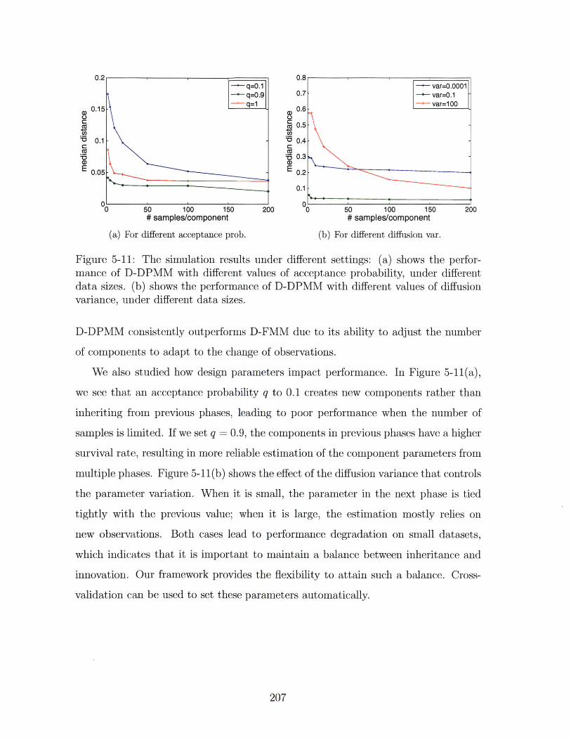
0.5-
0.1 -- 0.4 -
50.3
E 0.05- -.. 0.2-
0.1
00 50 100 150 200 00 50 100 150 200# samples/component # samples/component
(a) For different acceptance prob. (b) For different diffusion var.
Figure 5-11: The simulation results under different settings: (a) shows the perfor-
mance of D-DPMM with different values of acceptance probability, under different
data sizes. (b) shows the performance of D-DPMM with different values of diffusion
variance, under different data sizes.
D-DPMM consistently outperforms D-FMM due to its ability to adjust the number
of components to adapt to the change of observations.
We also studied how design parameters impact performance. In Figure 5-11(a),
we see that an acceptance probability q to 0.1 creates new components rather than
inheriting from previous phases, leading to poor performance when the number of
samples is limited. If we set q = 0.9, the components in previous phases have a higher
survival rate, resulting in more reliable estimation of the component parameters from
multiple phases. Figure 5-11(b) shows the effect of the diffusion variance that controls
the parameter variation. When it is small, the parameter in the next phase is tied
tightly with the previous value; when it is large, the estimation mostly relies on
new observations. Both cases lead to performance degradation on small datasets,
which indicates that it is important to maintain a balance between inheritance and
innovation. Our framework provides the flexibility to attain such a balance. Cross-
validation can be used to set these parameters automatically.
207
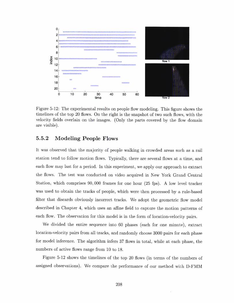
0-
4
18- >
8-X
S10S 1fow0
12-
14-
16-
18-
20-
0 10 20 30 40 50 60time ow
Figure 5-12: The experimental results on people flow modeling. This figure shows thetimelines of the top 20 flows. On the right is the snapshot of two such flows, with thevelocity fields overlain on the images. (Only the parts covered by the flow domainare visible).
5.5.2 Modeling People Flows
It was observed that the majority of people walking in crowded areas such as a rail
station tend to follow motion flows. Typically, there are several flows at a time, and
each flow may last for a period. In this experiment, we apply our approach to extract
the flows. The test was conducted on video acquired in New York Grand Central
Station, which comprises 90, 000 frames for one hour (25 fps). A low level tracker
was used to obtain the tracks of people, which were then processed by a rule-based
filter that discards obviously incorrect tracks. We adopt the geometric flow model
described in Chapter 4, which uses an affine field to capture the motion patterns of
each flow. The observation for this model is in the form of location-velocity pairs.
We divided the entire sequence into 60 phases (each for one minute), extract
location-velocity pairs from all tracks, and randomly choose 3000 pairs for each phase
for model inference. The algorithm infers 37 flows in total, while at each phase, the
numbers of active flows range from 10 to 18.
Figure 5-12 shows the timelines of the top 20 flows (in terms of the numbers of
assigned observations). We compare the performance of our method with D-FMM
208
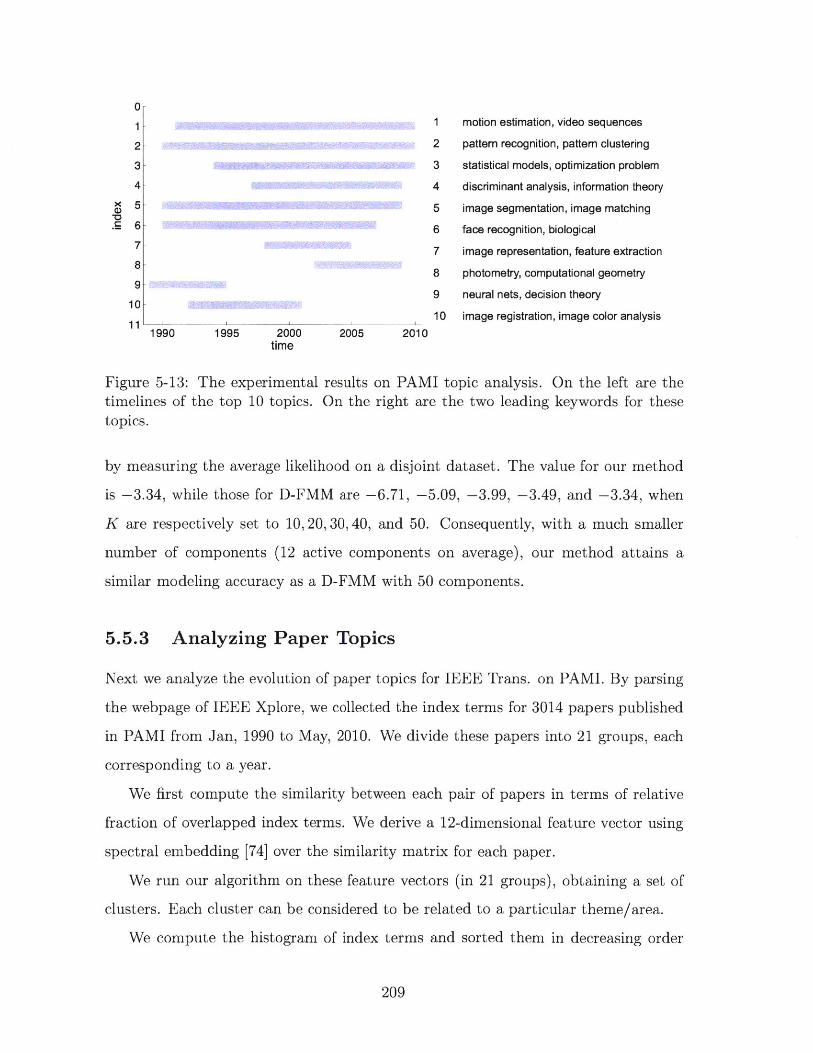
0-
1 - 1 motion estimation, video sequences
2- 2 pattern recognition, pattem clustering
3 3 statistical models, optimization problem
4 4 discriminant analysis, information theory
5- 5 image segmentation, image matching6- 6 face recognition, biological7- 7 image representation, feature extraction8- 8 photometry, computational geometry9
9 neural nets, decision theory10-
11 10 image registration, image color analysis1990 1995 2000 2005 2010
time
Figure 5-13: The experimental results on PAMI topic analysis. On the left are thetimelines of the top 10 topics. On the right are the two leading keywords for these
topics.
by measuring the average likelihood on a disjoint dataset. The value for our method
is -3.34, while those for D-FMM are -6.71, -5.09, -3.99, -3.49, and -3.34, when
K are respectively set to 10,20,30,40, and 50. Consequently, with a much smaller
number of components (12 active components on average), our method attains a
similar modeling accuracy as a D-FMM with 50 components.
5.5.3 Analyzing Paper Topics
Next we analyze the evolution of paper topics for IEEE Trans. on PAMI. By parsing
the webpage of IEEE Xplore, we collected the index terms for 3014 papers published
in PAMI from Jan, 1990 to May, 2010. We divide these papers into 21 groups, each
corresponding to a year.
We first compute the similarity between each pair of papers in terms of relative
fraction of overlapped index terms. We derive a 12-dimensional feature vector using
spectral embedding [74] over the similarity matrix for each paper.
We run our algorithm on these feature vectors (in 21 groups), obtaining a set of
clusters. Each cluster can be considered to be related to a particular theme/area.
We compute the histogram of index terms and sorted them in decreasing order
209
of frequency for each topic. Figure 5-13 shows the timelines of top 10 topics, and
together with the top two index terms for each of them. Not surprisingly, we see
that topics such as "neural networks" arise early and then diminish while "image
segmentation" and "motion estimation" persist.
5.6 Summary
We developed a principled framework for constructing dependent Dirichlet processes.
In contrast to most DP-based approaches, our construction is motivated by the intrin-
sic relation between Dirichlet processes and compound Poisson processes. In particu-
lar, we discussed three operations: superposition, subsampling, and point transition.
These operations produce DPs depending on others. We further combined these op-
erations to derive a Markov chain of DPs, leading to a prior of mixture models that
allows creation, removal, and location variation of component models under a unified
formulation. We also presented a Gibbs sampling algorithm for inferring the models.
The simulations on synthetic data and the experiments on modeling people flows and
paper topics clearly demonstrate that the proposed method is effective in estimating
mixture models that evolve over time.
210
Chapter 6
The Order of Layers
A natural scene that we see in real world typically comprises multiple objects with
different appearance and behaviors. As discussed in Chapter 1, these objects can
be modeled as layers, and each layer can be described by an appearance model and
a motion model. Previous chapters have developed tools to model appearance and
dynamic motion. However, this is not enough.
In real scenes, different layers may overlap with each other. Consequently, part
of a layer may be occluded by others and become invisible. Effective explanation of
such scenes has to take into account the occlusion relation between different layers,
which, in turn, is determined by the relative depth order between them.
In this chapter, a model of layer order is developed, which considers the relative
depth order between layers as a partial order generated from a distribution over the
partial order space. A key challenge, however, arises in inferring the partial order
from observations. MAP estimation is NP-hard, while standard MCMC sampling
methods are difficult to apply, as the underlying space is generally disconnected, due
to the combinatorial constraints that partial orders have to satisfy.
In this chapter, a generic sampling methodology is developed to address this diffi-
culty, which introduces bridging states between parts of the space that are otherwise
disconnected. Theoretical analysis of this method leads to bounds of the mixing
time. We also tested it empirically in an application to infer the order of layers in
real scenes.
211
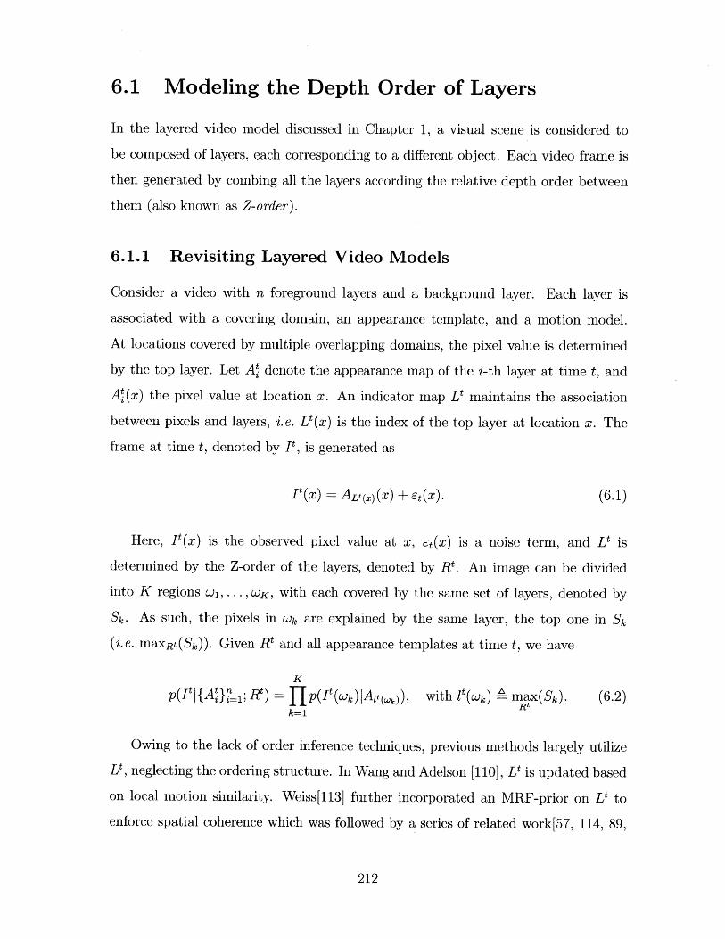
6.1 Modeling the Depth Order of Layers
In the layered video model discussed in Chapter 1, a visual scene is considered to
be composed of layers, each corresponding to a different object. Each video frame is
then generated by combing all the layers according the relative depth order between
them (also known as Z-order).
6.1.1 Revisiting Layered Video Models
Consider a video with n foreground layers and a background layer. Each layer is
associated with a covering domain, an appearance template, and a motion model.
At locations covered by multiple overlapping domains, the pixel value is determined
by the top layer. Let A denote the appearance map of the i-th layer at time t, and
A (x) the pixel value at location x. An indicator map L' maintains the association
between pixels and layers, i.e. Lt(x) is the index of the top layer at location x. The
frame at time t, denoted by P, is generated as
It(x) = AV()(x) + et(x). (6.1)
Here, It(x) is the observed pixel value at x, et(x) is a noise term, and Lt is
determined by the Z-order of the layers, denoted by Rt. An image can be divided
into K regions wi, ... , wK, with each covered by the same set of layers, denoted by
Sk. As such, the pixels in Wk are explained by the same layer, the top one in Sk
(i.e. maxRt (Sk)). Given Rt and all appearance templates at time t, we have
K
p(I t lfA lI=; Rt) 171 p(I(wk)|Aetew)), with lt (wk) A max(Sk). (6.2)k=1
Owing to the lack of order inference techniques, previous methods largely utilize
Lt, neglecting the ordering structure. In Wang and Adelson [110], Lt is updated based
on local motion similarity. Weiss[113] further incorporated an MRF-prior on Lt to
enforce spatial coherence which was followed by a series of related work[57, 114, 89,
212
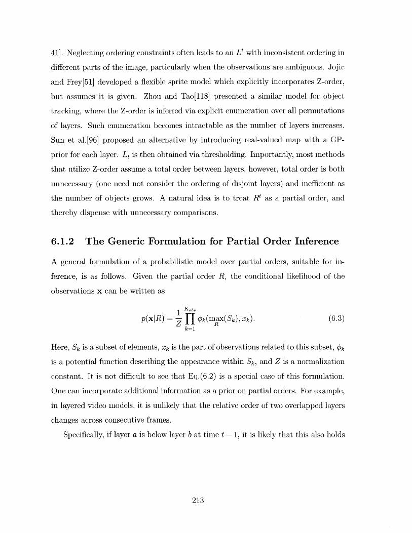
41]. Neglecting ordering constraints often leads to an Lt with inconsistent ordering in
different parts of the image, particularly when the observations are ambiguous. Jojic
and Frey[51] developed a flexible sprite model which explicitly incorporates Z-order,
but assumes it is given. Zhou and Tao[118] presented a similar model for object
tracking, where the Z-order is inferred via explicit enumeration over all permutations
of layers. Such enumeration becomes intractable as the number of layers increases.
Sun et al.[96] proposed an alternative by introducing real-valued map with a GP-
prior for each layer. Lt is then obtained via thresholding. Importantly, most methods
that utilize Z-order assume a total order between layers, however, total order is both
unnecessary (one need not consider the ordering of disjoint layers) and inefficient as
the number of objects grows. A natural idea is to treat Rt as a partial order, and
thereby dispense with unnecessary comparisons.
6.1.2 The Generic Formulation for Partial Order Inference
A general formulation of a probabilistic model over partial orders, suitable for in-
ference, is as follows. Given the partial order R, the conditional likelihood of the
observations x can be written as
1 Ko s,p(x|R) = -i $(max(Sk) , xk). (6.3)
Z Rk=1
Here, Sk is a subset of elements, Xk is the part of observations related to this subset, #kis a potential function describing the appearance within Sk, and Z is a normalization
constant. It is not difficult to see that Eq.(6.2) is a special case of this formulation.
One can incorporate additional information as a prior on partial orders. For example,
in layered video models, it is unlikely that the relative order of two overlapped layers
changes across consecutive frames.
Specifically, if layer a is below layer b at time t - 1, it is likely that this also holds
213
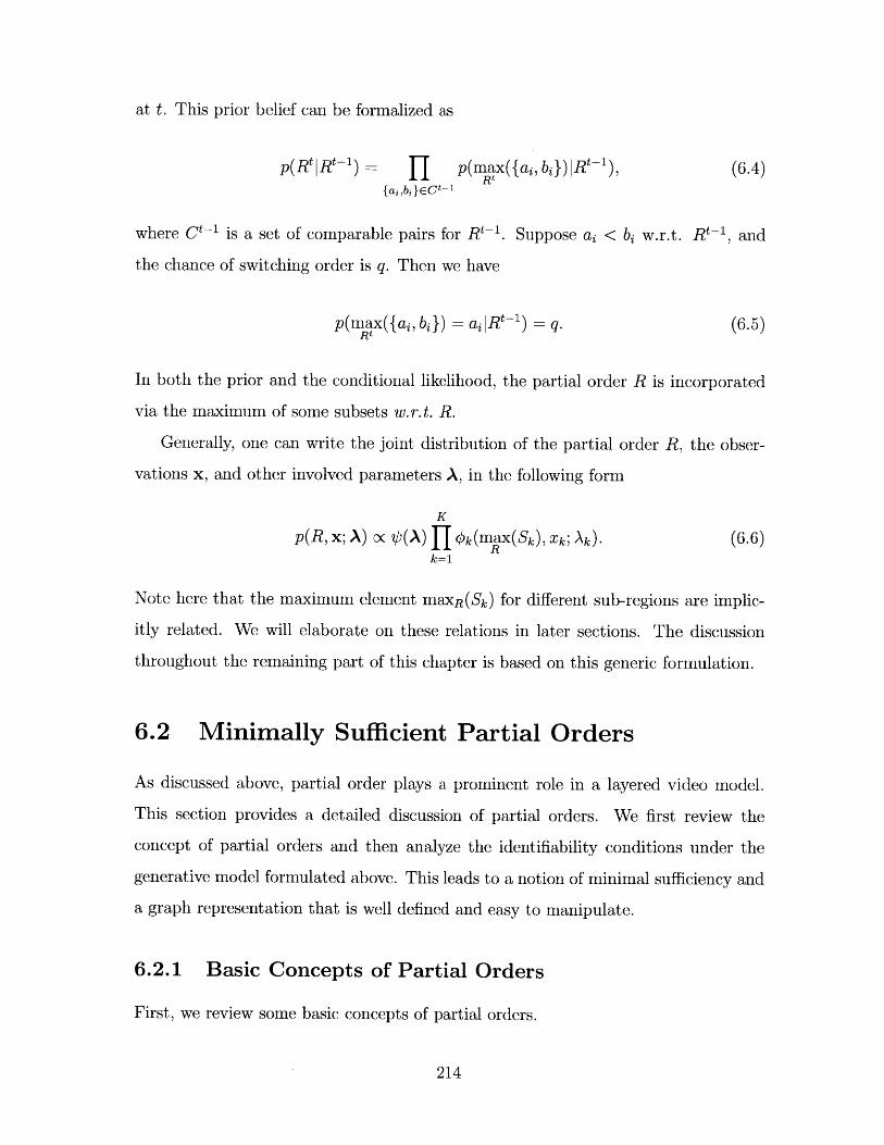
at t. This prior belief can be formalized as
p(Rt|Rtl) = J p(max({ai, bi})|Rt-), (6.4)Rt
{ai,bi}cCt-1
where Ct-i is a set of comparable pairs for Rt-. Suppose ai < bi w.r.t. Rt-, and
the chance of switching order is q. Then we have
p(max({ai, bi}) ail R'-) = q. (6.5)Rt
In both the prior and the conditional likelihood, the partial order R is incorporated
via the maximum of some subsets w.r.t. R.
Generally, one can write the joint distribution of the partial order R, the obser-
vations x, and other involved parameters A, in the following form
K
p(R, x; A) Oc @(A) fi Ok(max(Sk), Xz; Ak). (6.6)k=1
Note here that the maximum element maxR(Sk) for different sub-regions are implic-
itly related. We will elaborate on these relations in later sections. The discussion
throughout the remaining part of this chapter is based on this generic formulation.
6.2 Minimally Sufficient Partial Orders
As discussed above, partial order plays a prominent role in a layered video model.
This section provides a detailed discussion of partial orders. We first review the
concept of partial orders and then analyze the identifiability conditions under the
generative model formulated above. This leads to a notion of minimal sufficiency and
a graph representation that is well defined and easy to manipulate.
6.2.1 Basic Concepts of Partial Orders
First, we review some basic concepts of partial orders.
214
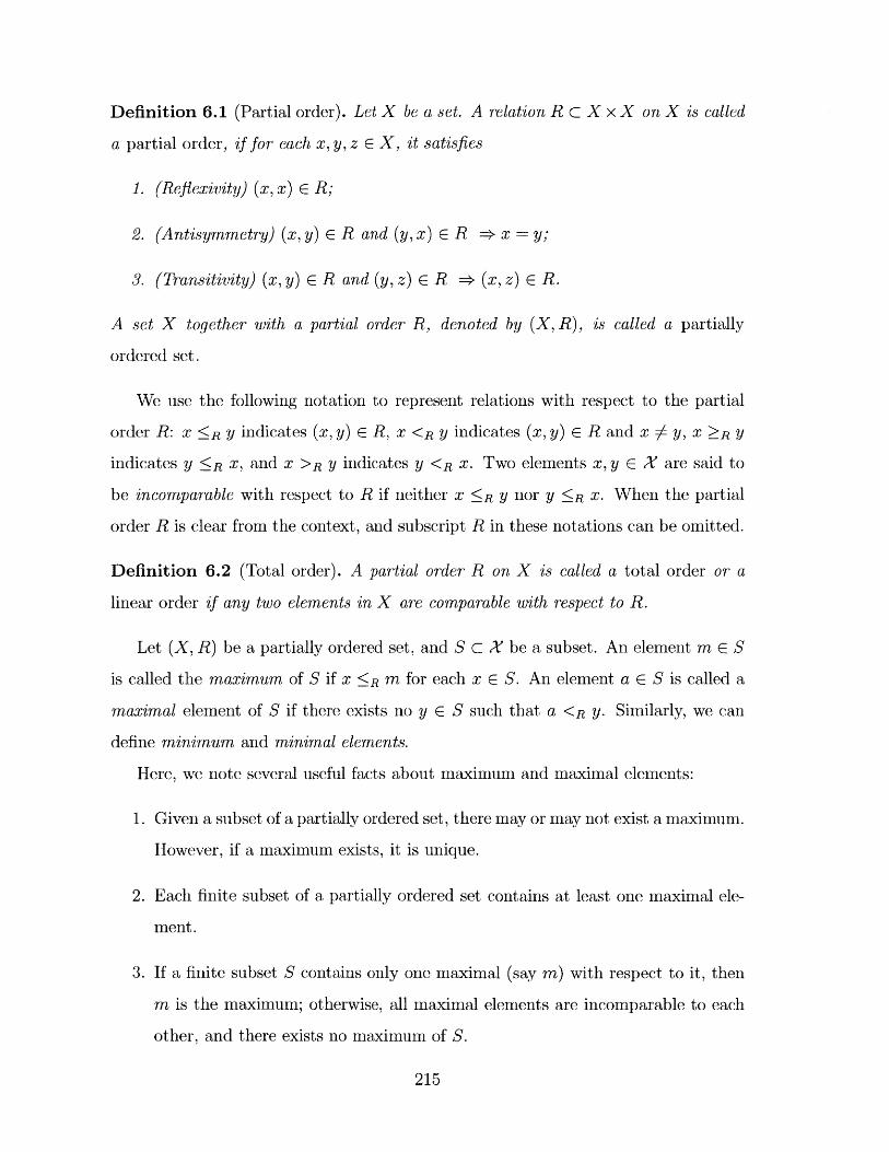
Definition 6.1 (Partial order). Let X be a set. A relation R C X x X on X is called
a partial order, if for each x, y, z C X, it satisfies
1. (Reflexivity) (x, x) E R;
2. (Antisymmetry) (x, y) E R and (y, x) E R * x = y;
3. (Transitivity) (x, y) E R and (y, z) e R (x, z) E R.
A set X together with a partial order R, denoted by (X, R), is called a partially
ordered set.
We use the following notation to represent relations with respect to the partial
order R: x _R y indicates (x, y) E R, x <R y indicates (x, y) e R and x -A y, X ;R y
indicates y R x, and x >R y indicates y <R x. Two elements x, y E X are said to
be incomparable with respect to R if neither x KR y nor y KR x. When the partial
order R is clear from the context, and subscript R in these notations can be omitted.
Definition 6.2 (Total order). A partial order R on X is called a total order or a
linear order if any two elements in X are comparable with respect to R.
Let (X, R) be a partially ordered set, and S C X be a subset. An element m E S
is called the maximum of S if x R m for each x E S. An element a E S is called a
maximal element of S if there exists no y E S such that a <R y. Similarly, we can
define minimum and minimal elements.
Here, we note several useful facts about maximum and maximal elements:
1. Given a subset of a partially ordered set, there may or may not exist a maximum.
However, if a maximum exists, it is unique.
2. Each finite subset of a partially ordered set contains at least one maximal ele-
ment.
3. If a finite subset S contains only one maximal (say m) with respect to it, then
m is the maximum; otherwise, all maximal elements are incomparable to each
other, and there exists no maximum of S.
215
4. Any finite subset of a totally ordered set has a unique maximal element, which
is also the maximum of the subset.
Since each partial order R is essentially a set of pairs, we can take intersections
between partial orders. And it turns out that intersection of partial orders remains a
partial order, as stated by the following proposition:
Proposition 6.1. Let R be a collection of partial orders on a set X, then the inter-
section ORER R remains a partial order.
Closures of Relations
Next, we introduce several useful concepts related to closures. With the notion of
closures, we can derive a partial order from an antisymmetric relation, which is useful
in later discussion.
In general, a closure of a subset S is often referred to a "minimum" superset of
S that possesses some properties. Specifically, we give a formal definition of reflexive
closure, transitive closure, and reflexive transitive closure.
Definition 6.3 (Reflexive closure). Let R be a relation on X, the intersection of all
reflexive relations on X that contain R is called the reflexive closure of R, which can
be written as
CLm(R) R U {(x, x) : x E X}. (6.7)
Definition 6.4 (Transitive closure). Let R be a relation on X, the intersection of all
transitive relations on X that contain R is called the transitive closure of R, which
can be written as
CLx(R) A {(x, y) : Ex= ZO, ... , ZK y E X, s.t. (zi_ 1, zi) E R for i = 1, ... , K}.
(6.8)
Definition 6.5 (Reflexive transitive closure). Let R be a relation on X, the intersec-
tion of all relations that are both reflexive and transitive and contain R is called the
216
reflexive transitive closure of R, which can be written as
CLm1(R) = CLs(CLT(R)) = CLx(CLm(R)). (6.9)
The following proposition states that any antisymmetric relation R can be made
into a partial order by constructing its reflexive transitive closure.
Proposition 6.2. Let R be an antisymmetric relation, then its reflexive transitive
closure is a partial order, and it is the intersection of all partial orders containing R.
If R is finite, we can construct its (reflexive) transitive closure within polynomial
time (the simplest way is to use Floyd- Warshall algorithm).
6.2.2 Sufficiency, Identifiability, and Minimality
In previous section, we established a generic probabilistic model, in which the joint
distribution of the partial order R, observations x, and other involved parameters A,
is given byK
p(R; x, A) oc 4(A) H # (Yk, max(Sk)). (6.10)k=1
Here, Si, ... , Sk are subsets of the layers, maxR(Sk) is the maximum of Sk with
respect to the partial order R, and V@ captures the prior factors that do not depend
on the partial order. Based on this model, we can further discuss the sufficiency and
minimality of the partial orders.
Sufficient Partial Order and Consistent Choice of Maximums
To perform evaluation or inference on the model given by Eq. (6.10), the partial or-
der R should contain all necessary pairs such that the maximum of each Sk can be
determined. Such a partial order is called a sufficient partial order, which is defined
formally as follows.
Definition 6.6 (Sufficient partial order). Let X be a set, and C C 2X be a collection
of subsets of X. A partial order R on X is said to be sufficient with respect to C if
217
for each S e C, the maximum of S exists.
Obviously, any total order on X is sufficient with respect to any collection C
of finite subsets. However, the converse is not true in general, meaning that a
sufficient partial order is not necessarily a total order. Consider a simple case as
follows. Let X = 1, 2,3 and C = {{1, 2}, {1, 3}}, then the partial order R =
((1, 1), (2, 2), (3, 3), (1, 2), (1,3)) is sufficient with respect to C, which is obviously not
a total order.
Each sufficient partial order gives rise to an assignment of maximum to each
element in C. Such assignments together constitute a choice function over C, which
is formally defined as below.
Definition 6.7 (Choice function). Let C be a collection of subsets of X. A choice
function on C is a map f : C -> X such that for each S E C, f(S) E S.
Intuitively, a choice function can be understood as choosing an element from each
subset S. We note that the well-known axiom of choice is based on a choice function.
Clearly, a sufficient partial order leads to a choice function that maps each subset S
in C to a maximum of S, which we call the choice of maximums.
Identifiability
We can see from Eq.(6.10) that the partial order is incorporated into the model
via the induced choice of maximums. Therefore, partial orders that yield the same
choice of maximums can not be distinguished by this model, as the joint probability
evaluates to the same value for any given y. In this case, we say that R1 and R 2 are
unidentifiable. Formally, the identifiability is defined as follows.
Definition 6.8 (Identifiability). Given a joint probabilistic model p(6, y) and 6 E 8.
We say that the set of parameters E is identifiable under this model, if p(y|6 1) and
p(y|82) are different distributions for any two distinct elements 1, 02 E 8-.
Definition 6.9 (Factor-wise identifiable model). Given a probabilistic model p(O, y)
218
with a product form as
K
p(0,y) oc b(y) I Ik (Yk, 7k(6)) . (6.11)k=1
Here, yk refers to the part of y that is involved in the k-th factor. Note that the
parts of y involved in different factors may overlap. This model is called factor-wise
identifiable, if k(-|i) # Pk(-q') whenever j q r', for each k = 1, ... , K. Here, Pk(-'r)
is defined to be'O (y)#Ok(yk, n7)
Pk (Yky )J = bYM ',qdl (6.12)
The factor-wise identifiability means that for each factor in Eq.(6.11), different
values of r7k (6) can be distinguished by the factor #k itself. Under the assumption of
factor-wise identifiability, we showed that a sufficient and necessary condition for a
set of partial orders to be identifiable is that they yield different choices of maximums,
as stated by the following lemma.
Lemma 6.1. Given a set X, a collection of subsets C = (S1,..., SK). and a proba-
bilistic model as in Eq.(6.10) with given parameters A. Suppose this model is factor-
wise identifiable, then a set of partial orders is identifiable under this model if and
only if they yield distinct choices of maximums.
Proof. The "only if" part of the statement is trivial to prove, as one can easily see
that when two partial orders yield exactly the same choice of maximums, they are
obviously unidentifiable. Since A is given and fixed, we omit it in the following
derivation for conciseness.
Next, we show the "if" part. Let R1 and R 2 be two different partial orders
in R. To prove they are identifiable, we have to show that p(.R 1 ) and p(.R 2) are
different distributions. Without losing generality, we assume that p(. R1) is absolutely
continuous with respect to p(.R 2), otherwise, they have already been different, and
219
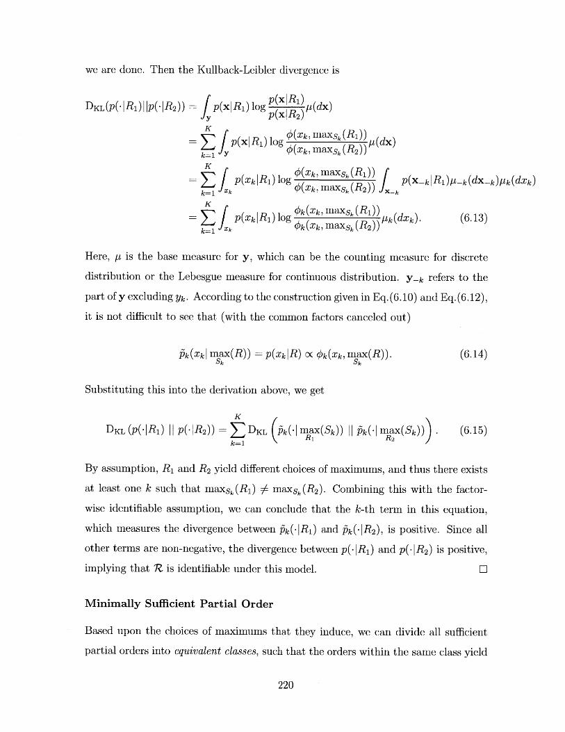
we are done. Then the Kullback-Leibler divergence is
DKL (P(' R1 ) p(. R 2 )) p(x R1 ) log p(x|R1) p(dx)Jy px R2) p(x
K
= p(x R1 ) log p(XkmaxSk (dx)k=1 y Xk,maxsk(R 2 ))
K
= JXIR1) log (Xk,maxsk(R)) k p(x-k R1)p1k(dx-k)ptk(dXk)
K X kk(Xk,maxsk(R1))
= 1 k|R 1 ) log d (Xkmaxs).(R)) (6.13)k=1 *k Ok (k, as(2))
Here, y is the base measure for y, which can be the counting measure for discrete
distribution or the Lebesgue measure for continuous distribution. Y-k refers to the
part of y excluding Yk. According to the construction given in Eq.(6.10) and Eq.(6.12),
it is not difficult to see that (with the common factors canceled out)
Pk (Xk max(R)) = p(Xk R) oc @k(Xk,max(R)).Sk Sk
(6.14)
Substituting this into the derivation above, we get
K KDKL (p(. IR1 ) p(. IR2)) I:DKL (Pk~ ( max(Sk)) 11Pk(.'nmax(Sk)))
k=1 LiR(6.15)
By assumption, R1 and R 2 yield different choices of maximums, and thus there exists
at least one k such that maxsk(R 1 ) # maxsk(R 2). Combining this with the factor-
wise identifiable assumption, we can conclude that the k-th term in this equation,
which measures the divergence between Pk(- R1 ) and Sk(- R 2 ), is positive. Since all
other terms are non-negative, the divergence between p(. R 1) and p(. R 2) is positive,
implying that R is identifiable under this model. D
Minimally Sufficient Partial Order
Based upon the choices of maximums that they induce, we can divide all sufficient
partial orders into equivalent classes, such that the orders within the same class yield
220
the same choice of maximums, and thus are unidentifiable under the probabilistic
model described above. Each such class has a unique representative which we call
minimally sufficient partial order, based upon which we develop our representation.
Definition 6.10 (Minimally sufficient partial orders). Given a set X and a collection
C of subsets. A partial order R is said to be minimally sufficient with respect to C if
R is sufficient but any of its proper subset is not.
Definition 6.11 (Consistent choice of maximums). Given a set of X and a collection
C of subsets. A choice of maximums over C is called consistent if there exists a partial
order that yields this choice.
Clearly, in order for R to induce a choice f over C, every pair in form of (a, f(S))
with a G S must be included in R, which we call an essential pair.
Definition 6.12 (Essential pairs). Given a set of X, a collection C of subsets, and a
consistent choice of maximums f over C. Each pair (a, b) such that there exists S E C
with a E S and b = f(S) is called a essential pair with respect to f.
Proposition 6.3. Given a set X and a consistent choice of maximums f over C.
Then a partial order R yields f as the choice of maximum if and only if all essential
pairs for f are contained in R.
Lemma 6.2. Given a set X, a collection of subsets C, and a consistent choice of
maximum f over C. There exists a unique minimally sufficient partial order that
yields f, which is the intersection of all sufficient partial orders that yield f as their
choice of maximum.
For conciseness of following discussion, we denote the intersection of all partial
orders that yield f, as described by this lemma, to be R,. To prove this lemma, we
have to show that R, is the unique minimally sufficient partial order with f as the
choice of maximums.
Proof. First of all, by proposition 6.1, R, is a partial order on X. In the following,
we have to show that it is sufficient, minimal, and is the unique minimal that yields
f.
221
We have known that the essential pairs for f are contained in every sufficient
partial order that yields f as the choice of maximum. As a consequence, all such
pairs are contained in their intersection R,., and thus R' is also a sufficient partial
order that yields f as the choice of maximum.
Note that R, can be equivalently defined as the intersection of all partial orders
comprised of all essential pairs for f. It implies for any of its proper subset, say R',
at least one essential pair, say (a, f(S)), is not contained in R'. Therefore f(S) is not
a maximum of S with respect to R'. Moreover, there is no other element in S can be
a maximum. (This claim can be shown as follows: suppose b : f(S) is a maximum
of S with respect to R'. Then f(S) <R' b, and thus f(S) <R. b as R' C R,, which
contradicts the assumption that f(S) is a maximum of S with respect to R,.) Hence,
any proper subset of R is not sufficient, and R is a minimally sufficient partial order.
Finally, we show the uniqueness. Suppose there is a different minimally sufficient
partial order R' that induces f. By the definition of R,, we know that R, is a
proper subset of R', which clearly contradicts the assumption that R' is minimally
sufficient. 7
Lemma 6.1 and Lemma 6.2 together characterize the key relationship between
identifiability and minimal sufficiency, as summarized below.
Given a set X, a collection C = (S 1,..., SK) of subsets of X. Under the probabilistic
model given in Eq.(6.10) with the assumption that it is factor-wise identifiable, we
have:
1. any partial orders that yield the same choice of maximums are unidentifiable;
2. given each consistent choice of maximums over C, there exists a unique mini-
mally sufficient partial order with respect to C that induces it, which is R';
3. the set of all minimally sufficient partial orders are identifiable.
222
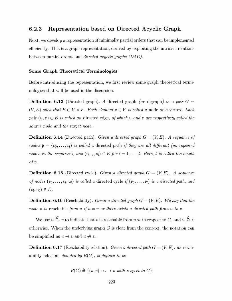
6.2.3 Representation based on Directed Acyclic Graph
Next, we develop a representation of minimally partial orders that can be implemented
efficiently. This is a graph representation, derived by exploiting the intrinsic relations
between partial orders and directed acyclic graphs (DAG).
Some Graph Theoretical Terminologies
Before introducing the representation, we first review some graph theoretical termi-
nologies that will be used in the discussion.
Definition 6.13 (Directed graph). A directed graph (or digraph) is a pair G
(V, E) such that E C V x V. Each element v E V is called a node or a vertex. Each
pair (u, v) c E is called an directed edge, of which u and v are respectively called the
source node and the target node.
Definition 6.14 (Directed path). Given a directed graph G = (V, E). A sequence of
nodes p = (vo,... , vj) is called a directed path if they are all different (no repeated
nodes in the sequence), and (vi 1, vi) E E for i = 1, ... , 1. Here, 1 is called the length
of p.
Definition 6.15 (Directed cycle). Given a directed graph G = (V, E). A sequence
of nodes (vo,... , vi, vo) is called a directed cycle if (vo,... , vi) is a directed path, and
(vi,vo) e E.
Definition 6.16 (Reachability). Given a directed graph G = (V, E). We say that the
node v is reachable from u if u = v or there exists a directed path from u to v.
We use u + v to indicate that v is reachable from u with respect to G, and u + v
otherwise. When the underlying graph G is clear from the context, the notation can
be simplified as u -+ v and u -4 v.
Definition 6.17 (Reachability relation). Given a directed path G = (V, E), its reach-
ability relation, denoted by R(G), is defined to be
R(G) {(u,v) : u -* v with respect to G}.
223
In other words, U R(G) v if and only if there exists a directed path from u to v.
Definition 6.18 (Directed acyclic graph). A directed graph G = (V, E) is called a
directed acyclic graph (often abbreviated to DAG), if there is no directed cycle in G,
i.e. given two distinct nodes u, v E V, if v is reachable from u via a directed path,
then u is not reachable from v.
In this document, we only consider directed graphs without self-loops (the edges
in form of (u, u)). This assumption is applied implicitly throughout the remaining
text. Directed acyclic graph has a close relation with partial order, as stated by the
following proposition.
Proposition 6.4. The reachability relation of a directed acyclic graph G = (V, E) is
a partial order defined on the set of nodes V.
The Graph Representation with Essential Pairs
Owing to the inherent relations between directed acyclic graphs and partial orders,
we can use a directed acyclic graph to represent a partial order.
Definition 6.19 (Compatible graph representation). An acyclic directed graph G
(X, E) is called compatible with a partial order R on X, if R = R(G), i.e. R is the
reachability relation of G. If this holds, we call G a compatible representation of R.
In general, there can be multiple graph representations that are compatible with a
partial order. For example, consider a partial order R over the finite set V = {a, b, c},
given by a < b < c. Then the graph G1 = {V, {(a, b), (b, c)}} and the graph G2
{V, {(a, b), (a, c), (b, c)}} are both compatible with R.
Proposition 6.5. Given an acyclic directed graph G = (V, E), the reachability rela-
tion R(G) is the intersection of all partial orders that contain every pair (u, v) G E.
Proof. Let Rinte, be the intersection of all partial orders that contain E. Here, we
are to show R(G) = Rinter. First, it is obvious that R(G) itself contains E, and
hence Rinte, C R(G). Next, we show R(G) C Rinter. It suffices to let R' be an
224
arbitrary partial order that contains every pair (u, v) E E and show R(G) c R'.
Given (s, t) c R(G), there exists uo,. .. , u,, such that uO = s, u, = t and (ui1, uj) E E
for i = 1, . . . , n. Since R' is transitive (as it is a partial order), (s, t) E R'. Therefore,
R(G) c R'.
In practice, especially in a dynamic context where the partial order can vary over
time, maintaining an exact representation is inefficient, as this requires keeping track
of every pair of reachable nodes, which is often unnecessary. Here, we use the graph
representation with essential pairs, which is much more efficient to maintain.
Definition 6.20 (Graph representation with essential pairs). Given a sufficient par-
tial order R with respect to a collection C of subsets on X. The graph representation
with essential pairs, denoted by Ge**(R), is defined to be Ge**(R) A (X, Eess(R)) with
edges connecting the essential pairs, as
Ee**(R) {(a, max(S)) : a E S, S E C}. (6.16)R
Again, we use an example to illustrate the essential graph representation. Consider
the partial order given by a < b < c, and a collection of subsets C = {{a, b}, {a, b, c}},
then the set of essential pairs is {(a, b), (a, c), (b, c)}. However, when C contains only
one set, as C = {{a, b, c}}, then the set of essential pairs becomes {(a, c), (b, c)}.
The following theorem establishes this representation as a valid representation for
minimally sufficient partial orders.
Theorem 6.1. Given a sufficient partial order R with respect to a collection C of
subsets of X, the graph representation with essential pairs Ge**(R) is a compatible
representation of the minimally sufficient partial order that yields the same choice of
maximum. In particular, if and only if R is a minimally sufficient partial order with
respect to C, Ge**(R) is compatible with R.
Proof. First, we note that according to Lemma 6.2, a given consistent choice of maxi-
mums f corresponds uniquely to a minimally sufficient partial order, which we denote
by R,. Suppose f is the choice yielded by the given sufficient partial order R. Then
225
by Proposition 6.3 and Eq.(6.16), we see that E*..(R) is contained in R, and every
partial order containing Ee'(R) yields the choice f. According to Proposition 6.5, the
reachability relation R(G***(R)) is the intersection of all partial orders that contain
E"..(R), which is equivalent to the intersection of all partial orders that yield f as
the choice of maximums. By Lemma 6.2, such an intersection is precisely the unique
minimally sufficient partial order that yields f. Therefore, GeS(R) is compatible with
R,, and as a result, it is compatible with R when R itself is minimally sufficient with
respect to C. F
Data Structure and Efficient Implementation
In practice, one can instantiate the graph representation with essential pairs as a
graph data structure (e.g. adjacency list) augmented with cross references between
the essential edges and the subsets that require them. In what follows, we describe
our implementation. Note that this is just one way to implement the representation,
which did offer satisfactory efficiency in our experiments. There can be other ways
to implement this.
Given a finite set X with IX| = n, a partial order R, and collection of subsets
C {S1,..., SK}. Our data structure to represent the graph with essential pairs
Ges(R) = (X, Ees(R)) comprises a list of edge-set-maps, each for a node x E X.
Such a map associates each outgoing edge e starting from x with a set of enforcing
subsets, denoted by S(e). Concretely, each essential edge is in form of (a, maxR(S)),
for which S is called an enforcing subset of e. Note that each edge e can have one
or multiple enforcing subsets. For example, if b is the maximum for both subsets Si
and S2, and a E S1 n S2 , then both Si and S2 are enforcing subsets of e.
It is not difficult to see that the space complexity of this data structure is O(n +
m+m'), where m A |Ees(R) is the number of edges, and m' = Ee S(e) is the sum
of the number of enforcing subsets for every edge, which, in turn, is equal to the total
number of enumerated essential edges for every subset in C (e.g. if an essential edge
226
is enforced by two subsets, it is counted twice here). Hence, we have
K
m < m' = (ZSk| < Kn. (6.17)k=1
It is often the case that |SkI < n for each k, then under such circumstances m' < Kn.
With this data structure, the following operations can be done efficiently:
1. Traversing all outgoing edges of a node x E X. The time complexity of getting
the set of edges given x, and that of visiting each edge in the set are both 0(1).
2. Given an edge e = (a, b), getting the reference to S(e) takes O(log(deg(a)))
to retrieve S(e), if the edge-set-map is implemented as a tree-based associative
container. If it is implemented as a hash map, then this operation takes 0(1)
time, generally at the cost of increased memory demand.
3. If S(e) is implemented as a balanced tree (e.g. red-black tree), it takes O(log(IS(e) )
to test whether it contains Sk, add one element to it, or remove an element from
it. If S(e) is implemented as a hash set, each of these operations takes 0(1)
time.
In practice, we may have to transform from one partial order to another, during
Markov chain based sampling, or dynamic transition. In our approach, the transform
is accomplished via a series of operations on the choices of maximums subject to
consistency constraints, which would, in return, result in the changes of the underly-
ing graph representation. These operations include (1) Withdrawal of a choice, (2)
query of candidates for a choice, (3) making a choice from candidates, (4) commit-
ting a choice. Among these operations, the third one, namely making a choice from
candidates, involves a probabilistic inference procedure that we will discuss in next
section. The remaining three operations can be done deterministically through op-
erations on the augmented graph structure as introduced above, which are described
below. Some of these operations may temporarily render the maximum element for
some sets unavailable. We set up an array c of length K to facilitate these operations.
227
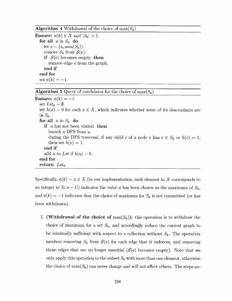
Algorithm 4 Withdrawal of the choice of max(Sk)
Ensure: c(k) E X and |Sk| > 1.for all a in Sk do
let e = (a, max(Sk)).remove Sk from S(e).if S(e) becomes empty then
remove edge e from the graph.end if
end forset c(k) = -1.
Algorithm 5 Query of candidates for the choice of max(Sk)
Ensure: c(k) = -1.set Lstk - 0.set h(x) = 0 for each x E X, which indicates whether some of its descendants arein Sk.for all u in Sk do
if u has not been visited thenlaunch a DFS from u.during the DFS traversal, if any child c of a node v has c E Sk or h(c) 1,then set h(v) = 1.
end ifadd u to Lst if h(u) = 0.
end forreturn Lstk.
Specifically, c(k) = x E X (in our implementation, each element in X corresponds to
an integer in [0, n - 1]) indicates the value x has been chosen as the maximum of Sk,
and c(k) -1 indicates that the choice of maximum for Sk is not committed (or has
been withdrawn).
1. (Withdrawal of the choice of max(Sk)): this operation is to withdraw the
choice of maximum for a set Sk, and accordingly reduce the current graph to
be minimally sufficient with respect to a collection without Sk. The operation
involves removing Sk from S(e) for each edge that it enforces, and removing
those edges that are no longer essential (S(e) becomes empty). Note that we
only apply this operation to the subset Sk with more than one element, otherwise
the choice of max(Sk) can never change and will not affect others. The steps are
228
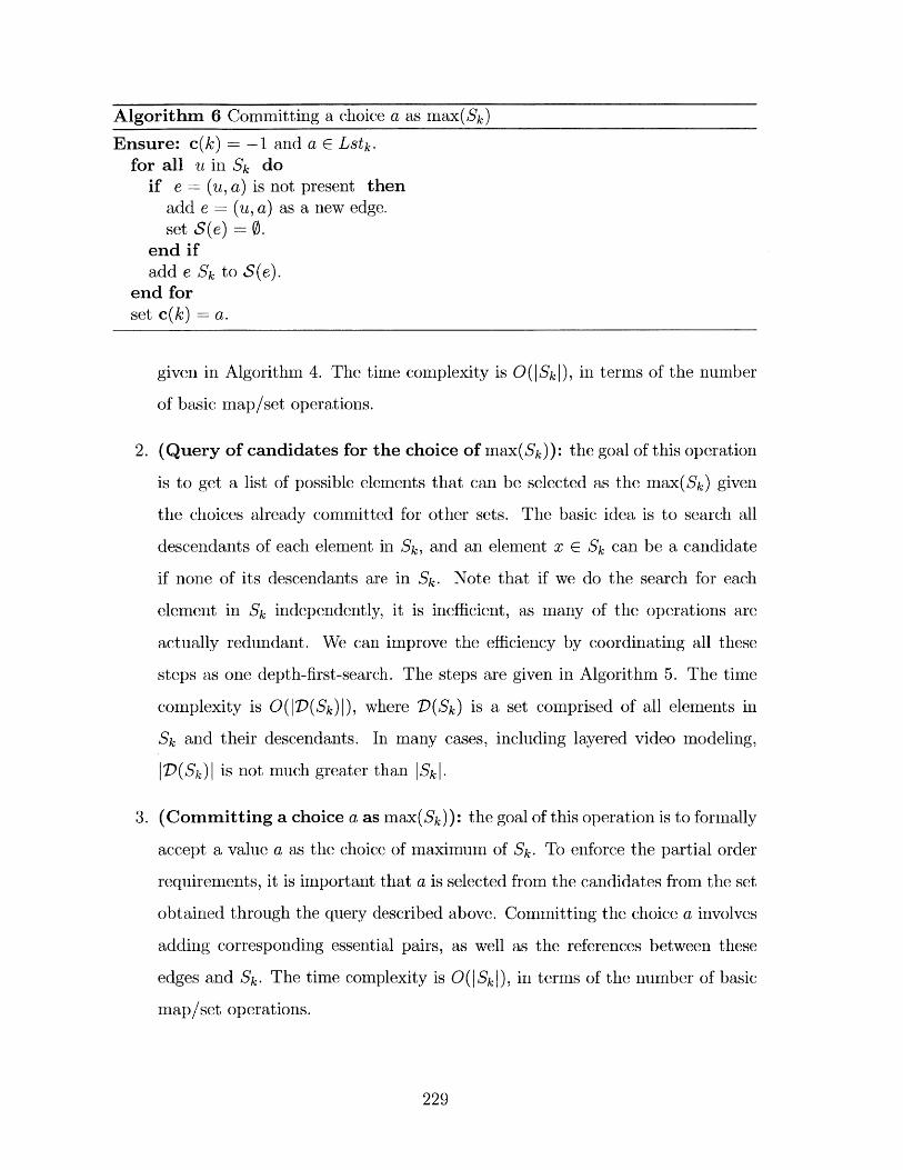
Algorithm 6 Committing a choice a as max(Sk)
Ensure: c(k) = -1 and a E Lstk.for all u in Sk do
if e = (u, a) is not present thenadd e - (u, a) as a new edge.set S(e) 0.
end ifadd e Sk to S(e).
end forset c(k) = a.
given in Algorithm 4. The time complexity is O(ISk|), in terms of the number
of basic map/set operations.
2. (Query of candidates for the choice of max(Sk)): the goal of this operation
is to get a list of possible elements that can be selected as the max(Sk) given
the choices already committed for other sets. The basic idea is to search all
descendants of each element in Sk, and an element x E Sk can be a candidate
if none of its descendants are in Sk. Note that if we do the search for each
element in Sk independently, it is inefficient, as many of the operations are
actually redundant. We can improve the efficiency by coordinating all these
steps as one depth-first-search. The steps are given in Algorithm 5. The time
complexity is O(|D(Sk)|), where D(Sk) is a set comprised of all elements in
Sk and their descendants. In many cases, including layered video modeling,
|D(Sk)| is not much greater than |SkI.
3. (Committing a choice a as max(Sk)): the goal of this operation is to formally
accept a value a as the choice of maximum of Sk. To enforce the partial order
requirements, it is important that a is selected from the candidates from the set
obtained through the query described above. Committing the choice a involves
adding corresponding essential pairs, as well as the references between these
edges and Sk. The time complexity is O(ISk|), in terms of the number of basic
map/set operations.
229
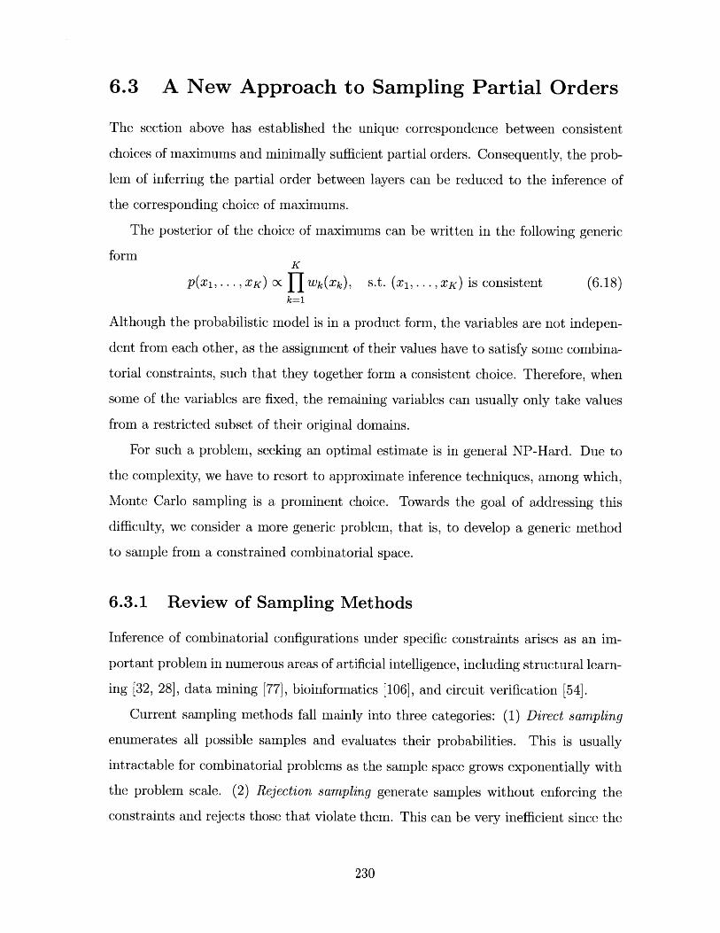
6.3 A New Approach to Sampling Partial Orders
The section above has established the unique correspondence between consistent
choices of maximums and minimally sufficient partial orders. Consequently, the prob-
lem of inferring the partial order between layers can be reduced to the inference of
the corresponding choice of maximums.
The posterior of the choice of maximums can be written in the following generic
formK
p(X1,... , XK) OC [1 Wk(Xk), s-t- (X1 ,... , XK) is consistent (6.18)k=1
Although the probabilistic model is in a product form, the variables are not indepen-
dent from each other, as the assignment of their values have to satisfy some combina-
torial constraints, such that they together form a consistent choice. Therefore, when
some of the variables are fixed, the remaining variables can usually only take values
from a restricted subset of their original domains.
For such a problem, seeking an optimal estimate is in general NP-Hard. Due to
the complexity, we have to resort to approximate inference techniques, among which,
Monte Carlo sampling is a prominent choice. Towards the goal of addressing this
difficulty, we consider a more generic problem, that is, to develop a generic method
to sample from a constrained combinatorial space.
6.3.1 Review of Sampling Methods
Inference of combinatorial configurations under specific constraints arises as an im-
portant problem in numerous areas of artificial intelligence, including structural learn-
ing [32, 28], data mining [77], bioinformatics [106], and circuit verification [54].
Current sampling methods fall mainly into three categories: (1) Direct sampling
enumerates all possible samples and evaluates their probabilities. This is usually
intractable for combinatorial problems as the sample space grows exponentially with
the problem scale. (2) Rejection sampling generate samples without enforcing the
constraints and rejects those that violate them. This can be very inefficient since the
230
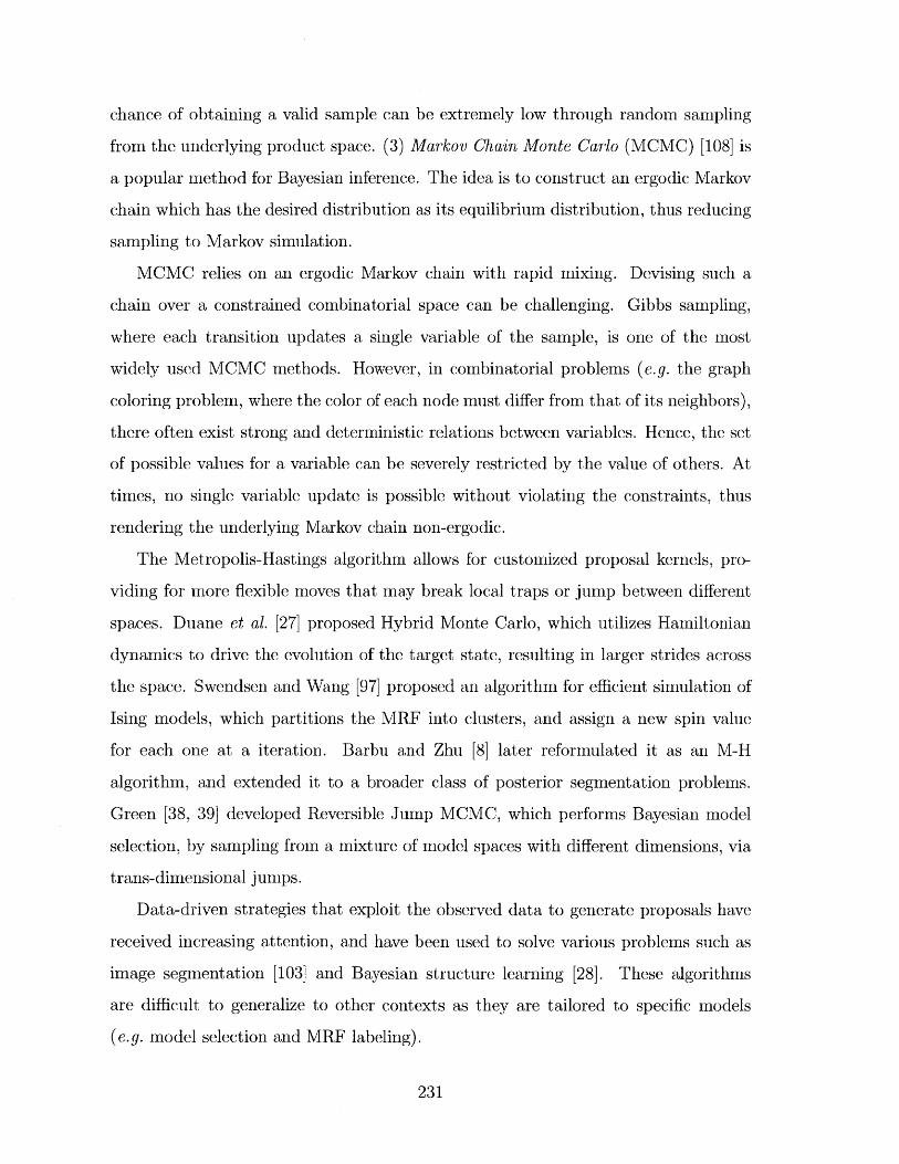
chance of obtaining a valid sample can be extremely low through random sampling
from the underlying product space. (3) Markov Chain Monte Carlo (MCMC) [108] is
a popular method for Bayesian inference. The idea is to construct an ergodic Markov
chain which has the desired distribution as its equilibrium distribution, thus reducing
sampling to Markov simulation.
MCMC relies on an ergodic Markov chain with rapid mixing. Devising such a
chain over a constrained combinatorial space can be challenging. Gibbs sampling,
where each transition updates a single variable of the sample, is one of the most
widely used MCMC methods. However, in combinatorial problems (e.g. the graph
coloring problem, where the color of each node must differ from that of its neighbors),
there often exist strong and deterministic relations between variables. Hence, the set
of possible values for a variable can be severely restricted by the value of others. At
times, no single variable update is possible without violating the constraints, thus
rendering the underlying Markov chain non-ergodic.
The Metropolis-Hastings algorithm allows for customized proposal kernels, pro-
viding for more flexible moves that may break local traps or jump between different
spaces. Duane et al. [27] proposed Hybrid Monte Carlo, which utilizes Hamiltonian
dynamics to drive the evolution of the target state, resulting in larger strides across
the space. Swendsen and Wang [97] proposed an algorithm for efficient simulation of
Ising models, which partitions the MRF into clusters, and assign a new spin value
for each one at a iteration. Barbu and Zhu [8] later reformulated it as an M-H
algorithm, and extended it to a broader class of posterior segmentation problems.
Green [38, 39] developed Reversible Jump MCMC, which performs Bayesian model
selection, by sampling from a mixture of model spaces with different dimensions, via
trans-dimensional jumps.
Data-driven strategies that exploit the observed data to generate proposals have
received increasing attention, and have been used to solve various problems such as
image segmentation [103] and Bayesian structure learning [28]. These algorithms
are difficult to generalize to other contexts as they are tailored to specific models
(e.g. model selection and MRF labeling).
231
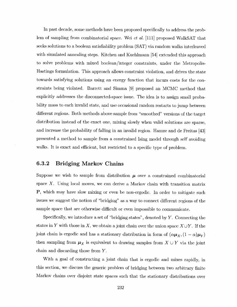
In past decade, some methods have been proposed specifically to address the prob-
lem of sampling from combinatorial space. Wei et al. [111] proposed WalkSAT that
seeks solutions to a boolean satisfiability problem (SAT) via random walks interleaved
with simulated annealing steps. Kitchen and Kuehlmann [54] extended this approach
to solve problems with mixed boolean/integer constraints, under the Metropolis-
Hastings formulation. This approach allows constraint violation, and drives the state
towards satisfying solutions using an energy function that incurs costs for the con-
straints being violated. Barrett and Simma [9] proposed an MCMC method that
explicitly addresses the disconnected-space issue. The idea is to assign small proba-
bility mass to each invalid state, and use occasional random restarts to jump between
different regions. Both methods above sample from "smoothed" versions of the target
distribution instead of the exact one, mixing slowly when valid solutions are sparse,
and increase the probability of falling in an invalid region. Hamze and de Freitas [43]
presented a method to sample from a constrained Ising model through self avoiding
walks. It is exact and efficient, but restricted to a specific type of problem.
6.3.2 Bridging Markov Chains
Suppose we wish to sample from distribution y over a constrained combinatorial
space X. Using local moves, we can derive a Markov chain with transition matrix
P, which may have slow mixing or even be non-ergodic. In order to mitigate such
issues we suggest the notion of "bridging" as a way to connect different regions of the
sample space that are otherwise difficult or even impossible to communicate.
Specifically, we introduce a set of "bridging states", denoted by Y. Connecting the
states in Y with those in X, we obtain a joint chain over the union space X U Y. If the
joint chain is ergodic and has a stationary distribution in form of (atx, (1 - a)py)
then sampling from px is equivalent to drawing samples from X U Y via the joint
chain and discarding those from Y.
With a goal of constructing a joint chain that is ergodic and mixes rapidly, in
this section, we discuss the generic problem of bridging between two arbitrary finite
Markov chains over disjoint state spaces such that the stationary distributions over
232
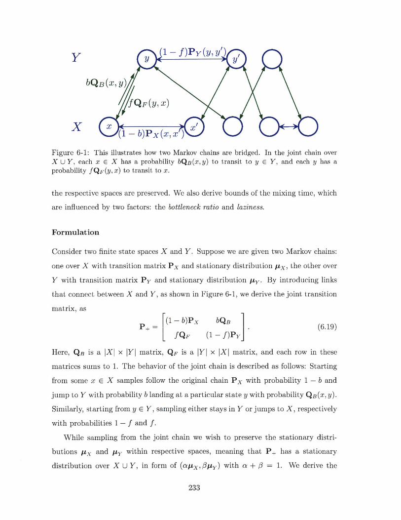
Y
bQB(x,
Figure 6-1: This illustrates how two Markov chains are bridged. In the joint chain over
X U Y, each x E X has a probability bQB(x,y) to transit to y E Y, and each y has aprobability fQF(y, x) to transit to x.
the respective spaces are preserved. We also derive bounds of the mixing time, which
are influenced by two factors: the bottleneck ratio and laziness.
Formulation
Consider two finite state spaces X and Y. Suppose we are given two Markov chains:
one over X with transition matrix Px and stationary distribution ptx, the other over
Y with transition matrix Py and stationary distribution py. By introducing links
that connect between X and Y, as shown in Figure 6-1, we derive the joint transition
matrix, as
+=F(1 - b)Px bQnl . (6.19)P fQF (1 - f)PYJ
Here, QB is a |X x |YI matrix, QF is a |Y| x |X| matrix, and each row in these
matrices sums to 1. The behavior of the joint chain is described as follows: Starting
from some x E X samples follow the original chain Px with probability 1 - b and
jump to Y with probability b landing at a particular state y with probability QB(X, y).
Similarly, starting from y E Y, sampling either stays in Y or jumps to X, respectively
with probabilities 1 - f and f.
While sampling from the joint chain we wish to preserve the stationary distri-
butions ix and py within respective spaces, meaning that P+ has a stationary
distribution over X U Y, in form of (apx, #pzy) with a + 3 = 1. We derive the
233
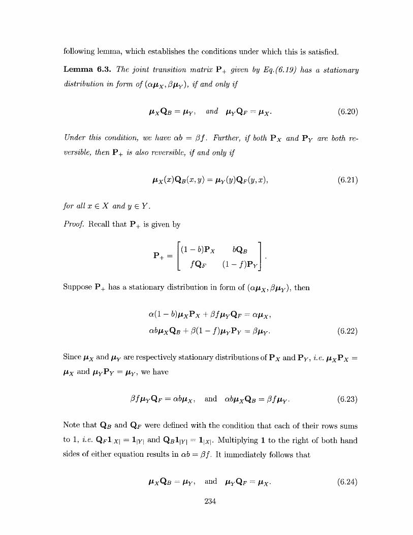
following lemma, which establishes the conditions under which this is satisfied.
Lemma 6.3. The joint transition matrix P+ given by Eq.(6.19) has a stationary
distribution in form of (aptx, puy ), if and only if
pXQB = yy, a
Under this condition, we have ab - Of.
versible, then P+ is also reversible, if and only if
pX W)QB p ) y (Y) QF(Y, X),
for all x E X and y E Y.
Proof. Recall that P+ is given by
[(1 - b)Px
Lf QF
bQB
(1 - f)PyJ
Suppose P+ has a stationary distribution in form of (apx, #py), then
a(1 - b)ptxPx + f AYQF apX,
aby/xQB + O(1 - f)pyPy = Opy.
Since iX and tty are respectively stationary distributions of Px and Py, i.e. pxPx
pX and pyPy = py, we have
O fIYQF = abpX, and abpXQB =Ofpy -
Note that QB and QF were defined with the condition that each of their rows sums
to 1, i.e. QF11XI lyl and QB11YI 1 X. Multiplying 1 to the right of both hand
sides of either equation results in ab = #f. It immediately follows that
pxQB = y and pYQF = pX- (6.24)
234
nd pYQF = pX' (6.20)
Further, if both Px and Py are both re-
(6.21)
(6.22)
(6.23)
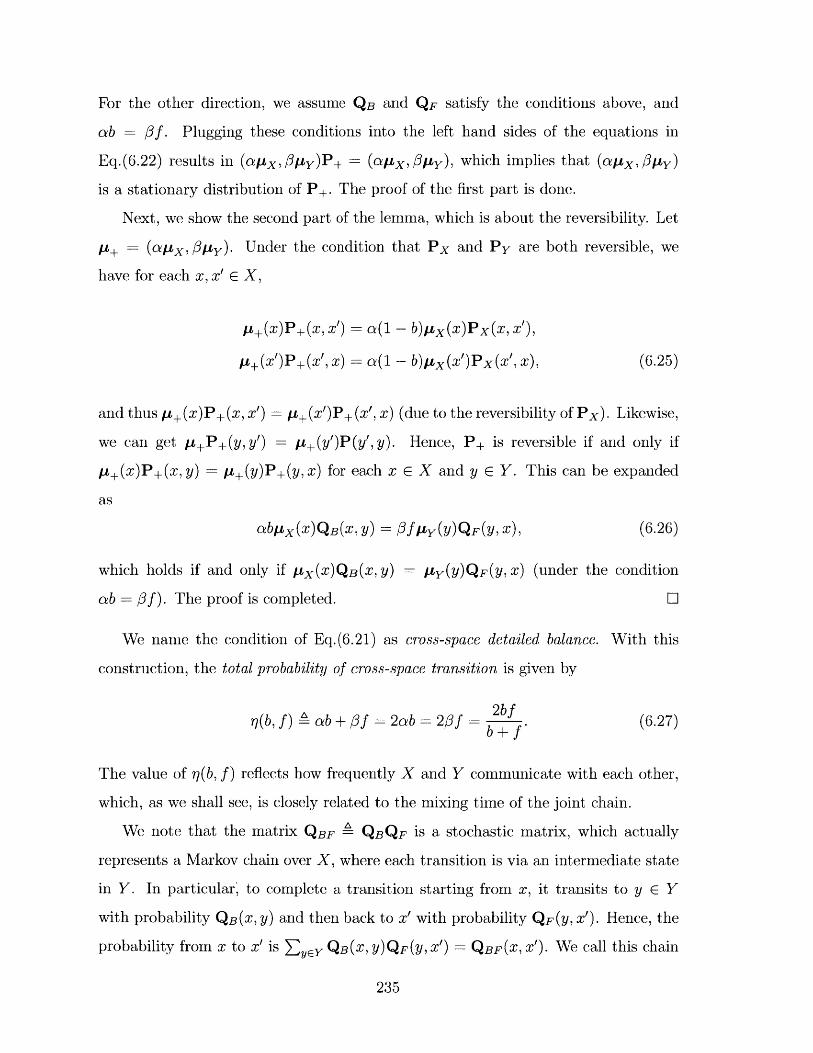
For the other direction, we assume QB and QF satisfy the conditions above, and
ab = #f. Plugging these conditions into the left hand sides of the equations in
Eq.(6.22) results in (apx, Opy)P+ = (apx, Opy), which implies that (apx, #py)
is a stationary distribution of P+. The proof of the first part is done.
Next, we show the second part of the lemma, which is about the reversibility. Let
p+ = (apx,#p~y). Under the condition that Px and Py are both reversible, we
have for each x, x' E X,
t+(x)P+(x, x') = a(1 - b)ttx(x)Px(x, x'),
p+(x')P+(x', x) = a(1 - b)Ax (x')Px (x', x), (6.25)
and thus p+ (x)P+(x, x') = p+(x')P+(x', x) (due to the reversibility of Px). Likewise,
we can get p+P+(y,y') = p+(y')P(y',y). Hence, P+ is reversible if and only if
p+(x)P+(x, y) = t+(y)P+(y, x) for each x e X and y E Y. This can be expanded
as
abyx(x)QB(x,y) = Of py(y)QF(y,X), (6.26)
which holds if and only if pux(x)QB(x, y) = yY(Y)QF(Y, x) (under the condition
ab = Of). The proof is completed.
We name the condition of Eq.(6.21) as cross-space detailed balance. With this
construction, the total probability of cross-space transition is given by
2bfr(b, f) ab+Of = 2ab 2#f = bf (6.27)
The value of 7(b, f) reflects how frequently X and Y communicate with each other,
which, as we shall see, is closely related to the mixing time of the joint chain.
We note that the matrix QBF QBQF is a stochastic matrix, which actually
represents a Markov chain over X, where each transition is via an intermediate state
in Y. In particular, to complete a transition starting from x, it transits to y E Y
with probability QB(X, y) and then back to x' with probability QF(Y, x'). Hence, the
probability from x to x' is E y QB(X, y)QF(y, X') QBF(X, X'). We call this chain
235
the collapsed chain of P+ over X. We can similarly get a collapsed chain over Y,
with transition matrix QFB QFQB-
Intuitively, these chains utilize states in the other space to provide alternative
transition routes, which, as stated by the following lemma, also lead to the same
stationary distributions.
Lemma 6.4. If the condition given by Eq. (6.20) holds, then px and py are respec-
tively stationary distributions of QBF and QFB- Moreover, if P+ is reversible, then
both QBF and QFB are reversible.
Proof. If (cLx, 3py) is a stationary distribution of P+, then Eq.(6.24) holds. Thus,
pXQBQF - yYQF =AX, (6.28)
implying that pzx is a stationary distribution of QBQF. Similarly, we can show that
py is a stationary distribution of QFQB.
Furthermore, if P+ is reversible, according to Lemma 6.3, we have px(x)QB(x, y)
AYy(y)QF(y, x) for each x E X and y E Y. Then for any x, x' E X,
px(x)QBF(X, X') A (X) S QB(X, Y)XQF((Y, X')yEY
S (x(x)QB (XY)QF (Y, X')yEY
= Y y(Y)QF(M X)QF (Y, X)yEY
Similarly, we can get
X(x')QBF(4 X) p M y(Y)QF(Y, X)QF (Y, X) -yEY
Hence,
pX (X)QBF tha QBF p rX We QBF e a - (t-2)
This implies that QBF is reversible. Likewise, we can show that QFB is reversible
236
under the condition that P+ is reversible. The proof is completed. E
On the other hand, as we will discuss later, the ergodicity and the mixing time of
the joint chain also depend on the characteristics of QBF and QFB-
6.3.3 Mixing Time Analysis
The efficiency of a Markov chain is often measured by the mixing time. Given an
ergodic Markov chain over X, with equilibrium distribution p, the mixing time is
tmix(E) A min{t : max |Pt(x,) - p||TV < E}. (6.30)
We assume that the eigenvalues of P are 1 - A, ... > A_ > -1. Then, the absolute
spectral gap of P is defined to be y,(P) A min{1 - A2 , 1 + A,}. The theorem [62]
below shows that the mixing time closely relates to this absolute spectral gap.
Theorem 6.2. Given a reversible Markov chain with transition matrix P, and E E
(0,1/2), then
log(1/(2E))(T - 1) tmix(E) log(1/(EymiJ))T-. (6.31)
Here, T is called the relaxation time, given by 1/'Y*(P).
In general, a chain tends to have slow mixing when the absolute spectral gap
is small, and when the gap is zero, the chain is non-ergodic and never mixes. The
absolute spectral gap depends on two factors, namely the bottleneck ratio, which
affects the value of 1 - A2 , i.e. the spectral gap, and the laziness of transition, which
influences 1 + A,.
Flows and Bottleneck Ratio
Given a Markov chain with transition matrix P, which has a stationary distribu-
tion p. For x, x' E X, we define the transition flow (or simply flow) from x to
x' to be F(x, x') A p(x)P(x, x'). For a reversible chain, the flows are symmetric,
i.e. F(x, x') = F(x', x). The notion of flow can also be extended to sets. Let A
237
and B be subsets of X, then the flow from A to B is defined to be F(A, B) A
ZXEA Zx'EB .T(x, x').
Consider a partition of X into two subsets S and its complement Sc, then the
transition flow ratio of S is <D(S, SC; P) A F'(S, Sc)/ min{p.(S), pi(Sc)}, where p is
used as a measure, i.e. pt(S) = ExEs p(x). Taking the minimum of such ratio values
of all partitions, we get the bottleneck ratio, which is formally defined as
( .F(S, Sc)<b,(P) = min '(S) C)} : S) SC # 0 . (6.32)
ScX min p(S),W pS)}
Jerrum and Sinclair [50] derived the theorem below that establishes both a lower
and upper bound of the spectral gap in terms of bottleneck ratio.
Theorem 6.3. Let A2 be the second largest eigenvalue of a reversible transition matrix
P, then
<D(P)/2 < 1 - A2 2<b,(P). (6.33)
This theorem shows that increasing the bottleneck ratio tends to expand the
spectral gap, and thus reduce the mixing time. Through theoretical study, we found
that the bottleneck ratio of the joint chain P+ given by Eq. (6.19) depends on both how
frequently the chain jumps between X and Y and how well the forward and backward
links couple with each other. The former is controlled by f and b, while the latter is
mainly reflected by the spectral structure of the coupled chain: QBF and QFB. We
further derived specific bounds that characterize their relations:
Theorem 6.4. The reversible transition matrix P+ as given by Eq. (6.19) has
,q(b, f) #' <b, < (P+) < max{b, f}. (6.34)2 $+ 1
Here, 77(b, f) = 2ab = 2Bf is the total probability of cross-space transition, $
min{<bC(QBF), D*(QFB)}-
This theorem gives both a lower bound and an upper bound of the bottleneck
ratio of P+. We can see that the bottleneck ratio is influenced by two factors: (1) the
238
frequency of cross-space transition. Frequent transition between X and Y generally
results in high bottleneck ratio; while if the communication between them is inactive,
the bottleneck ratio would be very low, leading to slow mixing. (2) the bottleneck
ratio of the collapsed chains. High bottleneck ratios of the collapsed chains indicate
that transition between different regions is made easy with the intermediate states,
and thus the joint chain can mix rapidly. More importantly, this theorem leads to:
Corollary 6.1. The joint chain P+ is ergodic when the collapsed chains (QBF and
QFB) are both ergodic.
Proof of Theorem 6.4
To prove theorem 6.4, we first establish a lemma on flow decomposition, and then
accomplish the proof based on the lemma.
For the joint chain P+, we analyze its bottleneck ratio by decomposing the flows.
Consider a partition of the union space X U Y into two parts: A U B (with A C X
and B C Y) and AC U BC (with AC = X/A and BC = Y/B). The flow between them
comprises three parts:
F(A, Ac) +.F(B, BC) + (.F(A, BC) + T(B, Ac)).
Here, F(A, Ac) is the flow within X, F(B, Bc) is the flow within Y, and F7(A, Bc) +
7(B, Ac) is the flow between X and Y. The first two are inherited from the original
Markov chains. We focus on the third one, which reflects the effect of bridging. For
this part of flow, we derive the following lemma by decomposing it along multiple
paths.
Lemma 6.5. Given arbitrary partition of X U Y into Au B and Ac U BC as described
above, we have
.F(A, BC) + .F(B, AC) > ab - 4 *(QBF)PX(A), (6.35)
239
when px(A) px(Ac), and
.F(A, Bc) + .F(B, Ac) >Of - (QFB)py(B), (6.36)
when py(B) py(BC).
Proof. To analyze the flow F(A, BC) + .F(B, AC), we further decompose it along mul-
tiple paths. Then, we have
F(A, B) = S abyX(x)QB(x, Y)xEA yEBC
(6.37)
= ab pX (x)QB(x,Y) 5 F (Y, x)xEA YEBc x' EEX
In this way, we decompose the flow into a sum of the terms in form of px(x)QB(x, Y)QF(Y,
which we call the path weight along x -+ y -+ x', denoted by w(x, y, x'). We can then
rewrite F(A, B) as
.F(A, B) = abxEA yEB x'eX
For conciseness, we use w(A, B, C) to denote the sum of paths traveling from A, via
B, and ending up in C, i.e. ExcAZ YEBZ x'c w(x, y, x'). Then, we have
.F(A, BC) ab(w(A, B , A) + w(A, BC, Ac)),
F(AC, B) ab(w(Ac, B, A) + L(AC, B, Ac)).
(6.39)
(6.40)
As F is symmetric for a reversible chain, we have F(B, AC) = F(AC, B), and thus
F(A, BC) + F(B, AC) ab(w(A, BC, Ac) + w(Ac, B, A))
= ab w(A, Y, Ac) (6.41)
240
w(x, y, X'). (6.38)
On the other hand, we note that
E W(x, y, x')xEA yeY x'sAc
xEA yeY x'scAc
x7A EC (x)xEA x'EAc
(X) QB(X, Y) QF (Y, X I
5 QB(X, y)QF(y, x')yCY
(6.42)=-SE Ix(x)QBF(XX) -xE A x'cAc
This is exactly the flow from A to Ac with respect to the collapsed chain QBF, i-C-
w(A Y, Ac) QBF(A, A). (6.43)
Assuming pxu(A) < ptx(AC), we have FQBF(A, Ac) D*(QBF)p(A), by the definition
of bottleneck ratio. Combining this with Eq.(6.41) results in
.F(A, Bc) +F(B, A) > ab -w( A,Y, Ac)
(6.44)
Likewise, with the assumption py(B) py(Bc), we have
F(A, Be) + .F(B, Ac) > #f -<D*(QFB)pY(B). (6.45)
The proof of the lemma is completed. D
Next, we continue to prove the main theorem.
Proof. Let p+ = (atx, Opy) be the stationary distribution of P+. For conciseness,
we let F,(A, B) A F(A U B, Ac U BC). When A and B are clear from the context,
we simply write F,. Then the bottleneck ratio of P+ is the minimum of the values
of F,(A, B)/I+(A U B), among all possible choices of A C X and B c Y such that
p+ (A U B) < 1/2 and A U B # 0. Throughout this proof, we assume A c X, B c Y,
241
w(A, Y, A')
> ab -<D,(QBF)pX -A)
and p-+(A U B) < 1/2, i.e. apx(A) + #py(B) < 1/2.
Under this assumption, there are three cases, which we respectively discuss as
follows.
Case 1. px(A) < 1/2 and py(B) < 1/2.
We have # = min{D(QBF), (*(QFB)} in the theorem. In addition, F, > F(A, BC)+
F(B, Ac). Combining this with Lemma 6.5, we get
F, > ab - #px(A), and F, > #f - #py(B). (6.46)
Note that q/2 ab = Of and a + #= 1. Thus
F8 aF8 ,+#F8Fs(> > B - ( ± ( r/#/2.pt+(A U B) - aptx(A)+#p~y(B) -(6.47)
Case 2. px(A) < 1/2 and py(B) > 1/2.
Given arbitrary K > 2, there are two possibilities:
Case 2.1. 1/r < px(X) < 1/2 and py(B) > 1/2. Then
1F8 > ab.- #px(A) > -ab#5.
K;(6.48)
Recall that p+(A U B) < 1/2. Thus
Fs 2u#p(A U B) -- K 2 (6.49)
Case 2.2. puX(X) < 1/t and py(B) > 1/2. Here, we utilize the following fact:
Fs > F(B, Ac) = F(B, X) - F(B, A). Then, by the definition of flow, we have
.F(B, X) = #fy(B) > Of /2, (6.50)
and by the symmetry of F (due to reversibility),
F(B, A) = F( A, B) F( A, Y) = ab/ r. (6.51)
242
With ab = 3f, combining the results above leads to
F, > #f /2 - ab/ = ab(1/2 - 1/). (6.52)
As a result, we get
Fs > 2ab(1/2 - 1/i) = 2(1 - 2/r,). (6.53)p+(A U B) 2
Case 3. px(A) > 1/2 and pty(B) < 1/2. Following a similar argument as we
developed above for case 2, given r, > 2, we can likewise get
Fs I 2 (px(X) > 1/s'),> 2 (6.54)
pL+(A U B) ((1 - 2/s,) (pX(X) < 1/n).
Note that ptx(A) > 1/2 and py(B) > 1/2 cannot hold simultaneously under the
assumption apx(A) + #ty(B) < 1/2. Integrating the results derived for all cases,
we obtainFs (A, B)- min 1 - 2 ,W> 2. (6.55)p-+(A, B) 2 K K
Note that this inequality holds for all A and B with 0 < p+(A U B) < 1/2. In this
way, we can get a series of lower bound of the bottleneck ratio, using different values
of K. And the supreme of these lower bounds remains a lower bound. It is easy to
see that the supreme attains when 2#/K - 1 - 2/K, leading to
sup min -#, 1- - (6.56)K>2 1+#
It follows that
<D*(P+) ; - . (6.57)2 # + 1
This completes the proof of the lower bound. Next, we show the upper bound, which
is easier. Due to the definition of bottleneck ratio, for any given partition of X U Y,
the flow ratio derived from that partition constitutes an upper bound of <D,(P+).
243
Here, we consider the partition with one part being X and the other being Y.
Then
F, = ab =3f, (6.58)
and thus the flow ratio is given by
F8mns = max(f, b). (6.59)minl(a, #
This gives an upper bound of <D,(P+). The proof of the theorem is completed. E
Laziness
Whereas increasing bottleneck ratio can enlarge the spectral gap, 1 - A2 , the mixing
time also depends on 1+ A, the distance between A, and -1. In general, a reasonable
value of 1 + A, can be achieved by laziness.
Lemma 6.6. Let P be a reversible transition matrix over X, such that P(x, x) > >
0 for each x E X then its smallest eigenvalue A, has A, > 2 - 1.
This shows that by maintaining a probability ( > 0 for the chain to stay (without
transiting to other states), we can keep A, away from -1.
Proof. Let P' = (P - I)/(1 - (). Since P has P(x, x) > ( for each x E X, the entries
of the matrix P' are all non-negative. In addition,
1 1P'1 = (P - (I)1 = I '(1 - (1) = 1. (6.60)
This implies that P' is also a stochastic matrix. Since P is reversible, all its eigenvalues
are real numbers. Without losing generality, we assume they are A, > ... > A,.
As P is a stochastic matrix, we have A, = 1 and A, > -1. According to the
spectral mapping theorem, the eigenvalues of P', denoted by A', .... , A', are given by
A' = (Ai - ()/(1 - (), for each i = 1,... ,n. As P' is a stochastic matrix, we have
A' > -1 and thus A-- > -1. Therefore, A > 2( - 1. The proof is completed. D
244
Given an arbitrary reversible chain with transition matrix P, we can make it
lazier by changing P to (1 - ()P + (I. However, it is worth noting that increasing
the laziness coefficient ( would on the other hand shrink the spectral gap from 1 - A2
to (1 - ()(1 - A2 ). Hence, it is advisable to select a ( that balances laziness and
spectral gap. Here, the optimal ( that maximizes the absolute spectral gap is given
by (= (A2 + An)/(A2 An - 2). When it is difficult to derive A2 and An, one can use
the estimates to set (.
6.3.4 Hierarchical Bridging Markov Chain
Based on the theory of bridging Markov chains, we develop practical algorithms to
construct the bridges and sample from the joint chain.
Construction of Bridges
Come back to our original problem of sampling from a distribution px over X, for
which we can get a Markov chain Px based on local moves. To improve the mixing,
we introduce "bridges" to facilitate non-local transition. Specifically, we first choose a
collection of state subsets of X: Si,. . . , Sm, and create a bridging state yi for each Si.
In this way, we get a set of new states Y ={yi, ... , ym}. Suppose each target state
in X has been covered by some such subset Next, for each x E X, we set a transition
probability QB(X, yi) = 1/m(x) for each yi associated with with it, i.e. x E Si, where
m(x) is the number of such bridges, and set QB(X, yi) = 0 when x ( Si. According to
Lemma 6.3, we can construct QF, the transition probabilities from Y to X, as follows
QF(yi, X) AX (X) / S [LX (X). (6.61)
It is not difficult to verify that the matrices QB and QF as above satisfy the cross-
space detailed balance in Eq.(6.21), with py given by
py(yS) c p:X(x'). (6.62)xESi
245
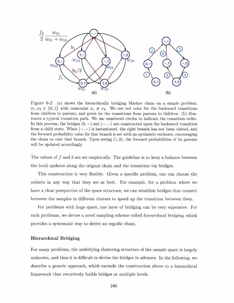
f2 W01-,
b2 20~ 31
0' - W10 - 10W0 2 0- ,' _1 -,0
0,1 1,0 0,1 1,0
(a) (b)
Figure 6-2: (a) shows the hierarchically bridging Markov chain on a simple problem:X1, X2 E {0, 1} with constraint x1 $ X2. We use red color for the backward transitionsfrom children to parents, and green for the transitions from parents to children. (b) illus-trates a typical transition path. We use numbered circles to indicate the transition order.In this process, the bridges (0, -) and (-, -) are constructed upon the backward transitionfrom a child state. When (-, -) is instantiated, the right branch has not been visited, andthe forward probability value for that branch is set with an optimistic estimate, encouragingthe chain to visit that branch. Upon seeing (1, 0), the forward probabilities of its parentswill be updated accordingly.
The values of f and b are set empirically. The guideline is to keep a balance between
the local updates along the original chain and the transition via bridges.
This construction is very flexible. Given a specific problem, one can choose the
subsets in any way that they see as best. For example, for a problem where we
have a clear perspective of the space structure, we can establish bridges that connect
between the samples in different clusters to speed up the transition between them.
For problems with huge space, one layer of bridging can be very expensive. For
such problems, we devise a novel sampling scheme called hierarchical bridging, which
provides a systematic way to derive an ergodic chain.
Hierarchical Bridging
For many problems, the underlying clustering structure of the sample space is largely
unknown, and thus it is difficult to devise the bridges in advance. In the following, we
describe a generic approach, which extends the construction above to a hierarchical
framework that recursively builds bridges at multiple levels.
246
Initially, we have the target state space X, where each sample is a discrete vector,
in form of (x 1, ... , XK). The target states constitute the 0-th level of the hierarchy.
For the first level of bridging, we introduce a set of bridges, denoted by Y1. Each
bridge in Y corresponds to a partial assignment, i.e. a vector with one of the value
removed. Take a state space {0, 1}3 for example. Consider (0, 0, 0) E X. By removing
the middle value, we get a partial vector (0, -, 0), where - indicates a slot at which
the value is removed. All vectors in form of (0, x 2, 0), which include (0, 0, 0) and
(0, 1, 0) here, are called the children of (0, -, 0), and (0, -, 0), in turn, is called the
parent of them.
Given bo, fi < 1, the transition between X and Y is described as follows. Starting
from a target state x E X, with probability 1 - bo, the chain stays in X, and with
probability bo, it transits to the parent of x in Y, by randomly removing a value.
Note that a vector of length K has K different parents, and thus the transition
probability from x to any particular parent is b0 /K. Starting from a bridge y E Y,
with probability 1 - fi, it stays at y, and with probability fi, it transits back to
X. In particular, the transition probability from y = (x1,... , -,... , XK) to x =
(x 1 , ... , Xz, ... , xK) is proportional to pz(x). To calculate this probability, one only
have to evaluate of pz(x) up to a scale. This is a useful property, as the normalization
constant of a distribution is often difficult to evaluate in practical problems.
The construction of the hierarchy can be completed by recursively adding levels
up to the root (the K-th level). Each bridge at the k-th level (denoted by Y)
is a partially assigned vector with k entries removed. Starting from y E Yk, the
probability of transiting to the upper level Yk+1 is bk. Specifically, each y E Y has
K - k assigned values, and thus it has a probability bk/(K - k) to transit to any of its
parent by randomly removing one of the assigned values. The chain also has a total
probability fk to transit to the lower level Yk-1. To accomplish such a transition, we
randomly pick one of the k unassigned slots (say the j-th entry), and draws a value
for xj, resulting a child state y'. The forward transition probability from y to y' is
proportional to pk_1(y'). For any bridge state y E Yk, the value pk(Y) is defined via
247
the recursive formula below
Pk(Y) C< S k_1(y). (6.63)y'cCh(y)
When k = 0, pto(x) A p(x) for x E X. Here, Ch(y) is the set of y's children in Yk-1.
Through this construction, we obtain a joint chain over X U Y U -- - U YK, which
we call the hierarchically bridging Markov chain, as illustrated in Figure 6-2(a). We
derive the theorem below that characterizes this chain:
Theorem 6.5. The hierarchically bridging Markov chain with bk < 1 for k = 0, ... , K-
1, and fk < 1 for k 1,..., K is ergodic. If we write the equilibrium distribution in
form of (CIO, O1p1,... , /K/pK), then (Si) yo equals the target distribution y; (S2) for
each k > 1, and y e Yk, pk(y) is proportional to the total probability of its descendant
target states (the target states derived by filling all its placeholders); (S3) a, the prob-
ability of being at the target level, is given by a- 1 1 I 3 (b0 ... b+_)/(f1 - fK).
Here, we briefly explain the statements. (Si), together with the proved ergodicity,
establishes the correctness of the construction, i.e. drawing samples from the joint
chain and retaining only those from X amounts to directly sampling from p. (S2)
characterizes the distribution within other levels. (S3) gives the probability that a
state drawn from the joint chain is a target state. From this statement, we derive
Corollary 6.2. If bk/fk+1 < K < 1 for each k = 1, . . . , K, then a > 1 - K.
This lower bound of a is independent from the number of levels K. Consequently,
despite the problem scale, one can maintain a considerable chance of drawing a target
state from the joint chain by keeping the backward/forward ratio below 1.
This corollary can be easily shown as follows.
Proof. Based on Theorem 6.5, we have
K bo -.. bk_1 < 1+ I Kk 1 (6.64)a + 1- fl 1 -
Hne k1
Hence, a > 1 - n~. The proof is done.D
248
Proof of Theorem 6.5
We show this theorem by progressively proving a series of claims as follows.
Claim 1. The augmented Markov chain is ergodic.
Proof. With bk > 0 for k = 0,... , K - 1, the root is accessible from each state
(including both complete and partial assignments). With fk > 0 for k = 1,..., K,
each state is accessible from root. These imply that any two states are accessible
from each other via the root. Therefore, the chain is irreducible. In addition, fK < 1
makes the chain aperiodic. As this is a finite Markov chain, we can conclude that it
is ergodic.
Since the chain is ergodic, it has a unique stationary distribution, i.e. its equi-
librium distribution. Therefore, it suffices to show that (apo, #1pi, .... , 3 KyK) that
satisfies the three statements in the theorem is a stationary distribution. D
Claim 2. Given vectors yo,... , pK respectively over the set of states at level
0,... , K, such that -o = y is a distribution over X, and for each k = 1,... , K, Pk
is defined recursively by
1p'k(Y) K (k 1) S L1(x), for y e Yk. (6.65)
xECh(y)
Then, pk for each k = 1, ... , K represents a distribution over Yk, and
-1
pk (Y) - (x), Vy E Y. (6.66)
Here, x >- y means that x is a descendant of y.
Proof. Obviously, when k = 1, according to the definition above, we have
1(y) = px(x) = p(x). (6.67)xeCh(y) xECh(y)
249
KThis satisfies Eq.(6.66), as = K, and it is clear that il is non-negative. In
addition, we have
p1(y) = Epx)yEY1 yEY1 xECh(y)
KZ Z px)yEY xECh(y)
p z(x) 1 .(6.68)xEX yEPa(x)
Here, Pa(x) is the set of parent states of x. In the derivation above, we use the fact
that x has K parents, i. e. |Pa(x)| = K. The identity above implies that p1 is a valid
distribution over Y. Therefore, the claim holds when k = 1.
Suppose that the claim holds for k = 1, ... , m with m < K, we are to show that it
also holds for k = m+ 1, so as to complete the induction. Note that yzm+1 is defined
as
p"m+(Y) = K n p Im(x), for y E Ym+1.xECh(y)
Again, ym+1 is obviously non-negative, and
pm+1(Y>) =K mS pm(z)yEYm+l yEYm+l zECh(y)
K m m(z) 1 11= (6.69)zEYm yEPa(x)
Similar to the derivation for k 1, here we apply the fact that Pa(x) = K - m for
each x E Ym. This shows that pm+1 is a valid distribution over Ym. Moreover, we
250
have for each y E Ym+1,
1ym+(Y) K - m
zECh(y)
-1K
kmJ)
1 (K - m)!m!
K-rm K!zeCh
(K - m - 1)!m!K! (m+1)
K
M +1 XEX:x>-y
xEX:x>-z
(y)
p x)xEX:x>-z
xEx:x>-y
p(X).
By induction, we can conclude that the claim holds for each k = 1, . . . , K.
When the construction is done up to the k-th level, the distribution p+ A
(ckOpO,... , ck,kp) is a stationary of the augmented Markov chain. Here, yo,... A
are given by Claim 2, and Ck,O,... , ck,k is defined such that for each k' = 0,... , k
1' Zk
with
1 bo --- bi_1Ck i - fl ... fl
' Zk f1i-- -fi
k.
Zk - 1+ .b0 f i _ .
Proof. We are going to show this claim by induction. Note that pO = y over X is a
stationary distribution of P. And po co,opo, thus co,o = 1. It immediately follows
that the claim is true for k - 0. Suppose this claim holds for k = 0,. . . , m with
m < K, we are to show that it also holds for k - m + 1. Note from Eq.(6.71) that
Cm+1,k _ ZmCm,k Zm+1'
Vk =0).I,
Hence, showing the claim holds for k =rn+1 is equivalent to showing that (cp, ,tm+i)
251
Claim 3.
(6.70)
F
(6.71)
(6.72)
(6.73)
7
is a stationary distribution of the augmented chain (up to (m + 1)-th level), with
Zm (6.74)Zm+1'
and0 3 Zm+1 - ZM 1 be --. bm (6.75)
Zm+1 Zm+1 fi ' -- fm+i
According to Lemma 6.3, it suffices to check that this distribution satisfies the cross-
space detailed balance given in Eq.(6.21), which is not difficult to verify based on the
construction described in section 3.2. D
In this proof, Claim 1 proves the ergodicity of the joint chain. Claim 2 con-
structs a set of vectors yo,... pJ, and states that they are valid distributions over
X, Yo, ... , YK, and satisfy the properties given in (S2). Claim 3 (induction up to
k = K) shows that the distributions constructed in Claim 2 is exactly a stationary
distribution of the joint chain. Since the chain is ergodic, this is the equilibrium
distribution. As a by product, Claim 3 also shows the the statement (S3) of the theo-
rem. For (Si), it is automatically established by the construction described in Claim
2. Therefore, we can conclude that the proof of the theorem has been completed.
6.3.5 Dynamic Construction
Whereas the total number of bridges can be huge generally for a moderate problem,
which however need not be explicitly instantiated prior to sampling. Instead, we can
build the chain progressively along with the sampling procedure. As shown in Figure 6-
2(b), except for the initial state that we start with, each state is instantiated only
upon the first transition to it. In addition, we maintain references from each state to
all its parents and children, to facilitate the transition from one state to another.
When a bridge state is constructed, one needs to determine the forward transition
probabilities from this state to its immediate children. Exact evaluation of these
probabilities requires complete knowledge of the distribution of all its descendants,
which is generally unavailable upon the construction. A natural idea is to obtain such
252
information by recursively visiting all the descendants. However, the complexity of
this method can grow exponentially as we travel up along the hierarchy, making it
infeasible in practice.
To address this issue, we adopt a dynamic programming strategy. Consider a
bridge y at the k-th level with a set of children Ch(y). Recall that for each child
state y' E Ch(y), the forward transition probability from y to y' is proportional to
pk1(y'). If y' has been visited, then pki(y') is immediately available. Otherwise, we
initially use a quick estimate of pk1 (y') and update it when y' and its descendants
are visited.
In general, one can overestimate the forwarding probability of an unvisited branch,
thereby encouraging exploration of unknown regions. The initial value need not be
accurate, as it is updated as the branch below y' is visited. A possible way to this
quick estimation is to assume all assignments in that branch are valid (i.e. satisfying
all constraints). For both applications described in next section, we employ this
way, which results in an estimate as the product of the marginal probabilities of the
available values.
In this scheme, the transition probabilities can change dynamically, resulting in
time-inhoniogeneity. In practice, such changes to the chain happen primarily during
burn-in, and thus have negligible effect on asymptotic behavior. It is also worth noting
that while the total number of states in X can be tremendous even for a problem
with moderate size, our algorithm generally only visit those states with non-negligible
probabilities. Though just constituting a small fraction of the entire space, they still
provide a close approximation of the target distribution.
6.4 Experiments
We assess the effectiveness of the proposed method on both synthetic and real data.
Specifically, we first test it on a constrained binary labeling problem, where the pro-
posed sampling algorithm is used to sample from the solution space subject to a set
of synthetic constraints. As the ground-truth is available for this problem, we can
253
perform a systematic study through this set of experiments.
We also test this approach on layered modeling for images and videos. The aim
here is to demonstrate both the effectiveness of the sampling method in sampling
partial orders and the the use of partial orders combined with our sampling approach
improves the solution.
6.4.1 Constrained Binary Labeling
Given a graph with n nodes and m edges, we are to set a binary label xi E {O, 1}
to each node. Here, each edge is associated with a constraint on the labels of its
two ends (e.g. xi j xj). We use an n-dimensional vector x E {0, 1} to represent a
label configuration, and use Q to denote the set of all configurations that satisfy the
constraints. In addition, each node has a preference function w: {0, 1} -+ R+. Then,
we get a distribution over Q, given by p(x) oc ]1'" wi(xi). While the probabilities are
in a product form, the labels are not independent as they are related to each other
via the constraints. This formulation actually stems from real world problems, such
as circuit design, scheduling, and object placement.
We first consider a 4-connected graph with 5 x 5 nodes. Though the graph might
seem small, it is sufficient to generate a large enough state space (up to 225), where
the differences of algorithm behaviors can be clearly seen. Importantly, with this
scale, it is feasible to evaluate the entire distribution through enumeration, enabling
direct comparison between the sample distribution and the true one. To obtain a
constrained problem, we randomly draw a constraint for each edge from a set of
constraints (xi = xj, xi f xj, xi = 1 or xo = 1, etc). In this way, we generate a set of
20 constrained labeling problems as a testbed.
On these problems, we compare three algorithms:
1. Gibbs sampling with long jump (GS-Jump): a method adapted from the one
proposed by [9]. At each iteration, we update all variables by Gibbs sampling,
and then propose a jump to arbitrary configuration drawn from the product
distribution, accepting it if the result is valid.
254
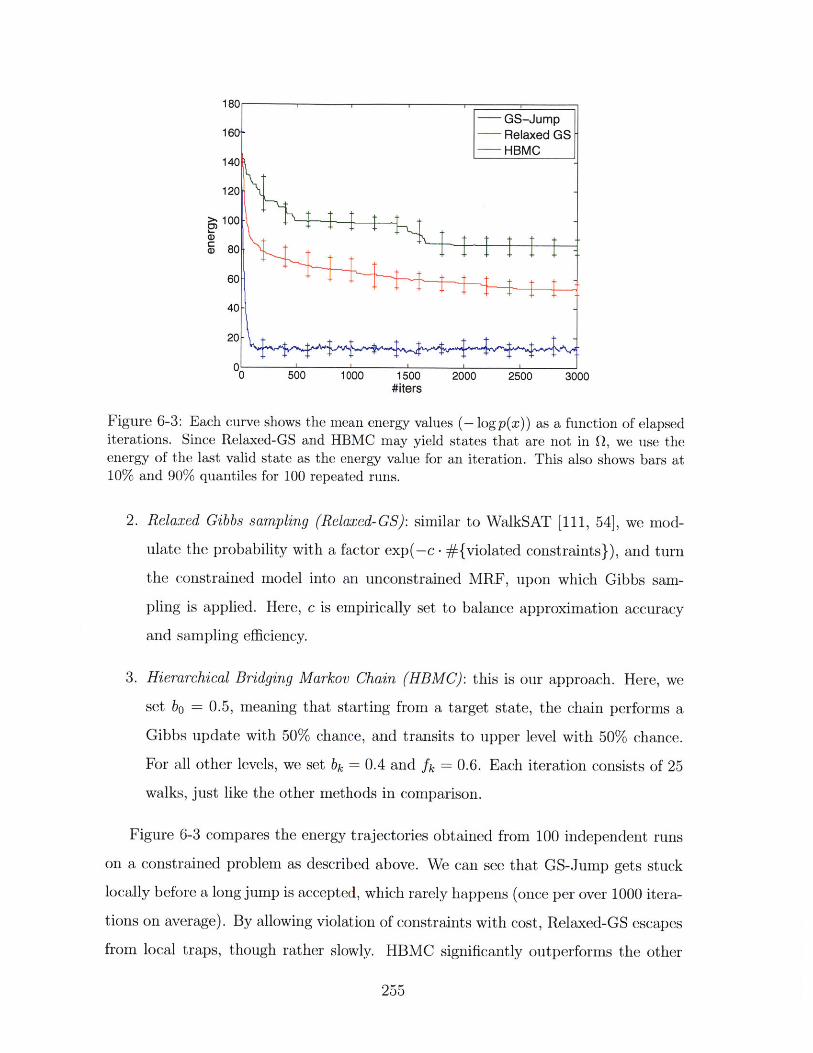
>100-4
8ao(D 80
60
40-
20-
0 500 1000 1500 2000 2500 3000#iters
Figure 6-3: Each curve shows the mean energy values (- log p(x)) as a function of elapsediterations. Since Relaxed-GS and HBMC may yield states that are not in Q, we use theenergy of the last valid state as the energy value for an iteration. This also shows bars at10% and 90% quantiles for 100 repeated runs.
2. Relaxed Gibbs sampling (Relaxed-GS): similar to WalkSAT [111, 54], we mod-
ulate the probability with a factor exp(-c -#{violated constraints}), and turn
the constrained model into an unconstrained MRF, upon which Gibbs sam-
pling is applied. Here, c is empirically set to balance approximation accuracy
and sampling efficiency.
3. Hierarchical Bridging Markov Chain (HBMC): this is our approach. Here, we
set bo = 0.5, meaning that starting from a target state, the chain performs a
Gibbs update with 50% chance, and transits to upper level with 50% chance.
For all other levels, we set bk = 0.4 and fk = 0.6. Each iteration consists of 25
walks, just like the other methods in comparison.
Figure 6-3 compares the energy trajectories obtained from 100 independent runs
on a constrained problem as described above. We can see that GS-Jump gets stuck
locally before a long jump is accepted, which rarely happens (once per over 1000 itera-
tions on average). By allowing violation of constraints with cost, Relaxed-GS escapes
from local traps, though rather slowly. HBMC significantly outperforms the other
255
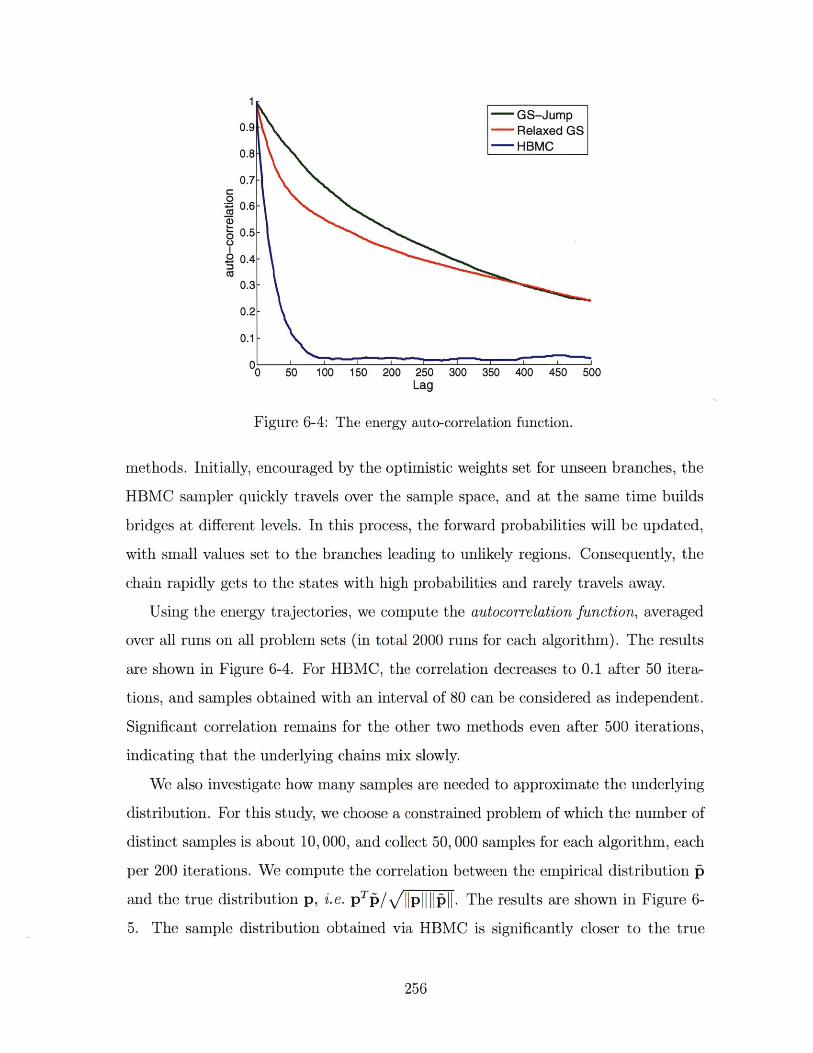
1
0.9
0.8
0.7
00.6
0 0.5
w 0.4CO
- GS-Jump- Relaxed GS-HBMC
'0 50 100 150 200 250 300 350 400 450 500Lag
Figure 6-4: The energy auto-correlation function.
methods. Initially, encouraged by the optimistic weights set for unseen branches, the
HBMC sampler quickly travels over the sample space, and at the same time builds
bridges at different levels. In this process, the forward probabilities will be updated,
with small values set to the branches leading to unlikely regions. Consequently, the
chain rapidly gets to the states with high probabilities and rarely travels away.
Using the energy trajectories, we compute the autocorrelation function, averaged
over all runs on all problem sets (in total 2000 runs for each algorithm). The results
are shown in Figure 6-4. For HBMC, the correlation decreases to 0.1 after 50 itera-
tions, and samples obtained with an interval of 80 can be considered as independent.
Significant correlation remains for the other two methods even after 500 iterations,
indicating that the underlying chains mix slowly.
We also investigate how many samples are needed to approximate the underlying
distribution. For this study, we choose a constrained problem of which the number of
distinct samples is about 10, 000, and collect 50, 000 samples for each algorithm, each
per 200 iterations. We compute the correlation between the empirical distribution t
and the true distribution p, i.e. pT /3pl|. The results are shown in Figure 6-
5. The sample distribution obtained via HBMC is significantly closer to the true
256
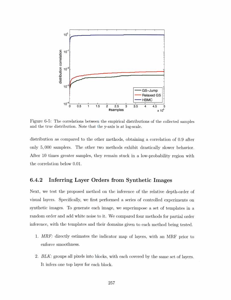
10
01
o 10-2Cus
0C.)C 2
~0
10 3-- GS-Jump-- Relaxed GS-- HBMC
1-0 0.5 1 1.5 2 2.5 3 3.5 4 4.5 5#samples x104
Figure 6-5: The correlations between the empirical distributions of the collected samplesand the true distribution. Note that the y-axis is at log-scale.
distribution as compared to the other methods, obtaining a correlation of 0.9 after
only 5, 000 samplers. The other two methods exhibit drastically slower behavior.
After 10 times greater samples, they remain stuck in a low-probability region with
the correlation below 0.01.
6.4.2 Inferring Layer Orders from Synthetic Images
Next, we test the proposed method on the inference of the relative depth-order of
visual layers. Specifically, we first performed a series of controlled experiments on
synthetic images. To generate each image, we superimpose a set of templates in a
random order and add white noise to it. We compared four methods for partial order
inference, with the templates and their domains given to each method being tested.
1. MRF: directly estimates the indicator map of layers, with an MRF prior to
enforce smoothness.
2. BLK: groups all pixels into blocks, with each covered by the same set of layers.
It infers one top layer for each block.
257
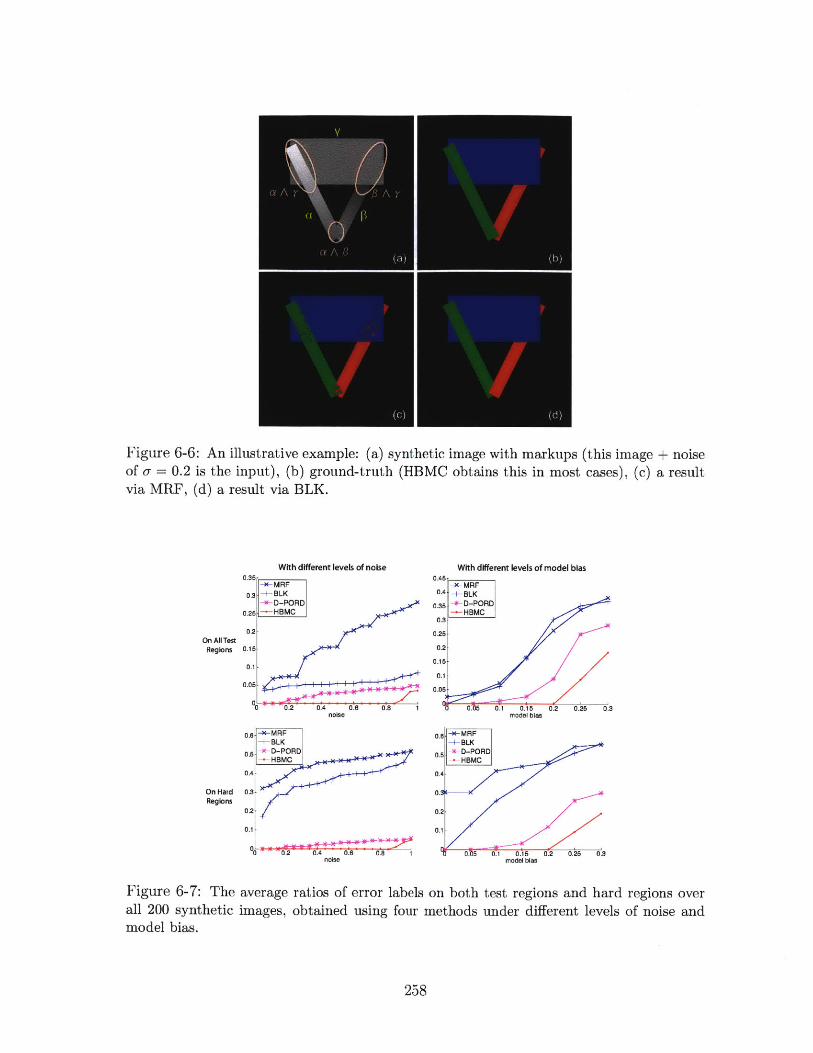
Figure 6-6: An illustrative example: (a) synthetic image with markups (this image + noiseof o- = 0.2 is the input), (b) ground-truth (HBMC obtains this in most cases), (c) a resultvia MRF, (d) a result via BLK.
With different levels of noise
*MRFBLK
+D-PORD-HBMC
noise
-4-MRF-+-BLK-- D-PORD-HBMC
- .2 0.4 0.6 0.8 1noise
With different levels of model bias
Figure 6-7: Theall 200 syntheticmodel bias.
average ratios of error labels on both test regions and hard regions overimages, obtained using four methods under different levels of noise and
258
0.35
0.3
0.25
0.2
0.15
0.1
0.06
0.860.5
0.4
0.3
0.2
0.1
On All TestRegions
On HardRegions
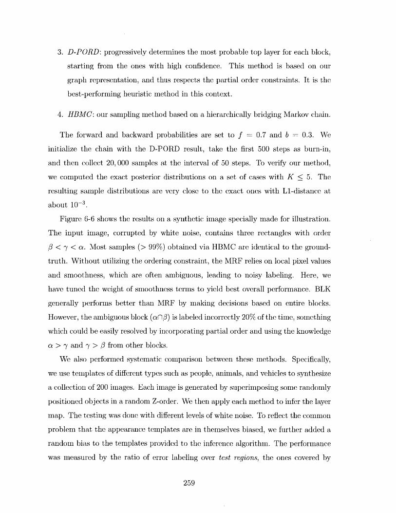
3. D-PORD: progressively determines the most probable top layer for each block,
starting from the ones with high confidence. This method is based on our
graph representation, and thus respects the partial order constraints. It is the
best-performing heuristic method in this context.
4. HBMC: our sampling method based on a hierarchically bridging Markov chain.
The forward and backward probabilities are set to f = 0.7 and b = 0.3. We
initialize the chain with the D-PORD result, take the first 500 steps as burn-in,
and then collect 20, 000 samples at the interval of 50 steps. To verify our method,
we computed the exact posterior distributions on a set of cases with K < 5. The
resulting sample distributions are very close to the exact ones with Li-distance at
about 10-.
Figure 6-6 shows the results on a synthetic image specially made for illustration.
The input image, corrupted by white noise, contains three rectangles with order
# < y < a. Most samples (> 99%) obtained via HBMC are identical to the ground-
truth. Without utilizing the ordering constraint, the MRF relies on local pixel values
and smoothness, which are often ambiguous, leading to noisy labeling. Here, we
have tuned the weight of smoothness terms to yield best overall performance. BLK
generally performs better than MRF by making decisions based on entire blocks.
However, the ambiguous block (an#) is labeled incorrectly 20% of the time, something
which could be easily resolved by incorporating partial order and using the knowledge
a > y and - > # from other blocks.
We also performed systematic comparison between these methods. Specifically,
we use templates of different types such as people, animals, and vehicles to synthesize
a collection of 200 images. Each image is generated by superimposing some randomly
positioned objects in a random Z-order. We then apply each method to infer the layer
map. The testing was done with different levels of white noise. To reflect the common
problem that the appearance templates are in themselves biased, we further added a
random bias to the templates provided to the inference algorithm. The performance
was measured by the ratio of error labeling over test regions, the ones covered by
259
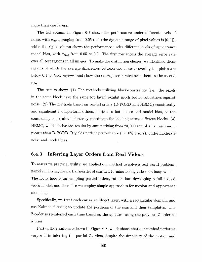
more than one layers.
The left column in Figure 6-7 shows the performance under different levels of
noise, with o-oise ranging from 0.05 to 1 (the dynamic range of pixel values is [0, 1]),
while the right column shows the performance under different levels of appearance
model bias, with Ubia, from 0.05 to 0.3. The first row shows the average error rate
over all test regions in all images. To make the distinction clearer, we identified those
regions of which the average differences between two closest covering templates are
below 0.1 as hard regions, and show the average error rates over them in the second
row.
The results show: (1) The methods utilizing block-constraints (i.e. the pixels
in the same block have the same top layer) exhibit much better robustness against
noise. (2) The methods based on partial orders (D-PORD and HBMC) consistently
and significantly outperform others, subject to both noise and model bias, as the
consistency constraints effectively coordinate the labeling across different blocks. (3)
HBMC, which derive the results by summarizing from 20, 000 samples, is much more
robust than D-PORD. It yields perfect performance (i.e. 0% errors), under moderate
noise and model bias.
6.4.3 Inferring Layer Orders from Real Videos
To assess its practical utility, we applied our method to solve a real world problem,
namely inferring the partial Z-order of cars in a 10-minute long video of a busy avenue.
The focus here is on sampling partial orders, rather than developing a full-fledged
video model, and therefore we employ simple approaches for motion and appearance
modeling.
Specifically, we treat each car as an object layer, with a rectangular domain, and
use Kalman filtering to update the positions of the cars and their templates. The
Z-order is re-inferred each time based on the updates, using the previous Z-order as
a prior.
Part of the results are shown in Figure 6-8, which shows that our method performs
very well in inferring the partial Z-orders, despite the simplicity of the motion and
260
Figure 6-8: The inferred partial orders of vehicles in 4 frames of a video (interval = 3 sec).Vehicles are marked with transparent rectangles in different colors. Below them are opaqueblocks that illustrate their Z-orders.
appearance models.
Implementation and Efficiency
In our C++ implementation, two techniques are used to accelerate the sampling
process: (1) caching visited states together with their transition tables in a hash map,
and (2) dynamically rearranging the entries of the transition table in descending order
of probabilities (We will publish our code).
The sampler runs very efficiently. For a typical layered video model with 8 to 10
layers, it makes about 10 million Markov transition steps per second. Hence, using our
scheme (20, 000 samples with 50 steps each), it takes 0.1 second to perform inference.
6.5 Summary
We developed a new representation of partial order based on minimal sufficiency,
and a principled approach for sampling from a constrained combinatorial space. The
method provides a general way to address the difficulty arising from disconnected state
spaces. The experiments demonstrated that our approach is effective and efficient in
sampling from the posterior distribution of partial orders, and that explicit utilization
of partial order can remarkably improve the robustness of the layered video model.
261
Chapter 7
Conclusions
In this work, we studied the modeling of dynamic visual scenes using a generative
Bayesian approach, particularly focusing on three key aspects: appearance, motion,
and the depth order between layers. we developed a series of machine learning tech-
niques to address the challenges arising as a consequence of the model formulation
and associated probabilistic inference. Included among these developments were a
new construction of dependent Dirichlet processes and a new method to sample from
constrained combinatorial spaces.
While does not yet achieve the ultimate goal of providing a complete and uni-
fied interpretation of visual scenes, this work does demonstrate the great potential
of probabilistic generative models in vision applications. Currently, discriminative
methods dedicated to specific tasks dominate the field of computer vision, probably
due to the fact that they showed good performance on numerous real world applica-
tions. However, the task-oriented nature of these methods makes it difficult, if not
impossible, to bring them together to interpret the visual world that we see every day
in a coherent fashion.
The exploration of generative approaches in this thesis is motivated by our deep
belief in the value of generative models for computer vision. The main advantage of
generative models is not that they perform better than discriminative methods on
specific tasks, but that they provide a flexible and elegant framework to incorporate
prior knowledge of different types and to integrate models of different structures
262
without comprising the mathematical rigor.
Using generative modeling, one may easily leverage the relations between different
aspects of a problem, and thus derive better solutions, addressing issues that would
otherwise be difficult to resolve. For example, as we have shown in Chapter 3, the
desire to express rich structures of local patterns and the need to ensure global co-
herence can be coupled elegantly through a generative MRF model. Moreover, in
Chapter 5, we showed that the construction of mixtures whose number of compo-
nents may change over time can be accomplished using a nonparametric generative
formulation. However, to our best knowledge, discriminative methods that solve such
problems in a satisfactory way have not existed yet.
7.1 Summary of Contributions
A major contribution of this work is the development of a Bayesian generative frame-
work that integrates the modeling of appearance, motion, and the depth order of
layers. In addition, we made a series of significant contributions to various topics, as
summarized below.
A new image model
To describe images and video frames, a new image model is developed in Chapter 3,
which integrates a probabilistic manifold model that can express a rich set of local
structures with a Markov random field that enforces coherence across local patches.
An important aspect of this formulation that distinguishes it from other high-order
MRF models, such as the Field of Experts [83], is that the likelihood that a patch
is generated from the patch manifold is used as the potential functions. This new
design of potential functions offers much greater capability of expressing local struc-
tures, as compared to those based on linear filter responses. In addition, through
the overlapping of local patches, the joint MRF encourages the global coherence of
images.
263
A new model of persistent motion patterns
Dynamics plays an important role in visual scene understanding. Whereas extensive
study has been devoted to accurate estimation of local velocities (e.g. object tracking
and optical flow), capturing persistent motion patterns over a region and during a
period may be more important in terms of understanding the activity underlying a
given scene. To effectively model persistent motion patterns, a new notion called
the geometry flow is introduced in Chapter 4, which unifies two different types of
motion characterizations, particularly an ensemble of trajectories and a continuous
transformation process. A Lie algebraic representation is then derived, which maps
each flow to an element in a vector space, thus greatly simplifying both probabilistic
formulation and flow estimation from observed scenes.
A new non-parametric construction of dynamic mixture models
Mixture models are used in both the image model and motion model to capture
complex distributions. For example, the patch manifold of the image model uses a
mixture distribution to describe local patterns, and the motion model uses a mixture
of flows to describe the motion patterns in a complex scene. In the past decade, non-
parametric mixture models based on Dirichlet processes were developed and became
popular. Such models allow for an indefinite (countably infinite) number of compo-
nents and as such, provide a flexible mechanism to construct mixture models when
the number of components is difficult to specify a priori.
To model dynamic scenes, we desire a mixture model which may evolve over time.
The key challenge here is to incorporate temporal dependency between mixture mod-
els at different time steps. To address this problem, we developed a new construction
of dependent Dirichlet processes in Chapter 5. By exploiting the inherent theoretical
connections between the Poisson and Dirichlet processes, this construction allows dy-
namically creating and removing components and varying the component parameters,
while guarantees that the marginal distribution of components at each time step is
itself a Dirichlet process.
264
A new method to infer partial orders
Our framework used layers to model visual scenes with multiple objects. A challenge
arising here is to determine the occlusion relation between layers, which, in turn,
is determined by their relative depth order. Layered models developed in previous
work either uses ad-hoc methods to estimate this order, or circumvents the problem
by directly inferring the association between pixels and layers. Neither approach
guarantees consistent occlusion reasoning.
We explored a generative approach to this problem in chapter 6, that is, to formu-
late a prior over the partial order between layers, and estimate it through inference. A
difficulty here is that a partial order has to satisfy a set of combinatorial constraints
(e.g. anti-symmetry and transitivity), and it is difficult to perform inference while
preserving these properties. In tackling this difficulty, we developed a new method
for MCMC sampling, which dynamically introduces virtual states that bridge differ-
ent parts of the space that would otherwise be disconnected due to the combinatorial
constraints. Though motivated by a specific vision problem, this is a generic method-
ology that can be applied to solve other inference problems over combinatorial spaces.
7.2 Future Directions
As mentioned, the work presented in this thesis shows the great potential of genera-
tive modeling in vision applications. However, many problems are yet to be solved.
Next, we briefly discuss several future directions to extend this work that we feel are
important and deserve further efforts.
Modeling dynamic shapes
One aspect that has not been addressed in this work is the modeling of shapes,
which, in our framework, determines the domain of each layer. Whereas there has
been extensive work on shape modeling, including active contours, level set methods,
and deep models, generative modeling of shapes, especially in a dynamic context,
remains a nontrivial challenge. In addition, it is also interesting to study how to
265
model the interactions between shapes and motion, and how to perform inference on
shapes when part of an object is occluded.
Semantic interpretation
The appearance and motion models establish an intermediate representation of vi-
sual scenes, which, however, does not directly provide a semantic interpretation of
the scene. An additional layer is needed to connect between this intermediate rep-
resentation and the semantics (e.g. the categories of objects and scenes, and their
relations). A possible approach to this problem is to consider a scene as composed
of parts coming from different topics, each associated with its own appearance and
motion model. To compose a scene, the spatial arrangement of these topics should
follow some regular patterns, which, again, can be captured using a generative model.
Adaptation for discriminative tasks
Though a generative model can be formulated and trained in a task-independent way,
it is often desirable to adapt the model to the target context when it is applied to
a specific task, especially the discriminative tasks (e.g. object recognition and scene
classification). We believe using specific knowledge about a particular context to
adapt a generic model not only increases the accuracy and efficiency, but also helps
to address ambiguities that would need specific contextual information to resolve.
Structured non-parametric models
Bayesian nonparametrics offers an elegant and powerful means to construct mixture
models without the need to specify the number of components in advance. However,
it is nontrivial to incorporate statistical dependencies between nonparametric models.
Previous efforts, including Hierarchical DP, Hierarchical Beta Process, and one of the
contributions of this thesis on Poisson-based Dependent DP, provide useful ways to
construct dependent nonparametric models. Yet, these are limited in several respects,
most notably the following: they can only be applied to the case where the dependency
graph has a tree structure, and there are no interactions between components.
266

The need to capture more complicated dependencies often arises in vision prob-
lems. Solving these problems requires the development of new nonparametric models.
Generally, there are several approaches to accomplish this: (1) introducing auxiliary
stochastic processes to help establish dependencies, (2) generalizing the point pro-
cesses that underlie the Dirichlet processes, or (3) generalizing the stick breaking pro-
cesses. We believe that these approaches are related to each other, and the analysis of
their relations may lead to the development of a more generic family of nonparametric
models.
267
Appendix A
Basics of Group Theory
A.1 Basic Concepts of Group
Group is a fundamental concept in modern algebra, which has played a significant
role in various fields in mathematics, physics, and computer science.
Definition A.1 (Group). A group (G, -) is defined as a set G with a binary operation
, which satisfies the following axioms:
1. The group is closed under the product operation -, i.e. Vx, y G G, a -b E G.
2. The product operation satisfies associativity: Vx, y, z G G, (x -y) -z = x -(y -z).
3. There exists an identity element e, such that Vx c G, e -x = x - e = x.
4. For each element x E G, there exists an inverse element x 1 E G, such thatx -1 -x -x1 e
It can be easily shown that the identity element of a group is unique, and for each
element in the group, its inverse element is unique.
In addition, the inverse operation has the following properties. For arbitrary
268
elements x, y in a group G,
(x -y)-1 y-1 -x-1,
(x-1)l =x,
e-1 =e.
Definition A.2 (Abelian Group, Commutative Group). A group G in which the
product operation satisfies commutativity, i.e. Vx, y E G, x - y = y . x, is called an
Abelian group, or a commutative group.
Abelian groups have a lot of nice properties that we will discuss later.
Definition A.3 (Symmetric Group). The symmetric group of a set X, denoted by
Sym(X), it the group consisting of all bijective mappings from X to X with the
product operation being the composition of mapping. Let f, g e Sym(X), then Vx cX, (f -g)(x) f(g(x)).
The identity element of a symmetric group is the identity map, that maps each
element to itself.
When X is a finite set, its symmetric group comprises all the permutations, which
is thus called a permutation group. When X is a continuous space, Sym(X) is con-
ventionally called a transformation group.
Definition A.4 (Subgroup). A subgroup of a group G is a subset H which is closed
under the group operation, i.e. it satisfies the following properties
1. H is closed under product operation, i.e. Vx, y E H, x - y E H.
2. H contains the identity element, e E H.
3. H is closed under inverse operation, i.e. Vx E H, x- 1 E H.
Actually, the three properties above is equivalent to the following: V, x, y E
H,x-ly E H.
269
Obviously, for each group G, {e} and G itself are subgroups of G, which are called
trivial subgroups. Other subgroups are called nontrivial subgroups.
Given any subset S of a group G, the subgroup generated by S is the smallest
subgroup that contains S, which comprises exactly all the products of elements in S
and their inverses.
Definition A.5 (Product Group, Direct Product). Let G and H be groups, their
product group, also known as direct product, denoted by G x H, consists of the Carte-
sian product of their underlying sets {(g, h) g C G and h E H}, with the product
operation defined as
(gi, hi) - (92, h2 ) = (gi - 92 , hi -h2).
The element of the product group is (eG, eH), in which eG and eH are respectively the
identity elements of G and H. And the inverse operation is thus defined by
(g, h)- 1 = (g- 1, h- 1).
The definition above can be extended to the product of multiple groups straight-
forwardly.
A.2 Group Homomorphisms and Kernels
We can define maps between groups, among which homomorphisms are of particular
interests.
Definition A.6 (Homomorphism). Let G and H be groups. A map ( : G -+ H is
called a homomorphism if it preserves product operations, i.e. Vx, y E G, cD(x y)
(x) -@(y).
It can be easily shown that the group homomorphism also has the following prop-
erties
1. It maps identity element to identity element, i.e. 1(eG) = eH-
270
2. It preserved inverse operation, i.e. Vx E G, (D(x))- 1 = @(x-).
If 4 is a bijective map, then D is called an isomorphism. An isomorphism of
a group onto itself is called an automorphism. Note that the set comprising all
automorphisms of a group G together with the composition as product operation is
also a group (a symmetric group), denoted by Aut(G).
Two groups G and H is said to be isomorphic, if there exists an isomorphism
between them.
Definition A.7. Let G and H be groups, and 4): G -+ H be a homomorphism, then
the kernel of G, denoted by ker G, is defined as {x c G|(x) = eH}, in which eH is
the identity element of H.
It can be easily shown that ker b is a subgroup of G. The kernel of an isomorphism
is {eG}-
A.3 Normal Subgroups and Quotient Groups
Definition A.8 (Coset). Given a subgroup H of a group G, the left coset of x E G
is xH - {xh h e H}, and the right coset of x is Hx = {hx h c H}.
The set of all left cosets forms a partition of G, i.e. two left cosets are either equal
or disjoint. The same applies to the set of all right cosets.
Given an arbitrary subgroup H, the left and right cosets may or may not be equal.
If they are equal, H is called a normal subgroup.
Definition A.9 (Normal Subgroup). A subgroup N of a group G is called a normal
subgroup, denoted by N < G, if it is invariant under conjugation, i.e. Vn E N, x c
G, xnx- 1 E N.
For a subgroup N of a group G, the statement that N is a normal subgroup is
equivalent to the following
For each x E G, xN = Nx, in other words, left cosets and right cosets are equal.
Hence, for a normal subgroup N, the left coset and right coset are both simply called
the coset.
271
Not every subgroup of a group is normal. However, all subgroups of an Abelian
group are normal. And, trivial subgroups are always normal.
Let N be a normal subgroup of G, we can define equivalence between any two
elements in G as
x ~ y <-> xy-1 E N.
With this equivalence, the equivalent class of x E G, is
[x] = xN = Nx,
which is exactly the coset of x.
In addition, the equivalence has the following properties.
1. the equivalent class (coset) of the identity element is the normal set, i.e. [e] = N.
2. equivalence is preserved under product operation, i.e. if x 1 - x 2 and y1 ~ Y2,
then x1 - y1 ~ X2 - Y2.
3. equivalence is preserved under inverse operation, i.e. if x 1 ~ x 2, then x, ~ x2 1
From these properties, we can see that the cosets in themselves constitute a group,
called the quotient group.
Definition A.10 (Quotient Group). Let N be a normal subgroup of a group G, the
quotient group, denoted by G/N, is the set of all cosets with respect to N, with the
product operation defined by
[x] - [y] = [x -y].
In addition, it can be easily shown that the identity element in G/N is [e] = N, and
the inverse operation can be given as
[x]1= [x-1].
Normal subgroups and homomorphisms have close relations.
272
Theorem A.1. Let G and H be groups, and (b : G -+ H be a homomorphism, then
ker 4J is a normal subgroup of G.
Conversely, Let N be a normal subgroup of G, then the map: b : G -+ G/N that
maps each element to its coset, i.e. J(x) = [x] = xN, is a homomorphism, whose
kernel is N.
The above theorem establishes the correspondence between normal subgroups and
homomorphisms.
One of the particular important normal subgroup of a group is its center.
Definition A.11 (Group Center). The center of a group G is the set Z(G) that
consists of the elements that commute with all elements in G, i.e.
Z(G)= {z E Gg- z = z -g, Vg E G}
It can be easily seen that
Vz E Z(G), Vg c G, g -z -g- = z.
Hence, Z(G) is a normal subgroup of G. And, it is obvious that Z(G) is an Abelian
group.
Let G be an Abelian group, then the center of G is G itself. At the other extreme,
a group is said to be centerless if its center is the trivial group {eG -
Definition A.12 (Inner Automorphism Group). The map 1) G -+ Aut(G) which
maps each element g E G to the corresponding conjugation $g defined by Vx E
G, $g(x) = gxg 1 . The range of <b is called the inner automorphism group, denoted
by Inn(G).
Consider When g E Z(G), we can easily see that $g(x) = x. Actually, it can be
shown that Z(G) is exactly the kernel of b, i.e. G/Z(G) is isomorphic to Inn(G).
273
A.4 Semidirect Product
Direct product discussed above is an elementary way to construct groups by inte-
grating component groups. However, many important groups are formed with its
generalization, called semidirect product. A semidirect product group also uses the
Cartesian product as underlying set, but with a generalized multiplication operation.
Definition A.13 (Semidirect Product). Let G be a group, N be a normal subgroup
of G (N < H), and H be a subgroup of G. Then G is said to be a semidirect product
of N and H, if
G = NH and NnH = {e}.
This condition is equivalent to any one of the following.
1. G = HN and N n H = {e},
2. each element in G can be written uniquely in form of n - h with n G N and H.
3. each element in G can be written uniquely in form of h - n with h E H and
n c N.
If this case, we say G splits over N.
Let G be a semidirect product of a normal subgroup N and a subgroup H, then
we have
1. In each equivalence class in the quotient group G/N, there exists a unique
element in H.
2. H is isomorphic to G/N, a natural isomorphism is to map each element h to
[h] = hN = Nh.
3. The map G -+ H that takes each element x E G to the unique element in
H n [x] is a homomorphism. It can be seen that the map is an identity map on
H and its kernel is N.
274
Definition A.14 (Normal Factor Semidirect Product w.r.t. Group Homomorphism).
Let N and H be two groups, and #5: H -+ Aut(N) be a group homomorphism. Then
the left normal factor semidirect product of N and H with respect to $, denoted by
N x0 H, is a group with the Cartesian product N x H as the underlying set, and the
multiplication defined as
(ni, hi) - (n2, h2) = (ni -O#l1(n2), hi - h2)
Hence, the identity element is (eN, eH), and the inverse operation is given by
(n , h)-= (#h-1(n-'), h- ).
Likewise, we can define the right normal factor semidirect product of N and H with
respect to $, denoted by N x4 H as a group with H x N being the underlying set, and
the multiplication defined as
(hi, ni) - (h2, n2) = (hi -h2, ni -#hl1(n2)).
It is obvious that if # is a trivial homomorphism that sends each h to the identity
map of N, i.e. Oh= IdN, then the normal factor semidirect product degenerates to
direct product.
In G = N x0 H, the pairs (n, eH) form a subgroup of G that is isomorphic to N,
while the pairs (eN, h) form a subgroup of H that is isomorphic to H. Similar results
can also be obtained for right normal factor semidirect product.
Theorem A.2. Let G be a semidirect product of its normal subgroup N and another
subgroup H, i.e. G = NH with Nn H = {e}. Then G is isomorphic to N x0 H and
H x N for some group homomorphism $.
One example is the # that maps each h E H to h E Aut(N) defined by
Oh(n) = h -n - h-.
275

Appendix B
Basics of Differential Geometry
B.1 Basic Concepts of Manifolds
Manifold is a fundamental concept in modern geometry, which is established based
on topology.
Definition B.1 (Topological Manifold). A topological space M is said to be a topolog-
ical manifold of dimension n, or a topological n-manifold, if it satisfies the following
properties
1. M is a Hausdorff space, i.e. each pair of distinct points in M have disjoint
neighborhood.
2. M is second countable, i.e. there exists a countable basis for the topology of M.
3. M is locally Euclidean, i.e. each point in M has a neighborhood that is homeo-
morphic to an open subset of R".
Definition B.2 (Chart). Let M be a topological n-manifold, a coordinate chart on
M is a pair (U, p), in which U is an open subset of M, and p : U -- R" is a
homeomorphism. Here, U is called the coordinate domain, while p is called a (local)
coordinate map. For each p E U, p(p) = (x1 (p), x 2(p), . n (p)) is called the local
coordinates with respect to the chart.
276
Definition B.3 (Smoothly Compatible Charts). Let (U, p) and (V, 4') be two charts,
they are said to be smoothly compatible, if they are either disjoint, or both the tran-
sition map 4' o op- : o(U n V) -+ @(U n V) and its inverse cp o 4'- are infinitely
differentiable.
Definition B.4 (Smooth Atlas). A smooth atlas is a collection of charts covering the
manifold which are smoothly compatible with each other. The smooth atlas is said to
be maximal if every chart that is smoothly compatible of each chart in the atlas has
been in the atlas.
Definition B.5 (Smooth Manifold). A smooth manifold is a topological n-manifold
M with a maximal smooth atlas A. This smooth atlas is also called the smooth
structure of M.
B.2 Smooth Maps
Definition B.6 (Smooth Map). Let M and N be smooth manifolds, then F : M -+ N
is said to be smooth if for every p e M, there exists local charts (U, 0) and (V, 4')
which respectively contain p and F(p), such that the function F = 4 o F o 0-1 is in-
finitely differentiable from p(U) to $(V). Here, the function F is called the coordinate
representation of F with respect to the given coordinate charts.
Especially, the function F : M -+ Rk is said to be smooth, if for each p E M,
there exists a local chart (U, p) that contains p such that f f o o-' is infinitely
differentiable.
The set of all smooth real-valued functions f : M -+ R constitutes a real vector
space, denoted by C (M).
Smooth Maps have the following properties
1. Smoothness is local. It means that a map F : M - N is smooth, if and only if
for every point p E M, there exists a neighborhood of p, say U, such that the
restriction Flu is smooth.
277
2. Let M and N be smooth manifolds, and let F : M - N be continuous maps.
{(Uc, oc} and {V4,3,0,} are smooth atlases for M and N. Then F is smooth if
and only if for each a and 3 with U n V # 0, #f o F o ya is smooth on its
domain of definition.
3. Any composition of smooth maps between smooth manifolds is smooth.
Definition B.7 (Diffeomorphism). A diffeomorphism between smooth manifolds M
and N is a smooth bijective map, whose inverse is also smooth. Two manifolds are
said to be diffeomorphic is there exists a diffeomorphism between them.
B.3 Tangent Vectors and Tangent Space
Tangent Space is a local linear approximation of the manifold, which is the basis of
Lie algebra theory. The elements in a tangent space are tangent vectors, which have
close relations with derivatives of smooth curves.
Definition B.8 (Derivation). Let M be a smooth manifold and p E M. A linear
map X : C*(M) --* R is called a derivation at p if it satisfies
X(f g) = f(p)Xg + g(p)Xf,
for all f, g c C*(M).
Definition B.9 (Tangent Space). The set of all derivations of C* (M) at p constitute
a vector space, which is called the tangent space of M at p, denoted by TM. Each
element in TpM is called a tangent vector.
We can see that each tangent vector corresponds to a derivation functional.
Tangent space of an n-dimensional manifold is isomorphic to R'.
Push-forwards are linear maps between tangent spaces.
Definition B.10 (Push-forward). Let M and N be smooth manifolds, and F : M -
278
N be a smooth map, for each p e M, the map F, : TpM -+ TF(p)N defined as
(F*X)(f) = X(f o F)
for each f E CO(N), is called the push-forward associated with F.
It can be easily shown that F, : TpM -+ TF(p)N is linear.
In addition, the map that takes F to F* has the following properties:
1. It takes identity map to identity map: (IdM)* = IdTpm.
2. (G o F), = G* o F*.
3. If F is a diffeomorphism, then F* is an isomorphism.
Let (U, sp) be a smooth chart on an n-manifold M, then p is a diffeomorphism
between U and its range, hence, y, : TM - T,(p)R is an isomorphism, so as (-1),.
T,(p)R' has a natural basis with the derivations 8/ax'l.(p), i = 1, 2, ... , n.
(9'), will take this basis to form a basis of TpM:
8x P
Then
1a
' 9 (P)
which acts on f E C (M) as
a fxi axi
f )(f o 5-1) =A ()
where f and P are respectively the coordinate representations of f and p with respect
to the given chart.
Then any vector X E TM can be uniquely written as a linear combination of the
basis
X-Exiax8
279
which acts at a smooth function f E C"(M) as
Xf = XafW).
Here (X', X 2 , ... , X") is the coordinate representation of X, which can be obtained
by
Xi= X(x ),
where x' is the i-th coordinate function in C".
Consider a smooth map F : U -+ V with U E R' and V E Rm, then F. is a linear
operator from an n-dimensional space to an m-dimensional space, which thus can be
represented by an m x n matrix. It can be shown that, this matrix is exactly the
Jacobian matrix of F at p, denoted by DF(p).
For a smooth map F : M - N between two general manifolds, the matrix
representation can be obtained with respect to fixed charts.
Definition B.11 (Curve). Let M be a manifold, a curve in M is a continuous map
J -+ M, with J E R being an interval. If M is a smooth manifold, and ' is a
smooth map, it is called a smooth curve.
Definition B.12 (Tangent Vector to a curve). Let -y be a smooth curve in a smooth
manifold M, the tangent vector to -y at to e J is
(d7'(to) = d, E T(to)M.
to!
It acts on a function f E C*M as a derivation by
d _d(f o 7)(17'(to) f = -- (f 0 -) = ~ y (to).-dt to dt
Let (U, ,o) be a smooth chart on M that contains -y(to), then we can have
8Y'(tO)f = (i)'(to) .a,ax -(to)
280
where -y(t) is the i-th coordinate component of 7(t), ((y')'(to), . , (yn)'(to)) is the
coordinate representation.
There exists close relations between tangent space and smooth curves.
Theorem B.1. Let M be a smooth manifold and p E M. Each X E TpM is the
tangent vector to some smooth curve in M.
For composite curve, we have
Let F : M -+ N be a smooth map, and 1y: J -+ M be a smooth curve in M, then
F o- : J -+ N is a smooth curve in N. The tangent vector at t = to to the composite
curve F o -y is given by
(F o -y)'(to) = F,(y'(to)). (B.1)
This proposition is often utilized to compute the push-forwards, as
FX = (F o -y)'(0), (B.2)
where -y is some smooth curve whose tangent vector is X at t - 0.
B.4 Vector Fields
Definition B.13 (Tangent bundle). The tangent bundle of a smooth manifold M,
denoted by TM, is the disjoint union of the tangent spaces at all points of M:
TM = TM.pCM
Each element in TM is a pair (p, X) with X £ TM.
The tangle bundle has a natural projection map 7r : TM -+ M, which maps (p, X)
to p. The natural projection map is a smooth map.
Definition B.14 (Vector Field). A vector field is a continuous map Y : M -+ TM,
281
usually written as p -+ Y,, which satisfies
7roY=Idm.
In other words, it is a continuous map that maps each point p in M to a tangent
vector in the corresponding tangent space TM.
If the map is smooth, it is called a smooth vector field.
Considering that each tangent vector is a derivation operator, then each vector
field is also a map that maps a real-valued smooth function to a real-valued smooth
function, by taking derivatives at each point in M using the corresponding tangent
vector.
B.5 Embedding and Submanifolds
Definition B.15 (Rank of Smooth Map). Let M and N be smooth manifolds, and
F : M -4 N be a smooth map. The rank of F at p E M is the rank of the linear
map F, : TpM -+ TF(p)N, which is just the rank of the Jacobian matrix DF(p) with
respect to any smooth chart.
If a smooth map F has the same rank k at every p E M, it is said to have a
constant rank k, denoted by rank(F) = k.
Definition B.16 (Submersion). A smooth map F : M -+ N is called a submersion
if F, is surjective at every point, i.e. rank(F) = dim N.
Definition B.17 (Immersion). A smooth map F : M - N is called an immersion
if F, is injective at every point, i.e. rank(F) = dim M.
Definition B.18 (Smooth Embedding). A smooth embedding is an immersion F
M -+ N that is also a topological embedding, i.e. a homeomorphism onto its image
F(M) C N.
The inverse function theorem relates the rank of a smooth map to invertibility.
282
Theorem B.2 (Inverse Function Theorem). Let M and N be smooth manifolds,
p C M, and F : M -+ N is a smooth map such that F, : TpM -+ TF(p)N is bijective,
i.e. DF(p) is of full rank, then there exists connected neighborhoods Uo of p and V
of F(p) such that Fluo : Uo - V is a diffeomorphism.
As a consequence, we have the following theorem.
Theorem B.3 (Rank Theorem). Suppose M and N are two smooth manifolds, and
F : M -+ N is a smooth map with constant rank k. For each p C M, there exist
smooth coordinate charts (U, a) centered at p, and (V, @) such that
7Po F o p- 1(zX . . ,. I h x I k+1 m.. IX ) __( 1, ... ., zX k0, .. ., 0).
Smooth submanifolds are modeled locally as embedding of Rk into R', identifying
Rk with the subspace of R' in form of
{{(x 1,...,o xk Iok+1 n X )I k+1 __. . _ n __ .
Definition B.19 (k-slice). If U is an open subset of R', a k-slice of U is any subset
in the form of
S ={(,. . . , k xk+1 n) xk+l ck+1 . , x"= c"
for some constants ck, ... ,c
The definition can be easily extended to generic manifold. Let M be a smooth
n-manifold, and (U, so) be a smooth chart on M. A subset S C U is a k-slice of U if
sp(S) is a k-slice of so(U).
Definition B.20 (Embedded Submanifold). A subset S c M is called an embedded
submanifold of dimension k, or embedded k-submanifold, if for each point p E S, there
exists a smooth chart (U, so) on M such that p C U and U n S is a k-slice of U.
Here, the chart (U, so) is called a slice chart for S in M.
283
Let S be an embedded submanifold of M, then dim M - dim S is called the
codimension of S in M.
Embedded submanifolds and embedding have close relations.
Theorem B.4. The image of a smooth embedding is an embedded submanifold.
Conversely, let S be an embedded submanifold of M, it has a unique smooth struc-
ture such that the inclusion map S " M is a smooth embedding.
The tangent space to a submanifold is a subspace of the tangent space to the
ambient manifold.
Theorem B.5. Suppose S C M is an embedded submanifold and p E S. The tangent
space TpS is a subspace of TM, and it is given by
TpS ={X E TpM: Xf =0 whenever f E C (M) and f s = 0}
284
Appendix C
Affine Transformation Group
In geometry, an affine transform is a transformation which preserves straight lines
and ratios of distances between points lying on a straightline. Affine transforms are
one of the most important family of geometric transforms and have been extensively
studied. In this work, we derive the first family of geometric flows - the affine flows
by extending affine transforms into continuous transform processes. Moreover, one
can construct more complex flows, using affine flows as the basic building blocks.
This section provides a brief review of affine transforms, and discusses their Lie
algebraic representations.
C.1 The Affine Transformation Group
The affine transform can be defined in either an algebraic way or a geometric way.
Definition C.1 (Affine Transformation). In algebra, an affine transformation, or
called an affine map, between two vector spaces consists of a linear transformation
followed by a translation
Tx = Ax + t,
here, the affine transformation is characterized by the pair (A, t), where A represents
the linear transformation, while t represents the translation.
In geometry, an affine transformation is a map that preserves collinearity of points
285
and ratios of distances between collinear points.
Affine transformation is not always invertible. An affine transformation (A, t) is
invertible if and only if the linear map A is invertible. In this notes, we only discuss
invertible affine transformations. Without explicit statement, an affine transformation
means an invertible one in the following text.
Definition C.2 (Affine Transformation Group). The set of all invertible affine trans-
formations for n-dimensional space form the affine transformation group, or called
Affine Group, denoted by Aff(n), with the group operations defined as follows. Let
Ti = (A 1 , ti) and T2 = (A 2, t 2 ) be two affine transforms, their composition acts on x
as
(T o T2 )(x) = T1(T 2(x)) = A1 A 2x + (ti + Ait 2 ).
Hence, the multiplication is defined as
(A 1 ,ti) - (A 2 , t 2 ) = (A1A 2, ti + Ait 2 ).
In addition, the inverse of T = (A, t) is
T-1= (A-1, -A- 1 t).
The identity element of the group Aff(n) is the identity transform (I, 0).
It can be shown that the affine transformation group is a Lie group with the natural
topology of the Cartesian product space GL(n, R) x R'. The affine transformation
group is not commutative.
Homogeneous coordinates and Matrix representation
Next, we discuss how an affine transform can be represented in a matrix form. An
affine transformation is generally not linear, and thus it cannot be directly represented
by a matrix.
286
To derive the matrix representation of affine transforms, homogeneous coordinates
is introduced.
Definition C.3 (Homogeneous Coordinates). In an n-dimensional space, the homo-
geneous coordinate of a point x =(x 1, x 2 , ... , xn)' is a vector of length n + 1, which
augments x with an extra one. In this notes, it is denoted by k, as
4 1 = z ,X2, ... ., Xn, 1) .
Using homogeneous coordinates, the affine transformation defined above can be
written asTx A t x
10 1 1
Hence, the affine transformation (A, t) can be uniquely represented by the (n + 1) x
A t(n + 1) matrix . The matrix is invertible if and only if the transformation is
0 1invertible.
With the matrix representation, we can formulate the application and composition
of affine transforms in form of matrix multiplication. What's more important, the
matrices in the aforementioned form constitute a group, which is a Lie subgroup of
GL(n + 1, R). The affine transformation group Aff(n) is isomorphic to this matrix
Lie group. In the following discussion, we treat them as identical.
Lie algebraic representation
According to the theory of Lie group and Lie algebra, for each matrix Lie group,
there exists a corresponding Lie algebra. The Lie algebra of Aff(n), denoted by
aff(n), comprises all the matrices such that the induced one-parameter subgroups lie
in Aff(n), that is
X E aff(n) <-> Vt E R, etX E Aff(n).
Hence, e t=O = X. As the bottom row of the matrix representation of affine
transforms are fixed, the bottom row of each matrix X E aff(n) must be an zero row
287
vector. In addition, for each matrix in form of
Y uX =,
0 0
we have
e =exp Y u 1 e (Y)u (C.1)0 0 0 1
Here, we have0 yk-1
Y) =1 k!k=1
which converges for every Y. When Y is invertible,
O(Y) = (e - - Y-I(e - I).
Therefore, etX E Aff(n). Hence, the Lie algebra aff(n) of Aff(n) consists of all
(n + 1) x (n + 1) consists of every matrix with zero bottom row. The dimensionality
of the Lie algebra aff(n) is equal to that of the Lie group Aff(n), which is
dim Aff(n) = dim aff(n) = n(n + 1). (C.2)
In particular, when n = 2 (i.e. for a two-dimensional space), the dimension is 6.
C.2 Factorization of the Affine Group
Next, we perform a complete analysis of the affine transform group, in order to
obtain a deeper understanding of its structure. The process would lead to a series of
important subgroups with interesting geometric and algebraic characteristics.
General linear group and translation group
First of all, the affine group Aff(n) can be factorized as the semidirect product between
the general linear group GL(n, R) and the translation group, which is isomorphic to
288
(R", +), as
Aff (n) = GL (n, R) x R'. (C.3)
This equations suggests that each affine transformation is uniquely expressed as a
linear transform followed by a translation.
Particularly, the translation group consists of all translation transforms. Each trans-
lation is characterized by a translation vector t, and acts on a point x as
Tx = x + t.
The group product of translations ti and t 2 is t 1 +t 2, and the inverse of the translation
t is -t. The identity element is given by 0. The translation group of an n-dimensional
vector space is an n-dimensional Lie group, which is commutative and isomorphic to
the additive group of real vector space (Rn, +-).
The general linear group, denoted by GL(n, R), consists of all invertible real matri-
ces. GL(n, R) is an n2-dimensional Lie group. As a matrix Lie group, its Lie algebra,
denoted by gl(n, R), consists of all n x n matrices.
GL(n, R) is not connected, and comprises two components. The matrices in one
component have positive determinant, while those in the other component have neg-
ative determinant. The component of matrices with positive determinants in itself is
a Lie subgroup, denoted by GL+(n, R).
Specifically, given a particular axis b, the linear group GL(n, R) can be factorized
into a semidirect product as
GL(n, R) = GL+(n, R) x ({1, -1}, x), (C.4)
where ({1, -1}, x) is isomorphic to the reflection group, with 1 corresponding to
the identity map, while -1 corresponding to the reflection along the axis b. The
above equation essentially establishes an important fact: Given an axis, each linear
transform can be either a transform with positive determinant or a transform with
positive determinant followed by a reflection along the given axis.
289
Special linear group and uniform scaling
Consider the determinant function det : GL+(n, R) -+ R+ that maps each linear
transform matrix to its determinant value. It is not difficult to see that this function
is a group homomorphism. The kernel of the determinant function is what we call
the special linear group, while the induced quotient group is isomorphic to the mul-
tiplicative group of positive real numbers (R+, x), which is also isomorphic to the
group of uniform scaling.
This suggests that GL+ (n, R) can be further decomposed into a direct product of
a special linear group SL(n, R) and a the group of uniform scaling, as
GL+ (n, R) = SL (n, R) x (R+, x ) (C.5)
The special linear group over the real number field, denoted by SL(n, R), consists
of all linear transforms with determinant one. All transforms in SL(n, R) are volume-
preserving. The dimension of SL(n, R) is n2 - 1.
The uniform scaling group consists of all uniform scaling transforms. Each uni-
form scaling is characterized by a scaling factor s E R+, and acts on a point x as
Tx = sx.
The uniform scaling group is a one-dimensional Abelian group, which is naturally
isomorphic to the multiplicative group of positive real numbers. It is the normal
subgroup of GL+(n, R) and GL(n, R).
Orthogonal group and special orthogonal group
A subgroup of the general linear group deserves special attention, that is, the group of
transforms that preserve Euclidean distances, called orthogonal group. The orthogonal
group of n-dimensional space, denoted by 0(n), is the group of all n x n orthogonal
matrices. A matrix A is said to be orthogonal, if A 1 = AT, i.e. ATA - AAT = I.
The dimension of 0(n) is n(n - 1)/2. The determinant of an orthogonal matrix
290
can be either 1 or -1. Correspondingly, the orthogonal group has two connected
components, respectively contain the matrices of determinant 1 and -1. The com-
ponent corresponding to the determinant one is a Lie subgroup of O(n) of the same
dimension, called special orthogonal group, denoted by SO(n). In general, SO(n) is
not commutative, except when n = 1 (in this case, it degenerates to the trivial group
1) and n = 2 (the 2D rotation group).
The transforms in O(n) preserve inner product, as
VR E O(n), Vx, y E R"n, (x, y) = (Rx, Ry).
As an immediate corollary, they preserve Euclidean distance, as
VR E O(n),Vx, y E R', ||x - yll =||Rx - Ryl1.
Conversely, every linear transform that preserves distances is orthogonal. In this
sense, the orthogonal group can be defined as the group of all distance-preserving
linear transforms.
Euclidean group
The transforms in translation group and orthogonal group, as well as their compo-
sitions are all distance-preserving, which together with their composite transforms
constitute the Euclidean group.
The Euclidean group of an n-dimensional vector space, denoted by E(n), consists
of all distance-preserving affine transforms. Each affine transform in E(n) is given by
(R, t), in which R E O(n). The dimension of E(n) is n(n + 1)/2. It can be factorized
as the semidirect product of the orthogonal group and the translation group.
E(n) = 0(n) x R'. (C.6)
In other words, each Euclidean transform can be uniquely expressed by an orthogonal
transform followed by a translation. Like GL(n, R), E(n) has two connected compo-
291
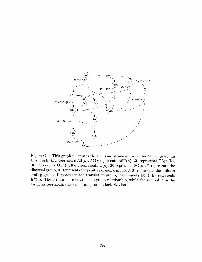
Figure C-1: This graph illustrates the relations of subgroups of the Affine group. Inthis graph, Af f represents Aff(n), Af f+ represents Aff+(n), GL represents GL(n, R),GL+ represents GL+(n, R), 0 represents 0(n), SO represents SO(n), D represents thediagonal group, D+ represents the positive diagonal group, U. S. represents the uniformscaling group, T represents the translation group, E represents E(n), E+ representsE+(n). The arrows represent the sub-group relationship, while the symbol x in theformulas represents the semidirect product factorization.
292
nents, respectively corresponding to determinants 1 and -1. The component with
transforms of determinant one in itself is a group, denoted by E+(n), which has
E+(n) - SO(n) x R'. (C.7)
Figure C-1 shows the relations between the aforementioned subgroups and how
the affine group is factorized into semidirect product of subgroups.
C.3 Two-dimensional Affine Transforms
In this work, we particularly focuses on the geometric transforms on a two dimensional
space. Here, a detailed analysis is performed on the two-dimensional affine group and
its associated Lie algebra.
In a two-dimensional space, an affine transforni is characterized by a 2 x 2 matrix
A 12 and a translation vector t . Let the transform T = (A, t)a21 a22 t2
send a point x= (X1 , x2) to x' (x', x'), we have
X = anixi + a 1 2 x 2 + t 1 ,
x - a 2 1x 1 + a 2 2 x 2 + t 2 .
All invertible 2D affine transforms constitute the 2D affine group, denoted Aff(2), of
dimension 6.
The Lie algebra of Aff(2), denoted aff(2), consists of all 3 x 3 matrices in the
following form
Y[ Y12 UJY U
=Y21 Y22 U2-0 0
0 0 0
293
Evaluation of the exponentiation mapping
Let
exp ( Y ul
0 0 -A
0
t
,J
then the matrices are related as follows.
A = e and t = p(Y)u =yf k-i
k=1 k
In this above, o(Y) is related to ey as
(C.10)
To derive the method of evaluating p(Y), we first generalize (-), getting a family
of functions {S(j) : M((R) -+ GL(n, R)}1 indexed by a nonnegative integer 1 as
00 yk-1((f)(Y) k!
k=l(C.11)
It can be shown that for each 1, this series is convergent. Obviously, when 1 = 0, it is
the exponential mapping, when 1 = 1, it is o(-) defined above. Moreover, the identity
in (C.10) can be generalized to
1S(Y) = I + + 1) 1! YO(l+1)(Y)
Especially, we have
P(Y) = I + (2)(Y)Y = I + Y 0( 2)(Y).
When Y is a 2 x 2 matrix, the computation can be done as follows.
non-singular, then
o(Y) = Y-'(e - I) = (ey - I)Y'.
294
(C.8)
(C.9)
(C.12)
(C.13)
If Y is
(C.14)
e Y= I + g(Y)Y = I + Y O(Y).
When Y is singular, we can accomplish the computation as below
(P(Y) = I + P(2) (tr(Y)) Y.
{X-2(ex - 1 -X),
0.5,)
C.4 Entries of the Lie algebraic representation
Here, we are going to investigate the meaning of each entry in the Lie algebraic
representation and study how they are related to the transforms. For the affine
transform T = eX, we write the Lie algebraic representation X as
Y uX ==
0 0
Y11
Y21
0
Y12 ui
Y22 U2
0 0
Let Ei, be a 3 x 3 matrix with the entry at the i-th row and j-th column being 1
and others being 0. Then, the canonical decomposition of X can be given by
X = yu1Euj + y12E 12 + y2 1E 2 1 + y22 E 22 + uiE 13 + U2 E 23 . (C.17)
Now, we examine these six components respectively.
Logarithm of scaling factors: yii and Y22
exp(yiIEu) =
[9 11 0 0
0 1 0
0 0 1
295
with
(C.15)
x 0.(C.16)
X21
-2
eylli1
[X2J
1 0 0- - - -
X1 Xiexp(y22E22) = 0 eY22 0 : K[i
0O 0 1 -2 -j 2X -j
Hence, the transforms corresponding to yu1Enj and y22E 22 are the scalings respectively
along x-axis and y-axis, by factors el" and eY22 . In this sense, yi and Y22 encode the
logarithm of scale factors along x-axis and y-axis.
Shearing coefficients: Y12 and Y21
1 Y12 0-
exp(y12E1 2 ) = 0 1 0 : X X + Y2X2]
1 0 0--
X1 X1
exp(y2 1E 2 1 ) = Y21 1 0 [:+ 1
X2 X2 + y2l1i
Hence, the transforms corresponding to y 12E 12 and y21E 21 are the shearing transforms
respectively parallel to x-axis and y-axis, with coefficients Y12 and Y21. In this sense,
Y12 and Y21 encode the shearing coefficients parallel to x-axis and y-axis.
Translation displacement: ui and u2
1 0 1-
exp(uiEis)=- 0 1 0 : 1 X1+U
0 0 1 - -
1 0 0X1 X1
exp(u 2 E 23 )= [0 1 U2 : ] []
LO 11 X2 X2 + U2
Hence, the transforms corresponding to uiE1 3 and u 2E23 are translations along x-
direction and y-direction respectively, and u1 , u2 encode the amount of displacement.
296
When X is a combination of multiple components, transforms of different types
will be interleaved together to form the compound transform. In this process, the
meaning of the individual elements will not be exactly what has been described above.
C.5 Important Subgroups of the 2D Affine Group
Now, we study the algebraic characteristics of several important geometric transforms.
Translation
Translation is moving points along some direction by a constant distance. It is char-
acterized by the translation vector t =(ti, t 2 )T, and can be expressed by
X1 X1+ ti
Here, ti and t 2 respectively represent the displacement along two axes. All transla-
tions form a subgroup of Aff(2), in which, the composition of two translations ti and
t 2 is ti + t 2, and the inverse of the translation t is -t. This group is an Abelian
group isomorphic to (R2,+).
ItThe matrix representation of the translation t is T [ . It is Lie algebraic
0 1
0 trepresentation is X = . T has a three-folded eigenvalue 1, and X has a
0 0three-folded eigenvalue 0. When t f 0, both T and X are not diagonalizable, as the
dimension of eigenspace is 2. Translation is isometric, and except for the identity
map, translation has no invariant point.
Rotation
Rotation is moving points around the origin in a circular manner, keeping the distance
from each point to the origin unchanged. It is characterized by the rotation radian
297
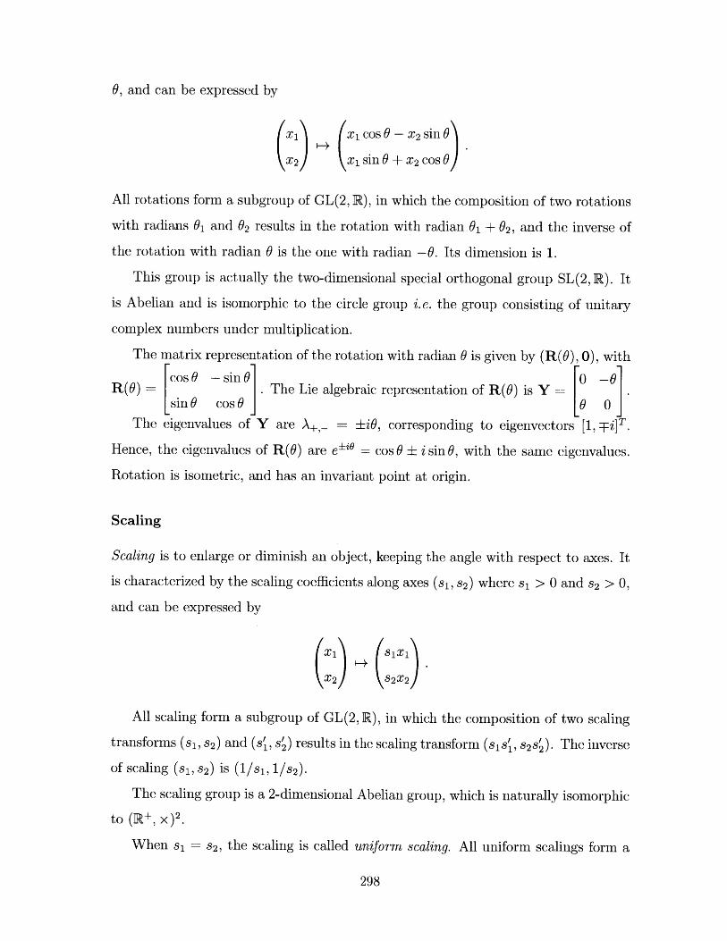
0, and can be expressed by
x1 x1 cos 0 - x 2 sin 0
x2 x1 sin 0 + x 2 cos J
All rotations form a subgroup of GL(2, R), in which the composition of two rotations
with radians 01 and 02 results in the rotation with radian 0 +02, and the inverse of
the rotation with radian 0 is the one with radian -0. Its dimension is 1.
This group is actually the two-dimensional special orthogonal group SL(2, R). It
is Abelian and is isomorphic to the circle group i.e. the group consisting of unitary
complex numbers under multiplication.
The matrix representation of the rotation with radian 0 is given by (R(0), 0), with
cos0 -sinl 0 -oR (0) = .The Lie algebraic representation of R(0) is Y =
sin 0 cos 0 0 0The eigenvalues of Y are A+,- = ±iO, corresponding to eigenvectors [1, Ti]T.
Hence, the eigenvalues of R(0) are e" = cos 0 i i sin 0, with the same eigenvalues.
Rotation is isometric, and has an invariant point at origin.
Scaling
Scaling is to enlarge or diminish an object, keeping the angle with respect to axes. It
is characterized by the scaling coefficients along axes (Si, s2) where si > 0 and s2 > 0,
and can be expressed by
X1 s121
All scaling form a subgroup of GL(2, R), in which the composition of two scaling
transforms (si, s2) and (si, s') results in the scaling transform(sis', s2S'). The inverse
of scaling (s1 , s 2 ) is (1/1, 1/s2).
The scaling group is a 2-dimensional Abelian group, which is naturally isomorphic
to (R+, x) 2 .
When s1 = 2, the scaling is called uniform scaling. All uniform scalings form a
298
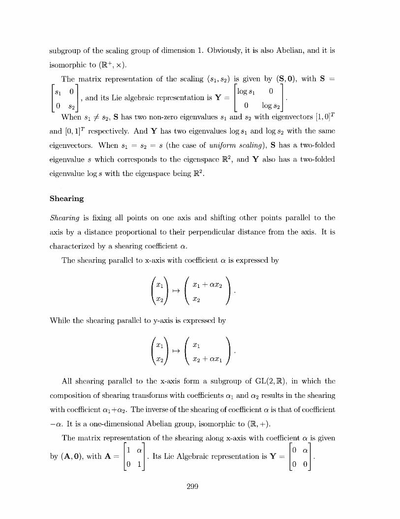
subgroup of the scaling group of dimension 1. Obviously, it is also Abelian, and it is
isomorphic to (R+, x).
The matrix representation of the scaling (Si, S2) is given by (S, 0), with S
si 0 and its Lie algebraic representation is Y log s 0
0 S2 0 log9S2
When si 4 S2, S has two non-zero eigenvalues si and s2 with eigenvectors [1 ,0 ]T
and [0, I]T respectively. And Y has two eigenvalues log si and log s2 with the same
eigenvectors. When si = s2 = s (the case of uniform scaling), S has a two-folded
eigenvalue s which corresponds to the eigenspace R2, and Y also has a two-folded
eigenvalue log s with the eigenspace being R2.
Shearing
Shearing is fixing all points on one axis and shifting other points parallel to the
axis by a distance proportional to their perpendicular distance from the axis. It is
characterized by a shearing coefficient a.
The shearing parallel to x-axis with coefficient a is expressed by
X1 X1 + aX2
While the shearing parallel to y-axis is expressed by
X1 X1
All shearing parallel to the x-axis form a subgroup of GL(2, R), in which the
composition of shearing transforms with coefficients al and a 2 results in the shearing
with coefficient al+a 2 . The inverse of the shearing of coefficient a is that of coefficient
-a. It is a one-dimensional Abelian group, isomorphic to (R, +).
The matrix representation of the shearing along x-axis with coefficient a is given
1 a 0 aby (A, 0), with A =.Its Lie Algebraic representation is Y =.
0 1 0 0
299
A has a three-folded eigenvalue 1, while Y has a three-folded eigenvalue 0. When
a f 0, both A and Y are not diagonalizable, as the dimension of the eigenspace is 1
with basis [1, 0 ]T. The shearing parallel to the y-axis has similar properties.
To sum up, all subgroups discussed above are Abelian groups. Except for scaling,
others are volume-preserving. The translations and rotations are further distance-
preserving. Actually, the Euclidean group in 2D space with positive determinant
E+(2) is the semidirect product of the rotation group and the translation group.
300
Bibliography
[1] Amr Ahmed and Eric Xing. Dynamic Non-Parametric Mixture Models and
The Recurrent Chinese Restaurant Process : with Applications to Evolutionary
Clustering. In Proc. of SDM'08, 2008.
[2] S. Ali and M. Shah. A lagrangian particle dynamics approach for crowd flow
segmentation and stability analysis. In Proc. of CVPR '07, 2007.
[3] Saad Ali and Mubarak Shah. A supervised learning framework for generic object
detection in images. In Proc. of ICCV'05, 2005.
[4] T. Amiaz, S. Fazekas, D. Chetverikov, and N. Kiryati. Detecting regions of
dynamic textures. In Conference on Scale Space and Variational Methods in
Computer Vision, 2007.
[5] P. Arbelaez, M. Maire, C. Fowlkes, and J. Malik. Countour detection and hi-
erarchical image segmentation. IEEE Trans. on Pattern Analysis and Machine
Intelligence, 33(5), 2011.
[6] M. Sanjeev Arulampalam, Simon Maskell, Neil Gordon, and Tim Clapp. A
tutorial on particle filters for online nonlinear/non-gaussian bayesian tracking.
IEEE Transactions on Signal Processing, 50:174-188, 2002.
[7] Simon Baker, Daniel Scharstein, J.P. Lewis, Stefan Roth, Michael J. Black, and
Richard Szeliski. A database and evaluation methodology for optical flow. In
Proc. of ICCV'07, 2007.
301
[8] Adrian Barbu and Song-Chun Zhu. Generalizing Swendsen-Wang to Sampling
Arbitrary Posterior Probabilities. IEEE Transactions on Pattern Analysis and
Machine Intelligence, 27(8), 2005.
[9] Leon Barrett and Aleksandr Simma. MCMC With Disconnected State Spaces,
2005.
[10] Marian Stewart Bartlett, Javier R. Movellan, and Terrence J. Sejnowski. Face
recognition by independent component analysis. IEEE Trans. on Neural Net-
works, 13(6), 2002.
[11] J. Bigun and G. Granlund. Optimal orientation detection of linear symmetry.
In Proc. of ICCV'87, 1987.
[12] Michael J. Black and P. Anandan. A framework for the robust estimation of
optical flow. In Proc. of ICCV'93, 1993.
[13] David M. Blei, Andrew Ng, and Michael I. Jordan. Latent dirichlet allocation.
Journal of Machine Learning Research, 3(4-5):993-1022, 2003.
[14] Yuri Boykov, Olga Veksler, and Ramin Zabih. Fast approximate energy mini-
mization via graph cuts. IEEE Trans. on Pattern Analysis and Machine Intel-
ligence, 23(11):1222-1239, 2011.
[15] Andres Bruhn, Joachim Weickert, and Christoph Schn6rr. Lucas/kanade meets
horn/schunck: Combining local and global optic flow methods. International
Journal of Computer Vision, 61:211-231, 2005.
[16] Liangliang Cao and Li Fei-Fei. Spatially coherent latent topic model for con-
current object segmentation and classification. In Proc. of ICCV'07, 2007.
[17] F Caron, Manuel Davy, and A Doucet. Generalized Polya Urn for Time-varying
Dirichlet Process Mixtures. In Proc. of UAI'07, 2007.
[18] Zhe Chen. Bayesian filtering: From kalman filters to particle filters, and beyond,
2003.
302
[19] Yeonseung Chung and David B. Dunson. The local Dirichlet Process. Annals
of the Inst. of Stat. Math., 63(1):59-80, 2009.
[20] Dorin Comaniciu, Visvanathan Ramesh, and Peter Meer. Real-time tracking of
non-rigid objects using mean shift. In Proc. of CVPR '00, 2000.
[21] T. F. Cootes and C. J. Taylor. A mixture model for representing shape variation.
Image and Vision Computing, 17(8):567-573, 1999.
[22] Timothy F. Cootes, D. Cooper, Christopher J. Taylor, and J. Graham. Active
shape models - their training and application. Computer Vision and Image
Understanding, 61:38-59, 1995.
[23] Timothy F. Cootes, Gareth J. Edwards, and Christopher J. Taylor. Active
appearance models. IEEE Transactions on Pattern Analysis and Machine In-
telligence, 23:681-685, 2001.
[24] D. Demirdjian, T. Ko, and T. Darrell. Constraining human body tracking. In
Proc. of ICCV'03, 2003.
[25] Tom Drummond and Roberto Cipolla. Real-time visual tracking of complex
structures. IEEE Transactions on Pattern Analysis and Machine Intelligence,
24:932-946, 2002.
[26] Tom Drummond and Roberto Cipollar. Real-time tracking of complex struc-
tures with on-line camera calibration. Image and Vision Computing, 20:427-
433, 2002.
[27] S. Duane, A.D. Kennedy, B.J. Pendleton, and D. Roweth. Hybrid monte carlo.
Physics Letters B, 195(2), 1987.
[28] Daniel Eaton and Kevin Murphy. Bayesian Structure Learning using Dynamic
Programming and MCMC. In Proc. of UAI'07, 2007.
[29] A. Efros and William Freeman. Image quilting for texture synthesis and trans-
fer. In Proc. of SIGGRAPH'01, 2001.
303
[30] Alexei A. Efros, Alexender C. Berg, Greg Mori, and Jitendra Malik. Recognizing
action at a distance. In Proc. of ICCV'03, 2003.
[31] Emily B. Fox, Erik B. Sudderth, Michael I. Jordan, and Alan S. Willsky. An
HDP-HMM for Systems with State Persistence, 2008.
[32] N. Friedman and D. Koller. Being Bayesian about network structure - A
Bayesian approach to structure discovery in Bayesian networks. Machine learn-
ing, 50(1):95-125, 2003.
[33] M. F.Tappen. Utilizing variational optimization to learn markov random fields.
In Proc. of ICCV'07, 2007.
[34] M. F.Tappen, C. Liu, E. H. Adelson, and William Freeman. Learning gaussian
conditional random fields for low-level vision. In Proc. of CVPR '07, 2007.
[35] Jan Gasthaus, Frank Wood, D. G6rur, and Y.W. Teh. Dependent Dirichlet
Process Spike Sorting. In Proc. of NIPS'09, 2009.
[36] D. Geman and G. Reynolds. Constrained restoration and the recovery of dis-
continuities. IEEE Trans. on Pattern Analysis and Machine Intelligence, 14,
1992.
[37] Lena Gorelick, Moshe Blank, Eli Shechtman, Michale Irani, and Ronen Basri.
Actions as space-time shapes. IEEE Transactions on Pattern Analysis and
Machine Intelligence, 29(12):2247-2253, 2007.
[38] Peter J. Green. Reversible Jump Markov Chain Monte Carlo Computation and
Bayesian Model Determination. Biometrika, 82(4), 1995.
[39] P.J. Green. Trans-dimensional Markov chain Monte Carlo. Highly structured
stochastic systems, 27, 2003.
[40] J. E Griffin and M. F. J Steel. Order-Based Dependent Dirichlet Processes.
Journal of the American Statistical Association, 101(473):179-194, March 2006.
304
[41] Matthias Grundmann, V Kwatra, Mei Han, and Irfan Essa. Efficient Hierar-
chical Graph-based Video Segmentation. In Proc. of CVPR '10, 2010.
[42] Yanlin Guo, Steve Hsu, Harpreet S. Sawhney, Rakesh Kumar, and Ying Shan.
Robust object matching for persistent tracking with heterogeneous features.
IEEE Transactions on Pattern Analysis and Machine Intelligence, 29:824-839,
2007.
[43] Firas Hamze and N. de Freitas. Intracluster Moves for Constrained Discrete-
Space MCMC. In Proc. of UAI'10, 2010.
[44] Tony X. Han, Huazhong Ning, and Thomas S. Huang. Efficient nonparametric
belief propagation with application to articulated body tracking. In Proc. of
CVPR'06, 2006.
[45] Xiaofei He and Partha Niyogi. Locality preserving projections. In Proc. of
NIPS'03, 2003.
[46] Thomas Hofmann. Probabilistic latent semantic indexing. In Proc. of SIGIR'99,
1999.
[47] Bernard K.P. Horn and Brian G. Schunck. Determining optical flow. Artificial
Intelligence, 17:185-203, 1981.
[48] Xiaolei Huang and Dimitris N. Metaxas. Metamorphs: Deformable shape and
appearance models. IEEE Transactions on Pattern Analysis and Machine In-
telligence, 30:1444-1459, 2008.
[49] Serdar Ince and Janusz Konrad. Occlusion-aware optical flow estimation. IEEE
Transactions on Image Processing, 17:1443-1451, 2008.
[50] M. R. Jerrum and A. J. Sinclair. Approximating the permanent. SIAM Journal
on Computing, 18:1149-1178, 1989.
[51] Nebojsa Jojic and Brendan J. Frey. Learning flexible sprites in video layers. In
Proc. of CVPR'01, 2001.
305
[52] Michael Kass, Andrew Witkin, and Demetri Terzopoulous. Snakes: Active
contour models. International Journal of Computcr Vision, pages 321-331,
1988.
[53] Seyoung Kim and Padhraic Smyth. Hierarchical dirichlet processes with random
effects. In Proc. of NIPS'06, 2006.
[54] Nathan Kitchen and Andreas Kuehlmann. A Markov Chain Monte Carlo Sam-
pler for Mixed Boolean/Integer Constraints. In Computer Aided Verification,
pages 446-461, 2009.
[55] Achim Klenke. Probability Theory: A Comprehensive Course. Springer, 2007.
[56] Iasonas Kokkinos and Alan Yuille. Unsupervised learning of object deformation
models. In Proc. of ICCV'07, 2007.
[57] M. Pawan Kumar, P.H.S. Torr, and A. Zisserman. Learning Layered Motion
Segmentations of Video. In Proc. of ICCV'05, 2005.
[58] Xiangyang Lan and D.P. Huttenlocher. A unified spatio-temporal articulated
model for tracking. In Proc. of CVPR'04, 2004.
[59] John M. Lee. Introduction to Smooth Manifolds. Springer, 2002.
[60] Julien Lefevre and Sylvain Baillet. Optical flow and advection on 2-riemannian
manifolds: A common framework. IEEE Transactions on Pattern Analysis and
Machine Intelligence, 30:1081-1092, 2008.
[61] Ido Leichter, Michael Lindenbaum, and Ehud Rivlin. Bittracker - a bitmap
tracker for visual tracking under very general conditions. IEEE Transactions
on Pattern Analysis and Machine Intelligence, 30:1572-1588, 2008.
[62] David A. Levin, Yuval Peres, and Elizabeth L. Wilmer. Markov Chains and
Mixing Times. American Mathematical Society, 2008.
[63] Fei-Fei Li and Pietro Perona. A bayesian hierarchical model for learning natural
scene categories. In Proc. of CVPR'05, 2005.
306
[64] A. Likas, N.P. Galatsanos, and I.E. Lagaris. A spatially constrained mixture
model for image segmentation. IEEE Trans. on Neural Networks, 16(2):494-
498, 2005.
[65] Bruce D. Lucas and Takeo Kanade. An iterative image registration technique
with an application to stereo vision. In Proc. of Imaging Understanding Work-
shop, 1981.
[66] Steven N. MacEachern. Dependent Nonparametric Processes. In Proceedings
of the Section on Bayesian Statistical Science, 1999.
[67] Ravikanth Malladi, James Sethian, and Baba Vermuri. Shape modeling with
front propagation: A level set approach. IEEE Transactions on Pattern Anal-
ysis and Machine Intelligence, 17:158-175, 1995.
[68] Abdol-reza Mansouri, Dipti Prasad Mukherjee, and Scott T. Acton. Constrain-
ing active contour evolution via lie groups of transformation. IEEE Transactions
on Image Processing, 13:853-863, 2004.
[69] Ross Messing, Chris Pal, and Henry Kautz. Activity recognition using the
velocity histories of tracked keypoints. In Proc. of ICCV'09, 2009.
[70] Amar Mitiche and Patrick Bouthemy. Computation and analysis of image mo-
tion: A synopsis of current problems and methods. International Journal of
Computer Vision, 19(1):29-55, 1996.
[71] Francese Moreno-noguer, Alberto Sanfeliu, and Dimitris Samaras. Dependent
multiple cue integration for robust tracking. IEEE Transactions on Pattern
Analysis and Machine Intelligence, 30:670-685, 2008.
[72] Peter Muller, Fernando Quintana, and Gary Rosner. A Method for Combining
Inference across Related Nonparametric Bayesian Models. J. R. Statist. Soc.
B, 66(3):735-749, August 2004.
307
[73] Radford M. Neal. Markov Chain Sampling Methods for Dirichlet Process Mix-
ture Models. Journal of computational and graphical statistics, 9(2):249-265,
2000.
[74] Andrew Ng, M. I. Jordan, and Yair Weiss. On spectral clustering: Analysis and
an algorithm. In Proc. of NIPS'01, 2001.
[75] Nikos Paragios and Rachid Deriche. Geodesic active contours and level sets for
the detection and tracking of moving objects. IEEE Transactions on Pattern
Analysis and Machine Intelligence, 22:266-280, 2000.
[76] Sylvain Paris, Pierre Kornprobst, Jack Tumblin, and Fredo Durand. Bilat-
eral filtering: Theory and applications. Foundations and Trends in Computer
Graphics and Vision, 4(1), 2008.
[77] Jian Pei, Haixun Wang, Jian Liu, Ke Wang, Jianyong Wang, and Philip S.
Yu. Discovering frequent closed partial orders from strings. IEEE Trans. on
Knowledge and Data Engineering, 18(11), 2006.
[78] Vinayak Rao and Yee Whye Teh. Spatial Normalized Gamma Processes. In
Proc. of NIPS'09, 2009.
[79] Carl Edward Rasmussen. The Infinite Gaussian Mixture Model. In Proc. of
NIPS'00, 2000.
[80] Carl Edward Rasmussen and Christopher K. I. Williams. Gaussian Processes
for Machine Learning. The MIT Press, 2006.
[81] Yogesh Rathi, Namrata Vaswani, Allen Tannenbaum, and Anthony Yezzi.
Tracking deforming objects using particle filtering for geometric active contours.
IEEE Transactions on Pattern Analysis and Machine Intelligence, 29:1470-
1475, 2007.
[82] Lu Ren, David B. Dunson, and Lawrence Carin. The Dynamic Hierarchical
Dirichlet Process. In Proc. of ICML'08, 2008.
308
[83] Stefan Roth and Michael J. Black. Fields of experts: A framework for learning
image priors. In Proc. of CVPR'05, 2005.
[84] Stefan Roth and Michael J. Black. Steerable random fields. In Proc. of ICCV'07,
2007.
[85] Stefan Roth and Michael J. Black. Fields of experts. International Journal of
Computer Vision, 82(2):205-229, 2008.
[86] Sam Roweis and Lawrence Saul. Nonlinear dimensionality reduction by locally
linear embedding. Science, 290:2323-2326, 2000.
K. G. Samuel and M. F.Tappen. Learning optimized map estimates in
continuously-valued mrf models. In Proc. of CVPR '09, 2009.
[88] U. Schmidt, Q. Gao, and S. Roth. A generative perspective on mrfs in low-level
vision. In Proc. of CVPR'10, 2010.
[89] Thomas Schoenemann and Daniel Cremers. High resolution Motion Layer De-
composition using Dual-space Graph Cuts. In Proc. of CVPR'08, 2008.
[90] J. Sethuraman. A Constructive Definition of Dirichlet Priors. Statistica Sinica,
4(2):639-650, 1994.
[91] Eli Shechtman and Michale Irani. Space-time behavior-based correlation or
how to tell if two underlying motion fields are similar without computing them.
IEEE Transactions on Pattern Analysis and Machine Intelligence, 29:2045-
2056, 2007.
[92] Hedvig Sidenbladh and Michael J. Black. Learning image statistics for bayesian
tracking. In Proc. of ICCV'01, 2001.
[93] C. Stauffer. Adaptive background mixture models for real- time tracking. In
Proc. of CVPR'99, 1999.
[94] Chris Stauffer and Eric Grimson. Adaptive background mixture models for
real-time tracking. In Proc. of CVPR '98, 1998.
309
[87]
[95] Deqing Sun, Stefan Roth, J.P. Lewis, and Michael J. Black. Learning optical
flow. In Proc. of ECCV'08, 2008.
[96] Deqing Sun, Erik B Sudderth, and Michael J Black. Layered Image Motion
with Explicit Occlusions, Temporal Consistency, and Depth Ordering. In Proc.
of NIPS'10, 2010.
[97] R.H. Swendsen and J. Wang. Nonuniversal critical dynamics in monte carlo
simulation. Physics Review Letters, 58(2), 1987.
[98] M. Tanaka and M. Okutomi. Locally adaptive learning for translation-variant
mrf image priors. In Proc. of CVPR'08, 2008.
[99] Yee Whye Teh. Dirichlet Process, 2007.
[100] Yee Whye Teh, Michael I. Jordan, Matthew J. Beal, and David M. Blei. Hi-
erarchical Dirichlet Processes. Journal of the American Statistical Association,
101(476):1566-1581, 2006.
[101] M. Tipping and C. Bishop. Mixtures of probabilistic principal component anal-
ysis. Neural Computation, 11(2), 1999.
[102] M. Tipping and C. Bishop. Probabilistic principal component analysis. J. R.
Statist. Soc. B, 61, 1999.
[103] Zhuowen Tu and Song-Chun Zhu. Image Segmentation by Data-Driven Markov
Chain Monte Carlo. IEEE Transactions on Pattern Analysis and Machine
Intelligence, 24(5), 2002.
[104] Matthew Turk and Alex Pentland. Eigenfaces for recognition. Journal of Cog-
nitive Neuroscience, 3(1):71-86, 1991.
[105] Matthew Turk and Alex Pentland. Face recognition using eigenfaces. In Proc.
of CVPR'91, 1991.
310
[106] G Vahedi, I V Ivanov, and E R Dougherty. Inference of Boolean networks under
constraint on bidirectional gene relationships. IET systems biology, 3(3):191-
202, 2009.
[107] Rene Vidal, Yi Ma, and Shankar Sastry. Generalized principal component
analysis (gpca). IEEE Trans. on Pattern Analysis and Machine Intelligence,
27(12):1945-1959, 2005.
[108] B. Walsh. Markov Chain Monte Carlo and Gibbs Sampling, 2002.
[109] J. Wang and E. Adelson. Representing moving images with layers.
Transaction on Image Processing, 3(5):625-638, 1994.
[110] John Y. Wang and Edward H. Adelson. Representing Moving Images with
Layers. IEEE Transactions on Image Processing, 3(5):625-38, 1994.
[111] Wei Wei, Jordan Erenrich, and Bart Selman. Towards Efficient Sampling :
Exploiting Random Walk Strategies. In Proc. of AAAI'04, volume 000, 2004.
[112] Joachim Weickert and Christoph Schn6rr. A theoretical framework for convex
regularizers in pde-based computation of image motion. International Journal
of Computer Vision, 45:245-264, 2001.
[113] Yair Weiss. Smoothness in Layers: Motion Segmentation using Nonparametric
Mixture Estimation. In Proc. of CVPR '97, 1997.
[114] Yair Weiss and Edward H. Adelson. A Unified Mixture Framework for Motion
Segmentation: Incorporating Spatial Coherence and Estimating the Number of
Models. In Proc. of CVPR'06, 2006.
[115] Yair Weiss and William Freenian. What makes a good model of natural images?
In Proc. of CVPR'07, 2007.
[116] Greg Welch and Gary Bishop. An introduction to the kalman filter. In SIG-
GRAPH 2001 Course, 2001.
311
IEEE
[117] Ming-Hsuan Yang. Kernel eigenfaces vs kernel fisherfaces: Face recognition
using kernel methods. In Prof. of International Conf. on Automatic Face and
Gesture Recognition, 2002.
[118] Yue Zhou and Hai Tao. A Background Layer Model for Object Tracking through
Occlusion. In Proc. of CVPR'03, 2003.
[119] Songchun Zhu, Yingnian Wu, and David Mumford. Filters, random fields and
maximum entropy (frame): Towards a unified theory of texture modeling. In-
ternational Journal of Computer Vision, 27(2):107-126, 1998.
[120] Xiaojin Zhu and John Lafferty. Time-Sensitive Dirichlet Process Mixture Mod-
els, 2005.
312