Lappeenranta University of TechnologySchool of Engineering ScienceMaster’s Programme in Computational Engineering and Technical PhysicsIntelligent Computing Major

Master’s Thesis

Shokoofeh Motamedi

NO-REFERENCE QUALITY ASSESSMENT OFMOBILE-CAPTURED VIDEOS BY UTILIZING MOBILESENSOR DATA

Examiners: Docent, D.Sc. Tuomas EerolaM.Sc. Olli Rantula

Supervisor: Janne Neuvonen

ABSTRACT

Lappeenranta University of TechnologySchool of Engineering ScienceMaster’s Programme in Computational Engineering and Technical PhysicsIntelligent Computing Major

Shokoofeh Motamedi

No-Reference Quality Assessment of Mobile-Captured Videos by Utilizing MobileSensor Data

Master’s Thesis

2018

68 pages, 17 figures and 8 tables.

Examiners: Docent, D.Sc. Tuomas EerolaM.Sc. Olli Rantula

Keywords: mobile-captured video, objective video quality assessment, mobile sensor data

Nowadays, recording videos using smartphones is a common practice in everyday life.One advantage of using smartphones for filming is the ability to capture the sensor dataduring filming to create sensor-rich videos. This thesis presents a no reference VideoQuality Assessment (VQA) tool specifically designed for sensor-rich videos. The VQAtool assesses the quality of a given video in three levels: pixel, bit-stream, and sensorlevel. In the pixel level, several measures are employed to assess the blurriness, contrast,and naturalness of the video. Video motion, scene complexity, and bit-stream quality areevaluated in bit-stream level. In the sensor level, the stability of the video is assessedby utilizing the sensor data. The performance of the proposed tool was assessed in twosteps. First, the capability of each measure was evaluated against a prepared database andthe measures with higher performance were selected for the final VQA tool. Then, theperformance of the tool was examined against an existing database. The results show apromising correlation.

PREFACE

I wish to thank my supervisor, D.Sc. Tuomas Eerola for his support, patience, positiveattitude, constructive feedback throughout the preparation of this thesis. I am so honoredand proud of working with such an excellent and experienced supervisor.

BCaster Oy has completely supported this research project. The whole research has beendesigned and conducted in BCaster Oy, and the full right of all outcome of this projectbelong to this company. All the data needed for this project has been collected usingBCaster mobile application and BCaster media platform. The database was anonymizedand only include data which was publicly available at the time of the running project.I am grateful to my colleagues in BCaster for giving me this opportunity to learn andexperience such a friendly and warm international atmosphere at work. Especially I wouldlike to thank Janne Neuvonen, Seppo Sormunen and my direct supervisor Olli Rantula forthe whole support and assistance they offered to me.

I am forever in debt to my family for their endless care and unconditional support. Myeverlasting appreciation goes to my husband for his understanding and encouragement.Whenever I was disappointed with the progress of the work, he was there for listeningall my excuses, for persuading me to work harder and for helping me to overcome thedark clouds. I am eternally thankful to my parent for their continuous care and support. Ilearned from my father how to set and plan my life’s goals, and my mother taught me howto achieve them by hardworking. My gratitude also goes to my brothers, for their supportand encouragement. Words cannot explain how blessed I am to have you all in my life.

To all of you my family, teachers, friends, and colleagues, I sincerely appreciate yourassistance and support.

Lappeenranta, August 1st, 2018

Shokoofeh Motamedi

4

CONTENTS

1 INTRODUCTION 81.1 Background . . . . . . . . . . . . . . . . . . . . . . . . . . . . . . . . . 81.2 Objectives and delimitations . . . . . . . . . . . . . . . . . . . . . . . . 101.3 Structure of the thesis . . . . . . . . . . . . . . . . . . . . . . . . . . . . 12

2 VIDEO QUALITY ASSESSMENT: REVIEW 132.1 Degradations in mobile-captured videos . . . . . . . . . . . . . . . . . . 132.2 Image and video quality assessment measures . . . . . . . . . . . . . . . 142.3 Pixel-based distortion-specific measures . . . . . . . . . . . . . . . . . . 15

2.3.1 Blurriness . . . . . . . . . . . . . . . . . . . . . . . . . . . . . . 162.3.2 Blockiness . . . . . . . . . . . . . . . . . . . . . . . . . . . . . 202.3.3 Contrast . . . . . . . . . . . . . . . . . . . . . . . . . . . . . . . 22

2.4 Pixel-based general purpose measures . . . . . . . . . . . . . . . . . . . 242.5 Bit-stream-based measures . . . . . . . . . . . . . . . . . . . . . . . . . 26

2.5.1 Bit-stream-based quality assessment . . . . . . . . . . . . . . . 262.5.2 Bit-stream-based video content characteristics . . . . . . . . . . . 27

2.6 Summary . . . . . . . . . . . . . . . . . . . . . . . . . . . . . . . . . . 29

3 STABILIZATION MEASURE 303.1 Mobile phone device sensors . . . . . . . . . . . . . . . . . . . . . . . . 303.2 Sensor fusion . . . . . . . . . . . . . . . . . . . . . . . . . . . . . . . . 323.3 Shakiness estimation . . . . . . . . . . . . . . . . . . . . . . . . . . . . 343.4 Summary . . . . . . . . . . . . . . . . . . . . . . . . . . . . . . . . . . 36

4 VIDEO QUALITY ASSESSMENT TOOL 374.1 Methodology . . . . . . . . . . . . . . . . . . . . . . . . . . . . . . . . 374.2 Target degradations . . . . . . . . . . . . . . . . . . . . . . . . . . . . . 374.3 The proposed method . . . . . . . . . . . . . . . . . . . . . . . . . . . . 384.4 Quality assessor modules . . . . . . . . . . . . . . . . . . . . . . . . . . 39

4.4.1 Pixel-level module . . . . . . . . . . . . . . . . . . . . . . . . . 404.4.2 bit-stream-level modules . . . . . . . . . . . . . . . . . . . . . . 404.4.3 Sensor-level module . . . . . . . . . . . . . . . . . . . . . . . . 41

4.5 Summary . . . . . . . . . . . . . . . . . . . . . . . . . . . . . . . . . . 42

5 EXPERIMENTS 435.1 Performance measures . . . . . . . . . . . . . . . . . . . . . . . . . . . 435.2 Experiment 1: Designing out of focus blurriness measure . . . . . . . . . 45

5.2.1 Data . . . . . . . . . . . . . . . . . . . . . . . . . . . . . . . . . 45

5

5.2.2 Results . . . . . . . . . . . . . . . . . . . . . . . . . . . . . . . 475.3 Experiment 2: The performance of the stability measures . . . . . . . . . 48

5.3.1 Data . . . . . . . . . . . . . . . . . . . . . . . . . . . . . . . . . 485.3.2 Results . . . . . . . . . . . . . . . . . . . . . . . . . . . . . . . 49

5.4 Experiment 3: The performance of quality measures . . . . . . . . . . . . 505.4.1 Data . . . . . . . . . . . . . . . . . . . . . . . . . . . . . . . . . 505.4.2 Results . . . . . . . . . . . . . . . . . . . . . . . . . . . . . . . 51

5.5 Experiment 4: Evaluating the performance of VQA tool . . . . . . . . . . 535.5.1 Data . . . . . . . . . . . . . . . . . . . . . . . . . . . . . . . . . 535.5.2 Results . . . . . . . . . . . . . . . . . . . . . . . . . . . . . . . 54

6 DISCUSSION 566.1 Limitations . . . . . . . . . . . . . . . . . . . . . . . . . . . . . . . . . 566.2 Future work . . . . . . . . . . . . . . . . . . . . . . . . . . . . . . . . . 57

7 CONCLUSION 59

REFERENCES 59

6

LIST OF ABBREVIATIONS AND SYMBOLSACA Angles change analysisACR Absolute Category RatingANN Artificial Neural NetworkCSF Contrast Sensitivity FunctionCPBD Cumulative Probability of Blur DetectionDCT Discrete Cosine TransformDFT Discrete Fourier TransformDWT Discrete Wavelet TransformEKF Extended Kalman FilterFA Focus AssessmentFISH Fast Image SharpnessFR Full ReferenceHVS Human Visual SystemIP Internet ProtocolIQA Image Quality AssessmentITU-T International Telecommunication Union - Telecommunication Standardization SectorJNB Just Noticeable BlurMB Macro BlocksMOS Mean Opinion ScoreMPEG Moving Picture Experts GroupMVG MultiVarient GaussianNIQE Natural Image Quality EvaluatorNR No ReferenceNSS Natural Scene StatisticNVS Natural Video StatisticPLCC Pearson Linear Correlation CoefficientOQoE Objective Quality of ExperienceQoE Quality of ExperienceQP Quantization ParameterRMS Root Mean SquareRMSE Root Mean Square ErrorRR Reduced ReferenceSC Scene ComplexitySNM Statistical Naturalness MeasuresSRCC Spearman’s Rank Correlation Coefficient

7

SVR Support Vector RegressionUMA Unintended motion analysisVM Video MotionVQA Video Quality AssessmentVQM Video Quality MonitorWLF Weighted Level FrameworkBk Blockiness measure of horizontal and vertical edgesBI , BP Bits of codec I-frames and codec P-framesBV LAP Focus measure based on variance of Laplacian coefficientscI average contrast in level lCWLF The overall score of contrast in WLF methodDx, Dy Horizontal and vertical edge mapEXY n Log-energy of of subband XY in level nGk Kalman gate in time kIk Inner blockiness measureLij Luminance value of pixel ijOaccMag Orientation obtained from acceleration and magnetometer sensorOfused Fused orientationOgyro Gyroscope orientationPe Blur probability of edge ePJNB JNB blur probabilitypk, pk−1 prediction error in time k and k − 1

QI , QP Average quantization of codec I-frames and codec P-framesR2 R-squaredrPLCC Pearson linear correlation coefficientrSRCC Spearman’s rank correlation coefficientSFISH Sharpness measure of fast image sharpness methodSCPBD Sharpness score of cumulative probability of blur detection methodSH , SV Subset of horizontal and vertical boundary pixelsSI Subset of inner pixelsSXY Subset of Sub-band of gray-scale image in XY decomposition levelwI Weight of level l in contrast measurevn Variance of pixel values in channel nx̂k, x̂k−1 States of system in time k and k − 1

zk Real sensor value in time kω(e) pixel width of edge eωJNB(e) JNB pixel width for edge e

8

1 INTRODUCTION

1.1 Background

Nowadays, a social life without digital media is not easy to imagine. Creating, sharing andwatching videos has been integrated into the daily lives of almost everybody. Embeddingthe high-quality camera into smartphones gives users the opportunity of capturing high-quality videos and photos. The increasing popularity of social networks, media services,and video sharing applications show that people have responded positively to the use ofthese opportunities.

Recording videos, like every other digital media, is prone to various degradations. Thesedegradations may be introduced by a number of sources such as the camera character-istics, environmental conditions, the nature of the subject and transmitting impairments.In the real-world scenarios, especially when it comes to filming in an uncontrolled envi-ronment by unskilled people, the number and the degree of degradations grow up. Themost visible distortions are the appearance of artifacts, focus-related degradations likeblurriness, color distortion, bad exposure, and stabilization issues [2].

Video degradations affect the quality of experience (QoE) of human observers. QoE isdefined as a subjective metric which indicates the degree of pleasure or displeasure ofuser when they are using an application or a service [3]. Predicting QoE, however, isdifficult because of the lack of knowledge about the low-level human visual system andalso psychological factors which affect the perceived QoE [4, 5].

Estimating or predicting the visual quality of a video through QoE metrics is useful inmany applications. A video sharing company can employ the video quality score as afactor during categorizing, filtering, manipulating or searching among the received con-tents. A network operator or a content provider can adapt the network settings regardingthe level of quality of video content to obtain the end-users satisfactory. Video qualityscore can be employed in streaming services and real-time communications to estimatethe quality of service.

Considering the link to the human perception, the most reliable method to assess the QoEof a video is performing a subjective test under controlled conditions [6] and analyzing theobtained opinions. Nevertheless, this technique is massively time-consuming, costly andprone to human factors [4, 7]. To deal with these limitations, several objective methods

9

have been proposed. The focus of objective approaches is automating the quality as-sessment with high correlation with subjective metrics and consequently with the humanvision system [2].

Based on the amount of available information about the image or video, existing Ob-jective QoE (OQoE) approaches can be classified into three categories: Full Reference(FR), Reduced Reference (RR) and no-reference (NR). Full reference methods such asPeak-Signal to Noise Ratio and Structural Similarities algorithms [5] assume that boththe pristine and the distorted version of the video are available. By this way, they focuson comparing the videos. FR methods are accurate, robust and highly correlated with thehuman perception [8]. In RR methods, only partial information such as some statisticsabout the reference file is available [9].

NR approaches, in contrary, assess the quality of image or video without any extra in-formation but the image or video itself. Although evaluating the quality of images andvideos is quite an easy task for a human subject, designing NR metrics which have ahigh correlation with human perception is yet an open issue [5]. However, regarding thefact that in most applications, no information about the original and undistorted source isavailable, NR approaches are highly on demand.

Assessing the quality of videos is not the same as evaluating the quality of a sequence ofimages. Although, any Image Quality Assessment (IQA) methods can be employed forboth images and video frames, concerning the nature of video contents is essential in aVideo Quality Assessment (VQA) task.

The temporal feature is an example of video specific characteristics which can assess thefreezes and jerkiness [5, 10], or motion coherency [11]. As another example, using re-buffering features on streaming context has shown a high correlation with the QoE [12, 13,14]. Also, knowing the video format can help the assessment process. For instance, theraw file of videos with Moving Picture Experts Group (MPEG)-4 format contains DiscreteCosine Transform (DCT) coefficients of the video. Thus, using DCT coefficients of theraw file instead of computing the coefficients from pixel values, can increase the speed ofcalculations significantly [11, 15].

The stability of the video content is another critical video quality feature which is notapplicable to images. The motion of the camera, in mobile-captured videos, introducesa lack of stability, so-called shakiness. It might happen intentionally or unintentionallyby shaky hands or body movement during filming. The stability is known as one ofthe most annoying issues in mobile-captured videos [2]. The effect of shakiness can be

10

estimated by measuring a specific type of blurriness called motion blur, which happensas a consequence of shakiness. However, it is difficult to assess the temporal impacts ofshakiness just based on the video analysis techniques.

Shakiness assessment can be performed easier in sensor-rich videos. In sensor-rich videos,sensor data are captured during the filming and stored with the video. GPS sensor is themost common one which can help to embed the location in the video file. The other sen-sors such as the accelerometer and gyroscope can be integrated in the same way. Theycan be used to detect the movements of the device. Thus, analyzing the sensor data canprovide a suitable measure for identifying shakiness.

In this thesis, we investigate different approaches in video quality assessment context.The final goal is to design and implement a reliable and fast NR video quality assessor.The proposed method is applied to the videos captured via Bcaster mobile application.Bcaster app is a filming application which captures the mobile sensor data during record-ing activity and produces sensor-rich videos.

1.2 Objectives and delimitations

The objective of this thesis is to design and implement a video quality assessment toolby employing several objective metrics. The focus is on the videos that are recordedusing hand-held mobile devices in free environmental conditions. Also, it is assumedthat videos are recorded with the high resolution of 1080p in MPEG4 format. This thesisproject aims to answer two central research questions.

Research question 1: What is a suitable design for an NR video quality assessment tool

to predict the perceived quality of videos captured by mobile devices?

Research question 2: How the stability of a video can be assessed utilizing sensor data?

A suitable design in the first research question refers to a design which can satisfy twomain criteria. First, the results need to correlate well with the human perceptions. Second,the design needs to provide a fast and reliable performance. The primary goal of thesecond research question is to understand the benefits of using sensor-rich videos forassessing the shakiness distortion. It studies novel ways to utilize mobile sensor data formeasuring the stability of the video as a quality parameter.

11

To address the research questions, six objectives are defined:

Objective 1: Find the most substantial degradations that occur in mobile-captured videos.

Objective 2: Select and implement an appropriate measure to estimate the amount of

each degradation.

Objective 3: Select a method to combine the individual measures to obtain the final

quality score of the assessment.

Objective 4: Find the most useful sensors in stability evaluating context.

Objective 5: Propose an algorithm to assess the stability.

Objective 6: Employ the stability measure in the video quality assessment tool.

Objective 1 intends to understand the issues introduced during the recording of videoswith hand-held devices. A literature study on related subjects is made to find the topconcerns in this context. In addition, the reasons or factors that determine the importanceof each issue should be investigated.

Objective 2 can be divided into two sub-objectives. The first sub-objective is to find theavailable measures for each degradation. To achieve this, the variation of each degradationis studied. For example, blurriness in images can be classified as motion blur, out of focusblur and so on, for each of which numerous measures have been proposed.

The second sub-objective is defining suitable criteria to categorize the measures and con-sequently to select the most appropriate one. Criteria definition can be achieved throughthe illusion of a literature study. The third sub-objective is to implement the measures andto assess its performance. After confirming the usability of the measure, it can be selectedfor the final version of the application.

Objective 3 aims to find a good solution to combine the results of selected measures toachieve the final quality score for each video. It can be done by using weighted averagingas the importance of each measure can be defined based on experiments.

Fulfilling Objective 4, first, the application of each available sensor in mobile devicesneed to be learned and second, the most suitable one or ones to detect shakiness would beselected. It needs a literature study and several experiments.

12

Objective 5 considers the design and implementation of an algorithm to estimate the rateof shakiness by analyzing the data captured from the selected sensor or sensors.

To achieve Objective 6, the proposed algorithm for stabilization measure need to be com-bined with other measures selected through Objectives 1-3.

One notable issue in this project is that the application needs to be able to assess thequality of videos captured in a casual way. It means that there is no control on the type ofmobile device and the hardware in use, the subject of filming and the person who recordthe videos. It makes the assessment even more challenging as there is no original videoeven for evaluating the performance of the application.

There are two possible solutions to tackle this limitation. The first one is to conduct acomprehensive subjective test which is very expensive and needs lots of considerations.The second solution is evaluating the performance of the application against an existingdatabase. The latter one is followed. For this purpose, the proposed tool is tested againstCamera Video Database (CVD2014) [1].

1.3 Structure of the thesis

This thesis report is organized into seven chapters. The related works are discussed inChapter 2 and 3. First, the existing approaches for assessing the quality of images andvideos are presented. Then, an introduction to mobile sensors and their application areelaborated. The details of the design and implementation of the proposed video qualityassessment tool are explained in Chapter 4. During these chapters, both research questionsare answered.

The conducted experiments and the evaluation of the proposed application are explainedin Chapter 5. A discussion about the results of the experiments and what is learned duringthis thesis is presented in Chapter 6. Also, some recommendations for the future work ispresented in this chapter. Finally, a conclusion is provided in Chapter 7.

13

2 VIDEO QUALITY ASSESSMENT: REVIEW

This chapter presents the literature review of degradations which occur in mobile-capturedvideos as well as the existing measures to assess the severity of each degradation.

2.1 Degradations in mobile-captured videos

nditions affects the quality of produced videos. To measure the quality of hand-heldrecordings, recognizing the different types of possible degradations in videos is necessary.As the focus of this thesis is over the videos in MPEG-4 format, the focus is on thedegradations that occur in videos using this codec.

Visible degradations in MPEG videos can be categorized into five main types [16, 17] asbelow:

• detail imperfections, such as visible blurring and lack of sharpness which causepoor, and inconsistent details,

• color imperfections, such as low contrast, unnatural brightness, and darkness,

• motion imperfections, such as jumpy motion, shakiness, frozen frames, shiftingblocks of pixels from previous frames, and stalling events,

• noise, such as Gaussian, white or Mosquito noise, and

• false patterns such as artifacts, mosaic patterns and color bleeding, staircase effectfalse edges, and color ringing.

These imperfections degrade the video quality by affecting hue, contrast, and edge or byproducing noise. Several factors may introduce these degradations. The primary originsof degradations are as follows:

• environment conditions, such as poor lighting, shaky or moving camera,

• imaging content, such as the fast motion of the subject,

• imaging system characteristics, such as out of focus, over/under exposure, camerashake, white balance, sensor noise,

14

• transmitting impairments, such as packet loss, bitrate selection schemes, and

• compression distortions, such as color ringing, color bleeding, mosaic patterns,staircase effect and false edges, jumpy motion, frozen frames, shifting blocks ofpixels from previous frames and blockiness caused by codecs based on DiscreteCosine Transform (DCT) [17].

The first two sources can be considered as social and physiological factors, and the oth-ers are under the technical elements category [18]. The importance of each source andthe resulting degradations highly depends on the application. For example, transmittingimpairments can cause stalling effects and re-buffering problems in streaming videos. As-sessing these degradations is the main points of interest for video content delivery servicessuch as YouTube and Netflix. On the other hand, in medical imaging, blur, low contrast,noise, and artifacts are the most problematic degradations [19].

In videos captured by mobile devices, in uncontrolled condition, both social and technicalfactors can cause imperfections. For example, recording in poor lighting can cause bothcolor imperfections and false patterns. As another example, shaky mobile devices mayrecord videos with focus problems. According to [2], the most dominant distortions arethe color and detail imperfections, stabilization and false patterns.

2.2 Image and video quality assessment measures

During the last decades, numerous objective Image and video quality assessment methodshave been proposed. OQoE methods can be categorized into pixel-based methods, whichassess the individual frames in the decoded file, and bit-stream-based techniques, whichwork directly with the coded bit-stream file. The focus of some pixel-based approaches ison one specific feature, called the specific-distortion methods, such as blurriness [15, 20],blockiness [21, 22], noise [23], and contrast [24, 25].

On the other hand, some pixel-based methods estimate the overall quality of the desiredfile. Such methods are known as general purpose methods. These methods typicallyextract some specific features and statistics from the image or video. The features areeither compared with the corresponding features from the natural scene images or videos[11, 26] or fitted to a perceptual model [27, 28].

Bit-stream-based methods, from another point of view, are concentrated on bit-stream

15

information such as coding bitrate, quantization parameter, and micro blocks. In thesemethods, bit-stream statistics are extracted to assess the quality of the file [29] or to es-timate specific degradations such as jumpy motion or stalling events [30, 31]. Since noIQA or VQA is robust to all distortions, some methods have been proposed that use acollection of individual methods and combine the results [5, 32]. An overview of theabove-mentioned methods is presented in Fig. 1. In this overview, the categorization ofmethods is adapted from [22].

Figure 1. An overview of image and video quality assessment methods.

2.3 Pixel-based distortion-specific measures

A straightforward approach to assess the quality of an image or video is focusing ona single degradation. As most of the degradations are visual, their assessment shouldbe done in pixel-level. In this section, three main visible degradations are reviewed:blurriness, contrast, and blockiness. The literature review focus on the methods which canestimate the degree of degradation rather than merely detecting the existence or absenceof the desired degradation.

16

2.3.1 Blurriness

Blurriness, as a loss of spatial detail and the spread of edges, is one of the most disruptivedegradations that can appear in an image. In practice, it can happen via several distortionssuch as lossy compression, de-noising filtering, median filtering, noise contamination,failed focus or relative movement of the camera and the object being captured [20]. Thetwo latter ones are the main factors causing blur in images (see Fig. 2). To study thesedegradations in a laboratory environment, defocus blur can be simulated by applying aGaussian filter, and linear motion blur can be modeled by degrading the specific directionsin the frequency domain [33].

(a) Motion blur (b) Out of focus blur

Figure 2. Examples of blurred images.

For assessing the blurriness, two main approaches are available. The first approach is toanalyze the frequency domain [15, 34, 35, 36, 37]. In this approach, blurriness is definedas a loss of energy in high-frequency components of the image. Thus, the increase in theloss of energy indicates a higher degree of blurriness in the image.

Second, regarding the spread of edge in a blurred image, the spatial domain informationcan be extracted [38, 39, 40]. Among both approaches, Human Vision System (HVS)model statistics such as visible blur and human contrast range can be taken into accountto improve the results [33, 41]. Similarly, using a saliency map to emphasize the regionof interest of the image in blur measurements is employed in some approaches [42].

There are several frequency-based approaches which can detect blurry images with a con-siderably low computational complexity. For this purpose, a filter, such as Laplacian filter[34, 43], Discrete Cosine Transform (DCT) [15, 35], Discrete Wavelet Transform (DWT)[36] or Discrete Fourier transform (DFT) [37] can be applied on the image. By analyzingthe log energy of the obtained coefficients and determining a threshold, the blurry andsharp images can be distinguished.

17

These approaches suffer from two main drawbacks. First, detecting the suitable thresholdis not easy and depends on the context of the image. It needs to be chosen empiricallyor with Meta-heuristic approaches [35]. Moreover, they only detect whether the image isblurred or not and cannot quantify the amount of degradation.

On the other hand, there are frequency-based approaches that estimate the rate of blurri-ness in an image. They use for example pyramids [34], spatial frequency sub-bands [36],a combination of both [15] or just the ratio of high-frequency pixels [44] for this purpose.They may average the computed statistics across different scales or compare the statisticsfrom different sub-bands to estimate the ratio of blurriness. For example, in [43], a focusmeasure is suggested based on variance of Laplacian coefficients as

BV LAP =∑i,j

[|L(i, j)| − L]2, (1)

where L(i, j) is the Laplacian coefficient of the image in pixel (i, j) and L is the mean ofabsolute values of Laplacian coefficients of the image.

Several methods have employed machine learning techniques for blurriness assessment.In [45], non-subsamples contourlet transform features are computed and the results arecombined using Support Vector Regression (SVR) to estimate the blurriness ratio. In[33], an Artificial Neural Network (ANN) model is employed to estimate the blurriness.To feed the network, several features are extracted from the local phase coherence sub-bands, brightness and contrast of the image, and the variance of frequency response of theHuman Vision System.

The spatial-based approaches mainly focus on analyzing the edge characteristics such asthe average width of the edges [38], the edge gradients [39] or point spread function [40].One of the most promising approaches in this context is proposed in [39]. It computesthe gradient profile sharpness histogram of the image and uses a just noticeable differencethreshold to assess the blurriness ratio. This method presents good results in both artificialand natural blurred images.

While most of the proposed approaches estimate the global blurriness, some studies con-centrate on measuring the motion blur [46, 47], the defocus blur [48, 49, 50] or classifyingimages based on the type of blur in the image [51]. In [46], the appearance of motion blurdue to camera-shake in digital images is investigated. The authors believe that the direc-tional and shape features of the Discrete Fourier Transform (DFT) spectra of the imageare helpful. The shape features can capture the degree of the orientation of the image due

18

to camera motion. Also, shape features indicate the degree of loss of the higher frequencycomponents of the image degraded by motion blur.

An extensive experimental survey of focus measures was done in [48]. For the experi-ments, a database consisting of digital images captured by cameras with autofocus facilityis prepared. The authors divided the 36 different focus measures into six categories basedon the type of their core operations: first and second order differentiation, data compres-sion, autocorrelation, image histogram, and image statistics. The results showed that thefirst and second derivative measures could distinguish the focused images more reliablyrather than the others.

Moreover, several sharpness measures have been proposed that estimate the local andglobal sharpness ratio by making a sharpness map of the image [41, 52, 53]. For instance,in [52], a Fast Image Sharpness (FISH) measure is proposed which operates in threesteps. First, the Discrete Wavelet Transform (DWT) sub-bands of the grayscale image isdecomposed with three levels of decomposition. Fig. 3 shows a sample image and itscomputed DWT sub-bands.

(a) Original image (b) DWT sub-bands.

Figure 3. An Example image and its DWT sub-bands in three levels.

Let SLHn, SHLn, SHHn be the Low-High (LH), High-Low (HL) and High-High (HH) sub-bands where n = 1, 2, 3 and represents the level of decomposition. Then, the log-energyof each sub-band at each decomposition level is measured as

EXYn = log 10(1 +1

Nn

∑i,j

S2XYn(i, j)), (2)

where XY represents decomposition levels (HH , LH or HL) and Nn is the number ofDWT coefficients in level n.

19

Then, the total log-energy at each decomposition level is computed as

En = (1− α)ELHn + EHLn

2+ αEHHn , (3)

where the parameter α is used to determine the importance of each subband. The authorsproposed the value 0.8 for this parameter to increase the effect of HH decomposition.

As the last step, the overall sharpness of the image is computed as

SFISH =3∑

n=1

23−nEn, (4)

where the factor 23−n is added to give the higher weights to the lower levels in which theedges are stronger. Based on the experiments [52], FISH is one of the fastest methodswith promising results.

Another sharpness measure is Cumulative Probability of Blur Detection (CPBD) [53]which takes HVS characteristics into account. This method employs the concept of JustNoticeable Blur (JNB) [54]. JNB introduces the probability of perceiving the blurrinessof an edge by the human eye utilizing a psychometric function. Based on JNB, if theprobability of detecting blur distortion in edge e is less than PJNB, which is 63%, thedistortion is not visible for the human eye and the edge can be assumed to be sharp.

The CPBD method contains three steps: 1) the image is divided to 64×64 blocks, and theedge blocks are determined using a Sobel edge detector, 2) the blur probability of eachedge estimates as

Pe = 1− exp(−| ω(e)

ωJNB(e)|β), (5)

where ω(e) is the width of edge e and ωJNB is the JNB edge width, β is a constant, 3) theCPBD score is computed as

PCPBD = P (Pe < PJNB) =

PJNB∑Pe=0

P (Pe), (6)

where P (Pe) is the value of the probability distribution function in Pe. The final score is anumber in the range of 0 to 1. The higher value denotes a sharper image. This metric wassuccessfully examined against Gaussian-blurred images from the LIVE database [55].

20

2.3.2 Blockiness

Blockiness is another irregularity in video frames with block-based coding like MPEG4that use DCT compression [34]. This degradation is defined as an artificial discontinuitybetween adjacent blocks in the image. Blockiness is known to be the most noticeabledistortion at low bitrate images and videos [21]. Fig. 4 shows two sample blocky images.Experiments show that blockiness is not always perceptible by human vision and it highlydepends on texture, luminance, and content of the image [21, 22, 56]. Therefore, it isimportant to consider an HVS model in assessing blocky images.

Figure 4. Two samples of blocky images.

Blockiness distortion can be assessed in both spatial and transform domain. In [57],a one-dimensional discrete Fourier transform is employed to compute a bi-directional(horizontal and vertical) blockiness measure. It pools the measures to assess the overallblockiness rate. The results were promising even when no a priori information is pro-vided. Hence, this approach does not employ any HVS model to refine the results. In[58], a block-based Discrete Cosine Transform (DCT) coding technique was employedto compute a block discontinuity map. A masking map is also provided using luminanceadaptation and texture masking adapted from human vision system (HVS) response. Asthe next step, the discontinuity and masking map are integrated to compute the noticeableblockiness map and gauge the perceptual quality of the image.

The spatial domain approaches, mostly, employ an edge detection technique and comparethe amount of brightness of neighboring blocks around edges [56]. For example, in [34],spatial features are extracted using the horizontal and vertical edge map, and HVS featuresare extracted from a background activity mask and background luminance weights. Asequential learning algorithm is employed for growing and pruning radial basis function(GAP-RBF) network and mapping the spatial features to the total blockiness score.

With an aim to decrease the computational cost, Liu and Heynderickx [21] proposed a

21

method that employs a grid detector to find the suspected blocky regions of the image.Then, a local pixel-based blocking measure is applied. The measure compares the gradi-ent energy of the desired region and its adjacent locations. The method is further supple-mented with a simplified model of HVS masking to obtain more reliable results. Usinglight-weight grid detector along with simplified HVS model makes this approach suitableand reliable for real-time applications.

Another approach in the spatial domain was proposed by Perra [59] comprising two mainsteps. First, the horizontal and vertical edge maps are produced using a Sobel operator asDx and Dy. Then, the edge maps are divided into blocks of 8 × 8 pixels. In the secondstep, the blockiness level of each block is assessed. For this purpose, the boundary andinner blockiness measures are defined. For boundary measure, vertical boundary pixels(SV ) and horizontal boundary pixels (SH) and for the inner measure, a subset of innerpixels (SI) are taken into account for further computations (see Fig. 5).

For boundary measure, the blockiness measure of horizontal and vertical edges are calcu-lated separately as

Bx =1

16

∑(i,j)∈SV

|Dx(i, j)|max(i,j)∈SV

(Dx(i, j)), (7)

andBy =

1

16

∑(i,j)∈SH

|Dy(i, j)|max(i,j)∈SH

(Dy(i, j)). (8)

(a) Horizontal border (b) Vertical border (c) Inner pixels

Figure 5. In [59] three sets of pixels in each block are examined for blockiness measures.

Then the boundary blockiness score is computed as

B = max(Bx, By). (9)

22

Also, the inner blockiness score is calculated as

I =1

20

∑(i,j)∈SI

√(Dx(i, j))2 + (Dy(i, j))2

max(√D2x +D2

y). (10)

.

Thus, the blockiness ratio of each block is defined as the normalized difference betweenthe adjusted boundary and inner blockiness score as

L =|Bk − Ik||Bk + Ik|/2

, (11)

where k controls the response of measure and the authors set the value to 2.3 based on theexperiments. The overall blockiness score of the image is the average of blockiness scoreof all blocks. The overall blockiness score is a value between zero and one and the highervalue, the stronger blockiness distortion in the image is.

This approach provides high performance with low computational complexity and is em-ployed as a part of several further systems [5, 60].

2.3.3 Contrast

Luminance contrast is one of the critical factors in assessing the quality of an image.Because of the sophisticated system of human vision, the definition of perceptual contrastis still an open topic [61]. A simple definition is the difference between light and dark partof the image. The more complicated definition is the difference between visual propertiesinvolved in distinguishing the objects in the image [61]. In general, the higher contrastpromotes finer details of the image and more visible objects (Fig. 6). The perceivedcontrast of an image is influenced by several factors including lightening conditions andimage content [61].

Several approaches have been proposed to measure the contrast of an image. A briefintroduction of classic global contrast measures is presented in [24]. The methods in thisgroup are called global contrast measures as they try to assign a single value of contrastfor the whole image by analyzing the range of luminosity and chromaticity value in theimage. Michelson [25] defined the contrast index Cm as

Cm =(Lmax − Lmin)(Lmax + Lmin)

, (12)

23

Figure 6. Examples of low contrast images.

where Lmax and Lmin are the maximum and the minimum luminance of the image re-spectively. Another global measure is Root Mean Square (RMS) contrast measure [62]which is still popular as a statistic feature. It is defined as standard deviation of individualpixel intensities and is calculated as

CRMS =

√√√√ 1

WH

W∑i

H∑j

(Lij − Lavg), (13)

where Lavg is the average of luminance of the image with size W × H and Lij is theintensity of the pixel at point (i, j). These classic global measures are applicable in verycontrolled and restrictive conditions rather natural images [24] and mainly fail in esti-mating the perceived contrast of natural images as they assume an equal weight for alldifferent spatial frequencies [63].

Also, several attempts have been made to mimic how the human vision system (HVS)perceives the contrast. As a result, a variety of contrast sensitivity functions (CSF) havebeen proposed. They consider the sensitivity of HVS to different frequencies to predictwhether the details are visible for the human eye [56]. However, some experiments showthat CSF works in only certain conditions and fails in practice for natural images [63].

Several local contrast measures have been developed to measure the contrast of naturalimages. The focus of local contrast approaches is on creating the local contrast mapby comparing each pixel with its neighbors [24, 64, 65] or using image statistics andemploying the machine learning approaches [66, 67]. In [24], a measure which computesthe local contrast among neighborhood pixels at various sub-sampled levels was proposed.The final contrast index is obtained by recombining the average contrast of each level.

Another low-complexity local contrast metric is called Weighted Level Framework (WLF)index [68] which correlates well with subjective tests [69]. WLF contains four steps: 1)the image is subsampled in a pyramid structure, 2) the local contrast is calculated for each

24

pixel, 3) a contrast map is created for each sub-sampled image, and 4) the contrast mapsare combined to obtain the final contrast value of the image. In each level of the pyramid,the overall contrast of color channel i is calculated as

Ci =1

Nl

Nl∑l

wlcl, (14)

where Nl indicates the number of levels, wl is the assigned weight of level l and cl is theaverage contrast in the same level. Experiments suggest using the variance of pixel valuesin level l in channel i as the weight of level (wl). The overall score is obtained by

CWLF =3∑

n=1

vnCn, (15)

where n represents the number of channels, red, green and blue respectively, and theweights vn are the variance of pixel values in the corresponding channel.

2.4 Pixel-based general purpose measures

Distortion-specific approaches introduced in the previous subsections assess the qualityof the image from just one aspect such as blur, blockiness or contrast. On the other hand,several methods have been proposed which try to assess the quality of the image as awhole with no knowledge of the type of distortion occurred in the image. Moreover, thereare several general purpose approaches which can identify the type and amount of thedistortion/s occured in the image or video [70].

Some general purpose techniques employ feature extraction and machine learning algo-rithms [27, 28]. These approaches extract particular features from the distorted image andtrain a machine learning model to classify the distorted and pristine images. For example,in [27], several features such as phase congruency, gradient, and entropy of the image areextracted and employed to train an Artificial Neural Network (ANN) model to estimatethe quality score of the image.

On the other hand, Natural Scene Statistic (NSS) approaches [11, 26] are based on anassumption that a particular statistical regularity exists in the natural and undistorted im-ages. Thus, one can use that regularity as a reference for assessing the quality of thedistorted images. By this way, the distortion degree of an image can be estimated by ana-lyzing the protuberances of the reference statistical regularities. By using natural images

25

as a reference, these approaches are also considered as Statistical Naturalness Measures(SNM) [26]. Moreover, experiments suggest that several characteristics of HVS such asvisual sensitivity to directional and structural information are either intrinsic or can beembedded in NSS techniques [71].

In [71], an NSS approach is proposed which employ the local Discrete Cosine Transform(DCT) coefficients for quality assessment. The DCT coefficients are fitted in a generalizedGaussian model, and several features are extracted from the obtained model. Model-basedfeatures are mapped to the final quality score using a Bayesian inference model. To makethe model robust to any specific distortion, the model can be calibrated for the desireddistortion during training. The limitation of this approach is that it is only robust againstthose distortion types which are included in the training phase. Thus, the performance ofthis approach for unknown degradations is not reliable [71].

Another NSS approach, called Natural Image Quality Evaluator (NIQE) [72], estimatesthe distance of a given image from the "naturalness". NIQE as a blind NR IQA techniqueworks with no knowledge about the type of distortion in the image or human opinions ofit. Moreover, NIQE employs the salient information of the image to consider the humanvisual characteristics and to obtain more reliable results.

The NSS features in NIQE are extracted from the mean and variance of each pixel inits 3x3 neighborhood block. The features are fitted to a MultiVariant Gaussian (MVG)model. It is shown that the coefficients of such model reliably follow the Gaussian dis-tribution in natural images [72]. Based on that notion, an MVG model is trained over acorpus of natural images and is used as the references model. The quality of any desiredimage can be predicted based on the distance of its MVG model and the reference model.Moreover, NIQE uses the salient map of the image and only the NSS features of blocksin the salient regions are taken into account.

Since the reference model is built using natural images with no or little distortion, anyviolation against the reference model reveals the existence of at least one distortion. Also,the degree of violation can indicate the severity of that distortion. In this way, NIQE isnot biased in any specific distortion. For example, in [73], NIQE method was successfullyapplied to a quality measure for printed images without retraining for new distortions.This feature makes NIQE a good candidate to be employed in an unconstrained context.

In addition, there are several blind video quality assessment approaches based on NaturalVideo Statistics (NVS) [74, 75]. Similar to NSS-based image quality approaches, thesemethods refer to statistical regularities in pristine and undistorted videos. They, also,

26

employ temporal statistical regularities to consider motion characteristic of the video. Forthis purpose, either motion direction is estimated to characterize the motion coherency[74] or local statistics of frame differences is employed [75]. However, these approachesmodel the naturalness of the video and fail to model any in-capture distortions. Highcomputation complexity is another negative point of NVS-based approaches [76].

2.5 Bit-stream-based measures

In many video-transmitting applications, such as video delivering services, assessing thequality of video from existing bit-stream information is necessary. Some bit-stream in-formation is shared in all type of video contents such as video resolution, frame-rate, andcoding bitrate. Also, some more specific features can be taken into account when thecodec of the video file is known.

Assessing the quality of MPEG video files, several bit-stream information can be em-ployed including video resolution, video codec, frame-rate, bitrate, packet-loss rate, thequantization parameter (QP), bits of intra-coded frames (I-frame) and Inter-coded frames(P-frame) [5, 30]. Table 1 provides a brief description of each parameter based on thedefinitions provided in [77] and [78].

In this section, focusing on NR techniques, three well-known bit-stream measures arereviewed: bit-stream quality of the file [78], scene complexity and level of motion [30].

2.5.1 Bit-stream-based quality assessment

During the last decades, several contributions toward NR VQA in bit-stream level hasbeen made. In this regard, the International Telecommunication Union (ITU-T) has pub-lished a standardized approach, called Recommendation ITU-T P.1203. It introduces aparametric model to assess the quality of video files encoded in H.264 or MPEG-4 AVC[78]. The result of this model is the predicted mean opinion score (MOS).

In ITU-T P.1203 recommendation [78], the quality of the file is assessed by consideringthe impact of both visual and audio encoding as well as Internet Protocol (IP) impair-ments. The recommendation combines the results to have an overall quality score onthe 5-point Absolute category rating (ACR) scale [6]. Moreover, the recommendationassesses the quality using a sliding window of the file, which provides the quality at per-

27

Table 1. Brief description of bit-stream parameters.

Parameter DescriptionVideo resolution The height and width of video frame in pixelVideo Codec The name of video compression techniqueFrame-rate The number of frame per second (fps)Coding bitrate The number of bits processing in a unit of time (Mbps)Packet-loss rate The rate of lost packets during transmissionQuantizationParameter (QP)

In DCT-based video codec, to improve coding efficiency, any blockof the DCT coefficients is quantized with dividing by an integer.The level of quantization can be defined by a quantization parame-ter (QP) in range of 0 to 51

Intra-codedframe (I-frame)

The frame which compressed with no dependency of other frames.Also known as keyframes

Inter-codedframe (P-frame)

The frame which compressed considering the spatial and temporalredundancies in I- and P- frames

Inter-codedframe (B-frame)

The frame which compressed considering the spatial and temporalredundancies in several preceding I-, P- and B-frames

Macroblock(MB)

Each frame divides into several macroblocks which represent a setof pixels and consider as the fundamental unit for codec compres-sion

one-second intervals.

The model suggested in the ITU-T recommendation comprises three modules: 1) quan-tization, 2) temporal and 3) upscaling (see Fig. 7). The quantization module addressesthe video compression artifacts. For this reason, the number of decoded Macroblocks(MB) and the Quantization Parameter (QP) in I- and P- and B- frames are employed. Thetemporal module assesses the temporal and jerkiness-related degradation based on theframe-rate of the video file in the desired window. Finally, the up-scaling module handlesthe spatial degradation due to fitting the content in the user’s screen. In each module,several constants are employed which their values are determined experimentally.

2.5.2 Bit-stream-based video content characteristics

Employing video content characteristics in assessing the quality of the video file, besidesthe basic bit-stream information available in the compressed domain, has been the point offocus of several approaches [5, 30, 77, 79]. Obtaining the content-based features withoutdecoding the video file is highly demanded in networked media delivery systems.

In [30], two spatial-temporal features of video content are employed for NR video quality

28

Figure 7. ITU-T P.1203.1 recommendation model for assessing the quality of video file [78].

assessment. The features are motivated by the masking effect characteristic of the humanvision system (HVS). Based on this characteristic, HVS cannot process the whole scene ofeach frame at once. Therefore, HVS pays more attention to the regions with perceivablemovements and new contents rather than non-salient parts of the image. Inspired by thischaracteristic of HVS, two features termed motion change and scene change are definedin [30]. These features are computed by employing the statistics of complex frames whichare P-frames with bits higher than the average bits of frames in their neighborhood.

A similar approach defines Scene Complexity (SC) and Video Motion (VM) as the spatial-temporal features of video content [79]. The Scene Complexity factor quantifies the num-ber of presented objects and scenes in the desired video, and the Video Motion (VM)factor demonstrates the presented movement in the video file.

The research suggests the more complex scene, the more bits needed to code the I-Frames.Also, as the motion in a video scene increase, the differences between pixel values inconsecutive frames increases which requires more bits to code the P-Frames. Since theQuantization (Q) parameter is utilized by rate control schemes to produce the desired bit-rate, it is essential to remove the effect of quantization parameter on the bits of coded I-and P-Frames. Therefore, SC and VM are defined as

SC =BI

2 · 106 · 0.91QI, (16)

and

VM =BP

2 · 106 · 0.87QP, (17)

29

where BI and BP represent the bits of codec I-Frames and P-Frames respectively. QI

and QP are the average I-Frames and P-Frames quantization parameters. Constant valuesare suggested based on the characteristics of AVC/H. 264 coding. Both SC and VM arescaled in the range [0, 1] [79].

The simplicity of calculation and high correlation with quality degradation make thesemetrics an excellent candidate to participate in quality assessing models [5, 77].

2.6 Summary

In this section, the most dominant degradations in mobile-captured videos were intro-duced. Then several video assessment approaches categorized in pixel-based, and bit-stream-based methods were discussed. Some techniques are distortion-specific such asblurriness, blockiness, and contrast while others assess the quality of the video file with ageneral scope such as statistic-based measures and bit-stream measures.

30

3 STABILIZATION MEASURE

This chapter presents an introduction to sensors employed in smartphone devices andtheir application in stabilization assessment. For this purpose, first, a brief introductionof mobile device sensors is provided. It is shown that none of the sensors are applicablealone because of their limitations including noise, offset, drifting along time and so on.The solution is fusing sensor data to obtain more reliable values. Therefore, some fusiontechniques are discussed. Then, existing approaches to detect the shakiness along withtheir application are reviewed.

3.1 Mobile phone device sensors

Nowadays, most mobile devices are empowered by several built-in sensors to measurethe environmental conditions such as air temperature, pressure, illumination as well asthe motion and position of the device in space [80]. Barometers and photometers areexamples of the environmental sensors. Motion sensors include the accelerometer, gravitysensor, gyroscope, and rotational vector sensor. The examples of position sensors areorientation sensor and magnetometer.

There are two types of sensors: hardware-based sensors which are physical compo-nents built into the device hardware, and software-based ones which capture one or morehardware-based sensors to compute new data. Hardware-based sensors, including ac-celerometer, gyroscope, and magnetometer, are embedded in almost all mobile devices,while, supporting software-based sensors such as orientation sensor and the gravity sensorare not offered in all devices [80].

For stabilization measures, both motion and position sensors, in particular, accelerome-ter, gyroscope, and magnetometer, can be employed. Since these sensors are among thestandard sensors [80], they are available on almost all mobile devices.

The accelerometer is a tiny component which can sense the force of Earth’s gravity down-ward and the magnitude of acceleration along each of three accelerometer axes, x, y, z(see Fig. 8). Accelerometer values are essential to detect whether the device is speedingup or slowing down in a straight line and also to detect the shakiness of the device [80].

However, accelerometer data cannot represent the rotation of the device along the ac-

31

celerometer axes. When the device has no motion, all accelerometer values remain thesame while the device is rotated. Moreover, the raw accelerometer data are very noisyand are not suitable to be used directly.

The gyroscope is another tiny component embedded in the device hardware which coversthe accelerometer rotating limitation. It measures the speed at which the device is rotating.When the device is fixed in any position, all gyroscope values are almost zero. Althoughgyroscope does not provide the exact angle directly, it can be calculated by integrating thegyroscope values over time. However, the accuracy of the calculated angle is not reliablebecause of the significant errors introduced by gyroscope noise and offset. Moreover,gyro drifts over time and its values lose the accuracy after a while [80]. This inaccuracycan be fixed using data collected from other sensors.

The magnetometer is another sensor which presents the magnetic field intensity in eachaccelerometer axes, x, y, and z and acts as a compass which detects the Earth’s magneticnorth. The magnetometer can be used for calculating the orientation of the device relativeto the magnetic north. The accuracy of this sensor is not high enough because of theexistence of magnetic perturbation in the device environment [80]. However, like othersensors, the errors can be reduced by utilizing data gathered from other sensors.

In recent mobile devices, a software-based orientation sensor is embedded. This sensorfuses the data coming from the accelerometer, magnetometer, and gyroscope and calcu-lates the orientation angles: pitch, roll, and yaw (azimuth) (see Fig. 8). Using these anglesthe orientation of the device relative to the Earth’s north can be defined [80].

Figure 8. Accelerometer axis and orientation angles

The range of values of all orientation angles is not the same. Pitch and roll angles changefrom −90 to +90. The values are zero on the horizon, and they change toward ±90depending on which direction the device turns. Assuming a mobile device on the tablewith screen up, turning to left and right side, around the Y axis, change the values of roll

32

angle. Turning the device to up and down, over the X axis, change the value of pitchangle. The yaw value range is between 0 to 360 which zero denotes North and clockwiseturn increases the value of angle toward 360.

Despite the importance and extensive usage of orientation angle, the accuracy and relia-bility of this sensor have not been confirmed by scientific experiments [81].

3.2 Sensor fusion

As discussed in the previous section, the data captured from each sensor is noisy andinaccurate. One standard solution to solve this issue is to use sensor fusion algorithms,which combine the data from two or more sensors and obtain more reliable and accu-rate values. In practice, sensor fusion is applied in advanced applications such as robotbalancing, human body tracking, enhanced motion gaming and estimating the orientationand the attitude of a device [82].

Employing sensor fusion algorithms in mobile devices aims to correct deficiencies ofeach sensor and to estimate the attitude of the device in terms of the pitch, roll, and yaw(azimuth) angles. By fusing the data captured from the accelerometer and gyroscope,the obtained angles represent the attitude and orientation of the device regarding the startpoint, the point that the fusion has been started. Adding magnetometer data has the benefitof using Earth’s north as a fixed reference and providing the accurate estimation of theposition and orientation of the device relative to the horizon.

The complementary filters are an example of a simple, yet reliable, fusion algorithms[81, 82, 83]. In a complementary filter, the accelerometer and magnetometer values arecombined to obtain inaccurate device orientation over long periods of time. Furthermore,gyroscope data is used in short time intervals to obtain the accurate changes in the orien-tation. By this way, the complementary filter works as the low-pass filter of accelerome-ter/magnetometer and the high-pass filter of gyroscope signals.

The complementary filter is defined in [83] as

Ofused = (1− α)Ogyro + αOaccMag, (18)

where Ogyro obtains from the values of the gyroscope sensor in a predefined time intervaland OaccMag is calculated from the data coming from accelerometer and magnetometer

33

sensors. The constant α is a weighting factor in determining the weight of each opera-tor and was experimentally set as 0.98 in [83]. By this integration, the high-frequencycomponent of OaccMag is replaced with the corresponding gyroscope orientation values.

The complementary filter is an easy and low complexity sample of sensor fusion. Accord-ing to [81], the accuracy of this filter, in normal conditions with no magnetic perturbations,is about ±14 degrees. However, to keep the results as accurate as possible, the samplingrate of capturing sensor data needs to be near 100Hz. Reducing the sample rate affectsthe accuracy of results significantly.

Kalman Filter is another sensor fusion algorithm which has been used extensively. KalmanFilter algorithm, in its basic form, is developed for linear systems. However, several vari-ations of this filter have been developed to manage non-linear data such as sensor data.Among them, Extended Kalman Filter (EKF), Unscented Kalman Filter and AdaptiveKalman Filters have been examined for sensor fusion applications [81].

Kalman filter works in a prediction-update cycle (Fig. 9). In each cycle, it predicts thecurrent state of the system based on the previous state and updates its prediction based onthe measurements obtained from the real (noisy) sensors.

Figure 9. Extended Kalman Filter (EKF) work flow

In prediction phase, the state of the system is predicted as

x̂k = ax̂k-1, (19)

where x̂k and x̂k−1 are the states of the system in time k and k − 1 respectively, and a isa constant. Since the predictions are prone to error, EKF defines a prediction error and

34

predicts it aspk = apk-1a. (20)

In the update phase, the real data captured from the sensor and the predicted data arecombined to achieve the most reliable estimation of the current state of the system as

x̂k = x̂k +Gk(zk − x̂k), (21)

where zk is the real sensor data. Gk is the Kalman gate constant which computes from pre-diction errors and the average noise of the sensor. Using the Kalman gate, the predictionerror can be updated as

pk = (1−Gk)pk. (22)

In [81], several sensor fusion algorithms were compared in different scenarios. The resultsrevealed that all variations of Kalman Filter techniques were among the best approachesfor fusing sensor data. For typical smartphone motions, the EKF fusion showed the av-erage accuracy of ±7 degrees, which was far better than the fusion approach used byAndroid and iOS with the average accuracy of ±20 degrees.

3.3 Shakiness estimation

Filming with hand-held devices is prone to be shaky because of intentionally and unin-tentionally movements of the device. The intentional movement is a motion that the film-maker performs purposely including panning and zooming the screen or tilting, rotatingor moving of the camera. On the other hand, the unwanted motion includes movementsof device-holder such as the shaky hand or small pose changes.

In the majority of recent smartphones, the native software of camera has the stabiliza-tion feature which aims to compensate for the unwanted motions. However, stabilizationperformance is not perfect. Also, this feature can be disabled by the user. Thus, a morereliable solution is needed.

Since any movement affects the device sensor data, one valid solution is to use motion andposition sensors to detect the amount of shakiness and score the stability of the createdvideo. The most suitable sensor is the accelerometer which detects all tiny movementsof the device. This sensor has extensive usage in detecting shake events as it is easy tomeasure the quick changes in the accelerometer data.

35

There are several use cases of recognizing shake events such as freefall detection, pe-dometer, device tilting, and games [82]. However, the quick movements do not usuallyhappen during filming, and therefore this approach is not helpful to detect the stability ofthe device. Furthermore, as mentioned before, the accelerometer data is noisy, and, also,does not help to identify the rotation of the device.

A better approach is to fuse the measurements obtained from two or more sensors. Theadvantages of using a sensor fusion technique include removing the noise and other limita-tions of each sensor, correcting deficiencies in sensor data and calculating the orientationof the device more accurately.

By this way, it is also possible to record the orientation of the device during recording, andform a motion signal which would show both wanted and unwanted motions. Frequencyanalysis can help to recognize the type of the motion as suggested in [84]. Based on thisapproach, high-frequency parts of the motion signal reflect quick movements with lowenergy which are the result of unwanted motion. On the other hand, low-frequency partsrepresent slow and intentional performed movements (see Fig. 10).

Figure 10. A sample motion captured from sensors represented as orientation angles (Azimuth,pitch, and roll) over time. (a) the captured sensor data, (b) extracted wanted motion. (c) extractedunwanted motion.

A low pass filter such as second-order Butterworth can be employed to extract the un-wanted motion from the original signal [84]. The filter is formulated as

H(s) =1

1 + (− s2

ω2c)2, (23)

36

where s is the signal and ω2c is the cutoff threshold which is set to 0.45 experimentally.

The unwanted motion is obtained by subtracting from the original signal. Extracting theunwanted motion using a low-pass filter provides useful insights for stabilization purpose[85, 84]. This information can be used for calculating the shakiness rate of a video.

3.4 Summary

In this chapter, a brief introduction of mobile device sensors was presented. The rel-evant sensors in detecting motion namely accelerometer, magnetometer, and gyroscopewere briefly introduced. Since the data captured from each sensor, individually, is noisyand inaccurate, two well-known sensor fusion algorithms were introduced. Furthermore,the application of an accelerometer sensor in detecting shaky motions was explained.Regarding the limitations of this sensor, the possibility of employing a fusion approachfor calculating the orientation angles was investigated. Moreover, a couple of successfulstrategies in using orientation information for detecting unwanted motion was introduced.

37

4 VIDEO QUALITY ASSESSMENT TOOL

In this chapter, the target degradations for designing VQA tool are introduced. Then,the proposed methodology to answer the two research questions is explained. Also, thearchitecture and constructing components of the tool is elaborated in detail.

4.1 Methodology

Since recording videos in open condition are prone to several distortions simultaneously,the proposed Video Quality Assessment (VQA) tool should cover as many degradations aspossible. The selected approach is assessing each degradation individually and combiningthe results to obtain the overall quality of a given video.

The proposed VQA tool is designed in three steps. First, the target degradations are se-lected based on the presented imperfection factors. Then, the significance of each degra-dation is assessed using a proper metric. In the last step, an integration approach is usedto combine the results of measures and obtain the final quality score.

The desired metric for each degradation should meet several criteria. First, a proper met-ric needs to have a good generalization ability which means it should not assess only oneparticular aspect of a degradation type. For example, to evaluate the blurriness, a metricwhich only estimates the blurriness raised by motion blur was not desired. Second, a suit-able metric returns the percentage of occurred imperfection. Thus, detecting the existenceor absence of distortion is not the point of interest. Third, if several suitable metrics for aspecific degradation are available, the metric with lower complexity is more desired.

For stability degradation, in particular, two novel approaches are proposed to identify theadverse movements and to score the video stability. By comparing the performance ofthose approaches, the superior method is employed for developing the VQA tool.

4.2 Target degradations

In the proposed VQA tool, degradations caused by the social and technical factors need tobe taken into account. The social factors, including environmental conditions and imag-ing content, produce the most annoying degradations such as blurriness and poor contrast.

38

Also, as the users are not professional, degradations caused by technical factors includ-ing out of focus, over/under exposure and shaky camera are very common in this context.Moreover, since, the recorded videos are uploaded to the cloud, and the assessment is per-formed on the transmitted contents, the transmission impairments can affect the quality.

Since the captured videos are assumed to be in high resolution, it is expected to encountervery few, or no degradations caused by DCT codec which are more annoying in low-resolution videos rather than high-resolution ones. Thus, this factor and correspondingdegradations are discarded.

Therefore, three pixel-based degradations are selected to be assessed, i.e. blurriness, con-trast, and naturalness. Moreover, the video characteristic, such as video motion and scenecomplexity are taken into account. Also, the stability of the video is evaluated using thedata captured from the sensor data during recording.

4.3 The proposed method

Proposed video quality assessment tool aims to assess the quality of given video with ano-reference approach. It means no knowledge about the degradations happened to thevideo is provided. In this context, a quality assessment tool designed comprising fourmodules. The outline of the tool’s architecture is presented in Fig. 11.

The input of the assessment tool is a sensor-rich video which contains the desired videoand embedded sensor data which are collected during filming. The video can be recordedby any hand-held device which is empowered by basic sensors including accelerometer,magnetometer, and gyroscope. Also, the video is assumed to be recorded in MPEG-4format. The output of the tool is the estimated quality of the video as a number in therange from 0 to 100.

The quality assessment comprises three modules: pixel-level, bit-stream-level, and sensor-level. The pixel-level module is in charge of assessing the degree of visual degradationsincluding blurriness, contrast, and naturalness. Since pixel-level module does not coverthe temporal characteristics of the video, the bit-stream level module is designed by defin-ing three measures namely video motion, scene complexity, and bit-stream quality.

The sensor-level module contains two blocks. In the first block, the orientation informa-tion of the device is calculated by fusing sensor data through an Extended Kalman Filter

39

Figure 11. The outline of Video Quality Assessment tool

(EKF) [84]. In the second block, the orientation information is analyzed to extract theunwanted motion and score the stability of the signal.

The results of all measures are sent to the integration module which computes the finalscore as

Q =∑i

wiSi, (24)

where Si is the score of module i, andwi is the weight of the corresponding module whichis determined experimentally. The output of this module is the overall quality of the givenvideo in the range from 0 to 100.

4.4 Quality assessor modules

Each component of the proposed VQA tool measures the quality of the given video fromone specific aspect. For each component, at least one candidate approach is selectedbased on the performed literature search. In the following sections, the chosen methodsare introduced.

40

4.4.1 Pixel-level module

In the pixel-level module, the visual quality of the video frames is assessed regardingthree measures: contrast, naturalness, and blurriness. For assessing the contrast, twoapproaches were selected: 1) RMS contrast [62] and 2) WLF index [68] (see Section2.3.3). The naturalness of the video frame is assessed employing NIQE measure [72] (seeSection 2.4).

For blurriness measure three approaches are chosen: 1) Cumulative Probability of BlurDetection (CPBD) [53] as a blurriness measure 2) Fast Image Sharpness (FISH) [52]as a frequency-based sharpness measure 3) a novel measure is proposed in this thesis,termed Focus Assessment (FA) which employs four focus metrics to assess out of focusblurriness. The algorithm of the first two methods are elaborated in Section 2.3.1 in detail.

Focus Assessment (FA) assesses how focused the image is. Although many efforts havebeen put on developing focus metrics, the performance of each metric highly depends onthe scene and the imaging device. Thus, it is not applicable to employ one metric forall imaging conditions [49]. Therefore, FA is designed to utilize a combination of focusmetrics to score the amount of out of focus blur reliably.

To design the FA measure, 28 focus metrics, introduced in [49] and [48], were selected ascandidate metrics. The list of metrics and their abbreviation is presented in table 2. Theabbreviations are defined based on the core function of each metric including Laplacian-based (LAP*), Gradient-based (GRA*), Wavelet-based (WAV*), Statistics-based (STA*),DCT-based (DCT*) and Miscellaneous (MIS*) metrics. A brief introduction of eachmetric is provided in [49]. The selection of focus metrics is presented in Section 5.2.

4.4.2 bit-stream-level modules

In the bit-stream module, three measures are employed. The first measure assesses thequality of file from the bit-stream aspect, based on ITU-T P1203 recommendation [78].The next two measures are video motion and scene complexity [79] which estimate thevideo degradation ratio by utilizing the spatial-temporal features of video content. Allmeasures are described in detail in Section 2.3.2.

41

Table 2. The candidate focus metrics selected for designing FA measure [77].

Focus operator Abbr. Focus operator Abbr.Gaussian derivative GRAD Histogram entropy STAHGradient energy GRAE Gray-level local variance STALTenengrad GRAN Normalized gray-level variance STANSquared gradient GRAS Histogram range STARThresholded absolute gradient GRAT DCT energy ratio DCTETenengrad variance GRAV DCT reduced energy ratio DCTRDiagonal Laplacian LAPD Absolute central moment MISAEnergy of Laplacian LAPE Brenner’s measure MISBModified Laplacian LAPM Image contrast MISCVariance of Laplacian LAPV Spatial frequency measure MISFRatio of the wavelet coefficients WAVR Helmli and Scherer’s mean MISHSum of wavelet coefficients WAVS Steerable filters-based MISSVariance of wavelet coefficients WAVV Image curvature MISUGray-level variance STAG Vollath’s autocorrelation MISV

4.4.3 Sensor-level module

For stability assessment component, two methods are proposed. The first method, termedAngles Change Analysis (ACA), is designed based on monitoring the changes in orienta-tion angles in every second. Any change, in each angle, that exceeds the threshold wouldbe considered as violence to the stability. Since the range of yaw value is twice otherangles (see Section 3), the threshold is set as one degree for pitch and roll angles, and twodegrees for yaw.

The stability score of each angle, for each second, is calculated as

S(t, a) =N∑i=1

|xit − xi(t−1)|c

, (25)

where xi is the value of angle a. xi and xi(t−1) denote the value of angle a in second t andt− 1 respectively. The c value is the threshold constant, and N is the number of availablesensor data in that period. The overall score of the video is the average of calculatedstability scores in each second.

The second method, named Unintended Motion Analysis (UMA), was inspired by theapproach introduced in [84] (see Section 3.3). In this method, it is assumed that themotion signal comprises intended and unintended motion. Intended motion is wantedmotion which user has moved during filming intentionally and motion happened by shaky

42

camera or user unwanted movements are considered as unintended motion. Intended andunintended motion were separated employing a Butterworth low-pass filter. Then, theintended motion was smoothed using a Savitzky-Golay filter [86] to remove all remainednoise and obtain the most realistic estimation of the intended motion.

The next step was calculating the Signal-to-Noise Ratio (SNR) of pure wanted motionto represent the amount of noise in the signal, and therefore, the quality of the originalsignal. The SNR score was calculated as

SSNR = 10 log10PwantedPunwanted

, (26)

where P represent the power of the signal which is computed as

P =1

N

N∑i=1

s2i , (27)

where N is the total number of values in the signal and si denotes the value of the signalin the point i.

Both measures were examined against the prepared dataset, and the measure with betterperformance was selected for VQA tool. The experiment is described in detail in Section5.3.

4.5 Summary

This chapter presented the methodology used in this thesis. Also, the details of targetdegradations and the proposed architecture of the VQA tool were described. Moreover,the chosen measures for each component were elaborated.

43

5 EXPERIMENTS

In this chapter, the measures used to evaluate the performance, the dataset used for theexperiments and the details of the tests are presented. For this project, four differentexperiments were designed and performed:

Experiment 1: Designing out of focus blurriness measure.

The goal of this experiment was to design a measure for out of focus blurriness which canadequately assess the de-focus blurriness.

Experiment 2: The performance of the stability measures.

This experiment was designed to assess the performance of the proposed stability metricusing a subjective test.

Experiment 3: The performance of quality measures.

This experiment aimed to evaluate the performance of the selected measure/measures foreach component of the proposed video quality assessment tool. The metrics with higherefficiency and lower computation complexity are chosen for final VQA tool.

Experiment 4: Evaluating the performance of proposed VQA tool.

During this experiment, the performance of video quality assessment tool was examinedagainst an existing database.

5.1 Performance measures

To evaluate the results of the experiments, two correlation metrics were employed namelyPearson Linear Correlation Coefficient PLCC) and Spearman’s Rank Correlation Coef-ficient (SRCC). Using PLCC, the linear correlation between the estimated score and thebenchmark can be assessed as

rPLCC =

∑Ni=1(xi − x)(yi − y)√∑Ni=1(xi − x)2(yi − y)2

, (28)

44

where xi denotes the estimated score, and yi is the benchmark. x and y are the averageof the scores and the benchmark respectively. N represents the total number of videos orimages examined in the experiment.

Moreover, the monotonic relationship between the estimated scores and the benchmarkwas assessed with SRCC metric. In this metric, the rank of each value is used for eval-uation. In this respect, the values of estimated scores are sorted in ascending order todetermine the rank of each value in the list. Also, the rank of values in the benchmark listis calculated in the same way. The correlation between the two lists is the relative orderof the values and can be formulated as

rSRCC = 1− 6∑N

i=1 (Xi − Yi)2

N(N2 − 1), (29)

where Xi and Yi are the ranks assigned to the xi and yi respectively.

The correlation coefficient obtained from both metrics is a number from −1 to 1. Valuescloser to one suggest high positive correlation and values closer to −1 denotes strongnegative correlation. The coefficient value close to zero indicates that no relationshipbetween the two lists is observed. The reliability of the correlation result verifies witha hypothesis which provides the level of marginal significance known as p-value. Thus,the correlation is significant if the p-value is less than the significant level of 0.05 whichmeans the chance that two variables are correlated randomly should be less than 5%.

Employing PLCC and SRCC, both linear and non-linear correlation between the esti-mated results of the experiment and the benchmark can be assessed.

Besides Experiment 1, the data are fitted to a quadratic regression model. To evaluate thegoodness of model fit, two statistics are evaluated: Root Mean Square Error (RMSE) andR-squared. The RMSE indicates the distance between real data and the predicted resultsof the model. The lower value of RMSE presents the higher accuracy of model predictionability which means a better fit. RMSE is defined as

RMSE =

√√√√ 1

n

n∑i=1

(di − pi)2 (30)

where di and pi represent the actual data and the predicted value respectively, and n is thenumber of samples.

R-squared is a statistical metric which indicates the percentage of data variation which is

45

explained by the model and defines as

R2 =

√∑ni=1 (pi − d̂)2∑ni=1 (di − d̂)2

(31)

where d̂ is the average of actual data. The higher R-squared value indicates a better fit.

5.2 Experiment 1: Designing out of focus blurriness measure

This experiment aimed to find a combination of four focus metrics out of 28 metrics,reviewed in [46], which can measure the out of focus blurriness in wild images. Thedesigned measure was a candidate to be used in final VQA tool.

5.2.1 Data

The test images used in this experiment were collected from three databases: 1) 175Gaussian-blurred images from LIVE database [55], 2) 125 Gaussian-blurred images fromthe TID2013 database [87], 3) 40 naturally-blurred images from the novel NaturalBlurdatabase which was designed for this experiment.

There are three limitations in images collected from both LIVE and TID2013 database.First, the images are distorted by Gaussian blur distortion artificially, and therefore nowild image is provided. Second, these databases are not designed for blurriness assess-ment specifically. Therefore, no other type of blurriness is provided, nor partially blurredimage is available in these databases.

Despite an extensive search, only one publicly available database, dedicated for blurrinessassessment, was found: CERTH Image Blur Dataset [37] including both naturally andartificially blurred images. However, in this dataset, each image is labeled as blurry or notblurry, and the degree of blurriness is not provided. It makes the database unsuitable forthis project.

To assess the performance of each metric against naturally blurred images, a new database,named NaturalBlur, was designed including 40 wild images suffered from defocus degra-dation. NaturalBlur database comprised 40 frames from 18 videos. The videos wererecorded in free imaging condition using one specific mobile application with 1920×1080

46

resolution. The frames were stored as JPEG images. Fig. 12 shows a subset of imagesfrom the prepared database.

Figure 12. Example images from NaturalBlur database.

A subjective test was designed to provide the mean opinion score of NaturalBlur database.For this purpose, ten non-expert users were invited to score the blurriness of each image inthe range from 0 to 10. Images were shown in a 21” Samsung screen each for 30 seconds.The blurriness score for each image was calculated as the mean of opinions.

Other experiment setups were as follows: 1) the experiment was performed on a MacBookPro with 3,1 GHz Intel Core i5 processor, 2) all metrics were implemented in MATLABR2017b, 3) the ’fitlm’ function in Matlab was used for creating a quadratic regressionmodel with considering ’Intercept’ term.

The experiment was designed to highlight the most proper focus metrics for FA measure.The experiment performed in two steps. First, all metrics applied to all test images toobtain the correlation and runtime performance. The metrics with poor performance wereexcluded from further processing. Then, all possible combinations of four metrics, fromthe remaining metrics, were fitted to a quadratic regression model.

47

5.2.2 Results

28 focus metrics were examined against the collected images. Table 3 shows the averagerunning time and the correlation between each focus metric’s result and the benchmark.It can be seen that some methods had very long runtime such as DCTE, DCTR, MISSand WAVR and some have a very low correlation with the benchmarks including GRAD,MISA, MISH, STAG, STAH, STAN metrics which make them undesirable for blurrinessmeasure. Therefore, the weak metrics, indicated by ’∗’ in Table 3, are excluded fromfurther processing.

Table 3. The average runtime as well as PLCC, and SRCC coefficients of focus metric in each ofthree test databases.

Runtime LIVE TID2013 NaturalBlurMetric (ms) PLCC SCRR PLCC SCRR PLCC SCRRGRAD* 15.18 -0.35 -0.32 0.13 0.17 -0.01 0.02GRAE 3.44 -0.60 -0.75 0.45 0.52 0.05 0.04GRAN 9.60 -0.46 -0.77 0.40 0.60 0.10 0.11GRAS 1.53 -0.55 -0.75 0.43 0.54 0.05 0.04GRAT 4.09 -0.60 -0.80 0.39 0.56 0.08 0.14GRAV 11.28 -0.30 -0.86 0.32 0.75 0.2 0.23LAPD 5.65 -0.53 -0.93 0.55 0.71 0.09 0.09LAPE 2.40 -0.56 -0.92 0.61 0.70 0.04 0.06LAPM 2.64 -0.52 -0.93 0.54 0.72 0.10 0.09LAPV 3.03 -0.36 -0.95 0.3 0.77 0.2 0.2WAVR* 67.02 -0.35 -0.98 0.26 0.79 0.18 0.20WAVS 38.33 -0.47 -0.97 0.54 0.75 0.10 0.12WAVV 35.84 -0.37 -0.98 0.28 0.78 0.16 0.20STAG* 1.56 -0.19 -0.2 0.10 0.13 0.04 0.07STAH* 0.71 -0.15 -0.1 -0.02 0.02 0.07 0.03STAL 18.63 -0.38 -0.54 0.35 0.46 -0.01 0.12STAN* 1.58 -0.20 -0.17 0.14 0.08 0.02 -0.1STAR 0.25 -0.0 -0.46 0.3 0.3 0.36 0.03DCTE* 16010.85 -0.41 -0.59 0.35 0.45 -0.17 -0.12DCTR* 15639.42 -0.36 -0.43 0.25 0.32 -0.18 -0.13MISA* 0.73 -0.04 -0.07 -0.007 -0.02 -0.12 0.0MISB* 7.26 -0.47 -0.79 0.41 0.61 0.10 0.14MISC 1382.88 -0.58 -0.79 0.44 0.55 0.07 0.05MISF 5.06 -0.63 -0.73 0.43 0.48 0.04 0.05MISH 9.52 -0.27 -0.71 0.31 0.68 0.12 0.20MISS * 61.37 -0.37 -0.26 -0.06 -0.06 -0.00 -0.02MISU 11.33 -0.57 -0.65 0.39 0.43 0.01 -0.02MISV 5.98 -0.46 -0.73 0.41 0.47 0.1 0.10

48

Since NaturalBlur was the most similar database to the context of this project, only thisdatabase was involved for the next test. There, all combination of four metrics out of18 remaining metrics were combined in a quadratic regression model. The aim was tofind all combinations with high performance. The results suggested only three promisingcombinations with Root Mean Squared Error (RMSE) less than 0.17 and R-squared higherthan 80 % (see Table 4). According to the results, the best set of metrics including LAPM,GRAN, STAR, WAVV was selected as FA measure, the candidate blur measure for thefinal video quality assessment tool.

Table 4. The promising combinations of focus metrics.

Selected metrics RMSE R-squaredLAPM, GRAN, STAR, WAVV 0.17 0.80MISV, STAL, STAR, WAVV 0.18 0.78GRAN, GRAV, STAR, STAL 0.19 0.75

5.3 Experiment 2: The performance of the stability measures

5.3.1 Data

In this project, two methods were proposed to assess the stability of given video by an-alyzing the sensor data namely Angles Change Analysis (ACA) and Unwanted MotionAnalysis (UMA) (see Section 4.4). In this experiment, a dataset was designed and pre-pared to assess the performance of the proposed methods.

The dataset contains 24 videos with the average length of 10 seconds. The videos wererecorded in four scenarios, which were inspired by real-world situations, using the fol-lowing procedures:

1) Start recording, walk on a straight line for ten seconds, stop filming.

2) Stand on a corner of a room, start filming from one wall, rotate 90 degrees toward theother wall in 8 seconds, stop recording.

3) Stand on the first step of a stairway, start filming, walking down for six steps, stoprecording.

49

4) Stand on a spot near a wall, hold the camera in front of eyes and near the wall, startrecording from the front view for 3 seconds, change the hand holding the phone fromright hand to the left one and continue recording for more 3 seconds, stop filming.

Five videos with three different phones including iPhone 6 plus, Huawei MYA L41, andiPhone 6s were recorded in each scenario. Two videos were recorded using iPhone 6 plus,two videos with Huawei MYA L41 and one video was recorded by iPhone 6s. Further-more, a reference video, for each scenario, was recorded using iPhone 6s installed on atripod. All videos were recorded on one day in the same location using the same mo-bile application to keep environmental noise and human errors as low as possible. As anexample, the orientation angles obtained from the first scenario are shown in Fig. 13.

Figure 13. The orientation angles obtained from the first scenario. (a) - (e) are signals obtainedfrom five test video; (f) the reference signal.

The benchmark score of stability, for each video, was computed as the Signal-to-NoiseRatio (SNR) of each motion signal of each video and the reference motion signal.

5.3.2 Results

Fig. 14, shows the correlation between the proposed methods and the benchmark.

The results showed that the ACA method has 72% correlation with the benchmark whilethe UMA method achieved 61% correlation. Therefore, the first measure, ACA, is se-lected for developing the final version of the VQA tool.

50

Figure 14. Pearson correlation between two proposed stability measures and the benchmark.

5.4 Experiment 3: The performance of quality measures

5.4.1 Data

The proposed video quality assessment tool comprises several components, each of whichassesses an individual aspect of the quality. The measure selected for each componentneeds to be evaluated against a proper dataset to prove its performance in the desiredcontext. Also, for two components, blurriness and contrast, more than one candidateapproach were introduced as described in Section 4.4. The candidates need to be evaluatedagainst the prepared dataset to detect the most suitable one to employ in the final VQAtool. Table 5 summarize the list of candidate measures for each module of the VQA tool.

Table 5. The candidate measures for each module in VQA tool.

Module measured subject candidate measureNaturalness NIQE [72]Contrast RMScontrast [62]

Pixel-level Contrast WLF index [68]Blurriness CPBD [53]Blurriness FISH [52]Blurriness (Proposed) FA

Video motion VM [79]Bit-stream-level Scene complexity SC [79]

Bitstream Quality ITU-P1203 [78]

Sensor-level Stability (proposed) ACA

For this experiment, a dataset containing 54 videos with the average length of 12 seconds

51

(Fig. 15) was prepared. The videos were recorded with a specific mobile applicationinstalled on 33 different smartphones. Recording resolution was 1280 × 720 and videoformat was MPEG-4. The videos were manually scored regarding six metrics; blurriness,contrast, naturalness, video motion, scene complexity, and stability. The scores were usedas the benchmark.

5.4.2 Results

The candidate measures were evaluated against the prepared dataset. The correlationbetween the predicted score of each measure and the benchmark was evaluated utilizingPLCC and SRCC. Table 6 presents the results of this experiment.

Table 6. The Pearson and Spearman correlation scores of candidate measures for the VQA tool.

Measure PLCC SRCCNaturalness, NIQE 72,58 66,71Contrast, RMS contrast 69,91 64,05Contrast, WLF index 47,17 33,76Blurrines, FISH 82,81 77,04Blurriness, CPBD 80,64 61,04Blurriness, FA 8,19 20,72VideoMotion, VM 81,08 79,24SceneComplexity, SC 81,47 77,55Stability, ACA 63,96 70,59

Based on the results, the approaches with promising performance were selected to beemployed in the final VQA tool. Thus, for the contrast component, the method basedon RMS contrast and for the blurriness component, the sharpness metric, called FISH,were selected. Moreover, the performance of other measures including naturalness, videoquality and video motion and stability were promising as they correlated well with thebenchmark. Therefore, the chosen measures were suitable to be employed for developingthe final VQA tool.

52

Figure 15. Example frames from the prepared dataset for evaluating each metric of video qualityassessment tool.

53

5.5 Experiment 4: Evaluating the performance of VQA tool

5.5.1 Data

In the proposed VQA tool, the results of each metric were sent to the integration modulewhere the final quality score of the video was calculated using an average weighting ap-proach in which the weights were determined experimentally. The goal of this experimentwas to assess the reliability of the obtained final score. For this purpose, the performanceof VQA tool was compared and judged against an existing video database.

For this experiment, no publicly available sensor-rich video database was found. The mostrelevant database in the context of this project is Camera Video Database (CVD2014) [1]which contains 234 videos using 78 different cameras of which 63 are mobile cameras.All video sequences in CVD2014 are captured in five different scenes namely City, Traf-fic, Newspaper, Talking head and Television. Fig. 16 provides sample frames from dif-ferent scenes. Restricting the content to five categories brings the advantage of having thesimilar scene with similar environmental conditions using different imaging devices.

Figure 16. Example frames from the CVD2014 dataset.

54

Moreover, no artificial distortion is applied to the videos, and all degradations are intro-duced during recording caused by environmental conditions or internal characteristics ofthe imaging system. The CVD2014 database provides the overall quality of each videousing a subjective experiment.

The only concern regarding CVD2014 database is that no sensor information is provided.However, since all videos are recorded using the fixed camera, utilizing stability measuredoes not change the results significantly. Thus, only the pixel-level and bit-stream-levelmodules of VQA tool were examined against the database.

To set the weights in the integration module, the measure scores for the 30 videos of theCVD2014 database, the first five videos of each scene, were fitted on a linear regressionmodel. The coefficients of the model were assigned to the weights.

5.5.2 Results

In this experiment, Pearson Linear Correlation Coefficients (PLCC) metric was employedto assess the correlation between VQA tool output and CVD2014 benchmark scores. Tohave a better understanding of the performance, the assessment was, also, conducted forpixel and bit-stream modules separately. Also, experiments were conducted for eachcategory of videos separately as well as the whole database. Results are shown in table 7.Fig. 17 visually presents the correlation obtained from each modules.

Table 7. PLCC values for CVD2014 database categorized by scenes and tool’s modules.

Scene Pixel-based Bit-stream Integrated resultsCity 61,48 73,34 76,63

Traffic 23,34 87,52 83,34Talking head 55,58 78,77 78,86Newspaper 74,54 78,25 78,51Television 82,23 60,76 80,42

All 60,64 67,96 75,56

Also, the average runtime of each module was calculated( see Table 8).

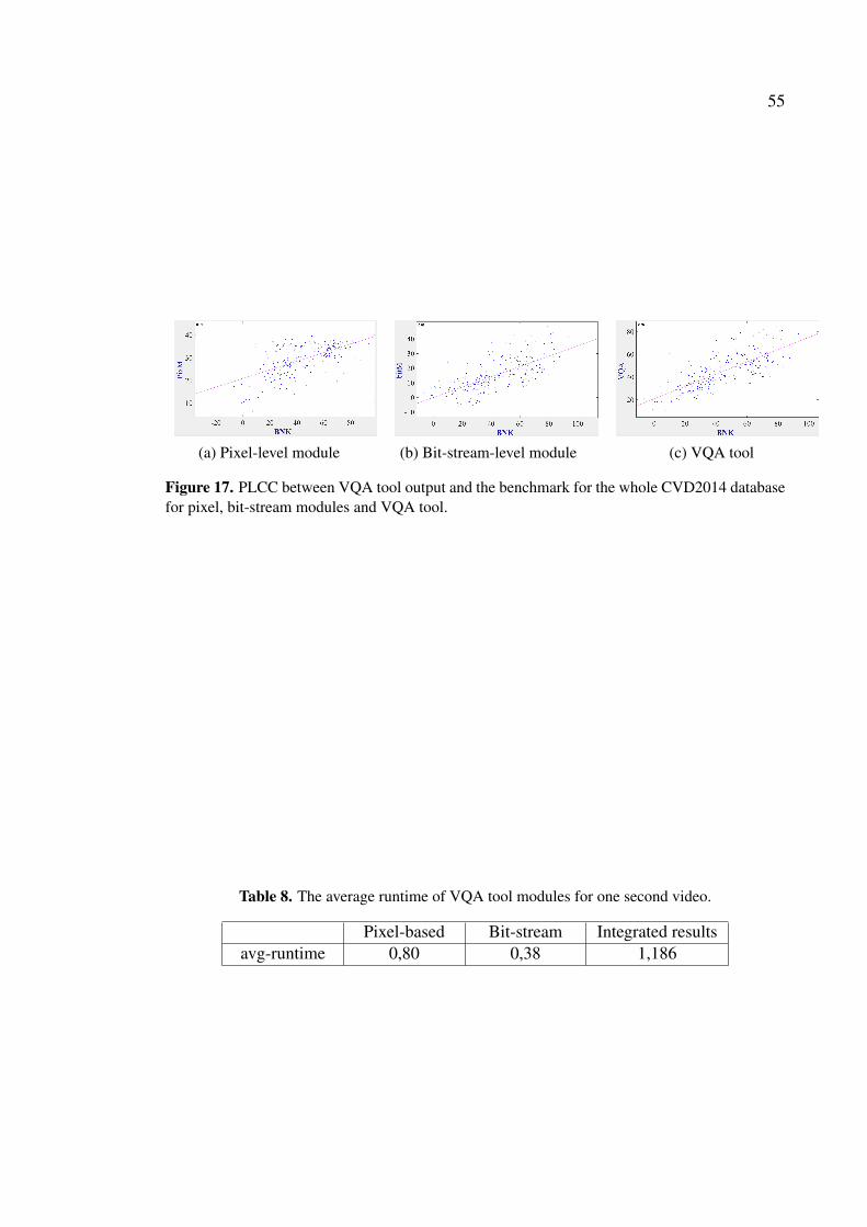
55

(a) Pixel-level module (b) Bit-stream-level module (c) VQA tool

Figure 17. PLCC between VQA tool output and the benchmark for the whole CVD2014 databasefor pixel, bit-stream modules and VQA tool.

Table 8. The average runtime of VQA tool modules for one second video.

Pixel-based Bit-stream Integrated resultsavg-runtime 0,80 0,38 1,186

56

6 DISCUSSION

This thesis proposed a video quality assessment (VQA) tool based on an objective ap-proach. The aim was to assess the quality of sensor-rich videos recorded by mobile de-vices. The main difficulty of this project rises from its generality context. It was assumedthat there is no control on any part of the recording process including environmental con-ditions, imaging system, and the content of filming. Therefore, no information on theexistence or absence of any degradation and type of it was provided.

Achieving this goal, a VQA tool was proposed in which several metrics are employed forassessing the quality of a video from different aspects. The final quality score is computedusing the weighted average. Moreover, as a novel approach, the values of basic sensor dataincluding the accelerometer, magnetometer, and gyroscope was captured during recordingand used to score the stability of the video. For this purpose, a stability measure wasproposed and examined with the prepared dataset.

The performance of the proposed VQA tool was assessed in two steps. First, each indi-vidual metric was assessed against a prepared dataset to make sure the metric is suitablefor the desired context. Then, the VQA tool was assessed against CVD2014 [1] to exam-ine its performance in a similar context. The results are promising with high correlation.Also, as it can be seen in Table 8, the runtime of VQA tool for each second of video takesroughly one second which is satisfactory.

The results reveal two interesting facts: first, it seems that the bit-stream-based moduleprovides a higher correlation with the benchmark rather than the pixel-based module. Itproves the advantage of using bit-stream measures in assessing the quality of video files.Second, as it can be seen in Table 7, each module is superior in some scenes but not all.However, using the integrated module, always improve the correlation. It means the ideaof using a combination of pixel and bit-stream based measures is promising.

6.1 Limitations

Although the performance of the proposed VQA tool is satisfactory during designed ex-periments, there were several limitations to this project. The proposed VQA tool can beapplied to the majority of videos in general scenarios. However, its performance on thevideos is prone to error for videos taken in particular situations. For example, if a user

57

increases the zoom level of the camera during recording, two issues will appear. First, thehigher level of digital zoom produces a lower resolution image or video frame. This issueincreases the probability of occurring blockiness degradation. However, in this project,the blockiness measure was discarded as it is not a significant degradation in high-qualityvideos. Second, When the camera is zoomed, any small changes in orientation angles,caused by shaky camera or user movement, profoundly affects the stability of video. It isunclear if the current stability measure can reflect this feature.

Furthermore, more experiments are needed to prove the performance of stability mea-sure. In this thesis, one limited dataset was prepared for this purpose, and the proposedapproach successfully passed the test. A more comprehensive dataset would help to dis-cover the shortages of proposed method which is an essential step toward improving theefficiency and accuracy of the algorithm. Also, having a large dataset and employingmachine learning methods could help to improve the performance.

Moreover, assessing the performance of VQA tool needs more experiments. The pro-posed tool is successfully assessed against the CVD2014 dataset. This dataset is the mostrelevant one in the context of this project as it employs different imaging systems andalso contains only natural distortions. However, lack of sensor-rich videos was the mostimportant missing feature in this dataset. Thus, the actual combination of all modules;pixel-, bit-stream- and sensor-based modules, were not assessed yet.

Another important limitation is the current integration module which works based onweighted average strategy. In this project, the weights are determined using several lim-ited experiments. Therefore, it is not easy to prove that the weights are chosen perfectlyand are optimal for all situations.

6.2 Future work

This project is ongoing, and the focus remains on improving the performance of the pro-posed VQA tool. The first plan is to invest in blurriness metrics and assess it more accu-rately. Adding extra measure with a specific focus on motion blur and out of focus blur isselected as the primary approaches to pursue.

Furthermore, examining the VQA tool against videos recorded with digital zoom andtesting them in particular situations is another part of the future plan. For this purpose,adding blockiness measure helps to recognize and rate the blockiness introduced with

58

digital zoom. Moreover, assessing the stability of the camera in zoom mode is anotherchallenge that needs more efforts.

Another possible extension could be improving the integration module. Using a machinelearning approach like SVR instead of the current weighting average could possibly im-prove the performance of the tool. Also, for future work, a more comprehensive datasetwill be prepared, and the labeling will be done using crowded sourcing techniques. Pro-viding the new dataset also enables employing a proper machine learning approach forthe integration module.

59

7 CONCLUSION

Using smartphones and tablets for filming is becoming more and more popular. Also,some camera applications capture device sensor data during filming and create sensor-rich videos. Assessing the quality of these videos has many applications in streamingservices, video sharing companies, and end-users for categorizing and searching videosbased on their quality.

Filming using hand-held devices by unprofessional and ordinary people in uncontrolledimaging and environmental condition, may produce poor quality videos such as blurred,poor contrast and shaky videos. This thesis started with introducing a comprehensiveliterature review to recognize the most annoying degradations happen in this context andthe available measures to assess those degradations.

As a practical part of the thesis, a Video Quality Assessment (VQA) tool was designedand implemented to assess the quality of sensor-rich videos. The tool was designed in anobjective approach which means no information regarding imaging device, environmentalcondition or imaging subject is required.

The proposed VQA tool comprised four modules namely pixel, bit-stream and sensor andintegration modules. Several measures are employed in each module to assess the qualityof given video from one specific aspect. In the pixel module, the contrast, blurriness, andnaturalness were assessed. In the bit-stream module, the video motion, scene complexityand bit-stream quality of the video file are rated. Furthermore, the tool utilizes sensor datato assess the stability of the video. Finally, the results of all measures are combined in theintegration module to produce one overall score as the quality of the video.

For all measures except stability, one or more approaches from the literature were se-lected as candidates. For assessing candidates, a new database containing 54 videos wasprepared, and all measures were examined against the database. For stability measure,two novel algorithms were suggested, and one specific database was designed and pre-pared to assess the performance of proposed methods. The measures which correlatedbest with the benchmarks were selected to be employed in the final VQA tool.

The performance of the proposed VQA tool was assessed against CVD2014 [1]. Theresults showed that using a combination of pixel and bit-stream module improve the per-formance regardless of the content of the videos.

60

REFERENCES

[1] Mikko Nuutinen, Toni Virtanen, Mikko Vaahteranoksa, Tero Vuori, Pirkko Oitti-nen, and Jukka Häkkinen. CVD2014-A Database for Evaluating No-ReferenceVideo Quality Assessment Algorithms. IEEE Transactions on Image Processing,25(7):3073–3086, July 2016.

[2] Deepti Ghadiyaram, Janice Pan, Alan C. Bovik, Anush K. Moorthy, Prasanjit Panda,and Kai-Chieh Yang. In-capture mobile video distortions: A study of subjectivebehavior and objective algorithms. IEEE Transactions on Circuits and Systems for

Video Technology, 2018. (under review).

[3] Kjell Brunnstrom, Sergio Ariel Beker, Katrien De Moor, Ann Dooms, and others.Qualinet white paper on definitions of quality of experience. European Network on

Quality of Experience in Multimedia Systems and Services, COST Action IC1003,March 2013.

[4] David S. Hands and S. E. Avons. Recency and duration neglect in subjective assess-ment of television picture quality. Applied Cognitive Psychology, 15(6):639–657,2001.

[5] Maria Torres Vega, Vittorio Sguazzo, Decebal Constantin Mocanu, and AntonioLiotta. An experimental survey of no-reference video quality assessment methods.International Journal of Pervasive Computing and Communications, 12(1):66–86,April 2016.

[6] International Telecommunication Union Telecommunication Standardization Sector(ITU-T). Subjective video quality assessment methods for multimedia applications.Recommendation P.910, April 2008.

[7] Sharath Chandra Guntuku, Michael James Scott, Gheorghita Ghinea, and Weisi Lin.Personality, culture, and system factors-impact on affective response to multimedia.Computing Research Repository (CoRR), abs/1606.06873, June 2016.

[8] Damon M. Chandler. Most apparent distortion: full-reference image quality assess-ment and the role of strategy. Journal of Electronic Imaging, 19(1):011006, January2010.

[9] Hiray Yogita V. and Hemprasad Y. Patil. A survey on image quality assessmenttechniques, challenges and databases. IJCA Proceedings on National Conference

on Advances in Computing (NCAC), 2015(7):34–38, December 2015.

61

[10] Silvio Borer. A model of jerkiness for temporal impairments in video transmission.In Second International Workshop on Quality of Multimedia Experience (QoMEX),pages 218–223. IEEE, June 2010.

[11] Michele A. Saad and Alan C. Bovik. Blind quality assessment of videos using amodel of natural scene statistics and motion coherency. In Forty six Asilomar Con-

ference on Signals, Systems and Computers (ASILOMAR), pages 332–336. IEEE,November 2012.

[12] Christos G. Bampis and Alan C. Bovik. Learning to predict streaming video QoE:Distortions, rebuffering and memory. Computing Research Repository (CoRR),abs/1703.00633, March 2017.

[13] Kalpana Seshadrinathan and Alan C. Bovik. Motion tuned spatio-temporal qualityassessment of natural videos. IEEE Transactions on Image Processing, 19(2):335–350, February 2010.

[14] Phong V. Vu, Cuong T. Vu, and Damon M. Chandler. A spatiotemporal most-apparent-distortion model for video quality assessment. In 18th IEEE International

Conference on Image Processing (ICIP), pages 2505–2508. IEEE, September 2011.

[15] Zheng Zhang, Yu Liu, Zhihui Xiong, Jing Li, and Maojun Zhang. Focus and blur-riness measure using reorganized dct coefficients for autofocus application. IEEE

Transactions on Circuits and Systems for Video Technology, 28(1):15–30, Jan 2018.

[16] Video Quality Experts Groups. Final report from the Video Quality Experts Groupon the validation of objective models of video quality assessment, Phase II (FR_tv2).VQEG, 2008.

[17] Michael Yuen and H. R. Wu. A survey of hybrid MC/DPCM/DCT video codingdistortions. Signal processing, 70(3):247–278, November 1998.

[18] Ni Pengpeng. Multimedia quality assessment. https://goo.gl/Ef72sc,2010. [Online; Accessed October 2017].

[19] Perry Sprawls. The Physical principles of medical imaging. Medical Physics Pub-lishing, Madison, Wisconsin, 2 edition, 1995.

[20] Rania Hassen, Zhou Wang, and Magdy Salama. No-reference image sharpness as-sessment based on local phase coherence measurement. In IEEE International Con-

ference on Acoustics Speech and Signal Processing (ICASSP), pages 2434–2437.IEEE, March 2010.

62

[21] Hantao Liu and Ingrid Heynderickx. A perceptually relevant no-reference blocki-ness metric based on local image characteristics. EURASIP Journal on Advances in

Signal Processing, 2009(1):263540, March 2009.

[22] Muhammad Shahid, Andreas Rossholm, Benny Lovstrom, and Hans-Jürgen Zeper-nick. No-reference image and video quality assessment: a classification and re-view of recent approaches. EURASIP Journal on image and Video Processing,2014(1):40, Aug 2014.

[23] Min Goo Choi, Jung Hoon Jung, and Jae Wook Jeon. No-reference image qualityassessment using blur and noise. International Journal of Computer Science and

Engineering, 3(2):76–80, February 2009.

[24] Alessandro Rizzi, Thomas Algeri, Giuseppe Medeghini, and Daniele Marini. Aproposal for contrast measure in digital images. In Conference on colour in graphics,

imaging, and vision (CGIV), volume 6, pages 187–192. Society for Imaging Scienceand Technology, 2004.

[25] Albert Abraham Michelson. Studies in optics. University of Chicago Press, Chicago,Illinois, United States, 1927.

[26] Deepti Ghadiyaram and Alan C. Bovik. Perceptual quality prediction on authenti-cally distorted images using a bag of features approach. Journal of Vision, 17(1):32,January 2017.

[27] Chaofeng Li, Alan Conrad Bovik, and Xiaojun Wu. Blind image quality assessmentusing a general regression neural network. IEEE Transactions on Neural Networks,22(5):793–799, May 2011.

[28] Hyung-Ju Park and Dong-Hwan Har. Digital Image Quality Assessment Based onStandard Normal Deviation. International Journal of Contents, 11(2):20–30, June2015.

[29] Decebal Constantin Mocanu, Jeevan Pokhrel, Juan Pablo Garella, Janne Seppanen,Eirini Liotou, and Manish Narwaria. No-reference video quality measurement:added value of machine learning. Journal of Electronic Imaging, 24(6):061208,December 2015.

[30] Hong Zhang, Fan Li, and Na Li. Compressed-domain-based no-reference videoquality assessment model considering fast motion and scene change. Multimedia

Tools and Applications, 76(7):9485–9502, April 2017.

63

[31] Savvas Argyropoulos, Alexander Raake, Marie-Neige Garcia, and Peter List. No-reference bit stream model for video quality assessment of H. 264/AVC video basedon packet loss visibility. In IEEE International Conference on Acoustics, Speech

and Signal Processing (ICASSP), pages 1169–1172. IEEE, May 2011.

[32] Bowen Wei and Yuan Zhang. No-reference video quality assessment with frame-level hybrid parameters for mobile video services. In 2nd IEEE International Con-

ference on Computer and Communications (ICCC), pages 490–494. IEEE, October2016.

[33] Alexandre Ciancio, Andre Luiz N. Targino da Costa, Eduardo A. B. da Silva, AmirSaid, Ramin Samadani, and Pere Obrador. No-reference blur assessment of digitalpictures based on multifeature classifiers. IEEE Transactions on Image Processing,20(1):64–75, January 2011.

[34] Deepa Maria Thomas. A novel hybrid approach to quality assessment using noreference blur and blockiness measure in JPEG images. International Journal of

Innovative Research and Development, 2(13), December 2013.

[35] Kanjar De and V. Masilamani. Fast no-reference image sharpness measure forblurred images in discrete cosine transform domain. In IEEE Students on Tech-

nology Symposium (TechSym), pages 256–261. IEEE, September 2016.

[36] Halime Boztoprak. An alternative image quality assessment method for blurredimages. Balkan Journal of Electrical and Computer Engineering, 4(1), March 2016.

[37] Eftichia Mavridaki and Vasileios Mezaris. No-reference blur assessment in naturalimages using fourier transform and spatial pyramids. In IEEE International Confer-

ence on Image Processing (ICIP), pages 566–570. IEEE, Oct 2014.

[38] Min Goo Choi, Jung Hoon Jung, and Jae Wook Jeon. No-reference image qualityassessment using blur and noise. International Journal of Computer Science and

Engineering, 3(2):76–80, 2009.

[39] Luhong Liang, Shiqi Wang, Jianhua Chen, Siwei Ma, Debin Zhao, and Wen Gao.No-reference perceptual image quality metric using gradient profiles for jpeg2000.Signal Processing: Image Communication, 25(7):502 – 516, Aug 2010. SpecialIssue on Image and Video Quality Assessment.

[40] Shiqian Wu, Weisi Lin, Shoulie Xie, Zhongkang Lu, Ee Ping Ong, and Susu Yao.Blind blur assessment for vision-based applications. Visual Communication and

Image Representation, 20(4):231 – 241, May 2009.

64

[41] Cuong T. Vu, Thien D. Phan, and Damon M. Chandler. S3: A Spectral and SpatialMeasure of Local Perceived Sharpness in Natural Images. IEEE Transactions on

Image Processing, 21(3):934–945, March 2012.

[42] Heng-Jun Zhao. No-inference image sharpness assessment based on wavelet trans-form and image saliency map. In International Conference on Wavelet Analysis and

Pattern Recognition (ICWAPR), pages 43–48, Jeju, South Korea, July 2016. IEEE.

[43] J. L. Pech-Pacheco, Gabriel Cristobal, Jesus Chamorro-Martinez, and J. Fernandez-Valdivia. Diatom autofocusing in brightfield microscopy: a comparative study. In15th International Conference on Pattern Recognition. ICPR-2000, volume 3, pages314–317 vol.3. IEEE, Aug 2000.

[44] Kanjar De and V. Masilamani. Image sharpness measure for blurred images infrequency domain. Procedia Engineering, 64(Supplement C):149–158, September2013.

[45] Kanjar de and V. Masilamani. Image Quality Assessment for Blurred Images UsingNonsubsampled Contourlet Transform Features. Journal of Computers, 12(2):156–164, March 2017.

[46] Taegeun Oh, Jincheol Park, Kalpana Seshadrinathan, Sanghoon Lee, and Alan Con-rad Bovik. No-Reference Sharpness Assessment of Camera-Shaken Imagesby Analysis of Spectral Structure. IEEE Transactions on Image Processing,23(12):5428–5439, December 2014.

[47] Taegeun Oh and Sanghoon Lee. Blind sharpness prediction based on image-basedmotion blur analysis. IEEE Transactions on Broadcasting, 61(1):1–15, March 2015.

[48] Hashim Mir, Peter Xu, and Peter Van Beek. An extensive empirical evaluation offocus measures for digital photography. In Proceedings of Society of Photo-Optical

Instrumentation Engineers (SPIE) Electronic Imaging, volume 9023, pages 9023 –9023 – 11, San Francisco, California, United States, March 2014. SPIE.

[49] Said Pertuz, Domenec Puig, and Miguel Angel Garcia. Analysis of focus measureoperators for shape-from-focus. Pattern Recognition, 46(5):1415–1432, May 2013.

[50] Said Pertuz, Domenec Puig, and Miguel Angel Garcia. Reliability measure forshape-from-focus. Image and Vision Computing, 31(10):725–734, October 2013.

[51] Ping Hsu and Bing-Yu Chen. Blurred image detection and classification. In Ad-

vances in Multimedia Modeling: 14th International Multimedia Modeling Confer-

ence (MMM), pages 277–286. Springer, January 2008.

65

[52] Phong V. Vu and Damon M. Chandler. A fast wavelet-based algorithm for global andlocal image sharpness estimation. IEEE Signal Processing Letters, 19(7):423–426,July 2012.

[53] Niranjan D. Narvekar and Lina J. Karam. A no-reference image blur metric based onthe cumulative probability of blur detection (CPBD). IEEE Transactions on Image

Processing, 20(9):2678–2683, Sept 2011.

[54] Rony Ferzli and Lina J. Karam. A no-reference objective image sharpness metricbased on the notion of just noticeable blur (JNB). IEEE Transactions on Image

Processing, 18(4):717–728, April 2009.

[55] Alan Conrad Bovik Hamid Rahim Sheikh, Zhou Wang. Live image quality as-sessment database release 2. http://live.ece.utexas.edu/research/quality. [Online; Accessed June 2018].

[56] Kongfeng Zhu. No-reference Video Quality Assessment and Applications. PhDthesis, Department of Computer and Information Science, University of Konstanz,Konstanz, Germany, July 2014.

[57] Chunhua Chen and Jeffrey A. Bloom. A blind reference-free blockiness measure.In Guoping Qiu, Kin Man Lam, Hitoshi Kiya, Xiang-Yang Xue, C.-C. Jay Kuo, andMichael S. Lew, editors, Advances in Multimedia Information Processing - PCM

2010, pages 112–123, Berlin, Heidelberg, September 2010. Springer Berlin Heidel-berg.

[58] Guangtao Zhai, Wenjun Zhang, Xiaokang Yang, Weisi Lin, and Yi Xu. No-referencenoticeable blockiness estimation in images. Signal Processing: Image Communica-

tion, 23(6):417 – 432, 2008.

[59] Cristian Perra. A low computational complexity blockiness estimation based onspatial analysis. In 22nd Telecommunications Forum Telfor (TELFOR), pages 1130–1133. IEEE, November 2014.

[60] Maria Torres Vega, Decebal Constantin Mocanu, Jeroen Famaey, Stavros Stavrou,and Antonio Liotta. Deep learning for quality assessment in live video streaming.IEEE Signal Processing Letters, 24(6):736–740, June 2017.

[61] Gabriele Simone, Marius Pedersen, and Jon Yngve Hardeberg. Measuring percep-tual contrast in digital images. Journal of Visual Communication and Image Repre-

sentation, 23(3):491–506, April 2012.

66

[62] M. Pavel, George Sperling, Thomas Riedl, and August Vanderbeek. Limits of visualcommunication: the effect of signal-to-noise ratio on the intelligibility of americansign language. Journal of the Optical Society of America A: Optics and Image

Science, and Vision, 4(12):2355–2365, December 1987.

[63] Andrew M. Haun and Eli Peli. Complexities of complex contrast. In Color Imaging

XVII: Displaying, Processing, Hardcopy, and Applications, page 82920E. Societyof Photo Optical Instrumentation Engineers (SPIE), January 2012.

[64] Alessandro Rizzi, Thomas Algeri, Giuseppe Medeghini, and Daniele Marini. Aproposal for contrast measure in digital images. Second European Conference on

Color in Graphics, Imaging and Vision, 2004(1):187–192, January 2004.

[65] Alessandro Rizzi, Gabriele Simone, and Roberto Cordone. A modified algorithmfor perceived contrast measure in digital images. In Second European Conference

on Color in Graphics, Imaging and Vision, volume 2008, pages 249–252. Societyfor Imaging Science and Technology, 2008.

[66] Kanjar De and V. Masilamani. No-reference image contrast measure using imagestatistics and random forest. Multimedia Tools and Applications, 76(18):18641–18656, September 2017.

[67] Yuming Fang, Kede Ma, Zhou Wang, Weisi Lin, Zhijun Fang, and Guangtao Zhai.No-reference quality assessment of contrast-distorted images based on natural scenestatistics. IEEE Signal Processing Letters, 22(7):838–842, July 2015.

[68] Gabriele Simone, Marius Pedersen, Jon Yngve Hardeberg, and Alessandro Rizzi.Measuring perceptual contrast in a multilevel framework. In Human Vision and

Electronic Imaging XIV, pages 72400Q–72400Q–9. Society of Photo Optical In-strumentation Engineers (SPIE), February 2009.

[69] Jean Baptiste Thomas, Jon Yngve Hardeberg, and Gabriele Simone. Image con-trast measure as a gloss material descriptor. In Computational Color Imaging: 6th

International Workshop (CCIW), pages 233–245. Springer, March 2017.

[70] Omar Alaql, Kambiz Ghazinour, and Cheng Chang Lu. No-reference image qualitymetric based on features evaluation. In IEEE 7th Annual Computing and Com-

munication Workshop and Conference (CCWC), pages 1–7, Las Vegas, NV, USA,January 2017. IEEE.

[71] Michele A. Saad, Alan Conrad Bovik, and Christophe Charrier. Blind Image Qual-ity Assessment: A Natural Scene Statistics Approach in the DCT Domain. IEEE

Transactions on Image Processing, 21(8):3339–3352, August 2012.

67

[72] Anish Mittal, Rajiv Soundararajan, and Alan C. Bovik. Making a completely blindimage quality analyzer. IEEE Signal Processing Letters, 20(3):209–212, November2013.

[73] Tuomas Eerola, Lasse T. Lensu, Heikki Kälviäinen, and Alan C. Bovik. Study ofno-reference image quality assessment algorithms on printed images. Journal of

Electronic Imaging, 23(6):061106, August 2014.

[74] Michele A. Saad and Alan Conrad Bovik. Blind quality assessment of videos us-ing a model of natural scene statistics and motion coherency. In 2012 Conference

Record of the Forty Sixth Asilomar Conference on Signals, Systems and Computers

(ASILOMAR), pages 332–336, Nov 2012.

[75] Anish Mittal, Michele A. Saad, and Alan Conrad Bovik. A completely blind videointegrity oracle. IEEE Transactions on Image Processing, 25(1):289–300, Jan 2016.

[76] P Muhammed Shabeer, Saurabhchand Bhati, and Sumohana S. Channappayya.Modeling sparse spatio-temporal representations for no-reference video quality as-sessment. In IEEE Global Conference on Signal and Information Processing (Glob-

alSIP), pages 1220–1224. IEEE, Nov 2017.

[77] Mohammed A. Aabed. Perceptual Video Quality Assessment and Analysis Using

Adaptive Content Dynamics. PhD thesis, Georgia Institute of Technology, May2017.

[78] International Telecommunication Union Telecommunication Standardization Sector(ITU-T). Parametric bitstream-based quality assessment of progressive downloadand adaptive audiovisual streaming services over reliable transport. Recommenda-

tion P.1203, December 2016.

[79] Jing Hu and Herb Wildfeuer. Use of content complexity factors in video over ipquality monitoring. In International Workshop on Quality of Multimedia Experi-

ence, pages 216–221. IEEE, July 2009.

[80] Greg Milette and Adam Stroud. Professional Android sensor programming. JohnWiley & Sons, Inc, Indianapolis, Indiana, 1 edition, 2012. OCLC: ocn779864098.

[81] Thibaud Michel, Pierre Genevès, Hassen Fourati, and Nabil Layaïda. On AttitudeEstimation with Smartphones. In IEEE International Conference on Pervasive Com-

puting and Communications, Kona, United States, March 2017.

[82] Jay Esfandyari, Roberto De Nuccio, and Gang Xu. Solutions for MEMS sensorfusion. Solid State Technology, 54(7):18–21, July 2011.

68

[83] Paul Lawitzki. Android Sensor Fusion Tutorial. https://www.codeproject.com/Articles/729759/Android-Sensor-Fusion-Tutorial, Febru-ary 2014. [Online; Accessed October 2017].

[84] William John Freeman. Digital Video Stabilization with Inertial Fusion. PhD Thesis,Virginia Tech, April 2013.

[85] Gustav Hanning, Nicklas Forslow, Per-Erik Forssen, Erik Ringaby, David Torn-qvist, and Jonas Callmer. Stabilizing cell phone video using inertial measurementsensors. In IEEE International Conference on Computer Vision Workshops (ICCV

Workshops), pages 1–8. IEEE, November 2011.

[86] Sophocles J. Orfanidis. Introduction to signal processing. Prentice Hall, EnglewoodCliffs, N.J., 1996.

[87] Nikolay Ponomarenko, Lina Jin, Oleg Ieremeiev, Vladimir Lukin, Karen Egiazarian,Jaakko Astola, Benoit Vozel, and Kacem. Image database tid2013: Peculiarities,results and perspectives. Signal Processing: Image Communication, 30:57 – 77,2015.