CRUSTACEAN COMMUNITIES OF THE MANGANESE NODULE PROVINCE

(DOMES SITE A COMPARED WITH DOMES SITE C)

REPORT FOR THE NATIONAL OCEANIC AND ATMOSPHERIC ADMINISTRATION OFFICE OFOCEAN AND COASTAL RESOURCE MANAGEMENT (OCEAN MINERALS AND ENERGY)

ON CONTRACT NA-84-ABH-0030

(Oregon State University Subcontract 2-5757-04)

GEORGE D.F. WILSON

A-002 Scripps Institution of Oceanography

La Jolla, California 92093

(currently 2003: Australian Museum, 6 College St., Sydney, NSW 2010 Australia)

December 1987(reprinted January 1999; converted to PDF November 2003)

- 1 -

TABLE OF CONTENTS

INTRODUCTION............................................................................................................. 2MATERIALS AND METHODS ..................................................................................... 3

SAMPLING LOCALITIES........................................................................................................................3SAMPLE COLLECTION AND PROCESSING........................................................................................4TAXONOMIC ANALYSIS .......................................................................................................................5DATA ANALYSIS.....................................................................................................................................6

TAXONOMIC RESULTS................................................................................................ 8CUMACEA ................................................................................................................................................8AMPHIPODA.............................................................................................................................................8TANAIDACEA ..........................................................................................................................................9ISOPODA. ................................................................................................................................................13

RESULTS AND DISCUSSION ..................................................................................... 13SAMPLING ARTIFACTS AND OTHER PROBLEMS..........................................................................13COMMUNITY STRUCTURE .................................................................................................................14

CONCLUSIONS ............................................................................................................. 17RECOMMENDATIONS................................................................................................ 18ACKNOWLEDGMENTS .............................................................................................. 19TABLE 1. ......................................................................................................................... 24TABLE 2. ......................................................................................................................... 26TABLE 3. ......................................................................................................................... 28TABLE 4. ......................................................................................................................... 29TABLE 5. ......................................................................................................................... 29TABLE 6. ......................................................................................................................... 30TABLE 7. ......................................................................................................................... 32TABLE 8. ......................................................................................................................... 34TABLE 9. ......................................................................................................................... 36TABLE 10. ....................................................................................................................... 38TABLE 11. ....................................................................................................................... 40TABLE 12. ....................................................................................................................... 42TABLE 13. ....................................................................................................................... 42TABLE 14........................................................................................................................ 43TABLE 15. ....................................................................................................................... 43

- 2 -

INTRODUCTION

The monitoring of environmental impacts of manganese nodule mining as requiredby the Deep Seabed Hard Mineral Resources Act (U.S. Congress Public Law 96-283)will require a strong baseline of information on the benthic fauna of the EquatorialPacific. Knowledge needed on the descriptive community structure of this regionspecifically includes such basic data as the identities and abundances of species from thisregion. This document contains the macrofaunal crustacean data from several cruises,and presents a comparative analysis of their community structure. The crustaceans weretaken from box corer samples from two sites in the manganese nodule province: DeepOcean Mining Environmental Study (DOMES) site A (Piper and Blueford, 1982; Jumarsand Self, unpublished) and the ECHO 1 locality (Spiess and Weydert, 1987; Wilson andHessler, 1987a) near DOMES site C1.

Although these data may be used for a variety of purposes, I wish to address twointerrelated questions. Are widely separated sites in the manganese nodule province partof the same benthic community? This question is prompted by concerns of establishingstable reference areas (SRA) in the manganese nodule province for monitoring the impactof nodule mining activities. If there is a high degree of dissimilarity over the areasdesignated for mining, then SRAs will have to be more numerous than in a homogeneousarea. Another study (Hecker and Paul, 1979) found substantial between-site differencesalthough their results require further interpretation. I will show that the crustaceancommunity structure, specifically the diversity and abundance relationships, is similarbetween sites, independent of species identities. However, species are different betweenthe two sites, especially in the Isopoda, resulting in little faunal similarity between thetwo sites.

Other more theoretical questions also may be addressed with these data. Aredifferences and similarities between the sites ecological (including biotic orenvironmental interactions) or historical (evolutionary) in nature? The ecological andhistorical aspects of the data are pursued because the environmental similarity of sites Aand C, and their geographic separation (1560 n.mi., 2890 km) allows tentativeconclusions about relative roles of ecology and history in structuring the communities inthe manganese nodule province.

Finally, in fulfillment of the NOAA contracts that supported this research, the rawcrustacean species data for these DOMES-related programs are presented in Tables 1-11.These data are available in a variety of electronic forms [from the author]. These datawill provide a strong baseline for further experimental studies of the diverse animalcommunities that make up the north Equatorial Pacific manganese nodule province.

1 For the remainder of this document, the DOMES site A locality (Jumars and Self,

unpublished) will be referred to as "site A", and the ECHO 1 locality (Spiess et al., 1984)may also be referred to as "site C" .

- 3 -

MATERIALS AND METHODS

SAMPLING LOCALITIES

Site A. This site is in the north Equatorial Pacific between the Clarion and Clippertonfracture zones (centered on 9º 24’ N, 151º 27’ W). The site is dominated by an east-westtrending valley with the depth varying between 4900 and 5200 m. The sediments aresiliceous clays with a mean clay content of 50%, the remainder being primarily siliceousooze (Piper et al., 1979a). Manganese nodules are present on the sediment surface; thenodule cover typically varies between 10% to 25% (Piper et al., 1979b; Piper andBlueford, 1982). The near-bottom water has salinities of 34.68‰ to 34.69‰ andtemperatures of 1.4±0.004º C (Hayes, 1979). The near-bottom daily-averaged currentvelocities were 2 cm/sec. The average flow is to the northwest at 0.45 cm/sec, with somelow-frequency fluctuations having periods from 2 to 5 months (Hayes, 1979). At similarsites to the east (11º N, 140º W), long-term sea-floor observations up to 3 years have notdetected current velocities sufficiently strong to generate shear stresses capable ofresuspending sediments (Gardner et al., 1984). Stratographic data show that episodes ofsediment erosion and redeposition took place as late as the Pleistocene (Piper et al.,1979a). The erosional events are associated with current intensification during glaciation(Johnston, 1972; Quinterno and Theyer, 1969), a process that is unimportant today.

In 1978, site A was impacted by a test mining for manganese nodules (Lavelle etal., 1981), with benthic samplings before and after the event (Jumars and Self,unpublished). Although the test mining was effective in generating a large sedimentaryplume at the sea floor (Lavelle et al., 1981), navigation difficulties prevented takingsamples directly in the impacted areas (Jumars and Self, unpublished). Because thebefore (1977) and after (1978) mining samples did not appear significantly different(ibid.), both data sets are treated as representative of the background benthic community.

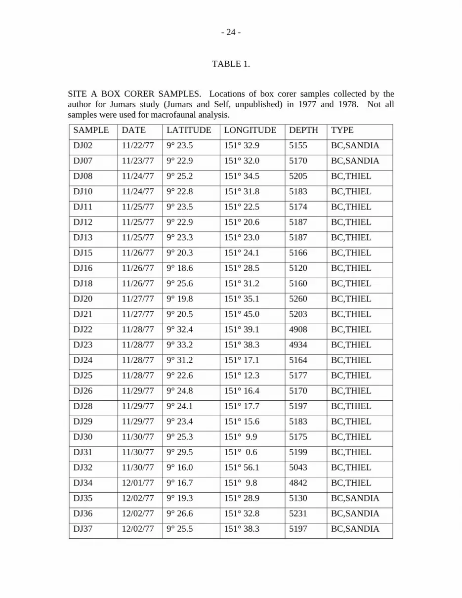
Box corer samples were taken in a 35-km by 60-km area: in November 1977, 24samples were collected; in May 1978, 26 samples were taken. The sample locations wereselected by picking points at random from an inner 10-km by 30-km area and from theremaining area separately. Sample locations were determined within a transponder netoperated by Ocean Management Incorporated or using ranges to a radar buoy at the sitewith an average positional accuracy of approximately \(+-0.5 km. Piper and Blueford(1982) provide a chart of the sample locations. Not all samples they show, however,were used for biological purposes. Table 1 lists the station data for both site A cruises.

Site C - the ECHO 1 locality. The location of the OMA test mining and the 1983 ECHO1 sampling program is 14º 40’ N, 126º 25’ W at depth of 4500 m. This site lies betweenthe Clipperton and Clarion fracture zones, 2000 km to the West of the Eastern PacificRise and is near DOMES site C (15º N, 125º W). The temperatures, salinities, andcurrent regime are similar to that at site A (Hayes, 1979). The sediments are transitionalbetween pelagic red clay and siliceous ooze and are generally dark yellowish brown atthe surface (Spiess et al., 1984). Because this site is just below the calcite compensationdepth, the sediment contains little or no calcareous debris (ibid.). The bathymetry,determined from a Sea Beam survey (de Moustier, 1985) shows elongate featurestrending North-South. The study site was on a relatively flat area with gentle slopes tothe East, and surrounded by depressions on the East and the West (deMoustier, 1985;

- 4 -

Spiess and Weydert, 1987).

Manganese nodules are the dominant feature of the sedimentary surface at theECHO 1 site (Spiess and Weydert, 1987) with coverages of 25% to 49% in theexperimental samples (Wilson and Hessler, 1987a) and average long axial lengthsranging from 5.0 to 6.75 cm (Spiess and Weydert, 1987). However, photographicsurveys using the Deep-Tow vehicle (Spiess and Weydert, 1987) and acousticreflectivities derived from Sea Beam surveys (de Moustier, 1985) show that nodulecoverages can range from 0 to 80 percent in this general area. The average nodule size(expressed as cm2) shows a significant inverse relationship with the nodules density (R =-0.96) at the sampling scale of 0.25 m2 (Wilson and Hessler, 1987a).

During 1978, OMA cruises to the ECHO 1 locality disturbed the sea floor withvarious versions of a wire-towed sled and a prototype mining vehicle (Spiess andWeydert, 1987). Active pumping of nodules from the sea floor and generation of asediment plume occurred only during a few occasions and primarily during a November-December 1978 OMA/DSV cruise on the R.V. Deepsea Miner II (Dick and Foell, 1985).Wilson and Hessler (1987a), however, found no detectable effects of the test miningdisturbance on the benthic fauna. Therefore, the data from this study are assumed to bemore or less representative of the general benthic community in the ECHO 1 (site C)locality. Table 2 provides the locality data for the 15 box corer samples that werecollected at site C.

SAMPLE COLLECTION AND PROCESSING

Site A. The sampling devices used were two versions of the USNEL 0.25 m2 box corer.One corresponded to that described by Hessler and Jumars (1974; see also Thiel, 1983)except that the vent doors were on the top of the coring head instead of on the sides(design by H. Thiel). This device was used to collect box cores numbered DJ08 throughDJ34. The remaining samples were collected with a box corer modified according todesigns prepared by R.R. Hessler, P.A. Jumars, and J. Finger (the “Sandia” box corer). Acomparison of isopod fractions collected by the two corers revealed no apparentdifference in their sampling efficiency. The corer box on either sampler contained no insitu subcores.

On recovery, the top water was drained through a 0.300 mm mesh sieve and thescreen residues were added to the main biological sample. A subcore with an internalarea of 46 cm2 was taken for geological analysis. The macrofaunal samples thusrepresent a surface area of 2454 cm2. The top 10 cm of a sample were placed in anelutriation device (Hessler and Jumars, 1974) and washed gently on to a 0.300-mm meshsieve. The screen residues were fixed in a sodium borate-buffered solution offormaldehyde in filtered seawater (1:5 by volume), and then preserved in 80% ethanolafter a fresh-water rinse. In the laboratory of P.A. Jumars (University of Washington),macrofaunal taxa were sorted under a dissecting microscope. The Crustacea were thensent to me for identification.

Site C. A modified version of the 0.25 m2 “Sandia” box corer was used to collectquantitative samples. This corer was modified by placing form-fitting seals on all ventdoor seating surfaces and a closed-foam neoprene gasket on the sample box seatingsurfaces. This modification resulted in a nearly complete seal that protected the sample

- 5 -

from mixing with external waters on recovery. The adequacy of this procedure wasdemonstrated by the cold water (9-12º C) on top of the samples as compared to a seasurface water temperature of 25º+, and the complete absence of epiplanktonic animalsfrom the samples. In samples taken at site A with older unsealed models of the box corer,the sample top water was approximately that of the sea surface and plankton such asepiplanktonic hyperiid amphipods have been found in the sample residue (see below).

For macrofaunal processing, each core was divided into 6 separate macrofaunalfractions: top water, nodule washings, aspirator water (material sucked up from surfacepuddles of fluid and sediment), 0-1 cm layer, 1-5 cm layer, and 5-10 cm layer. Thislayering facilitated rapid fixation of the animals and permitted a rough analysis of thedepth distribution of the fauna. Most animals were in the fractions with the leastsediment, thereby avoiding mechanical damage to the specimens and facilitating theirrapid removal from the sediment during sorting. All the nodules were washed andexamined to remove large encrusting fauna, with some nodules being carefully preservedfor another study. These fractions were sieved through 0.300 mm screens during thecruise. The entire top 1 cm layer and the screen residues of the lower layers were placedin 4% buffered formaldehyde-seawater for fixation. After several days of occasionalgentle agitation to aid fixation, the screen residues were washed with fresh water andplaced in 80% ethanol for long term preservation. In the laboratory, the samples weresorted to major taxa using Wild M5 stereomicroscopes, and the Crustacea were separatedfor further analysis.

TAXONOMIC ANALYSIS

This study is limited to the benthic peracarid Crustacea for the following reasons.(1) Other malacostracan taxa such as Mysidacea and Euphausiacea are rare and may bepelagic contaminants in the sample (see remarks on the Hyperiidea below). (2) Othercrustacean taxa such as the Ostracoda and Harpacticoidea are meiofaunal and were notcollected quantitatively. The macrofauna was collected in 0.3 mm mesh sieves, whiletypically these latter taxa require screen mesh sizes of 0.063 mm or less. The taxaconsidered in this report therefore are: Cumacea, Amphipoda, Tanaidacea, and Isopoda.The latter two taxa make up the bulk of the diversity and abundance of the Crustacea, andwill be the subject of most of the comparisons. Specimens of each taxon were inspectedindividually. When species not previously encountered in the samples were examined, apreliminary description, often with drawings, was made. After an initial sorting period,the specimens were re-examined to verify the homogeneity of the identifications. Thepoor state of published taxonomy for these taxa prevent identifying these species tonamed taxa. Instead, each species was given a unique code number that remainedconstant regardless of its higher taxon. These species codes were assigned independentlyof the geographic location of the specimens so that the two separate localities could becompared.

- 6 -

DATA ANALYSIS

The identification data were assembled into an electronic database (dBASE III,Ashton-Tate Inc.), which was programmed to present the data in a variety of formats. Aspreadsheet program (123, Lotus Inc.) was used to generate most of the graphics in thisreport, and to create the input files for the specific analysis programs. These programsinclude the normalized expected species shared (NESS) similarities (Grassle and Smith,1976); Sanders (1968) species rarefaction based on the hypergeometric model of Hurlbert(1971); and a bootstrapped estimator of the theoretical species richness of a communityusing the fit of a lognormal distribution. The latter two programs were written by theauthor and are available from him (see acknowledgments).

NESS. Similarities between localities or groups of samples were calculated using NESS,a family of methods that are “normalized” to equivalent sample sizes (Grassle and Smith,1976; Smith and Grassle, 1977). NESS at large sample sizes is also sensitive to the rarespecies in a sample, a desirable property for a similarity index used on deep-sea samples.Gallagher (personal communication, in preparation) has discovered that similarities fromNESS will give incorrectly high similarities with data where many taxa are representedby zero or one individual abundances. Most NESS programs have an ad hoc adjustmentto set similarities to 1 if the similarity exceeds 1, therefore hiding the magnitude of theproblem. Although data from shallow-water or from large samples like epibenthic sledsamples are not greatly affected by this problem, data from more sparsely populated boxcorer samples will sometimes exceed 1 by large amounts, indicating severe problemswith the analytical technique. Gallagher (ibid.) has corrected this problem by using avariant of the technique, and by correcting the sample size calculation procedure. Hisalgorithm is used here.

The Bootstrapped Lognormal Distribution. Although the NESS and rarefaction programsare based on well known algorithms, the bootstrap estimator of species richness requiresa detailed description. This is a new method joining the techniques of bootstrapestimators (Efron, 1979; Efron and Gong, 1982) with that of fitting the lognormaldistribution to species abundance data (Preston, 1948, 1962; Pielou, 1975), therebyestimating the community structure of a taxocene. Lognormal distributions as applied tocommunity structure from real species abundance data often have the property that thepeak of the individuals distribution coincides with the upper tail of the speciesdistribution. Distributions having this property are termed “canonical”. These canonicallognormal distributions have the further property that they can be used to estimate theexponent z of the well known species-area relationship. May (1975) has suggested thatthis canonical property is merely a general property of lognormal distributions, althoughrecently Sugihara (1980; see also Harmsen, 1983) has argued that it is a result of anunderlying niche partitioning process in natural communities. These results have beenfurther extended to suggest that canonical distributions will characterize communities thatare under assembly or under stress, while equilibrium communities will be less canonicaland will have a lower variance due to evolutionary accommodation (Harmsen, 1983).

These results suggest uses for the lognormal distribution that apply to theoreticalcommunity ecology. The pragmatic use of the lognormal distribution, however, stemsfrom the observation that communities will be made up of a few species that areextremely abundant, a few that are vanishingly rare, and a majority that range of

- 7 -

intermediate abundances. Most species will have minimum abundances beyond whichthey cannot maintain sufficient populations for continued reproduction: real,homogeneous communities, therefore, should be lognormal in form. This pattern ofabundances may effectively be estimated by a lognormal distribution, which tends toequalize the scale between the most and least abundant species as well as indicate theposition of the central majority of the species. Another advantage for using thelognormal distribution for studying community structure is that it uses all the data anddisplays it in a useful form, rather than distilling it down to a highly derived single value.An associated lognormal parameter is the estimation of the total species in the theoreticaldistribution, S*, calculated by integrating the area under the normal curve. Knowing thisnumber is highly desirable because not only will it tell an investigator how well he hassampled a community, but it will also permit the comparison of the complete speciesrichnesses of several communities. One cannot help look at a standard rarefaction curvewithout trying to extrapolate it in the mind’s eye to its asymptotic maximum. Such aprocedure would be objectionable (Fager, 1972; Tipper, 1979), while the estimate derivedfrom the truncated lognormal estimate uses manageable assumptions, some of which canbe tested statistically. For example, one can use a simple Chi Square test to measure thedeparture of the theoretical estimated distribution from the original. In addition, there areanalytical estimates for the mean and variance of the distribution. However, no analyticalestimate for S* exists for the standard lognormal (Pielou, 1975). Bulmer (1974) hasapplied a Poisson lognormal to species abundance data with some success, although thePoisson and the standard lognormal distributions give different S* estimates (Pielou,1975) without any objective way of deciding which should apply. Because the standardlognormal is the simpler distribution, I have chosen it for use in a bootstrap estimate ofS*, �.

Bootstrapping the lognormal distribution provides a computer intensive alternativeto calculating an analytical estimate of variance. Bootstrapping simulates samplingvariability by performing a Monte Carlo resampling of the original data with replacementto create new synthetic data sets of the same size, but with a random variation (Efron,1979; Efron and Gong, 1982). In this application, we wish to see how well the lognormaldistribution will estimate S* under further sampling. Although actual resampling is notpossible, we can assume that we have taken enough samples to characterize thedistribution at the current sample size. Resampling is done by randomly pickingindividuals from the original distribution and sorting them by species. Therefore, eachspecies has a probability of being picked proportional to its relative abundance in theactual pooled sample. However, because each individual is picked independently andwith replacement, the abundance of each species varies randomly. Individuals are pickeduntil a new data set is created that has exactly the same number of species and individualsbut with varying abundances of the individual species. If many data sets are taken, themean abundance of each species will approach the observed abundance. The individualsynthetic data sets are then fitted with the lognormal distribution and the value for S* isestimated for each. If this is done many times, the mean of the S* estimates is thebootstrap estimator of the theoretical total species in a community, �, with its associatedvariance, Var(�).

The lognormal distribution can be fitted in a variety of ways although the onechosen for this purpose uses the equations for a doubly truncated normal distribution for

- 8 -

which equations are provided by Cohen (1950). Real species abundance distributions aretruncated at the lower end because not enough samples were taken to collect all species ina community. They are truncated at the upper end because a discrete abundancedistribution is being estimated by a theoretical continuous distribution: there is an uppertail for abundances from less than one species. The algorithm and original program forthis procedure was created by George Sugihara (SIO) who wrote his Fortran 77 programto calculate independent estimates for entropy and evenness indices of a community. Iconverted his program to Pascal, generalized it so that it could handle different log bases,and added a bootstrapping algorithm that would calculate �, its variance, and its standarddeviation.

This program is currently being checked for the appropriateness of its estimates. Itdoes show the desirable qualities of estimating var(�) to be high for small data sets andsmall for large data sets. In addition, data sets with a low var(�) also are relativelyinvariant for differing log bases. Log base 2 has been retained as the distribution ofchoice because it divides an abundance distribution more finely. In addition, because thealgorithm splits boundary values between abundance bins, differences between bins inthe data are smoothed for log base 2 where integer boundary values are most frequent(Paul Smith, Southwest Fisheries Center, personal communication). Natural logs(Caswell and Weinberg, 1986) or log base 10 (Pielou, 1975) lack this smoothing effect.A further desirable property is the algorithm’s ability to qualitatively estimate differencesin species richness observed in samples displayed in rarefaction curves: if one curveappears to have a higher asymptote than another, their �’s will agree on this difference.Further tests will resample known distributions to establish the effectiveness of theprogram.

TAXONOMIC RESULTS

CUMACEA

The cumaceans were extremely rare in both sets of samples. Six specimens fromthe ECHO 1 locality were not identified. The 4 specimens from site A are identified asthe following: DJ11, Nannastacidae, genus indet. (specimen damaged); DJ35,Nannastacidae Procampylaspis sp. 2; DJ44, Nannastacidae Procampylaspis sp. 1; DJ69,Leuconidae Pseudoleucon sp.

The rarity of Cumacea in these quantitative samples corroborates observed densitiesin other samples from the North Pacific. For example, Hessler and Jumars (1974)collected no Cumacea in the Central North Pacific out of 12 box corer samples, whichsuggests that this group has densities less than 0.33 per m2. Overall faunal densities inthis latter oligotrophic region are lower than the site C (Wilson and Hessler, 1987a), sothe current estimates of 0.31 individuals of Cumacea per m2 for site A and 1.6 individualsper m2 for site C are reasonable values. Hecker and Paul (1979) observed the followingdensities per square meter of Cumacea over DOMES sites A, B, and C respectively: 0.0,0.78, 0.31. The rarity of Cumacea makes these estimates extremely difficult to interpret.

AMPHIPODA

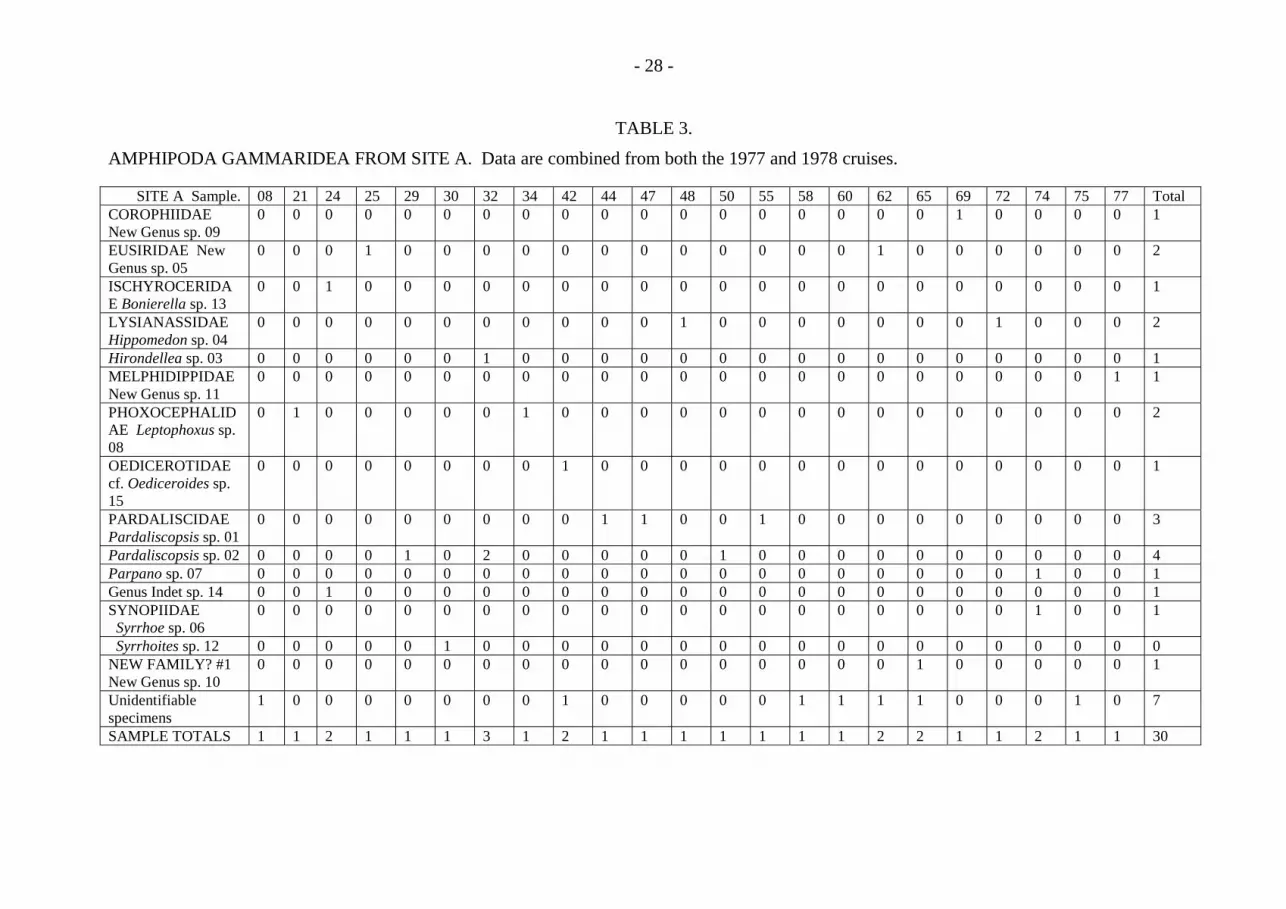
Table 3 and 4 shows the benthic amphipod species identified from both sites andTable 5 lists the hyperiid amphipod contaminants identified by T. Bowman. The material

- 9 -

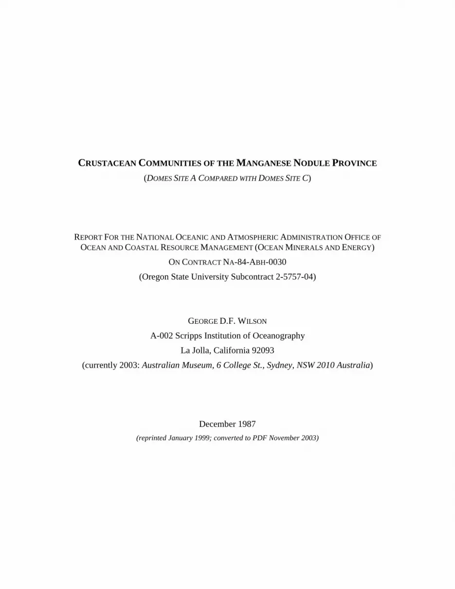
is interesting because of the presence of several new family-level taxa (Fig. 1) andbecause all species are new to science. The presence of two lysianassids indicates thatthe box corer is capable of capturing even these highly-motile demersal taxa. Again,Hessler and Jumars (1974) collected no Amphipoda in the Central North Pacific out of 12box corer samples, which suggests that their locality may have less than 0.33 amphipodsper m2. Hecker and Paul (1979) observed the following densities per square meter ofAmphipoda over DOMES sites A, B, and C respectively: 0.36, 0.97, 1.5. Estimates of2.3 individuals per m2 for site A and 4.5 individuals per m2 for site C are derived from thecurrent data. The low abundance of Amphipoda prevents comparing diversities betweenthe two sites or the site similarities based on amphipod taxa. Except for the twolysianassids, the gammaridean amphipods identified were strictly benthic forms. In factspecies Amphipods sp. 15 and sp. 51 seem to be burrowing forms because they werefound in lower layers of the samples.

TANAIDACEA

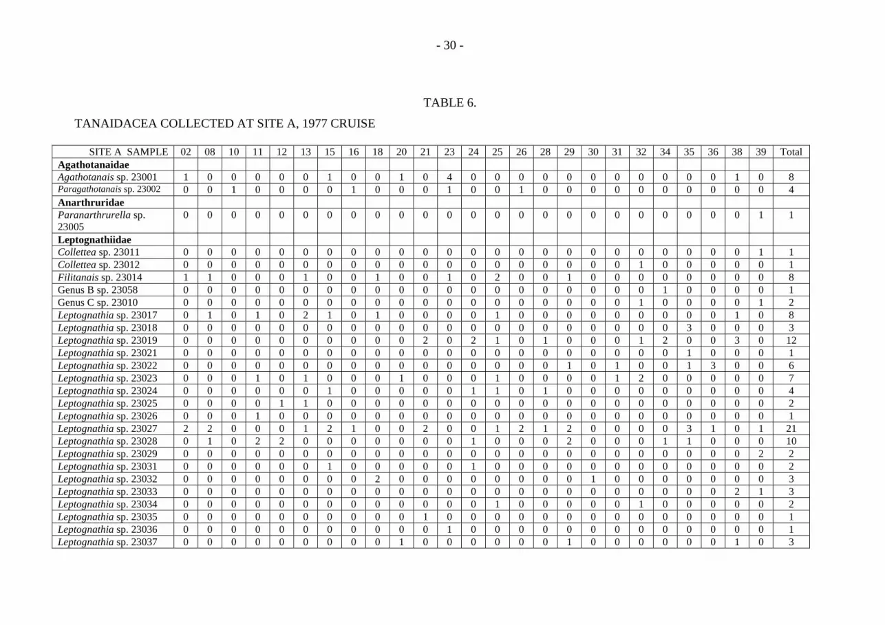
Tables 6, 7, and 8 show the distributions of species among sites A and C. Diversitywas high: 77 tanaid species were identified from both sites, with the majority of the

Figure 1. New taxa of benthic gammaridean Amphipoda. Scale bar = 1mm.

- 10 -

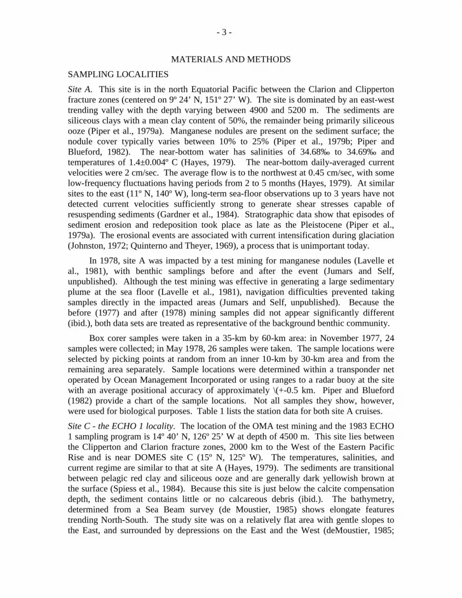
Figure 2. Percent composition (individuals and species) of families of Tanaidacea fromSite A and Site C.

species in the family Leptognathiidae (Fig. 2). Figure 3 shows common leptognathiidLeptognathia sp. 23019. The Neotanaidae (Neotanaidomorpha) and the Whitelegiidae(Apseudomorpha) were rare.

Comparison of these results with what has been known prior to this time indicatesthe poor state of deep-sea tanaid systematics. The 77 species listed here are roughly twotimes the number listed for the 4 to 5 km depth range in Sieg (1986), and most are likelyto be new species. Sieg (personal communication), who examined drawings made ofthese species, believes that the genus Leptognathia alone may eventually be split into 9 ormore genera.

In all, 375 tanaids were found in the site A samples and 181 in the ECHO 1samples. This gives densities of 29.4 and 48.3 individuals per m2 respectively. Hesslerand Jumars (1974) found 23.3 tanaids per m2, and Hecker and Paul (1979) found 21.7,15.0, and 28.6 per m2 for sites A, B, and C respectively.

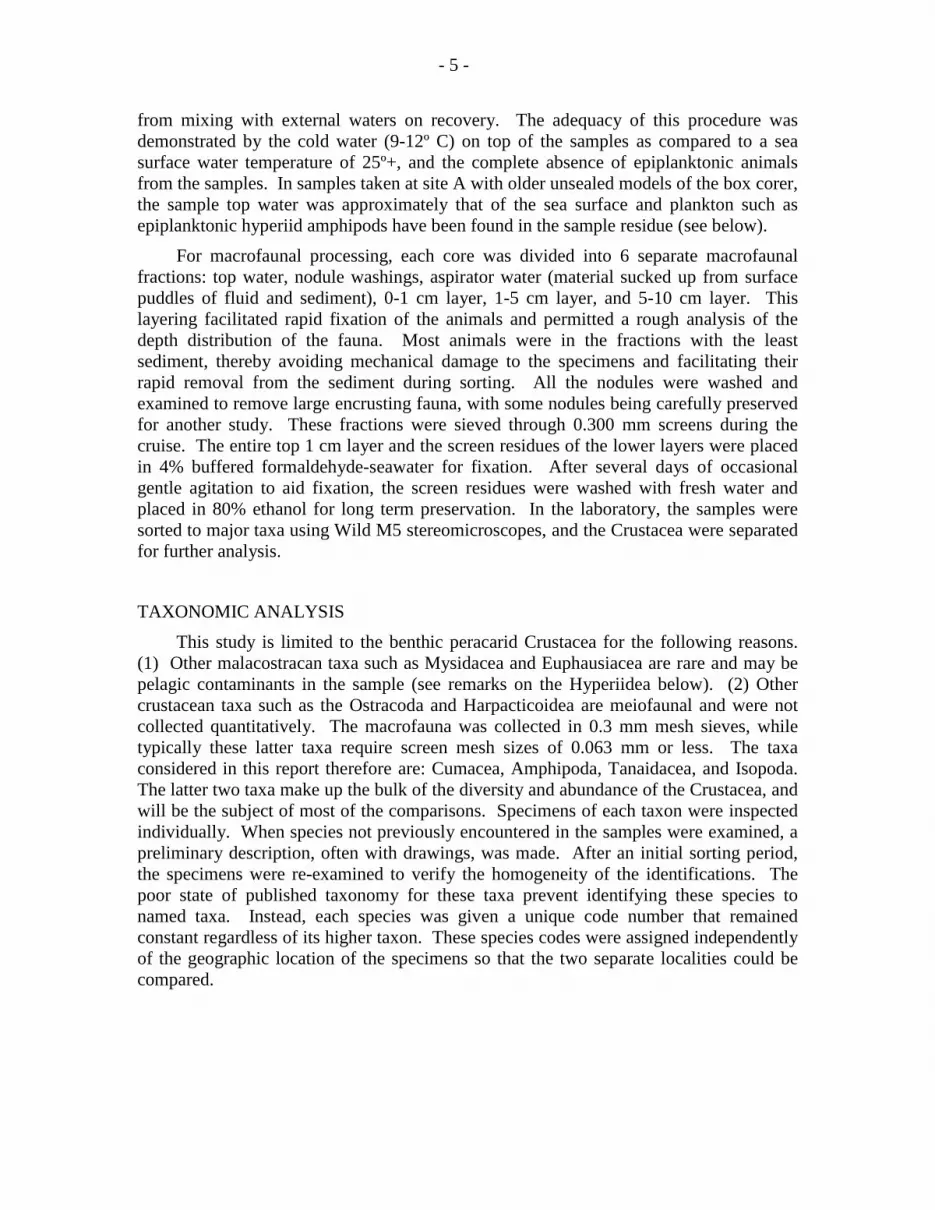
The tanaid populations are interesting because, out of 556 individuals, only 10males were found in the collection. Most tanaids have high sexual dimorphism, as can beseen in figure 3. The females are strictly tubiculous (e.g. Hassack and Holdich, 1987) orburrowing, while the males are greatly different. The males may be adapted for highmotility (enlarged swimming pleopods and walking legs) and ability to find females bychemosensory means (many enlarged aesthestacs on the antennae). In addition, the

- 11 -

Figure 3. Lateral views of male and female,Leptognathia sp. 23019 (Tanaidacea,Leptognathiidae).

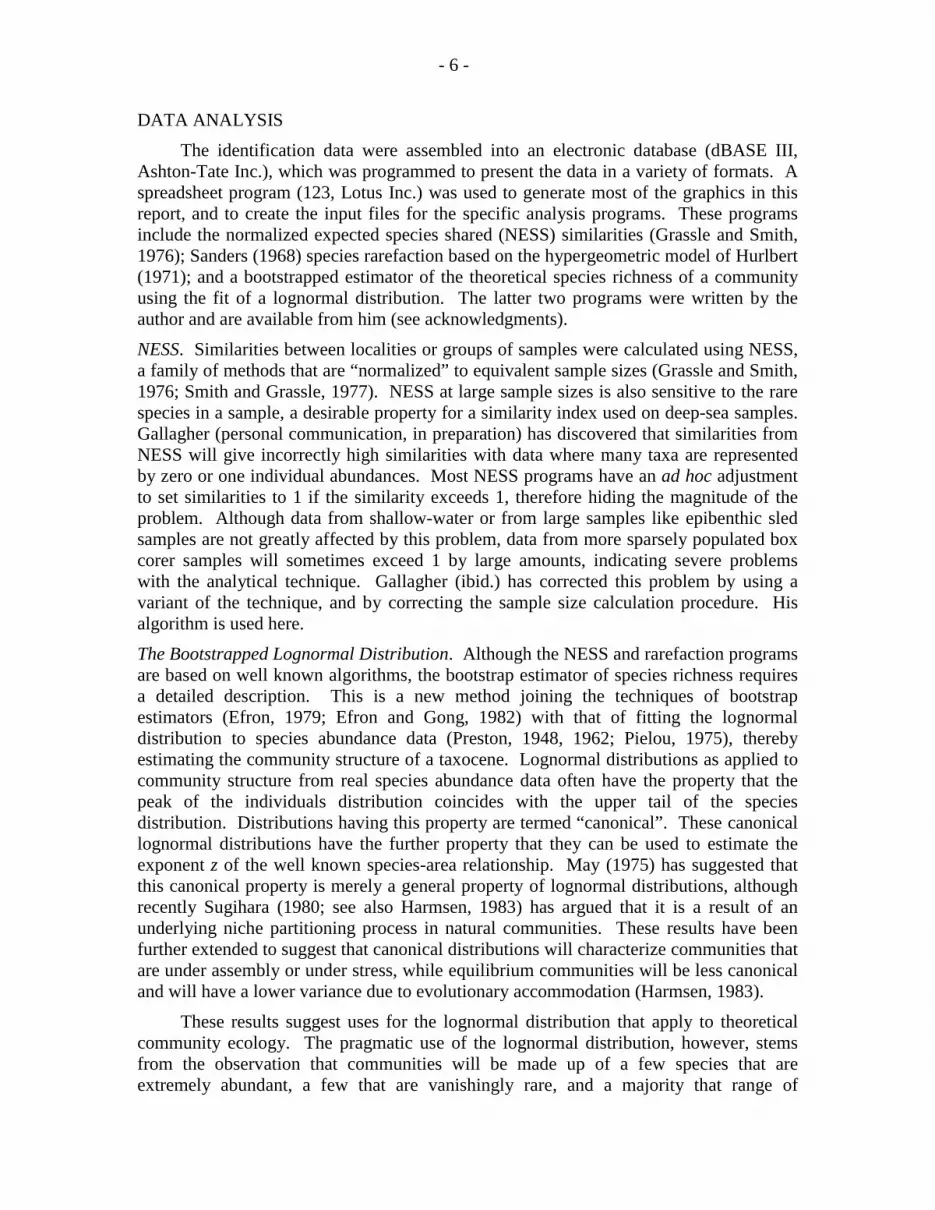
mouthparts of the males are greatly reduced and non-functional (Fig. 4), and there is no

Figure 4. Mouthparts (ventral view) of male and female Leptognathia sp. 23019(Tanaidacea, Leptognathiidae).

- 12 -

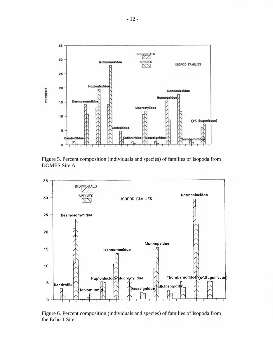
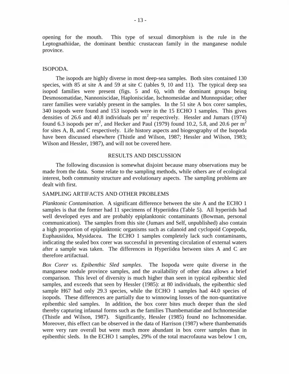
Figure 5. Percent composition (individuals and species) of families of Isopoda fromDOMES Site A.

Figure 6. Percent composition (individuals and species) of families of Isopoda fromthe Echo 1 Site.

- 13 -

opening for the mouth. This type of sexual dimorphism is the rule in theLeptognathiidae, the dominant benthic crustacean family in the manganese noduleprovince.

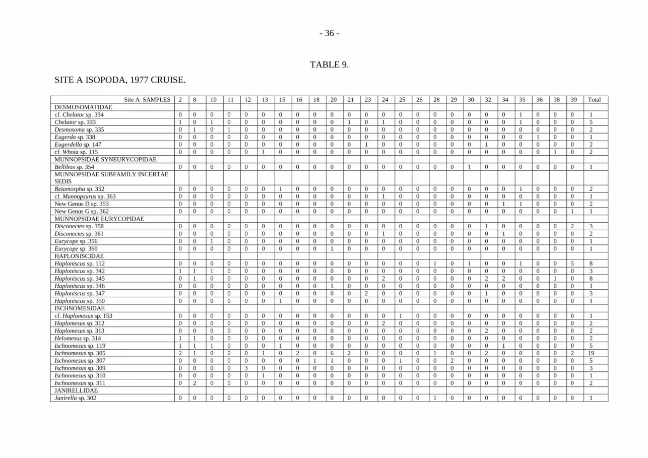
ISOPODA.

The isopods are highly diverse in most deep-sea samples. Both sites contained 130species, with 85 at site A and 59 at site C (tables 9, 10 and 11). The typical deep seaisopod families were present (figs. 5 and 6), with the dominant groups beingDesmosomatidae, Nannoniscidae, Haploniscidae, Ischnomesidae and Munnopsidae; otherrarer families were variably present in the samples. In the 51 site A box corer samples,340 isopods were found and 153 isopods were in the 15 ECHO 1 samples. This givesdensities of 26.6 and 40.8 individuals per m2 respectively. Hessler and Jumars (1974)found 6.3 isopods per m2, and Hecker and Paul (1979) found 10.2, 5.8, and 20.6 per m2

for sites A, B, and C respectively. Life history aspects and biogeography of the Isopodahave been discussed elsewhere (Thistle and Wilson, 1987; Hessler and Wilson, 1983;Wilson and Hessler, 1987), and will not be covered here.

RESULTS AND DISCUSSION

The following discussion is somewhat disjoint because many observations may bemade from the data. Some relate to the sampling methods, while others are of ecologicalinterest, both community structure and evolutionary aspects. The sampling problems aredealt with first.

SAMPLING ARTIFACTS AND OTHER PROBLEMS

Planktonic Contamination. A significant difference between the site A and the ECHO 1samples is that the former had 11 specimens of Hyperiidea (Table 5). All hyperiids hadwell developed eyes and are probably epiplanktonic contaminants (Bowman, personalcommunication). The samples from this site (Jumars and Self, unpublished) also containa high proportion of epiplanktonic organisms such as calanoid and cyclopoid Copepoda,Euphausiidea, Mysidacea. The ECHO 1 samples completely lack such contaminants,indicating the sealed box corer was successful in preventing circulation of external watersafter a sample was taken. The differences in Hyperiidea between sites A and C aretherefore artifactual.

Box Corer vs. Epibenthic Sled samples. The Isopoda were quite diverse in themanganese nodule province samples, and the availability of other data allows a briefcomparison. This level of diversity is much higher than seen in typical epibenthic sledsamples, and exceeds that seen by Hessler (1985): at 80 individuals, the epibenthic sledsample H67 had only 29.3 species, while the ECHO 1 samples had 44.0 species ofisopods. These differences are partially due to winnowing losses of the non-quantitativeepibenthic sled samples. In addition, the box corer bites much deeper than the sledthereby capturing infaunal forms such as the families Thambematidae and Ischnomesidae(Thistle and Wilson, 1987). Significantly, Hessler (1985) found no Ischnomesidae.Moreover, this effect can be observed in the data of Harrison (1987) where thambematidswere very rare overall but were much more abundant in box corer samples than inepibenthic sleds. In the ECHO 1 samples, 29% of the total macrofauna was below 1 cm,

- 14 -

suggesting that an epibenthic sled could miss a substantial portion of the benthic infauna.The epibenthic sled, however, is not the sampler of choice on manganese nodule bottomsbecause the great quantity of nodules that would collect in the bag would grind or crushthe specimens.

Densities and Washing Techniques. Table 12 demonstrates a clear difference betweenthe three programs that collected Crustacea in quantitative samples. The current group ofsamples had higher densities for all four main groups than has been reported before. TheNorth Pacific samples have genuinely lower densities because the overlying waters havea very low overlying productivity (Hessler and Jumars, 1974). The Hecker and Paul(1979) samples, however, were from nearly the same localities, and therefore should besimilar. Material may have been lost by that study during their washing process. Theselatter samples were “. . . washed with sea water, while compressed air was bubbledthrough it, for approximately 2 hours” (Hecker and Paul, 1979: p. 290). This processmay have lost material through the mesh because deep-sea animals are very fragile andwill break up under continued washing. In addition, narrow forms, such as tanaids ornannoniscid isopods, will pass longitudinally through a 300 micron mesh screen if theyare washed long enough. The upper layers of ECHO 1 samples and some site A sampleswere generally fixed in formaldehyde without washing immediately after recovery. Inthe washing of the lower layers, fragile material that collected on the screens were fixedrapidly, without waiting for the entire sample to be washed. Fixing in formaldehydehardens specimens and prevents loss or severe degradation when washing away thesediments, so that specimen recovery at sorting time is improved.

COMMUNITY STRUCTURE

Species Richness. Figure 7 shows Sanders rarefactions of the Tanaidacea and the Isopodafrom both sites. Two features are striking in these curves: within group diversities aresimilar, while between group diversities are distinctly different. At 150 individuals, site

Ffr

igure 7. Rarefaction of pooled species abundance data of Isopoda and Tanaidaceaom Site A and Site C

- 15 -

A has 60.2 isopod species and 45.0 tanaid species, and at the ECHO 1 locality the valuesare 58.6 and 43.2 species, respectively.Species Richness Within Taxocenes. In both the Isopoda and the Tanaidacea, the valuesare extremely similar with only a range of 1 or 2 species separating the two sites. This issurprising because the two sites are separated by 1560 km and do not have the samespecies compositions (see below). Several hypotheses might explain these results. Thesehypotheses are presented not to argue for one or another, but to suggest possibilities forfuture study of these communities.

1. The observations are spurious, further sampling will show different results, and littlecan be concluded from a study of species richness. A preliminary test can show thatthis may not be the case. If one divides the site A Isopod results into two independentgroups of samples, the 1977 and 1978 cruise samples, the species richness at 100individuals shows great similarity within the site: 46.6 and 46.2 species respectively.The consistency of these values indicates that the results are not stochastic, and thatthey may indicate something important about the crustacean community structure.

2. Assuming that the communities are at equilibrium, the overall similarity of thephysical and biotic environments at the two sites has controlled species richness tocertain values. That is, the two sites have similar available niche diversities and thisis reflected in the species that fill the niches. Unfortunately, the niche hypothesis isdifficult to test directly because no data exist on the natural history of these species.

3. The processes of dispersal, speciation and extinction at the two sites are similar,resulting in similar accumulations of species. Evolutionary processes are typicallyignored in the ecological literature (e.g. Rex, 1981), although they are the ultimatecontrollers of diversity in deep-sea communities (Wilson and Hessler, 1987b). If oneassumes that interactional processes are minimal or stochastic in these rarefied deep-sea communities, then the historical processes come to the foreground in theexplanation of deep-sea diversity. Again, we have no data on these rates, so thishypothesis is conjectural.

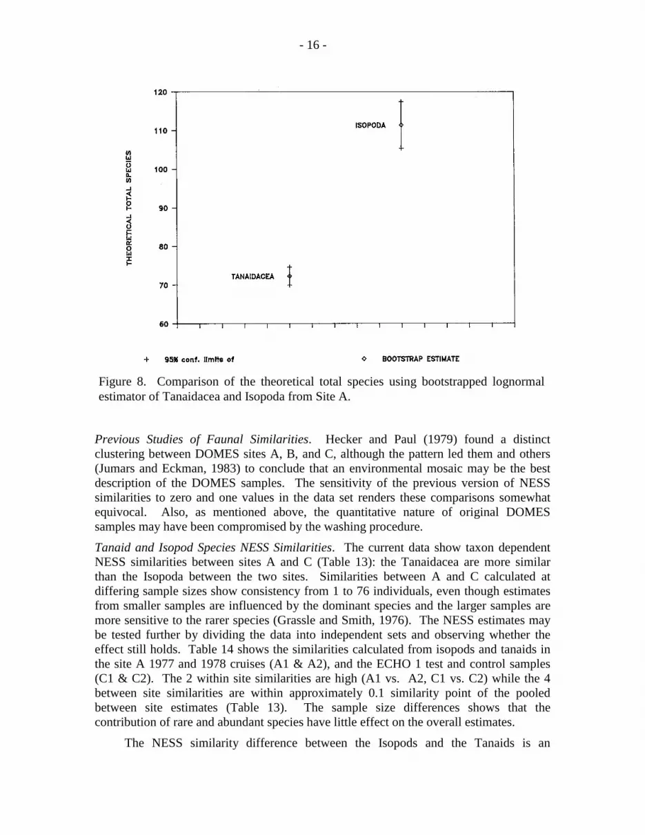
Species Richness Between Taxocenes. The similarities of the within taxon speciesrichnesses provide some confidence that a between taxa comparison may providemeaningful information. Despite the near equivalency of the densities of Isopoda andTanaidacea at both sites, they have distinctly different species richnesses (fig. 7). Thesite A data fitted with a lognormal distribution and bootstrap confidence limits (95%, twotailed) show a clear and statistically significant difference in the bootstrap estimate of thetheoretical total species: 111.4 species of Isopoda, and 72.3 species of Tanaidacea (fig.8). The ECHO 1 data could not be used for this procedure: too few individuals in thepooled samples prevented an accurate fit to the lognormal as indicated by excessivelywide bootstrap confidence limits.

- 16 -

Previous Studies of Faunal Similarities. Hecker and Paul (1979) found a distinctclustering between DOMES sites A, B, and C, although the pattern led them and others(Jumars and Eckman, 1983) to conclude that an environmental mosaic may be the bestdescription of the DOMES samples. The sensitivity of the previous version of NESSsimilarities to zero and one values in the data set renders these comparisons somewhatequivocal. Also, as mentioned above, the quantitative nature of original DOMESsamples may have been compromised by the washing procedure.

Tanaid and Isopod Species NESS Similarities. The current data show taxon dependentNESS similarities between sites A and C (Table 13): the Tanaidacea are more similarthan the Isopoda between the two sites. Similarities between A and C calculated atdiffering sample sizes show consistency from 1 to 76 individuals, even though estimatesfrom smaller samples are influenced by the dominant species and the larger samples aremore sensitive to the rarer species (Grassle and Smith, 1976). The NESS estimates maybe tested further by dividing the data into independent sets and observing whether theeffect still holds. Table 14 shows the similarities calculated from isopods and tanaids inthe site A 1977 and 1978 cruises (A1 & A2), and the ECHO 1 test and control samples(C1 & C2). The 2 within site similarities are high (A1 vs. A2, C1 vs. C2) while the 4between site similarities are within approximately 0.1 similarity point of the pooledbetween site estimates (Table 13). The sample size differences shows that thecontribution of rare and abundant species have little effect on the overall estimates.

The NESS similarity difference between the Isopods and the Tanaids is an

Figure 8. Comparison of the theoretical total species using bootstrapped lognormalestimator of Tanaidacea and Isopoda from Site A.

- 17 -

interesting result because the manganese nodule province is more or less continuous withno oceanographic or geomorphological discontinuities between sites A and C. The resultindicates that, on the average, tanaid species have larger ranges than isopod species;biogeographically speaking, isopods are more provincial than tanaids.

Although environmental interpretations of these data may be possible, anevolutionary hypothesis may explain both the NESS result and the differences in speciesrichness: the Tanaidacea have a higher gene flow than the Isopoda (Wilson, inpreparation). Although Isopoda and Tanaidacea brood their young and therefore do nothave any form of larval dispersal, the highly motile non-feeding males of tanaids maypermit greater gene flow within species compared to isopods where the sexes are moreequal in dispersal powers. This hypothesis predicts that tanaids will have lower rates ofspeciation (lower accumulation of species in an area) and species will have greater ranges(greater similarity between areas) than isopods. Because the current data bear out thesepredictions, the evolutionary hypothesis seems to be a viable possibility.

The ecological or evolutionary meaning of these NESS results should be tested bydata from an intermediate locality, such as DOMES site B. If the data were reflecting anevolutionary effect, we would observe that DOMES site B would be intermediatebetween the sites A and C. Causality due to some environmental or biotic interaction,however, may show a different pattern.

Tanaid and Isopod Family NESS Similarities. Figures 2, 5, and 6 show the relativecomposition of the tanaid and isopod faunas at site A and site C. NESS similarities at thefamily level (Table 15) corroborate the general impression that these localities are similarfor these taxocenes. From other data, both groups are known to be more or lesscosmopolitan at the family level in the deep sea (Sieg, 1986; Hessler et al., 1979; Hesslerand Wilson, 1983; Wilson and Hessler, 1987b). If these families can be interpreted asbeing internally homogeneous for particular lifestyles, as done by Thistle and Wilson(1987), then the data suggest that sites A and C are providing similar habitats for thesetaxocenes.

CONCLUSIONS

The two abundant Crustacean taxocenes, isopods and tanaids, appear to havequantitatively different contributions to the community structure of the manganese noduleprovince. Hurlbert (1971) recommends that estimation of species richness should bemade on taxocenes (phylogenetically related groups of organisms). Including isopodsand tanaids under the general taxocene “Peracarid Crustacea” as has been done in the past(e.g. Hecker and Paul, 1979) may lose useful information, as well as open the analysis tothe criticism that the groups included are not closely related.

Whether the differences between site A and site C are ecological or historical innature is clarified somewhat. Although the diversity of tanaids and isopods from the twosites are strikingly similar, as shown by the rarefaction analyses, the faunal similaritiesare different. In fact, the isopod fauna is almost completely replaced over the 1560nautical miles separating the two sites. The tanaids are more similar over the samedistance, but similarities of only 0.7-0.6 cannot be claimed as representing samples fromthe same distribution. If one can assume that the species of each taxocene are acting as

- 18 -

replicates of one another, then their diversity suggests that sites A and C have similarcommunity structures. The assembly of these communities, however, may be dependenton evolutionary effects such as dispersal, gene flow, speciation, and extinction. Becauseenvironmental or biotic interactions cannot be ruled out completely, tests of historicalhypotheses will require further research designed to distinguish between these andecological processes. Although the quantitative community structure can provide data onevolutionary questions (Wilson, in preparation), more detailed information will bederived from phylogenetic research on subgroups within taxocenes of the manganesenodule province.

For monitoring the impact of manganese nodule mining, these crustacean data showthat the manganese nodule province may not be faunally homogeneous over its entireextent, and that different taxocenes may be structured differently in this region. Thedesign of stable reference areas will have to take this feature into account. From anecological point of view, however, the study of impacts may be simplified if one acceptsthe somewhat nihilistic view that the species of each taxocene are replicates of each otherbecause they have the similar lifestyles. This assumption would permit generalizingresults on benthic impact experiments in one area to be more or less representative of theentire manganese nodule province.

The “species-as-replicates” assumption might apply to the highly monomorphicleptognathiid tanaids, but not necessarily for the isopods which show exceptionalmorphological heterogeneity. In fact, a recent study (Thistle and Wilson, 1987) foundthat abundances of different families of isopods were correlated with their possiblebenthic lifestyle (epifaunal vs. infaunal) and possible interactions with the physicalenvironment. Nevertheless, sites A and C show similar proportions of families,indicating that the hydrodynamic effects discussed by Thistle and Wilson (1987) may notbe structuring the isopod communities of the manganese nodule province.

RECOMMENDATIONS

1. The data in this report are currently obtainable from taxonomic specialists only.While the small quantity of the material was manageable, the portent for the future ismore serious. When mining begins on a commercial scale, continuous monitoring ofthe community structure of the manganese nodule province may be necessary. Suchcontinuous monitoring will generate much higher volumes of samples than dealt within this report. If the appropriate taxonomic references were available theidentifications could be done by laboratories collecting and sorting the samples,resulting in a much greater throughput of information in the monitoring system than iscurrently possible. These references, however, do not exist. Although the deep-seaisopod literature is slowly improving, no monographs summarize the current literatureand carefully illustrate many species from one locality. In this regard, the isopods ofthe manganese nodule province are poorly described: most of the species in this studyare new to science. Tanaidacea, Amphipoda and Cumacea are even more poorlyknown, and there are few active specialists of these deep-sea groups in the UnitedStates (T. Ragen, who identified the Tanaidacea in this project has devoted his careerto the study of pinniped biology). Compounding this problem, agencies rarely fundthe preparation of faunistic monographs even though these monographs are

- 19 -

invaluable to field workers. Support for the preparation of faunistic monographs ofwhole taxocenes (including the Crustacea, Polychaeta, and Mollusca) should beconsidered part of the preparation for monitoring of full-scale mining.

2. Tests of hypotheses discussed above will require that more sites be sampled in themanganese nodule province with the modern techniques. An obvious choice wouldbe to return to DOMES site B to take as many samples as possible. In addition, theECHO 1 site should be sampled further. If one accepts that 111 species of Isopods, asestimated for site A, might also be present at the ECHO 1 site then only half of thetotal species richness has been recovered.

3. This report makes available a great deal of detailed taxonomic data that can be used toexamine questions that prompted previous DOMES studies. The Jumars site A study(Jumars and Self, unpublished) attempted to detect differences from samples beforeand after the test mining, and the ECHO 1 study attempted to determine the degree ofrecolonization in a mined area 5 years after a test mining (Wilson and Hessler,1987a). The tanaid data may now be used to re-examine the conclusions reached bythose studies.

4. An assumption of previous impact studies is that environmental parameters and thealteration thereof might control the distribution and abundance of deep-sea species.By considering environmental heterogeneity as a natural experiment, the physicaldata from the Jumars study and the ECHO 1 study should be correlated with thespecies abundance data to determine whether there are any environmental parametersof importance. This has been done partially with the ECHO 1 data (Wilson andHessler, 1987a), although adding the tanaid data to the analysis may provide newinsights. The Jumars site A study may provide more information: the environmentalvariability in the form of sediment and nodule distribution was much greater at theeastern site (Piper and Blueford, 1982). Furthermore, if additional cruises are fieldedto the manganese nodule province, sampling should attempt to include as much of theenvironmental variability as possible. For example, additional samples from theECHO 1 locality could gather data from valleys where the sediment was distinctlyless stable and the nodule cover was much lower than on the top of the abyssal hills.Of course, the design of benthic experiments will control where the samples aretaken, but including environmental heterogeneity is necessarily important in any suchdesign.

ACKNOWLEDGMENTS

The Tanaidacea and Cumacea were sorted and identified by Timothy Ragen (ScrippsInstitution of Oceanography). A consultation with Jurgen Sieg (Universitat Osnabrück)on the tanaid identifications was informative and helped verify the correctness of ouridentifications. The gammaridean amphipod identifications were aided by a consultationwith J. Lauren Barnard (U.S. National Museum of Natural History), and the hyperiidamphipods were identified by Thomas E. Bowman (NMNH). I thank the latter twogentlemen for hosting my visits to the National Museum on several occasions. GeorgeSugihara (SIO) made the lognormal estimation program possible by generously allowing

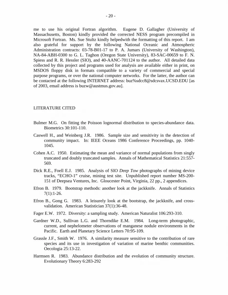
- 20 -

me to use his original Fortran algorithm. Eugene D. Gallagher (University ofMassachusetts, Boston) kindly provided the corrected NESS program precompiled inMicrosoft Fortran. Ms. Sue Stultz kindly helpedwith the formatting of this report. I amalso grateful for support by the following National Oceanic and AtmosphericAdministration contracts: 03-78-B01-17 to P. A. Jumars (University of Washington),NA-84-ABH-0300 to G. L. Taghon (Oregon State University), 83-SAC-00659 to F. N.Spiess and R. R. Hessler (SIO), and 40-AANC-701124 to the author. All detailed datacollected by this project and programs used for analysis are available either in print, onMSDOS floppy disk in formats compatible to a variety of commercial and specialpurpose programs, or over the national computer networks. For the latter, the author canbe contacted at the following INTERNET address: buz%sdcc8@sdcsvax.UCSD.EDU [asof 2003, email address is buzw@austmus.gov.au].

LITERATURE CITED

Bulmer M.G. On fitting the Poisson lognormal distribution to species-abundance data.Biometrics 30:101-110.

Caswell H., and Weinberg J.R. 1986. Sample size and sensitivity in the detection ofcommunity impact. In: IEEE Oceans 1986 Conference Proceedings, pp. 1040-1045.

Cohen A.C. 1950. Estimating the mean and variance of normal populations from singlytruncated and doubly truncated samples. Annals of Mathematical Statistics 21:557-569.

Dick R.E., Foell E.J. 1985. Analysis of SIO Deep Tow photographs of mining devicetracks, “ECHO-1” cruise, mining test site. Unpublished report number MS-200-151 of Deepsea Ventures, Inc. Gloucester Point, Virginia, 22 pp., 2 appendices.

Efron B. 1979. Bootstrap methods: another look at the jackknife. Annals of Statistics7(1):1-26.

Efron B., Gong G. 1983. A leisurely look at the bootstrap, the jackknife, and cross-validation. American Statistician 37(1):36-48.

Fager E.W. 1972. Diversity: a sampling study. American Naturalist 106:293-310.

Gardner W.D., Sullivan L.G. and Thorndike E.M. 1984. Long-term photographic,current, and nephelometer observations of manganese nodule environments in thePacific. Earth and Planetary Science Letters 70:95-109.

Grassle J.F., Smith W. 1976. A similarity measure sensitive to the contribution of rarespecies and its use in investigation of variation of marine benthic communities.Oecologia 25:13-22.

Harmsen R. 1983. Abundance distribution and the evolution of community structure.Evolutionary Theory 6:283-292

- 21 -

Harrison K. 1987. Deep-sea asellote isopods of the north-east Atlantic: the familyThambematidae. Zoologica Scripta 16:51-72.

Hassack E., Holdich D.M. 1987. The tubicolous habit amongst the Tanaidacea(Crustacea, Peracarida) with particular reference to deep-sea species. ZoologicaScripta 16:223-233.

Hayes S.P. 1979. Benthic current observations at DOMES sites A, B, and C in theTropical Central North Pacific Ocean. In: Marine geology and oceanography of thePacific manganese nodule province, J.L. Bischoff and D.Z. Piper, editors, PlenumPress, pp. 83-112.

Hecker B., Paul A.Z. 1979. Abyssal community structure of the benthic infauna of theEastern Equatorial Pacific: DOMES sites A, B, and C. In: Marine geology andoceanography of the Pacific manganese nodule province, J.L. Bischoff and D.Z.Piper, editors, Plenum Press, pp. 287-308.

Hessler R.R. 1985. A comparison of epibenthic sled samples from Southtow to box coresfrom ECHO I, in the context of species distributions. Unpublished report to theNational Oceanic and Atmospheric Administration on contract NA-84-AAA-02529, 16 pp.

Hessler R.R., Wilson G.D.F. 1983. The origin and biogeography of malacostracancrustaceans in the deep sea. In: Evolution, time and space: the emergence of thebiosphere. R.W. Sims, J.H. Price and P.E.S. Whalley, editors, Academic Press, pp.227-254.

Hessler R.R., P.A. Jumars. 1974. Abyssal community analysis from replicate box coresin the central North Pacific. Deep-Sea Research 21:185-209.

Hessler R.R., Wilson G.D.F., Thistle D. 1979. The deep-sea isopods: a biogeographicand phylogenetic overview. Sarsia 64(1-2):67-76.

Hurlbert S.H. 1971. The nonconcept of species diversity: a critique and alternativeparameters. Ecology 52:577-586.

Johnson D.A. 1972. Ocean-floor erosion in the equatorial Pacific. Bulletin of theGeological Society of America 83:3121-3144.

Jumars P.A., Eckman J.E. 1983. Spatial structure within deep-sea benthic communities.In: Deep-Sea Biology, The Sea, vol. 8, edited by G.T. Rowe, pp.399-451. J. Wiley& Sons, New York.

Lavelle J.W., Ozturgut E., Swift S.A., and Erickson B.H. 1981. Dispersal andresedimentation of the benthic plume from deep-sea mining operations: a modelwith calibration. Marine Mining 3:59-93.

May R. M. 1975. Patterns of species abundance and diversity. In: “Ecology andEvolution of Communities,” M.L. Cody and J.M. Diamond, eds., pp. 81-120.Cambridge, Mass: Belknap Press of Harvard.

de Moustier C.P. 1985. Inference of manganese nodule coverage from Sea Beamacoustic backscattering data.Geophysics 50:989-1001.

- 22 -

Pielou E.C. 1975. Ecological diversity. New York, N.Y.: Wiley, 165 pp.

Piper D.Z., Blueford J.R. 1982. Distribution, mineralogy, and texture of manganesenodules and their relation to sedimentation at DOMES Site A in the equatorialNorth Pacific. Deep-Sea Research 29:927-953.

Piper D.Z., Gardner J.V., Cook H.E. 1979a. Lithic and acoustic stratigraphy of theequatorial north Pacific: DOMES sites A, B, and C. In: Marine geology andoceanography of the Pacific manganese nodule province, J.L. Bischoff and D.Z.Piper, editors, Plenum Press, pp. 309-348.

Piper D.Z., Leong K., Cannon W.F. 1979b. Manganese nodule and surface sedimentcompositions: DOMES sites A, B, and C. In: Marine geology and oceanography ofthe Pacific manganese nodule province, J.L.Bischoff and D.Z. Piper, editors,Plenum Press, pp. 437-474.

Preston F.W. 1948. The commonness, and rarity, of species. Ecology 29:254-283.

Preston F.W. 1962. The canonical distribution of commonness and rarity. Ecology (twoparts) 43:185-215, 410-432.

Quinterno P., Theyer F. 1979. Biostratigraphy of the equatorial north Pacific: DOMESsites A, B, and C. Marine Geology and oceanography of the Pacific manganesenodule province, J.L. Bischoff and D.Z. Piper, editors, Plenum Press. pp. 349-364.

Rex M.A. Community structure in the deep-sea benthos. Annual Review of Ecology andSystematics 12:331-353.

Sanders H.L. 1968. Marine benthic diversity: a comparative study. American Naturalist102:243-282.

Sieg J. 1986. Distribution of the Tanaidacea: synopsis of the known data andsuggestions on possible distribution patterns. In: “Crustacean Biogeography,” R.H.Gore and K.L. Heck, eds. pp. 165-193. Boston, Ma: A.A. Balkema.

Smith W., Grassle J.F. 1977. Sampling properties of a family of diversity measures.Biometrics 33:283-292.

Spiess F.N., Hessler R.R., Wilson G.D.F., Weydert M., and Rude P. 1984. ECHO ICruise Report. SIO Reference 84-3:1-22. Marine Physical Laboratory, ScrippsInstitution of Oceanography, San Diego, CA.

Spiess F.N., Weydert M. 1987. Operational Aspects, Geology and Physical Effects ofDredging. In: “Environmental Effects of Deep-Sea Dredging,” by F.N. Spiess,R.R. Hessler, G. Wilson, and M. Weydert, Final Report to the National Oceanic andAtmospheric Administration on contract NA83-SAC-00659, pp. 1-23. ScrippsInstitution of Oceanography Reference 87-5, La Jolla, Calif., 86 pp.

Sugihara G. 1980. Minimal community structure: an explanationof species abundancepatterns.American Naturalist 116:770-787.

Thiel H. 1983. Meiobenthos and nanobenthos of the deep sea. In: Deep-sea biology. G.Row, editor, Wiley, pp. 167-230.

- 23 -

Thistle D., Wilson G.D.F. 1987. A hydrodynamically modified, abyssal isopod fauna.Deep-Sea Research 34:73-87.

Tipper J.C. 1979. Rarefaction and rarefiction - the use and abuse of a method inpaleoecology. Paleobiology 5:423-434.

Wilson G.D.F., Hessler R.R. 1987a. The effects of manganese nodule test mining on thebenthic fauna in the North Equatorial Pacific. In: “Environmental Effects of Deep-Sea Dredging,” by F.N. Spiess, R.R. Hessler, G. Wilson, and M. Weydert, FinalReport to the National Oceanic and Atmospheric Administration on contract NA83-SAC-00659, pp. 24-86. Scripps Institution of Oceanography Reference 87-5, LaJolla, Calif., 86 pp.

Wilson G.D.F., Hessler R.R. 1987b. Speciation in the deep sea. Annual Review ofEcology and Systematics 18:185-207.

- 24 -

TABLE 1.

SITE A BOX CORER SAMPLES. Locations of box corer samples collected by theauthor for Jumars study (Jumars and Self, unpublished) in 1977 and 1978. Not allsamples were used for macrofaunal analysis.

SAMPLE DATE LATITUDE LONGITUDE DEPTH TYPE

DJ02 11/22/77 9° 23.5 151° 32.9 5155 BC,SANDIA

DJ07 11/23/77 9° 22.9 151° 32.0 5170 BC,SANDIA

DJ08 11/24/77 9° 25.2 151° 34.5 5205 BC,THIEL

DJ10 11/24/77 9° 22.8 151° 31.8 5183 BC,THIEL

DJ11 11/25/77 9° 23.5 151° 22.5 5174 BC,THIEL

DJ12 11/25/77 9° 22.9 151° 20.6 5187 BC,THIEL

DJ13 11/25/77 9° 23.3 151° 23.0 5187 BC,THIEL

DJ15 11/26/77 9° 20.3 151° 24.1 5166 BC,THIEL

DJ16 11/26/77 9° 18.6 151° 28.5 5120 BC,THIEL

DJ18 11/26/77 9° 25.6 151° 31.2 5160 BC,THIEL

DJ20 11/27/77 9° 19.8 151° 35.1 5260 BC,THIEL

DJ21 11/27/77 9° 20.5 151° 45.0 5203 BC,THIEL

DJ22 11/28/77 9° 32.4 151° 39.1 4908 BC,THIEL

DJ23 11/28/77 9° 33.2 151° 38.3 4934 BC,THIEL

DJ24 11/28/77 9° 31.2 151° 17.1 5164 BC,THIEL

DJ25 11/28/77 9° 22.6 151° 12.3 5177 BC,THIEL

DJ26 11/29/77 9° 24.8 151° 16.4 5170 BC,THIEL

DJ28 11/29/77 9° 24.1 151° 17.7 5197 BC,THIEL

DJ29 11/29/77 9° 23.4 151° 15.6 5183 BC,THIEL

DJ30 11/30/77 9° 25.3 151° 9.9 5175 BC,THIEL

DJ31 11/30/77 9° 29.5 151° 0.6 5199 BC,THIEL

DJ32 11/30/77 9° 16.0 151° 56.1 5043 BC,THIEL

DJ34 12/01/77 9° 16.7 151° 9.8 4842 BC,THIEL

DJ35 12/02/77 9° 19.3 151° 28.9 5130 BC,SANDIA

DJ36 12/02/77 9° 26.6 151° 32.8 5231 BC,SANDIA

DJ37 12/02/77 9° 25.5 151° 38.3 5197 BC,SANDIA

- 25 -

SAMPLE DATE LATITUDE LONGITUDE DEPTH TYPE

DJ38 12/03/77 9° 36.3 151° 58.0 5086 BC,SANDIA

DJ39 12/03/77 9° 35.8 151° 6.8 5117 BC,SANDIA

DJ40 05/18/78 9° 23.5 151° 29.2 5256 BC,SANDIA

DJ41 05/18/78 9° 22.7 151° 28.0 5191 BC,SANDIA

DJ42 05/19/78 9° 23.6 151° 28.1 5219 BC,SANDIA

DJ44 05/19/78 9° 24.5 151° 27.5 5235 BC,SANDIA

DJ46 05/19/78 9° 28.0 151° 27.6 5216 BC,SANDIA

DJ47 05/20/78 9° 21.0 151° 28.7 5208 BC,SANDIA

DJ48 05/20/78 9° 22.0 151° 25.9 5165 BC,SANDIA

DJ49 05/20/78 9° 23.4 151° 25.3 5171 BC,SANDIA

DJ50 05/20/78 9° 22.1 151° 24.6 5086 BC,SANDIA

DJ52 05/21/78 9° 18.4 151° 26.0 5093 BC,SANDIA

DJ54 05/22/78 9° 20.7 151° 24.5 5064 BC,SANDIA

DJ55 05/22/78 9° 27.0 151° 34.0 5246 BC,SANDIA

DJ56 05/22/78 9° 20.1 151° 30.1 5159 BC,SANDIA

DJ58 05/23/78 9° 20.2 151° 33.1 5148 BC,SANDIA

DJ59 05/23/78 9° 17.6 151° 33.3 5011 BC,SANDIA

DJ60 05/23/78 9° 20.0 151° 26.2 5196 BC,SANDIA

DJ62 05/24/78 9° 15.2 151° 16.5 4921 BC,SANDIA

DJ63 05/24/78 9° 24.8 151° 30.2 5215 BC,SANDIA

DJ65 05/25/78 9° 26.4 151° 32.2 5253 BC,SANDIA

DJ66 05/25/78 9° 27.0 151° 35.9 5250 BC,SANDIA

DJ69 05/25/78 9° 15.8 151° 30.7 5049 BC,SANDIA

DJ70 05/26/78 9° 16.7 151° 28.7 4942 BC,SANDIA

DJ72 05/27/78 9° 33.8 151° 21.3 5240 BC,SANDIA

DJ73 05/27/78 9° 28.1 151° 15.6 5107 BC,SANDIA

DJ74 05/27/78 9° 24.4 151° 17.9 5283 BC,SANDIA

DJ75 05/27/78 9° 23.7 151° 17.1 5216 BC,SANDIA

DJ77 05/28/78 9° 21.3 151° 20.5 5034 BC,SANDIA

- 26 -

TABLE 2.

Position data of Box Corer Samples at the ECHO 1 locality (site C). The origin of thecoordinate system is at 14 34.00’ N, 125 30.00’W. X, Y coordinates determined withinMPL Deep-Tow Transponder Net (Spiess et al., 1984, Spiess and Weydert, 1987) parallelto lines of latitude and longitude, respectively.

sample coordinates

SampleX Y

Latitudeat 14°N(in min.)

Longitudeat 125°W(in min.)

Depth(m.)

H347 5416 7876 38.2762 26.9854 4511H348 4222 7500 38.0720 27.6513 4504H349 5069 8091 38.3925 27.1791 4517H350 5712 7593 38.1226 26.8208 4506H351 6497 6691 37.6334 26.3840 4516H352 6606 7749 38.2072 26.3241 4502H353 10295 14905 42.0879 24.2679 4516H354 10380 14391 41.8091 24.2202 4514H355 10288 14690 41.9712 24.2710 4510H356 10296 15580 42.4541 24.2664 4518H357 10277 15002 42.1404 24.2787 4510H358 10316 15099 42.1930 24.2556 4516H360 4442 13599 41.3797 27.5298 4500H361 14297 12528 40.7987 22.0379 4567H362 7443 14886 42.0775 25.8565 4480

- 28 -

TABLE 3.

AMPHIPODA GAMMARIDEA FROM SITE A. Data are combined from both the 1977 and 1978 cruises.

SITE A Sample. 08 21 24 25 29 30 32 34 42 44 47 48 50 55 58 60 62 65 69 72 74 75 77 TotalCOROPHIIDAENew Genus sp. 09

0 0 0 0 0 0 0 0 0 0 0 0 0 0 0 0 0 0 1 0 0 0 0 1

EUSIRIDAE NewGenus sp. 05

0 0 0 1 0 0 0 0 0 0 0 0 0 0 0 0 1 0 0 0 0 0 0 2

ISCHYROCERIDAE Bonierella sp. 13

0 0 1 0 0 0 0 0 0 0 0 0 0 0 0 0 0 0 0 0 0 0 0 1

LYSIANASSIDAEHippomedon sp. 04

0 0 0 0 0 0 0 0 0 0 0 1 0 0 0 0 0 0 0 1 0 0 0 2

Hirondellea sp. 03 0 0 0 0 0 0 1 0 0 0 0 0 0 0 0 0 0 0 0 0 0 0 0 1MELPHIDIPPIDAENew Genus sp. 11

0 0 0 0 0 0 0 0 0 0 0 0 0 0 0 0 0 0 0 0 0 0 1 1

PHOXOCEPHALIDAE Leptophoxus sp.08

0 1 0 0 0 0 0 1 0 0 0 0 0 0 0 0 0 0 0 0 0 0 0 2

OEDICEROTIDAEcf. Oediceroides sp.15

0 0 0 0 0 0 0 0 1 0 0 0 0 0 0 0 0 0 0 0 0 0 0 1

PARDALISCIDAEPardaliscopsis sp. 01

0 0 0 0 0 0 0 0 0 1 1 0 0 1 0 0 0 0 0 0 0 0 0 3

Pardaliscopsis sp. 02 0 0 0 0 1 0 2 0 0 0 0 0 1 0 0 0 0 0 0 0 0 0 0 4Parpano sp. 07 0 0 0 0 0 0 0 0 0 0 0 0 0 0 0 0 0 0 0 0 1 0 0 1Genus Indet sp. 14 0 0 1 0 0 0 0 0 0 0 0 0 0 0 0 0 0 0 0 0 0 0 0 1SYNOPIIDAE Syrrhoe sp. 06

0 0 0 0 0 0 0 0 0 0 0 0 0 0 0 0 0 0 0 0 1 0 0 1

Syrrhoites sp. 12 0 0 0 0 0 1 0 0 0 0 0 0 0 0 0 0 0 0 0 0 0 0 0 0NEW FAMILY? #1New Genus sp. 10

0 0 0 0 0 0 0 0 0 0 0 0 0 0 0 0 0 1 0 0 0 0 0 1

Unidentifiablespecimens

1 0 0 0 0 0 0 0 1 0 0 0 0 0 1 1 1 1 0 0 0 1 0 7

SAMPLE TOTALS 1 1 2 1 1 1 3 1 2 1 1 1 1 1 1 1 2 2 1 1 2 1 1 30

- 29 -

TABLE 4.

AMPHIPODA GAMMARIDEA FROM SITE C, ECHO 1 LOCALITY.

ECHO 1 SAMPLE 348 351 352 354 356 357 358 360 Totals

MELPHIDIPPIDAE NewGenus sp. 11

0 0 0 1 0 0 0 0 1

OEDICEROTIDAE cf.Oediceroides sp. 55

0 1 0 0 0 1 0 1 3

PARDALISCIDAEPardaliscopsis sp. 01

0 0 0 1 0 0 0 1 2

SYNOPIIDAE Pseudotironsp. 54

0 0 0 0 1 0 0 0 1

cf. Austrosyrrhoe sp. 52 1 0 0 0 1 0 2 0 4NEW FAMILY? #1 NewGenus sp. 51

1 2 2 0 0 0 0 0 5

NEW FAMILY? #2 NewGenus sp. 53

0 0 0 1 0 0 0 0 1

SAMPLE TOTAL 2 3 2 3 2 1 2 2 17

TABLE 5.

Amphipoda Hyperiidea From 1977 and 1978 cruises at Site A. Specimens identified by Dr. ThomasE. Bowman.

SITE A SAMPLE 25 35 41 42 46 48 50 56 73 TotalsEupronoe sp. 32 0 0 0 1 0 0 0 0 0 1Eupronoe sp. 33 0 0 1 0 0 0 0 0 0 1

Hyperietta vosseleri (Stebbing) 0 0 0 1 0 1 0 1 0 3Hyperietta stephenseni Bowman 0 0 0 0 0 0 0 0 1 1Lestrigonus bengalensis Giles 0 0 0 1 1 0 1 0 0 3Primno brevidens Bowman 1 0 0 0 0 0 0 0 0 1Unidentified poor specimen 0 1 0 0 0 0 0 0 0 1SAMPLE TOTAL 1 1 1 3 1 1 1 1 1 11

- 30 -

TABLE 6.

TANAIDACEA COLLECTED AT SITE A, 1977 CRUISE

SITE A SAMPLE 02 08 10 11 12 13 15 16 18 20 21 23 24 25 26 28 29 30 31 32 34 35 36 38 39 TotalAgathotanaidaeAgathotanais sp. 23001 1 0 0 0 0 0 1 0 0 1 0 4 0 0 0 0 0 0 0 0 0 0 0 1 0 8Paragathotanais sp. 23002 0 0 1 0 0 0 0 1 0 0 0 1 0 0 1 0 0 0 0 0 0 0 0 0 0 4AnarthruridaeParanarthrurella sp.23005

0 0 0 0 0 0 0 0 0 0 0 0 0 0 0 0 0 0 0 0 0 0 0 0 1 1

LeptognathiidaeCollettea sp. 23011 0 0 0 0 0 0 0 0 0 0 0 0 0 0 0 0 0 0 0 0 0 0 0 0 1 1Collettea sp. 23012 0 0 0 0 0 0 0 0 0 0 0 0 0 0 0 0 0 0 0 1 0 0 0 0 0 1Filitanais sp. 23014 1 1 0 0 0 1 0 0 1 0 0 1 0 2 0 0 1 0 0 0 0 0 0 0 0 8Genus B sp. 23058 0 0 0 0 0 0 0 0 0 0 0 0 0 0 0 0 0 0 0 0 1 0 0 0 0 1Genus C sp. 23010 0 0 0 0 0 0 0 0 0 0 0 0 0 0 0 0 0 0 0 1 0 0 0 0 1 2Leptognathia sp. 23017 0 1 0 1 0 2 1 0 1 0 0 0 0 1 0 0 0 0 0 0 0 0 0 1 0 8Leptognathia sp. 23018 0 0 0 0 0 0 0 0 0 0 0 0 0 0 0 0 0 0 0 0 0 3 0 0 0 3Leptognathia sp. 23019 0 0 0 0 0 0 0 0 0 0 2 0 2 1 0 1 0 0 0 1 2 0 0 3 0 12Leptognathia sp. 23021 0 0 0 0 0 0 0 0 0 0 0 0 0 0 0 0 0 0 0 0 0 1 0 0 0 1Leptognathia sp. 23022 0 0 0 0 0 0 0 0 0 0 0 0 0 0 0 0 1 0 1 0 0 1 3 0 0 6Leptognathia sp. 23023 0 0 0 1 0 1 0 0 0 1 0 0 0 1 0 0 0 0 1 2 0 0 0 0 0 7Leptognathia sp. 23024 0 0 0 0 0 0 1 0 0 0 0 0 1 1 0 1 0 0 0 0 0 0 0 0 0 4Leptognathia sp. 23025 0 0 0 0 1 1 0 0 0 0 0 0 0 0 0 0 0 0 0 0 0 0 0 0 0 2Leptognathia sp. 23026 0 0 0 1 0 0 0 0 0 0 0 0 0 0 0 0 0 0 0 0 0 0 0 0 0 1Leptognathia sp. 23027 2 2 0 0 0 1 2 1 0 0 2 0 0 1 2 1 2 0 0 0 0 3 1 0 1 21Leptognathia sp. 23028 0 1 0 2 2 0 0 0 0 0 0 0 1 0 0 0 2 0 0 0 1 1 0 0 0 10Leptognathia sp. 23029 0 0 0 0 0 0 0 0 0 0 0 0 0 0 0 0 0 0 0 0 0 0 0 0 2 2Leptognathia sp. 23031 0 0 0 0 0 0 1 0 0 0 0 0 1 0 0 0 0 0 0 0 0 0 0 0 0 2Leptognathia sp. 23032 0 0 0 0 0 0 0 0 2 0 0 0 0 0 0 0 0 1 0 0 0 0 0 0 0 3Leptognathia sp. 23033 0 0 0 0 0 0 0 0 0 0 0 0 0 0 0 0 0 0 0 0 0 0 0 2 1 3Leptognathia sp. 23034 0 0 0 0 0 0 0 0 0 0 0 0 0 1 0 0 0 0 0 1 0 0 0 0 0 2Leptognathia sp. 23035 0 0 0 0 0 0 0 0 0 0 1 0 0 0 0 0 0 0 0 0 0 0 0 0 0 1Leptognathia sp. 23036 0 0 0 0 0 0 0 0 0 0 0 1 0 0 0 0 0 0 0 0 0 0 0 0 0 1Leptognathia sp. 23037 0 0 0 0 0 0 0 0 0 1 0 0 0 0 0 0 1 0 0 0 0 0 0 1 0 3

- 31 -

SITE A SAMPLE 02 08 10 11 12 13 15 16 18 20 21 23 24 25 26 28 29 30 31 32 34 35 36 38 39 TotalLeptognathia sp. 23038 0 0 0 0 0 0 0 0 0 0 0 0 0 0 0 0 2 0 0 0 1 0 0 0 0 3Leptognathia sp. 23062 0 0 0 0 0 0 0 1 0 0 0 0 0 0 0 0 0 0 0 0 0 0 0 1 0 2Leptognathia sp. 23063 0 0 0 0 0 0 0 0 0 0 0 0 0 0 0 0 0 0 0 0 0 0 0 1 0 1Leptognathia sp. 23064 1 0 0 0 0 0 0 1 0 1 0 1 0 1 0 0 0 0 0 0 0 0 0 0 0 5Leptognathia sp. 23065 0 0 0 0 0 1 1 0 0 0 1 0 0 0 0 0 0 0 0 2 2 0 0 0 2 9Macrinella sp. 23041 2 2 0 0 0 0 0 0 0 0 0 0 0 1 1 0 0 0 0 1 1 0 0 0 0 8Macrinella sp. 23042 0 0 0 0 0 0 0 0 0 0 0 0 1 0 0 0 0 0 0 0 0 0 0 0 1 2Paratyphlotanais sp.23046

0 0 1 0 0 0 0 0 0 0 0 0 0 0 0 0 0 0 0 0 0 0 0 0 0 1

Typhlotanais sp. 23047 0 0 0 0 0 0 0 0 1 0 0 0 0 0 0 0 0 0 0 0 0 0 0 0 0 1Typhlotanais sp. 23048 0 0 0 0 0 0 0 0 0 0 0 2 1 0 0 0 0 0 0 0 0 0 0 0 0 3Typhlotanais sp. 23050 0 0 0 0 0 0 0 0 0 0 0 0 0 1 0 0 0 0 0 0 0 0 0 0 0 1Typhlotanais sp. 23053 0 0 0 0 0 0 1 0 0 0 0 0 0 0 0 0 0 0 0 0 0 0 0 0 1 2Typhlotanais sp. 23054 0 0 0 0 0 0 0 0 0 0 0 0 1 0 0 0 0 0 0 0 0 0 0 0 0 1Neotanaidae Neotanaissp. 23057

0 0 0 0 0 0 0 0 0 0 0 0 0 0 0 0 0 0 0 0 1 0 0 0 0 1

PseudotanaidaePseudotanais sp. 23060 0 0 0 0 0 0 0 0 0 0 0 0 0 0 0 0 0 1 0 0 0 0 0 0 0 1Pseudotanais sp.23061

0 1 1 0 0 1 0 0 0 0 0 0 0 0 0 2 0 0 0 0 0 0 0 0 0 5

WhitelegiidaeCarpoapseudes sp. 23009 0 0 0 0 0 0 0 0 0 0 0 0 0 0 0 0 0 0 0 1 0 0 0 0 0 1Leviapseudes sp. 23007 0 0 0 0 0 0 0 0 0 0 1 0 0 0 0 0 0 0 0 0 0 0 0 0 0 1Specimens NotIdentified To SpeciesLeptognathia sp. 0 0 0 0 0 0 0 0 0 0 0 0 0 1 0 0 0 0 0 0 0 0 0 0 0 1Leptognathiidae sp. 0 0 0 0 0 0 0 1 0 0 0 0 0 0 0 0 0 0 0 0 0 0 0 0 0 1Tanaidacea Indet. sp. 0 0 0 0 0 0 0 0 0 3 0 0 0 0 0 0 0 0 0 0 0 0 0 0 1 4SAMPLE TOTALS 7 8 3 5 3 8 8 5 5 7 7 10 8 12 4 5 9 2 2 10 9 9 4 10 12 172

- 32 -

TABLE 7.

TANAIDACEA FROM SITE A, 1978 CRUISE

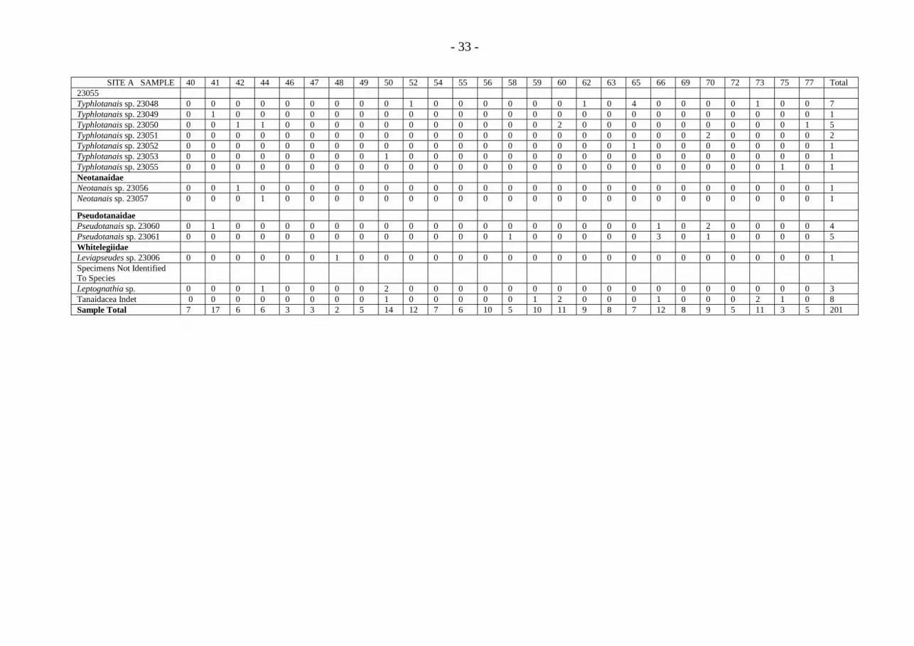
SITE A SAMPLE 40 41 42 44 46 47 48 49 50 52 54 55 56 58 59 60 62 63 65 66 69 70 72 73 75 77 TotalAgathotanaidaeAgathotanais sp. 23001 0 1 0 0 0 0 0 0 1 0 0 0 0 0 0 0 0 0 0 1 1 0 1 4 0 1 10Paragathotanais sp. 23002 0 0 0 0 0 0 0 0 0 0 1 0 0 0 0 0 0 0 0 0 0 0 0 0 0 1 2Paragathotanais sp. 23003 0 0 0 0 0 0 0 0 0 0 0 0 0 0 0 1 0 0 0 0 0 0 0 0 0 0 1AnarthruridaeParanarthrura sp. 23004 2 1 0 0 1 0 0 0 0 0 0 0 1 0 0 0 0 0 0 0 0 0 0 0 0 0 5LeptognathiidaeCollettea sp. 23012 0 0 0 0 0 0 0 0 0 0 0 0 0 0 0 0 0 3 0 0 0 0 0 0 0 0 3Filitanais sp. 23014 0 3 0 0 1 0 0 0 0 0 0 2 2 0 0 0 0 1 0 0 0 0 2 0 0 0 11Filitanais sp. 23015 0 0 0 0 0 0 0 0 1 0 0 0 0 0 0 0 0 0 0 0 0 0 0 0 0 0 1Genus B sp. 23044 0 0 0 0 0 0 0 0 0 0 0 0 0 0 0 0 0 1 0 0 0 0 0 0 0 0 1Leptognathia sp. 23017 0 0 0 0 0 0 0 0 0 0 0 0 1 0 0 1 1 0 0 0 0 0 0 0 0 0 3Leptognathia sp. 23018 0 0 0 0 0 0 0 0 0 0 0 0 0 0 0 2 1 0 0 0 0 0 0 0 0 0 3Leptognathia sp. 23019 1 0 0 1 0 1 0 0 0 0 1 0 0 0 0 0 0 1 0 0 0 0 0 0 0 0 5Leptognathia sp. 23020 0 0 0 0 0 0 0 0 0 0 1 0 0 0 0 0 0 0 0 0 0 0 0 0 0 0 1Leptognathia sp. 23021 0 0 0 0 0 0 0 1 1 0 0 1 0 0 0 0 0 0 0 0 0 0 0 0 0 0 3Leptognathia sp. 23022 0 0 0 0 1 0 0 0 0 0 0 0 0 0 0 0 0 0 0 0 0 0 0 0 0 0 1Leptognathia sp. 23023 0 0 3 0 0 0 0 0 2 0 0 0 0 0 0 0 1 0 0 0 0 0 0 0 0 0 6Leptognathia sp. 23024 0 0 0 0 0 0 1 0 0 0 0 0 0 0 0 0 0 0 0 0 0 0 0 0 0 1 2Leptognathia sp. 23025 0 4 0 0 0 0 0 0 1 2 0 0 4 0 0 0 0 2 0 0 0 0 0 0 0 0 13Leptognathia sp. 23027 0 0 0 1 0 0 0 1 0 3 1 0 1 0 4 0 0 0 1 1 1 2 1 0 0 0 17Leptognathia sp. 23028 0 1 0 1 0 0 0 0 0 0 0 0 1 2 2 0 0 0 1 0 1 0 0 0 0 0 9Leptognathia sp. 23030 0 0 0 0 0 0 0 0 0 1 0 0 0 0 0 0 0 0 0 0 0 0 0 0 0 0 1Leptognathia sp. 23031 0 0 0 0 0 0 0 0 0 0 0 0 0 0 0 0 0 0 0 1 0 0 0 0 0 0 1Leptognathia sp. 23032 0 0 0 0 0 0 0 1 1 4 1 1 0 1 0 0 0 0 0 2 0 0 0 0 0 0 11Leptognathia sp. 23033 0 0 0 0 0 1 0 1 2 0 0 0 0 0 0 0 0 0 0 0 1 0 0 0 0 0 5Leptognathia sp. 23034 0 2 0 0 0 0 0 0 0 0 0 0 0 0 0 0 0 0 0 0 0 0 0 0 0 0 2Leptognathia sp. 23035 0 2 0 0 0 1 0 1 0 0 0 0 0 0 0 0 0 0 0 0 0 0 0 0 0 0 4Leptognathia sp. 23036 0 0 0 0 0 0 0 0 0 0 0 0 0 0 0 0 0 0 0 0 2 1 0 0 0 0 3Leptognathia sp. 23038 0 0 0 0 0 0 0 0 0 0 0 0 0 1 0 0 3 0 0 0 0 0 0 0 0 0 4Leptognathia sp. 23062 0 0 0 0 0 0 0 0 0 0 0 0 0 0 1 0 0 0 0 0 1 0 0 0 0 0 2Leptognathia sp. 23063 0 0 0 0 0 0 0 0 0 0 1 0 0 0 0 0 0 0 0 0 0 0 0 0 0 0 1Leptognathia sp. 23064 0 0 0 0 0 0 0 0 1 1 1 0 0 0 0 0 0 0 0 0 0 0 0 0 0 0 3Leptognathia sp. 23065 1 1 1 0 0 0 0 0 0 0 0 0 0 0 0 3 2 0 0 0 1 1 0 0 0 0 10Libianus sp. 23040 0 0 0 0 0 0 0 0 0 0 0 0 0 0 1 0 0 0 0 0 0 0 0 1 0 0 2Macrinella sp. 23041 3 0 0 0 0 0 0 0 0 0 0 2 0 0 0 0 0 0 0 2 0 0 0 0 0 1 8Macrinella sp. 23042 0 0 0 0 0 0 0 0 0 0 0 0 0 0 0 0 0 0 0 0 0 0 0 2 0 0 2Macrinella sp. 23043 0 0 0 0 0 0 0 0 0 0 0 0 0 0 1 0 0 0 0 0 0 0 0 1 0 0 2Paraleptognathia sp. 23045 0 0 0 0 0 0 0 0 0 0 0 0 0 0 0 0 0 0 0 0 0 0 1 0 0 0 1Pseudoparatanais sp. 0 0 0 0 0 0 0 0 0 0 0 0 0 0 0 0 0 0 0 0 0 0 0 0 1 0 1

- 33 -

SITE A SAMPLE 40 41 42 44 46 47 48 49 50 52 54 55 56 58 59 60 62 63 65 66 69 70 72 73 75 77 Total23055Typhlotanais sp. 23048 0 0 0 0 0 0 0 0 0 1 0 0 0 0 0 0 1 0 4 0 0 0 0 1 0 0 7Typhlotanais sp. 23049 0 1 0 0 0 0 0 0 0 0 0 0 0 0 0 0 0 0 0 0 0 0 0 0 0 0 1Typhlotanais sp. 23050 0 0 1 1 0 0 0 0 0 0 0 0 0 0 0 2 0 0 0 0 0 0 0 0 0 1 5Typhlotanais sp. 23051 0 0 0 0 0 0 0 0 0 0 0 0 0 0 0 0 0 0 0 0 0 2 0 0 0 0 2Typhlotanais sp. 23052 0 0 0 0 0 0 0 0 0 0 0 0 0 0 0 0 0 0 1 0 0 0 0 0 0 0 1Typhlotanais sp. 23053 0 0 0 0 0 0 0 0 1 0 0 0 0 0 0 0 0 0 0 0 0 0 0 0 0 0 1Typhlotanais sp. 23055 0 0 0 0 0 0 0 0 0 0 0 0 0 0 0 0 0 0 0 0 0 0 0 0 1 0 1NeotanaidaeNeotanais sp. 23056 0 0 1 0 0 0 0 0 0 0 0 0 0 0 0 0 0 0 0 0 0 0 0 0 0 0 1Neotanais sp. 23057 0 0 0 1 0 0 0 0 0 0 0 0 0 0 0 0 0 0 0 0 0 0 0 0 0 0 1

PseudotanaidaePseudotanais sp. 23060 0 1 0 0 0 0 0 0 0 0 0 0 0 0 0 0 0 0 0 1 0 2 0 0 0 0 4Pseudotanais sp. 23061 0 0 0 0 0 0 0 0 0 0 0 0 0 1 0 0 0 0 0 3 0 1 0 0 0 0 5WhitelegiidaeLeviapseudes sp. 23006 0 0 0 0 0 0 1 0 0 0 0 0 0 0 0 0 0 0 0 0 0 0 0 0 0 0 1Specimens Not IdentifiedTo SpeciesLeptognathia sp. 0 0 0 1 0 0 0 0 2 0 0 0 0 0 0 0 0 0 0 0 0 0 0 0 0 0 3Tanaidacea Indet 0 0 0 0 0 0 0 0 1 0 0 0 0 0 1 2 0 0 0 1 0 0 0 2 1 0 8Sample Total 7 17 6 6 3 3 2 5 14 12 7 6 10 5 10 11 9 8 7 12 8 9 5 11 3 5 201

- 34 -

TABLE 8.

TANAIDACEA COLLECTED AT SITE C, ECHO 1 LOCALITY.ECHO 1 SAMPLE 347 348 349 350 351 352 353 354 355 356 357 358 360 361 362 Totals

LEPTOGNATHIIDAEColettea sp. 23011 1 0 0 0 0 1 0 0 0 0 0 0 0 0 0 2Filitanais sp. 23014 0 0 0 0 0 0 0 0 0 0 0 0 0 1 0 1Filitanais sp. 23015 0 0 0 0 0 0 0 0 0 0 0 0 0 0 1 1Genus C sp. 23010 0 1 0 0 0 0 0 0 1 1 0 0 0 0 0 3Genus D sp. 23102 0 0 0 0 1 0 0 0 0 1 0 0 0 0 0 2Leptognathia sp. 23017 0 2 0 0 0 0 0 2 0 0 0 0 0 1 1 6Leptognathia sp. 23019 0 1 2 2 0 1 1 0 0 0 0 0 0 0 1 8Leptognathia sp. 23022 0 0 0 2 0 0 0 2 0 0 0 1 0 1 0 6Leptognathia sp. 23023 0 1 0 0 0 0 0 1 0 0 1 0 1 0 0 4Leptognathia sp. 23024 0 0 0 0 0 2 0 0 0 0 1 0 0 0 0 3Leptognathia sp. 23027 2 1 0 1 0 1 0 3 0 2 2 3 1 0 0 16Leptognathia sp. 23028 0 0 1 0 0 0 0 0 2 1 0 4 1 7 2 18Leptognathia sp. 23029 0 0 0 0 0 0 0 0 0 1 0 0 0 0 0 1Leptognathia sp. 23030 0 0 1 0 0 1 0 0 0 0 0 0 0 0 0 2Leptognathia sp. 23031 1 0 4 0 1 0 1 1 0 0 1 1 0 0 0 10Leptognathia sp. 23032 2 0 0 1 0 0 0 0 0 0 0 0 0 0 0 3Leptognathia sp. 23036 0 0 0 0 0 0 0 0 2 1 0 2 0 0 0 5Leptognathia sp. 23064 0 0 0 1 0 0 1 0 1 0 0 0 0 0 0 3Leptognathia sp. 23065 0 6 1 1 1 0 0 0 0 0 2 0 1 0 0 12Leptognathia sp. 23101 2 5 1 0 2 1 0 0 0 1 3 3 1 0 1 20Leptognathia sp. 23103 0 0 0 0 0 0 0 0 0 0 0 0 1 0 0 1Leptognathia sp. 23104 0 0 0 0 0 0 0 1 0 0 0 0 0 0 0 1Leptognathia sp. 23105 0 0 0 0 1 0 0 0 0 0 0 0 0 0 0 1Leptognathia sp. 23106 0 0 1 0 0 0 0 0 0 0 0 0 0 0 0 1Leptognathia sp. 23107 0 0 0 0 0 0 0 0 0 0 0 0 2 0 0 2Leptognathia sp. 23108 0 0 0 0 0 0 0 0 0 1 0 0 0 0 0 1Leptognathia sp. 23109 0 0 1 0 0 0 0 0 0 0 0 0 0 0 0 1Macrinella sp. 23041 0 0 0 0 0 0 0 1 0 0 0 0 0 0 0 1Macrinella sp. 23043 0 0 0 0 1 0 0 0 0 0 0 0 0 0 0 1Pseudoparatanais sp. 23055 0 1 0 0 0 0 0 0 0 0 0 0 0 0 0 1Typhlotanais sp. 23047 0 0 0 0 0 0 1 0 0 0 0 0 0 0 0 1

- 35 -

ECHO 1 SAMPLE 347 348 349 350 351 352 353 354 355 356 357 358 360 361 362 TotalsTyphlotanais sp. 23048 0 0 1 0 0 0 0 1 1 0 0 0 0 0 0 3Typhlotanais sp. 23049 0 0 1 0 0 0 0 0 0 0 0 0 0 0 0 1Typhlotanais sp. 23050 0 0 0 0 0 0 1 0 0 0 0 0 1 1 0 3Typhlotanais sp. 23052 1 0 2 1 0 0 0 0 0 1 1 0 0 0 0 6Typhlotanais sp. 23053 0 0 0 1 0 0 0 0 0 0 1 0 1 0 2 5Typhlotanais sp. 23110 0 0 0 0 0 0 0 0 0 0 0 1 0 0 0 1Typhlotanais sp. 23111 0 0 0 0 0 0 0 0 0 1 0 0 0 0 0 1NEOTANAIDAENeotanais sp. 23112 0 0 0 0 1 0 0 0 0 0 0 0 0 0 0 1PSEUDOTANAIDAEParaiungentitanais sp. 23113 0 0 0 0 0 0 0 1 0 0 0 0 0 0 1 2Pseudotanais sp. 23060 0 0 0 0 0 1 0 0 0 1 1 0 0 0 0 3Pseudotanais sp. 23061 0 2 0 1 2 0 0 0 0 0 0 0 0 1 0 6Pseudotanais sp. 23114 0 0 0 0 0 0 0 0 0 0 0 1 0 0 0 1WHITELEGIIDAELeviapseudes sp. 23007 0 0 0 0 0 0 0 1 0 0 0 0 0 0 0 1Leviapseudes sp. 23115 0 0 0 0 0 0 0 1 0 0 0 0 0 0 0 1SPECIMENS NOT IDENTIFIED TO SPECIESTanaidacea Indet sp. 0 0 0 0 0 0 1 0 1 0 0 0 0 1 0 3Leptognathiidae sp. 2 0 0 0 0 0 0 0 0 0 0 0 1 0 0 3Leptognathia sp. 0 1 0 0 0 0 0 0 0 0 0 0 0 0 0 1Typhlotanais sp. 0 0 0 0 0 0 0 1 0 0 0 0 0 0 0 1SAMPLE TOTAL 11 21 16 11 10 8 6 16 8 12 13 16 11 13 9 181

- 36 -

TABLE 9.

SITE A ISOPODA, 1977 CRUISE.

Site A SAMPLES 2 8 10 11 12 13 15 16 18 20 21 23 24 25 26 28 29 30 32 34 35 36 38 39 TotalDESMOSOMATIDAEcf. Chelator sp. 334 0 0 0 0 0 0 0 0 0 0 0 0 0 0 0 0 0 0 0 0 1 0 0 0 1Chelator sp. 333 1 0 1 0 0 0 0 0 0 0 1 0 1 0 0 0 0 0 0 0 1 0 0 0 5Desmosoma sp. 335 0 1 0 1 0 0 0 0 0 0 0 0 0 0 0 0 0 0 0 0 0 0 0 0 2Eugerda sp. 338 0 0 0 0 0 0 0 0 0 0 0 0 0 0 0 0 0 0 0 0 0 1 0 0 1Eugerdella sp. 147 0 0 0 0 0 0 0 0 0 0 0 1 0 0 0 0 0 0 1 0 0 0 0 0 2cf. Whoia sp. 115 0 0 0 0 0 1 0 0 0 0 0 0 0 0 0 0 0 0 0 0 0 0 1 0 2MUNNOPSIDAE SYNEURYCOPIDAEBellibos sp. 354 0 0 0 0 0 0 0 0 0 0 0 0 0 0 0 0 0 1 0 0 0 0 0 0 1MUNNOPSIDAE SUBFAMILY INCERTAESEDISBetamorpha sp. 352 0 0 0 0 0 0 1 0 0 0 0 0 0 0 0 0 0 0 0 0 1 0 0 0 2cf. Munnopsurus sp. 363 0 0 0 0 0 0 0 0 0 0 0 0 1 0 0 0 0 0 0 0 0 0 0 0 1New Genus D sp. 353 0 0 0 0 0 0 0 0 0 0 0 0 0 0 0 0 0 0 0 1 1 0 0 0 2New Genus G sp. 362 0 0 0 0 0 0 0 0 0 0 0 0 0 0 0 0 0 0 0 0 0 0 0 1 1MUNNOPSIDAE EURYCOPIDAEDisconectes sp. 358 0 0 0 0 0 0 0 0 0 0 0 0 0 0 0 0 0 0 1 0 0 0 0 2 3Disconectes sp. 361 0 0 0 0 0 0 0 0 0 0 0 0 1 0 0 0 0 0 0 1 0 0 0 0 2Eurycope sp. 356 0 0 1 0 0 0 0 0 0 0 0 0 0 0 0 0 0 0 0 0 0 0 0 0 1Eurycope sp. 360 0 0 0 0 0 0 0 0 0 1 0 0 0 0 0 0 0 0 0 0 0 0 0 0 1HAPLONISCIDAEHaploniscus sp. 112 0 0 0 0 0 0 0 0 0 0 0 0 0 0 0 1 0 1 0 0 1 0 0 5 8Haploniscus sp. 342 1 1 1 0 0 0 0 0 0 0 0 0 0 0 0 0 0 0 0 0 0 0 0 0 3Haploniscus sp. 345 0 1 0 0 0 0 0 0 0 0 0 0 2 0 0 0 0 0 2 2 0 0 1 0 8Haploniscus sp. 346 0 0 0 0 0 0 0 0 0 1 0 0 0 0 0 0 0 0 0 0 0 0 0 0 1Haploniscus sp. 347 0 0 0 0 0 0 0 0 0 0 0 2 0 0 0 0 0 0 1 0 0 0 0 0 3Haploniscus sp. 350 0 0 0 0 0 0 1 0 0 0 0 0 0 0 0 0 0 0 0 0 0 0 0 0 1ISCHNOMESIDAEcf. Haplomesus sp. 153 0 0 0 0 0 0 0 0 0 0 0 0 0 1 0 0 0 0 0 0 0 0 0 0 1Haplomesus sp. 312 0 0 0 0 0 0 0 0 0 0 0 0 2 0 0 0 0 0 0 0 0 0 0 0 2Haplomesus sp. 313 0 0 0 0 0 0 0 0 0 0 0 0 0 0 0 0 0 0 2 0 0 0 0 0 2Helomesus sp. 314 1 1 0 0 0 0 0 0 0 0 0 0 0 0 0 0 0 0 0 0 0 0 0 0 2Ischnomesus sp. 119 1 1 1 0 0 0 1 0 0 0 0 0 0 0 0 0 0 0 0 1 0 0 0 0 5Ischnomesus sp. 305 2 1 0 0 0 1 0 2 0 6 2 0 0 0 0 1 0 0 2 0 0 0 0 2 19Ischnomesus sp. 307 0 0 0 0 0 0 0 0 1 1 0 0 0 1 0 0 2 0 0 0 0 0 0 0 5Ischnomesus sp. 309 0 0 0 0 3 0 0 0 0 0 0 0 0 0 0 0 0 0 0 0 0 0 0 0 3Ischnomesus sp. 310 0 0 0 0 0 1 0 0 0 0 0 0 0 0 0 0 0 0 0 0 0 0 0 0 1Ischnomesus sp. 311 0 2 0 0 0 0 0 0 0 0 0 0 0 0 0 0 0 0 0 0 0 0 0 0 2JANIRELLIDAEJanirella sp. 302 0 0 0 0 0 0 0 0 0 0 0 0 0 0 0 1 0 0 0 0 0 0 0 0 1

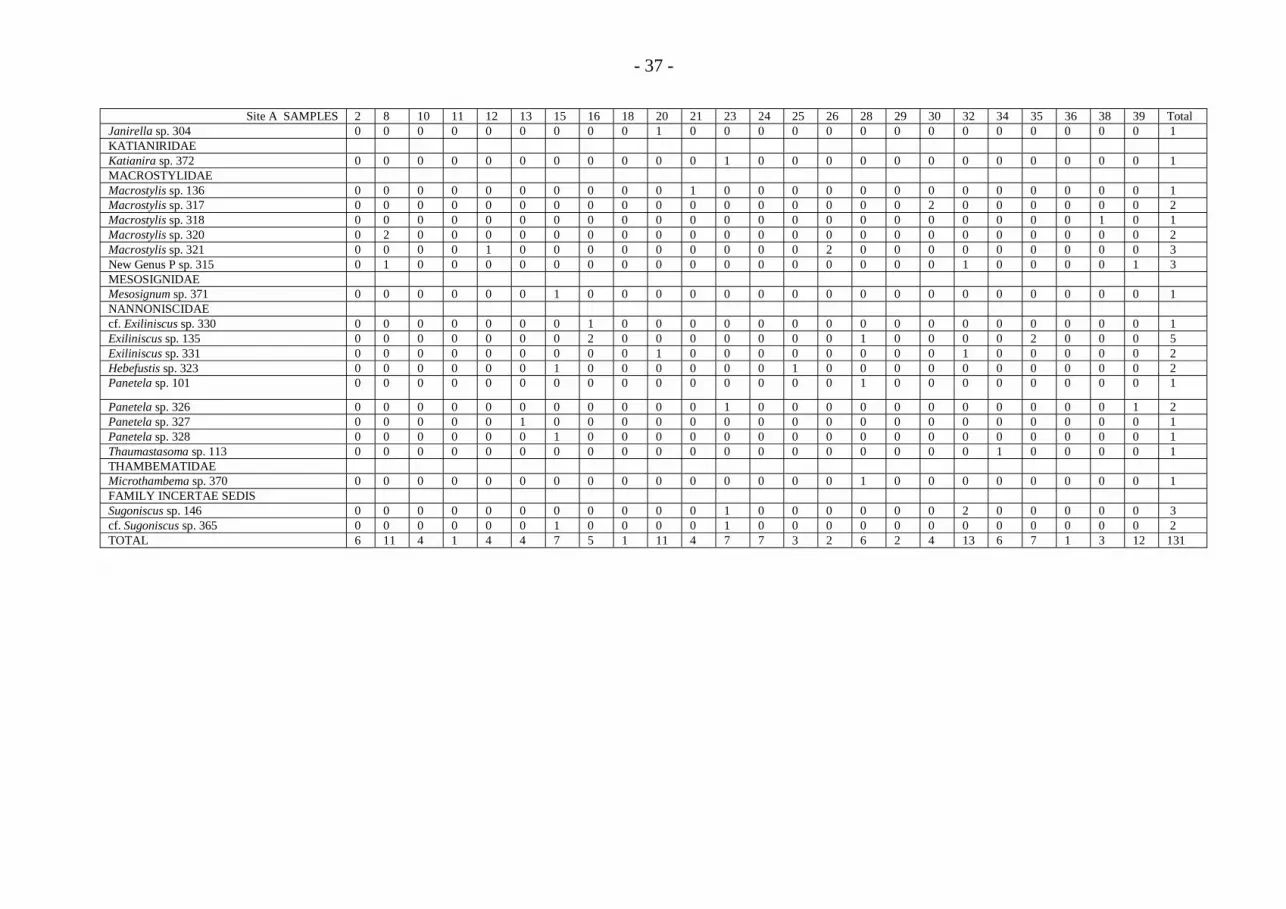
- 37 -

Site A SAMPLES 2 8 10 11 12 13 15 16 18 20 21 23 24 25 26 28 29 30 32 34 35 36 38 39 TotalJanirella sp. 304 0 0 0 0 0 0 0 0 0 1 0 0 0 0 0 0 0 0 0 0 0 0 0 0 1KATIANIRIDAEKatianira sp. 372 0 0 0 0 0 0 0 0 0 0 0 1 0 0 0 0 0 0 0 0 0 0 0 0 1MACROSTYLIDAEMacrostylis sp. 136 0 0 0 0 0 0 0 0 0 0 1 0 0 0 0 0 0 0 0 0 0 0 0 0 1Macrostylis sp. 317 0 0 0 0 0 0 0 0 0 0 0 0 0 0 0 0 0 2 0 0 0 0 0 0 2Macrostylis sp. 318 0 0 0 0 0 0 0 0 0 0 0 0 0 0 0 0 0 0 0 0 0 0 1 0 1Macrostylis sp. 320 0 2 0 0 0 0 0 0 0 0 0 0 0 0 0 0 0 0 0 0 0 0 0 0 2Macrostylis sp. 321 0 0 0 0 1 0 0 0 0 0 0 0 0 0 2 0 0 0 0 0 0 0 0 0 3New Genus P sp. 315 0 1 0 0 0 0 0 0 0 0 0 0 0 0 0 0 0 0 1 0 0 0 0 1 3MESOSIGNIDAEMesosignum sp. 371 0 0 0 0 0 0 1 0 0 0 0 0 0 0 0 0 0 0 0 0 0 0 0 0 1NANNONISCIDAEcf. Exiliniscus sp. 330 0 0 0 0 0 0 0 1 0 0 0 0 0 0 0 0 0 0 0 0 0 0 0 0 1Exiliniscus sp. 135 0 0 0 0 0 0 0 2 0 0 0 0 0 0 0 1 0 0 0 0 2 0 0 0 5Exiliniscus sp. 331 0 0 0 0 0 0 0 0 0 1 0 0 0 0 0 0 0 0 1 0 0 0 0 0 2Hebefustis sp. 323 0 0 0 0 0 0 1 0 0 0 0 0 0 1 0 0 0 0 0 0 0 0 0 0 2Panetela sp. 101 0 0 0 0 0 0 0 0 0 0 0 0 0 0 0 1 0 0 0 0 0 0 0 0 1

Panetela sp. 326 0 0 0 0 0 0 0 0 0 0 0 1 0 0 0 0 0 0 0 0 0 0 0 1 2Panetela sp. 327 0 0 0 0 0 1 0 0 0 0 0 0 0 0 0 0 0 0 0 0 0 0 0 0 1Panetela sp. 328 0 0 0 0 0 0 1 0 0 0 0 0 0 0 0 0 0 0 0 0 0 0 0 0 1Thaumastasoma sp. 113 0 0 0 0 0 0 0 0 0 0 0 0 0 0 0 0 0 0 0 1 0 0 0 0 1THAMBEMATIDAEMicrothambema sp. 370 0 0 0 0 0 0 0 0 0 0 0 0 0 0 0 1 0 0 0 0 0 0 0 0 1FAMILY INCERTAE SEDISSugoniscus sp. 146 0 0 0 0 0 0 0 0 0 0 0 1 0 0 0 0 0 0 2 0 0 0 0 0 3cf. Sugoniscus sp. 365 0 0 0 0 0 0 1 0 0 0 0 1 0 0 0 0 0 0 0 0 0 0 0 0 2TOTAL 6 11 4 1 4 4 7 5 1 11 4 7 7 3 2 6 2 4 13 6 7 1 3 12 131

- 38 -

TABLE 10.

SITE A ISOPODA, 1978 CRUISE.

SITE A SAMPLES 40 41 42 44 46 47 48 49 50 52 54 55 56 58 59 60 62 65 66 69 70 72 73 74 75 77 TotalDENDROTIIDAEDendromunna sp. 369 0 0 0 0 0 0 0 0 0 0 0 0 0 0 0 0 1 0 0 0 0 0 0 0 0 0 1DESMOSOMATIDAEBalbidocolon sp. 339 0 0 0 0 0 0 0 0 0 0 0 0 0 0 0 0 0 0 0 0 1 0 0 0 0 0 1Chelator sp. 333 0 1 0 0 0 1 0 0 0 0 1 0 0 0 0 0 0 0 0 0 0 0 0 0 0 0 3Desmosoma sp. 335 0 0 0 0 0 0 0 0 0 1 0 0 0 0 0 0 0 0 0 0 0 0 0 0 0 0 1Desmosoma sp. 336 0 0 1 0 0 0 0 0 0 0 0 0 0 0 0 0 0 0 0 0 0 0 0 0 0 0 1Eugerda sp. 337 1 0 0 0 0 0 0 0 0 0 0 0 0 0 0 0 0 0 0 0 0 1 0 0 0 0 2Eugerda sp. 338 0 0 0 0 0 0 0 0 0 0 0 0 0 0 0 0 0 0 0 0 1 0 0 0 0 0 1Eugerdella sp. 340 0 0 0 0 0 0 0 0 0 0 0 0 0 0 0 0 0 0 0 7 1 0 0 0 1 0 9Torwolia sp. 341 0 0 0 0 0 0 0 0 0 0 0 0 0 0 0 0 0 0 0 0 1 0 0 0 0 0 1Whoia sp. 104 0 1 0 0 0 0 0 0 0 0 0 0 0 0 0 0 0 0 0 0 0 0 0 0 0 1 2cf. Whoia sp. 115 0 0 0 1 0 0 0 0 0 0 0 0 0 0 0 0 0 0 0 0 0 0 0 0 0 1 2MUNNOPSIDAEEURYCOPINAEcf. Belonectes sp. 357 0 0 0 0 0 0 0 0 0 0 0 0 0 0 0 0 0 0 0 0 0 5 0 0 0 0 5Disconectes sp. 358 0 0 0 0 0 0 0 0 0 0 0 0 0 0 0 0 0 0 0 1 0 0 0 0 1 0 2Eurycope sp. 356 0 0 0 0 0 0 0 0 0 0 0 0 0 0 0 0 0 1 0 0 0 0 0 0 0 0 1MUNNOPSIDAESYNEURYCOPINAESyneurycope sp. 355 0 0 0 0 0 0 0 0 0 0 0 0 1 0 0 0 0 0 0 0 1 1 0 0 0 0 3MUNNOPSIDAESUBFAMILY INCERTAESEDISBetamorpha sp. 352 0 0 0 0 0 0 0 0 0 0 0 0 0 0 0 0 0 0 0 0 0 0 0 0 1 0 1New Genus H sp. 359 0 0 0 0 0 0 0 0 0 0 0 0 0 0 1 0 0 0 0 0 0 0 0 0 0 0 1Indeterminable sp. 364 0 0 0 0 0 0 0 0 0 0 0 0 0 0 0 0 0 1 0 0 1 0 0 0 0 0 2HAPLONISCIDAEAspidoniscus sp. 351 0 0 0 0 0 0 0 0 0 0 0 0 0 0 0 0 0 0 0 0 0 0 1 0 0 0 1Haploniscus sp. 112 1 1 0 1 2 0 0 1 1 0 0 0 1 0 0 0 0 0 0 0 0 0 0 0 0 0 8Haploniscus sp. 342 0 1 0 0 0 0 0 0 2 0 0 0 0 0 0 2 1 0 0 0 0 0 0 0 0 0 6Haploniscus sp. 343 0 0 0 0 0 1 0 0 0 0 0 0 1 0 0 0 0 0 0 0 1 0 0 0 0 0 3Haploniscus sp. 344 1 0 0 0 0 0 0 0 0 0 0 0 0 0 0 0 0 0 0 2 0 0 3 0 0 0 6Haploniscus sp. 345 0 0 0 0 0 0 0 0 0 0 0 0 0 0 0 0 0 0 0 0 2 0 0 0 0 0 2Haploniscus sp. 346 0 0 0 0 0 0 0 0 0 1 0 0 0 1 0 0 1 0 0 1 5 2 0 0 0 3 14Haploniscus sp. 348 0 0 0 0 0 0 0 0 0 1 0 0 0 0 0 0 0 0 0 0 0 0 0 0 0 0 1Haploniscus sp. 349 0 0 0 0 0 0 0 0 0 0 0 0 0 0 0 0 0 0 0 0 0 0 0 0 1 0 1ISCHNOMESIDAEHaplomesus sp. 312 0 0 1 0 0 0 0 0 0 0 0 0 0 0 0 0 0 0 0 0 0 0 0 0 0 0 1Helomesus sp. 314 0 0 0 0 0 1 0 0 0 0 0 0 0 0 0 0 0 0 0 1 1 0 0 0 0 0 3

- 39 -

SITE A SAMPLES 40 41 42 44 46 47 48 49 50 52 54 55 56 58 59 60 62 65 66 69 70 72 73 74 75 77 TotalIschnomesus sp. 119 1 0 0 0 0 0 0 0 0 1 0 0 0 0 1 1 1 0 1 0 3 0 0 0 0 0 9Ischnomesus sp. 305 0 1 0 0 2 1 0 0 1 0 0 0 1 0 0 1 1 3 0 1 0 0 0 0 0 0 12Ischnomesus sp. 306 0 0 0 0 0 0 0 0 1 0 1 0 0 0 0 0 0 0 0 0 0 0 0 0 0 0 2Ischnomesus sp. 307 0 1 1 0 0 0 0 0 0 2 1 1 1 2 2 0 0 0 1 2 2 0 0 0 0 0 16Ischnomesus sp. 308 1 0 0 0 0 0 0 0 0 0 0 0 0 0 0 0 0 0 0 0 0 0 0 0 0 0 1Ischnomesus sp. 309 0 0 0 0 0 0 1 0 0 4 0 0 0 3 0 0 0 0 0 0 0 0 0 0 0 0 8Ischnomesus sp. 310 0 0 0 0 0 0 0 0 0 0 1 0 0 0 0 0 0 0 0 0 0 0 0 0 0 0 1JANIRELLIDAEJanirella sp. 301 0 1 0 0 0 0 0 0 0 0 0 0 0 0 0 0 0 0 0 0 0 0 0 0 0 0 1Janirella sp. 303 1 0 0 0 0 0 0 0 0 0 0 0 0 0 0 0 0 0 0 0 0 0 1 0 0 0 2Janirella sp. 304 0 0 0 0 0 0 0 0 0 0 0 0 0 0 0 0 0 0 0 0 0 0 1 0 0 0 1MACROSTYLIDAEMacrostylis sp. 316 3 0 0 0 0 0 0 0 0 0 0 1 0 0 0 0 0 0 0 0 0 0 0 0 0 1 5Macrostylis sp. 317 0 0 0 0 0 0 0 0 0 0 0 0 0 0 1 0 0 0 0 0 0 0 1 0 0 0 2Macrostylis sp. 318 1 0 0 0 0 0 0 0 0 0 0 0 0 0 0 0 0 0 0 0 0 0 0 0 0 0 1Macrostylis sp. 319 0 0 0 0 0 1 0 0 0 0 0 0 0 0 0 0 0 0 0 0 0 0 0 0 0 0 1Macrostylis sp. 320 0 0 0 0 0 0 0 0 0 2 0 0 0 1 0 0 0 1 0 1 0 0 0 0 0 0 5Macrostylis sp. 321 0 0 0 0 0 0 0 0 0 0 0 0 2 0 0 0 0 0 1 0 0 0 1 0 0 0 4Macrostylis sp. 322 0 0 0 0 0 0 0 0 0 0 0 0 0 0 0 0 0 0 0 1 0 0 0 0 0 0 1New Genus P sp. 315 0 0 0 0 7 0 0 1 0 0 0 0 0 0 0 0 0 0 0 0 0 0 1 0 0 0 9NANNONISCIDAEcf. Exiliniscus sp. 330 0 0 0 0 0 0 0 0 0 0 0 0 0 0 0 0 0 0 0 0 2 0 0 0 0 0 2Exiliniscus sp. 135 0 0 0 0 0 0 1 0 0 0 0 0 0 0 0 0 0 0 0 0 0 0 0 0 0 0 1Exiliniscus sp. 329 0 0 0 0 0 0 0 0 0 0 0 0 0 0 0 0 0 0 0 0 2 0 0 0 0 0 2Hebefustis sp. 323 0 1 0 0 0 0 0 0 0 0 0 0 0 0 0 0 0 0 0 0 0 0 0 0 0 0 1Nannoniscus sp. 107 0 0 0 0 0 0 0 0 0 0 0 0 0 0 0 0 1 0 0 0 0 0 0 0 0 0 1Nannoniscus sp. 324 0 0 0 0 0 0 0 0 0 0 0 0 0 1 0 0 0 0 0 0 0 0 0 0 0 0 1Panetela sp. 101 0 1 0 0 0 0 0 0 0 0 0 0 0 0 1 0 0 0 0 0 0 0 0 0 0 0 2Panetela sp. 325 0 0 0 1 0 0 0 0 0 0 0 0 0 0 0 0 0 0 0 0 1 0 0 0 0 0 2Panetela sp. 326 0 0 0 0 0 0 0 0 0 0 0 0 1 0 1 0 0 0 0 0 0 0 1 0 0 0 3Panetela sp. 327 0 0 0 0 0 0 0 0 0 0 0 0 0 0 0 0 0 0 0 0 0 1 1 0 0 0 2Thaumastasoma sp. 113 0 1 0 0 0 0 0 1 1 0 0 0 0 0 0 0 0 0 0 0 0 0 0 1 0 0 4

Thaumastasoma sp. 151 0 0 1 0 0 0 0 0 0 0 0 0 0 0 0 0 0 0 0 0 0 0 0 0 0 0 1Thaumastasoma sp. 332 1 0 0 0 0 0 0 0 0 0 0 0 0 0 0 0 0 0 0 0 0 0 0 0 0 0 1THAMBEMATIDAEMicrothambema sp. 370 0 0 0 0 0 0 0 0 0 0 0 0 0 0 0 0 0 0 0 0 0 0 0 0 0 1 1FAMILY INCERTAESEDIScf. Sugoniscus sp. 121 0 0 0 0 0 0 0 0 0 0 0 0 0 0 0 0 0 0 0 0 1 0 0 0 0 0 1cf. Sugoniscus sp. 365 0 1 0 0 0 0 0 0 0 0 0 0 0 0 1 1 1 0 0 3 0 1 0 0 0 0 8cf. Sugoniscus sp. 366 0 1 0 0 0 0 0 0 1 0 0 0 0 0 0 0 0 0 0 0 2 0 0 0 0 0 4cf. Sugoniscus sp. 368 0 0 0 0 0 0 0 0 3 0 0 0 0 0 0 0 0 0 0 0 0 0 0 0 0 0 3Sugoniscus sp. 146 0 0 0 0 0 0 0 0 0 0 0 0 0 0 0 0 1 0 0 0 0 0 2 0 0 0 3TOTAL 11 12 4 3 11 5 2 3 10 12 4 2 8 8 8 5 8 6 3 20 28 11 13 1 4 7 209

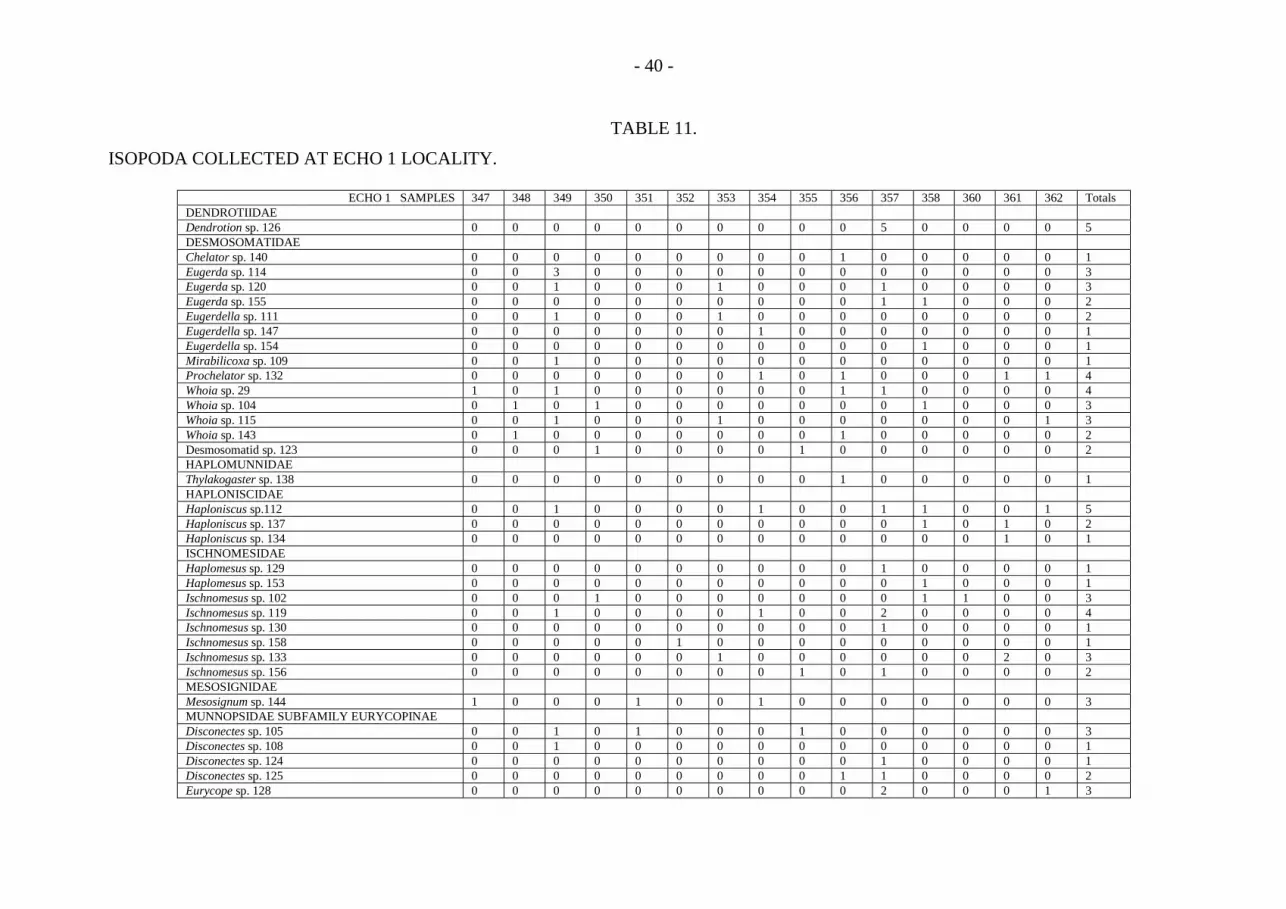
- 40 -

TABLE 11.

ISOPODA COLLECTED AT ECHO 1 LOCALITY.

ECHO 1 SAMPLES 347 348 349 350 351 352 353 354 355 356 357 358 360 361 362 TotalsDENDROTIIDAEDendrotion sp. 126 0 0 0 0 0 0 0 0 0 0 5 0 0 0 0 5DESMOSOMATIDAEChelator sp. 140 0 0 0 0 0 0 0 0 0 1 0 0 0 0 0 1Eugerda sp. 114 0 0 3 0 0 0 0 0 0 0 0 0 0 0 0 3Eugerda sp. 120 0 0 1 0 0 0 1 0 0 0 1 0 0 0 0 3Eugerda sp. 155 0 0 0 0 0 0 0 0 0 0 1 1 0 0 0 2Eugerdella sp. 111 0 0 1 0 0 0 1 0 0 0 0 0 0 0 0 2Eugerdella sp. 147 0 0 0 0 0 0 0 1 0 0 0 0 0 0 0 1Eugerdella sp. 154 0 0 0 0 0 0 0 0 0 0 0 1 0 0 0 1Mirabilicoxa sp. 109 0 0 1 0 0 0 0 0 0 0 0 0 0 0 0 1Prochelator sp. 132 0 0 0 0 0 0 0 1 0 1 0 0 0 1 1 4Whoia sp. 29 1 0 1 0 0 0 0 0 0 1 1 0 0 0 0 4Whoia sp. 104 0 1 0 1 0 0 0 0 0 0 0 1 0 0 0 3Whoia sp. 115 0 0 1 0 0 0 1 0 0 0 0 0 0 0 1 3Whoia sp. 143 0 1 0 0 0 0 0 0 0 1 0 0 0 0 0 2Desmosomatid sp. 123 0 0 0 1 0 0 0 0 1 0 0 0 0 0 0 2HAPLOMUNNIDAEThylakogaster sp. 138 0 0 0 0 0 0 0 0 0 1 0 0 0 0 0 1HAPLONISCIDAEHaploniscus sp.112 0 0 1 0 0 0 0 1 0 0 1 1 0 0 1 5Haploniscus sp. 137 0 0 0 0 0 0 0 0 0 0 0 1 0 1 0 2Haploniscus sp. 134 0 0 0 0 0 0 0 0 0 0 0 0 0 1 0 1ISCHNOMESIDAEHaplomesus sp. 129 0 0 0 0 0 0 0 0 0 0 1 0 0 0 0 1Haplomesus sp. 153 0 0 0 0 0 0 0 0 0 0 0 1 0 0 0 1Ischnomesus sp. 102 0 0 0 1 0 0 0 0 0 0 0 1 1 0 0 3Ischnomesus sp. 119 0 0 1 0 0 0 0 1 0 0 2 0 0 0 0 4Ischnomesus sp. 130 0 0 0 0 0 0 0 0 0 0 1 0 0 0 0 1Ischnomesus sp. 158 0 0 0 0 0 1 0 0 0 0 0 0 0 0 0 1Ischnomesus sp. 133 0 0 0 0 0 0 1 0 0 0 0 0 0 2 0 3Ischnomesus sp. 156 0 0 0 0 0 0 0 0 1 0 1 0 0 0 0 2MESOSIGNIDAEMesosignum sp. 144 1 0 0 0 1 0 0 1 0 0 0 0 0 0 0 3MUNNOPSIDAE SUBFAMILY EURYCOPINAEDisconectes sp. 105 0 0 1 0 1 0 0 0 1 0 0 0 0 0 0 3Disconectes sp. 108 0 0 1 0 0 0 0 0 0 0 0 0 0 0 0 1Disconectes sp. 124 0 0 0 0 0 0 0 0 0 0 1 0 0 0 0 1Disconectes sp. 125 0 0 0 0 0 0 0 0 0 1 1 0 0 0 0 2Eurycope sp. 128 0 0 0 0 0 0 0 0 0 0 2 0 0 0 1 3

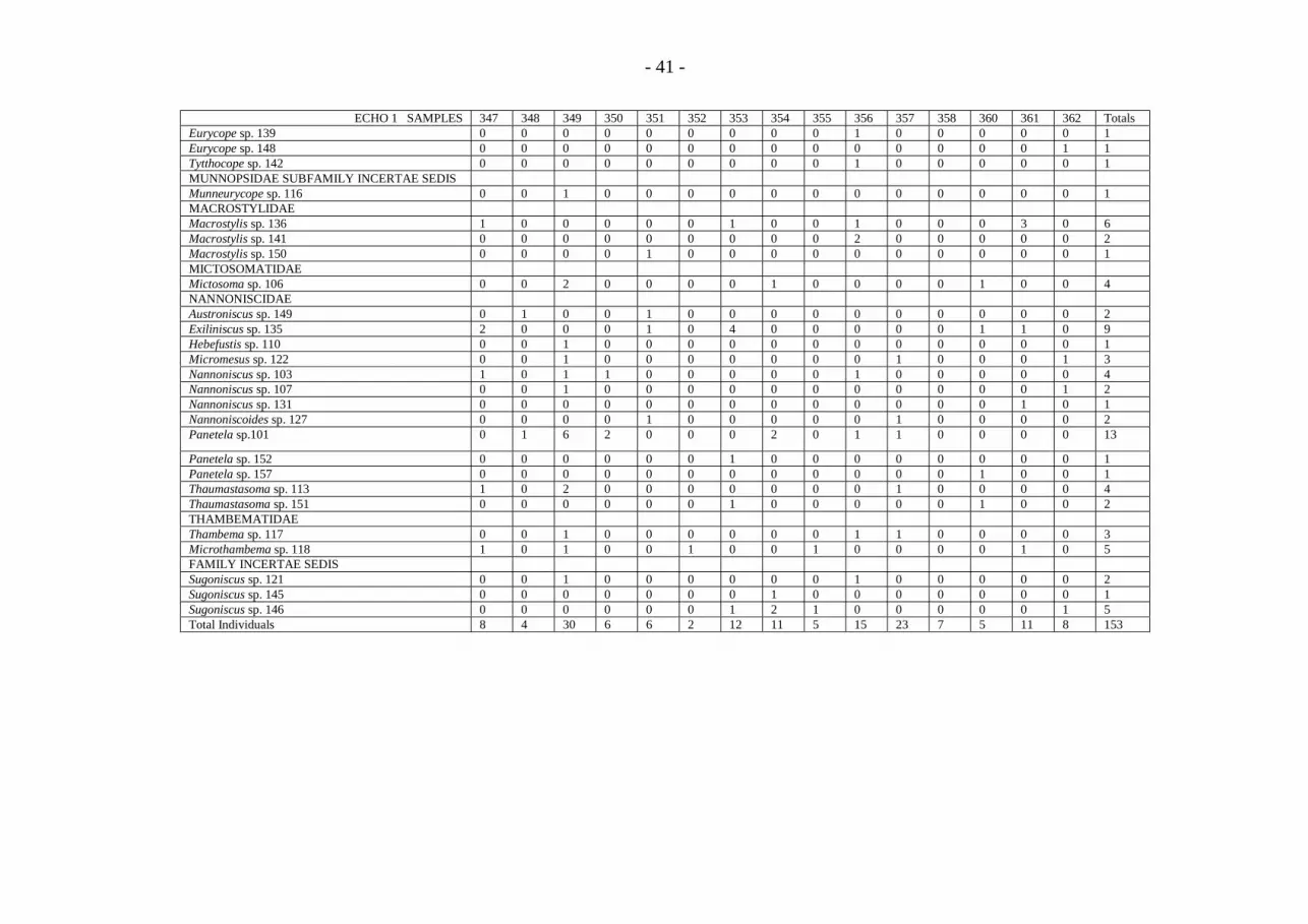
- 41 -

ECHO 1 SAMPLES 347 348 349 350 351 352 353 354 355 356 357 358 360 361 362 TotalsEurycope sp. 139 0 0 0 0 0 0 0 0 0 1 0 0 0 0 0 1Eurycope sp. 148 0 0 0 0 0 0 0 0 0 0 0 0 0 0 1 1Tytthocope sp. 142 0 0 0 0 0 0 0 0 0 1 0 0 0 0 0 1MUNNOPSIDAE SUBFAMILY INCERTAE SEDISMunneurycope sp. 116 0 0 1 0 0 0 0 0 0 0 0 0 0 0 0 1MACROSTYLIDAEMacrostylis sp. 136 1 0 0 0 0 0 1 0 0 1 0 0 0 3 0 6Macrostylis sp. 141 0 0 0 0 0 0 0 0 0 2 0 0 0 0 0 2Macrostylis sp. 150 0 0 0 0 1 0 0 0 0 0 0 0 0 0 0 1MICTOSOMATIDAEMictosoma sp. 106 0 0 2 0 0 0 0 1 0 0 0 0 1 0 0 4NANNONISCIDAEAustroniscus sp. 149 0 1 0 0 1 0 0 0 0 0 0 0 0 0 0 2Exiliniscus sp. 135 2 0 0 0 1 0 4 0 0 0 0 0 1 1 0 9Hebefustis sp. 110 0 0 1 0 0 0 0 0 0 0 0 0 0 0 0 1Micromesus sp. 122 0 0 1 0 0 0 0 0 0 0 1 0 0 0 1 3Nannoniscus sp. 103 1 0 1 1 0 0 0 0 0 1 0 0 0 0 0 4Nannoniscus sp. 107 0 0 1 0 0 0 0 0 0 0 0 0 0 0 1 2Nannoniscus sp. 131 0 0 0 0 0 0 0 0 0 0 0 0 0 1 0 1Nannoniscoides sp. 127 0 0 0 0 1 0 0 0 0 0 1 0 0 0 0 2Panetela sp.101 0 1 6 2 0 0 0 2 0 1 1 0 0 0 0 13

Panetela sp. 152 0 0 0 0 0 0 1 0 0 0 0 0 0 0 0 1Panetela sp. 157 0 0 0 0 0 0 0 0 0 0 0 0 1 0 0 1Thaumastasoma sp. 113 1 0 2 0 0 0 0 0 0 0 1 0 0 0 0 4Thaumastasoma sp. 151 0 0 0 0 0 0 1 0 0 0 0 0 1 0 0 2THAMBEMATIDAEThambema sp. 117 0 0 1 0 0 0 0 0 0 1 1 0 0 0 0 3Microthambema sp. 118 1 0 1 0 0 1 0 0 1 0 0 0 0 1 0 5FAMILY INCERTAE SEDISSugoniscus sp. 121 0 0 1 0 0 0 0 0 0 1 0 0 0 0 0 2Sugoniscus sp. 145 0 0 0 0 0 0 0 1 0 0 0 0 0 0 0 1Sugoniscus sp. 146 0 0 0 0 0 0 1 2 1 0 0 0 0 0 1 5Total Individuals 8 4 30 6 6 2 12 11 5 15 23 7 5 11 8 153

- 42 -

TABLE 12.

DENSITIES OF PERACARID CRUSTACEA FROM NORTH PACIFIC QUANTITATIVESAMPLES. (H&P = data from Hecker and Paul (1979), DOMES sites in the Equatorial NorthPacific; H&J = data from Hessler and Jumars (1974), North Pacific; last two rows in table are fromcurrent study. Densities marked with a “<” are sample series where no individuals were reported;the value in the table is a theoretical maximum derived by assuming a density if 1 individual hadbeen found in the sample area collected by the study.

TAXONLOCALITY

CUMACEA AMPHIPODA TANAIDACEA ISOPODA

N. Pacific (H&J) <0.33 <0.33 23.3 6.3Site A (H&P) <0.18 0.36 21.7 10.2Site B (H&P) 0.78 0.97 15.0 5.8Site C (H&P) 0.31 1.5 28.6 20.6

Site A 0.31 2.3 29.4 26.6

Site C (Echo 1) 1.6 4.5 48.3 40.8

TABLE 13.

TAXOCENE SPECIES SIMILARITIES BETWEEN SITE A AND ECHO 1 POOLED SAMPLES.Comparison of Tanaids and Isopods at different sample sizes. [Note added in 1999: E.D. Gallagher(pers. comm.) has discovered a problem with this version of the NESS algorithm that inflatessimilarities owing to the sparse matrix. The algorithm has been corrected but the comparisonremains valid.]

SAMPLE SIZE TANAIDACEA ISOPODA

1 0.631 0.210

25 0.670 0.243

50 0.670 0.236

76 0.656 0.222

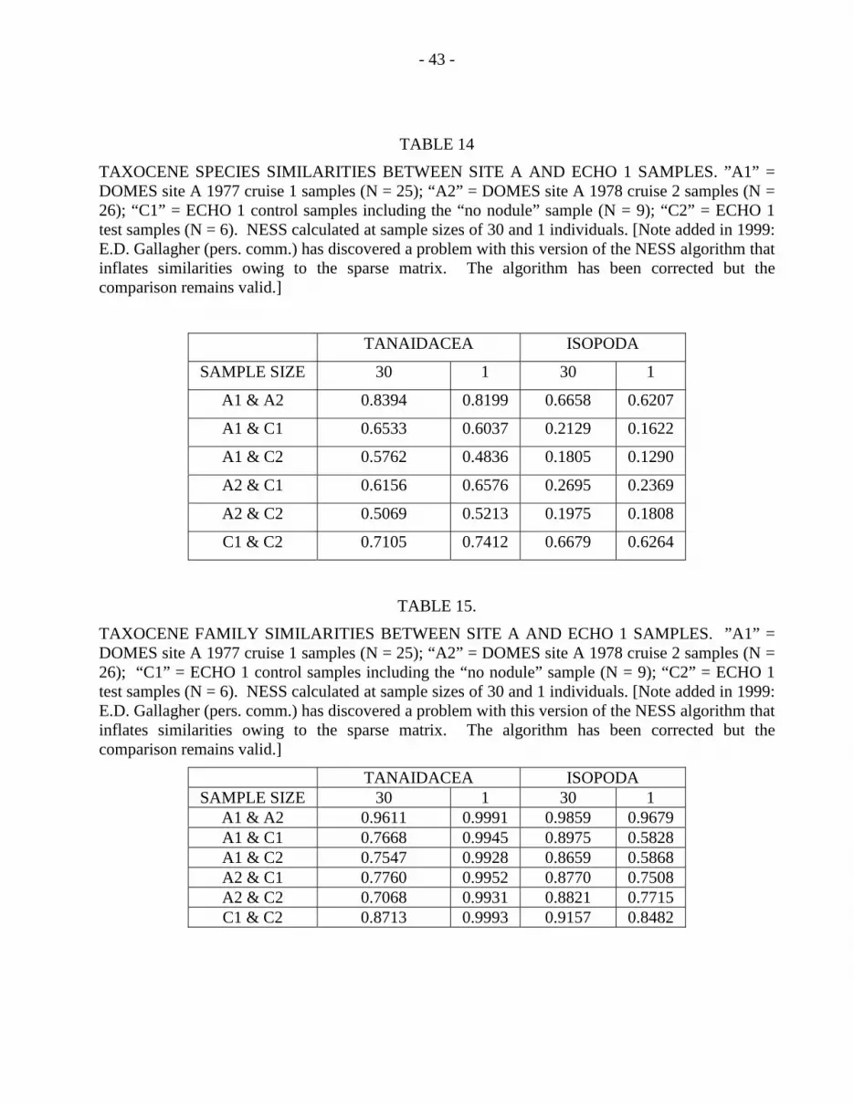
- 43 -

TABLE 14

TAXOCENE SPECIES SIMILARITIES BETWEEN SITE A AND ECHO 1 SAMPLES. ”A1” =DOMES site A 1977 cruise 1 samples (N = 25); “A2” = DOMES site A 1978 cruise 2 samples (N =26); “C1” = ECHO 1 control samples including the “no nodule” sample (N = 9); “C2” = ECHO 1test samples (N = 6). NESS calculated at sample sizes of 30 and 1 individuals. [Note added in 1999:E.D. Gallagher (pers. comm.) has discovered a problem with this version of the NESS algorithm thatinflates similarities owing to the sparse matrix. The algorithm has been corrected but thecomparison remains valid.]

TANAIDACEA ISOPODA

SAMPLE SIZE 30 1 30 1

A1 & A2 0.8394 0.8199 0.6658 0.6207

A1 & C1 0.6533 0.6037 0.2129 0.1622

A1 & C2 0.5762 0.4836 0.1805 0.1290

A2 & C1 0.6156 0.6576 0.2695 0.2369

A2 & C2 0.5069 0.5213 0.1975 0.1808

C1 & C2 0.7105 0.7412 0.6679 0.6264

TABLE 15.

TAXOCENE FAMILY SIMILARITIES BETWEEN SITE A AND ECHO 1 SAMPLES. ”A1” =DOMES site A 1977 cruise 1 samples (N = 25); “A2” = DOMES site A 1978 cruise 2 samples (N =26); “C1” = ECHO 1 control samples including the “no nodule” sample (N = 9); “C2” = ECHO 1test samples (N = 6). NESS calculated at sample sizes of 30 and 1 individuals. [Note added in 1999:E.D. Gallagher (pers. comm.) has discovered a problem with this version of the NESS algorithm thatinflates similarities owing to the sparse matrix. The algorithm has been corrected but thecomparison remains valid.]

TANAIDACEA ISOPODASAMPLE SIZE 30 1 30 1

A1 & A2 0.9611 0.9991 0.9859 0.9679A1 & C1 0.7668 0.9945 0.8975 0.5828A1 & C2 0.7547 0.9928 0.8659 0.5868A2 & C1 0.7760 0.9952 0.8770 0.7508A2 & C2 0.7068 0.9931 0.8821 0.7715C1 & C2 0.8713 0.9993 0.9157 0.8482