sharing, superposition and expansion
TRANSCRIPT
Sharing,Superpositionand Expansion
Geometrical Studies on theSemantics and Implementation
of λ-calculi and Proof-nets
Marco Solieri
Thèse
présentée et soutenue le 30 novembre 2016
pour obtenir le grade de Docteur de l’Université Paris 13, spécialité informatiqueet de Dottore di ricerca in informatica
dirigée et co-encadrée par Stefano Guerrini et Simone Martini, et Michele Pagani
preparée au sein du Laboratoire d’Informatique de Paris Nord
et du Dipartimento di Informatica – Scienza e Ingegneria
Jury (et rapporteurs) :
Laurent Regnier Professeur, Université d’Aix-Marseille Président rapporteur(Patrick Baillot Chercheur, ENS Lyon Rapporteur)Simone Martini Professeur, Université Paris 13 DirecteurMichele Pagani Professeur, Université Paris 7 Co-encadrantSimone Martini Professore, Università di Bologna Co-directeur
Ian Mackie Chercheur, École Polytechnique ExaminateurDamiano Mazza Chercheur, Université Paris 13 Examinateur
© Marco SolieriLIPN, Université Paris 13, Sorbonne Paris Cité, CNRSDISI, Università di Bologna, INRIAUniversité Franco-italiennemailto:[email protected]
http:///ms.xt3.it
Licensed under Creative Commons BY-NC-SA 4.0 Internationalcbna
Version 1.2Last updated on Friday 28th October, 2016 at 02:22
Typeset by the author, using LATEX, PGF/TikZ, Kile, TeXstudio and many other pieces of free software
Abstract
Elegant semantics and efficient im-plementations of functional program-ming languages can both be de-scribed by the very same math-ematical structures, most promin-ently within the Curry-Howard cor-respondence, where programs, typesand execution respectively coincidewith proofs, formulæ and normalisa-tion. Such a flexibility is sharpened bythe deconstructive and geometrical ap-proach pioneered by linear logic (LL)and proof-nets, and by Lévy-optimalreduction and sharing graphs (SG).
Adapting Girard’s geometry of in-teraction, this thesis introduces thegeometry of resource interaction(GoRI), a dynamic and denotationalsemantics, which describes, algebra-ically by their paths, terms of theresource calculus (RC), a linear andnon-deterministic variation of theordinary lambda calculus. Infiniteseries of RC-terms are also the domainof the Taylor-Ehrhard-Regnier expan-sion, a linearisation of LC. The thesisexplains the relation between theformer and the reduction by provingthat they commute, and provides anexpanded version of the executionformula to compute paths for thetyped LC.
SG are an abstract implementationof LC and proof-nets whose stepsare local and asynchronous, and shar-ing involves both terms and contexts.Whilst experimental tests on SG showoutstanding speedups, up to exponen-tial, with respect to traditional imple-mentations, sharing comes at price.The thesis proves that, in the re-stricted case of elementary proof-nets,where only the core of SG is needed,such a price is at most quadratic, henceharmless.
Résumé
Des sémantiques élégantes et des im-plémentations efficaces des langages deprogrammation fonctionnels peuventêtre décrits par les mêmes structuresmathématiques, notamment dans lacorrespondance Curry-Howard, où leprogrammes, les types et l’exécution,coïncident aux preuves, formules etnormalisation. Une telle flexibilitéest aiguisé par l’approche deconstruc-tif et géométrique de la logique lin-eaire (LL) et les réseaux de preuve, etde la réduction optimale et les graphesde partage (SG).
En adaptent la géométrie de l’interac-tion de Girard, cette thèse proposeune géométrie de l’interaction des res-sources (GoRI), une sémantique dy-namique et dénotationelle, qui décritalgébriquement par leur chemins,les termes du calcul des ressources(RC), une variation linéaire et non-déterministe du lambda calcul (LC).Les séries infinis dans RC sont aussile domaine du développement deTaylor-Ehrhard-Regnier, une linéarisa-tion du LC. La thèse explique la re-lation entre ce dernier et la réduc-tion démontrant qu’ils commutent, etprésente une version développé de laformule d’exécution pour calculer leschemins du LC typé.
Les SG sont un modèle d’implémen-tation du LC, dont les pas sont localeset asynchrones, et le partage impliqueet les termes et les contextes. Bienque les tests ont montré des accéléra-tions exceptionnelles, jusqu à expo-nentielles, par rapport aux implément-ations traditionnelles, les SG n’ont pasque des avantages. La thèse montreque, dans le cas restreint des reseauxélémentaires, où seule le cœur des SGest requis, les désavantages sont auplus quadratique, donc inoffensifs.
Sommario
Semantiche eleganti ed implemen-tazioni efficienti di linguaggi di pro-grammazione funzionale possono en-trambe essere descritte dalle stessestrutture matematiche, più notevol-mente nella corrispondenza Curry-Howard, dove i programmi, i tipi el’esecuzione coincidono, nell’ordine,con le dimostrazioni, le formule e lanormalizzazione. Tale flsesibilità èacuita dall’approccio decostruttivo egeometrico della logica lineare (LL)e le reti di dimostrazione, e dellariduzione ottimale e i grafi di condi-visione (SG).
Adattando la geometria dell’intera-zione di Girard, questa tesi introducela geometria dell’interazione dellerisorse (GoRI), una semantica din-amica e denotazionale che descrive,algebricamente tramite i loro per-corsi, i termini del calcolo dellerisorse (RC), una variante linearee non-deterministica del lambda cal-colo ordinario. Le serie infinitedi termini del RC sono inoltre ildominio dell’espansione di Taylor-Ehrhard-Regnier, una linearizzazionedel LC. La tesi spiega la relazionetra quest’ultima e la riduzione di-mostrando che esse commutano, efornisce una versione espansa della for-mula di esecuzione per calcolare i per-corsi del LC tipato.
I SG sono un modello d’implemen-tazione del LC, i cui passi sono loc-ali e asincroni, e la cui condivi-sione riguarda sia termini che contesti.Sebbene le prove sperimentali suiSG mostrino accellerazioni eccezion-ali, persino esponenziali, rispetto alleimplementazioni tradizionali, la con-divisione ha un costo. La tesi di-mostra che, nel caso ristretto delle retielementari, dove è necessario solo ilcuore dei SG, tale costo è al più quad-ratico, e quindi innocuo.

iv
Contents
1 Introduction 1
1.1 Proof nets . . . . . . . . . . . . . . . . . . . . . . . . . . . . . . . . . . . . . . 1
1.2 Geometry of Interaction . . . . . . . . . . . . . . . . . . . . . . . . . . . . . . 2
1.3 Taylor-Ehrhard-Regnier expansion and resource calculus . . . . . . . . . . . 3
1.4 Light logics . . . . . . . . . . . . . . . . . . . . . . . . . . . . . . . . . . . . . 3
1.5 Sharing graphs . . . . . . . . . . . . . . . . . . . . . . . . . . . . . . . . . . . 4
1.6 Lévy-optimal reduction . . . . . . . . . . . . . . . . . . . . . . . . . . . . . . 5
1.7 Summary of contributions . . . . . . . . . . . . . . . . . . . . . . . . . . . . 7
1.7.1 Superposition and expansion (Part I) . . . . . . . . . . . . . . . . . . 7
1.7.2 Sharing and efficiency (Part II) . . . . . . . . . . . . . . . . . . . . . . 9
2 Lambda-calculus, linear logic and geometry of interaction 11
2.1 Introduction . . . . . . . . . . . . . . . . . . . . . . . . . . . . . . . . . . . . . 12
2.2 Nets and terms . . . . . . . . . . . . . . . . . . . . . . . . . . . . . . . . . . . 12
2.2.1 Pre-nets . . . . . . . . . . . . . . . . . . . . . . . . . . . . . . . . . . . 12
2.2.2 Proof-nets and paths . . . . . . . . . . . . . . . . . . . . . . . . . . . 14
2.2.3 Lambda terms and nets . . . . . . . . . . . . . . . . . . . . . . . . . . 15
2.3 Proof-net reductions . . . . . . . . . . . . . . . . . . . . . . . . . . . . . . . . 16
2.3.1 General notions . . . . . . . . . . . . . . . . . . . . . . . . . . . . . . 16
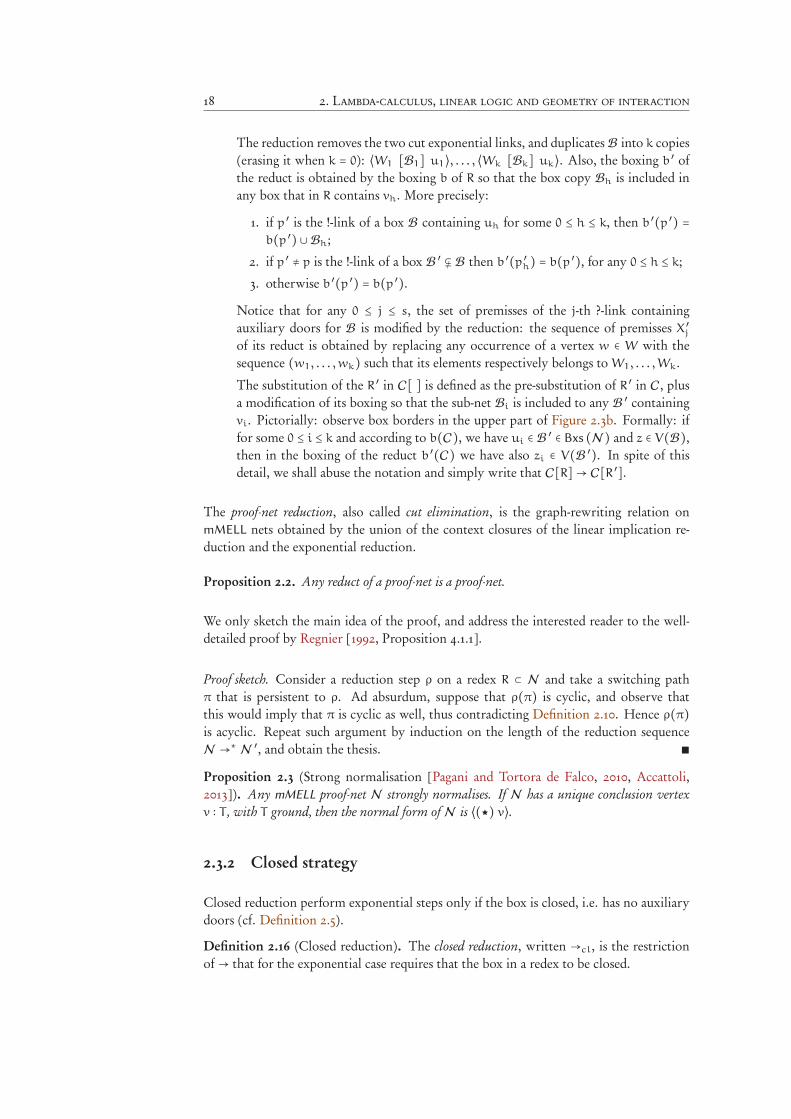
2.3.2 Closed strategy . . . . . . . . . . . . . . . . . . . . . . . . . . . . . . . 18
2.4 Execution paths . . . . . . . . . . . . . . . . . . . . . . . . . . . . . . . . . . . 20
vi CONTENTS
2.4.1 Statics . . . . . . . . . . . . . . . . . . . . . . . . . . . . . . . . . . . . 21
2.4.2 Dynamics . . . . . . . . . . . . . . . . . . . . . . . . . . . . . . . . . . 21
2.4.3 Closed dynamics . . . . . . . . . . . . . . . . . . . . . . . . . . . . . . 23
2.5 Computation as path execution . . . . . . . . . . . . . . . . . . . . . . . . . . 25
2.5.1 Dynamic algebra . . . . . . . . . . . . . . . . . . . . . . . . . . . . . . 25
2.5.2 Equivalence of execution and reduction . . . . . . . . . . . . . . . . 27
I Superposition and expansion 31
3 Geometry of Resource Interaction 33
3.1 Introduction . . . . . . . . . . . . . . . . . . . . . . . . . . . . . . . . . . . . . 34
3.2 Resource calculus . . . . . . . . . . . . . . . . . . . . . . . . . . . . . . . . . . 34
3.2.1 Syntax . . . . . . . . . . . . . . . . . . . . . . . . . . . . . . . . . . . . 35
3.2.2 Reduction . . . . . . . . . . . . . . . . . . . . . . . . . . . . . . . . . 35
3.3 Resource interaction nets . . . . . . . . . . . . . . . . . . . . . . . . . . . . . 36
3.3.1 Definition . . . . . . . . . . . . . . . . . . . . . . . . . . . . . . . . . 37
3.3.2 Term translation . . . . . . . . . . . . . . . . . . . . . . . . . . . . . . 38
3.3.3 Reduction . . . . . . . . . . . . . . . . . . . . . . . . . . . . . . . . . 39
3.4 Resource paths . . . . . . . . . . . . . . . . . . . . . . . . . . . . . . . . . . . 45
3.4.1 Statics . . . . . . . . . . . . . . . . . . . . . . . . . . . . . . . . . . . . 45
3.4.2 Dynamics . . . . . . . . . . . . . . . . . . . . . . . . . . . . . . . . . . 46
3.4.3 Comprehensiveness and bijection . . . . . . . . . . . . . . . . . . . . 48
3.4.4 Confluence and persistence . . . . . . . . . . . . . . . . . . . . . . . . 51
3.5 Resource execution . . . . . . . . . . . . . . . . . . . . . . . . . . . . . . . . . 54
3.5.1 Dynamic algebra and execution . . . . . . . . . . . . . . . . . . . . . 54
3.5.2 Invariance and regularity . . . . . . . . . . . . . . . . . . . . . . . . . 57
3.6 Discussion . . . . . . . . . . . . . . . . . . . . . . . . . . . . . . . . . . . . . . 60
3.6.1 Related works . . . . . . . . . . . . . . . . . . . . . . . . . . . . . . . 60
CONTENTS vii
3.6.2 Open questions . . . . . . . . . . . . . . . . . . . . . . . . . . . . . . 61
3.6.2.1 Higher expressivity . . . . . . . . . . . . . . . . . . . . . . 61
3.6.2.2 Geometry of differential interaction . . . . . . . . . . . . . 61
4 Taylor-Ehrhard-Regnier Expansion and Geometry of Interaction 63
4.1 Introduction . . . . . . . . . . . . . . . . . . . . . . . . . . . . . . . . . . . . . 64
4.1.1 Expansion and paths computation . . . . . . . . . . . . . . . . . . . 64
4.1.2 Outline . . . . . . . . . . . . . . . . . . . . . . . . . . . . . . . . . . . 65
4.2 Taylor-Ehrhard-Regnier expansion . . . . . . . . . . . . . . . . . . . . . . . . 65
4.2.1 Net expansion . . . . . . . . . . . . . . . . . . . . . . . . . . . . . . . 65
4.2.2 Term expansion and translation . . . . . . . . . . . . . . . . . . . . . 67
4.2.3 Path expansion . . . . . . . . . . . . . . . . . . . . . . . . . . . . . . . 71
4.3 Expansion and reduction . . . . . . . . . . . . . . . . . . . . . . . . . . . . . 75
4.4 Commutativity of reduction and expansion . . . . . . . . . . . . . . . . . . . 76
4.4.1 Commutativity on nets . . . . . . . . . . . . . . . . . . . . . . . . . . 76
4.4.2 Commutativity on paths . . . . . . . . . . . . . . . . . . . . . . . . . 80
4.5 Expansion and execution . . . . . . . . . . . . . . . . . . . . . . . . . . . . . 87
4.6 Discussion . . . . . . . . . . . . . . . . . . . . . . . . . . . . . . . . . . . . . . 89
4.6.1 Related works . . . . . . . . . . . . . . . . . . . . . . . . . . . . . . . 89
4.6.2 Open questions . . . . . . . . . . . . . . . . . . . . . . . . . . . . . . 89
4.6.2.1 Infinite paths . . . . . . . . . . . . . . . . . . . . . . . . . . 89
4.6.2.2 Resource abstract machine for the lambda-calculus . . . . 90
4.6.2.3 Combinatorics of path expansion . . . . . . . . . . . . . . 90
II Sharing and efficiency 91
5 Sharing implementation of bounded logics 93
5.1 Introduction . . . . . . . . . . . . . . . . . . . . . . . . . . . . . . . . . . . . . 94
viii CONTENTS
5.2 Elementary and light proof-nets . . . . . . . . . . . . . . . . . . . . . . . . . 95
5.3 Sharing implementation . . . . . . . . . . . . . . . . . . . . . . . . . . . . . . 98
5.3.1 Definition . . . . . . . . . . . . . . . . . . . . . . . . . . . . . . . . . 98
5.3.2 Rewriting properties . . . . . . . . . . . . . . . . . . . . . . . . . . . 99
5.4 Adequacy properties . . . . . . . . . . . . . . . . . . . . . . . . . . . . . . . . 102
5.4.1 Correctness . . . . . . . . . . . . . . . . . . . . . . . . . . . . . . . . . 102
5.4.2 Weak completeness . . . . . . . . . . . . . . . . . . . . . . . . . . . . 102
5.4.3 Optimality . . . . . . . . . . . . . . . . . . . . . . . . . . . . . . . . . 103
5.5 Correctness by syntactical simulation . . . . . . . . . . . . . . . . . . . . . . 104
5.5.1 Unshared graphs . . . . . . . . . . . . . . . . . . . . . . . . . . . . . . 104
5.5.2 From sharing graphs to unshared graphs . . . . . . . . . . . . . . . . 105
5.5.3 From unshared graphs to proof-nets . . . . . . . . . . . . . . . . . . 106
5.5.4 From sharing graphs to proof-nets . . . . . . . . . . . . . . . . . . . 107
6 Efficiency of sharing implementation 109
6.1 Introduction . . . . . . . . . . . . . . . . . . . . . . . . . . . . . . . . . . . . . 110
6.2 Cost measures . . . . . . . . . . . . . . . . . . . . . . . . . . . . . . . . . . . . 112
6.3 Input/output paths . . . . . . . . . . . . . . . . . . . . . . . . . . . . . . . . . 113
6.3.1 Statics . . . . . . . . . . . . . . . . . . . . . . . . . . . . . . . . . . . . 114
6.3.2 Dynamics . . . . . . . . . . . . . . . . . . . . . . . . . . . . . . . . . . 115
6.4 Sharing contexts . . . . . . . . . . . . . . . . . . . . . . . . . . . . . . . . . . 117
6.4.1 Variable occurrences and sharing contexts . . . . . . . . . . . . . . . 117
6.4.2 Positivity . . . . . . . . . . . . . . . . . . . . . . . . . . . . . . . . . . 120
6.4.3 Path irrelevance . . . . . . . . . . . . . . . . . . . . . . . . . . . . . . 132
6.5 Unshared cost of reductions . . . . . . . . . . . . . . . . . . . . . . . . . . . . 133
6.5.1 Share . . . . . . . . . . . . . . . . . . . . . . . . . . . . . . . . . . . . 133
6.5.2 Unshared cost of mIELL reduction . . . . . . . . . . . . . . . . . . . 134
6.5.3 Unshared cost of SG reduction . . . . . . . . . . . . . . . . . . . . . 142
CONTENTS ix
6.6 Unshared cost comparison . . . . . . . . . . . . . . . . . . . . . . . . . . . . 146
6.7 Discussion . . . . . . . . . . . . . . . . . . . . . . . . . . . . . . . . . . . . . . 149
6.7.1 Related works . . . . . . . . . . . . . . . . . . . . . . . . . . . . . . . 149
6.7.2 Open questions . . . . . . . . . . . . . . . . . . . . . . . . . . . . . . 150
Index 151

x CONTENTS
Chapter 1
Introduction
Computer science is one of the few where elegance and efficacy, which elsewhere arefrequently and variously opposed, can both be pursued exploiting their complementarit-ies. Programming language theory is a notable example. Both foundational and practicalquestions, for instance about semantics and implementations, can be phrased, exploredand sometimes answered employing the very same frameworks. A prominent one is theCurry-Howard correspondence with proof theory, since there models of functional pro-grams, types and execution essentially coincide with those of proofs, formulæ and norm-alisation.
A modest example is given by the contributions presented in this thesis, and the literaturewhich it is based upon, ranging from the denotational semantics of a non-deterministicvariation of the λ-calculus, to the efficiency of a distributed model of computation for theordinary one. Such conceptually distant results have all been understood and expressedwithin a narrow set of mathematical tools inspired by linear logic.
1.1 Proof nets
Linear logic [Girard, 1987] unveiled the relation between the algebraic concept of linear-ity and the computational property of a function argument to be used exactly once. Itsformulæ are syntactically discriminated depending on their usage in a proof, as if theyare resources whose access is not gratis. Linear formulæ must be used exactly once in theproof, whilst the others, marked by the exponential modality, can instead arbitrarily beduplicated or erased. Thanks to this separation, the λ-calculus is allowed to have a subtlertype system, where operations of duplication and erasure are detached from β-reduction.
Proof-nets are one of the key tools introduced by linear logic. They are a graphical rep-resentation of proofs in which each rule corresponds to a graph constructor named linkconnecting the main premises of the rule to its main conclusion. Such a graphical ap-proach allows to naturally equate proofs that, because of the rigidity of the traditionalsequent calculus, differ for bureaucratic details only. In the intuitionistic case, a proof-net
2 1. Introduction
is in fact a decorated graph representation of the corresponding λ-term (with explicit sub-stitutions, to be precise [Di Cosmo, Kesner, and Polonovski, 2000, Accattoli, 2013]) thatadds exponential boxes: delimited sub-graphs that can be erased or duplicated only as awhole. Another remarkable trait of proof-nets is that they allow the definition of the sys-tem not only with an inductive formalisation given by axioms and logical rules, but alsowith a geometrical condition on graphs that are freely built by assembling links together:acyclicity of some kind paths, called switching.
1.2 Geometry of Interaction
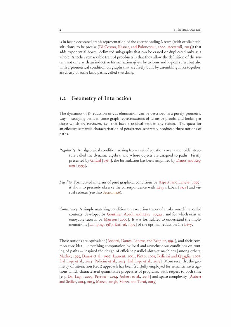
The dynamics of β-reduction or cut elimination can be described in a purely geometricway — studying paths in some graph representations of terms or proofs, and looking atthose which are persistent, i.e. that have a residual path in any reduct. The quest foran effective semantic characterisation of persistence separately produced three notions ofpaths.
Regularity An algebraical condition arising from a set of equations over a monoidal struc-ture called the dynamic algebra, and whose objects are assigned to paths. Firstlypresented by Girard [1989], the formulation has been simplified by Danos and Reg-nier [1995].
Legality Formulated in terms of pure graphical conditions by Asperti and Laneve [1995],it allow to precisely observe the correspondence with Lévy’s labels [1978] and vir-tual redexes (see also Section 1.6).
Consistency A simple matching condition on execution traces of a token-machine, calledcontexts, developed by Gonthier, Abadi, and Lévy [1992a], and for which exist anenjoyable tutorial by Mairson [2002]. It was formulated to understand the imple-mentations [Lamping, 1989, Kathail, 1990] of the optimal reduction à la Lévy.
These notions are equivalent [Asperti, Danos, Laneve, and Regnier, 1994], and their com-mon core idea — describing computation by local and asynchronous conditions on rout-ing of paths — inspired the design of efficient parallel abstract machines [among others,Mackie, 1995, Danos et al., 1997, Laurent, 2001, Pinto, 2001, Pedicini and Quaglia, 2007,Dal Lago et al., 2014, Pedicini et al., 2014, Dal Lago et al., 2015]. More recently, the geo-metry of interaction (GoI) approach has been fruitfully employed for semantic investiga-tions which characterised quantitative properties of programs, with respect to both time[e.g. Dal Lago, 2009, Perrinel, 2014, Aubert et al., 2016] and space complexity [Aubertand Seiller, 2014, 2015, Mazza, 2015b, Mazza and Terui, 2015].
1.3. Taylor-Ehrhard-Regnier expansion and resource calculus 3
1.3 Taylor-Ehrhard-Regnier expansion and resource calcu-
lus
The previously mentioned decomposition of the intuitionistic implication enabled a differ-ential constructor and linear combinations to extend: the λ-calculus into the differentialλ-calculus, discovered by Ehrhard and Regnier [2003]; and, more generally, linear logicinto the differential linear logic (DiLL) [Ehrhard and Regnier, 2006a, Tranquilli, 2011].These constructions allow considering the Taylor expansion of a term [Ehrhard and Reg-nier, 2008], which rewrites it as an infinite series of terms of the resource λ-calculus (RC).It is a completely linear restriction of the differential λ-calculus, similar to the λ-calculuswith multiplicities [Boudol, 1993], where the argument of an application is a superposi-tion of terms and must be linearly used. Taylor-Ehrhard-Regnier expansion contains anyfinite approximation of the head-normalisation of a term, as evoked by its commutativitywith Böhm trees: the expansion of the Böhm tree of a term is equal to the normal formof its expansion [Ehrhard and Regnier, 2006b].
The approximation of λ-calculus has been studied through linear logic’s sub-structural lensalso using affine calculi, those where duplication is forbidden, but erasure is allowed, [e.g.Mazza, 2015a], and also using legal paths to guide the very process of linearisation [Alvesand Florido, 2005]. Moreover, Taylor-Ehrhard-Regnier expansion originated various in-vestigations on quantitative semantics, using the concept of power series for describingprogram evaluation, and has been applied in various non-standard models of computation[see Danos and Ehrhard, 2011, Pagani, Selinger, and Valiron, 2014, for example].
1.4 Light logics
Intuitionistic Light Affine Logic (ILAL) is a variant of Girard’s Light Linear Logic (LLL)[1995] introduced by Asperti and Roversi [2002]. The key property of light logics is thatthey characterise the class of deterministic polynomial time functions: in these logics,the length of cut-elimination is related to the size of the proof by a polynomial func-tion, whose degree depends on the exponential depth of the proof, i.e., on the maximumnumber of nested exponential boxes in the corresponding proof net.
In light logics, the control of computational complexity is obtained by restricting the useof the !-exponential. In particular, the usual promotion rule of linear logic is replaced bya functorial version that simultaneously introduces the !-modality on all the formulæ ofthe sequent, with the proviso that the l.h.s. of the sequent contain at most one formula—relaxing this proviso we get elementary complexity instead. In order to code all the poly-nomial algorithms, light logics requires the introduction of another exponential modality§ named paragraph. For this second modality, contraction is not allowed, and its intro-duction rule is functorial—similarly to the case of the !-promotion, it adds a modality infront of every formula in the sequent—but, differing from the case of the !-promotion,there is no restriction on the size of the l.h.s. of the sequent and, on this side, the addedmodality can be either a § or an !. In details, here it is the promotion rules for ! and §:
4 1. Introduction
With some provisos due to the presence of second order quantifiers [Dal Lago and Baillot,2006], the exponential depth of a cut-free ILAL proof of a formula B = Ak ⊸ . . .A1 ⊸ A0
depends on the nesting depth of the exponential modalities in B. As a consequence, byensuring that a function f can be encoded by a proof of B and that its k arguments canbe suitably encoded (i.e., preserving a polynomial relation between the sizes of the inputdata and of the corresponding proofs) by a proof of type A1, . . . ,Ak, we can concludethat f can be computed in polynomial time. On the other hand, ILAL is complete, sinceevery polynomial time function can be represented into it [Asperti and Roversi, 2002],i.e., encoded by a suitable ILAL proof. Summing up, a function f is polynomial time if andonly if it can be represented in ILAL.
IEAL is an elementary time variant of ILAL. In fact, by simply removing the constraint ofa unique formula on the left-hand side of the !-promotion rule, the time complexity ofthe system passes from polynomial to elementary (i.e., bounded by a Kalmar elementaryfunction). In IEAL there is no need of the §-modality. Moreover, since every ILAL proofcan be transformed into an IEAL proof by replacing every § with an !, we see that ILAL isindeed a subsystem of IEAL.
1.5 Sharing graphs
Sharing graphs are a graph rewriting system introduced by Lamping [1989] [but also in-dependently by Kathail, 1990] in order to implement Lévy’s optimal reductions for λ-calculus β-reduction [1978, 1980]. Lamping’s technique was successively cleaned and re-formulated by Gonthier, Abadi, and Lévy [1992a], who also showed its relations with Gir-ard’s geometry of interaction [1989] and pointed out that, indeed, sharing graphs imple-ment a local and distributed algorithm for linear logic box duplication Gonthier, Abadi,and Lévy [1992b] [see Asperti and Guerrini, 1998, for a comprehensive presentation ofsharing graphs and optimal reductions]).
Sharing graphs for optimal reduction can be also seen as a variant of interaction nets [La-font, 1990], in which the interacting agents (the links) are indexed by a natural number.The key property of interaction nets is that they are strongly confluent. In fact, an inter-action net is formed by agents with a given number of ports, and edges connecting pairsof ports in distinct agents, such that each port has a unique incident edge. Each agent hasa unique principal port through which it can interact with another agent only if the edgeis connected to the principal port of the other agent too. Each redex formed by a pair ofconnected principal ports can be rewritten in a unique way. Summing up, the redexes ofan interaction net are disjoint and can be rewritten in a unique way; as a consequence, thecorresponding rewriting system is strongly confluent.
Among the sharing graphs rules that allow to implement β-reduction, only one, the βs-rule, actually corresponds to reducing one or several shared β-redexes; the other rulescorrespond instead to bookkeeping operations allowing to manage sharing and to explicitthe connection between links corresponding to β-redexes eventually hidden by sharingnodes. Optimal sharing graphs implement Lévy’s optimal reduction, in the sense that theoptimal sharing reduction of a term t corresponds to a Lévy family reduction of t whose
1.6. Lévy-optimal reduction 5
length is equal to the number of βs-rules in the sharing reduction.
1.6 Lévy-optimal reduction
The aim of Lévy-optimal theory [1978] was to define a notion of optimal cost for thereduction of a β-term. By reasoning on the notion of feasible sharing achievable in aneffective implementation of β-reduction, Lévy defined a notion of family of redexes col-lecting all the redexes that can be shared by some efficient implementation — since insome sense they can be seen as coming from a same origin — and he showed that thereexists a parallel reduction strategy reducing a whole family of redexes at each step. Ac-cording to this, the length of a family reduction reducing a needed redex at each step (aredex is needed when one of its residual must be reduced by, or is definitely present after,any reduction sequence of the initial term) gives a lower bound to the complexity of anyreduction of a term. Therefore, by giving an implementation of Lévy optimal reductionwith a cost at least polynomially related to the length of the number of Lévy families, onewould show that Lévy families are a good measure of the cost of the reduction of a λ-term.
Unfortunately, Asperti and Mairson [2001] proved that this is not case, by showing thatthe cost of the bookkeeping reduction in the sharing graph reduction of a term maybecome Kalmar-elementary bigger than the number of βs-rules in any normalizing reduc-tion, i.e. the cost of reducing such terms is not polynomially related to the number offamilies in the term. This result is sometimes misunderstood as a negative one about theefficiency of implementations with sharing graphs, even though it does not say anythingabout it. In fact, it is achieved by showing that the cost of the reduction of the λ-termsin a given family is at least Kalmar-elementar in their size. Nevertheless, such terms havea polynomial number of families. Thus the mismatch between the effective cost of thereduction and the Lévy optimal cost.
We stress that the above results does not address any negative consideration on sharingimplementations. They state that the number of bookkeeping operations in an optimalsharing reduction can be much bigger than the number of βs-rules, not bound by anyKalmar elementary function in the worst cases. But this is a consequence of the intrinsichardness of the language — the simply types λ-calculus — in which the cost of the reduc-tion cannot be bound by any Kalmar-elementary function [Statman, 1979]. Therefore, noother β-reduction implementation can do better than such a bound neither.
Empirical evidences from real implementations, for limited they can be, showed on theother hand very promising performances. For instance, benchmarks of the Bolognahigher order optimal machine [Asperti, Giovannetti, and Naletto, 1996] on pure λ-termsrecorded polynomial cost of reduction against an exponential one of traditional imple-mentations of functional languages. This does not scale to ‘real world’ functional pro-grams, for which performances were measured in the same order of magnitude. At themoment of writing, another optimal implementation, the King’s College lambda evalu-ator [Mackie, 2004] is considered the most efficient implementations of the λ-calculus.
The question of effective efficiency of sharing reduction is then still open, and the case oflight and elementary logics is particularly significant. In fact, in the general case, one can
6 1. Introduction
distinguish two kinds of bookkeeping rules: the duplication rules that propagate shar-ing links, and the rules for the control links, the so-called brackets, ensuring the properpropagation of sharing links. The duplication rules correspond to a step by step imple-mentation of the duplication of the arguments of β-rules— after the execution of a βs
rule, the argument of the rule is not duplicated, but a sharing node is inserted. The shar-ing node will then duplicate link by link the argument when and if necessary. Accordingto the downward orientation from the node corresponding to the root of a term to thenodes corresponding to variables, the scope of a duplication link ends at the variables ofthe duplicating term. However, in sharing reductions, duplication does not proceed down-wards only — from the root of a term towards its leafs, which correspond to its variables— but in some cases (when duplicating a λ-abstraction), a duplication link propagatingupwards is inserted. Such a link is like a closed bracket matching a corresponding duplic-ation link propagating downwards and delimit the bottom of its scope. In other words,matching links are associated to the same duplication process and they delimit the part ofthe graph that is left to duplicate.
Unfortunately, in the general case, matching links do not properly nest as a sequence ofmatching brackets, since in some cases a duplication link propagating downwards may facea duplication link propagating upwards that do not matches with it. When two matchinglinks faces, their scope is empty — they correspond to an opening bracket immediatelyfollowed by a closing one, so they have nothing to duplicate — and they can be erased;otherwise, the two links must swap continuing propagating (see the mux rules in Fig-ure 5.6a).
A direct implementation of sharing reduction requires then a sort of oracle allowing todecide when two facing sharing links are matching [see examples in Asperti and Guerrini,1998, introduction]. Lamping [1989] showed that such an oracle can be implemented bylabelling each link with an index and by introducing some new control nodes, namedbrackets, with a suitable set of rewriting rules managing link indexes. Lamping indexingensures that two facing sharing links are matching if and only if they have the same index.Variants of Lamping’s algorithm have been proposed in the literature, but in any case wehave some links and rules implementing duplication, and some additional links and rulesimplementing the oracle. The only exception are implementations of light/elementarylogics, where link indexes do not change along the reduction, which implies that theoracle is not needed.
Asperti, Coppola, and Martini [2004] extended the result by Asperti and Mairson [2001]to the particular case of elementary logic, proving that in this case also we can have termswith a polynomial number of Lévy’s families, and therefore a polynomial number of shar-ing β-reductions, which require a non-elementary duplication cost — since, again, theirreduction cannot be bound by any Kalmar-elementary function. Their analysis adds thenan argument in favor to sharing graph implementations. In fact, Baillot, Coppola, andDal Lago [2011] proved that the sharing implementation of elementary logic do not doworst then the tight lower-bound already known. Moreover they prove the above resultfor light logic too. In fact, the basic property of light and elementary logics is that thecost of the reduction of any proof is bound by a polynomial in the size of the proof, forthe light case, and by an elementary function, for the elementary case. Baillot, Coppolaand Dal Lago show that the cost of the sharing reduction of a light or elementary proof
1.7. Summary of contributions 7
can be bound by a polynomial and elementary function, respectively. Which allow to gettwo conclusions at the same time: first of all, another proof of the fact that light and ele-mentary logics are sound with respect to the expected computational bound; second, thatsharing implementation introduce an overhead with respect to the usual implementationof reduction that is limited by the same computational bound.
1.7 Summary of contributions
We will present results that can be ascribed to two lines of investigations, both rooted inthe related in their essence to the dynamics of linear logic’s contraction, and both basedon a geometrical viewpoint. The first, within the area of semantics, explore the structureof superposition of resource calculus and that of Taylor expansion. The second, in thetheory of implementation, tackle the question of efficiency of sharing graphs.
1.7.1 Superposition and expansion (Part I)
How can geometry of interaction and Taylor-Ehrhard-Regnier expansion interact? Whatis the GoI for resource calculus? How are paths dynamics related before and after theexpansion? Can we expand β-reduction into an infinite parallel step of resource reduc-tions? Is there a linear and non-deterministic GoI for the resource calculus? Can we useit to characterise persistent paths in λ-terms, via expansion? The first part of the thesisaddresses these questions and recounts the interplay between the two aforementioned se-mantic approaches, exploring both directions of their mutual influence.
In Chapter 2 we recall the needed preliminary notions about proof-nets for minimalMELL: the translation of λ-terms (Section 2.2), and the cut-elimination, together with checlosed reduction reduction strategy (Section 2.3). Also, we introduce a concise reworkedversion of the geometry of interaction for such framework. We will introduce the appro-priate notion of paths and inspect its dynamics, formalising the property of persistence,which intuitively is the ability to survive to the graph rewriting until the normal form(Section 2.4). On top of this, we articulate the algebraic structure of weights, traditionallynamed “the dynamic algebra” (Section 2.5). Such algebra features a structural part whichmodels path operations like concatenation and reversal, and a logical part which insteadrepresent the interaction between paths, that lies under the reduction of containing proof-nets. The main intuition behind it is that the algebra’s equations check for persistence ofa path by either: simplifying, and sometimes even neutralising, weights of sub-paths thatcan be deformed, or shortened by reduction; or annihilating the weights of those that canbe destroyed by the latter. We will show that the execution of a proof-net, i.e. the set ofweights assigned to all its paths, is invariant under reduction (Theorem 2.1). This impliesthat regularity is equivalent to persistence (Corollary 2.1).
In Chapter 3 we introduce resource interaction nets (RINs) and construct their geometryof interaction. RINs are a promotion-free fragment of minimal differential logic, or alinear-logic-like typing system and graphical formalism for RC. We first give an introduc-tion to RC (Section 3.2) and then, following the linear logic tradition, we present RINs
8 1. Introduction
(Section 3.3) by mean of a correctness criterion, and we also show that the inductive defin-ition by translation/typing of resource terms is equivalent, once it is closed by reduction.
We then adapt some of the previously introduced notions about paths to deal with thefact that the reduct of a term t is a sum of terms t1 + . . . + tn (Section 3.4). Also, weobserve that every path in the net-representation of ti has to be a residual of some pathin the net of t, and that the reduction strongly normalises. Thus, we say that a path oft is persistent whenever it has a residual in at least one of the addends of the reduct of(the net of) t. Restricting to the constant type, whose only inhabitant is the value ⋆, wehave t→ ⋆ + . . . + ⋆. Now there is only one persistent path of ⋆, the trivial one, thereforewe prove that persistent paths of t are as many as persistent paths of its normal form(Theorem 3.1).
Furthermore, we define a suitable GoI for RC, in order to characterise persistence (Sec-tion 3.5). We define the notion of regularity by rL∗, a monoidal structure simplifyingthe dynamic algebra, where exponential modalities (! and ?) become an n-ary variant ofthe multiplicatives connectives (resp. ⊗ and `), whose premises are not ordered. Mor-ally, they are the sum of those generalised multiplicatives we obtain by considering allthe n! permutations of their premises. We weigh paths with objects of rL∗, and thenconsider the sum of the weights of all paths in a RIN. What we obtain is the executionformula for resource nets, which is shown to be invariant under reduction (Theorem 3.5).Therefore, the construction provides a denotational semantics for RC and of the corres-ponding logic, that is a minimal, propositional and promotion-free fragment of DiLL.From invariance theorem not only we subsume the equivalence of persistence and reg-ularity (Theorem 3.4), that is the usual result of GoI constructions, but we also showthat the number of addends in a normal form is equal to the number of regular paths(Corollary 3.1).
In Chapter 4 we introduce a qualitative variant of Taylor-Ehrhard-Regnier expansion (Sec-tion 4.2), which maps a proof-net, or a path within it, in an infinite sum of simple RINs, orof set of paths within them. Since there the superposing sum is idempotent, the expansionis essentially the infinite set. Also, we define a notion of expanded cut-elimination (Sec-tion 4.3), a kind of infinite parallel reduction for RINs which reduces together all redexesthat are copied by the expansion. This allow us to prove (Section 4.4) the commutativitybetween reduction and Taylor-expansion both at the level of nets (Theorem 4.1) and paths(Theorem 4.3). Thank to this, we discover that the property of being persistent can betransferred along expansion: a path persists to mMELL reduction if and only if there is apath in its expansion which persists to RIN reduction (Theorem 4.4).
This last fact turns out to be particularly interesting, since it enable the definition (Sec-tion 4.5) of a variant of the execution formula for typed λ-calculus that is based on theGoRI. The idea is that, if we assign to every path π in a proof-net the infinite sets of rL∗-weights that belong to the expansions of π, we obtain an expanded formula enjoying theproperties of our interest: invariance (Theorem 4.5), hence characterisation of persistence(Corollary 4.1).
1.7. Summary of contributions 9
1.7.2 Sharing and efficiency (Part II)
Can we tighten the complexity overhead of sharing graph implementation of light andelementary linear logics under the currently known upper bounds (polynomial and ele-mentary)? Is it possible to do so by a direct syntactical simulation of sharing graphs inproof-nets? Can such approach unveil which components of the sharing graph machineryare the most efficient, and which other the most problematic?
Chapter 5 is devoted to present the sharing implementation of the elementary and lightvariants of mMELL, recalling its main properties and proving its correctness by syntacticalsimulations. In Section 5.2we present the proof-nets ofmIELL, that represent a frameworkof particular convenience because it considerably simplifies the rewriting system, whilstin Section 5.3 we introduce their sharing implementation — the system SG— and its basicproperties. A brief review of the most notable qualitative behavioural properties of SG asa Lévy-optimal implementation of mIELL proof-nets is given in Section 5.4. Among these,there is the correctness: any SG-normal-form of amIELL proof-net N is themIELL-normal-form of N . A proof is given in the concluding Section 5.5 (cf. Theorem 5.10), wherewe employ a simple syntactical simulation of SG in mIELL, exploiting an intermediaterewriting system— the unshared graphs (UG) — that possess the structure ofmIELL proof-nets and a some sharing markers corresponding to SG graphs.
In Chapter 6 we illustrate an original analysis of the complexity of SG reductions withrespect tomIELL reduction, showing that the former cannot be outperformed by the latter,up to a quadratic factor. The two reduction systems present a substantial behaviouraldifference in the way that they perform the duplication — small or big step — that isclarified when we firstly need to assign a cost for them (Section 6.2). With the intent toexploit the syntactical simulation between the system, we define on unshared graphs thenotion of sharing contexts (Section 6.4) that essentially tells, for every vertex and link ina graph, the exact set of lifts (or their copies) that eventually will come there along anyreduction.
This tool allow to formulate the two key quantitative correspondences. On the one hand,we can determine the set of sub-graphs of an unshared graph where a lift propagation willhappen, the share, that morally represent the non-local portion of a big step duplication’swork (Subsection 6.5.1). On the other hand, among a set of lifts that are the unfolding of ak-ary mux m, we can precisely select those that are on the boundary of the share and showthat their number correspond indeed to k. These two facts allow indeed to precisely trans-fer (Section 6.5) and compare (Section 6.6) the costs of mIELL and SG reductions in UG
reductions. We show that the cost of logical operations and duplications essentially matchbetween the two systems — the overhead is bounded by a linear function of the mIELL-cost. The same computational bound is obtained, this time indirectly, for annihilations,merges and most swap rules. We are able to limit some special kind of redundant swaps,instead, only by the product of the depth level of the graph and the square of the mIELL
cost. Hence, we will prove that the overhead of an SGRB-reduction, i.e. including theread-back rules, with respect to its mIELL simulation is at most quadratic (Theorem 6.1).

10 1. Introduction
Chapter 2
Lambda-calculus, linear logic and
geometry of interaction
Contents
2.1. Introduction 12
2.2. Nets and terms 12
2.2.1 Pre-nets 12
2.2.2 Proof-nets and paths 14
2.2.3 Lambda terms and nets 15
2.3. Proof-net reductions 16
2.3.1 General notions 16
2.3.2 Closed strategy 18
2.4. Execution paths 20
2.4.1 Statics 21
2.4.2 Dynamics 21
2.4.3 Closed dynamics 23
2.5. Computation as path execution 25
2.5.1 Dynamic algebra 25
12 2. Lambda-calculus, linear logic and geometry of interaction
2.5.2 Equivalence of execution and reduction 27
2.1 Introduction
Even since the seminal paper by Girard [1989] it was clear that the elegance of the geo-metry of interaction (GoI) construction reaches its maximum only in some limited cases,where it represents a true denotational semantics, guaranteeing invariance with respect toreduction. This chapter is devoted to recall preliminary notions of a convenient settingfor proof-nets and their translation of λ-terms, and to gently introduce the notion thatare needed to present an invariant GoI. In order to do so, we present a minimal fragmentof MELL and focus our attention on programs with ground types. There we exploit theconvenience of closed reduction, that eliminates an exponential cut only if the box has noauxiliary doors (see Fernández, Mackie, and Sinot [2005] for a recent operational discus-sion of various closed strategies, also includes complexity comparisions), and we are ableto formalise a strikingly simple, though detailed, proof of invariance
2.2 Nets and terms
We introduce the multiplicative exponential fragment of linear logic (MELL) restricting itto the minimal version, with propositional and polarised formulæ/types. We shall call itmMELL for short.
We use the terse formulation once dubbed nouvelle syntaxe and introduced by Regnier[1992], where all negative links/rules of the exponential fragment, that are dereliction,weakening and binary contraction, are represented with a unique object having an arbit-rary number of premisses. With respect to the seminal presentation by Girard [1987] andthe advances with respect to polarisation by Laurent [2002], this approach introduces anotable amount of conciseness and usability — from the syntax for terms/proofs to thedynamics of their computation/cut-elimination — not to mention its fruitful similaritiesto explicit substitution calculi [Di Cosmo et al., 2000, Accattoli, 2013, for instance].
2.2.1 Pre-nets
Definition 2.1 (Links). Given a denumerable set of symbols called vertices, a link is abiparted and typed hyperedge, i.e. a triple (P,K,C), where:
P is a sequence of vertices, called premisses;
K is an element a finite set of kinds;
C is a singleton of a vertex, called conclusion, disjoint from P.
2.2. Nets and terms 13
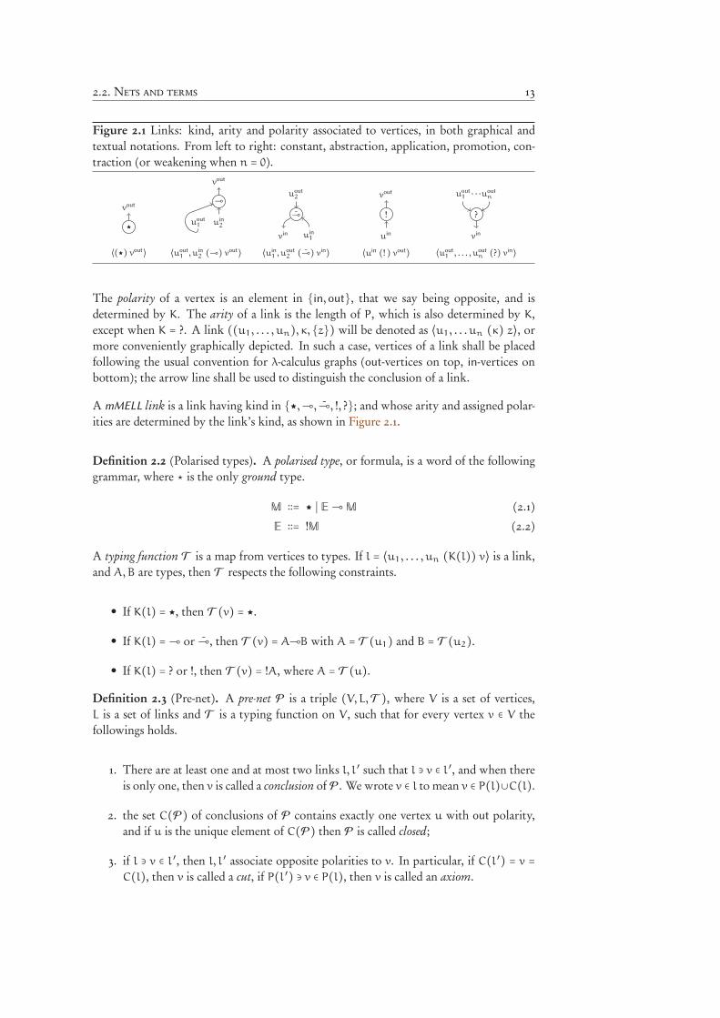
Figure 2.1 Links: kind, arity and polarity associated to vertices, in both graphical andtextual notations. From left to right: constant, abstraction, application, promotion, con-traction (or weakening when n = 0).
★
vout
⟨(★) vout⟩
⊸
vout
uin
2uout
1
⟨uout
1, u
in
2(⊸) vout⟩
⊸
uout
2
uin
1vin
⟨uin
1, u
out
2(⊸) vin⟩
!
vout
uin
⟨uin (! ) vout⟩
?
uout
1uout
n
vin
. . .
⟨uout
1, . . . , u
out
n(?) vin⟩
The polarity of a vertex is an element in {in,out}, that we say being opposite, and isdetermined by K. The arity of a link is the length of P, which is also determined by K,except when K = ?. A link ((u1, . . . , un), κ,{z}) will be denoted as ⟨u1, . . . un (κ) z⟩, ormore conveniently graphically depicted. In such a case, vertices of a link shall be placedfollowing the usual convention for λ-calculus graphs (out-vertices on top, in-vertices onbottom); the arrow line shall be used to distinguish the conclusion of a link.
A mMELL link is a link having kind in {★,⊸, ⊸, !, ?}; and whose arity and assigned polar-ities are determined by the link’s kind, as shown in Figure 2.1.
Definition 2.2 (Polarised types). A polarised type, or formula, is a word of the followinggrammar, where ⋆ is the only ground type.
M ∶∶= ★ ∣ E⊸M (2.1)
E ∶∶= !M (2.2)
A typing function T is a map from vertices to types. If l = ⟨u1, . . . , un (K(l)) v⟩ is a link,and A,B are types, then T respects the following constraints.
• If K(l) = ★, then T (v) = ★.• If K(l) =⊸ or ⊸, then T (v) = A⊸B with A = T (u1) and B = T (u2).• If K(l) = ? or !, then T (v) = !A, where A = T (u).
Definition 2.3 (Pre-net). A pre-net P is a triple (V, L,T ), where V is a set of vertices,L is a set of links and T is a typing function on V , such that for every vertex v ∈ V thefollowings holds.
1. There are at least one and at most two links l, l ′ such that l ∋ v ∈ l ′, and when thereis only one, then v is called a conclusion of P. We wrote v ∈ l to mean v ∈ P(l)∪C(l).
2. the set C(P) of conclusions of P contains exactly one vertex u with out polarity,and if u is the unique element of C(P) then P is called closed;
3. if l ∋ v ∈ l ′, then l, l ′ associate opposite polarities to v. In particular, if C(l ′) = v =
C(l), then v is called a cut, if P(l ′) ∋ v ∈ P(l), then v is called an axiom.
14 2. Lambda-calculus, linear logic and geometry of interaction
We shall also write V(P) and L(P) to denote the first and second component of P,respectively. The type of a pre-net P is the type T = T (v), where v ∈ C(P) of outpolarity, written P ∶ T .
The interior of P is the complement of C(P)with respect to V(P). The interface of a pre-net P is the set, for all v ∈ C(P), of the triple (v,T (v),p(v)) where the last is the polarityof v. Two pre-nets P,Q are equal when there exists a type-preserving isomorphism ≃ suchthat P ≃ Q. Given a pre-net P = (V, L,T ), a sub-pre-net P ′ of P is a pre-net (V ′, L ′,T )such that V ′ ⊆ V(P), L ′ ⊆ L(P ′), and T ′ is the restriction of T to V ′.
2.2.2 Proof-nets and paths
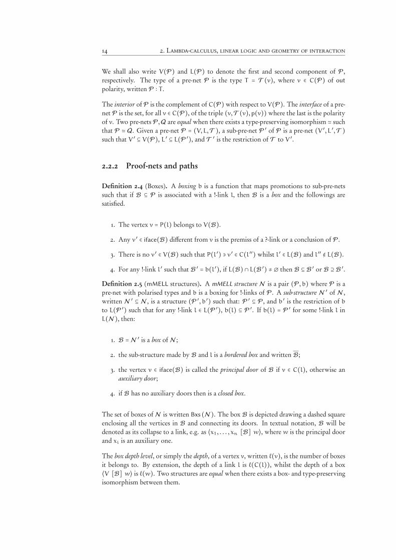
Definition 2.4 (Boxes). A boxing b is a function that maps promotions to sub-pre-netssuch that if B ⊆ P is associated with a !-link l, then B is a box and the followings aresatisfied.
1. The vertex v = P(l) belongs to V(B).2. Any v ′ ∈ iface(B) different from v is the premiss of a ?-link or a conclusion of P.
3. There is no v ′ ∈ V(B) such that P(l ′) ∋ v ′ ∈ C(l ′′) whilst l ′ ∈ L(B) and l ′′ ∉ L(B).4. For any !-link l ′ such that B ′ = b(l ′), if L(B) ∩ L(B ′) ≠ ∅ then B ⊆ B ′ or B ⊇ B ′.
Definition 2.5 (mMELL structures). A mMELL structure N is a pair (P, b) where P is apre-net with polarised types and b is a boxing for !-links of P. A sub-structure N ′ of N ,written N ′ ⊆ N , is a structure (P ′, b ′) such that: P ′ ⊆ P, and b ′ is the restriction of b
to L(P ′) such that for any !-link l ∈ L(P ′), b(l) ⊆ P ′. If b(l) = P ′ for some !-link l inL(N ), then:
1. B =N ′ is a box of N ;
2. the sub-structure made by B and l is a bordered box and written B;
3. the vertex v ∈ iface(B) is called the principal door of B if v ∈ C(l), otherwise anauxiliary door;
4. if B has no auxiliary doors then is a closed box.
The set of boxes of N is written Bxs (N ). The box B is depicted drawing a dashed squareenclosing all the vertices in B and connecting its doors. In textual notation, B will bedenoted as its collapse to a link, e.g. as ⟨x1, . . . , xn [B] w⟩, where w is the principal doorand xi is an auxiliary one.
The box depth level, or simply the depth, of a vertex v, written ℓ(v), is the number of boxesit belongs to. By extension, the depth of a link l is ℓ(C(l)), whilst the depth of a box⟨V [B] w⟩ is ℓ(w). Two structures are equal when there exists a box- and type-preservingisomorphism between them.
2.2. Nets and terms 15
In the rest of the chapter, we will mainly deal with the low-level notion of pre-net, so forthe sake of simplicity we will sometimes abuse the notation and talk about a structure (ora proof-net) where we mean to refer to its pre-net; and we shall as well omit the pedantryabout typing and boxing, for instance simply saying “the box of” or “the type of”, insteadof “the box assigned by the boxing to” or “the type associated by the typing to”.
Definition 2.6 (Paths). Given a pre-net P, two vertices u,w ∈ P are connected, if there isa link l ∈ P s.t. u,w ∈ l. A path π = (v1, . . . , vn) with n ≥ 0 in P is a sequence of verticess.t. for all i < n, the vertices vi, vi+1 are connected. We call π empty if its length is 0, trivialif its length is 1, atomic if it is 2, and remark that in the latter case π crosses exactly onelink. We shall write u ∼ v when there is a path from u to v.
Definition 2.7 (Basic path operators). Given π = (v1, . . . , vn) and φ = (u1, . . . , um) inP(N ), we denote the reversal of π by π† = (vn, . . . , v1). If vn = u1 then the concatenationof φ to π is defined as π ∶∶ π ′ = (v1, . . . , vn = u1, . . . um). If π ∈ P(N ) and φ ∈ P(M), wesay π = φ when N =M and, if ≃ is the isomorphism such that N ≃M, then vi ≃ ui, forany 1 ≤ i ≤ n =m.
Definition 2.8 (Straight paths). Let N be a proof-net and π a paths in N . If π crossesconsecutively the same link l, then π is called bouncing. If l is not a ⋆-link, and π crossesl through vi, vi+1 such that vi, vi+1 ∈ C(l) or vi, vi+1 ∈ P(l), then π is twisting. Whenπ is not bouncing nor twisting, π is straight. Given u, v ∈ V(P), we say u is consequentto v, written u ≼ v, if there is a straight path π from u to v such that all of its links arecrossed from a premiss to a conclusion. In such a case, we say π is a concluding path. Weconversely also say v is antecedent to u, written as v ≽ u or that π† is assuming.
Definition 2.9 (Switching and cyclic paths [Danos and Regnier, 1989]). A path π in apre-net P is switching when, for every link in L(P) being ⟨v, v ′ (⊸) u⟩, or ⟨V (?) u⟩ withv, v ′ ∈ V , π does not contain both v, v ′. A path γ = (v0, v1, . . . , vn, v0) for n > 0 is called acycle, and any π ⊇ γ is called cyclic.
Definition 2.10 (mMELL proof-nets). Given a net N , let L(N ) be the net obtained byinterpreting each box as a single link, i.e. such that we can traverse it with a unitarypath. Then, N is a mMELL proof-net if any switching path in L(N ) or in L(B), for anyB ∈ Bxs (N ), is acyclic.
2.2.3 Lambda terms and nets
Definition 2.11 (λ-terms). Let V be the grammar of a denumerable set of variable symbolsx, y, z, . . ., and let ⋆ be a constant dummy value. Then, the set Λ of terms is generated bythe following grammar.
T ∶∶= ⋆ ∣ V ∣ λV .T ∣ (T T ) (2.3)
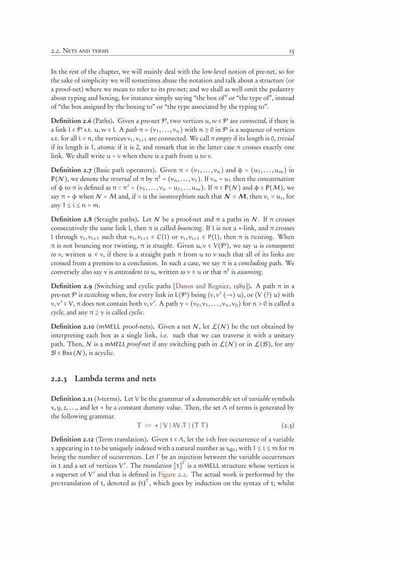
Definition 2.12 (Term translation). Given t ∈ Λ, let the i-th free occurrence of a variablex appearing in t to be uniquely indexed with a natural number as x@i, with 1 ≤ i ≤m for mbeing the number of occurrences. Let Γ be an injection between the variable occurrencesin t and a set of vertices V ′. The translation ⟦t⟧Γ is a mMELL structure whose vertices isa superset of V ′ and that is defined in Figure 2.2. The actual work is performed by thepre-translation of t, denoted as &t'Γ , which goes by induction on the syntax of t; whilst
16 2. Lambda-calculus, linear logic and geometry of interaction
Figure 2.2 Pre-translation & ' and translation ⟦ ⟧ of λ-terms into mMELL nets
!λx.t"Γ= !t"
Γ
⊸
v
?
u2
u1
w1 . . .wn
!t s"Γ=
⊸
!t"Γ
z1 . . . zm
!
!s"Γ
y1 . . . yn
v
u w
y
!⋆"Γ=
★
v ⟦t⟧Γ=
!t"Γ
w
? ?
v1 vl
. . . . . .
. . .
u11u1j ul1
ulk
!x@i"Γ= Γ(x@i)
the final step only adds a ?-link linking all occurrences of a given free variable x, for allfree variables of t. More precisely, the (pre-)translation is such that two vertices v, u arepremisses of the same ?-link if and only if Γ−1(v) = Γ−1(u). Since the choice of Γ produceno change in the translation, we shall omit to specify it.
Proposition 2.1. Any translation is a mMELL proof-net.
Proof. See the detailed work by Regnier [1992, Proposition 3.2.1]. ∎
Definition 2.13 (Variables). The free variables of a proof-net N is the set FVar(N ) of in-vertices of iface(N ), whilst BVar(N ) is the set of vertices which are connected to the firstpremiss of a⊸-link in L(N ), and which are called bounded variables. The set of variablesis then FBVar(N ) = BVar(N ) ∪ FVar(N ).
2.3 Proof-net reductions
Here we introduce the ordinary proof-net reduction recalling its most notable properties,and the closed variant, which acts on a box only if has no secondary doors, proving thatin our setting such restriction causes no loss of generality.
2.3.1 General notions
Notation 2.1 (Rewriting). We fix some quite usual notational conventions and termino-logy we shall employ for rewriting notions. Given a rewriting relation → on a set A, thesymbols →+ and →∗ respectively denote the transitive and the transitive-reflexive closuresof→. Given a,a ′ ∈ A, if a→ a ′ (resp. a→∗ a ′ ) we say that there is a rewriting step (resp.sequence) from the reducendum a to the reduct a ′. Also, if a sequence is made of k steps,
2.3. Proof-net reductions 17
we write→k. We write a /→ and say that a is a normal form, when there exists no a ′ suchthat a → a ′. If a →∗ a ′ /→, then we say that a ′ is a normal form of a; if a ′ is unique1wealso write NF(a) = a ′. Reduction steps are named with Greek letters ρ, σ, τ, . . ., and se-quences with barred letters, so that we can denote the reduct of a with respect to a step ρ
(resp. a sequence ρ) as ρ(a) (resp. ρ(a)).Definition 2.14 (Context and pre-substitution). A hole-link is a link with arbitrary arity,polarity and types. A single-hole pre-context C[ ], or simply a pre-context, is a pre-netwhose links contains exactly one hole-link h, and whose internal interface is the interfaceof h.
A mMELL context is a single-hole pre-context made of mMELL links and equipped with atyping T and a boxing b. Given a mMELL context C[ ] and a mMELL pre-net P whoseinterface is identical to the internal interface of C[ ], the pre-substitution of the pre-net inthe context, written C[P], is the pre-net obtained as follows.
1. Replace the hole link in C[ ] with P.
2. Given a bijection↔ between vertices of the internal interface of C and those of theinterface of P; for any v ∈ C and any v ′ ∈ P, if v↔ v ′, then in C[P] the two verticesare equated, and we write v≡v ′.
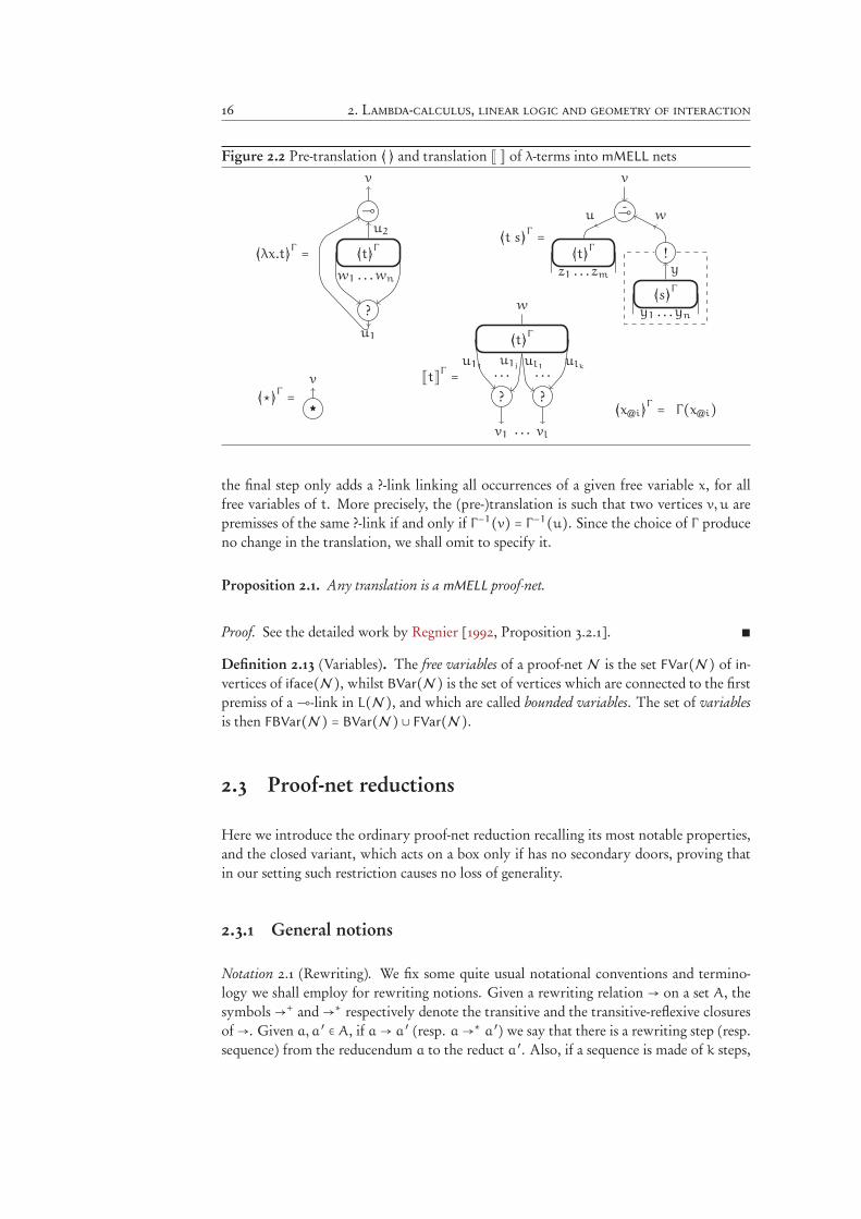
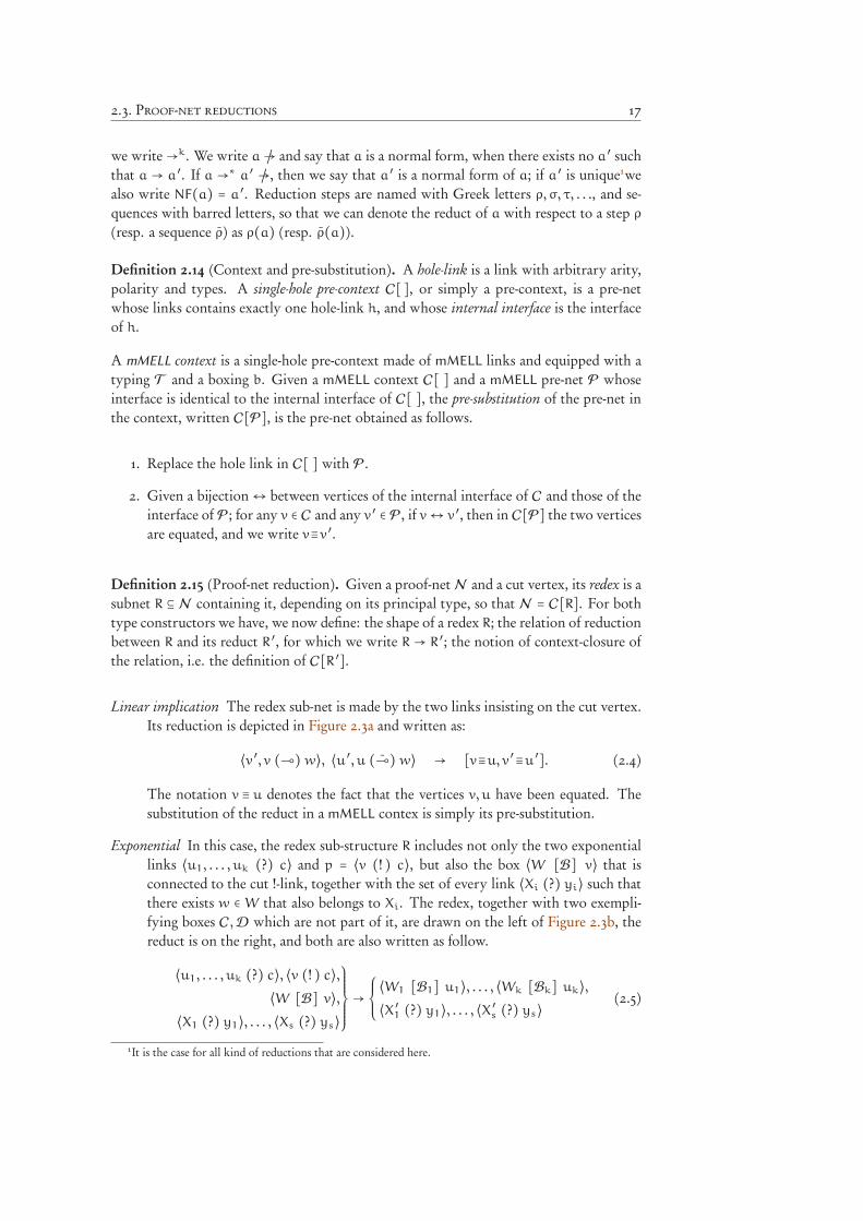
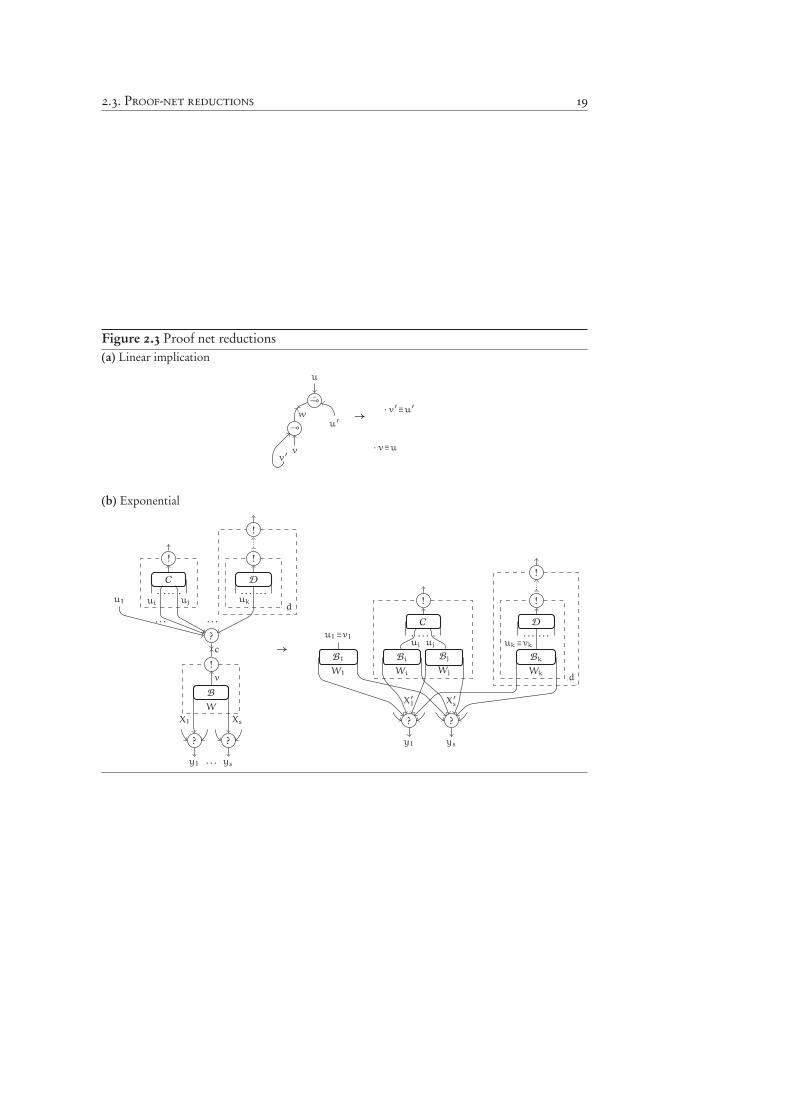
Definition 2.15 (Proof-net reduction). Given a proof-net N and a cut vertex, its redex is asubnet R ⊆ N containing it, depending on its principal type, so that N = C[R]. For bothtype constructors we have, we now define: the shape of a redex R; the relation of reductionbetween R and its reduct R ′, for which we write R → R ′; the notion of context-closure ofthe relation, i.e. the definition of C[R ′].
Linear implication The redex sub-net is made by the two links insisting on the cut vertex.Its reduction is depicted in Figure 2.3a and written as:
⟨v ′, v (⊸) w⟩, ⟨u ′, u (⊸) w⟩ → [v≡u, v ′≡u ′]. (2.4)
The notation v ≡ u denotes the fact that the vertices v, u have been equated. Thesubstitution of the reduct in a mMELL contex is simply its pre-substitution.
Exponential In this case, the redex sub-structure R includes not only the two exponentiallinks ⟨u1, . . . , uk (?) c⟩ and p = ⟨v (! ) c⟩, but also the box ⟨W [B] v⟩ that isconnected to the cut !-link, together with the set of every link ⟨Xi (?) yi⟩ such thatthere exists w ∈ W that also belongs to Xi. The redex, together with two exempli-fying boxes C,D which are not part of it, are drawn on the left of Figure 2.3b, thereduct is on the right, and both are also written as follow.
⟨u1, . . . , uk (?) c⟩, ⟨v (! ) c⟩,⟨W [B] v⟩,
⟨X1 (?) y1⟩, . . . , ⟨Xs (?) ys⟩
⎫⎪⎪⎪⎪⎪⎬⎪⎪⎪⎪⎪⎭→
⎧⎪⎪⎨⎪⎪⎩⟨W1 [B1] u1⟩, . . . , ⟨Wk [Bk] uk⟩,⟨X ′1 (?) y1⟩, . . . , ⟨X ′s (?) ys⟩ (2.5)
1It is the case for all kind of reductions that are considered here.
18 2. Lambda-calculus, linear logic and geometry of interaction
The reduction removes the two cut exponential links, and duplicates B into k copies(erasing it when k = 0): ⟨W1 [B1] u1⟩, . . . , ⟨Wk [Bk] uk⟩. Also, the boxing b ′ ofthe reduct is obtained by the boxing b of R so that the box copy Bh is included inany box that in R contains vh. More precisely:
1. if p ′ is the !-link of a box B containing uh for some 0 ≤ h ≤ k, then b ′(p ′) =b(p ′) ∪Bh;
2. if p ′ ≠ p is the !-link of a box B ′ ⊊ B then b ′(p ′h) = b(p ′), for any 0 ≤ h ≤ k;
3. otherwise b ′(p ′) = b(p ′).Notice that for any 0 ≤ j ≤ s, the set of premisses of the j-th ?-link containingauxiliary doors for B is modified by the reduction: the sequence of premisses X ′jof its reduct is obtained by replacing any occurrence of a vertex w ∈ W with thesequence (w1, . . . ,wk) such that its elements respectively belongs to W1, . . . ,Wk.
The substitution of the R ′ in C[ ] is defined as the pre-substitution of R ′ in C, plusa modification of its boxing so that the sub-net Bi is included to any B ′ containingvi. Pictorially: observe box borders in the upper part of Figure 2.3b. Formally: iffor some 0 ≤ i ≤ k and according to b(C), we have ui ∈ B
′ ∈ Bxs (N ) and z ∈ V(B),then in the boxing of the reduct b ′(C) we have also zi ∈ V(B ′). In spite of thisdetail, we shall abuse the notation and simply write that C[R]→ C[R ′].
The proof-net reduction, also called cut elimination, is the graph-rewriting relation onmMELL nets obtained by the union of the context closures of the linear implication re-duction and the exponential reduction.
Proposition 2.2. Any reduct of a proof-net is a proof-net.
We only sketch the main idea of the proof, and address the interested reader to the well-detailed proof by Regnier [1992, Proposition 4.1.1].
Proof sketch. Consider a reduction step ρ on a redex R ⊂ N and take a switching pathπ that is persistent to ρ. Ad absurdum, suppose that ρ(π) is cyclic, and observe thatthis would imply that π is cyclic as well, thus contradicting Definition 2.10. Hence ρ(π)is acyclic. Repeat such argument by induction on the length of the reduction sequenceN →∗ N ′, and obtain the thesis. ∎
Proposition 2.3 (Strong normalisation [Pagani and Tortora de Falco, 2010, Accattoli,2013]). Any mMELL proof-net N strongly normalises. If N has a unique conclusion vertexv ∶ T , with T ground, then the normal form of N is ⟨(★) v⟩.
2.3.2 Closed strategy
Closed reduction perform exponential steps only if the box is closed, i.e. has no auxiliarydoors (cf. Definition 2.5).
Definition 2.16 (Closed reduction). The closed reduction, written →cl, is the restrictionof → that for the exponential case requires that the box in a redex to be closed.
2.3. Proof-net reductions 19
Figure 2.3 Proof net reductions(a) Linear implication
⊸
⊸
u
u′
v
v′
w→
⋅ v′≡u′
⋅ v≡u
(b) Exponential
?
. . . . . .
u1
C
ui uj
. . . . .
!
D
uk
. . . . . .
!
!
d
!
c
B
W
v
? ?
y1 ys
X1 Xs
. . .
→
u1≡v1
B1
W1
C
. . . . .ui uj
!
Bi
Wi
Bj
Wj
D
. . . . . .
!
!
d
Bk
Wk
uk≡vk
? ?
y1 ys
X ′1 X ′s
20 2. Lambda-calculus, linear logic and geometry of interaction
Lemma 2.1 (Existence of closed exponential cut). Given amMELL proof-netN ∶ ★without⊸-cuts, either N is cut-free, or N contains an exponential cut on a closed box.
Proof. Given N a mMELL proof-net without ⊸-cuts, let c ∈ V(N ) be an exponentialcut such that ℓ(c) = 0, and B be the box whose !-link has conclusion c. We proceed byinduction on the number n of boxes at depth 0 crossed by π, which is finite thanks to thefiniteness of N .
1. If n = 0 then B is closed, so we found a witness and we conclude.
2. If n > 0, let a be the conclusion of a ?-link having a premiss that is an auxiliarydoor of B. Consider any straight and consequent path π starting from a. π cannotreach the conclusion of N , because otherwise the type on N would differ from ⋆(contradicting such hypothesis). π can neither reach a ⋆-link, since otherwise thetyping of links would be broken somewhere along π (Definition 2.2). Thereforeπ must reach a cut vertex c ′, whose depth by hypothesis cannot be smaller thanthe depth of c. But the depth of vertices along π can neither increase, because π isconsequent. Therefore ℓ(c ′) = ℓ(c). Morever, it must be the case that c ≠ c ′, sinceN is switching cyclic by Definition 2.10. Now repeat the previous reasoning rightfrom the beginning, using the cut c ′ as our target cut instead of c, and the box B ′
that is associated with c ′ in place of the target box B.
∎
Remark 2.1. Previous Lemma 2.1 holds a little more generally in full MELL, with theassumption that a proof-net does not contain any ?-link in any subtype of any of its con-clusions. Such assumption is the same that was firstly used by Girard [1989, Theorem 1,p. 239], and in our syntactical setting it implies that the only conclusion of the net hasground type.
Fact 2.1. For any given proof-net N , if N has a normal form N with respect to full mMELL
reduction, then there exist a N →∗cl N
Proof. The claim follows from normalisation (Proposition 2.3), confluence of the ordin-ary reduction, and the existence of closed exponential cuts (Lemma 2.1). ∎
2.4 Execution paths
In this section we formalise the notion of execution paths, the action of reduction on them.Together with the property of persistence, i.e. the ability of resisting to the rewriting, weshow that every path has a unique ancestor. We also present the closed reduction on proof-nets, which acts on a box only if it is closed, and prove that in this case path reductioninduces a bijection.
2.4. Execution paths 21
2.4.1 Statics
We now introduce two restrictions on the shape of paths that rule out those which, froma proof-theoretic or computational perspective, we can a priori recognise as meaningless.We want paths which do not bounce, nor twist in a proof-net. A third restriction is insteadunnecessary, but considerably improve the simplicity and readability.
Except for a cosmetic difference discussed in Remark 2.2, our formulation is essentially arework of the presentation given by Danos and Regnier [1995].
Definition 2.17 (Execution paths). Let N be a proof-net and π a paths in N . If there isno other path π ′ ∈ N such that π ⊆ π ′, where ⊆ is the inclusion ordering on sequences,then π is maximal. Finally if π is both straight and maximal, then π is an execution path.We denote with P(N ) the set of straight paths in N , whilst PE(N ) is the set of executionpaths.
Fact 2.2. If v is the extremum vertex of an execution path π ∈N , then v is either a conclusionof N , or the conclusion of a weakening.
Remark 2.2. Most of the previous literature about paths in LL proof-nets uses the notionof ‘composition’ instead of ‘concatenation’. As a result, the appropriate notation in func-tional style has been preferred, i.e. writing from right to left. We rather preferred thecognitive ease to orthodoxy2.
Remark 2.3. For the ease of presentation, we deliberately left a bit of ambiguity in thepath definition. It may happen that, given an ordered pair of vertices, there actually existtwo distinct hyperlink crossings. For instance, consider a pre-net having l = ⟨v (?) u⟩ andl ′ = ⟨u, v (⊸) w⟩, and a unitary path π = (u, v). What is the link crossed by π? In spite ofthis, all the possible ambiguities will be clarified either by the straightness of the paths wewill consider almost everywhere, or by a direct explanation. For instance, again withinthe net considered in the previous example, consider π ′ = (w,u, v,w) and notice that, ifπ ′ is straight, then there is a unique sequence of links crossed by π ′, i.e. (l ′, l, l ′). Indeed,the only other possible sequence of links, i.e. (l ′, l ′, l ′), would imply π ′ being twisting.
2.4.2 Dynamics
We now define the action of reduction on paths and the notion of persistence, and showsome elementary properties, the most notable of which is the fact that every path in areduct has a unique ancestor.
Definition 2.18 (Redex crossing and sufficient length). Given a reduction step ρ on aredex R ⊆ N , a redex crossing for R is a straight path χ that is maximal in R. Let ρ be areduction step on a redex R in N . A path π ∈N is long enough if and only if for any vertexr ∈ π, the fact that r ∈ R and r is not a conclusion of R implies there is a subpath χ ⊆ π thatis a crossing of R, and such that r ∈ χ. If π is long enough for ρ, then there exist n ≥ 0 suchthat
π = π0 ∶∶ χ1 ∶∶ π1 ∶∶ . . . ∶∶ χn ∶∶ πn,
2.notation favourite its recover easily should writing inverse the with accustomed reader The
22 2. Lambda-calculus, linear logic and geometry of interaction
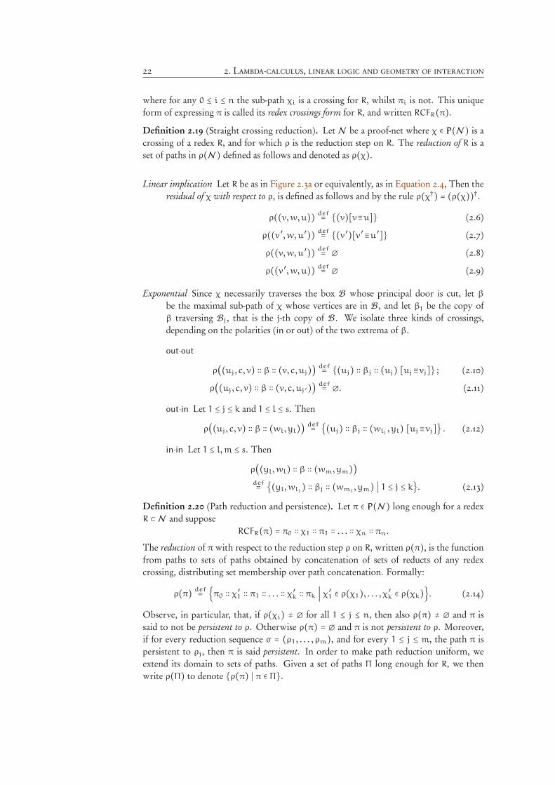
where for any 0 ≤ i ≤ n the sub-path χi is a crossing for R, whilst πi is not. This uniqueform of expressing π is called its redex crossings form for R, and written RCFR(π).Definition 2.19 (Straight crossing reduction). Let N be a proof-net where χ ∈ P(N ) is acrossing of a redex R, and for which ρ is the reduction step on R. The reduction of R is aset of paths in ρ(N ) defined as follows and denoted as ρ(χ).
Linear implication Let R be as in Figure 2.3a or equivalently, as in Equation 2.4, Then theresidual of χ with respect to ρ, is defined as follows and by the rule ρ(χ†) = (ρ(χ))†.
ρ((v,w,u)) def= {(v)[v≡u]} (2.6)
ρ((v ′,w,u ′)) def= {(v ′)[v ′≡u ′]} (2.7)
ρ((v,w,u ′)) def= ∅ (2.8)
ρ((v ′,w,u)) def= ∅ (2.9)
Exponential Since χ necessarily traverses the box B whose principal door is cut, let β
be the maximal sub-path of χ whose vertices are in B, and let βj be the copy ofβ traversing Bj, that is the j-th copy of B. We isolate three kinds of crossings,depending on the polarities ( in or out) of the two extrema of β.
out-out
ρ((uj, c, v) ∶∶ β ∶∶ (v, c, uj)) def= {(uj) ∶∶ βj ∶∶ (uj) [uj≡vj]} ; (2.10)
ρ((uj, c, v) ∶∶ β ∶∶ (v, c, uj ′)) def= ∅. (2.11)
out-in Let 1 ≤ j ≤ k and 1 ≤ l ≤ s. Then
ρ((uj, c, v) ∶∶ β ∶∶ (wl, yl)) def= {(uj) ∶∶ βj ∶∶ (wlj , yl) [uj≡vj]} . (2.12)
in-in Let 1 ≤ l,m ≤ s. Then
ρ((yl,wl) ∶∶ β ∶∶ (wm, ym))def= {(yl,wlj) ∶∶ βj ∶∶ (wmj
, ym) ∣ 1 ≤ j ≤ k}. (2.13)
Definition 2.20 (Path reduction and persistence). Let π ∈ P(N ) long enough for a redexR ⊂N and suppose
RCFR(π) = π0 ∶∶ χ1 ∶∶ π1 ∶∶ . . . ∶∶ χn ∶∶ πn.
The reduction of π with respect to the reduction step ρ on R, written ρ(π), is the functionfrom paths to sets of paths obtained by concatenation of sets of reducts of any redexcrossing, distributing set membership over path concatenation. Formally:
ρ(π) def= {π0 ∶∶ χ
′
1 ∶∶ π1 ∶∶ . . . ∶∶ χ′
k ∶∶ πk ∣ χ ′1 ∈ ρ(χ1), . . . , χ ′k ∈ ρ(χk)}. (2.14)
Observe, in particular, that, if ρ(χi) ≠ ∅ for all 1 ≤ j ≤ n, then also ρ(π) ≠ ∅ and π issaid to not be persistent to ρ. Otherwise ρ(π) = ∅ and π is not persistent to ρ. Moreover,if for every reduction sequence σ = (ρ1, . . . , ρm), and for every 1 ≤ j ≤ m, the path π ispersistent to ρj, then π is said persistent. In order to make path reduction uniform, weextend its domain to sets of paths. Given a set of paths Π long enough for R, we thenwrite ρ(Π) to denote {ρ(π) ∣ π ∈ Π}.
2.4. Execution paths 23
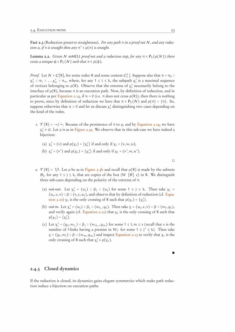
Fact 2.3 (Reduction preserve straightness). For any path π in a proof-netN , and any reduc-tion ρ, if π is straight then any π ′ ∈ ρ(π) is straight.Lemma 2.2. Given N mMELL proof-net and ρ reduction step, for any π ∈ PE(ρ(N )) thereexists a unique φ ∈ PE(N ) such that π ∈ ρ(φ).
Proof. Let N = C[R], for some redex R and some context C[ ]. Suppose also that π = π0 ∶∶
χ ′1 ∶∶ π1 ∶∶ . . . χ′
n ∶∶ πn, where, for any 1 ≤ i ≤ k, the subpath χ ′i is a maximal sequenceof vertices belonging to ρ(R). Observe that the extrema of χ ′i necessarily belong to theinterface of ρ(R), because π is an execution path. Now, by definition of reduction, and inparticular as per Equation 2.14, if n = 0 (i.e. π does not cross ρ(R)), then there is nothingto prove, since by definition of reduction we have that π ∈ PE(N ) and ρ(π) = {π}. So,suppose otherwise that n > 0 and let us discuss χ ′i distinguishing two cases depending onthe kind of the redex.
1. T (R) =⊸/⊸. Because of the persistence of π to ρ, and by Equation 2.14, we haveχ ′i ≠ ∅. Let ρ is as in Figure 2.3a. We observe that in this sub-case we have indeed abijection:
(a) χ ′i = (v) and ρ(χi) = {χ ′i} if and only if χl = (v,w,u);(b) χ ′i = (v ′) and ρ(χi) = {χ ′i} if and only if χl = (v ′,w,u ′).
◻
2. T (R) = !/?. Let ρ be as in Figure 2.3b and recall that ρ(R) is made by the subnetsBj, for any 1 ≤ j ≤ k, that are copies of the box ⟨W [B] c⟩ in R. We distinguishthree sub-cases depending on the polarity of the extrema of π.
(a) out-out. Let χ ′i = (uj) ∶∶ βj ∶∶ (uj) for some 1 ≤ j ≤ k. Then take χi =
(uj, c, v) ∶∶ β ∶∶ (v, c, uj), and observe that by definition of reduction (cf. Equa-tion 2.10) χi is the only crossing of R such that ρ(χi) = {χ ′i}.
(b) out-in. Let χ ′i = (uj) ∶∶ βj ∶∶ (wlj , yl). Then take χ = (uj, c, v) ∶∶ β ∶∶ (wl, yl),and verify again (cf. Equation 2.12) that χi is the only crossing of R such thatρ(χi) = {χ ′i}.
(c) Let χ ′i = (yl,wlj) ∶∶ βj ∶∶ (wmj, ym) for some 1 ≤ l,m ≤ s (recall that s is the
number of ?-links having a premiss in Wj ′ for some 1 ≤ j ′ ≤ k). Then takeχ = (yl,wl) ∶∶ β ∶∶ (wm, ym) and inspect Equation 2.13 to verify that χi is theonly crossing of R such that χ ′i ∈ ρ(χi).
∎
2.4.3 Closed dynamics
If the reduction is closed, its dynamics gains elegant symmetries which make path reduc-tion induce a bijection on execution paths.
24 2. Lambda-calculus, linear logic and geometry of interaction
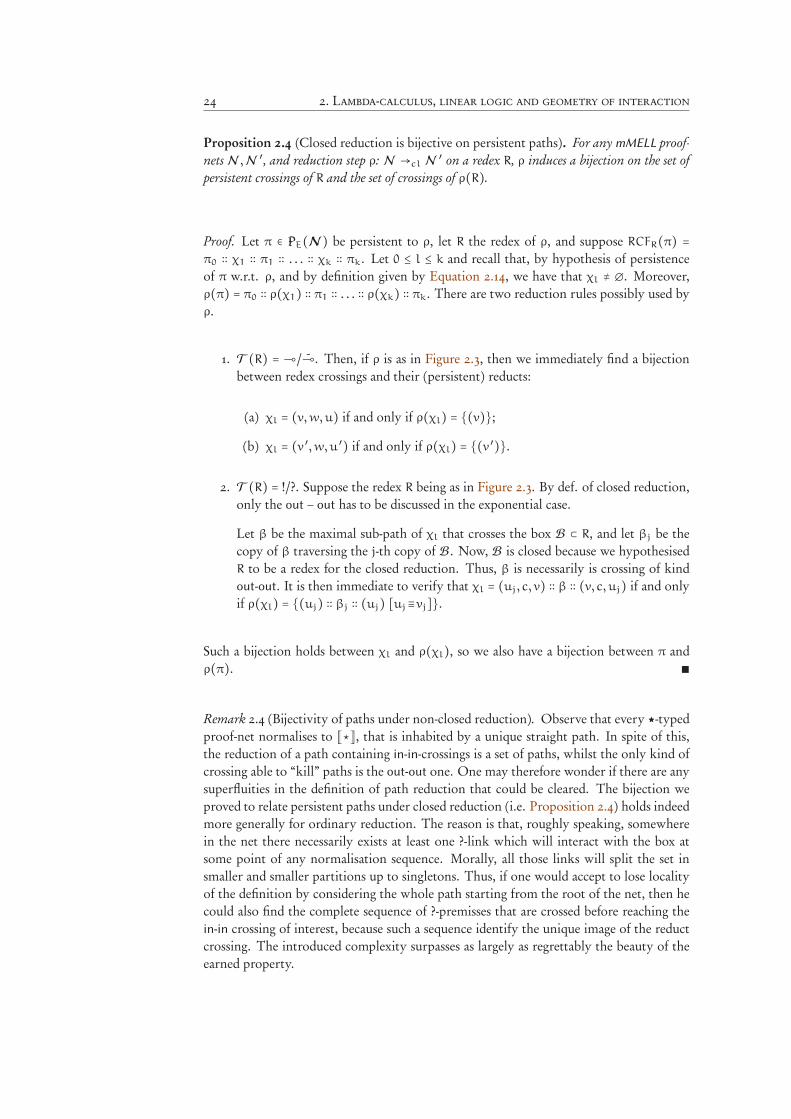
Proposition 2.4 (Closed reduction is bijective on persistent paths). For anymMELL proof-nets N ,N ′, and reduction step ρ: N →cl N ′ on a redex R, ρ induces a bijection on the set ofpersistent crossings of R and the set of crossings of ρ(R).
Proof. Let π ∈ PE(N ) be persistent to ρ, let R the redex of ρ, and suppose RCFR(π) =π0 ∶∶ χ1 ∶∶ π1 ∶∶ . . . ∶∶ χk ∶∶ πk. Let 0 ≤ l ≤ k and recall that, by hypothesis of persistenceof π w.r.t. ρ, and by definition given by Equation 2.14, we have that χl ≠ ∅. Moreover,ρ(π) = π0 ∶∶ ρ(χ1) ∶∶ π1 ∶∶ . . . ∶∶ ρ(χk) ∶∶ πk. There are two reduction rules possibly used byρ.
1. T (R) = ⊸/⊸. Then, if ρ is as in Figure 2.3, then we immediately find a bijectionbetween redex crossings and their (persistent) reducts:
(a) χl = (v,w,u) if and only if ρ(χl) = {(v)};(b) χl = (v ′,w,u ′) if and only if ρ(χl) = {(v ′)}.
2. T (R) = !/?. Suppose the redex R being as in Figure 2.3. By def. of closed reduction,only the out − out has to be discussed in the exponential case.
Let β be the maximal sub-path of χl that crosses the box B ⊂ R, and let βj be thecopy of β traversing the j-th copy of B. Now, B is closed because we hypothesisedR to be a redex for the closed reduction. Thus, β is necessarily is crossing of kindout-out. It is then immediate to verify that χl = (uj, c, v) ∶∶ β ∶∶ (v, c, uj) if and onlyif ρ(χl) = {(uj) ∶∶ βj ∶∶ (uj) [uj≡vj]}.
Such a bijection holds between χl and ρ(χl), so we also have a bijection between π andρ(π). ∎
Remark 2.4 (Bijectivity of paths under non-closed reduction). Observe that every ★-typedproof-net normalises to ⟦⋆⟧, that is inhabited by a unique straight path. In spite of this,the reduction of a path containing in-in-crossings is a set of paths, whilst the only kind ofcrossing able to “kill” paths is the out-out one. One may therefore wonder if there are anysuperfluities in the definition of path reduction that could be cleared. The bijection weproved to relate persistent paths under closed reduction (i.e. Proposition 2.4) holds indeedmore generally for ordinary reduction. The reason is that, roughly speaking, somewherein the net there necessarily exists at least one ?-link which will interact with the box atsome point of any normalisation sequence. Morally, all those links will split the set insmaller and smaller partitions up to singletons. Thus, if one would accept to lose localityof the definition by considering the whole path starting from the root of the net, then hecould also find the complete sequence of ?-premisses that are crossed before reaching thein-in crossing of interest, because such a sequence identify the unique image of the reductcrossing. The introduced complexity surpasses as largely as regrettably the beauty of theearned property.
2.5. Computation as path execution 25
2.5 Computation as path execution
2.5.1 Dynamic algebra
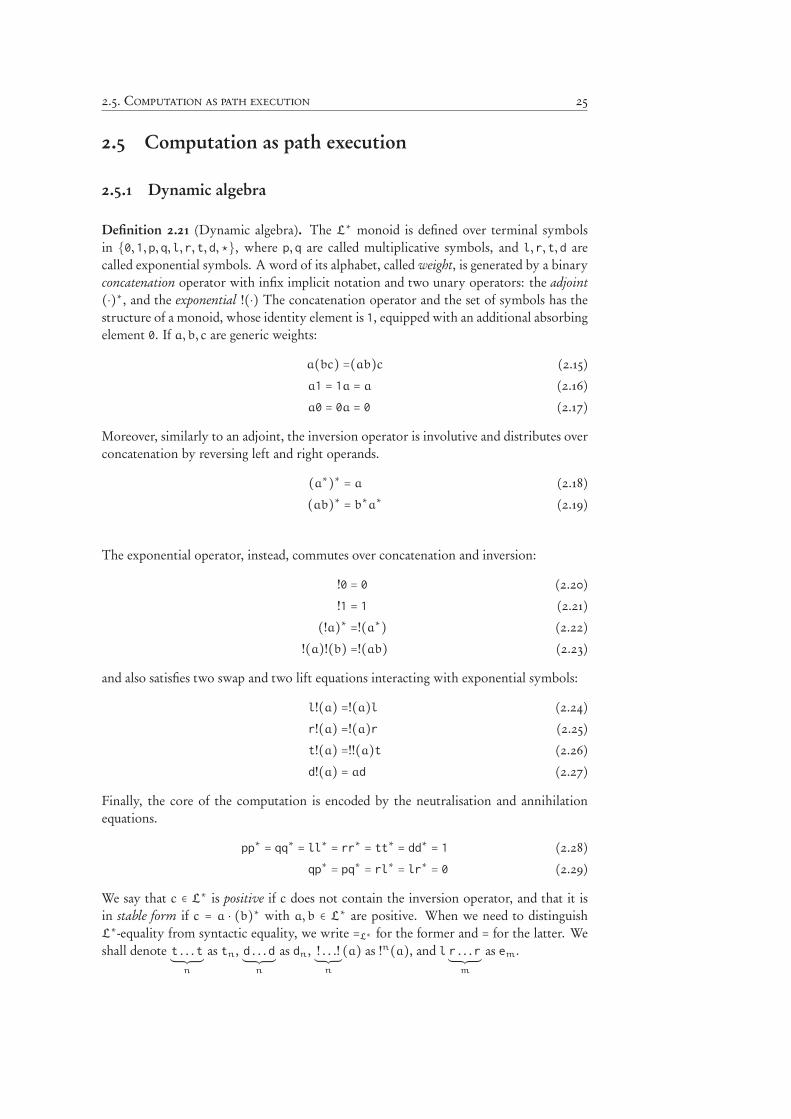
Definition 2.21 (Dynamic algebra). The L∗ monoid is defined over terminal symbolsin {0,1,p,q,l,r,t,d,⋆}, where p,q are called multiplicative symbols, and l,r,t,d arecalled exponential symbols. A word of its alphabet, called weight, is generated by a binaryconcatenation operator with infix implicit notation and two unary operators: the adjoint(⋅)∗, and the exponential !(⋅) The concatenation operator and the set of symbols has thestructure of a monoid, whose identity element is 1, equipped with an additional absorbingelement 0. If a, b, c are generic weights:
a(bc) =(ab)c (2.15)
a1 = 1a = a (2.16)
a0 = 0a = 0 (2.17)
Moreover, similarly to an adjoint, the inversion operator is involutive and distributes overconcatenation by reversing left and right operands.
(a∗)∗ = a (2.18)
(ab)∗ = b∗a∗ (2.19)
The exponential operator, instead, commutes over concatenation and inversion:
!0 = 0 (2.20)
!1 = 1 (2.21)
(!a)∗ =!(a∗) (2.22)
!(a)!(b) =!(ab) (2.23)
and also satisfies two swap and two lift equations interacting with exponential symbols:
l!(a) =!(a)l (2.24)
r!(a) =!(a)r (2.25)
t!(a) =!!(a)t (2.26)
d!(a) = ad (2.27)
Finally, the core of the computation is encoded by the neutralisation and annihilationequations.
pp∗ = qq∗ = ll∗ = rr∗ = tt∗ = dd∗ = 1 (2.28)
qp∗= pq
∗= rl
∗= lr
∗= 0 (2.29)
We say that c ∈ L∗ is positive if c does not contain the inversion operator, and that it isin stable form if c = a ⋅ (b)∗ with a, b ∈ L∗ are positive. When we need to distinguishL∗-equality from syntactic equality, we write =L∗ for the former and = for the latter. We
shall denote t . . .t:n
as tn, d . . .d:n
as dn, ! . . .!;n
(a) as !n(a), and l r . . .r:m
as em.
26 2. Lambda-calculus, linear logic and geometry of interaction
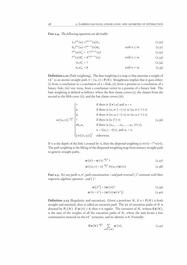
Fact 2.4. The following equations are derivable:
tn!m(a) =!m+n(a)tn (2.30)
dn!m(a) =!m−n(a)dn with n ≤m (2.31)
!m(a)t∗n = t∗!m+n(a) (2.32)
!m(a)d∗n = d∗!m−n(a) with n ≤m (2.33)
ene∗
n = 1 (2.34)
ene∗
m = 0 with n ≠m (2.35)
Definition 2.22 (Path weighting). The base weighting is a map w that associate a weight ofrL∗ to an atomic straight path π = (u, v) ∈ P(N ). Straightness implies that it goes either:
(i) from a conclusion to a conclusion of a ⋆-link; (ii) from a premiss to a conclusion of abinary link; (iii) vice versa, from a conclusion vertex to a premiss of a binary link. Thebase weighting is defined as follows, where the first clause covers (i), the clauses from thesecond to the fifth cover (ii), and the last clause covers (iii).
w((u, v)) def=
⎧⎪⎪⎪⎪⎪⎪⎪⎪⎪⎪⎪⎪⎪⎪⎪⎪⎪⎪⎨⎪⎪⎪⎪⎪⎪⎪⎪⎪⎪⎪⎪⎪⎪⎪⎪⎪⎪⎩
⋆ if there is ⟨(★) u⟩ and u = v
p if there is ⟨u,w (⊸) v⟩ or ⟨u,w (⊸) v⟩q if there is ⟨w,u (⊸) v⟩ or ⟨w,u (⊸) v⟩1 if there is ⟨u (! ) v⟩dtnei if there is ⟨u1, . . . , ui, . . . , uk (?) v⟩,
n = ℓ(ui) − ℓ(v), and ui = u
(w((v, u)))∗ otherwise.
(2.36)
If n is the depth of the link l crossed by π, then the deepened weighting is w(π) = !nw(π).The path weighting is the lifting of the deepened weighting map from unitary straight pathto generic straight paths.
w (∅) = w (v) def= 1 (2.37)
w ((u, v) ∶∶ π) def= w(u, v)w (π) (2.38)
Fact 2.5. For any paths π,π ′, path concatenation ∶∶ and path reversal ( )† commute with theirrespective algebraic operators ⋅ and ( )∗.
w (π†) = (w (π))∗ (2.39)
w (π ∶∶ π ′) = (w (π)w (π ′)) (2.40)
Definition 2.23 (Regularity and execution). Given a proof-net N , if π ∈ P(N ) is bothstraight and maximal, then is called an execution path. The set of execution paths of N isdenoted by PE(N ). If w (π) ≠ 0, then π is regular. The execution of N , written Ex(N ),is the sum of the weights of all the execution paths of N , where the sum forms a freecommutative monoid on the rL∗ structure, and its identity is 0. Formally:
Ex(N ) def= ∑
π∈PE(N )w (π) , (2.41)
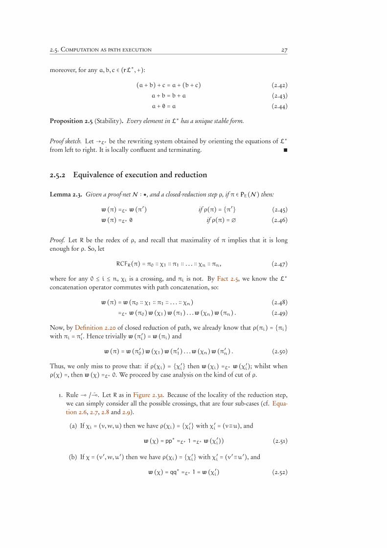
2.5. Computation as path execution 27
moreover, for any a, b, c ∈ (rL∗,+):(a + b) + c = a + (b + c) (2.42)
a + b = b + a (2.43)
a + 0 = a (2.44)
Proposition 2.5 (Stability). Every element in L∗ has a unique stable form.
Proof sketch. Let →L∗ be the rewriting system obtained by orienting the equations of L∗
from left to right. It is locally confluent and terminating. ∎
2.5.2 Equivalence of execution and reduction
Lemma 2.3. Given a proof-net N ∶ ★, and a closed-reduction step ρ, if π ∈ PE(N ) then:w (π) =L∗ w (π ′) if ρ(π) = {π ′} (2.45)
w (π) =L∗ 0 if ρ(π) = ∅ (2.46)
Proof. Let R be the redex of ρ, and recall that maximality of π implies that it is longenough for ρ. So, let
RCFR(π) = π0 ∶∶ χ1 ∶∶ π1 ∶∶ . . . ∶∶ χn ∶∶ πn, (2.47)
where for any 0 ≤ i ≤ n, χi is a crossing, and πi is not. By Fact 2.5, we know the L∗
concatenation operator commutes with path concatenation, so:
w (π) = w (π0 ∶∶ χ1 ∶∶ π1 ∶∶ . . . ∶∶ χn) (2.48)
=L∗ w (π0)w (χ1)w (π1) . . .w (χn)w (πn) . (2.49)
Now, by Definition 2.20 of closed reduction of path, we already know that ρ(πi) = {πi}with πi = π ′i. Hence trivially w (π ′i) = w (πi) and
w (π) = w (π ′0)w (χ1)w (π ′1) . . .w (χn)w (π ′n) . (2.50)
Thus, we only miss to prove that: if ρ(χi) = {χ ′i} then w (χi) =L∗ w (χ ′i); whilst whenρ(χ) =, then w (χ) =L∗ 0. We proceed by case analysis on the kind of cut of ρ.
1. Rule ⊸ /⊸. Let R as in Figure 2.3a. Because of the locality of the reduction step,we can simply consider all the possible crossings, that are four sub-cases (cf. Equa-tion 2.6, 2.7, 2.8 and 2.9).
(a) If χi = (v,w,u) then we have ρ(χi) = {χ ′i} with χ ′i = (v≡u), andw (χ) = pp∗ =L∗ 1 =L∗ w (χ ′i)) (2.51)
(b) If χ = (v ′,w,u ′) then we have ρ(χi) = {χ ′i} with χ ′i = (v ′≡u ′), andw (χ) = qq∗ =L∗ 1 = w (χ ′i) (2.52)
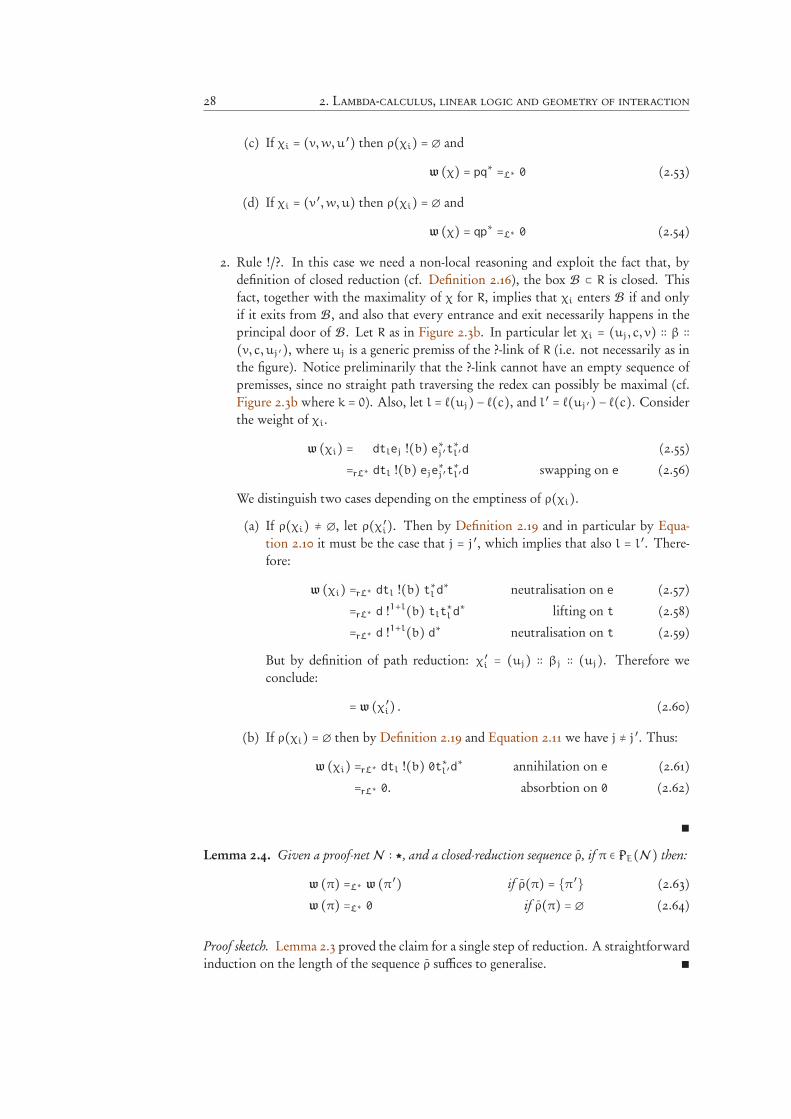
28 2. Lambda-calculus, linear logic and geometry of interaction
(c) If χi = (v,w,u ′) then ρ(χi) = ∅ and
w (χ) = pq∗ =L∗ 0 (2.53)
(d) If χi = (v ′,w,u) then ρ(χi) = ∅ and
w (χ) = qp∗ =L∗ 0 (2.54)
2. Rule !/?. In this case we need a non-local reasoning and exploit the fact that, bydefinition of closed reduction (cf. Definition 2.16), the box B ⊂ R is closed. Thisfact, together with the maximality of χ for R, implies that χi enters B if and onlyif it exits from B, and also that every entrance and exit necessarily happens in theprincipal door of B. Let R as in Figure 2.3b. In particular let χi = (uj, c, v) ∶∶ β ∶∶(v, c, uj ′), where uj is a generic premiss of the ?-link of R (i.e. not necessarily as inthe figure). Notice preliminarily that the ?-link cannot have an empty sequence ofpremisses, since no straight path traversing the redex can possibly be maximal (cf.Figure 2.3b where k = 0). Also, let l = ℓ(uj) − ℓ(c), and l ′ = ℓ(uj ′) − ℓ(c). Considerthe weight of χi.
w (χi) = dtlej !(b) e∗j ′t∗l ′d (2.55)
=rL∗ dtl !(b) eje∗j ′t∗l ′d swapping on e (2.56)
We distinguish two cases depending on the emptiness of ρ(χi).(a) If ρ(χi) ≠ ∅, let ρ(χ ′i). Then by Definition 2.19 and in particular by Equa-
tion 2.10 it must be the case that j = j ′, which implies that also l = l ′. There-fore:
w (χi) =rL∗ dtl !(b) t∗l d∗ neutralisation on e (2.57)
=rL∗ d !1+l(b) tlt∗l d∗ lifting on t (2.58)
=rL∗ d !1+l(b) d∗ neutralisation on t (2.59)
But by definition of path reduction: χ ′i = (uj) ∶∶ βj ∶∶ (uj). Therefore weconclude:
= w (χ ′i) . (2.60)
(b) If ρ(χi) = ∅ then by Definition 2.19 and Equation 2.11 we have j ≠ j ′. Thus:
w (χi) =rL∗ dtl !(b) 0t∗l ′d∗ annihilation on e (2.61)
=rL∗ 0. absorbtion on 0 (2.62)
∎
Lemma 2.4. Given a proof-net N ∶ ★, and a closed-reduction sequence ρ, if π ∈ PE(N ) then:w (π) =L∗ w (π ′) if ρ(π) = {π ′} (2.63)
w (π) =L∗ 0 if ρ(π) = ∅ (2.64)
Proof sketch. Lemma 2.3 proved the claim for a single step of reduction. A straightforwardinduction on the length of the sequence ρ suffices to generalise. ∎
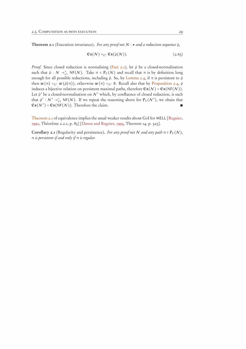
2.5. Computation as path execution 29
Theorem 2.1 (Execution invariance). For any proof-net N ∶ ★ and a reduction sequence ρ,
Ex(N ) =L∗ Ex(ρ(N )). (2.65)
Proof. Since closed reduction is normalising (Fact 2.1), let ρ be a closed-normalisationsuch that ρ ∶ N →
∗
cl NF(N ). Take π ∈ PE(N ) and recall that π is by definition longenough for all possible reductions, including ρ. So, by Lemma 2.4, if π is persistent to ρ
then w (π) =L∗ w (ρ(π)), otherwise w (π) =L∗ 0. Recall also that by Proposition 2.4, ρinduces a bijective relation on persistent maximal paths, therefore Ex(N ) = Ex(NF(N )).Let ρ ′ be a closed-normalisation on N ′ which, by confluence of closed reduction, is suchthat ρ ′ ∶ N ′
→∗
cl NF(N ). If we repeat the reasoning above for PE(N ′), we obain thatEx(N ′) = Ex(NF(N )). Therefore the claim. ∎
Theorem 2.1 of equivalence implies the usual weaker results about GoI forMELL [Regnier,1992, Théorème 2.2.1, p. 85] [Danos and Regnier, 1995, Theorem 14, p. 325].
Corollary 2.1 (Regularity and persistence). For any proof-net N and any path π ∈ PE(N ),π is persistent if and only if π is regular.
30 2. Lambda-calculus, linear logic and geometry of interaction
Part I
Superposition and expansion

Chapter 3
Geometry of Resource
Interaction
Contents
3.1. Introduction 34
3.2. Resource calculus 34
3.2.1 Syntax 35
3.2.2 Reduction 35
3.3. Resource interaction nets 36
3.3.1 Definition 37
3.3.2 Term translation 38
3.3.3 Reduction 39
3.4. Resource paths 45
3.4.1 Statics 45
3.4.2 Dynamics 46
3.4.3 Comprehensiveness and bijection 48
3.4.4 Confluence and persistence 51
3.5. Resource execution 54
34 3. Geometry of Resource Interaction
3.5.1 Dynamic algebra and execution 54
3.5.2 Invariance and regularity 57
3.6. Discussion 60
3.6.1 Related works 60
3.6.2 Open questions 61
3.6.2.1 Higher expressivity 61
3.6.2.2Geometry of differential interaction 61
3.1 Introduction
In this chapter, we consider the resource calculus and its translation into interaction nets,called resource nets, where we develop a quite simple theory of their paths. A suitable re-striction of the mMELL algebra is showed to be an extremely concise and precise semanticsfor the resource calculus.
The material here presented originally appeared in EPTCS [2015].
3.2 Resource calculus
The resource calculus (RC) is, on one hand, a linear and thus finitary restriction of theλ-calculus: in the application t S the function t must use exactly once each s belonging tothe multiset of arguments S, i.e. s cannot be duplicated nor erased, so reduction enjoysstrong normalisation. On the other hand, RC represent a non-deterministic extensionof the λ-calculus, since arguments are now finite multisets of ordinary terms. Therefore,the reduct of t S is defined as the superposition, i.e. a sum, of all the possible ways ofsubstituting each s ∈ S. In particular, the number of arguments provided to a functioncan be insufficient or excess the function’s request, i.e. the number of occurrences of thevariable bounded by the abstraction under consideration. In this case, computation isdeadlocked and the application reduces to 0, i.e. the empty sum.
3.2. Resource calculus 35
3.2.1 Syntax
Definition 3.1 (Simple resource terms and polyterms). The set ∆ of all the simple termsand the set ∆! of all simple poly terms are inductively generated by the following grammar.
V ∶∶= x, y, z, . . . variables (3.1)
M ∶∶= ⋆ ∣ V ∣ λV .M ∣ (M B) simple resource terms (3.2)
B ∶∶= 1 ∣ [M] ∣ B ⋅B simple resource polyterms (3.3)
V is a denumerable set. ⋆ is the constant dummy value. Brackets delimit multisets(or bags), the multiset sum (associative and commutative) is expressed in multiplicativenotation with the central dot ⋅, whose neutral element is the empty multiset 1. So that([x] ⋅ 1) ⋅ [y] = [x, y] is a simple polyterm. Simple terms are denoted by lowercase Latinletters s, t, u, . . ., polyterms by uppercase S, T,U, . . .. The set N⟨∆⟩ of terms (resp. the setN⟨∆!⟩ of polyterms) is the set of linear combinations of simple terms (resp. polyterms)having coefficients in the semiring of natural numbers N . All syntactic constructors ofsimple terms and polyterms to be extended to sums by (bi-)linearity, i.e. to commute withsums.
λx.(T + S) def= λx.T + λx.S (3.4)
(s + t) U def= (s U) + (t T) (3.5)
s (T +U) def= (s T) + (s U) (3.6)
[S + T] ⋅U def= [S] ⋅U + [T] ⋅U (3.7)
In order to increase readability and simplicity, in the rest of the chapter we shall omit the“resource” qualification in the calculus nomenclature.
Example 3.1. A non-simple term could be written as (λx.(2x + y))[z2 + 4u] to mean:2(λx.x)[z, z] + 8(λx.x)[u] + (λx.y)[z, z] + 4(λx.y)[u].Remark 3.1. The set of resource (poly-)term was defined by Ehrhard and Regnier [2003]as the finite sums over a generic commutative unit-equipped semiring R, even if theypreferred to restrict it to N. Indeed, whenever R admits negative elements, showed Vaux[2007], strong normalisation of the reduction is lost.
3.2.2 Reduction
Definition 3.2 (Context, redex and reduction). A simple context c(⋅) is a term of thefollowing grammar.
C ∶∶= (⋅) ∣ λV .C ∣ C B ∣M [C]⋅B (3.8)
A context C(⋅) is a sum of a simple context and a polyterm. A completion of a context C(⋅)with a term t, written C(t), is the substitution of the hole (⋅) within C(⋅) for t, possiblycapturing variables.A redex is a simple term of the form: (λx.s)T . Let the i-th free occurrence of x appearingin s to be uniquely indexed with a natural number as x@i, with 1 ≤ i ≤m for m being thenumber of occurrences. The reduction is the relation → between polyterms obtained by
36 3. Geometry of Resource Interaction
the context closure and the linear extension to sum of the following elementary reductionrule.
(λx.s) [t1, . . . , tn] →⎧⎪⎪⎪⎨⎪⎪⎪⎩
∑σn∈Sn
s {t1/x@σn(1), . . . , tn/x@σn(n)} if n =m
0 if n ≠m
(3.9)
Where Sn denotes the set of permutations over the set {1, . . . , n}, and {t/x} is the usualcapture-avoiding substitution.
Example 3.2. Let I = I ′ = λx.x@1 and also let t = λf.f@1[f@2[⋆]]. Then we have:
t[I, I ′]→ f1[f@2[⋆]]{I/f@2, I
′/f@2} + f1[f@2[⋆]]{I/f@2, I′/f@1}
= I[I ′[⋆]] + I ′[I[⋆]]→
2 I ′[⋆] + I[⋆]→
2 2⋆
= NF(t[I, I ′])Note also a case of annihilation in t[I] → 0. Finally, observe that if s = (λx.⋆)T → ⋆ thenT must be 1, otherwise s→ 0.
Proposition 3.1. (Ehrhard and Regnier [2003]) Resource reduction is confluent and strongnormalising.
3.3 Resource interaction nets
From an operational point of view, a net can be seen as a graphical, finer representationof typed terms by means of a variation of the syntax of linear logic proof-nets. From aproof-theoretic point of view, a net is a proof of a minimal, propositional, promotion-freefragment of differential linear logic [Ehrhard and Regnier, 2006a]. The negative expo-nential links have a symmetrical dual but is deprived of promotion, so that it merelyrepresents superposition of proofs and contexts.
Differential interaction nets (DINs) were introduced by Ehrhard and Regnier [2005] asthe graphical computational counterpart of a calculus that is not precisely the differentialλ-calculus [2003] (that would be the differential nets (DNs) Tranquilli [2011]), but insteadthe resource λ-calculus, the latter being a promotion-free restriction of the former. Avoid-ing this confusion is the reason for adopting, in our nomenclature, the term “resource in-teraction nets”. The syntax of (DINs) has two unary links, dereliction and co-dereliction;two binary links, contraction and co-contraction; and two zero-ary links, weakening andco-weakening. Resource nets are a restriction of DINs, formulated with the “so-called”nouvelle syntaxe, where exponential links’ arities are factorised to arbitrary arity. Thepresentation, firstly employed in this setting by Mazza and Pagani [2007] is not just muchmore compact, since the less are the links, much less are the reduction rules of the system,but it also enables us to nimbly reason modulo associativity, for we have it built-in forfree.
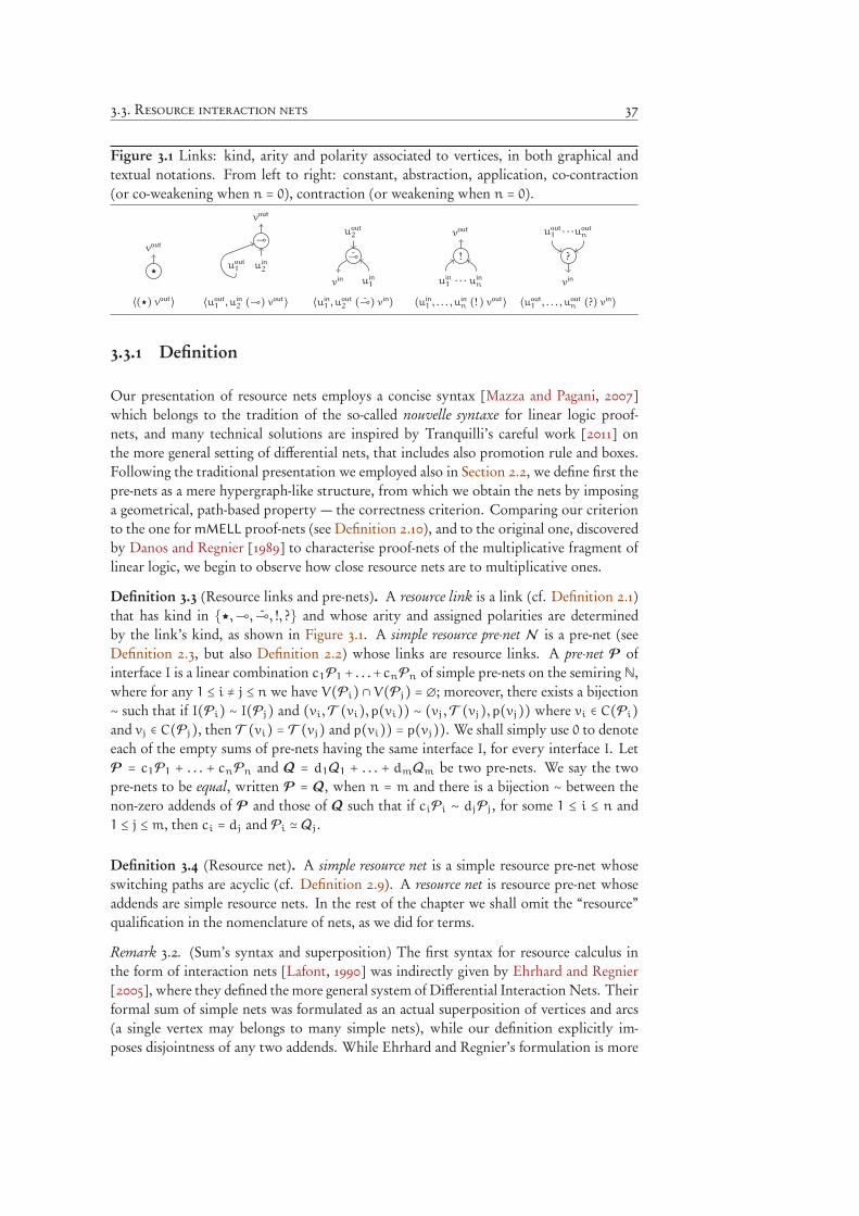
3.3. Resource interaction nets 37
Figure 3.1 Links: kind, arity and polarity associated to vertices, in both graphical andtextual notations. From left to right: constant, abstraction, application, co-contraction(or co-weakening when n = 0), contraction (or weakening when n = 0).
★
vout
⟨(★) vout⟩
⊸
vout
uin
2uout
1
⟨uout
1, u
in
2(⊸) vout⟩
⊸
uout
2
uin
1vin
⟨uin
1, u
out
2(⊸) vin⟩
!
vout
uin
1uin
n. . .
⟨uin
1, . . . , u
in
n(! ) vout⟩
?
uout
1uout
n
vin
. . .
⟨uout
1, . . . , u
out
n(?) vin⟩
3.3.1 Definition
Our presentation of resource nets employs a concise syntax [Mazza and Pagani, 2007]which belongs to the tradition of the so-called nouvelle syntaxe for linear logic proof-nets, and many technical solutions are inspired by Tranquilli’s careful work [2011] onthe more general setting of differential nets, that includes also promotion rule and boxes.Following the traditional presentation we employed also in Section 2.2, we define first thepre-nets as a mere hypergraph-like structure, from which we obtain the nets by imposinga geometrical, path-based property — the correctness criterion. Comparing our criterionto the one for mMELL proof-nets (see Definition 2.10), and to the original one, discoveredby Danos and Regnier [1989] to characterise proof-nets of the multiplicative fragment oflinear logic, we begin to observe how close resource nets are to multiplicative ones.
Definition 3.3 (Resource links and pre-nets). A resource link is a link (cf. Definition 2.1)that has kind in {★,⊸, ⊸, !, ?} and whose arity and assigned polarities are determinedby the link’s kind, as shown in Figure 3.1. A simple resource pre-net N is a pre-net (seeDefinition 2.3, but also Definition 2.2) whose links are resource links. A pre-net P ofinterface I is a linear combination c1P1 + . . .+cnPn of simple pre-nets on the semiring N,where for any 1 ≤ i ≠ j ≤ n we have V(Pi) ∩ V(Pj) = ∅; moreover, there exists a bijection∼ such that if I(Pi) ∼ I(Pj) and (vi,T (vi),p(vi)) ∼ (vj,T (vj),p(vj)) where vi ∈ C(Pi)and vj ∈ C(Pj), then T (vi) = T (vj) and p(vi)) = p(vj)). We shall simply use 0 to denoteeach of the empty sums of pre-nets having the same interface I, for every interface I. LetP = c1P1 + . . . + cnPn and Q = d1Q1 + . . . + dmQm be two pre-nets. We say the twopre-nets to be equal, written P = Q, when n = m and there is a bijection ∼ between thenon-zero addends of P and those of Q such that if ciPi ∼ djPj, for some 1 ≤ i ≤ n and1 ≤ j ≤m, then ci = dj and Pi ≃ Qj.
Definition 3.4 (Resource net). A simple resource net is a simple resource pre-net whoseswitching paths are acyclic (cf. Definition 2.9). A resource net is resource pre-net whoseaddends are simple resource nets. In the rest of the chapter we shall omit the “resource”qualification in the nomenclature of nets, as we did for terms.
Remark 3.2. (Sum’s syntax and superposition) The first syntax for resource calculus inthe form of interaction nets [Lafont, 1990] was indirectly given by Ehrhard and Regnier[2005], where they defined the more general system of Differential Interaction Nets. Theirformal sum of simple nets was formulated as an actual superposition of vertices and arcs(a single vertex may belongs to many simple nets), while our definition explicitly im-poses disjointness of any two addends. While Ehrhard and Regnier’s formulation is more
38 3. Geometry of Resource Interaction
appealing, since it is conceptually closer to the abstract notion of sum as a superposingoperator, their formalisation suffers of two non negligible issues we preferred to avoid.Firstly, the intuitive definition of path, i.e. a sequence of vertices, does not work in a sumof simple nets. Indeed, without additional constraints, a path would be allowed, from agiven addend, to enter a superposed sub-net and then exit in another addend. Secondly,the behaviour of nets reduction as a rewriting system becomes critically more involvedand less expressive. Indeed, with actual superposition, the reduction easily breaks manyof valuable properties of interaction nets. For instance, the length of any two reductionsequences between two given nets may differ, and a redex in a simple net is no more neces-sarily orthogonal to a redex in another addend (as we will show in Proposition 3.5). Evenwhen such a complexity is correctly managed (albeit not effortlessly), the standard notionof reduction turns out to implement a sort of parallel reduction, since it simultaneouslyacts on all addends sharing a superposed redex, and consequently narrowing its expressivepotential. A notable resemblance with this notion can be remarked in Chapter 4, aboutTaylor-Ehrhard expansion, where we shall define a notion reduction that acts in parallelon any redex that belong to the expansion of the same mMELL redex (Definition 4.7).
3.3.2 Term translation
Resource terms can be mapped into resource nets using the well known call-by-nametranslation. Similarly to what happens translating λ-terms into mMELL proof-nets, the⊸-link is used for translating λ-abstraction, the ⊸-link for application, and the ?-link forcontracting together all the occurrences of the same variable. In addition to this, we usethe generalised !-link for polyterm, and formal sum of nets for. . . formal sum of terms.
Definition 3.5 (Term translation). Let t be a simple term, and Γ an injection between thevariable occurrences in t and a set of vertices V ′. The simple pre-translation of t, denotedas &t'Γ , is the simple pre-net defined in Figure 3.2 by induction on the syntax of t and bythe following constraint. Two vertices v, u are premisses of the same ?-link if and only ifΓ−1(v) = Γ−1(u). The simple translation ⟦t⟧Γ is a pre-net whose vertices is a superset of V ′
and, again in Figure 3.2, which finalises the pre-translation by adding a ?-link connectingall occurrences of a given free variable x, for all free variables of t. Since the choice of Γ
produce no change in the translation, we shall omit to specify it.
The translation is the extension of the simple translation to linear combinations.
⟦c1t1 + . . . + cntn⟧ def= c1 ⟦t1⟧ + . . . + cn ⟦tn⟧ , (3.10)
where we recall that for any 1 ≤ i ≠ j ≤ n it must be the case that V(⟦ti⟧) ∩ V(⟦tj⟧) = ∅.
The translation is well defined, since its domain is the set of nets. A converse property,more weakly stated about translation and reduction, is presented later in Proposition 3.4.
Proposition 3.2. The translation of a term is a simple net.
Proof. Omitted. It suffices to adapt, or to restrict, in fact, the ordinary proof for thehomologous proposition for ordinary λ-terms and proof-nets of the multiplicative andexponential fragment of linear logic. (See Proposition 2.1.) ∎
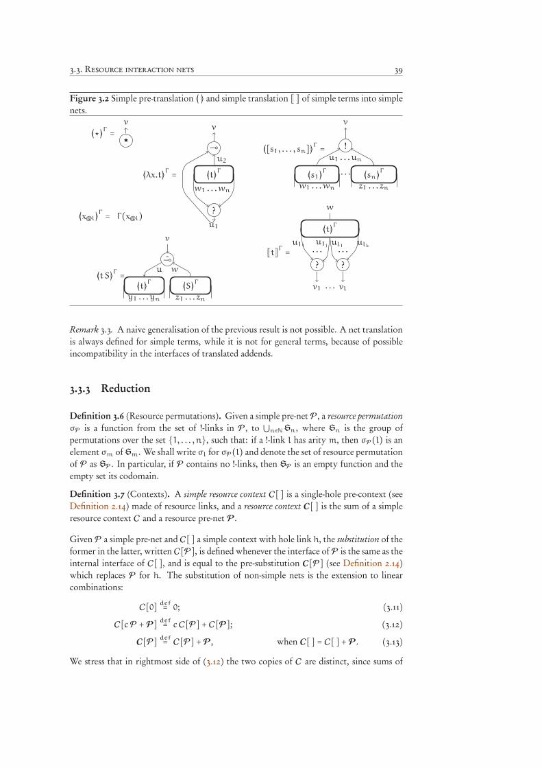
3.3. Resource interaction nets 39
Figure 3.2 Simple pre-translation & ' and simple translation ⟦ ⟧ of simple terms into simplenets.
!⋆"Γ=
★
v
!x@i"Γ= Γ(x@i)
!λx.t"Γ= !t"
Γ
⊸
v
?
u2
u1
w1 . . .wn
![s1, . . . , sn]"Γ=
!s1"Γ . . . !sn"
Γ
!
v
u1 . . . un
w1 . . .wn z1 . . . zn
!t S"Γ=
!t"Γ
!S"Γ
⊸
v
u w
y1 . . . yn z1 . . . zn
⟦t⟧Γ=
!t"Γ
w
? ?
v1 vl
. . . . . .
. . .
u11u1j ul1
ulk
Remark 3.3. A naive generalisation of the previous result is not possible. A net translationis always defined for simple terms, while it is not for general terms, because of possibleincompatibility in the interfaces of translated addends.
3.3.3 Reduction
Definition 3.6 (Resource permutations). Given a simple pre-net P, a resource permutationσP is a function from the set of !-links in P, to ⋃n∈NSn, where Sn is the group ofpermutations over the set {1, . . . , n}, such that: if a !-link l has arity m, then σP(l) is anelement σm of Sm. We shall write σl for σP(l) and denote the set of resource permutationof P as SP . In particular, if P contains no !-links, then SP is an empty function and theempty set its codomain.
Definition 3.7 (Contexts). A simple resource context C[ ] is a single-hole pre-context (seeDefinition 2.14) made of resource links, and a resource context C[ ] is the sum of a simpleresource context C and a resource pre-net P.
Given P a simple pre-net and C[ ] a simple context with hole link h, the substitution of theformer in the latter, written C[P], is defined whenever the interface of P is the same as theinternal interface of C[ ], and is equal to the pre-substitution C[P] (see Definition 2.14)which replaces P for h. The substitution of non-simple nets is the extension to linearcombinations:
C[0] def= 0; (3.11)
C[cP +P] def= cC[P] + C[P]; (3.12)
C[P] def= C[P] +P, when C[ ] = C[ ] +P. (3.13)
We stress that in rightmost side of (3.12) the two copies of C are distinct, since sums of
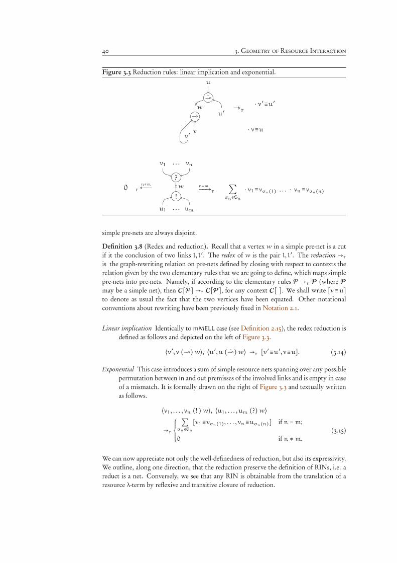
40 3. Geometry of Resource Interaction
Figure 3.3 Reduction rules: linear implication and exponential.
⊸
⊸
u
u′
vv′
w →r
⋅ v′≡u′
⋅ v≡u
?
!
v1 . . . vn
u1. . . um
w n=m
−−→r ∑σn∈Sn
⋅ v1≡vσn(1) . . . ⋅ vn≡vσn(n)0 r
n≠m
←−−
simple pre-nets are always disjoint.
Definition 3.8 (Redex and reduction). Recall that a vertex w in a simple pre-net is a cutif it the conclusion of two links l, l ′. The redex of w is the pair l, l ′. The reduction →r
is the graph-rewriting relation on pre-nets defined by closing with respect to contexts therelation given by the two elementary rules that we are going to define, which maps simplepre-nets into pre-nets. Namely, if according to the elementary rules P →r P (where P
may be a simple net), then C[P] →r C[P], for any context C[ ]. We shall write [v ≡u]to denote as usual the fact that the two vertices have been equated. Other notationalconventions about rewriting have been previously fixed in Notation 2.1.
Linear implication Identically to mMELL case (see Definition 2.15), the redex reduction isdefined as follows and depicted on the left of Figure 3.3.
⟨v ′, v (⊸) w⟩, ⟨u ′, u (⊸) w⟩ →r [v ′≡u ′, v≡u]. (3.14)
Exponential This case introduces a sum of simple resource nets spanning over any possiblepermutation between in and out premisses of the involved links and is empty in caseof a mismatch. It is formally drawn on the right of Figure 3.3 and textually writtenas follows.
⟨v1, . . . , vn (! ) w⟩, ⟨u1, . . . , um (?) w⟩
→r
⎧⎪⎪⎪⎨⎪⎪⎪⎩
∑σn∈Sn
[v1≡vσn(1), . . . , vn≡uσn(n)] if n =m;
0 if n ≠m.(3.15)
We can now appreciate not only the well-definedness of reduction, but also its expressivity.We outline, along one direction, that the reduction preserve the definition of RINs, i.e. areduct is a net. Conversely, we see that any RIN is obtainable from the translation of aresource λ-term by reflexive and transitive closure of reduction.
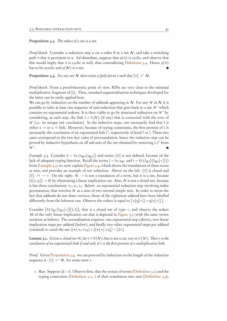
3.3. Resource interaction nets 41
Proposition 3.3. The reduct of a net is a net.
Proof sketch. Consider a reduction step ρ on a redex R in a net N , and take a switchingpath π that is persistent to ρ. Ad absurdum, suppose that ρ(π) is cyclic, and observe thatthis would imply that π is cyclic as well, thus contradicting Definition 3.4. Hence ρ(π)has to be acyclic and ρ(N ) is a net. ∎
Proposition 3.4. For any net N there exists a (poly-)term t such that ⟦t⟧→∗ N .
Proof sketch. From a proof-theoretic point of view, RINs are very close to the minimalmultiplicative fragment of LL. Then, standard sequentialisation techniques developed forthe latter can be easily applied here.We can go by induction on the number of addends appearing in N . For any N in N it ispossible to infer at least one sequence of anti-reduction that goes back to a net N ′ whichcontains no exponential redexes. It is then viable to go by structural induction on N ′ byconsidering, at each step, the link l ∈ L(N ) (if any) that is connected with the root ofN (i.e. its unique out conclusion). In the inductive steps, one necessarily find that l iseither a ⊸ or a ⊸ link. Moreover, because of typing constraints, the first premiss of l isnecessarily the conclusion of an exponential link l ′, respectively of kind ? or !. These twocases correspond to the two key rules of pre-translation, hence the inductive step can beproved by inductive hypothesis on all sub-nets of the net obtained by removing l, l ′ fromN ′. ∎
Example 3.3. Consider δ = λx.(x@1[x@2]) and notice ⟦δ⟧ is not defined, because of thelack of adequate typing function. Recall the terms I = λx.x@1 and t = λf.(f@1[(f@2[⋆])])from Example 3.2; we now explain Figure 3.4, which shows the translations of these termsas nets, and provides an example of net reduction. Above on the left: ⟦I⟧ is closed and⟦I⟧ ∶ !⋆ ⊸ ⋆. On the right: N ∶ ⋆ is not a translation of a term, but it is a net, because⟦t[x, y]⟧→N by eliminating a linear implication cut. Also, N is not a closed net, becauseit has three conclusions: v1, z1, z2. Below: an exponential reduction step involving indexpermutation, that rewrites N as a sum of two normal simple nets. In order to stress thefact that addends do not share vertices, those of the rightmost addend have been labelleddifferently from the leftmost one. Observe the reduct is equal to ⟦x[y[⋆]] + y[x[⋆]] ⟧.Consider ⟦λf.f@1[f@2[⋆]][I, I]⟧, that is a closed net of type ⋆, and observe the reductM of the only linear implication cut that is depicted in Figure 3.5 (with the same vertexnotation as before). The normalisation requires: one exponential step (above), two linearimplication steps per addend (below), and finally two other exponential steps per addend(omitted) to reach the net ⟨(★) v1≡v8⟩ + ⟨(★) v ′1≡v ′8⟩ = ⟦2⋆⟧.Lemma 3.1. Given a closed netN , let v ∈ V(N ) that is not a cut, nor in C(N ). Then v is theconclusion of an exponential link if and only if v is the first premiss of a multiplicative link.
Proof. Given Proposition 3.4, we can proceed by induction on the length of the reductionsequence ρ ∶ ⟦t⟧→∗ N , for some term t.
1. Base. Suppose ∣ρ∣ = 0. Observe first, that the syntax of terms (Definition 3.1) and thetyping constraints (Definition 2.2, ) of their translation into nets (Definition 3.5),
42 3. Geometry of Resource Interaction
Figure 3.4 Example: nets and reduction.
⟦I⟧ =
⊸
w1
?
w2
w3
N =
v1
⊸
!
⊸
?
!
!
★
z2 z1
v2
v4
v5
v6v7
v3 v8
N →r
v1
⊸
!
⊸
!
★
v2≡z2 v6≡z1
v4
v5
v7
v8
+
v′
1
⊸
!
⊸
!
★
v′
6≡z′
2v′
2≡z′
1
v′
4
v′
5
v′
7
v′
8
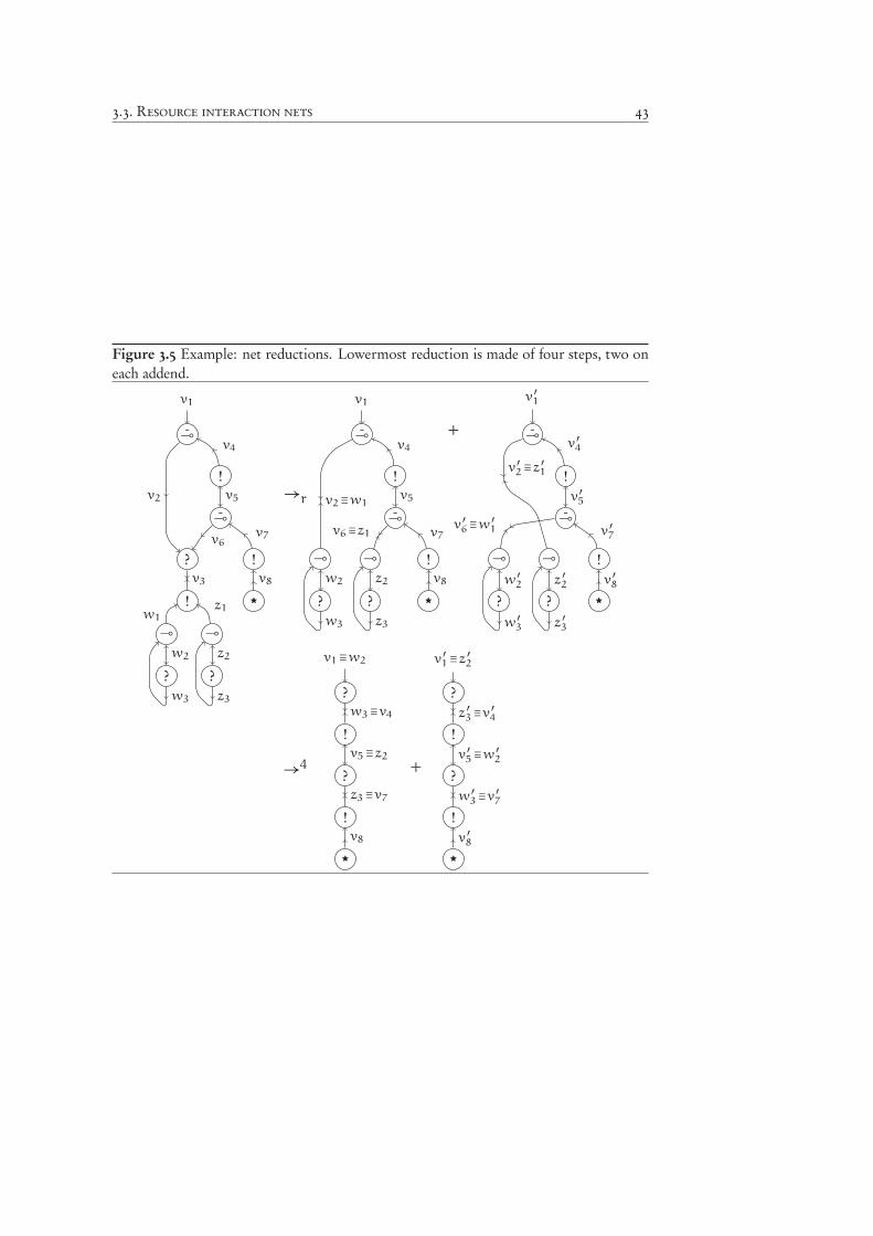
3.3. Resource interaction nets 43
Figure 3.5 Example: net reductions. Lowermost reduction is made of four steps, two oneach addend.
⊸
?
w2
w3
⊸
?
z2
z3
v1
⊸
!
⊸
?
!
!
★
v2
v4
v5
v6v7
v3 v8
w1
z1
→r
⊸
?
w2
w3
⊸
?
z2
z3
v1
⊸
!
⊸
!
★
v2≡w1
v4
v5
v6≡z1 v7
v8
+
⊸
?
w′
2
w′
3
⊸
?
z′
2
z′
3
v′
1
⊸
!
⊸
!
★
v′
2≡z′
1
v′
4
v′
5
v′
6≡w
′
1 v′
7
v′
8
→4
v1≡w2
?
!
?
!
★
w3≡v4
v5≡z2
z3≡v7
v8
+
v′
1≡z′
2
?
!
?
!
★
z′
3≡v′
4
v′
5≡w
′
2
w′
3≡v′
7
v′
8
44 3. Geometry of Resource Interaction
forces ⟦t⟧ to have the out conclusion r typed either with ⋆ or with⊸, otherwise t
would be a polyterm, contradicting the hypothesis. Therefore, a vertex that is theconclusion of an exponential link or the first premiss of a multiplicative one, cannotbe r, nor any another in conclusion of ⟦t⟧, because, since ⟦t⟧ is closed, there arenot. Secondly, an immediate verification of the definition of translation shows thatthe statement holds for ⟦t⟧, since: a ⊸-link and a ?-link are introduced when pre-translating an abstraction; a ⊸-link and a !-link are introduced when pre-translatingan application and the polyterm; and in both cases the statement holds.
2. Step. Suppose ∣ρ∣ > 0 and let ρ = ρ ′ρ ′′, for some reduction sequence ρ ′′, and for somestep ρ ′ of our interest acting on a redex R. For any z ∉ R the inductive hypothesis(IH) is trivially preserved. So let us focus on R and distinguish two cases dependingits type.
(a) T (R) = ⊸/⊸. Let R = ⟨u, v (⊸) w⟩, ⟨u ′, v ′ (⊸) w⟩. By IH, since v and v ′
are the first premisses of two multiplicative links, they must be conclusions ofa ?- and a !-link, respectively. Now, in ρ ′(R) we have the vertex v≡ v ′, wherethe claim trivially holds since it is a cut.
(b) T (R) = !/?. Let R = ⟨v1 . . . vn (?) w⟩, ⟨u1 . . . um (! ) w⟩. If n ≠ m thenρ ′(R) = 0 and there is nothing to prove, so let us assume otherwise. We showthat no vertex z in R can satisfy any of the two statements whose co-implicationis claimed.
i. If z = w, then it is a cut. Moreover, z cannot be the premiss of any link,since in R there are already two links connected to z, (cf. Definition 2.3,item 1).
ii. If z = vi (or z = ui ) for some 1 ≤ i ≤ n, then we observe that it cannotbe the conclusion of an exponential link l, nor the first premiss of a mul-tiplicative link l ′, since it would violate the typing constraints. Indeed,it must be the case that T (z) = !A, where either A = T (x) and x is anypremiss of l, or !A⊸ B = T (y) and y is the conclusion of l ′. This wouldrequire that T (w) = !!A, which does not belong to the grammar of types(cf. Definition 2.2).
∎
The following lemma may be used to prove the completeness of a new correctness criteriawith respect to the simple net we defined by translation.
Lemma 3.2 (Quasi-connectedness). For any simple net N such that N /→ 0, and any subnetN ′ ⊂ N , there exists no path connecting N ′ to the positive conclusion of N if and only if allthe links of N ′ are (co-)weakenings.
Proof. The “if” direction of the bi-implication in the thesis is obvious, from the fact thatany subnet built from (co-)weakenings have no conclusions and must be disconnectedfrom the main net’s conclusion. For the “only if” part, we use Proposition 3.4, and weproceed by induction on the length of the (possibly empty) reduction sequence ρ ∶ ⟦t⟧→∗N +N , for some term t and net N .
3.4. Resource paths 45
1. ∣ρ∣ = 0. Trivial – simply observe the ⟦⋅⟧ does not allow disconnections. ◻
2. ∣ρ∣ > 0 Suppose that ρ = ρ ′ρ ′′, for some reduction sequence ρ ′′ where the thesisholds (IH) and some reduction step ρ ′ on a redex R.
(a) If ρ ′ is a linear implication step, then, because of Lemma 3.1, the only dis-connection possibly created comes from a weakening connected to the firstspremiss of the⊸-link l ∈ R. Let us suppose it is the case, because otherwise IHis trivially preserved. Now, by definition of nets, and in particular by Defin-ition 2.3 and 2.2, the first premiss of the ⊸-link must be a !-link l ′. Then inρ ′(N ) the vertices l, l ′ form an exponential redex, which by hypothesis cannotmake N implode in 0, therefore by Equation 3.15 l must be a co-weakening.Hence N ′ = {l, l ′} and we conclude. ⧫
(b) Otherwise ρ ′ is a exponential implication step between two exponential linksl, l ′None of the premisses of l, l ′ can be the conclusion of a (co-) weakening, asstated by Lemma 3.1, therefore no new disconnection may be possibly created.Hence, the IH is trivially preserved and we conclude. ⧫
◻
∎
Proposition 3.5. Any two resource redex in a net are parallel.1.
Proof. Notice that any redex in a resource net involve exactly two links, one positive andone negative, and also that the cut involves the principal ports of the two links. These twofacts imply that two redexes cannot overlap. ∎
Proposition 3.6. Net reduction strongly normalises. Moreover, it simulates term reductionvia translation: for any term t, if t → t ′, then ⟦t⟧ →2
r ⟦t ′⟧ with a (⊸ /⊸)-step followed by a(!/?)-step.
Proof. See Tranquilli [2011] on the promotion-enabled generalisation of RINs and RC. ∎
3.4 Resource paths
We study the action of the reduction on paths, first by defining the appropriate notionof residual, i.e. the result of a reduction, and that of persistence, i.e. the capability ofresisting any reduction, that is a sort of normalisability.
3.4.1 Statics
Recall the basic definitions needed to ensure visibility by a GoI construction of the com-putation in a path, that are straightness and maximality introduced in Definition 2.17. In
1 For an introduction to basic concepts of rewriting theory in the more classic settings of terms, we addressthe reader, for instance, at Baader and Nipkow [1998].
46 3. Geometry of Resource Interaction
addition to those, we define a notion of comprehensiveness enabling a path to see the en-tirety of the computation. This last notion is the only original difference with respect tothe classic notion of path as formulated in Danos and Regnier [1995].
Definition 3.9 (Comprehensiveness). A path π ∈ N is comprehensive when it crosses allthe premisses of all the exponential links. The set of comprehensive execution paths in anysimple net N being a (non-zero) addend of N is written PEC(N ).Example 3.4. Recall the nets discussed in Example 3.3 and observe again Figure 3.4. Con-sider the net ⟦I⟧ and the path φ = (w1,w2,w3), which is straight and also maximal.Moreover, PE(⟦I⟧) = {φ,φ†}. Notice that in N the paths (v1, v4) and (v1, v2, v1) are notstraight — the former is twisting, while the latter is bouncing. What about PE(N )? Ifwe start from v1 we find two paths seeking for the head variable: π1 = (v1, v2, v3, z1) andπ2 = (v1, v2, v3, z2). Both π1, π2 are straight and maximal, thus execution, but they arenot comprehensive, since they do not cross v4 nor v7.
3.4.2 Dynamics
With the notions just introduced we now define the property of path persistence, thatintuitively means “surviving cut-elimination”. We first inspect the action of reduction onpaths, and isolate the notion of residual of a given path with respect to a given reduction.We shall go by induction on its subpaths that pass through a given redex, called crossings,and say that the residual(s) of a path are obtained by the substitution of the crossing withits residual(s), that are the images of reduction as naturally induced by the graph-rewriting.The case of linear implication is straightforward, because the rewriting is local and we onlyhave to ensure that a path does not partially belong to the redex. The case of exponentialsis instead more delicate, because the rewriting is global: a simple net is rewritten as a sumof simple nets, hence a path may be duplicated in several addends or destroyed. Whichaddends contain the residual(s) of a given crossing of the redex? If the reduction of anexponential redex R rewrites the simple net to which it belongs as the empty sum, thenalso the residual of the crossing is 0. Otherwise, the reduction rewrites the net as a sum ofsimple nets where any crossing always has a residual (cf. Definition 3.8). But two crossingsof R within a path may have residuals in different simple nets created by the reduction,each one obtained from a fixed permutation of premisses to substitute R. Therefore, theresidual of a path is a sum of paths, morally varying on the set of permutations they areallowed to follow.
Definition 3.10 (Linear implication residual). Let N be a net where χ ∈ P(N ) is a cross-ing of a linear implication redex R (see Definition 2.18). Suppose R as in the topmostredex of Figure 3.3 or, equivalently, as in Equation 3.14, and let ρ be the reduction stepon R. Then the residual of χ with respect to ρ, is defined as follows and by the ruleρ(χ†) = (ρ(χ))†.
ρ((v,w,u)) def= (v); (3.16)
ρ((v ′,w,u ′)) def= (v ′); (3.17)
ρ((v,w,u ′)) def= 0; (3.18)
ρ((v ′,w,u)) def= 0. (3.19)
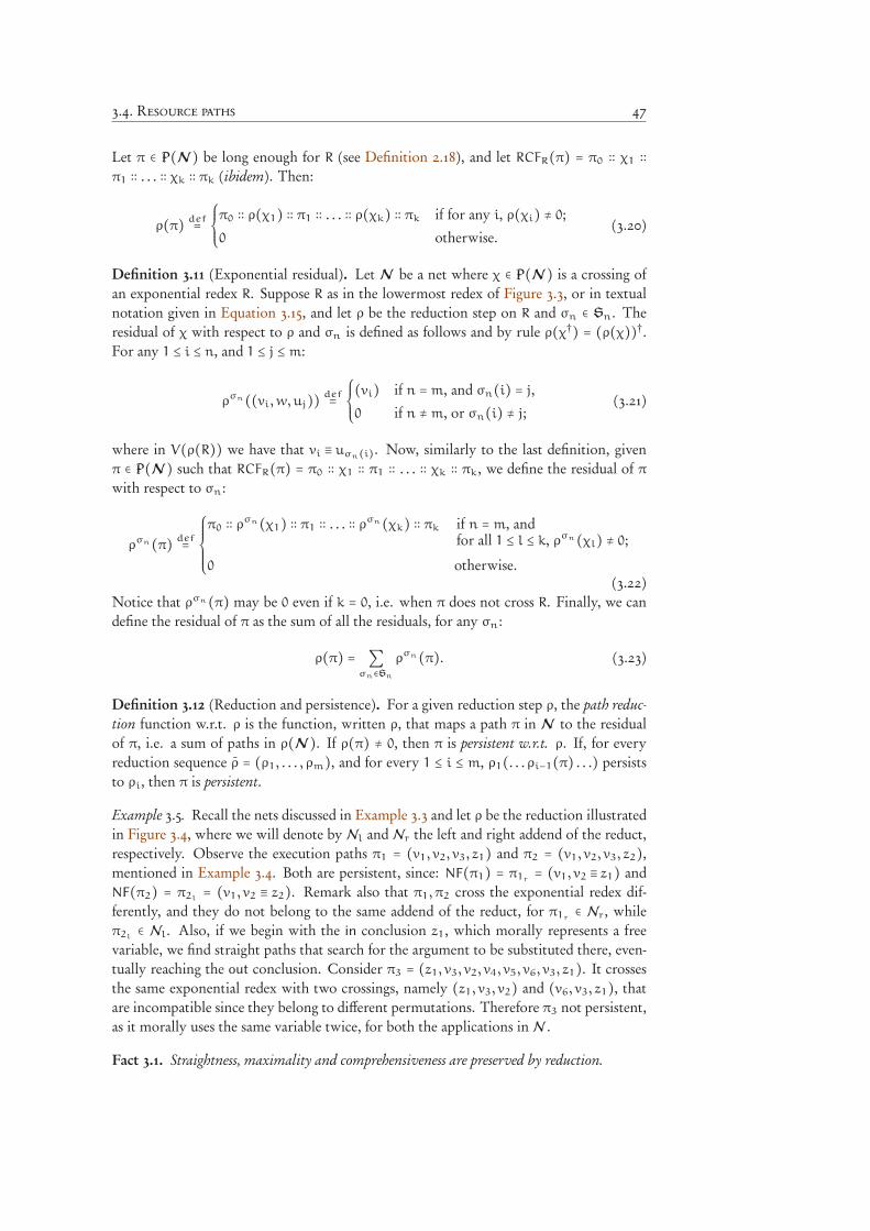
3.4. Resource paths 47
Let π ∈ P(N ) be long enough for R (see Definition 2.18), and let RCFR(π) = π0 ∶∶ χ1 ∶∶
π1 ∶∶ . . . ∶∶ χk ∶∶ πk (ibidem). Then:
ρ(π) def=
⎧⎪⎪⎨⎪⎪⎩π0 ∶∶ ρ(χ1) ∶∶ π1 ∶∶ . . . ∶∶ ρ(χk) ∶∶ πk if for any i, ρ(χi) ≠ 0;
0 otherwise.(3.20)
Definition 3.11 (Exponential residual). Let N be a net where χ ∈ P(N ) is a crossing ofan exponential redex R. Suppose R as in the lowermost redex of Figure 3.3, or in textualnotation given in Equation 3.15, and let ρ be the reduction step on R and σn ∈ Sn. Theresidual of χ with respect to ρ and σn is defined as follows and by rule ρ(χ†) = (ρ(χ))†.For any 1 ≤ i ≤ n, and 1 ≤ j ≤m:
ρσn((vi,w,uj)) def=
⎧⎪⎪⎨⎪⎪⎩(vi) if n =m, and σn(i) = j,
0 if n ≠m, or σn(i) ≠ j;(3.21)
where in V(ρ(R)) we have that vi ≡ uσn(i). Now, similarly to the last definition, givenπ ∈ P(N ) such that RCFR(π) = π0 ∶∶ χ1 ∶∶ π1 ∶∶ . . . ∶∶ χk ∶∶ πk, we define the residual of π
with respect to σn:
ρσn(π) def=
⎧⎪⎪⎪⎪⎨⎪⎪⎪⎪⎩
π0 ∶∶ ρσn(χ1) ∶∶ π1 ∶∶ . . . ∶∶ ρ
σn(χk) ∶∶ πk if n =m, andfor all 1 ≤ l ≤ k, ρσn(χl) ≠ 0;
0 otherwise.(3.22)
Notice that ρσn(π) may be 0 even if k = 0, i.e. when π does not cross R. Finally, we candefine the residual of π as the sum of all the residuals, for any σn:
ρ(π) = ∑σn∈Sn
ρσn(π). (3.23)
Definition 3.12 (Reduction and persistence). For a given reduction step ρ, the path reduc-tion function w.r.t. ρ is the function, written ρ, that maps a path π in N to the residualof π, i.e. a sum of paths in ρ(N ). If ρ(π) ≠ 0, then π is persistent w.r.t. ρ. If, for everyreduction sequence ρ = (ρ1, . . . , ρm), and for every 1 ≤ i ≤ m, ρ1(. . . ρi−1(π) . . .) persiststo ρi, then π is persistent.
Example 3.5. Recall the nets discussed in Example 3.3 and let ρ be the reduction illustratedin Figure 3.4, where we will denote by Nl and Nr the left and right addend of the reduct,respectively. Observe the execution paths π1 = (v1, v2, v3, z1) and π2 = (v1, v2, v3, z2),mentioned in Example 3.4. Both are persistent, since: NF(π1) = π1r
= (v1, v2 ≡ z1) andNF(π2) = π2l
= (v1, v2 ≡ z2). Remark also that π1, π2 cross the exponential redex dif-ferently, and they do not belong to the same addend of the reduct, for π1r
∈ Nr, whileπ2l∈ Nl. Also, if we begin with the in conclusion z1, which morally represents a free
variable, we find straight paths that search for the argument to be substituted there, even-tually reaching the out conclusion. Consider π3 = (z1, v3, v2, v4, v5, v6, v3, z1). It crossesthe same exponential redex with two crossings, namely (z1, v3, v2) and (v6, v3, z1), thatare incompatible since they belong to different permutations. Therefore π3 not persistent,as it morally uses the same variable twice, for both the applications in N .
Fact 3.1. Straightness, maximality and comprehensiveness are preserved by reduction.
48 3. Geometry of Resource Interaction
3.4.3 Comprehensiveness and bijection
The persistence property of a path naturally implies that it travels only through verticeswhose links morally contribute to the normalisation — a persistent path cannot cross(co-)weakenings2. Therefore, if we restrict ourselves to closed nets of constant type, weobtain a stronger property: a persistent execution path travel through all vertices of thenet that are not conclusions of a 0-ary exponential links. Despite what the creation ofsums may suggest at a first glance, RINs do not allow for duplication of paths. Intuitively,the set of persistent ones is split from the simple net containing the redex into the addendscreated by the reduction. We shall show indeed that path reduction for any step ρ inducesa bijection between the persistent paths of a net N and those of ρ(N ). To prove these twofacts, we first explicit in the next lemma an expected property: the alternation betweenmultiplicative and exponential operators that lies in the grammar of types has a naturaland graphical counterpart in links of nets.
Lemma 3.3. In a closed net N ∶ ★ any persistent execution path is comprehensive.
Proof. We shall prove a stronger statement: given a persistent path π ∈ PE(N ), a vertexv ∉ π if and only if there exists a (co-)weakening l such that v ∈ C(l).
1. The “if” direction of the claim follows from a mere observation of the Definition 2.6of execution paths. If π includes a conclusion of a (co-)weakening, then π is neces-sarily bouncing or non-maximal, in both cases contradicting the hypothesis that π
is an execution path. ◻
2. In order to prove the “only if” part of the claim, let us first recall that, by Defini-tion 3.4, for any simple net N ′ there exists a term such that N ′ either appears in itstranslation, or in some of its reducts. We now go by induction on a sequence (ρ)−1of expansions (or an anti-sequence of reductions) from NF(N ) back to N = ⟦t⟧, forsome term t. If NF(N ) = 0 there is nothing to prove, so we shall assume it to benon-zero.
a. Base. Suppose ∣ρ∣ = 0. Then NF(N ) = N = c ⟦t⟧ = ⟦c t⟧ for some c ∈ N.Therefore t = ⋆, because the only closed term whose translation is normalwith respect to net reduction is ⋆. Then ⟦t⟧ = ⟨(★) v⟩, and PE(⟦t⟧) = {(v, v)},hence the claim. ⧫
b. Step. Suppose ∣ρ∣ > 0. Let ρ ∶ N → N′ and N
′→∗ NF(N ). Also, let R be the
redex eliminated by ρ, and C[ ] its context. We then distinguish two sub-casesdepending on the type of R.
i. T (R) =⊸/⊸. Suppose N ′ to be an addend of N ′ containing the verticesv≡v1 ≡v2 and u≡u1 ≡u2, and assume N to be the addend of N contain-ing u, v. Let the expansion step be the following, which introduces thedistinct vertices v1, v2, u1, u2,w.
N′= C[u1≡u2, v1≡v2] ← C[⟨u1, v1 (⊸) w⟩, ⟨u2, v2 (⊸) w⟩]
(3.24)2The remark can be generalised also to GoI constructions for non-linear calculi, such as the ordinary λ-
calculus or mMELL proof-nets (presented in Chapter 2), where an abstraction with no occurrences of the boundvariable may erase its argument, or a weakening may erase the box that is cut with.
3.4. Resource paths 49
We firstly assume that π ∈ N ′, because otherwise π is unaffected andthe IH would be trivially preserved. Now v1, v2 are second premisses ofthe cut links, therefore, as established by Lemma 3.1, they cannot be theconclusion of a (co-)weakening, and consequently neither v can. Hence,by IH, v ∈ π and it is enough to observe, by Definition 3.10, that alsov1, v2 ∈ ρ−1(π). Let’s now discuss u. Observe first that, since u1 andu2 are first premisses of multiplicative links, we know from Lemma 3.1that they both must be conclusion of exponential links. Therefore, andby definition of reduction, u has to be an exponential cut. We distinguishtwo sub-cases.A. If u ∉ π, then by definition of path reduction, u1, u2 ∉ ρ−1(π).
Moreover, by IH we have that u the conclusion of a weakening ora co-weakening link.I. If u is the conclusion of a weakening, then observe that the co-
contraction whose conclusion is u must have arity 0. Otherwise,the reduction of u would rewrite N ′ as 0, contradicting the persist-ence hypothesis for π.
II. If instead u the conclusion of a co-weakening, then, dually withrespect to the previous case, and for the same reductio ad absurdum,the contraction that has conclusion in u must have arity 0.
Hence, in both cases u is a cut between 0-ary exponentials, which bydefinition of reduction implies that u1, u2 are respectively conclusionsof a weakening and a co-weakening link. ▲
B. Otherwise, u ∈ π. Then again by inspection of Definition 3.10, weverify that u1, u2 ∈ ρ
−1(π). ▲
◊
ii. T (R) = !/?. If the expansion affects no addends, i.e. if the reductionrewrites as 0 a simple net in N
′, then π is unaffected, since we assumed itto be persistent, and IH is trivially preserved. Otherwise, the arity of thetwo exponential links are equal, so let ρ be as follows.
C
⎡⎢⎢⎢⎣ ∑σn∈Sn
v1≡uσn(1), . . . , vn≡uσn(n)⎤⎥⎥⎥⎦
← C [⟨v1, . . . , vn (! ) w⟩, ⟨u1, . . . , un (?) w⟩] . (3.25)
A. If n = 0, and the reduct of the redex is empty, then trivially π cannotnot cross it. Nor can cross the redex, since the redex is made by awakening and a co-weakening link, and we supposed π maximal andpersistent. ▲
B. If n > 0, then let σn ∈ Sn and consider the vertex vi ≡ uσn(i). No-tice that it cannot be the conclusion of a 0-ary exponential link. Bycontraposition, suppose otherwise and notice that, by definition oftyping, in the reducendum we would have T (vi ≡ vσn(i)) = !A forsome type A. This would absurdly imply T (w) = !!A, that is not avalid type. Not being a (co-)weakening conclusion, by IH we havethat vi ≡uσn(i) ∈ π. To conclude it is then sufficient to observe thatby definition of reduction, either (vi,w, vσn(i)) or its reversal belongto ρ−1(π). ▲
50 3. Geometry of Resource Interaction
◊
⧫
◻
∎
Remark 3.4. The notion of path comprehensiveness appears to be similar the the triplengthiness introduced by Girard [1989, §2.1, p. 30] to characterise proof-nets among thenets in the case of MLL. This should not surprise, since the structure of resource nets, inits essence, only adds non-deterministic superposition to the structure of the multiplic-ative fragment of linear logic. Furthermore, we conjecture path comprehensiveness canbe easily adapted to obtain a concise and elegant criterion for the correctness of simpleresource net.
Theorem 3.1 (Reduction is bijective on persistent paths). For any closed net N ∶ ★, everyreduction step ρ induces a bijection between execution paths in N that are persistent to ρ andthose in ρ(N ).
Proof. Let π ∈ PE(N ) be persistent to ρ, let R the redex of ρ, and suppose RCFR(π) = π0 ∶∶
χ1 ∶∶ π1 ∶∶ . . . ∶∶ χk ∶∶ πk. There are two reduction rules possibly used by ρ.
1. T (R) =⊸/⊸. Because of the persistence of π to ρ, and by the definition given byEquation 3.20, we have χl ≠ 0, for all 0 ≤ l ≤ k, and ρ(π) = π0 ∶∶ ρ(χ1) ∶∶ π1 ∶∶ . . . ∶∶
ρ(χk) ∶∶ πk. Then, if ρ is as in Figure 3.3, the bijection is given as follows:
(a) χl = (v,w,u) if and only if ρ(χl) = (v);(b) χl = (v ′,w,u ′) if and only if ρ(χl) = (v ′).
Such a bijection holds between χl and ρ(χl), so we also have a bijection between π
and ρ(π). ◻
2. T (R) = !/?. Suppose the redex R being as in Figure 3.3. Because of the persistenceof π to ρ, and by the definition given by Equation 3.22 and 3.23, it must be the casethat n =m and that there exists a permutation σn ∈ Sn such that for all 0 ≤ l ≤ k, wehave ρσn(χl) ≠ 0. Moreover, by Lemma 3.3, π is comprehensive, which in particularmeans that vi, uj ∈ π for any 1 ≤ i, j ≤ n. Hence, for any 1 ≤ i ≤ n there exist0 ≤ l ≤ k and 0 ≤ j ≤ n such that χl is either (v1,w,uj) or its reversal. In both cases,by Equation 3.21, it must be the case that σn(i) = j so that ρσn(χl) = (vσn(i)≡uj).This means that σn is unique, and for any other σ ′n we have ρσ
′
n(π) = 0. We thenobtained a one-to-one correspondence between π and ρ(π). ◻
∎
Theorem 3.2 (Paths and addends). For any closed simple net N ∶ ★, the number of executionpersistent paths in N is equal to the number of addends of the normal form of N .
Proof. Any addend in a normal net is the simple net made by ⋆, which evidently has onlyone execution path, the unitary one on the only vertex. The thesis therefore is a corollaryof Theorem 3.1. ∎
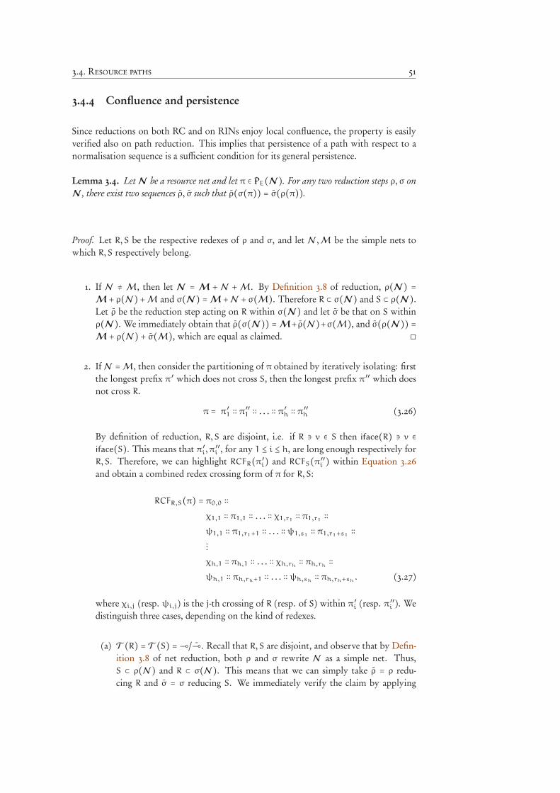
3.4. Resource paths 51
3.4.4 Confluence and persistence
Since reductions on both RC and on RINs enjoy local confluence, the property is easilyverified also on path reduction. This implies that persistence of a path with respect to anormalisation sequence is a sufficient condition for its general persistence.
Lemma 3.4. Let N be a resource net and let π ∈ PE(N ). For any two reduction steps ρ, σ onN , there exist two sequences ρ, σ such that ρ(σ(π)) = σ(ρ(π)).
Proof. Let R, S be the respective redexes of ρ and σ, and let N ,M be the simple nets towhich R, S respectively belong.
1. If N ≠ M , then let N = M + N +M . By Definition 3.8 of reduction, ρ(N ) =M + ρ(N )+M and σ(N ) =M +N +σ(M). Therefore R ⊂ σ(N ) and S ⊂ ρ(N ).Let ρ be the reduction step acting on R within σ(N ) and let σ be that on S withinρ(N ). We immediately obtain that ρ(σ(N )) =M+ρ(N )+σ(M), and σ(ρ(N )) =M + ρ(N ) + σ(M), which are equal as claimed. ◻
2. If N =M , then consider the partitioning of π obtained by iteratively isolating: firstthe longest prefix π ′ which does not cross S, then the longest prefix π ′′ which doesnot cross R.
π = π ′1 ∶∶ π′′
1 ∶∶ . . . ∶∶ π′
h ∶∶ π′′
h (3.26)
By definition of reduction, R, S are disjoint, i.e. if R ∋ v ∈ S then iface(R) ∋ v ∈
iface(S). This means that π ′i, π′′
i , for any 1 ≤ i ≤ h, are long enough respectively forR, S. Therefore, we can highlight RCFR(π ′i) and RCFS(π ′′i ) within Equation 3.26and obtain a combined redex crossing form of π for R, S:
RCFR,S(π) = π0,0 ∶∶
χ1,1 ∶∶ π1,1 ∶∶ . . . ∶∶ χ1,r1 ∶∶ π1,r1 ∶∶
ψ1,1 ∶∶ π1,r1+1 ∶∶ . . . ∶∶ ψ1,s1∶∶ π1,r1+s1
∶∶
⋮
χh,1 ∶∶ πh,1 ∶∶ . . . ∶∶ χh,rh ∶∶ πh,rh ∶∶
ψh,1 ∶∶ πh,rh+1 ∶∶ . . . ∶∶ ψh,sh∶∶ πh,rh+sh
. (3.27)
where χi,j (resp. ψi,j ) is the j-th crossing of R (resp. of S) within π ′i (resp. π ′′i ). Wedistinguish three cases, depending on the kind of redexes.
(a) T (R) = T (S) =⊸/⊸. Recall that R, S are disjoint, and observe that by Defin-ition 3.8 of net reduction, both ρ and σ rewrite N as a simple net. Thus,S ⊂ ρ(N ) and R ⊂ σ(N ). This means that we can simply take ρ = ρ redu-cing R and σ = σ reducing S. We immediately verify the claim by applying
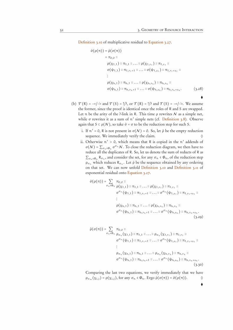
52 3. Geometry of Resource Interaction
Definition 3.10 of multiplicative residual to Equation 3.27.
σ(ρ(π)) = ρ(σ(π))= π0,0 ∶∶
ρ(χ1,1) ∶∶ π1,1 ∶∶ . . . ∶∶ ρ(χ1,r1) ∶∶ π1,r1 ∶∶
σ(ψ1,1) ∶∶ π1,r1+1 ∶∶ . . . ∶∶ σ(ψ1,s1) ∶∶ π1,r1+s1
∶∶
⋮
ρ(χh,1) ∶∶ πh,1 ∶∶ . . . ∶∶ ρ(χh,rh) ∶∶ πh,rh ∶∶
σ(ψh,1) ∶∶ πh,rh+1 ∶∶ . . . ∶∶ σ(ψh,sh) ∶∶ πh,rh+sh
. (3.28)
⧫
(b) T (R) = ⊸/⊸ and T (S) = !/?, or T (R) = !/? and T (S) = ⊸/⊸. We assumethe former, since the proof is identical once the roles of R and S are swapped.Let n be the arity of the ?-link in R. This time ρ rewrites N as a simple net,while σ rewrites it as a sum of n ′ simple nets (cf. Definition 3.8). Observeagain that S ⊂ ρ(N ), so take σ = σ to be the reduction step for such S.
i. If n ′ = 0, R is not present in σ(N ) = 0. So, let ρ be the empty reductionsequence. We immediately verify the claim. ◊
ii. Otherwise n ′ > 0, which means that R is copied in the n ′ addends ofσ(N ) = ∑σn∈Sn
σσnN . To close the reduction diagram, we then have toreduce all the duplicates of R. So, let us denote the sum of reducts of R as∑σn∈Sn
Rσn, and consider the set, for any σn ∈ Sn, of the reduction step
ρσnwhich reduces Rσn
. Let ρ be the sequence obtained by any orderingon that set. We can now unfold Definition 3.10 and Definition 3.11 ofexponential residual onto Equation 3.27.
σ(ρ(π)) = ∑σn∈Sn
π0,0 ∶∶
ρ(χ1,1) ∶∶ π1,1 ∶∶ . . . ∶∶ ρ(χ1,r1) ∶∶ π1,r1 ∶∶
σσn(ψ1,1) ∶∶ π1,r1+1 ∶∶ . . . ∶∶ σσn(ψ1,s1
) ∶∶ π1,r1+s1∶∶
⋮
ρ(χh,1) ∶∶ πh,1 ∶∶ . . . ∶∶ ρ(χh,rh) ∶∶ πh,rh ∶∶
σσn(ψh,1) ∶∶ πh,rh+1 ∶∶ . . . ∶∶ σσn(ψh,sh
) ∶∶ πh,rh+sh.
(3.29)
ρ(σ(π)) = ∑σn∈Sn
π0,0 ∶∶
ρσn(χ1,1) ∶∶ π1,1 ∶∶ . . . ∶∶ ρσn
(χ1,r1) ∶∶ π1,r1 ∶∶
σσn(ψ1,1) ∶∶ π1,r1+1 ∶∶ . . . ∶∶ σσn(ψ1,s1
) ∶∶ π1,r1+s1∶∶
⋮
ρσn(χh,1) ∶∶ πh,1 ∶∶ . . . ∶∶ ρσn
(χh,rh) ∶∶ πh,rh ∶∶
σσn(ψh,1) ∶∶ πh,rh+1 ∶∶ . . . ∶∶ σσn(ψh,sh
) ∶∶ πh,rh+sh.
(3.30)
Comparing the last two equations, we verify immediately that we haveρσm(χi,j) = ρ(χi,j), for any σn ∈ Sn. Ergo ρ(σ(π)) = σ(ρ(π)). ◊
⧫
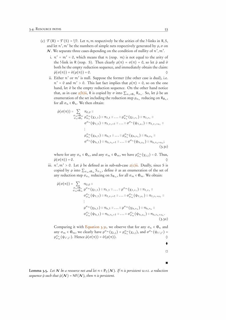
3.4. Resource paths 53
(c) T (R) = T (S) = !/?. Let n,m respectively be the arities of the ?-links in R, S,and let n ′,m ′ be the numbers of simple nets respectively generated by ρ, σ onN . We separate three cases depending on the condition of nullity of n ′,m ′.
i. n ′ = m ′ = 0, which means that n (resp. m) is not equal to the arity ofthe !-link in R (resp. S). Then clearly ρ(π) = σ(π) = 0, so let ρ and σ
both be the empty reduction sequence, and immediately obtain the claim:ρ(σ(π)) = σ(ρ(π)) = 0. ◊
ii. Either n ′ or m ′ is null. Suppose the former (the other case is dual), i.e.n ′ = 0 and m ′ > 0. This last fact implies that ρ(π) = 0, so on the onehand, let σ be the empty reduction sequence. On the other hand noticethat, as in case 2(b)ii, R is copied by σ into ∑σn∈Sn
Rσn. So, let ρ be an
enumeration of the set including the reduction step ρσnreducing on RSn
,for all σn ∈ Sn. We then obtain:
ρ(σ(π)) = ∑σm∈Sm
σn∈Sn
π0,0 ∶∶
ρσm
σn(χ1,1) ∶∶ π1,1 ∶∶ . . . ∶∶ ρ
σm
σn(χ1,r1) ∶∶ π1,r1 ∶∶
σσn(ψ1,1) ∶∶ π1,r1+1 ∶∶ . . . ∶∶ σσn(ψ1,s1
) ∶∶ π1,r1+s1∶∶
⋮
ρσm
σn(χh,1) ∶∶ πh,1 ∶∶ . . . ∶∶ ρ
σm
σn(χh,rh) ∶∶ πh,rh ∶∶
σσn(ψh,1) ∶∶ πh,rh+1 ∶∶ . . . ∶∶ σσn(ψh,sh
) ∶∶ πh,rh+sh;
(3.31)
where for any σn ∈ Sn, and any σm ∈ Sm, we have ρσmσn(χi,j) = 0. Thus,
ρ(σ(π)) = 0. ◊
iii. n ′,m ′ > 0. Let ρ be defined as in sub-sub-case 2(c)ii. Dually, since S iscopied by ρ into ∑σm∈Sm
Sσm, define σ as an enumeration of the set of
any reduction step σσnreducing on SSm
, for all σm ∈ Sm. We obtain:
ρ(σ(π)) = ∑σn∈Sn
σm∈Sm
π0,0 ∶∶
ρσm(χ1,1) ∶∶ π1,1 ∶∶ . . . ∶∶ ρσm(χ1,r1) ∶∶ π1,r1 ∶∶
σσn
σm(ψ1,1) ∶∶ π1,r1+1 ∶∶ . . . ∶∶ σ
σn
σm(ψ1,s1
) ∶∶ π1,r1+s1∶∶
⋮
ρσm(χh,1) ∶∶ πh,1 ∶∶ . . . ∶∶ ρσm(χh,rh) ∶∶ πh,rh ∶∶
σσn
σm(ψh,1) ∶∶ πh,rh+1 ∶∶ . . . ∶∶ σ
σn
σm(ψh,sh
) ∶∶ πh,rh+sh.
(3.32)
Comparing it with Equation 3.31, we observe that for any σn ∈ Sn andany σm ∈ Sm, we clearly have ρσm(χi,j) = ρσm
σn(χi,j), and σσn(ψi ′,j ′) =
ρσnσm(ψi ′,j ′). Hence ρ(σ(π)) = σ(ρ(π)). ◊
⧫
◻
∎
Lemma 3.5. Let N be a resource net and let π ∈ PE(N ). If π is persistent w.r.t. a reductionsequence ρ such that ρ(N ) = NF(N ), then π is persistent.
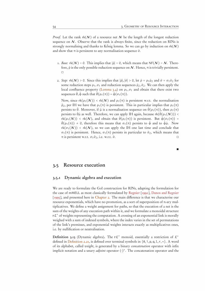
54 3. Geometry of Resource Interaction
Proof. Let the rank rk(N ) of a resource net N be the length of the longest reductionsequence on N . Observe that the rank is always finite, since the reduction on RINs isstrongly normalising and thanks to Kőnig lemma. So we can go by induction on rk(N )and show that π is persistent to any normalisation sequence σ.
1. Base: rk(N ) = 0. This implies that ∣ρ∣ = 0, which means that NF(N ) = N . There-fore, ρ is the only possible reduction sequence on N . Hence, π is trivially persistent.◻
2. Step: rk(N ) > 0. Since this implies that ∣ρ∣, ∣σ∣ > 0, let ρ = ρ1ρ2 and σ = σ1σ2 forsome reduction steps ρ1, σ1 and reduction sequences ρ2, σ2. We can then apply thelocal confluence property (Lemma 3.4) on ρ1, σ1 and obtain that there exist twosequences θ, φ such that θ(ρ1(π)) = φ(σ1(π)).Now, since rk(ρ1(N )) < rk(N ) and ρ1(π) is persistent w.r.t. the normalisationρ2, per IH we have that ρ1(π) is persistent. This in particular implies that ρ1(π)persists to θ. Moreover, if µ is a normalisation sequence on θ(ρ1(π)), then ρ1(π)persists to θµ as well. Therefore, we can apply IH again, because rk(θ(ρ1(N ))) <rk(ρ1(N )) < rk(N ), and obtain that θ(ρ1(π)) is persistent. But φ(σ1(π)) =θ(ρ1(π)) ≠ 0, therefore this means that σ1(π) persists to φ and to φµ. Nowrk(σ1(N )) < rk(N ), so we can apply the IH one last time and conclude thatσ1(π) is persistent. Hence, σ1(π) persists in particular to σ2, which means thatπ is persistent w.r.t. σ1σ2, i.e. w.r.t. σ. ◻
∎
3.5 Resource execution
3.5.1 Dynamic algebra and execution
We are ready to formulate the GoI construction for RINs, adapting the formulation forthe case of mMELL as most classically formulated by Regnier [1992], Danos and Regnier[1995], and presented here in Chapter 2. The main difference is that we characterise ourresource exponentials, which have no promotion, as a sort of superposition of n-ary mul-tiplicatives. We define a weight assignment for paths, so that the execution of a net is thesum of the weights of any execution path within it, and we formulate a monoidal structurerL∗ of weights representing the computation. A crossing of an exponential link is morally
weighed with a sum of indexed symbols, where the index varies in the set of permutationsof the link’s premisses, and exponential weights interacts exactly as multiplicatives ones,i.e. by nullification or neutralisation.
Definition 3.13 (Dynamic algebra). The rL∗ monoid, essentially a restriction of L∗
defined in Definition 2.21, is defined over terminal symbols in {0,1,p,q,l,r,⋆}. A wordof its alphabet, called weight, is generated by a binary concatenation operator with infiximplicit notation and a unary adjoint operator (⋅)∗. The concatenation operator and the
3.5. Resource execution 55
set of symbols has the structure of a monoid, whose identity element is 1, equipped withan additional absorbing element 0.
a(bc) =(ab)c; (3.33)
a1 = 1a = a; (3.34)
a0 = 0a = 0. (3.35)
Moreover, similarly to an adjoint, the inversion operator is involutive and distributes overconcatenation by reversing left and right operands.
(a∗)∗ = a; (3.36)
(ab)∗ = b∗a∗. (3.37)
Finally, it satisfies the neutralisation and annihilation equations, which represent the coreof the computation.
pp∗= qq
∗= ll
∗= rr
∗= 1; (3.38)
qp∗ = pq∗ = rl∗ = lr∗ = 0. (3.39)
We denote l r . . .r:n
as en, so that for any n ≠m ∈ N we have ene∗n = 1 and ene∗
m = 0.
Definition 3.14 (Path weighting). The permuted base weighting is a map w that associate aweight of rL∗ to an atomic straight path π = (u, v) ∈ P(N ) and a resource permutation σ.Straightness of π implies that it goes either: (i) from a conclusion to a conclusion of a ⋆-link; (ii) from a premiss to a conclusion of a binary link; (iii) vice versa, from a conclusionvertex to a premiss of a binary link. The permuted base weighting is defined as follows,where the first clause covers (i), the clauses from the second to the fifth cover (ii), and thelast clause covers (iii).
wσ((u, v)) =
⎧⎪⎪⎪⎪⎪⎪⎪⎪⎪⎪⎪⎪⎪⎪⎪⎨⎪⎪⎪⎪⎪⎪⎪⎪⎪⎪⎪⎪⎪⎪⎪⎩
⋆ if there is ⟨(★) u⟩ and u = v;
p if there is ⟨u,w (⊸) v⟩ or ⟨u,w (⊸) v⟩;q if there is ⟨w,u (⊸) v⟩ or ⟨w,u (⊸) v⟩;ei if there is ⟨u1, . . . , ui, . . . , un (?) v⟩ and ui = u;
eσr(i) if there is r = ⟨u1, . . . , ui, . . . , un (! ) v⟩ and ui = u;
(wσ((v, u)))∗ otherwise.(3.40)
The permuted weighting, denoted again as wσ(π), is the lifting of the permuted baseweighting to generic straight paths, and the path weighting, written w (π), is the sumof all the permuted weights of a path, for any resource permutation.
wσ((v)) = 1; (3.41)
wσ((u, v) ∶∶ π) = wσ((u, v))wσ(π); (3.42)
w (0) = 0; (3.43)
w (π) = ∑σ∈SN
wσ(π). (3.44)
56 3. Geometry of Resource Interaction
The sum forms a free commutative monoid on the rL∗ structure, and its identity is 0.Formally, we have that for any a, b, c ∈ (rL∗,+):
(a + b) + c = a + (b + c); (3.45)
a + b = b + a; (3.46)
a + 0 = a. (3.47)
Recall that SN cannot be empty — it contains at least the empty permutation, hence theweighting cannot be the empty sum.
Definition 3.15 (Regularity and execution). A path π is regular ifw (π) ≠ 0. The executionof a net N , is the sum of the weights of all its comprehensive execution paths, i.e.
Ex(N ) def= ∑
π∈PEC(N )w (π) . (3.48)
Example 3.6. Consider again the closed simple net M , whose reduction has been discussedin Example 3.3, and that is depicted in the leftmost extremity of Figure 3.5. To have an ideaof the execution of M and of the behaviour of the algebraic structure, let us consider anexecution comprehensive path, one of the persistent two, and compute its weight. Giventhat the path is palindromic, i.e. has the form π ∶∶ π†, we will consider only its first half,that goes from the root of the term to the constant. Moreover, we will break lines when apath inverts its polarity direction, i.e. if it walks from in to out or vice versa.
(v1, v2, v3,w1,w2,w3, ∑σ∈S2
q e1 e∗
σ(2) q∗e1⋅
w1, v3, v2, p eσ(2) e∗
1⋅
v4, v5, v6, v3, z1, z2, z3, p∗e∗
1 q e2 e∗
σ(1) q∗e1⋅
z1, v3, v6, p eσ(1) e∗
2 ⋅
v7, v8); p∗e∗
1 ⋆.
On the path: reduce it using the exponential rule. On the weight: apply (3.39) and then(3.35) on the addend s.t. σ = (2, 1), apply (3.38) and then (3.34) on the one s.t. σ = (1, 2).
→ (v1, v2≡w1,w2,w3, =rL∗ q q∗e1⋅
w1≡v2, p ⋅
v4, v5, v6≡z1, z2, z3, p∗e∗
1 q q∗e1⋅
z1≡v6, p ⋅
v7, v8) + p∗e∗
1 ⋆ +
0; 0.
Forget zeros on both side. On the path: reduce it using the leftmost linear implicationrule. On the weight: apply (3.38) and then (3.34).
→ (v1≡w2,w3≡v4, v5, v6≡z1, z2, z3, =rL∗ e1 e∗
1 q q∗e1⋅
z1≡v6, p ⋅
v7, v8); p∗e∗
1 ⋆ .
On the path: reduce it using the linear implication rule. On the weight: apply (3.38) andthen (3.34).
→ (v1≡w2,w3≡v4, v5≡z2, z3≡v7, v8); =rL∗ e1 e∗
1 e1 e∗
1 ⋆.
3.5. Resource execution 57
On the path: reduce it twice using exponential rules. On the weight: apply (3.38) andthen (3.34), and repeat.
→ (v1≡w2≡v5≡z2, z3≡v7, v8) =rL∗ e1 e∗
1 ⋆
→ (v1≡w2≡v5≡z2≡v8); =rL∗ ⋆ .
Therefore the persistent path turns out to be regular. Even more, along the reduction wemanaged to apply, for each step, some rL∗ equations so that the weight of every reduct isequal to the manipulated weight. The next two theorems shall generalise these two facts.
Remark 3.5 (L∗ versus rL∗ ). With respect to the L∗-monoid of mMELL that has beenpresented in Section 2.5 (cf. Definition 2.21), rL∗ has no exponential modality. In par-ticular rL∗ can be obtained by removing from L∗: the exponential operator ! and thecommutation and lifting equations. Hence, rL∗ ⊂ L∗. This is the reason for which wechoose to define the weighting function by externally factorising the complexity arisingfrom the non-deterministic behaviour of RINs. Albeit the weight assignment looses com-positionality, i.e. compatibility with respect to path concatenation, since it is not alwaysthe case that w (π ∶∶ π ′) = w (π)w (π ′), the formulation is remarkably simple and evokesprojections on orthogonal bases.
3.5.2 Invariance and regularity
We now show that the rL∗ monoid introduced above accurately computes path reduction.We prove the equivalence between regularity and persistence, and show that executionis invariant by reduction. Not only the construction is a suitable semantic for groundtyped RINs, but also possesses quantitative awareness, since, for any term, the number ofexecution paths that are regular is equal to the number of addends in its normal form.
Lemma 3.6. For any closed net N ∶ ★, any reduction step ρ, and any path π ∈ PEC(N ):w (π) =rL∗ w (ρ(π)) . (3.49)
Proof. Let π ∈ PE(N ) with N addend of N containing the redex R. Recall that π has tobe long enough for ρ, for it is maximal. Suppose the RCF of π w.r.t. R is π0 ∶∶ χ1 ∶∶ π1 ∶∶
. . . ∶∶ χk ∶∶ πk. We proceed by a case analysis of the kind of reduction rule.
1. T (R) =⊸ /⊸. Let R be as in the leftmost redex of Figure 3.3. We distinguish twosub-cases, depending on the nullity of ρ(π).(a) Suppose ρ(π) = 0. By definition of weighting (Equation 3.43) we havew (ρ(π)) =
0. Moreover, by Definition 3.10 and in particular (3.20), there must exists0 ≤ l ≤ k, such that ρ(χl) = 0. Hence, it must be the case that χl is either as in(3.18), or as in (3.19).
i. Suppose χl = (v,w,u ′). Then ρ(χl) = 0, and w (χl) = pq∗ =rL∗ 0.ii. Suppose χl = (v ′,w,u). Then ρ(χl) = 0, and w (χl) = qp∗ =rL∗ 0.
Again by definition of weighting (Equation 3.42, 3.44), and applying (3.35),we conclude w (π) =rL∗ 0 = w (ρ(π)). ⧫
58 3. Geometry of Resource Interaction
(b) Suppose ρ(π) ≠ 0. Then, again by definition of multiplicative residual, and inparticular by Equation 3.20, we know ρ(χl) ≠ 0 for any 0 ≤ l ≤ k. Hence, itmust be the case that χl is either as in Equation 3.16, or as in 3.17.
i. If χl = (v,w,u), then ρ(χl) = (v ′≡u ′), and w (χl) = pp∗ =rL∗ 1.ii. If otherwise χl = (v ′,w,u ′), then ρ(χl) = (v ′≡u ′), and w (χl) = qq∗ =rL∗
1.
Now, applying this fact on the definition given by Equation 3.20, and usingEquation 3.34 we conclude.
w (π) = ∑σ∈SN
wσ(π0) wσ(χ1) wσ(π1) . . . wσ(χk) wσ(πk)
= ∑σ∈SN
wσ(π0) wσ(π1) . . . wσ(πk)
= w (ρ(π)) .⧫
◻
2. T (R) = !/?. Let R be as in the rightmost redex of Figure 3.3, and let r be the !-linkinvolved in it. We distinguish again two sub-cases, depending on the nullity of ρ(π).(a) Suppose ρ(π) = 0. Then by Definition 3.11, in particular Equation 3.22, there
are only two possible causes.
i. Arity mismatch, i.e. when n ≠ m, where n,m are the arities of the twolinks. Because of the hypothesis of comprehensiveness of π, it must bethe case that k ≥ max(n,m). Then, whatever permutation σn ∈ Sn wechoose for the premisses of the !-link in R, there always exists a crossingχl, for some 0 ≤ l ≤ k, such that χl = (uσn(i),w, vj) and σn(i) ≠ j.
ii. Permutation incoherence, i.e. when n = m, but for any σn ∈ Sn thereexists a crossing χl ⊆ π such that σn(i) ≠ j. This morally happens whenπ tries to use more than once a resource, travelling from the same premissof the ?-link to two different premisses of the corresponding !-link.
Thus, in both cases there is a “wrong” crossing χl ⊂ π such that, for any re-source permutation σ ∈ SN (recall Definition 3.6), we havewσ(χl) = eσ(r)(i)e∗jwhere σ(r)(i) ≠ j. Hence, by (3.39), wσ(χl) = 0. By definition of weighting(Equation 3.42, 3.44) and applying (3.35), we have w (π) =rL∗ 0. But by thesame definition we also have w (ρ(π)) = 0, so we conclude.
(b) Suppose ρ(π) ≠ 0. Again by definition of path reduction, it must be the casethat n = m, and that there exists σ ′n ∈ Sn such that for all 0 ≤ l ≤ k we haveρσ
′
n(χl) ≠ 0. In particular, let χl be as in (3.21), and observe it must be alsothe case that σ ′n(i) = j, which allows ρσ
′
n(vi,w,uj) = (vσn(i)≡uj). Moreover,by the comprehensiveness hypothesis for π, σ ′n has to be unique, so that forany other σ ′′n, we have ρσ
′′
n(π) = 0. So, according to this, we split resourcepermutations SN into S ′N ∪ S
′′
N , where the former is the set of any σ ′ suchthat σ ′(r) = σ ′n, while, symmetrically, the latter contains any σ ′′ for which
3.5. Resource execution 59
σ ′′(r) ≠ σ ′n. Hence, by Definition 3.14 we obtain:
w (π) = ∑σ ′∈S ′
N
wσ′(π) + ∑
σ ′′∈S ′′N
wσ′′(π)
= ∑σ ′∈S ′
N
wσ′(π0) wσ
′(χ1) wσ′(π1) . . . wσ
′(χk) wσ′(πk) +
∑σ ′′∈S ′′
N
wσ′′(π0) wσ
′′(χ1) wσ′′(π1) . . . wσ
′′(χk) wσ′′(πk).
In the leftmost series, by (3.38), wσ′(χl) = eσ ′(r)(i)e∗j = 1. While in the right-
most, by (3.39), wσ′′(χl) = eσ ′′(r)(i)e∗j = 0, so it neutralises to 0. Therefore
we concluded:
=rL∗ ∑σ ′∈S ′
N
wσ′(π0) wσ
′(π1) . . . wσ′(πk)
= w (ρ(π)) .
◻
∎
Theorem 3.3. For any closed net N ∶ ★, any reduction sequence ρ, and any path π ∈ PEC(N ):
w (π) =rL∗ w (ρ(π)) . (3.50)
Proof. A straightforward induction on the length n of ρ.
1. Base. Suppose n = 0. Trivially, ρ(π) = π, so w (ρ(π)) = w (π).2. Step. Suppose n > 0. Let ρ = ρ ′ρ ′′, with ρ ′ a single step, ρ ′′ a sequence of re-
ductions. By Definition 3.12 of path reduction, ρ ′(ρ ′′(π)) = ρ(π). By previousLemma 3.6, w (ρ ′′(π)) =rL∗ w (ρ ′(ρ ′′(π))). But, by inductive hypothesis we havethat w (π) =rL∗ w (ρ ′′(π)) so we conclude.
∎
Theorem 3.4. For any closed net N ∶ ★, a path π ∈ PEC(N ) is persistent if and only if π isregular.
Proof. Immediate from Theorem 3.3. ∎
Theorem 3.5. For any closed net N ∶ ★ and any reduction sequence ρ,
Ex(N ) =rL∗ Ex(ρ(N )). (3.51)
60 3. Geometry of Resource Interaction
Proof. Consider first the execution of N (Definition 3.14 and Equation 3.48), and noticethat we can separate the weights of paths that are persistent to ρ from those of paths thatare not.
Ex(N ) = ∑π∈PEC(N )
w (π) = ∑π′∈PEC(N )
persistent to ρ
w (π ′) + ∑π′′∈PEC(N )
not persistent to ρ
w (π ′′) . (3.52)
But, by hypothesis of non-persistence w.r.t. ρ we have ρ(π) = 0, which implies by The-orem 3.3 that w (π ′′) = 0. Hence, the rightmost series is 0, and we obtain that:
= ∑π′∈PEC(N )
persistent to ρ
w (π ′) . (3.53)
Consider now the execution of ρ(N ), which by definition is:
Ex(ρ(N )) = ∑π ′′′∈PEC(ρ(N ))
w (π ′′′) . (3.54)
Observe that, by a straightforward induction on the length of ρ, we can generalise The-orem 3.1 to obtain the bijection induced by ρ between the paths in PEC(N ) persist to ρ
and those in PEC(ρ(N )). So let π ′ ∈ PEC(N ) persistent to ρ, and π ′′′ ∈ PEC(ρ(N )), suchthat ρ(π ′) = π ′′′. But by Theorem 3.3 we have w (π ′) = w (ρ(π ′))), hence we conclude.
= ∑π′∈PEC(N )
persistent to ρ
w (π ′) = Ex(N ). (3.55)
∎
Corollary 3.1. For any term ⟦t⟧ ∶ ★, the regular paths in ⟦t⟧ are as many as the (non-zero)addends in NF(t).
Proof. By definition of the calculus and of its nets syntax, NF(t) = n⋆, for some naturalnumber n. Clearly, PEC(⟦⋆⟧) contains a unique path, made by the unique vertex of ⟦⋆⟧.Then ∣PEC(⟦NF(t)⟧)∣ = n. But from last Theorem 3.5, Ex(⟦t⟧) = Ex(⟦NF(t)⟧), thereforethe claim. ∎
3.6 Discussion
3.6.1 Related works
A GoI construction for differential interaction nets (DINs) [Ehrhard and Regnier, 2006a]has already been formulated by De Falco [2008]. Besides the similarities in the technicalsetting of DINs, the geometry of resource interaction turns out to be simpler and moreeffective, mainly thanks to: (i) the restriction to closed and ground-typed resource nets,(ii) the associative syntax we adopted for exponential links, and (iii) the stronger notionof path we use. The first simplifies the shape of persistent paths, because it implies thatthey are palindromes — they first start from the root of the net, then travel until to
3.6. Discussion 61
a link representing the constant term ⋆, and finally return to the root — and uniquein every normal net/term. The second simplifies the management of the exponentiallinks, because it ensures associativity and delimits their dynamics in only one pair oflinks, whilst in De Falco’s work this property was completely lost and the system moreverbose. In the latter paper, the author uses binary exponential links and introduces asyntactical embedding of the sum in nets by mean of binary links of named sums, andthen recover associativity with an equivalence on nets. Compared to ours, De Falco’schoice results in a drastically more complex GoI construction, even though he suggestspossible extensions of his approach with promotion (corresponding to the full differentialλ-calculus) or even additives. The third ingredient allows us to consider full reduction, i.e.including the annihilating rule, whilst De Falco studied a “weak” variant, where that kindof redexes are frozen, and the GoI only characterises the corresponding notion of “weak-persistence”. Indeed, we restrict to paths that cross every exponential in the net and provethis assumption not being a limitation, since it is always true, in case of persistence. Thuswhenever t→ 0 a path necessarily crosses the annihilating redex, and the dynamic algebrais able to detect it.
3.6.2 Open questions
3.6.2.1 Higher expressivity
The geometry of resource interacton here presented is formulated on a restricted calcu-lus: it lacks not only ordinary constants, such as booleans or natural numbers, but also,and more importantly, it lacks the power of full recursion, i.e. of Turing completeness.Can we strengthen the expressivity of the calculi here considered beyond the minimalistformulation to get closer to real programming-language class?
If one wants to preserve the typed setting, the obvious direction is the inclusion of fixed-point combinators, to define a PCF-like variant of the resource calculus (RC), where therestriction to ground types remains innocuous.
3.6.2.2 Geometry of differential interaction
Is it possible to define a more general GoI-based model for the full differential λ-calculus,and for the full differential linear logic, where both superposition and non-linearity arepresent?
In that case, the shape of persistent crossings in an exponential redex does not necessar-ily respect the definition we gave here by means of fixed permutations, because differentcopies of a box containing a redex may need different resource assignments. Moreover,in order to obtain a degree of compositionality higher than our GoRI, one should mostprobably sacrifice the beauty of the invariance under reduction, and make do with a resultof equivalence between regularity and persistence. Nonetheless, the results about the dy-namics of Taylor expansion for paths that are presented in Chapter 4 provide a promisingstarting point for these investigations.
62 3. Geometry of Resource Interaction
Chapter 4
Taylor-Ehrhard-Regnier
Expansion and Geometry of
Interaction
Contents
4.1. Introduction 64
4.1.1 Expansion and paths computation 64
4.1.2 Outline 65
4.2. Taylor-Ehrhard-Regnier expansion 65
4.2.1 Net expansion 65
4.2.2 Term expansion and translation 67
4.2.3 Path expansion 71
4.3. Expansion and reduction 75
4.4. Commutativity of reduction and expansion 76
4.4.1 Commutativity on nets 76
4.4.2 Commutativity on paths 80
4.5. Expansion and execution 87
4.6. Discussion 89
64 4. Taylor-Ehrhard-Regnier Expansion and Geometry of Interaction
4.6.1 Related works 89
4.6.2 Open questions 89
4.6.2.1 Infinite paths 89
4.6.2.2Resource abstract machine for the lambda-calculus 90
4.6.2.3Combinatorics of path expansion 90
4.1 Introduction
4.1.1 Expansion and paths computation
The linear nature of resource calculus enables it to be considered as a suitable target lan-guage for the linearisation of ordinary λ-calculus. The graphical syntax of resource inter-action nets enhances such linearisation with a tight correspondence at the level of LinearLogic types: boxes’ content is duplicated with any arbitrary cardinality (thus also erased),promotions becomes co-contractions, boxes themselves are forgotten, and linear implica-tions just preserved. A quick look at Figure 4.1 provides the visual intuition. Each boxing-depth-recursive choice of those cardinalities is a simple resource net, while the (possiblyinfinite) series of all of them is a resource net, called the Taylor-Ehrhard-Regnier expan-sion of the original proof-net. Probably inspired by Girard’s notion of approximants ofthe exponential modality [1987], the expansion was originally formulated by Ehrhard andRegnier [2008] as a map from λ-terms to differential λ-terms, and then simplified to betargeted into its linear fragment, the resource calculus, expansion was also refined in atyped net-like counterpart, employing not only the call-by-name translation that we con-sider here [Mazza and Pagani, 2007, Pagani and Tasson, 2009], but also the call-by-valuediscipline [Carraro and Guerrieri, 2014]. Given that resource nets strongly normalise, theexpansion of a term can be interpreted as the series of its finite approximations, hence thelink with Taylor series and the notion of differentiation.
Paths in λ-terms, or proof-nets, already own a sort of linear nature, since they enter ina box from its principal door every time its content is needed by some external piece ofcomputation. In other, more operational, words, a path flows down an argument from itsroot every time it crosses an occurrence of a variable in need of being substituted.
How is paths dynamics related before and after the expansion? Can we expand β-reductioninto an infinite parallel step of resource reductions? Can we use the linear and non-deterministic GoI for the resource calculus presented in last chapter to characterise persist-ent paths in ordinary λ-terms, via expansion? This chapter addresses these questions andrecounts the interplay between the two aforementioned semantic approaches, exploringboth directions of their mutual influence.
4.2. Taylor-Ehrhard-Regnier expansion 65
4.1.2 Outline
We first introduce a qualitative variant of Taylor-Ehrhard-Regnier expansion, which mapsa proof-net, or a path within it, in an infinite sum of simple RINs, or of set of paths withinthem (Section 4.2, 4.2.3). Since here this sum is idempotent, the expansion is essentially aninfinite set. Also, we define a notion of expanded cut-elimination, a kind of infinite paral-lel reduction for RINs which reduces together all redexes that are copied by the expansion(Section 4.3). This enables us to show the commutativity Theorem 4.3: the expansionof the reducts of a path π is equivalent to the expanded reducts of the expansion of π.As a consequence, we can also show that persistence property can be transferred alongexpansion, i.e. π persists to MELL reduction if and only if there is π ′ in its expansionwhich persists to RIN reduction (Theorem 4.4). Lastly, we exploit these last results todefine a variant of the execution formula for the λ-calculus based on the GoRI (Chapter 3)— if we assign to every path π in a proof-net the infinite sets of rL∗-weights belongingto expansions of π, we obtain an expanded formula enjoying the properties of our in-terest: invariance under reduction (Theorem 4.5), hence characterisation of persistence(Corollary 4.1).
Most of the original material of the chapter will appear in MSC [2016].
4.2 Taylor-Ehrhard-Regnier expansion
4.2.1 Net expansion
Following definitions in the previous literature [e.g. Mazza and Pagani, 2007, Pagani andTasson, 2009], we introduce here the notion of Taylor-Ehrhard-Regnier expansion, as amap from mMELL proof-nets (see Definition 2.10 and 2.4) to infinite sums of resourceinteraction nets (see Definition 3.3). Although the challenging study of multiplicity coef-ficients is postponed to future investigations, we preserve coherence and employ sums toput together simple nets, even though the sum is idempotent so they essentially representthe support of the infinite series used in the original definition. Another particularityof the definition that is worth to remark is the fact that links’ premisses are sequences,and not mere sets, of vertices, which means that essentially co-contraction is representedin a non-commutative way. Because of this, the definition of expansion reflects this in-formation growth and preserve the ordering of all contraction links whose premisses areinvolved in the expansion of a box.
Definition 4.1 (Mixed nets). A simple mixed net is a pre-net built with resource ormMELL
links, i.e. possibly containing co-contractions and promotions, and a boxing functionwhich assign boxes to promotions (not to co-contractions, nor its premisses). A mixed netis a possibly infinite sum of simple mixed nets. The sum + is not only associative, com-mutative, and having an identity element, i.e. the empty sum 0, but it is also idempotent:M +M =M .
Definition 4.2 (Net expansion). Given a mixed pre-net N , and B ∈ Bxs (N ), the i-ary box expansion of B, written B
i, is depicted in Figure 4.1. Contractions’ premisses
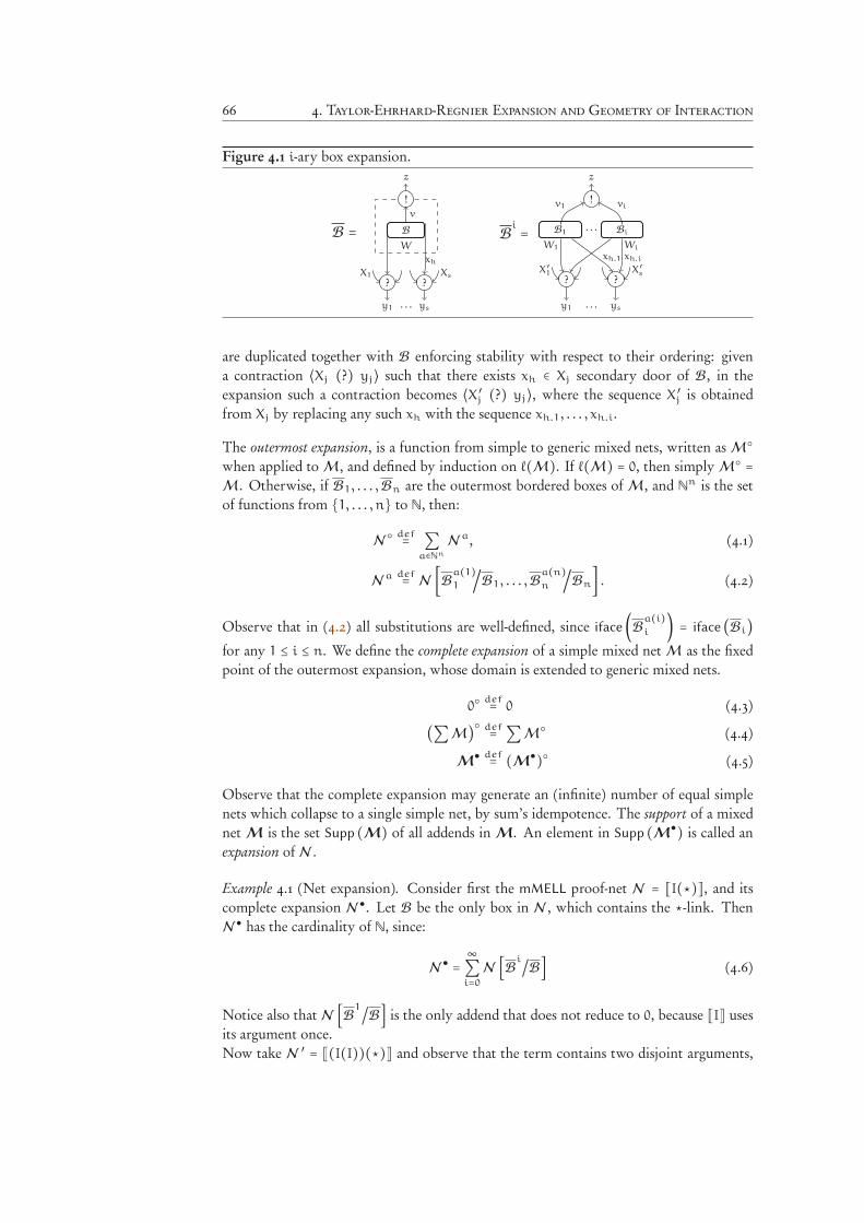
66 4. Taylor-Ehrhard-Regnier Expansion and Geometry of Interaction
Figure 4.1 i-ary box expansion.
B =
!
z
B
W
v
? ?
y1 ys
X1 Xs
xh
. . .
Bi=
!
z
B1
W1
v1
Bi
Wi
vi
. . .
? ?
y1 ys
X ′1
X ′s
xh.1 xh.i
. . .
are duplicated together with B enforcing stability with respect to their ordering: givena contraction ⟨Xj (?) yj⟩ such that there exists xh ∈ Xj secondary door of B, in theexpansion such a contraction becomes ⟨X ′j (?) yj⟩, where the sequence X ′j is obtainedfrom Xj by replacing any such xh with the sequence xh.1, . . . , xh.i.
The outermost expansion, is a function from simple to generic mixed nets, written as M○
when applied to M , and defined by induction on ℓ(M). If ℓ(M) = 0, then simply M○ =
M . Otherwise, if B1, . . . ,Bn are the outermost bordered boxes of M , and Nn is the set
of functions from {1, . . . , n} to N, then:
N ○def= ∑
a∈Nn
Na, (4.1)
Na def= N [Ba(1)
1 /B1, . . . ,Ba(n)n /Bn] . (4.2)
Observe that in (4.2) all substitutions are well-defined, since iface(Ba(i)i ) = iface (Bi)
for any 1 ≤ i ≤ n. We define the complete expansion of a simple mixed net M as the fixedpoint of the outermost expansion, whose domain is extended to generic mixed nets.
0○def= 0 (4.3)
(∑M)○ def= ∑M○ (4.4)
M● def= (M●)○ (4.5)
Observe that the complete expansion may generate an (infinite) number of equal simplenets which collapse to a single simple net, by sum’s idempotence. The support of a mixednet M is the set Supp (M) of all addends in M. An element in Supp (M●) is called anexpansion of N .
Example 4.1 (Net expansion). Consider first the mMELL proof-net N = ⟦I(⋆)⟧, and itscomplete expansion N ●. Let B be the only box in N , which contains the ⋆-link. ThenN ● has the cardinality of N, since:
N ● =∞
∑i=0
N [Bi/B] (4.6)
Notice also that N [B1/B] is the only addend that does not reduce to 0, because ⟦I⟧ usesits argument once.Now take N ′ = ⟦(I(I))(⋆)⟧ and observe that the term contains two disjoint arguments,
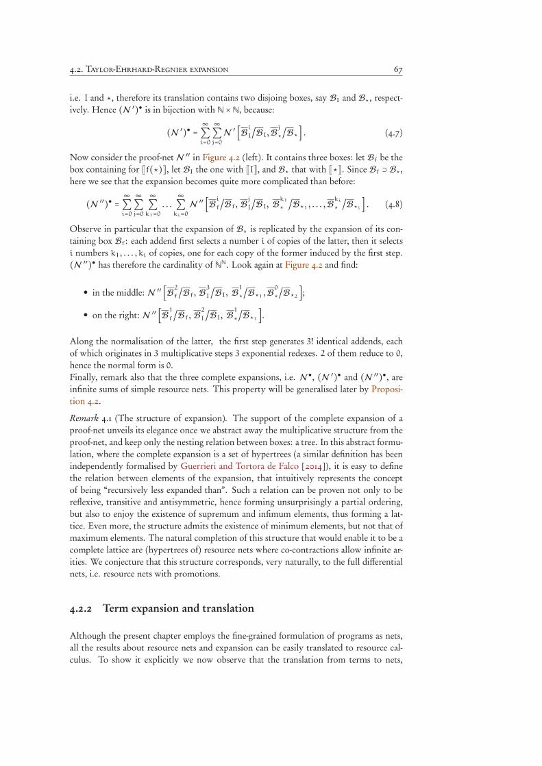
4.2. Taylor-Ehrhard-Regnier expansion 67
i.e. I and ⋆, therefore its translation contains two disjoing boxes, say BI and B⋆, respect-ively. Hence (N ′)● is in bijection with N ×N, because:
(N ′)● = ∞∑i=0
∞
∑j=0
N ′ [Bi
I/BI,Bj
⋆/B⋆] . (4.7)
Now consider the proof-net N ′′ in Figure 4.2 (left). It contains three boxes: let Bf be thebox containing for ⟦f(⋆)⟧, let BI the one with ⟦I⟧, and B⋆ that with ⟦⋆⟧. Since Bf ⊃ B⋆,here we see that the expansion becomes quite more complicated than before:
(N ′′)● = ∞∑i=0
∞
∑j=0
∞
∑k1=0
. . .∞
∑ki=0
N ′′ [Bi
f/Bf, Bj
I/BI, Bk1
⋆/B⋆1 , . . . ,Bki
⋆/B⋆i] . (4.8)
Observe in particular that the expansion of B⋆ is replicated by the expansion of its con-taining box Bf: each addend first selects a number i of copies of the latter, then it selectsi numbers k1, . . . , ki of copies, one for each copy of the former induced by the first step.(N ′′)● has therefore the cardinality of NN. Look again at Figure 4.2 and find:
• in the middle: N ′′ [B2
f/Bf, B3
I/BI, B1
⋆/B⋆1 ,B0
⋆/B⋆2];
• on the right: N ′′ [B1
f/Bf, B2
I/BI, B1
⋆/B⋆1].
Along the normalisation of the latter, the first step generates 3! identical addends, eachof which originates in 3 multiplicative steps 3 exponential redexes. 2 of them reduce to 0,hence the normal form is 0.Finally, remark also that the three complete expansions, i.e. N ●, (N ′)● and (N ′′)●, areinfinite sums of simple resource nets. This property will be generalised later by Proposi-tion 4.2.
Remark 4.1 (The structure of expansion). The support of the complete expansion of aproof-net unveils its elegance once we abstract away the multiplicative structure from theproof-net, and keep only the nesting relation between boxes: a tree. In this abstract formu-lation, where the complete expansion is a set of hypertrees (a similar definition has beenindependently formalised by Guerrieri and Tortora de Falco [2014]), it is easy to definethe relation between elements of the expansion, that intuitively represents the conceptof being “recursively less expanded than”. Such a relation can be proven not only to bereflexive, transitive and antisymmetric, hence forming unsurprisingly a partial ordering,but also to enjoy the existence of supremum and infimum elements, thus forming a lat-tice. Even more, the structure admits the existence of minimum elements, but not that ofmaximum elements. The natural completion of this structure that would enable it to be acomplete lattice are (hypertrees of) resource nets where co-contractions allow infinite ar-ities. We conjecture that this structure corresponds, very naturally, to the full differentialnets, i.e. resource nets with promotions.
4.2.2 Term expansion and translation
Although the present chapter employs the fine-grained formulation of programs as nets,all the results about resource nets and expansion can be easily translated to resource cal-culus. To show it explicitly we now observe that the translation from terms to nets,
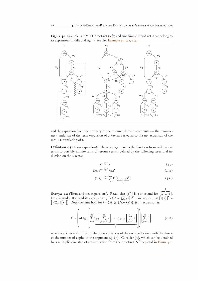
68 4. Taylor-Ehrhard-Regnier Expansion and Geometry of Interaction
Figure 4.2 Example: a mMELL proof-net (left) and two simple mixed nets that belong toits expansion (middle and right). See also Example 4.1, 4.3, 4.4.
⊸
?
w2
w3
v1
⊸
!
⊸
?
!
!
★
v2
v4
v5
v6v7
v3 v8
w1
⊸
?
w2
w3
⊸
?
x2
x3
⊸
?
z2
z3
v1
⊸
!
⊸ ⊸
?
!
! !
★
v2
v4
v5 y5
v6
y6
v7 y7
v3 v8
w1x1 z1
⊸
?
w2
w3
⊸
?
z2
z3
v1
⊸
!
⊸
?
!
!
★
v2
v4
v5
v6v7
v3 v8
w1 z1
and the expansion from the ordinary to the resource domains commutes — the resource-net translation of the term expansion of a λ-term t is equal to the net expansion of themMELL-translation of t.
Definition 4.3 (Term expansion). The term expansion is the function from ordinary λ-terms to possibly infinite sums of resource terms defined by the following structural in-duction on the λ-syntax.
x●def= x (4.9)
(λx.t)● def= λx.t● (4.10)
(t s)● def=∞
∑i=0
t●[s●, . . . , s●JKKKKKKKKKKKKKKKLKKKKKKKKKKKKKKKMi
] (4.11)
Example 4.2 (Term and net expansions). Recall that [sn] is a shortand for [iNKKKKKKKKOKKKKKKKP
s, . . . , s].Now consider I(⋆) and its expansion: (I(⋆))● = ∑∞i=0 I[⋆i]. We notice that ⟦I(⋆)⟧● =⟦∑∞i=0 I [⋆i]⟧. Does the same hold for t = (λf.f@1(f@2(⋆)))(I)? Its expansion is:
t● =
⎛⎜⎜⎜⎜⎜⎝λf.f@1
⎡⎢⎢⎢⎢⎢⎢⎢⎢⎢⎣
∞
∑i=0
f@2
⎡⎢⎢⎢⎣∞
∑k1=0
⋆
⎤⎥⎥⎥⎦ , . . . , f@i+1
⎡⎢⎢⎢⎣∞
∑ki=0
⋆
⎤⎥⎥⎥⎦JKKKKKKKKKKKKKKKKKKKKKKKKKKKKKKKKKKKKKKKKKKKKKKKKKKKKKKKKKKKKKKKKKKKKKKKKKKKKKKKKKKKKKKKKKKKKKKKKKKLKKKKKKKKKKKKKKKKKKKKKKKKKKKKKKKKKKKKKKKKKKKKKKKKKKKKKKKKKKKKKKKKKKKKKKKKKKKKKKKKKKKKKKKKKKKKKKKKKMi
⎤⎥⎥⎥⎥⎥⎥⎥⎥⎥⎦
⎞⎟⎟⎟⎟⎟⎠
⎡⎢⎢⎢⎣∞
∑j=0
Ij⎤⎥⎥⎥⎦ , (4.12)
where we observe that the number of occurrences of the variable f varies with the choiceof the number of copies of the argument f@2(⋆). Consider ⟦t⟧, which can be obtainedby a multiplicative step of anti-reduction from the proof-net N ′′ depicted in Figure 4.2.
4.2. Taylor-Ehrhard-Regnier expansion 69
With the help of Example 4.1, where we explored (N ′′)● (see in particular Equation 4.8),verify that ⟦t⟧● = ⟦t●⟧. The next proposition generalises such intuition.
Proposition 4.1 (Commutativity of translation and expansion). The net expansion of amMELL-translated term is equal to the RIN-translation of its expansion. For any t ∈ Λ,
⟦t⟧● = ⟦t●⟧ (4.13)
Proof. The definitions of ordinary and resource terms translations into proof-nets andresource nets are not uniformly inductive, since they both need the final step which adds?-link on all in conclusions that represent variable occurrences, (cf. Definition 2.12 and3.5). Therefore we will first work with the pre-translation, which can be easily handled,and then consider the final step.
1. We go by induction on the syntax of t, and we will prove as a sub-claim that
(&t'Γ)● = &t●'Γ ′ , for any variable to vertices injection Γ and some, appropriatelychosen one, Γ ′. We will omit to explicitly show that such claim holds converselyhold for any Γ ′ and some Γ , since it will be evident from the proof.
(a) t = ⋆. Then ⟦t⟧Γ = ⟨(★) v⟩ for some vertex v, and (&t'Γ)● = ⟨(★) v⟩. On the
other hand, t● = ⋆ and we immediately conclude &t●'Γ = ⟨(★) v⟩ = (&t'Γ)● ⧫
(b) t = x. Almost identically to previous case, we have &t'Γ = v, i.e. a mixed net
with no links and with one vertex v, therefore also (&t'Γ)● = v. But given that
t● = x, we already have &t●'Γ = v = (&t'Γ)●. ⧫
(c) t = λx.s. This inductive case is still quite simple. On the one hand we have
&t'Γ = ⟨u1, u2 (⊸) v⟩, ⟨w1, . . .wn (?) u2⟩, &s'Γ (4.14)
and trivially
(&t'Γ)● = ⟨u1, u2 (⊸) v⟩, ⟨w1, . . .wl (?) u2⟩,(&s'Γ)● , (4.15)
where the arity l of the ?-link depends on (&s'Γ)●. With the same simplicity,since by definition of expansion t● = λx.s●, we know that its translation is:
&t●'Γ ′ = ⟨u1, u2 (⊸) v⟩, ⟨w1, . . .wm (?) u2⟩, &s●'Γ ′ , (4.16)
where, similarly to Equation 4.15, the arity m depends on &s●'Γ ′ . Now, by
inductive hypothesis, we have (&s'Θ)● = &s●'Θ ′ for any Θ and some Θ ′. There-
fore for any choice of Supp((&s'Θ)●) ∋ s ′ ∈ Supp(&s●'Θ ′), it must be the casethat l =m. Therefore we conclude by taking Γ = Θ and Γ ′ = Θ ′. ⧫
(d) t = (r s). This inductive case is the really interesting one, since here we can seeexpansion at work. First of all:
&t'Γ = ⟨w,v (⊸) u⟩, ⟨x (! ) w⟩, &r'Γ , &s'Γ , (4.17)
70 4. Taylor-Ehrhard-Regnier Expansion and Geometry of Interaction
where u ∈ iface(&r'Γ) and x ∈ iface(&s'Γ), both unique elements with out
polarity; and &s'Γ is enclosed in a new box. Therefore, by definition of expan-sion:
(&t'Γ)● = ∞∑i=0
⟨w,v (⊸) u⟩, ⟨x1, . . . , xi (! ) w⟩,
(&r'Γ)● ,(&s1'Γ)● , . . .(&si'Γ)● , (4.18)
where xj is the out vertex in iface((&sj'Γ)●), and for any 1 ≤ j, j ′ ≤ i we have
iface((&sj'Γ)●) = iface((&sj ′'Γ)●). Now, looking at the right-hand side ofEquation 4.13, we have that
t● =∞
∑i=0
r● [s●1, . . . , s●i] . (4.19)
So consider the pre-translation with respect to any Γ ′:
&t●'Γ ′ = ∞∑i=0
⟨w,v (⊸) u⟩, ⟨x1, . . . , xi (! ) w⟩,&r●'Γ ′ , &s●1'Γ
′
, . . . , &s●i'Γ′
, (4.20)
where u is the unique out conclusion in iface(&r●'Γ ′) and for any 1 ≤ j ≤ i xj
is the unique out conclusion in I(_s●j `Γ′). Now, let y@h ′ be one the variable
occurrences of s●j , and assume it to be the expansion of the variable occurrencey@h of s. To prove the claim we need to impose that (Γ(y@h))● ∋ Γ ′(y@h ′).But this is always possible since, by inductive hypothesis, we have not only
that (&r'Θ)● = &r●'Θ ′ , for any Θ and some Θ ′ (and vice versa); but also that
(&sj'Ξ)● = _s●j `Ξ′
, for any Ξ and some Ξ ′ (and vice versa). ⧫
◻
2. Now we consider the final steps of translations. ⟦t⟧Γ = ⎫⎪⎪⎩&t'Γ⎧⎪⎪⎭Γ
. In step 1 we verified
that (&t'Γ)● = &t●'Γ ′ , and we showed the existence of Γ, Γ ′. Now, let N be the sum
of simple resource nets obtained from (&t'Γ)● by adding to it, for any variable y oft, a ?-link having as premiss any vertex belonging to (Γ(yh))●, for any occurrence
h of y. First of all, we easily verify that, by definition of expansion, N = (⟦t⟧Γ)●.Then, we observe that in ⟦t●⟧Γ ′ the translation similarly adds to &t●'Γ ′ a ?-link,for any variable y ′ of t●, a ?-link having as premiss any vertices in Γ(y ′h ′) for anyoccurrence h ′ of y ′. Therefore, by definition of Γ, Γ ′ and by the conclusion of step1, we have ⟦t●⟧Γ ′ =N . Hence the claim. ◻
∎
4.2. Taylor-Ehrhard-Regnier expansion 71
4.2.3 Path expansion
Observing the action of expansion on paths, we can identify the expansion of a path π
in a proof-net N as the series of paths which belong to the simple resource nets in thecomplete expansion of N and which correspond to π.
Recall the definition of paths in a mMELL proof-net, or in a RIN, and the definition of thestatic properties which are necessary to ensure their persistence, hence meaningfulnessas a description of computation: straightness, maximality, and comprehensiveness (seeDefinition 2.6, 2.17, 3.9).
Definition 4.4 (Box crossing). Given a proof-net N and π ∈ P(N ), its outermost-boxcrossing form is:
OBCF(π) def= ǫ0 ∶∶ β1 ∶∶ ǫ1 ∶∶ . . . ∶∶ βn ∶∶ ǫn, (4.21)
where, for every 1 ≤ i ≤ n, βi is a box crossing, that is a maximal subpath belonging toan outermost box B, i.e. ℓ(B) = 0. Notice that n may be null and that a crossing is notnecessarily a maximal path in B.
Definition 4.5 (Path expansion). Given N a mixed net and π ∈ P(N ), let B1, . . . ,Bm bethe outermost bordered boxes of N , let OBCF(π) be as in Equation 4.21, and let a ∈ Nm.Then the a-ary outermost expansion of π in N is the set of paths obtained by the action ofthe outermost expansion of N according to a.
πNa
=
⎧⎪⎪⎪⎨⎪⎪⎪⎩{π} if m = 0,
{ǫ0 ∶∶ β1kb(1)∶∶ ǫ1 ∶∶ . . . ∶∶ βnkb(n)
∶∶ ǫn ∣ 1 ≤ ki ≤ a(i)} otherwise,(4.22)
where for each crossing βj of Bb(j), we write βjkb(j)to the denote the image of βj in the
kb(j)th copy of the box Bb(j). Notice that the rightmost side of Equation 4.22 is emptywhenever there exists 1 ≤ i ≤ m such that a(i) = 0; while it is the singleton {ǫ0} if n = 0.The outermost expansion of a set of paths Π is the sum of sets of paths generated by thesum of all a-ary outermost expansions, extending its domain to sets of path. The sum ofpaths satisfies the same properties of the sum of simple resource nets.
ΠNa def= ⋃
π∈Π
πNa
(4.23)
ΠN○ def=
⎧⎪⎪⎪⎨⎪⎪⎪⎩
Π if m = 0,
∑a∈Nm
ΠNa
otherwise. (4.24)
The complete expansion of a sum of sets of paths Π is the fixpoint of the outermost expan-sion, where we neatly extend its domain to sums of sets of nets.
ΠN○ def= ∑
N∈Supp(N )Π⊇Π⊆P(N)
ΠN○
(4.25)
ΠN● def= (ΠN
●)N○
(4.26)
72 4. Taylor-Ehrhard-Regnier Expansion and Geometry of Interaction
When it does not lead to confusion, we shall ease the notation of {π}N ● writing πN●
. Thecomplete expansion of a vertex v is the sum of sets of vertices that is naturally obtained bythe complete expansion of the atomic path (v):
vN● def= ∑
Π∈Supp((v)N●){v ′ ∣ (v ′) ∈ Π} . (4.27)
We similarly define the complete expansion of a link l in N as the sum of sets of linksdefined as follows.
⟨U (κ) v⟩N ● def= ∑
V∈Supp(vN●)U∈Supp(uN●)u∈U
{l ′ = ⟨U ′ (κ ′) v ′⟩ ∣ v ′ ∈ V, u ′ ∈ U, l ′ ∈ L(N ●)} (4.28)
Example 4.3 (Path expansion, a gentle case). Recall from Example 4.1 the proof-net N =
⟦I(⋆)⟧ for which, as we previously discussed, we have Bxs (N ) = {B}. Recall also itscomplete expansion. Let π ∈ P(N ) that: starts from the root, crosses the ⊸-link fromthe conclusion to the second premiss, crosses the ⊸-link from the conclusion to the firstpremiss, and reaches the ⋆-link (all omitted crossings can be inferred by straightness).Recall from Equation 4.6 that for every i ∈ N there is a unique Ni ∈ Supp (N ●), i.e.N [Bi/B]. Now, observe that in Supp (πN
●) there is a unique set of paths Πi for everyexpansion of N . Moreover, since π crosses once the !-link entering B, and since Ni includeexactly i copies of B, we have that the cardinality of Πi is i. This means in particular thatΠ0 = ∅. Notice also that Ni →r 0 for any i ≠ 1, and that both π and π1 are persistentpaths.
Example 4.4 (Path expansion, two less gentle cases). Look again at Figure 4.2, where theproof-net N and two simple mixed nets M ,M ′ are depicted (from left to right). As wediscussed in preceding Example 4.1, let BI be the box which contains ⟦I⟧, and rememberthat M ,M ′ ∈ Supp (N ●).Let φ ∈ P(N ) be defined as follows:
φ = (v1, v2, v3,w1,w2,w3
w1, v3, v2,
v4, v5, v6, v3,w1,w2,w3). (4.29)
If Mi ∈ Supp (N ●) is one of the simple mixed nets that contains i copies of BI, noticethat there exists a unique Φi ∈ Supp (φN
●) that contains any φ ′ ∈ P(Mi) such thatφ ′ ∈ Φ ′i ∈ Supp (φN
●). This will be generalised by Fact 4.3.Now remark that φ enters twice in BI. In N ′′ we find 4 expanded paths of φ, 9 in M ′.The expansion of φ essentially computes an assignment of a copy of B to each crossing.Hence ∣Φi∣ = i2 if i > 0, 0 otherwise. More generally if φ had crossed BI n times, then∣Φi∣ = in, i.e. the number of n-tuples over (1, . . . , i).Consider π ∈ P(N ) defined as follows:
π = (v3, v6, v7, v8). (4.30)
Remark that π crosses once both Bf (the box with principal door in v4 ) and B⋆ (the boxwith principal door in v7 ). Notice that there is only one expanded path in M ′′, where
4.2. Taylor-Ehrhard-Regnier expansion 73
both boxes are expanded in one copy, i.e. (v3, v6, v7, v8). But there is again only oneexpanded path of π even in M ′, where Bf is expanded twice, i.e. (v3, v6, v7, v8), since inits second copy B⋆ has 0 copies (so there is only a prefix available: (v3, y6, y7)). To seethe more general picture, let Mi,j1,...,ji ∈ Supp (N ●) be one of the simple mixed nets thatcontains i copies of Bf, and ji copies of B⋆i , that is the i-th copy of B⋆. Let Πi,j1,...,ji
be the set of path belonging to the expansions of π inhabiting Mi,j1,...,ji . We can easilyverify that ∣Πi,j1,...,ji ∣ = i × ji. More generally, if π had contained n crossings of the twoboxes, we would have had ∣Πi,j1,...,ji ∣ = (i × ji)n.
Path expansion does not expand a path in the sense of increasing its length, since a pathin the expansion can be constructed by a vertex-by-vertex procedure. Also, expansionpreserves kind and in/out polarities of links, and types of vertices.
Fact 4.1 (Path expansion and length). The size of a path is preserved in its expansion’s ad-dends: for any π ∈ P(N ), and any π ′ ∈ πN
●
, ∣π∣ = ∣π ′∣.Fact 4.2. For any mMELL proof-net N , let l = ⟨U (κ) v⟩ ∈ L(N ) and l ′ = ⟨U ′ (κ ′) v ′⟩ ∈L ′ ∈ Supp (lN ●). Then:
1. κ = κ ′;
2. T (v) = T (v ′);3. for any u ∈ U and u ∈ U ′, if u ′ ∈ U ′′ ∈ Supp (uN
●) then T (u) = T (u ′).
Given a path π in a mixed net N , the sets of paths which form the expansion of π are inbijection with the simple mixed nets which form the expansion of N . This means thattwo paths belongs to the same set of paths that appears in the expansion of π if and onlyif they inhabit the same mixed net. Moreover, if path expansion is considered as a relationbetween the paths of a simple mixed net and those of another simple mixed net appearingin its complete expansion, then path expansion is injective, or: its inverse relation is afunction.
Fact 4.3 (Bijection between addends). GivenN a mixed net and π ∈ P(N ), let π ′ ∈ P(N ′)and π ′′ ∈ P(N ′′) such that N ′,N ′′ ∈ Supp (N ●). Also, let π ′ ∈ Π ′ and π ′′ ∈ Π ′′ such thatΠ ′, Π ′′ ∈ Supp (πN
●). Then N ′ =N ′′ if and only if Π ′ = Π ′′.
Lemma 4.1 (Path injectivity). Given two mixed nets N and N ′ ∈ Supp (N ●), for any pathπ ′ ∈ P(N ′):
1. there exist π ∈ P(N ) and Π ∈ Supp (πN●) such that π ′ ∈ Π;
2. for any γ ∈ P(N ), if π ′ ∈ Γ ∈ Supp (γN●) then Γ = Π and γ = π.
Proof. By immediate verification against the definition of path expansion. ∎
Remark 4.2 (Non-injectivity w.r.t. simple nets). The expansion functions of paths, ofvertices, and of links are not injective with respect to expansions of the containing net.Let us clarify with a counterexample for the case of vertices. Let v ∈ V(N ) for some
74 4. Taylor-Ehrhard-Regnier Expansion and Geometry of Interaction
mixed net N , and consider v ′, v ′′ appearing in vN●
, i.e. such that there exist V ′ ∈ vN●
forwhich v ′ ∈ V ′′, and V ′′ ∈ vN
●
for which v ′′ ∈ V ′′. Now, if v ′ ≠ v ′′, it may be the case thatV ′ ≠ V ′′, which means that v ′, v ′′ belongs to different addends of N ●, but we may alsohave V ′ = V ′′, which implies the converse.
Since path expansion preserve switchingness and acyclicity, we can finally show that ex-panded nets are sums of simple resource nets.
Lemma 4.2. Let N be a mixed net. If a path π ′ ∈ P(N ●) is switching (or acyclic), then thereexists π ∈ P(N ) which is switching (respectively acyclic).
Proof. We simply use the injectivity property of vertex expansion to show that switching-ness and acyclicity cannot be introduced by path expansion. We separately show inherit-ance of the two properties.
1. Switching. Recall that by Definition 2.9 given any v ′1, v′
2 premisses of the same linkof kind⊸ or ?, π ′ is switching when if π ′ contains v ′1, then it does not contain v ′2.Now, let v1, v2 ∈ V(N ) be such that v ′1 ∈ V1 ∈ Supp (vN
●
1 ) and v ′2 ∈ V2 ∈ Supp (vN●
2 ),whose existence and unicity is established by item 4.2.3. Now let π such that π ′ ∈
Π ∈ Supp (πN●), and assume that v ′1 ∈ π
′. Then, by definition of path expansion, itmust be the case that v1 ∈ π. Now, for the same reason, if v ′2 ∉ π
′ then v2 ∉ π, henceπ is switching. ◻
2. Cyclic. By Definition 2.9, π ′ is cyclic if it contains a cycle γ ′ = (v ′0, v ′1, . . . , v ′n, v ′0),with n > 0. Because of Lemma 4.1, there are two unique paths γ,π such that γ ′ ∈
Γ ∈ Supp (γN●) and π ′ ∈ Π ∈ Supp (πN
●). But by definition of path expansion, weknow that if γ ′ ⊆ π ′, then also γ ⊆ π. Moreover item 4.2.3 establishes that thereexists a unique v0 ∈ V(N ) such that v ′0 ∈ Supp (vN
●
0 ), hence γ is a cycle, and π iscyclic. ◻
∎
Proposition 4.2. The expansion of a mMELL proof-net is a possibly infinite sum of simpleresource interaction nets.
Proof. We directly show that any path in any expansion satisfies Definition 3.4. Let π ′ ∈
P(N ′), for some resource pre-net N ′ ∈ Supp (N ●) and for some proof-net N . Let π ∈
P(N ) such that π ′ ∈ Π ′ ∈ Supp (πN●), whose existence is guaranteed by Lemma 4.1. Now,
by last Lemma 4.2, if π ′ is switching (or cyclic) then also π is switching (respectively,cyclic). But by Definition 2.10 of mMELL proof-nets, if π is switching then it is not cyclic,which implies that there cannot exist π ′ switching and cyclic. So we conclude that anyN ′ satisfies the definition of simple resource net, and consequently that N ● is a resourcenet. ∎
4.3. Expansion and reduction 75
4.3 Expansion and reduction
Taylor expansion replaces boxes in a mMELL net with a number of copies of its content.Can we reduce all copies of a same redex together, in an infinitary parallel reduction? Wedefine such a reduction relation, which in a sense represent the Taylor expansion of themMELL cut-elimination, and which we call ‘expanded’.
We first define a notion of parallel reduction on resource nets that is a restriction of thatemployed by Pagani and Tranquilli [2009] to show confluence of resource calculus. In thesettings of resource interaction nets a parallel reduction is indeed not hard to formulate,since, oppositely to mMELL proof-nets, λ-terms and resource λ-terms, the RIN rewritingsystem does not allow overlaps, as mentioned in Proposition 3.5. Our limitation simplyaims at tightening it to ease the simulation of mMELL reduction, and is inspired from thefollowing observation, directly following from Fact 4.2.
Fact 4.4. A mMELL vertex is a cut if and only if its expansion is a sum of sets of cuts.
Definition 4.6 (Multi-hole contexts and substitution). A simple multi-hole context C⟦ ⟧,(resp. a multi-hole context C⟦ ⟧) is a simple resource context (resp. a linear combinationof simple resource contexts over the semiring of N) having a finite, possibly null, numberof hole links (see Definition 2.14 and recall that !-links are not promotions, nor they haveassociated boxes). If C⟦ ⟧ has holes h1, . . . , hn and N is a sum of simple resource pre-netsP1, . . . ,Pm, then C⟦N ⟧ consists of the (possibly empty) sum of any possible substitutionof the m (non-zero) addends of N into the n holes of C⟦ ⟧. Formally, if Nk denotes{1, . . . , k} (where N0 = {}), and A↣ B the set of injections from a set A to a set B:
C⟦N ⟧ = ∑c∈Nn↣Nm
iface(Pc(i))=iface(hi)
C[Pc(1)/h1, . . . ,Pc(n)/hn]. (4.31)
In particular, note that when n = 0, one simply get C⟦N ⟧ = C. Also, if m = 0 andconsequently N = 0, then C⟦N ⟧ = 0. Given C⟦ ⟧ a non-simple resource context, and N aresource pre-net, C⟦N ⟧ is the substitution of the latter in each addend of the former; i.e.:0⟦N ⟧ = 0 and (C + C)⟦N ⟧ = C⟦N ⟧ + C⟦N ⟧.Definition 4.7 (Parallel and expanded reduction). The closure of the simple reductionrelation with respect to multi-hole resource contexts is called parallel resource reductionand written ↠. Formally, given a resource net N = C⟦P1 + . . . + Pn⟧ where C⟦ ⟧ is amulti-hole context and P1, . . . ,Pn are pre-nets, if P1 → P1, . . . ,Pn → Pn then N ↠
C⟦P1+ . . .+Pn⟧. Given a mMELL proof-net N and a reduction step ρ on a cut c ∈ V(N ),the expanded reduction of ρ, written ρ●, is the parallel reduction of the set of any resourceredex in Supp (N ●) for any cut in Supp (c●).Notation 4.1. We extend the domain of resource reduction for paths to sets of paths. Forany reduction ρ, and any set of paths Π, we write ρ(Π) to denote ⋃π∈Π ρ(π).Remark 4.3 (Indirectness of definition of expanded reduction). Even though expandedreduction has been defined using expansion itself but it would be interesting to have in-stead a direct formulation. Given N a sum of simple resource nets image of N ●, how canone determine, with no knowledge of N , a sum of set of redexes R such that if N = N ●
then R = R●? A terse answer has been developed by the author, but requires a restric-tion undesired by the aim of this thesis: it need to be formalised on proof structures that
76 4. Taylor-Ehrhard-Regnier Expansion and Geometry of Interaction
enjoys connectedness, such as weakening-free proof-nets or λ-terms. In this setting, it isnot difficoult to exploit the property of ‘uniformity’ [Ehrhard and Regnier, 2008], that isthe relation of syntactical similarity which intrinsically belongs to all elements within theexpansion of the same term/net. In the latter (and more general) case of a weakening-freemMELL proof-net N , one can define a notion of locator of a vertex v ∈ V(N ) as its uniqueaccess path, i.e. the unique downward path that goes from the out-conclusion of a net (theroot of the corresponding term) to v, without crossing the first premiss of any ⊸-link.Then two cut are in the same expanded redex whenever their access paths cross the samesequence of kind of links, and for each ⊸-link of those they also cross the same vertex (i.e.the conclusion on the left or the first premiss on the right).
4.4 Commutativity of reduction and expansion
In this section we show how the Taylor-Ehrhard-Regnier expansion commutes with re-duction: reducing and then expanding a mMELL proof-net is equivalent to expanding andthen reducing it. The same result is then easily reformulated on paths as well, which im-plies that the persistence of a path is characterised by the existence of persistent paths inits expansion.
4.4.1 Commutativity on nets
Theorem 4.1 (Net expansion commutes with reduction step). For any mMELL net N andany reduction ρ
(ρ(N ))● = ρ●(N ●) (4.32)
Proof. We obtain the equivalence of the two sides of Equation 4.32 by direct, even thoughtechnically delicate, manipulations.
1. Firstly we get rid of some irrelevant addends from the two sides of Equation 4.32.
(a) Let N = C[R], where R is the mMELL redex of ρ for the cut, say c, and C isits context with hole h. By definition of mMELL reduction, ρ(N ) = C[ρ(R)],so (ρ(N ))● = (C[ρ(R)])●. Notice that within C● there are addends whichcontain one or more copies of h and which are multi-hole simple resourcecontexts; and others addends where h has been erased, and which are simpleresource nets. Let C be the sum of the former addends, and N the sum of thelatter ones. Hence, (ρ(N ))● = C⟦(ρ(R))●⟧ +N .
(b) Let, N ● = C′⟦R ′⟧ +N , where R
′ is the sum, for any c ′ ∈ c●, of the resourceredex of c ′, while C
′ is its multi-hole resource context, and N is again the sumof any non-zero addend in N ● which does not contain any c ′ ∈ c●. Hence,ρ●(N ●) = C
′ ⟦ρ●(R ′)⟧ +N .
Therefore, we just reduced the thesis to the equivalence between Supp (C ⟦(ρ(R))●⟧)and Supp (C ′ ⟦ρ●(R ′)⟧).

4.4. Commutativity of reduction and expansion 77
2. We distinguish two cases, depending on the type of the redex of c, which, as perFact 4.4, is equal to the type of the redex of any c ′ ∈ c●.
(a) (⊸/⊸) Straightforward, since linear implication redexes are identical on bothsides.
i. By definition of expansion, we have that (ρ(R))● contains exactly oneelement, which is equal to ρ(R). Therefore, we obtain that C ⟦(ρ(R))●⟧ =C ⟦ρ(R)⟧.
ii. For the same reason above, R ′ is identical to R, which implies that ρ●(R ′) =ρ(R), and also that C = C
′. We immediately obtain C′ ⟦ρ●(R ′)⟧ = C ⟦ρ(R)⟧.
Hence, C ⟦(ρ(R))●⟧ = C′ ⟦ρ●(R ′)⟧ which implies their respective supports are
equal, quod erat demonstrandum. ◻
(b) (!/?) This case is quite more involved from the previous one, because we haveto deal with the difference between the two notions of redexes. In the mMELL
redex we have an erasure or a duplication and a possible relocation of the argu-ment box, while on the resource net, where all of this work has already beenperformed by the expansion, the redex simply consists of a resource dispatch-ing. Such a complexity requires a deep analysis.
i. We first consider the right side of the equation we want to prove, i.e.C ⟦(ρ(R))●⟧. Suppose
R = ⟨u1, . . . , uk (?) c⟩, ⟨v (! ) c⟩, ⟨W [B] v⟩,⟨X1 (?) y1⟩, . . . , ⟨Xs (?) ys⟩. (4.33)
Then, as by Definition 2.15 of mMELL proof-net reduction (in particular,see Figure 2.3b and Equation 2.5),
ρ(R) = ⟨W1 [B1] u1⟩, . . . , ⟨Wk [Bk] uk⟩,⟨X ′1 (?) y1⟩, . . . , ⟨X ′s (?) ys⟩, (4.34)
where any X ′i is obtained by replacing any occurrence of a vertex w ∈ W
with the sequence (w1, . . . ,wk) such that its elements respectively belongsto W1, . . . ,Wk.Now observe the reduct and observe that we can write it as follows.
ρ(R) = C ′′ [⟨W1 [B1] u1⟩, . . . , ⟨Wk [Bk] uk⟩] (4.35)
C ′′ = ⟨X ′1 (?) y1⟩, . . . , ⟨X ′s (?) ys⟩,⟨W1 ∪ . . . ∪Wk (◻) u1 . . . uk⟩ (4.36)
where the ◻-link denotes a hole h ′, whose in conclusions are writtenas premisses, and its out conclusions as conclusions. Now, let C ′′′⟦⟧be the multi-hole context obtained by splitting h ′ into k distintict holesh1, . . . , hk such that for any 1 ≤ i ≤ k, we have hi = ⟨Wi (◻) ui⟩. Then,since the substitution of a net in a multi-hole context duplicates it, we canexpress ρ(N ) as C ′′′⟦B⟧. Therefore,
(ρ(N ))● = C ′′′⟦B⟧●.
78 4. Taylor-Ehrhard-Regnier Expansion and Geometry of Interaction
Furthermore, the explicit presence of the box enable us to safely decom-pose expansion (cf. Definition 4.2), and write:
(ρ(N ))● = (C ′′′)●⟦B●⟧.ii. Now let us analyse the left side of the equation of the claim, that is
C′ ⟦ρ●(R ′)⟧. First, we observe that there are addends of R ′ which reduce
to 0, because the arities of the two exponential links differs. Therefore,let R
′′ be the restriction of R ′ obtained by depriving it of any R ′ ∈ R ′
such that for some reduction ρ ′ ∈ ρ●, we have ρ ′(R ′) = 0. But the re-moved addends are irrelevant, therefore ρ●(R ′) = ρ●(R ′′), which meansC′ ⟦ρ●(R ′)⟧ = C
′ ⟦ρ●(R ′′)⟧.Now, by construction, any R ′′ ∈ Supp (R ′′) is necessarily made of twoexponential links of equal arity nR ′′ . Notice that in C
′ ⟦R ′′⟧, by definitionof multi-hole contexts substitution, R ′′ could be substituted only to a hole-link with equal interface, i.e. having nR ′′ out-vertices and nR ′′ in-verticesof corresponding types. Recall that !-link in R ′′ has been generated fromthe expansion of the promotion link of R, which implies that any hole-link compatible with R ′′ is connected to nR ′′ sub-nets being addends ofB●.Consider now the sum C
′′made of any multi-hole simple resource contextobtained by any C ′ ∈ C ′ by removing, in correspondence of any hole-link,all the copies of B, and consequently extending such a hole. Hence,
C′ ⟦R ′⟧ = C
′′
abbbbbc∑
R ′′∈Supp(R ′′)
⎛⎜⎜⎝R ′′,B●, . . . ,B●JKKKKKKKKKKKKKKKKKKKKKKLKKKKKKKKKKKKKKKKKKKKKKM
nR ′′
⎞⎟⎟⎠
deeeeef,
where nR ′′ is the arity of links in R ′′. By Definition 3.8 and 4.7, its reduc-tion corresponds to the replacement of any R ′′ ∈ R ′′ with a permutationof their vertices. I.e.
C′ ⟦ρ●(R ′)⟧ = C
′′
abbbbbbbc∑
R′′∈Supp(R ′′)
nR ′′∈SnR ′′
⎛⎜⎜⎝[σnR ′′],B●, . . . ,B●JKKKKKKKKKKKKKKKKKKKKKKLKKKKKKKKKKKKKKKKKKKKKKM
nR ′′
⎞⎟⎟⎠
deeeeeeef,
where for any R ′′, if u1, . . . , uk are premisses of the contraction link, andv1, . . . , vk are those of the co-contraction link, then [σnR ′′] denotes thevertex equation
[u ′k≡v ′σnR ′′(k), . . . , u′
k≡v′
σnR ′′(k)] .But the presence of such a permutation is redundant with respect to thesupport, because substitution in multi-hole contexts already spans overany possible permutation of its arguments. Hence,
Supp (ρ●(N ●)) = Supp⎛⎜⎜⎝C′′
abbbbbc∑
R ′′∈R ′′B●, . . . ,B●JKKKKKKKKKKKKKKKKKKKKKKLKKKKKKKKKKKKKKKKKKKKKKM
nR ′′
deeeeef
⎞⎟⎟⎠.
4.4. Commutativity of reduction and expansion 79
In the last expression we could further simplify the substituens by factor-ising the substituendum. Let C
′′′ be the series of the contexts obtainedfrom any non-zero addend of C
′′ by partitioning, similarly to what wedid before, any hole-link having nR ′′ out-vertices into nR ′′ distinguishedholes. Therefore, we can use a single expansion of B, and obtain:
Supp (ρ●(N ●)) = Supp (C ′′′ ⟦B●⟧) .In the first step of the exponential case we showed (ρ(N ))● = (C ′′′)●⟦B●⟧.In the second step we proved that Supp (ρ●(N ●)) = Supp (C ′′′ ⟦B●⟧). But byconstruction C
′′′ = (C ′′′)●, so we conclude. ◻
∎
Remark 4.4 (Expansion and substitution). Expansion is hardly compatible with reduction.In order to prove Theorem 4.1, we could imagine structuring our reasoning with a sort ofsubstitution lemma stating that “For any proof-net C[R], where R is a mMELL redex andC is a context, Supp ((C[R])●) = Supp (C●⟦R●⟧)”. Unfortunately, mMELL reduction hastwo non-local behaviour in the dynamics of the exponential case, one of which containsan insurmountable obstacle for such approach. The light of the old syntax of LinearLogic allows us to discriminate the two. One non-local behaviour, probably the moreevident one, lies in box duplication and erasure, i.e. the action of reducing, respectively,contraction and weakening. This poses no problem to expansion, since the object box istreated as an atomic whole. The other non-local behaviour comes from box deepeningand shallowing, i.e. the action of reducing, respectively, secondary doors and dereliction.This kind of reduction may involve other boxes, thus preventing the compositionality ofdesire. We consequently prefer to tackle the proof in its entirety.
By composition, we now straightforwardly generalise commutativity between expansionand reduction step, to reduction sequences: it suffices to iteratively apply Theorem 4.1.
Theorem 4.2 (Net expansion commutes with reduction sequence). For any mMELL netN and any reduction sequence ρ
(ρ(N ))● = ρ●(N ●) (4.37)
Proof. Let ρ = ρ1 . . . ρn. We go by induction on the length n.
1. (n = 0). Trivial: the thesis shrinks to the identity N ● =N ●.
2. (n > 0). By inductive hypothesis:
(ρn−1(. . . ρ1(N ) . . .))● = ρ●n−1(. . . ρ●1(N ●) . . .).Hence, we easily conclude applying Theorem 4.1:
(ρn(ρn−1(. . . ρ1(N ) . . .)))●
= ρ●n(ρ●n−1(. . . ρ●1(N ●) . . .)).
∎
80 4. Taylor-Ehrhard-Regnier Expansion and Geometry of Interaction
Remark 4.5 (Expanded redexes and Lévy families). Expanded reduction appears to bedeeply connected to the notion of parallel reduction on redex families discovered by Lévy[1980], which reduces in a single step all the redexes belonging to a given family, i.e. allthe copies that preceding reduction created so far. Similarly, in the expansion of a net N ,any simple resource net N ′ which does not reduce to 0, has performed all the copies beingnecessary to its normalisation. For this reason, we believe that between Lévy-parallelreduction on N equipped with an appropriate strategy (a least efficient one in terms ofnumber of copies), and expanded reduction on N ′, there lies a beautiful simulation. Weconjecture, indeed, that for every step ρ of the former and any corresponding step of thelatter, there is a natural bijection between the sets of simple redexes of the two.Furthermore, we notice that the very notion of families is at the heart of the duality ofthe two concepts of main interest of the present thesis: sharing and expansion. They aresomehow inverse operations on the use of arguments — the former considers any possiblenumber of usages, the latter minimises their representation with respect to their contexts.
4.4.2 Commutativity on paths
Lastly presented commutation result holds, indeed not surprisingly, not only for reduc-tion on nets, but also on paths. Because of such expectedness, we present an independentproof that is of particular interest because it enlightens deep internals of the linearisationof Linear Logic exponential modality, explaining when, where and how path persistencecan or cannot be preserved along expansion. To better enjoy the analysis, we shall struc-ture it in three steps. Firstly, we show that commutation holds in the core case of a redexcrossing and a single reduction step (Lemma 4.3); secondly, we enlarge our view to genericpaths (Lemma 4.4); thirdly, we generalise the result to reduction sequences (Theorem 4.3).Lastly we derive the equivalence between mMELL persistence of a path and the existenceof persistent path in its expansion (Theorem 4.4).
Lemma 4.3. Let R be a mMELL redex, ρ be its reduction step, and χ ∈ P(R). Then:Supp((ρ(χ))(ρ(R))●) = Supp(ρ● (χR
●)) . (4.38)
Proof. We distinguish two cases according to the type of redex.
1. T (R) = ⊸/⊸. Let R = ⟨v ′, v (⊸) w⟩, ⟨u ′, u (⊸) w⟩ as in Figure 2.3a. We imme-diately notice that, by Definition 4.2, R● = R while, as per Definition 4.5, we haveχR
●
= {χ}. We consider two sub-cases depending on the persistence of χ to ρ.
(a) ρ(χ) ≠ ∅. This implies that, by Definition 3.10 and in particular Equation 3.16,3.17, that χ is either (v ′,w,u ′), (v,w,u), or the reversal of these. Given thatfrom the analysis of one case the other three can be straightforwardly obtained,let us assume χ = (v ′,w,u ′). By definition of reduction, we have ρ(χ) ={(v ′)[v ′≡u ′]}. Moreover, by definition of path expansion, we have that
(ρ(χ))(ρ(R))● = {(v ′)[v ′≡u ′]}(ρ(R))● = {(v ′)[v ′≡u ′]} .Let us now look at χR
●
= {χ}, and consider its expanded reduction: ρ● (χR●) =
ρ● (χ). Notice that ρ● contains only one reduction step, which is identical to
4.4. Commutativity of reduction and expansion 81
ρ, because R● = R. Hence we conclude:
ρ● (χN●) = ρ(χ) = {(v ′)[v ′≡u ′]} .
⧫
(b) ρ(χ) = ∅. Then we immediately notice that by definition of path expansion:
(ρ(χ))(ρ(R))● = ∅(ρ(R))● = ∅.Moreover, given that, as we remarked in previous case, we have χR
●
= {χ}, andρ● = {ρ}, we immediately conclude:
ρ●(χR●) = ρ●(χ) = ρ(χ) = ∅.
⧫
◻
2. T (R) = !/?. Let R be as in Figure 2.3b:
R = ⟨u1, . . . , uk (?) c⟩, ⟨v (! ) c⟩, ⟨W [B] v⟩, ⟨X1 (?) y1⟩, . . . , ⟨Xs (?) ys⟩. (4.39)
We distinguish three sub-cases depending on the polarities of the extrema verticesof the crossing of B.
(a) out-out. Let χ = (uj, c, v) ∶∶ β ∶∶ (v, c, uj ′). Being the most interesting one,we shall discuss in full details this sub-case, further distinguishing two sub-sub-cases according to the persistence of χ.
i. χ persistent to ρ. Then, by definition of mMELL path reduction (in par-ticular Equation 2.10), j = j ′ and:
ρ (χ) = {(uj) ∶∶ βj ∶∶ (uj) [uj≡vj]} ,where we kept trivial paths as extrema for the sake of clarity. By Defini-tion 4.5:
(ρ(χ))(ρ(R))● = {(uj) ∶∶ βB●
j
j ∶∶ (uj)}Now let us look at the rightmost side of Equation 4.38, and apply thedefinition of path expansion. If B is the h-th of the m outermost boxes ofR,
(χ)R● = ∑a∈Nm
{(uj, c, vn) ∶∶ βB●
nn ∶∶ (vn, c, uj) ∣ 1 ≤ n ≤ a(h)},
so we can consider its expanded reduction w.r.t. ρ,
ρ● (χR●) = ∑
a∈Nm
{ρ● ((uj, c, vn) ∶∶ βB●
nn ∶∶ (vn, c, uj)) ∣ 1 ≤ n ≤ a(h)}.
Notice that in any element of any addend of the sum, the two outermostpaths are crossings of a resource redex of exponential type. The reduc-tion step ρ● performs by definition the reduction of any cut c ′ ∈ C ′ ∈
82 4. Taylor-Ehrhard-Regnier Expansion and Geometry of Interaction
Supp (c●), including c. Therefore, we can apply Definition 3.11 of pathreduction and in particular Equation 3.23.
ρ● (χR●) = ∑
a∈Nm
σ∈Sa(h)
{ρσ ((uj, c, vn) ∶∶ βB●
nn ∶∶ (vn, c, uj)) ∣ 1 ≤ n ≤ a(h)}
= ∑a∈N
m
σ∈Sa(h)
{ρσ ((uj, c, vn)) ∶∶ βB●
nn ∶∶ ρ
σ ((vn, c, uj)) ∣ 1 ≤ n ≤ a(h)}.
By definition (cf. Equation 3.21), ρσ maps to 0 whenever the arities mis-match, or when the permutation is not respected by all crossing; other-wise it reduces to a trivial path. Hence, recalling that k is the arity of thecut ?-link in R,
ρ● (χR●) = ∑
a∈Nm
σ∈Sa(h)
{(uj) ∶∶ βB●
nn ∶∶ (uj) [uj≡vσ(j)]
∣ 1 ≤ n ≤ a(h), k = a(h), σ(j) = n}.Because of the condition on a(h), we can immediately simplify as:
ρ● (χR●) = ∑
σ∈Sk
{(uj) ∶∶ βB●
nn ∶∶ (uj) [uj≡vσ(j)] ∣ 1 ≤ n ≤ k, σ(j) = n}.
Observe that for any σ ∈ Sk there exists a unique 1 ≤ n ≤ k such thatσ(j) = n. Therefore, every addend is a singleton of a path:
ρ● (χR●) = ∑
σ∈Sk
{(uj) ∶∶ βB●
σ(j)
σ(j) ∶∶ (uj) [uj≡vσ(j)] }.
Now observe that, for any {χ ′},{χ ′′} ∈ Supp (ρ● (χR●)), we have χ ′ = χ ′′,
since they are copies of the same path, within copies of the same sub-substructure. In particular, we have ∣Sk∣ = k! equal addends, which can besimplified in a single one, since the sum is idempotent, and conclude:
Supp(ρ● (χR●)) = {(uj) ∶∶ βB
●
j
j ∶∶ (uj) [uj≡vj] }= Supp((ρ(χ))(ρ(R))●) .
◊
ii. χ not persistent to ρ. Then, as per (2.11), j ≠ j ′ and ρ(χ) = ∅. Then,immediately by (4.24): (ρ(χ))(ρ(R))● = 0. The analysis of ρ● (χR
●) goesas we previously did, until we reach
ρ● (χR●) = ∑
a∈Nm
σ∈Sa(h)
{ρσ ((uj, c, vn)) ∶∶ βB●
nn ∶∶ ρ
σ ((vn, c, u ′j)) ∣ 1 ≤ n ≤ a(h)},
where we notice that, since j ≠ j ′, there exists no σ ∈ Sa(h) such thatσ(j) = n = σ(j ′). Therefore, by Equation 3.21, in every element ofany set of the summation that we are now considering, we have thatρσ ((uj, c, vn)) = 0 or ρσ ((vn, c, uj)) = 0. Hence, ρ● (χR
●) = 0. ◊
⧫
4.4. Commutativity of reduction and expansion 83
(b) out-in. We follow the same reasoning used in previous sub-case. Let 1 ≤ j ≤ k
and 1 ≤ l ≤ s, and then let χ = (uj, c, v) ∶∶ βi ∶∶ (wl, yl). Then:
ρ(χ) = {(uj) ∶∶ βj ∶∶ (wlj , yl) [uj≡vj]} .Hence,
(ρ(χ))(ρ(R))● = {(uj) ∶∶ βB●
j
j ∶∶ (wlj , yl)} ,
where βB●
j
j denotes the expansion of βj, i.e. the j-th copy of the path β, withrespect Bj i.e. the j-th copy of the box B containing β. On the other side ofEquation 4.38,
χR●
= ∑a∈Nm
{(uj, c, vn) ∶∶ βB●
nn ∶∶ (wlj , yl) ∣ 1 ≤ n ≤ a(h)}.
In this case, expanded reduction trivially deals with one cut per crossing of theexpansion. Therefore simply applying the definition of reduction, and thensimplifying by sum’s idempotence the k! equal singletons in the summation,we obtain:
ρ● (χR●) = ∑
σ∈Sk
{(uj) ∶∶ βB●
σ(j)
σ(j) ∶∶ (wlj , yl) [uj≡vσ(j)] }
= {(uj) ∶∶ βB●
j
j ∶∶ (wlj , yl) [uj≡vj] },
whose support is equal to Supp ((ρ(χ))(ρ(R))●), as required. ⧫
(c) in-in. Again, along the same line of reasoning, let 1 ≤ l,m ≤ s, and let χ =
(yl,wl) ∶∶ β ∶∶ (wm, ym). This time, differently from previous cases 2a and 2b,the set that is the reduct of χ may be empty or contain more than one path (cf.Equation 2.13).
ρ(χ) = {(yl,wlj) ∶∶ βj ∶∶ (wmj, ym) ∣ 1 ≤ j ≤ k} . (4.40)
Hence, its expansion is:
(ρ(χ))(ρ(R))● = {(yl,wlj) ∶∶ βB●
j
j ∶∶ (wmj, ym) ∣ 1 ≤ j ≤ k} .
On the right side of Equation 4.38, if B is the h-th of the b outermost boxesof R, we find that
(χ)R● = ∑a∈Nb
{(yl,wln) ∶∶ βB●
nn ∶∶ (wmn
, ym) ∣ 1 ≤ n ≤ a(h)}.
Now, consider its expanded reduction as we previously did:
ρ● (χR●) = ∑
a∈Nb
σ∈Sa(h)
{ρσ ((yl,wln) ∶∶ βB●
nn ∶∶ (wmn
, ym)) ∣ 1 ≤ n ≤ a(h)}.
84 4. Taylor-Ehrhard-Regnier Expansion and Geometry of Interaction
Let us consider the persistence w.r.t. ρ● of a path χ ′ ∈ X ′, for some addendX ′ of the sum. By definition, given a redex R ′ of some cut c ′ ∈ c●, χ ′ ispersistent if: a(h) = k ′, where k ′ is the arity of the ?-link cut in R ′ and isequal to k, the arity of the ?-link cut in R; every crossing of R ′ in χ ′ preservesσ ∈ Sa(h). Now, χ ′ contains no such crossing, so the second condition isalways (vacuously) satisfied. Hence, we can simplify by imposing a(h) = k
and applying the definition of exponential reduction.
= ∑σ∈Sk
{ρσ ((yl,wln) ∶∶ βB●
nn ∶∶ (wmn
, ym)) ∣ 1 ≤ n ≤ k}
= ∑σ∈Sk
{(yl,wln) ∶∶ βB●
nn ∶∶ (wmn
, ym) ∣ 1 ≤ n ≤ k}
Then, once again, k! equal addends are neutralised by sum’s idempotence:
= {(yl,wln) ∶∶ βB●
nn ∶∶ (wmn
, ym) ∣ 1 ≤ n ≤ k},
and we observe that its support is equal to Supp ((ρ(χ))(ρ(R))●). ⧫
◻
∎
Lemma 4.4 (Path expansion commutes with reduction step). LetN be amMELL proof-net,let ρ be a reduction step on N , and π ∈ PE(N ). Then
Supp((ρ(π))(ρ(N))●) = Supp(ρ●(πN●)) . (4.41)
Proof. Let R be the redex of ρ, so that N = C[R]. Being an execution path, π is necessarilylong enough for R, so let
RCFR(π) = γ0 ∶∶ χ1 ∶∶ γ1 ∶∶ . . . ∶∶ χk ∶∶ γk (4.42)
and let γ be a path in C such that
γ = γ0 ∶∶ θ1 ∶∶ γ1 ∶∶ . . . ∶∶ θk ∶∶ γk (4.43)
where θi for any 1 ≤ i ≤ k is an atomic path crossing its hole-link. Now let us analysepath expansion. By definition, we can express πN
●
as the appropriate substitution of anyχ ′i appearing in χR
●
i of the corresponding θ ′i appearing in γC●
:
πN●
= ∑Γ∈Supp(γC●)
X′
i∈Supp(χR●
i )
{γ ′0 ∶∶ χ ′1 ∶∶ γ ′1 ∶∶ . . . ∶∶ χ ′k ∶∶ γ ′k∣ γ ′0 ∶∶ θ ′1 ∶∶ γ ′1 ∶∶ . . . ∶∶ θ ′k ∶∶ γ ′k ∈ Γ, χ ′i ∈ X
′
i} (4.44)
Now, reduction of mMELL paths (Definition 2.20) acts on redex crossing:
ρ(π) = γ0 ∶∶ ρ(χ1) ∶∶ γ1 ∶∶ . . . ∶∶ ρ(χk) ∶∶ γk,
therefore, similarly to what we have done in Equation 4.44, we can write the expansion ofρ(π) as the expansion of γ where we substitute any sub-path θ ′i (that is an expansion of
4.4. Commutativity of reduction and expansion 85
θ) with any expansion of ρ(χi).(ρ(π))(ρ(N))● = ∑
Γ∈Supp(γC●)X′
i∈Supp(ρ(χi)(ρ(R))●)
{γ ′0 ∶∶ χ ′1 ∶∶ γ ′1 ∶∶ . . . ∶∶ χ ′k ∶∶ γ ′k∣ γ ′0 ∶∶ θ ′1 ∶∶ γ ′1 ∶∶ . . . ∶∶ θ ′k ∶∶ γ ′k ∈ Γ,χ ′i ∈ X
′
i} (4.45)
Now let us consider the action of expanded reduction on Equation 4.44. For any set ofresource redexes R ′ in the support of the expansion of R, let ρR
′
⊆ ρ● denote the set ofordinary resource reduction steps acting on every redex in R ′. We distinguish two casesaccording to the type of redex.
1. T (R) =⊸/⊸. We can directly apply Definition 3.10.
ρ● (πN●) = ∑
Γ∈Supp(γC●)R′∈Supp(R●)
X′′
i ∈Supp(ρR ′(χR ′●
i ))
{γ ′0 ∶∶ χ ′′1 ∶∶ γ ′1 ∶∶ . . . ∶∶ χ ′′k ∶∶ γ ′k∣ γ ′0 ∶∶ θ ′1 ∶∶ γ ′′1 ∶∶ . . . ∶∶ θ ′k ∶∶ γ ′′k ∈ Γ,χ ′′i ∈ X
′′
i } (4.46)
Therefore, from Equation 4.45 and 4.46, we deduce that it is enough to prove that
Supp(ρ(χi)(ρ(R))●) ?= Supp
⎛⎝ ∑R ′∈Supp(R●)
ρR′ (χR
′●
i )⎞⎠ ,
which is equivalent to the very statement of Lemma 4.3:
Supp(ρ(χi)(ρ(R))●) = Supp(ρ● (χR●
i )) .◻
2. T (R) = !/?. Similarly to the previous case, we now apply Definition 3.11 of pathreduction. This time the sum we obtain spans also over the resource permutation:
ρ● (πN●) = ∑
Γ∈Supp(γC●)R′∈Supp(R●)
σ∈SR ′
X′′
i ∈Supp(ρR ′σ(χR ′●
i ))
{γ ′0 ∶∶ χ ′′1 ∶∶ γ ′1 ∶∶ . . . ∶∶ χ ′′k ∶∶ γ ′k∣ γ ′0 ∶∶ θ ′1 ∶∶ γ ′′1 ∶∶ . . . ∶∶ θ ′k ∶∶ γ ′′k ∈ Γ,χ ′′i ∈ X
′′
i } (4.47)
Comparing Equation 4.45 and 4.47, we reduce the statement to:
Supp(ρ(χi)(ρ(R))●) ?= Supp
⎛⎜⎜⎜⎝∑
R′∈Supp(R●)
σ∈SR ′
ρR′σ (χR
′●
i )⎞⎟⎟⎟⎠
,
which is ensured again by Lemma 4.3:
Supp(ρ(χi)(ρ(R))●) = Supp(ρ● (χR●
i )) .◻
∎
86 4. Taylor-Ehrhard-Regnier Expansion and Geometry of Interaction
Theorem 4.3 (Path expansion commutes with reduction sequence). Let N be a mMELL
proof-net, let ρ be a reduction sequence on N , and π ∈ PE(N ). Then:Supp((ρ(π))(ρ(N))●) = Supp(ρ●(πN
●)) . (4.48)
Proof. Using Lemma 4.4, the proof reduces to a simple induction on the number of re-duction steps in ρ.
1. ( ∣ρ∣ = 0). Trivial: (ρ(π))(ρ(N))● = πN●
= Supp (ρ●(πN●)).
2. ( ∣ρ∣ > 0). Let ρ = ρ ′ρ ′′, where ρ ′ is a single step. By inductive hypothesis:
Supp((ρ ′′ (π))(ρ ′′(N))●) = Supp((ρ ′′)●(πN●)) .
Hence, we immediately conclude applying Lemma 4.4:
Supp((ρ ′(ρ ′′(π)))(ρ ′(ρ ′′(N)))●) = Supp((ρ ′)●((ρ ′′)●(πN●))) .
∎
Theorem 4.4. For any mMELL proof-net N , and π ∈ PE(N ), π is persistent if and only ifthere exists π ′ ∈ Π ∈ Supp (πN
●) which is persistent.
Proof. We separately prove necessity and sufficiency.
1. (⇐). By contraposition, suppose π non persistent. This means that there existsa mMELL reduction sequence σ such that σ(π) = ∅. Hence, (σ(π))(σ(N))● = ∅.Therefore, by commutativity of Theorem 4.3, also σ●(πN
●) = ∅. This allows us toconclude — for any Π ∈ Supp (πN
●) and for every π ′ ∈ Π, there exists some resourcereduction sequence σ ′ ⊆ σ● such that σ ′(π ′) = ∅. ◻
2. (⇒). Let σ be a reduction sequence N →∗ NF(N ). By hypothesis σ(π) ≠ ∅,
therefore (σ(π))NF(N)● ≠ ∅. By commutativity of expansion with reduction (The-orem 4.3), Supp((σ(π))NF(N)●) = Supp (σ● (πN
●)), which implies that σ● (πN●) ≠
∅. Hence, there exist Π ∈ Supp (πN●) and π ′ ∈ Π such that σ●(π ′) ≠ ∅. Now, since
σ(N ) is cut-free, by Fact 4.2 it must be the case that also σ●(N ●) is cut-free, i.e. itis in normal form with respect to resource reduction. Therefore, we conclude byLemma 3.5 that π ′ is persistent. ◻
∎
Remark 4.6 (Untyped future directions). Among results of present Section 4.3, the onlypoint where we used the fact that nets are typed is in the proof of Theorem 4.4, whichbenefited from the consequent normalisation property. We believe that a generalisation tofull λ-calculus is possible using more sophisticated rewriting techniques, allowing obtain-ing useful properties such as infinitary confluence. Thanks to that, the (⇒) part of theproof could be proved by contraposition: assuming that any π ′ ∈ π● is not persistent, andsupposing σ ′π ′(π ′) = 0, one can build a sequence of expanded reduction σ● that morallyis the completion with respect to expanded reduction of the union of any σπ ′ . Now σ●
would be such that σ●(π●) = 0, implying that π not persistent.
4.5. Expansion and execution 87
4.5 Expansion and execution
Theorem 4.4 showed that persistence of a mMELL execution path π can be characterisedby the existence of persistent resource paths in its expansion. But this, in turn, can becharacterised by regularity, as established in Theorem 3.4. So we can formulate an expan-ded variant of the notion of regularity, which characterise persistence of π using weightsof its expansion. Moreover, we can formulate a qualitative and expanded variant of theexecution formula for a ⋆-typed mMELL proof-net N . We weigh, within the rL∗ monoid,any path in any set of the sum obtained by expanding any path in N . Such expansion-execution is invariant with respect to mMELL reduction.
Definition 4.8 (Expansion-regularity and execution). The expanded weight of a mMELL
path π in a mMELL proof-net N is the sum of the rL∗ weights any of its comprehensiveexpansions:
w●(π) = ∑
π′∈Π∈Supp(πN●)
π′compr.
w (π ′) . (4.49)
We call π expansion-regular if w●(π) ≠ 0. The expansion-execution of N , written Ex●(N ),is the sum of the expanded weights of any execution path in N :
Ex●(N ) = ∑
π∈PE(N)w●(π). (4.50)
Last definition is not vacuous, since a comprehensive path always inhabit the expansionof a path, as clarified by the following fact, and could also be located by constructivereasoning.
Fact 4.5 (Comprehensive expansions). For any persistent path π in a closed mMELL netN ∶ ★, there exists a comprehensive path in πN
●
.
Proof. Immediate. By Theorem 4.4 there exists π ′ ∈ Π ∈ Supp (πN●) that is persistent and
which, as per Lemma 3.3, is necessarily comprehensive. ∎
Remark 4.7 (Construction of a comprehensive expansion of a persistent path). We provedthe existence of a comprehensive path within Supp (πN
●) by an indirect and non-constructiveargumentation. Nevertheless, it is not hard to sketch an algorithmic alternative construc-tion by shrinking any redundant expansion of N .Notice first that N ● necessarily contains a path π ′ that is comprehensive. Indeed, for anyN ′′ ∈ N ● and for any π ′′ ∈ πN
′′
, if π ′′ is not comprehensive then we can find anothernet N ′ where a path π ′, copy of π ′′, is comprehensive. Suppose that B ∈ Bxs (N ) is suchthat one of its expansions in N ′′ is not crossed by π ′′. Then let Pr(N ′′) be the simpleresource net obtained from N ′′ by pruning that missed copy of B. Clearly, there exists apath Pr(π ′′) ∈ P(Pr(N ′′)) which is identical to π ′′ but it lives in a “smaller” net. Thereevidently exists a fixed point N ′ = Pr(. . . Pr(N ′′)), where π ′ = Pr(. . . Pr(π ′′)) crosseseach expansion of each B ∈ Bxs (N ), and it is thus comprehensive.
As expected, the notion of expanded-regularity is equivalent to path persistence in ⋆-typedmMELL proof-nets.
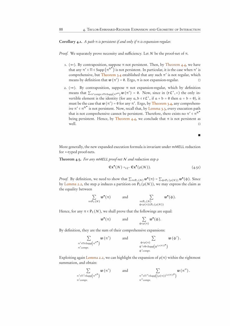
88 4. Taylor-Ehrhard-Regnier Expansion and Geometry of Interaction
Corollary 4.1. A path π is persistent if and only if π is expansion-regular.
Proof. We separately prove necessity and sufficiency. Let N be the proof-net of π.
1. (⇐). By contraposition, suppose π not persistent. Then, by Theorem 4.4, we havethat any π ′ ∈ Π ∈ Supp (πN
●) is not persistent. In particular, it is the case when π ′ iscomprehensive, but Theorem 3.4 established that any such π ′ is not regular, whichmeans by definition that w (π ′) = 0. Ergo, π is not expansion-regular. ◻
2. (⇒). By contraposition, suppose π not expansion-regular, which by definitionmeans that ∑π ′compr.∈Π∈Supp(πN●)w (π ′) = 0. Now, since in (rL∗,+) the only in-vertible element is the identity (for any a, b ∈ rL
∗, if a + b = 0 then a = b = 0), itmust be the case that w (π ′) = 0 for any π ′. Ergo, by Theorem 3.4, any comprehens-ive π ′ ∈ πN
●
is not persistent. Now, recall that, by Lemma 3.3, every execution paththat is not comprehensive cannot be persistent. Therefore, there exists no π ′ ∈ πN
●
being persistent. Hence, by Theorem 4.4, we conclude that π is not persistent aswell. ◻
∎
More generally, the new expanded execution formula is invariant under mMELL reductionfor ⋆-typed proof-nets.
Theorem 4.5. For any mMELL proof-net N and reduction step ρ
Ex●(N ) =rL∗ Ex●(ρ(N )). (4.51)
Proof. By definition, we need to show that ∑π∈PE(N)w●(π) = ∑φ∈PE(ρ(N))w
●(φ). Sinceby Lemma 2.2, the step ρ induces a partition on PE(ρ(N )), we may express the claim asthe equality between
∑π∈PE(N)
w●(π) and ∑
π∈PE(N)φ∈ρ(π)⊆PE(ρ(N))
w●(φ).
Hence, for any π ∈ PE(N ), we shall prove that the followings are equal:
w●(π) and ∑
φ∈ρ(π)w●(φ).
By definition, they are the sum of their comprehensive expansions:
∑π′∈Π∈Supp(πN●)
π′compr.
w (π ′) and ∑φ∈ρ(π)φ′∈Φ∈Supp(φ(ρ(N))●)
φ′compr.
w (φ ′) .
Exploiting again Lemma 2.2, we can highlight the expansion of ρ(π)within the rightmostsummation, and obtain:
∑π′∈Π′∈Supp(πN●)
π′compr.
w (π ′) and ∑π′′∈Π′′∈Supp((ρ(π))(ρ(N))●)
π′′compr.
w (π ′′) .
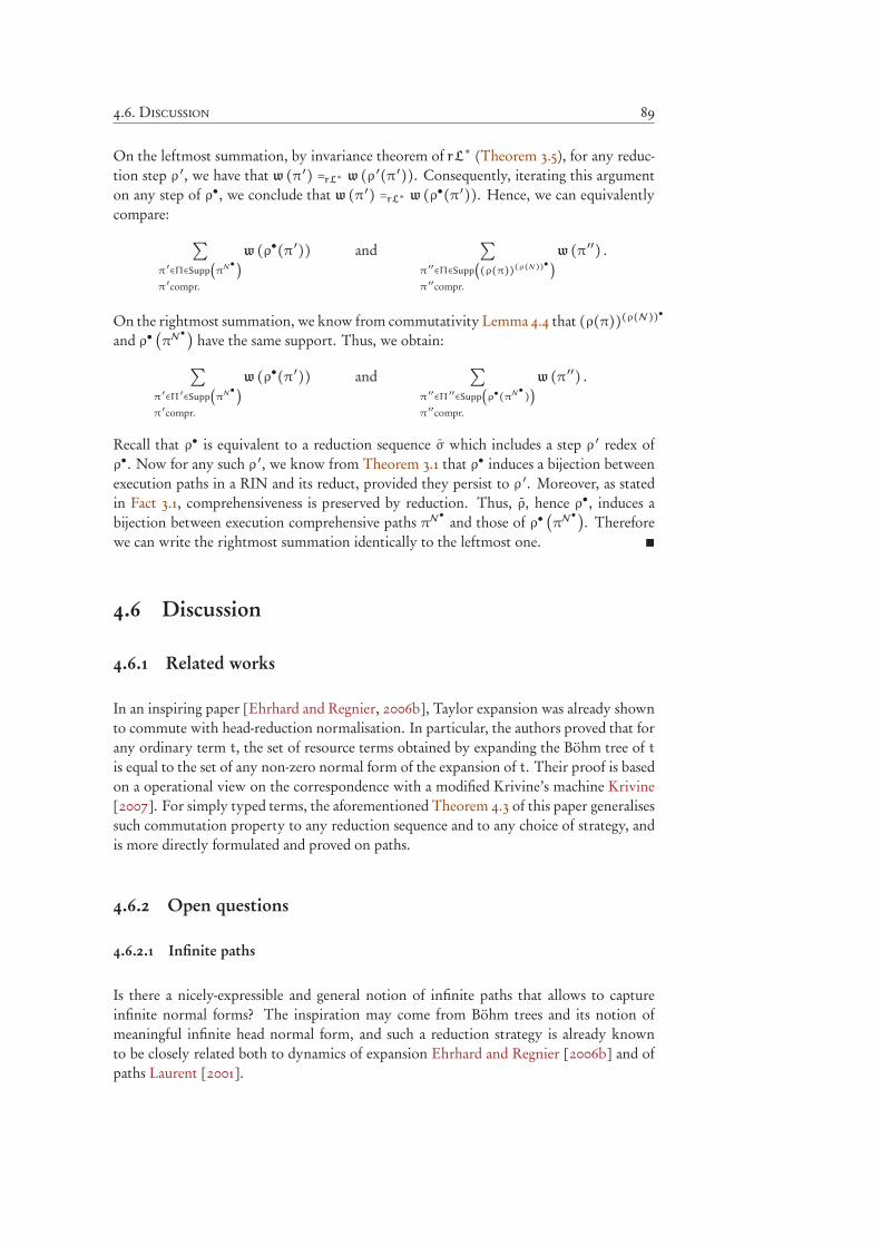
4.6. Discussion 89
On the leftmost summation, by invariance theorem of rL∗ (Theorem 3.5), for any reduc-tion step ρ ′, we have that w (π ′) =rL∗ w (ρ ′(π ′)). Consequently, iterating this argumenton any step of ρ●, we conclude that w (π ′) =rL∗ w (ρ●(π ′)). Hence, we can equivalentlycompare:
∑π′∈Π∈Supp(πN●)
π′compr.
w (ρ●(π ′)) and ∑π′′∈Π∈Supp((ρ(π))(ρ(N))●)
π′′compr.
w (π ′′) .
On the rightmost summation, we know from commutativity Lemma 4.4 that (ρ(π))(ρ(N))●and ρ● (πN
●) have the same support. Thus, we obtain:
∑π′∈Π′∈Supp(πN●)
π′compr.
w (ρ●(π ′)) and ∑π′′∈Π′′∈Supp(ρ●(πN●))
π′′compr.
w (π ′′) .
Recall that ρ● is equivalent to a reduction sequence σ which includes a step ρ ′ redex ofρ●. Now for any such ρ ′, we know from Theorem 3.1 that ρ● induces a bijection betweenexecution paths in a RIN and its reduct, provided they persist to ρ ′. Moreover, as statedin Fact 3.1, comprehensiveness is preserved by reduction. Thus, ρ, hence ρ●, induces abijection between execution comprehensive paths πN
●
and those of ρ● (πN●). Therefore
we can write the rightmost summation identically to the leftmost one. ∎
4.6 Discussion
4.6.1 Related works
In an inspiring paper [Ehrhard and Regnier, 2006b], Taylor expansion was already shownto commute with head-reduction normalisation. In particular, the authors proved that forany ordinary term t, the set of resource terms obtained by expanding the Böhm tree of tis equal to the set of any non-zero normal form of the expansion of t. Their proof is basedon a operational view on the correspondence with a modified Krivine’s machine Krivine[2007]. For simply typed terms, the aforementioned Theorem 4.3 of this paper generalisessuch commutation property to any reduction sequence and to any choice of strategy, andis more directly formulated and proved on paths.
4.6.2 Open questions
4.6.2.1 Infinite paths
Is there a nicely-expressible and general notion of infinite paths that allows to captureinfinite normal forms? The inspiration may come from Böhm trees and its notion ofmeaningful infinite head normal form, and such a reduction strategy is already knownto be closely related both to dynamics of expansion Ehrhard and Regnier [2006b] and ofpaths Laurent [2001].
90 4. Taylor-Ehrhard-Regnier Expansion and Geometry of Interaction
4.6.2.2 Resource abstract machine for the lambda-calculus
Can we design a non-deterministic linear abstract machine inspired by the constructionpresented here? In order to do so, we need to represent the expansion in a local manner,even if it has a twofold global nature: one in the argument superposition of RC, theother in the superposition of differently expanded terms. Removing the latter, indeedsubsumed by the former in a certain sense, the challenge becomes that of formalising anotion of expanded execution which does not explicitly consider the expansion of theproof-net, but which instead first assigns algebraic weights locally, and then computesthem in a distributed way. Starting from the approach presented here, the question maybe addressed by formalising expansion as a local graph-rewriting system.
4.6.2.3 Combinatorics of path expansion
What are the multiplicity coefficients for path expansion? A study of the non-trivialcombinatorial properties would complete our results, providing a tool to study the com-binatorics of ordinary paths in λ-terms. We believe it to be connected to the normalisationcomplexity and the expansion-related part of the framework to be fruitfully extendible ata quantitative level.

Part II
Sharing and efficiency

Chapter 5
Sharing implementation of
bounded logics
Contents
5.1. Introduction 94
5.2. Elementary and light proof-nets 95
5.3. Sharing implementation 98
5.3.1 Definition 98
5.3.2 Rewriting properties 99
5.4. Adequacy properties 102
5.4.1 Correctness 102
5.4.2 Weak completeness 102
5.4.3 Optimality 103
5.5. Correctness by syntactical simulation 104
5.5.1 Unshared graphs 104
5.5.2 From sharing graphs to unshared graphs 105
5.5.3 From unshared graphs to proof-nets 106
5.5.4 From sharing graphs to proof-nets 107
94 5. Sharing implementation of bounded logics
5.1 Introduction
Sharing graphs are a fine and versatile implementation technique for graph rewriting sys-tems, such as Λ and MELL. The sharing graphs machinery can be conceptually partitionedinto five components, each of which realizes a different type of operation.
Linear component implements the linear fragment of the target calculus, such as the mul-tiplicatives and their cut for MELL, or a linear variant of the β that postpone theduplication of the argument.
Duplication and sharing is the core component, also called the abstract algorithm, whichneeds a new kind of graph link, called mux, that essentially implements the duplica-tion in a distributed and atomic way. The mux propagation operation correspondsindeed to a sort of commutation of a contraction link over links contained insideanother exponential box, or to a step of partial duplication of an argument insideits context. Whilst the contraction link, or the λ binder construct, have only onepossible orientation — one input with several outputs — muxes allow also its dual— one output with several inputs, which means that muxes share not only terms,but also contexts.
Indexing management implements the exponential boxes information in a local and asyn-chronous way. It is also called the oracle, or the bookkeeper, and it can be imple-mented by mean of explicit hyperlinks (the bracket and the croissant), or by muxesthemselves, when all hyperlinks are labelled with indices of their box-nesting level.It corresponds to a sort of commutation of a dereliction link over links containedinside another exponential box.
Readback implements an unrestricted form of duplication in order to remove any sharingin a graph and to obtain an ordinary proof-net or a plain lambda tree. From apractical point of view, it is meant to be used at the end of the main reductionor normalization. To do so, it interacts with other links also when they are notconnected through a cut, i.e. with their conclusion.
Garbage collection implements erasure locally, link by link, and it is either represented byzero-ary muxes, or kept distinct by the usage of two new hyperlinks. It correspondsto a sort of commutation of the weakening link over links contained inside anotherexponential box.
This chapter is devoted to present the sharing implementation of the elementary and lightvariants of mMELL, recalling its main properties and proving its correctness by syntacticalsimulations. In Section 5.2we present the proof-nets ofmIELL, that represent a frameworkof particular convenience because it considerably simplifies the rewriting system, whilstin Section 5.3 we introduce their sharing implementation — the system SG— and its basicproperties. A brief review of the most notable qualitative behavioural properties of SG asa Lévy-optimal implementation of mIELL proof-nets is given in Section 5.4. Among these,
5.2. Elementary and light proof-nets 95
there is the correctness: any SG-normal-form of amIELL proof-net N is themIELL-normal-form of N . A proof is given in the concluding Section 5.5 (cf. Theorem 5.10), wherewe employ a simple syntactical simulation of SG in mIELL, exploiting an intermediaterewriting system— the unshared graphs (UG) — that possess the structure ofmIELL proof-nets and a some sharing markers corresponding to SG graphs.
5.2 Elementary and light proof-nets
We present a minimal, propositional and weakening-free fragment of ELL proof-nets,where proof-nets of the corresponding fragment of LLL can also be represented, as well asELL- and LLL- typed λI- terms.
A ELL proof-net is similar to a MELL proof-net, except from the fact that a vertex canbe the secondary door of at most one box. LLL proof-nets, instead, are a bit more com-plicated, because types/formulæneed to encompass an additional exponential modality §called paragraph1, which induces two new kinds (§ and §) of binary links with dual po-larisations. Hence we have two kind of boxes, associated not only to promotion links,but also to positive paragraph links. !-boxes have at most one secondary door, which is apremiss of a ?-link, §-boxes have instead an arbitrary number of secondary doors, whichare premiss of links of kind ? or §. These two restrictions tame the amount of duplicationpossibly needed by the reduction so that, quite interestingly, they are precise representa-tions of, respectively, the complexity classes: Kalmar-elementary time (Elementary, i.e.iterated exponentials) and polynomial time (PTime).
Fact 5.1 (Stratification). Given a LLL or ELL proof-net N , let v ∈ V(N ), l ∈ L(N ), ρ bereduction step on N . If there exist ρ(v), ρ(l) residuals of v, l, respectively, then ℓ(v) = ℓ(ρ(v))and ℓ(l) = ℓ(ρ(l)).Theorem 5.1 (Normalisation and complexity classes [Girard, 1995, Asperti and Roversi,2002]). Let Elementary be the set of functions that are computable in time bounded byK(h,n), where n is the size of the input, and K is the Kalmar function defined as follows:
K(0,n) = n, K(i + 1,n) = 2K(i,n). (5.1)
Let PTime be the set of functions computable in time bounded by a polynomial of the size of theinput n.
1. The set of functions computed by ELL is equal to Elementary. In particular, the lengthof a ELL reduction on a proof-net N is at most K(ℓ(N ), ∣N ∣).
2. The set of functions computed by LLL is equal to PTime. In particular, the length of a LLLreduction on a proof-net N is at most a polynomial of degree 2ℓ(N)+1.
We can now proceed to concretely present our simplified proof-net system and their re-duction. We opt to avoid the presence of 0-ary contractions for mere sake of simplicity,
1The name most probably comes from an erroneous translation of the French ‘paragraphe’, i.e. ‘section’,hence explaining the section sign § used as its symbol instead of the pilcrow �.
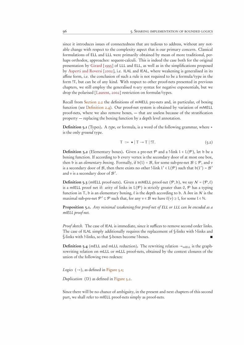
96 5. Sharing implementation of bounded logics
since it introduces issues of connectedness that are tedious to address, without any not-able change with respect to the complexity aspect that is our primary concern. Classicalformulations of ELL and LLL were primarily obtained by mean of more traditional, per-haps orthodox, approaches: sequent-calculi. This is indeed the case both for the originalpresentation by Girard [1995] of LLL and ELL, as well as in the simplifications proposedby Asperti and Roversi [2002], i.e. ILAL and IEAL, where weakening is generalised in itsaffine form, i.e. the conclusion of such a rule is not required to be a formula/type in theform !T , but can be of any kind. With respect to other proof-nets presented in previouschapters, we still employ the generalised n-ary syntax for negative exponentials, but wedrop the polarised [Laurent, 2002] restriction on formulæ/types.
Recall from Section 2.2 the definitions of mMELL pre-nets and, in particular, of boxingfunction (see Definition 2.4). Our proof-net system is obtained by variation of mMELL
proof-nets, where we also remove boxes, — that are useless because of the stratificationproperty — replacing the boxing function by a depth level annotation.
Definition 5.1 (Types). A type, or formula, is a word of the following grammar, where ⋆is the only ground type.
T ∶∶= ★ ∣ T ⊸ T ∣ !T . (5.2)
Definition 5.2 (Elementary boxes). Given a pre-net P and a !-link l ∈ L(P), let b be aboxing function. If according to b every vertex is the secondary door of at most one box,then b is an elementary boxing. Formally, if b(l) = B, for some sub-pre-net B ⊆ P, and v
is a secondary door of B, then there exists no other !-link l ′ ∈ L(P) such that b(l ′) = B ′
and v is a secondary door of B ′.
Definition 5.3 (mIELL proof-nets). Given a mMELL proof-net (P, b), we say N = (P, ℓ)is a mIELL proof net if: arity of links in L(P) is strictly greater than 0, P has a typingfunction in T , b is an elementary boxing, ℓ is the depth according to b. A box in N is themaximal sub-pre-net P ′ ⊆ P such that, for any v ∈ B we have ℓ(v) ≥ l, for some l ∈ N.
Proposition 5.1. Any minimal weakening-free proof-net of ELL or LLL can be encoded as amIELL proof-net.
Proof sketch. The case of IEAL is immediate, since it suffices to remove second order links.The case of ILAL simply additionally requires the replacement of §-links with !-links and§-links with ?-links, so that §-boxes become !-boxes. ∎
Definition 5.4 (mELL and mLLL reduction). The rewriting relation →mIELL is the graph-rewriting relation on mLLL or mLLL proof-nets, obtained by the context closures of theunion of the following two redexes:
Logics (⊸), as defined in Figure 5.1;
Duplication (D) as defined in Figure 5.2.
Since there will be no chance of ambiguity, in the present and next chapters of this secondpart, we shall refer to mIELL proof-nets simply as proof-nets.
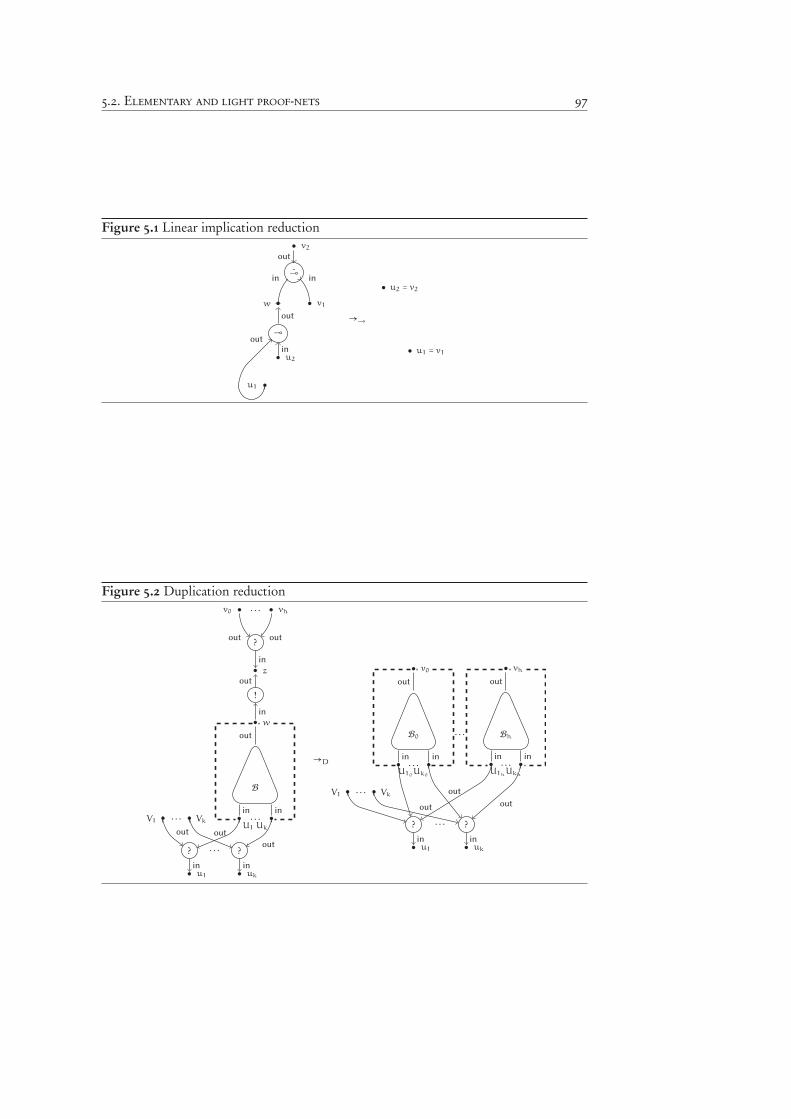
5.2. Elementary and light proof-nets 97
Figure 5.1 Linear implication reduction
⊸
• u2
in
•u1
out
⊸
•w
in
• v1
in
• v2
out
out→⊸
• u2 = v2
• u1 = v1
Figure 5.2 Duplication reduction
?
•v0
out
• vh
out
. . .
!
• z
out
in
B
•
in
•
in. . .
U1 Uk
• w
out
in
•V1 • Vk. . .
?
• u1
in
?
• uk
in
. . .
out out
out
→D
B0
•
in
•
in. . .
U10Uk0
• v0
out
Bh
•
in
•
in. . .
U1hUkh
• vh
out
. . .
•V1 • Vk. . .
?
• u1
in
?
• uk
in
. . .
out
out
out
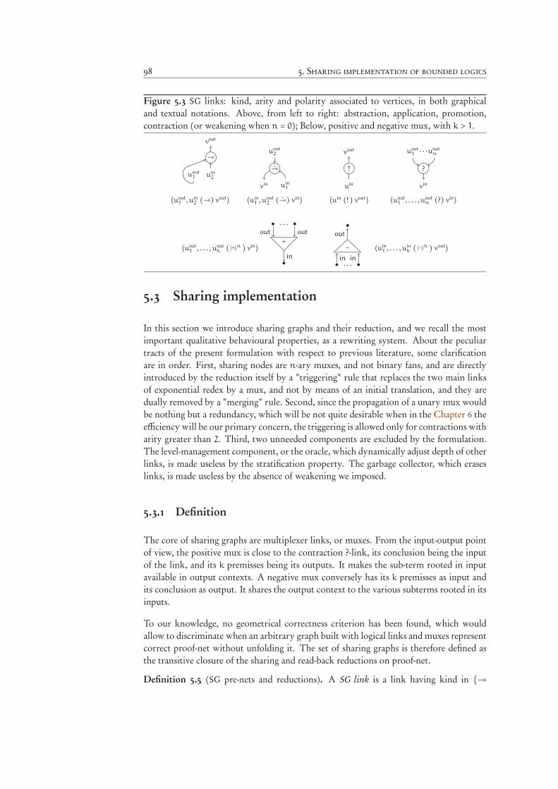
98 5. Sharing implementation of bounded logics
Figure 5.3 SG links: kind, arity and polarity associated to vertices, in both graphicaland textual notations. Above, from left to right: abstraction, application, promotion,contraction (or weakening when n = 0); Below, positive and negative mux, with k > 1.
⊸
vout
uin
2uout
1
⟨uout
1, u
in
2(⊸) vout⟩
⊸
uout
2
uin
1vin
⟨uin
1, u
out
2(⊸) vin⟩
!
vout
uin
⟨uin (! ) vout⟩
?
uout
1uout
n
vin
. . .
⟨uout
1, . . . , u
out
n(?) vin⟩
⟨uout
1, . . . , u
out
k( ∣+⟩n ) vin⟩
+
•
in
•
out
•
out
. . .
−
•
in
•
in. . .
•
out
⟨uin
1, . . . , u
in
k( ∣-⟩n ) vout⟩
5.3 Sharing implementation
In this section we introduce sharing graphs and their reduction, and we recall the mostimportant qualitative behavioural properties, as a rewriting system. About the peculiartracts of the present formulation with respect to previous literature, some clarificationare in order. First, sharing nodes are n-ary muxes, and not binary fans, and are directlyintroduced by the reduction itself by a "triggering" rule that replaces the two main linksof exponential redex by a mux, and not by means of an initial translation, and they aredually removed by a "merging" rule. Second, since the propagation of a unary mux wouldbe nothing but a redundancy, which will be not quite desirable when in the Chapter 6 theefficiency will be our primary concern, the triggering is allowed only for contractions witharity greater than 2. Third, two unneeded components are excluded by the formulation.The level-management component, or the oracle, which dynamically adjust depth of otherlinks, is made useless by the stratification property. The garbage collector, which eraseslinks, is made useless by the absence of weakening we imposed.
5.3.1 Definition
The core of sharing graphs are multiplexer links, or muxes. From the input-output pointof view, the positive mux is close to the contraction ?-link, its conclusion being the inputof the link, and its k premisses being its outputs. It makes the sub-term rooted in inputavailable in output contexts. A negative mux conversely has its k premisses as input andits conclusion as output. It shares the output context to the various subterms rooted in itsinputs.
To our knowledge, no geometrical correctness criterion has been found, which wouldallow to discriminate when an arbitrary graph built with logical links and muxes representcorrect proof-net without unfolding it. The set of sharing graphs is therefore defined asthe transitive closure of the sharing and read-back reductions on proof-net.
Definition 5.5 (SG pre-nets and reductions). A SG link is a link having kind in {⊸
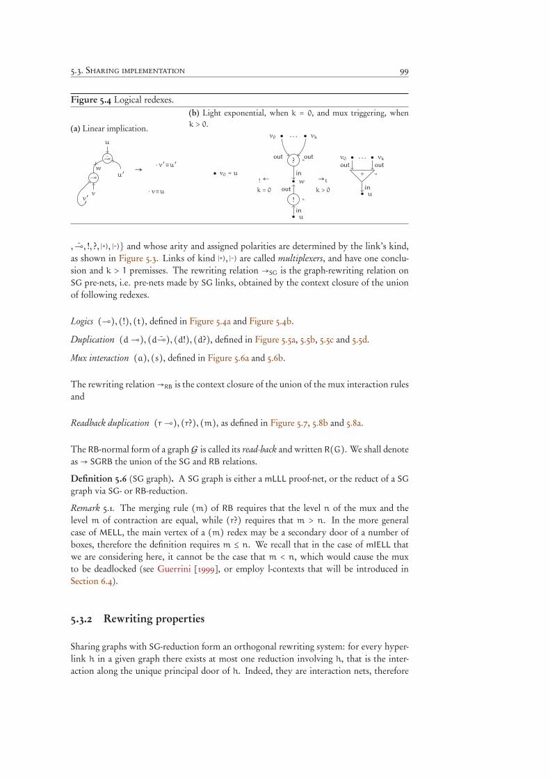
5.3. Sharing implementation 99
Figure 5.4 Logical redexes.
(a) Linear implication.
⊸
⊸
u
u′
v
v′
w→
⋅ v′≡u′
⋅ v≡u
(b) Light exponential, when k = 0, and mux triggering, whenk > 0.
?
•v0
out
• vk
out
. . .
n
!
• u
in
• w
out
n
in→t
k > 0
+ n
• u
in
•v0
out
• vk
out
. . .
! ←
k = 0
• v0 = u
, ⊸, !, ?, ∣+⟩, ∣-⟩} and whose arity and assigned polarities are determined by the link’s kind,as shown in Figure 5.3. Links of kind ∣+⟩, ∣-⟩ are called multiplexers, and have one conclu-sion and k > 1 premisses. The rewriting relation →SG is the graph-rewriting relation onSG pre-nets, i.e. pre-nets made by SG links, obtained by the context closure of the unionof following redexes.
Logics (⊸), (!), (t), defined in Figure 5.4a and Figure 5.4b.
Duplication (d⊸), (d⊸), (d!), (d?), defined in Figure 5.5a, 5.5b, 5.5c and 5.5d.
Mux interaction (a), (s), defined in Figure 5.6a and 5.6b.
The rewriting relation→RB is the context closure of the union of the mux interaction rulesand
Readback duplication (r⊸), (r?), (m), as defined in Figure 5.7, 5.8b and 5.8a.
The RB-normal form of a graph G is called its read-back and written R(G). We shall denoteas → SGRB the union of the SG and RB relations.
Definition 5.6 (SG graph). A SG graph is either a mLLL proof-net, or the reduct of a SGgraph via SG- or RB-reduction.
Remark 5.1. The merging rule (m) of RB requires that the level n of the mux and thelevel m of contraction are equal, while (r?) requires that m > n. In the more generalcase of MELL, the main vertex of a (m) redex may be a secondary door of a number ofboxes, therefore the definition requires m ≤ n. We recall that in the case of mIELL thatwe are considering here, it cannot be the case that m < n, which would cause the muxto be deadlocked (see Guerrini [1999], or employ l-contexts that will be introduced inSection 6.4).
5.3.2 Rewriting properties
Sharing graphs with SG-reduction form an orthogonal rewriting system: for every hyper-link h in a given graph there exists at most one reduction involving h, that is the inter-action along the unique principal door of h. Indeed, they are interaction nets, therefore
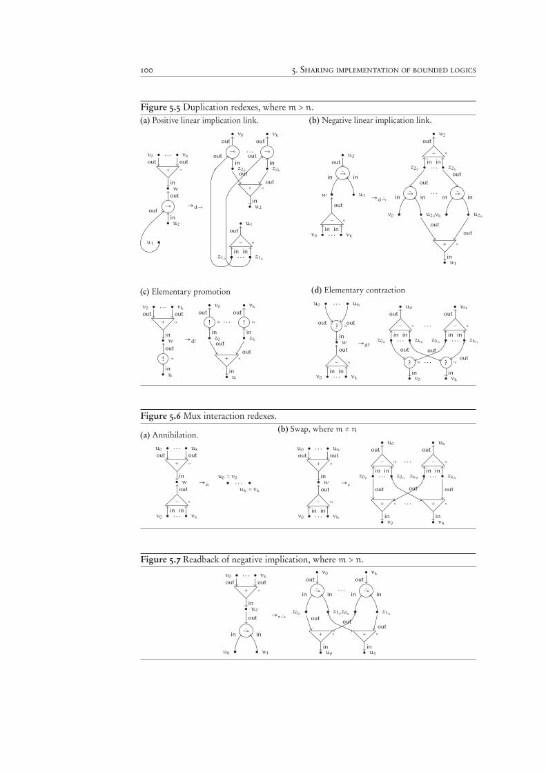
100 5. Sharing implementation of bounded logics
Figure 5.5 Duplication redexes, where m > n.(a) Positive linear implication link.
+ n
• w
in
•v0
out
• vk
out
. . .
⊸
• u2
in
•u1
out
out
→d⊸
⊸
• v0
out
• z20
in
⊸
• vk
out
• z2k
in
. . .
+ n
• u2
in
out
out
− n
•z10
in
• z1k
in. . .
• u1
out
•
out
•
out
(b) Negative linear implication link.
⊸
•w
in
• u1
in
• u2
out
− n
•v0
in
• vk
in. . .
out
→d⊸
− n
•z20
in
• z2k
in. . .
• u2
out
⊸
•v0
in
• u20
in⊸
•vk
in
• u2k
in. . .
out
out
+ n
• u1
in
out
out
(c) Elementary promotion
+ n
• w
in
•v0
out
• vk
out
. . .
!
• u
in
m
out
→d!
!
• z0
in
• v0
out
m !
• zk
in
• vk
out
m. . .
+ n
• u
in
out
out
(d) Elementary contraction
?
• w
in
•u0
out
• uh
out
. . .
m
− n
•v0
in
• vk
in. . .
out
→d?
− n
•z00
in
• zk0
in. . .
• u0
out
− n
•z0h
in
• zkh
in. . .
• uh
out
. . .
?
• v0
in
?
• vk
in
m m. . .
out out
out
Figure 5.6 Mux interaction redexes.
(a) Annihilation.
+ n
• w
in
•u0
out
• uk
out
. . .
− n
•v0
in
• vk
in. . .
out
→a •
u0 = v0
•
uk = vk
. . .
(b) Swap, where m ≠ n
+ n
• w
in
•u0
out
• uk
out
. . .
− m
•v0
in
• vh
in. . .
out
→s
− m
•z00
in
• z0h
in. . .
• u0
out
− m
•zk0
in
• zkh
in. . .
• uk
out
. . .
+ n
• v0
in
+ n
• vh
in
. . .
out out out
Figure 5.7 Readback of negative implication, where m > n.
+ n
• u2
in
•v0
out
• vk
out
. . .
⊸
•u0
in
• u1
in
out→r⊸
⊸
•z00
in
• z10
in
• v0
out
⊸
•z0k
in
• z1k
in
• vk
out
. . .
+ n
• u0
in
out
+ n
• u1
in
outout
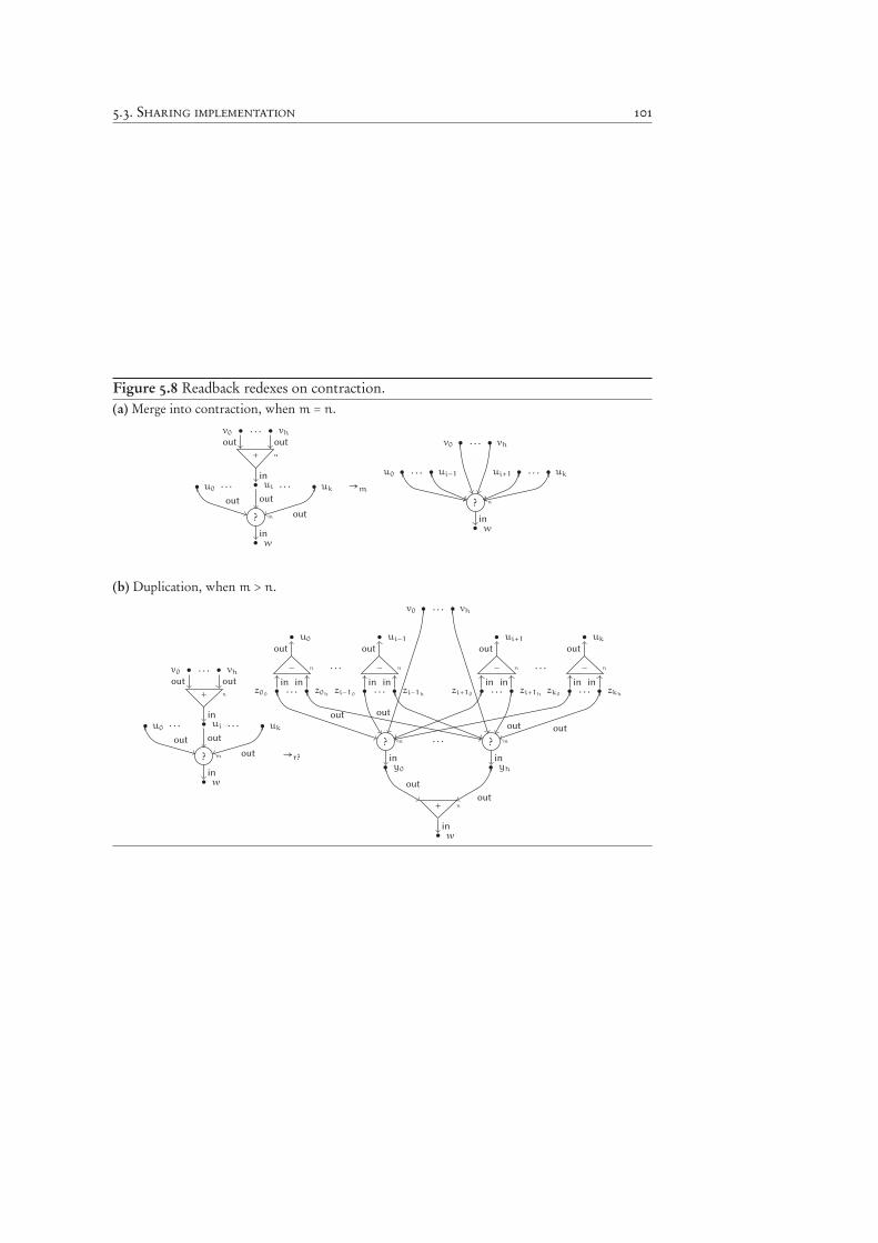
5.3. Sharing implementation 101
Figure 5.8 Readback redexes on contraction.(a) Merge into contraction, when m = n.
• u0
+ n
• ui
in
•v0
out
• vh
out
. . .
. . .• uk
. . .
?
• w
in
m
out out
out
→m
•v0 • vh. . .
•u0 • ui−1. . . •ui+1 • uk
. . .
?
• w
in
n
(b) Duplication, when m > n.
• u0
+ n
• ui
in
•v0
out
• vh
out
. . .
. . .• uk
. . .
?
• w
in
m
out out
out →r?
•v0 • vh. . .
− n
•z00
in
• z0h
in. . .
• u0
out
− n
•zi−10
in
• zi−1h
in. . .
• ui−1
out
. . . − n
•zi+10
in
• zi+1h
in. . .
• ui+1
out
− n
•zk0
in
• zkh
in. . .
• uk
out
. . .
?
• y0
in
m ?
• yh
in
m. . .
out out
out out
+ n
• w
in
out
out
102 5. Sharing implementation of bounded logics
they are locally confluent. The RB-reduction includes instead many rules which allowsinteractions between links that are not connected by their principal vertices. But In thiscase, as well as in the combined one, the system still enjoys good rewriting properties.
Theorem 5.2 (Confluence and normalisation). The rewriting systems RB and SGRB arestrongly normalising and confluent. Their normal forms are proof-nets.
Proof hint. With respect to the work by Guerrini et al. [2003, Theorems 4, 11.i and 11.ii],we have here only two minor differences: axioms and cut links are implicit, read-backrules are restricted to positive muxes only. ∎
Any SGRB sequence can be rearranged in order to postpone the read-back, i.e. the non-optimal duplications, at the end of the sharing normalisation. This is indeed the standardway of employing sharing graphs as an implementation.
Theorem 5.3 (Safety of laziness [Guerrini et al., 2003, Theorem 15]). Let N be a proof-netand N its SGRB -normal form. If G is the SG-normal form of N , then G →∗
RBN .
5.4 Adequacy properties
5.4.1 Correctness
Sharing graphs are a correct implementation of cut-elimination of proof-nets.
Theorem 5.4 (Correctness). Let N be a proof-net such that N →∗
SGG. Then there exists
N →∗mIELL
R(G).
The correctness of the sharing implementation in the general case of λ-calculus was firstestablished using a semantical analysis of GoI paths in the graphs [Gonthier, Abadi, andLévy, 1992a]. A comprehensive discussion is provided by Asperti [1998]. The first resultsof correctness obtained by syntactical means has been presented by Guerrini [1999], wheresharing graphs implements a generic framework of graph rewriting, and little later byGuerrini et al., who consider [2003, Theorem 13] the case of MELL proof-nets. In arestricted case similar to our interest — IEAL and ILAL proof-nets — correctness was alsomore recently proven with GoI-like semantics tools [Baillot, Coppola, and Dal Lago,2011].
We shall use an adaptation of the syntactic approach, based on an intermediate rewritingsystem called unshared graphs. The stratification property of mIELL allows us to provecorrectness by a simpler and neater presentation, provided here in Theorem 5.8.
5.4.2 Weak completeness
If we forget optimality, we can consider the rewriting system where all the duplicationrules are allowed, i.e. where muxes are allowed to propagate exhaustively and to complete
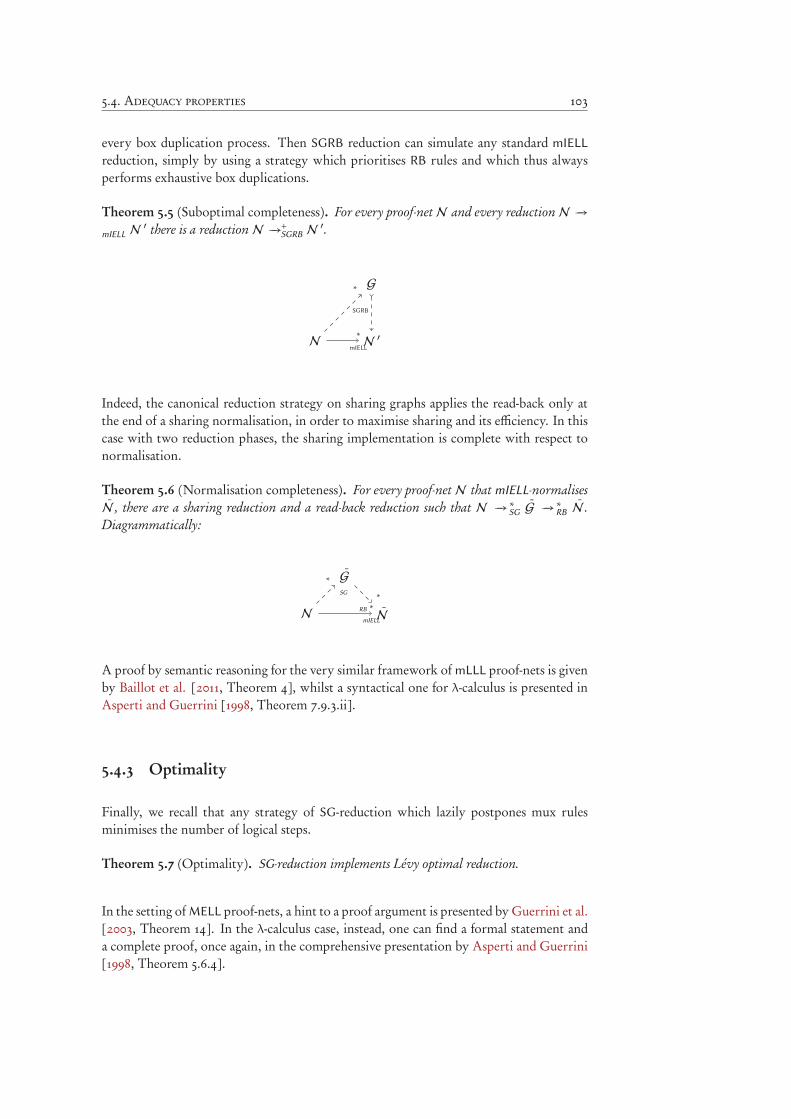
5.4. Adequacy properties 103
every box duplication process. Then SGRB reduction can simulate any standard mIELL
reduction, simply by using a strategy which prioritises RB rules and which thus alwaysperforms exhaustive box duplications.
Theorem 5.5 (Suboptimal completeness). For every proof-netN and every reductionN −→
mIELLN ′ there is a reduction N −→
+
SGRBN ′.
N
G
N ′∗
mIELL
∗
SGRB
Indeed, the canonical reduction strategy on sharing graphs applies the read-back only atthe end of a sharing normalisation, in order to maximise sharing and its efficiency. In thiscase with two reduction phases, the sharing implementation is complete with respect tonormalisation.
Theorem 5.6 (Normalisation completeness). For every proof-net N that mIELL-normalisesN , there are a sharing reduction and a read-back reduction such that N −→
∗
SGG −→
∗
RBN .
Diagrammatically:
N
G
N∗
mIELL
∗
SG∗
RB
A proof by semantic reasoning for the very similar framework of mLLL proof-nets is givenby Baillot et al. [2011, Theorem 4], whilst a syntactical one for λ-calculus is presented inAsperti and Guerrini [1998, Theorem 7.9.3.ii].
5.4.3 Optimality
Finally, we recall that any strategy of SG-reduction which lazily postpones mux rulesminimises the number of logical steps.
Theorem 5.7 (Optimality). SG-reduction implements Lévy optimal reduction.
In the setting ofMELL proof-nets, a hint to a proof argument is presented by Guerrini et al.[2003, Theorem 14]. In the λ-calculus case, instead, one can find a formal statement anda complete proof, once again, in the comprehensive presentation by Asperti and Guerrini[1998, Theorem 5.6.4].
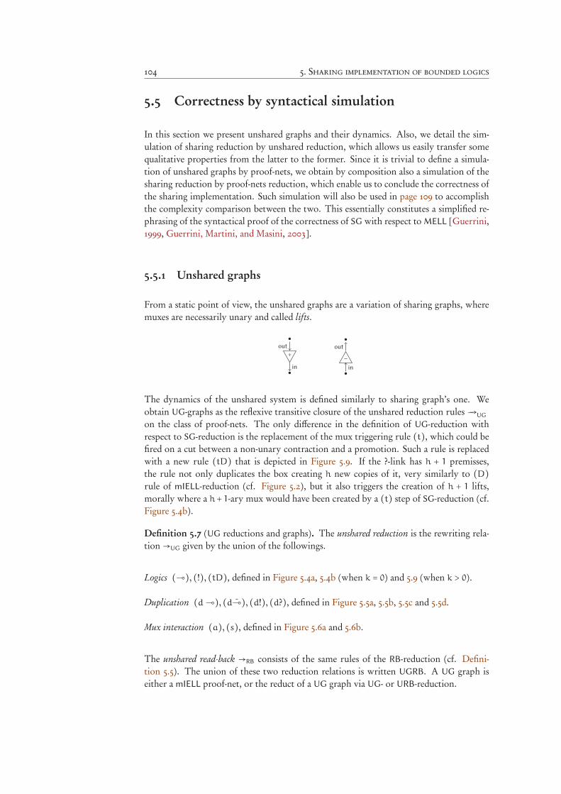
104 5. Sharing implementation of bounded logics
5.5 Correctness by syntactical simulation
In this section we present unshared graphs and their dynamics. Also, we detail the sim-ulation of sharing reduction by unshared reduction, which allows us easily transfer somequalitative properties from the latter to the former. Since it is trivial to define a simula-tion of unshared graphs by proof-nets, we obtain by composition also a simulation of thesharing reduction by proof-nets reduction, which enable us to conclude the correctness ofthe sharing implementation. Such simulation will also be used in page 109 to accomplishthe complexity comparison between the two. This essentially constitutes a simplified re-phrasing of the syntactical proof of the correctness of SG with respect to MELL [Guerrini,1999, Guerrini, Martini, and Masini, 2003].
5.5.1 Unshared graphs
From a static point of view, the unshared graphs are a variation of sharing graphs, wheremuxes are necessarily unary and called lifts.
+
•
in
•
out
−
•
in
•
out
The dynamics of the unshared system is defined similarly to sharing graph’s one. Weobtain UG-graphs as the reflexive transitive closure of the unshared reduction rules −→UG
on the class of proof-nets. The only difference in the definition of UG-reduction withrespect to SG-reduction is the replacement of the mux triggering rule (t), which could befired on a cut between a non-unary contraction and a promotion. Such a rule is replacedwith a new rule (tD) that is depicted in Figure 5.9. If the ?-link has h + 1 premisses,the rule not only duplicates the box creating h new copies of it, very similarly to (D)rule of mIELL-reduction (cf. Figure 5.2), but it also triggers the creation of h + 1 lifts,morally where a h+ 1-ary mux would have been created by a (t) step of SG-reduction (cf.Figure 5.4b).
Definition 5.7 (UG reductions and graphs). The unshared reduction is the rewriting rela-tion →UG given by the union of the followings.
Logics (⊸), (!), (tD), defined in Figure 5.4a, 5.4b (when k = 0) and 5.9 (when k > 0).
Duplication (d⊸), (d⊸), (d!), (d?), defined in Figure 5.5a, 5.5b, 5.5c and 5.5d.
Mux interaction (a), (s), defined in Figure 5.6a and 5.6b.
The unshared read-back →RB consists of the same rules of the RB-reduction (cf. Defini-tion 5.5). The union of these two reduction relations is written UGRB. A UG graph iseither a mIELL proof-net, or the reduct of a UG graph via UG- or URB-reduction.
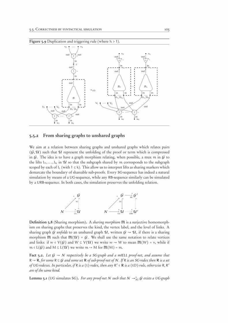
5.5. Correctness by syntactical simulation 105
Figure 5.9 Duplication and triggering rule (where h > 1).
?
•v0
out
• vh
out
. . .
n
!
• z
out
n
in
B
•
in
•
in. . .
U1 Uk
• w
out
in
•V1 • Vk. . .
?
• u1
in
n ?
• uk
in
n. . .
out
n
out
n
out
→tD
+n
• v0
out
+n
• vh
out
B0
•
in
•
in. . .
U10Uk0
• w0
out
in
Bh
•
in
•
in. . .
U1hUkh
• wh
out
in
. . .
•V1 • Vk. . .
?
• u1
in
?
• uk
in
. . .n
out
n
out
out
5.5.2 From sharing graphs to unshared graphs
We aim at a relation between sharing graphs and unshared graphs which relates pairs(G,U) such that U represent the unfolding of the proof or term which is compressedin G. The idea is to have a graph morphism relating, when possible, a mux m in G tothe lifts l1, . . . , lk in U so that the subgraph shared by m corresponds to the subgraphscoped by each of li (with 1 ≤ k). This allow us to interpret lifts as sharing markers whichdemarcate the boundary of shareable sub-proofs. Every SG-sequence has indeed a naturalsimulation by means of a UG-sequence, while any RB-sequence similarly can be simulatedby a URB-sequence. In both cases, the simulation preserves the unfolding relation.
N
G
U
∗
SG
∗
UGN
G
U
G ′
U ′
∗
SG
∗
UG
∗
RB
∗
URB
Definition 5.8 (Sharing morphism). A sharing morphismM is a surjective homomorph-ism on sharing graphs that preserves the kind, the vertex label, and the level of links. Asharing graph G unfolds to an unshared graph U , written G ↪ U , if there is a sharingmorphism M such that M(U) = G. We shall use the same notation to relate verticesand links: if w ∈ V(G) and W ⊆ V(U) we write w ↪ W to mean M(W) = v, while ifm ∈ L(G) and M ⊆ L(U) we write m↪M forM(M) =m.
Fact 5.2. Let G ↪ N respectively be a SG-graph and a mIELL proof-net, and assume thatR↪ R, for some R ⊆ G and some set R of sub-proof-net of N . If R is an SG-redex then R is a setof UG-redexes. In particular, if R is a (t)-redex, then any R ′ ∈ R is a (tD)-rule, otherwise R,R ′are of the same kind.
Lemma 5.1 (UG simulates SG). For any proof-net N such that N −→∗
SGG exists a UG-graph
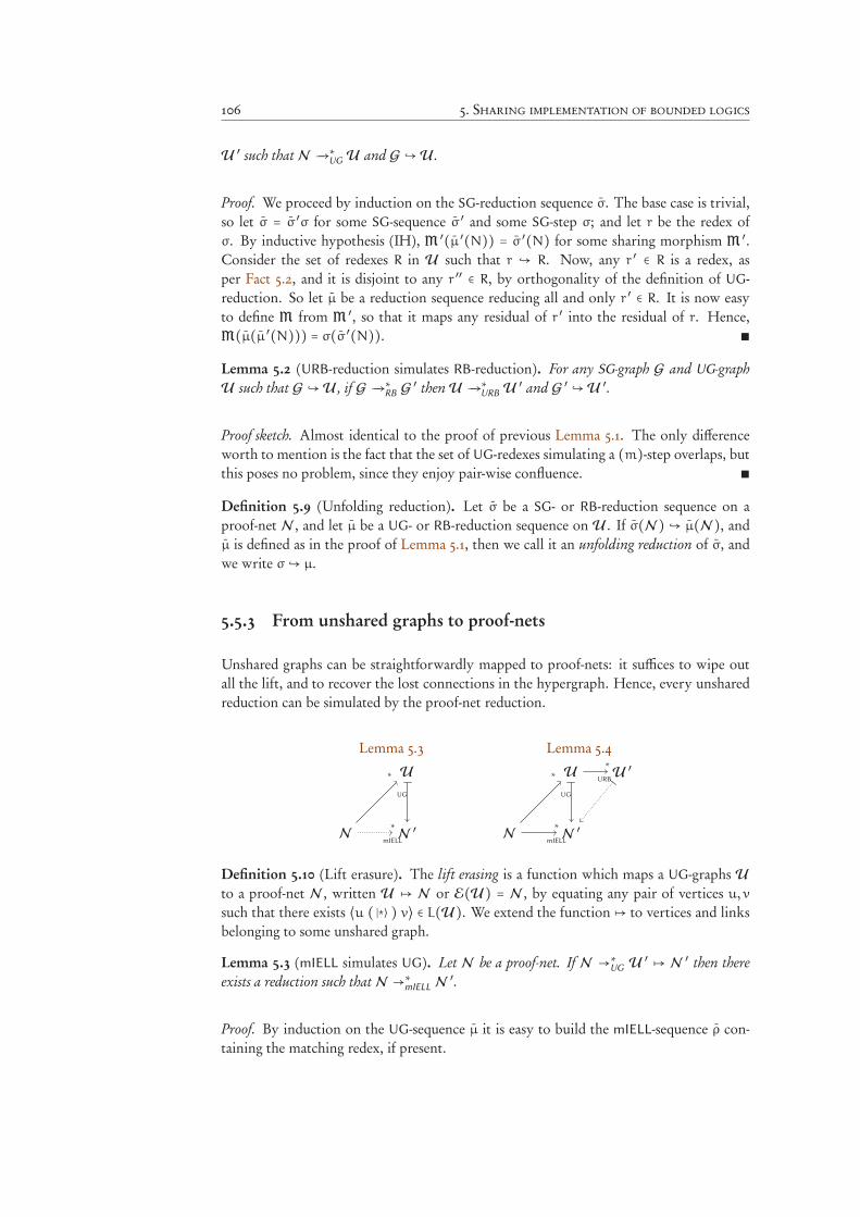
106 5. Sharing implementation of bounded logics
U ′ such that N −→∗
UGU and G ↪U .
Proof. We proceed by induction on the SG-reduction sequence σ. The base case is trivial,so let σ = σ ′σ for some SG-sequence σ ′ and some SG-step σ; and let r be the redex ofσ. By inductive hypothesis (IH), M ′(µ ′(N)) = σ ′(N) for some sharing morphism M ′.Consider the set of redexes R in U such that r ↪ R. Now, any r ′ ∈ R is a redex, asper Fact 5.2, and it is disjoint to any r ′′ ∈ R, by orthogonality of the definition of UG-reduction. So let µ be a reduction sequence reducing all and only r ′ ∈ R. It is now easyto define M from M ′, so that it maps any residual of r ′ into the residual of r. Hence,M(µ(µ ′(N))) = σ(σ ′(N)). ∎
Lemma 5.2 (URB-reduction simulates RB-reduction). For any SG-graph G and UG-graphU such that G ↪U , if G −→
∗
RBG ′ then U −→
∗
URBU ′ and G ′ ↪U ′.
Proof sketch. Almost identical to the proof of previous Lemma 5.1. The only differenceworth to mention is the fact that the set of UG-redexes simulating a (m)-step overlaps, butthis poses no problem, since they enjoy pair-wise confluence. ∎
Definition 5.9 (Unfolding reduction). Let σ be a SG- or RB-reduction sequence on aproof-net N , and let µ be a UG- or RB-reduction sequence on U . If σ(N ) ↪ µ(N ), andµ is defined as in the proof of Lemma 5.1, then we call it an unfolding reduction of σ, andwe write σ↪ µ.
5.5.3 From unshared graphs to proof-nets
Unshared graphs can be straightforwardly mapped to proof-nets: it suffices to wipe outall the lift, and to recover the lost connections in the hypergraph. Hence, every unsharedreduction can be simulated by the proof-net reduction.
Lemma 5.3 Lemma 5.4
N
U
N′
∗
UG
∗
mIELLN
U
N′
U′
∗
UG
∗
mIELL
∗
URB
Definition 5.10 (Lift erasure). The lift erasing is a function which maps a UG-graphs U
to a proof-net N , written U ↦ N or E(U) = N , by equating any pair of vertices u, v
such that there exists ⟨u ( ∣*⟩ ) v⟩ ∈ L(U). We extend the function ↦ to vertices and linksbelonging to some unshared graph.
Lemma 5.3 (mIELL simulates UG). Let N be a proof-net. If N →∗UG
U ′↦ N ′ then there
exists a reduction such that N →∗mIELL
N ′.
Proof. By induction on the UG-sequence µ it is easy to build the mIELL-sequence ρ con-taining the matching redex, if present.
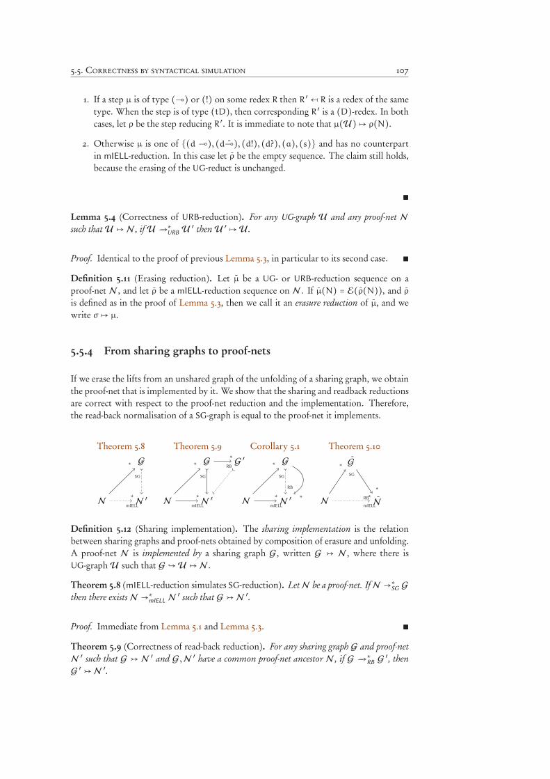
5.5. Correctness by syntactical simulation 107
1. If a step µ is of type (⊸) or (!) on some redex R then R ′ ←[ R is a redex of the sametype. When the step is of type (tD), then corresponding R ′ is a (D)-redex. In bothcases, let ρ be the step reducing R ′. It is immediate to note that µ(U)↦ ρ(N).
2. Otherwise µ is one of {(d ⊸), (d⊸), (d!), (d?), (a), (s)} and has no counterpartin mIELL-reduction. In this case let ρ be the empty sequence. The claim still holds,because the erasing of the UG-reduct is unchanged.
∎
Lemma 5.4 (Correctness of URB-reduction). For any UG-graph U and any proof-net N
such that U ↦N , if U −→∗
URBU ′ then U ′
↦U .
Proof. Identical to the proof of previous Lemma 5.3, in particular to its second case. ∎
Definition 5.11 (Erasing reduction). Let µ be a UG- or URB-reduction sequence on aproof-net N , and let ρ be a mIELL-reduction sequence on N . If µ(N) = E(ρ(N)), and ρ
is defined as in the proof of Lemma 5.3, then we call it an erasure reduction of µ, and wewrite σ↦ µ.
5.5.4 From sharing graphs to proof-nets
If we erase the lifts from an unshared graph of the unfolding of a sharing graph, we obtainthe proof-net that is implemented by it. We show that the sharing and readback reductionsare correct with respect to the proof-net reduction and the implementation. Therefore,the read-back normalisation of a SG-graph is equal to the proof-net it implements.
Theorem 5.8 Theorem 5.9 Corollary 5.1 Theorem 5.10
N
G
N ′
∗
SG
∗
mIELLN
G
N ′
G ′∗
SG
∗
mIELL
∗
RB
N
G
N ′
∗
SG
∗
mIELL
∗
RB
N
G
N
∗
SG
∗
RB∗
mIELL
Definition 5.12 (Sharing implementation). The sharing implementation is the relationbetween sharing graphs and proof-nets obtained by composition of erasure and unfolding.A proof-net N is implemented by a sharing graph G, written G ↣ N , where there isUG-graph U such that G ↪U ↦N .
Theorem 5.8 (mIELL-reduction simulates SG-reduction). LetN be a proof-net. IfN →∗SG
G
then there exists N →∗mIELL
N ′ such that G ↣N ′.
Proof. Immediate from Lemma 5.1 and Lemma 5.3. ∎
Theorem 5.9 (Correctness of read-back reduction). For any sharing graph G and proof-netN ′ such that G ↣ N ′ and G,N ′ have a common proof-net ancestor N , if G −→
∗
RBG ′, then
G ′ ↣N ′.
108 5. Sharing implementation of bounded logics
Proof. Immediate from Lemma 5.2 and Lemma 5.4. ∎
Corollary 5.1 (Correctness of read-back normalisation). For any proof-net N , let N ′ andG respectively be a proof-net such thatN −→
∗
mIELLN ′, and a sharing graph such thatN −→
∗
SGG.
If G −→∗
RBN ′ then G ↣N ′.
Proof. Immediate, by considering normalisation and confluence property of read-backreduction, and the fact that any RB-normal form is a proof-net. ∎
Theorem 5.10 (Normalisation correctness). For every proof-net N , if it normalises with asharing reduction and a read-back reduction N −→
∗
SGG −→
∗
RBN , then there is a normalisation
N −→mIELL
N .
Proof. Immediate, because the mIELL-reduction is the simulation of a SG-normalisation(cf. Theorem 5.8). ∎
Chapter 6
Efficiency of sharing
implementation
This chapter analyses the complexity of SG reductions with respect to mIELL reduction,proving that the former cannot be outperformed by the latter, up to a quadratic factor.Section 6.1will provide an introductive description of the proof, while outlining the wholechapter.
The results presented here have been developed in collaboration with Guerrini, and pre-viously communicated only in a preliminary form [Guerrini, Leventis, and Solieri, 2012].The main technique significantly extends an embryonic formulation by the author (2011),that allows to bound the overhead of SG-implementations of IEAL proof-nets, or ILAL
ones, only with an elementary function, respectively a polynomial one.
Contents
6.1. Introduction 110
6.2. Cost measures 112
6.3. Input/output paths 113
6.3.1 Statics 114
6.3.2 Dynamics 115
6.4. Sharing contexts 117
6.4.1 Variable occurrences and sharing contexts 117
6.4.2 Positivity 120
110 6. Efficiency of sharing implementation
6.4.3 Path irrelevance 132
6.5. Unshared cost of reductions 133
6.5.1 Share 133
6.5.2 Unshared cost of mIELL reduction 134
6.5.3 Unshared cost of SG reduction 142
6.6. Unshared cost comparison 146
6.7. Discussion 149
6.7.1 Related works 149
6.7.2 Open questions 150
6.1 Introduction
SG and mIELL are two reduction systems that, although equivalent with respect to norm-alisation, and although tightly related by a simulation, present a substantial behaviouraldifference in the way they perform the duplication. The latter has only one big-step du-plicating rule, i.e. (D), whose cost cannot be bounded by a constant, since it dependson the size of the duplicated box. The former has instead several small-step duplicatingrules, that are the initial (t), plus the various (dκ) and (rκ), and the rest of mux rules. Inall these cases, the cost is essentially atomic, because the only variable is the arity of themux. Because of this, we shall first define two different cost notions for SG and mIELL
reductions (Section 6.2).
Let us look at the mIELL-simulation of a SG reduction, and in particular at the UG reduc-tion sequence between them. Given the trivial role of lifts for the UG rewriting system —
they simply propagate themselves, commuting with all other links — once we label liftswith unique names preserved under copy, it is possible to identify, for every vertex andlink in the graph, the exact set of lifts (or their copies) that eventually will come therealong any reduction. In order to do so, given the simplicity of lift dynamics, it’s hardlyworth bring a GoI approach into its analysis, together with straight paths, which loopback and forth around the graph. It suffices to consider a new kind of paths, called in/outpaths, which goes always downward, or upward, with respect to figures, i.e. they alwaystravel from output to input, or vice versa (Section 6.3). Then, on a given path we are ableto statically inspect the sequence of lifts and infer their behaviour: positive ones need tobe propagated downward, negative ones upward, lifts on the same level erase each other.To formalise this, we do not need the complexity of the dynamic algebra, since it can bealgebraically modelled as a language of parentheses called sharing contexts (Section 6.4).The rough intuition behind them is that ( ) = [ ] = 1, while ( ] = [ ) = 0. We shallprove that the sharing contexts assigned to rooted paths cannot be 0 nor begin with a
6.1. Introduction 111
closed parenthesis, i.e. a negative lift (Proposition 6.1). Moreover, as anticipated, we showthat sharing contexts morally belong to vertices, rather than paths, because rooted pathsreaching the same vertex always carry the same context (Lemma 6.14).
With the aid of these tools, on the one hand, we can determine the set of sub-graphsof a UG graph U where a lift propagation will happen. We shall call it the share of U
(Subsection 6.5.1). On the other hand, among a set of lifts that are the unfolding of a muxm with k + 1 premisses, we can select which lifts are the original instances, i.e. created bythe (tD)-step which simulates the (t)-step that creates m, and which are their copies, i.e.duplicated by other (tD)-steps. We shall call the latter ones boundary lifts and show thattheir number is equal to the arity k of the mux.
We then obtain the key point to precisely transfer (Section 6.5) and compare (Section 6.6)the costs of mIELL and SG reductions in UG reductions. On the mIELL side, they key ideais to count the size of removed share. The (tD)-step can then have a constant cost, becausethe share grows exactly as the size of the duplicated box. Moreover, when (dκ) and (rκ)rules involve boundary lifts, they shrink the share, so they also have a constant cost.But on the SG side, we already noticed that lift movements are costly only when theyare boundary, so the cost of duplications match between the two systems: the SG-cost(beside an additional technical detail) is bounded by a linear function of the mIELL-cost(Lemma 6.20).
What about the other rules (Lemma 6.22)? The logical rules (⊸) and (!) and (t) areobviously the ones where SG outperforms mIELL. Indeed, each redex R in a SG graph G
has exactly one image in the simulating U that does not belong to the share, so we can saythat this ‘master copy’ is the costly one, from the point of view of SG reduction, whilst allthe other shared redexes have no cost. Conversely, these latter images of R (there is at leastone) are costly with respect to mIELL reduction, since they remove links and vertices fromthe share. Even more, each of them has double cost: the instantiation and the elimination.Therefore, for this portion we obtain a loose linear bound for SG-cost.
Last1 we proceed to discuss annihilations, merges, swaps, which at a first glance they arethe most difficult. Once again, we can transfer exactly the SG cost of a step of this kind tothe simulating UG sequence:
i. the rules (a) and (m) are costly when involve boundary lifts;
ii. the rule (s) is costly when creates new boundary lifts.
Rules of case (i) produce no variation at all in the size of the share, so we are forcedto provide a bound by external considerations. We limit the number of boundary anni-hilations and merges to the cost of other operations — any boundary lift destruction isnecessarily preceded by a lift creation, at most equal to the cost of other operations — sowe have a linear overhead here also.Rules of kind (ii), instead, usually produce an atomic decrease to the size of the share,hence they introduce no overhead. But this is not always the case: we have no share de-crease if the (s) redex is contained in a share component made by nothing but lifts. The
1... and least!
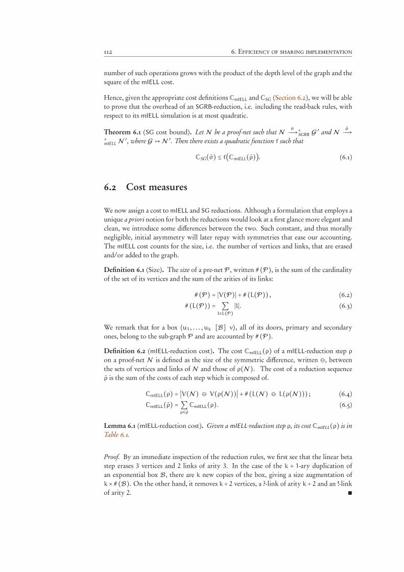
112 6. Efficiency of sharing implementation
number of such operations grows with the product of the depth level of the graph and thesquare of the mIELL cost.
Hence, given the appropriate cost definitions CmIELL and CSG (Section 6.2), we will be ableto prove that the overhead of an SGRB-reduction, i.e. including the read-back rules, withrespect to its mIELL simulation is at most quadratic.
Theorem 6.1 (SG cost bound). Let N be a proof-net such that Nσ−−→
∗
SGRBG ′ and N
ρ−−→
∗
mIELLN ′, where G ↣N ′. Then there exists a quadratic function f such that
CSG(σ) ≤ f(CmIELL(ρ)). (6.1)
6.2 Cost measures
We now assign a cost to mIELL and SG reductions. Although a formulation that employs aunique a priori notion for both the reductions would look at a first glance more elegant andclean, we introduce some differences between the two. Such constant, and thus morallynegligible, initial asymmetry will later repay with symmetries that ease our accounting.The mIELL cost counts for the size, i.e. the number of vertices and links, that are erasedand/or added to the graph.
Definition 6.1 (Size). The size of a pre-net P, written # (P), is the sum of the cardinalityof the set of its vertices and the sum of the arities of its links:
# (P) = ∣V(P)∣ + # (L(P)) , (6.2)
# (L(P)) = ∑l∈L(P)
∣l∣. (6.3)
We remark that for a box ⟨u1, . . . , uk [B] v⟩, all of its doors, primary and secondaryones, belong to the sub-graph P and are accounted by # (P).Definition 6.2 (mIELL-reduction cost). The cost CmIELL(ρ) of a mIELL-reduction step ρ
on a proof-net N is defined as the size of the symmetric difference, written ⊖, betweenthe sets of vertices and links of N and those of ρ(N ). The cost of a reduction sequenceρ is the sum of the costs of each step which is composed of.
CmIELL(ρ) = ∣V(N ) ⊖ V(ρ(N ))∣ + # (L(N ) ⊖ L(ρ(N ))) ; (6.4)
CmIELL(ρ) = ∑ρ∈ρ
CmIELL(ρ). (6.5)
Lemma 6.1 (mIELL-reduction cost). Given amIELL-reduction step ρ, its cost CmIELL(ρ) is inTable 6.1.
Proof. By an immediate inspection of the reduction rules, we first see that the linear betastep erases 3 vertices and 2 links of arity 3. In the case of the k + 1-ary duplication ofan exponential box B, there are k new copies of the box, giving a size augmentation ofk× # (B). On the other hand, it removes k+ 2 vertices, a ?-link of arity k+ 2 and an !-linkof arity 2. ∎
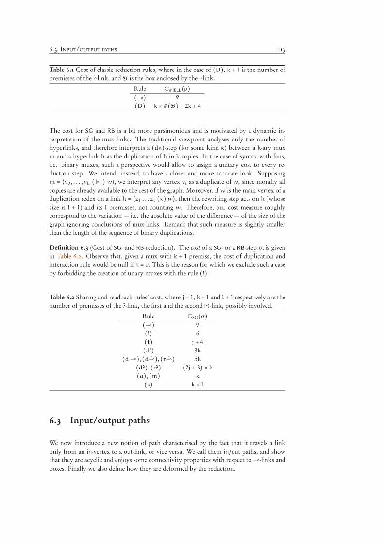
6.3. Input/output paths 113
Table 6.1 Cost of classic reduction rules, where in the case of (D), k + 1 is the number ofpremisses of the ?-link, and B is the box enclosed by the !-link.
Rule CmIELL(ρ)(⊸) 9
(D) k × # (B) + 2k + 4
The cost for SG and RB is a bit more parsimonious and is motivated by a dynamic in-terpretation of the mux links. The traditional viewpoint analyses only the number ofhyperlinks, and therefore interprets a (dκ)-step (for some kind κ) between a k-ary muxm and a hyperlink h as the duplication of h in k copies. In the case of syntax with fans,i.e. binary muxes, such a perspective would allow to assign a unitary cost to every re-duction step. We intend, instead, to have a closer and more accurate look. Supposingm = ⟨v0, . . . , vk ( ∣*⟩ ) w⟩, we interpret any vertex vi as a duplicate of w, since morally allcopies are already available to the rest of the graph. Moreover, if w is the main vertex of aduplication redex on a link h = ⟨z1 . . . zl (κ) w⟩, then the rewriting step acts on h (whosesize is l + 1) and its l premisses, not counting w. Therefore, our cost measure roughlycorrespond to the variation — i.e. the absolute value of the difference — of the size of thegraph ignoring conclusions of mux-links. Remark that such measure is slightly smallerthan the length of the sequence of binary duplications.
Definition 6.3 (Cost of SG- and RB-reduction). The cost of a SG- or a RB-step σ, is givenin Table 6.2. Observe that, given a mux with k + 1 premiss, the cost of duplication andinteraction rule would be null if k = 0. This is the reason for which we exclude such a caseby forbidding the creation of unary muxes with the rule (!).
Table 6.2 Sharing and readback rules’ cost, where j+ 1, k+ 1 and l+ 1 respectively are thenumber of premisses of the ?-link, the first and the second ∣*⟩-link, possibly involved.
Rule CSG(σ)(⊸) 9
(!) 6
(t) j + 4
(d!) 3k
(d⊸), (d⊸), (r⊸) 5k
(d?), (r?) (2j + 3) × k
(a), (m) k
(s) k × l
6.3 Input/output paths
We now introduce a new notion of path characterised by the fact that it travels a linkonly from an in-vertex to a out-link, or vice versa. We call them in/out paths, and showthat they are acyclic and enjoys some connectivity properties with respect to⊸-links andboxes. Finally we also define how they are deformed by the reduction.
114 6. Efficiency of sharing implementation
6.3.1 Statics
Definition 6.4 ( in/out paths). A path π ∶ u0 ∼ uk in a pre-net P is downward if forany 0 ≤ i < k − 1 the vertex ui is an out-vertex of li, and ui+1 is an in-vertex of li andui /∈ BVar(P). If π† is downward, then π is an upward path from uk to u0. A path is in/outwhen it is either downward or upward. We shall write u ≫ v when there is a downwardpath from u to v, and v≪ u when u≫ v.
Lemma 6.2 (Partial order). For any UG-graph U :
1. ≫ is a partial order for V(U);2. in/out paths contain no cycles.
Proof sketch. By a simple inspection of the definition of≫, we verify that is enjoys reflex-ivity and transitivity, so we pass to asymmetry and acyclicity. Given a in/out path π inU , let π ′ be the in/out path in E(U) obtained from π by making it jump over every liftcrossed by π. Remark now that by construction π ′ is a special case of switching path (cf.Definition 2.9), which considers only one of the two admitted switchings on⊸-links (theone on the second premiss), and which imposes the in/out direction. Moreover, mIELL
proof-nets do not contain cyclic swtiching paths, hence π ′ does not contain cycles. But πdiffer from the presence of lifts that cannot possibly introduce new cycles, thus also π isacyclic. ∎
Lemma 6.3 (Crossing links). Let π be a downward path in a UG-graph U and l a link inU . If l is not a⊸-link, then π contains at most 2 vertices of l; otherwise π contains at most 3vertices, and in such a case one is the lowermost extremum of π.
Proof. We separately consider the two disjointed propositions of the claim.
1. Suppose that l is not a ⊸-link. Then let u, v be two distinct vertices of π, respect-ively being an in-vertex and an in-vertex of the link l. Then (u, v) is by definition adownward path over l. Now clearly u must precede v in π, since otherwise, as perantisymmetry property of ≫ (Lemma 6.2), we would contradict our distinctnesshypothesis. Moreover, u, v have to be consecutive in π, because the existence ofπ ′ /= (u, v) would imply that (i) there exist two links l, l ′ both insisting on u withtheir in-vertex, and similarly that (ii) there exist two links l, l ′′ both insisting on v
with their out-vertex. Indeed, both these facts would be absurd, since at most onein- and one out-vertex connection are allowed by definitions of unshared graphs. Solet π = π ′ ∶∶ (u, v) ∶∶ π ′′, and by acyclicity we conclude that there cannot be other beother occurrences of u or v within π ′ or π ′′.
2. Suppose otherwise that l is a ⊸. In particular, let l = ⟨w,v (⊸) u⟩. Exactly asin the previous case, we have that u, v must be appear consecutively in such orderwithin π, so let π = π ′ ∶∶ (u, v) ∶∶ π ′′. Moreover, u, v cannot occur elsewhere in π ′
nor π ′′. Now, by definition of downward path there exists no w ′ such that w≫ w ′,therefore it must be the last and possibly unique vertex of π ′′. Hence the claim.
6.3. Input/output paths 115
∎
Lemma 6.4 (Connectivity). Given U a UG-graph, for any v ∈ V(U):
1. v≪ u where u is the root of U ,
2. v≫ u ′ for some u ′ ∈ FBVar(U).
Proof sketch. Immediate by Definition 2.3. ∎
Lemma 6.5 (Lambda-connectivity). Let ⟨u,w (⊸) z⟩ be a link in a UG-graph. Then v ∼ w
for any v such that v≫ u.
Proof sketch. Almost immediate from Lemma 6.4. ∎
Lemma 6.6 (Box connectivity). Let v be the root of a UG-graph U or the premiss of a !-link,and let u be the premiss of a ?-link h. If ℓ(u) > ℓ(v) and v ≫ u, then for any w premiss of hthere exists π ∶ v≫ z≫ w, such that z is the premiss of the principal door of the box of w.
Proof sketch. Almost immediate from Lemma 6.4. ∎
6.3.2 Dynamics
Remind the notions of crossing and sufficient length for a path with respect to some redex(cf. Definition 2.18).
Definition 6.5 (UG-residuals of downward maximal crossing). Let χ be a downward pathin a UG-graph U being a maximal crossing for a UG-redex R, and let ρ be its reduction.The residuals of χ with respect to ρ are the set of downward path defined as follows.
1. If R is a (⊸)-step, let it be as in Figure 5.4a. Then:
ρ((v2,w,u2)) = {(u2 = v2)}; (6.6)
ρ((u1)) = {(u1 = v1)}; (6.7)
ρ((v2, v1)) = {(u2 = v2) ∶∶ γ ∶∶ (u1 = v1) ∣ γ ∶ u2 ≫ u1} . (6.8)
Notice that the rightmost side of (6.8) is the empty set whenever u2 /≫ u1. But itcannot be the case, as per Lemma 6.5.
2. If R is a (!)-step, let it be as in Figure 5.4b Then:
ρ((v0,w,u)) = {(v0 = u)}. (6.9)
3. If R is a (d⊸)-step, let it be as in Figure 5.5a. Then:
ρ((v0,w,u2)) = {(v0, z20, u2)}; (6.10)
ρ((u1)) = {(u1)}. (6.11)
Remark in the last equation that we cannot write (u1, z0), since it would not pre-serve the extrema.
116 6. Efficiency of sharing implementation
4. If R is a (d⊸)-step, let it be as in Figure 5.5b. Then:
ρ((u2,w, v0)) = {(u2, z20, v0)}; (6.12)
ρ((u2, u1)) = {(u2, z20, u20
, u1)}. (6.13)
5. If R is a (d!)-step, let it be as in Figure 5.5c. Then:
ρ((v0,w,u)) = {(v0, z0, u)}. (6.14)
6. If R is a (d?)-step, let it be as in Figure 5.5d. Then for any 0 ≤ i ≤ h:
ρ((ui,w, v0)) = {(ui, z0i, v0)}. (6.15)
7. If R is a (a)-step, let it be as in Figure 5.6a. Then:
ρ((u0,w, v0)) = {(u0 = v0)}. (6.16)
8. If R is a (s)-step, let it be as in Figure 5.6b. Then:
ρ((u0,w, v0)) = {(u0, z00, v0)}. (6.17)
9. Otherwise R is a (tD)-step. Let it be as in Figure 5.9. Then:
ρ((vi, z,w) ∶∶ γ ∶∶ (u ′j, uj)) = {(vi,wi) ∶∶ γi ∶∶ (u ′ji , uj)}, (6.18)
where:
• 0 ≤ i ≤ h, and 1 ≤ j ≤ k;
• u ′j ∈ Uj is a premiss of the ?-link having conclusion in uj;
• γ ∶ w≫ u ′j is a path in the subnet b;
• γi is the i-th copy of γ in the subnet bi.
Definition 6.6 (URB-residuals of downward maximal crossing). Let χ be a downward pathin a UG-graph U being a maximal crossing for a URB-redex R, and let ρ be its reduction.The residuals of χ with respect to ρ are the set of downward path defined as follows.
1. If R is a (r⊸)-step, let it be as in Figure 5.7. Then:
ρ((v0, u2, u0)) = {(v0, z00, u0)}; (6.19)
ρ((v0, u2, u1)) = {(v0, z10, u1)}. (6.20)
2. If R is a (r?)-step, let it be as in Figure 5.8b. Then for any j ≠ i:
ρ((v0, ui,w)) = {(v0, y0,w)}; (6.21)
ρ((uj,w)) = {(uj, zj0 , z00,w)} . (6.22)
3. If R is a (m)-step, let it be as in Figure 5.8a. Then for any j ≠ i:
ρ((v0, ui,w)) = {(v0,w)}; (6.23)
ρ((uj,w)) = {(uj,w)} . (6.24)
6.4. Sharing contexts 117
Definition 6.7 (Residual of downward paths). Let π be a downward path in a UG-graphU and let R be a UG- or a URB-redex such that π is long enough for R. If ρ is the reductionstep of R, then the reduction of π with respect to ρ is a function from π to a set ρ(π) ofdownward paths in ρ(U). Let
π = π0 ∶∶ χ1 ∶∶ π1 ∶∶ . . . ∶∶ χn ∶∶ πn, (6.25)
where for any 0 ≤ i ≤ n the sub-path χi is a maximal crossing of a redex R. Then:
ρ(π) = {π0 ∶∶ χ′
1 ∶∶ π1 ∶∶ . . . ∶∶ χ′
n ∶∶ πn ∣ χ ′i ∈ ρ(χi)} , (6.26)
where the residuals of a maximal crossing of R are defined in Definition 6.5 and 6.6. Whenρ(π) is a singleton, we shall often directly refer to the unique π ′ ∈ ρ(π) simply as ρ(π).
6.4 Sharing contexts
In order to study the dynamics lifts in unshared graphs, we introduce a labelling of (ver-tices representing) occurrences of variables in (graphs representing) λ-terms. Over suchlabels we construct a very simple algebraic monoidal structure. Its objects, called contexts,are assigned to downward paths and models how lifts match each other. We will discovertwo key facts. First, lifts of a given level are always well-nested, as if they are parentheses(positive and negative lifts respectively correspond to open and close paarenthesis), whereone cannot close some that have not been previously opened, or a stack (positive and neg-ative lifts respectively correspond to the push and pop operations), where one cannot popsomething that have been previously pushed. Second, whilst a vertex may have more thanone access paths connecting it to the root, or to the “root” of a box, i.e. its principal door,all of these access paths have the same configuration of unmatched lifts (proceeding in themetaphor: unclosed parentheses, or elements in the stack).
6.4.1 Variable occurrences and sharing contexts
Definition 6.8 (Variable occurrences). Given V a finite set of symbols of variable names,V is the set of variable occurrences, that are triples in V × N × N, where the last twocomponents respectively select the index of a single occurrence and the maximal index ofall occurrences. Then, in a UG graph U , the labelling of variable occurrences VarO mapspremisses of ?- or ∣*⟩-links to V. We write xi∶k to denote (x, i, k) and Var for the firstprojection of VarO, i.e. if VarO(v) = xi∶k, then Var(v) = x. In particular, VarO satisfies thefollowings properties.
1. Injective on ?-links: if v ≠ w are two distinct premisses of ?-links in U , thenVarO(v) ≠ VarO(w).
2. Order-preserving and surjective on ?-links: if U contains ⟨v0, . . . , vk (?) w⟩, thenthere exists x ∈ V such that, for any 0 ≤ i ≤ k, VarO(vi) = xi∶k ∈V.
3. Coherent in the creation of ∣*⟩-links: if v is a premiss of the main ?-link in a (tD) re-dex R, and µ(v) is the premiss of a ∣+⟩-link, residual of v with respect to the reductionµ of R, then VarO(v) = VarO(µ(v)).
118 6. Efficiency of sharing implementation
4. Coherent in the copy of ∣*⟩-links: if v is a premiss of a ∣*⟩-link l and µ(v) is thepremiss of a ∣+⟩-link residual of v with respect to a reduction µ, then VarO(v) =VarO(µ(v)).
Definition 6.9 (Sharing context monoid). The sharing context monoid S∗ is generatedover V ∪ {0,1} by a binary operator ⋅, called concatenation, and a unary operator , saidnegation. Concatenation forms a monoid, having 1 as identity and 0 as absorbing element.If a, b, c ∈ S∗, then:
a ⋅ (b ⋅ c) = (a ⋅ b) ⋅ c (6.27)
a ⋅ 1 = 1 ⋅ a = a (6.28)
a ⋅ 0 = 0 ⋅ a = 0 (6.29)
Negation is involutive and distributes over concatenation reversing its order. If a, b ∈ V,then:
a = a (6.30)
a ⋅ b = b ⋅ a (6.31)
Moreover, concatenation of an object and its negation is either neutral or annihilating. Ifa, b ∈V with a ≠ 0 and a ≠ b, then:
a ⋅ a = 1 (6.32)
a ⋅ b = 0 (6.33)
When we need to distinguish S∗-equality from syntactic equality, we write =S∗ for theformer and = for the latter.
Definition 6.10 (Levelled sharing contexts). The levelled sharing contexts, or simply l-contexts, are sharing contexts whose syntax is enriched by a lifting operator ! whose n-thiterate is denoted by !n. An l-context γ naturally induces a map from N to S∗: for anya ∈ S∗, we define a(n + 1) = 1 and a(0) = a, whilst !γ(n + 1) = γ(n) and !γ(0) = 1.Moreover, l-contexts are uniformly null: if for some n ∈ N we have γ(n) = 0, thenγ(m) = 0 for any m ∈ N.Also, we write (γ) ∣n to denote the restriction of γ on n. Namely, if m ≠ n then(γ) ∣n(m) = γ(m); otherwise, if γ(m) ≠ 0, then (γ) ∣n(m) = 1. Finally, we shall writeγ =n γ ′ to mean that γ(m) = γ(m) for any m ≥ n, whilst γ =n γ ′ dually means thatγ(m) = γ ′(m) for any m < n. Also, γ =n
′
n γ ′ denotes the fact that γ(m) = γ ′(m) for anyn ≤m < n ′, so that γ =nn γ ′ means γ(n) = γ ′(n).Definition 6.11 (Positivity and stable forms). An object c ∈ S∗ is positive, denoted byc ⪰ 1, if c = 1 or c = a ⋅ b, where a ∈ V and b ⪰ 1. Dually, c is negative, written c ⪯ 1, ifc = 1 or c = a ⋅ b with a ∈V and b ⪯ 1. Observe that the intersection between the sets ofpositive and negative objects is 1 = 1, while the complement of their union is 0. A stableform of c ∈ S∗ is any a ⋅ b = c such that a ⪯ 1 and b ⪰ 1.Similarly, given an l-context γ ∈ N ↦ S∗, we say that γ is n-positive and write that γ ⪰n 1
if for any m ≥ n we have γ(m) ⪰ 1. In particular, when n = 0, we simply call γ positive,written γ ⪰ 1.
Lemma 6.7 (Stability or nullity). Every c ∈ S∗ is either equal to 0 or to a unique stableform.
6.4. Sharing contexts 119
Proof sketch. By orienting S∗-equations from left to right we obtain a rewriting system.It is terminating — consider as a strictly decreasing measure the sum of: the number ofatomic objects, the number of negated concatenation, the number of negated negations.Moreover it is locally confluent. ∎
Lemma 6.8 (Co-neutrality). If a, b ∈ S∗ such that a ⋅ b = a ≠ 0, then there exists c, d ∈ S∗
such that a = d ⋅ c and b = c ⋅ c, with c ⪰ 1.
Proof. We first observe that b ≠ 0. Indeed, if we suppose otherwise we would obtain thata ⋅ b = 0. But a ⋅ b = a, therefore we would have a = 0 contradicting our hypothesis. Soa, b are not null, hence they have a stable form.
a = d ′ ⋅ d (stable form) (6.34)
b = c ′ ⋅ c (stable form) (6.35)
a ⋅ b = d ′ ⋅ d ⋅ c ′ ⋅ c (6.34), (6.35) (6.36)
Now, d ⋅ c ′ cannot be null, so they have a stable form.
d ′ ⋅ c = e ′ ⋅ e (stable form) (6.37)
a ⋅ b = d ′ ⋅ e ′ ⋅ e ⋅ c (6.37), (6.36) (6.38)
d ′ ⋅ e ′ ⋅ e ⋅ c = d ′ ⋅ d (hypothesis), (6.38) (6.39)
e ′ ⋅ e ⋅ c = d (6.39) (6.40)
Observe that by definition d > 0, while e ′ ⪯ 1. Therefore e ′ ⪰ 1, i.e.
e ′ = 1 (6.41)
e ⋅ c = d (6.41), (6.40) (6.42)
a = d ′ ⋅ e ⋅ c (6.34), (6.42) (6.43)
which is our first claim. Moreover,
d ′ ⋅ e ⋅ c = d ′ ⋅ e ⋅ c ⋅ c ′ ⋅ c (hypothesis), (6.35), (6.43) (6.44)
1 = c ⋅ c ′ (6.44) (6.45)
c ′ = c (6.45) (6.46)
b = c ⋅ c (6.35), (6.46) (6.47)
that is the second claim. ∎
Definition 6.12 (Levelled sharing context assignment). Given a downward path π ∶ u≫ v
between two vertices u, v in a UG-graph, the sharing l-context of π is defined as follows.
s (()) = 1 (6.48)
s (π ∶∶ (u, v)) =
⎧⎪⎪⎪⎪⎪⎪⎪⎪⎨⎪⎪⎪⎪⎪⎪⎪⎪⎩
s (π) ⋅ !na if there is l = ⟨u ( ∣+⟩n ) v⟩ s.t. VarO(l) = a
s (π) ⋅ !na if there is l = ⟨v ( ∣-⟩n ) u⟩ s.t. VarO(l) = a
(s (π)) ∣n if there is ⟨u ( ?n ) v⟩s (π) if u, v belong to a link of kind in {⊸, ⊸, !}
(6.49)
120 6. Efficiency of sharing implementation
6.4.2 Positivity
This subsection is devoted to prove two fundamental properties of sharing l-contexts.The first is that positive and negative lifts are placed along downward paths as matchingparentheses, which algebraically means that contexts are always positive (after some level)if they start from the root of the graph (or a box within it). The second is that anyreduction different from the (d⊸)-rule does not affect contexts of downward paths.
Proposition 6.1 (Positivity). Let π be a downward path in a UG-graphU having maximumin v, being the root of U or the premiss of a !-link. Then s (π) ⪰ℓ(v) 1.
The proof requires four additional properties.
Lemma 6.9 (Long Invariance). If π is a downward path in a UG-graph U long enough forthe redex of a reduction step ρ, then s (π) = s (π ′) for any π ′ ∈ ρ(π).Lemma 6.10 (Lambda-compatibility). Let π ∶ u ≫ w and π ′ ∶ w ≫ v be two downwardpaths in a UG-graph U containing ⟨v,w (⊸) u ′⟩. If U is the root of U or the premiss of a!-link, then s (π) =ℓ(u) s (π ∶∶ π ′).Lemma 6.11 (Box compatibility). Let π ∶ u≫ v and π ′ ∶ u≫ v ′ be two downward paths ina UG-graph U such that: u is the root of U or a premiss of a !-link, and v, v ′ are premisses ofthe same ?-link, which implies that ℓ(v) = ℓ(v ′). Then s (π) =ℓ(v)
ℓ(u) s (π ′).Lemma 6.12 (Unary contraction). Let π ∶ u ≫ v be a downward path in a UG-graph U ,where u is a !-premiss, v is a ?-premiss. If u, v belong to a box B, then s (v) (ℓ(v)) = 1.
The four lemmas and the positivity proposition are so tightly related one with the otherthat their proof will require a mutually recursive approach: to prove a statement we willuse another as inductive hypothesis.
Proof of Lemma 6.9 (Long Invariance). Let R be the redex of ρ. Since π is long enough forR, let π = π0 ∶∶ χ1 ∶∶ π1 ∶∶ . . . ∶∶ χn ∶∶ πn, where χc is a maximal crossing of R, for any1 ≤ c ≤ n. Recall from Lemma 6.3 that a link l could be crossed by a downward path atmost: twice, if l is not a⊸-link, three times, if it is. But a redex contains two connectedlinks, therefore, if R does not contain a⊸-link then n = 1, otherwise n ≤ 2. Now, if n = 0
then ρ(π) = {π}, and both claims trivially hold. So we assume otherwise that n ⪰ 1, andproceed by a case analysis on the kind of rule employed by ρ ′.
1. Rule (⊸) and n ≤ 2. Let R be as in Figure 5.4a. Recall from Definition 6.5 thatχ can be of three kinds, among which (ui) is quite peculiar, since by Lemma 6.3,it does not allow right concatenation, and is the only one that can succeed anothermaximal crossing of the same redex R, namely (v2,w,u2). For these reasons, andby our hypotheses on π, we can simplify our analysis to the following four cases.
(a) Suppose that π crosses (v2,w,u2). Then by (6.6), we have ρ(χ) = {(v2 = u2)},and ρ(π) = {π0 ∶∶ (v2 = u2) ∶∶ π1}. So let π ′ = π0 ∶∶ π1 be the only elementof ρ(π). Now, by definition of l-context assignment, s (χ) = s (ρ(χ)) = 1.Therefore, s (π) = s (π ′).
6.4. Sharing contexts 121
(b) Assume that π crosses (v2, v1). This is one of the most interesting cases of thisproof. By (6.8) and (6.26), we have
ρ(χ) = {(u2 = v2) ∶∶ γ ∶∶ (u1 = v1) ∣ γ ∶ u2 ≫ u1} (6.50)
= {γ ∣ γ ∶ u2 ≫ u1} , (6.51)
ρ(π) = ρ(π0 ∶∶ χ ∶∶ π1) (6.52)
= {π0 ∶∶ γ ∶∶ π1 ∣ γ ∶ u2 ≫ u1} . (6.53)
Now consider π ′ = π0 ∶∶ γ ∶∶ π1 ∈ ρ(π), for some γ ∶ u2 ≫ u1. By definition ofcontext,
s (π ′) = s (π0 ∶∶ γ ∶∶ π1) (6.54)
= s (π0) ⋅ s (γ) ⋅ s (π1) . (6.55)
Now we can safely apply Lemma 6.10 on γ and obtain invariance.
= s (π0) ⋅ s (π1) (6.56)
= s (π0) ⋅ 1 ⋅ s (π1) (6.57)
= s (π0) ⋅ s (χ) ⋅ s (π1) (6.58)
= s (π) (6.59)
(c) If π crosses (u1), we immediately observe that ρ(π) = {π}, which triviallymeans that s (π) = s (π ′), for any π ′ ∈ ρ(π).
(d) If π crosses R first in (v2,w,u2) and then in (u1), exactly as we noticed in case1a, we have a unique π ′ ∈ ρ(π), that is π0 ∶∶ π1. Thus, s (π) = s (π ′).
2. Rule (!) and n = 1. Let R be as in the leftmost part of Figure 5.4b, let m be the depthof the !-link, and let also χ1 = (v0,w,u), that is the only possible maximal crossingof R. By definition, its l-context is as follows:
s (π) = (s (π0)) ∣m ⋅ s (π1) . (6.60)
By definition of residual, as per (6.9):
ρ(π) = ρ(π0 ∶∶ (v0,w,u) ∶∶ π1) (6.61)
= {π0 ∶∶ (v0 = u) ∶∶ π1} (6.62)
= {π0 ∶∶ π1}. (6.63)
Let π ′ ∈ ρ(π). Its l-context is
s (π ′) = s (π0) ⋅ s (π1) . (6.64)
So, let m ′ ≥ ℓ(v).
(a) If m ′ ≠ m, then (s (π0)) ∣m(m ′) = s (π0) (m ′), as by Definition 6.10 of re-striction operator. Hence, s (π ′) (m ′) = s (π) (m ′). Since by inductive hypo-thesis (IH) we have that s (π) (m ′) ⪰ 1, we also have s (π ′) (m ′) ⪰ 1.
122 6. Efficiency of sharing implementation
(b) Otherwise, m ′ = m. Observe that, by definition of proof-nets, v0 belong to abox B, so let π0 = η ∶∶ β, where β is the maximal suffix of π0, whose verticesare in B. Hence by definition:
s (π) (m) = s (η) (m) ⋅ (s (β)) ∣m(m) ⋅ s (π1) (m)= s (η) (m) ⋅ 1 ⋅ s (π1) (m). (6.65)
Now, by construction, the maximum of β is an !-premiss of B, and v0 isthe only ?-premiss of B, therefore we can apply Lemma 6.12, to obtain thats (β) (m) = 1.
s (π ′) (m) = s (η) (m) ⋅ s (β) (m) ⋅ s (π1) (m)s (π ′) (m) = s (η) (m) ⋅ 1 ⋅ s (π1) (m). (6.66)
Therefore s (π) (m) = s (π) (m).3. Rule (tD) and n = 1. Let R be as in Figure 5.9, and if l ′ is the ?-link in R, then
let m = ℓ(l ′) and a = VarO(l ′). Observe that by definition, χ1 is in the form(vj, z,w) ∶∶ γ ∶∶ (Uj ′ , uj ′), where 0 ≤ j ≤ h with h > 0, 1 ≤ j ′ ≤ k, and γ isa downward path in the box b. Remember that by definition of residual, and inparticular by (6.18),
ρ(π) = ρ (π0 ∶∶ (vj, z,w) ∶∶ γ ∶∶ (Uj ′ , uj ′) ∶∶ π1)= {π0 ∶∶ (vj,wi) ∶∶ γj ∶∶ (Uj ′
j, uj) ∶∶ π1} . (6.67)
Its l-context is by definition:
s (π) = s (π0 ∶∶ (vj, z,w) ∶∶ γ ∶∶ (Uj ′ , uj ′) ∶∶ π1)= (s (π0)) ∣m ⋅ (s (γ)) ∣m ⋅ s (π1) (6.68)
Let π ′ be the unique element of ρ(π), and observe it crosses the j-th lift introducedby the reduction, say l ′′. By definition of reduction and that of variable occurrences,ℓ(l ′′) = ℓ(l ′) =m and VarO(l ′′) = VarO(l ′) = a. Therefore,
s (π ′) = s (π0 ∶∶ (vj,wj) ∶∶ γj ∶∶ (Uj ′j, uj) ∶∶ π1)
= (s (π0) ⋅ !ma ⋅ s (γ)) ∣m ⋅ s (π1) . (6.69)
Let m ′ ≥ ℓ(v) and consider its equality with respect to m.
(a) If m ′ ≠m, we easily conclude. Indeed, by definitions of restriction and liftingwe obtain the claim from (6.68) and (6.69).
s (π) (m ′) = (s (π0) ⋅ s (γ) ⋅ s (π1)) (m ′)= s (π ′) (m ′). (6.70)
(b) Otherwise, m ′ =m. Consider again (6.68) and (6.69), and recall that, applyingProposition 6.1 of positivity as IH, s (π0) ⪰ℓ(v) 1 and s (γ) ⪰m 1. In particular,these imply that respectively s (π0) (m) ⪰ 1 and s (γ) (m) ⪰ 1. Now, bydefinition of restriction and lifting operators, we easily rewrite (6.68) into:
s (π) (m) = 1 ⋅ 1 ⋅ (s (π1)) (m) (6.71)
= s (π1) (m). (6.72)
6.4. Sharing contexts 123
Now, in (6.69) we can exploit again positivity as IH to obtain a ⋅s (γ) (m) ⪰ 1.Therefore we conclude.
s (π ′) (m) = 1 ⋅ (s (π1)) (m) (6.73)
= s (π) (m). (6.74)
4. Rule (d!) and n = 1. Assume R is as in the left of Figure 5.5c, where χ1 = (v0,w,u).Also, if l is the ∣+⟩-link in R, let n be its level, and let a = VarO(l) for some a ∈ S∗.By definition of l-context assignment,
s (π) = s (π0 ∶∶ (v0,w,u) ∶∶ π1) (6.75)
= s (π0) ⋅ !na ⋅ 1 ⋅ s (π1) (6.76)
By definition of residual, and in particular by (6.14):
ρ(π) = ρ(π0 ∶∶ (v0,w,u) ∶∶ π1) (6.77)
= {π0 ∶∶ (v0, z0, u) ∶∶ π0} (6.78)
So let π ′ be the unique path in ρ(π) and consider its l-context assignment.
s (π ′) = s (π0 ∶∶ (v0, z0, u) ∶∶ π1) (6.79)
= s (π0) ⋅ 1 ⋅ !na ⋅ s (π1) (6.80)
= s (π) (6.81)
5. Rule (d?) and n = 1. Let R be as in the right of Figure 5.5d, and let χ1 = (ui,w, v0),for some 0 ≤ i ≤ h. Also, if l is the ∣+⟩-link in R, let n be its level, and let a = VarO(l)for some a ∈ S∗. Finally, let m > n be the level of the ?-link. By definition ofl-context assignment,
s (π) = s (π0 ∶∶ (ui,w, v0) ∶∶ π1) (6.82)
= (s (π0)) ∣m ⋅ !na ⋅ s (π1) (6.83)
By definition of residual, and in particular by (6.15):
ρ(π) = ρ(π0 ∶∶ (ui,w, v0) ∶∶ π1) (6.84)
= {π0 ∶∶ (ui, z0i, v0) ∶∶ π0} (6.85)
So let π ′ be the unique path in ρ(π) and consider its l-context assignment, andobserve it is equivalent by definition of the restriction operator.
s (π ′) = s (π0 ∶∶ (ui, z0i, v0) ∶∶ π1) (6.86)
= (s (π0) ⋅ !na) ∣m ⋅ s (π1) (6.87)
= s (π) (6.88)
6. Rule (d ⊸) and 1 ≤ n ≤ 2. Let R be as in Figure 5.5a, and if h is the lift within R,then let a = VarO(h) and let m be its level.
124 6. Efficiency of sharing implementation
(a) Suppose that π contains only the maximal crossing (v0,w,u2). By definitionof l-context assignment we have that
s (π) = s (π0 ∶∶ (v0,w,u2) ∶∶ π1)) (6.89)
= s (π0 ∶∶ (v0,w) ∶∶ (w,u2) ∶∶ π1) (6.90)
= s (π0) ⋅ !ma ⋅ 1 ⋅ s (π1) . (6.91)
Now, by definition of downward path residual, in particular (6.10),
ρ(π) = ρ(π0 ∶∶ (v0,w,u2) ∶∶ π1) (6.92)
= {π0 ∶∶ (v0, z20, u2) ∶∶ π1}, (6.93)
So if we consider the l-context of π ′ ∈ ρ(π), we easily obtain that is equal tothat of π.
s (π ′) = s (π0 ∶∶ (v0, z20, u2) ∶∶ π1) (6.94)
= s (π0) ⋅ s ((v0, z20) ⋅ s ((z20
, u2)) ⋅ s (π1) (6.95)
= s (π0) ⋅ 1 ⋅ !ma ⋅ s (π1) (6.96)
= s (π) . (6.97)
(b) Assume that π crosses R only in (u1). By definition of l-context assignment,and of residual we have:
s (π) = s (π0 ∶∶ (u1)) = s (π0) , (6.98)
ρ(π) = ρ(π0 ∶∶ (u1)) = {π0 ∶∶ (u1)}. (6.99)
So, we immediately conclude: let π ′ ∈ ρ(π) and consider its context.
s (π ′) = s (π0 ∶∶ (u1)) = s (π) . (6.100)
(c) Otherwise π crosses R twice, and it must be the case that χ1 = (v0,w,u2),while χ2 = (u1). From previous cases 6a and 6b we have: s (χ1) = s (χ ′1) forany χ ′1 ∈ ρ(χ1), and s (χ2) = s (χ ′2) for any χ ′2 ∈ ρ(χ2). Hence the claim.
7. Rule (d⊸) and n = 1. Let R be as in the rightmost part of Figure 5.5b, and if h isthe lift within R, then let a = VarO(h) and m = ℓ(h). We distinguish two cases,according to the two possible maximal crossing of R.
(a) If χ1 = (u2,w, v0), then by definition of residual, and in particular by (6.12),
ρ(π) = ρ(π0 ∶∶ (u2,w, v0) ∶∶ π1) (6.101)
= {π0 ∶∶ (u2, z20, v1) ∶∶ π1} (6.102)
Let π ′ ∈ ρ(π). By simply inspecting the definition, we immediately verify thatthe l-context is unvaried.
s (π) = s (π0) ⋅ 1 ⋅ !ma ⋅ s (π1) (6.103)
= s (π0) ⋅ !ma ⋅ s (π1) (6.104)
= s (π0) ⋅ !ma ⋅ 1 ⋅ s (π1) (6.105)
= s (π ′) (6.106)
6.4. Sharing contexts 125
(b) Otherwise χ1 = (u2, u1). Its residual is by (6.13),
ρ(π) = ρ(π0 ∶∶ (u2, u1) ∶∶ π1) (6.107)
= {π0 ∶∶ (u2, z20, u20
, u1) ∶∶ π1}. (6.108)
While the l-context of π and that of π ′ ∈ ρ(π) are:s (π) = s (π0) ⋅ 1 ⋅ s (π1) (6.109)
s (π ′) = s (π0) ⋅ !ma ⋅ !na ⋅ s (π1) . (6.110)
Now, let m ′ ≥ l and consider its equality with respect to m.
i. If m ′ ≠m, then s (π) (m) = s (π ′) (m).ii. Otherwise, m ′ = m. By IH we have that s (π0 ∶∶ (u2, u1)) ⪰ℓ(v) 1, which
means that in particular s (π0) (m) ⋅ a ⪰ 1. Therefore, it must be the casethat s (π0) (m) = b ⋅ a, for some b ∈ S∗. Substituting it in (6.109) and(6.110), we obtain
s (π) (m) = b ⋅ a ⋅ s (π1) (m) (6.111)
s (π ′) (m) = b ⋅ a ⋅ a ⋅ a ⋅ s (π1) (m) (6.112)
= b ⋅ a ⋅ s (π1) (m). (6.113)
8. Rule (r?) and n = 1. Let R be as in Figure 5.8b, where h is the ∣+⟩-link and h ′ is the?-link involved R. Let m = ℓ(h), a = VarO(h). We have two kinds of downwardcrossings, which we analyse separately.
(a) Assume first χ1 = (v0, ui,w). By definition of residual and in particular by(6.21),
ρ(π) = ρ(π0 ∶∶ (v0, ui,w) ∶∶ π1) (6.114)
= {π0 ∶∶ (v0, y0,w) ∶∶ π1}. (6.115)
Let π ′ be the unique path in ρ(π) and inspect the definition of l-context as-signment. We immediately verify it is unvaried.
s (π) = s (π0) ⋅ !ma ⋅ 1 ⋅ s (π1) (6.116)
= s (π0) ⋅ 1 ⋅ !ma ⋅ s (π1) (6.117)
= s (π ′) (6.118)
(b) Otherwise, hypothesise that χ1 = (uj,w) where i ≠ j. By definition and inparticular by (6.22):
ρ(π) = ρ(π0 ∶∶ (uj,w) ∶∶ π1) (6.119)
= {π0 ∶∶ (uj, zj0 , z00,w) ∶∶ π1}. (6.120)
Now, let m ′ ≥ ℓ(v) and consider its equality with respect to m.
i. If m ′ ≠ m, then by definition of the lifting operator we immediately ob-tain that the l-context is invariant and that IH is consequently preserved.
s (π) (m ′) = (s (π0) ⋅ s (π1)) (m ′) (6.121)
= s (π ′) (m ′) (6.122)
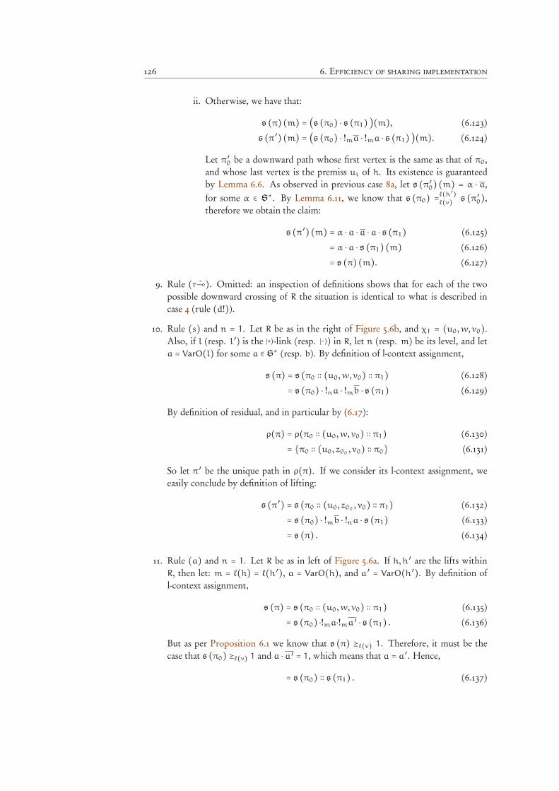
126 6. Efficiency of sharing implementation
ii. Otherwise, we have that:
s (π) (m) = (s (π0) ⋅ s (π1) )(m), (6.123)
s (π ′) (m) = (s (π0) ⋅ !ma ⋅ !ma ⋅ s (π1) )(m). (6.124)
Let π ′0 be a downward path whose first vertex is the same as that of π0,and whose last vertex is the premiss ui of h. Its existence is guaranteedby Lemma 6.6. As observed in previous case 8a, let s (π ′0) (m) = α ⋅ a,for some α ∈ S∗. By Lemma 6.11, we know that s (π0) =ℓ(h ′)ℓ(v) s (π ′0),therefore we obtain the claim:
s (π ′) (m) = α ⋅ a ⋅ a ⋅ a ⋅ s (π1) (6.125)
= α ⋅ a ⋅ s (π1) (m) (6.126)
= s (π) (m). (6.127)
9. Rule (r⊸). Omitted: an inspection of definitions shows that for each of the twopossible downward crossing of R the situation is identical to what is described incase 4 (rule (d!)).
10. Rule (s) and n = 1. Let R be as in the right of Figure 5.6b, and χ1 = (u0,w, v0).Also, if l (resp. l ′ ) is the ∣+⟩-link (resp. ∣-⟩) in R, let n (resp. m) be its level, and leta = VarO(l) for some a ∈ S∗ (resp. b). By definition of l-context assignment,
s (π) = s (π0 ∶∶ (u0,w, v0) ∶∶ π1) (6.128)
= s (π0) ⋅ !na ⋅ !mb ⋅ s (π1) (6.129)
By definition of residual, and in particular by (6.17):
ρ(π) = ρ(π0 ∶∶ (u0,w, v0) ∶∶ π1) (6.130)
= {π0 ∶∶ (u0, z00, v0) ∶∶ π0} (6.131)
So let π ′ be the unique path in ρ(π). If we consider its l-context assignment, weeasily conclude by definition of lifting:
s (π ′) = s (π0 ∶∶ (u0, z00, v0) ∶∶ π1) (6.132)
= s (π0) ⋅ !mb ⋅ !na ⋅ s (π1) (6.133)
= s (π) . (6.134)
11. Rule (a) and n = 1. Let R be as in left of Figure 5.6a. If h,h ′ are the lifts withinR, then let: m = ℓ(h) = ℓ(h ′), a = VarO(h), and a ′ = VarO(h ′). By definition ofl-context assignment,
s (π) = s (π0 ∶∶ (u0,w, v0) ∶∶ π1) (6.135)
= s (π0) ⋅!ma⋅!ma ′ ⋅ s (π1) . (6.136)
But as per Proposition 6.1 we know that s (π) ⪰ℓ(v) 1. Therefore, it must be thecase that s (π0) ⪰ℓ(v) 1 and a ⋅ a ′ = 1, which means that a = a ′. Hence,
= s (π0) ∶∶ s (π1) . (6.137)
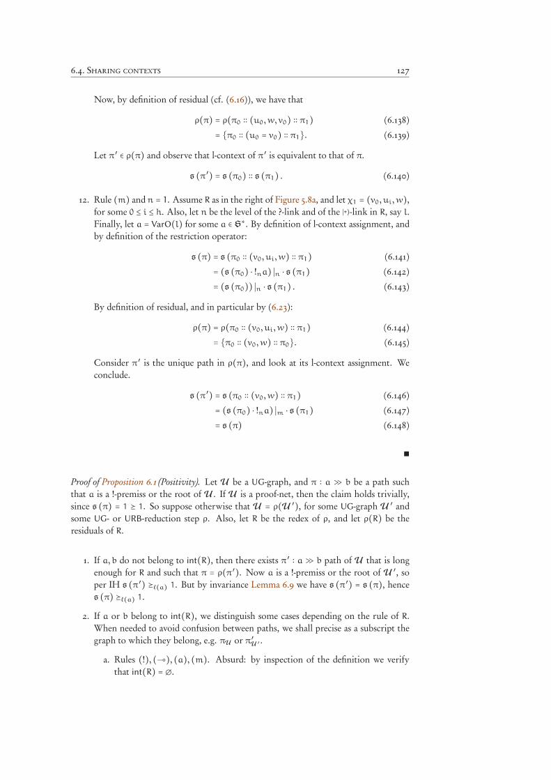
6.4. Sharing contexts 127
Now, by definition of residual (cf. (6.16)), we have that
ρ(π) = ρ(π0 ∶∶ (u0,w, v0) ∶∶ π1) (6.138)
= {π0 ∶∶ (u0 = v0) ∶∶ π1}. (6.139)
Let π ′ ∈ ρ(π) and observe that l-context of π ′ is equivalent to that of π.
s (π ′) = s (π0) ∶∶ s (π1) . (6.140)
12. Rule (m) and n = 1. Assume R as in the right of Figure 5.8a, and let χ1 = (v0, ui,w),for some 0 ≤ i ≤ h. Also, let n be the level of the ?-link and of the ∣+⟩-link in R, say l.Finally, let a = VarO(l) for some a ∈ S∗. By definition of l-context assignment, andby definition of the restriction operator:
s (π) = s (π0 ∶∶ (v0, ui,w) ∶∶ π1) (6.141)
= (s (π0) ⋅ !na) ∣n ⋅ s (π1) (6.142)
= (s (π0)) ∣n ⋅ s (π1) . (6.143)
By definition of residual, and in particular by (6.23):
ρ(π) = ρ(π0 ∶∶ (v0, ui,w) ∶∶ π1) (6.144)
= {π0 ∶∶ (v0,w) ∶∶ π0}. (6.145)
Consider π ′ is the unique path in ρ(π), and look at its l-context assignment. Weconclude.
s (π ′) = s (π0 ∶∶ (v0,w) ∶∶ π1) (6.146)
= (s (π0) ⋅ !na) ∣m ⋅ s (π1) (6.147)
= s (π) (6.148)
∎
Proof of Proposition 6.1 (Positivity). Let U be a UG-graph, and π ∶ a ≫ b be a path suchthat a is a !-premiss or the root of U . If U is a proof-net, then the claim holds trivially,since s (π) = 1 ⪰ 1. So suppose otherwise that U = ρ(U ′), for some UG-graph U ′ andsome UG- or URB-reduction step ρ. Also, let R be the redex of ρ, and let ρ(R) be theresiduals of R.
1. If a, b do not belong to int(R), then there exists π ′ ∶ a ≫ b path of U that is longenough for R and such that π = ρ(π ′). Now a is a !-premiss or the root of U ′, soper IH s (π ′) ⪰ℓ(a) 1. But by invariance Lemma 6.9 we have s (π ′) = s (π), hences (π) ⪰ℓ(a) 1.
2. If a or b belong to int(R), we distinguish some cases depending on the rule of R.When needed to avoid confusion between paths, we shall precise as a subscript thegraph to which they belong, e.g. πU or π ′U ′ .
a. Rules (!), (⊸), (a), (m). Absurd: by inspection of the definition we verifythat int(R) = ∅.
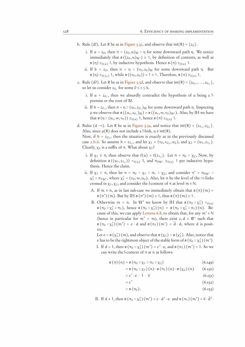
128 6. Efficiency of sharing implementation
b. Rule (d!). Let R be as in Figure 5.5c, and observe that int(R) = {z0}.i. If a = z0, then π = (z0, u)U ∶∶ η for some downward path η. We notice
immediately that s ((z0, u)U ′) ⪰ 1, by definition of contexts, as well ass (η) ⪰ℓ(a) 1, by inductive hypothesis. Hence s (π) ⪰ℓ(a) 1.
ii. If b = z0, then π = η ∶∶ (v0, z0)U for some downward path η. Buts (η) ⪰ℓ(z0) 1, while s ((v0, z0)) = 1 ⪰ 1. Therefore, s (π) ⪰ℓ(a) 1.
c. Rule (d?). Let R be as in Figure 5.5d, and observe that int(R) = {z00, . . . , z0k
},so let us consider z0i
for some 0 ≤ i ≤ k.
i. If a = z0i, then we absurdly contradict the hypothesis of a being a !-
premiss or the root of U .
ii. If b = z0i, then π = η ∶∶ (ui, z0i
)U for some downward path η. Inspectingρ we observe that s ((ui, z0i
)U) = s ((ui,w, v0)U ′). Also, by IH we havethat s (η ∶∶ (ui,w, v0)) ⪰ℓ(a) 1, hence s (π) ⪰ℓ(a) 1.
d. Rules (d ⊸). Let R be as in Figure 5.5a, and notice that int(R) = {z10, z20}.
Also, since ρ(R) does not include a !-link, a ∉ int(R).Now, if b = z20
, then the situation is exactly as in the previously discussedcase 2.b.ii. So assume b = z10
, and let χ1 = (v0, x20, u2), and χ2 = (u1, z10
).Clearly, χ2 is a suffix of π. What about χ1?
i. If χ1 ⊄ π, then observe that ℓ(a) > ℓ(z10). Let π = π0 ∶∶ χ2, Now, by
definition s ((u1, z10)) =ℓ(a) 1, and π0U ′ ⪰ℓ(a) 1 per inductive hypo-
thesis. Hence the claim.
ii. If χ1 ⊂ π, then let π = π0 ∶∶ χ1 ∶∶ π1 ∶∶ χ2, and consider π ′ = π0U ′ ∶∶
χ ′1 ∶∶ π1U ′ , where χ ′1 = (v0,w,u2). Also, let n be the level of the ∣*⟩-linkscrossed in χ1, χ2, and consider the l-context of π at level m ∈ N.
A. If m ≠ n, as in last sub-case we immediately obtain that s (π) (m) =s (π ′) (m). But by IH s (π ′) (m) ⪰ 1, thus s (π) (m) ⪰ 1.
B. Otherwise m = n. In U ′ we know by IH that s (π0 ∶∶ χ′
1) =ℓ(a)s (π0 ∶∶ χ
′
1 ∶∶ π1), hence s (π0 ∶∶ χ′
1) (n) = s (π0 ∶∶ χ′
1 ∶∶ π1) (n). Be-cause of this, we can apply Lemma 6.8, to obtain that, for any m ′ ∈ N
(hence in particular for m ′ = m), there exist c, d ∈ S∗ such thats (π0 ∶∶ χ
′
1) (m ′) = c ⋅ d and s (π1) (m ′) = d ⋅ d, where d is posit-ive.Let e = s (χ ′1) (m), and observe that s (χ1) = s (χ ′1). Also, notice thate has to be the rightmost object of the stable form of s (π0 ∶∶ χ
′
1) (m ′).I. If d = 1, then s (π0 ∶∶ χ
′
1) (m ′) = c ′ ⋅ e, and s (π1) (m ′) = 1. So wecan write the l-context of π at n as follows.
s (π) (n) = s (π0 ∶∶ χ1 ∶∶ π1 ∶∶ χ2) (6.149)
= s (π0 ∶∶ χ1) (n) ⋅ s (π1) (n) ⋅ s (χ2) (n) (6.150)
= c ′ ⋅ e ⋅ 1 ⋅ e (6.151)
= c ′ (6.152)
= s (π0) . (6.153)
II. If d ≠ 1, then s (π0 ∶∶ χ′
1) (m ′) = c ⋅ d ′ ⋅ e. and s (π1) (m ′) = e ⋅ d ′ ⋅
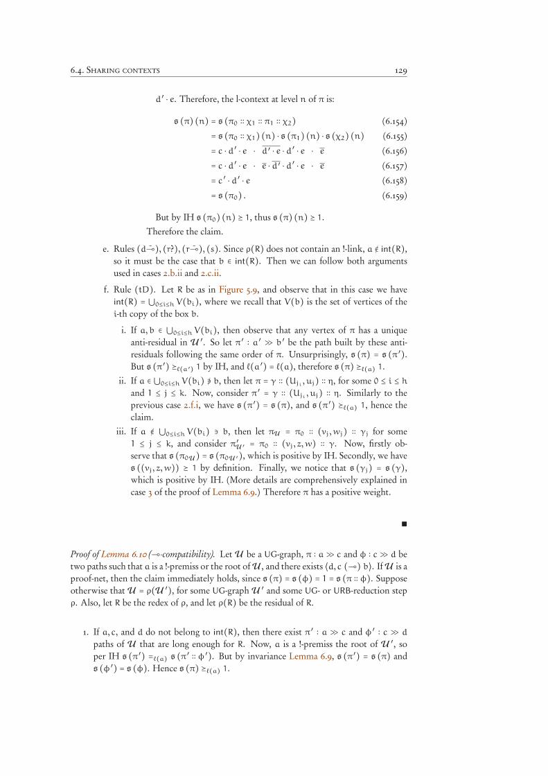
6.4. Sharing contexts 129
d ′ ⋅ e. Therefore, the l-context at level n of π is:
s (π) (n) = s (π0 ∶∶ χ1 ∶∶ π1 ∶∶ χ2) (6.154)
= s (π0 ∶∶ χ1) (n) ⋅ s (π1) (n) ⋅ s (χ2) (n) (6.155)
= c ⋅ d ′ ⋅ e ⋅ d ′ ⋅ e ⋅ d ′ ⋅ e ⋅ e (6.156)
= c ⋅ d ′ ⋅ e ⋅ e ⋅ d ′ ⋅ d ′ ⋅ e ⋅ e (6.157)
= c ′ ⋅ d ′ ⋅ e (6.158)
= s (π0) . (6.159)
But by IH s (π0) (n) ⪰ 1, thus s (π) (n) ⪰ 1.Therefore the claim.
e. Rules (d⊸), (r?), (r⊸), (s). Since ρ(R) does not contain an !-link, a ∉ int(R),so it must be the case that b ∈ int(R). Then we can follow both argumentsused in cases 2.b.ii and 2.c.ii.
f. Rule (tD). Let R be as in Figure 5.9, and observe that in this case we haveint(R) = ⋃0≤i≤h V(bi), where we recall that V(b) is the set of vertices of thei-th copy of the box b.
i. If a, b ∈ ⋃0≤i≤h V(bi), then observe that any vertex of π has a uniqueanti-residual in U ′. So let π ′ ∶ a ′ ≫ b ′ be the path built by these anti-residuals following the same order of π. Unsurprisingly, s (π) = s (π ′).But s (π ′) ⪰ℓ(a ′) 1 by IH, and ℓ(a ′) = ℓ(a), therefore s (π) ⪰ℓ(a) 1.
ii. If a ∈ ⋃0≤i≤h V(bi) ∌ b, then let π = γ ∶∶ (Uji , uj) ∶∶ η, for some 0 ≤ i ≤ h
and 1 ≤ j ≤ k. Now, consider π ′ = γ ∶∶ (Uji , uj) ∶∶ η. Similarly to theprevious case 2.f.i, we have s (π ′) = s (π), and s (π ′) ⪰ℓ(a) 1, hence theclaim.
iii. If a ∉ ⋃0≤i≤h V(bi) ∋ b, then let πU = π0 ∶∶ (vj,wj) ∶∶ γj for some1 ≤ j ≤ k, and consider π ′U ′ = π0 ∶∶ (vj, z,w) ∶∶ γ. Now, firstly ob-serve that s (π0U) = s (π0U ′), which is positive by IH. Secondly, we haves ((vj, z,w)) ⪰ 1 by definition. Finally, we notice that s (γj) = s (γ),which is positive by IH. (More details are comprehensively explained incase 3 of the proof of Lemma 6.9.) Therefore π has a positive weight.
∎
Proof of Lemma 6.10 (⊸-compatibility). Let U be a UG-graph, π ∶ a≫ c and φ ∶ c≫ d betwo paths such that a is a !-premiss or the root of U , and there exists ⟨d, c (⊸) b⟩. If U is aproof-net, then the claim immediately holds, since s (π) = s (φ) = 1 = s (π ∶∶ φ). Supposeotherwise that U = ρ(U ′), for some UG-graph U ′ and some UG- or URB-reduction stepρ. Also, let R be the redex of ρ, and let ρ(R) be the residual of R.
1. If a, c, and d do not belong to int(R), then there exist π ′ ∶ a ≫ c and φ ′ ∶ c ≫ d
paths of U that are long enough for R. Now, a is a !-premiss the root of U ′, soper IH s (π ′) =ℓ(a) s (π ′ ∶∶ φ ′). But by invariance Lemma 6.9, s (π ′) = s (π) ands (φ ′) = s (φ). Hence s (π) ⪰ℓ(a) 1.
130 6. Efficiency of sharing implementation
2. If a, c, or d belongs to int(R), we distinguish some cases depending on the rule ofR. Subscripts of paths denotes the graph to which they belong, e.g. πU , π ′U ′ .
a. Rules (!), (⊸), (a), (m). Absurd: by inspection of the definition we verifythat int(R) = ∅.
b. Rules (d?), (d⊸), (r⊸), (r?), (s). Then ρ(R) does not contain any link ofkind ! or⊸, so a, c, and d cannot be in int(R). Absurd.
c. Rule (d!). Let R be as in Figure 5.5c, and observe that int(R) = {z0}. Since weassumed c, d being respectively the second and the first premiss of a⊸-link, itmust be the case that c, d ≠ z0, which implies that a = z0. So, let π = (z0, u) ∶∶ ηfor some downward path η. By IH, we know that s (η) =ℓ(a) s (η ∶∶ φ). Hences (π) =ℓ(a) s (π ∶∶ φ).
d. Rule (d⊸). Let R be as in Figure 5.5a. We preliminarily notice that int(R) ={z10
, z20}. Also, since ρ(R) does not include a !-link, a ∉ int(R). Moreover, it
must the case that both c, d ∈ int(R). because ρ(R) contains both the premissesof a⊸-link. In particular, this mean that c = z20
, d = z10. Then the claim has
been proven in the proof of Proposition 6.1, case 2.d.ii (in particular Equa-tion 6.153 and 6.159).
e. Rule (tD). Let R be as in Figure 5.9, where int(R) = ⋃0≤i≤h V(Bi). By hypo-thesis on c, d we have that c belongs to int(R) if and only if d does so.
i. If a, c, d ∈ ⋃0≤i≤h V(bi), then observe that any vertex of π has a uniqueanti-residual in U ′. So let π ′ ∶ a ′ ≫ c ′ and φ ′ ∶ c ′ ≫ d ′ be the pathbuilt by these anti-residuals following the same order of π and φ, re-spectively. Then s (π) = s (π ′) and s (φ) = s (φ ′). By IH we haves (π ′) =a s (π ′ ∶∶ φ ′), therefore s (π) =a s (π ∶∶ φ).
ii. If a ∈ ⋃0≤i≤h V(bi) ∌ c, d, then let π = γ ∶∶ (Uji , uj) ∶∶ η for some 0 ≤ i ≤ h
and 1 ≤ j ≤ k. Now, consider π ′ = γ ∶∶ (Uji , uj) ∶∶ η, and observe thats (π ′) = s (π). Now, by IH we know s (π ′) =a s (π ′ ∶∶ φ), so we concludethat s (π) =a s (π ∶∶ φ), quod erat demonstrandum.
iii. If a ∉ ⋃0≤i≤h V(bi) ∋ c, d, then let π = π0 ∶∶ (vj,wj)U ∶∶ γj, for some1 ≤ j ≤ k. Now, consider π ′ = π0 ∶∶ (vj, z,w)U ′ ∶∶ γ. Let m be the level ofthe !-link in R. Now, firstly observe that s (π0U) = s (π0U ′) and s (γj) =s (γ). Moreover, by definition of l-context assignment, s (π0) (m) = 1.Therefore s (π ′) (m) = s (γ) (m). But s (π ′) (m) = s (π ′ ∶∶ φ) (m), thuss (γ) (m) = s (γ ∶∶ φ) (m). Secondly, we have s ((vj,wj)) ⪰ 1 per defin-ition. Thirdly, applying positivity Proposition 6.1 as IH, we obtain thats (γ) ⪰ℓ(a) 1, hence s (γj) ⪰ℓ(a) 1. Hence the claim. (See also case 3 ofthe proof of Lemma 6.9.)
∎
Proof sketch of Lemma 6.11 (Box-compatibility). To avoid pedantry, we provide only an out-line of the argumentation, since it is very similar to that of Lemma 6.10. One goes byinduction on the length of the reduction sequence from a proof-net, where the statementholds trivially, to the given UG-graph. Given a step ρ, Lemma 6.9 allows to obtain theclaim by IH in the case of paths whose counter-image with respect to ρ is long enough
6.4. Sharing contexts 131
for the redex of ρ. Otherwise, one proceeds with an inspection of possible redexes whoseresiduals are crossed by the paths π ∶ u≫ v and π ′ ∶ u≫ v ′ of interest.
• One interesting case is that of the (tD). Its behaviour is irrelevant at levels strictlysmaller than ℓ(u) and greater or than ℓ(v), which are out of the statements’ scope.In between such interval, the rule adds a lift in front of one of the copies of a boxB, which carry a S∗ object to the paths crossing it. It is sufficient to observe thatfor any box B ′ at level strictly smaller than ℓ(v), v ∈ B ′ if and only if v ′ ∈ B ′ (suchproperty comes from a crucial feature of mIELL: a ?-premiss belongs at most to onebox); and to recall the box connectivity Lemma 6.6. This allow to observe that anynew lift generated by a (tD)- step on B necessarily introduces a S∗ object whichbelongs to both the contexts of π,π ′
• The only other notable case is (r?). Assume it happens on v and involve a lift havingvariable occurrence c at level n, which therefore is the only one to be considered.By IH, both the n-th contexts of the anti-residuals of v, v ′ have suffix c. Thereforewhile c is not the suffix of the n-th l-context of v, the other premiss v ′ has c ⋅ c ′, sothey are equivalent.
∎
Proof sketch of Lemma 6.12 (Unary contraction). Let π ∶ u ≫ v be a downward path in aUG-graph U , where U is a !-premiss, v is a ?-premiss, and both belong to a box B. If U isa proof-net, then the claim holds trivially, since s (π) = 1 ⪰ 1. So suppose otherwise thatU = ρ(U ′), for some UG-graph U ′ and some UG- or URB-reduction step ρ. Let R be theredex of ρ, and ρ(R) its residual.
1. If u and v do not belong to int(R), then there exists π ′ ∶ u ≫ v path of U that islong enough for R and such that π = ρ(π ′). Now, a is a !-premiss or the root of U ′,so per IH s (π) = 1. But by invariance Lemma 6.9 we have s (π ′) = s (π), and inparticular s (π ′) (ℓ(u)) = s (π) (ℓ(u)) hence s (π ′) (ℓ(u)) = 1.
2. Otherwise u or v belongs to int(R).(a) Rules (!), (⊸), (d ⊸), (d⊸), (a), (s), (r⊸). Absurd: by inspection of the
definition we verify that int(R) = ∅.(b) Rules (d!). Let π = χ ∶∶ η, and π ′ = χ ′ ∶∶ η such that π ′ is long enough for R and
ρ(π ′) = π.
Now, by definition of UG-graph, the level of the involved lift has to be strictlysmaller than n. Therefore s (χ ′) (ℓ(u)) = s (χ) (ℓ(u)). But by IH s (η) (ℓ(u)),hence we conclude.
(c) Rules (d?), (r?). These cases are duals of 2b, and omitted.
(d) Rule (m). Let π = η ∶∶ χ, and π ′ = η ∶∶ χ ′ such that π ′ is long enough forR and ρ(π ′) = π. Consider the ∣+⟩-link l in R, and observe that by definition,s (χ ′) (ℓ(u)) = VarO(l) ≠ 1. Hence s (π ′) (ℓ(u)) =≠ 1. But this is the negationof IH. Absurd.
132 6. Efficiency of sharing implementation
(e) Rule (tD). Let R be as in Figure 5.9, and say the box of R is named C, andthe copies of C are named C0 . . . Ch, for some h > 0. In this case int(R) =⋃0≤i≤h V(Ci). We distinguish three cases depending on the level n of the boxC.
i. If n > ℓ(u), then in U we have that Ci ⊂ B for any 0 ≤ i ≤ h. This impliesthat there exists a downward path π ′ in U ′ such that ρ(π ′) = π. But thiscontradicts our assumption that u or v belong to int(R). Absurd.
ii. If n = ℓ(u), then there exists 0 ≤ i ≤ h such that Ch = B. Look again atFigure 5.9 and observe that v = Uji for some 1 ≤ j ≤ k, that is the residualof the ?-premiss Uj in U ′. But Uj has a total of h+1 residual vertices in U ,all being premiss of the same ?-link l. But this contradicts our hypothesisthat v is the only premiss of l. Thus there is nothing to be proven here.
iii. If n < ℓ(u), then there exists 0 ≤ i ≤ h such that Ci ⊃ B. Notice that π
is one of the h + 1 copies of some path π ′ of U ′, i.e. π ∈ ρ(π), for somedownward path π of U ′. Thus, s (π) = s (π ′), from which the claim.
∎
6.4.3 Path irrelevance
We show that the contexts of rooted paths to a given vertex does not depend on the choiceof the path, so we can generalise the definition of sharing levelled context as a notionabout vertices.
Lemma 6.13 (Path irrelevance). Let π ∶ u ≫ v and π ′ ∶ u ≫ v be two downward paths in aUG-graph U where u is the root of U or a premiss of a !-link. Then s (π1) =ℓ(u) s (π2).
Proof. Let U be a UG-graph, and let φ,φ ′ ∶ w≫ v be two paths in U . We go by inductionon the number e of vertices belonging to both paths.
1. If e = 1, then φ = φ ′ and the claim is trivially verified.
2. Otherwise e > 1, so let φ = γ ∶∶ π and φ ′ = γ ′ ∶∶ π ′ such that: γ,γ ′ ∶ w ≫ u
and π,π ′ ∶ u ≫ v, where u ≠ v. Since by definition s (φ) = s (γ) ⋅ s (π) ands (φ ′) = s (γ ′) ⋅ s (π ′), where per IH we have s (γ) = s (γ ′), we have just reducedthe claim to prove s (π) = s (π ′).By construction, v has to be the out vertex of a link having at least two in vertices.There are only two links of such kind: ⊸ and ?. But the first premiss of a ⊸-linkcannot be reached from its second premiss with an upward path. Therefore v is theconclusion of a ?-link l.Let z, z ′ respectively be the two premisses of l such that π = δ ∶∶ (z, v) and π ′ =
δ ′ ∶∶ (z ′, v). By Lemma 6.11, s (δ) =ℓ(w)ℓ(u) s (δ ′). And by definition of l-context
assignment, s (π) = (s (δ)) ∣ℓ(w) and s (π ′) = (s (δ ′)) ∣ℓ(w). Hence the claim.
∎
6.5. Unshared cost of reductions 133
Definition 6.13 (Sharing levelled context of a vertex). The sharing levelled context of avertex v ∈ V(U), for some UG-graph U whose root is r, is s (π) for any downward pathπ ∶ r≫ v.
Recall from Definition 2.3 that the interior of a pre-net P is the set of vertices of P thatare not its conclusions. Now we observe that the l-context of a given vertex is preservedunder reduction if it does not belong to the interior of the involved redex. If otherwise itis not the case, then the l-context may change. Most notably, this happens for any vertex v
belonging to a box B that is duplicated under a (tD)-step, where any rooted path reachinga copy of v crosses a different, and newly introduced, lift.
Lemma 6.14. Given a UG-graph U and a reduction step ρ on a redex R, if v ∉ int(R), thens (v) = s (v ′), for any residual v ′ of v.
Proof. By hypothesis any downward path π from the root r of U to v is long enough forR. By definition, there exists π ′ ∈ ρ(π) such that π ′ ∶ r≫ v ′. Moreover, by long invarianceLemma 6.9, we have s (π) = s (π ′) = s (v ′). ∎
6.5 Unshared cost of reductions
Thanks to sharing contexts, we can identify a set of sub-graphs in a UG graph whoselinks and vertices are morally waiting for a lift propagation: its share. As anticipated inSection 6.1, we introduce some additional precisions and tools that allow us to transferCmIELL and CSG in unshared reductions. More precisely, we define two distinct complexitymeasures for →UG, that are C
mIELLUG and C
SGUG. We show that for any simulation they are
indeed equivalent to their counterparts.
6.5.1 Share
Every time that in aUG-graph U we perform a (tD)-step on a k+1-ary contraction againsta box B, we distinguish 1 old copy of B, say B0 and call it the master copy of B, and k newcopies, say B1, . . .Bk, that are shared by the mux introduced in the simulating (t). So,if we call ‘master’ the 0th lifts and ‘sharing’ all the others, we are able to discriminate allthe vertices of U whose sharing l-context is neutral or master, from those whose sharingl-context is shared. These former are the share of U , which is partitioned in connectedcomponents.
Definition 6.14 (Share and master). A variable occurrence xi∶m is called master if i = 0.Given a lift ⟨u ( ∣*⟩ ) v⟩, if VarO(u) is master then it is a master lift, and it will be drawnin solid black, otherwise it is a sharing lift. A context a is master, written a ≈ 1 if a = 1,or a = x0∶m, or a = b and b ≈ 1, or a = b ⋅ c and b, c ≈ 1. Otherwise, we write a /≈ 1 andsay that a is shared. Similarly, a l-context α is master if α(n) /≈ 1 for any n ∈ N, otherwiseit is shared. A vertex is shared if its l-context is so, otherwise is master; a link is shared ifit has at least one shared vertex, otherwise is master.The share of a UG-graph U is the subgraph Sh (U) = (V ′, L ′), where V ′ ⊂ V(U) contains
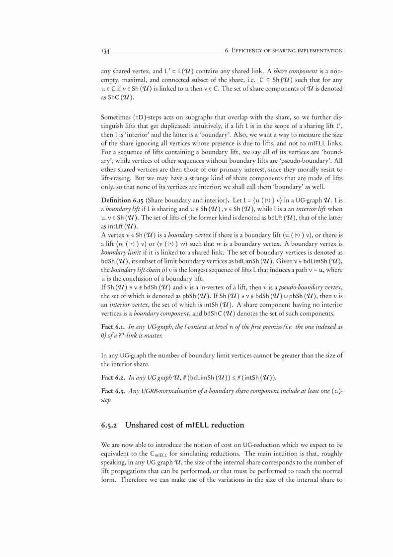
134 6. Efficiency of sharing implementation
any shared vertex, and L ′ ⊂ L(U) contains any shared link. A share component is a non-empty, maximal, and connected subset of the share, i.e. C ⊆ Sh (U) such that for anyu ∈ C if v ∈ Sh (U) is linked to u then v ∈ C. The set of share components of U is denotedas ShC (U).
Sometimes (tD)-steps acts on subgraphs that overlap with the share, so we further dis-tinguish lifts that get duplicated: intuitively, if a lift l is in the scope of a sharing lift l ′,then l is ‘interior’ and the latter is a ‘boundary’. Also, we want a way to measure the sizeof the share ignoring all vertices whose presence is due to lifts, and not to mIELL links.For a sequence of lifts containing a boundary lift, we say all of its vertices are ‘bound-ary’, while vertices of other sequences without boundary lifts are ‘pseudo-boundary’. Allother shared vertices are then those of our primary interest, since they morally resist tolift-erasing. But we may have a strange kind of share components that are made of liftsonly, so that none of its vertices are interior; we shall call them ‘boundary’ as well.
Definition 6.15 (Share boundary and interior). Let l = ⟨u ( ∣*⟩ ) v⟩ in a UG-graph U . l isa boundary lift if l is sharing and u ∉ Sh (U) , v ∈ Sh (U), while l is a an interior lift whenu, v ∈ Sh (U). The set of lifts of the former kind is denoted as bdL! (U), that of the latteras intL! (U).A vertex v ∈ Sh (U) is a boundary vertex if there is a boundary lift ⟨u ( ∣*⟩ ) v⟩, or there isa lift ⟨w ( ∣*⟩ ) v⟩ or ⟨v ( ∣*⟩ ) w⟩ such that w is a boundary vertex. A boundary vertex isboundary-limit if it is linked to a shared link. The set of boundary vertices is denoted asbdSh (U), its subset of limit boundary vertices as bdLimSh (U). Given v ∈ bdLimSh (U),the boundary lift chain of v is the longest sequence of lifts L that induces a path v ∼ u, whereu is the conclusion of a boundary lift.If Sh (U) ∋ v ∉ bdSh (U) and v is a in-vertex of a lift, then v is a pseudo-boundary vertex,the set of which is denoted as pbSh (U). If Sh (U) ∋ v ∉ bdSh (U) ∪ pbSh (U), then v isan interior vertex, the set of which is intSh (U). A share component having no interiorvertices is a boundary component, and bdShC (U) denotes the set of such components.
Fact 6.1. In any UG-graph, the l-context at level n of the first premiss (i.e. the one indexed as0) of a ?n-link is master.
In any UG-graph the number of boundary limit vertices cannot be greater than the size ofthe interior share.
Fact 6.2. In any UG-graph U , # (bdLimSh (U)) ≤ # (intSh (U)).Fact 6.3. Any UGRB-normalisation of a boundary share component include at least one (a)-step.
6.5.2 Unshared cost of mIELL reduction
We are now able to introduce the notion of cost on UG-reduction which we expect to beequivalent to the CmIELL for simulating reductions. The main intuition is that, roughlyspeaking, in any UG graph U , the size of the internal share corresponds to the number oflift propagations that can be performed, or that must be performed to reach the normalform. Therefore we can make use of the variations in the size of the internal share to
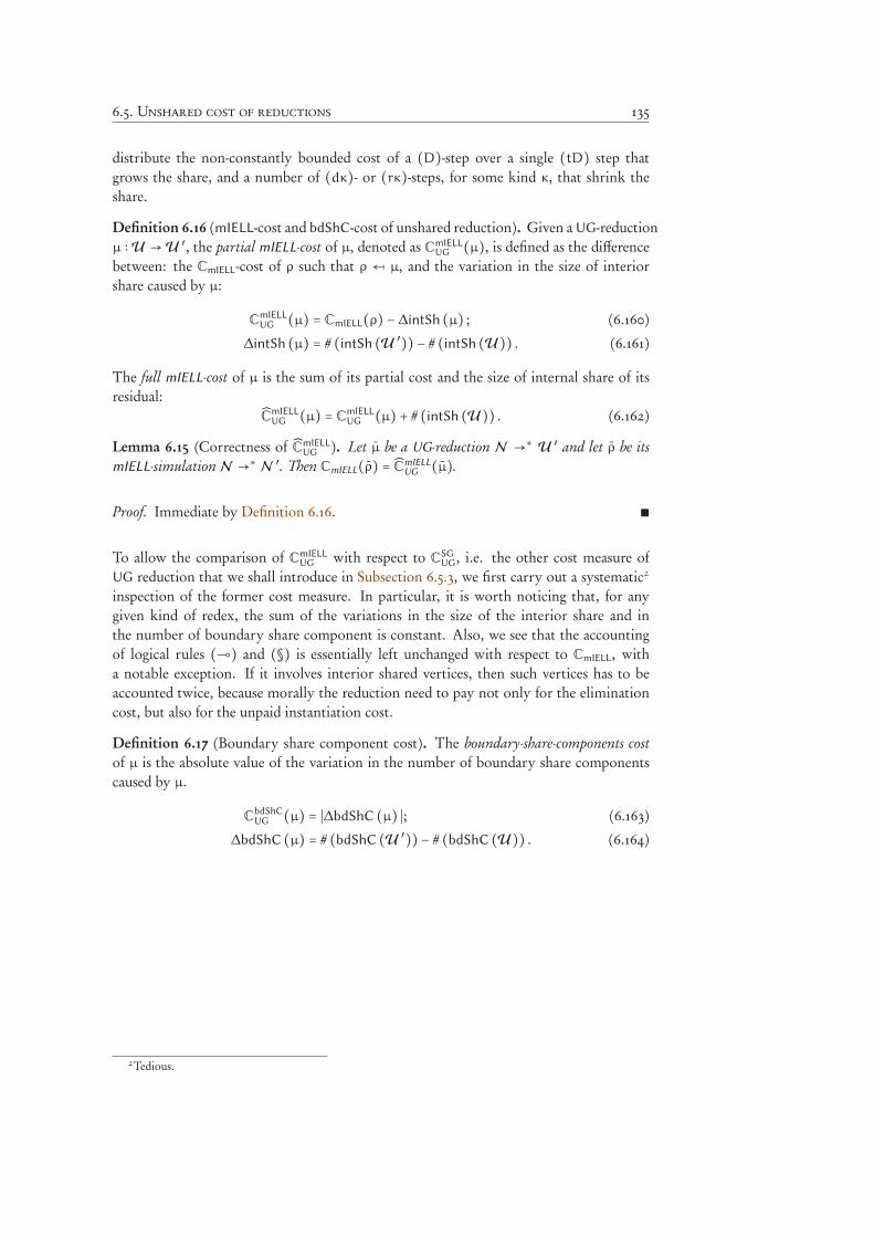
6.5. Unshared cost of reductions 135
distribute the non-constantly bounded cost of a (D)-step over a single (tD) step thatgrows the share, and a number of (dκ)- or (rκ)-steps, for some kind κ, that shrink theshare.
Definition 6.16 (mIELL-cost and bdShC-cost of unshared reduction). Given aUG-reductionµ ∶U →U ′, the partial mIELL-cost of µ, denoted as CmIELL
UG (µ), is defined as the differencebetween: the CmIELL-cost of ρ such that ρ ←[ µ, and the variation in the size of interiorshare caused by µ:
CmIELLUG (µ) = CmIELL(ρ) −∆intSh (µ) ; (6.160)
∆intSh (µ) = # (intSh (U ′)) − # (intSh (U)) . (6.161)
The full mIELL-cost of µ is the sum of its partial cost and the size of internal share of itsresidual:
CmIELLUG (µ) = CmIELL
UG (µ) + # (intSh (U)) . (6.162)
Lemma 6.15 (Correctness of CmIELLUG ). Let µ be a UG-reduction N →∗ U ′ and let ρ be its
mIELL-simulation N →∗ N ′. Then CmIELL(ρ) = CmIELL
UG(µ).
Proof. Immediate by Definition 6.16. ∎
To allow the comparison of CmIELLUG with respect to C
SGUG, i.e. the other cost measure of
UG reduction that we shall introduce in Subsection 6.5.3, we first carry out a systematic2
inspection of the former cost measure. In particular, it is worth noticing that, for anygiven kind of redex, the sum of the variations in the size of the interior share and inthe number of boundary share component is constant. Also, we see that the accountingof logical rules (⊸) and (§) is essentially left unchanged with respect to CmIELL, witha notable exception. If it involves interior shared vertices, then such vertices has to beaccounted twice, because morally the reduction need to pay not only for the eliminationcost, but also for the unpaid instantiation cost.
Definition 6.17 (Boundary share component cost). The boundary-share-components costof µ is the absolute value of the variation in the number of boundary share componentscaused by µ.
CbdShCUG (µ) = ∣∆bdShC (µ) ∣; (6.163)
∆bdShC (µ) = # (bdShC (U ′)) − # (bdShC (U)) . (6.164)
2Tedious.
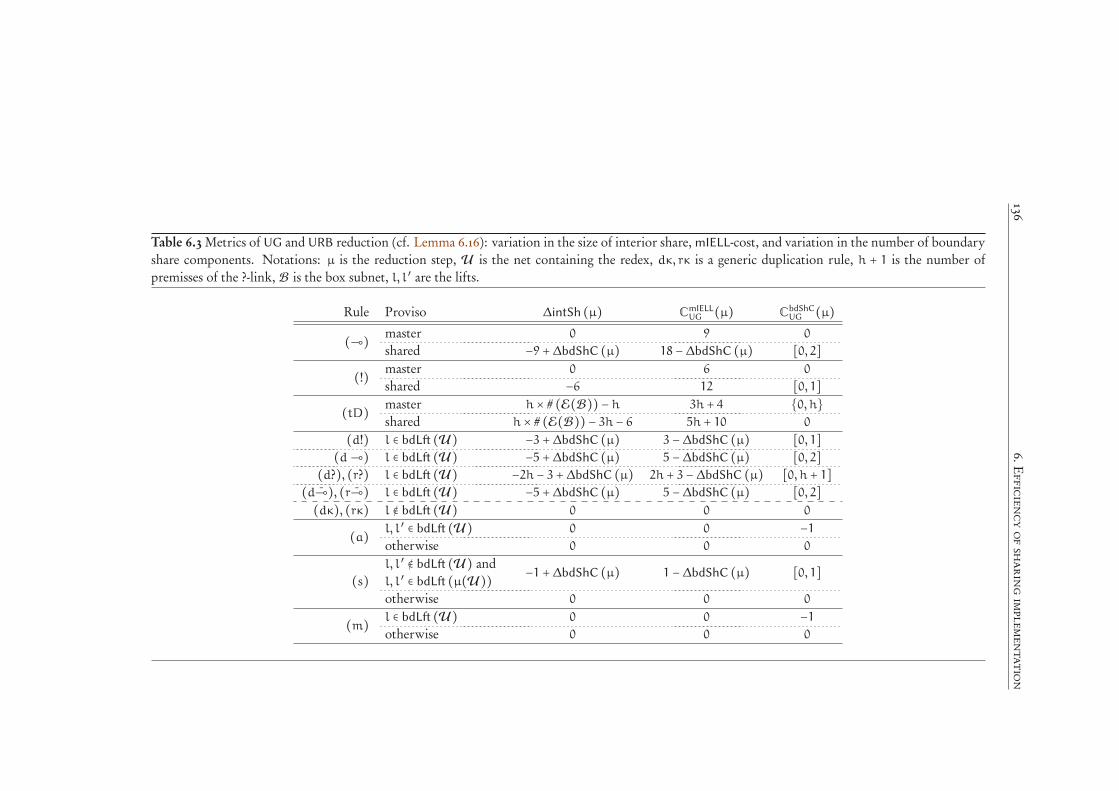
1366.
Effi
cien
cyofsharingimplem
entat
ion
Table 6.3 Metrics of UG and URB reduction (cf. Lemma 6.16): variation in the size of interior share, mIELL-cost, and variation in the number of boundaryshare components. Notations: µ is the reduction step, U is the net containing the redex, dκ, rκ is a generic duplication rule, h + 1 is the number ofpremisses of the ?-link, B is the box subnet, l, l ′ are the lifts.
Rule Proviso ∆intSh (µ) CmIELLUG (µ) C
bdShCUG (µ)
(⊸) master 0 9 0
shared −9 +∆bdShC (µ) 18 −∆bdShC (µ) [0, 2](!) master 0 6 0
shared −6 12 [0, 1](tD) master h × # (E(B)) − h 3h + 4 {0, h}
shared h × # (E(B)) − 3h − 6 5h + 10 0
(d!) l ∈ bdL! (U) −3 +∆bdShC (µ) 3 −∆bdShC (µ) [0, 1](d⊸) l ∈ bdL! (U) −5 +∆bdShC (µ) 5 −∆bdShC (µ) [0, 2]
(d?), (r?) l ∈ bdL! (U) −2h − 3 +∆bdShC (µ) 2h + 3 −∆bdShC (µ) [0, h + 1](d⊸), (r⊸) l ∈ bdL! (U) −5 +∆bdShC (µ) 5 −∆bdShC (µ) [0, 2](dκ), (rκ) l ∉ bdL! (U) 0 0 0
(a) l, l ′ ∈ bdL! (U) 0 0 −1
otherwise 0 0 0
(s)l, l ′ ∉ bdL! (U) and
−1 +∆bdShC (µ) 1 −∆bdShC (µ) [0, 1]l, l ′ ∈ bdL! (µ(U))otherwise 0 0 0
(m) l ∈ bdL! (U) 0 0 −1
otherwise 0 0 0
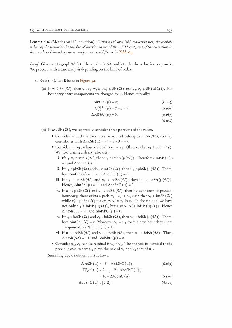
6.5. Unshared cost of reductions 137
Lemma 6.16 (Metrics on UG-reduction). Given a UG or a URB reduction step, the possiblevalues of the variation in the size of interior share, of the mIELL-cost, and of the variation inthe number of boundary share components and lifts are in Table 6.3.
Proof. Given a UG-graph U , let R be a redex in U , and let µ be the reduction step on R.We proceed with a case analysis depending on the kind of redex.
1. Rule (⊸). Let R be as in Figure 5.1.
(a) If w ∉ Sh (U), then v1, v2,w,u1, u2 ∉ Sh (U) and v1, v2 ∉ Sh (µ(U)). Noboundary share components are changed by µ. Hence, trivially:
∆intSh (µ) = 0; (6.165)
CmIELLUG (µ) = 9 − 0 = 9; (6.166)
∆bdShC (µ) = 0. (6.167)
(6.168)
(b) If w ∈ Sh (U), we separately consider three portions of the redex.
• Consider w and the two links, which all belong to intSh (U), so theycontributes with ∆intSh (µ) = −1 − 2 × 3 = −7.
• Consider u1, v1, whose residual is u1 = v1. Observe that v1 ∉ pbSh (U).We now distinguish six sub-cases.i. If u1, v1 ∈ intSh (U), then u1 ∈ intSh (µ(U)). Therefore ∆intSh (µ) =−1 and ∆bdShC (µ) = 0.
ii. If u1 ∈ pbSh (U) and v1 ∈ intSh (U), then u1 ∈ pbSh (µ(U)). There-fore ∆intSh (µ) = −1 and ∆bdShC (µ) = 0.
iii. If u1 ∈ intSh (U) and v1 ∈ bdSh (U), then u1 ∈ bdSh (µ(U)).Hence, ∆intSh (µ) = −1 and ∆bdShC (µ) = 0.
iv. If u1 ∈ pbSh (U) and v1 ∈ bdSh (U), then by definition of pseudo-boundary, there exists a path πi ∶ xi ≫ ui such that xi ∈ intSh (U)while x ′i ∈ pbSh (U) for every x ′i ≠ xi in πi. In the residual we havenot only u1 ∈ bdSh (µ(U)), but also xi, x
′
i ∈ bdSh (µ(U)). Hence∆intSh (µ) = −1 and ∆bdShC (µ) = 0.
v. If u1 ∈ bdSh (U) and v1 ∈ bdSh (U), then u1 ∈ bdSh (µ(U)). There-fore ∆intSh (U) = 0. Moreover v1 = u1 form a new boundary sharecomponent, so ∆bdShC (µ) = 1.
vi. If u1 ∈ bdSh (U) and v1 ∈ intSh (U), then u1 ∈ bdSh (U). Thus,∆intSh (U) = −1. and ∆bdShC (µ) = 0.
• Consider u2, v2, whose residual is u2 = v2. The analysis is identical to theprevious case, where u2 plays the role of v1 and v2 that of u1.
Summing up, we obtain what follows.
∆intSh (µ) = −9 +∆bdShC (µ) ; (6.169)
CmIELLUG (µ) = 9 − ( − 9 +∆bdShC (µ) )
= 18 −∆bdShC (µ) ; (6.170)
∆bdShC (µ) ∈ [0, 2]. (6.171)
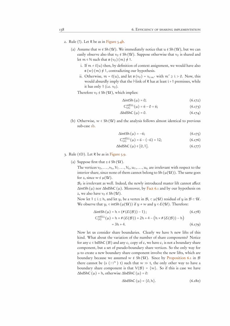
138 6. Efficiency of sharing implementation
2. Rule (!). Let R be as in Figure 5.4b.
(a) Assume that w ∉ Sh (U). We immediately notice that u ∉ Sh (U), but we caneasily observe also that v0 ∉ Sh (U). Suppose otherwise that v0 is shared andlet m ∈ N such that s (v0) (m) /≈ 1.
i. If m ≠ ℓ(u) then, by definition of context assignment, we would have alsos (w) (m) /≈ 1, contradicting our hypothesis.
ii. Otherwise, m = ℓ(u), and let s (v0) = xi∶m ′ with m ′ ≥ i > 0. Now, thiswould absurdly imply that the ?-link of R has at least i+1 premisses, whileit has only 1 (i.e. v0 ).
Therefore v0 ∉ Sh (U), which implies:
∆intSh (µ) = 0; (6.172)
CmIELLUG (µ) = 6 − 0 = 6; (6.173)
∆bdShC (µ) = 0. (6.174)
(b) Otherwise, w ∈ Sh (U) and the analysis follows almost identical to previoussub-case 1b.
∆intSh (µ) = −6; (6.175)
CmIELLUG (µ) = 6 − (−6) = 12; (6.176)
∆bdShC (µ) ∈ [0, 1]. (6.177)
3. Rule (tD). Let R be as in Figure 5.9.
(a) Suppose first that z ∉ Sh (U).The vertices v0, . . . , vh, V1 . . . , Vk, u1, . . . , uk are irrelevant with respect to theinterior share, since none of them cannot belong to Sh (µ(U)). The same goesfor z, since w ∉ µ(U).B0 is irrelevant as well. Indeed, the newly introduced master lift cannot affect∆intSh (µ) nor ∆bdShC (µ). Moreover, by Fact 6.1 and by our hypothesis onz, we also have v0 ∉ Sh (U).Now let 1 ≤ i ≤ h, and let yi be a vertex in Bi ⊂ µ(U) residual of y in B ⊂U .We observe that yi ∈ intSh (µ(U)) if y ≠ w and y ∈ E(U). Therefore:
∆intSh (µ) = h × (# (E(B)) − 1) ; (6.178)
CmIELLUG (µ) = h × # (E(B)) + 2h + 4 − (h × # (E(B)) − h)
= 3h + 4. (6.179)
Now let us consider share boundaries. Clearly we have h new lifts of thiskind. What about the variation of the number of share components? Noticefor any c ∈ bdShC (B) and any ci copy of c, we have ci is not a boundary sharecomponent, but a set of pseudo-boundary share vertices. So the only way forµ to create a new boundary share component involve the new lifts, which areboundary because we assumed w ∉ Sh (U). Since by Proposition 6.1 in B
there cannot be ⟨s ( ∣-⟩n ) t⟩ such that w ≫ t, the only other way to have aboundary share component is that V(B) = {w}. So if this is case we have∆bdShC (µ) = h, otherwise ∆bdShC (µ) = 0:
∆bdShC (µ) = {0, h}. (6.180)
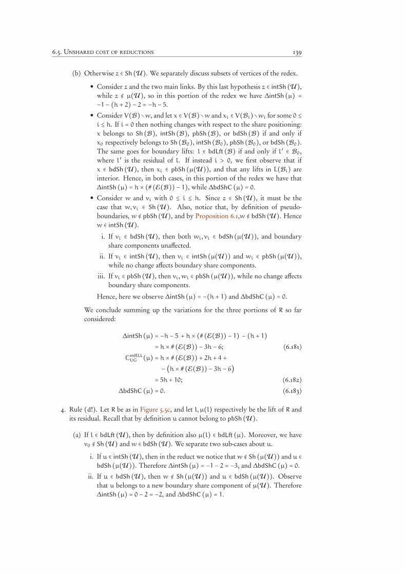
6.5. Unshared cost of reductions 139
(b) Otherwise z ∈ Sh (U). We separately discuss subsets of vertices of the redex.
• Consider z and the two main links. By this last hypothesis z ∈ intSh (U),while z ∉ µ(U), so in this portion of the redex we have ∆intSh (µ) =−1 − (h + 2) − 2 = −h − 5.
• Consider V(B)∖w, and let x ∈ V(B)∖w and xi ∈ V(Bi)∖wi for some 0 ≤
i ≤ h. If i = 0 then nothing changes with respect to the share positioning:x belongs to Sh (B), intSh (B), pbSh (B), or bdSh (B) if and only ifx0 respectively belongs to Sh (B0), intSh (B0), pbSh (B0), or bdSh (B0).The same goes for boundary lifts: l ∈ bdL! (B) if and only if l ′ ∈ B0,where l ′ is the residual of l. If instead i > 0, we first observe that ifx ∈ bdSh (U), then xi ∈ pbSh (µ(U)), and that any lifts in L(Bi) areinterior. Hence, in both cases, in this portion of the redex we have that∆intSh (µ) = h × (# (E(B)) − 1), while ∆bdShC (µ) = 0.
• Consider w and vi with 0 ≤ i ≤ h. Since z ∈ Sh (U), it must be thecase that w,vi ∈ Sh (U). Also, notice that, by definition of pseudo-boundaries, w ∉ pbSh (U), and by Proposition 6.1,w ∉ bdSh (U). Hencew ∈ intSh (U).i. If vi ∈ bdSh (U), then both wi, vi ∈ bdSh (µ(U)), and boundary
share components unaffected.
ii. If vi ∈ intSh (U), then vi ∈ intSh (µ(U)) and wi ∈ pbSh (µ(U)),while no change affects boundary share components.
iii. If vi ∈ pbSh (U), then vi,wi ∈ pbSh (µ(U)), while no change affectsboundary share components.
Hence, here we observe ∆intSh (µ) = −(h + 1) and ∆bdShC (µ) = 0.
We conclude summing up the variations for the three portions of R so farconsidered:
∆intSh (µ) = −h − 5 + h × (# (E(B)) − 1) − (h + 1)= h × # (E(B)) − 3h − 6; (6.181)
CmIELLUG (µ) = h × # (E(B)) + 2h + 4 +
− (h × # (E(B)) − 3h − 6)= 5h + 10; (6.182)
∆bdShC (µ) = 0. (6.183)
4. Rule (d!). Let R be as in Figure 5.5c, and let l, µ(l) respectively be the lift of R andits residual. Recall that by definition u cannot belong to pbSh (U).(a) If l ∈ bdL! (U), then by definition also µ(l) ∈ bdL! (µ). Moreover, we have
v0 ∉ Sh (U) and w ∈ bdSh (U). We separate two sub-cases about u.
i. If u ∈ intSh (U), then in the reduct we notice that w ∉ Sh (µ(U)) and u ∈
bdSh (µ(U)). Therefore ∆intSh (µ) = −1 − 2 = −3, and ∆bdShC (µ) = 0.
ii. If u ∈ bdSh (U), then w ∉ Sh (µ(U)) and u ∈ bdSh (µ(U)). Observethat u belongs to a new boundary share component of µ(U). Therefore∆intSh (µ) = 0 − 2 = −2, and ∆bdShC (µ) = 1.
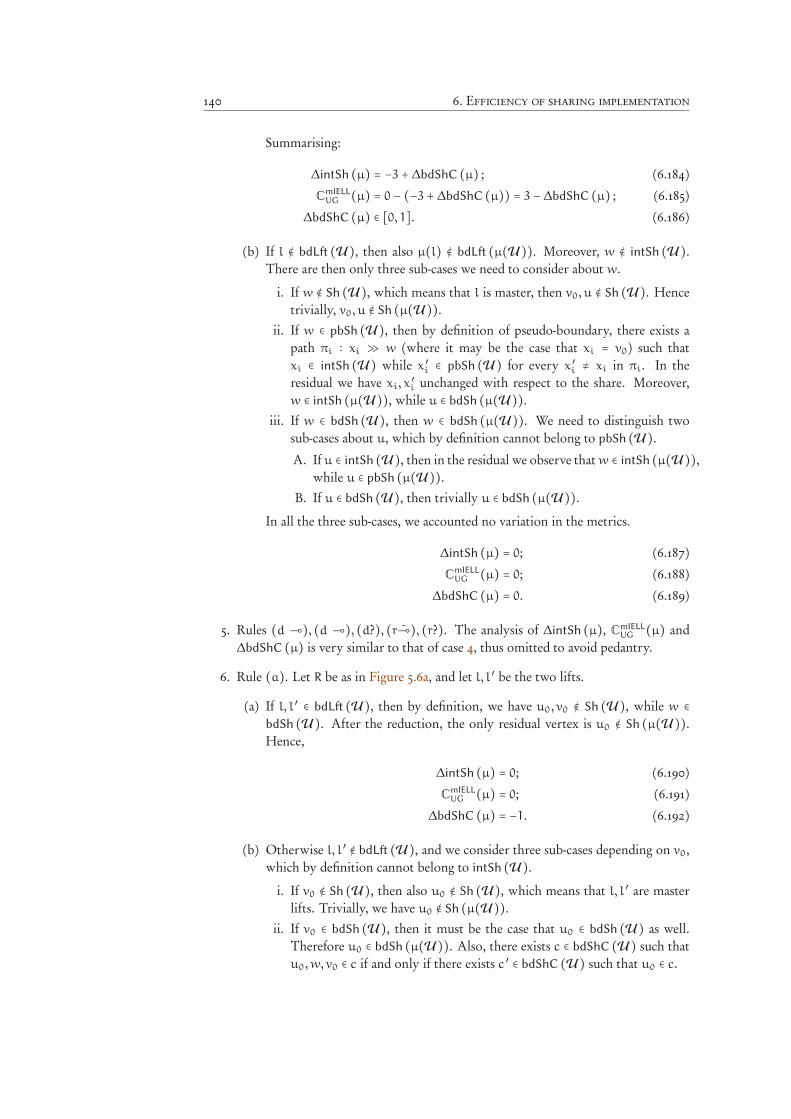
140 6. Efficiency of sharing implementation
Summarising:
∆intSh (µ) = −3 +∆bdShC (µ) ; (6.184)
CmIELLUG (µ) = 0 − (−3 +∆bdShC (µ)) = 3 −∆bdShC (µ) ; (6.185)
∆bdShC (µ) ∈ [0, 1]. (6.186)
(b) If l ∉ bdL! (U), then also µ(l) ∉ bdL! (µ(U)). Moreover, w ∉ intSh (U).There are then only three sub-cases we need to consider about w.
i. If w ∉ Sh (U), which means that l is master, then v0, u ∉ Sh (U). Hencetrivially, v0, u ∉ Sh (µ(U)).
ii. If w ∈ pbSh (U), then by definition of pseudo-boundary, there exists apath πi ∶ xi ≫ w (where it may be the case that xi = v0 ) such thatxi ∈ intSh (U) while x ′i ∈ pbSh (U) for every x ′i ≠ xi in πi. In theresidual we have xi, x
′
i unchanged with respect to the share. Moreover,w ∈ intSh (µ(U)), while u ∈ bdSh (µ(U)).
iii. If w ∈ bdSh (U), then w ∈ bdSh (µ(U)). We need to distinguish twosub-cases about u, which by definition cannot belong to pbSh (U).A. If u ∈ intSh (U), then in the residual we observe that w ∈ intSh (µ(U)),
while u ∈ pbSh (µ(U)).B. If u ∈ bdSh (U), then trivially u ∈ bdSh (µ(U)).
In all the three sub-cases, we accounted no variation in the metrics.
∆intSh (µ) = 0; (6.187)
CmIELLUG (µ) = 0; (6.188)
∆bdShC (µ) = 0. (6.189)
5. Rules (d ⊸), (d ⊸), (d?), (r⊸), (r?). The analysis of ∆intSh (µ), CmIELLUG (µ) and
∆bdShC (µ) is very similar to that of case 4, thus omitted to avoid pedantry.
6. Rule (a). Let R be as in Figure 5.6a, and let l, l ′ be the two lifts.
(a) If l, l ′ ∈ bdL! (U), then by definition, we have u0, v0 ∉ Sh (U), while w ∈
bdSh (U). After the reduction, the only residual vertex is u0 ∉ Sh (µ(U)).Hence,
∆intSh (µ) = 0; (6.190)
CmIELLUG (µ) = 0; (6.191)
∆bdShC (µ) = −1. (6.192)
(b) Otherwise l, l ′ ∉ bdL! (U), and we consider three sub-cases depending on v0,which by definition cannot belong to intSh (U).
i. If v0 ∉ Sh (U), then also u0 ∉ Sh (U), which means that l, l ′ are masterlifts. Trivially, we have u0 ∉ Sh (µ(U)).
ii. If v0 ∈ bdSh (U), then it must be the case that u0 ∈ bdSh (U) as well.Therefore u0 ∈ bdSh (µ(U)). Also, there exists c ∈ bdShC (U) such thatu0,w, v0 ∈ c if and only if there exists c ′ ∈ bdShC (U) such that u0 ∈ c.
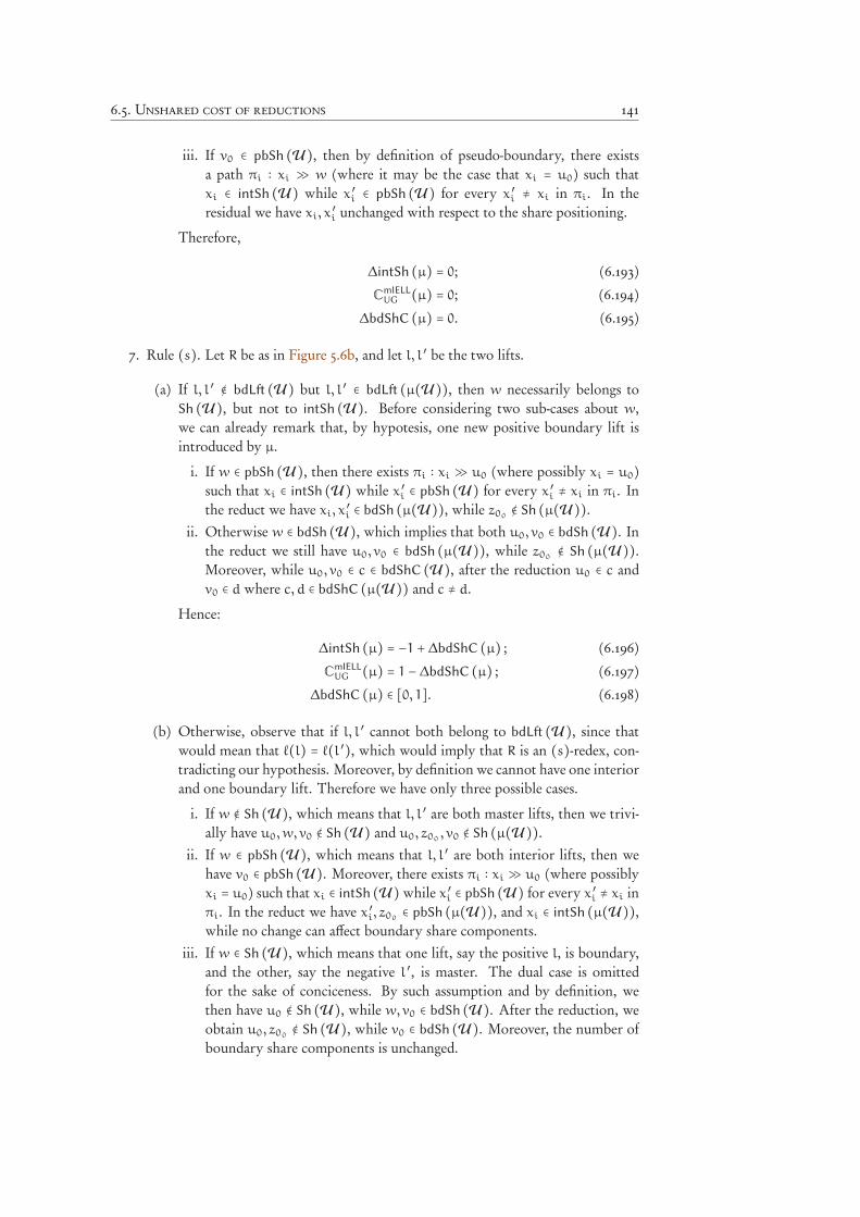
6.5. Unshared cost of reductions 141
iii. If v0 ∈ pbSh (U), then by definition of pseudo-boundary, there existsa path πi ∶ xi ≫ w (where it may be the case that xi = u0 ) such thatxi ∈ intSh (U) while x ′i ∈ pbSh (U) for every x ′i ≠ xi in πi. In theresidual we have xi, x
′
i unchanged with respect to the share positioning.
Therefore,
∆intSh (µ) = 0; (6.193)
CmIELLUG (µ) = 0; (6.194)
∆bdShC (µ) = 0. (6.195)
7. Rule (s). Let R be as in Figure 5.6b, and let l, l ′ be the two lifts.
(a) If l, l ′ ∉ bdL! (U) but l, l ′ ∈ bdL! (µ(U)), then w necessarily belongs toSh (U), but not to intSh (U). Before considering two sub-cases about w,we can already remark that, by hypotesis, one new positive boundary lift isintroduced by µ.
i. If w ∈ pbSh (U), then there exists πi ∶ xi ≫ u0 (where possibly xi = u0 )such that xi ∈ intSh (U) while x ′i ∈ pbSh (U) for every x ′i ≠ xi in πi. Inthe reduct we have xi, x
′
i ∈ bdSh (µ(U)), while z00∉ Sh (µ(U)).
ii. Otherwise w ∈ bdSh (U), which implies that both u0, v0 ∈ bdSh (U). Inthe reduct we still have u0, v0 ∈ bdSh (µ(U)), while z00
∉ Sh (µ(U)).Moreover, while u0, v0 ∈ c ∈ bdShC (U), after the reduction u0 ∈ c andv0 ∈ d where c, d ∈ bdShC (µ(U)) and c ≠ d.
Hence:
∆intSh (µ) = −1 +∆bdShC (µ) ; (6.196)
CmIELLUG (µ) = 1 −∆bdShC (µ) ; (6.197)
∆bdShC (µ) ∈ [0, 1]. (6.198)
(b) Otherwise, observe that if l, l ′ cannot both belong to bdL! (U), since thatwould mean that ℓ(l) = ℓ(l ′), which would imply that R is an (s)-redex, con-tradicting our hypothesis. Moreover, by definition we cannot have one interiorand one boundary lift. Therefore we have only three possible cases.
i. If w ∉ Sh (U), which means that l, l ′ are both master lifts, then we trivi-ally have u0,w, v0 ∉ Sh (U) and u0, z00
, v0 ∉ Sh (µ(U)).ii. If w ∈ pbSh (U), which means that l, l ′ are both interior lifts, then we
have v0 ∈ pbSh (U). Moreover, there exists πi ∶ xi ≫ u0 (where possiblyxi = u0 ) such that xi ∈ intSh (U) while x ′i ∈ pbSh (U) for every x ′i ≠ xi inπi. In the reduct we have x ′i, z00
∈ pbSh (µ(U)), and xi ∈ intSh (µ(U)),while no change can affect boundary share components.
iii. If w ∈ Sh (U), which means that one lift, say the positive l, is boundary,and the other, say the negative l ′, is master. The dual case is omittedfor the sake of conciceness. By such assumption and by definition, wethen have u0 ∉ Sh (U), while w,v0 ∈ bdSh (U). After the reduction, weobtain u0, z00
∉ Sh (U), while v0 ∈ bdSh (U). Moreover, the number ofboundary share components is unchanged.
142 6. Efficiency of sharing implementation
We conclude by summarising:
∆intSh (µ) = 0; (6.199)
CmIELLUG (µ) = 0; (6.200)
∆bdShC (µ) = 0. (6.201)
8. Rule (m). Let R be as in Figure 5.8a, and l its lift.
(a) If l ∈ bdL! (U), then ui ∈ bdSh (U), while v0,w ∉ Sh (U). After µ, weobtain no change with respect to the share positioning. On the other hand,{ui} ∈ bdShC (U), which is erased by µ. Therefore,
∆intSh (µ) = 0; (6.202)
CmIELLUG (µ) = 0; (6.203)
∆bdShC (µ) = −1. (6.204)
(b) Otherwise, we distinguish two sub-cases about u0, which by our assumptioncannot belong to intSh (U), nor to bdSh (U).
i. If ui ∉ Sh (U), then trivially also v0,w ∉ Sh (U). In the reduction ui iserased, and we have no change about internal share or its boundaries.
ii. If ui ∈ pbSh (U), then w ∉ Sh (U). Also, there exists πi ∶ xi ≫ v0
(where it may be the case that xi = v0 ) such that xi ∈ intSh (U) whilex ′i ∈ pbSh (U) for every x ′i ≠ xi in πi. Now, in the residual we have thatxi, x
′
i are unchanged with respect to the share positioning. Hence, againthere is no change about internal share or its boundaries.
∆intSh (µ) = 0; (6.205)
CmIELLUG (µ) = 0; (6.206)
∆bdShC (µ) = 0. (6.207)
∎
6.5.3 Unshared cost of SG reduction
We now define CSGUG, a second notion of cost on unshared graphs reduction that, symmet-
rically with respect to what we did with CmIELLUG , allows to transfer the CSG-cost of any
sharing reduction simulated by UG graphs. Looking at a simulation of such kind, thefirst inspiring idea is that, in a UG-graph U , all reductions inside Sh (U) have no cost.Indeed, shared vertices, shared links and shared redexes are copies of master copies, andonly these are represented in the SG-graph that unfold in U . Hence, we shall put costsonly to redexes outside the share. The second ingredient is the role played by lifts, whichmimic muxes’ dynamics while preserving coherence in the complexity account. For everymux m in G, we distribute the cost of a propagation against another kind of link, or of aninteraction with another mux, over the set of boundary lifts in the unfolding of m. Theseconsiderations lead us to the following definition.
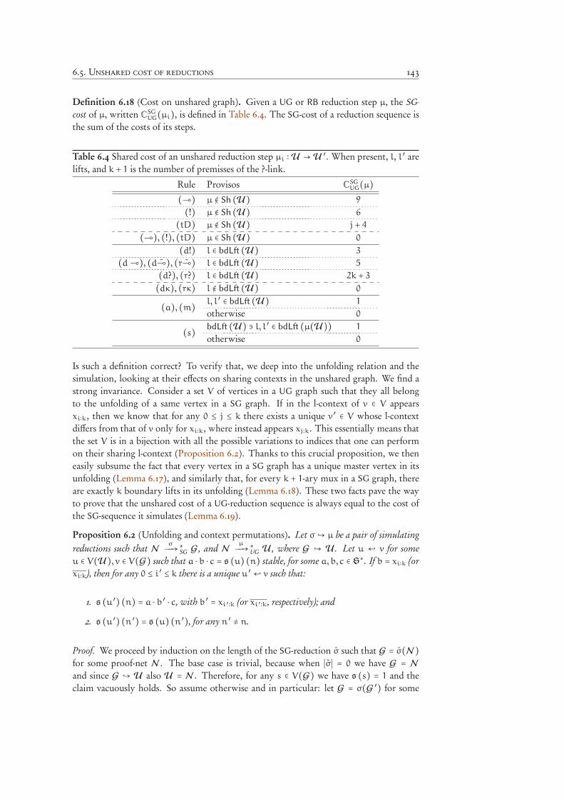
6.5. Unshared cost of reductions 143
Definition 6.18 (Cost on unshared graph). Given a UG or RB reduction step µ, the SG-cost of µ, written C
SGUG(µi), is defined in Table 6.4. The SG-cost of a reduction sequence is
the sum of the costs of its steps.
Table 6.4 Shared cost of an unshared reduction step µi ∶U →U ′. When present, l, l ′ arelifts, and k + 1 is the number of premisses of the ?-link.
Rule Provisos CSGUG(µ)
(⊸) µ ∉ Sh (U) 9
(!) µ ∉ Sh (U) 6
(tD) µ ∉ Sh (U) j + 4
(⊸), (!), (tD) µ ∈ Sh (U) 0
(d!) l ∈ bdL! (U) 3
(d⊸), (d⊸), (r⊸) l ∈ bdL! (U) 5
(d?), (r?) l ∈ bdL! (U) 2k + 3
(dκ), (rκ) l ∉ bdL! (U) 0
(a), (m) l, l ′ ∈ bdL! (U) 1
otherwise 0
(s) bdL! (U) ∋ l, l ′ ∈ bdL! (µ(U)) 1
otherwise 0
Is such a definition correct? To verify that, we deep into the unfolding relation and thesimulation, looking at their effects on sharing contexts in the unshared graph. We find astrong invariance. Consider a set V of vertices in a UG graph such that they all belongto the unfolding of a same vertex in a SG graph. If in the l-context of v ∈ V appearsxi∶k, then we know that for any 0 ≤ j ≤ k there exists a unique v ′ ∈ V whose l-contextdiffers from that of v only for xi∶k, where instead appears xj∶k. This essentially means thatthe set V is in a bijection with all the possible variations to indices that one can performon their sharing l-context (Proposition 6.2). Thanks to this crucial proposition, we theneasily subsume the fact that every vertex in a SG graph has a unique master vertex in itsunfolding (Lemma 6.17), and similarly that, for every k + 1-ary mux in a SG graph, thereare exactly k boundary lifts in its unfolding (Lemma 6.18). These two facts pave the wayto prove that the unshared cost of a UG-reduction sequence is always equal to the cost ofthe SG-sequence it simulates (Lemma 6.19).
Proposition 6.2 (Unfolding and context permutations). Let σ ↪ µ be a pair of simulatingreductions such that N
σ−−→
∗
SGG, and N
µ−−→
∗
UGU , where G ↪ U . Let u ↩ v for some
u ∈ V(U), v ∈ V(G) such that a ⋅ b ⋅ c = s (u) (n) stable, for some a, b, c ∈ S∗. If b = xi∶k (orxi∶k), then for any 0 ≤ i ′ ≤ k there is a unique u ′ ↩ v such that:
1. s (u ′) (n) = a ⋅ b ′ ⋅ c, with b ′ = xi ′∶k (or xi ′∶k, respectively); and
2. s (u ′) (n ′) = s (u) (n ′), for any n ′ ≠ n.
Proof. We proceed by induction on the length of the SG-reduction σ such that G = σ(N )for some proof-net N . The base case is trivial, because when ∣σ∣ = 0 we have G = N
and since G ↪ U also U = N . Therefore, for any s ∈ V(G) we have s (s) = 1 and theclaim vacuously holds. So assume otherwise and in particular: let G = σ(G ′) for some
144 6. Efficiency of sharing implementation
SG-reduction step σ on a redex S such that G ′ = σ ′(N ); let U ′↩ G ′; and let µ ↩ σ for
some UG-reduction sequence µ on a set of redexes M such that U = µ(U ′) = µ(µ ′(N )).Finally, take s ∈ V(G) and t ↩ s such that s (t) (n) = a ⋅ b ⋅ c where b = xl∶m or xl∶m, forsome n, l,m ∈ N, and some a, xl∶m, c ∈ S∗. Finally let 0 ≤ l ′ ≤ m be the index for whichwe want to prove the claim.
1. If s ∉ int(σ(S)), then by definition of reduction σ−1(s) = s. Moreover, for anyredex M ∈ M we also have t ∉ µ(M), as per definition of unfolding. Therefore,in accordance with invariance Lemma 6.14, s (t) = s (µ−1(t)). So let µ−1(tl) ↩σ−1(s) be the unique vertex of U ′ such that the claim holds by IH. Now, sinces (µ−1(tl)) = s (tl), we trivially conclude that the claim still holds.
2. If s ∈ int(σ(S)), then let M ∈ M such that t ∈M, and let µ ∈ µ be the reduction stepon M. We proceed with a case analysis on the kind of the redex S of σ.
(a) Rules (!), (⊸), (a), (m). Absurd: by inspection of the definition of the re-dexes, we verify that int(σ(S)) = ∅, contradicting the hypothesis of s ∈ int(σ(S)).
(b) Rule (d!). Let S be as in Figure 5.5c, and, since int(σ(S)) = {z0, . . . , zk},let s = zi. Now, assume vertex names in M are as in S, but with the primesymbol, and let t = z ′i ′ . Observe that in µ(M), as per definition of contextassignment, we have s (vi ′) = s (zi ′). But s (vi ′) belongs to C(M), where byLemma 6.14 it must have the same levelled context. Now, since vi ↪ vi ′ , letv ′′i ′′ be the unique vertex in U ′ such that vi ↪ v ′′i ′′ and it satisfies the claim,i.e. s (v ′′i ′′) (n) = a ⋅ xl ′∶m ⋅ c, while s (v ′′i ′′) (n ′) = s (v ′i ′) (n ′), for any n ′ ≠ n.So, let M ′′ be the redex containing v ′′i ′′ , and µ ′′ be its reduction step. Sinceit belongs to the C(M ′′), we find v ′′i ′′ also in µ ′′(M ′′) with the same levelled-context. Consider z ′′i ′′ in µ ′′(M ′′) and verify not only that zi ↪ z ′′i ′′ , but alsothat, as previously remarked, s (v ′′i ′′) = s (z ′′i ′′). Hence the claim.
(c) Rules (d?), (d ⊸), (d⊸), (s), (r⊸), (r?). The argument detailed in case 2bcan be applied here with only minor changes.
(d) Rule (tD). Let S be as in Figure 5.9, but let d be the level of !-link, and observethat int(σ(S)) = ⋃1≤i≤h Bi, where Bi denotes the i-copy of the interior of thebox B. Let the names of vertices and boxes in M be as in S, but with primesymbols. So let t ∈ B ′i ′ and consider σ−1(t). Assume the downward crossingof the i-th lift above B ′i ′ has context !ne, Also, let s (µ−1(t)) (d) = f ⋅g, wheref = s (vi). Then, by definition of context assignment, we first observe thefollowing.
s (t) (n ′) =⎧⎪⎪⎨⎪⎪⎩s (σ−1(t)) if d ′ ≠ d;
f ⋅ e ⋅ g if d ′ = d.(6.208)
Now, we observe that we can apply IH on µ−1(t). Namely, for any n ≠ d andfor any xl∶m ≠ e (or its negation), appearing in s (µ−1(t)) at the n-th context,we know there exists a unique vertex t ′ in U , such that σ−1(s) ↪ t ′ and forwhich: in s (t ′) (n) is obtained from s (t) substituting xl∶m for xl ′∶m, whiles (t ′) (n ′) = s (µ−1(t)) (n ′), for any n ′ ≠ n.
Now observe that t ′ belongs to a box B ′′ in a redex M ′, so let µ ′ be its reduc-tion step, which by definition of unfolding belongs to µ. Now, let t ′′ ∈ µ ′(t ′)
6.5. Unshared cost of reductions 145
be the vertex belonging in the i-th copy of the box B ′′, and verify that itsatisfies the claim.
∎
For every vertex in a SG graph, there exists a unique master vertex in its unfolding.
Lemma 6.17 (Master copy). Let Nσ−−→
∗
SGG and N
µ−−→
∗
UGRBU be two reduction sequences
such that σ ↪ µ. For any v ∈ V(G) and any V ′ ⊂ V(U), if v ↪ V ′ then there exists a uniquevm ∈ V
′ such that s (vm) ≈ 1, and it is called the master copy of v.
Proof. Immediate from Proposition 6.2 by fixing in its statement i ′ = 0. ∎
For every k + 1-ary mux in a SG graph, there are exactly k boundary lifts its unfolding.
Lemma 6.18 (Arities of muxes and cardinalities of their boundary lifts). Let Nσ−−→
∗
SGG
and Nµ−−→
∗
UGRBU be two reduction sequences such that σ ↪ µ. For any mux m ∈ L(G) of
arity k + 1, let L = {l ∈ bdL! (U) ∣m↪ l}. Then ∣L∣ = k.
Proof. Let m = ⟨u0, . . . uk ( ∣*⟩ ) z⟩ and consider the set L ′ ⊆ L(U) of any lift whosepremiss is the master copy of ui, for some 0 ≤ i ≤ k. Recall that, thanks to Lemma 6.17,we know that for any i the master copy is unique, so ∣L ′∣ = k+1. Now by definition of theunfolding relation, there is a sharing morphism between U and G which is connection-preserving and surjective (cf. Definition 5.8). Therefore, the master copy of z must be theconclusion of a lift lm ∈ L ′, which consequently is a master lift. Now let Lb = L ′ ∖ lm andnotice that it contains all and only the boundary lifts that are unfolding of m. Indeed, forevery li ∈ LB different than lm, we have ui ∉ Sh (U) while zi ∈ Sh (U). Thus Lb = L andtrivially ∣LB∣ = k. ∎
The unshared cost of a UG-reduction sequence is always equal to the cost of the SG-sequence it simulates.
Lemma 6.19 (Correctness of CSGUG ). If N
σ−−→
∗
SGG and N
µ−−→
∗
UGRBU are two reduction
sequences such that σ↪ µ, then CSG(σ) = CSG
UG(µ).
Proof. We go by induction on ∣σ∣. The base case is trivial, because when ∣σ∣ = 0 we haveG =N and since G ↪U also U =N . This means that CSG(σ) = CSG
UG(µ) = 0, so the claimvacuously holds. So assume ∣σ∣ > 0. Let G = σ(G ′) for some SG-reduction step σ on a re-dex S such that G ′ = σ ′(N ); let U ′
↩ G ′; and let µ↩ σ for some UG-reduction sequenceµ on a set of redexes M such that U = µ(U ′) = µ(µ ′(N )). By inductive hypothesis wealso assume CSG
UG(µ ′) = CSG(σ ′), so we need to prove that CSGUG(µ) = CSG(σ).
1. Suppose that S does not contain muxes, i.e. the rule of S is one of the following:(⊸), (!), (t). Then by Lemma 6.17, let M ∈ M be the unique redex such that forany v ′ ∈ M and any v ∈ S, if v ↪ v ′ then v ′ is the master copy of v. Now, let µ
146 6. Efficiency of sharing implementation
be the reduction of M and µ ′′ be the reduction of M ∖M. Now, observe that byDefinition 6.3 of CSG (see in particular Table 6.2) and Definition 6.18 of CSG
UG (seein particular Table 6.4) we have CSG
UG(µ) = CSG(σ), while CSGUG(µ ′′) = 0. Therefore
CSGUG(µ) = CSG(σ).
2. If S contains muxes, and is not a (s) rule, then let M ′′ ⊂ M be the set of anyredex in M whose lifts are boundary. First, observe that, again by Definition 6.3and 6.18 (cf. Table 6.2 and 6.4), for any reduction step µ ′′ on a redex of M ′′,we have CSG(σ) = k × CSG
UG(µ ′′), where k + 1 is the number of premisses of themux of S. Conversely, for any reduction step µ ′′′ on a redex of M ∖ M ′′, as perdefinition, CSG
UG(µ ′′′) = 0. But by Lemma 6.18 we know that ∣M ′′∣ = k. Thus,C
SGUG(µ) = CSG(σ).
3. Otherwise S is a (s) rule. Let k + 1 and l + 1 be the number of premisses of thepositive and negative mux of S, respectively. Observe that by definition of reduction(cf. Figure 5.6b) in σ(S) there are k+1 negative lifts with arity l+1, and l+1 positivelifts with arity k + 1.
By Lemma 6.18 this implies that M contains k positive boundary lifts and l negativeboundary lifts. Since by definition of boundary lift, there cannot be two boundarylifts in a (s) redex, the boundary lifts of M belong to different redexes. Now, againper Lemma 6.18, it must be the case that µ(M) contains (k+1)× l negative lifts, and(l+1)×k positive lifts. But this means that µ introduces k× l negative lifts and k× l
positive lifts, i.e. there are k × l redexes in M made of two pseudo-boundary liftswhich become boundary when swapped. (This happens when the levelled contextof premiss of the positive lift is 1 everywhere but at the level of the negative lift,where the context is identical to the variable occurrence of the and the negativelift.) Since CSG
UG assign a unitary cost of such reduction, and 0 otherwise, we obtainthat CSG
UG(µ) = k × l = CSG(σ).
∎
6.6 Unshared cost comparison
Thanks to the careful analysis of the metrics on UG-reduction so far accomplished, weare now able to prove the complexity bound. We first observe that for any UG-reduction,the difference between its sharing cost and its mIELL cost is bounded by its boundary-share-components cost (Lemma 6.20). Then, we proceed by bounding boundary-share-components cost to a quadratic function of the mIELL cost (Lemma 6.21 and 6.22). Insuch proof it is worth noticing that the only kind of reduction that we did not manage tobound by a linear function is the swap within a boundary share component generating anew component. In such a case, the bound depends linearly on the depth and quadraticallyon the mIELL cost. Finally we conclude by Theorem 6.1, which compares CSG with CmIELL
for any pair of simulating reduction sequence.
Lemma 6.20 (Bound for unshared costs comparison). For any proof-net N and any reduc-
tion sequence Nµ−−→
∗
UGRBU :
CSG
UG(µ) −CmIELL
UG (µ) ≤ CbdShCUG (µ). (6.209)
6.6. Unshared cost comparison 147
Proof. Given a step µ of µ, it suffices a mere inspection of Lemma 6.16 and Definition 6.18and, in particular, a comparison of the corresponding cases of Table 6.3 and Table 6.4, toimmediately verify the inequation. ∎
Lemma 6.21 (Redundant boundary share components). Given a UG-graph U , and v ∈
bdLimSh (U), let L ∶ u ∼ v be the boundary lift chain of v and let µ be a reduction sequenceon L. If n is the number of any (s)-step µ ∈ µ such that ∆bdShC (µ) = 1, then
n ≤ ℓ(U). (6.210)
Proof. By hypothesis, u ≫ v or v ≫ v. If both hold, then u = v and the claim is triviallyverified, because L = ∅. Otherwise, since the arguments of the two cases are identical, weshall assume u≫ v. Let µcs be the set of any (s)-step µ in µ such that CbdShC
UG (µ) = 1.
We will now prove that for any level n there may be at most one step µ ∈ µcs. This impliesthe claim, because in the worst case L contains lifts of any level l ≤ ℓ(U).For the sake of contradiction, assume otherwise that L contains: a ∣+⟩n-link l, a ∣+⟩n
′
-link l ′,and ∣-⟩n
′′
-link l ′′ such that there are two steps in µ swapping both l, l ′ with l ′′. (The dualsituation with one ∣+⟩-link and two ∣-⟩-link is identical, hence omitted.) Let VarO(l) = a,VarO(l ′) = b, and VarO(l ′′) = c. Then, there are some l-contexts γ1, γ2, γ3 such that:
s (v) = δ ⋅ γ1 ⋅ !na ⋅ γ2 ⋅ !n ′b ⋅ γ3JKKKKKKKKKKKKKKKKKKKKKKKKKKKKKKKKKKKKKKKKKKKKKKKKKKKKKKKKKKKKLKKKKKKKKKKKKKKKKKKKKKKKKKKKKKKKKKKKKKKKKKKKKKKKKKKKKKKKKKKKKMγ0
⋅!n ′′c ⋅ γ4, (6.211)
where γ0 is the l-context of the downward path π that goes from u to the conclusion of l ′′.Now, L contains only ∣*⟩-links, therefore any reductions in µ is necessarily an (s)- or an(a)-rule. By hypothesis, there is no (a)-rule involving l, l ′ or l ′′, hence π is long enoughfor any reduction step of µ. Therefore the context of π is invariant under any reductionpreceding the swap between l ′ and l ′′. For such (s)-step we hypothesised that in theredex the lifts are interior, while in the reduct they are boundary. Thus s (γ0) (n ′) = b
while s (γ0) (m) = 1 for any m ≠ n ′. But given the presence of the weight of l, i.e. !na,this implies that s (γ2) (n) = a, while s (γ2) (m) = 1, for any m ≠ n. Therefore that π
contains a ∣-⟩-link which annihilates with l. Absurd. ∎
Lemma 6.22 (Bound for closed border reduction). For any UGRB-reduction sequence µ ona proof-net N , CbdShC
UG(µ) is bounded by a quadratic function on C
mIELL
UG(µ).
Proof. Let µ be a UGRB-reduction sequence. We partition the reduction steps of µ intothree sets depending on their action on bdShC:
µe the set of any step µ of µ such that ∆bdShC (µ) = −1 (i.e. an erasure of a boundaryshare component), hence µ is of kind (a), (m);
µcs the set of any step µ of µ such that ∆bdShC (µ) = 1 and µ is of kind (s) (i.e. a creationof boundary share component with a swap);
µco the set of any step µ of µ that does not belong to µe or µcs.
148 6. Efficiency of sharing implementation
Hence, by construction:
CbdShCUG (µ) = CbdShC
UG (µe) +CbdShCUG (µcs) +CbdShC
UG (µco), (6.212)
so we can separately discuss the three addends.
1. CbdShCUG (µe). We observe that, since # (bdShC (⋅)) is always non negative, the num-
ber of erasures cannot outnumber the creations. Therefore,
CbdShCUG (µe) ≤ CbdShC
UG (µcs) +CbdShCUG (µco). (6.213)
2. CbdShCUG (µcs). Let µ ′cs be a maximal subsequence of µ such that, if µ = νµ ′csω for
some reduction sequences ν, ω, then any step of µ ′cs acts on the boundary lift chainL of every v ∈ bdLimSh (ν(U)). Now, by Lemma 6.21 we have that the normalisa-tion of L entail and increase of # (bdShC) of at most ℓ(U). Moreover, by Fact 6.2we know that # (bdLimSh (ν(U))) ≤ # (intSh (ν(U))). Therefore
CbdShCUG (µ ′cs) ≤ ℓ(U) × # (intSh (ν(U))) , (6.214)
and simplier:
≤ ℓ(U) × CmIELLUG (µ). (6.215)
Now, observe that the distinct sub-sequences of µ defined as µ ′cs are at most as manyas the number of steps µ ∈ µ such that CmIELL
UG (µ) = 0. Therefore:
CbdShCUG (µcs) ≤ ℓ(U) ×CmIELL
UG (µ) × CmIELLUG (µ), (6.216)
where, since CmIELLUG (µ) ≤ CmIELL
UG (µ), we can loosen and simplify as:
CbdShCUG (µcs) ≤ ℓ(U) × (CmIELL
UG (µ))2. (6.217)
3. CbdShCUG (µco). Recall from the account provided by Lemma 6.16 in Table 6.3 that,
for any step µ ∈ µco, CbdShCUG (µ) ≤ CmIELL
UG (µ). Therefore,
CbdShCUG (µco) ≤ CmIELL
UG (µco) (6.218)
≤ CmIELLUG (µ) (6.219)
≤ CmIELLUG (µ). (6.220)
Now we go back to (6.212) and substitute first (6.213):
CbdShCUG (µ) ≤ 2 × (CbdShC
UG (µcs) +CbdShCUG (µco)) (6.221)
and then (6.217) and (6.220)
CbdShCUG (µ) ≤ 2 × (ℓ(U) × (CmIELL
UG (µ))2 + CmIELLUG (µ)) (6.222)
≤ 2 × CmIELLUG (µ) + 2 × ℓ(U) × (CmIELL
UG (µ))2 . (6.223)
∎
6.7. Discussion 149
Proof of Theorem 6.1. By definition of↣, there exists an unshared graph U such that G ↪
U ↦N and there exists an intermediate unshared reduction µ ∶ N −→∗
UG U . On one side,by Lemma 6.15, we know that CmIELL(ρ) = CmIELL
UG (µ), and on the other, by Lemma 6.19,we similarly have: CSG(σ) = CSG
UG(µ).Now, as per Lemma 6.22 and Lemma 6.20, there exists a quadratic function f such that:
CSGUG(µ) ≤ CmIELL
UG (µ) + f (CmIELLUG (µ)) . (6.224)
But since CmIELLUG (µ) ≤ CmIELL
UG (µ), by definition:
CSGUG(µ) ≤ f (CmIELL
UG (µ)) , (6.225)
therefore
CSG(σ) = CSGUG(µ) ≤ f (CmIELL
UG (µ)) = f (CmIELL(ρ)) . (6.226)
Quod erat demonstrandum. ∎
6.7 Discussion
6.7.1 Related works
Baillot, Coppola, and Dal Lago [2011] proved a results similar to ours. In particular, theyshow that for any ILAL (or IEAL) proof-net N , the length of a SG-normalisation sequenceon N and a read-back sequence is bounded by a polynomial [ibidem, Proposition 12] (orKalmar-elementary [ibidem, Proposition 11]) function in the size of N . This essentiallymeans that SG-reduction cannot do dramatically worse than the reference systems, it can-not overstep their characteristic complexity classes. From a pragmatical point of view,this still tells us little, since one may think that the overhead is indeed polynomial, oreven Kalmar-elementary. The first and more important advance we have presented is thatwe proved a stronger and finer limitation — a quadratic bound, whose dominating por-tion are a special case of swaps. Moreover, since we bound the complexity of any SGRB
reduction sequence, and not necessarily a normalising one, our result is more generallystated, so it can be directly applied even with weaker notion of normal forms.
Their proof rests on a well-known correspondence between sharing reductions and GoI,adapting the ideas of the quantitative context semantics [Dal Lago, 2009]. Also, it seemshardly adaptable to prove a similar result for the general case, because their argumentdirectly exploits the known complexity bounds of the IEAL and ILAL. We instead accom-plished the result directly by more syntactical means, in a dynamic comparison of the twocost measures. Such technique and the tool of sharing contexts represents a complexity-aware extension of the syntactical approach that has been already fruitfully used before[Guerrini, Martini, and Masini, 2003].
150 6. Efficiency of sharing implementation
6.7.2 Open questions
Not much later its introduction, empirical benchmarks showed that sharing graphs canbe a very efficient implementation of the λ-calculus. Terms that allow massive amount ofsharing, indeed, can be normalised by a sharing-graph-based machine in polynomial time,whilst that requires exponential time with ordinary implementations in functional pro-gramming languages [Asperti, Giovannetti, and Naletto, 1996]. But the sharing machinerycomes at a price, that is still unknown for the general case, but that in the restricted case ofelementary proof-nets has been bounded, now quite satisfactorily, to a quadratic function.The result and the techniques open different questions.
Can we prove a similar complexity bound also in the general case of MELL proof-nets?Can we do so with the quantitative syntactic approach? The research hypothesis one mayrequire is the legitimation of a cost for exponential reductions that always depends onthe size of a box, even when they act on box nesting relocating one into another (e.g.promotion against dereliction).
Also on the same line, can we find not only a tight upper bound to the overhead intro-duced by optimal implementations, which gives a worst-case limitation, but also someconvincing best-case limitation? How much share is needed in order for the trade-off tobe convenient? When does the mux management overhead is amortised by the efficiencyof sharing?
Can we relate SG with other more concrete computational models like abstract machines?Some of them, like the IAM [Laurent, 2001], are of particular interest because of theirdistinguished space efficiency.
Sharing contexts appear as a powerful tool to study SG in their unshared counterpart.Not only they can be used to provide a simple proof of their completeness with re-spect to normalisation, since the absence of deadlocks is obtainable as consequence ofthe positivity property, very similarly to what was done by Guerrini [1999], though moresimply, thanks to the restricted setting of mIELL. But also offer a precise quantitative re-lation between a shared vertex in a sharing graph and its unfolding in the unshared graph(cf. Proposition 6.2). This makes of sharing context a promising tool to tackle all thesecomplexity-related questions about sharing implementation and Lévy families, more ingeneral.
We identified a kind of reduction steps that is critical for the complexity bound. Can itbe directly lowered finding a tighter bound, perhaps linear? If not, are there any tuningsfor the rewriting system under which the problem can be circumvented? For instance,one may explore the idea to introduce additional rules to reduce the number of redundantswap rules, as it was already proposed and implemented for redundant index-managementlinks [Asperti and Chroboczek, 1997] [Asperti and Guerrini, 1998, Chapter 9].
Index
Antecedent, see Vertex order relations
Box, 14auxiliary door, 14closed, 14depth, 14Elementary, 94Exponential, 14principal door, 14
Closed reduction, 19Consequent, see Vertex order relationsContext
mMELL, 17resource calculus, 33
completion, 33hole, 33simple, 33
resource netmulti-hole, 72
single-hole, 17Cost
mIELL reduction, 110RBreduction, 111SG reduction, 111
Crossingof an outermost box, 69
Cut elimination, see Reduction
Depth, see Box depthDynamic algebra, 24
ExecutionmMELL, 26
Expansionλ-term, 66mMELL net, 63
Exponential box, see Box
GraphSG, 97
λ-term, 15expansion, see Expansion, λ-termmMELL proof-net translation, seeTrans-
lation, λ-term in mMELL proof-net
Link, 12abstraction, 13application, 13arity, 12co-contraction, 35co-weakening, 35conclusion, 12constant, 13contraction, 13kind, 12mMELL, 13polarity, 12premiss, 12promotion, 13resource, 35SG, 96weakening, 13
L∗, see Dynamic Algebra
mELL
reduction, see Reduction, mELL
mIELL
proof-net, see Net, mIELL proof-netreduction cost, see Cost, mIELL reduc-
tionMixed net, 63mLLL
reduction, see Reduction, mLLL
mMELL
execution, see Executionexpansion, see Expansion, netproof-net, see Netreduction, see Reduction
Multiplexer, see Link, SG
152 INDEX
NetmMELL proof-net, 15mIELL proof-net, 94pre-net, 13size, 110variable, 16
bounded, 16free, 16
Normal form, 16
Path, 15assuming, 15atomic, 15bouncing, 15comprehensive, 44concatenation, 15concluding, 15crossing, 21cyclic, 15downward, 111equality, 15execution, 20expanded weighting, 84expansion-regularity, 84forms
redex crossing, 22input-output, 112length, 15long enough, 21maximal, 20persistent, 22regularity
resource net, 54resource reduction, 45reversal, 15straight, 15switching, 15trivial, 15twisting, 15upward, 112weighting
resource net, 53Pre-net, see NetProof-net
mMELL, see Net
RB
reduction cost, see Cost, RB reduction
RCF, see Redex crossing formRedex, see ReductionRedex crossing form, see Path formsReduct, 16Reduction
RB, 97SG, 96mELL, 94mLLL, 94mMELL, 17resource calculus, 33resource net, 37
expanded, 73parallel, 73
sequence, 16Resource
net, 35context, 37permutation, 37with promotion, see Mixed net
pre-net, 35simple pre-net, 35
Resource calculuspoly-term, 32term, 32
Resource dynamic algebra, 52Resource λ-term
translation in resource net, see Transla-tion, resource λ-term in resourcenets
Resource netexecution, 54
rL∗, see Resource dynamic algebra
SG
reduction cost, see Cost, SG reductionSG
graph, 97Sharing context
levelled, 116negative, 116positive, 116
lifting, 116monoid, 116negative, 116positive, 116restriction, 116stable form, 116
INDEX 153
Sharing graph, see SG, graphS∗
see Sharing context, monoid, 116Structure
mMELL structure, 14
Translationλ-term in mMELL proof-net, 15λ-term in resource net, 36
Typeground, 13mMELL, 13polarised, 13typing, 13
Variable occurrence, 115labelling, 115
Vertexorder relations
antecedent, 15consequent, 15
typing, see Type
Weightweighting
mMELL, 25
154 INDEX
Bibliography
Beniamino Accattoli. Linear Logic and Strong Normalization. In Femke van Raamsdonk,editor, 24th International Conference on Rewriting Techniques and Applications, RTA2013, June 24-26, 2013, Eindhoven, The Netherlands, volume 21 of LIPIcs, page 39–54.Schloss Dagstuhl - Leibniz-Zentrum fuer Informatik, 2013. ISBN 978-3-939897-53-8.doi: 10.4230/LIPIcs.RTA.2013.39.
Sandra Alves and Mário Florido. Weak linearization of the lambda calculus. TheoreticalComputer Science, 342(1):79–103, 2005. ISSN 0304-3975. doi: 10.1016/j.tcs.2005.06.005.URL http://www.sciencedirect.com/science/article/pii/S0304397505003403.
Andrea Asperti. Light affine logic. In Logic in Computer Science, 13th International Sym-posium, Proceedings, page 300–308. IEEE Computer Society, 1998.
Andrea Asperti and Juliusz Chroboczek. Safe Operators: Brackets Closed Forever Op-timizing Optimal lambda-Calculus Implementations. Applicable Algebra in Engineering,Communication and Computing, 8(6):437–468, December 1997. ISSN 0938-1279, 1432-0622. doi: 10.1007/s002000050083. URL http://link.springer.com/article/10.
1007/s002000050083.
Andrea Asperti and Stefano Guerrini. The Optimal Implementation of Functional Program-ming Languages, volume 45 of Cambridge tracts in theoretical computer science. Cam-bridge University Press, 1998.
Andrea Asperti and Cosimo Laneve. Paths, computations and labels in the lambda-calculus. Theoretical Computer Science, 142(2):277–297, 1995. ISSN 0304-3975. doi:10.1016/0304-3975(94)00279-7.
Andrea Asperti and Harry G. Mairson. Parallel Beta Reduction Is Not Elementary Re-cursive. Information and Computation, 170(1):49–80, 2001. doi: 10.1006/inco.2001.2869.
Andrea Asperti and Luca Roversi. Intuitionistic light affine logic. ACM Transactions onComputational Logic (TOCL), 3(1):137–175, 2002.
Andrea Asperti, Vincent Danos, Cosimo Laneve, and Laurent Regnier. Paths in thelambda-calculus. In Logic in Computer Science, 1994, page 426–436. IEEE, 1994. doi:10.1109/LICS.1994.316048.
Andrea Asperti, Cecilia Giovannetti, and Andrea Naletto. The Bologna optimalhigher-order machine. Journal of Functional Programming, 6(6):763–810, November1996. ISSN 1469-7653, 0956-7968. doi: 10.1017/S0956796800001994. URL https:
156 BIBLIOGRAPHY
//www.cambridge.org/core/journals/journal-of-functional-programming/
article/the-bologna-optimal-higher-order-machine/
1F2763B0F931680F9B15BDC750BEB343.
Andrea Asperti, Paolo Coppola, and Simone Martini. (Optimal) Duplication is not ele-mentary recursive. Information and Computation, 193, 2004.
Clément Aubert and Thomas Seiller. Characterizing co-NL by a group action. Mathem-atical Structures in Computer Science, FirstView:1–33, December 2014. ISSN 1469-8072.doi: 10.1017/S0960129514000267. URL http://journals.cambridge.org/article_
S0960129514000267.
Clément Aubert and Thomas Seiller. Logarithmic Space and Permutations. Informa-tion and Computation, November 2015. URL https://hal.archives-ouvertes.fr/
hal-01005701/document. To appear.
Clément Aubert, Marc Bagnol, and Thomas Seiller. Unary Resolution: Characteriz-ing Ptime. In Bart Jacobs and Christof Löding, editors, Foundations of Software Sci-ence and Computation Structures, number 9634 in Lecture Notes in Computer Science,page 373–389. Springer Berlin Heidelberg, April 2016. ISBN 978-3-662-49629-9 978-3-662-49630-5. doi: 10.1007/978-3-662-49630-5_22. URL http://link.springer.com/
chapter/10.1007/978-3-662-49630-5_22.
Franz Baader and Tobias Nipkow. Term Rewriting and All That. Cambridge UniversityPress, New York, NY, USA, 1998. ISBN 0-521-45520-0.
Patrick Baillot, Paolo Coppola, and Ugo Dal Lago. Light logics and optimal reduction:Completeness and complexity. Information and Computation, 209(2):118–142, 2011.
Gérard Boudol. The Lambda-calculus with multiplicities. Research report RR-2025, IN-RIA, 1993. URL https://hal.inria.fr/inria-00074646.
Alberto Carraro and Giulio Guerrieri. A Semantical and Operational Account of Call-by-Value Solvability. In Anca Muscholl, editor, Foundations of Software Science and Com-putation Structures, number 8412 in Lecture Notes in Computer Science, page 103–118.Springer Berlin Heidelberg, April 2014. ISBN 978-3-642-54829-1, 978-3-642-54830-7.
Ugo Dal Lago. Context semantics, linear logic, and computational complexity. ACMTransactions on Computational Logic (TOCL), 10(4):25:1–25:32, August 2009. ISSN 1529-3785. doi: 10.1145/1555746.1555749.
Ugo Dal Lago and Patrick Baillot. On light logics, uniform en-codings and polynomial time. Mathematical Structures in Com-puter Science, 16(4):713–733, August 2006. ISSN 1469-8072, 0960-1295. doi: 10.1017/S0960129506005421. URL https://www.cambridge.
org/core/journals/mathematical-structures-in-computer-science/
article/on-light-logics-uniform-encodings-and-polynomial-time/
42C3872CADDAD642FF742AB5BAD31497.
Ugo Dal Lago, Claudia Faggian, Ichiro Hasuo, and Akira Yoshimizu. The Geometry ofSynchronization. In Proceedings of the Joint Meeting of the Twenty-Third EACSL AnnualConference on Computer Science Logic (CSL) and the Twenty-Ninth Annual ACM/IEEE
BIBLIOGRAPHY 157
Symposium on Logic in Computer Science (LICS), CSL-LICS ’14, page 35:1–35:10, NewYork, NY, USA, 2014. ACM. ISBN 978-1-4503-2886-9. doi: 10.1145/2603088.2603154.URL http://doi.acm.org/10.1145/2603088.2603154.
Ugo Dal Lago, Claudia Faggian, Benoit Valiron, and Akira Yoshimizu. Parallelism andSynchronization in an Infinitary Context. In 2015 30th Annual ACM/IEEE Symposiumon Logic in Computer Science (LICS), page 559–572, July 2015. doi: 10.1109/LICS.2015.58.
Vincent Danos and Thomas Ehrhard. Probabilistic coherence spaces as a model of higher-order probabilistic computation. Information and Computation, 209(6):966–991, 2011.ISSN 0890-5401. doi: 10.1016/j.ic.2011.02.001.
Vincent Danos and Laurent Regnier. The structure of multiplicatives. Archive for Math-ematical Logic, 28(3):181–203, 1989. ISSN 0933-5846. URL http://dx.doi.org/10.
1007/BF01622878. 10.1007/BF01622878.
Vincent Danos and Laurent Regnier. Proof-nets and the Hilbert space. In Jean-YvesGirard, Yves Lafont, and Laurent Regnier, editors, Advances in Linear Logic, page307–328. Cambridge University Press, 1995. ISBN 9780511629150. doi: 10.1017/CBO9780511629150.016.
Vincent Danos, Marco Pedicini, and Laurent Regnier. Directed virtual reductions. In Dirkvan Dalen and Marc Bezem, editors, Computer Science Logic, number 1258 in LectureNotes in Computer Science, page 76–88. Springer Berlin Heidelberg, 1997. ISBN 978-3-540-63172-9, 978-3-540-69201-0. URL http://link.springer.com/chapter/10.1007/
3-540-63172-0_33.
Marc De Falco. The geometry of interaction of differential interaction nets. In Logicin Computer Science, 2008. LICS’08. 23rd Annual IEEE Symposium on, page 465–475.IEEE, June 2008. doi: 10.1109/LICS.2008.23.
Roberto Di Cosmo, Delia Kesner, and Emmanuel Polonovski. Proof Nets and ExplicitSubstitutions. In Jerzy Tiuryn, editor, Foundations of Software Science and ComputationStructures, number 1784 in Lecture Notes in Computer Science, pages 63–81. SpringerBerlin Heidelberg, March 2000. ISBN 978-3-540-67257-9 978-3-540-46432-7. URLhttp://link.springer.com/chapter/10.1007/3-540-46432-8_5. DOI: 10.1007/3-540-46432-8_5.
T. Ehrhard and L. Regnier. Differential interaction nets. Theoretical Computer Science, 364(2):166–195, 2006a. ISSN 0304-3975. doi: 10.1016/j.tcs.2006.08.003. URL http://www.
sciencedirect.com/science/article/pii/S0304397506005299. Logic, Language,Information and Computation11th Workshop on Logic, Language, Information andComputation.
Thomas Ehrhard and Laurent Regnier. The differential lambda-calculus. Theoretical Com-puter Science, 309(1):1–41, 2003. ISSN 0304-3975. doi: 10.1016/S0304-3975(03)00392-X.
Thomas Ehrhard and Laurent Regnier. Differential interaction nets. Electronic Notes inTheoretical Computer Science, 123:35–74, 2005.
Thomas Ehrhard and Laurent Regnier. Böhm Trees, Krivine’s Machine and the TaylorExpansion of Lambda-Terms. In Arnold Beckmann, Ulrich Berger, Benedikt Löwe,
158 BIBLIOGRAPHY
and JohnV. Tucker, editors, Logical Approaches to Computational Barriers, volume 3988of Lecture Notes in Computer Science, pages 186–197. Springer Berlin Heidelberg, 2006b.ISBN 978-3-540-35466-6. doi: {10.1007/11780342\_20}.
Thomas Ehrhard and Laurent Regnier. Uniformity and the Taylor expansion of ordinarylambda-terms. Theoretical Computer Science, 403(2):347–372, 2008. doi: 10.1016/j.tcs.2008.06.001.
M. Fernández, I. Mackie, and F.-R. Sinot. Closed reduction: explicit substitutions withoutalpha-conversion. Mathematical Structures in Computer Science, 15(2):343–381, April2005. ISSN 1469-8072, 0960-1295. doi: 10.1017/S0960129504004633.
Jean-Yves Girard. Linear logic. Theoretical Computer Science, 50(1):1–101, 1987. ISSN0304-3975. doi: 10.1016/0304-3975(87)90045-4.
Jean-Yves Girard. Geometry of interaction I: Interpretation of System F. Studies in Logicand the Foundations of Mathematics, 127:221–260, 1989. doi: 10.1016/S0049-237X(08)70271-4.
Jean-Yves Girard. Light linear logic. In Logic and computational complexity, page 145–176.Springer, 1995.
Georges Gonthier, Martìn Abadi, and Jean-Jacques Lévy. The geometry of optimallambda reduction. In Proceedings of the 19th ACM SIGPLAN SIGACT symposiumon Principles of programming languages, POPL ’92, page 15–26. ACM, 1992a. doi:10.1145/143165.143172.
Georges Gonthier, Martìn Abadi, and Jean-Jacques Lévy. Linear Logic Without Boxes. InLICS, page 223–234. IEEE Computer Society, 1992b. ISBN 0-8186-2735-2. doi: 10.1109/LICS.1992.185535.
Giulio Guerrieri and Lorenzo Tortora de Falco. A new point of view on the Taylor expan-sion of proof-nets and uniformity. Presented at Linearity 2014, the third InternationalWorkshop on Linearity, Vienna, July 2014.
Stefano Guerrini. A General Theory of Sharing Graphs. TCS: Theoretical ComputerScience, 227, 1999.
Stefano Guerrini, Simone Martini, and Andrea Masini. Coherence for sharing proof-nets.Theoretical computer science, 294(3):379–409, 2003.
Stefano Guerrini, Thomas Leventis, and Marco Solieri. Deep into optimality – complexityand correctness of sharing implementation of bounded logics. Presented at DICE 2012,Third International Workshop on Developments in Implicit Complexity, Tallin, 2012.URL http://ms.xt3.it/research/DeepIntoOptimality_2012-02-17.pdf.
Vinod Kathail. Optimal Interpreters for lambda-calculus based functional languages. PhDthesis, Massachusetts Institute of Technology, 1990.
Jean-Louis Krivine. A call-by-name lambda-calculus machine. Higher-Order and Sym-bolic Computation, 20(3):199–207, 2007. ISSN 1388-3690, 1573-0557. doi: 10.1007/s10990-007-9018-9.
BIBLIOGRAPHY 159
Yves Lafont. Interaction Nets. In Proceedings of the 17th ACM SIGPLAN-SIGACT Sym-posium on Principles of Programming Languages, POPL ’90, page 95–108. ACM, 1990.ISBN 0-89791-343-4. doi: 10.1145/96709.96718. URL http://doi.acm.org/10.1145/
96709.96718.
John Lamping. An algorithm for optimal lambda calculus reduction. In 17th ACM SIG-PLAN SIGACT Symposium on Principles of Programming Languages, page 16–30. ACM,1989. doi: 10.1145/96709.96711.
Olivier Laurent. A Token Machine for Full Geometry of Interaction (Extended Abstract).In Samson Abramsky, editor, Typed Lambda Calculi and Applications ’01, volume 2044of Lecture Notes in Computer Science, page 283–297. Springer, May 2001.
Olivier Laurent. Étude de la polarisation en logique. phdthesis, Université de la Médi-terranée - Aix-Marseille II, March 2002. URL https://tel.archives-ouvertes.fr/
tel-00007884/document.
Jean-Jacques Lévy. Réductions Correctes et Optimales dans le Lambda Calcul. PhD thesis,Université Paris VII, 1978.
Jean-Jacques Lévy. Optimal Reductions in the Lambda-Calculus. In J. P. Seldin and J. R.Hindley, editors, To H. B. Curry: Essays on Combinatory Logic, Lambda Calculus, andFormalism. Academic Press, 1980.
Ian Mackie. The geometry of interaction machine. In POPL 95 Proceedings of the22nd ACM SIGPLAN SIGACT symposium on Principles of programming languages, page198–208. ACM, 1995. doi: 10.1145/199448.199483.
Ian Mackie. Efficient lambda-Evaluation with Interaction Nets. In Vincent vanOostrom, editor, Rewriting Techniques and Applications, number 3091 in Lecture Notesin Computer Science, pages 155–169. Springer Berlin Heidelberg, 2004. ISBN 978-3-540-22153-1 978-3-540-25979-4. URL http://link.springer.com/chapter/10.1007/
978-3-540-25979-4_11.
Harry G. Mairson. From hilbert spaces to dilbert spaces: Context semantics made simple.In In 22 Nd Conference on Foundations of Software Technology and Theoretical ComputerScience, pages 2–17. Springer-Verlag, 2002.
Damiano Mazza. Infinitary Affine Proofs. Mathematical Structures in Computer Science,FirstView:1–22, 12 2015a. ISSN 1469-8072. doi: 10.1017/S0960129515000298. URLhttp://journals.cambridge.org/article_S0960129515000298.
Damiano Mazza. Simple Parsimonious Types and Logarithmic Space. In StephanKreutzer, editor, 24th EACSL Annual Conference on Computer Science Logic (CSL 2015),volume 41 of Leibniz International Proceedings in Informatics (LIPIcs), page 24–40, Dag-stuhl, Germany, 2015b. Schloss Dagstuhl–Leibniz-Zentrum fuer Informatik. ISBN 978-3-939897-90-3. doi: 10.4230/LIPIcs.CSL.2015.24. URL http://drops.dagstuhl.de/
opus/volltexte/2015/5405.
Damiano Mazza and Michele Pagani. The Separation Theorem for Differential Interac-tion Nets. In Nachum Dershowitz and Andrei Voronkov, editors, Logic for Program-ming, Artificial Intelligence, and Reasoning, number 4790 in Lecture Notes in Com-
160 BIBLIOGRAPHY
puter Science, page 393–407. Springer Berlin Heidelberg, January 2007. ISBN 978-3-540-75558-6 978-3-540-75560-9. URL http://link.springer.com/chapter/10.1007/
978-3-540-75560-9_29.
Damiano Mazza and Kazushige Terui. Parsimonious Types and Non-uniform Com-putation. In Magnús M. Halldórsson, Kazuo Iwama, Naoki Kobayashi, and Bet-tina Speckmann, editors, Automata, Languages, and Programming, Proceedings of IC-ALP, volume 9135 of Lecture Notes in Computer Science, page 350–361. Springer BerlinHeidelberg, 2015. ISBN 978-3-662-47665-9. doi: 10.1007/978-3-662-47666-6_28. URLhttp://dx.doi.org/10.1007/978-3-662-47666-6_28.
Michele Pagani and Christine Tasson. The Inverse Taylor Expansion Problem in LinearLogic. In 24th Annual IEEE Symposium on Logic In Computer Science, 2009. LICS ’09,page 222–231, August 2009. doi: 10.1109/LICS.2009.35.
Michele Pagani and Lorenzo Tortora de Falco. Strong normalization property for secondorder linear logic. Theoretical Computer Science, 411(2):410–444, January 2010. ISSN0304-3975. doi: 10.1016/j.tcs.2009.07.053. URL http://www.sciencedirect.com/
science/article/pii/S0304397509005180.
Michele Pagani and Paolo Tranquilli. Parallel Reduction in Resource Lambda-Calculus.In Zhenjiang Hu, editor, Programming Languages and Systems, 7th Asian Symposium(APLAS 2009), volume 5904 of Lecture Notes in Computer Science., page 226–242, 2009.
Michele Pagani, Peter Selinger, and Benoit Valiron. Applying Quantitative Semanticsto Higher-Order Quantum Computing. In P. Sewell, editor, The 41th Annual ACMSIGPLAN SIGACT Symposium on Principles of Programming Languages, POPL14, SanDiego, USA. ACM, 2014. doi: 10.1145/2535838.2535879.
Marco Pedicini and Francesco Quaglia. PELCR: Parallel Environment for OptimalLambda-calculus Reduction. ACM Transactions on Computational Logic, 8, 3(3), July2007. ISSN 1529-3785. doi: 10.1145/1243996.1243997. URL http://doi.acm.org/10.
1145/1243996.1243997.
Marco Pedicini, Giulio Pellitta, and Mario Piazza. Sequential and Parallel Abstract Ma-chines for Optimal Reduction. In Preproceedings of the 15th Symposium on Trends inFunctional Programming (TFP2014), 2014.
Matthieu Perrinel. On Context Semantics and Interaction Nets. In Proceedings of theJoint Meeting of the Twenty-Third EACSL Annual Conference on Computer Science Logic(CSL) and the Twenty-Ninth Annual ACM/IEEE Symposium on Logic in Computer Science(LICS), CSL-LICS ’14, page 73:1–73:10, New York, NY, USA, 2014. ACM. ISBN 978-1-4503-2886-9. doi: 10.1145/2603088.2603155. URL http://doi.acm.org/10.1145/
2603088.2603155.
Jorge Sousa Pinto. Parallel Implementation Models for the Lambda-Calculus Using theGeometry of Interaction. In Samson Abramsky, editor, Typed Lambda Calculi andApplications, volume 2044 of Lecture Notes in Computer Science, page 385–399. SpringerBerlin Heidelberg, 2001. ISBN 978-3-540-41960-0. doi: 10.1007/3-540-45413-6_30.
Laurent Regnier. Lambda-calcul et réseaux. PhD thesis, Université Paris VII, 1992.
BIBLIOGRAPHY 161
Marco Solieri. Ottimalità dell’ottimalità: complessità della riduzione su grafidi condivisione. Master’s thesis, Alma Mater Studiorum, Università diBologna, November 2011. URL http://amslaurea.cib.unibo.it/2744/1/
Solieri-OttimalitaDellOttimalita.pdf.
Marco Solieri. Geometry of Resource Interaction – A Minimalist Approach. InSandra Alves and Iliano Cervesato, editors, Proceedings Third International Workshopon Linearity, Vienna, Austria, 13th July, 2014, volume 176 of Electronic Proceedings inTheoretical Computer Science, page 79–94. Open Publishing Association, 2015. doi:10.4204/EPTCS.176.7. URL http://arxiv.org/abs/1502.04775.
Marco Solieri. Geometry of Resource Interaction and Taylor-Ehrhard-Regnier Expansionof Lambda-terms - A Minimalist Approach. Mathematical Structures in Computer Sci-ence, 2016. URL http://ms.xt3.it/research/GoRI-Taylor_2016-09-07.pdf. Toappear.
Richard Statman. The Typed lambda-Calculus is not Elementary Recursive. TheoreticalComputer Science, 9:73–81, 1979. doi: 10.1016/0304-3975(79)90007-0.
Paolo Tranquilli. Intuitionistic differential nets and lambda-calculus. Theoretical ComputerScience, 412(20):1979–1997, April 2011. ISSN 03043975. doi: 10.1016/j.tcs.2010.12.022.URL http://linkinghub.elsevier.com/retrieve/pii/S0304397510007139.
Lionel Vaux. On Linear Combinations of Lambda-Terms. In Franz Baader, editor, TermRewriting and Applications, volume 4533 of Lecture Notes in Computer Science, page374–388. Springer, 9 2007. ISBN 978-3-540-73447-5. doi: 10.1007/978-3-540-73449-9_28.URL http://dx.doi.org/10.1007/978-3-540-73449-9_28.