weighted superposition operators in some analytic function spaces
TRANSCRIPT

Volume 15, Number 6 October 2013 ISSN:1521-1398 PRINT,1572-9206 ONLINE
Journal of Computational Analysis and Applications EUDOXUS PRESS,LLC
987
Journal of Computational Analysis and Applications ISSNno.’s:1521-1398 PRINT,1572-9206 ONLINE SCOPE OF THE JOURNAL An international publication of Eudoxus Press, LLC(eight times annually) Editor in Chief: George Anastassiou Department of Mathematical Sciences, University of Memphis, Memphis, TN 38152-3240, U.S.A [email protected] http://www.msci.memphis.edu/~ganastss/jocaaa The main purpose of "J.Computational Analysis and Applications" is to publish high quality research articles from all subareas of Computational Mathematical Analysis and its many potential applications and connections to other areas of Mathematical Sciences. Any paper whose approach and proofs are computational,using methods from Mathematical Analysis in the broadest sense is suitable and welcome for consideration in our journal, except from Applied Numerical Analysis articles. Also plain word articles without formulas and proofs are excluded. The list of possibly connected mathematical areas with this publication includes, but is not restricted to: Applied Analysis, Applied Functional Analysis, Approximation Theory, Asymptotic Analysis, Difference Equations, Differential Equations, Partial Differential Equations, Fourier Analysis, Fractals, Fuzzy Sets, Harmonic Analysis, Inequalities, Integral Equations, Measure Theory, Moment Theory, Neural Networks, Numerical Functional Analysis, Potential Theory, Probability Theory, Real and Complex Analysis, Signal Analysis, Special Functions, Splines, Stochastic Analysis, Stochastic Processes, Summability, Tomography, Wavelets, any combination of the above, e.t.c. "J.Computational Analysis and Applications" is a peer-reviewed Journal. See the instructions for preparation and submission of articles to JoCAAA. Editor’s Assistant:Dr.Razvan Mezei,Lander University,SC 29649, USA. Journal of Computational Analysis and Applications( JoCAAA) is published by EUDOXUS PRESS,LLC,1424 Beaver Trail Drive,Cordova,TN38016,USA,[email protected]
http//:www.eudoxuspress.com.Annual Subscription Prices:For USA and Canada,Institutional:Print $550,Electronic $350,Print and Electronic $700.Individual:Print $300,Electronic $100,Print &Electronic $350.For any other part of the world add $80 more(postages) to the above prices for Print.No credit card payments. Copyright©2013 by Eudoxus Press,LLC,all rights reserved.JoCAAA is printed in USA. JoCAAA is reviewed and abstracted by AMS Mathematical Reviews,MATHSCI,and Zentralblaat MATH. It is strictly prohibited the reproduction and transmission of any part of JoCAAA and in any form and by any means without the written permission of the publisher.It is only allowed to educators to Xerox articles for educational purposes.The publisher assumes no responsibility for the content of published papers.
988
Editorial Board
Associate Editors of Journal of Computational Analysis and Applications
1) George A. Anastassiou Department of Mathematical Sciences The University of Memphis Memphis,TN 38152,U.S.A Tel.901-678-3144 e-mail: [email protected] Approximation Theory,Real Analysis, Wavelets, Neural Networks,Probability, Inequalities. 2) J. Marshall Ash Department of Mathematics De Paul University 2219 North Kenmore Ave. Chicago,IL 60614-3504 773-325-4216 e-mail: [email protected] Real and Harmonic Analysis 3) Mark J.Balas Department Head and Professor Electrical and Computer Engineering Dept. College of Engineering University of Wyoming 1000 E. University Ave. Laramie, WY 82071 307-766-5599 e-mail: [email protected] Control Theory,Nonlinear Systems, Neural Networks,Ordinary and Partial Differential Equations, Functional Analysis and Operator Theory
4) Dumitru Baleanu Cankaya University, Faculty of Art and Sciences, Department of Mathematics and Computer
Sciences, 06530 Balgat, Ankara, Turkey, [email protected] Fractional Differential Equations Nonlinear Analysis, Fractional Dynamics
5) Carlo Bardaro Dipartimento di Matematica e Informatica
20)Margareta Heilmann Faculty of Mathematics and Natural Sciences University of Wuppertal Gaußstraße 20 D-42119 Wuppertal, Germany, [email protected] wuppertal.de Approximation Theory (Positive Linear Operators) 21) Christian Houdre School of Mathematics Georgia Institute of Technology Atlanta,Georgia 30332 404-894-4398 e-mail: [email protected] Probability, Mathematical Statistics, Wavelets 22) Burkhard Lenze Fachbereich Informatik Fachhochschule Dortmund University of Applied Sciences Postfach 105018 D-44047 Dortmund, Germany e-mail: [email protected] Real Networks, Fourier Analysis,Approximation Theory 23) Hrushikesh N.Mhaskar Department Of Mathematics California State University Los Angeles,CA 90032 626-914-7002 e-mail: [email protected] Orthogonal Polynomials, Approximation Theory,Splines, Wavelets, Neural Networks 24) M.Zuhair Nashed Department Of Mathematics University of Central Florida PO Box 161364 Orlando, FL 32816-1364 e-mail: [email protected] Inverse and Ill-Posed problems, Numerical Functional Analysis, Integral Equations,Optimization,
989
Universita di Perugia Via Vanvitelli 1 06123 Perugia, ITALY TEL+390755853822 +390755855034 FAX+390755855024 E-mail [email protected] Web site: http://www.unipg.it/~bardaro/ Functional Analysis and Approximation Theory, Signal Analysis, Measure Theory, Real Analysis. 6) Martin Bohner Department of Mathematics and Statistics Missouri S&T Rolla, MO 65409-0020, USA [email protected] web.mst.edu/~bohner Difference equations, differential equations, dynamic equations on time scale, applications in economics, finance, biology. 7) Jerry L.Bona Department of Mathematics The University of Illinois at Chicago 851 S. Morgan St. CS 249 Chicago, IL 60601 e-mail:[email protected] Partial Differential Equations, Fluid Dynamics 8) Luis A.Caffarelli Department of Mathematics The University of Texas at Austin Austin,Texas 78712-1082 512-471-3160 e-mail: [email protected] Partial Differential Equations 9) George Cybenko Thayer School of Engineering Dartmouth College 8000 Cummings Hall, Hanover,NH 03755-8000 603-646-3843 (X 3546 Secr.) e-mail: [email protected] Approximation Theory and Neural Networks 10) Ding-Xuan Zhou Department Of Mathematics City University of Hong Kong
Signal Analysis 25) Mubenga N.Nkashama Department OF Mathematics University of Alabama at Birmingham Birmingham, AL 35294-1170 205-934-2154 e-mail: [email protected] Ordinary Differential Equations, Partial Differential Equations 26) Svetlozar T.Rachev Department of Statistics and Applied Probability University of California at Santa Barbara, Santa Barbara,CA 93106-3110 805-893-4869 e-mail: [email protected] and Chair of Econometrics,Statistics and Mathematical Finance School of Economics and Business Engineering University of Karlsruhe Kollegium am Schloss, Bau II,20.12, R210 Postfach 6980, D-76128, Karlsruhe,GERMANY. Tel +49-721-608-7535, +49-721-608-2042(s) Fax +49-721-608-3811 [email protected] Probability,Stochastic Processes and Statistics,Financial Mathematics, Mathematical Economics. 27) Alexander G. Ramm Mathematics Department Kansas State University Manhattan, KS 66506-2602 e-mail: [email protected] Inverse and Ill-posed Problems, Scattering Theory, Operator Theory, Theoretical Numerical Analysis, Wave Propagation, Signal Processing and Tomography 28) Ervin Y.Rodin Department of Systems Science and Applied Mathematics Washington University,Campus Box 1040 One Brookings Dr.,St.Louis,MO 63130- 4899
990
83 Tat Chee Avenue Kowloon,Hong Kong 852-2788 9708,Fax:852-2788 8561 e-mail: [email protected] Approximation Theory, Spline functions,Wavelets 11) Sever S.Dragomir School of Computer Science and Mathematics, Victoria University, PO Box 14428, Melbourne City, MC 8001,AUSTRALIA Tel. +61 3 9688 4437 Fax +61 3 9688 4050 [email protected] Inequalities,Functional Analysis, Numerical Analysis, Approximations, Information Theory, Stochastics. 12) Oktay Duman TOBB University of Economics and Technology, Department of Mathematics, TR-06530, Ankara, Turkey, oduma [email protected] Classical Approximation Theory, Summability Theory, Statistical Convergence and its Applications 13) Saber N.Elaydi Department Of Mathematics Trinity University 715 Stadium Dr. San Antonio,TX 78212-7200 210-736-8246 e-mail: [email protected] Ordinary Differential Equations, Difference Equations 14) Augustine O.Esogbue School of Industrial and Systems Engineering Georgia Institute of Technology Atlanta,GA 30332 404-894-2323 e-mail: [email protected] Control Theory,Fuzzy sets, Mathematical Programming, Dynamic Programming,Optimization 15) Christodoulos A.Floudas Department of Chemical Engineering Princeton University
314-935-6007 e-mail: [email protected] Systems Theory, Semantic Control, Partial Differential Equations, Calculus of Variations, Optimization and Artificial Intelligence, Operations Research, Math.Programming 29) T. E. Simos Department of Computer Science and Technology Faculty of Sciences and Technology University of Peloponnese GR-221 00 Tripolis, Greece Postal Address: 26 Menelaou St. Anfithea - Paleon Faliron GR-175 64 Athens, Greece [email protected] Numerical Analysis 30) I. P. Stavroulakis Department of Mathematics University of Ioannina 451-10 Ioannina, Greece [email protected] Differential Equations Phone +3 0651098283 31) Manfred Tasche Department of Mathematics University of Rostock D-18051 Rostock,Germany [email protected] rostock.de Numerical Fourier Analysis, Fourier Analysis,Harmonic Analysis, Signal Analysis, Spectral Methods, Wavelets, Splines, Approximation Theory 32) Gilbert G.Walter Department Of Mathematical Sciences University of Wisconsin- Milwaukee,Box 413, Milwaukee,WI 53201-0413 414-229-5077 e-mail: [email protected] Distribution Functions, Generalised Functions, Wavelets 33) Xin-long Zhou Fachbereich Mathematik, Fachgebiet Informatik Gerhard-Mercator-Universitat Duisburg
991
Princeton,NJ 08544-5263 609-258-4595(x4619 assistant) e-mail: [email protected] OptimizationTheory&Applications, Global Optimization 16) J.A.Goldstein Department of Mathematical Sciences The University of Memphis Memphis,TN 38152 901-678-3130 e-mail:[email protected] Partial Differential Equations, Semigroups of Operators 17) H.H.Gonska Department of Mathematics University of Duisburg Duisburg, D-47048 Germany 011-49-203-379-3542 e-mail:[email protected] duisburg.de Approximation Theory, Computer Aided Geometric Design 18) John R. Graef Department of Mathematics University of Tennessee at Chattanooga Chattanooga, TN 37304 USA [email protected] Ordinary and functional differential equations, difference equations, impulsive systems, differential inclusions, dynamic equations on time scales , control theory and their applications 19) Weimin Han Department of Mathematics University of Iowa Iowa City, IA 52242-1419 319-335-0770 e-mail: [email protected] Numerical analysis, Finite element method, Numerical PDE, Variational inequalities, Computational mechanics
Lotharstr.65,D-47048 Duisburg,Germany e-mail:[email protected] duisburg.de Fourier Analysis,Computer-Aided Geometric Design, Computational Complexity, Multivariate Approximation Theory, Approximation and Interpolation Theory 34) Xiang Ming Yu Department of Mathematical Sciences Southwest Missouri State University Springfield,MO 65804-0094 417-836-5931 e-mail: [email protected] Classical Approximation Theory, Wavelets 35) Lotfi A. Zadeh Professor in the Graduate School and Director, Computer Initiative, Soft Computing (BISC) Computer Science Division University of California at Berkeley Berkeley, CA 94720 Office: 510-642-4959 Sec: 510-642-8271 Home: 510-526-2569 FAX: 510-642-1712 e-mail: [email protected] Fuzzyness, Artificial Intelligence, Natural language processing, Fuzzy logic 36) Ahmed I. Zayed Department Of Mathematical Sciences DePaul University 2320 N. Kenmore Ave. Chicago, IL 60614-3250 773-325-7808 e-mail: [email protected] Shannon sampling theory, Harmonic analysis and wavelets, Special functions and orthogonal polynomials, Integral transforms
992
Instructions to Contributors
Journal of Computational Analysis and Applications A quartely international publication of Eudoxus Press, LLC, of TN.
Editor in Chief: George Anastassiou
Department of Mathematical Sciences University of Memphis
Memphis, TN 38152-3240, U.S.A.
1. Manuscripts files in Latex and PDF and in English, should be submitted via email to the Editor-in-Chief: Prof.George A. Anastassiou Department of Mathematical Sciences The University of Memphis Memphis,TN 38152, USA. Tel. 901.678.3144 e-mail: [email protected] Authors may want to recommend an associate editor the most related to the submission to possibly handle it. Also authors may want to submit a list of six possible referees, to be used in case we cannot find related referees by ourselves. 2. Manuscripts should be typed using any of TEX,LaTEX,AMS-TEX,or AMS-LaTEX and according to EUDOXUS PRESS, LLC. LATEX STYLE FILE. (Click HERE to save a copy of the style file.)They should be carefully prepared in all respects. Submitted articles should be brightly typed (not dot-matrix), double spaced, in ten point type size and in 8(1/2)x11 inch area per page. Manuscripts should have generous margins on all sides and should not exceed 24 pages. 3. Submission is a representation that the manuscript has not been published previously in this or any other similar form and is not currently under consideration for publication elsewhere. A statement transferring from the authors(or their employers,if they hold the copyright) to Eudoxus Press, LLC, will be required before the manuscript can be accepted for publication.The Editor-in-Chief will supply the necessary forms for this transfer.Such a written transfer of copyright,which previously was assumed to be implicit in the act of submitting a manuscript,is necessary under the U.S.Copyright Law in order for the publisher to carry through the dissemination of research results and reviews as widely and effective as possible.
993

4. The paper starts with the title of the article, author's name(s) (no titles or degrees), author's affiliation(s) and e-mail addresses. The affiliation should comprise the department, institution (usually university or company), city, state (and/or nation) and mail code. The following items, 5 and 6, should be on page no. 1 of the paper. 5. An abstract is to be provided, preferably no longer than 150 words. 6. A list of 5 key words is to be provided directly below the abstract. Key words should express the precise content of the manuscript, as they are used for indexing purposes. The main body of the paper should begin on page no. 1, if possible. 7. All sections should be numbered with Arabic numerals (such as: 1. INTRODUCTION) . Subsections should be identified with section and subsection numbers (such as 6.1. Second-Value Subheading). If applicable, an independent single-number system (one for each category) should be used to label all theorems, lemmas, propositions, corollaries, definitions, remarks, examples, etc. The label (such as Lemma 7) should be typed with paragraph indentation, followed by a period and the lemma itself. 8. Mathematical notation must be typeset. Equations should be numbered consecutively with Arabic numerals in parentheses placed flush right, and should be thusly referred to in the text [such as Eqs.(2) and (5)]. The running title must be placed at the top of even numbered pages and the first author's name, et al., must be placed at the top of the odd numbed pages. 9. Illustrations (photographs, drawings, diagrams, and charts) are to be numbered in one consecutive series of Arabic numerals. The captions for illustrations should be typed double space. All illustrations, charts, tables, etc., must be embedded in the body of the manuscript in proper, final, print position. In particular, manuscript, source, and PDF file version must be at camera ready stage for publication or they cannot be considered. Tables are to be numbered (with Roman numerals) and referred to by number in the text. Center the title above the table, and type explanatory footnotes (indicated by superscript lowercase letters) below the table. 10. List references alphabetically at the end of the paper and number them consecutively. Each must be cited in the text by the appropriate Arabic numeral in square brackets on the baseline. References should include (in the following order): initials of first and middle name, last name of author(s) title of article,
994
name of publication, volume number, inclusive pages, and year of publication. Authors should follow these examples: Journal Article 1. H.H.Gonska,Degree of simultaneous approximation of bivariate functions by Gordon operators, (journal name in italics) J. Approx. Theory, 62,170-191(1990). Book 2. G.G.Lorentz, (title of book in italics) Bernstein Polynomials (2nd ed.), Chelsea,New York,1986. Contribution to a Book 3. M.K.Khan, Approximation properties of beta operators,in(title of book in italics) Progress in Approximation Theory (P.Nevai and A.Pinkus,eds.), Academic Press, New York,1991,pp.483-495. 11. All acknowledgements (including those for a grant and financial support) should occur in one paragraph that directly precedes the References section. 12. Footnotes should be avoided. When their use is absolutely necessary, footnotes should be numbered consecutively using Arabic numerals and should be typed at the bottom of the page to which they refer. Place a line above the footnote, so that it is set off from the text. Use the appropriate superscript numeral for citation in the text. 13. After each revision is made please again submit via email Latex and PDF files of the revised manuscript, including the final one. 14. Effective 1 Nov. 2009 for current journal page charges, contact the Editor in Chief. Upon acceptance of the paper an invoice will be sent to the contact author. The fee payment will be due one month from the invoice date. The article will proceed to publication only after the fee is paid. The charges are to be sent, by money order or certified check, in US dollars, payable to Eudoxus Press, LLC, to the address shown on the Eudoxus homepage. No galleys will be sent and the contact author will receive one (1) electronic copy of the journal issue in which the article appears. 15. This journal will consider for publication only papers that contain proofs for their listed results.
995
Weighted superposition operators in some analytic
function spaces
A. El-Sayed Ahmed 1,2 and S. Omran1,3
1Taif University, Faculty of Science, Math. Dept. Taif, Saudi Arabia2 Sohag University, Faculty of Science, Math. Dept. Egypt
e-mail: [email protected] Valley University, Faculty of Science, Math. Dept. Egypt
Abstract
In this paper, we study boundedness and the compactness of weighted superposition operatorsbetween weighted logarithmic Bloch and Zygmund spaces. Moreover, we characterize all entire func-tions that transform a weighted logarithmic Bloch-type space into another by weighted superpositionoperators.
1 Introduction
Let D = z ∈ C : |z| < 1 be the open unit disk in the complex plane C and H(D) denote the class of allanalytic functions on D. Let X and Y be two metric spaces of analytic functions on the unit disk D andsuppose that φ denotes a complex-valued function of the plan C. The superposition operator Sφ on X isdefined by
Sφ(f) = φ f, f ∈ X.
If Sφf ∈ Y for f ∈ X, we say that φ acts by superposition from X into Y. We see that if X containslinear functions, φ must be an entire function. For a fixed u ∈ H(D), we define the operator Su,φ = uSϕ
on H(D) as follows:Su,φ(f) = uSϕf = u(φ f), f ∈ H(D).
The operator Su,φ will be called the weighted superposition operator. This operator generalizes thesuperposition operator Sφ(f) and the multiplication operator Muf = uf. To the best of our knowledge,the operator Su,φ is introduced in the present paper for the first time. The graph of Su,φ is usuallyclosed but, since the operator is nonlinear, this is not enough to assure its boundedness. Nonetheless,for a number of important spaces X, Y, such as Hardy, Bergman, Dirichlet, Bloch, etc., the mere actionSu,φ : X → Y implies that φ must belong to a very special class of entire functions, which in turn impliesboundedness. Our goal is to study the following questions:
(a) Which entire functions can transform one space into another?(b) Are there spaces (of the type considered) which are transformed one into another by specified classesof entire functions.?(c) When does ϕ induces a superposition operator form one space into another? When it is bounded.?
Such questions have been extensively studied for real valued functions (cf. [2], for example). In thecontext of analytic functions, the question was investigated for the Hardy and Bergman spaces andthe Nevanlinna class by Alvarez, Marquez and Vukotic [1] as well as by Camera and Gimenez [7, 8].The Bergman space Ap is the space of all Lp functions (with respect to Lebesgue area measure) whichare analytic in the unit disk. Camera and Gimenez prove that Sφ(Ap) ⊂ Aq if and only if φ is a
AMS: Primary 47 B 33 , Secondary 46 E 15.Key words and phrases: Weighted Bloch-type space, superposition operator, entire function.
1996
J. COMPUTATIONAL ANALYSIS AND APPLICATIONS, VOL. 15, NO.6, 996-1005, 2013, COPYRIGHT 2013 EUDOXUS PRESS, LLC
2
polynomial of degree at most p/q; note that our notation is different from theirs. Next, they show thatsuch operators are necessarily continuous, bounded and locally Lipschitz. They also consider similarproblems for superposition operators acting from Bergman spaces into the Nevanlinna area class, etc.Their method is based on choosing certain Ap “test functions” with the largest possible range and applyingsuitable Cauchy estimates. Later, Buckley and Vukotic considered superposition operators from Besovspaces into Bergman spaces in [5], univalent interpolation in Besov spaces and superposition into Bergmanspaces in [6] and those between the conformally invariant Qp spaces and Bloch-type spaces in [15]. WenXu studied superposition operators on Bloch-type spaces in [16]. Very recently in [12], for any pair ofnumbers (s, p) with 0 6 s < ∞ and 0 < p 6 ∞, the authors characterized superposition operators whichmap the conformally invariant Qs space into the Hardy space Hp, and also those which map Hp into Qs.
In this paper we study boundedness and compactness of weighted superpositions on weighted logarithmicBloch-type spaces and on Zygmund space too.Recall that the well known Bloch space (cf. [4]) is defined as follows:
B = f : f is analytic in D and supz∈D
(1− |z|2)|f ′(z)| < ∞;
the little Bloch space B0 (cf. [4]) is a subspace of B consisting of all f ∈ B such that
lim|z|→1−
(1− |z|2)|f ′(z)| = 0.
For 0 < α < ∞, the space of all analytic functions f ∈ D such that
‖f‖Bαlog
= supz∈D
(1− |z|2)α
(log
21− |z|2
)|f ′(z)| < ∞,
is called weighted logarithmic α-Bloch space Bαlog (see [3]). If α = 1 the space Bα
log is just the weightedBloch space Blog. The little weighted Bloch space Bα
log,0 is a subspace of Bαlog consisting of all f ∈ Bα
log
such that
lim|z|→1
(1− |z|2)α
(log
21− |z|2
)|f ′(z)| = 0.
From a theorem of Zygmund [11] and the closed graph theorem, we have an analytic function f belongsto the Zygmund space Z if and only if
supz∈D
(1− |z|2)|f ′′(z)| < ∞.
It is easy to see that the Zygmund space Z is a Banach space under the norm ‖.‖Z , where
‖f‖Z = |f(0)|+ |f ′(0)|+ supz∈D
(1− |z|2)|f ′′(z)|. (1)
We call the Zygmund space of D, denoted by Z0, is the closed subspace of Z consisting of functions fwith
lim|z|→1
(1− |z|2)|f ′′(z)| = 0.
From (1) it is easy to obtain
|f ′(z)− f ′(0)| ≤ C‖f‖Z log1
1− |z|2 (2)
Conformally invariant spaces of the disk. It is a standard fact that the set of all disk automorphisms (i.e.,of all one-to-one analytic maps ϕ of D onto itself), denoted Aut(D), coincides with the set of all Mobiustransformations of D onto itself:
Aut(D) = λϕa : |λ| = 1; a ∈ D,
AHMED, OMRAN: WEIGHTED SUPERPOSITION OPERATORS
997
3
where ϕa(z) = a−z1−az are the automorphisms: ϕa(ϕa(z)) ≡ z.
The space X of analytic functions in D, equipped with a semi-norm ρ, is said to be conformally invari-ant or Mobius invariant if whenever f ∈ X, then also f ϕ ∈ X for any ϕ ∈ Aut(D) and, moreover,ρ(f ϕ) ≤ Cρ(f) for some positive constant C and all f ∈ X.
Definition 1.1 In topology, a geometrical object or space is called simply connected (or 1-connected) ifit is path-connected and every path between two points can be continuously transformed into every otherwhile preserving the two endpoints in question.
Definition 1.2 A path from a point x to a point y in a topological space X is a continuous function ffrom the unit interval [0, 1] to X with f(0) = x and f(1) = y. A path-component of X is an equivalenceclass of X under the equivalence relation defined by x is equivalent to y if there is a path from x to y.The space X is said to be path-connected (or pathwise connected or 0-connected) if there is only onepath-component, i.e. if there is a path joining any two points in X.
Remark 1.1 Every path-connected space is connected, but the reverse is not always true.
Recall that a linear operator T : X → Y is said to be compact if it takes bounded sets in X to sets inY which have compact closure. For Banach spaces X and Y of the space of all analytic functions H(D),we call that T is compact from X to Y if and only if for each bounded sequence (xn) in X, the sequence(Txn) ∈ Y contains a subsequence converging to some limit in Y.
2 Weighted logarithmic Bloch space
Let the letter Ω denote a planar domain and ∂Ω its boundary.A univalent function in D is an analyticfunction which is one-to-one in the disk. By the Riemann mapping theorem [13], for any given simplyconnected domain Ω (other than the plane itself) there is such a function f (called a Riemann map) thattakes D onto Ω and the origin to a prescribed point. Denoting by dist(w, ∂Ω) the Euclidean distance ofthe point w to the boundary of the domain Ω, the Riemann map f has the following property:
14(1− |z|2)α|f ′(z)|
(log
21− |z|2
)≤ dist(f(z), ∂Ω) ≤ (1− |z|2)α|f ′(z)|
(log
21− |z|2
), (3)
for all z ∈ D. This estimate plays an important role in the geometric theory of functions. In particular,(3) tells us that a function f univalent in D belongs to Bα
log if and only if the image domain f(D) doesnot contain arbitrarily large disks.The auxiliary construction of a conformal map onto a specific weighted Bloch domain with the maximal(logarithmic) growth along a certain polygonal line displayed below might be of some independent interest.Thus, we state it separately as a lemma. Loosely speaking, such a domain can be imagined as a “highwayfrom the origin to infinity” of width 2δ. Somewhat similar constructions of simply connected domains asthe images of functions in various function spaces can be found in the recent papers [5] and [10].Now, we give some auxiliary results which are incorporated in the following lemmas.
Lemma 2.1 For each positive number δ and for every sequence wn of complex number such that w0 =0, |w1| ≥ 5δ, | arg w1 − θ0| < π
4 , arg wn θ0, or arg wn θ0 and
|wn| ≥ max
3|wn−1| ,n−1∑
k=1
|wk − wk−1|
for all n ≥ 2, (4)
there exists a domain Ω with the following properties:(i) Ω is simply connected;
(ii) Ω contains the infinite polygonal line L =∞⋃
n=1[wn−1, wn], where [wn−1, wn] denotes the line segment
from wn−1 to wn;
AHMED, OMRAN: WEIGHTED SUPERPOSITION OPERATORS
998
4
(iii) there exists a conformal mapping f of D onto Ω which takes the origin to a prescribed point belongsto Bα
log;(iv) dist(w, ∂D) = δ for each point w on L,where f denotes the increasing functions and f denotes the decreasing functions.
Proof: It is clear from (4) that |wn| ∞, as n → ∞. We construct the domain Ω as follows. Firstconnect the points wn by a polygonal line L as indicated in the statement. Let D(z, δ) = w : |z−w| < δand define
Ω =⋃D(z, δ) : z ∈ L,
i.e. let Ω be a δ-thickening of L. In other words, Ω is the union of simply connected cigar-shaped domains
Cn =⋃D(z, δ) : z ∈ [wn−1, wn].
By our choice of wn, it is easy to check inductively that |wn − wk| ≥ 5δ whenever n > k. Since ourconstruction implies that
Cn ⊂ w : |wn−1| − δ < |w| < |wn|+ δ,we see immediately that(a) for all m and n,Cm ∩ Cn 6= ∅, if and only if |m− n| ≤ l;(b) for all n,Cn ∩ Cn+1 is either D(wn, δ) or the interior of the convex hull of D(wn, δ) ∪ an for some
point an outside of D(wn, δ), where D(wn, δ) is the closure of D(wn, δ). Thus, each ΩN =N⋃
n=1Cn is also
simply connected. Since
Ω =∞⋃
N=1
ΩN and ΩN ⊂ ΩN+1 for all N,
we conclude that Ω is also simply connected (see [10]). By construction, dist(w, ∂Ω) ≤ δ for all w in Ω,hence any Riemann map onto Ω will belong to Bω. It is also clear that (iv) holds.The following lemma was proved by Tjani in [14]:
Lemma 2.2 [14] Let X, Y be two Banach spaces of analytic functions on D. Suppose that(i) the point evaluation functionals on X are continuous.(ii) the closed unit ball of X is a compact subset of X in the topology of uniform convergence on compactsets.(iii) T : X → Y is continuous when X and Y are given the topology of uniform convergence on compactsets.Then T is a compact operator if and only if given a bounded sequence (fn) in X such that fn → 0uniformly on compact sets, then the sequence (Tfn) converges to zero in the norm of Y.
Now, we prove the following results.
Lemma 2.3 Let X = Bαlog. Then
(i) Every bounded sequence (fn) ∈ X is uniformly bounded on compact sets.(ii) For any sequence (fn) on X such that ‖fn‖X → 0, fn − fn(0) → 0 uniformly on compact sets.
Proof: If z ∈ D(0, r), 0 < r < 1, then we have
|fn(z)− fn(0)| =∣∣∣∣
1∫
0
f ′n(zt)zdt
∣∣∣∣ ≤ ‖fn‖Bαlog
1∫
0
|z|dt
(1− |z|2t2)α
(log 2
1−|z|2
)
≤ C ‖fn‖Bαlog≤ C ‖fn‖X .
Hence the result follows.
AHMED, OMRAN: WEIGHTED SUPERPOSITION OPERATORS
999
5
Lemma 2.4 Let 0 < α < ∞, u ∈ H(D) and φ be an analytic self-map of D. Let X,Y = Blog or Bαlog.
Then Su,φ : X → Y is a compact operator if and only if Su,φ : X → Y is bounded and any boundedsequence (fn)n∈IN ∈ X with fn → 0 uniformly on compact sets as n → ∞, we have ‖Su,φfn‖Y → 0 asn →∞.
Proof: We will show that (i), (ii), and (iii) of Lemma 2.2 hold for our spaces. By Lemma 2.3 it is easyto see that (i) and (iii) hold. To show that (ii) holds, let (fn) be a sequence in the closed unit ball of X.Then by Lemma 2.3, (fn) is a uniformly bounded on compact sets. Therefore, by Montel’s theorem (see[9]), there is a subsequence (fnk
), where (n1 < n2 < n3 < . . .) such that fnk→ h uniformly bounded on
compact sets, for some h ∈ H(D). Thus we only need to show that h ∈ X.
If X = Bαlog, we have that
|h′(z)|(1− |z|2)α
(log
21− |z|2
)= lim
k→∞|f ′nk
(z)|(1− |z|2)α
(log
21− |z|2
)
≤ limk→∞
‖fnk‖Bα
log< ∞,
where we used Fatou’s theorem [13] and our hypothesis. Therefore, Lemma 2.2 yields that Su,φ : X → Yis a compact operator if and only if for any bounded sequence (fn) ∈ X with fn → 0 uniformly on com-pact sets as n →∞, |fn(f(0))|+ ‖Su,φfn‖Y → 0 as n →∞, which is clearly equivalent to the statementof this lemma. This completes the proof of the lemma.
Theorem 2.1 Assume that α > 0. Then, the closed set η in Bαlog,0 is compact if and only if it is bounded
and satisfies
lim|z|→1
supf∈η
(1− |z|2)α|f ′(z)|(
log2
1− |z|2)
= 0. (5)
Proof. Suppose η is compact. If ε > 0, then the balls centered at the elements of η with radii ε2 cover η,
so by compactness there exist f1, ..., fn ∈ η such that for every f ∈ η, we have ‖f − fj‖Bαlog
< ε2 for some
1 ≤ j ≤ n, and consequently
(1− |z|2)α|f ′(z)|(
log2
1− |z|2)≤ (1− |z|2)α|f ′j(z)|
(log
21− |z|2
)+
ε
2,
for all z ∈ D. For each j, there exists an rj ∈ (0, 1) such that
(1− |z|2)α|f ′j(z)|(
log2
1− |z|2)
<ε
2
whenever rj < |z| < 1. Setting r = maxr1, ..., rn, we have
(1− |z|2)α|f ′(z)|(
log2
1− |z|2)
<ε
2
whenever r < |z| < 1 and f ∈ η. This proves that (5) holds.Now suppose that η ⊂ Bα
log,0 is closed, bounded and satisfies (5). Then η is a normal family. If (fn) isa sequence in η, by passing to a subsequence (which we do not relabel) we may assume that fn → funiformly on compact subsets of D. We are done once we show that fn → f in Bα
log,0. Let ε > 0 be given.
By (5) there exists an r ∈ (0, 1) such that (1− |z|2)α|g′(z)|(
log 21−|z|2
)≤ ε
2 , for all r < |z| < 1 and all
g ∈ η. Since f ′n → f ′ uniformly on compact subsets of D, it follows that f ′n → f ′ pointwise on D, and thus
also (1− |z|2)α|f ′(z)|(
log 21−|z|2
)≤ ε
2 , for all r < |z| < 1. Hence (1− |z|2)α
(log 2
1−|z|2
)|f ′n(z)− f ′(z)| ≤
ε, for all r < |z| < 1. Since f ′n → f ′ uniformly on rD, there exists an IN such that |f ′n(z)− f ′(z)| ≤ ε forall |z| ≤ r and n ≥ N. It follows that
(1− |z|2)α
(log
21− |z|2
)|f ′n(z)− f ′(z)| ≤ ε
AHMED, OMRAN: WEIGHTED SUPERPOSITION OPERATORS
1000
6
for all z ∈ D and all n ≥ N. Thus fn → f in Bαlog. Since η is closed, it follows that f ∈ η. This proves
that the set η is compact.
3 Superposition operators on Zygmund space
Now we are ready to state and prove the main results in this section.
Theorem 3.1 Let 0 < α < ∞, u, f ∈ H(D) and φ be an analytic self-map of D. Then Su,φ : Z → Bαlog
is bounded if and only if
L := supz∈D
(1− |z|2)α|u(z)|(
log2
1− |z|2)(
log1
1− |f(z)|2)
< ∞. (6)
Proof: Suppose that (6) holds. Then for arbitrary z ∈ D and f ∈ Z, we have
(1− |z|2)α∣∣(Su,φf
)′(z)∣∣(
log2
1− |z|2)
= (1− |z|2)α|u(z)||φ′(f(z))|(
log2
1− |z|2)
≤ C‖φ‖Z(1− |z|2)α|u(z)|(
log2
1− |z|2)(
log1
1− |f(z)|2)
.
From this, (6) and since Su,φf(0) = 0, it follows that Su,φ : Z → Bαlog is bounded.
Conversely, assume that Su,φ : Z → Bαlog is bounded. Let
h(z) = (z − 1)[(
1 + log1
1− z
)2
+ 1]
and put
φa(z) =h(az)
a
(log
11− |a|2
)−1
(7)
for any a ∈ D such that 1√2
< |a| < 1. Then we have
φ′a(z) =(
log1
1− az
)2(log
11− |a|2
)−1
and
φ′′a(z) =2a
1− az
(log
11− az
)2(log
11− |a|2
)−1
which implies that
φ′′a(z) =2
1− |z|(
C + log1
1− |a|)2(
log1
1− |a|2)−1
≤ C
1− |z|for 1√
2< |a| < 1 and sup
1√2<|a|<1
‖φa‖Z < ∞. Therefore, we have
‖Su,φfφ(a)‖Bαlog
= supz∈D
(1− |z|2)α∣∣(Su,φfφ(a)
)′(z)∣∣(
log2
1− |z|2)
= supz∈D
(1− |z|2)α|u(z)||φ′f(a)(f(z))|(
log2
1− |z|2)
= supz∈D
(1− |z|2)α|u(z)|(
log1
1− f(a)f(z)
)2(log
11− |f(a)|2
)−1(log
21− |z|2
)
≥ (1− |a|2)α|u(a)|(
log1
1− |f(a)|2)(
log2
1− |a|2)
, (where z = a)
This together with the maximum modulus principle imply (6), completing the proof of the theorem.
AHMED, OMRAN: WEIGHTED SUPERPOSITION OPERATORS
1001
7
Theorem 3.2 Let 0 < α < ∞, u, f ∈ H(D) and φ be an analytic self-map of D. Then Su,φ : Z → Bαlog
is compact if and only if Su,φ : Z → Bαlog is bounded and
lim|f(z)|→1
(1− |z|2)α|u(z)|(
log2
1− |z|2)(
log1
1− |f(z)|2)
= 0. (8)
Proof: First assume that Su,φ : Z → Bαlog is bounded and (8) holds. From the boundedness of Su,φ with
φ(z) = z, we see that
L := supz∈D
(1− |z|2)α|u(z)|(
log2
1− |z|2)(
log1
1− |f(z)|2)
< ∞.
Let (φk)k∈IN be a sequence in Z such that supk∈IN
‖φk‖Z ≤ M and φk → 0 uniformly on compact subset of
D as k →∞. By (8) we have that for every ε > 0, there is a constant δ ∈ (0, 1), such that δ < |f(z)| < 1,implies
(1− |z|2)α|u(z)|(
log2
1− |z|2)(
log1
1− |f(z)|2)
<ε
M.
Let η = w ∈ D : |w| < δ. By (2), we have
‖Su,φfk‖Bαlog
= supz∈D
(1− |z|2)α∣∣φ′k(f(z))u(z)
∣∣(
log2
1− |z|2)
≤ supf(z)≤δ
(1− |z|2)α∣∣φ′k(f(z))||u(z)
∣∣(
log2
1− |z|2)
+ supδ<f(z)≤1
(1− |z|2)α∣∣φ′k(f(z))
∣∣ ∣∣u(z)∣∣(
log2
1− |z|2)
≤ L supw∈η
|φ′k(w)|+ C‖φk‖Z supδ<f(z)≤1
(1− |z|2)α|u(z)∣∣(
log1
1− |f(z)|2)
≤ L supw∈η
|φ′k(w)|+ ε C.
By the Cauchy estimate, if (φk)k∈IN is a sequence converges to zero on compact subset of D, then thesequence (φ′k)k∈IN also convergence to zero on compact subset of D as k → ∞. In particular, since η iscompact it follows that lim
k→∞supw∈η
|φ′k(w)| = 0. Using these facts and letting k →∞ in the last inequality,
we obtain that limk→∞
sup ‖Sgφfk‖Bα
ω≤ εC. Since ε is an arbitrary positive number it follows that the last
limit is equal to zero. Employing Lemma 2.2, the implication follows.Conversely, suppose that Su,φ : Z → Bα
ω is compact. Note that φa defined by (7) converges to zerouniformly on compact subset of D as |a| → 1− and
φ′a(a) = log1
1− |a|2 for each a ∈ D\0.
Let (zk)k∈IN be a sequence in D such that |f(zk)| → 1 as k → ∞. We choose test functions (φk)k∈IN
defined by
φk(z) =f(zk)z − 1
f(zk)
[(1 + log
11− f(zk)z
)2
+1](
log1
1− |f(zk)|2)−1
. (9)
From the proof Theorem 3.1, we see that supk∈IN
‖φk‖Z ≤ C. Moreover, φk converges to zero uniformly on
compact subset of D. Hence, in view of Lemma 2.3 it follows that ‖Su,φfk‖Bαlog→ 0, as k →∞. Since
‖Su,φfk‖Bαlog
= supzk∈D
(1− |zk|2)α∣∣φ′k(f(zk))u(zk)
∣∣(
log2
1− |zk|2)
≥ (1− |zk|2)α∣∣φ′k(f(zk))
∣∣ ∣∣u(zk)∣∣(
log2
1− |zk|2)
≥ (1− |zk|2)α|u(zk)∣∣(
log2
1− |zk|2)(
log1
1− |f(zk)|2)
.
AHMED, OMRAN: WEIGHTED SUPERPOSITION OPERATORS
1002
8
Therefore,
limk→∞
(1− |zk|2)α|u(zk)∣∣(
log2
1− |zk|2)(
log1
1− |f(zk)|2)
= 0,
from which the result follows.
Theorem 3.3 Let 0 < α < ∞, u, f ∈ H(D) and φ be an analytic self-map of D. Then Su,φ : Z → Bαlog,0
is bounded if and only if
lim|z|→1−
(1− |z|2)α|u(z)|(
log2
1− |z|2)
= 0. (10)
and
lim|f(z)|→1−
(1− |z|2)α|u(z)|(
log2
1− |z|2)(
log1
1− |f(z)|2)
= 0. (11)
Proof: Assume that (10) and (11) hold. By (11), we have that for every ε > 0 there exists r ∈ (0, 1)such that
(1− |z|2)α|u(z)|(
log2
1− |z|2)(
log1
1− |f(z)|2)
< ε
when r < |f(z)| < 1. From (11), there exists ρ ∈ (0, 1) such that
(1− |z|2)α|u(z)|(
log2
1− |z|2)
<ε
log 11−r2
when ρ < |z| < 1.Therefore, when ρ < |z| < 1 and r < |f(z)| < 1, we have that
(1− |z|2)α|u(z)|(
log2
1− |z|2)(
log1
1− |f(z)|2)
< ε. (12)
If ρ < |z| < 1 and |f(z)| ≤ r, then
(1− |z|2)α|u(z)| < (1− |z|2)α|u(z)|(
log2
1− |z|2)
log1
1− r2< ε. (13)
Combining (12) and (13), we obtain
lim|f(z)|→1−
(1− |z|2)α|u(z)|(
log2
1− |z|2)(
log1
1− |f(z)|2)
= 0. (14)
From this, by the maximum modulus theorem and Theorem 3.1 the boundedness of Su,φ : Z → Bαlog
follows. For any φ ∈ Z, in view of (2), we have
(1− |z|2)α|(Su,φ)′(z)|(
log2
1− |z|2)≤ C‖φ‖Z(1− |z|2)α|u(z)|
(log
21− |z|2
)(log
11− |f(z)|2
).
By (14), it follows that Su,φ ∈ Bαlog,0, for each φ ∈ Z. Since Bα
log,0 is a closed subset of Bαlog, we obtain
Su,φ(Z) ⊆ Bαlog,0. Therefore, Su,φ : Z → Bα
log,0 is bounded.Conversely, suppose that Su,φ : Z → Bα
log,0 is bounded, then φ(z) = z we obtain that (10) holds.Now assume that condition (11) does not hold. If it were, then it would exist ε0 > 0 and a sequence(zk)k∈N ∈ D, such that lim
k→∞|f(zk)| = 1 and
(1− |zk|2)α|u(zk)|(
log2
1− |zk|2)
log1
1− |f(zk)|2 ≥ ε0 > 0
for sufficiently large k. We may also assume that
1− |f(zk−1)|2
> 1− |f(zk)|, k ∈ N.
AHMED, OMRAN: WEIGHTED SUPERPOSITION OPERATORS
1003
9
Then, for every nonnegative integer s there is at most one zk such that 1− 12s ≤ f(zk) < 1− 1
2s+1 . Hence,there is m0 ∈ N such that for any Carleson window S = reiθ : 0 < 1 − r < l(S), |θ − θ0| < l(S) ands ∈ N, there are at most m0 elements in f(zk) ∈ S : 2−(s+1)l(S) < 1 − |f(zk)| < 2−sl(S). Therefore,(f(zk))k∈N is an interpolating sequence for Blog. Now, suppose that φ ∈ Blog such that
φ(z) =∫ f(z0)
0
log1
1− |ξ|2 dξ, k ∈ N.
Then from the definition of weighted logarithmic Bloch functions and Zygmund functions, we see thatφ ∈ Z. Then, we obtain
(1− |zk|2)α|(Su,φ)′(zk)|(
log2
1− |zk|2)
= (1− |zk|2)α|u(zk)||φ′(f(zk))|(
log2
1− |zk|2)
= (1− |zk|2)α|u(zk)|(
log2
1− |zk|2)(
log1
1− |f(zk)|2)
≥ ε0 > 0.
Since limk→∞
|f(zk)| = 1 implies that limk→∞
|zk| = 1, from the above inequality we obtain that Su,φ 6∈ Bαlog,0,
which is a contradiction.
In the next result, we consider the following operator:
S′u,φ(f) = u′Sϕf = u′(φ f), f ∈ H(D)
Theorem 3.4 Let 0 < α < ∞, u, f ∈ H(D) and φ be an analytic self-map of D. Then S′u,φ : Bαlog → Bα
log
is a compact operator if and only if
‖S′u,φ ϕa‖Bαlog→ 0 as |a| → 1−.
Proof: First, we suppose that S′u,φ : Bαlog → Bα
log is a compact operator. Then, we have ϕa(z) : a ∈ Dis a bounded set in Bα
log and ϕa − a → 0 uniformly on compact sets as |a| → 1−. Thus by Lemma 2.4,
lim|a|→1−
‖Su,φ ϕa‖Bαlog
= 0. (15)
Conversely, suppose that (15) holds and let (φn) be a bounded sequence in Bαlog such that φn → 0
uniformly on compact sets, as n → ∞. We will show that limn→0 ‖Su,φfn‖Bαlog
= 0. Let λ > 0 be givenand fix 0 < δ < 1 such that if |a| > δ, then ‖S′u,φ ϕa‖Bα
log< λ. Then, we have ‖S′u,φ ϕf(z0)‖Bα
log< λ.
Hence, for any n ∈ N and z0 ∈ D such that |f(z0)| > δ, we have
‖S′u,φfn‖Bαlog
= supz∈D
|φ′(fn(z0))| |u′(z0)|(1− |z0|2)α
(log
21− |z0|2
)
< ε |u′(z0)|(1− |z0|2)α
(log
21− |z0|2
)
≤ ε ||u||Bαlog≤ εconst. (16)
Since the set A = w : |w| ≤ δ is a compact subset of D and φ′n → 0 uniformly on compact sets andsupw∈A |φ′n(w)| → 0 as n →∞. Therefore we may choose n0 large enough so that |(φ′(fn))| < ε, for anyn > n0 and any z ∈ D such that |f(z)| ≤ δ. Then, for n ≥ n0, we have
‖S′u,φ fn‖Bαlog
< ε const. (17)
Thus (16) and (17) yield‖S′u,φ fn‖Bα
log< ε const. ∀ n ≥ n0. (18)
Thus (18) yield that ‖S′u,φ fn‖Bαlog
→ 0 as n → ∞. Hence by Lemma 2.2, ‖S′u,φ fn‖Bαlog
→ Bαlog is a
compact operator.
Acknowledgements.The authors are grateful to Taif University Saudi Arabia for its financial support of this research undernumber 1184/432/1.
AHMED, OMRAN: WEIGHTED SUPERPOSITION OPERATORS
1004
10
References
[1] V. Alvarez, M. A. Marquez and D. Vukotic, Superposition operators between the Bloch space andBergman spaces, Ark. Mat. 42(2004), 205-216.
[2] J. Appell and P.P. Zabrejko, Nonlinear Superposition Operators, Cambridge University Press, Cam-bridge, 1990.
[3] K. R. M. Attele, Toeplitz and Hankel operators on Bergman one space, Hokkaido Math. J.21(2)(1992), 279-293.
[4] R. Aulaskari and P. Lappan, Criteria for an analytic function to be Bloch and a harmonic or mero-morphic function to be normal, Complex Analysis and its Applications (Eds Y. Chung-Chun et al.),Pitman Research Notes in Mathematics 305, Longman (1994), 136-146.
[5] S. M. Buckley, J. L. Fernandez and D. Vukotic, Superposition operators on Dirichlet type spaces,in: Papers on Analysis: A Volume Dedicated to Olli Martio on the Occasion of his 60th Birthday,Rep. Univ. Jyvaskyla Dept. Math. Stat. 83, pp. 4161, University of Jyvaskyla, Jyvaskyla, 2001.
[6] S. M. Buckley and D. Vukotic, Univalent interpolation in Besov spaces and superposition intoBergman spaces, Potential Anal 29(2008) 1-16.
[7] G. A. Camera, Nonlinear superposition on spaces of analytic functions, in: Harmonic Analysis andOperator Theory (Caracas, 1994), Contemp. Math. 189, pp. 103-116, Amer. Math. Soc., Providence,RI, 1995.
[8] G. A. Camera and J. Gimenez, The nonlinear superposition operator acting on Bergman spaces,Compos. Math. 93 (1994), 23-35.
[9] J. B. Conway, Functions of one complex variable, Second Edition, Springer-Verlag, New York, 1978.
[10] J. J. Donaire, D. Girela and D. Vukotic, On univalent functions in some Mobius invariant spaces, J.Reine Angew. Math. 553 (2002), 43-72.
[11] P. Duren, Theory of HP spaces, Academic Press, New York, 1973.
[12] D. Girela and M. A. Marquez, Superposition operators between Qp spaces and Hardy spaces, J.Math. Anal. Appl. 364(2)(2010), 463-472.
[13] W. Rudin, Real and Complex Analysis, New York, 1987.
[14] M. Tjani, Compact composition operators on Besov spaces, Trans. Amer. Math. Soc. 355(11)(2003),4683-4698.
[15] C. Xiong, Superposition operators between Qp spaces and Bloch-type spaces, Complex Var. TheoryAppl. 50(12)(2005), 935-938.
[16] W. Xu, Superposition operators on Bloch-type spaces, Comput. Methods Funct. Theory 7(2)(2007),501-507.
AHMED, OMRAN: WEIGHTED SUPERPOSITION OPERATORS
1005
FUZZY FIXED POINTS OF CONTRACTIVE FUZZYMAPPINGS
AKBAR AZAM1 AND MUHAMMAD ARSHAD2
Abstract. We prove the existence of fuzzy xed points of a gen-eral class of fuzzy mappings satisfying a contractive condition on ametric space with the Hausdor¤ metric on the family of fuzzy setsand apply it to obtain fuzzy xed points of fuzzy locally contractivemappings.
1. Introduction and Preliminaries
Heilpern [16] rst introduced the concept of fuzzy mappings andestablished a xed point theorem for fuzzy contraction mappings. Af-terwards many researcher (e.g.,see [1, 2, 3, 4, 9, 10, 21, 22, 23, 24] andreference therein) extended the result of Heilpern and studied xedpoint theorems for fuzzy generalized contractive mappings. Recentlyin ([1, 2]), the authors obtained Heilpern xed points of fuzzy contrac-tive and fuzzy locally contractive mappings on a compact metric spacewith the d1 -metric for fuzzy sets. In [4] the authors studied xedpoint theorems of a wider class of fuzzy mappings and obtained somed1 -metric xed point results of the literature as corollaries.In the present paper we prove theorems concerning common xed
points of the same wider class [4] of fuzzy contractive and fuzzy locallycontractive mappings and obtain some d1-metric xed point resultsof [2] as corollaries. Our results also generalize/fuzzify several otherknown results (e.g., see [7, 13, 16, 18, 25]).Let (X; d) be a metric space and CB(X) = fA : A is nonempty
closed and bounded subset ofXg, C(X) = fA : A is nonempty compactsubset of Xg: For A;B 2 CB(X) and " > 0 the sets Nd("; A) andEdA;B are dened as follows: Nd("; A) = fx 2 X : d(x; a) < " forsome a 2 Ag; EdA;B = f" 2 A : Nd("; B); B : Nd("; A)g; whered(x;A) = inffd(x; y) : y 2 Ag. The Hausdor¤ metric dH on CB(X)
2000 Mathematics Subject Classication. 46S40; 47H10; 54H25.Key words and phrases. Fuzzy xed point; contractive type mappings; fuzzy set;
fuzzy mapping.1
1006
J. COMPUTATIONAL ANALYSIS AND APPLICATIONS, VOL. 15, NO.6, 1006-1014, 2013, COPYRIGHT 2013 EUDOXUS PRESS, LLC
2 A. AZAM AND M. ARSHAD
induced by d is dened as dH(A;B) = inf EdA;B: For x; y 2 X, an "-chain from x to y is a nite set of points x0; x1; x2; ; xn such thatx = x0; xn = y and d(xj; xj+1) " for all j = 0; 1; 2; ; n 1: Afuzzy set in X is a function with domain X and values in [0; 1]. If Ais a fuzzy set and x 2 X; then the function values A(x) is called themembership grade of x in A. The -level set of A, denoted by A, andis dened by
A = fx : A(x) g if 2 (0; 1];0A = fx : A(x) 0g:
Here B denotes the closure of the set B: A fuzzy set A in a metriclinear space X is said to be an approximate quantity if and only ifA is compact and convex in X for each 2 [0; 1] and sup
x2XA(x) = 1:
The family of all approximate quantities in a metric linear space X isdenoted by W (X). We denote the fuzzy set fxg by fxg unless anduntil it is stated, where A is the characteristic function of the crispset A. Let F (X) be the collection of all fuzzy sets in a metric space Xand
E(X) = fA 2 F (X)g : A 2 CB(X);8 2 [0; 1]g:EC(X) = fA 2 F (X)g : A 2 C(X);8 2 [0; 1]g:
For A;B 2 F (X) , A B means A(x) B(x) for each x 2 X: If thereexists an 2 [0; 1] such that A;B 2 CB(X) then dene
P(A;B) = infx2A; y2B
d(x; y);
D(A;B) = dH(A;B):
If A;B 2 CB(X) for each 2 [0; 1] then dene P (A;B) = supP(A;B);
D(A;B) = supD(A;B): If d is another metric on X then
P (A;B) = infx2A; y2B
d(x; y);
D(A;B) = d
H(
A;B):
Now dene d1 : E(X)E(X)! R (induced by the Hausdor¤ metricdH ) as
d1(A;B) = dH(A;B):
We note that d1 is a metric on E(X ) and the completeness of (X; d)implies that (CB(X); dH) and (E(X); d1) are complete. Moreover
(X; d) 7! (CB(X); dH) 7! (E(X); d1);
are isometrics embeddings by means x ! fxg (crisp set) and A !A respectively. Let X be an arbitrary set, Y be a metric space. Amapping T is called fuzzy mapping if T is a mapping from X into
1007
FUZZY FIXED POINTS 3
F (Y ). A fuzzy mapping T is a fuzzy subset on XY with membershipfunction T (x)(y). The function T (x)(y) is the grade of membership ofy in T (x). A point x 2 X is said to be fuzzy xed point of a fuzzymapping T if fxg T (x):
Lemma 1. [25] Let (X; d) be a metric space and A;B 2 CB(X) withdH(A;B) < "; then for each a 2 A there exists an element b 2 B suchthat d(a; b) < ":
Lemma 2. [25] Let (X; d) be a metric space and A;B 2 CB(X);thenfor each a 2 A; d(a;B) d(A;B):
In section 2 we extend Edelstein xed point theorem to fuzzy map-pings. Section 3 deals with the study of fuzzy xed point theorems forlocally contractive mappings. We extend the concept of locally con-tractive mappings of Edelstein [12, 13] (see also [1, 3, 6, 7, 18, 20, 25])to locally contractive fuzzy mappings and obtained a fuzzy xed pointsfor such mappings.
2. FIXED POINTS OF FUZZY CONTRACTIVE MAPS
One very pretty and signicant xed point theorem, originally dueto Edelstein [13] is that if (X; d) is a compact metric space and T :X ! X is a contractive mapping ( i.e d(Tx; Ty) < d(x; y) for eachx; y 2 X): Then there exists a unique xed point of T. Edelstein xedpoint theorem was further studied/extended by Da¤er and Kaneko[11],Hu and Rosen [18]. Beg [5] proved random analogue of this resultand obtained random xed points of contractive random mappings.Recently Grabiec [15] and Mihet [24] extended this result to fuzzymetric spaces. In the following theorem, we extend the above result toa general class of fuzzy mappings.
Theorem 1. Let (X; d) is a compact metric space and T : X ! X isa fuzzy mapping such that for each x 2 X there exists (x) 2 (0; 1]such that (x)T (x) is nonempty, compact and x,y2 X; x 6= y;
dH((x)T (x);(y) T (y) < d(x; y):
Then there exists x 2 X such that x 2(z) T (x):
Proof. For each x 2 X; pick (x) 2 (0; 1] such that (x)T (x) is non-empty, compact and dene a real valued function g : X ! R byg(x) = d(x;(x) T (x)): It follows that,
g(x) = d(x;(x) T (x)) d(x; y) + d(y;(x) T (x)) d(x; y) + d(y;(y) T (y)) + dH(
(x)T (x);(y) T (y)):
1008
4 A. AZAM AND M. ARSHAD
That is,
g(x) g(y) d(x; y) + dH((x)T (x);(y) T (y)):By symmetry, we obtained,
jg(x) g(y)j d(x; y) + dH((x)T (x);(y) T (y)):
It follows that g(x) = d(x;(x) T (x)) is continuous. By compactness,this function attains a minimum, say at x: Now, by compactness of(x)T (x); we can choose x1 2(x
) T (x) such that,
d(x; x1) = d(x;(x
) T (x)) = g(x):
Then x 2(z) T (x); otherwise,
g(x1) = d(x1;(x1) T (x1)) dH((x
)T (x);(x1) T (x1))
< d(x; x1) = d(x;(x
) T (x)) = g(x):
Which is a contradiction to the minimality of g(x) at x: It completesthe proof.
Example 1. Let X = [0;1); d(x; y) = jx yj; whenever x; y 2 X andA : (0;1)! F (X) be dened as follows:
A(x)(t) =
8>><>>:1 if 0 t < x
812if x
8 t x
413if x
4< t x
0 if x < t <1Now, dene T : X ! F (X) as follows:
T (x) =
f0g if x = 0A(x) if x 6= 0
Then, if x 6= 0; 1T (x) = [0; x8]; which is not compact and
12T (x) =
ft 2 X : T (x)(t) = 12g = [0; x
3]: Thus all conditions of Theorem 1 are
satised to obtain 0 2 12 T (0) while previously known result [4, Theorem
2.1] is not applicable to obtain it.
Corollary 1. Let (X; d) is a compact metric space and T : X ! EC(X) is a fuzzy mapping such that for each x; y 2 X; x 6= y
d(T (x); T (y)) < d(x; y):
Then there exists x 2 X such that x 2 T (x):
1009
FUZZY FIXED POINTS 5
Proof. Let x2 X, by hypothesis 1T (x) is nonempty compact subset ofX for each x. Thus
dH(1T (x);1 T (y)) D(T (x)T (y))
d1(T (x)T (y)) < d(x; y):
Apply theorem 1 to obtain x 2 X such that x 2 1T (x); hencefxg T (x):
3. FUZZY LOCALLY CONTRACTIVE MAPS
In this section we established fuzzy xed point theorem for locallycontractive fuzzy mappings. The following lemma is recorded from [27].
Lemma 3. [27] Let (X; d) is a compact conected metric space. Thenfor each " > 0 and x; y 2 X there exists an -chain from x to y and
the mapping d : X X ! R dened by d(x; y) = inffn1Xj=1
d(xj; xj+1) :
x0; x1; x2; ; xn is an - chain from x to yg is a metric on X equivalentto d. Furthermore, for x; y 2 X and " > 0 there exists an "-chain
x = x0; x1; x2; ; xn = y such that d(x; y) =n1Xj=1
d(xj; xj+1):
Theorem 2. Let (X; d) is a compact conected metric space and T :X ! F (X) is a fuzzy mapping such that the following conditions aresatised:
(i) For each x 2 X there exists (x) 2 (0; 1] such that (x)T (x) is
nonempty, compact and(ii) each x of X belongs to an open set U such that for each y; z 2 U;
y 6= zdH(
(y)T (y);(z) T (z)) < d(y; z):
Then there is a new metric d for X equivalent to d such that for eachx; y 2 X
dH((x)T (x);(y) T (y)) < d(x; y)
and there exists x 2 X such that x 2(z) T (x):
Proof. First, by Lemma 3 for each " > 0 and each pair of points p; q 2X there exists an "-chain p = x0; x1; x2; ; xn = q from p to q. Nextuse compactness of X to nd > 0 such that if x 6= y and d(x; y) < ,then dH((x)T (x);(y) T (y)) < d(x; y):
1010
6 A. AZAM AND M. ARSHAD
Now let d = d2 that is for p; q 2 X
d(p; q) = inffn1Xj=0
d(xj; xj+1) : x0; x1; x2; ; xn is an
2chain from p to qg:
By lemma 3, d is a metric on X equivalent to d and there exists an2chain p = x0; x1; x2; ; xn = q from p to q such that
d(p; q) =n1Xj=0
d(xj; xj+1):
Now, d(xj; xj+1) 2< implies that
dH((xj)T (xj);
(xj+1) T (xj+1)) < d(xj; xj+1) < :
It follows that
d(xj; xj+1) dH((xj)T (xj);(xj+1) T (xj+1)) > 0:
Assume that Mj = d(xj; xj+1) dH((xj)T (xj);(xj+1) T (xj+1)) for j =0; 1; 2; ; n 1: It further implies that Mj > 0 and(2)
dH((xj)T (xj);
(xj+1) T (xj+1)) < d(xj; xj+1)Mj
2for j = 0; 1; 2; ; n1:
Consider an arbitrary element y0 2(x0) T (x0):In the view of inequality(2) along with Lemma 2 we may choose y1 2(x1) T (x1) such thatd(y0; y1) < d(x0; x1) M0
2: Similarly, we may choose y2 2(x2) T (x2)
such that d(y1; y2) < d(x1; x2) M1
2: Continuing in this fashion we
produce a set of points y0; y1; y2; ; yn where yj 2(xj) T (xj) suchthat d(yj1; yj) < d(xj1; xj) Mj1
2for j = 0; 1; 2; ; n 1: Obviously
y0; y1; y2; ; yn is an 2chain formy0 to yn: Thus
d(y0; yn) = inffn1Xj=0
d(xj; xj+1) : x0; x1; x2; ; xn is an
2 chain from y0 to yng:
n1Xj=0
d(yj; yj+1)
n1Xj=0
(d(xj; xj+1)Mj
2):
1011
FUZZY FIXED POINTS 7
Since
d(p; q) =
n1Xj=0
d(xj; xj+1):
Therefore, d(y0; yn) d(p; q)n1Xj=0
(Mj
2): Assume that k = d(p; q)
n1Xj=0
(Mj
2); then k > 0 and y0 2 Nd(k;(xn) T (xn)): Hence
(3) (x0)T (x0) Nd(k;(xn) T (xn)):
Now consider an arbitrary element zn 2 (xn)T (xn): Again in the view ofinequality (2) along with Lemma 2, we may choose zn1 2 (xn1)T (xn1)
such that d(zn1; zn) d(x0; x1)(Mn12): Then by the same procedure
we obtain an 2chain z0; z1; z2; ; zn from z0 to zn where,
d(z0; zn) d(p; q)n1Xj=0
(Mj
2) = k:
Thus zn 2 Nd(k;(x0) T (x0)): Hence
(4) (xn)T (xn) Nd(k;(x0) T (x0)):
In the view of inequalities (3) and (4), it follows that k 2 Ed(x0)T (x0);(xn)T (xn):Thus
dH((x0)T (x0);
(xn) T (xn)) < k:
It further implies that
dH((p)T (p);(q) T (q)) < d(p; q)
n1Xj=0
(Mj
2) < d(p; q):
Hence for all x; y;
dH((p)T (x);(q) T (y)) < d(x; y):
Now by lemma 3 there exists x 2 X such that x 2(z) T (x):
Corollary 2. Let (X; d) is a compact conected metric space and T :X ! EC(X) is a fuzzy mapping such that the following conditionis satised: each x 2 X belongs to an open set U such that for eachy; z 2 U; y 6= z
d1(T (y); T (z)) < d(y; z):
Then there exists x 2 X such that fxg Tx: Here by providingfollowing theorem, we achieve set-valued version of Edelstein Theorems.
1012
8 A. AZAM AND M. ARSHAD
Theorem 3. Let (X; d) is a compact metric space and S : X ! C(X)be a set valued mapping such that either for each x; y 2 X; x 6= y
dH(S(x); S(y)) < d(x; y):
Then there exists x 2 X such that x 2 S(x):
Proof. Consider a fuzzy mapping T : X ! F (X) dened by as follows:
T (x)(t) =
910
t 2 S(x)110t 62 S(x):
Then910T (x) = S(x) hence by Theorem 1 and Theorem 2 there exists
x 2 X such that x 2 910 T (x) = S(x):
References
[1] A. Azam, I. Beg, Common xed points of fuzzy maps, Math. Comp. Modelling49 (2009) 1331-1336.
[2] A. Azam, M. Arshad and I. Beg, Fixed points of fuzzy contractive and fuzzylocally contractive maps, Chaos, Solitons & Fractals 42 (2009), 2836-2841.
[3] A. Azam, M. Arshad, A note on "Fixed point theorems for fuzzy mappings" byP. Vijayaraju and M. Marudai, Fuzzy Sets and Systems 161 (2010), 1145-1149.
[4] A. Azam, M. Arshad and P. Vetro, On a pair of fuzzy -c contractive mappings,Math. Comp. Modelling 52 (2010), 207-214.
[5] I. Beg, Random Edelstein theorem, Bull. Greek Math. Soc. 45 (2001), 31-41.[6] I. Beg. and A. Azam, Fixed points of multivalued locally contractive mappings,
Boll. Un. Mat. Ital. (4A) 7 (1990), 227-233.[7] I. Beg and A. Azam, Fixed points of asymptotically regular multivalued map-
pings, J. Austral. Math. Soc. (Series A) 53 (1992), 313-226.[8] I. Beg and N. Shahzad, Common random xed points of random multivalued
operators on metric spaces, Boll. U. M. I. 7 (9A) (1995), 493-503.[9] R. K. Bose and D. Sahani, Fuzzy mappings and xed point theorems, Fuzzy
Sets and Systems 21 (1987), 53-58.[10] A. Chitra, A note on the xed points of fuzzy maps on partially ordered topo-
logical spaces, Fuzzy Sets and Systems 19 (1986), 305-308.[11] P. Z. Da¤er and H . Kaneko, Multivalued f- contractive mappings, Boll. U. M.
I. 8-A, (1994), 233-241.[12] M. Edelstein, An extension of Banachs contraction principle, Proc. Amer.
Math. Soc. 12 (1961), 7-10.[13] M. Edelstein, On xed and periodic points under contractive mappings, J. Lon-
don Math. Soc. 37 (1962), 74-79.[14] A. George and P. Veeramani, On some results in fuzzy metric spaces, Fuzzy
Sets and System 64 (1994) 395-399.[15] M. Grabiec, Fixed points in fuzzy metric spaces, Fuzzy Sets and Systems 27
(1988), 385-389.[16] S. Heilpern, Fuzzy mappings and xed point theorems, J. Math. Anal. Appl.
83 (1981), 566-569.[17] R.D. Holmes, On xed and periodic points under certain set of mappings,
Canad. Math. Bull. 12 (1969), 813-822.
1013
FUZZY FIXED POINTS 9
[18] T. Hu and H. Rosen, Locally contractive and expansive mappings, Proc. Amer.Math. Soc. 86 (1982), 656-662.
[19] O. Kramosil and J. Michalek, Fuzzy metric and statistical metric spaces, Ky-bernetika 11 (1975), 336-344.
[20] S. Leader, A xed point principle for locally expansive multifunctions, Fund.Math.106 (1980), 99-104.
[21] B. S. Lee, Fixed points for nonexpansive fuzzy mappings in locally convexspaces, Fuzzy Sets and System 76 (1995), 247-251.
[22] B. S. Lee and S. J. Cho, A xed point theorem for contractive type fuzzy map-pings, Fuzzy Sets and Systems 61 (1994), 309-312.
[23] B. S. Lee, G. M. Lee, S. J. Cho and D. S. Kim, Generalized common xed pointtheorems for a sequence of fuzzy mappings, Internat. J. Math. & Math. Sci. 17(3) (1994) 437-440.
[24] D. Mihet, On fuzzy contractive mappings in fuzzy metric spaces, Fuzzy Setsand Systems 158 (2007), 915-921.
[25] S. B. Nadler, Multivalued contraction mappings, Pacic J. Math. 30 (1969),475- 488.
[26] D. Qiu, L. Shu and J. Guan, Common xed point theorems for fuzzy mappingsunder contraction condition, Chaos, Solitons & Fractals 41 (2009), 360-367.
[27] C. Waters, A xed point theorem for locally nonexpansive mappings in normedspace, Proc. Amer. Math. Soc. 97 (1986), 695-699.
1Department of Mathematics, COMSATS Institute of InformationTechnology, Chak Shahzad, Islamabad, Pakistan, 2Department of Math-ematics, Faculty of Basic and Applied Sciences, International IslamicUniversity, H-10, Islamabad, 44000, Pakistan.E-mail address: [email protected], [email protected]
1014
On explicit solutions to a polynomial equation
and its applications to constructing wavelets∗
D. H. Yuan 1,2, Y. Feng3, Y. F. Shen2, S. Z. Yang2,†
Abstract
In this paper, we address the problem of finding appropriate polyno-mial solution for a polynomial equation, which is corresponding to con-struct an orthonormalscaling filter mM (ξ) with the dilation factor 4 andproposed in [J.Math.Anal.Appl. 317(1):364-379]. By constructing meth-ods, we present explicitly solutions for this system. As application, weobtain orthonormal scaling function with dilation factor 4. In particular,we give some examples of constructing real and complex scaling function.Keywords: polynomial equation, orthonormal wavelet bases, scalingfunction, binomial theorem
1 Introduction
The usual method of constructing a compactly supported orthonormal waveletbases of L2(R), with dilation factor 4, is the construction of a mother scalingfunction Φ(·). This scaling function is an L2-solution of the following refinementequation:
Φ(X) =
N∑
n=0
αnΦ(4X − n), X ∈ R, αnn ⊂ R. (1)
Note that the orthonormality of the translates of Φ(·) implies that the trigono-metric polynomial
m0(ξ) =1
4
N∑
n=0
αneinξ
∗This work was supported by the National Natural Science Foundation of China(Grant No.11071152), the Natural Science Foundation of Guangdong Province (GrantNos.10151503101000025 and S2011010004511)
1Dept. of Math.,Hanshan Norm. Univ., Chaozhou, Guangdong, 521041, China.2Dept. of Math.,Shantou Univ., Shantou, Guangdong, 521041, China.3School of Computer and Inform.Tech., Xinyang Norm. Univ., Henan, 464000, China.†Corresponding Author. Email: [email protected]
1
1015
J. COMPUTATIONAL ANALYSIS AND APPLICATIONS, VOL. 15, NO.6, 1015-1025, 2013, COPYRIGHT 2013 EUDOXUS PRESS, LLC
satisfies the orthogonality condition
|m0(ξ)|2 + |m0(ξ + π/2)|2 + |m0(ξ + π)|2 + |m0(ξ + 3π/2)|2 = 1, ∀ξ ∈ [0, 2π].
(2)
It is well known that in order Φ(·) ∈ L2(R), it is necessary that
m0(ξ) =
(
1 + eiξ
2
)M (
1 + e2iξ
2
)M
L(eiξ) (3)
for some positive integersM , where L(eiξ) is some the trigonometric polynomial.By using (3), one concludes that
|mM (ξ)|2 : = |m0(ξ)|2
= cos2M (ξ) (1 + cos(ξ))M QM (cos(ξ)), QM (·) = |L(ei·)|2/2M (4)
Let X = cos(ξ), then by substituting (4) into (2), one concludes that the poly-nomial QM has to satisfy the following equation:
X2M[(1 +X)MQM (X) + (1−X)MQM (−X)]+ (1 −X2)M
×[
(1 +√
1−X2)MQM (√
1−X2) + (1−√
1−X2)MQM (−√
1−X2)]
= 1, ∀X ∈ [−1, 1]. (5)
Note that function (1 +X)MQM (X) + (1−X)MQM (−X) is even with respectto X , we can denote it by the symbol HM (X2). Therefore, the equation (5) canbe rewrite as
X2MHM (X2) + (1 −X2)MHM (1−X2) = 1, ∀X ∈ [−1, 1]. (6)
or
XMHM (X) + (1−X)MHM (1−X) = 1, ∀X ∈ [0, 1]. (7)
By Bezout lemma, Equation (7) has a unique solution of degree M − 1 HM (X),
HM (X) := PM (X) :=
M−1∑
k=0
(
2M − 1k
)
Xk(1−X)M−1−k. (8)
The problem of solving (2) is converted to the problem of finding an appropriatepolynomial QM satisfying
(1 +X)MQM (X) + (1−X)MQM (−X) = PM (X2), X ∈ [−1, 1], (9)
QM (X) > 0, X ∈ [−1, 1] (10)
where PM (X) is the solution of degree M − 1 of Equation
XMPM (X) + (1−X)MPM (1 −X) = 1, ∀X ∈ [0, 1].
2
YUAN ET AL: POLYNOMIAL EQUATION AND WAVELETS
1016
Karoui [1] proposed that the above system Eqs (9) and (10) can be solvednumerically by converting it to a system of quadratic equations. However, hepointed out that this methods are feasible for small enough M but large M .Moreover, the numerical method can not provide us with an explicit solutionthat depends on M .
In this paper, we address the problem of finding appropriate polynomialsolution for the system Eqs (9)and (10). We present some explicit solutions forthis system by constructing methods in section 2. As application, we obtainorthonormal scaling function with dilation factor 4 in section 3. In particular,some real or complex scaling functions are given in section 4.
2 Main results
In this section, we solve the system Eqs (9), (10) and provide some explicitlysolutions for this system. To this purpose, we need the following lemma, whichis Theorem 2.4 in [2].
Lemma 1 For given nonnegative integers N and l with l < N , let PN,l(X) :
=∑l
k=0
(
N + lk
)
Xk(1−X)l−k. Then
(I) PN,l(X) =∑l
k=0
(
N − 1 + kk
)
Xk,
(II) PN,l(X) > 0 for all x ∈ R if and only if l is an even number.
Remark 1 Note that PM (X) defined in (8) is PM,M−1(X) defined in Lemma1. Therefore, PM (X) > 0 if and only if M is an even number.
Firstly, we give a solution of the system Eqs (9), (10) of degreeM−1. Define
f(X) =
(
1
(1−X)(1− 2X)2
)M
(11)
and let TM (X) be the (M − 1)th-degree Taylor polynomial of the function f atX = 0. We have the following theorem.
Theorem 1 For any integer M > 1, let f(X) be the function defined in (11)and TM (X) be the (M − 1)th-degree Taylor polynomial of f at X = 0. ThenTM
(
1−X2
)
/2M is the unique solution of the system Eqs (9), (10) of degree M−1.
Proof. By the definition of TM (X) in (11), it is evident that TM (0) = 1 and allthe coefficients of TM (X) are nonnegative. Therefore, it is straightforward tosee that TM (X) > 1 for all X > 0.
Note that
(1 +X)MTM
(
1−X
2
)
/2M + (1−X)MTM
(
1 +X
2
)
/2M
3
YUAN ET AL: POLYNOMIAL EQUATION AND WAVELETS
1017
is an even function with respect to X on [−1, 1] and denote it by PM (X2). Itis easy to deduce that deg(PM (·)) 6 M − 1. To prove TM
(
1−X2
)
/2M is theunique solution of the system Eqs (9), (10) of degree M − 1, we have to showPM (X2) > 0 for all X ∈ [−1, 1] and
PM (X2) = PM (X2).
In fact, since1−X
2> 0,
1 +X
2> 0, ∀X ∈ [−1, 1]
and TM (X) > 1 for all X > 0, one obtains PM (X2) > 0 for all X ∈ [−1, 1].Now we are ready to prove PM (X2) = PM (X2). Denote
A(ξ) := cos2M (ξ/2) cos2M (ξ)TM (sin2(ξ/2)).
Han and Ji [3] proved that
A(ξ) +A(ξ + π/2) +A(ξ + π) +A(ξ + 3π/2) = 1. (12)
By the definition A and PM , we have
B(ξ) : = A(ξ) +A(ξ + π) = cos2M (ξ)(
cos2M (ξ/2)TM (sin2(ξ/2))
+ sin2M (ξ/2)TM (cos2(ξ/2)))
= cos2M (ξ)PM (1 − cos2M (ξ)) = X2MPM (X2)
A(ξ + π/2) +A(ξ + 3π/2) = B(ξ + π/2)
= cos2M (ξ + π/2)PM (1 − cos2M (ξ + π/2)) = (1−X2)MPM (1−X2)
with X = cos(ξ).Now by Eq. (12) and the above two identities, we conclude that
X2MPM (1−X2) + (X2)MPM (1−X2) = 1, ∀X ∈ [0, 1]. (13)
Taking Y = X2 in (13), we get
Y MPM (Y ) + (1− Y )MPM (1− Y ) = 1, ∀Y ∈ [0, 1].
Recall deg(PM (·)) 6 M − 1, the above relation implies that PM (Y ) must bethe polynomial PM (Y ). Thus, we prove
PM (X2) = PM (X2).
Since there is a unique solution of (9) with degree M − 1, we claim thatTM
(
1−X2
)
/2M is the unique solution of the system Eqs (9) and (10) of degreeM − 1.
The following Theorem 2 and 3 provide solutions QM of the system Eqs (9),(10) with deg(QM ) > M for fixed M .
4
YUAN ET AL: POLYNOMIAL EQUATION AND WAVELETS
1018
Theorem 2 For any odd integer M > 1, denote
Q0M (X) =
1
2M
2M−1∑
l=M
(
2M − 1l
)(
1 +X
2
)l−M (
1−X
2
)2M−1−l
.
Then,
QM (X) = Q0M (X)PM (X2). (14)
is a solution of the system Eqs (9), (10) and the degree of QM (X) is 3M − 3.
Proof. Note that
1 =
(
1 +X
2+
1−X
2
)2M−1
=
2M−1∑
l=0
(
2M − 1l
)(
1 +X
2
)l (1−X
2
)2M−1−l
= (1 +X)M 1
2M
2M−1∑
l=M
(
2M − 1l
)(
1 +X
2
)l−M (
1−X
2
)2M−1−l
+ (1−X)M 1
2M
M−1∑
l=0
(
2M − 1l
)(
1 +X
2
)l (1−X
2
)M−1−l
(15)
and(
2M − 1l
)
=
(
2M − 12M − 1− l
)
,
we have
Q0M (−X) =
1
2M
M−1∑
l=0
(
2M − 1l
)(
1 +X
2
)l (1−X
2
)M−1−l
.
Thus, we conclude from (15) that
(1 +X)M
Q0M (X) + (1−X)
MQ0
M (−X) = 1.
Multiplying the above equation by PM (X2), we obtain
(1 +X)M
Q0M (X)PM (X2) + (1−X)
MQ0
M (−X)PM (X2) = PM (X2).
Therefore
QM (−X) = Q0M (−X)PM ((−X)2) = Q0
M (−X)PM (X2).
Thus QM (X) is a solution of Eq (9).Let N = M and l = M − 1. Since M is an odd integer, then from Lemma 1
PN,l(X) = PM (X) > 0 for all X ∈ R. Hence
2MQ0M (X) = PM
(
1 +X
2
)
> 0, PM (X2) > 0
5
YUAN ET AL: POLYNOMIAL EQUATION AND WAVELETS
1019
orQM (X) = Q0
M (X)PM (X2) > 0
Therefore, QM (X) is a explicit solution for this system Eqs (9), (10). Note thatthe degree of Q0
M (X) is M − 1 and the degree of PM (X2) is 2M − 2, we obtainthe desired result.
Theorem 3 For any even integer M > 1, denote
Q0M (X) =
1
2M+1
2M+1∑
l=M+1
(
2M + 1l
)(
1 +X
2
)l−(M+1) (1−X
2
)2M+1−l
.
Then,
QM (X) = (1 +X)Q0M (X)PM (X2). (16)
is a solution of the system Eqs (9), (10) and the degree of QM (X) is equal to3M − 1.
Proof. Note that
1 =
(
1 +X
2+
1−X
2
)2M+1
=
2M+1∑
l=0
(
2M + 1l
)(
1 +X
2
)l (1−X
2
)2M+1−l
= (1 +X)M 1 +X
2M+1
2M+1∑
l=M+1
(
2M + 1l
)(
1 +X
2
)l−(M+1) (1−X
2
)2M+1−l
+ (1−X)M 1−X
2M+1
M∑
l=0
(
2M + 1l
)(
1 +X
2
)l (1−X
2
)M−l
. (17)
Denote
Q′M (X) :=
1 +X
2M+1
2M+1∑
l=M+1
(
2M + 1l
)(
1 +X
2
)l−(M+1) (1−X
2
)2M+1−l
.
By
(
2M + 1l
)
=
(
2M + 12M + 1− l
)
for l = 0, 1, · · · ,M , we obtain
Q′M (−X) =
1−X
2M+1
M∑
l=0
(
2M + 1l
)(
1 +X
2
)l (1−X
2
)M−l
.
Thus, we conclude from (17) that
(1 +X)M Q′M (X) + (1−X)M Q′
M (−X) = 1.
Multiplying the above equation by PM (X2), we obtain
(1 +X)M
Q′M (X)PM (X2) + (1−X)
MQ′
M (−X)PM (X2) = PM (X2),
6
YUAN ET AL: POLYNOMIAL EQUATION AND WAVELETS
1020
andQM (−X) = Q′
M (−X)PM ((−X)2) = Q′M (−X)PM (X2).
Thus QM (X) is a solution of Eq (9).Let N = M + 1 and l = M . Since M is a even integer, then from Lemma 1
PN,l(X) = PM+1(X) > 0 for all X ∈ R. Hence
Q0M (X)PM (X2) =
1
2M+1PM+1
(
1 +X
2
)
PM (X2) > 0, ∀X ∈ R. (18)
Note that 1 +X > 0 for X ∈ [−1, 1], we obtain
QM (X) = (1 +X)Q0M (X)PM (X2) > 0, X ∈ [−1, 1]
Therefore, QM (X) is a explicit solution for this system Eqs (9), (10). Note thatthe degree of Q0
M (X) is M and the degree of PM (X2) is 2M − 2, we obtain thedesired result.
3 Applications
To proceed further, we need the following version of Cohen’s condition forwavelet filters with dilation factor 4, see [4]. Note that this condition ensuresthe orthogonality of the translates for the scaling function and consequently thestability of the associated wavelet basis of L2(R).Cohen’s condition. Letm0(·) be a scaling filter with dilation factor 4. Assumethat there exists a compact set κ such that
(I) κ contains a neighborhood of the orign;(II) |κ| = 2π, and ∀ξ ∈ [−π, π], ∃k ∈ Z, satisfies ξ + 2πk ∈ κ;
(III) infk≥1 infξ∈κ |m0
(
ξ
4k
)
| > 0.
Theorem 4 For any odd integers M > 1, let QM be the polynomial given by(14). Then any scaling filter mM (ξ) given by
|mM (ξ)|2 = cos2M (ξ) (1 + cos(ξ))M
QM (cos(ξ))
generates orthonormal scaling function with dilation factor 4.
Proof. LetM > 1 be an odd integer, from Theorem 2, thenQM (X) is continuousand positive for all X ∈ R. Therefore there exists X0 ∈ [−1, 1] such thatQM (X0) > 0 and
QM (X) > QM (X0), ∀ X ∈ [−1, 1].
Consequently, the only roots of SM (X) := X2M (1 +X)MQM (X) inside [−1, 1]are −1, 0 or equivalently, mM (ξ) vanishes only at π, π/2. Let κ = [−π, π], then
ξ/4k ∈ [−π/4, π/4] and∣
∣mM
(
ξ/4k)∣
∣
2 > 1
2MQM (X0) > 0.
So that mM (ξ) satisfies Cohen’s condition. Thus we can obtain the desiredresult.
7
YUAN ET AL: POLYNOMIAL EQUATION AND WAVELETS
1021
Theorem 5 For any even integers M > 1, let QM be the polynomial given by(16). Then any scaling filter mM (ξ) given by
|mM (ξ)|2 = cos2M (ξ) (1 + cos(ξ))M
QM (cos(ξ))
generates orthonormal scaling function with dilation factor 4.
Proof. Since Q0M (X)PM (X2) is continuous and positive for all X ∈ R from
(18), then there exists X0 ∈ [−1, 1] such that QM (X0) > 0 and
QM (X) > QM (X0), ∀ X ∈ [−1, 1].
Consequently, the only roots of
SM (X) := X2M (1 +X)MQM (X) = X2M (1 +X)M+1Q0M (X)PM (X2)
inside [−1, 1] are −1, 0 or equivalently, mM (ξ) vanishes only at π, π/2. Letκ = [−π, π], then for any even integers M > 1,
ξ/4k ∈ [−π/4, π/4] and∣
∣mM
(
ξ/4k)∣
∣
2 > 1
2M+1QM (X0) > 0.
Therefore, mM (ξ) satisfies Cohen’s condition.
4 Examples
4.1 Construction of real scaling functions
When the scaling filter mM (ξ) is obtained, one can obtain high-pass filters bythe algorithm given in [5]. Therefore, we present here only the expression ofscaling filter mM (ξ). With the notation Z = eiξ, we give the following explicitexpressions of mM (ξ) for M = 3, 4, 5 by using the Riesz Lemma [6].
m3(ξ) =0.055356+ 0.13423Z + 0.210734Z2 + 0.303099Z3 + 0.247787Z4
+ 0.136913Z5 + 0.0487845Z6 − 0.0713197Z7 − 0.064884Z8
− 0.0172573Z9 − 0.00801157Z10 + 0.017604Z11 + 0.0117441Z12
− 0.0038828Z13 − 0.00150388Z14 + 0.000620209Z15
m4(ξ) =0.026537+ 0.0823424Z + 0.155013Z2 + 0.252279Z3
+ 0.276618Z4 + 0.219042Z5 + 0.132719Z6 − 0.00902654Z7
− 0.0776167Z8 − 0.0605182Z9 − 0.0424561Z10
+ 0.00986602Z11 + 0.0305473Z12 + 0.0085857Z13
+ 0.00319259Z14 − 0.00278122Z15 − 0.0059109Z16
+ 0.000491937Z17 + 0.00153169Z18 − 0.000337657Z19
− 0.000174237Z20 + 0.0000561525Z21
8
YUAN ET AL: POLYNOMIAL EQUATION AND WAVELETS
1022
m5(ξ) =0.0128164+ 0.0483373Z + 0.106319Z2 + 0.193386Z3
+ 0.257265Z4 + 0.257891Z5 + 0.20645Z6 + 0.081691Z7
− 0.0345989Z8 − 0.0768662Z9 − 0.082805Z10 − 0.0299905Z11
+ 0.0246983Z12 + 0.0258706Z13 + 0.0212312Z14
+ 0.00499153Z15 − 0.0123916Z16 − 0.00578444Z17
− 0.000321503Z18 − 0.0000588937Z19+ 0.00200214Z20
+ 0.000582568Z21 − 0.000852807Z22− 0.0000249286Z23
+ 0.000208516Z24 − 0.0000313929Z25− 0.000020983Z26
+ 0.0000055653Z27
0 0.5 1 1.5 2 2.5 3 3.5 4 4.5 5
−0.5
0
0.5
1
1.5
0 1 2 3 4 5 6 7
−0.5
0
0.5
1
1.5
0 1 2 3 4 5 6 7 8 9
−0.5
0
0.5
1
1.5
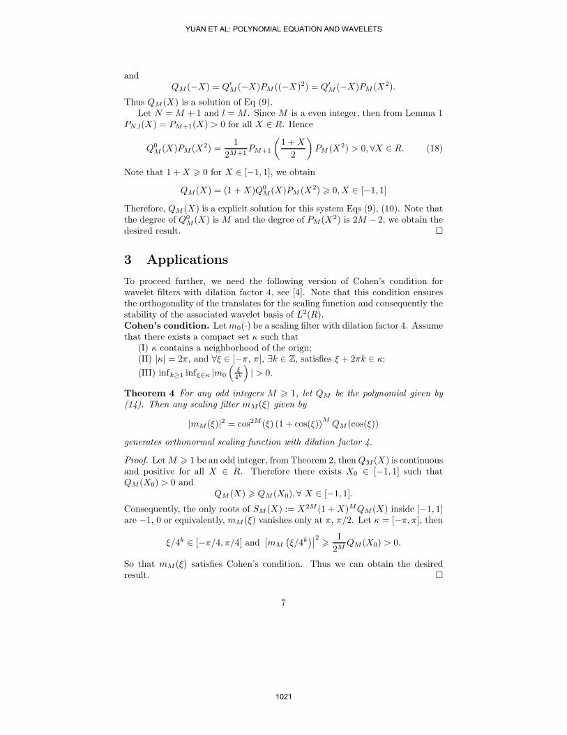
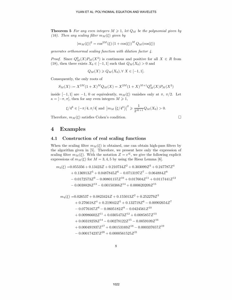
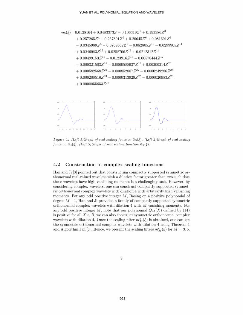
Figure 1: (Left 1)Graph of real scaling function Φ3(ξ), (Left 2)Graph of real scaling
function Φ4(ξ), (Left 3)Graph of real scaling function Φ5(ξ).
4.2 Construction of complex scaling functions
Han and Ji [3] pointed out that constructing compactly supported symmetric or-thonormal real-valued wavelets with a dilation factor greater than two such thatthese wavelets have high vanishing moments is a challenging task. However, byconsidering complex wavelets, one can construct compactly supported symmet-ric orthonormal complex wavelets with dilation 4 with arbitrarily high vanishingmoments. For any odd positive integer M , Basing on a positive polynomial ofdegree M − 1, Han and Ji provided a family of compactly supported symmetricorthonormal complex wavelets with dilation 4 with M vanishing moments. Forany odd positive integer M , note that our polynomial QM (X) defined by (14)is positive for all X ∈ R, we can also construct symmetric orthonormal complexwavelets with dilation 4. Once the scaling filter mc
M (ξ) is obtained, one can getthe symmetric orthonormal complex wavelets with dilation 4 using Theorem 1and Algorithm 1 in [3]. Hence, we present the scaling filtersmc
M (ξ) forM = 3, 5.
9
YUAN ET AL: POLYNOMIAL EQUATION AND WAVELETS
1023

mc3(ξ) = (−0.000691392+ 0.00581844i)Z(−7)
− (0.0108436+ 0.00128853i)Z(−6)
− (0.0184532+ 0.0370257i)Z(−5) − (0.0129805+ 0.0441327i)Z(−4)
+ (0.0196523− 0.0557696i)Z(−3) + (0.0969841− 0.0344487i)Z(−2)
+ (0.182313+ 0.0727629i)Z(−1) + (0.24402+ 0.0940838i)
+ (0.24402 + 0.0940838i)Z1 + (0.182313 + 0.0727629i)Z2
+ (0.0969841− 0.0344487i)Z3 + (0.0196523− 0.0557696i)Z4
− (0.0129805+ 0.0441327i)Z5 − (0.0184532+ 0.0370257i)Z6
− (0.0108436+ 0.00128853i)Z7 − (0.000691392− 0.00581844i)Z8
mc5(ξ) = (−0.000153418− 0.0002185575)Z(−13)
+ (0.000694473− 0.000487492i)Z(−12)
+ (0.00272565+ 0.00162133i)Z(−11) − (0.000244253− 0.00521591i)Z(−10)
+ (−0.00780018+ 0.00739194i)Z(−9) − (0.0180613− 0.00705253i)Z(−8)
+ (−0.0313129− 0.0119401i)Z(−7) − (0.0208646+ 0.046018i)Z(−6)
+ (0.0166215− 0.0749529i)Z(−5) + (0.0594812− 0.0956152i)Z(−4)
+ (0.111141− 0.0639564i)Z(−3) + (0.136773+ 0.0155634i)Z(−2)
+ (0.125668+ 0.0930182i)Z(−1) + (0.125332+ 0.163325i)
+ (0.125332+ 0.163325i)Z1 + (0.125668 + 0.0930182i)Z2
+ (0.136773+ 0.0155634i)Z3 + (0.111141− 0.0639564i)Z4
+ (0.0594812− 0.0956152i)Z5 + (0.0166215− 0.0749529i)Z6
− (0.0208646+ 0.046018i)Z7 − (0.0313129+ 0.0119401i)Z8
− (0.0180613− 0.00705253i)Z9 − (0.00780018− 0.00739194i)Z10
− (0.000244253− 0.00521591)Z11 + (0.00272565+ 0.00162133i)Z12
+ (0.000694473− 0.000487492i)Z13− (0.000153418+ 0.000218557i)Z14
10
YUAN ET AL: POLYNOMIAL EQUATION AND WAVELETS
1024
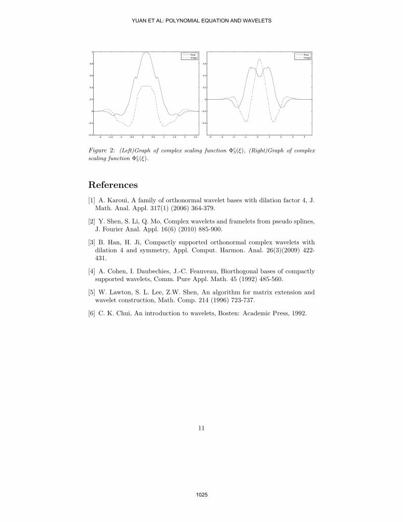
−2 −1.5 −1 −0.5 0 0.5 1 1.5 2 2.5−0.4
−0.2
0
0.2
0.4
0.6
0.8
1
RealImage
−4 −3 −2 −1 0 1 2 3 4
−0.4
−0.2
0
0.2
0.4
0.6
RealImage
Figure 2: (Left)Graph of complex scaling function Φc
3(ξ), (Right)Graph of complex
scaling function Φc
5(ξ).
References
[1] A. Karoui, A family of orthonormal wavelet bases with dilation factor 4, J.Math. Anal. Appl. 317(1) (2006) 364-379.
[2] Y. Shen, S. Li, Q. Mo, Complex wavelets and framelets from pseudo splines,J. Fourier Anal. Appl. 16(6) (2010) 885-900.
[3] B. Han, H. Ji, Compactly supported orthonormal complex wavelets withdilation 4 and symmetry, Appl. Comput. Harmon. Anal. 26(3)(2009) 422-431.
[4] A. Cohen, I. Daubechies, J.-C. Feauveau, Biorthogonal bases of compactlysupported wavelets, Comm. Pure Appl. Math. 45 (1992) 485-560.
[5] W. Lawton, S. L. Lee, Z.W. Shen, An algorithm for matrix extension andwavelet construction, Math. Comp. 214 (1996) 723-737.
[6] C. K. Chui, An introduction to wavelets, Bosten: Academic Press, 1992.
11
YUAN ET AL: POLYNOMIAL EQUATION AND WAVELETS
1025
Numerical solution of fully fuzzy linear matrix equations†
Kun Liua,b, Zeng-Tai Gonga,∗
aCollege of Mathematics and Statistics, Northwest Normal University, Lanzhou 730070, ChinabCollege of Mathematics and Statistics, Longdong University, Qingyang 745000, China
Abstract In this paper, we investigate the numerical solution of fully fuzzy linear matrix equationsAX = B. The fuzzy solution to the fully fuzzy matrix equations are expressed by the location indexsolution and the left and right fuzziness index function of this location index solution. The necessary andsufficient conditions for the existence of fuzzy solution and the solvability to fully fuzzy matrix equationsare also discussed. Some numerical examples are given to illustrate the efficiency of the proposed method.Keywords: Fuzzy numbers; Fuzzy arithmetic; Parametric form; Fully fuzzy linear matrix equations;Fuzzy solution.
1. Introduction
The concept of fuzzy numbers and fuzzy arithmetic operations with these fuzzy numbers were firstintroduced and investigated by Zadeh [17, 42], Dubois and Prade [21]. One major application of the fuzzynumber is treating linear systems whose parameters are all or partially represented by fuzzy numbers.Fuzzy systems are used to study a variety of problems ranging from fuzzy topological spaces [15] tocontrol chaotic systems (for example, in [22, 38]), fuzzy metric spaces [32], fuzzy linear systems (see[2, 4− 7, 11, 12, 18, 36, 37]), fuzzy differential equations (see [1, 8, 9, 14, 16, 27, 28, 34]), particle physics [35]and so on.
One field of applied mathematics that has many applications in various areas of science is solving asystem of linear equations. In many problems in various areas of science, which can be solved by solving asystem of linear equations. Some of the system parameters are vague or imprecise, and fuzzy mathematicsis better than crisp mathematics for mathematical modeling of these problems. It is immensely importantto develop numerical procedures that would appropriately treat a system of linear equations where someelements of the system are fuzzy, is called fuzzy system.
A general model for solving a fuzzy linear system whose coefficient matrix is crisp and its rightcolumn is an arbitrary fuzzy vector was first proposed by Friedman et al. [23] and his colleagues used theembedding method and replaced the original fuzzy linear system by a crisp linear system and then theysolved it. And studied duality in fuzzy linear systems Ax = Bx+ y, where A,B are real n× n matrices,both the unknown vector x and the constant y are vectors consisting of n fuzzy numbers in [29]. Alarge number of researches have been produced about how to solve numerically fuzzy linear systems (see[5− 7, 18]) and so on. Asady et al. [13], who merely considered the full row rank system, used the samemethod to solve the m×n fuzzy linear system for m ≤ n. Later, Zheng and Wang in [39, 43] discussed them× n general fuzzy linear system and the inconsistent fuzzy linear system by using generalized inversesof the coefficient matrix. Also, Wang et al. [40] presented an iterative algorithm for solving dual linearsystem of the form x = Ax+ u, where A is real n× n matrix, the unknown vector x and the constant uare all vectors consisting of fuzzy numbers and Abbasbandy [3] investigated the existence of a minimalsolution of general dual fuzzy linear equation system by means of matrix generalized inverse theory. Atthe same time, Muzziloi et al. [31] considered fully fuzzy linear systems of the form A1x+ b1 = A2x+ b2where A1, A2 are coefficient matrices consisting of fuzzy numbers and b1, b2 are vectors consisting of fuzzynumbers, respectively. And Dehghan et al. [19, 20] considered fully fuzzy linear systems Ax = b where A
†Supported by the Natural Scientific Fund of China (No.71061013) and the Scientific Research Project of NorthwestNormal University (No. NWNU-KJCXGC-03-61) of China.
∗Corresponding Author: Zeng-Tai Gong. Tel.:+86 09317971430.E-mail addresses: [email protected], [email protected](Zeng-Tai Gong) and [email protected](Kun Liu).
1026
J. COMPUTATIONAL ANALYSIS AND APPLICATIONS, VOL. 15, NO.6, 1026-1035, 2013, COPYRIGHT 2013 EUDOXUS PRESS, LLC
Kun Liu and Zeng-tai Gong : Numerical solution of fully fuzzy linear matrix equations
and b are a square matrix of fuzzy coefficient and a fuzzy vector, respectively. They also discussed theiterative solution of fully fuzzy linear systems.
It is well known that the fuzzy linear matrix equations (shown as FLME) has widely used in the controltheory and control engineering. However, few works have been done over the past decades. Allahviranlooet al. [10] studied fuzzy linear matrix equations of the form AXB = C where A ∈ Rm×n, B ∈ Rr×e andA,B and C are given matrices where C is a fuzzy matrix, and X is the unknown matrix by applyingthe Kronecker product to transform this system to nonsquare system. Gong et al. [25] investigated them× n inconsistent fuzzy matrix equation of the form AX = B where A is a crisp real matrix and B, Xare matrices consisting of fuzzy numbers by using generalized inverse of the matrix.
In this paper, we attempt to find a fuzzy solution of fully fuzzy linear matrix equations of the formAX = B based on a new arithmetic calculation in [30], where A and B are matrices consisting offuzzy numbers. To this end, we split the general fuzzy linear matrix equations into a location indexlinear matrix equations and two fuzziness matrix functions. First, we obtain a location index solutionby solving a location index linear matrix equations A0X = B0. Second, we select two fuzziness matrixfunctions maxA∗, B∗,maxA∗, B∗ as the left fuzziness index function and the right fuzziness indexfunction of this location index solution. Thus, a fuzzy solution is expressed by means of a location indexnumber and two fuzziness index function. Using this new fuzzy number arithmetic the solution of fullyfuzzy linear matrix equations is not only obtained easily, but also some restrictions, which assumed thesolution is positive fuzzy matrix in the existing literature, are overcame.
The outline of the paper is as follows: In Section 2, we recall some important fundamental results.In Section 3, the numerical solution of fully fuzzy linear matrix equations AX = B are discussed. Thenecessary and sufficient conditions for the existence of fuzzy solution and the solvability to fully fuzzymatrix equations are also discussed. In Section 4, some numerical examples are given to illustrate ourproposed method. The conclusion is drawn in Section 5.
2. Preliminaries
In this section, we give some definitions and introduce the notation which will be used throughoutthe paper.
Let us denote by RF the class of fuzzy subsets of the real axis (i.e.,u : R→ [0, 1]) (see [21]) satisfyingthe following properties:
(1) u is normal, i.e., there exists s0 ∈ R such that u(s0) = 1,(2) u is a convex fuzzy set (i.e., u(ts+ (1− t)r) ≥ minu(s), u(r),∀t ∈ [0, 1], r, s ∈ R),(3) u is upper semicontinuous on R,(4) cls ∈ R | u(s) > 0 is compact where cl denotes the closure of a subset.Then RF is called the space of fuzzy numbers. Obviously R ∈ RF. For 0 < α ≤ 1, set [u]α = s ∈ R |
u(s) ≥ α and [u]0 = cls ∈ R | u(s) > 0. Then from (1)-(4) it follows that if u belongs to RF then theα−level set [u]α is a non-empty compact interval for all 0 ≤ α ≤ 1.
An equivalent parametric form of an arbitrary fuzzy number is also given in Goetschel and Voxman[24] as follows:Definition 2.1. A fuzzy number u in parametric form is a pair (u, u) of functions u(r), u(r), 0 ≤ r ≤ 1,which satisfies the requirements:
(1) u(r) is a bounded monotonic increasing left continuous function,(2) u(r) is a bounded monotonic decreasing left continuous function,(3) u(r) ≤ u(r), 0 ≤ r ≤ 1.A crisp number x is simply represented by (u(r), u(r)) = x, 0 ≤ r ≤ 1 and called singleton.For arbitrary two fuzzy numbers x = (x(r), x(r)), y = (y(r), y(r)) and k, the addition, subtraction
and scalar multiplication are defined by the extension principle [41] and can be equivalently representedas follows:Definition 2.2. Let x = (x(r), x(r)), y = (y(r), y(r)) ∈ RF, 0 ≤ r ≤ 1 and real number k.
(1) x = y iff x(r) = y(r) and x(r) = y(r),(2) x+ y = (x(r) + y(r), x(r) + y(r)),(3) x− y = (x(r)− y(r), x(r)− y(r)),
(4) kx =
(kx(r), kx(r)), k ≥ 0,(kx(r), kx(r)), k < 0.
1027
Kun Liu and Zeng-tai Gong : Numerical solution of fully fuzzy linear matrix equations
The collection of all the fuzzy numbers with addition and scalar multiplication as defined above is aconvex cone.Definition 2.3. For arbitrary fuzzy numbers u = (u(r), u(r)), v = (v(r), v(r)) ∈ RF, the quantity
D(u, v) = sup0≤r≤1
max[| u(r)− v(r) |, | u(r)− v(r) |]
is called the distance between u and v.This metric is equivalent to the one by Puri and Ralescu [33] and Kaleva [26].For later use, we introduce a lattice L and fuzzy number (u0, u∗, u∗), with a parametric form and a
new fuzzy arithmetic (see [30]).Definition 2.4. A lattice L as
L = h | h : [0, 1]→ [0,∞) is nondecreasing and left continuous.The order in L is the natural order defined by h ≤ g if and only if h(r) ≤ g(r) for all r ∈ [0, 1]. It is
easy to show that[h ∨ g] = maxh(r), g(r),[h ∧ g] = minh(r), g(r),
where h ∨ g and h ∧ g are supremum and infimum of h and g.Definition 2.5. For arbitrary fuzzy number u = (u(r), u(r)), the number
u0 = 12(u(1) + u(1))
is said to be a location index number of u, and two nondecreasing left continuous functionsu∗ = u0 − u,u∗ = u− u0
are called the left fuzziness index function and the right fuzziness index function, respectively.According to Def. 2.5, every fuzzy number can be represented by (u0, u∗, u∗).
Definition 2.6. For arbitrary fuzzy numbers u = (u0, u∗, u∗) and v = (v0, v∗, v∗), the four arithmeticaloperations are defined by
uv = (u0v0, u∗ ∨ v∗, u∗ ∨ v∗),where uv is either of u+ v, u− v, u · v, uv .
The arithmetic is determined by the operations on both location index and fuzziness index functions.The location index number is taken in the ordinary arithmetic, whereas the fuzziness index functions areconsidered to follow the lattice rule which is least upper bound in the lattice L. Here and after this, weoperate all fuzzy arithmetic calculation using the above definition.Definition 2.7. A matrix A = (aij), i, j = 1, 2, · · ·n, is called a fuzzy matrix, if each element of A is afuzzy number with a parametric form as Def. 2.5, we represent A = (aij) that
aij = ((aij)0, (aij)∗, (aij)∗)
where (aij)0 is location index matrix of aij and (aij)∗, (aij)∗ are left fuzziness index matrix function and
right fuzziness index matrix function, respectively.Definition 2.8. A vector b = (bi) is called a fuzzy vector, if each element of b is a fuzzy number, withnew notation
b = ((bi)0, (bi)∗, (bi)∗) i = 1, 2, · · ·n,
where (bi)0 is location index vector of bi and (bi)∗, (bi)∗ are left fuzziness index vector function and right
fuzziness index vector function, respectively.
3. Fully Fuzzy linear matrix equations
In this section, we will investigate the fuzzy solution of fully fuzzy linear matrix equations of the formAX = B based on a new arithmetic calculation in [30]. We give the necessary and sufficient conditionsfor the existence of a fuzzy solution of fully fuzzy linear matrix equations and analyze the solvability offully fuzzy linear matrix equations AX = B.Definition 3.1. The model equations
a11 a12 · · · a1na21 a22 · · · a2n. . . . . . . . . . . . . . . . . . .an1 an2 · · · ann
x11 x12 · · · x1nx21 x22 · · · x2n. . . . . . . . . . . . . . . . . . .xn1 xn2 · · · xnn
=
b11 b12 · · · b1nb21 b22 · · · b2n. . . . . . . . . . . . . . . . . .bn1 bn2 · · · bnn
, (3.1)
where the left coefficient matrix A = (aij) (1 ≤ i, j ≤ n), and the right-hand matrix B = (bij) (1 ≤1028
Kun Liu and Zeng-tai Gong : Numerical solution of fully fuzzy linear matrix equations
i, j ≤ n) are all fuzzy number matrices which be defined as Def 2.7, is called a fully fuzzy linear matrixequations (FFLME).
Using matrix notation, we haveAX = B. (3.2)
Let A be a nonsingular fuzzy matrix. Then a fuzzy number matrix X = (X0, X∗, X∗) is called a
unique fuzzy solution of FFLME (3.1) ifA0X0 = B0, A∗ ∨X∗ = B∗, A
∗ ∨X∗ = B∗.Actually, X = (X0, X∗, X
∗) is also equivalent to X = (x1, x2 · · · , xn) if
Axl = bl, l = 1, 2, · · · , n, (3.3)
where xl = (((x1l)0, (x1l)∗, (x1l)∗), ((x2l)0, (x2l)∗, (x2l)
∗), · · · , ((xnl)0, (xnl)∗, (xnl)∗))T, l = 1, 2, · · · , n,is the lth column of unknown matrix X, and B = (b1, b2 · · · , bn), given by
bl = (((b1l)0, (b1l)∗, (b1l)∗), ((b2l)0, (b2l)∗, (b2l)
∗), · · · , ((bnl)0, (bnl)∗, (bnl)∗))T, l = 1, 2, · · · , n, is the lthcolumn of the right-hand fuzzy matrix B.
For the Eq. (3.3), we also can write as the following form:
n∑j=1
aijxl = bl, i, l = 1, 2, · · · , n. (3.4)
Theorem 3.1. If X = (X0, X∗, X∗) is a fuzzy solution of FFLME (3.1), then X0 = (A0)
−1B0, X∗ =maxA∗, B∗, X∗ = maxA∗, B∗.Proof. By virtue of Def 2.7, FFLME AX = B can write
(A0, A∗, A∗)(X0, X∗, X
∗) = (B0, B∗, B∗).
By Def 2.6, we have(A0X0, A∗ ∨X∗, A∗ ∨X∗) = (B0, B∗, B
∗).It follows
A0X0 = B0,A∗ ∨X∗ = B∗,A∗ ∨X∗ = B∗.
This impliesX0 = (A0)
−1B0, X∗ = maxA∗, B∗, X∗ = maxA∗, B∗.The proof is completed. Theorem 3.2. If the fuzzy linear matrix equations (3.1) has a fuzzy solution, then the following condi-tions hold:
(i).n∑j=1
(aij)0xl = (bil)0, i, l = 1, 2, · · · , n, has a solution as a crisp linear equation system;
(ii). max1≤j≤n
(aij)∗ ≤ (bil)∗, i, l = 1, 2, · · · , n, where bil ∈ B;
(iii). max1≤j≤n
(aij)∗ ≤ (bil)∗, i, l = 1, 2, · · · , n, where bil ∈ B.
Proof. Let xl (l = 1, 2, · · · , n) be a fuzzy solution of Eq. (3.4). That isn∑j=1
aijxl = bl.
Therefore,n∑j=1
((aij)0, (aij)∗, (aij)∗) · ((xjl)0, (xjl)∗, (xjl)∗)
= ((bil)0, (bil)∗, (bil)∗).
This implies
(n∑j=1
(aij)0(xjl)0, max1≤j≤n
(aij)∗, (xjl)∗, max1≤j≤n
(aij)∗, (xjl)∗)
= ((bil)0, (bil)∗, (bil)∗).
It followsn∑j=1
(aij)0(xjl)0 = (bil)0,
1029
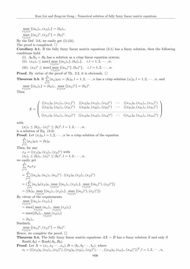
Kun Liu and Zeng-tai Gong : Numerical solution of fully fuzzy linear matrix equations
max1≤j≤n
(aij)∗, (xjl)∗ = (bil)∗,
max1≤j≤n
(aij)∗, (xjl)∗ = (bil)∗.
By the Def. 2.6, we easily get (i)-(iii).The proof is completed. Corollary 3.1. If the fully fuzzy linear matrix equations (3.1) has a fuzzy solution, then the followingconditions hold:
(i). A0X0 = B0 has a solution as a crisp linear equation system;(ii). (xil)∗ ≤ max max
1≤j≤n(aij)∗, (bil)∗, i, l = 1, 2, · · · , n;
(iii). (xil)∗ ≤ max max
1≤j≤n(aij)∗, (bil)∗, i, l = 1, 2, · · · , n.
Proof. By virtue of the proof of Th. 3.2, it is obviously.
Theorem 3.3. Ifn∑j=1
(aij)0xl = (bl)0, l = 1, 2, · · · , n has a crisp solution (xl)0, l = 1, 2, · · · , n, and
max1≤j≤n
(aij)∗ = (bil)∗, max1≤j≤n
(aij)∗ = (bil)∗.
Then
X =
((x11)0, (x11)∗, (x11)
∗) ((x12)0, (x12)∗, (x12)∗) · · · ((x1n)0, (x1n)∗, (x1n)∗)
((x21)0, (x21)∗, (x21)∗) ((x22)0, (x22)∗, (x22)
∗) · · · ((x2n)0, (x2n)∗, (x2n)∗). . . . . . . . . . . . . . . . . . . . . . . . . . . . . . . . . . . . . . . . . . . . . . . . . . . . . . . . . . . . . . . . . . . . . . . . . . .((xn1)0, (xn1)∗, (xn1)
∗) ((xn2)0, (xn2)∗, (xn2)∗) · · · ((xnn)0, (xnn)∗, (xnn)∗)
with
(xl)∗ ≤ (bl)∗, (xl)∗ ≤ (bl)
∗, l = 1, 2, · · · , n,is a solution of Eq. (3.3).Proof. Let (xl)0, l = 1, 2, · · · , n be a crisp solution of the equation
n∑j=1
(aij)0xl = (bl)0.
Then, for anyxjl = ((xjl)0, (xjl)∗, (xjl)
∗) with(xl)∗ ≤ (bl)∗, (xl)
∗ ≤ (bl)∗, l = 1, 2, · · · , n,
we easily getn∑j=1
aijxjl
=n∑j=1
((aij)0, (aij)∗, (aij)∗) · ((xjl)0, (xjl)∗, (xjl)∗)
= (n∑j=1
(aij)0(xjl)0, max1≤j≤n
(aij)∗, (xjl)∗, max1≤j≤n
(aij)∗), (xjl)∗)
= ((bl)0, max1≤j≤n
(aij)∗, (xjl)∗, max1≤j≤n
(aij)∗), (xjl)∗).By virtue of the requirements
max1≤j≤n
(aij)∗, (xjl)∗
= max max1≤j≤n
(aij)∗, max1≤j≤n
(xjl)∗
= max(bil)∗, max1≤j≤n
(xjl)∗
= (bil)∗.Similarly,
max1≤j≤n
(aij)∗, (xjl)∗ = (bil)∗.
Hence, we complete the proof. Theorem 3.4. The fully fuzzy linear matrix equations AX = B has a fuzzy solution if and only if
Rank(A0) = Rank(A0, B0).Proof. Let X = (x1, x2 · · · , xn), B = (b1, b2 · · · , bn), where
xl = (((x1l)0, (x1l)∗, (x1l)∗), ((x2l)0, (x2l)∗, (x2l)
∗), · · · , ((xnl)0, (xnl)∗, (xnl)∗))T, l = 1, 2, · · · , n,1030
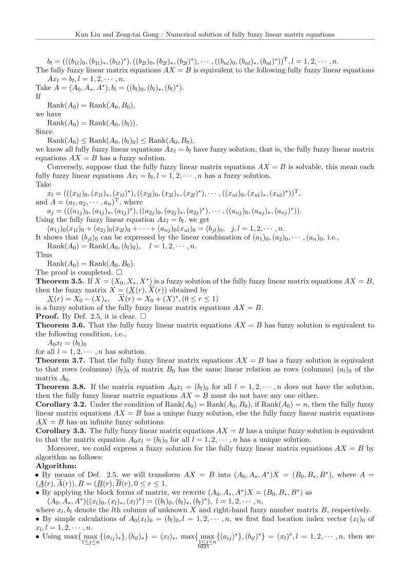
Kun Liu and Zeng-tai Gong : Numerical solution of fully fuzzy linear matrix equations
bl = (((b1l)0, (b1l)∗, (b1l)∗), ((b2l)0, (b2l)∗, (b2l)
∗), · · · , ((bnl)0, (bnl)∗, (bnl)∗))T, l = 1, 2, · · · , n.The fully fuzzy linear matrix equations AX = B is equivalent to the following fully fuzzy linear equations
Axl = bl, l = 1, 2, · · · , n.Take A = (A0, A∗, A
∗), bl = ((bl)0, (bl)∗, (bl)∗).
IfRank(A0) = Rank(A0, B0),
we haveRank(A0) = Rank(A0, (bl)).
SinceRank(A0) ≤ Rank(A0, (bl)0) ≤ Rank(A0, B0),
we know all fully fuzzy linear equations Axl = bl have fuzzy solution, that is, the fully fuzzy linear matrixequations AX = B has a fuzzy solution.
Conversely, suppose that the fully fuzzy linear matrix equations AX = B is solvable, this mean eachfully fuzzy linear equations Axl = bl, l = 1, 2, · · · , n has a fuzzy solution.Take
xl = (((x1l)0, (x1l)∗, (x1l)∗), ((x2l)0, (x2l)∗, (x2l)
∗), · · · , ((xnl)0, (xnl)∗, (xnl)∗))T,and A = (a1, a2, · · · , an)T, where
aj = (((a1j)0, (a1j)∗, (a1j)∗), ((a2j)0, (a2j)∗, (a2j)
∗), · · · , ((anj)0, (anj)∗, (anj)∗)).Using the fully fuzzy linear equation Axl = bl. we get
(a1j)0(x1l)0 + (a2j)0(x2l)0 + · · ·+ (anj)0(xnl)0 = (bjl)0, j, l = 1, 2, · · · , n.It shows that (bjl)0 can be expressed by the linear combination of (a1)0, (a2)0, · · · , (an)0, i.e.,
Rank(A0) = Rank(A0, (bl)0), l = 1, 2, · · · , n.Thus
Rank(A0) = Rank(A0, B0).The proof is completed. Theorem 3.5. If X = (X0, X∗, X
∗) is a fuzzy solution of the fully fuzzy linear matrix equations AX = B,then the fuzzy matrix X = (X(r), X(r)) obtained by
X(r) = X0 − (X)∗, X(r) = X0 + (X)∗, (0 ≤ r ≤ 1)is a fuzzy solution of the fully fuzzy linear matrix equations AX = B.Proof. By Def. 2.5, it is clear. Theorem 3.6. That the fully fuzzy linear matrix equations AX = B has fuzzy solution is equivalent tothe following condition, i.e.,
A0xl = (bl)0for all l = 1, 2, · · · , n has solution.Theorem 3.7. That the fully fuzzy linear matrix equations AX = B has a fuzzy solution is equivalentto that rows (columns) (bl)0 of matrix B0 has the same linear relation as rows (columns) (al)0 of thematrix A0.Theorem 3.8. If the matrix equation A0xl = (bl)0 for all l = 1, 2, · · · , n does not have the solution,then the fully fuzzy linear matrix equations AX = B must do not have any one either.Corollary 3.2. Under the condition of Rank(A0) = Rank(A0, B0), if Rank(A0) = n, then the fully fuzzylinear matrix equations AX = B has a unique fuzzy solution, else the fully fuzzy linear matrix equationsAX = B has an infinite fuzzy solutions.Corollary 3.3. The fully fuzzy linear matrix equations AX = B has a unique fuzzy solution is equivalentto that the matrix equation A0xl = (bl)0 for all l = 1, 2, · · · , n has a unique solution.
Moreover, we could express a fuzzy solution for the fully fuzzy linear matrix equations AX = B byalgorithm as follows:Algorithm:• By means of Def. 2.5, we will transform AX = B into (A0, A∗, A
∗)X = (B0, B∗, B∗), where A =
(A(r), A(r)), B = (B(r), B(r), 0 ≤ r ≤ 1.• By applying the block forms of matrix, we rewrite (A0, A∗, A
∗)X = (B0, B∗, B∗) as
(A0, A∗, A∗)((xl)0, (xl)∗, (xl)
∗) = ((bl)0, (bl)∗, (bl)∗), l = 1, 2, · · · , n,
where xl, bl denote the lth column of unknown X and right-hand fuzzy number matrix B, respectively.• By simple calculations of A0(xl)0 = (bl)0, l = 1, 2, · · · , n, we first find location index vector (xl)0 ofxl, l = 1, 2, · · · , n.• Using max max
1≤j≤n(aij)∗, (bil)∗ = (xl)∗, max max
1≤j≤n(aij)∗, (bil)∗ = (xl)
∗, l = 1, 2, · · · , n, then we
1031
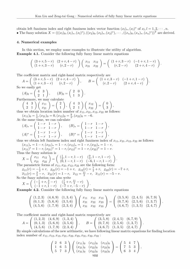
Kun Liu and Zeng-tai Gong : Numerical solution of fully fuzzy linear matrix equations
obtain left fuzziness index and right fuzziness index vector function (xl)∗, (xl)∗ of xl, l = 1, 2, · · · , n.
• The fuzzy solution X = (((xl)0, (xl)∗, (xl)∗), ((x2)0, (x2)∗, (x2)
∗), · · · , ((xn)0, (xn)∗, (xn)∗))T are derived.
4. Numerical examples
In this section, we employ some examples to illustrate the utility of algorithm.Example 4.1. Consider the following fully fuzzy linear matrix equations(
(3 + r, 5− r) (2 + r, 4− r)(1 + r, 3− r) (r, 2− r)
)(x11 x12x21 x22
)=
((1 + r, 3− r) (−1 + r, 1− r)
(r, 2− r) (2 + r, 4− r)
).
The coefficient matrix and right-hand matrix respectively are
A =
((3 + r, 5− r) (2 + r, 4− r)(1 + r, 3− r) (r, 2− r)
), B =
((1 + r, 3− r) (−1 + r, 1− r)
(r, 2− r) (2 + r, 4− r)
).
So we easily get
(A)0 =
(4 32 1
), (B)0 =
(2 01 3
).
Furthermore, we may calculate(4 32 1
)(x11x21
)=
(21
),
(4 32 1
)(x12x22
)=
(03
),
thus we obtain location index number of x11, x21, x12, x22 as follows:(x11)0 = 1
2 , (x21)0 = 0, (x12)0 = 92 , (x22)0 = −6.
At the same time, we can calculate
(A)∗ =
(1− r 1− r1− r 1− r
), (B)∗ =
(1− r 1− r1− r 1− r
),
(A)∗ =
(1− r 1− r1− r 1− r
), (B)∗ =
(1− r 1− r1− r 1− r
),
thus we obtain left fuzziness index and right fuzziness index of x11, x21, x12, x22 as follows:(x11)∗ = 1− r, (x21)∗ = 1− r, (x12)∗ = 1− r, (x22)∗ = 1− r,(x11)
∗ = 1− r, (x21)∗ = 1− r, (x12)∗ = 1− r, (x22)∗ = 1− r.Thus the fuzzy solution is
X =
(x11 x12x21 x22
)=
((12 , 1− r, 1− r) (92 , 1− r, 1− r)(0, 1− r, 1− r) (−6, 1− r, 1− r)
).
The parametric forms of x11, x21, x12, x22 are the following form:x11(r) = −1
2 + r, x21(r) = −1 + r, x12(r) = 72 + r, x22(r) = −7 + r,
x11(r) = 32 − r, x21(r) = 1− r, x12 = 11
2 − r, x11(r) = −5− r.So the fuzzy solution can also write
X =
((−1
2 + r, 32 − r) (72 + r, 112 − r)(−1 + r, 1− r) (−7 + r,−5− r)
).
Example 4.2. Consider the following fully fuzzy linear matrix equations (1, 2, 3) (4, 6, 9) (1, 3, 4)(0, 1, 3) (5, 6, 8) (3, 5, 6)(4, 5, 6) (1, 7, 9) (2, 3, 4)
x11 x12 x13x21 x22 x23x31 x32 x33
=
(3, 5, 8) (2, 4, 5) (6, 7, 9)(0, 7, 8) (2, 5, 6) (1, 3, 7)(4, 6, 7) (1, 3, 5) (2, 4, 7)
.
The coefficient matrix and right-hand matrix respectively are
A =
(1, 2, 3) (4, 6, 9) (1, 3, 4)(0, 1, 3) (5, 6, 8) (3, 5, 6)(4, 5, 6) (1, 7, 9) (2, 3, 4)
, B =
(3, 5, 8) (2, 4, 5) (6, 7, 9)(0, 7, 8) (2, 5, 6) (1, 3, 7)(4, 6, 7) (1, 3, 5) (2, 4, 7)
.
By simple calculations of the new arithmetic, we have following linear matrix equations for finding locationindex number of x11, x12, x13, x21, x22, x23, x31, x32, x33 : 2 6 3
1 6 55 7 3
(x11)0 (x12)0 (x13)0(x21)0 (x22)0 (x23)0(x31)0 (x32)0 (x33)0
=
5 4 77 5 36 3 4
,
1032
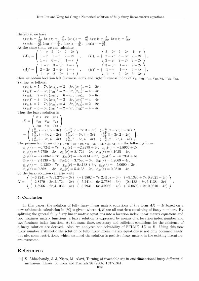
Kun Liu and Zeng-tai Gong : Numerical solution of fully fuzzy linear matrix equations
therefore, we have(x11)0 = 8
29 , (x12)0 = −1729 , (x13)0 = −62
29 , (x21)0 = 529 , (x22)0 = 22
29 ,
(x23)0 = 9929 , (x31)0 = 33
29 , (x32)0 = 629 , (x33)0 = −89
29 .At the same time, we can calculate
(A)∗ =
1− r 2− 2r 2− 2r1− r 1− r 2− 2r1− r 6− 6r 1− r
, (B)∗ =
2− 2r 2− 2r 1− r7− 7r 3− 3r 2− 2r2− 2r 2− 2r 2− 2r
,
(A)∗ =
1− r 3− 3r 1− r2− 2r 2− 2r 1− r1− r 2− 2r 1− r
, (B)∗ =
3− 3r 1− r 2− 2r1− r 1− r 4− 4r1− r 2− 2r 3− 3r
,
thus we obtain location left fuzziness index and right fuzziness index of x11, x21, x31, x12, x22, x32, x13,x23, x33 as follows:
(x11)∗ = 7− 7r, (x21)∗ = 3− 3r, (x31)∗ = 2− 2r,(x11)
∗ = 3− 3r, (x21)∗ = 2− 2r, (x31)
∗ = 4− 4r,(x12)∗ = 7− 7r, (x22)∗ = 6− 6r, (x32)∗ = 6− 6r,(x12)
∗ = 3− 3r, (x22)∗ = 3− 3r, (x32)
∗ = 4− 4r,(x13)∗ = 7− 7r, (x23)∗ = 3− 3r, (x33)∗ = 2− 2r,(x13)
∗ = 3− 3r, (x23)∗ = 2− 2r, (x33)
∗ = 4− 4r.Thus the fuzzy solution is
X =
x11 x12 x13x21 x22 x23x31 x32 x33
=
( 829 , 7− 7r, 3− 3r) (−17
29 , 7− 7r, 3− 3r) (−6229 , 7− 7r, 3− 3r)
( 529 , 3− 3r, 2− 2r) (2229 , 6− 6r, 3− 3r) (9929 , 3− 3r, 2− 2r)
( 329 , 2− 2r, 4− 4r) ( 6
29 , 6− 6r, 4− 4r) (−8929 , 2− 2r, 4− 4r)
.
The parametric forms of x11, x21, x31, x12, x22, x32, x13, x23, x33 are the following form:x11(r) = −6.7241 + 7r, x21(r) = −2.8279 + 3r, x31(r) = −1.8966 + 2r,x11(r) = 3.2759− 3r, x21(r) = 2.1724− 2r, x31(r) = 4.1035− 4r,x12(r) = −7.5862 + 7r, x22(r) = −5.2414 + 6r, x32(r) = −5.7931 + 6r,x12(r) = 2.4138− 3r, x22(r) = 3.7586− 3r, x32(r) = 4.2069− 4r,x13(r) = −9.1380 + 7r, x23(r) = 0.4138 + 3r, x33(r) = −5.0690 + 2r,x13(r) = 0.8621− 3r, x23(r) = 5.4138− 2r, x33(r) = 0.9310− 4r.
So the fuzzy solution can also write
X =
(−6.7241 + 7r, 3.2759− 3r) (−7.5862 + 7r, 2.4138− 3r) (−9.1380 + 7r, 0.8621− 3r)(−2.8279 + 3r, 2.1724− 2r) (−5.2414 + 6r, 3.7586− 3r) (0.4138 + 3r, 5.4138− 2r)(−1.8966 + 2r, 4.1035− 4r) (−5.7931 + 6r, 4.2069− 4r) (−5.0690 + 2r, 0.9310− 4r)
.
5. Conclusion
In this paper, the solution of fully fuzzy linear matrix equations of the form AX = B based on anew arithmetic calculation in [30] is given, where A,B are all matrices consisting of fuzzy numbers. Bysplitting the general fully fuzzy linear matrix equations into a location index linear matrix equations andtwo fuzziness matrix functions, a fuzzy solution is expressed by means of a location index number andtwo fuzziness index function. At the same time, necessary and sufficient conditions for the existence ofa fuzzy solution are derived. Also, we analyzed the solvability of FFLME AX = B. Using this newfuzzy number arithmetic the solution of fully fuzzy linear matrix equations is not only obtained easily,but also some restrictions, which assumed the solution is positive fuzzy matrix in the existing literature,are overcame.
References
[1] S. Abbasbandy, J. J. Nieto, M. Alavi, Turning of reachable set in one dimentional fuzzy differentialinclusions, Chaos, Solitons and Fractals 26 (2005) 1337-1341.
1033
Kun Liu and Zeng-tai Gong : Numerical solution of fully fuzzy linear matrix equations
[2] S. Abbasbandy, M. Otadi, M. Mosleh, Minimal solution of general dual fuzzy linear systems, Chaos,Solitions and Fractals 29 (2008) 638-652.
[3] S. Abbasbandy, M. Otadi, M. Mosleh, Minimal solution of general dual fuzzy linear systems, Chaos,Solitons and Fractals, 37 (2008) 1113-1124.
[4] T. Allahviranloo, A comment on fuzzy linear systems, Fuzzy Sets and Systems 140 (2003) 559.
[5] T. Allahviranloo, Numerical methods for fuzzy system of linear equations, Applied Mathematics andComputation 153 (2004) 493-502.
[6] T. Allahviranloo, Successive over relaxation iterative method for fuzzy system of linear equations,Applied Mathematics and Computation 162 (2005) 189-196.
[7] T. Allahviranloo, The Adomian decomposition method for fuzzy system of linear equations, AppliedMathematics and Computation 163 (2005) 553-563.
[8] T. Allahviranloo, E. Ahmady, N. Ahmady, Nth-order fuzzy linear differential equations, InformationSciences 178 (2008) 1309-1324.
[9] T. Allahviranloo, N. A. Kiani, N. Motamedi, Solving fuzzy differential equations by differentialtransformation method, Information Sciences 179 (2009) 956-966.
[10] T. Allahviranloo, N. Mikaeilvand, M. Barkhordary, Fuzzy linear matrix equation, Fuzzy Optimiza-tion and Decision Making 8 (2009) 165-177.
[11] T. Allahviranloo, S. Salahshour, Fuzzy symmetric solutions of fuzzy linear systems, Journal of Com-putational and Applied Mathematics 235 (2011) 4545-4553.
[12] T. Allahviranloo, S. Salahshour, M. Khezerloo, Maximal and minimal symmetric solutions of fullyfuzzy linear systems, Journal of Computational and Applied Mathematics 235 (2011) 4652-4662.
[13] B. Asady, S. Abbasbandy, M. Alavi, Fuzzy general linear systems, Applied Mathematics and Com-putation 169 (2005) 34-40.
[14] B. Bede, I. J. Rudas, A. L. Bencsik, First order linear fuzzy differential equations under generalizeddifferentiability, Information Sciences 177 (2007) 1648-1662.
[15] M. Caldas, S. Jafari, θ-Compact fuzzy topological spaces, Chaos, Solitons and Fractals 25 (2005)229-232.
[16] Y. Chalco-Cano, H. Roman-Flores, Comparation between some approaches to solve fuzzy differentialequations, Fuzzy Sets and Systems 160 (2009) 1517-1527.
[17] S. S. L. Chang, L. A. Zadeh, On fuzzy mapping and control, Systems, Man and Cybernetics, IEEETransactions 2 (1972) 30-33.
[18] M. Dehghan, B. Hashemi, Iterative solution of fuzzy linear systems, Applied Mathematics andComputation 175 (2006) 645-674.
[19] M. Dehghan, B. Hashemi, M. Ghatee, Computational methods for solving fully fuzzy linear systems,Applied Mathematics and Computation 179 (2006) 328-343.
[20] M. Dehghan, B. Hashemi, M. Ghatee, Solution of the full fuzzy linear systems using iterative tech-niques, Chaos, Solitons and Fractals 34 (2007) 316-336.
[21] D. Dubois, H. Prade, Operations on fuzzy numbers, International Journal of Systems Science 9(1978) 613-626.
[22] G. Feng, G. Chen, Adaptive control of discrete-time chaotic systems: a fuzzy control approach,Chaos, Solitons and Fractals 23 (2005) 459-467.
[23] M. Friedman, M. Ma, A. Kandel, Fuzzy linear systems, Fuzzy Sets and Systems 96 (1998) 201-209.
[24] R. Goetschel, W. Voxman, Elementary calculus, Fuzzy Sets and Systems 18 (1986) 31-43.
[25] Z. T. Gong, X. B. Guo, Inconsistent fuzzy matrix equations and its fuzzy least squares solutions,Applied Mathematical Modelling 35 (2011) 1456-1469.
[26] O. Kaleva, Fuzzy differential equations, Fuzzy Sets and Systems 24 (1987) 301-317.
1034
Kun Liu and Zeng-tai Gong : Numerical solution of fully fuzzy linear matrix equations
[27] V. Lupulescu, Initial value problem for fuzzy differential equations under dissipative conditions,Information Sciences 178 (2008) 4523-4533.
[28] M. Ma, M. Friedman, A. Kandel, Numerical solutions of fuzzy differential equations, Fuzzy Sets andSystems 105 (1999) 133-138.
[29] M. Ma, M. Friedman, A. Kandel, Duality in fuzzy linear systems, Fuzzy Sets and Systems 109 (2000)55-58.
[30] M. Ma, M. Friedman, A. Kandel, A new fuzzy arithmetic, Fuzzy Sets and Systems 108 (1999) 83-90.
[31] S. Muzzioli, H. Reynaerts, Fuzzy linear systems of the form A1x + b1 = A2x + b2, Fuzzy Sets andSystems 157 (2006) 939-951.
[32] J. H. Park, Intuitionistic fuzzy metric space, Chaos, Solitons and Fractals 22 (2004) 1039-1046.
[33] M. L. Puri, D. A. Ralescu, Differentials for fuzzy functions, Journal of Mathematical Analysis andApplications 91 (1983) 552-558.
[34] S. J. Song, C. X. Wu, Existence and uniqueness of solutions to Cauchy problem of fuzzy differentialequations, Fuzzy Sets and Systems 110 (2000) 55-67.
[35] Y. Tanaka, Y. Mizuno, T. Kado, Chaotic dynamics in the Friedman equation, Chaos, Solitons andFractals 24 (2005) 407-422.
[36] Z. F. Tian, L. J. Hu, D. Greenhalgh, Perturbation analysis of fuzzy linear systems, InformationSciences 180 (2010) 4706-4713.
[37] K. Wang, G. L. Chen, Y. M. Wei, Perturbation analysis for a class of fuzzy linear systems, Journalof Computational and Applied Mathematics 224 (2009) 54-65.
[38] J. Wang, G. D. Qiao, B. Deng, H∞ Variable universe adaptive fuzzy control for chaotic system,Chaos, Solitons and Fractals 24 (2005) 1075-1086.
[39] K. Wang, B. Zheng, Inconsistent fuzzy linear systems, Applied Mathematics and Computation 181(2006) 973-981.
[40] X. Wang, Z. Zhong, M. Ma, Iteration algorithms for solving a system of fuzzy linear equations,Fuzzy Sets and Systems 119 (2001) 121-128.
[41] R. R. Yager, D. P. Filev, SLIDE: a simple adaptive defuzzification method, IEEE Transactions onFuzzy Systems 1 (1993)69-78.
[42] L. A. Zadeh, The concept of a linguistic variable and its application to approximate reasoning,Information Science 8 (1975) 199-249.
[43] B. Zheng, K. Wang, General fuzzy linear systems, Applied Mathematics and Computation 181 (2006)1276-1286.
1035
Korovkin type approximation theorem forstatistical A-summability of double sequences
M. Mursaleena) and Abdullah Alotaibib)a) Department of Mathematics, Aligarh Muslim University, Aligarh 202002, India
b)Department of Mathematics, King Abdulaziz University, Jeddah 21589,Saudi Arabia
[email protected]; [email protected]
Abstract. In this paper, we prove a Korovkin type approximation theorem for a function of two
variables by using the notion of statistical A–summability. We also construct an example by Meyer-
Konig and Zeller operators to show that our result is stronger than those of previously proved by
other authors.
Keywords and phrases: Double sequence; density; statistical convergence; A–statistical convergence;
statistical A–summability; positive linear operator; Korovkin type approximation theorem.
AMS subject classification (2000): 41A10, 41A25, 41A36, 40A30, 40G15.
1. Introduction and preliminaries
The concept of statistical convergence for sequences of real numbers was introducedby Fast [8] and further studied many others.
Let K ⊆ N and Kn = k ≤ n : k ∈ K .Then the natural density of K is definedby δ(K) = limn n
−1|Kn| if the limit exists, where |Kn| denotes the cardinality of Kn.A sequence x = (xk) of real numbers is said to be statistically convergent to L
provided that for every ε > 0 the set Kε := k ∈ N : |xk − L| ≥ ε has natural densityzero, i.e. for each ε > 0,
limn
1
n|j ≤ n : |xj − L| ≥ ε| = 0.
By the convergence of a double sequence we mean the convergence in the Pring-sheim’s sense [18]. A double sequence x = (xjk) is said to be Pringsheim’s convergent(or P -convergent) if for given ε > 0 there exists an integer N such that |xjk − `| < εwhenever j, k > N . In this case, ` is called the Pringsheim limit of x = (xjk) and it iswritten as P − limx = `.
A double sequence x = (xjk) is said to be bounded if there exists a positive numberM such that |xjk| < M for all j, k.
Note that, in contrast to the case for single sequences, a convergent double se-quence need not be bounded.
The idea of statistical convergence for double sequences was introduced and studiedby Moricz [13] and Mursaleen and Edely [17], independently in the same year.
Let K ⊆ N × N be a two-dimensional set of positive integers and let Km,n =(j, k) : j ≤ m, k ≤ n. Then the two-dimensional analogue of natural density can bedefined as follows.
1036
J. COMPUTATIONAL ANALYSIS AND APPLICATIONS, VOL. 15, NO.6, 1036-1045, 2013, COPYRIGHT 2013 EUDOXUS PRESS, LLC
In case the sequence (K(m,n)/mn) has a limit in Pringsheim’s sense, then we saythat K has a double natural density and is defined as
P − limm,n
K(m,n)
mn= δ(2)K.
For example, let K = (i2, j2) : i, j ∈ N. Then
δ(2)K = P − limm,n
K(m,n)
mn≤ P − lim
m,n
√m√n
mn= 0,
i.e. the set K has double natural density zero, while the set (i, 2j) : i, j ∈ N hasdouble natural density 1
2.
A real double sequence x = (xjk) is said to be statistically convergent to thenumber L if for each ε > 0, the set
(j, k), j ≤ m and k ≤ n :| xjk − L |≥ ε
has double natural density zero. In this case we write st(2)- limj,k
xjk = L.
Remark 1.1. Note that if x = (xjk) is P -convergent then it is statistically convergentbut not conversely. See the following example.
Example 1.1. The double sequence x = (xjk) defined by
xjk =
1 , if j and k are squares;0 , otherwise .
(1.1.1)
Then x is statistically convergent to zero but not P -convergent.
Let C[a, b] be the space of all functions f continuous on [a, b]. We know that C[a, b]is a Banach space with norm
‖f‖C[a,b] := supx∈[a,b]
|f(x)|, f ∈ C[a, b].
The classical Korovkin approximation theorem states as follows (see [10]):Let (Tn) be a sequence of positive linear operators from C[a, b] into C[a, b]. Then
limn ‖Tn(f, x) − f(x)‖C[a,b] = 0, for all f ∈ C[a, b] if and only if limn ‖Tn(fi, x) −fi(x)‖C[a,b] = 0, for i = 0, 1, 2, where f0(x) = 1, f1(x) = x and f2(x) = x2.
Recently, such type of approximation theorems have been proved by many authorsby using the concept of statistical convergence and its variants, e.g. [2]–[6], [12], [14]–[16] and [20]. In [1] and [11] authors have used the concept of almost convergence. In[21] the Korovkin theorem was proved by using the test function 1, x
1−x ,y
1−y , (x
1−x)2 +
( y1−y )2. In this paper, we extend the result of [21] by using the notion of statisticalA–summability of double sequences and show that our result is stronger.
MURSALEEN, ALOTAIBI: KOROVKIN THEOREM
1037
2. Statistical A–summability
Let A =(amnij
),m, n, i, j ∈ N, be a four dimensional matrix and x = (xij) be a
double sequence. Then the double (transformed) sequence, Ax := (ymn), is denoted by
ymn :=
∞,∞∑i=1,,j=1
amnij xij,
where it is assumed that the summation exists as a Pringsheim limit (of the partialsums) for each (m,n) ∈ N2 = N × N. Also the sums ymn are called A−means of thedouble sequence x. We say that a sequence x is A−summable to the limit ` if theA−means exist for all m,n ∈ N in the sense of Pringsheim convergence,
limp,q→∞
p,q∑i,,j
amnij xij = ymn
andlim
m,n→∞ymn = `.
A two dimensional matrix transformation is said to be regular if it maps everyconvergent sequence into a convergent sequence with the same limit. The well-knownconditions for two dimensional matrix to be regular are known as Silverman-Toeplitzconditions.
In 1926, Robinson [19] presented a four dimensional analogue of the regularity byconsidering an additional assumption of boundedness. This assumption was made be-cause a double P−convergent sequence is not necessarily bounded. The definition andthe characterization of regularity for four dimensional matrices is known as Robinson-Hamilton regularity, or briefly, RH−regularity (see Robinson [19], Hamilton [9]).
Recall that a four dimensional matrix A is said to be RH−regular or bounded-regular (see Robinson [19], Hamilton [9]) if it maps every bounded P−convergent se-quence into a P− convergent sequence with the same P−limit. The Robinson-Hamiltonconditions state that a four dimensional matrix A =
(amnij
)is RH− regular if and only if
(RH1) P − limm,n amnij = 0 for each (i, j) ∈ N2,
(RH2) P − limm,n
∑(i,j)∈N2 amnij = 1
(RH3) P − limm,n
∑j∈N
∣∣amnij ∣∣ = 0 for each i ∈ N,
(RH4) P − limm,n
∑i∈N
∣∣amnij ∣∣ = 0 for each j ∈ N,
(RH5)∑
(i,j)∈N2
∣∣amnij ∣∣ is P−convergent,
(RH6) there exist finite positive integers A and B such that∑
i,j>B
∣∣amnij ∣∣ < A
holds for every (m,n) ∈ N2.Now, let A =
(amnij
)be a nonnegative RH−regular summability matrix, and let
K ⊆ N2. Then the A−density of K is given by
δ(2)A K := P − lim
m,n
∑(i,j)∈K
amnij
MURSALEEN, ALOTAIBI: KOROVKIN THEOREM
1038
provided that the limit on the right-hand side exists in Pringsheim’s sense. A realdouble sequence x = (xij) is said to be A− statistically convergent to a number L iffor every ε > 0,
δ(2)A
(i, j) ∈ N2 : |xij − L| ≥ ε
= 0
In this case, we write st(2)A − lim
m,nxm,n = L. Clearly, a P− convergent double sequence
is A−statistically convergent to the same limit but the converse need not be true. Forexample, take A = C (1, 1), which is the double Cesaro matrix, and the double sequencew = (wij) be defined as in Example 1.1. Then this sequence is statistically convergent(that is, C(1, 1)-statistically convergent) to 0 but not P -convergent, since A-densitycoincides with double natural density and C(1, 1)-statistical convergence coincides withthe notion of statistical convergence for double sequences (see Mursaleen and Edely[17]), i.e., the double natural density of K is given by
δ(2)C(1,1) K := δ2 K := P − lim
m,n
1
mn
∣∣(m,n) ∈ N2 : (m,n) ∈ K∣∣ ,
and x is statistically convergent to L if for each ε > 0
P − limm,n
1
mn
∣∣(i, j) ∈ N2, i ≤ m, j ≤ n : |xij − L| ≥ ε∣∣ = 0.
In this case we will write st(2)C(1,1) − limx = L or briefly st(2) − limx = L.
If A = I, the four dimensional identity matrix, then A− statistical convergencecoincides with Pringsheim’s convergence.
Statistical A−summability of a double sequence for a nonnegative RH−regularsummability matrix has recently been defined in [2] and proved that it is stronger thanA–statistical convergence for bounded double sequences. In [7], Edely and Mursaleenhave given the notion of statistical A− summability for single sequences.
Let A =(amnij
)be a nonnegative RH−regular summability matrix and x = (xij)
be a double sequence. We say that x is statistically A−summable to L if for everyε > 0,
δ(2)(
(m,n) ∈ N2 : |ymn − L| ≥ ε)
= 0.
So, if x is statistically A–summable to L then for every ε > 0,
P − limm,n
1
mn|(i, j) , i ≤ m, j ≤ n : |yij − L| ≥ ε| = 0.
Note that if a double sequence is bounded and A−statistically convergent to L,then it is A−summable to L; hence it is statistically A−summable to L but not con-versely (see [2]).
3. Main result
Let I = [0, A], J = [0, B], A,B ∈ (0, 1) and K = I × J . We denote by C(K) thespace of all continuous real valued functions on K. This space is a equipped with norm
‖f‖C(K) := sup(x,y)∈K
|f(x, y)|, f ∈ C(K).
MURSALEEN, ALOTAIBI: KOROVKIN THEOREM
1039
Let Hω(K) denote the space of all real valued functions f on K such that
| f(s, t)− f(x, y) |≤ ω(f ;
√(
s
1− s− x
1− x)2 + (
t
1− t− y
1− y)2),
where ω is the modulus of continuity, i.e.
ω(f ; δ) = sup(s,t),(x,y)∈K
|f(s, t)− f(x, y)| :√
(s− x)2 + (t− y)2 ≤ δ.
It is to be noted that any function f ∈ Hω(K) is continuous and bounded on K.The following result was given by Tasdelen and Erencin [21].
Theorem A. Let (Tj,k) be a double sequence of positive linear operators from Hω(K)into C(K). Then for all f ∈ Hω(K)
P - limj,k→∞
∥∥∥∥Tj,k(f ;x, y)− f(x, y)
∥∥∥∥C(K)
= 0. (1)
if and only if
P - limj,k→∞
∥∥∥∥Tj,k(fi;x, y)− fi∥∥∥∥C(K)
= 0 (i = 0, 1, 2, 3), (2)
wheref0(x, y) = 1, f1(x, y) =
x
1− x, f2(x, y) =
y
1− y,
andf3(x, y) = (
x
1− x)2 + (
y
1− y)2.
We prove the following result:
Theorem 3.1. LetA =(amnjk
)be nonnegativeRH–regular summability matrix method.
Let (Tj,k) be a double sequence of positive linear operators from Hω(K) into C(K).Then for all f ∈ Hω(K)
st(2)- limm,n→∞
∥∥∥∥ ∞,∞∑j,k=1,1
amnjk Tj,k(f ;x, y)− f(x, y)
∥∥∥∥C(K)
= 0. (3.1.0)
if and only if
st(2)- limm,n→∞
∥∥∥∥ ∞,∞∑j,k=1,1
amnjk Tj,k(1;x, y)− 1
∥∥∥∥C(K)
= 0, (3.1.1)
st(2)- limm,n→∞
∥∥∥∥ ∞,∞∑j,k=1,1
amnjk Tj,k(s
1− s;x, y)− x
1− x
∥∥∥∥C(K)
= 0, (3.1.2)
st(2)- limm,n→∞
∥∥∥∥ ∞,∞∑j,k=1,1
amnjk Tj,k(t
1− t;x, y)− y
1− y
∥∥∥∥C(K)
= 0, (3.1.3)
st(2)- limm,n→∞
∥∥∥∥ ∞,∞∑j,k=1,1
amnjk Tj,k((s
1− s)2 + (
t
1− t)2;x, y)− ((
x
1− x)2 + (
y
1− y)2)
∥∥∥∥C(K)
= 0.
(3.1.4)
MURSALEEN, ALOTAIBI: KOROVKIN THEOREM
1040
Proof. Since each 1, x1−x ,
y1−y , (
x1−x)2 + ( y
1−y )2 belongs to Hω(K), conditions (3.1.1)–
(3.1.4) follow immediately from (3.1.0). Let f ∈ Hω(K) and (x, y) ∈ K be fixed. Thenafter using the properties of f, a simple calculation gives that
| Tj,k(f ;x, y)−f(x, y) |≤ Tj,k(| f(s, t)−f(x, y) |;x, y)+ | f(x, y) || Tj,k(f0;x, y)−f0(x, y) |
≤ ε+ (ε+N +2N
δ2) | Tj,k(f0;x, y)− f0(x, y) | +4N
δ2| Tj,k(f1;x, y)− f1(x, y) |
+4N
δ2| Tj,k(f2;x, y)− f2(x, y) | +2N
δ2| Tj,k(f3;x, y)− f3(x, y) |
≤ ε+M | Tj,k(f0;x, y)− f0(x, y) | + | Tj,k(f1;x, y)− f1(x, y) |+ | Tj,k(f2;x, y)− f2(x, y) | + | Tj,k(f3;x, y)− f3(x, y) | ,
where N =‖ f ‖C(K) and
M = maxε+N +2N
δ2((
A
1− A)2 + (
B
1−B)2),
4N
δ2(
A
1− A),
4N
δ2(
B
1−B),
2N
δ2.
Now replacing Tj,k(f ;x, y) by∑∞,∞
j,k=1,1 amnjk Tj,k(f ;x, y) and taking sup(x,y)∈K , we get∥∥∥∥ ∞,∞∑
j,k=1,1
amnjk Tj,k(f ;x, y)−f(x, y)
∥∥∥∥C(K)
≤ ε+M
(∥∥∥∥ ∞,∞∑j,k=1,1
amnjk Tj,k(f0;x, y)−f0(x, y)
∥∥∥∥C(K)
+
∥∥∥∥ ∞,∞∑j,k=1,1
amnjk Tj,k(f1;x, y)−f1(x, y)
∥∥∥∥C(K)
+
∥∥∥∥ ∞,∞∑j,k=1,1
amnjk Tj,k(f2;x, y)−f2(x, y)
∥∥∥∥C(K)
+
∥∥∥∥ ∞,∞∑j,k=1,1
amnjk Tj,k(f3;x, y)− f3(x, y)
∥∥∥∥C(K)
). (3.1.5)
For a given r > 0 choose ε > 0 such that ε < r . Define the following sets
D := (j, k), j ≤ m and k ≤ n :
∥∥∥∥ ∞,∞∑j,k=1,1
amnjk Tj,k(f ;x, y)− f(x, y)
∥∥∥∥C(K)
≥ r,
D1 := (j, k), j ≤ m and k ≤ n :
∥∥∥∥ ∞,∞∑j,k=1,1
amnjk Tj,k(f0;x, y)− f0(x, y)
∥∥∥∥C(K)
≥ r − ε4K,
D2 := (j, k), j ≤ m and k ≤ n :
∥∥∥∥ ∞,∞∑j,k=1,1
amnjk Tj,k(f1;x, y)− f1(x, y)
∥∥∥∥C(K)
≥ r − ε4K,
D3 := (j, k), j ≤ m and k ≤ n :
∥∥∥∥ ∞,∞∑j,k=1,1
amnjk Tj,k(f2;x, y)− f2(x, y)
∥∥∥∥C(K)
≥ r − ε4K,
D4 := (j, k), j ≤ m and k ≤ n :
∥∥∥∥ ∞,∞∑j,k=1,1
amnjk Tj,k(f3;x, y)− f3(x, y)
∥∥∥∥C(K)
≥ r − ε4K.
Then from (2.1.5), we see that D ⊂ D1 ∪ D2 ∪ D3 ∪ D4 and therefore δ(2)D ≤δ(2)D1+ δ(2)D2+ δ(2)D3+ δ(2)D4. Hence conditions (3.1.1)–(3.1.4) imply thecondition (3.1.0).
MURSALEEN, ALOTAIBI: KOROVKIN THEOREM
1041
This completes the proof of the theorem.
If we replace the matrix A by identity double matrix in Theorem 3.1, then weimmediately get the following result:
Corollary 3.2 [6]. Let (Tj,k) be a double sequence of positive linear operators fromHω(K) into C(K). Then for all f ∈ Hω(K)
st(2)- limj,k→∞
∥∥∥∥Tj,k(f ;x, y)− f(x, y)
∥∥∥∥C(K)
= 0. (3.2.0)
if and only if
st(2)- limj,k→∞
∥∥∥∥Tj,k(1;x, y)− 1
∥∥∥∥C(K)
= 0, (3.2.1)
st(2)- limj,k→∞
∥∥∥∥Tj,k( s
1− s;x, y)− x
1− x
∥∥∥∥C(K)
= 0, (3.2.2)
st(2)- limj,k→∞
∥∥∥∥Tj,k( t
1− t;x, y)− y
1− y
∥∥∥∥C(K)
= 0, (3.2.3)
st(2)- limj,k→∞
∥∥∥∥Tj,k(( s
1− s)2 + (
t
1− t)2;x, y)− ((
x
1− x)2 + (
y
1− y)2)
∥∥∥∥C(K)
= 0. (3.2.4)
4. Example and the concluding remark
We show that the following double sequence of positive linear operators satisfiesthe conditions of Theorem 3.1 but does not satisfy the conditions of Corollary 3.2 andTheorem A.
Example 4.1. Consider the following Meyer-Konig and Zeller operators:
Bm,n(f ;x, y) := (1−x)m+1(1−y)n+1
∞∑j=0
∞∑k=0
f
(j
j +m+ 1,
k
k + n+ 1
)(m+ j
j
)(n+ k
k
)xjyk,
(4.1.1)where f ∈ Hω(K), and K = [0, A]× [0, B], A,B ∈ (0, 1).Since, for x ∈ [0, A], A ∈ (0, 1),
1
(1− x)m+1=∞∑j=0
(m+ j
j
)xj,
it is easy to see thatBm,n(f0;x, y) = f0(x, y).
Also, we obtain
Bm,n(f1;x, y) = (1− x)m+1(1− y)n+1
∞∑j=0
∞∑k=0
j
m+ 1
(m+ j
j
)(n+ k
k
)xjyk
MURSALEEN, ALOTAIBI: KOROVKIN THEOREM
1042
= (1− x)m+1(1− y)n+1x∞∑j=0
∞∑k=0
1
m+ 1
(m+ j)!
m!(j − 1)!
(n+ k
k
)xj−1yk
= (1− x)m+1(1− y)n+1x1
(1− x)m+2
1
(1− y)n+1=
x
(1− x),
and similarly
Bm,n(f2;x, y) =y
(1− y).
Finally, we get
Bm,n(f3;x, y) = (1−x)m+1(1−y)n+1
∞∑j=0
∞∑k=0
( j
m+ 1)2+(
k
n+ 1)2(m+ j
j
)(n+ k
k
)xjyk
= (1− x)m+1(1− y)n+1 x
m+ 1
∞∑j=0
∞∑k=0
j
m+ 1
(m+ j)!
m!(j − 1)!
(n+ k
k
)xj−1yk
+(1− x)m+1(1− y)n+1 y
n+ 1
∞∑j=0
∞∑k=0
k
n+ 1
(m+ j
j
)(n+ k)!
n!(k − 1)!xjyk−1
= (1− x)m+1(1− y)n+1 x
m+ 1x
∞∑j=0
∞∑k=0
(m+ j + 1)!
(m+ 1)!(j − 1)!
(n+ k
k
)xj−1yk
+∞∑j=0
∞∑k=0
(m+ j + 1
j
)(n+ k
k
)xjyk
+(1− x)m+1(1− y)n+1 y
n+ 1y
∞∑j=0
∞∑k=0
(n+ k + 1)!
(n+ 1)!(k − 1)!
(m+ j
j
)xjyk−1
+∞∑j=0
∞∑k=0
(n+ k + 1
k
)(m+ j
j
)xjyk
=m+ 2
m+ 1(
x
1− x)2 +
1
m+ 1
x
1− x+n+ 2
n+ 1(
y
1− y)2 +
1
n+ 1
y
1− y
→ (x
1− x)2 + (
y
1− y)2.
Therefore the conditions of Theorem A are satisfied and we get for all f ∈ Hω(K) that
P - limj,k→∞
∥∥∥∥Tj,k(f ;x, y)− f(x, y)
∥∥∥∥= 0. C(K)
Now, take A = C(1, 1) and define w = (wmn) by wmn = (−1)m for all n. Then thissequence is neither P–convergent nor A–statistically convergent but st(2)– limAw = 0(since P–limAw = 0).
Let Lm,n : Hω(K)→ C(K) be defined by
Lm,n(f ;x, y) = (1 + wmn)Bm,n(f ;x, y).
MURSALEEN, ALOTAIBI: KOROVKIN THEOREM
1043
It is easy to see that the sequence (Lm,n) satisfies the conditions (3.1.1), (3.2.2),(3.1.3) and (3.1.4). Hence by Theorem 3.1, we have
st(2)C(1,1)- lim
m,n→∞‖Lm,n(f ;x, y)− f(x, y)‖ = 0.
On the other hand, the sequence (Lm,n) does not satisfy the conditions of Theorem Aand Corollary 3.2, since (Lm,n) is neither P–convergent nor A–statistically convergent.That is, Theorem A and Corollary 3.2 do not work for our operators Lm,n. Hence ourTheorem 3.1 is stronger than Theorem A and Corollary 3.2.
References
[1] G. A. Anastassiou, M. Mursaleen and S. A. Mohiuddine, Some approximationtheorems for functions of two variables through almost convergence of doublesequences, Jour. Comput. Analy. Appl., 13 (2011) 37–40.
[2] C. Belen, M. Mursaleen and M. Yildirim, Statistical A–summability of doublesequences and a Korovkin type approximation theorem, Bull. Korean Math. Soc.,49(4) (2012) 851–861.
[3] K. Demirci and S. Karakus, Statistical A–summability of positive linear operators,Math. Comput. Model., 53 (2011) 189–195.
[4] K. Demirci and S. Karakus, Korovkin-type approximation theorem for double se-quences of positive linear operators via statistical A–summability, Results. Math.,doi: 10.1007/s00025-011-0140-y.
[5] F. Dirik and K. Demirci, Korovkin type approximation theorem for functions oftwo variables in statistical sense, Turk. J. Math., 34 (2010) 73–83.
[6] F. Dirik and K. Demirci, A Korovkin type approximation theorem for doublesequences of positive linesr operators of two variables in A–statistical sense, Bull.Korean Math. Soc., 47 (2010) 825–837.
[7] O. H. H. Edely and M. Mursaleen, On statistical A–summability, Math. Comput.Model., 49 (2009) 672–680.
[8] H. Fast, Sur la convergence statistique, Colloq. Math., 2 (1951) 241–244.
[9] H. J. Hamilton, Transformations of multiple sequences, Duke Math. J., 2 (1936)29–60.
[10] P. P. Korovkin, Linear Operators And Approximation Theory, Hindustan Publ.Co., Delhi, 1960.
[11] S. A. Mohiuddine, An application of almost convergence in approximation theo-rems, Appl. Math. Lett., 24 (2011) 1856–1860.
[12] S. A. Mohiuddine, A. Alotaibi and M. Mursaleen, Statistical summability (C, 1)and a Korovkin type approximation theorem, Jour. Ineq. Appl. 2012, 2012:172doi:10.1186/1029-242X-2012-172.
MURSALEEN, ALOTAIBI: KOROVKIN THEOREM
1044
[13] F. Moricz, Statistical convergence of multiple sequences, Arch. Math., 81 (2003)82–89.
[14] M. Mursaleen and A. Alotaibi, Statistical summability and approximation by dela Vallee-Poussin mean, Appl. Math. Lett., 24 (2011) 320–324 [Erratum: Appl.Math. Letters, 25 (2012) 665].
[15] M. Mursaleen and A. Alotaibi, Statistical lacunary summability and a Korovkintype approximation theorem, Ann. Univ. Ferrara, 57(2) (2011) 373–381.
[16] M. Mursaleen and A. Alotaibi, Korovkin type approximation theorem for functionsof two variables through statistical A-summability, Adv. Difference Equ., 2012,2012:65, doi:10.1186/1687-1847-2012-65.
[17] M. Mursaleen and Osama H. H. Edely, Statistical convergence of double sequences,J. Math. Anal. Appl., 288 (2003) 223–231.
[18] A. Pringsheim, Zur theorie der zweifach unendlichen Zahlenfolgen, Math. Z., 53(1900) 289–321.
[19] G. M. Robison, Divergent double sequences and series, Trans. Amer. Math. Soc.,28 (1926) 50–73.
[20] H. M. Srivastava, M. Mursaleen and Asif Khan, Generalized equi-statistical con-vergence of positive linear operators and associated approximation theorems,Math. Comput. Model., 55 (2012) 2040–2051.
[21] F. Tasdelen and A. Erencin, The generalization of bivariate MKZ operators bymultiple generating functions, J. Math. Anal. Appl., 331 (2007) 727–735.
MURSALEEN, ALOTAIBI: KOROVKIN THEOREM
1045
The properties of logistic function and
applications to neural network approximation∗
Zhixiang Chen1 Feilong Cao2†
1. Department of Mathematics, Shaoxing University,Shaoxing 312000, Zhejiang Province, P R China
2. Department of Mathematics, China Jiliang University,Hangzhou 310018, Zhejiang Province, P R China
Abstract
This paper discusses some analytic properties of logistic function and estimates some ap-proximation errors by operators with logistic function. Firstly, an equation of partitions ofunity for the logistic function is given. Then, two kinds of quasi-interpolation type neural net-work operators are constructed to approximate univariate and bivariate functions, respectively.Also, the errors of the approximation are estimated by means of the modulus of continuity offunction. Moreover, for approximated functions with high order derivatives, the approximationerrors by the constructed operator are estimated.
Keywords: logistic function, approximation, modulus of continuity, neural network op-erators
MSC: 41A25, 41A63
1 Introduction
A function σ defined on ℝ is called a sigmoid function if the following conditions are satisfied:
limx→+∞
σ(x) = a, limx→−∞
σ(x) = b, a = b.
Sigmoid function is a kind of important function, which usually is taken as activation function ofneural networks. A familiar example of sigmoid function is the logistic function defined by
σ(x) =1
1 + e−x. (1.1)
Feed-forward neural networks (FNNs) with one hidden layer are mathematically expressed as
Nn(x) =
n∑j=1
cjσ(⟨aj · x⟩+ bj), x ∈ ℝs, (1.2)
where σ is the activation function of the networks, for 1 ≤ j ≤ n, bj ∈ ℝ are the thresholds,aj ∈ ℝs, cj ∈ ℝ are input and output weights, respectively, and ⟨aj · x⟩ is the inner product of ajand x.
It is well-known that FNNs are universal approximators. Theoretically, any continuous functiondefined on a compact set can be approximated to any desired degree of accuracy by increasingthe number of hidden neurons (see [1]-[7]), which is called density problem. Yet, a related andimportant problem is that of complexity: determining the number of neurons required to guaranteethat all functions (belonging to a certain class) can be approximated to the prescribed degree ofaccuracy. We refer the reader to the related literature, for example, [8]-[12].
∗This research was supported by the National Natural Science Foundation of China(Nos. 61179041, 61272023)†Corresponding author. Email: [email protected]
1046
J. COMPUTATIONAL ANALYSIS AND APPLICATIONS, VOL. 15, NO.6, 1046-1056, 2013, COPYRIGHT 2013 EUDOXUS PRESS, LLC
M. Li, F. L. Cao, & Z. X. Chen: Jackson-type Operators on Spherical Cap
Recently, in [13] we discussed some properties of logistic function (1.1), and obtained an equa-tion of partition of unity for the function. Also, we constructed quasi-interpolation type neuralnetwork operators, and gave the estimates error of approximation. The further properties onthe logistic function were studied in [14] where a class of rational quasi-interpolation type neuralnetwork operators was constructed by using the logistic function. To approximate multivariatefunctions, a class of rational function type quasi-interpolation neural network operators with hy-perbolic tangent activation function was constructed in [15] and [16]. In this paper, motivated byinspiring articles [14]-[16], we further investigate the properties of logistic function, and give someapplications to neural network approximation.
2 Analytic properties of logistic function and applicationsto neural networks
It is easy to see that
1
e−x + 1=
ex
ex + 1= 1− 1
ex + 1,
1
ex + 1=
1
ex − 1− 2
e2x − 1,
and
limx→0
(1
ex − 1− 2
e2x − 1
)=
1
2=
1
ex + 1
∣∣∣∣x=0
.
Applying expansion (see P. 97 of [17]): xex−1 =
∑∞n=0
Bn
n! xn, where Bn is Bernoulli number, we
havex
ex − 1− 2x
e2x − 1=
∞∑n=1
(1− 2n)Bn
n!xn,
which leads to1
ex − 1− 2
e2x − 1=
∞∑n=1
(1− 2n)Bn
n!xn−1.
From the above arguments, we get
σ(x) = (1 +B1) +(22 − 1)B2
2!x+
(23 − 1)B3
3!x2 + · · ·+ (2n − 1)Bn
n!xn−1 + · · · .
Considering B3 = B5 = · · · = B2k+1 = 0, k = 1, 2, . . . , and (see Section 23.1.15 of [18])
B1 = −1
2, |B2k| >
2(2k)!
(2π)2k= 0, k = 1, 2, . . . ,
we therefore have
σ(x) =1
2+
∞∑k=1
b2k−1x2k−1, b2k−1 = 0, k = 1, 2, . . . . (2.3)
Thus, we have proved thatTheorem 1. Logistic function σ defined by (1.1) has property: σ(0) = 0, σ(2k−1)(0) = 0 for
k = 1, 2, . . ..We denote the space of continuous functions defined on [a, b] by C([a, b]), which is endowed
with the uniform norm. By Muntz Theorem (see Example 13 in P. 192 of [19]), we know that
span1, x, x3, . . . , x2k−1, . . .
is dense in C([0, 1]). Let Λn := span1, x, x3, . . . , x2n−1, n ∈ N, and En(f,Λn) := infg∈Λn ∥f − g∥be the best approximation to f ∈ C([0, 1]) from Λn.
Now we give a approximation theorem by FNNs:
1047
M. Li, F. L. Cao, & Z. X. Chen: Jackson-type Operators on Spherical Cap
Theorem 2. Let f ∈ C([0, 1]), n ∈ N. Then for any ε > 0, there exist FNNs:
Nn(x) =
n∑k=0
akσ(bkx)
where ak, bk ∈ ℝ, such that
|f(x)−Nn(x)| ≤ 80ω
(f,e
32
n
)+ ε, x ∈ [0, 1],
where ω(f, ·) is modulus of continuity defined by ω(f, t) = supx,y∈[0,1],|x−y|≤t |f(x)− f(y)|.Proof. For f ∈ C([0, 1]), there exists p ∈ Λn, such that ∥f − p∥ ≤ En(f,Λn). From [20], it
follows that
En(f,Λn) ≤ 80ω
(f,e
32
n
),
which implies
∥f − p∥ ≤ 80ω
(f,e
32
n
).
From Proposition 1 of [21], it follows that for any ε > 0, there exist real numbers (ai)0≤i≤n and(bi)0≤i≤n such that ∣∣∣∣∣p(x)−
n∑k=0
akσ(bkx)
∣∣∣∣∣ ≤ ε, x ∈ [0, 1].
Therefore, for any f ∈ C([0, 1]), there exist FNNs form as Nn(x) =∑n
k=0 akσ(bkx), such that∣∣∣∣∣f(x)−n∑
k=0
akσ(bkx)
∣∣∣∣∣ ≤ 80ω
(f,e
32
n
)+ ε, x ∈ [0, 1].
This completes the proof of Theorem 2. The following theorem called Muntz denseness Theorem on [−1, 1] can be found in [19](see
Example 21 in P. 205 of [19]).Theorem M. Suppose Λ := (λi)
∞i=1 is a sequence of distinct nonnegative integers. Then
span1, xλ1 , xλ2 , . . . is dense in C([−1, 1]) if and only if∑λi is even
1
λi= ∞ and
∑λi is odd
1
λi= ∞.
From Theorem M, we know that the condition C([0, 1]) in Theorem 2 can not be altered toC([−1, 1]).
Now we consider the derivatives of σ: σ(x) := (σ(x))′ = ex
(ex+1)2 . Obviously, σ(x) satisfies
limx→ −∞
σ(x) = limx→ +∞
σ(x) = 0,
and the function σ(x) := σ(x) + σ(x) has expansion:
σ(x) =3
4+
(22 − 1)B2
2!x+
3(24 − 1)B4
4!x2 + · · · ,
and satisfies:(i) lim
x→ +∞σ(x) = 1, lim
x→ −∞σ(x) = 0;
(ii) σ(k)(0) = 0, k = 0, 1, 2, . . ..Hence, combining Proposition 1 of [21] and the above deduction, we get
1048
M. Li, F. L. Cao, & Z. X. Chen: Jackson-type Operators on Spherical Cap
Proposition 1. Let f ∈ C([−1, 1]), n ∈ N. Then for any ε > 0, there exist FNNs:
Nn(x) =
n∑k=0
akσ(bkx),
such that|f(x)−Nn(x)| ≤ En(f) + ε,
where En(f) denotes the best approximation to f from the space of polynomials with degree atmost n.
Remark 1. Proposition 1 can be generalized to the case of f ∈ C([−1, 1]d), d ∈ N.
3 Partitions of unity of logistic function and applications toneural networks
Set
ψ(x) :=1
2(σ(x+ 1)− σ(x− 1)), x ∈ ℝ.
Then, ψ(x) has properties (see [13], [14]):(i) ψ(x) > 0;(ii)
∑∞k=−∞ ψ(x− k) = 1, ∀x ∈ ℝ;
(iii)∑∞
k=−∞ ψ(nx− k) = 1, ∀x ∈ ℝ, n ∈ N;(iv) ψ(x) is a density function;(v) ψ(x) is even: Φ(−x) = Φ(x);(vi) ψ(x) is decreasing on ℝ+.For n ∈ N, we set
φ(x) := σ(nx) =enx
enx + 1,
and
Φ(x) := φ(x+1
2)− φ(x− 1
2),
then, Φ(x) has properties as follows.Theorem 3. Φ(x) is even function. Moreover, for x > 0, Φ is positive and strictly decreasing.Proof. Since
φ(x+1
2) =
en(x+12 )
en(x+12 )+1
, φ(x− 1
2) =
en(x−12 )
en(x−12 )+1
,
by straightforward calculations, we have
φ(−x+1
2)− φ(−x− 1
2) =
en(−x+ 12 )
en(−x+ 12 )+1
− en(−x− 12 )
en(−x− 12 )+1
=1
en(x−12 )+1
− 1
en(x+12 )+1
=en(x+
12 )
en(x+12 ) + 1
− en(x−12 )
en(x−12 ) + 1
= φ(x+1
2)− φ(x− 1
2).
So Φ(−x) = Φ(x). That is to say that Φ(x) is even function.From
φ(x+1
2)− φ(x− 1
2) =
en(x+12 )
en(x+12 ) + 1
− enx
en(x−12 ) + 1
=enx(e
n2 − e−
n2 )
(en(x+12 ) + 1)(en(x−
12 ) + 1)
,
we get Φ(x) > 0.
1049
M. Li, F. L. Cao, & Z. X. Chen: Jackson-type Operators on Spherical Cap
Finally, we will prove that when x > 0,Φ(x) is strictly decreasing. In fact, from standardcalculations, it follows that(
en(x+12 )
en(x+12 ) + 1
)′
= n(en(x+12 ) + 1)−2en(x+
12 ) =: Λ1,
(en(x−
12 )
en(x−12 ) + 1
)′
= n(en(x−12 ) + 1)−2en(x−
12 ) =: Λ2.
Then
Λ1 − Λ2 = nenx(
en2
(en(x+12 ) + 1)2
− e−n2
(en(x−12 ) + 1)2
)= nenx
(e2nx − 1)(e−n2 − e
n2 )
(en(x+12 ) + 1)2(en(x−
12 ) + 1)2
< 0,
which shows that Φ(x) is strictly decreasing for x > 0. This finishes the proof of Theorem 3. In addition, from
φ(x+1
2)− φ(x− 1
2) =
enx(en2 − e−
n2 )
(en(x+12 ) + 1)(en(x−
12 ) + 1)
,
we can obtain
Φ(x) <e
n2
enx. (3.4)
Theorem 4. For x ∈ ℝ, there holds∑∞
i=−∞ Φ(x− i) = 1.Proof. Obviously, for x ∈ ℝ,
∞∑i=−∞
Φ(x− i) =∞∑
i=−∞
(φ(x+
1
2− i)− φ(x− 1
2− i)
)
=∞∑i=0
(φ(x+
1
2− i)− φ(x− 1
2− i)
)
+−1∑
i=−∞
(φ(x+
1
2− i)− φ(x− 1
2− i)
).
Since
j∑i=0
(φ(x+
1
2− i)− φ(x− 1
2− i)
)= φ(x+
1
2)− φ(x− 1
2) + φ(x− 1
2)− φ(x− 3
2) + · · ·
+ φ(x+1
2− j)− φ(x− 1
2− j)
= φ(x+1
2)− φ(x− 1
2− j),
we have
−1∑i=−j
(φ(x+
1
2− i)− φ(x− 1
2− i)
)=
j∑i=1
(φ(x+
1
2+ i)− φ(x− 1
2+ i)
)= φ(x+
3
2)− φ(x+
1
2) + φ(x+
5
2)− φ(x+
3
2) + · · ·
+ φ(x+1
2+ j)− φ(x− 1
2+ j)
= φ(x+1
2+ j)− φ(x+
1
2).
1050
M. Li, F. L. Cao, & Z. X. Chen: Jackson-type Operators on Spherical Cap
From
limj→∞
φ(x− 1
2− j) = 0, lim
j→∞φ(x+
1
2+ j) = 1,
we get∑∞
i=−∞ Φ(x− i) = 1. Thus, the proof of Theorem 4 is completed. Particularly, for any n ∈ N, we have
∑∞i=−∞ Φ(nx−i) = 1, x ∈ ℝ. Therefore, we can construct
operator for f ∈ C([−1, 1]):
Fn(f, x) :=n∑
k=−n
f
(k
n
)Φ(nx− k).
Now we prove the the following estimates of approximation error by the operator.Theorem 5. Let 0 < α < 1, n ∈ N, and 2n1− − 3 > 0. Then for any f ∈ C([−1, 1]), there
holds
|f(x)− Fn(f, x)| ≤ ω
(f,
1
n
)+ 4
(e−
n2 +
e−n(n1−α− 32 )
n
)∥f∥.
Proof. Obviously, we have
|f(x)− Fn(f, x)| =
∣∣∣∣∣f(x)∞∑
k=−∞
Φ(nx− k)−n∑
k=−n
f
(k
n
)Φ(nx− k)
∣∣∣∣∣≤
∣∣∣∣∣n∑−n
(f(x)− f
(k
n
))Φ(nx− k)
∣∣∣∣∣+ ∑|k|≥n+1
|f(x)|Φ(nx− k)
≤n∑
k=−n
∣∣∣∣f(x)− f
(k
n
)∣∣∣∣Φ(nx− k) + ∥f∥∑
|k|≥n+1
Φ(nx− k)
=: ∆1 + ∥f∥∆2,
where the fact Φ(x) > 0 proved in Theorem 3 is used.Next we estimate 1 and 2, respectively. For 0 < α < 1, we have
∆1 =∑
k:|x− kn |≤ 1
nα
∣∣∣∣f(x)− f
(k
n
)∣∣∣∣Φ(nx− k) +∑
k:|x− kn |> 1
nα
∣∣∣∣f(x)− f
(k
n
)∣∣∣∣Φ(nx− k)
≤ ω
(f,
1
n
) ∞∑k=−∞
Φ(nx− k) + 2∥f∥∑
k:|x− kn |> 1
nα
Φ(nx− k)
≤ ω
(f,
1
n
)+ 2∥f∥
∑k:|nx−k|>n1−α
Φ(nx− k).
From (4) and the fact that Φ(x) is strictly decreasing proved by Theorem 3, we obtain∑k:|x− k
n |> 1nα
Φ(nx− k) ≤ 2
∫ +∞
n1−α−1
Φ(x)dx ≤ 2
∫ +∞
n1−α−1
en2
enxdx =
2
ne−n(n1−α− 3
2 ).
Since −n ≤ nx ≤ n, |k| ≥ n+ 1, then |nx− k| ≥ 1, and
∆2 ≤ 2
(Φ(1) +
∫ ∞
1
Φ(x)dx
)≤ 2
(e−
n2 +
∫ ∞
1
en2
enxdx
)≤ 4e−
n2 .
Above arguments lead to
|f(x)− Fn(f, x)| ≤ ω
(f,
1
n
)+
4
ne−n(n1−α− 3
2 )∥f∥+ 4e−n2 ∥f∥
≤ ω
(f,
1
n
)+ 4
(e−
n2 +
e−n(n1−α− 32 )
n
)∥f∥.
1051
M. Li, F. L. Cao, & Z. X. Chen: Jackson-type Operators on Spherical Cap
The proof of Theorem 5 is completed. Let f ∈ CB(ℝ) be the set of continuous and bounded functions on ℝ. We construct operator
for f ∈ CB(ℝ):
Fn(f, x) :=∞∑
k=−∞
f
(k
n
)Φ(nx− k).
Then
|Fn(f, x)− f(x)| =
∣∣∣∣∣∞∑
k=−∞
f
(k
n
)Φ(nx− k)−
∞∑k=−∞
f(x)Φ(nx− k)
∣∣∣∣∣≤
∞∑k=−∞
∣∣∣∣f (kn)− f(x)
∣∣∣∣Φ(nx− k) =∑
k:|x− kn |≤ 1
nα
∣∣∣∣f(x)− f
(k
n
)∣∣∣∣Φ(nx− k)
+∑
k:|x− kn |> 1
nα
∣∣∣∣f(x)− f
(k
n
)∣∣∣∣Φ(nx− k) ≤ ω
(f,
1
n
)+ 2∥f∥
∑|nx−k|>n1−α
Φ(nx− k)
≤ ω
(f,
1
n
)+
4∥f∥n
e−n(n1−α− 32 ).
Hence, we getTheorem 6. Let 0 < α < 1, n ∈ N, and 2n1− − 3 > 0. Then for any f ∈ CB(ℝ), we have
|Fn(f, x)− f(x)| ≤ ω
(f,
1
n
)+
4
ne−n(n1−α− 3
2 )∥f∥.
Let
Ψ(x) := Ψ(x1, x2) := Φ(x1)Φ(x2), x = (x1, x2) ∈ ℝ2. (3.5)
Then∞∑
k=−∞
Ψ(x− k) :=
∞∑k1=−∞
∞∑k2=−∞
Ψ(x1 − k1, x2 − k2) = 1,
and∞∑
k=−∞
Ψ(nx− k) :=∞∑
k1=−∞
∞∑k2=−∞
Ψ(nx1 − k1, nx2 − k2) = 1.
For f(x1, x2) ∈ C([−1, 1]2), we introduce operator:
Gn(f ;x1, x2) :=n∑
k1=−n
n∑k2=−n
f
(k1n,k2n
)Ψ(nx1 − k1, nx2 − k2) =:
n∑k=−n
f
(k
n
)Ψ(nx− k).
We are interesting in the error f(x1, x2)−Gn(f ;x1, x2) and will prove the following estimates.Theorem 7. Let f ∈ C([−1, 1]2), 0 < α < 1, n ∈ N, and 2n1− − 3 > 0. Then
|Gn(f ;x1, x2)− f(x1, x2)| ≤ ω
(f ;
1
n,1
n
)+ 24
(e−
n2 +
1
ne−n(n1−α− 3
2 )
)∥f∥,
where ω (f ; δ1, δ2) is the modulus of continuity of f defined by
ω (f ; δ1, δ2) = supx,y∈[−1,1]2,|xi−yi|≤δi
|f(x)− f(y)|.
Proof. It is easy to see that
Gn(f ;x1, x2)− f(x1, x2) =n∑
k=−n
f
(k
n
)Ψ(nx− k)− f(x)
∞∑k=−∞
Ψ(nx− k)
1052
M. Li, F. L. Cao, & Z. X. Chen: Jackson-type Operators on Spherical Cap
=n∑
k1=−n
n∑k2=−n
(f
(k1n,k2n
)− f(x1, x2)
)Ψ(nx1 − k1, nx2 − k2)
−f(x)
∑|k1|≤n
∑|k2|>n
Ψ(nx− k) +∑
|k1|>n
∑|k2|≤n
Ψ(nx− k) +∑
|k1|>n
∑|k2|>n
Ψ(nx− k)
=: ∆3 − f(x)(∆4 +∆5 +∆6).
From the deductive process of Theorem 5, we can obtain that
∆4 =∑
|k1|≤n
∑|k2|>n
Ψ(nx1 − k1, nx2 − k2) =∑
|k1|≤n
∑|k2|>n
Φ(nx1 − k1)Φ(nx2 − k2)
≤∑
|k2|>n
Φ(nx2 − k2) ≤ 4e−n2 ,
∆5 =∑
|k1|>n
∑|k2|≤n
Ψ(nx1 − k1, nx2 − k2) ≤ 4e−n2 ,
and
∆6 =∑
|k1|>n
∑|k2|>n
Ψ(nx1 − k1, nx2 − k2) =∑
|k1|>n
Φ(nx1 − k1)∑
|k2|>n
Φ(nx2 − k2) ≤ 16e−n.
So, we have∆4 +∆5 +∆6 ≤ 24e−
n2 .
On the other hand,
|∆3| =
∣∣∣∣∣n∑
k1=−n
n∑k2=−n
(f(x1, x2)− f
(k1n,k1n
))Ψ(nx1 − k1, nx2 − k2)
∣∣∣∣∣≤
∑k1:|x1− k1
n |≤ 1nα
∑k2:|x2− k2
n |≤ 1nα
∣∣∣∣f(x1, x2)− f
(k1n,k1n
)∣∣∣∣Ψ(nx− k)
+∑
k1:|x1− k1n |> 1
nα
∑k2:|x2− k2
n |≤ 1nα
∣∣∣∣f(x1, x2)− f
(k1n,k1n
)∣∣∣∣Ψ(nx− k)
+∑
k1:|x1− k1n |≤ 1
nα
∑k2:|x2− k2
n |> 1nα
∣∣∣∣f(x1, x2)− f
(k1n,k1n
)∣∣∣∣Ψ(nx− k)
+∑
k1:|x1− k1n |> 1
nα
∑k2:|x2− k2
n |> 1nα
∣∣∣∣f(x1, x2)− f
(k1n,k1n
)∣∣∣∣Ψ(nx− k)
≤ ω
(f ;
1
n,1
n
)+
8∥f∥n
e−n(n1−α− 32 ) +
8∥f∥n2
e−n(2n1−α−3)
≤ ω
(f ;
1
n,1
n
)+
16∥f∥n
e−n(n1−α− 32 ).
Collecting the above estimates, we have
|Gn(f ;x1, x2)− f(x1, x2)| ≤ ω
(f ;
1
n,1
n
)+ 24
(e−
n2 +
1
ne−n(n1−α− 3
2 )
)∥f∥.
This completes the proof of Theorem 7. Finally, we will discuss the high order of approximation by means of the smoothness of f . That
is, we will prove the following Theorem 8.
1053
M. Li, F. L. Cao, & Z. X. Chen: Jackson-type Operators on Spherical Cap
Theorem 8. Let 0 < α < 1 and 2n1−−3 > 0. Then for any f ∈ CN ([−1, 1]), N ∈ N, we have
|Fn(f, x)− f(x)| ≤ 4e−n2 ∥f∥+
(3
n+
16
ne−n(n1−α− 3
2 )
)∥f∥N
+ ω
(f (N),
1
n
)1
nNN !+
2(N+2)∥f (N)∥nN !
e−n(n1−α− 32 ),
where ∥f∥N = max∥f ′∥, ∥f ′′∥, . . . , ∥f (N)∥.Proof. Applying Taylor’s formula with integral remainder:
f
(k
n
)=
N∑j=0
f (j)(x)
j!
(k
n− x
)j
+
∫ kn
x
(f (N)(t)− f (N)(x)
) ( kn − t)N−1
(N − 1)!dt,
we have
n∑k=−n
f
(k
n
)Φ(nx− k) =
N∑j=0
f (j)(x)
j!
n∑k=−n
Φ(nx− k)
(k
n− x
)j
+n∑
k=−n
Φ(nx− k)
∫ kn
x
(f (N)(t)− f (N)(x)
) ( kn − t)N−1
(N − 1)!dt
= f(x)n∑
k=−n
Φ(nx− k) +N∑j=1
f (j)(x)
j!
n∑k=−n
Φ(nx− k)
(k
n− x
)j
+
n∑k=−n
Φ(nx− k)
∫ kn
x
(f (N)(t)− f (N)(x)
) ( kn − t)N−1
(N − 1)!dt.
Therefore,
n∑k=−n
f
(k
n
)Φ(nx− k)− f(x) = −f(x)
∑|k|>n
Φ(nx− k) +
N∑j=1
f (j)(x)
j!
n∑k=−n
Φ(nx− k)
(k
n− x
)j
+
n∑k=−n
Φ(nx− k)
∫ kn
x
(f (N)(t)− f (N)(x)
) ( kn − t)N−1
(N − 1)!dt =: Ξ1 + Ξ2 + Ξ3.
The estimate of ∆2 implies immediately |Ξ1| ≤ 4e−n2 ∥f∥. Moreover,
|Ξ2| ≤N∑j=1
|f (j)(x)|j!
n∑k=−n
Φ(nx− k)
∣∣∣∣kn − x
∣∣∣∣j .Noting the fact
∣∣ kn − x
∣∣ ≤ 2 and using the estimate of ∆1 proved in Theorem 5, we obtain that
n∑k=−n
Φ(nx− k)
∣∣∣∣kn − x
∣∣∣∣j ≤ ∑k:| kn−x|≤ 1
nα
Φ(nx− k)
∣∣∣∣kn − x
∣∣∣∣j + ∑k:| kn−x|> 1
nα
Φ(nx− k)
∣∣∣∣kn − x
∣∣∣∣j
≤ 1
nj+
2(j+1)
ne−n(n1−α− 3
2 ).
Thus,
|Ξ2| ≤N∑j=1
|f (j)(x)|j!
(1
nj+
2(j+1)
ne−n(n1−α− 3
2 )
).
From the expansion of ex:
ex = 1 + x+x2
2!+ · · ·+ xk
k!+ · · · ,
1054
M. Li, F. L. Cao, & Z. X. Chen: Jackson-type Operators on Spherical Cap
and the inequality (see Section 3.6.6 of [22]):
ex ≤ 1 + x+x2
2+
x3
2(3− x), (0 ≤ x < 3),
it follows thatN∑j=1
1
j!nj<
3
n,
N∑j=1
2(j+1)
j!≤ 16.
Therefore,
|Ξ2| ≤(
3
n+
16
ne−n(n1−α− 3
2 )
)∥f∥N .
To estimate Ξ3, we use the result (see P. 72-73 of [23]):∣∣∣∣∣∫ k
n
x
(f (N)(t)− f (N)(x)
) ( kn − t)N−1
(N − 1)!dt
∣∣∣∣∣ ≤
ω(f (N), 1
nα
)1
nαNN !, | kn − x| ≤ 1
nα ,
∥f (N)∥ 2(N+1)
N ! , | kn − x| > 1nα
and deduce that
|Ξ3| ≤ ω
(f (N),
1
n
)1
nNN !
∑k:| kn−x|≤ 1
nα
Φ(nx− k) + ∥f (N)∥2(N+1)
N !
∑k:| kn−x|> 1
nα
Φ(nx− k)
≤ ω
(f (N),
1
n
)1
nNN !+
2(N+2)∥f (N)∥nN !
e−n(n1−α− 32 ).
Combining the estimates of Ξ1,Ξ2 and Ξ3 leads to
|Fn(f, x)− f(x)| ≤ 4e−n2 ∥f∥+
(3
n+
16
ne−n(n1−α− 3
2 )
)∥f∥N
+ ω
(f (N),
1
n
)1
nNN !+
2(N+2)∥f (N)∥nN !
e−n(n1−α− 32 ).
This finishes the proof of Theorem 8. Remark 2. For f ∈ C([−1, 1]2), we can establish the same result as Theorem 6.Remark 3. For f ∈ CN ([−1, 1]2), a similar result to Theorem 8 can be established.Remark 4. In fact, we can establish corresponding results in C([−1, 1]d) and CN ([−1, 1]d)(d >
2, d ∈ N).
References
[1] G. Cybenko, Approximation by superpositions of sigmoidal function, Math. of Control Signalsand System, 2 (1989) 303-314.
[2] K. I. Funahashi, On the approximaterealization of continuous mappings by neural networks,Neural Networks, 2 (1989) 183-192.
[3] K. Hornik, M. Stinchcombe, H. White, Universal approximation of an unknown mapping andits derivatives using multilayer feedforward networks, Neural Networks, 3 (1990) 551-560.
[4] C. K. Chui, X. Li, Approximation by ridge functions and neural networks with one hiddenlayer, J. Approx. Theory, 70 (1992) 131-141.
[5] T. P. Chen, H. Chen, Universal approximation to nonlinear operators by neural networks witharbitrary activation functions and its application to a dynamic system, IEEE Trans. NeuralNetworks, 6 (1995) 911-917.
1055
M. Li, F. L. Cao, & Z. X. Chen: Jackson-type Operators on Spherical Cap
[6] T. P. Chen, H. Chen, R. W. Liu, Approximation capability in C(Rn) by multilayer feedforwardnetworks and related problems, IEEE Trans. Neural Networks, 6 (1995) 25-30.
[7] T. P. Chen, H. Chen, Approximation capability to functions of several variables, nonlinearfunctionals, and operators by radial basis function neural networks, IEEE Trans. Neural Net-works, 6 (1995) 904-910.
[8] A. R. Barron, Universal approximation bounds for superpositions of a sigmoidal function,IEEE Trans. Inform. Theory, 39 (1993) 930-945.
[9] D. B. Chen, Degree of approximation by superpositions of a sigmoidal function, Approx.Theory & Appl., 9 (1993) 17-28.
[10] S. Suzuki, Constructive function approximation by three-layer neural networks, Neural Net-works, 11 (1998) 1049-1058.
[11] Y. Makovoz, Uniform approximation by neural networks, J. Approx. Theory, 95 (1998) 215-228.
[12] F. L. Cao, T. F. Xie, Z. B. Xu, The estimate for approximation error of neural networks: Aconstructive approach, Neurocomputing, 71 (2008) 626-630.
[13] Z. X. Chen, F. L. Cao, The approximation operators with sigmoidal functions, Computersand Mathematics with Applications, 58 (2009) 758-765.
[14] G. A. Anastassiou, Multivariate sigmoidal neural network approximation, Neural Networks,24 (2011) 378-386.
[15] G. A. Anastassiou, Univariate hyperbolic tangent neural network approximation, Mathemat-ical and Computer Modelling, 53 (2011) 1111-1132.
[16] G. A. Anastassiou, Multivariate hyperbolic tangent neural network approximation, Computersand Mathematics with Applications, 61 (2011) 809-821.
[17] E. M. Stein, R. Shakarchi, Fourier Analysis An Introduction, Princetion University Press,Princetion and Oxford, 2003.
[18] M. Abramowitz, I. A. Stegun, Handbook of Mathematical Functions, Dover Publ., New York,1968.
[19] P. Borwein, T. Erdelyi, Polynomials and Polynomial Inequalities, Springer-Verlag, 1995.
[20] D. Leviatan, Improved estimates in Muntz-Jackson theorems, in: Progress in ApproximationTheory, Academic Press, New York, 1991.
[21] J. G. Attali, G. Pages, Approximations of functions by a multilayer perceptron: a new ap-proach, Neural Networks, 10 (1997) 1069-1081.
[22] D. S. Mitrinovic, Analytic Inequalities, Springer-Verlag, 1970.
[23] G. A. Anastassiou, Quantitative Approximations, Chapman & Hall/CRC, Boca Raton, NewYork, 2001.
1056
ORTHOGONAL STABILITY OF AN ADDITIVE FUNCTIONAL
EQUATION IN BANACH MODULES OVER A C∗-ALGEBRA
HASSAN AZADI KENARY, CHOONKIL PARK, AND DONG YUN SHIN∗
Abstract. Using fixed point method, we prove the Hyers-Ulam stability of the followingadditive functional equation
m∑i=1
f
(mai +
m∑j=1,j =i
aj
)+ f
(m∑i=1
ai
)= 2f
(m∑i=1
ai
)in Banach modules over a unital C∗-algebra and in non-Archimedean Banach modules overa unital C∗-algebra.
1. Introduction and preliminaries
Assume that X is a real inner product space and f : X → ℝ is a solution of the orthogonalCauchy functional equation f(x+ y) = f(x) + f(y), ⟨x, y⟩ = 0. By the Pythagorean theoremf(x) = ∥x∥2 is a solution of the conditional equation. Of course, this function does not satisfythe additivity equation everywhere. Thus orthogonal Cauchy equation is not equivalent tothe classic Cauchy equation on the whole inner product space.
G. Pinsker [53] characterized orthogonally additive functionals on an inner product spacewhen the orthogonality is the ordinary one in such spaces. K. Sundaresan [65] generalizedthis result to arbitrary Banach spaces equipped with the Birkhoff-James orthogonality. Theorthogonal Cauchy functional equation f(x+y) = f(x)+f(y), x ⊥ y, in which ⊥ is an abstractorthogonality relation, was first investigated by S. Gudder and D. Strawther [30]. They defined⊥ by a system consisting of five axioms and described the general semi-continuous real-valued solution of conditional Cauchy functional equation. In 1985, J. Ratz [60] introduceda new definition of orthogonality by using more restrictive axioms than of S. Gudder and D.Strawther. Moreover, he investigated the structure of orthogonally additive mappings. J.Ratz and Gy. Szabo [61] investigated the problem in a rather more general framework.
Let us recall the orthogonality in the sense of J. Ratz; cf. [60].Suppose X is a real vector space (algebraic module) with dimX ≥ 2 and ⊥ is a binary
relation on X with the following properties:(O1) totality of ⊥ for zero: x ⊥ 0, 0 ⊥ x for all x ∈ X;(O2) independence: if x, y ∈ X − 0, x ⊥ y, then x, y are linearly independent;(O3) homogeneity: if x, y ∈ X,x ⊥ y, then αx ⊥ βy for all α, β ∈ ℝ;(O4) the Thalesian property: if P is a 2-dimensional subspace of X,x ∈ P and λ ∈ ℝ+,which is the set of nonnegative real numbers, then there exists y0 ∈ P such that x ⊥ y0 andx+ y0 ⊥ λx− y0.
The pair (X,⊥) is called an orthogonality space (module). By an orthogonality normedspace (normed module) we mean an orthogonality space (module) having a normed (normed
2010 Mathematics Subject Classification. Primary 39B55, 46S10, 47H10, 39B52, 47S10, 30G06, 46H25,46L05, 12J25.
Key words and phrases. Hyers-Ulam stability, orthogonally Cauchy-Jensen additive functional equation,fixed point, non-Archimedean Banach module over C∗-algebra, orthogonality space.∗Corresponding author.
1057
J. COMPUTATIONAL ANALYSIS AND APPLICATIONS, VOL. 15, NO.6, 1057-1068, 2013, COPYRIGHT 2013 EUDOXUS PRESS, LLC
H. AZADI KENARY, C. PARK, AND D.Y. SHIN
module) structure. Assume that if A is a C∗-algebra and X is a module over A and ifx, y ∈ X,x ⊥ y, then ax ⊥ by for all a, b ∈ A.
Some interesting examples are(i) The trivial orthogonality on a vector space X defined by (O1), and for non-zero elementsx, y ∈ X, x ⊥ y if and only if x, y are linearly independent.(ii) The ordinary orthogonality on an inner product space (X, ⟨., .⟩) given by x ⊥ y if andonly if ⟨x, y⟩ = 0.(iii) The Birkhoff-James orthogonality on a normed space (X, ∥.∥) defined by x ⊥ y if andonly if ∥x+ λy∥ ≥ ∥x∥ for all λ ∈ ℝ.
The relation ⊥ is called symmetric if x ⊥ y implies that y ⊥ x for all x, y ∈ X. Clearlyexamples (i) and (ii) are symmetric but example (iii) is not. It is remarkable to note, however,that a real normed space of dimension greater than 2 is an inner product space if and onlyif the Birkhoff-James orthogonality is symmetric. There are several orthogonality notions ona real normed space such as Birkhoff-James, Boussouis, Singer, Carlsson, unitary-Boussouis,Roberts, Phythagorean, isosceles and Diminnie (see [1]–[3], [5, 14, 35, 36, 44]).
The stability problem of functional equations originated from the following question of Ulam[67]: Under what condition does there is an additive mapping near an approximately additivemapping? In 1941, Hyers [32] gave a partial affirmative answer to the question of Ulam inthe context of Banach spaces. In 1978, Th.M. Rassias [55] extended the theorem of Hyers byconsidering the unbounded Cauchy difference ∥f(x+y)−f(x)−f(y)∥ ≤ ε(∥x∥p+∥y∥p), (ε >0, p ∈ [0, 1)). During the last decades several stability problems of functional equations havebeen investigated in the spirit of Hyers-Ulam-Rassias. The reader is referred to [11, 33, 37, 59]and references therein for detailed information on stability of functional equations.
R. Ger and J. Sikorska [29] investigated the orthogonal stability of the Cauchy functionalequation f(x + y) = f(x) + f(y), namely, they showed that if f is a mapping from anorthogonality space X into a real Banach space Y and ∥f(x + y) − f(x) − f(y)∥ ≤ ε for allx, y ∈ X with x ⊥ y and some ε > 0, then there exists exactly one orthogonally additivemapping g : X → Y such that ∥f(x)− g(x)∥ ≤ 16
3 ε for all x ∈ X.The first author treating the stability of the quadratic equation was F. Skof [64] by proving
that if f is a mapping from a normed space X into a Banach space Y satisfying ∥f(x+ y) +f(x − y) − 2f(x) − 2f(y)∥ ≤ ε for some ε > 0, then there is a unique quadratic mappingg : X → Y such that ∥f(x) − g(x)∥ ≤ ε
2 . P.W. Cholewa [8] extended the Skof’s theorem byreplacing X by an abelian group G. The Skof’s result was later generalized by S. Czerwik [9]in the spirit of Hyers-Ulam-Rassias. The stability problem of functional equations has beenextensively investigated by some mathematicians (see [6, 7, 10, 51], [16]–[18], [40], [56]–[58],[63]).
The orthogonally quadratic equation
f(x+ y) + f(x− y) = 2f(x) + 2f(y), x ⊥ y
was first investigated by F. Vajzovic [68] when X is a Hilbert space, Y is the scalar field, fis continuous and ⊥ means the Hilbert space orthogonality. Later, H. Drljevic [15], M. Fochi[28], and Gy. Szabo [66] generalized this result.
In 1897, Hensel [31] introduced a normed space which does not have the Archimedeanproperty. It turned out that non-Archimedean spaces have many nice applications (see [12,39, 41, 43]).
Definition 1.1. By a non-Archimedean field we mean a field K equipped with a function(valuation) | · | : K → [0,∞) such that for all r, s ∈ K, the following conditions hold:
(1) |r| = 0 if and only if r = 0; (2) |rs| = |r||s|; (3) |r + s| ≤ max|r|, |s|.Definition 1.2. Let X be a vector space over a scalar field K with a non-Archimedean non-trivial valuation | · | . A function || · || : X → R is a non-Archimedean norm (valuation) if itsatisfies the following conditions:
1058
ORTHOGONAL STABILITY OF ADDITIVE FUNCTIONAL EQUATION
(1) ||x|| = 0 if and only if x = 0; (2) ||rx|| = |r|||x|| (r ∈ K, x ∈ X); (3) The strong triangleinequality (ultrametric); namely, ||x + y|| ≤ max||x||, ||y||, x, y ∈ X. Then (X, ||.||) iscalled a non-Archimedean space.
Assume that if A is a C∗-algebra and X is a module over A, which is a non-Archimedeanspace, and if x, y ∈ X,x ⊥ y, then ax ⊥ by for all a, b ∈ A. Then (X, ||.||) is called anorthogonality non-Archimedean module.
Due to the fact that
||xn − xm|| ≤ max||xj+1 − xj || : m ≤ j ≤ n− 1 (n > m).
Definition 1.3. A sequence xn is Cauchy if and only if xn+1−xn converges to zero in anon-Archimedean space. By a complete non-Archimedean space we mean one in which everyCauchy sequence is convergent.
Let X be a set. A function d : X × X → [0,∞] is called a generalized metric on X if dsatisfies
(1) d(x, y) = 0 if and only if x = y; (2) d(x, y) = d(y, x) for all x, y ∈ X; (3) d(x, z) ≤d(x, y) + d(y, z) for all x, y, z ∈ X.
We recall a fundamental result in fixed point theory.
Theorem 1.4. [13] Let (X, d) be a complete generalized metric space and let J : X → X bea strictly contractive mapping with Lipschitz constant α < 1. Then for each given elementx ∈ X, either d(Jnx, Jn+1x) = ∞ for all nonnegative integers n or there exists a positiveinteger n0 such that
(1) d(Jnx, Jn+1x) < ∞, ∀n ≥ n0; (2) the sequence Jnx converges to a fixed pointy∗ of J ; (3) y∗ is the unique fixed point of J in the set Y = y ∈ X | d(Jn0x, y) < ∞; (4)d(y, y∗) ≤ 1
1−αd(y, Jy) for all y ∈ Y .
In 1996, G. Isac and Th.M. Rassias [34] were the first to provide applications of stabilitytheory of functional equations for the proof of new fixed point theorems with applications. Byusing fixed point methods, the stability problems of several functional equations have beenextensively investigated by a number of authors (see [4],[19]–[27],[45]–[52], [54]).
This paper is organized as follows: In Section 2, we prove the Hyers-Ulam stability of theorthogonally additive functional equation in Banach modules over a unital C∗-algebra. InSection 3, we prove the Hyers-Ulam stability of the orthogonally additive functional equationin non-Archimedean Banach modules over a unital C∗-algebra.
2. Stability of the orthogonally additive functional equation in Banach modulesover a C∗-algebra
Throughout this section, assume that A is a unital C∗-algebra with unit e and unitarygroup U(A) := u ∈ A | u∗u = uu∗ = e, (X,⊥) is an orthogonality normed module over Aand (Y, ∥.∥Y ) is a Banach module over A.
In this section, applying some ideas from [29, 33], we deal with the stability problem forthe orthogonally additive functional equation
m∑i=1
f
mxi + m∑j=1,j =i
xj
+ f
(m∑i=1
xi
)= 2f
(m∑i=1
xi
)for all x1, · · · , xm ∈ X with xi ⊥ xj for all i = j.
Theorem 2.1. Let φ : Xm → [0,∞) be a function such that there exists an α < 1 with
φ(x1, x2, · · · , xm) ≤ mαφ
(x
m,x2m, · · · , xm
m
)(2.1)
1059
H. AZADI KENARY, C. PARK, AND D.Y. SHIN
for all x1, · · · , xm ∈ X with xi ⊥ xj for all i = j. Let f : X → Y be a mapping satisfying∥∥∥∥∥∥m∑i=1
f
muxi + m∑j=1,j =i
uxj
+ f
(m∑i=1
uxi
)− 2uf
(m∑i=1
xi
)∥∥∥∥∥∥Y
≤ φ(x1, · · · , xn) (2.2)
for all u ∈ U(A) and all x1, · · · , xm ∈ X with xi ⊥ xj for all i = j. If for each x ∈ X themapping f(tx) is continuous in t ∈ ℝ, then there exists a unique orthogonally additive andA-linear mapping L : X → Y such that
∥f(x)− L(x)∥Y ≤ 1
m−mαψ (x) (2.3)
for all x ∈ X, where ψ(x) = φ(x, 0, · · · , 0).
Proof. Putting x1 = x and x2 = · · · = xm = 0 and u = e in (2.2), since x ⊥ 0, we get∥∥∥∥f(x)− f(mx)
m
∥∥∥∥Y≤ ψ(x)
m(2.4)
for all x ∈ X. Consider the set S := h : X → Y and introduce the generalized metric on S:
d(g, h) = inf µ ∈ ℝ+ : ∥g(x)− h(x)∥Y ≤ µψ (x) , ∀x ∈ X ,
where, as usual, inf ϕ = +∞. It is easy to show that (S, d) is complete (see [42]). Now weconsider the linear mapping J : S → S such that
Jg(x) :=1
mg (mx)
for all x ∈ X. Let g, h ∈ S be given such that d(g, h) = ε. Then ∥g(x)− h(x)∥Y ≤ εψ (x) forall x ∈ X. Hence
∥Jg(x)− Jh(x)∥Y =
∥∥∥∥g (mx)m− h (mx)
m
∥∥∥∥Y≤ ψ (mx)
m≤ mαψ (x)
m≤ αψ (x)
for all x ∈ X. So d(g, h) = ε implies that d(Jg, Jh) ≤ αε. This means that d(Jg, Jh) ≤αd(g, h) for all g, h ∈ S. It follows from (2.4) that
d(f, Jf) ≤ 1
m.
By Theorem 1.4, there exists a mapping L : X → Y satisfying the following:(1) L is a fixed point of J , i.e.,
L (mx) = mL(x) (2.5)
for all x ∈ X. The mapping L is a unique fixed point of J in the set M = g ∈ S : d(h, g) <∞. This implies that L is a unique mapping satisfying (2.5) such that there exists a µ ∈ (0,∞)satisfying ∥f(x)− L(x)∥Y ≤ µψ (x) for all x ∈ X;
(2) d(Jkf, L) → 0 as k → ∞. This implies the equality
limk→∞
1
mkf(mkx
)= L(x)
for all x ∈ X;(3) d(f, L) ≤ 1
1−αd(f, Jf), which implies the inequality
d(f, L) ≤ 1
m−mα.
1060
ORTHOGONAL STABILITY OF ADDITIVE FUNCTIONAL EQUATION
This implies that (2.3) holds true. Let u = e in (2.2). It follows from (2.1) and (2.2) that∥∥∥∥∥∥m∑i=1
L
mxi + m∑j=1,j =i
xj
+ L
(m∑i=1
xi
)− 2L
(m∑i=1
xi
)∥∥∥∥∥∥Y
= limk→∞
1
mk
∥∥∥∥∥∥m∑i=1
f
mk
mxi + m∑j=1,j =i
xj
+ f
(m∑i=1
mkxi
)− 2f
(m∑i=1
mkxi
)∥∥∥∥∥∥Y
≤ limk→∞
φ(mkx1,mkx2, · · · ,mkxm)
mk
≤ limk→∞
mkαnφ(x1, · · · , xm)
mk= 0
for all x1, · · · , xm ∈ X with xi ⊥ xj for all i = j. So
m∑i=1
L
mxi + m∑j=1,j =i
xj
+ L
(m∑i=1
xi
)− 2L
(m∑i=1
xi
)= 0
for all x1, · · · , xn ∈ X with x1 ⊥ xj for all i = j. Hence L : X → Y is an orthogonallyadditive mapping. Let x2 = · · · = xn = 0 in (2.2). It follows from (2.1) and (2.2) that
∥L(mux)−muL(x)∥Y = limk→∞
∥f(mk+1ux)−mf(mkux)∥Ymk
= m limk→∞
∥∥∥∥∥f(mk+1ux)
mk+1− f(mkux)
mk
∥∥∥∥∥Y
≤ limk→∞
ψ(mkx)
mk≤ lim
k→∞
mkαnψ(x)
mk
= limk→∞
αnψ(x) = 0
for all x ∈ X and all u ∈ U(A). So
muL
(x
m
)− L(ux) = 0
for all x ∈ X and all u ∈ U(A). Hence
L(ux) = muL
(x
m
)= uL(x) (2.6)
for all u ∈ U(A) and all x ∈ X.By the same reasoning as in the proof of [55, Theorem], we can show that L : X → Y is
ℝ-linear, since the mapping f(tx) is continuous in t ∈ ℝ for each x ∈ X and L : X → Y isadditive.
Since L is ℝ-linear and each a ∈ A is a finite linear combination of unitary elements (see[38, Theorem 4.1.7]), i.e., a =
∑mj=1 λjuj (λj ∈ C, uj ∈ U(A)), it follows from (2.6) that
L(ax) = L
m∑j=1
λjujx
= L
m∑j=1
|λj | ·λj|λj |
ujx
=m∑j=1
|λj |L(λj|λj |
ujx
)
=m∑j=1
|λj | ·λj|λj |
ujL(x) =m∑j=1
λjujL(x) = aL(x)
1061
H. AZADI KENARY, C. PARK, AND D.Y. SHIN
for all x ∈ X. It is obvious thatλj
|λj |uj ∈ U(A). Thus L : X → Y is a unique orthogonally
additive and A-linear mapping satisfying (2.3). Corollary 2.2. Let θ be a positive real number and p a real number with 0 < p < 1. Letf : X → Y be a mapping satisfying∥∥∥∥∥∥
m∑i=1
f
muxi + m∑j=1,j =i
uxj
+ f
(m∑i=1
uxi
)− 2uf
(m∑i=1
xi
)∥∥∥∥∥∥Y
≤ θ
(m∑i=1
∥xi∥p)
(2.7)
for all u ∈ U(A) and all x1, · · · , xm ∈ X with xi ⊥ xj for all i = j. If for each x ∈ X themapping f(tx) is continuous in t ∈ ℝ, then there exists a unique orthogonally additive andA-linear mapping L : X → Y such that
∥f(x)− L(x)∥Y ≤ θ∥x∥p
m−mp
for all x ∈ X.
Proof. The proof follows from Theorem 2.1 by taking
φ(x1, x2, · · · , xn) = θ
(n∑
i=1
∥xi∥p)
for all x1, · · · , xm ∈ X with xi ⊥ xj for all i = j. Then we can choose α = mp−1 and we getthe desired result. Theorem 2.3. Let f : X → Y be a mapping satisfying (2.2) for which there exists a functionφ : Xm → [0,∞) such that
φ
(x1m,x2m, · · · , xm
m
)≤ αφ (x1, x2, · · · , xm)
m
for all x1, · · · , xm ∈ X with xi ⊥ xj for all i = j. If for each x ∈ X the mapping f(tx) iscontinuous in t ∈ ℝ, then there exists a unique orthogonally additive and A-linear mappingL : X → Y such that
∥f(x)− L(x)∥Y ≤ αψ(x)
m−mα(2.8)
for all x ∈ X.
Proof. Let (S, d) be the generalized metric space defined in the proof of Theorem 2.1. Nowwe consider the linear mapping J : S → S such that
Jg(x) := mg
(x
m
)for all x ∈ X. Let g, h ∈ S be given such that d(g, h) = ε. Then ∥g(x)− h(x)∥Y ≤ εψ (x) forall x ∈ X. Hence
∥Jg(x)− Jh(x)∥Y =
∥∥∥∥mg ( xm)−mh
(x
m
)∥∥∥∥Y≤ mψ
(x
m
)≤ mαψ (x)
m≤ αψ (x)
for all x ∈ X. So d(g, h) = ε implies that d(Jg, Jh) ≤ αε. This means that d(Jg, Jh) ≤αd(g, h) for all g, h ∈ S. It follows from (2.4) that∥∥∥∥mf ( xm
)− f(x)
∥∥∥∥Y≤ ψ
(x
m
)≤ α
mψ(x).
Therefored(f, Jf) ≤ α
m.
1062
ORTHOGONAL STABILITY OF ADDITIVE FUNCTIONAL EQUATION
By Theorem 1.4, there exists a mapping L : X → Y satisfying the following:(1) L is a fixed point of J , i.e.,
L
(x
m
)=
1
mL(x) (2.9)
for all x ∈ X. The mapping L is a unique fixed point of J in the set M = g ∈ S : d(h, g) <∞. This implies that L is a unique mapping satisfying (2.9) such that there exists a µ ∈ (0,∞)satisfying ∥f(x)− L(x)∥Y ≤ µψ (x) for all x ∈ X;
(2) d(Jkf, L) → 0 as k → ∞. This implies the equality
limk→∞
mkf
(x
mk
)= L(x)
for all x ∈ X;(3) d(f, L) ≤ 1
1−αd(f, Jf), which implies the inequality
d(f, L) ≤ α
m−mα.
This implies that (2.8) holds true.The rest of the proof is similar to the proof of Theorem 2.1.
Corollary 2.4. Let θ be a positive real number and p a real number with p > 1. Let f : X → Ybe a mapping satisfying (2.7). If for each x ∈ X the mapping f(tx) is continuous in t ∈ ℝ,then there exists a unique orthogonally additive and A-linear mapping L : X → Y such that
∥f(x)− L(x)∥Y ≤ θ∥x∥p
mp −m
for all x ∈ X.
Proof. The proof follows from Theorem 2.3 by taking
φ(x1, x2, · · · , xn) = θ
(m∑i=1
∥xi∥p)
for all x1, · · · , xm ∈ X with xi ⊥ xj for all i = j. Then we can choose α = m1−p and we getthe desired result.
3. Stability of the orthogonally additive functional equation in non-ArchimedeanBanach modules over a C∗-algebra
Throughout this section, assume that A is a unital C∗-algebra with unit e and unitarygroup U(A) := u ∈ A | u∗u = uu∗ = e, (X,⊥) is an orthogonality non-Archimedeannormed module over A and (Y, ∥.∥Y ) is a non-Archimedean Banach module over A. Assumethat |m| = 1.
In this section, applying some ideas from [29, 33], we deal with the stability problem forthe orthogonally Jensen functional equation.
Theorem 3.1. Let φ : Xm → [0,∞) be a function such that there exists an α < 1 with
φ(x1, x2, · · · , xm) ≤ |m|αφ(x
m,x2m, · · · , xm
m
)(3.1)
for all x1, · · · , xm ∈ X with xi ⊥ xj for all i = j. Let f : X → Y be a mapping satisfying(2.2). If for each x ∈ X the mapping f(tx) is continuous in t ∈ ℝ, then there exists a uniqueorthogonally additive and A-linear mapping L : X → Y such that
∥f(x)− L(x)∥Y ≤ ψ (x)
|m| − |m|α(3.2)
1063
H. AZADI KENARY, C. PARK, AND D.Y. SHIN
for all x ∈ X.
Proof. It follows from (2.4) that∥∥∥∥f(x)− f(mx)
m
∥∥∥∥Y≤ ψ(x)
|m|(3.3)
for all x ∈ X. Let (S, d) be the generalized metric space defined in the proof of Theorem 2.1.Now we consider the linear mapping J : S → S such that
Jg(x) :=g(mx)
m
for all x ∈ X. It follows from (3.3) that d(f, Jf) ≤ |m|. By Theorem 1.4, there exists amapping L : X → Y satisfying the following:
(1) d(Jkf, L) → 0 as k → ∞. This implies the equality
limk→∞
1
mkf(mkx
)= L(x)
for all x ∈ X;(2) d(f, L) ≤ 1
1−αd(f, Jf), which implies the inequality
d(f, L) ≤ 1
|m| − |m|α.
This implies that (3.2) holds true. It follows from (3.1) and (2.2) that∥∥∥∥∥∥m∑i=1
L
muxi + m∑j=1,j =i
uxj
+ L
(m∑i=1
uxi
)− 2uL
(m∑i=1
xi
)∥∥∥∥∥∥Y
= limk→∞
1
|m|k
∥∥∥∥∥∥m∑i=1
f
mk
muxi + m∑j=1,j =i
uxj
+f
(m∑i=1
mkuxi
)− 2uf
(m∑i=1
mkxi
)∥∥∥∥∥Y
≤ limk→∞
φ(mkx1,mkx2, · · · ,mkxm)
|m|k
≤ limk→∞
|m|kαnφ(x1, · · · , xm)
|m|k= 0
for all u ∈ U(A) and all x1, · · · , xm ∈ X with xi ⊥ xj for all i = j. So
m∑i=1
L
muxi + m∑j=1,j =i
uxj
+ L
(m∑i=1
uxi
)= 2uL
(m∑i=1
xi
)
for all u ∈ U(A) and all x1, · · · , xn ∈ X with xi ⊥ xj for all i = j. Hence L : X → Y is anorthogonally additive mapping.
The rest of the proof is similar to the proof of Theorem 2.1. Corollary 3.2. Let θ be a positive real number and p a real number with p > 1. Let f : X → Ybe a mapping satisfying (2.7). If for each x ∈ X the mapping f(tx) is continuous in t ∈ ℝ,then there exists a unique orthogonally additive and A-linear mapping L : X → Y such that
∥f(x)− L(x)∥Y ≤ θ∥x∥p
|m| − |m|p+1
1064
ORTHOGONAL STABILITY OF ADDITIVE FUNCTIONAL EQUATION
for all x ∈ X.
Proof. The proof follows from Theorem 3.1 by taking
φ(x1, x2, · · · , xn) = θ
(n∑
i=1
∥xi∥p)
for all x1, · · · , xm ∈ X with xi ⊥ xj for all i = j. Then we can choose α = |m|p−1 and we getthe desired result. Theorem 3.3. Let f : X → Y be a mapping satisfying (2.2) and for which there exists afunction φ : Xm → [0,∞) such that
φ
(x1m,x2m, · · · , xm
m
)≤ αφ (x1, x2, · · · , xm)
|m|for all x1, · · · , xm ∈ X with xi ⊥ xj for all i = j. If for each x ∈ X the mapping f(tx) iscontinuous in t ∈ ℝ, then there exists a unique orthogonally additive and A-linear mappingL : X → Y such that
∥f(x)− L(x)∥Y ≤ αψ(x)
|m| − |m|α(3.4)
for all x ∈ X.
Proof. Let (S, d) be the generalized metric space defined in the proof of Theorem 2.1.Now we consider the linear mapping J : S → S such that
Jg(x) := mg
(x
m
)for all x ∈ X. It follows from (2.4) that d(f, Jf) ≤ α
|m| . The rest of the proof is similar to the
proofs of Theorems 2.1 and 3.1. Corollary 3.4. Let θ be a positive real number and p a real number with 0 < p < 1. Letf : X → Y be a mapping satisfying (2.7). If for each x ∈ X the mapping f(tx) is continuousin t ∈ ℝ, then there exists a unique orthogonally Jensen and A-linear mapping L : X → Ysuch that
∥f(x)− L(x)∥Y ≤ |m|θ∥x∥p
|m|p+1 − |m|for all x ∈ X.
Proof. The proof follows from Theorem 3.3 by taking
φ(x1, x2, · · · , xn) = θ
(n∑
i=1
∥xi∥p)
for all x1, · · · , xm ∈ X with xi ⊥ xj for all i = j. Then we can choose α = |m|1−p and we getthe desired result.
Acknowledgments
C. Park was supported by Basic Science Research Program through the National ResearchFoundation of Korea funded by the Ministry of Education, Science and Technology (NRF-2012R1A1A2004299). D. Y. Shin was supported by Basic Science Research Program throughthe National Research Foundation of Korea funded by the Ministry of Education, Science andTechnology (NRF-2010-0021792).
1065
H. AZADI KENARY, C. PARK, AND D.Y. SHIN
References
[1] J. Alonso and C. Benıtez, Orthogonality in normed linear spaces: a survey I. Main properties, ExtractaMath. 3 (1988), 1–15.
[2] J. Alonso and C. Benıtez, Orthogonality in normed linear spaces: a survey II. Relations between mainorthogonalities, Extracta Math. 4 (1989), 121–131.
[3] G. Birkhoff, Orthogonality in linear metric spaces, Duke Math. J. 1 (1935), 169–172.[4] L. Cadariu and V. Radu, Fixed point methods for the generalized stability of functional equations in a
single variable, Fixed Point Theory and Applications 2008, Art. ID 749392 (2008).[5] S.O. Carlsson, Orthogonality in normed linear spaces, Ark. Mat. 4 (1962), 297–318.[6] I. Chang, Stability of higher ring derivations in fuzzy Banach algebras, J. Computat. Anal. Appl. 14
(2012), 1059–1066.[7] I. Cho, D. Kang and H. Koh, Stability problems of cubic mappings with the fixed point alternative, J.
Computat. Anal. Appl. 14 (2012), 132–142.[8] P.W. Cholewa, Remarks on the stability of functional equations, Aequationes Math. 27 (1984), 76–86.[9] S. Czerwik, On the stability of the quadratic mapping in normed spaces, Abh. Math. Sem. Univ. Hamburg
62 (1992), 59–64.[10] S. Czerwik, Functional Equations and Inequalities in Several Variables, World Scientific Publishing Com-
pany, New Jersey, London, Singapore and Hong Kong, 2002.[11] S. Czerwik, Stability of Functional Equations of Ulam-Hyers-Rassias Type, Hadronic Press, Palm Harbor,
Florida, 2003.[12] D. Deses, On the representation of non-Archimedean objects, Topology Appl. 153 (2005), 774–785.[13] J. Diaz and B. Margolis, A fixed point theorem of the alternative for contractions on a generalized complete
metric space, Bull. Amer. Math. Soc. 74 (1968), 305–309.[14] C.R. Diminnie, A new orthogonality relation for normed linear spaces, Math. Nachr. 114 (1983), 197–203.[15] F. Drljevic, On a functional which is quadratic on A-orthogonal vectors, Publ. Inst. Math. (Beograd) 54
(1986), 63–71.[16] M. Eshaghi Gordji, M. Bavand Savadkouhi and M. Bidkham, Stability of a mixed type additive and
quadratic functional equation in non-Archimedean spaces, J. Computat. Anal. Appl. 12 (2010), 454–462.[17] M. Eshaghi Gordji and A. Bodaghi, On the stability of quadratic double centralizers on Banach algebras,
J. Computat. Anal. Appl. 13 (2011), 724–729.[18] M. Eshaghi Gordji, R. Farokhzad Rostami and S.A.R. Hosseinioun, Nearly higher derivations in unital
C∗-algebras, J. Computat. Anal. Appl. 13 (2011), 734–742.[19] M. Eshaghi Gordji and M. B. Ghaemi, S. Kaboli Gharetapeh, S. Shams and A. Ebadian, On the stability
of J∗-derivations, J. Geom. Phys. 60 (2010), 454–459.[20] M. Eshaghi Gordji and N. Ghobadipour, Stability of (α, β, γ)-derivations on Lie C∗-algebras, International
Journal of Geometric Methods in Modern Physics (to appear).[21] M. Eshaghi Gordji, T. Karimi and S. Kaboli Gharetapeh, Approximately n-Jordan homomorphisms on
Banach algebras, J. Inequal. Appl. 2009, Article ID 870843, 8 pages (2009).[22] M. Eshaghi Gordji, S. Kaboli Gharetapeh, T. Karimi, E. Rashidi and M. Aghaei, Ternary Jordan deriva-
tions on C∗-ternary algebras, J. Computat. Anal. Appl. 12 (2010), 463–470.[23] M. Eshaghi Gordji and H. Khodaei, Stability of functional equations, Lap Lambert Academic Publishing,
2010.[24] M. Eshaghi Gordji and A. Najati, Approximately J∗-homomorphisms : A fixed point approach, J. Geom.
Phys. 60 (2010), 800–814.[25] M. Eshaghi Gordji, J.M. Rassias and N. Ghobadipour, Generalized Hyers-Ulam stability of the generalized
(n, k)-derivations, Abstr. Appl. Anal. 2009, Article ID 437931, 8 pages (2009).[26] M. Eshaghi Gordji and M. B. Savadkouhi, Stability of a mixed type cubic-quartic functional equation in
non-Archimedean spaces, Appl. Math. Lett. 23 (2010), 1198–1202.[27] M. Eshaghi Gordji, S. Zolfaghari, J.M. Rassias and M.B. Savadkouhi, Solution and stability of a mixed
type cubic and quartic functional equation in quasi-Banach spaces, Abstr. Appl. Anal. 2009, Article ID417473, 14 pages (2009).
[28] M. Fochi, Functional equations in A-orthogonal vectors, Aequationes Math. 38 (1989), 28–40.[29] R. Ger and J. Sikorska, Stability of the orthogonal additivity, Bull. Polish Acad. Sci. Math. 43 (1995),
143–151.
1066
ORTHOGONAL STABILITY OF ADDITIVE FUNCTIONAL EQUATION
[30] S. Gudder and D. Strawther, Orthogonally additive and orthogonally increasing functions on vector spaces,Pacific J. Math. 58 (1975), 427–436.
[31] K. Hensel, Ubereine news Begrundung der Theorie der algebraischen Zahlen, Jahresber. Deutsch. Math.Verein 6 (1897), 83–88.
[32] D.H. Hyers, On the stability of the linear functional equation, Proc. Natl. Acad. Sci. USA 27 (1941),222–224.
[33] D.H. Hyers, G. Isac and Th.M. Rassias, Stability of Functional Equations in Several Variables, Birkhauser,Basel, 1998.
[34] G. Isac and Th.M. Rassias, Stability of ψ-additive mappings: Appications to nonlinear analysis, Internat.J. Math. Math. Sci. 19 (1996), 219–228.
[35] R.C. James, Orthogonality in normed linear spaces, Duke Math. J. 12 (1945), 291–302.[36] R.C. James, Orthogonality and linear functionals in normed linear spaces, Trans. Amer. Math. Soc. 61
(1947), 265–292.[37] S. Jung, Hyers-Ulam-Rassias Stability of Functional Equations in Mathematical Analysis, Hadronic Press,
Palm Harbor, Florida, 2001.[38] R.V. Kadison and J.R. Ringrose, Fundamentals of the Theory of Operator Algebras, Academic Press, New
York, 1983.[39] A.K. Katsaras and A. Beoyiannis, Tensor products of non-Archimedean weighted spaces of continuous
functions, Georgian Math. J. 6 (1999), 33–44.[40] H.A. Kenary, J. Lee and C. Park, Non-Archimedean stability of an AQQ-functional equation, J. Computat.
Anal. Appl. 14 (2012), 211–227.[41] A. Khrennikov, Non-Archimedean analysis: quantum paradoxes, dynamical systems and biological models,
Mathematics and its Applications 427, Kluwer Academic Publishers, Dordrecht, 1997.[42] D. Mihet and V. Radu, On the stability of the additive Cauchy functional equation in random normed
spaces, J. Math. Anal. Appl. 343 (2008), 567–572.[43] P.J. Nyikos, On some non-Archimedean spaces of Alexandrof and Urysohn, Topology Appl. 91 (1999),
1–23.[44] L. Paganoni and J. Ratz, Conditional function equations and orthogonal additivity, Aequationes Math. 50
(1995), 135–142.[45] C. Park, Fixed points and Hyers-Ulam-Rassias stability of Cauchy-Jensen functional equations in Banach
algebras, Fixed Point Theory and Applications 2007, Art. ID 50175 (2007).[46] C. Park, Generalized Hyers-Ulam-Rassias stability of quadratic functional equations: a fixed point ap-
proach, Fixed Point Theory and Applications 2008, Art. ID 493751 (2008).[47] C. Park, Y. Cho and H.A. Kenary, Orthogonal stability of a generalized quadratic functional equation in
non-Archimedean spaces, J. Computat. Anal. Appl. 14 (2012), 526–535.[48] C. Park, S. Jang and R. Saadati, Fuzzy approximate of homomorphisms, J. Computat. Anal. Appl. 14
(2012), 833–841.[49] C. Park, M. Eshaghi Gordji, Comment on “Approximate ternary Jordan derivations on Banach ternary
algebras” [Bavand Savadkouhi et al. J. Math. Phys. 50, 042303 (2009)], J. Math. Phys. 51, 044102 (2010);doi:10.1063/1.3299295 (7 pages).
[50] C. Park and A. Najati, Generalized additive functional inequalities in Banach algebras, Int. J. NonlinearAnal. Appl. 1 (2010), No. 2, 54–62.
[51] C. Park and J. Park, Generalized Hyers-Ulam stability of an Euler-Lagrange type additive mapping, J.Difference Equat. Appl. 12 (2006), 1277–1288.
[52] C. Park and Th.M. Rassias, Isomorphisms in unital C∗-algebras, Int. J. Nonlinear Anal. Appl. 1 (2010),No. 2, 1–10.
[53] A.G. Pinsker, Sur une fonctionnelle dans l’espace de Hilbert, C. R. (Dokl.) Acad. Sci. URSS, n. Ser. 20(1938), 411–414.
[54] V. Radu, The fixed point alternative and the stability of functional equations, Fixed Point Theory 4 (2003),91–96.
[55] Th.M. Rassias, On the stability of the linear mapping in Banach spaces, Proc. Amer. Math. Soc. 72 (1978),297–300.
[56] Th.M. Rassias, On the stability of the quadratic functional equation and its applications, Studia Univ.Babes-Bolyai Math. 43 (1998), 89–124.
[57] Th.M. Rassias, The problem of S.M. Ulam for approximately multiplicative mappings, J. Math. Anal. Appl.246 (2000), 352–378.
1067
H. AZADI KENARY, C. PARK, AND D.Y. SHIN
[58] Th.M. Rassias, On the stability of functional equations in Banach spaces, J. Math. Anal. Appl. 251 (2000),264–284.
[59] Th.M. Rassias (ed.), Functional Equations, Inequalities and Applications, Kluwer Academic Publishers,Dordrecht, Boston and London, 2003.
[60] J. Ratz, On orthogonally additive mappings, Aequationes Math. 28 (1985), 35–49.[61] J. Ratz and Gy. Szabo, On orthogonally additive mappings IV , Aequationes Math. 38 (1989), 73–85.[62] S. Shagholi, M. Eshaghi Gordji and M. Bavand Savadkouhi, Stability of ternary quadratic derivations on
ternary Banach algebras, J. Computat. Anal. Appl. 13 (2011), 1097–1105.[63] S. Shagholi, M. Eshaghi Gordji and M. Bavand Savadkouhi, Nearly ternary cubic homomorphism in ternary
Frechet algebras, J. Computat. Anal. Appl. 13 (2011), 1106–1114.[64] F. Skof, Proprieta locali e approssimazione di operatori, Rend. Sem. Mat. Fis. Milano 53 (1983), 113–129.[65] K. Sundaresan, Orthogonality and nonlinear functionals on Banach spaces, Proc. Amer. Math. Soc. 34
(1972), 187–190.[66] Gy. Szabo, Sesquilinear-orthogonally quadratic mappings, Aequationes Math. 40 (1990), 190–200.[67] S.M. Ulam, Problems in Modern Mathematics, Wiley, New York, 1960.
[68] F. Vajzovic, Uber das Funktional H mit der Eigenschaft: (x, y) = 0 ⇒ H(x+y)+H(x−y) = 2H(x)+2H(y),Glasnik Mat. Ser. III 2 (22) (1967), 73–81.
Hassan Azadi KenaryDepartment of Mathematics, Yasouj University, Yasouj 75914-353, Iran
E-mail address: [email protected], [email protected]
Choonkil ParkResearch Institute for Natural Sciences, Hanyang University, Seoul 133-791, Korea
E-mail address: [email protected]
Dong Yun ShinDepartment of Mathematics, University of Seoul, Seoul 130-743, Korea
E-mail address: [email protected]
1068
SOME CHARACTERIZATIONS AND CONVERGENCE
PROPERTIES OF THE CHOQUET INTEGRAL
WITH RESPECT TO A FUZZY MEASURE
OF FUZZY COMPLEX VALUED FUNCTIONS
Lee-Chae Jang
Department of Computer Engineering,Konkuk University, Chungju 380-701, Korea
e-mail: [email protected]
Abstract. In this paper, we consider Choquet integrals with respect to a fuzzy mea-sure and fuzzy complex valued functions. We define the Choquet integral with respectto a fuzzy measure of a fuzzy complex valued functions and investigate their character-
izations. Furthermore, we discuss some convergence properties of the Choquet integralwith respect to a fuzzy measure of an integrably bounded fuzzy complex valued mea-surable function.
§1. Introduction
Choquet integrals, introduced in [8,9,10], has emerged as an interesting extension ofthe Lebesgue integral. Puri and Ralescu [11] have been studied Lebesgue integral withrespect to a classical measure of closed set-valued measurable functions. In the papers[4-7], we defined interval-valued Choquet integrals and have studied some convergencetheorems for Choquet integrals with respect to a fuzzy measure of interval-valuedmeasurable functions under some sufficient conditions. Zhang, Guo and Liu [14]restudied Choquet integrals with respect to a fuzzy measure of closed set-valuedmeasurable functions.
Burkley [1-3] introduced the concept of fuzzy complex numbers, the differentiabilityand integrability of fuzzy complex valued functions on a complex plane C. Wang andLi [11] have researched generalized Lebesgue integrals with respect to a complexvalued fuzzy measure of fuzzy complex valued functions.
2000 AMS Subject Classification: 28E10, 03E72, 26E50
keywords and phrases : Choquet integrals, fuzzy measures, fuzzy complex numbers, fuzzy complexvalued functions
Typeset by AMS-TEX1
1069
J. COMPUTATIONAL ANALYSIS AND APPLICATIONS, VOL. 15, NO.6, 1069-1084, 2013, COPYRIGHT 2013 EUDOXUS PRESS, LLC
In this paper, we define the Choquet integral with respect to a fuzzy measure of afuzzy complex valued function and discuss their properties. In particular, we provesome convergence theorems for the Choquet integrals of a fuzzy complex valued func-tion. In section 2, we list the definitions and various properties of fuzzy measures andChoquet integrals. In section 3, we introduce fuzzy complex numbers and fuzzy com-plex valued functions. We define Choquet integrals with respect to a fuzzy measureof a fuzzy complex valued functions and discuss some of their some characterizations.In section 4, we discuss some convergence properties of the Choquet integrals of inte-grably bounded fuzzy complex valued functions. In section 5, we give a brief summeryresults and some conclusions.
§2. Definitions and Preliminaries
Throughout this paper, we assume that (X,ℑ(X)) is a measurable space and denoteℝ+ = [0,∞) and ℝ+ = [0,∞]. We list the definitions of fuzzy measures and Choquetintegrals(see [4-12]).
Definition 2.1. (1) A set function µ : ℑ(X) −→ ℝ+ is called a fuzzy measure if (i)µ(∅) = 0 and (ii) µ(A) ≤ µ(B) whenever A,B ∈ ℑ(X) and A ⊂ B.
(2) If µ(X) <∞, µ is said to be finite.(3) A set function µ is said to be lower semi-continuous if for each increasing
sequence An in ℑ(X),µ(∪∞
n=1An) = limn→∞
µ(An).
(4) A set function µ is said to be lower semi-continuous if for each decreasingsequenceAn in ℑ(X) with µ(A1) <∞,
µ(∩∞n=1An) = lim
n→∞µ(An).
(5) If µ is both lower semi-continuous and upper semi-continuous, it is said to besemi-continuous.
We remark that fuzzy measures are known to be the generalization of classical mea-sures where additivity is replaced by the weaker condition of monotonicity and thatfuzzy measures are not assumed to be semi-continuous. We introduce the Choquetintegral proposed by M. Sugeno(see [8]) as follows.
Definition 2.2. (1) The Choquet integral with respect to a fuzzy measure µ of ameasurable function f : X −→ ℝ+ on A ∈ ℑ(X) is defined by
(C)
∫A
fdµ =
∫ ∞
0
µ(x|f(x) > r ∩A)dr
where the integral on the right-hand side is the Lebesgue integral.2
JANG: CHOQUET INTEGRAL
1070
(2) A measurable function f is said to be C-integrable if the Choquet integral of fon X can be defined and its value is finite.
Instead of (C)∫Xfdµ, we will write (C)
∫fdµ. We consider the (decreasing) dis-
tribution function Gf (r) = µ(x|f(x) > r) of a measurable function f for anyr ∈ ℝ+ = [0,∞).
Definition 2.3. Let µ be a fuzzy measure on ℑ(X) and f a measurable function. Wesay that f and g are comonotonic, in symbol, f ∼ g if f(x) < f(x′) =⇒ g(x) ≤ g(x′)for all x, x′ ∈ X.
Now we introduce the following basic properties of the comonotonicity and theChoquet integral.
Theorem 2.4. [8-10, 12]) Let f, g, and ℎ be measurable functions. Then we have(1) f ∼ f ,(2) f ∼ g =⇒ g ∼ f ,(3) f ∼ a for all a ∈ ℝ+,(4) f ∼ g and g ∼ ℎ =⇒ f ∼ g + ℎ.
Theorem 2.5. [8-10, 12]) Let f and g be C-integrable functions. Then we have(1) if f ≤ g, then (C)
∫fdµ ≤ (C)
∫gdµ,
(2) if E1 ⊂ E2 and E1, E2 ∈ ℑ(X), then (C)∫E1fdµ ≤ (C)
∫E2fdµ,
(3) if f ∼ g and a, b ∈ ℝ+, then
(C)
∫(af + bg)dµ = a(C)
∫fdµ+ b(C)
∫gdµ,
(4) if we define (f ∨g)(x) = f(x)∨g(x) and (f ∧g)(x) = f(x)∧g(x) for all x ∈ X,then
(C)
∫f ∨ gdµ ≥ (C)
∫fdµ ∨ (C)
∫gdµ
and
(C)
∫f ∧ gdµ ≤ (C)
∫fdµ ∧ (C)
∫gdµ
Throughout this paper, I(ℝ+) is the class of all closed intervals in ℝ+, that is,
I(ℝ+) = [a−, a+]|a−, a+ ∈ ℝ+ and a− ≤ a+.
For any a ∈ ℝ+, we define a = [a, a]. Obviously, a ∈ I(ℝ+)(see[4-7]).
3
JANG: CHOQUET INTEGRAL
1071
Definition 2.6. If a = [a−, a+], b = [b−, b+] ∈ I(ℝ+) and c ∈ ℝ+, then we define thefollowing operations:
(1) a+ b = [a− + b−, a+ + b+].(2) ka = [ca−, ca+].(3) ab = [a−b−, a+b+].(4) a ∧ b = [a− ∧ b−, a+ ∧ b+].(5) a ∨ b = [a− ∨ b−, a+ ∨ b+].(6) a ≤ b if and only if a− ≤ b− and a+ ≤ b+.(7) a < b if and only if a ≤ b and a = b.(8) a ⊂ b if and only if b− ≤ a− and a+ ≤ b+.
Definition 2.7. If a = [a−k , a+k ] ∈ I(ℝ+) for k = 1, 2, · · · , then we define the
following operations:(1) ∧∞
k=1ak = [∧∞k=1a
−k ,∧∞
k=1a+k ].
(2) ∨∞k=1ak = [∨∞
k=1a−k ,∨∞
k=1a+k ].
Theorem 2.8. For a, b, c ∈ I(ℝ+), we have(1) idempotent law: a ∧ a = a, a ∨ a = a,(2) commutative law: a ∧ b = b ∧ a, a ∨ b = b ∨ a,(3) associative law: (a ∧ b) ∧ c = a ∧ (b ∧ c),(4) absorption law: a ∧ (a ∨ b) = a ∨ (a ∧ b) = a,(5) distributive law: a ∧ (b ∨ c) = (a ∧ b) ∨ (a ∧ c), a ∨ (b ∧ c) = (a ∨ b) ∧ (a ∨ c).
W note that (I(ℝ+), dH) is a metric space, where a mapping dH : I(ℝ+) ×I(ℝ+) −→ ℝ+ is the Hausdorff metric defined by
dH(A,B) = maxsupx∈A
infy∈B
|x− y|, supy∈B
infx∈A
|x− y|
for all A,B ∈ I(ℝ+). By the definition of the Hausdorff metric, it is easy to see thatfor any a = [a−, a+], b = [b−, b+] ∈ I(ℝ+), we have
dH(a, b) = max|a− − b−|, |a+ − b+|.
Note that for a sequence of closed intervals an converges to a, in symbols dH −limn→∞ an = a if limn→∞ dH(an, a) = 0 and that dH − limn→∞ an = a if and onlyif limn→∞ a−n = a− and limn→∞ a+n = a+. In the following definition, we introducefuzzy numbers and some operations on them which are used in the next sections.
Definition 2.9. A fuzzy set u on ℝ+ is called a fuzzy number if it satisfies thefollowing conditions;
(i) (normality) u(x) = 1 for some x ∈ ℝ+,4
JANG: CHOQUET INTEGRAL
1072
(ii) (fuzzy convexity) for every ∈ (0, 1],
uλ = x ∈ ℝ+| u(x) ≥ ∈ I(ℝ+),
where uλ is the level set of u.
Let FN(ℝ+) denote the class of all fuzzy numbers. We define the following basicoperations on FN(ℝ+)(see[8,9,12]); for every u, v ∈ FN(ℝ+) and k ∈ ℝ+,
(u+ v)λ = uλ + vλ,(ku)λ = kuλ,(uv)λ = uλvλ,u ≤ v if and only if uλ ≤ vλ, for all ∈ (0, 1],u < v if and only if u ≤ v and u = v,u ⊂ v if and only if uλ ⊂ vλ, for all ∈ (0, 1].
§3. Choquet integrals of fuzzy complex fuzzy functions
In this section, we consider a fuzzy number and fuzzy complex numbers(see[1-3,13]).
Definition 3.1. Let a, b ∈ FN(ℝ+). We define a double ordered fuzzy numbers (a, b)as follows:
(a, b) : C+ −→ [0, 1]
z = x+ yi 7−→ (a, b)(z) = a(x) ∧ y(y),
where C+ = x+ yi|x, y ∈ ℝ+. Then the mapping (a, b) determines a fuzzy complex
number, where a and b is called a real part and an imaginary part of (a, b), respectively.
We note that if we put C = (a, b), then a = ReC and b = ImC. Let FCN(C+)be the class of all fuzzy complex numbers on C+, writing
C ≡ a+ bi.
Note that if c = a+bi is a nonnegative complex number, then its membership functionis
c(z) =
1 if x = a, y = b
0 otherwise
where z = x+yi ∈ C+. Clearly, c ∈ FCN(C+), that is, a fuzzy complex number is alsoa generalization of an ordinary complex number. We recall that if C1, C2 ∈ FCN(C+)and we define
C1 ∗ C2 = (ReC1 ∗ReC2, ImC1 ∗ ImC2)
for an operation ∗ ∈ +,−,×,∧,∨, then clearly we have C1 ∗ C2 ∈ FCN(C+).
5
JANG: CHOQUET INTEGRAL
1073
Definition 3.2. Let C1, C2 ∈ FCN(C+). Then we define the following order andequality operations:
(1) C1 ≤ C2 if and only if ReC1 ≤ ReC2 and ImC1 ≤ ImC2.(2) C1 < C2 if and only if C1 ≤ C2 and C1 = C2.(3) C1 = C2 if and only if C1 ≤ C2 and C2 ≤ C1.(4) C1 ⊂ C2 if and only if ReC1 ⊂ ReC2 and ImC1 ⊂ ImC2.
From Definition 3.2, it is easy to see that if we define -cut set Cλ = z = x+ yi ∈C+|(ReC)(x) ≥ and (ImC)(y) ≥ , then it is a closed rectangle region in C+.Now, we consider fuzzy complex valued functions as follows(see [13]).
Definition 3.3. If a mapping f : C+ −→ FCN(C+) is defined by
z = x+ yi 7−→ f(z) = (Ref , Imf)(z) = Ref(x) ∧ Imf(y),
then f is called a fuzzy complex valued function on C+.
We note that for any ∈ (0, 1], let
fλ(z) ≡ (f(z))λ = ((Ref(x))λ, (Imf(y))λ), for all z = x+ yi ∈ C+,
where (Ref)λ ≡ [(Ref)−λ , (Ref)+λ ] and (Imf)λ ≡ [(Imf)−λ , (Imf)
+λ ] for all ∈ (0, 1]
and that f is said to be measurable if for any ∈ (0, 1], (Ref)λ and (Imf)λ aremeasurable. We introduce Choqeut integral of interval-valued measurable functionsas follows(see [4-7,14]).
Definition 3.4. ([4-7, 14]) Let (ℝ+,ℑ(ℝ+)) be a measurable space. A closed set-valued function F : X −→ I(ℝ+) is said to be measurable if for any open set O ⊂ ℝ+,
F−1(O) = x ∈ ℝ+|F (x) ∩O = ∅ ∈ ℑ(ℝ+).
Definition 3.5. ([4-7, 14]) (1) Let F be a closed set-valued function and A ∈ ℑ(ℝ+).The Choquet integral of F on A is defined by
(C)
∫A
Fdµ =
(C)
∫A
fdµ | f ∈ Sc(F )
,
where Sc(F ) is the family of measurable selections of F .(2) A closed set-valued functions F is said to be integrable if (C)
∫Fdµ = ∅.
(3) A closed set-valued function F is said to be integrably bounded if there exists aintegrable function g such that
∥ F (x) ∥= supr∈F (x)|r| ≤ g(x) for all x ∈ ℝ+.
6
JANG: CHOQUET INTEGRAL
1074
Theorem 3.6. ([14 Theorem 3.16(iii)]) Let µ be a semi-continuous fuzzy measure.If F = [f−, f+] : ℝ+ −→ I(ℝ+) is an integrably bounded interval-valued measurablefunction, then
(C)
∫Fdµ =
[(C)
∫f−dµ, (C)
∫f+dµ
].
Theorem 3.7. ([13])If f1 and f2 are fuzzy complex valued measurable functions, then
f1 ± f2 and f1 · f2 are fuzzy complex valued measurable functions, where f1 ± f2 =
(Ref1 ±Ref2, Imf1 ± Imf2) and f1 · f2 = (Ref1 ·Ref2, Imf1 · Imf2).
Now, we define the Choquet integral with respect to a fuzzy measure of a fuzzycomplex valued function as follows.
Definition 3.8. Let µ be a semi-continuous fuzzy measure on (ℝ+,ℑ(ℝ+)) and f =
(Ref , Imf) a fuzzy complex valued measurable function.
(1) For every A,B ∈ ℑ(ℝ+), the Choquet integral with respect to µ to f on A×Bis defined by(
(C)
∫A×B
fdµ
)λ
=
((C)
∫A
(Ref)λdµ, (C)
∫B
(Imf)λdµ
)for all ∈ (0, 1].
(2) If there exists u ∈ FCN(C+) such that (u)λ =((C)
∫A×B
fdµ)λfor all ∈
(0, 1], then f is said to be integrable on A×B.
(3) f is said to be integrably bounded if for any ∈ (0, 1], (Ref)λ and (Imf)λ areintegrably bounded.
Instead of (C)∫
R+×R+ fdµ, we will write (C)∫fdµ. If we set A× B = ℝ+ × ℝ+,
then we denote((C)
∫fdµ
)λ
=
((C)
∫(Ref)λdµ, (C)
∫(Imf)λdµ
).
In order to prove the existence of the Choquet integral of f , we need the Choquetintegral of a fuzzy complex valued measurable function to satisfy the following lemma.
Lemma 3.9 ([7,10]). Let [aλ, bλ]| ∈ (0, 1] be a family of nonempty closed in-tervals in I(ℝ+). If (i) for all 0 < 1 ≤ 2, [aλ1 , bλ1 ] ⊃ [aλ2 , bλ2 ] and (ii) for anyincreasing sequence k in (0, 1] converging to , [aλ, bλ] = ∩∞
k=1[aλk, bλk
]. Thenthere exists a unique fuzzy number u ∈ FN(ℝ+) such that the family [aλ, bλ] repre-sents the -level sets of a fuzzy number u.
7
JANG: CHOQUET INTEGRAL
1075
Conversely, if [aλ, bλ] are the -level sets of a fuzzy number u ∈ FN(ℝ+), then theconditions (i) and (ii) are satisfied.
From Theorem 3.6 and Definition 3.8, we obtain the following theorem.
Theorem 3.10. Let µ be a semi-continuous fuzzy measure on ℑ(ℝ+). If an integrably
bounded fuzzy complex valued measurable function f = (Ref , Imf) is measurable, thenfor any ∈ (0, 1],
(C)
∫(Ref)λdµ =
[(C)
∫(Ref)−λ dµ, (C)
∫(Ref)+λ dµ
]and
(C)
∫(Imf)λdµ =
[(C)
∫(Imf)−λ dµ, (C)
∫(Imf)+λ dµ
].
Lemma 3.11. If k is an increasing sequence in (0, 1] converging to and µ islower semi-continuous, then we have
limn→∞
µ(x|(Ref)−λn(x) > ) = µ(x|(Ref)−λ (x) > ),
limn→∞
µ(x|(Ref)+λn(x) > ) = µ(x|(Ref)+λ (x) > ),
limn→∞
µ(x|(Imf)−λn(x) > ) = µ(x|(Imf)−λ (x) > ),
andlimn→∞
µ(x|(Imf)+λn(x) > ) = µ(x|(Imf)+λ (x) > .
Under same condition for k in Lemma 3.11, we have
limn→∞
µ(x|(Ref)−λn(x) > ) = µ(∩∞
n=1x|(Ref)−λn(x) > ),
limn→∞
µ(x|(Ref)+λn(x) > ) = µ(∩∞
n=1x|(Ref)+λn(x) > ),
limn→∞
µ(x|(Imf)−λn(x) > ) = µ(∩∞
n=1x|(Imf)−λn(x) > ),
andlim
n→∞µ(x|(Imf)+λn
(x) > ) = µ(∩∞n=1x|(Imf)+λn
(x) > .
Thus, by Lemma 3.11, we can obtain the following theorem.
8
JANG: CHOQUET INTEGRAL
1076
Theorem 3.12. Let µ be a semi-continuous fuzzy measure. If a fuzzy complex valued
function f is integrably bounded and k is an increasing sequence in (0, 1] convergingto , then we have
(i) for any 0 < 1 ≤ 2 ≤ 1,((C)
∫fdµ
)λ1
⊃((C)
∫fdµ
)λ2
,
and (ii) for any increasing sequence k in (0, 1] converging to ,((C)
∫Refdµ
)λ
= ∩∞k=1
((C)
∫Refdµ
)λk
and ((C)
∫Imfdµ
)λ
= ∩∞k=1
((C)
∫Imfdµ
)λk
.
Proof. (i) Note that (Ref)λ1 = [(Ref)−λ1, (Ref)+λ1
] ⊂ (Ref)λ2 = [(Ref)−λ2, (Ref)+λ2
]implies
(Ref)−λ1≤ (Ref)−λ2
and (Ref)+λ1≤ (Ref)+λ2
and that (Imf)λ1 = [(Imf)−λ1, (Imf)+λ1
] ⊂ (Imf)λ2 = [(Imf)−λ2, (Imf)+λ2
] implies
(Imf)−λ1≤ (Imf)−λ2
and (Imf)+λ1≤ (Imf)+λ2
.
Thus, by Theorem 2.4(1) and Definition 2.5 (8) and Theorem 3.10, we obtain thefollowings: (
(C)
∫Refdµ
)λ1
= (C)
∫(Ref)λ1dµ
=
[(C)
∫(Ref)−λ1
dµ, (C)
∫(Ref)+λ1
dµ
]⊃[(C)
∫(Ref)−λ2
dµ, (C)
∫(Ref)+λ2
dµ
]= (C)
∫(Ref)λ2dµ =
((C)
∫Refdµ
)λ2
.
Similarly, we obtain the followings.((C)
∫Imfdµ
)λ1
⊃((C)
∫Imfdµ
)λ2
.
9
JANG: CHOQUET INTEGRAL
1077
(ii) Let k be an increasing sequence in (0, 1] converging to . Then, by Definition2.5 (4) and the monotone convergence theorem for Lebesgue integral, we can obtainthe followings.
(C)
∫(Ref)−λ dµ =
∫ ∞
0
µ(x|(Ref)−λ (x) > )d
=
∫ ∞
0
limn→∞
µ(x|(Ref)−λn(x) > )d
= limn→∞
∫ ∞
0
µ(x|(Ref)−λn(x) > )d
= limn→∞
(C)
∫(Ref)λndµ = ∩∞
n=1(C)
∫(Ref)−λn
dµ.
Similarly, we obtain the following three equalities.
(C)
∫(Ref)+λ dµ = ∩∞
n=1(C)
∫(Ref)+λn
dµ,
(C)
∫(Imf)−λ dµ = ∩∞
n=1(C)
∫(Imf)−λn
dµ,
and
(C)
∫(Imf)+λ dµ = ∩∞
n=1(C)
∫(Imf)+λn
dµ.
Thus we have((C)
∫Refdµ
)λ
=
[(C)
∫(Ref)−λ dµ, (C)
∫(Ref)+λ dµ
]=
[∩∞n=1(C)
∫(Ref)−λn
dµ,∩∞n=1(C)
∫(Ref)+λn
dµ
]= ∩∞
n=1
[(C)
∫(Ref)−λn
dµ,
∫(Ref)+λn
dµ
]= ∩∞
n=1(C)
∫(Ref)λndµ = ∩∞
n=1
((C)
∫Refdµ
)λn
.
By the same method of the above equality’s proof for Ref , we can obtain((C)
∫Imfdµ
)λ
= ∩∞n=1
((C)
∫Refdµ
)λn
.
From Theorem 3.12, we can obtain the following Remark which is the existence ofthe Choquet integral with respect to a fuzzy measure of an integrably bounded fuzzycomplex valued measurable function.
10
JANG: CHOQUET INTEGRAL
1078
Remark 3.13. By Theorem 3.12 and Lemma 3.11, there exists a fuzzy number u, v ∈FN(C+) such that
(u)λ =
((C)
∫Refdµ
)λ
and (v)λ =
((C)
∫Imfdµ
)λ
.
for all ∈ (0, 1]. If we put C = (u, v), then C ∈ FCN(C+) and
Cλ = (uλ, vλ) =
(((C)
∫Refdµ
)λ
,
((C)
∫Imfdµ
)λ
)=
((C)
∫fdµ
)λ
.
That is, if a fuzzy complex valued function f is integrably bounded, then f is integrable.
Thus, we have the following basic properties of Choquet integrals of fuzzy complexvalued measurable functions.
Theorem 3.14. Let µ be a semi-continuous fuzzy measure. The Choquet of integrablybounded fuzzy complex valued measurable functions has the following properties: forany two fuzzy complex valued measurable functions widetildef and widetildeg, then
(1) if f ≤ g, then (C)∫fdµ ≤ (C)
∫gdµ,
(2) if we define (f ∨ g)(z) = f(z)∨ g(z) and (f ∧ g)(z) = f(z)∧ g(z) for all z ∈ C+,then
(C)
∫f ∨ gdµ ≥ (C)
∫fdµ ∨ (C)
∫gdµ
and
(C)
∫f ∧ gdµ ≤ (C)
∫fdµ ∧ (C)
∫gdµ
§4. Some convergence properties of the fuzzy complex valued Choquet integral
In this section, we introduce some convergence properties of the Choquet integral,for examples, Denneberg’s convergence theorem and monotone convergence theoremfor Choquet integrals with respect to a fuzzy measure of real-valued measurable func-tions(see [11,12]).
Definition 4.1 ([10]). A sequence fn of measurable functions is said to convergeto f in distribution, in symbols G− limn→∞ fn = f , if
limn→∞
Gfn(r) = Gf (r), e.c.,
where ”e.c.” stands for ”except at most countably many values of r”.
11
JANG: CHOQUET INTEGRAL
1079
Theorem 4.2 ([10]). If fn is a sequence of measurable functions that convergesto f in distribution and if g and ℎ are integrable functions such that
Gh ≤ Gfn ≤ Gg e.c., n = 1, 2, · · · ,
then f is integrable and
limn→∞
(C)
∫fndµ = (C)
∫fdµ.
Theorem 4.3 ([9]). (1) If a fuzzy measure µ is semi-continuous and fn is anincreasing sequence of measurable functions which converges to f , µ − a.e., then wehave
limn→∞
(C)
∫fndµ = (C)
∫fdµ,
where ”P is µ− a.e.” means µ(x ∈ ℝ+|P (x) is not true ) = 0.(2) If a fuzzy measure µ is upper semi-continuous and fn is an decreasing se-
quence of measurable functions which converges to f , µ− a.e., and if there exists anintegrable function g such that f1 ≤ g, then we have
limn→∞
(C)
∫fndµ = (C)
∫fdµ.
We discuss some convergence theorems for Choquet integrals with respect to a fuzzymeasure of fuzzy complex valued measurable functions and define the new metric onFCN(C+).
Definition 4.4. A mapping D : FCN(C+)× FCN(C+) −→ ℝ+ is defined by
D(C1, C2) = max(ReC1, ReC2),(ImC1, ImC2),
where (u, v) = supλ∈(0,1] dH(uλ, vλ) for all u, v ∈ FN(ℝ+).
Note that (FCN(C+, D) is a metric space. By using this metric D, we define theconcept of convergence of a sequence in (FCN(C+, D).
Definition 4.5. A sequence Cn of fuzzy complex numbers in FCN(C+) is said toconverge to a fuzzy complex number C in the metric D, in symbols D− limn→∞ Cn =C, if
limn→∞D(Cn, C) = 0.
From the definition of metric D on FCN(C+), we can define the following defini-tions.
12
JANG: CHOQUET INTEGRAL
1080
Definition 4.6. A sequence fn of integrably bounded fuzzy complex valued mea-
surable functions on FCN(C+) is said to converges to f in distribution, in sym-
bols G − limn→∞ fn = f if four sequences (Refn)−λ , (Refn)+λ , (Imfn)
−λ , and
(Imfn)+λ converge to (Ref)−λ , (Ref)+λ , (Imf)
−λ , and (Imf)+λ in distribu-
tion, respectively.
By using Definition 4.6 and Theorem 2.5 and the definition of the metric D, we canobtain the following theorem under some sufficient conditions which is Denneberg-type convergence theorem for Choquet integral with respect to a fuzzy measure ofintegrably bounded fuzzy complex valued functions.
Theorem 4.7. Assume that a fuzzy complex valued function f is integrably bounded
and µ is a semi-continuous fuzzy measure. If fn is a sequence of fuzzy complex
valued measurable functions that converges to f in distribution, and if g and ℎ areintegrable functions such that
ℎ ≤ (Refn)−λ ≤ (Refn)
+λ ≤ g and ℎ ≤ (Imfn)
−λ ≤ (Imfn)
+λ ≤ g
for all ∈ (0, 1] and a.c. for n = 1, 2, · · · , then f is integrably bounded and
D − limn→∞
(C)
∫fndµ = (C)
∫fdµ.
Proof. Clearly, if we take z = x+ iy ∈ C+, then we have
∥(Ref)λ(x)∥ ≤ (Ref)+λ ≤ g(x) and ∥(Imf)λ(x)∥ ≤ (Imf)+λ ≤ g(x),
for all ∈ (0, 1]. Thus, f is integrably bounded. Since ℎ ≤ (Refn)−λ ≤ (Refn)
+λ ≤ g
and ℎ ≤ (Imfn)−λ ≤ (Imfn)
+λ ≤ g, Gh ≤ G(Refn)
−λ
≤ G(Refn)+λ
≤ Gg and Gh ≤G(Imfn)
−λ≤ G(Imfn)
+λ≤ Gg. Then, by Definition 4.6 and Theorem 4.2, we obtain
limn→∞
(C)
∫(Refn)
−λ dµ = (C)
∫(Ref)−λ dµ,
limn→∞
(C)
∫(Refn)
+λ dµ = (C)
∫(Ref)+λ dµ,
limn→∞
(C)
∫(Imfn)
−λ dµ = (C)
∫(Imf)−λ dµ,
and
limn→∞
(C)
∫(Imfn)
+λ dµ = (C)
∫(Imf)+λ dµ,
13
JANG: CHOQUET INTEGRAL
1081
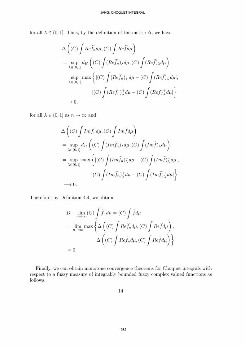
for all ∈ (0, 1]. Thus, by the definition of the metric ∆, we have
∆
((C)
∫Refndµ, (C)
∫Refdµ
)= sup
λ∈(0,1]
dH
((C)
∫(Refn)λdµ, (C)
∫(Ref)λdµ
)= sup
λ∈(0,1]
max
|(C)
∫(Refn)
−λ dµ− (C)
∫(Ref)−λ dµ|,
|(C)∫(Refn)
+λ dµ− (C)
∫(Ref)+λ dµ|
−→ 0,
for all ∈ (0, 1] as n→ ∞ and
∆
((C)
∫Imfndµ, (C)
∫Imfdµ
)= sup
λ∈(0,1]
dH
((C)
∫(Imfn)λdµ, (C)
∫(Imf)λdµ
)= sup
λ∈(0,1]
max
|(C)
∫(Imfn)
−λ dµ− (C)
∫(Imf)−λ dµ|,
|(C)∫(Imfn)
+λ dµ− (C)
∫(Imf)+λ dµ|
−→ 0.
Therefore, by Definition 4.4, we obtain
D − limn→∞
(C)
∫fndµ = (C)
∫fdµ
= limn→∞
max
∆
((C)
∫Refndµ, (C)
∫Refdµ
),
∆
((C)
∫Refndµ, (C)
∫Refdµ
)= 0.
Finally, we can obtain monotone convergence theorems for Choquet integrals withrespect to a fuzzy measure of integrably bounded fuzzy complex valued functions asfollows.
14
JANG: CHOQUET INTEGRAL
1082
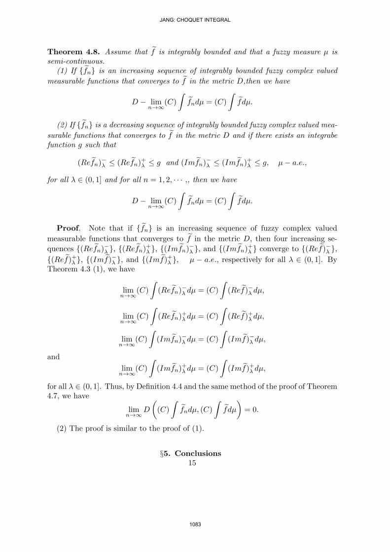
Theorem 4.8. Assume that f is integrably bounded and that a fuzzy measure µ issemi-continuous.
(1) If fn is an increasing sequence of integrably bounded fuzzy complex valued
measurable functions that converges to f in the metric D,then we have
D − limn→∞
(C)
∫fndµ = (C)
∫fdµ.
(2) If fn is a decreasing sequence of integrably bounded fuzzy complex valued mea-
surable functions that converges to f in the metric D and if there exists an integrabefunction g such that
(Refn)−λ ≤ (Refn)
+λ ≤ g and (Imfn)
−λ ≤ (Imfn)
+λ ≤ g, µ− a.e.,
for all ∈ (0, 1] and for all n = 1, 2, · · · ,, then we have
D − limn→∞
(C)
∫fndµ = (C)
∫fdµ.
Proof. Note that if fn is an increasing sequence of fuzzy complex valued
measurable functions that converges to f in the metric D, then four increasing se-
quences (Refn)−λ , (Refn)+λ , (Imfn)
−λ , and (Imfn)+λ converge to (Ref)−λ ,
(Ref)+λ , (Imf)−λ , and (Imf)+λ , µ − a.e., respectively for all ∈ (0, 1]. By
Theorem 4.3 (1), we have
limn→∞
(C)
∫(Refn)
−λ dµ = (C)
∫(Ref)−λ dµ,
limn→∞
(C)
∫(Refn)
+λ dµ = (C)
∫(Ref)+λ dµ,
limn→∞
(C)
∫(Imfn)
−λ dµ = (C)
∫(Imf)−λ dµ,
and
limn→∞
(C)
∫(Imfn)
+λ dµ = (C)
∫(Imf)+λ dµ,
for all ∈ (0, 1]. Thus, by Definition 4.4 and the same method of the proof of Theorem4.7, we have
limn→∞
D
((C)
∫fndµ, (C)
∫fdµ
)= 0.
(2) The proof is similar to the proof of (1).
§5. Conclusions15
JANG: CHOQUET INTEGRAL
1083
In this paper, by using, we use the Choquet integral with respect to a fuzzy mea-sure instead of the Lebesgue integral with respect to a classical measure, we definethe new concept of the Choquet integral with respect to a fuzzy measure of fuzzycomplex valued functions in Definition 3.8 and Theorems 3.10, 3.12. In Definitions4.4, 4.5, 4.6, and Theorems 4.7, 4.8, we investigate the existence of the fuzzy complexvalued Choquet integral and some convergence properties of the Choquet integrals ofintegrably bounded fuzzy complex valued functions.
In the future, we will study a probability measure approach to rank fuzzy complexnumbers and the theoretical fundamentals of leaning theory based on fuzzy complexrandom samples, etc.
Acknowledgement: This paper was supported by Konkuk University in 2013.
References
[1] J.J. Buckley, Fuzzy complex numbers, Fuzzy Sets and Systems 33 (1989), 333-345.[2] J.J. Buckley, Fuzzy complex analysis I, Fuzzy Sets and Systems 41 (1991), 269-284.
[3] J.J. Buckley, Fuzzy complex analysis II, Fuzzy Sets and Systems 49 (1992), 171-179.[4] L.C. Jang, B.M. Kil, Y.K. Kim, J.S. Kwon, Some properties of Choquet integrals of set-
valued functions, Fuzzy Sets and Systems 91 (1997), 61-67.[5] L.C. Jang, J.S. Kwon, On the representation of Choquet integrals of set-valued functions
and null sets, Fuzzy Sets and Systems 112 (2000), 1 233-239.[6] L.C. Jang, A note on the monotone interval-valued set function defined by the interval-
valued Choquet integral, Comm. Korean Math. Soc. 22(2) (2007), 227-234.[7] L.C. Jang, T. Kim, J.D. Jeon, and W.J. Kim, On Choquet integrals of measurable fuzzy
number-valued functions, Bull. Koran Math. Soc. 41(1) (2004), 95-107.[8] T. Murofushi and M. Sugeno, An interpretation of fuzzy measures and the Choquet integral
as an integral with respect to a fuzzy measure, Fuzzy Sets and Systems 29 (1989), 201-227.[9] T. Murofushi and M. Sugeno, A theory of fuzzy measure representations, the Choquet
integral, and null sets, J. math. Anal. Appl. 159 (1991), 532-549.[10] T. Murofushi, M.Sugeno, and M. Suzaki, Autocontinuity, convergence in measure, and
convergence in distribution, Fuzzy Sets and Systems 92 (1997), 197-203.
[11] M.L. Puri and D.A. Ralescu, Fuzzy random variable, J. Math. Anal. Appl. 114 (1986),409-422.
[12] M. Sugeno, Y. Narukawa and T. Murofushi, Choquet integral and fuzzy measures on locallycompact space, Fuzzy Sets and Systems 99 (1998), 205-211.
[13] G. Wang and X. Li, Generalized Lebesgue integrals of fuzzy complex valued functions, FuzzySets and Systems 127 (2002), 363-370.
[14] D. Zhang, C. Guo and D. Liu, Set-valued Choquet integrals revisited, Fuzzy Sets and Sys-tems 147 (2004), 475-485.
16
JANG: CHOQUET INTEGRAL
1084
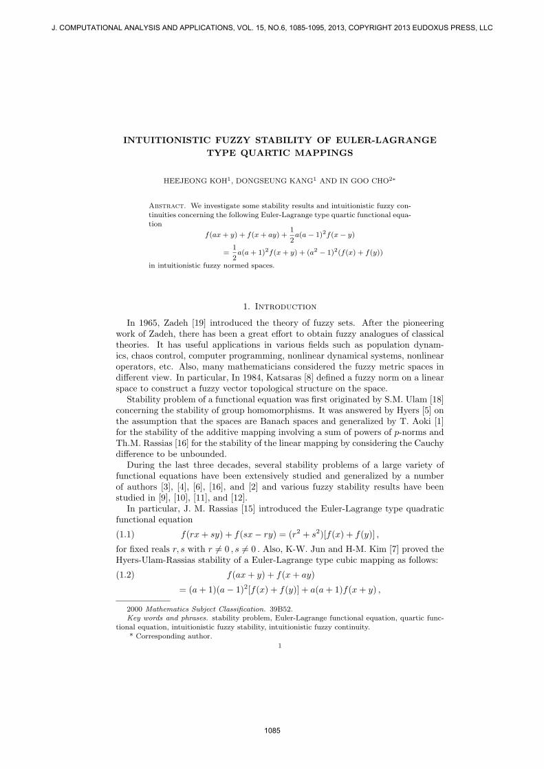
INTUITIONISTIC FUZZY STABILITY OF EULER-LAGRANGETYPE QUARTIC MAPPINGS
HEEJEONG KOH1, DONGSEUNG KANG1 AND IN GOO CHO2∗
Abstract. We investigate some stability results and intuitionistic fuzzy con-
tinuities concerning the following Euler-Lagrange type quartic functional equa-
tion
f(ax + y) + f(x + ay) +1
2a(a− 1)2f(x− y)
=1
2a(a + 1)2f(x + y) + (a2 − 1)2(f(x) + f(y))
in intuitionistic fuzzy normed spaces.
1. Introduction
In 1965, Zadeh [19] introduced the theory of fuzzy sets. After the pioneeringwork of Zadeh, there has been a great effort to obtain fuzzy analogues of classicaltheories. It has useful applications in various fields such as population dynam-ics, chaos control, computer programming, nonlinear dynamical systems, nonlinearoperators, etc. Also, many mathematicians considered the fuzzy metric spaces indifferent view. In particular, In 1984, Katsaras [8] defined a fuzzy norm on a linearspace to construct a fuzzy vector topological structure on the space.
Stability problem of a functional equation was first originated by S.M. Ulam [18]concerning the stability of group homomorphisms. It was answered by Hyers [5] onthe assumption that the spaces are Banach spaces and generalized by T. Aoki [1]for the stability of the additive mapping involving a sum of powers of p-norms andTh.M. Rassias [16] for the stability of the linear mapping by considering the Cauchydifference to be unbounded.
During the last three decades, several stability problems of a large variety offunctional equations have been extensively studied and generalized by a numberof authors [3], [4], [6], [16], and [2] and various fuzzy stability results have beenstudied in [9], [10], [11], and [12].
In particular, J. M. Rassias [15] introduced the Euler-Lagrange type quadraticfunctional equation
(1.1) f(rx + sy) + f(sx− ry) = (r2 + s2)[f(x) + f(y)] ,
for fixed reals r, s with r 6= 0 , s 6= 0 . Also, K-W. Jun and H-M. Kim [7] proved theHyers-Ulam-Rassias stability of a Euler-Lagrange type cubic mapping as follows:
f(ax + y) + f(x + ay)(1.2)
= (a + 1)(a− 1)2[f(x) + f(y)] + a(a + 1)f(x + y) ,
2000 Mathematics Subject Classification. 39B52.Key words and phrases. stability problem, Euler-Lagrange functional equation, quartic func-
tional equation, intuitionistic fuzzy stability, intuitionistic fuzzy continuity.
* Corresponding author.
1
1085
J. COMPUTATIONAL ANALYSIS AND APPLICATIONS, VOL. 15, NO.6, 1085-1095, 2013, COPYRIGHT 2013 EUDOXUS PRESS, LLC
2 HEEJEONG KOH, DONGSEUNG KANG, IN GOO CHO
where a 6= 0 ,±1 , for all x, y ∈ X .In this paper, we investigate the stability problem for the Euler-Lagrange type
quartic functional equation as follows:
(1.3) f(ax + y) + f(x + ay) +12a(a− 1)2f(x− y)
=12a(a + 1)2f(x + y) + (a2 − 1)2(f(x) + f(y)) ,
for fixed integer a with a 6= 0, ±1 .In fact, f(x) = x4 is a solution of (1.3) by virtue of the identity
(ax + y)4 + (x + ay)4 +12a(a− 1)2(x− y)4
=12a(a + 1)2(x + y)4 + (a2 − 1)2(x4 + y4) .
In this paper, we investigate some stability results and intuitionistic fuzzy con-tinuities concerning the equation (1.3) in intuitionistic fuzzy normed spaces.
Definition 1.1. A binary operation ∗ : [0, 1]× [0, 1] → [0, 1] is said to be a contin-uous t-norm if it satisfies the following conditions:
(1) * is associative and commutative, (2) * is continuous, (3) a ∗ 1 = a for alla ∈ [0, 1] , (4) a ∗ b ≤ c ∗ d whenever a ≤ c and b ≤ d , for each a, b, c, d ∈ [0, 1] .
Definition 1.2. A binary operation ♦ : [0, 1] × [0, 1] → [0, 1] is said to be acontinuous t-conorm if it satisfies the following conditions:
(1) ♦ is associative and commutative, (2) ♦ is continuous, (3) a♦0 = a for alla ∈ [0, 1] , (4) a♦b ≤ c♦d whenever a ≤ c and b ≤ d , for each a, b, c, d ∈ [0, 1] .
Saadati and Park introduced the concept of intuitionistic fuzzy normedspace; [17].
Definition 1.3. The five-tuple (X, µ, ν, ∗,♦) is called an intuitionistic fuzzynormed space(for short, IFNS) if X is a vector space, ∗ is a continuous t-norm,♦ is continuous t-conorm, and µ and ν are fuzzy sets on X × (0, 1) satisfying thefollowing conditions. For all x, y ∈ X and s, t > 0 ,
(1) µ(x, t) + ν(x, y) ≤ 1 ,(2) µ(x, t) > 0 ,(3) µ(x, t) = 1 if and only if x = 0 ,(4) µ(αx, t) = µ(x, t
|α| ) for each α 6= 0 ,
(5) µ(x, t) ∗ µ(y, s) ≤ µ(x + y, t + s) ,(6) µ(x, ·) : (0,∞) → [0.1] is continuous,(7) limt→∞ µ(x, t) = 1 and limt→0 µ(x, t) = 0 ,(8) ν(x, t) < 1 ,(9) ν(x, t) = 0 if and only if x = 0 ,
(10) ν(αx, t) = ν(x, t|α| ) for each α 6= 0 ,
(11) ν(x, t)♦ν(y, s) ≥ ν(x + y, t + s) ,(12) ν(x, ·) : (0,∞) → [0.1] is continuous,(13) limt→∞ ν(x, t) = 0 and limt→0 ν(x, t) = 1 .
In this case (µ, ν) is said to be an intuitionistic fuzzy norm.
Also, they investigated the concepts of convergence and Cauchy sequences in anintuittionistic fuzzy normed space as follows:
1086
EULER-LAGRANGE TYPE QUARTIC MAPPINGS 3
Let (X, µ, ν, ∗,♦) be an IFNS. A sequence (xk) is said to be intuittionistic fuzzyconvergent to L ∈ X if limk→∞ µ(xk − L, t) = 1 and limk→∞ ν(xk − L, t) = 0 ,for all t > 0 . A sequence (xk) is said to be intuittionistic fuzzy Cauchy sequenceif limk→∞ µ(xk+p − xk, t) = 1 and limk→∞ ν(xk+p − xk, t) = 0 , for all t > 0 andp = 1, 2, · · · . Also, (X, µ, ν, ∗,♦) is said to be complete if every intuitionistic fuzzyCauchy sequence in (X, µ, ν, ∗,♦) is intuitionistic fuzzy convergent in (X, µ, ν, ∗,♦) .
2. Intuitionistic Fuzzy Stability
Throughout this section, let X be a linear space and let Y be a intuitionisticfuzzy Banach space. Let a be a fixed integer with a 6= 0, ±1 , For convenience, weuse the following abbreviation:
(2.1) Daf(x, y) := f(ax + y) + f(x + ay) +12a(a− 1)2f(x− y)
−12a(a + 1)2f(x + y)− (a2 − 1)2(f(x) + f(y)) ,
for all x, y ∈ X .
Theorem 2.1. Let a be an integer with a 6= 0, ±1 , and let X be a linear space andlet (Z, µ′, ν′) be an intuitionistic fuzzy normed space(IFNS). Let φ : X ×X → Z bea function such that for some 0 < α < a4
(2.2) µ′(φ(ax, 0), t) ≥ µ′(αφ(x, 0), t) and ν′(φ(ax, 0), t) ≤ ν′(αφ(x, 0), t) ,
and limn→∞ µ′(φ(anx, any), a4nt) = 1 and limn→∞ ν′(φ(anx, any), a4nt) = 0 , forall x, y ∈ X and t > 0 . Suppose (Y, µ, ν) is an intuitionistic fuzzy Banach spaceand f : X → Y is a φ-approximately mapping such that f(0) = 0 and
(2.3) µ(Daf(x, y), t
)≥ µ′(φ(x, y), t)
and
(2.4) ν(Daf(x, y), t
)≤ ν′(φ(x, y), t)
for all t > 0 and all x, y ∈ X . Then there exists a unique Euler-Lagrange typequartic mapping Q : X → Y such that
(2.5) µ(Q(x)− f(x), t) ≥ µ′(φ(x, 0),12(a4 − α)t) ,
and
(2.6) ν(Q(x)− f(x), t) ≤ ν′(φ(x, 0),12(a4 − α)t) ,
for all x ∈ X and all t > 0 .
Proof. By letting y = 0 in inequalities (2.3) and (2.4), we have
(2.7) µ(f(ax)−a4f(x), t) ≥ µ′(φ(x, 0), t) and ν(f(ax)−a4f(x), t) ≤ ν′(φ(x, 0), t) ,
that is,
(2.8) µ(f(ax)
a4− f(x),
t
a4) ≥ µ′(φ(x, 0), t) ,
and
(2.9) ν(f(ax)
a4− f(x),
t
a4) ≤ ν′(φ(x, 0), t) ,
1087
4 HEEJEONG KOH, DONGSEUNG KANG, IN GOO CHO
for all x ∈ X and t > 0 . For each n ∈ N , letting x = anx in inequalities (2.8) and(2.9), we get
µ(a4n(
f(an+1x)a4(n+1)
− f(anx)a4n
),t
a4
)≥ µ′(φ(anx, 0), t)
ν(a4n(
f(an+1x)a4(n+1)
− f(anx)a4n
),t
a4
)≤ ν′(φ(anx, 0), t) .
By using the inequality (2.2), these previous inequalities imply that
µ(f(an+1x)
a4(n+1)− f(anx)
a4n,
t
a4(n+1)
)≥ µ′(φ(anx, 0), t) = µ′(φ(x, 0),
t
αn)
ν(f(an+1x)
a4(n+1)− f(anx)
a4n,
t
a4(n+1)
)≤ ν′(φ(x, 0),
t
αn) ,
for all x ∈ X , t > 0 , and n ≥ 0 . Now, switching t by αnt in the previous inequali-ties, we have
µ(f(an+1x)
a4(n+1)− f(anx)
a4n,
1a4
(α
a4)nt
)≥ µ′(φ(x, 0), t) ,
ν(f(an+1x)
a4(n+1)− f(anx)
a4n,
1a4
(α
a4)nt
)≤ ν′(φ(x, 0), t) ,
for all x ∈ X , t > 0 , and n ≥ 0 . Then
µ(f(anx)
a4n− f(x),
n−1∑k=0
1a4
(α
a4)kt
)= µ
( n−1∑k=0
(f(ak+1x)a4(k+1)
− f(akx)a4k
),n−1∑k=0
1a4
(α
a4)kt
)≥
n−1∏k=0
µ(f(ak+1x)
a4(k+1)− f(akx)
a4k,
1a4
(α
a4)kt
)≥ µ′(φ(x, 0), t) ,
and
ν(f(anx)
a4n− f(x),
n−1∑k=0
1a4
(α
a4)kt
)= ν
( n−1∑k=0
(f(ak+1x)a4(k+1)
− f(akx)a4k
),n−1∑k=0
1a4
(α
a4)kt
)≤
n−1∐k=0
ν(f(ak+1x)
a4(k+1)− f(akx)
a4k,
1a4
(α
a4)kt
)≤ ν′(φ(x, 0), t) ,
for all x ∈ X , t > 0 , and n ≥ 1 , where∏n
j=1 aj = a1 ∗ · · · ∗ an and∐n
j=1 aj =a1♦ · · ·♦an . For any integer s ≥ 0 , replacing x with asx in the previous inequali-ties, we have
µ(a4s[
f(an+sx)a4(n+s)
− f(asx)a4s
],n−1∑k=0
1a4
(α
a4)kt
)≥ µ′(φ(asx, 0), t) ,
and
ν(a4s[
f(an+sx)a4(n+s)
− f(asx)a4s
],n−1∑k=0
1a4
(α
a4)kt
)≤ ν′(φ(asx, 0), t) ,
that is,
µ(f(an+sx)
a4(n+s)− f(asx)
a4s,
1a4s
n−1∑k=0
1a4
(α
a4)kt
)≥ µ′(φ(x, 0),
t
αs) ,
1088
EULER-LAGRANGE TYPE QUARTIC MAPPINGS 5
and
µ(f(an+sx)
a4(n+s)− f(asx)
a4s,
1a4s
n−1∑k=0
1a4
(α
a4)kt
)≥ µ′(φ(x, 0),
t
αs) ,
for all x ∈ X , t > 0 , n ≥ 0 , and s ≥ 0 . Now, switching t by αst , we get
µ(f(an+sx)
a4(n+s)− f(asx)
a4s,
1a4s
n−1∑k=0
αs
a4(
α
a4)kt
)= µ
(f(an+sx)a4(n+s)
− f(asx)a4s
,n+s−1∑
k=s
1a4
(α
a4)kt
)≥ µ′(φ(x, 0), t) ,
and
ν(f(an+sx)
a4(n+s)− f(asx)
a4s,
1a4s
n−1∑k=0
αs
a4(
α
a4)kt
)= ν
(f(an+sx)a4(n+s)
− f(asx)a4s
,n+s−1∑
k=s
1a4
(α
a4)kt
)≤ ν′(φ(x, 0), t) ,
for all x ∈ X , t > 0 , n ≥ 0 , and s ≥ 0 . By putting t with tPn+s−1k=s
1a4 ( α
a4 )k, we have
(2.10) µ(f(an+sx)
a4(n+s)− f(asx)
a4s, t
)≥ µ′(φ(x, 0),
t∑n+s−1k=s
1a4 ( α
a4 )k) ,
and
(2.11) ν(f(an+sx)
a4(n+s)− f(asx)
a4s, t
)≤ ν′(φ(x, 0),
t∑n+s−1k=s
1a4 ( α
a4 )k) ,
for all x ∈ X , t > 0 , n ≥ 0 , and s ≥ 0 . Since 0 < α < a4 ,∑∞
k=0
(αa4
)k
< ∞ . Hence
limt→∞ µ′(φ(x, 0), tPn+s−1k=s
1a4 ( α
a4 )k) = 1 , and limt→∞ ν′(φ(x, 0), tPn+s−1
k=s1
a4 ( αa4 )k
) =
0 . Let ε > 0 and δ > 0 . Then there exists a t0 > 0 such thatµ′(φ(x, 0), t0Pn+s−1
k=s1
a4 ( αa4 )k
) ≥ 1 − ε , and ν′(φ(x, 0), t0Pn+s−1k=s
1a4 ( α
a4 )k) ≤ ε . Since∑∞
k=0t0a4
(αa4
)k
< ∞ , there exists a n0 ∈ N such that∑n+s−1
k=st0a4
(αa4
)k
< δ , for
all n + s > s ≥ n0 . Hence the sequence(
f(anx)a4n
)is a Cauchy sequence in (Y, µ, ν) .
Since (Y, µ, ν) is a Banach space, the sequence(
f(anx)a4n
)converges. Hence we can
define a function Q : X → Y by
Q(x) = limn→∞
f(anx)a4n
,
for all x ∈ X . Letting s = 0 in the inequalities (2.10) and (2.11), we have
µ(f(anx)
a4n− f(x), t
)≥ µ′(φ(x, 0),
t∑n−1k=0
1a4 ( α
a4 )k) ,
and
ν(f(anx)
a4n− f(x), t
)≤ ν′(φ(x, 0),
t∑n−1k=0
1a4 ( α
a4 )k) ,
1089
6 HEEJEONG KOH, DONGSEUNG KANG, IN GOO CHO
for all t > 0 and n > 0 . Hence we have
µ(Q(x)− f(x), t) = µ(Q(x)− f(anx)a4n
+f(anx)
a4n− f(x),
t
2+
t
2)
≥ µ(Q(x)− f(anx)
a4n,t
2
)∗ µ
(f(anx)a4n
− f(x),t
2
)≥ µ′
(φ(x, 0),
12
t∑n−1k=0
1a4
(αa4
)k
),
and
ν(Q(x)− f(x), t) = ν(Q(x)− f(anx)a4n
+f(anx)
a4n− f(x),
t
2+
t
2)
≤ ν(Q(x)− f(anx)
a4n,t
2
)∗ ν
(f(anx)a4n
− f(x),t
2
)≤ ν′
(φ(x, 0),
12
t∑n−1k=0
1a4
(αa4
)k
),
that is,
µ(Q(x)− f(x), t) ≥ µ′(φ(x, 0),12(a4 − α)t) ,
and
ν(Q(x)− f(x), t) ≤ ν′(φ(x, 0),12(a4 − α)t) ,
as n →∞ . Respectively, replacing x , y , and t by anx , any , and a4nt in inequalities(2.3) and (2.4), we have
µ(Daf(anx, any)
a4n, t
)≥ µ′(φ(anx, any), a4nt) ,
and
ν(Daf(anx, any)
a4n, t
)≤ ν′(φ(anx, any), a4nt) ,
for all x ∈ X , t > 0 , and n ∈ N . Since limn→∞ µ′(φ(anx, any), a4nt) = 1 andlimn→∞ ν′(φ(anx, any), a4nt) = 0 , the mapping Q : X → Y satisfies the equation(1.3), that is, it is the Euler-Lagrange type quartic mapping. It only remains toshow that the mapping Q : X → Y is unique. Assume Q′ : X → Y is anotherEuler-Lagrange type quartic mapping satisfying the inequalities (2.5) and (2.6). Itis easy to show that Q(anx) = a4nQ(x) and Q′(anx) = a4nQ′(x) , for all n ∈ N .
µ(Q(x)−Q′(x), t
)= µ
(Q(anx)a4n
− Q′(anx)a4n
, t)
≥ µ(Q(anx)
a4n− f(anx)
a4n,t
2
)∗ µ
(f(anx)a4n
− Q′(anx)a4n
,t
2
)≥ µ′
(φ(anx, 0),
a4n(a4 − α)4
t)≥ µ′
(φ(x, 0),
a4 − α
4
(a4
α
)n
t)
,
and
ν(Q(x)−Q′(x), t
)≤ ν′
(φ(x, 0),
a4 − α
4
(a4
α
)n
t)
,
1090
EULER-LAGRANGE TYPE QUARTIC MAPPINGS 7
for all x ∈ X and all t > 0 . Since limn→∞
(a4
α
)n
= ∞ ,
limn→∞
µ′(φ(x, 0),
a4 − α
4
(a4
α
)n
t)
= 1 and limn→∞
ν′(φ(x, 0),
a4 − α
4
(a4
α
)n
t)
= 0 .
Henceµ(Q(x)−Q′(x), t
)= 1 and ν
(Q(x)−Q′(x), t
)= 0 ,
for all x ∈ X and all t > 0 . We may conclude that Q(x) = Q′(x) , for all x ∈ X ,that is, the mapping Q : X → Y is unique, as desired.
Theorem 2.2. Let a be an integer with a 6= 0, ±1 , and let X be a linear space andlet (Z, µ′, ν′) be an intuitionistic fuzzy normed space(IFNS). Let φ : X ×X → Z bea function such that for some α > a4
(2.12) µ′(φ(x
a, 0), t) ≥ µ′(φ(x, 0), αt) and ν′(φ(
x
a, 0), t) ≤ ν′(φ(x, 0), αt) ,
and limn→∞ µ′(φ(a−nx, a−ny), a−4nt) = 1 and limn→∞ ν′(φ(a−nx, a−ny), a−4nt) =0 , for all x, y ∈ X and t > 0 . Suppose (Y, µ, ν) is an intuitionistic fuzzy Banachspace and f : X → Y is a φ-approximately mapping with f(0) = 0 satisfying theinequalities (2.3) and (2.4). Then there exists a unique Euler-Lagrange type quarticmapping Q : X → Y such that
(2.13) µ(Q(x)− f(x), t) ≥ µ′(φ(x, 0),(α− a4)
2t) ,
and
(2.14) ν(Q(x)− f(x), t) ≤ ν′(φ(x, 0),(α− a4)
2t) ,
for all x ∈ X and all t > 0 .
Proof. Letting x = xa in inequalities (2.7) of proof of Theorem 2.1, we have
(2.15)µ(f(x)− a4f(
x
a), t) ≥ µ′(φ(x, 0), αt) and ν(f(x)− a4f(
x
a), t) ≤ ν′(φ(x, 0), αt) ,
for all x ∈ X and t > 0 . Similar to the proof of Theorem 2.1, we can deduce
(2.16) µ(a4(n+s)f(a−(n+s)x)− a4sf(a−sx), t
)≥ µ′(φ(x, 0),
t∑n+s−1k=s
a4k
αk+1
) ,
and
(2.17) ν(a4(n+s)f(a−(n+s)x)− a4sf(a−sx), t
)≤ ν′(φ(x, 0),
t∑n+s−1k=s
a4k
αk+1
) ,
for all x ∈ X , t > 0 , and s ≥ 0 and n ≥ 0 . Since α > a4 and∑∞
k=0
(a4
α
)k
< ∞ ,
the Cauchy criterion for convergence in IFNS implies that(a4nf( x
an ))
is a Cauchysequence in the Banach space (Y, µ, ν) . A function Q : X → Y by
Q(x) = limn→∞
a4nf(x
an) ,
for all x ∈ X . Also, letting s = 0 and taking n →∞ in the inequalities (2.16) and(2.17), we have the inequalities (2.13) and (2.14). The remains follows from theproof of Theorem 2.1.
1091
8 HEEJEONG KOH, DONGSEUNG KANG, IN GOO CHO
3. Intutionistic fuzzy continuity
Throughout this section, let (X, || · ||) be a normed space. In [13], they definedand studied the intuitionistic fuzzy continuity. In this section, we will investigateinteresting results of continuous approximately Euler-Lagrange type quartic map-pings. Before proceeding the proof, we will state the definition of intuitionisticfuzzy continuity as follows.
Definition 3.1. [ [14, Definition 3.1]] Let f : R → X be a function, where R isendowed with the Euclidean topology and X is an intuitionistic fuzzy normed spaceequipped with intuitionistic fuzzy norm (µ , ν) . Them f is called intuitionistic fuzzycontinuous at a point s0 ∈ R if for all ε > 0 and all 0 < α < 1 there exists δ > 0such that for each s with 0 < |s− s0| < δ
µ(f(sx)− f(s0x), ε) ≥ α and ν(f(sx)− f(s0x), ε) ≤ 1− α .
Theorem 3.2. Let a be an integer with a 6= 0, ±1 ,and let X be a normed spaceand (Z, µ′, ν′) be an IFNS. Let (Y, µ, ν) be an intuitionistic fuzzy Banach space andf : X → Y be a (p, q)-approximately mapping with f(0) = 0 in the sense that forsome p, q and some z0 ∈ Z
(3.1) µ(Daf(x, y), t
)≥ µ′((||x||p + ||y||q)z0, t)
and
(3.2) ν(Daf(x, y), t
)≤ ν′((||x||p + ||y||q)z0, t)
for all t > 0 and all x, y ∈ X . If p, q < 4 , then there exists a unique Euler-Lagrangetype quartic mapping Q : X → Y such that
(3.3) µ(C(x)− f(x), t) ≥ µ′(||x||pz0,12(a4 − |a|p)t) ,
and
(3.4) ν(C(x)− f(x), t) ≤ ν′(||x||pz0,m2
2(a4 − |a|p)t) ,
for all x ∈ X and all t > 0 . Furthermore, if for some x ∈ X and all n ∈ N , themapping g : R → Y defined by g(s) = f(ansx) is intuitionistic fuzzy continuous,then the mappings s 7→ Q(sx) from R to Y is intuitionistic fuzzy continuous.
Proof. For x, y ∈ X and for some z0 ∈ Z , we define the function φ : X ×X → Zby φ(x, y) = (||x||p + ||y||q)z0 in Theorem 2.1. Since p < 4 , we have α = |a|p < a4 .Hence Theorem 2.1 implies the existence and uniqueness of the Euler-Lagrangetype quartic mapping Q : X → Y satisfying inequalities (3.3) and (3.4). Now, wewill show the intuitionistic fuzzy continuity. For each x ∈ X , t ∈ R and n ∈ N , wehave
µ(Q(x)− f(anx)a4n
, t) = µ(Q(anx)
a4n− f(anx)
a4n, t) = µ(Q(anx)− f(anx), a4nt)
≥ µ′(|a|np||x||pz0,a4n
2(a4 − |a|p)t) = µ′(||x||pz0,
a4n(a4 − |a|p)2 · |a|np
t) ,
and
ν(Q(x)− f(anx)a4n
, t) ≤ ν′(||x||pz0,a4n(a4 − |a|p)
2 · |a|npt) .
1092
EULER-LAGRANGE TYPE QUARTIC MAPPINGS 9
Let x ∈ X and s0 ∈ R be fixed and ε > 0 and 0 < β < 1 be given. For all s ∈ Rwith |s− s0| < 1 , by replacing x with sx in the previous inequalities,
µ(Q(sx)− f(ansx)a4n
, t) ≥ µ′(||sx||pz0,a4n(a4 − |a|p)
2 · |a|npt)
≥ µ′(||x||pz0,a4n(a4 − |a|p)
2 · |a|np(1 + |s0|)pt) ,
and
ν(Q(sx)− f(ansx)a4n
, t) ≤ ν′(||x||pz0,a4n(a4 − |a|p)
2 · |a|np(1 + |s0|)pt) .
Since ap < a4 , we have
limn→∞
a4n(a4 − |a|p)2 · |a|np(1 + |s0|)p
= ∞ .
Hence there exists n0 ∈ N such that
µ(Q(sx)− f(an0sx)
a4n0,ε
3
)≥ β and ν
(Q(sx)− f(an0sx)
a4n0,ε
3
)≤ 1− β ,
for all |s − s0| < 1 and s ∈ R . The intuitionistic fuzzy continuity of the mappingt 7→ f(an0tx) implies that there exists δ < 1 such that for each s with 0 < |s−s0| <δ , we get
µ(f(an0sx)
a4n0− f(an0s0x)
a4n0,ε
3) ≥ β and ν(
f(an0sx)a4n0
− f(an0s0x)a4n0
,ε
3) ≤ 1− β .
Thus
µ(Q(sx)−Q(s0x), ε) ≥ µ(Q(sx)− f(an0sx)a4n0
,ε
3) ∗
µ(f(an0sx)
a4n0− f(an0s0x)
a4n0,ε
3) ∗ µ(Q(s0x)− f(an0s0x)
a4n0,ε
3) ≥ β
andν(Q(sx)−Q(s0x), ε) ≤ 1− β ,
for all s ∈ R with 0 < |s− s0| < δ , that is, the mapping s 7→ Q(sx) is intuitionisticfuzzy continuous.
Theorem 3.3. Let a be an integer with a 6= 0, ±1 , and let X be a normed spaceand (Z, µ′, ν′) be an IFNS. Let (Y, µ, ν) be an intuitionistic fuzzy Banach spaceand f : X → Y be a (p, q)-approximately mapping with f(0) = 0 satisfying (3.1)and (3.2) for some p, q and some z0 ∈ Z . If p, q > 4 , then there exists a uniqueEuler-Lagrange type quartic mapping Q : X → Y such that
(3.5) µ(Q(x)− f(x), t) ≥ µ′(||x||pz0,12(|a|p − a4)t) ,
and
(3.6) ν(Q(x)− f(x), t) ≤ ν′(||x||pz0,12(|a|p − a4)t) ,
for all x ∈ X and all t > 0 . Furthermore, if for some x ∈ X and all n ∈ N , themapping g : R → Y defined by g(s) = f(ansx) is intuitionistic fuzzy continuous,then the mappings s 7→ Q(sx) from R to Y is intuitionistic fuzzy continuous.
1093
10 HEEJEONG KOH, DONGSEUNG KANG, IN GOO CHO
Proof. Similar to the proof of Theorem 3.2, we may define the function φ : X×X →Z by φ(x, y) = (||x||p + ||y||q)z0 . Then we have
µ′(φ(x
2, 0), t) = µ′(||x||pz0, |a|pt) and ν′(φ(
x
2, 0), t) = ν′(||x||pz0, |a|pt) ,
for all x ∈ X and all t > 0 . Since p > 4 , we have α = |a|p > a4 . Hence Theorem 2.2implies the existence and uniqueness of the Euler-Lagrange type quartic mappingQ : X → Y satisfying inequalities (3.5) and (3.6). The remains follow from theproof of Theorem 3.2.
Acknowledgement
This work was supported by the University of Incheon Research Grant in 2011.
References
[1] T. Aoki, On the stability of the linear transformation in Banach spaces, J. Math. Soc.
Japan 2 (1950) 64–66.[2] J.-H. Bae and W.-G. Park, On the generalized Hyers-Ulam-Rassias stability in Banach
modules over a C∗−algebra, J. Math. Anal. Appl. 294(2004), 196–205.
[3] S. Czerwik, On the stability of the quadratic mapping in normed spaces, Abh. Math. Sem.Univ. Hamburg 62 (1992), 59–64.
[4] Z. Gajda, On the stability of additive mappings, Internat. J. Math. Math. Sci., 14 (1991),
431–434.[5] D. H. Hyers, On the stability of the linear equation, Proc. Nat. Acad. Sci. U.S.A. 27 (1941),
222–224.
[6] D.H. Hyers and Th.M. Rassias, Approximate homomorphisms, Aequationes Mathematicae,44 (1992),125–153.
[7] K.-W. Jun and H.-M. Kim, On the stability of Euler-Lagrange type cubic functional equa-tions in quasi-Banach spaces, J. Math. Anal. Appl. 332 (2007), 1335–1350.
[8] A.K. Katsaras, Fuzzy topological vector spaces II, Fuzzy Sets and Systems, 12 (1984),
143–154.[9] A.K. Mirmostafaee, M. Mirzavaziri, M.S. Moslehian, Fuzzy stability of the Jensen func-
tional equation, Fuzzy Sets Syst, 159 (2008), 730–738.
[10] A.K. Mirmostafaee, M.S. Moslehian, Fuzzy versions of Hyers-Ulam-Rassias theorem,Fuzzy Sets Syst, 159 (2008), 720–729.
[11] A.K. Mirmostafaee, M.S. Moslehian, Fuzzy approximately cubic mappings, Inf Sci, 178
(2008), 3791-3798.[12] A.K. Mirmostafaee, M.S. Moslehian, Fuzzy almost quadratic functions, Results Math.
doi:10.1007/s00025-007-0278-9.
[13] A.K. Mirmostafaee, M.S. Moslehian, Nonlinear operators between intuitionistic fuzzynormed spaces and Frechet derivative , Chaos, Solitons and Fractals, 42 (2009), 1010-
1015.[14] M. Mursaleen, S.A. Mohiuddine, On Stability of a cubic functional equation in intuition-
istic fuzzy normed spaces, Chaos, Solitons and Fractals, 42 (2009), 2997–3005.
[15] J. M. Rassias, On the stability of the Euler-Lagrange functional equation, Chinese J. Math.,20 (1992) 185–190.
[16] Th. M. Rassias, On the stability of the linear mapping in Banach spaces, Proc. Amer.
Math. Soc. 72 (1978), 297–300.[17] R. Saadati, J.H. Park, On the intuitionistic fuzzy topological spaces, Chaos, Solitons and
Fractals 27 (2006), 331–344.[18] S. M. Ulam, Problems in Morden Mathematics, Wiley, New York (1960).[19] L.A. Zadeh, Fuzzy sets, Inform Control, 8 (1965), 338-353.
1Department of Mathematical Education, Dankook University, 126, Jukjeon, Suji,
Yongin, Gyeonggi, South Korea 448-701
E-mail address: [email protected] (H. Koh)E-mail address: [email protected] (D. Kang)
1094
EULER-LAGRANGE TYPE QUARTIC MAPPINGS 11
2Graduate School of Education, University of Incheon, 12-1, Songdo, Yeonsu, In-cheon, South Korea 406-772
E-mail address: [email protected] (I. G. Cho)
1095
STABILITY FOR AN n-DIMENSIONAL FUNCTIONAL EQUATION OF
QUADRATIC-ADDITIVE TYPE WITH THE FIXED POINT APPROACH
ICK-SOON CHANG AND YANG-HI LEE
Abstract. In this paper, we investigate the stability of a functional equation∑1≤i,j≤n,i=j
[f(xi + xj) + f(xi − xj)] − (n − 1)
n∑j=1
f(2xj) = 0
by using the fixed point methd in the sense of Cadariu and Radu.
1. Introduction and peliminaries
It is of interest to consider the concept of stability for a functional equation arising when we replacethe functional equation by an inequality which acts as a perturbation of the equation. The study ofstability problems had been formulated by Ulam [17] during a talk : under what condition does there existsa homomorphism near an approximate homomorphism ? In the following year, Hyers [6] was answeredaffirmatively the question of Ulam for Banach spaces, which states that if ε ≥ 0 and f : X → Y is amapping with X a normed space, Y a Banach space such that
||f(x+ y)− f(x)− f(y)|| ≤ ε (1.1)
for all x, y ∈ X , then there exists a unique additive mapping T : X → Y such that
||f(x)− T (x)|| ≤ ε
for all x ∈ X . A generalized version of the theorem of Hyers for approximately additive mappings was givenby Aoki [1] and for the theorem of Hyers for approximately linear mappings it was presented by Rassias[15] by considering the case when the inequality (1.1) is unbounded. Since then, more generalizations andapplications of the stability to a number of functional equations and mappings have been investigated (forexample, [5], [7], [8]-[14]).
In this very active area, almost all subsequent proofs have used the method of Hyers [6]. On the otherhand, Cadariu and Radu [2] observed that the existence of the solution for a functional equation and theestimation of the difference with the given mapping can be obtained from the fixed point alternative. Thismethod is called a fixed point method. In particular, they [3, 4] applied this method to prove the stabilitytheorems of the additive functional equation
f(x+ y)− f(x)− f(y) = 0. (1.2)
and the quadratic functional equation
f(x+ y) + f(x− y)− 2f(x)− 2f(y) = 0. (1.3)
Note that the additive mapping f1(x) = ax and quadratic mapping f2(x) = ax2 are solution of the functionalequations (1.2) and (1.3).
We now take account of the functional equation :∑1≤i,j≤n,i =j
[f(xi + xj) + f(xi − xj)]− (n− 1)
n∑j=1
f(2xj) = 0. (1.4)
2000 Mathematics Subject Classification : 39B52.Keywords and phrases : stability : fixed point method : n-dimensional quadratic-additive type functional equation. The
first author was supported by Basic Science Research Program through the National Research Foundation of Korea (NRF)funded by the Ministry of Education, Science and Technology (No. 2012-0002410).
1
1096
J. COMPUTATIONAL ANALYSIS AND APPLICATIONS, VOL. 15, NO.6, 1096-1103, 2013, COPYRIGHT 2013 EUDOXUS PRESS, LLC
2 I.-S. CHANG AND Y.-H. LEE
Hence, throughout this paper, we promise that the equation (1.4) is said to be an quadratic-additive typefunctional equation and every solution of the equation (1.4) is called a quadratic-additive mapping.
In this paper, we will deal with the stability of the functional equation (1.4) by using the fixed pointmethod : The stability of (1.4) can be obtained by handling the odd part and the even part of the givenmapping. But, in violation of this processing, we can take the desired solution at once instead of splittingthe given mapping into two parts.
Here and now, we recall the following result of the fixed point theory by Margolis and Diaz :
Theorem 1.1. (The alternative of fixed point) ([14] or [16]) Suppose that a complete generalized metricspace (X, d), which means that the metric d may assume infinite values, and a strictly contractive mappingJ : X → X with the Lipschitz constant 0 < L < 1 are given. Then, for each given element x ∈ X, either
d(Jnx, Jn+1x) = +∞, ∀n ∈ N ∪ 0,or there exists a nonnegative integer k such that :
(1) d(Jnx, Jn+1x) < +∞ for all n ≥ k ;(2) the sequence Jnx is convergent to a fixed point y∗ of J ;(3) y∗ is the unique fixed point of J in Y := y ∈ X, d(Jkx, y) < +∞ ;(4) d(y, y∗) ≤ (1/(1− L))d(y, Jy) for all y ∈ Y.
2. A general fixed point method
Throughout this paper, let V be a real or complex linear space and Y a Banach space. For a givenmapping f : V → Y, we use the following abbreviation
f(x1, x2, · · · , xn) :=∑
1≤i,j≤n,i=j
[f(xi + xj) + f(xi − xj)]− (n− 1)
n∑j=1
f(2xj)
for all x1, x2, · · · , xn ∈ V. Now we can prove some stability results of the functional equation (1.4).
Theorem 2.1. Let φ : V n → [0,∞) be a given function with φ(x, 0, · · · , 0) = φ(−x, 0, · · · , 0) for all x ∈ V.Suppose that the mapping f : V → Y satisfies
∥Df(x1, x2, · · · , xn)∥ ≤ φ(x1, x2, · · · , xn) (2.1)
for all x1, x2, · · · , xn ∈ V with f(0) = 0. If there exists a constant 0 < L < 1 such that φ has the property
φ(2x1, 2x2, · · · , 2xn) ≤ 2Lφ(x1, x2, · · · , xn) (2.2)
for all x1, x2, · · · , xn ∈ V, then there exists a unique quadratic-additive mapping F : V → Y such that
∥f(x)− F (x)∥ ≤ φ(x, 0, · · · , 0)2(n− 1)(1− L)
(2.3)
for all x ∈ V. In particular, F is given by
F (x) = limm→∞
(f(2mx) + f(−2mx)
2 · 22m +f(2mx)− f(−2mx)
2 · 2m
)(2.4)
for all x ∈ V.
Proof. Consider the setS := g : g : V → Y, g(0) = 0
and introduce a generalized metric on S by
d(g, h) = infK ∈ ℝ
∣∣∥g(x)− h(x)∥ ≤ Kφ(x, 0, · · · , 0) for all x ∈ V.
It is easy to see that (S, d) is a generalized complete metric space.Now we define a mapping J : S → S by
Jg(x) :=g(2x)− g(−2x)
4+g(2x) + g(−2x)
8for all x ∈ V. Note that
Jmg(x) =g(2mx)− g(−2nx)
2m+1+g(2mx) + g(−2mx)
2 · 4m
1097
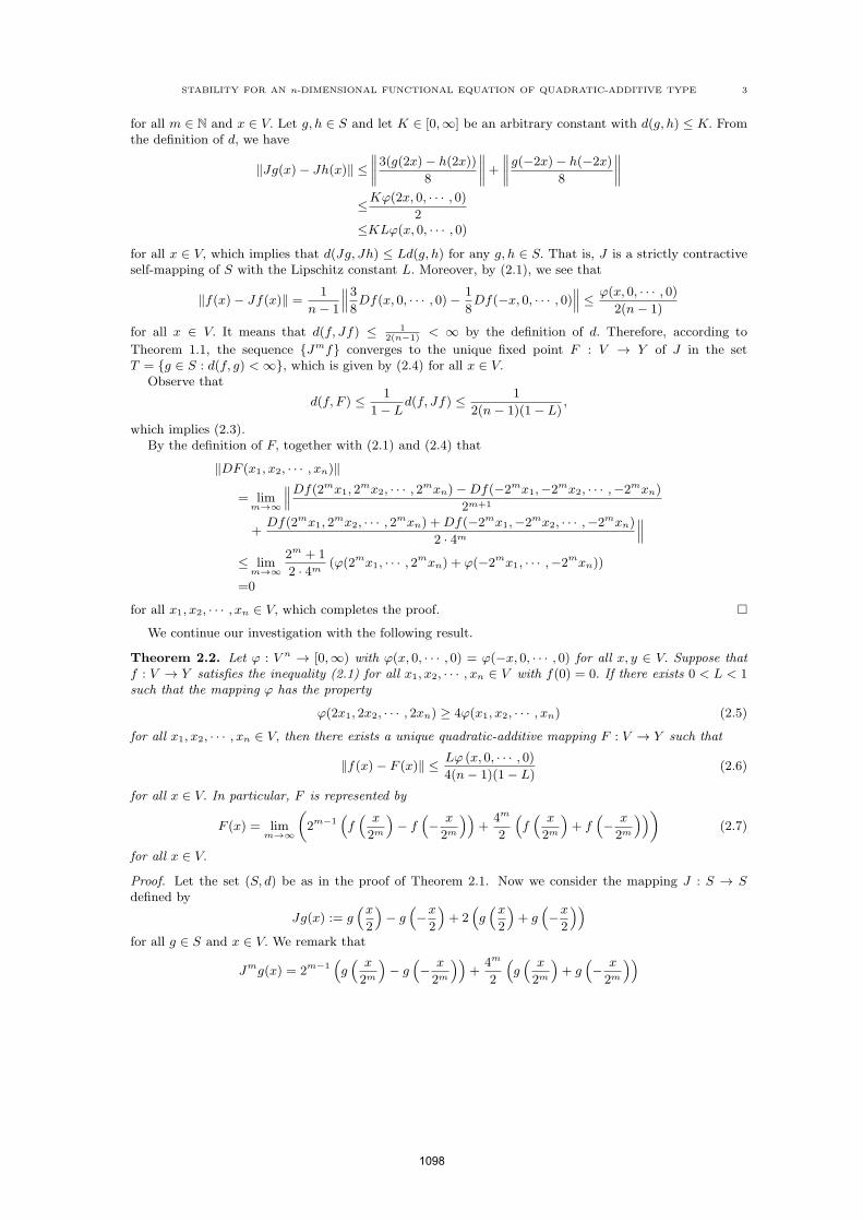
STABILITY FOR AN n-DIMENSIONAL FUNCTIONAL EQUATION OF QUADRATIC-ADDITIVE TYPE 3
for all m ∈ N and x ∈ V. Let g, h ∈ S and let K ∈ [0,∞] be an arbitrary constant with d(g, h) ≤ K. Fromthe definition of d, we have
∥Jg(x)− Jh(x)∥ ≤∥∥∥∥3(g(2x)− h(2x))
8
∥∥∥∥+
∥∥∥∥g(−2x)− h(−2x)
8
∥∥∥∥≤Kφ(2x, 0, · · · , 0)
2≤KLφ(x, 0, · · · , 0)
for all x ∈ V, which implies that d(Jg, Jh) ≤ Ld(g, h) for any g, h ∈ S. That is, J is a strictly contractiveself-mapping of S with the Lipschitz constant L. Moreover, by (2.1), we see that
∥f(x)− Jf(x)∥ =1
n− 1
∥∥∥38Df(x, 0, · · · , 0)− 1
8Df(−x, 0, · · · , 0)
∥∥∥ ≤ φ(x, 0, · · · , 0)2(n− 1)
for all x ∈ V. It means that d(f, Jf) ≤ 12(n−1)
< ∞ by the definition of d. Therefore, according to
Theorem 1.1, the sequence Jmf converges to the unique fixed point F : V → Y of J in the setT = g ∈ S : d(f, g) <∞, which is given by (2.4) for all x ∈ V.
Observe that
d(f, F ) ≤ 1
1− Ld(f, Jf) ≤ 1
2(n− 1)(1− L),
which implies (2.3).By the definition of F, together with (2.1) and (2.4) that
∥DF (x1, x2, · · · , xn)∥
= limm→∞
∥∥∥Df(2mx1, 2mx2, · · · , 2mxn)−Df(−2mx1,−2mx2, · · · ,−2mxn)
2m+1
+Df(2mx1, 2
mx2, · · · , 2mxn) +Df(−2mx1,−2mx2, · · · ,−2mxn)
2 · 4m∥∥∥
≤ limm→∞
2m + 1
2 · 4m (φ(2mx1, · · · , 2mxn) + φ(−2mx1, · · · ,−2mxn))
=0
for all x1, x2, · · · , xn ∈ V, which completes the proof. We continue our investigation with the following result.
Theorem 2.2. Let φ : V n → [0,∞) with φ(x, 0, · · · , 0) = φ(−x, 0, · · · , 0) for all x, y ∈ V. Suppose thatf : V → Y satisfies the inequality (2.1) for all x1, x2, · · · , xn ∈ V with f(0) = 0. If there exists 0 < L < 1such that the mapping φ has the property
φ(2x1, 2x2, · · · , 2xn) ≥ 4φ(x1, x2, · · · , xn) (2.5)
for all x1, x2, · · · , xn ∈ V, then there exists a unique quadratic-additive mapping F : V → Y such that
∥f(x)− F (x)∥ ≤ Lφ (x, 0, · · · , 0)4(n− 1)(1− L)
(2.6)
for all x ∈ V. In particular, F is represented by
F (x) = limm→∞
(2m−1
(f( x
2m
)− f
(− x
2m
))+
4m
2
(f( x
2m
)+ f
(− x
2m
)))(2.7)
for all x ∈ V.
Proof. Let the set (S, d) be as in the proof of Theorem 2.1. Now we consider the mapping J : S → Sdefined by
Jg(x) := g(x2
)− g
(−x2
)+ 2
(g(x2
)+ g
(−x2
))for all g ∈ S and x ∈ V. We remark that
Jmg(x) = 2m−1(g( x
2m
)− g
(− x
2m
))+
4m
2
(g( x
2m
)+ g
(− x
2m
))
1098
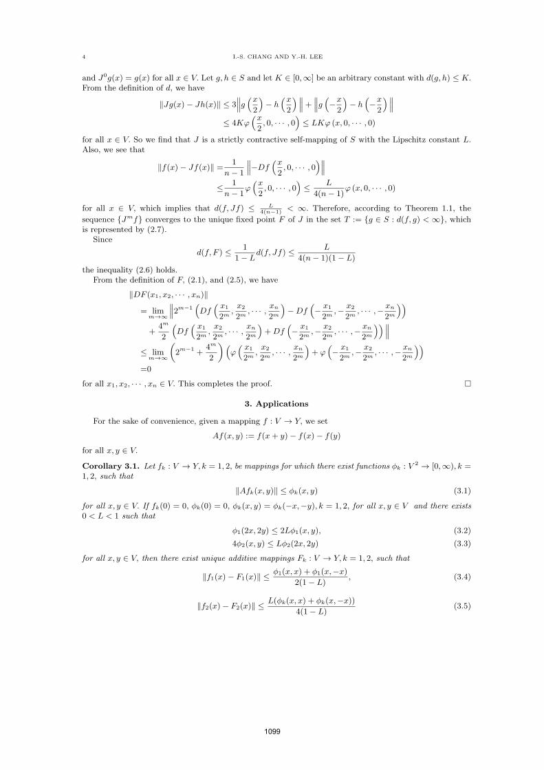
4 I.-S. CHANG AND Y.-H. LEE
and J0g(x) = g(x) for all x ∈ V. Let g, h ∈ S and let K ∈ [0,∞] be an arbitrary constant with d(g, h) ≤ K.From the definition of d, we have
∥Jg(x)− Jh(x)∥ ≤ 3∥∥∥g (x
2
)− h
(x2
)∥∥∥+∥∥∥g (−x
2
)− h
(−x2
)∥∥∥≤ 4Kφ
(x2, 0, · · · , 0
)≤ LKφ (x, 0, · · · , 0)
for all x ∈ V. So we find that J is a strictly contractive self-mapping of S with the Lipschitz constant L.Also, we see that
∥f(x)− Jf(x)∥ =1
n− 1
∥∥∥−Df (x2, 0, · · · , 0
)∥∥∥≤ 1
n− 1φ(x2, 0, · · · , 0
)≤ L
4(n− 1)φ (x, 0, · · · , 0)
for all x ∈ V, which implies that d(f, Jf) ≤ L4(n−1)
< ∞. Therefore, according to Theorem 1.1, the
sequence Jmf converges to the unique fixed point F of J in the set T := g ∈ S : d(f, g) < ∞, whichis represented by (2.7).
Since
d(f, F ) ≤ 1
1− Ld(f, Jf) ≤ L
4(n− 1)(1− L)
the inequality (2.6) holds.From the definition of F, (2.1), and (2.5), we have
∥DF (x1, x2, · · · , xn)∥
= limm→∞
∥∥∥2m−1(Df
( x12m
,x22m
, · · · , xn2m
)−Df
(− x12m
,− x22m
, · · · ,− xn2m
))+
4m
2
(Df
( x12m
,x22m
, · · · , xn2m
)+Df
(− x12m
,− x22m
, · · · ,− xn2m
))∥∥∥≤ lim
m→∞
(2m−1 +
4m
2
)(φ( x12m
,x22m
, · · · , xn2m
)+ φ
(− x12m
,− x22m
, · · · ,− xn2m
))=0
for all x1, x2, · · · , xn ∈ V. This completes the proof.
3. Applications
For the sake of convenience, given a mapping f : V → Y, we set
Af(x, y) := f(x+ y)− f(x)− f(y)
for all x, y ∈ V.
Corollary 3.1. Let fk : V → Y, k = 1, 2, be mappings for which there exist functions ϕk : V 2 → [0,∞), k =1, 2, such that
∥Afk(x, y)∥ ≤ ϕk(x, y) (3.1)
for all x, y ∈ V. If fk(0) = 0, ϕk(0) = 0, ϕk(x, y) = ϕk(−x,−y), k = 1, 2, for all x, y ∈ V and there exists0 < L < 1 such that
ϕ1(2x, 2y) ≤ 2Lϕ1(x, y), (3.2)
4ϕ2(x, y) ≤ Lϕ2(2x, 2y) (3.3)
for all x, y ∈ V, then there exist unique additive mappings Fk : V → Y, k = 1, 2, such that
∥f1(x)− F1(x)∥ ≤ ϕ1(x, x) + ϕ1(x,−x)2(1− L)
, (3.4)
∥f2(x)− F2(x)∥ ≤ L(ϕk(x, x) + ϕk(x,−x))4(1− L)
(3.5)
1099
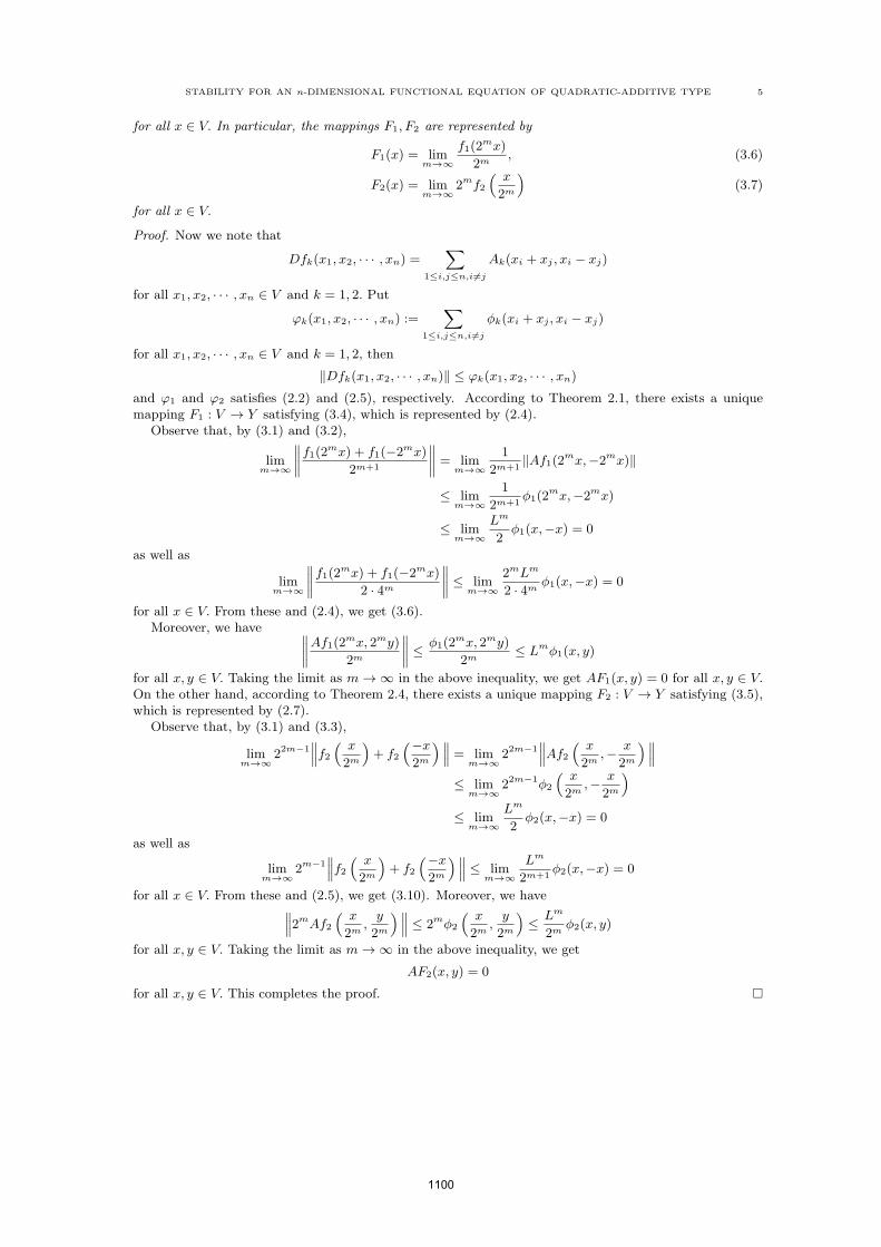
STABILITY FOR AN n-DIMENSIONAL FUNCTIONAL EQUATION OF QUADRATIC-ADDITIVE TYPE 5
for all x ∈ V. In particular, the mappings F1, F2 are represented by
F1(x) = limm→∞
f1(2mx)
2m, (3.6)
F2(x) = limm→∞
2mf2( x
2m
)(3.7)
for all x ∈ V.
Proof. Now we note that
Dfk(x1, x2, · · · , xn) =∑
1≤i,j≤n,i=j
Ak(xi + xj , xi − xj)
for all x1, x2, · · · , xn ∈ V and k = 1, 2. Put
φk(x1, x2, · · · , xn) :=∑
1≤i,j≤n,i=j
ϕk(xi + xj , xi − xj)
for all x1, x2, · · · , xn ∈ V and k = 1, 2, then
∥Dfk(x1, x2, · · · , xn)∥ ≤ φk(x1, x2, · · · , xn)and φ1 and φ2 satisfies (2.2) and (2.5), respectively. According to Theorem 2.1, there exists a uniquemapping F1 : V → Y satisfying (3.4), which is represented by (2.4).
Observe that, by (3.1) and (3.2),
limm→∞
∥∥∥∥f1(2mx) + f1(−2mx)
2m+1
∥∥∥∥ = limm→∞
1
2m+1∥Af1(2mx,−2mx)∥
≤ limm→∞
1
2m+1ϕ1(2
mx,−2mx)
≤ limm→∞
Lm
2ϕ1(x,−x) = 0
as well as
limm→∞
∥∥∥∥f1(2mx) + f1(−2mx)
2 · 4m
∥∥∥∥ ≤ limm→∞
2mLm
2 · 4m ϕ1(x,−x) = 0
for all x ∈ V. From these and (2.4), we get (3.6).Moreover, we have ∥∥∥∥Af1(2mx, 2my)2m
∥∥∥∥ ≤ ϕ1(2mx, 2my)
2m≤ Lmϕ1(x, y)
for all x, y ∈ V. Taking the limit as m → ∞ in the above inequality, we get AF1(x, y) = 0 for all x, y ∈ V.On the other hand, according to Theorem 2.4, there exists a unique mapping F2 : V → Y satisfying (3.5),which is represented by (2.7).
Observe that, by (3.1) and (3.3),
limm→∞
22m−1∥∥∥f2 ( x
2m
)+ f2
(−x2m
)∥∥∥ = limm→∞
22m−1∥∥∥Af2 ( x
2m,− x
2m
)∥∥∥≤ lim
m→∞22m−1ϕ2
( x
2m,− x
2m
)≤ lim
m→∞
Lm
2ϕ2(x,−x) = 0
as well as
limm→∞
2m−1∥∥∥f2 ( x
2m
)+ f2
(−x2m
)∥∥∥ ≤ limm→∞
Lm
2m+1ϕ2(x,−x) = 0
for all x ∈ V. From these and (2.5), we get (3.10). Moreover, we have∥∥∥2mAf2 ( x
2m,y
2m
)∥∥∥ ≤ 2mϕ2
( x
2m,y
2m
)≤ Lm
2mϕ2(x, y)
for all x, y ∈ V. Taking the limit as m→ ∞ in the above inequality, we get
AF2(x, y) = 0
for all x, y ∈ V. This completes the proof.
1100
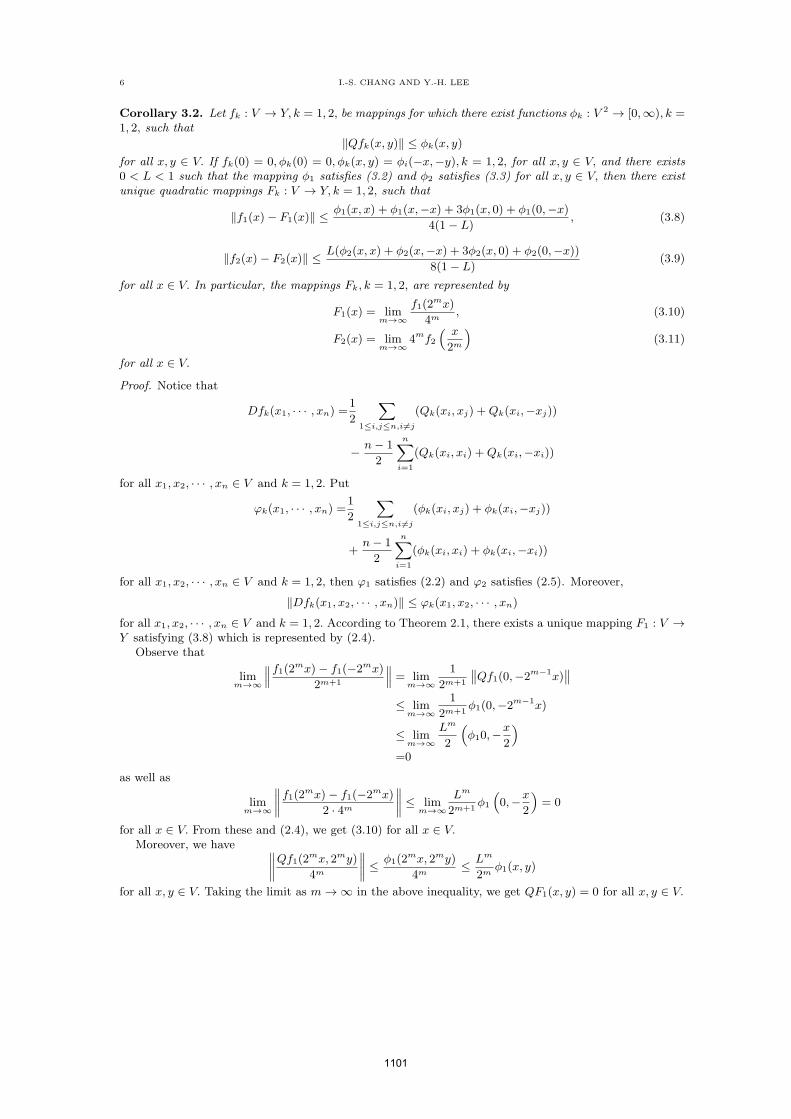
6 I.-S. CHANG AND Y.-H. LEE
Corollary 3.2. Let fk : V → Y, k = 1, 2, be mappings for which there exist functions ϕk : V 2 → [0,∞), k =1, 2, such that
∥Qfk(x, y)∥ ≤ ϕk(x, y)
for all x, y ∈ V. If fk(0) = 0, ϕk(0) = 0, ϕk(x, y) = ϕi(−x,−y), k = 1, 2, for all x, y ∈ V, and there exists0 < L < 1 such that the mapping ϕ1 satisfies (3.2) and ϕ2 satisfies (3.3) for all x, y ∈ V, then there existunique quadratic mappings Fk : V → Y, k = 1, 2, such that
∥f1(x)− F1(x)∥ ≤ ϕ1(x, x) + ϕ1(x,−x) + 3ϕ1(x, 0) + ϕ1(0,−x)4(1− L)
, (3.8)
∥f2(x)− F2(x)∥ ≤ L(ϕ2(x, x) + ϕ2(x,−x) + 3ϕ2(x, 0) + ϕ2(0,−x))8(1− L)
(3.9)
for all x ∈ V. In particular, the mappings Fk, k = 1, 2, are represented by
F1(x) = limm→∞
f1(2mx)
4m, (3.10)
F2(x) = limm→∞
4mf2( x
2m
)(3.11)
for all x ∈ V.
Proof. Notice that
Dfk(x1, · · · , xn) =1
2
∑1≤i,j≤n,i =j
(Qk(xi, xj) +Qk(xi,−xj))
− n− 1
2
n∑i=1
(Qk(xi, xi) +Qk(xi,−xi))
for all x1, x2, · · · , xn ∈ V and k = 1, 2. Put
φk(x1, · · · , xn) =1
2
∑1≤i,j≤n,i =j
(ϕk(xi, xj) + ϕk(xi,−xj))
+n− 1
2
n∑i=1
(ϕk(xi, xi) + ϕk(xi,−xi))
for all x1, x2, · · · , xn ∈ V and k = 1, 2, then φ1 satisfies (2.2) and φ2 satisfies (2.5). Moreover,
∥Dfk(x1, x2, · · · , xn)∥ ≤ φk(x1, x2, · · · , xn)
for all x1, x2, · · · , xn ∈ V and k = 1, 2. According to Theorem 2.1, there exists a unique mapping F1 : V →Y satisfying (3.8) which is represented by (2.4).
Observe that
limm→∞
∥∥∥f1(2mx)− f1(−2mx)
2m+1
∥∥∥ = limm→∞
1
2m+1
∥∥Qf1(0,−2m−1x)∥∥
≤ limm→∞
1
2m+1ϕ1(0,−2m−1x)
≤ limm→∞
Lm
2
(ϕ10,−
x
2
)=0
as well as
limm→∞
∥∥∥∥f1(2mx)− f1(−2mx)
2 · 4m
∥∥∥∥ ≤ limm→∞
Lm
2m+1ϕ1
(0,−x
2
)= 0
for all x ∈ V. From these and (2.4), we get (3.10) for all x ∈ V.Moreover, we have ∥∥∥∥Qf1(2mx, 2my)4m
∥∥∥∥ ≤ ϕ1(2mx, 2my)
4m≤ Lm
2mϕ1(x, y)
for all x, y ∈ V. Taking the limit as m→ ∞ in the above inequality, we get QF1(x, y) = 0 for all x, y ∈ V.
1101
STABILITY FOR AN n-DIMENSIONAL FUNCTIONAL EQUATION OF QUADRATIC-ADDITIVE TYPE 7
On the other hand, according to Theorem 2.2, there exists a unique mapping F2 : V → Y satisfying(3.9) which is represented by (2.7).
Observe that
4m∥∥∥f2 ( x
2m
)− f2
(− x
2m
)∥∥∥ =4m∥∥∥Qf2 (0,− x
2m+1
)∥∥∥≤4mϕ2
(0,− x
2m+1
)≤Lmϕ2
(0,−x
2
)for all x ∈ V. It leads us to get
limm→∞
4m(f2
( x
2m
)− f2
(− x
2m
))= 0, lim
m→∞2m
(f2
( x
2m
)− f2
(− x
2m
))= 0
for all x ∈ V. From these and (2.7), we obtain (3.11).Moreover, we have ∥∥∥4mQf2 ( x
2m,y
2m
)∥∥∥ ≤ 4mϕ2
( x
2m,y
2m
)≤ Lmϕ2(x, y)
for all x, y ∈ V. Taking the limit as m→ ∞ in the above inequality, we get QF2(x, y) = 0 for all x, y ∈ V,which completes the proof.
Corollary 3.3. Let X be a normed space and Y a Banach space. Suppose that the mapping f : X → Ysatisfies the inequality
∥Df(x1, x2, · · · , xn)∥ ≤ ∥x1∥p + ∥x2∥p + · · ·+ ∥xn∥p
for all x1, x2, · · · , xn ∈ X, where p ∈ (0, 1)∪ (2,∞). Then there exists a unique quadratic-additive mappingF : X → Y such that
∥f(x)− F (x)∥ ≤
∥x∥p
(n−1)(2p−4)if p > 2,
∥x∥p(n−1)(2−2p)
if p < 1
for all x ∈ X.
Proof. This follows from Theorem 2.1 and Theorem 2.2, by putting
φ(x1, x2, · · · , xn) := ∥x1∥p + ∥x2∥p + · · ·+ ∥xn∥p
for all x1, x2, · · · , xn ∈ X with L = 2p−1 < 1 if 0 < p < 1 and L = 22−p < 1 if p > 2.
Corollary 3.4. Let X be a normd space and Y a Banach space. Suppose that the mapping f : X → Ysatisfies the inequality
∥Df(x1, x2, · · · , xn)∥ ≤ θ∥x1∥p1∥x2∥p2 · · · ∥xn∥pn
for all x1, x2, · · · , xn ∈ X, where θ ≥ 0 and p1, p2, · · · , pn, p1 + p2 + · · · + pn ∈ (0, 1) ∪ (2,∞). Then f isitself a quadratic additive mapping.
Proof. This follows from Theorem 2.1 and Theorem 2.2, by letting
φ(x1, x2, · · · , xn) := ∥x1∥p1∥x2∥p2 · · · ∥xn∥pn
for all x1, x2, · · · , xn ∈ X with L = 2p−1 < 1 if 0 < p < 1 and L = 22−p < 1 if p > 2. References
[1] T. Aoki, On the stability of the linear mapping in Banach spaces, J. Math. Soc. Japan 2 (1950), 64–66.[2] L. Cadariu and V. Radu, Fixed points and the stability of Jensen’s functional equation, J. Inequal. Pure Appl.
Math. 4 (2003), Art. 4.[3] L. Cadariu and V. Radu, Fixed points and the stability of quadratic functional equations, An. Univ. Timisoara Ser.
Mat.-Inform. 41 (2003), 25–48.[4] L. Cadariu and V. Radu, On the stability of the Cauchy functional equation : a fixed point approach in iteration
theory, Grazer Mathematische Berichte, Karl-Franzens-Universitaet, Graz, Graz, Austria 346 (2004), 43–52.[5] P. Gavruta, A generalization of the Hyers-Ulam-Rassias stability of approximately additive mappings, J. Math.
Anal. Appl. 184 (1994), 431–436.[6] D.H. Hyers, On the stability of the linear functional equation, Proc. Natl. Acad. Sci. USA 27 (1941), 222–224.[7] G.-H. Kim, On the stability of functional equations with square-symmetric operation, Math. Inequal. Appl. 4
(2001), 257–266.[8] H.-M. Kim, On the stability problem for a mixed type of quartic and quadratic functional equation, J. Math. Anal.
Appl. 324 (2006), 358–372.
1102
8 I.-S. CHANG AND Y.-H. LEE
[9] Y.-H. Lee, On the stability of the monomial functional equation, Bull. Korean Math. Soc. 45 (2008), 397–403.[10] Y.H. Lee and K.W. Jun, A generalization of the Hyers-Ulam-Rassias stability of Jensen’s equation, J. Math. Anal.
Appl. 238 (1999), 305–315.[11] Y.H. Lee and K.W. Jun, A generalization of the Hyers-Ulam-Rassias stability of Pexider equation, J. Math. Anal.
Appl. 246 (2000), 627–638.[12] Y.-H. Lee and K.W. Jun, A note on the Hyers-Ulam-Rassias stability of Pexider equation, Korean Math. Soc. 37
(2000), 111–124[13] Y.-H. Lee and K.W. Jun, On the stability of approximately additive mappings, Proc. Amer. Math. Soc. 128 (2000),
1361–1369.[14] B. Margolis and J.B. Diaz, A fixed point theorem of the alternative for contractions on a generalized complete
metric space, Bull. Amer. Math. Soc. 74 (1968), 305–309.[15] Th.M. Rassias, On the stability of the linear mapping in Banach spaces, Proc. Amer. Math. Soc. 72 (1978), 297–300.[16] I.A. Rus, Principles and applications of fixed point theory, Ed. Dacia, Cluj-Napoca, (1979) (in Romanian).[17] S.M. Ulam, A collection of mathematical problems, Interscience, New York, (1968).
Ick-Soon Chang, Department of Mathematics, Mokwon University, Daejeon 302-729, Republic of Korea.E-mail address: [email protected]
Yang-Hi Lee, Department of Mathematics Education, Gongju National University of Education, Gongju 314-711,Republic of Korea.
E-mail address: [email protected]
1103
An identity of the q-Euler polynomials associated with thep-adic q-integrals on Zp
C. S. Ryoo
Department of Mathematics, Hannam University, Daejeon 306-791, Korea
Abstract : We introduce the q-Euler numbers and polynomials. By using these numbers andpolynomials, we investigate the alternating sums of powers of consecutive integers. By applyingthe symmetry of the fermionic p-adic q-integral on Zp, we give recurrence identities the q-Eulerpolynomials and q-analogue of alternating sums of powers of consecutive integers.
2000 Mathematics Subject Classification - 11B68, 11S40, 11S80.
Key words : Euler numbers and polynomials, q-Euler numbers and polynomials, alternating sums.
1. Introduction
Throughout this paper, we always make use of the following notations: C denotes the set ofcomplex numbers, Zp denotes the ring of p-adic rational integers, Qp denotes the field of p-adicrational numbers, and Cp denotes the completion of algebraic closure of Qp.
Let νp be the normalized exponential valuation of Cp with |p|p = p−νp(p) = p−1. When onetalks of q-extension, q is considered in many ways such as an indeterminate, a complex numberq ∈ C, or p-adic number q ∈ Cp. If q ∈ C one normally assume that |q| < 1. If q ∈ Cp, we normallyassume that |q − 1|p < p−
1p−1 so that qx = exp(x log q) for |x|p ≤ 1. For
g ∈ UD(Zp) = g|g : Zp → Cp is uniformly differentiable function,
the fermionic p-adic q-integral on Zp is defined by Kim as follows:
I−q(g) =∫
Zp
g(x)dμ−q(x) = limN→∞
[2]q1 + qpN
pN−1∑
x=0
g(x)(−q)x, see [1-10] . (1.1)
If we take g1(x) = g(x + 1) in (1.1), then we easily see that
qI−q(g1) + I−q(g) = [2]qg(0). (1.2)
For q ∈ Cp with |1 − q|p ≤ 1, the q-Euler polynomials ˜En,q(x) are defined by
˜Fq(x, t) =∞∑
n=0
˜En,q(x)tn
n!=
[2]qqet + 1
ext. (1.3)
The q-Euler numbers ˜En,q are defined by the generating function:
˜Fq(t) =∞∑
n=0
˜En,qtn
n!=
[2]qqet + 1
. (1.4)
The following elementary properties of the q-Euler numbers ˜En,q and polynomials ˜En,q(x) are readilyderived form (1.1), (1.2), (1.3) and (1.4). We, therefore, choose to omit details involved.
1104
J. COMPUTATIONAL ANALYSIS AND APPLICATIONS, VOL. 15, NO.6, 1104-1109, 2013, COPYRIGHT 2013 EUDOXUS PRESS, LLC
Theorem 1(Witt formula). For q ∈ Cp with |1 − q|p < 1, we have
˜En,q =∫
Zp
xndμ−q(x),
˜En,q(x) =∫
Zp
(x + y)ndμ−q(y).
Theorem 2. For any positive integer n, we have
˜En,q(x) =n∑
k=0
(
n
k
)
˜Ek,qxn−k.
2. The alternating sums of powers of consecutive q-integers
Let q be a complex number with |q| < 1. By using (1.3), we give the alternating sums of powersof consecutive q-integers as follows:
∞∑
n=0
˜En,qtn
n!=
[2]qqet + 1
= [2]q∞∑
n=0
(−1)nqnent.
From the above, we obtain
−∞∑
n=0
(−1)nqne(n+k)t +∞∑
n=0
(−1)n−kqn−kent =k−1∑
n=0
(−1)n−kqn−kent.
Thus, we have
− [2]q∞∑
n=0
(−1)nqne(n+k)t + [2]q(−1)−kq−k∞∑
n=0
(−1)nqnent
= [2]q(−1)−kq−kk−1∑
n=0
(−1)nqnent.
(2.1)
By using (1.3)and (1.4), and (2.1), we obtain
−∞∑
j=0
˜Ej,q(k)tj
j!+ (−1)−kq−k
∞∑
j=0
˜Ej,qtj
j!= [2]q
∞∑
j=0
(
(−1)−kq−kk−1∑
n=0
(−1)nqnnj
)
tj
j!.
By comparing coefficients oftj
j!in the above equation, we obtain
k−1∑
n=0
(−1)nqnnj =(−1)k+1qk
˜Ej,q(k) + ˜Ej,q
[2]q.
By using the above equation we arrive at the following theorem:
Theorem 3. Let k be a positive integer and q ∈ C with |q| < 1. Then we obtain
˜Tj,q(k − 1) =k−1∑
n=0
(−1)nqnnj =(−1)k+1qk
˜Ej,q(k) + ˜Ej,q
[2]q.
Remark 4. Let k be a positive integer and q ∈ C with |q| < 1. Then we have
limq→1
˜Tj,q(k − 1) =k−1∑
n=0
(−1)nnj =(−1)k+1Ej(k) + Ej
2,
RYOO: q-EULER POLYNOMIALS
1105
where Ej(x) and Ej denote the Euler polynomials and Euler numbers, respectively.
Next, we assume that q ∈ Cp. We obtain recurrence identities the q-Euler polynomials and theq-analogue of alternating sums of powers of consecutive integers.
By using (1.1), we have
qnI−q(gn) + (−1)n−1I−q(g) = [2]qn−1∑
l=0
(−1)n−1−lqlg(l),
where gn(x) = g(x + n). If n is odd from the above, we obtain
qnI−q(gn) + I−q(g) = [2]qn−1∑
l=0
(−1)n−1−lqlg(l) (cf. [1-5]). (2.2)
It will be more convenient to write (2.2) as the equivalent integral form
qn
∫
Zp
g(x + n)dμ−q(x) +∫
Zp
g(x)dμ−q(x) = [2]qn−1∑
k=0
(−1)kqkg(k). (2.3)
Substituting g(x) = ext into the above, we obtain
qn
∫
Zp
e(x+n)tdμ−q(x) +∫
Zp
extdμ−q(x) = [2]qn−1∑
j=0
(−1)jqjejt. (2.4)
After some elementary calculations, we have∫
Zp
extdμ−q(x) =[2]q
qet + 1,
∫
Zp
e(x+n)tdμ−q(x) = ent [2]qqet + 1
.
(2.5)
By using (2.4) and (2.5), we have
qn
∫
Zp
e(x+n)tdμ−q(x) +∫
Zp
extdμ−q(x) =[2]q(1 + qnent)
qet + 1.
From the above, we get[2]q(1 + qnent)
qet + 1=
[2]q∫
Zpextdμ−q(x)
∫
Zpq(n−1)xentxdμ−q(x)
. (2.6)
By substituting Taylor series of ext into (2.4), we obtain
∞∑
m=0
(
qn
∫
Zp
(x + n)mdμ−q(x) +∫
Zp
xmdμ−q(x)
)
tm
m!
=∞∑
m=0
⎛
⎝[2]qn−1∑
j=0
(−1)jqjjm
⎞
⎠
tm
m!.
By comparing coefficientstm
m!in the above equation, we obtain
qnm∑
k=0
(
m
k
)
nm−k
∫
Zp
xkdμ−q(x) +∫
Zp
xmdμ−q(x) = [2]qn−1∑
j=0
(−1)jqjjm.
By using Theorem 3, we have
qnm∑
k=0
(
m
k
)
nm−k
∫
Zp
xkdμ−q(x) +∫
Zp
xmdμ−q(x) = [2]q ˜Tm,q(n − 1). (2.7)
RYOO: q-EULER POLYNOMIALS
1106
By using (2.6) and (2.7), we arrive at the following theorem:
Theorem 5. Let n be odd positive integer. Then we have∫
Zpextdμ−q(x)
∫
Zpq(n−1)xentxdμ−q(x)
=∞∑
m=0
(
˜Tm,q(n − 1)) tm
m!.
Let w1 and w2 be odd positive integers. By (2.5), Theorem 5, and after some elementarycalculations, we obtain the following theorem.
Theorem 6. Let w1 and w2 be odd positive integers. Then we have∫
Zpew2xtdμ−qw2 (x)
∫
Zpq(w1w2−1)xew1w2txdμ−q(x)
=[2]qw2
[2]q
∞∑
m=0
(
˜Tm,qw2 (w − 1)wm2
) tm
m!. (2.8)
By (1.1), we obtain∫
Zp
∫
Zpe(w1x1+w2x2+w1w2x)tdμ−qw1 (x1)dμ−qw2 (x2)
∫
Zpq(w1w2−1)xew1w2xtdμ−q(x)
=ew1w2xt
∫
Zpew1x1tdμ−qw1 (x1)
∫
Zpew2x2tdμ−qw2 (x2)
∫
Zpq(w1w2−1)xew1w2xtdμ−q(x)
.
(2.9)
By using (2.8) and (2.9), after elementary calculations, we obtain
a =
(
∫
Zp
e(w1x1+w1w2x)tdμ−qw1 (x1)
)( ∫
Zpex2w2tdμ−qw2 (x2)
∫
Zpq(w1w2−1)xew1w2xtdμ−q(x)
)
=
( ∞∑
m=0
˜Em,qw1 (w2x)wm1
tm
m!
)(
[2]qw2
[2]q
∞∑
m=0
˜Tm,qw2 (w1 − 1)wm2
tm
m!
)
.
(2.10)
By using Cauchy product in the above, we have
a =∞∑
m=0
⎛
⎝
[2]qw2
[2]q
m∑
j=0
(
m
j
)
˜Ej,qw1 (w2x)wj1˜Tm−j,qw2 (w1 − 1)wm−j
2
⎞
⎠
tm
m!. (2.11)
By using the symmetry in (2.10), we obtain
a =
(
∫
Zp
e(w2x2+w1w2x)tdμ−qw2 (x2)
)( ∫
Zpex1w1tdμ−qw1 (x1)
∫
Zpq(w1w2−1)xew1w2xtdμ−q(x)
)
=
( ∞∑
m=0
˜Em,qw1 (w1x)wm2
tm
m!
)(
[2]qw1
[2]q
∞∑
m=0
˜Tm,qw1 (w2 − 1)wm1
tm
m!
)
.
Thus we obtain
a =∞∑
m=0
⎛
⎝
[2]qw1
[2]q
m∑
j=0
(
m
j
)
˜Ej,qw2 ,(w1x)wj2˜Tm−j,qw1 (w2 − 1)wm−j
1
⎞
⎠
tm
m!. (2.12)
By comparing coefficientstm
m!in the both sides of (2.11) and (2.12), we arrive at the following
theorem.
RYOO: q-EULER POLYNOMIALS
1107
Theorem 7. Let w1 and w2 be odd positive integers. Then we obtain
[2]qw2
m∑
j=0
(
m
j
)
˜Ej,qw1 (w2x)wj1˜Tm−j,qw2 (w1 − 1)wm−j
2
= [2]qw1
m∑
j=0
(
m
j
)
˜Ej,qw2 (w1x)wj2˜Tm−j,qw1 (w2 − 1)wm−j
1 ,
where ˜Ek,q(x) and ˜Tm,q(k) denote the q-Euler polynomials and the q-analogue of alternating sumsof powers of consecutive integers, respectively.
By using Theorem 2, we have the following corollary.
Corollary 8. Let w1 and w2 be odd positive integers. Then we obtain
[2]qw1
m∑
j=0
j∑
k=0
(
m
j
)(
j
k
)
wm−k1 wj
2xj−k
˜Ek,qw2˜Tm−j,qw1 (w2 − 1)
= [2]qw2
m∑
j=0
j∑
k=0
(
m
j
)(
j
k
)
wj1w
m−k2 xj−k
˜Ek,qw1˜Tm−j,qw2 (w1 − 1).
By using (2.9), we have
a =
(
ew1w2xt
∫
Zp
ex1w1tdμ−qw1 (x1)
)( ∫
Zpex2w2tdμ−qw2 (x2)
∫
Zpq(w1w2−1)xew1w2xtdμ−q(x)
)
=[2]qw2
[2]q
w1−1∑
j=0
(−1)jqw2j
∫
Zp
e
(
x1+w2x+jw2
w1
)
(w1t)
dμ−qw1 (x1)
=∞∑
n=0
⎛
⎝
[2]qw2
[2]q
w1−1∑
j=0
(−1)jqw2j˜En,qw1
(
w2x + jw2
w1
)
wn1
⎞
⎠
tn
n!.
(2.13)
By using the symmetry property in (2.13), we also have
a =
(
ew1w2xt
∫
Zp
ex2w2tdμ−qw2 (x2)
)( ∫
Zpex1w1tdμ−qw1 (x1)
∫
Zpq(w1w2−1)xew1w2xtdμ−q(x)
)
=[2]qw1
[2]q
w2−1∑
j=0
(−1)jqw1j
∫
Zp
e
(
x2+w1x+jw1
w2
)
(w2t)
dμ−qw2 (x2)
=∞∑
n=0
⎛
⎝
[2]qw1
[2]q
w2−1∑
j=0
(−1)jqw1j˜En,qw2
(
w1x + jw1
w2
)
wn2
⎞
⎠
tn
n!.
(2.14)
By comparing coefficientstn
n!in the both sides of (2.13) and (2.14), we have the following theorem.
Theorem 9. Let w1 and w2 be odd positive integers. Then we have
[2]qw2
w1−1∑
j=0
(−1)jqw2j˜En,qw1
(
w2x + jw2
w1
)
wn1
=[2]qw1
w2−1∑
j=0
(−1)jqw1j˜En,qw2
(
w1x + jw1
w2
)
wn2 .
(2.15)
RYOO: q-EULER POLYNOMIALS
1108
Remark 10. Let w1 and w2 be odd positive integers. If q → 1, we have
w1−1∑
j=0
(−1)jEn
(
w2x + jw2
w1
)
wn1 =
w2−1∑
j=0
(−1)jEn
(
w1x + jw1
w2
)
wn2 .
Substituting w1 = 1 into (2.15), we arrive at the following corollary.
Corollary 11. Let w2 be odd positive integer. Then we obtain
˜En,q(x) =[2]q
[2]qw2
w2−1∑
j=0
(−1)jqj˜En,qw2
(
x + j
w2
)
wn2 .
ACKNOWLEDGEMENT
This paper has been supported by the 2013 Hannam University Research Fund.
REFERENCES
1. T. Kim, q-Volkenborn integration, Russ. J. Math. phys., 9(2002), 288-299.
2. T. Kim, Note on the Euler numbers and polynomials, Adv. Stud. Contemp. Math., 17(2008),131-136.
3. T. Kim, Some identities for the Bernoulli, the Euler and the Genocchi numbers and polyno-mials, Adv. Stud. Contemp. Math., 20(2010), 23-28.
4. T. Kim, Euler numbers and polynomials associated with zeta function, Abstr. Appl. Anal.,Art. ID 581582, (2008), pp. 1-11
5. S-H. Rim, T. Kim and C.S. Ryoo, On the alternating sums of powers of consecutive q-integers,Bull. Korean Math. Soc., 43(2006), 611-617.
6. C.S. Ryoo and Y.S. Yoo, A note on Euler numbers and polynomials, Journal of Concreteand Applicable Mathematics, 7(2009), 341-348.
7. C. S. Ryoo, Calculating zeros of the twisted Genocchi polynomials, Adv. Stud. Contemp.Math., 17(2008), 147-159.
8. C. S. Ryoo, Some identities of the twisted q-Euler numbers and polynomials associated withq-Bernstein polynomials, Proc. Jangjeon Math. Soc., 14(2011), 239-248.
9. C. S. Ryoo, Some relations between twisted q-Euler numbers and Bernstein polynomials,Adv. Stud. Contemp. Math, 21(2011), 217-223.
10. C.S. Ryoo, Calculating zeros of the second kind Euler polynomials, Journal of ComputationalAnalysis and Applications, 12(4)(1010), 828-833.
RYOO: q-EULER POLYNOMIALS
1109
Approximate septic and octic mappings in quasi-β-normed spaces
Tian Zhou Xu*School of Mathematics, Beijing Institute of Technology, Beijing 100081, P.R.China
E-mail addresses: [email protected], [email protected]
John Michael RassiasPedagogical Department E.E., Section of Mathematics and Informatics, National and Capodistrian
University of Athens,4, Agamemnonos Str., Aghia Paraskevi, Athens 15342, Greece
E-mail addresses: [email protected], [email protected], [email protected]
Abstract In this paper, we achieve the general solution of the septic and octic functional equations. Moreover, we prove
the stability of the septic and octic functional equations in quasi-β-normed spaces.
Keywords Quasi-β-normed spaces; Septic mapping; Octic mapping; (β, p)-Banach spaces; Hyers–Ulam stability.
MR(2000) Subject Classification: 39B52, 39B82.
1. Introduction and preliminaries
The concept of stability for a functional equation arises when one replaces a functional equation by an inequali-
ty which acts as a perturbation of the equation. The first stability problem concerning group homomorphisms was
raised by Ulam [1] in 1940 and affirmatively solved by Hyers [2]. The result of Hyers was generalized by Rassias [3]
for approximate linear mappings by allowing the Cauchy difference operator CDf(x, y) = f(x+y)− [f(x)+f(y)]
to be controlled by ϵ(∥x∥p + ∥y∥p). In 1994, a generalization of Rassias’ theorem was obtained by Gavruta [4],
who replaced ϵ(∥x∥p + ∥y∥p) by a general control function φ(x, y) in the spirit of Rassias’ approach. The reader
is referred to [5–20] and references therein for more information on stability of functional equations.
In this paper, we achieve the general solutions of the septic functional equation
f(x+4y)−7f(x+3y)+21f(x+2y)−35f(x+y)+35f(x)−21f(x−y)+7f(x−2y)−f(x−3y) = 5040f(y) (1.1)
and the octic functional equation
f(x+ 4y)− 8f(x+ 3y) + 28f(x+ 2y)− 56f(x+ y) + 70f(x)− 56f(x− y) + 28f(x− 2y)
−8f(x− 3y) + f(x− 4y) = 40320f(y).(1.2)
Moreover, we prove the stability of the septic and octic functional equations in quasi-β-normed spaces. Since
f(x) = x7 is a solutions of (1.1), we say it quintic functional equation. Similarly, f(x) = x8 is a solutions of
(1.2), we say it septic functional equation. Every solution of the septic or octic functional equation is said to be
a septic or an octic mapping, respectively.
Let us recall some basic concepts concerning quasi-β-normed spaces (see [9, 16]). Let β be a fix real number
with 0 < β ≤ 1 and let K denote either ℝ or C. Let X be a linear space over K. A quasi-β-norm ∥ · ∥ is a
real-valued function on X satisfying the following:
(1) ∥x∥ ≥ 0 for all x ∈ X and ∥x∥ = 0 if and only if x = 0.
(2) ∥λx∥ = |λ|β∥x∥ for all λ ∈ K and all x ∈ X.
(3) There is a constant K ≥ 1 such that ∥x+ y∥ ≤ K(∥x∥+ ∥y∥) for all x, y ∈ X.
A quasi-β-normed space is a pair (X, ∥ · ∥), where ∥ · ∥ is a quasi-β-norm on X. The smallest possible K is
called the modulus of concavity of ∥ · ∥. A quasi-β-Banach space is a complete quasi-β-normed space.
A quasi-β-norm ∥ · ∥ is called a (β, p)-norm (0 < p ≤ 1) if ∥x + y∥p ≤ ∥x∥p + ∥y∥p for all x, y ∈ X. In this
case, a quasi-β-Banach space is called a (β, p)-Banach space. We can refer to [13] for the concept of quasi-normed
spaces and p-Banach spaces.
Given a p-norm, the formula d(x, y) := ∥x− y∥p gives us a translation invariant metric on X. By the Aoki-
Rolewicz theorem, each quasi-norm is equivalent to some p-norm. Since it is much easier to work with p-norms
than quasi-norms, henceforth we restrict our attention mainly to p-norms.
*Corresponding author.The first author was supported by the National Natural Science Foundation of China (NNSFC)(Grant No. 11171022).
1110
J. COMPUTATIONAL ANALYSIS AND APPLICATIONS, VOL. 15, NO.6, 1110-1119, 2013, COPYRIGHT 2013 EUDOXUS PRESS, LLC
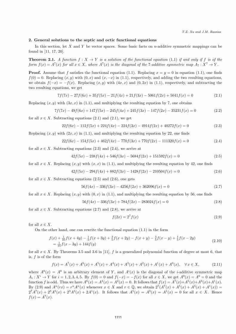
T.Z. Xu and J.M. Rassias
2. General solutions to the septic and octic functional equations
In this section, let X and Y be vector spaces. Some basic facts on n-additive symmetric mappings can be
found in [11, 17, 20].
Theorem 2.1. A function f : X → Y is a solution of the functional equation (1.1) if and only if f is of the
form f(x) = A7(x) for all x ∈ X, where A7(x) is the diagonal of the 7-additive symmetric map A7 : X7 → Y .
Proof. Assume that f satisfies the functional equation (1.1). Replacing x = y = 0 in equation (1.1), one finds
f(0) = 0. Replacing (x, y) with (0, x) and (x,−x) in (1.1), respectively, and adding the two resulting equations,
we obtain f(−x) = −f(x). Replacing (x, y) with (4x, x) and (0, 2x) in (1.1), respectively, and subtracting the
two resulting equations, we get
7f(7x)− 27f(6x) + 35f(5x)− 21f(4x) + 21f(3x)− 5061f(2x) + 5041f(x) = 0 (2.1)
Replacing (x, y) with (3x, x) in (1.1), and multiplying the resulting equation by 7, one obtains
7f(7x)− 49f(6x) + 147f(5x)− 245f(4x) + 245f(3x)− 147f(2x)− 35231f(x) = 0 (2.2)
for all x ∈ X. Subtracting equations (2.1) and (2.1), we get
22f(6x)− 112f(5x) + 224f(4x)− 224f(3x)− 4914f(2x) + 40272f(x) = 0 (2.3)
Replacing (x, y) with (2x, x) in (1.1), and multiplying the resulting equation by 22, one finds
22f(6x)− 154f(5x) + 462f(4x)− 770f(3x) + 770f(2x)− 111320f(x) = 0 (2.4)
for all x ∈ X. Subtracting equations (2.3) and (2.4), we arrive at
42f(5x)− 238f(4x) + 546f(3x)− 5684f(2x) + 151592f(x) = 0 (2.5)
for all x ∈ X. Replacing (x, y) with (x, x) in (1.1), and multiplying the resulting equation by 42, one finds
42f(5x)− 294f(4x) + 882f(3x)− 1428f(2x)− 210504f(x) = 0 (2.6)
for all x ∈ X. Subtracting equations (2.5) and (2.6), one gets
56f(4x)− 336f(3x)− 4256f(2x) + 362096f(x) = 0 (2.7)
for all x ∈ X. Replacing (x, y) with (0, x) in (1.1), and multiplying the resulting equation by 56, one finds
56f(4x)− 336f(3x) + 784f(2x)− 283024f(x) = 0 (2.8)
for all x ∈ X. Subtracting equations (2.7) and (2.8), we arrive at
f(2x) = 27f(x) (2.9)
for all x ∈ X.
On the other hand, one can rewrite the functional equation (1.1) in the form
f(x) + 135f(x+ 4y)− 1
5f(x+ 3y) + 35f(x+ 2y)− f(x+ y)− 3
5f(x− y) + 15f(x− 2y)
= 135f(x− 3y) + 144f(y)
(2.10)
for all x ∈ X. By Theorems 3.5 and 3.6 in [11], f is a generalized polynomial function of degree at most 6, that
is, f is of the form
f(x) = A7(x) +A6(x) +A5(x) +A4(x) +A3(x) +A2(x) +A1(x) +A0(x), ∀x ∈ X, (2.11)
where A0(x) = A0 is an arbitrary element of Y , and Ai(x) is the diagonal of the i-additive symmetric map
Ai : Xi → Y for i = 1, 2, 3, 4, 5. By f(0) = 0 and f(−x) = −f(x) for all x ∈ X, we get A0(x) = A0 = 0 and the
function f is odd. Thus we haveA6(x) = A4(x) = A2(x) = 0. It follows that f(x) = A7(x)+A5(x)+A3(x)+A1(x).
By (2.9) and An(rx) = rnAn(x) whenever x ∈ X and r ∈ Q, we obtain 27(A7(x) + A5(x) + A3(x) + A1(x)) =
27A7(x) + 25A5(x) + 23A3(x) + 2A1(x). It follows that A5(x) = A3(x) = A1(x) = 0 for all x ∈ X. Hence
f(x) = A7(x).
1111
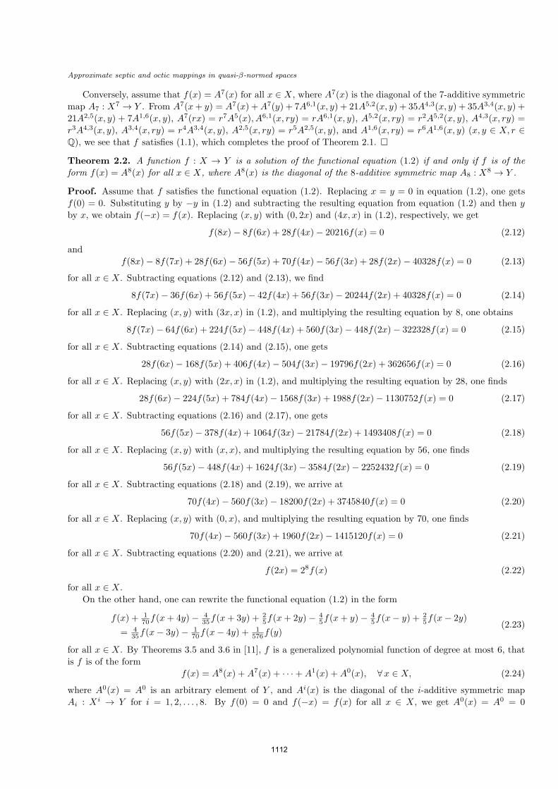
Approximate septic and octic mappings in quasi-β-normed spaces
Conversely, assume that f(x) = A7(x) for all x ∈ X, where A7(x) is the diagonal of the 7-additive symmetric
map A7 : X7 → Y . From A7(x+ y) = A7(x) +A7(y) + 7A6,1(x, y) + 21A5,2(x, y) + 35A4,3(x, y) + 35A3,4(x, y) +
21A2,5(x, y) + 7A1,6(x, y), A7(rx) = r7A5(x), A6,1(x, ry) = rA6,1(x, y), A5,2(x, ry) = r2A5,2(x, y), A4,3(x, ry) =
r3A4,3(x, y), A3,4(x, ry) = r4A3,4(x, y), A2,5(x, ry) = r5A2,5(x, y), and A1,6(x, ry) = r6A1,6(x, y) (x, y ∈ X, r ∈Q), we see that f satisfies (1.1), which completes the proof of Theorem 2.1.
Theorem 2.2. A function f : X → Y is a solution of the functional equation (1.2) if and only if f is of the
form f(x) = A8(x) for all x ∈ X, where A8(x) is the diagonal of the 8-additive symmetric map A8 : X8 → Y .
Proof. Assume that f satisfies the functional equation (1.2). Replacing x = y = 0 in equation (1.2), one gets
f(0) = 0. Substituting y by −y in (1.2) and subtracting the resulting equation from equation (1.2) and then y
by x, we obtain f(−x) = f(x). Replacing (x, y) with (0, 2x) and (4x, x) in (1.2), respectively, we get
f(8x)− 8f(6x) + 28f(4x)− 20216f(x) = 0 (2.12)
and
f(8x)− 8f(7x) + 28f(6x)− 56f(5x) + 70f(4x)− 56f(3x) + 28f(2x)− 40328f(x) = 0 (2.13)
for all x ∈ X. Subtracting equations (2.12) and (2.13), we find
8f(7x)− 36f(6x) + 56f(5x)− 42f(4x) + 56f(3x)− 20244f(2x) + 40328f(x) = 0 (2.14)
for all x ∈ X. Replacing (x, y) with (3x, x) in (1.2), and multiplying the resulting equation by 8, one obtains
8f(7x)− 64f(6x) + 224f(5x)− 448f(4x) + 560f(3x)− 448f(2x)− 322328f(x) = 0 (2.15)
for all x ∈ X. Subtracting equations (2.14) and (2.15), one gets
28f(6x)− 168f(5x) + 406f(4x)− 504f(3x)− 19796f(2x) + 362656f(x) = 0 (2.16)
for all x ∈ X. Replacing (x, y) with (2x, x) in (1.2), and multiplying the resulting equation by 28, one finds
28f(6x)− 224f(5x) + 784f(4x)− 1568f(3x) + 1988f(2x)− 1130752f(x) = 0 (2.17)
for all x ∈ X. Subtracting equations (2.16) and (2.17), one gets
56f(5x)− 378f(4x) + 1064f(3x)− 21784f(2x) + 1493408f(x) = 0 (2.18)
for all x ∈ X. Replacing (x, y) with (x, x), and multiplying the resulting equation by 56, one finds
56f(5x)− 448f(4x) + 1624f(3x)− 3584f(2x)− 2252432f(x) = 0 (2.19)
for all x ∈ X. Subtracting equations (2.18) and (2.19), we arrive at
70f(4x)− 560f(3x)− 18200f(2x) + 3745840f(x) = 0 (2.20)
for all x ∈ X. Replacing (x, y) with (0, x), and multiplying the resulting equation by 70, one finds
70f(4x)− 560f(3x) + 1960f(2x)− 1415120f(x) = 0 (2.21)
for all x ∈ X. Subtracting equations (2.20) and (2.21), we arrive at
f(2x) = 28f(x) (2.22)
for all x ∈ X.
On the other hand, one can rewrite the functional equation (1.2) in the form
f(x) + 170f(x+ 4y)− 4
35f(x+ 3y) + 25f(x+ 2y)− 4
5f(x+ y)− 45f(x− y) + 2
5f(x− 2y)
= 435f(x− 3y)− 1
70f(x− 4y) + 1576f(y)
(2.23)
for all x ∈ X. By Theorems 3.5 and 3.6 in [11], f is a generalized polynomial function of degree at most 6, that
is f is of the form
f(x) = A8(x) +A7(x) + · · ·+A1(x) +A0(x), ∀x ∈ X, (2.24)
where A0(x) = A0 is an arbitrary element of Y , and Ai(x) is the diagonal of the i-additive symmetric map
Ai : Xi → Y for i = 1, 2, . . . , 8. By f(0) = 0 and f(−x) = f(x) for all x ∈ X, we get A0(x) = A0 = 0
1112
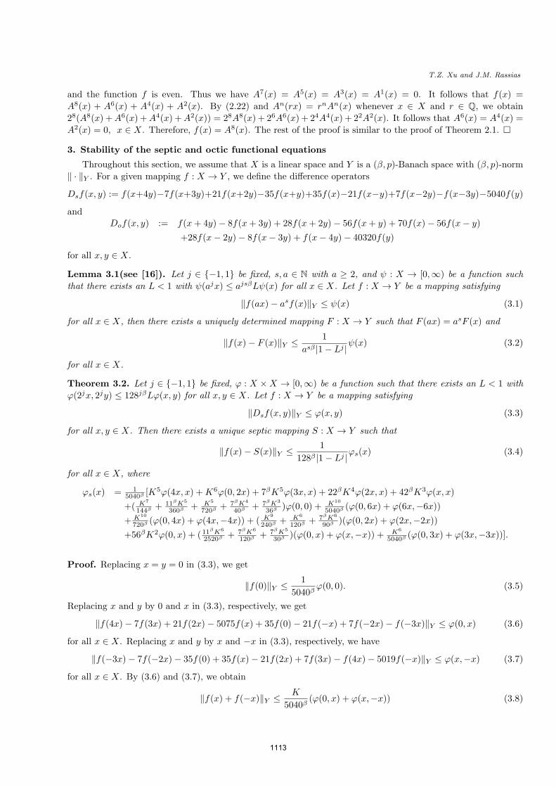
T.Z. Xu and J.M. Rassias
and the function f is even. Thus we have A7(x) = A5(x) = A3(x) = A1(x) = 0. It follows that f(x) =
A8(x) + A6(x) + A4(x) + A2(x). By (2.22) and An(rx) = rnAn(x) whenever x ∈ X and r ∈ Q, we obtain
28(A8(x) +A6(x) +A4(x) +A2(x)) = 28A8(x) + 26A6(x) + 24A4(x) + 22A2(x). It follows that A6(x) = A4(x) =
A2(x) = 0, x ∈ X. Therefore, f(x) = A8(x). The rest of the proof is similar to the proof of Theorem 2.1.
3. Stability of the septic and octic functional equations
Throughout this section, we assume that X is a linear space and Y is a (β, p)-Banach space with (β, p)-norm
∥ · ∥Y . For a given mapping f : X → Y , we define the difference operators
Dsf(x, y) := f(x+4y)−7f(x+3y)+21f(x+2y)−35f(x+y)+35f(x)−21f(x−y)+7f(x−2y)−f(x−3y)−5040f(y)
andDof(x, y) := f(x+ 4y)− 8f(x+ 3y) + 28f(x+ 2y)− 56f(x+ y) + 70f(x)− 56f(x− y)
+28f(x− 2y)− 8f(x− 3y) + f(x− 4y)− 40320f(y)
for all x, y ∈ X.
Lemma 3.1(see [16]). Let j ∈ −1, 1 be fixed, s, a ∈ N with a ≥ 2, and ψ : X → [0,∞) be a function such
that there exists an L < 1 with ψ(ajx) ≤ ajsβLψ(x) for all x ∈ X. Let f : X → Y be a mapping satisfying
∥f(ax)− asf(x)∥Y ≤ ψ(x) (3.1)
for all x ∈ X, then there exists a uniquely determined mapping F : X → Y such that F (ax) = asF (x) and
∥f(x)− F (x)∥Y ≤ 1
asβ |1− Lj |ψ(x) (3.2)
for all x ∈ X.
Theorem 3.2. Let j ∈ −1, 1 be fixed, φ : X ×X → [0,∞) be a function such that there exists an L < 1 with
φ(2jx, 2jy) ≤ 128jβLφ(x, y) for all x, y ∈ X. Let f : X → Y be a mapping satisfying
∥Dsf(x, y)∥Y ≤ φ(x, y) (3.3)
for all x, y ∈ X. Then there exists a unique septic mapping S : X → Y such that
∥f(x)− S(x)∥Y ≤ 1
128β |1− Lj |φs(x) (3.4)
for all x ∈ X, where
φs(x) = 15040β
[K5φ(4x, x) +K6φ(0, 2x) + 7βK5φ(3x, x) + 22βK4φ(2x, x) + 42βK3φ(x, x)
+( K7
144β+ 11βK5
360β+ K5
720β+ 7βK4
40β+ 7βK3
36β)φ(0, 0) + K10
5040β(φ(0, 6x) + φ(6x,−6x))
+ K10
720β(φ(0, 4x) + φ(4x,−4x)) + ( K9
240β+ K6
120β+ 7βK6
90β)(φ(0, 2x) + φ(2x,−2x))
+56βK2φ(0, x) + ( 11βK6
2520β+ 7βK6
120β+ 7βK5
30β)(φ(0, x) + φ(x,−x)) + K6
5040β(φ(0, 3x) + φ(3x,−3x))].
Proof. Replacing x = y = 0 in (3.3), we get
∥f(0)∥Y ≤ 1
5040βφ(0, 0). (3.5)
Replacing x and y by 0 and x in (3.3), respectively, we get
∥f(4x)− 7f(3x) + 21f(2x)− 5075f(x) + 35f(0)− 21f(−x) + 7f(−2x)− f(−3x)∥Y ≤ φ(0, x) (3.6)
for all x ∈ X. Replacing x and y by x and −x in (3.3), respectively, we have
∥f(−3x)− 7f(−2x)− 35f(0) + 35f(x)− 21f(2x) + 7f(3x)− f(4x)− 5019f(−x)∥Y ≤ φ(x,−x) (3.7)
for all x ∈ X. By (3.6) and (3.7), we obtain
∥f(x) + f(−x)∥Y ≤ K
5040β(φ(0, x) + φ(x,−x)) (3.8)
1113
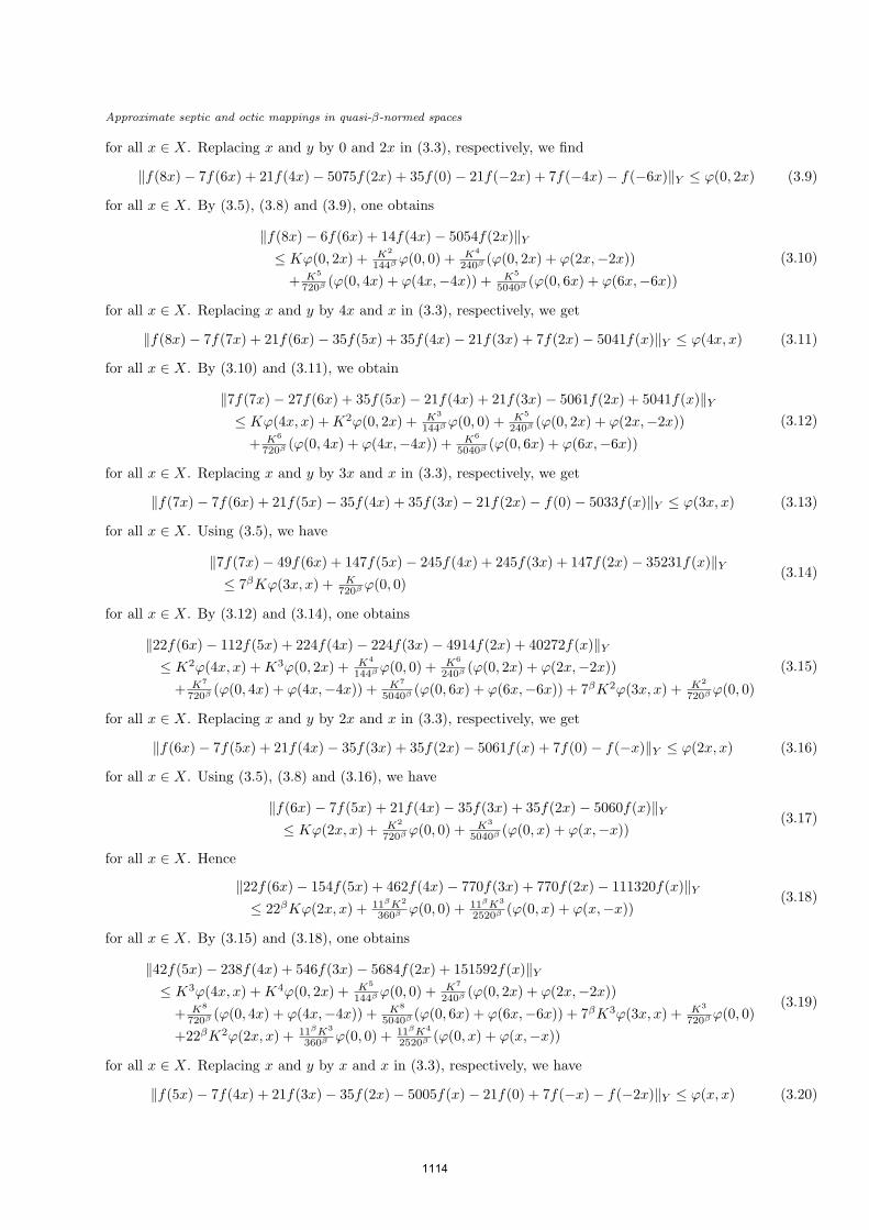
Approximate septic and octic mappings in quasi-β-normed spaces
for all x ∈ X. Replacing x and y by 0 and 2x in (3.3), respectively, we find
∥f(8x)− 7f(6x) + 21f(4x)− 5075f(2x) + 35f(0)− 21f(−2x) + 7f(−4x)− f(−6x)∥Y ≤ φ(0, 2x) (3.9)
for all x ∈ X. By (3.5), (3.8) and (3.9), one obtains
∥f(8x)− 6f(6x) + 14f(4x)− 5054f(2x)∥Y≤ Kφ(0, 2x) + K2
144βφ(0, 0) + K4
240β(φ(0, 2x) + φ(2x,−2x))
+ K5
720β(φ(0, 4x) + φ(4x,−4x)) + K5
5040β(φ(0, 6x) + φ(6x,−6x))
(3.10)
for all x ∈ X. Replacing x and y by 4x and x in (3.3), respectively, we get
∥f(8x)− 7f(7x) + 21f(6x)− 35f(5x) + 35f(4x)− 21f(3x) + 7f(2x)− 5041f(x)∥Y ≤ φ(4x, x) (3.11)
for all x ∈ X. By (3.10) and (3.11), we obtain
∥7f(7x)− 27f(6x) + 35f(5x)− 21f(4x) + 21f(3x)− 5061f(2x) + 5041f(x)∥Y≤ Kφ(4x, x) +K2φ(0, 2x) + K3
144βφ(0, 0) + K5
240β(φ(0, 2x) + φ(2x,−2x))
+ K6
720β(φ(0, 4x) + φ(4x,−4x)) + K6
5040β(φ(0, 6x) + φ(6x,−6x))
(3.12)
for all x ∈ X. Replacing x and y by 3x and x in (3.3), respectively, we get
∥f(7x)− 7f(6x) + 21f(5x)− 35f(4x) + 35f(3x)− 21f(2x)− f(0)− 5033f(x)∥Y ≤ φ(3x, x) (3.13)
for all x ∈ X. Using (3.5), we have
∥7f(7x)− 49f(6x) + 147f(5x)− 245f(4x) + 245f(3x) + 147f(2x)− 35231f(x)∥Y≤ 7βKφ(3x, x) + K
720βφ(0, 0)
(3.14)
for all x ∈ X. By (3.12) and (3.14), one obtains
∥22f(6x)− 112f(5x) + 224f(4x)− 224f(3x)− 4914f(2x) + 40272f(x)∥Y≤ K2φ(4x, x) +K3φ(0, 2x) + K4
144βφ(0, 0) + K6
240β(φ(0, 2x) + φ(2x,−2x))
+ K7
720β(φ(0, 4x) + φ(4x,−4x)) + K7
5040β(φ(0, 6x) + φ(6x,−6x)) + 7βK2φ(3x, x) + K2
720βφ(0, 0)
(3.15)
for all x ∈ X. Replacing x and y by 2x and x in (3.3), respectively, we get
∥f(6x)− 7f(5x) + 21f(4x)− 35f(3x) + 35f(2x)− 5061f(x) + 7f(0)− f(−x)∥Y ≤ φ(2x, x) (3.16)
for all x ∈ X. Using (3.5), (3.8) and (3.16), we have
∥f(6x)− 7f(5x) + 21f(4x)− 35f(3x) + 35f(2x)− 5060f(x)∥Y≤ Kφ(2x, x) + K2
720βφ(0, 0) + K3
5040β(φ(0, x) + φ(x,−x))
(3.17)
for all x ∈ X. Hence
∥22f(6x)− 154f(5x) + 462f(4x)− 770f(3x) + 770f(2x)− 111320f(x)∥Y≤ 22βKφ(2x, x) + 11βK2
360βφ(0, 0) + 11βK3
2520β(φ(0, x) + φ(x,−x))
(3.18)
for all x ∈ X. By (3.15) and (3.18), one obtains
∥42f(5x)− 238f(4x) + 546f(3x)− 5684f(2x) + 151592f(x)∥Y≤ K3φ(4x, x) +K4φ(0, 2x) + K5
144βφ(0, 0) + K7
240β(φ(0, 2x) + φ(2x,−2x))
+ K8
720β(φ(0, 4x) + φ(4x,−4x)) + K8
5040β(φ(0, 6x) + φ(6x,−6x)) + 7βK3φ(3x, x) + K3
720βφ(0, 0)
+22βK2φ(2x, x) + 11βK3
360βφ(0, 0) + 11βK4
2520β(φ(0, x) + φ(x,−x))
(3.19)
for all x ∈ X. Replacing x and y by x and x in (3.3), respectively, we have
∥f(5x)− 7f(4x) + 21f(3x)− 35f(2x)− 5005f(x)− 21f(0) + 7f(−x)− f(−2x)∥Y ≤ φ(x, x) (3.20)
1114
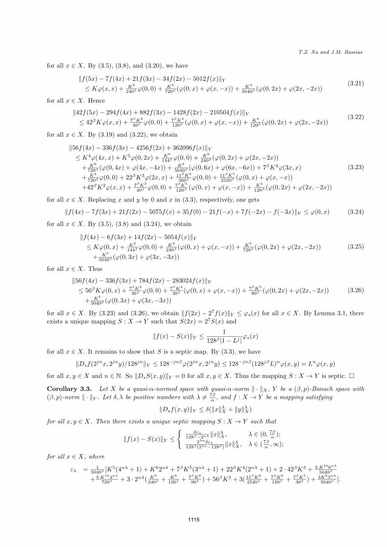
T.Z. Xu and J.M. Rassias
for all x ∈ X. By (3.5), (3.8), and (3.20), we have
∥f(5x)− 7f(4x) + 21f(3x)− 34f(2x)− 5012f(x)∥Y≤ Kφ(x, x) + K2
240βφ(0, 0) + K4
720β(φ(0, x) + φ(x,−x)) + K4
5040β(φ(0, 2x) + φ(2x,−2x))
(3.21)
for all x ∈ X. Hence
∥42f(5x)− 294f(4x) + 882f(3x)− 1428f(2x)− 210504f(x)∥Y≤ 42βKφ(x, x) + 7βK2
40βφ(0, 0) + 7βK4
120β(φ(0, x) + φ(x,−x)) + K4
120β(φ(0, 2x) + φ(2x,−2x))
(3.22)
for all x ∈ X. By (3.19) and (3.22), we obtain
∥56f(4x)− 336f(3x)− 4256f(2x) + 362096f(x)∥Y≤ K4φ(4x, x) +K5φ(0, 2x) + K6
144βφ(0, 0) + K8
240β(φ(0, 2x) + φ(2x,−2x))
+ K9
720β(φ(0, 4x) + φ(4x,−4x)) + K9
5040β(φ(0, 6x) + φ(6x,−6x)) + 7βK4φ(3x, x)
+ K4
720βφ(0, 0) + 22βK3φ(2x, x) + 11βK4
360βφ(0, 0) + 11βK5
2520β(φ(0, x) + φ(x,−x))
+42βK2φ(x, x) + 7βK3
40βφ(0, 0) + 7βK5
120β(φ(0, x) + φ(x,−x)) + K5
120β(φ(0, 2x) + φ(2x,−2x))
(3.23)
for all x ∈ X. Replacing x and y by 0 and x in (3.3), respectively, one gets
∥f(4x)− 7f(3x) + 21f(2x)− 5075f(x) + 35f(0)− 21f(−x) + 7f(−2x)− f(−3x)∥Y ≤ φ(0, x) (3.24)
for all x ∈ X. By (3.5), (3.8) and (3.24), we obtain
∥f(4x)− 6f(3x) + 14f(2x)− 5054f(x)∥Y≤ Kφ(0, x) + K2
144βφ(0, 0) + K4
240β(φ(0, x) + φ(x,−x)) + K5
720β(φ(0, 2x) + φ(2x,−2x))
+ K5
5040β(φ(0, 3x) + φ(3x,−3x))
(3.25)
for all x ∈ X. Thus
∥56f(4x)− 336f(3x) + 784f(2x)− 283024f(x)∥Y≤ 56βKφ(0, x) + 7βK2
36βφ(0, 0) + 7βK4
30β(φ(0, x) + φ(x,−x)) + 7βK5
90β(φ(0, 2x) + φ(2x,−2x))
+ K5
5040β(φ(0, 3x) + φ(3x,−3x))
(3.26)
for all x ∈ X. By (3.23) and (3.26), we obtain ∥f(2x) − 27f(x)∥Y ≤ φs(x) for all x ∈ X. By Lemma 3.1, there
exists a unique mapping S : X → Y such that S(2x) = 27S(x) and
∥f(x)− S(x)∥Y ≤ 1
128β |1− Lj |φs(x)
for all x ∈ X. It remains to show that S is a septic map. By (3.3), we have
∥Dsf(2jnx, 2jny)/128jn∥Y ≤ 128−jnβφ(2jnx, 2jny) ≤ 128−jnβ(128jβL)nφ(x, y) = Lnφ(x, y)
for all x, y ∈ X and n ∈ N. So ∥DsS(x, y)∥Y = 0 for all x, y ∈ X. Thus the mapping S : X → Y is septic.
Corollary 3.3. Let X be a quasi-α-normed space with quasi-α-norm ∥ · ∥X , Y be a (β, p)-Banach space with
(β, p)-norm ∥ · ∥Y . Let δ, λ be positive numbers with λ = 7β , and f : X → Y be a mapping satisfying
∥Dsf(x, y)∥Y ≤ δ(∥x∥λX + ∥y∥λX)
for all x, y ∈ X. Then there exists a unique septic mapping S : X → Y such that
∥f(x)− S(x)∥Y ≤
δελ
128β−2αλ ∥x∥λX , λ ∈ (0, 7β );2λαδελ
128β(2λα−128β)∥x∥λX , λ ∈ ( 7β ,∞);
for all x ∈ X, where
ελ = 15040β
[K5(4λ + 1) +K62λ + 7βK5(3λ + 1) + 22βK4(2λ + 1) + 2 · 42βK3 + 3⋅K106αλ
5040β
+ 3⋅K104αλ
720β+ 3 · 2λ( K9
240β+ K6
120β+ 7βK6
90β) + 56βK2 + 3( 11
βK6
2520β+ 7βK6
120β+ 7βK5
30β) + 3K63αλ
5040β].
1115
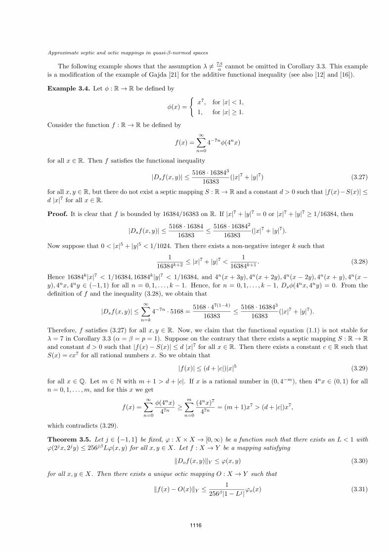
Approximate septic and octic mappings in quasi-β-normed spaces
The following example shows that the assumption λ = 7β cannot be omitted in Corollary 3.3. This example
is a modification of the example of Gajda [21] for the additive functional inequality (see also [12] and [16]).
Example 3.4. Let ϕ : ℝ → ℝ be defined by
ϕ(x) =
x7, for |x| < 1,
1, for |x| ≥ 1.
Consider the function f : ℝ → ℝ be defined by
f(x) =∞∑
n=0
4−7nϕ(4nx)
for all x ∈ ℝ. Then f satisfies the functional inequality
|Dsf(x, y)| ≤5168 · 163843
16383(|x|7 + |y|7) (3.27)
for all x, y ∈ ℝ, but there do not exist a septic mapping S : ℝ → ℝ and a constant d > 0 such that |f(x)−S(x)| ≤d |x|7 for all x ∈ ℝ.
Proof. It is clear that f is bounded by 16384/16383 on ℝ. If |x|7 + |y|7 = 0 or |x|7 + |y|7 ≥ 1/16384, then
|Dsf(x, y)| ≤5168 · 16384
16383≤ 5168 · 163842
16383(|x|7 + |y|7).
Now suppose that 0 < |x|5 + |y|5 < 1/1024. Then there exists a non-negative integer k such that
1
16384k+2≤ |x|7 + |y|7 < 1
16384k+1. (3.28)
Hence 16384k|x|7 < 1/16384, 16384k|y|7 < 1/16384, and 4n(x + 3y), 4n(x + 2y), 4n(x − 2y), 4n(x + y), 4n(x −y), 4nx, 4ny ∈ (−1, 1) for all n = 0, 1, . . . , k − 1. Hence, for n = 0, 1, . . . , k − 1, Dsϕ(4
nx, 4ny) = 0. From the
definition of f and the inequality (3.28), we obtain that
|Dsf(x, y)| ≤∞∑
n=k
4−7n · 5168 =5168 · 47(1−k)
16383≤ 5168 · 163843
16383(|x|7 + |y|7).
Therefore, f satisfies (3.27) for all x, y ∈ ℝ. Now, we claim that the functional equation (1.1) is not stable for
λ = 7 in Corollary 3.3 (α = β = p = 1). Suppose on the contrary that there exists a septic mapping S : ℝ → ℝand constant d > 0 such that |f(x)− S(x)| ≤ d |x|7 for all x ∈ ℝ. Then there exists a constant c ∈ ℝ such that
S(x) = cx7 for all rational numbers x. So we obtain that
|f(x)| ≤ (d+ |c|)|x|5 (3.29)
for all x ∈ Q. Let m ∈ N with m + 1 > d + |c|. If x is a rational number in (0, 4−m), then 4nx ∈ (0, 1) for all
n = 0, 1, . . . ,m, and for this x we get
f(x) =∞∑
n=0
ϕ(4nx)
47n≥
m∑n=0
(4nx)7
47n= (m+ 1)x7 > (d+ |c|)x7,
which contradicts (3.29).
Theorem 3.5. Let j ∈ −1, 1 be fixed, φ : X ×X → [0,∞) be a function such that there exists an L < 1 with
φ(2jx, 2jy) ≤ 256jβLφ(x, y) for all x, y ∈ X. Let f : X → Y be a mapping satisfying
∥Dof(x, y)∥Y ≤ φ(x, y) (3.30)
for all x, y ∈ X. Then there exists a unique octic mapping O : X → Y such that
∥f(x)−O(x)∥Y ≤ 1
256β |1− Lj |φo(x) (3.31)
1116
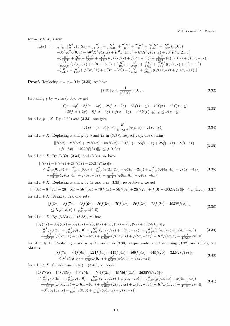
T.Z. Xu and J.M. Rassias
for all x ∈ X, where
φo(x) = 120160β
[K6
2βφ(0, 2x) + ( K7
1152β+ K6
40320β+ 7βK5
360β+ 7βK4
90β+ 35βK3
576β+ K6
630β)φ(0, 0)
+35βK2φ(0, x) + 56βK3φ(x, x) +K6φ(4x, x) + 8βK4φ(3x, x) + 28βK4φ(2x, x)
+( K9
1440β+ K7
90β+ 7βK6
288β+ K7
1440β)(φ(2x, 2x) + φ(2x,−2x)) + K11
10080β(φ(6x, 6x) + φ(6x,−6x))
+ K11
80640β(φ(8x, 8x) + φ(8x,−8x)) + ( K7
180β+ K7
5040β+ 7βK6
180β+ 7βK5
144β)(φ(x, x) + φ(x,−x))
+( K7
720β+ K7
144β)(φ(3x, 3x) + φ(3x,−3x)) + ( K7
1152β+ K10
2880β)(φ(4x, 4x) + φ(4x,−4x))].
Proof. Replacing x = y = 0 in (3.30), we have
∥f(0)∥Y ≤ 1
40320βφ(0, 0). (3.32)
Replacing y by −y in (3.30), we get
∥f(x− 4y)− 8f(x− 3y) + 28f(x− 2y)− 56f(x− y) + 70f(x)− 56f(x+ y)
+28f(x+ 2y)− 8f(x+ 3y) + f(x+ 4y)− 40320f(−y)∥Y ≤ φ(x,−y)(3.33)
for all x, y ∈ X. By (3.30) and (3.33), one gets
∥f(x)− f(−x)∥Y ≤ K
40320β(φ(x, x) + φ(x,−x)) (3.34)
for all x ∈ X. Replacing x and y by 0 and 2x in (3.30), respectively, one obtains
∥f(8x)− 8f(6x) + 28f(4x)− 56f(2x) + 70f(0)− 56f(−2x) + 28f(−4x)− 8f(−6x)
+f(−8x)− 40320f(2x)∥Y ≤ φ(0, 2x)(3.35)
for all x ∈ X. By (3.32), (3.34), and (3.35), we have
∥f(8x)− 8f(6x) + 28f(4x)− 20216f(2x)∥Y≤ K
2βφ(0, 2x) + K2
1152βφ(0, 0) + K4
1440β(φ(2x, 2x) + φ(2x,−2x)) + K5
2880β(φ(4x, 4x) + φ(4x,−4x))
+ K6
10080β(φ(6x, 6x) + φ(6x,−6x)) + K6
80640β(φ(8x, 8x) + φ(8x,−8x))
(3.36)
for all x ∈ X. Replacing x and y by 4x and x in (3.30), respectively, we get
∥f(8x)− 8f(7x) + 28f(6x)− 56f(5x) + 70f(4x)− 56f(3x) + 28f(2x) + f(0)− 40328f(x)∥Y ≤ φ(4x, x) (3.37)
for all x ∈ X. Using (3.32), one gets
∥f(8x)− 8f(7x) + 28f(6x)− 56f(5x) + 70f(4x)− 56f(3x) + 28f(2x)− 40328f(x)∥Y≤ Kφ(4x, x) + K
40320βφ(0, 0)
(3.38)
for all x ∈ X. By (3.36) and (3.38), we have
∥8f(7x)− 36f(6x) + 56f(5x)− 70f(4x) + 56f(3x)− 28f(2x) + 40328f(x)∥Y≤ K2
2βφ(0, 2x) + K3
1152βφ(0, 0) + K5
1440β(φ(2x, 2x) + φ(2x,−2x)) + K6
2880β(φ(4x, 4x) + φ(4x,−4x))
+ K7
10080β(φ(6x, 6x) + φ(6x,−6x)) + K7
80640β(φ(8x, 8x) + φ(8x,−8x)) +K2φ(4x, x) + K2
40320βφ(0, 0)
(3.39)
for all x ∈ X. Replacing x and y by 3x and x in (3.30), respectively, and then using (3.32) and (3.34), one
obtains∥8f(7x)− 64f(6x) + 224f(5x)− 448f(4x) + 560f(3x)− 448f(2x)− 322328f(x)∥Y≤ 8βφ(3x, x) + K2
630βφ(0, 0) + K3
5040β(φ(x, x) + φ(x,−x))
(3.40)
for all x ∈ X. Subtracting (3.39)− (3.40), we obtain
∥28f(6x)− 168f(5x) + 406f(4x)− 504f(3x)− 19796f(2x) + 362656f(x)∥Y≤ K3
2βφ(0, 2x) + K4
1152βφ(0, 0) + K6
1440β(φ(2x, 2x) + φ(2x,−2x)) + K7
2880β(φ(4x, 4x) + φ(4x,−4x))
+ K8
10080β(φ(6x, 6x) + φ(6x,−6x)) + K8
80640β(φ(8x, 8x) + φ(8x,−8x)) +K3φ(4x, x) + K3
40320βφ(0, 0)
+8βKφ(3x, x) + K3
630βφ(0, 0) + K4
5040β(φ(x, x) + φ(x,−x))
(3.41)
1117
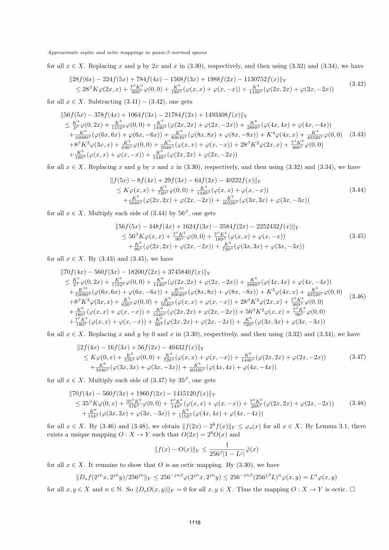
Approximate septic and octic mappings in quasi-β-normed spaces
for all x ∈ X. Replacing x and y by 2x and x in (3.30), respectively, and then using (3.32) and (3.34), we have
∥28f(6x)− 224f(5x) + 784f(4x)− 1568f(3x) + 1988f(2x)− 1130752f(x)∥Y≤ 28βKφ(2x, x) + 7βK2
360βφ(0, 0) + K4
180β(φ(x, x) + φ(x,−x)) + K4
1440β(φ(2x, 2x) + φ(2x,−2x))
(3.42)
for all x ∈ X. Subtracting (3.41)− (3.42), one gets
∥56f(5x)− 378f(4x) + 1064f(3x)− 21784f(2x) + 1493408f(x)∥Y≤ K4
2βφ(0, 2x) + K5
1152βφ(0, 0) + K7
1440β(φ(2x, 2x) + φ(2x,−2x)) + K8
2880β(φ(4x, 4x) + φ(4x,−4x))
+ K9
10080β(φ(6x, 6x) + φ(6x,−6x)) + K9
80640β(φ(8x, 8x) + φ(8x,−8x)) +K4φ(4x, x) + K4
40320βφ(0, 0)
+8βK2φ(3x, x) + K4
630βφ(0, 0) + K5
5040β(φ(x, x) + φ(x,−x)) + 28βK2φ(2x, x) + 7βK3
360βφ(0, 0)
+ K5
180β(φ(x, x) + φ(x,−x)) + K5
1440β(φ(2x, 2x) + φ(2x,−2x))
(3.43)
for all x ∈ X. Replacing x and y by x and x in (3.30), respectively, and then using (3.32) and (3.34), we have
∥f(5x)− 8f(4x) + 29f(3x)− 64f(2x)− 40222f(x)∥Y≤ Kφ(x, x) + K2
720βφ(0, 0) + K4
1440β(φ(x, x) + φ(x,−x))
+ K5
5040β(φ(2x, 2x) + φ(2x,−2x)) + K5
40320β(φ(3x, 3x) + φ(3x,−3x))
(3.44)
for all x ∈ X. Multiply each side of (3.44) by 56β , one gets
∥56f(5x)− 448f(4x) + 1624f(3x)− 3584f(2x)− 2252432f(x)∥Y≤ 56βKφ(x, x) + 7βK2
90βφ(0, 0) + 7βK4
180β(φ(x, x) + φ(x,−x))
+K5
90β(φ(2x, 2x) + φ(2x,−2x)) + K5
720β(φ(3x, 3x) + φ(3x,−3x))
(3.45)
for all x ∈ X. By (3.43) and (3.45), we have
∥70f(4x)− 560f(3x)− 18200f(2x) + 3745840f(x)∥Y≤ K5
2βφ(0, 2x) + K6
1152βφ(0, 0) + K8
1440β(φ(2x, 2x) + φ(2x,−2x)) + K9
2880β(φ(4x, 4x) + φ(4x,−4x))
+ K10
10080β(φ(6x, 6x) + φ(6x,−6x)) + K10
80640β(φ(8x, 8x) + φ(8x,−8x)) +K5φ(4x, x) + K5
40320βφ(0, 0)
+8βK3φ(3x, x) + K5
630βφ(0, 0) + K6
5040β(φ(x, x) + φ(x,−x)) + 28βK3φ(2x, x) + 7βK4
360βφ(0, 0)
+ K6
180β(φ(x, x) + φ(x,−x)) + K6
1440β(φ(2x, 2x) + φ(2x,−2x)) + 56βK2φ(x, x) + 7βK3
90βφ(0, 0)
+7βK5
180β(φ(x, x) + φ(x,−x)) + K6
90β(φ(2x, 2x) + φ(2x,−2x)) + K6
720β(φ(3x, 3x) + φ(3x,−3x))
(3.46)
for all x ∈ X. Replacing x and y by 0 and x in (3.30), respectively, and then using (3.32) and (3.34), we have
∥2f(4x)− 16f(3x) + 56f(2x)− 40432f(x)∥Y≤ Kφ(0, x) + K2
576βφ(0, 0) + K4
720β(φ(x, x) + φ(x,−x)) + K5
1440β(φ(2x, 2x) + φ(2x,−2x))
+ K6
5040β(φ(3x, 3x) + φ(3x,−3x)) + K6
40320β(φ(4x, 4x) + φ(4x,−4x))
(3.47)
for all x ∈ X. Multiply each side of (3.47) by 35β , one gets
∥70f(4x)− 560f(3x) + 1960f(2x)− 1415120f(x)∥Y≤ 35βKφ(0, x) + 35βK2
576βφ(0, 0) + 7βK4
144β(φ(x, x) + φ(x,−x)) + 7βK5
288β(φ(2x, 2x) + φ(2x,−2x))
+ K6
144β(φ(3x, 3x) + φ(3x,−3x)) + K6
1152β(φ(4x, 4x) + φ(4x,−4x))
(3.48)
for all x ∈ X. By (3.46) and (3.48), we obtain ∥f(2x)− 28f(x)∥Y ≤ φo(x) for all x ∈ X. By Lemma 3.1, there
exists a unique mapping O : X → Y such that O(2x) = 28O(x) and
∥f(x)−O(x)∥Y ≤ 1
256β |1− Lj |φ(x)
for all x ∈ X. It remains to show that O is an octic mapping. By (3.30), we have
∥Dof(2jnx, 2jny)/256jn∥Y ≤ 256−jnβφ(2jnx, 2jny) ≤ 256−jnβ(256jβL)nφ(x, y) = Lnφ(x, y)
for all x, y ∈ X and n ∈ N. So ∥DoO(x, y)∥Y = 0 for all x, y ∈ X. Thus the mapping O : X → Y is octic.
1118
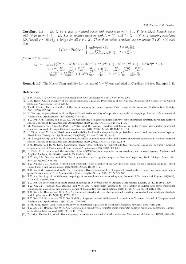
T.Z. Xu and J.M. Rassias
Corollary 3.6. Let X be a quasi-α-normed space with quasi-α-norm ∥ · ∥X , Y be a (β, p)-Banach space
with (β, p)-norm ∥ · ∥Y . Let δ, λ be positive numbers with λ = 8β , and f : X → Y be a mapping satisfying
∥Dof(x, y)∥Y ≤ δ(∥x∥λX + ∥y∥λX) for all x, y ∈ X. Then there exists a unique octic mapping O : X → Y such
that
∥f(x)−O(x)∥Y ≤
δελ
256β−2αλ ∥x∥λX , λ ∈ (0, 8β );2λαδελ
256β(2λα−256β)∥x∥λX , λ ∈ ( 8β ,∞);
for all x ∈ X, where
ελ = 120160β
[K6
2β2λ + 35βK2 + 2 · 56βK3 +K6(4λ + 1) + 8βK4(3λ + 1) + 28βK4(2λ + 1)
+4 · 2λ( K9
1440β+ K7
90β+ 7βK6
288β+ K7
1440β) + 4( K7
180β+ K7
5040β+ 7βK6
180β+ 7βK5
144β)
+4⋅K116αλ
10080β+ 4⋅K118αλ
80640β+ 4 · 3λ( K7
720β+ K7
144β) + 4 · 4λ( K7
1152β+ K10
2880β)].
Remark 3.7. The Hyers–Ulam stability for the case of λ = 8β was excluded in Corollary 3.6 (see Example 3.4).
References
[1] S.M. Ulam, A Collection of Mathematical Problems, Interscience Publ., New York, 1960.
[2] D.H. Hyers, On the stability of the linear functional equation, Proceedings of the National Academy of Sciences of the United
States of America, 27(1941) 222-224.
[3] Th.M. Rassias, On the stability of the linear mapping in Banach spaces, Proceedings of the American Mathematical Society,
72(2)(1978) 297–300.
[4] P. Gavruta, A generalization of the Hyers-Ulam-Rassias stability of approximately additive mappings, Journal of Mathematical
Analysis and Applications, 184(3)(1994) 431–436.
[5] T.Z. Xu, J.M. Rassias, and W.X. Xu, On the stability of a general mixed additive-cubic functional equation in random normed
spaces, Journal of Inequalities and Applications, 2010(2010), Article ID 328473, 1–16.
[6] M. Mohamadi, Y.J. Cho, C. Park, P. Vetro, and R. Saadati, Random stability of an additive-quadratic quartic functional
equation, Journal of Inequalities and Applications, 2010(2010), Article ID 754210, 1–18.
[7] L. Cadariu and V. Radu, Fixed points and stability for functional equations in probabilistic metric and random normed spaces,
Fixed Point Theory and Applications, 2009(2009), Article ID 589143, 1–18.
[8] M. Eshaghi Gordji and M.B. Savadkouhi, Stability of mixed type cubic and quartic functional equations in random normed
spaces, Journal of Inequalities and Applications, 2009(2009), Article ID 527462, 1–9.
[9] J.M. Rassias and H.-M. Kim, Generalized Hyers-Ulam stability for general additive functional equations in quasi-β-normed
spaces, Journal of Mathematical Analysis and Applications, 356(2009) 302–309.
[10] C. Park, Fixed points and the stability of an AQCQ-functional equation in non-Archimedean normed spaces, Abstract and
Applied Analysis, 2010(2010), Article ID 849543, 1–15.
[11] T.Z. Xu, J.M. Rassias, and W.X. Xu, A generalized mixed quadratic-quartic functional equation, Bull. Malays. Math. Sci.
Soc., 35(3)(2012) 633–649.
[12] T.Z. Xu and J.M. Rassias, A fixed point approach to the stability of an AQ-functional equation on β-Banach modules. Fixed
Point Theory and Applications, 2012(2012), Article ID 32, 1–21.
[13] T.Z. Xu, J.M. Rassias, and W.X. Xu, Generalized Hyers-Ulam stability of a general mixed additive-cubic functional equation in
quasi-Banach spaces, Acta Mathematica Sinica, English Series, 28(3)(2012) 529–560.
[14] T.Z. Xu, Stability of multi-Jensen mappings in non-Archimedean normed spaces, Journal of Mathematical Physics, 53(2012),
Article ID 023507, 1–9.
[15] T.Z. Xu, On the stability of multi-Jensen mappings in β-normed spaces, Applied Mathematics Letters, 25(2012) 1866–1870.
[16] T.Z. Xu, J.M. Rassias, M.J. Rassias, and W.X. Xu, A fixed point approach to the stability of quintic and sextic functional
equations in quasi-β-normed spaces, Journal of Inequalities and Applications, 2010(2010), Article ID 423231, 1–23.
[17] T.Z. Xu, J.M. Rassias, and W.X. Xu, A generalized mixed additive-cubic functional equation, Journal of Computational Analysis
and Applications, 13(7)(2011), 1273–1282.
[18] T.Z. Xu, J.M. Rassias, and W.X. Xu, Stability of ageneral mixed additive-cubic equation in F -spaces, Journal of Computational
Analysis and Applications, 14(6)(2012), 1026–1037.
[19] S.-M. Jung, Hyers-Ulam-Rassias Stability of Functional Equations in Nonlinear Analysis, Springer, New York, 2011.
[20] T.Z. Xu, J.M. Rassias, and W.X. Xu, A generalized mixed type of quartic-cubic-quadratic-additive functional equations, Ukraini-
an Mathematical Journal, 63(3)(2011) 461–479.
[21] Z. Gajda, On stability of additive mappings, International Journal of Mathematics and Mathematical Sciences, 14(1991) 431–434.
1119
Power harmonic operators and their applicationsin group decision making
Jin Han Park, Jung Mi Park, Jong Jin SeoDepartment of Applied Mathematics, Pukyong National University,
Busan 608-737, South [email protected](J.H. Park), [email protected](J.J. Seo)
Young Chel Kwun∗
Department of Mathematics, Dong-A University,Busan 608-714, South Korea
Abstract
The power average (PA) operator, power geometric (PG) operator,power ordered weighted average (POWA) operator and power orderedweighted geometric (POWG) operator are the nonlinear weighted aggre-gation tools whose weighting vectors depend on input arguments. In thispaper, we develop a power harmonic (PH) operator and a power orderedweighted harmonic (POWH) operator, and study some properties of theseoperators. Then we extends the PH and POWH operators to uncertain en-vironments, i.e, develop an uncertain PH (UPH) operator and its weightedform, and uncertain POWH (UPOWH) operator to aggregate the inputarguments taking the form of interval numbers. Moreover, we utilize theweighted PH and POWH operators, respectively, to develop an approachto group decision making based on preference relations and utilize theweighted UPH and UPOWH operators, respectively, to develop an ap-proach to group decision making based on uncertain preference relations.Finally, an example is used to illustrate the applicability of both the de-veloped approaches.
Keywords: Group decision making, power harmonic (PH) opera-tor, power ordered weighted harmonic (POWH) operator, uncertain PH(UPH) operator, uncertain POWH (UPOWH) operator.
2000 AMS Subject Classifications: 90B50, 91B06, 90C29
1 Introduction
Information aggregation is an essential process of gathering relevant informa-tion from multiple sources by using a proper aggregation technique. Manytechniques, such as the weighted average operator [1], the weighted geomet-ric mean operator [2], harmonic mean operator [3], weighted harmonic mean
∗Corresponding author.This study was supported by research funds from Dong-A University.
1120
J. COMPUTATIONAL ANALYSIS AND APPLICATIONS, VOL. 15, NO.6, 1120-1137, 2013, COPYRIGHT 2013 EUDOXUS PRESS, LLC
J.H. Park, J.M. Park, J.J. Seo, Y.C. Kwun
(WHM) operator [3], ordered weighted average (OWA) operator [4], orderedweighted geometric operator [5, 6], weighted OWA operator [7], induced OWAoperator [8], induced ordered weighted geometric operator [9], uncertain OWAoperator [10], hybrid aggregation operator [11], linguistic aggregation operators[12, 14, 15, 16, 17, 18] and so on have been developed to aggregate data in-formation. However, yet most of existing aggregation operators do not takeinto account the information about the relationship between the values beingfused. Yager [19] introduced a tool to provide more versatility in the informa-tion aggregation process, i.e., developed a power average (PA) operator and apower OWA (POWA) operator. In some situations, however, these two opera-tors are unsuitable to deal with the arguments taking the forms of multiplicativevariables because of lack of knowledge, or data, and decision makers’ limited ex-pertise related to the problem domain. So, based on this tool, Xu and Yager [20]developed additional new geometric aggregation operators, including the powergeometric (PG) operator, weighted PG operator and power ordered weightedgeometric (POWG) operator, whose weighting vectors depend upon the inputarguments and allow values being aggregated to support and reinforce eachother. In this paper, we will develop some new harmonic aggregation opera-tors, including the power-harmonic (PH) operator, weighted PH operator, andpower-ordered weighted harmonic (POWH) operator, and apply them to groupdecision making. In order to do this, the remainder of this paper is arrangedin following sections. In Section 2, we first review some aggregation operators,including the PA, PG, POWA and POWG operators. Then, we develop a PHoperator and its weighted form based on the PA (or PG) operator and the har-monic mean, and a POWH operator based on the POWA (POWG) operatorand the harmonic mean, and investigate some of their properties, such as com-mutativity, idempotency and boundedness. The relationship among the PA, PGand PH operators and the relationship the POWA, POWG and POWH oper-ators are also discussed. In Section 3, we utilize the weighted PH and POWHoperators, respectively, to develop an approach to group decision making. InSection 4, we develop an uncertain PH (UPH) operator and its weighted formand uncertain POWH (UPOWH) operator to aggregate the input arguments,which are expressed in interval numbers, and also study the properties of theseoperators. In Section 5, we utilize the weighted UPH and UPOWH operators,respectively, to develop an approach to group decision making based on uncer-tain preference relations. Section 6 illustrates the presented approach with apractical example. Section 7 ends the paper with some concluding remarks.
2 Power harmonic operators
Yager [19] introduced a nonlinear weighted average aggregation operation tool,which is called PA operator, and can be defined as follows:
PA(a1, a2, . . . , an) =∑n
i=1(1 + T (ai))ai∑ni=1(1 + T (ai))
(1)
where
T (ai) =n∑
j=1,j 6=i
Sup(ai, aj) (2)
and Sup(a, b) is the support for a from b, which satisfies the following three prop-erties: 1) Sup(a, b) ∈ [0, 1], 2) Sup(a, b) = Sup(b, a), 3) Sup(a, b) ≥ Sup(x, y) if
1121
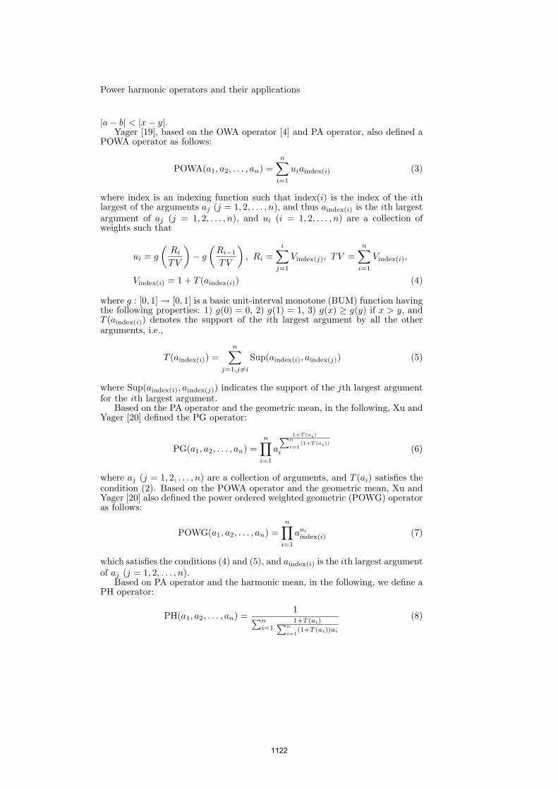
Power harmonic operators and their applications
|a− b| < |x− y|.Yager [19], based on the OWA operator [4] and PA operator, also defined a
POWA operator as follows:
POWA(a1, a2, . . . , an) =n∑
i=1
uiaindex(i) (3)
where index is an indexing function such that index(i) is the index of the ithlargest of the arguments aj (j = 1, 2, . . . , n), and thus aindex(i) is the ith largestargument of aj (j = 1, 2, . . . , n), and ui (i = 1, 2, . . . , n) are a collection ofweights such that
ui = g
(Ri
TV
)− g
(Ri−1
TV
), Ri =
i∑j=1
Vindex(j), TV =n∑
i=1
Vindex(i),
Vindex(i) = 1 + T (aindex(i)) (4)
where g : [0, 1] → [0, 1] is a basic unit-interval monotone (BUM) function havingthe following properties: 1) g(0) = 0, 2) g(1) = 1, 3) g(x) ≥ g(y) if x > y, andT (aindex(i)) denotes the support of the ith largest argument by all the otherarguments, i.e.,
T (aindex(i)) =n∑
j=1,j 6=i
Sup(aindex(i), aindex(j)) (5)
where Sup(aindex(i), aindex(j)) indicates the support of the jth largest argumentfor the ith largest argument.
Based on the PA operator and the geometric mean, in the following, Xu andYager [20] defined the PG operator:
PG(a1, a2, . . . , an) =n∏
i=1
a
1+T (ai)∑n
i=1(1+T (ai))
i (6)
where aj (j = 1, 2, . . . , n) are a collection of arguments, and T (ai) satisfies thecondition (2). Based on the POWA operator and the geometric mean, Xu andYager [20] also defined the power ordered weighted geometric (POWG) operatoras follows:
POWG(a1, a2, . . . , an) =n∏
i=1
aui
index(i) (7)
which satisfies the conditions (4) and (5), and aindex(i) is the ith largest argumentof aj (j = 1, 2, . . . , n).
Based on PA operator and the harmonic mean, in the following, we define aPH operator:
PH(a1, a2, . . . , an) =1∑n
i=11+T (ai)∑n
i=1(1+T (ai))ai
(8)
1122
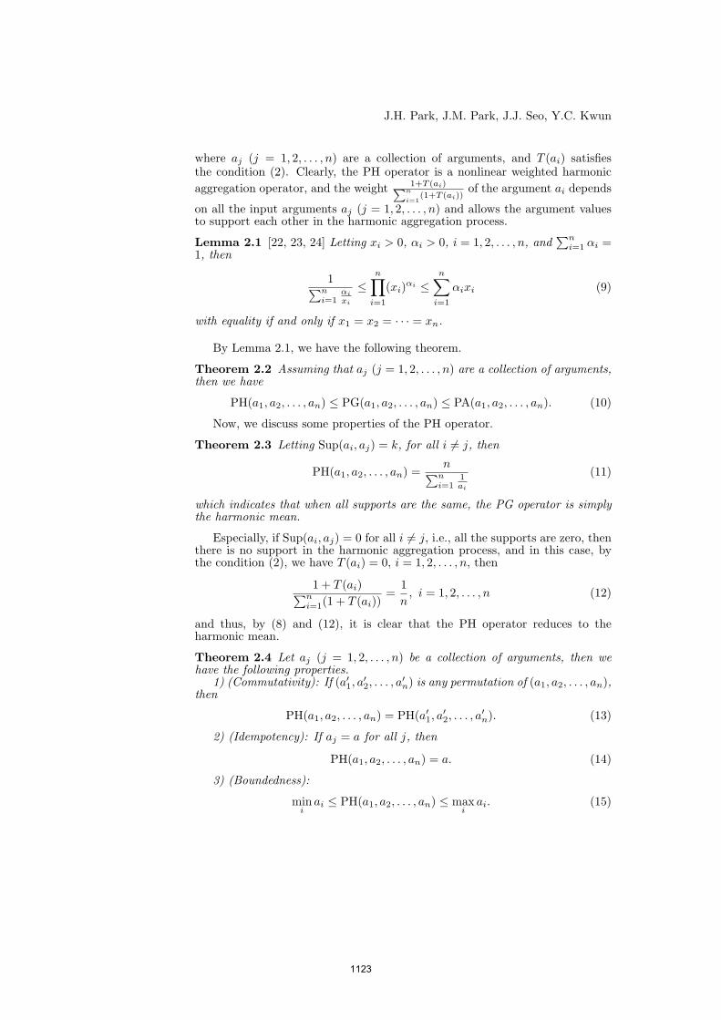
J.H. Park, J.M. Park, J.J. Seo, Y.C. Kwun
where aj (j = 1, 2, . . . , n) are a collection of arguments, and T (ai) satisfiesthe condition (2). Clearly, the PH operator is a nonlinear weighted harmonicaggregation operator, and the weight 1+T (ai)∑n
i=1(1+T (ai))
of the argument ai depends
on all the input arguments aj (j = 1, 2, . . . , n) and allows the argument valuesto support each other in the harmonic aggregation process.
Lemma 2.1 [22, 23, 24] Letting xi > 0, αi > 0, i = 1, 2, . . . , n, and∑n
i=1 αi =1, then
1∑ni=1
αi
xi
≤n∏
i=1
(xi)αi ≤n∑
i=1
αixi (9)
with equality if and only if x1 = x2 = · · · = xn.
By Lemma 2.1, we have the following theorem.
Theorem 2.2 Assuming that aj (j = 1, 2, . . . , n) are a collection of arguments,then we have
PH(a1, a2, . . . , an) ≤ PG(a1, a2, . . . , an) ≤ PA(a1, a2, . . . , an). (10)
Now, we discuss some properties of the PH operator.
Theorem 2.3 Letting Sup(ai, aj) = k, for all i 6= j, then
PH(a1, a2, . . . , an) =n∑n
i=11ai
(11)
which indicates that when all supports are the same, the PG operator is simplythe harmonic mean.
Especially, if Sup(ai, aj) = 0 for all i 6= j, i.e., all the supports are zero, thenthere is no support in the harmonic aggregation process, and in this case, bythe condition (2), we have T (ai) = 0, i = 1, 2, . . . , n, then
1 + T (ai)∑ni=1(1 + T (ai))
=1n
, i = 1, 2, . . . , n (12)
and thus, by (8) and (12), it is clear that the PH operator reduces to theharmonic mean.
Theorem 2.4 Let aj (j = 1, 2, . . . , n) be a collection of arguments, then wehave the following properties.
1) (Commutativity): If (a′1, a′2, . . . , a
′n) is any permutation of (a1, a2, . . . , an),
then
PH(a1, a2, . . . , an) = PH(a′1, a′2, . . . , a
′n). (13)
2) (Idempotency): If aj = a for all j, then
PH(a1, a2, . . . , an) = a. (14)
3) (Boundedness):
mini
ai ≤ PH(a1, a2, . . . , an) ≤ maxi
ai. (15)
1123
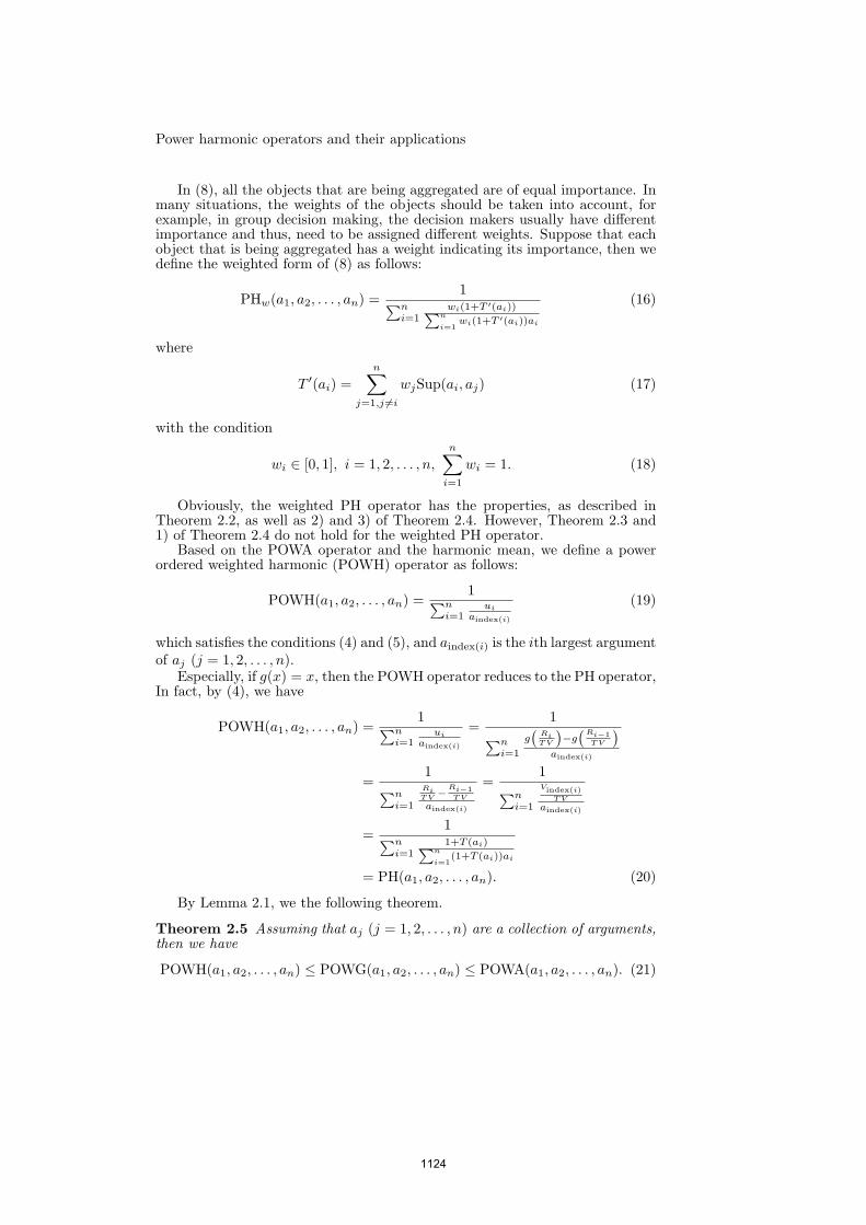
Power harmonic operators and their applications
In (8), all the objects that are being aggregated are of equal importance. Inmany situations, the weights of the objects should be taken into account, forexample, in group decision making, the decision makers usually have differentimportance and thus, need to be assigned different weights. Suppose that eachobject that is being aggregated has a weight indicating its importance, then wedefine the weighted form of (8) as follows:
PHw(a1, a2, . . . , an) =1∑n
i=1wi(1+T ′(ai))∑n
i=1wi(1+T ′(ai))ai
(16)
where
T ′(ai) =n∑
j=1,j 6=i
wjSup(ai, aj) (17)
with the condition
wi ∈ [0, 1], i = 1, 2, . . . , n,n∑
i=1
wi = 1. (18)
Obviously, the weighted PH operator has the properties, as described inTheorem 2.2, as well as 2) and 3) of Theorem 2.4. However, Theorem 2.3 and1) of Theorem 2.4 do not hold for the weighted PH operator.
Based on the POWA operator and the harmonic mean, we define a powerordered weighted harmonic (POWH) operator as follows:
POWH(a1, a2, . . . , an) =1∑n
i=1ui
aindex(i)
(19)
which satisfies the conditions (4) and (5), and aindex(i) is the ith largest argumentof aj (j = 1, 2, . . . , n).
Especially, if g(x) = x, then the POWH operator reduces to the PH operator,In fact, by (4), we have
POWH(a1, a2, . . . , an) =1∑n
i=1ui
aindex(i)
=1∑n
i=1
g(
RiT V
)−g(
Ri−1T V
)aindex(i)
=1∑n
i=1
RiT V −
Ri−1T V
aindex(i)
=1∑n
i=1
Vindex(i)T V
aindex(i)
=1∑n
i=11+T (ai)∑n
i=1(1+T (ai))ai
= PH(a1, a2, . . . , an). (20)
By Lemma 2.1, we the following theorem.
Theorem 2.5 Assuming that aj (j = 1, 2, . . . , n) are a collection of arguments,then we have
POWH(a1, a2, . . . , an) ≤ POWG(a1, a2, . . . , an) ≤ POWA(a1, a2, . . . , an). (21)
1124
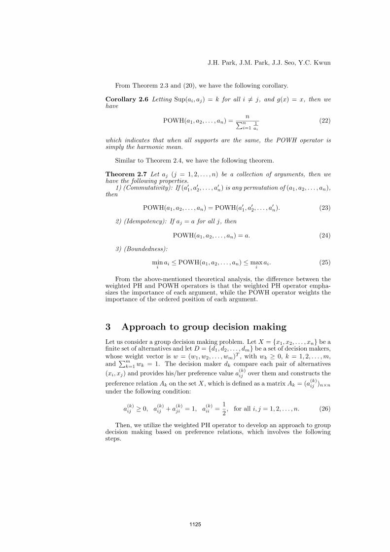
J.H. Park, J.M. Park, J.J. Seo, Y.C. Kwun
From Theorem 2.3 and (20), we have the following corollary.
Corollary 2.6 Letting Sup(ai, aj) = k for all i 6= j, and g(x) = x, then wehave
POWH(a1, a2, . . . , an) =n∑n
i=11ai
(22)
which indicates that when all supports are the same, the POWH operator issimply the harmonic mean.
Similar to Theorem 2.4, we have the following theorem.
Theorem 2.7 Let aj (j = 1, 2, . . . , n) be a collection of arguments, then wehave the following properties.
1) (Commutativity): If (a′1, a′2, . . . , a
′n) is any permutation of (a1, a2, . . . , an),
then
POWH(a1, a2, . . . , an) = POWH(a′1, a′2, . . . , a
′n). (23)
2) (Idempotency): If aj = a for all j, then
POWH(a1, a2, . . . , an) = a. (24)
3) (Boundedness):
mini
ai ≤ POWH(a1, a2, . . . , an) ≤ maxi
ai. (25)
From the above-mentioned theoretical analysis, the difference between theweighted PH and POWH operators is that the weighted PH operator empha-sizes the importance of each argument, while the POWH operator weights theimportance of the ordered position of each argument.
3 Approach to group decision making
Let us consider a group decision making problem. Let X = x1, x2, . . . , xn be afinite set of alternatives and let D = d1, d2, . . . , dm be a set of decision makers,whose weight vector is w = (w1, w2, . . . , wm)T , with wk ≥ 0, k = 1, 2, . . . ,m,and
∑mk=1 wk = 1. The decision maker dk compare each pair of alternatives
(xi, xj) and provides his/her preference value a(k)ij over them and constructs the
preference relation Ak on the set X, which is defined as a matrix Ak = (a(k)ij )n×n
under the following condition:
a(k)ij ≥ 0, a
(k)ij + a
(k)ji = 1, a
(k)ii =
12, for all i, j = 1, 2, . . . , n. (26)
Then, we utilize the weighted PH operator to develop an approach to groupdecision making based on preference relations, which involves the followingsteps.
1125
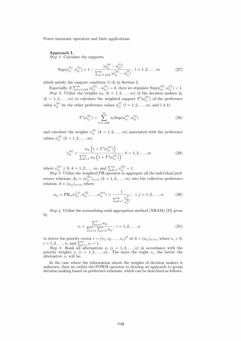
Power harmonic operators and their applications
Approach I.Step 1: Calculate the supports
Sup(a(k)ij , a
(l)ij ) = 1−
|a(k)ij − a
(l)ij |∑m
l=1,l 6=k |a(k)ij − a
(l)ij |
, l = 1, 2, . . . ,m (27)
which satisfy the support condition 1)-3) in Section 2.Especially, if
∑ml=1,l 6=k |a
(k)ij − a
(l)ij | = 0, then we stipulate Sup(a(k)
ij , a(l)ij ) = 1.
Step 2: Utilize the weights wk (k = 1, 2, . . . ,m) of the decision makers dk
(k = 1, 2, . . . ,m) to calculate the weighted support T ′(a(k)ij ) of the preference
value a(k)ij by the other preference values a
(l)ij (l = 1, 2, . . . ,m, and l 6= k)
T ′(a(k)ij ) =
m∑l=1,l 6=k
wlSup(a(k)ij , a
(l)ij ) (28)
and calculate the weights v(k)ij (k = 1, 2, . . . ,m) associated with the preference
values a(k)ij (k = 1, 2, . . . ,m)
v(k)ij =
wk
(1 + T ′(a(k)
ij ))
∑mk=1 wk
(1 + T ′(a(k)
ij )) , k = 1, 2, . . . ,m (29)
where v(k)ij ≥ 0, k = 1, 2, . . . ,m, and
∑mk=1 v
(k)ij = 1.
Step 3: Utilize the weighted PH operator to aggregate all the individual pref-erence relations Ak = (a(k)
ij )n×n (k = 1, 2, . . . ,m) into the collective preferencerelation A = (aij)n×n, where
aij = PHw(a(1)ij , a
(2)ij , . . . , a
(m)ij ) =
1∑mk=1
v(k)ij
a(k)ij
, i, j = 1, 2, . . . , n. (30)
Step 4: Utilize the normalizing rank aggregation method (NRAM) [25] givenby
vi =
∑nj=1 aij∑n
i=1
∑nj=1 aij
, i = 1, 2, . . . , n (31)
to derive the priority vector v = (v1, v2, . . . , vn)T of A = (aij)n×n, where vi > 0,i = 1, 2, . . . , n, and
∑ni=1 vi = 1.
Step 5: Rank all alternatives xi (i = 1, 2, . . . , n) in accordance with thepriority weights vi (i = 1, 2, . . . , n). The more the wight vi, the better thealternative xi will be.
In the case where the information about the weights of decision makers isunknown, then we utilize the POWH operator to develop an approach to groupdecision making based on preference relations, which can be described as follows.
1126
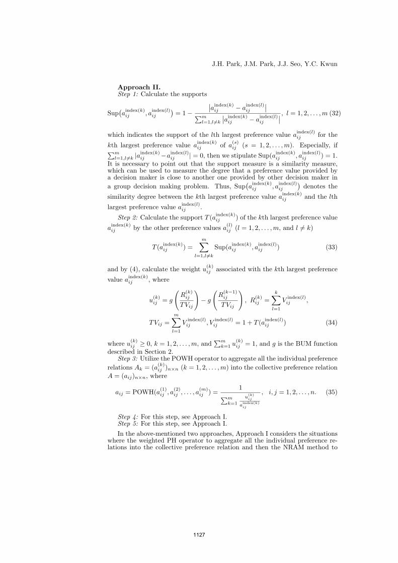
J.H. Park, J.M. Park, J.J. Seo, Y.C. Kwun
Approach II.Step 1: Calculate the supports
Sup(aindex(k)ij , a
index(l)ij
)= 1−
∣∣aindex(k)ij − a
index(l)ij
∣∣∑ml=1,l 6=k
∣∣aindex(k)ij − a
index(l)ij
∣∣ , l = 1, 2, . . . ,m (32)
which indicates the support of the lth largest preference value aindex(l)ij for the
kth largest preference value aindex(k)ij of a
(s)ij (s = 1, 2, . . . ,m). Especially, if∑m
l=1,l 6=k |aindex(k)ij −a
index(l)ij | = 0, then we stipulate Sup(aindex(k)
ij , aindex(l)ij ) = 1.
It is necessary to point out that the support measure is a similarity measure,which can be used to measure the degree that a preference value provided bya decision maker is close to another one provided by other decision maker ina group decision making problem. Thus, Sup
(aindex(k)ij , a
index(l)ij
)denotes the
similarity degree between the kth largest preference value aindex(k)ij and the lth
largest preference value aindex(l)ij .
Step 2: Calculate the support T (aindex(k)ij ) of the kth largest preference value
aindex(k)ij by the other preference values a
(l)ij (l = 1, 2, . . . ,m, and l 6= k)
T (aindex(k)ij ) =
m∑l=1,l 6=k
Sup(aindex(k)ij , a
index(l)ij ) (33)
and by (4), calculate the weight u(k)ij associated with the kth largest preference
value aindex(k)ij , where
u(k)ij = g
(R
(k)ij
TVij
)− g
(R
(k−1)ij
TVij
), R
(k)ij =
k∑l=1
Vindex(l)ij ,
TVij =m∑
l=1
Vindex(l)ij , V
index(l)ij = 1 + T (aindex(l)
ij ) (34)
where u(k)ij ≥ 0, k = 1, 2, . . . ,m, and
∑mk=1 u
(k)ij = 1, and g is the BUM function
described in Section 2.Step 3: Utilize the POWH operator to aggregate all the individual preference
relations Ak = (a(k)ij )n×n (k = 1, 2, . . . ,m) into the collective preference relation
A = (aij)n×n, where
aij = POWH(a(1)ij , a
(2)ij , . . . , a
(m)ij ) =
1∑mk=1
u(k)ij
aindex(k)ij
, i, j = 1, 2, . . . , n. (35)
Step 4: For this step, see Approach I.Step 5: For this step, see Approach I.In the above-mentioned two approaches, Approach I considers the situations
where the weighted PH operator to aggregate all the individual preference re-lations into the collective preference relation and then the NRAM method to
1127
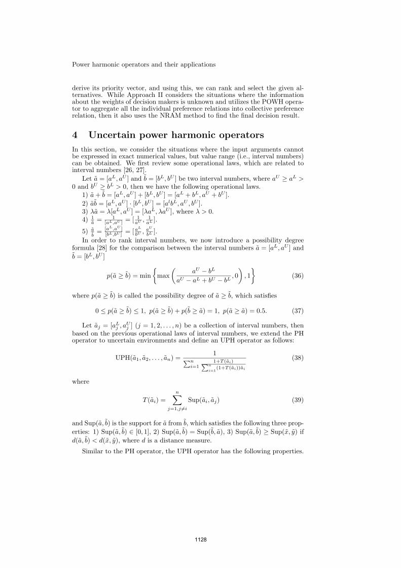
Power harmonic operators and their applications
derive its priority vector, and using this, we can rank and select the given al-ternatives. While Approach II considers the situations where the informationabout the weights of decision makers is unknown and utilizes the POWH opera-tor to aggregate all the individual preference relations into collective preferencerelation, then it also uses the NRAM method to find the final decision result.
4 Uncertain power harmonic operators
In this section, we consider the situations where the input arguments cannotbe expressed in exact numerical values, but value range (i.e., interval numbers)can be obtained. We first review some operational laws, which are related tointerval numbers [26, 27].
Let a = [aL, aU ] and b = [bL, bU ] be two interval numbers, where aU ≥ aL >0 and bU ≥ bL > 0, then we have the following operational laws.
1) a + b = [aL, aU ] + [bL, bU ] = [aL + bL, aU + bU ].2) ab = [aL, aU ] · [bL, bU ] = [albL, aU , bU ].3) λa = λ[aL, aU ] = [λaL, λaU ], where λ > 0.4) 1
a = 1[aL,aU ]
= [ 1aU , 1
aL ].
5) ab
= [aL,aU ][bL,bU ]
= [aL
bU , aU
bL ].In order to rank interval numbers, we now introduce a possibility degree
formula [28] for the comparison between the interval numbers a = [aL, aU ] andb = [bL, bU ]
p(a ≥ b) = min
max(
aU − bL
aU − aL + bU − bL, 0)
, 1
(36)
where p(a ≥ b) is called the possibility degree of a ≥ b, which satisfies
0 ≤ p(a ≥ b) ≤ 1, p(a ≥ b) + p(b ≥ a) = 1, p(a ≥ a) = 0.5. (37)
Let aj = [aLj , aU
j ] (j = 1, 2, . . . , n) be a collection of interval numbers, thenbased on the previous operational laws of interval numbers, we extend the PHoperator to uncertain environments and define an UPH operator as follows:
UPH(a1, a2, . . . , an) =1∑n
i=11+T (ai)∑n
i=1(1+T (ai))ai
(38)
where
T (ai) =n∑
j=1,j 6=i
Sup(ai, aj) (39)
and Sup(a, b) is the support for a from b, which satisfies the following three prop-erties: 1) Sup(a, b) ∈ [0, 1], 2) Sup(a, b) = Sup(b, a), 3) Sup(a, b) ≥ Sup(x, y) ifd(a, b) < d(x, y), where d is a distance measure.
Similar to the PH operator, the UPH operator has the following properties.
1128
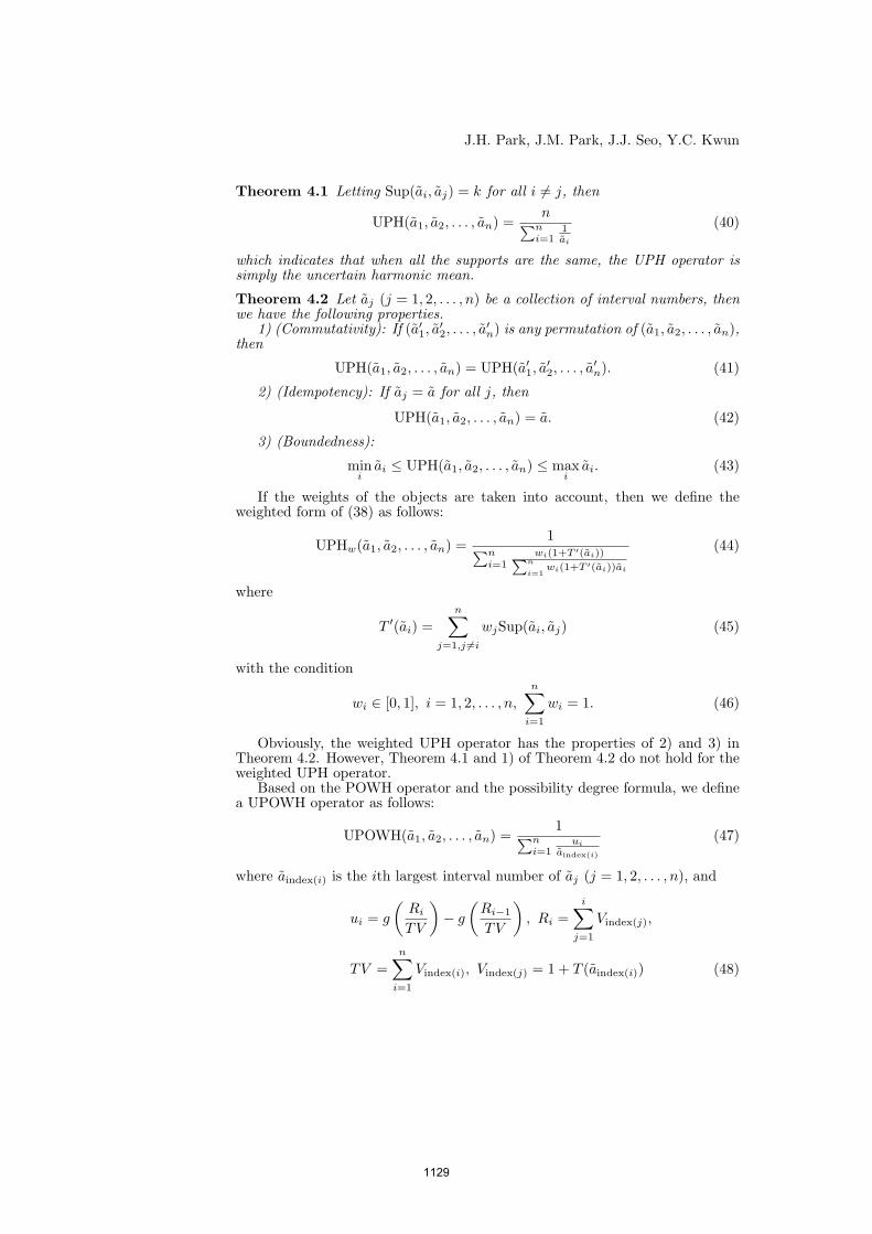
J.H. Park, J.M. Park, J.J. Seo, Y.C. Kwun
Theorem 4.1 Letting Sup(ai, aj) = k for all i 6= j, then
UPH(a1, a2, . . . , an) =n∑n
i=11ai
(40)
which indicates that when all the supports are the same, the UPH operator issimply the uncertain harmonic mean.
Theorem 4.2 Let aj (j = 1, 2, . . . , n) be a collection of interval numbers, thenwe have the following properties.
1) (Commutativity): If (a′1, a′2, . . . , a
′n) is any permutation of (a1, a2, . . . , an),
then
UPH(a1, a2, . . . , an) = UPH(a′1, a′2, . . . , a
′n). (41)
2) (Idempotency): If aj = a for all j, then
UPH(a1, a2, . . . , an) = a. (42)
3) (Boundedness):
mini
ai ≤ UPH(a1, a2, . . . , an) ≤ maxi
ai. (43)
If the weights of the objects are taken into account, then we define theweighted form of (38) as follows:
UPHw(a1, a2, . . . , an) =1∑n
i=1wi(1+T ′(ai))∑n
i=1wi(1+T ′(ai))ai
(44)
where
T ′(ai) =n∑
j=1,j 6=i
wjSup(ai, aj) (45)
with the condition
wi ∈ [0, 1], i = 1, 2, . . . , n,n∑
i=1
wi = 1. (46)
Obviously, the weighted UPH operator has the properties of 2) and 3) inTheorem 4.2. However, Theorem 4.1 and 1) of Theorem 4.2 do not hold for theweighted UPH operator.
Based on the POWH operator and the possibility degree formula, we definea UPOWH operator as follows:
UPOWH(a1, a2, . . . , an) =1∑n
i=1ui
aindex(i)
(47)
where aindex(i) is the ith largest interval number of aj (j = 1, 2, . . . , n), and
ui = g
(Ri
TV
)− g
(Ri−1
TV
), Ri =
i∑j=1
Vindex(j),
TV =n∑
i=1
Vindex(i), Vindex(j) = 1 + T (aindex(i)) (48)
1129
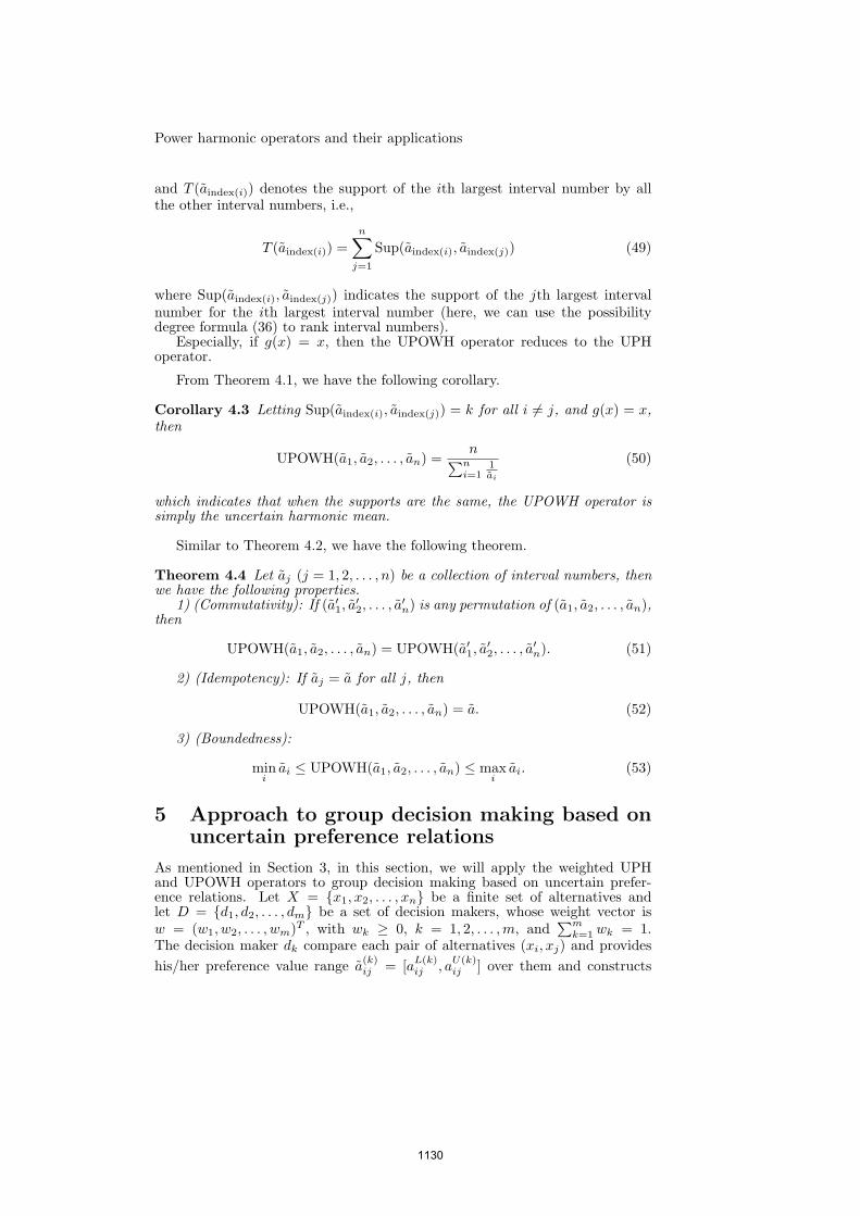
Power harmonic operators and their applications
and T (aindex(i)) denotes the support of the ith largest interval number by allthe other interval numbers, i.e.,
T (aindex(i)) =n∑
j=1
Sup(aindex(i), aindex(j)) (49)
where Sup(aindex(i), aindex(j)) indicates the support of the jth largest intervalnumber for the ith largest interval number (here, we can use the possibilitydegree formula (36) to rank interval numbers).
Especially, if g(x) = x, then the UPOWH operator reduces to the UPHoperator.
From Theorem 4.1, we have the following corollary.
Corollary 4.3 Letting Sup(aindex(i), aindex(j)) = k for all i 6= j, and g(x) = x,then
UPOWH(a1, a2, . . . , an) =n∑n
i=11ai
(50)
which indicates that when the supports are the same, the UPOWH operator issimply the uncertain harmonic mean.
Similar to Theorem 4.2, we have the following theorem.
Theorem 4.4 Let aj (j = 1, 2, . . . , n) be a collection of interval numbers, thenwe have the following properties.
1) (Commutativity): If (a′1, a′2, . . . , a
′n) is any permutation of (a1, a2, . . . , an),
then
UPOWH(a1, a2, . . . , an) = UPOWH(a′1, a′2, . . . , a
′n). (51)
2) (Idempotency): If aj = a for all j, then
UPOWH(a1, a2, . . . , an) = a. (52)
3) (Boundedness):
mini
ai ≤ UPOWH(a1, a2, . . . , an) ≤ maxi
ai. (53)
5 Approach to group decision making based onuncertain preference relations
As mentioned in Section 3, in this section, we will apply the weighted UPHand UPOWH operators to group decision making based on uncertain prefer-ence relations. Let X = x1, x2, . . . , xn be a finite set of alternatives andlet D = d1, d2, . . . , dm be a set of decision makers, whose weight vector isw = (w1, w2, . . . , wm)T , with wk ≥ 0, k = 1, 2, . . . ,m, and
∑mk=1 wk = 1.
The decision maker dk compare each pair of alternatives (xi, xj) and provideshis/her preference value range a
(k)ij = [aL(k)
ij , aU(k)ij ] over them and constructs
1130
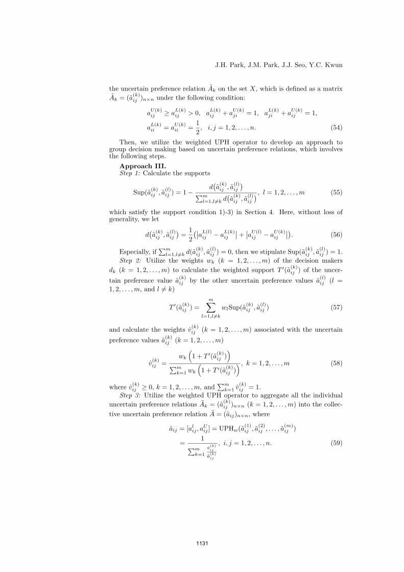
J.H. Park, J.M. Park, J.J. Seo, Y.C. Kwun
the uncertain preference relation Ak on the set X, which is defined as a matrixAk = (a(k)
ij )n×n under the following condition:
aU(k)ij ≥ a
L(k)ij > 0, a
L(k)ij + a
U(k)ji = 1, a
L(k)ji + a
U(k)ij = 1,
aL(k)ii = a
U(k)ii =
12, i, j = 1, 2, . . . , n. (54)
Then, we utilize the weighted UPH operator to develop an approach togroup decision making based on uncertain preference relations, which involvesthe following steps.
Approach III.Step 1: Calculate the supports
Sup(a(k)ij , a
(l)ij ) = 1−
d(a(k)ij , a
(l)ij
)∑ml=1,l 6=k d
(a(k)ij , a
(l)ij
) , l = 1, 2, . . . ,m (55)
which satisfy the support condition 1)-3) in Section 4. Here, without loss ofgenerality, we let
d(a(k)ij , a
(l)ij
)=
12(∣∣aL(l)
ij − aL(k)ij
∣∣+ ∣∣aU(l)ij − a
U(k)ij
∣∣). (56)
Especially, if∑m
l=1,l 6=k d(a(k)ij , a
(l)ij ) = 0, then we stipulate Sup(a(k)
ij , a(l)ij ) = 1.
Step 2: Utilize the weights wk (k = 1, 2, . . . ,m) of the decision makersdk (k = 1, 2, . . . ,m) to calculate the weighted support T ′(a(k)
ij ) of the uncer-
tain preference value a(k)ij by the other uncertain preference values a
(l)ij (l =
1, 2, . . . ,m, and l 6= k)
T ′(a(k)ij ) =
m∑l=1,l 6=k
wlSup(a(k)ij , a
(l)ij ) (57)
and calculate the weights v(k)ij (k = 1, 2, . . . ,m) associated with the uncertain
preference values a(k)ij (k = 1, 2, . . . ,m)
v(k)ij =
wk
(1 + T ′(a(k)
ij ))
∑mk=1 wk
(1 + T ′(a(k)
ij )) , k = 1, 2, . . . ,m (58)
where v(k)ij ≥ 0, k = 1, 2, . . . ,m, and
∑mk=1 v
(k)ij = 1.
Step 3: Utilize the weighted UPH operator to aggregate all the individualuncertain preference relations Ak = (a(k)
ij )n×n (k = 1, 2, . . . ,m) into the collec-tive uncertain preference relation A = (aij)n×n, where
aij = [alij , a
Uij ] = UPHw(a(1)
ij , a(2)ij , . . . , a
(m)ij )
=1∑m
k=1
v(k)ij
a(k)ij
, i, j = 1, 2, . . . , n. (59)
1131
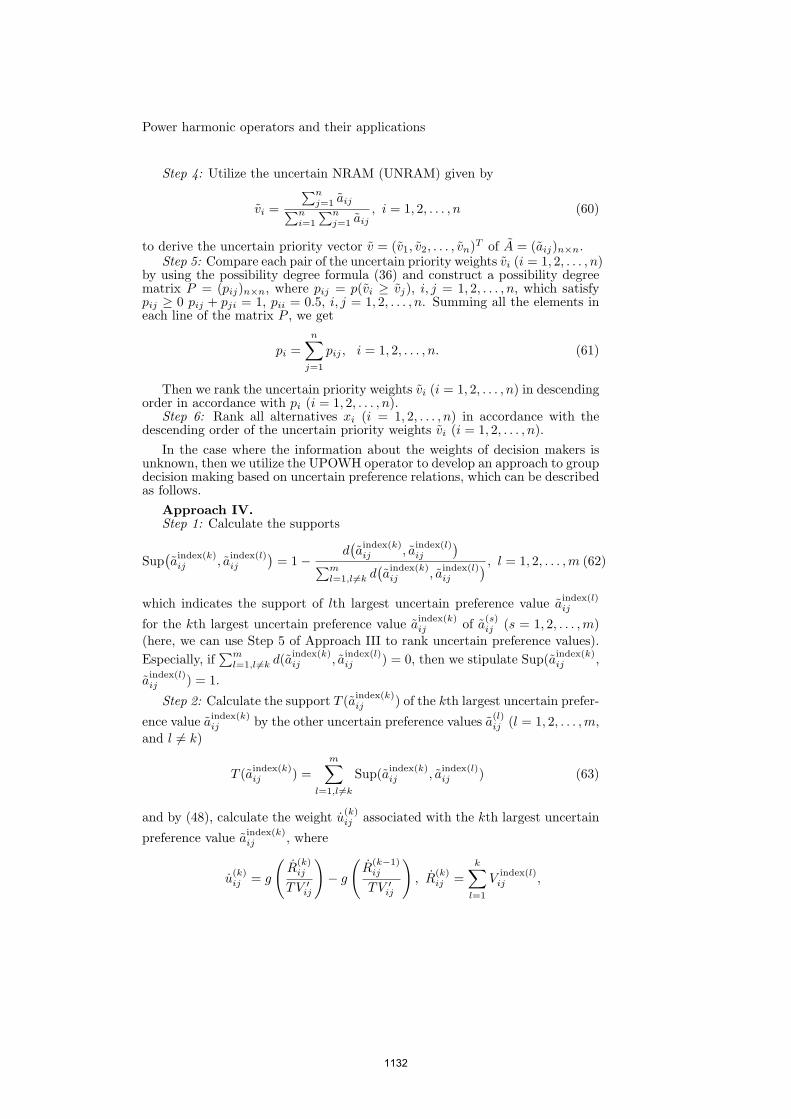
Power harmonic operators and their applications
Step 4: Utilize the uncertain NRAM (UNRAM) given by
vi =
∑nj=1 aij∑n
i=1
∑nj=1 aij
, i = 1, 2, . . . , n (60)
to derive the uncertain priority vector v = (v1, v2, . . . , vn)T of A = (aij)n×n.Step 5: Compare each pair of the uncertain priority weights vi (i = 1, 2, . . . , n)
by using the possibility degree formula (36) and construct a possibility degreematrix P = (pij)n×n, where pij = p(vi ≥ vj), i, j = 1, 2, . . . , n, which satisfypij ≥ 0 pij + pji = 1, pii = 0.5, i, j = 1, 2, . . . , n. Summing all the elements ineach line of the matrix P , we get
pi =n∑
j=1
pij , i = 1, 2, . . . , n. (61)
Then we rank the uncertain priority weights vi (i = 1, 2, . . . , n) in descendingorder in accordance with pi (i = 1, 2, . . . , n).
Step 6: Rank all alternatives xi (i = 1, 2, . . . , n) in accordance with thedescending order of the uncertain priority weights vi (i = 1, 2, . . . , n).
In the case where the information about the weights of decision makers isunknown, then we utilize the UPOWH operator to develop an approach to groupdecision making based on uncertain preference relations, which can be describedas follows.
Approach IV.Step 1: Calculate the supports
Sup(aindex(k)ij , a
index(l)ij
)= 1−
d(aindex(k)ij , a
index(l)ij
)∑ml=1,l 6=k d
(aindex(k)ij , a
index(l)ij
) , l = 1, 2, . . . ,m (62)
which indicates the support of lth largest uncertain preference value aindex(l)ij
for the kth largest uncertain preference value aindex(k)ij of a
(s)ij (s = 1, 2, . . . ,m)
(here, we can use Step 5 of Approach III to rank uncertain preference values).Especially, if
∑ml=1,l 6=k d(aindex(k)
ij , aindex(l)ij ) = 0, then we stipulate Sup(aindex(k)
ij ,
aindex(l)ij ) = 1.
Step 2: Calculate the support T (aindex(k)ij ) of the kth largest uncertain prefer-
ence value aindex(k)ij by the other uncertain preference values a
(l)ij (l = 1, 2, . . . ,m,
and l 6= k)
T (aindex(k)ij ) =
m∑l=1,l 6=k
Sup(aindex(k)ij , a
index(l)ij ) (63)
and by (48), calculate the weight u(k)ij associated with the kth largest uncertain
preference value aindex(k)ij , where
u(k)ij = g
(R
(k)ij
TV ′ij
)− g
(R
(k−1)ij
TV ′ij
), R
(k)ij =
k∑l=1
Vindex(l)ij ,
1132
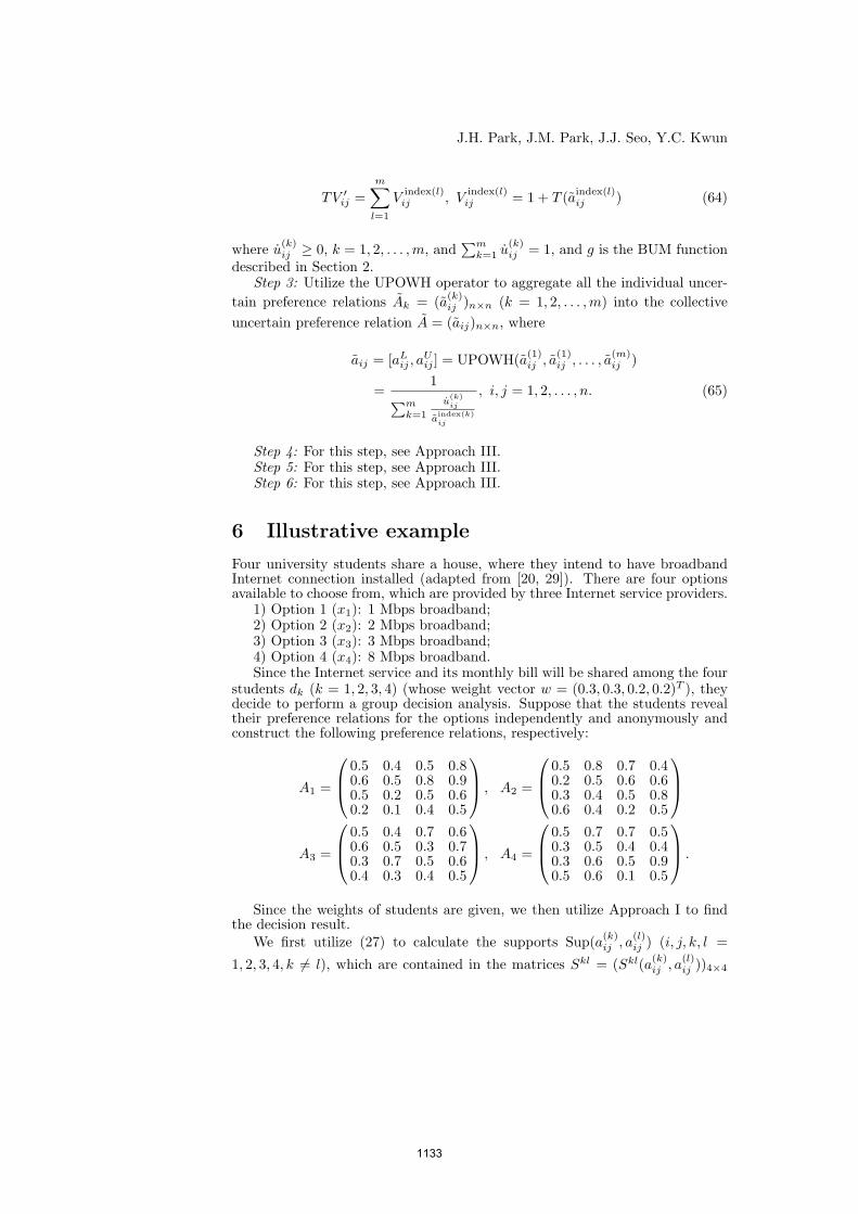
J.H. Park, J.M. Park, J.J. Seo, Y.C. Kwun
TV ′ij =
m∑l=1
Vindex(l)ij , V
index(l)ij = 1 + T (aindex(l)
ij ) (64)
where u(k)ij ≥ 0, k = 1, 2, . . . ,m, and
∑mk=1 u
(k)ij = 1, and g is the BUM function
described in Section 2.Step 3: Utilize the UPOWH operator to aggregate all the individual uncer-
tain preference relations Ak = (a(k)ij )n×n (k = 1, 2, . . . ,m) into the collective
uncertain preference relation A = (aij)n×n, where
aij = [aLij , a
Uij ] = UPOWH(a(1)
ij , a(1)ij , . . . , a
(m)ij )
=1∑m
k=1
u(k)ij
aindex(k)ij
, i, j = 1, 2, . . . , n. (65)
Step 4: For this step, see Approach III.Step 5: For this step, see Approach III.Step 6: For this step, see Approach III.
6 Illustrative example
Four university students share a house, where they intend to have broadbandInternet connection installed (adapted from [20, 29]). There are four optionsavailable to choose from, which are provided by three Internet service providers.
1) Option 1 (x1): 1 Mbps broadband;2) Option 2 (x2): 2 Mbps broadband;3) Option 3 (x3): 3 Mbps broadband;4) Option 4 (x4): 8 Mbps broadband.Since the Internet service and its monthly bill will be shared among the four
students dk (k = 1, 2, 3, 4) (whose weight vector w = (0.3, 0.3, 0.2, 0.2)T ), theydecide to perform a group decision analysis. Suppose that the students revealtheir preference relations for the options independently and anonymously andconstruct the following preference relations, respectively:
A1 =
0.5 0.4 0.5 0.80.6 0.5 0.8 0.90.5 0.2 0.5 0.60.2 0.1 0.4 0.5
, A2 =
0.5 0.8 0.7 0.40.2 0.5 0.6 0.60.3 0.4 0.5 0.80.6 0.4 0.2 0.5
A3 =
0.5 0.4 0.7 0.60.6 0.5 0.3 0.70.3 0.7 0.5 0.60.4 0.3 0.4 0.5
, A4 =
0.5 0.7 0.7 0.50.3 0.5 0.4 0.40.3 0.6 0.5 0.90.5 0.6 0.1 0.5
.
Since the weights of students are given, we then utilize Approach I to findthe decision result.
We first utilize (27) to calculate the supports Sup(a(k)ij , a
(l)ij ) (i, j, k, l =
1, 2, 3, 4, k 6= l), which are contained in the matrices Skl = (Skl(a(k)ij , a
(l)ij ))4×4
1133
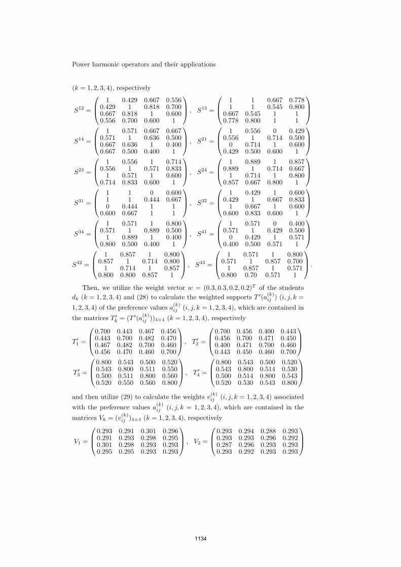
Power harmonic operators and their applications
(k = 1, 2, 3, 4), respectively
S12 =
1 0.429 0.667 0.5560.429 1 0.818 0.7000.667 0.818 1 0.6000.556 0.700 0.600 1
, S13 =
1 1 0.667 0.7781 1 0.545 0.800
0.667 0.545 1 10.778 0.800 1 1
S14 =
1 0.571 0.667 0.6670.571 1 0.636 0.5000.667 0.636 1 0.4000.667 0.500 0.400 1
, S21 =
1 0.556 0 0.4290.556 1 0.714 0.500
0 0.714 1 0.6000.429 0.500 0.600 1
S23 =
1 0.556 1 0.7140.556 1 0.571 0.833
1 0.571 1 0.6000.714 0.833 0.600 1
, S24 =
1 0.889 1 0.8570.889 1 0.714 0.667
1 0.714 1 0.8000.857 0.667 0.800 1
S31 =
1 1 0 0.6001 1 0.444 0.6670 0.444 1 1
0.600 0.667 1 1
, S32 =
1 0.429 1 0.6000.429 1 0.667 0.833
1 0.667 1 0.6000.600 0.833 0.600 1
S34 =
1 0.571 1 0.8000.571 1 0.889 0.500
1 0.889 1 0.4000.800 0.500 0.400 1
, S41 =
1 0.571 0 0.4000.571 1 0.429 0.500
0 0.429 1 0.5710.400 0.500 0.571 1
S42 =
1 0.857 1 0.8000.857 1 0.714 0.800
1 0.714 1 0.8570.800 0.800 0.857 1
, S43 =
1 0.571 1 0.8000.571 1 0.857 0.700
1 0.857 1 0.5710.800 0.70 0.571 1
.
Then, we utilize the weight vector w = (0.3, 0.3, 0.2, 0.2)T of the studentsdk (k = 1, 2, 3, 4) and (28) to calculate the weighted supports T ′(a(k)
ij ) (i, j, k =
1, 2, 3, 4) of the preference values a(k)ij (i, j, k = 1, 2, 3, 4), which are contained in
the matrices T ′k = (T ′(a(k)
ij ))4×4 (k = 1, 2, 3, 4), respectively
T ′1 =
0.700 0.443 0.467 0.4560.443 0.700 0.482 0.4700.467 0.482 0.700 0.4600.456 0.470 0.460 0.700
, T ′2 =
0.700 0.456 0.400 0.4430.456 0.700 0.471 0.4500.400 0.471 0.700 0.4600.443 0.450 0.460 0.700
T ′
3 =
0.800 0.543 0.500 0.5200.543 0.800 0.511 0.5500.500 0.511 0.800 0.5600.520 0.550 0.560 0.800
, T ′4 =
0.800 0.543 0.500 0.5200.543 0.800 0.514 0.5300.500 0.514 0.800 0.5430.520 0.530 0.543 0.800
and then utilize (29) to calculate the weights v
(k)ij (i, j, k = 1, 2, 3, 4) associated
with the preference values a(k)ij (i, j, k = 1, 2, 3, 4), which are contained in the
matrices Vk = (v(k)ij )4×4 (k = 1, 2, 3, 4), respectively
V1 =
0.293 0.291 0.301 0.2960.291 0.293 0.298 0.2950.301 0.298 0.293 0.2930.295 0.295 0.293 0.293
, V2 =
0.293 0.294 0.288 0.2930.293 0.293 0.296 0.2920.287 0.296 0.293 0.2930.293 0.292 0.293 0.293
1134
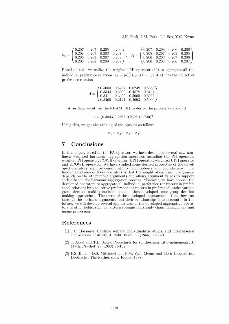
J.H. Park, J.M. Park, J.J. Seo, Y.C. Kwun
V3 =
0.207 0.207 0.205 0.2060.208 0.207 0.203 0.2080.206 0.203 0.207 0.2080.206 0.208 0.208 0.207
, V4 =
0.207 0.208 0.206 0.2060.208 0.207 0.203 0.2050.206 0.203 0.207 0.2060.206 0.205 0.206 0.207
.
Based on this, we utilize the weighted PH operator (30) to aggregate all theindividual preference relations Ak = (a(k)
ij )4×4 (k = 1, 2, 3, 4) into the collectivepreference relation
A =
0.5000 0.5237 0.6248 0.53830.3344 0.5000 0.4878 0.61570.3411 0.3499 0.5000 0.69920.3460 0.2121 0.2093 0.5000
.
After this, we utilize the NRAM (31) to derive the priority vector of A
v = (0.3003, 0.2661, 0.2596, 0.1740)T .
Using this, we get the ranking of the options as follows:
x1 x2 x3 x4.
7 Conclusions
In this paper, based on the PA operator, we have developed several new non-linear weighted harmonic aggregation operators including the PH operator,weighted PH operator, POWH operator, UPH operator, weighted UPH operatorand UPOWH operator. We have studied some desired properties of the devel-oped operators, such as commutativity, idempotency and boundedness. Thefundamental idea of these operators is that the weight of each input argumentdepends on the other input arguments and allows argument values to supporteach other in the harmonic aggregation process. Moreover, we have applied thedeveloped operators to aggregate all individual preference (or uncertain prefer-ence) relations into collective preference (or uncertain preference) under variousgroup decision making environment and then developed some group decisionmaking approaches. The merit of the developed approaches is that they cantake all the decision arguments and their relationships into account. In thefuture, we will develop several applications of the developed aggregation opera-tors in other fields, such as pattern recognition, supply chain management andimage processing.
References
[1] J.C. Harsanyi, Cardinal welfare, individualistic ethics, and interpersonalcomparisons of utility, J. Polit. Econ. 63 (1955) 309-321.
[2] J. Aczel and T.L. Saaty, Procedures for synthesizing ratio judgements, J.Math. Psychol. 27 (1983) 93-102.
[3] P.S. Bullen, D.S. Mitrinovi and P.M. Vasi, Means and Their Inequalities,Dordrecht, The Netherlands: Reidel, 1988.
1135
Power harmonic operators and their applications
[4] R.R. Yager, On ordered weighted averaging aggregation operators in multi-criteria decision making, IEEE Trans. Syst. Man Cybern. 18 (1988) 183-190.
[5] F. Chiclana, F. Herrera and E. Herrera-Viedma, Integrating multiplicativepreference relations in a multipurpose decision-making model based onfuzzy preference relations, Fuzzy Sets Syst. 122 (2001) 277-291.
[6] Z.S. Xu and Q.L. Da, The ordered weighted geometric averaging operators,Int. J. Intell. Syst. 17 (2002) 709-716.
[7] V. Torra, The weighted OWA operators, Int. J. Intell. Syst. 12 (1997)153-166.
[8] R.R. Yager and D.P. Filev, Induced ordered weighted averaging operators,IEEE Trans. Syst. Man Cybern. 29 (1999) 141-150.
[9] Z.S. Xu and Q.L. Da, An overview of operators aggregating information,Int. J. Intell. Syst. 18 (2003) 953-969.
[10] Z.S. Xu and Q.L. Da, The uncertain OWA operators, Int. J. Intell. Syst.17 (2002) 569-575.
[11] Z.S. Xu, Uncertain Multiple Attribute Decision Making: Methods andApplications, Beijing, China: Tsinghua Univ. Press, 2004.
[12] R.R. Yager, Generalized OWA aggregation operator, Fuzzy Optim. Deci-sion Making 3 (2004) 93-107.
[13] R.R. Yager, An approach to ordinal decision making, Int. J. Approx. Rea-soning 12 (1995) 237-261.
[14] F. Herrera, E. Herrera-Viedma and J.L. Verdegay, A sequential selectionprocess in group decision making with a linguistic assessment approach,Inf. Sci. 85 (1995) 223-239.
[15] F. Herrera and L. Martınez, A 2-tuple fuzzy linguistic representation modelfor computing with words, IEEE Trans. Fuzzy Syst. 8 (2000) 746-752.
[16] Z.S. Xu, A method based on linguistic aggregation operators for groupdecision making with linguistic preference relations, Inf. Sci. 166 (2004)19-30.
[17] J.H. Park, M.G. Gwak and Y.C. Kwun, Linguistic harmonic mean opera-tors and their applications to group decision making, Int. J. Adv. Manuf.Technol. 57 (2011) 411-419.
[18] J.H. Park, M.G. Gwak and Y.C. Kwun, Uncertain linguistic harmonicmean operators and their applications to multiple attribute group decisionmaking, Computing 93 (2011) 47-64.
[19] R.R. Yager, The power average operator, IEEE Trans. Syst. Man Cybern.A. Syst. Humans 31 (2001) 724-731.
[20] Z.S. Xu and R.R. Yager, Power-geometric operators and their use in groupdecision making, IEEE Trans. Fuzzy Syst. 18 (2010) 94-105.
1136
J.H. Park, J.M. Park, J.J. Seo, Y.C. Kwun
[21] Y. Xu, J.M. Merigo and H. Wang, Linguistic power aggregation operatorsand their application to multiple attribute group decision making, Appl.Math. Modelling (2011), doi: 10.1016/j.amp.2011.12.002.
[22] O. Holder, Uber einen Mittelwertsatz, Gottingen Nachrichten (1889) 38-47.
[23] J.L. Jensen, Sur les fonctions convexes et les inegualites entre les valeursmoyennes, Acta Math. 30 (1906) 175-193.
[24] Wikipedia, http://en.wikipedia.org/wiki/Generalizedmean.
[25] Z.S. Xu, Q.L. Da and L.H. Liu, Normalizing rank aggregation method forpriority of a fuzzy preference relation and its effectiveness, Int. J. Approx.Reasoning 50 (2009) 1287-1297.
[26] R.N. Xu and X.Y. Zhai, Extensions of the analytic hierarchy process infuzzy environment, Fuzzy Sets Syst. 52 (1992) 251-257.
[27] G. Bojadziev and M. Bojadziev, Fuzzy Sets, Fuzzy Logic, Applications,World Scientific, Singapore, 1995.
[28] G. Faccinetti, R.G. Ricci and S. Muzzioli, Note on ranking fuzzy triangularnumbers, Int. J. Intell. Syst. 13 (1998) 613-622.
[29] Y.M. Wang and C. Parkan, Optimal aggregation of fuzzy preference rela-tions with an application to broadband internet service selection, Eur. J.Oper. Res. 187 (2008) 1476-1486.
1137
MULTIPLICATIONAL COMBINATIONS AND A GENERAL SCHEME OFSINGLE-STEP ITERATIVE METHODS FOR MULTIPLE ROOTS
SIYUL LEE1,∗ AND HYEONGMIN CHOE1
1Seoul Science High School, Seoul 110-530, Republic of Korea
ABSTRACT. In this paper, a general form of single-step iterative methods for multiple roots ofnonlinear equations is derived under a number of assumptions of optimization. Definition of multi-plicational combinations and their properties are used upon the optimization procedure. Among all,we construct a family of iterative methods with nine parameters and simplest terms, and we obtain23 simplest iterative methods within the family, those including all existing methods of single-stepscheme. Numerical comparisons between the methods also present interesting and noteworthy re-sults.
1. INTRODUCTION
Solving nonlinear equations is one of the most basic problems of mathematics, yet it is oftengreatly complicated. Therefore, to develop methods to obtain roots of a nonlinear equation f(x) =0 has become crucial, especially with advance of computational technology.
Newton’s method, defined by
xn+1 = xn −f(xn)
f ′(xn)(1)
makes use of an approximated root to obtain a new approximation with less error. This classicalmethod, however, ceases to be efficient when a multiple root of f is to be obtained. In such cases,one may solve a nonlinear equation u(x) = 0 where u(x) = f(x)/f ′(x) instead of f(x) = 0,since u(x) has multiple roots of f(x) as its simple roots, see [1, p.126]. When multiplicity m ofthe desired root of f is known, one may use the modified Newton’s method,
xn+1 = xn −mfnf ′n
(2)
where f (i)n denotes f (i)(xn) instead of the original Newton’s method (1).The modified Newton’s method for multiple roots is quadratically convergent. More advanced
iterative algorithms with cubic or higher order of convergence are actively being developed, in
Keywords: Newton’s method, Iterative methods, Single-step methods, Nonlinear equations, Cubic order, Multipleroots.
2010 MSC: 65H05.E-mail addresses: [email protected](S. Lee), [email protected](H. Choe).
1138
J. COMPUTATIONAL ANALYSIS AND APPLICATIONS, VOL. 15, NO.6, 1138-1149, 2013, COPYRIGHT 2013 EUDOXUS PRESS, LLC
S. LEE AND H. CHOE
order to improve the computational efficiency. One widely known cubically convergent example isHalley’s method(HM), namely,
xn+1 = xn −fn
m+12m f ′n −
fnf ′′n2f ′n
, (3)
see [2].The Euler-Chebyshev method(ECM),
xn+1 = xn −m(3−m)
2
fnf ′n− m2
2
fn2f ′′nf ′n
3 (4)
is also of cubic convergence, see [1].Osada in [3] and Chun and Neta in [4], developed other cubically convergent iterative methods,
xn+1 = xn −1
2m(m+ 1)
fnf ′n
+1
2(m− 1)2
f ′nf ′′n, (5)
and
xn+1 = xn −2m2fn
2f ′′nm(3−m)fnf ′nf
′′n + (m− 1)2f ′n
3 , (6)
OM and CNM in short, respectively.Biazar and Ghanbari in [5] assumed a form of Newton-like methods with four parameters as
follows:
xn+1 = xn −Afnf
′n2f ′′n +Bf ′n
4 + Cfn2f ′′n
2
f ′n3f ′′n +Dfnf ′nf
′′n2 . (7)
From the error equation of the assumed method, parameters are controlled to make the methodcubically convergent. A new method thereby introduced is
xn+1 = xn −f ′n
m+32(m−1)f
′′n −
m(m+1)2(m−1)2
fnf ′′n2
f ′n2
, (8)
which is to be referred to as Biazar and Ghanbari’s method(BGM).In Section 2.1, we start with basic but essential definitions. We also define multiplicational
combinations with restricted derivatives of f , and write a general expression for them. Then,a Newton-like method with nine parameters is constructed under a number of assumptions. InSection 2.2, we derive the error equation of the method and solve for parameters to obtain a cubicconvergence. In such a way, we derive a number of Newton-like methods, some of which areintroduced previously. Section 3 contains numerical comparisons between the methods introducedor derived.
2. DEVELOPMENT OF METHODS
2.1. Construction of the scheme. Before we begin, the order of convergence and multiple rootsmust be defined clearly.
1139
SINGLE-STEP ITERATIVE METHODS FOR MULTIPLE ROOTS
Definition 1. (See [6]) With α a real number, and n a non-negative integer, if a real sequence xnconverges to α and for n large enough there exist constants c ≥ 0 and p ≥ 0 that satisfy
| xn+1 − α |≤ c | xn − α |p, (9)
then the maximum of p is said to be an order of convergence of xn to α.
Definition 2. (See [7, p.79]) A root α of an equation f(x) = 0 is said to have the multiplicity m ifand only if f(α) = 0, f ′(α) = 0, f ′′(α) = 0, . . . , f (m−1)(α) = 0 and f (m)(α) 6= 0. In this case,f can be written as
f(x) = (x− α)mg(x), (10)
with g(α) 6= 0.
Now, as a preparation for the rest of the section, we define a new concept of multiplicationalcombinations.
Definition 3. Let f be a two times differentiable function. With any integers a,b, and c such thata+ b+ c = 0,
Fk,−c = faf ′bf ′′c (11)
is a multiplicational combination of f , f ′, and f ′′, with differential order k=b+2c.
Multiplicational combinations acquire an important property that will be used importantly forthe discussion followed.
Theorem 1. If Fk,−c is a multiplicational combination of f , f ′, and f ′′, with differential order k,
Fk,−c = Fk,s = (f ′
f)k(
f ′2
ff ′′)s, (12)
for some integer s = −c. The converse is also true.
Proof. Let Fk,−c = faf ′bf ′′c for integers a, b, and c. By Definition 3, a+b+c = 0 and b+2c = k.Solving the system gives a = −k + c and b = k − 2c. Thus
Fk,−c = f−k+cf ′k−2cf ′′c = (f ′
f)k(
f ′2
ff ′′)−c. (13)
Letting s = −c, we have
Fk,s = (f ′
f)k(
f ′2
ff ′′)s. (14)
If u = (f′
f )k( f ′2
ff ′′ )s,
u = f−k−sf ′k+2sf ′′−s = Fk,s, (15)
and thus is a multiplicational combination of f , f ′, and f ′′, with differential order k. This completesthe proof.
1140
S. LEE AND H. CHOE
Single-step iterative methods are generally expressed as xn+1 = xn − g(xn), where g(xn)denotes an iteration function of xn. For computational efficiency, we only consider g(xn)’s thatconsist of fn, f ′n, f ′′n and a finite number of fundamental arithmetic operations between them. Withthe assumption, g(xn) can be written as follows:
g(xn) =
∑a,b,c fn
af ′nbf ′′n
cθ(a, b, c)∑a,b,c fn
af ′nbf ′′n
cφ(a, b, c), (16)
where θ and φ symbolize the linear combination of fnaf ′nbf ′′n
c’s in the numerator and the denomi-nator, respectively. It is reasonable to assume that all terms included in the sum are required to havethe same arithmetic order, namely, a+ b+ c. Thus, by an appropriate division, both the numeratorand the denominator each reduces to a linear combination of multiplicational combinations. Thenby Theorem 1,
g(xn) =
∑k,s (
f ′
f )k( f ′2
ff ′′ )sθ(k, s)∑
k,s(f ′
f )k( f ′2
ff ′′ )sφ(k, s)
. (17)
Here, for optimization(see Remark 1), we assume that the numerator and the denominator eachconsists of multiplicational combinations of uniform differential order. That is, for integers k1 andk2,
g(xn) =(f′
f )k1∑
s (f ′2
ff ′′ )sθ(s)
(f′
f )k2∑
s(f ′2
ff ′′ )sφ(s)
. (18)
Theorem 2. For an iteration function defined by (18), if xn+1 = xn−g(xn) is cubically convergentto α, the root of f(x) = 0 with multiplicity m, it is required that k1 − k2 = −1.
Proof. Taylor’s expansion for f about a multiple root α of f(x) = 0 with multiplicity m gives
f(xn) = f (m)(α)(c0emn + c1e
m+1n + c2e
m+2n + · · · ), (19)
f ′(xn) = f (m)(α)mc0em−1n + (m+ 1)c1emn + (m+ 2)c2e
m+1n + · · · , (20)
and
f ′′(xn) = f (m)(α)m(m− 1)c0em−2n + (m+ 1)mc1e
m−1n + (m+ 2)(m+ 1)c2e
mn , (21)
where cn’s and en are defined as follows:
cn =1
(m+ n)!
f (m+n)(α)
f (m)(α), en = xn − α. (22)
Then,fnf ′n
=1
men −
1
m2
c1c0e2n +
(m+ 1
m3
c21c20− 2
m2
c2c0
)e3n + · · · , (23)
f ′2nfnf ′′n
=m
m− 1− 2
(m− 1)2c1c0en +
( 3m2 + 1
m(m− 1)3c21c20− 6
(m− 1)2c2c0
)e2n + · · · , (24)
and thusg(xn) =
(en +O(e2n)
)k2−k1(1 +O(en))= ek2−k1n +O(ek2−k1+1
n ). (25)
1141
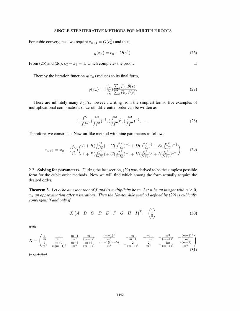
SINGLE-STEP ITERATIVE METHODS FOR MULTIPLE ROOTS
For cubic convergence, we require en+1 = O(e3n) and thus,
g(xn) = en +O(e3n). (26)
From (25) and (26), k2 − k1 = 1, which completes the proof.
Thereby the iteration function g(xn) reduces to its final form,
g(xn) = (fnf ′n
)
∑s F0,sθ(s)∑s F0,sφ(s)
. (27)
There are infinitely many F0,s’s, however, writing from the simplest terms, five examples ofmultiplicational combinations of zeroth differential order can be written as
1,f ′2
ff ′′, (f ′2
ff ′′)−1, (
f ′2
ff ′′)2, (
f ′2
ff ′′)−2, · · · . (28)
Therefore, we construct a Newton-like method with nine parameters as follows:
xn+1 = xn − (fnf ′n
)
(A+B( f ′n2
fnf ′′n) + C( f ′n
2
fnf ′′n)−1 +D( f ′n
2
fnf ′′n)2 + E( f ′n
2
fnf ′′n)−2
1 + F ( f ′n2
fnf ′′n) +G( f ′n
2
fnf ′′n)−1 +H( f ′n
2
fnf ′′n)2 + I( f ′n
2
fnf ′′n)−2
)(29)
2.2. Solving for parameters. During the last section, (29) was derived to be the simplest possibleform for the cubic order methods. Now we will find which among the form actually acquire thedesired order.
Theorem 3. Let α be an exact root of f and its multiplicity be m. Let n be an integer with n ≥ 0,xn an approximation after n iterations. Then the Newton-like method defined by (29) is cubicallyconvergent if and only if
X(A B C D E F G H I
)T=
(10
)(30)
with
X =
(1m
1m−1
m−1m2
m(m−1)2
(m−1)2m3 − m
m−1 −m−1m − m2
(m−1)2 − (m−1)2m2
1m2
m+1m(m−1)2
m−3m3
m+3(m−1)3
(m−1)(m−5)m4 − 2
(m−1)22m2 − 4m
(m−1)34(m−1)
m3
)(31)
is satisfied.
1142
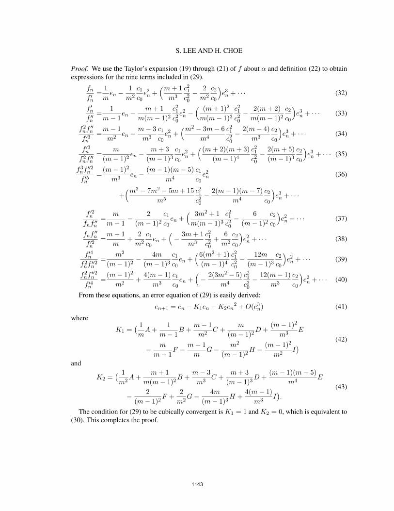
S. LEE AND H. CHOE
Proof. We use the Taylor’s expansion (19) through (21) of f about α and definition (22) to obtainexpressions for the nine terms included in (29).
fnf ′n
=1
men −
1
m2
c1c0e2n +
(m+ 1
m3
c21c20− 2
m2
c2c0
)e3n + · · · (32)
f ′nf ′′n
=1
m− 1en −
m+ 1
m(m− 1)2c21c20e2n −
( (m+ 1)2
m(m− 1)3c21c20− 2(m+ 2)
m(m− 1)2c2c0
)e3n + · · · (33)
f2nf′′n
f ′3n=m− 1
m2en −
m− 3
m3
c1c0e2n +
(m2 − 3m− 6
m4
c21c20− 2(m− 4)
m3
c2c0
)e3n + · · · (34)
f ′3nf2nf
′′n
=m
(m− 1)2en −
m+ 3
(m− 1)3c1c0e2n +
((m+ 2)(m+ 3)
(m− 1)4c21c20− 2(m+ 5)
(m− 1)3c2c0
)e3n + · · · (35)
f3nf′′2n
f ′5n=(m− 1)2
m3en −
(m− 1)(m− 5)
m4
c1c0e2n (36)
+(m3 − 7m2 − 5m+ 15
m5
c21c20− 2(m− 1)(m− 7)
m4
c2c0
)e3n + · · ·
f ′2nfnf ′′n
=m
m− 1− 2
(m− 1)2c1c0en +
( 3m2 + 1
m(m− 1)3c21c20− 6
(m− 1)2c2c0
)e2n + · · · (37)
fnf′′n
f ′2n=m− 1
m+
2
m2
c1c0en +
(− 3m+ 1
m3
c21c20
+6
m2
c2c0
)e2n + · · · (38)
f ′4nf2nf
′′2n
=m2
(m− 1)2− 4m
(m− 1)3c1c0en +
(6(m2 + 1)
(m− 1)4c21c20− 12m
(m− 1)3c2c0
)e2n + · · · (39)
f2nf′′2n
f ′4n=(m− 1)2
m2+
4(m− 1)
m3
c1c0en +
(− 2(3m2 − 5)
m4
c21c20− 12(m− 1)
m3
c2c0
)e2n + · · · (40)
From these equations, an error equation of (29) is easily derived:
en+1 = en −K1en −K2en2 +O(e3n) (41)
where
K1 =( 1mA+
1
m− 1B +
m− 1
m2C +
m
(m− 1)2D +
(m− 1)2
m3E
− m
m− 1F − m− 1
mG− m2
(m− 1)2H − (m− 1)2
m2I) (42)
and
K2 =( 1
m2A+
m+ 1
m(m− 1)2B +
m− 3
m3C +
m+ 3
(m− 1)3D +
(m− 1)(m− 5)
m4E
− 2
(m− 1)2F +
2
m2G− 4m
(m− 1)3H +
4(m− 1)
m3I).
(43)
The condition for (29) to be cubically convergent is K1 = 1 and K2 = 0, which is equivalent to(30). This completes the proof.
1143
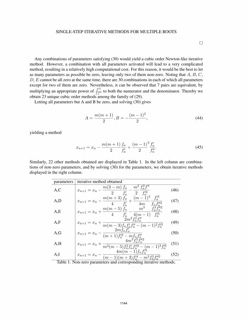
SINGLE-STEP ITERATIVE METHODS FOR MULTIPLE ROOTS
Any combinations of parameters satisfying (30) would yield a cubic order Newton-like iterativemethod. However, a combination with all parameters activated will lead to a very complicatedmethod, resulting in a relatively high computational cost. For this reason, it would be the best to letas many parameters as possible be zero, leaving only two of them non-zero. Noting that A, B, C,D, E cannot be all zero at the same time, there are 30 combinations in each of which all parametersexcept for two of them are zero. Nevertheless, it can be observed that 7 pairs are equivalent, bymultiplying an appropriate power of f ′2
ff ′′ to both the numerator and the denominator. Thereby weobtain 23 unique cubic order methods among the family of (29).
Letting all parameters but A and B be zero, and solving (30) gives
A =m(m+ 1)
2, B = −(m− 1)2
2, (44)
yielding a method
xn+1 = xn −m(m+ 1)
2
fnf ′n
+(m− 1)
2
2 f ′nf ′′n. (45)
Similarly, 22 other methods obtained are displayed in Table 1. In the left column are combina-tions of non-zero parameters, and by solving (30) for the parameters, we obtain iterative methodsdisplayed in the right column.
parameters iterative method obtained
A,C xn+1 = xn −m(3−m)
2
fnf ′n− m2
2
f2nf′′
f ′3n(46)
A,D xn+1 = xn −m(m+ 3)
4
fnf ′n
+(m− 1)3
4m
f ′3nfnf ′′2n
(47)
A,E xn+1 = xn +m(m− 5)
4
fnf ′n− m3
4(m− 1)
f3nf′′2n
f ′5n(48)
A,F xn+1 = xn +2m2f2nf
′′n
m(m− 3)fnf ′nf′′n − (m− 1)2f ′3n
(49)
A,G xn+1 = xn −2mfnf
′n
(m+ 1)f ′2n −mfnf ′′n(50)
A,H xn+1 = xn +4m3f3nf
′′2n
m2(m− 5)f2nf′nf′′2n − (m− 1)3f ′5n
(51)
A,I xn+1 = xn −4m(m− 1)fnf
′3n
(m− 1)(m+ 3)f ′4n −m2f2nf′′2n
(52)
Table 1. Non-zero parameters and corresponding iterative methods.
1144
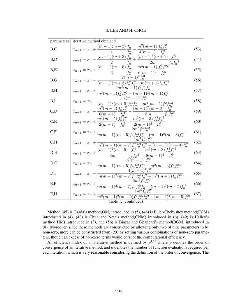
S. LEE AND H. CHOE
parameters iterative method obtained
B,C xn+1 = xn +(m− 1)(m− 3)
4
f ′nf ′′n− m2(m+ 1)
4(m− 1)
f2nf′′n
f ′3n(53)
B,D xn+1 = xn −(m− 1)(m+ 3)
2
f ′nf ′′n
+(m− 1)2(m+ 1)
2m
f ′3nfnf ′′2n
(54)
B,E xn+1 = xn +(m− 1)(m− 5)
6
f ′nf ′′n− m3(m+ 1)
6(m− 1)2f3nf
′′2n
f ′5n(55)
B,G xn+1 = xn −2(m− 1)2f ′3n
(m− 1)(m+ 3)f ′2n f′′n −m(m+ 1)fnf ′′2n
(56)
B,H xn+1 = xn +4m2(m− 1)f2nf
′nf′′n
m2(m− 3)f2nf′′2n − (m− 1)2(m+ 1)f ′4n
(57)
B,I xn+1 = xn −4(m− 1)3f ′5n
(m− 1)2(m+ 5)f ′4n f′′n −m2(m+ 1)f2nf
′′3n
(58)
C,D xn+1 = xn −m2(m+ 3)
6(m− 1)
f2nf′′n
f ′3n+
(m− 1)2(m− 3)
6m
f ′3nfnf ′′2n
(59)
C,E xn+1 = xn +m2(m− 5)
2(m− 1)
f2nf′′n
f ′3n− m2(m− 3)
2(m− 1)2f3nf
′′2n
f ′5n(60)
C,F xn+1 = xn +2m3f3nf
′′2n
m(m− 1)(m− 5)fnf ′3n f′′n − (m− 1)2(m− 3)f ′5n
(61)
C,H xn+1 = xn +4m4f4nf
′′3n
m2(m− 1)(m− 7)f2nf′3n f′′2n − (m− 1)3(m− 3)f ′7n
(62)
D,E xn+1 = xn +(m− 1)2(m− 5)
8m
f ′3nfnf ′′2n
− m3(m+ 3)
8(m− 1)2f3nf
′′2n
f ′5n(63)
D,G xn+1 = xn −2(m− 1)3f ′5n
m(m− 1)(m+ 5)fnf ′2n f′′2n −m2(m+ 3)f2nf
′′3n
(64)
D,I xn+1 = xn −4(m− 1)4f ′7n
m(m− 1)2(m+ 7)fnf ′4n f′′2n −m3(m+ 3)f3nf
′′4n
(65)
E,F xn+1 = xn +2m4f4nf
′′3n
m(m− 1)2(m− 7)fnf ′5n f′′n − (m− 1)3(m− 5)f ′7n
(66)
E,H xn+1 = xn +4m5f5nf
′′4n
m2(m− 1)2(m− 9)f2nf′5n f′′2n − (m− 1)4(m− 5)f ′9n
(67)
Table 1. (continued)
Method (45) is Osada’s method(OM) introduced in (5), (46) is Euler-Chebyshev method(ECM)introduced in (4), (48) is Chun and Neta’s method(CNM) introduced in (6), (49) is Halley’smethod(HM) introduced in (3), and (56) is Biazar and Ghanbari’s method(BGM) introduced in(8). Moreover, since these methods are constructed by allowing only two of nine parameters to benon-zero, more can be constructed from (29) by setting various combinations of non-zero parame-ters, though an excess of non-zero terms would corrupt the computational efficiency.
An efficiency index of an iterative method is defined by p1/d where p denotes the order ofconvergence of an iterative method, and d denotes the number of function evaluations required pereach iteration, which is very reasonable considering the definition of the order of convergence. The
1145
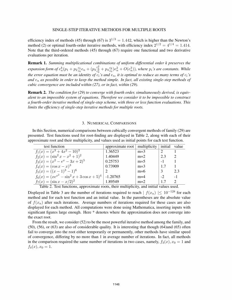
SINGLE-STEP ITERATIVE METHODS FOR MULTIPLE ROOTS
efficiency index of methods (45) through (67) is 31/3 = 1.442, which is higher than the Newton’smethod (2) or optimal fourth-order iterative methods, with efficiency index 21/2 = 41/4 = 1.414.Note that the third-ordered methods (45) through (67) require one functional and two derivativeevaluations per iteration.
Remark 1. Summing multiplicational combinations of uniform differential order k preserves theexpansion form of ekn(p1 + p2
c1c0en + (p3
c21c20
+ p4c2c0)e2n + O(e3n)), where pi’s are constants. While
the error equation must be an identity of ci’s and en, it is optimal to reduce as many terms of ci’sand en as possible in order to keep the method simple. In fact, all existing single-step methods ofcubic convergence are included within (27), or in fact, within (29).
Remark 2. The condition for (29) to converge with fourth order, simultaneously derived, is equiv-alent to an impossible system of equations. Therefore we consider it to be impossible to constructa fourth-order iterative method of single-step scheme, with three or less function evaluations. Thislimits the efficiency of single-step iterative methods for multiple roots.
3. NUMERICAL COMPARISONS
In this Section, numerical comparisons between cubically convergent methods of family (29) arepresented. Test functions used for root-finding are displayed in Table 2, along with each of theirapproximate root and their multiplicity, and values used as initial points for each test function.
test function approximate root multiplicity initial valuef1(x) = (x3 + 4x2 − 10)3 1.36523 m=3 2 1f2(x) = (sin2 x− x2 + 1)2 1.40449 m=2 2.3 2f3(x) = (x2 − ex − 3x+ 2)5 0.25753 m=5 -1 1f4(x) = (cosx− x)3 0.73909 m=3 1.7 1f5(x) = ((x− 1)3 − 1)6 2 m=6 3 2.3f6(x) = (xex
2 − sin2 x+ 3 cosx+ 5)4 -1.20765 m=4 -2 -1f7(x) = (sinx− x/2)2 1.89549 m=2 1.7 2
Table 2. Test functions, approximate roots, their multiplicity, and initial values used.Displayed in Table 3 are the number of iterations required to reach | f(xn) |≤ 10−128 for eachmethod and for each test function and an initial value. In the parentheses are the absolute valueof f(xn) after such iterations. Average numbers of iterations required for these cases are alsodisplayed for each method. All computations were done using Mathematica, inserting inputs withsignificant figures large enough. Here * denotes where the approximation does not converge intothe exact root.
From the result, we consider (52) to be the most powerful iterative method among the family, and(50), (56), or (63) are also of considerable quality. It is interesting that though (64)and (65) oftenfail to converge into the root either temporarily or permanently, other methods have similar speedof convergence, differing by no more than 1 in average number of iterations. In fact, all methodsin the comparison required the same number of iterations in two cases, namely, f3(x), x0 = 1 andf4(x), x0 = 1.
1146
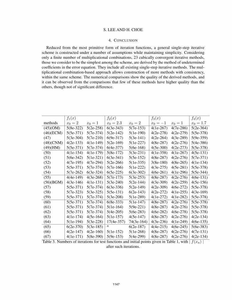
S. LEE AND H. CHOE
4. CONCLUSION
Reduced from the most primitive form of iteration functions, a general single-step iterativescheme is constructed under a number of assumptions while maintaining simplicity. Consideringonly a finite number of multiplicational combinations, 23 cubically convergent iterative methods,those we consider to be the simplest among the scheme, are derived by the method of undeterminedcoefficients in the error equation. They include all existing single-step iterative methods. The mul-tiplicational combination-based approach allows construction of more methods with consistency,within the same scheme. The numerical comparisons show the quality of the derived methods, andit can be observed from the comparisons that few of these methods have higher quality than theothers, though not of significant difference.
f1(x) f2(x) f3(x) f4(x)methods x0 = 2 x0 = 1 x0 = 2.3 x0 = 2 x0 = −1 x0 = 1 x0 = 1.7(45)(OM) 5(8e-322) 5(2e-258) 6(3e-343) 5(7e-153) 4(1e-267) 4(7e-286) 5(2e-364)(46)(ECM) 5(5e-371) 5(7e-374) 5(2e-142) 5(1e-190) 4(2e-278) 4(2e-279) 5(5e-378)(47) 5(3e-304) 5(7e-210) 6(9e-317) 5(3e-141) 4(2e-264) 4(3e-289) 5(9e-359)(48)(CNM) 4(2e-133) 4(1e-149) 5(2e-169) 5(1e-227) 4(8e-287) 4(2e-276) 5(4e-386)(49)(HM) 5(5e-371) 5(7e-374) 6(4e-377) 5(6e-168) 4(5e-300) 4(2e-273) 5(5e-378)(50) 4(1e-154) 4(1e-179) 5(8e-172) 5(3e-231) 4(1e-358) 4(1e-267) 4(5e-131)(51) 5(6e-342) 5(1e-321) 6(3e-341) 5(5e-152) 4(8e-287) 4(2e-276) 5(7e-371)(52) 4(7e-195) 4(7e-294) 5(2e-266) 5(1e-335) 3(8e-180) 4(8e-265) 4(1e-134)(53) 5(5e-371) 5(7e-374) 5(7e-166) 5(1e-222) 4(3e-275) 4(5e-281) 5(5e-378)(54) 5(7e-262) 6(3e-324) 6(5e-225) 6(3e-302) 4(6e-261) 4(1e-296) 5(5e-344)(55) 4(4e-149) 4(3e-268) 5(7e-173) 5(3e-253) 4(8e-287) 4(2e-276) 4(6e-131)(56)(BGM) 4(3e-146) 4(1e-131) 5(3e-240) 5(2e-144) 4(3e-309) 4(2e-259) 4(5e-156)(57) 5(5e-371) 5(7e-374) 6(3e-336) 5(2e-149) 4(2e-309) 4(6e-272) 5(5e-378)(58) 5(7e-323) 5(3e-325) 5(5e-131) 6(2e-143) 4(2e-272) 4(1e-255) 4(3e-169)(59) 5(5e-371) 5(7e-374) 5(3e-208) 5(1e-289) 4(1e-272) 4(1e-282) 5(5e-378)(60) 5(5e-371) 5(7e-374) 6(8e-333) 5(1e-147) 4(8e-287) 4(2e-276) 5(5e-378)(61) 5(5e-371) 5(7e-374) 5(1e-164) 5(9e-221) 4(8e-287) 4(2e-276) 5(5e-378)(62) 5(5e-371) 5(7e-374) 5(4e-205) 5(6e-283) 4(6e-282) 4(6e-278) 5(5e-378)(63) 4(1e-174) 4(5e-164) 5(1e-157) 4(5e-147) 4(8e-287) 4(2e-276) 4(2e-134)(64) 5(1e-194) 5(3e-228) 17(4e-357) 74(3e-164) 4(3e-236) 4(1e-249) 4(6e-135)(65) 6(2e-370) 5(3e-185) * 6(2e-187) 4(4e-215) 4(6e-245) 5(6e-383)(66) 4(2e-147) 4(2e-160) 5(1e-152) 5(1e-268) 4(8e-287) 4(2e-276) 4(7e-131)(67) 4(1e-171) 5(8e-390) 5(9e-153) 5(4e-299) 4(8e-287) 4(2e-276) 4(2e-134)
Table 3. Numbers of iterations for test functions and initial points given in Table 1, with | f(xn) |after such iterations.
1147
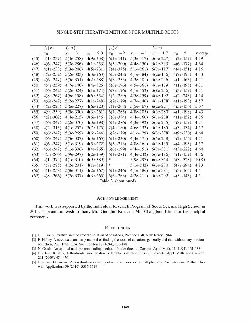
SINGLE-STEP ITERATIVE METHODS FOR MULTIPLE ROOTS
f4(x) f5(x) f6(x) f7(x)x0 = 1 x0 = 3 x0 = 2.3 x0 = −2 x0 = −1 x0 = 1.7 x0 = 2 average
(45) 4(1e-237) 5(4e-258) 4(9e-238) 6(1e-141) 5(3e-317) 5(3e-227) 4(2e-157) 4.79(46) 4(6e-247) 5(3e-286) 4(1e-253) 6(5e-200) 4(4e-150) 5(2e-333) 4(6e-177) 4.64(47) 4(1e-233) 5(3e-246) 4(5e-231) 7(4e-375) 5(1e-261) 5(2e-187) 4(4e-151) 4.86(48) 4(2e-252) 5(2e-303) 4(3e-263) 6(5e-248) 4(1e-184) 4(2e-146) 4(7e-195) 4.43(49) 4(6e-247) 5(5e-351) 4(2e-288) 6(8e-255) 4(3e-181) 5(3e-276) 4(1e-165) 4.71(50) 4(4e-259) 4(7e-140) 4(4e-326) 5(6e-196) 4(5e-361) 4(1e-139) 4(1e-195) 4.21(51) 4(6e-242) 5(2e-324) 4(1e-274) 6(7e-196) 4(1e-152) 5(8e-236) 4(3e-157) 4.71(52) 4(8e-267) 4(6e-158) 4(6e-354) 5(2e-289) 4(5e-259) 4(4e-192) 4(2e-243) 4.14(53) 4(6e-247) 5(2e-277) 4(1e-248) 6(8e-189) 4(7e-140) 4(1e-178) 4(1e-193) 4.57(54) 4(2e-223) 5(6e-227) 4(6e-220) 7(2e-268) 5(5e-167) 6(2e-221) 4(5e-130) 5.07(55) 4(9e-259) 5(5e-300) 4(3e-261) 6(7e-265) 4(8e-205) 5(3e-280) 4(1e-198) 4.43(56) 4(2e-308) 4(4e-215) 3(6e-146) 7(6e-354) 4(4e-160) 5(1e-228) 4(1e-152) 4.36(57) 4(6e-247) 5(2e-370) 4(3e-298) 6(3e-286) 4(3e-192) 5(3e-245) 4(8e-157) 4.71(58) 4(2e-315) 4(1e-252) 3(7e-175) 7(4e-180) 4(6e-132) 5(1e-185) 4(3e-134) 4.57(59) 4(6e-247) 5(3e-269) 4(6e-244) 6(2e-179) 4(1e-129) 5(3e-378) 4(9e-230) 4.64(60) 4(6e-247) 5(5e-307) 4(3e-265) 6(1e-230) 4(4e-171) 5(5e-248) 4(2e-156) 4.71(61) 4(6e-247) 5(1e-319) 4(5e-272) 6(3e-213) 4(8e-161) 4(1e-135) 4(4e-193) 4.57(62) 4(6e-247) 5(1e-306) 4(4e-265) 6(6e-199) 4(4e-151) 5(2e-331) 4(3e-228) 4.64(63) 4(5e-266) 5(9e-297) 4(2e-259) 6(1e-281) 4(4e-242) 5(7e-186) 4(1e-159) 4.36(64) 4(1e-372) 4(1e-310) 4(9e-389) * 5(9e-297) 6(4e-354) 5(3e-328) 10.85(65) 4(7e-285) 4(2e-201) 4(1e-319) * 5(1e-242) 6(3e-270) 5(7e-294) 4.83(66) 4(1e-258) 5(8e-311) 4(2e-267) 6(1e-246) 4(1e-186) 6(1e-381) 4(3e-163) 4.5(67) 4(8e-266) 5(7e-307) 4(3e-265) 6(6e-263) 4(2e-211) 5(3e-292) 4(5e-145) 4.5
Table 3. (continued)
ACKNOWLEDGEMENT
This work was supported by the Individual Research Program of Seoul Science High School in2011. The authors wish to thank Mr. Googhin Kim and Mr. Changbum Chun for their helpfulcomments.
REFERENCES
[1] J. F. Traub, Iterative methods for the solution of equations, Prentice Hall, New Jersey, 1964.[2] E. Halley, A new, exact and easy method of finding the roots of equations generally and that without any previous
reduction, Phil. Trans. Roy. Soc. London 18 (1694), 136-148[3] N. Osada, An optimal multiple root-finding method of order three, J. Comput. Appl. Math. 51 (1994), 131-133[4] C. Chun, B. Neta, A third-order modification of Newton’s method for multiple roots, Appl. Math. and Comput.
211 (2009), 474-479[5] J.Biazar, B.Ghanbari, A new third-order family of nonlinear solvers for multiple roots, Computers and Mathematics
with Applications 59 (2010), 3315-3319
1148
S. LEE AND H. CHOE
[6] S. Weerakoon, T. G. I. Fernando, A variant of Newton’s method with accelerated third-order convergence, Appl.Math. Lett. 13 (2000), 87-93.
[7] R. L. Burden, J. D. Faires, Numerical Analysis 8/e IE, Brooks/Cole Cengage Learning, 2005.
1149
COMPACT DIFFERENCES OF VOLTERRA COMPOSITIONOPERATORS FROM BERGMAN-TYPE SPACES TO
BLOCH-TYPE SPACES
ZHI JIE JIANG
Abstract. This paper characterizes the metrically compactness of differences
of Volterra composition operators from the weighted Bergman-type space Apu,0 < p <∞, to the Bloch-type space B∞v of analytic functions on the unit disk
D in terms of inducing symbols ϕ1, ϕ2 : D → D and ψ1, ψ2 : D → C.
1. Introduction
Let D be the open unit disk in the complex plane, H(D) the space of all analyticfunctions on D, and H∞(D) = H∞ the space of all bounded analytic functions onD with the supremum norm ‖f‖∞ = supz∈D |f(z)|.
Let dA(z) = 1πdxdy be the normalized Lebesgue measure on D. A positive
continuous function u on [0, 1) is normal, if there exist positive numbers s and t,0 < s < t, such that u(r)/(1−r)s is decreasing on [0, 1) and limr→1 µ(r)/(1−r)s = 0;u(r)/(1− r)t is increasing on [0, 1) and limr→1 u(r)/(1− r)t =∞. For 0 < p <∞and the normal function u, the Bergman-type space Apu(D) = Apu consists of allf ∈ H(D) such that
‖f‖pp,u =∫
D|f(z)|pu
p(|z|)1− |z|
dA(z) <∞.
When p ≥ 1, the Bergman-type space with the norm ‖ · ‖p,u becomes a Banachspace. If p ∈ (0, 1), it is a Frechet space with the translation invariant metric
d(f, g) = ‖f − g‖pp,u.
Let v be a positive continuous function on D (weight). The weighted-type spaceH∞v (D) = H∞v consists of all f ∈ H(D) such that
‖f‖H∞v = supz∈D
v(z)|f(z)| <∞.
It is known that H∞v is a Banach space. The Bloch-type space B∞v (D) = B∞vconsists of all f ∈ H(D) such that
‖f‖v = supz∈D
v(z)|f ′(z)| <∞.
Various kinds of weights and related weighted-type spaces and Bloch-type spaceshave been studied, e.g., in [1, 2, 4, 10, 11, 12].
2000 Mathematics Subject Classification. Primary 47B38; Secondary 47B33, 47B37.Key words and phrases. Volterra composition operator, Bergman-type space, weighted-type
space, Bloch-type space, metrically bounded operator, metrically compact operator.
1
1150
J. COMPUTATIONAL ANALYSIS AND APPLICATIONS, VOL. 15, NO.6, 1150-1157, 2013, COPYRIGHT 2013 EUDOXUS PRESS, LLC
2 ZHI JIE JIANG
Let ϕ be an analytic self-map of D and ψ be an analytic function on D. Forf ∈ H(D) the Volterra composition operator Vϕ,ψ is defined by
Vϕ,ψf(z) =∫ z
0
(f ϕ)(ξ)(ψ ϕ)′(ξ)dξ, z ∈ D.
As a kind of integral-type operator, the Volterra composition operators have beenstudied in [7, 14, 17].
LetX and Y be topological vector spaces whose topologies are given by translation-invariant metrics dX and dY , respectively, and L : X → Y be a linear operator. Itis said that L is metrically bounded if there exists a positive constant K such that
dY (Lf, 0) ≤ KdX(f, 0)
for all f ∈ X. When X and Y are Banach spaces, the metrically boundednesscoincides with the usual definition of bounded operators between Banach spaces.Recall that L : X → Y is metrically compact if it maps bounded sets into relativelycompact sets. If X and Y are Banach spaces then metrically compactness becomesusual compactness. For some results in this topic see [3, 5, 9, 16, 18, 19].
Let ϕ1, ϕ2 be nonconstant analytic self-maps of D and ψ1, ψ2 ∈ H(D). Differ-ences of Voterra composition operators on H(D) are defined as follows
(Vϕ1,ψ1−Vϕ2,ψ2)(f)(z) =∫ z
0
((fϕ1)(ξ)(ψ1ϕ1)′(ξ)−(fϕ2)(ξ)(ψ2ϕ1)′(ξ)
)dξ, z ∈ D.
Differences of composition operators was studied first on the Hardy space H2(D)in [3]. Recently Nieminen [13] has characterized the compactness of differenceof weighted composition operators Wϕ1,ψ1 −Wϕ2,ψ2 on weighted-type space givenby standard weights. Lindstrom and wolf [9] have generalized Nieminen’s resultto more general weights v and u and found an expression for the essential norm‖Wϕ1,ψ1 −Wϕ2,ψ2‖e,H∞v →H∞u , where max‖ϕ1‖∞, ‖ϕ2‖∞ = 1.
Here we continue this line of research and investigate the metrically compactnessof differences of Volterra composition operators acting from the weighted Bergman-type space Apu to the Bloch-type space B∞v on the open unit disk. These resultsextend the corresponding results on the single Volterra composition operators (see,for example, [7, 14, 17]).
For w ∈ D, let σw be the Mobius transformation of D defined by σw(z) =(w − z)/(1− wz). Note that the pseudo-hyperbolic metric ρ(z, w) = |σw(z)|.
Throughout this paper, constants are denoted by C, they are positive and maydiffer from one occurrence to the other. The notation a b means that there is apositive constant C such that a/C ≤ b ≤ Ca.
2. Auxiliary results
The proof of the following lemma is standard, so it will be omitted (see, e.g.,Lemma 3 in [15]).
Lemma 1. Assume that p > 0, u is a normal function on [0, 1), v is a weighton D, ϕ1, ϕ2 are analytic self-maps of D, ψ1, ψ2 are analytic functions on D andthe operator Vϕ1,ψ1 − Vϕ2,ψ2 : Apu → B∞v is metrically bounded. Then the operatorVϕ1,ψ1 − Vϕ2,u2 : Apu → B∞v is metrically compact if and only if for every bounded
1151
COMPACT DIFFERENCES OF VOLTERRA COMPOSITION OPERATORS 3
sequence (fn)n∈N in Apu such that fn → 0 uniformly on every compact subset of Das n→∞ it follows that
limn→∞
‖(Vϕ1,ψ1 − Vϕ2,ψ2)fn‖v = 0.
The following lemma was proved in [8].
Lemma 2. There exists a constant C > 0 independent of f ∈ Apu such that
|f(z)| ≤ C‖f‖p,uu(|z|)(1− |z|2)1/p
. (1)
Lemma 3. Let p > 0, u is a normal function on [0, 1), v is a weight on D, ϕ isan analytic self-map of D and ψ is an analytic function on D. Then the operatorVϕ,ψ : Apu → B∞v is metrically bounded if and only if
supz∈D
v(z)|ϕ′(z)||ψ′(z)|u(|ϕ(z)|)(1− |ϕ(z)|2)1/p
<∞. (2)
Proof. Suppose that Vϕ,ψ : Apu → B∞v is metrically bounded. For a fixed w ∈ D,setting
fw(z) =(1− |ϕ(w)|2)t+1
u(|ϕ(w)|)(1− ϕ(w)z)1/p+t+1,
then it is easy to show fw ∈ Apu and ‖fw‖p,u ≤ C. Thus
C‖Vϕ,ψ‖ ≥ ‖Vϕ,ψfw‖v = supz∈D
v(z)|ϕ′(z)||ψ′(z)||fw(ϕ(z))|
≥ v(w)|ϕ′(w)||ψ′(w)||fw(ϕ(w))|
=v(w)|ϕ′(w)||ψ′(w)|
u(|ϕ(w)|)(1− |ϕ(w)|2)1/p.
So, we prove that (2) holds.If (2) holds, by Lemma 2, then we have
‖Vϕ,ψf‖v = supz∈D
v(z)|ϕ′(z)||ψ′(z)||f(ϕ(z))|
≤ C supz∈D
v(z)|ϕ′(z)||ψ′(z)|u(|ϕ(z)|)(1− |ϕ(z)|2)1/p
‖f‖p,u.
It follows that Vϕ,ψ : Apu → B∞v is metrically bounded.
The next lemma shows that H∞ ⊆ Apu.
Lemma 4. Assume that p > 0 and u is a normal function on [0, 1). Then H∞ ⊆Apu.
Proof. For f ∈ H∞, we assume that |f(z)| ≤ M for all z ∈ D. Then by thedefinition of the normal function and the Beta function,
‖f‖pp,u =∫
D|f(z)|pu
p(|z|)1− |z|
dA(z) ≤M∫
D
up(|z|)1− |z|
dA(z)
= M
∫D
up(|z|)(1− |z|)ps
(1− |z|)ps−1dA(z)
=M
π
∫ 2π
0
∫ 1
0
up(r)(1− r)ps
(1− r)ps−1rdrdθ
1152
4 ZHI JIE JIANG
≤ 2Mup(0)B(2, ps),
where B(2, ps) is the Beta function. Thus we prove that f ∈ Apu.
The following lemma is very useful in the proof of the main result.
Lemma 5. Assume that u is a normal function on [0, 1) such that u is continuouslydifferentiable. Then there exists a constant C > 0 such that∣∣∣u(|z|)(1− |z|2)1/pf(z)− u(|w|)(1− |w|2)1/pf(w)
∣∣∣ ≤ C‖f‖p,uρ(z, w) (3)
for all f ∈ Apu and for all z, w in D.
Proof. By Lemma 3 we have that if f ∈ Apu, then f ∈ H∞u(|z|)(1−|z|2)1/p and
moreover ‖f‖u(|z|)(1−|z|2)1/p ≤ C‖f‖p,u. By the definition of normal function, itfollows that
u(|z|)(1− |z|2)1/p
(1− |z|)1/p+tis increasing on [0, 1), where t is the positive number in the definition of normalfunction. Then by the proof in [9], we obtain that u(|z|)(1 − |z|2)1/p satisfies thefollowing so-called Lusky condition (which is due to Lusky [11])
infn∈N
u(1− 2−n−1)(1− (1− 2−n−1)2)1/p
u(1− 2−n)(1− (1− 2−n)2)1/p> 0.
Therefore, by the Lemma 1 in [9], for each f ∈ H∞u(|z|)(1−|z|2)1/p and z, V ∈ D there
exists a C > 0 such that∣∣∣u(|z|)(1− |z|2)1/pf(z)− u(|w|)(1− |w|2)1/pf(w)∣∣∣ ≤ C‖f‖u(|z|)(1−|z|2)1/pρ(z, w)
≤ C‖f‖p,uρ(z, w).
From this inequality estimate (3) follows.
3. Main results
In this section we formulate and prove the main result of this paper.
Theorem 1. Assume that p > 0, u is a normal function on [0, 1) such that uis continuously differentiable, v is a weight on D, ϕ1, ϕ2 are nonconstant analyticself-maps of D, ψ1, ψ2 are analytic functions on D and Vϕ1,ψ1 , Vϕ2,ψ2 : Apu → B∞vare metrically bounded operators. Then the operator Vϕ1,ψ1 − Vϕ2,ψ2 : Apu → B∞v ismetrically compact if and only if the following conditions hold:(a)
lim|ϕ1(z)|→1
v(z)|ϕ′1(z)||ψ′1(z)|u(|ϕ1(z)|)(1− |ϕ1(z)|2)
1p
ρ(ϕ1(z), ϕ2(z)) = 0;
(b)
lim|ϕ2(z)|→1
v(z)|ϕ′2(z)||ψ′2(z)|u(|ϕ2(z)|)(1− |ϕ2(z)|2)
1p
ρ(ϕ1(z), ϕ2(z)) = 0;
(c)
limmin|ϕ1(z)|,|ϕ2(z)|→1
v(z)∣∣∣ ϕ′1(z)ψ′1(z)
u(|ϕ1(z)|)(1− |ϕ1(z)|2)1p
− ϕ′2(z)ψ′2(z)
u(|ϕ2(z)|)(1− |ϕ2(z)|2)1p
∣∣∣ = 0.
1153
COMPACT DIFFERENCES OF VOLTERRA COMPOSITION OPERATORS 5
Proof. Suppose that the operator Vϕ1,ψ1 − Vϕ2,ψ2 : Apu → B∞v is metricallycompact. If ‖ϕ1‖∞ < 1, then (a) vacuously holds. Hence assume that ‖ϕ1‖∞ = 1.Suppose to the contrary that (a) is not true. Then there exists a sequence (zn)n∈Nsuch that |ϕ1(zn)| → 1 as n→∞ and
δ := limn→∞
v(zn)|ϕ′1(zn)||ψ′1(zn)|u(|ϕ1(zn)|)(1− |ϕ1(zn)|2)1/p
ρ(ϕ1(zn), ϕ2(zn)) > 0. (4)
Since |ϕ1(zn)| → 1 as n → ∞, we can use the proof of Theorem 3.1 in [6] to findfunctions fn ∈ H∞, n ∈ N, such that
∞∑n=1
|fn(z)| ≤ 1, for all z ∈ D, (5)
and
fn(ϕ1(zn)) > 1− 12n, n ∈ N. (6)
Since fn ∈ H∞, by Lemma 4 we have that fn ∈ Apu and ‖fn‖p,u ≤ C for all n ∈ N.Note that form (6) it follows that lim
n→∞|fn(ϕ1(zn))| = 1. Now, we define
kn(z) =(1− |ϕ(zn)|2)t+1
u(|ϕ(zn)|)(1− ϕ(zn)z)1/p+t+1, n ∈ N.
By the proof of Theorem 3.1 in [8], we obtain that that supn∈N ‖kn‖p,u ≤ C. Putgn(z) = fn(z)σϕ2(zn)(z)kn(z), n ∈ N. Then clearly gn ∈ Apu with supn∈N ‖gn‖p,u ≤C and gn → 0 uniformly on compact subsets of D as n→∞. Since Vϕ1,ψ1−Vϕ2,ψ2 :Apu → B∞v is metrically compact, by Lemma 1 we get
limn→∞
‖(Vϕ1,ψ1 − Vϕ2,ψ2)gn‖v = 0. (7)
On the other hand, from the definition of the space B∞v , the definition of functionsgn and by using (6), we have that
‖(Vϕ1,ψ1 − Vϕ2,ψ2)gn‖v ≥v(zn)∣∣ϕ′1(zn)ψ′1(zn)gn(ϕ1(zn))− ϕ′2(zn)ψ′2(zn)gn(ϕ2(zn))
∣∣=v(zn)
∣∣ϕ′1(zn)ψ′1(zn)fn(ϕ1(zn))σϕ2(zn)(ϕ1(zn))kn(ϕ1(zn))∣∣
≥v(zn)|ϕ′1(zn)||ψ′1(zn)|ρ(ϕ1(zn), ϕ2(zn))
u(|ϕ1(zn)|)(1− |ϕ1(zn)|2)1p
(1− 1
2n). (8)
Letting n→∞ in (8) and using (4), we obtain
limn→∞
‖(Vϕ1,ψ1 − Vϕ2,ψ2)gn‖v ≥ limn→∞
v(zn)|ϕ′1(zn)||ψ′1(zn)|ρ(ϕ1(zn), ϕ2(zn))
u(|ϕ1(zn)|)(1− |ϕ1(zn)|2)1p
= δ > 0,
which contradicts (7). This shows that
limn→∞
v(zn)|ϕ′1(zn)||ψ′1(zn)|u(|ϕ1(zn)|)(1− |ϕ1(zn)|2)
1p
ρ(ϕ1(zn), ϕ2(zn)) = 0,
for every sequence (zn)n∈N such that |ϕ1(zn)| → 1 as n→∞, which implies (a).Condition (b) is proved similarly. Hence we omit it.Now, we prove (c). Suppose to the contrary that (c) does not hold. Then there
is a sequence (zn)n∈N such that min|ϕ1(zn)|, |ϕ2(zn)| → 1 as n→∞ and
β := limn→∞
v(zn)∣∣∣ ϕ′1(zn)ψ′1(zn)
u(|ϕ1(zn)|)(1− |ϕ1(zn)|2)1p
− ϕ′2(zn)ψ′2(zn)
u(|ϕ2(zn)|)(1− |ϕ2(zn)|2)1p
∣∣∣. (9)
1154
6 ZHI JIE JIANG
We may also assume that there is the following limit
l := limn→∞
ρ(ϕ1(zn), ϕ2(zn)) ≥ 0. (10)
Assume that l > 0. Then we have that for sufficiently large n, say n ≥ n0
0 <β
2≤ v(zn)
∣∣∣ ϕ′1(zn)ψ′1(zn)
u(|ϕ1(zn)|)(1− |ϕ1(zn)|2)1p
− ϕ′2(zn)ψ′2(zn)
u(|ϕ2(zn)|)(1− |ϕ2(zn)|2)1p
∣∣∣≤2l
( v(zn)|ϕ′1(zn)||ψ′1(zn)|u(|ϕ1(zn)|)(1− |ϕ1(zn)|2)
1p
+v(zn)|ϕ′2(zn)||ψ′2(zn)|
u(|ϕ2(zn)|)(1− |ϕ2(zn)|2)1p
)ρ(ϕ1(zn), ϕ2(zn)).
(11)
Letting n → ∞ in (11) and using (a) and (b), we arrive at a contradiction. Thus,we can assume that l = 0. Let the sequences of functions (fn)n∈N and (kn)n∈N bedefined as above. Set
hn(z) = fn(z)kn(z), n ∈ N.Then supn∈N ‖hn‖p,u ≤ C and hn → 0 uniformly on compact subsets of D asn→∞. Hence by Lemma 1
limn→∞
‖(Vϕ1,ψ1 − Vϕ2,ψ2)hn‖v = 0. (12)
Since Vϕ2,ψ2 : Apu → B∞v is metrically bounded, then by Lemma 3 we have that
M := supz∈D
v(z)|ϕ′2(z)||ψ′2(z)|u(|ϕ2(z)|)(1− |ϕ2(z)|2)1/p
<∞. (13)
We have
‖(V ϕ1,ψ1 − Vϕ2,ψ2)hn‖v ≥ v(zn)∣∣ϕ′1(zn)ψ′1(zn)hn(ϕ1(zn))− ϕ′2(zn)ψ′2(zn)hn(ϕ2(zn))
∣∣=v(zn)
∣∣ϕ′1(zn)ψ′1(zn)fn(ϕ1(zn))kn(ϕ1(zn))− ϕ′2(zn)ψ′2(zn)fn(ϕ2(zn))kn(ϕ2(zn))∣∣
≥v(zn)∣∣∣ ϕ′1(zn)ψ′1(zn)fn(ϕ1(zn))u(|ϕ1(zn)|)(1− |ϕ1(zn)|2)1/p
− ϕ′2(zn)ψ′2(zn)fn(ϕ1(zn))u(|ϕ2(zn)|)(1− |ϕ2(zn)|2)1/p
∣∣∣− v(zn)
∣∣∣ ϕ′2(zn)ψ′2(zn)fn(ϕ1(zn))u(|ϕ2(zn)|)(1− |ϕ2(zn)|2)1/p
− ϕ′2(zn)ψ′2(zn)fn(ϕ2(zn))kn(ϕ2(zn))∣∣∣
≥v(zn)∣∣∣ ϕ′1(zn)ψ′1(zn)u(|ϕ1(zn)|)(1− |ϕ1(zn)|2)1/p
− ϕ′2(zn)ψ′2(zn)u(|ϕ2(zn)|)(1− |ϕ2(zn)|2)1/p
∣∣∣(1− 12n)
− v(zn)|ϕ′2(zn)||ψ′2(zn)|u(|ϕ2(zn)|)(1− |ϕ2(zn)|2)1/p
∣∣∣u(|ϕ1(zn)|)(1− |ϕ1(zn)|2)1/phn(ϕ1(zn))
− u(|ϕ2(zn)|)(1− |ϕ2(zn)|2)1/phn(ϕ2(zn))∣∣∣. (14)
From (13), applying Lemma 5 to the functions hn with the points z = ϕ1(zn) andw = ϕ2(zn), and by using the fact supn∈N ‖hn‖p,u ≤ C, we get
v(zn)|ϕ′2(zn)||ψ′2(zn)|u(|ϕ2(zn)|)(1− |ϕ2(zn)|2)1/p
∣∣∣u(|ϕ1(zn)|)(1− |ϕ1(zn)|2)1/phn(ϕ1(zn))− u(|ϕ2(zn)|)
(1− |ϕ2(zn)|2)1/phn(ϕ2(zn))∣∣∣ ≤ CMρ(ϕ1(zn), ϕ2(zn)). (15)
Using (15) in (14), then letting n → ∞ is such obtained inequality and using (12)we obtain that β = 0, which is a contradiction. This proves (c).
Now we assume that conditions (a)-(c) hold. Assume (fn)n∈N is a boundedsequence in Apu such that fn → 0 uniformly on compact subsets of D. To prove
1155
COMPACT DIFFERENCES OF VOLTERRA COMPOSITION OPERATORS 7
that Vϕ1,ψ1−Vϕ2,ψ2 : Apu → B∞v is a metrically compact operator, in view of Lemma1, it is enough to show that ‖(Vϕ1,ψ1 −Vϕ2,ψ2)fn‖v → 0 as n→∞. Suppose to thecontrary that this is not true. Then for some ε > 0 there is a subsequence (fnk
)k∈Nof (fn)n∈N such that ‖(Vϕ1,ψ1 − Vϕ2,ψ2)fnk
‖v ≥ 2ε > 0 for every k ∈ N. We mayassume that (fnk
)k∈N is (fn)n∈N. Then there is a sequence (zn)n∈N in D such that
v(zn)∣∣ϕ′1(zn)ψ′1(zn)fn(ϕ1(zn))− ϕ′2(zn)ψ′2(zn)fn(ϕ2(zn))
∣∣ ≥ ε > 0, n ∈ N. (16)
We may also assume that the sequences (ϕ1(zn))n∈N and (ϕ2(zn))n∈N converge.If it were max|ϕ1(zn)|, |ϕ2(zn)| → q < 1, then from (16), since for the testfunction f(z) ≡ 1 ∈ Apu (by Lemma 4), from the boundedness of the operatorsVϕi,ψi : Apu → B∞v , i = 1, 2, we have that ψ1 ϕ1, ψ2 ϕ2 ∈ B∞v and sincefn(ϕi(zn)) → 0 as n → ∞, i = 1, 2, we would obtain a contradiction. Hencemax|ϕ1(zn)|, |ϕ2(zn)| → 1 as n → ∞. We can suppose that |ϕ1(zn)| → 1 andϕ2(zn) → z0 as n → ∞. Also, we can suppose that limit in (10) exists. Assumethat l > 0. Then by (a) and (b), we get
lim|ϕ1(zn)|→1
v(zn)|ϕ′1(zn)||ψ′1(zn)|u(|ϕ1(zn)|)(1− |ϕ1(zn)|2)1/p
ρ(ϕ1(zn), ϕ2(zn)) = 0 (17)
and
lim|ϕ2(zn)|→1
v(zn)|ϕ′2(zn)||ψ′2(zn)|u(|ϕ2(zn)|)(1− |ϕ2(zn)|2)1/p
ρ(ϕ1(zn), ϕ2(zn)) = 0. (18)
From (16) and Lemma 2, it follows that
0 <ε ≤ v(zn)|ϕ′1(zn)||ψ′1(zn)|u(|ϕ1(zn)|)(1− |ϕ1(zn)|2)
1p
∣∣∣u(|ϕ1(zn)|)(1− |ϕ1(zn)|2)1p fn(ϕ1(zn))
∣∣∣+
v(zn)|ϕ′2(zn)||ψ′2(zn)|u(|ϕ2(zn)|)(1− |ϕ2(zn)|2)
1p
∣∣∣u(|ϕ2(zn)|)(1− |ϕ2(zn)|2)1p fn(ϕ2(zn))
∣∣∣≤C( v(zn)|ϕ′1(zn)||ψ′1(zn)|u(|ϕ1(zn)|)(1− |ϕ1(zn)|2)
1p
+v(zn)|ϕ′2(zn)||ψ′2(zn)|
u(|ϕ2(zn)|)(1− |ϕ2(zn)|2)1p
)‖fn‖p,u. (19)
Letting n→∞ in (19) and using (18) we obtain a contradiction. Thus, we concludethat l = 0 which implies that |ϕ2(zn)| → 1 as n → ∞. From (16), Lemmas 2, 3and 5, and using (a) and (b) we have
0 < ε ≤ v(zn)∣∣ϕ′1(zn)ψ′1(zn)f(ϕ1(zn))− ϕ′2(zn)ψ′2(zn)f(ϕ2(zn))
∣∣≤ v(zn)|ϕ′1(zn)||ψ′1(zn)|u(|ϕ1(zn)|)(1− |ϕ1(zn)|2)
1p
∣∣∣u(|ϕ1(zn)|)(1− |ϕ1(zn)|2)1p f(ϕ1(zn))
− u(|ϕ2(zn)|)(1− |ϕ2(zn)|2)1p f(ϕ2(zn))
∣∣∣+ v(zn)∣∣∣ ϕ′1(zn)ψ′1(zn)
u(|ϕ1(zn)|)(1− |ϕ1(zn)|2)1p
− ϕ′2(zn)ψ′2(zn)
u(|ϕ2(zn)|)(1− |ϕ2(zn)|2)1p
∣∣∣u(|ϕ2(zn)|)(1− |ϕ2(zn)|2)1p |f(ϕ2(zn))|
≤ C v(zn)|ϕ′1(zn)||ψ′1(zn)|u(|ϕ1(zn)|)(1− |ϕ1(zn)|2)
1p
‖fn‖p,uρ(ϕ1(zn), ϕ2(zn)) + v(zn)
×∣∣∣ ϕ′1(zn)ψ′1(zn)
u(|ϕ1(zn)|)(1− |ϕ1(zn)|2)1p
− ϕ′2(zn)ψ′2(zn)
u(|ϕ2(zn)|)(1− |ϕ2(zn)|2)1p
∣∣∣‖fn‖p,u−→ 0,
1156
8 ZHI JIE JIANG
as n→∞, which is a contradiction. The proof is complete.
Acknowledgments. This work is supported by the Introduction of Talent Projectof SUSE (Grant No.2011RC13).
References
[1] J. Bonet, P. Domanski, M. Lindstrom and J. Taskinen, Composition operators between
weighted Banach spaces of analytic functions, J. Austral. Math. Soc. (Serie A) 64 (1998),101-118.
[2] M. D. Contreras and A. G. Hernandez-Dıaz, Weighted composition operators in weighted
Banach spaces of analytic functions, J. Austral. Math. Soc. (Serie A) 69 (2000), 41-60.[3] C. C. Cowen and B. D. MacCluer, Composition Operators on Spaces of Analytic Functions,
CRC Press, 1995.
[4] X. Fu, X. Zhu, Weighted composition operators on some weighted spaces in the unit ball,Abstr. Appl. Anal. Vol. 2008, Article ID 605807, (2008), 8 pages.
[5] T. Hosokawa and K. Izuchi, Essential norms of differences of composition operators on H∞,
J. Math. Japan. 57 (2005), 669-690.[6] T. Hosokawa, K. Izuchi and D. Zheng, Isolated points and essential components of composi-
tion operators on H∞, Proc. Amer. Math. Soc. 130 (2002), 1765-1773.
[7] S. Li, Volterra composition operators between weighted Bergman spaces and Bloch typespaces, J. Korean Math. Soc. 45 (2008), 229-248.
[8] S. Li and S. Stevic, Weighted composition operators from Bergman-type spaces into Blochspaces, Proc. Indian Acad. Sci. Math. Sci. 117 (3) (2007), 371-385.
[9] M. Lindstrom and E. Wolf, Essential norm of the difference of Veighted composition operators,
Monatsh. Math. 153 (2008), 133-143.[10] V. Lusky, On the structure of Hv0(D) and hv0(D), Math. Nachr. 159 (1992), 279-289.
[11] V. Lusky, On weighted spaces of harmonic and holomorphic functions, J. London Math. Soc.
51 (1995), 309-320.[12] A. Montes-Rodriguez, Weighted composition operators on weighted Banach spaces of analytic
functions. J. London Math. Soc. 61 (3) (2000), 872-884.
[13] P. J. Nieminen, Compact differences of composition operators on Bloch and Lipschitz spaces,Comput. Methods Funct. Theory. 7 (2) (2007), 325-344.
[14] A. G. Siskakis and R. Zhao, An Volterra type operator on spaces of analytic functions,
Contemp. Math. (232) (1999), 299-311.[15] S. Stevic, Composition operators between H∞ and the α-Bloch spaces on the polydisc, Z.
Anal. Anwend. 25 (2006), 457–466.[16] S. Stevic, Essential norms of weighted composition operators from the α-Bloch space to a
weighted-type space on the unit ball, Abstr. Appl. Anal. vol. 2008, Article ID 279691 (2008),
11 pages.[17] S. Stevic, On a new integral-type operator from the weighted Bergman space to the Bloch-
type space on the unit ball, Discrete Dynamics in Nature and Society. Vol. 2008, Article ID
154263, (2009), 14 pages.[18] S. Stevic, Essential norms of weighted composition operators from the Bergman space to
weighted-type spaces on the unit ball, Ars. Combin. 91 (2009), 391-400.
[19] S. Stevic, Norm and essential norm of composition followed by differentiation from α-Blochspaces to H∞µ , Appl. Math. Comput. 207 (2009), 225–229.
Zhi Jie Jiang, School of Science, Sichuan University of Science and Engineering,
Zigong, Sichuan, 643000, ChinaE-mail address: [email protected]
1157
SOME NEW ERROR INEQUALITIES FOR A TAYLOR-LIKE FORMULA
WENJUN LIU AND QILIN ZHANG
Abstract. Some new error inequalities for a Taylor-like formula are established. Sharpbounds are given when n is an odd and even integer, respectively.
1. Introduction
Error analysis for the Taylor and generalized Taylor formulas has been extensively studiedin recent years. The approach from an inequalities point of view to estimate the errorterms has been used in these studies (see [1]-[18] and the references therein). In [19], byappropriately choosing the Peano kernel
Gn(x) =
1
n!
(x− 3a+ t
4
)n−1 [x+
(n− 3)a− (n+ 1)t
4
], x ∈
[a,a+ t
2
],
1
n!
(x− a+ 3t
4
)n−1 [x+
(n− 3)t− (n+ 1)a
4
], x ∈
(a+ t
2, t
],
(1)
a Taylor-like formula was derived as follows.
Lemma 1. ([19]) Let f : [a, t] → ℝ be a function such that f (n) is absolutely continuous.Then
f(t) =f(a)−n∑
k=1
(−1)k(t− a)k
4kk!(1 + k)
[fk(t)− (−1)kfk(a)
]−
n∑k=2
(−1)k(t− a)k
4kk!(1− k)[1− (−1)k]fk
(a+ t
2
)+R(f). (2)
By introducing the notations
Fn(t, a) =f(a)−n∑
k=1
(−1)k(t− a)k
4kk!(1 + k)
[fk(t)− (−1)kfk(a)
]−
n∑k=2
(−1)k(t− a)k
4kk!(1− k)[1− (−1)k]fk
(a+ t
2
),
the following error inequalities were derived in [19].
Theorem 1. Let f : [a, t] → ℝ be a function such that f (n) is absolutely continuous.
If there exist real numbers n,Γn such that n ≤ f (n+1)(x) ≤ Γn, x ∈ [a, t], then
|f(t)− Fn(t, a)| ≤Γn − n(n+ 1)!
2n+ 2
4n+1(t− a)n+1, if n is odd (3)
2010 Mathematics Subject Classification. 26D10, 41A58, 41A80.Key words and phrases. Taylor-like formula, approximation error, inequality, sharp bound.This paper was typeset using AMS-LATEX.
1158
J. COMPUTATIONAL ANALYSIS AND APPLICATIONS, VOL. 15, NO.6, 1158-1164, 2013, COPYRIGHT 2013 EUDOXUS PRESS, LLC
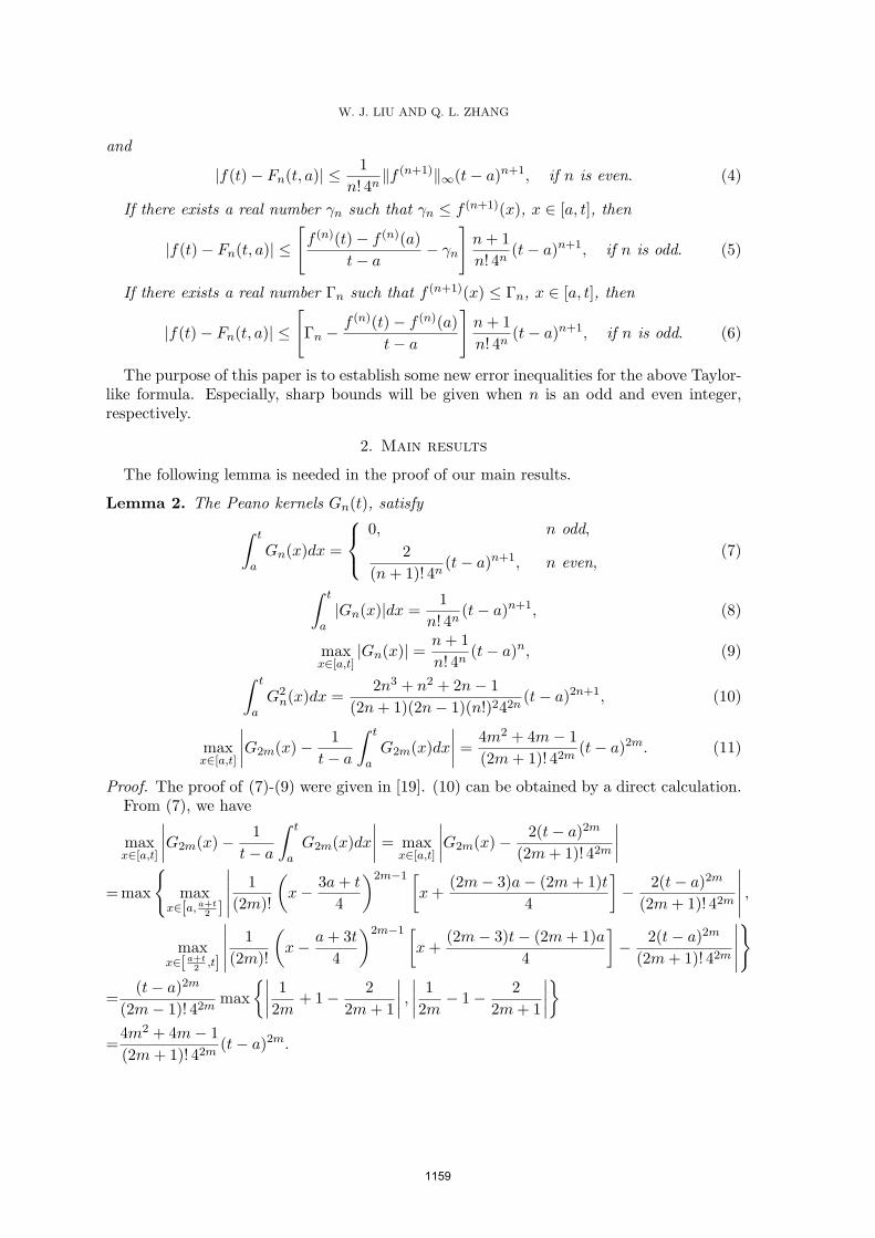
W. J. LIU AND Q. L. ZHANG
and
|f(t)− Fn(t, a)| ≤1
n! 4n∥f (n+1)∥∞(t− a)n+1, if n is even. (4)
If there exists a real number n such that n ≤ f (n+1)(x), x ∈ [a, t], then
|f(t)− Fn(t, a)| ≤
[f (n)(t)− f (n)(a)
t− a− n
]n+ 1
n! 4n(t− a)n+1, if n is odd. (5)
If there exists a real number Γn such that f (n+1)(x) ≤ Γn, x ∈ [a, t], then
|f(t)− Fn(t, a)| ≤
[Γn − f (n)(t)− f (n)(a)
t− a
]n+ 1
n! 4n(t− a)n+1, if n is odd. (6)
The purpose of this paper is to establish some new error inequalities for the above Taylor-like formula. Especially, sharp bounds will be given when n is an odd and even integer,respectively.
2. Main results
The following lemma is needed in the proof of our main results.
Lemma 2. The Peano kernels Gn(t), satisfy∫ t
aGn(x)dx =
0, n odd,
2
(n+ 1)! 4n(t− a)n+1, n even,
(7)
∫ t
a|Gn(x)|dx =
1
n! 4n(t− a)n+1, (8)
maxx∈[a,t]
|Gn(x)| =n+ 1
n! 4n(t− a)n, (9)∫ t
aG2
n(x)dx =2n3 + n2 + 2n− 1
(2n+ 1)(2n− 1)(n!)242n(t− a)2n+1, (10)
maxx∈[a,t]
∣∣∣∣G2m(x)− 1
t− a
∫ t
aG2m(x)dx
∣∣∣∣ = 4m2 + 4m− 1
(2m+ 1)! 42m(t− a)2m. (11)
Proof. The proof of (7)-(9) were given in [19]. (10) can be obtained by a direct calculation.From (7), we have
maxx∈[a,t]
∣∣∣∣G2m(x)− 1
t− a
∫ t
aG2m(x)dx
∣∣∣∣ = maxx∈[a,t]
∣∣∣∣G2m(x)− 2(t− a)2m
(2m+ 1)! 42m
∣∣∣∣=max
max
x∈[a,a+t2 ]
∣∣∣∣∣ 1
(2m)!
(x− 3a+ t
4
)2m−1 [x+
(2m− 3)a− (2m+ 1)t
4
]− 2(t− a)2m
(2m+ 1)! 42m
∣∣∣∣∣ ,max
x∈[a+t2
,t]
∣∣∣∣∣ 1
(2m)!
(x− a+ 3t
4
)2m−1 [x+
(2m− 3)t− (2m+ 1)a
4
]− 2(t− a)2m
(2m+ 1)! 42m
∣∣∣∣∣
=(t− a)2m
(2m− 1)! 42mmax
∣∣∣∣ 1
2m+ 1− 2
2m+ 1
∣∣∣∣ , ∣∣∣∣ 1
2m− 1− 2
2m+ 1
∣∣∣∣=4m2 + 4m− 1
(2m+ 1)! 42m(t− a)2m.
1159
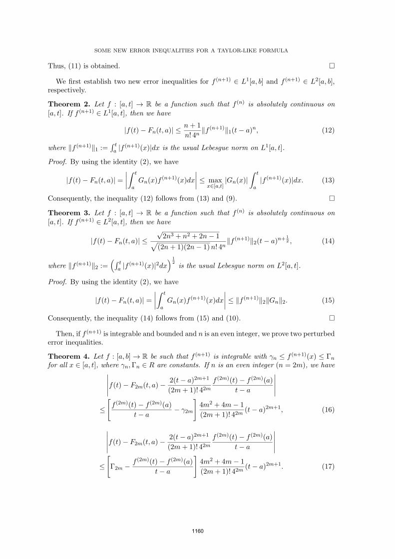
SOME NEW ERROR INEQUALITIES FOR A TAYLOR-LIKE FORMULA
Thus, (11) is obtained.
We first establish two new error inequalities for f (n+1) ∈ L1[a, b] and f (n+1) ∈ L2[a, b],respectively.
Theorem 2. Let f : [a, t] → ℝ be a function such that f (n) is absolutely continuous on
[a, t]. If f (n+1) ∈ L1[a, t], then we have
|f(t)− Fn(t, a)| ≤n+ 1
n! 4n∥f (n+1)∥1(t− a)n, (12)
where ∥f (n+1)∥1 :=∫ ta |f
(n+1)(x)|dx is the usual Lebesgue norm on L1[a, t].
Proof. By using the identity (2), we have
|f(t)− Fn(t, a)| =∣∣∣∣∫ t
aGn(x)f
(n+1)(x)dx
∣∣∣∣ ≤ maxx∈[a,t]
|Gn(x)|∫ t
a|f (n+1)(x)|dx. (13)
Consequently, the inequality (12) follows from (13) and (9).
Theorem 3. Let f : [a, t] → ℝ be a function such that f (n) is absolutely continuous on
[a, t]. If f (n+1) ∈ L2[a, t], then we have
|f(t)− Fn(t, a)| ≤√2n3 + n2 + 2n− 1√
(2n+ 1)(2n− 1)n! 4n∥f (n+1)∥2(t− a)n+
12 , (14)
where ∥f (n+1)∥2 :=(∫ t
a |f(n+1)(x)|2dx
) 12is the usual Lebesgue norm on L2[a, t].
Proof. By using the identity (2), we have
|f(t)− Fn(t, a)| =∣∣∣∣∫ t
aGn(x)f
(n+1)(x)dx
∣∣∣∣ ≤ ∥f (n+1)∥2∥Gn∥2. (15)
Consequently, the inequality (14) follows from (15) and (10).
Then, if f (n+1) is integrable and bounded and n is an even integer, we prove two perturbederror inequalities.
Theorem 4. Let f : [a, b] → ℝ be such that f (n+1) is integrable with n ≤ f (n+1)(x) ≤ Γn
for all x ∈ [a, t], where n,Γn ∈ R are constants. If n is an even integer (n = 2m), we have∣∣∣∣∣f(t)− F2m(t, a)− 2(t− a)2m+1
(2m+ 1)! 42mf (2m)(t)− f (2m)(a)
t− a
∣∣∣∣∣≤
[f (2m)(t)− f (2m)(a)
t− a− 2m
]4m2 + 4m− 1
(2m+ 1)! 42m(t− a)2m+1, (16)
∣∣∣∣∣f(t)− F2m(t, a)− 2(t− a)2m+1
(2m+ 1)! 42mf (2m)(t)− f (2m)(a)
t− a
∣∣∣∣∣≤
[Γ2m − f (2m)(t)− f (2m)(a)
t− a
]4m2 + 4m− 1
(2m+ 1)! 42m(t− a)2m+1. (17)
1160
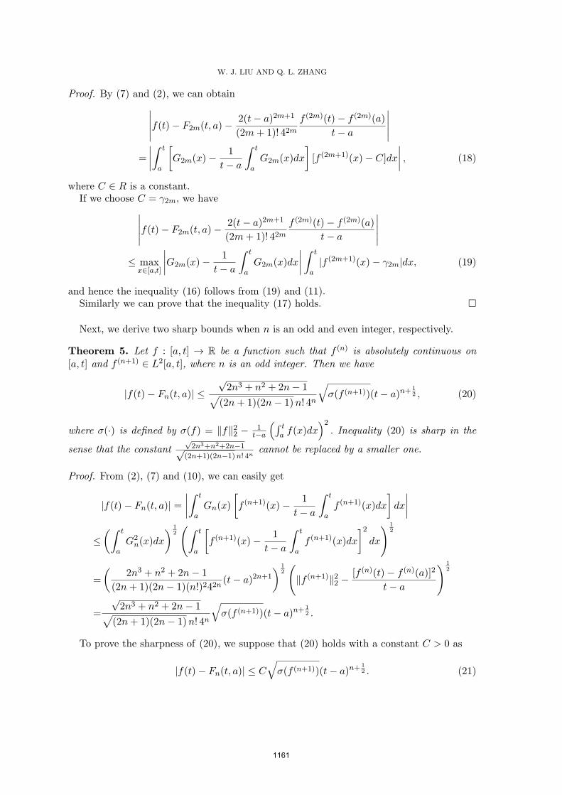
W. J. LIU AND Q. L. ZHANG
Proof. By (7) and (2), we can obtain∣∣∣∣∣f(t)− F2m(t, a)− 2(t− a)2m+1
(2m+ 1)! 42mf (2m)(t)− f (2m)(a)
t− a
∣∣∣∣∣=
∣∣∣∣∫ t
a
[G2m(x)− 1
t− a
∫ t
aG2m(x)dx
][f (2m+1)(x)− C]dx
∣∣∣∣ , (18)
where C ∈ R is a constant.If we choose C = 2m, we have∣∣∣∣∣f(t)− F2m(t, a)− 2(t− a)2m+1
(2m+ 1)! 42mf (2m)(t)− f (2m)(a)
t− a
∣∣∣∣∣≤ max
x∈[a,t]
∣∣∣∣G2m(x)− 1
t− a
∫ t
aG2m(x)dx
∣∣∣∣ ∫ t
a|f (2m+1)(x)− 2m|dx, (19)
and hence the inequality (16) follows from (19) and (11).Similarly we can prove that the inequality (17) holds.
Next, we derive two sharp bounds when n is an odd and even integer, respectively.
Theorem 5. Let f : [a, t] → ℝ be a function such that f (n) is absolutely continuous on
[a, t] and f (n+1) ∈ L2[a, t], where n is an odd integer. Then we have
|f(t)− Fn(t, a)| ≤√2n3 + n2 + 2n− 1√
(2n+ 1)(2n− 1)n! 4n
√σ(f (n+1))(t− a)n+
12 , (20)
where σ(·) is defined by σ(f) = ∥f∥22 − 1t−a
(∫ ta f(x)dx
)2. Inequality (20) is sharp in the
sense that the constant√2n3+n2+2n−1√
(2n+1)(2n−1)n! 4ncannot be replaced by a smaller one.
Proof. From (2), (7) and (10), we can easily get
|f(t)− Fn(t, a)| =∣∣∣∣∫ t
aGn(x)
[f (n+1)(x)− 1
t− a
∫ t
af (n+1)(x)dx
]dx
∣∣∣∣≤(∫ t
aG2
n(x)dx
) 12
(∫ t
a
[f (n+1)(x)− 1
t− a
∫ t
af (n+1)(x)dx
]2dx
) 12
=
(2n3 + n2 + 2n− 1
(2n+ 1)(2n− 1)(n!)242n(t− a)2n+1
) 12
(∥f (n+1)∥22 −
[f (n)(t)− f (n)(a)]2
t− a
) 12
=
√2n3 + n2 + 2n− 1√
(2n+ 1)(2n− 1)n! 4n
√σ(f (n+1))(t− a)n+
12 .
To prove the sharpness of (20), we suppose that (20) holds with a constant C > 0 as
|f(t)− Fn(t, a)| ≤ C√σ(f (n+1))(t− a)n+
12 . (21)
1161
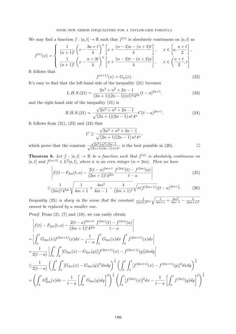
SOME NEW ERROR INEQUALITIES FOR A TAYLOR-LIKE FORMULA
We may find a function f : [a, t] → ℝ such that f (n) is absolutely continuous on [a, t] as
f (n)(x) =
1
(n+ 1)!
(x− 3a+ t
4
)n [x+
(n− 2)a− (n+ 2)t
4
], x ∈
[a,a+ t
2
],
1
(n+ 1)!
(x− a+ 3t
4
)n [x+
(n− 2)t− (n+ 2)a
4
], x ∈
(a+ t
2, t
]It follows that
f (n+1)(x) = Gn(x). (22)
It’s easy to find that the left-hand side of the inequality (21) becomes
L.H.S.(21) =2n3 + n2 + 2n− 1
(2n+ 1)(2n− 1)(n!)242n(t− a)2n+1, (23)
and the right-hand side of the inequality (21) is
R.H.S.(21) =
√2n3 + n2 + 2n− 1√
(2n+ 1)(2n− 1)n! 4nC(t− a)2n+1. (24)
It follows from (21), (23) and (24) that
C ≥√2n3 + n2 + 2n− 1√
(2n+ 1)(2n− 1)n! 4n,
which prove that the constant√2n3+n2+2n−1√
(2n+1)(2n−1)n! 4nis the best possible in (20).
Theorem 6. Let f : [a, t] → ℝ be a function such that f (n) is absolutely continuous on
[a, t] and f (n+1) ∈ L2[a, t], where n is an even integer (n = 2m). Then we have∣∣∣∣∣f(t)− F2m(t, a)− 2(t− a)2m+1
(2m+ 1)! 42mf (2m)(t)− f (2m)(a)
t− a
∣∣∣∣∣ (25)
≤ 1
(2m)! 42m
√1
4m+ 1+
4m2
4m− 1− 4
(2m+ 1)2
√σ(f (2m+1))(t− a)2m+ 1
2 . (26)
Inequality (25) is sharp in the sense that the constant 1(2m)! 42m
√1
4m+1 + 4m2
4m−1 − 4(2m+1)2
cannot be replaced by a smaller one.
Proof. From (2), (7) and (10), we can easily obtain∣∣∣∣∣f(t)− F2m(t, a)− 2(t− a)2m+1
(2m+ 1)! 42mf (2m)(t)− f (2m)(a)
t− a
∣∣∣∣∣=
∣∣∣∣∫ t
aG2m(x)f (2m+1)(x)dx− 1
t− a
∫ t
aG2m(x)dx
∫ t
af (2m+1)(x)dx
∣∣∣∣=
1
2(t− a)
∣∣∣∣∫ t
a
∫ t
a[G2m(x)−G2m(y)][f (2m+1)(x)− f (2m+1)(y)]dxdy
∣∣∣∣≤ 1
2(t− a)
(∫ t
a
∫ t
a[G2m(x)−G2m(y)]2dxdy
) 12(∫ t
a
∫ t
a[f (2m+1)(x)− f (2m+1)(y)]2dxdy
) 12
=
(∫ t
aG2
2m(x)dx− 1
t− a
[∫ t
aG2m(y)dy
]2) 12(∫ t
a[f (2m)(x)]2dx− 1
t− a
[∫ t
af (2m)(y)dy
]2) 12
1162
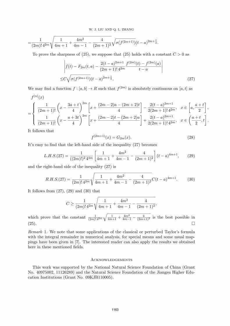
W. J. LIU AND Q. L. ZHANG
=1
(2m)! 42m
√1
4m+ 1+
4m2
4m− 1− 4
(2m+ 1)2
√σ(f (2m+1))(t− a)2m+ 1
2 .
To prove the sharpness of (25), we suppose that (25) holds with a constant C > 0 as∣∣∣∣∣f(t)− F2m(t, a)− 2(t− a)2m+1
(2m+ 1)! 42mf (2m)(t)− f (2m)(a)
t− a
∣∣∣∣∣≤C√σ(f (2m+1))(t− a)2m+ 1
2 . (27)
We may find a function f : [a, b] → R such that f (2m) is absolutely continuous on [a, t] as
f (n)(x)
=
1
(2m+ 1)!
(x− 3a+ t
4
)2m [x+
(2m− 2)a− (2m+ 2)t
4
]− 2(t− a)2m+1
2(2m+ 1)! 42m, x ∈
[a,a+ t
2
],
1
(2m+ 1)!
(x− a+ 3t
4
)2m [x+
(2m− 2)t− (2m+ 2)a
4
]+
2(t− a)2m+1
2(2m+ 1)! 42m, x ∈
(a+ t
2, t
].
It follows that
f (2m+1)(x) = G2m(x). (28)
It’s easy to find that the left-hand side of the inequality (27) becomes
L.H.S.(27) =1
((2m)!)2 44m
[1
4m+ 1+
4m2
4m− 1− 4
(2m+ 1)2
](t− a)4m+1, (29)
and the right-hand side of the inequality (27) is
R.H.S.(27) =1
(2m)! 42m
√1
4m+ 1+
4m2
4m− 1− 4
(2m+ 1)2C(t− a)4m+1. (30)
It follows from (27), (29) and (30) that
C ≥ 1
(2m)! 42m
√1
4m+ 1+
4m2
4m− 1− 4
(2m+ 1)2,
which prove that the constant 1(2m)! 42m
√1
4m+1 + 4m2
4m−1 − 4(2m+1)2
is the best possible in
(25).
Remark 1. We note that some applications of the classical or perturbed Taylor’s formulawith the integral remainder in numerical analysis, for special means and some usual map-pings have been given in [7]. The interested reader can also apply the results we obtainedhere in these mentioned fields.
Acknowledgements
This work was supported by the National Natural Science Foundation of China (GrantNo. 40975002, 11126289) and the Natural Science Foundation of the Jiangsu Higher Edu-cation Institutions (Grant No. 09KJB110005).
1163
SOME NEW ERROR INEQUALITIES FOR A TAYLOR-LIKE FORMULA
References
[1] M. Akkouchi, Improvements of some integral inequalities of H. Gauchman involving Taylor’s remainder,Divulg. Mat. 11 (2) (2003), 115–120.
[2] G. A. Anastassiou and S. S. Dragomir, On some estimates of the remainder in Taylor’s formula, J. Math.Anal. Appl., 263 (2001), 246–263.
[3] L. Bougoffa, Some estimations for the integral Taylor’s remainder, JIPAM. J. Inequal. Pure Appl. Math.4 (5) (2003), Article 86, 4 pp.
[4] P. Cerone, Generalized Taylor’s formula with estimates of the remainder, in Inequality Theory andApplications, Vol 2, 33–52. Nova Sicence Publ., New York, 2003.
[5] S. S. Dragomir, New estimation of the remainder in Taylor’s formula using Gruss type inequalities andapplications, Math. Inequal. Appl., 2 (2) (1999), 183–193.
[6] S. S. Dragomir and A. Sofo, A perturbed version of the generalised Taylor’s formula and applications,in Inequality theory and applications. Vol. 4, 71–84, Nova Sci. Publ., New York, 2007.
[7] S. S. Dragomir, A. Sofo and P. Cerone, A perturbation of Taylor’s formula with integral remainder,Tamsui Oxf. J. Math. Sci., 17 (1) (2001), 1–21.
[8] H. Gauchman, Some integral inequalities involving Taylor’s remainder I, JIPAM. J. Inequal. Pure Appl.Math., 3 (2) (2002), Article 26, 9 pp.
[9] H. Gauchman, Some integral inequalities involving Taylor’s remainder. II, JIPAM. J. Inequal. Pure Appl.Math. 4 (1) (2003), Article 1, 5 pp.
[10] D.-Y. Hwang, Improvements of some integral inequalities involving Taylor’s remainder, J. Appl. Math.Comput. 16 (1-2) (2004), 151–163.
[11] Huy V. N., Ngo Q. A., New inequalities of Ostrowski-like type involving n knots and the Lp-norm ofthe m-th derivative, Appl. Math. Lett., 22 (2009), 1345–1350.
[12] W. J. Liu, Several error inequalities for a quadrature formula with a parameter and applications,Comput. Math. Appl., 56 (2008) 1766–1772.
[13] Z. Liu, Note on inequalities involving integral Taylor’s remainder, JIPAM. J. Inequal. Pure Appl. Math.6 (3) (2005), Article 72, 6 pp.
[14] M. Matic, J. Pecaric and N. Ujevic, On new estimation of the remainder in generalized Taylor’s formula,Math. Inequal. Appl., 2 (3) (1999), 343–361.
[15] Y. X. Shi and Z. Liu, Some sharp Simpson type inequalities and applications, Applied MathematicsE-Notes, 9 (2009), 205–215.
[16] E. Talvila, Estimates of the remainder in Taylor’s theorem using the Hentstock-Kurzweil integral,Czechoslovak Math. J., 55 (4) (2005), 933–940.
[17] N. Ujevic, A new generalized perturbed Taylor’s formula, Nonlin. Funct. Anal. Appl., 7 (2) (2002),255-267.
[18] N. Ujevic, On generalized Taylor’s formula and some related results, Tamsui Oxford J. Math., 19 (1)(2003), 27-39.
[19] N. Ujevic, Error Inequalities for a Taylor-like Formula, CUBO A Mathematical Journal, 10 (1) (2008),11–18.
(W. J. Liu) College of Mathematics and Statistics, Nanjing University of Information Sci-ence and Technology, Nanjing 210044, China
E-mail address: [email protected]
(Q. L. Zhang) College of Atmospheric Physics, Nanjing University of Information Scienceand Technology, Nanjing 210044, China
1164
ADDITIVE FUNCTIONAL INEQUALITIES IN GENERALIZED
QUASI-BANACH SPACES
LEXIN LI, GANG LU, CHOONKIL PARK, AND DONG YUN SHIN∗
Abstract. In this paper, we investigate the Hyers-Ulam stability of the following functioninequalities
∥af(x) + bf(y) + cf(z)∥ ≤∥∥∥∥Kf (ax+ by + cz
K
)∥∥∥∥ (0 < |K| < |a+ b+ c|),
∥af(x) + bf(y) +Kf(z)∥ ≤∥∥∥∥Kf (ax+ by
K+ z
)∥∥∥∥ (0 < K < |a+ b+K|)
in generalized quasi-Banach spaces.
1. Introduction and preliminaries
The stability problem of functional equations originated from a question of Ulam [1] in 1940,
concerning the stability of group homomorphisms. Let (G1, .) be a group and let (G2, ∗) be a
metric group with the metric d(., .). Given ϵ > 0, does there exist a δ0, such that if a mapping
h : G1 → G2 satisfies the inequality d(h(x.y), h(x)∗h(y)) < δ for all x, y ∈ G1, then there exists
a homomorphism H : G1 → G2 with d(h(x),H(x)) < ϵ for all x ∈ G1? In the other words,
Under what condition does there exists a homomorphism near an approximate homomorphism?
The concept of stability for functional equation arises when we replace the functional equation
by an inequality which acts as a perturbation of the equation. In 1941, Hyers [2] gave the first
affirmative answer to the question of Ulam for Banach spaces. Let f : E → E′ be a mapping
between Banach spaces such that
∥f(x+ y)− f(x)− f(y)∥ ≤ δ
for all x, y ∈ E, and for some δ > 0. Then there exists a unique additive mapping T : E → E′
such that
∥f(x)− T (x)∥ ≤ δ
for all x ∈ E. Moreover, if f(tx) is continuous in t ∈ ℝ for each fixed x ∈ E, then T is ℝ-linear.In 1978, Th.M. Rassias [3] proved the following theorem.
Theorem 1.1. Let f : E → E′ be a mapping from a normed vector space E into a Banach
space E′ subject to the inequality
∥f(x+ y)− f(x)− f(y)∥ ≤ ϵ(∥x∥p + ∥y∥p) (1.1)
2010 Mathematics Subject Classification. Primary 39B62, 39B52, 46B25.Key words and phrases. Hyers-Ulam stability; additive functional inequality; generalized quasi-Banach space;
additive mapping.∗Corresponding author.
1165
J. COMPUTATIONAL ANALYSIS AND APPLICATIONS, VOL. 15, NO.6, 1165-1175, 2013, COPYRIGHT 2013 EUDOXUS PRESS, LLC
L. LI, G. LU, C. PARK, AND D.Y. SHIN
for all x, y ∈ E, where ϵ and p are constants with ϵ > 0 and p < 1. Then there exists a unique
additive mapping T : E → E′ such that
∥f(x)− T (x)∥ ≤ 2ϵ
2− 2p∥x∥p (1.2)
for all x ∈ E. If p < 0 then inequality (1.1) holds for all x, y = 0, and (1.2) for x = 0. Also, if
the function t 7→ f(tx) from ℝ into E′ is continuous in t ∈ ℝ for each fixed x ∈ E, then T is
ℝ-linear.
In 1991, Gajda [4] answered the question for the case p > 1, which was raised by Th.M.
Rassias. On the other hand, J.M. Rassias [5] generalized the Hyers-Ulam stability result by
presenting a weaker condition controlled by a product of different powers of norms.
Theorem 1.2. ([6, 7]) If it is assumed that there exist constants Θ ≥ 0 and p1, p2 ∈ ℝ such
that p = p1 + p2 = 1, and f : E → E′ is a mapping from a norm space E into a Banach space
E′ such that the inequality
∥f(x+ y)− f(x)− f(y)∥ ≤ Θ∥x∥p1∥y∥p2
for all x, y ∈ E, then there exists a unique additive mapping T : E → E′ such that
∥f(x)− T (x)∥ ≤ Θ
2− 2p∥x∥p,
for all x ∈ E. If, in addition, f(tx) is continuous in t ∈ ℝ for each fixed x ∈ E, then T is
ℝ-linear
More generalizations and applications of the Hyers-Ulam stability to a number of functional
equations and mappings can be found in [8]–[22].
In [23], Park et al. investigated the following inequalities
∥f(x) + f(y) + f(z)∥ ≤∥∥∥∥2f (x+ y + z
2
)∥∥∥∥ ,∥f(x) + f(y) + f(z)∥ ≤ ∥f(x+ y + z)∥,
∥f(x) + f(y) + 2f(z)∥ ≤∥∥∥∥2f (x+ y
2+ z
)∥∥∥∥in Banach spaces. Recently, Cho et al. [24] investigated the following functional inequality
∥f(x) + f(y) + f(z) ≤∥∥∥∥Kf (x+ y + z
K
)∥∥∥∥ (0 < |K| < |3|)
in non-Archimedean Banach spaces. Lu and Park [25] investigated the following functional
inequality ∥∥∥∥∥N∑i=1
f(xi)
∥∥∥∥∥ ≤
∥∥∥∥∥Kf(∑N
i=1(xi)
K
)∥∥∥∥∥ (0 < |K| ≤ N)
in Frechet spaces.
In [26], we investigated the following functional inequalities
∥f(x) + f(y) + f(z)∥ ≤∥∥∥∥Kf (x+ y + z
K
)∥∥∥∥ (0 < |K| < 3), (1.3)
1166
FUNCTIONAL INEQUALITIES IN GENERALIZED QUASI-BANACH SPACES
∥f(x) + f(y) +Kf(z)∥ ≤∥∥∥∥Kf (x+ y
K+ z
)∥∥∥∥ (0 < K = 2) (1.4)
and proved the Hyers-Ulam stability of the functional inequalities (1.3) and (1.4) in Banach
spaces.
We consider the following functional inequalities
∥af(x) + bf(y) + cf(z)∥ ≤∥∥∥∥Kf (ax+ by + cz
K
)∥∥∥∥ (0 < |K| < |a+ b+ c|), (1.5)
∥af(x) + bf(y) +Kf(z)∥ ≤∥∥∥∥Kf (ax+ by
K+ z
)∥∥∥∥ (0 < K < |a+ b+K|), (1.6)
where a, b, c are nonzero real numbers.
Now, we recall some basic facts concerning quasi-Banach spaces and some preliminary results.
Definition 1.3. ([27, 28]) Let X be a linear space. A quasi-norm is a real-valued function on
X satisfying the following:
(1) ∥x∥ ≥ 0 for all x ∈ X and ∥x∥ = 0 if and only if x = 0.
(2) ∥λx∥ = |λ|∥x∥ for all λ ∈ ℝ and all x ∈ X.
(3) There is a constant C ≥ 1 such that ∥x+ y∥ ≤ C(∥x∥+ ∥y∥) for all x, y ∈ X.
The pair (X, ∥ · ∥) is called a quasi-normed space if ∥ · ∥ is a quasi-norm on X.
A quasi-Banach space is a complete quasi-normed space.
Baak [29] generalized the concept of quasi-normed spaces.
Definition 1.4. ([29]) Let X be a linear space. A generalized quasi-norm is a real-valued
function on X satisfying the following:
(1) ∥x∥ ≥ 0 for all x ∈ X and ∥x∥ = 0 if and only if x = 0.
(2) ∥λx∥ = |λ| · ∥x∥ for all λ ∈ ℝ and all x ∈ X.
(3) There is a constant C ≥ 1 such that ∥∑∞
j=1 xj∥ ≤∑∞
j=1C∥xj∥ for all x1, x2, · · · ∈ X
with∑∞
j=1 xj ∈ X.
The pair (X, ∥·∥) is called a generalized quasi-normed space if ∥·∥ is a generalized quasi-norm
on X. The smallest possible C is called the modulus of concavity of ∥ · ∥.A generalized quasi-Banach space is a complete generalized quasi-normed space.
In this paper, we show that the Hyers-Ulam stability of the functional inequalities (1.5) and
(1.6) in generalized quasi-Banach spaces.
Throughout this paper, assume that X is a generalized quasi-normed vector space with
generalized quasi-norm ∥ · ∥ and that (Y, ∥ · ∥) is a generalized quasi-Banach space. Let C be
the modulus of concavity of ∥ · ∥.
2. Hyers-Ulam stability of the functional inequality (1.5)
Throughout this section, assume that K is a real number with 0 < |K| < |a+ b+ c|.
Proposition 2.1. Let f : X → Y be a mapping such that
∥af(x) + bf(y) + cf(z)∥ ≤∥∥∥∥Kf (ax+ by + cz
K
)∥∥∥∥ (2.1)
for all x, y, z ∈ X. Then the mapping f : X → Y is additive.
1167
L. LI, G. LU, C. PARK, AND D.Y. SHIN
Proof. Letting x = y = z = 0 in (2.1), we get
∥(a+ b+ c)f(0)∥ ≤ ∥Kf(0)∥.
So f(0) = 0.
Letting z = 0 and y = − bax in (2.1), we get∥∥∥af(x) + bf
(−abx)∥∥∥ ≤ ∥Kf(0)∥ = 0
for all x ∈ X. So f(x) = − baf(−
abx) for all x ∈ X.
Replacing x by −x and letting y = 0 and z = acx in (2.1), we get∥∥∥af(−x) + cf
(acx)∥∥∥ ≤ ∥Kf(0)∥ = 0
for all x ∈ X. So f(−x) = − caf(
acx) for all x ∈ X. Then we get
∥f(x) + f(−x)∥ =
∥∥∥∥− baf (−ab x)− c
af(acx)∥∥∥∥
=1
|a|
∥∥∥af(0) + bf(−abx)+ cf
(acx)∥∥∥
≤ 1
|a|
∥∥∥∥Kf (a · 0− babx+ cacx
K
)∥∥∥∥ = 0
Thus f(x) = −f(−x).∥f(x) + f(y)− f(x+ y)∥ = ∥f(x) + f(y) + f(−x− y)∥
=
∥∥∥∥−aaf(−aax)− b
af(−a
by)− c
af(ax+ ay
c)
∥∥∥∥=
1
|a|
∥∥∥∥af(−aax) + bf(−aby) + cf(
ax+ ay
c)
∥∥∥∥=
1
|a|
∥∥∥∥∥Kf(a · (−a
ax) + b · (−abx) + c · a(x+y)
c
K
)∥∥∥∥∥ = 0.
Thus
f(x+ y) = f(x) + f(y)
for all x, y ∈ X, as desired.
Theorem 2.2. Assume that a mapping f : X → Y satisfies the inequality
∥af(x) + bf(y) + cf(z)∥ ≤∥∥∥∥Kf (ax+ by + cz
K
)∥∥∥∥+ ϕ(x, y, z), (2.2)
where ϕ : X3 → [0,∞) satisfies ϕ(0, 0, 0) = 0 and
ϕ(x, y, z) :=
∞∑j=0
( ca
)jϕ
((ac
)jy,(ac
)jz,(ac
)jx
)<∞
for all x, y, z ∈ X. Then there exists a unique additive mapping A : X → Y such that
∥A(x)− f(x)∥ ≤ C2
|a|
[ϕ(x,−a
bx, 0)+ ϕ
(0,−a
bx,a
cx)]
(2.3)
for all x ∈ X.
1168
FUNCTIONAL INEQUALITIES IN GENERALIZED QUASI-BANACH SPACES
Proof. Letting x = y = z = 0 in (2.2), we get ∥(a+b+c)f(0)∥ ≤ ∥Kf(0)∥+ϕ(0, 0, 0) = ∥Kf(0)∥.So f(0) = 0.
Letting y = 0 and z = −acx in (2.2), we get
∥∥∥af(x) + cf(−acx)∥∥∥ ≤ ϕ
(x, 0,−a
cx)
for all x ∈ X. So∥∥f(x) + c
af(−acx)∥∥ ≤ 1
|a|ϕ(x, 0,−a
cx)for all x ∈ X.
Letting y = −abx and z = 0 in (2.2), we obtain
∥∥∥∥f(x) + b
af(−abx)∥∥∥∥ ≤ 1
|a|ϕ(x,−a
bx, 0)
for all x ∈ X. So
∥∥∥f(x)− c
af(acx)∥∥∥ =
∥∥∥∥f(x) + b
af(−axb
)− b
af(−axb
)− c
af(acx)∥∥∥∥
≤ C
(∥∥∥∥f(x) + b
af(−axb
)∥∥∥∥+ ∥∥∥∥ baf (−axb )+ c
af(acx)∥∥∥∥)
≤ C
|a|
[ϕ(x,−ax
b, 0)+ ϕ
(0,−ax
b,ax
c
)] (2.4)
for all x ∈ X.
It follows from (2.4) that
∥∥∥( ca)lf((a
c)lx)− (
c
a)mf
((a
c)mx
)∥∥∥≤ C
m−1∑j=l
∥∥∥( ca)jf((a
c)jx)− (
c
a)j+1f
((a
c)j+1x
)∥∥∥≤ C2
|a|
m−1∑j=l
( ca
)j [ϕ
((ac
)jx,−a
b
(ac
)jx, 0
)+ ϕ
(0,−a
b
(ac
)jx,(ac
)j+1x
)]
for all nonnegative integers m and l with m > l and all x ∈ X. It means that the se-
quence ( ca)nf((ac )
nx) is a Cauchy sequence for all x ∈ X. Since Y is complete, the sequence
( ca)nf((ac )
nx) converges. We define the mappingA : X → Y byA(x) = limn→∞( ca)nf((ac )
nx)for all x ∈ X. Moreover, letting l = 0 and passing the limit m→ ∞, we get (2.3).
1169
L. LI, G. LU, C. PARK, AND D.Y. SHIN
Next, we show that A : X → Y is an additive mapping.
∥A(x) +A(−x)∥ = limn→∞
(c
a)n∥∥∥∥f (anxcn
)+ f
(−anxcn
)∥∥∥∥≤ C lim
n→∞(c
a)n[∥∥∥∥f (anxcn
)+b
af
(−ab· a
nx
cn
)∥∥∥∥+
∥∥∥∥f (−anxcn)+c
af
(a
c· a
nx
cn
)∥∥∥∥+
∥∥∥∥ baf(−ab· a
nx
cn
)+c
af
(a
c· a
nx
cn
)∥∥∥∥]≤ C
1
|a|limn→∞
(c
a)n[ϕ
(anx
cn,−a
b
anx
cn, 0
)+ ϕ
(−a
nx
cn, 0,
an+1x
cn+1
)+ ϕ
(0,−a
b
anx
cn,an+1x
cn+1
)]= 0
and so A(−x) = −A(x) for all x ∈ X.
∥A(x) +A(y)−A(x+ y)∥| = limn→∞
(c
a)n∥∥∥∥f (anxcn
)+ f
(any
cn
)− f
(an(x+ y)
cn
)∥∥∥∥= C lim
n→∞(c
a)n[∥∥∥∥f (anxcn
)+b
af
(−ab
anx
cn
)∥∥∥∥+
∥∥∥∥f (anycn)+c
af
(−a
n+1y
cn+1
)∥∥∥∥+
∥∥∥∥f (an(x+ y)
cn
)+b
af
(−ab
anx
cn
)+c
af
(−a
n+1y
cn+1
)∥∥∥∥]≤ C
1
|a|limn→∞
(c
a)n[ϕ
(anx
cn,−a
b(anx
cn), 0
)+ ϕ
(any
cn, 0,−a
c(anx
cn)
)+ϕ
(an(x+ y)
cn,−a
b(anx
cn),−a
c(anx
cn)
)]= 0
for all x, y ∈ X. Thus the mapping A : X → Y is additive.
Now, we prove the uniqueness of A. Assume that T : X → Y is another additive mapping
satisfying (2.3). Then we obtain
∥A(x)− T (x)∥ = (c
a)n∥∥∥A((a
c)nx)− T
((a
c)nx)∥∥∥
≤ C · ( ca)n[∥∥∥A((a
c)nx)− f
((a
c)nx)∥∥∥
+∥∥∥T ((a
c)nx)− f
((a
c)nx)∥∥∥]
≤ 2CC2
|a|
[ϕ(x,−a
bx, 0)+ ϕ(0,−a
bx,a
cx)]
which tends to zero as n → ∞ for all x ∈ X. Then we can conclude that A(x) = T (x) for all
x ∈ X. This complete the proof.
1170
FUNCTIONAL INEQUALITIES IN GENERALIZED QUASI-BANACH SPACES
Corollary 2.3. Let p and θ be positive real numbers with p > 1. Let f : X → Y be a mapping
satisfying
∥af(x) + bf(y) + cf(z)∥ ≤∥∥∥∥Kf (ax+ by + cz
K
)∥∥∥∥+ θ(∥x∥p + ∥y∥p + ∥z∥p)
for all x, y, z ∈ X. Then there exists a unique additive mapping A : X → Y such that
∥f(x)−A(x)∥ ≤ C
|a|· cp + ap
cp − c(a+ b)p−1θ∥x∥p
for all x ∈ X.
3. Hyers-Ulam stability of the functional inequality (1.6)
Throughout this section, assume that K, a, b are nonzero real numbers with 0 < K = 2 and
|a+ b+K| ≥ K.
Proposition 3.1. Let f : X → Y be a mapping such that
∥af(x) + bf(y) +Kf(z)∥ ≤∥∥∥∥Kf (ax+ by
K+ z
)∥∥∥∥ (3.1)
for all x, y, z ∈ X. Then the mapping f : X → Y is additive.
Proof. Letting x = y = z = 0 in (3.1), we get
∥(K + a+ b)f(0)∥ ≤ ∥Kf(0)∥.
So f(0) = 0.
Letting y = −abx and z = 0 in (3.1), we get∥∥∥af(x) + bf
(−abx)∥∥∥ ≤ ∥Kf(0)∥ = 0
for all x ∈ X. So f(x) = − baf(−
abx) for all x ∈ X.
Replacing x by −x and letting y = 0 and z = aKx in (3.1), we get∥∥∥af(−x) +Kf
( aKx)∥∥∥ ≤ ∥Kf(0)∥ = 0
for all x ∈ X. So f(−x) = −Ka f(
aKx) for all x ∈ X.
Thus we get
∥f(x) + f(−x)∥ =1
|a|
∥∥∥bf (−abx)+Kf
( aKx)∥∥∥ ≤ 1
|a|∥f(0)∥ = 0
for all x ∈ X. So f(−x) = −f(x) for all x ∈ X.
Letting z = −x−yK in (3.1), we get∥∥∥∥af(x) + bf(y)−Kf
(ax+ by
K
)∥∥∥∥ =
∥∥∥∥af(x) + bf(y) +Kf
(−ax− by
K
)∥∥∥∥≤ ∥Kf(0)∥ = 0
for all x, y ∈ X. Thus
Kf
(ax+ by
K
)= af(x) + bf(y) (3.2)
1171
L. LI, G. LU, C. PARK, AND D.Y. SHIN
for all x, y ∈ X. Letting y = 0 in (3.2), we get f(x) = aK f(Kxa
)for all x ∈ X. Letting x = 0 in
(3.2), we get f(y) = bK f(Kyb
). So
∥f(x) + f(y)− f(x+ y)∥ =
∥∥∥∥ aK f
(Kx
a
)+
b
Kf
(Ky
b
)+ f(−x− y)
∥∥∥∥=
1
|K|
∥∥∥∥af (Kxa)+ bf
(Ky
b
)+Kf(−x− y)
∥∥∥∥ = 0
for all x, y ∈ X, as desired.
Theorem 3.2. Assume that a mapping f : X → Y satisfies the inequality
∥af(x) + bf(y) +Kf(z)∥ ≤∥∥∥∥Kf (ax+ by
K+ z
)∥∥∥∥+ ϕ(x, y, z), (3.3)
where ϕ : X3 → [0,∞) satisfies ϕ(0, 0, 0) = 0 and
ϕ(x, y, z) :=
∞∑j=1
∣∣∣∣( aK )j∣∣∣∣ϕ((
K
a
)j
x,
(K
a
)j
y,
(K
a
)j
z
)<∞
for all x, y, z ∈ X. Then there exists a unique additive mapping A : X → Y such that
∥A(x)− f(x)∥ ≤ C2
|K|
[ϕ
(0,−K
ax, x)
)+ ϕ
(K
ax,−K
bx, 0
)](3.4)
for all x ∈ X.
Proof. Letting x = y = z = 0 in (3.3), we get ∥(K + a + b)f(0)∥ ≤ ∥Kf(0)∥ + ϕ(0, 0, 0) =
∥Kf(0)∥. So f(0) = 0.
Letting x = 0, y = −Kxb , z = x in (3.3), we obtain∥∥∥∥af(0) + bf
(−Kbx
)+Kf(x)
∥∥∥∥ ≤ ϕ
(0,−K
bx, x
)for all x ∈ X.
Letting y = 0, z = −Kxa in (3.3), we obtain∥∥∥∥af(x) + bf(0) +Kf
(−axK
)∥∥∥∥ ≤ ϕ(x, 0,−ax
K
)for all x ∈ X.
Letting x = Kxa , y = −Kx
b , z = 0 in (3.3), we get∥∥∥∥af (Kxa)+ bf
(−Kx
b
)+Kf(0)
∥∥∥∥ ≤ ϕ
(Kx
a,−Kx
b, 0
)for all x ∈ X. So∥∥∥∥f(x)− a
Kf
(K
ax
)∥∥∥∥≤ C
[∥∥∥∥f(x) + b
Kf
(−Kx
b
)∥∥∥∥+ ∥∥∥∥ bK f
(−Kbx
)+
a
Kf
(K
ax
)∥∥∥∥]≤ C
|K|
[ϕ
(0,−K
bx, x
)+ ϕ
(K
ax,−K
bx, 0
)] (3.5)
1172
FUNCTIONAL INEQUALITIES IN GENERALIZED QUASI-BANACH SPACES
for all x ∈ X. It follows from (3.5) that∥∥∥∥∥( aK )l f((
K
a
)l
x
)−( aK
)mf
((K
a
)m
x
)∥∥∥∥∥≤ C
m−1∑j=l
∥∥∥∥∥( aK )j f((
K
a
)j
x
)−( aK
)j+1f
((K
a
)j+1
x
)∥∥∥∥∥≤ C2
m−1∑j=l
∣∣∣( aK
)j∣∣∣ [∥∥∥∥∥f(
((K
a
)j
x
)+
b
Kf
(−Kb
((K
a
)j
x
)))
∥∥∥∥∥+
∥∥∥∥∥ bK f
(−Kb
((K
a
)j
x
))+
a
Kf
(K
a
((K
a
)j
x
))∥∥∥∥∥]
≤ C2
|K|
m−1∑j=l
∣∣∣( aK
)j∣∣∣ [ϕ(0,−K
a
(K
a
)j
x,
(K
a
)j
x
)+ ϕ
(K
a
(K
a
)j
x,−Kb
(K
a
)j
x, 0
)]
for all nonnegative integers m and l with m > l and all x ∈ X. It means that the se-
quence ( aK )nf((Ka )
nx) is a Cauchy sequence for all x ∈ X. Since Y is complete, the se-
quence ( aK )nf((Ka )
nx) converges. So we may define the mapping A : X → Y by A(x) =
limn→∞(( aK )nf((Ka )
nx)) for all x ∈ X.
Moreover, by letting l = 0 and passing the limit m→ ∞, we get (3.4).
Now, we show that A is additive.
∥A(x) +A(y)−A(x+ y)∥
= limn→∞
∣∣∣ aK
∣∣∣n ∥∥∥∥f((Ka )nx) + f((K
a)ny)− f((
K
a)n(x+ y))
∥∥∥∥≤ C lim
n→∞
∣∣∣ aK
∣∣∣n [∥∥∥∥f ((Ka)n
x
)+
b
Kf
(−Kb
(K
a
)n
x
)∥∥∥∥+
∥∥∥∥f ((Ka)n
y
)+
a
Kf
(−Ka
(K
a
)n
y
)∥∥∥∥+
∥∥∥∥ aK f
(−Ka
(K
a
)n
y
)+
b
Kf
(−Kb
(K
a
)n
x
)+ f
((K
a
)n
(x+ y)
)∥∥∥∥]≤ C lim
n→∞
∣∣∣ aK
∣∣∣n [ϕ(0,−Kb
(K
a
)n
x,
(K
a
)n
x
)+ ϕ
(−Ka
(K
a
)n
y, 0,
(K
a
)n
y
)+ ϕ
(−Ka
(K
a
)n
y,−Kb
(K
a
)n
x,
(K
a
)n
(x+ y)
)]= 0
for all x, y ∈ X. So the mapping A : X → Y is an additive mapping.
1173
L. LI, G. LU, C. PARK, AND D.Y. SHIN
Now, we show that the uniqueness of A. Assume that T : X → Y is another additive mapping
satisfying (3.4). Then we get
∥A(x)− T (x)∥ = limn→∞
∣∣∣ aK
∣∣∣n ∥∥∥∥A ∣∣∣∣(Ka∣∣∣∣n x)− T
((K
a
)n
x
)∥∥∥∥≤ C lim
n→∞
∣∣∣ aK
∣∣∣n [∥∥∥∥A((Ka)n
x
)− f
((K
a
)n
x
)∥∥∥∥+ ∥∥∥∥T ((Ka)n
x
)− f
((K
a
)n
x
)∥∥∥∥]≤ 2C
C2
|K|limn→∞
[ϕ
(0,−K
a
(K
a
)n
x,
(K
a
)n
x)
)+ ϕ
(K
a
(K
a
)n
x,−Kb
(K
a
)n
x, 0
)]= 0
for all x ∈ X. Thus we may conclude that A(x) = T (x) for all x ∈ X. This proves the
uniqueness of A. So the mapping A : X → Y is a unique additive mapping satisfying (3.4).
Corollary 3.3. Let p, θ and K be positive real numbers with p > 1 and |a+ b+K| > K. Let
f : X → Y be a mapping satisfying
∥af(x) + bf(y) +Kf(z)∥ ≤∥∥∥∥Kf (ax+ by
K+ z
)∥∥∥∥+ θ(∥x∥p + ∥y∥p + ∥z∥p)
for all x, y, z ∈ X. Then there exists a unique additive mapping A : X → Y such that
∥f(x)−A(x)∥ ≤1K
(aK
)p+ 3a
K(aK
)p − aK
θ∥x∥p
for all x ∈ X.
Acknowledgments
C. Park was supported by Basic Science Research Program through the National Research
Foundation of Korea funded by the Ministry of Education, Science and Technology (NRF-
2012R1A1A2004299). D. Y. Shin was supported by Basic Science Research Program through
the National Research Foundation of Korea funded by the Ministry of Education, Science and
Technology (NRF-2010-0021792).
References
[1] S.M. Ulam, A Collection of the Mathematical Problems, Interscience Publ., New York, 1960.[2] D.H. Hyers, On the stability of the linear functional equation, Proc. Natl. Acad. Sci. USA 27 (1941), 222–224.[3] Th.M. Rassias, On the stability of the linear mapping in Banach spaces, Proc. Amer. Math. Soc. 72 (1978),
297–300.[4] Z. Gajda, On stability of additive mappings, Internat. J. Math. Math. Sci. 14 (1991), 431–434.[5] J.M. Rassias, On approximation of approximately linear mappings by linear mappings, Bull. Sci. Math. 108
(1984), 445–446.[6] J.M. Rassias, On approximation of approximately linear mappings by linear mappings, J. Funct. Anal. 46
(1982), 126–130.[7] J.M. Rassias, On a new approximation of approximately linear mappings by linear mappings, Discuss. Math.
7 (1985), 193–196.[8] S. Jung, Hyers-Ulam-Rassias Stability of Functional Equations in Mathematical Analysis, Hadronic Press
Inc., Palm Harbor, Florida, 2001.[9] G. Lu, C. Park, Hyers-Ulam stability of additive set-valued functional equations, Appl. Math. Lett. 24 (2011),
1312–1316.
1174
FUNCTIONAL INEQUALITIES IN GENERALIZED QUASI-BANACH SPACES
[10] I. Chang, Stability of higher ring derivations in fuzzy Banach algebras, J. Computat. Anal. Appl. 14 (2012),1059–1066.
[11] I. Cho, D. Kang, H. Koh, Stability problems of cubic mappings with the fixed point alternative, J. Computat.Anal. Appl. 14 (2012), 132–142.
[12] M. Eshaghi Gordji, M. Bavand Savadkouhi, M. Bidkham, Stability of a mixed type additive and quadraticfunctional equation in non-Archimedean spaces, J. Computat. Anal. Appl. 12 (2010), 454–462.
[13] M. Eshaghi Gordji, A. Bodaghi, On the stability of quadratic double centralizers on Banach algebras, J.Computat. Anal. Appl. 13 (2011), 724–729.
[14] M. Eshaghi Gordji, R. Farokhzad Rostami, S.A.R. Hosseinioun, Nearly higher derivations in unital C∗-algebras, J. Computat. Anal. Appl. 13 (2011), 734–742.
[15] M. Eshaghi Gordji, S. Kaboli Gharetapeh, T. Karimi, E. Rashidi, M. Aghaei, Ternary Jordan derivationson C∗-ternary algebras, J. Computat. Anal. Appl. 12 (2010), 463–470.
[16] H.A. Kenary, J. Lee, C. Park, Non-Archimedean stability of an AQQ-functional equation, J. Computat.Anal. Appl. 14 (2012), 211–227.
[17] C. Park, Y. Cho, H.A. Kenary, Orthogonal stability of a generalized quadratic functional equation in non-Archimedean spaces, J. Computat. Anal. Appl. 14 (2012), 526–535.
[18] C. Park, S. Jang, R. Saadati, Fuzzy approximate of homomorphisms, J. Computat. Anal. Appl. 14 (2012),833–841.
[19] S. Shagholi, M. Eshaghi Gordji, M. Bavand Savadkouhi, Stability of ternary quadratic derivations on ternaryBanach algebras, J. Computat. Anal. Appl. 13 (2011), 1097–1105.
[20] S. Shagholi, M. Eshaghi Gordji, M. Bavand Savadkouhi, Nearly ternary cubic homomorphism in ternaryFrechet algebras, J. Computat. Anal. Appl. 13 (2011), 1106–1114.
[21] C. Park, Homomorphisms between Poisson JC∗-algebra, Bull. Braz. Math. Soc. 36 (2005), 79–97.[22] C. Park, Hyers-Ulam-Rassias stability of homomorphisms in quasi-Banach algebras, Bull. Sci. Math. 132
(2008), 87–96.[23] C. Park, Y. Cho, M. Han, Functional inequalities associated with Jordan-von Neumann type additive func-
tional equations, J. Inequal. Appl. 2007, Art. ID 41820 (2007).[24] Y. Cho, C. Park, R. Saadati, Functional inequalities in non-Archimedean Banach spaces, Appl. Math. Lett.
23 (2010), 1238–1242.[25] G. Lu, Y. Jiang, C. Park, Functional inequality in Frechet spaces, J. Computat. Anal. Appl. (to appear)[26] G. Lu, C. Park, Additive functional inequalities in Banach spaces (preprint).[27] Y. Benyamini, J. Lindenstrauss, Geometric Nolinear Functional Analysis, Vol. 1, Colloq. Publ. 48, Amer.
Math. Soc., Providence, 2000.[28] S. Rolewicz, Metric Linear Spaces, PWN-Polish Sci. Publ., Reidel and Dordrecht, 1984.[29] C. Baak, Generalized quasi-Banach spaces, J. Chungcheong Math. Soc. 18 (2005), 215–222.
Lexin LiSchool of Equipment Engineering, Shenyang Ligong University, Shenyang, 110159P.R. China
E-mail address: [email protected]
Gang LuDepartment of Mathematics, School of Science, ShenYang University of Technology, Shenyang110178, P.R. China
E-mail address: [email protected]
Choonkil ParkDepartment of Mathematics, Research Institute for Natural Sciences, Hanyang University, Seoul133-791, Korea
E-mail address: [email protected]
Dong Yun ShinDepartment of Mathematics, University of Seoul, Seoul 130-743, Korea
E-mail address: [email protected]
1175

1176
TABLE OF CONTENTS, JOURNAL OF COMPUTATIONAL
ANALYSIS AND APPLICATIONS, VOL. 15, NO. 6, 2013
Weighted Superposition Operators in Some Analytic Function Spaces, A. El-Sayed Ahmed and S. Omran,…….……………………………………………………………………………996
Fuzzy Fixed Points of Contractive Fuzzy Mappings, Akbar Azam and Muhammad Arshad,1006
On Explicit Solutions to a Polynomial Equation and its Applications to Constructing Wavelets, D. H. Yuan, Y. Feng, Y. F. Shen, and S. Z. Yang,…………………………………………1015
Numerical Solution of Fully Fuzzy Linear Matrix Equations, Kun Liu and Zeng-Tai Gong,1026
Korovkin Type Approximation Theorem for Statistical A-Summability of Double Sequences, M. Mursaleen and Abdullah Alotaibi,…………………………………………………………1036
The Properties of Logistic Function and Applications to Neural Network Approximation, Zhixiang Chen and Feilong Cao,……………………………………………………………1046
Orthogonal Stability of an Additive Functional Equation in Banach Modules Over a ∗ −Algebra, Hassan Azadi Kenary, Choonkil Park, and Dong Yun Shin,…………………1057
Some Characterizations and Convergence Properties of the Choquet Integral with Respect to a Fuzzy Measure of Fuzzy Complex Valued Functions, Lee-Chae Jang,…………………1069
Intuitionistic Fuzzy Stability of Euler-Lagrange Type Quartic Mappings, Heejeong Koh, Dongseung Kang, and In Goo Cho,………………………………………………………1085
Stability for an n-Dimensional Functional Equation of Quadratic-Additive Type with the Fixed Point Approach, Ick-Soon Chang and Yang-Hi Lee,…………………………………… 1096
An Identity of the q-Euler Polynomials Associated with the p-Adic q-Integrals on ℤ, C. S.
Ryoo,………………………………………………………………………………………1104
Approximate Septic and Octic Mappings in Quasi--Normed Spaces,Tian Zhou Xu, J.Rassias,1110
Power Harmonic Operators and Their Applications in Group Decision Making, Jin Han Park, Jung Mi Park, and Jong Jin Seo, Y.C.Kwun,..…………………………………………….1120
Multiplicational Combinations and a General Scheme of Single-Step Iterative Methods for Multiple Roots, Siyul Lee and Hyeongmin Choe,……………………………………….1138
TABLE OF CONTENTS, JOURNAL OF COMPUTATIONAL
ANALYSIS AND APPLICATIONS, VOL. 15, NO. 6, 2013
(continued)
Compact Differences of Volterra Composition Operators from Bergman-Type Spaces to Bloch-Type Spaces, Zhi Jie Jiang,………………………………………………………………1150
Some New Error Inequalities for a Taylor-Like Formula, Wenjun Liu and Qilin Zhang,1158
Additive Functional Inequalities in Generalized Quasi-Banach Spaces, Lexin Li, Gang Lu, Choonkil Park, and Dong Yun Shin,…………………………………………………….1165