the linguistic weighted average

The Linguistic Weighted Average

Dongrui Wu, Student Member, IEEE, and Jerry M. Mendel, Life Fellow, IEEE

Abstract— The focus of this paper is the linguistic weightedaverage (LWA), which is a generalization of the fuzzy weightedaverage (FWA) that is obtained by replacing the type-1 fuzzyinputs in the FWA by interval type-2 fuzzy sets (IT2 FSs).Consequently, the output of the LWA is an IT2 FS. In this paper,the relations between the LWA and the FWA are studied. It isshown that finding the LWA can be decomposed into findingtwo FWAs, where α-cuts and KM algorithms are used. Hence,the computational cost of a LWA is about twice that of a FWA.A flowchart for computing the LWA is also provided.

I. INTRODUCTION

The weighted average (WA) is arguably the earliest andstill most widely used form of aggregation. In this paper wefocus on a new situation for the WA, one in which boththe quantities being averaged (the attributes) as well as theweights are words. The resulting WA is called a linguisticWA (LWA). Our Example below illustrates a decision-makingsituation where the LWA is needed. First, however, weremind the reader of the well-known formula for the WA,i.e.

y =∑n

i=1 xiwi∑ni=1 wi

= f(x1, . . . , xn, w1, . . . , wn) (1)

in which wi are the weights that act upon the attributes (e.g.,decisions, features, indicators, etc.), xi. Normalization isachieved by dividing the weighted numerator sum by the sumof all of the weights. While it is always true that the sum ofthe normalized weights that act upon each xi add to one, it isnot a requirement that the sum of the un-normalized weightsmust add to one. In many situations requiring

∑ni=1 wi = 1

is too restrictive; so, we do not impose such a requirement.It is the normalization that makes the calculation of the LWAvery challenging.

In the LWA the weights are always words that are modeledas interval type-2 fuzzy sets (IT2 FSs) [14], and the attributesmay also be (but do not have to be) words that are alsomodeled as IT2 FSs1. We denote the LWA as YLWA, where

YLWA =∑n

i=1 XiWi∑ni=1 Wi

(2)

The tildes over all quantities denote IT2 FSs.Before we formalize the LWA more carefully, it is instruc-

tive to provide an example that illustrates where it could beused.

Dongrui Wu and Jerry M. Mendel are with the Department of Electri-cal Engineering-Systems, University of Southern California, Los Angeles,CA 90089-2564, USA (phone: 213-740-4445; fax: 213-740-4651; email:[email protected], [email protected]).

1How to obtain IT2 FS models for words is an on-going research area,and one method for doing this can be found in [12] and [13]. In this paper,we assume that such models have already been established.

Example: Consider the following distributed and hier-archical decision-making situation. There are n judges (orexperts, managers, commanders, referees, etc.) who haveto provide a subjective decision or judgement D about asituation (e.g., quality of a submitted journal article). Theywill do this by providing a linguistic evaluation (i.e., a word,term, or phrase) for each of m pre-specified and pre-rankedevaluation-categories, C1, C2, . . . , Cm, using a pre-specifiedvocabulary of ti terms (i = 1, 2, . . . ,m), because it maybe too problematic to provide a numerical score for thesecategories. For a submitted journal article, the categoriesmight be importance, content, depth, presentation, etc.; and,for e.g. presentation, the terms might be excellent, good,adequate, marginal and poor.

We assume that each of the category terms has beenmodeled a priori as an IT2 FS T ; so, for each Ci there isthe associated IT2 FS TCi

. Additionally, we assume that them evaluation-categories have also been linguistically rank-ordered a priori, so that each Ci is associated with a linguisticweight, modeled as the IT2 FS Wi. The judges do not have tobe concerned with any of the a priori rankings and modeling;it has all been done before they have been asked to judge.

After the judges have chosen a linguistic term for the mcategories, the following LWA is automatically computed:

Dj =∑m

i=1 WiTCi∑mi=1 Wi

j = 1, 2, . . . , n. (3)

These n IT2 FSs are then sent to a control (command)center (e.g., the associate editor); however, because judgesmay not be of equal expertise, we shall also assume thateach judge’s level-of-expertise has been pre-specified usinga linguistic term TJi

provided by the judge from a smallvocabulary of terms (e.g., low expertise, moderate expertise,high expertise). The linguistic evaluations from the n judges,Dj , are then aggregated using a second LWA, as

D =

∑nj=1 TJj

Dj∑nj=1 TJj

(4)

This second LWA is also sent to the control (command)center. Using Dj (j = 1, 2, . . . , n) and/or D, a final decisionor judgement is made at the control (command) center. �

There is a hierarchy of averages that can be associated with(1). We enumerate them next so that it will be clear wherethe LWA studied in this paper stands in this hierarchy.

1) ∀wi and ∀xi are crisp numbers: In this case, y is acrisp number, the commonly-used arithmetic weightedaverage, a number that is easily computed using arith-metic.

0-7803-9489-5/06/$20.00/©2006 IEEE

2006 IEEE International Conference on Fuzzy SystemsSheraton Vancouver Wall Centre Hotel, Vancouver, BC, CanadaJuly 16-21, 2006

566

Authorized licensed use limited to: University of Southern California. Downloaded on October 30, 2008 at 17:28 from IEEE Xplore. Restrictions apply.

2) ∀wi are crisp numbers, and ∀xi are interval numbers,i.e. xi = [ai, bi] where interval end-points ai and biare pre-specified: In this case, y is an interval number(a weighted average of intervals), i.e. y = [yl, yr],where yl and yr are easily computed [because intervalsets only appear in the numerator of (1)] using intervalarithmetic.

3) ∀xi are crisp numbers, and ∀wi are interval numbers,i.e. wi = [ci, di] where interval end-points ci and di

are pre-specified: This is a special case of the fuzzyweighted average (FWA) [1], [8], [4], [7], [3], [2], [9]that also corresponds to the so-called centroid of aninterval type-2 fuzzy set (IT2 FS) [14]. In this case, yis also an interval number, i.e. y = [yl, yr], but there areno known closed-form formulas for computing yl andyr. The KM iterative algorithms [5], [14] have beenused to compute yl and yr. These algorithms are super-exponentially and monotonically convergent [10], so ittakes very few iterations for them to converge to theactual values of yl and yr.

4) ∀xi are interval numbers, i.e. xi = [ai, bi] whereinterval end-points ai and bi are pre-specified, and∀wi are interval numbers, i.e. wi = [ci, di] whereinterval end-points ci and di are pre-specified: This isanother special case of the FWA that also correspondsto the so-called generalized centroid of IT2 FSs [14].As in Case 3, y is also an interval number, i.e. y =[yl, yr], but again there are no known closed-formformulas for computing yl and yr. The KM iterativealgorithms have also been used to compute yl and yr.

5) ∀xi are type-1 fuzzy numbers, i.e. each xi is describedby the membership function (MF) of a type-1 fuzzyset (T1 FS), µXi

(xi), where this MF must be pre-specified, and ∀wi are also type-1 fuzzy numbers, i.e.each wi is described by the MF of a T1 FS, µWi

(wi),where this MF must also be pre-specified. This caseis the FWA, and now y is a T1 FS, with MF µY (y), butthere is no known closed-form formula for computingµY (y). Recently, Liu and Mendel [9] showed howthe KM algorithms can be used to compute an α-cutdecomposition [6] of µY (y).

6) ∀xi are IT2 FSs, i.e. each xi is described by the foot-print of uncertainty (FOU) of an IT2 FS, FOU(xi),where this FOU must be pre-specified, and ∀wi arealso IT2 FSs, i.e. each wi is described by the FOU ofan IT2 FS, FOU(wi), where this MF must also bepre-specified. Of course, there could be special sub-cases of this case, where only one or the other of theweights or attributes are IT2 FSs. This case is the LWA,and now y is an IT2 FS.

In this work we focus on the LWA of Item 6. The restof this paper is organized as follows. Section II reviews themain results on the FWA, which serves as the basis to deducethe LWA algorithms. In Section III several theorems for theLWA are introduced. A flowchart for computing the LWA ispresented in Section IV, followed by an example. Section Vdraws conclusions.

II. THE FUZZY WEIGHTED AVERAGE

Because the idea of the FWA is used in the derivation ofthe LWA, it is briefly introduced in this section.

The FWA is defined as [1], [8], [4], [7], [3], [2], [9]:

YFWA =∑n

i=1XiWi∑ni=1Wi

(5)

Note that all Wi and Xi are T1 FSs. Consequently, YFWA

is also a T1 FS.The FWA problem has been studied in multiple criteria

decision making [1], [8], [4], [7], [3], [2] and computing thegeneralized centroid of an IT2 FS [5], [14], [11]. The fastestway to date to perform the computations are KM algorithms[9] introduced next.

In the KM algorithms approach, we first discretize thecomplete range of the membership [0, 1] of the fuzzy num-bers X1,X2, . . . , Xn and W1,W2, . . . ,Wn into m α-cuts,α1, · · · , αm. For each αj , we find the corresponding intervalsfor xi in Xi and wi in Wi (i = 1, 2, . . . , n). Denote the end-points of the intervals of xi and wi by [ai(αj), bi(αj)] and[ci(αj), di(αj)], respectively, i.e.

xi ∈ [ai(αj), bi(αj)] and wi ∈ [ci(αj), di(αj)]

The output of the FWA algorithm for this particular α-cut,YFWA(αj), is an interval, i.e.

YFWA(αj) =∑n

i=1Xi(αj)Wi(αj)∑ni=1Wi(αj)

(6)

=

min

∀ xi∈[ai(αj), bi(αj)]∀ wi∈[ci(αj), di(αj)]

f(x1, . . . , xn, w1, . . . , wn|αj),

max∀ xi∈[ai(αj), bi(αj)]∀ wi∈[ci(αj), di(αj)]

f(x1, . . . , xn, w1, . . . , wn|αj)

(7)

where

f(x1, . . . , xn, w1, . . . , wn|αj) ≡∑n

i=1 xi(αj)wi(αj)∑ni=1 wi(αj)

(8)

It has been observed that [8], [5]

min∀ xi∈[ai(αj), bi(αj)]∀ wi∈[ci(αj), di(αj)]

f(x1, . . . , xn, w1, . . . , wn|αj)

= min∀wi∈[ci(αj), di(αj)]

∑ni=1 ai(αj)wi(αj)∑n

i=1 wi(αj)≡ fL(αj) (9)

and

max∀ xi∈[ai(αj), bi(αj)]∀ wi∈[ci(αj), di(αj)]

f(x1, . . . , xn, w1, . . . , wn|αj)

= max∀wi∈[ci(αj), di(αj)]

∑ni=1 bi(αj)wi(αj)∑n

i=1 wi(αj)≡ fR(αj) (10)

These results are easy to prove because Xi(αj) appear onlyin the numerator of (6), and so the smallest values of Xi(αj)

567


fL(αj) = min∀ k∈[1, n−1]

∑ki=1 ai(αj)di(αj) +

∑ni=k+1 ai(αj)ci(αj)∑k

i=1 di(αj) +∑n

i=k+1 ci(αj)≡∑kL

i=1 ai(αj)di(αj) +∑n

i=kL+1 ai(αj)ci(αj)∑kL

i=1 di(αj) +∑n

i=kL+1 ci(αj)(11)

fR(αj) = max∀ k∈[1, n−1]

∑ki=1 bi(αj)ci(αj) +

∑ni=k+1 bi(αj)di(αj)∑k

i=1 ci(αj) +∑n

i=k+1 di(αj)≡∑kR

i=1 bi(αj)ci(αj) +∑n

i=kR+1 bi(αj)di(αj)∑kR

i=1 ci(αj) +∑n

i=kR+1 di(αj)(12)

are used to find the smallest value of (6), whereas the largestvalues of Xi(αj) are used to find the largest value of (6).

Using KM algorithms [5], [9] presented in [15], fL(αj)and fR(αj) can be efficiently computed as (11) and (12)(given at the top of this page), where kL and kR are switchpoints satisfying

akL(αj) ≤ fL(αj) ≤ akL+1(αj) (13)

bkR(αj) ≤ fR(αj) ≤ bkR+1(αj) (14)

When all m intervals [fL(αj), fR(αj)] are found, the MFof YFWA, µYF W A

(y), is computed as

µYF W A(y) = sup

∀αj(j=1,...,m)

αjIYF W A(αj)(y) (15)

where

IYF W A(αj)(y) ={

1 ∀ y ∈ [fL(αj), fR(αj)]0 ∀ y /∈ [fL(αj), fR(αj)]

(16)

is an indicator function of YFWA(αj).

III. LWA THEORY

The formulas for the LWA are derived in this section. Forthe convenience of the readers, we summarize all symbolsused in the derivation in Table I. For notation simplicityand to save space, we omit the dependence on αj in allsymbols in the derivations. Readers should keep in mind thatall the derivations are for a particular α-cut, αj . Proofs ofall theorems are in [15] and will be included in the journalversion of this paper.

A. Introduction

The definition of the LWA is given in (2). Because an IT2FS is completely determined by its FOU [14], YLWA canalso be expressed as

YLWA = 1/FOU(YLWA) ≡ 1/[Y LWA, Y LWA] (17)

where Y LWA and Y LWA are the lower and upper member-ship function (LMF and UMF) of YLWA, respectively, andthe notation in (17) means that the secondary membershipgrade equals 1 at all elements in FOU(YLWA). Hence,computing YLWA is equivalent to computing YLWA andY LWA.

B. Computing the LWA

α-cuts are used to calculate YLWA and Y LWA. First, thecomplete range of the membership [0, 1] is discretized intom α-cuts, α1, · · · , αm; then, for each αj , the correspondingintervals for xi in Xi and wi in Wi are found, where Xi

and Wi are embedded type-1 fuzzy sets of Xi and Wi (seeFig. 1).

TABLE I

NOTATIONS USED IN THE DERIVATION. SEE ALSO FIGS. 1 AND 5.

Notation Meaning

Xi ith attribute; an IT2 FSXi Embedded T1 FS of Xi

Xi UMF of Xi

Xi LMF of Xi

[ai(αj), bi(αj)] α-cut on Xi

[ail(αj), bir(αj)] α-cut on Xi

[air(αj), bil(αj)] α-cut on Xi

Wi Weight associated with Xi; an IT2 FSWi Embedded T1 FS of Wi

W i UMF of Wi

W i LMF of Wi

[ci(αj), di(αj)] α-cut on Wi

[cil(αj), dir(αj)] α-cut on W i

[cir(αj), dil(αj)] α-cut on W i

YLWA LWA computed from Xi and Wi

Y LWA UMF of YFWA

Y LWA LMF of YFWA

[fL(αj), fR(αj)] α-cut on an embedded T1 FS of YLWA

[fLl(αj), fRr(αj)] α-cut on Y FWA

[fLr(αj), fRl(αj)] α-cut on Y FWA

hmax Maximum height of all Xi and all W ihmin Minimum height of all Xi and all W i

U See (??)PX See (21)PW See (22)

a′ir(αj) See (45)

b′il(αj) See (46)c′ir(αj) See (49)d′il(αj) See (50)

We always use a normal IT2 FS; i.e. the maximummembership grades of the UMFs of all type-2 fuzzy setsequal unity. This means that each α-cut on the UMFs willproduce an interval for αj �= 1, or at least, a crisp point forαj = 1.

Generally, the LMFs of Xi and Wi have different heights(maximum membership grades), as shown in Figs. 2(a) and2(b). Denote the height of Xi as hXi

, and the height ofW i as hW i

, respectively. Assume the maximum (minimum)height of all Xi and all W i is hmax (hmin), i.e.

hmax = max{ max∀ i∈[1, n]

hXi, max

∀ i∈[1, n]hW i

} (18)

hmin = min{ min∀ i∈[1, n]

hXi, min

∀ i∈[1, n]hW i

} (19)

Then, depending on the position of the α-cut, there are threedifferent cases:

1. 0 ≤ αj ≤ hmin: the α-cuts on all UMFs and LMFsexist, as shown in Fig. 2;

2. hmin < αj ≤ hmax: the α-cuts on all UMFs exist while

568


ilaira

irb

ilb

jα

iaib

iX%

iX iX

u

x0

1

iX

(a)

ilc

irc

ird

ild

jα

ic id

iW%

iW

w

u

0

1

iW

iW

(b)

Fig. 1. The variables used in the derivation. (a) Variables for Xi; and, (b)Variables for Wi. The dashed curves are embedded T1 FSs.

the α-cuts on some LMFs do not exist, as shown inFig. 3;

3. hmax < αj ≤ 1: the α-cuts on all UMFs exist, butnone of them exist on the LMFs, as shown in Fig. 4.

In order to distinguish between these three cases, we define

U = {1, 2, . . . , n} (20)

and assume PX ⊆ U and PW ⊆ U are finite sets consistingof integer indexes such that{ ∀ i ∈ PX , hXi

< αj ; air and bil do not exist∀ i ∈ U − PX , hXi

≥ αj ; air and bil exist(21)

and{ ∀ i ∈ PW , hW i< αj ; cir and dil do not exist

∀ i ∈ U − PW , hW i≥ αj ; cir and dil exist

(22)

For example, in Fig. 2 we have U = {1, 2, 3}, PX = ∅ andPW = ∅; consequently, αj in Fig. 2 produces intervals onall Xi and W i. In Fig. 3 we have U = {1, 2, 3}, PX ={1, 2} and PW = {3}; consequently, αj in Fig. 3 does notproduce intervals on X1, X2 and W 3. In Fig. 4 we have U ={1, 2, 3}, PX = {1, 2, 3} and PW = {1, 2, 3}; consequently,αj in Fig. 4 does not produce an interval on any Xi andW i.

We can now classify the three cases by using PX and PW .When both PX and PW are empty, we are in Case 1; whenboth PX and PW equal U , we are in Case 3; otherwise,we are in Case 2. Next, we shall consider the three casesindividually.

1

�

jα

1X�u

x

3X�2X�

2rb2la

minh

2lb2ra

1Xmaxh

(a)

1

�

jα

1W�u

w

3W�2W�

2lc

1W

2rc2rd2ld

maxh

minh

(b)

Fig. 2. Case 1: 0 ≤ αj ≤ hmin. Variables for (a) Xi and (b) Wi.

1

�

jα

1X�u

x

3X�2X�

3la1rb1la3ra

3lb 3rb

minh

1lb′ 1ra′maxh

(a)

1

�

jα

1W�u

w

3W�2W�

1ld3lc1rd1lc 1rc

3rdmaxh 3ld ′ 3rc′

minh

(b)

Fig. 3. Case 2: hmin < αj ≤ hmax. Variables for (a) and (b) Wi.

C. Case 1: 0 ≤ αj ≤ hmin

When 0 ≤ αj ≤ hmin, the α-cuts on all UMFs andLMFs of Xi and Wi exist, as shown in Fig. 2. We denotethe interval on Xi as [ai, bi], and the interval on Wi as[ci, di], respectively. If we consider all the embedded T1FSs, as shown in Figs. 1(a) and 1(b), then ai ∈ [ail, air],bi ∈ [bil, bir], ci ∈ [cil, cir] and di ∈ [dil, dir].

Note that in (11) and (12) for the FWA, each of ai, bi, ciand di can assume only one value; consequently, fL and fR

are crisp numbers. However, in Case 1 of the LWA, ai, bi, ciand di can assume values continuously in their correspondingα-cut intervals. Numerous different combinations of ai, bi,ci and di can be formed. fL and fR need to be computedfor all the combinations. By collecting all fL we obtain acontinuous interval [fLl, fLr], and, by collecting all fR we

569


1

�

jα1X�u

x

3X�2X�

2rb2lb′

minh2la 2ra′maxh

(a)

1

�

jα1W�u

w

3W�2W�

2lc2rd

maxh2rc′2ld ′

minh

(b)

Fig. 4. Case 3: hmax < αj ≤ 1. Variables for (a) Xi and (b) Wi.

obtain a continuous interval [fRl, fRr], so that

YLWA(αj) = [fLr, fRl] (23)

andY LWA(αj) = [fLl, fRr] (24)

as shown in Fig. 5.

LlfLrf Rrf

Rlf

jα

Lf Rf

LWAY�LWAYLWAY

u

y0

1

α′α′′

Fig. 5. Variables for YLWA.

To find YLWA(αj) and Y LWA(αj) we need to findfLl, fLr, fRl and fRr. Consider fLl first. It is the minimumof fL [see (11)] when ai ∈ [ail, air], ci ∈ [cil, cir], anddi ∈ [dil, dir], i.e.

fLl = min∀ai∈[ail, air ]

∀ci∈[cil, cir ],∀di∈[dil, dir ]

fL (25)

Substituting fL in (11) into (25), we obtain

fLl = min∀ai ∈ [ail, air ]∀ci ∈ [cil, cir ]∀di ∈ [dil, dir ]

min∀ k∈[1, n−1]

k∑i=1

aidi +n∑

i=k+1

aici

k∑i=1

di +n∑

i=k+1

ci

≡ min∀ai ∈ [ail, air ]∀ci ∈ [cil, cir ]∀di ∈ [dil, dir ]

∑kL

i=1 aidi +∑n

i=kL+1 aici∑kL

i=1 di +∑n

i=kL+1 ci(26)

Because ai appear only in the numerator of (26), thesmallest values of ai should be used to find the smallestvalue of (26). i.e.

fLl = min∀ci∈[cil,cir ]∀di∈[dil,dir ]

∑kL1i=1 aildi +

∑ni=kL1+1 ailci∑kL1

i=1 di +∑n

i=kL1+1 ci(27)

where kL1 is the switch point for a particular combinationof (a1l, . . . , anl, ci, . . . , cn, d1, . . . , dn).

Similarly, we can also express fLr, fRl and fRr as

fLr = max∀ci∈[cil,cir ]∀di∈[dil,dir ]

∑kL2i=1 airdi +

∑ni=kL2+1 airci∑kL2

i=1 di +∑n

i=kL2+1 ci(28)

fRl = min∀ci∈[cil,cir ]∀di∈[dil,dir ]

∑kR1i=1 bilci +

∑ni=kR1+1 bildi∑kR1

i=1 ci +∑n

i=kR1+1 di

(29)

fRr = max∀ci∈[cil,cir ]∀di∈[dil,dir ]

∑kR2i=1 birci +

∑ni=kR2+1 birdi∑kR2

i=1 ci +∑n

i=kR2+1 di

(30)

So far, we have only fixed ai for fLl and fLr, and bi forfRl and fRr. Next, we show that it is also possible to fix ciand di for fLl, fLr, fRl and fRr.

Theorem 1: It is true that

akLl, l ≤ fLl ≤ akLl+1, l (31)

and that fLl in (27) can be specified as

fLl =

∑kLl

i=1 aildir +∑n

i=kLl+1 ailcil∑kLl

i=1 dir +∑n

i=kLl+1 cil; (32)

where kLl is the switch point for fLl. i.e., fLl is obtainedby setting

di = dir for i ≤ kLl

ci = cil for i ≥ kLl + 1

}(33)

in the right-hand side of (27). This means that fLl onlydepends on the UMF of Wi, W i. �


akLr, r ≤ fLr ≤ akLr+1, r (34)

and that fLr in (28) can be specified as

fLr =

∑kLr

i=1 airdil +∑n

i=kLr+1 aircir∑kLr

i=1 dil +∑n

i=kLr+1 cir; (35)

where kLr is the switch point for fLr. i.e., fLr is obtainedby setting

di = dil for i ≤ kLr

ci = cir for i ≥ kLr + 1

}(36)

in the right-hand side of (28). This means that fLr onlydepends on the LMF of Wi, W i. �


bkRl, l ≤ fRl ≤ bkRl+1, l (37)

and that fRl in (29) can be specified as

fRl =

∑kRl

i=1 bilcir +∑n

i=kRl+1 bildil∑kRl

i=1 cir +∑n

i=kRl+1 dil

; (38)

570


where kRl is the switch point for fRl. i.e., fRl is obtainedby setting

ci = cir for i ≤ kRl

di = dil for i ≥ kRl + 1

}(39)

in the right-hand side of (29). This means that fRl onlydepends on the LMF of Wi, W i. �


bkRr, r ≤ fRr ≤ bkRr+1, r (40)

and that fRr in (30) can be specified as

fRr =

∑kRr

i=1 bircil +∑n

i=kRr+1 birdir∑kRr

i=1 cil +∑n

i=kRr+1 dir

; (41)

where kRr is the switch point for fRr. i.e., fRr is obtainedby setting

ci = cil for i ≤ kRr

di = dir for i ≥ kRr + 1

}(42)

in the right-hand side of (30). This means that fRr onlydepends on the UMF of Wi, W i. �

Using the above theorems we can show:Theorem 5: fLr ≤ fRl for all 0 ≤ αj ≤ hmin. i.e.,

there is a gap (fLr, fRl) between the left-hand intervalfL = [fLl, fLr] and the right-hand interval fR = [fRl, fRr].�

D. Case 2: hmin < αj ≤ hmax

When hmin < αj ≤ hmax, the α-cuts on all UMFs exist.As shown in Section III-C, fLl and fRr depend only on theUMFs; thus, the formulas for them remain unchanged, i.e.Theorems 1 and 4 can still be used to compute fLl and fRr

in Case 2. However, when hmin < αj ≤ hmax, the α-cutson some LMFs do not exist; i.e. the α-cut cannot produceintervals on those LMFs lower than αj , as shown in Figs. 3(a)and 3(b). Because fLr and fRl do depend on the LMFs, i.e.,fLr in (35) depends on air, dil and cir, and fRl in (38)depends on bil, cir and dil, we need to find new solutionsfor them in Case 2.

Comparing ai and bi with their ranges in Case 1, we seethat they change in Case 2, i.e. (see Fig. 3)

ai ∈ [ail, a′ir] (43)

bi ∈ [b′il, bir] (44)

where

a′ir ={bir ∀ i ∈ PX

air ∀ i ∈ U − PX(45)

and

b′il ={ail ∀ i ∈ PX

bil ∀ i ∈ U − PX(46)

Similarly (see Fig. 3),

ci ∈ [cil, c′ir] (47)

di ∈ [d′il, dir] (48)

where

c′ir ={dir ∀ i ∈ PW

cir ∀ i ∈ U − PW(49)

and

d′il ={cil ∀ i ∈ PW

dil ∀ i ∈ U − PW(50)

Following the same procedure used to prove Theorem 2, weobtain:

Theorem 2′: It is true that

a′kLr, r ≤ fLr ≤ a′kLr+1, r (51)

and that fLr in Case 2 can be specified as

fLr =

∑kLr

i=1 a′ird

′il +

∑ni=kLr+1 a

′irc

′ir∑kLr

i=1 d′il +

∑ni=kLr+1 c

′ir

; (52)

where kLr is the switch point for fLr, and, a′ir, c′ir and d′ilare defined in (45), (49) and (50). �

Theorem 3′: It is true that

b′kRl, l ≤ fRl ≤ b′kRl+1, l (53)

and that fRl in Case 2 can be specified as

fRl =

∑kRl

i=1 b′ilc

′ir +

∑ni=kRl+1 b

′ild

′il∑kRl

i=1 c′ir +

∑ni=kRl+1 d

′il

; (54)

where kRl is the switch point for fRl, and, b′il, c′ir and d′il

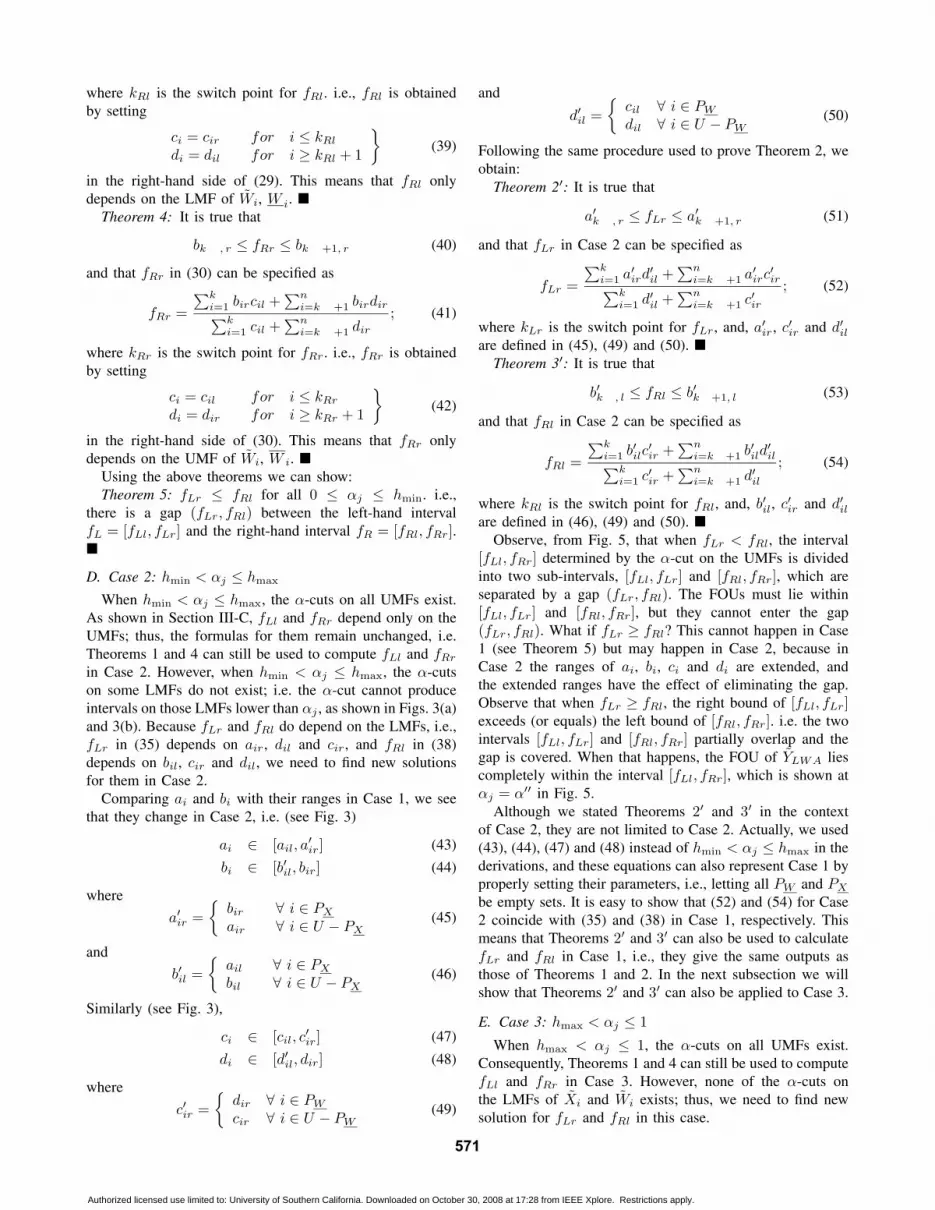
are defined in (46), (49) and (50). �Observe, from Fig. 5, that when fLr < fRl, the interval

[fLl, fRr] determined by the α-cut on the UMFs is dividedinto two sub-intervals, [fLl, fLr] and [fRl, fRr], which areseparated by a gap (fLr, fRl). The FOUs must lie within[fLl, fLr] and [fRl, fRr], but they cannot enter the gap(fLr, fRl). What if fLr ≥ fRl? This cannot happen in Case1 (see Theorem 5) but may happen in Case 2, because inCase 2 the ranges of ai, bi, ci and di are extended, andthe extended ranges have the effect of eliminating the gap.Observe that when fLr ≥ fRl, the right bound of [fLl, fLr]exceeds (or equals) the left bound of [fRl, fRr]. i.e. the twointervals [fLl, fLr] and [fRl, fRr] partially overlap and thegap is covered. When that happens, the FOU of YLWA liescompletely within the interval [fLl, fRr], which is shown atαj = α′′ in Fig. 5.

Although we stated Theorems 2′ and 3′ in the contextof Case 2, they are not limited to Case 2. Actually, we used(43), (44), (47) and (48) instead of hmin < αj ≤ hmax in thederivations, and these equations can also represent Case 1 byproperly setting their parameters, i.e., letting all PW and PX

be empty sets. It is easy to show that (52) and (54) for Case2 coincide with (35) and (38) in Case 1, respectively. Thismeans that Theorems 2′ and 3′ can also be used to calculatefLr and fRl in Case 1, i.e., they give the same outputs asthose of Theorems 1 and 2. In the next subsection we willshow that Theorems 2′ and 3′ can also be applied to Case 3.

E. Case 3: hmax < αj ≤ 1

When hmax < αj ≤ 1, the α-cuts on all UMFs exist.Consequently, Theorems 1 and 4 can still be used to computefLl and fRr in Case 3. However, none of the α-cuts onthe LMFs of Xi and Wi exists; thus, we need to find newsolution for fLr and fRl in this case.

571


Observe that Case 3 can also be represented by (43), (44),(47) and (48) by setting all PX and PW to U ; thus, Theorems6 and 7 in Section III-D can also be used here to computefLr and fRl. Because PX and PW are U , (45), (46), (49)and (50) in Section III-D become

a′ir = bir ∀ i ∈ [1, n]b′il = ail ∀ i ∈ [1, n]c′ir = dir ∀ i ∈ [1, n]d′il = cil ∀ i ∈ [1, n]

(55)

Substituting (55) into (52) and (54), we obtain

fLr =

∑kLr

i=1 bircil +∑n

i=kLr+1 birdir∑kLr

i=1 cil +∑n

i=kLr+1 dir

(56)

fRl =

∑kRl

i=1 aildir +∑n

i=kRl+1 ailcil∑kRl

i=1 dir +∑n

i=kRl+1 cil(57)

Note that fLl and fRr, which determine the α-cut on Y LWA,are calculated by (32) and (41), respectively. Comparing (56)with (41), it is observed that fLr in (56) is the same as fRr

in (41) 2. Besides, fRl in (57) is also the same as fLr in(32); thus, in Case 3,

fLl = fRl (58)

fLr = fRr (59)

Consequently,

[fLl, fLr] = [fRl, fRr] = [fLl, fRr] (60)

(60) means that the FOU of YLWA fills in the entire interval[fLl, fRr] (see α′′ in Fig. 5), which is completely determinedby the α-cuts on the UMFs.

Theorem 6: When hmax < αj ≤ 1, the FOU of YLWA

fills in the entire interval [fLl, fRr]. Consequently, there isno need to calculate fLr and fRl. �

F. Relations between the LWA and the FWA

By summarizing the results above, we can connect theLWA and the FWA.

Theorem 7: The UMF of the LWA, Y LWA, is completelydetermined by the UMFs of the attributes, Xi, and the UMFsof the corresponding weights, W i (i = 1, 2, . . . , n). Morespecifically, Y LWA is the FWA of Xi and W i. i.e. let

YFWA =∑n

i=1XiW i∑ni=1W i

(61)

Then,Y LWA = YFWA � (62)

Generally, it is impossible to find a similar theorem forY LWA, because to compute Y LWA we need to considerthree different cases; however, we can do that for a specialcase of Y LWA, where all LMFs of Xi and Wi have the sameheight.

2The switch point in (56) is denoted as kLr and that in (41) is denoted askRr ; however, because all bir , cil and dir are the same in (56) and (41),when the KM algorithm is used to compute (56) and (41), the resultingswitch points will be the same. Consequently, (56) and (41) are the same.

Theorem 8: If all LMFs of Xi and Wi have the sameheight, then Y LWA is the FWA of Xi and W i. i.e. let

Y ′FWA =

∑ni=1XiW i∑n

i=1W i

(63)

Then,Y LWA = Y ′

FWA � (64)

IV. LWA ALGORITHMS

A flowchart of the LWA algorithms is shown in Fig. 6.To save computational cost, different α-cuts are chosen forY LWA and Y LWA [15]. The procedures in the two dashedrectangles can be computed in parallel. Furthermore, theKM algorithms in the two dotted rectangles in each dashedrectangle can also be computed in parallel. The detailedalgorithms are given in [15].

As an example, consider Xi and Wi shown in Fig. 7(a) and7(b), respectively. The resulting YLWA is shown in Fig. 7(c).201 α-cuts were employed. The dashdot curve in Fig. 7(c)indicates the overlapped area where fLr(αj) > fRl(αj) (seeSection III-D).

0 1 2 3 4 5 6 7 8 9 10 11 12 13 14 15 16 17 18 19 200

0.2

0.4

0.6

0.8

1

x

u∼X

1

∼X

2

∼X

3

(a)

0 1 2 3 4 5 6 7 8 9 10 11 12 13 14 15 16 17 18 19 200

0.2

0.4

0.6

0.8

1u

w

∼W

1

∼W

2

∼W

3

(b)

0 1 2 3 4 5 6 7 8 9 10 11 12 13 14 15 16 17 18 19 200

0.2

0.4

0.6

0.8

1u

y

∼Y

LWA

(c)

Fig. 7. MFs of (a) Xi (b) Wi and (c) YLWA.

V. CONCLUSIONS

In this paper, we have introduced the concept of the LWA.α-cuts and KM algorithms were employed to compute it.Because the LWA is a generalization of the FWA from T1FSs to IT2 FSs, there should be close relations between them.We have shown that finding the LWA, YLWA, is equivalentto finding its UMF, Y LWA, and LMF, Y LWA. Moreover,Y LWA is the FWA of the UMFs of the attributes, Xi,and the UMFs of the corresponding weights, Wi. Y LWA is

572


Select -cuts for LWAp Yα

Set 1j =

Find ( ), ( ), ( ),

and ( ), 1,2, ,ir j il j ir j

il j

a b c

d i n

α α αα

′ ′ ′

′ = �

Use KM algorithm

to compute ( )Lr jf αUse KM algorithm

to compute ( )Rl jf α

( ) [ ( ), ( )]LWA j Lr j Rl jY f fα α α=

j p=1j j= + ��

Construct LWAY

��

Select -cuts for LWAm Yα

Set 1j =

Use KM algorithm

to compute ( )Ll jf αUse KM algorithm

to compute ( )Rr jf α

( ) [ ( ), ( )]LWA j Ll j Rr jY f fα α α=

j m= 1j j= +��

Construct LWAY

��

Find ( ), ( ), ( ),

and ( ), 1,2, ,il j ir j il j

ir j

a b c

d i n

α α αα = �

1/[ , ]LWA LWA LWAY Y Y=�

Fig. 6. Flowchart for the LWA.

more complicated than Y LWA, but it can also be computedefficiently by using α-cuts and KM algorithms. For thespecial case where all the LMFs of Xi and Wi have thesame height, Y LWA is the FWA of the LMFs of Xi andWi. Hence, the computational cost of a LWA is about twicethat of a FWA.

ACKNOWLEDGEMENT

This study was funded by the Center of Excellence forResearch and Academic Training on Interactive Smart Oil-field Technologies (CiSoft); CiSoft is a joint University ofSouthern California-Chevron initiative.

REFERENCES

[1] W. M. Dong and F. S. Wong, “Fuzzy weighted averages and imple-mentation of the extension priniple,” Fuzzy sets and systems, vol. 21,pp. 183–199, 1987.

[2] D. Dubois, H. Fargier, and J. Fortin, “A generalized vertex method forcomputing with fuzzy intervals,” in Proc. FUZZ-IEEE, pp. 541–546,Budapest, Hungary, 2004.

[3] Y.-Y. Guh, C.-C. Hon, and E. S. Lee, “Fuzzy weighted average: Thelinear programming approach via Charnes and Cooper’s rule,” FuzzySets and Systems, vol. 117, pp. 157–160, 2001.

[4] Y.-Y. Guh, C.-C. Hon, K.-M. Wang, and E. S. Lee, “Fuzzy weightedaverage: A max-min paired elimination method,” J. of Computers andMathematics with Application, vol. 32, pp. 115–123, 1996.

[5] N. N. Karnik and J. M. Mendel, “Centroid of a type-2 fuzzy set,”Information Sciences, vol. 132, pp. 195–220, 2001.

[6] G. J. Klir and B. Yuan, Fuzzy Sets and Fuzzy Logic: Theory andApplications. Upper Saddle River, NJ: Prentice-Hall, 1995.

[7] D. H. Lee and D. Park, “An efficient algorithm for fuzzy weightedaverage,” Fuzzy sets and systems, vol. 87, pp. 39–45, 1997.

[8] T.-S. Liou and M.-J. J. Wang, “Fuzzy weighted average: An improvedalgorithm,” Fuzzy Sets and Systems, vol. 49, pp. 307–315, 1992.

[9] F. Liu and J. M. Mendel, “Aggregation using the fuzzy weightedaverage, as computed using the Karnik-Mendel algorithms,” submittedfor publication, Nov. 2005.

[10] J. M. Mendel and F. Liu, “Super-exponential convergence of theKarnik-Mendel algorithms for computing the centroid of an intervaltype-2 fuzzy set,” accepted for publication in IEEE Trans. on FuzzySystems, 2006.

[11] J. M. Mendel and H. Wu, “New results about the centroid of an intervaltype-2 fuzzy set, including the centroid of a fuzzy granule,” acceptedfor publication in Information Sciences, 2006.

[12] ——, “Type-2 fuzzistics for symmetric interval type-2 fuzzy sets: Part1, forward problems,” accepted for publication in IEEE Trans. onFuzzy Systems, 2006.

[13] ——, “Type-2 fuzzistics for symmetric interval type-2 fuzzy sets: Part2, inverse problems,” accepted for publication in IEEE Trans. on FuzzySystems, 2006.

[14] J. M. Mendel, Rule-Based Fuzzy Logic Systems: Introduction and NewDirections. Upper Saddle River, NJ: Prentice-Hall, 2001.

[15] D. Wu and J. M. Mendel, “On the linguistic weighted average,” Signaland Image Processing Institute, University of Southern California, LosAngeles, CA, Tech. Rep., 2006.

573


the linguistic weighted average

Documents