l_:!ravitaticj>n - cern document server
TRANSCRIPT
l_:!RAVITATICJ>N AND
COSMOLOGY/ //
,/
Proceedings of the XV IAGRG Conference held at the North Bengal University
November 4-7, 1989
EDITED BY
S. Mukherjee Physics Department, North Bengal University
A.R. Prasanna Physical Research Laboratory, Ahmedabad
A.K. Kembhavi Inter-University Centre for Astronomy and Astrophysics, Pune
PUBLISHING FOR ONE WORLD
WILEY EASTERN LIMITED New Delhi Bangalore Bombay Calcutta Madras Hyderabad
Pune Lucknow Guwahati
•
Copyright © 1992, Wiley Eastern Limited
WILEY EASTERN LIMITED
4835/24 Ansari Road, Daryaganj, New Delhi 110 002 4654/21 D"cl,ryaganj, New Delhi 110 002 27 Bull Temple Road, Basavangudi, Bangalore 560 00-1 Post Box No. 4124, Saraswati Mandir School, Kennedy Bridge,
Nana Chowk, Bombay 400 007 40/8 Ballygunge Circular Road, Calcutta 700 019 No. 6, First Main Road, Gandhi Nagar, Madras 600 020 1-2-412/9 Gaganmahal, Near A.V. College, Domalguda,
Hyderabad 500 029 Flat No. 2, Building No. 7, Indira Co-operative Housing Society Ltd,
Indira Heights, Paud Fatta, Erandawane, Karve Road, Pune 411 038 18 Pandit Madan Mohan Malviya Marg, Lucknow 226 001 Pan Bazar, Rani Bari, Guwahati 781 001
This book or any part thereof may not be reproduced in any form without the written permission of the publisher .
This book is not to be sold outside the country to which it is consigned by Wiley Eastern Limited.
ISBN 81-224-0415-4
Published by H.S . Poplai for Wiley Eastern Limited, 4835/24 Ansari Roa.cl, Daryaganj, New Delhi 110 002. Production supervised by O.P. Batra, typeset by .Scribe Consultants, B4/30 Safdarjung Enclave, New Delhi 110 029 and printed at Ramprintograph, C-11'! Okhla Industrial Area Phase I, New Delhi 110 020. Printed in India.
Preface
The Fifteenth Conference of the Indian Association for General Relativity and Gravitation (IAGRG) was held during November 4-7, 1989 on the verdant campus of North Bengal University, except for the concluding session which was conducted on the neighbourfog mountain resort of Darjeeling. The IAGRG Conference is held usually once in 18 months, in which the members and invited scientists discuss and review the developments in the field of gravitation theory, and its tests and applications.
The proceedings of the Fifteenth Conference consisted of special lectures, invited talks, contributed papers and group discussions. The present volume contains 14 lectures. The topics have been selected to cover the fast emerging areas of research in the fields of gravitation, both classical and quantum, relativistic astrophysics and cosmology. The lectures in general start with a short review, tracing the developments in the subject before presenting the most recent results, including the contribution of the speaker.
The lectures have been arranged in chapters to give the text coherence and continuity. The first chapter deals with classical gravity and its application to some astrophysical problems including pulsars and black holes. The fibre bundle techniques in particular, have been discussed separately. The second chapter is devoted entirely to the problem of gravitational wave detection. Techniques of detection1 methods of data analysis and some recent observations have been covered to make the chapter almost self-contained. The third chapter deals with the overlapping fields of particle physics and cosmology. Applications of superstring theories to particle physics and the phase transitions of the early universe have been discussed in the light of recent developments. The fourth chapter contains two lectures on quantum cosmology, dealing in particular with the problem of the choice of initial conditions.
The last chapter consists of two special lectures. The first one by Professor N. Mukunda, is the first "Vaidya Raychaudhuri Lecture". It presents a critical analysis of the developments in relativity and quantum theory that eventually makes it possible to view gravitation as a gauge theory. The second lecture by Professor J.C. Bhattacharyya is the valedictory lecture of the Conference in which he
vi Preface
recalls the interaction of physical theories with astronomical observations in the past and also summarizes the present and proposed facilities for astronomical studies in India.
It gives us great pleasure to thank the members of the National Programme Committee of the Conference for their valuable suggestions which helped to .make the programme useful for all concerned. We are thankful to the authorities of North Bengal University, in particular, to the Vice-Chancellor, Professor K .N. Chatterjee and all members of the Physics and Mathematics Departments for making excellent arrangements for the Conference. Special mention may b~ made for the help we received from Mr. D. Chakraborty, Dr. S.K. Ghoshal, Sri A. Acharyya, Dr. S. Paul, Dr. N. Kar, Dr. P.K. Mondal, Mr. J. Sankrityayana, Dr. P. Chakraborti, Professor S. Karanjai and Dr. K.K. Nandi. We are thankful to Dr. B.C. Paul for his help in the editorial work. We are also grateful to the Principal and faculty members of St. Joseph's College, Darjeeling for making arrangements for the valedictory session in this beautiful Himalayan resort. Finally, we are thankful to Mr. A. Machwe for his help in bringing out this volume.
S. MUKHERJEE
A. R. PRASANNA
A. K. KEMBHAVI
Contents
CHAPTER 1: CLASSICAL GRAVITY General Relativity Effect in Pulsars: N. Panchapakesan / 3 Unusual Black Holes: About Some Stable (Non-evaporating) Extremal Solutions of the Einstein Equations: E. Recami and V. Tonin-Zanchin / 8
1
Role of Angular Momentum in Relativistic Astrophysics: Sandip K. Chakraborti / 19 Fibre Bundles in Gravitational Theory: Eric A. Lord / 30
CHAPTER 2: GRAVITATIONAL WAVE DETECTION 43
Gravitational Wave Detection: S. V. Dhurandhar / 45 Techniques of Gravitational Wave Data Analysis: B.S. Sathyaprakash / 56 Rome-Maryland Gravitational Radiation Antenna Correlations with Neutrino Detectors at Mont Blanc, Kamioka and Baksan Associated with Supernova 1987 A: J. Weber / 80
CHAPTER 3: GRAVITY AND PARTICLE PHYSICS 89 Particle Physics Applications of Superstring Theory: P. Nath and R. Arnowitt / 91 Description of Intrinsic Abelian and Non-Abelian Interactions of a Test String: Kameshwar C. Wali / 109 Phase Transitions in the Early Universe: A. Mukherjee / 120
CHAPTER 4: QUANTUM GRAVITY AND QUANTUM COSMOLOGY 141
Boundary Conditions and Quantum Cosmology: D.P. Datta and S. Mukherjee / 143 Quantum Gravity, Torsion and the Wave Function of the Universe: P. Bandyopadhyay / 158
CHAPTER 5: SPECIAL LECTURES
Many Views of the Summit: N. Mukunda / 171 Interdependence of Theory and Observation in Astronomy: J.C. Bhattacharyya / 191
Index / 199
169
•
CHAPTER 1
CLASSICAL GRAVITY

General Relativity Effect in Pulsars
N. PANCHAPAKESAN
Department of Physics and Astrophysics University of Delhi, Delhi 110 007
1. Introduction
As President of The Indian Association of General Relativity and Gravitation, I have great pleasure in welcoming you all to this periodical meeting. We are grateful to the Vice-Chancellor, North Bengal University and in particular to Professor S. Mukherjee, Head of the Physics Department for excellant arrangements and hospitality.
In my talk today I would like to trace very briefly the evolution of research in the field of General Theory of Relativity (GTR) in recent times before going on to present some of the work1 done at Delhi along with my coworkers (V.B. Bhatia, Namrata Chopra and Bhabani Majumdar ).
The three tests suggested by Einstein in 1915 involved small corrections to Newtonian results. Since then many predictions have been made which are predictions of GTR in their own right. The instability of supermassive stars predicted by Chandrasekhar2 is one such example. So are all the pr~dictions about black holes. All these, however, still await confirmation by observations. The progress of technology would make this possible in near future.
The main event of importance in recent times has been the flowing of the mainstream of physics into the area of GTR. Any scheme of unification of forces in physics has to include GTR in an essential way. Between relativists and other physicists, it is no longer 'we' and 'they' but 'us' (may be a bit reluctantly). This should also tell us the modifications (if any) needed by Einstein's theory. Superstring theory has been largely in the forefront recently. However, there has also been a breakthrough by Ashtekar3 along more canonical lines.
During these years the language of GTR and more especially that of field theory has undergone a profound change. The geometrical nature of the subject has brought in mkny ideas from topology and differential geometry which have made the subject richer and more complex.4
An exciting contact has also been made with quantum mechanics, especially with its theory of measurements. Hawking5 and Penrose6
4 Gravitation and Cosmology
have presented quite a few seminal ideas and set the ball rolling. GTR is now in the centrestage and will continue to be there till these problems a.re solved. With these general remarks I now move on to the specific application of GTR to Pulsars.
2. Kerr Metric for Pulsars
Pulsars are believed to be neut.ron stars, highly compact objects wit] a radius ,...., 10 km and mass ,..., l.5M0 . They emit extremely regular pulses whose origin is not y t ompletely understood. Tli.ey ha.ve a high magnetic field "' 1012 Gauss. The magn. tic energy is more than the gravitatjona.J. energy a.nd the origin of pulses is widely believ d to be related to electromagnetic interaction w:ith the rotation of the star. Pulsar periods vary from 1 msec or even less to about 4 sec. Such small periods, if they are due to rotation, indicate that the star must be .more compact than a white dwarf and hence must be a ne~tron star. Most treatments of pulsars n~lect effects of GTR. The Schwarzschild radius for stars of one solar mass are "' 3 km and so pulsars have a radius about 3 times their Schwarzschild radius. Therefore, one would expect effects of GTR to be important close to the surface.
The exact solution of GTR corresponding to a rotating axisymrnetric system is the Kerr metric which has an event horizon. In a neutron sta.r the Kerr metric becomes inapplicable, before reaching the horizon, at the surface of the star. Unlike in the Schwarzschild case we do not know a metric which describes the interior of a star and goes smoothly to a Kerr metric outside the surface of the star. Kapoor and Datta7 studied the effects of GTR on pulsar characteristics using the rotationally perturbed metric of Hartle and Thorne. In the following we will use Kerr metric to study the effects of spacetime curvature on pulsar characteristics.
We write the Kerr metric as ( c = G = 1)
ds2 = e211 dt2 - e2"'( d</> - wdt)2 - e2 µ.d(/l - e2>.dr2
== g0 pdx0t dx{J
with YafJ given by
Ytt == 1 - 2Mr = e2v - w2e21" p2
2aM r sin2 () 2.1.
gq,f = =we .,, p2
• 2 . p 2>.
Yrr = - ti, = -e
(1)
(2)
(3)
(4)
General Relativity Effect in Pulsars 5
where
g88 = -p2 = -e2µ
. 2 ()[( 2 2 ) 2a2Mrsin
2()]
g<l><I> = - sm r + a + 2 p = - e2 ,µ
• 2 ()
=~2~ p2
p2 = r 2 + a 2 cos2 ()
.6. = r2 -- 2M r + a2
~ = (r 2 + a2) 2 - a 2 .6.sin2
()
2aMr w=~
(5)
(6)
(7)
and M = mass of pulsar and a = angular momentum per unit mass. The four velocity of the photon emitter is
dxcx dt ucx = --, xcx = t, r, (}, </>; uo = - = e-v(l - v2)-1/2
ds ds s (8)
dr _ O d(J _ d</> _ n dt - l - 0, - H
ds ds ds ds (9)
where V 8 is the tangential velocity of the err_iitter as seen by a locally non-rotating observer (vs = 1 at the light cylinder). The metric corresponds to the Lagrangian
L = ~[e2vi2 - e2>..r2 - e2µ()2 - e2<1>(J>- wi)2] (10) 2
The Euler-Lagrange equations give
9o3i + 933¢ = -h (11) (12)
where h and / are constants. These two constants are due to the absence of t or </> terms in the Lagrangian. Thus, h is the orbital angular momentum and 'Y is the energy of the photon. We obtain
d</> 1(go3 - qgoo) dt 1(1 +wq) (l3
) d).. = go3 - 900933. ' d).. 900 + wgo3
q = -h/r is finite and defined as the impact parameter of the photon. ).. is an affine parameter. The net angle of deflection </>o is given by
{D d</>/d).. </>o =}re dr/d).. dr (14)
where Dis the loca.tion of the distant observer. When the photon is confined to one plane, the (J dependence is absent and we have
e2vdt2 - e2>.dr2 - e2.P(d</>- wdt)2 = 0 (15)
giving
6 GraV'itation and Cosmology
where (17)
and (18)
with (19)
and (20)
In the above, re is the point of emission and 6 the azimuthal angle at which the photon is emitted . Similarly
T = 1.D g(r,qe) dr (21)
with an appropriate g(r, qe)· The net deflection D.<f>o = </>0(6) - 6. Apart from D.<f> we also calculate D. and t:'. The increased deflection results in reduction of intensity. We define
D. = d6new = d<f>o I do do 1.= 1••
(22)
D. is called the divergence index. We also define a deamplification factor
with
I - [1 + Z(0)] 3
t: - l+Z(6) € (23)
intensity( Dnew) sin 6 1 6 1 € = intensity(6) = D. sin 6new = D. 6new = .6_2 (
24)
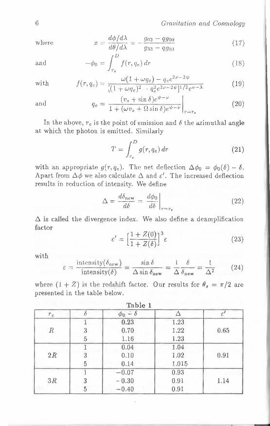
where (1 + Z) is the redshift factor. Our results for 83 = 7r /2 are presented in the table below.
Table 1 re 6 <Po ..:... 8 D. t: '
1 0.23 1.23 R 3 0.70 1.22 0.65
5 1.16 1.23 1 0.04 1.04
2R 3 0.10 1.02 0.91 5 0.14 1.015 1 -0.07 0.93
3R 3 -0.30 0.91 1.14 5 -0.40 0.91
General Relativity Effect in Pulsars 7
3. Discussions of Results
We notice from the table given above that when re = R, c' = o.6, indicating a decrease in intensity due to a widening of the beam. For re = 3R, c1 = 1.4, which indicates an increase in intensity due to beam narrowing. In an observation this may lead to an over.estimation of the brightness temperature. To understand this result physically, we notice that
<Po ex sin -l ( q:); qe ex sin b' (25)
where b' is the angle made by the photon with the radial direction in the locally non-rotating frame. The angle b between the photon and the radial direction in the rest frame of the pulsar and its magnetosphere is related to b' by the transformation
. ,, V 8 + sinb s1nu = -----
1 + V 8 sin b (26)
where 8' is not a linear function of 8 for large values of 8. So when Vs is large, d</Jo/d8 < 1 and the beam tends to converge rather than diverge. If the distance of emission is re "' 3R the over-estimate of brightness temperature can be "' 15%. We can say that special relativistic effect dominates over the GTR effect at 3R.
One can also calculate the difference in arrival time from different points of the magnetosphere. We find !:l.r ,..., 10-20 µs while the observed !:l.r < 6 µs. The calculated time is based on the RudermanSutherland (R-S) theory. The discrepancy with observation throws considerable doubt on the applicability of R-S theory in this case.
References
1. Bhatia, V.B., Chopra, N., Majumder, B. and Panchapakesan, N. Astrophys. J., 326, {1988), 63.
2. Chandrasekhar, S. Phys. Rev. Lett., 14, (1964), 114, 437. 3. Ashtekar, A. Phys. Rev. Lett., 57, (1986), 2244; "New Perspectives ir.
Canonical Gravity", Naples: Bibliopolis, 1988. 4. Misner, C.W., Thorne, K.S. and Wheeler, J.A. Gravitation, W.R. Freeman
and Company, San Francisco, 1973. 5. Hawking, S.W. Phys. Rev., D 14, (1976), 2460. 6. Penrose, R. 300 Years of Gravitation, ed. Hawking and Israel, Cambridge
University Press, 1989. 7. Kapoor, R.C. and Datta, B. Astrophys. J., 297, {1985), 413.
Unusual Black IIoles: About
Some Stable (Non-evaporating)
Extrernal Solutions of
Einstein Equations*
ERASMO RECAMia,c AND VILSON TONIN-ZANCHIN 3 'b
a Department of Applied Mathematics State University at Campinas, S.P., Brazil
b Gleb Wataghin Institute of Physics State University at Campinas, S.P., Brazil
c Dipartimento di Fisica Universita Statale di Catania, Catania, Italy
and LN.F.N., Sezione di Catania, Catania, Italy
1. Introduction
Within a purely classical approach to "strong gravity", that is to say, within our geometric approach to hadron structure1 , we came to associate hadron constituents with suitable stationary, axisymmetric solutions of certain new Einstein-type equations, supposed to describe the strong field inside hadrons.
Such Einstein-type equations are nothing but the ordinary Einstein equations (with cosmological term) suitably scaled down2 • .As a consequence, the cosmological constant A and the masses M result, in such a theory, to be scaled up and transformed into a "hadronic constant" and into "strong masses", respectively.1 •2
Due to the unusual range of the values therefore assumed by A, M and the other parameters (see Sec. 2), and even more due to our requirements, we met a series of solutions of the Kerr-Newman-de Sitter type, which had not received enough attention in the previous literature. In particular, the requirement that those "(strong) black hole" solutions be stable (i.e., that their surface temperature, or surface gravity3 , be vanishingly small), implied the coincidence of at least two of their (three, in general) horizons. This condition
* Work partially supported by CNPq, FAPESP, CAPES, and by INFN, M.P.I. and CNR.
Unusual Black Holes 9
gives the black hole such interesting properties that it is worthwhile studying them also in the case of ordinary gravity, that is to say of ordinary Einstein equations. This is the aim of the present paper. Let us stress that some of the novelty of the present approach resides in our particular point of view, i.e., in the fact that we are going to regard every black hole studied below as a (localized) object described by an external observer living in a four-dimensional spacetime asymptotically de Sitter. Thus, for investigating the properties of those objects, we shall use Boyer-Lindquist-type coordinates.
2. The Horizons Associated with a Central, Stationary Body, and their Main Properties
Let us consider Einstein equations with cosmological term
1 [k =- 87rc4G] . Rµv - 29µvR~ + Agµv = -kTµ,,; (1)
Choose (whenever convenient) units such that G = 1, c = 1, and look for the vacuum solutions describing the stationary axisymmetric field created by a rotating charged source. This solution is the Kerr-Newman-de Sitter (KNdS) space-time, whose metric in BoyerLindquist-type4 coordinates (t,r,8,<p) can be written as5 (with the signature -2):
ds2 = - p2 [ dr2
/ B + d82 / D] - p - 2 A - 2 [ (a dt - ( r 2 + a 2 )d<p ]2 sin 2 8
+ BA-2 p-2[dt - a sin2 8 dcp]2, (2)
with m = GM/c2, a= J/Mc, p2 = r 2 + a2 cos2 8, A= 1 + Aa2 /3,
B = B(r) = (r2 + a2 )(1 - Ar2 /3) - 2mr + Q2, D = D(fJ) =
1 + (Aa2 cos2 8)/3, Q2 = ( G / 47re0 c4 )q2 , quantities M, J and q being mass, angular momentum and electric charge of the source, respectively. For simplicity, let us here analyze only the case A > 0.
One meets the event horizons of the space (2) in correspondence with the divergence of the coefficient 9rr, i.e., when B( r) = 0. This equation,
( Ar2)
(r2 + a 2) 1- T - 2mr + Q2 = 0, (3)
admits four roots, one of which, ro, is always real and negative. The interesting case is when Eq. (3) has four real solutions; in that case we shall have three positive roots. Let us call them ri, r2, r3, with r3 2: r2 ;::: r1. [The case in which A < 0 is less interesting, since it yields at most two real positive roots]. We shall see that at r = r3 we have a cosmological horizon6 , while at r = r 2 and r = r1 we meet two black hole horizons analogous to the two well known r = r + and r == r _ horizons of the Kerr metric.
10 Gravitation and Cosmology
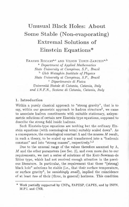
The three horizons 1, 2, 3, in the general case when they are all real , divide the space into four parts I, II, III and IV (see Fig. 1). On each horizon, quantity grr = gu diverges,'i.e ., grr = 0. Quantity grr does change sign when passing from any region to the adjacent ones.
IV
Fig. 1. Given an almost pointlike stationary body, generating, when A f:. 0, a Kerr-Newman-de Sitter space-time, in t~e Boyer-Lindquist coordinates it will , in general, possess thT'ee horizons 1, 2, 3, which divide t he associated space into the four regions I , II, III , IV. On the horizons grr diverges, i.e., grr = 0. Quantity grr does change sign when passing from any one region to the adjacent ones. Surface 3 is the cosmological horizon and surfaces 2, 1 are the outer and inner black hole horizons, respectively.
For instance, in regions III and I it is always grr < 0, as expected in the case of an ordinary Kerr black hole; on the contrary, in regions II and IV it is always grr > 0. Actually, it is possible to define a Killing ve tor K "' which is simultaneously time-like in regions III and I (but not in regions II and IV too). 7 '8 Therefore one can have stationary observers ( r = const.) only in regions III and I, in the sense that only there the r =constant, trajectories are time-like. Let us call time-like the (ordinary type) regions III and I; and space-like the other two regions II and IV. From a more formal point of view, let us represent the properties of such regions, and of their horizons, by depicting the behaviour of their various radial null geodesics.
For simplicity, let us confine ourselves to the static case (ReissnerNordstrom-de Sitter metric), which is not qualitatively different. From Eq. (2), by putting a= 0, we find for those geodesics:
ds2 = Fdt2 - p-t dr2 = O; F:: B/r2 (4)
Unusual Black Holes 11
By integration of Eq. ( 4), after some algebra one gets [m = 0, 1, 2, 3]:
3
t = =t=3A-1 2..: amr?n log(_!__ - 1) + C'F m=O Tm
(4')
where C:f are integration constants, and am are "constants" whose values depend on the values of the four roots ro, r 1, r2, r3 of Eq. (3). In Eq. ( 4') the upper (lower) sign corresponds to outgoing (ingoing) geodesics.
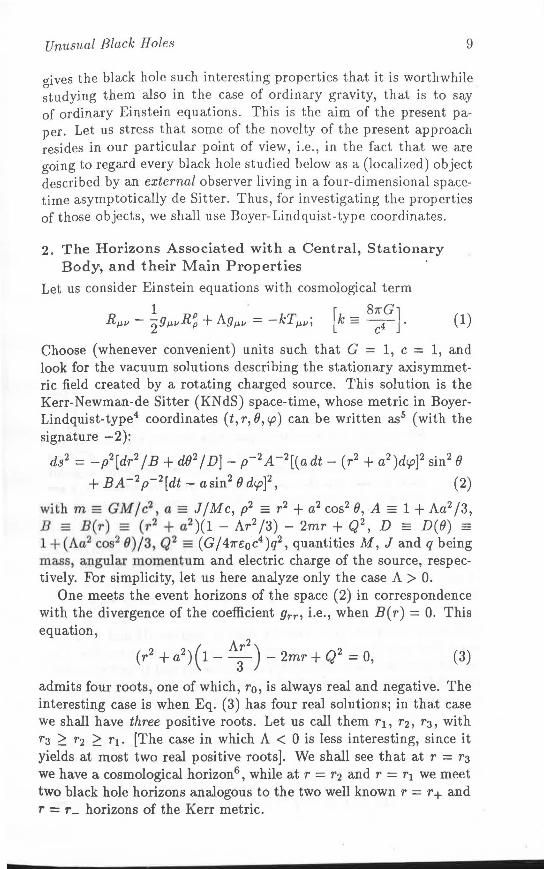
The behaviour of the radial null geodesics t = t( r) is given in Fig. 2 for the four regions. One has to recall, however, that such a figure does not represent, in a complete manner, the casual structure of our space-time. That structure can be inferred from the PenroseCarter diagram for the present case (straightforwardly constructable by following refs.6
•9
•10
) which shows a self-repeating chain of eight regions (four regions and the time-reserved ones), such that-for instance-the "collapsing" region II is causally connected with the "collapsing" region IV (but not with the "expanding" region IV).
t region I region Il region III region IV
Fig. 2. The behaviour of the outgoing and ingoing radial null geodesics in the (four) different regions of the Reissner-Nordstrom-de Sitter geometry (static case), in Schwarzschild-like coordinaiea. The case depicted here corresponds in particular to r2 = 2r1 , r3 = 3r1 (with ro = - ri - r2 - r3) . The semi-cones appearing in this figure point towards the future.
We are particularly interested, however, in the case when two or more of our horizons coincide.
12 Gravitation and Cosmology
3. On the Horizon Temperatures (Surface Gravities)
In the general (stationary, i.e., KNdS) case of metric (2), the Bek. enstein-Hawking temperature11 Tn of each horizon in Figs. 1 and 2
is known to be proportional to the horizon surface gravity as follows:
(5)
where kB is the Boltzman constant and n = 1, 2, 3. On any nullsurface (in particular on every horizon) the surface gravity12 •13 can be defined by the equation 8µ,(KvKv) = -2/Kµ, symbols 8µ representing the covariant derivatives.
To evaluate the surface gravities /n, let us then recall that our metric (2) does admit two Killing vectors Kf, J(~, the former being related to time-translation invariance and the latter to rotational invariance of the space-time. By linear combination of J(r and K~ one can construct Killing vectors J(~ = Kt+ Wnl(~ which vanish on the nth horizon; i.e., which satisfy the relation (Kn)µ(Kn)µ = 0. One finds Wn = gtr.p/gr.pr.p (evaluated at r = r 11 ). We finally get the expression Tn = ctn for the horizon temperatures (and for A f. 0) with
cA o,3 Tn = 6A(r2 + a2 ) ·IT (rn - r1), (l = 0, 1, 2, 3) (6)
n l'tn
Equation (6) yields the result that the horizon temperature can be vanishingly small only when two (or more) horizons tend to coincide; i.e., when two (or more) roots ri of Eq. (3) tend to coincide. This result is important since it leads to the conditions for a BH (black hole) to be stable, i.e., it implies some relations among mass, radius, charge, angular momentum (a.nd A) of a stable BH.
In the particular (Kerr-Newman) case when A = 0, one gets only two (or no) horizons, corresponding to r ± = m ± J m2 - aZ - Q2, and Eq. (6) has to be replaced by T± = t:(r+ - r_)/(ri + a2).
We get a stable (T = 0) black hole solution when
r+ = r_ = m,
that is to say, when the Regge-like condition does hold:
m2 = a2 + Q2.
(7a)
(7b)
Incidentally, let us notice* that in this particular case the horizons
* Notice that one could geometrically describe the "extremal,, (stable) black holes as an external, macroscopic observer would do for a "strong black hole" {hadron). In other words, we might a priori identify all the regions of the same type (either I, or II or III, or IV) that one meets when studying the related Penrose-Carter diagrams.
Unusual Black Holes 13
r_, r+ behave as r1, r2 of Figs. 1, 2 (cf. also Carter9). However, since
in this case, region II disappeared, then the whole BH interior is timelike!, as is the external region III. Let us call a solution of this type a "time-like black hole" (at variance with the ordinary "space-like BHs").
4, About the Stable Schwarzschild-de Sitter Black Hole
Another interesting case is that of the Schwarzschild-de Sitter metric (cf. Gibbons and Hawking9
), in which Q2 = a2 = 0, so that B = -Ar4/3 + r2 - 2mr and two horizons only (with radii r_ = rB,
r + = re, respectively) are met, whose surface temperatures are
cA (3m 2 ) T± = 3ri A - r ± . (8)
Moreover, the requirement T = 0 implies that TB =re =rand that r = (3m/ A)113 • The last equation can be read a..s
r = A-1/
2 :;: 3m, (rB =re = r) (9)
since those two radii coincide (only) when
9Am2 = 1. (10)
For completeness sake, let us mention that the two horizons' radii can be written as 2r± = (/31 + /32) ± H(/31 - /32), with /31,2 =
(/3 ± .j132 - A-3)1/3; J3 = 3m/A. Let us observe that the condition for a BH to be stable yields,
besides the BH radius (as a function of m and A), a further relation between m and A.
More interesting, here, is the observation that r _ and r + behave like r2 and r3 , respectively, of Figs. 1 and 2. For this reason we call r_ =TB, r+ =re (B =black hole horizon, C =cosmological horizon). When TB tends to coincide with re, the (time-like) regions of type III do disappear, so that we are left only with regions of type II and IV, and the BH tends to occupy the whole space inside the cosmological horizon (roughly speaking, the BH itself can be regarded as a model for a cosmos). It is worthwhile mentioning that, by choosing for A the value IAI ~ 10-52 m-2 ordinarily assumed for our cosmos, the condition {10) yieldA M ~ ! >< 1053 kg, which is close to the estimated mass of our own cosmos. Incidentally, when passing to the "strong BH" case1•2 , with A replaced by ~ ~ (1040 )2 A, one would get M = m'JI'.
5. Mass Formulas for Stable Kerr-Newman-de Sitter Black Holes
Let us now consider tbe characteristics of stable BHs in the general
14 Gravitation and Cosmology
(KNdS) case when the source is endowed also with angular momentum (stationary case) and charge. We have at our disposal two equations: (i) the equation B(r) = 0 which yields, as before, th ta.dii rn corresponding to the horizons; and (ii) the equation T = 0, implying th coincidence of two, or more,* radii rn, which guarantees the horizon stability. Those two equations yield the system:
Ar4
( Aa2
) 2 2 2 } - J + 1 - -3- r - 2mr + a + Q = 0
Ar3 ( Aa2 ) (ll) - 23 + 1 - -3- r - m = 0.
The second equation requires the vanishing of the derivative B'(r) in correspondence with the values rn which satisfy the first equation [B(r) = O]. Such a. second equation, therefore, ensures the solu-tions of the system to be double (or triple) "roots" of the equation B(r) =·o.
After some algebra, we get explicitly (besides the first equation, yielding the stable BH radii) a second equation providing us with a link among the various parameters m, A, a, Q:
3mu } r=--E
9m2 u( 6u - E) + 2TJE2 = 0 (12)
with E = 362 + 4A671 - 18m2 A, 6 = 1 - Aa2 /3, 71 = a2 + Q2 and u :: 62 - 4A7].
It is easy to verify that: (i) for A = O, Eqs. (12) reduce to Eqs. (7a), (7b ); and that (ii) for 71 = a2 + Q2 = O, Eqs. (12) reduce to Eqs. (9), (10).
Equations (12) do yield, of course, both the stable BH solutions resulting from the coincidence of r1, r2, and those resulting from the coincidence of r2, r3, viz., the second of Eqs. (12) can be written as
3mu = 3m ± E 26
9m2 2TJ 462 - -g-, (13)
from which one can of course construct two independent systems (yielding r + and r _, respectively, as a. function of three out of the four remaining parameters m, A, a, Q).
Let us consider the two cases separately:
* Let us recall that the real positive radii [the roots of Eq. (3)] can be at most three; actually they can be one or three. The latter case is of course the only interesting one and we shall imagine in the following that three out of thoee (four) roots have actually positive real values, even if our formulas have general validity.
Unusual Black Holes 15
(i) When r1 = r2 = r _,the regions of type II (Figs. 1-2) do disappear and we obtain a stable Kerr-Newman-de Sitter BH, similar to the stable BH encountered at the end of Section 3, in the particular KerrN ewman case. In that case, however, the stable BH was surrounded by asymptotically fiat regions of type II!, whilst in the present case our stable BH is surrounded by two types of regions (since we are still in presence of a cosmological r = r3 horizon): regions of type III, and (space-like, asymptotically de Sitter) regions of type IV.
In other words, both the exter!lal (III) and the internal (I) regions of the present stable BH are time-like regions, separated just by a semipermeable membrane. Let us emphasize that the Killing vector J(I-' is time-like everywhere inside our stable BH; any causal observer Oc can live therein without falling into the singularity r = 0: that, incidentally, will appear to Oc as a naked singularity.
Finally, the regions of type IV are analogous to the exterior of a de Sitter ( cosmological) .horizon.
(ii) When r2 = r3 = r+, the regions of type III (Figs. 1-2) do disappear and we obtain a BH, bounded by a stable horizon originating from the fusion of a BH type (r2) surface and a cosmological-type ( r3 ) horizon. The stable r2 = r3 null surface can be regarded, therefore, both as a BH membrane and as a cosmological horizon. Outside such a surface, we meet regions of type IV, asymptotically de Sitter.
Both the internal (II) and the external (JV) black hole regions are space-like, since the time-like type (III) regions (where causal observers usually live) disappeared. In regions II and IV no stationary observers can exist.
Inside the r2 = r3 surface, we moreover find at r = r1 a null surface that can be considered the internal BH boundary, as in the Kerr-Newman (or Kerr) case. In other words, the r 1 horizon separates space-like regions II from time-like regions I, as it occurs in the interior of an ordinary Kerr-Newman BH.
6. The Particular Case of the Triple Coincidences
In the very special case when all the three positive roots of Eq. (3) do coincide, i.e., when r1 = r2 = ra, we shall meet a stable BH with a single horizon, whose radius takes on a simple analytical expression. Let us write Eq. (13) more convenient!~ as:
r = ~; ± J:;22 - 2871
and observe that the condition of triple coincidence (which implies the existence of a single positive solution) requires the vanishing of
16 Gravitation and Cosmology
the square root, i.e., yields the solution:
3m r = ~' (14)
with two simultaneous Regge-like constraints ('fl= a 2 + Q 2):
8 m2 = 9 fJ(az + Q2 ); (14a)
with 8 = 1 - (Aa2 /3) and
2 263 m =
9A. (14b)
Equation (14b) comes from inserting Eqs. (14), (14a) in either of Eqs. (11).
In the present case, all the regions II and IIJ did disa.ppea.r; and the (type I) interior of our stable BR is time- "ke whilst its (type IV) exterior is space-like. Such a solution is therefore a. "time-like black hole". Again, regions IV are asymptotically de Sitter.
Such a BH solution is conveniently interpretable [Sections 4 a.nd 5(ii)] also as a. cosmological model, viz., as a. model of a. (stable) cosmos.
7. A Few Comments
Let us stress, first of a.ll, that for stable BHs we get "Regge-like" relations among their mass a.nd angular momentum and/or charge and/or the cosmological constant. 1'or instance, in the case A = 0 we get Eq. (7b ):
m2 = a2 + Q2, (Th)
which-when q is negligible-can just be written as M 2 = cJ / G; that is to say (with c = G = 1):
M2 = J (7')
On the contrary, when J = 0 and q is still negligible, we get Eq. (10), which gives M 2 = (c4 /9G2 )A-1
, or (with c = G = 1):
(101)
In the most general case, the considered relation (among M, J, q, A) is involved, and is given by the second one of Eqs. (12). In the (simpler) case of Section 6, i.e., of the "triple coincidence", we obtain two such relations, viz., Eqs. (14a), (14b ), which are still complicated. However, if IAa2 1<1, Eqs. (14) yield both
8 m2
'.::= g(a2 + Q2), (141a)
Unusual Black Holes 17
to be compared with Eqs. (7b ), (7'), and (with c = G = 1):
M2 "'~A -1 - 9 , (14'b)
to be compared with Eq. (101).
The most interesting point is that-with the exception of Eqs. (7b ), (7')-all such "Regge-like" relations can be attributed also to our (stable) cosmological models, i.e., to our stable "cosmoses".
Finally, let us mention that elsewhere we shall apply (and interpret) the results presented in this paper to the case of "strong gravity" theories and "strong BHs", i.e., to the case of hadronic physics.
Acknowledgements
Useful discussions are acknowledged with R.H.A. Farias, E. Giannetto, A. Italiano, P.S. Letelier, G.D. Maccarrone, W.A. Rodrigues Jr., Q.A.G. de Souza, and particularly with L.A.B. Annes, A. Insolia, J.A. Roversi and S. Samba.taro; as well as the collaboration of F. Aversa, F. Nobili and M. Lourdes S. Silva. One of the authors (ER) is also extremely grateful to Prof. S. Mukherjee and to all the organizers of this conference (and the editors of these proceedings) for their very kind interest.
References
1. See e.g., Caldirola, P., Pavsic, M. and Recami, E.: Nuovo Cimento, B48 (1978), 205; Phys. Lett., A66 (1978), 9; Lett. Nuovo Cimento, 24 (1979), 565. See also Recami, E. and Castorina, P.: ibidem, 15 (1976), 357; Italiano, A. and Recami, E.: ibidem, 40 (1984), 140; Recami, E.: Found. Phys., 13 (1983), 341; Italiano, A.: et al., Hadronic J., 7 (1984), 1321.
2. Recami, E.: Prog. Part. Nucl. Phys., 8 (1982), 401. See also Recami, E. in "Old and New Questions in Physics, Cosmology ... ", ed. by Van der Merwe, A., Plenum, N.Y., 1982, p. 377.
3. Reca.mi, E., Martinez, J.M. and Tonin-Zanchin, V.: Prog. Part. Nucl. Phys., 17 (1986), 143; Tonin-Zanchin, V.: M.Sc. thesis, UNICAMP, 1987. See also Recami, E. and Tonin-Zanchin, V.: Phys. Lett., Bl 77 (1986), 304; B181 (1986), 416.
4. Boyer, R.H. and Lindquist, R.W.: J. Math. Phys., 8 (1967), 265. 5. Carter, B.: Commun. Math. Phys., 17 (1970), 233; in "Les Astres Occlus",
Gordon and Breach, N.Y., 1973. 6. See e.g., Hawking, S.W. and Ellis, G.F.R.: "The Large Scale Structure of
Space-Time", Cambridge Univ. Press, 1973, in particular Secs. 5.5, 5.6 and references therein.
7. Cf. also Trofimenko, A.P. and Gurin, V.S.: Pramana, 28 (1987), 379; Recami, E. and Shah, K.T.: Lett. Nuovo Cimento, 24 (1979), 115; Recami, E.: Riv. Nuovo Cimento, 9 (1986), No. 6.
18 Gravitation and Cosmology
8. See e.g., Recami, E.: Found. Phya., 8 (1978), 329; Pavsic, M. and Recami, E.: Lett. Nuovo Cim., 34 (1982), 357; Recami, E. and Rodrigues J r., W.A.: Found. PhytJ., 12 (1982), 709; Italia.no, A.: Hadronic J., 9 (1986) , 9.
9. Gibbons, G.W. a.nd Hawking, S.W.: Phys. Rev., 015 (1977), 2738, in particular Fig. 4 therein; Carter, 8.: Phya. Rev., 141 (1966), 1242 , in particular Fig. 1 therein; Phys . Lett., 21 (1966), 423, in particular Fig. 1 therein.
10. Mellor, F. and Moss, I. Class. Quantum Grav., 6 (1989), 1379, in particular Fig. 1 therein. See also Davies, P.C.W.: Class. Quantum Grav., 6 (1989), 1909.
11. See e.g., Bekenstein, J.D.: Phys. Rev., D9 (1974), 3292; Hawking, S.W.: Commun. Math. Phys., 43 (1975), 199.
12. Bardeen, J.M., Carter, B. and Hawking, S.W.: Commun. Math. Phys., 31 (1973), 1161.
13. Zheng, Z. and Yuanxing, G .: Proc. 3rd Marcel Grossmann Meeting on Gen . Relat., ed. Ning, H., North-Holland, Amstefdam, 1983, 1177.
Role of Angular Momentum in
Relativisitic Astrophysics
SANDIP K. CHAKRABARTI
Tata Institute of Fundamental Research, Bombay 400 005
1. Introduction
One does not have to be especially observant to note that all arounc us, at every ssale--large or small-some angular motion is present either in the fo,rm of turbulent eddies, or in the form of systemati< rotation. Presence of rotation, in general, makes the system mud richer in terms of the number of physical processes which can go Oii
inside it. The situation becomes ever more interesting because of the fact that in stationary systems, the angular momentum, which is a measure of rotation (around a point inside or outside the system) is a conserved quantity. Thus, if it is taken away from one part of a system, it must be given to some other. Consider, for example, an accretion disk around a star. Its very existence is due to the angular motion of .the infalling matter. The centrifugal force slows down the infall and allows a number of physical processes (e.g., thermonuclear reactions) to go on in that period. During the slow inf all, an efficient conversion of the gravitational energy into radiation takes place due to the presence of viscosity in the flow. These physical processes (stationary or non-stationary) are manifested in the observed spectra of radiation and energetic particles emitted from the surface of the disk. Most of the non-stationary phenomena. such as the time variabilities -are thought to be due to instabilities at the inner region of the accretion disk. Even when matter is finally a.ccreted on the star, the angular momentum transferred in the process spins it up. In the extreme case, the rotational motion may destabilize the star and break it apart or the excess angular momentum may be thrown away at a large distance by magnetic field or by gravitational radiation.
In the present paper, we shall not go into each and every aspect of the rotating a.strophysical flows. Rather, we shall concentrate only on some of those systems in which both the rotational as well as the general relativistic effects are important. The systems we have in mind are: (A) thick accretion disks around black holes, (B) transonic
20 Gravitation and Cosmology
fiows around compact stars, (C) close binary stars, and (D) rotating flows close to a Kerr black hole. Below we discuss them in detail.
2. Thick Accretion Disks
Accretion <lisks a.re found in intera ting bjnary systems. They ar a.ls thought t b present at t,h cent r of most of the galaxies . In a binary, th matter from the low mass companion star is slowly stripped off duet th tidal eff ·ts of the compa t primary star. The matter being unable to los the orbital angular momentum instantan ously forms a. ctuasi stationary accretion disk around the primary. Th disk becom s a temporary reservoir of matter as the matter accretes slowly on th primary by losing some angular momentum due to the presence of viscosity. The loss of angular momentum may take pla e if there are large scale magnetic fields anchored to the inner part of th · clisk. As the matt r accretes due to the gravitational pull of the central star it emits rad.ia.tion, which in tum exerts a fore back on the matter througb scattering. The critical accretion rate at whkh these two fore s match is called the Eddington rate (ME)· For a spherically symmetric flow in which th Thomson scattering domina.tes, th.is rate is about ME = 0.2M0 M 8 yr- 1 , where Ms is the mass of the· central star in units of 08 M0 , M0 being the ma.ss of the sun. When the a cretion rate Mis Jess than ME, the radiation force is so Low that only dominant forces acting on the matter are
i E
-;::
-... <
2 .0
I I I 1s I I I . I .-~ I ~------I~ ...... -;-- Id ---- ··.--...-:.-'/
/
, ..
/'
./1 I N
0 R~
-
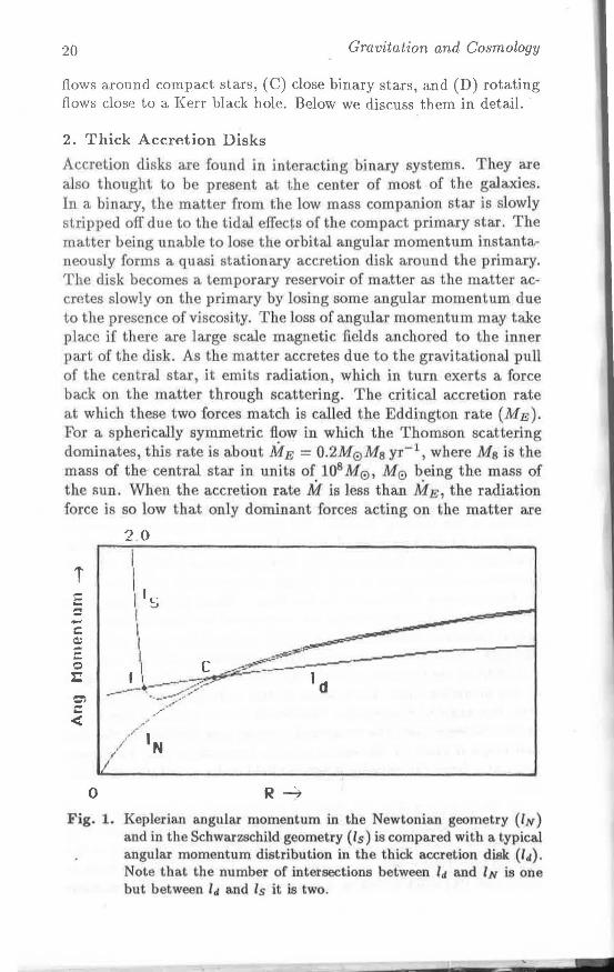
Fig. 1. Keplerian angular momentum in the Newtonian geometry (IN) and in the Schwa.rzschild geom try (ls) is compared with a. typical angular momentum distribution in the thick accretion disk (14). Note that the number of intersections between 111 and lN is one but between 111 and ls it is two.
Role of Angular Momentum 21
the gravitational pull of the central star and the centrifugal force due to the angular motion. In a stationary system these two forces balance and the matter is distributed in Keplerian orbits. The disk formed is geometrically thin, as the transverse thickness h is much less than the radial distance r ( h ~ r). This disk is called the 'thin accretion disk'. When the accretion rate is much higher than the Eddington rate, the radiation force becomes comparable to the centrifugal force. The disk fattens (h "' r) and the vertical structure is supported by the radiation pressure. The angular momentum distribution of stationary configurations becomes very much different from the Keplerian distribution1 . Fig. 1 shows a typical angular momentum distribution (ld) inside a thick accretion disk as opposed to the Keplerian distribution ZN in Newtonian geometry and ls in the Schwarschild geometry.
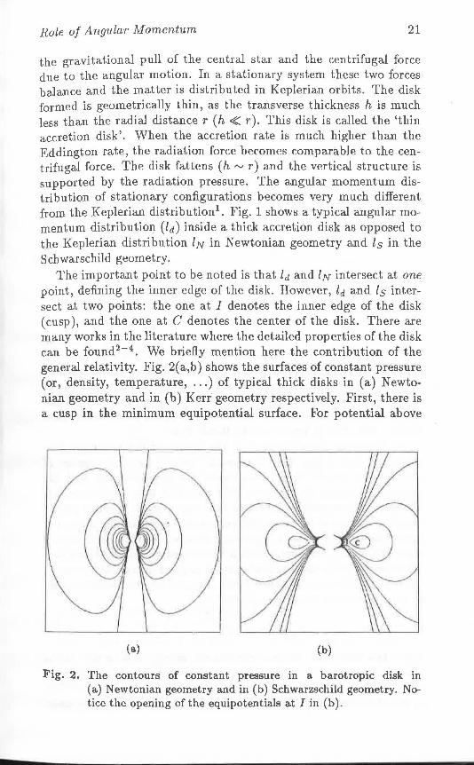
The important point to be noted is that ld and ZN intersect at one point, defining the inner edge of the disk. However, ld and ls intersect at two points: the one at I denotes the inner edge of the disk (cusp), and the one at C denotes the center of the disk. There are many works in the literature where the detailed properties of the disk can be found 2- 4 • We briefly mention here the contribution of the general relativity. Fig. 2( a,b) shows the surfaces of constant pressure (or, density, temperature, ... ) of typical thick disks in (a) Newtonian geometry and in (b) Kerr geometry respectively. First, there is a cusp in the minimum equipotential surface. For potential above
(a) (b)
Fig. 2. The contours of constant pressure in a barotropic disk in (a) Newtonian geometry and in (b) Schwarzschild geometry. Notice the opening of the equipotentials at I in (b).
· 22 Gravitation and Cosmology
this value there is an opening (I) and matter of the disk can fall on to the hole through it. Secondly, in a barotropic flow, the surfaces of constant angular momentum in a Newtonian disk are R = constant surfaces, where R is the axial distance. However, in a general relativistic flow, these are >. = constant surfaces where >. is the socalled von-Zeipel parameter. 4 These surfaces could be topologically cylindrical5 and/or toroidal.6 When cylindrical, they reE>emble flat cylinders geometrically pulled towards the hole on the equatorial plane (Fig. 4). A typical distribution of angular momentum l == c>.n (where c and n are constants) allows one to study all the thermodynamical properties of a thick disk.4 Because the potential is open near the cusp I, and the disk has a pressure maximum at the center C right behind it, the accretion is possible even in the presence of very low viscosity. Different aspects of the thick accretion disks ' are currently under active scrutiny; interested readers may look into Chakrabarti7 for a recent review.
3. Transonic Flows Around Compact Stars
One of the important properties of an accretion flow on a black hole is that the fl.ow is transonic; it changes from subsonic (at a large distance) to supersonic (near the black hole). The location where this transition takes place is known as the sonic point. In the radial accretion of an. adiabatic flow there is exactly one such point in the entire flow. Because of this, the adiabatic radial fl.ow cannot have shocks. This flow is known as the Bondi flow.
An important breakthrough in the theory of the transonic flow occurred when Liang and Thompson8 found that th~ number of sonic points can be .thr e when there is a large rotation and the background metric is that of a Schwarzschild hole. Subsequently, Chang and Ostriker9 pointed out th<1-t the number of sonic points could be increased by many different ways: for example, when the flow is suddenly heated, a supersonic :flow is forced to become subsonic. Presently, however, we stick to the proposition by Liang and Thompsons, since usually a substantial angular motion is present in the disk. To demonstrate their point, we consider the ~pecific energy of a thin flow in a black hole geometry:
I 2 2 z2 I ( ) c; = -fJ + na + - - --. 1
2 2r2 r - 1
Here, the fost term denotes the kinetic energy due to the radial motion, the ~econd term contains the 'PdV' work plus the thermal energy (pf p + f = na2 for a.n adiabatic equation of state p ex: p1+1/n, p, p and f being the matter density, pressure and the specific inter-
Role of Angular Momentum 23
nal energy of the flow respectively and n being the polytropic index of the flow), the third term denotes the rotational kinetic energy (l being t11e specific angular momentum), and the final term denotes t.he pseudo-Newton.ian potential mimicking the Schwarzschild black hole geometry.2 The radial distance r is written in units of 2GM/c2
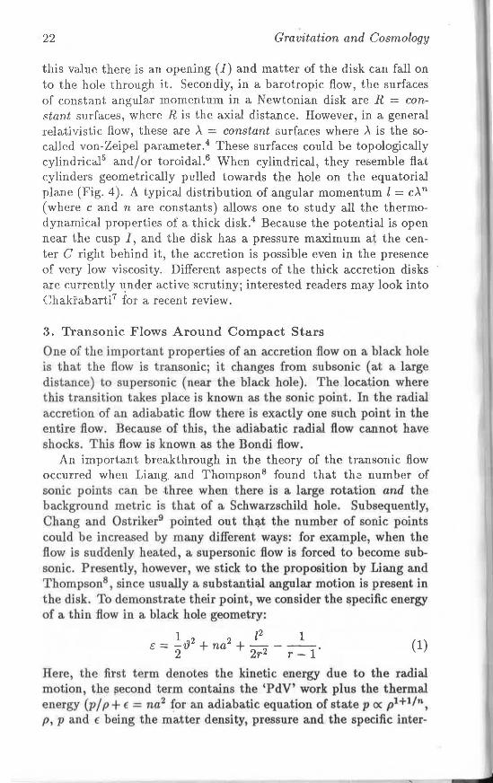
and the velocities are written in units of the velocity of light. For a non-dissipative flow t: is conserved and for a given t:, as one approaches the horizon, r --+ 1, the potential term dominates over the third term. The negative sign in the potential causes the phase trajectories to look 'hyperbolic'. The same is true as r --+ oo. In the region T "' l, the third term with the positive sign dominates over the fourth. As a result the phase space trajectories are elliptical, just as in the case of a simple harmonic oscillator. As example of the complete trajectory is shown 10 in Fig. 3. Here the Mach number
r .. ru ru
2.80
2 60
2.40
2.20
2 00
1.80
1 60 M
) 40
I 20
1.00
0.80
0.60
0.40
0.20
0 0<0-40 0.90 , 40 1.90
109 ( r)
Fig. 3. The phase space trajectory of adiabatic accretion flow in the Kerr geometry. The Mach number M of the flow is plotted against the logarithmic radial distance. The arrowed curve indicates the stationary solution which includes a shock. The shock location could be at r,2 or at r.a. This ambiguity disappears in dissipative isothermal flow .11
of the fl.ow is plotted against the radial distance. Note that at locations ri and T 0 the fl.ow crosses the sonic point (M = 1). The arrow indicates a flow which develops a shock after becoming supersonic at To. The shock location could be either Ts2 or T 8 3. The uniqueness of the solution with shocks is shown when the dissipation is present.11 (The other two formal locations T81 and rs4 shown in the diagram are not possible for a black hole accretion.) The postshock fl.ow con-
24 Gravitation and Cosmology
tinues further and crosses the sonic point at r; before disappearing inside the horizon.
In the present situation we demonstrated that the angular motion, together with the general relativistic background, allows a black hole accretion flow to have a stationary solution which includes shocks. In fact, the shock forms due to the brake in the flow by the centrifugal force, and the pseudo-Newtonian potential provides the flow with a 'supersonic' exit to match the boundary condition on the black hole horizon . If the potential were Newtonian, the flow would have remained subsonic after the shock to match the boundary condition (zero radial velocity) on the star surface. Detailed properties of the transonic flows are discussed in Chakrabarti.11
4. Close Binary Stars
According to the theory of general relativity, when an object is accelerated it emits Gravitational Wave (GW). It is similar to the Emission of Electromagnetic (EM) radiation from an accelerated charged particle. The important difference lies in the fact that the power of the EM radiation emitted depends on the change in the dipole moment of a charge distribution, whereas the power of the GW radiation depends upon the change in the quadrupole moment of a mass distribution. In analogy with the EM wave, the power radiated in GW is obtained roughly by following the rules: (a) replace the
·· four current vector Ji as the source of the EM field by the compact energy-momentum tensor (Tik) as the source of the gravitational field, (b) the role of vector potential Ai is played by a combination of the perturbation of the metric hij, ( c) the gauge transformation of Maxwell theory is replaced by the co-ordinate transformation. The GW power radiated turns out ta be (see e.g., Misner et al.12 ) •
.E = - G naf32 (2a)
45 '
where
naf3 = J €(3xaxf3 - 00tf3x'Yx'Y)dv (2b)
is the quadrupole moment, f is the mass density, dv is the volume occupied by the mass elements, oaf3 is the Dirac symbol and G is the gravitational constant.
Binary stars have a large varying quadrupole moment. Some angular momentum is lost in the gravity waves because of which the orbital period of the binary decreases. This effect can be calculated quite accurately by linearizing the equations of general relativity13
Ro"le of Angular Momentum
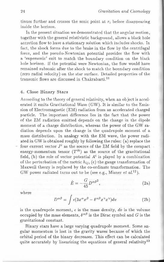
and the rate of change of period is given by,
p = - 1927rGs/3 Pb/27r-s/3(1 - e2)-1 /2 5c5
( 73 37 ) x 1 + -e2 + -e4 m m (m + m )-1/ 3 24 96 p 8 p 8
25
(3)
where e is the eccentricity of the orbit and mp and ms are the masses of .the primary and the secondary stars respectively.
The orbiting pulsar PSR 1913+16 discovered by Hulse and Taylor14 is the most studied binary pulsar. It is found that the observed P agrees with the calculated value given by Eq. (3) in 1 part in 1013. This not only verifies that the general theory of relativity is a correct theory of gravity, at least up to a distance of few Kpc, but also provides us with the most accurate clock.
6. Force on Rotating Flows Around Black Holes
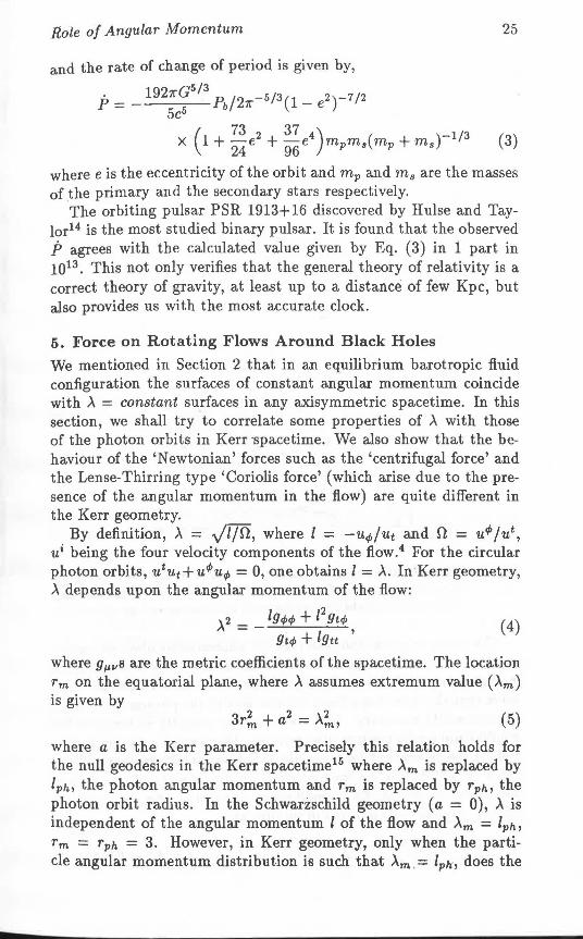
We mentioned in Section 2 that in an equilibrium barotropic fluid configuration the surfaces of constant angular momentum coincide with >. = constant surfaces in any axisymmetric spacetime. In this section, we shall try to correlate some properties of >. with those of the photon orbits in Kerr ·spacetime. We also show that the behaviour of the 'Newtonian' forces such as the 'centrifugal force' and the Lense-Thirring type 'Coriolis force' (which arise due to the presence of the angular momentum in the fl.ow) are quite different in the Kerr geometry.
By definition, >. = ...;rm, where l = -u<t>/Ut and n = u<I> Jut' ui being the four velocity components of the fl.ow. 4 For the circular photon orbits, utut+ u<f>u.p = O, one obtains l = >.. In Kerr geometry, >. depends upon the angular momentum of the fl.ow:
>.2 = _ lY<1><1> + l2Yt<t>, ( 4)
gt</>+ lgtt
where 9µvB are the metric coefficients of the spacetime. The location rm on the equatorial plane, where >. assumes extremum value (>.m) is given by
(5)
where a is the Kerr parameter. Precisely this relation holds for the null geodesics in the Kerr spacetime15 where Am is replaced by lphi the photon angular momentum and Tm is replaced by Tph, the photon orbit radius. In the Schwarzschild geometry (a = 0), A is independent of the angular momentum l of the flow and Am = lph,
Tm = Tph = 3. However, in Kerr geometry, only when the particle angular momentum distribution is such that Am .= lph·, does the
26 Gravitation and Cosmology
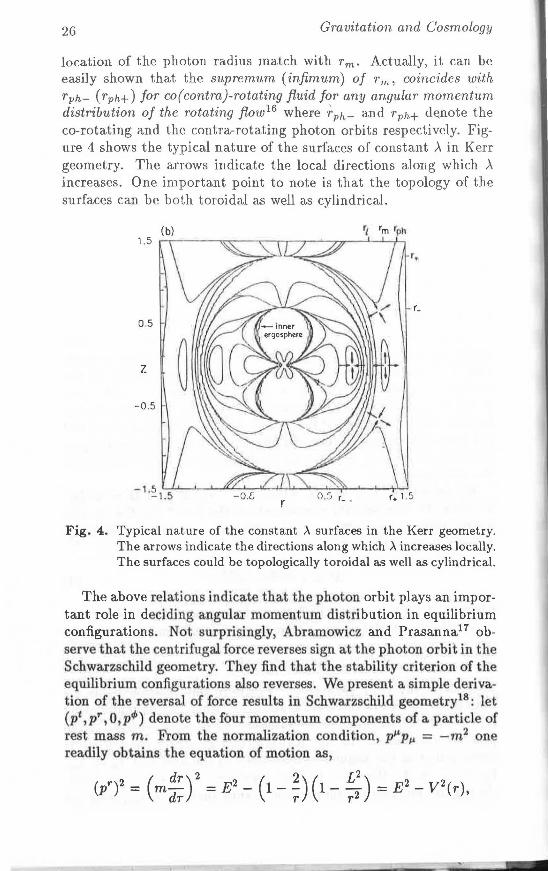
location of the photon radius match with Tm· Actually, it can be easily shown that the supremum ( infimum) of Tm, coincides with Tph- ( Tph+) for co( contra)-rotating fluid for any angular momentum distribution of the rotating fiow 16 where rph- and Tph+ de.note the co-rotating and the contra-rotating photon orbits respectively. Figure 4 shows the typical nature of the surfaces of constant ,\ in Kerr geometry. The arrows indicate the local directions along which ,\ increases. One important point to note is that the topology of the surfaces can be both toroidal as well as cylindrical.
r_
0.5
z
-0.5
-i.~1.5 -0,[, 0 .5 r_ . r. 1.5 r
Fig. 4. Typical nature of the constant A surfaces in the Kerr geometry. The arrows indicate the directions along which A increases locally. The surfaces could be topologically toroidal as well as cylindrical.
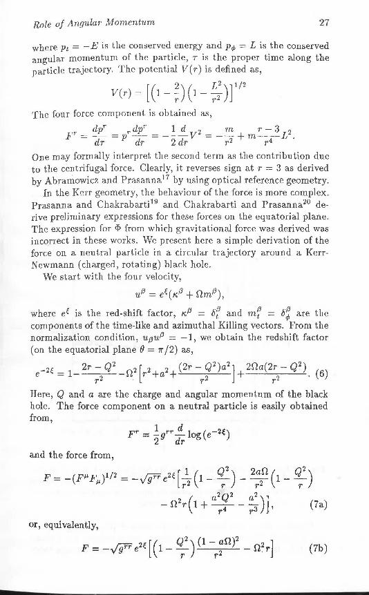
The above relations indicate that the photon orbit plays an important role in deciding angular momentum distribution in equilibrium configurations. Not surprisingly> Abramowicz and Prasanna17 observe that the centrifugal force reverses sign at the photon orbit in the Schwarzschild geometry. They find that the stability criterion of the equilibrium configurations also reverses. We present a. simple derivation of the reversal of force results in Schwarzschild geometry18 : let (pt ,pr, O>plf>) denote the four momentum components of a. particle of rest mass m. From the normalization condition, pµpµ = -m2 one readily obtains the equation of motion as,
(pr)2 = ( m :~)2 = E 2 - ( 1 - ~) ( 1 - ~:) = E 2
- V 2 (r),
Role of Angular Momentum 27
where Pt = -Eis the conserved energy and Pc/> = L is the conserved angular momentum of the particle, r is the proper time along the particle trajectory. The potential V( r) is defined as,
v(r)= [(1-f)(1-~:)r12
The four force component is obtained as,
pr= dpr =Pr dpr = -~~ v2 = - m + m r - 3 L2. dr dr 2 dr r2 r4
One may formally interpret the second term as the contribution due to the centrifugal force. Clearly, it reverses sign at r = 3 as derived by Abramowicz and Prasanna17 by using optical reference geometry.
In the Kerr geometry, the behaviour of the force is more complex. Prasanna and Chakrabarti19 and Chakrabarti and Prasanna20 derive preliminary expressions for these forces on the equatorial plane. The expression for Cf> from which gravitational force was derived was incorrect in these works. We present here a simple derivation of the force on a neutral particle in a circular trajectory around a KerrNewmann (charged, rotating) black hole.
We start with the four velocity,
uf3 = e€(K,f3 + nmP),
where e€ is the red-shift factor, ,..,P = bf and mf = b~ are the components of the time-like and azimuthal Killing vectors. From the normalization condition, upu/3 = -1, we obtain the redshift factor (on the equatorial plane () = 7r /2) as,
-2€ - 2r - Q2
n2 [ 2 2 (2r - Q2
)a2
] 2na(2r - Q2
) ( ) e - 1- 2 H r +a + 2 + 2 • 6
r r r
Here, Q and a are the charge and angular momentum of the black hole. The force component on a neutral particle is easily obtained from,
and the force from,
i/2 r::rr 2€[ 1 ( Q2
) 2an( Q2
) F = -(FIJ,F) = -ygrre - 1- - - - 1- -µ r2 r r2 r
( a2Q2 a2 )) - n2r 1 + -- - - '
r4 r3 (7a)
or, equivalently,
Q2 (1 af!)2 F =-if e2€ [ (1---;:--) -r2 - f!2r) (7b)
28 Gravitation and Cosmology
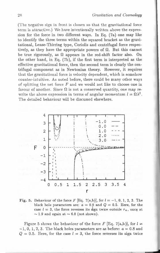
(The negative sign in front is chosen so that the gravitational force term is attractive.) We have intentionally written above the expression for the force in two different ways. In Eq. (7a) one may like t.o identify the three terms within the squared bracket as the gravitational Lense-Thlrring typ , Coriolis and centrifugal force respectively, as they have the a.ppropriate powers of n. But this cannot be true rigorously, as n appears in the red-shift factor also. On the other hand, in Eq. (7b ), if tne first term is interpreted as the ffective gravitational force, then the second term is clearly the cen
trifugal component as in Newtonian theory. However, it requires that the gravitational force is velocity dependent, which is somehow counter-intuitive. As noted before, there could be many other ways of splitting the net force F and we would not like to choose one in favour of another. Since n is not a conserved quantity, one may rewrite the above expression in terms of angular momentum l = n>.2 •
The detailed behaviour will be discussed elsewhere.
4
3
2
1
F o -1
-2
-3
-4
\ ' I
-1.0 0.0 1. 0 2.0 3.0
0 0.5 1 1.5 2 2.5 3 3.5 4
r
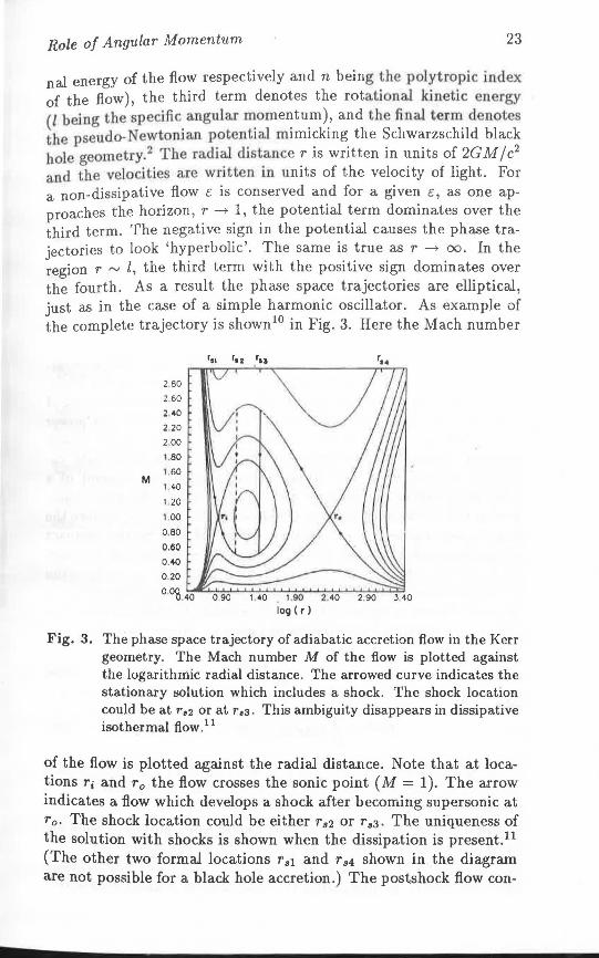
Fig. 5. Behaviour of the force F [Eq. 7(a,b)], for l = -1, 0, 1, 2, 3. The black hole parameters are: a = 0.8 and Q = 0.5. Here, for the case l = 3, the force reverses its Jign twice outside r+, once at ,....., 1.9 and again at,....., 6.0 (not shown).
Figure 5 shows the behaviour of the force F [Eq. 7( a,b )], for l = -1, 0, 1, 2, 3. The black holes parameters are as before: a = 0.8 and Q = 0.5. Here, for the case l = 3, the force reverses its sign twice
Role of Angular Momentum 29
outsider+, once at"' 1.9 and again at"' 6.0 (not shown). The reversal of the net force implies that the Rayleigh stability
criterion will also reverse. 11-
20 This has important bearing on the structure and stability of the a.ccreting compact objects.
The author is thankful to Prof. S. Mukherjee for the hospitality provided at the meeting.
References
1. Maraschi, L., Reina, C. and Treves, A.: Astrophys. J., 35 (1974), 389. 2. Paczyri.ski, B. and Wiita, P.: Astron. Astrophys., 88 (1980), 23. 3. Abramowicz, M.A., Calvani, M. and Nobili, L.: Astrophys. J., 242 (1980),
772. 4. Chakrabarti, S.K.: "Active Galactic Nuclei", Dyson, J. (ed.), Univ. of
Manchester Press 1984; Chakrabarti, S.K.: Astrophys. J. 288 (1985), 1. 5. Abramowicz, M.A.: Acta Astron., 24 (1974), 45. 6. Chakrabarti, S.K.: Mon. Not. R. Astron. Soc. (in press). 7. Chakrabarti, S.K.: Comm. Astrophys., No. 4 (1990). 8. Liang, E.P.T. and Thompson, K.A.: Astrophys. J., 240 (1980), 271. 9. Chang, K.M. and Ostriker, J.P.: Astrophys. J., 288 (1985), 428.
10. Chakrabarti, S.K.: Astrophys. J., 350 (1990), 275. 11. Cha.krabarti, S.K.: Mon. Not. R. Astron. Soc., 243 (1990), 610; Cha.kra
barti, S.K.: "Theory of Transonic Astrophysical Flowe", World Scientific Co., Singapore, 1990.
12. Misner, C.W., Thorne, K.S. and Wheeler, J.A.: "Gravitation", San Fran-cisco: Freeman, 1973.
13. Peters, P.C. and Mathews, J.: Phys. Rev., 131 (1963), 435. 14. Hulse, R.A. and Taylor, J.H.: Astrophys. J. (Lett.), 195 (1975), L 51. 15. Chandrasekhar, S.: "Mathematical Theory of Black Holes", Oxford: Cla
rendon Press, 1983. 16. Cha.krabarti, S.K.: Mon. Not. R. Astron. Soc., 245 (1990), 747. 17. Abramowicz, M.A. and Pra.sanna, A.R.: Mon. Not. R. Astron. Soc. (in
press). 18. Chakrabarti, S.K. and Shiek, A.Y.: Am. J. Phys. (submitted). 19. Prasanna, A.R. and Chakraba.rti, S.K.: "General Relativity and Gravita
tion" (in press). 20. Chakrabarti, S.K. and Prasanna, A.R.: J. Astron. and Astrophys., 11
(1990), 29.
Fiber Bundles in
Gravitational Theory
ERIC A. LORD
Department of Applied Mathematics and Centre for Theoretical Studies
Indian Institute of Science, Bangalore 560 012
1. Introduction
In 1954, Yang ai;id Mills introduced a new idea into theoretical physics, which later came to dominate the physicist's view of the fundamental structure of the physical forces of nature. The YangMills theory is the 'gauge theory of a non-Abelian symmetry group', and is essentially a generalization of Maxwell's theory of electromagnetism, which is the gauge theory .of a one-parameter Abelian group.
The theory of Yang and Mills dealt specifically with the isospin symmetry of nuclear forces. The gauging of the isospin group SU(2) leads to a triplet of isospin-1 mesons as analogues of the photon; the non-Abelian nature of the group gives rise to nonlinearity of their field equations. The eminently successful Salam-Weinberg unification of the weak and electromagnetic forces (1973) exploited the Yang-Mills ideas. The observed distinction between the weak forces and the electromagnetic forces, including the masses of the W ± and the Z, come from a spontaneous symmetry breaking mechanism (Higgs mechanism). Quantum chromodyn?-ffiics (QCD) is, similarly, a gauge theory for the strong interactions, in which the Yang-Mills particles are the 'gluons' that mediate the forces between quarks. Attempts to unify the electromagnetic, weak and strong forces by further exploiting the Yang-Mills idea are the 'grand unified theories' (GUTs). The hope is to find a group that contains the SalamWeinberg group and the unitary symmetry group of QCD in a nontrivial way, to gauge the group, and to introduce appropr-iate-Higgs mechanisms to break the symmetry so as to obtain the observed behaviour of the three kinds of fundamental interaction.
In all these developments, the gravitational forces are 'conspicuous by their absence'. From the outset, Einstein's general relativity has stood alone, isol~ted from the developments that have taken place in our understanding of the other fundamental forces. This immense
Fiber Bundles in Gravitational Theory 31
conceptual gap was the source of Einstein's opposition to the developments that took place in physics as a result of the advent of quantum theory, an opposition summarized in his famous statement "God does not play dice." At present the gap appears not quite so unbridgeable (though the problem of the unification of all the forces of nature, mcluding gravitation, is still formidable). Ip fact, Einstein's gravitational theory and various modifications and extensions of it, can be understood as 'gauge theories' in the Yang-Mills sense. We shall not discuss the physics of these theories; our aim here is only to throw some light on the geometrical concepts that allow gravitational theories to be viewed as gauge theories. More details will be found in the references.
2. Gauging a Non-Abelian Group
Let 1/J be a set of physical fields of a Lagrangian theory invariant under a group of linear transformations
1/J - S1f;. (1)
When S is made space-time dependent, invariance is maintained by replacing derivatives of 1/J by a generalized derivative
(2)
where ri is a linear combination of the generators Ga of the group,
f; == riaGa, (3)
provided the 'gauge potentials' ria have the transformation law
r; - sris-1 - (B;S)s-1
. (4)
The 'gauge fields' Fij a are defined by
[Di,D.1] = Fii = FiiaGa = a,ri - airi + [ri,ri]· (5)
They transform homogeneously: . -1
Fii - SFiiS . (6)
This is the basic Yang-Mills idea. We have a generalization of the electromagnetic potential and the electromagnetic field. Under an infinitesimal gauge t~ansformation and an infinitesimal coordinate transformation,
(7)
we have
01/J = ~j 8j1/J + E'i/J, (8)
ori = ~iairi + (ai~i)r; - D,£, Dj£ = 8j€ + [ri,E]. (9)
32 Gravitation and Cosmology
Changing the parameters to);= eiri - E, we have the following neat 'manifestly invariant' forms for the infinitesimal changes:
3. Lie Groups
fi'lj; = ei Di'l/J :- >..'lj;,
6Ti = ei Fii +Di>..
(10) (11)
A Lie group G is a group whose elements constitute a differentiable manifold. An element of G can be regarded as a transformation on the manifold, or as a point of the manifold. We shall write g to denote an element of G when the former aspect is emphasized, and we shall write z when we wish to emphasize the latter aspect. Associated with any element g, there is a transformation on the manifold G, called left translation:
z --+ L 9 z = gz. (12)
Similarly, right translation is defined by
z --+ R9 z = zg. (13)
A left-invariant vector field on G is a vector field that is unchanged by any left translation. A left-invariant field generates a one-parameter group of right translations, and vice-versa. The commutation of two left-invariant vector fields is a left-invariant vector field. So the left-invariant vector fields form an algebra under commutation, called the Lie algebra of G. A basis for the Lie algebra is a set {RA} of left-invariant vector fields. It constitutes a vielbein on the manifold G. [ Vielbein: German for 'many legs', a. generalization of the terminology vierbein ('four legs') meaning 'tetrad'.] We write A, B, ... for the vielbein labels and M, N, ... for coordinateba.sed indices. Denote the elements of the matrix of components of the 'left-vielbein' {RA} by RAM. The elements of the inverse matrix can then be denoted by RMAi they are the components of a set {RA} of 'one-forms' (i.e., covariant as opposed to contravaria.nt vectors), constituting the basis 'dual' to {RA}· The structure constants of the group Gare given by
(14)
Let S be· any matrix representation of the Lie group G; i.e., S(z) is a. matrix field on the manifold G satisfying S(g)S(z) = S(gz), S(z-1 ) = s-1 (z). The matrix generators GA for the representation Sa.re
GA= s-1 RA(s). (15)
They can be shown to satisfy
[GA,Gs] = C~8Gc. (16)
Fiber Bundles in Grovitational Theory 33
An ordinary one-form maps a vector to a scalar. A 'Lie algebra.valued' one-form maps a vector to an element of the Lie algebra, l.e., to a left-invariant vector field. The Maurer-Cartan form 0 is the one-form that maps a vector X at a point z of G to the unique left-invariant field that takes the value X a.t z. In a representation S, O is represented by a matrix-valued one-form
(} = OAGA, (17)
where the coefficients ()A are ordinary one-forms. Since OAG A maps RB to its representative matrix GB, we have ()A(RB) = 6AB, so ()A = RA. Therefore
O=GARA.
Observe also that the matrix-valued one-form s-1 dS satisfies
cs-1 dS)RA = s-1 RA(S) =GA,
and hence (J = s-I dS
(18)
(19)
in any representation S. If G is a matrix group, we can use the self representation and write simply
0 = z-1 dz. (20)
Then, from dz = z(J and d dz = 0 we get the Maurer-Cartan equation
d(J + (J " (J = o. (21)
In terms of components, this is
aMRNA - oNRMA + RM8 RNccBcA = o, (22)
which is equivalent to
RAMOMRBN - RBM{)MRAN = CABc RcN. (23)
That is, the Maurer-Cartan equation and the commutation relations (14) are equivalent.
4. Fiber Bundles
The theory of fiber bundles was developed by mathematicians as a branch of pure mathematics. Exciting developments began in the 1960s with the realization that the mathematicians' 'fiber bundles' and the physicists' 'gauge theories' were essentially identical. The mathematicians' preoccupation with the global topological properties of the geometrical structures known as fiber bundles then provided physicists with methods and concepts that released the study
34 Gravitation and Cosmology
of gauge theories from its preoccupation with local concepts (formulated in terms of differential equations).
A fiber bundle is constructed from a bundle space P and a J_,ie group G, the structural group, which acts on P without fixed points. The orbits of the action of G are the fibers, which are subspaces of P. There is one fiber Fz through each point z of P. The fibers are required to be all homeomorphic to a fiber space F so that the action of G on P corresponds to an action of G on F. The set of all fibers is homeomorphic to a space M, the base space, and a projection operator 11' maps P to M, each point z being mapped to a. unique point x = 11'Z E M so that all the points of a fiber are mapped to the same point of M. A point x E M specifies a unique fiber Fx = 11'-l x
in P. With hindsight, one can see that the first use of a fiber bundle
in physics was in fact the Kaluza-Klein theory. The group G is the electromagnetic gauge group, the bundle space is five-dimensional and the fibers one-dimensional. The four-dimensional base-space is space-time.
A principal fiber bundle P(M, G) is a fiber bundle for which the fiber space Fis the manifold of the structural group G. We denote the action of an element g of G on P, by the notation
z--+ zg = R9 z. (24)
An equivariant field W on Pis a field belonging to a linear representation S of G with the transformation law
(25)
This can be written as
(26)
so that an equivariant field can be seen to be determined on the whole of a fiber Fz if its value at any point z of the fiber is given.
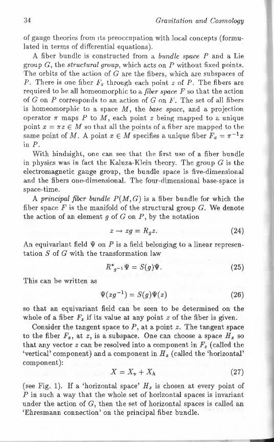
Consider the tangent space to P, at a point z. The tangent space to the fiber Fz, at z, is a subspace. One can choose a Space Hz so that any vector z can be resolved into a component in Fz (called the 'vertical' component) and a component in Hz (called the 'horizontal' component):
(27)
(see Fig. 1). If a 'horizontal space' Hz is chosen at every point of Pin such a way that the whole set of horizontal spaces is invariant under the action of G, then the set of horizontal spaces is called an 'Ehresmann connection' on the principal fiber bundle.
Fiber Bundles in Gravitational Theory 35
' M
\ ' ' \ ~ X= 1T Z
Fig. 1
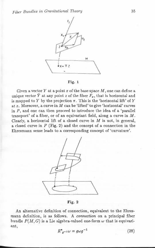
Given a vector Y at a point x of the base space M, one can define a unique vector Y at any point z of the fiber Fx, that is horizontal and is mapped to Y by the projection 1r. This is the 'horizontal lift' of Y at z. Moreover, a curve in M can be 'lifted' to give 'horizontal' curves in P, and one can then proceed to introduce the idea of a 'parallel transport' of a fiber, or of an equivariant field, along a curve in M. Clearly, a horizontal lift of a closed curve in M is not, in general, a closed curve in P (Fig. 2) and the concept of a connection in the Ehresmann sense leads to a corresponding concept of 'curvature'.
\~ \ Fig. 2
An alternative definition of connection, equivalent to the Ehresmann definition, is as follows. A connection on a principal fiber bundle P(M, G) is a Lie algebra-valued one-form w that is equivariant,
R• -1 g-IW = gwg (28)
36 Gravitation and Cosmology
and that maps any vertical vector at a point z to the corresponding left-invariant field on F':
w(Xv) = O(Xv)· (29)
Given such an w, Ehrcsmann's horizontal spaces can be constructed from those vectors Xh that satisfy w(Xh) = 0. The curvature asso·· ciated with a connection w is defined to be the Lie algebra-valued two-form
0 = 2(dw + w /\ w). (30)
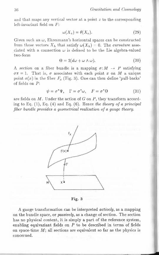
A section on a fiber bundle is a mapping a: M -t P satisfying arr = 1. That is, a associates with each point x on M a unique point a(x) in the fiber Fx (Fig. 3). One can then define 'pull-backs' of fields on P:
7/J=a*w, f=a*w, F=a*0 (31)
are fields on M. Under the action of G on P, they transform according to Eq. (1), Eq. ( 4) and Eq. (6). Hence the theory of a principal fiber bundle provides a geometrical realization of a gauge theory.
Fig. 3
A gauge transformation .can be interpreted actively, as a mapping on the bundle space, or passively, as a change of section. The section has no physical content, it is simply a part of the reference system, enabling equivariant fields on P to be described in terms of fields on space-time M; all sections are equivalent so far as the physics is concerned.
Fiber Bundles in Gravitational Theory 37
The gauge transformations do not affect the points of space-time: the fibers are acted upon but not moved by an active gauge transformation. So the fiber bundle theory we have described is of use only for the gauge theory of an internal symmetry group.
Now, as was shown by Kibble for the Poincare group, the YangMills idea of gauging a symmetry group can be applied also to spacetime groups, as well as to internal symmetries. Indeed, in the case of the Poincare group, the Yang-Mills trick led to a theory similar to Einstein theory, but with non-vanishing torsion (the ECKS theory). To incorporate this kind of extension of the Yang-Mills idea into fiber bundle language, one needs to consider transformations on a bundle space that shift the fibers around. A very elegant way of doing this was introduced by Ne'eman and Regge. The base space in their approach is a coset space. The version of coset bundle theory that we describe below was developed by Lord and Goswami.
5. Coset B undies
Let G be a Lie group and H a Lie subgroup. Let H act on G by right translation:
(32)
We then have a principal fiber bundle G(G/H,H). The bundle space is the manifold G. The structural group is H (acting on the right) and the fibers are the cosets zH. The base space is the coset space G / H, which will be interpreted as space-time. G may contain internal symmetries as well as space-time symmetry (such as the Poincare group, the de Sitter group or the conformal group).
Consider the left action of the whole of G on the coset bundle:
z -t L9 z = gz. (33)
The points of the base space are not invariant under this action. Writing x = 1f'Z, the effect on the base space is
X -t X1 = 7rg7r-lX. (34)
If a section u is introduced, the action can be conceived as consisting of a 'space-time dependent' action of the structural group H, and an action [Eq. (34)) on space-time:
gu(x) = u(x')h(x,g). (35)
We now define gauge transformations to be the most general transformations on the space G( G / H, H) that preserve the fiber bundle structure. That is, a gauge transformation z -t f ( z) is a mapping that commutes with the right action of the structural group H:
f(i)h = f(zh). (36)
33 Gravitation and Cosmology
I I \Ix I \ h'
Fig. 4
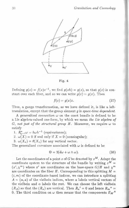
Defining g(z) = J(z)z- 1 , we find g(zh) = g(z), so that g(z) is constant over each fiber, and so we can write g(z) = g(x). Then
J(z) = g(x )z. (37)
Thus, a gauge transformation, as we have defined it, is like a lefttranslation, except that the group element g is space-time dependent.
A generalized connection w on the coset bundle is defined to be a Lie algebra-valued one-form, by which we mean the Lie algebra of G, not just of the structural group H. Moreover, we require w to satisfy l. R;_ 1 w = hwh- 1 (equivariance); 2. w(X) = 0 if and only if X = 0 (nonsingular); 3. w(Xv) = B(Xv) for any vertical vector.
The generalized curvature associated with w is defined to be
0=2(dw+w/\w). (38)
Let the coordinates of a point z of G be denoted by zM. Adapt the coordinate system to the structure of the bundle by writing zM = (x1,xm) where xi are coordinates on the base-space G/H and xm are coordi'nates on the fiber H. Corresponding to this splitting M = ( i, m) of the coordinate-based indices, we can introduce a splitting A = (a, a) of the vielbein indices, where a labels vertical vectors of the vielbein and a labels the rest. We can choose the left vielbein (RA) so that the (Ra) are vertical. Then Ra i = 0 and hence Rm er = 0. The third condition on w then means that the components EMA
Fiber Bundles in Gravitational Theory 39
of w have the form
(39)
The equivariance of w then implies that the only nonvanisliing components 0 MNA of the curvature are 0ijA.
Let a be a section. The components of a( x) have the form
<7M (x) = (xi, am(x )). (40)
Employing a to 'pull back' equivariant fields, we define
'I/;= a*'lt = 1lt(9'). ( 41)
r = a*w. That is,
fiA = <1M.iEMA(r:1), }
or, more explicitly, rt'~ = E/~(u) = e/~,
r,a. = Eia(u) + um.iRm a(o}
(42)
F = a*0. That is,
FijA = aM.WN.j0MNA(a) = 0;/(a). (43)
We find that (44)
i.e., (45)
We can compute the action of an infinitesimal gauge transformation zM -+ zM - AM on these space-time fields. The gauge transformation is determined by the parameters
AA(x) = r:T* EAA = AA(o-). (46)
We find (47)
where
But 8;'1/; = aM.iw.M(a) = 'lt,,(a) + aj'lt.m(a),
and the infinitesimal form of the equivariance condition on 1lt 1s 1lt .m = -Rm a Ga 1lt. Substituting these expressions, we get
QA'l/J = EAi(a)(oi'l/J+ fiaGa'l/J)-6AaGa1/J,
i.e.,
40 Gravitation and Cosmology
Defining ~i = >.a ea i, we obtain the transformation law
o'lj; = ~; Di1/J - >.aGa1f1. (48)
off= aM.;oEMA(a). Now EMA is a covariant vector on the manifold G, so
oEMA = ANaNEMA + (oMAN)ENA
= f)MAA + AN(fJNEMA - ()MENA).
But eMNA ={)MENA - 8NEMA + EM 8 ENCCacA'
so (using the vielbein components EMA for converting indices),
oEMA = OMAA + A 8 (CMBA - 0MaA).
Therefore,
or/~ a~ (oM>.A + >. 8 EMC(a)CcaA - >. 8 Ea_N (a)0MNA(a))
= (8i>.A + >. 8 f;CCcaA)- ~jFijA·
We obtain the transformation law of the potentials in the form
A . A A } hT; = e Fji +Di>. , (49)
V;>-.A = 8;>.A - >.BI'ic Gae A.
The fiber bundle theory has provided us with the appropriate generalizations of the transformation laws given by Eq. (1) and Eq. (4), for the case where G contains a space-time symmetry.
6. Poincare Gauge ri:heory
Finally, we shall illustrate the transformation laws we have found, by applying them to a particular example. Let G be the Poincare group. Denote the generators of Lorentz rotations by Ga/3 (= -Gf3a) and translation generators by Ga. H is the Lorentz group. G / H is space-time. The commutation relations are:
[Ga, G/3] = o, } [ G af3' G.,,] = T/a-yG /3 - T/{3-yG Cl''
[Gaf3, G.,,o] = T/a-yG/36 - T/{3-yGao + T/{JoGa-y - T/aoG/3-y
(50)
Writing
f · - e·aG + ~r.af3G 13 (51) ,-, Cl' 2' Q')
Fi;= 8iti - 8;fi + [ri,f;] = Fi/"Ga + ~Fi;a13 Gaf3, (52)
Fiber Bµ,ndles in Gravitational Theory 41
we find
F f3 -- fJ.e·fJ -8·e·f3 - e·"f· f3 + e·"ffJ (53) IJ - I J J t t J')' J 'I',
F · f3 - '1.f. f3 - l'l.f. f3 - f· "I~- f3 + f · "f· f3 (54) iJOI - Ui JOI UJ tQ IQ J')' JC> l"f l
(where 'r/o(J has been used as a raising-lowering operator). The translational components ei
0 off i define a tetrad, and we can construct a metric and a set of connection coefficients on space-time:
(55)
(56)
Then the 'translational gauge potentials' Fi/ turn out to be the torsion, and the 'rotational gauge potentials' Fijk 1 turn out to be the curvature, associated with these connection coefficients. The connection coefficients are metric-compatible, j.e.,
oigik - C/g1k - f;k 1911 = o. (57)
Writing
,\ = ,\ 0 Go + ~,\0f3Gof3 and defining the parameters
(58)
(59)
we find that the transformation laws [Eq. ( 48) and Eq. ( 49)] are
be; 0 = ~iEJ1 e; 0 + (8i~i)ej 0 + eif3lp 0, (60)
of· f3 - tia-r- f3 + (o·ti)r. {3 - D·f 11 } IQ - <,, J tQ 1<, JC> I Q l
(61) Dlf3_!l_,.f3 f·",.f3+,.'Yf.f3
t Q - U1 <<;> - IQ ""! <<;> I')' '
b'ljJ = ~i8i'l/J + ~€0f3G0,o'l/J. (62)
These are identical to the transformation laws for a tetrad, a set of 'spin coefficients' and a field representing the Lorentz group, under the combined action of a Lorentz rotation of the tetrad and a general coordinate transformation.
To justify the assertion that these are indeed the transformation laws appropriate to a gauged Poincare group, we impose the restrictions
r . (J - 0 IQ - l (63)
and consider just those transformations [Eqs. (60)-(61)) that maintain these restrictions. We have Fij = 0 and D; = 8;, and so
O = 8i~i +€iii} (64) O = 8;€ik·
42 Gravitation and Cosmology
Hence Ejk is constant, and
(65)
just the effect of an infinitesimal action of the Poincare group on Minkowski space-time. The field 'ljJ transforms accor<ling to
. 1 .. b'l/; = aJaj'l/; + 2€'J(xJ)j - Xjai + G;1)'1/J, (66)
as it should. In terms of the bundle space, we have the left action of the Poincare group on itself.
References
1. Hehl, F.W.: Four lectures on the Poincare gauge field theory, in Proceedings of the 6th Course of the International School of Cosmology and Gravitation; Bergmann, P.G. and Sabbata, V. (eds.), Plenum Press, 1978.
2. Hehl, F.W., Lord, E.A. and Ne'eman, Y.: Phys. Rev., Dl 7 (1978), 428. 3. Ivanenko, D. and Sardanashvily, S.: Phys. Rep., 94 (1983), 1. 4. Lord, E.A . and Goswami, P.: Pramana, 25 (1985), 635. 5. Lord, E.A. "Gauge Theories of Gravity" in Proceedings of the National
Symposium on Recent Developments in Theoretical Physics, I<ottayam, India, Sudarshan, E.C.G., Srinivasa Rao, I<. and Sridhar, R. (eds.), World Scientific, 1986.
6. Lord, E.A. and Goswami, P.: 1. Math. Phys ., 27 (1986), 2415; ibid., 27 (1986), 3051; ibid., 29 (1988), 258.
7. M ukunda, N .: "Gauge Approach to Classical Gravity", in Proceedings of the Workshop on Gravitation and Relativistic Astrophysics, Ahmedabad, Prasanna, A.R., Narlikar, J.V . and Vishveshwara, C.V. (eds.), Indian Academy of Sciences, Bangalore, 1982.
8. Ne'eman, Y. and Regge, T.: Phys. Lett., B74 (1978), 54 .
CHAPTER 2
GRAVITATIONAL WAVE DETECTION

Gravitational Wave Detection
S.V. DHURANDHAR
Inter- University Centre for Astronomy and Astrophysics Ganeshkhind, Pune 411 007
1. Introduction
The direct detection of gravitational waves in perhaps the most challenging problem in experimental physics today. Success in this field will benefit both astronomy, where new information is expected to emerge and fundamental physics, where the properties of the 'graviton' can be studied. Cosmic gravitational waves emanate by coherent bulk motions of matter while electromagnetic waves are usually emitted from regions of atomic size, e.g., atoms, molecules, charged particles, etc. Gravitational waves are emitted from strong gravity and relativistic velocity regions, whereas electromagnetic waves come almost entirely from weak gravity, low velocity regions. Also, matter is almost transparent to gravitational waves due to the weak coupling of gravity. Hence the gravitational waves pass easily through matter while the electromagnetic radiation is absorbed or scattered. These differences entail that the information that we are likely to gain from the observation of gravitational waves will be different from that of the electromagnetic radiation and it will provide a complementary view of the universe. For astrophysics, the observation of gravitational waves can bring us information on:
1. dynamics of gravitational collapse, supernovae explosions 2. rotation and asymmetry of progenitors 3. direct detection of black holes and their properties 4. possibility of determining directly the absolute distance to a
galaxy and hence provide a handle to estimate reasonably the Hubble constant
5. coalescing compact binary stars.
The key role played by the gravitational interaction in the 'unification of all fundamental forces' or the detection of the 'graviton' is as important as the detection of the W, Z bosons of the electroweak theory. Using a network of gravity wave detectors it would be possible to measure the velocity and polarization properties of the gravitational wave and hence infer the mass and spin of the graviton.
46 Gravitation and Cosmology
In the strong field regime, gravitational wave observations are our best bet in proving the existence of black holes and studying their properties, e.g., quasi-normal modes- the transient vibrations of the black holes. Stochastic gravitational waves emitted by phase transitions occurring during the early universe era can tell us about the physics of the unification of interactions. The very weak coupling aids in looking far back into early epochs of the universe.
I have chosen to concentrate on a few topics, partly due to my own interests and partly due to the exploding activity in these areas. In this paper I will describe two types of detectors, the Weber bars and laser interferometers, their noise limitations and then some likely sources for detectors such as supernovae and coalescing binaries. Finally, I will turn to a way of determining the Hubble constant from observation of coalescing binary systems. I will, however, begin with the mathematical description of the gravitational wave and its effect on test-particles.
2. Tl1e Formalism
(a) Description of the Gravitational Wave
In general relativity, gravitational waves are ripples in the curvature of space-time and propagate with the speed of light (see, for example, Misner, Thorne and Wheeler, MTW, 1973). Due to the inherent nonlinearity of the theory, it is not possible to demarcate between the contributions to curvature from the wave and the steady background curvature produced by such objects as stars, galaxies, etc. This means gravitational waves are not precisely defined entities. However, in realistic astrophysical situations, the wavelength of the waves is very short compared to the length scales over which important curvatures change. Hence we may write the total lliemann tensor
TOT AL (GW) ..J B) Riikl = Riikl + li.i;k1 (2.1)
as a sum of two pieces, one due to the gravitational wave and the second due to the background R~fJ,, where RWJ1 is the averaged Riemann tensor over several wavelengths. In symbols,
(B) ( Rij kl = Rij kl }over several wavelengths• (2.2)
This is the so called 'two length scale expansion' of MTW. The formalism has been developed by Brill and Hartle (1964) and Isaacson (1968).
Gravitational Wave Detection 47
(b} Effect on Test Particles and Polarizations of the Gravitational Wave
The Riemann tensor is operational through the relative accelerations it produces between 'neighbouring' test particles, viz., the equation of geodesic deviation. To qualify the word 'neighbouring' we need to define two length scales and compare them. One of them is the distance between the test particles and the other is the wavelength. We assume that the distance between the test particles is much smaller than the wavelength (the long wave length approximation). This assumption is justified for earth-based detectors for which the size can be at most a few kilometres while the wavelength of the gravitational wave is in hundreds of kilometres as expected from cosmic sources.
We assume a frame in which the particles are at rest in absence of the gravitational wave. This amounts to a local time slicing of the space-time; a 4-velocity vector field U is -chosen which is the velocity vector field of the test particles. Let ~ be the connecting vector between the test particles. Then we may write down the geodesic deviation equation for the vector ~
2 . d e i i k I dt2 = -Rijk1U ~ U , (2.3)
where t is the proper time of a reference test particle and the Riemann tensor is that of the gravitational wave only. It is useful to use a dimensionless gravitational wave field hjk, the contribution of the wave to the background metric in the so-called transverse traceless ( T1) gauge, since it has simple relationships to the displacements the wave produces on the test particles. We write this field as hf{. We then have,
(2.4)
Since the waves that we expect are very weak, we expect that the displacements produced will be of the same order. For example, a supernova in our own galaxy is likely to produce h ~ jhµ 11 I ,..., 10- 17 •
Accordingly, we may write the separation vector e• as a sum of two pieces, one a constant part e(o) plus a small varying part 5e',
(2.5)
Substituting this into the geodesic devia,tion equation and then solving it to the first order, we have
~ci _!hi TTck U<,, - 2 k 'i.(O)• (2.6)
The h'{,t can be written as a sum of two linear polarization compo-
48 Gravitation and Cosmology
nents, hTT - h + I x
ik - +eik + ix eik' (2.7)
where e+ and ex are polarization tensors corresponding to_'+' and 'x' polarizations respectively. If we choose z-axis along the propagation direction, the non-vanishing components of e+ and ex are
e+ - e+ - 1} xx -- - yy -
x x 1 exy = eyx =
(2.8)
The wave is easily visualized by its effect on a circular ring of test particles. Let us consider a linearly polarized wave (say with hx = 0). The circle first changes into an ellipse in the first quarter period, becomes again a circle at half period, then an ellipse at three-quarter period with major and minor axes interchanged from the ellipse at the quarter period and again back to the circle at full period. The x polarization affects likewise, only the axes of the ellipse are inclined at 45°. The force field associated with the wave is quadrupolar and corresponds to the spin-two nature of the gravitational field (MTW).
This principle can be used to model and design a detector for gravitational waves. One can use two separated particles as in a bar, or better still a quadrupolar arrangement of three particles, the particles being placed at the extremities of two perpendicular baselines. One then needs to measure the distance (or differential distance) between them as a function of time. But the catch is that this change in distance is so minute (typically 1 part in 1020 or 1022 or so which one hopes to measure in future) that the noise from various other factors easily overwhelms the signal. Therefore elimination of noise is a very crucial and very difficult aspect of the experiment.
3. Detectors
(a) Bar Detectors
Bar detectors have been under development since Joseph Weber's pioneering efforts which began in the late 1950s. More effort has gone into this type of detector than any other type. A resonant bar detector consists of a large, solid bar usually made of aluminium, in which mechanical oscillations are produced by gravitational waves. A transducer converts the mechanical signal into an electrical signal which is amplified and then recorded. From astrophysics, 1 kHz is a reasonable frequency to expect from gravitational wave sources and hence the typical lengths of resonant bars a.re a.round 2 metres and masses a.re several tonnes. This size gives the required frequency for the fundamental mode of the bar. The bar can be modelled as two
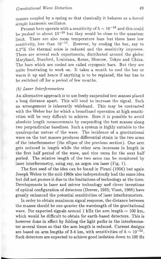
Gravitational Wave Detection 49
masses coupled by a spring so that classically it behaves as a forced simple harmonic oscillator.
Present ha.rs operate with a. sensitivity of h rv 10-18 a.nd this could be pushed to about 10-20 but they would be close to the quantum limit. There are also room temperature bars but these have low sensitivity, less than io-11 . However, by cooling the bar, say to 4.2°K the thermal noise is reJuced a.nd the sensitivity improves. There are several such experiments, distributed around the globe: Maryland, Stanford, Louisiana, Rome, Moscow, Tokyo and China. The bars which a.re cooled a.re called cryogenic bars. But they are quite frustrating to work on. It takes a. month to cool the bar or warm it up a.nd hence if anything is to be replaced, the bar has to be switched off for a period of few months.
(b) Laser Interferometers
An alternative approach is to use freely suspended test masses placed a long distance a.part. This will tend to increase the signal. Such an arrangement is inherently wideband. This may be contrasted with the Weber ba.r for which a. broadband operation at high sensitivities will be very difficult to achieve. Here it is possible to avoid absolute length measurements by suspending the test masses a.long two perpendicular baselines. Such a system is highly suitable to the quadrupolar nature of the wave. The incidence of a gravitational wave on the test masses produces differential strain in the two arms of the interferometer (the ellipse of the previous section). One arm gets reduced in length while the other arm increases in length in the first half period of the wave, a.nd vice versa for the next half period. The relative length of the two arms ca.n be monitored by laser interferometry, using say, an argon ion laser (Fig. l).
The first seed of the idea can be found in Pirani (1956) but again Joseph Weber in the mid-1960s also independently had the same idea but did not pursue it due to the limitations of technology at the time. Developments in laser a.nd mirror technology and clever inventions of optical configuration of detectors (Drever, 1983; Vinet, 1988) have greatly enhanced the potential sensitivities of laser interferometers.
In order to obtain maximum signal response, the distance between the masses should be one quarter the wavelength of the gravitational wave. For expected signals around 1 kHz the arm length·"' 100 km, which would be difficult to obtain for earth-based detectors. This is however done in effect by folding the light paths in the interferometer several times so that the arm length is reduced. Current designs are based on arm lengths of 3-4 km, with sensitivities of h "' 10-22 •
Such detectors are expected to achieve good isolation down to 100 Hz
50
~END
ru '" MIRROR
STATION
MID STATION
Gravitation and Cosmology
HST MASSES 2 END MIRRORS
BEAM SPLITTER
+CORNER MIRRORS
LASER BEAM AND PIPE ENCL OSUR!i WITH VACUUM
CENTRAL STATION
SPLITTER
CORNER MIRROR
PHOTO DIODE
END MIRROR
MID STATION
Fig. 1
or possibly, with the Italian design of multiple pendulums, to 10 Hz. This wideband operation has made it possible to think of a wider range of sources. An exciting such source is the coalescing binary. The present laser interferometers are basically prototypes whose arm lengths are in the range of 10 m-40 m. Such detectors are in Caltech, Glasgow, Munich and in Japan. These interferometers have sensitivities of a few times 10-18 or 10-19 , There are also special purpose interferometers designed to study particular problems, in M.l.T., Paris and Pisa. However, tQ achieve higher sensitivities, in the range of 10-22 , it is necessary to increase the arm length to 3 or 4 km. All the above working groups have plans to build the fullscale detectors if they are funded. The Americans plan to build two detectors (LIGO project). The high cost of the project has resulted in many international collaborations. From the scientific viewpoint, it is useful to have as many as possible. At least three detectors, or preferably four (for noise elimination and consistency), are necessary to give full information of the detected gravitational wave. This information can be decoded more accurately if the detectors are widely separated around the globe since it results in larger time delays and hencP. a.Uowing more accuracy in finding the direction of the source.
Gravitational Wave Detection 51
Since the measurements are so delicate, the battle against various noises is very crucial. Basically there are three sources of noise: seismic or mechanical, thermal noise and the photon shot noise. Detailed accounts of noise can be found elsewhere (Thorne 1989). The seismic/mechanical noises are reduced by using pendulum suspensions for the test masses and the supports for the pendulum themselves being isolated using stacks of rubber and lead sheets. The thermal noise occurs in the pendulum modes as well as in the internal resonances of the test masses. This noise is reduced by making the natural frequency of the pendulum ,...., 1 Hz-much lower . than expected gravitational wave frequency and having a, high Q. The internal resonances of the masses have frequencies > 5 kHz- greater than the expected gravitational wave frequency-and high Q. The test masses are suspended in vacuum ,...., 10-s Torr, which reduces the stray partic\es hitting the mirrors and the scattering of the laser beam, resulting in noise reduction. The photon shot noise is the most important one and it could be reduced by increasing the laser power. However, a continuous wave laser in a single frequency mode has very low power, at best 5 W. But there are clever schemes to effectively increase the laser power by light recycling techniques (Drever, 1983).
4. Sources of Gravitational Waves
I shall not discuss all possible sources here but I will restrict myself, briefly, to two important sources:
1. Supernova 2. Compact coalescing binary systems.
Finally I will come to estimating the Hubble constant using coalescing binaries. For computing the wave pattern emitted by a gravitational wave source, the 'quadrupolar formalism' is very important as it gives accurate results for most soufces. It was originally given by Einstein for weak sources and slow motion. This was later generalized to include compact sources as well {Landau, Lifshitz, 1941; Fock, 1959; lpser, 1971).
All that is required is that the size of the source be small compared to the wavelength of waves it emits. In this formalism the TT wave tensor is related to the mass quadrupole moment of the source by
2{)2[ ' ]TT h~T = -;;. {)t2 Qi/,(t - r) ' (4.1)
where r is the.distance to the source's centre of mass, tis the proper time measured by the observer at rest with respect to the centre of mass of the' 11ource, t - r the retarded time, the TT superscript referring to the transverse and traceless part of Qilci and Qi1c is the
52 Gravitation and Cosmology
mass quadrupole moment of the source. The Q;k can be written in terms of the mass density,
( 4.2)
where the superscript STF means symmetric and trace-free and xi
are Cartesian coordinates centred at the source.
(a) Supernovae
The supernova being the most violent event that we know of, is the most likely candidate for the detection of gravitational waves. Although coalescing binaries seem to compete strongly with this source, at least as far as laser interferometers are concerned, it still remains very important. Astrophysically, the detection of electromagnetically quiet supernovae would be extremely important. The strength of the waves emitted by a supernova depends initially on the amount of non-sphericity of the gravitational collapse and to some extent on whether the collapse is pressure-free or not. However, we have very little knowledge about the degree of non-sphericity of the collapse. But we can characterize the wave bursts by the amount of energy that it emits in gravitational waves. Strong bursts would contain, say 0.1M0 c2 energy which would give h"" 6 x 10-18 if the burst occurred in our galaxy. This could be detected by the present bars; such bursts if they occurred in the Virgo cluster could produce h "" 4 x 10-21 ,
which could be detected by a medium-sized laser interferometer of arm length ,......, 100 metres. A moderate burst would contain energy "" 0.0lM c2
• A non-axisymmetric collapse is expected to provide a larger burst of energy than a more symmetric one. For a. burst at a distance of 60 Mpc the h ""4 x 10- 22
• In the corresponding volume, the event rate for such bursts could be several thousand per year.
(b) Coalescing Binaries
This seems to be the most prominent source for detection by laser interferometry. The coalescing binary consists of two compact objects which revolve around each othe.r. The orbit of such a system is well approximated as a simple Newtonian orbit of two mass points and which decays by the quadrupole radiation reaction. The compact objects then spiral together losing energy and angular momentum in the process and fin11.lly coalesce (Peter and Mathews, 1963). In the last stages of coalescence, a gravitational wave with regular waveform, growing amplitude and frequency is emitted in a burst. Tidal and post-Newtonian effects are important in the last stage of the collapse; calculations of this can he found (Krolak and Schutz, 1987). A numerical simulation has .recently been done, taking into account
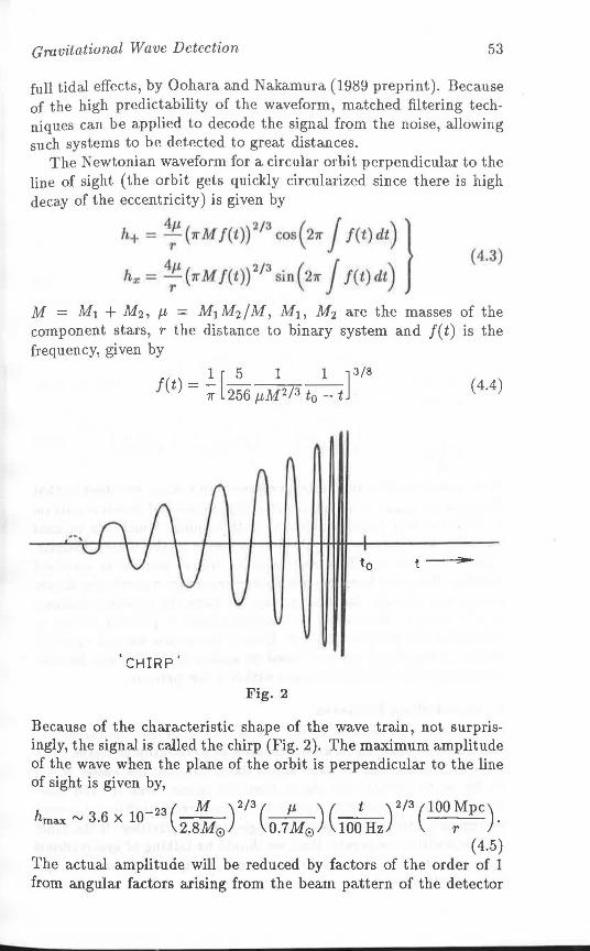
Gravitational Wave Detection 53
full tidal effects, by Oohara and Nakamura (1989 preprint). Because of the high predictability of the waveform, matched filtering techniques can be applied to decode the signal from the noise, allowing such systems to be detected to great distances.
The Newtonian waveform for a circular orbit perpendicular to the line of sight (the orbit gets quickly circularized since there is high deca,y of the eccentricity) is given by
h+ = 4: ( 7r M f(t))
213 cos ( 27r j f(t) dt) }
hx = 4; (7rMf(t)) 213
sin( 27r j f(t) dt) (4.3)
M = M1 + M2, µ = M1M2/M, Mi, M2 are the masses of the component stars, r the distance to binary system and f(t) is the frequency, given by
1[5 1 1 ]3/8 f(t) = ; 256 µM 213 to - t ( 4.4)
Fig. 2
Because of the characteristic shape of the wave train, not surprisingly, the signal is called the chirp (Fig. 2). The maximum amplitude of the wave when the plane of the orbit is perpendicular to the line of sight is given by,
h _23 ( M )2/3( µ )( t )2/3(100Mpc) max "' 3.6 X 10 .
2.8M0 0.7M0 lOOHz r ( 4.5)
The actual amplitude will be reduced by factors of the order of 1 from angular factors arising from the beam pattern of the detector
54 Gravitation and Cosmology
and because of the plane of the orbit being not perpendicular to the line of sight. It should be possible to get full information about the wave using a network of detectors (Tinto and Schutz, 1989; Dhurandhar and Tinto, 1988) and then get hmax from this. From the expressions for the waveform it should be possible to determine the mass parameter µM 213 but not the individual masses. Individual masses could be found from post-Newtonian effects if these effects are strong enough to be detected.
The event rate is calculated using pulsar birth rates and the volume from which the signals would be detectable. Earlier calculations have shown that this rate is about 3 per year out to 100 Mpc. But using matched filtering techniques and a full scale interferometer, one should be able to detect binaries out to 1000 Mpc, allowing for an event rate of about 300 per year.
(c) The Hubble Constant from Coalescing Binaries
Since the frequency grows as the orbit decays by radiation reaction, we have coalescence time-scale given by,
f ( M )-2/3( µ )-1( f )-8/3 T = -d" = 5.6 X (4.6) (;J 2.8M0 0.7M0 lOOHz
If we compare with the earlier expression for hmax we observe that the product hmaxT is independent of the masses and depends only on r. This is a very peculiar property of this source, which can be used fruitfully to determine the absolute distance to the binary (Schutz, 1986). One can therefore use coalescing binary sources as standard candles. If we now have an optical counterpart for a particular binary source and identify the host galaxy, we have the absolute distance to the galaxy. Measuring its redshift makes it possible for us to determine the Hubble constant. Even if the events are not optically visible, a statistical method based on galaxy clustering can be used to estimate the Hubble constant within a few percent.
5. Concluding Remarks
In the past two decades or so, one is struck by the enormous advance in our theoretical understanding of gravitational waves. The more understanding we have about likely sources, the easier will it be for us to identify the signal from tJie noise. One is even more impressed by the progress made by the experimentalists to invent, design and strive for detectors with greater sensitivities. If the fund- · ing authorities cooperate, then we should be talking of gravitational wave astronomy. There is no doubt that the quest will succeed, the only question is when.
-
~ I - - ·
Gravitational Wave Detection 55
References
I. Brill, D.R. and Hartle, J.B.: Phys. Rev. B, 135 (1964), 271. 2. Dhurandhar, S.V. and Tinto, M.: Mon. Not. R. Astr. Soc., 234 (1988),
663. 3. Drever, R.: in Dereulle and Piran, (1983), 321. 4. Fack, V.A.: "Theory of Space, Time and Gravitation", Section 87, Perga-
mon, London, 1959.
5. Ipser, J.R.: Astrophysical Jourrial, 166 (1971) , 175. 6. Isaacson, R.A.: Phy6. Reu., 166 (1968a.,b), 1263, 1272. 7. Krolak, A. a.nd Schutz, 'B.F.: GRG, 19 (1987), 1163. 8. Landau , L.D. and Lifshltz E.M.: "The Classical Theory of Fields" , Addison
Wesley, Cambridge, Mass. (1951) .
9. Misner, C.W., Thorne K.S. and Wheeler J .A. : "Gravitation", W.H. Free-man and Co., San Francisco, 1973.
10. Oohara, I< . an"tl Nakamura, T.: (1989) preprint. 11. Pete.r., P.C... a.nd Mathews, J. : Pliya. Reu., 131 (1963), 435. 12. Pirani, F.A.E.: Acta Physi. Poloni, 15 (1956), 389. _ 13. Schutz, B .F.: Nature, 823 (1986), 310.
14. Thorne, K.S.: in "300 Years of Gravitation", ed. Hawking, S.W. and Israel, W., Cambridge University Press, 1989.
15. Tinto M. and Schutz B.F.: "Gravitational Wave Data. Analysis", Kluwer, Dordrecht, 3 (1989).
16. Vinet, J.Y., Meers, B., Man, C.N. and Brillet, A.: Phys. Rev. D., 38 (1988), 433.
Techniques of Gravitational Wave
Data Analysis
B.S. SATHYAPILAKASH
Inter- University Centre for Astronomy and Astrophysics Ganeshkhind, Pune 411 007
1. Introduction
General relativity predicts the production of gravitational waves by systems whose quadrupole moment has a non-trivial time dependence. Their direct detection has been a longstanding problem in experimental physics. Nevertheless, there are indirect evidences which confirm the existence of gravitational waves. For instance, the slowdown of the period of the binary pulsar 1913+ 16, due to emission of gravitational radiation is in agreement with the- predictions of general relativity to better than 1 % accuracy, as shown by Damour and Taylor recently. 1 Direct detection of gravitational waves is very hard due to weakness of gravitational coupling constant. The proposed new generation of long baseline laser interferometric detectors have very high sensitivity. In a detector each of whose arms is 3 km, the final sensitivity can be as good as 10-24 (see Ref. 2). Due to their inherent broadband nature and high sensitivity, these detectors can pick up signals from a variety of sources. Burst of gravitational radiation from supernovae events occurring as far as Virgo cluster, periodic signals from old and new pulsars, stochastic background gravitational radiation, quasi-normal modes of a black hole are some of the promising events.3 •4
Coalescing compact binaries are one of the most important sources for which one may make use of the inherent broadband nature of these detectors. The waveform from these sources is often referred to as the chirp signal. There are a number of such binaries spotted in our galaxy in recent times.2 A binary system of stars emits gravitational waves at a frequency equal to twice the orbital frequency. The power ewitted in the form of gravitational radiation from such a system was first calculated by Peter and Mathews. 5 The average rate at which the system radiates increases as the inverse fifth power
Gravitational Wave Data Analysis 57
of the distance between the two stars. As the system looses energy, the two stars spiral in, leading to an increase in the orbital frequency. Consequently, there is an increase in the amplitude and frequency of the radiation. Finally, the two stars coalesce, emitting a burst of gravitational radiation, just before coalescence, with a very characteristic spectrum. The waveform of radiation emitted by coalescing binaries was first obtained by Clarke and Eardley in the Newtonian approx.imation.6 They pointed out that compact binaries could be realistic sources of gravitational waves. In the initial stages, both the frequency and the amplitude will be very low and the signal becomes detectable only at the very last stages. As a result, the .effective time of observation of these signals will be very low; typically, a few seconds. Thorne pointed out that these sources will be very important for laser interferometric detectors, which are inherently broadband.3
The coalescing binary signal will most probably not stand above the broadband noise of the detector. However, since the waveform of the signal is well predicted, it is possible to employ special techniques to pick out the signal from noisy data. There have been efforts to understand the nature of the signal during final stages of coalescence. Just before the stars coalesce, post-Newtonian and tidal effects become very important. These effects could significantly change the nature of the waveform from that predicted by Newtonian approximation. Using the formalism of Wagoner and Will,7 Krolak8 has calculated the first order post-Newtonian corrections to the waveform. He has shown that in this order one can neglect the tidal effects and the eccentricity of the orbits. The analysis shows that the interferometric detectors operating at full sensitivity will be able to detect post-Newtonian effects. Damour and Iyer9 have extended the multipolar gravitational wave generation formalism10 by deriving the post-Newtonian-accurate expressions for tl,te spin multipole moments. It would be fruitful to work out the post-Newtonian effects to coalescing binary signal in this formalism to get an accurate waveform at final stages of coalescence.
There have also been several efforts to develop special techniques of both detection a.nd data analysis to enhance the .signal-tcrnoise ratio of coalescing binary signals. Recycling techniques11 of detection in combination with data analysis12 can improve the signal-tcrnoise ratio. As for data analysis, there are developments of se~eral algorithms, notably the matched filtering first suggested by Thorne.3
The matched filtering technique can be used to pick signals buried in noisy data. It involves correlating the output of a detector with a copy of the expected signal called a matched filter. The amplitude of the correlation will be very large when the signal is present in the
58 Gravitation and Cosmology
data stream and it would be noisy otherwise. The exact waveform from binaries will depend on several parameters. Since the values of these parameters are a priori unknown, one needs to correlate the output of the detector with several filters corresponding to differ·· ent values of the parameters. Since the number of filters that can be used is finite, the filters' parameters will be, in general, different from a signal that arrives at the detector. A mismatch in the parameters brings down the signal-to-noise ratio. As a result, one may completely miss even a signal which could have been otherwise detected by correlating it with a filter that matches with it. This situation can be remedied by using a large number of filters. But there is a limit on the number of filters, if one intends to do on-line analysis of data. This is because the available computing speed is limited. Therefore, it has become important to develop data analysis strategies which make best use of computability to improve upon detectability.
An interesting algorithm is developed by Smith 13 to detect, in one go, all coalescing binary waveforms whose frequencies remain strictly in proportion to one another right up to the moment of coalescence. The method involves re-sampling a data stream at increasingly larger rates so as to compensate for the increase in frequency of the signal. When the signal is present, the Fourier transform of the re-sampled data will peak at a particular frequency depending on how fast the data is re-sampled. The rate at which re-sampling is done is the same for all waveforms whose frequencies remain in proportion to one another till the coalescence time. This method has the advantage that one does not have to construct a lattice of waveforms and compute cross-correlation with every one of the templates--a simple Fourier transform will pick up the signal. However, it is not clear whether one can save on computing time, since it is necessary to perform re-sampling of data for every time of arrival and at different rates, so as not to miss out classes of waveforms that have their frequencies in proportion to one another. Smith's method will be better if the number of filters required is too large.
In this article I will restrict myself to a few topics discussed above. I shall discuss in Sec. 2 the technology needed in achieving sensitivities ""' 10-22 and below. This treatment will be simple and is aimed at order-of-magnitude estimates. In Sec. 3 I will discuss the nature of the coalescing binary waveform and its Fourier transform. In Sec. 4 I will consider some of the envisaged data analysis techniques. This includes the threshold and the summation mode of data analysis and the matched filtering technique which is used to pick out signals whose waveform is known accurately.
- - -
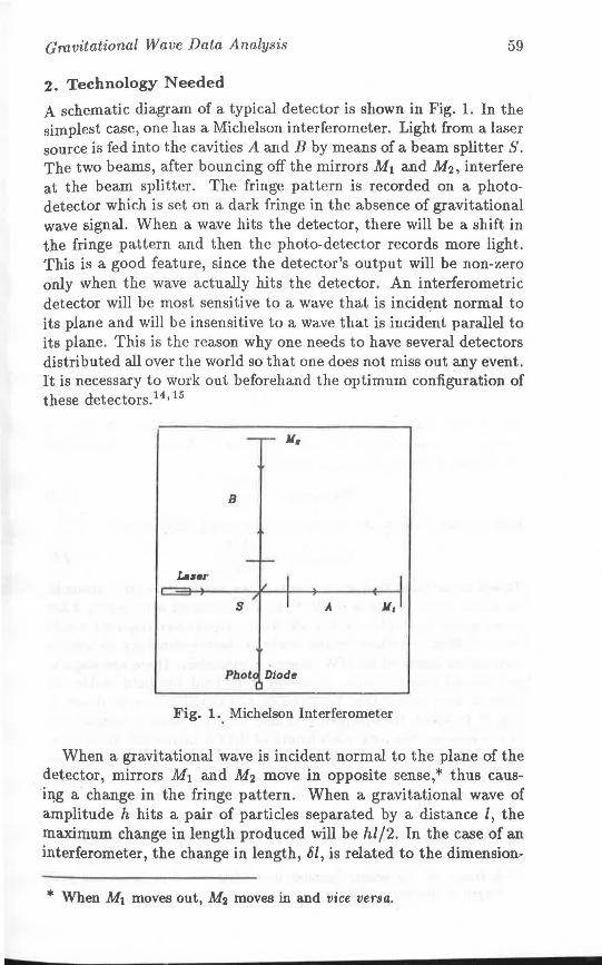
Gravitational Wave Data Analysis 59
2. Technology Needed
A schematic diagram of a typical detector is shown in F'ig. 1. In the simplest case, one has a Michelson interferometer. Light from a laser source is fed into the cavities A and B by means of a beam splitter S. The two beams, after bouncing off the mirrors M1 and M2, interfere at the beam splitter. The fringe pattern is recorded on a photodetector which is set on a dark fringe in the absence of gravitational wave signal. When a wave hits the detector, there will be a shift in the fringe pattern and then the photo-detector records more light. This is a good feature, since the detector's output will be non-zero only when the wave actually hits the detector. An interferometric detector will be most sensitive to a wave that is incid~nt normal to its plane and will be insensitive to a wave that is incident parallel to its plane. This is the reason why one needs to have several detectors distributed all over the world so that one does not miss out any event. It is necessary to work out beforehand the optimum configuration of these detectors. 14 • 15
B
s A JI,
Phot Diode
Fig. 1 .. Michelson Interferometer
When a gravitational wave is incident normal to the plane of the detector, mirrors Mi and M2 move in opposite sense,* thus caus· i:r~g a change in the fringe pattern. When a gravitational wave of amplitude h hits a pair of particles separated by a distance I, the maximum change in length produced will he hl/2. In the case of an interferometer, the change in length, ol, is related to the dimension·
* When Mi moves out, M2 moves in and vice versa.
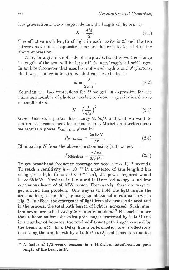
60 Gravitation and Cosmology
less gravitational wave amplitude and the length of the arm by
8l=4hl_ (2.1) 2
The effective path length of light in each cavity is 2l and the two mirrors move in the opposite sense and hence a factor of 4 in the above expression.
Thus, for a given amplitude of the gravitational wave, the change in length of the arm will be larger if the arm length is itself larger. In an interferometer that uses laser of wavelength >. and N photons, the lowest change in length, ol, that can be detected is
>. bl = 2../N. (2.2)
Equating the two expressions for 81 we get an expression for the minimum number of photons needed to detect a gravitational wave of amplitude h:
(2.3)
Given that each photon has energy 2Trhc/ >. and that we want to perform a measurement for a time r, in a Michelson interferometer we require a power PMichelson given by
2TrhcN PMichelson = AT (2.4)
Eliminating N from the above equation using (2.3) we get 7rnc>-.
PMichelson = Sh 212 T • (2.5)
To get broadband frequency coverage we need a r "" 10-3 seconds. To reach a sensitivity h "" 10-22 in a detector of arm length 3 km using green light ( >. = 5.0 X 10- 5 cm), the power required would be ,..., 65 MW. Nowhere in the world is there technology to achieve continuous lasers of 65 MW power. Fortunately, there are ways to get around this problem. One way 'is to hold the light inside the arms as long as possible, by using ~ additional mirror as shown in Fig. 2. In effect, the emergence of light from the arms is delayed and _in the process, the total path length of light is increased. Such interferometers are called Delay line interferometers. 16 For each bounce that a beam suffers, the extra path length traversed by it is OZ and in n number of bounces, the total additional path length covered by the beam is nt5l. In a Delay line interferometer, one is effectively increasing the arm length by a factor* (n/2) and hence a reduction
* A factor of 1/2 occurs because in a Michelson interferometer path length of the beam is 21.
- ' - ...--.
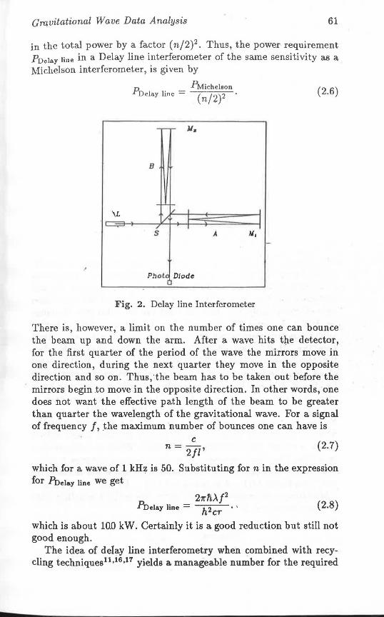
Gm.vitational Wave Data Analysis 61
in the total power by a factor (n/2)2 • Thus, the power requirement Poela.y line in a Delay line interferometer of the same sensitivity as a Michelson interferometer, is given by
R J\ticheleon Delay line = ( n/2)2 (2.6)
B
\L
s A JI,
Phot Diode
Fig. 2. Delay line Interferometer
There is, however, a limit on the number of times one can bounce the beam up and down the arm. After a wave hits the detector, for the first quarter of the period of the wave the mirrors move in one direction, during the next quarter they move in the opposite direction and so on. Thus, ·the beam has to be taken out before the mirrors begin to move in the opposite direction. In other words, one does not want the effective path length of the beam to be greater than quarter the wavelength of the gravitational wave. For a signal of frequency f, .the maximum number of bounces one can have is
c n = 2fl' {2.7)
which for a wave of 1 kHz is 50. Substituting for n in the expression for Poelay line we get
2trft'A/2
Poelay line = h2 {2.8) CT
which is about lOD kW. Certainly it is a good reduction but still not good enough.
The idea of delay line interferometry when combined with recycling techniques11 •16 •17 yields a. manageable number for the required
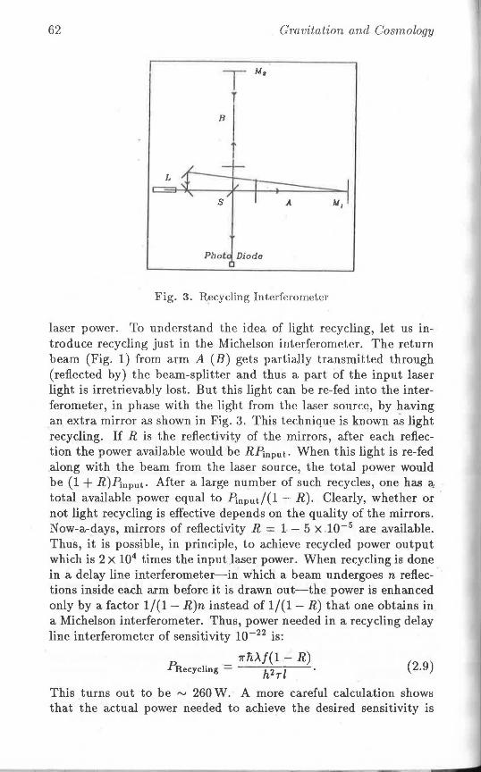
62 Gravitation and Cosmology
B
/,
A J.11
Fig. 3. R~cycling Interferometer
laser power. To understand the idea of light recycling, let us introduce recycling just in the Michelson interferometer. The return beam (Fig. 1) from arm A (B) gets partially transmitted through (reflected by) the beam-splitter and thus a part of the input laser light is irretrievably lost. But this light can be re-fed into the interferometer, in phase with the light from the laser source, by having an extra mirror as shown in Fig. 3. This technique is known a-slight recycling. If R is the reflectivity of the mirrors, after each reflection the power available would be RPinput. When this light is re-fed along with the beam from the laser source, the total power would be (1 + R)E\nput. After a large number of such recycles, one has ~ total available power equal to Pinputf (1 - R). Clearly, whether or · not light recycling is effective depends on the quality of the mirrors. Now-a-days, mirrors of reflectivity R = 1 - 5 x .10-5 are available. Thus, it is possible, in principle, to achieve recycled power output which is 2 X 10⁴ times the input laser power. When recycling is done in a delay line interferometer-in which a beam undergoes n reflections inside each arm before it is drawn out-the power is enhanced only by a factor 1/(1 - R)n instead of 1/(1 - R) that one obtains in a Michelson interferometer. Thus, power needed in a recycling delay line interferometer of sensitivity 10-22 is:
?rn>.f(l - R) PRecycling = h2rl · (2.9)
This turns out to be ""' 260 W. A more careful calculation shows that the actual power needed to achieve the desired sensitivity is
- - ~.
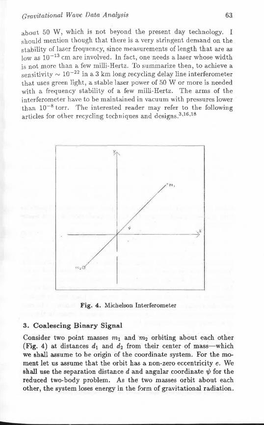
Gravitational Wave Data Analysis 63.
about 50 W, which is not beyond the present day technology. I should mention though that there is a very stringent demand on the stability of laser frequency, since measurements of length that are as low as 10-13 cm are involved. In fact, one needs a laser whose width is not more than a few milli-Hertz. To summarize then, to achieve a sensitivity ,...., 10·- 22 in a 3 km long recycling delay line interferometer that uses green light, a stable laser power of 50 W or more is needed with a frequency stability of a few milli-Hertz. The arms of the interferometer have to be maintained in vacuum with pressures lower than 10-8 torr. The interested reader may refer to the following articles for other recycling techniques and designs.3 •16 •18
• m,
Fig. 4. Michelson Interferometer
3. Coalescing Binary Signal
Consider two point masses m1 and m2 orbiting a.bout ea.ch other (Fig. 4) at distances di and d2 from their center of mass-which we shall assume to he origin of the coordinate system. For the moment let us assume that the orbit has a non-zero eccentricity e. We shall use the separation distance d and angular coordinate 1/J for the reduced two-body problem. As the two masses orbit about each other, the system loses energy in the form of gravitational radiation.
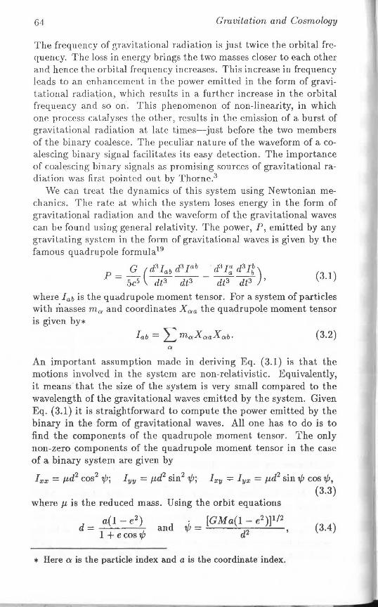
61 Gravitation and Cosmology
The frequency of gravitational radiation is just twice the orbital frequency. The loss in energy brings the two masses closer to each other and hence the orbital frequency increases. This increase in frequency leads to an enhancement in the power emitted in the form of gravitational radiat;ion, which results in a further increase in the orbital frequency and so on. This phenomenon of non-linearity, in which one process catalyses the other, results in the emission of a burst of gravitational radiation at late times-just before the two members of the binary coalesce. The peculiar nature of the waveform of a coalescing binary signal facilitates its easy detection. The importance of coalescing binary signals as promising sources of gravitational radiation was first pointed out by Thorne.3
We can treat the dynamics of this system using Newtonian mechanics. The rate at which the system loses energy in the form of gravitational radiation and the waveform of the gravitational waves can be found using general relativity. The power, P, emitted by any gravitating system in the form of gravitational waves is given by the famous quadrupole formula19
G ( d3 lab d3 Jab d3 I~ d3 I~) P=- -------
5c5 dt3 dt3 dt3 dt3 ' (3.1)
where lab is the quadrupole moment tensor. For a system of particles with masses ma and coordinates Xaa the quadrupole moment tensor is given by*
lab= L m()tX()taX0tb· Of
(3.2)
An important assumption made in deriving Eq. (3.1) is that the motions involved in the system are non-relativistic. Equivalently, it means that the size of the system is very small compared to the wavelength of the gravitational waves emitted by the system. Given Eq. (3.1) it is straightforward to compute the power emitted by the binary in the form of gravitational waves. All one has to do is to find the components of the quadrupole moment tensor. The only non-zero components of the quadrupole moment tensor in the case of a binary system are given by
Ixx = µd2 cos2 'I/;; ! 1111 = µd2 sin2 'I/;; Ix11 = Iyx = µd2 sin ,,P cos ,,P,
whereµ is the reduced mass. Using the orbit equations
d = a(l - e2
)
1 + e cos ,,P and
· [GM a(l - e2 )]112
,,p = d2 '
* Here a is the particle index and a is the coordinate index.
(3.3)
(3.4)
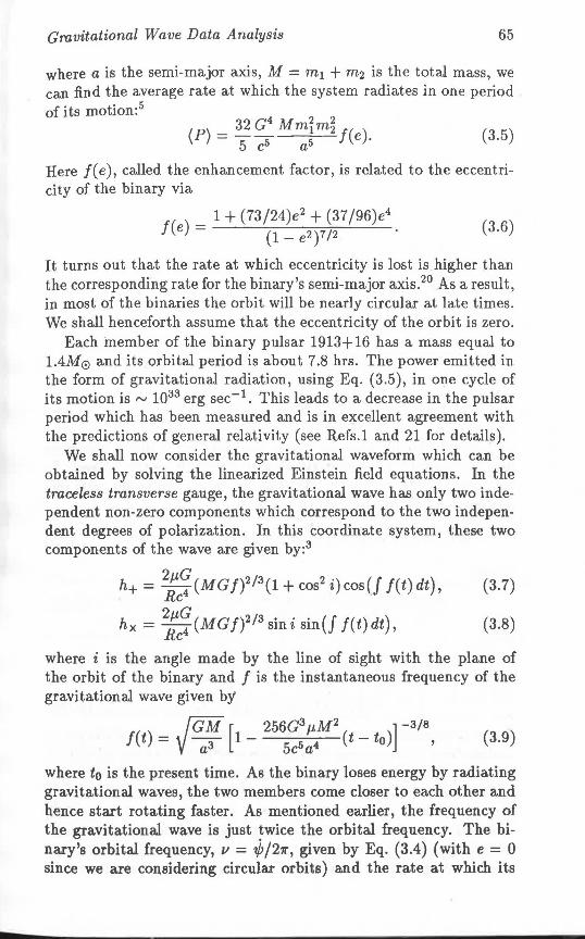
Grovitational Wave Data Analysis 65
where a is the semi-major axis, M = m1 + m2 is the total mass, we can find the average rate at which the system radiates in one period of its motion:5
(3.5)
Here J( e ), called the enhancement factor, is related to the eccentricity of the binary via
f(e) = 1 + (73/24)e2 + (37/96)e4
(1-e2)7/2 (3.6)
It turns out that the rate at which eccentricity is lost is higher than the corresponding rate for the binary's semi-major axis.20 As a result, in most of the binaries the orbit will be nearly circular at late times. We shall henceforth assume that the eccentricity of the orbit is zero.
Each member of the binary pulsar 1913+ 16 has a mass equal to 1.4M0 and its orbital period is about 7.8 hrs. The power emitted in the form of gravitational radiation, using Eq. (3.5), in one cycle of its motion is "' 1033 erg sec-1 • This leads to a decrease in the pulsar period which has been measured and is in excellent agreement with the predictions of general relativity (see Refs.l and 21 for details).
We shall now consider the gravitational waveform which can be obtained by solving the linearized Einstein field equations. In the traceless transverse gauge, the gravitational wave has only two independent non-zero components which correspond to the two independent degrees of polarization. In this coordinate system, these two components of the wave are given by:3
h+ = 2:c~ (MGJ)213 (1 + cos2 i)cos(f J(t)dt), (3.7)
hx = 2:c~(MGJ)2 13 sini sin(J J(t)dt), (3.8)
where i is the angle made by the line of sight with the plane of the orbit of the binary and f is the instantaneous frequency of the gravitational wave given by
_ P!f-M [ 256G3 µM 2 ] -3/8 f(t) - -
3 1 -
5 5 4 (t - to) ,
a ca (3.9)
where t0 is the present time. As the binary loses energy by radiating gravitational waves, the two members come closer to each other and hence start rotating faster. As mentioned earlier, the frequency of the gravitational wave is just twice the orbital frequency. The binary's orbital frequency, v = ,(pj2Tr, given by Eq. (3.4) (with e = 0 since we are considering circular orbits) a.nd the rate at which its
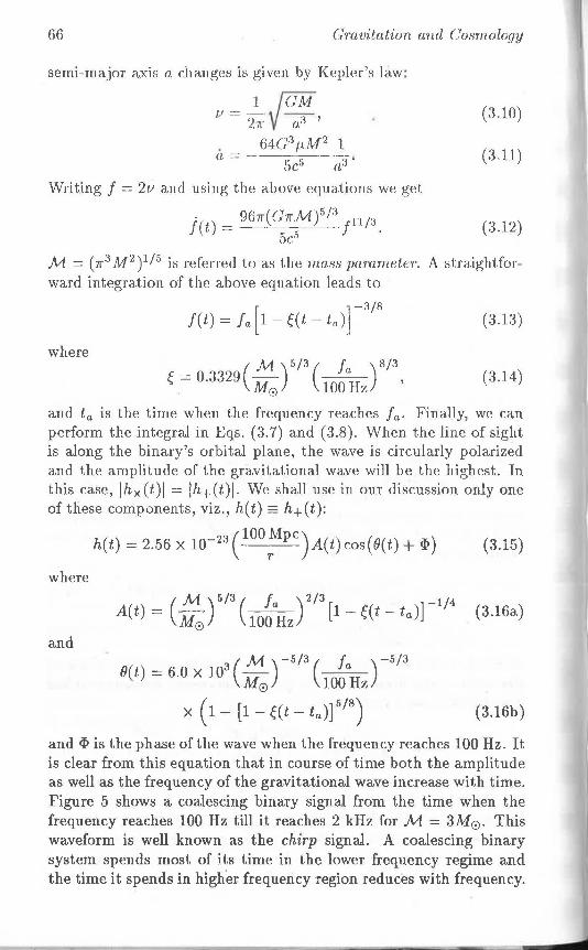
66 Gravitation and Cosmolog'!}
semi-major axis a changes is given by Kepler's law:
i' = 2~· f!!!- , (3 .1.0)
. 64G3/tM2 l a - - ----·-- ·
-- 5c5 a:3 • (3.l 1)
Writing f = 21; and using the above equations we get
96 (,., M ·)5 13 j(t) = . Jr dJl' I !11/:i •
5c5 (3.12)
M = ( Jr3 M 2
)115 is referred to as the mass parameter. A straightfor
ward integration of the above equation leads to
[ ]
-3/8 J(t) =fa 1 - t(t - ta) (3.13)
where
(3.14)
and ta is the time when the frequency reaches fa· Finally, we can perform the integral in Eqs. (3. 7) and (3.8). When the line of sight is along the binary's orbital plane, the wave is circularly polarized and the amplitude of the gravitational wave will be the highest. In this case, lhx (t)i = ih+(t)i. We shall use in our discussion only one of these components, viz., h(t) = h+(t):
( 100 Mpc) h(t) = 2.56 x 10⁻²³ - r A(t)cos(O(t) +<I>) (3.15)
where
A(t) = ( M )513 (-1'!_) 213
[1-e(t - ta)r114 (3.16a) M0 lOOHz
and
(M)-5/3( f, )-5/3
O(t) = 6.0 x 10³ M aH 0 100 z
x ( 1 - [1 - e(t - ta)J518) (3.16b)
and <I> is the phase of the wave when the frequency reaches 100 Hz. It is clear from this equation that in course of time both the amplitude as well as the frequency of the gravitational wave increase with time. Figure 5 shows a coalescing binary signal from the time when the frequency reaches 100 Hz till it reaches 2 kHz for M = 3M0 . This waveform is well known as the chirp signal. A coalescing binary system spends most of its time in the lower frequency regime and the time it spends in higher frequency region reduces with frequency.
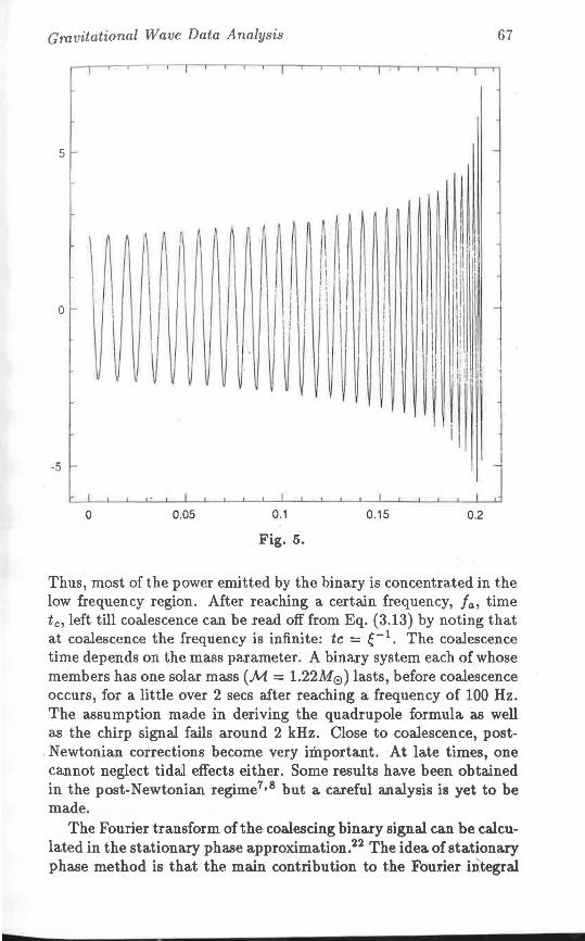
Grovitational Wave Data Analysis 67
5
Thus, most of the power emitted by the binary is concentrated in the low frequency region. After reaching a certain frequency, fa, time tc, left till coalescence can be Iead off from Eq. (3.13) by noting that at coalescence the frequency is infinite: tc = e-1 . The coalescence time depends on the mass parameter. A binary system each of whose members has one solar mass (M = 1.22M0 ) lasts, before coalescence occurs, for a little over 2 secs after reaching a frequency of 100 Hz. The assumption made in deriving the quadrupole formula as well as the chirp signal fails around 2 kHz. Close to coalescence, postNewtonian corrections become very important. At late times, one cannot neglect tidal effects either. Some results have been obtained in the post-Newtonian regime7•8 but a careful analysis is yet to be made.
The Fourier transform of the coalescing binary signal ca.n be calculated in the stationary phase approximation.22 The idea of stationary phase method is that the main: contribution to the Fourier integral
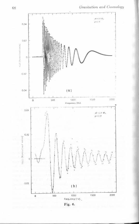
68
0.04
0.02
0 -
-0 .02 -
-0 04
0
0 04
0 02 -
[
7 .
0
-0.02
500
I'
o 500
Gmvitation and Cosmology
(0)
1000 rrvquoni::y (th)
( b)
1000
Frequency (Hz) .•
Fig. 6.
;1~ 10A1"1 /> I IJ -1
1500
..11 ,~ 1.o M0
p = l 0
1500
2000
2000
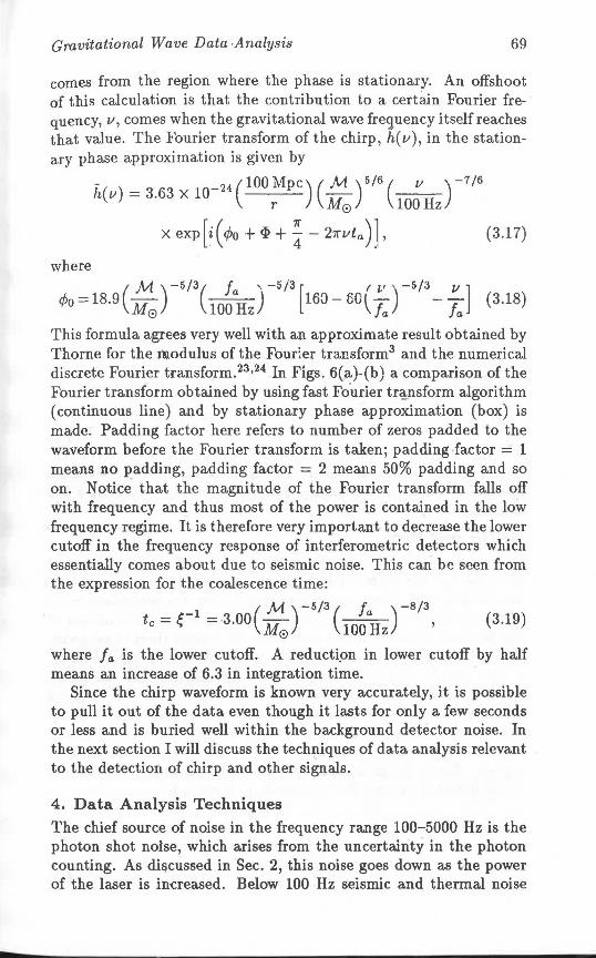
Gravitational Wave Data Analysis 69
comes from the region where the phase is stationary. An offshoot of this calculation is that the contribution to a certain Fourier frequency, v, comes when the gravitational wave frequency itself reaches that value. The Fourier transform of the chirp, h(v), in the stationary phase approximation is given by
h(v) = 3.63 x 10⁻²⁴(lOOMpc) ( M )5/6( v )-7/6 r M0 lOOHz
X exp [i ( </>o + <I> + ~ - 27rvta)], (3.17)
(3.18)
This formula agrees very well with an approximate result obtained by Thorne for the roodulus of the Four1er tra.nsform3 and the numerical discrete Fourier transform.23 •24 In Figs. 6(a)-(b) a comparison of the Fourier transform obtained by using fast Fo.urier tr~nsform algorithm (continuous line) and by stationary phase approximation (box) is made. Padding factor here refers to number of zeros padded to the waveform before the Fourier transform is taken; padding factor = 1 means no padding, padding factor = 2 means 50% padding and so on. Notice that the magnitude of the Fourier transform falls off with frequency and thus most of the power is contained in the low frequency regime. It is therefore very important to decrease the lower cutoff in the frequency response of interferometric detectors which essentially comes about due to seismic noise. This can be seen from the expression for the coalescence time:
_1 ( M )-5/3 ( fa )-s/3 tc = e =·3.00 M0 lOOHz , (3.19)
where fa is the lower cutoff. A reductipn in lower cutoff by half means an increase of 6.3 in integration time.
Since the chirp waveform is known very accurately, it is possible to pull it out of the data even though it lasts for only a few seconds or less and is buried well within the background detector noise. In the next section I will discuss the techniques of data analysis relevant to the detection of chirp and other signals.
4. Data Analysis Techniques
The chief source of noise in the frequency range 100-5000 Hz is the photon shot noise, which arises from the uncertainty in the photon counting. As di!jcussed in Sec. 2, this noise goes down as the power of the laser is increased. Below 100 Hz seismic and thermal noise
70 Gravilaiion and Cosmology
dominate and they set a lower limit on the frequency response of the detector. We shall be interested in data analysis in the frequency range 100- 5000 Hz so that we need to be concerned about only photon shot noise. We shall assume that this noise is stationary (i.e., that its nature does not depend on time) and white (i.e., that it has a fl.at power spectrum). In addition, we shall assume that at a typical sampled point the noise amplitude, n, is governed by Gaussian probability distribution with standard deviation a:
1 ( n2
' p(n) =--exp --). ./'iia 2a2 ( 4.1)
It is straightforward to prove that the sum of two random variableseach of which obeys a Gaussian distribution with the same standard deviation·-also obeys a Gaussian distribution but with v'2 times the individual standard deviation. Therefore, the sum of the noise taken from k identical detectors each of whose noise, ni, obeys a Gaussian distribution with standard deviation a, also obeys a normal distribution but with a standard deviation sea.led up Vk:
.......... 1 ( '1]2 ) P('IJ = 6 n;) = Vhl-;;. exp - 2ka2 . ( 4.2)
Given the output of one or several detectors one can envisage several data analysis techniques. I will discuss in 'the following a few of them.
(i) Threshold Mode
The simplest and the most straightforward way of detecting a signal is to use the threshold criteria. In the threshold mode of analysis, one intends to discover signals that stand above the broadband noise of the detector. An event is said to have occurred if the output of -the detector crosses a preset threshold. Whenever there is an event, it could have been either generated by the noise or triggered off by a true signal. The threshold is set by demanding that the noisegenerated faise alarms arc less than a certain number in a. given duration of time. By choosing the number of false alarms to be sufficiently small in a sufficiently long duration of time, one can be confident about the occurrence of events triggered off by true signals. Now, the probability that the noise amplitude, n, from a single detector exceeds the threshold, x, is given by
p = p(n ~ x) = ~ 1= exp(- n2
2)dn v 211" O' x 2a
~ ~(~ - : 3 + · · ·) exp(-~2
). (4.3)
Gravitational Wave Data Analysis 71
where p = x/ (!is a measure of the threshold in terms of the standard deviation of the signal. The above approximation is valid for p > 1. It is sufficient to choose only two terms in the above expansion to get an accuracy of 103 for p > 2.5. If we demand that there be no more than one false alarm in a time T, for data sampled at a rate ~. then the threshold is determined by the equation
1 2 1 (2) N - p - ln p - - ln - + ln = 0 2 2 1r
(4.4)
where N = f),,T is the total number of observation points. Assuming that for data sampled at 1 kHz there be no more than one false alarm per year we get* p = 6.63. This means that only when the signal strength at the detector has a value 6.63 times the standard deviation of the background noise can we say that there is an event. Therefore, a given threshold (or equivalently a given strength of noise) sets a limit on the amplitude of the gravitational waves that can be detected. This in turn means a limit on the distance up to which we can see using a particular detector. For instance, for a detector of sensitivity ,...., 10-21 , the above threshold means that the detector can record normal supernova events (that emit a power,..., 0.01M0 c2
in the form of gravitational waves) out to a distance of ,..., 4 Mpc. We can also ask for coincident events in several detectors, say at
the same site with independent but identical noise (same u), in which case the threshold comes down. If Pi, i = 1, ... , k, are the probabilities of false alarms in k detectors, then the probability, P, that there is a simultaneous false alarm in every one of these detectors is given by
(4.5)
Demanding as before that there be only one false alarm in N data points, we obtain an equation for the threshold, Pt(k), in the threshold mode for k detectors, given by
1 2 1 (2) 1 -pt (k) - lnpt(k) - - ln - + -lnN = 0. 2 2 1r k
(4.6)
The first two rows in Table 4.1 list thesholds corresponding to coincident events for different number of detectors located at the same site for N equal to 3 x 10¹⁰ and 1.5 x 1~12 , respectively. A factor of 1.5 reduction as we go from one to two detectors means an increase
* The threshold is quite insensitive to our choice of .N since we are already at a 60' level.
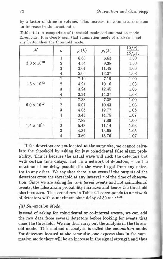
72 Gravitation and Cosmology
by a factor of three in volume. This increase in volume also means an increase in the event rate. Table 4.1: A comparison of threshold mode and summation mode thresholds. It is clearly seen that summation mode of analysis is not any better than the threshold mode.
N k Pt(k) P:t(k) (Sf P)t (S/p)a
1 6.63 6.63 1.00 3.0 x 10¹⁰ 2 4.54 9.38 1.03
3 3.61 11.49 1.06 4 3.06 13.27 1.08. 1 7.19 7.19 1.00
1.5 x 10¹² 2 4.94 10.16 1.03 3 3.94 12.45 1.05 4 3.34 14.37 1.08 1 7.38 7.38 1.00
6.0 x 10¹² 2 5.07 10.43 1.03 3 4.05 12.77 1.05 4 3.43 14.75 1.07 1 7.89 7.89 1.00
1.4 x 10¹⁴ 2 5.43 11.14 1.03 3 4.34 13.65 1.05 4 3.69 15.76 1.07
If the detectors are not located at the same site, we cannot calculate the threshold by asking for just coincidental false alarm probability. This is because the actual wave will click the detectors but with certain time delays. Let, in a network of detectors, T be the maximum time delay possible for the wave to get from any detector to any other. We say that there is an event if the outputs of the detectors cross the threshold at any interval T of the time of observation. Since we are Mking for co-interval events and not coincidental events, the false alarm probability increases and hence the .threshold also increases. The second row in Table 4.1 corresponds to a network of detectors with a maximum time delay of 50 ms. 25126
(ii) Summation Mode
Instead of asking for coincidental. or co-interval events, we can add the raw data from several detectors before looking for events that cross the threshold. We can then carry out the analysis in the threshold mode. This method of analysis is called the summation mode. For detectors located at the same site, one expects that in the summation mode there will be an increase in the signal strength and thus
Grovitational Wave Data Analysis 73
hopes to do better than the threshold mode. Howev~r, as shown below, this is not the case. Let us first consider summation mode of analysis for identical detectors located at the same site. Let "I= 2: ni
be the sum of outputs from several detectors. From Eq. (4.2), it is clear that "I obeys a Gaussian distribution. The problem now is similar to that of the threshold mode for one detector but with u replaced by Vf u. Thus, summation mode threshold p3 (k) fork detectors is given by
Pa(k) = ..fk Pt(l). (4.7)
The third column in Table 4.1 lists the value of the threshold in summation mode analysis. Though the summation mode threshold turns out to be higher than in the threshold mode threshold, the signal has now increased k-fold. Thus, the quantity of relevance is the ratio of signal-to-threshold in the two cases which are listed in the fifth column of Table 4.1. It is clear from Table 4.1 that the summation mode of analysis is not any different from threshold mode of analysis for detectors located at the same site. However, when detectors are located at different sites, the summation mode not only leads to an increase in the false alarm probability but also to a very great increase in computation time. Thus, for detectors located at different sites, it is more sensible to adopt the threshold mode of analysis.
(iii) Matche.d Filtering Technique
In both threshold and summation mode of analysis we are looking for signals that stand above the broadband noise of the detector. However, when the waveform of signals are known to sufficient accuracy, it is possible to search for them even if they are buried in the background noise. As shown in Sec. 3, signals from coalescing binaries are known very well and this aspect can be made use of to pick out these signals even when their strength is much lower than the noise level. However, one has to cope with the fact that the values of the parameters of the signal-the mass parameter, the phase of the signal when it begins to be detected and the time of arrival-are a priori unknown. Matched filtering involves correla~ing the output of a detector With several filters that a.re constructed with a knowledge of the ranges of the various parameters. Threshold analysis is then carried out by treating correlation function as the raw data. For simplicity, let us assume that the detector noise is a Gaussian random noise with zero mean and a :flat power spectrum. This means that the noise amplitude satisfies
(n(/), n(/')) = u26(! - !'), (4.8)
74 Gmvitation and Cosmology
where a is the standard dev.iation of the noise. Let q(t) be the optimum filter that maximizes the signal-to-noise ratio. We shall assume that the filters are normalized in the sense that the peak of the auto-correlation function is equal to unity: (q o q)(O) = 1. The detector O(t) consists of the noise n(t) and the signal h(t):
O(t) = n(t) + h(t). (4.9)
The signal is the ensemble average of the correlation of the output with the filter:
s = ((0 0 q)(t)}. (4.10)
The noise is the square root of the variance of the correlation:
( 2 )1/2
N = ((0 o q)(t) - ((0 o q)(t)}) (4.11)
The filter that maximizes S / N can be found by using the variational principle. In this case, the filter that corresponds to the maximum of the correlation is the signal itself.26 •27 •28 •29 (In general, the detector noise will not have a flat power spectrum and in that case the optimum filter is the signal to be detected modulo the noise. See the above references for details.) Figures 7(a)-(c) illustrate the power of the matched filtering. In Fig. 7(b ), we have the noise that contains the chirp signal of Fig. 7(a), which is weaker than the noise by a factor of 3. On correlating the data in Fig. 7(b) with the right filter, the presence of the signal is revealed, as is apparent from Fig. 7(c).
Coalescing binaries can have ma.ss parameter in the range [0.5M0 , 30M0 ] and its phase a.nd time of arrival ate arbitrary. The output of the detector has to be passed through several filters that differ in the values of the various para.meters. We thus have a. lattice space of filters . . The time of arrival of the signal can be fixed, in principle, by looking at the pea.k of the correlation function. However, as I shall show· below, a filter with the va.iues of the para.meters slightly different from the actual values of a signal can lead to a wrong estimate of the arrival time.
Let us first consider filters with a fixed value of the phase. By demanding that the neighbouring filters have a peak cross-correlation value greater than the threshold set by the correlation noise, we ca.n detect a. chirp signal with a.ny value of the mass parameter in that neighbourhood.30 However, the threshold sets a. lower limit on the strength of the signal that can be detected. Let q0 denote a. filter corresponding to the value of the ma.es parameter equal to .Ma. Further, let us assume that the filters are arranged in the increasing order of the value of the mass para.meter. Denoting the set of filters
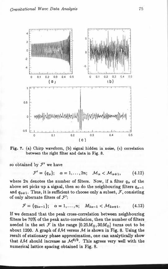
Gravitational Wave Data Analysis 75
4
5 2
0 0
-2
-4 -5
0 0.1 0.2 0,3 0.4 0.5 0 0.1 0.2 0.3 0.4 05
(a I I b)
l 0.5
0 0.1 0.2 0.3 0.4 0.5
( c )
Fig. 7. (a) Chirp waveform, (b) signal hidden in. noise, (c) correlation between the right filter and data in Fig. 8.
so obtained by :F' we have
:F' = {qa}; a= 1, ... , 2n; Ma < Ma+i, (4.12)
where 2n denotes the number of filters. Now, if a filter qa of the above set picks up a signal, then so do the neighbouring filters qa-1 a.nd qa+l· Thus, it is sufficient to choose only a subset, :F, consisting of only alternate filters of :F':
:F = {q2a-1}; Q = 1,. ·. ,n; M2a-1 < M2a+l· (4.13)
If we demand that the peak cross-correlation between neighbouring filters be 703 of the peak auto-correlation, then the number of filters needed in the set :Fin the range [0.25M0 ,30M0 ] turns out to be about 1200. A graph of 6M versus Mis shown in Fig. 8. Using the result of stationary phase approximation, one can analytically show that 6M should increase as M 813 • This agrees very well with the numerical lattice spacing obtained in Fig. 8.
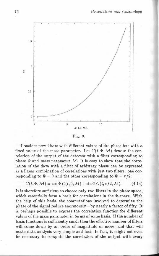
76 Gravitation and Cosmology
1.5
0 5 -
.1 0 10
,,I( ( i n M0 )
Fig. 8.
Consider now filters with different values of the phase but with a fixed value of the mass parameter. Let C ( t, cI>, M) denote the correlation of the output of the detector with a filter corresponding to phase <I> and mass parameter M. It is easy to show that the correlation of the data with a filter of arbitrary phase can be expressed as a linear combination of correlations with just two filters: one corresponding to cI> = 0 and the other corresponding to cI> = 11' /2:
C(t, cI>, M) =cos <I> C(t, 0, M) +sin <I> C(t, 11' /2, M). (4.14)
It is therefore sufficient to choose only two filters in the phase space, which essentially form a basis for correlations in the cI>-space. With the help of this basis, the computations involved to determine the phase of the signal reduce enormously-by nearly a factor of fifty. It is perhaps possible to express the correlation function for different values of the mass parameter in terms of some basis. If the number of basis functions is sufficiently small then the effective number of filters will come down by an order of magnitude or more, and that will make data analysis very simple and fast. In fact, it might not even be necessary to compute the correlation of the output with every
Gravitational Wave Data Analysis 77
filter; a knowledge of the correlation with just the basis functions ~ight tell us whether or not the signal is present. With the criteria that the neighbouring filters have their peak cross-correlation value not less than the threshold, we need a total of 2400 filters in the 2-dimensional mass-phase lattice space.
Let me now come back to the question of the arrival time. Suppose we are given a set of filters with which the data needs to be correlated. For simplicity, I will consider only filters with different values of the mass parameter. Let the data contain a signal with the value of the mass parameter in the range [M2a-1, M2a+I]· The peak correlation will be the lowest when the signal's mass parameter value is equal to M2a· If the signal is strong enough, both q2a-1 and q2a+I will detect the signal but with different times of arrival. The reason for this can be understood with a simple example. Suppose we are interested in detecting a sinusoidal signal. If the frequency of the incoming signal is wand our filter has a frequency wo slightly different from w, then still the sinusoidal signal will be detected but with an error ctarr in the time of arrival of the signal. It is easy to see that ct arr <X ( w - Wo ). Similarly, in the case of a chirp signal, a slight mismatch in the values of the parameters of the signal will reflect itself as an error in the estimation of the time of arrival.22 •31
This error will be proportional to the difference in the values of the parameters of the signal and the filter. Hence, after a signal is detected it is necessary to determine the values of the various parameters by choosing a finer grid of parameters.
Acknowledgements
I should like to thank Sanjeev Dhurandha.r and Bernard Schutz, who essentially introduced me to the subject of gravitational radiation and data analysis. I owe my tha.n~s to my colleagues Patrick Das Gupta and Sanjay Wagh for many fruitful discussions. This research was funded by CSIR through a research associateship.
References
1. Damour, T. and T11¥lor, J.: "On the Orbital Period ·of the Binary Pulsar 1913+16", to appear in Attrophyt. J., {1990).
2. Hough, J. et al.: "Proposal for a Joint German-British Interferometric Gra:vitational Wave Detector", Max Plarik Institute for Quantum Optics, MPQ Report, No. 147, GWD/137/JH{89), 1989.
3. Thome, K.S.: "Gravitational Radiation", in 300 Year• of Gravitation, {eds.) Hawking, S.W. and Isreal, W., Cambridge University Press, CAmbridge, 1987.
78 Gravitation and Cosmology
4. Schutz, B.F.: "Sources of Gravitational Waves", in Gravitational Wave Data Analysis, (ed.) Schutz, B.F., Kluwer, Dordrecht, 1989.
5. Peter, P.C. and Mathews, J.: Phys. Rev., 131 (1963), 435.
6. Clarke, J.P.A. and Eardley, D.M.: Astrophys. J., 216 (1977), 311.
7. Wagoner, R.V. and Will, C.M.: Astrophys. J., 210 (1976), 764.
8. Krolak, A.: "Coalescing Binaries to Post-Newtonian Order", in Gravitation Wave Data Analysis, (ed.) Schutz, B.F., Kluwer, Dordrecht, 1989.
9. Damour, T. and Iyer, B.R.: Ann. Inst. Henri Poincare, Phys. Theor., 1990 (submitted).
10. Blanchet, L. and Damour, T.: Ann. Inst. Henri Poincare, 60 (1989), 377.
11. Drever, R.W .P.: "Interferometric Detectors of Gravitational Radiation", in Gravitational Radiation, (eds.) Deruelle, N. and Piran, T., North Holland, Amsterdam (1983); see al o Vinet, J.Y., Meers, B.J., Man, C.N. and Brillet, A.: Phys. Rev., 038 (1988), 433.
12. Dhurandhar, S.V., Krolak A. and Lobo, J.A.: Mon. Not. R. Aatr. Soc., 237 (1989), 333.
13. Smith, S.: Pliys. Rev., 036 (1987), 2901; LivaB used tn.ie method to Ha.rch for pulsara; Liva.a, J.C.: "Upper Limits for .Gravitational Radiation from Some Astrophysical Sources", Ph.D. Thesis, MassKhusetts Institute of Technology, Cambridge, Mass., 1987.
14. Dhurandhar, S.V. and Tinto, M.: MNRAS, 234 (1989), 663.
15. Gursel, Y. and Tinto, M.: Phys. Rev., 046 (1989), 1234.
16. Brillet, A., Man, C.N., Meers, B.J. and Vinet, J.Y.: Phys. Rev., 038 {1988), 433.
17. Meers, B.J.: Phys. Rev., 038 {1988), 2317.
18. Schutz, B.F.: "Gravitational Waves", to be published in the proceedings of Relativity Meeting, 1989, Universitat Autonoma de Barcelona, Spa.in, Sept. 1989.
19. Landau, D. and Lifshitz, E.M.: "ClaBsical Theory of Fields", Pergamon Press, Cha.p. 13, 1975.
20. Schutz, B.F .: "A First Course in General Relativity", Cambridge University Press, Cambridge, 1985,.
21. Shapiro, S.L. and Teukolsky, S.A.: "Black Holes, White Dwarfs and Neutron Stars", John Wiley, Chap. 16, 1983.
22. Dhurandhar, S.V., Krolak, A., Schutz B.F. and Watkins, J.: in preparation. 23. Dhurandha.r, S.V., Da.s Gupta P. and Sathya.pra.kash, B.S.: "Gravitational
Wave Data. Analysis of the Coalescing Binary Signal: The Fourier Transform", IUCAA Preprint, Ma.y, 1990.
24. Lawrence, S., Achar, N. and Schutz, B.F.: "On the Analysis of Gravitational Wave Data", in Gravitational Wave Data Analysis, (ed.) Schutz, B.F., Kluwer, Dordrecht, 1989.
25. Schutz, B.F.: "Data. Analysis Requirements of Networks of Detectors", in Gravitational Wave Data Analysis, (ed.) Schutz, B.F., Kluwer, Dordrecht, 1989.
26. Schutz, B.F.: "Data Processing, Analysis and Storage for Interferometric Antennas" 1 to a.ppe&r in The Detection of Gravitational Radiation, (ed.) Blair, D., C~brldge Un.iveraity Presa, Ca.mbridge, 1989.
27. Helstrom, C.W.: "Sta.tiatical Theory of Signal Detection", 2nd. ed., Pergamon Press, London, 1968.
Gravitational Wave Data Analysis 79
28. Davies, M.H.A.: "A Review of Sta.tistica.l Theory of Signal Detection", in Gravitational Wave Data Analysis, {ed.) Schutz, B.F., Kluwer, Dordrecht, 1989.
29. Sha.nmuga.n, K.S. a.nd Breiphol, A.M.: "Random Signals: Detection, Estimation a.nd Data. Analysis", Chap. 6, John Wiley, 1989.
30. Sa.thya.pra.k.a.sh, B.S. a.nd Dhura.ndha.r, S.V.: {1990) "Gravitational Wave Data. Analysis of the Coalescing Binary Signal: A Criterion for Choosing Filters", to appear in Phys. Rev. D.
31. Lobo, J.A.: "Coalescing Binary Signals' Arrival Time Estimation: The Performance of a. Long Baseline Interferometri~ GW Antenna.", preprint, 1990.
Rome-Maryland Gravitational
Radiation Antenna Correlations with
Neutrino Detectors at Mont Blanc,
Kamioka and Baksan Associated with
Supernova 1987 A
J. WEBER
University of Maryland, College Park, Maryland 20742 and Univ_ersity of California, Irvine, California 92717
1. Introductibn
For twenty years, a gravitational radiation antenna has been operating at the University of Maryland, "waiting for a supernova",
Gravitational radiation antennas at Rome and Maryland, and several neutrino detectors, were operating during the rapid evolutionary phase of Supernova 1987 A. Five neutrinos were observed at about 0245 Universal Time, 23 February 1987, on the Mont Blanc neutrino detector .1 Pulses were observed on both Rome and Maryland gravitational antennas 1.2 s earlier than these Mont Blanc events.
The analyses therefore begin with the assumption that the neutrinos and gravitational detectors might have correlated outputs for a 1.2 s earlier gravitational antenna time. The two gravitational antenna outputs are at first combined and treated as one.
2. Maryland-Rome Gravitational' Antenna Correlations
In two hours there were about .100 neutrino events. The total event sum of the gravitational antenna outputs is obtained for times of the 100 neutrino detector events minus 1.2 s. If there are correlation.B, the gravitational antenna output sum will be much larger than for other times. A large number of time delays 6, between neutrino detector events and gravitational outputs, in increments of one second, are introduced and the gravitational antenna sums again carried out. The number of time delay values giving gravitational antenna sums larger than the zero 6 value is studied, as the center time of the two-hour interval is changed. Let this value be n. If the central
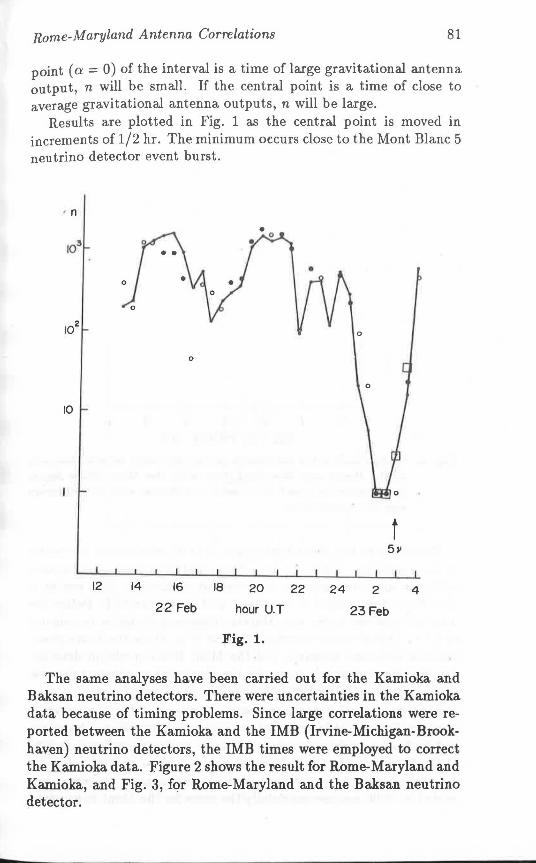
Rome-Maryland Antenna Correlations 81
point (a = 0) of the interval is a time of large gravitational antenna output, n will be small. If the central point is a time of close to average gravitational antenna outputs, n will be large.
Results are plotted in Fig. 1 as the central point is moved in increments of 1/2 hr. The minimum occurs close to the Mont Blanc 5 neutrino detector event burst.
, n
103
102
0
0
10
t 511
12 14 16 18 20 22 24 2 4
22 Feb hour U.T 23Feb
Fig. 1.
The same analyses have been carried out for the Kamioka and Baksan neutrino detectors. There were uncertainties in the Kamioka data because of timing problems. Since large correlations were reported between the Kamioka and the IMB (Irvine-Michigan-Brookhaven) neutrino detectors, the IMB times were employed to correct the Kamioka data. Figure 2 shows the result for Rome-Maryland and Ka.mioka, and Fig. 3, for Rome-Maryland and the Baksan neutrino detector.
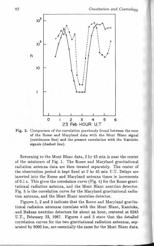
82 Gravitation and Cosmology
' I
2 ' 10 I I I
' I I J
n I
+
10
0 2 3 4 5 6 23 Feb HOUR U .T
Fig. 2. Comparison of the correlation previously found between the sum of the Rome and Maryland data with the Mont Blanc signal (continuous line) and the present correlation with thEl Kamioka signals (dashed line) .
Returning to the Mont Blanc data., 2 hr 45 min is near the center of the minimum of Fig. 1. The Rome and Maryland gravitational radiation antenna data are then treated separately. The center of the observation period is kept fixed at 2 hr 45 min U .T. Delays are inserted into the Rome and Maryland antenna times in increments of 0.1 s. This gives the correlation curve (Fig. 4) for the Rome gravitational radiation antenna, and the Mont Blanc neutrino detector. Fig. 5 is the correlation curve for the Maryland gravitational radiation antenna, and the Mont Blanc neutrino detector.
Figures 1, 2 and 3 indicate that the Rome and Maryland gravitational radiation antennas correlate with the Mont Blanc, Kamioka, and Baksan neutrino detectors for about an hour, centered at 0245 U.T., February 23, 1987. Figures 4 and 5 state that the detailed correlation curves for the two gravitational radiation antennas, separated by 8000 km, are essentially the same for the Mont Blanc data.
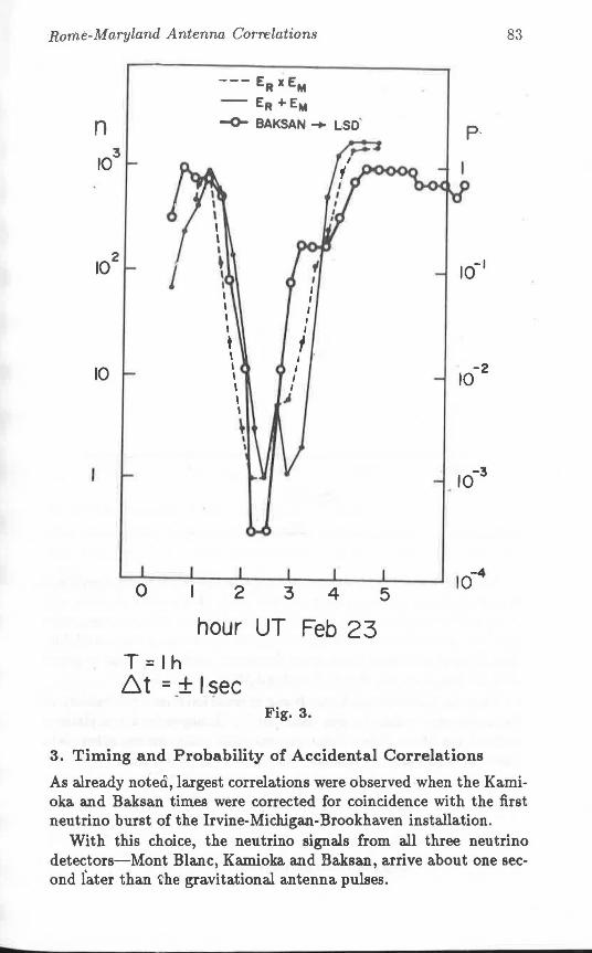
Rome-Maryland Antenna Correlations 83
--- ERxEM
- ER +EM
-0- BAKSAN -+ LSD'
102
I
• I I I I I I I I
t f I I
10 I I 10-2 I I I I I " I
~ I I
10-3
0 2 3 4 5
hour UT Feb 2 3 T = lh 6t =+I sec
Fig. 3.
3. Timing and Probability of Accidental Correlations
As already notea, largest correlations were observed when the Kamioka and Baksan times were corrected for coincidence with the first neutrino burst of the Irvine-Michigan-Brookhaven installation.
With this choice, the neutrino signals from all three neutrino detectors-Mont Blanc, Kamioka a.nd Baksa.n, arrive about one second fater than 'Che gravitational antenna pulses.
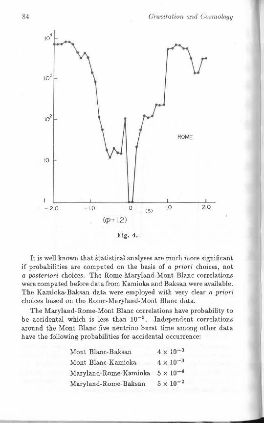
84
4 10
10
-2 0 -10 0
(<p+ 1.2)
Fig. 4.
Gravitation and Cosmology
ROME
(SJ 1.0 2.0
It is well known that statistical analyses are much more significant if probabilities are computed on the basis of a priori choices, not a posteriori choites. The Rqme-Maryland-Mont Blanc correlations were computed before data from Kamioka a.nd Baksan were available. The Kamioka-Baksan data were employed with very clear a priori choices based on the Rome-Maryland-Mont Blanc data.
The Maryland-Rome-Mont Blanc correlations have probability to be accidental which is less than 10-5 • Independent correlations around the Mont Blanc five neutrino burst time among other data have the following probabilities for accidental occurrence:
Mont Blanc-Baksan
Mont Blanc-Kamioka
4 x 10⁻³
4 x 10·- 3
Maryland-Rome-Kamioka 5 x 10⁻⁴
Maryland-Rome-Baksan 5 x 10⁻²
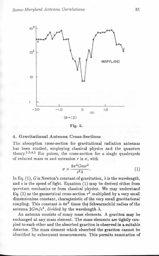
Rome-Maryland Antenna Correlations 85
MARYLAND
10
-2.0 -1.0 0 1.0 (Sl
(Q>+l .2)
Fig. 5.
4. Gravitational Antenna Cross-Sections
The absorption cross-section for gravitational radiation antennas has been studied, employing classical physics and the quantum theory. 2
•3
•4 •5 For pulses, the cross-section for a single quadrupole
of reduced mass m and extension r is a, with
87r3Gmr2
(J' = c2A
(1)
In Eq. (1 ), G is Newton's constant of gravitation, A is the wavelength, and c is the speed of light. Equation (1) may be derived either from qu; .. 11tum mechanics or from classical physics. We may understand Eq. (1) as the geometrical cross-section r 2 multiplied by a very small dimensioniess constant, char~eristic of the very small gravitational coupling. This constant is 411"3 times th' Schwarzschild radius of the antenna 2Gm/ c2
, divided by t he waveleng~h A. An antenna consists of many mass elements. A graviton may be
exchanged at any ma.ss element. The ma.ss elements are tightly coupled to ea.ch other and the absorbed graviton is observed in a suitable detector. The mass element which absorbed the graviton cannot be identified by subsequent measurements. This permits summation of
86 Gravitation and Cosmology
the probability amplitude over all possible absorber mass elements.
5. S Matrix Many Body Cross-Section
The S matrix for interaction of gravitational radia1ion with an ensemble of quadrupoles is taken as
s = ~c J (FI (Roioj + Rciio)(qi + qH)r1-/fiA1fJA Io) d4x. (2)
A Riemann normal coordinate system is employed. m is again the reduced mass of a quadrupole and! r1 is the vector extension . . The Riemann tensor is the plane wave summation
(3)
where dk is an annihilation operator for a graviton with wavenumber k. 1(,~lOj is a fr~quency dependent normalization factor. if; A is a creation operator for a mass quadrupole oscillator with harmonic oscillator coordinate qi:
(4) s n
In Eq. (4), f is the position three-vector, n refers to the nth mass element. a 8 n is an annihilation operator for the state with harmonic oscillator wavefunction 1/;3 n·
Suppose first that there is only one mass quadrupole at r = Tn
and it undergoes a transition from the state with energy E,, to E,,+1:
S = ~ "\:"nk ·r'qj e-K(f'k·r)+i(w±w0 )tdt. 2 J . h.,/'iir Li: 0103 v+t,v
In Eq. (5), q11+1,v is the harmonic oscillator matrix element for the final state with v + 1, and initial state with quantum number v.
We may extend this result to the many quadrupole case for the following conditions. The elastic solid antenna consists of tightly coupled mass elements. Exchanged gravitons are ob~rved at a detection system with no way of determining which mass element absorbed them. Therefore, the probability amplitude for the system is a sum of Eq. (5) over all absorber mass elements. Since the gravitational wavelength is large compared with the antenna dimensions, phase factors exp[-i(Pk ·fn)/h] are very close to unity. 'I1he N quadrupole sum is, therefore
S - N mc2 J "\:" -nk I j i(w±w.,)tdt N - n.,/'iir L..J ''-OIOjr q,,±1,ve •
k
(6)
Rome-Maryland Antenna Correlations 87
The integration in Eq. (6) gives a delta function in frequency,
_ Nmc2v'2if 1 i SN - --n--R(wo)otojr q11±i,v· ,(7)
Equation (7) gives the cross-section for net absorption as
7 _ 21r N2m2 c4 V I R(wo)o1ojr 1 1 2 (q~+1,v - q~_ 1 ,J (
8)
- n2 rc
In Eq. (8), r is a long time:
IR( ) · 12 - 41rwoGUINCIDENT (9) wo 0103 - Ac7 •
In Eq. (9), G is Newton's constant of gravitation, U1NCIDENT is the incident energy. The area is A:
crhwA U1NCIDENT = v (10)
Making use of Eqs. (8), (9) and (10), and the harmonic oscillator matrix elements, one gets for the cross-section
81r3Gmr2 N 2
(11) u=-----c2.X
To apply Eq. (11) to an elastic solid antenna, it is required that each quadrupole have a normal mode frequency close to the normal mode of the bar w0 being observed. Detailed analyses show that planar slabs, with plane normal to the longitudinal a.xis are resonant at the normal mode frequency. For the quadrupoles, we will choose planar mass elements driven with Tespect to the center of mass.5
The thickness is apprqXimately the length of an atomic cell. Let the total number of atoms in the antenna be NA. N, the total number of slabs is given in terms of the length .L and atomic spacing Sa as
L NsLAB ~ Sa. (12)
The value of r 2 in Eq. (11) is then the mean square distance from the center. For a bar with length L
L2 (r2} =ii'
In Eq. (11) the product mN is the total mass,
M = mATOMN A= msLAeNsLAB·
Equations (ll), {12), (13) and (14) then give
811'3 ML3
u= 12c2.XSa'
(13)
{14)
(15)
88 Gravitation and Cosmology
Appropriate corrections to Eq. ( 15) will involve taking heat bath interactions into account.
6. Effects of Heat Bath Interactions
The quantum theory of the heat bath interactions has been described elsewhere. For a single quadrupole, the classical and quantum theories give the same results. The absorbed energy for the continuous spectrum is2
ij = __ OoO 0(30 D Jjj ww'c4 Rµ (w)r 0 R"'µ r(Jei(w-w')tdt..,;dw'dt
27r (-w2 + iwD /m + k/m)(-w' 2 - iw' D /m + k/m)' (16)
In Eq. (16), D is the dissipation and k is the force constant. For the many quadrupole system, single quadrupoles may have
very low quality factor, Qi = wm/ D much less than unity. For this case, Eq. (16) leads to a modification of Eq. (15) as
87r3 M L3 Q1G 0'=------
12c2 >..Sa (15A)
For the operating antenna at the University of Maryland, Eq. (15A) gives the cross-section"' 2 x 10-13 cm2 • This implies that the supernova6 gravitational radiation energy was approximately 10-3
solar masses per pulse. For continuous sinusoidal signals, it has been shown5 that Eq.
(15A) is also valid, in agreement with near field experiments. This research was supported by the Universities of Maryland and
California, and by the Strategic Defense Initiative Organization, Office of Innovative Science and Technology and managed by the Harry Diamond Laboratories.
References
I. Aglietta, M. et al.: n Nuovo Cimento, 12C (1989), 75. 2. Weber, J.: Phya. Rev. 117 (f960), 306. 3. Ruffini, R. and Wheeler, J.A.: "Relativistic Cosmology and Space Plat
forms", in Proceedinga of the Conference on Space Physics, ESRO, Paris, Fra.nce (1971).
4. Weber, J.: Found. Phys., 14 (1984), 1185. 5. Weber, J.: in Vol. 3 Eddington Centenary Symposium, (eds.) Weber, J.
and Karade, T.M.: World Scient., 1986, p. 1077. 6. In reference 5, a model is considered in which individual atoms couple to
the Riemann tensor and exert forces on planar slabs. This model also gives Eq. (15A).
CHAPTER 3
GRAVITY AND PARTICLE PHYSICS
-- -
Particle Physics Applications
of Superstring Theory
PRAN NATH
Department of Physics, Northeastern University Boston, MA 02115
R. ARNOWITT
Center for Theoretical Physics, Depm iment of Physics Texas A f3 M University, College Station, TX 77843
1. Introduction
Superstring theory offers the hope for the unification of all fundamental interactions including gravity.1 A very strong constraint on any superstring theory is that it reproduce a low energy theory at the electro-weak scale consistent with the current experiment. We discuss here some possibilities for the low energy physics that results from the compactifications of the Es XE~ heterotic superstring theory. 2 There are a number of compactifications of the heterotic string which have been discussed in the literature. Some of these a.re the Calabi-Yau compactifications,3 compactification on orbifolds,4
and on blown-up orbifolds.5 Four-dimensional string theories6 and constructions based on N = 2 superconformal field theories7 also represent possible vacua of the compactified heterotic string. Phenomenology of certain four-dimensional string models has been pursued by many authors8 •9 with encouraging results. One generic drawback of the four-dimensional string models, however, is the large number of possibilities for three-generation models available in this approach, although phenomenological constraints strongly limit these.
Below we shall discuss phenomenology that results from compactification on three-generation Calabi-Yau models. The most well known of these is the so-called CP3 x CP3 /Z3 model,10 which has been investigated rather extensively.11 - 20 The other two 3-generation models consist of a CP3 x CP2 /Z3 Ix Z~ model21 - 25 (where Z3
acts freely but Z~ does not) and a CP2 x CP2 /Z3 x Z~ x Z~ (where Z3
and z~ act freely but z~ does not). While the three models referred to above have been shown to be di:ffeomorphic27 (the three models are defined in somewhat greater detail in Appendix A), their Yukawa
92 Gravitation and Cosmology
couplings are expected to be very different. In the following, we shall focus mostly on the phenomenology of the CP3 x CP3 /Z3 and of the CP3 x CP2 /Z3 x Z~ models, although many of our conclusions are model independent and valid for a large class of 3-generation models. We begin by discussing the properties of the CP3 x CP3 /Z3 and CP3 x CP 2 /Z3 x Z~ models briefly.
(1) CP3 x C P3 /Z3 Model
The compact manifold here is a submanifold of CP3 x CP3 /Z3 of vanishing first Chern class. It is described by the intersection of three polynomials P; = 0 ( i = 1, 2, 3) given in Appendix A. According to the analysis of Candelas et al.3 the Calabi-Yau compactifications preserve N = 1 supersymmetry and compactifications on simply connected manifolds breaks the symmetry E8 x E~ of the heterotic string down to the symmetry E6 x E~. On CP3 x CP3 /Z3, the flux breaking due to Wilson lines allows the further breaking of E6
to (SU(3)]3 or SU(6) x U(l). The (SU(3)]3 breaking of E6 turns out to be the phenomenologically more appealing possibility. The matter multiplets of the theory fall into 27 a.nd 27 representations of E6 in Calabi-Yau compactifications. Under [SU(3)]3 the 27 and 27-plets may be decomposed further as follows: 27 = Q(3, 3, 1) + Qc(3,1,3) + L(l,3,3), where Q = (q,D), Qc = (uc,dc,Dc) and L = (l,H,H',ec,1/,N). Here l, H, H' are SU(2)L doublets while ec, vc and N are SU(2)L singlets with vc and N also SU(5) and SO(lO) singlets respectively. We shall assume that the flux breaking occurs at a scale Mc close to the Planck sccle Mpi, i.e.,
Mc~ Mp1 = 2.4 x 10¹⁸ GeV. (1.1)
After flux breaking, the massless modes of the theory in the matter sector consists of the following:
[7Q(3, 3, 1) + 4Q(3, 3, 1)] + [7Qc(3, 1, 3) + 4Qc(3, 1, 3)]
+. (9L(l, 3, 3) + 6L(l, 3, 3)]. (1.2)
In ·cp3 x CP3 /Z3 compactification, matter parity invariance is found to be a necessary ingredient in achieving proton stability. Here one defines matter parity by M2 = CUz where C transforms the eight complex (homogeneous) co-ordinates of CP3 x CP3 as follows: C[(xox1x2x3)®(YoY1Y2Y3)] = [(xox1x3x2)®(YoY1.Y3Y2)] and Uz is an element of (SU(3)]3 defined by Uz = diag(l, 1, 1) ® diag(-1, -1, 1) ® diag(-1,-1,1) so that under Uz SU(2)L and SU(2)R doublets interchange sign while the SU(2)L ® SU(2)R singlets are unaffected. The above definitions allow one to classify states as either even or odd under U z and C. Thus one may decompose massless states of
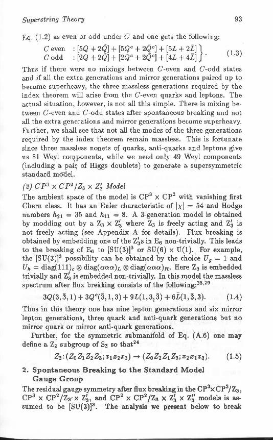
Superstring Theory 93
Eq. (1.2) as even or odd under C and one gets the following:
C even : [5Q + 2q] + [5Qc + 2qcJ + [5L + 2~] } (1.3) Codd : (2Q + 2Q] + [2Qc + 2Q 0
] + (4L + 4L] ·
Thus if there were no mixings between C-even and C-odd states and if all the extra generations and mirror generations paired up to become superheavy, the three massless generations required by the index theorem will arise from the C-even quarks and leptons. The actual situation, however, is not all this simple. There is mixing between C-even and C-odd states after spontaneous breaking and not all the extra generations and mirror generations become superheavy. Further, we shall see that not all the modes of the three generations required by the index theorem remain massless. This is fortunate since three massless nonets of quarks, anti-quarks and leptons give us 81 Weyl co~ponents, while we need only 49 Weyl components (including a paii; of Higgs doublets) to generate a supersymmetric standard. model.
(2) CP3 x CP2 /Z3 x Z~ Model
The ambient space of the model is CP3 x CP2 with vanishing first Chern class. It has an Euler characteristic of lxl = 54 and Hodge numbers h21 = 35 and h11 = 8. A 3-generation model is obtained by modding out by a Z3 x z; where Z3 is freely acting and z; is not freely acting (see Appendix A for details). Flux breaking is obtained by embedding one of the z;s in E6 non-trivially. This leads to the breaking of Es to [SU(3)]3 or SU(6) x U(l). For example, the (SU(3)]3 possibility can be obtained by the choice U9 = 1 and uh= diag(lll)c ® diag(aaa)L ® diag(aaa)R· Here Z3 is embedded trivially and z; is embed·ded non-trivially. In this model the massless spectrum after flux breaking consists of the following: 28 ·29
3Q(3, 3, 1) + 3Q 0 (3, 1, 3) + 9L(l, 313) + 6L(l, 3, 3). (1.4)
Thus in this theory one has nine lepton generations and six mirror 1epton generations, three quark and anti-quark generations but no mirror quark or mirror anti-quark generations.
Further, for the symmetric submanifold of Eq. (A.6) one may define a Z2 subgroup of S3 so that24
Z2: (ZoZ1Z2Z3; x1x2x3)--+ (ZoZ2Z1Z3; x2x1x3). (1.5)
2. Spontaneous Breaking to the Standard Model Gauge Group
The residual gauge symmetry after flux breaking in the CP3x CP3 /Z3 ,
CP3 x CP2 /Z3 • x z;, and CP2 x CP2 /Z3 x Z~ x ~ models is assumed to be [SU(3)]3. The analysis we present below to break
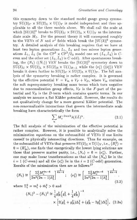
94 Gravitation and Cosmology
this symmetry down to the standard model gauge group symmetry SU(3)c x SU(2)L x U(l)y is model independent and thus applicable to all the three models above. We shall call the sea.le at which [SU(3)]3 breaks to SU(3)c X SU(2)L x U(l)y as the intermediate scale Mr. For the present theory it will correspond roughly to the VEVs of N and vc fields which break the [SU(3)]3 symmetry. A detailed analysis of this breaking requires that we have at least two lepton generations Li, L2 and two mirror lepton gener-
- - 3 3 -ations Li, L2 (in the CP X CP /Z3 model one set ( LJ, L2 ) is C-even and the other set (L2,L2) is C-odd). After spontaneous breaking, the (N1) ((N1)) VEV breaks the [SU(3)]3 symmetry down to SU(3)c X SU(2)L x SU(2)R X U(l)B-L while the (v2) ((v2)) VEV breaks it down further to SU(3)c X SU(2)L X U(l)y. The full analysis of the symmetry breaking is rather complex. It is governed by the effective potential V = Vm + Vp +VD, where Vm contains the soft supersymmetry breaking mass terms which turn negative due to renormalization group effects, Vp is the F-part of t_he potential and VD is the D-term which contains quartic terms. In our analysis we assume a, fl.at Kahler potential. However, the results do not qualitatively change for a more general Kahler potential. The non-renormalizable interactions that govern the intermediate scale breaking have characteristically the form
(2.1) n
The full analysis of the minimization of the effective potential is rather complex. However, it is possible to analytically solve the minimization equations on the submanifold of VEVs if one limits oneself to physically intersecting directions. Thus for example, on the submanifold of VEVs that preserve SU(2)L X U(l)y, i.e., (Hl} = 0 = (H~i), one finds that energetically the lowest lying solutions a.re those that preserve matter parity, i.e., (Nr) = 0 = (v;). Further, one may make linear transformations so that ill the (Nn) lie in the i = 1 (C-even) and all the (v;) lie in the i = 2 (C-odd) generation. Results of the minimization then are as follows: 17
_ -,- - ~
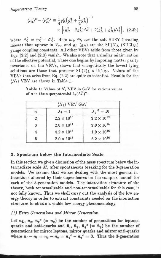
Superstring Theory 95
(112)2 - (v~)2 ~ lgh (gt+ lgh)-1 x [ (gk - 2gi,)~f + 2(gi, + 9k)~~] ' (2.3b)
where ~~ = mr - mr. Here mi, mi are the soft SUSY breaking masses that appear in Vm, and 9L (gR) are the SU(3)L (SU(3)R) gauge coupling constants. All other VEVs aside from those given by Eqs. (2.2) a.nd (2.3) vanish. We also note that a similar minimization of the effective potential, where one begins by imposing matter parity invariance on the VEVs, shows that energetically the lowest lying solutions are those that preserve SU(2)L X U(l)y. Values of the VEVs that arise from Eq. (2.2) are quite substantial. Results for the (Nt) VEV are shown in Table 1.
Table 1: Values of Ni VEV in GeV for various values of n in the superpotential A1 (LL r.
(N1) VEV GeV
n >.1 = 1 >.12 = 10
2 2.2 x 10¹⁰ 2.2 x 10¹²
3 2.0 x 10¹⁴ 2.0 x 10¹⁵
4 4.2 x 10¹⁵ 1.9 x 10¹⁶
5 2.0 x 10¹⁶ 6.2 x 10¹⁶
3. Spectrum below the Intermediate Scale
In this section we give a discussion of the mass spectrum below the intermediate scale M1 after spontaneous breaking for the 3-generation models. We assume that we are dealing with the most general interactions allowed by their dependences on the complex moduli for each of the 3-generation models. The interaction structure of the theory, both renormalizable and non-renormalizable for this case, is not fully known. Thus we shall carry out the analysis of the low energy theory in order to extract constraints needed on the interaction structure to obtain a viable low energy phenomenology.
(1) Eztra Generations and Mirror Generation
Let nL, nq, nq c (= n9 ) be the number of generations for leptons, quarks and anti-quarks and n1, n9 , n9 c ( = n9) be the number of generations for mirror leptons, mirror quarks and mirror anti-quarks where n1 - n1 = n9 - n9 = n 9 c - n9 c = 3. Thus the 3-genera.tion
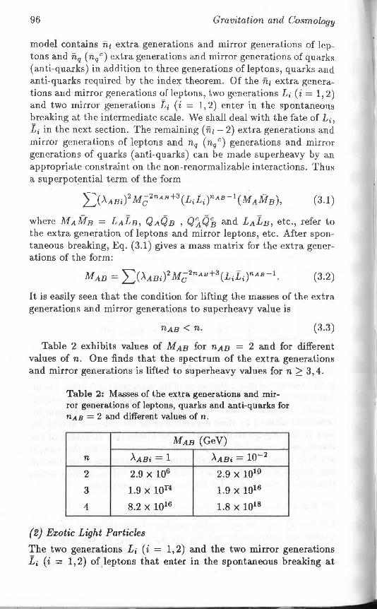
96 Gravitation and Cosmology
model contains fit extra generations and mirror generations of leptons and nq (nqc) extra. generations and mirror generations of quarks (anti-quarks) in addition to three generations ofleptons, quarks and anti-quarks required by the index theorem. Of the n1 extra generations and mirror generations ofleptons, two generations Li ( i = 1, 2) and two mirror gBnerations Li ( i = 1, 2) enter in the spontaneous breaking at the intermediate scale. We shall deal with the fate of Li, Li in the next section. The remaining (n 1 - 2) extra generations and mirror generations of leptons and nq ( nq c) generations and mirror generations of quarks (anti-quarks) can be made super heavy by an appropriate constraint on the non-renormalizable interactions. Thus a superpot_ential term of the form
(3.1)
where MAMB = LAIB, QAQB , QA.Q8 and LALB, etc., refer to the extra generation of leptons and mirror leptons, etc. After spontaneous breaking, Eq. (3.1) gives a mass matrix for the extra generations of the form:
MAB = 'L)AABi)2 MC: 2nAB+3 (LiLirAB- 1. (3.2)
It is easily seen that the condition for lifting the masses of the extra generations and mirror generations to superheavy value is
(3.3)
Table 2 exhibits values of MAB for nAB = 2 and for different values of n. One finds that the spectrum of the extra generations and mirror generations is lifted to super heavy values for n ~ 3, 4.
Table 2: Masses of the extra generations and mirror generations of leptons, quarks and anti-quarks for nAB = 2 and different values of n.
MAB (GeV)
n AABi = 1 AABi = 10-2
2 2.9 x 10⁶ 2.9 x 10¹⁰
3 1.9 x 10n 1.9 x 10¹⁶
4 8.2 x 10¹⁶ 1.8 x 10¹⁸
(2) Exotic Light Particles
The two generations Li ( i = 1, 2) and the two mirror generations Li ( i = 1, 2) of,leptons that enter in the spontaneous breaking at
·--- --·
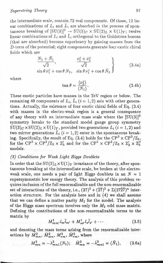
Superstring Theory 97
the intermediate scale, contain .72 real components. Of these, 12 linear combinations of Li and Li are absorbed in the process of spontaneous breaking of [SU(3)]3
-+ SU(3)c x SU(2)l, x U(l)y; twelve linear combinations of Li and Li orthogonal to the Goldstone bosons (that are absorbed) become superheavy by gaining masses from the D-term of the potential; eight components generate four exotic chiral fields which are
Ni+ N1 vi+ Pi } J2 ' J2
sin() Pf + cos() N2, sin() vf + cos() N2 (3.4a)
where
(3.4b)
These exotic particles have masses in the Te V region or below. The remaining 40 components of Li, Li ( i = 1, 2) mix with other generations. Actually, the existence of four exotic chiral fields of Eq. (3.4) with masses in the electro-weak region is a general consequence of any theory with an intermediate mass scale where the [SU(3)]3 symmetry breaks _to the standard model gauge group symmetry SU(3)c x SU(2)L x U(l)y, provided two generations Li ( i = 1, 2) and two mirror generations Li ( i = 1, 2) enter in the spontaneous breaking. Specifically, the result of Eq. (3.4) holds for the CP3 x CP3 /Z3 ,
for the CP3 x CP2 /Z3 x z; and for the CP2 x CP2 /Z3 x z; x Z~ models-.
(3) Conditions for Weak Light Higgs Doublets
In order that the SU(2)L x U(l)y invariance of the theory, after spontaneous breaking at the intermediate scale, be broken at the electroweak scale, one needs a pair of light Higgs doublets in an N = 1 supersymmetric low energy theory. The analysis of this problem requires inclusion of the full renormalizable and the non-renormalizable set of interactions of the theory, i.e., (27)3 + (27)3 + :E(2727)" interaction structure. For the analysis here and in (4) we shall assume that we can define a matter parity M 2 for the model. The analysis of the Higgs mass spectrum involves only the M2 odd mass matrix. Defining the contributions of the non-renorma.lizable terms to the matrix by
(3.5)
and denoting the mass terms arising from the renormalizable inter-2 -2 3 -3
actions by Mm"' Mm"' Mrm' Mrm' where
{3.6a)
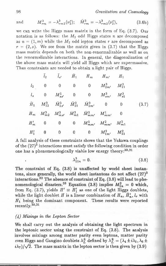
98 Gravitation and Cosmology
and (3.6b)
we can write the Higgs mass matrix in the form of Eq. (3.7). Our notation is as follows: the M2 odd Higgs states n are dewmposed as n = (1, m) while the M2 odd lep~on states r are decomposed as r = (2, s ). We see from the matrix given in (3.7) that the Higgs mass matrix depends on both the non-renormalizable as well as on the renormalizable interactions. In general, the diagonalization of the above mass matrix will yield all Higgs which are supermassive. Thus constraints are needed to obtain a light pair of Higgs.
0 0
H' 0 0 m
Hi 0 0
0
0
- 2 Mu
0
0
0
0
0
Hm 1
0
M:nm'
M3 al
0
0
(3.7)
A full analysis of these constraints shows that the Yukawa couplings of the (27)3 interactions must satisfy the following condition in order one has a phenomenologically viable low energy theory:30 •31
).~ln = 0. (3.8)
The constraint of Eq. (3.8) ·is unaffe~ted by world sheet instantons, since generally, the world sheet instantons do not affect (27)3
intera.ctions.32 The absence of constraint .of Eq. (3.8) will lead to phenomenological disasters.33 Equation (3.8) implies Mf n = 0 which, from Eq. (3.7), yields H' = Hi as one of the light Higgs doublets, while the light doublet His a linear combination of Hn, Ji~, lr with Hi being the dominant component. These results were reported recently.30•31
(4) Mixings in the Lepton Sector
We shall carry out the analysis of obtaining the light spectrum in the leptonic sector using the constraint of Eq. (3.8). The analysis involves mixings among matter parity even leptons, matter parity even Higgs and Gaugino doublets >.t defined by >.i = (>.4 ±i>.s, >.s ± i>.7 )/./'}.. The mass matrix in the lepton sector is then given by (3 .. 9)
- ' ~ -
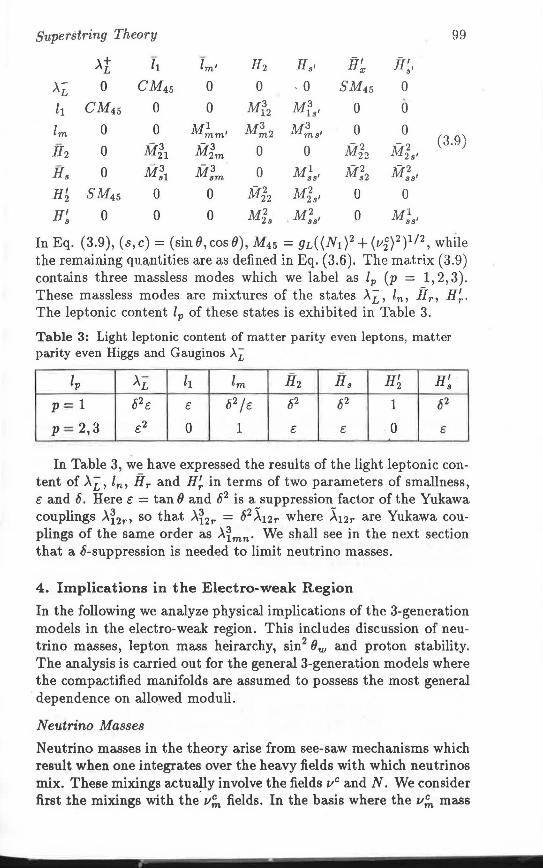
Supetstring Theory 99
,>.+ L T1 Tm' H2 Hs' H' x fl~.
.x-L 0 CM4s 0 0 ' 0 SM4s 0
li CM4s 0 0 M'f 2 M'fs• 0 0
lm 0 0 M!nm• M3 M!s• 0 0 m2 (3.9) ff2 0 -3 -3 0 0
-2 -2 M21 M2m M22 M2s'
Hs 0 -3 Ms1
-3 Msm 0 M}s'
-2 Ms2
-2 Mss'
H~ SM4s 0 0 - 2
M22 Mis• 0 0
H' 0 0 0 M:js M;s' 0 l s Mss'
In Eq. (3.9), (s,c) = (sinO,cosO), M4s = 9L((N1 ) 2 +(vi) 2 ) 112 , while the remaining qua,ntities are as defined in Eq. (3.6). The matrix (3.9) contains three massless modes which we label as Ip (p = 1, 2, 3). These massless modes are mixtures of the states .X£, ln, Hr, H~. The leptonic content lp of these states is exhibited in Table 3.
Table 3: Light leptonic content of matter parity even leptons, matter parity even Higgs and Gauginos >. [,
lp .x-L li lm H2 Hs H~ H' 8
p=l c2c E 82/c c2 c2 1 c2
p = 2,3 £2 0 1 E E 0 E
In Table 3, we have expressed the results of the light leptonic content of .>. L, ln, it r and H~ in terms of two parameters of smallness, E and 6. Here E =tan 0 and 62 is a suppression factor of the Yukawa couplings .Xr2r, so that .Xr2r = 62 5.12r where 5.12r are Yukawa couplings of the same order as .>.fmn· We shall see in the next section that a a-suppression is needed to limit neutrino masses.
4. Implications in the Electr~weak Region
In the following we analyze physical implications of the 3-generation models in the electro-weak region. This includes discussion of neutrino masses, lepton mass heirarchy, sin2 Ow and proton stability. The analysis is carried out for the general 3-generation models where the compactified manifolds are assumed to possess the most general dependence on allowed moduli.
Neutrino Masses
Neutrino masses in the theory arise from see-saw mechanisms which result when one integrates over the heavy fields with which neutrinos mix. These mixings actually involve the fields vc and N. We consider first the mixings with the. vin fields. In the basis where the vin mass
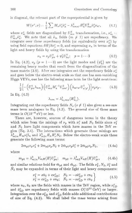
100 Gravitation and Cosmology
is diagonal, the relevant part of the superpotential is given by
W( c ) l ~ M - c - c \ 3 H2 u2 - c I/ ,v = 2 0 al/al/a - "nmn' n mal/al/n•, ( 4.1)
where v;, :fields are diagonalized by u;ia transformation, i.e., v;;,, == U!av~. We note that all Vm fields (m :I 1) are superheavy. We integrate over these super heavy fields (or equivalently over v~) by using field equations bW / liii~ = 0, and expressing Vn in terms of the light and heavy fields by using the transformation
(4.2)
In Eq. ( 4.2), vP (p = 1···3) are the light modes and { -iPD are the remaining heavy modes that result from the diagonalization of the mass matrix (3.9). After one integrates out the superheavy fields v~ and goes below the electro-weak scale so that one has non-vanishing Higgs VEVs, one has the following mass term for the light neutrinos:
~ [-( UJn-Anm) ( U!aM;1 u;m') ( Am•n• U~'p')] vpvp'. ( 4.3)
In Eq. ( 4.3) Anm = A~ 1 mn(H~J.
Integrating out the super heavy fields Ns ( s # 1) also gives a see-saw mass term analogous to Eq. ( 4.3). The general size of these mass terms is 0(10-6 eV) or less.
There are, however, sources of dangerous terms in the theory which arise from the mixings of Vp with vf and N2 fields since vf and N2 have light components which have masses in the TeV region (Eq. 3.4). The interactions which generate these mixings are A~1nHmvfln and .\~2 rllnH~N2. Below the electro-weak scale these generate the following mass terms:
( 4.4a)
where
mp1 = A~1n VmH(ll)UJn; mv2 = A;n2 VnH(H)UJr, ( 4.4b)
and similar relations hold for mp1 and mp2. The fields vf, N2, iif and N2 may be expanded in terms of their light and heavy components:
vf = sn2 + cvf v; f-!_2 = -siif v + cn2 } ( 4_5) iif = ciifv + sn2; N2 = -svfv + cn2
where n2, n2 are the fields with masses in the TeV region, while vfv and iifv are superheavy fields with masses 0(1015 GeV) or larger. Integration over the vfv and iifv fields adds additional contributions of size of Eq. ( 4.3). We shall label the mass terms arising from
Superstring Theory 101
the integration over the collective set of superheavy heavy fields, as (1/2)vpµpp' llp'. Then the neutrino mass matrix that results from integrating out the superheavy fields is a 5 x 5 matrix which contains the mixings of the fields vp (p = 1, 2, 3), n 2 and n2• This 5 x 5 matrix is exhibited in ( 4.6).
111 112 113 n2 n2
111 µ11 µ12 µ13 m1 m' 1
112 µ12 µ22 µ23 m2 m' 2 (4.6) m' 113 µ13 µ23 µ33 m3 3
n2 m1 m2 m3 Mn Mu
n2 m' 1 m' 2 m' 3 M21 M22
Here µii are 0(10-6 -10-13 eV), Mi; are 0(103 GeV) and mi, m~ are scaled by the Higgs VEVs (H) and (H') but must be constrained to limit the neutrino masses. The full analysis of the spectrum of ( 4.6) reveals25 the existence of one ultralight mode [µ 1 = 0(10-6 eV)], two light modes µ2,3 = (mUM,m~2 /M), where M = O(Mi;), and two heavy neutral modes Ml,2 = O(Mi;), i.e., one has34
µ1 = 0(10-6 eV); µ2,3 = (;;); Ml,2 = O(Mi;), (4.7)
where m = O(miimD and M = O(Mi;). Ifwe use 10 eV as a figure of merit for the upper limit on µ 2 ,3 , we find the following constraint on c and 6:34
_c ~ 0.05, 6 ~ .03c1/ 2 • (4.8)
In this model, lie, 11 µ and 11,,.. are expected to be significant admixtures of the mass eigen-states. This is so because the mixing angles of neutrino oscillations depend on the ratios (mUmi), which can be substantial. Further, for this theory Ami; = Iµ; - µjl lies in the range 0( e V)2 and thus the model may be testable in the near future by improved limits on l~ml2 vs sin2 29 analysis.
Lepton Mass Hierarchy
The mass terms in the charged lepton sector arise from the couplings
' 3 H' cz>. (4 9) l\ijk >.ie; k· •
More specifically, the charged lepton masses arise predominantly from the term i = 1, j = m, k = m' (m, m' =f 1). Substitution of the expansion
(4.10)

102 Gravitation and Cosmology
in Eq. ( 4.9), where u;Jn is 0(1) and Upm is defined in Table 3, gives
the lepton mass term e~M;;,ep', where
and ~2
<7i = o("C: )j 0:; 1 {Ji= 0(1).
In Eq. (4.11) we used
and
M (1) _ ,3 uitut (H'\ pp' - "'Imm' pm p'm' 11
t -{O(o2/c:, p=l upn - 0(1) ,, p = 2, 3
Diagonalization of M ( /) gives
and
where
me 1 a
mµ rsinOc m,,. 1 + r 2 '
fJ r = -,
a
- -fY. • fJ
cos Oc = a(:J
( 4.lla)
( 4.llb)
( 4.12a)
(4.12b)
(4.13a)
(4.13b)
(4.13c)
and a, {3, a are the lengths of the vectors ;, ~and;;, From Eqs. ( 4.8) and (4.13a), we see that the experimental smallness of the me/m,,. ratio finds a natural explanation because of the smallness of the 62 / c: ratio which arises from the analysis of the neutrino masses. From Eqs. ( 4.8) and ( 4.13a) we find that
( 4.14)
and thus the hierarchy of me and m,. masses is naturally obtained. Further, Eq. (4.13b) shows that mµ. / m,. < 1. If we fix the value of r to be r ~ 3, which gives the correct experimental. value of me/ m,.,., one finds that a value of sin Oc ~ 0.3 gives the desired experimental value of mµ. / m,,.. Thus we find that it is possible to find a natural mechanism for the lepton mass hierarchy within the framework of the 3-generation models.
Superstring Theory 103
Proton Stability and sin2 Ow
Matter parity invariance plays an important role in proton stability a.s discussed already in Sec. 1. It was pointed out in Sec. 1 that the desired breaking of the [SU(3)]3 symmetry must preserve matter below the intermediate scale in order to avoid rapid proton decay. However, even with matter parity invariance, there is allowed proton decay via baryon number and lepton number violating interactions of type udD> lqDc from the (27)3 interactions (see Appendix A). Suppression of this decay to satisfy the current experimental lower bound on proton lifetime35 requires a D quark mass 2'. 1015 GeV.19 One may also discuss proton decay via exotic quark interactions which are allowed by matter parity invariance. Suppression of this decay requires exotic quark masses 2'. 108 GeV. However, since the exotic quark masses are expected to acquire masses ,..., 1015 GeV or greater, one finds proton decay via exotic quarks to be negligible. The proton decay via exchange of exotic particles will be absent if there are no exotic quarks in the theory. For example, the CP3 x CP 2 /Z3 x Z~ model has only three generations and mirror generations. There is no proton decay via exotic particles in this model.
We.note that the spectrum of the 3-generation Calabi-Yau models as analyzed in Secs. 2 and 3 above, consists of just the spectrum of the N = 1 supersymmetric standard model with the additional four chiral SU(3)c x SU(2)L x U(l)y neutral fields of Eq. (3.4). Since the SU(3)c X SU(2)L x U(l)y neutral fields do not contribute to the evolution equations of the gauge couplings below the intermediate scale, the analysis of sin2 Ow is very similar to that for the case of the N = 1 supersymmetric standard model. Specifically, it is possible to achieve conformity with the current world average of sin2 9w of 0.230 ± .005 (Ref. 36), with a value ~f M1 ~ 1016 GeV.
Implications of LEP Results
Finally we discuss briefly the implications of the recent determination of the z0 width and the equivalent number of neutral generations implied by the data. The LEP analysis gives37 N v = 3.25 ± 0.22. If the error bars are significantly reduced and Nv is found to be different from 3 by a significant fraction, it may provide an important signal for the presence of supersymmetric effects in this energy domain. It is well known that the coupling of the supersymmetric particles ha.s a widely varying coupling strength to the z0 (Ref. 38, 39): thus while the coupling of the z0 to the Wino W(-) is 'indus-
trial strength', i.e., f(Z0 --+ wt-)+ W(~»Jf(Z0
--+ vv) ~ 2 - 3.5,
the coupling of z0 to the 'twilight Zino' Z3 is small, i.e., f(Z0 --+
104 Gravitation and Cosmology
Z3 + Z3 )/f(Z0 --+ vv) ~ 0.6 for Z3 mass of~ 10 GeV. This ratio will be further reduced due to ph.ase-space effects if the Z3 mass happens to be in the vicinity of Mzo /2. Thus the existence of a neutral Z3
below Mzo /2 can provide an explanation for a fractional deviation of Nv from 3. Further, su h a.n observed deviation of Nv from 3 may provide support for a possible und rlying N = 1 supersymmetrlc theory and ultimately also for the superstring theory in which the N = 1 supersymmetric theory is to be emb dded.
5. Conclusion
We have investigated the phenomenology of 3-generation Calabi-Yau models under the assumption that matter parity invariance holds a.hove the intermediate mass scale. Within this framework, several model independe'nt aspects of the analysis which hold for a.ny 3-generatio"!l C~labi• Yau model obeying the. above conditions, were obtained. Specifically, the existence of four exotic cltiral superfields which are SU(3)c x SU(2)L x U(l)y singlets and have masses in the electro-weak region was pointed out. Constraints on the interaction structure of the 3-generation models, to achieve a viable low energy phenomenologically, were deduced. It was shown that the imposition of these constraints allows for the deduction of a model below the intermediate mass scale which is close to the N = 1 supersymmetric standard model. One remarkable result that emerges from the analysis of the 3-generation models is the existence of one ultra-light neutrino with mass 0(10-6 eV) with the other two light neutrinos possessing masses in the O(eV) range. It was also pointed out that the symmetric 3-generation models (where the moduli are all assumed to vanish) are not expected to be phenomenologically viable.
Acknowledgements
This research was supported in pa.rt by gra.nt nos. PHY-8706873 and PHY-8907887.
Appendix A
CP3 x CP3 /Z3 .Model
The CP3 x CP3 /Z3 model is defined as the submanifold given by the intersection of the following three polynomials (a = 0, 1, 2, 3;
- · -
Superstring Theory 105
i=l,2,3):
Pi = L x! + aixoxixz + azxoxix3 = 0
P2 = XoYo + L CiXiYi + c4x2y3 + c5x3y2 = 0 (A.1)
P3 = LY~+ biY0YiY2 + b2YoYiY3 = 0
The above manifold depends on 9 moduli (ai, a2, bi, b2, ci-c5 ). The C-invariant manifold [C transformation is defined in Sec. 1 following Eq. (1.2)] can be obtained from Eq. (A.1) by the restriction a2 = ai, b2 =bi, c3 = c2, c4 = c5. The manifold of Eq. (A.l) is madded by the Z3 group G with element g whose action on the co-ordinates is given by
g: (xo, xi, x2, X3j Yo, Yi, Y2, y3)
-+ (xo, a2xi, ax2, ax3; Yo, ayi, a2yz, a 2y3), (A.2)
where a 3 = 1. The form of the most general [SU(3))3 potential in this model depends on four Yukawa. coupling constants and has the following form for the ,(27)3 interactions:
\} da a' a" \ 2 a' aa 11 c c c W3 = "'ijkEaa'a" i uj Dk + "'ijk£ Uaida 1jDa"k
+ .A~ik(-H~ H~iNk - Hf vjl>.k + H~iejl~) - .Atik(Df NiD~k - Dfeju~k + Dfvjd~k
+ a>.l DC a n>- c a>.H' de ) qi >.j ak - q>.i j Uak - qi >.j ak ·
(A.3)
We shall denote by r, r' the C-odd states and by n, n' the C~even states.
CP3 x CP2 /Za x Z~ Model The general CP3 x CP2 /Z3 x z; model is obtained by the intersection of the following polynomials (a= 0 - 3, i = 1 - 3):
P1 = L z! + ai(Z1Z2Z3) + azZo L z,zi+l = 0
P2 = L ZiX~ + biZox1x2xa + bzZo L x~ (A.4)
+ b3 L zix~+i + b4 L z,x~+2 + bs (I:: zi)x1x2x3 = o The manifold of Eq. (A.4) is a manifold of vanishing first Chern class and hence a Calabi-Yau manifold. Its Euler characteristic is lxl = 54. We mod Eq. (A.4) by H = Za x Z~ group, where the action of Z3 and Z~ is given by
Z3:g(ZoZ1Z2Z3;x1x2x3)-+ (ZoZ1Z2Za;x2x3x1) } (A.5)
Z~:h(ZoZ1Z2Z3;x1x2xa)-+ (ZoZ1Z2Za;x1ax~,a2 xa)
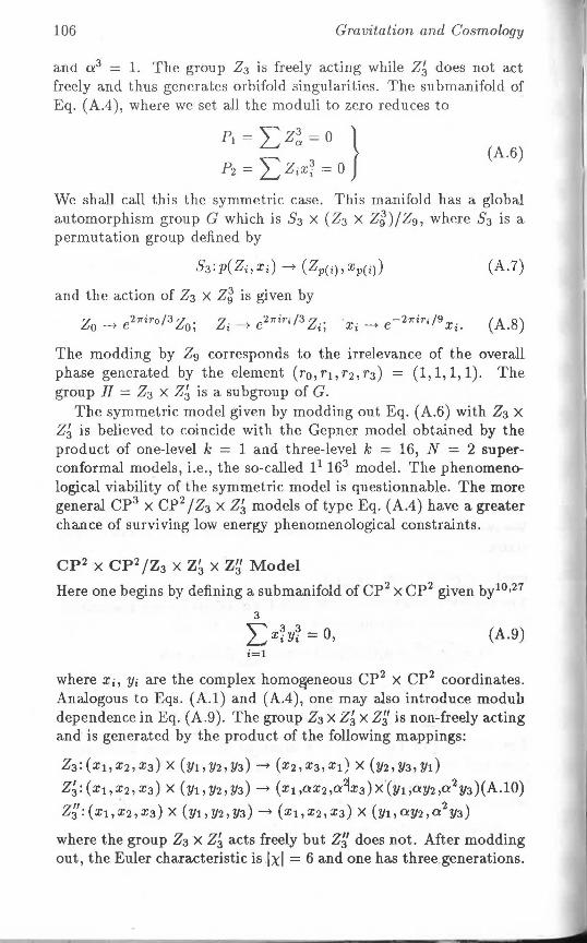
106 Gravitation and Cosmology
and a 3 = 1. The group Z3 is freely acting while Z~ does not act freely and thus generates orbifold singularities. The submanifold of Eq. (A.4), where we set all the moduli to zero reduces to
P1 = L z; = o } P2 = I:zixf = o
(A.6)
We shall call this the symmetric case. This manifold has a global automorphism group G which is S3 X (Z3 x Z2)/Z9, where S3 is a permutation group defined by
83: p( Z;, xi) -+ ( zp(i), xp(i))
and the action of Z3 x Z~ is given by
Z e27riro /3 z . 0-+ o, Z . e21firi/3z .. i~ i,
(A.7)
(A.8)
The madding by Z9 corresponds to the irrelevance of the overall phase generated by the element (ro,ri,r2 ,r3) = (1,1,1,1). The group H = Z3 x Z~ is a subgroup of G.
The symmetric model given by madding out Eq. (A.6) with Z3 x Z~ is believed to coincide with the Gepner model obtained by the product of one-level k = 1 and three-level k = 16, N = 2 superconformal models, i.e., the so-called 11 163 model. The phenomenological viability of the symmetric model is questionnable. The more general CP3 x CP2 /Z3 x Z~ models of type Eq. (A.4) have a greater chance of surviving low energy phenomenological constraints.
CP2 x CP2 /Z3 x z; x Z~ Model
Here one begins by defining a submanifold of CP2 x CP2 given by10·27
3
"'""'x~y~ = 0 ~ '' ' i=l
(A.9)
where Xi, Yi are the complex homo&eneous CP2 x CP2 coordinates. Analogous to Eqs. (A.l) and (A.4), one may also introduce moduli dependence in Eq. (A.9). The group Z3 x Z~ x Z~' is non-freely acting and is generated by the product of the following mappings:
Z3:(xi,x2,x3) X (y1,Y2,y3)-+ (x2,X3,x1) X (y2,y3,y1)
Z~: (xi,x2, x3) X (y1, Y2, y3)-+ (x1 ,ax2,a~x3) x"(y1,ay2,a2y3)(A.l0)
Z~':(xi,~2,x3) X (y1,y2,y3)-+ (xi,x2,x3) X (yi,ay2,a2y3)
where the group Z3 x Z~ acts freely but Z~' does not. After madding out, the Euler characteristic is lxl = 6 and one has three generations.
Superstring Theory 107
References
1. For a review of development of tne superstring theory see "Superstring Theory", by Green, M., Schwarz, J. and Witten, E., Cambridge University Press, 1987.
2. Gross, D.G., Harvey, J., Martinec, E. and Rhom, R.: Phys. Lett., 55 {1985), 502; Nucl. Phys., B258 (1985), 253.
3. Candelas, P., Horowitz, G.T., Strominger, A. a.nd Witten, E.: Nucl. Phys., B256 (1985), 46.
4. Dixon, L., Harvey, J., Vafa, C. and Witten, F.: Nucl. Phys., B261 (1986), 678; B274 {1986), 285; Na.rain, K.S., Sa.rma.di, M.H. a.nd Va.fa, C.: Nucl. Phys., B288 {1987), 551; lbaiies, L.E., Nilles, H.P. a.nd Quenedo, F.: Phys. Lett., B187 {1987), 215.
5. Cvetic, M. in Proceedings of the Eighth Workshop on Grand Unification a.t Syracuse 1987, (ed.) Wali, K.C.: World Scientific, Singapore, 1987, p. 312.
6. Nara.in, K.S.: Phya. Lett., 169B {1986}, 41; Kawai, H., Lewellen, D.C. and Tye, S.H.: Nucl. Phys., B286 (1987), 1; Antoniodis, I., Bachas, C. and Kounnas, C.: Nucl. Phya., B289 (1987), 87; Lerche, W., Lust, D. and Schellekens, A.N.: Nucl. Phya., B287 (1987), 477; Chamseddine, A.H. and Derendinger, J.P.: Nucl. Phya., B301 (1988), 381; Cha.mseddine, A.H. and Quiros, M.: CERN-TH, 5100/88.
7. Gepner, D.: Phya. Lett., B199 {1987), 380; Nucl. Ph1!fJ., B296 {1988), 75. 8. Antoniodis, I., Ellis, J., Hagelin, J.S. and Nanopoulos, D.V.: PhytJ. Lett.,
194B (1987), 231; Campbell, B., Ellis, J., Hagelin, J.S., Nanopoulos, D.V. and Olive, K.: Phys. Lett., 197B {1987), 355.
9. See Font, A.: Talk at the Europhysics Conference on High Energy Physics, Madrid, Spain, September 1989.
10. Tian, G. a.nd Yau, S.T. in Proceedings of the Argonne Symposium on "Anomalies, Geometry and Topology", (eds.) Bardeen, W.A. and White, R.A.: World Scientific, Singapore, 1986.
11. Greene, B., Kirklin, K.H., Miron, P.J. and Ross, G.G.: PhytJ. Lett., B180 {1986), 691; Nucl. Phya., B274 (1986), 574; B278 (1986), 667; B292 (1987), 606.
12. Ellis, J., Enqvist, K., Olive, K.A. and Reiss, D.: Nucl. Phys., B296 (1986), 129; Ellis, J., Enqvist, K., Nanopoulos, D.V. and Olive, K.A.: Phys. Lett., B188 (1987), 415; Dine, M. and Lee, C.: Phya. Lett., B203 (1988), 371.
13. Candelas, P.: Nucl. P,.ys., B298 (1988), 458; Kalara, S. and Mohapa.tra, R.N.: Phys. Rev., 036 (1987), 3474.
14. Bento, M.C., Ha.II, L. and Ross, G.G.: Nucl. Phys., B292 (1987), 400. 15. Laza.rides, G., Panagiotakopoulos, C. and Shafi, Q.: Nucl. Phys., B278
(1986), 657; Phys. Rev. Lett., 56 (1986), 432; Laza.rides, G. and Shafi, Q.: UT-STPD-1/88-UT-STPD-3/88.
16. del Aguilla, F. and Coughlan, C.D.: Phys. Lett., 215B (1988), 93. 17. Nath, P. and Arnowitt, R.: PhytJ. Rev., 039 (1989), 2006. 18. Arnowitt, R. and Nath, P.: Phys. Rev., 040 (1989), 191. 19. Nath, P. and Arnowitt, R.: Phys. Rev. Lett., 62 (1989), 1427. 20. Arnowitt, R. and Nath, P.: Phys. Rev. Lett., 62 (1989), 2225. 2L Schimmrigk, R.: Phys. Lett., 193B (1988), 757. 22. The Yukawa couplings of this cla.BS of models have been given by a number
of authors (see Ref. 23), while the phenomenology has been discussed in Ref. 24.
108 Gravitation and Cosmology
23. Sotkov, G. and Stanishkov, M.: Phys. Lett., B215 (1988), 674; Kato, A. and Kitazawa, Y.: University of Tokyo Preprint, UT-535, 1988; Cordes, S.F. and Kikuchi, Y.: CTP-TAMU-92/88; Mod. Phys. Lett., A4 (1989), 1365; Greene, B.R., Liitkens, C.A. and Ross, G.G.: NORDITA-89/8P; HUTP-88/ A.062.
24. Ross, G.G.: "A Three-Generation Heterotic String Model", to be published in Proceedings of the "Strings 89" Conference at Texas A&M University, (ed.) Arnowitt, R., Bryan, R., Duff, M. and Pope, C.: World Scientific, Singapore, 1989.
25. Recently 25 new three-generation models have been discovered using CalabiYau manifolds in weighted prnjective space P4 (see Ref. 26). However, all of these models are formulated on simply connected manifolds and thus are not phenomenologically viable models.
26. Candelas, P., Lynker, M. and Schimmrigk, R.: "Calabi-Yau Manifolds in Weighted P4", UTTG-37-89; NSF-ITP-89··164.
27. Greene, B.R. and Kirklin, K.H.: Commun. Math. Phys., 113 (1987), 105. 28. Greene, B.R., Liitken, C.A. and Ross, G.G.: NORDITA-89/8P; HUTP-
88/ A062. 29. The alternate possibility is the case where Z~ is embedded trivially, i.e.,
U,. = 1 and Za is embedded non-trivially, i.e., U 9 = diag(l ll)c ®diag(O'O'O')L ® diag(O'O'O')R·
30. Nath, P. and Arnowitt, R.: "An Overview of Three-Generation Calabi-Yau Models", to appear in Proceedings of the "High Energy and Cosmology Workshop" at Trieste, Italy, 1989, (ed.) Pati, J.C. and Shafi, Q.: World Scientific, Singapore.
31. Arnowitt, R. and Na.th, P.: "Model Building on Ca.labi-Ya.u- Manifolds", to appear in Proceedings of the International Europhysics Conference on High Energy Physics, Madrid, Spa.in, September 6-13, 1989.
32. Distler, J. and Greene, B.R.: Nucl. Phys., B309 (1988), 295. 33. del Aguilla., F., Coughlan, C.D. and Masip, M.: Phys. Lett. 227B (1989),
55. 34. Na.th, P. and Arnowitt, R.: "Neutrino Masses in Three-Generation Calabi
Yau Models", to appear in Proceedings of the International Europhysics Conference on High Energy Physics, Madrid, Spain, September 6-13, 1989.
35. See Totsuk.a, Y. in Proceedings of the XXIV International Conference on High Energy Physics, Munich, August 4-10, 1988, p. 282.
36. Amaldi, V. et al., Phya. Rev., 036 (1987), 1385; Costa, G. et al., Nucl. Phya., B297 (1988), 244.
37. The result is taken from Thresher, J., talk a.t CERN, October 13, 1989. A more recent revised value is N., = 3.01 ± 0.15 ± .05.
38. For a review, see Nath, P., Arnowitt, R. and Chamseddine, A.H.: "Applied N = 1 Supergravity", World Scientific, Singapore, 1983.
39. Arnowitt, R., Cha.mseddine, A.H. and Nath, P.: Phys. Rev. Lett., 60 (1983), 232; Cha.mseddine, A.H., Na.th, P. and Arnowitt, R.: Phys. Lett., 129B (1983), 445.
Description of Intrinsic Abelian
and Non-Abelian Interactions
of a Test String*
KAMESHWAR C. WALI
Physics Department, Syracuse University Syracuse, New York 13244-1130, USA
1. Introduction
In a classic paper in 1971, Nambu discussed the electromagnetic interactions of a ha.dronic string with dual resonance model in mind.2
Although dual resonance model is no longer in vogue, the questions Nam bu raised, such as gauge invariance and parametric invariance, remain relevant if quarks and leptons are extended unidimensional objects. Moreover, recently there- has been considerable interest in cosmic vortex lines which may have been formed in the early universe.3 For cosmological purposes, the transverse dimensions of cosmic vortex can be ignored, and consequently from a practical point of view, the vortex can be considered as a Nambu-Gotto string. While the possibility of observing such strings through their gravitational effects (gravitational lensing and gravitational radiation) has created a great deal of interest, Witten's demonstration that, if such strings are superconducting, they will have more dramatic observational effects than their gravitational counterparts, has brought the study of their electromagnetic interactions to the forefront.4 •5
In this paper we use the dimensional reduction techniques inherent in Kaluza-Klein theories6 to describe the interactions of a string. We recall that in the case of a point particle, its free propagation in a curved four space-time background defines a geodesic. If the particle is charged and if there a.re external electromagnetic fields, the trajectory is modified. However, if the gauge potentials corresponding to the fields are embedded in a higher dimensional metric tensor, as a matter of reality or merely as a technical device, the physical fourdimensional trajectory modified by the interactions can be viewed as a, projection of a parent Kaluza-Klein geodesic.
* This paper is based on the joint work with Aharon Davidson.1
110 Gravitation and Cosmology
In the case of a string, its free propagation is described by the Nam bu-Gotto action. If we embed the gauge potentials in a generalized metric tensor GM N, then the equation of motion in the assumed higher dimensions take the form
[o(- G)1/2] _ o(-G)1/2 _ -"--M~- M - 0, M = 0,1,2, ... ' ox ( ox ,( '
(1.1)
where ( = r,a, G = det llG7 ull = the determinant of the induced two-metric G7 u on the world sheet, and
OXM
ox':(= T("
From these equations, we can derive a set of locally conserved currents due to isometries of the extra dimensions beyond the conventional four. Using these currents, we can reduce the above equation to the form
[6(- g)
112] - o(-g)
112 =!gauge+ rcalar + relf (1.2) oxµ ( oxµ µ I-'. µ ' ·' . where 9 = det ll9Tull = det ll9µ11x;7 x~ull·
The physical interpretation of Eq. (1.2) is clear. The left-hand side represents the equation of motion arising from the background four-dimensional metric and the right-hand side represents forces arising from the gauge and scalar potentials embedded in the extra dimensions.
In the next section, we shall consider the case of an Abelian interaction of a test string. In Sec. 3, the example of a circular test loop will be discussed with emphasis on its self-interactions. These self-interactions are intrinsic to the string and are present even when 9µ 11 is flat, and eyen when the external fields are absent. Further, these self-interactions produce dynamically stable solutions whose physical interpretation tells us that the test loop is superconducting and has angular momentum because of the intrinsic electromagnetic currents. In Sec. 4, we consider briefly the non-Abelian case by introducing two extra degrees of freedom. The final section is devoted to a summary and conclusions.
2. Abelian (Electromagnetic) Interactions of a Test String
Following the general ideas of Kaluza-Klein theory,6 let us consider the free propagation of a test string in a five-dimensional space-time whose metric GMN is described by
G = ,1..-l/J [9µ11 + </JAµA11 MN 'I' </JA11 (2.1)
- ---.~ - ~
Interactions of a Test String 111
so that, with µ, 11 = 0, 1, 2, 3 and Aµ as the external electromagnetic potential,
Gµ11 = cp-1 l 3 (gµ11 + </JAµA11), Gsµ= Gµs = cp2/
3 Aµ, Gss = </J. (2.2)
If we set <P = 1 and suppress the scalar (Brans-Dicke) degree of freedom, Eq. (2.1) leads one virtually to Einstein-Maxwell theory. We can then ignore the question whether th& fifth-dimension is a reality and treat it merely as a technical device to introduce electromagnetic interactions. Although it is straightforward to include <P and carry out the analysis, for the sake of simplicity, we shall set </> = 1.
Let Ya = ( r, O') denote the intrinsic coordinates of the string. Then, the two metric Gaf3 induced on the world-sheet described by the free propagation of the string is given by
(2.3)
where
If we define (2.4)
then (2.5)
where (2.6)
Let us define
G = det llGaf311 and g = det ll9af311· (2.7)
Then, (2.8)
where f.Ol"Y f.{J6 g 6
g0t{3 - 'Y - , -g
0tf3 = [ 0 1] f. -1 0 ,
so that 0t{3 J;Ot
g 9(36 = (J6. (2.9)
The Nambu-Gotto action S for the string is given by
S = -c j j dydy2 [-G]112, (2.10)
112 Gravitation and Cosmology
where c is a constant, which we shall set equal to unity. independent of x 5 , we obtain the conservation law
(Q a) . h Qa __ 8L __ _ 8L 1 ,a= 0 wit
8x~a 8Aa
where
Since G is
(2.11)
(2.12)
Using Eq. (2.11), we would like to remove the dependence of G on x5a and write the dynamical equations of motion in the physical four-dimensional space-time. Lis a function of xµ, xµa and L\a. The equations of motion that follow from Eq. (2.12) hav~ the form
[ fJL a ] [ fJL a A 11 ] 8x;a + Q Aµ ,a - OXµ + Q v,µX,a = O, (2.13)
where we have used Eqs. (2.6) and (2.11). It is easy to 'verify that the above equations of motion can be
derived fro:rrul,Il ''effective' Lagrangian £, given by
£ = L(xµ,x;a,Lia) + Qa(Aµx;a - Ka), (2.14)
where Lia is .6.a expressed in terms of xµ, xµa and Qa, so that £, is a function of only the four-dimensional c~ordinates xµ, their derivatives and the conserved quantities Qa. We note further that· we can define
(2.15)
where V( r, a) is a scalar function of ( r, a) on the world sheet. Then, ( Q 0 ),o = 0 is identically satisfied. Further, if we substitute Eq. (2.15) in Eq. (2.14) and vary with respect to V';13, we obtain the condition
€a.O(A1,x;a - Lia),13 = 0, (2.16)
which follows from Eq. (2.6) and the requirement (x~a),13 = (x~13 ),a· We can look upon V( r, a) as a scalar potential on the world
sheet, which replaces the fifth-dimensional coordinate x5 (r,a). The intrinsic electromagnetic properties of the string are embodied in V ( r, a). Thus the effective four-dimensional Lagrangian £, takes the form
£ = [-g(l + gal3 LiaLi13)]112 + E013V';13(Aµx;a - Lia), (2.17)
where, from the relation
a _ 8L _ _ 1/2 gal3 .6.13 Q - 8Aa - ( g) [1 + g-Y6 A-yA5]112 '
we obtain
(2.18)
- - J - ..._..
Interactions of a Test String 113
Substituting for ~a in Eq. (2.17),
[, = [-g(l + ga.8V:aV:,a)]112 + €a,8V:.OAµx;a (2.19a)
[ €a,8 ]
= F9 M + H V:.a Aµx;a , (2.19b)
where we have defined M = (1 + ga.8V:a V:.a)t/2 The four-dimensional equations of motion that follow from Eqs.
(2.19) are
where
and
. 8Av 8Aµ with Fµv = ~ - ~' uxµ uxv
/ &elf= _!_ [· c-;OM - M oFg ~ [ c-; oM] ] µ ll V -g i: ·µ ,a i: µ V -g i: µ · 1v.t vX vX ,a vX ,a ,a
(2.20)
(2.21)
(2.21)
The electromagnetiC force given by Eq. (2.21) is the familiar analog of the point particle case with M playing the role of generalized inertial 'mass', which is not necessarily a constant in the case of the string, in contrast with that of a point particle. It stays as a local quantity. It has its origin in the intrinsic electromagnetic properties of the string, since it does not vanish even in flat space devoid of external potentials. The expression for /~elf given by Eq. (2.21) has no analog in the point particle case.
3. Self-Interactions of Circular Loops
To illustrate the dynamical consequences of the self-interactions arising out of intrinsic electromagnetic properties of the string, we shall consider a circular test string propagating in a flat background with no external fields.
We note that the world-sheet is characterized by the condition of periodicity in a, namely,
(r,u + 211') = (r,u),
which implies that the internal topology of this world-sheet is Rix S1. Transformations on the world-sheet are then restricted tor - A(r), <r - <r + B( r ). Taking this into consideration, let us require the world~sheet metric 9a.8 expressed in cylindrical coordinates
9a,8 = -z~z~ + ZaZ,8 + rar,a + r 2cpacp,a, (3.1)
114 Gravitation and Cosmology
to be a independent. This requirement is satisfied by the following ansatz:
x0 (T,a) = T, z(T,a) = 0, r(T,a) = r(T), cp(T,a) =a. (3.2)
Further, since only the derivatives of V appear in the Lagrangian, we can choose
V~r,a) = v(T) + na, (3.3)
where n is necessarily a constant. This is not the most general assumption. However, it is sufficiently general to illustrate our main point. Further, if we consider the analogous assumption for x5 (T,a) = j(T)+na, n has to be an integer to lend itself to the interpretation that as a goes from 0 to 27r, x 5 wraps around n times. We shall soon see the physical implication of this assumption. The effective Lagrangian (with no external fields) has the form
(3.4)
From Eqs. (3.1), (3.2), (3.3) and (3.4), it is straightforward to calculate the equations of motion. Since x 0 , V and cp do not appear explicitly in the Lagrangian (3.4),
d~ c2 ~ n2) = 0 --t
r2 + n2 E = f = constant, (3.5)
.:!__ (v + r2) = o --t
dr f vr2
m = f = constant, (3.6)
ddT(nvf·r2)--o ~ ~ l = nm = constant, (3.7)
where dot refers to differentiation with respect to T and f = [(1 -r2 )(r2 + n2 ) - r2 v2 ]112 • The above constants of the motion imply the consistency relations,
v(T) = Er~r) (r2(;) + n2), (3.8a)
E2r2(r) + (r2(1) + m2n2) = E2 - n2 - m2. r 2 (r)
(3.8b)
Combining these with the equation giving the value of r(; ), namely,
ddr (r(r2; n2)) = 7(-r(l ~ r-2 - v2)), (3.9)
we obtain the solution
r 2 (r) = A2 + a2 cos 2r,
E (3.10)
Interactions of a Test String
where
A2 = !(E2 - n2
- m2) ' and a4 = A4
- n2 m2•
2
115
(3.11)
Equation (3.10) represents a stable, oscillatory solution with a periodicity 1T' E. The currents Q'T and Qu are given by
2
Qu = Eu'Tv;'T = -v( r) = ~ ( 1 + r2C T)). (3.12)
According to the standard Kaluza-Klein interpretation, Q'T represents the total charge and hence, on empirical grounds, n is an integer. We, therefore, do not have to invoke the:correspondence between V(r,O') and x5 • Further,
1 J ~[, Lz oc Pr.p = 21T' ~cp dO' =nm,
where Lz is the z-component of the angular momentum. It is c1ear that this angular momentum has its origin in the electromagnetic self-interaction, and one can show that m is the total number of magnetic fl.uxons involved.
Further, since the solution has the periodicity of 1T' E, we may ask whether an observer in four space-time dimensions can tell the difference between T = 0 and T = 1T' E configurations. In order that the two configurations a.re totally indistinguishable, the selfinteractions ought to have a periodicity as well. Therefore, it is crucial that dx5 = 21T' N, where N is an integer, since otherwise a non-vanishing phase [exp id v( T)] will manifest itself in the selfinteractions. Interestingly, from integrating Eq. (3.Sa), we find that
dv = ±(lml + lnl)'IT', (3.13)
and hence the condition that there be no phase change leads to
lml + lnl = 2N. (3.14)
Note that if m = O, the charge is quantized in units of two. Therefore, m # 0. Then, it follows that the test loop with unit charge has integral number of magnetic ftuxons. Hence, it superconducts, has non-vanishing angular momentum, since nm # 0.
Finally, a word about the generalized 'inertial' mass,
r 2(r)+n2
MJ = r2(r) + m2. (3.15)
For the static solution r 2(r) = mn, M 2 is obviously a constant. But this is kinematic coinddence. The alternate way in which M 2
116 Gravitation and Cosmology
can be a constant is when m 2 = n 2 • Tlds seems to have deeper physical significance, since it follows from a simple covariant constraint
(3.16)
and may be regarded as a generalized equivalence principle: Further, if lml = lnl, then lml + lnl = 2lnl, and therefore we have two angular momentum states ( m = ± 1) for a test loop with unit charge.
4. Non-Abelian Circular Loop
Suppose we introduce two additional degrees of freedom and consider an underlying M4 x S2 line element, namely,
ds2 = -dt2 + dz2 + dr2 + r 2dcp2 + (da 2 + sin2 ad(32), (4))
where a(r,a) and f3(r,a) are the additional degrees of freedom. The circular loop ansatz will be as in the abelian case x0 = r, z = 0, r = r( T), cp = a. The new intrinsic properties of the string will be embodied in a( r, a) and (3( r, a). The simplest ansatz of sufficient complexity for our purpose is
a(r,a) = A(r), (3(r,a) = B(r) + na,
so chosen that the world-sheet metric is a independent:
(4.2)
G o o + 2 2(3 (3 (4 3) ru = -x,rx,u+z,-rz,u+r,rr,u r 'P,r'P,u+a,ra,u+a ,r ,u .
Since the Lagrangian is independent of x0 ( r, a), cp( r, a) and f3(r,u), we obtain three constants of motion. Using thei;e, the circular loop ansatz, and Eq. ( 4.2), we can derive the following equations for r(r), A(r) and B(r):
1 ·2 [ 2 n2n2] 2 w2 r + r + ----;:2 = c1, ( 4.4a)
1 . n2
-A2 + [-- + n2 sin2 A] w 2 sin2 A
( 4.4b)
. [ 1. nz J B=Ow --+-, sin2 A r 2 ( 4.4c)
where c1 , c2 , w and n are constants with a consistency condition among them, viz.,
2 2 1 Cl+ Cz = 2· (4.5)
w Equation ( 4.4a) resembles the equation for a non-relativistic simple harmonic oscillator carrying 'angular momentum' On and total energy c~ (~ 2IOnl). It is the 0 2n2 /r2 term that prevents the collapse of the circular loop, as evident from the solution
1 (1 )1/2 r2 (T)= 2c~+ 4c~-02 n2 cos2wT. (4.6)
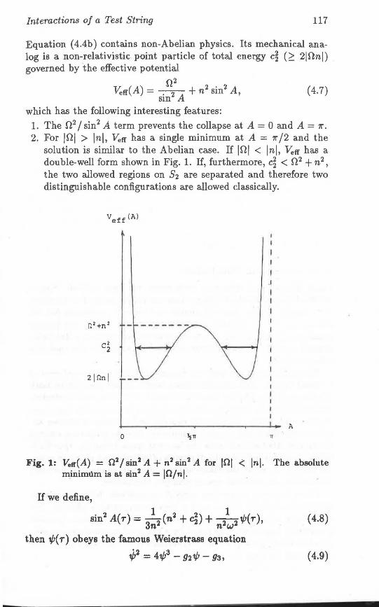
Interactions of a Test String 117
Equation ( 4.4b) contains non-Abelian physics. Its mechanical analog is a non-relativistic point particle of total energy c~ (~ 2J!lnl) governed by the effective potential
Vetr(A)= .n: +n2 sin2 A, (4.7) sm A
which has the following interesting features:
1. The n2 I sin2 A term prevents the collapse at A = 0 and A = 'Tr.
2. For JOI > lnl, Vetr has a single minimum at A = 7r /2 and the solution is similar to the Abelian case. If JOI < lnl, Vetr has a double-well form shown in Fig. 1. If, furthermore, c~ < 0 2 + n2 ,
the two allowed regions on S2 are separated and therefore two distinguishable configurations are allowed classically.
veff (A)
.I
I I I
112+n2
c2 2
21nnl r- I I I
I .. A
0 ~1T 71
Fig. 1: °Veff{A) = 0 2 / sin2 A + n 2 sin2 A for IOI <: lnl. The absolute
rninimllm is at sin2 A= IO/nl.
H we define,
sin2 A(r) = 3
12 (n2 + c~) + ~1/J(r), (4.8)
n . n w then ¢( r) obeys the famous Weierstrass equation
·2 3 1/J = 41/J - 921/J - g3, (4.9)
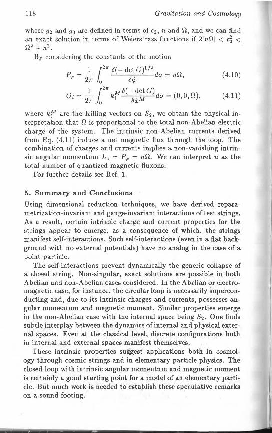
118 Gravitation and Cosmology
where 92 and 93 are defined in terms of c2, n and n, and we can find an exact solution in terms of Weierstrass functions if 2JnnJ < c~ < n2 + n2.
By considering the constants of the motion
_ 1 1 2 71" 6(- det G)1/2 _
p"' - - du - nn, 271" 0 6cp (4.10)
Q. = __!_ 1271" kM 6( - det G) d = (0 0 n) t 2 t i:"M (J ' ,H'
11" 0 ux (4.11)
where kf'1 are the Killing vectors on S2 , we obtain the physical interpretation that n is proportional to the total non-Abel1an electric charge of the system. The intrinsic non-Abelian currents derived from Eq. (4.11) induce a net magnetic flux through the loop. The combination of charges and currents implies a non-vanishing intrinsic angular momentum Lz = P"' = nn. We can interpret n as the total number of quantized magnetic fluxons.
For further details see Ref. 1.
5. Summary and Conclusions
Using dimensional reduction techniques, we have derived reparametrization-invariant and gauge-invariant interactions of test strings. As a result, certain intrinsic charge and current properties for the strings appear to emerge, as a consequence of which, the strings manifest self-interactions. Such self-interactions (even in a flat background with no external potentials) have no analog in the case of a point particle.
The self-interactions prevent dynamically the generic collapse of a closed string. Non-singular, exact solutions are possible in both Abelian and non-Abelian cases considered. In the Abelian or electromagnetic case, for instance, the circular loop is necessarily superconducting and, due to its intrinsic charges and currents, possesses angular momentum and magnetic moment. Similar properties emerge in the non-Abelian case with the internal space being S2 • One find's subtle interplay between the dynamics of internal and physical external spaces. Even at the classical level, discrete configurations both in internal and external spaces manifest themselves.
These intrinsic properties suggest applications both in cosmology through cosmic strings and in elementary particle physics. The closed loop with intrinsic angular momentum a.nd magnetic moment is certainly a good starting point for a model of an elementary particle. But much work is needed to establish these speculative remarks on a sound footing.
----. - -
Interactions of a Test String 119
6. Acknowledgements
This work was supported by the U.S. Department of Energy under contract No. DE-FG02-85ER40231.
References
1. Davidson, A. and Wall, K.C.: Phys. Lett., 213B (1988), 439; Davidson, A. and Wa.li, K.C.: Phys. Rev. Lett., 61 {1988), 1450; A more detailed pa.per of the a.hove authors is currently under preparation.
2. Na.mbu, Y.: Phys. Rev., 04 (1971), 1193. 3. See for instance, Vilenkin, A.: Phys. Rep., 121, 5 (1985), 264-315. 4. Witten, E.: Nucl. Phys., B249 (1985), 557. 5. Neilsen, N.K. a.nd Olesen, P.: Nucl. Phys., B291 (1987), 8~:1; ibid., B298
(1988), 776. References to their earlier a.nd other relevant papers a.re contained themn.
6. For reference to original as well a.s more recent developments, see Appelquist, T., Chodos, A. and Freund, P.G.O.: "Modern Ka.luza.-Klein Theories", Addison-Wesley Publishing Company, Inc., 1987.
Phase Transitions in the
Early Universe
AMITABHA MUKHERJEE
Department of Physics and Astrophysics University of Delhi, Delhi 110 007
1. Introduction
In the past decade, the subject of phase transitions in the early universe has come to be of great importance. There has been a convergence of interests between particle physicists, seeking a testing ground for their theories at energies far beyond present accelerator capabilities, and cosmologists, looking for possible solutions to some of the problems that beset the 'standard' big-bang cosmological model. In addition to inputs from particle physics models and cosmology, the study of phase transitions in the early universe involves ideas from quantum field theory, statistical mechanics and foundational aspects of quantum mechanics. Thus the scope of the study is vast. and any presentation necessarily selective. What is attempted here is a bird's-eye view of the subject, incorporating some recent work as well as posing some open questions, without any claim of being comprehensive.1
2. General Considerations
We know from condensed-matter physics that a phase transition is characterized by a change in the behaviour ·of some order parameter. As an example, consider the paramagnetic-ferromagnetic phase transition. Above a critical temperature Tc, the Curie point, the paramagnetic phase is the stable one, while below Tc the ferromagnetic phase is stable. (Here the notion of stabl.lity is purely thermodynamic: the stabler of two phases is the_ one for which the free energy is lower.) The order parameter is the macroscopic magnetisation M. The para-phase has M = 0 while the ferro-phase shows spontaneous magnetization, i.e., has M > O. The presence of long-ra.nge order in the phase which is sta.ble a.t low temperatures-and its absence in the phase which is stable at high temperatures- is cha.ra.cteristic of a large number of systems.
~. -. - - --
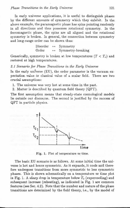
Phase Transitions in the Early Universe 121
In early universe applications, it is useful to distinguish phases by the different amounts of symmetry which they exhibit. In the above example, the paramagnetic phase has spins pointing randomly in all directions and thus possesses rotational symmetr-y. In the ferromagnetic phase, the spins are all aligned and the rotational symmetry is broken. In general, the connection between symmetry and long-range order can be shown thus:
Disorder +-+ Symmetry Order +-+ Symmetry-breaking
Generically, symmetry is broken at low temperatures (T < Tc) and restored at high temperatures.
2.1 Scenario for Phase Transitions in the Early Universe
In the early universe (EU), the order parameter is the vacuum expectatiOR -value or classical value of a scalar field. There are two crucial assumptions:
1. The universe was very hot at some time in the past. 2. Matter is described by quantum field theory (QFT).
The first assumption means that steady-state cosmological models lie outside our discourse. The second is justified by the success of QFT in particle physics.
T
_ _ ___ j_ _ _
I I I
...... ...... _ time
Fig. 1. Plot of temperature vs time.
The basic EU scenario is as follows. At some initial time the universe is hot and hence symmetric. As it expands, it cools ancl therefore undergoes transitions from more symmetric to less symmetric phases. This is shown schematically on a temperature vs time plot in Fig. 1. A sharp drop in temperature below Tc (supercooling) and subsequent inCA"ease (reheating), as indicated in Fig. 1 are common features (see Set. 4.2). Note that the number and nature of the phase transitions are determined by the field theory, i.e., by the model of
122 Gravitation and Cosmology
fundamental interactions which we assume. The sequence of transitions essentially corresponds to the hierarchy of energy scales in any model. In the following section, we enumerate the transitions which are expected to be important according to the standard wisdom of particle physics.
2.2 Important Phase Transitions in the Early Universe
According to the currently accepted EU chronology, at very early times the temperature was greater than the Planck scale (""' 1019
GeV). Thus the behaviour of the universe as a whole was quantummechanical. It is believed that superstring theories will give a consistent way to quantise gravity. These theories possess a phase transition at ""' 1019 GeV.
There are good theoretical reasons (and no experimental evidence!) to believe that Grand Unified Theories ( G UTs) of weak, electromagnetic and strong interactions are a correct description of physics at very high energies. Correspondingly, there is a phase transition at ""' 1015 Ge V. Most particle physicists also believe that Nature is supersymmetric at such energies. There is, perhaps, a phase transition related to supersymmetry at around 1011 GeV.
The Glashow-Salam-Weinberg electroweak theory is now well established. The symmetry-breaking scale for this theory is around 250 GeV. The corresponding phase transition at ""' 102 GeV is one which everyone expects.
Strong interactions are supposed to be described by quantum chromodynamics (QCD). There are two phase changes associated with this theory: the chiral symmetry transition and the confinement/ deconfinement transition. Both have a characteristic scale -of 102 MeV.
At still lower temperatures (T < 10 MeV) there are other important transitions, such as the nuclear matter/nuclei transition. We shall exercise a particle physicist's prerogative and not consider those any further.
2.3 Classification of Phase Tmnsitions
Here we consider the classification of phase transitions according to two distinct criteria:· order of tansition and 'fast' vs 'slow'.
The distinction between first-order and second-order transitions has been made much of in the literature. It should, be remembered that in modern statistical mechanics the order of a transition is not considered very important. Nor do different definitions of the order of a tr.,,nsition always agree. Nevertheless, it is useful to adopt the following as operational definitions. In a first-order transition,
Phase Transitions in the Early Universe 123
the order parameter makes a sudden jump due to quantum tunnelling, while in a second-order transition, it evolves classically in time. Clearly we can also have a transition of mixed order in which the order parameter attains its final value through both quantum tunnelling and classical evolution. It should be emphasized that a purely (or overwhelmingly) second-order phase transition is a very unnatural thing, usually obtained by fine tuning of parameters in the theory. The generic phase transition involves potential barriers and tunnelling.
While the classification of phase transitions by their order is very general, the distinction between fast and slow transitions2 is peculiar to an expanding universe. 'Fast' and 'slow' are defined relative to the rate of expansion. More concretely, the quantity of interest is f', the transition probability per unit volume, defined by
- r f = V'
where r is the total transition rate and V the total volume. This has dimensions of (length )-4 • Now the characteristic length scale for an expanding universe is n-1 , where His the Hubble parameter. Thus the dimensionless quantity which characterizes a phase transition is
€:: f /H4•
A transition is slow if€ ~ 1; an example is the GUT transition. A fast transition is characterized by € "' 1. This is the case with the electroweak transition.
3. The Effective Potential The concept of the effective potential is both natural and useful in discussing phase transitions in QFT. Since detailed expositions of the effective potential technique exist in the literature,3 only a quick summary will be given below.
3.1 Definition of Vetr ( rp) Consider, for definiteness, the theory of a single scalar field, given by the Lagrangian
1 C = 2,8µip8µr.p - U(r.p). (3.1)
Classically, the energy is a minimum fJr that configuration which minimizes U ( <.p ). Our aim is to define an effective potential Vetr for the quantum theory which reduces to U(r.p) in the classical limit. .
Formally, we add a term J(x)r.p(x) to Eq. (3.1). The generating functional for Green functions, Z( J), is defined by
Z(J) = (0 I T[exp(i J Jipd4 x)] I 0). (3.2)
124 Gravitation and Cosmology
The related quantity W(J) is defined by
iW(J) = ln Z(J), (3.3)
and generates connected Green functions. One-particle-irreducible Green functions are generated by a function f( If), given by
f(<P)= [w(J)-JJ(x)cp(x)d4 x] 6w_. (3.4) 6J -<P
Formally, cp( x ), the argument of the functional f, is an arbitrary test function. In a translationally invariant theory, however, q; must be a constant. Then the effective potential Vetr( q;) is defined by
(3.5)
For more details, the reader is referred to ltzykson and Zuber.3 Here we list some important properties of V,,ff( tj;), which form the basis for its EU applications.
S.2 Properties of V,,ff( q;)
1. Vetr(<P) = U(cp) + O(n) (3.6) Thus Vetr satisfies our requirement that V,,tr( tj;) ---+ U( q;) in the limit n --7 0.
2. In the class of homogeneous stationary states with (c,o} = ip, Vetr( q;) is the minimum expectation value of the energy density. This justifies the interpretation of Vetr( ij;) as the free energy density. Thus, to investigate thermodynamic stability, we should look at the critical behaviour of Vetr· In a stable or metastable phase, the classical value of c,o should equal that at a minimum of V,,tr( tj;).
3. If V,,tr( cp) has a minimum at a non-zero value of q;, any symmetry which does not leave i:p invariant is spontaneously broken.
The above properties make V,,tr( q;) central to any study of symmetry-breaking in scalar QFT. In theories which have other fields in interaction with scalar fields, the situation is slightly more complicated. Nevertheless, °Vet£ remains important. In conventional GUTs as well as electroweak theory, the other fields are spin-1/2 fermions and spin-1 gauge fields. The Lagrangian can be written in the following schematic form:
L = LKE +Ly - U(c,o). (3.7)
Here LKE denotes the kinetic-energy term fur all fields, which incorporates the gauge interactions t'hrough minimal coupling, while Ly denotes the Yukawa coupling of fermions to scalar fields. The
-----~ ' - ___._ ..
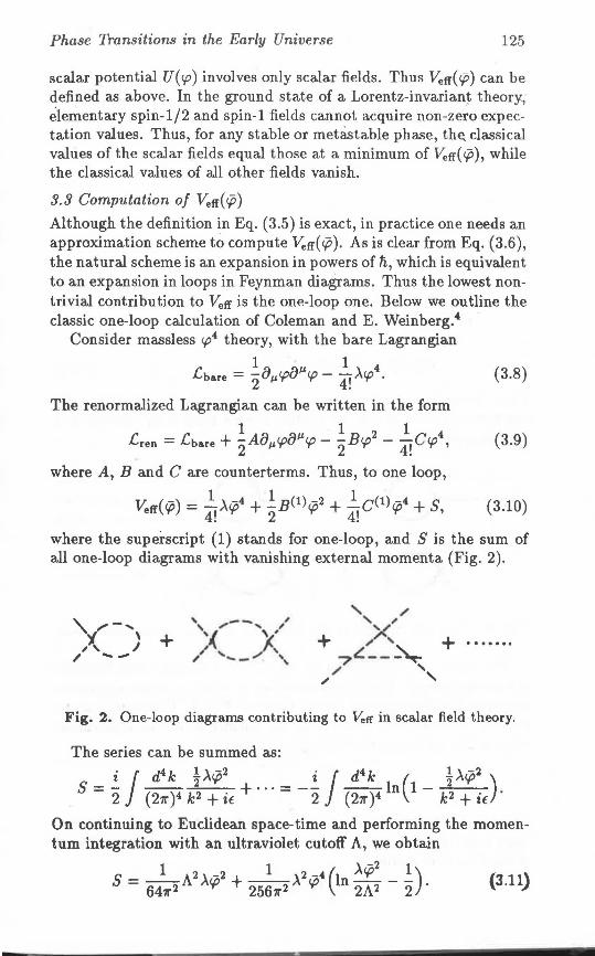
Phase Transitions in the Early Universe 125
scalar potential U( c.p) involves only scalar fields. Thus Vet1( <P) can be defined as above. In the ground state of a Lorentz-invarian.t theory, elementary spin-1/2 and spin-1 fields cannot acquire non-zero expectation values. Thus, for any stable or metastable phase, th~ classical values of the scalar fields equal those at a minimum of Vet1( <P), while the classical values of all other fields vanish.
3.3 Computation of Veff( <P) Although the definition in Eq. (3.5) is exact, in practice one needs an approximation scheme to compute Veff( <fi). As is clear from Eq. (3.6), the natural scheme is an expansion in powers of Ti, which is equivalent to an expansion in loops in Feynman diagrams. Thus the lowest nontrivial contribution to Vet1 is the one-loop one. Below we outline the classic one-loop calculation of Coleman and E. Weinberg.•
Consider massless r.p4 theory, with the bare Lagrangian
r - 1 ~ ~µ. 1 ' 4 "-'bare - ?,uµ. <.pu <.p - 41 A<.p • (3.8)
The renormalized Lagrangian can be written in the form
- 1 a aµ. 1 2 1 4 Lren - Lbare + 2 A µ.<.p 'P - 2 Br.p -
4! Ccp ' (3.9)
where A, B and C are counterterms. Thus, to one loop,
1 1 1 Vetr(<P) = 4!A<fi4 + 2B(1)<P2 + 4!C(l)<P4 + S, (3.10)
where the superscript (1) stands for one-loop, and S is the sum of all one-loop diagrams with vanishing external momenta (Fig. 2).
',..- ..... ,'( )
" --' / ' , ',, + ,,,,,..., + ...... .
...,,~--~ / ' ,, '
Fig. 2. One-loop diagrams contributing to V..tr in scalar field theory.
On continuing to Euclidean space-time and performing the momentum integration with an ultraviolet cutoff A, we obtain
1 2 -2 1 2 -• ( A<fi2 1) S = 6411"2 A A<.p + 25611'2 A c.p ln 2A2 - 2 . (3.11)
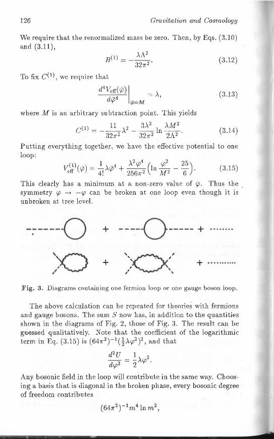
126 Gravitation and Cosmology
We require that the renormalized mass be zero. Then, by Eqs. (3.10) and (3.11),
B(1) - - >.A2 - 327r2. (3.12)
To fix C(1), we require that
d4
Vetr( <P) I = >. d-4 ' <p q>=M
(3.13)
where M is an arbitrary subtraction point. This yields
c<1) = -~>.2 - 3>.2 ln >.M2. 327r 2 3271" 2 2A 2
(3.14)
Putting everything together, we have the effective potential to one loop:
v(l)(-) - ~>. -4 + >.2rp4 (in rp2 - 25) elf <p - 4! <p . 256112 M 2 6 . (3.15)
This clearly has a minimum at a non-zero value of rp. Thus the symmetry <p -t -<p can be broken at one loop even though it is unbroken at tree level.
-~----0 + ---:-0----- + ········
' ..... CX,' + + ......... .. , ' ,' ...
Fig. 3. Diagrams containing one fermion loop or one gauge boson loop.
The above calculation can be repeated for theories with fermions and gauge bosons. The sum Snow has, in addition to the quantities shown in the diagrams of Fig. 2, those of Fig. 3. The result can be guessed qualitatively. Note that the coefficient of the logarithmic term in Eq. (3.15) is (647r2
)-1 ( !>.cp2) 2 , and that
d2U - ~>. 2 d<p2 - 2 <p .
Any bosonic field in the loop will contribute in the same way. Choosing a basis that is diagonal in the broken phase, every bosonic degree of freedom contributes
Phase Tronsitions in the Early Universe 127
where m is the mass. A Dirac fermion contributes
-4(647r2)-1 m 4 ln m 2 •
A class of theories which is of particular interest is one in which all the scalar v.e.v.'s are proportional to one another, and gauge fields and fermions acquire masses from this single v.e.v. Then
(1) - - l -4 >.2q;4 ( q;2 25) Veff ( c.p) - 4! >.c.p + c 25611'2 ln M2 - 6 '
where c is essentially a sum over (mass)4 terms.
3.4 Yeff( rp) at Non-zero Temperature
(3.16)
In deriving formulae like those given in Eq. (3.15), we used ordinary, zero-temperature QFT. But the early universe is very hot. Thus we need to do QFT at non-zero temperatures, where particles propagate in a thermal bath of temperature T. The formalism for this was developed in the mid-1970s.5 We have to replace Green functions G(xi, ... ,xn) by their T-dependent counterparts Gf3:
1 {3 = kT" (3.17)
The effect of finite f3 is a change in boundary conditions. On continuation to imaginary time, bosonic operators are periodic and fermionic operators are antiperiodic.
Periodicity in ix0 implies discreteness in the allowed values of ik0 .
Thus the Feynman rules change, e.g.,
etc.
Applying this to the calculation of i:~) ( rp) for scalar field theory, we obtain
i:~)/3( rp) = U( rp) + J (~:~3 [ ~k + * ln(l - e-f3Ek)]
+ counterterms. (3.18)
We can separate out the T-dependent part VT( rp):
VT( rp) = * J (~:~3 [1n(l - e-f3v'k2 +~>-~2 )]. (3.19)
Carrying out the angular integration, we have
VT('?)= 211'!{34 1( & f3), (3.20)
128 Gravitation and Cosmology
where
I(y) = 1= x2 dx ln(l - exp(-Jx2 + y2)). (3.21)
Note that VT( rp) is finite; thus at non-zero T there are no new renormalization consta:r:its beyond those in the zero-T theory.
The extension of Eqs. (3.20)-(3.21) to gauge theories is straightforward: in Eq. (3.20), the argument of T(y) is replaced by {3 times the square root of the appropriate mass term. Thus we have, for SU(2) x U(l),
(3.22)
where Ow is the electroweak mixing angle and g, the SU(2) coupling. Similarly, for minimal SU(5),
18 ( {25 ) VT( rp) = 7r2 [34 I v S gipf3 , (3.23)
where g is the gauge coupling. The above calculation can also be repeated for fermion loops, tak
ing the antiperiodicity into account. This has the effect of replacing I(y) by J(y), where
J(y)= 1= dxx2[1n{(1+x2
;Y2)/2}
+ ln { 1 + exp ( - ~ J x2 + y2) } J . (3.24)
At high temperatures (gr:p{3 ~ 1), I(y) can be expanded in a power series:
7r4 y2 7r2 I(y) ~ -- + - + O(y4
). 45 12
(3.25)
Thus, for example, for SU(2) X U(l),
1 7r2 Vetr('P, T) = Ve~)IJ(r:p) ~ Vetr('P, 0) +
32{3 2 (3g2 + g12
)cp2 - l0{34 ,
(3.26) where g' = g tan Ow-·
Because of the T 2 r:p2 term in Eq. (3.26), for T ~ Tc the only minimum of Vetr( r:p, T) is at r:p = 0. At some T a minimum appears (Fig. 4). At Tc, by definition, the two minima have equal depth. For T < Tc the minimum at rp = 0 becomes energetically unfavourable (metastable) and a phase transition takes place.
For some sufficiently low temperature T*, the minimum at r:p = 0 becomes a maximum, and the classical field can roll to the new
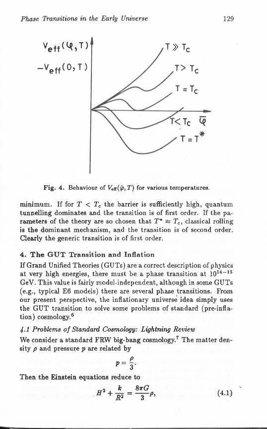
Phase Transitions in the Early Universe 129
lq
T =T*
Fig. 4. Behaviour of V..fl'( ip, T) for various temperatures.
minimum. If for T < Tc the barrier is sufficiently high, quantum tunnelling dominates and the transition is of first order. If the parameters of the theory are so chosen that T• ~ Tc, classical rolling is the dominant mechanism, and the transition is of second order. Clearly the generic transition is of first order.
4. The GUT Transition and Inflation
If Grand Unified Theories (GUTs) are a correct description of physics at very high energies, there must be a phase transition at 1014 - 15
GeV. This value is fairly model-independent, although in some GUTs (e.g., typical E6 models) there are several phase transitions. From our present perspective, the inflationary univers~ idea simply uses the GUT transition to solve some problems of standard (pre-inflation) cosmology. 6
4.1 Problems of Standard Cosmology: Lightning Review
We consider a standard FRW big-bang cosmology.7 The matter density p and pressu~e pare related by
p p- -- 3·
Then the Einstein equations reduce to
2 k 81rG H + R2 = -3-p, (4.1)
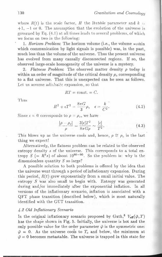
130 Gravitation and Cosmology
where R( t) is the scale factor, H the I-l u b blc parameter and k == + 1, -1 or 0. The assumption that the evolution of the universe is governed by Eq. (4.1) a.t a.11 times leads to several problems, of which we focus on two in the following:
1. Horizon Prob! m: The horizon volume (i.e., the volume within which comm.uni ·ation by light si nals is possible) was in tlle past, much less than the volume ofLh univers . Thns Lh present universe has volv -d from many causally disconnected regions. If s the observed large-scale homogeneity of the universe is a. mystery.
2. Flatn s P1·oblem: The ohserved matter density p today is within a.n order of magnitude of the criti al density Pc corr sponding to a flat universe. That this is unexp cted can be seen as follows. Let us assume adir •. hatic expansion, so that
Thu&
RT = const. = C.
2 87rG JI + ET2 = --p,
3
k -f = c2.
Since E = 0 corresponds to p =Pc, we have
( 4.2)
( 4.3)
This blows up as the universe cools and, hence, p ~ Pc is the last thing we expect!
Alternatively, the flatness problem can be related to the observed entropy density s of the universe. This corresponds to a total entropy S ( = R 3 s) of about 1080 - 90 . So the problem is: why is the dimensionless quantity S so large?
A possible solution to both problems is offered by the idea that the universe went through a period of inflationary expansion. During this period, R(t) grew exponentially from a small initial value. The entropy S was also small to begin with. Entropy was generated during and/or immediately after the exponential inflation. In all versions of the inflationary scenario, inflation is associated with a QFT phase transition (described below), which is most naturally identified with the GUT transition.
4. 2 Old Inflationary Scenario
In the original inflationary scenario proposed by Guth, 8 Vetr( r.p, T) has the shap·e shown in Fig. 5. Initially, the universe is hot and the only possible value for the order parameter cp is the symmetric one: cp = 0. As the universe coots to Tc and below, the minimum at cp = 0 becomes metastable. The universe is trapped in this state for
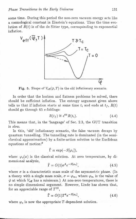
Phase Transitions in the Early Universe 131
some time. During this period the non-zero vacuum energy acts like a cosmological constant in Einstein's equations. Thus the time evolution of R(t) is of the de Sitter type, corresponding to exponential inflation.
T »Tc
Fig. 5. Shape of V.1r( cp, T) in the old inflationary scenario.
In order that the horizon and flatness problems be solved, there should be sufficient inflation. The entropy argument given above tells us that if inflation starts at some time ti and ends at t1, R(t) should go through 65 e-foldings:
R(t1) ~ e65 R(ti). (4.4)
This means that, in the 'language' of Sec. 2.3, the GUT transition is slow.
In this, 'old' inflationary scenario, the false vacuum decays by quantum tunnelling. The tunnelling rate is dominated (in the semi-classical approximation) by a finite-action solution to the Euclidean equations of motion:9
f' oc exp(-S[<pc]),
wher( 'Pc( x) is the classical solution. At zero temperature, by dimensional analysis,
(4.5)
where (j is a characteristic mass scale of the asymmetric phase. (In a theory with a single mass scale, (j = <f'm, where 'Pm is the value of rp at which Vetr has a minimum.) At non-zero temperatures, there is no simple dimensional argument. However, Linde has shown that, for an appreciable range of T10 ,
f' = 0(1)T4e-S(ipc), (4.6)
where 'Pc is now the appropriate T-dependent solution.
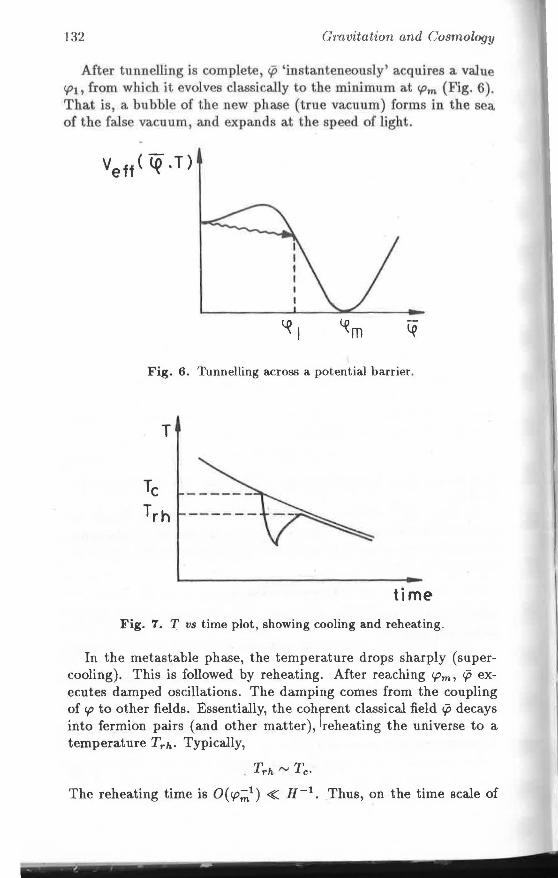
132 Gravitation and Cosmology
After tunnelling is complete cp 'instanteneously' acquires a value <pi, from wh.i hit volves c1assically to the minimum a.t <I'm (Fig. 6). That is, a bubble of the new phase (true vacuum) forms in the sea of the false vacuum, and expands at the speed of light.
Fig. 6. Tunnelling across a potential barrier.
time
Fig. 'T. T vs time plot, showing cooling and reheating.
In the metastable phase, the temperature drops sharply (supercooling). This is followed by reheating. After reaching <I'm, cp executes damped oscillations. The damping comes from the coupling of <p to other fields. Essentially, the cohfrent classical field i:p decays into fermion pairs (and other matter), !reheating the universe to a temperature Trh· Typically,
The reheating time is 0( rp~1 ) ~ n-1 . Thus, on the time scale of
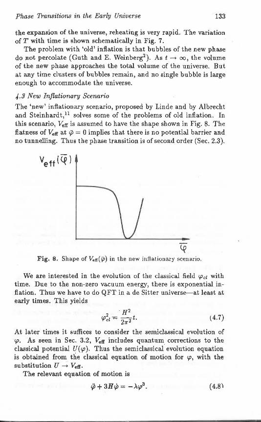
Phase Transitions in the Early Universe 133
the expansion of the universe, reheating is very rapid. The variation of T with time is shown schematically in Fig. 7.
The problem with 'old' inflation is that bubbles of the new phase do not percolate (Guth and E. Weinberg2 ). As t-+ oo, the volume of the new phase approaches the total volume of the universe. But at any time clusters of bubbles remain, and no single bubble is large enough to accommodate the universe .
. {3 New Inflationary Scenario
The 'new' inflationary scenario, proposed by Linde and by Albrecht and Steinhardt,11 solves some of the problems of old inflation. In this scenario, l'etr is assumed to have the shape shown in Fig. 8. The flatness of l'etr at q; = 0 implies that there is no potential barrier and no tunnelling. Thus the phase transition is of second order (Sec. 2.3).
4> Fig. 8. Shape of V..tr( cp) in the new inflationary scenario.
We are interested in the evolution of the classical field 'Pel with time. Due to the non-zero vacuum energy, there is exponential inflation. Thus we have to do QFT in a de Sitter universe-at least at early times. This yields
l4.7)
At later times it suffices to consider the semiclassical evolution of cp. As seen in Sec. 3.2, l'etr includes quantum corrections to the classical potential U( 'P ). Thus the semiclassicai' evolution equation is obtained from the classical equation of motion for cp, with the substitution U -+ Vetr·
The relevant equation of motion is
(4.8)
134 Gmvitation and Cosmology
Approximate solutions to Eq. (4.8) can be obtained in two time regions:
(i) Slow rolling: Here <{; can be neglected, yielding
(3ii 1 rp(t) = v -v:-;;t* - t.
(ii) Acceleration: Here the II<{! term is negligible. Thus
fi -1 rp(t) = y-:\ [a -- (t - to)] .
( 4.9)
( 4.10)
An approximate solution to Eq. ( 4.8), valid for all times of interest, is obtained by suitably combining Eqs. (4.9) and (4.10). The presence of a large damping term implies that reheating is rapid, as in the old inflationary SO\nario.
The main prQblem with this scenario, from our present perspective, is - that the form 6f Yerr shown in Fig. 8 is not generic. It requires a special choice of parameters to produce the flat portion . Moreover, the horizon and flatness problems can be solved only if inflation is sustained for sufficient time. This requires a fine tuning of rp(O). Thus the new inflationary scenario is not 'natural'. There have been many attempts to solve this problem. From the point of view of phase transitions, the most interesting idea is perhaps 'eternal chaotic inflation' suggested by Linde,12 in whi~h the new phase nucleates randomly in the entire volume of the old phase. Space considerations do not permit a review of this and other newer inflationary scenarios.
5. The Electroweak. Transition
No one seriously doubts that the Glashow-Salam-Weinberg ( GSW) theory provides a correct description of electroweak interactions, at least below 1 Te V. Thus the electroweak phase transition at ,..,, 102 GeV fs a must. While this transition takes place too late in the evolution of the universe to have a bearing on the horizon and flatness problems, it is of great significance for particle physics.
The mass mH of the Higgs boson, left free by the GSW theory, is perhaps the single most important undetermined quantity in presentday particle physics. There have been many theoretical attempts to put bounds on mH, but the best bounds come from the cosmological arguments de~cribed below.
5.1 The Zem-Temperature Potential '
At zero temperature, the one-loop effective potential can be rewrit-
Phase Transitions in the Early Universe 135
ten in the form
[ 1 1 c.p2 1
Vetr(c.p) = B 2aa2cp2 - 4 (a + 2)c.p4 + c.p4 ln a 2·j, (5.1)
which has an extremum at c.p = a for all valu~s of a and B. We identify this non-trivial extremum with the SU(2) x U(l)-breaking uhase. Then a is related to the Fermi constant Gp:
a= (V'i.GF)-1/
2 ~ 246GeV.
The dimensionless constant B is given by
B = 16: 2 0"4 [3 ~ m! +mt - 4 ;= m}]. (5.2)
where the three terms come from vector, scalar and fer mi on loops respectively. If all fermions as well as the scalar (Higgs) boson are light,
B ~ 1.78 x 10⁻⁴ • (5.3)
If there is a heavy fermion, B can be much smaller, because of the minus sign in Eq. (5.2). The Higgs mass mH is obtained by differentiating Eq. (5.1):
(5.4)
For -oo < a ~ 4, mH ~an have any value: A bound (Linde, Weinberg13 ) is obtained by requiring that the extremum at <.p = u be an absolute minimum. This implies that
a< 2.
Thus mk > 4Bu2
•
For the value of B given by Eq. (5.3), this corresponds to
mH ,<: 7GeV.
5.2 Temperature Effects
Temperature effects can be included as in Sec. 3.4. We write
Vetr(r.p,T) = Vetr(c.p) + VT(c.p).
(~.5)
(5.6)
If all fermions are light, VT('P) for electroweak theory is given by Eq. (3.22):
V ( ) = 3T4
[21 (gc.p) I(grpsecOw)] T c.p 211'2 2T + 2T ' . (5.7)
The essence of the cosmological argument then is in the following two requirements:
136 Gravitation and Cosmology
1. th~ transition to the SU(2) X U(l)-breaking phase should be fast enough so that it is completed on a time scale characteristic of the expanding universe; and
2. the entropy production during the transition should not be excessive.
To impose (1), we need an expression for the tunnelling action (see Sec. 4.2). This needs detailed numerical computation. Witten 14
argued that the high-temperature expansion for the potential can be used to calculate the action even at low T. He concluded that the phase transition is completed at very low temperatures ( < 1 eV), which is difficult to understand from a particle-physics point of view. Guth and E. Weinberg,15 and Cook and Mahanthappa16 did more detailed calculations, and obtained a bound
mH ;(, 9GeV. (5.8)
They restricted a to be positive or zero. If it is allowed to be negative (Mahajan et al.17 ), very low temperatures can be a.voided. · Requirement (2) is imposed in the following way. Let Tt denote
the final temperature when the transition is complete, and Trh the reheating temperature. Then the process of phase transition followed by reheating ca.uses the entropy density s to increase by a factor (Trh/Tt) 3 • If reheating is 'normal', as in most simple models, Trh ~ Tc. Thus s increases by a factor
Now a GUT calculation reproduces the observed ratio of baryon density n 8 to entropy density:18
nB ,...., 10-9±1. s ·
Since no baryon number is produced at the weak sea.le, entropy production would ca.use this ratio to be diluted. Requiring nB/ s to be within acceptable limits implies that
Tt ;(, 10-2 Tc. (5.9)
This yields the bound of Eq. (5.8).
5.3 Effect of a Heavy Fermion
The numerical results mentioned above get dramatically altered if there is a heavy fermion in the theory. There is indeed a candidate for such a fermion: the top quark, for which the lower mass limit is now around 75 GeV. In a more model-independent vein, a.ssuf1*
- ---- ~
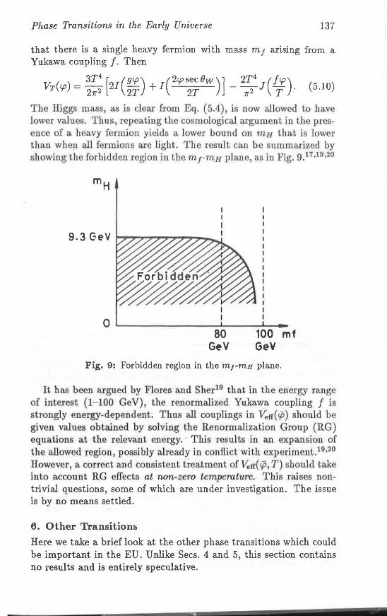
Phase Transitions in the Early Universe 137
that there is a single heavy fermion with mass m f arising from a Yukawa coupling f. Then
VT( cp) = ~~: [21(;;) + 1( 2cp~e;Bw)] - 2~4
J(1;). (5.10)
The Higgs mass, as is clear from Eq. (5.4) , is now allowed to have low r va.lu s. Thus, repeating the cosmological argument in the presence of a heavy fermion yields a lower bound on m H that is lower than wlte.p. all fermions are light. The result can be summarized by showing the forb.idden region in the m r m 11 plane, as in Fig. g ,17.l9,20
80 100 mf GeV GeV
Fig. 9: Forbidden region in the m1-mH plane.
It has been argued by Flores and Sher19 that in the en rgy range of interest (1- 100 GeV), the renormalized Yukawa coupling f is strongly energy-dependent . Thus all couplings in Vetr( <P) should be given values obtained by solving the Renormalization Group (RG) equations at the relevant energy. This results in an expansion of the allowed Iegion, possibly already in conflict with experiment.19•20
However, a correct and consistent treatment of V, tr( i:p , T) should t ake into account RG effects at non-zero temperature. This raises nontrivial questions, some of which are under investigation. The issue is by no means settled.
6. Other Transitionb
Here we take a brief look at the other phase transitions which could be important in the EU. Unlike Secs. 4 and 5, this section contains no results and is entirely speculative.
138 Gravitation and Cosmology
The reason why the other transitions are not as well understood as the GUT and electroweak transitions is as follows. In the former, the order parameter is either unknown, or is known not to be the classical value of a scalar field. Thus the technique of the effective potential is not particularly useful in studying these transitions. Some speculative comments on each transition follow.
{i) The String Transition
Superstring theories21 differ from the theories consider d above in two crucial ways. Firstly, these are most naturally formulated in a spacetime of dimension D > 4. Secondly, the spectrum contains particles of arbitrarily large mass. To make a connection with conventional particle physics, assume that D- 4 spa e-time dimensions are compact. Although not unique, the compactifica.tion of Candelas et al. 22 is now sta.nda.rd. Naively, two limits seem to be involved here.
String theory -----+ Field theory - ---> Field theory
D=lO l D=lO 1 D=4
zero slope limit compactification limit
This leads to the following questions:
Q.l. Are there two phase transitions or one? Q.2. How do we deal with a phase transition where the ·dimension-
ality of space-time changes? ·
The answer to Q .f appears to be that there is only one transition. More than one scale does not arise naturally in string theories. Thus the only relevant length scale is the radius of the compact dimensions and the only phase transition is that associated with compactification. Q.2 is much mQie difficult to answer. In condensed-matter physics, the most important quantity characterizing phase transitions is the spatial dimensionality of the system. Thus the compactification transition brings up problems that are both conceptual and technical. We are far from answering these questions.
(ii) The Supersymmetry Transition
The behaviour of supersymmetric field theories at non-zero temperatures has been the subject of a long-standing controversy. Many authors23 have reported results on this, but the issue remains murky.
Without going into details, one can state the question as follows:
Question: Does supersymmetry (SUSY) behave like other symmetries in the matter of phase transitions?
Phase Transitions in the Early Universe 139
The claims made in the literature broadly correspond to two views. The first is that SUSY is necessarily broken at all non-zero temperatures, because of the different statistics obeyed by the fermionic and bosonic partners of a SUSY multiplet. The second view is that SUSY is just like any internal symmetry, being broken at low temperatures and restored at high temperatures. The truth apparently lies somewhere in between.
ln addition to the vexed problem of the transition associated with SUSY breaking, supersymmetric theories throw up another problem in the EU. This is because all currently popular supersymmetric GUTs24 require an intermediate scale. There is a recent claim25
that such models generate too much entropy to be consistent with observation, but this is far from established.
(iii) and (iv) The Confinement and Chiral Transitions
Both these transitions are associated with QCD. The transition frqm a confined (nucleon) phase to a deconfined (quark) phase has a characteristic scale given by the A parameter, whose value is around 300 MeV. The transition associated with the breaking of chiral symmetry is perhaps the longest-studied QFT phase transition. Its sea.le is given by the pion mass: 140 MeV. The big question is: why are the scales for these transitions so nearly equal, while the transitions themselves are clearly physically distinct? The direction the answer can take is evident: both scales a.re associated with QCD, which has a single dimensional constant arising due to renormalization. However, while this constant is naturally identified with A, its connection with chiral symmetry breaking remains obscure. Perhaps lattice gauge theory will give the answer. It is indeed possible that the two phase transitions will turn out to be one and the same. The significance of this in EU scenarios remains to be explored.
References
1. For detailed reviews see: Brandenberger, R.: Rev. Mod. Phys., fi7 (1985), l; Linde, A.D. in "The Very Early Universe" ed. Gibbons, G.W., Hawking, S.W. and Sikloe, S.T.c., Cambridge University Press, Cambridge, 1983.
2. Guth, A.H. a.nd Weinberg, E.J.: Nucl. Phys., B212 (1983), 321. 3. See, e.g., Itzykson, C. a.nd Zuber, J.: "Quantum Field Theory", McGraw
Bill, New York, 1980. 4. Coleman, S. and Weinberg, E.J.: Phys. Rev., D~ (1973), 1888. fi. Kir1hnit1, D.A. and Linde, A.D.: Sov. Phys. - JETP, 40 (1974), 628;
Benaud, C.: Phya. Rev., 09 (1974), 3313; Dolan, L. and Ja.ckiw, R.: Ph11a. ,Re.,., Dt (1974), 3320; Weinberg, S. Phfl•· Rev., D9 (1974), 3357. For a review Me Linde, A.D. Rep. Prog. Phr1a., 42 (1979), 389.
- .. -.. •
140 Gravilalfon and Cosmuloqy
6. See, e.g. Hrnndenbergcr, TL, Ref. l. 7. Weinberg, S.: "Gravit.atiou aud Cosmology", John Wiley and Sons, New
York, 1972, p. 169. 8. Gnt.h, A.H.: PhyB. Rev., D23 (1981), 317. 9. for an excellent. review sec Coleman, S.: "Erice Lectures 1977", in The
Whys of Sulmuclear l'hysics, (cJ.) Zic!tichi, A., Plenum, New York, 1979. 10. Linde, A.D.: Nucl. Phy.s., B216 (1983), 121. 11. Linde, A.D.: Phys. Lett., 108Il (1982), 389; Albrecht, A. and Steinhardt,
P.J.: Phys. Rev. Lett. 48 (1982), 1220. 12. Linde, A.D.: Phy8. f,e/.t., l.29B (1983), 177. 13. Linde, A.D.: JETJ? Lett. , 23 (1976), 64; Weinberg, S. Phys. Rev. Lett., 36
(1976), 291 .. 11. Witten, E.: Nucl. l'hys., B177 (1981), 477. 15. Guth, A.H. and Weinberg, E.J.: Pliys. Rev. Lett., 45 (1980), 1131. 16. Cook, G.P. and Mahantha.ppa , ICT.: Phys. flev., D23 (1981), 1321. 17. Mahajan, S., Mukherjee, A. , Panchapa.kesa.n, N., Saxena, R.P. and Sethi,
S.K.: University of Delhl Report, 1989, unpublished. 1.8. Kolb, E.W. and T'urner, M.S.: Ann. Rev. Nucl. Part. Sci., 33 (1983), 645. 19. Flores, R.A. and Sher, M.: Phys. Lett., 129B (1983), 411. 20. Sher, M.: Phys. Rep., 179C (1989), 273. 21. Green, M.B., Schwarz, J. and Witten, E.: "Supcrstring Theory", Cambridge
University Press, Cambridge, 1987. 22. Candelas, P., Horowitz, G., Strominger, A. and Witten, E.: Nucl. Phys.,
B258 (1985), 46. 23. Das, A. and Kaku, M .: Phys. Rev., D18 (1978), 4540; van Hove, L.: Nucl.
Phys., B207 (1982), 15; Girardello, L. , Grisaru, M.T. and Salomonson, P.: Nucl. Phys., Bl 78 (1981), 331; Anishetty, R., Basu, R. and Sharatchandra, H.S.: Int. J. Mod. Phys. A3 (1988), 875.
24. Ellis, J. "Supersyrnrnetric GUTs", CERN Report No. TH.3802, 1984. 25. Ellis, J., Endqvist, K., Nanopoulos, D.V. and Olive, K.A.: CERN Preprint
No. TH.5315, 1989.
- --
CHAPTER 4
QUANTUM GRAVITY AND QUANTUM COSMOLOGY
- .. ~ . . ,
Boundary Conditions and
Quantum Cosmology
D.P. DATTA Mathematics Department
North Eastern 1(,egional Institute of Science and Technology Naharlagun, Arunachal Pradesh 791 110
and S. MUKHERJEE
Physics Department, North Bengal University District Darjeeling, 734 430
and Inter- University Centre for Astronomy and Astrophysics Ganeshkhind, Pune 411 007
1. Introduction
Remarkable progress has been made in the field of cosmology during the last decade. A feature shared by most of the new developments is the introduction of the quantum theory in the study of the global structure of the universe. Basically there have been two approaches for incorporating the concepts of quantum mechanics in cosmology. In the first approach, the gravitational field is treated as an unquantized classical background on which one describes the interactions of quantized matter fields. Inflationary models, based on this approach seem to solve some of the problems of the standard classical cosmology. However, a model based on this approach cannot qualify as a complete theory. The classical singularity theorems of General Relativity Theory (GRT) predict that the universe must have had a past time-like singularity, a Big Bang. The problem is perhaps nonexistent, since in a realistic scenario, one encounters a break-down of classital GRT at about the Planck length scale (lp ,...., 10-33 cm), where it becomes essential to treat gravity also quantum mechanically. Thus any complete cosmological theory should involve a theory of quantum gravity. This leads one to look for a Quantum Cosmology (QC) which provides a quantum description of the universe as a whole. The initial conditions for the evolution of the universe in the post-Planckian era will have to be determined from this quantum state. QC should also provide an interpretation of the classical description of the universe through a suitable semiclassical treatment.
- . ~ •
144 Gravitation and Cosmology
This second approach of incorporating ·quantum ideas in cosmology has already become a subject of intense activities, in spite of the fact that we still do not have an acceptable theory of quantum gravity.
The current surge of activities in QC has been inspired by two attractive proposals, one by Hartle and 1Iawking1 •2 (HH) and the other by Vilenkin3 •4 for the choice of boundary conditions for the quantum state of the universe. One of the motivations of the proposals is to realize a description of the creation of the universe. Th e possibility that the gravitational vacuum fluctuations could have led to the creation of the universe was realized by Tryon5 in the early seventies. It was noted that if the universe is closed, its energy, linear momentum and angular momentum should vanish. Also, any conserved charge (coupled to a gauge field) is zero. The uncertainty principle, therefore, suggests that a tiny Planck size universe is likely to appear every now and then, without violating any conservation principle, out of the vacuum (nothing). Most of these are likely to recollapse into nothingness. But there is non-zero finite probability that a tiny bubble may find itself in an inflationary phase, leading eventually to a large universe. The physical picture outlined above, however, needs a theoretical framework, and the recent activities in cosmology are essentially aimed at achieving this. Attention has also been given to the problem of interpretation of the results one may obtain by applying quantum mechanics to cosmology. The conventional Copenhagen interpretation of QM is adequate for a local quantum system which is supposed to interact with an external observer described by the classical physics. The measurement of an observable is, therefore, accompanied by a collapse of the wave function. The above interpretation is, however, inadequate if one considers a quantum state of the universe as a whole. There is no external observer here. It has been suggested that a meaningful way of interpreting quantum mechanics in the context of cosmology is to refer to measurements 'within' the system, in the sense of a typical 'Many World Interpretation'. Here, one may calculate only conditional probabilities. Thus, given a scale factor a and given that the universe is expanding, one may calculate the probability that some physical variable (say, a scalar field) assumes a given value. Though the above interpretation does provide a prescription for extracting information out of a wave function, new concepts are necessary if one wishes to say something about the origin of the universe.
This paper reviews briefly the status of the boundary condition proposals. Section 2 contains a brief discussion of the basic formalism of QC. The boundary condition proposals are dealt with in Sec. 3. The proposals are critically analyzed in Secs. 4 and 5. The last
Boundary Conditions and Quantum Cosmology 145
section contains some general remarks.
2. Formalism
The basic formalism that is being followed in the current studies in QC is based on a combination of both canonical and path integral formulations of quantum gravity. 7 Let us consider the action
I(g,</>) = z;2 j d4xFg(R- 2A) + J d4xFg.C(</>,9ij),
1 .C(</>,9ii) = 28µ</>8µ.</>- V(</>),
(2.1)
where the gravitational part includes a cosmological constant term and the matter Lagrangian is given by that of a scalar field </>_. lp = (1611"G)112 is the Planck length, G is Newton's constant and we have chosen n = c = 1.
To define the metric in a general way, we consider a compact 3-surface S which divides a given connectP,d 4-manifold into two parts. One can introduce a coordinate t in the neighbourhood of S such that S is the surface t = 0 with coordinates xi ( i = 1, 2, 3). The 4-metric then assumes the standard form:
ds2 = -(N2 - NiNi)dt 2 + 2Nidxidt + hijdxidxi, (2.2)
where N is the lapse function, Ni is the shift vector and hij is the metric on the 3-geometry. In the Hamiltonian formulation of gravity7
the 3-metdc hij and matter field </> are regarded as independent canonical variables. Writing Pij and P.p for canonically conjugate momenta, the Hamiltonian assumes the form
where
Ho = z;aijklPijpkl + 1;2V'h(-3 R + 2A)
+ y'h [ p~ + h.ii 8</>. 8</>. + 2V ( </> )] 2 h 8x 1 8xJ
Hi = -2PH + hii 8<1>. P Ii 8xJ <P
Gijkl = ~h- 1 l2 (hi1chjt + hi1hj1c - hijh1c1)
(2.3)
(2.4)
(2.5)
(2.6)
Gijkl may be considered as the metric on the. superspace with signature ( - + + + ++ ). The quantum state of the universe can now be described by a wave function ~( hij' </>) defined on the superspace.
- - ... .
146 Gravitation and Cosmology
Since N, Ni are independent Lagrange variables, one can write the constraint equations which determine <I>(~ij,</>):
Jl i <I> = 0,
!Toil> = 0.
(2.7)
(2.8)
The momentum constraint (2.7) implies that the wave function (P must be an invariant of coordinate diffeomorphisms. The energ~· constraints (2.8), on the other hand, take into account the tirneinvariance of the general relativity. This is the Wheeler-De Witt (WD) equa~ion. The time independence of the WD equation may lead to an impression that it would fail to predict the evolution of the universe. That this need not be the case may be seen from the following. The structure of the WD equation (2.8) shows that it is a second-order hyperbolic differential equation having a time-like variable. The Cauchy initial value problem may therefore. be relevant in this context. One can thus expect to construct the evolution of the universe internally out of the time-like variable. Some recent studies have made significant contributions towards the formulation of this description, although the choice of this time-like variable is not ·unique. York8 has suggested that the trace of the extrinsic curvature J( should play this role, whereas Ashtekar9 has made another interesting choice, with very promising results . .
We note that. the configuration space of the wave function consists of space-like closed 3-geometries with matter fields defined on them, i.e., <I> = <I>(hii, </> ). The transition amplitude that connects the initial configuration ( h~j, </>') with the final configuration ( h~j, </>") is given by a path integral
(h~j,</>" I h~j,¢') = J og;jO</>exp[iI(gij,</>)], (2.9)
where the sum is over all 4-geometries and field configurations which match the given values on two given space-like boundaries. By definitioh, for a given initial configuration, the propagator (2.9) must satisfy the momentum constraint (2. 7) and the WD equation (2.8 ). By a natural extension of the ordinary quantum mechanical path integral, the wave function <I>( h;j, ¢)for a given configuration ( hij, ¢) may be defined as
'f il <I>(hii, ¢) = N c 6giio¢e , (2.10)
where the path integral is over all 4-geometries with a space-like boundary on which the induced metric is hij and matter field assumes the value ¢. The remaining description of C contains the
~ -- ,
Boundary Conditions and Quantum Cosmology 147
specification of certain boundary conditions in the past time-like direction of the given surface. The HH proposal1 provides one such prescription. The wave function and the propagator, by definition, must satisfy the relation
(2.11)
Note, however, that the path integrals in Eqs. (2.9) and (2.10) defining a quantum state of the universe are purely formal. A complete definition needs to answer other relevant issues, like (i) the inclusion of gauge-fixing terms, (ii) the regularization scheme, (iii) the measure, (iv) the issue of convergence, etc. Re ently, Elalliwell10
considered some of these, e.g., the gauge-fixing terms and the measure in the framework of a minisuperspace. In subsequent sections we discuss the boundary condition proposals and the problems of convergence and the hermiticity in some detail.
3. Boundary Conditions Proposals
(A) Hartle-Hawking's Proposal
The HH boundary condition proposal •u<1.Kes use of the Euclidean pa.th integral formulation of quantum gravity. Instead of the Lorentzsignatured 4-geometries, one has to consider only the Euclidean 4-geometries in the path integral. The prescription rests on the assumption that the path integral over all Euclidean metrics is equivalent to the path integral over all Lorentz-signatured metrj s. The wave function is then given by
(3.1)
where IE is the Euclidean action, IE = -if, and the integration is over all real, positive definite Euclidean 4-geoinetries with a compact 3-boundary on which the induced metric is hij, and over all real Euclidean field configurations</> whi_ch.match </>o on the boundary. The proposal selects a very special class of geometries for the remaining specification of C. It states that the 4-geo:m,etries must be compact and that the fields </> must be regular on these 4-geometries. This means, in particular, that a relevant 4-geometry does not have any boundary in the past of the given compact boundary with induced metric hi;· In other words, the universe has no boundary at all. The amplitude (3.1) may also be interpreted as the amplitude connecting the 'zero' 3-geometry with the given 3-geometry and hence, the amplitude for the universe to emerge out of nothing. HH suggest that
- . . •
148 Gravitation and Cosmology
the quantum state defined by Eq. (3.1) may, in principle, be taken to represent the ground state wave function of the universe, in analogy with the ordinary quantum mechanical result that a quantum state that evolves out from a configuration at the negative infinity of Euclidean time is a ground state. However, Brown and Martinez11
point out that such an interpretation will not be proper because, unlike in the case for a quantum mechanical amplitude, the proper time interval between initial and final 3-geometries is not kept fixed in Eq. (3.1) but is rather integrated over. Thus, the path integral (3.1) should be compared to the path integral representation of a Green function for the time dependent Schroedinger equation. For such a Green function, the usual techniques of obtaining the ground state do not apply. In addition, there are other well-known problems in Euclidean gravity. The Euclidean path integral is not, in general, well-defined, sinl':e IE is not positive-definite. Thus the action (3.1), with matter term neglected, can be made arbitrarily negative by choosing a rapidly varying conformal factor n in
9ij == n9ij· (3.2)
To make the integral convergent, Gibbons-Hawking-Perry12 gave an ansatz: divide the integral into two parts: (i) over the equivalence class of the metrics !Jii represented by the condition R(!J) == 4A, and (ii) over the conformal factor n. For each equivalence class, rotate the contour of integration over n at each point so that it is parallel to the imaginary axis. The action then becomes positive-definite and the Euclidean path integral converges. The ansatz, valid for pure gravity, may fail for an action with non-conformally coupled matter fields. Moreover, not all compact 4-metrics can be conformally classified as above. Thus HH's original proposal remains incomplete until the problem of the convergence of the path integral is settled. It may be noted that the semiclassical approximation for the ground state wave-function is obtained by evaluating the functional integral by the method of steepest descents. With only one stationary phase point, this gives in the case of pure gravity
(3.3)
where Ic1( hij) is the Euclidean action evaluated at the stationary phase point, i.e., at the solution gz'v of the Euclidean field equation Rµv = Agµ,,, inducing the metric hij on the three-surface boundary, and D..-1 / 2 is a combination of determinants giving the fluctuation about g~1,,, including those corresponding to ghosts. In the case of more than one stationary-phase point, one has to choose the contour of integration in the path integral to include the dominant
Boundary Conditions and Quantum Cosmology 149
contribution. Usually the stationary phase point giving the lowest value of 'RIE gives the dominant contribution. Since the wave function is assumed to be real, if there are two stationary-phase points with complex values of the action, one gets equal contributions from stationary-phase points with complex conjugate values of the action. The semiclassical wave function vanishes if there is no stationary-phase point. We shall discuss the recent developments in this connection in the next section.
(BJ Vilenkin's Tunneling Boundary Condition (TBC)
The tunneling boundary condition proposal of Vilenkin3 •4 is usually stated in terms of the behaviour of the wave function in the superspace. The motivation is to draw an analogy with the tunneling process in ordinary quantum mechanics. Originally, Vilenkin13
looked for a re-interpretation of the de Sitter instanton
a(r) = >.-112 sin(v":Xr), T =it, (3.4)
as a vacuum instability. In that case, the second order fluctuations in the action (2.1) must have a negative mode yielding V"(</>o) < 0. A bubble universe may therefore nucleate out of the vacuum on a maximum of the potential· V ( </>) at </> = <Po, where </>o is a constant classical solution. Recall, however, that the negative mode in the path integral determinant leads to an imaginary part in the energy eigenvalue of the corresponding WD operator. This, however, leads to a difficulty in the interpretation of the scenario. In fact, the WD operator being constrained to assume a 'zero' eigenvalue, fails to accommodate an imaginary eigenvalue and hence an unstable state. In other words, the problem lies in the fact that the WD equation is strictly time independent, whereas an instability in vacuum intrin§i- -cally defines a concept of 'time' (e.g., decay width). It is, however, possible to interpret the cosmic nucleation in the sense of an instanton which connects two distinct vacua in disconnected sectors int.he superspace.
The WD equation (2. 7) is a second order functional partial differential equation which is obviously difficult to analyze. The common practice is to restrict to a finite dimensional submanifold, the minisuperspace, where all but a finite number of the gravitational and matter degrees of freedom are frozen out. The full QC thus reduces to a simpler quantum mechanical model, solutions of which may be easily obtained. In a suitable minisuperspace, Vilenkin's4 criteria for the choice of the wave function may be stated as:
(a) In the classically allowed (Lorentzian) sector, the wave function contains only the outgoing components,
J .')0 Cmvilalion and Cosmology
(b) The wave function decays exponentially in the classically forbidden Euclidean region,
( c) The wave function is complex.
On the basis of a semiclassical analysis of the UH wave function, one may also state the no-boundary proposal in terms of the behaviour of the wave function in a minisuperspace:4
(a) In the Lorent.zian sector the wave function contains equal amplitudes of the outgoing and incoming waves,
( b) In the Euclidean sector, it increases exponentially, ( c) The wave function is real.
Finally, it may be pointed out that there is another (inequivalent) formulation of TBC in terms of a Lorentzian path integral: the wave function can be given by a path integral over Lorentzian 4-geometries which close off in the past. It appears that this path integral representation of TBC fails to respect some general consistency constraints.H
4. The de Sitter Minisuperspace
Let us consider the simplest minisuperspace, the de Sitter model. The four-geometries are, therefore, homogeneous, isotopic and closed, parametrized by a single scale factor a( t). The 4-metric can be written as
(4.1)
where u2 = t;/24rr2, and N, the lapse function, represents the gen
eral time-coordinate tranformation freedom. For the sake of simplicity, we drop the matter Lagrangian from the action. The action (2.1) thus reduces to
1 j N [(aa) 2 2 4 ] I= -2 dt-; N - a + Aa , (4.2)
where A = ~ A<T2, and the WD equation (2. 7) becomes
[-a-P.!!....aP.!!_ + a2 - >.a4 ]<I>(a) = 0. (4.3)
da da
The indexp represents some, but not all, of the factor-ordering ambiguities. These ambiguities introduce a new element of uncertainty in the cosmological scenario. We show thif by considering two special cases: p = 0 and p = -1. The (super) potential
U(a) = a2 - Aa4 (4.4)
in the WD equation ( 4.2), in general constitutes a barrier in the minisu perspace for the scale factor a( t). The barrier has height ( 4>. )-1 ,
Boundary Conditions and Quantum Cosmology 151
separating the minimum at a = 0 from the classically allowed sector U < 0. This picture, however, is not universal. Notice that for p = -1, the zero 3-geometry a = 0 (nothing) is completely hidden under the barrier (U > 0). In this case the WD equation ( 4.3) reduces to the form
d2 [4 dq2 - 1 + .Xq] •(q) = o, (4.5)
with q = a2 • Equation ( 4.5) is the pure de Sitter WD equation with the scale factor q defined by the special choice of the metric15
ds2 = u 2 ( - ~
2
dt2 + qdO~). ( 4.6)
The action (2.1) then assumes the fol'lll
1 J q2 I= - 2 dtN(4
N 2 + .Xq-1). (4.7)
Note that the predictions of the Einstein's field equations with metrics (4.1) and (4.6), for pure gravity with a cosmological constant A, are identical, as expected. However, the corresponding WD equations (4.3) and (4.5) respectively describe distinct quantum theories, the predictions agreeing only at the semi classical level. However, as is already evident from the structures of Eq. (4.3) (with p = 0) and Eq. (4.5), the interpretation that the semiclassical wave function provides the tunneling amplitude from 'nothing' appears to be dependent on the value of p, because 'nothing' (a = 0) lies totally in the forbidden region of minisuperspace for Eq. ( 4.5). A boundary condition (at a= 0) should conceivably specify in a general way (i.e., independently of p as well as the metric) a prescription for selecting a unique wave function out of the geneal 2-parameter family of solutions, which does not seem to be the case here.
The WD equation ( 4.5) is exactly solvable.4 •15 The most general solution is given by
•(q) = c1Ai(-z) + c2Bi(-z), (4.8)
where z = (1 - .Xq)(2.X)-213 , Ai(z) and Bi(z) are two linearly independent Airy functions. Some problems of the BC proposals will be discussed in the next section by considering this simple solution.
&. Problems with BC Proposals
(A) Operator-ordering Ambiguity In the uaual procedure of canonical quantization, operator-ordering ambiguity arises when one replaces the momenta. Pi by the corresponding differential operators. As pointed out in the'last section,
152 Gravitation and Cosmology
the ambiguity may affect the interpretation of a cosmological scenario. Halliwell10 has shown that the operator-ordering ambiguity manifests itself as an ambiguity in the c~oice of a covariant measure in the configuration space path integral. Hawking and Page17
have suggested that the ambiguity be resolved by requiring that the differential operator in the WD equation should be the Laplacian operator in the natural metric on the superspace. For the WD eq nation in the de Sitter minisuperspace, [Eq. (4.5)], this gives p = 1. The suggestion leads to other problems. In particular, the Hamiltonian is no longer a linear function of N, as it should be if N is to be treated as a Lagrange's multiplier. Hawking and Page hope that the non-linear dependence on N should cancel out in a realistic theory. This actually happens in supergravity theories which contain equal number of fermionic and bosonic degrees of freedom. The ambiguity needs to be resolved decisively.
(BJ Problem of the Half-infinite Range for q
The fact that the three-metric hij satisfies. det hij 2 0, ( q 2: 0 in the de Sitter minisuperspace), leads to a complication, already known in ordinary quantum mechanics. For q 2: 0, the corresponding canonical momentum P cannot be represented by a hermitian operator P, otherwise by operating with the unitary translation operator one could translate into the forbidden domain, q < 0. However, the Hamiltonian can still be made hermitian if one assumes boundary conditions at q ~ 0, of the type 'f/;(O) + a'f/;1(0) = 0, with a an arbitrary constant. One has to find the eigenfunction 'l/Jn(q) subject to the above boundary conditions and then construct the propagators from the following expression:
(q",t" I q',t') = LeiEn(t"-t')'l/J~(q")'l/Jn(q'). (5.1) n
However, in the path-integral approach, the existence of a boundary at q ~ 0 leads to a problem in the evaluation of the propagator by the usual skeletonization procedure. With a restricted q ( q > 0 ), between any two points there are two classical paths, one direct and another which gets reflected from the boundary at q = 0. Both the paths should contribute to the WKB approximation of the propagator. One should, therefore, consider not just a single term of the form eis, but two such terms. A change of variables p = ln q, with -oo < p < +oo, does not help, because the problem is due to the presence of more than one classical paths connecting any two points. The choice of a variable with a range (-oo, +oo) may nevertheless be useful in implementing a canonical quantization, as the corre-
Boundary Conditions and Quantum Cosmology 153
sponding conjugate momentum may be represented by a hermitian operator.
In the case of a massive scalar field <p, the requirement of a hermitian Hamiltonian does not unduly restrict18 the wave function at a = 0. The variables a and <p behave like polar coordinates in two dimensions, with a measuredµ( a, r.p) = a2 da d<p, permitting the wave function even a weak singularity at a = 0. It is, howev~r, not clear if one should insist on a hermitian Hamiltonian in quantum cosmology.
(CJ The Convergence Problem and the Choice of Complex Contours
The problem of convergence of path integral expressions have been briefly discussed in Sec. 4. As pointed out there, the proposal of Gibbons, Hawking and Perry12 for a rotation of conformal mode integration contour does not solve the convergence problem. Hartle19
has suggested a more general approach. This involves taking the integral along the steepest descent path in t he space of complex four-metrics. Thus, one t akes g~,v as complex and the integration is done along the contour along which the real part of the action increases most rapidly. The method may be explained by following Halliwell and Louko,15 who consider t he de Sit ter minisuperspace mentioned in the last section. In the gauge N = 0, one can write the minisuperspace propagator as
G(q" I q) = J dT(q",T I q,O), (5.2)
where T is proportional to N and (q", T I q', 0) is the Euclidean quantum mechanical propagator,
(q",T I q',O) = j DpDqexp[-IE(p,q)], (5.3)
which satisfies the Euclidean Schroedinger equation .. Operating by the Hamiltonian at q11
, we get
H"G(q" I q') = - j dT :i,(q",T I q',o) = .:...[(q;',T I q',o)J::, (5.4)
where Ti, T2 give the end-points of the T-contour. If T has a range (- oo,+oo), the R.H.S. of Eq. (5.4) is zero, provided (q",T I q',O) goes to zero at the end-points. If T has a half-infuUte range, with T1 = O, G is a G1een's function of the WD operator, provided (q" , T I q', 0) has some convergence properties. Halliwell and Louko have shown that for a de Sitter minisuperspace, there are a number of contours for which these convergence properties follow. They consider the path integral expressions for G(q" I q') a.swell as G(q" Ip')
154 Gravitatfon and Cosmology
and show that the q and p integrations can be done easily while the T-integral needs a complex contour for convergence. A useful method of evaluating the path integrals in this case is to shift the variable of integration.
q(t) = q(t) + Q(t), p(t) = p(t) + P(t), (5.5)
where ij(t) and p(t) are solutions of the field equations corresponding to the action IE, satisfying the appropriate boundary conditions. Thus for G(q" I q'), we have g(T) = q(T) = q", and q(O) = q(O) = 0. Note that q does not satisfy the Hamiltonian constraint H = 0, so that it is not a saddle point to the T-integral. The Schroedinger propagator. (q11
, t I q', 0) then reduces essentially to a path integraJ over Q(t), satisfying Q(T) = Q(O) = O. It can be shown by a scaling argument that the path integral over Q(t) contributes only a factor ""r-112 :to the measure. Thus the full propagator G(q" I q') reduces to a. single ordinary integral
J dT G(q" I q') ex: - 1 exp[-Io(q",q',T)],
T'i (5.6)
where the action Io at the saddle-point is given by
II I - ~2T3 [>.(q" + q') - ~] - (qi/ - q')2 Io(q 'q 'T) - 24 + 4 2 T BT (5.7)
The integral can now be evaluated exactly in terms of Airy functions, once a choice for the T-contour is made. The int~gral (5.6) has four saddle-points whose locations for each of the two cases, >.q' < >.q" < 1 and >.iJ." > 1 > >.q' are of interest here. In the first case, two of the saddle-points actually belong to the second sheet of the complex plane (note that due to the factor r-1 / 2 in the interground, the T-plane is double-sheeted). The saddle-points for >.q" > 1 > >.q' are complex. They correspond to complex geometries consisting of a section of a 4-sphere matched on a section of a de Sitter space. The two real saddle points for >.q' < >.q" < 1 correspond to solutions representing a section of a 4-sphere, which ·does/does not include the equator. The analysis of Halliwell and Louko shows that there are indeed a number of possible T-coutours, each one of which is able to give an acceptable ncrboundary wave function 'l/JH·
The status of the HH proposal can now be summarized. It is obvious that the no-boundary condition cannot specify uniquely the ground-state wave function. One has also to specify the contour. In their original paper, 1 Hartle and Hawking opined that the dominant contribution to the path integral should come from the saddle-point corresponding to less than half of a 4-sphere. As mentioned above,
Boundary Conditions and Quantum Cosmology 155
this is only one of the possibilities. There are many allowed contours, some of which do not even pass through this saddle-point, that can give convergent results. The particular choice of HH has not been properly motivated. To settle this issue, Halliwell and Hartle15 have recently suggested that one should choose a contour so that the results ~atisfy some sensible criteria for consistency and physical predictions. The following criteria have been suggested.
(1) The integral defining the wave function tPH should converge. (2) tPH should satisfy the constraint equations (2.7) and (2.8). (3) The wave function should lead to a classical space-time when
the universe is large. This can happen provided there is little interference between alternative histories for space-time geometry for scales much larger than lp and, in addition, the histories are strongly correlated acco'tding to classical laws.
( 4) Another 'essential physical requirement is the reproduction of quantum field theory for matter when the space-time is almost_ classical.
(5) The contour is to be chosen so that 'the model can accommodate any possible dependence of the coupling constants of the effective low energy theory on the initial conditions of the universe. An example may be cited here. When wormhole topologies are included in the Euclidean sum over histories, a mechanism for making the cosmological constant vanish becomes available. A restriction on the class of 4-geometries to be included in the sum follows if one insists on having the above result as a prediction.
Halliwell and Hartl~ note that even the imposition of all these criteria does not uniquely specify the contour. There are still many no-boundary wave functions.
In this context, it is possible to analyze one version of Vilenkin's proposal which can be formulated as a Lorentzian sum over hi11tories, defined ·by a suitable choice of contour. Halliwell and Lauko have shown that the relevant contour here is dominated by a saddlepoint for which Rylg < 0, which does not satisfy the criterion ( 4) given above. The objection, however, may not hold for the other (inequivalent) fo.rm of Vilenkin 's proposal.
6. Discussion
We have presented in earlier sections a brief overview of the boundary condition pro1,>osals of HH and Vilenkin. The extensive work done in this field during the last few years has helped considerably to examine critically the concepts involved and their limitations. Some
- "' -.. •
156 Gravitation and Cosmology
of the ideas presented in earlier works now stand modified. Of particular interest in this connection is the question of relative merits of the Euclidean formulation. Brown and Martinez11 have recently re-examined this issue. They conclude that it is quite adequate to consider a sum over Lorentzian 4-geometries so far as the QC is concerned. They consider the de Sitter minisuperspace with the spatial 3-volume x as the degree of freedom to be quantized and use the WKB approximation to derive the following results:
G(x" Ix')= tPT(x")'l/;H(x')O(x" - x') + 'l/;T(x')'l/;H(x")O(x' - x"), (6.1)
where() is a step function, 'l/;T(x) and 'l/;H(x) are the solutions of the WD equations satisfying TBC and HH boundary conditions mentioned in Sec. 3. Thus G( x", x') is itself not a wave function. However, as a function of x" and with x" > x', G( x", x') is proportional to 'l/;T(x). Again, if the system is time-reversal invariant, i.e., (x",T I x',O) = (x',T I x",O), it can be shown that
'RG(x",x') = 'l/;H(x")'l/;H(x'), (6.2)
so that RG( x", x') is a HH wave function in each of its arguments. The validity of Eq. (6.1) seems to go beyond the WKB approximation. It is, therefore, suggested that the Green function G(x", x'), defined as a sum over Lorentzian geometries, is the basic object to be studied in QC. This is to be contrasted with the method discussed in the last section where the path integral is defined as a sum over complex geometries (and complex matter field) to be evaluated along a steepest descent contour.
The issues are still open and QC seems poised for rapid and interesting development both in concepts and calculational techniques.
Acknowledgements
The authors would like to thank B.C. Paul for discussions. S. Mukherjee is thankful to the Inter-University Centre for Astronomy and Astrophy.sics (IUCAA) for the -Award of a Senior Associateship.
References
1. Ha.rtle, J.B. and Hawking, S.W.: Phys. Rev., D28 (1983), 2960, 2. Hawking, S.W.: Nucl. Phys., B239 (1984), 257. 3. Vilenkin, A.: Phys. Rev., D33 (1986), 3560. 4. Vilenkin, A.: Phys. Rev., D37 (1988), 888. 5. Tryon, E.P.: Nature, 246 (1973), 396. 6. See e.g., Tipler, F.J., in "Quantum Concepts in Space and Time", (ed.)
Penrose, R., and Isham, C.J., Oxford University PreBS, 1986, p. 204. •
Boundary Conditions and Quantum Cosmology 157
7. Kuchar, K., in "Quantum Gravity", vol. 2, (ed.) Isha.rn, C.J., et al., Oxford University Press, 1982, p. 329.
8. York, J.W.: Phys. Rev. Lett., 28 (1972), 1082. 9. Ashtekar, A.: Phys. Rev. Lett., 61 (1986), 2244; Phys. Rev., 036 (1987),
1587. . 10. Halliwell, J.J.: Phys. Rev., 038 (1988), 2468. 11. Brown, J.D. and Martinez, E.A.: Phys. Rev., 042 (1990), 1931. 12. Gibbons, G.W., Hawking, S.W. and Perry, M.J.: Nucl. Phys., B138 (1978),
141. 13. Vilenkin, A.: Phys. Rev., 027 (1983'), 2848. 14. Halliwell, J .J. and Hartle, J.B.: Phys. Rev., 041 (1990), 1815. 15. Halliwell, J .J . and Louko, J .: Phys. Rev., 039 (1989), 2206 . 16. Halliwell, J .J . and Louko, J .: Phys. Rev., 040 (1989), 1868. 17. Hawking, S.W. and Page, D.N.: Nucl. Phys., B268 (1986), 185. 18 . Kiefer, C .: Phys. Rev., 038 (1988), 1761. 19. Hartle, J.B.: Santa Barbara Report, 1988 (unpublished).
- .. ~- - ~ . .
Quantum Gravity, Torsion and the
Wave Function of the Universe
PRATUL BANDYOPADHYAY
Indian Statistical Institute, Calcutta 700 035
To study the quantum nature of the universe, Hartle and Hawking' proposed the wave function of the universe which is considered to be a function 1/J(h,<p) of the 3-metric and matter fields on a space-like surface. The wave function satisfies a sort of Schrodinger equation, known as the Wheeler-D.e Witt equation
( 1 8 1/2 8 (3) ) ----h Gii k1-- - R- 2.X + 871'GToo 1/J = 0.
2h112 8hij ' 8hk1 (1)
Hawking,2 to solve the cosmological constant problem, has taken the solution as an Euclidean path integral
1/J ex j d[g]d[c.p] exp[-S(g, c.p)], (2)
where the integration is carried over all Euclidean signature 4-metrics gµv and matter fields c.p defined on a 4-manifold M4, that have the 3-manifold M3 ( h, c.p) with 3-metric hij and matter fields </>as a boundary. Here S is the Euclidean action:
S = _!__G [ vg(R + 2.X) +matter terms+ surface terms (3) 1671' 7 }M
4
Hartle and Hawking proposed as a cosmological initial condition that the manifold M4 should have no boundaries other than M3 (h, c.p).
However, this Euclidean path integral cannot be termed in strict sense a quantum mechanical object. Rather, it conforms with the classical statistical mechanical quantity. Indeed, Weinberg3 has discussed at length the problems related with this, particularly the difficulties with the probability interpretation. Hawking described how in quantum cosmology there will arise a distribution of values for the effective cosmological constant with an enormous peak at Aeff = 0. Recently, Coleman4 formulated a mechanism based on the concept of wormholes and baby universes, which produces a distribution of values for the cosmological constant with an even sharper peak. As pointed out by Weinberg, in case the wave function of the universe is
Wave Function of the Universe 159
written in terms of Feynman path integral, their argument of having a peak at Aeff = 0 crumbles down. Besides, to have the cosmological constant as a dynamical variable, Hawking has introduced a 3-form gauge field , the meaning of which is not dear. Though in Coleman's approach the fictitious 3-form gauge field was avoided, it relie.d on the existence of \\-'.Ormholes and baby universes, the origin of which is not very clear.
Here we shall put forward the idea that to consider the wave function of the universe, we will have to take into account the quantization procedure which leads to the Feynman path integral, rather than the Euclidean path integral considered by Hawking and Coleman. Indeed this quantization procedure involves a new geometry which takes into account complexified Minkowski space-time for the microlocal domain5 and leads to the Einstein-Cartan action for gravity. The new geometrical ingredient necessary for quantization suggests that we should introduce a 'direction vector' attached to each space-time point in a complexified domain, which leads to the generation of an 'internal helicity' giving rise to the internal symmetry like fermion number for a relativistic particle and the non-relativistic case is obtained in the sharp point limit. This internal helicity, arising out of the attached 'direction vector', is found to be associated with spinorial variables 0, 0, where(} (0) is a two-component spinor. Thus this new geometry necessary for the quantization of a fermion in Minkowski space-time can be formulated in terms of spinor structures attached to each space-time point and thus effectively corresponds to a superspace. The gravitational action corresponding to this geometry leads to the Einstein-Cartan action where the Cartan term is related to this spinor structure. Thus we can view that quantum gravity is essentially the effect of this quantum geometry which gives rise to the torsion and thus torsion may be considered as the quantum effect.
When we consider that the two opposite orientations of the 'direction vector' eµ attached to the space-time point Xµ in complexified Minkowski space-time havi~g the coordinate Zµ. = Xµ + ieµ. give rise to two opposite internal helicities corresponding to fermion and antifermion, we can formulate the 'internal helicity' in terms of the space-time metric gµ 11 (X,e,8) where(} (8) is a two-component variable.6 In fact, for a massive spinor lwe can choose the chiral coordinates in this space as
zµ = x1-1 +~>.~ea (a= 1,2), (4)
where we identify the complex coordinate zµ = xµ + ieµ witheµ=
- . -· - . •
160 Gravitation and Cosmology
~.X~0°. We can now replace the chiral coordinates by the matrices
where
zAA' = xAA' + ~_xAA' O"' 2 a '
0 1 A.A' 1 [ X - X
X = -../2 x2 - iX3 xi+ iX 3
]
xo +xi AA' ( ) and .Xa E SL 2,C .
With these relations, the twistor equation is now modified as
(5)
(6)
(7)
where ff A ( 7r A') is the spinorial variable corresponding to the fourmomentum variable pµ, the conjugate of Xµ, and is given by the matrix representation
and za = (wA' 7r A'),
with WA = i( XAA' + ~_x~A' 0a) 7r A'.
Equation (7) now involves the helicity operator
S = -A~i\' Oa 1f A 7r A' ,
(8)
(9)
which we identify as the internal helicity of the particle and corresponds to the fermion number. It may be noted that we have taken the matrix representation of Pµ, the conjugate of Xµ in the complex coordinate Zµ = Xµ +itµ as pAA' = iArrA', implying P! = 0 and so the particle will have mass due to the non-vanishing character of the quantity ~~- It is observed that the complex conjugate of the chiral coordinate will give rise to a massive particl€ with opposite internal helicity correponding to an antifermion. In the null plane where ~~ = 0, we can write the chiral coordinate as
AA' AA' Z -A A' Z =X . +20 0 , (10)
where the coordinate ~µ is replaced by ~AA' = ~(}AoA'. In this case the helicity operator is given by
-A A' S = -0 0 1fA7rA' =-EE, (11)
where c = iOA' rr A', t = -iiJAi A· It has to be noted that the state with the helicity + 1/2 is the vacuum state of the fermion operator
clS = +1/2} = 0. (12)
Wave Function of the Universe 161
Similarly, the state with the internal helicity -1/2 is the vacuum state of the fermion operator
tlS = -1/2) =,Q. (13)
In case of a massive spinor we can define the plane n- where the coordinate Zµ. = Xµ. + ieµ. is such that eµ. belongs to the interior of the forward light cone ~ ~ 0 and as such represents the upper half plane with the condition det ~ > O and t Tr e > 0. The plane n+ is given by the set of all coordinates Zµ. with ~µ. in the interior of the backward light cone (~ ~ 0). The map Z -+ z• sends n- to D+. The space M of null plane ( det ~ = 0) is the Shilov boundary, so that a function holomorphic inn- (D+) is determined by its boundary values. Thus if we consider that a.ny function ip(z) = tp(x) + iip(fl lwlomorphic in the whole domain1 we not<: that the helicity +1/2 (-1/2) given by the operator ilJA 7r A' (- iOA?r A) in the null plane may be taken to be the limiting value of the internal helicity in the upper (lower) half-plane.
In this complexified space-time exhibiting the internal helicity states, we can write the metric as
- AA' -A A' 9µ.v(X,0,0) = 9µ.v IJ 0 • (14)
It has been shown elsewhere7 that this metric structure gives rise to the SL(2,C) gauge theory of gravitation and generates the field strength tensor Fµ.v given in terms of the gauge fields Aµ., which are matrix-valued·having the SL(2,C) group structure, and is given by
Fµ.v = 8vAµ. - 8µ.Av + [Aµ., Av]· (15)
Since 0 ( 0) is the spinorial variable which represents the 'direction vector' attached to the space-time point, this effectively represents the stochastic extension of a relativistic quantum particle representing a fermion. This suggests that for a relativistic quantum particle which is taken as a stochastically extended one, the fermionic character of a particle associates the functions defined on stochastic phase space with matrix valued non-Abelian gauge fields having the SL(2,C) group structure. This also helps us to conceive a massive fermion as a Skyrme soliton, where the Skyrme term in the Lagrangian appears as an effect of quantization.5 The gravitational effect arising out of this spinorial term can thus be taken as quantum gravity.
Now to study this effect, following Carmell and Malin8 we choose as a Lagrangian density in the given superspace, the simplest Lagrangian density which is invariant under SL(2,C) transformations:
L - Tr 0t{J-r6p F. - f. a{J "(6• (16)
- . - .. - · ~ •
162 Gravitation and Cosmology
The corresponding field equation is given by
05(Ecx(J-y{i F0t,a) - [Ao,Ea(J-yo Fa(J] = 0.
Now writing
- -F - f ·g µ11 - µv •
(1'7)
(18)
where g = (91, 92, 9:i) are tangent vectors to the generators of the SL(2,C) group, where
r. [ 1 0] [eZ 0 ] [ 1 91(Z) = z l , 92(Z) = O e-z , 93(Z) = O ~] l (19)
with the definition _ [d9m(Z) ]
9m - dZ ' Z=O
(20)
implying 9m(Z) = exp(Z9m), we find
91 = [ ~ ~ ] , .Q2 = [ ~ ~1 ] ' .Q3= [ ~ ~ ] · (21)
This suggests that the field equations are to satisfy the condition
{3 - - -.. Eµ
110t (811! 0t{J - a 11 X J 0t{J) = 0. (22)
Now we define a four-vector density Jt ·by
Jµ = f_µ110t{J;; x !-(} 11 0t{J l
which, when substituted in Eq. (17) gives
J-µ - µ110t{J{) !-(} - E 11 0t{JI
which satisfies the relation
!) J- µ - µ110t{J !) !) f- - 0 Uµ 8 - E UµU11 cx{J - •
Thus J~ is the conserved current density in superspa.ce.
(23)
(24)
(25)
When the superspace is Riemannian with metric structure, the conserved current may be written as
Jµ = ]µ + !._fµ11cx(J;; X J-w (26) x 11 e>{JI
where x is the Einstein gravitational wnstant (x = -87rG/c1 ),
F~ = ]~ · g, ]~ is the Weyl part of the vector J 0t/3' Jµ is the contribution to the conserved current due to the energy-momentum tensor8 and the second part of the r.h.s. of Eq. (25) is the contribution of the spinorial variable (} corresponding to the effect of quantum
Wave Function of the Universe 163
gravity as well as of N = 1 supergravity. The action in superspace is now given by
where 1 1
A = K 2 = 16
1rG, K = Planck length.
N 9w using the relations af3µ.v -
f. f.a(3µ.v - -e (0)
Raf3'"f6 = R°'13'Y6 - e'Yaes13
where
(27)
(28)
(29)
R~0J'Y6 = -8aWf3'Y6 + 013Wa'"f6 + W~'YWJ3a6 - w3'Ywaa6 (30)
denotes the Riemannian curvature and is related to rotation, whereas the second term e'Yae6/3 is related to translation.9 The scalar curvature is given by
R = R(o) e'Y6 e6f3 (31) 0t()'"f6 •
Now neglecting the Gauss-Bonnet topological term [R<0>]2 and other small terms, we get finally 7
S = S1 + S2, (32)
where
(33)
Again, writing .... -w 2 av X f af3 = K Svaf3, (34)
the second pa.rt of the action becomes
S2 = - ; 2 J Svaf3sva/3 a' X, (35)
giving rise to the torsion term. Thus the total action becomes
S = S1 + S2 = j d4X(- 8~2 R- 1: 2 Svaf3svaf3)e, (36)
which is the well-known Einstein-Cartan action. We note that the torsion term arising out of the SL(2,C) gauge
fields may be taken to represent an effective cosmological constant. The conservation of current
- .. . '
(37)
1G4 Gmvitation and Cosmology
suggests that we cau define a topological charge which can be taken to represent the fermion number. Indeed, in a recent paper10 it has been shown that the consistency of the conservation of currents suggests that the three components of the vector ./~ satisfy a set of equations
·Jf = -Jf /2; J~l = Jf /2 (38)
and the charge corresponding to the gauge field pa.rt is given by
q = J J~ d3 x. (39)
So from the relation
Jµ = €1w>.a;{ X f~ = €1w>.a3 J~ () v >.a v >.a'
we have Jg(X) = Eov>.aa,,fi~ = Eov>.aCv>.aC(X),
and for the generalized current we can write
Jf (X) = Eµv>.aCv>.aC(X).
Thus from the relation
8µJf(X) = O,
we find ac ax = 0·
µ
This helps us to write the torsion term in the action as
fh = C 2 J vgd4 X,
(40)
( 41)
(42)
(43)
(44)
with proper normalization of the constant factors. Thus J2 can be taken to represent the cosmological constant as a dynamical variable with C 2 = 2>..
Now noting that for a positively (negatively) charged fermion
the corresponding SL(2,C) current is J~ (J! = -J~), a neutral system comprising equal numbers of positively charged and negatively charged fermions, the total current vanishes, implying that the cosmological constant will vanish for
1 a neutral system. It may
be remarked here that though for protons as well as for electronsthe main charged constituents of matter-we conventionally take baryon number and lepton number as +1, yet if we assign for a proton fermion number +1 and for an electron the fermion number -1, it will not alter the physics as we have baryon number and lepton number separately conserved. Besides, for the neutral component
Wave Function of the Universe 165
of matter, viz., neutron, we know that these are composite objects of positively and negatively charged components, so that neutrons will not contribute anything to the overall current J~ and, as such, to the overall torsion. Thus we can conclude that the neutrality of the universe suggests that we should have vanishing cosmological constant.
We can now define the wave function of the universe as the Feynman path integral:
1/J ex j d[g]d[r.p]d[A]exp(iS(g,r.p,A)). (45)
Here the action contains, apart from the metric term, the torsion term arising out of the SL(2,C) gauge fields Aµ. associated with the internal stochastic extension of the particle.
It may be.mentioned here that recently Suen and Young11 have considered the wave function of the universe in the usual form of the Feynman path integral with the time coordinate being real:
1/J[hi;,<.p] = i d[g]d[r.p]eiS[g,cp), (46)
where the set L includes all possible non-singular Lorentzian fourgeometries which induce hij on one of their boundaries, together with all fields <.p regular on them. However, to have a consistent solution, these authors have considered the universe as a 'leaking' system, suggesting that the 'particle' eventually escapes to infinity, where such an escape is either classically allowed or takes place through 'tunneling' in the quantum case. In a 'minisuperspace' model, these authors considered the line element
ds2 = a 2 ii2(-N 2dt2 + d!l~), (47)
where a 2 = 2G /37r and dS15 is the line element on a unit 3-sphere. The a.ction is given by
S=--1-. jd4 XFg(R-2..\)+-
1-fd3 X../hK. (48)
l67rG . 87rG
We note that with the introduction of the cosmological term,.\ in the action, we can reduce the function in Eqs. ( 45)-( 46) as the contribution of the gauge field is contained in ..\. In terms of the conformal time 'I = J N dt, this. gives
where
s = ~ j d11[-a2 + (a2
- ..\a4)], (49)
. da a=d11
and ..\ = 2G A. 97r
- ~ --· ~ . .
] 66 Gravitation and Cosmology
For a Robertson-Walker universe with a small cosmological constant A > 0, Eq. (46) becomes
'¢( a0 ) = j d[ N]d[a] exp( iS), ( 50) L
and the paths are chosen to satisfy
a= ii0 at T/ = 0, ii(t) E [O, a], N E [O, a]. (51)
The path integration is carried out in three steps: (1) firstly, we sum over all paths ii( t) which begin at T/ = 'r/i with a certain a. = iii for a certain N(t); (2) then we sum over all possible N(t), which corresponds to adding up paths which connect ii; and iio with all possible proper times; and (3) we integrate over all possible ii;. Thus we write
_7/_J(iio) = j d[iii]d[N] .l;-•ao d[iii] exp[·-iS]
= j d[iii]d[N]'¢1t;(<1.o,TJ = o). (52)
The Hamiltonian .ll(a) corresponding to the Schrodingcr equation
can be written as
where
1 {)2 H(a) = --
8_2 + V(a),
2 a
(-) ·{ tca2 - >.a4
) for a> o Va= · a for ii :S 0
where we have replaced ~2 -> -82 /8ii2
•.
(53)
(54)
The wave function 7/Ja; describes a particle in a half-cut anharmonic potential initially located at ii;. For >. > 0, Suen and Young have observed that this is a leaking system and t/Ja; can contain only outgoing waves of the form exp(i>.112a3 /3)exp(-ifrt) for large a. However, from our interpretation of the origin of the local cosmological constant arising out of torsion related to the 'direction vector' eµ. attached to the space-time point Xµ. giving rise to quantum geometry, we note that for a massive particle, eµ. is defined only in the interior of the forward (backward) light cone for a particle (antiparticle) and ·the torsion term in the action, manifested through the cosmologic.µ constant >., effectively defines the wave function '1/Ja; such that it describes a particle in a half-cut anharmonic potential. Thus the condition >. > 0 does not essentially define a leaking
Wave Function of the Universe 167
potential. Rather, it defines the disconnected nature of microloca.l space-time which is responsible for the torsion term. Indeed, from the asymptotic behaviour of the wave function 11 ,
{
Naoe-a~/2 uo ~ A,-1/2
,,P(ao) = 1! e-l/3>.e(-i/3)>.l/2a,~ ao > A,-1/2 (55) ao
we note that for A. < 0, the wave function is ill defined. Indeed, from Eq. ( 44), where the action corresponding to the torsion term is written as S2 = C2 J d4 X vg, the identification of C2 = 2A. suggests that ').. can never be negative.
We now discuss certain specific characteristics of the wave function Of the universe in terms of the Feynman path integral. The wave function behaves as a0 for small a0 , as is evident from Eq. (55), and hence tends to zero as the scale function of the universe tends to zero. This result is in contrast with the condition ,,P(a0 = 0) = 1 for the Hartle-Hawking wave function. In the large a0 region (a0 > ~-1 12 ), the wave function corresponds to an expanding universe da/d17 = vfXa2 > 0, and the collapsing component of the Hartle-Hawking wave function does not arise.
It may be added here that due to the antisymmetric nature of the current Jt, the Riemann-Cartan space-time U4 involving metric and torsion, will have a unique topology characterized by the Pontryagin index. Indeed, the term fa/3"1°Tr Fa13F"l0 in the Lagrangian (Eq. 16) can actually be expressed as a four-divergence of the form 8µnµ., where
nis = -16
111'2 £µ.a/3"1Tr [~AaF.8"1 - ~(AaA.aA"I)]. (5~)
We recognize that the gauge field Lagrangian is related to the Pontryagin density
P = __ .:.!_Tr. F Fµ.v = 8 nµ. 1611'2 µ.v µ '
(57)
and nµ. is the corresponding Chern-Simons secondary characteristic class. The Pontryagin index
q=f Pcrx (58)
is then a topological invariant. This may be taken to induce .certain topological fixtures like wormholes in the microloca.I domain. Indeed, the disconnected nature inherent in quantum geometry which is manifested in the microlocal space-time structure related to the internal structure of an elementary particle, suggests that these worm-
168 Gravitation and Cosmology
holes are of Planck dimension or less. So these can be taken to connect 4-manifolds that are large compared to the Planck scale. The corresponding 3-surfaces associated with wormholes can be considered as baby universes and appear as a boundary of the 4--manifold. However such a baby universe state is an empty state, which is consistent with the requirement of Hartle-Hawking boundary condition.
Finally, we may add here that a similar path integral formulation of the wave function of the univese using a 'tunneling' bo.undary condition has been considered by Vilenkin.12 However, in the present formalism we have associated this with the microlocal space-time corresponding to quantum geometry and hence it may be considered as a.n outcome of the 'quantization' of the universe.
References
1. Hartle , J.B. and Hawking, S.W.: Phys. Rev., D28 (1980), 1960. 2. Hawking, S.W .: Phys. Lett., B134 (1984) , 403. 3. Weinberg, S.: Rev. Mod. Phys., 61 (1989), 1. 4. Coleman, S. : Harvard University preprint. 5. Bandyopadhyay, P . and Hajra, K. : J. Math . Phys ., 28 (1987), 711. 6. Bandyopadhyay, P. Int. J. Mod. Phys., A4 (1989), 4449. 7. Bandyopadhyay, A., Chatterjee, P. and Bandyopadhyay, P.: Gen. Rel.
Grav., 18 (1986), 1193. 8. Carmeli, M. and Malin, S.: Ann. Phys., 103 (1977), 208; Carmeli, M.:
"Group Theory and General Relativity", McGraw-Hill, New York, 1984; Nissani, N.: Phys. Rep., 109 (1984), 2, 121.
9. Kaku, M., Townsend, P.K. and van Nieuwenhuisen, P.: Phys. Lett., B69 (1977), 305 .
10. Roy, A . and Bandyopadhyay, P.: J. Math. Phys., 30 (1989), 2366. 11. Suen, W.M. and Young, K .: Phys. Rev., D39 (1989), 2201. 12. Vilenkin, A .: Phys. Rev., D30 (1984), 509; 32 (1985), 2511; 33 (1986),
3560; 37 (1988), 888.
CHAPTER 5
SPECIAL LECTURES
- .--------- ' - - & . ,
Many Views of the Summit*
N. MUKUNDA
Centre for Theoretical Studies and Department of Physics Indian Institute of Science, Bangalore
1. Introduction
I deem it a. great honour and a privilege to be invited to give this talk in honour of Professors Prahlad Chunilal Vaidya and Amal Kumar Raychaudhuri. They are two of the senior and m st respected relativists, nay theoretical physicists, in our country today; and this is the first in a series of talks instituted in their names. In a way, through their lifelong devotion to their work, and especially in their choice to fashion their careers and carry out theiI researches based totally in India, they remind us of Satyendranath Bose and Meghnad Saha, theorists and pioneers of an earlier generation. It is with respectful admiration that I present this talk to them.
I would like to address myself to students and young research workers getting interested in problems in relativity a.nd gravitation, and to present with a light touch some points of view illuminating different aspects of the general theory of relativity. This theory is legitimately regarded as the summit of classical, i'.e., pre-quantum physics; and is often described as a supreme combination of physical insight, mathematical beauty and harmony, "one of the greatest e:xamples of the power of speculative thought". Indeed, in the words of Landan and Lifshitz, "It is probably the most beautiful of aU existing theories." It is instructive and important to realize, however, that the triumphant completion of the general theory of relativity by Albert Einstein in November 1915 was preceded by a long period of gestation, several years of ha.rd labour, with quite a few false steps and misconceptions on the way. Especially in view of some remarks to be made later on, let us rap.idly remind ourselves of some parts of this heroic one-man struggle.
* First Vaidya-Raychaudhuri Endowment Award lecture, delivered on November 7, 1989, at Darjeeling during the XV Conference of the Indian Association for General Relativity and Gravitation organized by the Department of Physics, North Bengal University, West Bengal, India.
~ . · -a - .
172 Gravitation and Cosmology
2. The Meaning of General Covariance
As we all know, the essential structure of special relativity ha<l been worked out by Einstein, sitting in his cha1r in the patent 9ffice in Berne, in 1905. It was in November 1907, sitting in that same chair preparing a review of special relativity, that there occurred the first of many deep insights into the problem of gravitation.1 Later characterized by him as "the happiest thought of my life", it was tht first understanding of the Principle of Equivalence, that a gravitational fleld could be eliminated or transformed away by passing to a suitably accelerated non-inertial frame of reference. In attempting to re oncile Newtonian gravity and special relativity, Einstein saw very soon tha.t in fact special relativity had to be extended to include gravity. With great courage, after tl1is realization he gave up Lorentz invariance as a global requirement and, in a manner of speaking, began the sea.rch for a "la.rger symmetry group" to encompass gravitation. During the period April 1911 to August 1912 spent at Prague, several important advances were made: first analysis of the gravitational bending of light; the gravitational red shift; the dependence of the speed of light on the gravitational field; and probably more important than all these, the understanding on the one hand that Newtonian gravitation and special relativity were both incomplete, and on the other hand that the equivalence principle is only a local statement. Added to all these, Einstein began to take the first steps orr the long road to finding a dynamical description of gravitation itself.
By the time Einstein moved to Zurich in August 1912, the necessity of giving up Euclidean geometry, of enlarging Lorentz invariance to covariance under general coordinate transformations, and also of replacing the single scalar Newtonian gravitational potential by a ten-component metric tensor field, had all become clear. Then he suddenly realized that the key to his problems lay in the Gauss theory ofSurfaces developed in the early 19th century. His friend Marcel Grossmann introduced him to the later work of Riemann, a.nd then on to the Italian masters Gregorio Ricci-Curbastro and Tullio LeviCivita. The problem posed by Einstein to Grossmann was: use the theory of invariants and covariants under general coordinate transformations to construct a suitable tensor r µv out of the metric tensor 9µv and its spacetime derivatives; thus arrive at a generalization of the Poisson equation for the Newtonian gravitational potential in the symbolic form:
\12</>=47rGp - fµ,,(g,:!) =KOµ,,,
Many Views of the Summit 173
where Oµ.v is the matter-radiation energy momentum tensor, and . K = 87rG.
c4 (1)
However, at this stage Einstein had not yet fully grasped the extremely subtle implications of the requirement of general covariance! On incorrent physical reasoning he had convinced himself that the field equations he was looking for must have the property that, given appropriate boundary conditions, the ten metric functions 9µ.v( x) on space-time ought to be completely determined by a given source function 0µ. 11 (x). In today's terminology, Einstein and Grossmann had not appreciated the gauge aspect of the problem, the fact that the freedom to perform arbitrary general coordinate transformations should legitimately leave the field equations underdetermined to that extent, and that this was to be expected. They were at this stage deceived by the covariant constancy of the metric,
9µ.v;>. = 0, (2)
and were unaware of the Bianchi identities. Due to these reasons, in their 1913 work they deliberately reduced the earlier postulated general covariance under all coordinate transformations to invariance under linear transformations alone, definitely a backward step.
One can understand in retrospect what a struggle it .must have meant to think through and analyze such delicate problems, something never before encountered in any physical theory. It recalls to mind Galileo's struggles three centuries earlier to arrive at the most useful definition of acceleration. The resolution came during the period July to November 1915. While the demand of general· covariance under curvilinear coordinate transformations was reinstated, for ·a while Einstein limited himself to unimodular transformations for which the Jacobian was unity-we see it as the desire to avoid distinguishing scalars and tensors from the corresponding densities. At a later stage, even the demand
det (g µ.v( x)) = 1 (3)
on the metric was imposed. The final resolution of all these problems,, and the elucidation of the field equations in complete form, came by November 25, 1915; even at this stage, though, the Bianchi identities were not in his grasp! While the field equations had essentially been cast into the form
(4)
the covariant conservation of the left hand side was regarded as a
..- . · ~ - . .
174 Gravitation and Cosmology
constraint on it imposed by the conservation of the energy momentum tensor:
(5)
Today of course we do just the opposite! The right hand side is an identity, so for consistency the sources must obey the left hand side.
Both the joy of discovery of the final result, and the clearing away of ~he misconceptions of so many years of effort, are best captured in Einstein's own words of 1915: "Scarcely anyone who fully understands this theory can escape from its magic," and much later in 1933; "The years of searching in the dark for a truth that one feels but cannot express, the intense desire and the alternations of confidence and misgiving until one breaks through to clarity and understanding are known only to him who has himself experienced them."
3. The Action for Gravitation
Just like Newton's enunciation of the principles of dynamics, and later Maxwell's equations for the electromagnetic field, here too the new law was discovered directly at the level of differential equations of motion. The idea of a variational principle and an action came in each case as a later formal development. In the case of general relativity, however, it was a very close thing indeed. 2 Einstein and the mathematician David Hilbert had been in frequent correspondence, especially during November 1915. And it happened that on November 20, five days before Einstein presented his final field equations, Hilbert submitted a paper containing essentially the same equations but derived from a variational principle. It is sobering to know, however, that he too was then unaware of the Bianchi relations! Thus Hilbert was the :first to give the correct expression for the action in general relativity. One important difference was that while Einstein had left unspecified the expression for the energy-momentum tensor Oµ.v, except for its symmetry and covariant conservation, Hilbert had assumed a definite action for the sources too and so had specific expressions for Bµ.v· Initially there was a slight misunderstanding, essentially on grounds of priority, but it was evidently later cleared up between them. But from a human point of view it is interesting, indeed reassuring, to see evidence of attachment to one's proudest discoveries. Around that period, Einstein said of Hilbert's work: "Hilbert's ansatz for matter seems childish to me;" and on another occasion a little later, "I don't like Hilbert's presentation ... unnecessarily special ... unnecessarily complicated ... not honest in structure." One may well compare such expressions of feeling
Many Views of the Summit 175
with what Heisenberg and Schrodinger said of one another's work a decade later.3 In a footnote to his paper establishing the equivalence of matrix and wave mechanics, Schrodinger says: "My theory was inspired by L. de Broglie and by brief but infinitely far-seeing remarks of A. Einstein. I was absolutely unaware of any genetic relationship with Heisenberg. I naturally knew about his theory, but because of the very difficult appearing methods of transcendental algebra and the lack of Anschaulichkeit, I felt deterred by it, if not to say repelled." But Heisenberg was not to be outdone, as is evident from his letter to Pauli: ''The more I think of the physical part of the Schrodinger theory, the more abominable I find it. What Schrodinger writes about Anschaulichkeit makes scarcely any sense, in other words I think it is bullshit. The greatest result of his theory is the calculation of the matrix elements." What human sentiments and expressions!
4. Constrained Dynamics, Reduction of Manifest Covariance
Let me now return to one of my main themes. The importance of the action for a dynamical system, as standing logically prior to classical equations of motion, was emphasized by the development of quantum theory. An action based on a Lagrange function of course also aJlows passage to the canonical Hamiltonian form, as a step in the quantization process. One of the first attempts to give a canonical treatment for general relativity is due to Leon Rosenfeld, in 1930.4
But he ran into difficulties in applying the standard rules familiar from mechanics, again for the same technical mathematical reasons that had caused Einstein so much trouble earlier. Namely, because of the general covariance under arbitrary coordinate changes, the field equations do not and cannot determine an unambiguous time evolution for all ten metric field components. During the thirties, Dirac did some work of a general nature concerning such dynamical systems for wJtich the Lagrangian· fails to permit a simple passage to the Hamiltonian formalism.5 Specifically, he studied the properties of systems for which the Lagrangian is homogeneous of degree one in velocities: I
.;8L(q,q)_L( ') q {)qi - q' q . (6)
In such cases he introduced the phrase 'Hamiltonian equation' in place of 'Hamiltonian function': as one sees, the naive Hamiltonian simply vanishes. Starting sometime in the early forties, Dirac then
- ~ ~ ' .
176 Gravitation and Cosmology
undertook a systematic and important extension of the age-old formalism of classical dynamics, creating new concepts and methods capable of handling such and other singular Lagrangian systems. The subject goes by the name 'Constrained Hamiltonian Dynamics', and his final comprehensive presentation of it was at a Canadian mathematical seminar in 1949.6 It is indeed a very beautiful and powerful contribution to the general formalism of analytical dynamics, which reveals its true value in relativistic problems and more recently in the analysis of gauge theories. The strongest motivation for this work was of course the desire to give a satisfactory and complete canonical treatment of general relativity. Around the late forties and early fifties, Peter Bergmann and his collaborators also did some very original work analyzing canonical aspects of generally covariant field theories, and the concepts of primary and secondary constraints are due to them.7 But the setting up of a comprehensive formalism for constrained systems, with the additional notions of first and second class constraints, their distinct transformation theoretic roles, and the important concept of the Dirac bracket, are all due to Dirac. The application of these methods to the EinsteinHilbert action for general relativity was given by him in 1958,8 while Arnowitt, Deser and Misner also gave a comparable treatment soon aft,er.9
The importance of the canonical formalism lies mainly in the fact that the true dynamical degrees of freedom are unambiguously identified and separated from non-dynamical variables. Dirac was able to show in a clean way that the four components g,,0 of the metric drop out as being essentially non-dynamical, corresponding to the four-fold freedom of general coordi_nate transformations. He found a way to alter the Einstein-Hilbert action density, amounting to a contact transformation, to mak~ this quite explicit. However the use of canonical methods generally reduces the extent to which manifest covariance can be maintained. Already one restricts the possible choices of space-time coordinate systems so that each threedimensional surface x0 = constant is spacelike; and then one limits general coordinate transformations to those that maintain this property. As a result of referring the dynamics to these special surfaces, the manifest general covariance of the action or Lagrangian based treatment is considerably reduced. At the end of his efforts in 1958, Dirac was led to say8 : "One starts with ten degrees of freedom for each point in space, corresponding to the ten g1..v, but one finds with the method here followed that some drop out, leaving only six, corresponding to the six gra· This is a substantial simplification, but it can be obtained only at the expense of giving up four-dimensional
Many Views of the Summit 177
symmetry. I am inclined to believe from this that four-dimensional symmetry is not a fundamental property of the physical world ... The present paper shows that Hamiltonian methods, if expressed in their simplest form, force one to abandon the four-dimensional symmetry." Somewhat later in 1962 he expressed it thus:10 "The gravitational field is a tensor field with ten components. One finds that six of the components are adequate for describing everything of physical importance and the other four can be dropped out of the equations. One cannot, however, pick out the six important components from the complete set of ten in any way that does not destroy the four-dimensional symmetry. Thus if one insists on preserving four-dimensional symmetry in the equations, one cannot adapt the theory of gravitation to a discussion of measurements in the way quantum theor~ requires, without being forced to a more complicated description than is needed by the physical situation. This result has led me to doubt how fundamental the four-dimensional requirement in physics is." Here one may mention that Regge and collaborators have recently tried to build up a formalism which combines the virtues of differential geometric methods-which capture the essence of general covariance-with the spirit of Hamiltonian methods, to ameliorate the situation described by Dirac.11
The use of gen€ral curved spacelike three-dimensional surfaces in space-time for specifying initial data in a canonical framework, and the reduction in the extent of manifest .covariance when one uses canonical methods, a.re both already familiar within special relativity. In passing from the Galilean to the special relativistic view of space-time, the most important change is in the meaning of simultaneity. The set of events, which can be regarded as being simultaneous with a given event gets enlarged from merely a three-dimensional (flat) section to anon-trivial (open) four-dimensional region in spacetime. This leads to far greater flexibility'in viewing a relativistic dynamical problem as the 'evolution of initial data'. Already in 1932 Dircic, Fock and Podolsky built up the so-called multi-time formalism to describe a relativistic many-electron theory.2 Thus, instead of choosing a single common time (in some inertial frame) as the evolution parameter, one picks instead a separate time parameter ti, f2, ... for each of the electrons (see Fig. 1 ); one must only ensure that (classically!) the corresponding space-time points on the various world-lines are pairwise mutually spacelike.
This formalism led later to the Tomonaga-Schwinger formalism in special relativistic quantum field. theory: for a general curved spacelike hypersurface <r in Minkowski space-time, one has a state vector (functional) 'P[u] which is subject to a functional Schrooinger equa-
~ -c----- I - .... . .
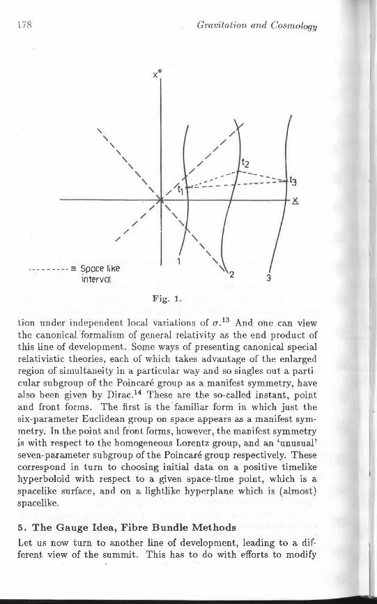
178
' ' ' ' ' '\
XO
' ' '
Gravitation and Cosmology
/ /
/~1 :...
/
/ /
/
~~~~~~~_.,.~"*'"~----1--~~--.,_.~~~~+-x
/
. --------= Space Ii ke interval
/
/ /
/ ' ' '
Fig. 1.
' '\ ' '
" 2 3
tion under independent local variations of o .13 And one can view the canonical "formalism of general relativity as the end product of this line of development. Some ways of presenting canonical special relativistic theories, each of which takes advantage of the enlarged region of simultaneity in a particular way and so singles out a particular subgroup of the Poincare group as a manifest symmetry, have also been given by Dirac.14 These are the so-called instant, point and front forms. The first is the familiar form in which just the six-parameter Euclidean group on space appears as a manifest symmetry. In the point and front forms, however, the manifest symmetry 1s with respect to the homogeneous Lorentz group, and an 'unusual' seven-parameter subgroup of the Poincare group respectively. These correspond in turn to choosing initial data on a positive timelike hyperboloid with respect to a given space-time point, which is a spacelike surface, and on a lightlike hyperplane which is (almost) spacelike.
5. The Gauge Idea, Fibre Bundle Methods
Let us now turn to another line of development, leading to a different view of the summit. This has to do with efforts to modify
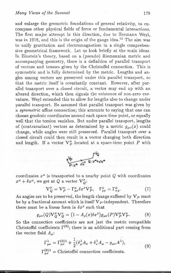
Many Views of the Summit 179
and enlarge the geometric foundations of general rela,tivity, to encompass other physical fields of force or fundamental interactions. The first major attempt in this direction, due to Hermann Weyl, was in 1918, and this is the origin of the gauge idea. 15 The aim was to unify gravitation and electromagnetism in a single comprehensive geometrical framework. Let us look briefly at the main ideas. In Einstein's theory, based on a (pseudo) Riemannian metric and accompanying geometry, there is a definition of parallel transport of vectors and tensors given by the Christoffel connection. This is symmetric and is fully determined by the metric. Lengths and angles among vectors are preserved under this parallel transport, so that the metric itself is covariantly constant. However, after parallel transport over a closed circuit, a vector may end up with an altered direction, which then signals the existence of non-zero cur-· vature. Weyl extended this to allow for lengths also to change under parallel transport. He assumed that parallel transport was given by a symmetric affine connection; this amounts to saying that one .can choose geodesic coordinates around each space-time point, or equally well that the torsion vanishes. But under parallel transport, lengths of (contra variant) vectors as determined by a metric g µv( x) could change, while angles were still preserved. Parallel transport over a closed circuit could then result in a vector changing both direction and length. If a vector V~ located at a space-time point P with
coordinates xµ is transported to a nearby point Q with coordinates xµ +oxµ, we get at Q a vector VQ:
Vµ - vµ rµ c pv· " rµ - rµ (7) Q - p - puuX p, pu - up·
As angles are to be preserved, the length change suffered by V p must be by a fractional amount which is itself V p-independent. Therefore there must be a linear form in oxP such that
Yµv(Q)VqVQ = (1- Ap(x)15xP)gµ.,(P)V~VJ,. (8)
So the connection coefficients are not just the metric compatible Christoffel coefficients r<0 >; there is an additional part coming from the vector field Aµ:
r;., = r~0J>· + ~(o;A" + o;Aµ - 9µ11A~), r~0J>- = Christoffel connection coefficients.
(9)
~ ... . ~ . . v •
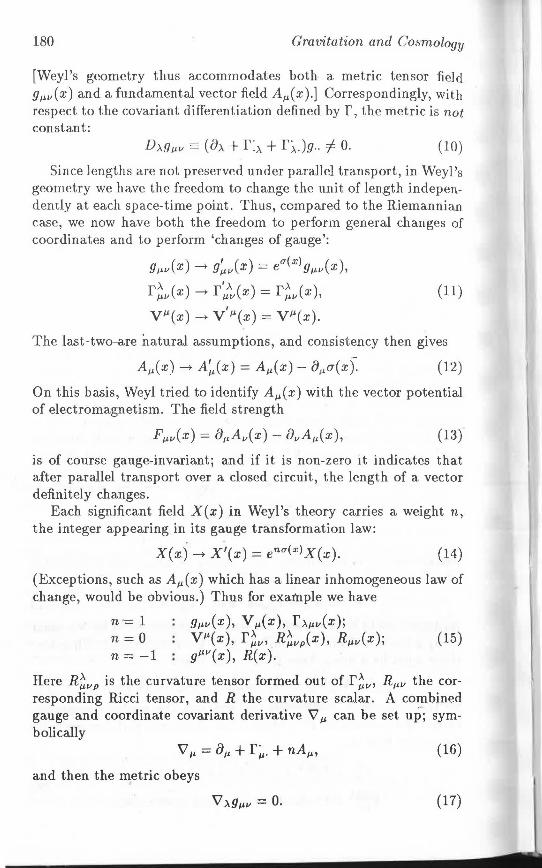
180 Gravitation and Cosmology
[Weyl's geometry thus accommodates both a metric tensor field gµ 11 (x) and a fundamental vector field Aµ(x).] Correspondingly, with respect to the covariant differentiation defined by r' the metric is not constant:
(10)
Since lengths are not preserved under parallel transport, in Weyl 's geometry we have the freedom to change the unit of length independently at each space-time point. Thus, compared to the Riemannian case, we now have both the freedom to perform general changes of coordinates and to perform 'changes of gauge':
9µ11(x)-+ 9~ 11 (x) = ea(x)9µ11(x), ,\ I A A r µ11(x)-+ r µ11(x) = r µ11(x), (11)
I
Vµ(x)-+ V µ(x) = Vµ(x).
The last-two-are natural assumptions, and consistency then gives
(12)
On this basis, Weyl tried to identify Aµ(x) with the vector potential of electromagnetism. The field strength
(13)
is of course gauge-invariant; and if it is non-zero it indicates that after parallel transport over a closed circuit, the length of a vector definitely changes.
Each significant field X( x) in Weyl's theory carries a weight n, the integer appearing in its gauge transformation law:
X(x.)-+ X'(x) = ena(x)X(x). (14)
(Exceptions, such as Aµ ( x) which has a linear inhomogeneous law of change, would be obvious.) Thus for example we have
n-= 1 9µ11(x), Vµ(x), f>.µv(x); n = 0 Vµ(x), f~11 , R~11p(x), Rµv(x); (15) n = -1 gµ 11 (x), R(x).
Here R;11 P is the curvature tensor formed out of f~ 11 , Rµ 11 the corresponding Ricci tensor, and R the curvature scalar. A combined gauge and coordinate covariant derivative V7 µ can be set up; symbolically
V7 µ = 8µ + r~. + nAµ,
and then the metric obeys
(16)
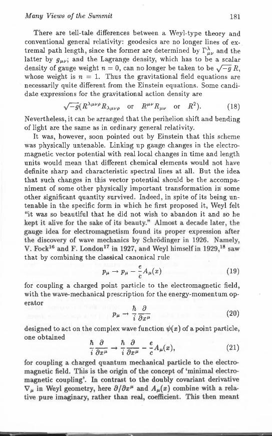
Many Views of the Summit 181
There are tell-tale differences between a Weyl-type theory and conventional general relativity: geodesics are no longer lines of extremal path length, since the former are determined by r~ll and the latter by gµ. 11 ; and the Lagrange density, which has to be a scalar density of gauge weight n = 0, can no longer be taken to be AR, whose weight is n = 1. Thus the gravitational field equations are necessarily quite different from the Einstein equations. Some candidate expressions for the gravitational action density are
Fg(R>..µ.llp R>.µ. 11p or Rµ. 11 Rµ. 11 or R2). (18)
Nevertheless, it can be arranged that the perihelion shift and bending of light are the same as in ordinary general relativity.
It was, however, soon pointed out by Einstein that this scheme was physically untenable. Linking up gauge changes in the electromagnetic vector potential with real local changes in time and length units would mean that different chemical elements would not have definite sharp and characteristic spectral lines at -all. But the idea that such changes in this vector potential should be the accompaniment of some other physically important transformation in some other significant quantity survived. Indeed, in spite of its being untenable in the specific form in which he first proposed it, Weyl felt "it was so beautiful that he did not wish to abandon it and so he kept it alive for the sa.ke of its beauty." Almost a. de ade later, the gauge idea for electromagnetism found its proper expression after the discovery of wave mechanics by Schrodinger in 1926. Namely, V. Fock16 and F. London17 in 1927, and Weyl himselfjn 1929,18 saw that by combining the classical canonical rule
e Pµ.-+ Pµ. - "'.""Aµ.(x) (19)
c
for coupling a charged point particle to the electromagnetic field, with the wave-mechanical prescription for the energy-momentum operator n a
Pµ. -+ i f)xµ. (20)
designed to act on the complex wave function t/J( x) of a point particle, one obtained
h 8 h 8 e -- -+ -- - -A (x) i {)xµ i {)xµ c µ ' (21)
for coupling a charged quantum mechanical particle to the electromagnetic field. This is the origin of the concept of 'minimal electromagnetic coupling'. In contnst to the doubly covariant derivative V µin Weyl geometry, here 8/fJxµ a.nd Aµ(x) combine with a relative pure imaginary, rather than real, coefficient. This then meant
~ ., .... . .. .
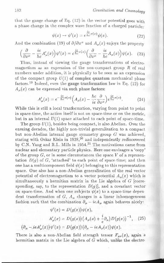
182 Gravitation and Cosmology
that the gauge change of Eq. (12) in the vector potential goes with a phase change in the complex wave function of a charged particle:
ie 1/;(x) ---+ 1/J'(x) = ehcc(x)1f;(x ). (22)
And the combination (19) of D/fJx 1" and Aµ(x) enjoys the property
( 8 ie 1 ( )) '( ) ie_a'x) ( 0 ie ( )) (23.) oxJ.L - ncA.u x 1/J x = ehc \ oxJ.L - ncAµ x 1/J(x).
Thus, instead of viewing the gauge transformations of electromagnetism as an expression of the non-compact group R of real numbers under addition, it is physically to be seen as an expression of the compact group U(l) of complex quantum mechanical phase factors. 19 Indeed, even the gauge tranformation law in Eq. (12) for Aµ ( x) can be expressed via such phase factors:
A' (x) = e-~~a(x) (A (x) - ~c _§_-)eJ,~a(x)_ (24) 1" µ ie 8xJ.L
While this is still a local tranformation, varying from point to point in space-time, the action itself is not on space-time or on the metric, but in an internal U ( 1) space attached to each point of space-time.
The group U(l), besides being compact, is also Abelian. Over the ensuing decades, the highly non-trivial generalization to a compact but non-Abelia.n internal gauge symmetry group G was achieved, staring with Oskar Klein in 1938,20 and independently rediscovered by C.N. Yang and R.L. Mills in 1954.21 The motivations came from nuclear and elementary particle physics. Here one envisages a 'copy' of the group G, or in some circumstances the space V of a representation D(g) of G, 'attached' to each point of space-time; and then one has a multicomponent field 1/;( x) belonging to this representation space. One also has a non-Abelian generalization of the real vector potential of electromagnetism to a vector potential Aµ( x) which is simultaneously a hermitian matrix in the Lie algebra of G (corresponding, say, to the representation D(g )] , and a covariant vector on space-time. And when one subjects 'lj;(x) to a space-time dependent transformation of G, Aµ changes in a linear inhomogeneous fashion such that the combination 8µ - ieAµ again behaves nicely:
'lj;'(x) = D(g(x))'!j;(x),
A~(x) = D(g(x)) (Aµ(xl) + iaµ)D(g(x))-1
, (25) e
(aµ - _ _ieA~(x))1/J 1 (x) = D(g(x)) (8µ - ieAµ(x))1/J(x).
There is also a non-Abelian field strength tensor Fµ,,(x), again a hermitian matrix in the Lie algebra of G which, unlike the electro-
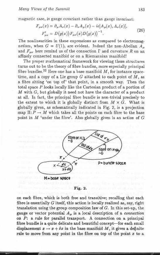
Many Views of the Summit 183
magnetic case, is gauge covariant rather than gauge invariant :
Fµ 11 (x) = 8µA 11 (x)- 811 Aµ(x)- ie[Aµ(x),A 11 (x)],
F~ 11 = D(g(x))Fµ 11(x)D(g(x)f1
• (26)
The nonlinearities in these expressions as compared to electromagnetism, when G = U(l), are evident. Indeed the non-Abelian Aµ and Fµ 11 here remind us of the connection r and curvature R on an affi.pely connected manifold or on a Riemannian manifold!
The proper mathematical framework for viewing these structures turns out to be the theory of fibre bundles, more especially principal fibre bundles. 22 Here one has a base manifold M, for instance spacetime, and a copy of a Lie group G attached to each point of M, as a fibre sitting 'on top of' that point, in a smooth way. Then the total space P looks locally like the Cartesian product of a portion of M with G, but globally it need not have the character of a product at all. In fact, the principal fibre bundle is non-trivial precisely to the extent to which it is globally distinct from M X G. What is globally given, as schematically indicated in Fig. 2, is a projection map II: P -+ M which takes all the points on each fibre to the base point in M 'under the fibre'. Also globally given is an action of G
(-;iii>(; ~
M • baH iPQCt
Fig. 2.
P• bundle SPote
on each fibre, which is both free and transitive; recalling that each fibre is essentially G itself, this action is locally realized as, say, right translation using the group composition law of G. In this set-up, the gauge or vector potential Aµ is a local description of a connection on P: a rule for parallel transport. A connection on a principal fibre bundle is a quite delicate and beautiful concept-for each small displacement z -+ x + 6x in the base manifold M, it gives a de(inite rule to move from any point in the fibre on top of the point x to a
-- . ~ . ·- '
184 Gravitation and Cosmology
definite corresponding point in the fibre on top of x +bx. Remember here that each fibre looks like and can be taken to be the group G itself. 'Thus a connection tells us how to 'lift' an open or closed curve in the base M to definite curves in the total space P, and these lifted curves go into one another under the global G action on the fibres. However, the lifts of a closed curve in M could well be open in P: one returns to the same fibre but to a generally different point than the starting one! This signals the existence of and is described by the curvature, of which Fµv is a local expression.
The theory of principal fibre bundles and connections on them was set up by Cartan and others quite early, in the twenties and thirties. (It was around the same time that Cartan developed the elegant calculus of differential forms.) The nice thing in this framwork is that the linear inhomogeneously transforming vector potential Aµ defined over (local portions of) the base manifold M is elevated to a covariantly behaving geometrical object-a connection form-on the total space P. Both Aµ and Fµv on Mare local descriptions via local cross-sections of G-covariant and globally defined geometrical objects more properly viewed as existing in the large space P. Then the gauge tranformation rules for Aµ and Fµv are results of changing this local description by changing the cross-section.
In this language, one can say that while Weyl's original theory attempted to view electromagnetism via an R-bundle over spacetirne M, each fibre being essentially the entire real line ,viewed as a group under addition, later developments in quantum mechanics replaced this by a U(l)-bundle over space-time. At the same time, Weyl's attempt to modify Riemannian geometry got transmuted to a scheme in which the gauge transformations of electromagnetism are tied up with transfo;mations in an internal space, referring to a non-space-time symmetry. How does all this now connect up with general relativity? Can we, with this additional insight and the later development of non-Abelian gauge theory, go back and re-examine general relativity itself, and view it as a kind of gauge theory? Here the story goes back again to Cartan and his work in the twenties! 23
While a given base manifold M (of dimension n, say) and a given Lie group G can, in principle, be combined in many inequivalent ways to form many principal fibre bundles, and one could then conceive of connections on each of them, there is a particular case which is specially singled out: a given base space M on its own determines unambiguously a particular principal fibre bundle for which the fibre or structure group is GL(n,R). For n = 4 we have GL(4,R). The point is that there is no freedom in the way in which M and G L( n, R) are glued together to form this particular bundle, the so-called frame
Many Views of the Summit 185
bundle on M; it is completely. fixed by the global topological properties of M itself. The key concept here is Cartan's 'repere mobile': a freely chosen anholonomic non-coordinate based frame or basis of vectors at each point of M. In four dimensions, we call it a vierbein or tetrad. Even without a metric on M we have the framework of this specific principal fibre bundle in which affine connections and parallel transport of vectors and tensors can be thought of: we need to deal with connections on th frame bundle of M. In a local description, this connection is given by affine connection coefficients r~v(x) over M, which a.re in general not symmetric, so there is room for torsion. Thus, while in a general principal fibre bundle with a group G over a base M, the key concepts are just those of connection and curvature only, in the particular ase of the frame bundle we have connection, curvature and torsion (not to speak of torture) as well. Another way of singling out this particular principal fibre bundle is to say that with the help of the dual basis to the vierbein, which constitutes a covariant geometric object or form called the 'soldering form', the individual fibres GL( 4,R) are soldered to points of the base M in a more intimate way than the fibres of a general principal fibre bundle. There is extra geometrical structure in a frame bundle. All this was worked out by Cartan in complete generality by about 1922! In case M carries a (pseudo) Riemannian metric as well, the tetrad can naturally be chosen to bring the metric 9µ,v at each point to diagonal Minkowski form, and then the Lorentz group S0(3,1) appears as a local gauge group as well.
That the fibre bundle concept should be useful to handle a spacetime can be seen in another, more elementary sense as well. In fact, this becomes evident in the passc~ge from the Aristotelian to the Galilean principle of relativity.22 In Aristotelian physics governed by the notions of absolute time and absolute space or absolute rest, each of the two statements-"the events A and B are simultaneous in time", "the events A and B occur at the same spatial location at different times"-ha.s an invariant meaning. Thus space-time is just the Cartesian product of space and time. But with Galilean relativity, where two inertial observers could have a uniform rel~tive velocity, the second statement above no longer has an invariant meaning! Simultaneity in time still has an absolute meaning, but not so coincidence in space. Therefore space-time is not a Cartesian product any more. Since time differences between events have absolute meaning, we can say that what is well-defined is a projection from space-time on to the one-dimensional time axis, so the former is a fibre bundle over the latter as base, with each fibre isomorphic to three-dimensional space. With special relativity, of course, there
] 86 Gravitation and Cosmology
are further changes and this bundle structure is lost. One can now try to close the circle an_d ask: are geometrical the
ories of gravity also gauge theories, similar to Yang-Mills theories based on an internal symmetry? The answer is a qualified yes, to some extent dependent on definitions of terms. An attempt to answer this question was first made by Utiyama in 1956,26 and completed more satisfactorily by Kibble in 1961,25 and Sciama in 1962.26 The situation is that if one starts with a special relativistic Lagrangian field theory invariant under global Poincare transformations, and in the spirit of the Yang-Mills argument one makes the ten parameters of the Poincare group arbitrary, independent space-time functions, one can then in a natural and intelligent way modify the Lagrangian so as to be invariant under this gauged Poincare group. The resulting theory is then a generally covariant field theory of the same general type that Cartan invented in the 1920s! This is called the Einstein-Cartan approach to gravity, on account of an interesting correspondence between them in the period 1929-1932 when Einstein was working with the idea of absolute or distant parallelism and Cartan told him, as usual, that he had done it years ago. 27 Adapting the Yang-Mills method from an internal compact symmetry group G to the Poincare group, one naturally finds that several geometric objects have to come in: a vierbein or tetrad h on space-time; a 'spin-connection' A which is just like a Yang-Mills gauge potential but with the Lorentz group S0(3,1) (more properly SL(2,C)] as a local internal gauge group; and an affine connection r on space-time:
Aab = -Aba µ µ
vierbein or tetrad; inverse to tetrad components of soldering form; spin connection = Yang-Mills gauge potential for local SL(2,C) transformations; affine connection coefficients on space-time
(27)
One is dealing here with a principal fibre bundle on spacetime which is a combination of the frame bundle and an SL(2,C) bundle! There is thus room here for both curvature and torsion, unlike a pure internal gauge symmetry; this agrees with what we said earlier, namely the frame bundle on a base manifold has richer structure and more intrinsic geometric objects than a general principal fibre bundle. Giving due allowance for these facts, one can view the Einstein-Cartan theory as the result of gauging the Poincare group of special relativity. As the vierbein has one leg in each group-GL( 4,R) and
Many Views of the Summit 187
SL(2,C)-conta.ined in the fibres, the natural condition to impose is
(28)
This is like the square root of the covariant constancy of the metric in ordinary general relativity! The vierbein and the spin connection can be regarded as the fundamental gravitational. variables. In terms of them, both the metric and the affine connection, and then the torsion and the curvature, are determined:
= hµah~; = h~Dµ(A)h~, = SL(2,C) - covariant derivative; = r>- - r>- =torsion· µ11 11µ '
R;11P = 811r;P - 8pr;11 + r~Pr~ 11 - f~11 r~p·
(29)
While·the coupling of matter fields to the gravitational variables is unambiguoulsy determined, one can examine various possible choices for the gravitational. action. One is free to set the torsion equal to zero from the beginning as a kinematical. condition; then we have left the minimum extension of conventional. general relativity needed to handle spinorial matter fields. If the torsion is present, its source is the spin density of matter; and whether or not it propagates depends very much on the choice of gravitational Lagrangian.
There have been generalizations of all this in several dire~tions. 28
For instance, one can put the entire Poincare group, rathe~ than just its homogeneous part, into the fibre, then the vierb~in and the spinconnection can be loo~ed upon to some extent as similar geometric objects, as the former become translational gauge potentials. Naturally we do not go into details here, but here we have another view of the summit.
6. General Relativity and Quantum Theory
Now I come to the last view of the summit that I wish to present. This has to do, with an interesting comparison between quantum theory and general relativity. As you may know, Bohr tried on many occasions to win Einstein's approval and support for his Principle of Complementarity, a key ingredient of his interpretation of quantum mechanics; but these of course Einstein never gave. That Bohr tried very hard to convince Einstein is clear from a phrase in his 1949 article summing up of their years of debate when he says:29 "The principal aim, however, of these considerations, which were not least inspired by the hope of influencing Einstein's attitude, was .... " It is then interesting to see what attitude Bohr took towards general relativity! I began by saying that it is common to regard general
. . - . :;-. ...
188 Gravitation and Cosmology
relativity as the summit of classical physics. Bohr however viewed it differently. He felt that "The abstract character of the formalisms concerned is indeed, on closer examination, as typical of relativity theory as it is of quantum mechanics, and it is in this respect purely a matter of tradition if the former theory is considered as a completion of classical physics rather than as a first fundamental step in the thoroughgoing revision of our conceptual means of comparing observations, which the modern development of physics has forced upon us." 30 Presumably in the hope of convincing Einstein, he went even further and tried to draw analogies between the two theories. For instance, he pointed out that in quantum mechanics, while object and apparatus are both ultimately quantum mechanical in nature, the theory of measurement makes us distinguish them and insist that the latter be describable in the limiting classical language; analogously in relativity, while general covariance tends to obliterate the difference between time and space coordinates, we are ultimately obliged to recognize the physical distinction between them. As another instance, he said that in relativity our description of any phenomenon depends in an essential way on the space-time coordinate system, even though it may be supported by definite rules of transformation; the analogy in quantum mechanics is that complementarity limits our attempts to interpret results of experiments independently of the experimental apparatus or arrangement. In case it is just a bit difficult to follow this, I offer you two statements, one by Dirac on relativity and the other by Heisenberg on quantum mechanics, which may help. Speaking of the metric tensor components Dirac says:31
"They determine both the coordinate system and the curvature of the space ... They describe not only the gravitational field, but also the system of coordinates. The gravitational field and the system of coordinates are inextricably mixed up in the Einstein theory, and one cannot describe the one without the other." Compare this with Heisenberg's statement on the nature of the wave function in quantum mechanics:32 "This probability function represents a mixture of two things, partly a fact and partly our knowledge of a fact." There is some similarity in these statements, and this is possibly what Bohr was hinting at.
7. Conclusion
I would now like to conclude, in a manner befitting this place and this occasion, this series of long-distance views of general relativity I have tried to bring before your eyes. But here I am a victim of the phenomenon of "anticipatory plagiarism" which is described in a recent article by Gunther Stent in this way:33 "Anticipatory
Many Views of the Summit 189
plagiarism occurs when someone steals your original idea and publishes it a hundred years before you were born." It so happens that in a lecture to the Indian Academy of Sciences in 1985 .S. Chandrasekhar already said exactly what I would like to say now. As there is hardly any chance of improving upon his expression let me quote him verbatim:34 "The pursuit of science has often been compared to the scaling of mountains, high and not so high. But who amongst us can hope, even in imagination, to scale the Everest and reach its summit when the sky is blue and the air is still, and in the stillness of the air survey the entire Himalayan range in the dazzling white of the snow stretching to infinity? None of us can hope for a comparable vision of nature and of the universe around us. But there is nothing mean or lowly in standing in the valley below and awaiting the sun to rise over Kanchenjunga."
References
1. Pa.is, A.: "Subtle is the Lord ... The Science a.nd the Life of Albert Einstein", Oxford University Press (1982), Chapter IV, especially p. 250 ff.
2. Ref. 1, p. 257 ff. 3. See, for instance, Moore, W.: "Schrodinger-Life a.nd Thought,'' Cambridge
University Press, 1989, pp. 211, 221. 4. Rosenfeld, L .. : Ann. Physik, li (1930), 113; Ann. Inst. H. Poincare, 2 (1932),
25. 5. Dirac, P.A.M.: Proc. Camb. Phil. Soc., 29 (1933) 389. 6. Dirac, P.A.M.: Can. J. Maths., 2 (1950), 129. 7. Anderson, J.L. a.nd Bergmann, P.G.: Phys. Rev., 83 (1951), 1018. 8. Dirac, P.A.M.: Proc. Roy. Soc., A246 (1958), 333. 9. Arnowitt, R., Deser, S. a.nd Misner, C.W.: Phys. Rev., 116 (1959), 1322;
117 (1960), 1595. 10. Dirac, P.A.M.: Scient. Amer., 208 (1963), 45. 11. Regge, T.: "The Group Manifold Approach to Unified Gravity", Les
Houches Lectures, 1983. 12. Dirac, P.A.M., Fock, V.A., Podolsky, B.: Phys. Z. Sowjetunion, 2 (1932),
468, reprinted in "Quantum Electrodynamics", Schwinger, J. (ed.), Dover Publications, Inc.,·New York, 1958.
13. See, for instance "Quantum Electrodynamics'', Schwinger, J. (ed.), Dover Pblica.tions, Inc., New York, 1958.
14. Dirac, P.A.M.: Rev. Mod. Phys., 21 (1949), 392. 15. Weyl, H.: "Space Time Matter", 4th edn. (1922), reprinted by Dover Pub
lications, Inc., New York, 1952, § 34, 35; see a.lso Pauli, W.: "Theory of Relativity", Pergamon Press, 1958, p. 192 ff.
16. Fock, V.A.: Zeit. /. Phys., 39 (1927), 226. 17. London, F.: Zeit. f. Phys., 42 (1927), 375; Naturwiss., lli (1927), 187.
18. Weyl, H.: Zeit. /. Phys., li6 (1929), 330.
190 Gravitation and Cosmology
19. Yang, C.N.: "Geometry and Physics" in "To Fulfill a Vision: Jerusalem Einstein Centennial Symposium on Gauge Theories and Unification of Physical Forces", Neeman, Y. (ed.), Addison-Wesley, 1981.
20. Klein, 0., in "New Theories in Physics", International Institute of Intellectual Cooperation, League of Nations, 1938, pp. 77-93.
21. Yang, C.N. and Mills, R.L.: Phys. Rev., 96 (1954), 191. 22. See, for instance, Trautman, A.: "Fibre Budles Associated with Space
Time", Reports on Mathematical Physics, 1 (1970), 29; "Differential Geometry for Physicists", Bibliopolis, Napoli, 1984.
'>3 . Cartan, E.: "On Manifolds with an Affine Connection and the Theory of General Relativity", translated by Ashteka.r, A., Bibliopolis, Napoli 1986.
24. Utiyama, R.: Phys. Rev., 101 (1956), 1597. 25. Kibble, T.W.B .: J. Math. Phys ., 2 (1961), 212. 26 . Sciama, D.W., in "Recent Trends in General Relativity", Pergamon Press,
1962. 27. "Elie Cartan-Albert Einstein-Letters on Absolute Parallelism 1929-1932",
Debever Robert (ed.), Princeton University Press, 1979. 28. For more details see, for instance, Pra.sa.nna, A.R.: "Differential Forms
and Einstein-Cartan Theory in Gravitation, Gauge Theories and the Early Universe", Iyer, B.R., Mukunda., N. and Vishveshwa.ra, C.V., (eds.), Kluwer Academic Publishers (Dordrecht), 1989.
29. Bohr, N.: "Discussion with Einstein on Epistemological Problems in Atomic Physics", in Albert Einstein: Philosopher Scientist, The Library of Living Philosophers, Inc., Eva11ston, Illinois, 7 (1949), 199; reprinted in Bohr, N.: "Atomic Physics and Human Knowledge", Science Editions, Inc., New York, 1961, p. 52.
30. Bohr, N.: "Atomic Physics a.nd Human Knowledge", Science Editions, Inc., New York, 1961, p. 65.
31. Dirac, P.A.M.: "General Theory of Relativity", John Wiley, New York 1975, pp. 9, 26.
32. Heisenberg, W.: "Physics and Philosophy", Harper and Row, New York, 1958, p. 45.
33. Stent, G.: "Complexity and Complementarity in the Phenomenon of Mind", University of California (Berkeley) Preprint (1989); the phrase is due to Robert Merton.
34. Chandra.sekha.r, S.: "Truth and Beauty-Aesthetics and Motivations in Science", Chica.go University Press, 1987, p. 26.
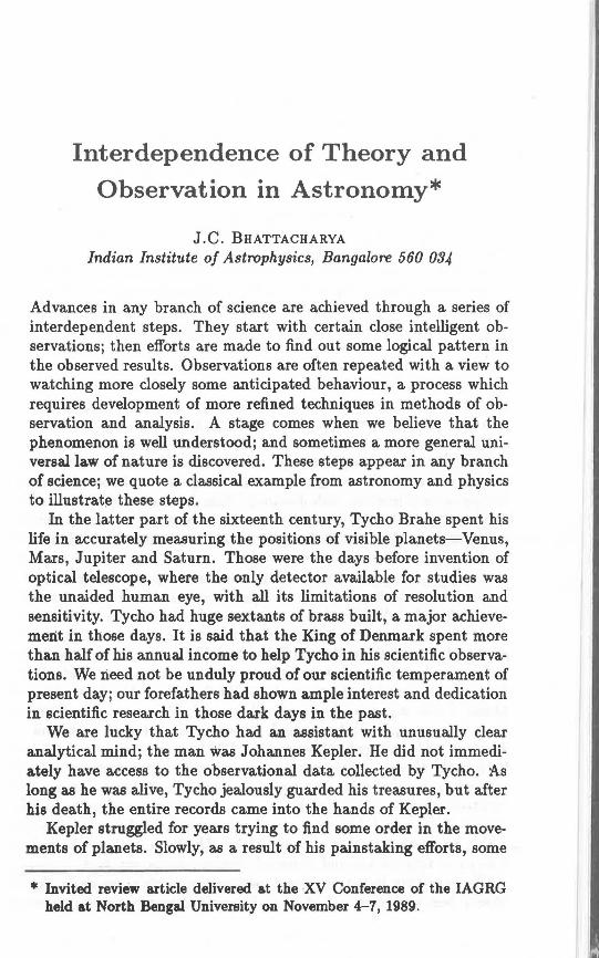
Interdependence of Theory and
Observation in Astronomy*
J.C. BHATTACHARYA
Indian Institute of Astrophysics, Bangalore 560 034
Advances in any branch of science are achieved through a series of interdependent steps. They start with certain close intelligent observations; then efforts are made to find out some logical pattern in the observed results. Observations are often repeated with a view to watching more closely some anticipated behaviour, a process which requires development of more refined techniques in methods of observation and analysis. A stage comes when we believe that the phenomenon is well understood; and sometimes a more general universal law of nature is discovered. These steps appear in any branch of science; we quote a classical example from astronomy and physics to illustrate these steps.
In the latter part of the sixteenth century, Tycho Brahe spent his life in accurately measuring the positions of visible planets-Venus, Mars, Jupiter and Saturn. Those were the days before invention of optical telescope, where the only detector available for studies was the unaided human eye, with all its limitations of resolution and sensitivity. Tycho had huge sextants of brass built, a major achievement in those days. It is said that the King of Denmark spent more than half of his annual income to help Tycho in his scientific observations. We Ii.eed not be unduly proud of our scientific temperament of present day; our forefathers had shown ample interest and dedication in scientific research in those dark days in the past.
We are lucky that Tycho had a.n assistant with unusually clear analytical mind; the man was Johannes Kepler. He did not immediately have access to the observational data collected by Tycho. :As long as he was alive, Tycho jealously guarded his treasures, but after his death, the entire records came into the hands of Kepler.
Kepler struggled for years trying to find some order in the movements of planets. Slowly, as a result of his painstaking efforts, some
• Invited review article delivered at the XV Conference of the IAGRG held at North Bengal University on November 4-7, 1989.
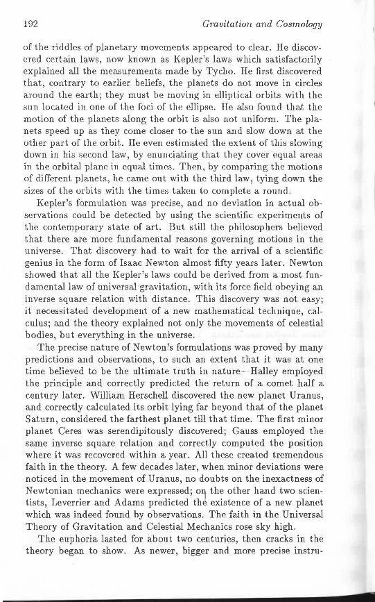
192 Gravitation and Cosmology
of the riddles of planetary movements appeared to clear. He discovered certain laws, now known as Kepler's laws which satisfactorily explained all the measurements made by Tycho. He first discovered that, contrary to earlier beliefs, the planets do not move in circles around the earth; they must be moving in elliptical orbits with the sun located in one of the foci of the ellipse. He also found that the motion of the plan-ets along the orbit is also not uniform. The planets speed up as they come closer to the sun and slow down at the other part of the orbit. He even estimated the extent of this slowing down in his second law, by enunciating that they cover equal areas in the orbital plane in equal times. Then, by comparing the motions of different planets, he came out with the third law, tying down the sizes of the orbits with the times taken to complete a round.
Kepler's formulation was precise, and no deviation in actual observations could be detected by using the scientific experiments of the contemporary state of art. But still the philosophers believed that there are more fundamental reasons governing motions in the universe. That discovery had to wait for the arrival of a scientific genius in the form of Isaac Newton almost fifty years later. Newton showed that all the Kepler's laws could be derived from a most fundamental law of universal ·gravitation, with its force field obeying an inverse square relation with distance. This discovery was not easy; it necessitated development of a new mathematical technique, calculus; and the theory explained not only the movements of celestial bodies, but everything in the universe.
The precise nature of Newton's formulations was proved by many predictions and observations, to such an extent that it was at one time believed to be the ultimate truth in nature-Halley employed the principle and correctly predicted the return of a comet half a century later. William Herschell discovered the new planet Uranus, and correctly calculated its orbit lying far beyond that of the planet Saturn, considered the farthest planet till that time. The first minor planet Ceres was serendipitously discovered; Gauss employed the same inverse square relation and correctly computed the position where it was recovered within a year. All these created tremendous faith in the theory. A few decades later, when minor deviations were noticed in the movement of Uranus, no doubts on the inexactness of Newtonian mechanics were expressed; 011 the other hand two scientists, Leverrier and Adams predicted th~ existence of a new planet which was indeed found by observations. The faith in the Universal Theory of Gravitation and Celestial Mechanics rose sky high.
The euphoria lasted for about two centuries, then cracks in the theory began to show. As newer, bigger and more precise instru-
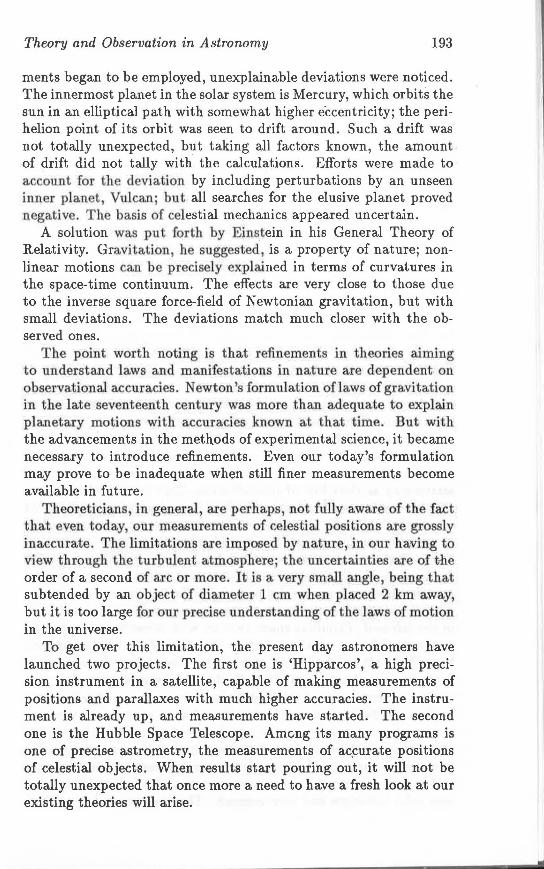
Theory and Observation in Astronomy 193
ments began to be employed, unexplainable deviations were noticed. The innermost planet in the solar system is Mercury, which orbits the sun in an elliptical path with somewhat higher eccentricity; the perihelion point of its orbit was seen to drift around. Such a drift was not totally unexpected, but taking all factors known, the amount of drift did not tally with the calculations. Efforts were made to ac ount for the deviation by including perturbations by an unseen inner planet, Vulcan; but all searches for the elusive planet proved negative. The basis of celestial mechanics appeared uncertain.
A solution was put forth by Eins.tein in his General Theory of Relativity. Gravitation, he suggested, is a property of nature; nonlinear motions ca.n be precisely explained in terms of curvatures in the space-time continuum. The effects are very close to those due to the inverse square force-field of Newtonian gravitation, but with small deviations. The deviations match much closer with the observed ones.
The point worth noting is that refinements in theories aiming to understand laws and manifestations in nature are dependent on observational accuracies. Newton's formulation oflaws of gravitation in the late seventeenth century was more than adequate to explain planetary motions with accuracies known at that time. But with the advancements in the methods of experimental science, it became necessary to introduce refinements. Even our today's formulation may prove to be inadequate when still finer measurements become available in future.
Theoreticians, in general, are perhaps, not fully aware of the fact that even today our measurements of celestial positions are grossly inaccurate. The limitations are imposed by nature, in our having to view through the turbulent atmosphere; the uncertainties a.re oft-he order of a second of arc or more. It is a very small angle, being that subtended by an object of diameter 1 cm when placed 2 km away, but it is too large for our precise understanding of the laws of motion in the universe.
To get over this limitation, the present day astronomers have launched two projects. The first one is 'Hipparcos', a high precision instrument in a satellite, capable of making measurements of positions and parallaxes with much higher accuracies. The instrument is already up, and measurements have started. The second one is the Hubble Space Telescope. Amcng its many programs is one of precise astrometry, the measurements of ac,curate positions of celestial objects. When results start pouring out, it will not be totally unexpected that once more a need to have a fresh look at our existing theories will arise.
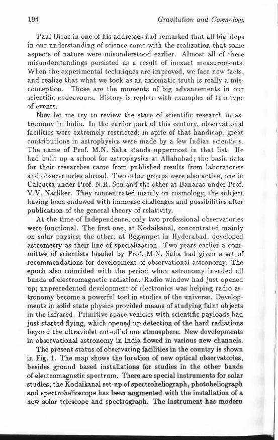
194 Gravitation and Cosmology
Paul Dirac in one of his addresses had remarked that all big steps in our understanding of science come with the realization that some aspects of nature were misunderstood earlier. Almost all of these misunderstandings persisted as a result of inexact measurements. When the experimental techniques are improved, we face new facts, and realize that what we took as an axiomatic truth is really a misconception. Those are the moments of big advancements in our scientific endeavours. History is replete with examples of this type of events.
Now let me try to review the state of scientific research in astronomy in India. In the earlier part of this century, observational facilities were extremely restricted; in spite of that handicap, great contributions in astrophysics were made by a few Indian scientists. The name of Prof. M.N. Saha stands uppermost in that list. He had built up a school for astrophysics at Allahabad; the basic data for their researches came from published results from laboratories and observatories abroad. Two other groups were also active, one in Calcutta under Prof. N .R. Sen and the other at Banaras under Prof. V.V. Narliker. They concentrated mainly on cosmology, the subject having been endowed with immense challenges and possibilities after publication of the general theory of relativity.
At the time of Independence, only two professional observatories were functional. The first one, at Kodaikanal, concentrated mainly on solar physics; the other, at Begampet in Hyderabad, developed astrometry as their line of specialization. Two years earlier a committee of scientists headed by Prof. M.N. Saha had given a set of recommendations for development of observational astronomy. The epoch also coincided with the period when astronomy invaded all bands of electromagnetic radiation. · Radio window had just opened up; unprecedented development of electronics was helping radio astronomy become a powerful tool in studies of the universe. Developments in solid state physics provided means of studying faint objects in the infra.red. Primitive space vehicles with scientific payloads had just started flying, which openeg up detection of the hard radiations beyond the ultraviolet cut-off of our atmosphere. New developments in observational astronomy in India flowed in various new channels.
The present status of observating facilities in the country is shown in Fig. 1. The map shows the location of new optical observatories, besides ground based installations for studies in the other bands of electromagnetic spectrum. There are special instruments for solar studies; the Kodaikanal set-up of spectroheliograph, photoheliograph and spectrohelioscope has been augmented with the installation of a new solar telescope and spectrograph. The instrument has modern
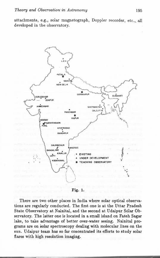
Theory and Observation· in Astronomy 195
attachments, e.g., solar magnetograph, Doppler recorder, etc.,. all developed in the observatory .
SOMllAV rfNAllAYANGAON
PUNE
• PANCHMARI
··· -·
• RAIPUR
• EXISTING
• UNDER DEVELOPMENT
• TEACHING OBSERVATORY
Fig. 1.
There are two other places in India where solar optical observations are regularly conducted. The first one is at the Uttar Pradesh State Observatory at Nainital, and the second at Udaiplir Solar Observatory. The latter one is located in a small island on Fateh Sagar lake, to take ad.vantage of better over-water seeing. Nainital programs are on solar spectroscopy dealing with molecular lines on the sun. Udaipur team has so far concentrated its efforts to study solar flares with high resolution imaging.
' • A - - ~
196 Gravitation and Cosmology
Koda.ikanal also has some night observational facilities, but the major stellar installation is at Kavalur. The new observatory, named after the legendary astronomer, of our times, Vainu Bappu, has telescopes of various sizes and matching focal plane instruments for several programs in the frontiers of astronomy today. The largest aperture telescope here is the Vainu Bappu Telescope; with a clear aperture of 232 cm, it is at present the largest optical telescope in Asia. The telescope has been totally fabricated in India, and it took about ten years for its completion.
The Nizamiah Observatory at Hyderabad is no longer functional; their observational activities have been shifted to Japal-Rangapur Observatory, 60 km south-east of the city. A 48 inch aperture optical telescope is the main instrument here; programs in photometry and spectroscopy are being pursued on objects in our galaxy. The scientists here have carried out high quality observations on variable stars.
A new observatory for optical observations was started by the Uttar Pradesh State Government after Independence; the person responsible for locating, equipping and starting the observatory was Dr. Va.inn Bappu. Researches on many current topics of present day astronomy are being carried out here. Some of the recent discoveries in the solar system from India came through observations by 2 onemetre Zeiss telescopes; one of them is located here, the other being at the Va.inu Bappu Observatory, Kavalur.
Radio observations of astronomical objects in India started after Independence. First observations were recorded at Koda.ikanal in 1952. A major project in this area was undertaken in 1965 when scientists from Tata Institute of Fundamental Research, Bombay, started building a large steerable cylindrical dish · for meter wave observations at Ootacammand in the Nilgiris. The telescope was completed in 1970, and contributed a few bits of vital information about the radio universe.
Another project aiming to study radiations in the long wave region was started by a team of scientists from the Indian Institute of Astrophysics at Kodaikanal in mid-sixties. They were joined by another team from the Raman Research Institute in Bangalore, and completed a decameter radial array telescope at Gauribidanur in Karnata.ka in 1979. Several astronomical bodies which cannot be studied except through these decameter waves were investigated by using this telescope.
At the present moment no observatories are engaged in observations in the centimeter waveband; some attempts to monitor 10 cm flux from the sun were made at Koda.ikanal in the late sixties. When
Theory and Observation in Astronomy 197
suitable equipment was built and set up, owing to lack of manpower these observations have remained suspended.
In the millimeter wave region, a committed effort has been made by the scientists of the Raman Research Institute in Bangalore. They have built' up a fully steerable dish of 10 'rn diameter of the required surface accuracy and fabricated the complete receiving equipment. Several students in the institute have taken up research projects based on observations using this set-up.
The importance of infrared observations has been brought out through recent advances in our understanding of the universe. The band is wide, starting from the red end of the visible spectrum around one micron and stretching to the millimeter wave region of wavelength one thousand times longer. The techniques needed in different parts on the band are different. In the near infrared, equipment used in optical observations can be used with a little modification, whereas millimeter wave techniques are employed at the other end. In the near and middle infrared, as well as in the extreme far infrared, equipment located high up in the mountains can be used, but elsewhere, high flying aircraft, balloons, rockets and satellites are employed. In search of observations around 100 microns, TIFR scientists have deployed a balloon-borne 1 m diameter far IR telescope fabricated within the country.
For near and middle infrared observations searches for suitable sites have been going on for the last few years. A 48 inch IR telescope totally fabricated in India has been installed on a mountain top in Rajasthan; the new site at Gurusikhar near Mount Abu promises to be a good site for near and middle infrared, but searches for a still better site in the high ranges in the Himalayas have been continuing.
On the other side of the visible band, the high energy radiations are absorbed by our earth's atmosphere, and only way of direct observations is to send up the equipment above the absorbing layer of our atmosphere. Such an equipment for studies of celestial X-rays has been fabricated by a group of scientists belonging to TIFR and flown in a balloon from the National Balloon Facility at Hyderabad. Some X-ray instruments have been sent up by the Indian scientists in rockets, and one incor.porated in the first Indian satellite ARYABHATA.
For extreme high energy photons in the gamma ray region, nature has provided a method of indirect observations. These photons break up in electron-positron pairs; the components, having relativistic velocities, produce visible Cerenkov radiation. These radiations can be detected from the ground. Two scientific groups in India, one at Gulmarg in Kashmir and the other at Pachmarhi in Madhya Pradesh
198 Gravitation and Cosmology
are engaged in these studies. This sums up the present efforts in India in observational astro
nomy using electromagnetic radiations. There are other means of getting information about the far reaches of the universe, e.g., by particle streams, or other energy fluxes like gravitational radiation. Cosmic rays represent a major field where considerable efforts of Indian scientists have been spent. over the past half-a-century. The latest effort in this field has been the unique experiment "Anuradha" flown in the space shuttle, which has brought out new information about the nature of that enigmatic stream of particles. Thoughts and speculations about using many newer ideas are being voiced by members of the scientific community in India today.
Index
Accretion disk 20 Angular momentum 19 Antenna correlations 80 Anuradha 198 Aryabhata 19 7'
Bar detectors 48 Bekenstein-Hawking temperature 11 Big Bang cosmology 129
problems 129 Binary pulsar 1913+16 65 Binary stare 24, 45
coalescing 51, 52, 56, 63, 66 Black holes 8, 25 Bondi flow 22 Boyer-Lindquist coordinates 9, 10 Bundle space 34
Chaotic inflation 134 Chiral transitions 139 Circular loops 113 Chirp signal 56
waveform 75 Coalescence time 69 Compa.ctifi.cations
Calabi-Yau 91, 104 Orbifolde 91
Compact eta.rs 22 Confinement 139 Connection 35, 179, 183, 187 Coset bundles 37 Convergence problem of Euclidean
pa.th integral 153 Constrained dynamics 175 cps x cps 1z; model 92, 104 cps x CP2 /Z3 x Z~ model 93, 105 CP2 x CP2 /Zs x Z~ x Z~ model 106
Cylindrica.l coordinates 113
Data analysis for gravitational wave 56 techniques 69 threshold mode 70 summation mode 72
de Sitter instanton 149 minisuperspa.ce 150
Effective potential 117, 123 properties 124 computation 125 at non-zero temperature 127 effect of a heavy fermion 136
Einstein-Cartan action 159, 163, 186 Electro-weak transition 134 Ergoephere 26 Euclidean path integral 153, 158 Exotic light particles 96
Flatness problem 130 Fibre bundles 30, 33, 178, 183
principal 34, 184, 186
Gauge theory 31, 128, 178, 184 Gaugino doublets 98 Gibbons-Hawking-Perry ansatz 148 Gia.show-Salam-Weinberg theory 134 Grand Unified Theory 30, 122, 123,
129, 131 Gravitational antenna cross-section
85 Gravitational wave
description 46 detection 45 polarization 46, 66
200
power 64 sources 51, 57
Hartle-Hawking proposal 147, 149, 168 status 154
Heat bath interactions 88 Helicity operator 160 Higgs mechanism 30, 135 Higgs mass spectrum 97
matrix 98 Horizon temperature 11 Hubble space telescope 193
Inertial mass 113 Inflation 129, 143
old,scenario 129, 131, 133 new scenario 133
Interferometers delay line 60, 61 laser 49 Michelson 59 recycling 62, 63
Kepler J. 191 Kerr metric 4, 9
of black hole 10 Kerr-Newman-de Sitter space-time
8, 9, 10 of black hole 13
Lepton mass hierarchy 101 Lie groups 32 LIGO project 50
Magnetic fluxons 115, 118 Matched filtering technique 73 Maurer-Cartan form 33 Mirror generation 95
Nambu-Gotto action 110, 111 string 109
Neutrino detectors 80 Baksan 80, 81
IMB 81 Kamioka 80, 81 Mont Blanc 80, 81
Neutrino masses 99, 101 Non-Abelian group 31
Order parameter 120
IndP,x
Operator ordering ambiguity 151
Phase transitions 120 classification 122 scenario in early universe 121
Planck length 143 Principle of equivalence 172 Proton stability 103
Quadrupole moment tensor 64 Quantum cosmology 143 Quantum chromodyna.mics 30, 122,
139
Shilov boundary 161 Skyrme soliton 161 Slow rolling 134 Spontaneous symmetry breaking 93 String transition 138
electromagnetic interaction 110 Supernova 52 Supersymmetry transition 138
Tunnelling across a potential barrier 131
Vierbein 186 Vilenkin's boundary condition 149,
155, 168
Wheeler-DeWitt equation 146, 158 Wino 103 Wormhole 155, 158
Zero temperature potential 134 Zino 103
I