karol popławski - cern document server
TRANSCRIPT
CER
N-T
HES
IS-2
019-
142
03/0
7/20
19
Institute of Theory of Electrical Engineering, Measurement and Information Systems
in the field of study Applied Automatic Control and Robotics and specialisation Automatic Control
Detector Control System for SciFi tracker in LHCb
thesis number in the Faculty thesis register 171488
Karol Popławski
thesis supervisor
prof. dr hab. inż. Andrzej Michalski
CERN project supervisor
dr Sune Jakobsen
WARSAW 2019
Abstract
Large Hadron Collider is experiencing major upgrade during Long Shutdown 2. During
that period the LHCb experiment will improve many detectors including Scintillating Fibre
(SciFi) Tracker as part of the tracking system upgrade. Beside the Data Acquisition required
for particle physics analysis there are services enabling proper and safe environment for
that. The goal of this thesis is to explain the challenges during establishing and
implementation of Detector Control System (DCS) for SciFi tracker. The design and layout of
SciFi tracker will be briefly clarified. Explanation of DCS itself will be broaden by the
communication methods between the systems and their final implementation in LHCb
specific network and software. The software upgrade foresees the enhancement towards
fast and understandable framework. It will bring new approaches to ease the user’s
experience while using the control system. The thesis will point out the requirements
needed during testing of the tracker parts. The separate research was established to study
the commissioning needs along with the differences between hardware testing and
commissioning. Furthermore the improvements of the needs will be brought to the
attention. The latter will simplify the usage of created tools and their new features.
Moreover the built system will be described to enable further development and including
the created solutions in different detectors. Finally the thesis will focus on including DCS in a
Supervisory Control And Data Acquisition (SCADA) system and therefore in general
Experiment Control System (ECS) used in LHCb Control Area to operate the full experiment.
New implementation and navigation will be shown through Finite State Machine (FSM) tree
used as the control tool to operate the ECS.
Streszczenie
Wielki Zderzacz Hadronów zostanie poddany wielu usprawnieniom i przemianom
podczas Long Shutdown 2. W tym czasie eksperyment LHCb usprawni i zmodernizuje wiele
detektorów włączając w to Scintillating Fibre (SciFi) Tracker (Traker cząstek z włókien
scyntylujących) jako część systemu śledzenia cząstek. Poza zbieraniem danych ze zderzeń
(Data Acquisition, DAQ), potrzebnych do rozwoju fizyki cząstek elementarnych, występuje
zbiór usług, tzw. slow controls (systemy wolnego sterowania, poza DAQ), pozwalających na
właściwe i bezpieczne ich rejestrowanie. Celem niniejszej pracy dyplomowej jest wyjaśnienie
wyzwań powstałych podczas tworzenia i wdrażania Systemu Sterowania Detektorem
(Detector Control System) dla trakera SciFi. Zostanie przedstawiony projekt i konstrukcja
trakera SciFi. Wyjaśnienie samego DCS wraz z jego podsystemami zostanie poszerzone o
metody komunikacji pomiędzy nimi oraz o ich ostateczne wdrożenie w strukturę sieciową i
software właściwe dla LHCb. Nowy software ma na celu nie tylko podstawowe sterowanie,
ale również autor przewiduje jego rozszerzenie w celu uzyskania szybkiego, zrozumiałego
oraz łatwo dostępnego pakietu. Przyniesie on nowe rozwiązania ułatwiające użytkowanie
podczas operowania systemem sterowania. Praca wyszczególni wymagania stawiane
badanemu systemowi w czasie przeprowadzanych testów nad częściami trakera. Osobne
badanie zostało przeprowadzone w celu zgłębienia potrzeb i różnic systemu sterowania
podczas testowania sprzętu oraz podczas oddania do eksploatacji części detektora.
Dodatkowo zostaną szczególnie zaprezentowane usprawnienia nałożone na powyższe
wymagania. Nakładki pozwolą na ułatwienie użycia narzędzi software’owych oraz
wprowadzą dodatkowe opcje sterowania. Ponadto powstały system zostanie objaśniony,
aby umożliwić dalszą jego rozbudowę oraz wdrożenie do innych detektorów o podobnej
strukturze DCS. Ostatecznie w pracy zostanie objaśnione włączenie DCS do systemu SCADA
(Supervisory Control And Data Acquisition) oraz jego nadrzędnej, centralnej wersji Systemu
Sterowania Eksperymentem (Experiment Control System) odpowiedzialnego za pełne
sterowanie LHCb. Zostanie zaprezentowany nowy sposób wdrożenia i poruszania się po
drzewie automatu skończonego (Finite State Machine), używanego jako narzędzie do
sterowania oraz zarządzania ECS.


Acknowledgements
I would like to thank all my fellow colleagues from CERN for input to the project and
the ability to constantly deepen my knowledge in many fields. The tools I have created
would not have been made without feedback from SciFi group members. I would like to
specially thank my supervisor Sune Jakobsen and colleague/supervisor Lukas Gruber for
challenging me to always create the systems even better and user friendly. There were many
other people from my former group that were co-sharing the knowledge with me like Tara,
Daniel, Mauricio and Snow. Individual thanks to Luis Granado Cardoso for having patience in
explaining every software connected problem. Thank you all my CERN and non-CERN friends,
that made the stay there so uncommon. And the last but not the least I would also like to
thank my thesis supervisor prof. Michalski for approving the subject from the beginning and
support until the end.
Dziękuję całej rodzinie i bliskim za wspieranie mnie, nawet jeśli nie było to łatwe, a
temat mojej pracy był dla Was niezrozumiały.

1
Table of contents
1. Introduction .......................................................................................................... 3
1.1. Tracking system of LHCb ................................................................................... 6
2. Scintillating Fibre Tracker ..................................................................................... 8
2.1. Scintillating Fibres ............................................................................................. 8
2.2. Design and layout of Scintillating Fibre Tracker ............................................... 9
2.2.1. DCS as part of Experiment Control System ................................................. 14
2.2.1. SciFi tracker services ................................................................................... 16
2.2.2. Project requirements .................................................................................. 20
2.2.3. Used software ............................................................................................. 21
3. Detector Control System .................................................................................... 23
3.1. Challenges and improvements of DCS............................................................ 23
3.2. DCS MONitoring .............................................................................................. 25
3.2.1. Vacuum system panel ................................................................................. 29
3.2.2. Dry gas panel for prototype C-Frame ......................................................... 30
3.3. C-Frame temperature readout ....................................................................... 32
3.3.1. Temperature measurement ........................................................................ 32
3.3.2. Wire connection and PLC communication .................................................. 32
3.3.3. C-Frame temperature monitoring GUI ....................................................... 33
3.4. DCS Low Voltage ............................................................................................. 38
3.4.1. LV control panel for experts........................................................................ 39
3.4.2. Everyday usage of Low Voltage .................................................................. 43
4. SciFi Tracker assembly and commissioning........................................................ 49
4.1. Monitoring panels .......................................................................................... 49
4.1.1. Parent panel ................................................................................................ 49

2
4.1.2. Cooling plant ............................................................................................... 52
5. DCS as part of Finite State Machine structure ................................................... 56
5.1. SFDCSLV FSM .................................................................................................. 56
5.2. SFDCSMON FSM ............................................................................................. 64
5.2.1. Dry Gas FSM ................................................................................................ 64
6. Achievements and further DCS development .................................................... 68
7. Conclusion .......................................................................................................... 69
Bibliography .................................................................................................................. 70
Attachments ................................................................................................................. 71
Attachment 1 ............................................................................................................ 71
Attachment 2 ............................................................................................................ 73
3
1. Introduction
The Large Hadron Collider beauty (LHCb) experiment is one of the four biggest
experiments on Large Hadron Collider (LHC). LHC is a 27 km in circumference underground
accelerator made for particle physics research. It is built by an international collaboration at
European Organisation for Nuclear Research (CERN) and is colliding protons or lead ions with
nearly the speed of light. These collisions are recorded and analysed to broaden the
knowledge of matter. The Interaction Point 8 (IP8) of LHC is the cavern of LHCb - an
experiment of special purpose on LHC ring. Specialized in beauty quark physics, it is mainly
focused on studying antimatter and CP-violation.
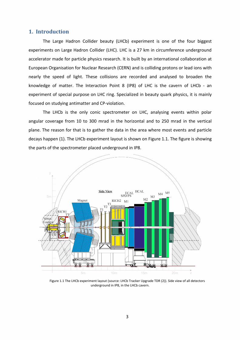
The LHCb is the only conic spectrometer on LHC, analysing events within polar
angular coverage from 10 to 300 mrad in the horizontal and to 250 mrad in the vertical
plane. The reason for that is to gather the data in the area where most events and particle
decays happen (1). The LHCb experiment layout is shown on Figure 1.1. The figure is showing
the parts of the spectrometer placed underground in IP8.
Figure 1.1 The LHCb experiment layout (source: LHCb Tracker Upgrade TDR (2)). Side view of all detectors underground in IP8, in the LHCb cavern.

4
Starting from collision point the parts of LHCb experiment are as follows (3):
o Vertex Locator (VELO), designed to perform an accurate positioning of fast decaying
particles in particular B-mesons.
o Ring Imagining Cherenkov (RICH) detectors measuring the particles’ speed by
emission of Cherenkov radiation. The system consisting of an upstream detector
RICH1 and a downstream detector RICH2 is able to identify charged particles over the
mass range 1-150 GeV/c.
o Dipole magnet with an integrated field of 4 Tm. The magnet bends charged particles
and according to the curvature registered by the tracking system the charge and
mass can be measured.
o Tracking system divided into the Outer Tracker and the Silicon Tracker. Before
magnet the silicon Trigger Tracker (TT) is present. After Lorentz force bending there
are 3 tracking stations each with the silicon Inner Tracker (IT) (4) – placed close to the
beam pipe – and gas-filled straw tube technology Outer Tracker (OT) (5) covering
areas further from the beam pipe.
o The calorimeter system, measuring the amount of energy lost as each of its layers.
The system consists of: the Scintillating Pad Detector (SPD), the Pre-Shower Detector
(PS), the ‘‘shashlik’’-type Electromagnetic Calorimeter (ECAL), and the scintillating tile
iron plate Hadron Calorimeter (HCAL). The SPD checks if the particle is charged or
neutral, while the PS indicates the electromagnetic character of the particle. Both of
them are used as a trigger in association with ECAL. After the discrimination between
the neutral and charged particles the energy measurements take place – ECAL
gathers the data of the charged ones whilst the HCAL is responsible for the energy of
the remaining hadrons.
o Muon system responsible for detecting muons present in the final states of many B-
decays. These play a major role in CP asymmetry and are important to understand
the differences between matter and antimatter. It is composed of 5 stations from
which one is placed before the calorimeter system. Each of the 5 muon chambers is
filled with a mixture of three gases carbon dioxide, argon, and tetrafluoromethane.
Their reaction with the passing muons can be therefore detected.
The system of detectors above registers, directly or indirectly, different properties of
particles such as energy and charge. After the readout, the computing algorithms are used to
5
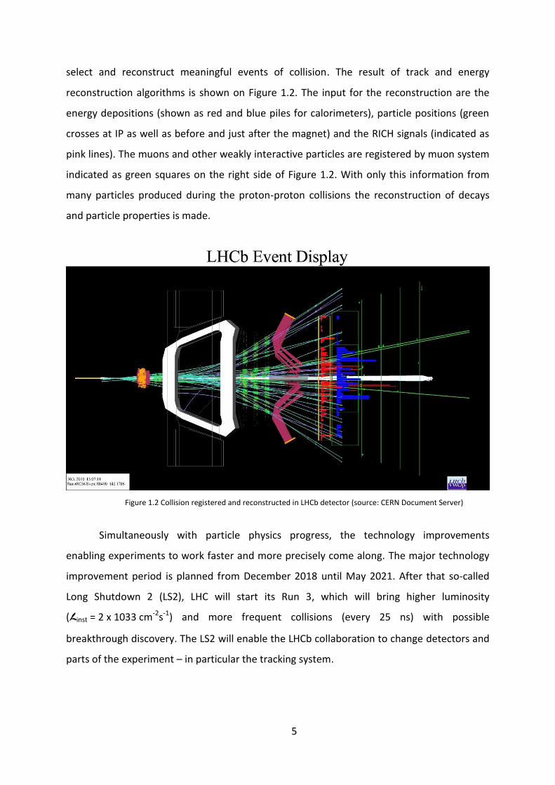
select and reconstruct meaningful events of collision. The result of track and energy
reconstruction algorithms is shown on Figure 1.2. The input for the reconstruction are the
energy depositions (shown as red and blue piles for calorimeters), particle positions (green
crosses at IP as well as before and just after the magnet) and the RICH signals (indicated as
pink lines). The muons and other weakly interactive particles are registered by muon system
indicated as green squares on the right side of Figure 1.2. With only this information from
many particles produced during the proton-proton collisions the reconstruction of decays
and particle properties is made.
Figure 1.2 Collision registered and reconstructed in LHCb detector (source: CERN Document Server)
Simultaneously with particle physics progress, the technology improvements
enabling experiments to work faster and more precisely come along. The major technology
improvement period is planned from December 2018 until May 2021. After that so-called
Long Shutdown 2 (LS2), LHC will start its Run 3, which will bring higher luminosity
(Linst = 2 x 1033 cm-2s-1) and more frequent collisions (every 25 ns) with possible
breakthrough discovery. The LS2 will enable the LHCb collaboration to change detectors and
parts of the experiment – in particular the tracking system.

6
1.1. Tracking system of LHCb
Tracking system of LHCb consists of series of stations with Inner Tracker (IT) and
Outer Tracker (OT) components. Their tasks are:
o To find and track charged particles between Vertex Locator (VELO) and the
calorimeters: Electromagnetic Calorimeter (ECAL) and Hadron Calorimeter
(HCAL); and measure the particle momenta.
o Provide precise measurements of the direction of track segments in the two Ring
Imaging Cherenkov (RICH) detectors.
o Link measurements in VELO, calorimeters and muon detector.
More detailed design and tasks of both are explained in respective Technical Design
Report (TDR) (4) and (5). Both of the trackers are supposed to register the curvature of
particle tracks influenced by dipole magnet of 4 Tm bending power (6).
During LS2 an upgrade of tracking system is foreseen. The upgrade of LHCb Data
Acquisition (DAQ) and trigger system from 1 MHz up to 40 MHz read-out is required from all
detectors. Along with them the tracking system will enable the LHCb experiment to track
particles with full read-out of front-end electronics (FEE) of 40 MHz trigger system.
Moreover, the whole LHCb will be designed to cope with the nominal operational luminosity
increased by a factor of 5 in comparison to the current state. Detailed information about the
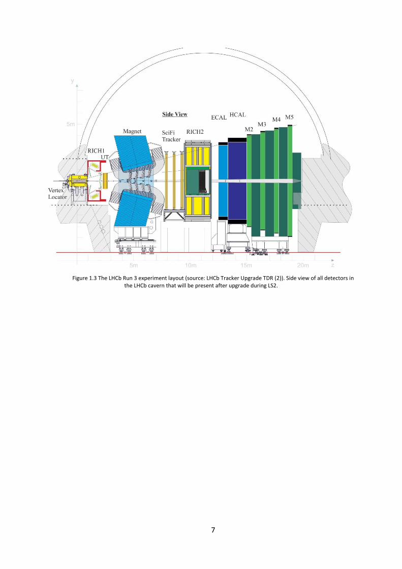
Tracker Upgrade can be found in its TDR (2). IT and OT detectors will be replaced with two
new detectors – Upstream Tracker (UT) and Scintillating Fibre Tracker (SciFi, SF), both shown
on Figure 1.3. This thesis is focused on the design and implementation of Detector Control
System for SciFi Tracker.
7
Figure 1.3 The LHCb Run 3 experiment layout (source: LHCb Tracker Upgrade TDR (2)). Side view of all detectors in the LHCb cavern that will be present after upgrade during LS2.
8
2. Scintillating Fibre Tracker
There are three downstream tracking stations: T1, T2 and T3. Before LS2 they were
consisted of two detectors:
IT – silicon micro-strip detector covering an area of 0.35m2 in the high track density
around the beam-pipe.
OT – large straw detector covering 99% of 30m2 surface of the tracking stations
surface (2).
During LS2 these tracking stations will be upgraded with the SciFi tracker that will
cover full acceptance after the magnet – from the edge of the beam-pipe to about 3m in the
horizontal and 2.4m in the vertical plane.
2.1. Scintillating Fibres
In order to register every charged particle passing through the detector layers, they
are built of scintillating plastic fibres with diameter of 250µm. After particle hit the ionisation
energy is deposited, producing the excitation of the polymer core of the fibre. To improve
the efficiency of the scintillation mechanism (quite poor relaxation time and light yield of the
base material) an organic fluorescent dye with matched excitation energy level structures is
added to the polystyrene base. Energy is transferred from the base to the dye, where the
excited energy state of the latter will relax by emission of the photons. After this multi-step
process most of the produced photons are lost and only some of them stay inside the
scintillating core – trapping efficiency for the scintillation light in a single hemisphere is
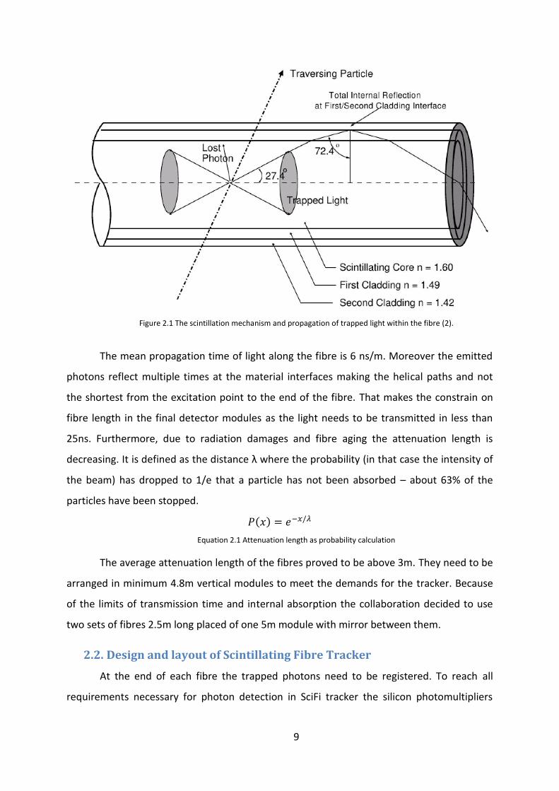
5.34% (2). Then the trapped light travels inside the fibre due to total internal reflections
between core and both claddings (Figure 2.1).
9
Figure 2.1 The scintillation mechanism and propagation of trapped light within the fibre (2).
The mean propagation time of light along the fibre is 6 ns/m. Moreover the emitted
photons reflect multiple times at the material interfaces making the helical paths and not
the shortest from the excitation point to the end of the fibre. That makes the constrain on
fibre length in the final detector modules as the light needs to be transmitted in less than
25ns. Furthermore, due to radiation damages and fibre aging the attenuation length is
decreasing. It is defined as the distance λ where the probability (in that case the intensity of
the beam) has dropped to 1/e that a particle has not been absorbed – about 63% of the
particles have been stopped.
𝑃(𝑥) = 𝑒−𝑥/𝜆
Equation 2.1 Attenuation length as probability calculation
The average attenuation length of the fibres proved to be above 3m. They need to be
arranged in minimum 4.8m vertical modules to meet the demands for the tracker. Because
of the limits of transmission time and internal absorption the collaboration decided to use
two sets of fibres 2.5m long placed of one 5m module with mirror between them.
2.2. Design and layout of Scintillating Fibre Tracker
At the end of each fibre the trapped photons need to be registered. To reach all
requirements necessary for photon detection in SciFi tracker the silicon photomultipliers
10
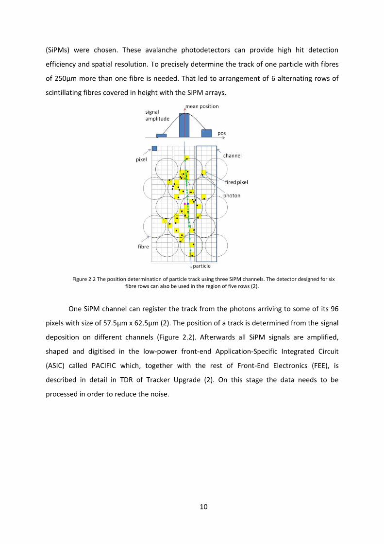
(SiPMs) were chosen. These avalanche photodetectors can provide high hit detection
efficiency and spatial resolution. To precisely determine the track of one particle with fibres
of 250µm more than one fibre is needed. That led to arrangement of 6 alternating rows of
scintillating fibres covered in height with the SiPM arrays.
Figure 2.2 The position determination of particle track using three SiPM channels. The detector designed for six fibre rows can also be used in the region of five rows (2).
One SiPM channel can register the track from the photons arriving to some of its 96
pixels with size of 57.5µm x 62.5µm (2). The position of a track is determined from the signal
deposition on different channels (Figure 2.2). Afterwards all SiPM signals are amplified,
shaped and digitised in the low-power front-end Application-Specific Integrated Circuit
(ASIC) called PACIFIC which, together with the rest of Front-End Electronics (FEE), is
described in detail in TDR of Tracker Upgrade (2). On this stage the data needs to be
processed in order to reduce the noise.
11
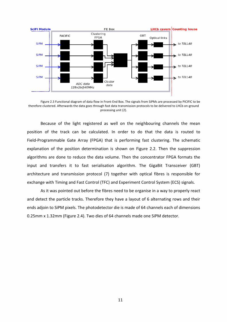
Figure 2.3 Functional diagram of data flow in Front-End Box. The signals from SiPMs are processed by PICIFIC to be therefore clustered. Afterwards the data goes through fast data transmission protocols to be delivered to LHCb on-ground
processing unit (2).
Because of the light registered as well on the neighbouring channels the mean
position of the track can be calculated. In order to do that the data is routed to
Field-Programmable Gate Array (FPGA) that is performing fast clustering. The schematic
explanation of the position determination is shown on Figure 2.2. Then the suppression
algorithms are done to reduce the data volume. Then the concentrator FPGA formats the
input and transfers it to fast serialisation algorithm. The GigaBit Transceiver (GBT)
architecture and transmission protocol (7) together with optical fibres is responsible for
exchange with Timing and Fast Control (TFC) and Experiment Control System (ECS) signals.
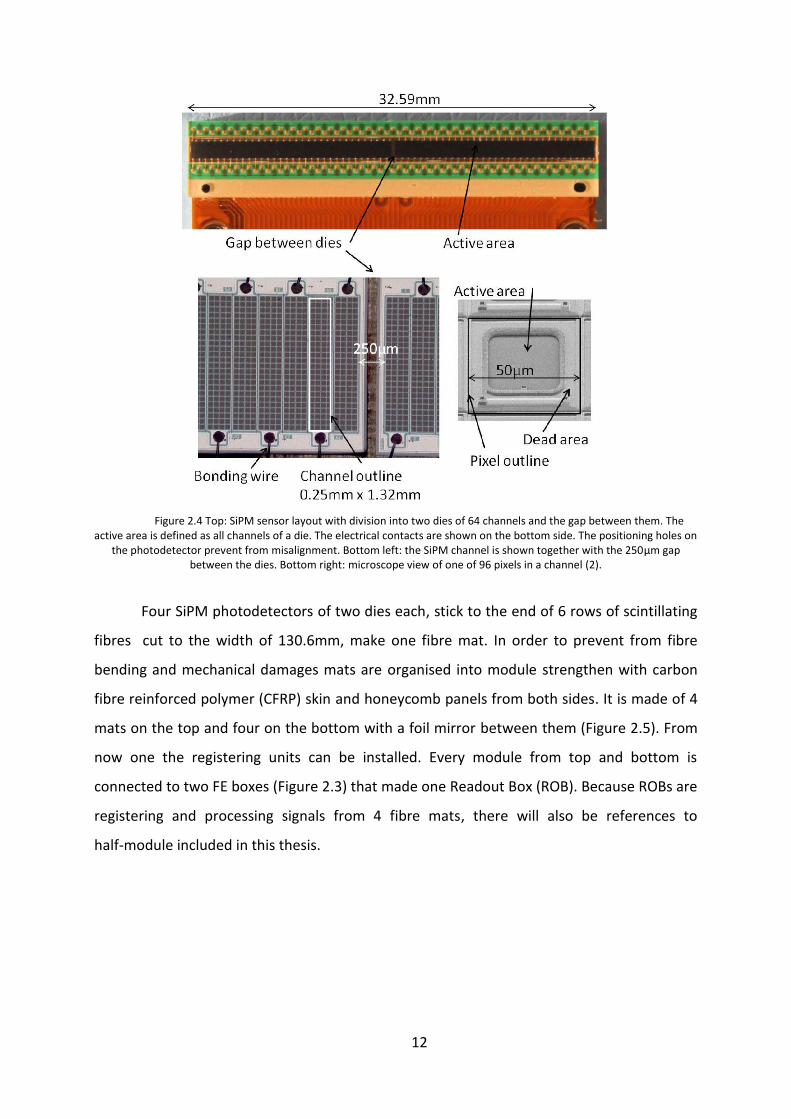
As it was pointed out before the fibres need to be organise in a way to properly react
and detect the particle tracks. Therefore they have a layout of 6 alternating rows and their
ends adjoin to SiPM pixels. The photodetector die is made of 64 channels each of dimensions
0.25mm x 1.32mm (Figure 2.4). Two dies of 64 channels made one SiPM detector.
12
Figure 2.4 Top: SiPM sensor layout with division into two dies of 64 channels and the gap between them. The active area is defined as all channels of a die. The electrical contacts are shown on the bottom side. The positioning holes on
the photodetector prevent from misalignment. Bottom left: the SiPM channel is shown together with the 250µm gap between the dies. Bottom right: microscope view of one of 96 pixels in a channel (2).
Four SiPM photodetectors of two dies each, stick to the end of 6 rows of scintillating
fibres cut to the width of 130.6mm, make one fibre mat. In order to prevent from fibre
bending and mechanical damages mats are organised into module strengthen with carbon
fibre reinforced polymer (CFRP) skin and honeycomb panels from both sides. It is made of 4
mats on the top and four on the bottom with a foil mirror between them (Figure 2.5). From
now one the registering units can be installed. Every module from top and bottom is
connected to two FE boxes (Figure 2.3) that made one Readout Box (ROB). Because ROBs are
registering and processing signals from 4 fibre mats, there will also be references to
half-module included in this thesis.
13
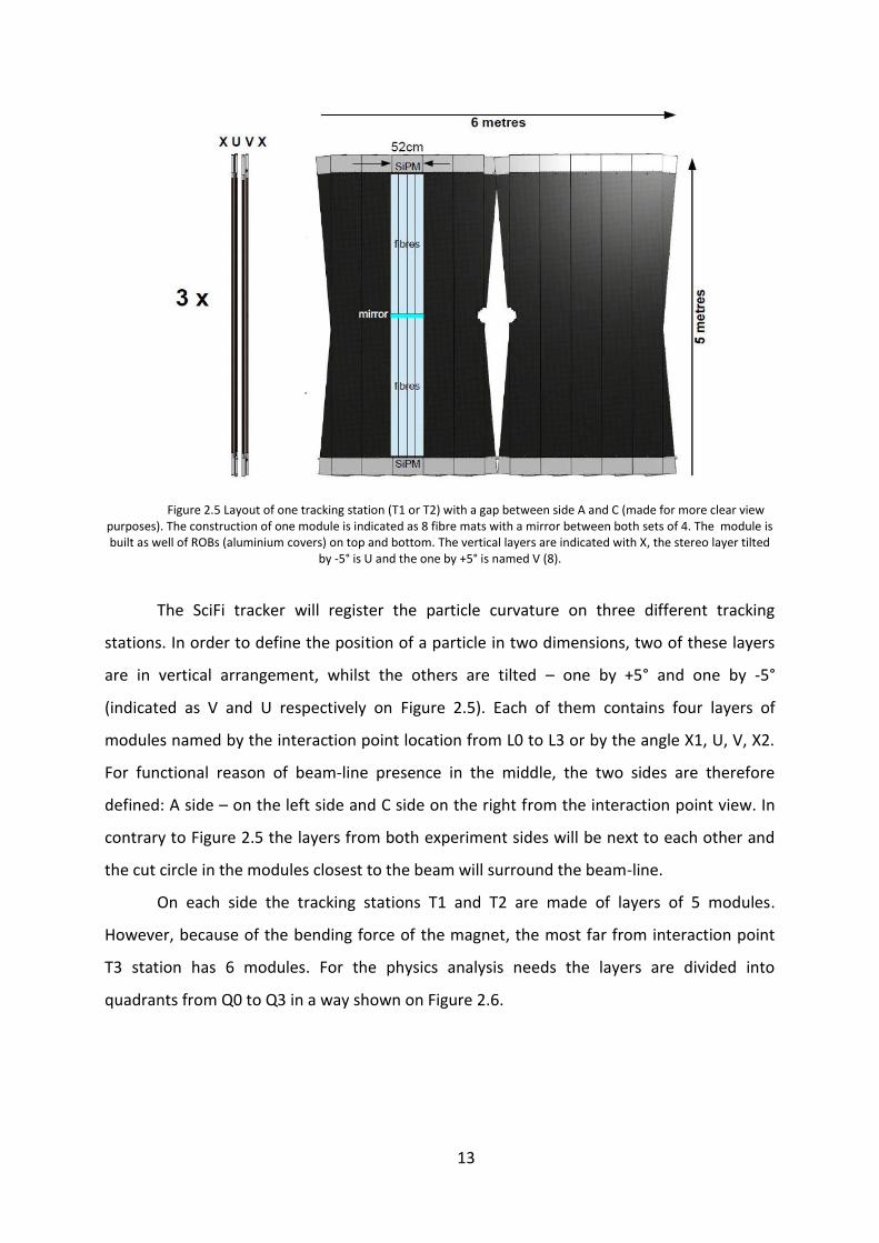
Figure 2.5 Layout of one tracking station (T1 or T2) with a gap between side A and C (made for more clear view purposes). The construction of one module is indicated as 8 fibre mats with a mirror between both sets of 4. The module is built as well of ROBs (aluminium covers) on top and bottom. The vertical layers are indicated with X, the stereo layer tilted
by -5° is U and the one by +5° is named V (8).
The SciFi tracker will register the particle curvature on three different tracking
stations. In order to define the position of a particle in two dimensions, two of these layers
are in vertical arrangement, whilst the others are tilted – one by +5° and one by -5°
(indicated as V and U respectively on Figure 2.5). Each of them contains four layers of
modules named by the interaction point location from L0 to L3 or by the angle X1, U, V, X2.
For functional reason of beam-line presence in the middle, the two sides are therefore
defined: A side – on the left side and C side on the right from the interaction point view. In
contrary to Figure 2.5 the layers from both experiment sides will be next to each other and
the cut circle in the modules closest to the beam will surround the beam-line.
On each side the tracking stations T1 and T2 are made of layers of 5 modules.
However, because of the bending force of the magnet, the most far from interaction point
T3 station has 6 modules. For the physics analysis needs the layers are divided into
quadrants from Q0 to Q3 in a way shown on Figure 2.6.
14
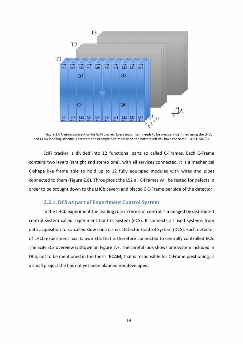
Figure 2.6 Naming convention for SciFi tracker. Every major item needs to be precisely identified using the LHCb and CERN labelling scheme. Therefore the example half-module on the bottom left will have the name T1L0Q1M4 (9).
SciFi tracker is divided into 12 functional parts so called C-Frames. Each C-Frame
contains two layers (straight and stereo one), with all services connected. It is a mechanical
C-shape like frame able to hold up to 12 fully equipped modules with wires and pipes
connected to them (Figure 2.8). Throughout the LS2 all C-Frames will be tested for defects in
order to be brought down to the LHCb cavern and placed 6 C-Frame per side of the detector.
2.2.1. DCS as part of Experiment Control System
In the LHCb experiment the leading role in terms of control is managed by distributed
control system called Experiment Control System (ECS). It connects all used systems from
data acquisition to so-called slow controls i.e. Detector Control System (DCS). Each detector
of LHCb experiment has its own ECS that is therefore connected to centrally controlled ECS.
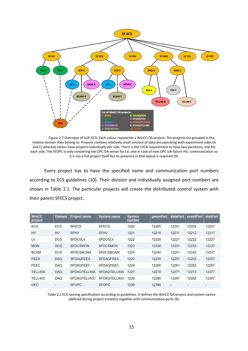
The SciFi ECS overview is shown on Figure 2.7. The careful look shows one system included in
DCS, not to be mentioned in the thesis. BCAM, that is responsible for C-Frame positioning, is
a small project the has not yet been planned nor developed.
15
Figure 2.7 Overview of SciFi ECS. Each colour represents a WinCC OA project. The projects are grouped in the relative domain they belong to. Projects contains relatively small amount of data are operating both experiment sides (A and C) whereas others have projects individually per side. There is the LHCb requirement to have two partitions, one for
each side. The SFOPC is only containing the OPC DA server for LV, and in case of new OPC UA failure HV, communication so it is not a full project itself but its presence in that layout is required (9).
Every project has to have the specified name and communication port numbers
according to ECS guidelines (10). Their division and individually assigned port numbers are
shown in Table 2.1. The particular projects will create the distributed control system with
their parent SFECS project.
Table 2.1 ECS naming specification according to guidelines. It defines the WinCC OA project and system names (defined during project creation) together with communication ports (9).

16
All WinCC OA projects are using Linux Operating System (OS) machines and
developers need to log in remotely. Because of the OPC DA server that could run only on
Windows OS the additional computer was included in the distributed system.
The functional tool to operate full ECS is Finite State Machine (FSM) (10). It is a
mathematical model of computation used by all LHC experiments. This virtual machine is
passing the states from one level to another in reaction to developer defined inputs. It is a
list of states, initial states and the conditions for transition between them. Its functionality
and proper work between levels of its tree structure is provided by relevant CERN control
group (11). The task for developers of each system listed in Table 2.1 is to define the lowest
level state transition from the hardware (Device Unit, DU) to its upper level (Control Unit,
CU). This is done by FSM recipes connecting the device value or triggered alarm with its state
in FSM structure. Moreover the implementation of every system includes building the FSM
tree from the top level to device assignment, along with creating the control panels at least
showing the overall information of leafs of one node. It is worth mentioning that there were
some nodes without control panels during LHC Run 2. The author decided to add panels to
every tree level to provide the user with information regardless the chosen node.
2.2.1. SciFi tracker services
There is as well large group of services that make this tracking possible. Supplying
with current or cooling enables to gather data and ensures stable performance for active
detector units.
17
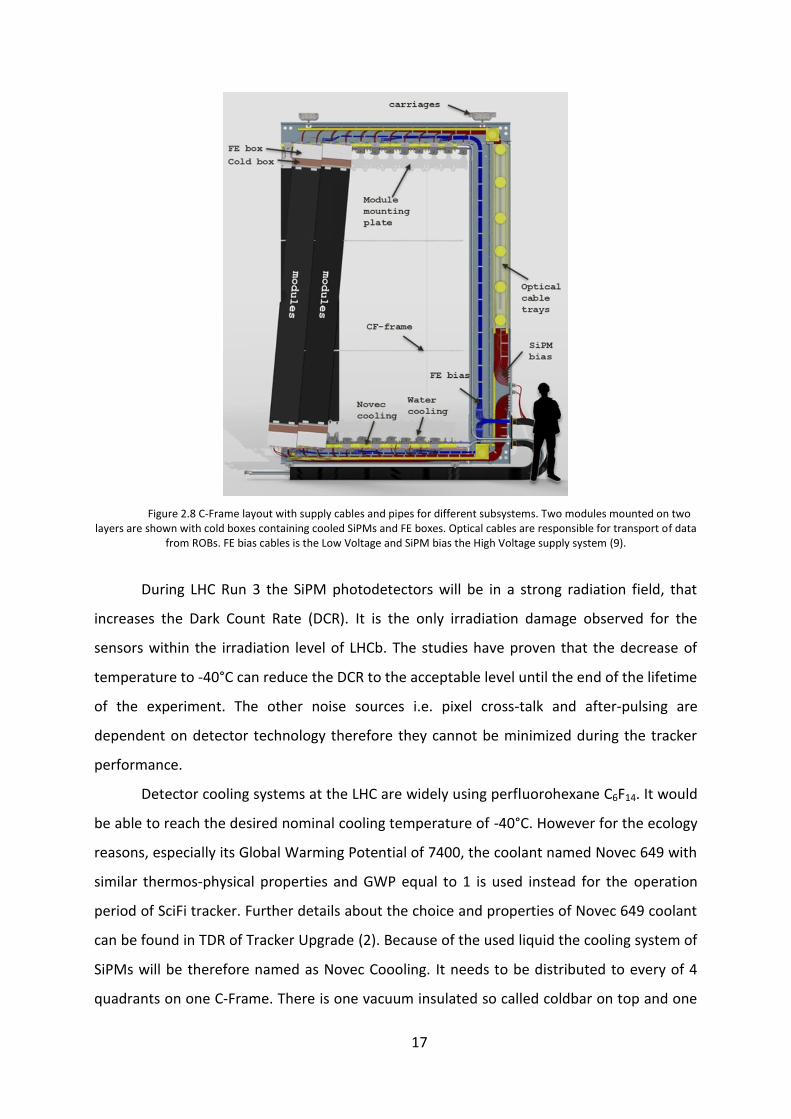
Figure 2.8 C-Frame layout with supply cables and pipes for different subsystems. Two modules mounted on two layers are shown with cold boxes containing cooled SiPMs and FE boxes. Optical cables are responsible for transport of data
from ROBs. FE bias cables is the Low Voltage and SiPM bias the High Voltage supply system (9).
During LHC Run 3 the SiPM photodetectors will be in a strong radiation field, that
increases the Dark Count Rate (DCR). It is the only irradiation damage observed for the
sensors within the irradiation level of LHCb. The studies have proven that the decrease of
temperature to -40°C can reduce the DCR to the acceptable level until the end of the lifetime
of the experiment. The other noise sources i.e. pixel cross-talk and after-pulsing are
dependent on detector technology therefore they cannot be minimized during the tracker
performance.
Detector cooling systems at the LHC are widely using perfluorohexane C6F14. It would
be able to reach the desired nominal cooling temperature of -40°C. However for the ecology
reasons, especially its Global Warming Potential of 7400, the coolant named Novec 649 with
similar thermos-physical properties and GWP equal to 1 is used instead for the operation
period of SciFi tracker. Further details about the choice and properties of Novec 649 coolant
can be found in TDR of Tracker Upgrade (2). Because of the used liquid the cooling system of
SiPMs will be therefore named as Novec Coooling. It needs to be distributed to every of 4
quadrants on one C-Frame. There is one vacuum insulated so called coldbar on top and one
18
on the bottom of each C-Frame (Figure 2.9). From there the Novec lines are connected to
every coldbox by S-shape vacuum insulated pipes (Figure 2.10).
During LS2 the cooling commissioning of every C-Frame will be done with the Baby
Cooling Plant (Baby Plant). This smaller version of the final cooling plant will supply the
vacuum insulated Novec coolant pipes to reach the temperature down to the nominal value
of -40°C and below to around -50°C in order to test the cooling possibilities, the insulation
and dry gas dew point.
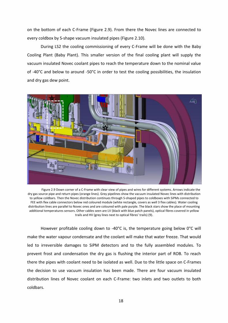
Figure 2.9 Down corner of a C-Frame with clear view of pipes and wires for different systems. Arrows indicate the dry gas source pipe and return pipes (orange lines). Grey pipelines show the vacuum insulated Novec lines with distribution
to yellow coldbars. Then the Novec distribution continues through S-shaped pipes to coldboxes with SiPMs connected to FEE with flex cable connectors below red coloured module (white rectangle, covers as well 3 flex cables). Water cooling
distribution lines are parallel to Novec ones and are coloured with pale purple. The black stars show the place of mounting additional temperatures sensors. Other cables seen are LV (black with blue patch panels), optical fibres covered in yellow
trails and HV (grey lines next to optical fibres’ trails) (9).
However profitable cooling down to -40°C is, the temperature going below 0°C will
make the water vapour condensate and the coolant will make that water freeze. That would
led to irreversible damages to SiPM detectors and to the fully assembled modules. To
prevent frost and condensation the dry gas is flushing the interior part of ROB. To reach
there the pipes with coolant need to be isolated as well. Due to the little space on C-Frames
the decision to use vacuum insulation has been made. There are four vacuum insulated
distribution lines of Novec coolant on each C-Frame: two inlets and two outlets to both
coldbars.
19
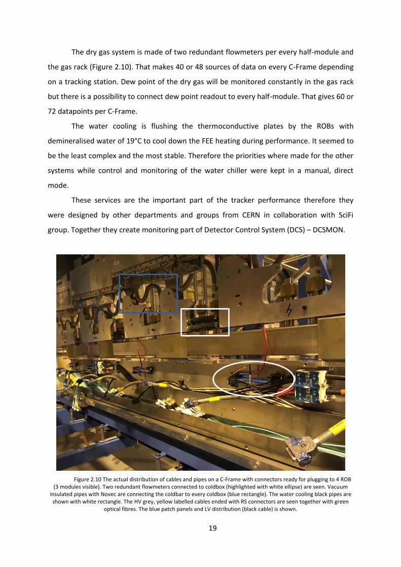
The dry gas system is made of two redundant flowmeters per every half-module and
the gas rack (Figure 2.10). That makes 40 or 48 sources of data on every C-Frame depending
on a tracking station. Dew point of the dry gas will be monitored constantly in the gas rack
but there is a possibility to connect dew point readout to every half-module. That gives 60 or
72 datapoints per C-Frame.
The water cooling is flushing the thermoconductive plates by the ROBs with
demineralised water of 19°C to cool down the FEE heating during performance. It seemed to
be the least complex and the most stable. Therefore the priorities where made for the other
systems while control and monitoring of the water chiller were kept in a manual, direct
mode.
These services are the important part of the tracker performance therefore they
were designed by other departments and groups from CERN in collaboration with SciFi
group. Together they create monitoring part of Detector Control System (DCS) – DCSMON.
Figure 2.10 The actual distribution of cables and pipes on a C-Frame with connectors ready for plugging to 4 ROB (3 modules visible). Two redundant flowmeters connected to coldbox (highlighted with white ellipse) are seen. Vacuum
insulated pipes with Novec are connecting the coldbar to every coldbox (blue rectangle). The water cooling black pipes are shown with white rectangle. The HV grey, yellow labelled cables ended with RS connectors are seen together with green
optical fibres. The blue patch panels and LV distribution (black cable) is shown.

20
There are two voltage systems present at SciFi detector. One is responsible for
supplying the SiPM photodetectors. It is changing the setpoint for every SiPM according to
its temperature, irradiation level and the voltage feedback from measurements done by FEE.
The other supplies the ROBs and FEE in them. Besides these services DCS is divided also into
the second voltage system. The electronics are consuming a lot of energy while processing
data, configuring or applying new settings. Because of that the separate Low Voltage (LV)
system is needed. The desired value of the power supply output is 8V while the current
varies from 1A to more than 20A depending on FEE mode. The author of this thesis is
responsible for the full distributed SCADA system operating LV.
2.2.2. Project requirements
As it was described throughout the chapter, the Detector Control System for SciFi
tracker is a complex domain of its overall control system. The challenges and requirements
of the project were therefore:
o Establish a robust – bilateral for LV – communication with the used subcomponents
using diverse protocols and standards i.e.: TCP/IP, OPC DA, DIP/DIM. In case of
connection interruption the users are ought to be informed about that state.
o Create a structure of gathered values so that they could be traceable later. Every
values needs to have its own unrepeatable identifier dependant on position at the
detector.
o Point and connect prepared like that values to their devices like sensors or actuators.
o Archive the values in the Remote Database (RDB) with a reasonable smoothing, that
reduces the amount of stored data. Smoothing defines the frequency the values are
saved to the database even if they are constantly changing. It enables to define
thresholds both value and time dependent, below which no retrieved value will be
stored. The DCS values are updated every 100ms. Storing all of them will cluttered
the database with irrelevant values. This is why there is a strong need to make time
and relative value constrains on smoothing configuration.
o Create control panels showing the values retrieved from DCS subsystems. They need
to be able to show values and enable to plot the history of their changes. These
panels are mainly used during the C-Frame testing and commissioning.

21
2.2.3. Used software
The standard software for distributed SCADA system used at CERN is WinCC Open
Architecture (WinCC OA), currently owned by Siemens. It can contains many user defined
projects that enable the developer to create visual layout of a system and connect the fields,
of created like this control panel, with so called datapoints (DPs). The latter are the storages
of data organised in a raw format (float, integer etc.) or in a structure of raw formats e.g. a
group called “channel” with parameters “on/off”, “voltage” and “current”. The control
scripts can be defined for one of possible actions (like pressing the button or initializing of a
shape) and are written in WinCC OA specific programming language comparable to C#. On
the top of that software a framework called JCOP (Joint COntrol Project) was created at
CERN to simplify the usage of it (12).
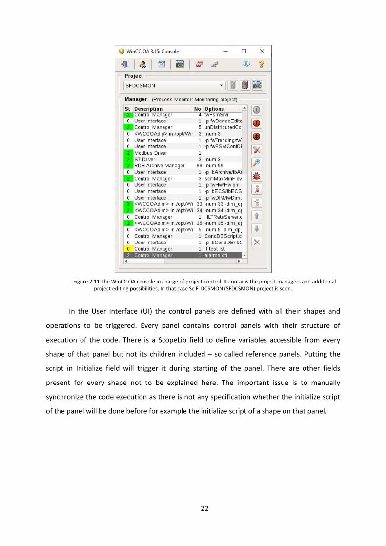
WinCC OA projects have multiple managers (Figure 2.11) that are responsible for
tasks from running the User Interface to running the control scripts. The latest are enabling
to define the procedure running constantly like for example calculating the data from
datapoints.
22
Figure 2.11 The WinCC OA console in charge of project control. It contains the project managers and additional project editing possibilities. In that case SciFi DCSMON (SFDCSMON) project is seen.
In the User Interface (UI) the control panels are defined with all their shapes and
operations to be triggered. Every panel contains control panels with their structure of
execution of the code. There is a ScopeLib field to define variables accessible from every
shape of that panel but not its children included – so called reference panels. Putting the
script in Initialize field will trigger it during starting of the panel. There are other fields
present for every shape not to be explained here. The important issue is to manually
synchronize the code execution as there is not any specification whether the initialize script
of the panel will be done before for example the initialize script of a shape on that panel.

23
3. Detector Control System
Detector Control System (DCS) is a distributed control system enabling slow control
of the detector. It is not responsible for registering nor transport of data but makes it
possible to change settings. In a final implementation it is also a part of another control
system named in LHCb Collaboration as Experiment Control System (ECS). The latter is a
SCADA distributed control environment responsible for proper particle identification, data
flow, work of services and safety system. It will be explained more in chapter 5 “DCS as part
of ”. DCS is divided into Low Voltage supplying and monitoring part that contains all services
explained in chapter 2.2. The latter means that these services ought to have alarms, be
visualised and archived by the author whilst the control will be made by the designers and
experts group.
3.1. Challenges and improvements of DCS
Beside the requirements listed in section 2.2.2, the author of this thesis did some
major improvements to simplify the usage and future development of the control system.
Moreover he took part in the design of the final control system based on Finite State
Machine (FSM) tree. Through the latter the DCS has to be included in bigger distributed
system called Experiment Control System (ECS). All additional developed features are listed
below:
Easy migration of test and final panels between different projects. The panels
therefore create all needed components while simultaneously checking if the project
has been set properly.
One panel to control them all. In case of more than one controlled device the
software enables the user to connect to the other hardware without the changing
the panel nor configuration.
The user of the old implementation control panels for DCS could be easily
overwhelmed with information available there. Moreover control panels have many
functionalities without clear explanation of their usage. Therefore the help to the
panel usage has been added to simplify the user experience with the interface.
Control panels with clear graphics indicating the values of examined parts. Big view
with location of used sensors has to be added.

24
Values stored according to tested C-Frame. During LS2 all of 12 C-Frames need to be
tested and commissioned. While using only one set of systems and devices to do
that, the need to store the retrieved data under different name appears. Because of
that the C-Frame testing panels are ought to have the possibility to change the name
under which the values are kept. That will simplify the malfunctioning devices
tracking, enabling in the future to keep the history of hardware operation in one
continuous base.
Gradual change of colour coding according to the value. That makes the control panel
user spot the highest values at one glance. It is especially important while monitoring
the temperature and its distribution throughout the device. Moreover it enables to
detect the error triggering level before it happens in the contrary to green/red
colouring.
Due to constant design and improving of DCSMON subsystems appearing during the
commissioning, the tools for future development have been created. That includes
for example creation of the scripts to subscribe to published by DIP values with one
button as soon as the names of publications will be known.
Following the LHCb rules establish the distributed connection between the control
systems and exchange the data between them. That will simplify the usage of all
systems during commissioning.
Create the FSM tree structure for full DCS. The FSM algorithm for communication
between different levels of the tree is predefined but the structure itself need to be
done with names, labels and control panels included. Defining every node by hand is
time consuming whilst creating the script to create it needs to be carefully studied.
Therefore the panel to create FSM tree was created and used as well in HV project.
Usage in another projects is possible with minor naming changes.
Creating FSM control panels that change their properties according to the tree node
location. That will allow to reduce the number of used panels from one per node to
one per tree level. In comparison to “one per node” that will reduce space by 95% for
LV domain. The idea was spread and implemented for HV that will decrease the panel
memory occupancy by approximately 98.5%.

25
FSM control panels showing the states of connected sub-nodes and more simple
navigation to them. During LHC Run 2 the user was able to select the sub-domains
from their list by names. After the authors development there will be the possibility
to move across the tree from the control panel by detector structure oriented GUI
(Graphical User Interface).
The challenges of the project are the required steps of progressively growing control
system. They describe the tasks that control software developer needs to provide.
Throughout the project features exceeding the minimum needs were created. Because of
that the detailed description of the requirements is omitted in the thesis and the main focus
is brought to the new tools and their implementation.
3.2. DCS MONitoring
DCSMON can therefore be divided into vacuum, dry gas, Novec and water cooling
services. During the C-Frame commissioning it appeared that there is a need to monitor the
temperature on C-Frame itself. This system is explained in details in section 3.3.
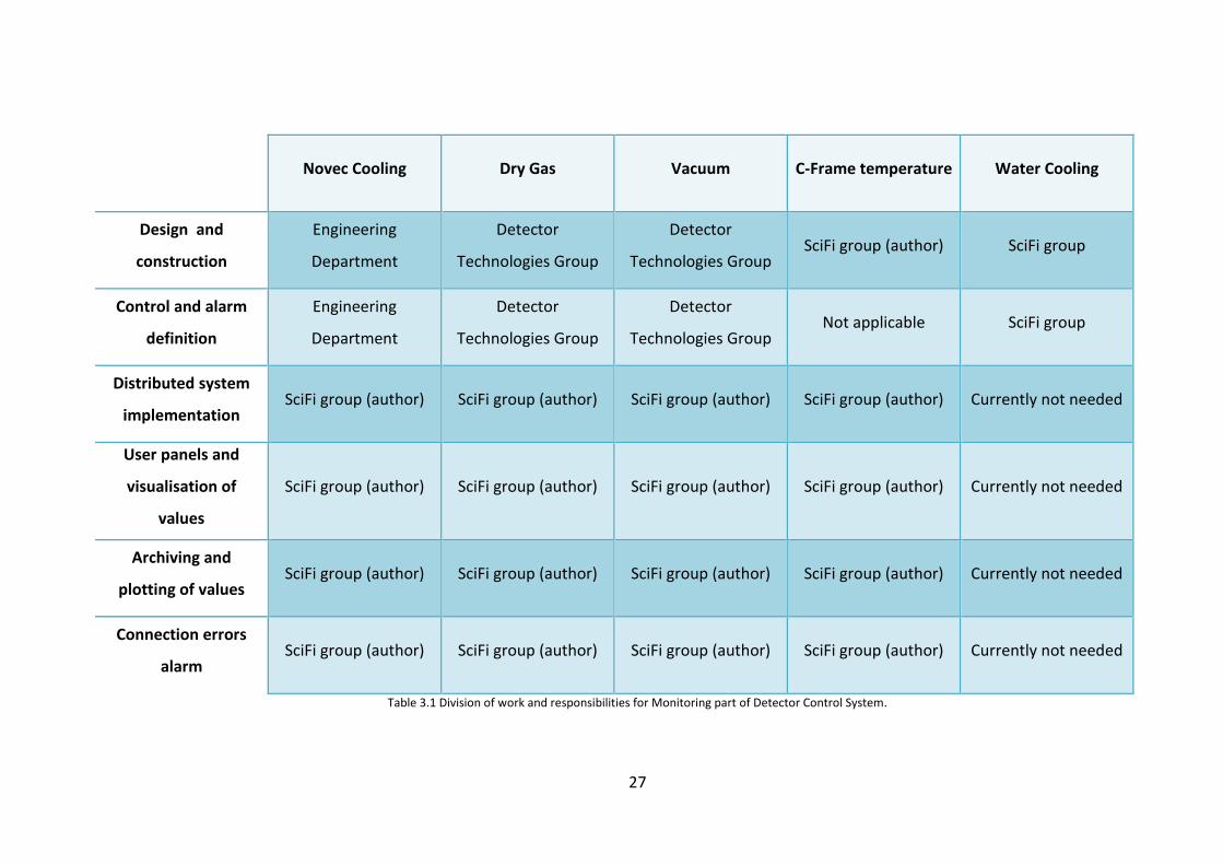
Although the control and triggering of important alarms for most of MON systems
was not the author’s responsibility they needed to be included in the distributed SCADA
system of LHCb with respect to its requirements. The division of work and responsibility is
explained in details in Table 3.1.
The constantly monitored parameters of the Novec Cooling system are: the flow of
coolant through C-Frame, the return temperature at the end of the coldbar and internal
parameters of Cooling Plant above all the setpoint and amount of coolant in the circuit.
Vacuum system parameters are monitored on the C-Frame and on the vacuum rack
itself. They include information gathered from pumps and gauges measuring the vacuum on
both rack and C-Frame.
Dry gas monitoring is connected to two redundant flow sensors on each module and
has the possibility to connect to dew point measurement.
Due to the different system design there is a need to retrieve the data by various
protocols. Hardware and software specification together with communication protocols are
clearly shown on the Table 3.2. C-Frame temperature monitoring and the Novec so called
Baby Cooling Plant communicate with control software by the direct TCP/IP protocol. The

26
most uncommon protocol used is DIP/DIM developed at CERN. Data Interchange Protocol
(DIP) is a communication system allowing small amount of real-time data to be exchanged
between loosely coupled heterogeneous systems (13). DIP practically is based on
publications of values that the appropriated user can subscribe to. It has its roots in
Distributed Information Management (DIM) system. Both were launched and are widely
used at CERN allowing to connect to the data without the knowledge of the other systems.
Because of the diversity of DCSMON systems the details could be find in a relevant
reports and notes available on SciFi public page (9) and Tracker Upgrade TDR (2).
27
Novec Cooling Dry Gas Vacuum C-Frame temperature Water Cooling
Design and
construction
Engineering
Department
Detector
Technologies Group
Detector
Technologies Group SciFi group (author) SciFi group
Control and alarm
definition
Engineering
Department
Detector
Technologies Group
Detector
Technologies Group Not applicable SciFi group
Distributed system
implementation SciFi group (author) SciFi group (author) SciFi group (author) SciFi group (author) Currently not needed
User panels and
visualisation of
values
SciFi group (author) SciFi group (author) SciFi group (author) SciFi group (author) Currently not needed
Archiving and
plotting of values SciFi group (author) SciFi group (author) SciFi group (author) SciFi group (author) Currently not needed
Connection errors
alarm SciFi group (author) SciFi group (author) SciFi group (author) SciFi group (author) Currently not needed
Table 3.1 Division of work and responsibilities for Monitoring part of Detector Control System.

28
Novec Cooling Dry Gas Vacuum C-Frame temperature Water Cooling
Functional hardware
during LS2
Novec Baby Cooling
Plant Dry Gas rack Vacuum rack
PLC with PT100
sensors Water Chiller
Data acquisition
during LS2
Direct from PLC
through TCP/IP DIP/DIM protocol DIP/DIM protocol
Direct from PLC
through TCP/IP
CAN Bus (not needed
yet)
User panels for
commissioning Final development Final development Final development First version ready Not needed yet
Final hardware
during LHC Run 3 Novec Cooling Plant Dry Gas system Vacuum system Not applicable
Water Cooling Plant
of LHCb
Data acquisition
during LHC Run 3 DIP/DIM protocol DIP/DIM protocol DIP/DIM protocol Not applicable DIP/DIM protocol
User panels for
distributed system in
LHC Run 3
Not finalised Final development Not finalised Not applicable Not started
Table 3.2 Hardware specification, communication protocols and software needs for DCSMON during commissioning and Run 3.
29
3.2.1. Vacuum system panel
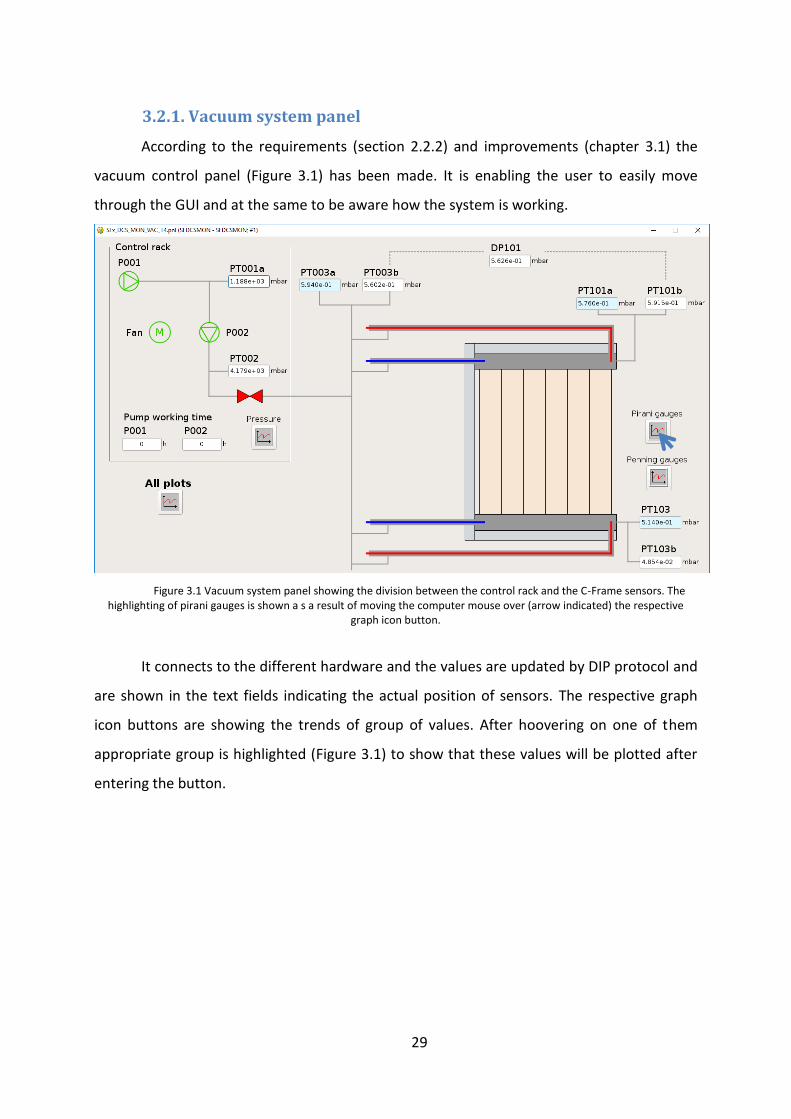
According to the requirements (section 2.2.2) and improvements (chapter 3.1) the
vacuum control panel (Figure 3.1) has been made. It is enabling the user to easily move
through the GUI and at the same to be aware how the system is working.
Figure 3.1 Vacuum system panel showing the division between the control rack and the C-Frame sensors. The highlighting of pirani gauges is shown a s a result of moving the computer mouse over (arrow indicated) the respective
graph icon button.
It connects to the different hardware and the values are updated by DIP protocol and
are shown in the text fields indicating the actual position of sensors. The respective graph
icon buttons are showing the trends of group of values. After hoovering on one of them
appropriate group is highlighted (Figure 3.1) to show that these values will be plotted after
entering the button.
30
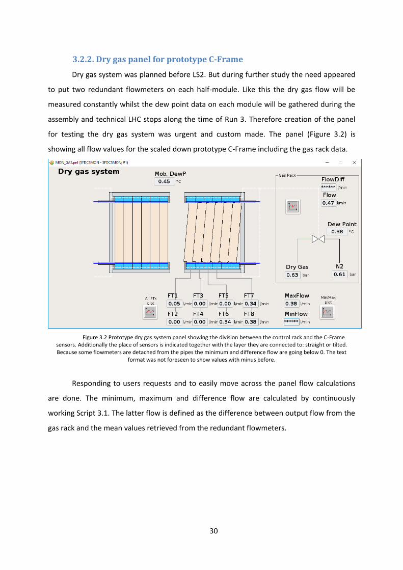
3.2.2. Dry gas panel for prototype C-Frame
Dry gas system was planned before LS2. But during further study the need appeared
to put two redundant flowmeters on each half-module. Like this the dry gas flow will be
measured constantly whilst the dew point data on each module will be gathered during the
assembly and technical LHC stops along the time of Run 3. Therefore creation of the panel
for testing the dry gas system was urgent and custom made. The panel (Figure 3.2) is
showing all flow values for the scaled down prototype C-Frame including the gas rack data.
Figure 3.2 Prototype dry gas system panel showing the division between the control rack and the C-Frame sensors. Additionally the place of sensors is indicated together with the layer they are connected to: straight or tilted. Because some flowmeters are detached from the pipes the minimum and difference flow are going below 0. The text
format was not foreseen to show values with minus before.
Responding to users requests and to easily move across the panel flow calculations
are done. The minimum, maximum and difference flow are calculated by continuously
working Script 3.1. The latter flow is defined as the difference between output flow from the
gas rack and the mean values retrieved from the redundant flowmeters.
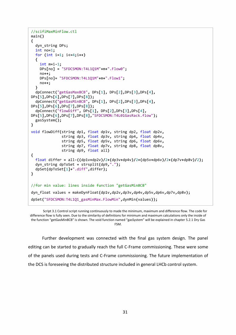
31
Script 3.1 Control script running continuously to made the minimum, maximum and difference flow. The code for difference flow is fully seen. Due to the similarity of definitions for minimum and maximum calculations only the inside of the function “getGasMin8CB” is shown. The void function named “gasSystem” will be explained in chapter 5.2.1 Dry Gas
FSM.
Further development was connected with the final gas system design. The panel
editing can be started to gradually reach the full C-Frame commissioning. These were some
of the panels used during tests and C-Frame commissioning. The future implementation of
the DCS is foreseeing the distributed structure included in general LHCb control system.
//scifiMaxMinFlow.ctl main() { dyn_string DPs; int no=1; for (int i=1; i<=4;i++) { int m=i-1; DPs[no] = "SFDCSMON:T4L1Q1M"+m+".Flow0"; no++; DPs[no]= "SFDCSMON:T4L1Q1M"+m+".Flow1"; no++; } dpConnect("getGasMax8CB", DPs[1], DPs[2],DPs[3],DPs[4], DPs[5],DPs[6],DPs[7],DPs[8]); dpConnect("getGasMin8CB", DPs[1], DPs[2],DPs[3],DPs[4], DPs[5],DPs[6],DPs[7],DPs[8]); dpConnect("flowDiff", DPs[1], DPs[2],DPs[3],DPs[4], DPs[5],DPs[6],DPs[7],DPs[8],"SFDCSMON:T4L01GasRack.flow"); gasSystem(); }
void flowDiff(string dp1, float dp1v, string dp2, float dp2v, string dp3, float dp3v, string dp4, float dp4v, string dp5, float dp5v, string dp6, float dp6v, string dp7, float dp7v, string dp8, float dp8v, string dp9, float all) { float differ = all-((dp1v+dp2v)/2+(dp3v+dp4v)/2+(dp5v+dp6v)/2+(dp7v+dp8v)/2); dyn_string dpToSet = strsplit(dp9,"."); dpSet(dpToSet[1]+".diff",differ); }
//for min value: lines inside function "getGasMin8CB"
dyn_float values = makeDynFloat(dp1v,dp2v,dp3v,dp4v,dp5v,dp6v,dp7v,dp8v);
dpSet("SFDCSMON:T4L1Q1_gasMinMax.FlowMin",dynMin(values));

32
3.3. C-Frame temperature readout
During the prototype C-Frame tests the concerns about the vacuum insulation in
several SciFi customly made parts grown. ROBs had the internal temperature sensors but
there was not a possibility to monitor the temperature on the weakest parts if it comes to
the thermic isolation and to see the distribution of cooling. The author established fully the
new DCSMON system from hardware configuration, through PLC programming and its
communication to its final Graphical User Interface (GUI).
3.3.1. Temperature measurement
The C-Frame temperature measurement is based on 4 PT100 temperature sensors,
connected with 12m long cables to the designated PLC. These are the platinum resistance
thermometers with resistance equal to 100Ω in temperature 0°C. Measuring its changes
(0.385Ω/°C) enables to read the temperature indirectly. Two sensors were placed on both
side of C-Frame on custom made brass connectors between vacuum insulated Novec lines
(right star on Figure 2.9), one on a cold box (top left of Figure 2.9) and one to view the
ambient temperature and its influence on the previous 3 readouts. The task included the
future increase of sensors up to 8 pieces.
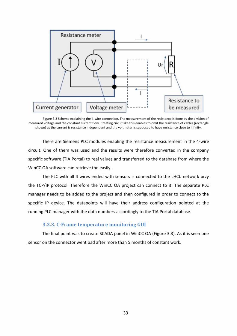
3.3.2. Wire connection and PLC communication
Because of the length of the sensing cables between the sensors and PLC the wire
resistance gains importance. The need to create a cabling system that does not change the
measurement appears. Therefore the 4-wire connection was used. Two wires are
transferring the constant current and playing the role of power supply whilst the other two
are connected to voltmeter (Figure 3.3).
33
Figure 3.3 Scheme explaining the 4-wire connection. The measurement of the resistance is done by the division of measured voltage and the constant current flow. Creating circuit like this enables to omit the resistance of cables (rectangle
shown) as the current is resistance independent and the voltmeter is supposed to have resistance close to infinity.
There are Siemens PLC modules enabling the resistance measurement in the 4-wire
circuit. One of them was used and the results were therefore converted in the company
specific software (TIA Portal) to real values and transferred to the database from where the
WinCC OA software can retrieve the easily.
The PLC with all 4 wires ended with sensors is connected to the LHCb network przy
the TCP/IP protocol. Therefore the WinCC OA project can connect to it. The separate PLC
manager needs to be added to the project and then configured in order to connect to the
specific IP device. The datapoints will have their address configuration pointed at the
running PLC manager with the data numbers accordingly to the TIA Portal database.
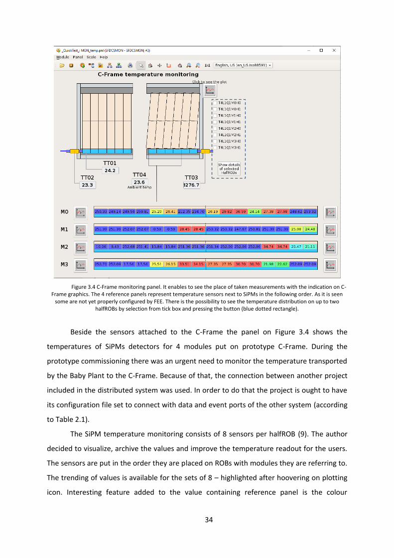
3.3.3. C-Frame temperature monitoring GUI
The final point was to create SCADA panel in WinCC OA (Figure 3.3). As it is seen one
sensor on the connector went bad after more than 5 months of constant work.
34
Figure 3.4 C-Frame monitoring panel. It enables to see the place of taken measurements with the indication on C-Frame graphics. The 4 reference panels represent temperature sensors next to SiPMs in the following order. As it is seen
some are not yet properly configured by FEE. There is the possibility to see the temperature distribution on up to two halfROBs by selection from tick box and pressing the button (blue dotted rectangle).
Beside the sensors attached to the C-Frame the panel on Figure 3.4 shows the
temperatures of SiPMs detectors for 4 modules put on prototype C-Frame. During the
prototype commissioning there was an urgent need to monitor the temperature transported
by the Baby Plant to the C-Frame. Because of that, the connection between another project
included in the distributed system was used. In order to do that the project is ought to have
its configuration file set to connect with data and event ports of the other system (according
to Table 2.1).
The SiPM temperature monitoring consists of 8 sensors per halfROB (9). The author
decided to visualize, archive the values and improve the temperature readout for the users.
The sensors are put in the order they are placed on ROBs with modules they are referring to.
The trending of values is available for the sets of 8 – highlighted after hoovering on plotting
icon. Interesting feature added to the value containing reference panel is the colour
35
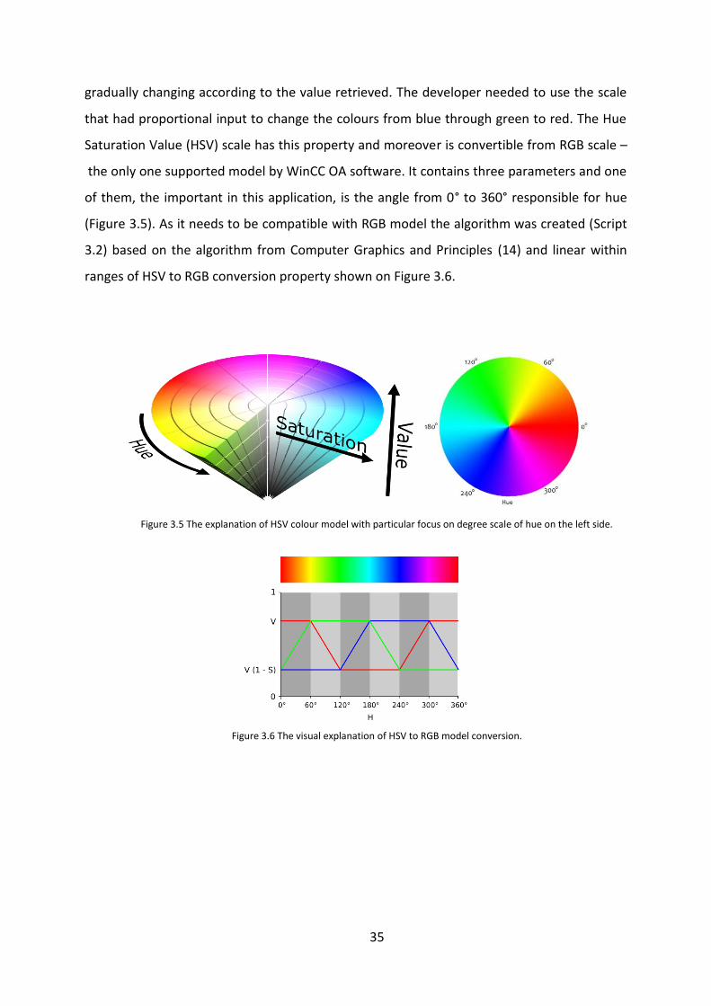
gradually changing according to the value retrieved. The developer needed to use the scale
that had proportional input to change the colours from blue through green to red. The Hue
Saturation Value (HSV) scale has this property and moreover is convertible from RGB scale –
the only one supported model by WinCC OA software. It contains three parameters and one
of them, the important in this application, is the angle from 0° to 360° responsible for hue
(Figure 3.5). As it needs to be compatible with RGB model the algorithm was created (Script
3.2) based on the algorithm from Computer Graphics and Principles (14) and linear within
ranges of HSV to RGB conversion property shown on Figure 3.6.
Figure 3.5 The explanation of HSV colour model with particular focus on degree scale of hue on the left side.
Figure 3.6 The visual explanation of HSV to RGB model conversion.
36
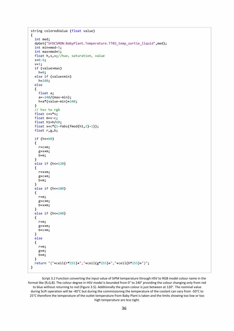
Script 3.2 Function converting the input value of SiPM temperature through HSV to RGB model colour name in the format like {R,G,B}. The colour degree in HSV model is bounded from 0° to 240° providing the colour changing only from red
to blue without returning to red (Figure 3.5). Additionally the green colour is just between at 120°. The nominal value during SciFi operation will be -40°C but during the commissioning the temperature of the coolant can vary from -50°C to
25°C therefore the temperature of the outlet temperature from Baby Plant is taken and the limits showing too low or too high temperature are less tight.
string coloredValue (float value) { int med; dpGet("SFDCSMON:BabyPlant.Temperature.TT03_temp_sortie_liquid",med); int min=med-5; int max=med+5; float h,s,v;//hue, saturation, value s=0.6; v=1; if (value>max) h=0; else if (value<min) h=240; else { float a; a=-240/(max-min); h=a*(value-min)+240; } // hsv to rgb float c=v*s; float m=v-c; float h1=h/60; float x=c*(1-fabs(fmod(h1,2)-1)); float r,g,b; if (h<=60) { r=c+m; g=x+m; b=m; } else if (h<=120) { r=x+m; g=c+m; b=m; } else if (h<=180) { r=m; g=c+m; b=x+m; } else if (h<=240) { r=m; g=x+m; b=c+m; } else { r=m; g=m; b=m; } return "{"+ceil(r*255)+","+ceil(g*255)+","+ceil(b*255)+"}"; }
37
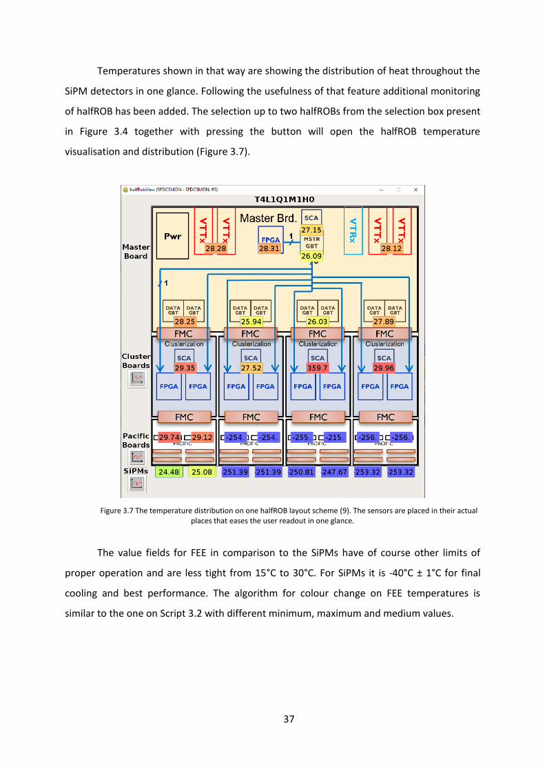
Temperatures shown in that way are showing the distribution of heat throughout the
SiPM detectors in one glance. Following the usefulness of that feature additional monitoring
of halfROB has been added. The selection up to two halfROBs from the selection box present
in Figure 3.4 together with pressing the button will open the halfROB temperature
visualisation and distribution (Figure 3.7).
Figure 3.7 The temperature distribution on one halfROB layout scheme (9). The sensors are placed in their actual places that eases the user readout in one glance.
The value fields for FEE in comparison to the SiPMs have of course other limits of
proper operation and are less tight from 15°C to 30°C. For SiPMs it is -40°C ± 1°C for final
cooling and best performance. The algorithm for colour change on FEE temperatures is
similar to the one on Script 3.2 with different minimum, maximum and medium values.
38
3.4. DCS Low Voltage
DCS is built as well by a high current, low voltage system of 8V. The current depends
on the FEE mode and during commissioning varies between 1A and more than 20A. The
maximum current was foreseen on the level of 50A. Because of the losses due to the cable
resistance the input voltage for FEE will be lowered by at least 0.8V. The ROBs will perform
properly and stably with the nominal voltage of 6.5V. The higher the voltage is the more
stable the FEE get, so this is why further losses due to e.g. inductance cannot appear.
LV is based on MAgnetic field and RAdiation TOleraNt (MARATON) power supplies.
This 12 channel power supply (PS) can be stored in the LHCb cavern close to the experiment
without losing its properties. This is crucial especially when the resistance losses have much
influence on the desired value, which is the case in SciFi application. It is controlled by its
own Remote Control Module (RCM) placed on the not irradiated side of the experiment – in
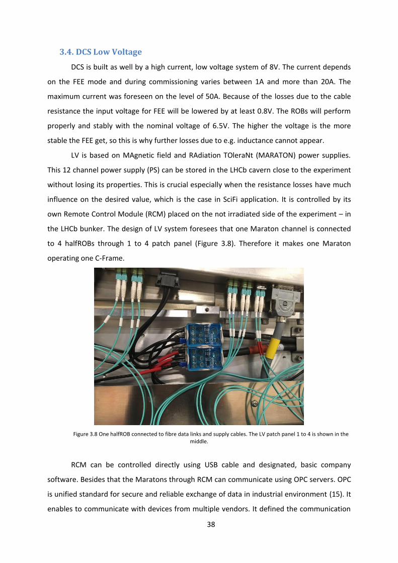
the LHCb bunker. The design of LV system foresees that one Maraton channel is connected
to 4 halfROBs through 1 to 4 patch panel (Figure 3.8). Therefore it makes one Maraton
operating one C-Frame.
Figure 3.8 One halfROB connected to fibre data links and supply cables. The LV patch panel 1 to 4 is shown in the middle.
RCM can be controlled directly using USB cable and designated, basic company
software. Besides that the Maratons through RCM can communicate using OPC servers. OPC
is unified standard for secure and reliable exchange of data in industrial environment (15). It
enables to communicate with devices from multiple vendors. It defined the communication

39
between Clients and Servers, or between Servers, including full control and feedback from
hardware. OPC was borne as a standardized middleware to connect to devices using differed
PLC specific protocols. It stood from OLE (Object Linking and Embedding) for Process Control
which in today’s evolved usage and application stands from Open Platform Communications.
Right now, with OPC UA specifications, it is a cross platform communication with both
Windows and Linux operating systems included. For now OPC DA is in use to communicate
with Maraton RCM as the power supply provider tools for OPC UA are in progress of
development.
During the PS testing period there was a need to develop a tool to easily control one
RCM. Because of that two panels were created. One meets the daily user criteria with the
most important values shown and the possibility to add customized channel configuration.
Partially in contrary the expert panel was developed not only to connect to RCM and show
all data gathered from PS but also to connect to different RCMs with the same panel.
Moreover both these panels are creating all datapoints internally required so they can be
freely used between different WinCC OA projects regardless their name or structure.
3.4.1. LV control panel for experts
Before testing every C-Frame one Maraton PS with designated RCM was provided.
The LV rack was assembled to contained them together with the current outlets. In order to
test the power supply itself the control panel shown on Figure 3.9 has been developed.
Beside showing data gathered from Maraton PS it enables the user to choose which PS it
controls.
40
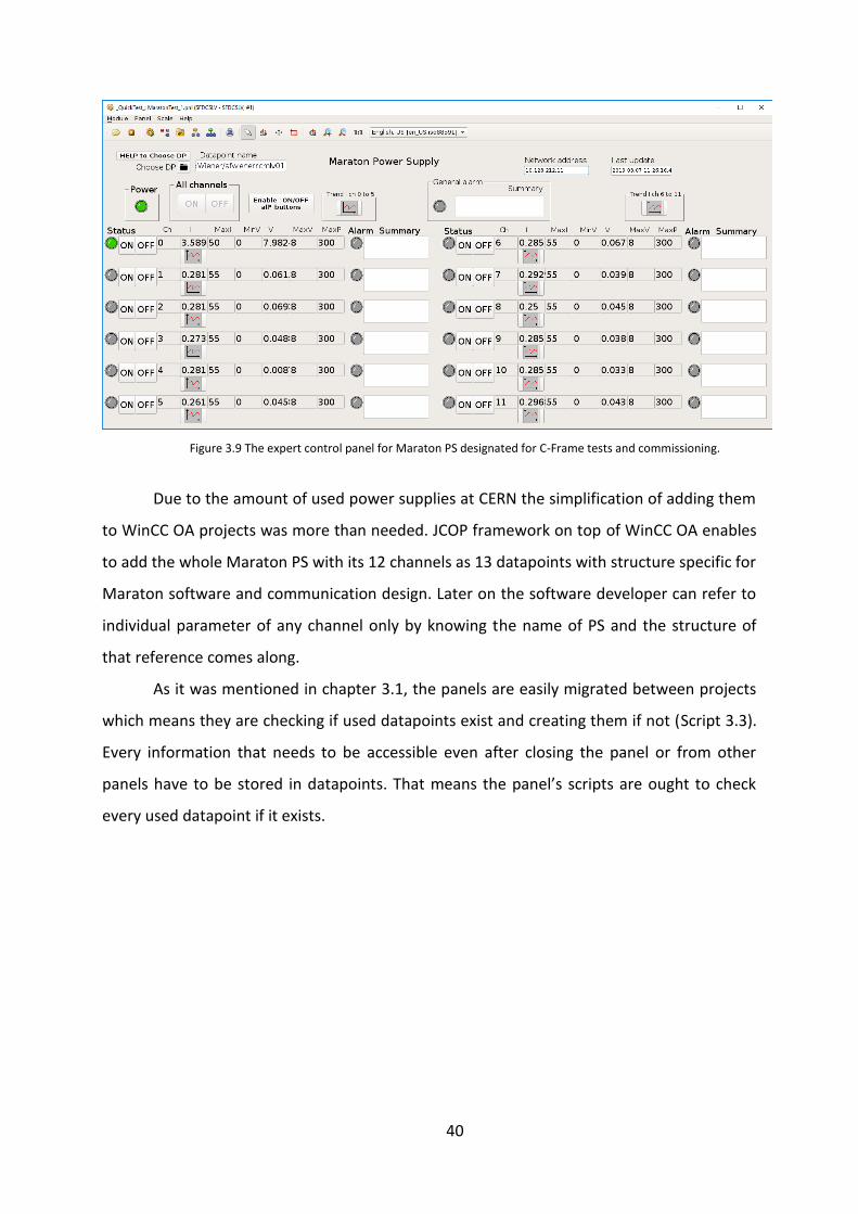
Figure 3.9 The expert control panel for Maraton PS designated for C-Frame tests and commissioning.
Due to the amount of used power supplies at CERN the simplification of adding them
to WinCC OA projects was more than needed. JCOP framework on top of WinCC OA enables
to add the whole Maraton PS with its 12 channels as 13 datapoints with structure specific for
Maraton software and communication design. Later on the software developer can refer to
individual parameter of any channel only by knowing the name of PS and the structure of
that reference comes along.
As it was mentioned in chapter 3.1, the panels are easily migrated between projects
which means they are checking if used datapoints exist and creating them if not (Script 3.3).
Every information that needs to be accessible even after closing the panel or from other
panels have to be stored in datapoints. That means the panel’s scripts are ought to check
every used datapoint if it exists.
41
Script 3.3 Usage of WinCC OA build in functions to create a needed datapoint. Additionally assigning to the variable the value of the datapoint. In that case the datapoint of a type string contains the controlled power supply. It is
defined in ScopeLib to be accessible from the other shapes.
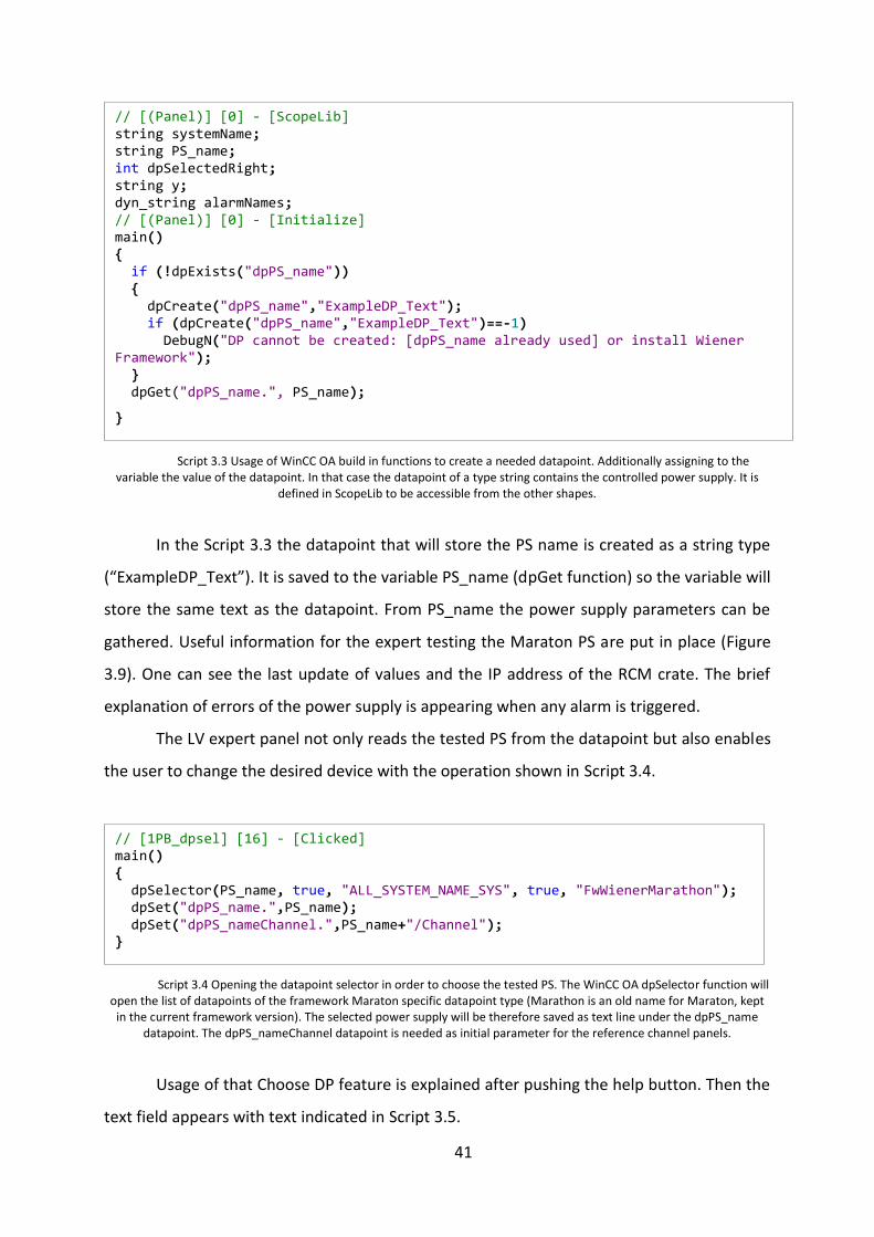
In the Script 3.3 the datapoint that will store the PS name is created as a string type
(“ExampleDP_Text”). It is saved to the variable PS_name (dpGet function) so the variable will
store the same text as the datapoint. From PS_name the power supply parameters can be
gathered. Useful information for the expert testing the Maraton PS are put in place (Figure
3.9). One can see the last update of values and the IP address of the RCM crate. The brief
explanation of errors of the power supply is appearing when any alarm is triggered.
The LV expert panel not only reads the tested PS from the datapoint but also enables
the user to change the desired device with the operation shown in Script 3.4.
Script 3.4 Opening the datapoint selector in order to choose the tested PS. The WinCC OA dpSelector function will open the list of datapoints of the framework Maraton specific datapoint type (Marathon is an old name for Maraton, kept
in the current framework version). The selected power supply will be therefore saved as text line under the dpPS_name datapoint. The dpPS_nameChannel datapoint is needed as initial parameter for the reference channel panels.
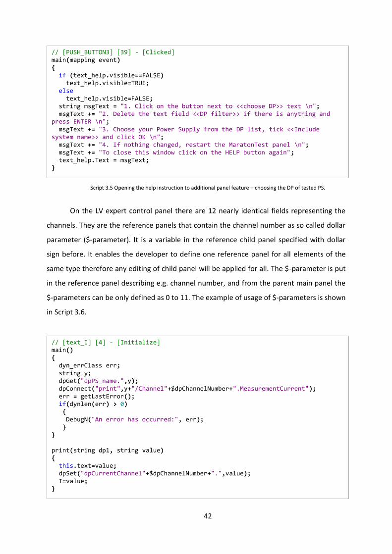
Usage of that Choose DP feature is explained after pushing the help button. Then the
text field appears with text indicated in Script 3.5.
// [(Panel)] [0] - [ScopeLib] string systemName; string PS_name; int dpSelectedRight; string y; dyn_string alarmNames; // [(Panel)] [0] - [Initialize] main() { if (!dpExists("dpPS_name")) { dpCreate("dpPS_name","ExampleDP_Text"); if (dpCreate("dpPS_name","ExampleDP_Text")==-1) DebugN("DP cannot be created: [dpPS_name already used] or install Wiener Framework"); } dpGet("dpPS_name.", PS_name);
}
// [1PB_dpsel] [16] - [Clicked] main() { dpSelector(PS_name, true, "ALL_SYSTEM_NAME_SYS", true, "FwWienerMarathon"); dpSet("dpPS_name.",PS_name); dpSet("dpPS_nameChannel.",PS_name+"/Channel"); }
42
Script 3.5 Opening the help instruction to additional panel feature – choosing the DP of tested PS.
On the LV expert control panel there are 12 nearly identical fields representing the
channels. They are the reference panels that contain the channel number as so called dollar
parameter ($-parameter). It is a variable in the reference child panel specified with dollar
sign before. It enables the developer to define one reference panel for all elements of the
same type therefore any editing of child panel will be applied for all. The $-parameter is put
in the reference panel describing e.g. channel number, and from the parent main panel the
$-parameters can be only defined as 0 to 11. The example of usage of $-parameters is shown
in Script 3.6.
// [PUSH_BUTTON3] [39] - [Clicked] main(mapping event) { if (text_help.visible==FALSE) text_help.visible=TRUE; else text_help.visible=FALSE; string msgText = "1. Click on the button next to <<choose DP>> text \n"; msgText += "2. Delete the text field <<DP filter>> if there is anything and press ENTER \n"; msgText += "3. Choose your Power Supply from the DP list, tick <<Include system name>> and click OK \n"; msgText += "4. If nothing changed, restart the MaratonTest panel \n"; msgText += "To close this window click on the HELP button again"; text_help.Text = msgText; }
// [text_I] [4] - [Initialize] main() { dyn_errClass err; string y; dpGet("dpPS_name.",y); dpConnect("print",y+"/Channel"+$dpChannelNumber+".MeasurementCurrent"); err = getLastError(); if(dynlen(err) > 0) { DebugN("An error has occurred:", err); } } print(string dp1, string value) { this.text=value; dpSet("dpCurrentChannel"+$dpChannelNumber+".",value); I=value; }

43
Script 3.6 Definition of showing the current from one channel in a text field. It is the script from the reference panel so the $-parameter is seen as a channel number. In the upper level panel the $-parameter will be defined and the
field will perform it tasks properly. The usage of WinCC OA dpConnect function is shown. It enables to execute the defined function (in that case void type named “print”) every time there is a change in the datapoint – second parameter. All errors
appearing are stored. Moreover the respective dpCurrentChannel datapoint is changed, because it is the DP that predefined plotting button connects to.
The channel reference panel connects to the PS channel showing all gathered data
together with current and voltage settings. It can switch on and off the channel and plot the
current – the most crucial value during testing of Maratons for SciFi. As it was for the power
supply, sources of channel alarms are shown after any of them is appearing. An additional
option of On/Off switching of all channels has been added in respect to power supply testing
experts needs. Though the protection from unintentional usage of these buttons came aside.
3.4.2. Everyday usage of Low Voltage
During the test period of every C-Frame there is only one power supply used.
Because of that there was no longer the need to keep the possibility of changing of the
tested hardware. Therefore another panel has been created (Figure 3.10) in order to
represent only the user specific parameters on the main screen with different options
particular for daily usage in constantly changing surrounding.
44
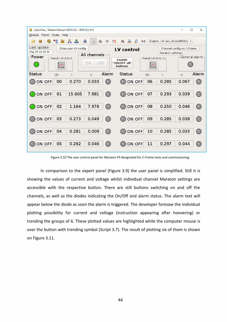
Figure 3.10 The user control panel for Maraton PS designated for C-Frame tests and commissioning.
In comparison to the expert panel (Figure 3.9) the user panel is simplified. Still it is
showing the values of current and voltage whilst individual channel Maraton settings are
accessible with the respective button. There are still buttons switching on and off the
channels, as well as the diodes indicating the On/Off and alarm status. The alarm text will
appear below the diode as soon the alarm is triggered. The developer foresaw the individual
plotting possibility for current and voltage (instruction appearing after hoovering) or
trending the groups of 6. These plotted values are highlighted while the computer mouse is
over the button with trending symbol (Script 3.7). The result of plotting six of them is shown
on Figure 3.11.
45
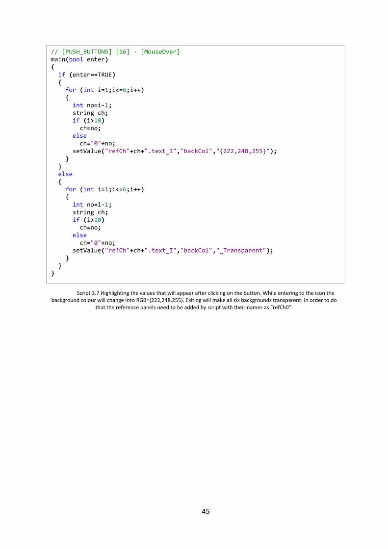
Script 3.7 Highlighting the values that will appear after clicking on the button. While entering to the icon the background colour will change into RGB={222,248,255}. Exiting will make all six backgrounds transparent. In order to do
that the reference panels need to be added by script with their names as “refCh0”.
// [PUSH_BUTTON5] [16] - [MouseOver] main(bool enter) { if (enter==TRUE) { for (int i=1;i<=6;i++) { int no=i-1; string ch; if (i>10) ch=no; else ch="0"+no; setValue("refCh"+ch+".text_I","backCol","{222,248,255}"); } } else { for (int i=1;i<=6;i++) { int no=i-1; string ch; if (i>10) ch=no; else ch="0"+no; setValue("refCh"+ch+".text_I","backCol","_Transparent"); } } }
46
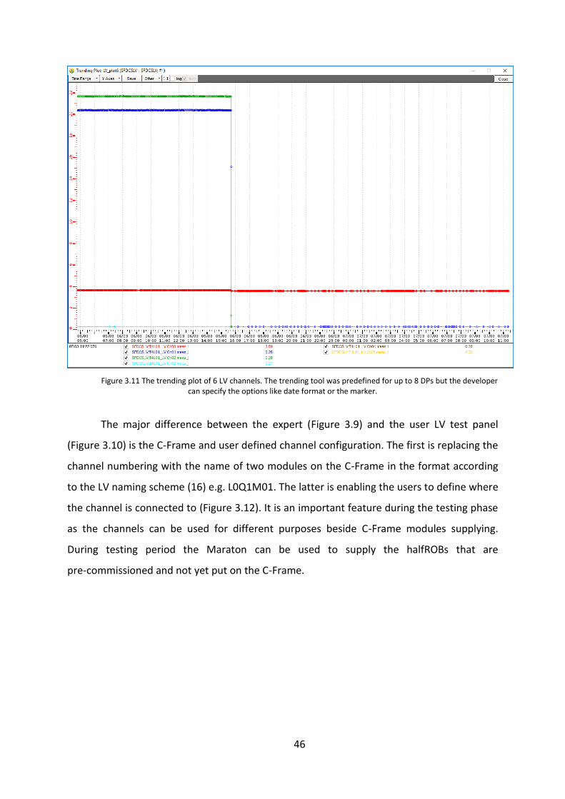
Figure 3.11 The trending plot of 6 LV channels. The trending tool was predefined for up to 8 DPs but the developer can specify the options like date format or the marker.
The major difference between the expert (Figure 3.9) and the user LV test panel
(Figure 3.10) is the C-Frame and user defined channel configuration. The first is replacing the
channel numbering with the name of two modules on the C-Frame in the format according
to the LV naming scheme (16) e.g. L0Q1M01. The latter is enabling the users to define where
the channel is connected to (Figure 3.12). It is an important feature during the testing phase
as the channels can be used for different purposes beside C-Frame modules supplying.
During testing period the Maraton can be used to supply the halfROBs that are
pre-commissioned and not yet put on the C-Frame.
47
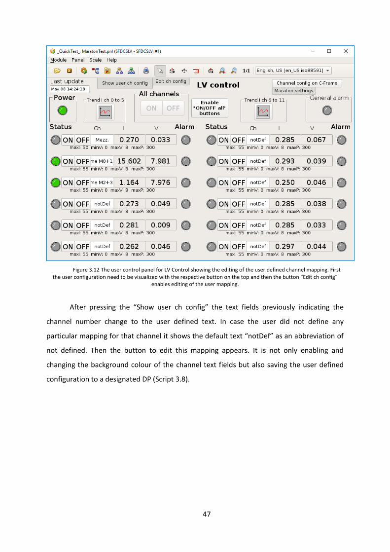
Figure 3.12 The user control panel for LV Control showing the editing of the user defined channel mapping. First the user configuration need to be visualized with the respective button on the top and then the button “Edit ch config”
enables editing of the user mapping.
After pressing the “Show user ch config” the text fields previously indicating the
channel number change to the user defined text. In case the user did not define any
particular mapping for that channel it shows the default text “notDef” as an abbreviation of
not defined. Then the button to edit this mapping appears. It is not only enabling and
changing the background colour of the channel text fields but also saving the user defined
configuration to a designated DP (Script 3.8).
48
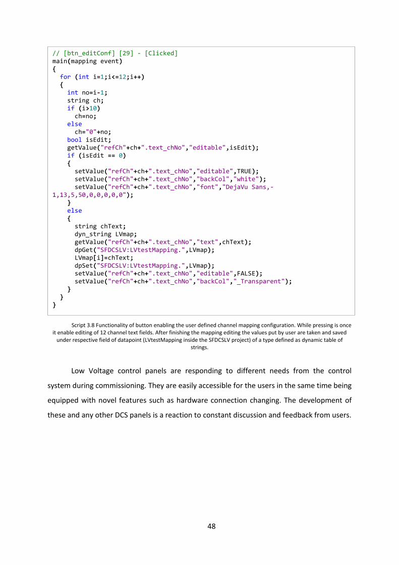
Script 3.8 Functionality of button enabling the user defined channel mapping configuration. While pressing is once it enable editing of 12 channel text fields. After finishing the mapping editing the values put by user are taken and saved
under respective field of datapoint (LVtestMapping inside the SFDCSLV project) of a type defined as dynamic table of strings.
Low Voltage control panels are responding to different needs from the control
system during commissioning. They are easily accessible for the users in the same time being
equipped with novel features such as hardware connection changing. The development of
these and any other DCS panels is a reaction to constant discussion and feedback from users.
// [btn_editConf] [29] - [Clicked] main(mapping event) { for (int i=1;i<=12;i++) { int no=i-1; string ch; if (i>10) ch=no; else ch="0"+no; bool isEdit; getValue("refCh"+ch+".text_chNo","editable",isEdit); if (isEdit == 0) { setValue("refCh"+ch+".text_chNo","editable",TRUE); setValue("refCh"+ch+".text_chNo","backCol","white"); setValue("refCh"+ch+".text_chNo","font","DejaVu Sans,-1,13,5,50,0,0,0,0,0"); } else { string chText; dyn_string LVmap; getValue("refCh"+ch+".text_chNo","text",chText); dpGet("SFDCSLV:LVtestMapping.",LVmap); LVmap[i]=chText; dpSet("SFDCSLV:LVtestMapping.",LVmap); setValue("refCh"+ch+".text_chNo","editable",FALSE); setValue("refCh"+ch+".text_chNo","backCol","_Transparent"); } } }

49
4. SciFi Tracker assembly and commissioning
During the assembly and commissioning of SciFi tracker all systems need to be fully
functioning is order to properly test the C-Frame before bringing it 100m underground to the
LHCb cavern. Moreover fully functioning systems need to have software tools in order to
control the hardware, visualize its readback settings and keep the history of values read
from all sensors. Additionally, there is one set of systems specially made to test each of 12 C-
Frames but their data acquired need to be tracked individually. Therefore the author created
framework of user and control panels in order to easily communicate with hardware through
different protocols, while keeping the requirements of CERN, LHCb and SciFi. His goal of
work and this thesis was to meet these minimum requirements and therefore simplify the
Human-Machine Interface. The software is ought to be more clear and meaningful with one
look. The user needs to understand and properly use the control panels without deep
understanding of the controlled system.
4.1. Monitoring panels
C-Frame testing is bringing many challenges and needs from the monitoring project
of the Detector Control System. There are as well possibilities to bring useful innovatory
solutions to appearing situations. The graphically oriented UI has been done for all systems.
Due to some similarity between them only chosen control panels and scripts will be
explained.
4.1.1. Parent panel
As one can divide the DCSMON project into four different systems the user needed to
open 4 control panels from the Linux console without an overview of them all. Because of
that the upper level, parent panel has been created indicating the state of each system
(Figure 4.1).

50
Figure 4.1 The parent panel for monitoring showing the DCSMON systems. It includes LED graphics indicating if the connection to each system (according to Table 3.2 protocols) is properly made.
From this panel the user is able to access the control panels of shown systems at
once. Moreover it enables the developer to work independently from the users and in case
the improvements are done change only the name of panel to be open. It is particularly
important if the tests are in progress or the developer needs to provide the console
command line each time the major change has been done.
Because of the variety of protocols and ways of communicating with hardware (Table
3.2) the additional alarm showing if the connection is properly established is included. The
internal errors of each system are done by respective group (Table 3.1) and were not
implemented here. The diodes are showing the connection state of one datapoint from each
domain that has the most frequent update of its value. If there was no update for the past 5
minutes the respective alarm needs to be triggered indicated not only with the diode. The
separate e-mail has to be sent with information about the connection error. In order to do
that continuous calculations (Script 4.1) need to be done in a control script run by WinCC OA
Console (Figure 2.11) control manager.
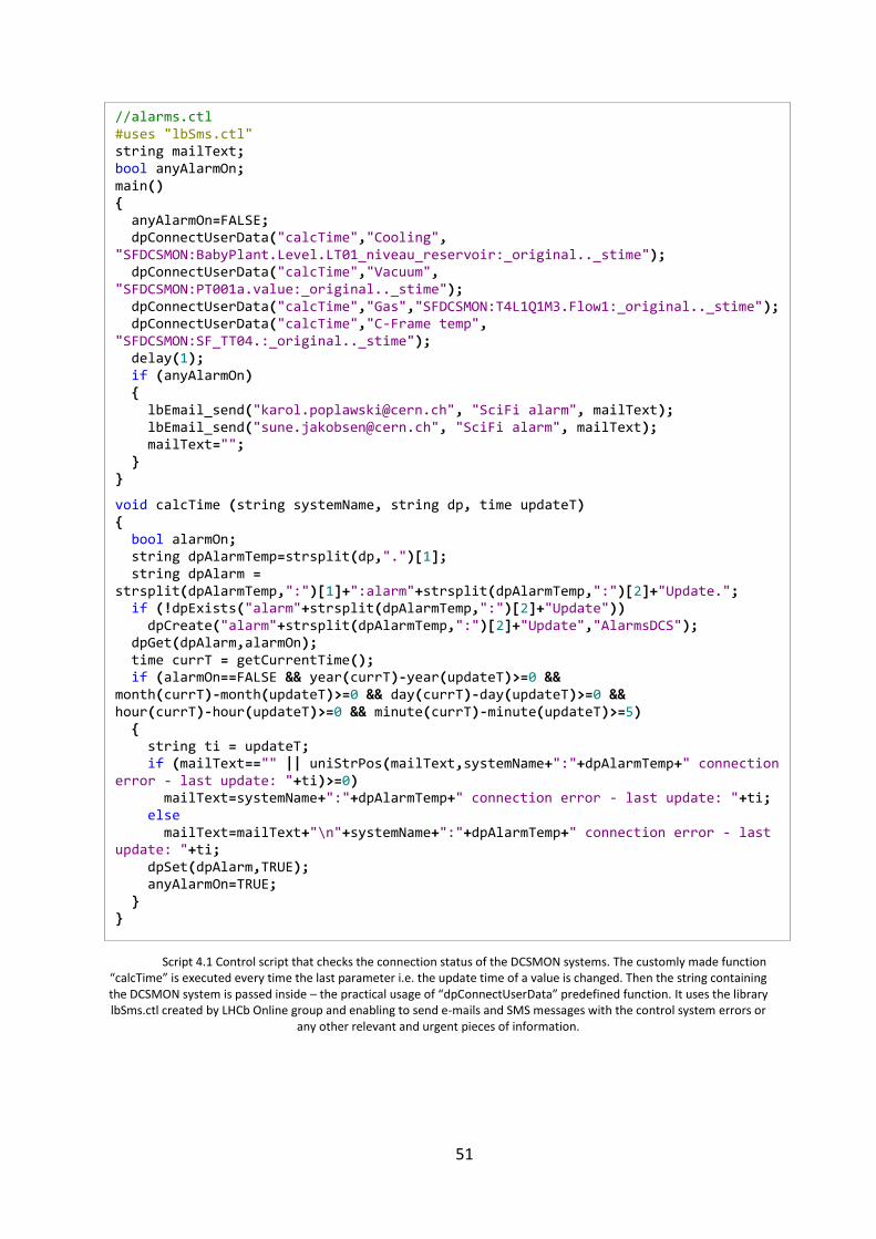
51
Script 4.1 Control script that checks the connection status of the DCSMON systems. The customly made function “calcTime” is executed every time the last parameter i.e. the update time of a value is changed. Then the string containing the DCSMON system is passed inside – the practical usage of “dpConnectUserData” predefined function. It uses the library lbSms.ctl created by LHCb Online group and enabling to send e-mails and SMS messages with the control system errors or
any other relevant and urgent pieces of information.
//alarms.ctl #uses "lbSms.ctl" string mailText; bool anyAlarmOn; main() { anyAlarmOn=FALSE; dpConnectUserData("calcTime","Cooling", "SFDCSMON:BabyPlant.Level.LT01_niveau_reservoir:_original.._stime"); dpConnectUserData("calcTime","Vacuum", "SFDCSMON:PT001a.value:_original.._stime"); dpConnectUserData("calcTime","Gas","SFDCSMON:T4L1Q1M3.Flow1:_original.._stime"); dpConnectUserData("calcTime","C-Frame temp", "SFDCSMON:SF_TT04.:_original.._stime"); delay(1); if (anyAlarmOn) { lbEmail_send("[email protected]", "SciFi alarm", mailText); lbEmail_send("[email protected]", "SciFi alarm", mailText); mailText=""; } }
void calcTime (string systemName, string dp, time updateT) { bool alarmOn; string dpAlarmTemp=strsplit(dp,".")[1]; string dpAlarm = strsplit(dpAlarmTemp,":")[1]+":alarm"+strsplit(dpAlarmTemp,":")[2]+"Update."; if (!dpExists("alarm"+strsplit(dpAlarmTemp,":")[2]+"Update")) dpCreate("alarm"+strsplit(dpAlarmTemp,":")[2]+"Update","AlarmsDCS"); dpGet(dpAlarm,alarmOn); time currT = getCurrentTime(); if (alarmOn==FALSE && year(currT)-year(updateT)>=0 && month(currT)-month(updateT)>=0 && day(currT)-day(updateT)>=0 && hour(currT)-hour(updateT)>=0 && minute(currT)-minute(updateT)>=5) { string ti = updateT; if (mailText=="" || uniStrPos(mailText,systemName+":"+dpAlarmTemp+" connection error - last update: "+ti)>=0) mailText=systemName+":"+dpAlarmTemp+" connection error - last update: "+ti; else mailText=mailText+"\n"+systemName+":"+dpAlarmTemp+" connection error - last update: "+ti; dpSet(dpAlarm,TRUE); anyAlarmOn=TRUE; } }
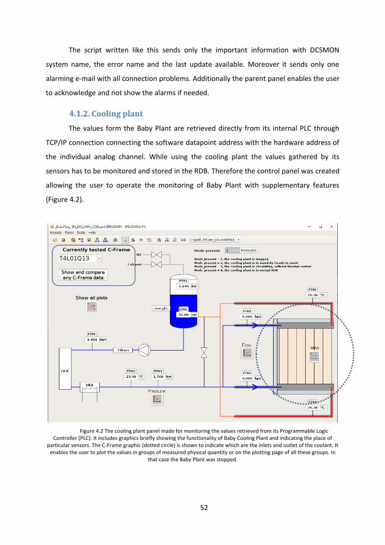
52
The script written like this sends only the important information with DCSMON
system name, the error name and the last update available. Moreover it sends only one
alarming e-mail with all connection problems. Additionally the parent panel enables the user
to acknowledge and not show the alarms if needed.
4.1.2. Cooling plant
The values form the Baby Plant are retrieved directly from its internal PLC through
TCP/IP connection connecting the software datapoint address with the hardware address of
the individual analog channel. While using the cooling plant the values gathered by its
sensors has to be monitored and stored in the RDB. Therefore the control panel was created
allowing the user to operate the monitoring of Baby Plant with supplementary features
(Figure 4.2).
Figure 4.2 The cooling plant panel made for monitoring the values retrieved from its Programmable Logic Controller (PLC). It includes graphics briefly showing the functionality of Baby Cooling Plant and indicating the place of
particular sensors. The C-Frame graphic (dotted circle) is shown to indicate which are the inlets and outlet of the coolant. It enables the user to plot the values in groups of measured physical quantity or on the plotting page of all these groups. In
that case the Baby Plant was stopped.

53
Baby Plant panel (Figure 4.2) is equipped with easily accessible graphics and shapes
representing the process happening inside and its actual layout. The sensors are placed
accordingly to their actual location in the plant. C-Frame graphic has its “cold” inlets shown
with blue and the outlets going to the cooling plant to close the circuit. With additional key if
needed panel made like this is user friendly and logical. Apart from that it contains the
groups of plots allowing the user to see the history of the set of values: pressure, flow and
temperature. Level of the coolant and the plant mode have their own individual graphs.
After pointing on the button the respective set is highlighted with blue, not to disturb the
user but only to catch the attention and to instantly place the plotted values. The GUI is
allowing to show all plots. Respective button titled “Show all plots” opens the trending page
containing 5 plots of pressures, flows, temperatures, level and mode ordered the same way
as shown for 6 plots on Figure 4.3. The level is both indicated with value in the text field and
with the changing size blue rectangle next to the level plot button.
Particular attention needs to be drawn to the smoothed edged rectangle in the top
left corner of Figure 4.2. It is showing the C-Frame name and allows to select the currently
tested C-Frame from the dropdown box. “T4L01Q13” is the name of 13th, prototype C-Frame
that was used to see the challenges for the next serial production 12 ones and check if there
are any improvements needed. Not to overwrite the existing C-Frame names in the
database, that not used tracking station T4 was invented. Moreover to dropdown selection
the name “none” has been added. It is used to be able to store the Baby Plant data even if
no C-Frame is attached.
The dropdown box is the functional part to realise the improvements to the project
listed in the chapter 3.1. By changing the selected C-Frame the algorithm enables to store
the retrieved data in the appropriately named datapoints (Script 4.2). Like this after one
change every value registered by the Baby Plant will be stored at the datapoint like “[C-
Frame name].[BabyPlant.value]”.
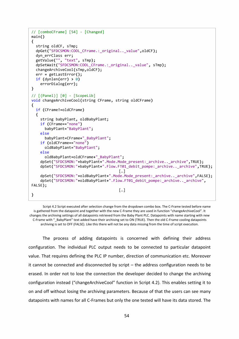
54
Script 4.2 Script executed after selection change from the dropdown combo box. The C-Frame tested before name is gathered from the datapoint and together with the new C-Frame they are used in function “changeArchiveCool”. It
changes the archiving settings of all datapoints retrieved from the Baby Plant PLC. Datapoints with name starting with new C-Frame with “_BabyPlant” text added have their archiving set to ON (TRUE). Then the old C-Frame cooling datapoints
archiving is set to OFF (FALSE). Like this there will not be any data missing from the time of script execution.
The process of adding datapoints is concerned with defining their address
configuration. The individual PLC output needs to be connected to particular datapoint
value. That requires defining the PLC IP number, direction of communication etc. Moreover
it cannot be connected and disconnected by script – the address configuration needs to be
erased. In order not to lose the connection the developer decided to change the archiving
configuration instead (“changeArchiveCool” function in Script 4.2). This enables setting it to
on and off without losing the archiving parameters. Because of that the users can see many
datapoints with names for all C-Frames but only the one tested will have its data stored. The
// [comboCFrame] [54] - [Changed] main() { string oldCF, sTmp; dpGet("SFDCSMON:COOL_CFrame.:_original.._value",oldCF); dyn_errClass err; getValue("", "text", sTmp); dpSetWait("SFDCSMON:COOL_CFrame.:_original.._value", sTmp); changeArchiveCool(sTmp,oldCF); err = getLastError(); if (dynlen(err) > 0) errorDialog(err); }
// [(Panel)] [0] - [ScopeLib] void changeArchiveCool(string CFrame, string oldCFrame) { if (CFrame!=oldCFrame) { string babyPlant, oldBabyPlant; if (CFrame=="none") babyPlant="BabyPlant"; else babyPlant=CFrame+"_BabyPlant"; if (oldCFrame=="none") oldBabyPlant="BabyPlant"; else oldBabyPlant=oldCFrame+"_BabyPlant"; dpSet("SFDCSMON:"+babyPlant+".Mode.Mode_present:_archive.._archive",TRUE); dpSet("SFDCSMON:"+babyPlant+".Flow.FT01_debit_pompe:_archive.._archive",TRUE);
[…] dpSet("SFDCSMON:"+oldBabyPlant+".Mode.Mode_present:_archive.._archive",FALSE); dpSet("SFDCSMON:"+oldBabyPlant+".Flow.FT01_debit_pompe:_archive.._archive", FALSE);
[…] }
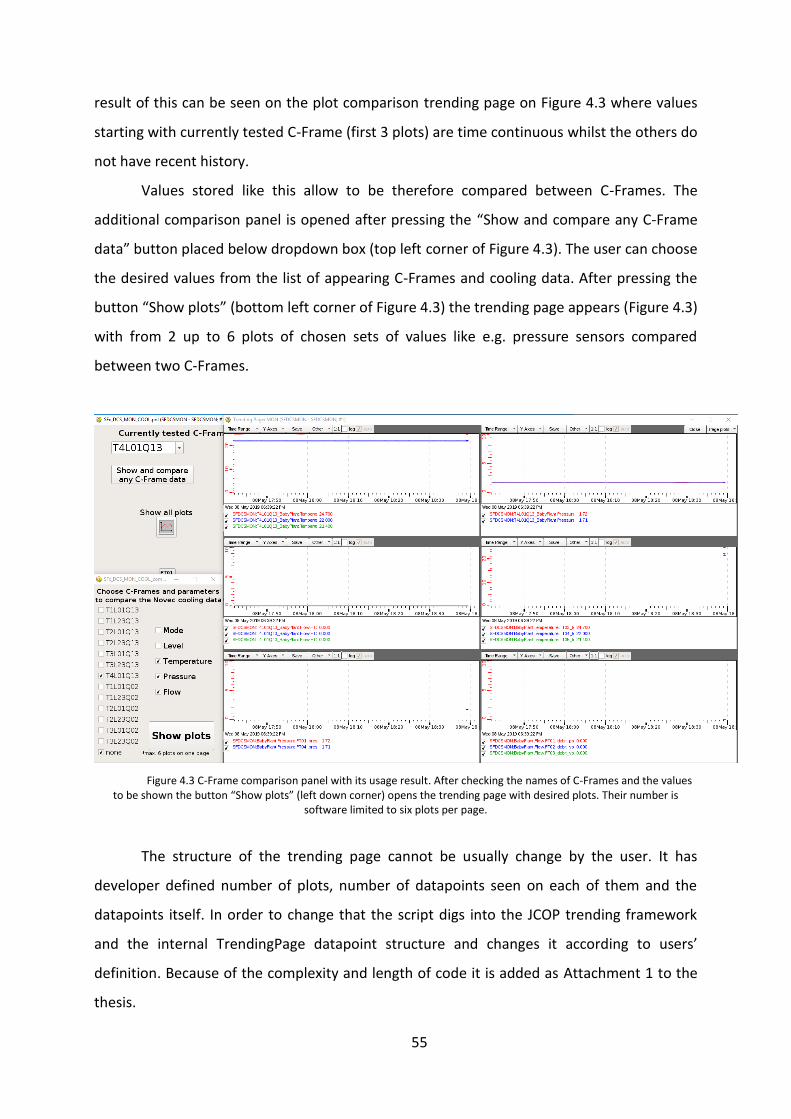
55
result of this can be seen on the plot comparison trending page on Figure 4.3 where values
starting with currently tested C-Frame (first 3 plots) are time continuous whilst the others do
not have recent history.
Values stored like this allow to be therefore compared between C-Frames. The
additional comparison panel is opened after pressing the “Show and compare any C-Frame
data” button placed below dropdown box (top left corner of Figure 4.3). The user can choose
the desired values from the list of appearing C-Frames and cooling data. After pressing the
button “Show plots” (bottom left corner of Figure 4.3) the trending page appears (Figure 4.3)
with from 2 up to 6 plots of chosen sets of values like e.g. pressure sensors compared
between two C-Frames.
Figure 4.3 C-Frame comparison panel with its usage result. After checking the names of C-Frames and the values to be shown the button “Show plots” (left down corner) opens the trending page with desired plots. Their number is
software limited to six plots per page.
The structure of the trending page cannot be usually change by the user. It has
developer defined number of plots, number of datapoints seen on each of them and the
datapoints itself. In order to change that the script digs into the JCOP trending framework
and the internal TrendingPage datapoint structure and changes it according to users’
definition. Because of the complexity and length of code it is added as Attachment 1 to the
thesis.
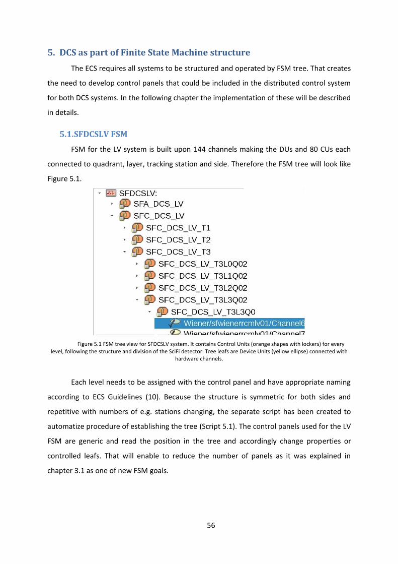
56
5. DCS as part of Finite State Machine structure
The ECS requires all systems to be structured and operated by FSM tree. That creates
the need to develop control panels that could be included in the distributed control system
for both DCS systems. In the following chapter the implementation of these will be described
in details.
5.1. SFDCSLV FSM
FSM for the LV system is built upon 144 channels making the DUs and 80 CUs each
connected to quadrant, layer, tracking station and side. Therefore the FSM tree will look like
Figure 5.1.
Figure 5.1 FSM tree view for SFDCSLV system. It contains Control Units (orange shapes with lockers) for every level, following the structure and division of the SciFi detector. Tree leafs are Device Units (yellow ellipse) connected with
hardware channels.
Each level needs to be assigned with the control panel and have appropriate naming
according to ECS Guidelines (10). Because the structure is symmetric for both sides and
repetitive with numbers of e.g. stations changing, the separate script has been created to
automatize procedure of establishing the tree (Script 5.1). The control panels used for the LV
FSM are generic and read the position in the tree and accordingly change properties or
controlled leafs. That will enable to reduce the number of panels as it was explained in
chapter 3.1 as one of new FSM goals.
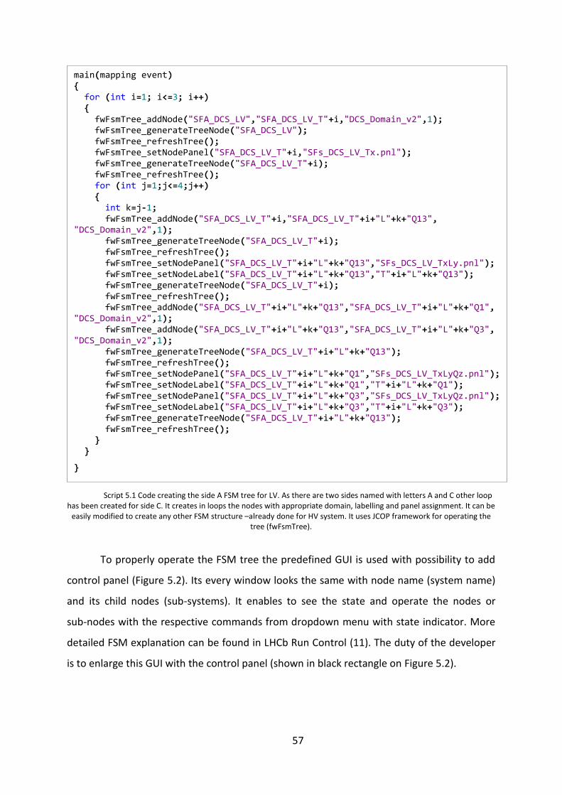
57
Script 5.1 Code creating the side A FSM tree for LV. As there are two sides named with letters A and C other loop has been created for side C. It creates in loops the nodes with appropriate domain, labelling and panel assignment. It can be
easily modified to create any other FSM structure –already done for HV system. It uses JCOP framework for operating the tree (fwFsmTree).
To properly operate the FSM tree the predefined GUI is used with possibility to add
control panel (Figure 5.2). Its every window looks the same with node name (system name)
and its child nodes (sub-systems). It enables to see the state and operate the nodes or
sub-nodes with the respective commands from dropdown menu with state indicator. More
detailed FSM explanation can be found in LHCb Run Control (11). The duty of the developer
is to enlarge this GUI with the control panel (shown in black rectangle on Figure 5.2).
main(mapping event) { for (int i=1; i<=3; i++) { fwFsmTree_addNode("SFA_DCS_LV","SFA_DCS_LV_T"+i,"DCS_Domain_v2",1); fwFsmTree_generateTreeNode("SFA_DCS_LV"); fwFsmTree_refreshTree(); fwFsmTree_setNodePanel("SFA_DCS_LV_T"+i,"SFs_DCS_LV_Tx.pnl"); fwFsmTree_generateTreeNode("SFA_DCS_LV_T"+i); fwFsmTree_refreshTree(); for (int j=1;j<=4;j++) { int k=j-1; fwFsmTree_addNode("SFA_DCS_LV_T"+i,"SFA_DCS_LV_T"+i+"L"+k+"Q13", "DCS_Domain_v2",1); fwFsmTree_generateTreeNode("SFA_DCS_LV_T"+i); fwFsmTree_refreshTree(); fwFsmTree_setNodePanel("SFA_DCS_LV_T"+i+"L"+k+"Q13","SFs_DCS_LV_TxLy.pnl"); fwFsmTree_setNodeLabel("SFA_DCS_LV_T"+i+"L"+k+"Q13","T"+i+"L"+k+"Q13"); fwFsmTree_generateTreeNode("SFA_DCS_LV_T"+i); fwFsmTree_refreshTree(); fwFsmTree_addNode("SFA_DCS_LV_T"+i+"L"+k+"Q13","SFA_DCS_LV_T"+i+"L"+k+"Q1", "DCS_Domain_v2",1); fwFsmTree_addNode("SFA_DCS_LV_T"+i+"L"+k+"Q13","SFA_DCS_LV_T"+i+"L"+k+"Q3", "DCS_Domain_v2",1); fwFsmTree_generateTreeNode("SFA_DCS_LV_T"+i+"L"+k+"Q13"); fwFsmTree_refreshTree(); fwFsmTree_setNodePanel("SFA_DCS_LV_T"+i+"L"+k+"Q1","SFs_DCS_LV_TxLyQz.pnl"); fwFsmTree_setNodeLabel("SFA_DCS_LV_T"+i+"L"+k+"Q1","T"+i+"L"+k+"Q1"); fwFsmTree_setNodePanel("SFA_DCS_LV_T"+i+"L"+k+"Q3","SFs_DCS_LV_TxLyQz.pnl"); fwFsmTree_setNodeLabel("SFA_DCS_LV_T"+i+"L"+k+"Q3","T"+i+"L"+k+"Q3"); fwFsmTree_generateTreeNode("SFA_DCS_LV_T"+i+"L"+k+"Q13"); fwFsmTree_refreshTree(); } }
}
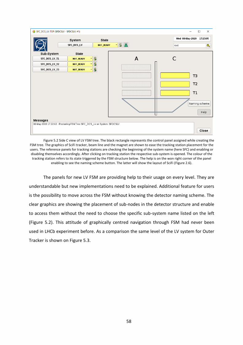
58
Figure 5.2 Side C view of LV FSM tree. The black rectangle represents the control panel assigned while creating the FSM tree. The graphics of SciFi tracker, beam line and the magnet are shown to ease the tracking station placement for the users. The reference panels for tracking stations are checking the beginning of the system name (here SFC) and enabling or disabling themselves accordingly. After clicking on tracking station the respective sub-system is opened. The colour of the tracking station refers to its state triggered by the FSM structure below. The help is on the won right corner of the panel
enabling to see the naming scheme button. The latter will show the layout of SciFi (Figure 2.6).
The panels for new LV FSM are providing help to their usage on every level. They are
understandable but new implementations need to be explained. Additional feature for users
is the possibility to move across the FSM without knowing the detector naming scheme. The
clear graphics are showing the placement of sub-nodes in the detector structure and enable
to access them without the need to choose the specific sub-system name listed on the left
(Figure 5.2). This attitude of graphically centred navigation through FSM had never been
used in LHCb experiment before. As a comparison the same level of the LV system for Outer
Tracker is shown on Figure 5.3.
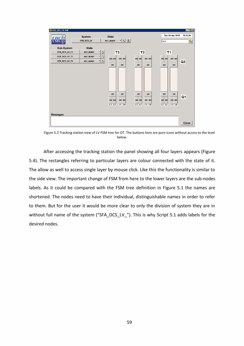
59
Figure 5.3 Tracking station view of LV FSM tree for OT. The buttons here are pure icons without access to the level below.
After accessing the tracking station the panel showing all four layers appears (Figure
5.4). The rectangles referring to particular layers are colour connected with the state of it.
The allow as well to access single layer by mouse click. Like this the functionality is similar to
the side view. The important change of FSM from here to the lower layers are the sub-nodes
labels. As it could be compared with the FSM tree definition in Figure 5.1 the names are
shortened. The nodes need to have their individual, distinguishable names in order to refer
to them. But for the user it would be more clear to only the division of system they are in
without full name of the system (“SFA_DCS_LV_”). This is why Script 5.1 adds labels for the
desired nodes.
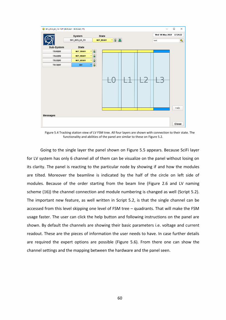
60
Figure 5.4 Tracking station view of LV FSM tree. All four layers are shown with connection to their state. The functionality and abilities of the panel are similar to these on Figure 5.2.
Going to the single layer the panel shown on Figure 5.5 appears. Because SciFi layer
for LV system has only 6 channel all of them can be visualize on the panel without losing on
its clarity. The panel is reacting to the particular node by showing if and how the modules
are tilted. Moreover the beamline is indicated by the half of the circle on left side of
modules. Because of the order starting from the beam line (Figure 2.6 and LV naming
scheme (16)) the channel connection and module numbering is changed as well (Script 5.2).
The important new feature, as well written in Script 5.2, is that the single channel can be
accessed from this level skipping one level of FSM tree – quadrants. That will make the FSM
usage faster. The user can click the help button and following instructions on the panel are
shown. By default the channels are showing their basic parameters i.e. voltage and current
readout. These are the pieces of information the user needs to have. In case further details
are required the expert options are possible (Figure 5.6). From there one can show the
channel settings and the mapping between the hardware and the panel seen.
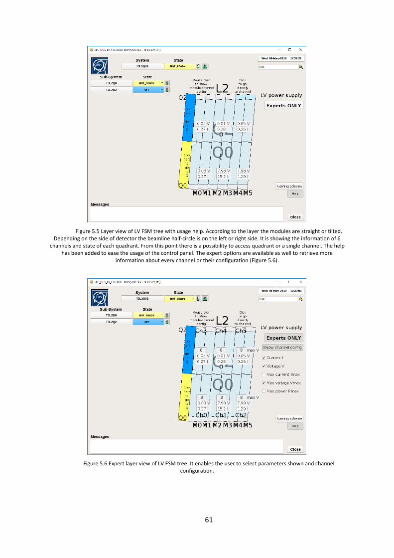
61
Figure 5.5 Layer view of LV FSM tree with usage help. According to the layer the modules are straight or tilted. Depending on the side of detector the beamline half-circle is on the left or right side. It is showing the information of 6
channels and state of each quadrant. From this point there is a possibility to access quadrant or a single channel. The help has been added to ease the usage of the control panel. The expert options are available as well to retrieve more
information about every channel or their configuration (Figure 5.6).
Figure 5.6 Expert layer view of LV FSM tree. It enables the user to select parameters shown and channel configuration.
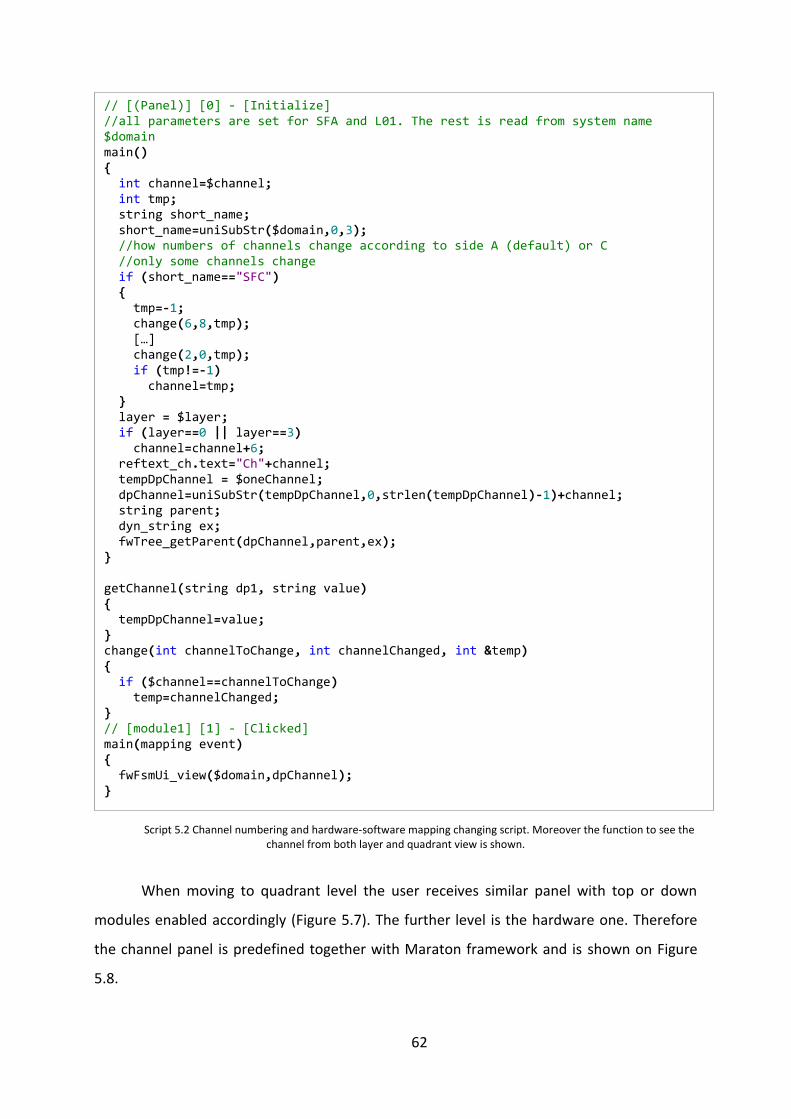
62
Script 5.2 Channel numbering and hardware-software mapping changing script. Moreover the function to see the channel from both layer and quadrant view is shown.
When moving to quadrant level the user receives similar panel with top or down
modules enabled accordingly (Figure 5.7). The further level is the hardware one. Therefore
the channel panel is predefined together with Maraton framework and is shown on Figure
5.8.
// [(Panel)] [0] - [Initialize] //all parameters are set for SFA and L01. The rest is read from system name $domain main() { int channel=$channel; int tmp; string short_name; short_name=uniSubStr($domain,0,3); //how numbers of channels change according to side A (default) or C //only some channels change if (short_name=="SFC") { tmp=-1; change(6,8,tmp); […] change(2,0,tmp); if (tmp!=-1) channel=tmp; } layer = $layer; if (layer==0 || layer==3) channel=channel+6; reftext_ch.text="Ch"+channel; tempDpChannel = $oneChannel; dpChannel=uniSubStr(tempDpChannel,0,strlen(tempDpChannel)-1)+channel; string parent; dyn_string ex; fwTree_getParent(dpChannel,parent,ex); } getChannel(string dp1, string value) { tempDpChannel=value; } change(int channelToChange, int channelChanged, int &temp) { if ($channel==channelToChange) temp=channelChanged; } // [module1] [1] - [Clicked] main(mapping event) { fwFsmUi_view($domain,dpChannel); }
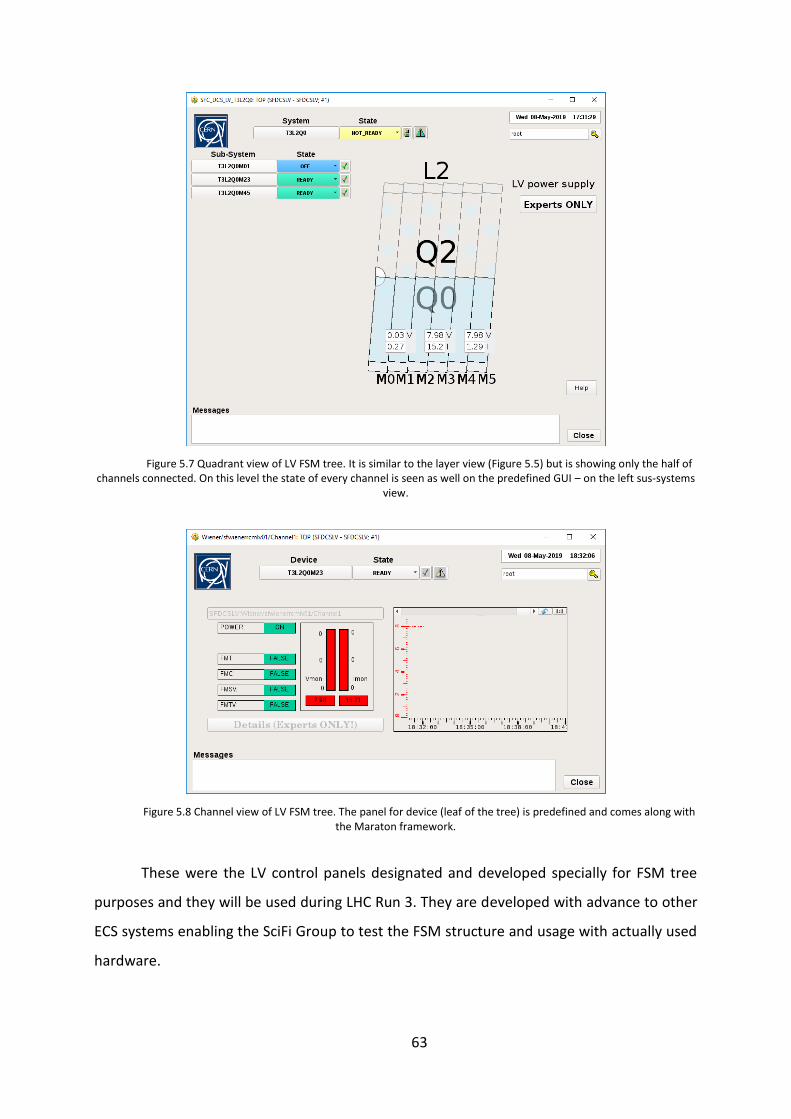
63
Figure 5.7 Quadrant view of LV FSM tree. It is similar to the layer view (Figure 5.5) but is showing only the half of channels connected. On this level the state of every channel is seen as well on the predefined GUI – on the left sus-systems
view.
Figure 5.8 Channel view of LV FSM tree. The panel for device (leaf of the tree) is predefined and comes along with the Maraton framework.
These were the LV control panels designated and developed specially for FSM tree
purposes and they will be used during LHC Run 3. They are developed with advance to other
ECS systems enabling the SciFi Group to test the FSM structure and usage with actually used
hardware.

64
5.2. SFDCSMON FSM
The monitoring part of DCS will have few Device Units as each system will be the DU
itself. Because of that there was no need to create the FSM tree by script. Therefore there
will be one control panel for every system right now similar to the ones in chapter 4.1 then
gradually developed as the design of services will progress. The final Dry Gas panel
designated for FSM has been created to show the desired goal for other services.
5.2.1. Dry Gas FSM
User of LHCb ECS are used to have one panel with all values to see if everything is
working properly. On the other hand other users or experts would like to see the sensors
assignment and history of the faulty ones. To join the supposedly opposite requirements the
control panel shown on Figure 5.9.
The panel contains all flowmeters for one side. They are grouped in layers and then
into tracking stations. As it can be seen most flow values are in grey. That is because the
reference panel of text field is disabling itself if the value that connects to it is not updated
for some time (Script 5.3). Otherwise the value is displayed along with gradually changing
colour model, similar to Script 3.2 but with different limits. The flow of gas requirements are
from 0.5 to 1 l/min and values below 0.4 and above 1.1 l/min should trigger the alarm.
Therefore the colours need to change accordingly and symmetrically because the lower the
flow is the worse influence it has on the dew point and SiPM performance itself.
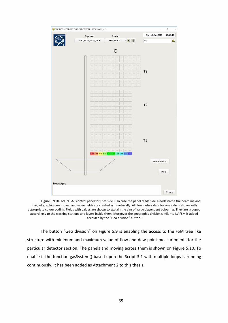
65
Figure 5.9 DCSMON GAS control panel for FSM side C. In case the panel reads side A node name the beamline and magnet graphics are moved and value fields are created symmetrically. All flowmeters data for one side is shown with
appropriate colour coding. Fields with values are shown to explain the aim of value dependent colouring. They are grouped accordingly to the tracking stations and layers inside them. Moreover the geographic division similar to LV FSM is added
accessed by the “Geo division” button.
The button “Geo division” on Figure 5.9 is enabling the access to the FSM tree like
structure with minimum and maximum value of flow and dew point measurements for the
particular detector section. The panels and moving across them is shown on Figure 5.10. To
enable it the function gasSystem() based upon the Script 3.1 with multiple loops is running
continuously. It has been added as Attachment 2 to this thesis.
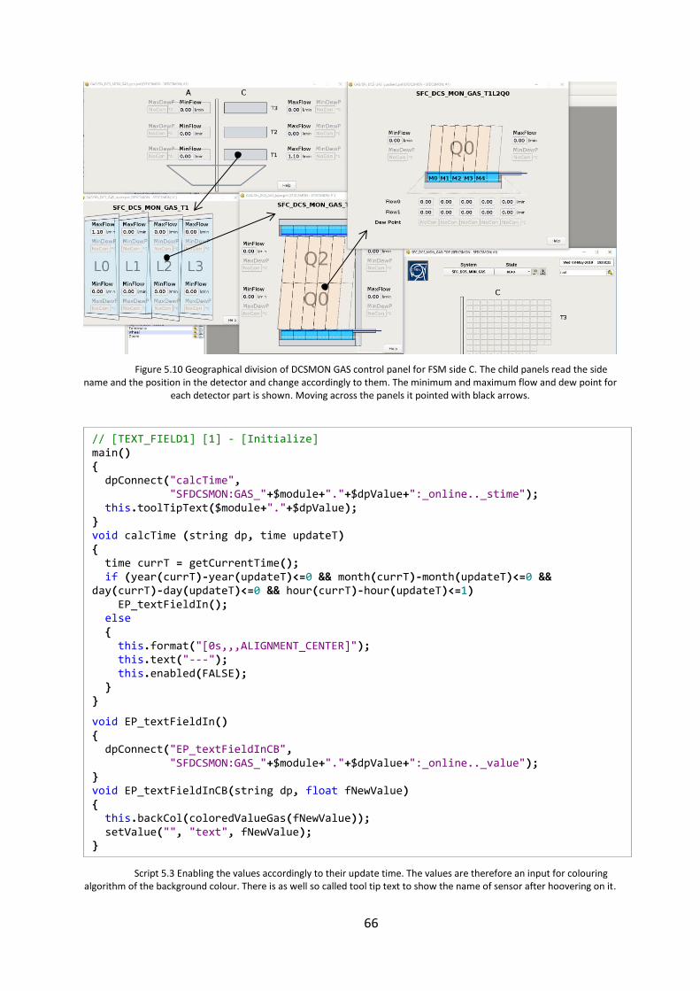
66
Figure 5.10 Geographical division of DCSMON GAS control panel for FSM side C. The child panels read the side name and the position in the detector and change accordingly to them. The minimum and maximum flow and dew point for
each detector part is shown. Moving across the panels it pointed with black arrows.
Script 5.3 Enabling the values accordingly to their update time. The values are therefore an input for colouring algorithm of the background colour. There is as well so called tool tip text to show the name of sensor after hoovering on it.
// [TEXT_FIELD1] [1] - [Initialize] main() { dpConnect("calcTime", "SFDCSMON:GAS_"+$module+"."+$dpValue+":_online.._stime"); this.toolTipText($module+"."+$dpValue); } void calcTime (string dp, time updateT) { time currT = getCurrentTime(); if (year(currT)-year(updateT)<=0 && month(currT)-month(updateT)<=0 && day(currT)-day(updateT)<=0 && hour(currT)-hour(updateT)<=1) EP_textFieldIn(); else { this.format("[0s,,,ALIGNMENT_CENTER]"); this.text("---"); this.enabled(FALSE); } }
void EP_textFieldIn() { dpConnect("EP_textFieldInCB", "SFDCSMON:GAS_"+$module+"."+$dpValue+":_online.._value"); } void EP_textFieldInCB(string dp, float fNewValue) { this.backCol(coloredValueGas(fNewValue)); setValue("", "text", fNewValue); }
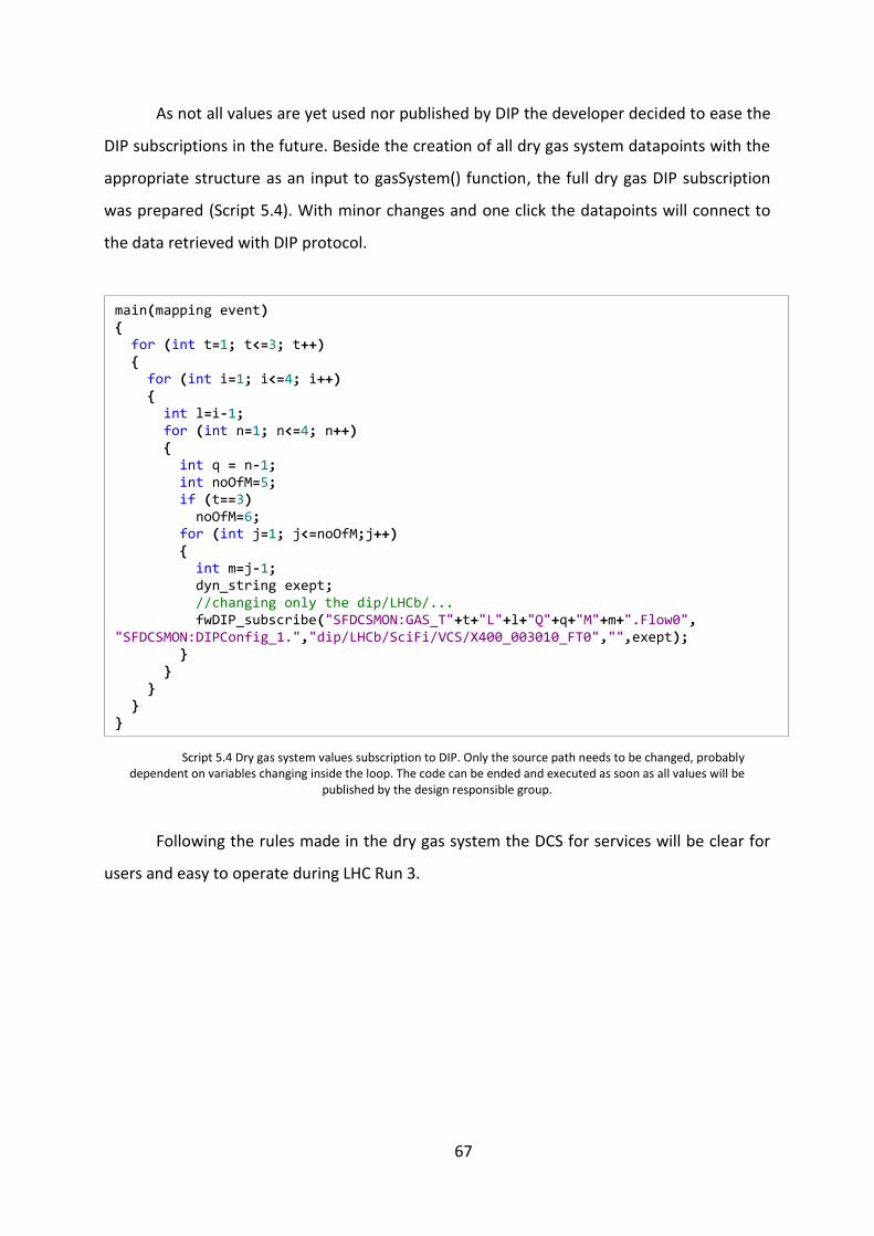
67
As not all values are yet used nor published by DIP the developer decided to ease the
DIP subscriptions in the future. Beside the creation of all dry gas system datapoints with the
appropriate structure as an input to gasSystem() function, the full dry gas DIP subscription
was prepared (Script 5.4). With minor changes and one click the datapoints will connect to
the data retrieved with DIP protocol.
Script 5.4 Dry gas system values subscription to DIP. Only the source path needs to be changed, probably dependent on variables changing inside the loop. The code can be ended and executed as soon as all values will be
published by the design responsible group.
Following the rules made in the dry gas system the DCS for services will be clear for
users and easy to operate during LHC Run 3.
main(mapping event) { for (int t=1; t<=3; t++) { for (int i=1; i<=4; i++) { int l=i-1; for (int n=1; n<=4; n++) { int q = n-1; int noOfM=5; if (t==3) noOfM=6; for (int j=1; j<=noOfM;j++) { int m=j-1; dyn_string exept; //changing only the dip/LHCb/... fwDIP_subscribe("SFDCSMON:GAS_T"+t+"L"+l+"Q"+q+"M"+m+".Flow0", "SFDCSMON:DIPConfig_1.","dip/LHCb/SciFi/VCS/X400_003010_FT0","",exept); } } } } }

68
6. Achievements and further DCS development
The project of software DCS development required knowledge of many systems. To
make it properly the author needed to know the hardware, communication protocols and
software implementation but the requirements were achieved. During the progress
additional development appeared to be possible. The clear new attitude to graphics and
help added to all control panels can be one example. The importance was also put on
communication with actual users. The development has been made with constant questions
for feedback from them. Furthermore the tools made for SciFi were spotted by another
detectors. The test and FSM panels for LV is an example of that exchange. The check tests
for all Maratons used during Run 2 and foreseen for Run 3 will be done with the author’s
panel. Muon system and Upstream Tracker are basing their commissioning and FSM on LV
panels described before.
The Detector Control System will be exploited during the commissioning of all
detector C-Frame. Therefore constant improvements or debugging can be made in case they
are needed. The monitoring of services is ought to evolve. But the tools and scripts to do
that were developed and they need to be joined accordingly to the final design and
implementation.

69
7. Conclusion
The Detector Control System is a complex part of the Scintillating Fibre Tracker
leading to many requirements. The developer needs to follow them and respond to the
appearing maintenance problems. The tools for testing the DCS hardware for SciFi have been
established and constantly improved throughout the process of the tests. Afterwards the
tools for C-Frame assembly and commissioning in respect to DCS were created to make it
possible to communicate with respective systems properly. The additional features have
been added to simplify the usage and to organise the tracking of test results in the database.
Moreover the software has been programmed to enable the growth of the slow controls and
further development. Finally the structure of control system has been established within the
guidelines and according to additional possibilities. The FSM tree for DCS has been renewed
and rebuild with useful features, whilst not shocking the experienced users. Moreover the
tools have been transferred to other detectors to share the facilitations and the approach.
The project had many aspects and requirements to meet within the desired tight schedule.
Even though the author was able to implement additional features useful for users and
future developers.
70
Bibliography
1. Collaboration, LHCb. LHCb : Technical Proposal. Geneva : CERN, 1998.
2. Collaboration CERN, LHCb. LHCb Tracker Upgrade Technical Design Report. CERN.
2014. Tech. rep.
3. LHCb, C. E. R. N. LHCb public page. Accessed: 2019-03-27.
4. Barbosa-Marinho, P. R., et al., et al. LHCb inner tracker: Technical Design Report.
Geneva : CERN, 2002. revised version number 1 submitted on 2002-11-13 14:14:34.
5. Barbosa-Marinho, P. R., et al., et al. LHCb outer tracker: Technical Design Report.
Geneva : CERN, 2001.
6. Amato, S., et al., et al. LHCb magnet: Technical Design Report. Geneva : CERN,
2000.
7. The GBT Project. Moreira, P., et al., et al. 2009.
8. Joram, Christian, et al., et al. LHCb Scintillating Fibre Tracker Engineering Design
Review Report: Fibres, Mats and Modules. CERN. Geneva : s.n., 2015. Tech. rep.
9. SciFi, C. E. R. N. SciFi public page. Accessed: 2019-06-04.
10. LHCb Online, C. E. R. N. ECS Guidelines. Accessed: 2019-06-10.
11. The LHCb run control. Alessio, F., et al., et al. 2010. Journal of Physics: Conference
Series. Vol. 219, p. 022009.
12. JCOP Collaboration, C. E. R. N. JCOP page. Accessed: 2019-06-07.
13. Industrial Controls, C. E. R. N. DIP public page. Accessed: 2019-06-06.
14. Foley, J. D. and et al. Computer Graphics: Principles and Practice (2nd ed.). [ed.]
CA: Addison-Wesley. s.l. : Redwood City, 1995. ISBN: ISBN 978-0-201-84840-3.
15. OPCFoundation. OPC Foundation page. Accessed: 2019-06-06.
16. Karol Poplawski SciFi, C. E. R. N. SciFi LV naming scheme. Accessed: 2019-06-10.
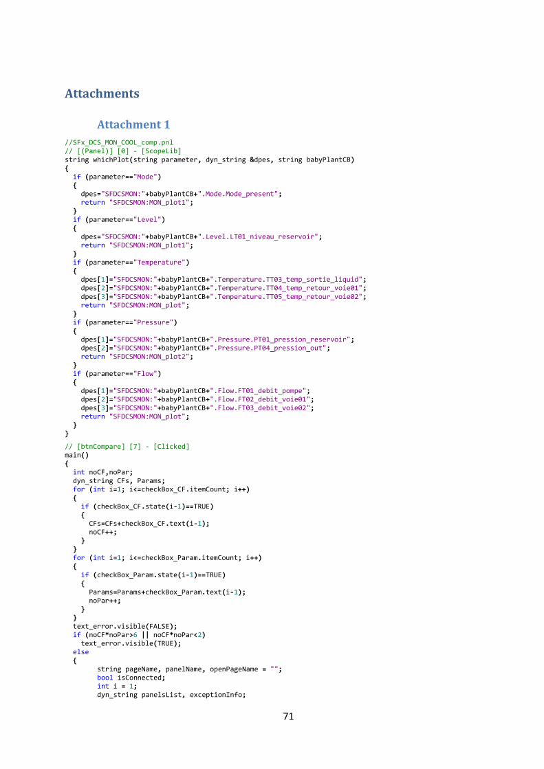
71
Attachments
Attachment 1
//SFx_DCS_MON_COOL_comp.pnl // [(Panel)] [0] - [ScopeLib] string whichPlot(string parameter, dyn_string &dpes, string babyPlantCB) { if (parameter=="Mode") { dpes="SFDCSMON:"+babyPlantCB+".Mode.Mode_present"; return "SFDCSMON:MON_plot1"; } if (parameter=="Level") { dpes="SFDCSMON:"+babyPlantCB+".Level.LT01_niveau_reservoir"; return "SFDCSMON:MON_plot1"; } if (parameter=="Temperature") { dpes[1]="SFDCSMON:"+babyPlantCB+".Temperature.TT03_temp_sortie_liquid"; dpes[2]="SFDCSMON:"+babyPlantCB+".Temperature.TT04_temp_retour_voie01"; dpes[3]="SFDCSMON:"+babyPlantCB+".Temperature.TT05_temp_retour_voie02"; return "SFDCSMON:MON_plot"; } if (parameter=="Pressure") { dpes[1]="SFDCSMON:"+babyPlantCB+".Pressure.PT01_pression_reservoir"; dpes[2]="SFDCSMON:"+babyPlantCB+".Pressure.PT04_pression_out"; return "SFDCSMON:MON_plot2"; } if (parameter=="Flow") { dpes[1]="SFDCSMON:"+babyPlantCB+".Flow.FT01_debit_pompe"; dpes[2]="SFDCSMON:"+babyPlantCB+".Flow.FT02_debit_voie01"; dpes[3]="SFDCSMON:"+babyPlantCB+".Flow.FT03_debit_voie02"; return "SFDCSMON:MON_plot"; } }
// [btnCompare] [7] - [Clicked] main() { int noCF,noPar; dyn_string CFs, Params; for (int i=1; i<=checkBox_CF.itemCount; i++) { if (checkBox_CF.state(i-1)==TRUE) { CFs=CFs+checkBox_CF.text(i-1); noCF++; } } for (int i=1; i<=checkBox_Param.itemCount; i++) { if (checkBox_Param.state(i-1)==TRUE) { Params=Params+checkBox_Param.text(i-1); noPar++; } } text_error.visible(FALSE); if (noCF*noPar>6 || noCF*noPar<2) text_error.visible(TRUE); else { string pageName, panelName, openPageName = ""; bool isConnected; int i = 1; dyn_string panelsList, exceptionInfo;
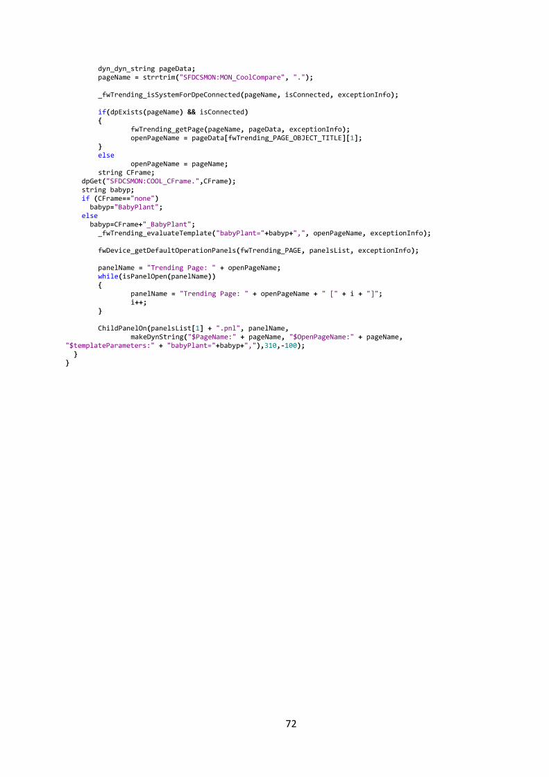
72
dyn_dyn_string pageData; pageName = strrtrim("SFDCSMON:MON_CoolCompare", "."); _fwTrending_isSystemForDpeConnected(pageName, isConnected, exceptionInfo); if(dpExists(pageName) && isConnected) { fwTrending_getPage(pageName, pageData, exceptionInfo); openPageName = pageData[fwTrending_PAGE_OBJECT_TITLE][1]; } else openPageName = pageName; string CFrame; dpGet("SFDCSMON:COOL_CFrame.",CFrame); string babyp; if (CFrame=="none") babyp="BabyPlant"; else babyp=CFrame+"_BabyPlant"; _fwTrending_evaluateTemplate("babyPlant="+babyp+",", openPageName, exceptionInfo); fwDevice_getDefaultOperationPanels(fwTrending_PAGE, panelsList, exceptionInfo); panelName = "Trending Page: " + openPageName; while(isPanelOpen(panelName)) { panelName = "Trending Page: " + openPageName + " [" + i + "]"; i++; } ChildPanelOn(panelsList[1] + ".pnl", panelName, makeDynString("$PageName:" + pageName, "$OpenPageName:" + pageName, "$templateParameters:" + "babyPlant="+babyp+","),310,-100); } }
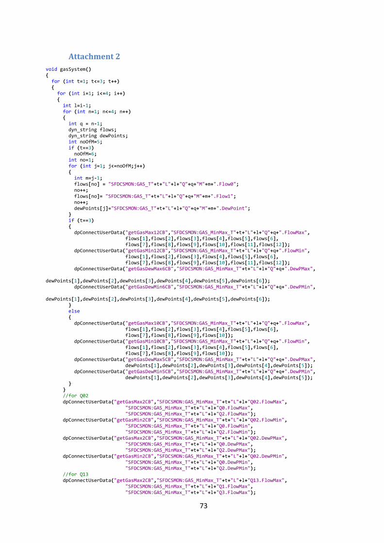
73
Attachment 2
void gasSystem() { for (int t=1; t<=3; t++) { for (int i=1; i<=4; i++) { int l=i-1; for (int n=1; n<=4; n++) { int q = n-1; dyn_string flows; dyn_string dewPoints; int noOfM=5; if (t==3) noOfM=6; int no=1; for (int j=1; j<=noOfM;j++) { int m=j-1; flows[no] = "SFDCSMON:GAS_T"+t+"L"+l+"Q"+q+"M"+m+".Flow0"; no++; flows[no]= "SFDCSMON:GAS_T"+t+"L"+l+"Q"+q+"M"+m+".Flow1"; no++; dewPoints[j]="SFDCSMON:GAS_T"+t+"L"+l+"Q"+q+"M"+m+".DewPoint"; } if (t==3) { dpConnectUserData("getGasMax12CB","SFDCSMON:GAS_MinMax_T"+t+"L"+l+"Q"+q+".FlowMax", flows[1],flows[2],flows[3],flows[4],flows[5],flows[6], flows[7],flows[8],flows[9],flows[10],flows[11],flows[12]); dpConnectUserData("getGasMin12CB","SFDCSMON:GAS_MinMax_T"+t+"L"+l+"Q"+q+".FlowMin", flows[1],flows[2],flows[3],flows[4],flows[5],flows[6], flows[7],flows[8],flows[9],flows[10],flows[11],flows[12]); dpConnectUserData("getGasDewMax6CB","SFDCSMON:GAS_MinMax_T"+t+"L"+l+"Q"+q+".DewPMax", dewPoints[1],dewPoints[2],dewPoints[3],dewPoints[4],dewPoints[5],dewPoints[6]); dpConnectUserData("getGasDewMin6CB","SFDCSMON:GAS_MinMax_T"+t+"L"+l+"Q"+q+".DewPMin", dewPoints[1],dewPoints[2],dewPoints[3],dewPoints[4],dewPoints[5],dewPoints[6]); } else { dpConnectUserData("getGasMax10CB","SFDCSMON:GAS_MinMax_T"+t+"L"+l+"Q"+q+".FlowMax", flows[1],flows[2],flows[3],flows[4],flows[5],flows[6], flows[7],flows[8],flows[9],flows[10]); dpConnectUserData("getGasMin10CB","SFDCSMON:GAS_MinMax_T"+t+"L"+l+"Q"+q+".FlowMin", flows[1],flows[2],flows[3],flows[4],flows[5],flows[6], flows[7],flows[8],flows[9],flows[10]); dpConnectUserData("getGasDewMax5CB","SFDCSMON:GAS_MinMax_T"+t+"L"+l+"Q"+q+".DewPMax", dewPoints[1],dewPoints[2],dewPoints[3],dewPoints[4],dewPoints[5]); dpConnectUserData("getGasDewMin5CB","SFDCSMON:GAS_MinMax_T"+t+"L"+l+"Q"+q+".DewPMin", dewPoints[1],dewPoints[2],dewPoints[3],dewPoints[4],dewPoints[5]); } } //for Q02 dpConnectUserData("getGasMax2CB","SFDCSMON:GAS_MinMax_T"+t+"L"+l+"Q02.FlowMax", "SFDCSMON:GAS_MinMax_T"+t+"L"+l+"Q0.FlowMax", "SFDCSMON:GAS_MinMax_T"+t+"L"+l+"Q2.FlowMax"); dpConnectUserData("getGasMin2CB","SFDCSMON:GAS_MinMax_T"+t+"L"+l+"Q02.FlowMin", "SFDCSMON:GAS_MinMax_T"+t+"L"+l+"Q0.FlowMin", "SFDCSMON:GAS_MinMax_T"+t+"L"+l+"Q2.FlowMin"); dpConnectUserData("getGasMax2CB","SFDCSMON:GAS_MinMax_T"+t+"L"+l+"Q02.DewPMax", "SFDCSMON:GAS_MinMax_T"+t+"L"+l+"Q0.DewPMax", "SFDCSMON:GAS_MinMax_T"+t+"L"+l+"Q2.DewPMax"); dpConnectUserData("getGasMin2CB","SFDCSMON:GAS_MinMax_T"+t+"L"+l+"Q02.DewPMin", "SFDCSMON:GAS_MinMax_T"+t+"L"+l+"Q0.DewPMin", "SFDCSMON:GAS_MinMax_T"+t+"L"+l+"Q2.DewPMin"); //for Q13 dpConnectUserData("getGasMax2CB","SFDCSMON:GAS_MinMax_T"+t+"L"+l+"Q13.FlowMax", "SFDCSMON:GAS_MinMax_T"+t+"L"+l+"Q1.FlowMax", "SFDCSMON:GAS_MinMax_T"+t+"L"+l+"Q3.FlowMax");
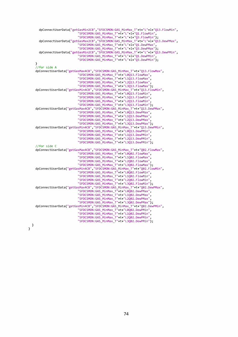
74
dpConnectUserData("getGasMin2CB","SFDCSMON:GAS_MinMax_T"+t+"L"+l+"Q13.FlowMin", "SFDCSMON:GAS_MinMax_T"+t+"L"+l+"Q1.FlowMin", "SFDCSMON:GAS_MinMax_T"+t+"L"+l+"Q3.FlowMin"); dpConnectUserData("getGasMax2CB","SFDCSMON:GAS_MinMax_T"+t+"L"+l+"Q13.DewPMax", "SFDCSMON:GAS_MinMax_T"+t+"L"+l+"Q1.DewPMax", "SFDCSMON:GAS_MinMax_T"+t+"L"+l+"Q3.DewPMax"); dpConnectUserData("getGasMin2CB","SFDCSMON:GAS_MinMax_T"+t+"L"+l+"Q13.DewPMin", "SFDCSMON:GAS_MinMax_T"+t+"L"+l+"Q1.DewPMin", "SFDCSMON:GAS_MinMax_T"+t+"L"+l+"Q3.DewPMin"); } //for side A dpConnectUserData("getGasMax4CB","SFDCSMON:GAS_MinMax_T"+t+"Q13.FlowMax", "SFDCSMON:GAS_MinMax_T"+t+"L0Q13.FlowMax", "SFDCSMON:GAS_MinMax_T"+t+"L1Q13.FlowMax", "SFDCSMON:GAS_MinMax_T"+t+"L2Q13.FlowMax", "SFDCSMON:GAS_MinMax_T"+t+"L3Q13.FlowMax"); dpConnectUserData("getGasMin4CB","SFDCSMON:GAS_MinMax_T"+t+"Q13.FlowMin", "SFDCSMON:GAS_MinMax_T"+t+"L0Q13.FlowMin", "SFDCSMON:GAS_MinMax_T"+t+"L1Q13.FlowMin", "SFDCSMON:GAS_MinMax_T"+t+"L2Q13.FlowMin", "SFDCSMON:GAS_MinMax_T"+t+"L3Q13.FlowMin"); dpConnectUserData("getGasMax4CB","SFDCSMON:GAS_MinMax_T"+t+"Q13.DewPMax", "SFDCSMON:GAS_MinMax_T"+t+"L0Q13.DewPMax", "SFDCSMON:GAS_MinMax_T"+t+"L1Q13.DewPMax", "SFDCSMON:GAS_MinMax_T"+t+"L2Q13.DewPMax", "SFDCSMON:GAS_MinMax_T"+t+"L3Q13.DewPMax"); dpConnectUserData("getGasMin4CB","SFDCSMON:GAS_MinMax_T"+t+"Q13.DewPMin", "SFDCSMON:GAS_MinMax_T"+t+"L0Q13.DewPMin", "SFDCSMON:GAS_MinMax_T"+t+"L1Q13.DewPMin", "SFDCSMON:GAS_MinMax_T"+t+"L2Q13.DewPMin", "SFDCSMON:GAS_MinMax_T"+t+"L3Q13.DewPMin"); //for side C dpConnectUserData("getGasMax4CB","SFDCSMON:GAS_MinMax_T"+t+"Q02.FlowMax", "SFDCSMON:GAS_MinMax_T"+t+"L0Q02.FlowMax", "SFDCSMON:GAS_MinMax_T"+t+"L1Q02.FlowMax", "SFDCSMON:GAS_MinMax_T"+t+"L2Q02.FlowMax", "SFDCSMON:GAS_MinMax_T"+t+"L3Q02.FlowMax"); dpConnectUserData("getGasMin4CB","SFDCSMON:GAS_MinMax_T"+t+"Q02.FlowMin", "SFDCSMON:GAS_MinMax_T"+t+"L0Q02.FlowMin", "SFDCSMON:GAS_MinMax_T"+t+"L1Q02.FlowMin", "SFDCSMON:GAS_MinMax_T"+t+"L2Q02.FlowMin", "SFDCSMON:GAS_MinMax_T"+t+"L3Q02.FlowMin"); dpConnectUserData("getGasMax4CB","SFDCSMON:GAS_MinMax_T"+t+"Q02.DewPMax", "SFDCSMON:GAS_MinMax_T"+t+"L0Q02.DewPMax", "SFDCSMON:GAS_MinMax_T"+t+"L1Q02.DewPMax", "SFDCSMON:GAS_MinMax_T"+t+"L2Q02.DewPMax", "SFDCSMON:GAS_MinMax_T"+t+"L3Q02.DewPMax"); dpConnectUserData("getGasMin4CB","SFDCSMON:GAS_MinMax_T"+t+"Q02.DewPMin", "SFDCSMON:GAS_MinMax_T"+t+"L0Q02.DewPMin", "SFDCSMON:GAS_MinMax_T"+t+"L1Q02.DewPMin", "SFDCSMON:GAS_MinMax_T"+t+"L2Q02.DewPMin", "SFDCSMON:GAS_MinMax_T"+t+"L3Q02.DewPMin"); } }