fermilab-thesis-2004-93_2.pdf - cern document server
TRANSCRIPT
CER
N-T
HES
IS-2
004-
090
UNIVERSITE DE GENEVE FACULTE DES SCIENCESDepartement de physique nucleaire et corpusculaire Professeur Allan G. Clark
Search for the B0d → µµK∗0 Decay at CDF
and Studies of ATLAS Silicon Tracker Modules
THESE
presentee a la Faculte des Sciences de l’Universite de Genevepour obtenir le grade de Docteur es sciences, mention physique
par
Andras Zsenei
d’Hongrie
These No 3510
GENEVEAtelier de reproduction de la Section de Physique
2003


Acknowledgements
This thesis could not have been completed without the advices, efforts, supportand encouragement of countless people, a few of which I would like to mention.
First of all I would like to thank Professor Allan Clark for the invaluable guid-ance he has provided and for giving me the possibility to participate in two greathigh energy physics experiments – ATLAS and CDF – which are at the forefront ofresearch. I would like to thank Xin Wu who supervised the CDF part of the thesis.He patiently answered all my questions and both his knowledge of the theory and ofthe ntuples was of great help. I would like also to acknowledge the great discussionswe had about statistics with Mario Campanelli, and the clear explanations about theconfidence intervals of Bob Cousins.
I would like to thank Prof. Martin Pohl and Prof. Carlo Dionisi for accepting toparticipate in the jury of my thesis, and for their astute remarks.
I would also like to thank the rest of the University of Geneva group – Daniela, Di-dier, Lorenzo, Federica, Cristina, Mauro, Monica, Yanwen, Sofia, Manuel, Shulamit,Anna – for everything over the last several years. Special thanks to Mariane whocorrected the French part of my thesis.
Many thanks to the technicians of the University of Geneva – Eric, Gerard, Alain,Philippe, Jean, Jean-Pierre – who were a tremenduous help both during the con-struction of analog modules and the cooling tests. I am also grateful to Catherineand Peggy for the administrative help they gave during all those years, and to Yannwhom you could count on to solve any computer problem even late at night.
Kind thanks to all the people with whom I was working at CERN: Peter Weil-hammer, Alan Rudge, Wladek, Carlos, Jan, Marcin, Lars and all the others. Julio inparticular was a tremenduous help and I had a really great time working with him,whether it was in the beam test over the week-end or in the lab.
I would also like to thank all the people I was working with at Fermilab: ChristophPaus who teached me how to skim the ntuples, Frank Wuerthwein with his thoroughknowledge of Bgenerator, Andreas Korn who usually knew the answer to everythingand was very helpful to share it.
I would like to thank the Russian community for making life a lot more interestingat Fermilab. The birthday parties, barbecues, lunches, dance lessons and other funactivities with Boris, Alex, Alexei, Andrei, Julia L., Julia P., Konstantin and all theothers will be sorely missed. Many thanks to the cubicle co-owners and neighbours

– Anne-Sylvie, Chris, Kirby amongst others –, who not only made it a nice place tobe, but brought me to baseball and basketball games as well. There are many otherpeople to whom I am grateful: Houck, James, Jim, Arnold, Jerome, Stephane andthe list could go on.
I have good memories of working with you all, and wish everyone the best of luck.Last but not least, I would like to thank my friends and family for all their love
and support.
Contents
1 Resume xix1.1 Introduction theorique . . . . . . . . . . . . . . . . . . . . . . . . . . xix1.2 L’experience CDF au Tevatron . . . . . . . . . . . . . . . . . . . . . . xx1.3 La recherche de la desintegration B0
d → µµK∗0 a CDF . . . . . . . . xxi1.4 L’experience ATLAS au LHC . . . . . . . . . . . . . . . . . . . . . . xxv1.5 Construction et evaluation de modules ATLAS equipes de SCTA128 . xxvi
I Theoretical Motivation 1
2 The Standard Model and beyond 32.1 The Standard Model . . . . . . . . . . . . . . . . . . . . . . . . . . . 3
2.1.1 CP-violation . . . . . . . . . . . . . . . . . . . . . . . . . . . . 42.1.2 The unitarity triangle . . . . . . . . . . . . . . . . . . . . . . . 62.1.3 Recent results on the CKM Unitarity Triangle . . . . . . . . . 8
2.2 The FCNC Decays of B Mesons . . . . . . . . . . . . . . . . . . . . . 132.2.1 Introduction . . . . . . . . . . . . . . . . . . . . . . . . . . . . 132.2.2 The b → sl+l− decays . . . . . . . . . . . . . . . . . . . . . . . 15
2.3 Beyond the Standard Model . . . . . . . . . . . . . . . . . . . . . . . 19
II Search for the B0d → µµK∗0 decay at the CDF experiment 23
3 The CDF experiment at the Tevatron 253.1 The Tevatron . . . . . . . . . . . . . . . . . . . . . . . . . . . . . . . 25
3.1.1 Proton production . . . . . . . . . . . . . . . . . . . . . . . . 263.1.2 Antiproton production . . . . . . . . . . . . . . . . . . . . . . 273.1.3 The Tevatron . . . . . . . . . . . . . . . . . . . . . . . . . . . 27
3.2 The CDF experiment . . . . . . . . . . . . . . . . . . . . . . . . . . . 303.2.1 Overview of the CDF experiment . . . . . . . . . . . . . . . . 303.2.2 The CDF Tracking System . . . . . . . . . . . . . . . . . . . . 313.2.3 The calorimetry . . . . . . . . . . . . . . . . . . . . . . . . . . 403.2.4 Muon detectors . . . . . . . . . . . . . . . . . . . . . . . . . . 423.2.5 The Cherenkov Luminosity Counters . . . . . . . . . . . . . . 47
v
vi CONTENTS
3.2.6 Trigger . . . . . . . . . . . . . . . . . . . . . . . . . . . . . . . 48
4 Search for the B0d → µµK∗0 decay 59
4.1 Introduction . . . . . . . . . . . . . . . . . . . . . . . . . . . . . . . . 594.2 The datasets . . . . . . . . . . . . . . . . . . . . . . . . . . . . . . . . 604.3 Preselection . . . . . . . . . . . . . . . . . . . . . . . . . . . . . . . . 644.4 Baseline selection . . . . . . . . . . . . . . . . . . . . . . . . . . . . . 664.5 Optimization of the selection requirements . . . . . . . . . . . . . . . 70
4.5.1 The isolation . . . . . . . . . . . . . . . . . . . . . . . . . . . 704.5.2 The transverse decay length . . . . . . . . . . . . . . . . . . . 714.5.3 The pointing angle . . . . . . . . . . . . . . . . . . . . . . . . 734.5.4 The optimization procedure . . . . . . . . . . . . . . . . . . . 74
4.6 Acceptance and efficiencies . . . . . . . . . . . . . . . . . . . . . . . . 824.6.1 Monte Carlo Calculations . . . . . . . . . . . . . . . . . . . . 83
4.7 Energy loss, B field corrections and track refitting . . . . . . . . . . . 864.8 Final selection . . . . . . . . . . . . . . . . . . . . . . . . . . . . . . . 874.9 Future prospects at CDF . . . . . . . . . . . . . . . . . . . . . . . . . 924.10 Conclusions . . . . . . . . . . . . . . . . . . . . . . . . . . . . . . . . 93
III Performance of ATLAS modules using the SCTA128 chip 95
5 The ATLAS experiment at the LHC 975.1 The Large Hadron Collider . . . . . . . . . . . . . . . . . . . . . . . . 975.2 ATLAS overview . . . . . . . . . . . . . . . . . . . . . . . . . . . . . 1005.3 The Inner Detector . . . . . . . . . . . . . . . . . . . . . . . . . . . . 1055.4 Trigger, Data Acquisition and Controls . . . . . . . . . . . . . . . . . 1115.5 The Silicon Tracker (SCT) . . . . . . . . . . . . . . . . . . . . . . . . 1125.6 The modules . . . . . . . . . . . . . . . . . . . . . . . . . . . . . . . . 114
5.6.1 Front-end electronics for modules for Si trackers . . . . . . . . 1175.6.2 The digital solution (ABCD) . . . . . . . . . . . . . . . . . . . 1185.6.3 The analogue solution (SCTA) . . . . . . . . . . . . . . . . . . 118
5.7 Physics Potential of the ATLAS Detector . . . . . . . . . . . . . . . . 1195.7.1 B → µµ(X) . . . . . . . . . . . . . . . . . . . . . . . . . . . . 120
6 Performance of ATLAS modules using the SCTA128 chip 1256.1 Introduction . . . . . . . . . . . . . . . . . . . . . . . . . . . . . . . . 1256.2 The digital solution (ABCD) . . . . . . . . . . . . . . . . . . . . . . . 125
6.2.1 Evolution of the design of the ABCD chip . . . . . . . . . . . 1256.2.2 The ABCD chip . . . . . . . . . . . . . . . . . . . . . . . . . . 1276.2.3 Electrical module prototypes . . . . . . . . . . . . . . . . . . . 1286.2.4 Effects of radiation on the ABCD . . . . . . . . . . . . . . . . 130
6.3 The analogue solution (SCTA128) . . . . . . . . . . . . . . . . . . . . 1316.3.1 The SCTA128 chip . . . . . . . . . . . . . . . . . . . . . . . . 132
CONTENTS vii
6.3.2 Laboratory setup . . . . . . . . . . . . . . . . . . . . . . . . . 1356.3.3 Single chip tests . . . . . . . . . . . . . . . . . . . . . . . . . . 1366.3.4 Module construction . . . . . . . . . . . . . . . . . . . . . . . 1426.3.5 Si strip detector module at the test bench . . . . . . . . . . . 1446.3.6 Beam test setup . . . . . . . . . . . . . . . . . . . . . . . . . . 1486.3.7 Beam test results . . . . . . . . . . . . . . . . . . . . . . . . . 1486.3.8 Test of a linear optical link . . . . . . . . . . . . . . . . . . . . 1506.3.9 Conclusions . . . . . . . . . . . . . . . . . . . . . . . . . . . . 156
A Number of signal events for the B0d → J/ψK∗0 decay 159
B Signal optimization plots for S2/(S +B) 165
C Signal optimization plots for S2/(a/2 +√B)2 171
D Estimated background for the B0d → µµK∗0 decay 177
E Number of estimated B0d → µµK∗0 events 183
Bibliography 189

viii CONTENTS
List of Figures
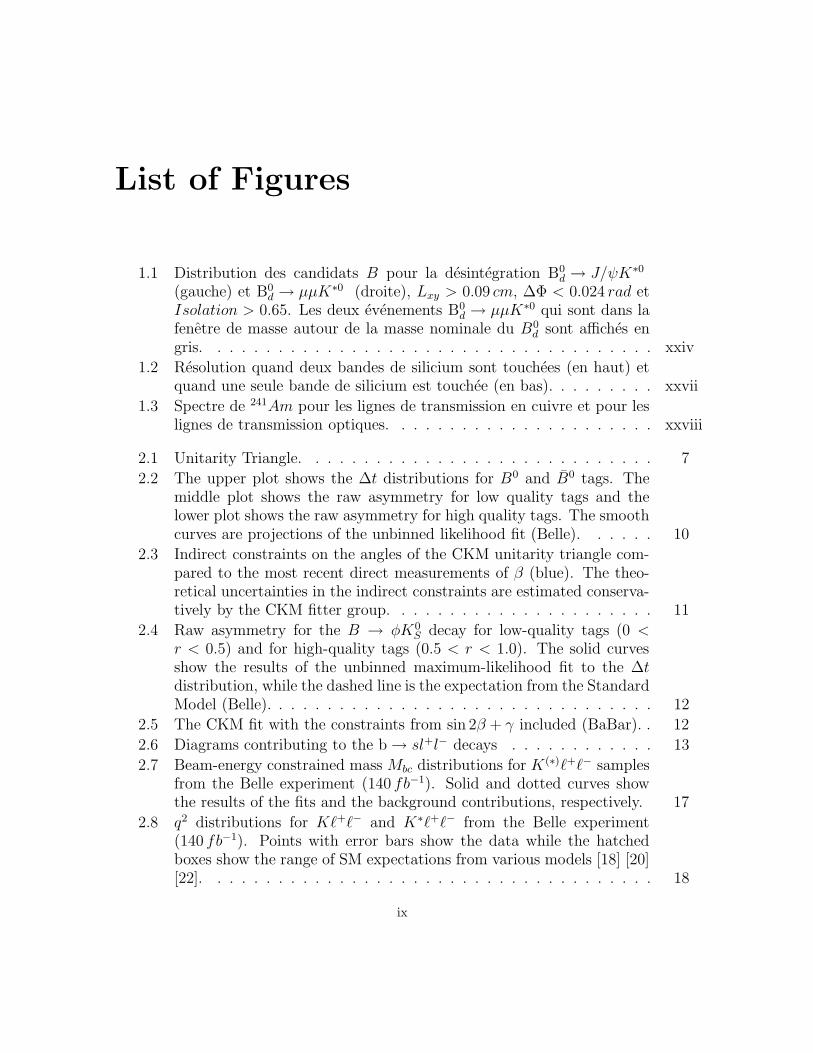
1.1 Distribution des candidats B pour la desintegration B0d → J/ψK∗0
(gauche) et B0d → µµK∗0 (droite), Lxy > 0.09 cm, ∆Φ < 0.024 rad et
Isolation > 0.65. Les deux evenements B0d → µµK∗0 qui sont dans la
fenetre de masse autour de la masse nominale du B0d sont affiches en
gris. . . . . . . . . . . . . . . . . . . . . . . . . . . . . . . . . . . . . xxiv
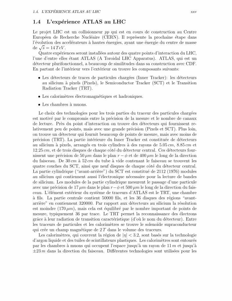
1.2 Resolution quand deux bandes de silicium sont touchees (en haut) etquand une seule bande de silicium est touchee (en bas). . . . . . . . . xxvii
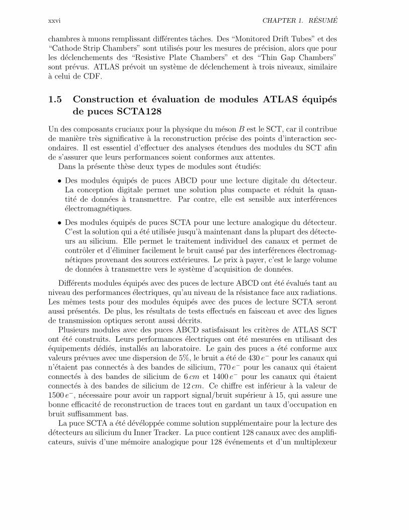
1.3 Spectre de 241Am pour les lignes de transmission en cuivre et pour leslignes de transmission optiques. . . . . . . . . . . . . . . . . . . . . . xxviii
2.1 Unitarity Triangle. . . . . . . . . . . . . . . . . . . . . . . . . . . . . 7
2.2 The upper plot shows the ∆t distributions for B0 and B0 tags. Themiddle plot shows the raw asymmetry for low quality tags and thelower plot shows the raw asymmetry for high quality tags. The smoothcurves are projections of the unbinned likelihood fit (Belle). . . . . . 10
2.3 Indirect constraints on the angles of the CKM unitarity triangle com-pared to the most recent direct measurements of β (blue). The theo-retical uncertainties in the indirect constraints are estimated conserva-tively by the CKM fitter group. . . . . . . . . . . . . . . . . . . . . . 11
2.4 Raw asymmetry for the B → φK0S decay for low-quality tags (0 <
r < 0.5) and for high-quality tags (0.5 < r < 1.0). The solid curvesshow the results of the unbinned maximum-likelihood fit to the ∆tdistribution, while the dashed line is the expectation from the StandardModel (Belle). . . . . . . . . . . . . . . . . . . . . . . . . . . . . . . . 12
2.5 The CKM fit with the constraints from sin 2β + γ included (BaBar). . 12
2.6 Diagrams contributing to the b → sl+l− decays . . . . . . . . . . . . 13
2.7 Beam-energy constrained mass Mbc distributions for K(∗)`+`− samplesfrom the Belle experiment (140 fb−1). Solid and dotted curves showthe results of the fits and the background contributions, respectively. 17
2.8 q2 distributions for K`+`− and K∗`+`− from the Belle experiment(140 fb−1). Points with error bars show the data while the hatchedboxes show the range of SM expectations from various models [18] [20][22]. . . . . . . . . . . . . . . . . . . . . . . . . . . . . . . . . . . . . 18
ix
x LIST OF FIGURES
2.9 Beam-energy constrained mass (mES) distribution for the K`+`− mo-des from the BaBar experiment. The solid curve is the sum of allfit components, including signal; the dashed curve is the sum of allbackground components. . . . . . . . . . . . . . . . . . . . . . . . . . 18
2.10 The dilepton invariant mass squared distribution for B → K∗µ+µ− .The solid lines represent the SM and the shaded area signals theform-factor related uncertainties. The dotted lines correspond to theSUGRA model with C7 = −1.2 ·CSM
7 , C9 = 1.03 ·CSM9 and C10 = 1.0 ·
CSM10 . The long-short dashed lines correspond to an allowed point in the
parameter space of the MIA-SUSY model given by C7 = −0.83 ·CSM7 ,
C9 = 0.92 ·CSM9 and C10 = 1.61 ·CSM
10 . The black lines show the sum ofthe short-distance and long-distance contributions, while the magentalines show the corresponding pure short-distance spectra. . . . . . . . 20
2.11 The normalized forward-backward asymmetry in B → K∗µ+µ− decayas a function of s. The solid line denotes the SM prediction. Thedotted lines correspond to the SUGRA model with C7 = −1.2 · CSM
7 ,C9 = 1.03 ·CSM
9 and C10 = 1.0 ·CSM10 with the upper and lower curves
representing the C7 < 0 and C7 > 0 case, respectively. The long-shortdashed (blue) lines correspond to the MIA-SUSY model, using theparameters C7 = ±0.83 · CSM
7 , C9 = 0.92 · CSM9 and C10 = 1.61 · CSM
10
with the upper and lower curves representing the C7 < 0 and C7 > 0case, respectively. The dashed curves indicating a positive asymmetryfor large s correspond to the MIA-SUSY models using the parametersC7 = ±0.83 · CSM
7 , C9 = 0.79 · CSM9 and C10 = −0.38 · CSM
10 . . . . . . 21
3.1 The accelerator complex at Fermilab. . . . . . . . . . . . . . . . . . . 26
3.2 Instantenuous luminosities at the start of the stores through the endof 2003 [56]. . . . . . . . . . . . . . . . . . . . . . . . . . . . . . . . . 29
3.3 The luminosity delivered by the Tevatron since the start of Run II untilJanuary 2004 [55]. . . . . . . . . . . . . . . . . . . . . . . . . . . . . . 29
3.4 The coordinate system of the CDF experiment. . . . . . . . . . . . . 30
3.5 Three dimensional view of the CDF detector showing the position ofthe detector subsystems. . . . . . . . . . . . . . . . . . . . . . . . . . 32
3.6 Elevation view of the CDF detector showing the position of the differentsubsystems. . . . . . . . . . . . . . . . . . . . . . . . . . . . . . . . . 33
3.7 Overview of the CDF tracking system. . . . . . . . . . . . . . . . . . 34
3.8 Overall view of the different silicon subsystems. . . . . . . . . . . . . 35
3.9 Design of the Layer 00. . . . . . . . . . . . . . . . . . . . . . . . . . . 35
3.10 SVX barrel and bulkhead. . . . . . . . . . . . . . . . . . . . . . . . . 36
3.11 Perspective views of the z and φ-sides of a Layer 0 ladder. . . . . . . 37
3.12 Impact parameter resolution in µm as a function of the pT for trackspassing through passive material without Layer 00 hits (red), and withLayer 00 hits (blue). . . . . . . . . . . . . . . . . . . . . . . . . . . . 37
LIST OF FIGURES xi
3.13 Efficiency as a function of η of the calorimeter seeded outside-in silicontracking for tracks with three (blue), four (green) and five (red) siliconhits. . . . . . . . . . . . . . . . . . . . . . . . . . . . . . . . . . . . . 38
3.14 1/6 section of the COT endplate. . . . . . . . . . . . . . . . . . . . . 39
3.15 Resolution of the Central Outer Tracker. . . . . . . . . . . . . . . . . 40
3.16 Location of the different components of the muon system in azimuthφ and pseudorapidity η. . . . . . . . . . . . . . . . . . . . . . . . . . 43
3.17 Schematic view of the 16 cells of a CMU module. . . . . . . . . . . . 44
3.18 Layout of a CMP wall with steel, chambers (CMP) and counters (CSP).Counter readout is located at z = 0. Counter layers are offset from thechambers and from each other in x to allow overlapping light guidesand PMTs and saving space. . . . . . . . . . . . . . . . . . . . . . . . 44
3.19 Schematic view of a CMP-CMX tube (left), and the drift tube layoutin a CMX module covering 150 in azimuth (right). . . . . . . . . . . . 45
3.20 A detailed section of the IMU Barrel, showing several chamber cellsand the corresponding scintillators. . . . . . . . . . . . . . . . . . . . 46
3.21 Integrated luminosity delivered by the Tevatron (red) and recorded byCDF (blue) through the end of 2003 [56]. . . . . . . . . . . . . . . . . 47
3.22 Functional block diagram of the CDF data flow. . . . . . . . . . . . . 48
3.23 Block diagram of the Run II trigger system. . . . . . . . . . . . . . . 49
3.24 Level 1 CMU trigger efficiency as a function of muon pT and muontrack φ after excluding bad wedge in 240-270 degree. For the efficiencyas a function of φ the muons are required to have pT > 3GeV/c. . . . 51
3.25 Level 1 CMX trigger efficiency as a function of muon 1/pT and muonφ. For the right plot the filled square points are for the averagedefficiencies, the dot points are for the East CMX efficiencies, and theopen square are for the West CMX efficiencies. . . . . . . . . . . . . . 51
3.26 Architecture of the SVT trigger. . . . . . . . . . . . . . . . . . . . . . 53
3.27 Impact parameter distribution of SVT tracks. σ = 50µm = 35µm ⊕33µm = SV T resolution⊕ beam. . . . . . . . . . . . . . . . . . . . . 54
3.28 SVT efficiency versus the pT and φ of the muon from B → J/ψXdecays for tracks with 4 R − φ silicon hits for data (blue) and MonteCarlo simulation (red) [79]. . . . . . . . . . . . . . . . . . . . . . . . . 55
3.29 Invariant mass distribution of B → h+h− decays. . . . . . . . . . . . 55
3.30 Level 3 block diagram. . . . . . . . . . . . . . . . . . . . . . . . . . . 57
4.1 Extrapolating the COT track from the outside into the SVX. . . . . . 64
4.2 Invariant mass distribution of the dimuons after the preselection. . . . 66
4.3 Different regions of the analysis. . . . . . . . . . . . . . . . . . . . . . 69
4.4 Invariant mass distribution of the B candidates after the baseline se-lection requirements for the resonant (left) and non-resonant (right)decays. . . . . . . . . . . . . . . . . . . . . . . . . . . . . . . . . . . . 70

xii LIST OF FIGURES
4.5 The points with error bars show background subtracted data for B0d →
J/ψK∗0 decays after baseline selection and Lxy > 0.01, ∆Φ < 0.1 cuts.The shaded histogram shows the background from the high 500MeVsideband of the data. . . . . . . . . . . . . . . . . . . . . . . . . . . . 71
4.6 Transverse decay length distribution for the signal region from MC(histogram) and from the high sideband region of 500MeV from data(shaded histogram). The two histograms are normalized in order tohave the same area. . . . . . . . . . . . . . . . . . . . . . . . . . . . . 72
4.7 Comparison of background subtracted data (points with error bars)and MC (solid histogram) for B0
d → J/ψK∗0 deacays after baseline se-lection and iso > 0.65, Lxy > 0.01, ∆Φ < 0.1 cuts. The shadedhistogram shows the background from the 500MeV high sideband ofthe data. . . . . . . . . . . . . . . . . . . . . . . . . . . . . . . . . . . 72
4.8 Pointing angle distribution for the signal region from B0d → µµK∗0 MC
(histogram) and from the high sideband region of 500MeV from data(shaded histogram). The two histograms are normalized to have thesame area. . . . . . . . . . . . . . . . . . . . . . . . . . . . . . . . . . 73
4.9 Comparison of background subtracted data (points with error bars)and MC (solid histogram) for B0
d → J/ψK∗0 decays after baseline se-lection and iso > 0.65, Lxy > 0.01, ∆Φ < 0.1 cuts. The shadedhistogram shows the background from the high 500MeV sideband ofthe data. . . . . . . . . . . . . . . . . . . . . . . . . . . . . . . . . . . 74
4.10 Examples of background fits with cuts that result in high statistics(left, baseline cuts), and with cuts that result in low statistics (right,baseline cuts and Lxy > 0.075, isolation > 0.65). . . . . . . . . . . . . 76
4.11 Correlations between the three discriminating variables for events sat-isfying the baseline cuts in both the low and high mass sideband (left),and only the high mass sideband (right). . . . . . . . . . . . . . . . . 78
4.12 Rejection of the ∆Φ and Lxy cuts for events passing baseline require-ments (but no cut on isolation). . . . . . . . . . . . . . . . . . . . . . 79
4.13 Example of fitting the B peak of B0d → J/ψK∗0 decay (baseline cuts
and ∆Φ < 0.048, isolation > 0.7, Lxy > 0.6). . . . . . . . . . . . . . . 804.14 Correlations between the three discriminating variables for events sat-
isfying the baseline cuts for the B0d → J/ψK∗0 decay. On the left side
are shown the events in the high sideband region, and on the right theevents from the B peak region. . . . . . . . . . . . . . . . . . . . . . . 81
4.15 Example plot for number of B0d → J/ψK∗0 events for Iso > 0.7 and
different values of Lxy and ∆Φ cuts (the first column represents eventswith no Lxy cut, while the upper row represents events with no ∆Φ cut). 82
4.16 Comparison of background subtracted data (points with error bars)and MC (solid histogram) for B0
d → J/ψK∗0 deacays after baseline se-lection and iso > 0.65, Lxy > 0.01, ∆Φ < 0.1 cuts. The shadedhistogram shows the background from the 500MeV high sideband ofthe data. . . . . . . . . . . . . . . . . . . . . . . . . . . . . . . . . . . 84
LIST OF FIGURES xiii
4.17 Comparison of background subtracted data (points with error bars)and MC (solid histogram) for B0
d → J/ψK∗0 deacays after baseline se-lection and iso > 0.65, Lxy > 0.01, ∆Φ < 0.1 cuts. The shadedhistogram shows the background from the 500MeV high sideband ofthe data. . . . . . . . . . . . . . . . . . . . . . . . . . . . . . . . . . . 85
4.18 Invariant mass distribution of the B candidates of the B0d → J/ψK∗0
decay without refitting the tracks (left) and applying the refit proce-dure (right). . . . . . . . . . . . . . . . . . . . . . . . . . . . . . . . . 86
4.19 Figure of merit S2/(1/2 +B)2 for iso > 0.7 without refitting the tracks. 874.20 Figure of merit S2/B for iso > 0.65. . . . . . . . . . . . . . . . . . . . 884.21 B candidate distribution for the B0
d → µµK∗0 decay, Lxy > 0.09 cm,∆Φ < 0.024 rad and Isolation > 0.65. The two events falling insidethe mass window are drawn in grey. . . . . . . . . . . . . . . . . . . . 89
4.22 B candidate distribution for the B0d → J/ψK∗0 decay, Lxy > 0.09cm,
∆Φ < 0.024rad and Isolation > 0.65. . . . . . . . . . . . . . . . . . . 894.23 Scatter plot of B0
d → µµK∗0 candidates, Lxy > 0.09cm, ∆Φ < 0.024radand Isolation > 0.65. . . . . . . . . . . . . . . . . . . . . . . . . . . . 90
5.1 Overall view of the LHC accelerator complex. . . . . . . . . . . . . . 985.2 Overall view of the ALICE, LHCb and CMS detectors. . . . . . . . . 995.3 Overall view of the ATLAS detector . . . . . . . . . . . . . . . . . . . 1015.4 Three-dimensional view of the ATLAS calorimetry . . . . . . . . . . . 1035.5 Transverse view of the muon spectrometer . . . . . . . . . . . . . . . 1045.6 The Inner Detector . . . . . . . . . . . . . . . . . . . . . . . . . . . . 1055.7 Transverse impact parameter resolution (d0) and longitudinal impact
parameter resolution projected transversely to the track direction (z0×sin θ) as function of |η| for muons of pT = 1GeV and pT = 200GeVfor both layouts. . . . . . . . . . . . . . . . . . . . . . . . . . . . . . 108
5.8 Angular resolution in φ and cot θ of charged tracks as function of pTfor |η| < 0.25 for both layouts. . . . . . . . . . . . . . . . . . . . . . . 109
5.9 Inverse transverse momentum resolution of charged tracks as a functionof pT in |η| < 2.5 for DC1 layout. The resolution plot for the Initiallayout is identical. . . . . . . . . . . . . . . . . . . . . . . . . . . . . . 110
5.10 Schematic layout of the Trigger and DAQ system of ATLAS. . . . . . 1115.11 The four nested barrels of the SCT. . . . . . . . . . . . . . . . . . . . 1135.12 Distribution for number of radiation lengths for pixels, SCT, TRT and
external services and patch-panels. . . . . . . . . . . . . . . . . . . . 1145.13 3 SCT barrel modules mounted on a test structure. . . . . . . . . . . 1155.14 SCT forward module. . . . . . . . . . . . . . . . . . . . . . . . . . . . 1155.15 Four Outer Modules on the Forward Sector with the wiggly cooling
pipes. . . . . . . . . . . . . . . . . . . . . . . . . . . . . . . . . . . . 1165.16 Reconstructed signal (cross-hatched) and background for B0
d → K∗0µµ(left) and B0
s → φ0µµ (right) decays with 30 fb−1. . . . . . . . . . . . 121
xiv LIST OF FIGURES
5.17 Sensitivity of AFB to the Wilson coefficient C7. The three points arethe simulation results. The solid line shows the Standard Model pre-diction, the dotted lines show the range predicted by the MSSM forR7 = C7/C
SM7 > 0 and the dashed lines show the range predicted by
the MSSM for R7 < 0. . . . . . . . . . . . . . . . . . . . . . . . . . . 123
6.1 ABCD block diagram. . . . . . . . . . . . . . . . . . . . . . . . . . . 1276.2 Noise in mV versus channel number distribution along a module (6
ABCDNT chips). Channels 256-288 are bonded to 6 cm detector strips.Channels 341-383 are not bonded to the detector. All other channelsare bonded to 12 cm detector strips. . . . . . . . . . . . . . . . . . . . 129
6.3 Noise distribution in mV along one module (6 ABCD2T chips). . . . 1306.4 Picture of one module prototype with 6 ABCD2T chips for the SCT
detector barrel. . . . . . . . . . . . . . . . . . . . . . . . . . . . . . . 1316.5 Block diagram of the SCTA128VG chips . . . . . . . . . . . . . . . . 1336.6 Simulation results of 2 chips sending data sequentially (only 5 analogue
channels simulated instead of 128). . . . . . . . . . . . . . . . . . . . 1346.7 The setup used for the SCTA-DAQ . . . . . . . . . . . . . . . . . . . 1356.8 Single chip tests (the chip is in a protected space underneath the PCB).1376.9 Gain linearity for a single channel . . . . . . . . . . . . . . . . . . . . 1386.10 Gain across the 128 channels of a single chip . . . . . . . . . . . . . . 1386.11 Noise across the 128 channels of a single chip . . . . . . . . . . . . . . 1396.12 ADB pedestal map in one SCTA chip . . . . . . . . . . . . . . . . . . 1406.13 ADB pedestal spread distribution for all channels in a chip . . . . . . 1406.14 Pulse shapes at the output of the multiplexer obtained from the delay
scan for two consecutive trigger delays. . . . . . . . . . . . . . . . . . 1416.15 A hybrid equipped with 6 SCTA128HC chips . . . . . . . . . . . . . . 1426.16 Module equipped with SCTA128HC chips and AC-coupled ATLAS
barrel detectors. . . . . . . . . . . . . . . . . . . . . . . . . . . . . . . 1436.17 Module equipped with SCTA128HC chips and DC-coupled ATLAS
forward detectors. . . . . . . . . . . . . . . . . . . . . . . . . . . . . . 1446.18 Characteristics of the two leftmost chips on the hybrid . . . . . . . . 1456.19 Characteristics of the leftmost two chips of the module . . . . . . . . 1466.20 ENC for SCTA128VG chips connected to various length silicon strip
detectors . . . . . . . . . . . . . . . . . . . . . . . . . . . . . . . . . . 1476.21 Linearity of the chip based on radioactive source tests. . . . . . . . . 1476.22 Signal over noise for 12.8 cm strips . . . . . . . . . . . . . . . . . . . 1496.23 Resolution of double-hit and single-hit clusters. . . . . . . . . . . . . 1496.24 Charge sharing among adjacent strips . . . . . . . . . . . . . . . . . . 1506.25 Noise occupancy versus efficiency for 12.8 cm silicon strip detector
module equipped with SCTA128HC chips. . . . . . . . . . . . . . . . 1516.26 Signal over noise from data taken with 100GeV pion beam for a chip
connected to 12.8 cm detector strips. . . . . . . . . . . . . . . . . . . 1516.27 VCSEL light output versus current . . . . . . . . . . . . . . . . . . . 152
LIST OF FIGURES xv
6.28 Residuals of least-squares fit . . . . . . . . . . . . . . . . . . . . . . . 1536.29 Header of an SCTA chip with optical readout. . . . . . . . . . . . . . 1536.30 Noise for copper and optical readout. . . . . . . . . . . . . . . . . . . 1546.31 Calibration linearity for copper and optical readout. . . . . . . . . . . 1546.32 241Am spectra for both copper and optical readout . . . . . . . . . . 1556.33 Chip response linearity with radioactive sources and optical readout . 156
A.1 Number of B0d → J/ψK∗0 events for Iso > 0.5. . . . . . . . . . . . . . 160
A.2 Number of B0d → J/ψK∗0 events for Iso > 0.55. . . . . . . . . . . . . 160
A.3 Number of B0d → J/ψK∗0 events for Iso > 0.6. . . . . . . . . . . . . . 161
A.4 Number of B0d → J/ψK∗0 events for Iso > 0.65. . . . . . . . . . . . . 161
A.5 Number of B0d → J/ψK∗0 events for Iso > 0.7. . . . . . . . . . . . . . 162
A.6 Number of B0d → J/ψK∗0 events for Iso > 0.75. . . . . . . . . . . . . 162
A.7 Number of B0d → J/ψK∗0 events for Iso > 0.8. . . . . . . . . . . . . . 163
B.1 Figure of merit S2/(S +B) for Iso > 0.5. . . . . . . . . . . . . . . . . 166B.2 Figure of merit S2/(S +B) for Iso > 0.55. . . . . . . . . . . . . . . . 166B.3 Figure of merit S2/(S +B) for Iso > 0.6. . . . . . . . . . . . . . . . . 167B.4 Figure of merit S2/(S +B) for Iso > 0.65. . . . . . . . . . . . . . . . 167B.5 Figure of merit S2/(S +B) for Iso > 0.7. . . . . . . . . . . . . . . . . 168B.6 Figure of merit S2/(S +B) for Iso > 0.75. . . . . . . . . . . . . . . . 168B.7 Figure of merit S2/(S +B) for Iso > 0.8. . . . . . . . . . . . . . . . . 169
C.1 Figure of merit S2/(a/2 +B)2 for Iso > 0.5. . . . . . . . . . . . . . . 172C.2 Figure of merit S2/(a/2 +B)2 for Iso > 0.55. . . . . . . . . . . . . . 172C.3 Figure of merit S2/(a/2 +B)2 for Iso > 0.6. . . . . . . . . . . . . . . 173C.4 Figure of merit S2/(a/2 +B)2 for Iso > 0.65. . . . . . . . . . . . . . 173C.5 Figure of merit S2/(a/2 +B)2 for Iso > 0.7. . . . . . . . . . . . . . . 174C.6 Figure of merit S2/(a/2 +B)2 for Iso > 0.75. . . . . . . . . . . . . . 174C.7 Figure of merit S2/(a/2 +B)2 for Iso > 0.8. . . . . . . . . . . . . . . 175
D.1 Estimated background for the B0d → µµK∗0 decay for Iso > 0.5. . . . 178
D.2 Estimated background for the B0d → µµK∗0 decay for Iso > 0.55. . . . 178
D.3 Estimated background for the B0d → µµK∗0 decay for Iso > 0.6. . . . 179
D.4 Estimated background for the B0d → µµK∗0 decay for Iso > 0.65. . . . 179
D.5 Estimated background for the B0d → µµK∗0 decay for Iso > 0.7. . . . 180
D.6 Estimated background for the B0d → µµK∗0 decay for Iso > 0.75. . . . 180
D.7 Estimated background for the B0d → µµK∗0 decay for Iso > 0.8. . . . 181
E.1 Number of estimated B0d → µµK∗0 events for Iso > 0.5. . . . . . . . . 184
E.2 Number of estimated B0d → µµK∗0 events for Iso > 0.55. . . . . . . . 184
E.3 Number of estimated B0d → µµK∗0 events for Iso > 0.6. . . . . . . . . 185
E.4 Number of estimated B0d → µµK∗0 events for Iso > 0.65. . . . . . . . 185
E.5 Number of estimated B0d → µµK∗0 events for Iso > 0.7. . . . . . . . . 186
E.6 Number of estimated B0d → µµK∗0 events for Iso > 0.75. . . . . . . . 186

xvi LIST OF FIGURES
E.7 Number of estimated B0d → µµK∗0 events for Iso > 0.8. . . . . . . . . 187

List of Tables
2.1 Main properties of the fermions . . . . . . . . . . . . . . . . . . . . . 42.2 The CKM matrix elements in the tree and penguin decays of the K,
D and B mesons. . . . . . . . . . . . . . . . . . . . . . . . . . . . . . 132.3 Theoretical predictions based on the Standard Model for the exclusive
decays B → Kl+l− . . . . . . . . . . . . . . . . . . . . . . . . . . . . . 162.4 Latest observations and limits of rare B decays by the Belle and BaBar
experiments. . . . . . . . . . . . . . . . . . . . . . . . . . . . . . . . . 16
3.1 Parameters of the Tevatron for Run I and Run II [49] [53]. Recentdevelopments suggest, that Run IIb will use essentially the same pa-rameters as Run IIa [51]. . . . . . . . . . . . . . . . . . . . . . . . . . 28
3.2 Characteristics of the Run II silicon detectors. . . . . . . . . . . . . . 343.3 Characteristics of the Run II calorimeters of the CDF detector. . . . 413.4 Design parameters of the CDF II Muon Detectors. . . . . . . . . . . . 42
4.1 Summary of the Level 1 rare B triggers. . . . . . . . . . . . . . . . . 604.2 Cuts common to all Level 3 rare B triggers. . . . . . . . . . . . . . . 614.3 Summary of the Level 3 rare B triggers (common cuts are shown in
Table 4.2). . . . . . . . . . . . . . . . . . . . . . . . . . . . . . . . . . 614.4 Summary of the Level 3 rare B trigger rates, rejections and efficiencies.
The rejection is normalized to the corresponding L1 trigger rate. Theefficiency is normalized to the number of generated events. . . . . . . 62
4.5 Datasets used in the present study. . . . . . . . . . . . . . . . . . . . 634.6 Preselection cuts applied to the data sample. Following the CDF con-
vention the various quantities are always expressed in GeV and cmunless otherwise stated. . . . . . . . . . . . . . . . . . . . . . . . . . . 67
4.7 Baseline selection cuts applied to the data sample. . . . . . . . . . . . 684.8 The linear correlation coefficients for the discriminating variables in
the sideband region for the B0d → µµK∗0 decay. . . . . . . . . . . . . 77
4.9 The rejection of isolation cuts from events passing the baseline cutsand ∆Φ < 0.5. . . . . . . . . . . . . . . . . . . . . . . . . . . . . . . . 77
4.10 The linear correlation coefficients for the discriminating variables inthe signal region for the B0
d → J/ψK∗0 decay. . . . . . . . . . . . . . 804.11 Selection efficiencies for the B0
d → µµK∗0 and B0d → J/ψK∗0 decays. . 85
xvii

xviii LIST OF TABLES
4.12 Values of the two figures of merit after the baseline cuts, Lxy > 0.09 cmand ∆Φ < 0.024 rad for different values of the isolation cut. . . . . . . 88
4.13 Projected number of B0d → µµK∗0 decays (based on [51]). . . . . . . . 92
5.1 Design parameters of the LHC . . . . . . . . . . . . . . . . . . . . . . 98
Chapter 1
Resume
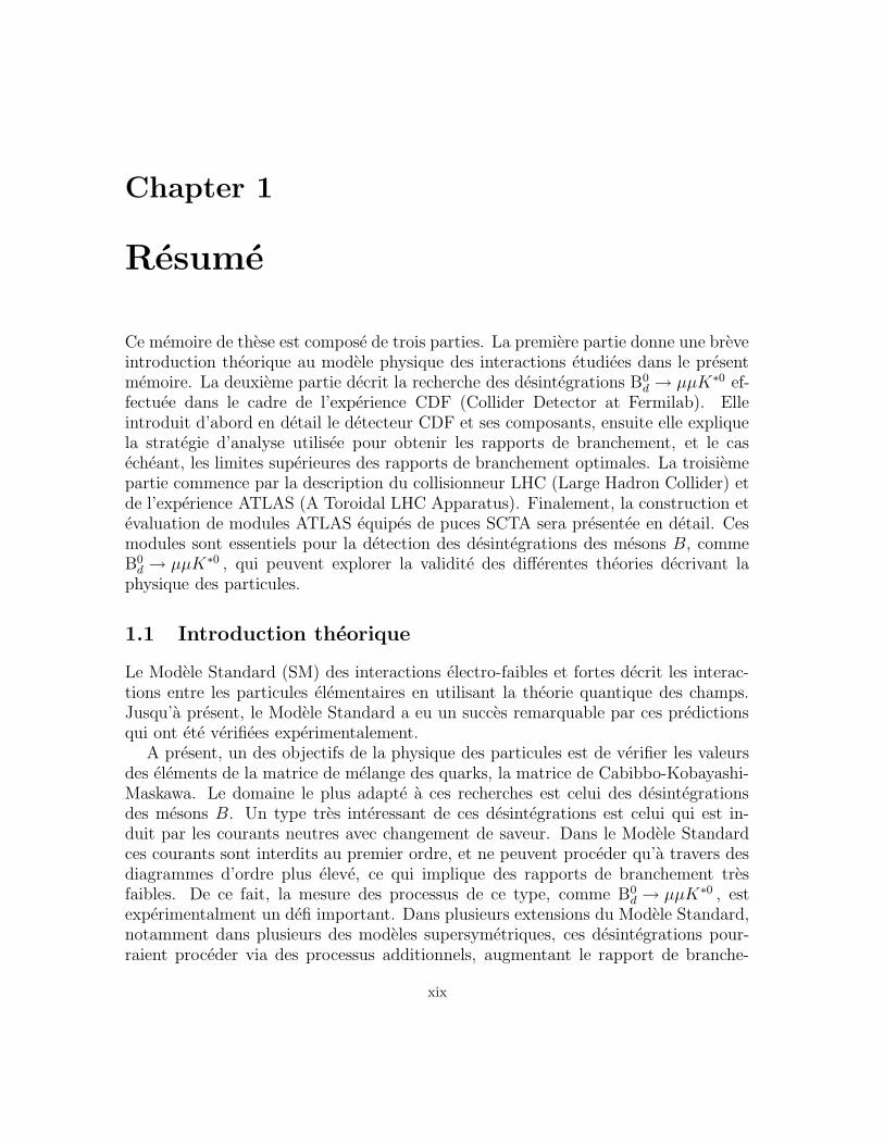
Ce memoire de these est compose de trois parties. La premiere partie donne une breveintroduction theorique au modele physique des interactions etudiees dans le presentmemoire. La deuxieme partie decrit la recherche des desintegrations B0
d → µµK∗0 ef-fectuee dans le cadre de l’experience CDF (Collider Detector at Fermilab). Elleintroduit d’abord en detail le detecteur CDF et ses composants, ensuite elle expliquela strategie d’analyse utilisee pour obtenir les rapports de branchement, et le casecheant, les limites superieures des rapports de branchement optimales. La troisiemepartie commence par la description du collisionneur LHC (Large Hadron Collider) etde l’experience ATLAS (A Toroidal LHC Apparatus). Finalement, la construction etevaluation de modules ATLAS equipes de puces SCTA sera presentee en detail. Cesmodules sont essentiels pour la detection des desintegrations des mesons B, commeB0d → µµK∗0 , qui peuvent explorer la validite des differentes theories decrivant la
physique des particules.
1.1 Introduction theorique
Le Modele Standard (SM) des interactions electro-faibles et fortes decrit les interac-tions entre les particules elementaires en utilisant la theorie quantique des champs.Jusqu’a present, le Modele Standard a eu un succes remarquable par ces predictionsqui ont ete verifiees experimentalement.
A present, un des objectifs de la physique des particules est de verifier les valeursdes elements de la matrice de melange des quarks, la matrice de Cabibbo-Kobayashi-Maskawa. Le domaine le plus adapte a ces recherches est celui des desintegrationsdes mesons B. Un type tres interessant de ces desintegrations est celui qui est in-duit par les courants neutres avec changement de saveur. Dans le Modele Standardces courants sont interdits au premier ordre, et ne peuvent proceder qu’a travers desdiagrammes d’ordre plus eleve, ce qui implique des rapports de branchement tresfaibles. De ce fait, la mesure des processus de ce type, comme B0
d → µµK∗0 , estexperimentalment un defi important. Dans plusieurs extensions du Modele Standard,notamment dans plusieurs des modeles supersymetriques, ces desintegrations pour-raient proceder via des processus additionnels, augmentant le rapport de branche-
xix
xx CHAPTER 1. RESUME
ment. La mesure d’un rapport de branchement different de celui predit par le ModeleStandard pourrait etre l’indication de nouveaux phenomenes physiques au-dela decelui-ci.
1.2 L’experience CDF au Tevatron
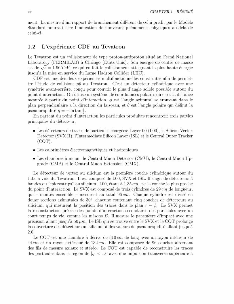
Le Tevatron est un collisionneur de type proton-antiproton situe au Fermi NationalLaboratory (FERMILAB) a Chicago (Etats-Unis). Son energie de centre de masseest de
√s = 1.96TeV , ce qui en fait le collisionneur atteignant la plus haute energie
jusqu’a la mise en service du Large Hadron Collider (LHC).CDF est une des deux experiences multifonctionnelles construites afin de permet-
tre l’etude de collisions pp au Tevatron. C’est un detecteur cylindrique avec unesymetrie avant-arriere, concu pour couvrir le plus d’angle solide possible autour dupoint d’interaction. On utilise un systeme de coordonnees polaires ou r est la distancemesuree a partir du point d’interaction, φ est l’angle azimutal se trouvant dans leplan perpendiculaire a la direction du faisceau, et θ est l’angle polaire qui definit lapseudorapidite η = − ln tan θ
2.
En partant du point d’interaction les particules produites rencontrent trois partiesprincipales du detecteur:
• Les detecteurs de traces de particules chargees: Layer 00 (L00), le Silicon VertexDetector (SVX II), l’Intermediate Silicon Layer (ISL) et le Central Outer Tracker(COT).
• Les calorimetres electromagnetiques et hadroniques.
• Les chambres a muon: le Central Muon Detector (CMU), le Central Muon Up-grade (CMP) et le Central Muon Extension (CMX).
Le detecteur de vertex au silicium est la premiere couche cylindrique autour dutube a vide du Tevatron. Il est compose de L00, SVX et ISL. Il s’agit de detecteurs abandes ou “microstrips” au silicium. L00, etant a 1.35 cm, est la couche la plus prochedu point d’interaction. Le SVX est compose de trois cylindres de 29 cm de longueur,qui – montes ensemble – mesurent au total 96 cm. Chaque cylindre est divise endouze sections azimutales de 30o, chacune contenant cinq couches de detecteurs ausilicium, qui mesurent la position des traces dans le plan r − φ. Le SVX permetla reconstruction precise des points d’interaction secondaires des particules avec uncourt temps de vie, comme les mesons B. Il mesure le parametre d’impact avec uneprecision allant jusqu’a 50µm. Le ISL qui se trouve entre le SVX et le COT prolongela couverture des detecteurs au silicium a des valeurs de pseudorapidite allant jusqu’a2.0.
Le COT est une chambre a derive de 310 cm de long avec un rayon interieur de44 cm et un rayon exterieur de 132 cm. Elle est composee de 96 couches alternantdes fils de mesure axiaux et stereo. Le COT est capable de reconstruire les tracesdes particules dans la region de |η| < 1.0 avec une impulsion transverse superieure a
1.3. LA RECHERCHE DE LA DESINTEGRATION B0D → µµK∗0 A CDF xxi
400MeV/c. Les detecteurs de traces se trouvent a l’interieur du champ magnetiquede 1.4T produit par un aimant solenoıdal place autour d’eux.
Les calorimetres electromagnetiques et hadroniques bases sur la technologie desscintillateurs mesurent le passage des particules avec |η| < 3.64. Les chambres amuons sont situees a l’exterieur des calorimetres electromagnetiques et hadroniques.Dans la region centrale (|η| < 0.6) le CMU est constitue de quatre couches dechambres a derive. Elles identifient les muons par le biais de leur fort pouvoir depenetration, en reconstruisant des segments de traces et les associant aux traces re-construites par le SVX et le COT. Derriere 60 cm d’acier additionnels se trouvent lesquatre plans de chambres a derive du CMP, qui permettent un taux de rejet de bruitde fond encore plus important que le CMU. La couverture des chambres a muons estcompletee par le CMX qui couvre la region 0.6 < |η| < 1.0. Les chambres a muonsincluent aussi des scintillateurs qui permettent de mesurer avec precision le tempsexact de passage de la particule.
Le systeme de declenchement est compose de trois niveaux consecutifs, chacundiminuant le nombre d’evenements d’un ou deux ordres de grandeur. Une partiespecialement interessante du deuxieme niveau du systeme de declenchement est le Sili-con Vertex Tracker, qui, pour la premiere fois pour un collisionneur, permet d’avoir descoupures sur les quantites comme le parametre d’impact, et cela avec une resolutionde 50µm. Ceci permet de selectionner des desintegrations B0
d → µµK∗0 avec uneefficacite accrue tout en rejetant la majeure partie du bruit de fond.
1.3 La recherche de la desintegration B0d → µµK∗0 a CDF
Pour la presente recherche, un echantillon de donnees collectees pendant la periodede Mars 2002-Aout 2003 correspondant a une luminosite integree de 215 pb−1, estutilise. Le rapport de branchement de la desintegration B0
d → µµK∗0 est mesure parrapport a celui de la desintegration B0
d → J/ψK∗0 . Ainsi, plusieurs facteurs difficilesa determiner – comme la luminosite, la section efficace de production du meson B0
d etcertaines efficacites de reconstruction et de selection – et leurs incertitudes peuventetre elimines. Le K∗0 est reconstruit a partir d’un kaon et d’un pion, alors que le J/ψest reconstruit a partir de deux muons pour avoir des etats finaux identiques pour lesdeux desintegrations.
Pour reconstruire les deux desintegrations B0d → µµK∗0 et B0
d → J/ψK∗0 , on com-mence par choisir des evenements qui ont ete selectionnes par un des declenchementsa dimuons1. Cela signifie que l’impulsion transverse des muons detectes par CMUdoit etre superieure a 1.5GeV , ceux detectes par CMX superieure a 2.0GeV et ceuxdetectes par CMP superieure a 3.0GeV . Pour chacun des muons, la difference entrele point de detection dans une des chambres a muons et l’extrapolation de la tracedepuis le systeme de trajectographie, doit etre inferieure a 30 cm, 50 cm et 25 cm pourCMU, CMX et CMP, respectivement. Une masse invariante des deux muons entre 0
1Ce sont d’ailleurs les declenchements du niveau 1 qui sont optimises pour l’acquisition des J/ψ, ce qui est tresprecieux pour le canal B0
d→ J/ψK∗0 .
xxii CHAPTER 1. RESUME
et 6GeV est requise.
La prochaine etape, consiste a reconstruire le kaon K∗0 a partir d’un kaon etd’un pion. Puisque CDF n’est pas tres performant pour l’identification des kaonset des pions pour la plage d’impulsions transverses pertinentes, pour chaque traceon envisage les deux hypotheses. L’impulsion transverse de chacune des traces doitetre superieure a 0.5GeV , la masse invariante de la paire kaon-pion doit etre dansune fourchette de ±100MeV autour de la masse de K∗0 publiee par le Particle DataGroup, et l’impulsion transverse du candidat K∗0 doit etre superieure a 2GeV . Cescoupures diminuent sensiblement le bruit de fond combinatoire du a l’identificationerronee kaon-pion.
La derniere etape est la reconstruction du meson B0d . Un fit cinematique de
moindres-carres des quatre traces est effectue ou les traces sont contraintes de provenird’un meme vertex, et la variable decrivant la qualite du fit devant etre inferieure a15. Ainsi les candidats dont les traces sont proches dans l’espace mais ne proviennentpas d’un meme vertex, seront elimines. L’impulsion transverse du candidat B0
d doitetre superieure a 6GeV .
Pour les candidats B0d → J/ψK∗0 , la masse invariante des deux muons doit etre a
moins de 200MeV de la masse du J/ψ, et la masse invariante du candidat doit etrea moins de 50MeV de la masse du B0
d. Pour les candidats B0d → µµK∗0 , la masse
invariante du candidat doit aussi etre a moins de 50MeV de la masse du B0d . Par
contre, on exclut les regions de ±200MeV autour de la resonance J/ψ, et ±100MeVautour de la resonance ψ(2S).
Apres les coupures de base, qui viennent d’etre decrites, une optimisation esteffectuee sur trois variables choisies pour diminuer le bruit de fond dans la mesure dupossible, tout en gardant une efficacite maximale pour le signal recherche. Les troisvariables choisies pour l’optimisation sont l’isolation, la longueur de desintegrationtransverse et l’angle d’ouverture.
Au cours de la fragmentation d’un quark b, le meson B resultant a tendance aemporter la majeure partie de l’impulsion du quark initial. Il en resulte qu’une grandefraction de l’impulsion mesuree dans un cone autour de meson B est portee par lesparticules issues de la desintegration du meson B. Cette fraction, definie comme
I =pB
T
pBT
+∑
pT, est appelee isolation. La somme est une somme scalaire incluant toutes
les traces (sauf celles des particules issues de la desintegration du B) qui se trouvent
a l’interieur du cone defini par ∆R =√
(∆η)2 + (∆φ)2 autour du vecteur d’impulsiondu candidat.
La deuxieme variable d’optimisation est liee au fait que les mesons B ont un tempsde vie relativement long compare au celui de la majeure partie du bruit de fond.Ainsi, la longueur de desintegration propre permet d’eliminer une grande portion dece bruit de fond. Pour la determination de cette quantite il est tres important dereconstruire la position de la desintegration du meson, appelee vertex secondaire,avec une grande precision. Pour obtenir cette precision on requiert que le passage desparticules soit enregistre dans au moins 20 (16) couches axiaux (stereo) du COT, et 3couches du SVX. Pour les pions et kaons de basse impulsion transverse cette exigence
1.3. LA RECHERCHE DE LA DESINTEGRATION B0D → µµK∗0 A CDF xxiii
est encore plus stricte, car on demande que le passage de la particule soit enregistredans au moins 4 des couches du detecteur au silicium. La longueur de desintegration
transverse est definie comme Lxy = ~lxy · ~pBT /pBT , ou ~lxy est le vecteur qui pointe duvertex primaire2 au vertex secondaire, ~pBT est le vecteur de l’impulsion transverse duB reconstruit et pBT est sa valeur absolue. Pour s’assurer qu’on choisit des tracesreconstruites avec une bonne precision, l’incertitude sur la longueur de desintegrationtransverse doit etre inferieure a 150µm. Pour eliminer des evenements representantdes pathologies, Lxy doit etre inferieur a 1 cm, et la longueur de desintegration propredoit etre inferieure a 0.5 cm.
Une autre quantite, qui constitue un fort critere de rejet de bruit de fond, est l’angled’ouverture (∆Φ) entre le vecteur d’impulsion du B reconstruit (~pBT ) et la direction
de sa trace ( ~lxy). Il est clair que les deux muons, le kaon et le pion provenant dumeme meson B, les deux vecteurs doivent etre paralleles.
La procedure d’optimisation est executee en evaluant trois differentes “Figure ofMerit” (FOM) pour les differentes valeurs de coupure pour ces trois variables. LesFOM determinent le choix optimal des coupures pour rejeter le plus de bruit de fondpossible tout en gardant la plus grande partie du signal. Pour evaluer ces FOM ondoit estimer le bruit de fond et le nombre de desintegrations B0
d → µµK∗0 .
Le bruit de fond attendu est estime en extrapolant le nombre d’evenements ob-serves dans les regions laterales, de masse invariante du candidat B entre 4.379GeV/c2
et 5.179GeV/c2 et entre 5.379GeV/c2 et 6.279GeV/c2. Comme apres les coupures debase et les coupures d’optimisation le nombre de candidats commence a devenir rela-tivement bas, pour augmenter la statistique une etude a ete faite pour comprendre lesdependences entre les variables d’optimisation. Il en a ete deduit, que l’isolation a eteindependante de l’angle d’ouverture et de la longueur de desintegration transverse.Ainsi, le pouvoir de rejet de bruit de fond des coupures sur l’isolation a ete etudieindependamment de celui des deux autres, ce qui a permis d’utiliser des echantillonsplus grandes pour les deux etudes.
Pour estimer le nombre de desintegrations B0d → µµK∗0 attendues, on utilise le
fait que ce nombre est lie au nombre de desintegrations B0d → J/ψK∗0 . Il suffit de
multiplier ce dernier par le rapport de leurs efficacites de coupures de base respec-tifs – qu’on extrait en utilisant des simulations Monte Carlo –, par des correctionstheoriques et par le rapport des deux rapports de branchement pour obtenir le nom-bre attendu de desintegrations B0
d → µµK∗0 . Pour calculer le nombre de candidatsB0d → J/ψK∗0 on effectue un fit de la distribution de la masse invariante des candidats
B0d avec une fonction Gaussienne combinee avec une fonction lineaire (Figure 1.1).
La fonction lineaire tient compte du bruit de fond, alors que la fonction Gaussiennedecrit le signal qu’on obtient en l’integrant entre 5.229GeV/c2 et 5.329GeV/c2.
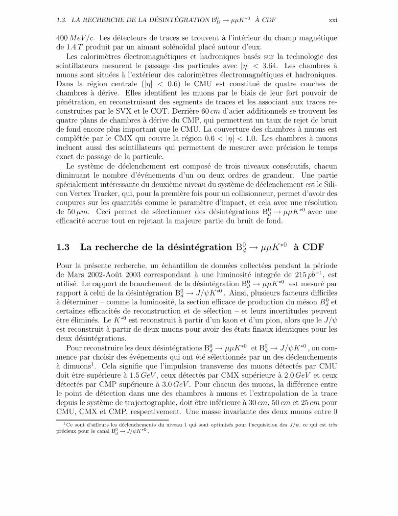
Une fois que toutes les quantites necessaires pour l’optimisation sont definies, oncalcule les FOM pour la combinaison de 10 differentes coupures sur la longueur dedesintegration transverse, de 10 differentes coupures sur l’angle d’ouverture et de 10differentes coupures sur l’isolation. L’optimisation a determine que les coupures les
2Le vertex d’interaction pp.
xxiv CHAPTER 1. RESUME
)[GeV]*0KµµM(5 5.05 5.1 5.15 5.2 5.25 5.3 5.35 5.4 5.45 5.5
can
did
ates
/5M
eV
0
5
10
15
20
25 18.0±N(Bd)=179.1 0.002±Mean: 5.278
2.1±=25.1 σ
>0.9xy candidates after the final cuts, iso>0.65, delphi<0.024, L*0KΨJ/
)[GeV]*0KµµM(4.7 4.8 4.9 5 5.1 5.2 5.3 5.4 5.5 5.6 5.7
can
did
ates
/10M
eV
0
0.5
1
1.5
2
2.5
3
3.5
candidates (grey) after final selection*0Kµµ
Figure 1.1: Distribution des candidats B pour la desintegration B0d → J/ψK∗0 (gauche) et
B0d → µµK∗0 (droite), Lxy > 0.09 cm, ∆Φ < 0.024 rad et Isolation > 0.65. Les deux evenements
B0d → µµK∗0 qui sont dans la fenetre de masse autour de la masse nominale du B0
d sont affiches engris.
plus efficaces sont 900µm pour la valeur minimale de la longueur de desintegrationtransverse, 0.024 rad pour la valeur maximale de l’angle d’ouverture et 0.65 pour lavaleur minimale de l’isolation. Les distributions des masses invariantes des candidatsB0d → J/ψK∗0 et B0
d → µµK∗0 satisfaisant a toutes ces coupures sont montrees surla Figure 1.1. 179 ± 18 candidats B0
d → J/ψK∗0 sont observes dans la region dusignal. Il y a deux candidats observes dans la region du signal pour la desintegrationB0d → µµK∗0 , alors que 1.001 evenement de bruit de fond est attendu. La methode
de Feldman et Cousins, basee sur des distributions de Poisson et sur l’approche de lastatistique frequentiste, donne les intervalles de confiance suivantes sur le rapport debranchement de la desintegration B0
d → µµK∗0 :
[0.84, 19.57]× 10−7 CI = 68.75% (1.1)
[0.0, 29.56] × 10−7 CI = 90% (1.2)
[0.0, 34.44] × 10−7 CI = 95% (1.3)
Cela implique une observation pour un intervalle de confiance a 68.75%, et deslimites superieures pour des intervalles de confiance a 90% et 95%. L’incertitudesur les limites des intervalles a ete estimee en changeant l’estimation du bruit defond par une deviation standard, ce qui donne les erreurs suivantes pour les limitesdes intervalles: 0.84+0.79
−0.73, 19.57 ± 2.52, 29.56 ± 3.67 et 34.44 ± 4.24. L’experienceCDF continuera a acquerir des donnees jusqu’en 2009, et devrait avoir au total 40-80evenements B0
d → µµK∗0 pour cette date, ce qui permettrait l’observation de cettedesintegration pour les intervalles de confiance a 90% et 95%.
1.4. L’EXPERIENCE ATLAS AU LHC xxv
1.4 L’experience ATLAS au LHC
Le projet LHC est un collisionneur pp qui est en cours de construction au CentreEuropeen de Recherche Nucleaire (CERN). Il represente la prochaine etape dansl’evolution des accelerateurs a hautes energies, ayant une energie du centre de massede
√s = 14TeV .
Quatre experiences seront installees autour des quatre points d’interaction du LHC,l’une d’entre elles etant ATLAS (A Toroidal LHC Apparatus). ATLAS, qui est undetecteur plurifonctionnel, a beaucoup de similitudes dans sa construction avec CDF.En partant de l’interieur vers l’exterieur on trouve les composants suivants:
• Les detecteurs de traces de particules chargees (Inner Tracker): les detecteursau silicium a pixels (Pixels), le Semiconductor Tracker (SCT) et le TransitionRadiation Tracker (TRT).
• Les calorimetres electromagnetiques et hadroniques.
• Les chambres a muons.
Le choix des technologies pour les trois parties du traceur des particules chargeesest motive par le compromis entre la precision de la mesure et le nombre de canauxde lecture. Pres du point d’interaction on trouve des detecteurs qui fournissent re-lativement peu de points, mais avec une grande precision (Pixels et SCT). Plus loin,on trouve un detecteur qui fournit beaucoup de points de mesure, mais avec moins deprecision (TRT). La partie interieure du Inner Tracker est constituee de detecteursau silicium a pixels, arranges en trois cylindres a des rayons de 5.05 cm, 8.85 cm et12.25 cm, et de trois disques de chaque cote du detecteur central. Ces detecteurs four-nissent une precision de 50µm dans le plan r−φ et de 400µm le long de la directiondu faisceau. De 30 cm a 52 cm du tube a vide contenant le faisceau se trouvent lesquatre couches du SCT, ainsi que neuf disques de chaque cote du detecteur central.La partie cylindrique (“avant-arriere”) du SCT est constitue de 2112 (1976) modulesau silicium qui contiennent aussi l’electronique necessaire pour la lecture de bandesde silicium. Les modules de la partie cylindrique mesurent le passage d’une particuleavec une precision de 17µm dans le plan r−φ et 500µm le long de la direction du fais-ceau. L’element exterieur du systeme de traceurs d’ATLAS est le TRT, une chambrea fils. La partie centrale contient 50000 fils, et les 36 disques des regions “avant-arriere” en contiennent 320000. Par rapport aux detecteurs au silicium la resolutionest moindre (170µm), mais cela est equilibre par le nombre important de points demesure, typiquement 36 par trace. Le TRT permet la reconnaissance des electronsgrace a leur radiation de transition caracteristique (d’ou le nom du detecteur). Entreles traceurs de particules et les calorimetres se trouve le solenoıde supraconducteurqui cree un champ magnetique de 2T dans le volume des traceurs.
Les calorimetres, qui couvrent la region de |η| < 3.2, sont bases sur la technologied’argon liquide et des tuiles de scintillateurs plastiques. Les calorimetres sont entourespar les chambres a muons qui occupent l’espace jusqu’a un rayon de 11m et jusqu’a±23m dans la direction du faisceau. Differentes technologies sont utilisees pour les
xxvi CHAPTER 1. RESUME
chambres a muons remplissant differentes taches. Des “Monitored Drift Tubes” et des“Cathode Strip Chambers” sont utilises pour les mesures de precision, alors que pourles declenchements des “Resistive Plate Chambers” et des “Thin Gap Chambers”sont prevus. ATLAS prevoit un systeme de declenchement a trois niveaux, similairea celui de CDF.
1.5 Construction et evaluation de modules ATLAS equipes
de puces SCTA128
Un des composants cruciaux pour la physique du meson B est le SCT, car il contribuede maniere tres significative a la reconstruction precise des points d’interaction sec-ondaires. Il est essentiel d’effectuer des analyses etendues des modules du SCT afinde s’assurer que leurs performances soient conformes aux attentes.
Dans la presente these deux types de modules sont etudies:
• Des modules equipes de puces ABCD pour une lecture digitale du detecteur.La conception digitale permet une solution plus compacte et reduit la quan-tite de donnees a transmettre. Par contre, elle est sensible aux interferenceselectromagnetiques.
• Des modules equipes de puces SCTA pour une lecture analogique du detecteur.C’est la solution qui a ete utilisee jusqu’a maintenant dans la plupart des detecte-urs au silicium. Elle permet le traitement individuel des canaux et permet decontroler et d’eliminer facilement le bruit cause par des interferences electromag-netiques provenant des sources exterieures. Le prix a payer, c’est le large volumede donnees a transmettre vers le systeme d’acquisition de donnees.
Differents modules equipes avec des puces de lecture ABCD ont ete evalues tant auniveau des performances electriques, qu’au niveau de la resistance face aux radiations.Les memes tests pour des modules equipes avec des puces de lecture SCTA serontaussi presentes. De plus, les resultats de tests effectues en faisceau et avec des lignesde transmission optiques seront aussi decrits.
Plusieurs modules avec des puces ABCD satisfaisant les criteres de ATLAS SCTont ete construits. Leurs performances electriques ont ete mesurees en utilisant desequipements dedies, installes au laboratoire. Le gain des puces a ete conforme auxvaleurs prevues avec une dispersion de 5%, le bruit a ete de 430 e− pour les canaux quin’etaient pas connectes a des bandes de silicium, 770 e− pour les canaux qui etaientconnectes a des bandes de silicium de 6 cm et 1400 e− pour les canaux qui etaientconnectes a des bandes de silicium de 12 cm. Ce chiffre est inferieur a la valeur de1500 e−, necessaire pour avoir un rapport signal/bruit superieur a 15, qui assure unebonne efficacite de reconstruction de traces tout en gardant un taux d’occupation enbruit suffisamment bas.
La puce SCTA a ete developpee comme solution supplementaire pour la lecture desdetecteurs au silicium du Inner Tracker. La puce contient 128 canaux avec des amplifi-cateurs, suivis d’une memoire analogique pour 128 evenements et d’un multiplexeur
1.5. CONSTRUCTION ET EVALUATION DE MODULES ATLAS EQUIPES DE SCTA128xxvii
Figure 1.2: Resolution quand deux bandes de silicium sont touchees (en haut) et quand une seulebande de silicium est touchee (en bas).
analogique pour transmettre les donnees vers le systeme d’acquisition de donnees. Lacaracterisation des proprietes analogiques de la puce SCTA est non seulement im-portante pour le projet SCTA, mais aussi pour la version digitale, ABCD. En effet,le traitement initial des signaux est identique pour SCTA et ABCD, mais dans laseconde tous les effets presents avant le discriminateur sont masques par le fait quele signal est binaire.
La premiere etape de la caracterisation des puces s’est effectuee immediatementapres leur fabrication. Ensuite, les caracteristiques – comme le gain et les differentscomposants du bruit – ont ete recontrolees au laboratoire immediatement apres ledecoupage. Les puces ont aussi ete irradiees pour controler leur conformite avec lesexigences posees par l’environnement du LHC. Les puces jugees adequates ont eteensuite montees sur des modules correspondants aux normes d’ATLAS.
Apres leur construction les modules analogiques ont ete evalues en utilisant uneinstallation dediee au laboratoire. Le gain des puces etait conforme aux specifications,et le bruit a ete de 1700 e− pour les bandes de detecteur de 12 cm, et 1100 e− pourles bandes de detecteur de 6 cm, ce qui montre l’influence de la capacite representeepar les bandes de silicium. La linearite des puces SCTA a ete verifiee en utilisant dessources radioactives de Terbium, Americium et Cobalt.
Une etape tres importante pour l’evaluation des modules analogiques est de verifierleur comportement dans des conditions les plus proches possibles de celles rencontreesdans LHC, i.e dans un faisceau test. Les resultats de ces experiences montrent que
xxviii CHAPTER 1. RESUME
Figure 1.3: Spectre de 241Am pour les lignes de transmission en cuivre et pour les lignes de trans-mission optiques.
la resolution des modules en cas de trajectoires perpendiculaires aux modules pourles cas quand une seule bande de silicium enregistre le passage de la particule estde 21µm, alors qu’elle est de 3µm quand deux bandes adjacentes enregistrent lepassage de la particule (Figure 1.2). Le comportement des modules analogiques pourdes trajectoires inclinees a ete satisfaisant. Cela a ete aussi le cas pour le tauxd’occupation en bruit qui est de l’ordre de 10−4 pour des efficacites proches de 99%.
Les modules analogiques ont aussi ete utilises pour caracteriser la ligne de transmis-sion optique developpe pour la transmission des signaux analogiques. Les experiencesont montre que la ligne contribue de maniere negligeable aux bruits deja existants dela lecture electronique des modules. Des mesures effectuees avec des sources radioac-tives ont aussi montre que les spectres des rayons γ de ces sources sont transmis sansmodification apparente (Figure 1.3), ce qui prouve le bon fonctionnement de la lignede transmission optique.

Part I
Theoretical Motivation
1


Chapter 2
The Standard Model and beyond
2.1 The Standard Model
The experimental and theoretical developments of the last 50 years have led to thedevelopment of the Standard Model (SM) of strong and electroweak interactions.Since it is described in great detail in many textbooks (for example [1] and [2]), thediscussion given here will be brief.
The most important concept of the modern fundamental physics is that of sym-metry. Noether’s theorem states that to every symmetry corresponds a conservedquantity. For example, invariance under translations, time displacements, rotationsand Lorentz transformations lead to the conservation of momentum, angular momen-tum, and energy. Other symmetries include the parity, that is, the mirror imageof any physical process also represents a perfectly possible physical process; chargeconjugation which changes a particle to its antiparticle1. Apart from the discretesymmetries, like the ones just mentioned, there are also local gauge symmetries: thephase variation permitted by a local symmetry conserves the invariance of the la-grangian if there is a compensating field which is considered to be the mediator ofinteractions between particles. The Standard Model describes the fundamental par-ticles and their interactions via the electroweak and the strong force. The force ofgravity is negligibly small at the particle level and is not yet described by the SM.
The SM has three types of particles:
• fermions which are the elementary particles and have spin 12
• bosons which are the interaction fields between fermions and have spin 1
• the Higgs-boson which is a consequence of the spontaneous symmetry breakingof the electroweak sector, and has spin 0. The Higgs boson is yet to be discoveredexperimentally
The main properties of the fermions are summarized in Table 2.1.1It changes all the ‘internal’ quantum numbers – charge, baryon number, lepton number, strangness, beauty –
while leaving mass, energy, momentum and spin untouched.
3
4 CHAPTER 2. THE STANDARD MODEL AND BEYOND
Quarks d u s c b t
Mass (GeV/c2) 0.008 0.004 0.15 1.4 4.5 174
Charge -1/3 +2/3 -1/3 +2/3 -1/3 +2/3
Leptons e νe µ νµ τ ντ
Mass (GeV/c2) 0.0005 0 0.105 0 1.8 0
Charge -1 0 -1 0 -1 0
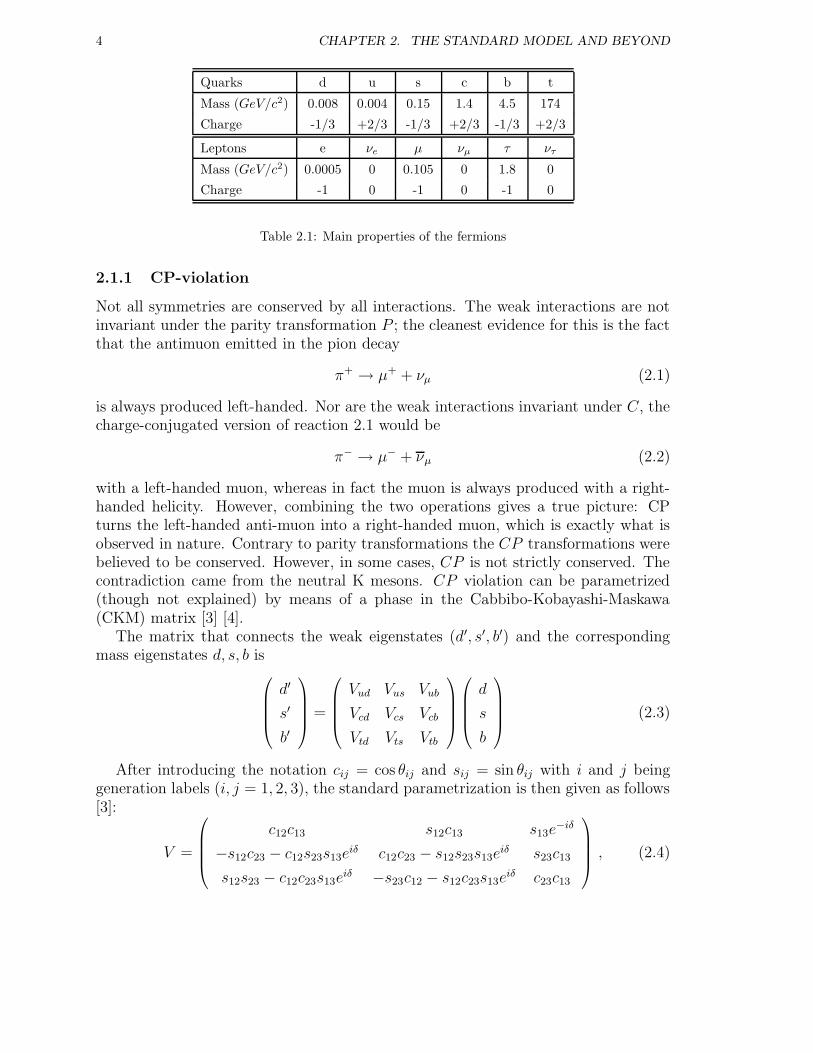
Table 2.1: Main properties of the fermions
2.1.1 CP-violation
Not all symmetries are conserved by all interactions. The weak interactions are notinvariant under the parity transformation P ; the cleanest evidence for this is the factthat the antimuon emitted in the pion decay
π+ → µ+ + νµ (2.1)
is always produced left-handed. Nor are the weak interactions invariant under C, thecharge-conjugated version of reaction 2.1 would be
π− → µ− + νµ (2.2)
with a left-handed muon, whereas in fact the muon is always produced with a right-handed helicity. However, combining the two operations gives a true picture: CPturns the left-handed anti-muon into a right-handed muon, which is exactly what isobserved in nature. Contrary to parity transformations the CP transformations werebelieved to be conserved. However, in some cases, CP is not strictly conserved. Thecontradiction came from the neutral K mesons. CP violation can be parametrized(though not explained) by means of a phase in the Cabbibo-Kobayashi-Maskawa(CKM) matrix [3] [4].
The matrix that connects the weak eigenstates (d′, s′, b′) and the correspondingmass eigenstates d, s, b is
d′
s′
b′
=
Vud Vus Vub
Vcd Vcs Vcb
Vtd Vts Vtb
d
s
b
(2.3)
After introducing the notation cij = cos θij and sij = sin θij with i and j beinggeneration labels (i, j = 1, 2, 3), the standard parametrization is then given as follows[3]:
V =
c12c13 s12c13 s13e−iδ
−s12c23 − c12s23s13eiδ c12c23 − s12s23s13e
iδ s23c13
s12s23 − c12c23s13eiδ −s23c12 − s12c23s13e
iδ c23c13
, (2.4)
2.1. THE STANDARD MODEL 5
where δ is the phase necessary for CP violation. cij and sij can all be chosen to bepositive and δ may vary in the range 0 ≤ δ ≤ 2π. However, the measurements of CPviolation in K decays force δ to be in the range 0 < δ < π.
Extensive phenomenology of the last years has shown that s13 and s23 are smallnumbers: O(10−3) and O(10−2), respectively. Consequently to an excellent accuracyc13 = c23 = 1 and the four independent parameters are given as
s12 = |Vus|, s13 = |Vub|, s23 = |Vcb|, δ (2.5)
with the phase δ extracted from CP violating transitions or loop processes sensitiveto |Vtd|. The latter fact is based on the observation that for 0 ≤ δ ≤ π, as required bythe analysis of CP violation in the K system, there is a one–to–one correspondencebetween δ and |Vtd|.
For numerical evaluations the use of the standard parametrization is strongly re-commended. However, once the four parameters in (2.5) have been determined it isoften useful to make a change of basic parameters in order to see the structure of theresult more transparently. This brings us to the Wolfenstein parametrization.
The original Wolfenstein parametrization is an approximate parametrization ofthe CKM matrix in which each element is expanded as a power series in the smallparameter λ = |Vus| = 0.22,
V =
1 − λ2
2λ Aλ3(%− iη)
−λ 1 − λ2
2Aλ2
Aλ3(1 − %− iη) −Aλ2 1
+ O(λ4) , (2.6)
and the set (2.5) is replaced by
λ, A, %, η . (2.7)
Looking back at (2.4) and imposing the following relations
s12 = λ , s23 = Aλ2 , s13e−iδ = Aλ3(%− iη) (2.8)
to all orders in λ. It follows then that
% =s13
s12s23cos δ, η =
s13
s12s23sin δ. (2.9)
(2.8) and (2.9) represent simply the change of variables from (2.5) to (2.7). Makingthis change of variables in the standard parametrization (2.4) it follows that the CKMmatrix as a function of (λ,A, %, η) satisfies unitarity exactly. Another property is thatin view of c13 = 1 −O(λ6) the relations between sij and |Vij| in (2.5) are satisfied tohigh accuracy.
In order to improve the accuracy of the unitarity triangle discussed below theO(λ5) correction to Vtd is also included. In summary then Vus, Vcb, Vub, Vtd and Vtsare given to an excellent approximation as follows:
Vus = λ, Vcb = Aλ2 (2.10)
6 CHAPTER 2. THE STANDARD MODEL AND BEYOND
Vub = Aλ3(%− iη), Vtd = Aλ3(1 − %− iη) (2.11)
Vts = −Aλ2 +1
2A(1 − 2%)λ4 − iηAλ4 (2.12)
with
% = %(1 − λ2
2), η = η(1 − λ2
2). (2.13)
The advantage of this generalization of the Wolfenstein parametrization over othergeneralizations found in the literature is the absence of relevant corrections to Vus,Vcb and Vub and an elegant change in Vtd which allows a simple generalization of theunitarity triangle.
The Wolfenstein parameterization has several nice features. In particular, it offersin conjunction with the unitarity triangle a very transparent geometrical representa-tion of the structure of the CKM matrix and allows the derivation of several analyticresults. This turns out to be very useful in the phenomenology of rare decays and ofCP violation.
2.1.2 The unitarity triangle
The unitarity V V + = 1 of the CKM-matrix implies orthogonality of the differentrows and columns. The orthogonality relations can be represented as six “unitarity”triangles in the complex plane. Analyzing the shape of the six unitarity trianglesby using the original Wolfenstein parametrization, it turns out that most of thesetriangles are very squashed ones.
Only in two of the unitarity triangles are all three sides of comparable magnitude(O(λ3)), while in the others one side is suppressed relative to the remaining onesby O(λ4) and O(λ2). For the two triangles with comparable sides the sides agreeat the O(λ3) level and differ only through O(λ5) corrections. Neglecting the lattersubleading contributions they describe the unitarity triangle that appears usually inthe literature:
VudV∗
ub + VcdV∗
cb + VtdV∗
tb = 0. (2.14)
Phenomenologically this triangle is very interesting as it involves simultaneously theelements Vub, Vcb and Vtd.
In most analyses of the unitarity triangle present in the literature only terms O(λ3)are kept in (2.14). It is, however, straightforward to include the next-to-leading O(λ5)terms.
VcdV∗
cb = −Aλ3 + O(λ7). (2.15)
Thus to an excellent accuracy VcdV∗
cb is real with |VcdV ∗
cb| = Aλ3. Keeping O(λ5)corrections and rescaling all terms in (2.14) by Aλ3
1
Aλ3VudV
∗
ub = % + iη,1
Aλ3VtdV
∗
tb = 1 − (% + iη) (2.16)

2.1. THE STANDARD MODEL 7
with % and η defined in (2.13). Thus (2.14) can be represented as the unitarity trianglein the complex (%, η) plane. This is shown in Figure 2.1. The length of the side CBwhich lies on the real axis equals unity when eq. (2.14) is rescaled by VcdV
∗
cb. Beyondthe leading order in λ the point A does not correspond to (%, η) but to (%, η). Clearlywithin 3% accuracy % = % and η = η. Yet in the distant future the accuracy ofexperimental results and theoretical calculations may improve considerably so thatthe more accurate formulation will be appropriate.
ρ+iη 1−ρ−iη
βγ
α
C=(0,0) B=(1,0)
A=(ρ,η)
Figure 2.1: Unitarity Triangle.
For numerical calculations the following procedure for the construction of the uni-tarity triangle is recommended:
• Use the standard parametrization in phenomenological applications to find s12,s13, s23 and δ.
• Translate to the set (λ, A, %, η) using (2.8) and (2.9).
• Calculate % and η using (2.13).
Using simple trigonometry sin(2φi), φi = α, β, γ, can be expressed in terms of(%, η) as follows:
sin(2α) =2η(η2 + %2 − %)
(%2 + η2)((1 − %)2 + η2)(2.17)
sin(2β) =2η(1 − %)
(1 − %)2 + η2(2.18)
sin(2γ) =2%η
%2 + η2=
2%η
%2 + η2. (2.19)
The lengths CA and BA in the rescaled triangle of Figure 2.1, denoted by Rb andRt, respectively, are given by
Rb ≡|VudV ∗
ub||VcdV ∗
cb|=√
%2 + η2 = (1 − λ2
2)1
λ
∣∣∣∣
VubVcb
∣∣∣∣ (2.20)
8 CHAPTER 2. THE STANDARD MODEL AND BEYOND
Rt ≡|VtdV ∗
tb||VcdV ∗
cb|=√
(1 − %)2 + η2 =1
λ
∣∣∣∣
VtdVcb
∣∣∣∣ . (2.21)
The expressions for Rb and Rt given here in terms of (%, η) are excellent approxi-mations. Clearly Rb and Rt can also be determined by measuring two of the anglesφi:
Rb =sin(β)
sin(α)=
sin(α + γ)
sin(α)=
sin(β)
sin(γ + β)(2.22)
Rt =sin(γ)
sin(α)=
sin(α + β)
sin(α)=
sin(γ)
sin(γ + β). (2.23)
The angles β and γ of the unitarity triangle are related directly to the complexphases of the CKM-elements Vtd and Vub, respectively, through
Vtd = |Vtd|e−iβ, Vub = |Vub|e−iγ. (2.24)
The angle α can be obtained through the relation
α + β + γ = 180◦ (2.25)
expressing the unitarity of the CKM-matrix.The triangle depicted on Figure 2.1 together with |Vus| and |Vcb| gives a full des-
cription of the CKM matrix. Looking at the expressions for Rb and Rt, it is clear thatwithin the Standard Model the measurements of four CP conserving decays sensitiveto |Vus|, |Vub|, |Vcb| and |Vtd| can tell whether CP violation (η 6= 0) is predicted in theStandard Model. This is a very remarkable property of the Kobayashi-Maskawa pic-ture of CP violation: quark mixing and CP violation are closely related to each other.In the context of the SM, the potential interest in rare B-decays is that they wouldprovide a quantitative determination of the quark-flavor rotation matrix, in particu-lar the matrix elements Vtd, Vtb and Vts, the first one being extremely important, astogether with Vub it carries the CP-violating phase [5] [6].
There is, of course, the very important question whether the CKM picture ofCP violation is correct and more generally whether the Standard Model offers acorrect description of weak decays of hadrons. In order to answer these importantquestions it is essential to calculate as many branching ratios as possible, measurethem experimentally and check whether they all can be described by the same set ofthe parameters (λ,A, %, η). In the language of the unitarity triangle this means thatthe various curves in the (%, η) plane extracted from different decays should cross eachother at a single point. Moreover the angles (α, β, γ) in the resulting triangle shouldagree with those extracted in the future from CP-asymmetries in B-decays.
2.1.3 Recent results on the CKM Unitarity Triangle
With the successful turn-on of the BaBar and Belle experiments in the last few years,many experimental measurements in the b sector have achieved impressive precision.The Fermilab Tevatron, with the upgraded CDF and D0 detectors has also started to

2.1. THE STANDARD MODEL 9
produce measurements which are complimentary to those of BaBar and Belle, as theyoffer the opportunity to measure the heavier B hadrons which are not accessible atthe Υ(4S) resonance. The primary mission of the B-factory experiments is to searchfor the breaking of the CP -symmetry in B meson decays and examine the consistencyof the measurements with the expected values within the CKM mechanism.
The measurement of sin 2β, the CP -violating asymmetry in B0 decays to charmo-nium final states (b→ ccs), by the CDF, BaBar and Belle collaborations establishedthe breaking of CP -symmetry in B decays [7] [8] [9]. The way to measure the largeCP -asymmetries in the decays of neutral B mesons to CP eigenstates is to study theΥ(4S) → B0B0 → fCPftag decay chain, where one of the B mesons decays at timetCP to a final state fCP and the other decays at time ttag to a final state ftag thatdistinguishes between B0 and B0. The decay rate has a time dependence given by[10] [11]
e−
|∆t|τB0
4τB0
{1 + q · [S sin (∆md∆t) + A cos (∆md∆t)]} (2.26)
where τB0 is the B0 lifetime, ∆md is the mass difference between the two B0 masseigenstates, ∆t = tCP − ttag, q = +1(−1) is the b flavor charge when the taggingB meson is a B0 (B0), and S and A are the CP -violation parameters. To a goodapproximation the SM predicts
S = −ξf sin 2β (2.27)
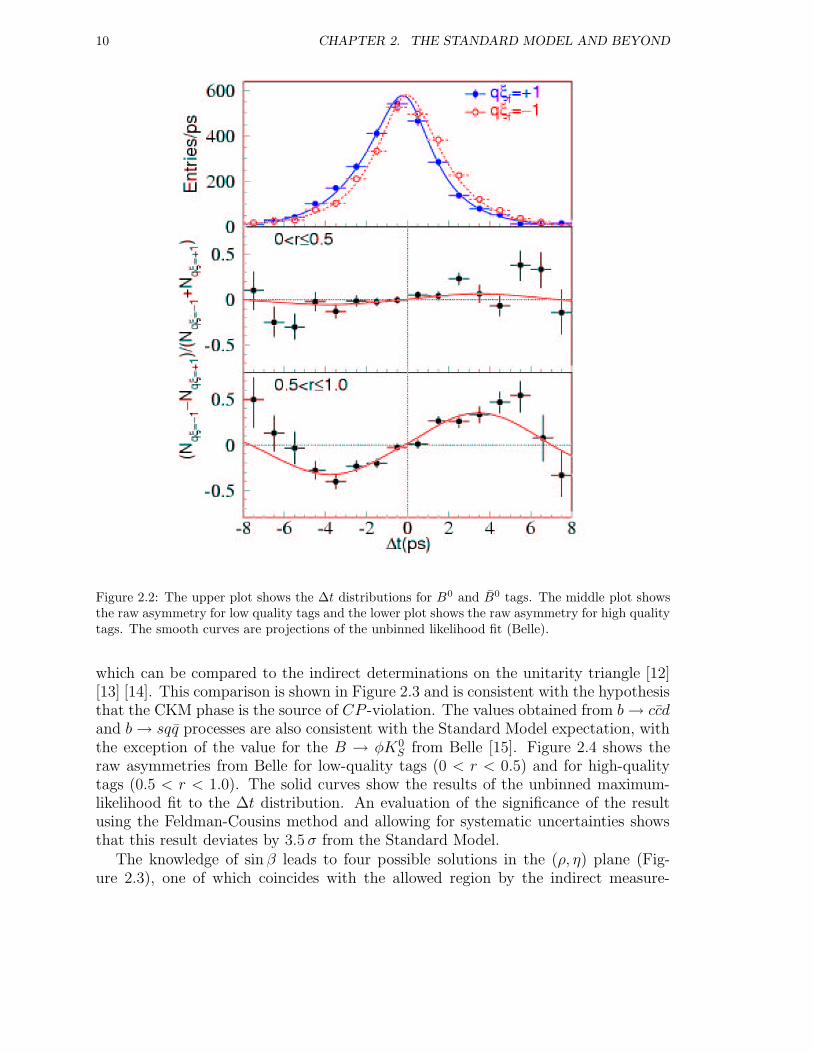
where ξf = +1(−1) corresponds to CP -even (CP -odd) final states. Direct CP -violation, A= 0 is expected for both b → ccs and b → sss transitions. BaBar andBelle reconstruct B0 decays to the following b → ccs eigenstates: J/ψKS, ψ(2S)KS,χc1KS for ξf = −1 and J/ψKL for ξf = +1. The two classes should have CP -asymmetries of opposite sign. Both experiments also use B0 → J/ψK∗0 decays withK∗0 → KSπ
0, where the final state is a mixture of even and odd CP with the CP -odd fraction relatively small ((19 ± 4)% for Belle and (16 ± 3.5)% for BaBar). Thesamples of CP -eigenstates are large and clean [10]. Figure 2.2 shows the new Belledata. The ∆t distributions show a clear shift between B0 and B0 tags. For low-quality tags (0 < r < 0.5) only a modest asymmetry is visible, while for high-qualitytags (0.5 < r < 1.0) a very clear asymmetry with a sinusoidal time modulation ispresent. The final results are extracted from an unbinned maximum likelihood fit tothe ∆t distributions that takes into account resolution, mistagging and backgrounddilution. The new Belle result with 140 fb−1 is
sin 2β = 0.733 ± 0.057 ± 0.028 (2.28)
while the same analysis from BaBar (78 fb−1) yields
sin 2β = 0.741 ± 0.067 ± 0.03 (2.29)
From these results a new world average can be calculated
sin 2β = 0.736 ± 0.049 (2.30)
10 CHAPTER 2. THE STANDARD MODEL AND BEYOND
Figure 2.2: The upper plot shows the ∆t distributions for B0 and B0 tags. The middle plot showsthe raw asymmetry for low quality tags and the lower plot shows the raw asymmetry for high qualitytags. The smooth curves are projections of the unbinned likelihood fit (Belle).
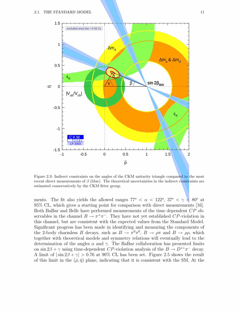
which can be compared to the indirect determinations on the unitarity triangle [12][13] [14]. This comparison is shown in Figure 2.3 and is consistent with the hypothesisthat the CKM phase is the source of CP -violation. The values obtained from b→ ccdand b→ sqq processes are also consistent with the Standard Model expectation, withthe exception of the value for the B → φK0
S from Belle [15]. Figure 2.4 shows theraw asymmetries from Belle for low-quality tags (0 < r < 0.5) and for high-qualitytags (0.5 < r < 1.0). The solid curves show the results of the unbinned maximum-likelihood fit to the ∆t distribution. An evaluation of the significance of the resultusing the Feldman-Cousins method and allowing for systematic uncertainties showsthat this result deviates by 3.5 σ from the Standard Model.
The knowledge of sin β leads to four possible solutions in the (ρ, η) plane (Fig-ure 2.3), one of which coincides with the allowed region by the indirect measure-
2.1. THE STANDARD MODEL 11
-1.5
-1
-0.5
0
0.5
1
1.5
-1 -0.5 0 0.5 1 1.5 2
sin 2βWA
∆md
∆ms & ∆md
εK
εK
|Vub/Vcb|
sin 2βWAγ βα
ρ
η
excluded area has < 0.05 CL
C K Mf i t t e r
LP 2003
Figure 2.3: Indirect constraints on the angles of the CKM unitarity triangle compared to the mostrecent direct measurements of β (blue). The theoretical uncertainties in the indirect constraints areestimated conservatively by the CKM fitter group.
ments. The fit also yields the allowed ranges 77o < α < 122o, 37o < γ < 80o at95% CL, which gives a starting point for comparison with direct measurements [16].Both BaBar and Belle have performed measurements of the time dependent CP ob-servables in the channel B → π+π−. They have not yet established CP -violation inthis channel, but are consistent with the expected values from the Standard Model.Significant progress has been made in identifying and measuring the components ofthe 2-body charmless B decays, such as B → π0π0, B → ρπ and B → ρρ, whichtogether with theoretical models and symmetry relations will eventually lead to thedetermination of the angles α and γ. The BaBar collaboration has presented limitson sin 2β + γ using time-dependent CP -violation analysis of the B → D∗+π− decay.A limit of | sin 2β + γ| > 0.76 at 90% CL has been set. Figure 2.5 shows the resultof this limit in the (ρ, η) plane, indicating that it is consistent with the SM. At the
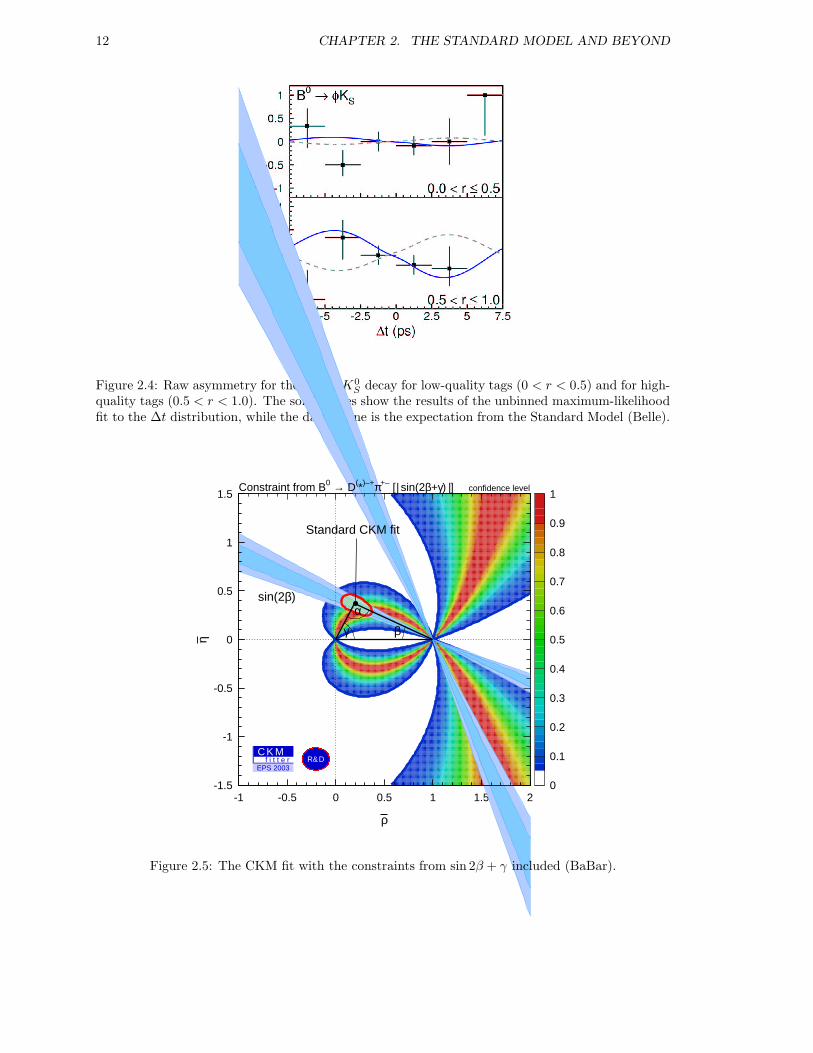
12 CHAPTER 2. THE STANDARD MODEL AND BEYOND
Figure 2.4: Raw asymmetry for the B → φK0S decay for low-quality tags (0 < r < 0.5) and for high-
quality tags (0.5 < r < 1.0). The solid curves show the results of the unbinned maximum-likelihoodfit to the ∆t distribution, while the dashed line is the expectation from the Standard Model (Belle).
-1.5
-1
-0.5
0
0.5
1
1.5
-1 -0.5 0 0.5 1 1.5 20
0.1
0.2
0.3
0.4
0.5
0.6
0.7
0.8
0.9
1
sin(2β)
γ β
α
Standard CKM fit
ρ
η
Constraint from B0 → D(*)–+π+– [| sin(2β+γ) |] confidence level
CK Mf i t t e r
EPS 2003R&D
Figure 2.5: The CKM fit with the constraints from sin 2β + γ included (BaBar).
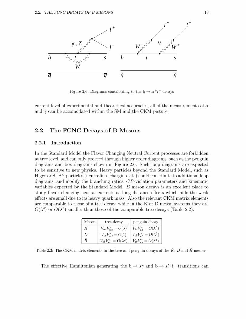
2.2. THE FCNC DECAYS OF B MESONS 13
q q
b st
W
γ , Z
l +
l −
q q
b st
W +W − ν
l − l +
Figure 2.6: Diagrams contributing to the b → sl+l− decays
current level of experimental and theoretical accuracies, all of the measurements of αand γ can be accomodated within the SM and the CKM picture.
2.2 The FCNC Decays of B Mesons
2.2.1 Introduction
In the Standard Model the Flavor Changing Neutral Current processes are forbiddenat tree level, and can only proceed through higher order diagrams, such as the penguindiagrams and box diagrams shown in Figure 2.6. Such loop diagrams are expectedto be sensitive to new physics. Heavy particles beyond the Standard Model, such asHiggs or SUSY particles (neutralino, chargino, etc) could contribute to additional loopdiagrams, and modify the branching ratios, CP -violation parameters and kinematicvariables expected by the Standard Model. B meson decays is an excellent place tostudy flavor changing neutral currents as long distance effects which hide the weakeffects are small due to its heavy quark mass. Also the relevant CKM matrix elementsare comparable to those of a tree decay, while in the K or D meson systems they areO(λ4) or O(λ5) smaller than those of the comparable tree decays (Table 2.2).
Meson tree decay penguin decay
K VusV∗
ud = O(λ) VtsV∗
td = O(λ5)
D VcsV∗
ud = O(1) VcbV∗
ub = O(λ5)
B VcbV∗
ud = O(λ2) VtbV∗
ts = O(λ2)
Table 2.2: The CKM matrix elements in the tree and penguin decays of the K, D and B mesons.
The effective Hamiltonian generating the b → sγ and b → sl+l− transitions can
14 CHAPTER 2. THE STANDARD MODEL AND BEYOND
be written as follows2:
Heff = −4GF√2V ∗
tsVtb10∑
i=1
Ci(µ)Oi(µ) (2.31)
where Oi(µ) are dimension-six operators at the scale µ, Ci(µ) are the correspond-ing Wilson coefficients which represent the effective strength of short distance inter-actions, GF is the Fermi coupling constant, and the Cabibbo-Kobayashi-Maskawadependence has been made explicit. The operators can be chosen as follows [17] [18]:
O1 = (sLγµTacL)(cLγ
µT abL) (2.32)
O2 = (sLγµcL)(cLγµbL) (2.33)
O3 = (sLγµbL)∑
q
(qγµq) (2.34)
O4 = (sLγµTabL)
∑
q
(qγµT aq) (2.35)
O5 = (sLγµ1γµ2
γµ3bL)
∑
q
(qγµ1γµ2γµ3q) (2.36)
O6 = (sLγµ1γµ2
γµ3T abL)
∑
q
(qγµ1γµ2γµ3T aq) (2.37)
O7 =e
g2s
mb(sLσµνbR)Fµν (2.38)
O8 =1
gsmb(sLσ
µνT abR)Gaµν (2.39)
O9 =e2
g2s
(sLγµbL)∑
l
(lγµl) (2.40)
O10 =e2
g2s
(sLγµbL)∑
l
(lγµγ5l) (2.41)
where the subscripts L and R refer to left- and right-handed components of thefermion fields, Fµν and Ga
µν denote the QED and QCD field strength tensors respec-tively. The Ci(µ) are evaluated perturbatively at the high energy scale O(mW ). Inorder to obtain the low energy theory, the Ci(µ) are evolved down to the scale O(mb)using renormalization group equations which guarantee that the µ dependence ofCi(µ) is cancelled by the µ dependence of Oi(µ), thus the observables should notdepend on the renormalization scale µ. The advantage of this approach is that if
2The assumption here is that the combination (V ∗usVub) of the CKM matrix elements can be neglected.
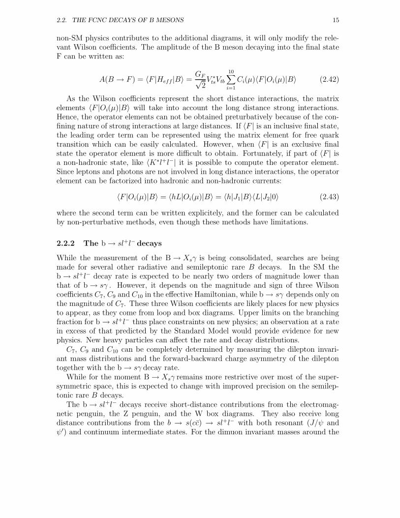
2.2. THE FCNC DECAYS OF B MESONS 15
non-SM physics contributes to the additional diagrams, it will only modify the rele-vant Wilson coefficients. The amplitude of the B meson decaying into the final stateF can be written as:
A(B → F ) = 〈F |Heff |B〉 =GF√
2V ∗
tsVtb10∑
i=1
Ci(µ)〈F |Oi(µ)|B〉 (2.42)
As the Wilson coefficients represent the short distance interactions, the matrixelements 〈F |Oi(µ)|B〉 will take into account the long distance strong interactions.Hence, the operator elements can not be obtained preturbatively because of the con-fining nature of strong interactions at large distances. If 〈F | is an inclusive final state,the leading order term can be represented using the matrix element for free quarktransition which can be easily calculated. However, when 〈F | is an exclusive finalstate the operator element is more difficult to obtain. Fortunately, if part of 〈F | isa non-hadronic state, like 〈K∗l+l−| it is possible to compute the operator element.Since leptons and photons are not involved in long distance interactions, the operatorelement can be factorized into hadronic and non-hadronic currents:
〈F |Oi(µ)|B〉 = 〈hL|Oi(µ)|B〉 = 〈h|J1|B〉〈L|J2|0〉 (2.43)
where the second term can be written explicitely, and the former can be calculatedby non-perturbative methods, even though these methods have limitations.
2.2.2 The b → sl+l− decays
While the measurement of the B → Xsγ is being consolidated, searches are beingmade for several other radiative and semileptonic rare B decays. In the SM theb → sl+l− decay rate is expected to be nearly two orders of magnitude lower thanthat of b → sγ . However, it depends on the magnitude and sign of three Wilsoncoefficients C7, C9 and C10 in the effective Hamiltonian, while b → sγ depends only onthe magnitude of C7. These three Wilson coefficients are likely places for new physicsto appear, as they come from loop and box diagrams. Upper limits on the branchingfraction for b → sl+l− thus place constraints on new physics; an observation at a ratein excess of that predicted by the Standard Model would provide evidence for newphysics. New heavy particles can affect the rate and decay distributions.C7, C9 and C10 can be completely determined by measuring the dilepton invari-
ant mass distributions and the forward-backward charge asymmetry of the dileptontogether with the b → sγ decay rate.
While for the moment B → Xsγ remains more restrictive over most of the super-symmetric space, this is expected to change with improved precision on the semilep-tonic rare B decays.
The b → sl+l− decays receive short-distance contributions from the electromag-netic penguin, the Z penguin, and the W box diagrams. They also receive longdistance contributions from the b → s(cc) → sl+l− with both resonant (J/ψ andψ′) and continuum intermediate states. For the dimuon invariant masses around the
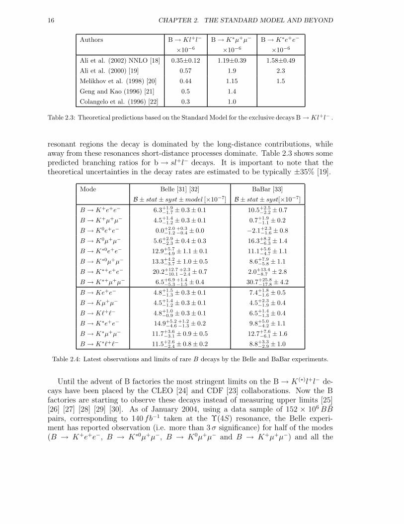
16 CHAPTER 2. THE STANDARD MODEL AND BEYOND
Authors B → Kl+l− B → K∗µ+µ− B → K∗e+e−
×10−6 ×10−6 ×10−6
Ali et al. (2002) NNLO [18] 0.35±0.12 1.19±0.39 1.58±0.49
Ali et al. (2000) [19] 0.57 1.9 2.3
Melikhov et al. (1998) [20] 0.44 1.15 1.5
Geng and Kao (1996) [21] 0.5 1.4
Colangelo et al. (1996) [22] 0.3 1.0
Table 2.3: Theoretical predictions based on the Standard Model for the exclusive decays B → Kl+l− .
resonant regions the decay is dominated by the long-distance contributions, whileaway from these resonances short-distance processes dominate. Table 2.3 shows somepredicted branching ratios for b → sl+l− decays. It is important to note that thetheoretical uncertainties in the decay rates are estimated to be typically ±35% [19].
Mode Belle [31] [32] BaBar [33]
B ± stat± syst±model [×10−7] B ± stat± syst[×10−7]
B → K+e+e− 6.3+1.9−1.7 ± 0.3± 0.1 10.5+2.5
−2.2 ± 0.7
B → K+µ+µ− 4.5+1.4−1.2 ± 0.3± 0.1 0.7+1.9
−1.1 ± 0.2
B → K0e+e− 0.0+2.0−1.2
+0.3−0.4 ± 0.0 −2.1+2.3
−1.6 ± 0.8
B → K0µ+µ− 5.6+2.9−2.3 ± 0.4± 0.3 16.3+8.2
−6.3 ± 1.4
B → K∗0e+e− 12.9+5.7−4.9 ± 1.1± 0.1 11.1+5.6
−4.7 ± 1.1
B → K∗0µ+µ− 13.3+4.2−3.7 ± 1.0± 0.5 8.6+7.9
−5.8 ± 1.1
B → K∗+e+e− 20.2+12.7−10.1
+2.3−2.4 ± 0.7 2.0+13.4
−8.7 ± 2.8
B → K∗+µ+µ− 6.5+6.9−5.3
+1.4−1.5 ± 0.4 30.7+25.8
−17.8 ± 4.2
B → Ke+e− 4.8+1.5−1.3 ± 0.3± 0.1 7.4+1.8
−1.6 ± 0.5
B → Kµ+µ− 4.5+1.4−1.2 ± 0.3± 0.1 4.5+2.3
−1.9 ± 0.4
B → K`+`− 4.8+1.0−0.9 ± 0.3± 0.1 6.5+1.4
−1.3 ± 0.4
B → K∗e+e− 14.9+5.2−4.6
+1.2−1.3 ± 0.2 9.8+5.0
−4.2 ± 1.1
B → K∗µ+µ− 11.7+3.6−3.1 ± 0.9± 0.5 12.7+7.6
−6.1 ± 1.6
B → K∗`+`− 11.5+2.6−2.4 ± 0.8± 0.2 8.8+3.3
−2.9 ± 1.0
Table 2.4: Latest observations and limits of rare B decays by the Belle and BaBar experiments.
Until the advent of B factories the most stringent limits on the B → K (∗)l+l− de-cays have been placed by the CLEO [24] and CDF [23] collaborations. Now the Bfactories are starting to observe these decays instead of measuring upper limits [25][26] [27] [28] [29] [30]. As of January 2004, using a data sample of 152 × 106BBpairs, corresponding to 140 fb−1 taken at the Υ(4S) resonance, the Belle experi-ment has reported observation (i.e. more than 3 σ significance) for half of the modes(B → K+e+e−, B → K∗0µ+µ−, B → K0µ+µ− and B → K+µ+µ−) and all the
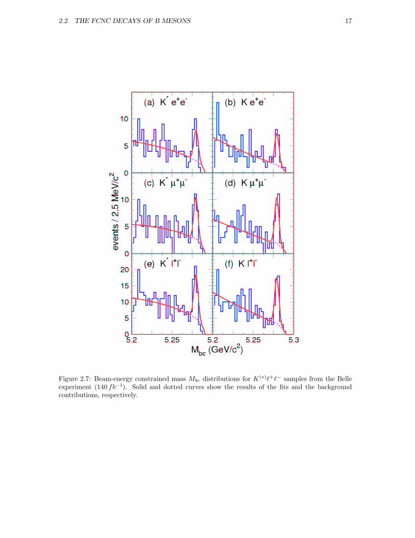
2.2. THE FCNC DECAYS OF B MESONS 17
Figure 2.7: Beam-energy constrained mass Mbc distributions for K(∗)`+`− samples from the Belleexperiment (140 fb−1). Solid and dotted curves show the results of the fits and the backgroundcontributions, respectively.
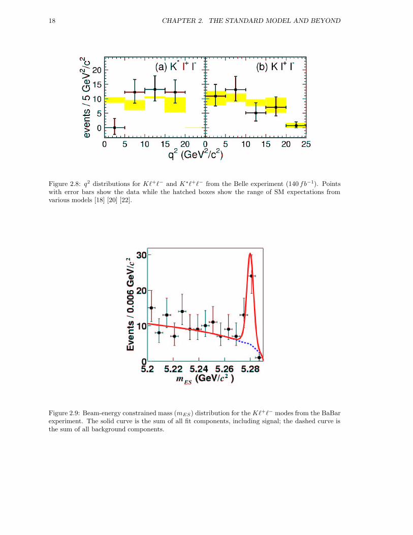
18 CHAPTER 2. THE STANDARD MODEL AND BEYOND
Figure 2.8: q2 distributions for K`+`− and K∗`+`− from the Belle experiment (140 fb−1). Pointswith error bars show the data while the hatched boxes show the range of SM expectations fromvarious models [18] [20] [22].
Figure 2.9: Beam-energy constrained mass (mES) distribution for the K`+`− modes from the BaBarexperiment. The solid curve is the sum of all fit components, including signal; the dashed curve isthe sum of all background components.
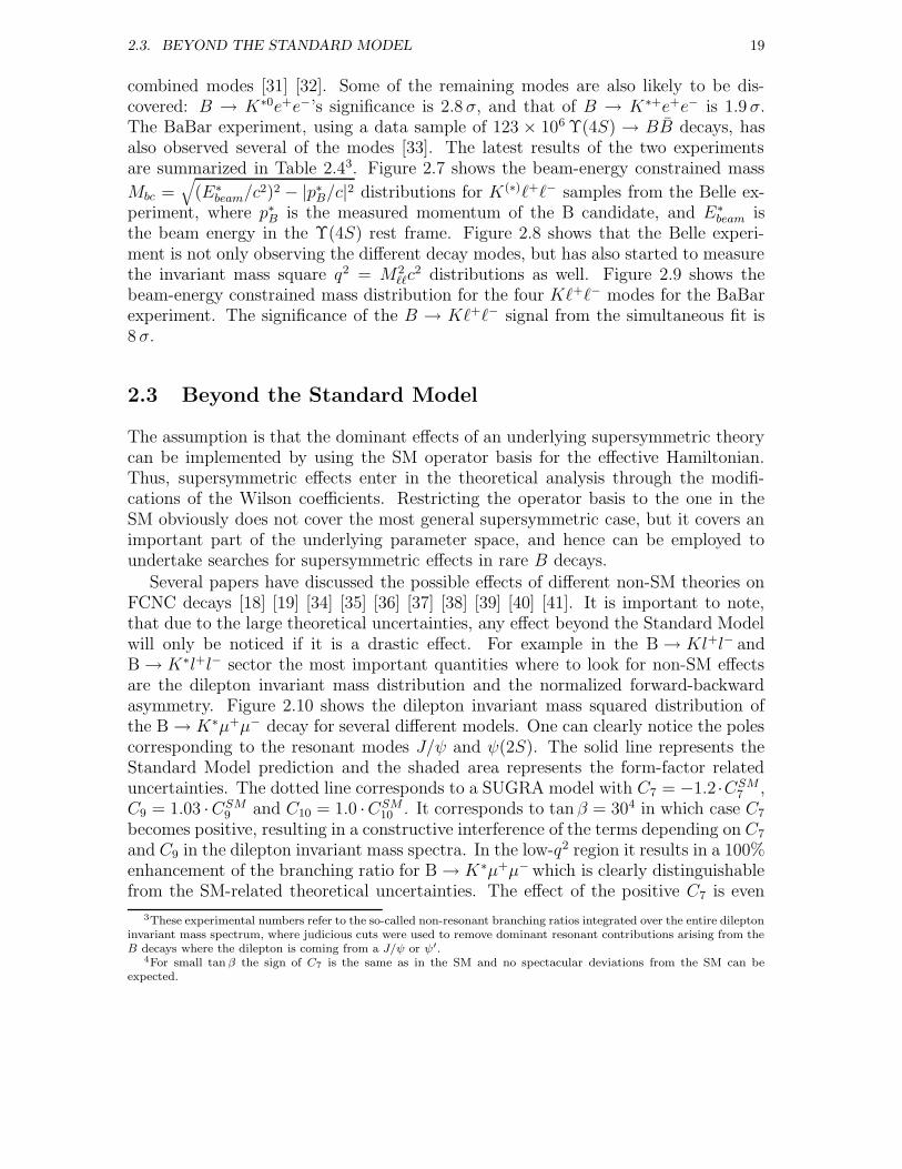
2.3. BEYOND THE STANDARD MODEL 19
combined modes [31] [32]. Some of the remaining modes are also likely to be dis-covered: B → K∗0e+e−’s significance is 2.8 σ, and that of B → K∗+e+e− is 1.9 σ.The BaBar experiment, using a data sample of 123 × 106 Υ(4S) → BB decays, hasalso observed several of the modes [33]. The latest results of the two experimentsare summarized in Table 2.43. Figure 2.7 shows the beam-energy constrained mass
Mbc =√
(E∗beam/c
2)2 − |p∗B/c|2 distributions for K(∗)`+`− samples from the Belle ex-periment, where p∗B is the measured momentum of the B candidate, and E∗
beam isthe beam energy in the Υ(4S) rest frame. Figure 2.8 shows that the Belle experi-ment is not only observing the different decay modes, but has also started to measurethe invariant mass square q2 = M2
``c2 distributions as well. Figure 2.9 shows the
beam-energy constrained mass distribution for the four K`+`− modes for the BaBarexperiment. The significance of the B → K`+`− signal from the simultaneous fit is8 σ.
2.3 Beyond the Standard Model
The assumption is that the dominant effects of an underlying supersymmetric theorycan be implemented by using the SM operator basis for the effective Hamiltonian.Thus, supersymmetric effects enter in the theoretical analysis through the modifi-cations of the Wilson coefficients. Restricting the operator basis to the one in theSM obviously does not cover the most general supersymmetric case, but it covers animportant part of the underlying parameter space, and hence can be employed toundertake searches for supersymmetric effects in rare B decays.
Several papers have discussed the possible effects of different non-SM theories onFCNC decays [18] [19] [34] [35] [36] [37] [38] [39] [40] [41]. It is important to note,that due to the large theoretical uncertainties, any effect beyond the Standard Modelwill only be noticed if it is a drastic effect. For example in the B → Kl+l− andB → K∗l+l− sector the most important quantities where to look for non-SM effectsare the dilepton invariant mass distribution and the normalized forward-backwardasymmetry. Figure 2.10 shows the dilepton invariant mass squared distribution ofthe B → K∗µ+µ− decay for several different models. One can clearly notice the polescorresponding to the resonant modes J/ψ and ψ(2S). The solid line represents theStandard Model prediction and the shaded area represents the form-factor relateduncertainties. The dotted line corresponds to a SUGRA model with C7 = −1.2 ·CSM
7 ,C9 = 1.03 ·CSM
9 and C10 = 1.0 ·CSM10 . It corresponds to tan β = 304 in which case C7
becomes positive, resulting in a constructive interference of the terms depending on C7
and C9 in the dilepton invariant mass spectra. In the low-q2 region it results in a 100%enhancement of the branching ratio for B → K∗µ+µ− which is clearly distinguishablefrom the SM-related theoretical uncertainties. The effect of the positive C7 is even
3These experimental numbers refer to the so-called non-resonant branching ratios integrated over the entire dileptoninvariant mass spectrum, where judicious cuts were used to remove dominant resonant contributions arising from theB decays where the dilepton is coming from a J/ψ or ψ′.
4For small tan β the sign of C7 is the same as in the SM and no spectacular deviations from the SM can beexpected.
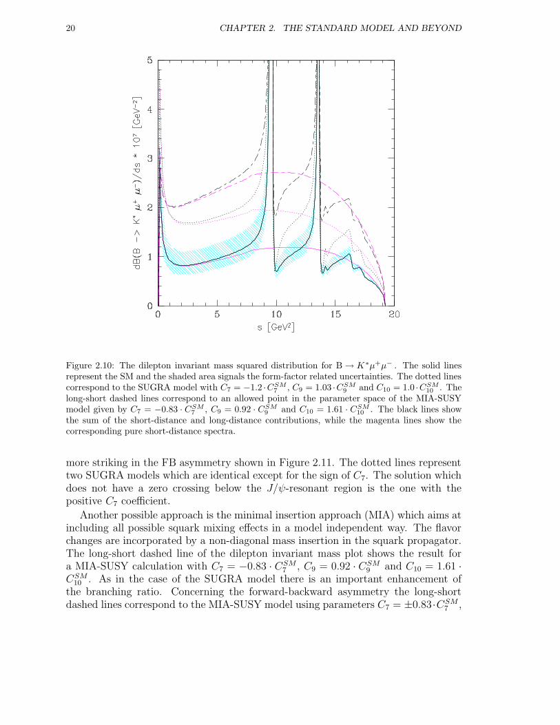
20 CHAPTER 2. THE STANDARD MODEL AND BEYOND
Figure 2.10: The dilepton invariant mass squared distribution for B → K∗µ+µ− . The solid linesrepresent the SM and the shaded area signals the form-factor related uncertainties. The dotted linescorrespond to the SUGRA model with C7 = −1.2 ·CSM
7 , C9 = 1.03 ·CSM9 and C10 = 1.0 ·CSM
10 . Thelong-short dashed lines correspond to an allowed point in the parameter space of the MIA-SUSYmodel given by C7 = −0.83 · CSM
7 , C9 = 0.92 · CSM9 and C10 = 1.61 · CSM
10 . The black lines showthe sum of the short-distance and long-distance contributions, while the magenta lines show thecorresponding pure short-distance spectra.
more striking in the FB asymmetry shown in Figure 2.11. The dotted lines representtwo SUGRA models which are identical except for the sign of C7. The solution whichdoes not have a zero crossing below the J/ψ-resonant region is the one with thepositive C7 coefficient.
Another possible approach is the minimal insertion approach (MIA) which aims atincluding all possible squark mixing effects in a model independent way. The flavorchanges are incorporated by a non-diagonal mass insertion in the squark propagator.The long-short dashed line of the dilepton invariant mass plot shows the result fora MIA-SUSY calculation with C7 = −0.83 · CSM
7 , C9 = 0.92 · CSM9 and C10 = 1.61 ·
CSM10 . As in the case of the SUGRA model there is an important enhancement of
the branching ratio. Concerning the forward-backward asymmetry the long-shortdashed lines correspond to the MIA-SUSY model using parameters C7 = ±0.83·CSM
7 ,
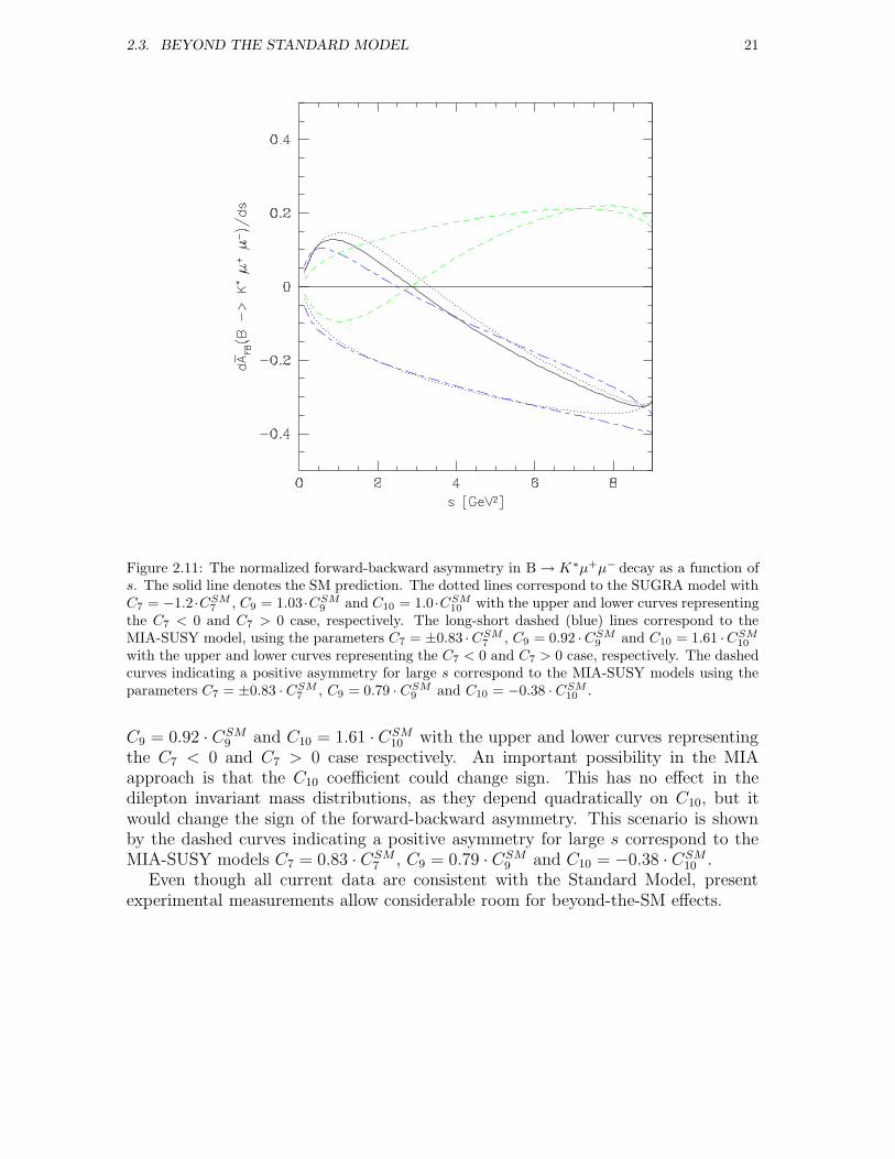
2.3. BEYOND THE STANDARD MODEL 21
Figure 2.11: The normalized forward-backward asymmetry in B → K∗µ+µ− decay as a function ofs. The solid line denotes the SM prediction. The dotted lines correspond to the SUGRA model withC7 = −1.2 ·CSM
7 , C9 = 1.03 ·CSM9 and C10 = 1.0 ·CSM
10 with the upper and lower curves representingthe C7 < 0 and C7 > 0 case, respectively. The long-short dashed (blue) lines correspond to theMIA-SUSY model, using the parameters C7 = ±0.83 ·CSM
7 , C9 = 0.92 ·CSM9 and C10 = 1.61 ·CSM
10
with the upper and lower curves representing the C7 < 0 and C7 > 0 case, respectively. The dashedcurves indicating a positive asymmetry for large s correspond to the MIA-SUSY models using theparameters C7 = ±0.83 · CSM
7 , C9 = 0.79 · CSM9 and C10 = −0.38 · CSM
10 .
C9 = 0.92 · CSM9 and C10 = 1.61 · CSM
10 with the upper and lower curves representingthe C7 < 0 and C7 > 0 case respectively. An important possibility in the MIAapproach is that the C10 coefficient could change sign. This has no effect in thedilepton invariant mass distributions, as they depend quadratically on C10, but itwould change the sign of the forward-backward asymmetry. This scenario is shownby the dashed curves indicating a positive asymmetry for large s correspond to theMIA-SUSY models C7 = 0.83 · CSM
7 , C9 = 0.79 · CSM9 and C10 = −0.38 · CSM
10 .Even though all current data are consistent with the Standard Model, present
experimental measurements allow considerable room for beyond-the-SM effects.

22 CHAPTER 2. THE STANDARD MODEL AND BEYOND
Part II
Search for the B0d → µµK∗0 decay at
the CDF experiment
23

Chapter 3
Detectors for studying rare Bdecays I: The CDF experiment atthe Tevatron
The Collider Detector at Fermilab (CDF) is one of the two general purpose detectorsbuilt to study high-energy pp collisions at the Tevatron, located at the Fermi Na-tional Accelerator Laboratory. After introducing the accelerator chain, the differentcomponents of the detector and the trigger system will be described in detail.
3.1 The Tevatron
The Tevatron is a proton-antiproton collider located at the Fermi National AcceleratorLaboratory (FNAL) in Chicago. It produced the first pp collisions in 1983, andsince then has had several phases of running. Between 1992 and 1996 the centerof mass collision energy achieved by the accelerator was 1.8TeV . This phase iscalled Run I and 120 pb−1 of data1 have been collected which enabled, amongst othermeasurements, the discovery of the top quark [47]. In 1996 the accelerator wastemporarily shut down in order to implement a series of improvements to increasesubstantially the luminosity [48]. This second phase, called Run II, was initially aimedat achieving 15 fb−1 integrated luminosity. Due to some experimental difficultiesdescribed later in this section the integrated luminosity goals have been adjusted firstto 6.5−11 fb−1 [49], then to 4.4−8.6 fb−1 [51]. Run II itself was planned to consist oftwo parts, Run IIa and Run IIb. Between the two runs a shutdown of several monthswas foreseen in order to replace the silicon detectors of the experiments designed tosurvive 2 fb−1 of integrated luminosity. Because of lack of funding and the lowerthan expected luminosity CDF will not replace the silicon detectors as planned, andcontinue to take data without major upgrades of the detector. For Run II the centerof mass collision energy has also been raised to
√s = 1.96 TeV, so until the Large
Hadron Collider is completed at CERN, it will remain the highest energy collider in1Integrated luminosities are usually given in units of barn−1, corresponding to 1024 cm−2, i.e. 1 pb−1 = 1036 cm−2.
25
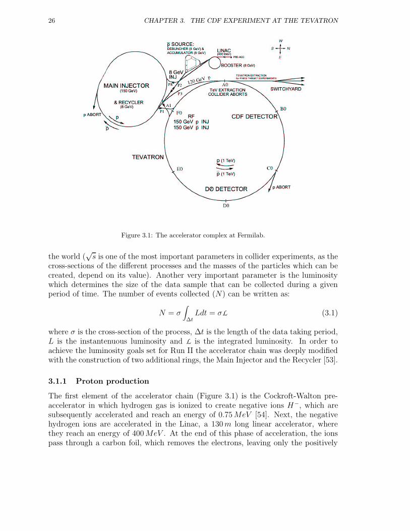
26 CHAPTER 3. THE CDF EXPERIMENT AT THE TEVATRON
Figure 3.1: The accelerator complex at Fermilab.
the world (√s is one of the most important parameters in collider experiments, as the
cross-sections of the different processes and the masses of the particles which can becreated, depend on its value). Another very important parameter is the luminositywhich determines the size of the data sample that can be collected during a givenperiod of time. The number of events collected (N) can be written as:
N = σ∫
∆tLdt = σL (3.1)
where σ is the cross-section of the process, ∆t is the length of the data taking period,L is the instantenuous luminosity and L is the integrated luminosity. In order toachieve the luminosity goals set for Run II the accelerator chain was deeply modifiedwith the construction of two additional rings, the Main Injector and the Recycler [53].
3.1.1 Proton production
The first element of the accelerator chain (Figure 3.1) is the Cockroft-Walton pre-accelerator in which hydrogen gas is ionized to create negative ions H−, which aresubsequently accelerated and reach an energy of 0.75MeV [54]. Next, the negativehydrogen ions are accelerated in the Linac, a 130m long linear accelerator, wherethey reach an energy of 400MeV . At the end of this phase of acceleration, the ionspass through a carbon foil, which removes the electrons, leaving only the positively
3.1. THE TEVATRON 27
charged protons. The third stage of the accelerator chain is the Booster, a synchrotronwith a diameter of 475m, where electric fields accelerate protons until they reach anenergy of 8GeV . The fourth stage is the Main Injector. It is a new synchrotron witha diameter of 1 km which was completed in 1999. The Main Injector accelerates theprotons from 8GeV to 150GeV and groups them in bunches of 2.7 × 10¹¹ particles.
3.1.2 Antiproton production
The antiproton production rate is one of the main limiting factors in achieving higherluminosity, so for Run II particular emphasis was put onto the improvement of theantiproton beam. Besides producing proton bunches for the collisions in the Tevatron,as mentioned earlier, the Main Injector is also producing 120GeV protons in bunchesof 2 × 10¹² particles which then enter in collision with a nickel target. The resultingparticles are collected with magnetic lenses, then the antiprotons are filtered witha dipole magnet. On the average, 50000 protons are needed for the production ofevery single antiproton. The antiprotons are then sent to the Debuncher which is atriangular ring of 505m in length. The Debuncher reduces the dispersion of the energyof the antiprotons using stochastic cooling. Finally, the antiprotons are transferred tothe Accumulator where they are further cooled and stacked in bunches before beingtransferred to the Main Injector. The complex described above needs 8 hours in orderto accumulate 1.3 × 10¹² antiprotons. The antiprotons are then accelerated in theMain Injector to 150GeV and form bunches of 3 × 10¹⁰ particles.
One of the main improvements of Run II is the construction of the Recycler, whichis installed in the same tunnel as the Main Injector. Originally its aim was to recyclethe antiprotons remaining after the end of a store (which corresponds to 75% of theinitial number). This would have enabled to double the number of antiprotons forthe next store. As of early 2004, work on recycling antiprotons has been stopped andthe Recycler is expected to serve as a second antiproton storage ring, fulfilling theoriginal aim in a different fashion [50]. After the installation of the electron coolingthe Recycler is expected to be integrated in the rest of the complex in early 2005 [51][52].
3.1.3 The Tevatron
The last element in the chain of the accelerators is the Tevatron, a superconductingsynchrotron. The Tevatron accelerates protons and antiprotons, which it receives fromthe Main Injector, from 150GeV to 980GeV . Between Run I and Run II the energyof the beam has been increased from 900 to 980GeV and a new cryogenic systemhas been installed. There are 36 bunches of protons and 36 bunches of antiprotonscirculating in the opposite direction. The two beams are focused using quadrupolemagnets in two regions around the ring where they collide every 396 ns. The twogeneral purpose collider experiments installed in these two regions are CDF and D0.In the region of CDF the beam has a longitudinal dispersion of σz ' 30 cm, and atransverse dispersion of σt ' 30µm.

28 CHAPTER 3. THE CDF EXPERIMENT AT THE TEVATRON
Run Ib Run II present Run IIa nominal Run IIb nominal
p bunches × p bunches 6 × 6 36 × 36 36× 36 140× 121
p/bunch 2.3 · 1011 2.1 · 1011 2.7 · 1011 2.7 · 1011
p/bunch 5.5 · 1010 2.5 · 1010 3.0 · 1010 3.0 · 1010
L [cm−2s−1] 0.16 · 1031 4.1 · 1031 8.6 · 1031 16 · 1031
L [pb−1/week] 3.2 6-8 17 32
Bunch spacing [ns] ≈3500 396 396 132
Crossing angle [µrad] 0 0 0 136
Energy (p+ p) [GeV ] 900 + 900 980 + 980 980 + 980 980 + 980
Table 3.1: Parameters of the Tevatron for Run I and Run II [49] [53]. Recent developments suggest,that Run IIb will use essentially the same parameters as Run IIa [51].
The accelerator has been running since March 2001. Many improvements havebeen implemented to correct the problems that were identified during the start-upperiod:
• Modification of the injection helix
• Proton beam loading compensation in Main Injector
• Accumulator stochastic cooling upgrade
• C-0 Lambertson magnets removal
However, there are still several problems to which satisfactory solutions have notbeen found yet:
• Emittance preservation throughout the complex
• Beam-beam interaction in the Tevatron
• Proton and antiproton acceleration efficiencies (Tevatron)
• Beam lifetimes
• Transfer losses
At present2 the instantenuous initial luminosity is topping out at 5×1031 cm−2s−1
(see Figure 3.2), which is significantly lower than expected (Table 3.1). The same canbe said about the weekly integrated luminosity which is 2-3 times lower than planned(Figure 3.3). The modified aim is to reach 3×1032 cm−2s−1 instantenuous luminosityand 4.4−8.6 fb−1 integrated luminosity by 20093 [49]. For the Run IIb a structure of140 proton bunches and 121 antiproton bunches was foreseen. However, this wouldhave implied the reduction of time between collisions to 132ns, significantly increasing
2i.e. end of 2004.3However, this number could be decreased by 15% if the 7 month shutdown goes ahead as planned in 2006.
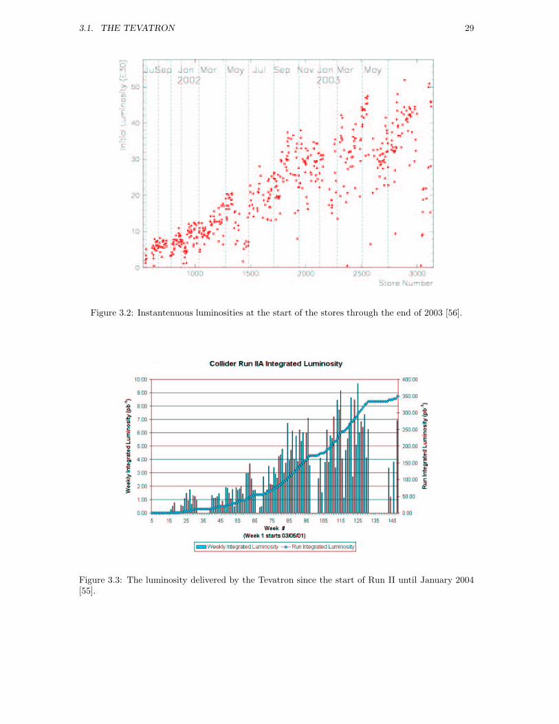
3.1. THE TEVATRON 29
Figure 3.2: Instantenuous luminosities at the start of the stores through the end of 2003 [56].
Figure 3.3: The luminosity delivered by the Tevatron since the start of Run II until January 2004[55].
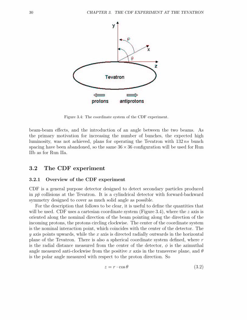
30 CHAPTER 3. THE CDF EXPERIMENT AT THE TEVATRON
Figure 3.4: The coordinate system of the CDF experiment.
beam-beam effects, and the introduction of an angle between the two beams. Asthe primary motivation for increasing the number of bunches, the expected highluminosity, was not achieved, plans for operating the Tevatron with 132ns bunchspacing have been abandoned, so the same 36×36 configuration will be used for RunIIb as for Run IIa.
3.2 The CDF experiment
3.2.1 Overview of the CDF experiment
CDF is a general purpose detector designed to detect secondary particles producedin pp collisions at the Tevatron. It is a cylindrical detector with forward-backwardsymmetry designed to cover as much solid angle as possible.
For the description that follows to be clear, it is useful to define the quantities thatwill be used. CDF uses a cartesian coordinate system (Figure 3.4), where the z axis isoriented along the nominal direction of the beam pointing along the direction of theincoming protons, the protons circling clockwise. The center of the coordinate systemis the nominal interaction point, which coincides with the center of the detector. They axis points upwards, while the x axis is directed radially outwards in the horizontalplane of the Tevatron. There is also a spherical coordinate system defined, where ris the radial distance measured from the center of the detector, φ is the azimuthalangle measured anti-clockwise from the positive x axis in the transverse plane, and θis the polar angle measured with respect to the proton direction. So
z = r · cos θ (3.2)
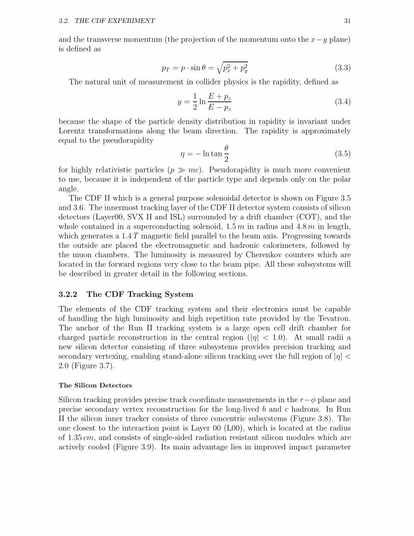
3.2. THE CDF EXPERIMENT 31
and the transverse momentum (the projection of the momentum onto the x−y plane)is defined as
pT = p · sin θ =√
p2x + p2
y (3.3)
The natural unit of measurement in collider physics is the rapidity, defined as
y =1
2lnE + pzE − pz
(3.4)
because the shape of the particle density distribution in rapidity is invariant underLorentz transformations along the beam direction. The rapidity is approximatelyequal to the pseudorapidity
η = − ln tanθ
2(3.5)
for highly relativistic particles (p � mc). Pseudorapidity is much more convenientto use, because it is independent of the particle type and depends only on the polarangle.
The CDF II which is a general purpose solenoidal detector is shown on Figure 3.5and 3.6. The innermost tracking layer of the CDF II detector system consists of silicondetectors (Layer00, SVX II and ISL) surrounded by a drift chamber (COT), and thewhole contained in a superconducting solenoid, 1.5m in radius and 4.8m in length,which generates a 1.4T magnetic field parallel to the beam axis. Progressing towardsthe outside are placed the electromagnetic and hadronic calorimeters, followed bythe muon chambers. The luminosity is measured by Cherenkov counters which arelocated in the forward regions very close to the beam pipe. All these subsystems willbe described in greater detail in the following sections.
3.2.2 The CDF Tracking System
The elements of the CDF tracking system and their electronics must be capableof handling the high luminosity and high repetition rate provided by the Tevatron.The anchor of the Run II tracking system is a large open cell drift chamber forcharged particle reconstruction in the central region (|η| < 1.0). At small radii anew silicon detector consisting of three subsystems provides precision tracking andsecondary vertexing, enabling stand-alone silicon tracking over the full region of |η| <2.0 (Figure 3.7).
The Silicon Detectors
Silicon tracking provides precise track coordinate measurements in the r−φ plane andprecise secondary vertex reconstruction for the long-lived b and c hadrons. In RunII the silicon inner tracker consists of three concentric subsystems (Figure 3.8). Theone closest to the interaction point is Layer 00 (L00), which is located at the radiusof 1.35 cm, and consists of single-sided radiation resistant silicon modules which areactively cooled (Figure 3.9). Its main advantage lies in improved impact parameter
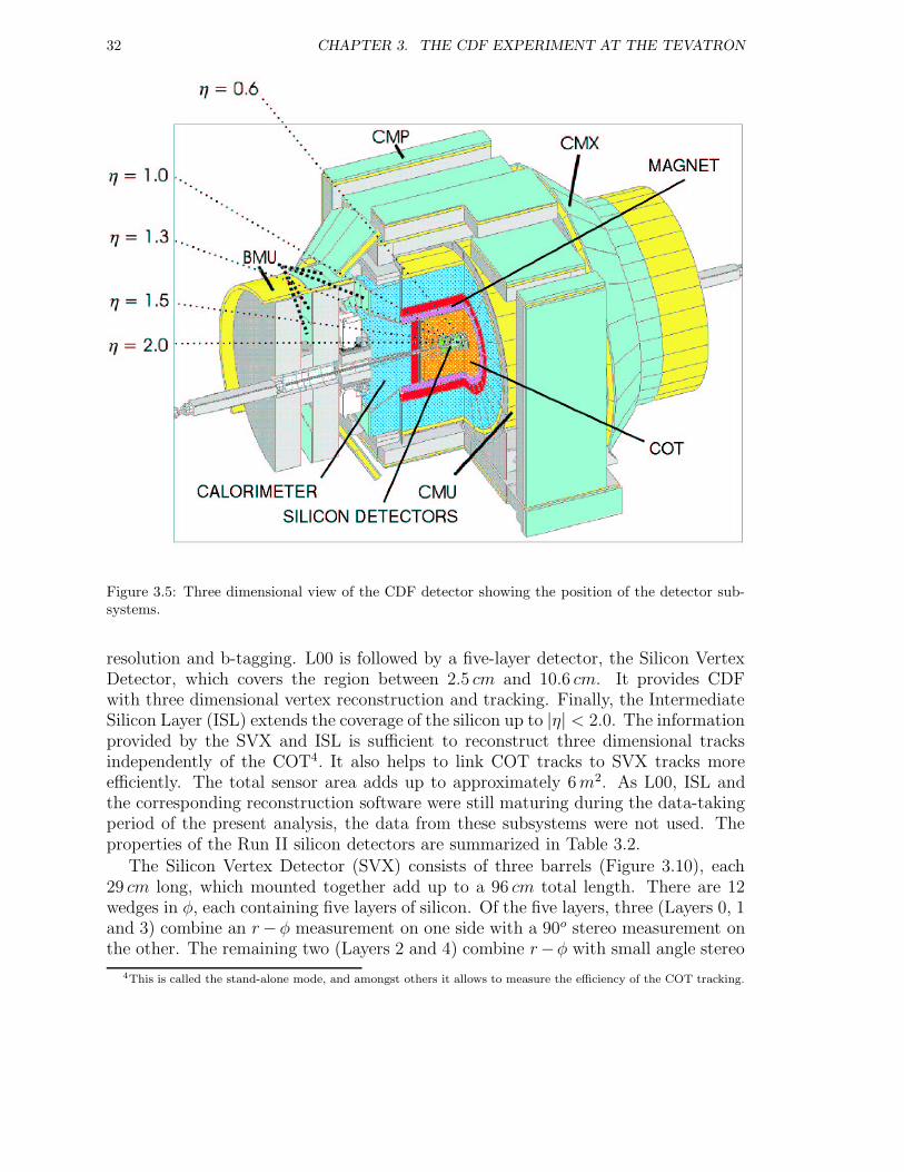
32 CHAPTER 3. THE CDF EXPERIMENT AT THE TEVATRON
Figure 3.5: Three dimensional view of the CDF detector showing the position of the detector sub-systems.
resolution and b-tagging. L00 is followed by a five-layer detector, the Silicon VertexDetector, which covers the region between 2.5 cm and 10.6 cm. It provides CDFwith three dimensional vertex reconstruction and tracking. Finally, the IntermediateSilicon Layer (ISL) extends the coverage of the silicon up to |η| < 2.0. The informationprovided by the SVX and ISL is sufficient to reconstruct three dimensional tracksindependently of the COT4. It also helps to link COT tracks to SVX tracks moreefficiently. The total sensor area adds up to approximately 6m2. As L00, ISL andthe corresponding reconstruction software were still maturing during the data-takingperiod of the present analysis, the data from these subsystems were not used. Theproperties of the Run II silicon detectors are summarized in Table 3.2.
The Silicon Vertex Detector (SVX) consists of three barrels (Figure 3.10), each29 cm long, which mounted together add up to a 96 cm total length. There are 12wedges in φ, each containing five layers of silicon. Of the five layers, three (Layers 0, 1and 3) combine an r− φ measurement on one side with a 90o stereo measurement onthe other. The remaining two (Layers 2 and 4) combine r−φ with small angle stereo
4This is called the stand-alone mode, and amongst others it allows to measure the efficiency of the COT tracking.
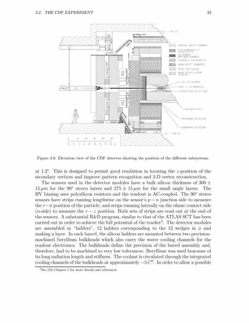
3.2. THE CDF EXPERIMENT 33
Figure 3.6: Elevation view of the CDF detector showing the position of the different subsystems.
at 1.2o. This is designed to permit good resolution in locating the z-position of thesecondary vertices and improve pattern recognition and 3-D vertex reconstruction.
The sensors used in the detector modules have a bulk silicon thickness of 300 ±15µm for the 90o stereo layers and 275 ± 15µm for the small angle layers. TheHV biasing uses polysilicon resistors and the readout is AC-coupled. The 90o stereosensors have strips running lengthwise on the sensor’s p− n junction side to measurethe r−φ position of the particle, and strips running laterally on the ohmic contact side(n-side) to measure the r − z position. Both sets of strips are read out at the end ofthe sensors. A substantial R&D program, similar to that of the ATLAS SCT has beencarried out in order to achieve the full potential of the tracker5. The detector modulesare assembled in “ladders”, 12 ladders corresponding to the 12 wedges in φ andmaking a layer. In each barrel, the silicon ladders are mounted between two precision-machined beryllium bulkheads which also carry the water cooling channels for thereadout electronics. The bulkheads define the precision of the barrel assembly and,therefore, had to be machined to very low tolerances. Beryllium was used beacause ofits long radiation length and stiffness. The coolant is circulated through the integratedcooling channels of the bulkheads at approximately −5C0. In order to allow a possible
5See [59] Chapter 5 for more details and references.
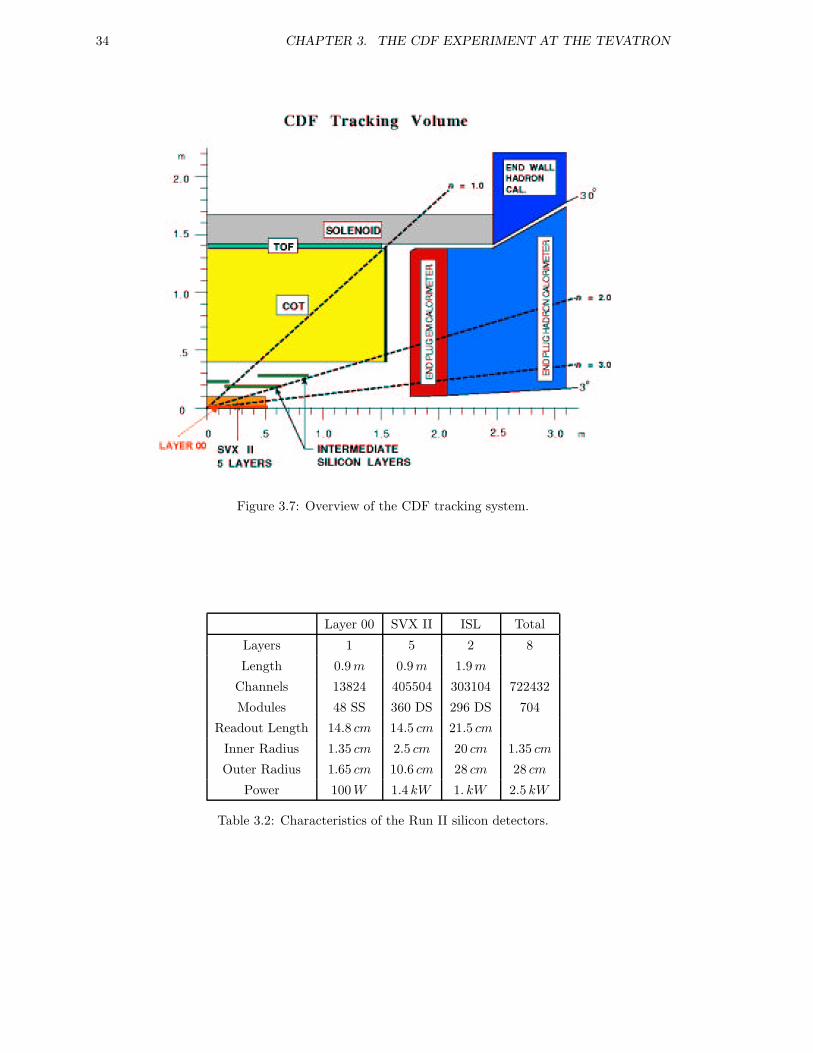
34 CHAPTER 3. THE CDF EXPERIMENT AT THE TEVATRON
Figure 3.7: Overview of the CDF tracking system.
Layer 00 SVX II ISL Total
Layers 1 5 2 8
Length 0.9m 0.9m 1.9m
Channels 13824 405504 303104 722432
Modules 48 SS 360 DS 296 DS 704
Readout Length 14.8 cm 14.5 cm 21.5 cm
Inner Radius 1.35 cm 2.5 cm 20 cm 1.35 cm
Outer Radius 1.65 cm 10.6 cm 28 cm 28 cm
Power 100W 1.4 kW 1. kW 2.5 kW
Table 3.2: Characteristics of the Run II silicon detectors.
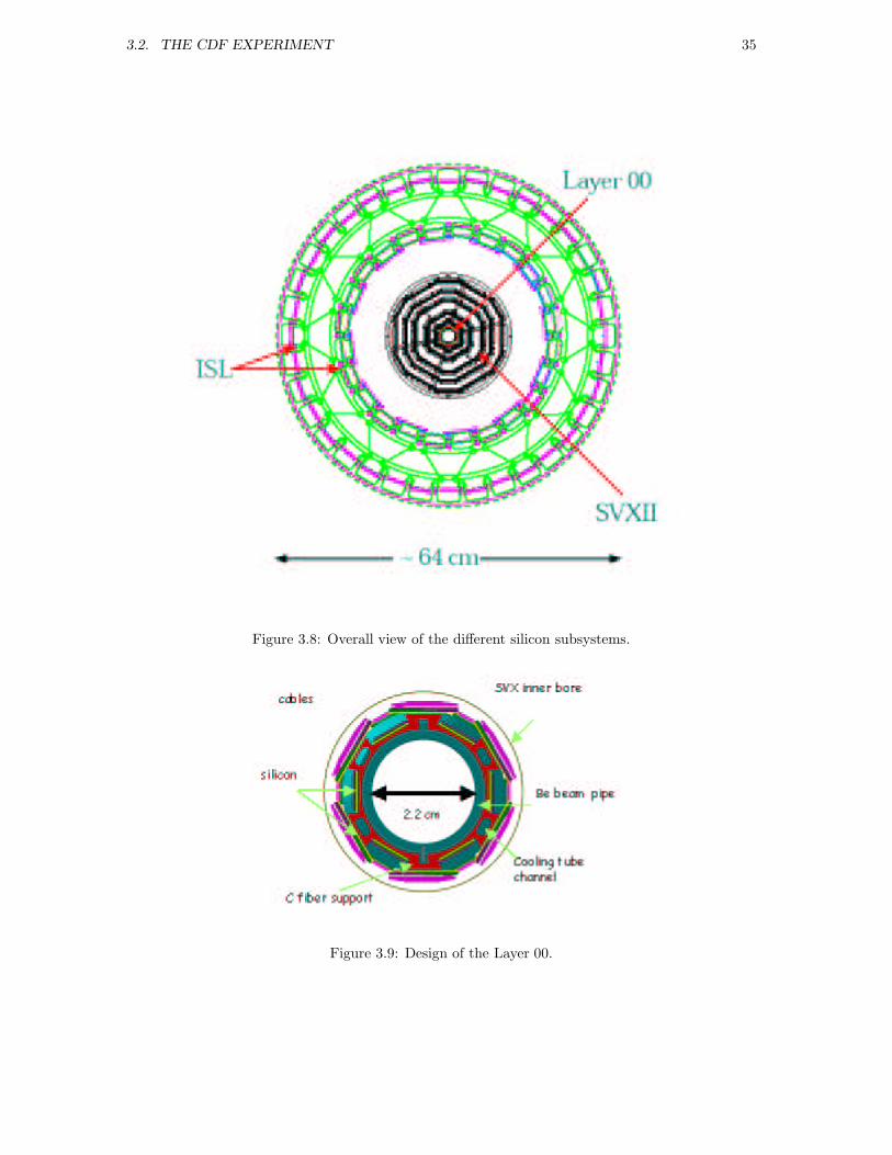
3.2. THE CDF EXPERIMENT 35
Figure 3.8: Overall view of the different silicon subsystems.
Figure 3.9: Design of the Layer 00.
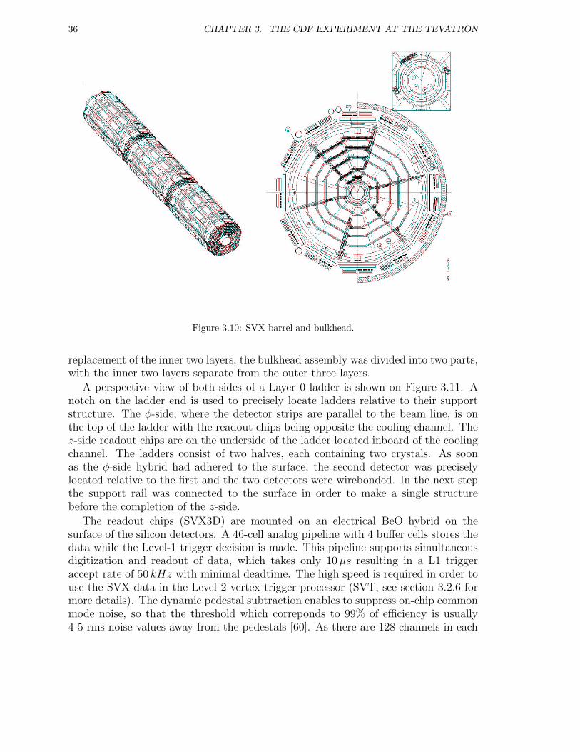
36 CHAPTER 3. THE CDF EXPERIMENT AT THE TEVATRON
Figure 3.10: SVX barrel and bulkhead.
replacement of the inner two layers, the bulkhead assembly was divided into two parts,with the inner two layers separate from the outer three layers.
A perspective view of both sides of a Layer 0 ladder is shown on Figure 3.11. Anotch on the ladder end is used to precisely locate ladders relative to their supportstructure. The φ-side, where the detector strips are parallel to the beam line, is onthe top of the ladder with the readout chips being opposite the cooling channel. Thez-side readout chips are on the underside of the ladder located inboard of the coolingchannel. The ladders consist of two halves, each containing two crystals. As soonas the φ-side hybrid had adhered to the surface, the second detector was preciselylocated relative to the first and the two detectors were wirebonded. In the next stepthe support rail was connected to the surface in order to make a single structurebefore the completion of the z-side.
The readout chips (SVX3D) are mounted on an electrical BeO hybrid on thesurface of the silicon detectors. A 46-cell analog pipeline with 4 buffer cells stores thedata while the Level-1 trigger decision is made. This pipeline supports simultaneousdigitization and readout of data, which takes only 10µs resulting in a L1 triggeraccept rate of 50 kHz with minimal deadtime. The high speed is required in order touse the SVX data in the Level 2 vertex trigger processor (SVT, see section 3.2.6 formore details). The dynamic pedestal subtraction enables to suppress on-chip commonmode noise, so that the threshold which correponds to 99% of efficiency is usually4-5 rms noise values away from the pedestals [60]. As there are 128 channels in each
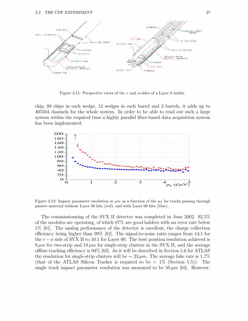
3.2. THE CDF EXPERIMENT 37
Figure 3.11: Perspective views of the z and φ-sides of a Layer 0 ladder.
chip, 88 chips in each wedge, 12 wedges in each barrel and 3 barrels, it adds up to405504 channels for the whole system. In order to be able to read out such a largesystem within the required time a highly parallel fiber-based data acquisition systemhas been implemented.
Figure 3.12: Impact parameter resolution in µm as a function of the pT for tracks passing throughpassive material without Layer 00 hits (red), and with Layer 00 hits (blue).
The commissionning of the SVX II detector was completed in June 2002. 92.5%of the modules are operating, of which 87% are good ladders with an error rate below1% [61]. The analog performance of the detector is excellent, the charge collectionefficiency being higher than 99% [62]. The signal-to-noise ratio ranges from 14:1 forthe r−φ side of SVX II to 10:1 for Layer 00. The best position resolution achieved is9µm for two-strip and 18µm for single-strip clusters in the SVX II, and the averageoffline tracking efficiency is 94% [63]. As it will be described in Section 5.6 for ATLASthe resolution for single-strip clusters will be ∼ 23µm. The average fake rate is 1.7%(that of the ATLAS Silicon Tracker is required to be < 1% (Section 5.5)). Thesingle track impact parameter resolution was measured to be 50µm [64]. However,
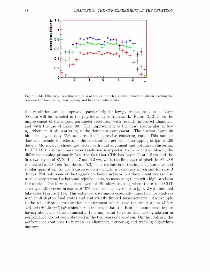
38 CHAPTER 3. THE CDF EXPERIMENT AT THE TEVATRON
Figure 3.13: Efficiency as a function of η of the calorimeter seeded outside-in silicon tracking fortracks with three (blue), four (green) and five (red) silicon hits.
this resolution can be improved, particularly for low-pT tracks, as soon as Layer00 data will be included in the physics analysis framework. Figure 3.12 shows theimprovement of the impact parameter resolution with recently improved alignmentand with the use of Layer 00. The improvement is the most spectacular at lowpT , where multiple scattering is the dominant component. The current Layer 00hit efficiency is only 65% as a result of aggressive clustering cuts. This numberdoes not include the effects of the substantial fraction of overlapping strips in L00design. Moreover, it should get better with final alignment and optimized clustering.In ATLAS the impact parameter resolution is expected to be ∼ 110 − 150µm, thedifference coming primarily from the fact that CDF has Layer 00 at 1.5 cm and thefirst two layers of SVX II at 2.7 and 4.3 cm, while the first layer of pixels in ATLASis situated at 5.05 cm (see Section 5.3). The resolution of the impact parameter andsimilar quantities, like the transverse decay length, is extremely important for rare Bdecays. Not only some of the triggers are based on them, but these quantities are alsoused as very strong background rejection cuts, so measuring them with high precisionis essential. The forward silicon layers of ISL allow tracking where there is no COTcoverage. Efficiencies in excess of 70% have been achieved out to |η| < 2 with minimalfake rates (Figure 3.13). This extended coverage is especially important for analyseswith multi-lepton final states and statistically limited measurements. An exampleis the top dilepton cross-section measurement which gave the result σtt = (7.6 ±3.4(stat) ± 1.5(syst)) pb which is ∼ 30% better than the Run I measurement despitehaving about the same luminosity. It is important to note, that no degradation inperformance has yet been observed in the two years of operation. On the contrary, theperformance continues to increase as alignment, clustering and tracking algorithmsimprove.
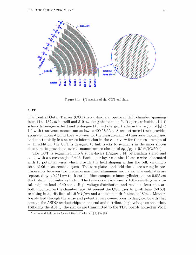
3.2. THE CDF EXPERIMENT 39
Figure 3.14: 1/6 section of the COT endplate.
COT
The Central Outer Tracker (COT) is a cylindrical open-cell drift chamber spanningfrom 44 to 132 cm in radii and 310 cm along the beamline6. It operates inside a 1.4 Tsolenoidal magnetic field and is designed to find charged tracks in the region of |η| <1.0 with transverse momentum as low as 400MeV/c. A reconstructed track providesaccurate information in the r−φ view for the measurement of transverse momentum,and substantially less accurate information in the r− z view for the measurement ofη. In addition, the COT is designed to link tracks to segments in the inner silicondetectors, to provide an overall momentum resolution of δpT/p
2T < 0.1%/(GeV/c).
The COT is segmented into 8 super-layers (Figure 3.14) alternating stereo andaxial, with a stereo angle of ±2o. Each super-layer contains 12 sense wires alternatedwith 13 potential wires which provide the field shaping within the cell, yielding atotal of 96 measurement layers. The wire planes and field sheets are strung in pre-cision slots between two precision machined aluminum endplates. The endplates areseparated by a 0.251 cm thick carbon-fiber composite inner cylinder and an 0.635 cmthick aluminum outer cylinder. The tension on each wire is 150 g resulting in a to-tal endplate load of 40 tons. High voltage distribution and readout electronics areboth mounted on the chamber face. At present the COT uses Argon-Ethane (50:50),resulting in a drift field of 1.9 keV/cm and a maximum drift time of 180ns. Mother-boards feed through the sense and potential wire connections to daughter boards thatcontain the ASDQ readout chips on one end and distribute high voltage on the other.Following the ASDQ, the signals are transmitted to the TDC boards housed in VME
6For more details on the Central Outer Tracker see [59] [65] [66]
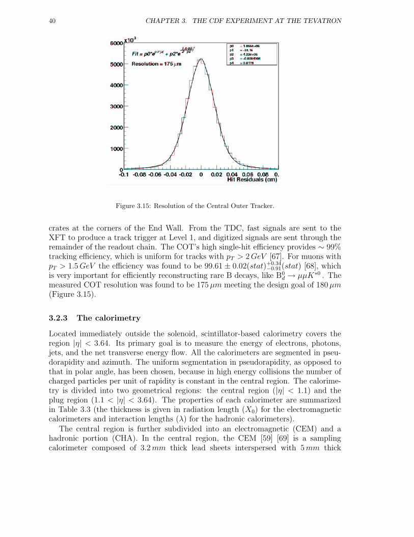
40 CHAPTER 3. THE CDF EXPERIMENT AT THE TEVATRON
Figure 3.15: Resolution of the Central Outer Tracker.
crates at the corners of the End Wall. From the TDC, fast signals are sent to theXFT to produce a track trigger at Level 1, and digitized signals are sent through theremainder of the readout chain. The COT’s high single-hit efficiency provides ∼ 99%tracking efficiency, which is uniform for tracks with pT > 2GeV [67]. For muons withpT > 1.5GeV the efficiency was found to be 99.61 ± 0.02(stat)+0.34
−0.91(stat) [68], whichis very important for efficiently reconstructing rare B decays, like B0
d → µµK∗0 . Themeasured COT resolution was found to be 175µm meeting the design goal of 180µm(Figure 3.15).
3.2.3 The calorimetry
Located immediately outside the solenoid, scintillator-based calorimetry covers theregion |η| < 3.64. Its primary goal is to measure the energy of electrons, photons,jets, and the net transverse energy flow. All the calorimeters are segmented in pseu-dorapidity and azimuth. The uniform segmentation in pseudorapidity, as opposed tothat in polar angle, has been chosen, because in high energy collisions the number ofcharged particles per unit of rapidity is constant in the central region. The calorime-try is divided into two geometrical regions: the central region (|η| < 1.1) and theplug region (1.1 < |η| < 3.64). The properties of each calorimeter are summarizedin Table 3.3 (the thickness is given in radiation length (X0) for the electromagneticcalorimeters and interaction lengths (λ) for the hadronic calorimeters).
The central region is further subdivided into an electromagnetic (CEM) and ahadronic portion (CHA). In the central region, the CEM [59] [69] is a samplingcalorimeter composed of 3.2mm thick lead sheets interspersed with 5mm thick
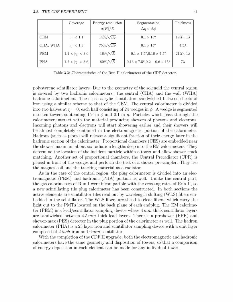
3.2. THE CDF EXPERIMENT 41
Coverage Energy resolution Segmentation Thickness
σ(E)/E ∆η × ∆φ
CEM |η| < 1.1 14%/√ET 0.1× 15o 19X0, 1λ
CHA, WHA |η| < 1.3 75%/√ET 0.1× 15o 4.5λ
PEM 1.1 < |η| < 3.6 16%/√E 0.1× 7.5o,0.16× 7.5o 21X0, 1λ
PHA 1.2 < |η| < 3.6 80%/√E 0.16× 7.5o,0.2 − 0.6 × 15o 7λ
Table 3.3: Characteristics of the Run II calorimeters of the CDF detector.
polystyrene scintillator layers. Due to the geometry of the solenoid the central regionis covered by two hadronic calorimeters: the central (CHA) and the wall (WHA)hadronic calorimeters. These use acrylic scintillators sandwiched between sheets ofiron using a similar scheme to that of the CEM. The central calorimeter is dividedinto two halves at η = 0, each half consisting of 24 wedges in φ. A wedge is segmentedinto ten towers subtending 15o in φ and 0.1 in η. Particles which pass through thecalorimeter interact with the material producing showers of photons and electrons.Incoming photons and electrons will start showering earlier and their showers willbe almost completely contained in the electromagnetic portion of the calorimeter.Hadrons (such as pions) will release a significant fraction of their energy later in thehadronic section of the calorimeter. Proportional chambers (CES) are embedded nearthe shower maximum about six radiation lengths deep into the EM calorimeters. Theydetermine the location of the incident particle within a tower and allow shower-trackmatching. Another set of proportional chambers, the Central Preradiator (CPR) isplaced in front of the wedges and perform the task of a shower presampler. They usethe magnet coil and the tracking material as a radiator.
As in the case of the central region, the plug calorimeter is divided into an elec-tromagnetic (PEM) and hadronic (PHA) portion as well. Unlike the central part,the gas calorimeters of Run I were incompatible with the crossing rates of Run II, soa new scintillating tile plug calorimeter has been constructed. In both sections theactive elements are scintillator tiles read out by wavelength shifting (WLS) fibers em-bedded in the scintillator. The WLS fibers are sliced to clear fibers, which carry thelight out to the PMTs located on the back plane of each endplug. The EM calorime-ter (PEM) is a lead/scintillator sampling device where 4mm thick scintillator layersare sandwiched between 4.5mm thick lead layers. There is a preshower (PPR) andshower-max (PES) detector in the plug portion of the calorimeter as well. The hadroncalorimeter (PHA) is a 23 layer iron and scintillator sampling device with a unit layercomposed of 2 inch iron and 6mm scintillator.
With the completion of the CDF II upgrade, both the electromagnetic and hadroniccalorimeters have the same geometry and disposition of towers, so that a comparisonof energy deposition in each element can be made for any individual tower.
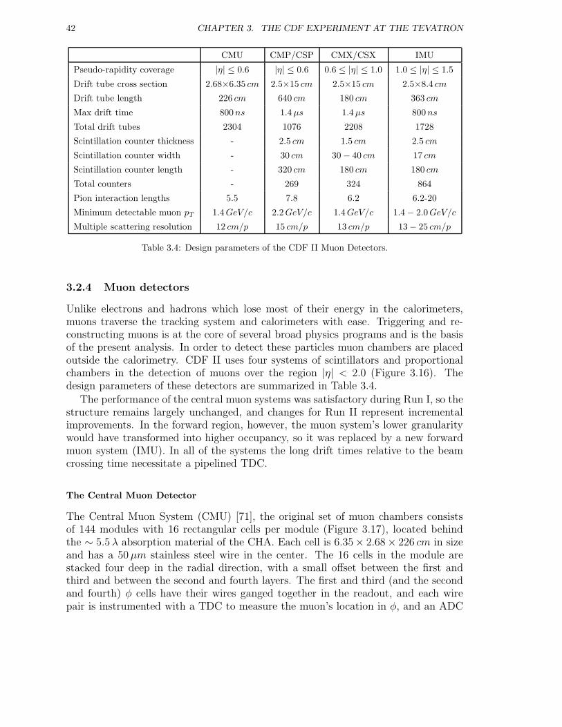
42 CHAPTER 3. THE CDF EXPERIMENT AT THE TEVATRON
CMU CMP/CSP CMX/CSX IMU
Pseudo-rapidity coverage |η| ≤ 0.6 |η| ≤ 0.6 0.6 ≤ |η| ≤ 1.0 1.0 ≤ |η| ≤ 1.5
Drift tube cross section 2.68×6.35 cm 2.5×15 cm 2.5×15 cm 2.5×8.4 cm
Drift tube length 226 cm 640 cm 180 cm 363 cm
Max drift time 800ns 1.4µs 1.4µs 800ns
Total drift tubes 2304 1076 2208 1728
Scintillation counter thickness - 2.5 cm 1.5 cm 2.5 cm
Scintillation counter width - 30 cm 30 − 40 cm 17 cm
Scintillation counter length - 320 cm 180 cm 180 cm
Total counters - 269 324 864
Pion interaction lengths 5.5 7.8 6.2 6.2-20
Minimum detectable muon pT 1.4GeV/c 2.2GeV/c 1.4GeV/c 1.4 − 2.0GeV/c
Multiple scattering resolution 12 cm/p 15 cm/p 13 cm/p 13− 25 cm/p
Table 3.4: Design parameters of the CDF II Muon Detectors.
3.2.4 Muon detectors
Unlike electrons and hadrons which lose most of their energy in the calorimeters,muons traverse the tracking system and calorimeters with ease. Triggering and re-constructing muons is at the core of several broad physics programs and is the basisof the present analysis. In order to detect these particles muon chambers are placedoutside the calorimetry. CDF II uses four systems of scintillators and proportionalchambers in the detection of muons over the region |η| < 2.0 (Figure 3.16). Thedesign parameters of these detectors are summarized in Table 3.4.
The performance of the central muon systems was satisfactory during Run I, so thestructure remains largely unchanged, and changes for Run II represent incrementalimprovements. In the forward region, however, the muon system’s lower granularitywould have transformed into higher occupancy, so it was replaced by a new forwardmuon system (IMU). In all of the systems the long drift times relative to the beamcrossing time necessitate a pipelined TDC.
The Central Muon Detector
The Central Muon System (CMU) [71], the original set of muon chambers consistsof 144 modules with 16 rectangular cells per module (Figure 3.17), located behindthe ∼ 5.5λ absorption material of the CHA. Each cell is 6.35× 2.68× 226 cm in sizeand has a 50µm stainless steel wire in the center. The 16 cells in the module arestacked four deep in the radial direction, with a small offset between the first andthird and between the second and fourth layers. The first and third (and the secondand fourth) φ cells have their wires ganged together in the readout, and each wirepair is instrumented with a TDC to measure the muon’s location in φ, and an ADC
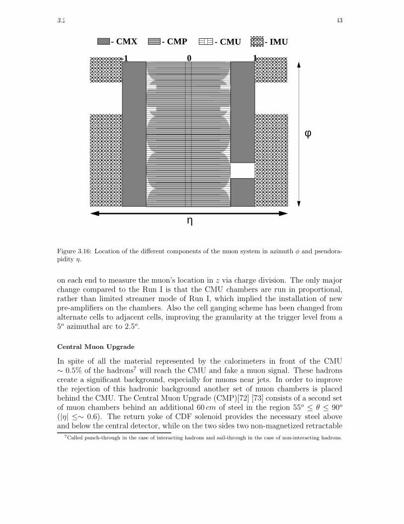
3.2. THE CDF EXPERIMENT 43
- CMX - CMP - CMU
φ
η
0 1-1 � � � � � � � � � � � � � � � � � � � � � � � � � � � � � � � � � � � � � �� � � � � � � � � � � � � � � � � � � � � � � � � � � � � � � � � � � � � �� � � � � � � � � � � � � � � � � � � � � � � � � � � � � � � � � � � � � �� � � � � � � � � � � � � � � � � � � � � � � � � � � � � � � � � � � � � �� � � � � � � � � � � � � � � � � � � � � � � � � � � � � � � � � � � � � �
� � � � � � � � � � � � � � � � � � � � � � � � � � � � � � � � � � � � � � �� � � � � � � � � � � � � � � � � � � � � � � � � � � � � � � � � � � � � � �� � � � � � � � � � � � � � � � � � � � � � � � � � � � � � � � � � � � � � �� � � � � � � � � � � � � � � � � � � � � � � � � � � � � � � � � � � � � � �� � � � � � � � � � � � � � � � � � � � � � � � � � � � � � � � � � � � � � �� � � � � � � � � � � � � � � � � � � � � � � � � � � � � � � � � � � � � � �� � � � � � � � � � � � � � � � � � � � � � � � � � � � � � � � � � � � � � �� � � � � � � � � � � � � � � � � � � � � � � � � � � � � � � � � � � � � � �� � � � � � � � � � � � � � � � � � � � � � � � � � � � � � � � � � � � � � �� � � � � � � � � � � � � � � � � � � � � � � � � � � � � � � � � � � � � � �� � � � � � � � � � � � � � � � � � � � � � � � � � � � � � � � � � � � � � �� � � � � � � � � � � � � � � � � � � � � � � � � � � � � � � � � � � � � � �� � � � � � � � � � � � � � � � � � � � � � � � � � � � � � � � � � � � � � �� � � � � � � � � � � � � � � � � � � � � � � � � � � � � � � � � � � � � � �� � � � � � � � � � � � � � � � � � � � � � � � � � � � � � � � � � � � � � �� � � � � � � � � � � � � � � � � � � � � � � � � � � � � � � � � � � � � � �� � � � � � � � � � � � � � � � � � � � � � � � � � � � � � � � � � � � � � �� � � � � � � � � � � � � � � � � � � � � � � � � � � � � � � � � � � � � � �
� � � � � � � � � � � � � � � � � � � � � � � � � � � � � � � � � � � � � �� � � � � � � � � � � � � � � � � � � � � � � � � � � � � � � � � � � � � �� � � � � � � � � � � � � � � � � � � � � � � � � � � � � � � � � � � � � �� � � � � � � � � � � � � � � � � � � � � � � � � � � � � � � � � � � � � �� � � � � � � � � � � � � � � � � � � � � � � � � � � � � � � � � � � � � �
� � � � � � � � � � � � � � � � � � � � � � � � � � � � � � � � � � � � � �� � � � � � � � � � � � � � � � � � � � � � � � � � � � � � � � � � � � � �� � � � � � � � � � � � � � � � � � � � � � � � � � � � � � � � � � � � � �� � � � � � � � � � � � � � � � � � � � � � � � � � � � � � � � � � � � � �� � � � � � � � � � � � � � � � � � � � � � � � � � � � � � � � � � � � � �� � � � � � � � � � � � � � � � � � � � � � � � � � � � � � � � � � � � � �� � � � � � � � � � � � � � � � � � � � � � � � � � � � � � � � � � � � � �� � � � � � � � � � � � � � � � � � � � � � � � � � � � � � � � � � � � � �� � � � � � � � � � � � � � � � � � � � � � � � � � � � � � � � � � � � � �� � � � � � � � � � � � � � � � � � � � � � � � � � � � � � � � � � � � � �� � � � � � � � � � � � � � � � � � � � � � � � � � � � � � � � � � � � � �� � � � � � � � � � � � � � � � � � � � � � � � � � � � � � � � � � � � � �� � � � � � � � � � � � � � � � � � � � � � � � � � � � � � � � � � � � � �� � � � � � � � � � � � � � � � � � � � � � � � � � � � � � � � � � � � � �� � � � � � � � � � � � � � � � � � � � � � � � � � � � � � � � � � � � � �� � � � � � � � � � � � � � � � � � � � � � � � � � � � � � � � � � � � � �� � � � � � � � � � � � � � � � � � � � � � � � � � � � � � � � � � � � � �� � � � � � � � � � � � � � � � � � � � � � � � � � � � � � � � � � � � � �
� � � � � � � � � � � � � � �� � � � � � � � � � � � � � � - IMU
Figure 3.16: Location of the different components of the muon system in azimuth φ and pseudora-pidity η.
on each end to measure the muon’s location in z via charge division. The only majorchange compared to the Run I is that the CMU chambers are run in proportional,rather than limited streamer mode of Run I, which implied the installation of newpre-amplifiers on the chambers. Also the cell ganging scheme has been changed fromalternate cells to adjacent cells, improving the granularity at the trigger level from a5o azimuthal arc to 2.5o.
Central Muon Upgrade
In spite of all the material represented by the calorimeters in front of the CMU∼ 0.5% of the hadrons7 will reach the CMU and fake a muon signal. These hadronscreate a significant background, especially for muons near jets. In order to improvethe rejection of this hadronic background another set of muon chambers is placedbehind the CMU. The Central Muon Upgrade (CMP)[72] [73] consists of a second setof muon chambers behind an additional 60 cm of steel in the region 55o ≤ θ ≤ 90o
(|η| ≤∼ 0.6). The return yoke of CDF solenoid provides the necessary steel aboveand below the central detector, while on the two sides two non-magnetized retractable
7Called punch-through in the case of interacting hadrons and sail-through in the case of non-interacting hadrons.
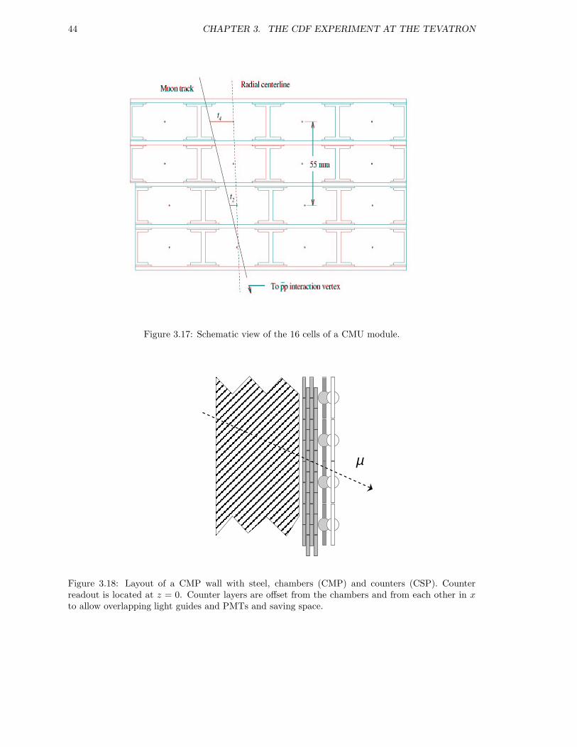
44 CHAPTER 3. THE CDF EXPERIMENT AT THE TEVATRON
Figure 3.17: Schematic view of the 16 cells of a CMU module.
µ
Figure 3.18: Layout of a CMP wall with steel, chambers (CMP) and counters (CSP). Counterreadout is located at z = 0. Counter layers are offset from the chambers and from each other in xto allow overlapping light guides and PMTs and saving space.
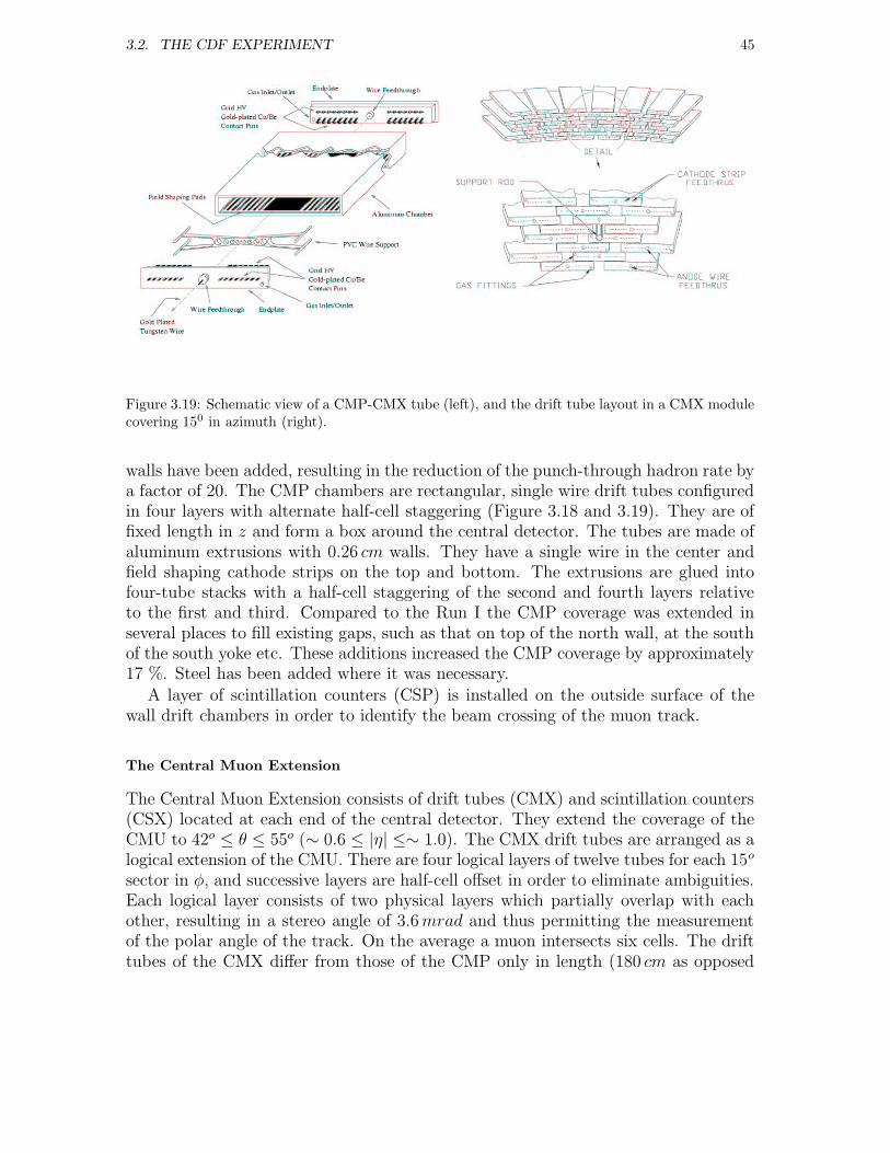
3.2. THE CDF EXPERIMENT 45
Figure 3.19: Schematic view of a CMP-CMX tube (left), and the drift tube layout in a CMX modulecovering 150 in azimuth (right).
walls have been added, resulting in the reduction of the punch-through hadron rate bya factor of 20. The CMP chambers are rectangular, single wire drift tubes configuredin four layers with alternate half-cell staggering (Figure 3.18 and 3.19). They are offixed length in z and form a box around the central detector. The tubes are made ofaluminum extrusions with 0.26 cm walls. They have a single wire in the center andfield shaping cathode strips on the top and bottom. The extrusions are glued intofour-tube stacks with a half-cell staggering of the second and fourth layers relativeto the first and third. Compared to the Run I the CMP coverage was extended inseveral places to fill existing gaps, such as that on top of the north wall, at the southof the south yoke etc. These additions increased the CMP coverage by approximately17 %. Steel has been added where it was necessary.
A layer of scintillation counters (CSP) is installed on the outside surface of thewall drift chambers in order to identify the beam crossing of the muon track.
The Central Muon Extension
The Central Muon Extension consists of drift tubes (CMX) and scintillation counters(CSX) located at each end of the central detector. They extend the coverage of theCMU to 42o ≤ θ ≤ 55o (∼ 0.6 ≤ |η| ≤∼ 1.0). The CMX drift tubes are arranged as alogical extension of the CMU. There are four logical layers of twelve tubes for each 15o
sector in φ, and successive layers are half-cell offset in order to eliminate ambiguities.Each logical layer consists of two physical layers which partially overlap with eachother, resulting in a stereo angle of 3.6mrad and thus permitting the measurementof the polar angle of the track. On the average a muon intersects six cells. The drifttubes of the CMX differ from those of the CMP only in length (180 cm as opposed
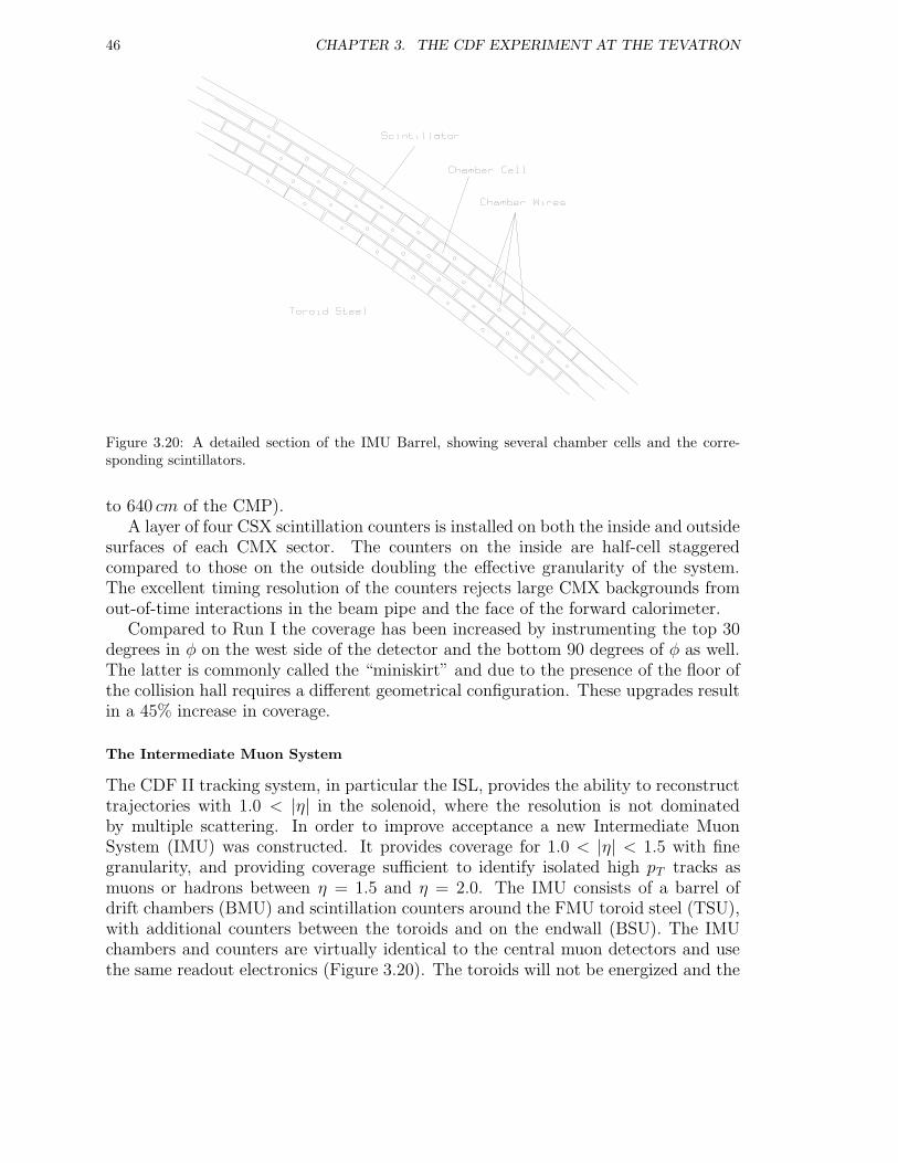
46 CHAPTER 3. THE CDF EXPERIMENT AT THE TEVATRON
Figure 3.20: A detailed section of the IMU Barrel, showing several chamber cells and the corre-sponding scintillators.
to 640 cm of the CMP).A layer of four CSX scintillation counters is installed on both the inside and outside
surfaces of each CMX sector. The counters on the inside are half-cell staggeredcompared to those on the outside doubling the effective granularity of the system.The excellent timing resolution of the counters rejects large CMX backgrounds fromout-of-time interactions in the beam pipe and the face of the forward calorimeter.
Compared to Run I the coverage has been increased by instrumenting the top 30degrees in φ on the west side of the detector and the bottom 90 degrees of φ as well.The latter is commonly called the “miniskirt” and due to the presence of the floor ofthe collision hall requires a different geometrical configuration. These upgrades resultin a 45% increase in coverage.
The Intermediate Muon System
The CDF II tracking system, in particular the ISL, provides the ability to reconstructtrajectories with 1.0 < |η| in the solenoid, where the resolution is not dominatedby multiple scattering. In order to improve acceptance a new Intermediate MuonSystem (IMU) was constructed. It provides coverage for 1.0 < |η| < 1.5 with finegranularity, and providing coverage sufficient to identify isolated high pT tracks asmuons or hadrons between η = 1.5 and η = 2.0. The IMU consists of a barrel ofdrift chambers (BMU) and scintillation counters around the FMU toroid steel (TSU),with additional counters between the toroids and on the endwall (BSU). The IMUchambers and counters are virtually identical to the central muon detectors and usethe same readout electronics (Figure 3.20). The toroids will not be energized and the
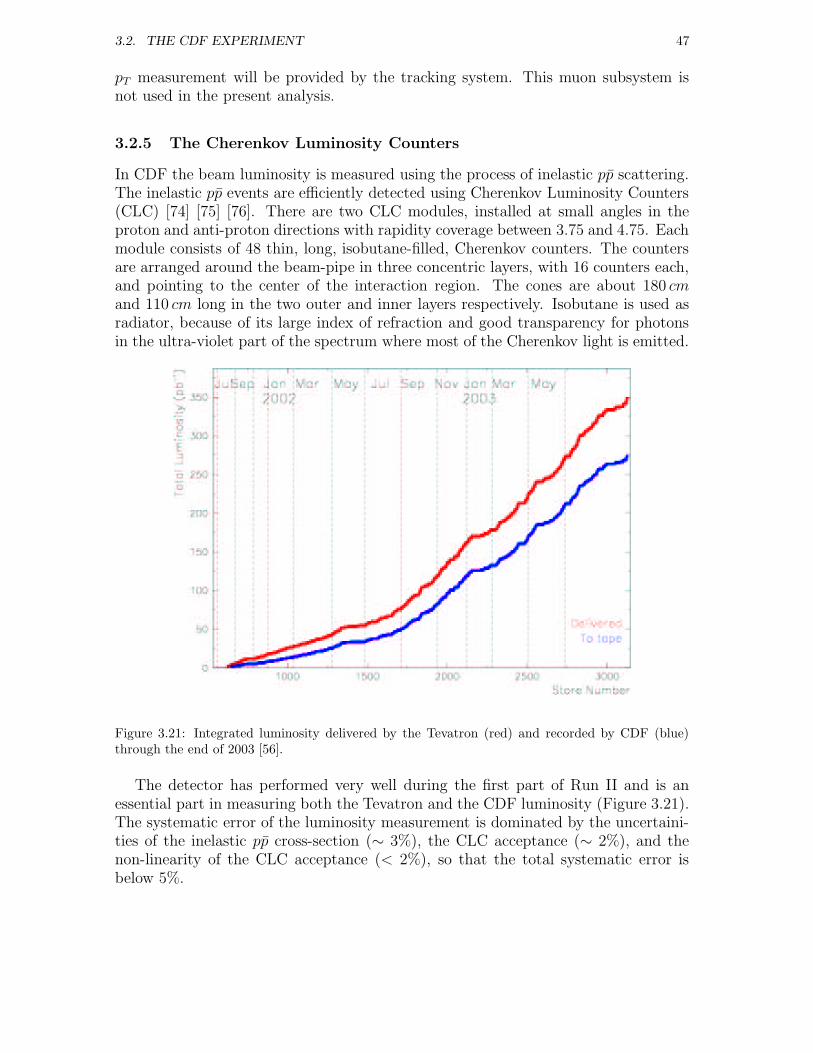
3.2. THE CDF EXPERIMENT 47
pT measurement will be provided by the tracking system. This muon subsystem isnot used in the present analysis.
3.2.5 The Cherenkov Luminosity Counters
In CDF the beam luminosity is measured using the process of inelastic pp scattering.The inelastic pp events are efficiently detected using Cherenkov Luminosity Counters(CLC) [74] [75] [76]. There are two CLC modules, installed at small angles in theproton and anti-proton directions with rapidity coverage between 3.75 and 4.75. Eachmodule consists of 48 thin, long, isobutane-filled, Cherenkov counters. The countersare arranged around the beam-pipe in three concentric layers, with 16 counters each,and pointing to the center of the interaction region. The cones are about 180 cmand 110 cm long in the two outer and inner layers respectively. Isobutane is used asradiator, because of its large index of refraction and good transparency for photonsin the ultra-violet part of the spectrum where most of the Cherenkov light is emitted.
Figure 3.21: Integrated luminosity delivered by the Tevatron (red) and recorded by CDF (blue)through the end of 2003 [56].
The detector has performed very well during the first part of Run II and is anessential part in measuring both the Tevatron and the CDF luminosity (Figure 3.21).The systematic error of the luminosity measurement is dominated by the uncertaini-ties of the inelastic pp cross-section (∼ 3%), the CLC acceptance (∼ 2%), and thenon-linearity of the CLC acceptance (< 2%), so that the total systematic error isbelow 5%.
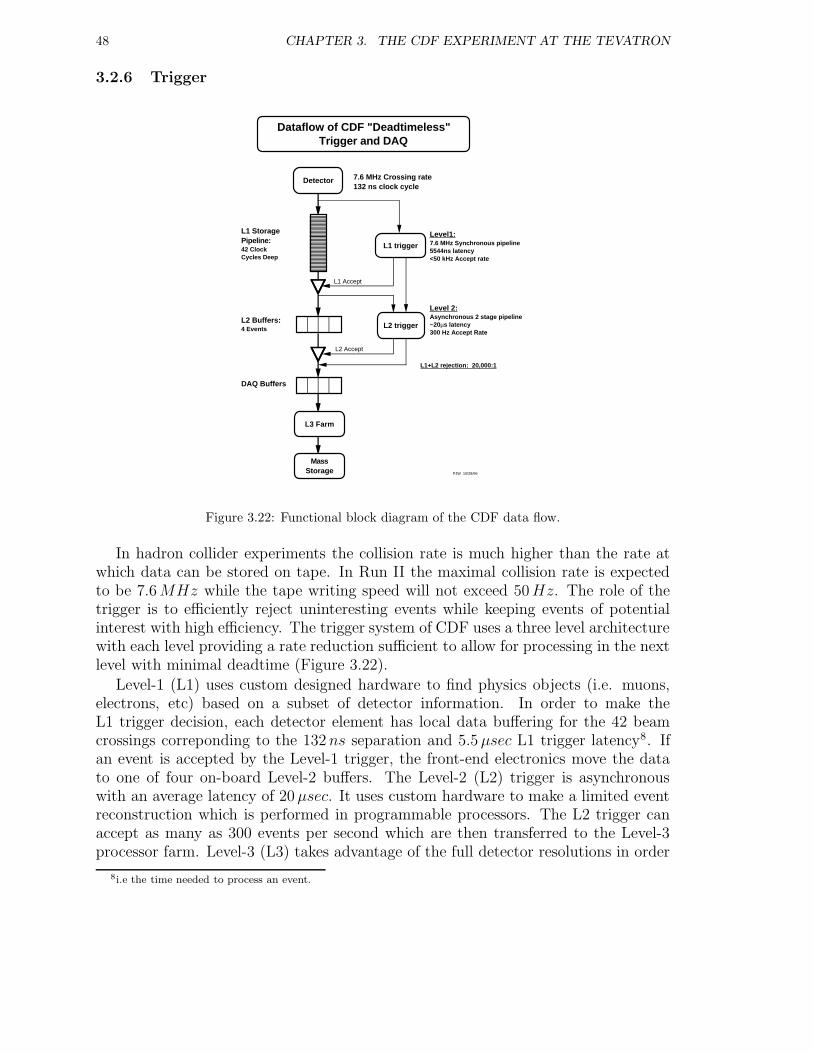
48 CHAPTER 3. THE CDF EXPERIMENT AT THE TEVATRON
3.2.6 Trigger
L2 trigger
Detector
L3 Farm
MassStorage
L1 Accept
Level 2:Asynchronous 2 stage pipeline~20µs latency300 Hz Accept Rate
L1+L2 rejection: 20,000:1
7.6 MHz Crossing rate132 ns clock cycle
L1 trigger
Level1:7.6 MHz Synchronous pipeline5544ns latency<50 kHz Accept rate
L2 Accept
L1 StoragePipeline:42 Clock Cycles Deep
L2 Buffers: 4 Events
DAQ Buffers
PJW 10/28/96
Dataflow of CDF "Deadtimeless" Trigger and DAQ
Figure 3.22: Functional block diagram of the CDF data flow.
In hadron collider experiments the collision rate is much higher than the rate atwhich data can be stored on tape. In Run II the maximal collision rate is expectedto be 7.6MHz while the tape writing speed will not exceed 50Hz. The role of thetrigger is to efficiently reject uninteresting events while keeping events of potentialinterest with high efficiency. The trigger system of CDF uses a three level architecturewith each level providing a rate reduction sufficient to allow for processing in the nextlevel with minimal deadtime (Figure 3.22).
Level-1 (L1) uses custom designed hardware to find physics objects (i.e. muons,electrons, etc) based on a subset of detector information. In order to make theL1 trigger decision, each detector element has local data buffering for the 42 beamcrossings correponding to the 132ns separation and 5.5µsec L1 trigger latency8. Ifan event is accepted by the Level-1 trigger, the front-end electronics move the datato one of four on-board Level-2 buffers. The Level-2 (L2) trigger is asynchronouswith an average latency of 20µsec. It uses custom hardware to make a limited eventreconstruction which is performed in programmable processors. The L2 trigger canaccept as many as 300 events per second which are then transferred to the Level-3processor farm. Level-3 (L3) takes advantage of the full detector resolutions in order
8i.e the time needed to process an event.
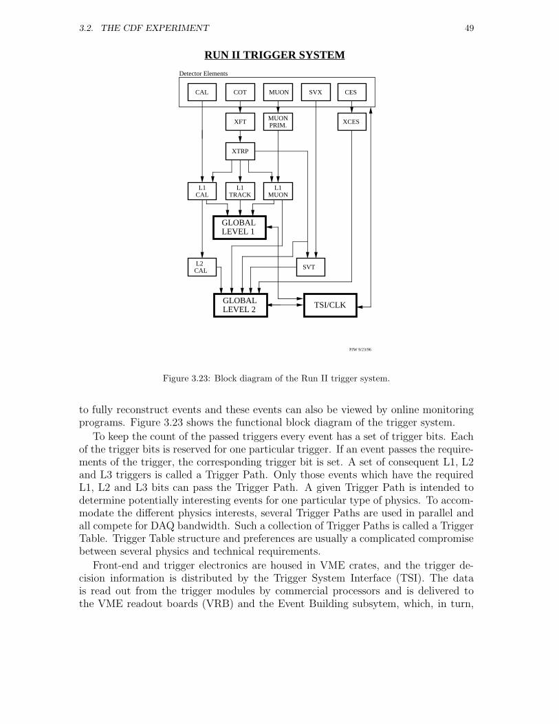
3.2. THE CDF EXPERIMENT 49
RUN II TRIGGER SYSTEM
Detector Elements
GLOBAL LEVEL 1
L1 CAL
COT
XFT
MUON
MUONPRIM.
L1MUON
L2 CAL
CAL
XTRP
L1TRACK
SVX
SVT
CES
XCES
PJW 9/23/96
GLOBAL LEVEL 2 TSI/CLK
Figure 3.23: Block diagram of the Run II trigger system.
to fully reconstruct events and these events can also be viewed by online monitoringprograms. Figure 3.23 shows the functional block diagram of the trigger system.
To keep the count of the passed triggers every event has a set of trigger bits. Eachof the trigger bits is reserved for one particular trigger. If an event passes the require-ments of the trigger, the corresponding trigger bit is set. A set of consequent L1, L2and L3 triggers is called a Trigger Path. Only those events which have the requiredL1, L2 and L3 bits can pass the Trigger Path. A given Trigger Path is intended todetermine potentially interesting events for one particular type of physics. To accom-modate the different physics interests, several Trigger Paths are used in parallel andall compete for DAQ bandwidth. Such a collection of Trigger Paths is called a TriggerTable. Trigger Table structure and preferences are usually a complicated compromisebetween several physics and technical requirements.
Front-end and trigger electronics are housed in VME crates, and the trigger de-cision information is distributed by the Trigger System Interface (TSI). The datais read out from the trigger modules by commercial processors and is delivered tothe VME readout boards (VRB) and the Event Building subsytem, which, in turn,

50 CHAPTER 3. THE CDF EXPERIMENT AT THE TEVATRON
concentrates and delivers the data to the L3 trigger subsystem. L3 is a “farm” ofcommercial parallel processors, where each event is processed by a single processor.Finally, the Data Logging system writes the events to mass storage and a subset ofevents to the DAQ monitoring system.
Level 1
The L1 hardware consists of three parallel synchronous processing streams whichoutput their data to the Global L1 processing unit. One of the streams finds muons(MUON PRIM and L1 MUON of Figure 3.23), another one finds calorimeter basedobjects (L1 CAL), and the third one finds tracks in the COT (XFT - XTRP - L1TRACK). This latter is the most significant change from Run I, as previously trackfinding was available only at L2. As the muon and electron triggers require a trackpointing at the corresponding detector element, the tracks are also fed to the muonand calorimeter streams. Up to 64 different triggers can be formed using simple ANDsand ORs of objects from these streams. The decision is made every 132ns by theGlobal L1 unit.
The addition of the eXtremely Fast Tracker (XFT) is a significant improvementover Run I where tracks were available only at L2. The XFT is highly parallel andprocesses data from each bunch crossing. The tracking results from the XFT areavailable fast enough so that they can be used in L1 trigger decisions. Its track-finding efficiency is 96 % for tracks with pT > 1.5GeV , the momentum resolutionis σ(1/pT ) = 1.7%/GeV , and the resolution in φ0 is 5mrad [77]. The latter is veryimportant for the present analysis as XFT tracks will be used as the seed for the SVTat L2. Track identification is accomplished in two subsystems, the Finder and theLinker. The Finder searches for high-pT track segments in each of the outer-four axialsuperlayers of the COT. Each found segment is characterized by a mean φ position inthe axial SL. The Linker then searches for a four-out-of-four match among segmentsin the four layers, consistent with a prompt high-pT track. The XFT divides the COTinto 288 segments, each covering 1.25 degrees, with one track allowed per segment.Each XFT board sends its list of tracks to the extrapolation unit (XTRP), whichdistributes the tracks or information derived from the tracks to the L1 and L2 triggersubsystems.
The calorimeter triggers are divided into object triggers (electrons, photons andjets) and global triggers (
∑ET and E/T ). In the case of the object triggers the thresh-
olds are applied to individual calorimeter trigger towers, while in the case of the globaltriggers those thresholds are applied after summing energies over all towers. Some ofthe calorimeter triggers use track information in order to reduce the trigger rate. Forexample, in the case of the low-ET electron trigger tracks from the L1 track processor(XFT) are available for matching to the tower, and towers with significant hadronicenergy can be rejected.
A muon trigger is defined as a muon stub match with an associated XFT track.A muon stub is defined as a pattern of hits in the muon chambers consistent withthe passage of a charged particle. CMU and CMX stubs represent a pair of hits on
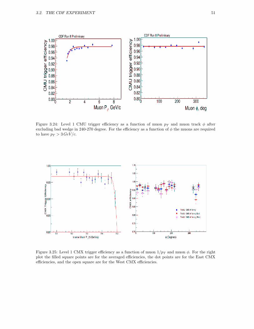
3.2. THE CDF EXPERIMENT 51
Figure 3.24: Level 1 CMU trigger efficiency as a function of muon pT and muon track φ afterexcluding bad wedge in 240-270 degree. For the efficiency as a function of φ the muons are requiredto have pT > 3GeV/c.
Figure 3.25: Level 1 CMX trigger efficiency as a function of muon 1/pT and muon φ. For the rightplot the filled square points are for the averaged efficiencies, the dot points are for the East CMXefficiencies, and the open square are for the West CMX efficiencies.
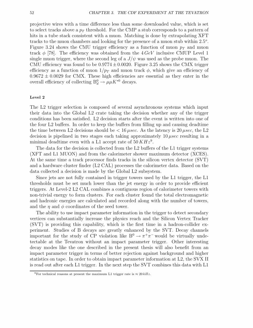
52 CHAPTER 3. THE CDF EXPERIMENT AT THE TEVATRON
projective wires with a time difference less than some downloaded value, which is setto select tracks above a pT threshold. For the CMP a stub corresponds to a pattern ofhits in a tube stack consistent with a muon. Matching is done by extrapolating XFTtracks to the muon chambers and looking for the presence of a muon stub within 2.5o.Figure 3.24 shows the CMU trigger efficiency as a function of muon pT and muontrack φ [78]. The efficiency was obtained from the 4GeV inclusive CMUP Level 1single muon trigger, where the second leg of a J/ψ was used as the probe muon. TheCMU efficiency was found to be 0.9774± 0.0020. Figure 3.25 shows the CMX triggerefficiency as a function of muon 1/pT and muon track φ, which give an efficiency of0.9672 ± 0.0029 for CMX. These high efficiencies are essential as they enter in theoverall efficiency of collecting B0
d → µµK∗0 decays.
Level 2
The L2 trigger selection is composed of several asynchronous systems which inputtheir data into the Global L2 crate taking the decision whether any of the triggerconditions has been satisfied. L2 decision starts after the event is written into one ofthe four L2 buffers. In order to keep the buffers from filling up and causing deadtimethe time between L2 decisions should be < 16µsec. As the latency is 20µsec, the L2decision is pipelined in two stages each taking approximately 10µsec resulting in aminimal deadtime even with a L1 accept rate of 50KHz9.
The data for the decision is collected from the L2 buffers of the L1 trigger systems(XFT and L1 MUON) and from the calorimeter shower maximum detector (XCES).At the same time a track processor finds tracks in the silicon vertex detector (SVT)and a hardware cluster finder (L2 CAL) processes the calorimeter data. Based on thedata collected a decision is made by the Global L2 subsystem.
Since jets are not fully contained in trigger towers used by the L1 trigger, the L1thresholds must be set much lower than the jet energy in order to provide efficienttriggers. At Level-2 L2 CAL combines a contiguous region of calorimeter towers withnon-trivial energy to form clusters. For each cluster found the total electromagneticand hadronic energies are calculated and recorded along with the number of towers,and the η and φ coordinates of the seed tower.
The ability to use impact parameter information in the trigger to detect secondaryvertices can substantially increase the physics reach and the Silicon Vertex Tracker(SVT) is providing this capability, which is the first time in a hadron-collider ex-periment. Studies of B decays are greatly enhanced by the SVT. Decay channelsimportant for the study of CP violation like B0 → π+π− would be virtually unde-tectable at the Tevatron without an impact parameter trigger. Other interestingdecay modes like the one described in the present thesis will also benefit from animpact parameter trigger in terms of better rejection against background and higherstatistics on tape. In order to obtain impact parameter information at L2, the SVX IIis read out after each L1 trigger. In the next step the SVT combines this data with L1
9For technical reasons at present the maximum L1 trigger rate is ≈ 20 kHz.
3.2. THE CDF EXPERIMENT 53
SVX-II
COT
XFT
digitization
Hit Finder
Associative
Memory
Hit Buffer
TrackFitter
L2 Decision
Tracks
Clusters
Roads
XFT
SVX
L1
L2
TrackPacket
Tracks
Figure 3.26: Architecture of the SVT trigger.
tracking information from the XFT and computes track parameters with resolutionand efficiency comparable to full offline analysis10.
The SVT has been implemented on custom design VME 9U boards, organized in 12identical subsystems, corresponding to the 12 wedges of the SVX along the azimuthalangle. After tracking information is received from SVX II it is fed to the Hit Finderboards (Figure 3.26). The Hit Finder performs pedestal subtraction and bad channelsuppression. It then scans the data for clusters of hit strips. As soon as clusters sa-tisfying the requirements are found, the centroid of the cluster and the most probabletrack intersection point at that SVX layer is computed. In the meantime, the listof tracks found by the XTRP is transmitted to the Associative Memory Sequencer(AMS). As soon as the clusters from the Hit Finder are available from the output of theMerger, they are also transmitted to the Associative Memory Sequencer. The AMSuses a lookup table to convert the 14-bit cluster centroid into a coarser Superstripin preparation for the pattern recognition stage11 and transmits the information tothe Associative Memory (AM) boards. On the AM boards each chip stores 128combinations of outer tracks and coarse SVX hits. Each combination represents alegitimate particle trajectory and is called a road. The roads are programmable, so
10Unfortunately, during the initial period of running there several parts of the SVT system were brought intofunctioning gradually. That means during the initial period of running the acceptance of the SVT was significantlylower than expected.
11The size of the Superstrip is programmable.
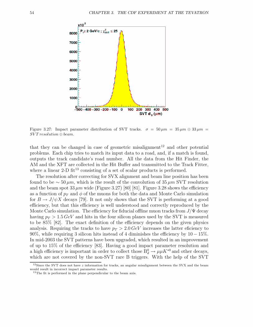
54 CHAPTER 3. THE CDF EXPERIMENT AT THE TEVATRON
Figure 3.27: Impact parameter distribution of SVT tracks. σ = 50µm = 35µm ⊕ 33µm =SV T resolution⊕ beam.
that they can be changed in case of geometric misalignment12 and other potentialproblems. Each chip tries to match its input data to a road, and, if a match is found,outputs the track candidate’s road number. All the data from the Hit Finder, theAM and the XFT are collected in the Hit Buffer and transmitted to the Track Fitter,where a linear 2-D fit13 consisting of a set of scalar products is performed.
The resolution after correcting for SVX alignment and beam line position has beenfound to be ∼ 50µm, which is the result of the convolution of 35µm SVT resolutionand the beam spot 33µm wide (Figure 3.27) [80] [81]. Figure 3.28 shows the efficiencyas a function of pT and φ of the muons for both the data and Monte Carlo simulationfor B → J/ψX decays [79]. It not only shows that the SVT is performing at a goodefficiency, but that this efficiency is well understood and correctly reproduced by theMonte Carlo simulation. The efficiency for fiducial offline muon tracks from J/Ψ decayhaving pT > 1.5GeV and hits in the four silicon planes used by the SVT is measuredto be 85% [82]. The exact definition of the efficiency depends on the given physicsanalysis. Requiring the tracks to have pT > 2.0GeV increases the latter eficiency to90%, while requiring 3 silicon hits instead of 4 diminishes the efficiency by 10− 15%.In mid-2003 the SVT patterns have been upgraded, which resulted in an improvementof up to 15% of the efficiency [83]. Having a good impact parameter resolution anda high efficiency is important in order to collect those B0
d → µµK∗0 and other decays,which are not covered by the non-SVT rare B triggers. With the help of the SVT
12Since the SVT does not have z information for tracks, an angular misalignment between the SVX and the beamwould result in incorrect impact parameter results.
13The fit is performed in the plane perpendicular to the beam axis.
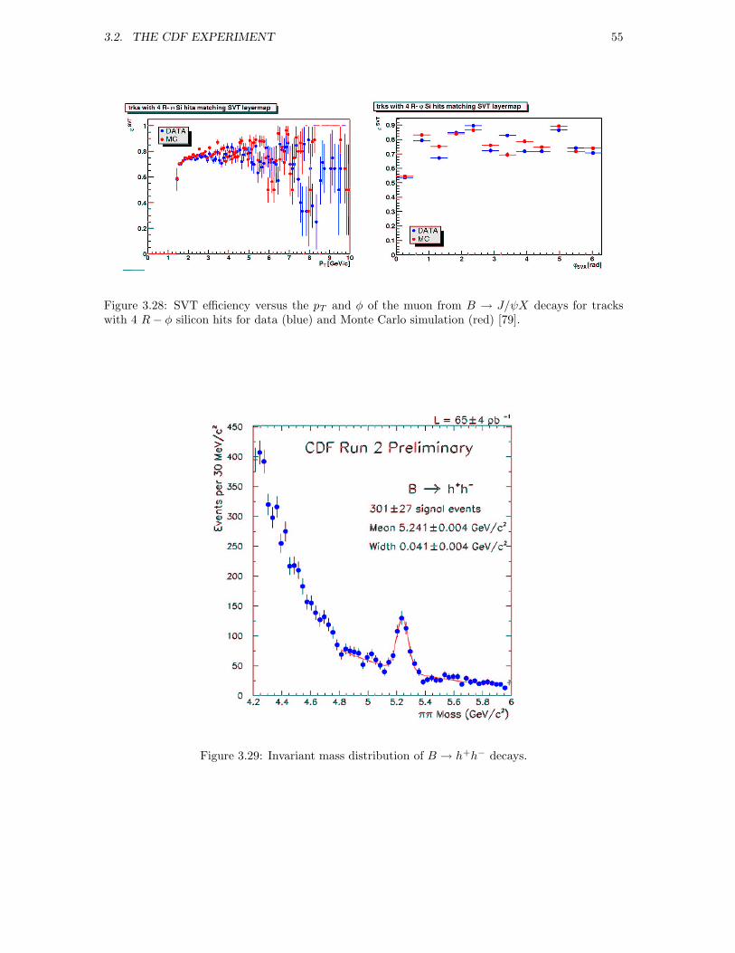
3.2. THE CDF EXPERIMENT 55
Figure 3.28: SVT efficiency versus the pT and φ of the muon from B → J/ψX decays for trackswith 4 R− φ silicon hits for data (blue) and Monte Carlo simulation (red) [79].
Figure 3.29: Invariant mass distribution of B → h+h− decays.
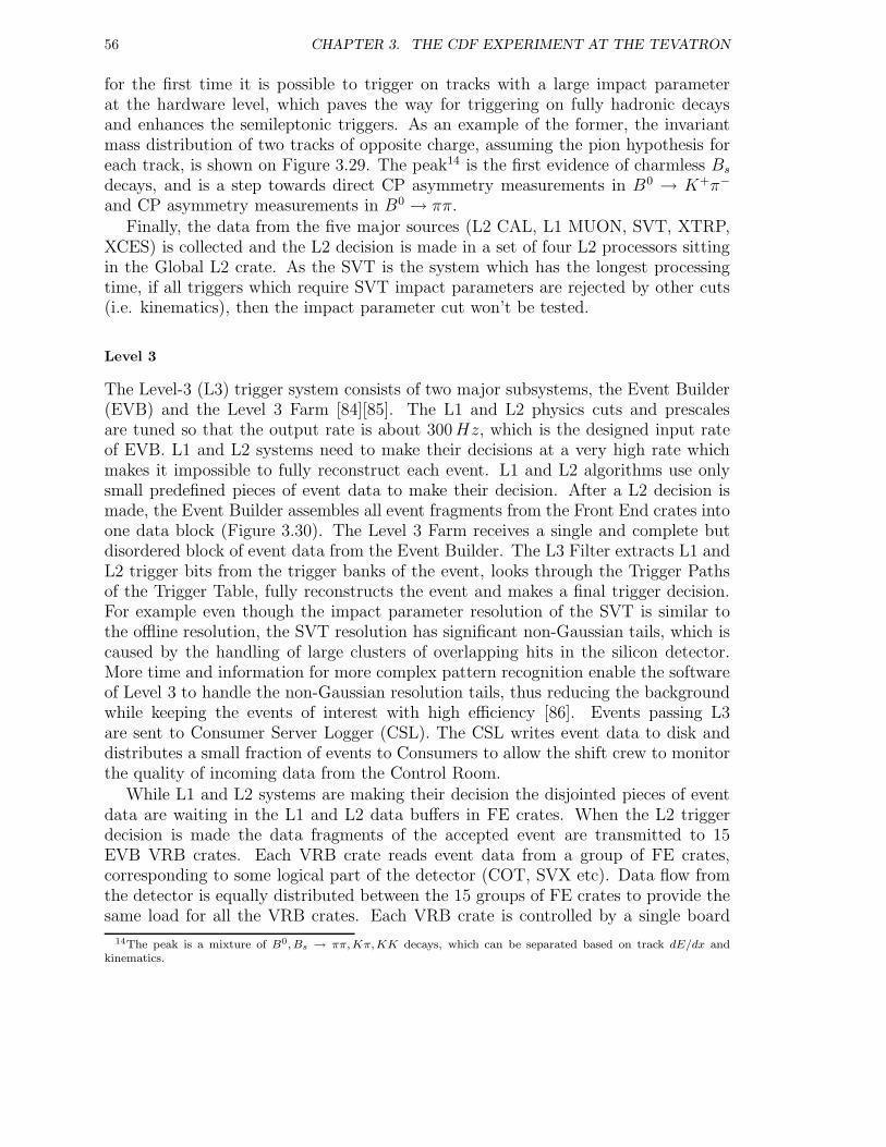
56 CHAPTER 3. THE CDF EXPERIMENT AT THE TEVATRON
for the first time it is possible to trigger on tracks with a large impact parameterat the hardware level, which paves the way for triggering on fully hadronic decaysand enhances the semileptonic triggers. As an example of the former, the invariantmass distribution of two tracks of opposite charge, assuming the pion hypothesis foreach track, is shown on Figure 3.29. The peak14 is the first evidence of charmless Bs
decays, and is a step towards direct CP asymmetry measurements in B0 → K+π−
and CP asymmetry measurements in B0 → ππ.Finally, the data from the five major sources (L2 CAL, L1 MUON, SVT, XTRP,
XCES) is collected and the L2 decision is made in a set of four L2 processors sittingin the Global L2 crate. As the SVT is the system which has the longest processingtime, if all triggers which require SVT impact parameters are rejected by other cuts(i.e. kinematics), then the impact parameter cut won’t be tested.
Level 3
The Level-3 (L3) trigger system consists of two major subsystems, the Event Builder(EVB) and the Level 3 Farm [84][85]. The L1 and L2 physics cuts and prescalesare tuned so that the output rate is about 300Hz, which is the designed input rateof EVB. L1 and L2 systems need to make their decisions at a very high rate whichmakes it impossible to fully reconstruct each event. L1 and L2 algorithms use onlysmall predefined pieces of event data to make their decision. After a L2 decision ismade, the Event Builder assembles all event fragments from the Front End crates intoone data block (Figure 3.30). The Level 3 Farm receives a single and complete butdisordered block of event data from the Event Builder. The L3 Filter extracts L1 andL2 trigger bits from the trigger banks of the event, looks through the Trigger Pathsof the Trigger Table, fully reconstructs the event and makes a final trigger decision.For example even though the impact parameter resolution of the SVT is similar tothe offline resolution, the SVT resolution has significant non-Gaussian tails, which iscaused by the handling of large clusters of overlapping hits in the silicon detector.More time and information for more complex pattern recognition enable the softwareof Level 3 to handle the non-Gaussian resolution tails, thus reducing the backgroundwhile keeping the events of interest with high efficiency [86]. Events passing L3are sent to Consumer Server Logger (CSL). The CSL writes event data to disk anddistributes a small fraction of events to Consumers to allow the shift crew to monitorthe quality of incoming data from the Control Room.
While L1 and L2 systems are making their decision the disjointed pieces of eventdata are waiting in the L1 and L2 data buffers in FE crates. When the L2 triggerdecision is made the data fragments of the accepted event are transmitted to 15EVB VRB crates. Each VRB crate reads event data from a group of FE crates,corresponding to some logical part of the detector (COT, SVX etc). Data flow fromthe detector is equally distributed between the 15 groups of FE crates to provide thesame load for all the VRB crates. Each VRB crate is controlled by a single board
14The peak is a mixture of B0, Bs → ππ,Kπ,KK decays, which can be separated based on track dE/dx andkinematics.
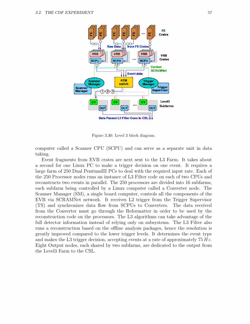
3.2. THE CDF EXPERIMENT 57
Figure 3.30: Level 3 block diagram.
computer called a Scanner CPU (SCPU) and can serve as a separate unit in datataking.
Event fragments from EVB crates are next sent to the L3 Farm. It takes abouta second for one Linux PC to make a trigger decision on one event. It requires alarge farm of 250 Dual PentiumIII PCs to deal with the required input rate. Each ofthe 250 Processor nodes runs an instance of L3 Filter code on each of two CPUs andreconstructs two events in parallel. The 250 processors are divided into 16 subfarms,each subfarm being controlled by a Linux computer called a Converter node. TheScanner Manager (SM), a single board computer, controls all the components of theEVB via SCRAMNet network. It receives L2 trigger from the Trigger Supervisor(TS) and synchronizes data flow from SCPUs to Converters. The data receivedfrom the Converter must go through the Reformatter in order to be used by thereconstruction code on the processors. The L3 algorithms can take advantage of thefull detector information instead of relying only on subsystems. The L3 Filter alsoruns a reconstruction based on the offline analysis packages, hence the resolution isgreatly improved compared to the lower trigger levels. It determines the event typeand makes the L3 trigger decision, accepting events at a rate of approximately 75Hz.Eight Output nodes, each shared by two subfarms, are dedicated to the output fromthe Level3 Farm to the CSL.

58 CHAPTER 3. THE CDF EXPERIMENT AT THE TEVATRON
Chapter 4
Search for the B0d → µµK∗0 decay
4.1 Introduction
Chapter 2 showed that B physics in general, and especially in the last few years, is oneof the most interesting areas of high energy physics for testing the Standard Model.The importance of the b → sl+l− decays for discerning supersymmetric effects inobserved physics quantities has been described. One of the most promising decayswas found to be B0
d → µµK∗0 , which can show supersymmetric contributions eitherby an enhanced branching ratio, or by a change in the forward-backward asymmetry.
In the previous chapter it was shown why the CDF detector is especially welladapted for carrying out measurements in the field of B physics. It has a powerfultracking system with silicon layers as close as 1.35 cm to the interaction region pro-viding the precision tracking and a drift chamber providing the continuous tracking.Together with the SVT the silicon detector provides 50µm resolution for the impactparameter, which enables CDF to select events of interest with higher efficiency al-ready at the trigger level. Extensive muon systems provide an excellent basis forcollecting events of semi-muonic or muonic decays, like B0
d → µµK∗0 .
Although the present data is not sufficient to measure the forward-backward asym-metry in B0
d → µµK∗0 decays, its branching ratio is starting to be within the reach ofthe CDF experiment. The present chapter will describe the principle of the measure-ment performed in order to obtain that branching ratio, or – if the case arises – set anupper limit on it. The chapter first introduces the data sample on which the analysiswas performed and the trigger cuts inherent to them. Various selection cuts, aimedat eliminating the background, will be described next. Three of the most efficientdiscriminating variables were chosen in order to perform an optimization procedureon them. The procedure, based on figures of merit will be described in Section 4.5.Section 4.6 will show how the efficiencies of various cuts have been obtained fromMonte Carlo calculations. Finally, the branching ratios and upper limits for variousconfidence intervals will be presented together with a short outlook to the future ofthe B0
d → µµK∗0 decay at CDF.
59
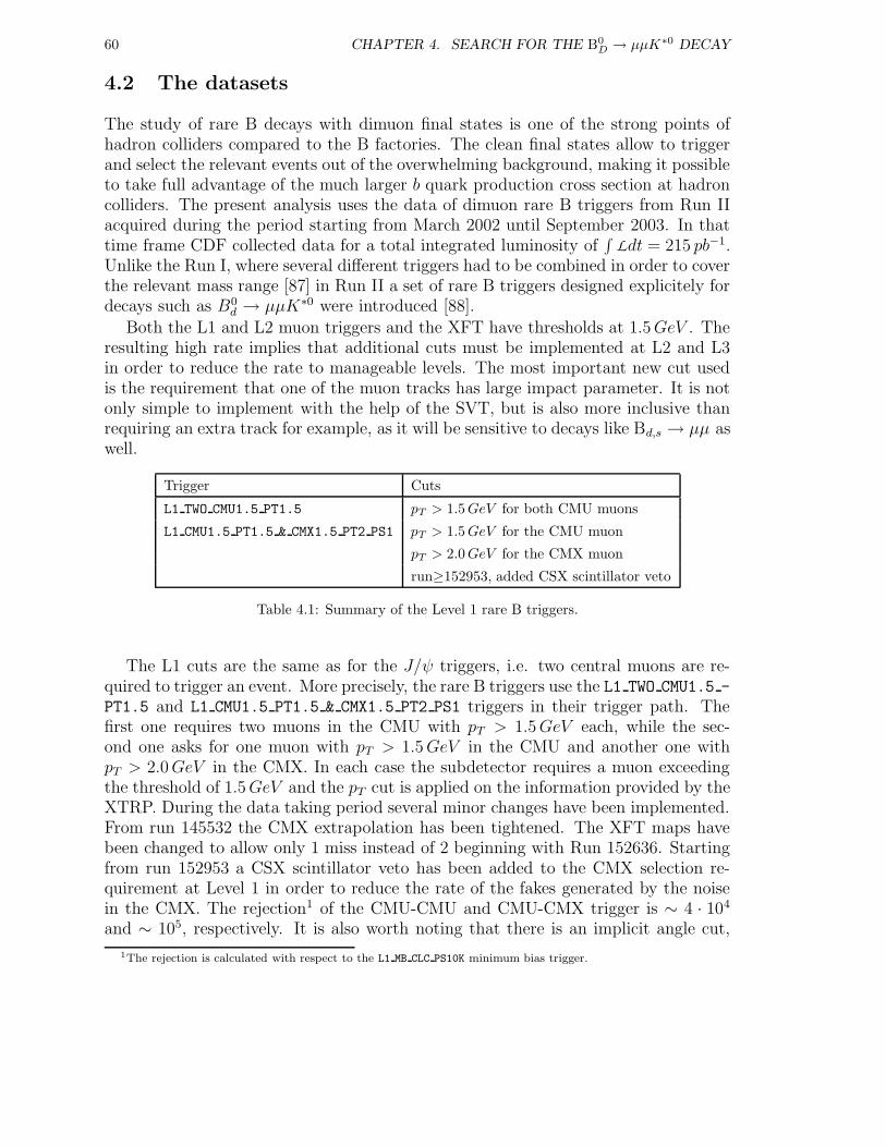
60 CHAPTER 4. SEARCH FOR THE B0D → µµK∗0 DECAY
4.2 The datasets
The study of rare B decays with dimuon final states is one of the strong points ofhadron colliders compared to the B factories. The clean final states allow to triggerand select the relevant events out of the overwhelming background, making it possibleto take full advantage of the much larger b quark production cross section at hadroncolliders. The present analysis uses the data of dimuon rare B triggers from Run IIacquired during the period starting from March 2002 until September 2003. In thattime frame CDF collected data for a total integrated luminosity of
∫
Ldt = 215 pb−1.Unlike the Run I, where several different triggers had to be combined in order to coverthe relevant mass range [87] in Run II a set of rare B triggers designed explicitely fordecays such as B0
d → µµK∗0 were introduced [88].Both the L1 and L2 muon triggers and the XFT have thresholds at 1.5GeV . The
resulting high rate implies that additional cuts must be implemented at L2 and L3in order to reduce the rate to manageable levels. The most important new cut usedis the requirement that one of the muon tracks has large impact parameter. It is notonly simple to implement with the help of the SVT, but is also more inclusive thanrequiring an extra track for example, as it will be sensitive to decays like Bd,s → µµ aswell.
Trigger Cuts
L1 TWO CMU1.5 PT1.5 pT > 1.5GeV for both CMU muons
L1 CMU1.5 PT1.5 & CMX1.5 PT2 PS1 pT > 1.5GeV for the CMU muon
pT > 2.0GeV for the CMX muon
run≥152953, added CSX scintillator veto
Table 4.1: Summary of the Level 1 rare B triggers.
The L1 cuts are the same as for the J/ψ triggers, i.e. two central muons are re-quired to trigger an event. More precisely, the rare B triggers use the L1 TWO CMU1.5 -
PT1.5 and L1 CMU1.5 PT1.5 & CMX1.5 PT2 PS1 triggers in their trigger path. Thefirst one requires two muons in the CMU with pT > 1.5GeV each, while the sec-ond one asks for one muon with pT > 1.5GeV in the CMU and another one withpT > 2.0GeV in the CMX. In each case the subdetector requires a muon exceedingthe threshold of 1.5GeV and the pT cut is applied on the information provided by theXTRP. During the data taking period several minor changes have been implemented.From run 145532 the CMX extrapolation has been tightened. The XFT maps havebeen changed to allow only 1 miss instead of 2 beginning with Run 152636. Startingfrom run 152953 a CSX scintillator veto has been added to the CMX selection re-quirement at Level 1 in order to reduce the rate of the fakes generated by the noisein the CMX. The rejection1 of the CMU-CMU and CMU-CMX trigger is ∼ 4 · 104
and ∼ 105, respectively. It is also worth noting that there is an implicit angle cut,
1The rejection is calculated with respect to the L1 MB CLC PS10K minimum bias trigger.
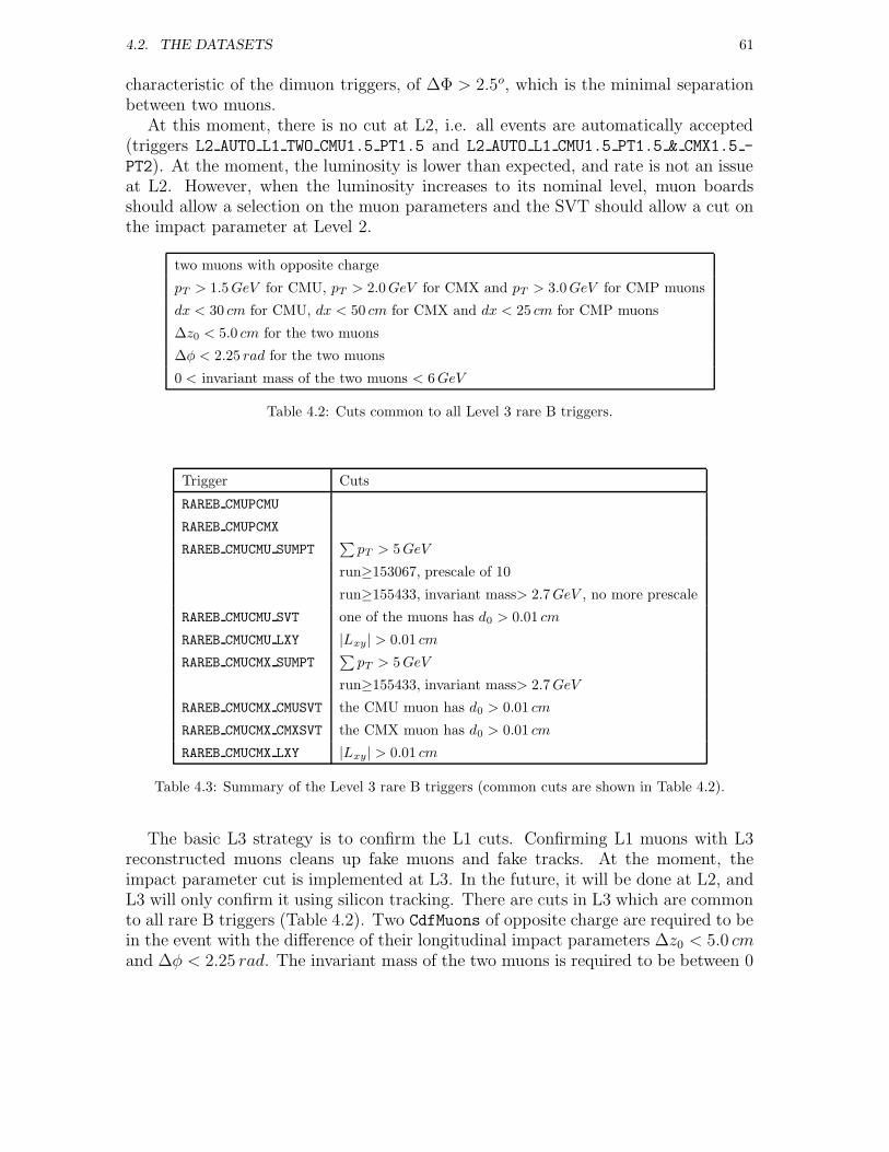
4.2. THE DATASETS 61
characteristic of the dimuon triggers, of ∆Φ > 2.5o, which is the minimal separationbetween two muons.
At this moment, there is no cut at L2, i.e. all events are automatically accepted(triggers L2 AUTO L1 TWO CMU1.5 PT1.5 and L2 AUTO L1 CMU1.5 PT1.5 & CMX1.5 -
PT2). At the moment, the luminosity is lower than expected, and rate is not an issueat L2. However, when the luminosity increases to its nominal level, muon boardsshould allow a selection on the muon parameters and the SVT should allow a cut onthe impact parameter at Level 2.
two muons with opposite charge
pT > 1.5GeV for CMU, pT > 2.0GeV for CMX and pT > 3.0GeV for CMP muons
dx < 30 cm for CMU, dx < 50 cm for CMX and dx < 25 cm for CMP muons
∆z0 < 5.0 cm for the two muons
∆φ < 2.25 rad for the two muons
0 < invariant mass of the two muons < 6GeV
Table 4.2: Cuts common to all Level 3 rare B triggers.
Trigger Cuts
RAREB CMUPCMU
RAREB CMUPCMX
RAREB CMUCMU SUMPT∑pT > 5GeV
run≥153067, prescale of 10
run≥155433, invariant mass> 2.7GeV , no more prescale
RAREB CMUCMU SVT one of the muons has d0 > 0.01 cm
RAREB CMUCMU LXY |Lxy| > 0.01 cm
RAREB CMUCMX SUMPT∑pT > 5GeV
run≥155433, invariant mass> 2.7GeV
RAREB CMUCMX CMUSVT the CMU muon has d0 > 0.01 cm
RAREB CMUCMX CMXSVT the CMX muon has d0 > 0.01 cm
RAREB CMUCMX LXY |Lxy| > 0.01 cm
Table 4.3: Summary of the Level 3 rare B triggers (common cuts are shown in Table 4.2).
The basic L3 strategy is to confirm the L1 cuts. Confirming L1 muons with L3reconstructed muons cleans up fake muons and fake tracks. At the moment, theimpact parameter cut is implemented at L3. In the future, it will be done at L2, andL3 will only confirm it using silicon tracking. There are cuts in L3 which are commonto all rare B triggers (Table 4.2). Two CdfMuons of opposite charge are required to bein the event with the difference of their longitudinal impact parameters ∆z0 < 5.0 cmand ∆φ < 2.25 rad. The invariant mass of the two muons is required to be between 0
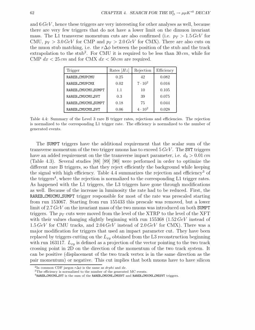
62 CHAPTER 4. SEARCH FOR THE B0D → µµK∗0 DECAY
and 6GeV , hence these triggers are very interesting for other analyses as well, becausethere are very few triggers that do not have a lower limit on the dimuon invariantmass. The L1 transverse momentum cuts are also confirmed (i.e. pT > 1.5GeV forCMU, pT > 3.0GeV for CMP and pT > 2.0GeV for CMX). There are also cuts onthe muon stub matching, i.e. the r∆φ between the position of the stub and the trackextrapolation to the stub2. For CMU it is required to be less than 30 cm, while forCMP dx < 25 cm and for CMX dx < 50 cm are required.
Trigger Rates [Hz] Rejection Efficiency
RAREB CMUPCMU 0.25 42 0.082
RAREB CMUPCMX 0.02 7 · 102 0.016
RAREB CMUCMU SUMPT 1.1 10 0.105
RAREB CMUCMU SVT 0.3 39 0.075
RAREB CMUCMX SUMPT 0.18 75 0.044
RAREB CMUCMX SVT 0.06 4 · 102 0.028
Table 4.4: Summary of the Level 3 rare B trigger rates, rejections and efficiencies. The rejectionis normalized to the corresponding L1 trigger rate. The efficiency is normalized to the number ofgenerated events.
The SUMPT triggers have the additional requirement that the scalar sum of thetransverse momentum of the two trigger muons has to exceed 5GeV . The SVT triggershave an added requirement on the the transverse impact parameter, i.e. d0 > 0.01 cm(Table 4.3). Several studies [88] [89] [90] were performed in order to optimize thedifferent rare B triggers, so that they reject efficiently the background while keepingthe signal with high efficiency. Table 4.4 summarizes the rejection and efficiency3 ofthe triggers4, where the rejection is normalized to the corresponding L1 trigger rates.As happened with the L1 triggers, the L3 triggers have gone through modificationsas well. Because of the increase in luminosity the rate had to be reduced. First, theRAREB CMUCMU SUMPT trigger responsible for most of the rate was prescaled startingfrom run 153067. Starting from run 155433 this prescale was removed, but a lowerlimit of 2.7GeV on the invariant mass of the two muons was introduced on both SUMPT
triggers. The pT cuts were moved from the level of the XTRP to the level of the XFTwith their values changing slightly beginning with run 155368 (1.52GeV instead of1.5GeV for CMU tracks, and 2.04GeV instead of 2.0GeV for CMX). There was amajor modification for triggers that used an impact parameter cut. They have beenreplaced by triggers cutting on the Lxy obtained from the L3 reconstruction beginningwith run 163117. Lxy is defined as a projection of the vector pointing to the two trackcrossing point in 2D on the direction of the momentum of the two track system. Itcan be positive (displacement of the two track vertex is in the same direction as thepair momentum) or negative. This cut implies that both muons have to have silicon
2In common CDF jargon r∆φ is the same as drphi and dx.3The efficiency is normalized to the number of the generated MC events.4RAREB CMUCMX SVT is the sum of the RAREB CMUCMX CMUSVT and RAREB CMUCMX CMXSVT triggers.
4.2. THE DATASETS 63
Dataset Runs Date Total size Luminosity
jbmu08 140886-152952 13.03-16.10.2002 501GB 45 pb−1
jrar08 152953-158732 16.10.2002-13.02.2003 239GB 48 pb−1
jrar09 158733-168889 13.02-06.09.2003 775GB 122 pb−1
All 140886-168889 13.03.2002-06.09.2003 1515GB 215 pb−1
Table 4.5: Datasets used in the present study.
tracks with |η| < 1.2 associated with them.
Level 3 writes out the data to appropriate streams. All the data relevant to thepresent thesis were written out to stream J, which is the stream containing the eventstriggered by muons. The data is reconstructed offline and is further divided intodifferent datasets. The advantage of the offline is that it has much more time andinformation at its disposal than Level 3. It has access to the run dependent conditions,such as alignment and calibration constants of the various subdetector systems. Thesedatasets are closely related to the Level 3 triggers.
The present analysis spans a time frame where three types of datasets were used5:
• Runs 140886-152952: the rare B triggers were written out to the jbmu08 datasettogether with other dimuon triggers
• Runs 152953-158732: as the number of datasets increased from 20 to 34 the rareB triggers were assigned a separate dataset, jrar08.
• Runs 158733-168889: the version of the production was changed, so the rare Btriggers were written out to the dataset jrar096.
The data corresponding to these datasets were written out to tapes. The advantageof the tapes is that space is freely available, however, running analysis on data whichis stored on tapes, can be slow. The alternative solution is to store the data on harddisks on file servers. It reduces considerably the time needed for analyses, however,the space tends to be limited. In order to be able to store the data necessary for thepresent analysis on hard disks, it has been “stripped”, i.e. its size has been greatlyreduced. In order to reduce data size, raw data banks which were not necessaryfor the present study were dropped and in the case of the jbmu08 dataset, eventscorresponding to other triggers than the rare B triggers, were dropped as well. Theresulting data were stored on the fcdfdata041 file server.
5Theoretically, the number at the end of the dataset describes the version. Hence, jbmu06 was processed withversion 4.8.0 of the offline software, jbmu08 and jrar08 with version 4.8.4a etc. However, the processing pass 09 isa special one. Of the 2429 files 681 were processed with version 4.8.4a, 1047 with version 4.8.4g1, 701 with version4.8.5, and 81 with version 4.8.4a but with no silicon alignment, so they were omitted.
6Actually, there are a couple of runs from the 153xxx and 155xxx range that were processed already for the jrar09dataset, but there is no duplication between jrar08 and jrar09.
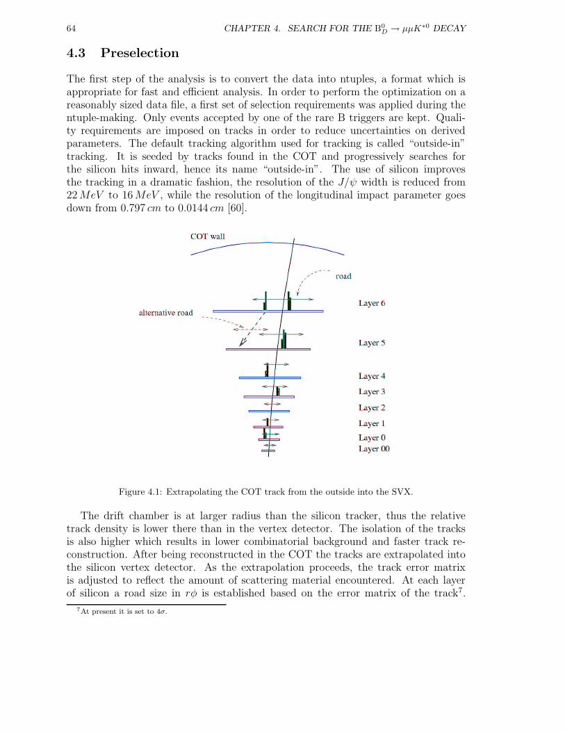
64 CHAPTER 4. SEARCH FOR THE B0D → µµK∗0 DECAY
4.3 Preselection
The first step of the analysis is to convert the data into ntuples, a format which isappropriate for fast and efficient analysis. In order to perform the optimization on areasonably sized data file, a first set of selection requirements was applied during thentuple-making. Only events accepted by one of the rare B triggers are kept. Quali-ty requirements are imposed on tracks in order to reduce uncertainties on derivedparameters. The default tracking algorithm used for tracking is called “outside-in”tracking. It is seeded by tracks found in the COT and progressively searches forthe silicon hits inward, hence its name “outside-in”. The use of silicon improvesthe tracking in a dramatic fashion, the resolution of the J/ψ width is reduced from22MeV to 16MeV , while the resolution of the longitudinal impact parameter goesdown from 0.797 cm to 0.0144 cm [60].
Figure 4.1: Extrapolating the COT track from the outside into the SVX.
The drift chamber is at larger radius than the silicon tracker, thus the relativetrack density is lower there than in the vertex detector. The isolation of the tracksis also higher which results in lower combinatorial background and faster track re-construction. After being reconstructed in the COT the tracks are extrapolated intothe silicon vertex detector. As the extrapolation proceeds, the track error matrixis adjusted to reflect the amount of scattering material encountered. At each layerof silicon a road size in rφ is established based on the error matrix of the track7.
7At present it is set to 4σ.
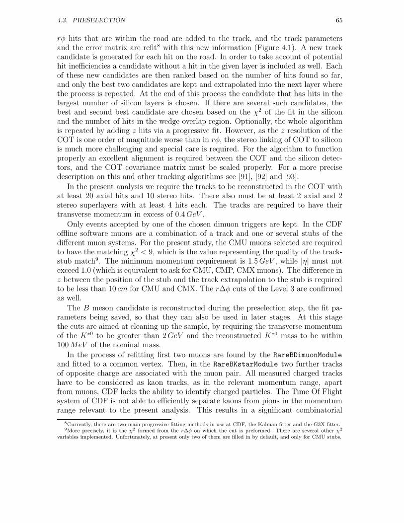
4.3. PRESELECTION 65
rφ hits that are within the road are added to the track, and the track parametersand the error matrix are refit8 with this new information (Figure 4.1). A new trackcandidate is generated for each hit on the road. In order to take account of potentialhit inefficiencies a candidate without a hit in the given layer is included as well. Eachof these new candidates are then ranked based on the number of hits found so far,and only the best two candidates are kept and extrapolated into the next layer wherethe process is repeated. At the end of this process the candidate that has hits in thelargest number of silicon layers is chosen. If there are several such candidates, thebest and second best candidate are chosen based on the χ2 of the fit in the siliconand the number of hits in the wedge overlap region. Optionally, the whole algorithmis repeated by adding z hits via a progressive fit. However, as the z resolution of theCOT is one order of magnitude worse than in rφ, the stereo linking of COT to siliconis much more challenging and special care is required. For the algorithm to functionproperly an excellent alignment is required between the COT and the silicon detec-tors, and the COT covariance matrix must be scaled properly. For a more precisedescription on this and other tracking algorithms see [91], [92] and [93].
In the present analysis we require the tracks to be reconstructed in the COT withat least 20 axial hits and 10 stereo hits. There also must be at least 2 axial and 2stereo superlayers with at least 4 hits each. The tracks are required to have theirtransverse momentum in excess of 0.4GeV .
Only events accepted by one of the chosen dimuon triggers are kept. In the CDFoffline software muons are a combination of a track and one or several stubs of thedifferent muon systems. For the present study, the CMU muons selected are requiredto have the matching χ2 < 9, which is the value representing the quality of the track-stub match9. The minimum momentum requirement is 1.5GeV , while |η| must notexceed 1.0 (which is equivalent to ask for CMU, CMP, CMX muons). The difference inz between the position of the stub and the track extrapolation to the stub is requiredto be less than 10 cm for CMU and CMX. The r∆φ cuts of the Level 3 are confirmedas well.
The B meson candidate is reconstructed during the preselection step, the fit pa-rameters being saved, so that they can also be used in later stages. At this stagethe cuts are aimed at cleaning up the sample, by requiring the transverse momentumof the K∗0 to be greater than 2GeV and the reconstructed K∗0 mass to be within100MeV of the nominal mass.
In the process of refitting first two muons are found by the RareBDimuonModule
and fitted to a common vertex. Then, in the RareBKstarModule two further tracksof opposite charge are associated with the muon pair. All measured charged trackshave to be considered as kaon tracks, as in the relevant momentum range, apartfrom muons, CDF lacks the ability to identify charged particles. The Time Of Flightsystem of CDF is not able to efficiently separate kaons from pions in the momentumrange relevant to the present analysis. This results in a significant combinatorial
8Currently, there are two main progressive fitting methods in use at CDF, the Kalman fitter and the G3X fitter.9More precisely, it is the χ2 formed from the r∆φ on which the cut is preformed. There are several other χ2
variables implemented. Unfortunately, at present only two of them are filled in by default, and only for CMU stubs.
66 CHAPTER 4. SEARCH FOR THE B0D → µµK∗0 DECAY
)[GeV]µµM(0 1 2 3 4 5 6
Nu
mb
er o
f ca
nd
idat
es
0
200
400
600
800
1000
1200
2x10 invariant massµµ
Figure 4.2: Invariant mass distribution of the dimuons after the preselection.
background.As refitting tracks is a very time-consuming operation, it is only done on the four
tracks that form a B candidate. A least-square kinematic fit of the candidate tracks isperformed, the tracks being constrained to come from a common secondary vertex10.
There is no mass constraint applied to the muon pair as in FCNC decays thedimuon mass is not fixed and at this stage no attempt is made to separate B0
d →µ+µ−K∗0 and B0
d → J/ψK∗0 candidates, as the former ones will be used for nor-malization and different other studies. The summary of the applied cuts is listed inTable 4.6.
The dimuon invariant mass distribution after the preselection cuts is shown inFigure 4.2. There is a very pronounced J/ψ peak, and one can also clearly distinguishthe ψ(2S) → µ+µ−, φ→ K+K− → µ+µ− and ρ→ π+π− → µ+µ− peaks.
4.4 Baseline selection
Runs, in order to be selected in the analysis, must satisfy certain conditions. Therelevant detectors must be declared operational by both the online and offline moni-toring. Online monitoring starts from basic checks, such as whether the given detectorsubsystem and all its components are turned on, and continues with the monitoring ofthe performance of each detector subsystem by looking at the monitoring programsattached to the DAQ system, which provide in real time plots of different physicsquantities corresponding to data from various triggers. These real time checks arefollowed by more in-depth checks once the data is written to tapes, where addi-tional information and the full analysis framework are used to show through various
10This is called a vertex-constrained fit.

4.4. BASELINE SELECTION 67
RareBDimuonModule RareBKstarModule
Cuts on muons
opposite charge
pT (µ) > 1.5
|η| < 1.0
dz(CMU) < 10.0
χ2xposition < 9.0
dz(CMX) < 10.0
axial hits ≥ 20
stereo hits ≥ 10
axial SL ≥ 2 with hits ≥ 4
stereo SL ≥ 2 with hits ≥ 4
dphi < 3.14
dx(CMU,CMP ) < 30.0
dx(CMX) < 50.0
Cuts on tracks
pT (track) > 0.4
axial hits ≥ 20
stereo hits ≥ 10
axial SL ≥ 2 with hits ≥ 4
stereo SL ≥ 2 with hits ≥ 4
Cuts on K∗0
pT (K∗0) > 2.0
0.796 < M(K∗0) < 0.996
0 < dphi(Kπ) < 180
dz(Kπ) < 10.0
Table 4.6: Preselection cuts applied to the data sample. Following the CDF convention the variousquantities are always expressed in GeV and cm unless otherwise stated.
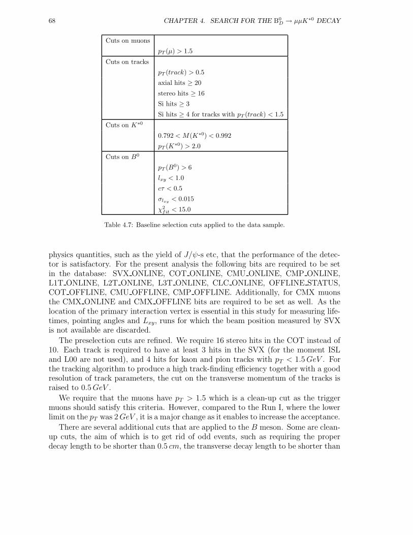
68 CHAPTER 4. SEARCH FOR THE B0D → µµK∗0 DECAY
Cuts on muons
pT (µ) > 1.5
Cuts on tracks
pT (track) > 0.5
axial hits ≥ 20
stereo hits ≥ 16
Si hits ≥ 3
Si hits ≥ 4 for tracks with pT (track) < 1.5
Cuts on K∗0
0.792 < M(K∗0) < 0.992
pT (K∗0) > 2.0
Cuts on B0
pT (B0) > 6
lxy < 1.0
cτ < 0.5
σlxy< 0.015
χ2fit < 15.0
Table 4.7: Baseline selection cuts applied to the data sample.
physics quantities, such as the yield of J/ψ-s etc, that the performance of the detec-tor is satisfactory. For the present analysis the following bits are required to be setin the database: SVX ONLINE, COT ONLINE, CMU ONLINE, CMP ONLINE,L1T ONLINE, L2T ONLINE, L3T ONLINE, CLC ONLINE, OFFLINE STATUS,COT OFFLINE, CMU OFFLINE, CMP OFFLINE. Additionally, for CMX muonsthe CMX ONLINE and CMX OFFLINE bits are required to be set as well. As thelocation of the primary interaction vertex is essential in this study for measuring life-times, pointing angles and Lxy, runs for which the beam position measured by SVXis not available are discarded.
The preselection cuts are refined. We require 16 stereo hits in the COT instead of10. Each track is required to have at least 3 hits in the SVX (for the moment ISLand L00 are not used), and 4 hits for kaon and pion tracks with pT < 1.5GeV . Forthe tracking algorithm to produce a high track-finding efficiency together with a goodresolution of track parameters, the cut on the transverse momentum of the tracks israised to 0.5GeV .
We require that the muons have pT > 1.5 which is a clean-up cut as the triggermuons should satisfy this criteria. However, compared to the Run I, where the lowerlimit on the pT was 2GeV , it is a major change as it enables to increase the acceptance.
There are several additional cuts that are applied to the B meson. Some are clean-up cuts, the aim of which is to get rid of odd events, such as requiring the properdecay length to be shorter than 0.5 cm, the transverse decay length to be shorter than
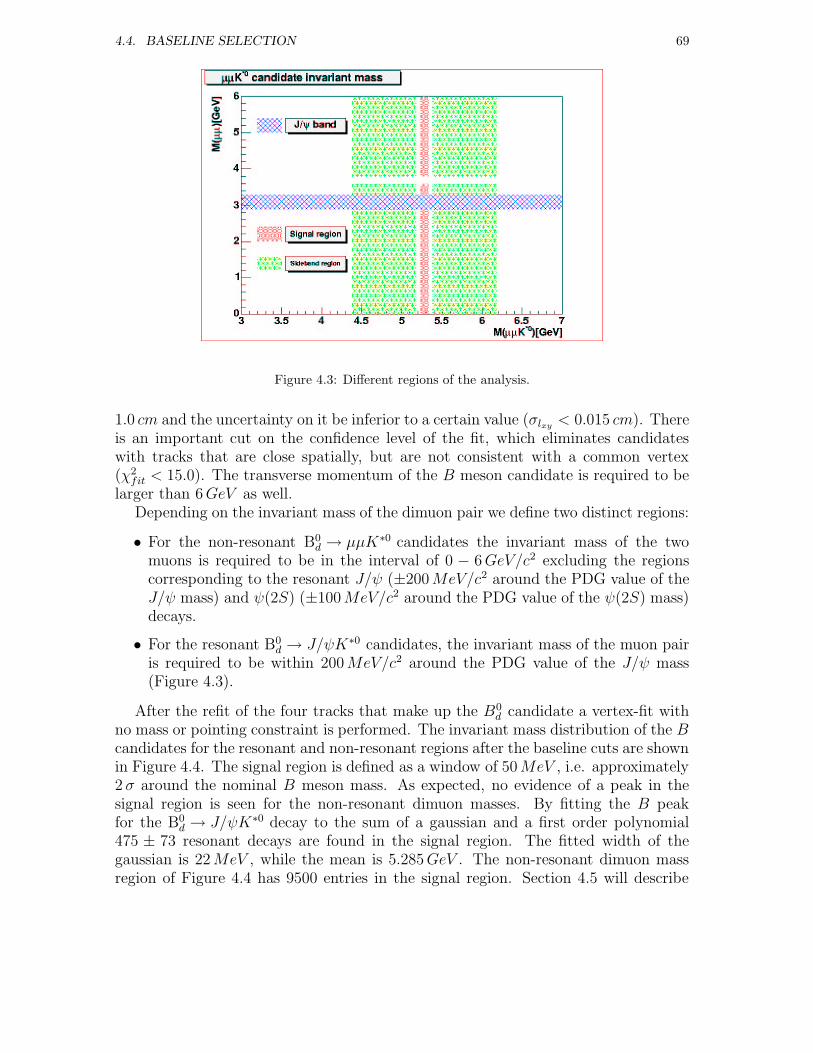
4.4. BASELINE SELECTION 69
Figure 4.3: Different regions of the analysis.
1.0 cm and the uncertainty on it be inferior to a certain value (σlxy< 0.015 cm). There
is an important cut on the confidence level of the fit, which eliminates candidateswith tracks that are close spatially, but are not consistent with a common vertex(χ2
fit < 15.0). The transverse momentum of the B meson candidate is required to belarger than 6GeV as well.
Depending on the invariant mass of the dimuon pair we define two distinct regions:
• For the non-resonant B0d → µµK∗0 candidates the invariant mass of the two
muons is required to be in the interval of 0 − 6GeV/c2 excluding the regionscorresponding to the resonant J/ψ (±200MeV/c2 around the PDG value of theJ/ψ mass) and ψ(2S) (±100MeV/c2 around the PDG value of the ψ(2S) mass)decays.
• For the resonant B0d → J/ψK∗0 candidates, the invariant mass of the muon pair
is required to be within 200MeV/c2 around the PDG value of the J/ψ mass(Figure 4.3).
After the refit of the four tracks that make up the B0d candidate a vertex-fit with
no mass or pointing constraint is performed. The invariant mass distribution of the Bcandidates for the resonant and non-resonant regions after the baseline cuts are shownin Figure 4.4. The signal region is defined as a window of 50MeV , i.e. approximately2 σ around the nominal B meson mass. As expected, no evidence of a peak in thesignal region is seen for the non-resonant dimuon masses. By fitting the B peakfor the B0
d → J/ψK∗0 decay to the sum of a gaussian and a first order polynomial475 ± 73 resonant decays are found in the signal region. The fitted width of thegaussian is 22MeV , while the mean is 5.285GeV . The non-resonant dimuon massregion of Figure 4.4 has 9500 entries in the signal region. Section 4.5 will describe
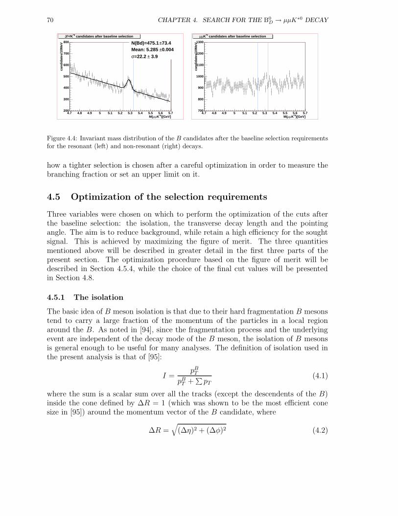
70 CHAPTER 4. SEARCH FOR THE B0D → µµK∗0 DECAY
)[GeV]*0KµµM(4.7 4.8 4.9 5 5.1 5.2 5.3 5.4 5.5 5.6 5.7
can
did
ates
/10M
eV
200
300
400
500
600
700
800 73.4±N(Bd)=475.1 0.004±Mean: 5.285
3.9±=22.2 σ
candidates after baseline selection*0KΨJ/
)[GeV]*0KµµM(4.7 4.8 4.9 5 5.1 5.2 5.3 5.4 5.5 5.6 5.7
can
did
ates
/10M
eV
700
800
900
1000
1100
1200
1300
candidates after baseline selection*0Kµµ
Figure 4.4: Invariant mass distribution of the B candidates after the baseline selection requirementsfor the resonant (left) and non-resonant (right) decays.
how a tighter selection is chosen after a careful optimization in order to measure thebranching fraction or set an upper limit on it.
4.5 Optimization of the selection requirements
Three variables were chosen on which to perform the optimization of the cuts afterthe baseline selection: the isolation, the transverse decay length and the pointingangle. The aim is to reduce background, while retain a high efficiency for the soughtsignal. This is achieved by maximizing the figure of merit. The three quantitiesmentioned above will be described in greater detail in the first three parts of thepresent section. The optimization procedure based on the figure of merit will bedescribed in Section 4.5.4, while the choice of the final cut values will be presentedin Section 4.8.
4.5.1 The isolation
The basic idea of B meson isolation is that due to their hard fragmentation B mesonstend to carry a large fraction of the momentum of the particles in a local regionaround the B. As noted in [94], since the fragmentation process and the underlyingevent are independent of the decay mode of the B meson, the isolation of B mesonsis general enough to be useful for many analyses. The definition of isolation used inthe present analysis is that of [95]:
I =pBT
pBT +∑pT
(4.1)
where the sum is a scalar sum over all the tracks (except the descendents of the B)inside the cone defined by ∆R = 1 (which was shown to be the most efficient conesize in [95]) around the momentum vector of the B candidate, where
∆R =√
(∆η)2 + (∆φ)2 (4.2)
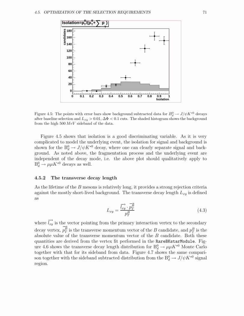
4.5. OPTIMIZATION OF THE SELECTION REQUIREMENTS 71
Isolation0 0.1 0.2 0.3 0.4 0.5 0.6 0.7 0.8 0.9 1
can
did
ates
0
20
40
60
80
100
120
140
160
180
)T
p∑+BT/(pB
TIsolation=p
Figure 4.5: The points with error bars show background subtracted data for B0d → J/ψK∗0 decays
after baseline selection and Lxy > 0.01, ∆Φ < 0.1 cuts. The shaded histogram shows the backgroundfrom the high 500MeV sideband of the data.
Figure 4.5 shows that isolation is a good discriminating variable. As it is verycomplicated to model the underlying event, the isolation for signal and background isshown for the B0
d → J/ψK∗0 decay, where one can clearly separate signal and back-ground. As noted above, the fragmentation process and the underlying event areindependent of the decay mode, i.e. the above plot should qualitatively apply toB0d → µµK∗0 decays as well.
4.5.2 The transverse decay length
As the lifetime of the B mesons is relatively long, it provides a strong rejection criteriaagainst the mostly short-lived background. The transverse decay length Lxy is definedas
Lxy =
−→lxy ·
−→pBT
pBT(4.3)
where−→lxy is the vector pointing from the primary interaction vertex to the secondary
decay vertex,−→pBT is the transverse momentum vector of the B candidate, and pBT is the
absolute value of the transverse momentum vector of the B candidate. Both thesequantities are derived from the vertex fit performed in the RareBKstarModule. Fig-ure 4.6 shows the transverse decay length distribution for B0
d → µµK∗0 Monte Carlotogether with that for its sideband from data. Figure 4.7 shows the same compari-son together with the sideband subtracted distribution from the B0
d → J/ψK∗0 signalregion.
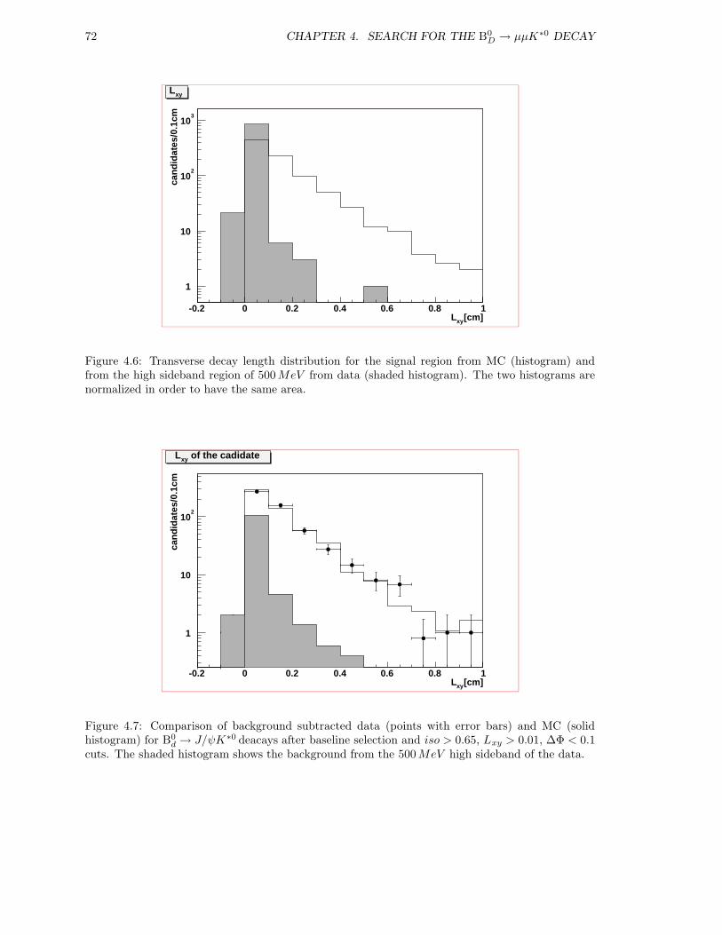
72 CHAPTER 4. SEARCH FOR THE B0D → µµK∗0 DECAY
[cm]xyL-0.2 0 0.2 0.4 0.6 0.8 1
can
did
ates
/0.1
cm
1
10
102
103
xyL
Figure 4.6: Transverse decay length distribution for the signal region from MC (histogram) andfrom the high sideband region of 500MeV from data (shaded histogram). The two histograms arenormalized in order to have the same area.
[cm]xyL-0.2 0 0.2 0.4 0.6 0.8 1
can
did
ates
/0.1
cm
1
10
102
of the cadidatexyL
Figure 4.7: Comparison of background subtracted data (points with error bars) and MC (solidhistogram) for B0
d → J/ψK∗0 deacays after baseline selection and iso > 0.65, Lxy > 0.01, ∆Φ < 0.1cuts. The shaded histogram shows the background from the 500MeV high sideband of the data.

4.5. OPTIMIZATION OF THE SELECTION REQUIREMENTS 73
[rad]φ ∆0 0.05 0.1 0.15 0.2 0.25 0.3 0.35 0.4 0.45 0.5
can
did
ates
/0.0
5rad
0
200
400
600
800
1000
1200
1400
Pointing angle
Figure 4.8: Pointing angle distribution for the signal region from B0d → µµK∗0 MC (histogram) and
from the high sideband region of 500MeV from data (shaded histogram). The two histograms arenormalized to have the same area.
Another quantity related to the transverse decay length is the proper decay length:
cτ = Lxy ·mB0
pBT(4.4)
Even though the variable used for optimization is the minimum transverse decaylength, cuts on its maximal value and on the maximal value of the proper decay lengthare used as clean-up cuts as discussed earlier. The requirements on the transversedecay length, proper decay length, as well as that on the pointing angle, which will bediscussed next, require precise measurement of the primary and secondary vertices. Abeamline calculated by the SVX is required for each run used in this study so that theprimary vertex is measured with sufficient precision, and all tracks are required to haveat least three silicon hits in order to have a precise secondary vertex reconstruction.
4.5.3 The pointing angle
The final variable used as a strong rejection criteria in the optimization is the pointing
angle, which is the angle between the momentum vector of the B meson (−→pBT ) and its
flight path in the transverse (r−φ) plane (−→lxy). It is clear that because the two muons,
the kaon and the pion are coming from the B, the two vectors should point in thesame direction, i.e. ∆Φ should be close to 0 (Figure 4.8 for B0
d → µµK∗0 ). Figure 4.9shows both the comparison between MC signal and the signal obtained from the data,and the distribution from the sidebands of the data for the B0
d → J/ψK∗0 decay.
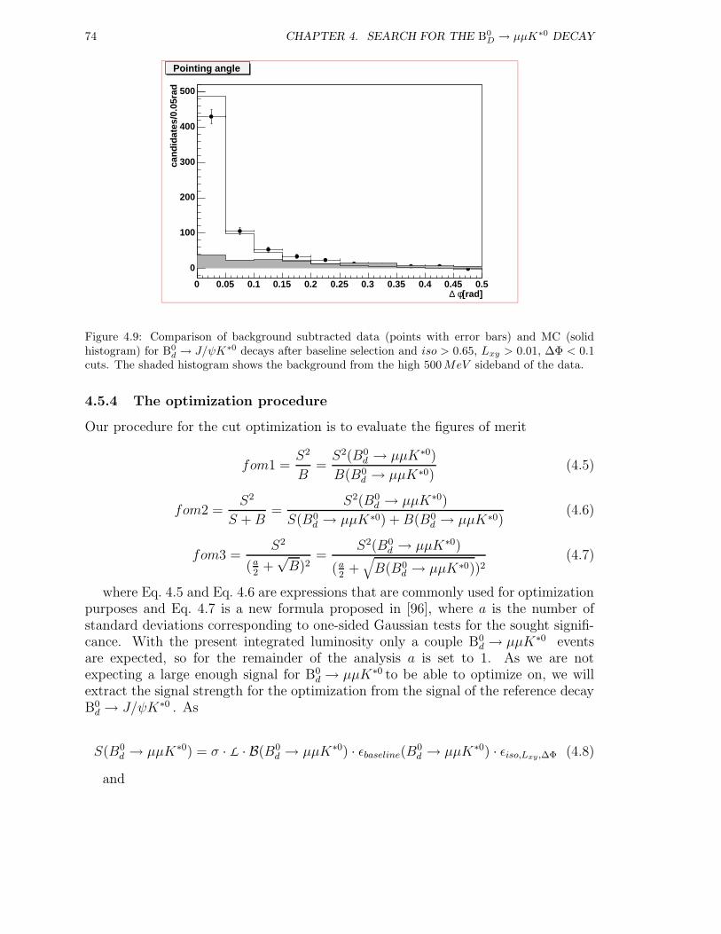
74 CHAPTER 4. SEARCH FOR THE B0D → µµK∗0 DECAY
[rad]φ ∆0 0.05 0.1 0.15 0.2 0.25 0.3 0.35 0.4 0.45 0.5
can
did
ates
/0.0
5rad
0
100
200
300
400
500
Pointing angle
Figure 4.9: Comparison of background subtracted data (points with error bars) and MC (solidhistogram) for B0
d → J/ψK∗0 decays after baseline selection and iso > 0.65, Lxy > 0.01, ∆Φ < 0.1cuts. The shaded histogram shows the background from the high 500MeV sideband of the data.
4.5.4 The optimization procedure
Our procedure for the cut optimization is to evaluate the figures of merit
fom1 =S2
B=S2(B0
d → µµK∗0)
B(B0d → µµK∗0)
(4.5)
fom2 =S2
S +B=
S2(B0d → µµK∗0)
S(B0d → µµK∗0) +B(B0
d → µµK∗0)(4.6)
fom3 =S2
(a2
+√B)2
=S2(B0
d → µµK∗0)
(a2
+√
B(B0d → µµK∗0))2
(4.7)
where Eq. 4.5 and Eq. 4.6 are expressions that are commonly used for optimizationpurposes and Eq. 4.7 is a new formula proposed in [96], where a is the number ofstandard deviations corresponding to one-sided Gaussian tests for the sought signifi-cance. With the present integrated luminosity only a couple B0
d → µµK∗0 eventsare expected, so for the remainder of the analysis a is set to 1. As we are notexpecting a large enough signal for B0
d → µµK∗0 to be able to optimize on, we willextract the signal strength for the optimization from the signal of the reference decayB0d → J/ψK∗0 . As
S(B0d → µµK∗0) = σ · L · B(B0
d → µµK∗0) · εbaseline(B0d → µµK∗0) · εiso,Lxy,∆Φ (4.8)
and

4.5. OPTIMIZATION OF THE SELECTION REQUIREMENTS 75
S(B0d → J/ψK∗0) = σ·L ·B(B0
d → J/ψK∗0)·εbaseline(B0d → J/ψK∗0)·εiso,Lxy,∆Φ (4.9)
where the efficiencies of the isolation, Lxy and pointing cuts can be considered thesame for the two decays. Dividing Eq. 4.8 by Eq.4.9 gives
S(B0d → µµK∗0) = S(B0
d → J/ψK∗0)· B(B0d → µµK∗0)
B(B0d → J/ψK∗0)
· εbaseline(B0d → µµK∗0)
εbaseline(B0d → J/ψK∗0)
·εrel(4.10)
Let us define
ε =B(B0
d → µµK∗0)
B(B0d → J/ψK∗0)
· εbaseline(B0d → µµK∗0)
εbaseline(B0d → J/ψK∗0)
· εrel (4.11)
where εrel denotes all the other relative efficiencies discussed in Section 4.6.1 andthe branching ratios are:
• B(B0d → µµK∗0) = 11.7+3.6
−3.1 ± 0.8 ± 0.6 × 10⁻⁷ from the results presented atthe Lepton-Photon 2003 conference by the Belle experiment [30], which is inexcellent agreement with the 1.19± 0.39× 10⁻⁶ recently published by Ali. et al.[18].
• B(B0d → J/ψK∗0) = 1.31 ± 0.07 × 10⁻³ from [3]11
• B(J/ψ → µ+µ−) = 5.88 ± 0.10 % from [3]
hence
B(B0d → µµK∗0)
B(B0d → J/ψK∗0)
= 1.52 ± 0.49 × 10⁻² (4.12)
so equations 4.5, 4.6 and 4.7 can be rewritten
fom1 =S2(B0
d → J/ψK∗0) · ε2B(B0
d → µµK∗0)(4.13)
fom2 =S2(B0
d → J/ψK∗0) · ε2S(B0
d → J/ψK∗0) · ε +B(B0d → µµK∗0)
(4.14)
fom3 =S2(B0
d → J/ψK∗0) · ε2
(12
+√
B(B0d → µµK∗0))2
(4.15)
So, in order to calculate the two types of figure of merit, two quantities are neededto be measured from the data for each set of cuts:
• B(B0d → µµK∗0): the background expected in the signal region.
• S(B0d → J/ψK∗0): the number of B0
d → J/ψK∗0 decays observed.
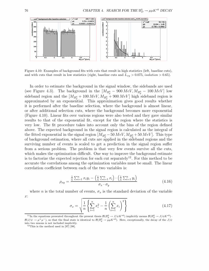
76 CHAPTER 4. SEARCH FOR THE B0D → µµK∗0 DECAY
/ ndf 2χ 209.7 / 156p0 0.04878± 5.751 p1 0.009172± -0.04307
)[GeV]*0KµµM(4 4.5 5 5.5 6 6.5 7
can
did
ates
/10M
eV
0
50
100
150
200
250
300
350
/ ndf 2χ 209.7 / 156p0 0.04878± 5.751 p1 0.009172± -0.04307
background after baseline selection*0Kµµ
/ ndf 2χ 51 / 61p0 1.45± 13.54 p1 0.3062± -2.736
)[GeV]*0KµµM(4 4.5 5 5.5 6 6.5 7
can
did
ates
/10M
eV
0
1
2
3
4
5
6
7
8
9 / ndf 2χ 51 / 61p0 1.45± 13.54 p1 0.3062± -2.736
>0.075, iso>0.65xy background after baseline selection and L*0Kµµ
Figure 4.10: Examples of background fits with cuts that result in high statistics (left, baseline cuts),and with cuts that result in low statistics (right, baseline cuts and Lxy > 0.075, isolation > 0.65).
In order to estimate the background in the signal window, the sidebands are used(see Figure 4.3). The background in the [MB0
d− 900MeV,MB0
d− 100MeV ] low
sideband region and the [MB0d
+ 100MeV,MB0d
+ 900MeV ] high sideband region isapproximated by an exponential. This approximation gives good results whetherit is performed after the baseline selection, where the background is almost linear,or after additional selection cuts, where the background becomes more exponential(Figure 4.10). Linear fits over various regions were also tested and they gave similarresults to that of the exponential fit, except for the region where the statistics isvery low. The fit procedure takes into account only the bins of the region definedabove. The expected background in the signal region is calculated as the integral ofthe fitted exponential in the signal region [MB0
d−50MeV,MB0
d+50MeV ]. This type
of background estimation, where all cuts are applied in the sideband regions and thesurviving number of events is scaled to get a prediction in the signal region sufferfrom a serious problem. The problem is that very few events survive all the cuts,which makes the optimization difficult. One way to improve the background estimateis to factorize the expected rejection for each cut separately12. For this method to beaccurate the correlations among the optimization variables must be small. The linearcorrelation coefficient between each of the two variables is:
ρxy =
1n
∑ni=1 xiyi −
(1n
∑ni=1 xi
)
·(
1n
∑ni=1 yi
)
σx · σy(4.16)
where n is the total number of events, σx is the standard deviation of the variablex:
σx =
√√√√√
1
n
n∑
i=1
x2i −
1
n
(n∑
i=1
xi
)2
(4.17)
11In the equations presented throughout the present thesis B(B0d→ J/ψK∗0) implicitly means B(B0
d→ J/ψK∗0) ·
B(J/ψ → µ+µ−), so that the final state is identical to B(B0d→ µµK∗0). Here, exceptionally, the decay of the J/ψ
into two muons is not included implicitly.12This is the method used in [97] [98].
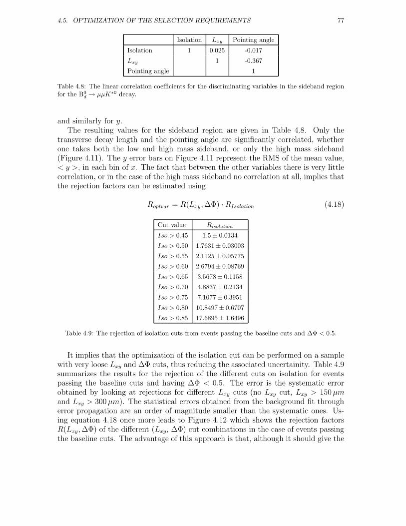
4.5. OPTIMIZATION OF THE SELECTION REQUIREMENTS 77
Isolation Lxy Pointing angle
Isolation 1 0.025 -0.017
Lxy 1 -0.367
Pointing angle 1
Table 4.8: The linear correlation coefficients for the discriminating variables in the sideband regionfor the B0
d → µµK∗0 decay.
and similarly for y.The resulting values for the sideband region are given in Table 4.8. Only the
transverse decay length and the pointing angle are significantly correlated, whetherone takes both the low and high mass sideband, or only the high mass sideband(Figure 4.11). The y error bars on Figure 4.11 represent the RMS of the mean value,< y >, in each bin of x. The fact that between the other variables there is very littlecorrelation, or in the case of the high mass sideband no correlation at all, implies thatthe rejection factors can be estimated using
Roptvar = R(Lxy,∆Φ) ·RIsolation (4.18)
Cut value Risolation
Iso > 0.45 1.5± 0.0134
Iso > 0.50 1.7631± 0.03003
Iso > 0.55 2.1125± 0.05775
Iso > 0.60 2.6794± 0.08769
Iso > 0.65 3.5678± 0.1158
Iso > 0.70 4.8837± 0.2134
Iso > 0.75 7.1077± 0.3951
Iso > 0.80 10.8497± 0.6707
Iso > 0.85 17.6895± 1.6496
Table 4.9: The rejection of isolation cuts from events passing the baseline cuts and ∆Φ < 0.5.
It implies that the optimization of the isolation cut can be performed on a samplewith very loose Lxy and ∆Φ cuts, thus reducing the associated uncertainity. Table 4.9summarizes the results for the rejection of the different cuts on isolation for eventspassing the baseline cuts and having ∆Φ < 0.5. The error is the systematic errorobtained by looking at rejections for different Lxy cuts (no Lxy cut, Lxy > 150µmand Lxy > 300µm). The statistical errors obtained from the background fit througherror propagation are an order of magnitude smaller than the systematic ones. Us-ing equation 4.18 once more leads to Figure 4.12 which shows the rejection factorsR(Lxy,∆Φ) of the different (Lxy, ∆Φ) cut combinations in the case of events passingthe baseline cuts. The advantage of this approach is that, although it should give the
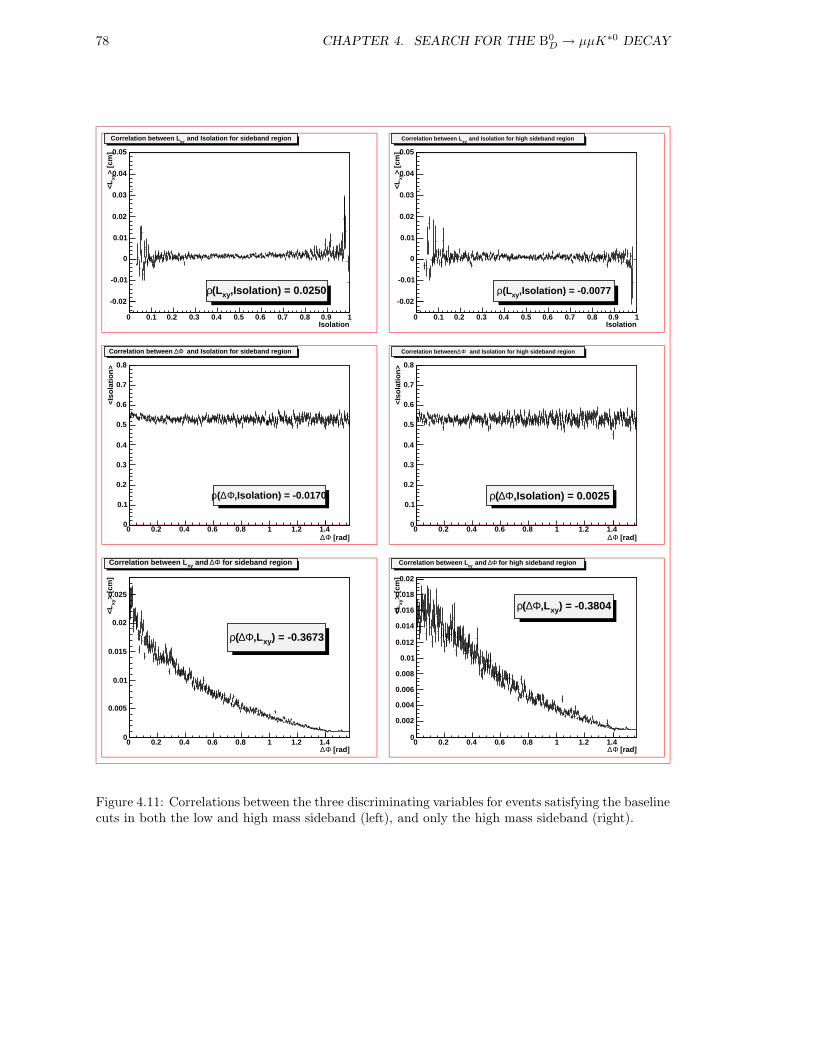
78 CHAPTER 4. SEARCH FOR THE B0D → µµK∗0 DECAY
Isolation0 0.1 0.2 0.3 0.4 0.5 0.6 0.7 0.8 0.9 1
> [c
m]
xy<L
-0.02
-0.01
0
0.01
0.02
0.03
0.04
0.05
,Isolation) = 0.0250xy(Lρ
and Isolation for sideband regionxy
Correlation between L
Isolation0 0.1 0.2 0.3 0.4 0.5 0.6 0.7 0.8 0.9 1
> [c
m]
xy<L
-0.02
-0.01
0
0.01
0.02
0.03
0.04
0.05
,Isolation) = -0.0077xy(Lρ
and Isolation for high sideband regionxy
Correlation between L
[rad]Φ∆0 0.2 0.4 0.6 0.8 1 1.2 1.4
<Iso
lati
on
>
0
0.1
0.2
0.3
0.4
0.5
0.6
0.7
0.8
,Isolation) = -0.0170Φ∆(ρ
and Isolation for sideband regionΦ∆Correlation between
[rad]Φ∆0 0.2 0.4 0.6 0.8 1 1.2 1.4
<Iso
lati
on
>
0
0.1
0.2
0.3
0.4
0.5
0.6
0.7
0.8
,Isolation) = 0.0025Φ∆(ρ
and Isolation for high sideband regionΦ∆Correlation between
[rad]Φ∆0 0.2 0.4 0.6 0.8 1 1.2 1.4
> [c
m]
xy<L
0
0.005
0.01
0.015
0.02
0.025
) = -0.3673xy,LΦ∆(ρ
for sideband regionΦ∆ and xyCorrelation between L
[rad]Φ∆0 0.2 0.4 0.6 0.8 1 1.2 1.4
> [c
m]
xy<L
0
0.002
0.004
0.006
0.008
0.01
0.012
0.014
0.016
0.018
0.02
) = -0.3804xy,LΦ∆(ρ
for high sideband regionΦ∆ and xy
Correlation between L
Figure 4.11: Correlations between the three discriminating variables for events satisfying the baselinecuts in both the low and high mass sideband (left), and only the high mass sideband (right).
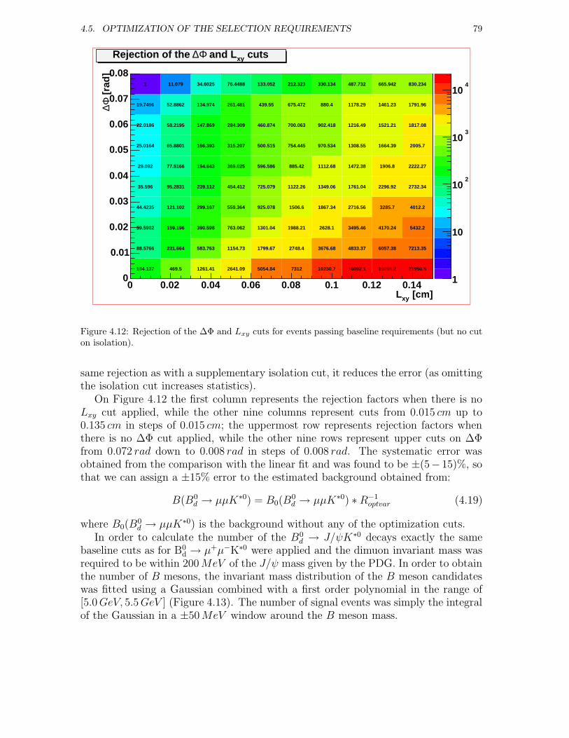
4.5. OPTIMIZATION OF THE SELECTION REQUIREMENTS 79
1
10
102
103
104
[cm]xyL0 0.02 0.04 0.06 0.08 0.1 0.12 0.14
[ra
d]
Φ∆
0
0.01
0.02
0.03
0.04
0.05
0.06
0.07
0.08
184.137 469.5 1261.41 2641.09 5054.84 7312 10230.7 16092.1 19095.2 21950.5
88.5766 231.664 583.763 1154.73 1799.67 2748.4 3676.68 4833.37 6057.38 7213.35
59.5902 159.196 390.598 763.062 1301.04 1988.21 2628.1 3495.46 4170.24 5432.2
44.4235 121.102 299.167 559.364 925.078 1506.6 1867.34 2716.56 3285.7 4012.2
35.596 95.2831 239.112 454.412 725.079 1122.26 1349.06 1761.04 2296.92 2732.34
29.092 77.5166 194.643 369.025 596.586 885.42 1112.68 1472.38 1906.8 2222.27
25.0164 65.8801 166.393 315.207 500.515 754.445 970.534 1308.55 1664.39 2005.7
22.0186 58.2195 147.869 284.309 460.874 700.063 902.418 1216.49 1521.21 1817.08
19.7496 52.8862 134.974 261.481 439.55 675.472 880.4 1178.29 1461.23 1791.96
1 11.079 34.6025 76.4488 133.052 212.323 330.134 487.732 665.942 830.234
cutsxy and LΦ∆Rejection of the
Figure 4.12: Rejection of the ∆Φ and Lxy cuts for events passing baseline requirements (but no cuton isolation).
same rejection as with a supplementary isolation cut, it reduces the error (as omittingthe isolation cut increases statistics).
On Figure 4.12 the first column represents the rejection factors when there is noLxy cut applied, while the other nine columns represent cuts from 0.015 cm up to0.135 cm in steps of 0.015 cm; the uppermost row represents rejection factors whenthere is no ∆Φ cut applied, while the other nine rows represent upper cuts on ∆Φfrom 0.072 rad down to 0.008 rad in steps of 0.008 rad. The systematic error wasobtained from the comparison with the linear fit and was found to be ±(5− 15)%, sothat we can assign a ±15% error to the estimated background obtained from:
B(B0d → µµK∗0) = B0(B
0d → µµK∗0) ∗R−1
optvar (4.19)
where B0(B0d → µµK∗0) is the background without any of the optimization cuts.
In order to calculate the number of the B0d → J/ψK∗0 decays exactly the same
baseline cuts as for B0d → µ+µ−K∗0 were applied and the dimuon invariant mass was
required to be within 200MeV of the J/ψ mass given by the PDG. In order to obtainthe number of B mesons, the invariant mass distribution of the B meson candidateswas fitted using a Gaussian combined with a first order polynomial in the range of[5.0GeV, 5.5GeV ] (Figure 4.13). The number of signal events was simply the integralof the Gaussian in a ±50MeV window around the B meson mass.
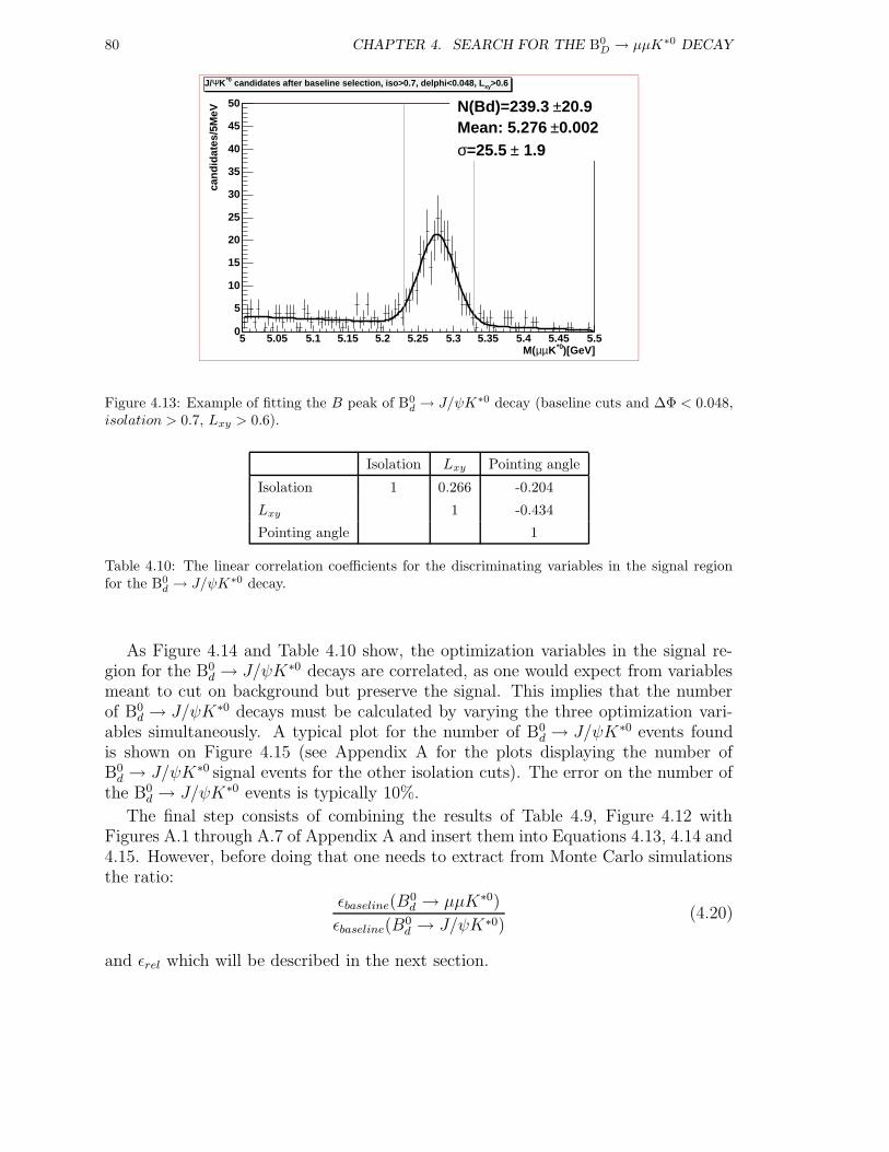
80 CHAPTER 4. SEARCH FOR THE B0D → µµK∗0 DECAY
)[GeV]*0KµµM(5 5.05 5.1 5.15 5.2 5.25 5.3 5.35 5.4 5.45 5.5
can
did
ates
/5M
eV
0
5
10
15
20
25
30
35
40
45
50 20.9±N(Bd)=239.3 0.002±Mean: 5.276
1.9±=25.5 σ
>0.6xy candidates after baseline selection, iso>0.7, delphi<0.048, L*0KΨJ/
Figure 4.13: Example of fitting the B peak of B0d → J/ψK∗0 decay (baseline cuts and ∆Φ < 0.048,
isolation > 0.7, Lxy > 0.6).
Isolation Lxy Pointing angle
Isolation 1 0.266 -0.204
Lxy 1 -0.434
Pointing angle 1
Table 4.10: The linear correlation coefficients for the discriminating variables in the signal regionfor the B0
d → J/ψK∗0 decay.
As Figure 4.14 and Table 4.10 show, the optimization variables in the signal re-gion for the B0
d → J/ψK∗0 decays are correlated, as one would expect from variablesmeant to cut on background but preserve the signal. This implies that the numberof B0
d → J/ψK∗0 decays must be calculated by varying the three optimization vari-ables simultaneously. A typical plot for the number of B0
d → J/ψK∗0 events foundis shown on Figure 4.15 (see Appendix A for the plots displaying the number ofB0d → J/ψK∗0 signal events for the other isolation cuts). The error on the number of
the B0d → J/ψK∗0 events is typically 10%.
The final step consists of combining the results of Table 4.9, Figure 4.12 withFigures A.1 through A.7 of Appendix A and insert them into Equations 4.13, 4.14 and4.15. However, before doing that one needs to extract from Monte Carlo simulationsthe ratio:
εbaseline(B0d → µµK∗0)
εbaseline(B0d → J/ψK∗0)
(4.20)
and εrel which will be described in the next section.
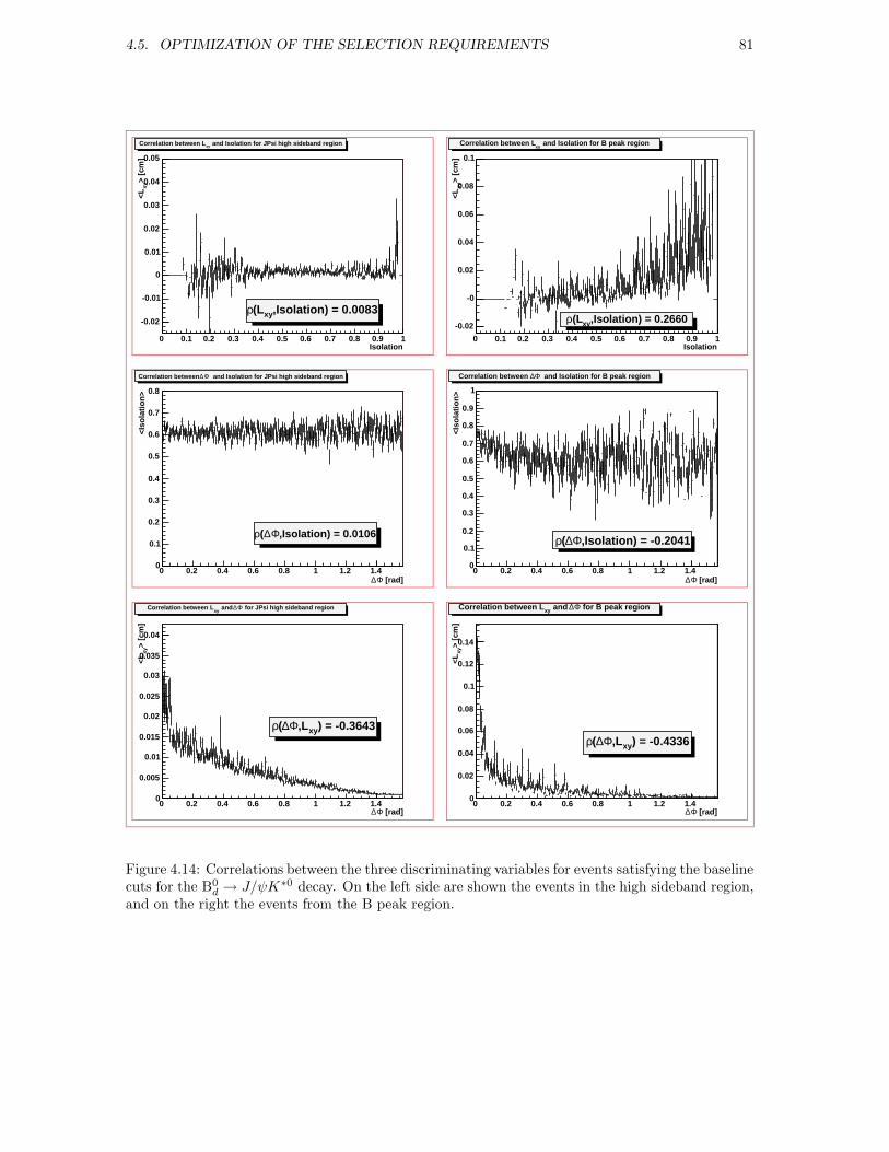
4.5. OPTIMIZATION OF THE SELECTION REQUIREMENTS 81
Isolation0 0.1 0.2 0.3 0.4 0.5 0.6 0.7 0.8 0.9 1
> [c
m]
xy<L
-0.02
-0.01
0
0.01
0.02
0.03
0.04
0.05
,Isolation) = 0.0083xy(Lρ
and Isolation for JPsi high sideband regionxyCorrelation between L
Isolation0 0.1 0.2 0.3 0.4 0.5 0.6 0.7 0.8 0.9 1
> [c
m]
xy<L
-0.02
-0
0.02
0.04
0.06
0.08
0.1
,Isolation) = 0.2660xy(Lρ
and Isolation for B peak regionxy
Correlation between L
[rad]Φ∆0 0.2 0.4 0.6 0.8 1 1.2 1.4
<Iso
lati
on
>
0
0.1
0.2
0.3
0.4
0.5
0.6
0.7
0.8
,Isolation) = 0.0106Φ∆(ρ
and Isolation for JPsi high sideband regionΦ∆Correlation between
[rad]Φ∆0 0.2 0.4 0.6 0.8 1 1.2 1.4
<Iso
lati
on
>
0
0.1
0.2
0.3
0.4
0.5
0.6
0.7
0.8
0.9
1
,Isolation) = -0.2041Φ∆(ρ
and Isolation for B peak regionΦ∆Correlation between
[rad]Φ∆0 0.2 0.4 0.6 0.8 1 1.2 1.4
> [c
m]
xy<L
0
0.005
0.01
0.015
0.02
0.025
0.03
0.035
0.04
) = -0.3643xy,LΦ∆(ρ
for JPsi high sideband regionΦ∆ and xy
Correlation between L
[rad]Φ∆0 0.2 0.4 0.6 0.8 1 1.2 1.4
> [c
m]
xy<L
0
0.02
0.04
0.06
0.08
0.1
0.12
0.14
) = -0.4336xy,LΦ∆(ρ
for B peak regionΦ∆ and xyCorrelation between L
Figure 4.14: Correlations between the three discriminating variables for events satisfying the baselinecuts for the B0
d → J/ψK∗0 decay. On the left side are shown the events in the high sideband region,and on the right the events from the B peak region.
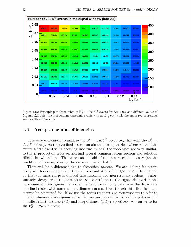
82 CHAPTER 4. SEARCH FOR THE B0D → µµK∗0 DECAY
100
150
200
250
300
350
400
450
[cm]xyL0 0.02 0.04 0.06 0.08 0.1 0.12 0.14
[ra
d]
Φ∆
0
0.01
0.02
0.03
0.04
0.05
0.06
0.07
0.08
events in the signal window (iso>0.7)*0 KψNumber of J/
104.02 106.638 103.168 102.6 92.7938 85.9366 83.3971 77.2584 69.7903 61.2656
172.32 181.545 175.612 171.408 156.249 141.175 134.387 121.351 111.924 102.665
210.505 218.998 212.474 205.966 188.701 170.926 160.413 144.109 131.485 120.694
233.654 241.211 235.329 226.916 206.531 184.781 172.264 154.032 140.81 128.983
252.413 259.088 251.659 242.215 218.785 195.415 180.65 157.181 143.232 130.34
289.047 291.774 279.809 264.215 238.631 210.36 194.35 165.778 146.567 132.794
307.159 306.469 295.085 278.127 250.769 220.291 202.412 171.223 148.253 133.294
317.172 315.763 303.359 286.019 256.343 221.489 203.874 172.672 148.688 133.752
327.92 324.804 309.756 292.88 261.792 225.229 205.803 173.069 148.371 133.752
454.89 419.966 368.98 332.336 277.41 234.719 211.354 175.491 149.405 135.223
Figure 4.15: Example plot for number of B0d → J/ψK∗0 events for Iso > 0.7 and different values of
Lxy and ∆Φ cuts (the first column represents events with no Lxy cut, while the upper row representsevents with no ∆Φ cut).
4.6 Acceptance and efficiencies
It is very convenient to analyze the B0d → µµK∗0 decay together with the B0
d →J/ψK∗0 decay. As the two final states contain the same particles (where we take theevents where the J/ψ is decaying into two muons) the topologies are very similar,so the B production cross section and several common reconstruction and selectionefficiencies will cancel. The same can be said of the integrated luminosity (on thecondition, of course, of using the same sample for both).
There will be a difference due to theoretical factors. We are looking for a raredecay which does not proceed through resonant states (i.e. J/ψ or ψ ′). In order todo that the mass range is divided into resonant and non-resonant regions. Unfor-tunately, decays from resonant states will contribute to the signal observed in thenon-resonant mass regions, i.e. experimentally we can only determine the decay rateinto final states with non-resonant dimuon masses. Even though this effect is small,it must be accounted for. If we use the terms resonant and non-resonant to refer todifferent dimuon mass regions while the rare and resonance induced amplitudes willbe called short-distance (SD) and long-distance (LD) respectively, we can write forthe B0
d → µµK∗0 decay:
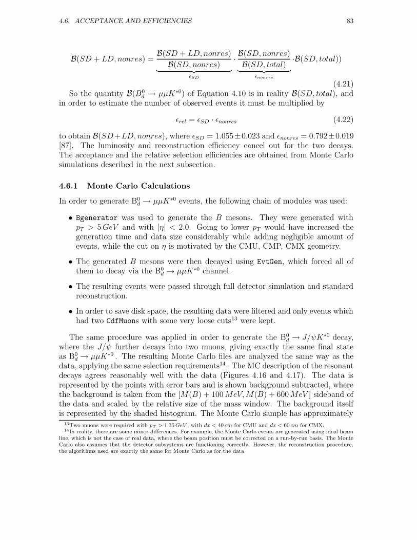
4.6. ACCEPTANCE AND EFFICIENCIES 83
B(SD + LD, nonres) =B(SD + LD, nonres)
B(SD, nonres)︸ ︷︷ ︸
εSD
· B(SD, nonres)
B(SD, total)︸ ︷︷ ︸
εnonres
·B(SD, total))
(4.21)So the quantity B(B0
d → µµK∗0) of Equation 4.10 is in reality B(SD, total), andin order to estimate the number of observed events it must be multiplied by
εrel = εSD · εnonres (4.22)
to obtain B(SD+LD, nonres), where εSD = 1.055±0.023 and εnonres = 0.792±0.019[87]. The luminosity and reconstruction efficiency cancel out for the two decays.The acceptance and the relative selection efficiencies are obtained from Monte Carlosimulations described in the next subsection.
4.6.1 Monte Carlo Calculations
In order to generate B0d → µµK∗0 events, the following chain of modules was used:
• Bgenerator was used to generate the B mesons. They were generated withpT > 5GeV and with |η| < 2.0. Going to lower pT would have increased thegeneration time and data size considerably while adding negligible amount ofevents, while the cut on η is motivated by the CMU, CMP, CMX geometry.
• The generated B mesons were then decayed using EvtGen, which forced all ofthem to decay via the B0
d → µµK∗0 channel.
• The resulting events were passed through full detector simulation and standardreconstruction.
• In order to save disk space, the resulting data were filtered and only events whichhad two CdfMuons with some very loose cuts13 were kept.
The same procedure was applied in order to generate the B0d → J/ψK∗0 decay,
where the J/ψ further decays into two muons, giving exactly the same final stateas B0
d → µµK∗0 . The resulting Monte Carlo files are analyzed the same way as thedata, applying the same selection requirements14. The MC description of the resonantdecays agrees reasonably well with the data (Figures 4.16 and 4.17). The data isrepresented by the points with error bars and is shown background subtracted, wherethe background is taken from the [M(B) + 100MeV,M(B) + 600MeV ] sideband ofthe data and scaled by the relative size of the mass window. The background itselfis represented by the shaded histogram. The Monte Carlo sample has approximately
13Two muons were required with pT > 1.35GeV , with dx < 40 cm for CMU and dx < 60 cm for CMX.14In reality, there are some minor differences. For example, the Monte Carlo events are generated using ideal beam
line, which is not the case of real data, where the beam position must be corrected on a run-by-run basis. The MonteCarlo also assumes that the detector subsystems are functioning correctly. However, the reconstruction procedure,the algorithms used are exactly the same for Monte Carlo as for the data
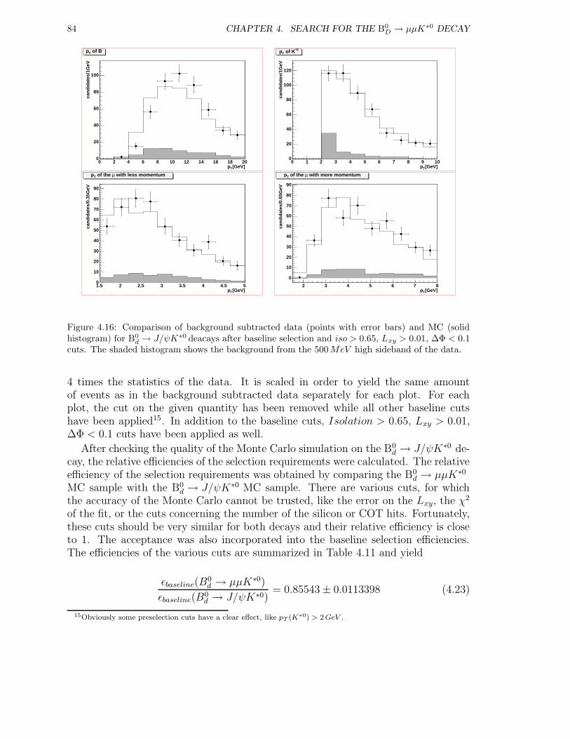
84 CHAPTER 4. SEARCH FOR THE B0D → µµK∗0 DECAY
[GeV]Tp0 2 4 6 8 10 12 14 16 18 20
can
did
ates
/1G
eV
0
20
40
60
80
100
of BTp
[GeV]Tp0 1 2 3 4 5 6 7 8 9 10
can
did
ates
/1G
eV
0
20
40
60
80
100
120
*0 of KTp
[GeV]Tp1.5 2 2.5 3 3.5 4 4.5 5
can
did
ates
/0.3
5GeV
0
10
20
30
40
50
60
70
80
90
with less momentumµ of the Tp
[GeV]Tp2 3 4 5 6 7 8
can
did
ates
/0.6
5GeV
0
10
20
30
40
50
60
70
80
90
with more momentumµ of the Tp
Figure 4.16: Comparison of background subtracted data (points with error bars) and MC (solidhistogram) for B0
d → J/ψK∗0 deacays after baseline selection and iso > 0.65, Lxy > 0.01, ∆Φ < 0.1cuts. The shaded histogram shows the background from the 500MeV high sideband of the data.
4 times the statistics of the data. It is scaled in order to yield the same amountof events as in the background subtracted data separately for each plot. For eachplot, the cut on the given quantity has been removed while all other baseline cutshave been applied15. In addition to the baseline cuts, Isolation > 0.65, Lxy > 0.01,∆Φ < 0.1 cuts have been applied as well.
After checking the quality of the Monte Carlo simulation on the B0d → J/ψK∗0 de-
cay, the relative efficiencies of the selection requirements were calculated. The relativeefficiency of the selection requirements was obtained by comparing the B0
d → µµK∗0
MC sample with the B0d → J/ψK∗0 MC sample. There are various cuts, for which
the accuracy of the Monte Carlo cannot be trusted, like the error on the Lxy, the χ2
of the fit, or the cuts concerning the number of the silicon or COT hits. Fortunately,these cuts should be very similar for both decays and their relative efficiency is closeto 1. The acceptance was also incorporated into the baseline selection efficiencies.The efficiencies of the various cuts are summarized in Table 4.11 and yield
εbaseline(B0d → µµK∗0)
εbaseline(B0d → J/ψK∗0)
= 0.85543 ± 0.0113398 (4.23)
15Obviously some preselection cuts have a clear effect, like pT (K∗0) > 2GeV .
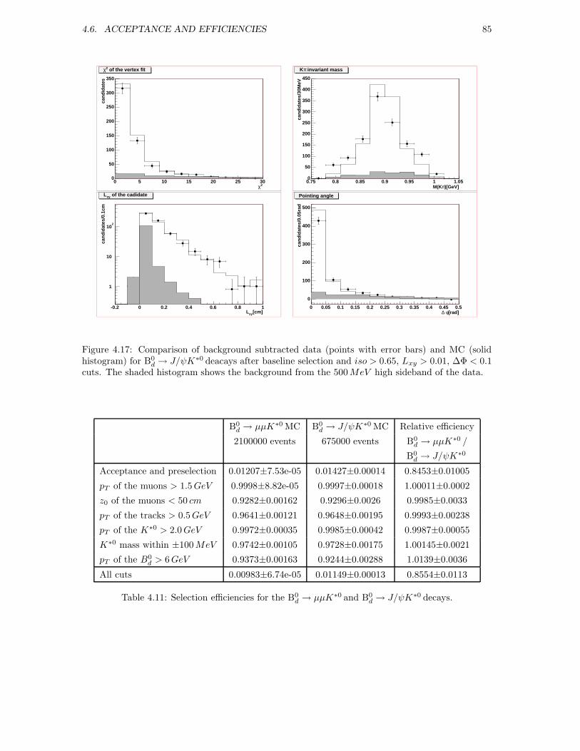
4.6. ACCEPTANCE AND EFFICIENCIES 85
2χ0 5 10 15 20 25 30
can
did
ates
0
50
100
150
200
250
300
350
of the vertex fit2χ
)[GeV]πM(K0.75 0.8 0.85 0.9 0.95 1 1.05
can
did
ates
/30M
eV
0
50
100
150
200
250
300
350
400
450
invariant massπK
[cm]xyL-0.2 0 0.2 0.4 0.6 0.8 1
can
did
ates
/0.1
cm
1
10
102
of the cadidatexyL
[rad]φ ∆0 0.05 0.1 0.15 0.2 0.25 0.3 0.35 0.4 0.45 0.5
can
did
ates
/0.0
5rad
0
100
200
300
400
500
Pointing angle
Figure 4.17: Comparison of background subtracted data (points with error bars) and MC (solidhistogram) for B0
d → J/ψK∗0 deacays after baseline selection and iso > 0.65, Lxy > 0.01, ∆Φ < 0.1cuts. The shaded histogram shows the background from the 500MeV high sideband of the data.
B0d → µµK∗0 MC B0
d → J/ψK∗0 MC Relative efficiency
2100000 events 675000 events B0d → µµK∗0 /
B0d → J/ψK∗0
Acceptance and preselection 0.01207±7.53e-05 0.01427±0.00014 0.8453±0.01005
pT of the muons > 1.5GeV 0.9998±8.82e-05 0.9997±0.00018 1.00011±0.0002
z0 of the muons < 50 cm 0.9282±0.00162 0.9296±0.0026 0.9985±0.0033
pT of the tracks > 0.5GeV 0.9641±0.00121 0.9648±0.00195 0.9993±0.00238
pT of the K∗0 > 2.0GeV 0.9972±0.00035 0.9985±0.00042 0.9987±0.00055
K∗0 mass within ±100MeV 0.9742±0.00105 0.9728±0.00175 1.00145±0.0021
pT of the B0d > 6GeV 0.9373±0.00163 0.9244±0.00288 1.0139±0.0036
All cuts 0.00983±6.74e-05 0.01149±0.00013 0.8554±0.0113
Table 4.11: Selection efficiencies for the B0d → µµK∗0 and B0
d → J/ψK∗0 decays.
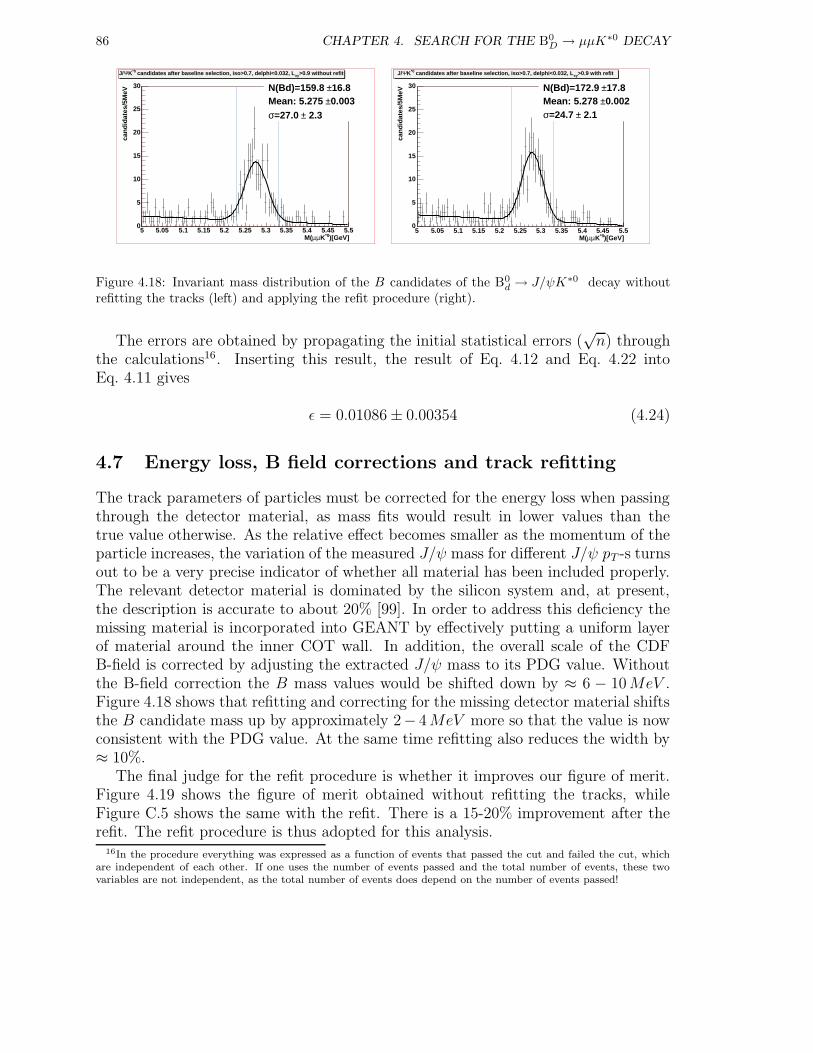
86 CHAPTER 4. SEARCH FOR THE B0D → µµK∗0 DECAY
)[GeV]*0KµµM(5 5.05 5.1 5.15 5.2 5.25 5.3 5.35 5.4 5.45 5.5
can
did
ates
/5M
eV
0
5
10
15
20
25
30 16.8±N(Bd)=159.8 0.003±Mean: 5.275
2.3±=27.0 σ
>0.9 without refitxy candidates after baseline selection, iso>0.7, delphi<0.032, L*0KΨJ/
)[GeV]*0KµµM(5 5.05 5.1 5.15 5.2 5.25 5.3 5.35 5.4 5.45 5.5
can
did
ates
/5M
eV
0
5
10
15
20
25
30 17.8±N(Bd)=172.9 0.002±Mean: 5.278
2.1±=24.7 σ
>0.9 with refitxy candidates after baseline selection, iso>0.7, delphi<0.032, L*0KΨJ/
Figure 4.18: Invariant mass distribution of the B candidates of the B0d → J/ψK∗0 decay without
refitting the tracks (left) and applying the refit procedure (right).
The errors are obtained by propagating the initial statistical errors (√n) through
the calculations16. Inserting this result, the result of Eq. 4.12 and Eq. 4.22 intoEq. 4.11 gives
ε = 0.01086 ± 0.00354 (4.24)
4.7 Energy loss, B field corrections and track refitting
The track parameters of particles must be corrected for the energy loss when passingthrough the detector material, as mass fits would result in lower values than thetrue value otherwise. As the relative effect becomes smaller as the momentum of theparticle increases, the variation of the measured J/ψ mass for different J/ψ pT -s turnsout to be a very precise indicator of whether all material has been included properly.The relevant detector material is dominated by the silicon system and, at present,the description is accurate to about 20% [99]. In order to address this deficiency themissing material is incorporated into GEANT by effectively putting a uniform layerof material around the inner COT wall. In addition, the overall scale of the CDFB-field is corrected by adjusting the extracted J/ψ mass to its PDG value. Withoutthe B-field correction the B mass values would be shifted down by ≈ 6 − 10MeV .Figure 4.18 shows that refitting and correcting for the missing detector material shiftsthe B candidate mass up by approximately 2− 4MeV more so that the value is nowconsistent with the PDG value. At the same time refitting also reduces the width by≈ 10%.
The final judge for the refit procedure is whether it improves our figure of merit.Figure 4.19 shows the figure of merit obtained without refitting the tracks, whileFigure C.5 shows the same with the refit. There is a 15-20% improvement after therefit. The refit procedure is thus adopted for this analysis.
16In the procedure everything was expressed as a function of events that passed the cut and failed the cut, whichare independent of each other. If one uses the number of events passed and the total number of events, these twovariables are not independent, as the total number of events does depend on the number of events passed!
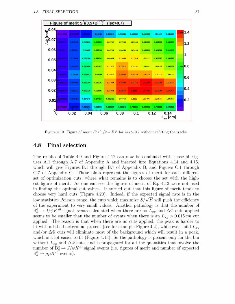
4.8. FINAL SELECTION 87
0.2
0.4
0.6
0.8
1
1.2
1.4
[cm]xyL0 0.02 0.04 0.06 0.08 0.1 0.12 0.14
[ra
d]
Φ∆
0
0.01
0.02
0.03
0.04
0.05
0.06
0.07
0.08
(iso>0.7)2)-1/2/(0.5+B2Figure of merit S
0.0726263 0.159702 0.320191 0.525063 0.685396 0.663642 0.738001 0.809492 0.763886 0.686255
0.0999071 0.241752 0.504348 0.844534 0.989712 1.07754 1.1203 1.13496 1.11516 1.06352
0.116979 0.291421 0.603328 0.986553 1.21844 1.33577 1.3887 1.44786 1.33329 1.34188
0.119132 0.294958 0.617188 0.963791 1.17339 1.31846 1.31172 1.41246 1.32129 1.27914
0.119593 0.30123 0.638453 1.00849 1.15517 1.25055 1.20128 1.18215 1.15712 1.06819
0.113416 0.280245 0.595498 0.953927 1.12372 1.17611 1.15192 1.08482 1.04835 0.951759
0.112574 0.26979 0.574386 0.912043 1.06884 1.13646 1.11516 1.05317 0.972625 0.893628
0.110211 0.258941 0.55885 0.878308 1.04765 1.08056 1.05236 0.989961 0.904012 0.826067
0.105995 0.253499 0.543995 0.849991 1.03732 1.07595 1.05134 0.990676 0.889638 0.831863
0.0110869 0.0952183 0.224777 0.36931 0.429841 0.455222 0.511621 0.516889 0.50423 0.485628
Figure 4.19: Figure of merit S2/(1/2 +B)2 for iso > 0.7 without refitting the tracks.
4.8 Final selection
The results of Table 4.9 and Figure 4.12 can now be combined with those of Fig-ures A.1 through A.7 of Appendix A and inserted into Equations 4.14 and 4.15,which will give Figures B.1 through B.7 of Appendix B, and Figures C.1 throughC.7 of Appendix C. These plots represent the figures of merit for each differentset of optimization cuts, where what remains is to choose the set with the high-est figure of merit. As one can see the figures of merit of Eq. 4.13 were not usedin finding the optimal cut values. It turned out that this figure of merit tends tochoose very hard cuts (Figure 4.20). Indeed, if the expected signal rate is in the
low statistics Poisson range, the cuts which maximize S/√B will push the efficiency
of the experiment to very small values. Another pathology is that the number ofB0d → J/ψK∗0 signal events calculated when there are no Lxy and ∆Φ cuts applied
seems to be smaller than the number of events when there is an Lxy > 0.015 cm cutapplied. The reason is that when there are no cuts applied, the peak is harder tofit with all the background present (see for example Figure 4.4), while even mild Lxyand/or ∆Φ cuts will eliminate most of the background which will result in a peak,which is a lot easier to fit (Figure 4.13). So the pathology is present only for the binwithout Lxy and ∆Φ cuts, and is propagated for all the quantities that involve thenumber of B0
d → J/ψK∗0 signal events (i.e. figures of merit and number of expectedB0d → µµK∗0 events).
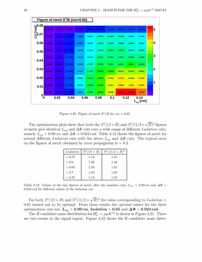
88 CHAPTER 4. SEARCH FOR THE B0D → µµK∗0 DECAY
1
2
3
4
5
[cm]xyL0 0.02 0.04 0.06 0.08 0.1 0.12 0.14
[ra
d]
Φ∆
0
0.01
0.02
0.03
0.04
0.05
0.06
0.07
0.08
/B (iso>0.65)2Figure of merit S
0.107863 0.294189 0.756113 1.56875 2.44181 2.96795 3.92949 5.31278 5.11165 4.65183
0.145955 0.422817 0.990501 1.86106 2.43299 3.04381 3.72615 3.98806 4.2244 4.16093
0.146248 0.416761 0.963762 1.75482 2.52145 3.18209 3.75019 4.03721 3.89438 4.21309
0.134262 0.385624 0.906885 1.57354 2.17651 2.88539 3.16378 3.66723 3.61571 3.66831
0.121409 0.348335 0.828406 1.46358 1.91673 2.40898 2.5302 2.5126 2.6636 2.60748
0.131357 0.358801 0.827062 1.41122 1.84475 2.16797 2.37455 2.30673 2.30405 2.19366
0.129732 0.34109 0.797096 1.35788 1.71911 2.04042 2.24619 2.19226 2.05217 1.99261
0.122605 0.321812 0.74678 1.29472 1.64783 1.91219 2.11576 2.06892 1.88542 1.81617
0.118567 0.31085 0.717044 1.25002 1.64355 1.91578 2.11665 2.01221 1.80423 1.79106
0.00994286 0.110146 0.263452 0.472043 0.558792 0.658487 0.846139 0.853838 0.832599 0.846246
Figure 4.20: Figure of merit S2/B for iso > 0.65.
The optimization plots show that both the S2/(S+B) and S2/(1/2+√B)2 figures
of merit give identical Lxy and ∆Φ cuts over a wide range of different Isolation cuts,namely Lxy > 0.09 cm and ∆Φ < 0.024 rad. Table 4.12 shows the figures of merit forseveral different Isolation cuts with the above Lxy and ∆Φ cuts. The typical erroron the figures of merit obtained by error propagation is ∼ 0.3.
Isolation S2/(S +B) S2/(1/2 +B)2
> 0.55 1.13 1.31
> 0.6 1.20 1.46
> 0.65 1.28 1.67
> 0.7 1.23 1.65
> 0.75 1.13 1.55
Table 4.12: Values of the two figures of merit after the baseline cuts, Lxy > 0.09 cm and ∆Φ <0.024 rad for different values of the isolation cut.
For both S2/(S +B) and S2/(1/2+√B)2 the value corresponding to Isolation >
0.65 turned out to be optimal. From these results the optimal values for the threeoptimization cuts are: Lxy > 0.09 cm, Isolation > 0.65 and ∆Φ < 0.024 rad.
The B candidate mass distribution for B0d → µµK∗0 is shown in Figure 4.21. There
are two events in the signal region. Figure 4.22 shows the B candidate mass distri-
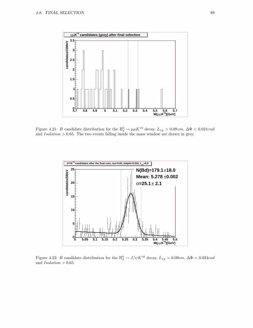
4.8. FINAL SELECTION 89
)[GeV]*0KµµM(4.7 4.8 4.9 5 5.1 5.2 5.3 5.4 5.5 5.6 5.7
can
did
ates
/10M
eV
0
0.5
1
1.5
2
2.5
3
3.5
candidates (grey) after final selection*0Kµµ
Figure 4.21: B candidate distribution for the B0d → µµK∗0 decay, Lxy > 0.09 cm, ∆Φ < 0.024 rad
and Isolation > 0.65. The two events falling inside the mass window are drawn in grey.
)[GeV]*0KµµM(5 5.05 5.1 5.15 5.2 5.25 5.3 5.35 5.4 5.45 5.5
can
did
ates
/5M
eV
0
5
10
15
20
25 18.0±N(Bd)=179.1 0.002±Mean: 5.278
2.1±=25.1 σ
>0.9xy candidates after the final cuts, iso>0.65, delphi<0.024, L*0KΨJ/
Figure 4.22: B candidate distribution for the B0d → J/ψK∗0 decay, Lxy > 0.09cm, ∆Φ < 0.024rad
and Isolation > 0.65.
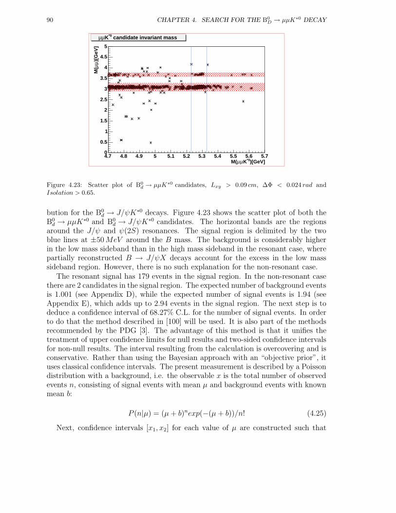
90 CHAPTER 4. SEARCH FOR THE B0D → µµK∗0 DECAY
)[GeV]*0KµµM(4.7 4.8 4.9 5 5.1 5.2 5.3 5.4 5.5 5.6 5.7
)[G
eV]
µµM
(
0
0.5
1
1.5
2
2.5
3
3.5
4
4.5
5
candidate invariant mass*0Kµµ
Figure 4.23: Scatter plot of B0d → µµK∗0 candidates, Lxy > 0.09 cm, ∆Φ < 0.024 rad and
Isolation > 0.65.
bution for the B0d → J/ψK∗0 decays. Figure 4.23 shows the scatter plot of both the
B0d → µµK∗0 and B0
d → J/ψK∗0 candidates. The horizontal bands are the regionsaround the J/ψ and ψ(2S) resonances. The signal region is delimited by the twoblue lines at ±50MeV around the B mass. The background is considerably higherin the low mass sideband than in the high mass sideband in the resonant case, wherepartially reconstructed B → J/ψX decays account for the excess in the low masssideband region. However, there is no such explanation for the non-resonant case.
The resonant signal has 179 events in the signal region. In the non-resonant casethere are 2 candidates in the signal region. The expected number of background eventsis 1.001 (see Appendix D), while the expected number of signal events is 1.94 (seeAppendix E), which adds up to 2.94 events in the signal region. The next step is todeduce a confidence interval of 68.27% C.L. for the number of signal events. In orderto do that the method described in [100] will be used. It is also part of the methodsrecommended by the PDG [3]. The advantage of this method is that it unifies thetreatment of upper confidence limits for null results and two-sided confidence intervalsfor non-null results. The interval resulting from the calculation is overcovering and isconservative. Rather than using the Bayesian approach with an “objective prior”, ituses classical confidence intervals. The present measurement is described by a Poissondistribution with a background, i.e. the observable x is the total number of observedevents n, consisting of signal events with mean µ and background events with knownmean b:
P (n|µ) = (µ+ b)nexp(−(µ + b))/n! (4.25)
Next, confidence intervals [x1, x2] for each value of µ are constructed such that
4.8. FINAL SELECTION 91
P (x ∈ [x1, x2]|µ) = α. The confidence interval [µ1, µ2] we are looking for is theunion of all values of µ for which the corresponding acceptance interval contains themeasured value (i.e. n0 = 2). From Table II of [100] for b = 1.0 and n0 = 2 thecorresponding interval is:
[µ1, µ2] = [0.14, 3.25] CI = 68.75% (4.26)
In particular, the interval contains the fixed unknown µt (number of signal events)in a fraction α = 68.27% of experiments. This is different from the Bayesian statementthat the degree of belief that µt is in [µ1, µ2] is α. Using the same procedure confidenceintervals for α = 90% and α = 95% can be constructed:
[µ1, µ2] = [0.0, 4.91] CI = 90% (4.27)
[µ1, µ2] = [0.0, 5.72] CI = 95% (4.28)
In these latter cases the confidence intervals transform automatically into upperlimits. Unfortunately, at present, there is no accepted method to incorporate theuncertainty in the background estimate into the result [101]. Work is still in progressto find an adequate solution to the problem [102] [103] [104] [105] [106]. Takingthe ±15% systematic error of Section 4.5.4 on the background estimate of 1.001 thebackground is varied by one standard deviation, and using the tables of [107] 0.14+0.13
−0.12
and 3.25± 0.15 are obtained for the lower and upper limits of the confidence intervalfor 68.75%. The same numbers for the lower and upper limits of the 90% (95%)confidence intervals are 0.0 and 4.91± 0.15 (0.0 and 5.72± 0.15), respectively17 . Thecorresponding confidence intervals for the branching ratios can be obtained usingEq. 4.10:
B(B0d → µµK∗0) = B(B0
d → J/ψK∗0)· S(B0d → µµK∗0)
S(B0d → J/ψK∗0)
·εbaseline(B0d → J/ψK∗0)
εbaseline(B0d → µµK∗0)
· 1
εrel(4.29)
[0.84, 19.57]× 10−7 CI = 68.75% (4.30)
[0.0, 29.56] × 10−7 CI = 90% (4.31)
[0.0, 34.44] × 10−7 CI = 95% (4.32)
These are consistent both with the theoretical predictions presented in Chapter 2and with the results presented at the Lepton-Photon 2003 conference by the Belleexperiment [31] [32]. By propagating the error on the interval limits stemming fromthe uncertainty on the background and combining it with the errors on the otherquantities of Eq. 4.29 the following values are obtained for the lower and upper limits
17There is no error on the 0.0, as it represents the transition to an upper limit.
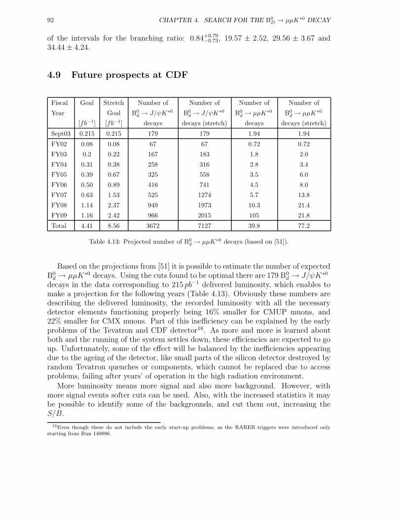
92 CHAPTER 4. SEARCH FOR THE B0D → µµK∗0 DECAY
of the intervals for the branching ratio: 0.84+0.79−0.73, 19.57 ± 2.52, 29.56 ± 3.67 and
34.44 ± 4.24.
4.9 Future prospects at CDF
Fiscal Goal Stretch Number of Number of Number of Number of
Year Goal B0d → J/ψK∗0 B0
d → J/ψK∗0 B0d → µµK∗0 B0
d → µµK∗0
[fb−1] [fb−1] decays decays (stretch) decays decays (stretch)
Sept03 0.215 0.215 179 179 1.94 1.94
FY02 0.08 0.08 67 67 0.72 0.72
FY03 0.2 0.22 167 183 1.8 2.0
FY04 0.31 0.38 258 316 2.8 3.4
FY05 0.39 0.67 325 558 3.5 6.0
FY06 0.50 0.89 416 741 4.5 8.0
FY07 0.63 1.53 525 1274 5.7 13.8
FY08 1.14 2.37 949 1973 10.3 21.4
FY09 1.16 2.42 966 2015 105 21.8
Total 4.41 8.56 3672 7127 39.8 77.2
Table 4.13: Projected number of B0d → µµK∗0 decays (based on [51]).
Based on the projections from [51] it is possible to estimate the number of expectedB0d → µµK∗0 decays. Using the cuts found to be optimal there are 179 B0
d → J/ψK∗0
decays in the data corresponding to 215 pb−1 delivered luminosity, which enables tomake a projection for the following years (Table 4.13). Obviously these numbers aredescribing the delivered luminosity, the recorded luminosity with all the necessarydetector elements functioning properly being 16% smaller for CMUP muons, and22% smaller for CMX muons. Part of this inefficiency can be explained by the earlyproblems of the Tevatron and CDF detector18. As more and more is learned aboutboth and the running of the system settles down, these efficiencies are expected to goup. Unfortunately, some of the effect will be balanced by the inefficiencies appearingdue to the ageing of the detector, like small parts of the silicon detector destroyed byrandom Tevatron quenches or components, which cannot be replaced due to accessproblems, failing after years’ of operation in the high radiation environment.
More luminosity means more signal and also more background. However, withmore signal events softer cuts can be used. Also, with the increased statistics it maybe possible to identify some of the backgrounds, and cut them out, increasing theS/B.
18Even though these do not include the early start-up problems, as the RAREB triggers were introduced onlystarting from Run 140886.
4.10. CONCLUSIONS 93
4.10 Conclusions
A search for the flavor changing neutral current process B0d → µµK∗0 has been per-
formed in pp collisions at√s = 1.96TeV produced at the Collider Detector at
Fermilab (CDFII). These decays are forbidden at tree-level in the Standard Model,but proceed at low rate through penguin and box diagrams. The search for theB0d → µµK∗0 decay has been conducted using data accumulated until September 2003
corresponding to 215 pb−1 integrated luminosity. Judicious cuts have been applied inorder to reduce the background to an acceptable level. Three strongly discriminatingvariables have been chosen and the cuts on them were optimized using diverse figuresof merit. Due to its similarity to the B0
d → µµK∗0 decay the B0d → J/ψK∗0 decay
was used as a reference. Monte Carlo simulations were used to calculate those effi-ciencies which could not be obtained from the data. Analysis performed on the datayields the following confidence intervals for the branching ratio of B0
d → µµK∗0 :
[0.84, 19.57]× 10−7 CI = 68.75% (4.33)
[0.0, 29.56] × 10−7 CI = 90% (4.34)
[0.0, 34.44] × 10−7 CI = 95% (4.35)
That improves the
B(B0d → µµK∗0) < 4.0 × 10⁻⁶ (90% C.L.) (4.36)
measured in Run I [87]. It is consistent with the predictions of the Standard Modeland the measurements of the BaBar and Belle experiments. As the Tevatron continuesto gather luminosity, CDF should be able to replace the upper limits given by the90% and 95% confidence intervals with measurements and confirm the observationsmade at the B factories.

94 CHAPTER 4. SEARCH FOR THE B0D → µµK∗0 DECAY
Part III
Performance of ATLAS modulesusing the SCTA128 chip
95

Chapter 5
Detectors for studying rare Bdecays II: The ATLAS experimentat the LHC
5.1 The Large Hadron Collider
The Large Hadron Collider is the new particle accelerator under construction atCERN. It should be completed by 2005 and will bring protons into head-on collisionsat higher energies than ever achieved. The LHC will provide an energy of 7TeV perbeam, which will give rise to a center-of-mass energy of 14TeV . This center-of-massenergy is one magnitude higher than that reached by the Tevatron at Fermilab, andcorresponds to the conditions prevailing in the Universe just 10−12 seconds after the“Big Bang”. The LHC design luminosity is 1034cm−2s−1. However, in the first fewyears, while the performance is still being optimized, the machine luminosity will be≈ 1033cm−2s−1, so during this period the LHC experiments will be well adapted toexploit the field of B physics. When the design luminosity is reached the focus willshift towards the Higgs sector of the Standard Model. The Higgs boson is responsiblefor the masses of all known particles and its discovery is the main challenge of theLHC. There are four important experiments planned to be installed at the interactionpoints of the accelerator: ALICE, ATLAS, CMS and LHCb.
In order to achieve the 1034cm−2s−1 luminosity the LHC will take advantage of theexisting accelerator infrastructure at CERN (Figure 5.1) [109]. Protons will be pre-accelerated and injected from the SPS at an energy of 450GeV . In order to reach thedesign luminosity the LHC is filled with 2808 proton bunches each containing 1.1×10¹¹
protons. The time separation between the bunches is 24.95ns which corresponds toa 40 MHz collision frequency. After the injection the protons are accelerated up to7TeV and remain in the accelerator for periods of ≈ 10 hours, which is called a store.Extremely large magnetic fields are needed in order to bend the 7TeV proton beamsaround the 27 km ring of the LHC. Specially designed super-conducting dipoles willprovide an 8.33T magnetic field for both beams. Apart from the 1296 dipoles, a large
97
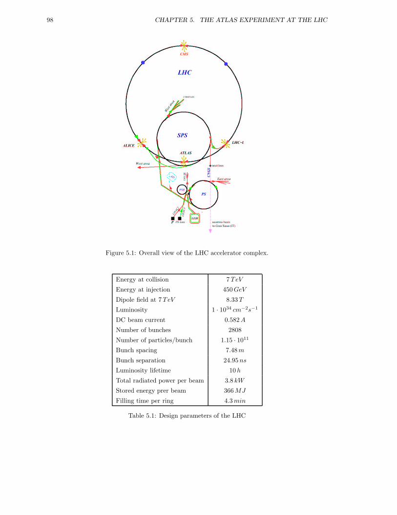
98 CHAPTER 5. THE ATLAS EXPERIMENT AT THE LHC
Figure 5.1: Overall view of the LHC accelerator complex.
Energy at collision 7TeV
Energy at injection 450GeV
Dipole field at 7TeV 8.33T
Luminosity 1 · 1034 cm−2s−1
DC beam current 0.582A
Number of bunches 2808
Number of particles/bunch 1.15 · 1011
Bunch spacing 7.48m
Bunch separation 24.95ns
Luminosity lifetime 10h
Total radiated power per beam 3.8 kW
Stored energy prer beam 366MJ
Filling time per ring 4.3min
Table 5.1: Design parameters of the LHC
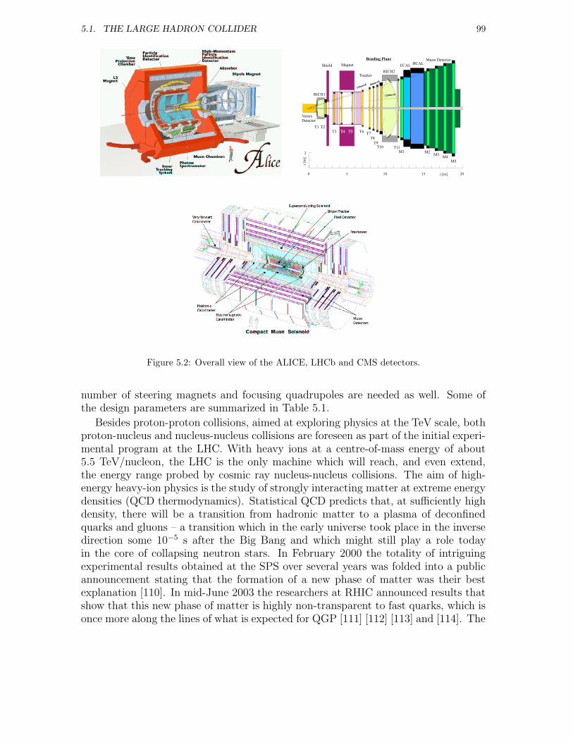
5.1. THE LARGE HADRON COLLIDER 99
Figure 5.2: Overall view of the ALICE, LHCb and CMS detectors.
number of steering magnets and focusing quadrupoles are needed as well. Some ofthe design parameters are summarized in Table 5.1.
Besides proton-proton collisions, aimed at exploring physics at the TeV scale, bothproton-nucleus and nucleus-nucleus collisions are foreseen as part of the initial experi-mental program at the LHC. With heavy ions at a centre-of-mass energy of about5.5 TeV/nucleon, the LHC is the only machine which will reach, and even extend,the energy range probed by cosmic ray nucleus-nucleus collisions. The aim of high-energy heavy-ion physics is the study of strongly interacting matter at extreme energydensities (QCD thermodynamics). Statistical QCD predicts that, at sufficiently highdensity, there will be a transition from hadronic matter to a plasma of deconfinedquarks and gluons – a transition which in the early universe took place in the inversedirection some 10−5 s after the Big Bang and which might still play a role todayin the core of collapsing neutron stars. In February 2000 the totality of intriguingexperimental results obtained at the SPS over several years was folded into a publicannouncement stating that the formation of a new phase of matter was their bestexplanation [110]. In mid-June 2003 the researchers at RHIC announced results thatshow that this new phase of matter is highly non-transparent to fast quarks, which isonce more along the lines of what is expected for QGP [111] [112] [113] and [114]. The
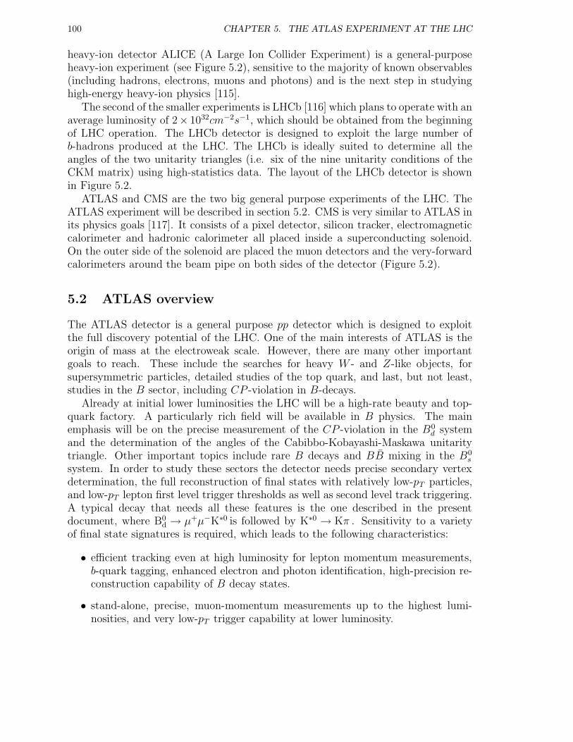
100 CHAPTER 5. THE ATLAS EXPERIMENT AT THE LHC
heavy-ion detector ALICE (A Large Ion Collider Experiment) is a general-purposeheavy-ion experiment (see Figure 5.2), sensitive to the majority of known observables(including hadrons, electrons, muons and photons) and is the next step in studyinghigh-energy heavy-ion physics [115].
The second of the smaller experiments is LHCb [116] which plans to operate with anaverage luminosity of 2× 1032cm−2s−1, which should be obtained from the beginningof LHC operation. The LHCb detector is designed to exploit the large number ofb-hadrons produced at the LHC. The LHCb is ideally suited to determine all theangles of the two unitarity triangles (i.e. six of the nine unitarity conditions of theCKM matrix) using high-statistics data. The layout of the LHCb detector is shownin Figure 5.2.
ATLAS and CMS are the two big general purpose experiments of the LHC. TheATLAS experiment will be described in section 5.2. CMS is very similar to ATLAS inits physics goals [117]. It consists of a pixel detector, silicon tracker, electromagneticcalorimeter and hadronic calorimeter all placed inside a superconducting solenoid.On the outer side of the solenoid are placed the muon detectors and the very-forwardcalorimeters around the beam pipe on both sides of the detector (Figure 5.2).
5.2 ATLAS overview
The ATLAS detector is a general purpose pp detector which is designed to exploitthe full discovery potential of the LHC. One of the main interests of ATLAS is theorigin of mass at the electroweak scale. However, there are many other importantgoals to reach. These include the searches for heavy W - and Z-like objects, forsupersymmetric particles, detailed studies of the top quark, and last, but not least,studies in the B sector, including CP -violation in B-decays.
Already at initial lower luminosities the LHC will be a high-rate beauty and top-quark factory. A particularly rich field will be available in B physics. The mainemphasis will be on the precise measurement of the CP -violation in the B0
d systemand the determination of the angles of the Cabibbo-Kobayashi-Maskawa unitaritytriangle. Other important topics include rare B decays and BB mixing in the B0
s
system. In order to study these sectors the detector needs precise secondary vertexdetermination, the full reconstruction of final states with relatively low-pT particles,and low-pT lepton first level trigger thresholds as well as second level track triggering.A typical decay that needs all these features is the one described in the presentdocument, where B0
d → µ+µ−K∗0 is followed by K∗0 → Kπ . Sensitivity to a varietyof final state signatures is required, which leads to the following characteristics:
• efficient tracking even at high luminosity for lepton momentum measurements,b-quark tagging, enhanced electron and photon identification, high-precision re-construction capability of B decay states.
• stand-alone, precise, muon-momentum measurements up to the highest lumi-nosities, and very low-pT trigger capability at lower luminosity.
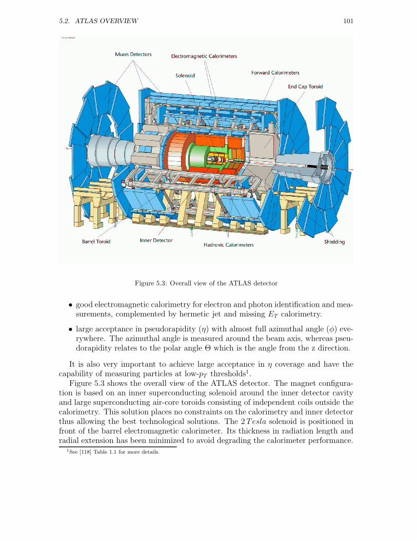
5.2. ATLAS OVERVIEW 101
Figure 5.3: Overall view of the ATLAS detector
• good electromagnetic calorimetry for electron and photon identification and mea-surements, complemented by hermetic jet and missing ET calorimetry.
• large acceptance in pseudorapidity (η) with almost full azimuthal angle (φ) eve-rywhere. The azimuthal angle is measured around the beam axis, whereas pseu-dorapidity relates to the polar angle Θ which is the angle from the z direction.
It is also very important to achieve large acceptance in η coverage and have thecapability of measuring particles at low-pT thresholds1.
Figure 5.3 shows the overall view of the ATLAS detector. The magnet configura-tion is based on an inner superconducting solenoid around the inner detector cavityand large superconducting air-core toroids consisting of independent coils outside thecalorimetry. This solution places no constraints on the calorimetry and inner detectorthus allowing the best technological solutions. The 2Tesla solenoid is positioned infront of the barrel electromagnetic calorimeter. Its thickness in radiation length andradial extension has been minimized to avoid degrading the calorimeter performance.
1See [118] Table 1.1 for more details.
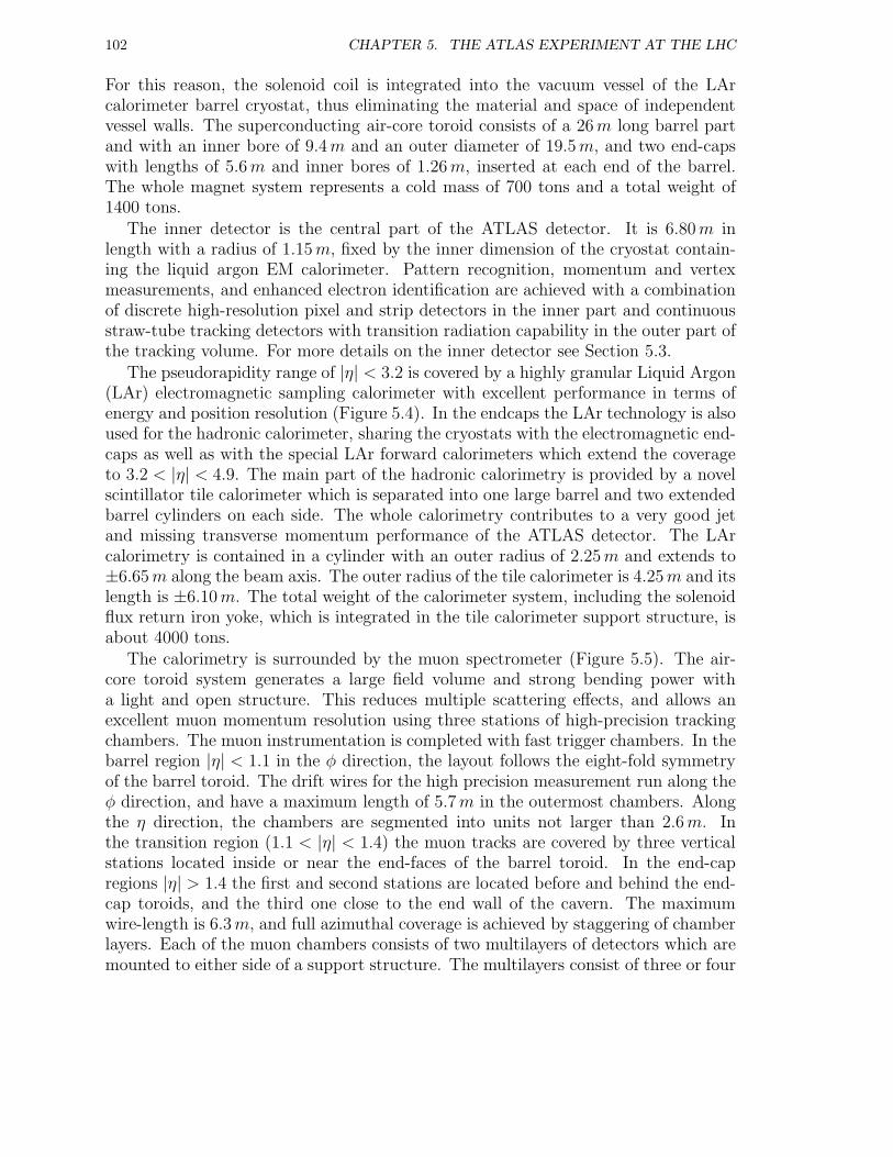
102 CHAPTER 5. THE ATLAS EXPERIMENT AT THE LHC
For this reason, the solenoid coil is integrated into the vacuum vessel of the LArcalorimeter barrel cryostat, thus eliminating the material and space of independentvessel walls. The superconducting air-core toroid consists of a 26m long barrel partand with an inner bore of 9.4m and an outer diameter of 19.5m, and two end-capswith lengths of 5.6m and inner bores of 1.26m, inserted at each end of the barrel.The whole magnet system represents a cold mass of 700 tons and a total weight of1400 tons.
The inner detector is the central part of the ATLAS detector. It is 6.80m inlength with a radius of 1.15m, fixed by the inner dimension of the cryostat contain-ing the liquid argon EM calorimeter. Pattern recognition, momentum and vertexmeasurements, and enhanced electron identification are achieved with a combinationof discrete high-resolution pixel and strip detectors in the inner part and continuousstraw-tube tracking detectors with transition radiation capability in the outer part ofthe tracking volume. For more details on the inner detector see Section 5.3.
The pseudorapidity range of |η| < 3.2 is covered by a highly granular Liquid Argon(LAr) electromagnetic sampling calorimeter with excellent performance in terms ofenergy and position resolution (Figure 5.4). In the endcaps the LAr technology is alsoused for the hadronic calorimeter, sharing the cryostats with the electromagnetic end-caps as well as with the special LAr forward calorimeters which extend the coverageto 3.2 < |η| < 4.9. The main part of the hadronic calorimetry is provided by a novelscintillator tile calorimeter which is separated into one large barrel and two extendedbarrel cylinders on each side. The whole calorimetry contributes to a very good jetand missing transverse momentum performance of the ATLAS detector. The LArcalorimetry is contained in a cylinder with an outer radius of 2.25m and extends to±6.65m along the beam axis. The outer radius of the tile calorimeter is 4.25m and itslength is ±6.10m. The total weight of the calorimeter system, including the solenoidflux return iron yoke, which is integrated in the tile calorimeter support structure, isabout 4000 tons.
The calorimetry is surrounded by the muon spectrometer (Figure 5.5). The air-core toroid system generates a large field volume and strong bending power witha light and open structure. This reduces multiple scattering effects, and allows anexcellent muon momentum resolution using three stations of high-precision trackingchambers. The muon instrumentation is completed with fast trigger chambers. In thebarrel region |η| < 1.1 in the φ direction, the layout follows the eight-fold symmetryof the barrel toroid. The drift wires for the high precision measurement run along theφ direction, and have a maximum length of 5.7m in the outermost chambers. Alongthe η direction, the chambers are segmented into units not larger than 2.6m. Inthe transition region (1.1 < |η| < 1.4) the muon tracks are covered by three verticalstations located inside or near the end-faces of the barrel toroid. In the end-capregions |η| > 1.4 the first and second stations are located before and behind the end-cap toroids, and the third one close to the end wall of the cavern. The maximumwire-length is 6.3m, and full azimuthal coverage is achieved by staggering of chamberlayers. Each of the muon chambers consists of two multilayers of detectors which aremounted to either side of a support structure. The multilayers consist of three or four
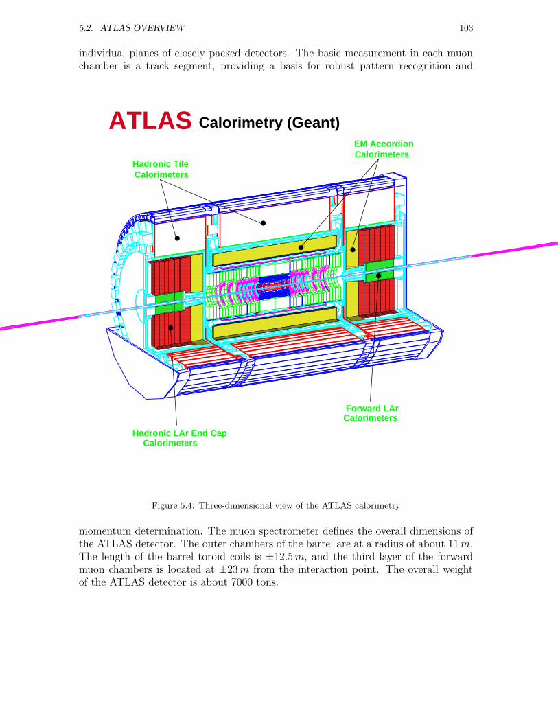
5.2. ATLAS OVERVIEW 103
individual planes of closely packed detectors. The basic measurement in each muonchamber is a track segment, providing a basis for robust pattern recognition and
ATLAS Calorimetry (Geant)
Calorimeters
Calorimeters
Calorimeters
Calorimeters
Hadronic Tile
EM Accordion
Forward LAr
Hadronic LAr End Cap
Figure 5.4: Three-dimensional view of the ATLAS calorimetry
momentum determination. The muon spectrometer defines the overall dimensions ofthe ATLAS detector. The outer chambers of the barrel are at a radius of about 11m.The length of the barrel toroid coils is ±12.5m, and the third layer of the forwardmuon chambers is located at ±23m from the interaction point. The overall weightof the ATLAS detector is about 7000 tons.
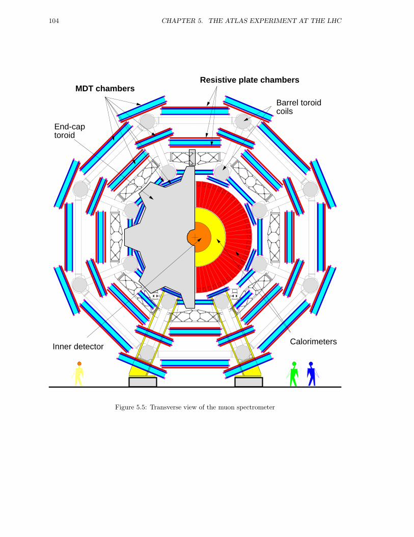
104 CHAPTER 5. THE ATLAS EXPERIMENT AT THE LHC
End-captoroid
Barrel toroidcoils
Calorimeters
MDT chambersResistive plate chambers
Inner detector
Figure 5.5: Transverse view of the muon spectrometer
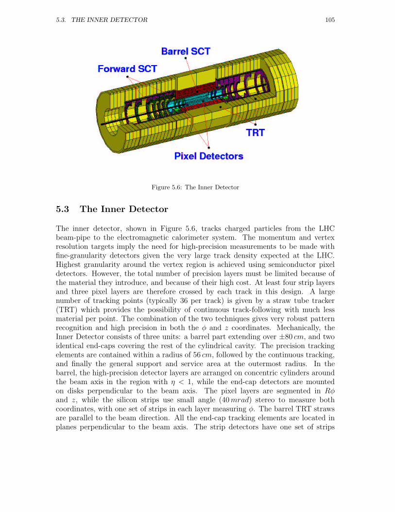
5.3. THE INNER DETECTOR 105
Figure 5.6: The Inner Detector
5.3 The Inner Detector
The inner detector, shown in Figure 5.6, tracks charged particles from the LHCbeam-pipe to the electromagnetic calorimeter system. The momentum and vertexresolution targets imply the need for high-precision measurements to be made withfine-granularity detectors given the very large track density expected at the LHC.Highest granularity around the vertex region is achieved using semiconductor pixeldetectors. However, the total number of precision layers must be limited because ofthe material they introduce, and because of their high cost. At least four strip layersand three pixel layers are therefore crossed by each track in this design. A largenumber of tracking points (typically 36 per track) is given by a straw tube tracker(TRT) which provides the possibility of continuous track-following with much lessmaterial per point. The combination of the two techniques gives very robust patternrecognition and high precision in both the φ and z coordinates. Mechanically, theInner Detector consists of three units: a barrel part extending over ±80 cm, and twoidentical end-caps covering the rest of the cylindrical cavity. The precision trackingelements are contained within a radius of 56 cm, followed by the continuous tracking,and finally the general support and service area at the outermost radius. In thebarrel, the high-precision detector layers are arranged on concentric cylinders aroundthe beam axis in the region with η < 1, while the end-cap detectors are mountedon disks perpendicular to the beam axis. The pixel layers are segmented in Rφand z, while the silicon strips use small angle (40mrad) stereo to measure bothcoordinates, with one set of strips in each layer measuring φ. The barrel TRT strawsare parallel to the beam direction. All the end-cap tracking elements are located inplanes perpendicular to the beam axis. The strip detectors have one set of strips
106 CHAPTER 5. THE ATLAS EXPERIMENT AT THE LHC
running in radial directions, and a set of stereo strips at an angle of 40mrad. Thecontinuous tracking consists of radial straws arranged into wheels.
The layout provides full tracking coverage over |η| < 2.5, including impact param-eter measurements and vertexing for heavy-flavour and τ tagging. The resolution willbe typically σRφ = 12µm and σz = 66 − 77µm for the pixel layers, σRφ = 16µmand σz = 580µm for the silicon detectors, and σperstraw = 170µm for the TRT2.The secondary vertex measurement performance will be enhanced with an innermostadditional layer of pixels, at a radius of about 5.05 cm, as close as is practical aroundthe beam pipe. The lifetime of such a detector will be limited by radiation damage,and would need replacement after a few years. A large amount of interesting physicscan be done with this detector during the initial lower luminosity running, especiallyin the B sector. The mechanical design allows for the possibility of replacing theB-layer, which will remain an important tool for the B-tagging.
The pixel detector is designed to provide a very high-granularity, high-precisionset of measurements as close to the interaction point as possible. The system providesthree of the precision measurements over the full acceptance, and determines the im-pact parameter resolution and the ability of the Inner Detector to find short-livedparticles such as b-quarks and τ -leptons. The two-dimensional segmentation of thesensors gives space points without any of the ambiguities associated with projectivegeometries, but requires the use of advanced electronic techniques and interconnec-tions for the readout. In addition, the pixel system must be radiation hardened towithstand over 300 kGy of ionising radiation and over 5.1014/cm2 neutrons in tenyears of operation.
The system offers 80 million detector elements, each 50µm in the Rφ direction and400µm in z, which are invaluable for the task of pattern recognition in the crowdedenvironment of the LHC. The system consists of three barrels at average radii of5.05 cm, 8.85 cm, and 12.25 cm, and three disks on each side, between radii of 11 and20 cm, which complete the angular coverage. It is designed to be highly modular,containing 1744 barrel and disk modules [120]. The modules are overlapped on thesupport structure in order to give a hermetic coverage.
The SCT system is designed to provide four precision measurements per track inthe intermediate radial range, contributing to the measurement of momentum, impactparameter and vertex position, as well as providing good pattern recognition by theuse of high granularity. It is described in more detail in Section 5.5.
The TRT is based on the use of straw detectors, which can operate at the veryhigh rates needed by virtue of their small diameter and the isolation of the sensewires within individual gas envelopes. Electron identification capability is added byemploying a gas mixture based on xenon with the addition of CO2 and O2 to detecttransition-radiation photons created in a radiator between the straws. This techniqueis intrinsically radiation hard, and allows a large number of measurements, typically36, to be made on every track at modest cost. However the detector must copewith a large occupancy and high counting rates at the LHC design luminosity. Each
2For more details see [119] Table 1-1.
5.3. THE INNER DETECTOR 107
straw is 4mm in diameter, giving a fast response and good mechanical propertiesfor a maximum straw length of 144 cm. The barrel contains about 50000 straws,each divided in two at the centre in order to reduce the occupancy and read out ateach end. The end-caps contain 320000 radial straws, with the readout at the outerradius. The total number of electronic channels is 420000. Each channel providesa drift-time measurement, giving a spatial resolution of 170µm per straw, and twoindependent thresholds. These allow the detector to discriminate between trackinghits, which pass the lower threshold, and transition-radiation hits, which pass thehigher. The barrel section is built of individual modules covering the radial rangefrom 56 to 107 cm. The modularity was chosen as a compromise between the easeof construction and maintenance, and the additional structural elements involved.The two end-caps each consist of 18 wheels. The 14 wheels nearest the interactionpoint cover the radial range from 64 to 103 cm, while the last four wheels extend toan inner radius of 48 cm in order to maintain a constant number of crossed strawsover the full acceptance. At rates of 12MHz, only about 70% of the straws givecorrect drift time measurements because of shadowing effects, but the large numberof straws per track guarantees a measurement accuracy of better than 50µm averagedover all straws at the LHC design luminosity, including errors from alignment. Hencethe TRT contributes to the accuracy of the momentum measurement in the InnerDetector by providing a set of measurements roughly equivalent to a single point of50µm precision. It aids the pattern recognition by the addition of around 36 hitsper track, and allows a simple and fast level-2 track trigger to be implemented. Inaddition it provides additional discrimination between electrons and hadrons, with apion rejection varying with η between a factor of 15 and 200 at 90% electron efficiency.
All tracks with |η| < 2.5 are measured with six precision space-points and about36 straws, except for a slight degradation across the barrel to end-cap transitionregion at the largest η. With the B-layer present, seven precision points are obtained.The momentum resolution of the Inner Detector is limited by several factors: theradial space available in the cavity, which limits the lever arm, the strength of themagnetic field, and the intrinsic precision of the detector elements. In addition, above|η| = 1.85, tracks leave the Inner Detector volume before reaching the maximumradius of the cavity, thereby reducing the field integral available as compared to thelower |η| regions. These effects limit the momentum resolution achievable in the end-cap regions, especially for |η| > 2. This achievable resolution is sufficient to identifythe charge sign of particles up to the highest energies expected at LHC.
Extensive simulations have been performed in order to characterize the phyisicsperformance of the ID [121], [122] and [123]. Since the time of the Physics TDR,only small changes have occurred to the positions and dimensions of the SCT andTRT. However, major changes have been made to the Pixel system, in particularto the innermost layer, the B-layer. The radius of the B-layer has been increasedin order to accommodate a larger beam pipe and the whole Pixel detector has beengiven an independent insertion capability so that it can be inserted later or replacedif damaged by radiation. This latter development has caused a serious increase inthe amount of material, with the pixel-barrel radiation-thickness increased by 50%
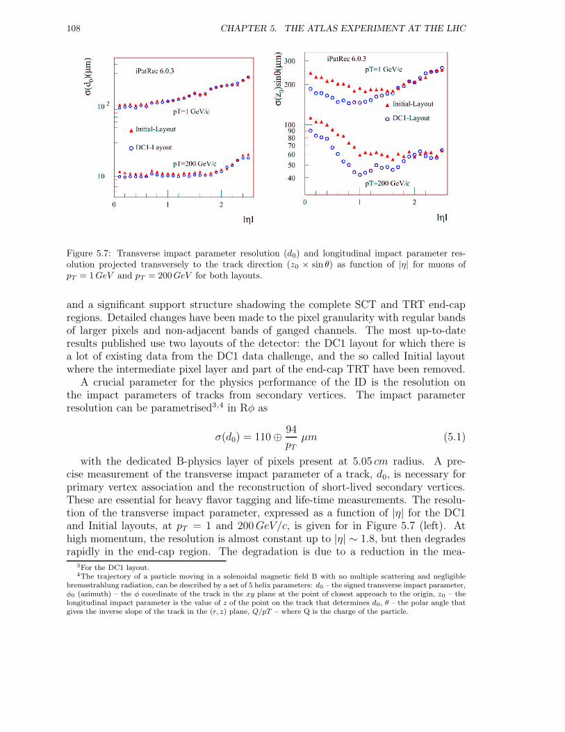
108 CHAPTER 5. THE ATLAS EXPERIMENT AT THE LHC
Figure 5.7: Transverse impact parameter resolution (d0) and longitudinal impact parameter res-olution projected transversely to the track direction (z0 × sin θ) as function of |η| for muons ofpT = 1GeV and pT = 200GeV for both layouts.
and a significant support structure shadowing the complete SCT and TRT end-capregions. Detailed changes have been made to the pixel granularity with regular bandsof larger pixels and non-adjacent bands of ganged channels. The most up-to-dateresults published use two layouts of the detector: the DC1 layout for which there isa lot of existing data from the DC1 data challenge, and the so called Initial layoutwhere the intermediate pixel layer and part of the end-cap TRT have been removed.
A crucial parameter for the physics performance of the ID is the resolution onthe impact parameters of tracks from secondary vertices. The impact parameterresolution can be parametrised3 ,4 in Rφ as
σ(d0) = 110 ⊕ 94
pTµm (5.1)
with the dedicated B-physics layer of pixels present at 5.05 cm radius. A pre-cise measurement of the transverse impact parameter of a track, d0, is necessary forprimary vertex association and the reconstruction of short-lived secondary vertices.These are essential for heavy flavor tagging and life-time measurements. The resolu-tion of the transverse impact parameter, expressed as a function of |η| for the DC1and Initial layouts, at pT = 1 and 200GeV/c, is given for in Figure 5.7 (left). Athigh momentum, the resolution is almost constant up to |η| ∼ 1.8, but then degradesrapidly in the end-cap region. The degradation is due to a reduction in the mea-
3For the DC1 layout.4The trajectory of a particle moving in a solenoidal magnetic field B with no multiple scattering and negligible
bremsstrahlung radiation, can be described by a set of 5 helix parameters: d0 – the signed transverse impact parameter,φ0 (azimuth) – the φ coordinate of the track in the xy plane at the point of closest approach to the origin, z0 – thelongitudinal impact parameter is the value of z of the point on the track that determines d0, θ – the polar angle thatgives the inverse slope of the track in the (r, z) plane, Q/pT – where Q is the charge of the particle.
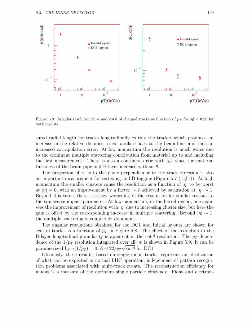
5.3. THE INNER DETECTOR 109
Figure 5.8: Angular resolution in φ and cot θ of charged tracks as function of pT for |η| < 0.25 forboth layouts.
sured radial length for tracks longitudinally exiting the tracker which produces anincrease in the relative distance to extrapolate back to the beam-line, and thus anincreased extrapolation error. At low momentum the resolution is much worse dueto the dominant multiple scattering contribution from material up to and includingthe first measurement. There is also a continuous rise with |η|, since the materialthickness of the beam-pipe and B-layer increase with sin θ.
The projection of z0 onto the plane perpendicular to the track direction is alsoan important measurement for vertexing and B-tagging (Figure 5.7 (right)). At highmomentum the smaller clusters cause the resolution as a function of |η| to be worstat |η| = 0, with an improvement by a factor ∼ 2 achieved by saturation at |η| ∼ 1.Beyond this value, there is a slow worsening of the resolution for similar reasons tothe transverse impact parameter. At low momentum, in the barrel region, one againsees the improvement of resolution with |η| due to increasing cluster size, but here thegain is offset by the corresponding increase in multiple scattering. Beyond |η| ∼ 1,the multiple scattering is completely dominant.
The angular resolutions obtained for the DC1 and Initial layouts are shown forcentral tracks as a function of pT in Figure 5.8. The effect of the reduction in theB-layer longitudinal granularity is apparent in the cot θ resolution. The pT depen-dence of the 1/pT resolution integrated over all |η| is shown in Figure 5.9. It can be
parametrized by σ(1/pT ) = 0.55 ⊕ 22/pT√
sin θ for DC1.
Obviously, these results, based on single muon tracks, represent an idealizationof what can be expected in normal LHC operation, independent of pattern recogni-tion problems associated with multi-track events. The reconstruction efficiency formuons is a measure of the optimum single particle efficiency. Pions and electrons
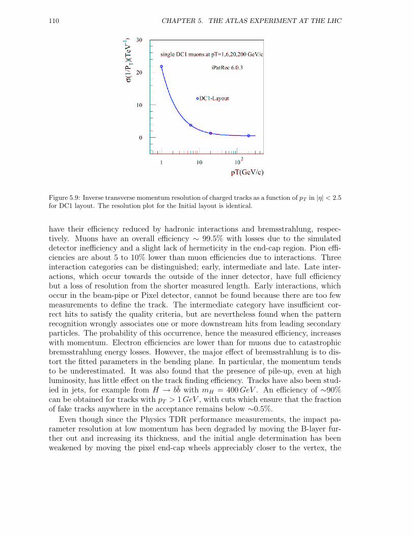
110 CHAPTER 5. THE ATLAS EXPERIMENT AT THE LHC
Figure 5.9: Inverse transverse momentum resolution of charged tracks as a function of pT in |η| < 2.5for DC1 layout. The resolution plot for the Initial layout is identical.
have their efficiency reduced by hadronic interactions and bremsstrahlung, respec-tively. Muons have an overall efficiency ∼ 99.5% with losses due to the simulateddetector inefficiency and a slight lack of hermeticity in the end-cap region. Pion effi-ciencies are about 5 to 10% lower than muon efficiencies due to interactions. Threeinteraction categories can be distinguished; early, intermediate and late. Late inter-actions, which occur towards the outside of the inner detector, have full efficiencybut a loss of resolution from the shorter measured length. Early interactions, whichoccur in the beam-pipe or Pixel detector, cannot be found because there are too fewmeasurements to define the track. The intermediate category have insufficient cor-rect hits to satisfy the quality criteria, but are nevertheless found when the patternrecognition wrongly associates one or more downstream hits from leading secondaryparticles. The probability of this occurrence, hence the measured efficiency, increaseswith momentum. Electron efficiencies are lower than for muons due to catastrophicbremsstrahlung energy losses. However, the major effect of bremsstrahlung is to dis-tort the fitted parameters in the bending plane. In particular, the momentum tendsto be underestimated. It was also found that the presence of pile-up, even at highluminosity, has little effect on the track finding efficiency. Tracks have also been stud-ied in jets, for example from H → bb with mH = 400GeV . An efficiency of ∼90%can be obtained for tracks with pT > 1GeV , with cuts which ensure that the fractionof fake tracks anywhere in the acceptance remains below ∼0.5%.
Even though since the Physics TDR performance measurements, the impact pa-rameter resolution at low momentum has been degraded by moving the B-layer fur-ther out and increasing its thickness, and the initial angle determination has beenweakened by moving the pixel end-cap wheels appreciably closer to the vertex, the
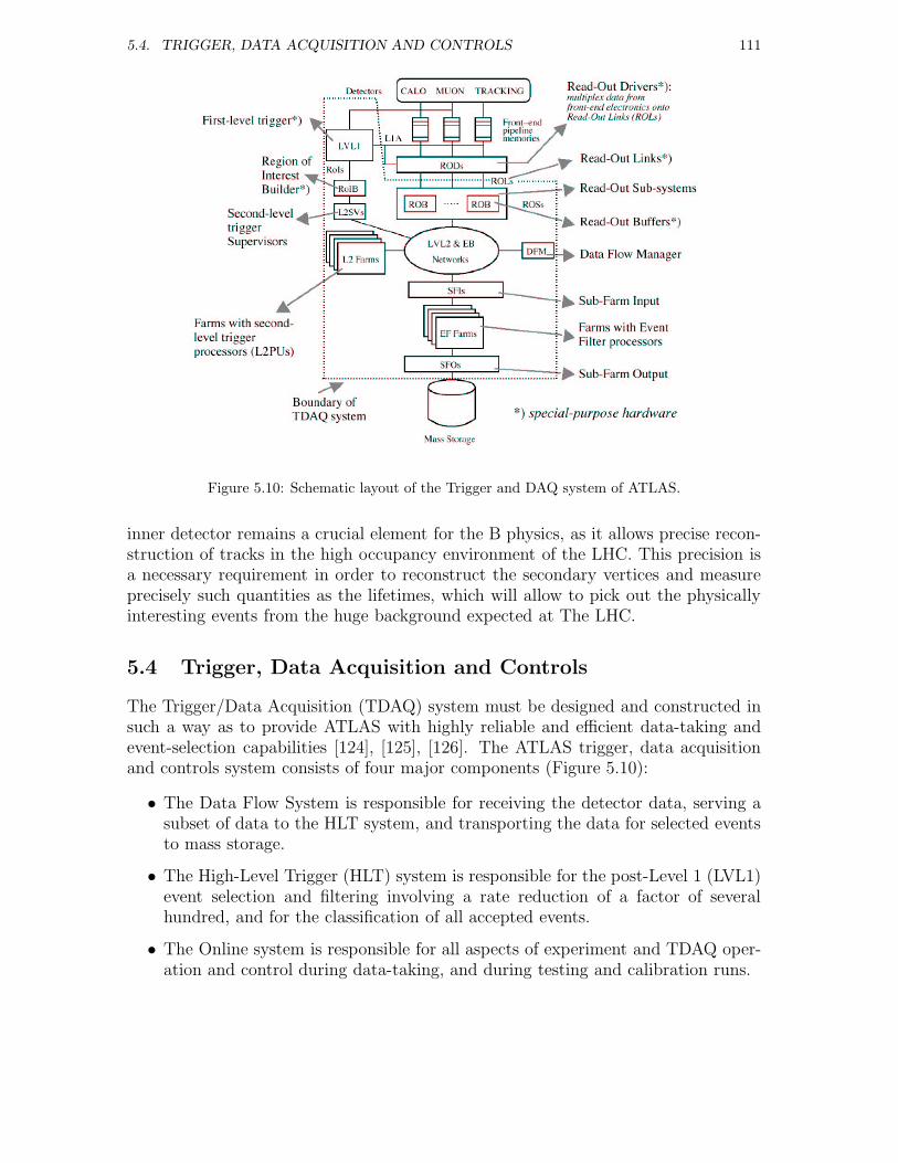
5.4. TRIGGER, DATA ACQUISITION AND CONTROLS 111
Figure 5.10: Schematic layout of the Trigger and DAQ system of ATLAS.
inner detector remains a crucial element for the B physics, as it allows precise recon-struction of tracks in the high occupancy environment of the LHC. This precision isa necessary requirement in order to reconstruct the secondary vertices and measureprecisely such quantities as the lifetimes, which will allow to pick out the physicallyinteresting events from the huge background expected at The LHC.
5.4 Trigger, Data Acquisition and Controls
The Trigger/Data Acquisition (TDAQ) system must be designed and constructed insuch a way as to provide ATLAS with highly reliable and efficient data-taking andevent-selection capabilities [124], [125], [126]. The ATLAS trigger, data acquisitionand controls system consists of four major components (Figure 5.10):
• The Data Flow System is responsible for receiving the detector data, serving asubset of data to the HLT system, and transporting the data for selected eventsto mass storage.
• The High-Level Trigger (HLT) system is responsible for the post-Level 1 (LVL1)event selection and filtering involving a rate reduction of a factor of severalhundred, and for the classification of all accepted events.
• The Online system is responsible for all aspects of experiment and TDAQ oper-ation and control during data-taking, and during testing and calibration runs.
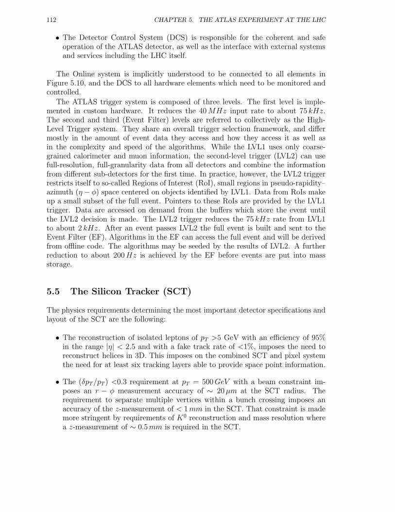
112 CHAPTER 5. THE ATLAS EXPERIMENT AT THE LHC
• The Detector Control System (DCS) is responsible for the coherent and safeoperation of the ATLAS detector, as well as the interface with external systemsand services including the LHC itself.
The Online system is implicitly understood to be connected to all elements inFigure 5.10, and the DCS to all hardware elements which need to be monitored andcontrolled.
The ATLAS trigger system is composed of three levels. The first level is imple-mented in custom hardware. It reduces the 40MHz input rate to about 75 kHz.The second and third (Event Filter) levels are referred to collectively as the High-Level Trigger system. They share an overall trigger selection framework, and differmostly in the amount of event data they access and how they access it as well asin the complexity and speed of the algorithms. While the LVL1 uses only coarse-grained calorimeter and muon information, the second-level trigger (LVL2) can usefull-resolution, full-granularity data from all detectors and combine the informationfrom different sub-detectors for the first time. In practice, however, the LVL2 triggerrestricts itself to so-called Regions of Interest (RoI), small regions in pseudo-rapidity–azimuth (η − φ) space centered on objects identified by LVL1. Data from RoIs makeup a small subset of the full event. Pointers to these RoIs are provided by the LVL1trigger. Data are accessed on demand from the buffers which store the event untilthe LVL2 decision is made. The LVL2 trigger reduces the 75 kHz rate from LVL1to about 2 kHz. After an event passes LVL2 the full event is built and sent to theEvent Filter (EF). Algorithms in the EF can access the full event and will be derivedfrom offline code. The algorithms may be seeded by the results of LVL2. A furtherreduction to about 200Hz is achieved by the EF before events are put into massstorage.
5.5 The Silicon Tracker (SCT)
The physics requirements determining the most important detector specifications andlayout of the SCT are the following:
• The reconstruction of isolated leptons of pT >5 GeV with an efficiency of 95%in the range |η| < 2.5 and with a fake track rate of <1%, imposes the need toreconstruct helices in 3D. This imposes on the combined SCT and pixel systemthe need for at least six tracking layers able to provide space point information.
• The (δpT/pT ) <0.3 requirement at pT = 500GeV with a beam constraint im-poses an r − φ measurement accuracy of ∼ 20µm at the SCT radius. Therequirement to separate multiple vertices within a bunch crossing imposes anaccuracy of the z-measurement of < 1mm in the SCT. That constraint is mademore stringent by requirements of K0 reconstruction and mass resolution wherea z-measurement of ∼ 0.5mm is required in the SCT.
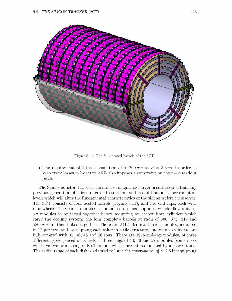
5.5. THE SILICON TRACKER (SCT) 113
Figure 5.11: The four nested barrels of the SCT.
• The requirement of 2-track resolution of < 200µm at R = 30 cm, in order tokeep track losses in b-jets to <5% also imposes a constraint on the r−φ readoutpitch.
The Semiconductor Tracker is an order of magnitude larger in surface area than anyprevious generation of silicon microstrip trackers, and in addition must face radiationlevels which will alter the fundamental characteristics of the silicon wafers themselves.The SCT consists of four nested barrels (Figure 5.11), and two end-caps, each withnine wheels. The barrel modules are mounted on local supports which allow units ofsix modules to be tested together before mounting on carbon-fibre cylinders whichcarry the cooling system; the four complete barrels at radii of 300, 373, 447 and520mm are then linked together. There are 2112 identical barrel modules, mountedin 12 per row, and overlapping each other in a tile structure. Individual cylinders arefully covered with 32, 40, 48 and 56 rows. There are 1976 end-cap modules, of threedifferent types, placed on wheels in three rings of 40, 40 and 52 modules (some diskswill have two or one ring only).The nine wheels are interconnected by a space-frame.The radial range of each disk is adapted to limit the coverage to |η| ≤ 2.5 by equipping
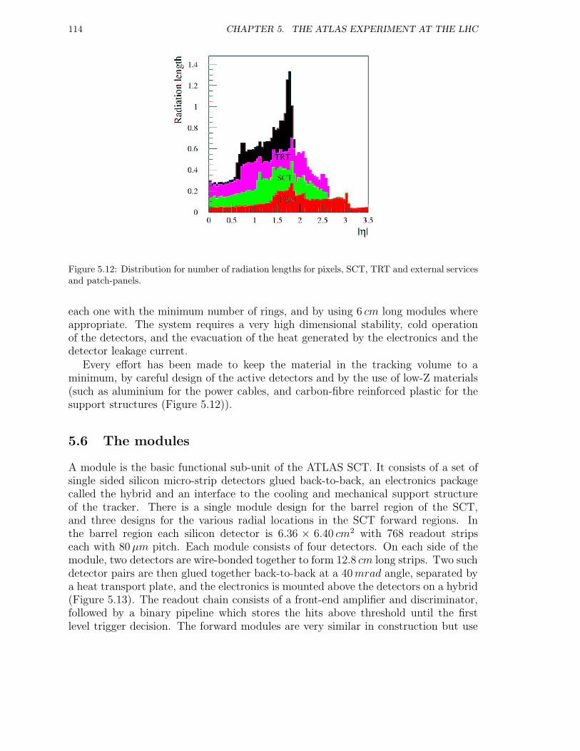
114 CHAPTER 5. THE ATLAS EXPERIMENT AT THE LHC
Figure 5.12: Distribution for number of radiation lengths for pixels, SCT, TRT and external servicesand patch-panels.
each one with the minimum number of rings, and by using 6 cm long modules whereappropriate. The system requires a very high dimensional stability, cold operationof the detectors, and the evacuation of the heat generated by the electronics and thedetector leakage current.
Every effort has been made to keep the material in the tracking volume to aminimum, by careful design of the active detectors and by the use of low-Z materials(such as aluminium for the power cables, and carbon-fibre reinforced plastic for thesupport structures (Figure 5.12)).
5.6 The modules
A module is the basic functional sub-unit of the ATLAS SCT. It consists of a set ofsingle sided silicon micro-strip detectors glued back-to-back, an electronics packagecalled the hybrid and an interface to the cooling and mechanical support structureof the tracker. There is a single module design for the barrel region of the SCT,and three designs for the various radial locations in the SCT forward regions. Inthe barrel region each silicon detector is 6.36 × 6.40 cm2 with 768 readout stripseach with 80µm pitch. Each module consists of four detectors. On each side of themodule, two detectors are wire-bonded together to form 12.8 cm long strips. Two suchdetector pairs are then glued together back-to-back at a 40mrad angle, separated bya heat transport plate, and the electronics is mounted above the detectors on a hybrid(Figure 5.13). The readout chain consists of a front-end amplifier and discriminator,followed by a binary pipeline which stores the hits above threshold until the firstlevel trigger decision. The forward modules are very similar in construction but use
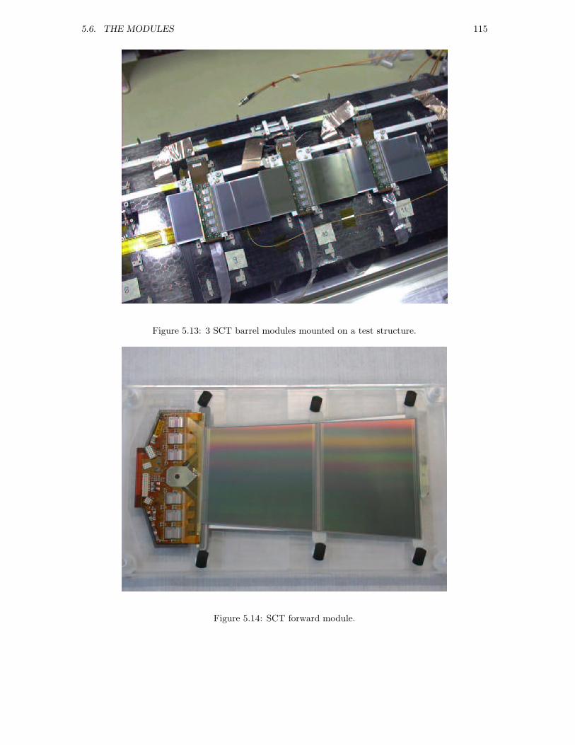
5.6. THE MODULES 115
Figure 5.13: 3 SCT barrel modules mounted on a test structure.
Figure 5.14: SCT forward module.
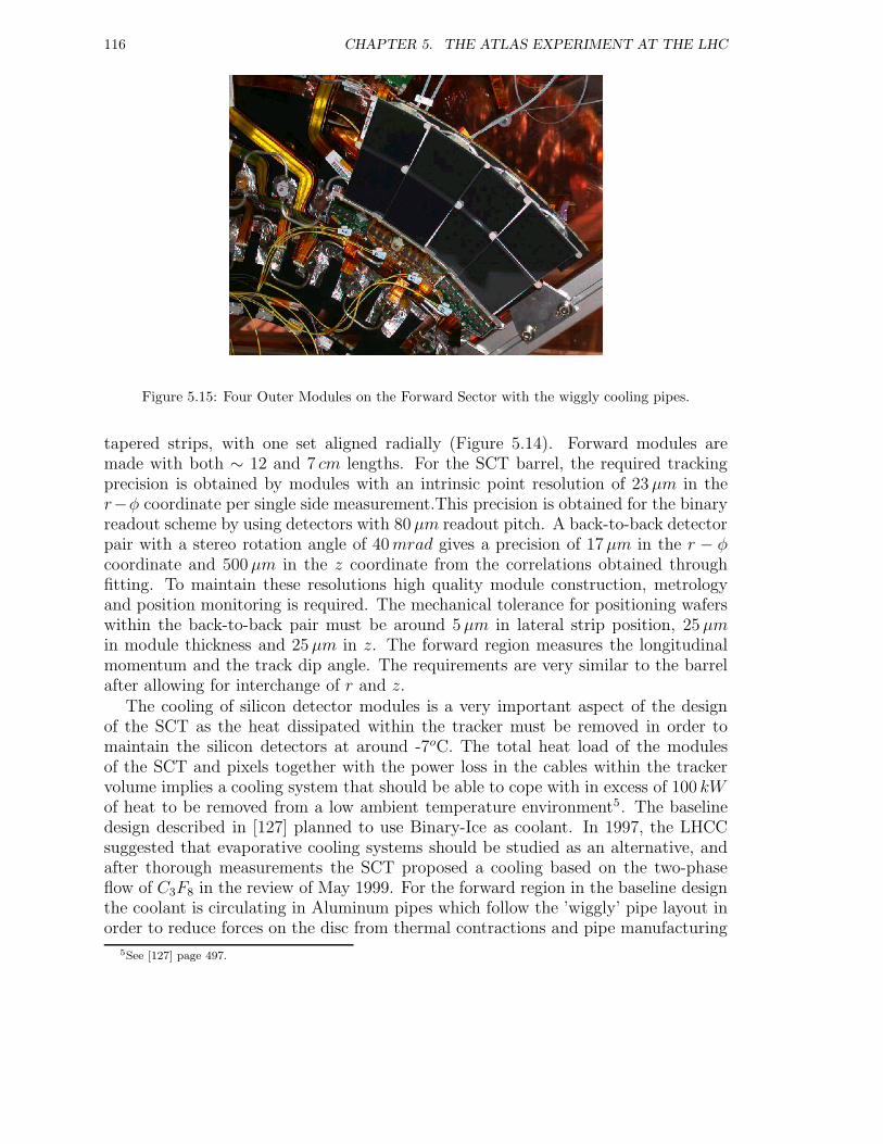
116 CHAPTER 5. THE ATLAS EXPERIMENT AT THE LHC
Figure 5.15: Four Outer Modules on the Forward Sector with the wiggly cooling pipes.
tapered strips, with one set aligned radially (Figure 5.14). Forward modules aremade with both ∼ 12 and 7 cm lengths. For the SCT barrel, the required trackingprecision is obtained by modules with an intrinsic point resolution of 23µm in ther−φ coordinate per single side measurement.This precision is obtained for the binaryreadout scheme by using detectors with 80µm readout pitch. A back-to-back detectorpair with a stereo rotation angle of 40mrad gives a precision of 17µm in the r − φcoordinate and 500µm in the z coordinate from the correlations obtained throughfitting. To maintain these resolutions high quality module construction, metrologyand position monitoring is required. The mechanical tolerance for positioning waferswithin the back-to-back pair must be around 5µm in lateral strip position, 25µmin module thickness and 25µm in z. The forward region measures the longitudinalmomentum and the track dip angle. The requirements are very similar to the barrelafter allowing for interchange of r and z.
The cooling of silicon detector modules is a very important aspect of the designof the SCT as the heat dissipated within the tracker must be removed in order tomaintain the silicon detectors at around -7oC. The total heat load of the modulesof the SCT and pixels together with the power loss in the cables within the trackervolume implies a cooling system that should be able to cope with in excess of 100 kWof heat to be removed from a low ambient temperature environment5. The baselinedesign described in [127] planned to use Binary-Ice as coolant. In 1997, the LHCCsuggested that evaporative cooling systems should be studied as an alternative, andafter thorough measurements the SCT proposed a cooling based on the two-phaseflow of C3F8 in the review of May 1999. For the forward region in the baseline designthe coolant is circulating in Aluminum pipes which follow the ’wiggly’ pipe layout inorder to reduce forces on the disc from thermal contractions and pipe manufacturing
5See [127] page 497.
5.6. THE MODULES 117
tolerances (see the pipes on the left side of Figure 5.15). The heat from the hybridsand the sensors is conducted to the coolant via two aluminum cooling blocks for outerand middle modules, and via a single cooling block for the inner modules [128]. Thereare three separate cooling circuits per quadrant, corresponding to the inner, middleand outer module rings, where the inlets and outlets are manifolded at the patchpanel.
5.6.1 Front-end electronics for modules for Si trackers
In many previous tracking detectors, electrons could be drifted over large distancesin gaseous detectors, and signals could be transmitted along silicon strip detectors,thus placing the electronics outside of the active tracking volume. The high rates atLHC make this impossible over the acceptance of the ATLAS system. Instead, thetracking detectors must be designed with their electronics in close proximity to theactive elements. Therefore the LHC operating conditions present a big challenge tothe front-end electronics of Si trackers for experiments designed for high luminosityphysics. Requirements on the front-end electronics of Si strip detectors are verydemanding. The readout has to be close to the Si sensor and therefore needs tobe radiation hard up to doses of 10Mrad and up to fluences of 3 · 1014 chargedparticles/cm2 and 2 · 1014 neutrons/cm2.
Due to the high occupancy expected at full luminosity operation the pulse shapingtime has to be short. To avoid pileup of events in single channels double pulseresolution has to be of the order of 50ns. It is convenient to have a peaking time ofthe output pulse equivalent to the bunch crossing frequency of 40MHz.
The noise performance is dictated by the most probable signal from a minimumionising particle (MIP) crossing a 300µm thick Si sensor, which is 22500 charges. Toobtain a good efficiency for track reconstruction and maintain at the same time alow noise occupancy a signal over noise ratio better than 15:1 is required. This isequivalent to a noise smaller than 1500 e− Equivalent Noise Charge (ENC).
The size of irreducible noise contributions, shot noise from leakage current in theirradiated Si sensor and base current in an irradiated bipolar junction transistor andpreamplifier series noise, are determined by the chosen sensor element size. Thesensor element size cannot be too small in order to limit the number of channels,and also cannot exceed a certain size to keep the detector capacitance low. As acompromise for these requirements ATLAS has chosen to have detector geometrieswith strip length from 6 cm to 12.8 cm. The strip pitch is given by the required spatialresolution in the range of σ = 5 − 25µm.
Several architectures have been developed for LHC experiments. The two differentconcepts presented here are the following:
• Full analogue read-out with transmission of all data via analogue optical linksto the external read-out processors for digitalisation with flash ADCs. This isthe concept used so far in most collider experiments for Si trackers and vertexdetectors. It allows individual treatment of data in each channel with optimized
118 CHAPTER 5. THE ATLAS EXPERIMENT AT THE LHC
and adaptable software and thereby the most detailed control and monitoringof the whole system. Analogue readout is to a large extent immune to externalelectromagnetic pickup since common mode noise can be fully eliminated withsoftware. The price to pay is the heavier load on data transmission from the de-tector as one needs both higher bit rate and better quality for the links. Modulesequipped with SCTA128 chips were used to study this architecture.
• Another possibility is the binary scheme for the readout of silicon strip detectors.The binary architecture allows a more compact design and has the advantage ofa much reduced data transfer rate with more chips using a single optical link.This architecture is, however, not immune at all to common mode noise and sois very sensitive to external electromagnetic interference. This is the choice ofthe ATLAS baseline using ABCD chips.
5.6.2 The digital solution (ABCD)
In the beginning two technological options were considered for the binary architecture:
• The ABCD design is a single chip implementation of the binary readout archi-tecture for silicon strip detectors in the ATLAS SCT. It is fabricated using theDMILL technology, which being BiCMOS one, offers a possibility to implementthe complete architecture in one chip.
• A design employing two separate chips: CAFE-M a front-end chip realized inthe MAXIM bipolar process and ABC, a binary pipeline chip realized in theHoneywell bulk CMOS process.
After thorough testing of both the ABCD and the CAFE-M ABC combination[129] [130] the former was choosen as the option to develop.
The ABCD chip has all the blocks of the binary readout architecture; the front-endcircuitry employing a bipolar transistor in the input stage, discriminators, a binarypipeline, a derandomizing buffer, data compression logic and the readout control logic.There were different measurements carried out in order to evaluate the performanceof the chip. Electrical prototype modules were built where the chips were placed ona ceramic hybrid and connected to detector strips of various length. A more detaileddescription of the ABCD design and these measurements is the theme of Section 6.2.
5.6.3 The analogue solution (SCTA)
The analogue solution is represented by the SCTA chip which comprises the follow-ing building blocks: 128 channels with front-end amplifiers, analogue memory (ADB)with the capacity to store 128 analogue samples, control logic providing a derandom-izing function (up to 8 events), a command decoder and a fast analogue multiplexer tooutput serial data. In addition to the basic functional blocks, internal calibration cir-cuitry containing an 8-bit DAC to control the calibration level has been implementedto improve the testability of the chip. Four 5-bit DACs for the bias of the analogue
5.7. PHYSICS POTENTIAL OF THE ATLAS DETECTOR 119
part of the chip have been implemented in order to compensate for the drifts afterirradiation and optimize chip performance for various parameters.
An extensive set of measurements was performed in order to evaluate the perfor-mance of the chip. The characterization of the front-end part was not only importantfor the SCTA, but also for the ABCD as well. The two chips share basically the samefront-end, but in the case of the ABCD the binary architecture prevents a study ofthe subtler effects. First, the basic parameters of the chip have been evaluated in asingle chip setup using internal calibration circuitry. Next, the chips were mountedon hybrids and connected to silicon detectors. The resulting modules were tested inthe laboratory using internal calibration circuitry and radioactive sources. As thefinal step, the modules were transferred to the SPS X5 West area for beam tests. Theanalogue modules were also used as a mean of testing a linear optical link for analoguedata transmission for LHC experiments. How these measurements were performedand what results did they give rise to is described in great detail in Section 6.3.
5.7 Physics Potential of the ATLAS Detector
The rate of B-hadron production at the LHC is enormous thanks to the large hadroniccross-section for b-quark production and the high luminosity of the machine (even atso-called low luminosity L =1033 cm−2s−1). About one collision in every hundredwill produce a b-quark pair, which results in a considerably better signal-to-noiseratio than at lower-energy hadron machines such as the Tevatron. In ATLAS, aninclusive-muon trigger with a pT threshold of 6GeV will make an initial selection ofB-events. Using this inclusive selection, about 25% of the muon-trigger events willcontain b-quarks. In the first year of operation, some 2.3 × 10¹⁰ b-quark pair eventswill be selected for more detailed analysis in the LVL2 trigger and event filter, thatare focused on the selection of specific classes of final states. This event rate will behigher than in any accelerator presently operating.
Although the main focus of the ATLAS physics programme is the search for andstudy of physics beyond the Standard Model, through the production and decay ofnew types of particles, an important range of B-physics studies is planned. In fact, animportant aim of the B-physics work is to test the Standard Model through precisionmeasurements of B-hadron decays that together will over-constrain the CKM matrix,possibly giving indirect evidence for new physics. This programme of work will includethe following: precise measurements of CP violation in B-meson decays, which in theStandard Model is due to a single phase in the CKM matrix; precise measurementsof the periods of flavour oscillations in B0
s as well as B0d mesons, and of relative decay
rates such measurements constrain the elements of the CKM matrix; searches forand measurements of very rare decays which are strongly suppressed in the StandardModel and where significant enhancements could provide indirect evidence for newphysics. Many of the ATLAS measurements will be more precise than those fromexperiments at lower-energy machines, thanks to the greater available statistics.
At the LHC, the general-purpose experiments ATLAS and CMS will face stiff
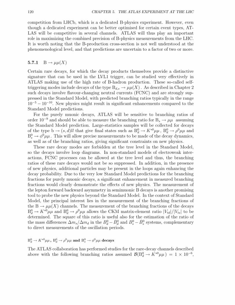
120 CHAPTER 5. THE ATLAS EXPERIMENT AT THE LHC
competition from LHCb, which is a dedicated B-physics experiment. However, eventhough a dedicated experiment can be better optimised for certain event types, AT-LAS will be competitive in several channels. ATLAS will thus play an importantrole in maximizing the combined precision of B-physics measurements from the LHC.It is worth noting that the B-production cross-section is not well understood at thephenomenological level, and that predictions are uncertain to a factor of two or more.
5.7.1 B → µµ(X)
Certain rare decays, for which the decay products themselves provide a distinctivesignature that can be used in the LVL1 trigger, can be studied very effectively inATLAS making use of the high rate of B-hadron production. These so-called self-triggering modes include decays of the type Bd,s → µµ(X) . As described in Chapter 2such decays involve flavour-changing neutral currents (FCNC) and are strongly sup-pressed in the Standard Model, with predicted branching ratios typically in the range10−5 − 10−10. New physics might result in significant enhancements compared to theStandard Model predictions.
For the purely muonic decays, ATLAS will be sensitive to branching ratios oforder 10−9 and should be able to measure the branching ratio for Bs → µµ assumingthe Standard Model prediction. Large-statistics samples will be collected for decaysof the type b → (s, d)ll that give final states such as B0
d → K∗0µµ , B0d → ρ0µµ and
B0s → φ0µµ . This will allow precise measurements to be made of the decay dynamics,
as well as of the branching ratios, giving significant constraints on new physics.These rare decay modes are forbidden at the tree level in the Standard Model,
so the decays involve loop diagrams. In non-standard models of electroweak inter-actions, FCNC processes can be allowed at the tree level and thus, the branchingratios of these rare decays would not be so suppressed. In addition, in the presenceof new physics, additional particles may be present in the loops again enhancing thedecay probability. Due to the very low Standard Model predictions for the branchingfractions for purely muonic decays, a significant enhancement in measured branchingfractions would clearly demonstrate the effects of new physics. The measurement ofthe lepton forward backward asymmetry in semimuonic B decays is another promisingtool to probe the new physics beyond the Standard Model. In the context of StandardModel, the principal interest lies in the measurement of the branching fractions ofthe B → µµ(X) channels. The measurement of the branching fractions of the decaysB0d → K∗0µµ and B0
d → ρ0µµ allows the CKM matrix-element ratio |Vtd|/|Vts| to bedetermined. The square of this ratio is useful also for the estimation of the ratio ofthe mass differences ∆ms/∆md in the B0
d− B0d and B0
s − B0s systems, complementary
to direct measurements of the oscillation periods.
B0d → K∗0µµ , B0
d → ρ0µµ and B0s → φ0µµ decays
The ATLAS collaboration has performed studies for the rare-decay channels describedabove with the following branching ratios assumed B(B0
d → K∗0µµ ) = 1 × 10⁻⁶,
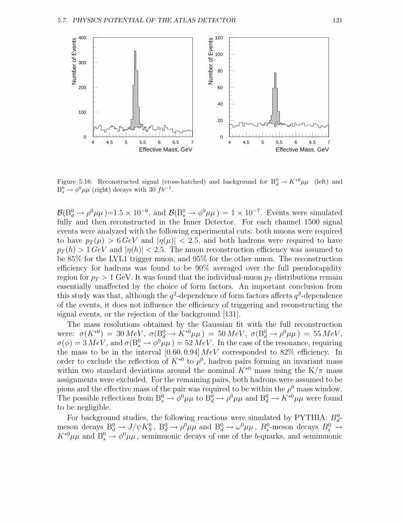
5.7. PHYSICS POTENTIAL OF THE ATLAS DETECTOR 121
0
100
200
300
400
4 4.5 5 5.5 6 6.5 7
Effective Mass, GeV
Num
ber
of E
vent
s
0
20
40
60
80
100
120
4 4.5 5 5.5 6 6.5 7
Effective Mass, GeV
Num
ber
of E
vent
s
Figure 5.16: Reconstructed signal (cross-hatched) and background for B0d → K∗0µµ (left) and
B0s → φ0µµ (right) decays with 30 fb−1.
B(B0d → ρ0µµ )=1.5 × 10⁻⁶, and B(B0
s → φ0µµ ) = 1 × 10⁻⁷. Events were simulatedfully and then reconstructed in the Inner Detector. For each channel 1500 signalevents were analyzed with the following experimental cuts: both muons were requiredto have pT (µ) > 6GeV and |η(µ)| < 2.5, and both hadrons were required to havepT (h) > 1GeV and |η(h)| < 2.5. The muon reconstruction efficiency was assumed tobe 85% for the LVL1 trigger muon, and 95% for the other muon. The reconstructionefficiency for hadrons was found to be 90% averaged over the full pseudorapidityregion for pT > 1 GeV. It was found that the individual-muon pT distributions remainessentially unaffected by the choice of form factors. An important conclusion fromthis study was that, although the q2-dependence of form factors affects q2-dependenceof the events, it does not influence the efficiency of triggering and reconstructing thesignal events, or the rejection of the background [131].
The mass resolutions obtained by the Gaussian fit with the full reconstructionwere: σ(K∗0) = 30MeV , σ(B0
d → K∗0µµ ) = 50MeV , σ(B0d → ρ0µµ ) = 55MeV ,
σ(φ) = 3MeV , and σ(B0s → φ0µµ ) = 52MeV . In the case of the resonance, requiring
the mass to be in the interval [0.60, 0.94]MeV corresponded to 82% efficiency. Inorder to exclude the reflection of K∗0 to ρ0, hadron pairs forming an invariant masswithin two standard deviations around the nominal K∗0 mass using the K/π massassignments were excluded. For the remaining pairs, both hadrons were assumed to bepions and the effective mass of the pair was required to be within the ρ0 mass window.The possible reflections from B0
s → φ0µµ to B0d → ρ0µµ and B0
d → K∗0µµ were foundto be negligible.
For background studies, the following reactions were simulated by PYTHIA: B0d-
meson decays B0d → J/ψK0
S , B0d → ρ0µµ and B0
d → ω0µµ , B0s -meson decays B0
s →K∗0µµ and B0
s → φ0µµ , semimuonic decays of one of the b-quarks, and semimuonic
122 CHAPTER 5. THE ATLAS EXPERIMENT AT THE LHC
decays of both b-quarks. It was found that the last reaction gave the main contribu-tion to the background. Therefore, 13000 events of this type were simulated and ana-lyzed similarly to the signal events. The mass distributions for the B0
d → K∗0µµ andB0s → φ0µµ signals are shown, together with those for the backgrounds, in Figure 5.16.
The application of all cuts leaves about 9% of the simulated signal events. The ex-pected numbers of signal and background events after three years of LHC running atlow luminosity are presented in the following table:
Channel Branching ratio Signal Background
B0d → K∗0µµ 1.5 × 10⁻⁶ 2000 290
B0d → ρ0µµ 10−7 220 950
B0s → φ0µµ 10−6 410 140
From the ratio of the branching fractions for the two decay modes B0d → K∗0µµ and
B0d → ρ0µµ , the ratio |Vtd|/|Vts| can be determined, since the decay rates are propor-
tional to the respective CKM matrix elements:
N(B0d → ρ0µµ)
N(B0d → K∗0µµ)
= κd|Vtd|2|Vts|2
(5.2)
where κd is the ratio of form factors squared. The ratio |Vtd|/|Vts| can be mea-sured with a statistical accuracy of 14% for 30 fb−1 of low-luminosity data; thetheoretical systematic uncertainty is about 7% [132]. Note that the reflection fromB0d → K∗0µµ to B0
d → ρ0µµ is sizeable due to the large difference in the branchingratios assumed for the two channels. After assigning the wrong mass hypothesesto the K∗0 decay products, the decay B0
d → K∗0µµ , reconstructed as B0d → ρ0µµ ,
gives a mass peak below, but close to, the B0d mass. In contrast, the combina-
torial background is approximately flat. Taking into account that the branchingratio for B0
d → K∗0µµ can be measured with high accuracy, it is assumed that theB0d → ρ0µµ signal can be extracted from an overall fit.The general trend of the behaviour of forward backward (FB) charge asymmetry
AFB for Standard Model, shown on Figure 5.17, is that the asymmetry is positive atlow q2, has a zero at s = q2/M2
B ≈ 0.14, and then becomes negative, irrespective of thedetails of the form-factor behaviour (except for the resonant region). The maximumof AFB(s) occurs at s = 0.05. For the MSSM, the shape of AFB is sensitive to thevalue of C7, or equivalently to the value of R7 = C7/C
SM7 . For R7 > 0 the shape is
similar to that in the Standard Model, but for R7 < 0 the asymmetry is negative atlow q2.
In the simulation, the resonant region 0.33 < s < 0.55 was excluded from the analy-sis. To estimate the experimental resolution of AFB measurements in B0
d → K∗0µµdecays, the total numbers of signal and background events after three years of low-luminosity running were used. If negative values of AFB are experimentally observedin the first s-region, this will demonstrate a clear signal of non-standard physics. Themeasurements in the second and third s-regions, which practically do not depend on
5.7. PHYSICS POTENTIAL OF THE ATLAS DETECTOR 123
-0.5
-0.25
0
0.25
0.5
0 0.2 0.4 0.6
B0d → K*0µ+µ-
Figure 5.17: Sensitivity of AFB to the Wilson coefficient C7. The three points are the simulationresults. The solid line shows the Standard Model prediction, the dotted lines show the range pre-dicted by the MSSM for R7 = C7/C
SM7 > 0 and the dashed lines show the range predicted by the
MSSM for R7 < 0.
the models, will show possible systematic uncertainties in the experimental data. Theexpected measurement accuracy is sufficient to separate the Standard Model and theMSSM in the case R7 <0 using measurements in the first s-region.
B0d → µµ and Bs → µµ decays
Purely muonic B-decays are predicted to have very low branching fractions within theStandard Model (10−9 − 10−10), whereas they may have significantly higher ones innon-standard models. Simulationswere made with PYTHIA event generator. Afterapplying all the cuts, the numbers of events expected for 30 fb−1 at low luminosityis sufficient to observe the Bs → µµ channel, assuming the branching fraction pre-dicted by the Standard Model. The significance of the signal, however, is only 2.8 σ.The feasibility to reconstruct the purely muonic Bd,s → µµ decays at high luminositywas also estimated. This estimation was based on the assumption that the pixel Blayer will be operational at high luminosity, and that no degradation of the impact-parameter and pT resolutions will occur. For each channel, 1000 signal events with
124 CHAPTER 5. THE ATLAS EXPERIMENT AT THE LHC
corresponding pile-up were fully simulated and reconstructed in the Inner Detector.The background was studied at the particle level using the parametrisation for pTand impact parameter resolutions from ATLFAST. A sample of 10 000 backgroundevents with pile-up was used for this study. The numbers of events for both channelsand the corresponding backgrounds expected for 100 fb−1 are given in the followingtable:
Channel Signal Background
B0d → µµ 14 660
Bs → µµ 92 660
Combining the low- and high-luminosity samples, a 4.3 σ significance can be ob-tained for the Bs → µµ channel. The 95% CL upper limit for the branching fractionfor B0
d → µµ obtained with the combined sample would be 3 × 10⁻¹⁰. It should benoted, however, that the B mass resolution of 69MeV is not good enough to sepa-rate Bs and Bd on an event-by-event basis, but their relative fractions would haveto be fitted from the joint mass distribution. The study of rare muonic B decays athigh luminosity will significantly improve the results which can be obtained at lowluminosity, especially if data collection is continued for several years.
In conclusion, ATLAS will be able to study rare semi-muonic and muonic B-decays.It will be possible to measure branching ratios of the decay channels B0
d → K∗0µµ ,B0s → φ0µµ and B0
d → ρ0µµ . From the ratio of branching fractions for the two latterchannels, it will be possible to determine the ratio |Vtd|/|Vts| with a 14% statisti-cal accuracy within the Standard Model. Measurements of the forward backwardcharge asymmetry in the decay B0
d → K∗0µµ will also be feasible and may reveal newphysics effects, for example in some parameter-space regions of the MSSM. Com-bining three years of low-luminosity and one year of high-luminosity data taking, theBs → µµ decay would be observed and a stringent upper limit for the B0
d → µµ decaywould be set, assuming Standard Model branching ratios. Given that these decaysare highly suppressed in the Standard Model, there are hopes that any non-standardphysics effects would significantly enhance the branching ratios, in which case thesignals would be easier to detect.
Chapter 6
Construction and evaluation ofATLAS modules equipped with theSCTA128 chip
6.1 Introduction
The present chapter first introduces the baseline binary chip used for ATLAS modules.Several measurements aiming at checking the relevant design parameters and theradiation-hardness of the modules equipped with ABCD chips will be described. Next,the back-up solution based on an analogue readout chip (SCTA128) will be presented.Measurements of the parameters at chip, hybrid and module level will be described, aswell as tests performed in the SPS X5 west beam test area. One of the disadvantagesof the ABCD resides in the difficulty of the evaluation of a digital design, as most ofthe effects, like common mode noise, are masked by the digital output. The ABCDand SCTA128 share basically the same front-end design which makes of the SCTA128an excellent solution to study the behaviour of the front-end of both chips.
6.2 The digital solution (ABCD)
6.2.1 Evolution of the design of the ABCD chip
The first modules equipped with the ABCD chips from the first batch were builtin 1998-1999. These modules were showing much higher noise than expected: 900electrons on the hybrid, and 1600 electrons when the chips were connected to 6 cmdetector strips. In the modules using chips from the second batch there was alsoobserved a large noise increase, observed only when all chips were mounted to thebiased detectors. The excess noise was unavoidable on modules with more than a fewtenths of channels connected to 12 cm strips at nominal operating conditions. Differ-ent combinations in hybrid ground plane geometry and different grounding schemesused to connect the detector bias to the analogue ground of the chip were testedbut without gaining any substantial improvement. Another unexpected problem was
125
126 CHAPTER 6. PERFORMANCE OF ATLAS MODULES USING THE SCTA128 CHIP
that of the large spread of discriminator thresholds. For the binary architecture oneof the most critical issues is the uniformity of parameters of the front-end circuit andmatching of the discriminator threshold.
In order to correct these problems a new design (ABCD2T/NT) with protectionagainst noise pick-up and the selection of new components from the technology hasbeen done. Both new technology choice and design change were made to reduce thethreshold spread observed on ABCD2 chips. The new ABCD2NT version keeps ahigh gain (140mV/fC) in signal amplification, but large size analogue componentsare used to improve the matching properties. Also new high value resistors wereused (extrinsic base resistor), instead of low implant resistors. The ABCD2T versionis using a more drastic option to reduce offset mismatch: there is a 4 bit linearDAC (trim DAC) included in each channel to correct for individual mismatch ofthe threshold in the range of 150mV . The 128 trim DACs are loaded with a newinstruction set developed for this version of the chip. The ABCD2T design offers,however, better robustness with respect to radiation effects and therefore was chosenas the preferred option for the SCT.
The ABCD2T version has met all basic requirements of the ATLAS SCT, how-ever, detailed evaluation of the ABCD2T chips, including extensive radiation testing,pointed to some possible improvements. These improvements, which concern mainlyimprovement of the radiation resistance and reduction of the design sensitivity tovariation of the process parameters, have been implemented in the ABCD3T version[134]. One of the problems was that the internal calibration circuitry showed non-linearity for low input charges. It was not a critical issue, however, a good absoluteprecision is required for setting the working threshold in the discriminators whichimpact the efficiency and noise occupancy. The threshold setting will be based oncalibration using internal calibration circuit, so the precision of this circuit around thenominal threshold setting, i.e. 1 fC, is a key issue. The source of the non-linearity hasbeen identified and corrected for. Another problem was that the trim DAC responsecurves appeared to be non-linear and exhibited large spread from channel-to-channel.A non-linear response of the trim DAC is not a serious problem as the trimmingprocedure is based on measurement of the trim DAC characteristics and using theseresults in a look-up table. However, trim DACs in some channels become so non-linear that those channels fell outside the trimming range. Since for good chips it isrequired for all the channels to be within the specification, that effect, if not corrected,would impact significantly the yield in the production. The source of the problem hasbeen identified in the design and an easy correction has been found. Radiation testsalso showed that the spread of the discriminator offset increased significantly afterirradiation and exceeded the range of the trim DACs. In order to not compromisethe precision of threshold correction for non-irradiated chips and to guarantee thatfor fully irradiated chips all the channels can be corrected, a set of ranges has beenimplemented in the ABCD3T design. In the ABCD2T chips excessive leakage currentwas observed after irradiation. The source of the leakage has been traced down andcorrected as well for ABCD3T.
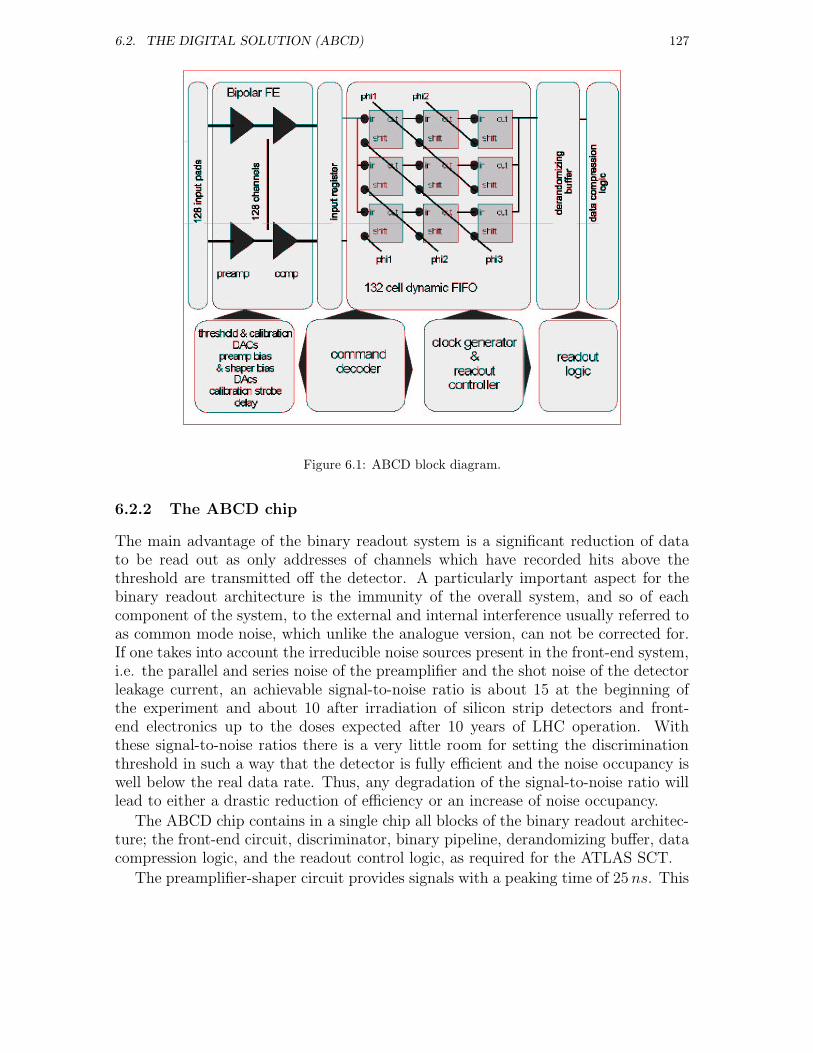
6.2. THE DIGITAL SOLUTION (ABCD) 127
Figure 6.1: ABCD block diagram.
6.2.2 The ABCD chip
The main advantage of the binary readout system is a significant reduction of datato be read out as only addresses of channels which have recorded hits above thethreshold are transmitted off the detector. A particularly important aspect for thebinary readout architecture is the immunity of the overall system, and so of eachcomponent of the system, to the external and internal interference usually referred toas common mode noise, which unlike the analogue version, can not be corrected for.If one takes into account the irreducible noise sources present in the front-end system,i.e. the parallel and series noise of the preamplifier and the shot noise of the detectorleakage current, an achievable signal-to-noise ratio is about 15 at the beginning ofthe experiment and about 10 after irradiation of silicon strip detectors and front-end electronics up to the doses expected after 10 years of LHC operation. Withthese signal-to-noise ratios there is a very little room for setting the discriminationthreshold in such a way that the detector is fully efficient and the noise occupancy iswell below the real data rate. Thus, any degradation of the signal-to-noise ratio willlead to either a drastic reduction of efficiency or an increase of noise occupancy.
The ABCD chip contains in a single chip all blocks of the binary readout architec-ture; the front-end circuit, discriminator, binary pipeline, derandomizing buffer, datacompression logic, and the readout control logic, as required for the ATLAS SCT.
The preamplifier-shaper circuit provides signals with a peaking time of 25ns. This
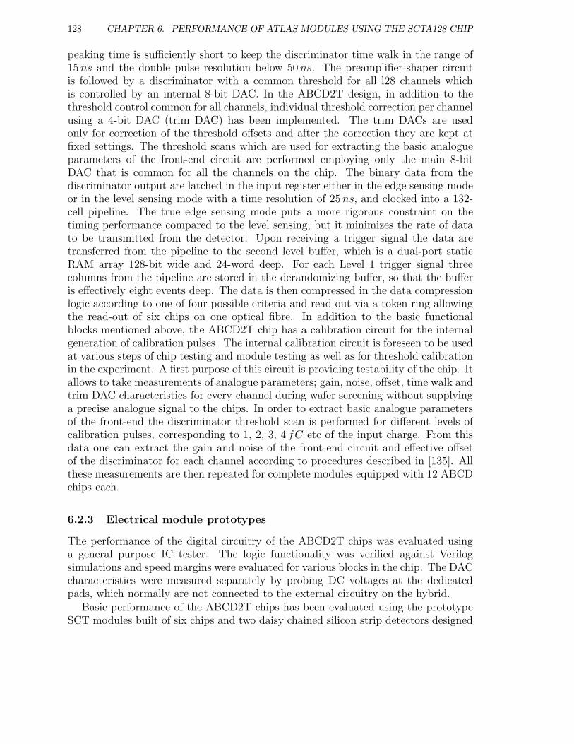
128 CHAPTER 6. PERFORMANCE OF ATLAS MODULES USING THE SCTA128 CHIP
peaking time is sufficiently short to keep the discriminator time walk in the range of15ns and the double pulse resolution below 50ns. The preamplifier-shaper circuitis followed by a discriminator with a common threshold for all l28 channels whichis controlled by an internal 8-bit DAC. In the ABCD2T design, in addition to thethreshold control common for all channels, individual threshold correction per channelusing a 4-bit DAC (trim DAC) has been implemented. The trim DACs are usedonly for correction of the threshold offsets and after the correction they are kept atfixed settings. The threshold scans which are used for extracting the basic analogueparameters of the front-end circuit are performed employing only the main 8-bitDAC that is common for all the channels on the chip. The binary data from thediscriminator output are latched in the input register either in the edge sensing modeor in the level sensing mode with a time resolution of 25ns, and clocked into a 132-cell pipeline. The true edge sensing mode puts a more rigorous constraint on thetiming performance compared to the level sensing, but it minimizes the rate of datato be transmitted from the detector. Upon receiving a trigger signal the data aretransferred from the pipeline to the second level buffer, which is a dual-port staticRAM array 128-bit wide and 24-word deep. For each Level 1 trigger signal threecolumns from the pipeline are stored in the derandomizing buffer, so that the bufferis effectively eight events deep. The data is then compressed in the data compressionlogic according to one of four possible criteria and read out via a token ring allowingthe read-out of six chips on one optical fibre. In addition to the basic functionalblocks mentioned above, the ABCD2T chip has a calibration circuit for the internalgeneration of calibration pulses. The internal calibration circuit is foreseen to be usedat various steps of chip testing and module testing as well as for threshold calibrationin the experiment. A first purpose of this circuit is providing testability of the chip. Itallows to take measurements of analogue parameters; gain, noise, offset, time walk andtrim DAC characteristics for every channel during wafer screening without supplyinga precise analogue signal to the chips. In order to extract basic analogue parametersof the front-end the discriminator threshold scan is performed for different levels ofcalibration pulses, corresponding to 1, 2, 3, 4 fC etc of the input charge. From thisdata one can extract the gain and noise of the front-end circuit and effective offsetof the discriminator for each channel according to procedures described in [135]. Allthese measurements are then repeated for complete modules equipped with 12 ABCDchips each.
6.2.3 Electrical module prototypes
The performance of the digital circuitry of the ABCD2T chips was evaluated usinga general purpose IC tester. The logic functionality was verified against Verilogsimulations and speed margins were evaluated for various blocks in the chip. The DACcharacteristics were measured separately by probing DC voltages at the dedicatedpads, which normally are not connected to the external circuitry on the hybrid.
Basic performance of the ABCD2T chips has been evaluated using the prototypeSCT modules built of six chips and two daisy chained silicon strip detectors designed
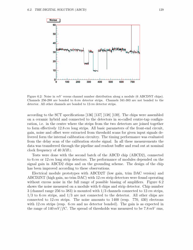
6.2. THE DIGITAL SOLUTION (ABCD) 129
Figure 6.2: Noise in mV versus channel number distribution along a module (6 ABCDNT chips).Channels 256-288 are bonded to 6 cm detector strips. Channels 341-383 are not bonded to thedetector. All other channels are bonded to 12 cm detector strips.
according to the SCT specifications [136] [137] [138] [139]. The chips were assembledon a ceramic hybrid and connected to the detectors in so-called centre-tap configu-ration, i.e. in the centre where the strips from the two detectors are joined togetherto form effectively 12.8 cm long strips. All basic parameters of the front-end circuit,gain, noise and offset were extracted from threshold scans for given input signals de-livered form the internal calibration circuitry. The timing performance was evaluatedfrom the delay scan of the calibration strobe signal. In all these measurements thedata was transferred through the pipeline and readout buffer and read out at nominalclock frequency of 40MHz.
Tests were done with the second batch of the ABCD chip (ABCD2), connectedto 6 cm or 12 cm long strip detectors. The performance of modules depended on thesignal gain in ABCD2 chips and on the grounding scheme. The design of the chiphas been improved according to these observations.
Electrical module prototypes with ABCD2T (low gain, trim DAC version) andABCD2NT (high gain, no trim DAC) with 12 cm strip detectors were found operatingwithout excess noise in the full range of possible biasing of amplifiers. Figure 6.2shows the noise measured on a module with 6 chips and strip detector. Chip number3 (channel range 256 to 383) is mounted with 1/3 channels connected to 12 cm strips,1/3 to 6 cm strips, and 1/3 are not connected to the detector. All other chips areconnected to 12 cm strips. The noise amounts to 1400 (resp. 770, 430) electronswith 12 cm strips (resp. 6 cm and no detector bonded). The gain is as expected inthe range of 140mV/fC. The spread of thresholds was measured to be 7.8mV rms,
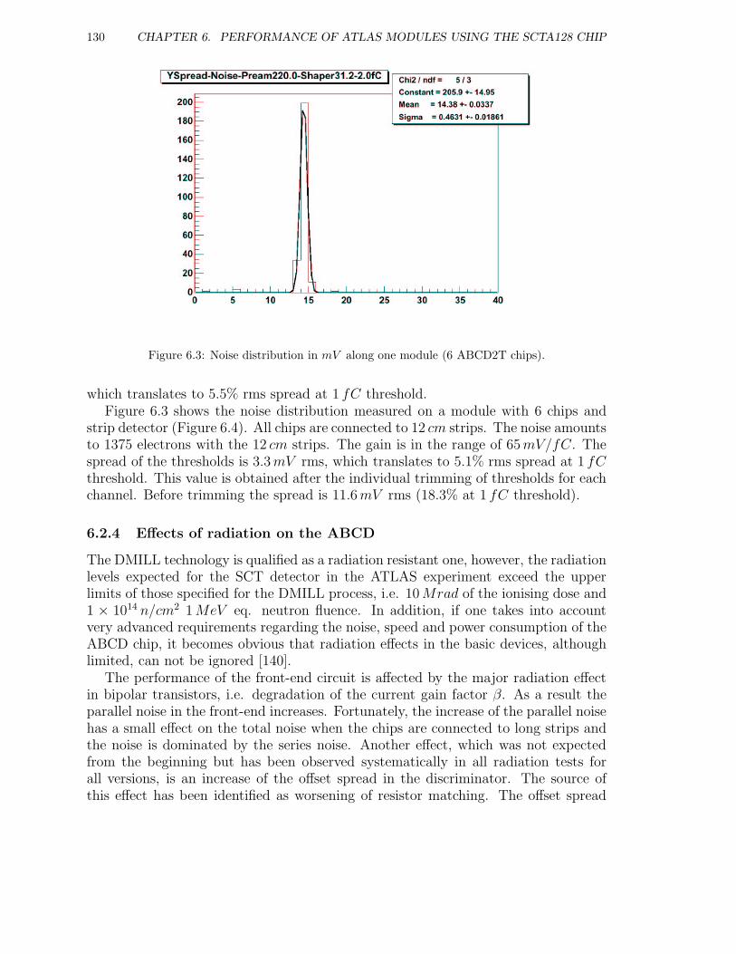
130 CHAPTER 6. PERFORMANCE OF ATLAS MODULES USING THE SCTA128 CHIP
Figure 6.3: Noise distribution in mV along one module (6 ABCD2T chips).
which translates to 5.5% rms spread at 1 fC threshold.Figure 6.3 shows the noise distribution measured on a module with 6 chips and
strip detector (Figure 6.4). All chips are connected to 12 cm strips. The noise amountsto 1375 electrons with the 12 cm strips. The gain is in the range of 65mV/fC. Thespread of the thresholds is 3.3mV rms, which translates to 5.1% rms spread at 1 fCthreshold. This value is obtained after the individual trimming of thresholds for eachchannel. Before trimming the spread is 11.6mV rms (18.3% at 1 fC threshold).
6.2.4 Effects of radiation on the ABCD
The DMILL technology is qualified as a radiation resistant one, however, the radiationlevels expected for the SCT detector in the ATLAS experiment exceed the upperlimits of those specified for the DMILL process, i.e. 10Mrad of the ionising dose and1 × 1014 n/cm2 1MeV eq. neutron fluence. In addition, if one takes into accountvery advanced requirements regarding the noise, speed and power consumption of theABCD chip, it becomes obvious that radiation effects in the basic devices, althoughlimited, can not be ignored [140].
The performance of the front-end circuit is affected by the major radiation effectin bipolar transistors, i.e. degradation of the current gain factor β. As a result theparallel noise in the front-end increases. Fortunately, the increase of the parallel noisehas a small effect on the total noise when the chips are connected to long strips andthe noise is dominated by the series noise. Another effect, which was not expectedfrom the beginning but has been observed systematically in all radiation tests forall versions, is an increase of the offset spread in the discriminator. The source ofthis effect has been identified as worsening of resistor matching. The offset spread
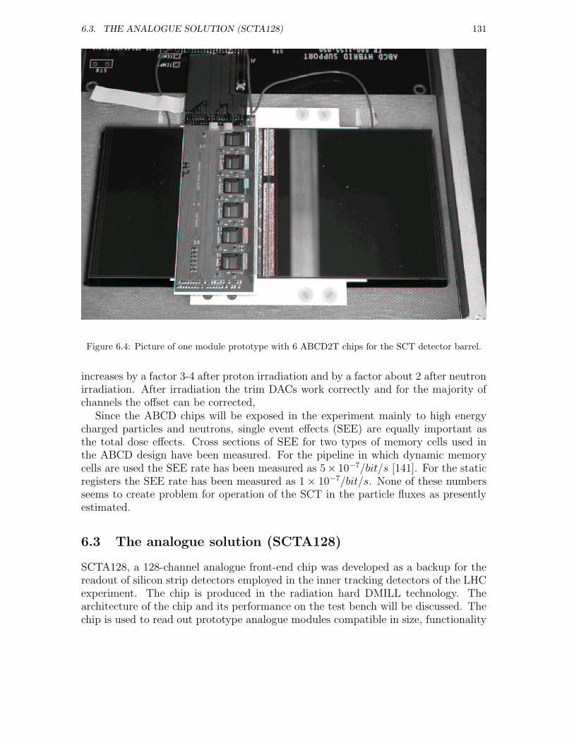
6.3. THE ANALOGUE SOLUTION (SCTA128) 131
Figure 6.4: Picture of one module prototype with 6 ABCD2T chips for the SCT detector barrel.
increases by a factor 3-4 after proton irradiation and by a factor about 2 after neutronirradiation. After irradiation the trim DACs work correctly and for the majority ofchannels the offset can be corrected,
Since the ABCD chips will be exposed in the experiment mainly to high energycharged particles and neutrons, single event effects (SEE) are equally important asthe total dose effects. Cross sections of SEE for two types of memory cells used inthe ABCD design have been measured. For the pipeline in which dynamic memorycells are used the SEE rate has been measured as 5× 10⁻⁷/bit/s [141]. For the staticregisters the SEE rate has been measured as 1 × 10⁻⁷/bit/s. None of these numbersseems to create problem for operation of the SCT in the particle fluxes as presentlyestimated.
6.3 The analogue solution (SCTA128)
SCTA128, a 128-channel analogue front-end chip was developed as a backup for thereadout of silicon strip detectors employed in the inner tracking detectors of the LHCexperiment. The chip is produced in the radiation hard DMILL technology. Thearchitecture of the chip and its performance on the test bench will be discussed. Thechip is used to read out prototype analogue modules compatible in size, functionality
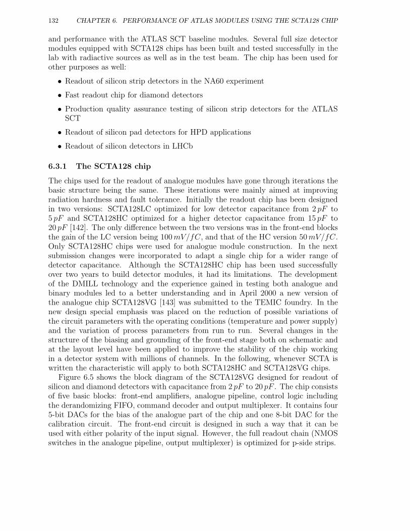
132 CHAPTER 6. PERFORMANCE OF ATLAS MODULES USING THE SCTA128 CHIP
and performance with the ATLAS SCT baseline modules. Several full size detectormodules equipped with SCTA128 chips has been built and tested successfully in thelab with radiactive sources as well as in the test beam. The chip has been used forother purposes as well:
• Readout of silicon strip detectors in the NA60 experiment
• Fast readout chip for diamond detectors
• Production quality assurance testing of silicon strip detectors for the ATLASSCT
• Readout of silicon pad detectors for HPD applications
• Readout of silicon detectors in LHCb
6.3.1 The SCTA128 chip
The chips used for the readout of analogue modules have gone through iterations thebasic structure being the same. These iterations were mainly aimed at improvingradiation hardness and fault tolerance. Initially the readout chip has been designedin two versions: SCTA128LC optimized for low detector capacitance from 2 pF to5 pF and SCTA128HC optimized for a higher detector capacitance from 15 pF to20 pF [142]. The only difference between the two versions was in the front-end blocksthe gain of the LC version being 100mV/fC, and that of the HC version 50mV/fC.Only SCTA128HC chips were used for analogue module construction. In the nextsubmission changes were incorporated to adapt a single chip for a wider range ofdetector capacitance. Although the SCTA128HC chip has been used successfullyover two years to build detector modules, it had its limitations. The developmentof the DMILL technology and the experience gained in testing both analogue andbinary modules led to a better understanding and in April 2000 a new version ofthe analogue chip SCTA128VG [143] was submitted to the TEMIC foundry. In thenew design special emphasis was placed on the reduction of possible variations ofthe circuit parameters with the operating conditions (temperature and power supply)and the variation of process parameters from run to run. Several changes in thestructure of the biasing and grounding of the front-end stage both on schematic andat the layout level have been applied to improve the stability of the chip workingin a detector system with millions of channels. In the following, whenever SCTA iswritten the characteristic will apply to both SCTA128HC and SCTA128VG chips.
Figure 6.5 shows the block diagram of the SCTA128VG designed for readout ofsilicon and diamond detectors with capacitance from 2 pF to 20 pF . The chip consistsof five basic blocks: front-end amplifiers, analogue pipeline, control logic includingthe derandomizing FIFO, command decoder and output multiplexer. It contains four5-bit DACs for the bias of the analogue part of the chip and one 8-bit DAC for thecalibration circuit. The front-end circuit is designed in such a way that it can beused with either polarity of the input signal. However, the full readout chain (NMOSswitches in the analogue pipeline, output multiplexer) is optimized for p-side strips.
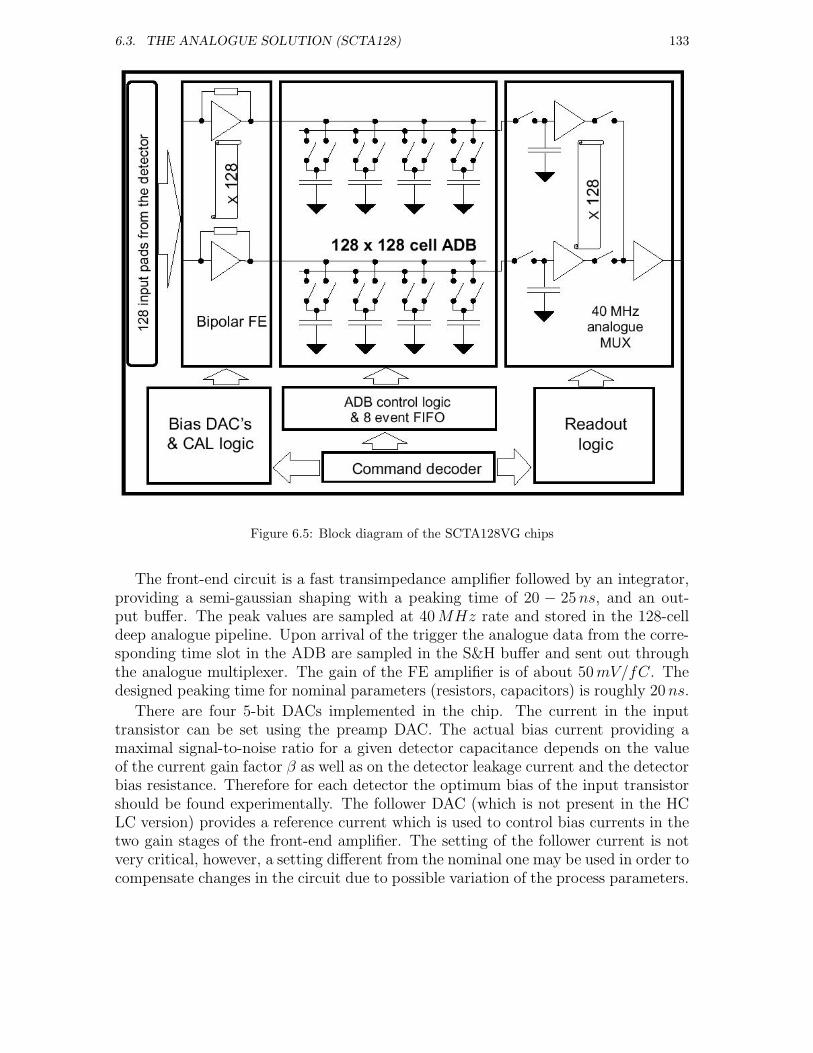
6.3. THE ANALOGUE SOLUTION (SCTA128) 133
Figure 6.5: Block diagram of the SCTA128VG chips
The front-end circuit is a fast transimpedance amplifier followed by an integrator,providing a semi-gaussian shaping with a peaking time of 20 − 25ns, and an out-put buffer. The peak values are sampled at 40MHz rate and stored in the 128-celldeep analogue pipeline. Upon arrival of the trigger the analogue data from the corre-sponding time slot in the ADB are sampled in the S&H buffer and sent out throughthe analogue multiplexer. The gain of the FE amplifier is of about 50mV/fC. Thedesigned peaking time for nominal parameters (resistors, capacitors) is roughly 20ns.
There are four 5-bit DACs implemented in the chip. The current in the inputtransistor can be set using the preamp DAC. The actual bias current providing amaximal signal-to-noise ratio for a given detector capacitance depends on the valueof the current gain factor β as well as on the detector leakage current and the detectorbias resistance. Therefore for each detector the optimum bias of the input transistorshould be found experimentally. The follower DAC (which is not present in the HCLC version) provides a reference current which is used to control bias currents in thetwo gain stages of the front-end amplifier. The setting of the follower current is notvery critical, however, a setting different from the nominal one may be used in order tocompensate changes in the circuit due to possible variation of the process parameters.
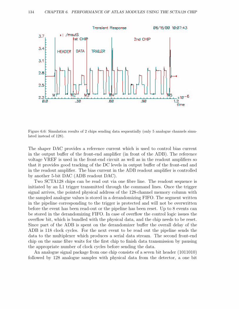
134 CHAPTER 6. PERFORMANCE OF ATLAS MODULES USING THE SCTA128 CHIP
Figure 6.6: Simulation results of 2 chips sending data sequentially (only 5 analogue channels simu-lated instead of 128).
The shaper DAC provides a reference current which is used to control bias currentin the output buffer of the front-end amplifier (in front of the ADB). The referencevoltage VREF is used in the front-end circuit as well as in the readout amplifiers sothat it provides good tracking of the DC levels in output buffer of the front-end andin the readout amplifier. The bias current in the ADB readout amplifier is controlledby another 5-bit DAC (ADB readout DAC).
Two SCTA128 chips can be read out via one fibre line. The readout sequence isinitiated by an L1 trigger transmitted through the command lines. Once the triggersignal arrives, the pointed physical address of the 128-channel memory column withthe sampled analogue values is stored in a derandomizing FIFO. The segment writtenin the pipeline corresponding to the trigger is protected and will not be overwrittenbefore the event has been read-out or the pipeline has been reset. Up to 8 events canbe stored in the derandomizing FIFO. In case of overflow the control logic issues theoverflow bit, which is bundled with the physical data, and the chip needs to be reset.Since part of the ADB is spent on the derandomizer buffer the overall delay of theADB is 118 clock cycles. For the next event to be read out the pipeline sends thedata to the multiplexer which produces a serial data stream. The second front-endchip on the same fibre waits for the first chip to finish data transmission by pausingthe appropriate number of clock cycles before sending the data.
An analogue signal package from one chip consists of a seven bit header (1011010)followed by 128 analogue samples with physical data from the detector, a one bit
6.3. THE ANALOGUE SOLUTION (SCTA128) 135
Figure 6.7: The setup used for the SCTA-DAQ
buffer overflow flag, a four bit BCO counter and a four bit T1 counter (Figure 6.6).The above format of the data is independent of mode of readout (single or two chipreadout). The total time for readout on one fibre for two chips is thus 2× (7 + 128 +1 + 4 + 4) × 25ns = 7.2µs.
The four-bit BCO counter and L1 counter returned by the chip can be used forunique association of each trigger with the physical data from the detector. Themaximum clock rate of the multiplexer and the readout circuit is the same as thesampling rate of the data, i.e. 40MHz. The chips can be read out with a lowerrate (40MHz divided by 2, 4, or 8) which is programmable. All the communicationwith the chip (i.e. sending the level 1 triggers, sending the software reset, loading theDACs, issuing the internal calibration pulses) is executed via a fast 40MHz serialinterface by sending a bit pattern synchronous to the main clock.
6.3.2 Laboratory setup
The laboratory setup used in order to measure the characteristics is shown on Fig-ure 6.7. The acquisition program was first written under Windows. Later, whenNational Instruments provided Linux drivers for its apparatus the DAQ program was
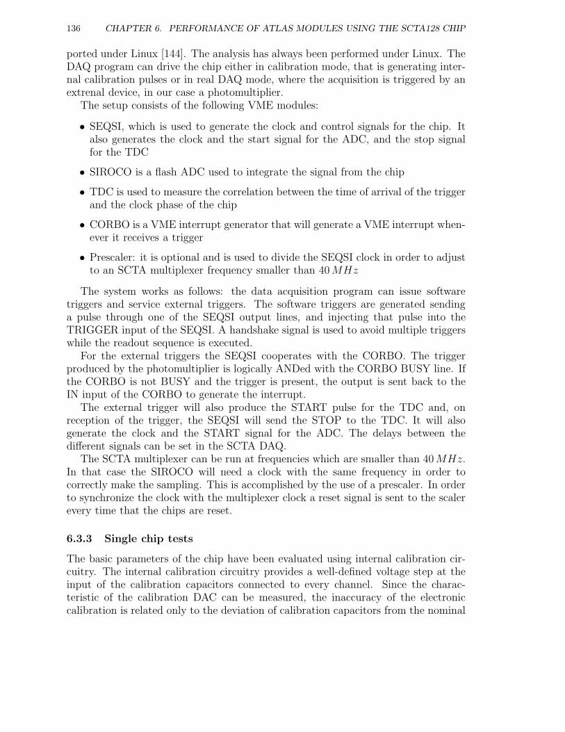
136 CHAPTER 6. PERFORMANCE OF ATLAS MODULES USING THE SCTA128 CHIP
ported under Linux [144]. The analysis has always been performed under Linux. TheDAQ program can drive the chip either in calibration mode, that is generating inter-nal calibration pulses or in real DAQ mode, where the acquisition is triggered by anextrenal device, in our case a photomultiplier.
The setup consists of the following VME modules:
• SEQSI, which is used to generate the clock and control signals for the chip. Italso generates the clock and the start signal for the ADC, and the stop signalfor the TDC
• SIROCO is a flash ADC used to integrate the signal from the chip
• TDC is used to measure the correlation between the time of arrival of the triggerand the clock phase of the chip
• CORBO is a VME interrupt generator that will generate a VME interrupt when-ever it receives a trigger
• Prescaler: it is optional and is used to divide the SEQSI clock in order to adjustto an SCTA multiplexer frequency smaller than 40MHz
The system works as follows: the data acquisition program can issue softwaretriggers and service external triggers. The software triggers are generated sendinga pulse through one of the SEQSI output lines, and injecting that pulse into theTRIGGER input of the SEQSI. A handshake signal is used to avoid multiple triggerswhile the readout sequence is executed.
For the external triggers the SEQSI cooperates with the CORBO. The triggerproduced by the photomultiplier is logically ANDed with the CORBO BUSY line. Ifthe CORBO is not BUSY and the trigger is present, the output is sent back to theIN input of the CORBO to generate the interrupt.
The external trigger will also produce the START pulse for the TDC and, onreception of the trigger, the SEQSI will send the STOP to the TDC. It will alsogenerate the clock and the START signal for the ADC. The delays between thedifferent signals can be set in the SCTA DAQ.
The SCTA multiplexer can be run at frequencies which are smaller than 40MHz.In that case the SIROCO will need a clock with the same frequency in order tocorrectly make the sampling. This is accomplished by the use of a prescaler. In orderto synchronize the clock with the multiplexer clock a reset signal is sent to the scalerevery time that the chips are reset.
6.3.3 Single chip tests
The basic parameters of the chip have been evaluated using internal calibration cir-cuitry. The internal calibration circuitry provides a well-defined voltage step at theinput of the calibration capacitors connected to every channel. Since the charac-teristic of the calibration DAC can be measured, the inaccuracy of the electroniccalibration is related only to the deviation of calibration capacitors from the nominal
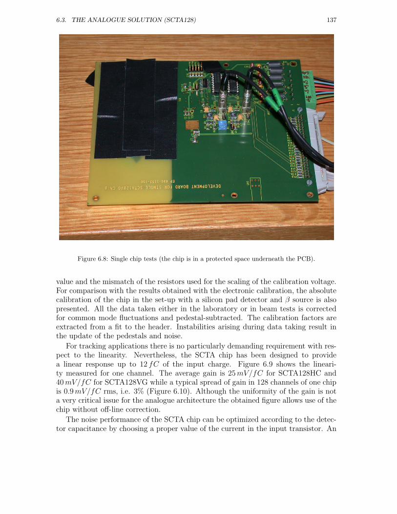
6.3. THE ANALOGUE SOLUTION (SCTA128) 137
Figure 6.8: Single chip tests (the chip is in a protected space underneath the PCB).
value and the mismatch of the resistors used for the scaling of the calibration voltage.For comparison with the results obtained with the electronic calibration, the absolutecalibration of the chip in the set-up with a silicon pad detector and β source is alsopresented. All the data taken either in the laboratory or in beam tests is correctedfor common mode fluctuations and pedestal-subtracted. The calibration factors areextracted from a fit to the header. Instabilities arising during data taking result inthe update of the pedestals and noise.
For tracking applications there is no particularly demanding requirement with res-pect to the linearity. Nevertheless, the SCTA chip has been designed to providea linear response up to 12 fC of the input charge. Figure 6.9 shows the lineari-ty measured for one channel. The average gain is 25mV/fC for SCTA128HC and40mV/fC for SCTA128VG while a typical spread of gain in 128 channels of one chipis 0.9mV/fC rms, i.e. 3% (Figure 6.10). Although the uniformity of the gain is nota very critical issue for the analogue architecture the obtained figure allows use of thechip without off-line correction.
The noise performance of the SCTA chip can be optimized according to the detec-tor capacitance by choosing a proper value of the current in the input transistor. An
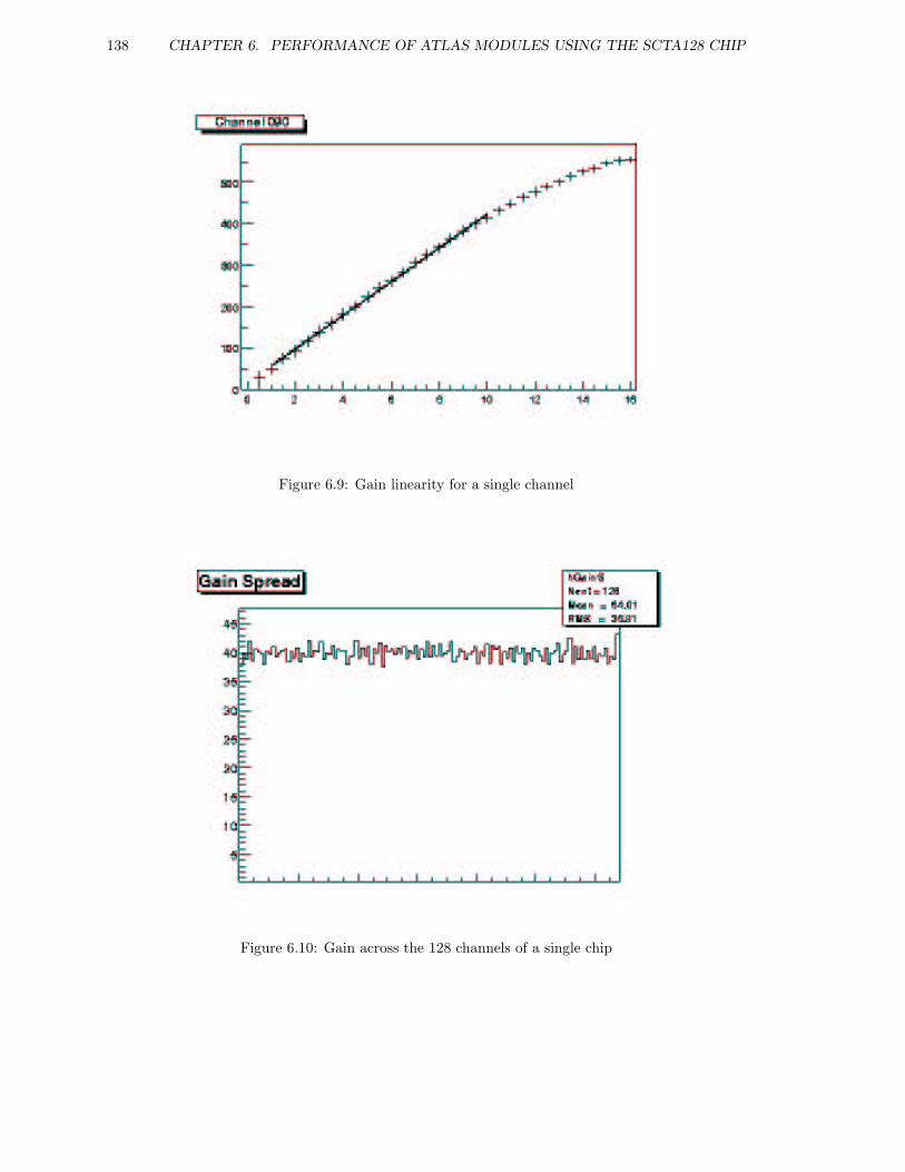
138 CHAPTER 6. PERFORMANCE OF ATLAS MODULES USING THE SCTA128 CHIP
Figure 6.9: Gain linearity for a single channel
Figure 6.10: Gain across the 128 channels of a single chip
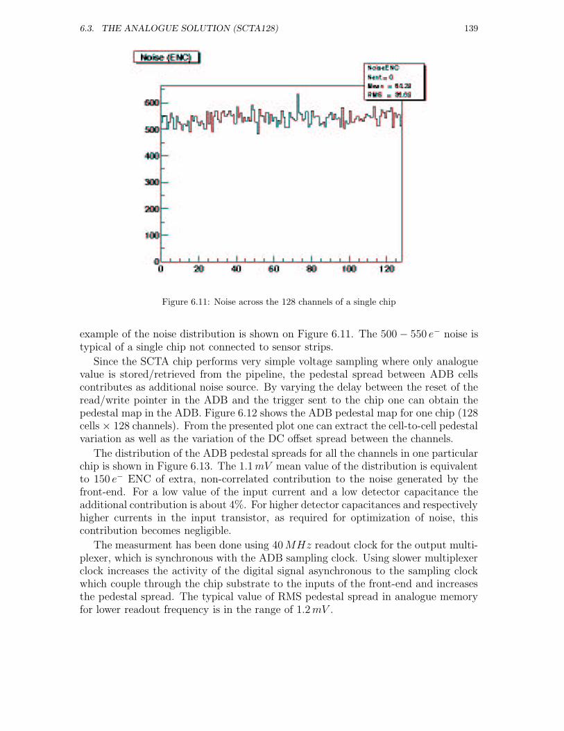
6.3. THE ANALOGUE SOLUTION (SCTA128) 139
Figure 6.11: Noise across the 128 channels of a single chip
example of the noise distribution is shown on Figure 6.11. The 500 − 550 e− noise istypical of a single chip not connected to sensor strips.
Since the SCTA chip performs very simple voltage sampling where only analoguevalue is stored/retrieved from the pipeline, the pedestal spread between ADB cellscontributes as additional noise source. By varying the delay between the reset of theread/write pointer in the ADB and the trigger sent to the chip one can obtain thepedestal map in the ADB. Figure 6.12 shows the ADB pedestal map for one chip (128cells × 128 channels). From the presented plot one can extract the cell-to-cell pedestalvariation as well as the variation of the DC offset spread between the channels.
The distribution of the ADB pedestal spreads for all the channels in one particularchip is shown in Figure 6.13. The 1.1mV mean value of the distribution is equivalentto 150 e− ENC of extra, non-correlated contribution to the noise generated by thefront-end. For a low value of the input current and a low detector capacitance theadditional contribution is about 4%. For higher detector capacitances and respectivelyhigher currents in the input transistor, as required for optimization of noise, thiscontribution becomes negligible.
The measurment has been done using 40MHz readout clock for the output multi-plexer, which is synchronous with the ADB sampling clock. Using slower multiplexerclock increases the activity of the digital signal asynchronous to the sampling clockwhich couple through the chip substrate to the inputs of the front-end and increasesthe pedestal spread. The typical value of RMS pedestal spread in analogue memoryfor lower readout frequency is in the range of 1.2mV .
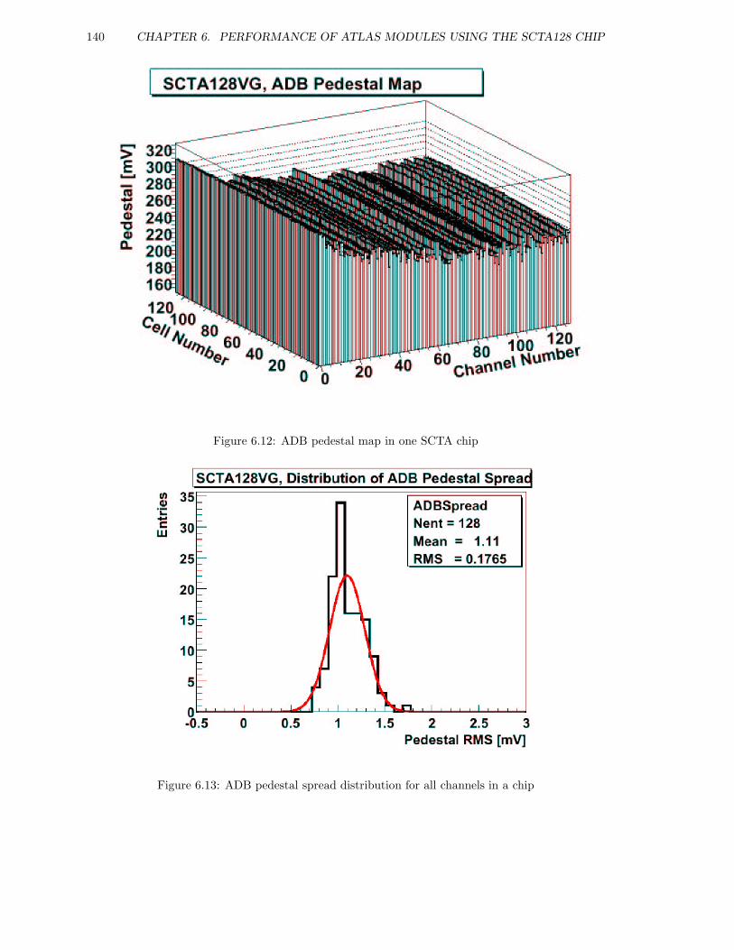
140 CHAPTER 6. PERFORMANCE OF ATLAS MODULES USING THE SCTA128 CHIP
Figure 6.12: ADB pedestal map in one SCTA chip
Figure 6.13: ADB pedestal spread distribution for all channels in a chip
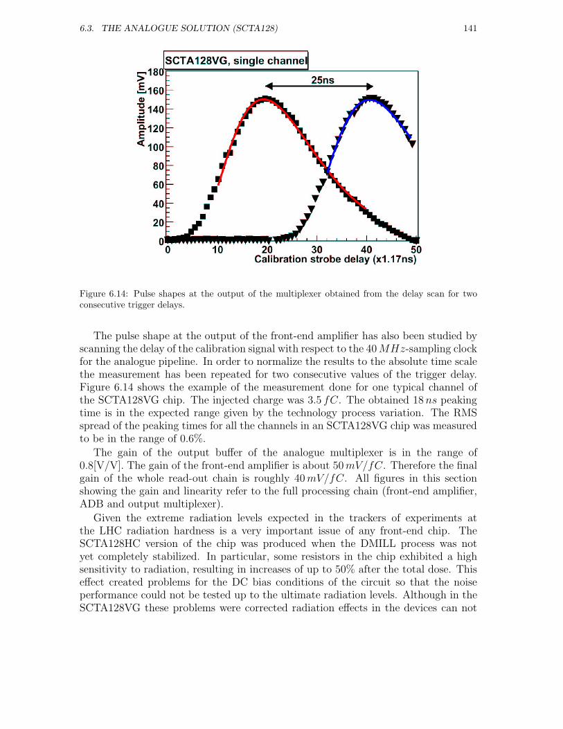
6.3. THE ANALOGUE SOLUTION (SCTA128) 141
Figure 6.14: Pulse shapes at the output of the multiplexer obtained from the delay scan for twoconsecutive trigger delays.
The pulse shape at the output of the front-end amplifier has also been studied byscanning the delay of the calibration signal with respect to the 40MHz-sampling clockfor the analogue pipeline. In order to normalize the results to the absolute time scalethe measurement has been repeated for two consecutive values of the trigger delay.Figure 6.14 shows the example of the measurement done for one typical channel ofthe SCTA128VG chip. The injected charge was 3.5 fC. The obtained 18ns peakingtime is in the expected range given by the technology process variation. The RMSspread of the peaking times for all the channels in an SCTA128VG chip was measuredto be in the range of 0.6%.
The gain of the output buffer of the analogue multiplexer is in the range of0.8[V/V]. The gain of the front-end amplifier is about 50mV/fC. Therefore the finalgain of the whole read-out chain is roughly 40mV/fC. All figures in this sectionshowing the gain and linearity refer to the full processing chain (front-end amplifier,ADB and output multiplexer).
Given the extreme radiation levels expected in the trackers of experiments atthe LHC radiation hardness is a very important issue of any front-end chip. TheSCTA128HC version of the chip was produced when the DMILL process was notyet completely stabilized. In particular, some resistors in the chip exhibited a highsensitivity to radiation, resulting in increases of up to 50% after the total dose. Thiseffect created problems for the DC bias conditions of the circuit so that the noiseperformance could not be tested up to the ultimate radiation levels. Although in theSCTA128VG these problems were corrected radiation effects in the devices can not
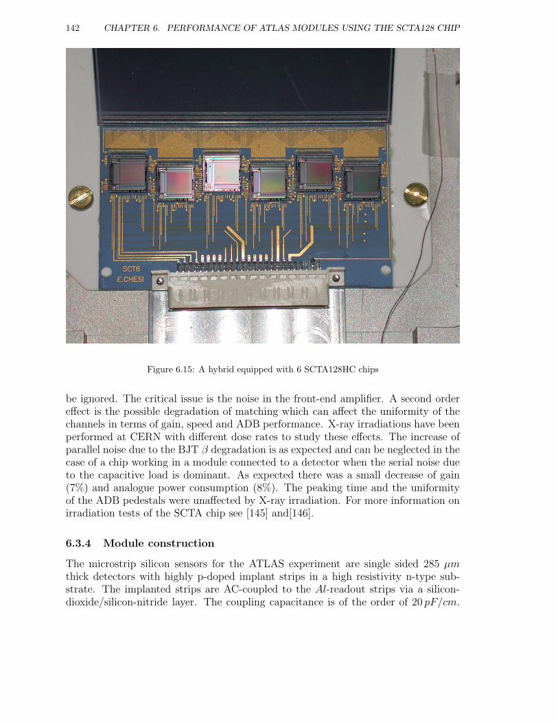
142 CHAPTER 6. PERFORMANCE OF ATLAS MODULES USING THE SCTA128 CHIP
Figure 6.15: A hybrid equipped with 6 SCTA128HC chips
be ignored. The critical issue is the noise in the front-end amplifier. A second ordereffect is the possible degradation of matching which can affect the uniformity of thechannels in terms of gain, speed and ADB performance. X-ray irradiations have beenperformed at CERN with different dose rates to study these effects. The increase ofparallel noise due to the BJT β degradation is as expected and can be neglected in thecase of a chip working in a module connected to a detector when the serial noise dueto the capacitive load is dominant. As expected there was a small decrease of gain(7%) and analogue power consumption (8%). The peaking time and the uniformityof the ADB pedestals were unaffected by X-ray irradiation. For more information onirradiation tests of the SCTA chip see [145] and[146].
6.3.4 Module construction
The microstrip silicon sensors for the ATLAS experiment are single sided 285 µmthick detectors with highly p-doped implant strips in a high resistivity n-type sub-strate. The implanted strips are AC-coupled to the Al-readout strips via a silicon-dioxide/silicon-nitride layer. The coupling capacitance is of the order of 20 pF/cm.
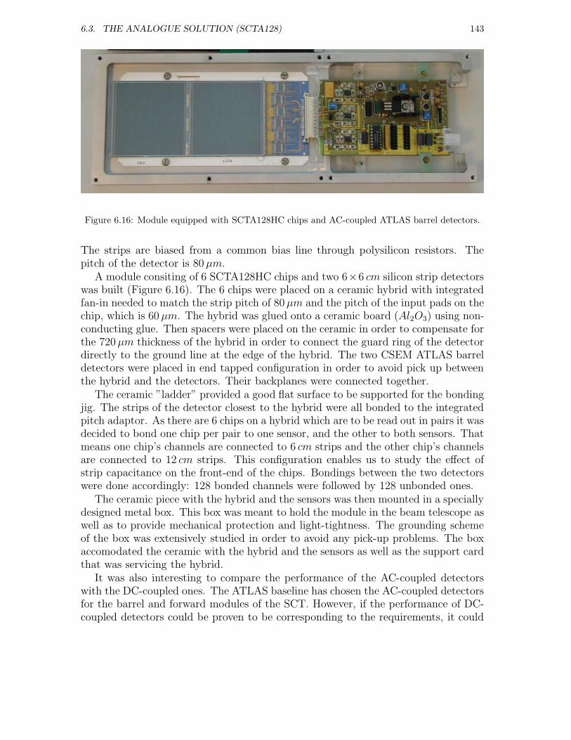
6.3. THE ANALOGUE SOLUTION (SCTA128) 143
Figure 6.16: Module equipped with SCTA128HC chips and AC-coupled ATLAS barrel detectors.
The strips are biased from a common bias line through polysilicon resistors. Thepitch of the detector is 80µm.
A module consiting of 6 SCTA128HC chips and two 6×6 cm silicon strip detectorswas built (Figure 6.16). The 6 chips were placed on a ceramic hybrid with integratedfan-in needed to match the strip pitch of 80µm and the pitch of the input pads on thechip, which is 60µm. The hybrid was glued onto a ceramic board (Al2O3) using non-conducting glue. Then spacers were placed on the ceramic in order to compensate forthe 720µm thickness of the hybrid in order to connect the guard ring of the detectordirectly to the ground line at the edge of the hybrid. The two CSEM ATLAS barreldetectors were placed in end tapped configuration in order to avoid pick up betweenthe hybrid and the detectors. Their backplanes were connected together.
The ceramic ”ladder” provided a good flat surface to be supported for the bondingjig. The strips of the detector closest to the hybrid were all bonded to the integratedpitch adaptor. As there are 6 chips on a hybrid which are to be read out in pairs it wasdecided to bond one chip per pair to one sensor, and the other to both sensors. Thatmeans one chip’s channels are connected to 6 cm strips and the other chip’s channelsare connected to 12 cm strips. This configuration enables us to study the effect ofstrip capacitance on the front-end of the chips. Bondings between the two detectorswere done accordingly: 128 bonded channels were followed by 128 unbonded ones.
The ceramic piece with the hybrid and the sensors was then mounted in a speciallydesigned metal box. This box was meant to hold the module in the beam telescope aswell as to provide mechanical protection and light-tightness. The grounding schemeof the box was extensively studied in order to avoid any pick-up problems. The boxaccomodated the ceramic with the hybrid and the sensors as well as the support cardthat was servicing the hybrid.
It was also interesting to compare the performance of the AC-coupled detectorswith the DC-coupled ones. The ATLAS baseline has chosen the AC-coupled detectorsfor the barrel and forward modules of the SCT. However, if the performance of DC-coupled detectors could be proven to be corresponding to the requirements, it could
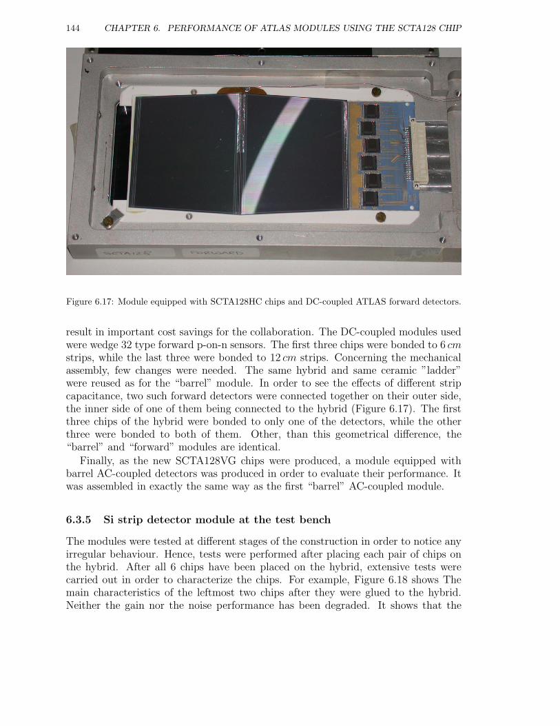
144 CHAPTER 6. PERFORMANCE OF ATLAS MODULES USING THE SCTA128 CHIP
Figure 6.17: Module equipped with SCTA128HC chips and DC-coupled ATLAS forward detectors.
result in important cost savings for the collaboration. The DC-coupled modules usedwere wedge 32 type forward p-on-n sensors. The first three chips were bonded to 6 cmstrips, while the last three were bonded to 12 cm strips. Concerning the mechanicalassembly, few changes were needed. The same hybrid and same ceramic ”ladder”were reused as for the “barrel” module. In order to see the effects of different stripcapacitance, two such forward detectors were connected together on their outer side,the inner side of one of them being connected to the hybrid (Figure 6.17). The firstthree chips of the hybrid were bonded to only one of the detectors, while the otherthree were bonded to both of them. Other, than this geometrical difference, the“barrel” and “forward” modules are identical.
Finally, as the new SCTA128VG chips were produced, a module equipped withbarrel AC-coupled detectors was produced in order to evaluate their performance. Itwas assembled in exactly the same way as the first “barrel” AC-coupled module.
6.3.5 Si strip detector module at the test bench
The modules were tested at different stages of the construction in order to notice anyirregular behaviour. Hence, tests were performed after placing each pair of chips onthe hybrid. After all 6 chips have been placed on the hybrid, extensive tests werecarried out in order to characterize the chips. For example, Figure 6.18 shows Themain characteristics of the leftmost two chips after they were glued to the hybrid.Neither the gain nor the noise performance has been degraded. It shows that the
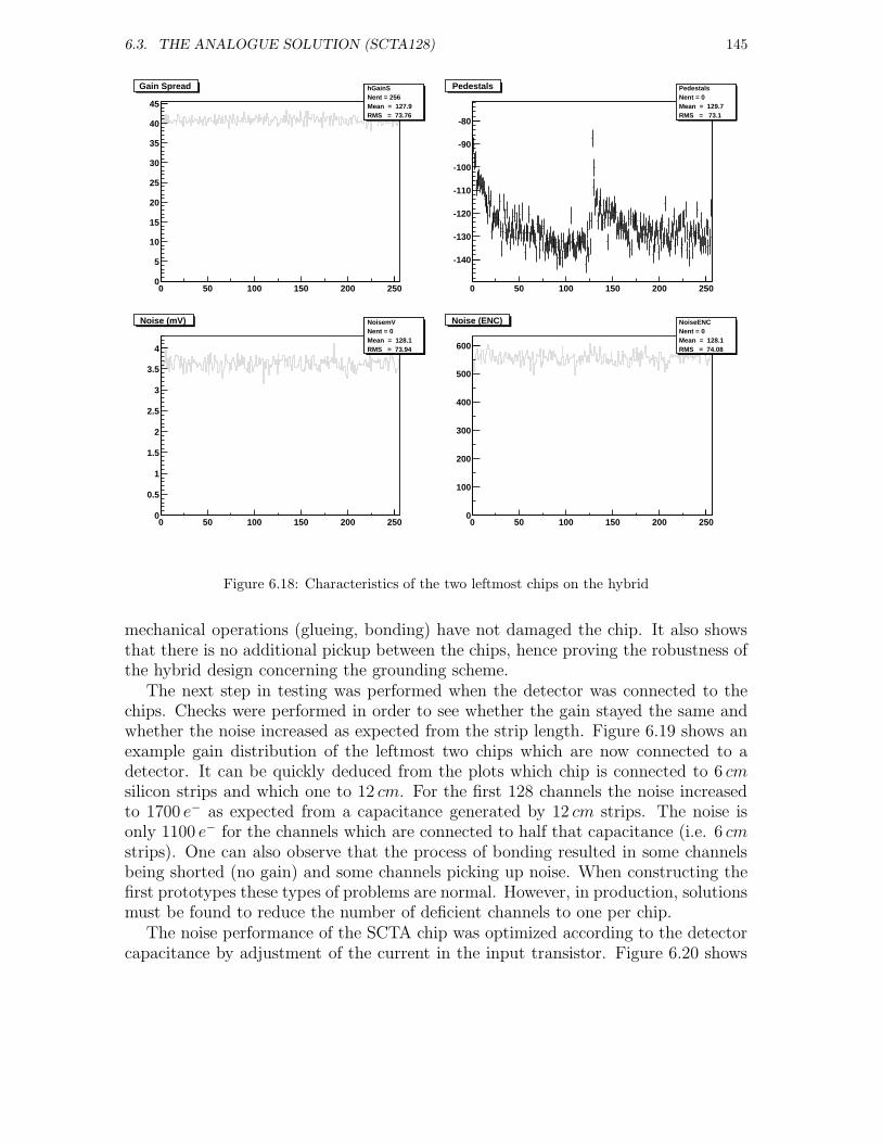
6.3. THE ANALOGUE SOLUTION (SCTA128) 145
0 50 100 150 200 2500
5
10
15
20
25
30
35
40
45
hGainSNent = 256 Mean = 127.9RMS = 73.76
Gain Spread hGainSNent = 256 Mean = 127.9RMS = 73.76
0 50 100 150 200 250
-140
-130
-120
-110
-100
-90
-80
PedestalsNent = 0 Mean = 129.7RMS = 73.1
Pedestals PedestalsNent = 0 Mean = 129.7RMS = 73.1
0 50 100 150 200 2500
0.5
1
1.5
2
2.5
3
3.5
4
NoisemVNent = 0 Mean = 128.1RMS = 73.94
Noise (mV) NoisemVNent = 0 Mean = 128.1RMS = 73.94
0 50 100 150 200 2500
100
200
300
400
500
600
NoiseENCNent = 0 Mean = 128.1RMS = 74.08
Noise (ENC) NoiseENCNent = 0 Mean = 128.1RMS = 74.08
Figure 6.18: Characteristics of the two leftmost chips on the hybrid
mechanical operations (glueing, bonding) have not damaged the chip. It also showsthat there is no additional pickup between the chips, hence proving the robustness ofthe hybrid design concerning the grounding scheme.
The next step in testing was performed when the detector was connected to thechips. Checks were performed in order to see whether the gain stayed the same andwhether the noise increased as expected from the strip length. Figure 6.19 shows anexample gain distribution of the leftmost two chips which are now connected to adetector. It can be quickly deduced from the plots which chip is connected to 6 cmsilicon strips and which one to 12 cm. For the first 128 channels the noise increasedto 1700 e− as expected from a capacitance generated by 12 cm strips. The noise isonly 1100 e− for the channels which are connected to half that capacitance (i.e. 6 cmstrips). One can also observe that the process of bonding resulted in some channelsbeing shorted (no gain) and some channels picking up noise. When constructing thefirst prototypes these types of problems are normal. However, in production, solutionsmust be found to reduce the number of deficient channels to one per chip.
The noise performance of the SCTA chip was optimized according to the detectorcapacitance by adjustment of the current in the input transistor. Figure 6.20 shows
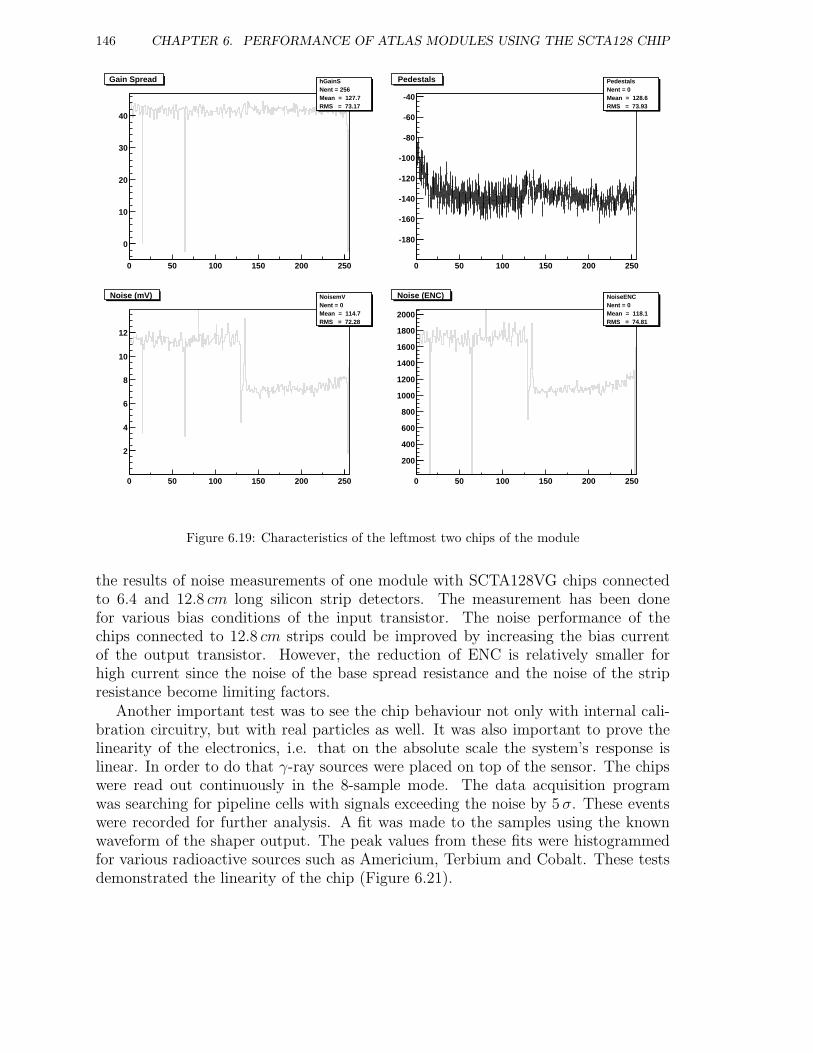
146 CHAPTER 6. PERFORMANCE OF ATLAS MODULES USING THE SCTA128 CHIP
0 50 100 150 200 250
0
10
20
30
40
hGainSNent = 256 Mean = 127.7RMS = 73.17
Gain Spread hGainSNent = 256 Mean = 127.7RMS = 73.17
0 50 100 150 200 250
-180
-160
-140
-120
-100
-80
-60
-40
PedestalsNent = 0 Mean = 128.6RMS = 73.93
Pedestals PedestalsNent = 0 Mean = 128.6RMS = 73.93
0 50 100 150 200 250
2
4
6
8
10
12
NoisemVNent = 0 Mean = 114.7RMS = 72.28
Noise (mV) NoisemVNent = 0 Mean = 114.7RMS = 72.28
0 50 100 150 200 250
200
400
600
800
1000
1200
1400
1600
1800
2000
NoiseENCNent = 0 Mean = 118.1RMS = 74.81
Noise (ENC) NoiseENCNent = 0 Mean = 118.1RMS = 74.81
Figure 6.19: Characteristics of the leftmost two chips of the module
the results of noise measurements of one module with SCTA128VG chips connectedto 6.4 and 12.8 cm long silicon strip detectors. The measurement has been donefor various bias conditions of the input transistor. The noise performance of thechips connected to 12.8 cm strips could be improved by increasing the bias currentof the output transistor. However, the reduction of ENC is relatively smaller forhigh current since the noise of the base spread resistance and the noise of the stripresistance become limiting factors.
Another important test was to see the chip behaviour not only with internal cali-bration circuitry, but with real particles as well. It was also important to prove thelinearity of the electronics, i.e. that on the absolute scale the system’s response islinear. In order to do that γ-ray sources were placed on top of the sensor. The chipswere read out continuously in the 8-sample mode. The data acquisition programwas searching for pipeline cells with signals exceeding the noise by 5 σ. These eventswere recorded for further analysis. A fit was made to the samples using the knownwaveform of the shaper output. The peak values from these fits were histogrammedfor various radioactive sources such as Americium, Terbium and Cobalt. These testsdemonstrated the linearity of the chip (Figure 6.21).
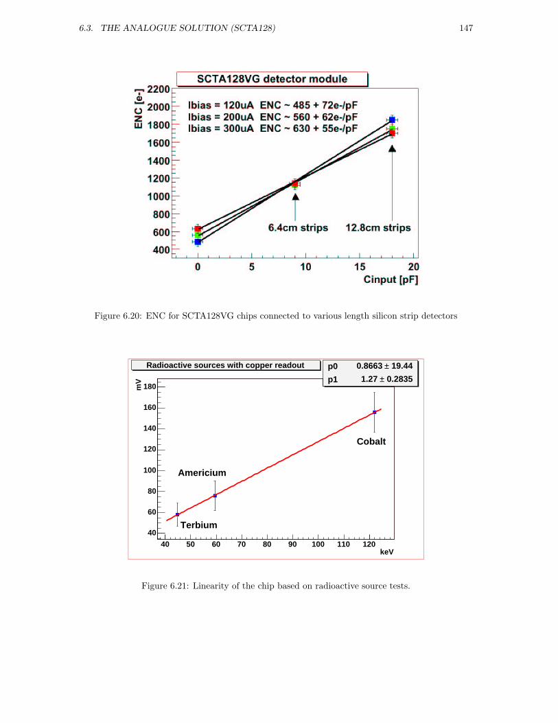
6.3. THE ANALOGUE SOLUTION (SCTA128) 147
Figure 6.20: ENC for SCTA128VG chips connected to various length silicon strip detectors
keV40 50 60 70 80 90 100 110 120
mV
40
60
80
100
120
140
160
180
p0 19.44± 0.8663
p1 0.2835± 1.27
p0 19.44± 0.8663
p1 0.2835± 1.27
Terbium
Americium
Cobalt
Radioactive sources with copper readout
Figure 6.21: Linearity of the chip based on radioactive source tests.
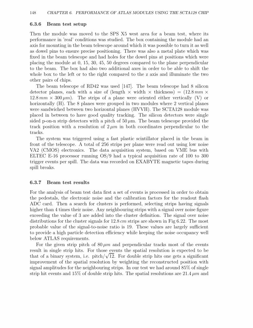
148 CHAPTER 6. PERFORMANCE OF ATLAS MODULES USING THE SCTA128 CHIP
6.3.6 Beam test setup
Then the module was moved to the SPS X5 west area for a beam test, where itsperformance in ’real’ conditions was studied. The box containing the module had anaxis for mounting in the beam telescope around which it was possible to turn it as wellas dowel pins to ensure precise positioning. There was also a metal plate which wasfixed in the beam telescope and had holes for the dowel pins at positions which wereplacing the module at 0, 15, 30, 45, 50 degrees compared to the plane perpendicularto the beam. The box had also two additional axes in order to be able to shift thewhole box to the left or to the right compared to the z axis and illuminate the twoother pairs of chips.
The beam telescope of RD42 was used [147]. The beam telescope had 8 silicondetector planes, each with a size of (length × width × thickness) = (12.8mm ×12.8mm × 300µm). The strips of a plane were oriented either vertically (V) orhorizontally (H). The 8 planes were grouped in two modules where 2 vertical planeswere sandwiched between two horizontal planes (HVVH). The SCTA128 module wasplaced in between to have good quality tracking. The silicon detectors were singlesided p-on-n strip detectors with a pitch of 50µm. The beam telescope provided thetrack position with a resolution of 2µm in both coordinates perpendicular to thetracks.
The system was triggered using a fast plastic scintillator placed in the beam infront of the telescope. A total of 256 strips per plane were read out using low noiseVA2 (CMOS) electronics. The data acquisition system, based on VME bus withELTEC E-16 processor running OS/9 had a typical acquisition rate of 100 to 300trigger events per spill. The data was recorded on EXABYTE magnetic tapes duringspill breaks.
6.3.7 Beam test results
For the analysis of beam test data first a set of events is processed in order to obtainthe pedestals, the electronic noise and the calibration factors for the readout flashADC card. Then a search for clusters is performed, selecting strips having signalshigher than 4 times their noise. Any neighbouring strips with a signal over noise figureexceeding the value of 3 are added into the cluster definition. The signal over noisedistributions for the cluster signals for 12.8 cm strips are shown in Fig 6.22. The mostprobable value of the signal-to-noise ratio is 19. These values are largely sufficientto provide a high particle detection efficiency while keeping the noise occupancy wellbelow ATLAS requirements.
For the given strip pitch of 80µm and perpendicular tracks most of the eventsresult in single strip hits. For those events the spatial resolution is expected to bethat of a binary system, i.e. pitch/
√12. For double strip hits one gets a significant
improvement of the spatial resolution by weighting the reconstructed position withsignal amplitudes for the neighbouring strips. In our test we had around 85% of singlestrip hit events and 15% of double strip hits. The spatial resolutions are 21.4µm and
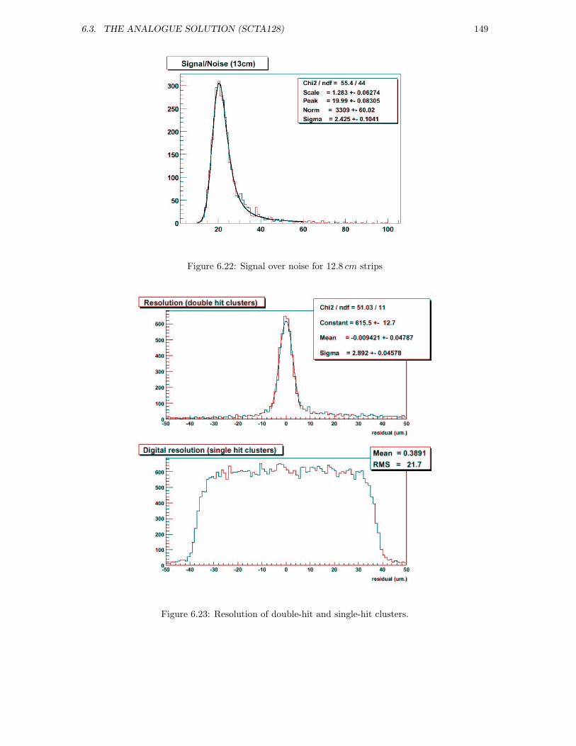
6.3. THE ANALOGUE SOLUTION (SCTA128) 149
Figure 6.22: Signal over noise for 12.8 cm strips
Figure 6.23: Resolution of double-hit and single-hit clusters.
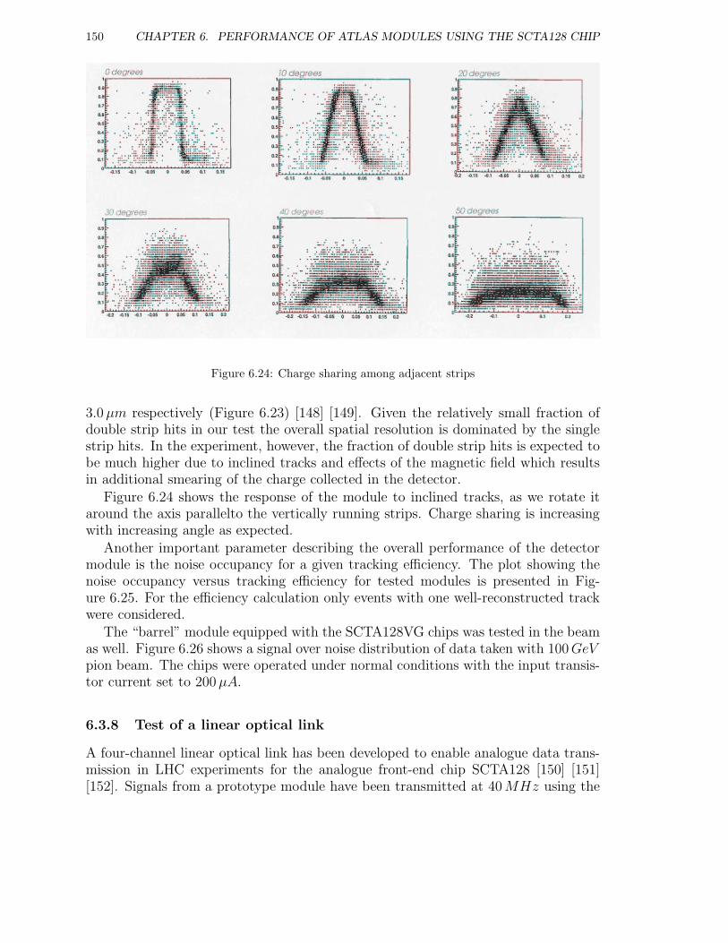
150 CHAPTER 6. PERFORMANCE OF ATLAS MODULES USING THE SCTA128 CHIP
Figure 6.24: Charge sharing among adjacent strips
3.0µm respectively (Figure 6.23) [148] [149]. Given the relatively small fraction ofdouble strip hits in our test the overall spatial resolution is dominated by the singlestrip hits. In the experiment, however, the fraction of double strip hits is expected tobe much higher due to inclined tracks and effects of the magnetic field which resultsin additional smearing of the charge collected in the detector.
Figure 6.24 shows the response of the module to inclined tracks, as we rotate itaround the axis parallelto the vertically running strips. Charge sharing is increasingwith increasing angle as expected.
Another important parameter describing the overall performance of the detectormodule is the noise occupancy for a given tracking efficiency. The plot showing thenoise occupancy versus tracking efficiency for tested modules is presented in Fig-ure 6.25. For the efficiency calculation only events with one well-reconstructed trackwere considered.
The “barrel” module equipped with the SCTA128VG chips was tested in the beamas well. Figure 6.26 shows a signal over noise distribution of data taken with 100GeVpion beam. The chips were operated under normal conditions with the input transis-tor current set to 200µA.
6.3.8 Test of a linear optical link
A four-channel linear optical link has been developed to enable analogue data trans-mission in LHC experiments for the analogue front-end chip SCTA128 [150] [151][152]. Signals from a prototype module have been transmitted at 40MHz using the
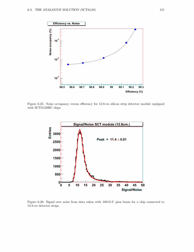
6.3. THE ANALOGUE SOLUTION (SCTA128) 151
Figure 6.25: Noise occupancy versus efficiency for 12.8 cm silicon strip detector module equippedwith SCTA128HC chips.
Figure 6.26: Signal over noise from data taken with 100GeV pion beam for a chip connected to12.8 cm detector strips.
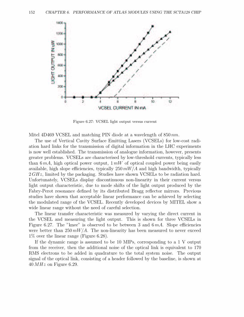
152 CHAPTER 6. PERFORMANCE OF ATLAS MODULES USING THE SCTA128 CHIP
Figure 6.27: VCSEL light output versus current
Mitel 4D469 VCSEL and matching PIN diode at a wavelength of 850nm.The use of Vertical Cavity Surface Emitting Lasers (VCSELs) for low-cost radi-
ation hard links for the transmission of digital information in the LHC experimentsis now well established. The transmission of analogue information, however, presentsgreater problems. VCSELs are characterised by low-threshold currents, typically lessthan 6mA, high optical power output, 1mW of optical coupled power being easilyavailable, high slope efficiencies, typically 250mW/A and high bandwidth, typically2GHz, limited by the packaging. Studies have shown VCSELs to be radiation hard.Unfortunately, VCSELs display discontinuous non-linearity in their current versuslight output characteristic, due to mode shifts of the light output produced by theFabry-Perot resonance defined by its distributed Bragg reflector mirrors. Previousstudies have shown that acceptable linear performance can be achieved by selectingthe modulated range of the VCSEL. Recently developed devices by MITEL show awide linear range without the need of careful selection.
The linear transfer characteristic was measured by varying the direct current inthe VCSEL and measuring the light output. This is shown for three VCSELs inFigure 6.27. The ”knee” is observed to be between 3 and 6mA. Slope efficiencieswere better than 250mW/A. The non-linearity has been measured to never exceed1% over the linear range (Figure 6.28).
If the dynamic range is assumed to be 10 MIPs, corresponding to a 1 V outputfrom the receiver, then the additional noise of the optical link is equivalent to 170RMS electrons to be added in quadrature to the total system noise. The outputsignal of the optical link, consisting of a header followed by the baseline, is shown at40MHz on Figure 6.29.
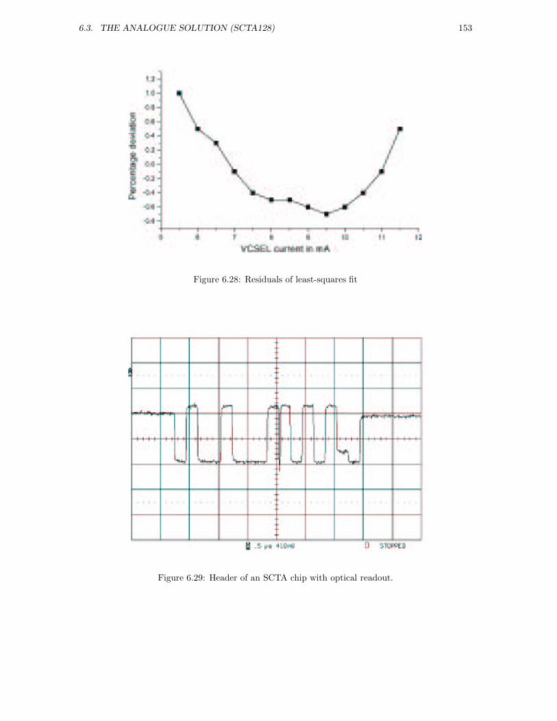
6.3. THE ANALOGUE SOLUTION (SCTA128) 153
Figure 6.28: Residuals of least-squares fit
Figure 6.29: Header of an SCTA chip with optical readout.
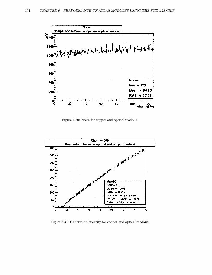
154 CHAPTER 6. PERFORMANCE OF ATLAS MODULES USING THE SCTA128 CHIP
Figure 6.30: Noise for copper and optical readout.
Figure 6.31: Calibration linearity for copper and optical readout.
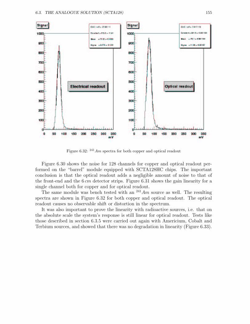
6.3. THE ANALOGUE SOLUTION (SCTA128) 155
Figure 6.32: 241Am spectra for both copper and optical readout
Figure 6.30 shows the noise for 128 channels for copper and optical readout per-formed on the “barrel” module equipped with SCTA128HC chips. The importantconclusion is that the optical readout adds a negligible amount of noise to that ofthe front-end and the 6 cm detector strips. Figure 6.31 shows the gain linearity for asingle channel both for copper and for optical readout.
The same module was bench tested with an 241Am source as well. The resultingspectra are shown in Figure 6.32 for both copper and optical readout. The opticalreadout causes no observable shift or distortion in the spectrum.
It was also important to prove the linearity with radioactive sources, i.e. that onthe absolute scale the system’s response is still linear for optical readout. Tests likethose described in section 6.3.5 were carried out again with Americium, Cobalt andTerbium sources, and showed that there was no degradation in linearity (Figure 6.33).
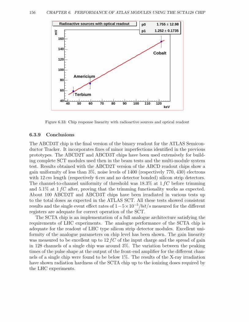
156 CHAPTER 6. PERFORMANCE OF ATLAS MODULES USING THE SCTA128 CHIP
keV40 50 60 70 80 90 100 110 120
mV
40
60
80
100
120
140
160
p0 12.98± 1.755
p1 0.1735± 1.252
p0 12.98± 1.755
p1 0.1735± 1.252
Terbium
Americium
Cobalt
Radioactive sources with optical readout
Figure 6.33: Chip response linearity with radioactive sources and optical readout
6.3.9 Conclusions
The ABCD3T chip is the final version of the binary readout for the ATLAS Semicon-ductor Tracker. It incorporates fixes of minor imperfections identified in the previousprototypes. The ABCD2T and ABCD3T chips have been used extensively for build-ing complete SCT modules used then in the beam tests and the multi-module systemtest. Results obtained with the ABCD2T version of the ABCD readout chips show again uniformity of less than 3%, noise levels of 1400 (respectively 770, 430) electronswith 12 cm length (respectively 6 cm and no detector bonded) silicon strip detectors.The channel-to-channel uniformity of threshold was 18.3% at 1 fC before trimmingand 5.1% at 1 fC after, proving that the trimming functionality works as expected.About 100 ABCD2T and ABCD3T chips have been irradiated in various tests upto the total doses as expected in the ATLAS SCT. All these tests showed consistentresults and the single event effect rates of 1−5×10⁻⁵/bit/s measured for the differentregisters are adequate for correct operation of the SCT.
The SCTA chip is an implementation of a full analogue architecture satisfying therequirements of LHC experiments. The analogue performance of the SCTA chip isadequate for the readout of LHC type silicon strip detector modules. Excellent uni-formity of the analogue parameters on chip level has been shown. The gain linearitywas measured to be excellent up to 12 fC of the input charge and the spread of gainin 128 channels of a single chip was around 3%. The variation between the peakingtimes of the pulse shape at the output of the front-end amplifier for the different chan-nels of a single chip were found to be below 1%. The results of the X-ray irradiationhave shown radiation hardness of the SCTA chip up to the ionizing doses required bythe LHC experiments.
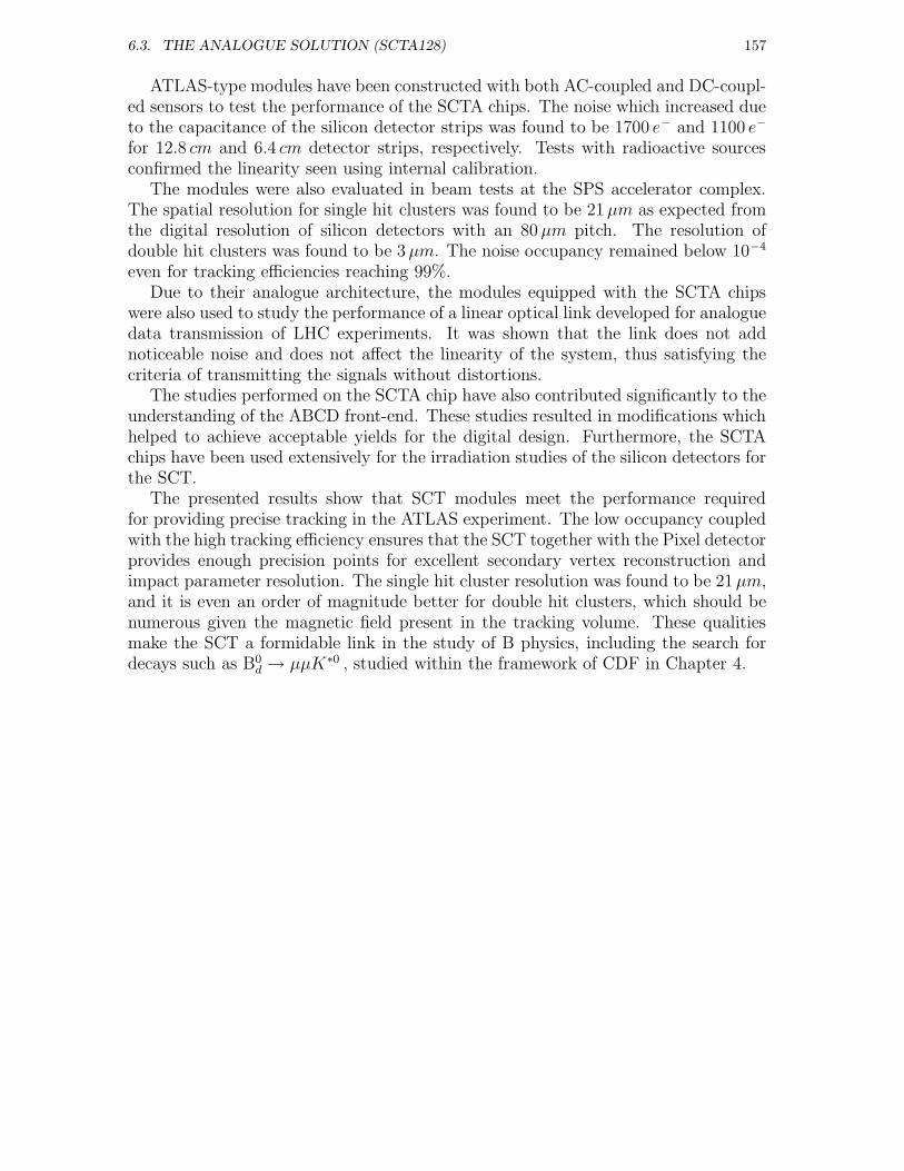
6.3. THE ANALOGUE SOLUTION (SCTA128) 157
ATLAS-type modules have been constructed with both AC-coupled and DC-coupl-ed sensors to test the performance of the SCTA chips. The noise which increased dueto the capacitance of the silicon detector strips was found to be 1700 e− and 1100 e−
for 12.8 cm and 6.4 cm detector strips, respectively. Tests with radioactive sourcesconfirmed the linearity seen using internal calibration.
The modules were also evaluated in beam tests at the SPS accelerator complex.The spatial resolution for single hit clusters was found to be 21µm as expected fromthe digital resolution of silicon detectors with an 80µm pitch. The resolution ofdouble hit clusters was found to be 3µm. The noise occupancy remained below 10−4
even for tracking efficiencies reaching 99%.Due to their analogue architecture, the modules equipped with the SCTA chips
were also used to study the performance of a linear optical link developed for analoguedata transmission of LHC experiments. It was shown that the link does not addnoticeable noise and does not affect the linearity of the system, thus satisfying thecriteria of transmitting the signals without distortions.
The studies performed on the SCTA chip have also contributed significantly to theunderstanding of the ABCD front-end. These studies resulted in modifications whichhelped to achieve acceptable yields for the digital design. Furthermore, the SCTAchips have been used extensively for the irradiation studies of the silicon detectors forthe SCT.
The presented results show that SCT modules meet the performance requiredfor providing precise tracking in the ATLAS experiment. The low occupancy coupledwith the high tracking efficiency ensures that the SCT together with the Pixel detectorprovides enough precision points for excellent secondary vertex reconstruction andimpact parameter resolution. The single hit cluster resolution was found to be 21µm,and it is even an order of magnitude better for double hit clusters, which should benumerous given the magnetic field present in the tracking volume. These qualitiesmake the SCT a formidable link in the study of B physics, including the search fordecays such as B0
d → µµK∗0 , studied within the framework of CDF in Chapter 4.

158 CHAPTER 6. PERFORMANCE OF ATLAS MODULES USING THE SCTA128 CHIP
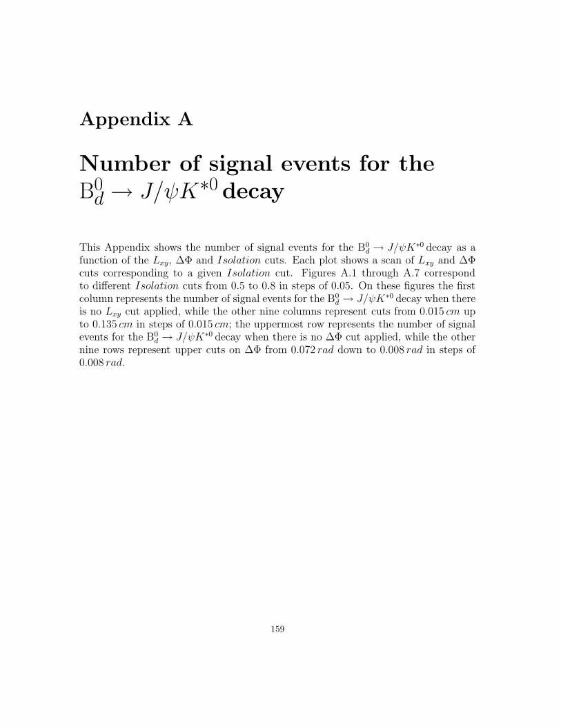
Appendix A
Number of signal events for theB0d → J/ψK∗0 decay
This Appendix shows the number of signal events for the B0d → J/ψK∗0 decay as a
function of the Lxy, ∆Φ and Isolation cuts. Each plot shows a scan of Lxy and ∆Φcuts corresponding to a given Isolation cut. Figures A.1 through A.7 correspondto different Isolation cuts from 0.5 to 0.8 in steps of 0.05. On these figures the firstcolumn represents the number of signal events for the B0
d → J/ψK∗0 decay when thereis no Lxy cut applied, while the other nine columns represent cuts from 0.015 cm upto 0.135 cm in steps of 0.015 cm; the uppermost row represents the number of signalevents for the B0
d → J/ψK∗0 decay when there is no ∆Φ cut applied, while the othernine rows represent upper cuts on ∆Φ from 0.072 rad down to 0.008 rad in steps of0.008 rad.
159
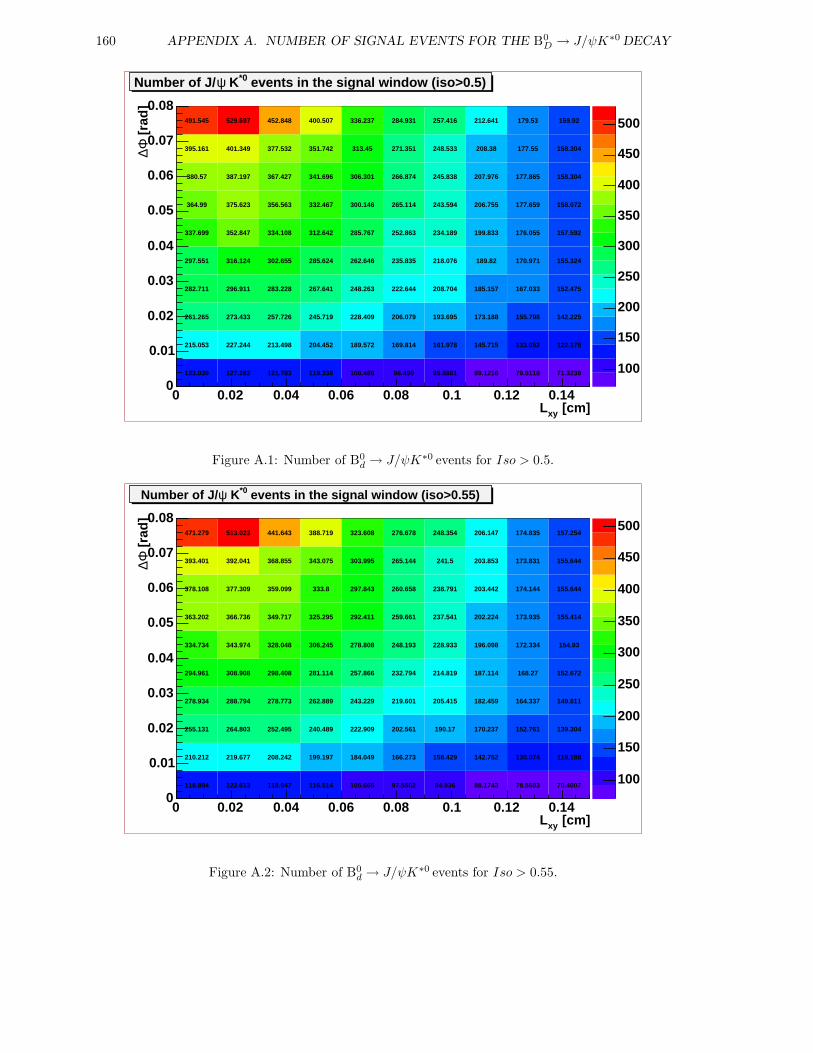
160 APPENDIX A. NUMBER OF SIGNAL EVENTS FOR THE B0D → J/ψK∗0 DECAY
100
150
200
250
300
350
400
450
500
[cm]xyL0 0.02 0.04 0.06 0.08 0.1 0.12 0.14
[ra
d]
Φ∆
0
0.01
0.02
0.03
0.04
0.05
0.06
0.07
0.08
events in the signal window (iso>0.5)*0 KψNumber of J/
123.039 127.282 121.783 119.338 108.486 98.499 95.8881 89.1216 79.5118 71.3239
215.053 227.244 213.498 204.452 189.572 169.814 161.978 145.715 133.052 122.175
261.265 273.433 257.726 245.719 228.409 206.079 193.695 173.188 155.708 142.225
282.711 296.911 283.228 267.641 248.263 222.644 208.704 185.157 167.033 152.475
297.551 316.124 302.655 285.624 262.646 235.835 218.076 189.82 170.971 155.324
337.699 352.847 334.108 312.642 285.767 252.863 234.189 199.833 176.055 157.592
364.99 375.623 356.563 332.467 300.146 265.114 243.594 206.755 177.659 158.072
380.57 387.197 367.427 341.696 306.301 266.874 245.838 207.976 177.865 158.304
395.161 401.349 377.532 351.742 313.45 271.351 248.533 208.38 177.55 158.304
491.545 529.697 452.848 400.507 336.237 284.931 257.416 212.641 179.53 159.92
Figure A.1: Number of B0d → J/ψK∗0 events for Iso > 0.5.
100
150
200
250
300
350
400
450
500
[cm]xyL0 0.02 0.04 0.06 0.08 0.1 0.12 0.14
[ra
d]
Φ∆
0
0.01
0.02
0.03
0.04
0.05
0.06
0.07
0.08
events in the signal window (iso>0.55)*0 KψNumber of J/
118.894 122.613 118.947 116.514 105.665 97.5502 94.936 88.1743 78.5683 70.4007
210.212 219.677 208.242 199.197 184.049 166.273 158.429 142.752 130.074 119.188
255.131 264.803 252.495 240.489 222.909 202.561 190.17 170.237 152.761 139.304
278.934 288.794 278.773 262.889 243.229 219.601 205.415 182.459 164.337 149.811
294.961 308.908 298.408 281.114 257.866 232.794 214.819 187.114 168.27 152.672
334.734 343.974 328.048 306.245 278.808 248.193 228.933 196.098 172.334 154.93
363.202 366.736 349.717 325.295 292.411 259.661 237.541 202.224 173.935 155.414
378.108 377.309 359.099 333.8 297.843 260.658 238.791 203.442 174.144 155.644
393.401 392.041 368.855 343.075 303.995 265.144 241.5 203.853 173.831 155.644
471.279 513.023 441.643 388.719 323.608 276.678 248.354 206.147 174.835 157.254
Figure A.2: Number of B0d → J/ψK∗0 events for Iso > 0.55.
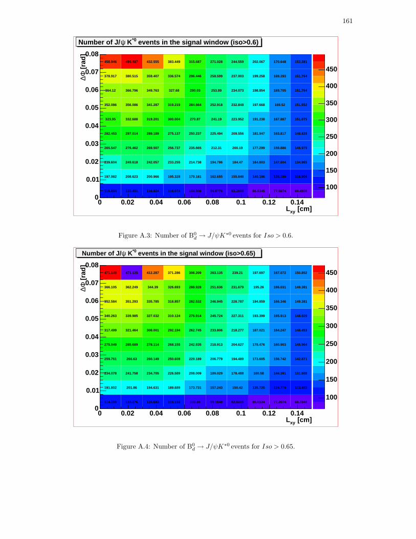
161
100
150
200
250
300
350
400
450
[cm]xyL0 0.02 0.04 0.06 0.08 0.1 0.12 0.14
[ra
d]
Φ∆
0
0.01
0.02
0.03
0.04
0.05
0.06
0.07
0.08
events in the signal window (iso>0.6)*0 KψNumber of J/
116.854 120.401 116.924 116.074 104.506 95.8776 93.2808 86.5345 77.9874 69.4508
197.982 208.623 200.966 195.328 179.181 162.655 155.846 140.186 128.199 116.906
239.604 249.618 242.057 233.255 214.738 194.786 184.47 164.603 147.804 134.965
265.547 276.462 269.507 256.737 235.665 212.31 200.19 177.299 159.886 145.979
282.453 297.014 289.189 275.137 250.237 225.494 209.556 181.947 163.817 148.828
323.95 332.688 319.201 300.004 270.87 241.19 223.952 191.238 167.887 151.075
352.086 356.086 341.287 319.219 284.664 252.918 232.848 197.668 169.52 151.552
364.12 366.796 349.763 327.68 290.03 253.89 234.073 198.854 169.705 151.764
378.917 380.515 359.407 336.574 296.446 258.599 237.003 199.258 169.393 151.764
458.946 495.487 432.555 383.449 315.687 271.028 244.559 202.067 170.648 153.381
Figure A.3: Number of B0d → J/ψK∗0 events for Iso > 0.6.
100
150
200
250
300
350
400
450
[cm]xyL0 0.02 0.04 0.06 0.08 0.1 0.12 0.14
[ra
d]
Φ∆
0
0.01
0.02
0.03
0.04
0.05
0.06
0.07
0.08
events in the signal window (iso>0.65)*0 KψNumber of J/
114.359 118.276 115.683 115.156 103.85 95.1948 92.6015 85.8534 77.3074 68.7848
191.802 201.86 194.631 189.689 173.731 157.243 150.42 135.725 124.779 113.483
234.078 241.758 234.705 226.589 208.009 189.029 178.488 160.58 144.391 131.588
259.761 266.63 260.149 250.608 229.189 206.779 194.489 173.605 156.742 142.871
275.949 285.689 278.114 268.155 242.935 218.913 204.627 178.476 160.903 145.964
317.499 321.464 308.001 292.194 262.745 233.806 218.277 187.021 164.247 148.453
340.263 339.985 327.032 310.124 276.914 245.724 227.311 193.399 165.913 148.929
352.584 351.293 335.785 318.857 282.532 246.945 228.787 194.859 166.346 149.381
366.105 362.249 344.39 326.693 288.928 251.636 231.679 195.26 166.031 149.381
471.149 471.125 412.287 371.286 306.209 263.135 239.21 197.697 167.072 150.852
Figure A.4: Number of B0d → J/ψK∗0 events for Iso > 0.65.

162 APPENDIX A. NUMBER OF SIGNAL EVENTS FOR THE B0D → J/ψK∗0 DECAY
100
150
200
250
300
350
400
450
[cm]xyL0 0.02 0.04 0.06 0.08 0.1 0.12 0.14
[ra
d]
Φ∆
0
0.01
0.02
0.03
0.04
0.05
0.06
0.07
0.08
events in the signal window (iso>0.7)*0 KψNumber of J/
104.02 106.638 103.168 102.6 92.7938 85.9366 83.3971 77.2584 69.7903 61.2656
172.32 181.545 175.612 171.408 156.249 141.175 134.387 121.351 111.924 102.665
210.505 218.998 212.474 205.966 188.701 170.926 160.413 144.109 131.485 120.694
233.654 241.211 235.329 226.916 206.531 184.781 172.264 154.032 140.81 128.983
252.413 259.088 251.659 242.215 218.785 195.415 180.65 157.181 143.232 130.34
289.047 291.774 279.809 264.215 238.631 210.36 194.35 165.778 146.567 132.794
307.159 306.469 295.085 278.127 250.769 220.291 202.412 171.223 148.253 133.294
317.172 315.763 303.359 286.019 256.343 221.489 203.874 172.672 148.688 133.752
327.92 324.804 309.756 292.88 261.792 225.229 205.803 173.069 148.371 133.752
454.89 419.966 368.98 332.336 277.41 234.719 211.354 175.491 149.405 135.223
Figure A.5: Number of B0d → J/ψK∗0 events for Iso > 0.7.
100
150
200
250
300
350
400
[cm]xyL0 0.02 0.04 0.06 0.08 0.1 0.12 0.14
[ra
d]
Φ∆
0
0.01
0.02
0.03
0.04
0.05
0.06
0.07
0.08
events in the signal window (iso>0.75)*0 KψNumber of J/
87.9679 91.4661 88.973 89.0579 82.4983 77.5245 75.9456 70.398 63.862 55.3275
144.609 153.099 148.213 145.331 132.788 121.437 116.617 107.731 99.2778 90.0716
177.872 186.814 181.323 175.968 161.477 147.1 138.555 126.45 114.725 104.007
198.673 207.692 202.297 195.019 178.255 159.906 149.315 134.917 122.395 110.589
218.919 227.471 219.107 210.096 190.075 171.032 157.946 138.382 124.859 111.944
249.982 256.226 245.271 230.62 209.419 185.463 170.828 146.098 128.255 114.427
268.891 272.84 261.767 245.203 222.176 195.434 178.987 151.664 129.963 114.92
280.492 283.512 270.62 253.524 228.237 196.883 180.695 153.376 130.657 115.633
293.14 292.662 276.67 259.638 232.673 200.619 182.627 153.763 130.339 115.633
404.12 378.608 332.367 294.338 243.415 206.095 184.901 153.794 129.67 115.367
Figure A.6: Number of B0d → J/ψK∗0 events for Iso > 0.75.

163
50
100
150
200
250
300
[cm]xyL0 0.02 0.04 0.06 0.08 0.1 0.12 0.14
[ra
d]
Φ∆
0
0.01
0.02
0.03
0.04
0.05
0.06
0.07
0.08
events in the signal window (iso>0.8)*0 KψNumber of J/
78.2852 81.003 79.1494 78.3231 72.714 68.9739 67.0386 62.2014 57.336 48.7313
123.525 128.68 125.69 121.514 112.517 103.19 99.1171 91.6614 84.8726 75.6707
148.762 155.813 152.149 145.444 135.525 122.957 117.161 106.613 96.4988 86.8464
168.158 174.698 170.782 162.14 150.664 134.103 126.268 113.473 103.193 92.4693
183.177 191.205 187.319 176.631 161.679 144.369 133.776 116.983 105.69 93.8595
209.609 215.383 209.602 193.12 178.955 157.607 145.204 123.663 109.092 96.4402
226.626 230.069 223.893 206.348 189.996 165.837 152.556 128.522 110.088 96.959
235.344 238.282 231.261 213.602 195.01 167.287 154.26 130.208 110.777 97.6705
243.315 242.635 234.171 216.99 196.761 169.321 155.231 130.628 110.476 97.6705
324.359 315.941 283.469 247.295 206.582 174 157.491 130.7 109.853 97.4242
Figure A.7: Number of B0d → J/ψK∗0 events for Iso > 0.8.

164 APPENDIX A. NUMBER OF SIGNAL EVENTS FOR THE B0D → J/ψK∗0 DECAY
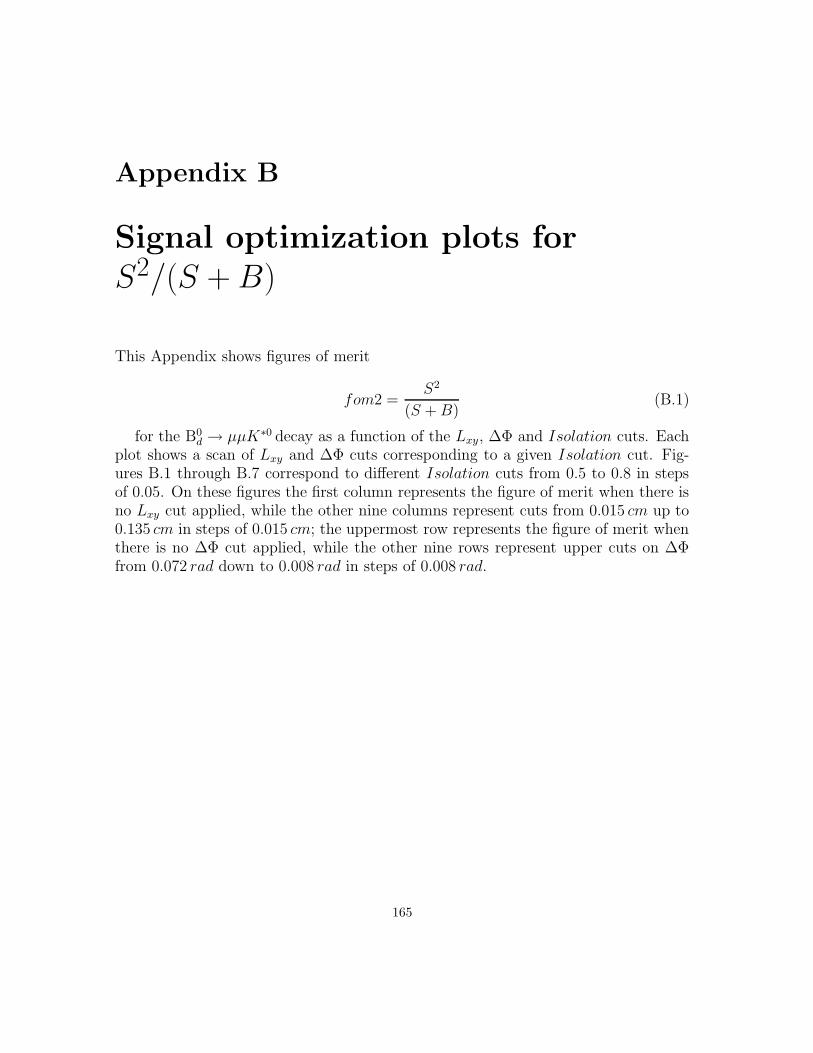
Appendix B
Signal optimization plots forS2/(S +B)
This Appendix shows figures of merit
fom2 =S2
(S +B)(B.1)
for the B0d → µµK∗0 decay as a function of the Lxy, ∆Φ and Isolation cuts. Each
plot shows a scan of Lxy and ∆Φ cuts corresponding to a given Isolation cut. Fig-ures B.1 through B.7 correspond to different Isolation cuts from 0.5 to 0.8 in stepsof 0.05. On these figures the first column represents the figure of merit when there isno Lxy cut applied, while the other nine columns represent cuts from 0.015 cm up to0.135 cm in steps of 0.015 cm; the uppermost row represents the figure of merit whenthere is no ∆Φ cut applied, while the other nine rows represent upper cuts on ∆Φfrom 0.072 rad down to 0.008 rad in steps of 0.008 rad.
165
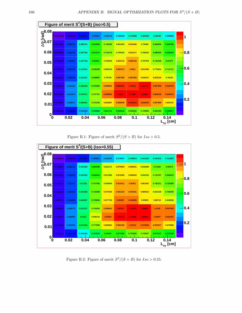
166 APPENDIX B. SIGNAL OPTIMIZATION PLOTS FOR S2/(S +B)
0.2
0.4
0.6
0.8
1
[cm]xyL0 0.02 0.04 0.06 0.08 0.1 0.12 0.14
[ra
d]
Φ∆
0
0.01
0.02
0.03
0.04
0.05
0.06
0.07
0.08
0.0589766 0.150074 0.315329 0.506846 0.621711 0.636142 0.694022 0.720982 0.652455 0.589617
0.0872827 0.239127 0.469631 0.721235 0.844287 0.898908 0.964316 0.932533 0.897989 0.852141
0.0872629 0.241974 0.476471 0.737751 0.935564 1.0183 1.07097 1.03867 0.963025 0.944474
0.0766267 0.220163 0.452943 0.679483 0.859552 0.981691 1.00321 1.01774 0.957599 0.918743
0.0682826 0.198568 0.422467 0.648853 0.79748 0.897366 0.887659 0.835247 0.825334 0.78224
0.0719919 0.202332 0.424624 0.646355 0.800215 0.860372 0.8821 0.813459 0.776631 0.712721
0.0724168 0.19586 0.417716 0.63542 0.764029 0.833723 0.860125 0.797978 0.725439 0.67377
0.0694009 0.184706 0.397794 0.613274 0.743178 0.799194 0.831217 0.768342 0.686505 0.635319
0.0671914 0.180739 0.385741 0.602994 0.746269 0.801393 0.832366 0.75469 0.666855 0.629756
0.00534262 0.0679913 0.152201 0.25548 0.305118 0.339648 0.412698 0.402936 0.38198 0.369855
/(S+B) (iso>0.5)2Figure of merit S
Figure B.1: Figure of merit S2/(S +B) for Iso > 0.5.
0.2
0.4
0.6
0.8
1
[cm]xyL0 0.02 0.04 0.06 0.08 0.1 0.12 0.14
[ra
d]
Φ∆
0
0.01
0.02
0.03
0.04
0.05
0.06
0.07
0.08
0.0655267 0.164116 0.346364 0.542826 0.64943 0.672889 0.725083 0.742937 0.670137 0.604249
0.0992888 0.263706 0.517644 0.777996 0.893665 0.952198 1.01012 0.972699 0.929327 0.876598
0.0991853 0.268406 0.5322 0.808133 1.00353 1.09058 1.13498 1.09494 1.00967 0.981447
0.0889703 0.246778 0.512237 0.754283 0.936614 1.06562 1.07879 1.08488 1.0148 0.967509
0.0800779 0.224958 0.480867 0.725854 0.877758 0.98459 0.966696 0.90595 0.88718 0.836558
0.0844395 0.228362 0.480558 0.719288 0.874548 0.941215 0.953351 0.880532 0.833108 0.768398
0.0856191 0.22189 0.47253 0.707392 0.836069 0.912411 0.92911 0.861987 0.782231 0.729389
0.0818201 0.208615 0.447632 0.682016 0.811996 0.872506 0.894043 0.832181 0.742787 0.690416
0.079551 0.205178 0.434209 0.669498 0.812171 0.876084 0.896251 0.818389 0.72262 0.68474
0.00588354 0.0762725 0.17255 0.285621 0.334355 0.376957 0.449914 0.441302 0.420312 0.412825
/(S+B) (iso>0.55)2Figure of merit S
Figure B.2: Figure of merit S2/(S +B) for Iso > 0.55.
167
0.2
0.4
0.6
0.8
1
1.2
[cm]xyL0 0.02 0.04 0.06 0.08 0.1 0.12 0.14
[ra
d]
Φ∆
0
0.01
0.02
0.03
0.04
0.05
0.06
0.07
0.08
/(S+B) (iso>0.6)2Figure of merit S
0.079291 0.194819 0.398143 0.613879 0.704288 0.712766 0.756778 0.7627 0.695868 0.622263
0.110768 0.294986 0.581641 0.872334 0.972216 1.0255 1.08232 1.03089 0.983177 0.917896
0.110201 0.297085 0.595401 0.900127 1.08171 1.15345 1.20231 1.14484 1.05318 1.01739
0.101654 0.282086 0.584835 0.858305 1.03147 1.14731 1.16637 1.15254 1.07524 1.02178
0.0926389 0.259949 0.553965 0.834026 0.977654 1.0759 1.06229 0.984074 0.95734 0.900808
0.0997815 0.267244 0.55941 0.831862 0.981138 1.04267 1.05931 0.967368 0.907621 0.836244
0.101543 0.261947 0.554383 0.823655 0.946468 1.0202 1.04108 0.954713 0.858433 0.798011
0.0958175 0.247125 0.524441 0.796854 0.922141 0.978871 1.00526 0.924882 0.818776 0.759149
0.0932207 0.24246 0.509839 0.782898 0.925637 0.985878 1.0103 0.910966 0.798217 0.753455
0.00707502 0.0899625 0.208126 0.34662 0.394661 0.445238 0.531273 0.513177 0.48245 0.471123
Figure B.3: Figure of merit S2/(S +B) for Iso > 0.6.
0.2
0.4
0.6
0.8
1
1.2
[cm]xyL0 0.02 0.04 0.06 0.08 0.1 0.12 0.14
[ra
d]
Φ∆
0
0.01
0.02
0.03
0.04
0.05
0.06
0.07
0.08
0.0992413 0.239353 0.47197 0.695742 0.77132 0.766567 0.800533 0.792965 0.72093 0.643476
0.136395 0.354435 0.674382 0.977607 1.06247 1.09372 1.13543 1.07597 1.02575 0.950581
0.13829 0.359653 0.699278 1.02421 1.19131 1.24761 1.27762 1.21758 1.1177 1.06685
0.128161 0.340291 0.686465 0.996959 1.16098 1.26259 1.26635 1.24494 1.15711 1.09015
0.116681 0.313164 0.650056 0.97395 1.11003 1.19636 1.18293 1.09399 1.05498 0.985658
0.126535 0.325352 0.663063 0.976716 1.12027 1.16929 1.18608 1.07989 1.00521 0.929092
0.125331 0.312237 0.650955 0.967636 1.09371 1.15615 1.1759 1.07248 0.959276 0.892595
0.1188 0.296771 0.619812 0.942293 1.07196 1.11613 1.14254 1.04598 0.922421 0.856738
0.115132 0.28808 0.601659 0.924272 1.07848 1.1261 1.14941 1.03232 0.901697 0.851111
0.00992357 0.107824 0.248808 0.422559 0.478382 0.535138 0.638205 0.610839 0.570655 0.557948
/(S+B) (iso>0.65)2Figure of merit S
Figure B.4: Figure of merit S2/(S +B) for Iso > 0.65.
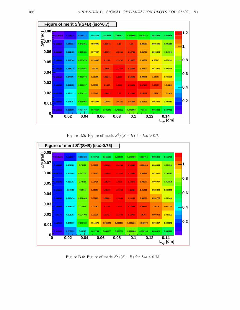
168 APPENDIX B. SIGNAL OPTIMIZATION PLOTS FOR S2/(S +B)
0.2
0.4
0.6
0.8
1
1.2
[cm]xyL0 0.02 0.04 0.06 0.08 0.1 0.12 0.14
[ra
d]
Φ∆
0
0.01
0.02
0.03
0.04
0.05
0.06
0.07
0.08
/(S+B) (iso>0.7)2Figure of merit S
0.110231 0.255188 0.474467 0.673667 0.731342 0.727872 0.749803 0.7342 0.668823 0.587751
0.148464 0.378283 0.699066 0.982207 1.04088 1.05241 1.07407 1.01195 0.963482 0.899519
0.151186 0.391111 0.736131 1.05145 1.19021 1.22 1.22643 1.15761 1.07903 1.03169
0.140462 0.370828 0.726817 1.02859 1.1637 1.2255 1.20622 1.17503 1.10559 1.04333
0.132333 0.344167 0.692974 1.00799 1.12241 1.1738 1.13592 1.04071 1.01091 0.945131
0.142266 0.358775 0.714557 1.0186 1.15461 1.17077 1.16007 1.04309 0.974061 0.901044
0.138689 0.340544 0.695474 0.999896 1.1293 1.15792 1.15575 1.03831 0.93707 0.87054
0.130653 0.322429 0.665681 0.977227 1.11374 1.12261 1.12786 1.01717 0.905423 0.84005
0.125613 0.311827 0.642351 0.959995 1.11948 1.13 1.13 1.00568 0.886646 0.835116
0.0126543 0.116736 0.269411 0.452726 0.519491 0.559672 0.648596 0.620844 0.583522 0.569625
Figure B.5: Figure of merit S2/(S +B) for Iso > 0.7.
0.2
0.4
0.6
0.8
1
[cm]xyL0 0.02 0.04 0.06 0.08 0.1 0.12 0.14
[ra
d]
Φ∆
0
0.01
0.02
0.03
0.04
0.05
0.06
0.07
0.08
0.112209 0.259055 0.46349 0.637244 0.693363 0.692932 0.712886 0.690166 0.630431 0.545977
0.149539 0.375165 0.668722 0.914675 0.955279 0.966193 0.986223 0.948079 0.896457 0.823642
0.15475 0.398382 0.724302 1.00226 1.11017 1.12783 1.12751 1.0765 0.993003 0.929092
0.145881 0.386279 0.72957 1.00091 1.1136 1.1535 1.12859 1.09969 1.02016 0.94226
0.143062 0.373414 0.716003 1.00287 1.09601 1.13646 1.09151 1.00208 0.951773 0.86948
0.153072 0.39038 0.7504 1.03051 1.15186 1.15658 1.1308 1.01311 0.929826 0.840266
0.152942 0.381282 0.74918 1.03415 1.15184 1.1625 1.14279 1.02077 0.903037 0.816598
0.147111 0.367689 0.727151 1.02397 1.14895 1.13532 1.12348 1.00791 0.879886 0.795025
0.144557 0.358582 0.70541 1.00955 1.15363 1.14766 1.12865 0.998695 0.863449 0.79096
0.0145245 0.136987 0.311628 0.498753 0.555565 0.591865 0.670658 0.636795 0.584396 0.551701
/(S+B) (iso>0.75)2Figure of merit S
Figure B.6: Figure of merit S2/(S +B) for Iso > 0.75.
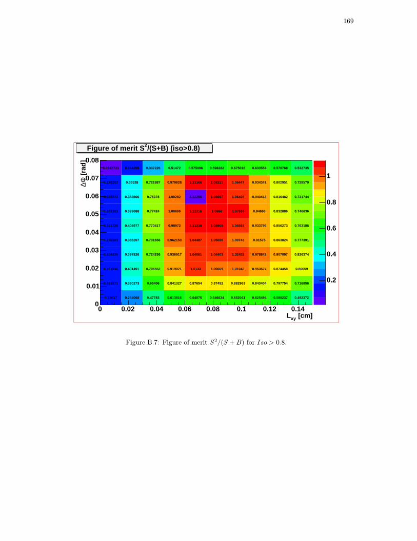
169
0.2
0.4
0.6
0.8
1
[cm]xyL0 0.02 0.04 0.06 0.08 0.1 0.12 0.14
[ra
d]
Φ∆
0
0.01
0.02
0.03
0.04
0.05
0.06
0.07
0.08
0.13017 0.284068 0.47783 0.613816 0.64875 0.646634 0.652041 0.625494 0.580237 0.492372
0.161871 0.380273 0.65406 0.841327 0.87654 0.87452 0.882963 0.843404 0.797754 0.716856
0.161646 0.401491 0.705552 0.919021 1.0133 1.00669 1.01042 0.953527 0.874458 0.80659
0.156439 0.397826 0.724256 0.936917 1.04061 1.04403 1.02452 0.978843 0.907097 0.826374
0.150383 0.386207 0.731656 0.962153 1.04487 1.05055 1.00743 0.91575 0.863824 0.777391
0.161728 0.404977 0.770417 0.98972 1.11238 1.08905 1.05565 0.933796 0.856273 0.763186
0.163383 0.399088 0.77424 1.00666 1.12216 1.0998 1.07666 0.94666 0.832886 0.746636
0.155973 0.383506 0.75378 1.00282 1.12206 1.08067 1.06498 0.940413 0.816482 0.731744
0.150202 0.36528 0.721887 0.979628 1.11166 1.08331 1.06447 0.934341 0.802951 0.728579
0.0142723 0.144295 0.337226 0.51472 0.575096 0.598282 0.675016 0.630554 0.570768 0.532735
/(S+B) (iso>0.8)2Figure of merit S
Figure B.7: Figure of merit S2/(S +B) for Iso > 0.8.

170 APPENDIX B. SIGNAL OPTIMIZATION PLOTS FOR S2/(S +B)
Appendix C
Signal optimization plots forS2/(a/2 +
√B)2
This Appendix shows figures of merit
fom3 =S2
(a2
+√B)2
(C.1)
for the B0d → µµK∗0 decay as a function of the Lxy, ∆Φ and Isolation cuts. The
value of a has been chosen to search for a one σ discovery. Each plot shows a scanof Lxy and ∆Φ cuts corresponding to a given Isolation cut. Figures C.1 throughC.7 correspond to different Isolation cuts from 0.5 to 0.8 in steps of 0.05. On thesefigures the first column represents the figure of merit when there is no Lxy cut applied,while the other nine columns represent cuts from 0.015 cm up to 0.135 cm in stepsof 0.015 cm; the uppermost row represents the figure of merit when there is no ∆Φcut applied, while the other nine rows represent upper cuts on ∆Φ from 0.072 raddown to 0.008 rad in steps of 0.008 rad. For the present data a = 1 was chosen (seeSection 4.5.4).
171
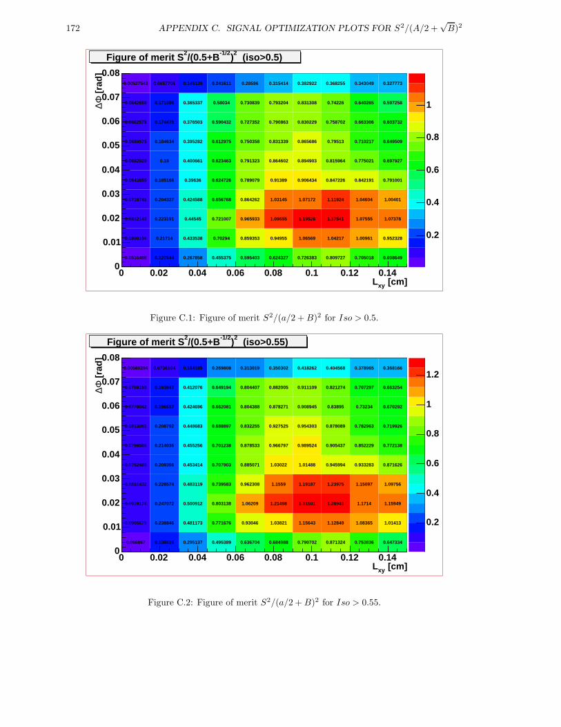
172 APPENDIX C. SIGNAL OPTIMIZATION PLOTS FOR S2/(A/2 +√B)2
0.2
0.4
0.6
0.8
1
[cm]xyL0 0.02 0.04 0.06 0.08 0.1 0.12 0.14
[ra
d]
Φ∆
0
0.01
0.02
0.03
0.04
0.05
0.06
0.07
0.08
(iso>0.5)2)-1/2/(0.5+B2Figure of merit S
0.0516498 0.127644 0.267858 0.455375 0.595403 0.624327 0.726383 0.809727 0.705018 0.608649
0.0800194 0.21714 0.433538 0.70294 0.859353 0.94955 1.06569 1.04217 1.00961 0.952328
0.0812143 0.223191 0.44545 0.721007 0.965933 1.09655 1.19528 1.17541 1.07555 1.07378
0.0718741 0.204327 0.424588 0.656768 0.864262 1.03145 1.07172 1.11924 1.04604 1.00401
0.0643855 0.185166 0.39636 0.624726 0.789079 0.91389 0.906434 0.847226 0.842191 0.791001
0.0682929 0.19 0.400661 0.623463 0.791323 0.864602 0.894903 0.815964 0.775021 0.697927
0.0689575 0.184634 0.395282 0.612975 0.750358 0.831339 0.865686 0.79513 0.710217 0.649509
0.0662575 0.174475 0.376503 0.590432 0.727352 0.790863 0.830229 0.758702 0.663306 0.603732
0.0642859 0.171086 0.365337 0.58034 0.730839 0.793204 0.831308 0.74226 0.640265 0.597258
0.00527543 0.0657706 0.145129 0.241611 0.28596 0.315414 0.382922 0.368255 0.343049 0.327773
Figure C.1: Figure of merit S2/(a/2 +B)2 for Iso > 0.5.
0.2
0.4
0.6
0.8
1
1.2
[cm]xyL0 0.02 0.04 0.06 0.08 0.1 0.12 0.14
[ra
d]
Φ∆
0
0.01
0.02
0.03
0.04
0.05
0.06
0.07
0.08
(iso>0.55)2)-1/2/(0.5+B2Figure of merit S
0.056867 0.138516 0.295137 0.495389 0.636704 0.684988 0.790702 0.871324 0.753836 0.647334
0.0905679 0.238846 0.481173 0.771676 0.93046 1.03821 1.15643 1.12849 1.08365 1.01413
0.0919174 0.247072 0.500912 0.803138 1.06209 1.21498 1.31501 1.28946 1.1714 1.15949
0.0831432 0.228574 0.483119 0.739583 0.962308 1.1559 1.19187 1.23975 1.15097 1.09756
0.0752469 0.209356 0.453414 0.707903 0.885071 1.03022 1.01488 0.945994 0.933283 0.871626
0.0798566 0.214036 0.455256 0.701238 0.878533 0.966797 0.989524 0.905437 0.852229 0.772138
0.0813051 0.208792 0.448683 0.688897 0.832255 0.927525 0.954303 0.878089 0.782963 0.719926
0.0779042 0.196657 0.424696 0.662081 0.804388 0.878271 0.908945 0.83895 0.73234 0.670292
0.0759159 0.193847 0.412076 0.649194 0.804407 0.882005 0.911109 0.821274 0.707297 0.663254
0.00580294 0.0736104 0.164185 0.269808 0.313019 0.350302 0.418262 0.404568 0.378965 0.368166
Figure C.2: Figure of merit S2/(a/2 +B)2 for Iso > 0.55.
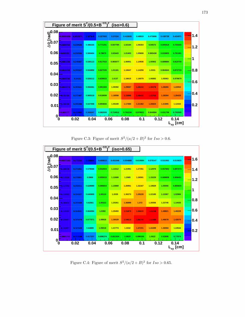
173
0.2
0.4
0.6
0.8
1
1.2
1.4
[cm]xyL0 0.02 0.04 0.06 0.08 0.1 0.12 0.14
[ra
d]
Φ∆
0
0.01
0.02
0.03
0.04
0.05
0.06
0.07
0.08
(iso>0.6)2)-1/2/(0.5+B2Figure of merit S
0.068077 0.163582 0.343247 0.582008 0.724912 0.762234 0.870821 0.944594 0.831759 0.702595
0.100219 0.266288 0.547008 0.894656 1.05339 1.17494 1.31362 1.26824 1.21905 1.12434
0.101419 0.272487 0.565318 0.918099 1.18558 1.33895 1.46492 1.41703 1.28304 1.26429
0.0944374 0.260641 0.556461 0.861583 1.09392 1.29557 1.35102 1.38478 1.28265 1.22054
0.0865786 0.24131 0.526212 0.830933 1.0137 1.16615 1.16079 1.06892 1.05063 0.979679
0.0939405 0.250027 0.533859 0.827035 1.01181 1.10647 1.14259 1.0331 0.964844 0.872723
0.0960289 0.246087 0.530113 0.817015 0.965077 1.06951 1.10936 1.00902 0.889884 0.815705
0.090853 0.232536 0.500404 0.78679 0.93443 1.01403 1.05808 0.965438 0.833803 0.761061
0.0886053 0.228628 0.486335 0.771291 0.937784 1.02164 1.06354 0.94572 0.805919 0.753305
0.00696689 0.0865571 0.197648 0.327883 0.37034 0.415935 0.49919 0.475806 0.439729 0.424971
Figure C.3: Figure of merit S2/(a/2 +B)2 for Iso > 0.6.
0.2
0.4
0.6
0.8
1
1.2
1.4
1.6
[cm]xyL0 0.02 0.04 0.06 0.08 0.1 0.12 0.14
[ra
d]
Φ∆
0
0.01
0.02
0.03
0.04
0.05
0.06
0.07
0.08
(iso>0.65)2)-1/2/(0.5+B2Figure of merit S
0.0841352 0.200538 0.417237 0.696374 0.851934 0.8829 0.996396 1.0622 0.92806 0.77874
0.122457 0.320628 0.64889 1.05018 1.21774 1.3332 1.47201 1.41699 1.36594 1.24544
0.126497 0.330478 0.677571 1.08928 1.38029 1.54613 1.66746 1.62489 1.46678 1.42679
0.118382 0.314531 0.664094 1.0392 1.29493 1.51879 1.56639 1.61259 1.48821 1.40228
0.108432 0.290439 0.62561 1.00333 1.20261 1.36899 1.372 1.26556 1.23745 1.14435
0.118563 0.304327 0.640905 1.00119 1.2035 1.30273 1.35228 1.22185 1.13367 1.02984
0.117952 0.292911 0.628989 0.986804 1.15868 1.26961 1.32167 1.19829 1.05055 0.965605
0.112115 0.278801 0.5969 0.955015 1.12689 1.2085 1.26591 1.15229 0.989809 0.906451
0.108926 0.271061 0.578588 0.932803 1.13312 1.21961 1.27351 1.12976 0.957663 0.897573
0.00975183 0.103332 0.235654 0.400815 0.451549 0.504888 0.610684 0.578147 0.531563 0.515825
Figure C.4: Figure of merit S2/(a/2 +B)2 for Iso > 0.65.
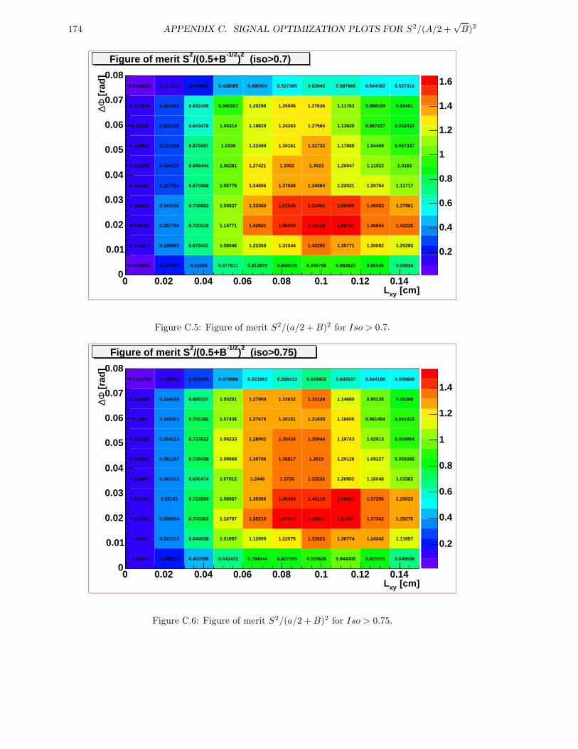
174 APPENDIX C. SIGNAL OPTIMIZATION PLOTS FOR S2/(A/2 +√B)2
0.2
0.4
0.6
0.8
1
1.2
1.4
1.6
[cm]xyL0 0.02 0.04 0.06 0.08 0.1 0.12 0.14
[ra
d]
Φ∆
0
0.01
0.02
0.03
0.04
0.05
0.06
0.07
0.08
(iso>0.7)2)-1/2/(0.5+B2Figure of merit S
0.0916092 0.210476 0.41699 0.677611 0.813878 0.848678 0.940766 0.983825 0.85946 0.69834
0.131517 0.339899 0.678431 1.08046 1.22358 1.31544 1.42292 1.35771 1.30582 1.20293
0.136759 0.357759 0.720019 1.14771 1.42601 1.56509 1.65128 1.58783 1.46604 1.43226
0.128431 0.341036 0.708663 1.09537 1.33368 1.51545 1.52462 1.55455 1.46063 1.37961
0.121897 0.317524 0.670968 1.05776 1.24556 1.37568 1.34084 1.22021 1.20794 1.11717
0.132252 0.334136 0.695444 1.06281 1.27421 1.3392 1.3523 1.20047 1.11922 1.0163
0.129512 0.317816 0.675097 1.0339 1.22499 1.30161 1.32732 1.17888 1.04469 0.957337
0.12236 0.301206 0.643478 1.00314 1.19828 1.24263 1.27584 1.13825 0.987827 0.902432
0.117949 0.291691 0.619105 0.980307 1.20298 1.25006 1.27636 1.11763 0.956529 0.89401
0.0124023 0.111201 0.253663 0.428065 0.490304 0.527365 0.62043 0.587666 0.544062 0.527312
Figure C.5: Figure of merit S2/(a/2 +B)2 for Iso > 0.7.
0.2
0.4
0.6
0.8
1
1.2
1.4
[cm]xyL0 0.02 0.04 0.06 0.08 0.1 0.12 0.14
[ra
d]
Φ∆
0
0.01
0.02
0.03
0.04
0.05
0.06
0.07
0.08
(iso>0.75)2)-1/2/(0.5+B2Figure of merit S
0.09029 0.208001 0.402098 0.641472 0.784544 0.827869 0.920635 0.944308 0.825691 0.649536
0.12956 0.331272 0.644558 1.01057 1.12909 1.22075 1.32623 1.30774 1.24242 1.11057
0.137481 0.359954 0.708363 1.10707 1.35219 1.47472 1.54817 1.51666 1.37342 1.29276
0.131283 0.35161 0.712859 1.08067 1.30366 1.46084 1.46119 1.49662 1.37296 1.25023
0.130007 0.341933 0.696474 1.07012 1.2446 1.3726 1.32532 1.20952 1.16048 1.03382
0.140584 0.361287 0.735438 1.09568 1.30796 1.36817 1.3613 1.20128 1.09227 0.955395
0.141286 0.354113 0.733822 1.09233 1.28902 1.35435 1.35944 1.19743 1.02913 0.904954
0.1364 0.342003 0.709182 1.07436 1.27675 1.30151 1.31635 1.16606 0.981454 0.861415
0.134488 0.334019 0.685337 1.05251 1.27909 1.31632 1.32129 1.14689 0.95135 0.85388
0.0141799 0.129571 0.291925 0.470896 0.523963 0.558413 0.644602 0.605537 0.544186 0.505669
Figure C.6: Figure of merit S2/(a/2 +B)2 for Iso > 0.75.
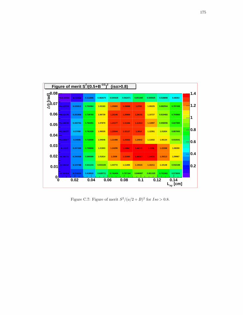
175
0.2
0.4
0.6
0.8
1
1.2
1.4
[cm]xyL0 0.02 0.04 0.06 0.08 0.1 0.12 0.14
[ra
d]
Φ∆
0
0.01
0.02
0.03
0.04
0.05
0.06
0.07
0.08
(iso>0.8)2)-1/2/(0.5+B2Figure of merit S
0.101494 0.224122 0.418528 0.628721 0.746404 0.787164 0.846987 0.851335 0.762462 0.573606
0.136817 0.329788 0.631234 0.933155 1.04772 1.11465 1.19315 1.16211 1.10148 0.942198
0.140371 0.356928 0.690099 1.01814 1.2509 1.32493 1.40313 1.34631 1.20213 1.09967
0.13805 0.357269 0.709808 1.01903 1.24295 1.33967 1.34793 1.3396 1.22268 1.08359
0.134107 0.34905 0.716608 1.04046 1.21498 1.29353 1.24642 1.11832 1.06134 0.919341
0.146087 0.37059 0.761028 1.06535 1.29944 1.32127 1.3014 1.12351 1.01834 0.867693
0.148655 0.366793 0.764251 1.07879 1.29177 1.31346 1.31513 1.12897 0.958096 0.827985
0.142479 0.352808 0.739769 1.06739 1.28146 1.26969 1.28181 1.10727 0.919482 0.793889
0.137673 0.335912 0.703064 1.03183 1.25993 1.26898 1.2769 1.09225 0.892554 0.787498
0.0138554 0.134932 0.313006 0.482679 0.540639 0.562471 0.651085 0.599925 0.528898 0.48363
Figure C.7: Figure of merit S2/(a/2 +B)2 for Iso > 0.8.

176 APPENDIX C. SIGNAL OPTIMIZATION PLOTS FOR S2/(A/2 +√B)2
Appendix D
Estimated background for theB0d → µµK∗0 decay
This Appendix shows the number estimated background events for the B0d → µµK∗0
decay as a function of the Lxy, ∆Φ and Isolation cuts. Each plot shows a scan ofLxy and ∆Φ cuts corresponding to a given Isolation cut. Figures D.1 through D.7correspond to different Isolation cuts from 0.5 to 0.8 in steps of 0.05. On thesefigures the first column represents the number of estimated background events for theB0d → µµK∗0 decay when there is no Lxy cut applied, while the other nine columns
represent cuts from 0.015 cm up to 0.135 cm in steps of 0.015 cm; the uppermost rowrepresents the number of estimated background events for the B0
d → µµK∗0 decaywhen there is no ∆Φ cut applied, while the other nine rows represent upper cuts on∆Φ from 0.072 rad down to 0.008 rad in steps of 0.008 rad.
177
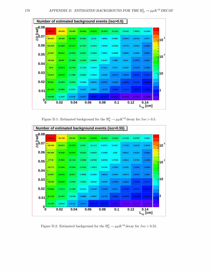
178 APPENDIX D. ESTIMATED BACKGROUND FOR THE B0D → µµK∗0 DECAY
1
10
102
103
[cm]xyL0 0.02 0.04 0.06 0.08 0.1 0.12 0.14
[ra
d]
Φ∆
0
0.01
0.02
0.03
0.04
0.05
0.06
0.07
0.08
Number of estimated background events (iso>0.5)
28.9196 11.3422 4.22159 2.01627 1.05348 0.728277 0.520507 0.330918 0.278874 0.242599
60.1192 22.9866 9.12213 4.61161 2.95897 1.93755 1.44836 1.10175 0.87912 0.738236
89.363 33.4503 13.6333 6.97866 4.09301 2.67837 2.02624 1.52345 1.27694 0.980295
119.873 43.9726 17.7999 9.52002 5.75644 3.53455 2.85174 1.96026 1.62071 1.32724
149.6 55.8878 22.2705 11.7188 7.34424 4.74501 3.9473 3.02387 2.31839 1.94894
183.046 68.697 27.3586 14.4303 8.92605 6.01427 4.7859 3.6167 2.79272 2.39627
212.867 80.8311 32.0035 16.8941 10.6393 7.05837 5.48683 4.06951 3.19946 2.65501
241.848 91.4669 36.0127 18.7302 11.5545 7.60668 5.90099 4.37748 3.50062 2.93062
269.634 100.691 39.4532 20.3654 12.115 7.88361 6.04857 4.51941 3.64431 2.9717
5325.16 480.654 153.895 69.6565 40.0232 25.0805 16.1303 10.9182 7.99643 6.41404
Figure D.1: Estimated background for the B0d → µµK∗0 decay for Iso > 0.5.
1
10
102
103
[cm]xyL0 0.02 0.04 0.06 0.08 0.1 0.12 0.14
[ra
d]
Φ∆
0
0.01
0.02
0.03
0.04
0.05
0.06
0.07
0.08
Number of estimated background events (iso>0.55)
24.1364 9.46626 3.52336 1.68279 0.879238 0.607824 0.434418 0.276186 0.23275 0.202474
50.1758 19.1847 7.61338 3.84888 2.46957 1.61709 1.20881 0.919526 0.733718 0.616136
74.5828 27.9178 11.3785 5.82443 3.41605 2.23538 1.69111 1.27148 1.06574 0.818159
100.046 36.6998 14.8559 7.94546 4.80436 2.94995 2.38008 1.63604 1.35265 1.10772
124.857 46.6442 18.5871 9.78055 6.12954 3.96021 3.29444 2.52373 1.93494 1.6266
152.771 57.3349 22.8336 12.0436 7.44973 5.01955 3.99434 3.01852 2.33082 1.99994
177.66 67.4621 26.7103 14.0999 8.87966 5.89096 4.57934 3.39644 2.67028 2.21589
201.848 76.3388 30.0564 15.6323 9.64343 6.34858 4.925 3.65347 2.92163 2.44591
225.038 84.0371 32.9279 16.997 10.1113 6.57971 5.04817 3.77192 3.04156 2.48019
4444.41 401.156 128.442 58.1357 33.4036 20.9323 13.4624 9.11238 6.67387 5.3532
Figure D.2: Estimated background for the B0d → µµK∗0 decay for Iso > 0.55.
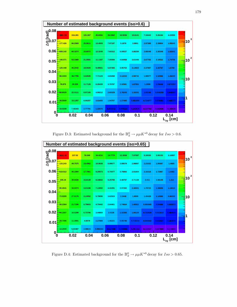
179
1
10
102
103
[cm]xyL0 0.02 0.04 0.06 0.08 0.1 0.12 0.14
[ra
d]
Φ∆
0
0.01
0.02
0.03
0.04
0.05
0.06
0.07
0.08
Number of estimated background events (iso>0.6)
19.0298 7.46343 2.77791 1.32675 0.693213 0.479223 0.342506 0.217752 0.183506 0.159636
39.5599 15.1257 6.00257 3.03455 1.94707 1.27495 0.953056 0.724977 0.578481 0.485777
58.8029 22.0111 8.97105 4.59212 2.69329 1.76243 1.33331 1.00246 0.840258 0.645057
78.879 28.935 11.7128 6.26439 3.78787 2.32581 1.87651 1.2899 1.06646 0.873357
98.4403 36.7755 14.6545 7.71123 4.83268 3.12233 2.59741 1.98977 1.52556 1.28245
120.448 45.2042 18.0026 9.49551 5.87355 3.95753 3.14923 2.37987 1.83767 1.5768
140.071 53.1888 21.0591 11.1167 7.00094 4.64458 3.61046 2.67783 2.10532 1.74706
159.142 60.1874 23.6972 12.3249 7.60312 5.00537 3.88299 2.88048 2.30349 1.92842
177.426 66.2569 25.9611 13.4009 7.97197 5.1876 3.9801 2.97388 2.39804 1.95545
3504.08 316.281 101.267 45.8356 26.3362 16.5036 10.6141 7.18443 5.26184 4.22059
Figure D.3: Estimated background for the B0d → µµK∗0 decay for Iso > 0.6.
1
10
102
103
[cm]xyL0 0.02 0.04 0.06 0.08 0.1 0.12 0.14
[ra
d]
Φ∆
0
0.01
0.02
0.03
0.04
0.05
0.06
0.07
0.08
Number of estimated background events (iso>0.65)
14.2909 5.60487 2.08615 0.996363 0.520588 0.359886 0.257214 0.163527 0.137809 0.119883
29.7086 11.3591 4.5078 2.27888 1.46221 0.95746 0.715724 0.544442 0.434427 0.364808
44.1597 16.5299 6.73706 3.44859 2.0226 1.32355 1.00129 0.752829 0.631016 0.484424
59.2364 21.7296 8.79603 4.70442 2.84461 1.74664 1.40922 0.968685 0.80089 0.655872
73.9265 27.6176 11.0052 5.79096 3.62924 2.3448 1.9506 1.49428 1.14566 0.96309
90.4541 33.9474 13.5196 7.13092 4.41091 2.97202 2.36501 1.78723 1.38005 1.18414
105.19 39.9436 15.8149 8.34842 5.25755 3.48797 2.71138 2.011 1.58105 1.312
119.512 45.1994 17.7961 9.25573 5.70977 3.75893 2.91604 2.16318 1.72987 1.4482
133.243 49.7575 19.4962 10.0638 5.98677 3.89578 2.98897 2.23332 1.80087 1.4685
2631.49 237.52 76.049 34.4216 19.7779 12.3938 7.97097 5.39535 3.95153 3.16957
Figure D.4: Estimated background for the B0d → µµK∗0 decay for Iso > 0.65.
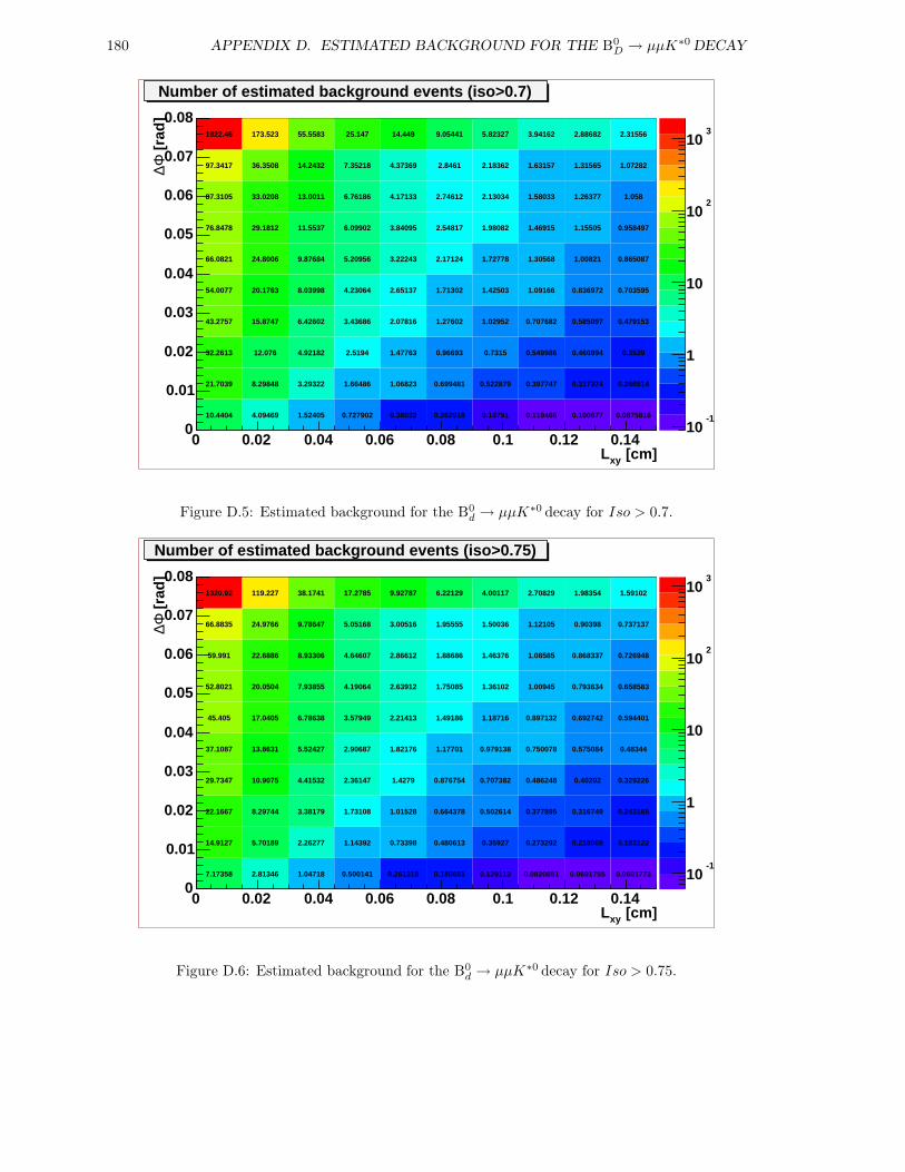
180 APPENDIX D. ESTIMATED BACKGROUND FOR THE B0D → µµK∗0 DECAY
10-1
1
10
102
103
[cm]xyL0 0.02 0.04 0.06 0.08 0.1 0.12 0.14
[ra
d]
Φ∆
0
0.01
0.02
0.03
0.04
0.05
0.06
0.07
0.08
Number of estimated background events (iso>0.7)
10.4404 4.09469 1.52405 0.727902 0.38032 0.262918 0.18791 0.119466 0.100677 0.0875816
21.7039 8.29848 3.29322 1.66486 1.06823 0.699481 0.522879 0.397747 0.317374 0.266514
32.2613 12.076 4.92182 2.5194 1.47763 0.96693 0.7315 0.549986 0.460994 0.3539
43.2757 15.8747 6.42602 3.43686 2.07816 1.27602 1.02952 0.707682 0.585097 0.479153
54.0077 20.1763 8.03998 4.23064 2.65137 1.71302 1.42503 1.09166 0.836972 0.703595
66.0821 24.8006 9.87684 5.20956 3.22243 2.17124 1.72778 1.30568 1.00821 0.865087
76.8478 29.1812 11.5537 6.09902 3.84095 2.54817 1.98082 1.46915 1.15505 0.958497
87.3105 33.0208 13.0011 6.76186 4.17133 2.74612 2.13034 1.58033 1.26377 1.058
97.3417 36.3508 14.2432 7.35218 4.37369 2.8461 2.18362 1.63157 1.31565 1.07282
1922.46 173.523 55.5583 25.147 14.449 9.05441 5.82327 3.94162 2.88682 2.31556
Figure D.5: Estimated background for the B0d → µµK∗0 decay for Iso > 0.7.
10-1
1
10
102
103
[cm]xyL0 0.02 0.04 0.06 0.08 0.1 0.12 0.14
[ra
d]
Φ∆
0
0.01
0.02
0.03
0.04
0.05
0.06
0.07
0.08
Number of estimated background events (iso>0.75)
7.17358 2.81346 1.04718 0.500141 0.261318 0.180651 0.129113 0.0820851 0.0691755 0.0601773
14.9127 5.70189 2.26277 1.14392 0.73398 0.480613 0.35927 0.273292 0.218068 0.183122
22.1667 8.29744 3.38179 1.73108 1.01528 0.664378 0.502614 0.377895 0.316749 0.243165
29.7347 10.9075 4.41532 2.36147 1.4279 0.876754 0.707382 0.486248 0.40202 0.329226
37.1087 13.8631 5.52427 2.90687 1.82176 1.17701 0.979138 0.750078 0.575084 0.48344
45.405 17.0405 6.78638 3.57949 2.21413 1.49186 1.18716 0.897132 0.692742 0.594401
52.8021 20.0504 7.93855 4.19064 2.63912 1.75085 1.36102 1.00945 0.793634 0.658583
59.991 22.6886 8.93306 4.64607 2.86612 1.88686 1.46376 1.08585 0.868337 0.726948
66.8835 24.9766 9.78647 5.05168 3.00516 1.95555 1.50036 1.12105 0.90398 0.737137
1320.92 119.227 38.1741 17.2785 9.92787 6.22129 4.00117 2.70829 1.98354 1.59102
Figure D.6: Estimated background for the B0d → µµK∗0 decay for Iso > 0.75.

181
50
100
150
200
250
300
[cm]xyL0 0.02 0.04 0.06 0.08 0.1 0.12 0.14
[ra
d]
Φ∆
0
0.01
0.02
0.03
0.04
0.05
0.06
0.07
0.08
events in the signal window (iso>0.8)*0 KψNumber of J/
78.2852 81.003 79.1494 78.3231 72.714 68.9739 67.0386 62.2014 57.336 48.7313
123.525 128.68 125.69 121.514 112.517 103.19 99.1171 91.6614 84.8726 75.6707
148.762 155.813 152.149 145.444 135.525 122.957 117.161 106.613 96.4988 86.8464
168.158 174.698 170.782 162.14 150.664 134.103 126.268 113.473 103.193 92.4693
183.177 191.205 187.319 176.631 161.679 144.369 133.776 116.983 105.69 93.8595
209.609 215.383 209.602 193.12 178.955 157.607 145.204 123.663 109.092 96.4402
226.626 230.069 223.893 206.348 189.996 165.837 152.556 128.522 110.088 96.959
235.344 238.282 231.261 213.602 195.01 167.287 154.26 130.208 110.777 97.6705
243.315 242.635 234.171 216.99 196.761 169.321 155.231 130.628 110.476 97.6705
324.359 315.941 283.469 247.295 206.582 174 157.491 130.7 109.853 97.4242
Figure D.7: Estimated background for the B0d → µµK∗0 decay for Iso > 0.8.

182 APPENDIX D. ESTIMATED BACKGROUND FOR THE B0D → µµK∗0 DECAY
Appendix E
Number of estimated signal eventsfor the B0
d → µµK∗0 decay
This Appendix shows the number estimated signal events for the B0d → µµK∗0 decay
as a function of the Lxy, ∆Φ and Isolation cuts. Each plot shows a scan of Lxy and∆Φ cuts corresponding to a given Isolation cut. Figures E.1 through E.7 correspondto different Isolation cuts from 0.5 to 0.8 in steps of 0.05. On these figures the firstcolumn represents the number of estimated signal events for the B0
d → µµK∗0 decaywhen there is no Lxy cut applied, while the other nine columns represent cuts from0.015 cm up to 0.135 cm in steps of 0.015 cm; the uppermost row represents the num-ber of estimated signal events for the B0
d → µµK∗0 decay when there is no ∆Φ cutapplied, while the other nine rows represent upper cuts on ∆Φ from 0.072 rad downto 0.008 rad in steps of 0.008 rad.
183
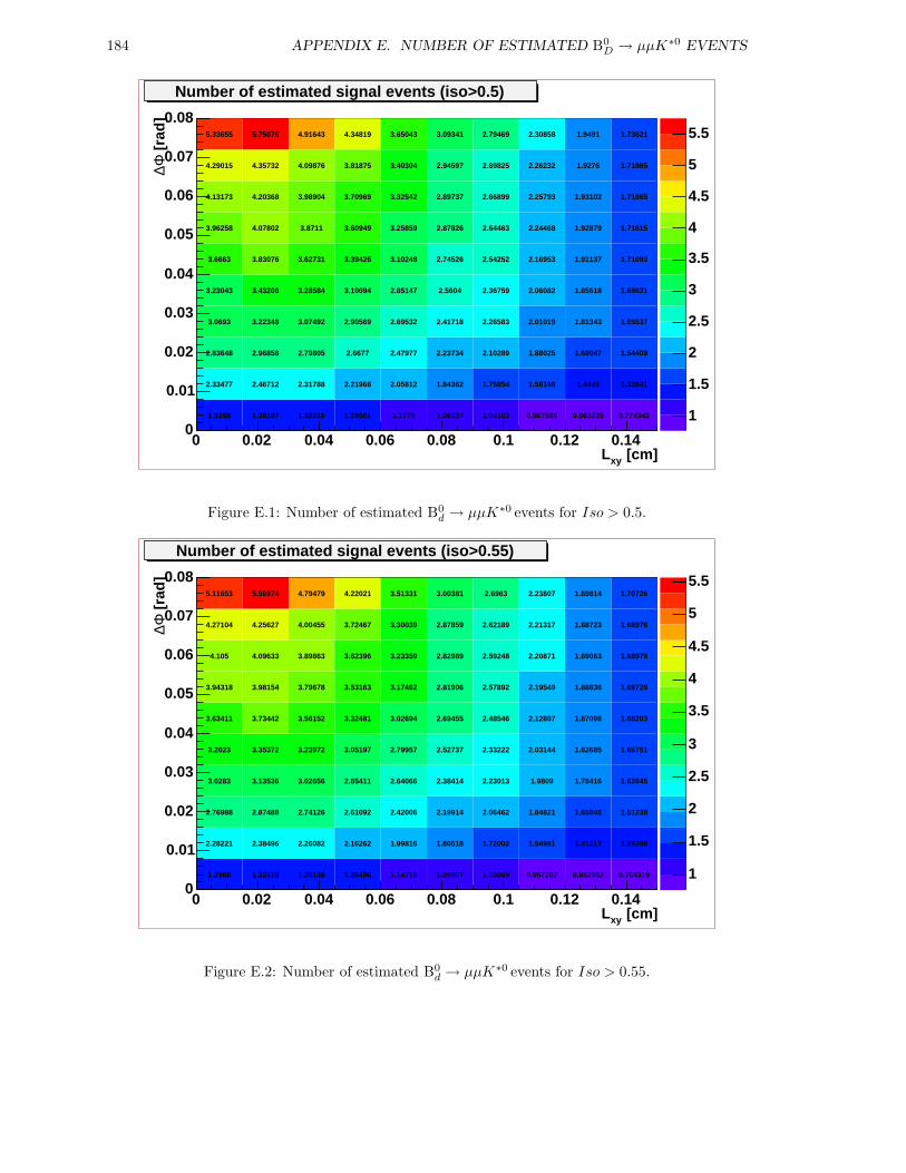
184 APPENDIX E. NUMBER OF ESTIMATED B0D → µµK∗0 EVENTS
1
1.5
2
2.5
3
3.5
4
4.5
5
5.5
[cm]xyL0 0.02 0.04 0.06 0.08 0.1 0.12 0.14
[ra
d]
Φ∆
0
0.01
0.02
0.03
0.04
0.05
0.06
0.07
0.08
Number of estimated signal events (iso>0.5)
1.3358 1.38187 1.32216 1.29561 1.1778 1.06937 1.04103 0.967566 0.863235 0.774342
2.33477 2.46712 2.31788 2.21968 2.05812 1.84362 1.75854 1.58198 1.4445 1.32641
2.83648 2.96858 2.79805 2.6677 2.47977 2.23734 2.10289 1.88025 1.69047 1.54409
3.0693 3.22348 3.07492 2.90569 2.69532 2.41718 2.26583 2.01019 1.81343 1.65537
3.23043 3.43206 3.28584 3.10094 2.85147 2.5604 2.36759 2.06082 1.85618 1.68631
3.6663 3.83076 3.62731 3.39426 3.10248 2.74526 2.54252 2.16953 1.91137 1.71093
3.96258 4.07802 3.8711 3.60949 3.25859 2.87826 2.64463 2.24468 1.92879 1.71615
4.13173 4.20368 3.98904 3.70969 3.32542 2.89737 2.66899 2.25793 1.93102 1.71865
4.29015 4.35732 4.09876 3.81875 3.40304 2.94597 2.69825 2.26232 1.9276 1.71865
5.33655 5.75076 4.91643 4.34819 3.65043 3.09341 2.79469 2.30858 1.9491 1.73621
Figure E.1: Number of estimated B0d → µµK∗0 events for Iso > 0.5.
1
1.5
2
2.5
3
3.5
4
4.5
5
5.5
[cm]xyL0 0.02 0.04 0.06 0.08 0.1 0.12 0.14
[ra
d]
Φ∆
0
0.01
0.02
0.03
0.04
0.05
0.06
0.07
0.08
Number of estimated signal events (iso>0.55)
1.2908 1.33118 1.29138 1.26496 1.14718 1.05907 1.03069 0.957282 0.852992 0.764319
2.28221 2.38496 2.26082 2.16262 1.99816 1.80518 1.72002 1.54981 1.41217 1.29399
2.76988 2.87488 2.74126 2.61092 2.42006 2.19914 2.06462 1.84821 1.65848 1.51238
3.0283 3.13536 3.02656 2.85411 2.64066 2.38414 2.23013 1.9809 1.78416 1.62645
3.2023 3.35372 3.23972 3.05197 2.79957 2.52737 2.33222 2.03144 1.82685 1.65751
3.63411 3.73442 3.56152 3.32481 3.02694 2.69455 2.48546 2.12897 1.87098 1.68203
3.94318 3.98154 3.79678 3.53163 3.17462 2.81906 2.57892 2.19549 1.88836 1.68728
4.105 4.09633 3.89863 3.62396 3.23359 2.82989 2.59248 2.20871 1.89063 1.68978
4.27104 4.25627 4.00455 3.72467 3.30039 2.87859 2.62189 2.21317 1.88723 1.68978
5.11653 5.56974 4.79479 4.22021 3.51331 3.00381 2.6963 2.23807 1.89814 1.70726
Figure E.2: Number of estimated B0d → µµK∗0 events for Iso > 0.55.
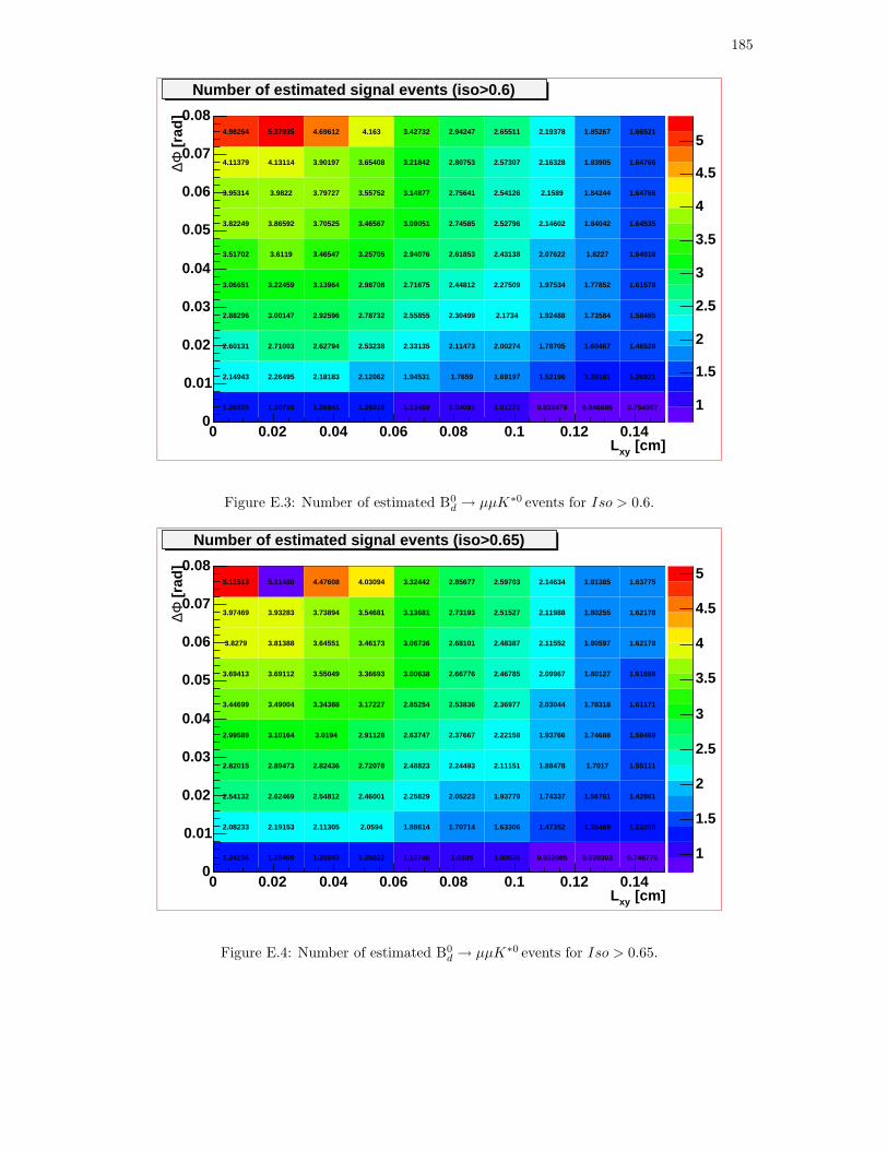
185
1
1.5
2
2.5
3
3.5
4
4.5
5
[cm]xyL0 0.02 0.04 0.06 0.08 0.1 0.12 0.14
[ra
d]
Φ∆
0
0.01
0.02
0.03
0.04
0.05
0.06
0.07
0.08
Number of estimated signal events (iso>0.6)
1.26865 1.30716 1.26941 1.26019 1.13459 1.04091 1.01272 0.939479 0.846686 0.754007
2.14943 2.26495 2.18183 2.12062 1.94531 1.7659 1.69197 1.52196 1.39181 1.26921
2.60131 2.71003 2.62794 2.53238 2.33135 2.11473 2.00274 1.78705 1.60467 1.46528
2.88296 3.00147 2.92596 2.78732 2.55855 2.30499 2.1734 1.92488 1.73584 1.58485
3.06651 3.22459 3.13964 2.98708 2.71675 2.44812 2.27509 1.97534 1.77852 1.61578
3.51702 3.6119 3.46547 3.25705 2.94076 2.61853 2.43138 2.07622 1.8227 1.64018
3.82249 3.86592 3.70525 3.46567 3.09051 2.74585 2.52796 2.14602 1.84042 1.64535
3.95314 3.9822 3.79727 3.55752 3.14877 2.75641 2.54126 2.1589 1.84244 1.64766
4.11379 4.13114 3.90197 3.65408 3.21842 2.80753 2.57307 2.16328 1.83905 1.64766
4.98264 5.37935 4.69612 4.163 3.42732 2.94247 2.65511 2.19378 1.85267 1.66521
Figure E.3: Number of estimated B0d → µµK∗0 events for Iso > 0.6.
1
1.5
2
2.5
3
3.5
4
4.5
5
[cm]xyL0 0.02 0.04 0.06 0.08 0.1 0.12 0.14
[ra
d]
Φ∆
0
0.01
0.02
0.03
0.04
0.05
0.06
0.07
0.08
Number of estimated signal events (iso>0.65)
1.24156 1.28409 1.25593 1.25022 1.12746 1.0335 1.00535 0.932085 0.839303 0.746776
2.08233 2.19153 2.11305 2.0594 1.88614 1.70714 1.63306 1.47352 1.35469 1.23205
2.54132 2.62469 2.54812 2.46001 2.25829 2.05223 1.93779 1.74337 1.56761 1.42861
2.82015 2.89473 2.82436 2.72078 2.48823 2.24493 2.11151 1.88478 1.7017 1.55111
2.99589 3.10164 3.0194 2.91128 2.63747 2.37667 2.22158 1.93766 1.74688 1.58469
3.44699 3.49004 3.34388 3.17227 2.85254 2.53836 2.36977 2.03044 1.78318 1.61171
3.69413 3.69112 3.55049 3.36693 3.00638 2.66776 2.46785 2.09967 1.80127 1.61688
3.8279 3.81388 3.64551 3.46173 3.06736 2.68101 2.48387 2.11552 1.80597 1.62178
3.97469 3.93283 3.73894 3.54681 3.13681 2.73193 2.51527 2.11988 1.80255 1.62178
5.11513 5.11486 4.47608 4.03094 3.32442 2.85677 2.59703 2.14634 1.81385 1.63775
Figure E.4: Number of estimated B0d → µµK∗0 events for Iso > 0.65.

186 APPENDIX E. NUMBER OF ESTIMATED B0D → µµK∗0 EVENTS
1
1.5
2
2.5
3
3.5
4
4.5
[cm]xyL0 0.02 0.04 0.06 0.08 0.1 0.12 0.14
[ra
d]
Φ∆
0
0.01
0.02
0.03
0.04
0.05
0.06
0.07
0.08
Number of estimated signal events (iso>0.7)
1.12931 1.15774 1.12007 1.11389 1.00743 0.932988 0.905417 0.838772 0.757692 0.665143
1.87083 1.97098 1.90657 1.86093 1.69635 1.53269 1.459 1.31747 1.21513 1.1146
2.28539 2.3776 2.30677 2.23611 2.04867 1.85569 1.74156 1.56455 1.42749 1.31034
2.53671 2.61876 2.55489 2.46356 2.24224 2.00611 1.87022 1.67228 1.52873 1.40033
2.74038 2.81284 2.73218 2.62965 2.37529 2.12156 1.96127 1.70646 1.55502 1.41507
3.1381 3.1677 3.0378 2.8685 2.59074 2.28382 2.11 1.7998 1.59123 1.44171
3.33473 3.32724 3.20365 3.01954 2.72253 2.39163 2.19753 1.85892 1.60954 1.44713
3.44344 3.42815 3.29348 3.10522 2.78304 2.40464 2.21339 1.87465 1.61426 1.45211
3.56013 3.5263 3.36293 3.17971 2.8422 2.44524 2.23434 1.87896 1.61082 1.45211
4.9386 4.55944 4.0059 3.60807 3.01176 2.54827 2.29461 1.90526 1.62204 1.46808
Figure E.5: Number of estimated B0d → µµK∗0 events for Iso > 0.7.
1
1.5
2
2.5
3
3.5
4
[cm]xyL0 0.02 0.04 0.06 0.08 0.1 0.12 0.14
[ra
d]
Φ∆
0
0.01
0.02
0.03
0.04
0.05
0.06
0.07
0.08
Number of estimated signal events (iso>0.75)
0.955041 0.99302 0.965953 0.966875 0.895659 0.841661 0.824518 0.76429 0.693331 0.600674
1.56997 1.66215 1.6091 1.57782 1.44164 1.31841 1.26608 1.16961 1.07783 0.977881
1.9311 2.02819 1.96857 1.91043 1.75311 1.59702 1.50425 1.37282 1.24553 1.12917
2.15694 2.25485 2.19627 2.11727 1.93526 1.73605 1.62107 1.46475 1.3288 1.20064
2.37673 2.46959 2.37878 2.28095 2.06358 1.85684 1.71477 1.50238 1.35555 1.21534
2.71398 2.78176 2.66283 2.50378 2.27359 2.01352 1.85462 1.58614 1.39242 1.2423
2.91927 2.96214 2.84192 2.6621 2.4121 2.12177 1.9432 1.64657 1.41097 1.24765
3.04522 3.078 2.93804 2.75243 2.4779 2.13751 1.96176 1.66516 1.41851 1.25539
3.18254 3.17734 3.00372 2.81881 2.52606 2.17807 1.98272 1.66936 1.41505 1.25539
4.38741 4.11044 3.60841 3.19554 2.64268 2.23751 2.00741 1.66969 1.40779 1.25251
Figure E.6: Number of estimated B0d → µµK∗0 events for Iso > 0.75.
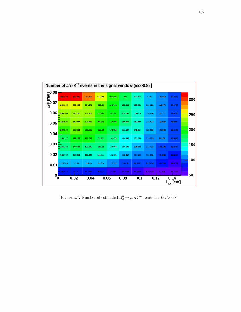
187
50
100
150
200
250
300
[cm]xyL0 0.02 0.04 0.06 0.08 0.1 0.12 0.14
[ra
d]
Φ∆
0
0.01
0.02
0.03
0.04
0.05
0.06
0.07
0.08
events in the signal window (iso>0.8)*0 KψNumber of J/
78.2852 81.003 79.1494 78.3231 72.714 68.9739 67.0386 62.2014 57.336 48.7313
123.525 128.68 125.69 121.514 112.517 103.19 99.1171 91.6614 84.8726 75.6707
148.762 155.813 152.149 145.444 135.525 122.957 117.161 106.613 96.4988 86.8464
168.158 174.698 170.782 162.14 150.664 134.103 126.268 113.473 103.193 92.4693
183.177 191.205 187.319 176.631 161.679 144.369 133.776 116.983 105.69 93.8595
209.609 215.383 209.602 193.12 178.955 157.607 145.204 123.663 109.092 96.4402
226.626 230.069 223.893 206.348 189.996 165.837 152.556 128.522 110.088 96.959
235.344 238.282 231.261 213.602 195.01 167.287 154.26 130.208 110.777 97.6705
243.315 242.635 234.171 216.99 196.761 169.321 155.231 130.628 110.476 97.6705
324.359 315.941 283.469 247.295 206.582 174 157.491 130.7 109.853 97.4242
Figure E.7: Number of estimated B0d → µµK∗0 events for Iso > 0.8.

188 APPENDIX E. NUMBER OF ESTIMATED B0D → µµK∗0 EVENTS
Bibliography
[1] F. Halzen and A. Martin, Quarks & Leptons, John Wiley & Sons, New York,1984
[2] David Griffiths, Introduction to Elementary Particles, Harper & Row Publishers,New York, 1987
[3] Particle Data Group, The Review of Particle Physics, Particle Listings 2003
http://pdg.lbl.gov
[4] Andrzej J. Buras, Robert Fleischer, Quark mixing, CP violation and rare decaysafter the top quark discovery, hep-ph/9704376
http://arxiv.org/abs/hep-ph/9704376
[5] A. Ali, G. Hiller, A theoretical reappraisal of branching ratios and CP asymme-tries in the decays B → (Xd, Xs)`
+`− and determination of the CKM parameters,Euro. Phys. Jour. C8, 619 (1999)
http://www.springerlink.com/app/home/content.asp?wasp
=fl9grlrwrrce6d62eaak&referrer=contribution&format
=2&page=1&pagecount=11
[6] C. S. Kim, T. Morozumi, A. I. Sanda, B → Xql+l−(q = d, s) and determination
of |Vtd/Vts|, Phys. Rev. D56, 7240 (1997)
http://prola.aps.org/pdf/PRD/v56/i11/p7240_1
[7] T. Affolderet al., A Measurement of sin 2β from B → J/ψK0S with the CDF
Detector, Phys. Rev. D61, 072005 (2000)
http://prola.aps.org/abstract/PRD/v61/i7/e072005
[8] B. Aubertet al. (BaBar collaboration), Measurement of the CP Asymmetry Am-plitude sin 2β with B0 Mesons, Phys. Rev. Lett. 89, 201802 (2002)
http://ojps.aip.org/getpdf/servlet/GetPDFServlet?filetype=
pdf&id=PRLTAO000089000020201802000001&idtype=cvips
189
190 BIBLIOGRAPHY
[9] K. Abe et al. (Belle Collaboration), Improved measurement of mixing-inducedCP violation in the neutral B meson system, Phys. Rev. D66, 071102 (2002)
http://ojps.aip.org/getpdf/servlet/GetPDFServlet?filetype=
pdf&id=PRVDAQ000066000007071102000001&idtype=cvips
[10] Tom Browder, Results on the CKM angle φ1 (β), presented at the XXI Interna-tional Symposium on Lepton and Photon interactions at High Energies, Fermilab,2003
http://conferences.fnal.gov/lp2003/program/
S5/browder_s05_ungarbled.pdf
[11] A. B. Carter and A. I. Sanda, Phys. Rev. D23, 1567 (1981); I. I. Bigi and A. I.Sanda, Nucl. Phys. B193, 85 (1981)
[12] A. Hocker, H. Lacker, S. Laplace and F. Le Diberder, A new approach to a globalfit of the CKM matrix, Eur. Phys. J. C21, 225-259 (2001)
http://www.edpsciences.org/articles/epjc/pdf/2001/12/epjc0729.pdf
[13] Klaus Schubert, CKM Matrix Element Magnitudes, presented at the XXI In-ternational Symposium on Lepton and Photon interactions at High Energies,Fermilab, 2003
http://conferences.fnal.gov/lp2003/program/S6/schubert_s06.pdf
[14] Home page of the CKM fitter group
http://ckmfitter.in2p3.fr/
[15] Belle collaboration, Measurement of Time-Dependent CP-Violating Asymmetriesin B0 → φKS, K
+K−K0S and η′K0
S Decays, Phys. Rev. Lett. 91, 261602 (2003)
http://ojps.aip.org/getpdf/servlet/GetPDFServlet?filetype=
pdf&id=PRLTAO000091000026261602000001&idtype=cvips
[16] Hassan Jawahery, CKM Unitarity Angles α and γ, presented at the XXI In-ternational Symposium on Lepton and Photon interactions at High Energies,Fermilab, 2003
http://conferences.fnal.gov/lp2003/program/S5/jawahery_s05.pdf
[17] C. Bobeth, A. J. Buras, F. Krger, J. Urban, CD Corrections to B → Xd,sνν,Bd,s → l+l−, K → πνν and KL → µ+µ− in the MSSM, Nucl. Phys. B630,87-131 (2002)
BIBLIOGRAPHY 191
http://documents.cern.ch/cgi-bin/
setlink?base=preprint&categ=hep-ph&id=0204225
[18] A. Ali, E. Lunghi, C. Greub, G. Hiller, Improved Model-Independent Analysis ofSemileptonic and Radiative Rare B Decays, Phys. Rev. D66,034002 (2002)
http://ojps.aip.org/getabs/servlet/GetabsServlet?prog=
normal&id=PRVDAQ000066000003034002000001&idtype=cvips&gifs=no
[19] A. Ali, P. Ball, L. T. Handoko, G. Hiller, Comparative study of the decays B →(K,K∗)l+l− in the standard model and supersymmetric theories, Phys. Rev. D61,074024 (2000)
http://prola.aps.org/pdf/PRD/v61/i7/e074024
[20] D. Melikhov, N. V. Nikitin, S. Simula, Rare exclusive semileptonic b→ s transi-tions in the standard model, Phys. Rev. D57, 6814-6828 (1998)
http://prola.aps.org/abstract/PRD/v57/i11/p6814_1
[21] C. Q. Geng, C. P. Kao, Lepton Polarization Asymmetry in B → K (∗)l+l−, Phys.Rev. D54, 5636-5641 (1996)
http://prola.aps.org/abstract/PRD/v54/i9/p5636_1
[22] P. Colangelo, F. De Fazio, P. Santorelli, and E. Scrimieri, QCD sum rule analysisof the decays B → Kl+l− and B → K∗l+l−, Phys. Rev. D53, 3672-3686 (1996)
http://prola.aps.org/abstract/PRD/v53/i7/p3672_1
[23] CDF Collaboration, Search for the Flavor-Changing Neutral Current DecaysB+ → µ+µ−K+ and B0 → µ+µ−K∗0, Phys. Rev. Lett. 83, 3378-3383 (1999)
http://prola.aps.org/abstract/PRL/v83/i17/p3378_1
[24] CLEO Collaboration, Improved Upper Limits on the FCNC Decays B → K`+`−
and B → K∗(892)`+`−, Phys. Rev. Lett. 87, 181803 (2001)
http://ojps.aip.org/getabs/servlet/GetabsServlet?prog=
normal&id=PRLTAO000087000018181803000001&idtype=cvips&gifs=yes
[25] B. Aubert et al. (BABAR Collaboration), Search for the Rare Decays B → Kl+l−
and B → K∗l+l−, Phys. Rev. Lett. 88, 241801 (2002)
http://ojps.aip.org/getabs/servlet/GetabsServlet?prog=
normal&id=PRLTAO000088000024241801000001&idtype=cvips&gifs=yes
192 BIBLIOGRAPHY
[26] K. Abe et al. (Belle Collaboration). Observation of the Decay B → Kl+l−, Phys.Rev. Lett. 88, 021801 (2002)
http://ojps.aip.org/getabs/servlet/GetabsServlet?prog=
normal&id=PRLTAO000088000002021801000001&idtype=cvips&gifs=yes
[27] Jeffrey D. Richman (BABAR Collaboration), Evidence for the flavor changingneutral current decays B → K`+`− and B → K∗`+`−, ICHEP 2002, Amsterdam,July 27, 2002
https://oraweb.slac.stanford.edu:8080/pls/
slacquery/BABAR_DOCUMENTS.DetailedIndex?P_BP_ID=3278
[28] B. Brau, Selected topics on rare B decays, presented at the 5th InternationalConference on Hyperons, Charm and Beauty Hadrons, Vancouver, June 25-29,2002
http://beach2002.physics.ubc.ca/talks/Ben_Brau.pdf
[29] K. Abe et al. (Belle Collaboration), Study of the Electroweak Penguin DecayB → K(∗)`+`−, BELLE-CONF-0241
http://belle.kek.jp/conferences/ICHEP2002/
Papers-pdf/belle-conf-0241.pdf
[30] Radiative and electroweak rare B decays, presented by Mikihiko Nakao in Lepton-Photon 2003 on behalf of Belle, BaBar, CLEO, CDF and D0
http://conferences.fnal.gov/lp2003/program/S7/nakao_s07.pdf
[31] K. Abe et al. (Belle Collaboration), Observation of B− > K∗l+l−, Phys. Rev.Lett. 91, 261601 (2003)
http://ojps.aip.org/getpdf/servlet/GetPDFServlet?filetype
=pdf&id=PRLTAO000091000026261601000001&idtype=cvips
[32] A. Ishikawa et al. (Belle Collaboration), Observation of B → K∗`+`−, hep-ex/0308044
http://arxiv.org/abs/hep-ex/0308044
[33] B. Aubert et al. (BABAR Collaboration), Evidence for the Rare Decay B →K∗l+l− and Measurement of B → Kl+l−, PUB-03/021
https://oraweb.slac.stanford.edu:8080/pls/slacquery/bbrdownload/
babar-pub-03021.ps?P_FRAME=DEST&P_DOC_ID=6935
BIBLIOGRAPHY 193
[34] C. Greub, A. Ioannissian, D. Wyler, Effects of new physics in the rare decaysB → Kl+l− and B → K∗l+l−, Phys. Lett. B346, 149 (1995)
http://preprints.cern.ch/cgi-bin/
setlink?base=preprint&categ=hep-ph&id=9408382
[35] J. L. Hewett, J. D. Wells, Searching for supersymmetry in rare B decays, Phys.Rev. D55, 5549(1997)
http://preprints.cern.ch/cgi-bin/
setlink?base=preprint&categ=hep-ph&id=9610323
[36] T. M. Aliev, A. Ozpineci, M. Savci, Exclusive B → K∗l+l− decay with polarizedK∗ and new physics effects, Phys. Lett. B511, 49-58 (2001)
http://documents.cern.ch/cgi-bin/
setlink?base=preprint&categ=hep-ph&id=0103261
[37] T. M. Aliev, M. K. Cakmak, A. Ozpineci, M. Savci, New physics effects to thelepton polarizations in the B → Kl+l− decay, Phys. Rev. D64, 055007 (2001)(10 pages)
http://documents.cern.ch/cgi-bin/
setlink?base=preprint&categ=hep-ph&id=0103039
[38] T. M. Aliev, M. K. Cakmak, M. Savci, General analysis of lepton polarizations inrare B → K∗l+l− decay beyond the standard model, Nucl. Phys. B607, 305-325(2001)
http://documents.cern.ch/cgi-bin/
setlink?base=preprint&categ=hep-ph&id=0009133
[39] T. M. Aliev, A. Ozpineci, M. Savci, Fourth generation effects in rare exclusiveB → K∗l+l− decay, Nucl. Phys. B585, 275-289 (2000)
http://documents.cern.ch/cgi-bin/
setlink?base=preprint&categ=hep-ph&id=0002061
[40] T. M. Aliev, D. A. Demir, M. Savci, Probing the sources of CP violation viaB → K∗l+l− decay, Phys. Rev. D62, 074016 (2000)
http://ojps.aip.org/getabs/servlet/GetabsServlet?prog=
normal&id=PRVDAQ000062000007074016000001&idtype=cvips&gifs=no
[41] T. M. Aliev, C. S. Kim, Y. G. Kim, A Systematic Analysis of the ExclusiveB → K∗l+l− Decay, Phys. Rev. D62, 014026 (2000)
194 BIBLIOGRAPHY
http://ojps.aip.org/getabs/servlet/GetabsServlet?prog=
normal&id=PRVDAQ000062000001014026000001&idtype=cvips&gifs=no
[42] Study of the Flavor-Changing Neutral Current Decay B → K (∗)l+l− with Belle,Thesis of Akimasa Ishikawa, Nagoya University, March 2002
http://belle.kek.jp/belle/theses/doctor/
ishikawa02/main.ps.gz
[43] Search for the Decays B0d → µ+µ−, B0
s → µ+µ− and B0s → µ+µ−φ in pp Colli-
sions at√s = 1.8TeV , Thesis of Thomas Speer, University of Geneva, 2000
[44] Giulia Manca, A Measurement Of The Ratio R =σ
W± ·Br(W±→e±ν)
σZ0 ·Br(Z0→e+e−)
in pp collisions
at 1.96 TeV, CDF internal note CDF/THESIS/ELECTROWEAK/CDFR/6521
http://www-cdf.fnal.gov/thesis/cdf6521_ratiothesis.ps.gz
[45] A Measurement of the Z Boson Production Cross-section Multiplied by the MuonBranching Fraction, Thesis of Gavin Hesketh, 2003
http://www-d0.fnal.gov/results/publications_talks/
thesis/hesketh/thesis.ps
[46] Electron Identification and its Application to the Measurment of the Top QuarkProduction Cross Section, Thesis of Florian Beaudette, 2003
http://www-d0.fnal.gov/results/publications_talks/
thesis/beaudette/thesis.ps
[47] F. Abe et al. (CDF Collaboration), Observation of top quark production in anti-pp collisions, Phys. Rev. Lett. 74, 2626-2631 (1995)
http://prola.aps.org/abstract/PRL/v74/i14/p2626_1
S. Abachi et al. (D0 Collaboration), Observation of the top quark, Phys. Rev.Lett. 74, 2632-2637 (1995)
http://prola.aps.org/abstract/PRL/v74/i14/p2632_1
[48] M. Church, Substantial Upgrades to Tevatron Luminosity, hep-ex/0105041
http://documents.cern.ch/cgi-bin/
setlink?base=preprint&categ=hep-ex&id=0105041
[49] Steve Holmes, Performance Goals for the Accelerator Complex, P5 Meeting atFermilab, March 26, 2003, unpublished

BIBLIOGRAPHY 195
http://www.fnal.gov/directorate/program.planning/P5_Holmes.pdf
[50] Run II Plan V2.0 (Part-1), Presentation of P. Bhat in the Director’s Review ofRun II Luminosity Plan, January 20-22, 2004, unpublished
http://www-bdnew.fnal.gov/doereview04/Temple/
Presentations/03_bhat_Temple04.ppt
[51] The Run II Luminosity Upgrade, sent to DOE June 15, 2003, unpublished
http://www-bd.fnal.gov/doereview03/docs/Overview7.1.pdf
[52] Recycler Status and Commissioning Plan/Electron Cooling, Presentation of S.Nagaitsev in the Director’s Review of Run II Luminosity Plan, January 20-22,2004, unpublished
http://www-bdnew.fnal.gov/doereview04/Temple/
Presentations/05_Nagaitsev_Temple04.ppt
[53] Run II Handbook
http://www-bd.fnal.gov/lug/runII_handbook/RunII_index.html
[54] http://www.fnal.gov//pub/inquiring/physics/accelerators/chainaccel.html
[55] http://www.fnal.gov/pub/now/tevlum.html
[56] http://www-cdfonline.fnal.gov/opshelp/stores/
[57] Commissioning of the Run IIa CDF Slicon Detector, Presented by A. Sill in the8th International Conference on Instrumentation for Colliding Beam Physics
http://www-cdf.fnal.gov/internal/silicon/talks/Instr2002.pdf
[58] Status of CDF Tracking, Presented by S. Nahn at ICHEP 2002
http://www-cdf.fnal.gov/internal/silicon/talks/trackIChep.ppt
[59] The CDF II Collaboration, The CDF II Detector Technical Design Report,FERMILAB-Pub-96/390-E
http://www-cdf.fnal.gov/internal/upgrades/tdr/tdr.html
[60] The CDF II Silicon Tracker, Presented by I. Volobouev at DPF 2002
http://dpf2002.velopers.net/talks_pdf/280talk.pdf
196 BIBLIOGRAPHY
[61] C. Issever (CDF Collaboration, The CDF Run IIa Silicon Detector and its Up-grade RunIIb, FERMILAB-CONF-03/401-E. Published Proceedings 12th Inter-national Workshop on Vertex Detection, Lake District, Cumbria, UK, September14-19, 2003
http://www-cdf.fnal.gov/physics/conferences/
cdf6782_vertex2003_v3.ps
[62] R. Rossin (CDF Collaboration), The CDF Silicon Vertex Detector for Run II,FERMILAB-CONF-03/397-E. Published Proceedings 8th International Confer-ence on Advanced Technology and Particle Physics (ICATPP 2003): Astroparti-cle, Particle, Space Physics, Detectors and Medical Physics Applications, Como,Italy, October 6-10, 2003
http://www-cdf.fnal.gov/physics/conferences/
cdf6735_Como2003proceedings_2.pdf
[63] C. Hill (CDF Collaboration), Operational Experience and Performance of theCDFII Silicon Detector, FERMILAB-CONF-03/412-E. Published Proceedings6th International Conference on Large Scale Applications and Radiation Hard-ness of Semiconductor Detectors, Florence, Italy, September 29-October 1
http://www-cdf.fnal.gov/physics/conferences/
cdf6764_run2a_si_op_rd03.ps
[64] Commissioning, operation and first physics results of the CDF Run2a Silicon andstatus of its future upgrade for Run2b, Presented by G. Bolla on EPS-HEP July2003
http://www-cdf.fnal.gov/internal/silicon/talks/EPSHEP-GB.pdf
[65] COT Group, A. Mukherjee, R. Wagner, CDF Central Outer Tracker,CDF internal note CDF/DOC/TRACKING/CDFR/6227, unpublished
http://www-cdf.fnal.gov/cdfnotes/cdf6227_CDF_COT.ps
[66] K Burkett (CDF Collaboration), Design and Construction of the CDF CentralOuter Tracker, FERMILAB-Conf-2000-128-E
http://www-cdf.fnal.gov/physics/conferences/cdf5321_cot_pisa_v1.ps
[67] The Central Outer Tracker for Run II at CDF, presented by D. Ambrose in the9th Pisa Meeting May 25-31, 2003
http://penn01.fnal.gov/~cot/tlk/elba-2003-talk.ps

BIBLIOGRAPHY 197
[68] C. Chen et al., Measurement of the Track Reconstruction Efficiency in theCOT Using a MC Track Embedding Technique, CDF internal noteCDF/PHYS/BOTTOM/CDFR/6394, unpublished
http://www-cdf.fnal.gov/cdfnotes/cdf6394_cot_eff_v3.ps
[69] L. J. Balka et al., The CDF central electromagnetic calorimeter, Nucl. Instrum.& Meth. A267, 272-279 (1988)
http://www.Sciencedirect.com/science?_ob=IssueURL&_tockey
=%23TOC%235314%231988%23997329997%23352577%23FLP%23Volume_267,
_Issues_2-3,_Pages_237-563_(1_May_1988)&_auth=y&view=c&_acct=
C000050221&_version=1&_urlVersion=0&_userid=10&md5=
ac62fa29f2fc2e74f20be978fa1cc9b4
[70] Y Fukui et al., CDF end plug electromagnetic calorimeter using conductive plasticproportional tubes, Nucl. Instrum. & Meth. A267, 280-300 (1988)
http://www.Sciencedirect.com/science?_ob=IssueURL&_tockey=
%23TOC%235314%231988%23997329997%23352577%23FLP%23Volume_267,
_Issues_2-3,_Pages_237-563_(1_May_1988)&_auth=y&view=c&_acct=
C000050221&_version=1&_urlVersion=0&_userid=10&md5=
ac62fa29f2fc2e74f20be978fa1cc9b4
[71] G. Ascoli et al., The CDF Central Muon Detector, Nucl. Instrum. & Meth. A268,33-40 (1988)
[72] The CDF Collaboration, The 1992 CDF Muon System Upgrade, CDF internalnote CDF/PUB/MUON/PUBLIC/2858
[73] G. Brandenburg, T. Liss, P. Schlabach et al., The CDF Run 1 Muon SystemUpgrade, CDF internal note CDF/DOC/MUON/PUBLIC/6362
http://www-cdf.fnal.gov/cdfnotes/cdf6362_Run1_muon_upgrade.ps
[74] Performance of the CDF Cherenkov Luminosity Counters, Presented by SongMing Wang at DPF 2002
http://dpf2002.velopers.net/talks_pdf/62talk.pdf
[75] D. Acosta et al., The performance of the CDF Luminosity Monitor, Submittedto Nucl. Instrum. & Meth., May 2002
http://www-cdf.fnal.gov/internal/people/links/
JacoboKonigsberg/instr02.ps
198 BIBLIOGRAPHY
[76] D. Acosta et al., The CDF Cherenkov Luminosity Monitor, CDF internal noteCDF/PUB/CDF/PUBLIC/5559, published in Nucl. Instr. & Meth. A461, 540-544 (2001)
http://www-cdf.fnal.gov/cdfnotes/cdf5559_CLC_NIM.ps.gz
[77] E.J. Thomson et al. (CDF Collaboration), Online track processor for the CDFupgrade, IEEE Trans. Nucl. Sci. 49, 1063 (2002)
http://ieeexplore.ieee.org/xpl/tocresult.jsp?isNumber=22285&page=2
[78] Yuri Gotra, James Kraus, Ting Miao, Run II Level 1 Low pT Muon Trig-ger Efficiency Measurement, CDF internal noteCDF/PHYS/TRIGGER/PUBLIC/6162, unpublished
http://www-cdf.fnal.gov/cdfnotes/cdf6162_L1_trigger_eff_v1.ps
[79] M. Casarsa et al., SVT absolute efficiency from simulation, Reco Tag Meeting ofFebruary 21, 2003
http://www-cdf.fnal.gov/internal/physics/bottom/reco-tag/TALKS/
030221/casarsa.ps.gz
[80] I. Vila (CDF Collaboration), Performance and First Physics Results of the SVTTrigger at CDF II, FERMILAB-CONF-03/219-E, Published Proceedings 2ndWorkshop on the CKM Unitarity Triangle, Durham, England, April 5-9, 2003
http://www-cdf.fnal.gov/physics/conferences/cdf6564_SVT_Durham.ps
[81] J. Thom (CDF Collaboration), Rare Charm and B Decays at CDF, FERMILAB-CONF-03/387-E, Published Proceedings International Europhysics Conferenceon High-Energy Physics (HEP 2003), Aachen, Germany, July 17-23, 2003
http://www-cdf.fnal.gov/physics/conferences/
cdf6752_rare_D_B_EPS2003.ps
[82] B. Ashmanskas et al. (CDF Collaboration), The CDF Silicon Vertex Trigger,FERMILAB-CONF-03/168-E, Published Proceedings 9th Pisa Meeting on Ad-vanced Detectors: Frontier Detectors for Frontier Physics, La Biodola, Isolad’Elba, Italy, May 25-31, 2003
http://www-cdf.fnal.gov/physics/conferences/cdf6502_elba_svt.ps
[83] M. Bishai (CDF Collaboration), Beauty and Charm Physics at CDF Run II,FERMILAB-CONF-03/310-E, Published Proceedings 4th International Sympo-sium on LHC Physics and Detectors (LHC 2003), Batavia, IL, May 1-3, 2003

BIBLIOGRAPHY 199
http://www-cdf.fnal.gov/physics/conferences/
cdf6657_lhc2003_proc_rev2.ps
[84] K. Anikeev et al., EVB and Level3 for Aces, CDF internal noteCDF/DOC/LEVEL-3/PUBLIC/5793, unpublished
http://www-cdf.fnal.gov/cdfnotes/cdf5793_Level3_EVB_for_Aces.ps.gz
[85] K. Anikeev et al., Event Builder and Level 3 Manual for Experts, CDF internalnote CDF/DOC/ONLINE/PUBLIC/6138, unpublished
http://www-cdf.fnal.gov/cdfnotes/cdf6138_Evb_Level3_MANUAL.ps
[86] R. G. C. Oldeman (CDF Collaboration), Performance of CDF for B Physics,FERMILAB-CONF-03/156-E, Published Proceedings 2nd Workshop on theCKM Unitarity Triangle, Durham, England, April 5-9, 2003
http://www-cdf.fnal.gov/physics/conferences/
cdf6469_Bperformance.ps
[87] Wolfram Erdmann, Thomas Speer, Search for the rare decays B+ → µµK+ andB0d → µµK∗0, CDF internal note CDF/ANAL/BOTTOM/CDFR/4517
http://www-cdf.fnal.gov/cdfnotes/cdf4517_rare_B_search.ps.gz
[88] Allan Clark, Xin Wu, Andras Zsenei, Run II Dimuon Trigger for Rare B Decays,CDF internal note CDF/DOC/BOTTOM/CDFR/5635, unpublished
http://www-cdf.fnal.gov/cdfnotes/
cdf5635_run2_rareb_dimu_trig.ps.gz
[89] Rare B Triggers Status and Plans, Presented by Andras Zsenei at the Triggerand Dataset Working Group August 6, 2002
http://www-cdf.fnal.gov/internal/upgrades/daq_trig/
twg/files02/020806_zsenei.pdf
[90] Rare B trigger status and optimization, Presented by Andras Zsenei at the Triggerand Dataset Working Group November 7, 2002
http://www-cdf.fnal.gov/internal/physics/bottom/
jpsi/Nov7_02/Andras_nov7.pdf
[91] K. Bloom and W.-M. Yao, ”Outside-In” Silicon Tracking at CDF, CDF internalnote CDF/DOC/TRACKING/CDFR/5991, unpublished
http://www-cdf.fnal.gov/cdfnotes/cdf5991_OI_Tracking.ps.gz
200 BIBLIOGRAPHY
[92] M. Feindt, S. Menzemer, K. Rinnert, TrackingKal - A Tracking and Align-ment Software Package for the CDFII Silicon Detector, CDF internal noteCDF/THESIS/TRACKING/PUBLIC/5968
http://www-cdf.fnal.gov/thesis/cdf5968_silicon_tracking.ps.gz
[93] Paolo Gatti, Performance of the new tracking system at CDF II, CDF internalnote CDF/THESIS/TRACKING/PUBLIC/5561
http://www-cdf.fnal.gov/thesis/cdf5561_tracking_performance.ps.gz
[94] K. Kelley, B. Mattingly, P. Sphicas, A Study of the Isolation of B Mesons, CDFinternal note CDF/ANAL/BOTTOM/CDFR/2765, unpublished
http://www-cdf.fnal.gov/cdfnotes/cdf2765_b_meson_isolation.ps.gz
[95] G. Bauer J. Friedman K. Kelley T. Shah P. Sphicas, A Study of the Isolationof B-Mesons Part II, CDF internal note CDF/ANAL/BOTTOM/CDFR/3684,unpublished
http://www-cdf.fnal.gov/cdfnotes/cdf3684_b_isolation_part_ii.ps.gz
[96] G. Punzi, Sensitivity of searches for new signals and its optimization,physics/0308063
http://doc.cern.ch//archive/electronic/physics/0308/0308063.pdf
[97] D.Glenzinski, M.Herndon, T.Kamon, V.Krutelyov, C.-J.Lin, J.Thom, A.Yagil,A Search for Bs → µ+µ− Decays Using RunII Data, CDF internal noteCDF/DOC/BOTTOM/CDFR/6397
http://www-cdf.fnal.gov/cdfnotes/cdf6397_BsMuMu_170pb.ps
[98] Search for FCNC decay Bs → µµ, presentation of D. Glezinski at the RECO-TAG meeting of July 24, 2003
http://www-cdf.fnal.gov/internal/physics/bottom/
bmtg_minutes/Jul_24_2003/BGroup_BsMuMu_030724.pdf
[99] K.Anikeev, G.Bauer, I.Furic, S.Gromoll, A.Korn, I.Kravchenko, Ch.Paus, A.Rakitin, J.Tseng, Calibration of Energy Loss and Magnetic Field using J/psiEvents in Run II, CDF internal note CDF/DOC/BOTTOM/CDFR/5958, un-published
http://www-cdf.fnal.gov/cdfnotes/cdf5958_eloss-bfield-calib.ps.gz
[100] Feldman, G J; Cousins, R D, A Unified Approach to the Classical StatisticalAnalysis of Small Signals, Phys. Rev. D57, 3873-3889 (1998)
BIBLIOGRAPHY 201
http://prola.aps.org/abstract/PRD/v57/i7/p3873_1
[101] Bob Cousins, private communication
[102] G. Feldman, Multiple Measurements and Parameters in the Unified Approach,Workshop on Confidence Limits, Fermilab, March 28, 2000
http://conferences.fnal.gov/cl2k/copies/feldman2.pdf
[103] Wolfgang A. Rolke and Angel M. Lopez, Confidence intervals and upper boundsfor small signals in the presence of background noise, Nucl. Instrum. & Meth.A458, 745 (2001)
[104] J. Conrad, O. Botner, A. Hallgren, and C. Perez de los Heros, Including sys-tematic uncertainties in confidence interval construction for Poisson statistics,Phys. Rev. D67, 012002 (2003)
http://ojps.aip.org/getpdf/servlet/GetPDFServlet?filetype=
pdf&id=PRVDAQ000067000001012002000001&idtype=cvips
[105] Gary C. Hill, Comment on ”Including systematic uncertainties in confidenceinterval construction for Poisson statistics”, Phys. Rev. D67, 118101 (2003),
http://ojps.aip.org/getpdf/servlet/GetPDFServlet?filetype=
pdf&id=PRVDAQ000067000011118101000001&idtype=cvips
[106] N. Reid, D.A.S. Fraser, Likelihood inference in the presence of nuisance param-eters, physics/0312079
http://xxx.lanl.gov/abs/physics/0312079
[107] http://www.physics.ucla.edu/~cousins/stats/expandedtables_68_90_95.ps
[108] The ATLAS Inner Tracker and the detection of light supersymmetric Higgsbosons, Thesis of Marcel Vos, University of Twente, 2003
http://atlas.web.cern.ch/Atlas/documentation/
thesis/vos/vosthesis.pdf
[109] The Large Hadron Collider Home Page
http://lhc-new-homepage.web.cern.ch/lhc-new-homepage/
[110] http://www.cerncourier.com/main/article/40/3/13
[111] S. S. Adler et al. (PHENIX Collaboration), Absence of Suppression in ParticleProduction at Large Transverse Momentum in
√sNN = 200GeV d+Au Colli-
sions, nucl-ex/0306021,
202 BIBLIOGRAPHY
www.arxiv.org/abs/nucl-ex/0306021
[112] B.B.Back et al. (PHOBOS Collaboration), Centrality dependence of chargedhadron transverse momentum spectra in d+Au collisions at
√sNN = 200GeV ,
nucl-ex/0306025
www.arxiv.org/abs/nucl-ex/0306025
[113] I. Arsene et al. (BRAHMS Collaboration), Transverse Momentum Spectra inAu+Au and d+Au Collisions at
√sNN=200 GeV and the Pseudorapidity Depen-
dence of High pT Suppression, nucl-ex/0307003
www.arxiv.org/abs/nucl-ex/0307003
[114] J. Adams et al. (STAR Collaboration), Multiplicity fluctuations in Au+Au col-lisions at
√sNN = 130 GeV, nucl-ex/0307007
www.arxiv.org/abs/nucl-ex/0307007
[115] ALICE Collaboration, ALICE: technical proposal for a large ion collider ex-periment at the CERN LHC, CERN-LHCC-95-71, LHCC-P-3, Geneva, CERN,1995
http://documents.cern.ch/cgi-bin/
setlink?base=generic&categ=public&id=cer-0214817
[116] LHCb Collaboration, LHCb: Technical Proposal, CERN-LHCC-98-004, LHCC-P-4, Geneva, CERN, 20 Feb 1998
http://lhcb-tp.web.cern.ch/lhcb-tp/
[117] CMS Collaboration, Technical proposal, CERN-LHCC-94-38, LHCC-P-1,Geneva, CERN, 1994
http://documents.cern.ch/cgi-bin/
setlink?base=generic&categ=public&id=cer-0212026
[118] ATLAS Collaboration, ATLAS: technical proposal for a general-purpose pp ex-periment at the Large Hadron Collider at CERN, CERN-LHCC-94-43, LHCC-P-2, Geneva, CERN, 1994, ISBN 92-9083-067-0
http://documents.cern.ch/cgi-bin/
setlink?base=generic&categ=public&id=cer-0212025
[119] ATLAS TDR 4, CERN/LHCC/97-16, ISBN 92-9083-102-2
http://atlas.web.cern.ch/Atlas/GROUPS/INNER_DETECTOR/TDR/tdr.html

BIBLIOGRAPHY 203
[120] Home page of the Pixel detector (ATLAS)
http://atlas.web.cern.ch/Atlas/GROUPS/INNER_DETECTOR/
PIXELS/pixel.html
[121] ATLAS Collaboration, ATLAS Detector and Physics Performance: TechnicalDesign Report 1, CERN-LHCC-99-014, ATLAS-TDR-14, Geneva, CERN, 25May 1999
http://documents.cern.ch/cgi-bin/
setlink?base=generic&categ=public&id=cer-0317330
[122] ATLAS Collaboration, ATLAS Detector and Physics Performance: TechnicalDesign Report 2, CERN-LHCC-99-015, ATLAS-TDR-15, Geneva, CERN, 25May 1999
http://documents.cern.ch/cgi-bin/
setlink?base=generic&categ=public&id=cer-0317331
[123] N. Benekos, R. Clifft, M. Elsing, A. Poppleton, ATLAS Inner Detector Perfor-mance, ATLAS internal note ATL-COM-INDET-2003-023, unpublished
http://doc.cern.ch//archive/electronic/cern/others/
atlnot/Communication/indet/com-indet-2003-023.pdf
[124] ATLAS High Level Trigger, Data Acquisition and Controls, ATLAS-TDR-016,CERN-LHCC-2003-022
http://doc.cern.ch//archive/electronic/other/
generic/public/cer-002375189.pdf
[125] J. Vermeulen et al., The Baseline DataFlow System of the ATLAS Trigger &DAQ, ATL-DAQ-2003-032
http://doc.cern.ch//archive/electronic/cern/
others/atlnot/Note/daq/daq-2003-032.pdf
[126] R. Hauser, The ATLAS Trigger System, SN-ATLAS-2003-027, ATL-DAQ-2003-047
http://doc.cern.ch//archive/electronic/cern/
preprints/snotes/sn-atlas-2003-027.pdf
[127] ATLAS TDR 5, CERN/LHCC/97-17, ISBN 92-9083-103-0
http://atlas.web.cern.ch/Atlas/GROUPS/INNER_DETECTOR/
TDR/tdr-figs.html#Vol.II
204 BIBLIOGRAPHY
[128] http://www.hep.man.ac.uk/atlas/module/
[129] D. Campbell et al., The development of a rad-hard CMOS chip for the binaryreadout of the ATLAS semiconductor tracker, 5th Conference on Electronics forLHC Experiments, Snowmass, CO, USA, 20 - 24 Sep 1999, CERN-LHCC-99-033
http://doc.cern.ch/archive/cernrep//1999/99-09/p152.pdf
[130] T. Dubbs et al., The developement of the CAFE-P/CAFE-M bipolar chips forthe ATLAS semiconductor tracker, 5th Conference on Electronics for LHC Ex-periments, Snowmass, CO, USA, 20 - 24 Sep 1999, CERN-LHCC-99-033
http://doc.cern.ch/archive/cernrep//1999/99-09/p123.pdf
[131] D. Melikhov et al., Studying the physics beyond the Standard Model in raresemileptonic B-decay B0
d → K∗0µµ - with ATLAS detector, ATLAS Internal NotePHYS-98-123 (1998)
[132] A. Ali, Gian-F. Giudice, T. Mannel, T. M. Aliev, C. S. Kim and M. Savci,Towards a model-independent analysis of rare B decays, Phys. Lett. B441, 410(1998), ERN-TH-7346-94, hep-ph-9408213, Geneva, CERN, 2 Aug 1993 Pub-lished in: Z. Phys. C67 417-432 (1995)
[133] Evaluation of Silicon sensors for the ATLAS Silicon Tracker, and TPC recon-struction in the HARP Experiment, Thesis of Maria Cristina Morone, Geneva,2003
[134] ABCD3T Specification ver. 1.2
http://chipinfo.web.cern.ch/chipinfo/docs/abcd3t_spec_v1.2.pdf
[135] W. Dabrowski, J. Kaplon, R. Szczygiel, SCT128B - a prototype chip for binaryreadout of silicon strip detectors, Nucl. Instrum. & Meth. A421 303-315 (1999)
[136] F. Anghinolfi et al., Performance of the electrical module prototypes for theATLAS silicon tracker, 5th Conference on Electronics for LHC Experiments,Snowmass, CO, USA, 20 - 24 Sep 1999, CERN-LHCC-99-033
http://doc.cern.ch/archive/cernrep//1999/99-09/p118.pdf
[137] W. Dabrowski et al., Design and performance of the ABCD chip for the binaryreadout of silicon strip detectors in the ATLAS semiconductor tracker, IEEETrans. Nucl. Sci. 47 (2000) no.6 (pt.1), pp.1843-50 1999 IEEE Nuclear ScienceSymposium and Medical Imaging Conference, Seattle, WA, USA, 24 - 30 Oct1999 - IEEE, Piscataway, NJ, 1999. - 382-9 (vol.1)
[138] J. Bernabeu et al., Results of the 1999 H8 beam tests of ATLAS-SCT prototypes,Nucl. Instrum. & Meth. A466 (2001) no.2, pp.397-405

BIBLIOGRAPHY 205
http://weblib.cern.ch/cgi-bin/ejournals?publication=Nucl.+Instrum.
+Methods+Phys.+Res.,+A&volume=466&year=2001&page=397
[139] W. Dabrowski et al., The ABCD binary readout chip for silicon strip detectors inthe ATLAS silicon tracker, 4th Workshop on Electronics for LHC Experiments,Rome, Italy, 21 - 25 Sep 1998, CERN-LHCC-98-036 - pp.175-179
[140] W. Dabrowski et al., Radiation hardness of the ABCD chip for the binary read-out of silicon strip detectors in the ATLAS semiconductor tracker, 5th Conferenceon Electronics for LHC Experiments, Snowmass, CO, USA, 20 - 24 Sep 1999,CERN-LHCC-99-033
http://doc.cern.ch/archive/cernrep//1999/99-09/p113.pdf
[141] W. Dabrowski et al., Progress in development of the readout chip for the AT-LAS semiconductor tracker, 6th Workshop on Electronics for LHC Experiments,Cracow, Poland, 11 - 15 Sep 2000, CERN-LHCC-2000-041 - pp.115
http://doc.cern.ch/archive/cernrep/2000/2000-010/p115.pdf
[142] SCTA128LC & SCTA128HC Chip Specification Version 0.1
[143] SCTA128VG Specification version 1.3
http://chipinfo.web.cern.ch/chipinfo/docs/scta128vg_spec1-3.pdf
[144] Documentation for the SCTA128VG Linux Data Acquisition software
http://chipinfo.web.cern.ch/chipinfo/docs/sctadaq.pdf
[145] E. Chesi et al., Performance of a 128 channel analogue front-end chip for read-out of Si strip detector modules for LHC experiments, IEEE Trans. Nucl. Sci.47 (2000) no.4 (Pt.1), pp.1434-1441, 1999 IEEE Nuclear Science Symposiumand Medical Imaging Conference, Seattle, WA, USA, 24 - 30 Oct 1999 - IEEE,Piscataway, NJ, 1999. - pp.94-101
[146] J. Kaplon et al., Progress in Development of the Analogue Read-out Chip for Sil-icon Strip Detector Modules for LHC Experiments, 7th Workshop on Electronicsfor LHC Experiments, Stockholm, Sweden, 10 - 14 Sep 2001, CERN-LHCC-2001-034
http://doc.cern.ch/archive/cernrep/2001/2001-005/p90.pdf
[147] Dirk Meier, Diamond Detectors for Particle Detection and Tracking, PhD thesissubmitted at University of Heidelberg, January 1999
http://atlas.web.cern.ch/Atlas/documentation/
thesis/meier/thesis.html
206 BIBLIOGRAPHY
[148] J. Lozano Bahilo et al., Results with Si Strip Detector Modules with Full Ana-logue Readout for LHC, 4th International Meeting on Front End Electronics forTracking Detectors at Future High Luminosity Colliders , 16 - 19 May 2000,Perugia, Italy
[149] J. Kaplon et al., Analogue read-out chip for Si strip detector modules forLHC experiments, 6th Workshop on Electronics for LHC Experiments, Cracow,Poland, 11 - 15 Sep 2000, CERN-LHCC-2000-041 - pp.120
http://doc.cern.ch/archive/cernrep/2000/2000-010/p120.pdf
[150] J. Lozano-Bahilo, A. Rudge, A. Zsenei, A linear optical link using radiationhard VCSELs, Nucl. Instrum. & Meth. A461 (2001) no.1-3, pp.530-6
http://weblib.cern.ch/cgi-bin/ejournals?publication=Nucl.+Instrum.
+Methods+Phys.+Res.,+A&volume=461&year=2001&page=530
[151] J. Lozano-Bahilo, A. Rudge, A. Zsenei, A Linear Optical Link using VCSELs,4th International Meeting on Front End Electronics for Tracking Detectors atFuture High Luminosity Colliders, 16 - 19 May 2000, Perugia, Italy
[152] J. Lozano-Bahilo, A. Rudge, A. Zsenei, A Linear Optical Link Using Radia-tion Hard VCSELs, Frontier Detectors for Frontier Physics, 8th Pisa Meeting onAdvanced Detectors, May 21-27, 2000 - La Biodola, Isola d’Elba, Italy