ares design study - cern document server
TRANSCRIPT
INFN - Laboratori Nazionali di Frascati Servizio Documentazione
LNF-90/00S(R) 17 Gennaio 1990
ARES DESIGN STUDY THE MACHINE

Editors
C. Pagani
S. Tazzari
G. Vignola
M. Bassetti
C. Biscari
R. Boni
M. Castellano
A. Cattoni
N. Cavallo
V. Chimenti
U. Gambardella
S. Guiducci
S. Kulinski
P. Michelato
L. Palumbo
M. Piccolo
C. Sanelli
L. Serafini
M. Serio
F. Tazzioli
L. Trasatti
Printed and Published by Servizio Documentazione dei
Laboratori Nazionali di Frascati dell1NFN
INFN - Laboratori Nazjonali dj Frascatj Servizio Documentazione
ARES DESIGN STUDY THE MACHINE
LNF-90/005 (R l 17 Gennaio 1990
P.Amadei(l), A.Aragona(l), M.Barone(l), S.Bartalucci(l), M.Bassetti(l), M.E.Biagini(l),
C.Biscari(l), R.Boni(l), M.Castellano(l), A.Cattoni(l), N.Cavallo(3), F.Cevenini(3,8),
V.Chimenti(l), S.De Simone(l), D.Di Gioacchino(l), G.Di Pirro(l), S.Faini(l), G.Felici(l),
M.Ferrario, L.Ferrucci, S.Gallo(l), U.Gambardella(l), A.Ghigo(l), S.Guiducci<l),
S.Kulinski(O, M.R.Masullo(3), P.Michelato(2), G.Modestino(l), C.Pagani(2,7), L.Palumbo(1,5),
R.Parodi(4), P.Patteri<O, A.Peretti(2), M.Piccolo(O, M.Preger(l), G.RaffoneO), C.Sanelli(l),
L.Serafini(2), M.Serio(l), F.Sgamma<O, B.Spataro(l), L.Trasatti(l), S.Tazzari(l,6), F.Tazzioli(l),
C.VaccarezzaO), M.Vescovi(l), G.Vignola(l).
(1) INFN, Laboratori Nazionali di Frascati- CP13, 00040- Frascati (Italy)
(2) INFN, Sezione di Milano, Via Celoria 16, 20133- Milano (Italy)
(3) INFN, Sezione di Napoli, Mostra d'Oltremare, Pad.20, 80125- Napoli (Italy)
(4) INFN, Sezione di Genova, Via Dodecaneso- Genova (Italy)
(5) Universita di Roma "La Sapienza", Dip. di Energetica, Via A.Scarpa 14,00161- Roma (Italy)
(6) Universita di Roma "Tor Vergata", Dip di Fisica- Via 0. Raimondo- Roma (Italy)
(7) Universita di Milano, Dip. di Fisica- Via Celoria 16, 20133- Milano (Italy)
(8) Universita di Napoli, Dip. di Se. Fisiche- Mostra d'Oltremare, Pad.20, 80125 - Napoli (Italy)
ARES Design Study
The Machine
TABLE OF CONTENTS
1. ·GENERAl~ DESCRIPTION .............................................. 1
1.1. - Design Basics ....................................................... 1
1.2. - Short History of the Project ....................................... 3
1.3. - Goals ................................................................. 5
1.4. - The Physics : an Outline ........................................... 6 1.4.1 - Physics Program for a <I>-Factory.............................................. 6
1.4.2 - X-VUV FEL Experiments ....................................................... 8
1.5. - Linac ................................................................. ll
1.6. - <I>-Factory ............................................................ 16
2. - L IN A C ......................................................... , ........... 18
2.1. - Optics ................................................................ 18
2.1.1 - Introduction ....................................................................... 18
2.1.2 - Linac Focusing ................................................................... 18
2.1.3 - Recirculation Lattices ............................................................ 22
2.2. - Beam Dynamics .................................................... . 26
2.2.1 - Introduction ....................................................................... 26
2.2.2- Induced Wake Fields ............................................................. 26
2.2.3 - Single Bunch Dynamics ......................................................... 28
a) Longitudinal Wake Field ...................................................... 28
b) Transverse Wake Field ........................................................ 29
2.3. - e· and e+ Generation ................................................ 31
2.3.1 - Introcuction ....................................................................... 31
2.3.2 - The Electron Preinjector ......................................................... 33
2.3.2.1- RF preinjector ............................................................... 33
a) Basic Theory .................................................................... 35
b) Contputational Tools ........................................................... 37
c) Results of the Numerical Simulations ........................................ 38
d) Photocathodes ................... : .............................................. 43
e) Laser System .................................................................... 45
f) Diagnostics ...................................................................... 47
2.3.2.2 - Standard electron preinjector .............................................. 48
a) The Gun ......................................................................... 48
b) The Buncher System ........................................................... 49
c) Capture Section ................................................................. 50
2.3.3 - Positron Production .............................................................. 51
a) Introduction ..................................................................... 51
b) Converter and Magnetic Focusing ............................................ 51
c) High Gradient Capture Section ............................................... 54
d) Remarks on the Positron Recirculation ...................................... 55
2.3.4 - Transport Channels and Pulsed Inflector ...................................... 56
a) Pulsed Inflector ................................................................. 56
b) L1-L2 Transport Line .......................................................... 57
2.4. - Acceleration System ................................................ . 59
2.4.1 - Superconducting Cavities ....................................................... 59
a) Frequency ....................................................................... 61
b) Cavity Geometry ............................................................... 62
c) HOM and Main Couplers ...................................................... 66
2.4.2 - Radiofrequency ................................................................... 69
a) General Design Criteria ........................................................ 69
b) Power Sources .................................................................. 70
c) The Control System ............................................................ 71
2.4.3 - Cryogenics ........................................................................ 73
a) Introduction ..................................................................... 73
b) Cold Box ........................................................................ 74
c) Distribution System ............................................................ 77
d) Compressors and Ancillary Equipment. ..................................... 78
d) Cryostats ........................................................................ 81
2.5. - Vacuum System ......................•............................... 85
2.5.1 - Introduction ....................................................................... 85
2.5.2 - The Cryomodule .................................................................. 85
2.5.3 - The Cryomodule Pumping System ............................................. 86
2.5.4 - Recirculation Beam Lines Vacuum System ................................... 88
2.6. - Magnets and Power Supplies .....•................................. 89
2.6.1 - Linac Quadrupoles ............................................................... 89
2.6.2 - Recirculation Arc Dipole Magnets .............................................. 92
2.6.3 - Recirculation Arc Quadrupoles ................................................. 95
3. ·THE <P-FACTORY .•.....................•.............................. lOO
3.1. - Introduction ......................•................................ 100
3.2. - Design Criteria •......................•.....•......•...•........... 101
3.2.1- BasicFormulae ................................................................. 101
3.2.2 - Collision Frequency ............................................................ 103 3.2.3 - Vertical 13-Function at the IP ................................................. 104
3.2.4 - Coupling Coefficient. .......................................................... 105
3.2.5 - Design Emittance ............................................................... 106
3.2.6 - The Linear Tune Shift Parameter~-································· ......... 106
3.2.7 - Luminosity Scaling Laws ..................................................... 107
3.2.8 - Conclusions ..................................................................... 110
3.3. - Beam Optics ••......•...........•..........••...................... lll 3.3.1 - Low-13 Insertion ................................................................ 111
3.3.2 - Storage Rings ................................................................... 116
3.3.3 - Dynamic Aperture .............................................................. 124
3.3.4 - Injection Aperture .............................................................. 125
3.4. - Beam Stability and Lifetimes ..............•..................... 126
3.4.1 - Single Bunch Dynamics ....................................................... 126
3.4.2 - Beam Lifetime .................................................................. 129
3.4.3 - Multibunch Instabilities ........................................................ 130
3.5. - General Considerations on Beam Diagnostic and
Instrumentation ••.........•.............•...........•....•..•.••.. 133
3.6. - RF System ..•...................................................... 134
3.7. - Vacuum System ..•...•..............••••...•...•••..•............ 135
3.8. ·- The Detector Solenoid ....•....••.................•..•............ 136
4. • BEAM INSTRUMENTATION AND CONTROL SYSTEM .......... 139
4.1. - Basic Requirements ................................................ 139
4.2. - Beam Diagnostics .................................................. 141
4.3. - Beam Position Monitors ........................................... 142
4.4.- Control System ..................................................... 145
4.4.1 - Introduction ...................................................................... 145
4.4.2 - Distributed System .............................................................. 146
4.4.3 - Centralized System .............................................................. 150
5. - BUILDINGS AND UTILITIES ....................................... 154
5 .1. - Genera I Des cri p t ion ................................................ 154
5.2. - Plants and General Services ......•............................... 158
5.2.1 - Description ....................................................................... 158
5.2.2 - Power Inventory ................................................................. 161
APPENDIX
ARES THE MACHINE
1.- GENERAL DESCRIPTION
1.1. - DESIGN BASICS
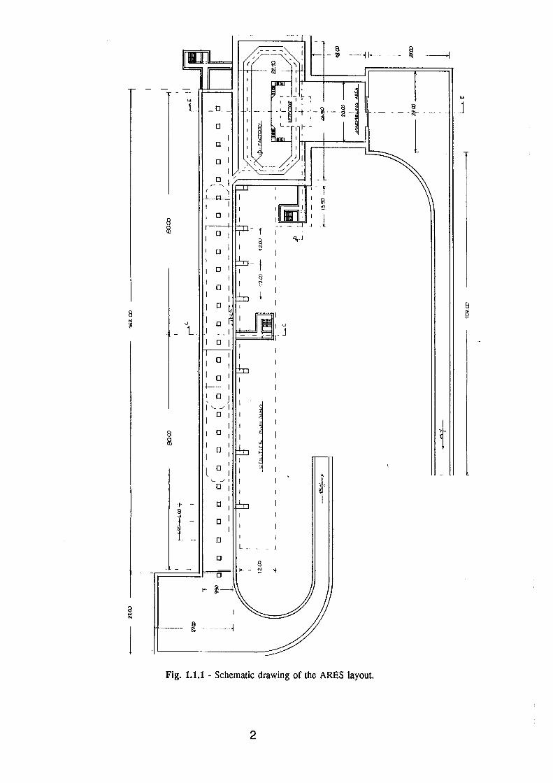
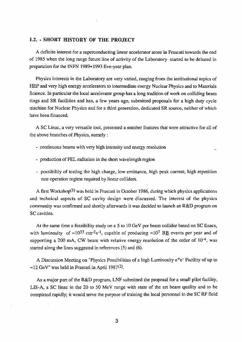
The ARES accelerator complex consists of a 510 Me V once-recirculated se Linac and of a
two-ring colliding beam <!>-Factory .
The Linac serves as :
- an injector for the storage rings
- a FEL driver
- a test facility.
A schematic drawing of the layout is shown in Fig. 1.1.1
The <!>-Factory design luminosity is 1032 cm-2s-1 at 510 Me V. The storage rings are
separated vertically and meet at a single interaction region; the opposite straight sections are
dedicated to RF and injection. The rings are optimized at the <I> peak but can reach a top energy
of~ .6 GeV. The injector energy allows the rings to be 'topped off at the nominal energy,
thereby improving the average integrated luminosity at the <I>.
The chosen parameters are conservative enough that, according to some of the existing
models for the beam-beam limit, there is some hope to gradually achieve somewhat higher
luminosities. The Se Linac also leaves open the possibility of testing the potential of a linear
against -circular collider.
1
a ~
8 ~
-t ~ " J t
... L
"
_0.-
0
0
0
I 0
I
I
0
l .. 1
0 l--I 0 I 1'----1
0 I
I 0
0
0
'- --' I
0
- Jj
-- 0
0
0
1-- ~--~
8 !:j
I.-.
"lo··J
I
I
~·
L --
a ~- - ~ >I
Fig. 1.1.1 - Schematic drawing of the ARES layout.
2
... .J a
---[tr----
l
t
1.2. · SHORT HISTORY OF THE PROJECT
A definite interest for a superconducting linear accelerator arose in Frascati towards the end
of 1985 when the long range future line of activity of the Laboratory started to be debated in
preparation for the INFN 1989+ 1993 five-year plan.
Physics interests in the Laboratory are very varied, ranging from the institutional topics of
HEP and very high energy accelerators to intermediate energy Nuclear Physics and to Materials
Science. In particular the local accelerator group has a long tradition of work on colliding beam
rings and SR facilities and has, a few years ago, submitted proposals for a high duty cycle
machine for Nuclear Physics and for a third generation, dedicated SR source, neither of which
have been financed.
A se Linac, a very versatile tool, presented a number features that were attractive for all of
the above branches of Physics, namely :
- continuous beams with very high intensity and energy resolution
- production of FEL radiation in the short wavelength region
- possibility of testing the high charge, low emittance, high peak current, high repetition
rate operation regime required by linear colliders.
A first Workshop(!) was held in Frascati in October 1986, during which physics applications
and technical aspects of se cavity design were discussed. The interest of the physics
community was confirmed and shortly afterwards it was decided to launch an R&D program on
se cavities.
At the same time a feasibility study on a 5 to 10 Ge V per beam collider based on se linacs,
with luminosity of :::::IQ33 cm-2s-1, capable of producing :::::107 BB events per year and of
supporting a 200 mA, ew beam with relative energy resolution of the order of IQ-4, was
started along the lines suggested in references (5) and (6).
A Discussion Meeting on "Physics Possibilities of a high Luminosity e+e- Facility of up to
:::::12 GeV" was held in Frascati in Aprill987(2).
As a major part of the R&D program, LNF submitted the proposal for a small pilot facility,
LIS-A, a Se linac in the 20 to 50 Me V range with state of the art beam quality and to be
completed rapidly; it would serve the purpose of training the local personnel in the se RF field
3
and it would also allow to study high power, high efficiency FELs in the infrared region, in
collaboration with the neighbouring ENEA Laboratory.
LISA was approved at the end of 1987 and is today near to completion.
At about the same time INFN included in its five-year budget- approved by the Government
in 1988 - provisions to carry out a vigorous R&D program on "the technology of linear
accelerators and seRF cavities" including "a prototype low emittance, high pulse current
injector, .. the development and construction of about 30, 10 MeV/m, high Q, Se cavities, .. the
assembly of a string of cavities and of its ancillary equipment, .. the detailed design of a
damping ring .. and of .. a positron source". The whole program was intended to develop the
technologies and to test some of the most critical techniques proposed for the future linear
colliders; it would be the basis for a subsequent decision to build a high quality accelerator for
HEP.
The BB Factory feasibility study was completed during a third Workshop held in
Courmayeur, in December 1987. A number of critical points in the design of a such high
luminosity accelerators were evidenced and a number of important ideas and alternatives were
put forward. However, in the course of the following discussions with INFN, it appeared that
the dimensions of the project were not compatible with the size of the foreseeable commitment
of resources.
A step-by step approach was therefore needed: from the accelerator side, a test facility of a
more modest size but still capable of testing most of the critical technical solutions of larger
installations seemed the best solution and, from the physics side, the great, albeit short-term,
interest of a <I>-Factory, a much smaller project than a BB Factory, had actually been pointed out
during the Courmayeur meeting(5). Work therefore continued in this new direction.
Towards the end of 1988 the INFN Executive Committee formally decided to start the ARES
Project with the charge of carrying out the R&D work laid down in the Plan and of producing a
proposal for an accelerator complex that would include a <I>-Factory.
The present report covers the design work done during 1989 on the proposed ARES facility.
Prototyping work on cavities was also financed and is in progress.
4
1.3. - GOALS
The goals of the project are - in compliance with the INFN five-year plan document - to
develop the technology of linear accelerators, SC RF cavities and electron colliders, in order to
build an accelerator complex consisting of high-field, high current, low emittance SC
accelerator and of an annexed <I>-Factory.
• The first priority phase (phase 1) includes a <1>-Factory with a luminosity of at least 1Q32
cm-2s-1 - consisting of two separate high current storage rings - and a SC Linac configuration
capable of producing electrons and positrons, at the desired rate and at the full <1> energy, for
injection into the storage rings.
A R&D program, partly overlapping phase 1, would include the development of
- high performance RF cavities ( Eacc"" 10 MV /m @ Q "" 3 1Q9 )
- high current low emittance beams and associated equipment (gun, steering, lenses,
compressor, etc),
- special components and equipment for the two-ring collider.
• The subsequent phase would be devoted to the exploitation of the se Linac potential as
a FEL driver and as a test bench for the future high energy colliders.
A FEL program to produce high power laser beams in the region of wavelengths below 100
nm, not accessible to ordinary lasers (1) is briefly outlined in § 1.4.2.
Concerning future colliders, the focal points of interest for ARES are :
- the generation and acceleration of low ernittance beams with high peak currents and the
development of SC resonators such as to constitute a significant step towards collider
grade parameters,
- the investigation of the linear-against-circular principle to produce high luminosity e+e
collisions.
The cl>-Factory storage rings are in fact designed so that low emittance lattice configurations
necessary to obtain a high luminosity to beam power ratio in a linear-against-circular scheme
can rather easily be obtained; the rings are also located deep underground, to better handle the
high beam powers involved.
5
An actual layout for the linac-against-ring test facility needs further detailed work and is not
included in the present report.
Last, se Linacs are a necessary step in the strive towards energies much higher than those
obtainable today. Already now they are being considered as possible power sources for the
future Linear eolliders and - as soon as the se RF cavity technology will allow fields in the
order of 40+-50 MV/m to be reached with high Q's- fully se Linear eolliders will become the
most cost-effective way of achieving very high energies(4). se resonators will also permit to
reach the very high pulse currents and very low emittances and energy spreads required by high
luminosity, multi-TeV Linear eolliders much more easily and with much lower energy
consumption than afforded by 'warm' structures.
1.4 ~ THE PHYSICS AN OUTLINE
A very short overview of the Physics programme is given here. A more detailed description
of the physics goals and of the experimental apparata is given in a separate volume.
1.4.1 - Physics Proeram for a <1>-Factory
Many physics topics can be addressed by a <I>-Factory operating at a peak luminosity of
1-2 x 1032 cm-2 sec-1• It is clear, however, that the first priority in the experimental program to
be carried out at such a facility will be given to the measurements regarding eP violation
phenomena. Examples of other interesting measurements that could be also carried out at such a
high luminosity e+ e- collider are:
• Measurement of the e+ e- total cross section around 1 Ge V.
• Measurement of the v J..L mass.
• Measurement of the 1t and K form factor
• High statistic study of the 11 and/or 11' resonances.
The physics measurements will prescribe- for each of the topics mentioned above -the
characteristics of the experimental apparatus. However, because the design of the high
luminosity storage rings is based on a single interaction point, the detector for such a facility has
6
to be optimized in such a way that it can meet most of the requirements of most of the
experiments to be carried out.
CP viobtio.n is one of the most interesting phenomena in the entire field of particle physics.
The existence of pr~esses violating CP invariance is experimentally established in Kaon decays
(6), but its origin is not completely clear. The explanation of CP violating processes is someho~ buHt into the Standard Model with 3 generation of quarks, but the overall pattern of CP
vio.latipn might he suggestive of Physics beyond the Standard Model; as a matter of fact at the
moment of this writing it is not clear whether the superweak hypothesis (7) is ruled out. by t~e
late~t e,xperimentalfindings of Na-31 (8) and E-731 (9).
1 Th{me~surement of CP violation in K0 decays, as it can be obtained at an e+ e- Factory
operated at the <P, will yield, provided the luminosity of the facility exceeds 1032 cm-2s-1 , a
measurement of E'/E not only with statistical accuracies bettet than the ones achieved so far with
":K~ng beams but, most important, with systematic errors, which in the case of K7ong beams are
.or ·are going to be in the near future the limiting factor to the precision of the various
· measurements, that will be substantially.reduced thanks to the pair production of the K\s(O,Iong)
K0 · andto·th~ overconstrained kinematical situation. short
., \;
If the facility could be upgraded so that the luminosity would increase by an order of
magnitude, ("" 1 + 2 x 1033 cm-2 sec-1) then a completely new field of measurements, regarding
CP violation ih the K~hort decays will open up, a field which is much more difficult to cover . .., ' 0 '
wi,t~ the I<;ho.rt beams technique.
As'noted previously, even if the main goal for a <!>-Factory is the study of CP violation
'phenomena in the K system, other interesting pieces of experimental information will become ~ ~ ! • t
available with the running of such a facility equipped with a suitable detector. To this regard we
~ould Hke to st~ess that a 1032 cm-2 sec-1 machine will make available to experimenters data
bases between 100 and 1000 times bigger than the ones collected up to now, with such obvious
aqvant~ges that they need not be mentioned.
In' condttsion from the point of view of fundamental interaction physics a <P-Factory, is, in
our opinion, a well balanced investment: the Physics return is quite high and the field covered is '·
to a large extent unique.
7
1.4.2 - X-YUY FEL Experiment~)
In the context of the ARES project the production of high brightness e-beams at an energy
of 300-600 Me V is foreseen, with typical peak currents in the range 200+400 A and with
anticipated normalized transverse emittance of 4+8•1 o-6 m rad (rrns emittance ).
The availability of these beams makes a wide set of FEl experiments in the VUV and soft X
rays spectrum regions feasible; radiation wavelengths ranging from 150 nm down to 20and, as
an ultimate goal, 10 nm could be covered.
Because in this region of the e. m. spectrum - photon energies ranging from 7 e V to 100 e V -
efficient mirrors are not available, coherent radiation must be generated by means of single pass
high-gain FEL processes, of the SASE (self amplified from spontaneous emission) type.
As it will be shown later, the beams produced by the ARES se LINAe are able, once
injected into a properly tuned wiggler, to strongly radiate coherent radiation in the exponential
gain regime, starting from noise. Detailed 3D numerical simulations(9) have indicated that a high
power input signal is not needed if the beam emittance is low enough to ensure a ,good
transverse phase-space overlapping between the electrons and the photon beams. Moreover,. the
FEL gain (in the high gain regime) exhibits a threshold behaviour, because Pellegrini's rule(lO)
En~ (A, y)/(2 1t) -makes it very sensitive to the beam emittance. A low emittance is therefore
essential.
Recently A.M. Sessler and W.Barletta01) proposed an interesting mechanism to improve the
performance of high gain single pass FEL's. Filling the wiggler beam pipe with low pressure
Helium and injecting a 'leaCiing', high current (500 A) electron bunch an ionized plasma channel
consisting of a positively charged column of Helium ions is produced. Injecting a 'trailing' high
brightness bunch into the plasma channel one can fully or partially (depending on the Helium
pressure) neutralize the beam space charge, giving rise to an intense pinch field (typicaUy of the
order of a few MGauss) which strongly focuses the beam. Since the FEL gain depends on the
beam current density, the jon focussing can strongly enhance the FEL performance.
One-dimensional model predictions02) for a few typical ARES beams are listed in Table
1.4.1 j in tem1s of the main parameters characterizing the wiggler and the FEL outputs. The four
types of beams presented have been selected to represent what could be achieved in successive
upgrading steps of the se LINAe performance. The first 300 MeV beam can be produced
without any recirculation: its emittance and current values are conservative.
The next two intermediate beams require recirculation through the last LINAe section to
raise the energy to 500-600 Me V. An emittance ~ 5 1()-6 m rad at a peak current of 400 A seems
feasible on the basis of the preliminary calculations because of the low RF frequency (500
8
MHz) selected for the LINAe cavities, which strongly reduces the emittance and energy spread
degradation induced by wake-fields.
The wiggler parameters listed in Table 1.4.1 are typical of hybrid undulators: the field levels
are even slightly lower than the values predicted by the Halbach' scaling laws(13). The
fabrication of such 10 to 15 m longwigglers, is therefore well within the limits of the present
state of the· art .
Ion focussing has been incorporated in the last two cases, producing wavelengths down to
21 and 11 nm. The values listed for the parameter H give the corresponding reduction of the
betatron wavelength in the wiggler., At H=.25 for example, the beam radius is pinched by a
factor of two because of ion focussing. The output peak power of the coherent radiation
generated in the wiggler is also listed in Table 1.4.1, together with the saturation length.
The results of some three dimensional numerical simulations, performed with the FRED-3D
code(14) are reported (enclosed in parenthesis) for the sake of comparison. As an example, for
the case at 50 nm, the output power c;omputed by FRED-3D is 40 MW after 20 m of wiggler:
the radiation field power is still continuously growing exponentially at a gain of 3.3 dB/m. The
lower gain observed in the FRED-3D calculations, with respect to the one-dimensional model,
is due to the fact that the beam emittance is just above the Pellegrini's threshold.
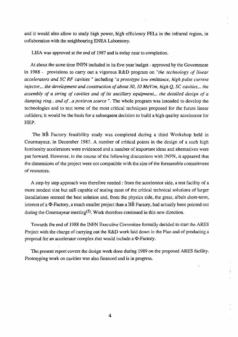
The radiation field power behaviour along the wiggler, as computed by FRED-3D for the 21
nm case, is reported in Fig. 1.4.1 (solid line). The typical exponential gain can be observed,
with a saturation power level of 320 MW. In this case a slight ion-focussing effect (H=.38) has
been applied to overcome'the violation of Pellegrini's rule. The saturation power level is lower
because of diffraction effects tending to remove the radiation from the electron beam.
The last case presented can be viewed as the ultimate goal for the FEL driver : a double
recirculation in the last se LINAe section could boost the beam energy up to 820 MeV.
Pushing down the beam emittance to the lowest foreseeable value, the output power of the
coherent radiation generated in the wiggler can reach 650 MW, with a radiation wavelength of
11 nm, i.e. a photon energy of 117 e V. The required wiggler length is "" 10 meters.
The preliminary studies, together with the performed simulations, indicate that bursts of
VUV and soft X-ray coherent radiation will be available at the ARES se LINAe facility: this
opens great possibilities to perform both accelerator physics experiments in the mainstream of
the Te V electron-positron colliders and a large class of experiments within the environment of
solid state and applied physics.
9
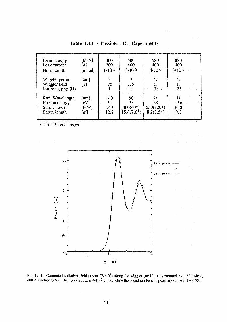
Table 1.4.1 - Possible FEL Experiments
Beam energy [Me V] 300 500 580 820 Peak current [A] 200 400 400 400 Norm emitt. [mrad] 1•10-5 8•10-6 4·10-6 3·10-6
Wiggler period [cm] 3 3 2 2 Wiggler field [T] .75 .75 1. 1. Ion focussing (H) 1 1 .38 .. 25 .,
Rad. Wavelength [nm] 140 50 21 11 Photon energy [eV] 9 25 58 116 Satur. power [MW] 140 400(40*) 550(320*) 650 Satur. length [m] 12.2 15.(17.6*) 8.2(7.5*) 9.7
* FRED-3D calculations
3. field power-
port power ·--···
2.
--3:
..... QJ
;J: 0
a.. I.
o ·o'-. _..____.__1 o-' ...._....,'---:,,_. _..___._ _ _.____._-=2 .
z (m)
Fig. 1.4.1 - Computed radiation field power [W •108] along the wiggler t tn •1 0], as generated by a 580 Me V, 400 A electron.beam. The norm. emitt. is 4·10-6 m rad, while the added ion focusing corresponds to: H = 0.38.
1 0
1.5 - LINAC
The Se Linac has to provide electron and positron beams at 510 Me V. The positron intensity must be such that a current of the order of 1 A can be injected in each of the <I>-Factory rings in
a time of the order of a few minutes. In addition, the Linac must be capable of reaching a single
pass energy high enough to perform significant FEL experiments and beam quality tests, so that
very low emittance beams can be accelerated without degradation.
While the ideal situation - both from the point of view of positron production and from that
of beam quality- would be to install a number of se cavities sufficient to reach the full 510
Me V energy in one pass, cost considerations favour a solution in which a number of cavities are
used more than once by recirculating the beam through them, an option afforded by the se structure that is capable of carrying up to several mA of average current.
Recirculation of course implies ring-like transport channels; these have a finite relative
momentum acceptance estimated at around 4% at most (3).
On the other hand, positrons are generated within a finite momentum bite, that needs to be
as large a possible to increase the yield; it is generally assumed to be of the order of 10 Me V. In
our case the momentum spread requirements for <!>-Factory injection-± 2.5 Me V- are more
stringent (see§ 2.3.) . Nevertheless, positrons must be accelerated to an energy larger than""
300 Me V before they can be recirculated.
This fixes the minimum single-pass energy to be provided.
Two other problems have to be taken into account in determining the Linac configuration:
- the capture section following the positron converter has to be 'warm', because of
radiation problems and also because the field in the capture section should be as high as
possible to maximise the capture section acceptance and increase the conversion
efficiency.
from the converter onwards, and until an energy of ""100 Me V or higher has been
reached, the positron beam can not be put through any bending magnet because its energy
dispersion, as already explained above, is too large.
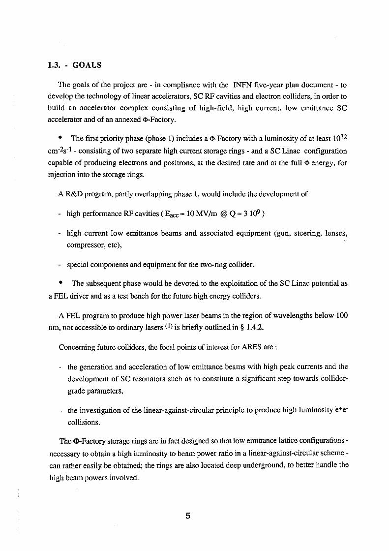
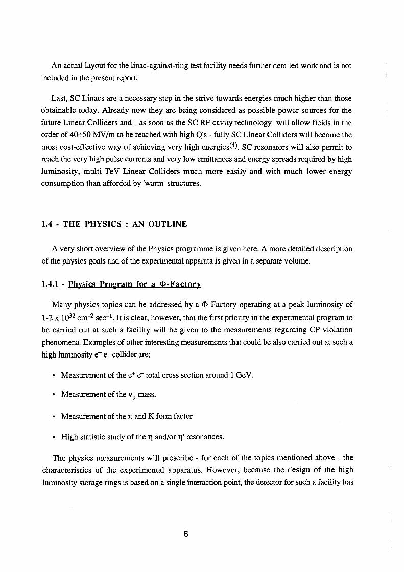
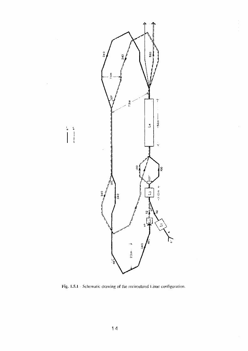
The ensemble of these constraints leads to the configuration schematically shown in Fig.
1.5.1. Figure 1.5.2 shows, schematically, the physical arrangement of the transport and
recirculation channels in the vertical plane. A short description of the rationale of the layout is
given below.
1 1
Electrons are generated by the gun G, passed through a matching section that - depending on
the type of gun- may include a chopper, a prebuncher, a warm section and other diagnostics
and control elements (see § 2.3.2. - The Electron Preinjector), and accelerated by Linac Section
L1 consisting of four se cavities each providing a nominal voltage gain of 12 MV. The electron
preinjector output energy is~ 4 Me V.
At the output ofL1 the nominal beam energy is therefore= 52 Me V or slightly higher, the
exact value depending on the type of gun that is being used (see § 2.3.2.).
Each four-cell se cavity in section L1 has its own cryostat and forms a cryomodule, the
smallest unit of the cryogenic structure that can be individually tested. The distance between
focusing elements is minimised in the low energy region where space-charge forces are
important.
The distance between adjacent cryostats is kept to the minimum value of one RF wavelength
(0.6 m); focusing, diagnostics, control and vacuum components are integrated within this
length (see§ 2.6.).
The axis through the gun and section L1 is below the main Linac axis and parallel to it. The
vertical distance between the two is 1.0 m.
After Section L1 the electron beam enters an achromatic isochronous transport channel
(Te12) including a pulsed dipole, is deflected unto the main Linac axis and enters Section L2,
identical to section L1, that boosts its energy by a further 48 Me V (nominal). The overall
nominal electron beam energy at the output ofL2 is therefore~ = 100 Me V.
The pulsed dipole is necessary because in the positron mode electron and positron bunches
follow each other at a distance of only a few hundred ns and the positron bunch must enter
section L2 undeflected.
Following Section L2 the electron beam is brought to the main Linac Section, L3, through
an isochronous achromatic channel (Te23) that includes all splitter and combiner devices
required to handle the primary and recirculated electron and positron beams.
Section L3 consists of 20 four-cell cavities, with one cryostat for each pair to increase the
Linac filling factor. The cryomodule therefore contains of two cavities.
The overall nominal voltage provided by Section L3 is 240 MV. The electron beam norriinal
energy at the output of L3 is therefore ~= 340 Me V.
In the electron mode, electrons are then brought back to the input of L3 through the
isochronous achromatic transport channel indicated in Fig.1.1 as Te3 and passed once more
through L3.
1 2
The electron beam final nominal energy at the output of the Linac is thus ~ ~ 580 Me V
affording a safety factor of= 12% with respect to the required energy of 510 Me V. In terms of
accelerating voltage in the SC cavities this means that the actually required avetage accelerating
voltage could be as low as 8.7 MV/m.
In the positron mode, the =300 Me V electron beam that has passed once through the Linac is
brought back to the positron converter, PC, thtough the isochronous achromatic channel TC2
(see Fig. 1.5.2). The PC is described in more detail in the following.
The positrons produced in the converter target are collected in the 1.5 m long warm section
LW4 (see Fig.l.5.2) that provides an accelerating field of = 35 MV/m and an overall
accelerating voltage of= 40 Me V. They thus reach the input ofL2 with about the same energy
as that of electrons incoming from Ll and are further accelerated, through L2 . At this point
they can be put through the splitter and recombiner magnets of the transport channel to L3.
The = 300 Me V positron beam at the output of L3 is then recirculated once, via transport
channel TC3, and finally reaches its final nominal energy of 510 Me V.
1 3
I +
"' "'
0 -r M
!.
" I I
0 -r M
r f
f
I I r
r V
r
E -r "'
-V
E S' A
I
Fig. 1.5.1 -Schematic drawing of the rccirculatcd Linac configuration.
1 4
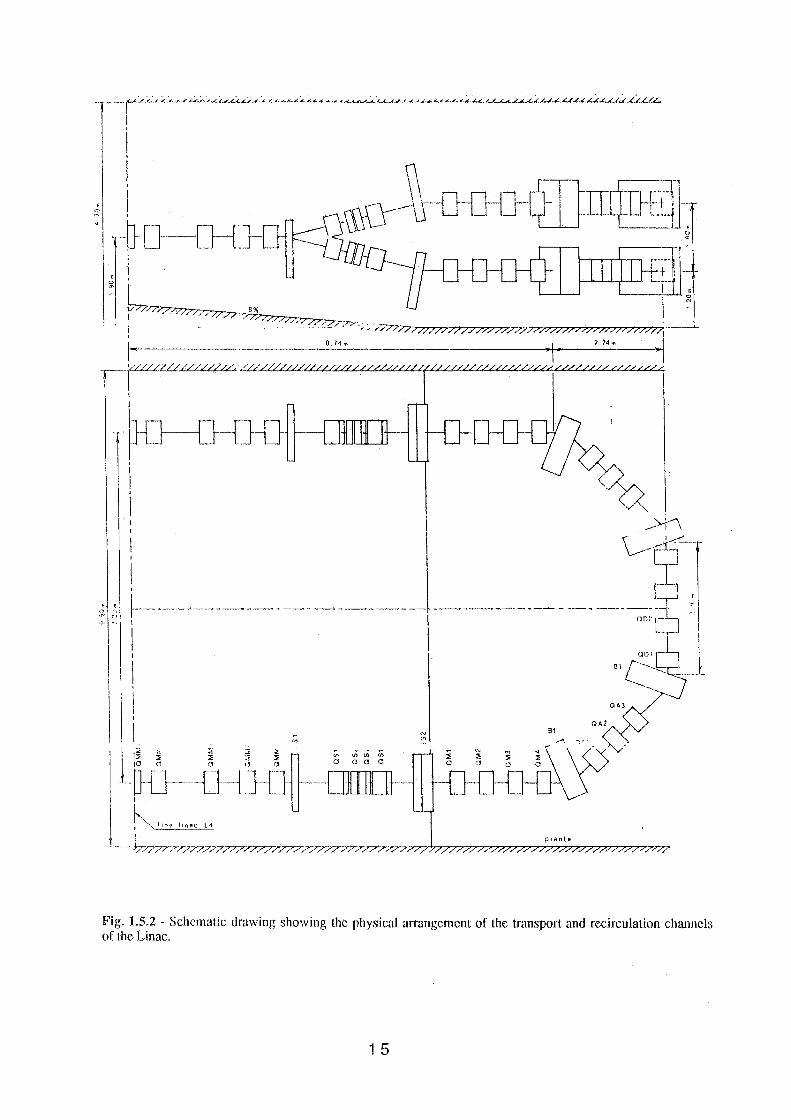
Fig. 1.5.2 - Schematic drawing showing the physical arrangement of the transport and recirculation channels of the Linac.
1 5
1.6. - <I>-F ACTORY
The main goal of the ARES <!>-Factory is a luminosity ;:::: 1032 cm~2sec-1 at 510 Me V.
This kind of luminosity has never been reached or even approached in a reliable way at such
relatively low energies; the system parameters must therefore be catefully chosen and optimized
based on the available experience an on existing models and scaling laws.
On the other hand a tight time schedule asks for a basically proven design, that relies on only
a very limited amount of R&D and is flexible enough to allow the key machine parameters to be
varied so as to optimize the luminosity and to explore alternative collision schemes such as the
the linear-against-circular solution.
The proposed ARES design is therefore based on conventional technology, with electrons
and positrons circulating in two separate storage rings, one above the other; and colliding head
on in a single interaction point. The two separate rings make it possible to increase the number
of bunches and gain a substantial factor on luminosity through the high permissible collision
frequency.
The rings are compact but the chosen bending field values do not require se dipoles; a
number of unexplored engineering problems related to the design of 'curved' se dipoles, to the
much stronger non linearities deriving from the very small bending radius and to synchrotron
radiation in a superconducting environment ate thus avoided.
The values of the betatron functions at the crossing point are low but not so low as to create
problems with beam instabilities because of the very small longitudinal bunch length or with
interferences of the interaction point quadrupoles with the experimental apparatus.
The beam emittance value is also a good compromise between the large values favoured by
luminosity and the need to keep the machine physical aperture reasonable; the design of the
lattice is moreover such that the emittance can be tuned over a wide range of values.
The coupling coefficient, K, has been carefully optimized to reach the best compromise
between lifetime and luminosity in the light of existing models and scaling laws
The maximum allowed linear tune shift in the beam-beam interaction, ~max , is the most
important parameter and the primary limiting factor of luminosity. As of today no satisfactory
theory exists that fully explains the mechanism of this limitation.
The value chosen in the ARES design takes into account all known scaling laws (15) and a
recent model developed in Frascati (16).
All scaling laws predict that the maximum obtainable luminosity increases with increasing
radiation damping, although with different power laws. The approach chosen for the ARES
factory attempts at establishing a 'maximum likelihood' value and is believed to leave some
1 6
margin for development and improvements. Some basic features of the different models can and
will be tested on ADONE, as discussed in more detail in Chapter 3.2.7.
The values of circulating current necessary to achieve the desired goal are high but not higher
than obtained, as top performance, at some existing SR sources (17 ).
A summary of the Factory main parameters is given in Table 1.6. 1.
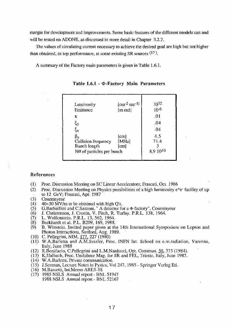
Table 1.6.1 - <!>-Factory Main Parameters
Luminosity Emittance 1(
~y ~X
[cm-2 sec-lJ [m rad]
~Y [cm] Collisioh frequency [MHz] Bunch length [cm] Ner of particles per bunch
1032 w-6 .01 .04
.04
4.5 71.4
3 8.9 1010
References
(1) (2)
(3) (4) (5) (6) (7) (8) (9)
(10) (11)
(12) (13) (14) (15) (16) (17)
Proc. Discussion Meeting on SC Linear Accelerators; Frascati, Oct. 1986 Proc. Discussion Meeting on Physics possibilities of a high luminosity e+e- facility of up to 12 GeV; Frascati, Apr. 1987 Courmayeur 40+-50 MV/m to be obtained with high Q's. G.Barbiellini and C.Santoni, "A detector for a <1>-factory", Courniayeur J. Christenson, J. Cronin, V. Pitch, R. Turlay. P.R.L. 138, 1964. L. Wolfenstein. P.R.L. 13, 562, 1964. Burkhardt et al. P.L. B209, 169, 1988. B. Winstein. Invited paper given at the 14th International Symposium on Lepton and Photon Interactions, Sanford, Aug. 1989. C. Pellegrini, NIM, 177. 227 (1980) W.A.Barletta and A.M.Sessler, Ptoc. INFN Int. School on e.m.radiation, Varenna, Italy, June 1988 R.Bonifacio, C.Pellegrini and L.M.Narducci, Opt. Commun. 50, 373 (1984). K.Halbach, Proc. Undulator Mag. for SR and FEL, Trieste, Italy, June 1987. W.A.Barletta, Private communication. J.Seeman, Lecture Notes in Pysics, Vol247, 1985- Springer Verlag Ed. M.Bassetti, Int.Memo ARES-18 · 1985 NSLS Annual report- BNL 51947 1988 NSLS Annual report- BNL 52167
1 7
2.- LINAC
2.1. - OPTICS
2.1.1 - Intr<Hiuction
As exp1ained in§ 1.5., the SC linear accelerator has three sections:
- Section Ll consisting of four se cavities each providing a nominal accelerating voltage of
12 MV. The total nominal beam energy at its output is"" 50 MeV. Each four-cell Se
cavity in section Ll has its own cryostat and constitutes a cryomodule.
- Section L2 is identical toLl and accelerates- from"" 50 Me V to"" 100 Me V- both the
positron beam coming from the capture section and the electron beam coming from Ll.
- Section L3 consists of 20 fou~-cel1 cavities, with one cryostat to a pair of cavities to
increase the Linac filling factor; the cryomodule is correspondingly longer. Its overall
nominal output energy is"" 340 MeV. Electron and positron beams are passed through
this section twice to reach their final nominal energy of""' 580 Me V.
2.1.2. - Linac focusing
Transverse focalization along the Linac is provided by a PODO sequence of 0.2 m long
quadrupoles, one per cryogenic module.
The distance between quadrupoles is 3 m in Ll and L2; the focalization can be made weaker
on L3, and the half FODO cell is therefore lengthened to 5.4 m to fit the longer cryomodule.
The first section, Ll, needs a special treatment.
This because the effect of the RP field of an accelerating cavity on the beam transverse
optical functions is negligible only insofar as the beam energy increase in the cavity is smaller
than the input energy (I); else, the PODO lattice focusing is highly perturbed and a strong
mismatch occurs and proper corrective action has to be taken.
The condition is not verified along the first part of Ll since the beam is injected at 4 Me V
and accelerated by the first cavity to 16 MeV. Both the input betatron functions and the
quadrupole strengths must therefore be modified to compensate for the RP cavity effects.
1 8
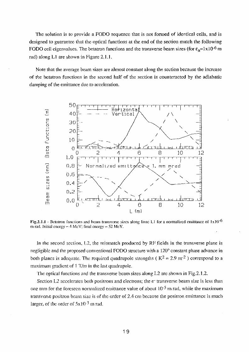
The solution is to provide a FODO sequence that is not formed of identical cells, and is
designed to guarantee that the optical functions at the end of the section match the following
FODO cell eigenvalues. The betatron functions and the transverse beam sizes (for E0 =1xi0-6 m
rad) along L 1 are shown in Figure 2.1.1.
Note that the average beam sizes are almost constant along the section because the increase
of the betatron functions in the second half of the section is counteracted by the adiabatic
damping of the emittance due to acceleration.
50 ~
E 40 (I)
30 c 0 rl
+-> 20 u c :J 10 u_
!0 0 _IJ (]) 0 m 1.0
E 0.8 E
(I) 0.6
(])
N r~
0.4 (I)
E Oo2 10 m OaO m 0
2 I I I I" Normallzed
4
"'-..,
I I
8 10 I I 11 I
L mm mrod /" /
/
/ /
lot I rbcn;-, :(I tCCIT]-b le! I ducol 2 4 6 8 10
L Cml
12
12
Fig.2.1.1 -Betatron functions and beam transverse sizes along linac Ll for a normalized emitt:ance of Ixlo-6 m rad. Initial energy= 4 Me V; final energy= 52 Me V.
In the second section, L2, the mismatch produced by RF fields in the transverse plane is
negligible and the proposed conventional FODO structure with a 120° constant phase advance in
both planes is adequate. The required quadrupole strengths ( K2 = 2.9 m-2 ) corre-spond to a
maximum I:_,rradient of 1 T/m in the last quadrupole.
The optical functions and the transverse beam sizes along L2 are shown in Fig.2.1.2.
Section L2 accelerates both positrons and electrons; the e· transverse beam size is less than
one mm for the foreseen normalized emittance value of about IQ-5 m rad, while the maximum
transverse positron beam size is of the order of 2.4 cm because the positron ernittance is much
larger, of the order of 5x l()-3 m rad.
1 9
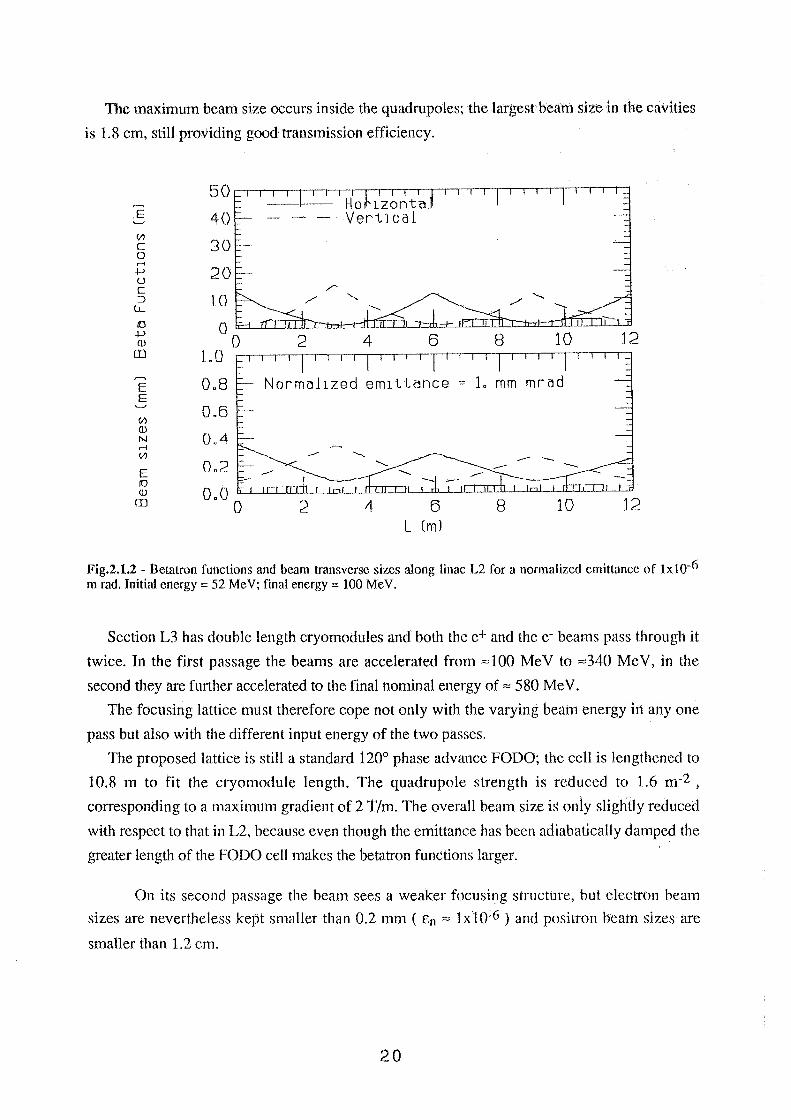
The maximum beam size occurs inside the quadrupoles; the largest beam size in the cavities
is 1.8 cm, still providing good transmission efficiency.
E
(I)
c 0 rl
+-> u c :::>
(L
10 .w Q)
m
E E
(I) Q)
N r-1 (I)
E 10 Q)
m
50
40
30
20
10
0
1.0
0.8
0.6
OA
0.2
0.0
-
0
0 2 4 6 L Cml
8 10
Fig.2.1.2 - Betatron functions and beam transverse sizes along linac L2 for a normalized emittancc of lxlo-6 m rad. Initial energy= 52 Me V; final energy= 100 Me V.
Section L3 has double length cryomodules and both the e+ and the e- beams pass through it
twice. In the first passage the beams are accelerated from zlOO MeV to ::-=:340 MeV, in the
second they are fmther accelerated to the final nominal energy of"" 580 Me V.
The focusing lattice must therefore cope not only with the varying beam energy in any one
pass but also with the different input energy of the two passes.
The proposed lattice is still a standard 120° phase advance FODO; the cell is lengthened to
10.8 m to fit the cryomodule length. The quadrupole strength is reduced to 1.6 rn-2 ,
corresponding to a maximum gradient of 2 T/m. The overall beam size is on1y slightly reduced
with respect to that in L2, because even though the emittance has been adiabatically damped the
greater length of the FODO cell makes the betatron functions larger.
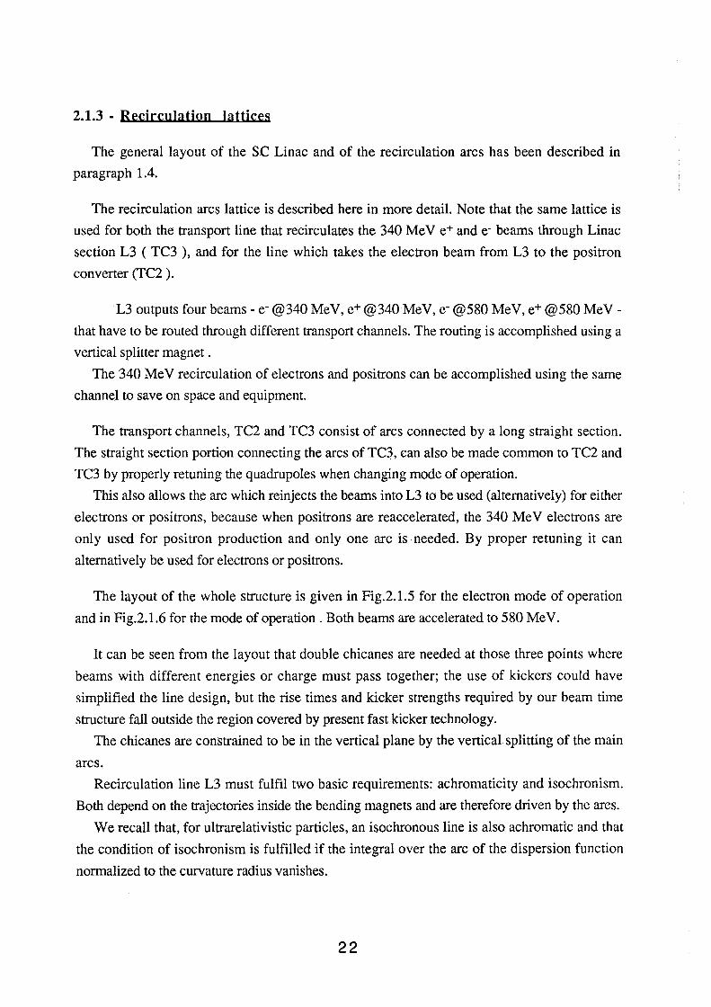
On its second passage the beam sees a weaker focusing structure, but electron beam
sizes are nevertheless kept smaller than 0.2 mm (En "" lx"I0-6) and positron beam sizes are
smaller than 1.2 cm.
20
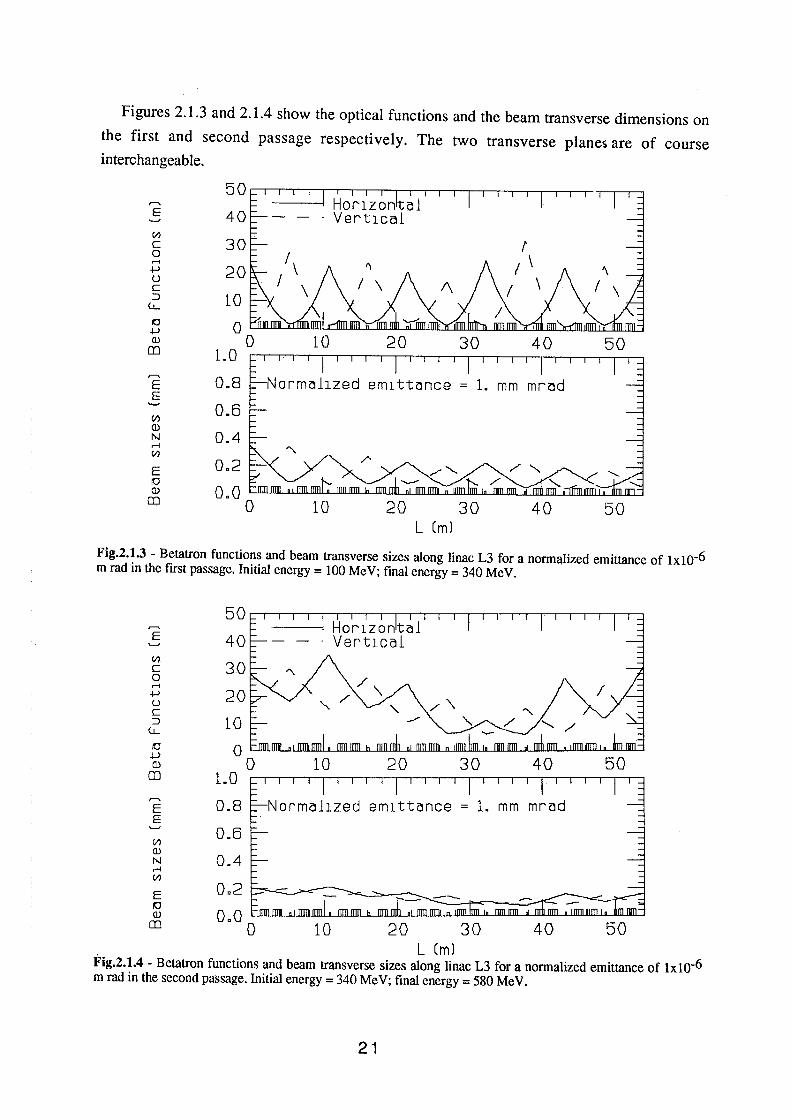
Figures 2.1.3 and 2.1.4 show the optical functions and the beam transverse dimensions on
the first and second passage respectively. The two transverse planes are of course interchangeable.
r-,
E 40 (I)
c 0 ......
-!-> u c ::J 10 u_
10 -!-> Q.)
m
E E
(I) Q.)
N .--1 (I)
E 10 Q.)
m
1.0
0.8
0.6
0.4
Oa2
0.0 0 10 20 30 40 50
L Cml
Fig.2.1.3 - Betatron functions and beam transverse sizes along linac L3 for a normalized emittance of lxl0-6 m rad in the first passage. Initial energy= 100 Me V; final energy= 340 Me V.
(I)
c 0 ......
-!-> u c ::J
u_
10 .w Q.)
m
E E
(I) Q.)
50~~~~~~~~~~~,-111:1111~
40
30
20
1.0
0.8
0.6
20 30
em1 ttc:~nce = 1. mm
N 0.4 .--1 (I)
E 10 Q.)
m
0 a 2 t__:;:---=-__.><:
0 • 0 Ot..rnnJllll.._llllllllllDl L..O JJDlJIDLh..JJlrnli2BLOnLlllllJlliLn.JllllD.3.1Illl0...lLJ.IIll..JUll...JjLJJJ4.1UJJOIIL..D...l.Ullll.liJillJ~.LIW.....I
L Cml Fig.2.1.4- Betatron functions and beam transverse sizes along linac L3 for a normalized emittance of lxlo-6 m rad in the second passage. Initial energy= 340 Me V; final energy= 580 Me V.
21
2.1.3 - Recirculation lattices
The general layout of the SC Linac and of the recirculation arcs has been described in
paragraph 1.4.
The recirculation arcs lattice is described here in more detail. Note that the same lattice is
used for both the transport line that recirculates the 340 Me V e+ and e- beams through Linac
section L3 ( TC3 ), and for the line which takes the electron beam from L3 to the positron
converter (TC2 ).
L3 outputs four beams- e- @340 Me V, e+ @340 Me V, e- @580 Me V, e+ @580 Me V
that have to be routed through different transport channels. The routing is accomplished using a
vertical splitter magnet .
The 340 Me V recirculation of electrons and positrons can be accomplished using the same
channel to save on space and equipment.
The transport channels, TC2 and TC3 consist of arcs connected by a long straight section.
The straight section portion connecting the arcs of TC3, can also be made common to TC2 and
TC3 by properly retuning the quadrupoles when changing mode of operation.
This also allows the arc which reinjects the beams into L3 to be used (alternatively) for either
electrons or positrons, because when positrons are reaccelerated, the 340 Me V electrons are
only used for positron production and only one arc is needed. By proper retuning it can
alternatively be used for electrons or positrons.
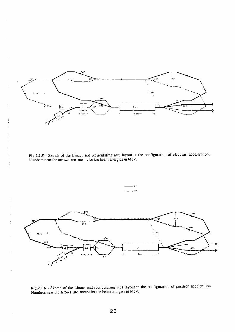
The layout of the whole structure is given in Fig.2.1.5 for the electron mode of operation
and in Fig.2.1.6 for the mode of operation. Both beams are accelerated to 580 Me V.
It can be seen from the layout that double chicanes are needed at those three points where
beams with different energies or charge must pass together; the use of kickers could have
simplified the line design, but the rise times and kicker strengths required by our beam time
structure fall outside the region covered by present fast kicker technology.
The chicanes are constrained to be in the vertical plane by the vertical splitting of the main
arcs.
Recirculation line L3 must fulfil two basic requirements: achromaticity and isochronism.
Both depend on the trajectories inside the bending magnets and are therefore driven by the arcs.
We recall that, for ultrarelativistic particles, an isochronous line is also achromatic and that
the condition of isochronism is fulfilled if the integral over the arc of the dispersion function
normalized to the curvature radius vanishes.
22
L4
54 m"~
Fig.2.1.5 - Sketch of the Linacs and recirculating arcs layout in the configuration of electron acceleration. Numbers near the arrows are meant for the beam energies in Me V.
-·----- e+
Fig.2.1.6 - Sketch of the Linacs and recirculating arcs layout in the configuration of positron acceleration. Numbers near the arrows are meant for the beam energies in Me V.
23
To meet the above specification a configuration with four dipoles, each bending the beam
through 45° , has been chosen. Negative dispersion is produced at the two inner dipoles, so as
to compensate both the positive dispersion introduced by the two outer dipoles and that
produced by the splitter.
The splitter in turn consists of an achromatic, 15° bend chicane in the vertical plane.
The whole line is symmetric around the midpoint of the arc; the half arc consists of the
following sequence : a matching section between L3 and the splitter, the splitter vertical chicane,
a matching section between the splitter chicane and the arc, the 90° arc.
The overall arc length is 27.1 m.
The eigenvalues of the FODO lattice configuration along L3, described in § 2.1.2, provide
the betatron function values at the output of L3; these are matched to those of the arc by the first
matching section. The matching conditions to be fulfilled by the other matching sections - at the
other end of the first arc and at both ends of the two other arcs - are of course different and the
sections will consequently be tuned differently.
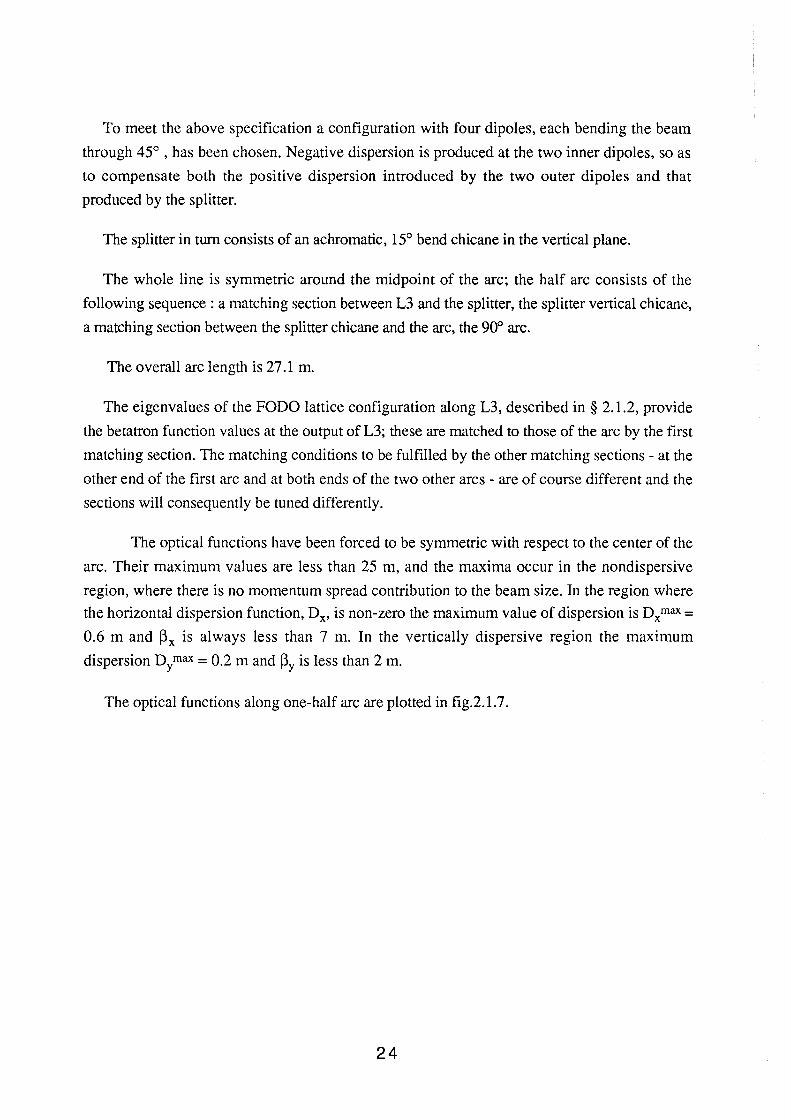
The optical functions have been forced to be symmetric with respect to the center of the
arc. Their maximum values are less than 25 m, and the maxima occur in the nondispersive
region, where there is no momentum spread contribution to the beam size. In the region where
the horizontal dispersion function, Dx, is non-zero the maximum value of dispersion is Dxmax = 0.6 m and ~x is always less than 7 m. In the vertically dispersive region the maximum
dispersion Dy max = 0.2 m and ~Y is less than 2 m.
The optical functions along one-half arc are plotted in fig.2.1.7.
24
~. ~~~~~~-+-T-T-r~~~~~~~T-~~~~~~~-T~
z:i.
al.
15.
10.
s. 0.
:E!IeU11:ran twJcl.ic:ms (m.)
~~~~~-r~4-~~~~~-4-+~~~~*-~~~~~~ 2.
1.
~--------~~~~----------~----~~~~0.
li--1---il--ll--l--f.-+-+-+--+--l--+--+--+--+--l-+-+-+-+--~~~--+-+--+--+--"il -1.
2.5 5.0 7.5 10. 12.5
Fig.2.1.7- Optical functions in half recirculating arc .
The quadrupoles are 0.30 m long. The highest quadrupole strength, K2 max= 13m-2, is
needed in the vertical chicane to satisfy the achromaticity condition; it corresponds to a field
gradient Gmax = 15 T/m.
The arc configuration, as described, applies to all four arcs of the proposed layout (see
Figs. 1.5.1 and 1.5.2). The matching sections between the arcs and the vertical chicanes must
still be defined, keeping in mind that if the chicanes are not isochronous the horizontal
dispersion function inside the arcs must be adjusted for overall isochronism; this can be
obtained easily because of the presence of the two symmetric quadrupole triplets between the
45° dipoles. Any other condition on the total transfer matrix can be fulfilled by properly retuning
the quadrupoles of the long straight sections between the arcs.
25
2.2 · BEAM DYNAMICS
2.2.1 - Introduction
The dynamics of an "ensemble" of charges in a linear accelerator is affected by the so called
"collective forces". These forces are generated by the electromagnetic fields created by the
interaction of the beam with the surrounding walls. They act back on the beam itself perturbing
the dynamics of particles guided by the externally applied fields. The physical process is
characterized by energy loss of the beam and, depending on the current intensity, by instability
phenomena in both the longitudinal and the transverse dimensions.
Collective effects are analyzed in the time domain by means of the "wake-potentials",
defined as the integrated field per unit charge experienced by a unit test particle travelling in the
fields induced by the bunches accelerated in the linac, in both the longitudinal and the transverse
dimension.
Single bunch dynamics is dominated by the intensity - over the length of the bunch - of the
short range wakefield mainly originated by the interaction of the bunch current with sharp
discontinuities in the vacuum envelope.
The dynamics of many bunches in a linear accelerator is instead affected by long-range
wakefields mainly due to persistent (high-Q) parasitic resonant modes excited by the bunch
current in the r.f. cavities or in other cavity-like objects.
2.2.2 - Induced Wake-fields
The longitudinal wake-potential is defined as the energy lost by a unit charge that travels in
the e.m. field created by a point charge Q a distance 't away, in. front:
Wz('t)=-~~ Ez(z,t=~-'t)dz [Volt I Coulomb]
The above integral is relative to a point charge and defines the impulsive (Green function)
wake-potential. The effective wake potential seen by a charge within a bunch depends on the
bunch charge distribution p('t) and can be calculated by means of the folding integral:
26
W ,f.t) = J t Wz (t- t')r(t') dt' -00
[Volt I Coulomb]
If the trailing charge is also subject to transverse forces, a transverse wake potential is
introduced and defined as the transverse momentum kick per unit charge experienced by the test
particle:
M(t) = { [E(z,t) + vx B(z,t)].l dz
M(t) w j_('t) = -
Qro
. h z wlt t=--'t c
By analogy with the longitudinal case we compute the effect on a real bunch, with a given
space distribution, by applying the folding integral:
The first step in the analysis of collective phenomena is to estimate the integrated longitudinal
and transverse wakes. This can be done- more or less rigorously- by different methods.
For closed structures, both the longitudinal and the transverse impulsive wakes can be
calculated as sums over the normal modes of the structure. This method is however in practice
limited by the fact that r.f. cavities are not perfectly closed structures so that, above the iris cut
off frequency, some analytical correction is needed.
We estimated the impulsive wake potentials by applying general frequency-scaling laws to
the SLAC and CEBAF wake-potentials. The approximated result has then been used to derive
the bunch wakes and compare them with those calculated directly in the time domain by means
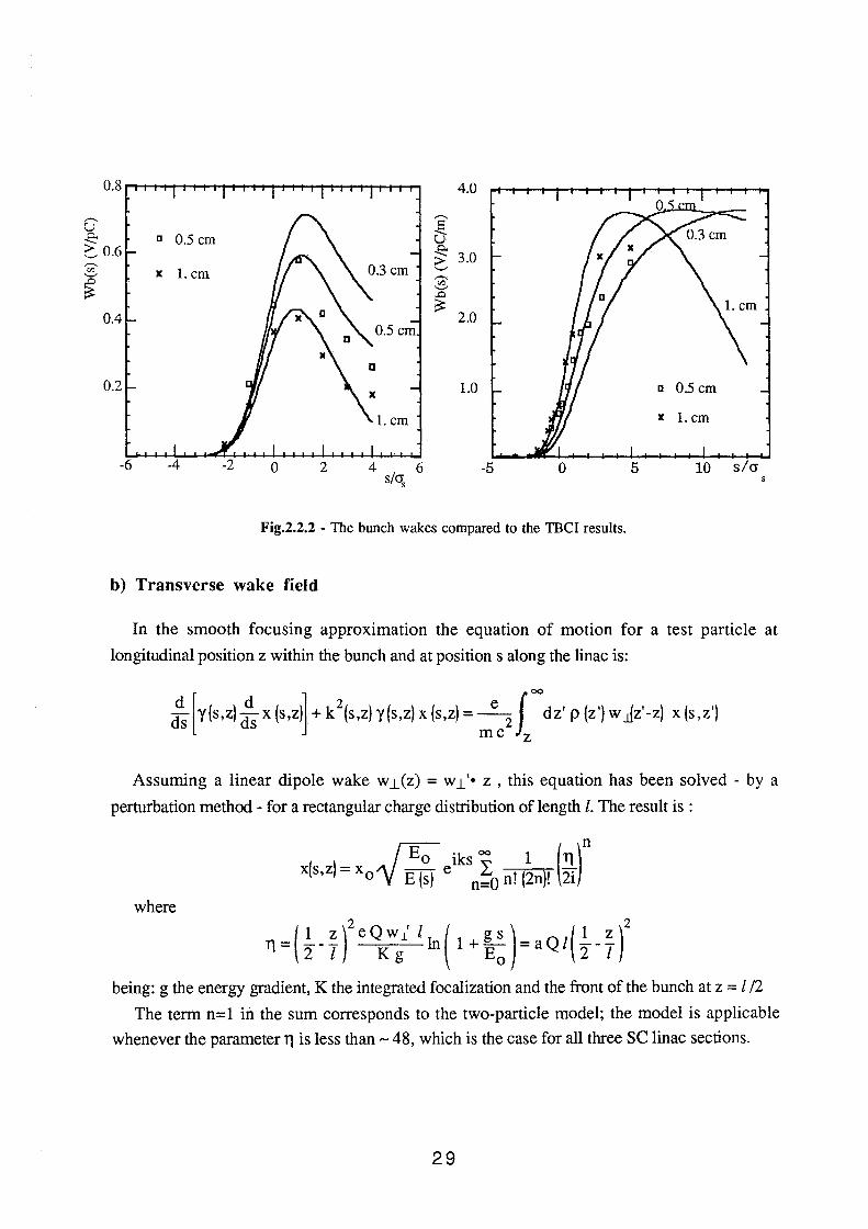
of the TBCI computer code.
The code - severely limited by CPU time required for the huge number of mesh points -
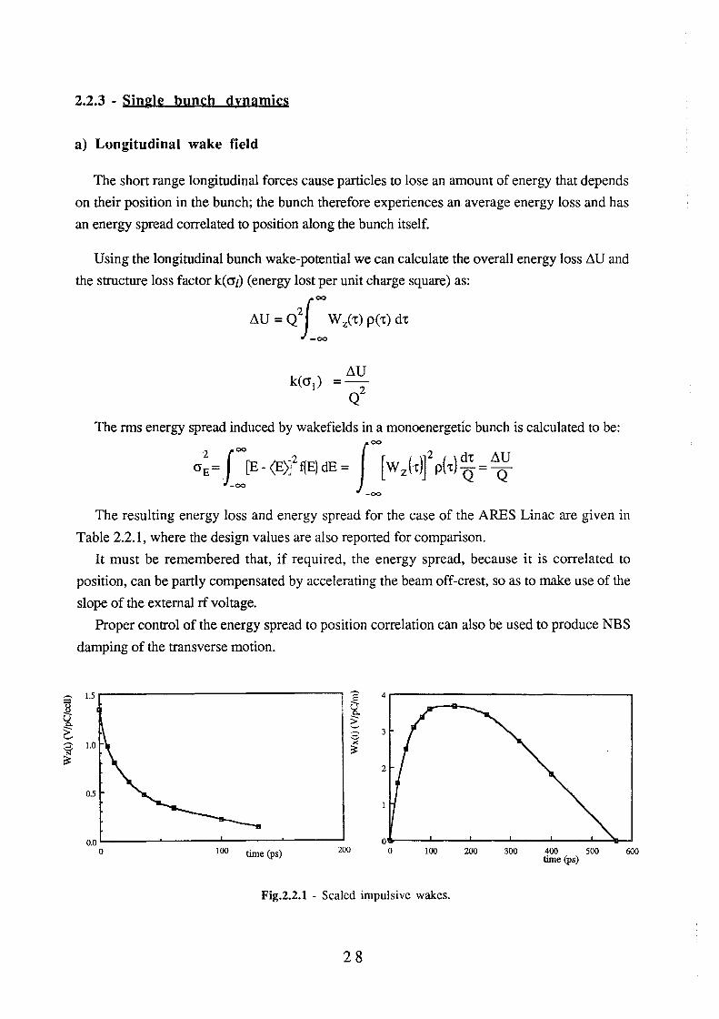
computes the wakefield induced by a gaussian bunch integrated over the bunch distribution that
approaches the wake Green function for very short bunches . The scaled impulsive wakes are
shown in Fig.2.2.1. The bunch wakes are compared to the TBCI results in Fig.2.2.2.
27
a ~
~ ~ ~
2.2.3 - Single bunch dynamics
a) Longitudinal wake field
The short range longitudinal forces cause particles to lose an amount of energy that depends
on their position in the bunch; the bunch therefore experiences an average energy loss and has
an energy spread correlated to position along the bunch itself.
Using the longitudinal bunch wake-potential we can calculate the overall energy loss ~U and
the structure loss factor k(O't) (energy lost per unit charge square) as:
!J.U ~ Qf= W ,(,) p(') d'
The rms energy spread induced by wakefields in a monoenergetic bunch is calculated to be:
a!~ ([E- (E)f ~E) dE ~ fr W z (1)j' ph)~ ~ !J.~ -00
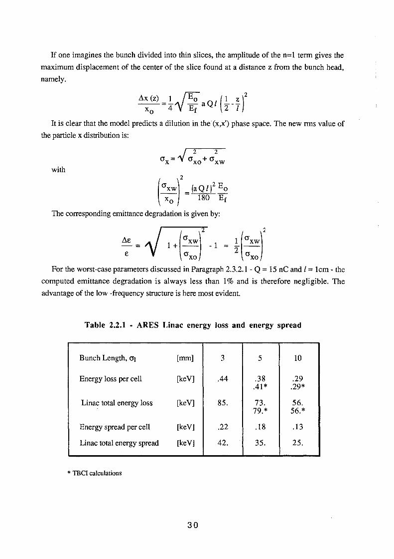
The resulting energy loss and energy spread for the case of the ARES Linac are given in
Table 2.2.1, where the design values are also reported for comparison.
It must be remembered that, if required, the energy spread, because it is correlated to
position, can be partly compensated by accelerating the beam off-crest, so as to make use of the
slope of the external rf voltage.
Proper control of the energy spread to position correlation can also be used to produce NBS
damping of the transverse motion.
1.5 'E 4
C2. ~ ~ 3 '><. 1.0 ~
2
0.5
0.0 L_ __ __._ ___ ....L-___ ......._ __ ___,1
0 100 200 100 200 300 400 500 time (ps)
time (ps) 600
Fig.2.2.1 - Scaled impulsive wakes.
28
,..-....
"' '-'
~
0.8 4.0
,..-....
c 0.5 cm -€ u ~ 3.0 >
X l.cm '-' ,..-....
"' '-'
~ 2.0
1.0 c 0.5 cm
l.cm x l.cm
-5 -6 2 0 4 6 s/q
10 s/cr 0 5
Fig.2.2.2 - The bunch wakes compared to the TBCI results.
b) Transverse wake field
In the smooth focusing approximation the equation of motion for a test particle at
longitudinal position z within the bunch and at position s along the linac is:
foo
d d 2 e ds [y(s,z} ds x (s,z}] + k {s,z} y{s,z} x (s,z} = -
2 dz' p {z'} w jz'-z) x (s,z')
me z
Assuming a linear dipole wake w_1_(z) = w_1_'• z, this equation has been solved - by a
perturbation method - for a rectangular charge distribution of length l. The result is :
where
11 = { _!_ - ~ )2 e Q w .t.' l 1n ( 1 + [! ) = a Q l ( _!_ - ~ )2 2 l Kg E0 2 l
being: g the energy gradient, K the integrated focalization and the front of the bunch at z = I !2
The term n=l in the sum corresponds to the two-particle model; the model is applicable
whenever the parameter 11 is less than- 48, which is the case for all three se linac sections.
29
If one imagines the bunch divided into thin slices, the amplitude of the n=l term gives the
maximum displacement of the center of the slice found at a distance z from the bunch head,
namely.
~x (z) = .!_ {E;; a Q l ( .!_ -~ )2 x 0 4 ~ Ef 2 l
It is clear that the model predicts a dilution in the (x,x') phase space. The new rms value of
the particle x distribution is:
with 2
(crxw) =(a Q 1)
2 Eo
x0 180 Er
The corresponding emittance degradation is given by:
t.e = - j 1 + (crxw)
2
_ 1 = ~ (crxw)
2
e ~ crxo crxo
For the worst-case parameters discussed in Paragraph 2.3.2.1 - Q = 15 nC and l = 1cm- the
computed emittance degradation is always less than 1% and is therefore negligible. The
advantage of the low -frequency structure is here most evident.
Table 2.2.1 - ARES Linac energy loss and energy spread
Bunch Length, <Jt [mm] 3 5 10
Energy loss per cell [keV] .44 .38 .29 .41 * .29*
Linac total energy loss [keV] 85. 73. 56. 79.* 56.*
Energy spread per cell [keV] .22 .18 .13
Linac total energy spread [keV] 42. 35. 25.
* TBCI calculations
30
2.3. - e- AND e+ GENERATION
2.3.1 - Introduction
The general requirements for the generation and acceleration of electrons and positrons to be
injected in the ARES <I>-Factory rings have been discussed in References (2)+ (4).
The general layout of the linac is presented in Fig. 1.4.1. As shown in Fig. 1.4.1, the 48
Me V se linac section L2, common to e- and e+, is fed by two separate preinjectors : the
electron preinjector, consisting of the high energy(~ 4 Me V) gun followed by a 48 Me V SC
preaccelerator section, L1, and the positron preinjector consisting of the positron converter and
the warm capture section L4.
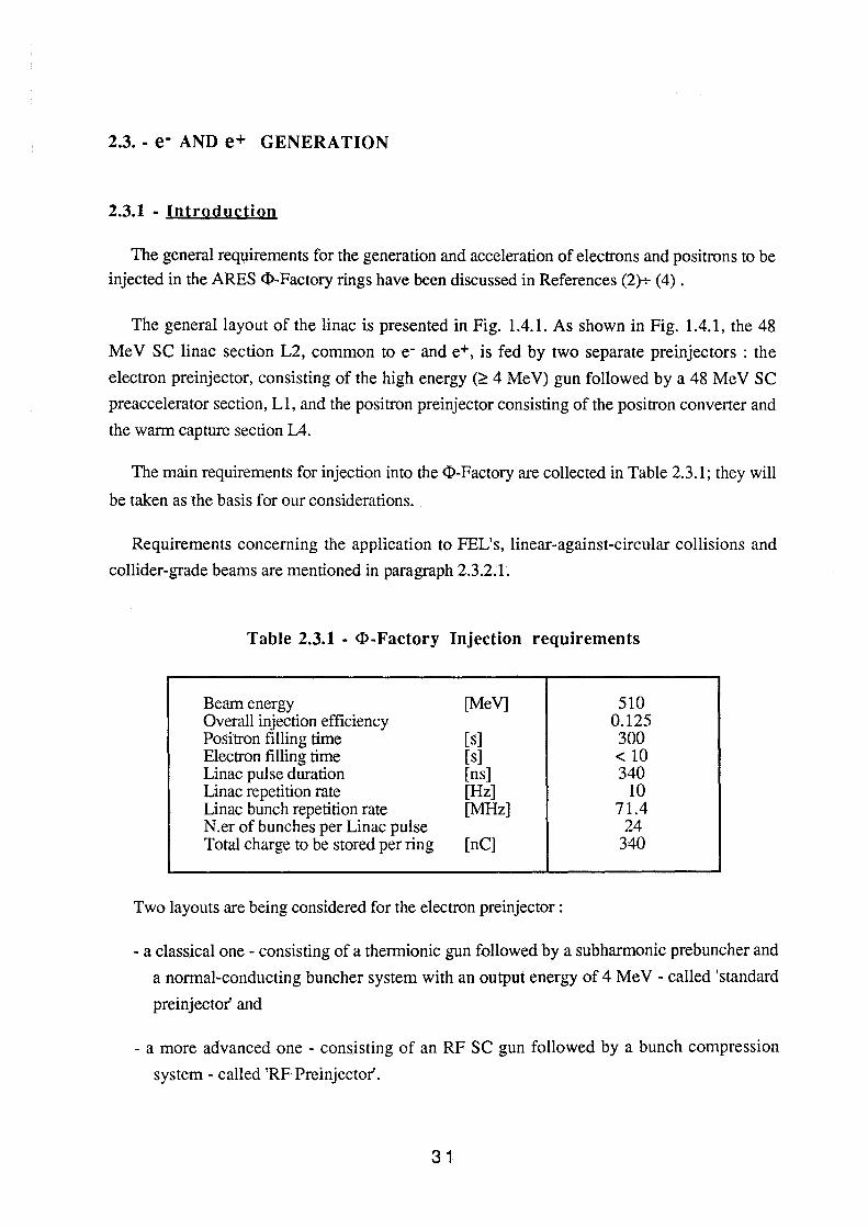
The main requirements for injection into the <I>-Factory are collected in Table 2.3.1; they will
be taken as the basis for our considerations.
Requirements concerning the application to FEL's, linear-against-circular collisions and
collider-grade beams are mentioned in paragraph 2.3.2.1.
Table 2.3.1 - <I>-Factory Injection requirements
Beam energy Overall injection efficiency Positron filling time Electron filling time Linac pulse duration Linac repetition rate Linac bunch repetition rate N.er of bunches per Linac pulse Total charge to be stored per ring
[Me V]
[s] [s] [ns] [Hz] [MHz]
[ne]
Two layouts are being considered for the electron preinjector:
510 0.125 300 <10 340
10 71.4
24 340
- a classical one - consisting of a thermionic gun followed by a subharmonic prebuncher and
a normal-conducting bunch er system with an output energy of 4 Me V - called 'standard
preinjector' and
- a more advanced one - consisting of an RF se gun followed by a bunch compression
system - called 'RF Preinjector'.
31
The standard preinjector is almost identical to that of LISA (5,6), produces a beam of average
quality, and can be implemented directly without any need for special R&D; it is described in
detail in this paragraph.
The RF preinjector is a highly sophisticated system capable of producing state-of-the-art
collider and FEL-grade beams in addition to those needed for injection into the <I>-Factory. Its
implementation will require substantial R&D work. It is described here only briefly; a separate,
detailed description is given in Paragraph 2.3.2.1.
A final decision on which system to implement for the injection into the <I>-Factory will have
to be taken in due time during the development of the Project.
To evaluate the performance required of the preinjector in the injection mode has been
evaluated - for positrons - as described in the following. The injection of electrons is much
faster and need not be treated in detail.
The total positron charge to be stored in the <I>-Factory e+ ring is:
where% is the bunch charge and h the ring RF harmonic number (24); the average linac
current required to fill the positron ring in a time Tfp is therefore:
where ql is the linac pulse charge, fr the linac repetition rate and lli the overall injection
efficiency. We have assumed lli = 0.125 and Tfp = 300 s, to obtain:
Iav""" 10 nA
Since the ring revolution period, To, is:
for a linac pulse of the same duration and a linac repetition rate fr = 10 Hz, the required linac
pulse charge, ql> and average pulse current, Ipt• are :
To generate such a positron pulse current, we need from the electron gun cathode a pulse
current, Ig, given by :
32
lg = lpl I (Tic 11-)
where Tic is the electron to positron conversion efficiency and 11- is the gun-to-converter
transport efficiency.
The value of Tic depends on the accepted momentum bite. The requirement of a momentum
standard deviation of± 5 lQ-3 atE = 510 Me V for positron injection into the storage ring
corresponds to
Tic ,., .015 GeV-1.
For a conversion energy of,., 300 Me V it follows that
Using the same parameters for the injection of electrons, an electron ring filling time,
of only ,., 1.5 seconds is obtained.
2.3.2. - The electron preinjector
2.3.2.1 - RF preinjector
As mentioned in the introduction, one of the most important design problems to solve for the
design of Te V electron-positron colliders is the generation of intense, bright beams(6-11).
High current (some hundreds of Amperes) and low normalized emittance (some mm mrad)
electron beams, accelerated to .5 + 1 Ge V, are also required for short wavelength (in the range
from VUV to soft X rays) high gain, high power, single-pass FEL's (11-13).
The accelerated beam brightness can not be higher than that generated at the gun and
transmitted through the main accelerator injection system; the performance of the Linac injector
is therefore a primary concern.
As extensively reported in a dedicated paper (14), it is foreseen to develop, for ARES, a
state-of-the-art injector that can also produce the more conventional beams needed for injection
into the <!>-Factory rings.
33
Preliminary results on the expected performance are reviewed in the following, together with
the rationale-of the choices that have been made. We remark here that the proposed Se laser
driven RF gun operating at 500 MHz (the ARES se Linac frequency) and featuring a 30 MY/m
electric field value at the photocathode, looks very promising; in particular, the low operating
frequency guarantees that harmful RF and wake-field induced effects are much less severe than
in other similar projects (7,8,15).
The use of superconducting cavities is mandatory for ew or high repetition rate operation
with high electric field on the cathode surface. The clean environment, typical of a se cavity, is
also instrumental in lengthening the cathode lifetime (16).
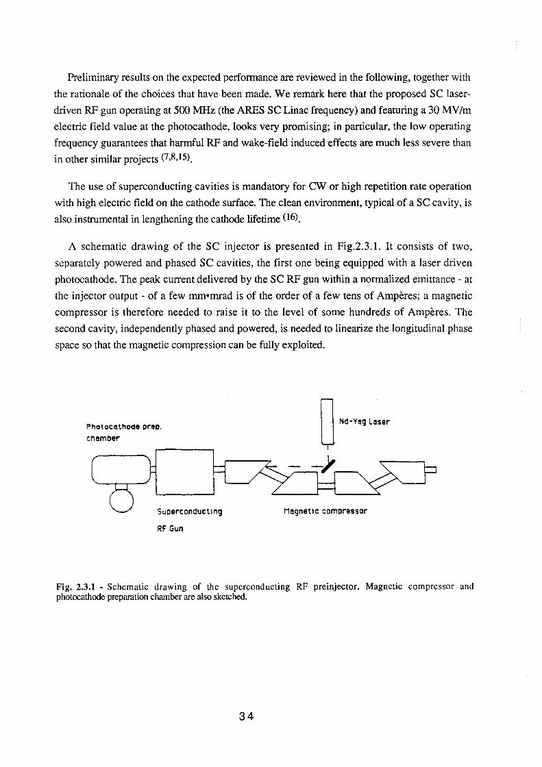
A schematic drawing of the Se injector is presented in Fig.2.3.1. It consists of two,
separately powered and phased se cavities, the first one being equipped with a laser driven
photocathode. The peak current delivered by the se RF gun within a normalized emittance - at
the injector output - of a few mm•mrad is of the order of a few tens of Amperes; a magnetic
compressor is therefore needed to raise it to the level of some hundreds of Amperes. The
second cavity, independently phased and powered, is needed to linearize the longitudinal phase
space so that the magnetic compression can be fully exploited.
F'hotocothode prep.
eh ember
Superconduct 1 ng
RF Gun
0 Nd-Vog Loser
Megnet 1 c compressor
Fig. 2.3.1 - Schematic drawing of the superconducting RF preinjector. Magnetic compressor and photocathode preparation chamber are also sketched.
34
a) Basic Theory
The geometry of the gun cavities and the cathode and laser pulse characteristics are dictated
by the need to preserve beam quality throughout the injection system.
The main phenomena tending to raise the electron bunch transverse temperature and
therefore to blow-up the normalized transverse emittance, e0 , are:
- RF linear effects
- RF non linear effects
- Wake field effects
A detailed discussion of these effects is given in Reference (14).
Here we just recall, for a better understanding of the main design problems, the results of a
first order estimate (14,17) of the transverse normalized emittance deterioration suffered by a
bunch emitted and accelerated in the RF gun, based on the following approximations :
- the electric RF field on the axis is a pure sinusoid;
- off axis RF fields are derived through a linear expansion;
- wake field effects are neglected; the bunch charge density distribution can be either
gaussian or uniform.
- the emitted bunch is mono-energetic and beam envelope variations through the gun are
neglected (only transverse and longitudinal momentum transfers are considered).
We also note that our definition of the normalized emittance is the following (18,19): ' v 2 2 2 En= <X > <p X > - <X p x>
The results of the above approximations can be summarized in the following formula:
2 2 2 .1.eror= .1.eRF+ .1.e 32 + 2 J x .1.eRF.1.e~
where .1.esc is the emittance increase due to the space charge forces and .1.ERF is that due to
RF linear effects, both computed at the injection phase <1>o that minimizes the emittance blow-up.
1x is the transverse correlation factor(14) . .1.esc • .1.ERF and <l>o are defined by the following
equations:
-6 5.7•10 •Qb[nC]
.1.e 32 [mrad]=--------------------------sin <l>o • E0[MV/m] • (3crJm] +5crz£m])
35
E = E0 sin (coRF t + <l>o)
2 2 ~ERF [m rad] = .69 • E0[MV/m] • ar • (kRF• a)
The normalized transverse emittance at the gun exit, E00, is given, in terms of the emittance
at the cathode, Enc. and of the total emittance increase, by:
Under the approximation that all photo-electrons emerge from the cathode with the same
energy (i.e. neglecting the straggling inside the cathode), assuming that this energy is given by
the difference between the laser photon energy and the work function of the cathode material
and considering a laser pulse with a double gaussian distribution in radius and time (with rms
widths O"r and O"t ), the normalized emittance at the cathode surface, Enc. is given by :
E0 Jmrad]= _ ~ • ar[m] 'V 3moe2
where: W = hVIaser- Wt [eV] and Wt is thee- work function
To minimize Enc one can decrease the laser spot until the limit on the maximum cathode
current density (typically 500 A/cm2) is reached, giving a minimum laser spot radius of the
order of 1 mm for some tens of Ampere of cathode current. All considered, typical values of Enc
range from ""'.8 to ""' 2 mm•mrad.
Once the RF frequency and the peak value electric field on the cathode have been fixed, the
value of the output emittance is a function only of the bunch charge, O"r and O"z.
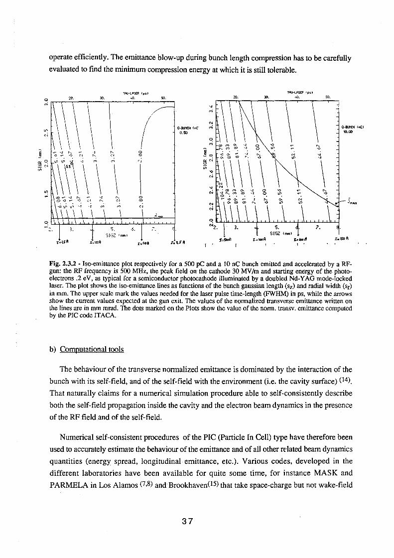
Figure 2.3.2 shows the iso-emittance lines as functions of the bunch spot radius and length
for two different bunch charges, .5 nC and 10 nC. They are computed with the ARES
parameters, namely an RF frequency of 500 MHz and a cathode peak field of 30 MV /m.
It can be easily seen that the emittance of short bunches is dominated by the space charge
effect while that of long bunches is dominated by RF effects.
In defying the actual bunch shape the behaviour in the longitudinal phase space, not
accounted for in the diagram, must also be considered. Too long bunches (;::: few tenths of RF
degrees) come out curved in longitudinal phase space and the magnetic compressor can not
36
operate efficiently. The emittance blow-up during bunch length compression has to be carefully
evaluated to find the minimum compression energy at which it is still tolerable.
f.:""'A I . I . I •
Fig. 2.3.2- Iso-emittance plot respectively for a 500 pC and a 10 nC bunch emitted and accelerated by a RFgun: the RF frequency is 500 MHz, the peak field on the cathode 30 MY /m and starting energy of the photoelectrons .2 eV, as typical for a semiconductor photocathode illuminated by a doubled Nd-YAG mode-locked laser. The plot shows the iso-emittance lines as functions of the bunch gaussian length (sz) and radial width (sr) in mm. The upper scale mark the values needed for the laser pulse time-length (FWHM) in ps, while the arrows show the current values expected at the gun exit. The values of the normalized transverse emittance written on the lines are in mm mrad. The dots marked on the Plots show the value of the norm. transv. emittance computed by the PlC code IT A CA.
b) Computational tools
The behaviour of the transverse normalized emittance is dominated by the interaction of the
bunch with its self-field, and of the self-field with the environment (i.e. the cavity surface) (14).
That naturally claims for a numerical simulation procedure able to self-consistently describe
both the self-field propagation inside the cavity and the electron beam dynamics in the presence
of the RF field and of the self-field.
Numerical self-consistent procedures of the PlC (Particle In Cell) type have therefore been
used to accurately estimate the behaviour of the emittance and of all other re·lated beam dynamics
quantities (energy spread, longitudinal emittance, etc.). Various codes, developed in the
different laboratories have been available for quite some time, for instance MASK and
PARMELA in Los Alamos (7,8) and Brookhaven(l5) that take space-charge but not wake-field
37
effects into account, in a manner that is not self-consistent, TBCI-SF (a self consistent PlC
code of the MAFIA family) in Wuppertal(16).
A new PlC code, named ITACA(20,21), recently developed by some of the authors at the
Milan University has been used to design the ARES RF gun. ITACA has been extensively
checked against other codes, agrees well with other analytical and experimental results, and has
novel features and distinctive advantages.
ITACA is an axi-symmetrical code which solves, self-consistently, a sub-system of the
Maxwell + Newton Lorentz equations for cylindrical symmetric fields and sources. The bunch
current is assumed to have radial and axial components and the self-field is assumed to be a
monopole field (TMonp-like). A specially developed charge assignment algorithm minimizes
unphysical fluctuations in the driving term, and the equations of motion fourth-order integration
algorithm can compute all quantities related to particle dynamics - notably transverse and
longitudinal emittances, energy spread, rms divergence, etc- very accurately.
An eigenvector finder, that can compute the TManp resonating modes of any axi-symmetrical
structure, is included in the package to compute the accelerating RF field distribution inside the
gun cavity.
The PARMELA-SUPERFISH code system, suitable for studying the bunch dynamics in the
presence of the RF and the space-charge fields only, is operational both in Frascati and in
Milan. It will be used to study the magnetic compressor.
c) Results of the numerical simulations
The gun SC RF cavity design must not only comply with the requirements by beam
dynamics, but also those needed for reliable operation beam dynamics at the maximum
accelerating field.
Re-entrant cavities, that are more difficult to clean, were therefore 'a priori' discarded. A
number of other constraints follow :
- Because enough space must be left free on the cut-off tubes for the main coupler and the
ROM coupler, radius and length of the cut-off tubes must exceed certain minimum
values. The proposed values are: 85 mm for the radius and 150 mm for the length.
- Because the cells must be coupled in the 7t-mode the coupling coefficient (usually a few
percent) also has a minimum value determining the iris thickness and aperture.
38
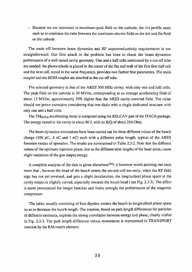
- Because we are interested in maximum peak field on the cathode, the iris profile must
such as to minimize the ratio between the maximum electric field on the iris and the field
on the cathode
The trade off between beam dynamics and RF superconductivity requirements is not
straightforward. Our first attack to the problem has been to check the beam dynamics
performance of a well tested cavity geometry. One and a half cells terminated by a cut-off tube
are needed: the photocathode is placed in the center of the flat end wall of the first first half cell
and the next cell, tuned to the same frequency, provides two further free parameters. The main
coupler and the HOM coupler are attached to the cut-off tube.
The selected geometry is that of the ARES 500 MHz cavity, with only one and half cells.
The peak field on the cathode is 30 MV /m, corresponding to an average accelerating field of
about 13 MV/m, approximately 30% higher than the ARES cavity nominal field. The value
should not prove excessive considering that one deals with a single dedicated structure with
only one and a half cells.
The TMo10-1t accelerating mode is computed using the RELCA V part of the ITA CA package.
The energy stored in the cavity is about 86 J, with an R/Q of about 210 Ohm.
The beam dynamics simulations have been carried out for three different values of the bunch
charge (100 pC, .5 nC and 1 nC) each with a different pulse length, typical of the ARES
foreseen modes of operation. The results are summarized in Table 2.3.2. Note that the different
values of the optimum injection phase, due to the different time lengths of the laser pulse, cause
slight variations of the gun output energy.
A complete analysis of the data is given elsewhere(14); it however wo~th pointing out once
more that, because the head of the bunch enters the second cell too early, when the RF field
sign has not yet reversed, and gets a slight deceleration, the longitudinal phase space at the
cavity output is slightly curved, especially towards the bunch head (see Fig. 2.3.3). The effect
is more pronounced for longer bunches and limits strongly the performance of the magnetic
compressor.
The latter, usually consisting of four dipoles, rotates the bunch in longitudinal phase space
so as to decrease the bunch-length. The rotation, based on path length differences for particles
of different momenta, exploits the strong correlation between energy and phase, clearly visible
in Fig. 2.3.3. The path length difference versus momentum is represented in TRANSPORT
notation by the R56 matrix element.
39
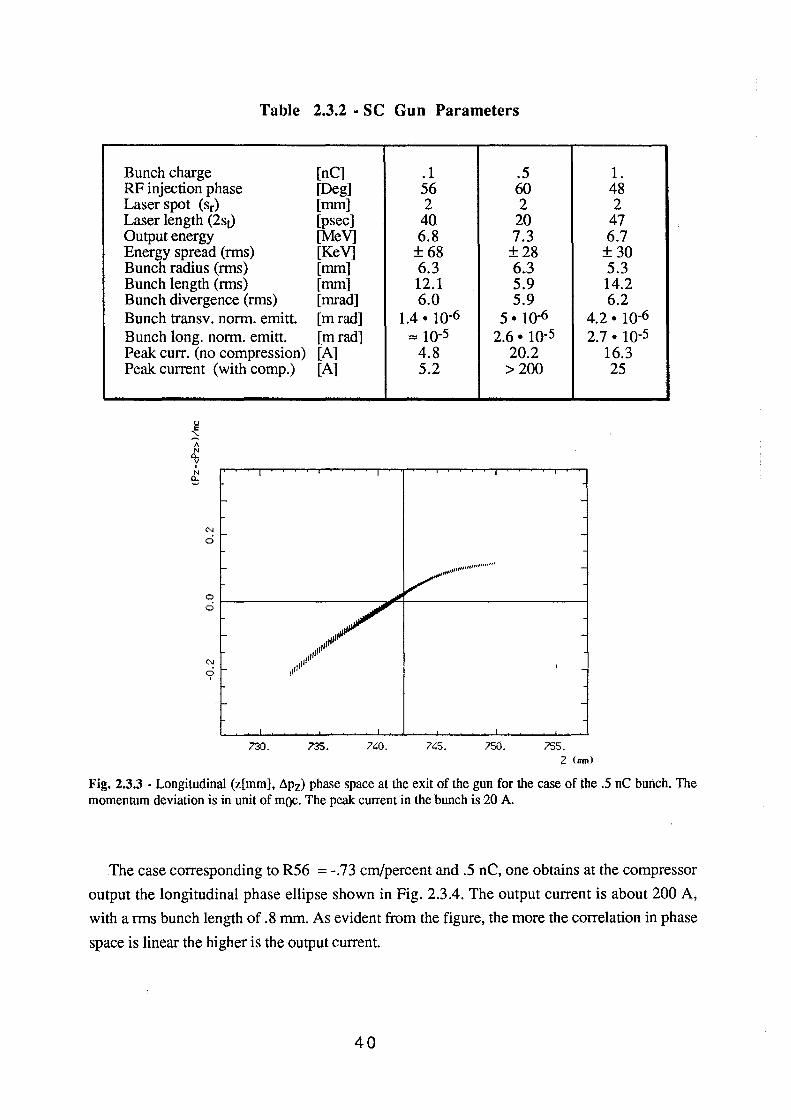
Table 2.3.2 - SC Gun Parameters
Bunch charge RF injection phase Laser spot (sr) Laser length (2st) Output energy Energy spread (rms) Bunch radius (rms) Bunch length (rms) Bunch divergence (rms) Bunch transv. norm. emitt. Bunch long. norm. emitt. Peak curr. (no compression) Peak current (with comp.)
1\ N y N a...
730.
[nC] [Deg] [mm] [psec] [Me V] [KeV] [mm] [mm] [mrad] [m rad] [m rad] [A] [A]
735. 740.
.1 .5 56 60 2 2 40 20 6.8 7.3 ±68 ±28 6.3 6.3 12.1 5.9 6.0 5.9
1.4. lQ-6 5. lQ-6 = lQ-5 2.6. lQ-5
4.8 5.2
,,,,,,,,, .. ,,,,,,,
20.2 >200
1. 48 2
47 6.7 ±30 5.3 14.2 6.2
4.2. lQ-6 2.7. 10-5
16.3 25
745. 750. 755. Z (nrn)
Fig. 2.3.3 - Longitudinal (z[mm], dpz) phase space at the exit of the gun for the case of the .5 nC bunch. The momentum deviation is in unit of moc. The peak current in the bunch is 20 A.
The case corresponding to R56 = -.73 cm/percent and .5 nC, one obtains at the compressor
output the longitudinal phase ellipse shown in Fig. 2.3.4. The output current is about 200 A,
with arms bunch length of .8 mm. As evident from the figure, the more the correlation in phase
space is linear the higher is the output current.
40
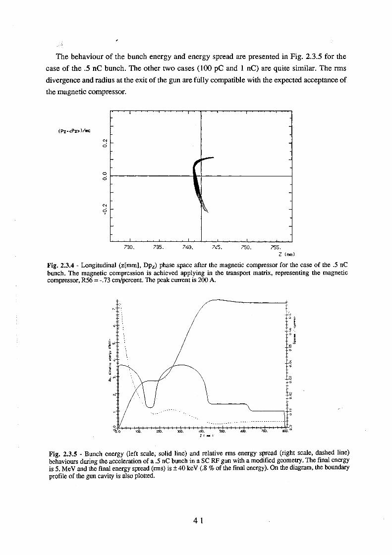
The behaviour of the bunch energy and energy spread are presented in Fig. 2.3.5 for the
case of the .5 nC bunch. The other two cases (100 pC and 1 nC) are quite similar. Therms
divergence and radius at the exit of the gun are fully compatible with the expected acceptance of
the magnetic compressor.
I I I
1- -!Pz-<Pz>llmc
1- -
1- ,t,--- -0
ci
1- -
1--~
1- -
I
730. 735. 7<:;0. 7<:;5. 750. ?SS. Z (mm)
Fig. 2.3.4 - Longitudinal (z[mm], Dpz) phase space after the magnetic compressor for the case of the .5 nC bunch. The magnetic compression is achieved applying in the transport matrix, representing the magnetic compressor, R56 = -.73 cm/percent. The peak current is 200 A.
'• " ,... ,: '' ''
'' '0 ' ~
; . ' {''· I> ' ! . : . ..,, u
100. 200. 300. 400. Z I M I
Soo,
8 0
Fig. 2.3.5 - Bunch energy (left scale, solid line) and relative rms energy spread (right scale, dashed line) behaviours during the acceleration of a .5 nC bunch in a SC RF gun with a modified geometry. The final energy is 5. Me V and the final energy spread (rms) is± 40 keY (.8% of the final energy). On the diagram, the boundary profile of the gun cavity is also plotted.
41
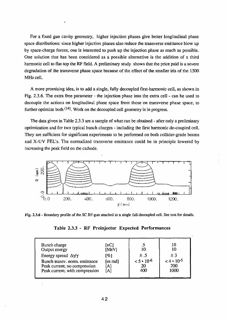
For a fixed gun cavity geometry, higher injection phases give better longitudinal phase
space distributions: since higher injection phases also reduce the transverse emittance blow up
by space-charge forces, one is interested to push up the injection phase as much as possible.
One solution that has been considered as a possible alternative is the addition of a third
harmonic cell to flat-top the RF field. A preliminary study shows that the price paid is a severe
degradation of the transverse phase space because of the effect of the smaller iris of the 1500
MHzcell.
A more promising idea, is to add a single, fully decoupled first-harmonic cell, as shown in
Fig. 2.3.6. The extra free parameter - the injection phase into the extra cell - can be used to
decouple the actions on longitudinal phase space from those on transverse phase space, to
further optimize both (14). Work on the decoupled cell geometry is in progress.
The data given in Table 2.3.3 are a sample of what can be obtained - after only a preliminary
optimization and for two typical bunch charges - including the first harmonic de-coupled cell.
They are sufficient for significant experiments to be performed on both collider-grade beams
and X-UV FEL's. The normalized transverse emittance could be in principle lowered by
increasing the peak field on the cathode.
""'"'0 EO EN
200. 400. 600. 800. 1000. 1200.
Fig. 2.3.6 - Boundary profile of the SC RF-gun attached to a single full-decoupled cell. See text for details.
Table 2.3.3 - RF Preinjector Expected Performances
Bunch charge [nC] .5 10 Output energy [Me V] 10 10 Energy spread lly/y (%] ±.5 ±3 Bunch transv. norm. emittance [mrad] < 5. 10-6 < 4. 10-5 Peak current; no compression [A] 20 200 Peak current; with compression [A] 400 1000
42
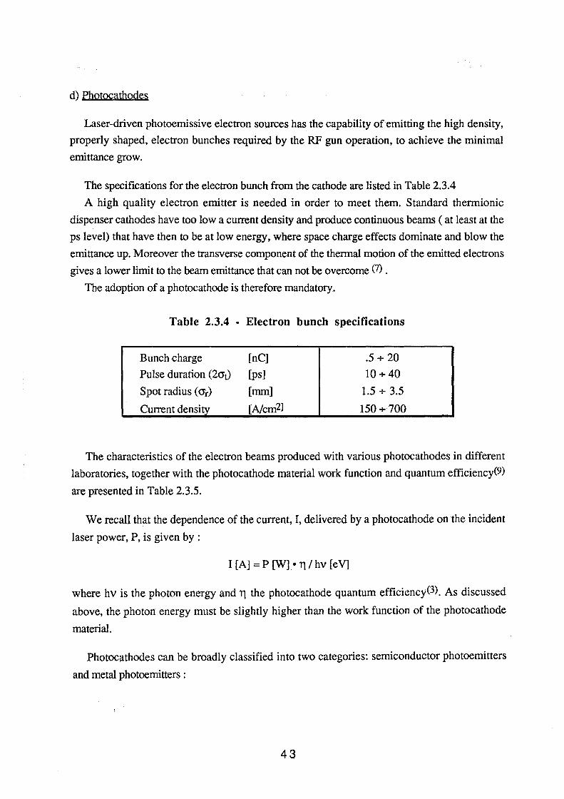
d) Photocathodes
Laser-driven photoemissive electron sources has the capability of emitting the high density,
properly shaped, electron bunches required by the RF gun operation, to achieve the minimal
emittance grow.
The specifications for the electron bunch from the cathode are listed in Table 2.3.4
A high quality electron emitter is needed in order to meet them. Standard thermionic
dispenser cathodes have too low a current density and produce continuous beams ( at least at the
ps level) that have then to be at low energy, where space charge effects dominate and blow the
emittance up. Moreover the transverse component of the thermal motion of the emitted electrons
gives a lower limit to the beam emittance that can not be overcome (7) •
The adoption of a photocathode is therefore mandatory.
Table 2.3.4 - Electron bunch specifications
Bunch charge [nC] .5 + 20
Pulse duration (20"t) [ps] 10+40
Spot radius ( O"r) [mm] 1.5 + 3.5
Current density_ [Ncm2l 150 + 700
The characteristics of the electron beams produced with various photocathodes in different
laboratories, together with the photocathode material work function and quantum efficiency(9)
are presented in Table 2.3.5.
We recall that the dependence of the current, I, delivered by a photocathode on the incident
laser power, P, is given by:
I [A]= P [W] •11 I hv [eV]
where hv is the photon energy and 11 the photocathode quantum efficiency(3). As discussed
above, the photon energy must be slightly higher than the work function of the photocathode
material.
Photocathodes can be broadly classified into two categories: semiconductor photoemitters
and metal photoemitters :
43
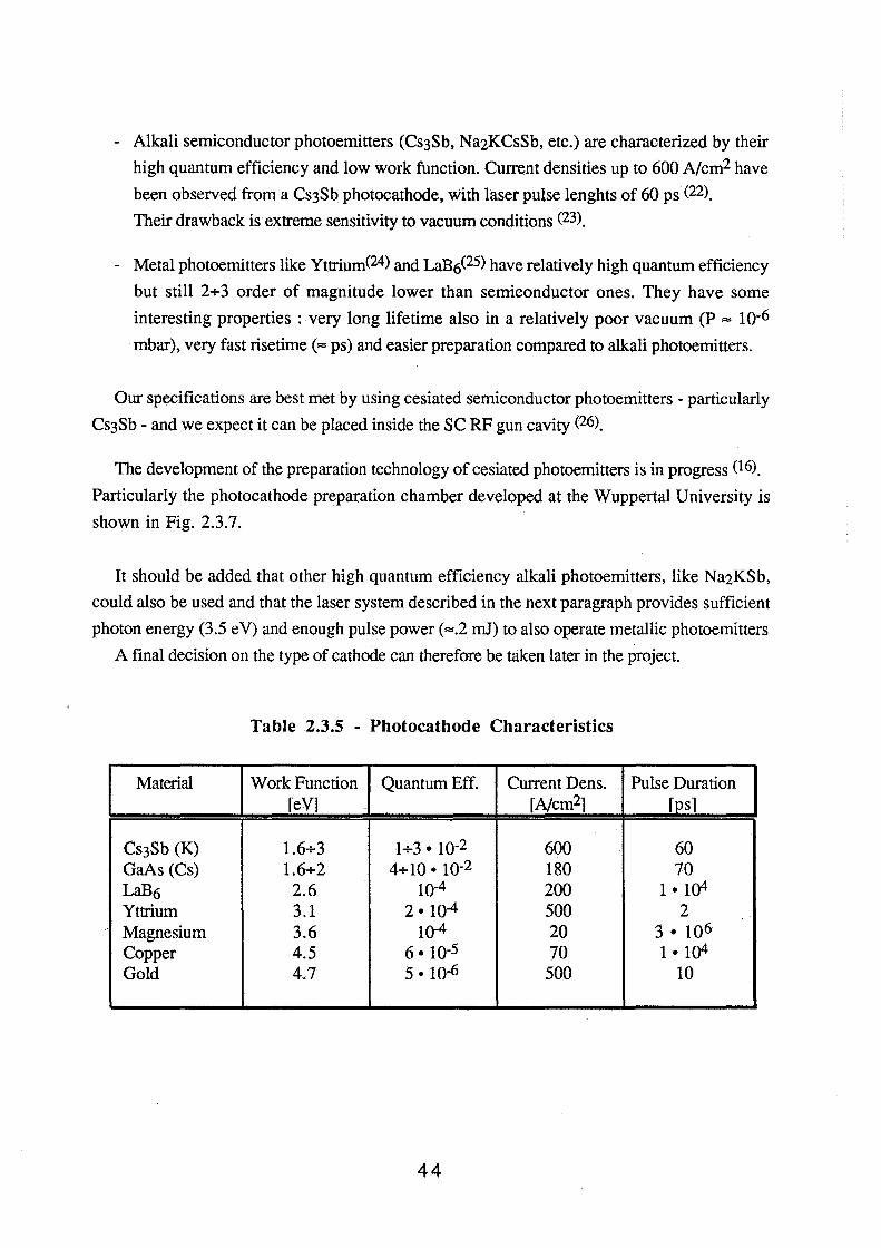
- Alkali semiconductor photoemitters (Cs3Sb, Na2KCsSb, etc.) are characterized by their
high quantum efficiency and low work function. Current densities up to 600 A/cm2 have
been observed from a Cs3Sb photocathode, with laser pulse lenghts of 60 ps (22).
Their drawback is extreme sensitivity to vacuum conditions (23).
- Metal photoemitters like Yttrium(24) and LaB6(25) have relatively high quantum efficiency
but still 2+3 order of magnitude lower than semiconductor ones. They have some
interesting properties : very long lifetime also in a relatively poor vacuum (P = lQ-6
mbar), very fast risetime ("" ps) and easier preparation compared to alkali photoemitters.
Our specifications are best met by using cesiated semiconductor photoemitters - particularly
Cs3Sb - and we expect it can be placed inside the SC RF gun cavity (26).
The development of the preparation technology of cesiated photoemitters is in progress (16).
Particularly the photocathode preparation chamber developed at the Wuppertal University is
shown in Fig. 2.3.7.
It should be added that other high quantum efficiency alkali photoemitters, like Na2KSb,
could also be used and that the laser system described in the next paragraph provides sufficient
photon energy (3.5 eV) and enough pulse power (=.2 mJ) to also operate metallic photoemitters
A final decision on the type of cathode can therefore be taken later in the project.
Table 2.3.5 - Photocathode Characteristics
Material Work Function Quantum Eff. Current Dens. Pulse Duration [eV] [Ncm2] [Q_s]
Cs3Sb (K) 1.6+3 1+3. lQ-2 600 60 GaAs (Cs) 1.6+2 4+ 10 • 10-2 180 70 LaB6 2.6 10-4 200 1 • 104 Yttrium 3.1 2. 10-4 500 2 Magnesium 3.6 10-4 20 3. 106 Copper 4.5 6 • 10-s 70 1. 104 Gold 4.7 5. 10-6 500 10
44
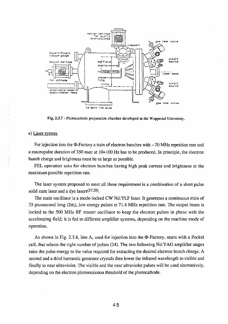
3ayard-Alparl vacuum gouge
mol! on beoll owa fOr" t;'lUCW'll
111 f. cro~::o lclnca
le 11oln l.on po..rnp
alkoll source
olkoll source
gaa l9ok "olva
Fig. 2.3.7 -Photocathode preparation chamber developed at the Wuppertal University.
e) Laser system
For injection into the <I>-Factory a train of electron bunches with - 70 MHz repetition rate and
a macropulse duration of 350 nsec at 10+100 Hz has to be produced. In principle, the electron
bunch charge and brightness must be as large as possible.
FEL operation asks for electron bunches having high peak current and brightness at the
maximum possible repetition rate.
The laser system proposed to meet all these requirement is a combination of a short pulse
solid state laser and a dye lasers(27,28).
The main oscillator is a mode-locked CW Nd:YLF laser. It generates a continuous train of
35 picosecond long (2crt), low energy pulses at 71.4 MHz repetition rate. The output beam is
locked to the 500 MHz RF master oscillator to keep the electron pulses in phase with the
accelerating field; it is fed to different amplifier systems, depending on the machine mode of
operation.
As shown in Fig. 2.3.8, line A, used for injection into the <I>-Factory. starts with a Po~kel
cell, that selects the right number of pulses (24). The two following Nd:YAG amplifier stages
raise the pulse energy to the value required for extracting the desired electron bunch charge. A
second and a third harmonic generator crystals then lower the infrared wavelength to visible and
finally to near ultraviolet. The visible and the near ultraviolet pulses will be used alternatively,
depending_ on the electron photoemission threshold of the photocathode.
45
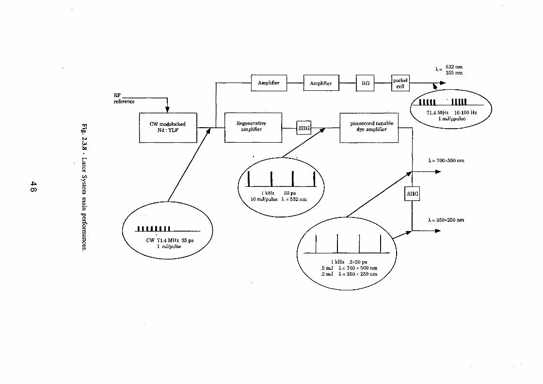
"-j
~-N (M Qo I
l '
"" (I)
~ Cl)
~ '< (I) ....
0'> ~
3 3
"" :r "C::l ~
§> .... 3 "" ::l n ~ r'
RF _____ __,
reference
CW modelocked Nd:YLF
CW 71.4 MHz 35 ps 1 nJ/pulse
Amplifier
Regenerative amplifier
picosecond tunable dye amplifier
I I I I 1 kHz .2+20 ps
.5 mJ A= 700 + 500 nm
.2 mJ A = 350 + 250 nm
A= 532 nm 355 nm
A= 700+500 nm
A= 350+250 nm
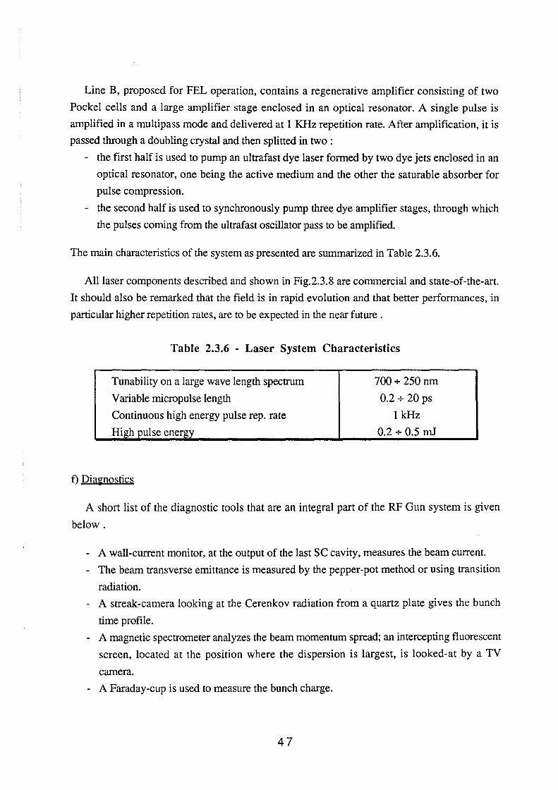
Line B, proposed for FEL operation, contains a regenerative amplifier consisting of two
Pockel cells and a large amplifier stage enclosed in an optical resonator. A single pulse is
amplified in a multipass mode and delivered at 1 KHz repetition rate. After amplification, it is
passed through a doubling crystal and then splitted in two :
- the first half is used to pump an ultrafast dye laser formed by two dye jets enclosed in an
optical resonator, one being the active medium and the other the saturable absorber for
pulse compression.
- the second half is used to synchronously pump three dye amplifier stages, through which
the pulses coming from the ultrafast oscillator pass to be amplified.
The main characteristics of the system as presented are summarized in Table 2.3.6.
All laser components described and shown in Fig.2.3.8 are commercial and state-of-the-art.
It should also be remarked that the field is in rapid evolution and that better performances, in
particular higher repetition rates, are to be expected in the near future .
Table 2.3.6 - Laser System Characteristics
Tunability on a large wave length spectrum
Variable micropulse length
Continuous high energy pulse rep. rate
High pulse energy
f) Diagnostics
700+250 nm
0.2 + 20 ps
1kHz
0.2 + 0.5 mJ
A short list of the diagnostic tools that are an integral part of the RF Gun system is given
below.
- A wall-current monitor, at the output of the last SC cavity, measures the beam current.
- The beam transverse emittance is measured by the pepper-pot method or using transition
radiation.
- A streak-camera looking at the Cerenkov radiation from a quartz plate gives the bunch
time profile.
- A magnetic spectrometer analyzes the beam momentum spread; an intercepting fluorescent
screen, located at the position where the dispersion is largest, is looked-at by a TV
camera.
- A Faraday-cup is used to measure the bunch charge.
47
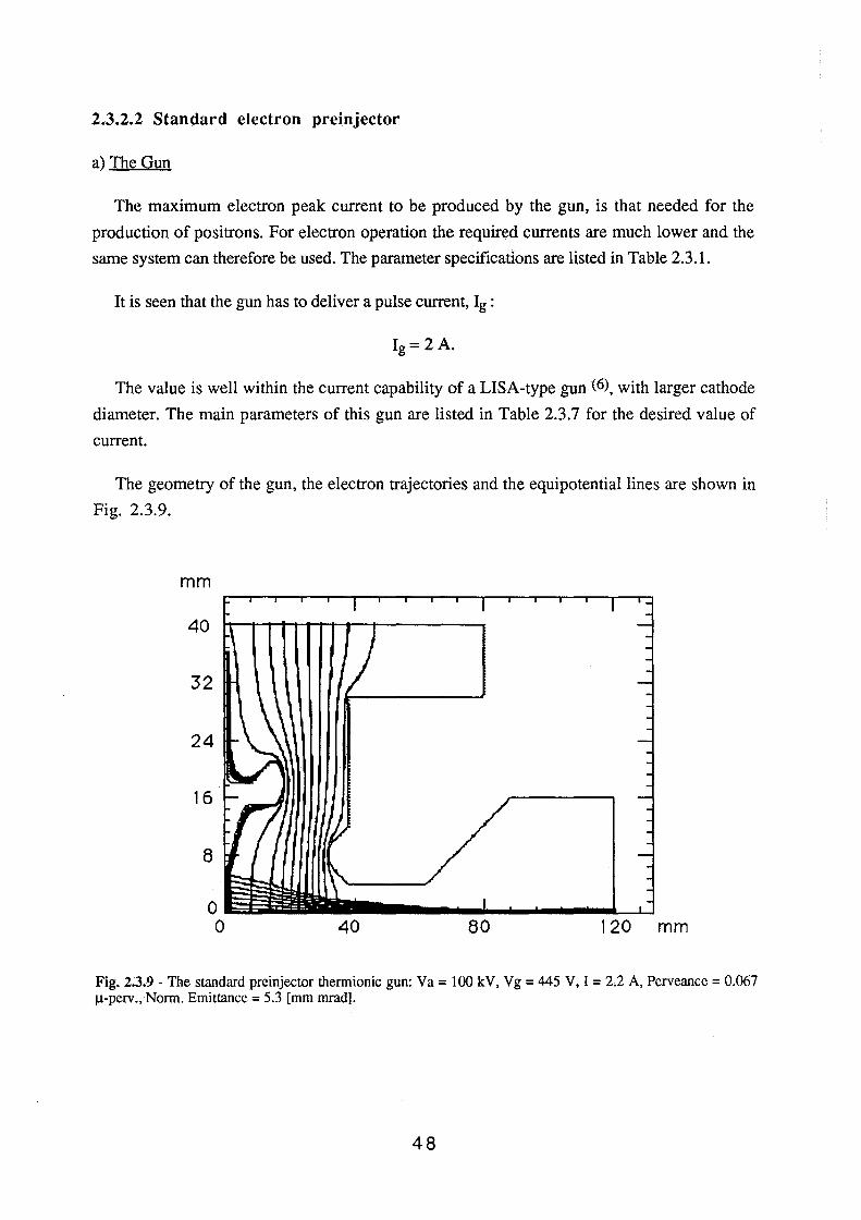
2.3.2.2 Standard electron preinjector
a) The Gun
The maximum electron peak current to be produced by the gun, is that needed for the
production of positrons. For electron operation the required currents are much lower and the
same system can therefore be used. The parameter specifications are listed in Table 2.3.1.
It is seen that the gun has to deliver a pulse current, Ig :
Ig= 2 A.
The value is well within the current capability of a LISA-type gun (6), with larger cathode
diameter. The main parameters of this gun are listed in Table 2.3.7 for the desired value of
current.
The geometry of the gun, the electron trajectories and the equipotentiallines are shown in
Fig. 2.3.9.
mm
40
32
24
16
8
0 0 40 80 120 mm
Fig. 2.3.9- The standard preinjector thermionic gun: V a= 100 kV, Vg = 445 V, I= 2.2 A, Perveance = 0.067 J.L-perv., Norm. Emittance = 5.3 [mm mrad].
48
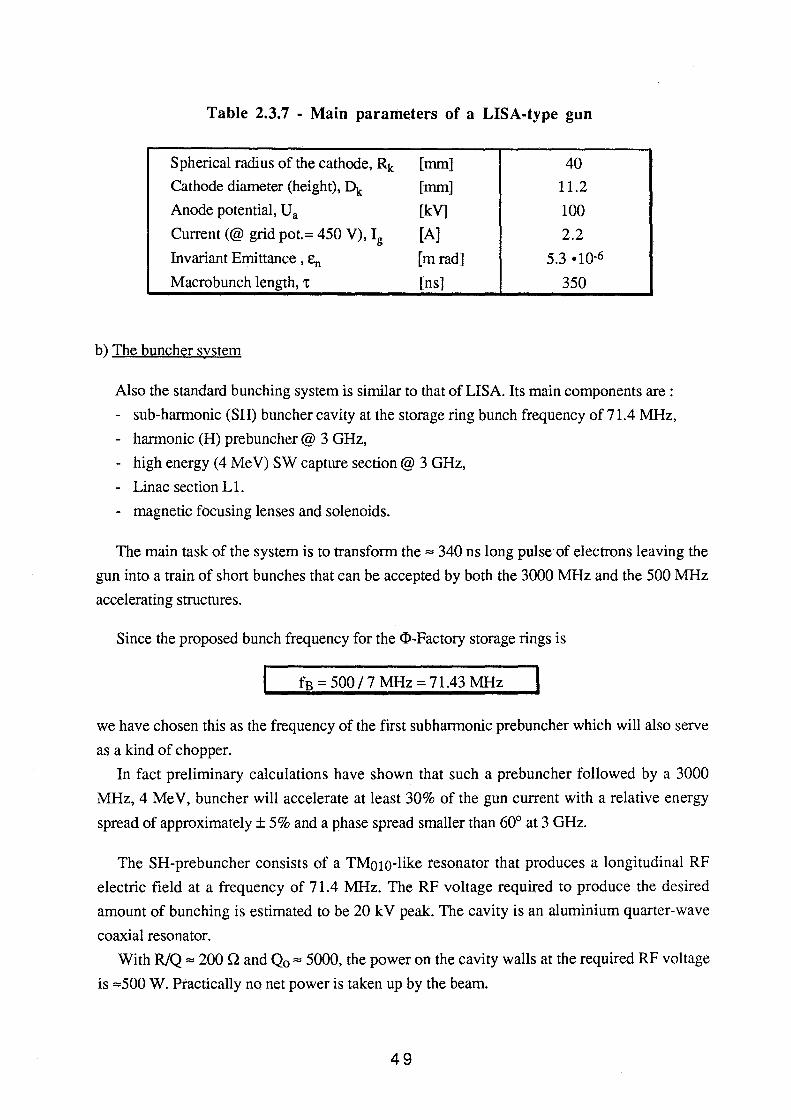
Table 2.3.7 - Main parameters of a LISA-type gun
Spherical radius of the cathode, Rk [mm] 40
Cathode diameter (height), ~ [mm] 11.2
Anode potential, U a [kV] 100
Current(@ grid pot.= 450 V), Ig [A] 2.2
Invariant Emittance , En [m rad] 5.3 ·10-6
Macrobunch length, 't [ns] 350
b) The buncher system
Also the standard bunching system is similar to that of LISA. Its main components are :
- sub-harmonic (SH) buncher cavity at the storage ring bunch frequency of 71.4 MHz,
- harmonic (H) prebuncher @ 3 GHz,
- high energy ( 4 Me V) SW capture section @ 3 GHz,
- Linac section L 1.
- magnetic focusing lenses and solenoids.
The main task of the system is to transform the ,. 340 ns long pulse of electrons leaving the
gun into a train of short bunches that can be accepted by both the 3000 MHz and the 500 MHz
accelerating structures.
Since the proposed bunch frequency for the <!>-Factory storage rings is
fs = 500 I 7 MHz = 71.43 MHz
we have chosen this as the frequency of the first subharmonic prebuncher which will also serve
as a kind of chopper.
In fact preliminary calculations have shown that such a prebuncher followed by a 3000
MHz, 4 Me V, buncher will accelerate at least 30% of the gun current with a relative energy
spread of approximately± 5% and a phase spread smaller than 60° at 3 GHz.
The SH-prebuncher consists of a TMow-like resonator that produces a longitudinal RF
electric field at a frequency of 71.4 MHz. The RF voltage required to produce the desired
amount of bunching is estimated to be 20 kV peak. The cavity is an aluminium quarter-wave
coaxial resonator.
With R/Q"" 200 Q and Q0 "" 5000, the power on the cavity walls at the required RF voltage
is :::::500 W. Practically no net power is taken up by the beam.
49
The RF source is a solid state amplifier driven by a low level signal, prescaled from the 500
MHz main reference source of the superconducting linac. The usual amplitude and phase
controls of the cavity drive are foreseen, in addition to the cavity tuning system needed to keep
the resonant frequency constant independent of temperature.
The 3 GHz harmonic H-prebuncher system provides additional bunching before acceleration
in the capture section. A reentrant copper pill-box cavity operating in the fundamental TMo10
mode is used. At 3 GHz the cavity main parameters are the following:
Zeff ... 1.5 Mn Q0 ,.. 10,000.
For a gap RF voltage of 10+ 15 kV peak, the power dissipated in the cavity is less then 200
W, a value easily obtainable either by derivation from the capture section feed line or from a
dedicated solid state amplifier. The control system is the same as that for the SH buncher except
for the cavity tuning system that will probably not be necessary because of the large resonator
bandwidth.
c) Capture Section
The Capture Section has a field of,.. 12 Me V /m, is approximately 50 cm long and accelerates
the electron beam to an energy of,.. 4 Me V; it consists of a graded-~ standing wave (SW)
biperiodic structure of the same type as that used for LISA.
The average effective shunt impedance, Zerr, is ,.. 70 MW /m.
To produce the desired energy gain the RF power required is given by the sum of the power
dissipated in the cavity, Po
Pn= ( V ace )2 I ( Zerf. 1) ,.. 0.5 MW
and the beam power, Ps, for an average beam current, <lb >,of 600 mAin the 350 ns long
macrobunch.
PB =V ace. <lb> = 2.4 MW
The overall RF power over the 1 JlS long RF pulse is thus :
P,.. 3 MW.
The coupling factor between the RF source and the section is :
corresponding to the no-beam standing wave ratio (SWR) in the waveguide.
50
The average power needed is only 30 W due to the very low duty factor. In the S-band
frequency range klystrons for this output power are in large supply. The klystron is connected
to the capture section through a waveguide and is protected against reflections by a RF isolator.
Standard RF feedbacks loops on amplitude and phase have to be provided to keep the beam
parameters in accordance with the design values.
2.3.3 - Positron production
a) Introduction
Electrons from the capture section are fed to the first Se Linac section, Ll. Section Ll
consists of 4 standard four-cell superconducting cavities, each in its own cryostat, giving a
nominal overall voltage of 48 MY. The electrons enter Ll with a nominal energy of 4 Me V and
exit from Ll with a nominal energy of 52 Me V. The relative energy spread has decreased to
±5xl0-3 and the phase spread is less than± 5°@ 500 MHz.
This allows the beam to be injected unto the main se linac axis using a pulsed inflector. The
beam is further accelerated to 100 Me V in section L2 and then injected into the main section,
L3, and the recirculation system.
To generate the positrons, electrons that have reached the nominal energy of 340 Me V after
one passage through the main linac are bent back to the e-e+ converter.
Because the transport channel from the output of the linac to the converter is isochronous
and achromatic, the above phase spread of the electrons will be conserved and the phase of the
produced positrons, at the entrance of the 3 GHz positron capture section, will be contained
within 60°.
The main components of the positron production line are:
-converter
- magnetic focusing
- high gradient capture and acceleration section
b) Converter and magnetic focusing
The average power of the 300 Me V electron beam striking the converter is :
51
where t = 340 ns is the pulse duration, fr = 10Hz is the repetition frequency, E is the primary
electron energy, Tl- the electron bunching and transport efficiency, and Ig the electron gun pulse
current.
For high energy electrons the energy loss is almost entirely due to bremsstrahlung - for heavy elements such as W, Au or Pb this is already true for energies higher than about 20 m0 c2
(29)- and the power pissipated in the converter is only a fraction of Pc. The average energy loss
per cm is given by
( -dE/dx)md = N E Fmd
where N is the number of atoms per cm3, E is the energy of the incident electrons and Frad is a
bremsstrahlung cross section.
Again, for energies E >> E0 = 137 moc2 z-1/3- where Z is the atomic number of the target
material (for gold, E0 "" 32 m0c2 ) -, Fmd is practically independent on the energy of the incident
electrons(29). According to Amman(30), for E > 100 Me V the ratio of the power deposited to the
primary beam energy is practically constant and the deposited power ,Pd. is approximately 16%
of the incident power. For our case:
Pd"" .16 Pc= 0.11 kW
This is much below the power rating of the ADONE converter (about 3 kW). Considering
the good performance of the latter, we therefore propose to adopt a similar solution for ARES.
The energy of the incident electrons is higher for ARES than for ADO NE (300 Me V instead
of about 100 Me V) and the thickness of the converter target has accordingly been increased
from "" 1 to "" 1.5 radiation lengths.
For good positron production efficiency the diameter of the electron beam spot on the
converter should be of the order of 1 mm. This is obtained by means of a special focusing
system consisting of a quadrupole triplet. Care must also be taken to ensure that the spot
diameter does not decrease below "" 1 mm, because excessive power density would cause
excessive thermld stresses and eventually damage the target.
To optimize the positron capture efficiency, the converter should be closely followed by a
high magnetic field("" 5+ 6 Tesla) region and then by a short capture section with a very high
accelerating electric field and immersed in a solenoidal magnetic field.
The very intense magnetic field next to the converter is generated by a pulsed tapered
solenoid with the help of a 'flux concentrator' similar to those employed at SLAC and DESY.
The magnetic field value in the flux concentrator must be matched to that of the the capture
52
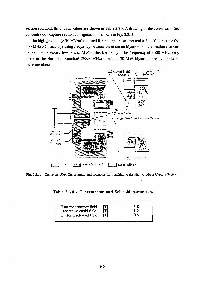
section solenoid; the chosen values are shown in Table 2.3.8. A drawing of the converter- flux
concentrator- capture section configuration is shown in Fig. 2.3.10.
The high gradient(> 30 MV/m) required for the capture section makes it difficult to use the
500 MHz SC linac operating frequency because there are no klystrons on the market that can
deliver the necessary few tens of MW at this frequency . The frequency of 3000 MHz, very
close to the European standard (2998 MHz) at which 30 MW klystrons are available, is
therefore chosen.
Vacuum Chamber
Tcn~ct Cartnge
""'J'apcred Field \ Sole noicl \
Uniform Field s,; Svlerwid
\ /ligh Gradient Capture Scclwn
1, :,--l iran f;,~ ~tainless i:)tcel C\ Cu \Vi rulings
Fig. 2.3.10 - Converter: Flux Concentrator and solenoids for matching to the High Gradient Capture Section
Table 2.3.8 - Concentrator and Solenoid parameters
Flux concentrator field [T] Tapered solenoid field [T] Uniform solenoid field [T]
53
5.8 1.2 0.5
Note that in our case the SLED-type pulse compression technique can not be used because
the combination of long pulse duration (400 ns) and low positron peak current (a few mA)
would lead to an unacceptable high energy dispersion (>20%) (4).
c) High gradient capture section
The main specifications for the capture section are the following:
High field gradient E ;::: 30MV/m
Short length L ~ 2m No SLED; single Klystron drive PRFmax = 35MW
Maximum cavity input power PRF ""30MW.
Different types of accelerating structures can be chosen to fulfil the above requirements : a
preliminary discussion on the choice of the accelerating structure is given in (4) where the choice
has been restricted to travelling wave (TW) constant gradient (CO) and standing wave (SW)
structures. By choosing for the length the value L = 1.5 m and for the power PRF = 30 MW,
one obtains for the accelerating field E , and the overall nominal voltage V ace the values shown
in the following Table 2.3.9.
Taking into account that the mean positron energy accepted for acceleration will be about 10
MeV, both structure types can accelerate the positrons to an average energy ;::: 50 MeV,
comparable to that of the electron beam produced by the electron source at the location where
both beams merge. The standing wave structure, capable of higher fields and therefore
affording a larger safety factor, is nevertheless preferred.
Table 2.3.8 - Accelerating structure parameters
RF Structure
CO Travelling wave
n/2 biperiodic SW
54
E [MY/m]
27
37
Voce [M V]
40
56
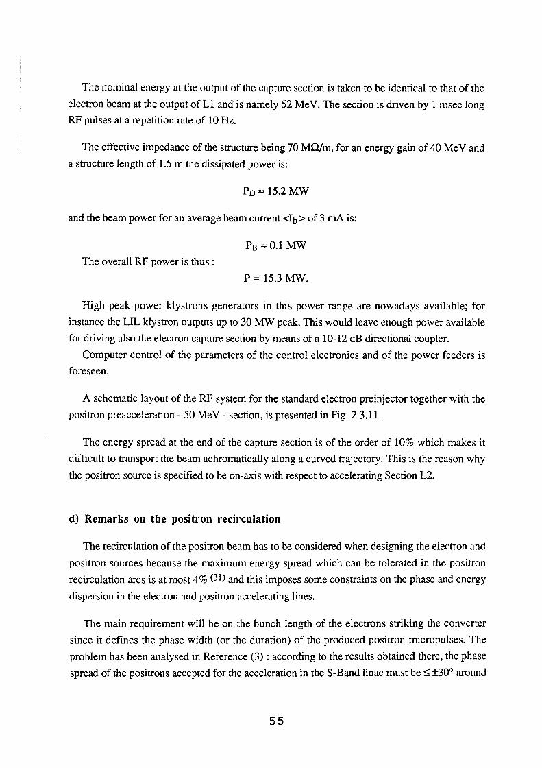
The nominal energy at the output of the capture section is taken to be identical to that of the
electron beam at the output of L 1 and is namely 52 Me V. The section is driven by 1 msec long
RF pulses at a repetition rate of 10 Hz.
The effective impedance of the structure being 70 M.O/m, for an energy gain of 40 Me V and
a structure length of 1.5 m the dissipated power is:
Po"" 15.2MW
and the beam power for an average beam current <lb > of 3 mA is:
PB =::0.1 MW
The overall RF power is thus :
P = 15.3 MW.
High peak power klystrons generators in this power range are nowadays available; for
instance the LIL klystron outputs up to 30 MW peak. This would leave enough power available
for driving also the electron capture section by means of a 10-12 dB directional coupler.
Computer control of the parameters of the control electronics and of the power feeders is
foreseen.
A schematic layout of the RF system for the standard electron preinjector together with the
positron preacceleration - 50 Me V - section, is presented in Fig. 2.3.11.
The energy spread at the end of the capture section is of the order of 10% which makes it
difficult to transport the beam achromatically along a curved trajectory. This is the reason why
the positron source is specified to be on-axis with respect to accelerating Section L2.
d) Remarks on the positron recirculation
The recirculation of the positron beam has to be considered when designing the electron and
positron sources because the maximum energy spread which can be tolerated in the positron
recirculation arcs is at most 4% (31) and this imposes some constraints on the phase and energy
dispersion in the electron and positron accelerating lines.
The main requirement will be on the bunch length of the electrons striking the converter
since it defines the phase width (or the duration) of the produced positron micropulses. The
problem has been analysed in Reference (3) : according to the results obtained there, the phase
spread of the positrons accepted for the acceleration in the S-Band linac must be s; ±30° around
55
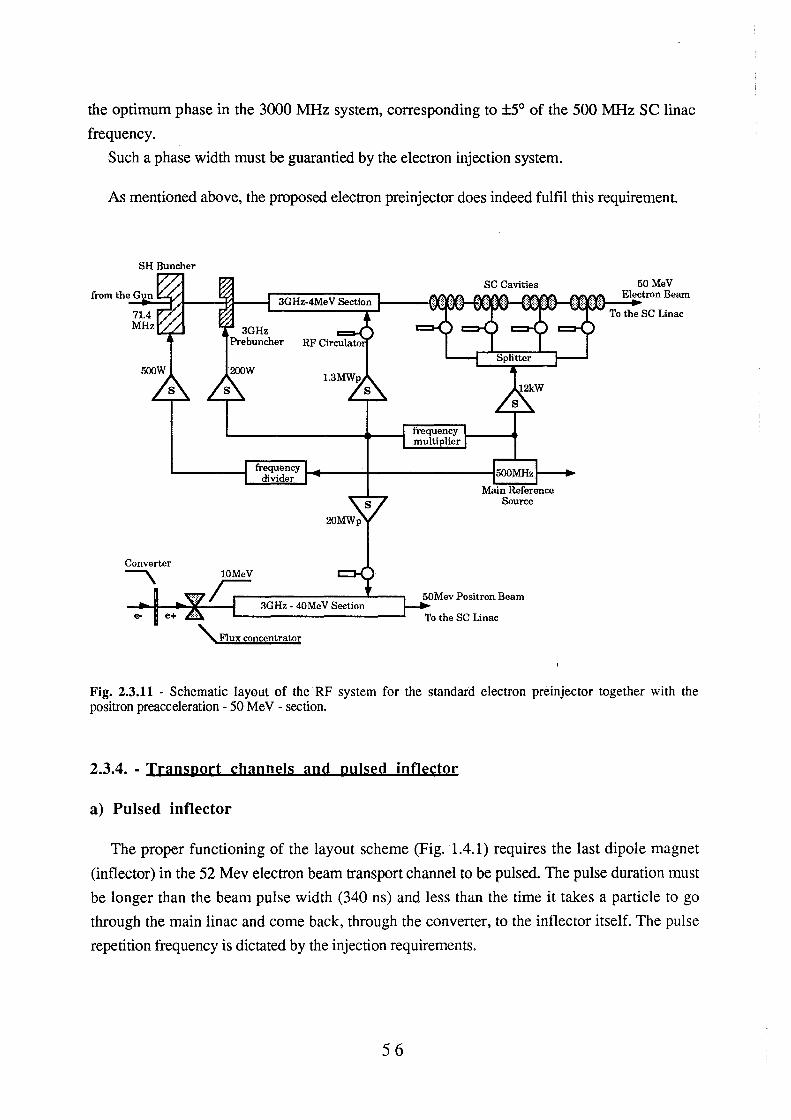
the optimum phase in the 3000 MHz system, corresponding to ±5° of the 500 MHz SC linac
frequency.
Such a phase width must be guarantied by the electron injection system.
As mentioned above, the proposed electron preinjector does indeed fulfil this requirement.
SH Buncher
To the SC Linac
Fig. 2.3.11 - Schematic layout of the RF system for the standard electron preinjector together with the positron preacceleration- 50 Me V- section.
2.3.4. - Transport channels and pulsed inflector
a) Pulsed inflector
The proper functioning of the layout scheme (Fig. 1.4.1) requires the last dipole magnet
(inflector) in the 52 Mev electron beam transport channel to be pulsed. The pulse duration must
be longer than the beam pulse width (340 ns) and less than the time it takes a particle to go
through the main linac and come back, through the converter, to the inflector itself. The pulse
repetition frequency is dictated by the injection requirements.
56
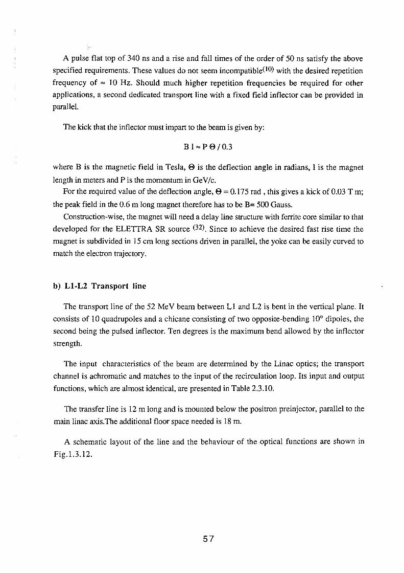
A pulse flat top of 340 ns and a rise and fall times of the order of 50 ns satisfy the above
specified requirements. These values do not seem incompatibleOO) with the desired repetition
frequency of "" 10 Hz. Should much higher repetition frequencies be required for other
applications, a second dedicated transport line with a fixed field inflector can be provided in
parallel.
The kick that the inflector must impart to the beam is given by:
B 1 ""P e /0.3
where B is the magnetic field in Tesla, 8 is the deflection angle in radians, 1 is the magnet
length in meters and Pis the momentum in GeV/c.
For the required value of the deflection angle, 8 = 0.175 rad , this gives a kick of 0.03 T m;
the peak field in the 0.6 m long magnet therefore has to be B= 500 Gauss.
Construction-wise, the magnet will need a delay line structure with ferrite core similar to that
developed for the ELETTRA SR source (32). Since to achieve the desired fast rise time the
magnet is subdivided in 15 cm long sections driven in parallel, the yoke can be easily curved to
match the electron trajectory.
b) Ll-L2 Transport line
The transport line of the 52 Me V beam between L1 and L2 is bent in the vertical plane. It
consists of 10 quadrupoles and a chicane consisting of two opposite-bending 10° dipoles, the
second being the pulsed inflector. Ten degrees is the maximum bend allowed by the inflector
strength.
The input characteristics of the beam are determined by the Linac optics; the transport
channel is achromatic and matches to the input of the recirculation loop. Its input and output
functions, which are almost identical, are presented in Table 2.3.10.
The transfer line is 12 m long and is mounted below the positron preinjector, parallel to the
main linac axis.The additional floor space needed is 18 m.
A schematic layout of the line and the behaviour of the optical functions are shown in
Fig.1.3.12.
57
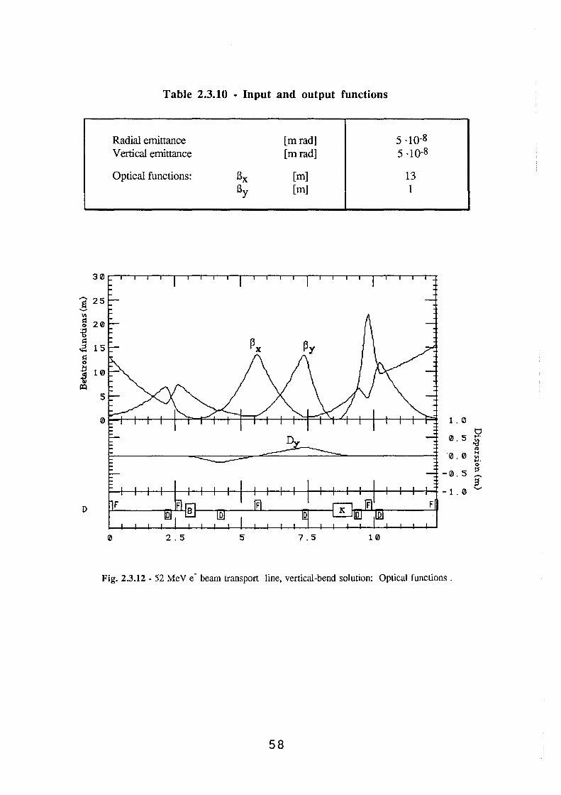
Table 2.3.10 - Input and output functions
Radial ernittance [mrad] 5 ·10-8 Vertical ernittance [m rad] 5 ·l0-8
Optical functions: Bx [m] 13 By [m] 1
s
0 1.0 t:::J
0.5 .... olg I»
0.0 lo( VI .... 0
-0.5 ~ ..-.. a
-1.0 .......
0 2.5 5 7.5 10
Fig. 2.3.12 - 52 MeV e- beam transport line, vertical-bend solution: Optical functions .
58
2.4 • ACCELERATION SYSTEM
2.4.1 - Superconductina= cayities
Superconducting cavities performances, compared to those of normal conducting cavities,
outweigh the disadvantage of their very low operating temperature. In fact, their quality factor
Q0 being 4 + 5 orders of magnitude higher than that of standard copper cavities, they can be
operated ew - at low temperature - while the large amount of stored energy makes for a much
reduced beam energy spread.
For the construction of high acceleration field cavities for ultrarelativistic particles, the use of
bulk Niobium is favoured because of its relatively high critical temperature, Tc = 9.2 K, and its
good mechanical properties compared to those of other superconducting metals.
At 500 MHz, theoretical upper limits can be derived for the corresponding accelerating field
and Q values from the Nb upper critical field (Hc2 = 1600 Gauss) and from its surface
resistance, Rs , at 4.2 K calculated from the BeS theory of superconductivity ; one obtains : Ea
""40 MV/m and Q0 "" 4 x 10⁹ (33).
With present technology, fields in the range of Ea~ 10 MV/m (at 4.2 K and 500 MHz) and
low-field Q values "" 3.4 x 10⁹ are routinely obtained in vertical tests of four-cell cavities.
Degradation of Q0 vs Ea and of the maximum Ea when cavities are horizontal, are topics under
investigation. The field emission of Nb surface in se cavities, a factor limiting the obtainable Q
at high surface electric fields, is related to the surface cleaning: it has been ascertained that very
clean Nb surfaces can support fields larger than 100 MV/m without electron emission.
To raise Q0 , se cavities can be operated at lower temperatures; this does not however
usually improve Ea in the same way because Ea is limited by the presence of non
superconducting defects. These defects also produce the so called "residual" surface resistance,
Rres . The value of Rres , that can not be computed from theory because it depends on the actual
surface physical and chemical conditions, of course sets the lowest useful temperature of
operation, below which no further benefit on Q0 is obtained.
The presence of surface defects is considered unavoidable and the main effort over the past
10 years, has been devoted to reducing their size and number and to handle the local heating
they generate. In fact better cryostabilization by using high thermal conductivity Nb, is the best
techinque known to raise Ea .
59
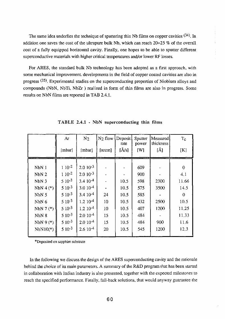
The same idea underlies the technique of sputtering thin Nb films on copper cavities (34). In
addition one saves the cost of the ultrapure bulk Nb, which can reach 20+25% of the overall
cost of a fully equipped horizontal cavity. Finally, one hopes to be able to sputter different
superconductive materials with higher critical temperatures and/or lower RF losses.
For ARES, the standard bulk Nb technology has been adopted as a first approach, with
some mechanical improvement. developments in the field of copper coated cavities are also in
progress (35). Experimental studies on the superconducting properties of Niobium alloys and
compounds (NbN, NbTi, NbZr ) realized in form of thin films are also in progress. Some
results on NbN films are reported in TAB 2.4.1.
TABLE 2.4.1 - NbN superconducting thin films
Ar N2 N2 flow Deposit. Sputter Measured Tc rate power thickness
[mbar] [mbar] [seem] [A/s] [W] [AJ [K]
NbN 1 110-2 2.0 10-3 - - 609 - 0
NbN2 110-2 2.0 10-3 - - 900 - 4.1
NbN3 5 10-3 3.4 10-4 - 10.5 598 2300 11.66
NbN 4 (*) 5 10-3 3.0 10-4 - 10.5 575 3500 14.5
NbN5 5 10-3 3.4 10-4 24 10.5 585 - 0
NbN6 5 10-3 1.2 10-4 10 10.5 432 2500 10.5
NbN 7 (*) 5 10-3 1.2 10-4 10 10.5 407 1200 11.25
NbN8 5 10-3 2.0 10-4 15 10.5 484 - 11.33
NbN 9 (*) 5 10-3 2.0 10-4 15 10.5 484 900 11.6
NbN10(*) 5 10-3 2.6 10-4 20 10.5 545 1200 12.3
*Deposited on sapphire substrate
In the following we discuss the design of the ARES superconducting cavity and the rationale
behind the choice of its main parameters. A summary of the R&D program that has been started
in collaboration with Italian industry is also presented, together with the expected milestones to
reach the specified performance. Finally, fall-back solutions, that would anyway guarantee the
60
minimum performance needed for injection into the <I>-Factory, within the proposed time
schedule, are sketched.
a) Frequency
To guarantee the high quality of beam specified in paragraph 2.3.2.1, we are forced to select
a se Linac frequency on the low side of the .35 GHz + 3 GHz range currently used for the
acceleration of ultrarelativistic beams. In fact one can show (36) that to ensure the kind of single
bunch performance required for linear colliders and FEL's, the frequency should lie below
1500 MHz.
If we further restrict the choice to most commonly used frequency values, we are left with
only two frequencies: 350 MHz, developed and used at eERN, and 500 MHz, developed and
used at DESY, KEK and on LISA in our own Laboratory.
From a purely technical point of view, the advantages of 500 MHz over 350 MHz are mainly
three:
- 500 MHz is a sub-harmonic of other widely used frequencies: 1, 1.5 and 3 GHz;
- standard power sources are easily found on the market;
- the cavities and their ancillary equipment, being smaller, are easier to handle.
The last argument is of course important but the two others are more fundamental since they
are linked to the positron capability required from our Linac and, we believe, to the
development potential of the accelerator.
In fact, from the latter point of view, one of the goals of ARES is to produce a very low
emittance beam, with high peak current and high repetition rate, so that the installation may
become a test bench for future Te V colliders.
As shown by several authors (37) a fully superconducting linear accelerators may become
advantageous for se Te V eolliders if accelerating fields exceeding 30 MV /m can be achieved
since the cost would then become competitive - for long (10+20 cells) structures in the
frequency range upwards of""' 3 GHz - with that of warm structures. The rate of increase of the
useful field in se cavities over the past 10 years, together with the number and quality of R&D
programs in progress all over the world, make it reasonable to envisage that the goal will be
reached in the not too distant future. In a 3 GHz eollider, however, the high peak current, high
bunch charge, low emittance first part of the accelerator (below""' 1GeV) would presumably
have to operate at much lower frequency. ARES could therefore be considered as a prototype of
the injector for a Te V collider and, as such, it should be operated on a subharmonic of one of
the higher standard frequencies.
61
A number of other minor advantages and disadvantages can be found for each of the two
frequencies. Some the arguments that are usually given and that, in our opinion, balance out
are:
- the 350 MHz cavity has a lower RF power loss per meter of active length. In fact the BCS
part of the surface resistance, at a given temperature, scales like ro2.
- for a constant number of cells, 350 MHz requires less cavities and less associated
equipment. For a given Eacc, the numbers scale like ro.
- the 500 MHz cavity has a smaller surface (it scales like ro-2) and therefore, presumably, a
smaller number of field emitters and defects that limit the maximum field holding
capability and produce the negative slope in the measured Q versus Eacc curves.
- the 500 MHz cavity smaller overall dimension, scaling like ro-3, give greater freedom to
implement and test cleaning techniques.
It is our conclusion that with 500 MHz cavities the chance obtaining the high specified
design value of Eacc is greater.
Moreover, on an overall project basis, it has to be taken into account that the slight capital
cost increase for cavities is almost exactly balanced by the lower cost of the RF power sources,
which - at 500 MHz and for the .ARES power level- are standard and available from stock.
b) Cavity Geometry
Once the operation frequency has been fixed, the base cavity geometry has to be optimized to
best meet the overall design specifications, and all the ancillary equipment has to be designed.
In practice, as far as geometry is concerned, the only important parameter is the number of cells
because, since 1979, all se accelerating structures for ultrarelativistic particles are either
spherical or elliptical. As a consequence, apart from the frequency scaling factor, they differ just
on minor details (usually dictated by the fabrication procedure) that affect the overall cavity
parameters only marginally .
The origin of this uniform design were the experimental results first obtained in Genova(38),
and later confirmed by other Laboratories (39,40), showing that multipacting- at that time the
foremost field limitation - was suppressed by giving the cavity a proper (spherical or elliptical)
shape.
For ARES we choose four cells per cavity, a reasonable compromise between filling factor
(which increases with the number of cells) and maximum field holding capability (which
decreases with the number of cells).
62
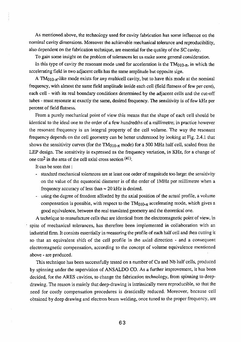
As mentioned above, the technology used for cavity fabrication has some influence on the
nominal cavity dimensions. Moreover the achievable mechanical tolerance and reproducibility,
also dependent on the fabrication technique, are essential for the quality of the SC cavity.
To gain some insight on the problem of tolerances let us make some general consideration.
In this type of cavity the resonant mode used for acceleration is the TMoi0-7t• in which the
accelerating field in two adjacent cells has the same amplitude but opposite sign.
A TMoi0-1t-like mode exists for any multicell cavity, but to have this mode at the nominal
frequency, with almost the same field amplitude inside each cell (field flatness of few per cent),
each cell - with its real boundary conditions determined by the adjacent cells and the cut-off
tubes -must resonate at exactly the same, desired frequency. The sensitivity is of few kHz per
percent of field flatness.
From a purely mechanical point of view this means that the shape of each cell should be
identical to the ideal one to the order of a few hundredths of a millimetre; in practice however
the resonant frequency is an integral property of the cell volume. The way the resonant
frequency depends on the cell geometry can be better understood by looking at Fig. 2.4.1 that
shows the sensitivity curves (for the TMoi0-7t mode) for a 500 MHz half cell, scaled from the
LEP design. The sensitivity is expressed as the frequency variation, in KHz, for a change of
one cm2 in the area of the cell axial cross section (41).
It can be seen that :
- standard mechanical tolerances are at least one order of magnitude too large: the sensitivity
on the value of the equatorial diameter is of the order of lMHz per millimetre when a
frequency accuracy of less than ,.. 20 kHz is desired.
- using the degree of freedom afforded by the axial position of the actual profile, a volume
compensation is possible, with respect to the TMoi0-7t accelerating mode, which gives a
good equivalence, between the real translated geometry and the theoretical one.
A technique to manufacture cells that are identical from the electromagnetic point of view, in
spite of mechanical tolerances, has therefore been implemented in collaboration with an
industrial firm. It consists essentially in measuring the profile of each half cell and then cutting it
so that an equivalent shift of the cell profile in the axial direction - and a consequent
electromagnetic compensation, according to the concept of volume equivalence mentioned
above - are produced.
This technique has been successfully tested on a number of Cu and Nb half cells, produced
by spinning under the supervision of ANSALDO CO. As a further improvement, it has been
decided, for the ARES cavities, to change the fabrication technology, from spinning to deep
drawing. The reason is mainly that deep-drawing is intrinsically more reproducible, so that the
need for costly compensation procedures is drastically reduced. Moreover, because cell
obtained by deep drawing and electron beam welding, once tuned to the proper frequency, are
63
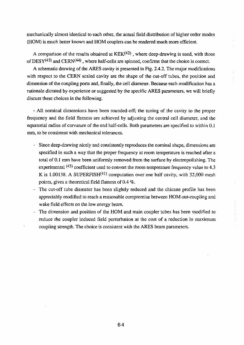
mechanically almost identical to each other, the actual field distribution of higher order modes
(ROM) is much better known and HOM couplers can be rendered much more efficient.
A comparison of the results obtained at KEK(42) , where deep-drawing is used, with those
ofDESY(43) and CERN(44), where half-cells are spinned, confirms that the choice is correct.
A schematic drawing of the ARES cavity is presented in Fig. 2.4.2. The major modifications
with respect to the CERN scaled cavity are the shape of the cut-off tubes, the position and
dimension of the coupling ports and, finally, the cell diameter. Because each modification has a
rationale dictated by experience or suggested by the specific ARES parameters, we will briefly
discuss these choices in the following.
- All nominal dimensions have been rounded-off; the tuning of the cavity to the proper
frequency and the field flatness are achieved by adjusting the central cell diameter, and the
equatorial radius of curvature of the end half-cells. Both parameters are specified to within 0.1
mm, to be consistent with mechanical tolerances.
- Since deep-drawing nicely and consistently reproduces the nominal shape, dimensions are
specified in such a way that the proper frequency at room temperature is reached after a
total of 0.1 mm have been uniformly removed from the surface by electropolishing. The
experimental (45) coefficient used to convert the room temperature frequency value to 4.3
K is 1.00138. A SUPERFISH(41) computation over one half cavity, with 32,000 mesh
points, gives a theoretical field flatness of 0.4 %.
- The cut-off tube diameter has been slightly reduced and the chicane profile has been
appreciably modified to reach a reasonable compromise between HOM out-coupling and
wake field effects on the low energy beam.
- The dimension and position of the HOM and main coupler tubes has been modified to
reduce the coupler induced field perturbation at the cost of a reduction in maximum
coupling strength. The choice is consistent with the ARES beam parameters.
64
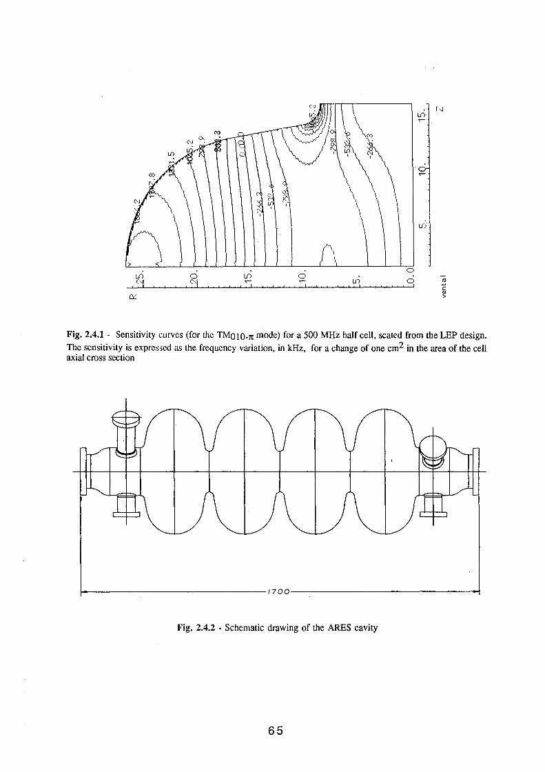
N
Lf)
0 IJ) 0 IJ) 0 -;o N l?i ~ ~ IJ) 0
I I I I I I I I I ..... c Q)
ex:: >
Fig. 2.4.1 - Sensitivity curves (for the TM010-1t mode) for a 500 MHz half cell, seated from the LEP design.
The sensitivity is exprcs;;cd as the frequency variation, in kHz, for a change of one cm2 in the area of the cell axial cross section
~---------------------------------1700----------------------------------~
Fig. 2.4.2 - Schematic drawing of the ARES cavity
65
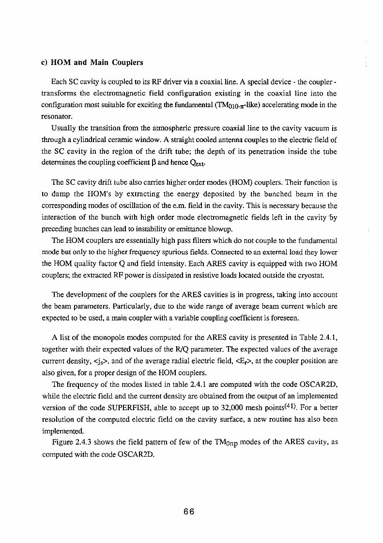
c) HOM and Main Couplers
Each SC cavity is coupled to its RF driver via a coaxial line. A special device- the coupler
transforms the electromagnetic field configuration existing in the coaxial line into the
configuration most suitable for exciting the fundamental (TMo10-1rlike) accelerating mode in the
resonator.
Usually the transition from the atmospheric pressure coaxial line to the cavity vacuum is
through a cylindrical ceramic window. A straight cooled antenna couples to the electric field of
the se cavity in the region of the drift tube; the depth of its penetration inside the tube
determines the coupling coefficient ~ and hence Qext·
The SC cavity drift tube also carries higher order modes (HOM) couplers. Their function is
to damp the HOM's by extracting the energy deposited by the bunched beam in the
corresponding modes of oscillation of the e.m. field in the cavity. This is necessary because the
interaction of the bunch with high order mode electromagnetic fields left in the cavity i>y
preceding bunches can lead to instability or emittance blowup.
The HOM couplers are essentially high pass filters which do not couple to the fundamental
mode but only to the higher frequency spurious fields. Connected to an external load they lower
the HOM quality factor Q and field intensity. Each ARES cavity is equipped with two HOM
couplers; the extracted RF power is dissipated in resistive loads located outside the cryostat.
The development of the couplers for the ARES cavities is in progress, taking into account
the beam parameters. Particularly, due to the wide range of average beam current which are
expected to be used, a main coupler with a variable coupling coefficient is foreseen. I
A list of the monopole modes computed for the ARES cavity is presented in Table 2.4.1,
together with their expected values of the RIQ parameter. The expected values of the average
current density, <js>, and of the average radial electric field, <Er>, at the coupler position are
also given, for a proper design of the HOM couplers.
The frequency of the modes listed in table 2.4.1 are computed with the code OSCAR2D,
while the electric field and the current density are obtained from the output of an implemented
version of the code SUPERFISH, able to accept up to 32,000 mesh points(41). For a better
resolution of the computed electric field on the cavity surface, a new routine has also been
implemented.
Figure 2.4.3 shows the field pattern of few of the TMonp modes of the ARES cavity, as
computed with the code OSCAR2D.
66
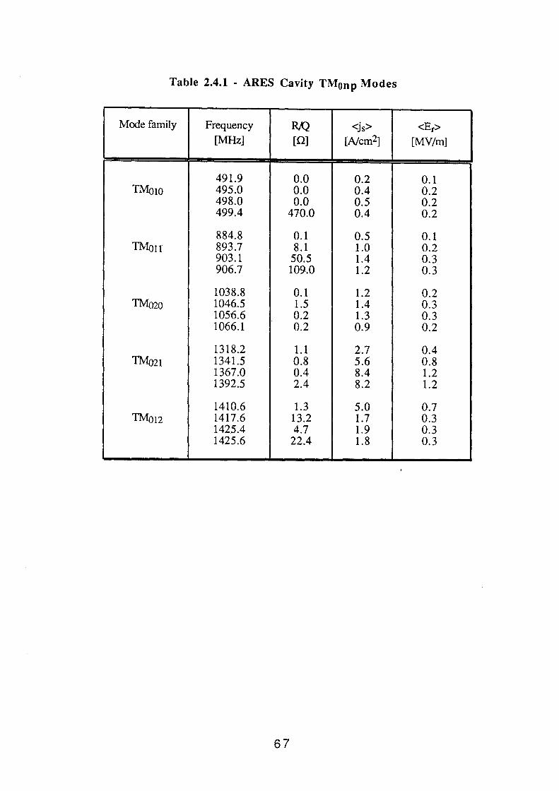
Table 2.4.1 - ARES Cavity TMonp Modes
Mode family Frequency RJQ <js> <Er> [MHz] [Q] [Ncm2] [MV/m]
491.9 0.0 0.2 0.1 TMow 495.0 0.0 0.4 0.2
498.0 0.0 0.5 0.2 499.4 470.0 0.4 0.2
884.8 0.1 0.5 0.1 'fMo11 893.7 8.1 1.0 0.2
903.1 50.5 1.4 0.3 906.7 109.0 1.2 0.3
1038.8 0.1 1.2 0.2 TMo2o 1046.5 1.5 1.4 0.3
1056.6 0.2 1.3 0.3 1066.1 0.2 0.9 0.2
1318.2 1.1 2.7 0.4 'fMo2I 1341.5 0.8 5.6 0.8
1367.0 0.4 8.4 1.2 1392.5 2.4 8.2 1.2
1410.6 1.3 5.0 0.7 TMot2 1417.6 13.2 1.7 0.3
1425.4 4.7 1.9 0.3 1425.6 22.4 1.8 0.3
67
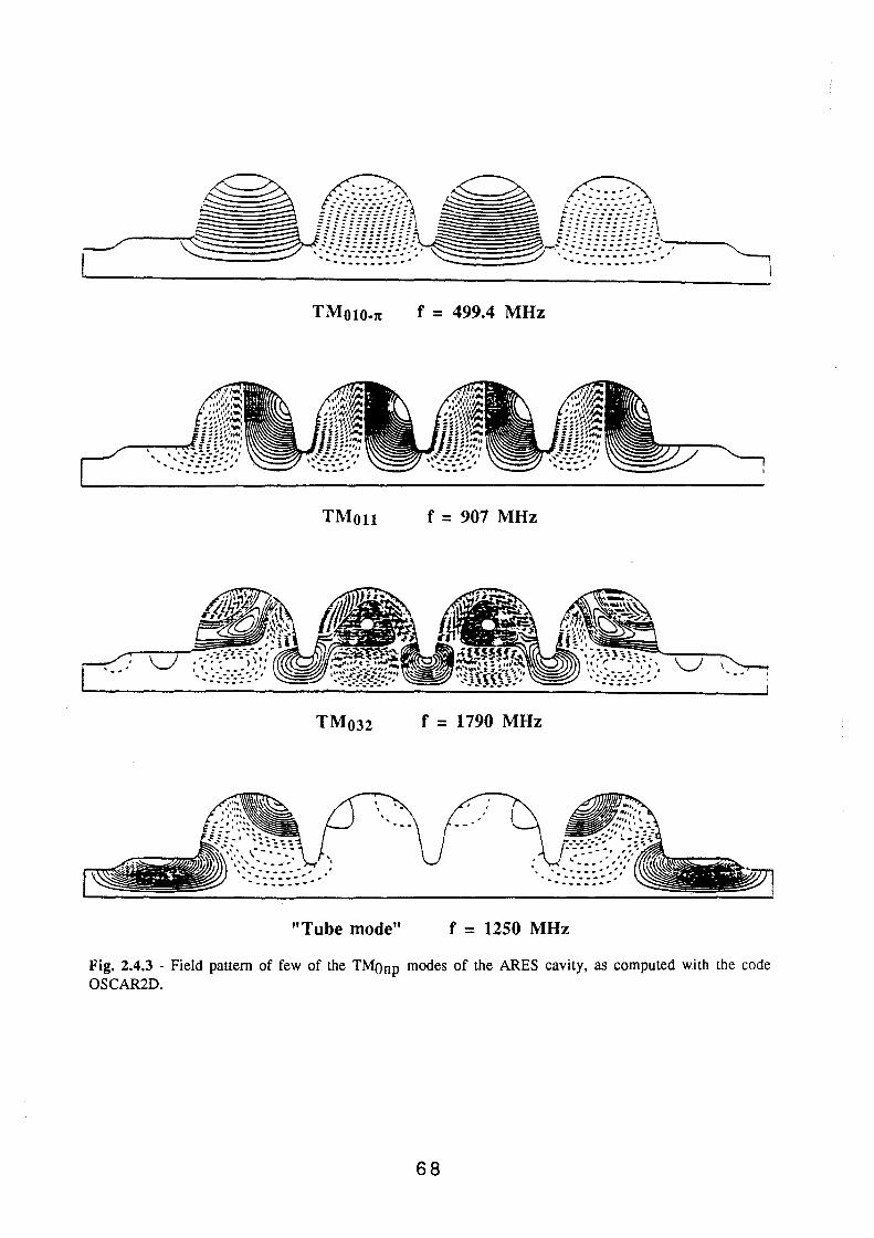
TMot0-1t f = 499.4 MHz
TMou f 907 MHz
TMo32 f = 1790 MHz
..... -- .. - .. ... ______ _
"Tube mode" f = 1250 MHz
Fig. 2.4.3 - Field pattern of few of the TMonp modes of the ARES cavity, as computed with the code OSCAR2D.
68
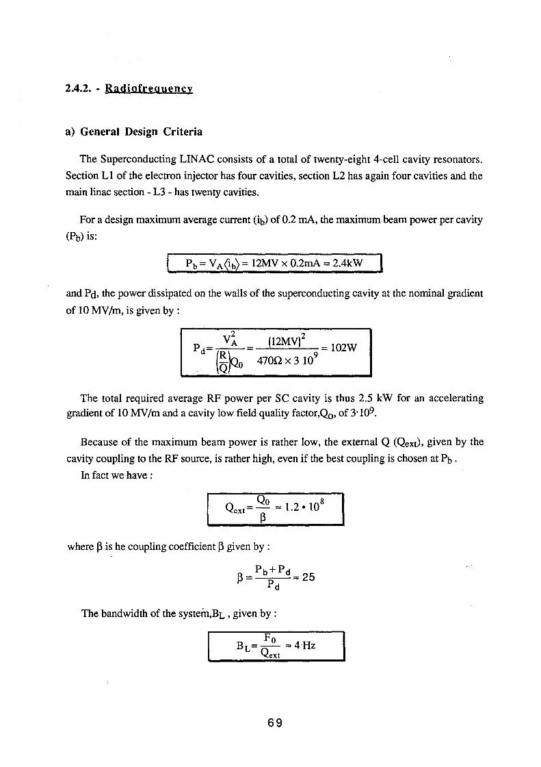
2.4.2. - Radiofrequency
a) General Design Criteria
The Superconducting LINAC consists of a total of twenty-eight 4-cell cavity resonators.
Section Ll of the electron injector has four cavities, section L2 has again four cavities and the
main linac section - L3 - has twenty cavities.
For a design maximum average current Cib) of 0.2 mA, the maximum beam power per cavity
(Pb) is:
Pb =V A(ib) = 12MV X 0.2mA = 2.4kW
and Pd, the power dissipated on the walls of the superconducting cavity at the nominal gradient
of 10 MY /m, is given by :
y2A 2 p I12MV} = 102W
d= (~~O = 470Q X 3 109
The total required average RF power per SC cavity is thus 2.5 kW for an accelerating gradient of 10 MY/m and a cavity low field quality factor,Q0 , of 3·109.
Because of the maximum beam power is rather low, the external Q (Qext), given by the
cavity coupling to the RF source, is rather high, even if the best coupling is chosen at Pb .
In fact we have :
where ~ is he coupling coefficient ~ given by :
The bandwidth of the systein,BL , given by :
69
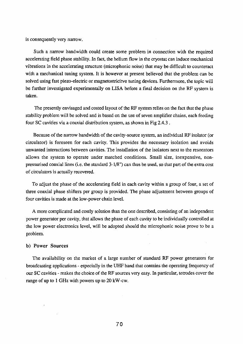
is consequently very narrow.
Such a narrow bandwidth could create some problem in connection with the required
accelerating field phase stability. In fact, the helium flow in the cryostat can induce mechanical
vibrations in the accelerating structure (microphonic noise) that may be difficult to counteract
with a mechanical tuning system. It is however at present believed that the problem can be
solved using fast piezo-electric or magnetostricitve tuning devices. Furthermore, the topic will
be further investigated experimentally on LISA before a final decision on the RF system is
taken.
The presently envisaged and costed layout of the RF system relies on the fact that the phase
stability problem will be solved and is based on the use of seven amplifier chains, each feeding
four se cavities via a coaxial distribution system, as shown in Fig 2.4.3 .
Because of the narrow bandwidth of the cavity-source system, an individual RF isolator (or
circulator) is foreseen for each cavity. This provides the necessary isolation and avoids
unwanted interactions between cavities. The installation of the isolators next to the resonators
allows the system ~o operate under matched conditions. Small size, inexpensive, non
pressurised coaxial lines (i.e. the standard 3-1/8") can thus be used, so that part of the extra cost
of circulators is actually recovered.
To adjust the phase of the accelerating field in each cavity within a group of four, a set of
three coaxial phase shifters per group is provided. The phase adjustment between groups of
four cavities is made at the low-power chain level.
A more complicated and costly solution than the one described, consisting of an independent
power generator per cavity, that allows the phase of each cavity to be individually controlled at
the low power electronics level, will be adopted should the microphonic noise prove to be a
problem.
b) Power Sources
The availability on the market of a large number of standard RF power generators for
broadcasting applications - especially in the UHF band that contains the operating frequency of
our se cavities - makes the choice of the RF sources very easy. In particular, tetrodes cover the
range of up to 1 GHz with powers up to 20 kW-cw.
70
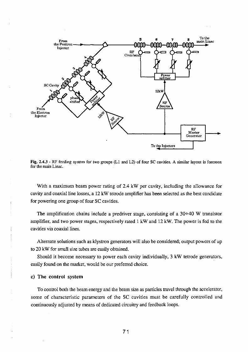
From 5 the Positron-.... ----< ~~-----t
Injector
6 7
12kW
To the Injectors
8 To the mainLinac
RF Master
Generator
Fig. 2.4.3 - RF feeding system for two groups (Ll and L2) of four SC cavities. A similar layout is foreseen for the main Linac.
With a maximum beam power rating of 2.4 kW per cavity, including the allowance for
cavity and coaxial line losses, a 12 kW tetrode amplifier has been selected as the best candidate
for powering one group of four se cavities.
The amplification chains include a predriver stage, consisting of a 30+40 W transistor
amplifier, and two power stages, respectively rated 1 kW and 12 kW. The power is fed to the
cavities via coaxial lines.
Alternate solutions such as klystron generators will also be considered; output powers of up
to 20 kW for small size tubes are easily obtained.
Should it become necessary to power each cavity individually, 3 kW tetrode generators,
easily found on the market, would be our preferred choice.
c) The control system
To control both the beam energy and the beam size as particles travel through the accelerator,
some of characteristic parameters of the se cavities must be carefully controlled and
continuously adjusted by means of dedicated circuitry and feedback loops.
71
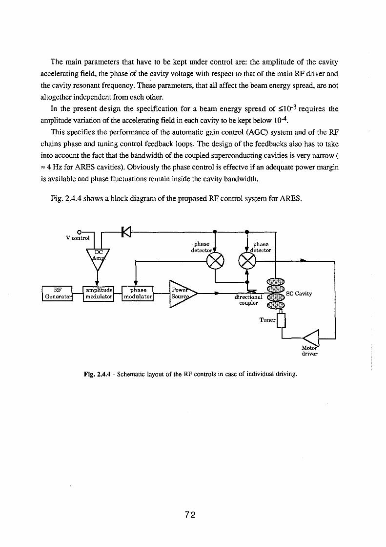
The main parameters that have to be kept under control are: the amplitude of the cavity
accelerating field, the phase of the cavity voltage with respect to that of the main RF driver and
the cavity resonant frequency. These parameters, that all affect the beam energy spread, are not
altogether independent from each other.
In the present design the specification for a beam energy spread of ~~o-3 requires the
amplitude variation of the accelerating field in each cavity to be kept below 10-4.
This specifies the performance of the automatic gain control (AGC) system and of the RF
chains phase and tuning control feedback loops. The design of the feedbacks also has to take
into account the fact that the bandwidth of the coupled superconducting cavities is very narrow (
""'4Hz for ARES cavities). Obviously the phase control is effectve if an adequate power margin
is available and phase fluctuations remain inside the cavity bandwidth.
Fig. 2.4.4 shows a block diagram of the proposed RF control system for ARES.
driver
Fig. 2.4.4 - Schematic layout of the RF controls in case of individual driving.
72
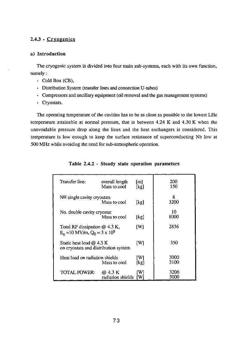
2.4.3 - Cryo~enics
a) Introduction
The cryogenic system is divided into four main sub-systems, each with its own function,
namely:
- Cold Box (CB),
- Distribution System (transfer lines and connection U-tubes)
- Compressors and ancillary equipment (oil removal and the gas management systems)
- Cryostats.
The operating temperature of the cavities has to be as close as possible to the lowest LHe
temperature attainable at normal pressure, that is between 4.24 K and 4.30 K when the
unavoidable pressure drop along the lines and the heat exchangers is considered. This
temperature is low enough to keep the surface resistance of superconducting Nb low at
500 MHz while avoiding the need for sub-atmospheric operation.
Table 2.4.2 - Steady state operation parameters
Transfer line: overall length [m] 200 Mass to cool [kg] 150
Ner single cavity cryostats 8 Mass to cool [kg] 3200
No. double cavity cryostat 10 Mass to cool [kg] 8000
Total RF dissipation @ 4.3 K, [W] 2856 Ea =10 MV/m, Qo = 3 x 10⁹
Static heat load @ 4.3 K [W] 350 on cryostats and distribution system
Heat load on radiation shields [W] 3000 Mass to cool [kg] 3100
TOTAL POWER: @ 4.3 K [W] 3206 radiation shields [W] 3000
73
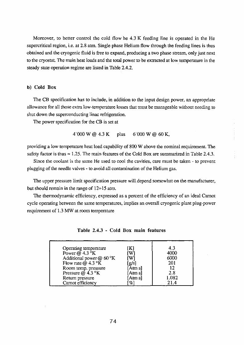
Moreover, to better control the cold flow he 4.3 K feeding line is operated in the He
supercritical region, i.e. at 2.8 atm. Single phase Helium flow through the feeding lines is thus
obtained and the cryogenic fluid is free to expand, producing a two phase stream, only just next
to the cryostat. The main heat loads and the total power to be extracted at low temperature in the
steady state operation regime are listed in Table 2.4.2.
b) Cold Box
The CB specification has to include, in addition to the input design power, an appropriate
allowance for all those extra low-temperature losses that must be manageable without needing to
shut down the superconducting linac refrigeration.
The power specification for the CB is set at
4'000 W@ 4.3 K plus 6'000 W@ 60 K,
providing a low temperature heat load capability of 800 W above the nominal requirement. The
safety factor is thus "" 1.25. The main features of the Cold Box are summarized in Table 2.4.3.
Since the coolant is the same He used to cool the cavities, care must be taken - to prevent
plugging of the needle valves - to avoid all contamination of the Helium gas.
The upper pressure limit specification pressure will depend somewhat on the manufacturer,
but should remain in the range of 12+ 15 atm.
The thermodynamic efficiency, expressed as a percent of the efficiency of an ideal Carnot
cycle operating between the same temperatures, implies an overall cryogenic plant plug-power
requirement of 1.3 MW at room temperature
Table 2.4.3 - Cold Box main features
Operating temperature Power@ 4.3 °K Additional power@ 60 °K Flow rate @ 4.3 °K Room temp. pressure Pressure @ 4.3 °K Return pressure Carnot efficiency
74
[K] [W] [W] [g/s] [Atm a] [Atm a] [Atma] [%]
4.3 4000 6000 201 12 2.8
1.082 21.4
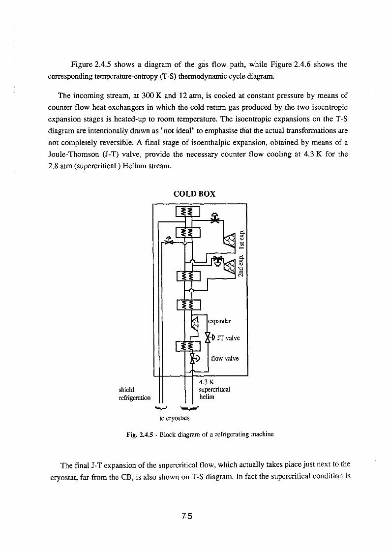
Figure 2.4.5 shows a diagram of the gas flow path, while Figure 2.4.6 shows the
corresponding temperature-entropy (T-S) thermodynamic cycle diagram.
The incoming stream, at 300 K and 12 atm, is cooled at constant pressure by means of
counter flow heat exchangers in which the cold return gas produced by the two isoentropic
expansion stages is heated-up to room temperature. The isoentropic expansions on the T-S
diagram are intentionally drawn as "not ideal" to emphasise that the actual transformations are
not completely reversible. A final stage of isoenthalpic expansion, obtained by means of a
Joule-Thomson (J-T) valve, provide the necessary counter flow cooling at 4.3 K for the
2.8 atm (supercritical) Helium stream.
COLD BOX
4.3 K shield supercritical refrigeration helim
........ ._,_. to cryostats
~ .... "' -
Fig. 2.4.5 - Block diagram of a refrigerating machine
The final J-T expansion of the supercritical flow, which actually takes place just next to the
cryostat, far from the CB, is also shown on T -S diagram. In fact the supercritical condition is
75
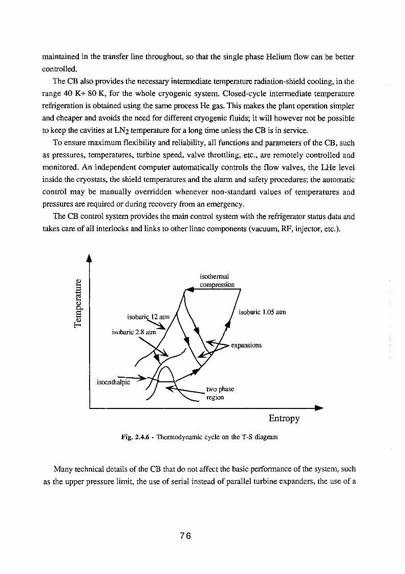
maintained in the transfer line throughout, so that the single phase Helium flow can be better
controlled.
The CB also provides the necessary intermediate temperature radiation-shield cooling, in the
range 40 K+ 80 K, for the whole cryogenic system. Closed-cycle intermediate temperature
refrigeration is obtained using the same process He gas. This makes the plant operation simpler
and cheaper and avoids the need for different cryogenic fluids; it will however not be possible
to keep the cavities at LN2 temperature for a long time unless the CB is in service.
To ensure maximum flexibility and reliability, all functions and parameters of the CB, such
as pressures, temperatures, turbine speed, valve throttling, etc., are remotely controlled and
monitored. An independent computer automatically controls the flow valves, the LHe level
inside the cryostats, the shield temperatures and the alarm and safety procedures; the automatic
control may be manually overridden whenever non-standard values of temperatures and
pressures are required or during recovery from an emergency.
The CB control system provides the main control system with the refrigerator status data and
takes care of all interlocks and links to other linac components (vacuum, RF, injector, etc.).
isobaric 12 atm
isobaric 2.8 ~
isothermal compression
isobaric 1.05 atm
Entropy
Fig. 2.4.6- Thermodynamic cycle on the T-S diagram
Many technical details of the CB that do not affect the basic performance of the system, such
as the upper pressure limit, the use of serial instead of parallel turbine expanders, the use of a
76
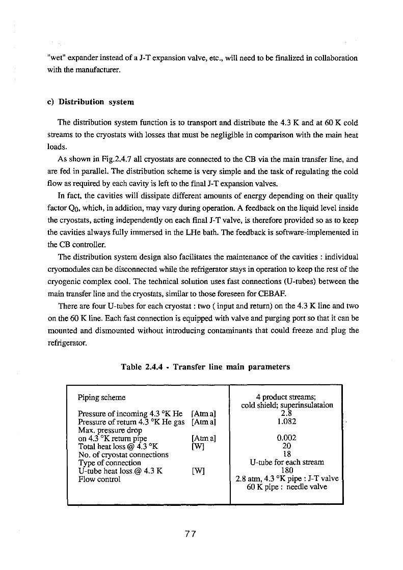
"wet" expander instead of a J-T expansion valve, etc., will need to be finalized in collaboration
with the manufacturer.
c) Distribution system
The distribution system function is to transport and distribute the 4.3 K and at 60 K cold
streams to the cryostats with losses that must be negligible in comparison with the main heat
loads.
As shown in Fig.2.4. 7 all cryostats are connected to the CB via the main transfer line, and
are fed in parallel. The distribution scheme is very simple and the task of regulating the cold
flow as required by each cavity is left to the f'mal J-T expansion valves.
In fact, the cavities will dissipate different amounts of energy depending on their quality
factor Qo, which, in addition, may vary during operation. A feedback on the liquid level inside
the cryostats, acting independently on each final J-T valve, is therefore provided so as to keep
the cavities always fully immersed in the LHe bath. The feedback is software-implemented in
the CB controller.
The distribution system design also facilitates the maintenance of the cavities : individual
cryomodules can be disconnected while the refrigerator stays in operation to keep the rest of the
cryogenic complex cool. The technical solution uses fast connections (U-tubes) between the
main transfer line and the cryostats, similar to those foreseen for CEBAF.
There are four U-tubes for each cryostat : two ( input and return) on the 4.3 K line and two
on the 60 K line. Each fast connection is equipped with valve and purging port so that it can be
mounted and dismounted without introducing contaminants that could freeze and plug the
refrigerator.
Table 2.4.4 - Transfer line main parameters
Piping scheme
Pressure of incoming 4.3 °K He Pressure of return 4.3 °K He gas Max. pressure drop on 4.3 °K return pipe Total heat loss@ 4.3 °K No. of cryo~tat connections Type of connection U-tube heat loss@ 4.3 K Flow control
[Atma] [Atma]
[Atma] [W]
[W]
77
4 product streams; cold shield; superinsulataion
2.8 1.082
0.002 20 18
U-tube for each stream 180
2.8 atm, 4.3 °K pipe : J-T valve 60 K pipe : needle valve
A cross sectional view of the main transfer line is shown in the inset of Figure 2.4.7 . It is of
the four-product-stream type with shield and superinsulation. The expected dynamic heat loss is
less than 0.1 W/m@ 4.3 K. The main parameters are listed in Table 2.4.4.
As previously pointed out the pressure drop along the 4.3 K return line has to be kept as
low as 210-3 atm in order to keep the LHe bath temperature inside the cryostat close to 4.3 K.
The pressure drop on the 4.3 K, 2.8 atm feed line is not as critical as that on the return line;
it is only necessary to keep the end pressure higher than 2.245 atm, the critical pressure of He.
It is also worth noting that no cooling occurs during the isoenthalpic expansion of He from 2.8
to 1.082 atm at 4.3 K.
As it can be seen from the data of Table 2.4.4 the largest heat load in the distribution system,
180 W@ 4.3 K, comes from the U-tube connections. The distribution system thermal losses
add up to .,. 5 % of the overall 4.3 K heat load.
d) Compressors and ancillary equipment
An efficient compression system is vital to keep the cryogenic plant working. Figure 2.4.8
shows the block diagram of the CB together with the compressors, purifiers, and medium
pressure storage tanks.
Two make the system more reliable two compressors are mounted in parallel so that one can
be switched on if the other fails. This because, while in the event of a fault on the CB the
compressor can keep the cavities cold for a long time, a compressor fault will cause the LHe
evaporation to stop and the cavities to warm up very fast.
Unless the compressor is equipped with an oil removal system and downstream adsorbing
filters, during compression the pure Helium will become contaminated with the compressor
lubricant oil. As first approach we foresee only one heavy-duty purifier that can work
continuously for one year; the filters can be replaced and/or purged while the purifier is in
service.
78
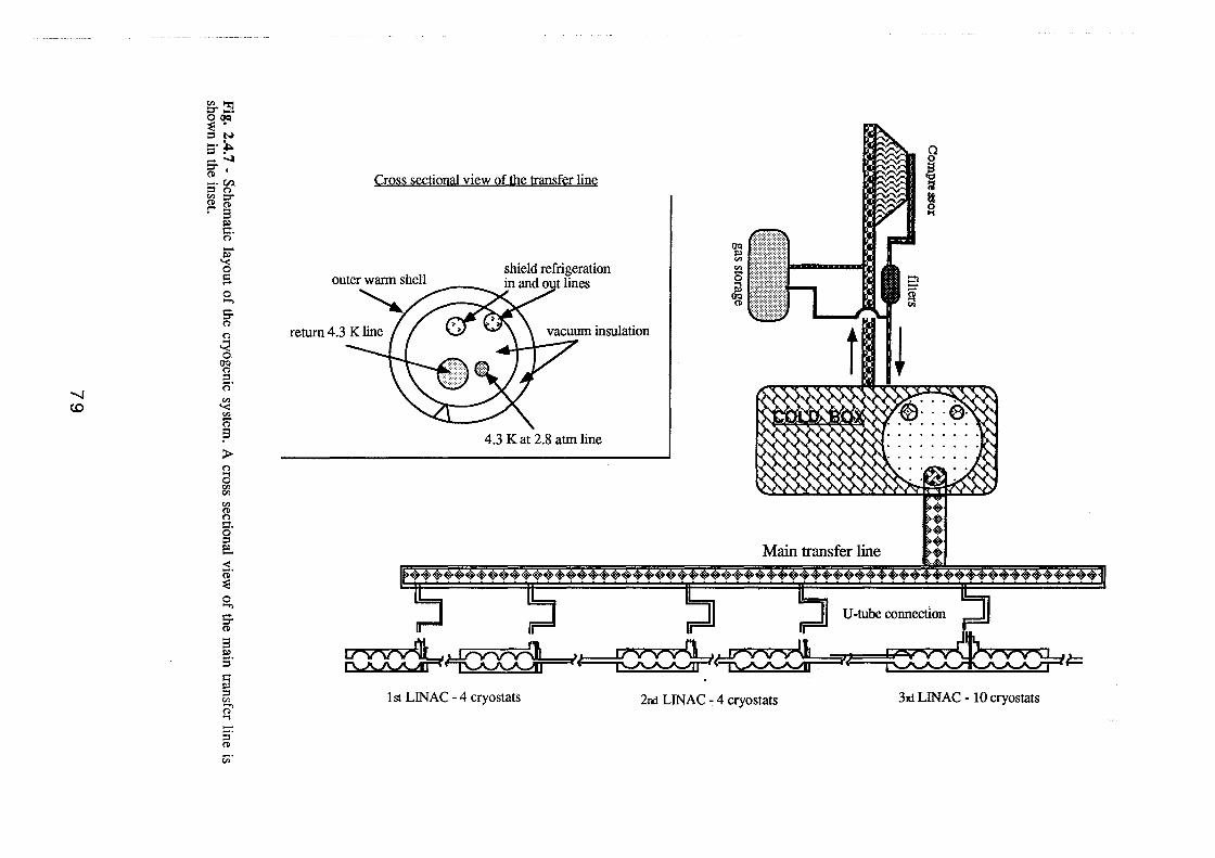
Cl)~ ::r .... OIJQ ~ . ::s~ .... "" ::s • s-"'-~ (1) I
.... en ::s (") Cll::r' (1) (1)
"s s:>:> :;:!. (")
£;" a c:: .... 0 ....... Er (1)
(")
~ ()Q (1) ::s .... (")
Cl) ......
'< Cl)
<.0 ~ p > (")
a Cl) Cl)
{I) (1) (") :;:!. 0 ::s e:.. < n· ~ 0 ....... Er (1)
s s:>:> s· ~ ::s Cl)
;> .... -s· (1)
c;;·
Cross sectional view of the transfer line
4.3 Kat 2.8 atm line
1st LINAC- 4 cryostats 2n:J LINAC- 4 cryostats
Q 0 ,g ; 1:8 0 1-1
3:td LINAC- 10 cryostats
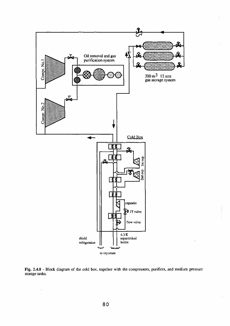
Oil removal and gas purification system
Cold Box
4.3K shield supercritical refrigeration helim
~ .._,_. to cryostats
200m3 12atm gas storage system
Fig. 2.4.8 - Block diagram of the cold box, together with the compressors, purifiers, and medium pressure storage tanks.
80
The system operates as follows: when the system is warm the pure Helium gas is stored in
the pure gas storage tank and all the piping, cryostats, compressors and the CB, are filled with
pure Helium gas.
The total gas inventory is about 2142 m3 S.T.P., or 186m3 at room temperature and
12 atm.
For easier handling and purification the storage tank consists of three separate vessels of
70 m3 each. After the compressors and the CB have been started the He starts to condense in
the CB, the transfer lines and the cryostats, so that the return pressure lowers; this actuates a
constant pressure make up valve that takes gas from the vessels and fills the return line at
constant pressure. Once the steady state is reached, i.e. the cryostats are full of LHe, the CB
starts operating in a closed cycle and the vessels can be closed.
When the cryostats have to be warmed up, the Helium can be recovered either by means of
the CB compressors, in the form of pure He, and stored in the storage vessels or using a
standard recovery system (gas bag and high pressure compressor, not included in the drawing).
The latter system however leaves the He exposed to contaminants.
d) Cryostats
From an engineering point of view, the cryostat must provide a proper environment for the
SC cavities. Thermal insulation, shielding from magnetic fields, removal of the RF heat at
constant temperature (:::::: 4.3 K), tuning, auxiliary equipment, clean conditions, UHV
techniques, easy handling and mounting are the main features that have to be kept in mind in
designing and manufacturing the cryostat.
At this stage no development has been attempted since SC cryostats have reached a
satisfactory standard level of performance; the preliminary design and manufacture
specifications are therefore based on existing designs, notably those for the CERN cavities <46).
The main components making up our cryostat are:
- outer vacuum vessel,
- GHe cooled radiation shield,
- magnetic shield,
- LHe vessel,
- thermal-magnetostrictive tuners (three).
Internal electrical cabling, waveguides, feedthrough tubes, support rods, niobium beam-pipe
extensions, probes, etc., are also considered parts of the cryostat.
Two prototypes are under construction at ANSALDO CO.
81
Vacuum vessel
A stainless-steel (AISI 316 LN) bar to which two rings of the same material are welded is
the main support structure; aluminium-alloy staves are then bolted to the s.s. rings
circumference. Two covering plates and a stainless-steel outer shell give the vacuum vessel the
final required stiffness.
After assembly the vessel is He-leak pressure tested.
GHe cooled radiation shield
The GHe cooled radiation shield is made of high conductivity, phosphorous free ETP or OF
copper plates. The shield surface temperatures is kept approximatively constant by the GHe
evaporated from the LHe bath; the cold gas flows inside copper pipes brazed on the copper
sheets. The radiation shield is sorrounded by a multilayer, aluminized mylar (NRC-2)
"superinsulation" blanket to decrease the radiant heat load on the shield; the blanket also
provides a low thermal conductivity layer on the path of residual gas molecules.
Mafmetic shield
Any magnetic flux in the vicinity of the cavity is "captured" within the niobium during cool
down and produces a degradation of the se cavity performance.
Beside avoiding the use of magnetic materials in the construction of the cryostat, the cavity
has therefore to be shielded, during cool-down, from external magnetic fields; a Jl-metal shield
is therefore usually incorporated in the cryostat.
Other precautions must nevertheless be observed during the cool-down sequence of
operations; for example the tuner may be switched on only when the cavity is already cold
because magnetic fields may appear during tuner activation.
LHe tank
The LHe tank is a low magnetic permeability stainless-steel (AISI 316 LN) container built
from two half-shells; its shape follows approximatively the shape of the cavity in order to
minimize the LHe volume.
The half-shells are formed by pressing and then welded together. The complete shell is
finally TIG-welded to the cavity end-flanges.
The final weld is performed after mechanically tuning the cavity, an operation consisting in a
plastic deformation of each individual cell. The deformation should produce the desired RF field
flatness and at the same time preserve the elastic behaviour of the four-cell cavity necessary for
82
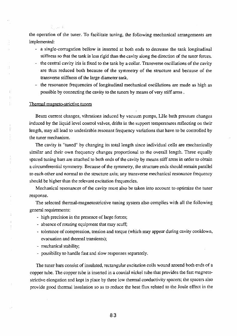
the operation of the tuner. To facilitate tuning, the following mechanical arrangements are
implemented:
- a single-corrugation bellow is inserted at both ends to decrease the tank longitudinal
stiffness so that the tank is less rigid than the cavity along the direction of the tuner forces.
- the central cavity iris is fixed to the tank by a collar. Transverse oscillations of the cavity
are thus reduced both because of the symmetry of the structure and because of the
transverse stiffness of the large diameter tank.
- the resonance frequencies of longitudinal mechanical oscillations are made as high as
possible by connecting the cavity to the tuners by means of very stiff arms .
Thermal magneto-strictive tuners
Beam current changes, vibrations induced by vacuum pumps, LHe bath pressure changes
induced by the liquid level control valves, drifts in the support temperatures reflecting on their
length, may all lead to undesirable resonant frequency variations that have to be controlled by
the tuner mechanism.
The cavity is "tuned" by changing its total length since individual cells are mechanically
similar and their own frequency changes proportional to the overall length. Three equally
spaced tuning bars are attached to both ends of the cavity by means stiff arms in order to obtain
a circumferential symmetry. Because of the symmetry, the structure ends should remain parallel
to each other and normal to the structure axis; any transverse mechanical resonance frequency
should be higher than the relevant excitation frequencies.
Mechanical resonances of the cavity must also be taken into account to optimize the tuner
response.
The selected thermal-magnetostrictive tuning system also complies with all the following
general requirements:
- high precision in the presence of large forces;
- absence of rotating equipment that may scuff;
- tolerance of compression, tension and torque (which may appear during cavity cooldown,
evacuation and thermal transients);
- mechanical stability;
- possibility to handle fast and slow responses separately.
The tuner bars consist of insulated, rectangular excitation coils wound around both ends of a
copper tube. The copper tube is inserted in a coaxial nickel tube that provides the fast magneto
strictive elongation and kept in place by three low thermal conductivity spacers; the spacers also
provide good thermal insulation so as to reduce the heat flux related to the Joule effect in the
83
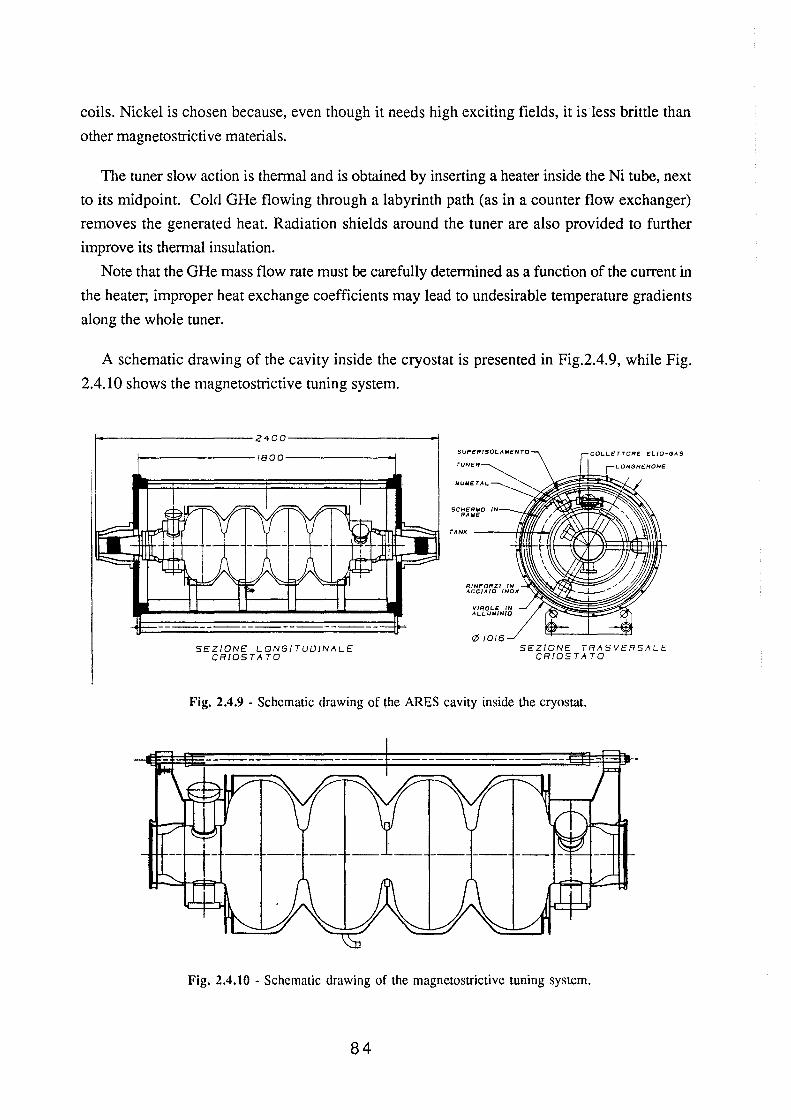
coils. Nickel is chosen because, even though it needs high exciting fields, it is less brittle than
other magnetostrictive materials.
The tuner slow action is thermal and is obtained by inserting a heater inside the Ni tube, next
to its midpoint. Cold GHe flowing through a labyrinth path (as in a counter flow exchanger)
removes the generated heat. Radiation shields around the tuner are also provided to further
improve its thermal insulation.
Note that the GHe mass flow rate must be carefully determined as a function of the current in
the heater; improper heat exchange coefficients may lead to undesirable temperature gradients
along the whole tuner.
A schematic drawing of the cavity inside the cryostat is presented in Fig.2.4.9, while Fig.
2.4.10 shows the magnetostrictive tuning system.
~-----------------2400------------------~
SEZIONE LONG/TUO/NIILE CRIOSTII TO
SUPERISOLA.IriENTO
TUNER
.WUWETAL
SCHERWO IN RA .WC
0/016 SEZIONE TRIISVERSIILE
CRIOSTII TO
Fig. 2.4.9 - Schematic drawing of the ARES cavity inside the cryostat.
Fig. 2.4.10 - Schematic drawing of the magnetostrictive tuning system.
84
2.5 - VACUUM SYSTEM
2.5.1 - Introduction
In superconducting accelerator systems very high vacuum is mainly required to protect the . superconducting RF cavities from the condensation of molecules of the residual gases on the
low temperature superconducting surface: the condensation of few hundreds of monolayers on
the superconducting niobium surface would seriously degrade the RF cavity performance, in
particular lowering its Q value.
In fact, for a se linear accelerator this is the dominant phenomenon that sets the most severe
requirements on the vacuum system ; interaction with the residual gas is a comparatively minor
effect because the beam covers only a few hundreds of meters within the accelerator.
The pressure in the beam pipe and the se cavities must be in in the w-8 mbar range before
cavity cooldown can be started in order to guarantee operation of the RF cavity for at least 2
years at a Q value not lower than 90 % of its initial value.
Very clean vacuum condition (no oil, no dust and no hydrocarbons) are imperative but no
titanium sublimation pump can be used because titanium can easily form unwanted alloys with
niobium.
It should also be recalled that se cavity cryostats have to be evacuated to provide the
necessary thermal insulation between room temperature and the liquid helium container.
From the point of view of vacuum the ARES linac complex consists of 3 superconducting
Sections - that total 18 cryomodules - and about 200 meters of beam lines.
2.5.2 - The cryomodule
The cryomodule is the smallest unit of the superconducting accelerator structure that can be
individually tested. Each cryomodule consists of either 4 or 8 RF cells, assembled in a single
cryostat.
A gate valve is mounted at each end of a cryomodule to make it easier to test it and to prevent
any contamination of the cavities after the initial testing by keeping them under good vacuum
conditions at all subsequent times.
Moreover, thanks to the valves, each cryomodule can be separated from the accelerating
structure, for instance to replace a defective cryomodule, without breaking the vacuum in the
adjacent modules .
The all-metal, bakeable gate valves have a 100 mm inside diameter.
85
No elastomer sealing is acceptable because the outgassing rate would be too high. Moreover,
all-metal gate valves can be supplied with RF contacts that perform a direct electrical connection
between the two valve flanges, thereby shielding the inner valve mechanism from the beam.
A bake-out jacket is permanently assembled around the valve; it allows to perform a
moderate temperature (200 ooC) bake-out.
A total of 36 all-metal valves are needed for the three superconducting linac sections.
The pumping of the cryostat vacuum chamber is ensured, on each cryomodule, by a 50 1/s
turbomolecular pump, connected to a valved port. After leak testing, if the chamber is He-tight,
the valve can be closed and the pump can be switched off after the cryomodule has been cooled
down. Should a leak be detected, the turbomolecular pump can be kept in continuous operation
to keep the pressure in the insulation chamber below lQ-4 mbar until the leak has been repaired.
2.5.3 - The cryomodule pumping system
As explained above, each cryomodule is terminated at each end by a valve.
In normal operation the valves are opened only when the pressure in the beam pipe has
become lower then 1 o-9 mbar, to reduce the amount of condensable gases entering the
cryomodule.
A room temperature stainless steel beam pipe connects two adjacent cryomodules; the UHV
pumping system is connected to the pipe through a bellow.
The UHV pump is 230 1/s Starcell ion pump that maintains the pressure in the beam pipe at
less than lQ-7 mbar when the RF cavity is at room temperature.
Two other bellows are mounted at the pipe ends - on the beam line - to compensate for
manufacturing tolerances and to simplify the beam pipe alignment easier. A proper shielding
sleeve with sliding contacts must be provided inside all bellows to keep the vacuum chamber
impedance seen by the beam low (46,47).
The beam pipe connecting two cryomodules contains all beam monitors. A focusing
quadrupole also fits around it.
Figure 2.5.1 shows the layout of a cryomodule connection assembly.
The total niobium surface exposed to vacuum is about 4 m2; the overall surface of the
stainless steel parts is instead less than 1 m2. In order to reduce the outgassing a moderate in
situ bake-out("" 150 °C) of the beam pipe is foreseen. Thin kapton heaters are mounted on the
chamber and fit in the space between the beam pipe and the quadrupole pole faces.
A total of 15 ion pumps are used along the SC linac sections.
Rough pumping of the system and pumping during bake-out operations will be ensured by a
mobile station that can be connected to the beam pipe, close to the ion pump, by means of an all
metal corner valve. After bake-out, at the start of normal operation of the ion pump the roughing
86

Fig. 2.5.1 -Layout of the connection assembly between two cryomodules of the sections Ll and L2.
system is detached from the beam tube.
In all, three roughing stations are foreseen for all Linac vacuum systems.
The solution is obviously cheaper than providing a fixed roughing pump station at each of
the 22 forevacuum ports.
The roughing system must be absolutely free from hydrocarbons to avoid contamination. It
consists of a magnetic-bearings turbomolecular pump with dry forevacuum pump or -
alternatively - of a refrigerator-cooled cryopump backed by a dry pump.
An ionization gauge is mounted close to the beam tube and connected to the control
system, to provide information on the total pressure in the beam line.
Table 2.5.1 • SC Linac Vacuum Components
Ion pumps Gate valves RGA Ion gauge Forevacuum pons
Section Ll 3 8 3 3 3 Section L2 3 8 3 3 3 Section L3 9 20 9 9 9
Total 15 36 15 15 15
87
A residual gas analyzer (RGA) is also mounted close to each high vacuum pumping port,
between pairs of cryomodules, and provides on-line information on the composition of the
residual gas in the beam pipe.
A total of 19 RGAs, controlled through a multiplexed system, are mounted on the SC linac.
The information on the residual gas composition is used to diagnose the presence of a leak or of
a pump malfunctioning before a permanent degradation of the RF cavity performances can
occur.
Table 2.5.1 shows the inventory of the SC linac vacuum components.
2.5.4 - Recirculation beam lines yacuum system
From the point of view of vacuum the recirculation beam line consists mainly of"" 160 m of a
100 mm inner diameter stainless steel tube, vacuum pumps, valves, gauges and forevacuum
ports.
Vacuum requirements in the recirculation line, as previously explained, are less stringent
than on the se linac because the line contains no superconducting exposed surface.
To pump-down the recirculation lines, only 25 ion pumps- identical to the ones used in SC
linac, ""10 m away from each other - are therefore sufficient. The estimated mean pressure will
be in the 1 o-8 mbar range.
Usual UHV surface cleaning treatments are used in order to reduce stainless steel outgassing
(48). Medium temperature in-situ bake-out("" 300 °C) is foreseen.
Forepumping is normally done by connecting one of the mobile pumping stations to one of
the 7 valved ports. The presence of 6 all-metal gate valves on the beam line makes it easier to
service the vacuum system and to deal with abnormal situations.
22 ionization gauges and 7 RGA's are used for vacuum monitoring and diagnostics.
Table 2.5.2 summarizes the main vacuum components of the whole Linac system.
Table 2.5.2 - Vacuum Component Overall Inventory
Ion pumps Gate valves RGA Ion gauge Forevacuum ports
Beam lines 25 6 5 22 7 se Linacs 15 36 15 15 15
Total 40 42 20 37 22
88
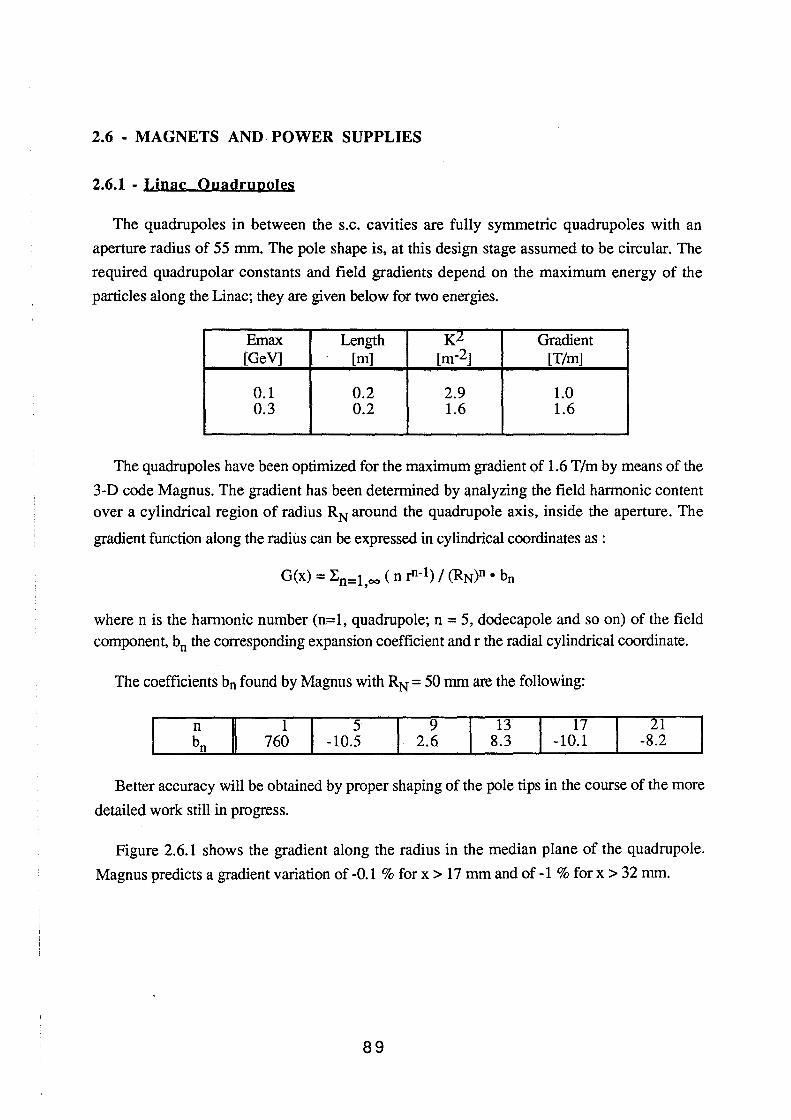
2.6 - MAGNETS AND POWER SUPPLIES
2.6.1 - Linac Ouadrupoles
The quadrupoles in between the s.c. cavities are fully symmetric quadrupoles with an
aperture radius of 55 mm. The pole shape is, at this design stage assumed to be circular. The
required quadrupolar constants and field gradients depend on the maximum energy of the
particles along the Linac; they are given below for two energies.
Emax Length K2 Gradient [GeV] [m] [m-2] [T/m]
0.1 0.2 2.9 1.0 0.3 0.2 1.6 1.6
The quadrupoles have been optimized for the maximum gradient of 1.6 T/m by means of the
3-D code Magnus. The gradient has been determined by analyzing the field harmonic content over a cylindrical region of radius RN around the quadrupole axis, inside the aperture. The
gradient function along the radius can be expressed in cylindrical coordinates as :
where n is the harmonic number (n=1, quadrupole; n = 5, dodecapole and so on) of the field component, b
0 the corresponding expansion coefficient and r the radial cylindrical coordinate.
The coefficients bn found by Magnus with RN= 50 mm are the following:
~n 11
13 8.3 l -1o~i 21
-8.2
Better accuracy will be obtained by proper shaping of the pole tips in the course of the more
detailed work still in progress.
Figure 2.6.1 shows the gradient along the radius in the median plane of the quadrupole.
Magnus predicts a gradient variation of -0.1 % for x > 17 mm and of -1 % for x > 32 mm.
89
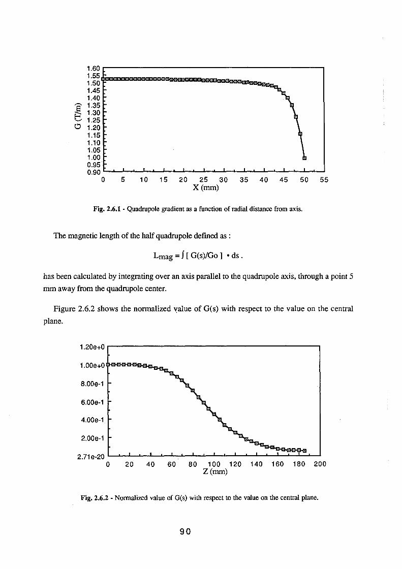
1.60..-------------------------,
1 . 55 I!H:· ·lml· ::a· . 00. ·a· ·:Hlll· 00. ·lllt:i· ·~m~· lHll· . I!Kl· ·H!I· ·D· 00. ·11!11· ·D· [li!J· • maac~~~ilr.. 1.50 [' ........... . 1.45 1.40
8 1.35 ~ 1.30 _. 1.25 0 1.20
1.15 1.10 1.05 1.00 0.95 0.90 .__~~....__......_......_-'-____ __._---&.._....L_....L---1----'L..-.O.__~,.,__,.,__......_...&....-'-.....I
0 5 10 15 20 25 30 X(mm)
35 40 45 50
Fig. 2.6.1 - Quadrupole gradient as a function of radial distance from axis.
The magnetic length of the half quadrupole defined as :
Lmag = f [ G(s)/Go ] • ds .
55
has been calculated by integrating over an axis parallel to the quadrupole axis, through a point 5
mm away from the quadrupole center.
Figure 2.6.2 shows the normalized ~alue of G(s) with respect to the value on the central
plane.
8.00e-1
6.00e-1
4.00e-1
2.00e-1
2. 71 e-20 .__.....__,__...&....-'----&..--"___._.__.....__,__...&....-'----&..--"___._.__....._......_...&....__.
0 20 40 60 80 1 00 120 140 160 180 200 Z(mm)
Fig. 2.6.2 - Normalized value of G(s) with respect to the value on the central plane.
90
The value for (Lmag/2 ) obtained by integrating the curve of Fig. 2.6.2 (half length) is 103.6
mm, this means that the mechanical length of the quadrupole must be 142.8 mm instead of the
nominal 150 mm to obtain the desired magnetic length of 200 mm.
The same cross-section has been adopted for the two kinds of quadrupole. Corrector
windings are provided for dipolar correction of the beam orbit. The quadrupole will be shielded
so that the fringe fields can not get to the se cavities.
The mechanical lay-out of the quadrupole is shown in Fig. 2.6.3.
Table 2.6.1 lists the basic parameters.
Table 2.6.1 - Quadrupole basic parameters
Gradient( maximum) [T/m] 1.6 Inscribed radius [mm] 55 Pole field [T] 0.09 Pole shape circular Ampere-turns per pole 2000 Current [A] 40.8 Current density [Nmm2] 3.14 Turns per pole 49 Copper conductor 4.5*4.5 0 3 Magnetic length [m] 0.2 Magnet resistance [mQ] 200 Power [W] 341 Voltage [V] 8.2 Iron weight [Kg] 73 Copper weight [Kg] 15,5
The main characteristics of power supplies needed to individually power each quadrupole are
the following:
Voltage Current Stability Ripple (rms) Resolution
[V] [A]
12.5 50
~ 1 *1o-4 ~ 1 *1o-4 ,. s *1o-5
The reserve voltage necessary to account for voltage drops on connections is included.
Further optimization of the system should include arrangements where magnets can be
powered in series so as to simplify the power supplies and the corresponding control circuitry.
91
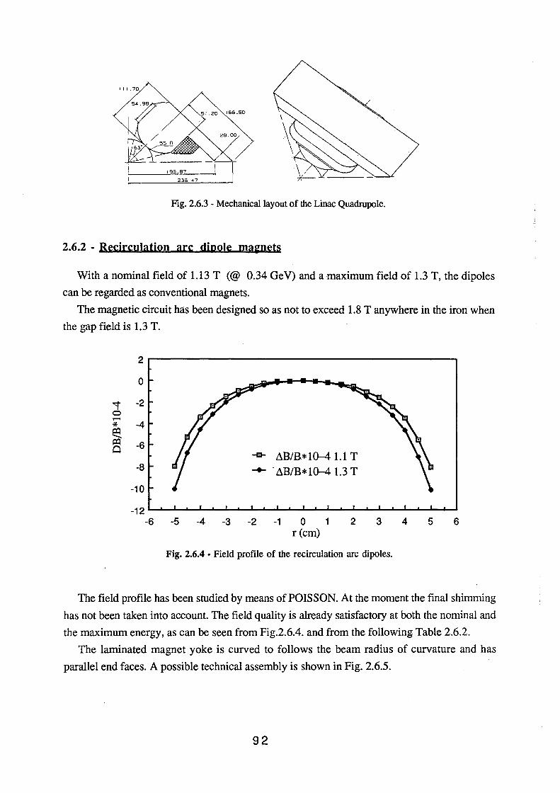
Fig. 2.6.3 - Mechanical layout of the Linac Quadrupole.
2.6.2 - Recirculation arc dipole maJmets
With a nominal field of 1.13 T (@ 0.34 GeV) and a maximum field of 1.3 T, the dipoles
can be regarded as conventional magnets.
The magnetic circuit has been designed so as not to exceed 1.8 T anywhere in the iron when
the gap field is 1.3 T.
2
0
oo::t' -2 I
0 -* -4 ~ IX) -6 0
-a- t1B/B * 1 Q-4 1.1 T -8 -+- "t1B/B*1o-4 1.3 T
-10
-12 -6 -5 -4 -3 -2 -1 0 1 2 3 4 5 6
r (cm)
Fig. 2.6.4 • Field profile of the recirculation arc dipoles.
The field profile has been studied by means of PO IS SON. At the moment the final shimming
has not been taken into account. The field quality is already satisfactory at both the nominal and
the maximum energy, as can be seen from Fig.2.6.4. and from the following Table 2.6.2.
The laminated magnet yoke is curved to follows the beam radius of curvature and has
parallel end faces. A possible technical assembly is shown in Fig. 2.6.5.
92
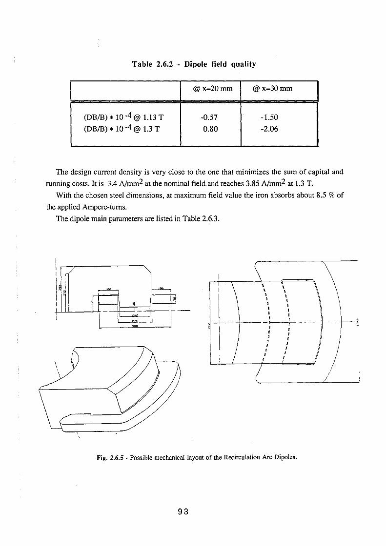
Table 2.6.2 - Dipole field quality
@ x=20 mm I @ x=30 mm
(DB/B)* 10-4@ 1.13 T -0.57 -1.50
(DB/B) * 10 -4@ 1.3 T 0.80 -2.06
The design current density is very close to the one that minimizes the sum of capital and
running costs. It is 3.4 A/mm2 at the nominal field and reaches 3.85 A/mm2 at 1.3 T.
With the chosen steel dimensions, at maximum field value the iron absorbs about 8.5 % of
the applied Ampere-turns.
The dipole main parameters are listed in Table 2.6.3.
I /
I~ 1
~ I I
l
\ \
'"' ~~~
~ 3
- - f-2<2
77A
"""
\ \ \ \
' ' ' I --+--- -+--- -lf----71-11 I a I
1: I H I
If I q I
H 0 ,,
Fig. 2.6.5 - Possible mechanical layout of the Recirculation Arc Dipoles.
93
J
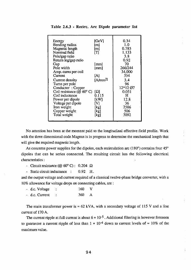
Table 2.6.3 - Recirc. Arc Dipole parameter list
Energy [GeV] 0.34 Bending radius [m] 1.0 Magnetic length [m] 0.785 Nominal field [T] 1.133 Pole/gap ratio 3.8 Return leg/gap ratio 0.92 Gap [mm] 70 Pole width [mm] 266/244 Amp.-turns per coil 34,000 Current [A] 354 Current density [Nmm21 3.4 Turns per pole 96 Conductor : Copper 12*12 07 Coil resistance(@ 60° C) [Q] 0.051 Coil inductance 0.115 H Power per dipole [kW] 12.8 Voltage per dipole [V] 36 Iron weight [kg] 2586 Copper weight [kg] 506 Total weight [kg] 3092
No attention has been at the moment paid to the longitudinal effective field profile. Work
with the three dimensional code Magnus is in progress to determine the mechanical length that
will give the required magnetic length.
As concerns power supplies for the dipoles, each recirculation arc (180°) contains four 45°
dipoles that can be series connected. The resulting circuit has the following electrical
characteristics :
- Circuit resistance (@ 60° C) : 0.204 Q
- Static circuit inductance : 0.92 H.
and the output voltage and current required of a classical twelve-phase bridge converter, with a
10% allowance for voltage drops on connecting cables, are :
d.c. Voltage 160 V
- d.c. Current 360 A
The main transformer power is "" 62 kVA, with a secondary voltage of 115 V and a line
current of 170 A. The current ripple at full current is about 6 * IQ-5 . Additional filtering is however foreseen
to guarantee a current ripple of less than 1 * 10-4 down to current levels of"" 10% of the
maximum value.
94
The power supply resolution is better than 1 * I0-4. A long term stability of the same order
or better can easily be reached by means of a high stability ( 1 * lQ-6) commercial transducer.
2.6.3 - Recirculation arc quadrupoles
The recirculation arc lattice contains 34 quadrupoles, whose characteristics are listed in
Reference (49) and summarised in Table 2.6.3 ..
The magnetic length, 0.3 m, is the same for all quadrupoles. The values of k2 (and of the
gradient G) are very different, ranging from a minimum of 1.08 m-2 (G= 1.22 T/m) to a
maximum of 13.32 m-2 (15.1 T/m).
The quadrupole has been optimized for the average value of k2, i.e. 6.68 m-2; the currents
are then scaled so as to reach the other gradient values with the same geometry. A single type of
quadrupole is thus foreseen at this first-order optimization stage and, consequently, no attempt
to simplify the powering scheme has made; these points will have to be reconsidered in the
course of further study.
The electromagnetic design has been made using the hi-dimensional code Poisson; two
possible solutions, both with hyperbolic pole profiles have been studied. The first fits around a
rectangular vacuum chamber with a cross-section of ll(horizontal) * 7 (vertical) cm2, the
second fits around an elliptical vacuum chamber inscribed in the above rectangle. In both cases
the pole profile is hyperbolic.
Because of the eight-fold symmetry of the magnet only one-half pole, has been studied.
The magnetic field can be expressed in complex form as :
(Bx- i By)= i * L, n *(An +i Bn)/R * (z!R)(n-1)
where Bx and By are the horizontal and vertical components of the field respectively, n is the
harmonic number ( 2 for quadrupole, 6 for 12-pole and so on), An and Bn are the coefficients
of the expansion, R is a normalization radius and z is the complex variable. The normalization
radius is 60 mm for the rectangular vacuum chamber case and 40 mm for the other case.
The field along the x axis can be obtained by simply replacing z by x and taking the first
derivative to obtain the field gradient.
In our approximation Bn is identically zero for all n's and An takes on the values shown in
Table 2.6.4 for the optimized quadrupole at the average gradient. At maximum gradient the
scaling factors are 2.3 for the rectangular chamber and 2.37 for the elliptical vacuum chamber.
At the lowest gradient the scaling factors become (1/ 5.40) and (1/ 5.43) respectively.
The gradient uniformity for the two quadrupole apertures is shown in Fig. 2.6.6.
95
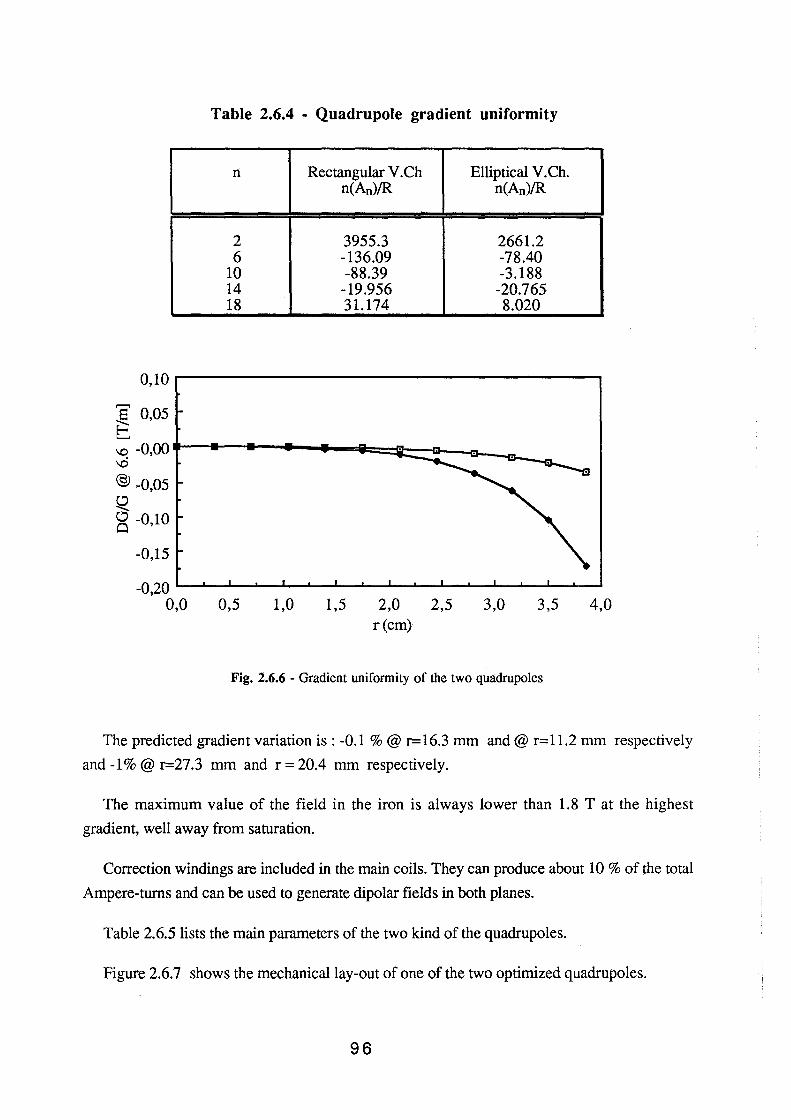
Table 2.6.4 - Quadrupole gradient uniformity
n Rectangular V.Ch Elliptical V.Ch. n(An)/R n(An)/R
2 3955.3 2661.2 6 -136.09 -78.40
10 -88.39 -3.188 14 -19.956 -20.765 18 31.174 8.020
0,10 ,...------------------------.
8 0,05 ~ .........
\0 -o,oo r--------------==lil=:::::;:~~-a--m--_ -.6
@> -0,05
~ g -0,10
-0,15
-0,20 .__........__.____.__...__........_~__.._....._........_--'-___._.....__.___,____..__.
0,0 0,5 1,0 1,5 2,0 r(cm)
2,5 3,0 3,5
Fig. 2.6.6 - Gradient uniformity of the two quadrupoles
4,0
The predicted gradient variation is: -0.1 %@ r=16.3 mm and@ r=11.2 mm respectively
and -1%@ r=27.3 mm and r = 20.4 mm respectively.
The maximum value of the field in the iron is always lower than 1.8 T at the highest
gradient, well away from saturation.
Correction windings are included in the main coils. They can produce about 10 % of the total
Ampere-turns and can be used to generate dipolar fields in both planes.
Table 2.6.5 lists the main parameters of the two kind of the quadrupoles.
Figure 2.6.7 shows the mechanical lay-out of one of the two optimized quadrupoles.
96
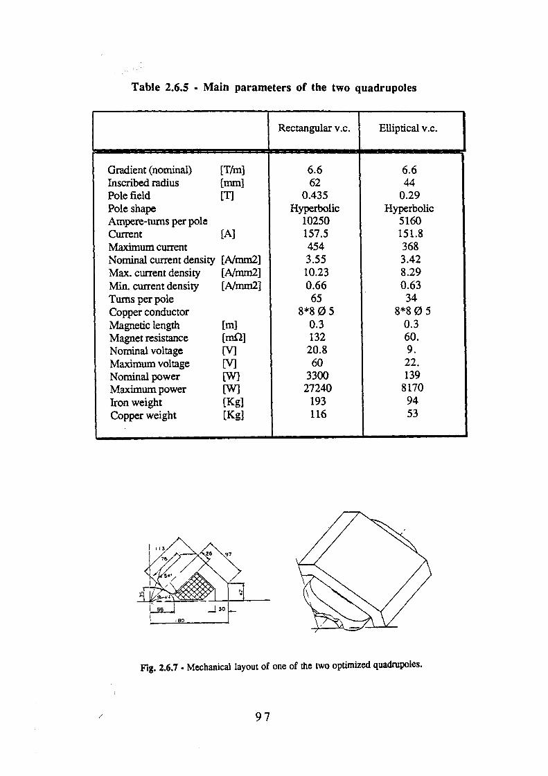
Table 2.6.5 • Main parameters of the two quadrupoles
Rectangular v.c. Elliptical v.c.
Gradient (nominal) [T/m] 6.6 6.6 Inscribed radius [mm] 62 44 Pole field [T] 0.435 0.29 Pole shape Hyperbolic Hyperbolic Ampere-turns per pole 10250 5160 Current [A] 157.5 151.8 Maximum current 454 368 Nominal current density [Nmm2] 3.55 3.42 Max. current density [Nmm2] 10.23 8.29 Min. current density [Nmm2] 0.66 0.63 Turns per pole 65 34 Copper conductor 8*805 8*80 5 Magnetic length [m] 0.3 0.3 Magnet resistance [m!l] 132 60. Nominal voltage [V] 20.8 9. Maximum voltage [V] 60 22. Nominal power [W] 3300 139 Maximum power [W] 27240 8170 Iron weight [Kg] 193 94 Copper weight [Kg] 116 53
Fig. 2.6.7. Mechanical layout of one of the two optimized quadrupoles.
97
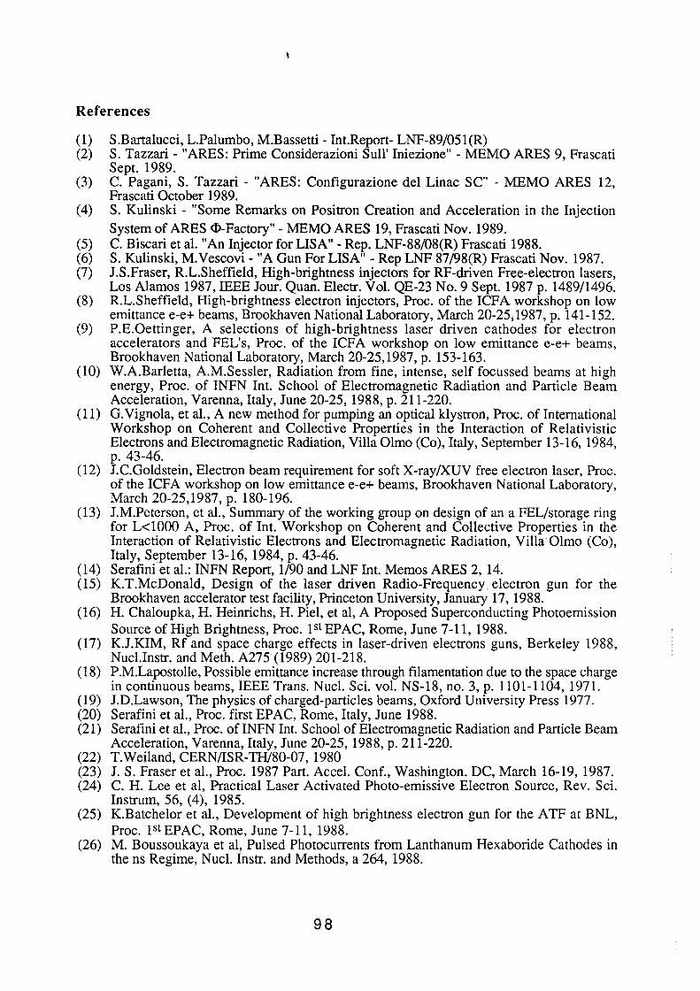
References
(1) S.Bartalucci, L.Palumbo, M.Bassetti- Int.Report- LNF-89/051(R) (2) S. Tazzari - "ARES: Prime Considerazioni Sull' Iniezione" - MEMO ARES 9, Frascati
Sept. 1989. (3) C. Pagani, S. Tazzari- "ARES: Configurazione del Linac SC" - MEMO ARES 12,
Frascati October 1989. (4) S. Kulinski- "Some Remarks on Positron Creation and Acceleration in the Injection
System of ARES <1>-Factory"- MEMO ARES 19, Frascati Nov. 1989. (5) C. Biscari et al. "An Injector for LISA"- Rep. LNF-88/08(R) Frascati 1988. (6) S. Kulinski, M.Vescovi- "A Gun For LISA"- Rep LNF 87/98(R) Frascati Nov. 1987. (7) J.S.Fraser, R.L.Sheffield, High-brightness injectors for RF-driven Free-electron lasers,
Los Alamos 1987, IEEE Jour. Quan. Electr. Vol. QE-23 No. 9 Sept. 1987 p. 1489/1496. (8) R.L.Sheffield, High-brightness electron injectors, Proc. of the ICFA workshop on low
emittance e-e+ beams, Brookhaven National Laboratory, March 20-25,1987, p. 141-152. (9) P.E.Oettinger, A selections of high-brightness laser driven cathodes for electron
accelerators and FEL's, Proc. of the ICFA workshop on low emittance e-e+ beams, Brookhaven National Laboratory, March 20-25,1987, p. 153-163.
(10) W.A.Barletta, A.M.Sessler, Radiation from fine, intense, self focussed beams at high energy, Proc. of INFN Int. School of Electromagnetic Radiation and Particle Beam Acceleration, Varenna, Italy, June 20-25, 1988, p. 211-220.
(11) G. Vignola, et al., A new method for pumping an optical klystron, Proc. of International Workshop on Coherent and Collective Properties in the Interaction of Relativistic Electrons and Electromagnetic Radiation, Villa Olmo (Co), Italy, September 13-16, 1984, p. 43-46.
(12) J.C.Goldstein, Electron beam requirement for soft X-ray/XUV free electron laser, Proc. of the ICFA workshop on low emittance e-e+ beams, Brookhaven National Laboratory, March 20-25,1987, p. 180-196.
(13) J.M.Peterson, et al., Summary of the working group on design of an a FEL/storage ring for L<1000 A, Proc. of Int. Workshop on Coherent and Collective Properties in the Interaction of Relativistic Electrons and Electromagnetic Radiation, Villa Olmo (Co ), Italy, September 13-16, 1984, p. 43-46.
(14) Serafini et al.: INFN Report, 1/90 and LNF Int. Memos ARES 2, 14. (15) K.T.McDonald, Design of the laser driven Radio-Frequency, electron gun for the
Brookhaven accelerator test facility, Princeton University, January 17, 1988. (16) H. Chaloupka, H. Heinrichs, H. Piel, et al, A Proposed Superconducting Photoemission
Source of High Brightness, Proc. tstEPAC, Rome, June 7-11, 1988. (17) K.J.KIM, Rf and space charge effects in laser-driven electrons guns, Berkeley 1988,
Nucl.lnstr. and Meth. A275 (1989) 201-218. (18) P.M.Lapostolle, Possible emittance increase through filamentation due to the space charge
in continuous beams, IEEE Trans. Nucl. Sci. vol. NS-18, no. 3, p. 1101-1104, 1971. (19) J.D.Lawson, The physics of charged-particles beams, Oxford University Press 1977. (20) Serafini et al., Proc. first EPAC, Rome, Italy, June 1988. (21) Serafini et al., Proc. of INFN Int. School of Electromagnetic Radiation and Particle Beam
Acceleration, Varenna, Italy, June 20-25, 1988, p. 211-220. (22) T.Weiland, CERN/ISR-TH/80-07, 1980 (23) J. S. Fraser et al., Proc. 1987 Part. Accel. Conf., Washington. DC, March 16-19, 1987. (24) C. H. Lee et al, Practical Laser Activated Photo-emissive Electron Source, Rev. Sci.
Instrum, 56, (4), 1985. (25) K.Batchelor et al., Development of high brightness electron gun for the A TF at BNL,
Proc. 18tEPAC, Rome, June 7-11, 1988. (26) M. Boussoukaya et al, Pulsed Photocurrents from Lanthanum Hexaboride Cathodes in
the ns Regime, Nucl. Instr. and Methods, a 264, 1988.
98
(27) (28)
(29) (30)
(31) (32)
(33) (34)
(35)
(36) (37)
(38) (39) (40)
(41)
(42)
(43)
(44)
(45) (46)
(47)
(48)
(49)
H.E.Koechner, Solid State Laser Engineering, Springer-Verlag, New York, 1976. S.L.Shapiro, Ultrashort Light Pulses: Picosecond Techniques and Applications, Springer-Verlag, New York, 1977. W. Heitler- "The Quantum Theory of Radiation". Oxford 1966. F. Amman- "Positron Accelerators in Linear Accelerators". Edited by P. Lapostolle , A.L. Septier. North Holland 1970. U. Amaldi et al. Proc. Courmayer Workshop Dec. 1987 page 78. G. Stange- "Considerations for the Kicker Magnets Design for the Sincrotrone Trieste"Trieste July 1989. H. Piel, Wuppertal University note WUB 87-13, (1987). C. Benvenuti, N. Cirelli, M. Hauer, W. Weingarten, Proc. 2nd Workshop on RF Superconductivity, H. Lengeler Ed., Geneva, July 23-27, 1984 D. Di Gioacchino, U. Gambardella, P. Gislon, G. Paterno', C. Vaccarezza, INFN note LNF 89/064 (R), (1989) Proc. Discussion Meeting on SC Linear Accelerators, Frascati, October 1986. R.Sundelin, "Fully Superconducting Linear Colliders", Proc. Capri Workshop on Linear Colliders, Capri, 13-17 June 1988. V.Lagomarsino, G.Manuzio, R.Parodi, R.Vaccarone, IEEE Trans. MAG-15, 25 (1979). C.M.Lyneis, H.A.Schwettman, J.P.Turneaure, Appl. Phys. Lett. 31, 541 (1977). U.Klein and D.Proch, Proc. of the Conf. on Future Possibilities for Electron Ace., Charlottesville (Virginia), 1979. L.Serafini, S.Gustafsson, C.Pagani, Proc. 11th Int. Conf. on Cyclotrons and Their Appl., Tokyo, October 1986, Ionics Pub., Tokyo, 370 (1987). T.Tajima, T.Furuya, T.Suzuki and Y.Iino, "Pre-tuning of TRISTAN Superconducting RF Cavities", Proc. 4th Workshop on RF Soperconduc., KEK, Japan, August 1989. B.Dwersteg et al. "Superconducting Cavities for HERA", Proc. 3st Workshop on RF Soperconductivity, ANL,Argonne, Illinois, September 1987. Ph.Bernard et al., "Superconducting RF Cavities for LEP", Proc. 1st European Particle Ace. Conf., Rome, Italy, June 1988. D.Boussard et al., CERNIEFIRF 88-3, 12 October 1988. Ph.Bernard et al., Test of a 352 MHz Superconducting Cavity in the CERN SPS, Proc. European Particle Accelerator Conference, Rome, June 1988, p. 988. World Scientific, Singapore. "The Vacuum Bellows and the Optimization of their Shielding", LEP Note 568, Sept.l986. A. G. Mathewson, "The effect of cleaning and other treatments on the vacuum properties of technological materials used in ultra-high vacuum." Proc. lOth Italian Nat. Conf.on Vacuum Science and Technology, Stresa, Italy, Oct. 1987, ll Vuoto. LNF Internal note Ares-22
99

3. - THE <I>-FACTORY
3.1. • INTRODUCTION
The main goals of the ARES <I>-Factory are:
- Achievement of 1Q32 cm-2sec-lluminosity at 510 Me V.
- Construction and commissioning in 5-6 years .
- Possibility to investigate the linear-against -circular collision scheme.
The nature of a <I>-Factory in itself dictates a minimum target luminosity of 1Q32 cm-2sec-l,
and at least a non negligible probability that an improvement factor of the order of 3 can be
gradually achieved.
A luminosity of 1Q32 cm-2sec-l has never been reached or even approached in a reliable way
on existing machines in the <I> energy range; the system parameters must therefore be carefully
researched, chosen and optimized and new solutions must be identified.
On the other hand, the luminosity optimization process itself is uncertain because there is no
theory that fully explains the performance limitations of existing storage rings.
Our philosophy has been to make educated guesses on the basis of the available data, models
and scaling laws.
Moreover, when one considers the tight time schedule, one concludes that the design should
not require more than a limited amount of R&D, and must be flexible enough to allow the key
machine parameters to be easily changed to fine-tune the luminosity and to exploit alternative
collision schemes.
In agreement with the general criteria described above the design presented here
• is based on conventional technology, and
• has two distinctive features:
- electrons and positrons circulate in two vertically separated storage rings and collide head
on in a single interaction point ;
- the ring magnetic lattice is a 4 period modified Chasman-Green type with a 1.9 Tesla
conventional wiggler magnet inside the achromat. This last choice allows ample emittance
tunability and at the same time gives strong radiation damping, one of the fundamental
properties that lead to high luminosity.
In case even more damping should prove to be necessary, it can be produced by inserting
additional wiggler magnets.
100

3.2. - DESIGN CRITERIA
3.2.1 - Basic formulae
The single bunch luminosity for an electron-positron storage ring collider is given by the
well known formula : f N2
L=-----4 1t O'x O'y
(3.1)
where f is the revolution or collision frequency, N is the number of electrons and positrons
(assumed to be the same) and O'x and O'y are the horizontal and vertical r.m.s. beam sizes at the
interaction point, IP.
During a collision the two bunches focus each other causing a tune shift .1Q. An appropriate
indicator of the focusing force, in a linear approximation, is the tune shift parameter ~ given by
(3.2)
where y is the electron energy in units of its rest mass, re the classical electron radius, ~x.y the
value of the horizontal (vertical) betatron function at the IP. For all practical cases :
(3.3)
For a given beam current,~ is usually different in the horizontal and vertical planes (~x <<
~y)· However, in order to achieve the maximum luminosity, it is convenient to have
~=~X= ~y This condition can be satisfied by choosing
K=~=b=~ Ex ~x O'x
(3.4)
(3.5)
where K is the coupling coefficient (I) that can take on any value between 0 and 1. By putting
equations (3.2), (3.4), (3.5) together, luminosity and~ can be rewritten as:
or equivalently
and
~2 f e ( 1 + K)
~y
L = X (;. J --"~'-2-f -:-~-'-~ l_+_K..:...)
1 01
(3.6)
(3.7)
~=~N 2rr:y e (3.8)
Eqs. (3.6) and (3.7) show the interrelation between the luminosity, K, 13y and 13x. To gain
in luminosity, for example, it is not sufficient to assume a smallj3y, but it is also necessary to
reduce either 13x or the coupling coefficient according to (3.5).
Equations (3.6) and (3.7) also remark, from the quadratic dependence of luminosity on~.
the leading parameter role of the linear tune shift in collider design.
~ is generally assumed to depend quadratically on the number of crossings per turn, ni,
namely: 1
~oc-
~
ni is usually equal to twice the number of bunches in one beam.
(3.9)
If one tries to increase the luminosity by increasing ni , and therefore the collision frequency
f, ~decreases according to eq. (3.9) and defeats the-purpose (insofar as 3.9 is exact), as can be
seen from eq. (3.6) or (3.7) . This is the reason why electrostatic separating plates are used to
reduce ni while mantaining the same frequency of crossings (see for example CESR(2) where ni
is reduced from 14 to 2 by an electrostatic separation system producing a pretzel like orbit
deformation) .
The maximum attainable ~value can not be computed from theory. Experimentally,
however, the maximum value for ~ (in the case of two interactions per turn), averaged over
most of the existing electron colliders, is remarkably constant at :
< ~max > = .038 ± .013 (3.10)
As shown by eq~ (3.8), equation (3.10) sets an empirical limit on the ratio between the
number of particles N and the beam emittance E, i.e. a limit on the transverse beam density.
Therefore, as e and N can not be indefinitely increased because of aperture and instability limits,
eq. (3.10) sets a limit on the luminosity.
102
3.2.2 - Colljsjon freguency
From the luminosity point of view one would like the collision frequency to be as high as
possible or, equivalently, the storage ring footprint to be as compact as possible.
Ultra-compact rings on the other hand require the use of superconductive dipoles, a feature
we do not deem desirable for the machine under design for reasons we try to explain in the
following.
Straight superconducting magnets are used in large high energy proton accelerators, whether
existing (Tevatron, HERA, etc) or planned (HLC, SSC, RHIC), with very large bending
radius.
For a <I>-Factory however the bending radius would be extremely small (p <<1 m) and one
would have to face the engineering problems connected with the design of such 'curved'
dipoles, the strong non linearities coming from the small bending radius and the large
synchrotron radiation power in a superconducting environment.
While therefore it is true that small superconducting machines are being developed for
industrial applications and have also been proposed (3,4) for <I>-factories, the adoption of such a
technology is in our opinion more appropriate for an R&D program than for a time-pressed
project.
Moreover, we maintain that the gain in collision frequency is not substantial because the ring
size will eventually be dominated by the need for space to accomodate the low-P insertion and
the experimental apparatus.
In conclusion the most efficient way of increasing the collision frequency is multi bunch
operation.
In multibunch operation one has of course, according to eq.(3.9), to avoid parasitic
collisions that lower the tolerable tune shift parameter ~ . One has the choice of either design
complicated separation schemes or store the beams in two (horizontally or vertically) separated
rings and collide them head-on in a single interaction point.
We propose to build two vertically separated rings because, for several practical reasons, the
gain in collision frequency is greater for the two-ring scheme; the gain-factor is -{2 on ...[rli and,
consequently, on~. We choose the vertical solution because less expensive than the horizontal
one from the conventional constructions point of view.
Experience with DORIS(5) has shown that the crossing angle should be as close to zero as
possible, and that any residual error crossing angle has to be canceled by accurately monitoring
and correcting the orbits.
On the 'minus' side it should also be mentioned that multibunch operation is prone to
multibunch instabilities, that have to be carefully suppressed, and it is at risk of ion trapping
unless proper, nontrivial countermeasures are taken.
103
If Lb is the spatial separation between two consecutive bunches and we assume to fill
uniformely all the ring circumference, the collision frequency becomes
Our design choice is :
c f= Lb
I f= ~ = 71.4 MHz, giving Lb = 4.2 m.
The first unwanted crossing would occur at a distance Lt/2 from the IP, and the electrostatic
separation system must therefore provide a vertical beam separation (6) ~ Y > 2 O"x at a
distance of 2.1 m from the IP. This distance is not very large but, in our opinion, due to the
relatively low energy, a suitable separation scheme can be designed.
3.2.3 - vertical 6-function at the lP
The luminosity increases linearly with the inverse of ~Y at the lP. To take full advantage of
this dependence, one has to be ready to pay a price in terms of RF system voltage, ring
impedance and, because also the r.m.s longitudinal bunch length must be small, of single
bunch instabilities. In fact, an empirical rule states that
_h O"z ~- 1.5
in order to avoid geometrical luminosity reductions.
In addition, the Liouville theorem prescribes that to a very small ~Y at the lP there must
correspond a large beam divergence; the latter has to be corrected locally, as close as possible to
the IP, or the necessary machine acceptance will become too large.
In practice, one is forced to put a very strong quadrupole close to the interaction point that
will necessarily limit the solid angle available for the experiment.
This kind of limitation, common to all the low-~ schemes, is particularly severe in the case
of a <I>-Factory; it imposes a coordinated design of the low-~ insertion and the experimental
apparatus.
The beam divergence correcting quadrupole also has the effect of raising the machine
chromaticity that has to be corrected by the addition of strong sextupoles; the dynamic aperture
is consequently reduced.
In conclusion, the value of i3y can not be arbitrarily small; a reasonable choice for the design
value turns out to be :
104
~y =4.5 cm with O'z = 3.0 cm.
The low-~ insertion will be designed with a wide range of tunability around this value.
Lower values of 13y, such as those claimed by other designs, could therefore be attempted once
the machine behaviour has been fully understood, providing an upgrade potential for
luminosity.
3.2.4 - Couolim: coefficient
The coupling coefficient design value has been chosen to be :
K = .01
this choice, apparently in contrast with the main goal of maximizing the luminosity (see Eq.
3.6), will be justified in § 3.2.7. We add here a few practical considerations.
From eq. (3.5) we deduce that, with K =.01:
~x = 100 • ~Y = 4.5 m
To achieve such very low value of the coupling coefficient is however not easy; the
orbit has to be measured and corrected very precisely, and the vertical dispersion function has to
be carefully minimized, especially because of the vertical beam separation scheme. The
Touschek effect, limiting the useful lifetime, also becomes of paramount importance. In our
case we compute a Touschek lifetime - 4 hrs.
The problems are nevertheless solvable; many storage rings in operation have obtained K
values less than 1%. In particular, the Brookhaven 750 Me V VUV ring has reached K = 0.0017, after careful machine alignment and after spending one day to correct the residual
closed orbit to the desired precision (7).
Alternative solutions, with lower emittance or smaller ~Y (small O'z), would no doubt require
stronger coupling to reach an acceptable lifetime.
A potential advantage of the low coupling is the reduction of ion trapping at least when the
design dynamic vacuum of- IQ-9 torr is assumed.
105
3.2.5 - Desi~m emittance
The emittance e affects the luminosity linearly but cannot be made arbitrarily large; the limit
is given by the machine physical and dynamic apertures necessary for a reasonable beam
lifetime. Very large emittance also implies that the number of particles, N, necessary to achieve
a large 1; is very large (see 3.8).
All considered, a reasonable choice for e is :
e = 10-6 m·rad
but, as for the case of ~Y , the storage ring is designed to allow a wide range of tunability and
consequently has some potential for improvement. The upper emittance limit is essentially
determined by aperture requirements, while the lower one is in the lQ-9 m·rad range.
3.2.6 - The linear tune shift parameter s The linear tune shift 1;, appearing squared in the luminosity formula, plays the most
important role and, because of (3.10), is the fundamental, not yet fully understood limiting
factor (see also § 3.2.7).
A sensible choice is to estimate the luminosity value on the basis of the experimental average
~;max given by (3.10), namely: ~~---------------s-m_a_x-~-.-0-4---------~
By this choice we also implicitly fix the number of particles per bunch, N : by substituting
the values of e and 1; into (3.8) we obtain:
N = 8.9 1010 particles/bunch
and the resulting average current in each beam is :
< i > = e f N = 1.02 A
This is an unusually high current value that will require a careful design of the RF and the
vacuum systems. Let us however point out that similar current values have been reached at
storage rings now in operation : as an example, a current in excess of 1.3 Amp has been
accumulated in the BNL VUV ring (7) that runs routinely with stored currents of .8+.9 Amp.
106
3.2.7 - Luminosity scalina: laws
As often mentioned above, there is no exhaustive explanation of the luminosity limit.
Among existing phenomenological models we have singled out the work by J.Seeman (8)
and by M.Bassetti (9), because the former is in reasonable agreement with the ~max experimental
data from several machines, while the latter introduces something new in the direction of a
better understanding the luminosity limits. In the following we briefly summarize their results.
Let us ftrst recall the defmition of the synchrotron integrals 12 an 13 (10) :
f ds p2
Dip f ds
lp31 Dip
(3.11)
For an isomagnetic machine with a bending radius p, the integrals over one turn are given
by:
(3.12)
U0 (10) and crR(9), the radiation energy loss per turn and the r.m.s. quantum fluctuation per
turn respectively, can be expressed through (3.11) as follows :
U0 (KeV)- 14.1 E4(GeV) l2 (m-1)
aR (KeV)- 6.5 E 35(GeV) ...J13 (m-2)
(3.13)
(3.14)
J.Seeman has reviewed, in a very exhaustive paper (8), the data on beam-beam interaction
obtained at most of the existing e+e- storage rings; he shows that by empirically fitting the
dependence of the linear tune-shift ~ on the various relevant parameters he can explain them all
rather well. His best ftt shows that the maximum vertical linear tune shift (at the maximum
luminosity) divided by the beam energy, increases with the square rO?t of 1/(niP), where ni is
the number of crossings per turn and p is the bending radius. This can be expressed as:
(h._ 'r""- 1.4 1o-s ~ 12 (~-I) const - rr- ( 3. 15) 'Y ) nt -\J p ni
By substituting eq. (3.15) into (3.6) we have a ftrst luminosity scaling law :
L max oc y6 12 (Seeman's law)
107
The open question is if one is allowed to extrapolate the experimental fit (3.15) to the case
of a very small bending radius (large U0); the Novosibirsk <P-Factory design by Barkov et ai.(3)
featuring a very small bending radius ( p = 28cm with 6 Tesla s.c. dipoles), claims a ~max of
"".07 in both planes, not far from the value one would calculate from (3.15).
Using the conservative value ~max = .04 discussed under§ 3.2.6 and considering that we
have only one crossing point, we obtain from (3.6) and (3.15) the minimum acceptable value of
12:
(Seeman's criterion)
or, equivalently through (3.13), the minimum acceptable value of the radiated energy:
U0 min- 10.5 KeY.
In a recent study (9) M. Bassetti suggests that a further luminosity limitation comes from the
perturbation of the radiative damping mechanism by the beam-beam interaction. In fact the
maximum energy, Lllibb , lost or gained by a particle working against the electric field of the
opposite beam must - according to his model - be lower than the average quantum fluctuation,
O"R ,of the synchrotron radiation between two interactions, in order for the machine to behave
properly. According to his formalism Lllibb is given by:
Lllibb (KeV)- 3.58 103 re Ff'~)!!_ - ~ O"x ~y
(3.16)
0" where F is a form factor shown in Fig. 3.1 that depends strongly on the ratio K = :::.:t..
O"x
By analising the behaviour of existing storage rings, it is found that at maximum luminosity
many storage rings have :
(3.17)
The coefficient has been derived empirically and will require further studies with numerical
simulations and experimental check. Eq. (3.17) implies a limitation on the maximum N,
independently from the transverse beam density. By using (3.17), according to Bassetti, we
can write a luminosity scaling law :
(Bassetti's law)
108
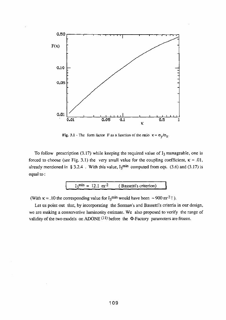
F(K)
0.10
o.a5
0.01 0.05 <1.1 0.5 j
Fig. 3.1 -The form factor F as a function of the ratio K = aylax.
To follow prescription (3.17) while keeping the required value of l3 manageable, one is
forced to choose (see Fig. 3.1) the very small value for the coupling coefficient, K = .01,
already mentioned in § 3.2.4 . With this value, l3min computed from eqs. (3.6) and (3.17) is
equal to:
( Bassetti's criterion)
(With K = .10 the corresponding value for 13min would have been -900m-2!).
Let us point out that, by incorporating the Seeman's and Bassetti's criteria in our design,
we are making a conservative luminosity estimate. We also proposed to verify the range of
validity of the two models on ADO NE (11) before the <I>-Factory parameters are frozen.
109
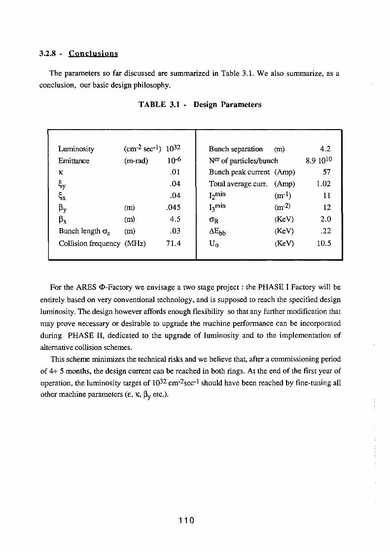
3.2.8 - Conclusions
The parameters so far discussed are summarized in Table 3.1. We also summarize, as a
conclusion, our basic design philosophy.
TABLE 3.1 - Design Parameters
Luminosity (cm-2 sec-1) 1Q32 Bunch separation (m) 4.2
Emittance (m-rad) 10-6 Ner of particles/bunch 8.9 1Q10
1( .01 Bunch peak current (Amp) 57
~y .04 Total average curr. (Amp) 1.02
~X .04 12min (m-1) 11
~y (m) .045 13min (m-2) 12
~X (m) 4.5 O'R (KeV) 2.0
Bunch length O'z (m) .03 ~Ebb (KeV) .22
Collision frequency (MHz) 71.4 Uo (KeV) 10.5
For the ARES <1>-Factory we envisage a two stage project: the PHASE I Factory will be
entirely based on very conventional technology, and is supposed to reach the specified design
luminosity. The design however affords enough flexibility so that any further modification that
may prove necessary or desirable to upgrade the machine performance can be incorporated
during PHASE 11, dedicated to the upgrade of luminosity and to the implementation of
alternative collision schemes.
This scheme minimizes the technical risks and we believe that, after a commissioning period
of 4+ 5 months, the design current can be reached in both rings. At the end of the first year of
operation, the luminosity target of 1Q32 cm-2sec-1 should have been reached by fine-tuning all
other machine parameters (E, K, ~Y etc.).
1 1 0
3.3. - BEAM OPTICS
3.3.1 - Low-13 insertion
The low-~ insertion and the vertical separation system are the most crucial parts of the <1>
Factory design, because of the constraints imposed by the experimental apparatus and by the
relatively short bunch-to-bunch longitudinal distance Lb.
The experimental apparatus, not yet completely defined, has of course to cover the largest
possible solid angle; a solenoidal field of""' .5 + 1. kG over a length of approximately 5 meters
on each side of the lP is also required. The beam trajectory will be actively shielded from
solenoidal field, with the exception of± 0.5 m around the lP, where the vacuum chamber wall
must be very thin and no active or passive shield can be used.
The details of of the residual field compensation and of the resulting shielding arrangement
are still under study and only a general feasibility study is therefore presented.
The most serious constraint posed by the experimental apparatus on the design of the low-~
insertion is the requirement of a large unencumbered solid angle around the IP. A tentative
agreement has been reached with the users on a low-~ insertion confined to a cone of half
aperture angle 8 = 8.5° , over a length of± 5 m from the IP. The distance of the first
quadrupole from the lP is ;::: 45 cm and the quadrupole maximum outer diameter 0Q is given by:
0o = 2 · tan (8.5°) · 45 cm = 13.45 cm
It is important, because of the low K': value chosen, to suppress the vertical dispersion
function Dy locally. Moreover the beam separation system has to satisfy the condition:
Ll Y > 2 O'x I at the first unwanted collision point (Li/2) as well as at the second one ( Lb).
The relevant lattice design parameters are as follows:
~X= 4.5 cm ~x = 4.5 m 1( =.01 E = I0-6 m·rad Lb=4.2 m
Starting from the lP, there is a first lattice region, inside the detector, where two electrostatic
separators, VS 1 and VS2, begin to gradually separate the beams. The separators are
schematized as vertical magnets with a bending radius given by .511 'Y
PE (m)- E (MV/m)
1 1 1
where E = V I d is the electric field value , V the voltage and d the distance between the
plates. We assume:
PE= 200 m, V= lOOKV, d = 4 cm
to obtain:
E ""2.5 MVolt/m
The 13-functions in the region from the lP to the second unwanted crossing are shown in
Fig. 3.2; the resulting half-separation Y and the horizontal beam size crx are plotted in Fig.3.3
By inspecting Fig. 3.3 we can see that the criterion .1 Y > 2 crx is satisfied.
Let us point out that the first quadrupole, QFl, is rather weak and focussing in the horizontal
plane. This provides better control over the ~ functions along the rest of the insertion.
The mechanical design of the first two quadrupoles, QFl and QDl, whose maximum
allowable outer diameters are
0oF1 = 13.45 cm 0om = 20.92 cm I is still under study; at the moment the most likely solution for QFl foresees the use of
permanent magnets.
In the second region, near the edge of the detector, we increase the vertical separation with
two thin septum magnets VB 1 and VB2 . Two additional vertical magnets VB3 and VB4, of
opposite sign, take the beam horizontally to the following dispersion suppressor region. The
dispersion suppressor consist of three 1200 FODO cells with missing magnets.
The 13-functions in the region in between the lP and VB4 are plotted in Fig. 3.4; the vertical
dispersion Dy is shown in Fig. 3.5 .
Fig.3.6 shows the vertical half separation, Y, along the low-13 insertion.
Finally the low-13 insertion is connected to the main arcs by a matching section consisting
of four quadrupoles.
11 2
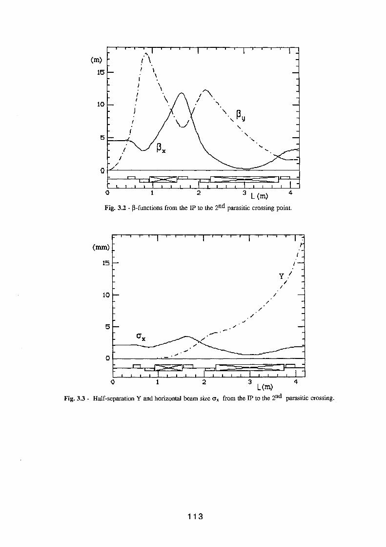
" (m) ,· \ 15 \
I \
I \ \
I I
10
3 L (m)
Fig. 3.2 - ~-functions from the lP to the 2nd parasitic crossing point.
(mm)
15
10
5 -· 1
/
/
3 L(m)
I
y , I
4
Fig. 3.3 - Half-separation Y and horizontal beam size <Yx from the lP to the 2nd parasitic crossing.
11 3
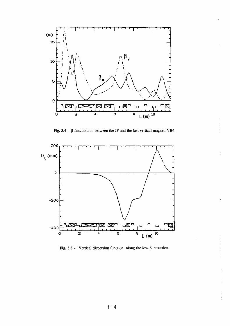
(m) '1. I. "I
15 I . I
10 :'. Py } l
l
5 \
Fig. 3.4 - J3-functions in between the lP and the last vertical magnet, VB4.
Dy (mm)
-:200
Fig. 3.5 - Vertical dispersion function along the low-J3 insertion.
114
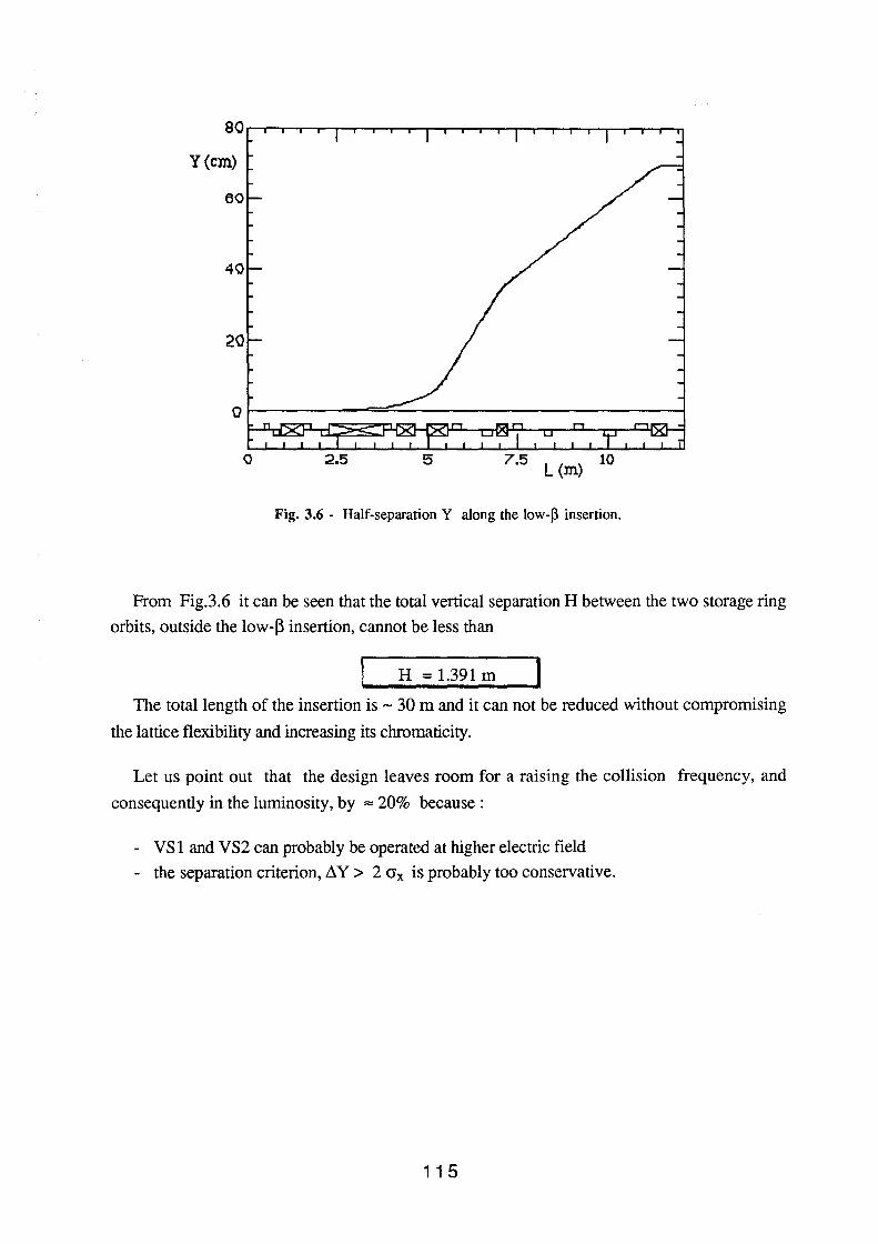
80~-r,-r.rT-r,-r.rT~~~~~~~~~~
Y(cm)
0 7.5 L (m) 10
Fig. 3.6 - Half-separation Y along the low-~ insertion.
From Fig.3.6 it can be seen that the total vertical separation H between the two storage ring
orbits, outside the low-~ insertion, cannot be less than
H = 1.391 m
The total length of the insertion is - 30 m and it can not be reduced without compromising
the lattice flexibility and increasing its chromaticity.
Let us point out that the design leaves room for a raising the collision frequency, and
consequently in the luminosity, by ""20% because:
- VS 1 and VS2 can probably be operated at higher electric field
- the separation criterion, .1 Y > 2 <Jx is probably too conservative.
11 5
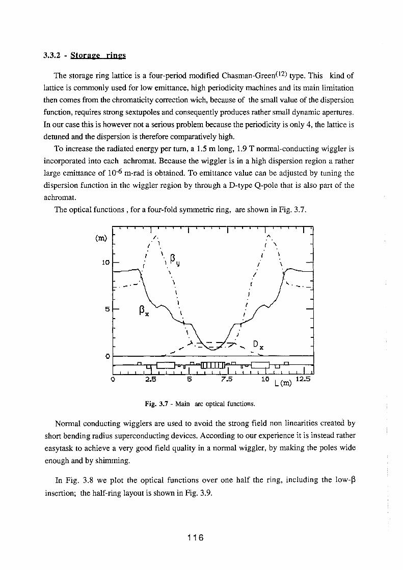
3.3.2 - Stora~:e rin~:s
The storage ring lattice is a four-period modified Chasman-Green(12) type. This kind of
lattice is commonly used for low emittance, high periodicity machines and its main limitation
then comes from the chromaticity correction wich, because of the small value of the dispersion
function, requires strong sextupoles and consequently produces rather small dynamic apertures.
In our case this is however not a serious problem because the periodicity is only 4, the lattice is
detuned and the dispersion is therefore comparatively high.
To increase the radiated energy per turn, a 1.5 m long, 1.9 T normal-conducting wiggler is
incorporated into each achromat. Because the wiggler is in a high dispersion region a rather
large emittance of 10-6 m-rad is obtained. To emittance value can be adjusted by tuning the
dispersion function in the wiggler region by through a D-type Q-pole that is also part of the
achromat.
The optical functions, for a four-fold symmetric ring, are shown in Fig. 3.7.
/.
I l (m)
( '\
10 \
\ Py I \ I
\
5
:2.5 5
Fig. 3.7 - Main arc optical functions.
Normal conducting wigglers are used to avoid the strong field non linearities created by
short bending radius superconducting devices. According to our experience it is instead rather
easytask to achieve a very good field quality in a normal wiggler, by making the poles wide
enough and by shimming.
In Fig. 3.8 we plot the optical functions over one half the ring, including the low-f3
insertion; the half-ring layout is shown in Fig. 3.9.
1 1 6
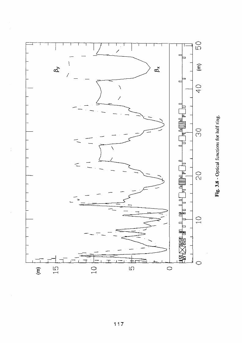
0
/ LO
->. >< E CO. CO. -
I
\ 0 ~
/
-bb c:
·~:: 4-<
0 -m
(Y) ..c:
1-< - ..8 - Cll c: 0 ...... ...... C,) c: t8 -- m
C,) ...... ......
0 0 (\J
QO ~ el:> ·-~
":::>
-0
_... ...---i
~
0
11 7
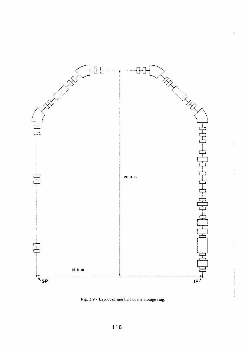
/
~ 20.0 m
I !
I 1
15.8 m J ...__. _____ __1, __ _
'sP
Fig. 3.9 - Layout of one half of the storage ring.
11 8
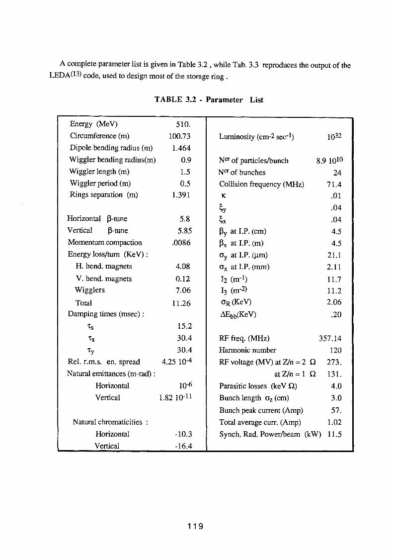
A complete parameter list is given in Table 3.2 , while Tab. 3.3 reproduces the output of the
LEDA (13) code, used to design most of the storage ring .
TABLE 3.2 - Parameter List
Energy (MeV) 510.
Circumference (m) 100.73 Luminosity (cm-2 sec-1) 1Q32
Dipole bending radius (m) 1.464
Wiggler bending radius(m) 0.9 Ner of particles/bunch 8.9 1010
Wiggler length (m) 1.5 Ner of bunches 24 Wiggler period (m) 0.5 Collision frequency (MHz) 71.4 Rings separation (m) 1.391 K .01
~y .04
Horizontal f3-tune 5.8 ~X .04
Vertical f3-tune 5.85 f3y at I.P. (cm) 4.5
Momentum compaction .0086 f3x at I.P. (m) 4.5
Energy loss/turn (Ke V) : cry at I.P. (Jlm) 21.1
H. bend. magnets 4.08 crx at I.P. (mm) 2.11
V. bend. magnets 0.12 12 (m-1) 11.7 Wigglers 7.06 13 (m-2) 11.2
Total 11.26 crR (KeY) 2.06
Damping times (msec): Lllibb(Ke V) .20
ts 15.2
'tx 30.4 RF freq. (MHz) 357.14
ty 30.4 Harmonic number 120
Rei. r.m.s. en. spread 4.25 1Q-4 RF voltage (MV) at Z)n = 2 Q 273.
Natural emittances (m-rad) : at Z/n = 1 Q 131.
Horizontal lQ-6 Parasitic losses (ke V Q) 4.0
Vertical 1.82 lQ-11 Bunch length crz (cm) 3.0
Bunch peak current (Amp) 57.
Natural chromaticities : Total average curr. (Amp) 1.02
Horizontal -10.3 Synch. Rad. Power/beam (kW) 11.5
Vertical -16.4
1 1 9
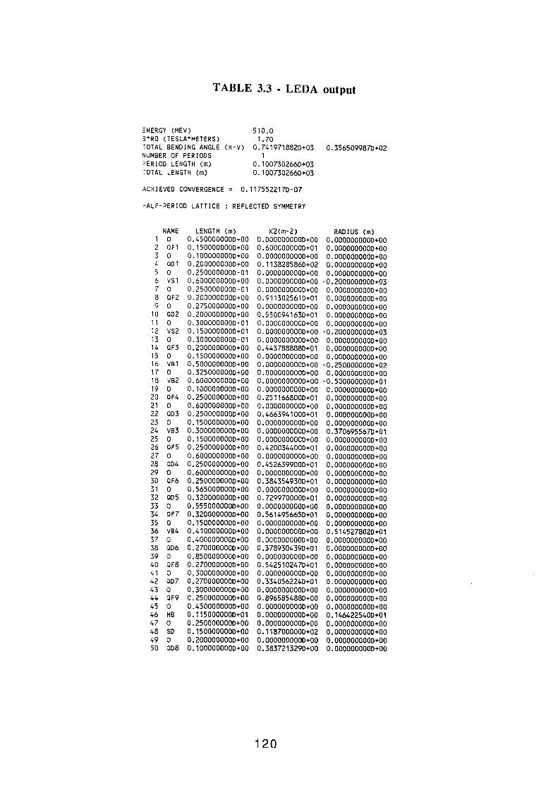
TABLE 3.3 - LEDA output
::NERGY (MEV) 510.0 3*RO (TESLA*METERS) 1. 70 TOTAL BENDING ANGLE (H-V) 0.741971882D+03 0.3565099870+02 NUMBER OF PERIODS 1 ~ERIOD LENGTH (m) 0. 1 00730266D+03 ~OTAL LENGTH (m) 0.100730266D+03
ACHIEVED CONVERGENCE 0.1175522170-07
rlALF-PERIOD LATTICE : REFLECTED SYMMETRY
NAME LENGTH (m) K2<m-2) RADIUS (m) 1 0 0.450000000D+OO O.OOOOOOOOOD+OO O.OOOOOOOOOD+OO 2 OF1 0.150000000D+OO 0.600000000D+01 O.OOOOOOOOOD+OO 3 0 0.100000000D+OO O.OOOOOOOOOD+OO O.OOOOOOOOOD+OO 4 OD1 0.200000000D+OO 0.113828586D+02 O.OOOOOOOOOD+OO 5 0 0.250000000D-01 O.OOOOOOOOOD+OO O.OOOOOOOOOD+OO 6 VS1 0.600000000D+OO O.OOOOOOOOOD+OO -0.200000000D+03 7 0 0.250000000D-01 O.OOOOOOOOOD+OO 0.0000000000+00 8 OF2 0.200000000D+OO 0.9113025610+01 O.OOOOOOOOOD+OO 9 0 0.275000000D+OO O.OOOOOOOOOD+OO O.OOOOOOOOOD+OO
10 OD2 0.200000000D+OO 0.550094163D+01 O.OOOOOOOOOD+OO 11 0 0.300000000D·01 O.OOOOOOOOOD+OO O.OOOOOOOOOD+OO 12 VS2 0. 150000000D+01 O.OOOOOOOOOD+OO -0.200000000D+03 13 0 0.300000000D-01 O.OOOOOOOOOD+OO O.OOOOOOOOOD+OO 14 OF3 0.200000000D+OO 0.443788888D+01 O.OOOOOOOOOD+OO 15 0 0.150000000D+OO O.OOOOOOOOOD+OO O.OOOOOOOOOD+OO 16 VB1 0.500000000D+OO O.OOOOOOOOOD+OO -0.250000000D+02 17 0 0.32SOOOOOOD+OO O.OOOOOOOOOD+OO O.OOOOOOOOOD+OO 18 VB2 0.600000000D+OO O.OOOOOOOOOD+OO -0.500000000D+01 19 0 0.100000000D+OO O.OOOOOOOOOD+OO O.OOOOOOOOOD+OO 20 OF4 0.2500000000+00 0. 2511668000+0 1 0.0000000000+00 21 0 0.600000000D+OO 0.0000000000+00 0.0000000000+00 22 OD3 0.2500000000+00 0.4663941000+01 0.0000000000+00 23 0 0.1500000000+00 0.0000000000+00 0.0000000000+00 24 VB3 0.3000000000+00 0.0000000000+00 0 .3706955670+01 25 0 0. 1500000000+00 0.0000000000+00 0.0000000000+00 26 OF5 0.2500000000+00 0.4200344000+01 0.0000000000+00 27 0 0.600000000D+OO 0.0000000000+00 0.0000000000+00 28 004 0.2500000000+00 0.4526399000+01 0.0000000000+00 29 0 0.6000000000+00 0.0000000000+00 0.0000000000+00 30 OF6 0.2500000000+00 0.3843549300+01 0.0000000000+00 31 0 0.5650000000+00 0.0000000000+00 0.0000000000+00 32 OD5 0.3200000000+00 0. 7299700000+01 0.0000000000+00 33 0 0.5550000000+00 O.OOOOOOOOOD+OO 0.0000000000+00 34 OF7 0.3200000000+00 0.5614956650+01 0.0000000000+00 35 0 0.1500000000+00 0.0000000000+00 O.OOOOOOOOOD+OO 36 VB4 0.4100000000+00 0.0000000000+00 0.5145278020+01 37 0 0.4000000000+00 0.0000000000+00 0.0000000000+00 38 006 0.2700000000+00 0.3789304390+01 0.0000000000+00 39 0 0.8500000000+00 0.0000000000+00 O.OOOOOOOOOD+OO 40 OF8 0.2700000000+00 0. 54251024 7D+O 1 0.0000000000+00 41 0 0.3000000000+00 0.0000000000+00 0.0000000000+00 42 007 0.270000000D+OO 0.3340562240+01 0.0000000000+00 43 0 0.3000000000+00 0.0000000000+00 0.0000000000+00 44 OF9 0.2500000000+00 0.8965854880+00 0.0000000000+00 45 0 0.4500000000+00 0.0000000000+00 0.0000000000+00 46 HB 0.1150000000+01 0.0000000000+00 0 . 1464225400+0 1 47 0 0.2500000000+00 0.0000000000+00 0.0000000000+00 48 so 0. 150000000D+OO 0.118700000D+02 O.OOOOOOOOOD+OO 49 0 0.200000000D+OO O.OOOOOOOOOD+OO O.OOOOOOOOOD+OO 50 OD8 0.100000000D+OO 0.383721329D+OO O.OOOOOOOOOD+OO
120
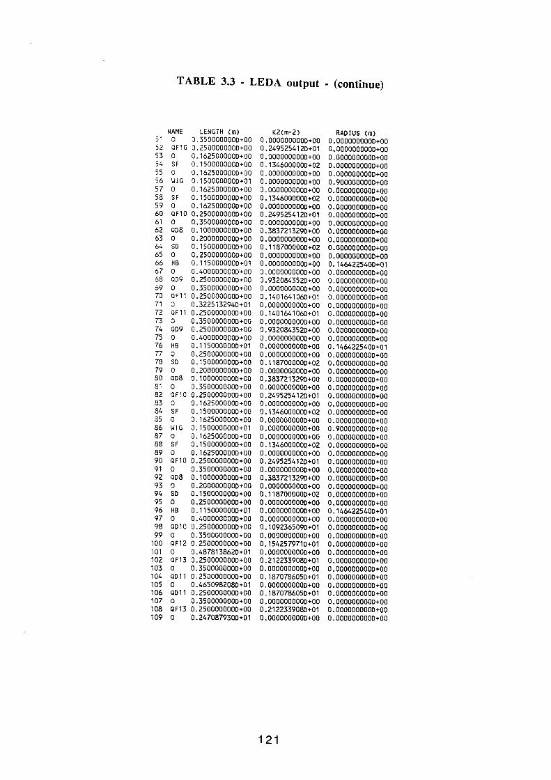
TABLE 3.3 - LEDA output - (continue)
NAME LENGTH (m) K2<m·2) RADIUS (m) 51 0 0.3500000000+00 0.0000000000+00 0.0000000000+00 52 OF10 0.2500000000+00 0.2495254120+01 0.0000000000+00 53 0 0.1625000000+00 0.0000000000+00 0.0000000000+00 54 SF 0.1500000000+00 0.1346000000+02 0.0000000000+00 55 0 0.1625000000+00 0.0000000000+00 0.0000000000+00 56 WIG 0.1500000000+01 0.0000000000+00 0.9000000000+00 57 0 0. 1625000000+00 0.0000000000+00 0.0000000000+00 58 SF 0. 1500000000+00 0. 1346000000+02 0.0000000000+00 59 0 0. 1625000000+00 0.0000000000+00 0.0000000000+00 60 OF10 0.2500000000+00 0.2495254120+01 0.0000000000+00 61 0 0.3500000000+00 0.0000000000+00 0.0000000000+00 62 008 0.1000000000+00 0.3837213290+00 0.0000000000+00 63 0 0.2000000000+00 0.0000000000+00 0.0000000000+00 64 so 0. 1500000000+00 0. 1187000000+02 0.0000000000+00 65 0 0.2500000000+00 0.0000000000+00 0.0000000000+00 66 HB 0. 1150000000+01 0.0000000000+00 0.1464225400+01 67 0 0.4000000000+00 0.0000000000+00 0.0000000000+00 68 009 0.2500000000+00 0.9320843520+00 0.0000000000+00 69 0 0.3500000000+00 0.0000000000+00 0.0000000000+00 70 OF11 0.2500000000+00 0.1401641060+01 0.0000000000+00 71 0 0.3225132940+01 0.0000000000+00 0.0000000000+00 72 OF11 0.2500000000+00 0.1401641060+01 0.0000000000+00 73 0 0.3500000000+00 0.0000000000+00 0.0000000000+00 74 009 0.2500000000+00 0.9320843520+00 0.0000000000+00 75 0 0.4000000000+00 0.0000000000+00 0.0000000000+00 76 HB 0.1150000000+01 0.0000000000+00 0.1464225400+01 77 0 0.2500000000+00 0.0000000000+00 0.0000000000+00 78 so 0. 1500000000+00 0. 1187000000+02 0.0000000000+00 79 0 0.2000000000+00 0.0000000000+00 0.0000000000+00 80 008 0.1000000000+00 0.3837213290+00 0.0000000000+00 81 0 0.3500000000+00 0.0000000000+00 0.0000000000+00 82 OF10 0.2500000000+00 0.2495254120+01 0.0000000000+00 83 0 0.1625000000+00 0.0000000000+00 0.0000000000+00 84 SF 0.1500000000+00 0. 1346000000+02 0.0000000000+00 85 0 0. 1625000000+00 0.0000000000+00 0.0000000000+00 86 WIG 0. 1500000000+0 1 0.0000000000+00 0.9000000000+00 87 0 0.1625000000+00 0.0000000000+00 0.0000000000+00 88 SF 0. 1500000000+00 0.1346000000+02 0.0000000000+00 89 0 0.1625000000+00 0.0000000000+00 0.0000000000+00 90 OF10 0.2500000000+00 0.2495254120+01 0.0000000000+00 91 0 0.3500000000+00 0.0000000000+00 0.0000000000+00 92 008 0.1000000000+00 0.3837213290+00 0.0000000000+00 93 0 0.2000000000+00 0.0000000000+00 0.0000000000+00 94 so 0. 1500000000+00 0.1187000000+02 0.0000000000+00 95 0 0.2500000000+00 0.0000000000+00 0.0000000000+00 96 HB 0.1150000000+01 0.0000000000+00 0. 1464225400+01 97 0 0.4000000000+00 0.0000000000+00 0.0000000000+00 98 0010 0.2500000000+00 0.1092365090+01 0.0000000000+00 99 0 0.3500000000+00 0.0000000000+00 0.0000000000+00
100 OF12 0.2500000000+00 0.1542579710+01 0.0000000000+00 101 0 0.4878138620+01 0.0000000000+00 0.0000000000+00 102 OF13 0.2500000000+00 0.2122339080+01 0.0000000000+00 103 0 0.3500000000+00 0.0000000000+00 0.0000000000+00 104 0011 0.2500000000+00 0. 1870786050+01 0.0000000000+00 105 0 0.4650982080+01 0.0000000000+00 0.0000000000+00 106 0011 0.2500000000+00 0. 1870786050+01 0.0000000000+00 107 0 0.3500000000+00 0.0000000000+00 0.0000000000+00 108 OF13 0.2500000000+00 0.2122339080+01 0.0000000000+00 109 0 0. 24 70879300+01 0.0000000000+00 0.0000000000+00
1 21
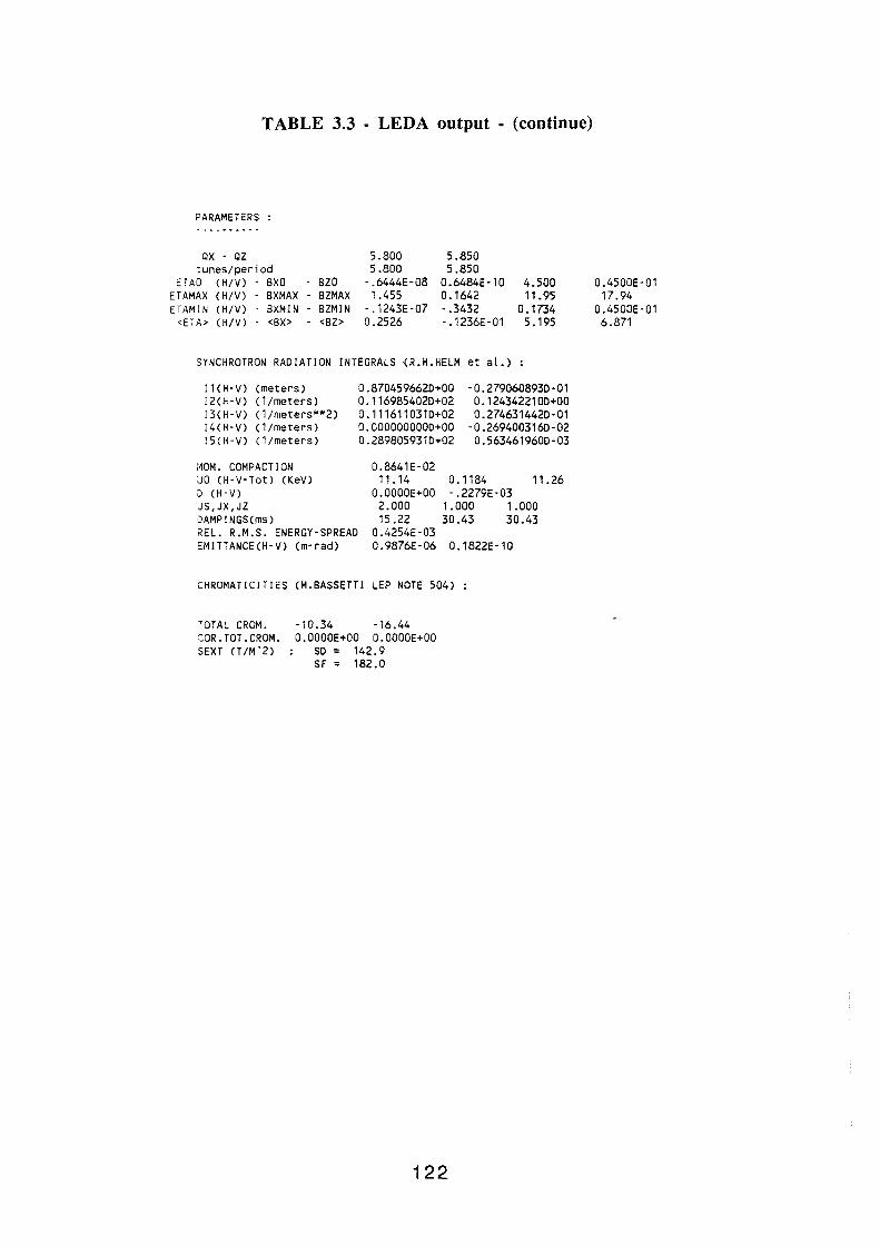
TABLE 3.3 - LEDA output - (continue)
PARAMETERS
QX • QZ tunes/period
ETAO (H/V) BXO BZO ETAMAX (H/V) BXMAX · BZMAX ETAM!N (H/V) BXMIN BZMIN
<ETA> (H/V) <BX> - <BZ>
5.800 5.800
·.6444E·08 1.455
·. 1243E-07 0.2526
5.850 5.850
0.6484E-10 0.1642 -.3432 ·. 1236E ·01
4.500 11.95
0.1734 5.195
SYNCHROTRON RADIATION INTEGRALS (R.H.HELM et al.) :
!1(H·V) (meters) !2(H·V) (1/meters) !3(H·V) (1/meters**2) 14(H·V) (1/meters) !5(H·V) (1/meters)
~~OM. COMPACT I ON JO (H·V·Tot) (KeV) ~ (H·V) JS,JX,JZ ClAMPINGS(ms) KEL. R.M.S. ENERGY-SPREAD EMITTANCE(H·V) (m·rad)
0.8704596620+00 0.1169854020+02 0.1116110310+02 0.0000000000+00 0.2898059310+02
0.8641E-02
-0.2790608930-01 0.1243422100+00 0.2746314420-01
-0.2694003160-02 0.5634619600-03
11.14 0.1184 11.26 O.OOOOE+OO -.2279E-03
2.000 1.000 1.000 15.22 30.43 30.43
0.4254E-03 0.9876E-06 0.1822E-10
CHROMATICITIES (M.BASSETTI LEP NOTE 504) :
TOTAL CROM. COR.TOT.CROM. SEXT (T/M"2)
-10.34 -16.44 O.OOOOE+OO O.OOOOE+OO
so = 142.9 SF = 182.0
122
0.4500E-01 17.94
0.4500E-01 6.871
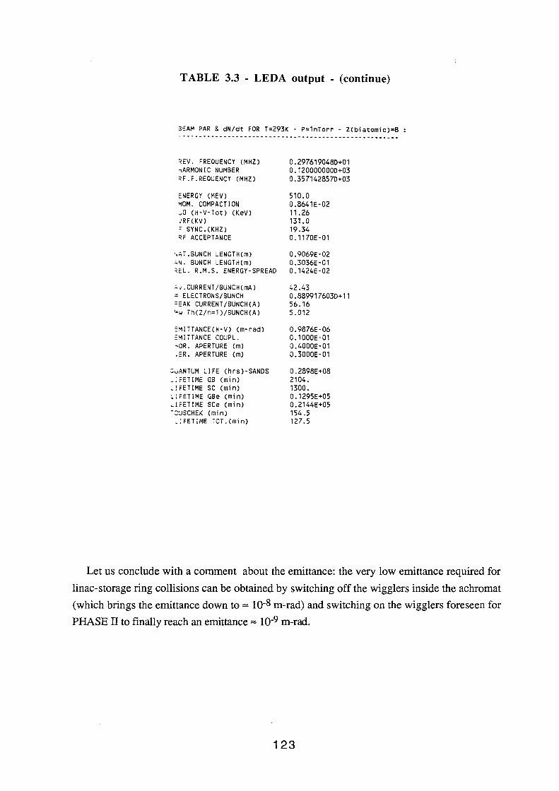
TABLE 3.3 - LEDA output - (continue)
BEAM PAR & dN/dt FOR T=293K - P=1nTorr - Z(biatomic)=8 ------------------------------------------------------
'EV. FREQUENCY (MHZ) "ARMONIC NUMBER ,F.F.REQUENCY (MHZ)
ENERGY (MEV) "!OM. COMPACTION JO (H-V-Tot) (KeV) /RF(KV) ;: SYNC.(KHZ) RF ACCEPTANCE
~T.BUNCH LENGTH(m) N. BUNCH LENGTH(m)
0.2976190480+01 0.1200000000+03 0.3571428570+03
510.0 0.8641E-02 11.26 131.0 19.34 0.1170E-01
EL. R.M.S. ENERGY-SPREAD
0.9069E-02 0.3036E-01 0.1424E-02
~J.CURRENT/BUNCH(mA)
= ELECTRONS/BUNCH ~EAK CURRENT/BUNCH(A) ~w Th(Z/n=1)/BUNCH(A)
EMITTANCE(H-V) (m-rad) E'll TT ANCE COUPL. ~oR. APERTURE (m) .ER. APERTURE (m)
:vANTUM LIFE (hrs)-SANOS .:FETIME GB (min) L!rETIME SC (min) ~iFETIME GBe (min) ~iFETIME SCe (min) -~SCHEK (min)
.:FETIME TOT.(min)
42.43 0.8899176030+11 56.16 5.012
0.9876E-06 0.1000E-01 0.4000E-01 0.3000E-01
0.2898E+08 2104. 1300. 0. 1295E+05 0.2144E+05 154.5 127.5
Let us conclude with a comment about the emittance: the very low emittance required for
linac-storage ring collisions can be obtained by switching off the wigglers inside the achromat
(which brings the emittance down to:::::: lQ-8 m-rad) and switching on the wigglers foreseen for
PHASE II to finally reach an emittance:::::: lQ-9 m-rad.
123
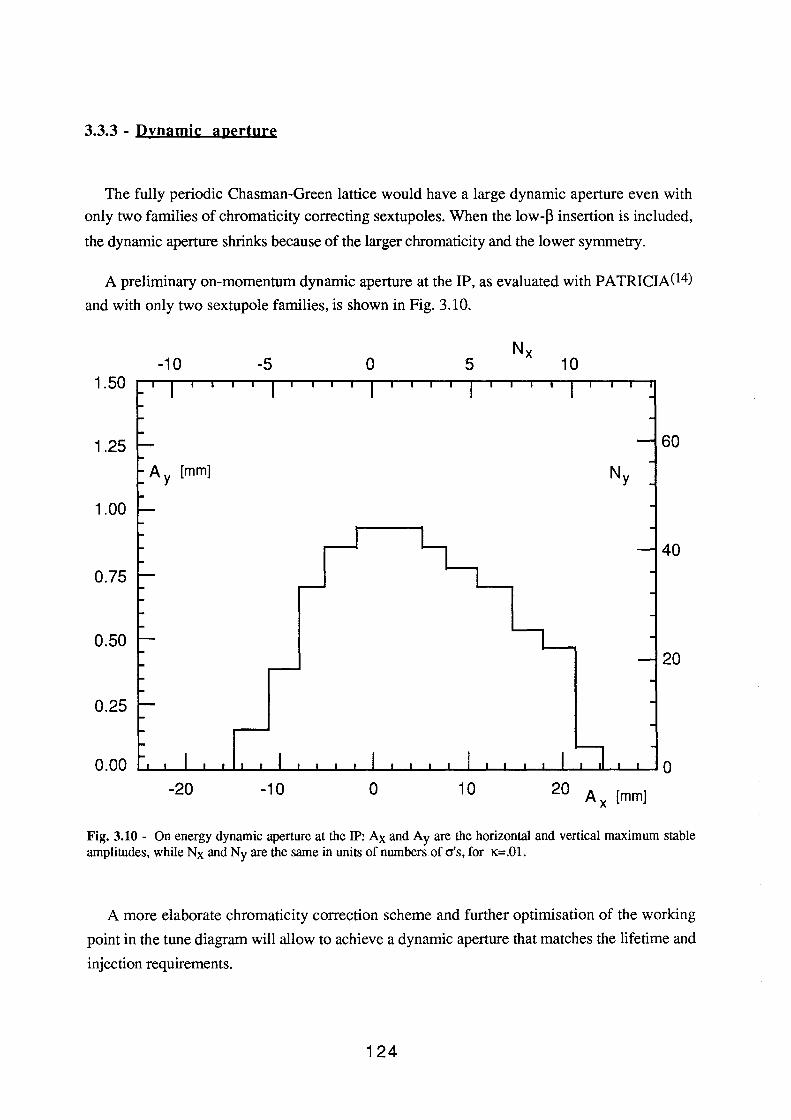
3.3.3 - Dynamic aperture
The fully periodic Chasman-Green lattice would have a large dynamic aperture even with
only two families of chromaticity correcting sextupoles. When the low-~ insertion is included,
the dynamic aperture shrinks because of the larger chromaticity and the lower symmetry.
A preliminary on-momentum dynamic aperture at the lP, as evaluated with PATRICIA04)
and with only two sextupole families, is shown in Fig. 3.10.
-10 1.50
1.25
1.00
0.75
0.50
0.25
0.00
-20
-5 0
-10 0
5
10
10
20 A [mm] X
Fig. 3.10 - On energy dynamic aperture at the IP: Ax and Ay are the horizontal and vertical maximum stable amplitudes, while Nx and Ny are the same in units of numbers of cr's, for K=.Ol.
A more elaborate chromaticity correction scheme and further optimisation of the working
point in the tune diagram will allow to achieve a dynamic aperture that matches the lifetime and
injection requirements.
124
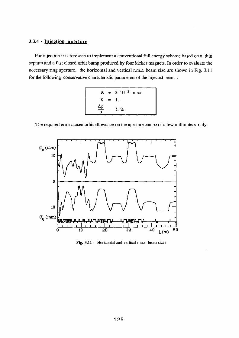
3.3.4 - In iection aperture
For injection it is foreseen to implement a conventional full energy scheme based on a thin
septum and a fast closed orbit bump produced by four kicker magnets. In order to evaluate the
necessary ring aperture, the horizontal and vertical r.m.s. beam size are shown in Fig. 3.11
for the following conservative characteristic parameters of the injected beam :
e = 2. 10-5 m rad
1( = 1. ~p
= 1.% _Q
The required error closed orbit allowance on the aperture can be of a few millimiters only.
crx (mm)
10
0 ~----------------------------------------~
Fig. 3.11 - Horizontal and vertical r.m.s. beam sizes
125
3.4. - BEAM STABILITY AND LIFETIMES.
High currents in both the single and the multibunch modes of operation, short bunch
lengths, long lifetimes and the stablest possible beam conditions are all to be achieved at the
same time, thereby putting severe constraints on the design of the overall system.
The above parameters are very much interconnected: single-Tousheck lifetime can be
relevant at the energy of 510 Me V and is determined by the bunch density and the momentum
acceptance. In turn the bunch density depends on the lattice and RF parameters, and can be
affected by intrabeam scattering and by J.L-wave instabilities whose current thresholds are related
to the vacuum chamber geometry and the RF cavity properties.
A self consistent computation has therefore been carried out to find an optimum. The main
phenomena considered in the analysis are: single bunch instabilities including turbulent bunch
lengthening, lifetime limiting effects (such as Tousheck scattering, gas scattering, and beam
beam single bremsstrahlung), coupled bunch instabilities and intrabeam scattering.
3.4.1 - Sim:le bunch dynamics
Instabilities are caused by the electromagnetic fields excited by the interaction of the bunch
with the surrounding structure. The effects of these fields on the bunch dynamics are estimated
using the concept of "machine impedance".
The single bunch dynamics is affected by those bunch excited fields whose strength is
relevant over a distance of the order of the bunch length. The fields are mainly produced in
correspondence with vacuum chamber discontinuities (including the cavity irises) and are
described in the frequency domain by the so called broad band (BB) impedance. They cause the
particles to lose energy depending on their position and therefore induce additional momentum
spread and bunch-lengthening.
The threshold peak current of this "turbulent" bunch-lengthening is given by:
2 "' = 27t ac (E/e) ap Iz Z/n
With the <rp and <le values given in Tab. 3.2, one obtains
'Iz "" 5 Amp·!l
126
(3.18)
The 57 A design peak current exceeds the ~-wave threshold for any reasonable choice of RF
parameters and BB impedances. In order to keep the bunch length at the design value the values
of the RF parameters h (harmonic number) and~ (Peak voltage) must satisfy the equation:
(3.19)
where
cos($,) ~ .Y I - (~)' (3.20)
with U = U0 + Uz, U0 being the radiation loss and Uz the energy dissipated in the resistive
impedance.
Note that Uz depends on the bunch-length ( crz-3), and therefore for short bunches it may
contribute significanlty to the overall losses:
Dz (ke V) "" 4 ~~B (Q) (3.21)
Equation 3.19 has been solved for h, as a function of~ and Z/n. Since the impedance can
be only roughly estimated several BB impedance values, chosen in the range
~~B = 1 + lOQ
(a reasonable range covering the measured impedances of almost all existing machines) have
been considered.
Fig. 3.12 shows the curves (dashed lines) relating the peak voltage,~. necessary to obtain
the nominal bunch-length of 3 cm, to the harmonic number h. It is apparent that by choosing
the RF frequency to be"" 350 MHz, the bunch-length can be controlled using reasonable peak
voltage values independent of the exact machine impedance value.
On the contrary, the effect of the short-range wakefields on the transverse dynamics is
destructive, and most often determines the maximun storable current. By assuming a beam pipe
radius b = 3 cm, equal to the bunch-length, and using the relation between the longitudinal and
the transverse BB impedance:
one finds that the current stays below the transverse threshold, provided that h and ~ fulfill the
condition:
127
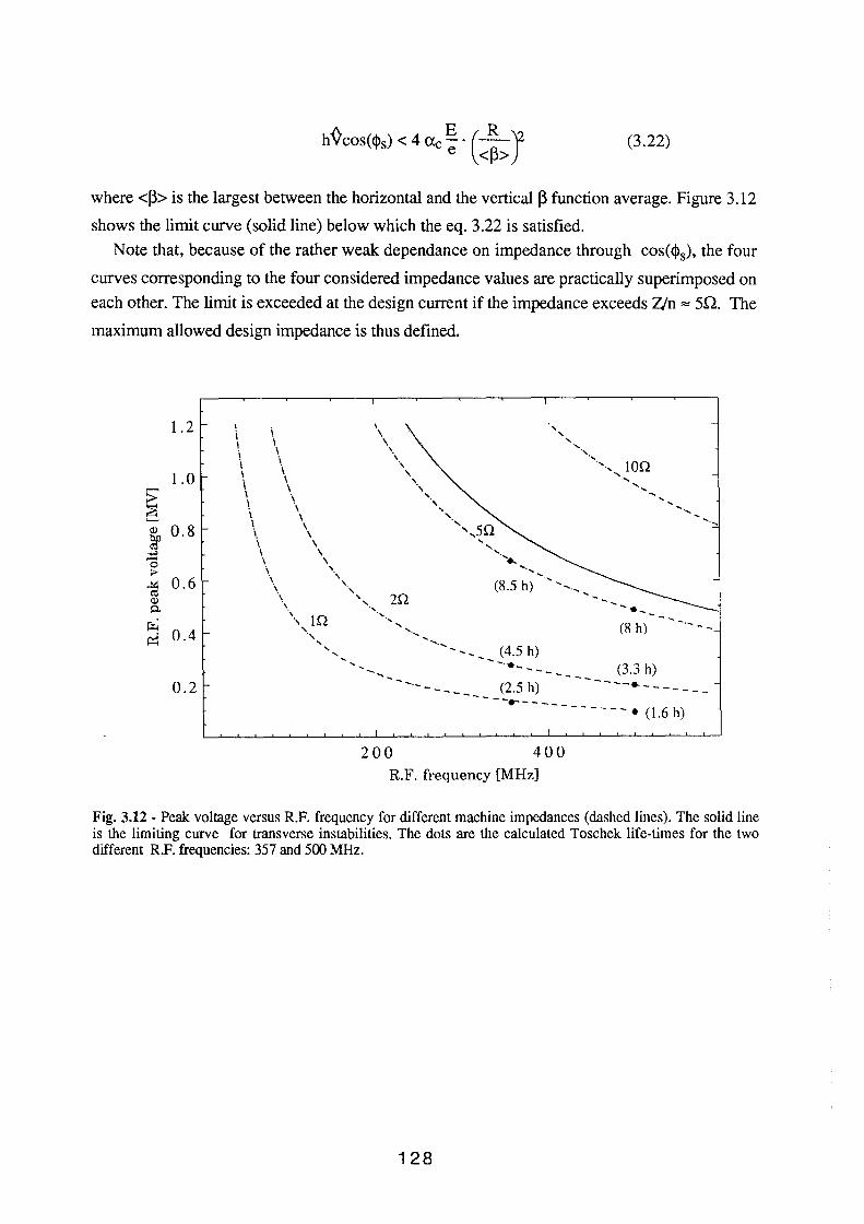
h ~cos( <l>s) < 4 <le E · (_L J2 e <~>)
(3.22)
where<~> is the largest between the horizontal and the vertical ~function average. Figure 3.12
shows the limit curve (solid line) below which the eq. 3.22 is satisfied.
Note that, because of the rather weak dependance on impedance through cos(<J>s), the four
curves corresponding to the four considered impedance values are practically superimposed on
each other. The limit is exceeded at the design current if the impedance exceeds Z/n "" 5Q. The
maximum allowed design impedance is thus defined.
1.2
1.0
§ .......
Q) 0.8 b.O C\1 ..., -0 > ~ 0.6
Q)
0.
~ 0.4 ~
0.2
I
i I
i I \ i
I I
\
i I \ i I \ \ I \ \ \ \
\ I \
\ \
\ \
\ \ \
\ \
\
' ., ' ·,
\ lQ '·,
' ' ',
', 2Q ., ..........
.................
' ....... _ --·-
200
(8.5 h) -._ (8 h)
........... , (4.5 h)
-- -.• _--- -·- (3.3 h)
.,
--·--
---- --·---------- (2.5 h) --- --... -----------. (1.6 h)
400 R.F. frequency [MHz]
Fig. 3.12- Peak voltage versus R.F. frequency for different machine impedances (dashed lines). The solid line is the limiting curve for transverse instabilities. The dots are the calculated Toschek life-times for the two different R.F. frequencies: 357 and 500 MHz.
128
3.4.2 - Beam Lifetime
The single Touschek scattering effect induces a momentum deviation depending on the
bunch density and r.m.s. angular divergence O'x·· The Touschek lifetime 'tT averaged along the
machine, has been calculated assuming that the machine acceptance is limited longitudinally by
the RF bucket heigth and transversely by the physical aperture. The results of the calculation are
shown as dots on the iso-impedance curves in Fig. 3.12 , for the chosen RF parameter values .
It is found that, since the bunch volume stays constant along the curves, lifetimes are limited by
the physical aperture in the upper-left region while, moving down and to the right, they
decrease because the RF momentum acceptance is reduced. Remembering the constraints on the
RF parameters deriving from single bunch dynamics, we conclude that an RF frequency
around 350 MHz, giving a lifetime of several hours, is the most suitable for our purposes.
At 350 MHz the Touschek lifetime, 'tT, is practically limited only by the RF acceptance, ERF
and by varying the peak voltage in the range 0.1+ 0.7 MV, ERF can be changed from 1.2%
to 2.8%.
The lifetimes relative to all other mentioned processes are calculated on the basis of this
choice.
Radiation in the bending magnets and in the wigglers leads to the loss of those particles with
energy deviations larger than the machine energy acceptance. The effect however, even
including the momentum spread increase induced by microwave instabilities give a practically
infinite quantum life time 'tq provided too high values of the frequency are avoided. As an
example, should one choose 500 instead of 350 MHz, for (Z/n)BB = 1 Q one would need only
93 KV peak voltage to keep the bunch length at 3 cm but the R.F. momentum acceptance
would be reduced to 0.8% and the quantum lifetime would dramatically drop to 80 minutes.
By choosing a 350 MHz system, the range of R.F. momentum acceptances (""1.2% +""
2.8% ) is such that other phenomena causing energy deviations of the particles in the bunch do
not affect the overall beam lifetime. Single bremsstrahlung in beam-beam collisions gives a
lifetime of 20 hours at least, inelastic scattering on the residual gas a lifetime of 35 hours in the
worst case and, elastic scattering on residual gas -causing particles to be lost on the beam pipe -
gives a lifetime of 22 hours at the design pressure of:;;::: 1 o-9 torr.
In conclusion we expect an overall beam lifetime in the range 3+6 hours limited by Tousheck
scattering. Topping-off injection is nevertheless desirable in order to keep the average
luminosity high.
129
3.4.3 - Multibuncb instabilities
The impedance of parasitic high order modes (ROM) are characterized by a resonant
frequency ffir, a shunt impedance Rg and a quality factor Q8:
They are responsible for the multi bunch instabilities. Many of such narrow band impedances
are originated in the RF cavities or in cavity-like vacuum chamber components coupled to the
beams.
The motion of M equidistant bunches is similar to that of M rigid coupled oscillators. The
frequency spectrum of the oscillations is given by a set of sidebands at frequencies:
fp = f0 (Mp + n +mv8), [m =1,2, ... ; n = O+M-1; -oo < p < +oo]
The amplitude of these sidebands is not constant but depends on the bunch length a and
shape and on the frequency fp· According to Sacherer's theory (15) a single sideband of the
umperturbed distribution will undergo a complex frequency shift ~COrn because of the coupling.
The real part of ~corn gives a real frequency shift while its imaginary part causes the oscillation
amplitude to grow with a rise time:
A simple approximation of the growth rate can be derived (16) under the following
assumptions holding in our machine: M( cr/R) <<1 and a single side band fp coupled to the
resonator, i.e. f/f0 << Q8• In the particular case of full coupling we get:
. h- c wit ro =-(j
where I is the total current, and the double factorial applies only to odd terms.
130
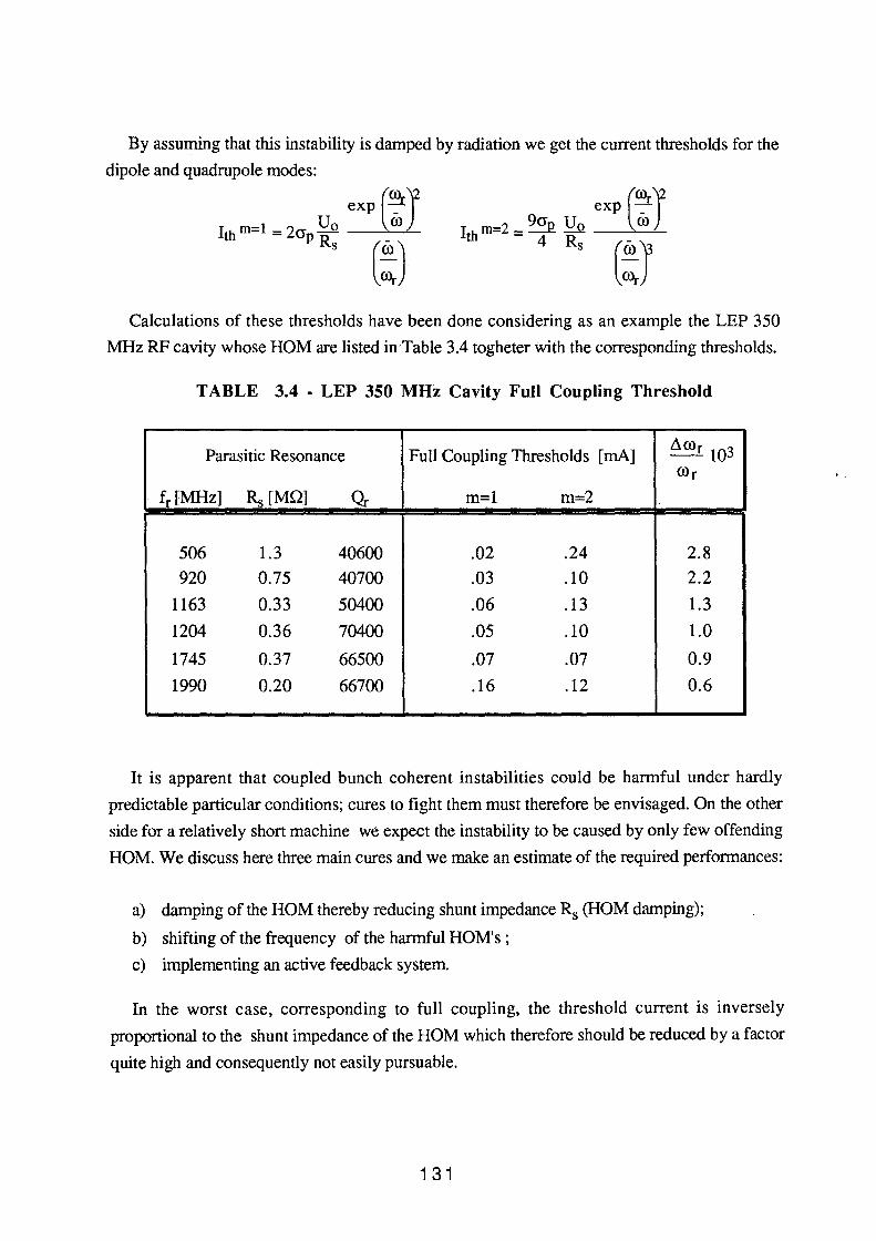
By assuming that this instability is damped by radiation we get the current thresholds for the
dipole and quadrupole modes:
exn (~\2 Ith m=l = 2cr Uo ~
PR, (!) exp (COr J2
I m=2 - 9crp U o ro ) th - 4 R, (!J
Calculations of these thresholds have been done considering as an example the LEP 350
MHz RF cavity whose HOM are listed in Table 3.4 togheter with the corresponding thresholds.
TABLE 3.4 - LEP 350 MHz Cavity Full Coupling Threshold
Parasitic Resonance Full Coupling Thresholds [rnA] .1.ror 1Q3
ror
fr [MHz] R8 [MQ] Q. m=l m=2
506 1.3 40600 .02 .24 2.8
920 0.75 40700 .03 .10 2.2
1163 0.33 50400 .06 .13 1.3
1204 0.36 70400 .05 .10 1.0
1745 0.37 66500 .07 .07 0.9
1990 0.20 66700 .16 .12 0.6
It is apparent that coupled bunch coherent instabilities could be harmful under hardly
predictable particular conditions; cures to fight them must therefore be envisaged. On the other
side for a relatively short machine we expect the instability to be caused by only few offending
HOM. We discuss here three main cures and we make an estimate of the required performances:
a) damping of the HOM thereby reducing shunt impedance R8 (HO M damping);
b) shifting of the frequency of the harmful HOM's ;
c) implementing an active feedback system.
In the worst case, corresponding to full coupling, the threshold current is inversely
proportional to the shunt impedance of the HOM which therefore should be reduced by a factor
quite high and consequently not easily pursuable.
1 31
. '
By shifting the HOM frequency there is a strong increase of the current threshold by a factor:
In order to store the design current, a frequency shift of- 0.3 % could be required, as
shown in the last column of Table 3.4.
Finally the use of a feedback system introduces a damping given by:
1 1 f0 eVFB tnFB = 2 Eo ~p/p
where ~ is the relative bunch energy deviation.
The feedback signal, in order to damp all possible coupled modes, has to act separately on
each bunch. Accordingly the system bandwidth should be at least twice the bunch frequency,
therefore the use of broad band longitudinal strip-line kickers is required. The feedback system
gain turns out to be very high and most likely limited by the maximum allowed voltage
(200+500 V) on the longitudinal strip-line kickers.
In conclusion, we have given a rather pessimistic estimate of multi bunch instabilities, in the
worst possible scenario. It is clear however that the problem must be carefully studied
foreseeing the combined use of HOM frequencies detuning and of feedback systems, including
the one recently developed by Kohaupt (17).
132
3.5. - GENERAL CONSIDERATIONS ON BEAM DIAGNOSTIC AND
INSTRUMENTATION
The beam instrumentation to be implemented in the <I>-Factory storage rings is discussed in
the following, with reference to the peculiar features wich influence the design and choice.
The storage rings characteristics, which reflect in particular requirements of the beam
instrumentation and of the general hardware, are the following:
- High current ( - 1 A ). The longitudinal and transverse parasitic impedance of the vacuum
chamber should be the lowest possible to increase the thresholds of collective instabilities.
- Many bunches. The rather large number of circulating bunches calls for a careful design
of the RF cavities, where coupled bunch instabilities are most likely to be excited by high
order resonating modes. The more seriously offending modes may be identified and
damped in the cavities by suitable antennas, but nevertheless a coupled-bunch feedback
system must be provided.
- Small bunch dimensions (cry<- 0.02 mm at the lP ). Careful closed-loop control of the
stability of the IP vs. drifts of the longitudinal and vertical bunch position in the separate
rings is required.
- Small coupling factor ( K- .01). To achieve such low value of the coupling factor, a
careful control of the closed orbit distorsion at quadrupoles and sextupoles locations is
required in order to reduce the strength of the driving term of vertical dispersion. Vertical
dispersion is also introduced, and must be suppressed, by the vertical bending of the
separator in the Interaction Region and by rotated quadrupoles and vertically misaligned
sextupoles. Careful surveying and high absolute accuracy of the beam position monitors
is required.
133
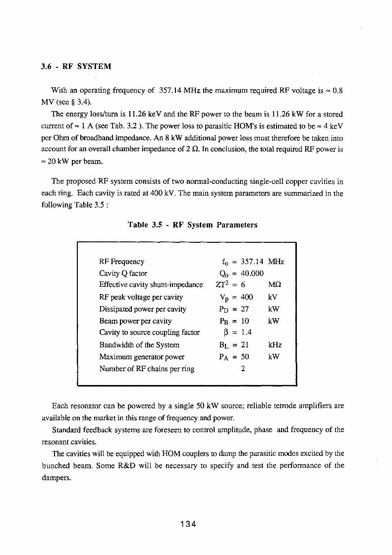
3.6 - RF SYSTEM
With an operating frequency of 357.14 MHz the maximum required RF voltage is~ 0.8
MV (see § 3.4).
The energy loss/turn is 11.26 ke V and the RF power to the beam is 11.26 kW for a stored
current of~ 1 A (see Tab. 3.2 ). The power loss to parasitic HOM's is estimated to be"" 4 keY
per Ohm of broadband impedance. An 8 kW additional power loss must therefore be taken into
account for an overall chamber impedance of 2 n. In conclusion, the total required RF power is
~ 20 kW per beam.
The proposed RF system consists of two normal-conducting single-cell copper cavities in
each ring. Each cavity is rated at 400 kV. The main system parameters are summarized in the
following Table 3.5:
Table 3.5 - RF System Parameters
RF Frequency f0 = 357.14 MHz
Cavity Q factor Q0 = 40.000
Effective cavity shunt-impedance zr2 = 6 Mn
RF peak voltage per cavity Vp = 400 kV
Dissipated power per cavity Po = 27 kW
Beam power per cavity PB = 10 kW
Cavity to source coupling factor ~ = 1.4
Bandwidth of the System BL = 21 kHz
Maximum generator power PA =50 kW
Number of RF chains per ring 2
Each resonator can be powered by a single 50 kW source; reliable tetrode amplifiers are
available on the market in this range of frequency and power.
Standard feedback systems are foreseen to control amplitude, phase and frequency of the
resonant cavities.
The cavities will be equipped with HOM couplers to damp the parasitic modes excited by the
bunched beam. Some R&D will be necessary to specify and test the performance of the
dampers.
134
3. 7 - VACUUM SYSTEM
Ultra high vacuum (UHV) is necessary in an electron storage ring in order to achieve good
beam lifetime and to avoid ion trapping.
Good vacuum conditions have to be maintained in the presence of the heavy gas load
produced by the radiation induced photo-desorption. Hard radiated photons (hv > 10 e V)
extract photoelectrons from the inside wall of the vacuum chamber; these in turn extract atoms
or molecules absorbed on the surface. The process is characterized by the "photodesorption
efficiency" parameter, D, wich gives the average number of desorbed molecules per incident
photon. Typical values of D are in the range of 10-1+ 1 o-7 molecules/photon. The lowest D
values are reached with appropriate treatments of the vacuum chamber and after long periods of
conditioning with the stored beam(::.: 100 Ah).
From the design parameter values listed in Tab 3.2 we estimate a total gas load, Q, of
Q = 8.7 10-6 mbar Vs for D = 10-6 molecules/photon
The total pumping speed, S, necessary to achieve the design value of 10-9 mbar is therefore :
S = Q/p = 8700 Vs. I With 10 identical ion pumps per sector we obtain a required nominal pumping speed of 220
Vs per pump; a rough figure of 400 Vs per pump actual pumping speed is estimated to account
for the pumping speed degradation at 10-9 mbar and for vacuum chamber conductances. The
preferred vacumm chamber material is stainless steel; usual UHV technology precautions such
as accurate cleaning procedures, high temperature bake-out, etc., will also have to be taken.
In summary, the main vacuum system components for the two rings are:
- 2 stainless steel vacuum chambers
- bakeout systems
- 80 sputter ion pumps, 400 Vs each.
- 8 cryopumps, 1500 Vs each.
- 8 oil-free roughing pumps.
- 16 U.H.V. gauges.
- 1 mass spectrometer (8 heads).
- interfaces to the central control system.
135
3.8 - THE DETECTOR SOLENOID
The main specifications for the Detector solenoid are :
- Axial length :::::: 10 m
- Radius :::::: 5 m
- Axial magnetic field 1 kGauss max
- Field on axis :::::: 0
The main conclusions from of a preliminary feasibilty study of the solenoid are presented
here. The details can be found in Reference (18).
The detector and the detector solenoid have to clear the region inside a conical surface,
coaxial with the beam, having a half-aperture angle of 8.5° and the vertex on the IP. The beam
has to be shielded from the solenoidal field; however, no shield can be foreseen in the± 22 cm
region surrounding the IP because the experiment tolerates only a very thin layer of material in
that region.
The solenoid main coil dimensions are:
- average radius
- thickness
- totallength
and the iron yoke ones are :
437.5 cm
25 cm
9 m
- maximum external radius 5 m
- thickness 25 cm
- thickness of the terminating iron plates 25 cm
- terminating iron plate hole radius 7 5 cm
The main solenoid linear current density, determined using PO IS SON, is:::::: 88900 Nm. An
active shielding system using current sheets has also been investigated; a typical layout,
including the current sheet profile and the field lines as computed by POISSON, is shown in
Figure 3.13.
Finally, the magnetic field on axis is plotted for different shield configurations in Figure
3.14. From these preliminary calculations we do not anticipate any problem in locally
compensating the residual solenoidal field even though the correction scheme has not yet been
worked out in full detail.
136
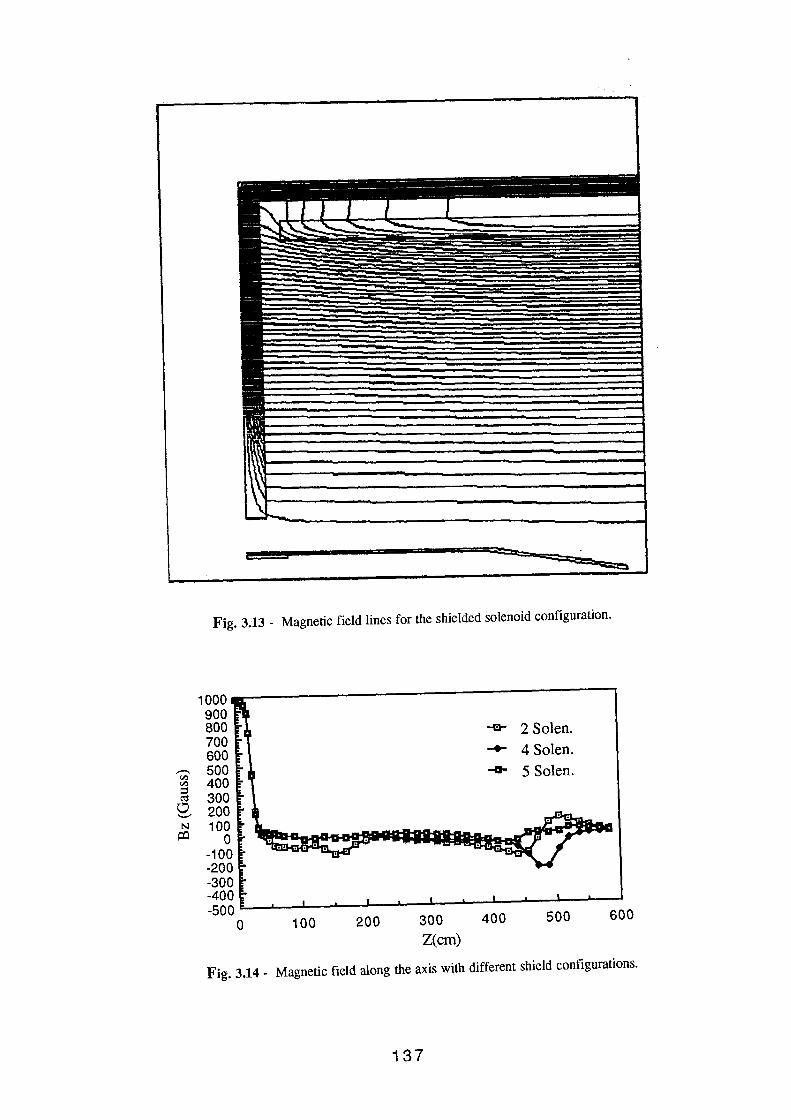
Fig. 3.13 - Magnetic field lines for the shielded solenoid configuration.
1000 900 800 -e- 2 Solen. 700 600
..... 4 Solen .
-- 500 -a- 5 Solen. Cll Cll 400 8 300 0 200 '-" N 100 ~ 0
-100 -200 -300 -400 -500
0 100 200 300 400 500 600
Z(cm)
Fig. 3.14- Magnetic field along the axis with different shield configurations.
137
References
(1) M.Sands, The physics of electron storage rings. An introduction, SLAC-121,(1970) (2) R.Littauer et al., XII Intern. Conference on High Energy Accelerators, FNAL (1983) (3) Barkov et al., The F-Factory project in Novosibirsk, Proc. of 1989 ICFA Meeting on
Beam Dynamics, Novosibirsk (4) W.A.Barletta and C.Pellegrini, A full energy positron source for the UCLA F-Factory
CAA 0048,UCLA 10/89 (5) H.Neseman, Proc. UCLA Workshop "Linear Collider, BB Factory, Conceptual design,
Jan.1987, Edited by D.H.Stork, World Scientific- Singapore. (6) S.Myers and J.Jowett, Proceeding of the Tau-Charm Factory Workshop, SLAC-343
(1989) (7) 1985 NSLS Annual report - BNL 51947
1988 NSLS Annual report- BNL 52167 G.Vignola, private communication
(8) J.Seeman, Lectures Notes in Physics, Vol. 247 (1985)- Springer Verlag Ed. (9) M.Bassetti, Int. Memo ARES 18 (1989) (10) R.H.Helm, M.J.Lee, P.L.Morton, M.Sands, IEEE Trans. Nucl. Sci., NS 20 (1973) (11) M.Bassetti, S.Guiducci, M. Preger, G. Vignola, Int.Memo ARES 26 (1989) (12) R.Chasman, G.K.Green and M.Rowe, IEEE Trans. Nucl. Sci., NS 22 (1975) (13) J.B.Murphy and G.Vignola, LEDA: A computer code for linear lattices (Unpublished) (14) H.Wiedeman, PEP Note 220 (1976) (15) F.Sacherer, IEEE Trans. Nucl. Sci., NS 24 (1977) (16) S.Bartalucci and L.Palumbo, Int. Memo T-120 (1985) (17) R.D. Kohaupt, DESY 86-121 (1986) (18) C.Sanelli, Int. Memo ARES 32 (1990)
138

4.- BEAM INSTRUMENTATION AND CONTROL SYSTEM
4.1. - BASIC REQUIREMENTS
The Beam Instrumentation and Control system should allow the Ares performance and
hardware to be monitored and controlled from a single Main Control Room. All monitoring and
control components and systems , such as Diagnostics elements, DC and pulsed Magnets, RF,
Beam and Machine timing, Cryogenics, Vacuum, etc., must be under full computer control. To
be more specific, the Beam Instrumenrtation and Control system should fulfill the following
basic requirements:
- to present meaningful yet concise information or alarms about the operational status of the
hardware and the performance of components;
- to automatically reset to a wanted condition a given sub-component, component or a
combination thereof in a consistent and safe way;
- to decode complex commands (e.g. set-up of a particular Linac beam) into a sequence of
separate, synchronized, interdependent actions. A machine timing system is thus
necessary to synchronize the various states of the accelerators. A fast analogic beam
timing system is also necessary to tag the various beams (electrons, positrons, electrons
for positron conversion, FEL);
- to let the machine physicist interact with the Instrumentation & Control system in a
transparent way in terms of accelerator physics quantities;
- to simulate, in real time, the effect of commands on performance;
- to simulate the beam behaviour according to analytical or empirical models of the various
components in order to avoid or reduce to a minimum, already in the commissioning
stage, the trial and error time-consuming practice;
- to be extremely reliable and capable of fast response times.
The requirements listed above are rather crucial especially in view of the experimental nature
of the machine that will require maximum operating flexibility. In particular the last one is
essential for a safe handling of high power beams in a superconducting environment.
Moreover, as extensive use of modeling is to be implemented since the very beginning, the
full integration of the diagnostic system into the computer control system is a major design
constraint.
The ultimate goal of the diagnostic and control system is the capability for the operator to set
the requested value of a given beam characteristics (e.g. emittance, current intensity, time
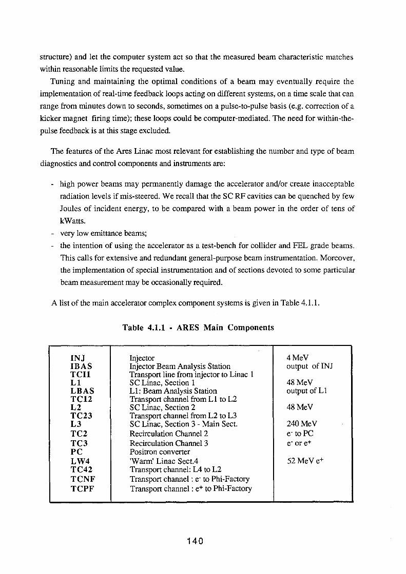
structure) and let the computer system act so that the measured beam characteristic matches
within reasonable limits the requested value.
Tuning and maintaining the optimal conditions of a beam may eventually require the
implementation of real-time feedback loops acting on different systems, on a time scale that can
range from minutes down to seconds, sometimes on a pulse-to-pulse basis (e.g. correction of a
kicker magnet firing time); these loops could be computer-mediated. The need for within-the
pulse feedback is at this stage excluded.
The features of the Ares Linac most relevant for establishing the number and type of beam
diagnostics and control components and instruments are:
- high power beams may permanently damage the accelerator and/or create inacceptable
radiation levels if mis-steered. We recall that the SC RF cavities can be quenched by few
Joules of incident energy, to be compared with a beam power in the order of tens of
kWatts.
- very low emittance beams;
- the intention of using the accelerator as a test-bench for collider and FEL grade beams.
This calls for extensive and redundant general-purpose beam instrumentation. Moreover,
the implementation of special instrumentation and of sections devoted to some particular
beam measurement may be occasionally required.
A list of the main accelerator complex component systems is given in Table 4.1.1.
Table 4.1.1 - ARES Main Components
INJ Injector 4MeV IBAS Injector Beam Analysis Station output of INJ TCU Transport line from injector to Linac 1 Ll SC Linac, Section 1 48MeV LBAS L1: Beam Analysis Station output ofL1 TC12 Transport channel from L1 to L2 L2 SC Linac, Section 2 48MeV TC23 Transport channel from L2 to L3 L3 SC Linac, Section 3- Main Sect. 240MeV TC2 Recirculation Channel2 e- to PC TC3 Recirculation Channel 3 e- ore+ PC Positron converter LW4 'Warm' Linac Sect.4 52 MeVe+ TC42 Transport channel: L4 to L2 TCNF Transport channel : e- to Phi-Factory TCPF Transport channel: e+ to Phi-Factory
140
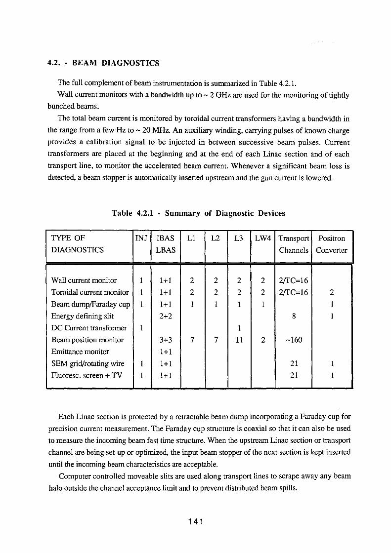
4.2. - BEAM DIAGNOSTICS
The full complement of beam instrumentation is summarized in Table 4.2.1.
Wall current monitors with a bandwidth up to- 2 GHz are used for the monitoring of tightly
bunched beams.
The total beam current is monitored by toroidal current transformers having a bandwidth in
the range from a few Hz to - 20 MHz. An auxiliary winding, carrying pulses of known charge
provides a calibration signal to be injected in between successive beam pulses. Current
transformers are placed at the beginning and at the end of each Linac section and of each
transport line, to monitor the accelerated beam current. Whenever a significant beam loss is
detected, a beam stopper is automatically inserted upstream and the gun current is lowered.
Table 4.2.1 - Summary of Diagnostic Devices
TYPE OF INJ IBAS L1 L2 L3 LW4 Transport Positron
DIAGNOSTICS LBAS Channels Converter
Wall current monitor 1 1+1 2 2 2 2 2/TC=16
Toroidal current monitor 1 1+1 2 2 2 2 2/TC=16 2
Beam dump/Faraday cup 1 1+1 1 1 1 1 1
Energy defming slit 2+2 8 1
DC Current transformer 1 1
Beam position monitor 3+3 7 7 11 2 -160
Emittance monitor 1+1
SEM grid/rotating wire 1 1+1 21 1
Fluoresc. screen + TV 1 1+1 21 1
Each Linac section is protected by a retractable beam dump incorporating a Faraday cup for
precision current measurement. The Faraday cup structure is coaxial so that it can also be used
to measure the incoming beam fast time structure. When the upstream Linac section or transport
channel are being set-up or optimized, the input beam stopper of the next section is kept inserted
until the incoming beam characteristics are acceptable.
Computer controlled moveable slits are used along transport lines to scrape away any beam
halo outside the channel acceptance limit and to prevent distributed beam spills.
141
At the exit of the injector a measurement station (IBAS) is provided to fully characterize the
beam in the longitudinal and transverse phase-space. The measurement station includes a
spectrometer magnet to measure the beam energy and energy spread and a transverse RF cavity
to measure bunch length. The basic arrangement is similar to that implemented on Lisa (1).
The measurement of a low emittance beam is best done at low energy, at the injector output,
in two steps. The beam transverse size is first measured, at a given location, by scraping it with
a motorized blade, measuring the transmitted current to a Faraday cup as a function of the
scraper position and computing the transverse charge distribution by differentiation. The
opening angle is then measured by passing the beam through a narrow slit and measuring the
transverse dimensions by means of a fluorescent screen and a TV camera, located downstream
the slit after a sufficiently long drift space.
An emittance measurement station (LBAS) is provided at the the end of the first
superconducting Linac section, Ll.
Energy measurements are done in the non-zero dispersion regions of the transport lines and
of the recirculation arcs by means of fluorescent screens and TV cameras or secondary emission
devices such as rotating wires or retractable wire grids. No beam intercepting devices are
foreseen on the se Linac.
The beam emittance is measured at the output of the Linac sections LW 4, L2, L3 in order to
dinamically match the optical functions of the following transport channels and to optimize
beam steering; this minimises the emittance degradation. The transverse emittance is determined
by measuring the beam transverse dimensions with a fluorescent screen as a function of the
orientation of the phase-space ellipse corresponding, i.e. of the strength of an upstream
quadrupole. Since the transport matrix from quadrupole to screen is known, the beam emittance
can be determined by a quadratic fit of the beam size vs. quadrupole strength curve (2).
4.3. - BEAM POSITION MONITORS
Beam position monitors (BPM) are used to measure and steer the beam trajectory in the
Linacs, transport channels and arcs.
Longitudinal and transverse wake fields in the RF cavities, that may blow up the beam
longitudinal and transverse emittances, have to be reduced to a minimum; the beam must
therefore be made to enter the Linac section as exactly as possible on axis and be kept there.
Preliminary calculations (3) show that, because of the relatively low Linac frequency, the
absolute accuracy required of the beam position monitors is - 0.1 mm, comparable to the
142
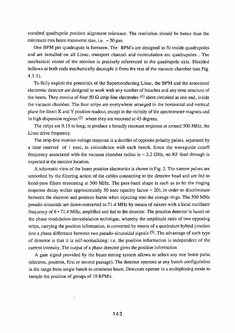
standard quadrupole position alignment tolerance. The resolution should be better than the
minimum rms beam transverse size, i.e. - 50 ~m.
One BPM per quadrupole is foreseen. The BPM's are designed to fit inside quadrupoles
and are installed on all Linac, transport channel and recirculation arc quadrupoles . The
mechanical center of the monitor is precisely referenced to the quadrupole axis. Shielded
bellows at both ends mechanically decouple it from the rest of the vacuum chamber (see Fig.
4.3.1).
To fully exploit the potentials of the Superconducting Linac, the BPM and the associated
electronic detector are designed to work with any number of bunches and any time structure of
the beam. They consist of four 50 n strip-line electrodes (4) short circuited at one end, inside
the vacuum chamber. The four strips are everywhere arranged in the horizontal and vertical
plane for direct X and Y position readout, except in the vicinity of the spectrometer magnets and
in high dispersion regions (2) where they are mounted at 45 degrees.
The strips are 0.15 m long, to produce a broadly resonant response at around 500 MHz, the
Linac drive frequency.
The strip-line monitor voltage response is a doublet of opposite polarity pulses, separated by
a time interval of 1 nsec, in coincidence with each bunch. Since the waveguide cutoff
frequency associated with the vacuum chamber radius is- 2.2 GHz, no RF feed-through is
expected at the monitor location.
A schematic view of the beam position electronics is shown in Fig. 2. The narrow pulses are
smoothed by the filtering action of the cables connecting to the detector head and are fed to
band-pass filters resonating at 500 MHz. The pass-band shape is such as to let the ringing
response decay within approximately 50 nsec (quality factor- 20), in order to discriminate
between the electron and positron bursts when injecting into the storage rings. The 500 MHz
pseudo-sinusoids are down-converted to 71.4 MHz by means of mixers with a local oscillator
frequency of 6 • 71.4 MHz, amplified and fed to the detector. The position detector is based on
the phase modulation-demodulation technique, whereby the amplitude ratio of two opposing
strips, carrying the position information, is converted by means of a quadrature hybrid junction
into a phase difference between two pseudo-sinusoidal signals (5). The advantage of such type
of detector is that it is self-normalizing: i.e. the position information is independent of the
current intensity. The output of a phase detector gives the position information.
A gate signal provided by the beam timing system allows to select any one beam pulse
(electron, positron, first or second passage). The detector operates at any bunch configuration
in the range from single bunch to continous beam. Detectors operate in a multiplexing mode to
sample the position of groups of 10 BPM's.
143
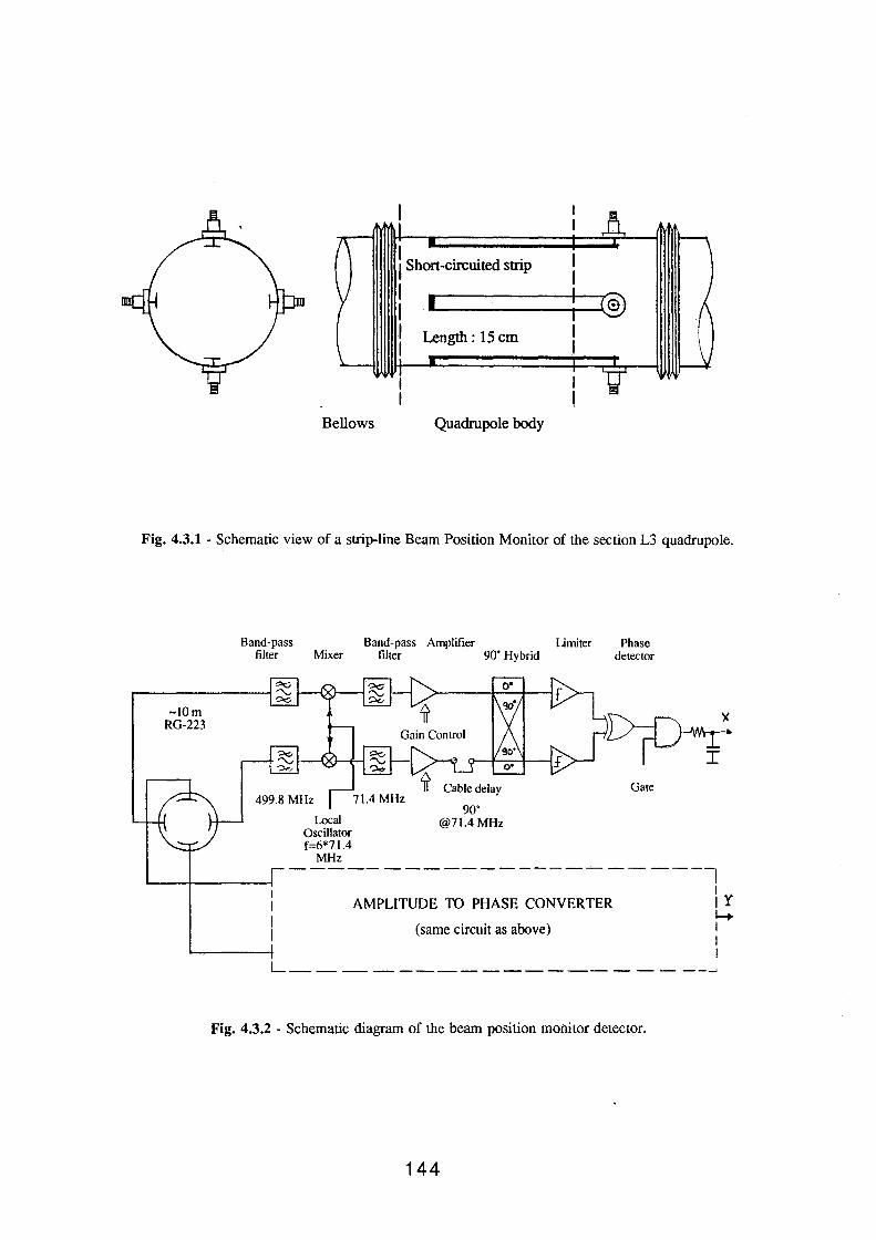
Bellows
ISh · · ed · 1 ort-ctrewt stnp
I I -· ------t----1® I Length: 15 cm
Quadrupole body
Fig. 4.3.1 - Schematic view of a strip-line Beam Position Monitor of the section L3 quadrupole.
-!Om RG-223
Band-pass Band-pass Amplifier Limiter Phase filter Mixer filter 90' Hybrid detector
Local Oscillator f=6*71.4
MHz
90' @71.4 MHz
Gate
-----------------------1
AMPLITUDE TO PHASE CONVERTER
(same circuit as above)
IY 4 I I I
L--------------------~
Fig. 4.3.2 - Schematic diagram of the beam position monitor detector.
144

4.4. - CONTROL SYSTEM
4.4.1 - Introduction
The Control System is a very critical point for an accelerator complex, especially if tight
constraints are posed on beam quality and or on the performance of the machines, the last being
heavily dependent on the availability of a good and reliable hardware and software environment.
The Control System has therefore to be part of the machine design itself and must develop in
parallel with it. It can be thought of as having two main parts:
- the "real machine" part consisting of the control hardware and software used to interface
equipment and instrumentation; its design must take into account the accelerator
topological and functional distribution and avoid data flow bottle-necks.
- the "virtual machine" part consisting of the control, modeling, simulation and optimization
software; its design and commissioning is determined by accelerator physics and is,
therefore, closely related to the machine type and the specified overall performance.
The initial design of a new accelerator control system is always complicated by the
accelerator components and parameters to be controlled not usually being completely specified
at the beginning of a project and also by the fact that performance as well as cost of components
and tools that come on the market evolve very fast on the time scale of the average project.
The vertical growth of hardware capabilities in the computer field (computing power and
memory capacity keep doubling every 2-3 years, and the growth curve shows no signs of a
plateaux) creates an environment where whatever is functioning is definitely old. Moreover, the
corresponding development in the software field keeps delivering new tools which are not only
powerful, but also easy to learn and to use. The situation is thus definitely unstable but, on the
other hand, an ever increasing number of powerful tools, which become reliable very soon
because the number of users is also growing fast, are thrown on the market. The involvement
of industry in the electronic standards also provides the user with always new and more reliable
instruments. A classical example is the amazing speed at which the VME standard has diffused,
as compared to CAMAC.
On the other hand the lifetime of an accelerator is comparatively long and during its span the
machines are usually partially or even totally reconfigured. Hardware and software products
used in the system should therefore be standard, possibly non proprietary, with large diffusion,
so that they may be expected to receive strong support from the manufacturer over many years.
We have here tried to lay down some basic scenarios, based on current philosophies about
hardware and software architectures(6) so as to be able to derive reasonably reliable cost and
manpower estimates. A definite detailed solution has not however being singled out as yet and a
145
final committment will be made only at the very last moment compatible with the time scale of
the project.
It is worth recalling here that, from the point of view of the control system, the general
features of the ARES accelerator complex are:
- Linac and <l>-Factory are separate but must be able to operate synchronously and in very
strict correlation.
- The physical dimensions of the site are of the order of a few hundred meters.
- The accelerators are also to be used as a test benches for accelerator development. This
means that the control system must be particularly flexible and friendly towards both
professional operators and machine physicists.
Two different lines of approach to the problem of designing the system are being
investigated, based on what has or is being done on similar projects such as LEP(7), ESRF,
ELETTRA (8), and our own LISA (9).
One is a 'conventional' distributed system, along the lines of those installed and tested on
LEP or being implemented at ESRF and ELETTRA, the other is a less conventional centralized
system based on the one being implemented for LISA.
Both have advantages and disadvantages that will be briefly discussed in the following.
From the point of view of capital cost there are no substantial differences and a final decision on
which to adopt can be taken later.
Both are based on the use of VME as a peripheral interface.It is the most modern, practical
and widespreaded modular electronics interface standard and distributed processing system.
Because many of multi-vendor products based on the 68K family are available, specific choices
are not critical.
4.4.2 - Distributed system
As said above, the accelerator complex consists of two distinct parts: the recirculating linac
and the double storage ring. Although the control system is unique the linac and the rings
machines are operated separately. From the machine component point of view several sub
systems can be identified such as magnet power supplies, RF, vacuum and refrigeration
equipment, beam diagnostics sensors, alarm monitoring and access control. A structure capable
of coping separately with all procedures and functionalities along the machine - a flexible,
modular and open scheme, implemented using intelli&ent and hierarchical levels - is the answer
to the problem.
It includes a local area network (i. e. ETHERNET), workstations with high processing
speed and very powerful graphics to serve as consoles for the human interface, one of the
146
several software tools able to generate windows, menus, etc., and finally an operating system
for the peripheral CPU's which has already been used and debugged.
The whole system is distributed, so to ensure local processing power to set, monitor and
diagnose the hardware. Topological and/or functional criteria are taken into account. A modular
approach, provides the required flexibility.
Based on the above concepts, the four logical level architecture briefly described in the
following is proposed(lO); its block-diagram is shown in Fig. 4.4.1. Note that although not
each box in the diagram has been named at this stage, real products have been considered for
the various blocks.
First level
A few workstation consoles and one server provide the man interface to operate the
accelerator. The powerful graphics capabilities can be used to increase the "bandwidth" of the
operator comprehension and the processing power provides adequate support for modeling
and/or simulation.
The server provides the general Data-Base, the normal spooling and log file management,
other service programs and the link to the external network. Sub-systems and low level
instrumentations can be deep-accessed through personal computers, with unsophisticated tools.
A special personal computer is completely dedicated to the continuous monitoring of alarm
messages incoming from the lower levels.
Second level
It consists of several supervisor processors that manage all procedures needed to operate
different machine sub-systems and provide general control functions for all main accelerator
parameters. To limit the need for throughput to the first level, they also filter-out insignificant
messages and are thus able to manage the sector they supervise without overloading the
consoles.
The processors are connected to an appropriate network so that they can be physically placed
where they are most useful.
Third level
The third level consists of several additional processors, sharing the VME bus, that manage
smaller accelerator parts or sub-systems. They mainly provide setting and readout functions for
all linked modules. A continuous monitoring procedure informs the second level supervisor on
the status of the hardware. A distributed Data-Base can thus be up-dated.
147
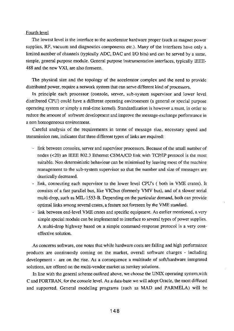
Fourth level
The lowest level is the interface to the accelerator hardware proper (such as magnet power
supplies, RP, vacuum and diagnostics components etc.). Many of the interfaces have only a
limited number of channels (typically ADC, DAC and I/0 bits) and can be served by a same,
simple, general purpose module. General purpose instrumentation interfaces, typically IEEE-
488 and the new VXI, are also foreseen.
The physical size and the topology of the accelerator complex and the need to provide
distributed power, require a network system that can serve different kind of processors.
In principle each processor (console, server, sub-system supervisor and lower level
distributed CPU) could have a different operating environment (a general or special purpose
operating system or simply a real-time kernel). Standardization is however a must, in order to
reduce the amount of software development and improve the message-exchange performance in
a non homogeneous environment.
Careful analysis of the requirements in terms of message size, necessary speed and
transmission rate, indicates that three different types of links are required:
- link between consoles, server and supervisor processors. Because of the small number of
nodes ( <20) an IEEE 802.3 Ethernet CSMNCD link with TCP/IP protocol is the most
suitable. Non deterministic behaviour can be minimised by leaving most of the machine
management to the sub-system supervisor so that the number and size of messages are
drastically decreased.
- link, connecting each supervisor to the lower level CPU's ( both in VME crates). It
consists of a fast parallel bus, like VICbus (formerly VMV bus), and of a slower serial
multi-drop, such as MIL-1553-B. Depending on the particular demand, both can provide
optimal links among several crates, a feature not foreseen by the VME standard.
- link between end-level VME crates and specific equipment. As earlier mentioned, a very
simple special module can be implemented to interface to several types of power supplies.
A multi-drop highway based on a simple command-response protocol is a very cost
effective solution.
As concerns software, one notes that while hardware costs are falling and high performance
products are continuosly coming on the market, overall software charges - including
development - are on the rise. As a consequence a multitude of soft/hardware integrated
solutions, are offered on the multi-vendor market as turnkey solutions.
In line with the general scheme outlined above, we choose the UNIX operating system, with
C and FORTRAN, for the console level. As a data-base we will adopt Oracle, the most diffused
and supported. General modeling programs (such as MAD and PARMELA) will be
148
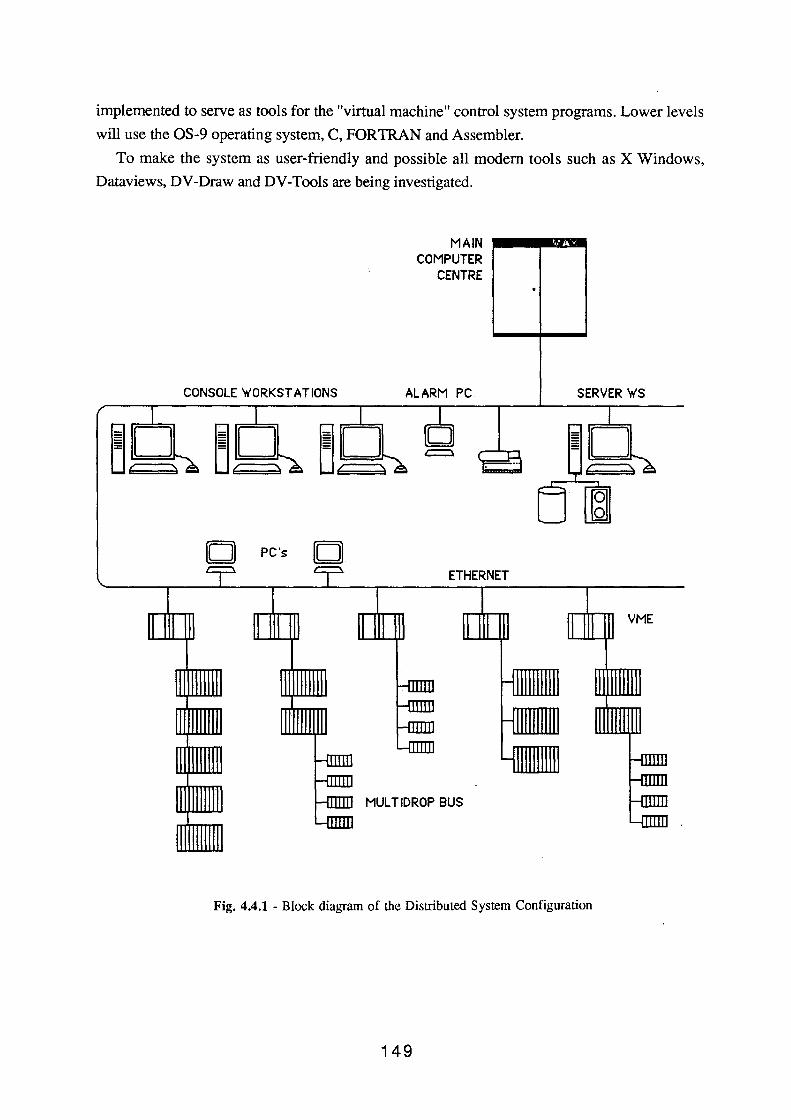
implemented to serve as tools for the "virtual machine" control system programs. Lower levels
will use the OS-9 operating system, C, FORTRAN and Assembler.
To make the system as user-friendly and possible all modern tools such as X Windows,
Dataviews, DV-Draw and DV-Tools are being investigated.
CONSOLE 'w'ORKST AT IONS
0 PC's 0
M A IN ,__.-mr!'lllll COMPUTER
CENTRE
ALARM PC SERVER 'w'S
ETHERNET
MUL T IDROP BUS
Fig. 4.4.1 - Block diagram of the Distributed System Configuration
149
The main advantage of the system is mainly that of requiring very little development and of
being able of readily making use of the hardware and software tools, developed for instance in
the course of the joint program between ESRF, Elettra, CERN, et al. that has resulted in a
marked improvement in standardization.
4.4.3 - Centralized system
The controls for LISA (I) were (and are being) developed in an attempt to develop a new
approach to an integrated accelerator control system and to use the fact that increasingly
powerful tools are continuously being marketed.
As an example it will become possible to use FDDI instead of ETHERNET, with a net
increase in speed of a factor of ten. Copper cables will be replaced by fiber-optics cables,
allowing larger distances to be covered without repeaters and increasing the connection
reliability, at least as long as low radiation environments are considered. OS-9 will be probably
replaced by the Motorola VMEexex, which supports not only multitasking but also
multiprocessor systems.
During the development of the LISA control system, quite a few new ideas have been
implemented and more are being tested.
The basic idea is to concentrate and centralize the communication system because a
centralized system is more simple to handle and also more reliable, since attention can be paid to
only a small number of easily replaceable units.
This is contrary to what is generally claimed about the reliability of a distributed system, but
it has to be noted that there is a conceptual difference between an accelerator control system and
a system which has to meet military standards: reliability considerations can change dramatically
when a network which has to be able to continue functioning, even partially, in case of
intentional damage is considered instead of a control system - limited to a few buildings - for an
experimental physics setup.
The implementation of a centralized system is made possible by the availability of very fast
parallel buses (2).
The LISA system is built around a central VME processor which coordinates all the
communications between different parts of the entire setup and keeps updated a central memory
which constitutes the prototype of the system database.
150
SUPERVISOR
~~~ /ccnsd...._>., /G.-cnsd...._'>. /G.-cnsei..._>,
ACCELERATOR CONTROLLERS
mail boxes
ARES
SIMPLE VERY FAST HIGHLY RELIABLE
Fig. 4.4.2 - Block diagram of the Centralized System Configuration.
In a multiple accelerator environment it would be very easy to extend this scheme using a
tree configuration. You would have more than one central processor, possibly one for each
machine, and an additional upper level coordinating the local supervisors. The different roots of
the tree would act as filtering bridges, transmitting to the upper levels only the necessary
1 51
information and shielding the main supervisor from local traffic. A possible block diagram is
shown in Figure 4.4.2.
The high speed local buses used in LISA suffer from distance problems: it is very difficult to
operate them at distances over 100 meters. Fortunately, several fiber optic connections are
appearing on the market to replace our 60 conductor cables. Although the optical fibers are
sensitive to radiation damage, it is easy to implement a mixed system where large distances are
covered by fiber optics trunks, while local cables could cover the high radiation level
sections.As far as software aspects are concerned, new and powerful tools are being developed
for the easy implementation of the human interface, which has been a gigantic problem up to
now. Hypercard is a first example of this kind of software.
For the peripheral CPU software the usual solution of a multitasking system is nowadays
strongly under objection. A multitasking system for a peripheral CPU which only has to look at
a few memory locations every now and then looks very much like trying to kill a fly with a
cannon. The opposite point of view is represented by the famous statement "One task, one
processor". This is an optimal way to look at things, although, as with every beautiful
theoretical construction, it sometimes suffers from implementation problems, like having to buy
a new CPU to perform some really trivial task. The intrinsic soundness of the principle
however lies in its extreme simplicity.
The main advantages of the centralized system configuration is the large bandwidth afforded
by the direct memory access mechanism. For example, the LISA system allows the exchange of
1700 messages per second in between (the three) levels, while comparable systems built around
ETHERNET have a capacity of only a few tens of messages per second.
An additional advantage of such a hierarchical system is the centralized database. A single
location for all machine status data means no problems of memory consistency and very easy
maintenance.
Although some authors find the 'centralized' software a difficulty, the central argument for
this kind of solution is that new, powerful tools are becoming available and should be used and
that the statement "old is more reliable" does not apply to software.
152
References
(1)
(2)
(3) (4) (5)
(6)
(7)
(8)
(9) (10)
B. Spataro, LNF Internal Memo LIS-30 (1988) M. Bassetti, B. Spataro, LNF Internal Memo LIS-42 (1989) M. Castellano, LNF Internal Memo LIS-53 (1989) R. Boni, A. Gallo, LNF Internal Memo LIS-68 (1990) J. Rees, L. Rivkin, SLAC-PUB-3305 (1984) K.T. Me Donald, D.P. Russel, Lecture Notes in Physics-343, M. Month and S. Turner eds., pp. 122-132. Springer-Verlag 1989. S. Bartalucci, C. Biscari, L. Palumbo, LNF Internal Memo ARES-20 (1989) R. E. Shafer, IEEE Transactions on Nuclear Science, Vol NS-32, No 5, p. 1933 (1985). E. F. Higgings, J. E. Griffin, IEEE Transactions on Nuclear Science, Vol NS-22, No 3, p. 1574 (1975). J. Borer, R. Jung, CERN 84-15, p. 416 (1984). Int. Conf. on Accelerator and Large Experimental Physics Control Systems, Vancouver, October 1989. P.G.Innocenti, "The LEP Control System: Architecture, feature and performance", CERN-SPS/89-35 (ACC) (1989). M.Mignacco, Int. Conf on Accelerator and Large Experimental Physics Control Systems, Vancouver, October 1989. M.Castellano et al., IEEE Trans, on Nucl. Sci . .J,Q, 1619 (89). N.Cavallo, LNF Internal Memo ARES-29 (1989)
153
5. - BUILDINGS AND UTILITIES
5.1. - GENERAL DESCRIPTION
A site independent design study of the civil engineering work for the project has been done
to identify the main requirements and estimate the costs (see Chapt. 5).
A flow chart of the approach to project planning is shown in Fig. 5.1.1. All main elements
of the plan have been studied to arrive at the proposed choices.
The planimetry shown in Fig. 5.1.2, includes the Linac tunnel and experimental hall, the ci>
Factory hall including the detector assembly space, the power and plant buildings, urbanization
and roadwork.
The tunnel, the ci>-Factory hall and the Linac experimental hall structures are underground
earth covered concrete structures for reasons of radiation shielding.
The concrete structure thickness and the foundation depth should be optimized to minimize
costs. At this stage it has been assumed that five meters of 2.4 t/mc concrete, or an equivalent
earth (1.6 t/mc) thickness are required to guarantee good shielding under all operating
conditions. Such a preliminary estimate is probably conservative and will be refined by more
detailed shielding calculations.
The Linac tunnel is a 162 m long box-like concrete structure having a useful internal width
of 10 m; it is equipped with two 3 ton cranes having a minimum hook height of 3.7 m. The
first 30 m of tunnel house the linac injector and the last 30 m serve as experimental hall for the
Linac itself. A line of central pillars at 6 m intervals divides the tunnel in two longitudinally;
unencumbered passage of people and cable runs from one side to the other, flexible space
allocation and the possibility of future upgrades are thus guaranteed. At present it is foreseen to
lay out the RF structure on one side and the recirculation channels on the other.
The roof is a 1 m thick concrete slab covered by 6 m of earth. The accelerator floor is 12 m
below the ground level. To keep a minimum beam height with respect to the floor of 1.2 m , the
floor is actually at -13 m over the first 60 m of tunnel and at -12.7 m over the last 35 m; two
ramps, with a maximum slope of 8%, connect these terminal areas to the central one.
The tunnel entrance is connected to the surface by a 5 m wide ramp road; in front of the
entrance a yard provides manouvering space for incoming lorries. Two more accesses to the
tunnel, to serve as personnel accesses and fire escapes, are placed one at the linac end opposite
to the entrance and the other at the tunnel midpoint. They are equipped with stairways and with
a goods lift. The maximum distance to a fire escape is thus about 40 m, in compliance with
existing regulations.
154
The three 580 Me V beams generated by the Linac lie in the same vertical plane. The center
beam continues straight-on towards the linac experimental area, the other two are bent sideways and brought through the side shielding wall to the <1>-Factory Hall, whose floor is at the same
level as the tunnel floor, for injection into the storage rings.
A 46 m by 20 m hall, physically separated from the tunnel by the side shielding wall,
houses the <I>-Factory and its experimental equipment. A ramp like the one mentioned above
allows heavy equipment to be brought to it. The hall is also equipped with a personnel access
and fire escape exit similar to the ones giving access to the tunnel.
The Hall houses the· storage rings and the Detector. Extra space, separated from the rest of
the room by a wall of moveable shielding blocks, is also provided, into which the Detector
detector can be retracted, using hydraulic lifting-jacks and rails, for assembly and maintenance
while the storage rings are in operation. A 28 m span, 50 ton crane serves the whole area. A 5
m high clearance is provided above the detector for installation and shielding.
The Hall is about 16 m high and its roof, ""' 2 m above ground, is forseen to serve as the
floor for a service building. The solution will have to be cleared by Health Physics; at this stage
of the design, it has been foreseen to protect the service building by providing concrete
shielding right next to and above the storage rings.
All other service buildings are at ground level.
A general purpose service building, also used as a klystron gallery, runs above and parallel
to the Linac tunnel, is connected to it by one of the above described staircases and goods lift,
and extends over part of the <I>-Factory hall ; connecting cable ducts are provided for cables and
piping (RF wave guides, electrical cables, cryogenic transfer lines, water piping, etc.).
The building is 12 m wide and is serviced by a crane with 6 m hook height.
Besides the RF generators it houses the cold-box, all magnet power supplies and all
conventional plants such as heating and air conditioning, compressed air, water cooling,
electrical distribution etc. for the Linac and the <I>-Factory, and includes some office space, a
few small laboratories and the main control room.
A full description of he urbanization works, such as sewer system, internal roads, water
cooling system, electric and telephone installations, landscaping, fences, illumination etc., is at
the moment missing, because details will depend almost entirely on the chosen site.
155
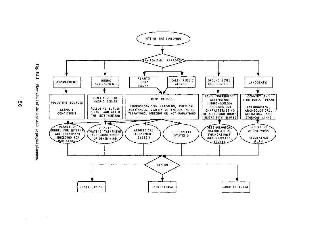
"'"l c[Ci.
!Jl ~ -I "r1 0 ~ (") ::r __. I» .... -(J1 0
0') ....., -::r (ll
I» "0 "0 a I» (")
::r
s "0 .... .2. (ll (") -"0 f.) ::s ::s s·
(!Cl
POLLUTING SOURCES
CLIMATE CONDITIONS
QUALITY OF THE HYDRIC BODIES
POLLUTING BURDEN BEFORE AND AFTER THE INTERVENTION
INSTALLATION
RISK CAUSES:
MICROORGANISMS PATOGENS, CHEMICAL SUBSTANCES, QUALITY OF ENERGY, NOISE, VIBRATIONS, IONIZING OR NOT RADIATIONS
r-· -----1 GROUND LEVEL UNDERGROUND
LAND MORPHOLOGY SEISMOLOGY
HIDRO-GEOLOGY GEOTECHN I QUE
CHARACTERISTICS Of SOILS AND ROCKS INSTABILITY SLOPES
LANDSCAPE
COUNTRY AND TERRITORIAL PLANS
ENVIRONMENT, ARCHEOLOGICAL, ARTISTICAL AND STOR ICAL Ll NKS
ARCHITECTURAL
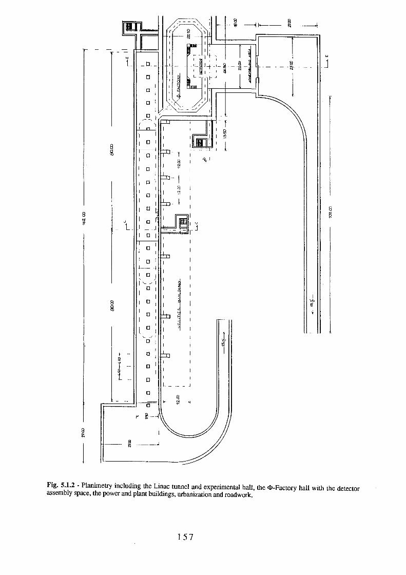
... "' j 1_ _D_- -I_ 8
-- -~- ---
0
j 0
8 ~
0 ~---
I 0 I ' / -I I'-----" I
0 I I
~ I I
8 D I I @ D
0
"- ... /I
~· 0
- 0 -t a ... t 0
t 0 L_ -- - J
0 8
=--a- ~- ~ >I
Fig. 5.1.2 - Planimetry including the Linac tunnel and experimental hall, the <t>-Factory hall with the detector assembly space, the power and plant buildings, urbanization and road work.
157
5.2. • PLANTS AND GENERAL SERVICES
5.2.1 - Description
The two main buildings housing technological and conventional industrial plants,
laboratories, offices, control rooms, etc., one serving the Linac the other serving the <1>-
Factory, are at ground level.
The first runs above and parallel to the Linac tunnel and is equipped with a 5 ton crane
covering the full building length. This solution optimizes plant layout and costs.
The cold-box is installed on central area so that a symmetrical feed system for the accelerator
cryostats can be implemented with only one liquid helium and gas descent, serving the same
numbers of cryostats right and left, is needed. The balanced load makes the plant less
expensive.
The Linac service building includes offices and laboratories physically separated from the
plants mentioned by means of moveable walls which provide maximum flexibilty in adapting to
any future requirement.
The helium compressors to which the cold box is connected are noisy and must therefore be
accomodated outside the main building; a 7 m x 20 m industrial type building will house a
sound-proof enclosure containing two 1 MW compressors; another separate compartment in the
same building is used for the gas purification and oil removal machinery. Three 12 atm, 200
m3 gas storing tanks are installed in the open.
The central heating system will also occupy a small, separate construction.
The <1>-Factory service building is built over the latter (Fig. 5.2.1.), to which it is connected
by an internal stair with an adjacent goods lift (Fig. 5.2.2). Also this one receives at its interior
all the plants for the machines and the conventional ones, offices and laboratories included.
Only one control room, for the linear accelerator and the <1>-Factory is located in this
building. It is necessary therefore to provide for it an enhanced removable floor which permits
the passage of computers cables and others services, as well as an air-conditioning pipe system.
158
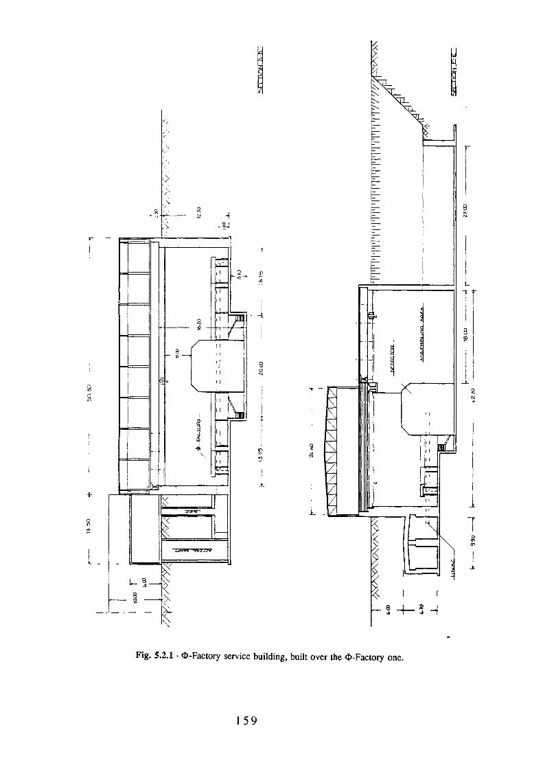
tv,
',
,·\
/
,\
•/
<) \
;\
-~" g ~ p:__ • ·J ';:! ~ .,
l T I I I !
~ I 8
r= ... -"' '=-
"'' ,\ ... ~;oj r=-.•,
~
I -r -
1=-p.:.. ,, "' I ~
;;~
,,
I t=
I '!J t: .(\
f-1
I': ! I 2 I'' )I i
-!! kf I
I 11
I !1- ~- ,, ' " I .;
I 11
1' 11
" l
11
~ 11
j r"T ;---
I r,
IU-
"' trr-
I . i i ~ I
I 8 i I
I ~ ·-t I ~
_:[
~ 8 j I
CS I
"' 1 _1..
..... - g ! N ...
11
11
~ ~
"' ~
! 11
I I ~ !
t '< 11 ~ -r:>n<r
_t_ I
l ~ '< l~ ~ 1
0
"' "' :z:::l'i'AI; ~~~, ...
-
~ I.-~-R
1-- ~ ~ :;.. <
l .... -
·--- - ~ K
Fig. 5.2.1 - ct>-Factory service building, built over the ct>-Factory one.
159
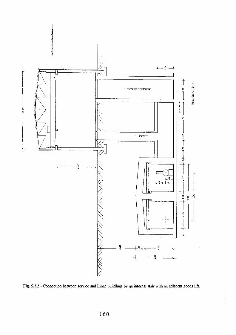
t -+---- ~ ~
t I I ! - --:lJYHt; SSJJJY e I 1 I /, ll 8 ~
N ) j. ..,.
-~' Q.
1 I - r:ro:r- ~
I ~
r ~ 2
----·
l 'i3
L-------- ~ 1 I Q N ...
J I
Q 0 ~ ... "' ""' r--5:1 -r ~
I
""' 0 J ... "' /" - .... - -
1 /
"' '?; I
/ :!:!::!
~ t
8 'b ~+'t--- ~ :) -lS f
~ ~ r
Fig. 5.2.2 - Connection between service and Linac buildings by an internal stair with an adjacent goods lift.
160
5.2.2 - Power Inventory
Usual the most power demanding systems are the magnets and the radio frequency,but here
the use of superconducting components requires a significant part of the whole power to be
devoted to cryogenics. The numbers listed in the power inventory are a first order estimate done
for the purpose of cost evaluation; for minor details, still missing, concerning mostly
conventional electrical services, the forecast is based on estimates derived from similar
installations.
In particular, conventional plants include heating, air conditioning, lighting, compressed air
plants, alarm & fire protections, etc. The power devoted to helium compressors depends on the
liquefaction rate needed by the s.c. cavities and by the main detector solenoid. Another
important power demand comes from the conventional1.9 Tesla wigglers for the <!>-Factory;
the numbers are scaled from those of the wiggler installed on Adone. Finally, it must be noted
that the listed power - except ,of course, that for the general building services - is intended as
maximum requirement, with both machines in operation at maximum energy.
The total power inventory is detailed in the following Table 5.2.1 and adds up to about 7.5
MW.
161
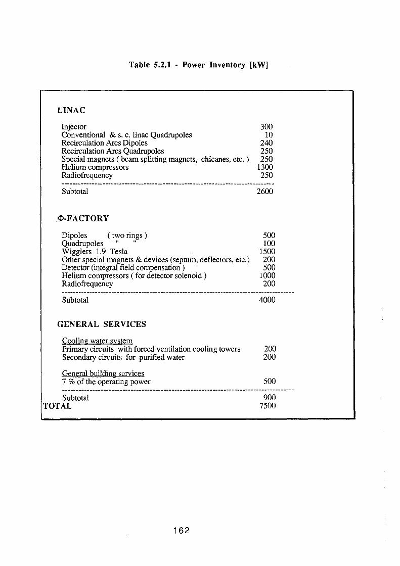
Table 5.2.1 - Power Inventory [kW]
LINAC
Injector 300 Conventional & s. c. linac Quadrupoles 10 Recirculation Arcs Dipoles 240 Recirculation Arcs Quadrupoles 250 Special magnets ( beam splitting magnets, chicanes, etc. ) 250 Helium compressors 1300 Radiofrequency 250
Subtotal 2600
<l>-F ACTORY
Dipoles ( two rings ) 500 Quadrupoles " " 100 Wigglers 1.9 Tesla 1500 Other special magnets & devices (septum, deflectors, etc.) 200 Detector (integral field compensation ) 500 Helium compressors ( for detector solenoid ) 1000 Radiofrequency 200
Subtotal 4000
GENERAL SERVICES
Cooling water system Primary circuits with forced ventilation cooling towers 200 Secondary circuits for purified water 200
General building services 7 % of the operating power 500
Subtotal TOTAL
162
900 7500
APPENDIX
X-VUV POSSIBLE FEL EXPERIMENTS
L.Serafini. M.Ferrario, C.Pagani, A.Ghigo*, P.Ytichelato, A.Peretti
lNFN and Umversn.a di Milano ·Via Celona 16. 20133 Milano *L.l\IFN Laboraton ~az10nali di Frascati · P.O. BOX 13. 00044 Frascau
l • Introduction
The availability of intense electron .beams of high quality makes the ARES SC LINAC
complex a unique facility to perform several experiments in the X-ray VUV FEL mainstream.
In this chapter we present a feasibility study of a device able to generate coherent radiation of
high brightness in the soft X-ray VUV spectral region (photon energies in the 10-120 eV
range), together with a tentative list of the possible FEL experiments.
Detailed, but still preliminary, numerical simulations will be extensively reported: they
anticipate the FEL performances and support the enclosed lists of parameters concerning the
beam quality requirements and the wiggler characteristics. These simulations have been carried
out taking into account a new recently proposed technique: the "ion focussing" of the beam,
achieved with a pre-ionized plasma channel added inside the beam pipe in the wiggler{5).
Some new applications of old ideas are also presented here for the flrst time, in the last two
sections: they deal with the subject of coherent spontaneous emission. Inside our range of
radiation wavelengths such new schemes will open the possibility to obtain coherent radiation
wavelength of""' 50 A, in the so called "water window". The new experimental physics field
which may be explored with such a radiation source is, in our opinion, as wide as needed to
justify the big effort to build such a device.
Indeed. it is well known that the shorter is the radiation wavelength, the higher must be the
beam quality needed to operate a single pass high-gain FEL in the SASE (Self Amplified from
Spontaneous Emission) mode. As shown elsewhere<O, the choice of a low frequency and a
superconducting structure for the beam acceleration plays a crucial re le in minimizing the beam
quality degradation through the LINAC. In this respect, the injection system turns out to be one
of the most important part of the whole complex.
It is wonhwhile to mention that the SC LINAC will also constitute an experimental tool to
study the beam-beam and the beam-radiation field interactions: such effects are of great
relevance in the design of all future e+ e· Te V colliders. A better understanding of the
beamstrahlung processes will surely allow to improve the feasibility and the performances of
such machines.
2 • One Dimensional Model Predictions.
As elsewhere presented in more detail(l), the expected beam characteristics at the LL'l'AC
output, for FEL experiments, can be summarized as shown in Table 1. Having available beams
with a relativistic factor, y, in the range 600+ 1200, one can easily observe that the resonant
radiation wavelength, given by the usual FEL resonance relationship, lies in the range 200-20
nm (for the first harmonic) when wigglers with typical periods of a few centimetres are
considered. In fact the FEL resonance equation is:
2 A.w(l + aw)
A. = r 2 2y n
where: A.w is the wiggler period, Ar the n-th harmonic radiation wavelength and aw is the
dimensionless vector potential of the wiggler. In a planar wiggler aw is related to the peak
magnetic field, Bw, by the fonnula: aw = .66 Aw [cm] Bw [T].
Table l . Expected Beam Characteristics
Beam energy
Peak current
Norm. transv. emitt.
Relative energy spread
[Me V]
[A]
[m rad]
300 + 580 (820*)
400
4+8·10-6
.5+ 1·10·3
1000
4+5·10·5
2+5·10·3
* Evenrually obtainable wtth a second recirculation.
Unfonunately, the scaling law for the exponential growth of the radiation field 1s quite
unfavourable in the very shon wavelength domain. The gain length, Lg, i.e. the length over

3
which the radiation field intensity grows by a factor e, scales indeed like the beam energy
divided by the cubic root of the wiggler period, as in the following formula, which holds in the
cold-beam limit and before sarurati.on(2):
where J is the beam current density.
To reach the VUV to soft X-ray domain (radiation wavelength between 10 and 100 nm) high
y and short wiggler periods are both needed, Bw being dependent on Aw as will be shown later.
That i.mplies that fine and intense beams must be used in order to overcome by the increase in
current density the corresponding increase of the gain length.
It is well known that in an untapered wiggler, because of the exponential growth of the
radiation field, once the high gain regime is achieved, intensity reaches saturation after a typical
length of the order of 4 1t Lg: at that point the radiation power, Pr, is roughly given by the beam
power, P},, times the Pearce parameter, p, (p = Aw/41tLg), that is Pr = p Pb(2). Then, the
saturated radiation power comes out invariant with respect to the beam energy.
A more important scaling law sets a threshold for the radiated power, which must be high
enough to ensure that the quantum fluctuations in the photon beam do not destroy the coherence
properties of the radiated field: the condition is given by
-6 Pr[MW] > 5.910
2 2 A.r qf
where qr is the maximum quantum fluctuation compatible with the radiated field coherence; qr
should actually be of the same order of magnitude as the ratio between the incoherent radiated
power and the coherent one, so as to ensure that the incoherent quantum noise does not
significantly perturb the coherence of the radiated field. The previous relationship comes from
the scaling of the quantum fluctuation with the inverse square root of the number of photons per
wavelength(3).
The requirement of a radiated power scaling like the square of the frequency (i.e. the square
of the photon energy) actually sets one of the major limits in going towards the X-ray domain.
The transverse size, fb, of the electron beam in a wiggler with appropriate shaping of the
pole face is given by(4):
being: (1)
Where En is the transverse normalized emittance of the beam and the parameter H represents the
effect of the ion focussing in decreasing the betatron wavelength A.~. In absence of 10n
focuss1ng H = 1: the 10n focus sing effect makes H < 1 (5).
The relevance of producing low emittance beams and to increase the focussing strength of the
wiggler optics is then straightforward. The ion focussing scheme consists essentially 1n
producing, inside the beam pipe along the wiggler, a tenuous ion channel: this is generated by
injecting an intense leading low energy ( == 300 Me V) electron beam into a low pressure helium
column. The beam ionizes the helium gas and the space charge field of the beam ejects the
detached plasma electrons from the beam vicinity. The charge of the second injected electron
beam is partially, or totally (depending on the helium pressure) compensated in passing through
the ion channel. The pinch field acting on the beam increases the focussing strength, decreases
the beam transverse size and produces a substantial gain length contraction. Finally, it is
worthwhile noting that the gain length scales with the cubic root of H.
Two major constraints on the quality of the electron beam injected into the wiggler must be
taken into account when the cold beam limit approximation is abandoned. The transverse and
the longitudinal phase spaces of the electron and of the photon beams must be matched if the
interaction between the two beams has to be ensured all along the wiggler, in order to set up the
energy exchange which is the basic condition to achieve an exponential gain in the radiated field
power. For the transverse phase space one must match the emittance of the electron beam with
the emittance of a diffraction limited radiation beam; this means that<6):
A.ry en= -- fl
21t
where ft must be kept below 1 (as discussed later).
(2)
Since the line-width of the radiated field at saturation is of the order of p, the energy spread
of the injected beam must be less than this quantity: in practice it has been found from
simulations(7) that the proper condition is given by:
~y p -<y 4
A last condition comes from the requirement that diffraction does not remove radiation from
the edge of the electron beam over a length shoner than the gain length; this requires the
Rayleigh length, Zr. to be larger than the gain length. Lg(8):
being and 2
Z = 7t rb r
A.r
In some sense this condition sets a limit to the extent to which the ion focussing can be pushed:
a reduction of the beam radius causes a decrease of the gain length, scaling like the square of
the cubic root of the radius, but unfonunately also the Rayleigh length decreases scaling like the
square of the radius. The best compromise on the effectiveness of the ion focussing technique
is.reached when f3 == l, that is when the diffracted power is not higher then the power increase
due to the exponential gain. A further ion focussing increase, making f3 > 1. no longer
improves the FEL performance, as will be shown later.
Taking into account what could be a typical step-by-step upgrading of the SC LINAC
facility, especially in terms of beam current and output emittance, we listed in Table 2 the
corresponding envisageable FEL experiments: the table has been divided into four sections, to
list the quantities related to the beam requirements, to the wiggler characteristics, to the FEL
radiated power and to the above mentioned parameter fj, that control the validity of the one
dimensional evaluation. The quantity f2 = f 12·f3 must be less than 1 (5). The two parameters S
and K measure the slippage effect and the superradiance behaviour of the FEL, as defined in
ref.(9).
Moving from left to right on Table 2 the difficulty of the FEL experiment grows. both
because of the tighter beam quality requirements and of the difficulties in manufacturing the
required wiggler.
A few comments on the beam parameters are in order:
• the first anticipated beam will be produced by the LINAC without any recirculation. with
a peak current of 200 A and a transverse normalized emittance (rms value of 1·1 0·5) fully
consistent with the preliminary design of the injection systemO).
• the energy spread shown in the Table takes into accounts the eff~ct of the longitudinal
wake-field excited inside the RF cavities: here it must be remarked that such low values
for the energy spread are made possible only by the low RF frequency selected for the
LINAC.
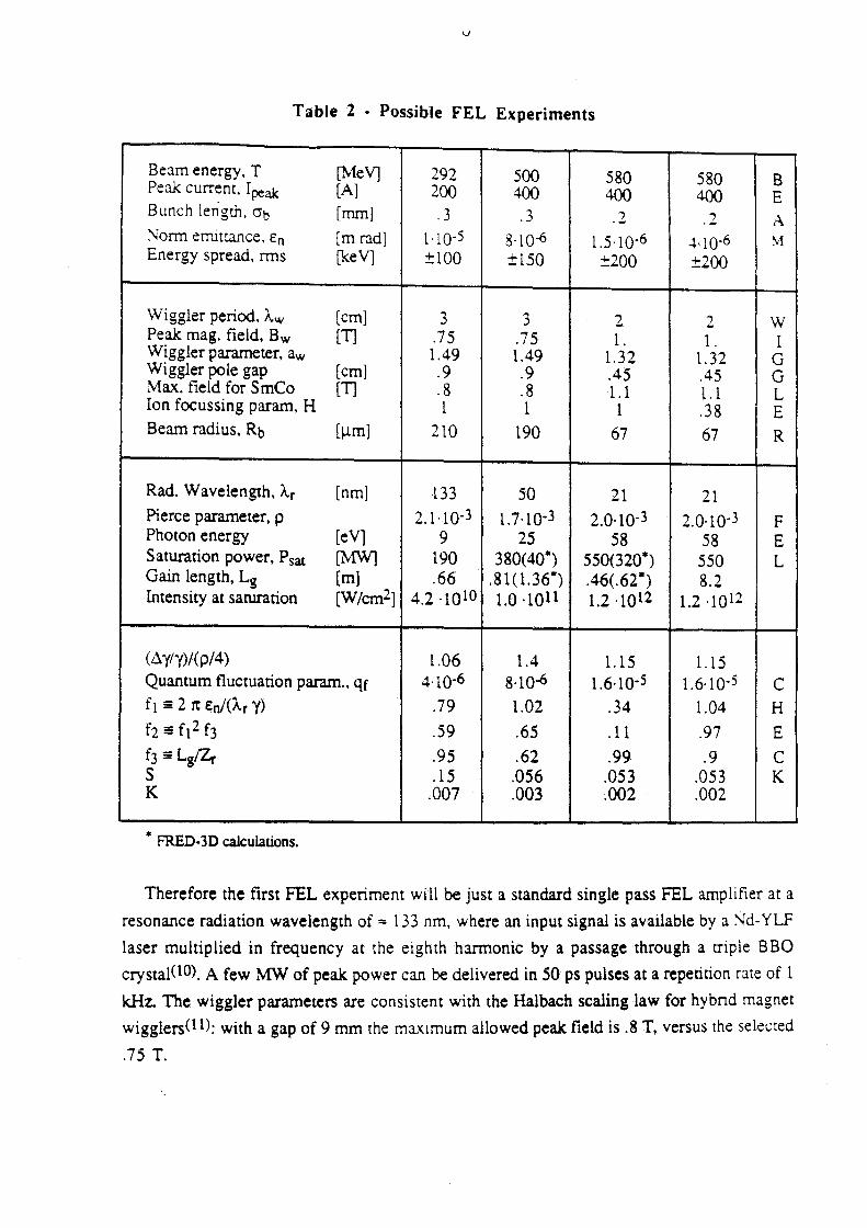
V
Table 2 • Possible FEL Experiments
Beam energy, T [Me V] 292 500 580 580 B Peak current. Ipeak [A] 200 400 400 400 E Bunch length. crb [mm! .3 .3 .2 .2 A ~orm emmance, En [m radj 1·1Q·5 8·10-6 1.5·10-6 -+·1 o-6 ~ Energy spread, rms [keY] ±100 ±150 ±200 ±200
Wiggler period, Aw [cm] 3 3 2 2 w Peak mag. field, Bw [T] .75 .75 1. 1. I Wiggler parameter, aw 1.49 1.49 1.32 1.32 G Wiggler pole gap [cm] .9 .9 .45 .45 G Max. field for SmCo [T] .8 .8 1.1 1.1 L Ion focussing param, H 1 1 1 .38 E Beam radius, Rb [).I. m! 210 190 67 67 R
Rad. Wavelength, "A.r [nm] 133 50 21 21 Pierce parameter, p 2.1·10-3 1.7·10·3 2.0·10-3 2.0·10·3 F Photon energy [eV] 9 25 58 58 E Saturation power, Psat [MW] 190 380(40*) 550(320*) 550 L Gain length, Lg [m] .66 .81( 1.36*) .46(.62*) 8.2 Intensity at saturation [Wfcm2] 4.2 ·lQlO 1.0 ·lOll 1.2 ·1012 1.2 ·1Ql2
(D.y/'y)/(p/4) 1.06 1.4 1.15 1.15 Quantum fluctuation param., qr 4·10-6 8·10-6 1.6·10-5 1.6·10·5 c ft = 2 1t En/(Ar Y) .79 1.02 .34 1.04 H
f2 = ft 2 f3 .59 .65 .11 .97 E f3 = Lg/Zr .95 .62 .99 .9 c s .15 .056 .053 .053 K K .007 .003 .002 .002
* FRED-3D calculations.
Therefore the first FEL experiment will be just a standard single pass FEL amplifier at a
resonance radiation wavelength of= 133 nm, where an input signal is available by a :--rd- YLF
laser multiplied in frequency at the eighth harmonic by a passage through a triple BBO
crystal00). A few MW of peak power can be delivered in 50 ps pulses at a repetition rate of 1
kHz. The wiggler parameters are consistent with the Halbach scaling law for hybnd magnet
wigglers(ll): with a gap of 9 mm the max1mum allowed peak field is .8 T, versus the selected
.75 T.
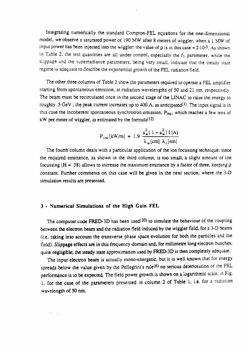
Integrating numerically the standard Compton-FEL equations for the one-dimensional
model, we observe a saturated power of 190 MW after 8 meters of wiggler, when a 1 ~ of
input power has been injected into the wiggler: the value of p is in this case == 2·1 Q-3. As shown
in Table 2, the test quantities are all under control, especially the f1 parameter, while the
slippage and the superradiance parameters, being very small, indicate that the steady state
regime is adequate to describe the exponential growth of the FEL radiation field.
The other three columns of Table 2 show the parameters required to operate a FEL amplifier
starting from spontaneous emission, at radiation wavelengths of 50 and 21 nm, respectively.
The beam must be recirculated once in the second stage of the LINAC to raise the energy to
roughly .5 GeV ; the peak current increases up to 400 A, as anticipated( I). The input signal is in
this case the incoherent spontaneous synchrotron emission, Pine• which reaches a few tens of
kW per meter of wiggler, as estimated by the formula02)
2 2 aw ( 1 + aw) I [A]
Pinc(kW/m] = 1.9 ------A.w [cm] A.r [nm]
The founh column deals with a particular application of the ion focussing technique: since
the required emittance, as shown in the third column, is too small, a slight amount of ion
focussing (H = .38) allows to increase the maximum emittance by a factor of three, keepmg p
constant. Funher comments on this case will be given in the next section, where the 3-D
simulation results are presented.
3 • Numerical Simulations of the High Gain FEL
The computer code FRE0-30 has been used(20) to simulate the behaviour of the coupling
between the electron beam and the radiation field induced by the wiggler field, for a 3-D beams
(i.e. taking into account the transverse phase space evolution for both the particles and the
field). Slippage effects are in this frequency-domain and, for millimetre long electron bunches,
quite negligible; the steady state approximation used by FRE0-30 is then completely adequate.
The input electron beam is actually mono-energetic, but it is well known that for energy
spreads below the value given by the Pellegrini's rule(6) no serious deterioration of the FEL
perfonnance is to be expected. The field power growth is shown on a logarithmic scale. m Fig.
1, for the case of the parameters presented in column 2 of Table 1, i.e. for a radiation
wavelength of 50 nm.
After three meters of lethargy, the signal grows exponentially up to 30 MW; the latter value
is reached at the end of a 20 m long wiggler. Since the gain is about 3.2 dB/m, as shown in
Fig. 2, a funher 3.5 meters of wiggler length would be needed to reach the 1-D estimated
saturation power at 380 MW.
The observed gain length, Lg. is therefore 1.36 m, which must be compared to the value of
. 81 m, predicted by the 1-D model. The discrepancy can be understood taking into account that
the Rayleigh length, Zr. for this case is slightly above the gain length. Since the 1-D model is
valid in the limit Zr >> Lg (i.e. f3 << 1 ), the gain decrease due to diffraction effects cannot be
accounted for by the 1-D model. The same holds for the transverse phase space effects: smce
the emittance is just above threshold, (fl = l.02), one must expect the 1-D calculation to predict
a higher gain than the 3-D one.
We want to point out that a coherent input signal of 100 W has been used to start the FEL,
even though no coherent signal is available at this wavelength (50 nm). In particular, since
FRED-30 is not able to simulate the start up from the Schottky noise or from the incoherent
spontaneous emission, 100 W has to be taken just as a reference value, to be compared to the
incoherent synchrotron radiation power, which is in this case 36 kW/m. Harmonic switching
(see below) or other exotic ideas like the SHOK scheme(l3) could overcome the input signal
problem.
-ill: .. • • 0
Q,
z (m)
Fig. 1 - Field power growth, on a log scale. with the parameters presented in colwnn 2 of Table l.
: [ ~ l. / ....... ····
= 0
(,:)
I.
0. . ......
0. 101
.... ··
I.
t (m)
. -·· ....
.. j j
............
Fig. 2- Incremental (solid line) and average (dashed line) gain along the wiggler for the case of F1g. 1.
The full exploitation of the ion focussing technique has been carefully studied for the case of the
21 nm radiation wavelength, with a 580 Me V beam at 400 A (third column of Table 2). The
field power computed by FRED-30 along the wiggler is shown in Fig. 3 and 4 on logarithmic
and linear scales, respectively. The input signal is still a 100 W coherent field. The incoherent
synchrocron radiation power is in this case 85 kW per meter of wiggler, or, equivalently, 1.7 kW per wiggler period.
(•1;------r--------,
~ (•7 ~
l l
l - l ,!!. E•S
... • • 0
~ l l
(•l
l
(•I ~------:"~------! 0. I o' I. 2.
z {m)
Fig. 3 · Field power growth, on a log scale, with the parameters presented in colwnn 3 of Table 2.
l'
:.
-;a
... • • 0 ~
I.
to'
o,. 10
1
z {m)
Fig. 4 - Same as Fig. 3. but on a linear scale. The power is in units of 1 o' W.
After 2 meters of lethargy the exponential gain sets in and the radiation field reaches the 320
MW saturation power level at z = 12 m: the corresponding intensity is 1.2·1012 W/cm2,
confined in a narrow cone of about .1 mm rms radius and 1.1·10-5 rad rms angular width. In
Figs. 5 and 6 the intensity profiles are plotted as functions of the transverse coordinate x of the
wiggler, at the entrance (z = 0) and at the exit of the wiggler (z = 20 m) respectively.
The input field is a gaussian laser beam focussed at z = 0. At the wiggler exit the intensity
proflle, due to diffraction effect, shows that some radiation escapes from the electron beam: the
gaussian fit (dashed curve in Fig. 6) reveals that the optical guiding and the diffraction along the
wiggler produce a distortion of the intensity profile, which is no longer gaussian. It should be
noted that the peak value of Fig. 6 (5·1011) is lower than the peak value ( 1.2·1012) at saturation
(z = 12 m).
Moreover, the phase profile of the radiation field at z = 20 m, shown in Fig. 7, indicates that
the radiation beam is de-focussed, since the phase increases off-axis.
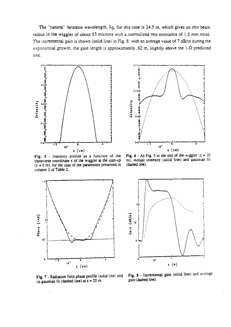
The "natural" betatron wavelength, A.~, for this case is 24.5 m, which gives an rms beam
radius in the wiggler of about 53 microns with a normalized rms emittance of 1.5 mm mrad.
The incremental gain is shown (solid line) in Fig. 8: with an average value of 7 dB/m during the
exponential growth, the gain length is approximately .62 m, slightly above the 1-D predicted
one.
-.. c • c -
C•l .---r-------r-----,---. j: ~
I !
(tl
.... •• .$
1 (cm) Fig. S • Intensity profile as a function of the transverse coordinate x of the wiggler at the stan-up (z = 0 m), for the case of the parameters presented in column 3 of Table 2.
-.::1 c:o .l .. -• ... c:o .c Q,
101
o. L-.~.)------:0~. ____ .... sr----' ,, .. x (cm)
Fig. 7 . Radiation field phase profile (solid line) and its gaussian fit (dashed line) at z = 20 m.
C•l% r---,r------r-----.--...,
-.. c • c ....
• ••• '· . s
z (c11)
Fig. 6 • As Fig. 5 at the end of the wtggler (z = 20 m). Actual intensity (solid line) and gausstan fit (dashed line).
e ........ =
.l
:!. 101
c ·-c:o ~
·t! 0.
. ..
101
l (m)
I -1 I
~ I
Fig. 8 • Incremental gain (solid line) and average gain (dashed line).
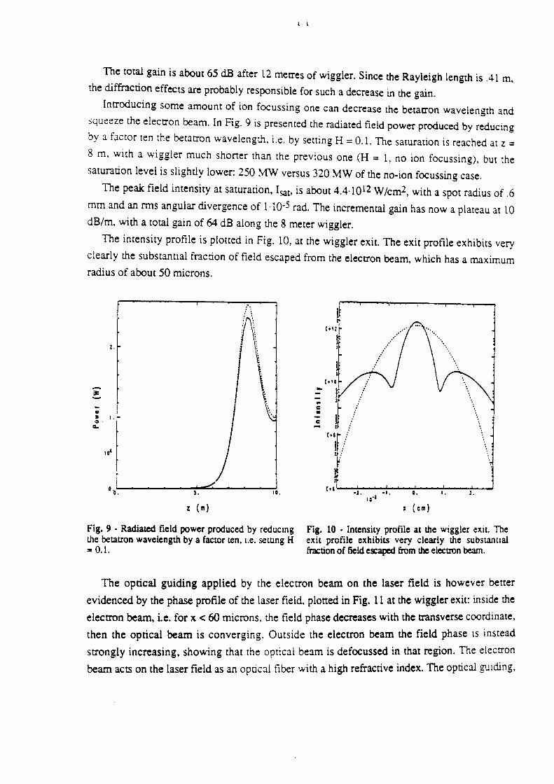
1 1
The total gain is about 65 dB after 12 metres of wiggler. Since the Rayleigh length is .41 m,
the diffraction effects are probably responsible for such a decrease in the gain.
Introducing some amount of ion focussing one can decrease the betatron wavelength and
squc:eze the electron beam. In Fig. 9 is presented the radiated field power produced by reducing
by a factor ten the betatron wavelength, i.e. by setting H = 0.1. The saturation is reached at z =
8 m, with a wiggler much shorter than the previous one (H = l, no ion focussing), but the
saturation level is slightly lower: 250 MW versus 320 MW of the no-ion focussing case.
The peak field intensity at saturation, Isat. is about 4.4·1012 W/cm2, with a spot radius of .6
mm and an rms angular divergence of 1·1 Q-5 rad. The incremental gain has now a plateau at 10
dB/m, with a total gain of 64 dB along the 8 meter wiggler.
The intensity profile is plotted in Fig. 10, at the wiggler exit. The exit profile exhibits very
clearly the substantial fraction of field escaped from the electron beam, which has a max1mum
radius of about 50 microns.
-~ ... •
%.
ll 1. Q
Q.,
0~.~.----------~~-.~--------~10. z (m)
Fig. 9 - Radiated field power produced by reducmg lhe betauon wavelength by a factor ten, 1.e. setung H = 0.1.
-.. c: • c: .... : .....
£•&
I / j:
r •' '---~1 ........ -.,!-.......... ""'-f', .......... "-'-:, ............... ~z ........ ...J
to"1
1 (cm)
Fig. 10 • Intensity profile at lhe wiggler ex1t. The exit profile exhibits very clearly the substantial fraction of field escaped from the electron beam.
The optical guiding applied by the electron beam on the laser field is however better
evidenced by the phase profile of the laser field, plotted in Fig. 11 at the wiggler exit: inside the
electron beam, i.e. for x < 60 microns, the field phase decreases with the transverse coordinate,
then the optical beam is converging. Outside the electron beam the field phase is instead
strongly increasing, showing that the optical beam is defocussed in that region. The electron
beam acts on the laser field as an optical tiber with a high refractive index. The optical guiding,
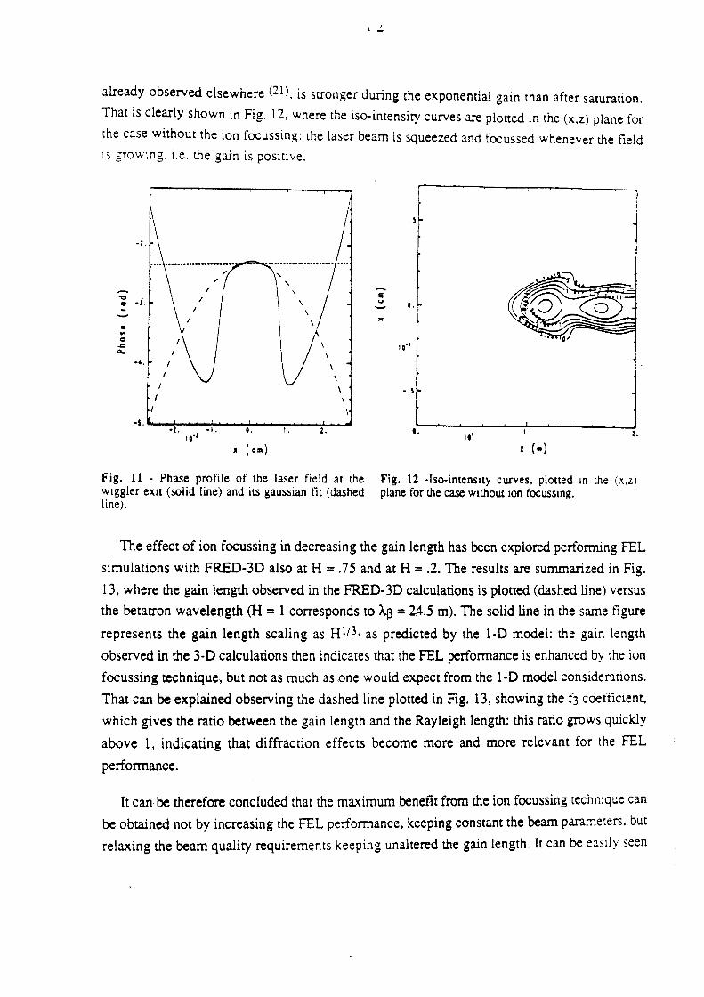
l !.
already observed elsewhere <21 ). is srronger during the exponential gain than after saturation. That is clearly shown in Fig. 12, where the iso-imensity curves are plotted in the (x,z) plane for
the case without the ion focussing: the laser beam is squeezed and focussed whenever the field ts growing. i.e. the gain is positive.
.. -
•S. --.+L-----'!-, .--:0-. ----:1-, ........... ~~~.--..M to'1
1 (cm)
Fig. 11 - Phase profile of the laser field at the w1ggler ex.1t (solid line) and its gausstan fit (dashed line).
e ... .. 0 .
-. s
.-. __._ .......... , .-. .._____._----:, -. __..._..____,___.____.1.
z (m)
Fig. 12 -Iso-intensay curves, plotted m the (x.z) plane for the case wtthout 10n focussmg.
The effect of ion focussing in decreasing the gain length has been explored performing FEL
simulations with FRE0-30 also at H = .75 and at H = .2. The results are summarized in Fig.
13, where the gain length observed in the FRE0-30 calculations is plotted (dashed line) versus
the betarron wavelength (H = 1 corresponds to A.~ = 24.5 m). The solid line in the same figure
represents the gain length scaling as H 1/3. as predicted by the 1-D model: the gain length
observed in the 3-D calculations then indicates that the FEL performance is enhanced by the ion
focussing technique, but not as much as one would expect from the 1-D model consideranons.
That can be explained observing the dashed line plotted in Fig. 13, showing the f3 coefficient,
which gives the ratio between the gain length and the Rayleigh length: this ratio grows quickly
above 1, indicating that diffraction effects become more and more relevant for the FEL
perfonnance.
It can be therefore concluded that the maximum benefit from the ion focussing techmque can
be obtained not by increasing the FEL performance, keeping constant the beam parameters, but
relaxing the beam quality requirements keeping unaltered the gain length. It can be east!y seen
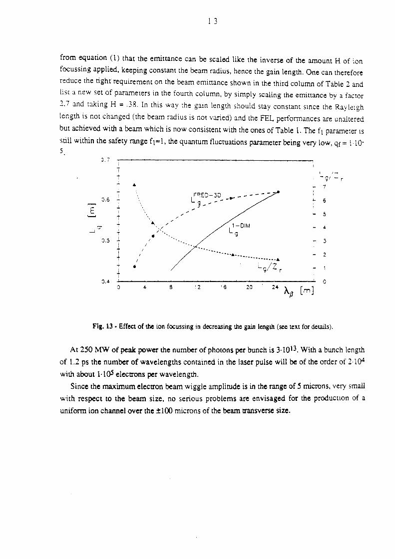
l 3
from equation ( 1) that the ernittance can be scaled like the inverse of the amount H of ion
focussing applied, keeping constant the beam radius, hence the gain length. One can therefore
reduce the tight requirement on the beam eminance shown in the third column of Table 2 and
list :1 new set of parameters in the founh column, by simply scaling the emittance by a factor
2.7 and taking H = 38. In this way the gain length should stay constant smce the Rayle1gh
length is not changed (the beam radius is not varied) and the FEL performances are unaltered
but achieved with a beam which is now consistent with the ones of Table l. The f1 parameter 1s
still within the safety range f 1 = l' the quantum fluctuations parameter being very low. qf = 1·1 os
0.7
0.5
I ... I
t
i -J. I
t ... I I
i
5 1 0. l
+ -;-
1 I
0.4 0
•
I
•
I
I
I
I
4
/
8
I ,....,
- g; - r
- 7 ---' "PED-.30 _.- - ---L~ .......... -- ... 6
- 5
- 4
- .3
-- . .......... ··-·······---.......• - 2
i.. 9/Z r - 1
0 16 20 24 Ap [m]
Fig. 13 • Effect of the ion focussing in decreasing the gain length (see text for details).
At 250 MW of peak power the number of photons per bunch is 3-1013. With a bunch length
of 1.2 ps the number of wavelengths contained in the laser pulse will be of the order of 2·104
with about l·lOS electrons per wavelength.
Since the maximum electron beam wiggle amplitude is in the range of 5 microns, very small
with respect to the beam size, no serious problems are envisaged for the producnon of a
uniform ion channel over the ±lOO microns of the beam transverse size.
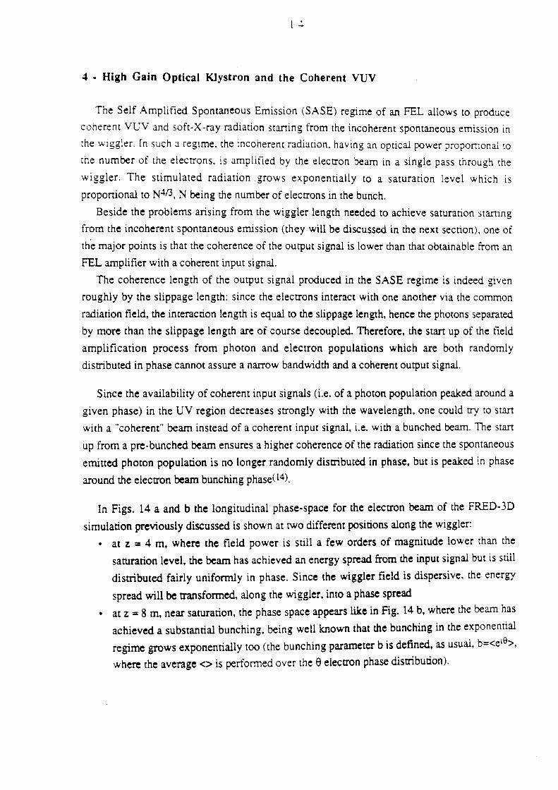
4 • High Gain Optical Klystron and the Coherent VUV
The Self Amplified Spontaneous Emission (SASE) regime of an FEL allows to produce
coherent VCV and soft-X-ray radiation starting from the incoherent spontaneous emission in
the wiggler. In such a reg1me, the incoherent radianon, having an optical power propomonal to
the number of the electrons, is amplified by the electron beam in a single pass through the
wiggler. The stimulated radiation grows exponentially to a saturation level which 1s
proportional to N4!3, N being the number of electrons in the bunch.
Beside the problems arising from the wiggler length needed to achieve saturation startmg
from the incoherent spontaneous emission (they will be discussed in the next section), one of
the major points is that the coherence of the output signal is lower than that obtainable from an
FEL amplifier with a coherent input signal.
The coherence length of the output signal produced in the SASE regime is indeed given
roughly by the slippage length: since the electrons interact with one another via the common
radiation field, the interaction length is equal to the slippage length, hence the photons separated
by more than the slippage length are of course decoupled. Therefore, the start up of the field
amplification process from photon and electron populations which are both randomly
distributed in phase cannot assure a narrow bandwidth and a coherent output signal.
Since the availability of coherent input signals (i.e. of a photon population peaked around a
given phase) in the UV region decreases strongly with the wavelength, one could try to start
with a "coherent" beam instead of a coherent input signal, i.e. with a bunched beam. The start
up from a pre-bunched beam ensures a higher coherence of the radiation since the spontaneous
emitted photon population is no longer randomly distributed in phase, but is peaked in phase
around the electron beam bunching phase(l4).
In Figs. 14 a and b the longitudinal phase-space for the electron beam of the FRED-30
simulation previously discussed is shown at two different positions along the wiggler:
• at z = 4 m, where the field power is still a few orders of magnitude lower than the
saturation level, the beam has achieved an energy spread from the input signal but is still
distributed fairly uniformly in phase. Since the wiggler field is dispersive, the energy
spread will be transformed, along the wiggler, into a phase spread
• at z = 8 m, near saturation, the phase space appears like in Fig. 14 b, where the beam has
achieved a substantial bunching, being well known that the bunching in the exponential
regime grows exponentially too (the bunching parameter b is defined, as usual, b=<el6>.
where the average <> is perfoimed over the e electron phase distribution).
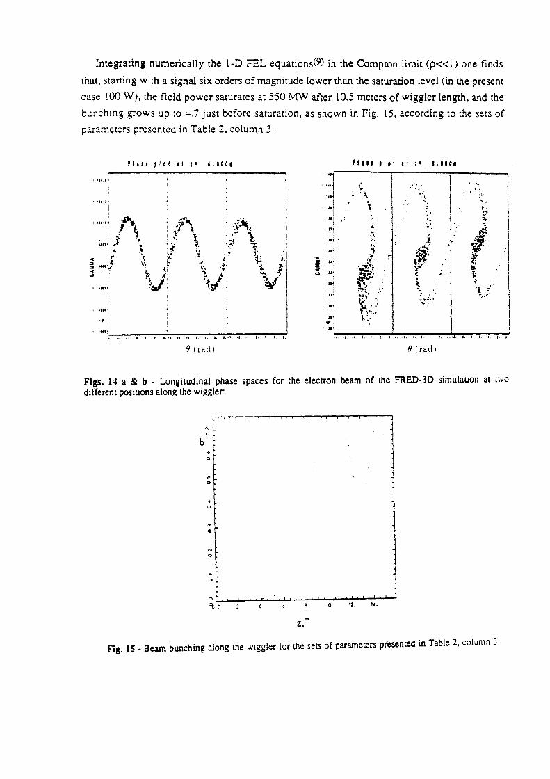
Integrating numerically the 1-D FEL equations(9) in the Compton limit (p<< 1) one finds
that, starting with a signal six orders of magnitude lower than the saturation level (in the present
case 100 W), the field power saturates at 550 MW after 10.5 meters of wiggler length, and the
bunch1ng grows up to ==.7 just before saturation. as shown in Fig. 15, according to the sets of
parameters presented in Table 2, column 3.
na11 Jlol 11 " L0001 "'" Jltl al z• 1.0101 l.rtJ
' :::::J l j I i I
' '"'"!1
:1.~: 11
1
-f\ j·.:~. 1 ~- .l .~· ~.
• I ~ 't , ,-+ l; UtH ~~· ~ : j f. 1 .~;' ";:
; ~ . ~:.· v 1;. ~·· ·' .... !~ .'i 1 :.j:
.( . ·~ ~ ·~ '· ~ ·-r· ,.1. ~ ·-- ·! ·~ t:· .... . t. ' ... ·•' ·~ T, ~ . l' .J (A ... ~-. •
' ..... ~ ~J '{/ ·~l
' '""] ...
.. ,.'! . 1''
·~ .. ·.,, ..•.
' "' ". ~. ' . , ..
' '" ' ,,
~-' '" ·' ·-'
• ' '"l
•.·. ·-· : ... .i . ' ... ;.,
" ,I
~~· I.IU ~ .... .~.
. 2'-'"
~~;. :
:a .... ;,' ~ I.IU . ~· ~ . • t.IU , ... ~ c··::. , .
I.IJI ..
·: w· •. !(' -~ 1.111 ·.·' ...... ·:·
~ •. ·~· .. !.tU ' .. ... ·:· ,_,,.
' ...
t tUtH•-:".,.-•• ~. -.,-:".~. -:-,-:-,, "":",,.!.:.,-.• ~ .. ...,...,:-:"',,-:",-. ~ •. -,:"":. ,';'"', 7..,"": .• ::'"", '"':'a.--:"'o -;,-. -:-',, ~-. •1. •t. I. I, J, j,•f. •f, •L t. I. I. J, of, •L •1. I. I f. ).
~ I ra<i I B (rad)
Figs. 14 a & b - Longitudinal phase spaces for the electron beam of the FRED-30 simulauon at two different pos1uons along the wiggler:
Q
b '0
Q
"' 0
" 0
0
"' Q
0
Q
ct,0 3. 10. 12. "-
Z,
Fig. lS • Beam bunching along the w1ggler for the sets of parameters presented in Table 2, column 3.
l 0
Staning from these considerations and following the scheme of the optical klystron(l5), we
propose to separate the wiggler into two pans: the first one acts as a buncher and the second
one as a radiator. If the two pans are decoupled, that is the radiation generated in the buncher is
discarded. the radiator works as a generator of coherent spontaneous radiation at its proper
resonant wavelength. In other words, truncating the exponential gain at a suitable point close to
saturanon and discarding the radiated field generated so far (which is scarcely coherent), one
can get a bunched beam able to radiate coherent synchrotron radiation, in a trans1ent
"superradiant" regime involving the overall beam.
The separation of the electron and the radiation beam can be achieved via a small magnetic
defl~~tion at the end of the first wiggler: such a deflection must of course ensure that the
debunching effect on the beam is negligible with respect to the radiation wavelength scale.
Since to the first order, the path length difference, 6L, for a beam with energy spread !ly/y
deflected by a magnet of angle 9 (assumed small) and radius of curvac..;.re Pb is given by:
3 6y9
pb--6y
setting Pb = 2 m (B = .96 Tat 580 Me V) and 9 = 5 mrad, 6L is less than 1 nm for 6y/y of the
order of 1 %, as typical near the saturation. Over 1 m, which could be the separation of the two
wigglers (in order to achieve a shift of a few mm between the beam and the radiation) the path
length difference due to the emittance, given by:
6L == L 69 2
2
where 6 e is the rms beam divergence
is of the order of 1 nm. Therefore the debunching effect at the entrance of the radiator can be
kept small with respect to the radiation wavelength (20 nm).
Other possibilities to achieve the beam-field separation such as thin radiation absorbers or
wiggler truncations (no half period at the wiggler end) must be investigated, but could in
principle be exploited.
In order to evaluate the field power generated in the radiator we apply a cut to the numerical
integration of the FEL-Compton equanon(9), which corresponds to the first wiggler exit. At the
cut (working actually as a variable threshold) we simply reduce the field intensity to zero, we
keep the panicle phase space unaltered (assuming zero debunching in the transpon between the
two wigglers) and we insen the new resonance condition (proper of the radiator) by zeroing the
l I
detuning. This is simply achieved by keeping <p> = 0, i.e. by summing the quantity <p> at the
threshold to all the particles, where <p> is the normalized detuning, given by:
<'t-Y(> <p> = ----'--
PYr
That IS equivalent to shtft the resonant wavelength to the new value -proper of the radiator
which is determined by the beam energy at the end of the first wiggler.
In the present case the beam energy loss in the first wiggler, &y, is always small - .04%
~ .15% of its initial energy - hence the wavelength increase, OAr. of the radiation emmed in the
radiator is very small with respect to the resonant wavelength, Ar, of the first ''bunching"
wiggler, according to the equation:
8A.r oy -=-2-~.3%
A.r Y
The field power generated in the radiator is plotted in Fig. 16 versus the cumulative length of
the system buncher wiggler- radiator, for three different threshold positions. The crosses show
the standard steady state behaviour of the field power (i.e. for a buncher wiggler extending
without any threshold) with a saturation level of 550 MW at z = 10.5 m: the curve is plotted just
for reference. The solid line, the dashed line and the dotted one mark the field growth in the
radiator when the length of the buncher wiggler is 8 m. 8.8 m and 9.6 m respectively. When
the threshold is located at z = 8.8 m one gets 100 MW of field power from the first wiggler,
then with two meters of radiator length (from z = 8.8 m to z = 10.8 m) the coherent
spontaneous emission grows to 700 MW and then saturates again. Shifting the threshold
towards larger z's causes the radiation to saturate in a shoner length (from z = 9.6 m to z = 10.9 m) lowering at the same time the power level (260 MW).
Since the threshold variation requires a variable length of the buncher wiggler (which can
cause serious technological problems), the same effect can be achieved by varying the tnput
signal power and taking a fixed bunch er wiggler length, as shown in Fig. 17. Here the buncher
wiggler length is assumed to be 8 m and the radiator starts at z = 8 m. The effect on the
longitudinal phase of the beam transpon from the wiggler to the radiator is neglected. As tn Fig.
16, the crossed line shows the standard steady state exponential growth, while the other lines
show the field power in the radiator for three different input powers at the entrance of the
buncher wiggler: the solid line is referred to 100 W, the dashed to 400 Vv and the dotted one to
1000 w.
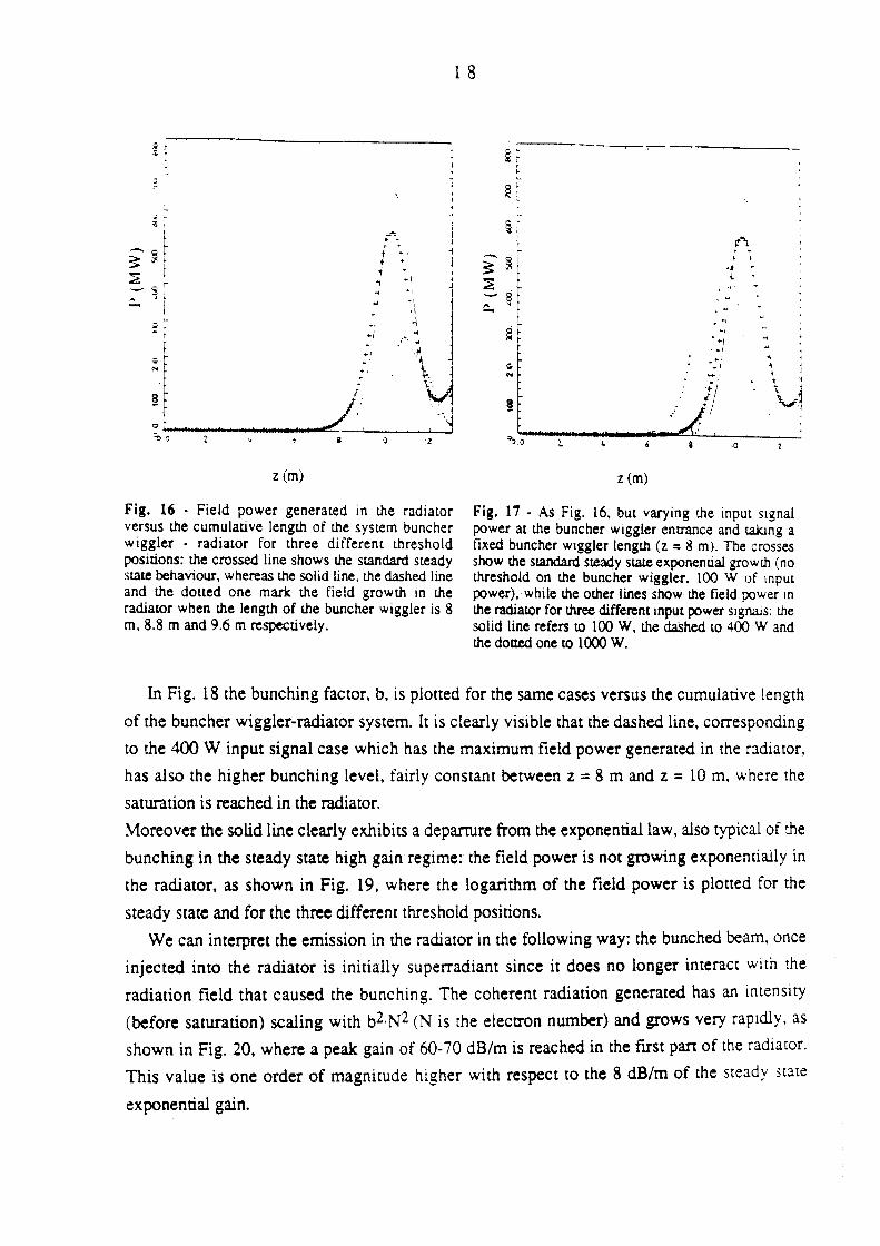
;--~. , J :· ~ , ~ •I
~ i 1 t 1 • 1 1ft n ~~ • t ""!)0 a ·z
z (m)
Fig. 16 · Field power generated m the radiator versus the cumulative length of the system buncher wtggler • radiator for three different threshold positions: the crossed line shows the standard steady state behaviour, whereas the solid tine, the dashed line and the dotted one mark the field growth m the radiator when the length of the buncher wiggler is 8 m, 8.8 m and 9.6 m respectively.
1 8
~; ·-~-.-
~
~:
§! r - ~~ ::
:E
. f
-~ . . { - 8
c.. ~
.. , ~ •I . •'
" .•t •I .. ....,
! :; f; .
.:1>0.0 1. ·0
z (m)
Fig. 17 · As Fig. 16, but varying the input stgnal power at the buncher wtggler entrance and taking a fixed buncher wtggler length (z = 8 m). The crosses show the standard steady state exponential growth (no threshold on the buncher wiggler, lOO W of tnput power), while the other lines show the field power m the radiator for three different mput power stgnals: the solid line refers to lOO W, the dashed to 400 Wand the dotted one to 1000 W.
In Fig. 18 the bunching factor, b, is plotted for the same cases versus the cumulative length
of the buncher wiggler-radiator system. It is clearly visible that the dashed line, corresponding
to the 400 W input signal case which has the maximum field power generated in the radiator,
has also the higher bunching level, fairly constant between z = 8 m and z = lO m, where the
saturation is reached in the radiator.
Moreover the solid line clearly exhibits a departure from the exponential law, also typical of the
bunching in the steady state high gain regime: the field power is not growing exponentially in
the radiator, as shown in Fig. 19, where the logarithm of the field power is plotted for the
steady state and for the three different threshold positions.
We can interpret the emission in the radiator in the following way: the bunched beam. once
injected into the radiator is initially superradiant since it does no longer interact with the
radiation field that caused the bunching. The coherent radiation generated has an intensity
(before saturation) scaling with b2. N2 (N is the electron number) and grows very rap1dly. as
shown in Fig. 20, where a peak gain of 60-70 dB/m is reached in the first part of the radiator.
This value is one order of magnitude higher with respect to the 8 dB/m of the steady state
exponential gain.
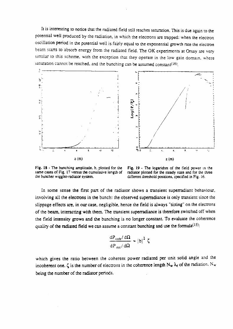
It is interesting to notice that the radiated field still reaches saturation. This is due again to the
potential well produced by the radiation, in which the electrons are trapped: when the electron
oscillation period in the potential well is fairly equal to the exponential growth rate the electron
beam starts to absorb energy from the radiated field. The OK experiments at Orsay are very
Similar to this scheme, with the exception that they operate in the low gain domam. where
saturanon cannot be reached, and the bunching can be assumed constant\16).
.... ... ... _...,
""'
<)I
ol
~ I I_
_,.i c[
r I
~~ t
J T, ., 2. 10 1%
z (m)
Fig. 18 - The bunching amplitude, b, plotted for the same cases of Fig. 17 versus the cumulative length of the buncher wtggler-radiator system.
I
I
z (m)
Fig. 19 - The logarithm of the field power m the radiator plotted for the steady state and for the three different threshold positions, specified in Fig. 16.
' 1 1
J 1
~ 1
In some sense the first pan of the radiator shows a transient superradiant behaviour,
involving all the electrons in the bunch: the observed superradiance is only transient since the
slippage effects are, in our case, negligible, hence the field is always "sitting" on the electrons
of the beam, interacting with them. The transient superradiance is therefore switched off when
the field intensity grows and the bunching is no longer constant. To evaluate the coherence
quality of the radiated field we can assume a constant bunching and use the formula05):
dPcah/dQ = lbl2 ~ dP 1nc1 ctn
which gives the ratio between the coherent power radiated per unit solid angle and the
incoherent one. ~is the number of electrons in the coherence length Nw A.r of the radiation, Nw
being the number of the radiator periods.
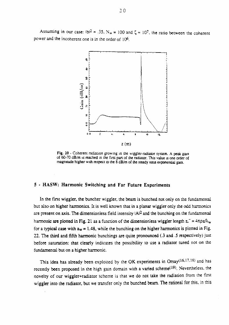
20
Assuming in our case: lbl 2 = .35, Nw = 100 and~= 107, the ratio be~ween the coherent
power and the incoherent one is in the order of 106.
= ~ ---
0 0 '·
l
o. 10 1'-
z (m)
Fig. 20 · Coherent radiation growmg m the wiggler-radiator system. A peak gam of 60-70 dB/m IS reached in the first part of the radiator. This value IS one order of magmtude higher w1th respect to the 8 dB/m of the steady state exponential gam.
S • HASW: Harmonic Switching and Far Future Experiments
In the first wiggler, the buncher wiggler, the beam is bunched not only on the fundamental
but also on higher hannonics. It is well known that in a planar wiggler only the odd harmonics
are present on axis. The dimensionless field intensity IAI2 and the bunching on the fundamental
harmonic are plotted in Fig. 21 as a function of the dimensionless wiggler length z.- = 41tpzMw
for a typical case with aw = 1.48, while the bunching on the higher harmonics is plotted in Fig.
22. The third and fifth hannonic bunchings are quite pronounced (.3 and .5 respectively) just
before saturation: that clearly indicates the possibility to use a radiator tuned not .on the
fundamental but on a higher harmonic.
This idea has already been exploited by the OK experiments in Orsay(l6,l 7,18) and has
recently been proposed in the high gain domain with a varied scheme(l9). Nevertheless. the
novelty of our wiggler+radiator scheme is that we do not take the radiation from the tirst
wiggler into the radiator, but we transfer only the bunched beam. The rational for this, in this
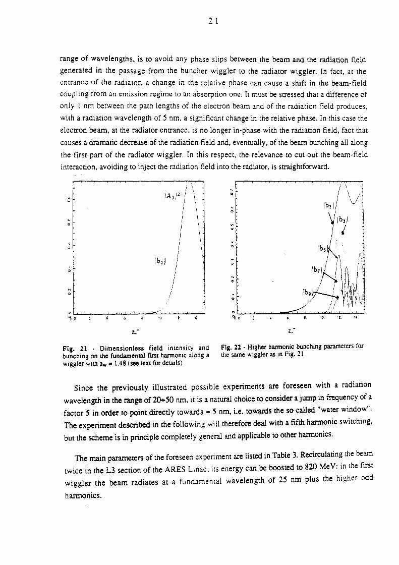
2 1
range of wavelengths, is to avoid any phase slips between the beam and the radiation field
generated in the passage from the buncher wiggler to the radiator wiggler. In fact, at the
entrance of the radiator, a change in the relative phase can cause a shift in the beam-field
cdupling from an emission regime to an absorption one. It must be stressed that a difference of
only l nm between the path lengths of the electron beam and of the radiation field produces.
with a radiation wavelength of 5 nm, a significant change in the relative phase. In this case the
electron beam, at the radiator entrance, is no longer in-phase with the radiation field, fact that
causes a dramatic decrease of the radiation field and, eventually, of the beam bunching all along
the first pan of the radiator wiggler. In this respect, the relevance to cut out the beam-field
interaction, avoiding to inject the radiation field into the radiator, is straightforward.
I
\ 1 IA 1 /2 I
0
\ .. 0
" \ .:>
lbll '
0
" 0
0
"to .. 6. 8.
z:
Fig. 21 - Dimensionless field intensity and bunching on the fundamental flrst harmomc along a wtggler with aw = 1.48 (see text for detalls)
\ " 0 ~/ " 0
V'
Q
" 0
Q
N
0
0
0
~0 z. 6 . 8. ,,
z:
Fig. 22 · Higher harmonic bunching parameters for the same wiggler as in Fig. 21
Since the previously illustrated possible experiments are foreseen with a radiation
wavelength in the range of 20+50 nm, it is a natural choice to consider a jump in frequency of a
factor 5 in order to point directly towards= 5 nm, i.e. towards the so called "water window".
The experiment described in the following will therefore deal with a fifth harmonic switching,
but the scheme is in principle completely general and applicable to other hannonics.
The main parameters of the foreseen experiment are listed in Table 3. Recirculating the beam
twice in the L3 section of the ARES Linac. its energy can be boosted to 820 Me V: in the first
wiggler the beam radiates at a fundamental wavelength of 25 nrn plus the higher odd
harmonics.
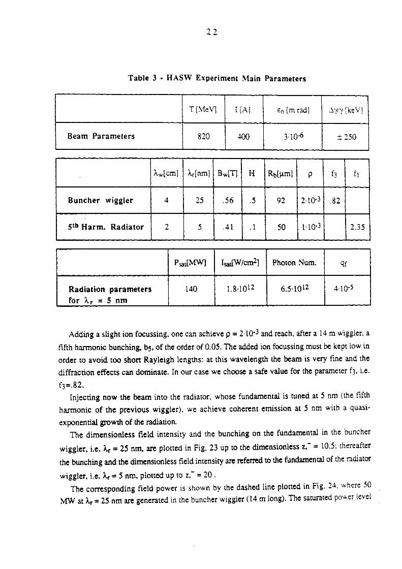
22
Table 3 • HASW Experiment Main Parameters
T [Me\ll I [A] En [m rad] j.'fl'f [keV1
Beam Parameters 820 400 JlQ-6 ± 250
Aw[cm] Ar[nm] Bw[TJ H Rb[J..Lm] p f3 fl
Buncher wiggler 4 25 .56 .5 92 2·10·3 .82
Stb Harm. Radiator 2 5 .41 . 1 50 1·10·3 2.35
Psat[MWJ IsatfW fcm2] Photon Num. qc
Radiation parameters 140 1.8·1012 6.5·1012 4·1Q·5
for A.r = 5 nm
Adding a slight ion focussing, one can achieve p = 2·10·3 and reach, after a 14 m wiggler, a
fifth harmonic bunching, bs, of the order of 0.05. The added ion focussing must be kept low in
order to avoid too short Rayleigh lengths: at this wavelength the beam is very fine and the
diffraction effects can dominate. In our case we choose a safe value for the parameter f3, i.e.
f3=.82. Injecting now the beam into the radiator. whose fundamental is tuned at 5 nm (the fifth
harmonic of the previous wiggler), we achieve coherent emission at 5 nm with a quasi
exponential growth of the radiation. The dimensionless field intensity and the bunching on the fundamental in the buncher
wiggler, i.e. Ar = 25 nm, are plotted in Fig. 23 up to the dimensionless z,- = 10.5: thereafter
the bunching and the dimensionless field intensity are referred to the fundamental of the radiator
wiggler, i.e. A.r = 5 nm. plotted up to z.- = 20 . The corresponding field power is shown by the dashed line plotted in Fig. 24. where 50
MW at A.r = 25 nm are generated in the buncher wiggler (14 m long). The saturated power level
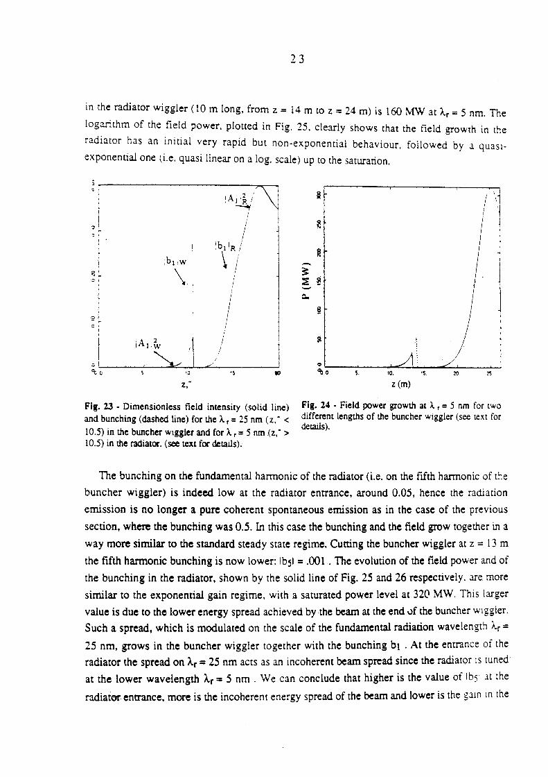
23
in the radiator wiggler (10 m long, from z = 14 m to z = 24 m) is 160 MW at Ar = 5 nm. The
logarithm of the field power, plotted in Fig. 25, clearly shows that the field growth in the
radiator has an initial very rapid but non-exponential behav10ur, followed by a quasiexponential one (i.e. quasi linear on a log. scale) up to the saturation.
3~--------------~------~~~ tA1 :~ t
----4( I i I
I I
lb ' ' I IR!
:b1iw \ \
I
I I
I I
IAII~ 11 I
I I
.-~, < 10 1$ .,
z:
Fig. 23 • Dimensionless field intensity (solid line) and bunching (dashed line) for the A. r = 25 nm ( z: <
10.5) in the buncher wtggler and for A. r = 5 nm {z; > 10.5) in the radiator. (see text for details).
~ I 1 I
I 11 '
~
~ -~ ::E ~ Q.,
~
' 0
~0 s. tO.
z (m)
Fig. 24 - Field power growth at A. r = 5 nm for two different lengths of the buncher wiggler (see text for details).
The bunching on the fundamental harmonic of the radiator (i.e. on the fifth harmonic of tl":e
buncher wiggler) is indeed low at the radiator entrance, around 0.05, hence the radiation
emission is no longer a pure coherent spontaneous emission as in the case of the previous
section, where the bunching was 0.5. In this case the bunching and the field grow together in a
way more similar to the standard steady state regime. Cutting the buncher wiggler at z = 13 m
the fifth harmonic bunching is now lower: lbsl = .001 . The evolution of the field power and of
the bunching in the radiator, shown by the solid line of Fig. 25 and 26 respectively. J.re. more
similar to the exponential gain regime, with a saturated power level at 320 MW. This larger
value is due to the lower energy spread achieved by the beam at the end 0f the buncher w1ggler. Such a spread, which is modulated on the scale of the fundamental radiation wavelength Ar =
25 nm, grows in the buncher wiggler together with the bunching bt . At the entrance of the radiator the spread on A.r = 25 nm acts as an incoherent beam spread since the radiator ts tuned
at the lower wavelength A.r = 5 nm . We can conclude that higher is the value of lbsl at the
radiator entrance. more is the incoherent energy spread of the beam and lower is the gatn tn the
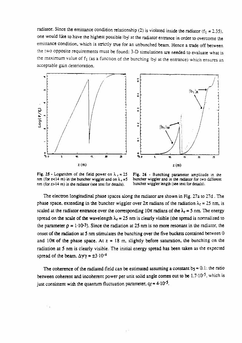
radiator. Since the emittance condition relationship (2) is violated inside the radiator (ft = 2.35),
one would like to have the highest possible lb5l at the radiator entrance in order to overcome the
emittance condition, which is strictly true for an unbunched beam. Hence a trade off between
the two opposite requirements must be found: 3-D simulations are needed to evaluate what is
the maximum value of f1 (as a function of the bunching lbsl at the entrance) which ensures an
acceptable gain deterioration .
...
...
.. --c.•
" c. ... 0'1 0 ...J ..
z (m)
Fig. 25 • Logarithm of the field power on ~ r = 25 nm (for z<l4 m) in the buncher wiggler and on~ r =5 nm (for z> 14 m) in the radiator (see text for details).
... 0
..
.;
.... 0
N
0
z (m)
Fig. 26 - Bunching parameter amplitude m t.he buncher wiggler and in the radiator for two different buncher wiggler length (see text for details).
The electron longitudinal phase spaces along the radiator are shown in Fig. 27a to 27d. The
phase space, extending in the buncher wiggler over 21t radians of the radiation A.r = 25 nm, is
scaled at the radiator entrance over the corresponding 1 01t radians of the A.r == 5 nm. The energy
spread on the scale of the wavelength Ar == 25 nm is clearly visible (the spread is normalized to
the parameter p = l·lQ-3). Since the radiation at 25 nm is no more resonant in the radiator, the
onset of the radiation at 5 nm stimulates the bunching over the five buckets contained between 0
and 1 01t of the phase space. At z == 18 m, slightly before saturation, the bunching on the
radiation at 5 nm is clearly visible. The initial energy spread has been taken as the expected
spread of the beam, 6:yly == ±3·10-4
The coherence of the radiated field can be estimated assuming a constant bs = 0.1: the ratio
between coherent and incoherent power per unit solid angle comes out to be 1.7·10-5. which is
just consistent with the quantum fluctuation parameter, qf = 4·10·5.
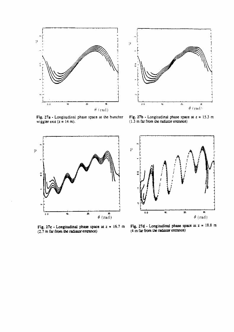
"'[ p r ·•
" CO
u.u 10.
H lracl)
Fig. 27a • Longitudinal phase space at the buncher wiggler exu (z = 14 m).
0 0 10. 20. .1).
8 ( rad)
Fig. 27c • Longitudinal phase space at z = 16.7 m (2.7 m far from the radiarorenttanee)
r r
N i
~ p r r
- r r
0 0 10. .'l. l)
Blrad)
'
1 , ;
. '
l
Fig. 27b • Longitudinal phase space at z = 15.3 m (1.3 m far from the radiator entrance)
p
Q
Q
0.0
~~
!l . ' . ; • 1
\. \! \1
10.
.-~~:.
I
! A, 'I \
l :V: a I • • t , ~ . ~ ! y
20. .11.
f) ( rad)
Fig. 27d • Longitudinal phase space at z = 18.8 m (4 m far from the radiator entrance)
Lb
6 • Conclusion
The high energy particle accelerator community agrees that one of the most relevant topic, on the way of the Te V electron-positron collider realization, is the capability to generate electron beams with high peak current and very low normalized emittance. The construction of an
intermediate energy LINAC able to produce high quality beams seems to be a necessary step
towards the TeV collider. In this respect, a soft X-ray FEL must be viewed as a test bench of
the beam quality achieved. We have shown that with the ARES SC Linac facility several
experiments in this context are envisageable: the link X-ray FEL's - SC LINAC's will
hopefully be a marriage of convenience.
Acknowledgments
We are indebted to W.A.Barletta and A.M.Sessler for their suppon and encouragement in
proposing the X-VUV FEL experiments in the ARES project context. We thank especially
W.A.Barletta for the numerical simulations made with FRED-3D and we are also grateful to
G. Vignola and M.Castellano for helpful and valuable discussions.
References
(1)
(2)
(3)
(4)
(5)
(6)
(7)
(8)
(9)
"Ares Design Study (The Machine)" - Repon LNF-90/00S(R), January 17th 1990, Frascati.
R.Bonifacio, C.Pellegrini and L.M.Narducci -Optics Comm 50 ( 1084) 373.
G.Preparata- QFT of the FEL- Phys. Rev. ala. 233 (1988)
E.T.Scharlemann ·"Wiggle plane focussing in a linear wiggler"- LLNL Repon UCRL-92429.
W.A.Barletta and A.M.Sessler - Proc. of the INFN lnt. School on Electromagnetic Radiation and Particle Beams Acceleration- VareMa (Italy), June 1988, p. 211-220.
C.Pellegrini- NIM. A227 (1980) 177.
J.B.Murphy, C.Pellegrini and R.Bonifacio- Optics Comm. 53 (1985) 197.
E.T.Scharlemann, A.M.Sessler and J.S.Wunele- NIM A239 (1985) 29.
R.Bonifacio et al. - Proc. of the INFN Int. School on Electromagnetic Radiation and Particle Beams Acceleration- Varenna (Italy), June 1988, p. 35.
( 10) A.Ghigo, Int. Rep. LNF-Ares, 35 (1990)
(11) K.Halbach- Proc. of "Undulator ~agnets for SR and FEL"- Trieste (Italy), June 1987.
( 12) :-.I. Caval1o- Ph.D. Thesis· University of Salemo, 1985.
(13) L.Serat1ni et al.- To be published.
(14) D.F.Alferov and E.G.Bessonov - Sov. Phys. Tech. Phys. 2A ® 1979, 450.
(15) R.Coisson ·Part. Accelerators.ll (1981) 245.
(16) J.M.Onega et al. - NlM A237 (1985) 268.
(17) R.Prazeres and J.M.Onega · IEEE Journal of Q. El. ~(1989) 2316.
(18) M.Billardon, R.Coisson and Y.Lapierre- Appl. Phys. B39 (1986) 9.
( 19) R.Bonifacio et al. · Proc. Int. FEL Conference 1989.
(20) W.A.Barletta, private communication.
(21) E.T.Scharlemann. A.M.Sessler and J.S.Wurtele, Proc. of lnt. Work. on Coherent and Collective Prop. in the lnt. of rel. electr.and e.m.Rad., Como, Italy, Sept. 1984, p.29.