CERN-ACC-Note-2020-0002Geneva, July 28, 2020

e

The Large Hadron-Electron Collider at the HL-LHC

LHeC and FCC-he Study Group

To be submitted to J. Phys. G

CERN-ACC-Note-2020-0002Geneva, July 28, 2020

The Large Hadron-Electron Collider at the HL-LHC

LHeC and FCC-he Study Group

Abstract

The Large Hadron electron Collider (LHeC) is designed to move the field of deep inelasticscattering (DIS) to the energy and intensity frontier of particle physics. Exploiting energyrecovery technology, it collides a novel, intense electron beam with a proton or ion beam fromthe High Luminosity–Large Hadron Collider (HL-LHC). The accelerator and interaction regionare designed for concurrent electron-proton and proton-proton operation. This report representsan update of the Conceptual Design Report (CDR) of the LHeC, published in 2012. It comprisesnew results on parton structure of the proton and heavier nuclei, QCD dynamics, electroweakand top-quark physics. It is shown how the LHeC will open a new chapter of nuclear particlephysics in extending the accessible kinematic range in lepton-nucleus scattering by several ordersof magnitude. Due to enhanced luminosity, large energy and the cleanliness of the hadronicfinal states, the LHeC has a strong Higgs physics programme and its own discovery potentialfor new physics. Building on the 2012 CDR, the report represents a detailed updated design ofthe energy recovery electron linac (ERL) including new lattice, magnet, superconducting radiofrequency technology and further components. Challenges of energy recovery are described andthe lower energy, high current, 3-turn ERL facility, PERLE at Orsay, is presented which usesthe LHeC characteristics serving as a development facility for the design and operation of theLHeC. An updated detector design is presented corresponding to the acceptance, resolution andcalibration goals which arise from the Higgs and parton density function physics programmes.The paper also presents novel results on the Future Circular Collider in electron-hadron mode,FCC-eh, which utilises the same ERL technology to further extend the reach of DIS to evenhigher centre-of-mass energies.

LHeC Study Group

P. Agostini1, H. Aksakal2, S. Alekhin3,4, P. P. Allport5, N. Andari6, K. D. J. Andre7,8,D. Angal-Kalinin9,10, S. Antusch11, L. Aperio Bella12, L. Apolinario13, R. Apsimon14,10, A. Apyan15,G. Arduini8, V. Ari16, A. Armbruster8, N. Armesto1, B. Auchmann8, K. Aulenbacher17,18,G. Azuelos19, S. Backovic20, I. Bailey14,10, S. Bailey21, F. Balli6, S. Behera22, O. Behnke23,I. Ben-Zvi24, M. Benedikt8, J. Bernauer25,26, S. Bertolucci8,27, S. S. Biswal28, J. Blumlein23,A. Bogacz29, M. Bonvini30, M. Boonekamp31, F. Bordry8, G. R. Boroun32, L. Bottura8, S. Bousson6,A. O. Bouzas33, C. Bracco8, J. Bracinik5, D. Britzger36, S. J. Brodsky35, C. Bruni6, O. Bruning8,H. Burkhardt8, O. Cakir16, R. Calaga8, A. Caldwell36, A. Calıskan37, S. Camarda8,N. C. Catalan-Lasheras8, K. Cassou38, J. Cepila39, V. Cetinkaya40, V. Chetvertkova8, B. Cole41,B. Coleppa42, A. Cooper-Sarkar21, E. Cormier43, A. S. Cornell44, R. Corsini8, E. Cruz-Alaniz7,J. Currie45, D. Curtin46, M. D’Onofrio7, J. Dainton14, E. Daly29, A. Das47, S. P. Das48, L. Dassa8,J. de Blas45, L. Delle Rose49, H. Denizli50, K. S. Deshpande51, D. Douglas29, L. Duarte52,K. Dupraz38,53, S. Dutta54, A. V. Efremov55, R. Eichhorn56, K. J. Eskola57, E. G. Ferreiro1,O. Fischer58, O. Flores-Sanchez59, S. Forte60,61, A. Gaddi8, J. Gao62, T. Gehrmann63,A. Gehrmann-De Ridder63,64, F. Gerigk8, A. Gilbert65, F. Giuli66, A. Glazov23, N. Glover45,R. M. Godbole67, B. Goddard8, V. Goncalves68, G. A. Gonzalez-Sprinberg52, A. Goyal69, J. Grames29,E. Granados8, A. Grassellino70, Y. O. Gunaydin2, Y. C. Guo71, V. Guzey72, C. Gwenlan21,A. Hammad11, C. C. Han73,74, L. Harland-Lang21, F. Haug8, F. Hautmann21, D. Hayden75,J. Hessler36, I. Helenius57, J. Henry29, J. Hernandez-Sanchez59, H. Hesari76, T. J. Hobbs77, N. Hod78,G. H. Hoffstaetter56, B. Holzer8, C. G. Honorato59, B. Hounsell7,10,38, N. Hu38, F. Hug17,18,A. Huss8,45, A. Hutton29, R. Islam22,79, S. Iwamoto80, S. Jana58, M. Jansova81, E. Jensen8, T. Jones7,J. M. Jowett8, W. Kaabi38, M. Kado30, D. A. Kalinin9,10, H. Karadeniz82, S. Kawaguchi83, U. Kaya84,R. A. Khalek85, H. Khanpour76,86, A. Kilic87, M. Klein7, U. Klein7, S. Kluth36, M. Koksal88,F. Kocak87, M. Korostelev21, P. Kostka7, M. Krelina89, J. Kretzschmar7, S. Kuday90, G. Kulipanov91,M. Kumar92, M. Kuze83, T. Lappi57, F. Larios33, A. Latina8, P. Laycock24, G. Lei93, E. Levitchev91,S. Levonian23, A. Levy94, R. Li95,96, X. Li62, H. Liang62, V. Litvinenko24,25, M. Liu71, T. Liu97,W. Liu98, Y. Liu99, S. Liuti100, E. Lobodzinska23, D. Longuevergne38, X. Luo101, W. Ma62,M. Machado102, S. Mandal103, H. Mantysaari57,104, F. Marhauser29, C. Marquet105, A. Martens38,R. Martin8, S. Marzani106,107, J. McFayden8, P. Mcintosh9, B. Mellado92, F. Meot56, A. Milanese8,J. G. Milhano13, B. Militsyn9,10, M. Mitra108, S. Moch23, M. Mohammadi Najafabadi76, S. Mondal104,S. Moretti109, T. Morgan45, A. Morreale25, P. Nadolsky77, F. Navarra110, Z. Nergiz111, P. Newman5,J. Niehues45, E. A. Nissen8, M. Nowakowski112, N. Okada113, G. Olivier38, F. Olness77, G. Olry38,J. A. Osborne8, A. Ozansoy16, R. Pan95,96, B. Parker24, M. Patra114, H. Paukkunen57, Y. Peinaud38,D. Pellegrini8, G. Perez-Segurana14,10, D. Perini8, L. Perrot38, N. Pietralla115, E. Pilicer87, B. Pire105,J. Pires13, R. Placakyte116, M. Poelker29, R. Polifka117, A. Polini118, P. Poulose22, G. Pownall21,Y. A. Pupkov91, F. S. Queiroz119, K. Rabbertz120, V. Radescu121, R. Rahaman122, S. K. Rai108,N. Raicevic123, P. Ratoff14,10, A. Rashed124, D. Raut125, S. Raychaudhuri114, J. Repond126,A. H. Rezaeian127,128, R. Rimmer29, L. Rinolfi8, J. Rojo85, A. Rosado59, X. Ruan92, S. Russenschuck8,M. Sahin129, C. A. Salgado1, O. A. Sampayo130, K. Satendra22, N. Satyanarayan131, B. Schenke24,K. Schirm8, H. Schopper8, M. Schott18, D. Schulte8, C. Schwanenberger23, T. Sekine83, A. Senol50,A. Seryi29, S. Setiniyaz14,10, L. Shang132, X. Shen95,96, N. Shipman8, N. Sinha133, W. Slominski134,S. Smith9,10, C. Solans8, M. Song135, H. Spiesberger18, J. Stanyard8, A. Starostenko91, A. Stasto136,A. Stocchi38, M. Strikman136, M. J. Stuart8, S. Sultansoy84, H. Sun101, M. Sutton137,L. Szymanowski138, I. Tapan87, D. Tapia-Takaki139, M. Tanaka83, Y. Tang140, A. T. Tasci141,A. T. Ten-Kate8, P. Thonet8, R. Tomas-Garcia8, D. Tommasini8, D. Trbojevic24,56, M. Trott142,I. Tsurin7, A. Tudora8, I. Turk Cakir82, K. Tywoniuk143, C. Vallerand38, A. Valloni8, D. Verney38,E. Vilella7, D. Walker45, S. Wallon38, B. Wang95,96, K. Wang95,96, K. Wang144, X. Wang101,Z. S. Wang145, H. Wei146, C. Welsch7,10, G. Willering8, P. H. Williams9,10, D. Wollmann8,C. Xiaohao12, T. Xu147, C. E. Yaguna148, Y. Yamaguchi83, Y. Yamazaki149, H. Yang150, A. Yilmaz82,P. Yock151, C. X. Yue71, S. G. Zadeh152, O. Zenaiev8, C. Zhang153, J. Zhang154, R. Zhang62,Z. Zhang38, G. Zhu95,96, S. Zhu132, F. Zimmermann8, F. Zomer38, J. Zurita155,156 and P. Zurita34

1 Universidade de Santiago de Compostela (USC), Santiago de Compostela, Spain2 Kahramanmaras Sutcu Imam University, Kahramanmaras, Turkey3 Universitat Hamburg, Hamburg, Germany4 Institute of High Energy Physics (IHEP), Protvino, Russia5 University of Birmingham, Birmingham, United Kingdom6 Universite Paris-Saclay, Saint-Aubin, France7 University of Liverpool, Liverpool, United Kingdom8 European Organization for Nuclear Research (CERN), Geneve, Switzerland9 Science and Technology Facilities Council (STFC) - Daresbury Laboratory, Daresbury, UnitedKingdom10 Cockcroft Institue of Accelerator Science and Technology, Daresbury, United Kingdom11 Universitat Basel, Basel, Switzerland12 Chinese Academy of Sciences - Institute of High Energy Physics (IHEP), Beijing, China13 Laboratorio de Instrumentacao e Fisica Experimental de Particulas (LIP), Lisbon, Portugal14 University of Lancaster, Lancaster, United Kingdom15 A. Alikhanian National Laboratory (AANL), Yerevan, Armenia16 Ankara University, Ankara, Turkey17 Johannes Gutenberg University Mainz (JGU) - PRISMA Cluster of Excellence, Mainz, Germany18 Johannes Gutenberg-Universitat Mainz (JGU), Mainz, Germany19 Universite de Montreal, Montreal, Candada20 University of Montenegro, Podgorica, Montenegro21 University of Oxford, Oxford, United Kingdom22 Department of Physics, Indian Institute of Technology, Guwahati, Assam, India23 Deutsches Elektronen-Synchrotron (DESY), Hamburg, Germany24 Brookhaven National Laboratory (BNL), Upton, USA25 Stony Brook University, Stony Brook, USA26 BNL Research Center, RIKEN, Upton, NY, USA27 Universita di Bologna, Bologna, Italy28 Ravenshaw University, Cuttack, India29 Thomas Jefferson National Accelerator Facility (Jefferson Lab), Newport News, USA30 Istituto Nazionale di Fisica Nucleare (INFN) - Sezione di Roma, Rome, Italy31 Commissariat a l’Energie Atomique (CEA) - Institut de Recherche sur les Lois Fondamentales del’Univers (IRFU), Gif-sur-Yvette, France32 Razi University, Kermanshah, Iran33 Centro de Investigacion y de Estudios Avanzados (CINVESTAV), Merida, Mexico34 Universitat Regensburg, Regensburg, Germany35 SLAC National Accelerator Laboratory, Menlo Park, USA36 Max-Planck-Institut fur Physik, Munich, Germany37 Gumushane University, Gumushane, Turkey38 Universite Paris-Saclay, CNRS/IN2P3, IJCLab, Orsay, France39 Faculty of Nuclear Sciences and Physical Engineering, Czech Technical University in Prague, Prague,Czech Republic40 Kutahya Dumlupinar University, Kutahya, Turkey41 Columbia University, New York, USA42 Indian Institute of Technology (IIT), Gandhinagar, India43 Laboratoire Photonique, Numerique et Nanosciences (LP2N), IOGS-CNRS-Universite Bordeaux,Talence, France44 University of Johannesburg (UJ), Johannesburg, South Africa45 Institute for Particle Physics Phenomenology, Durham University, Durham, United Kingdom46 University of Toronto, Toronto, Canada47 Osaka University, Osaka, Japan48 Universidad de los Andes, Santiago, Columbia49 Istituto Nazionale di Fisica Nucleare (INFN) - Sezione di Firenze, Firenze, Italy50 Bolu Abant Izzet Baysal University, Bolu, Turkey51 University of Maryland, College Park, USA52 Universidad de la Republica - Instituto de Fisica Facultad de Ciencias (IFFC), Montevideo, Uruguay

4

53 Universite Paris-Sud, Orsay, France54 Sri Guru Tegh Badadur Khalsa College, Delhi, India55 Joint Institute for Nuclear Research (JINR), Dubna, Russia56 Cornell University, Ithaca, USA57 University of Jyvaskyla, Jyvaskyla, Finland58 Max-Planck-Institut fur Kernphysik, Heidelberg, Germany59 Benemerita Universidad Autonoma de Puebla (BUAP), Puebla, Mexico60 Universita degli Studi di Milano, Milano, Italy61 Istituto Nazionale di Fisica Nucleare (INFN) - Sezione di Milano, Milano, Italy62 University of Science and Technology of China (USTC), Hefei, China63 Department of Physics, Universitat Zurich, Zurich, Switzerland64 Institute for Theoretical Physics, ETH, Zurich, Switzerland65 Northwestern University, Evanston, USA66 University of Rome Tor Vergata and INFN, Sezione di Roma 2, Rome, Italy67 Indian Institute of Science (IISc), Bangalore, India68 Universidade Federal de Pelotas (UFPel), Pelotas, Brazil69 University of Delhi, Delhi, India70 Fermi National Accelerator Laboratory (FNAL), Batavia, USA71 Liaoning Normal University (LNNU), Dalian, China72 Petersburg Nuclear Physics Institute (PNPI), Petersburg, Russia73 University of Tokyo, Tokyo, Japan74 Kavli Institute for the Physics and Mathematics of the Universe (KIPMU), Kashiwa, Japan75 Michigan State University, East Lansing, USA76 Institute for Research in Fundamental Sciences (IPM), Tehran, Iran77 Southern Methodist University, Dallas, USA78 Weizmann Institute of Science, Rehovot, Israel79 Department of Physics, Mathabhanga College, Cooch Behar, West Bengal, India80 Universita degli Studi di Padova, Padua, Italy81 Universite de Strasbourg, Strasbourg, France82 Giresun University, Giresun, Turkey83 Tokyo Institute of Technology, Tokyo, Japan84 TOBB University of Economic and Technology (TOBB ETU), Ankara, Turkey85 Vrije University, Amsterdam, Netherlands86 University of Science and Technology of Mazandaran, Behshahr, Iran87 Uludag University, Bursa, Turkey88 Sivas Cumhuriyet University, Sivas, Turkey89 Universidad Tecnica Federico Santa Maria, Valparaiso, Chile90 Istanbul Aydin University, Istanbul, Turkey91 Siberian Branch of Russian Academy of Science - Budker Institute of Nuclear Physics (BINP),Novosibirsk, Russia92 University of the Witwatersrand, Johannesburg, South Africa93 Tsinghua University, Beijing, China94 Tel-Aviv University, Tel Aviv, Israel95 Zhejiang Institute of Modern Physics (ZIMP), Hangzhou, China96 Zhejiang University (ZJU), Hangzhou, China97 Xiamen University (XMU), Xiamen, China98 University College London, London, United Kingdom99 Henan Institute of Science and Technology (HIST), Xinxiang, China100 University of Virginia, Charlottesville, USA101 Dalian University of Technology (DLUT), Dalian, China102 Universidade Federal do Rio Grande do Sul (UFRGS), Porto Alegre, Brazil103 Institut de Fısica Corpuscular – CSIC/Universitat de Valencia, Paterna (Valencia), Spain104 University of Helsinki, Helsinki, Finland105 CPHT, CNRS, Ecole Polytechnique, I. P. Paris, France106 University Genova, Genova, Italy107 Istituto Nazionale di Fisica Nucleare (INFN) - Sezione di Genova, Genova, Italy

5

108 Harish-Chandra Research Institute (HRI), Allahabad, India109 University of Southampton, Southampton, United Kingdom110 Universidade de Sao Paulo (USP), Sao, Paolo111 Nigde Omer Halisdemir University, Nigde, Turkey112 Universidad de los Andes, Carrera, Colombia113 The University of Alabama, Tuscaloosa, USA114 Tata Institute of Fundamental Research (TIFR), Mumbai, India115 Technische Universitat Darmstadt, Darmstadt, Germany116 Homeday GmbH Berlin, Berlin, Germany117 Charles University, Praque, Czech Republic118 Istituto Nazionale di Fisica Nucleare (INFN) - Sezione di Bologna, Bologna, Italy119 Univ. Federal do Rio Grande do Norte, Natal, Brazil120 Karlsruher Institut fur Technologie (KIT), Karlsruhe, Germany121 IBM Deutschland RnD, GmbH, Urbar, Germany122 Indian Institute of Science Education and Research (IISER), Kolkata, India123 Univ. of Montenegro, Podgorica, YUOGSLAVIA124 Shippensburg University of Pennsylvania, Shippensburg, Pennsylvania, USA125 University of Delaware, Newark, USA126 Argonne National Laboratory, Argonne, USA127 Oracle, San Fransisco, USA128 Applied AI Center of Excellence, San Francisco, USA129 Usak University, Usak, Turkey130 National University of Mar del Plata, Mar del Plata, Argentina131 Oklahoma State University (OSU), Stillwater, USA132 Peking University (PKU), Beijing, China133 Institute of Mathematical Sciences (IMSc), Chennai, India134 Jagiellonian University, Cracow, Poland135 Anhui University (AHU), Hefei, China136 Pennsylvania State University (PSU), University Park, USA137 University of Sussex, Sussex, United Kingdom138 Narodowe Centrum Badan Jadrowych (NCBJ), Warsaw, Poland139 Kansas State University, Manhattan, USA140 Korea Institute for Advanced Study (KIAS), Cheongryangri-dong, Korea141 Kastamonu University, Kastamonu, Turkey142 Københavns, Universitet - Niels Bohr Institutet (NBI), Copenhagen143 University of Bergen, Bergen, Norway144 Wuhan University of Technology, Wuhan, China145 Asia Pacific Center for Theoretical Physics (APCTP), Pohang, Korea146 University of California (UC), Riverside, USA147 Hebrew University of Jerusalem - Racah Inst. of Physics, Jerusalem, Israel148 Universidad Pedagogica y Tecnologica de Colombia, Tunja, Colombia149 Kobe University, Kobe, Japan150 Lawrence Berkeley National Laboratory (LBNL), Berkeley, USA151 Fellow Royal Astronomical Society of New Zealand (FRASNZ), Auckland, New Zealand152 Universitat Rostock, Rostock, Germany153 National Center for Theoretical Sciences (NCTS), Hsinchu, Taiwan154 Nankai University (NKU), Tianjin, China155 Karlsruher Institut fur Technologie (KIT) - Institut fur Theoretische Teilchenphysik (TTP),Karlsruhe, Germany156 Karlsruher Institut fur Technologie (KIT) - Institut fur Kernphysik (IKP), Karlsruhe, Germany

6

Preface

This paper represents the updated design study of the Large Hadron-electron Collider, theLHeC, a TeV energy scale electron-hadron (eh) collider which may come into operation duringthe third decade of the lifetime of the Large Hadron Collider (LHC) at CERN. It is an account,accompanied by numerous papers in the literature, for many years of study and development,guided by an International Advisory Committee (IAC) which was charged by the CERN Direc-torate to advise on the directions of energy frontier electron-hadron physics at CERN. End of2019 the IAC summarised its observations and recommendations in a brief report to the DirectorGeneral of CERN, which is here reproduced as an Appendix.

The paper outlines a unique, far reaching physics programme on deep inelastic scattering (DIS),a design concept for a new generation collider detector, together with a novel configurationof the intense, high energy electron beam. This study builds on the previous, detailed LHeCConceptual Design Report (CDR), which was published eight years ago [1]. It surpasses theinitial study in essential characteristics: i) the depth of the physics programme, owing to theinsight obtained mainly with the LHC, and ii) the luminosity prospect, for enabling a novel Higgsfacility to be built and the prospects to search for and discover new physics to be strengthened.It builds on recent and forthcoming progress of modern technology, due to major advancesespecially of the superconducting RF technology and as well new detector techniques.

Unlike in 2012, there has now a decision been taken to configure the LHeC as an electron linac-proton or nucleus ring configuration, which leaves the ring-ring option [1, 2] as a backup. Inep, the high instantaneous luminosity of about 1034 cm−2s−1 may be achieved with the electronaccelerator built as an energy recovery linac (ERL) and because the brightness of the LHC ex-ceeds early expectations by far, not least through the upgrade of the LHC to its high luminosityversion, the HL-LHC [3,4]. For ePb collisions, the corresponding per nucleon instantaneous lu-minosity would be about 1033 cm−2s−1. The LHeC is designed to be compatible with concurrentoperation with the LHC. It thus represents a unique opportunity to advance particle physics bybuilding on the singular investments which CERN and its global partners have made into theLHC facility.

Since the 2012 document, significant experience with multi-turn ERL design, construction, andoperation has been gained with the Cornell-BNL ERL Test Accelerator (CBETA), which hasaccelerated and energy recovered beam in all of its 4 turns [5, 6]. Extending much beyond theCDR, a configuration has newly been designed for a low energy ERL facility, termed PERLE [7],which is moving ahead to be built at Orsay by an international collaboration. The major pa-rameters of PERLE have been taken from the LHeC, such as the 3-turn configuration, source,the 802 MHz frequency and cavity-cryomodule technology, in order to make PERLE a suitablefacility for the development of LHeC ERL technology and the accumulation of operating ex-

7

perience prior to and later in parallel with the LHeC. In addition, the PERLE facility has astriking low energy physics programme, industrial applications and will be an enabler for ERLtechnology as the first facility to operate in the 10 MW power regime.

While the 2012 CDR focussed the physics discussion on the genuine physics of deep inelasticscattering leading much beyond HERA, a new focus arose through the challenges and opportu-nities posed by the HL-LHC. It is demonstrated that DIS at the LHeC can play a crucial rolein sustaining and enriching the LHC programme, a consequence of the results obtained at theLHC, i.e. the discovery of the Higgs boson, the non-observation of supersymmetry (SUSY) orother non Standard Model (SM) exotic particles and, not least, the unexpected realisation ofthe huge potential of the LHC for discovery through precision measurements in the strong andelectroweak sectors. Thus, it was felt time to summarise the recent seven years of LHeC devel-opment, also in support of the current discussions on the future of particle physics, especiallyat the energy frontier. Both for the LHeC [8–10] and PERLE [11], documents were submittedfor consideration to the European Strategy for Particle Physics Update.

The LHeC is a once in our lifetime opportunity for substantial progress in particle physics. Itcomprises, with a linac shorter than the pioneering two-mile linac at SLAC, a most ambitiousand exciting physics programme, the introduction of novel accelerator technology and the com-plete exploitation of the unique values of and spendings into the LHC. It requires probably lesscourage than that of Pief Panofsky and colleagues half a century ago. Finally, not least, onemay realise that the power LHeC needed without the energy recovery technique is beyond 1 GWwhile the electron beam is dumped at injection energy. It therefore is a significant step towardsgreen accelerator technology, a major general desire and requirement of our times. This paperaims at substantiating these statements in the various chapters following.

Oliver Bruning (CERN) and Max Klein (University of Liverpool)

8

Contents

Preface 7

1 Introduction 151.1 The Context . . . . . . . . . . . . . . . . . . . . . . . . . . . . . . . . . . . . . . 15

1.1.1 Particle Physics - at the Frontier of Fundamental Science . . . . . . . . . 151.1.2 Deep Inelastic Scattering and HERA . . . . . . . . . . . . . . . . . . . . . 17

1.2 The Paper . . . . . . . . . . . . . . . . . . . . . . . . . . . . . . . . . . . . . . . . 181.2.1 The LHeC Physics Programme . . . . . . . . . . . . . . . . . . . . . . . . 181.2.2 The Accelerator . . . . . . . . . . . . . . . . . . . . . . . . . . . . . . . . 201.2.3 PERLE . . . . . . . . . . . . . . . . . . . . . . . . . . . . . . . . . . . . . 211.2.4 The Detector . . . . . . . . . . . . . . . . . . . . . . . . . . . . . . . . . . 22

1.3 Outline . . . . . . . . . . . . . . . . . . . . . . . . . . . . . . . . . . . . . . . . . 23

2 LHeC Configuration and Parameters 242.1 Introduction . . . . . . . . . . . . . . . . . . . . . . . . . . . . . . . . . . . . . . . 242.2 Cost Estimate, Default Configuration and Staging . . . . . . . . . . . . . . . . . 252.3 Configuration Parameters . . . . . . . . . . . . . . . . . . . . . . . . . . . . . . . 262.4 Luminosity . . . . . . . . . . . . . . . . . . . . . . . . . . . . . . . . . . . . . . . 27

2.4.1 Electron-Proton Collisions . . . . . . . . . . . . . . . . . . . . . . . . . . . 282.4.2 Electron-Ion Collisions . . . . . . . . . . . . . . . . . . . . . . . . . . . . . 29

2.5 Linac Parameters . . . . . . . . . . . . . . . . . . . . . . . . . . . . . . . . . . . . 292.6 Operation Schedule . . . . . . . . . . . . . . . . . . . . . . . . . . . . . . . . . . . 30

3 Parton Distributions - Resolving the Substructure of the Proton 333.1 Introduction . . . . . . . . . . . . . . . . . . . . . . . . . . . . . . . . . . . . . . . 33

3.1.1 Partons in Deep Inelastic Scattering . . . . . . . . . . . . . . . . . . . . . 343.1.2 Fit Methodology and HERA PDFs . . . . . . . . . . . . . . . . . . . . . . 35

3.2 Simulated LHeC Data . . . . . . . . . . . . . . . . . . . . . . . . . . . . . . . . . 383.2.1 Inclusive Neutral and Charged Current Cross Sections . . . . . . . . . . . 383.2.2 Heavy Quark Structure Functions . . . . . . . . . . . . . . . . . . . . . . 41

3.3 Parton Distributions from the LHeC . . . . . . . . . . . . . . . . . . . . . . . . . 433.3.1 Procedure and Assumptions . . . . . . . . . . . . . . . . . . . . . . . . . . 433.3.2 Valence Quarks . . . . . . . . . . . . . . . . . . . . . . . . . . . . . . . . . 463.3.3 Light Sea Quarks . . . . . . . . . . . . . . . . . . . . . . . . . . . . . . . . 473.3.4 Strange Quark . . . . . . . . . . . . . . . . . . . . . . . . . . . . . . . . . 483.3.5 Heavy Quarks . . . . . . . . . . . . . . . . . . . . . . . . . . . . . . . . . . 523.3.6 The Gluon PDF . . . . . . . . . . . . . . . . . . . . . . . . . . . . . . . . 533.3.7 Luminosity and Beam Charge Dependence of LHeC PDFs . . . . . . . . . 55

9

3.3.8 Weak Interactions Probing Proton Structure . . . . . . . . . . . . . . . . 573.3.9 Parton-Parton Luminosities . . . . . . . . . . . . . . . . . . . . . . . . . . 61

3.4 The 3D Structure of the Proton . . . . . . . . . . . . . . . . . . . . . . . . . . . . 64

4 Exploration of Quantum Chromodynamics 714.1 Determination of the strong coupling constant . . . . . . . . . . . . . . . . . . . . 71

4.1.1 Strong coupling from inclusive jet cross sections . . . . . . . . . . . . . . . 724.1.2 Pinning Down αs with Inclusive and Jet LHeC Data . . . . . . . . . . . . 764.1.3 Strong coupling from other processes . . . . . . . . . . . . . . . . . . . . . 79

4.2 Discovery of New Strong Interaction Dynamics at Small x . . . . . . . . . . . . . 804.2.1 Resummation at small x . . . . . . . . . . . . . . . . . . . . . . . . . . . . 814.2.2 Disentangling non-linear QCD dynamics at the LHeC . . . . . . . . . . . 844.2.3 Low x and the Longitudinal Structure Function FL . . . . . . . . . . . . . 894.2.4 Associated jet final states at low x . . . . . . . . . . . . . . . . . . . . . . 954.2.5 Relation to Ultrahigh Energy Neutrino and Astroparticle physics . . . . . 96

4.3 Diffractive Deep Inelastic Scattering at the LHeC . . . . . . . . . . . . . . . . . . 994.3.1 Introduction and Formalism . . . . . . . . . . . . . . . . . . . . . . . . . . 994.3.2 Pseudodata for the reduced cross section . . . . . . . . . . . . . . . . . . . 1054.3.3 Potential for constraining diffractive PDFs at the LHeC . . . . . . . . . . 1054.3.4 Hadronic Final States in Diffraction and hard rapidity gap processes . . . 108

4.4 Theoretical Developments . . . . . . . . . . . . . . . . . . . . . . . . . . . . . . . 1104.4.1 Prospects for Higher Order pQCD in DIS . . . . . . . . . . . . . . . . . . 1104.4.2 Theoretical Concepts on the Light Cone . . . . . . . . . . . . . . . . . . . 111

5 Electroweak and Top Quark Physics 1165.1 Electroweak Physics with Inclusive DIS data . . . . . . . . . . . . . . . . . . . . 116

5.1.1 Electroweak effects in inclusive NC and CC DIS cross sections . . . . . . 1165.1.2 Methodology of a combined EW and QCD fit . . . . . . . . . . . . . . . . 1175.1.3 Weak boson masses MW and MZ . . . . . . . . . . . . . . . . . . . . . . . 1185.1.4 Further mass determinations . . . . . . . . . . . . . . . . . . . . . . . . . 1205.1.5 Weak Neutral Current Couplings . . . . . . . . . . . . . . . . . . . . . . . 1215.1.6 The neutral current ρNC and κNC parameters . . . . . . . . . . . . . . . . 1225.1.7 The effective weak mixing angle sin2 θeff,`

W . . . . . . . . . . . . . . . . . . 1235.1.8 Electroweak effects in charged-current scattering . . . . . . . . . . . . . . 1255.1.9 Conclusion . . . . . . . . . . . . . . . . . . . . . . . . . . . . . . . . . . . 126

5.2 Direct W and Z Production and Anomalous Triple Gauge Couplings . . . . . . . 1275.2.1 Direct W and Z Production . . . . . . . . . . . . . . . . . . . . . . . . . . 1275.2.2 Anomalous Triple Gauge Couplings . . . . . . . . . . . . . . . . . . . . . 128

5.3 Top Quark Physics . . . . . . . . . . . . . . . . . . . . . . . . . . . . . . . . . . . 1305.3.1 Wtq Couplings . . . . . . . . . . . . . . . . . . . . . . . . . . . . . . . . . 1305.3.2 Top Quark Polarisation . . . . . . . . . . . . . . . . . . . . . . . . . . . . 1325.3.3 Top-γ and Top-Z Couplings . . . . . . . . . . . . . . . . . . . . . . . . . . 1325.3.4 Top-Higgs Coupling . . . . . . . . . . . . . . . . . . . . . . . . . . . . . . 1345.3.5 Top Quark PDF and the Running of αs . . . . . . . . . . . . . . . . . . . 1345.3.6 FCNC Top Quark Couplings . . . . . . . . . . . . . . . . . . . . . . . . . 1345.3.7 Summary of Top Quark Physics . . . . . . . . . . . . . . . . . . . . . . . 137

6 Nuclear Particle Physics with Electron-Ion Scattering at the LHeC 1396.1 Introduction . . . . . . . . . . . . . . . . . . . . . . . . . . . . . . . . . . . . . . 1396.2 Nuclear Parton Densities . . . . . . . . . . . . . . . . . . . . . . . . . . . . . . . 141

10

6.2.1 Pseudodata . . . . . . . . . . . . . . . . . . . . . . . . . . . . . . . . . . . 1436.2.2 Nuclear gluon PDFs in a global-fit context . . . . . . . . . . . . . . . . . 1456.2.3 nPDFs from DIS on a single nucleus . . . . . . . . . . . . . . . . . . . . . 146

6.3 Nuclear diffraction . . . . . . . . . . . . . . . . . . . . . . . . . . . . . . . . . . . 1516.3.1 Exclusive vector meson diffraction . . . . . . . . . . . . . . . . . . . . . . 1526.3.2 Inclusive diffraction on nuclei . . . . . . . . . . . . . . . . . . . . . . . . . 156

6.4 New Dynamics at Small x with Nuclear Targets . . . . . . . . . . . . . . . . . . . 1586.5 Collective effects in dense environments – the ‘ridge’ . . . . . . . . . . . . . . . . 1596.6 Novel QCD Nuclear Phenomena at the LHeC . . . . . . . . . . . . . . . . . . . . 159

7 Higgs Physics with LHeC 1637.1 Introduction . . . . . . . . . . . . . . . . . . . . . . . . . . . . . . . . . . . . . . . 1637.2 Higgs Production in Deep Inelastic Scattering . . . . . . . . . . . . . . . . . . . . 164

7.2.1 Kinematics of Higgs Production . . . . . . . . . . . . . . . . . . . . . . . 1647.2.2 Cross Sections and Rates . . . . . . . . . . . . . . . . . . . . . . . . . . . 166

7.3 Higgs Signal Strength Measurements . . . . . . . . . . . . . . . . . . . . . . . . 1677.3.1 Higgs Decay into Bottom and Charm Quarks . . . . . . . . . . . . . . . . 1697.3.2 Higgs Decay into WW . . . . . . . . . . . . . . . . . . . . . . . . . . . . . 1757.3.3 Accessing Further Decay Channels . . . . . . . . . . . . . . . . . . . . . . 1777.3.4 Systematic and Theoretical Errors . . . . . . . . . . . . . . . . . . . . . . 179

7.4 Higgs Coupling Analyses . . . . . . . . . . . . . . . . . . . . . . . . . . . . . . . . 1807.5 Measuring the Top-quark–Higgs Yukawa Coupling . . . . . . . . . . . . . . . . . 1827.6 Higgs Decay into Invisible Particles . . . . . . . . . . . . . . . . . . . . . . . . . . 186

8 Searches for Physics Beyond the Standard Model 1898.1 Introduction . . . . . . . . . . . . . . . . . . . . . . . . . . . . . . . . . . . . . . . 1898.2 Extensions of the SM Higgs Sector . . . . . . . . . . . . . . . . . . . . . . . . . . 189

8.2.1 Modifications of the Top-Higgs interaction . . . . . . . . . . . . . . . . . . 1908.2.2 Charged scalars . . . . . . . . . . . . . . . . . . . . . . . . . . . . . . . . . 1908.2.3 Neutral scalars . . . . . . . . . . . . . . . . . . . . . . . . . . . . . . . . . 1918.2.4 Modifications of Higgs self-couplings . . . . . . . . . . . . . . . . . . . . . 1928.2.5 Exotic Higgs boson decays . . . . . . . . . . . . . . . . . . . . . . . . . . . 193

8.3 Searches for supersymmetry . . . . . . . . . . . . . . . . . . . . . . . . . . . . . . 1938.3.1 Search for the SUSY Electroweak Sector: prompt signatures . . . . . . . . 1948.3.2 Search for the SUSY Electroweak Sector: long-lived particles . . . . . . . 1958.3.3 R-parity violating signatures . . . . . . . . . . . . . . . . . . . . . . . . . 196

8.4 Feebly Interacting Particles . . . . . . . . . . . . . . . . . . . . . . . . . . . . . . 1978.4.1 Searches for heavy neutrinos . . . . . . . . . . . . . . . . . . . . . . . . . 1978.4.2 Fermion triplets in type III seesaw . . . . . . . . . . . . . . . . . . . . . . 1988.4.3 Dark photons . . . . . . . . . . . . . . . . . . . . . . . . . . . . . . . . . 2008.4.4 Axion-like particles . . . . . . . . . . . . . . . . . . . . . . . . . . . . . . . 201

8.5 Anomalous Gauge Couplings . . . . . . . . . . . . . . . . . . . . . . . . . . . . . 2028.5.1 Radiation Amplitude Zero . . . . . . . . . . . . . . . . . . . . . . . . . . . 203

8.6 Theories with heavy resonances and contact interaction . . . . . . . . . . . . . . 2038.6.1 Leptoquarks . . . . . . . . . . . . . . . . . . . . . . . . . . . . . . . . . . . 2048.6.2 Z’ mediated charged lepton flavour violation . . . . . . . . . . . . . . . . . 2068.6.3 Vector-like quarks . . . . . . . . . . . . . . . . . . . . . . . . . . . . . . . 2068.6.4 Excited fermions (ν∗, e∗, u∗) . . . . . . . . . . . . . . . . . . . . . . . . . . 2078.6.5 Colour octet leptons . . . . . . . . . . . . . . . . . . . . . . . . . . . . . . 2078.6.6 Quark substructure and Contact interactions . . . . . . . . . . . . . . . . 207

11

8.7 Summary and conclusion . . . . . . . . . . . . . . . . . . . . . . . . . . . . . . . 208

9 Influence of the LHeC on Physics at the HL-LHC 2109.1 Precision Electroweak Measurements at the HL-LHC . . . . . . . . . . . . . . . 210

9.1.1 The effective weak mixing angle . . . . . . . . . . . . . . . . . . . . . . . 2109.1.2 The W -boson mass . . . . . . . . . . . . . . . . . . . . . . . . . . . . . . . 2129.1.3 Impact on electroweak precision tests . . . . . . . . . . . . . . . . . . . . 214

9.2 Higgs Physics . . . . . . . . . . . . . . . . . . . . . . . . . . . . . . . . . . . . . . 2169.2.1 Impact of LHeC data on Higgs cross section predictions at the LHC . . . 2169.2.2 Higgs Couplings from a simultaneous analysis of pp and ep collision data 218

9.3 Further precision SM measurements at the HL-LHC . . . . . . . . . . . . . . . . 2219.4 High Mass Searches at the LHC . . . . . . . . . . . . . . . . . . . . . . . . . . . 225

9.4.1 Strongly-produced supersymmetric particles . . . . . . . . . . . . . . . . . 2259.4.2 Contact interactions . . . . . . . . . . . . . . . . . . . . . . . . . . . . . . 225

9.5 PDFs and the HL-LHC and the LHeC . . . . . . . . . . . . . . . . . . . . . . . . 2269.5.1 PDF Prospects with the HL-LHC and the LHeC . . . . . . . . . . . . . . 2269.5.2 Parton luminosities at the HL-LHC . . . . . . . . . . . . . . . . . . . . . 2289.5.3 PDF Sensitivity: Comparing HL-LHC and LHeC . . . . . . . . . . . . . . 229

9.6 Impact of New Small-x Dynamics on Hadron Collider Physics . . . . . . . . . . . 2299.7 Heavy Ion Physics with eA Input . . . . . . . . . . . . . . . . . . . . . . . . . . 231

10 The Electron Energy Recovery Linac 23610.1 Introduction – Design Goals . . . . . . . . . . . . . . . . . . . . . . . . . . . . . 23610.2 The ERL Configuration of the LHeC . . . . . . . . . . . . . . . . . . . . . . . . 237

10.2.1 Baseline Design – Lattice Architecture . . . . . . . . . . . . . . . . . . . 23810.2.2 30 GeV ERL Options . . . . . . . . . . . . . . . . . . . . . . . . . . . . . 24910.2.3 Component Summary . . . . . . . . . . . . . . . . . . . . . . . . . . . . . 249

10.3 Electron-Ion Collisions . . . . . . . . . . . . . . . . . . . . . . . . . . . . . . . . 24910.4 Beam-Beam Interactions . . . . . . . . . . . . . . . . . . . . . . . . . . . . . . . 251

10.4.1 Effect on the electron beam . . . . . . . . . . . . . . . . . . . . . . . . . . 25110.4.2 Effect on the proton beam . . . . . . . . . . . . . . . . . . . . . . . . . . . 254

10.5 Arc Magnets . . . . . . . . . . . . . . . . . . . . . . . . . . . . . . . . . . . . . . 25410.5.1 Dipole magnets . . . . . . . . . . . . . . . . . . . . . . . . . . . . . . . . . 25410.5.2 Quadrupole magnets . . . . . . . . . . . . . . . . . . . . . . . . . . . . . . 254

10.6 LINAC and SRF . . . . . . . . . . . . . . . . . . . . . . . . . . . . . . . . . . . . 25710.6.1 Choice of Frequency . . . . . . . . . . . . . . . . . . . . . . . . . . . . . . 25810.6.2 Cavity Prototype . . . . . . . . . . . . . . . . . . . . . . . . . . . . . . . 25810.6.3 Cavity-Cryomodule . . . . . . . . . . . . . . . . . . . . . . . . . . . . . . 26110.6.4 Electron sources and injectors . . . . . . . . . . . . . . . . . . . . . . . . 26410.6.5 Positrons . . . . . . . . . . . . . . . . . . . . . . . . . . . . . . . . . . . . 26810.6.6 Compensation of Synchrotron Radiation Losses . . . . . . . . . . . . . . 27210.6.7 LINAC Configuration and Infrastructure . . . . . . . . . . . . . . . . . . 273

10.7 Interaction Region . . . . . . . . . . . . . . . . . . . . . . . . . . . . . . . . . . . 27310.7.1 Layout . . . . . . . . . . . . . . . . . . . . . . . . . . . . . . . . . . . . . 27310.7.2 Proton Optics . . . . . . . . . . . . . . . . . . . . . . . . . . . . . . . . . 27510.7.3 Electron Optics . . . . . . . . . . . . . . . . . . . . . . . . . . . . . . . . 28310.7.4 Interaction Region Magnet Design . . . . . . . . . . . . . . . . . . . . . . 291

10.8 Civil Engineering . . . . . . . . . . . . . . . . . . . . . . . . . . . . . . . . . . . 29410.8.1 Placement and Geology . . . . . . . . . . . . . . . . . . . . . . . . . . . . 29410.8.2 Underground infrastructure . . . . . . . . . . . . . . . . . . . . . . . . . . 295

12

10.8.3 Construction Methods . . . . . . . . . . . . . . . . . . . . . . . . . . . . . 29810.8.4 Civil Engineering for FCC-eh . . . . . . . . . . . . . . . . . . . . . . . . . 29910.8.5 Cost estimates . . . . . . . . . . . . . . . . . . . . . . . . . . . . . . . . . 30110.8.6 Spoil management . . . . . . . . . . . . . . . . . . . . . . . . . . . . . . . 302

11 Technology of ERL and PERLE 30311.1 Energy Recovery Linac Technology - Status and Prospects . . . . . . . . . . . . 304

11.1.1 ERL Applications . . . . . . . . . . . . . . . . . . . . . . . . . . . . . . . 30411.1.2 Challenges . . . . . . . . . . . . . . . . . . . . . . . . . . . . . . . . . . . 30411.1.3 ERL Landscape . . . . . . . . . . . . . . . . . . . . . . . . . . . . . . . . . 307

11.2 The ERL Facility PERLE . . . . . . . . . . . . . . . . . . . . . . . . . . . . . . . 30811.2.1 Configuration . . . . . . . . . . . . . . . . . . . . . . . . . . . . . . . . . . 30811.2.2 Importance of PERLE towards the LHeC . . . . . . . . . . . . . . . . . . 30911.2.3 PERLE Layout and Beam Parameters . . . . . . . . . . . . . . . . . . . . 31011.2.4 PERLE Lattice . . . . . . . . . . . . . . . . . . . . . . . . . . . . . . . . . 31111.2.5 The Site . . . . . . . . . . . . . . . . . . . . . . . . . . . . . . . . . . . . . 31211.2.6 Building PERLE in Stages . . . . . . . . . . . . . . . . . . . . . . . . . . 31311.2.7 Concluding Remark . . . . . . . . . . . . . . . . . . . . . . . . . . . . . . 314

12 Experimentation at the LHeC 31512.1 Introduction . . . . . . . . . . . . . . . . . . . . . . . . . . . . . . . . . . . . . . 31512.2 Overview of Main Detector Elements . . . . . . . . . . . . . . . . . . . . . . . . . 31712.3 Inner Tracking . . . . . . . . . . . . . . . . . . . . . . . . . . . . . . . . . . . . . 318

12.3.1 Overview and Performance . . . . . . . . . . . . . . . . . . . . . . . . . . 31812.3.2 Silicon Technology Choice . . . . . . . . . . . . . . . . . . . . . . . . . . . 322

12.4 Calorimetry . . . . . . . . . . . . . . . . . . . . . . . . . . . . . . . . . . . . . . 32512.5 Muon Detector . . . . . . . . . . . . . . . . . . . . . . . . . . . . . . . . . . . . . 32812.6 Forward and Backward Detectors . . . . . . . . . . . . . . . . . . . . . . . . . . 330

12.6.1 Zero-Degree (Neutron) Calorimeter . . . . . . . . . . . . . . . . . . . . . . 33012.7 Detector Installation and Infrastructure . . . . . . . . . . . . . . . . . . . . . . . 33312.8 Detector Design for a Low Energy FCC-eh . . . . . . . . . . . . . . . . . . . . . . 337

13 Conclusion 340

A Statement of the International Advisory Committee 344

B Membership of Coordination 347

13

Chapter 1

Introduction

1.1 The Context

1.1.1 Particle Physics - at the Frontier of Fundamental Science

Despite its striking success, the Standard Model (SM) has been recognised to have major defi-ciencies. These may be summarised in various ways. Some major questions can be condensedas follows:

• Higgs boson Is the electroweak scale stabilised by new particles, interactions, symme-tries? Is the Higgs boson discovered in 2012 the SM Higgs boson, what is its potential?Do more Higgs bosons exist as predicted, for example, in super-symmetric theories?

• Elementary Particles The SM has 61 identified particles: 12 leptons, 36 quarks andanti-quarks, 12 mediators, 1 Higgs boson. Are these too many or too few? Do right-handedneutrinos exist? Why are there three families? What makes leptons and quarks different?Do leptoquarks exist, is there a deeper substructure?

• Strong Interactions What is the true parton dynamics and structure inside the proton,inside other hadrons and inside nuclei – at different levels of resolution? How is confinementexplained and how do partons hadronise? How can the many body dynamics of the QuarkGluon Plasma (QGP) state be described in terms of the elementary fields of QuantumChromodynamics? What is the meaning of the AdS/CFT relation and of supersymmetryin strong interactions? Do axions, odderons, instantons exist?

• GUT Is there a genuine, grand unification of the interactions at high scales, would thisinclude gravitation? What is the correct value of the strong coupling constant, is latticetheory correct in this respect? Is the proton stable?

• Neutrinos Do Majorana or/and sterile neutrinos exist, is there CP violation in theneutrino sector?

• Dark Matter Is dark matter constituted of elementary particles or has it another origin?Do hidden or dark sectors of nature exist and would they be accessible to acceleratorexperiments?

These and other open problems are known, and they have been persistent questions to ParticlePhysics. They are intimately related and any future strategic programme should not be confinedto only one or a few of these. The field of particle physics is far from being understood,

15

despite the phenomenological success of the SUL(2)×U(1)× SUc(3) gauge field theory termedthe Standard Model. Certain attempts to declare its end are in contradiction not only to theexperience from a series of past revolutions in science but indeed contrary to the incompletestatus of particle physics as sketched above. The question is not why to end particle physics buthow to proceed. The answer is not hidden in philosophy but requires new, better, affordableexperiments. Indeed the situation is special as expressed by Guido Altarelli a few years ago: It isnow less unconceivable that no new physics will show up at the LHC. . . We expected complexityand instead we have found a maximum of simplicity. The possibility that the Standard modelholds well beyond the electroweak scale must now be seriously considered [12] . This is reminiscentof the time before 1969, prior to anything like a Standard Model, when gauge theory was justfor theorists, while a series of new accelerators, such as the 2 mile electron linac at Stanford orthe SPS at CERN, were planned which resulted in a complete change of the paradigm of particlephysics.

Ingenious theoretical hypotheses, such as on the existence of extra dimensions, on SUSY, of un-particles or the embedding in higher gauge groups, like E8, are a strong motivation to develophigh energy physics rigorously further. In this endeavour, a substantial increase of precision,the conservation of diversity of projects and the extension of kinematic coverage are a necessity,likely turning out to be of fundamental importance. The strategic question in this context,therefore, is not just which new collider should be built next, as one often hears, but how wemay challenge the current and incomplete knowledge best. A realistic step to progress comprisesa new e+e− collider, built perhaps in Asia, and complementing the LHC with an electron energyrecovery linac to synchronously operate ep with pp at the LHC, the topic of this paper.

One may call these machines first technology generation colliders as their technology has beenproven to principally work [13]. Beyond these times, there is a long-term future reaching tothe year 2050 and much beyond, of a second, further generation of hadron, lepton and electron-hadron colliders. CERN has recently published a design study of a future circular hh, eh ande+e− collider (FCC) complex [14–16], which would provide a corresponding base. For electron-hadron scattering this opens a new horizon with the FCC-eh, an about 3 TeV centre-of-masssystem (cms) energy collider which in this paper is also considered, mostly for comparison withthe LHeC. A prospect similar to FCC is also being developed in China [17,18].

A new collider for CERN at the level ofO(1010) CHF cost should have the potential to change theparadigm of particle physics with direct, high energy discoveries in the 10 TeV mass range. Thismay only be achieved with the FCC-hh including an eh experiment. The FCC-hh/eh complexdoes access physics to several hundred TeV, assisted by a qualitatively new level of QCD/DIS.A prime, very fundamental goal of the FCC-pp is the clarification of the Higgs vacuum potentialwhich can not be achieved in e+e−. This collider therefore has an overriding justification beyondthe unknown prospects of finding new physics nowadays termed “exotics”. It accesses rare Higgsboson decays, high scales and, when combined with ep, it measures the SM Higgs couplings tobelow percent precision. There is a huge, fundamental program on electroweak and stronginteractions, flavour and heavy ions for FCC-hh to be explored. This represents CERN’s uniqueopportunity to build on the ongoing LHC program, for many decades ahead. The size of theFCC-hh requires this to be established as a global enterprise. The HL-LHC and the LHeC canbe understood as very important steps towards this major new facility, both in terms of physicsand technology. The present report outlines a road towards realising a next generation, energyfrontier electron-hadron collider as part of this program, which would maximally exploit andsupport the LHC.

16

1.1.2 Deep Inelastic Scattering and HERA

The field of deep inelastic lepton-hadron scattering (DIS) [19] was born with the discovery [20,21]of partons [22,23] about 50 years ago. It readily contributed fundamental insights, for exampleon the development of QCD with the confirmation of fractional quark charges and of asymptoticfreedom or with the spectacular finding that the weak isospin charge of the right-handed electronwas zero [24] which established the Glashow-Weinberg-Salam “Model of Leptons” [25] as thebase of the united electroweak theory. The quest to reach higher energies in accelerator basedparticle physics led to generations of colliders, with HERA [26] as the so far only electron-protonone.

HERA collided electrons (and positrons) of Ee = 27.6 GeV energy off protons of Ep = 920 GeVenergy achieving a centre-of-mass energy,

√s = 2

√EeEp, of about 0.3 TeV. It therefore extended

the kinematic range covered by fixed target experiments by two orders of magnitude in Bjorkenx and in four-momentum transfer squared, Q2, with its limit Q2

max = s. HERA was built in lessthan a decade, and it operated for 16 years. Together with the Tevatron and LEP, HERA waspivotal to the development of the Standard Model.

HERA had a unique collider physics programme and success [27]. It established QCD as the cor-rect description of proton substructure and parton dynamics down to 10−19 m. It demonstratedelectroweak theory to hold in the newly accessed range, especially with the measurement ofneutral and charged current ep scattering cross sections beyond Q2 ∼M2

W,Z and with the proofof electroweak interference at high scales through the measurement of the interference struc-ture functions F γZ2 and xF γZ3 . The HERA collider has provided the core base of the physicsof parton distributions, not only in determining the gluon, valence, light and heavy sea quarkmomentum distributions in a much extended range, but as well in supporting the foundation ofthe theory of unintegrated, diffractive, photon, neutron PDFs through a series of correspond-ing measurements. It discovered the rise of the parton distributions towards small momentumfractions, x, supporting early QCD expectations on the asymptotic behaviour of the structurefunctions [28]. Like the TeVatron and LEP/SLC colliders which explored the Fermi scale ofa few hundred GeV energy, determined by the vacuum expectation value of the Higgs field,

v = 1/√√

2GF = 2MW /g ' 246 GeV, HERA showed too that there was no supersymmetric orother exotic particle with reasonable couplings existing at the Fermi energy scale.

HERA established electron-proton scattering as an integral part of modern high energy particlephysics. It demonstrated the richness of DIS physics, and the feasibility of constructing andoperating energy frontier ep colliders. What did we learn to take into a next, higher energy epcollider design? Perhaps there arose three lessons about:

• the need for higher energy, for three reasons: i) to make charged currents a real, precisionpart of ep physics, for instance for the complete unfolding of the flavour composition ofthe sea and valence quarks, ii) to produce heavier mass particles (Higgs, top, exotics) withfavourable cross sections, and iii) to discover or disproof the existence of gluon saturationfor which one needs to measure at lower x ∝ Q2/s, i.e. higher s than HERA had available;

• the need for much higher luminosity : the first almost ten years of HERA provided just ahundred pb−1. As a consequence, HERA could not accurately access the high x region,and it was inefficient and short of statistics in resolving puzzling event fluctuations;

• the complexity of the interaction region when a bent electron beam caused synchrotronradiation while the opposite proton beam generated quite some halo background throughbeam-gas and beam-wall proton-ion interactions.

17

Based on these and further lessons a first LHeC paper was published in 2006 [29]. The LHeCdesign was then intensely worked on, and a comprehensive CDR appeared in 2012 [1]. This hasnow been pursued much further still recognising that the LHC is the only existing base to realisea TeV energy scale electron-hadron collider in the accessible future. It offers highly energetic,intense hadron beams, a long time perspective and a unique infrastructure and expertise, i.e.everything required for an energy frontier DIS physics and innovative accelerator programme.

1.2 The Paper

1.2.1 The LHeC Physics Programme

This paper presents a design concept of the LHeC, using a 50 GeV energy electron beam tobe scattered off the LHC hadron beams (proton and ion) in concurrent operation1. Its maincharacteristics are presented in Chapter 2. The instantaneous luminosity is designed to be1034 cm−2s−1 exceeding that of HERA, which achieved a few times 1031 cm−2s−1, by a factor ofseveral hundreds. The kinematic range nominally is extended by a factor of about 15, but in factby a larger amount because of the hugely increased luminosity which is available for exploringthe maximum Q2 and large x ≤ 1 regions, which were major deficiencies at HERA. The coverageof the Q2, x plane by previous and future DIS experiments is illustrated in Fig. 1.1.

The LHeC would provide a major extension of the DIS kinematic range as is required for thephysics programme at the energy frontier. For the LHC, the ep/A detector would be a newmajor experiment. A number of major themes would be explored with significant discoverypotential. These are presented in quite some detail in seven chapters of this paper dedicated tophysics:

• Based on the unique hadron beams of the LHC and employing a point-like probe, theLHeC would represent the world’s cleanest, high resolution microscope for exploring thesubstructure of and dynamics inside matter, which may be termed the Hubble telescopefor the smallest dimensions. The first chapter on physics, Chapter 3, is devoted to themeasurement of parton distributions with the LHeC, and it also presents the potential toresolve proton structure in 3D.

• Chapter 4 is devoted to the deep exploration of QCD. A key deliverable of the LHeC isthe clarification of the parton interaction dynamics at small Bjorken x, in the new regimeof very high parton densities but small coupling which HERA discovered but was unableto clarify for its energy was limited. It is first shown that the LHeC can measure αs toper mille accuracy followed by various studies to illustrate the unique potential of theLHeC to pin down the dynamics at small x. The chapter also covers the seminal potentialfor diffractive DIS to be developed. It concludes with brief presentations on theoreticaldevelopments on pQCD and of novel physics on the light cone.

• The maximum Q2 exceeds the Z, W boson mass values (squared) by two orders of magni-tude. The LHeC, supported by variations of beam parameters and high luminosity, thusoffers a unique potential to test the electroweak SM in the spacelike region with unprece-dented precision. The high ep cms energy leads to the copious production of top quarks,of about 2 · 106 single top and 5 · 104 tt events. Top production could not be observed

1The CDR in 2012 used a 60 GeV beam energy. Recent considerations of cost, effort and synchrotron radiationeffects led to preference of a small reduction of the energy. Various physics studies presented here still use 60 GeV.While for BSM, top and Higgs physics the high energy is indeed important, the basic conclusions remain valid ifeventually the energy was indeed chosen somewhat smaller than previously considered. This is further discussedbelow. A decision on the energy would come with the approval obviously.

18

x

Q2 /

GeV

2

FCC-heLHeCHERAEICBCDMSNMCSLAC

10-1

1

10

10 2

10 3

10 4

10 5

10 6

10 7

10 -7 10 -6 10 -5 10 -4 10 -3 10 -2 10 -1

Figure 1.1: Coverage of the kinematic plane in deep inelastic lepton-proton scattering by some initialfixed target experiments, with electrons (SLAC) and muons (NMS, BCDMS), and by the ep colliders:the EIC (green), HERA (yellow), the LHeC (blue) and the FCC-eh (brown). The low Q2 region for thecolliders is here limited to about 0.2 GeV2, which is covered by the central detectors, roughly and perhapsusing low electron beam data. Electron taggers may extend this to even lower Q2. The high Q2 limit atfixed x is given by the line of inelasticity y = 1. Approximate limitations of acceptance at medium x, lowQ2 are illustrated using polar angle limits of η = − ln tan θ/2 of 4, 5, 6 for the EIC, LHeC, and FCC-eh,

respectively. These lines are given by x = exp η ·√Q2/(2Ep), and can be moved to larger x when Ep is

lowered below the nominal values.

.

at HERA but will thus become a central theme of precision and discovery physics withthe LHeC. In particular, the top momentum fraction, top couplings to the photon, the Wboson and possible flavour changing neutral currents (FCNC) interactions can be studiedin a uniquely clean environment (Chapter 5).

• The LHeC extends the kinematic range in lepton-nucleus scattering by nearly four ordersof magnitude. It thus will transform nuclear particle physics completely, by resolving thehitherto hidden parton dynamics and substructure in nuclei and clarifying the QCD basefor the collective dynamics observed in QGP phenomena (Chapter 6).

• The clean DIS final state in neutral and charged current scattering and the high integratedluminosity enable a high precision Higgs physics programme with the LHeC. The Higgsproduction cross section is comparable to the one of Higgs-strahlung at e+e−. This opensunexpected extra potential to independently test the Higgs sector of the SM, with high

19

precision insight especially into the H −WW/ZZ and H − bb/cc couplings (Chapter 7).

• As a new, unique, luminous TeV scale collider, the LHeC has an outstanding opportunityto discover new physics, such as in the exotic Higgs, dark matter, heavy neutrino and QCDareas (Chapter 8).

• With concurrent ep and pp operation, the LHeC would transform the LHC into a 3-beam,twin collider of greatly improved potential which is sketched in Chapter 9. Throughultra-precise strong and electroweak measurements, the ep experiment would make theHL-LHC complex a much more powerful search and measurement laboratory than currentexpectations, based on pp only, do entail. The joint pp/ep LHC facility together with anovel e+e− collider will make a major step in the study of the SM Higgs Boson, leadingfar beyond the HL-LHC. Putting pp and ep results together, as is illustrated for PDFs,will lead to new insight, especially when compared with its single pp and ep components.

The development of particle physics, the future of CERN, the exploitation of the singular LHCinvestments, the culture of accelerator art, all make the LHeC a unique project of great interest.It is challenging in terms of technology, affordable given budget constraints and it may still berealised in the two decades of currently projected LHC lifetime.

1.2.2 The Accelerator

The LHeC provides an intense, high energy electron beam to collide with the LHC. It representsthe highest energy application of energy recovery linac (ERL) technology which is increasinglyrecognised as one of the major pilot technologies for the development of particle physics becauseit utilises and stimulates superconducting RF technology progress, and it increases intensitywhile keeping the power consumption low.

The LHeC instantaneous luminosity is determined through the integrated luminosity goal ofO(1) ab−1 caused by various physics reasons. The electron beam energy is chosen to achieve TeVcms collision energy and enable competitive searches and precision Higgs boson measurements.A cost-physics-energy evaluation is presented here which points to choosing Ee ' 50 GeV asa new default value, which was 60 GeV before [1]. The wall-plug power has been constrainedto 100 MW. Two super-conducting linacs of about 900 m length, which are placed opposite toeach other, accelerate the passing electrons by 8.3 GeV each. This leads to a final electron beamenergy of about 50 GeV in a 3-turn racetrack energy recovery linac configuration.

For measuring at very low Q2 and for determining the longitudinal structure function FL, seebelow, the electron beam energy may be reduced to a minimum of about 10 GeV. For maximisingthe acceptance at large Bjorken x, the proton beam energy, Ep, may be reduced to 1 TeV. Thisdetermines a minimum cms energy of 200 GeV, below HERA’s 319 GeV. If the ERL may becombined in the further future with the double energy HE-LHC [30], the proton beam energyEp could reach 14 TeV and

√s be increased to 1.7 TeV. This is extended to 3.5 TeV for the FCC-

eh with a 50 TeV proton energy beam. We thus have the unique, exciting prospect for futureDIS ep scattering at CERN with an energy range from below HERA to the few TeV region,at hugely increased luminosity and based on much more sophisticated experimental techniquesthan had been available at HERA times.

A spectacular extension of the kinematic range will be expected for deep inelastic lepton-nucleusscattering which was not pursued at DESY. Currently, highest energy lN data are due to fixedtarget muon-nucleus experiments, such as NMC and COMPASS, with a maximum

√s of about

20 GeV which permits a maximum Q2 of 400 GeV2. This will be extended with the EIC at

20

Brookhaven to about 104 GeV2. The corresponding numbers for ePb scattering at LHeC (FCC-eh) are

√s ' 0.74 (2.2) TeV and Q2

max = 0.54 (4.6) 106 GeV2. The kinematic range in eAscattering will thus be extended through the LHeC (FCC-eh) by three (four) orders of magnitudeas compared to the current status. This will thoroughly alter the understanding of parton andcollective dynamics inside nuclei.

The ERL beam configuration is located inside the LHC ring but outside its tunnel, whichminimises any interference with the main hadron beam infrastructure. The electron acceleratormay thus be built independently, to a considerable extent, of the status of operation of theproton machine. The length of the ERL has configuration to be a fraction 1/n of the LHCcircumference as is required for the e and p matching of bunch patterns. Here the return arcscount as two single half rings. The chosen electron beam energy of 50 GeV leads, for n = 5, toa circumference U of 5.4 km for the electron racetrack 2. A 3-pass ERL configuration had beenadopted also for the FCC-eh albeit maintaining the original 60 GeV as default which had a 9 kmcircumference.

For the LHC, the ERL would be tangential to IP2. According to current plans, IP2 is givento the ALICE detector with a program extending to LS4, the first long shutdown following thethree year pause of the LHC operation for upgrading the luminosity performance and detectors.There are plans for a new heavy ion detector to move into IP2. The LS4 shutdown is currentlyscheduled to begin in 2031 with certain likelihood of being postponed to 2032 or later as recentevents seem to move LS3 forward and extend its duration to three years.

For FCC-eh the preferred position is interaction point L, for geological reasons mainly, and thetime of operation fully depending on the progress with FCC-hh, beginning at the earliest in thelate 40ies if CERN went for the hadron collider directly after the LHC.

The LHeC operation is transparent to the LHC collider experiments owing to the low leptonbunch charge and resulting small beam-beam tune shift experienced by the protons. The LHeCis thus designed to run simultaneously with pp (or pA or AA) collisions with a dedicated finaloperation of a few years.

The paper presents in considerable detail the design of the LHeC (Chapter 10), i.e. the opticsand lattice, components, magnets, as well as designs of the linac and interaction region besidesspecial topics such as the prospects for electron-ion scattering, positron-proton operation and anovel study of beam-beam interaction effects. With the more ambitious luminosity goal, witha new lattice adapted to 50 GeV, with progress on the IR design, a novel analysis of the civilengineering works and, especially, the production and successful test [31] of the first SC cavityat the newly chosen default frequency of 801.58 MHz, this report considerably extends beyondthe initial CDR. This holds especially since several LHeC institutes have recently embarked onthe development of the ERL technology with a low energy facility, PERLE, to be built at IJCLaboratory at Orsay.

1.2.3 PERLE

Large progress has been made in the development of superconducting, high gradient cavitieswith quality factors, Q0, beyond 1010. This will enable the exploitation of ERLs in high-energyphysics colliders, with the LHeC as a prime example, while considerations are also broughtforward for future e+e− colliders [32] and for proton beam cooling with an ERL tangential toeRHIC. The status and challenges of energy recovery linacs are summarised in Chapter 11.

2The circumference may eventually be chosen to be 6.8 km, the length of the SPS, which would relax certainparameters and ease an energy upgrade.

21

This chapter also presents the design, status and prospects for the ERL development facilityPERLE. The major parameters of PERLE have been taken from the LHeC, such as the 3-turnconfiguration, source, frequency and cavity-cryomodule technology, in order to make PERLE asuitable facility for the development of LHeC ERL technology and the accumulation of operatingexperience prior to and later in parallel with the LHeC.

An international collaboration has been established to build PERLE at Orsay. With the designgoals of 500 MeV electron energy, obtained in three passes through two cryo-modules and of20 mA, corresponding to 500 nC charge at 40 MHz bunch frequency, PERLE is set to becomethe first ERL facility to operate at 10 MW power. Following its CDR [7] and a paper submittedto the European strategy [11], work is directed to build a first dressed cavity and to releasea TDR by 2021/22. Besides its value for accelerator and ERL technology, PERLE is alsoof importance for pursuing a low energy physics programme, see [7], and for several possibleindustrial applications. It also serves as a local hub for the education of accelerator physicistsat a place, previously called Linear Accelerator Laboratory (LAL), which has long been at theforefront of accelerator design and operation.

There are a number of related ERL projects as are characterised in Chapter 11. The realisationof the ERL for the LHeC at CERN represents a unique opportunity not only for physics andtechnology but as well for a next and the current generation of accelerator physicists, engineersand technicians to realise an ambitious collider project while the plans for very expensive nextmachines may take shape. Similarly, this holds for a new generation of detector experts, asthe design of the upgrade of the general purpose detectors (GPDs) at the LHC is reachingcompletion, with the question increasingly posed about opportunities for new collider detectorconstruction to not loose the expertise nor the infrastructure for building trackers, calorimetersand alike. The LHeC offers the opportunity for a novel 4π particle physics detector design,construction and operation. As a linac-ring collider, it may serve one detector of a size smallerthan CMS and larger than H1 or ZEUS.

1.2.4 The Detector

Chapter 12 on the detector relies to a large extent on the very detailed write-up on the kinemat-ics, design considerations, and realisation of a detector for the LHeC presented in the CDR [1].In the previous report one finds detailed studies not only on the central detector and its magnets,a central solenoid for momentum measurements and an extended dipole for ensuring head-on epcollisions, but as well on the forward (p and n) and backward (e and γ) tagging devices. Thework on the detector as presented here was focussed on an optimisation of the performance andon the scaling of the design towards higher proton beam energies. It presents a new, consistentdesign and summaries of the essential characteristics in support of many physics analyses thatthis paper entails.

The most demanding performance requirements arise from the ep Higgs measurement pro-gramme, especially the large acceptance and high precision desirable for heavy flavour taggingand the requirement to resolve the hadronic final state. This has been influenced by both therapidity acceptance extensions and the technology progress of the HL-LHC detector upgrades.A key example, also discussed, is the HV-CMOS Silicon technology, for which the LHeC is anideal application due to the much limited radiation level as compared to pp.

Therefore we have now completed two studies of design: previously, of a rather conventionaldetector with limited cost and, here, of a more ambitious device. Both of these designs appearfeasible. This regards also the installation. The paper presents a brief description of the installa-tion of the LHeC detector at IP2 with the result that it may proceed within two years, including

22

the dismantling of the there residing detector. This calls for modularity and pre-mounting ofdetector elements on the surface, as was done for CMS too. It will be for the LHeC detectorCollaboration, to be established with and for the approval of the project, to eventually designthe detector according to its understanding and technical capabilities.

1.3 Outline

The paper is organised as follows. For a brief overview, Chapter 2 summarises the LHeC charac-teristics. Chapter 3 presents the physics of the LHeC seen as a microscope for measuring PDFsand exploring the 3D structure of the proton. Chapter 4 contains further means to explore QCD,especially low x dynamics, together with two sections on QCD theory developments. Chapter 5describes the electroweak and top physics potential of the LHeC. Chapter 6 presents the seminalnuclear particle physics potential of the LHeC, through luminous electron-ion scattering explor-ing an unexplored kinematic territory. Chapter 7 presents a detailed analysis of the opportunityfor precision SM Higgs boson physics with charged and neutral current ep scattering. Chapter 8is a description of the salient opportunities to discover physics beyond the Standard Model withthe LHeC, including non-SM Higgs physics, right-handed neutrinos, physics of the dark sector,heavy resonances and exotic substructure phenomena. Chapter 9 describes the interplay of epand pp physics, i.e. the necessity to have the LHeC for fully exploiting the potential of the LHCfacility, e.g. through the large increase of electroweak precision measurements, the considerableextension of search ranges and the joint ep and pp Higgs physics potential. Chapter 10 presentsthe update of the design on the electron accelerator with many novel results such as on thelattice and interaction region, updated parameters for ep and eA scattering, new specificationsof components, updates on the electron source,. . . The chapter also presents the encouraging re-sults of the first LHeC 802 MHz cavity. Chapter 11 is devoted, first, to the status and challengesof energy recovery based accelerators and, second, to the description of the PERLE facility be-tween its CDR and a forthcoming TDR. Chapter 12 describes the update of the detector studiestowards an optimum configuration in terms of acceptance and performance. Chapter 13 presentsa summary of the paper including a time line for realising the LHeC to operate with the LHC.An Appendix presents the statement of the International Advisory Committee on its evaluationof the project together with recommendations about how to proceed. It also contains an accountfor the membership in the LHeC organisation, i.e. the Coordination Group and finally the listof Physics Working Group convenors.

23

Chapter 2

LHeC Configuration and Parameters

2.1 Introduction

The Conceptual Design Report (CDR) of the LHeC was published in 2012 [1]. The CDR defaultconfiguration uses a 60 GeV energy electron beam derived from a racetrack, three-turn, intenseenergy recovery linac (ERL) achieving a cms energy of

√s = 1.3 TeV, where s = 4EpEe is

determined by the electron and proton beam energies, Ee and Ep. In 2012, the Higgs boson,H, was discovered which has become a central topic of current and future high energy physics.The Higgs production cross section in charged current (CC) deep inelastic scattering (DIS) atthe LHeC is roughly 100 fb. The Large Hadron Collider has so far not led to the discovery ofany exotic phenomenon. This forces searches to be pursued, in pp but as well in ep, with thehighest achievable precision in order to access a maximum range of phase space and possiblyrare channels. The DIS cross section at large x roughly behaves like (1 − x)3/Q4, demandingvery high luminosities for exploiting the unknown regions of Bjorken x near 1 and very highQ2, the negative four-momentum transfer squared between the electron and the proton. Forthe current update of the design of the LHeC this has set a luminosity goal about an order ofmagnitude higher than the 1033 cm−2s−1 which had been adopted for the CDR. There arises thepotential, as described subsequently in this paper, to transform the LHC into a high precisionelectroweak, Higgs and top quark physics facility.

The ep Higgs production cross section rises approximately with Ee. New physics may be relatedto the heaviest known elementary particle, the top quark, the ep production cross section ofwhich rises more strongly than linearly with Ee in the LHeC kinematic range as that is notvery far from the tt threshold. Searches for heavy neutrinos, SUSY particles, etc. are the morepromising the higher the energy is. The region of deep inelastic scattering and pQCD requiresthat Q2 be larger than M2

p ' 1 GeV2. Access with DIS to very low Bjorken x requires highenergies because of x = Q2/s, for inelasticity y = 1. In DIS, one needs Q2 > M2

p ' 1 GeV2.Physics therefore requires a maximally large energy. However, cost and effort set realistic limitssuch that twice the HERA electron beam energy, of about 27 GeV, appeared as a reasonableand affordable target value.

In the CDR [1] the default electron energy was chosen to be 60 GeV. This can be achieved withan ERL circumference of 1/3 of that of the LHC. Recently, the cost was estimated in quite somedetail [33], comparing also with other accelerator projects. Aiming at a cost optimisation andproviding an option for a staged installation, the cost estimate lead to defining a new defaultconfiguration of Ee = 50 GeV with the option of starting in an initial phase with a beam energyof Ee = 30 GeV and a a circumference of 5.4 km which is 1/5 of the LHC length. Lowering Ee is

24

also advantageous for mastering the synchrotron radiation challenges in the interaction region.Naturally, the decision on Ee is not taken now. This paper comprises studies with differentenergy configurations, mainly Ee = 50 and 60 GeV, which are close in their centre-of-massenergy values of 1.2 and 1.3 TeV, respectively.

Up to beam energies of about 60 GeV, the ERL cost is dominated by the cost for the supercon-ducting RF of the linacs. Up to this energy the ERL cost scales approximately linearly with thebeam energy. Above this energy the return arcs represent the main contribution to the cost andto the ERL cost scaling is no longer linear. Given the non-linear dependence of the cost on Ee,for energies larger than about 60 GeV, significantly larger electron beam energy values may onlybe justified by overriding arguments, such as, for example, the existence of leptoquarks 1. Highervalues of

√s are also provided with enlarged proton beam energies by the High Energy LHC

(Ep = 13.5 TeV) [30] and the FCC-hh [16] with Ep between 20 and possibly 75 TeV, dependingon the dipole magnet technology.

2.2 Cost Estimate, Default Configuration and Staging

In 2018 a detailed cost estimate was carried out [33] following the guidance and practice ofCERN accelerator studies. The assumptions were also compared with the DESY XFEL cost.The result was that for the 60 GeV configuration about half of the total cost was due to the twoSC linacs. The cost of the arcs decreases more strongly than linearly with decreasing energy,about ∝ E4 for synchrotron radiation losses and ∝ E3 when emittance dilution is required to beavoided [34]. It was therefore considered to set a new default of 50 GeV with a circumference of1/5 of that of the LHC, see Sect. 2.3, compared to 1/3 for 60 GeV. Furthermore, an initial phaseat 30 GeV was considered, within the 1/5 configuration but with only partially equipped linacs.The HERA electron beam energy was 27 GeV. The main results, taken from [33] are reproducedin Tab. 2.1.

The choice of a default of 50 GeV at 1/5 of the LHC circumference results, as displayed, ina total cost of 1, 075 MCHF for the initial 30 GeV configuration and an additional, upgradecost to 50 GeV of 296 MCHF. If one restricted the LHeC to a non-upgradeable 30 GeV onlyconfiguration one would, still in a triple racetrack configuration, come to roughly a 1 km longstructure with two linacs of about 500 m length, probably in a single linac tunnel configuration.The cost of this version of the LHeC is roughly 800 MCHF, i.e. about half the 60 GeV estimatedcost. However, this would essentially reduce the LHeC to a QCD and electroweak machine, stillvery powerful but accepting substantial losses in its Higgs, top and BSM programme.

A detailed study was made on the cost of the civil engineering, which is also discussed subse-quently. This concerned a comparison of the 1/3 vs the 1/5 LHC circumference versions, andthe FCC-eh. The result is illustrated in Fig. 2.1. It shows that the CE cost for the 1/5 version isabout a quarter of the total cost. The reduction from 1/3 to 1/5 economises about 100 MCHF.

Choices of the final energy will be made later. They depend not only on a budget but also on thefuture development of particle physics at large. For example, it may turn out that, for some yearsinto the future, the community may not find the O(10) GCHF required to build any of the e+e−

1If these existed with a mass of say M = 1.5 TeV this would require, at the LHC with Ep = 7 TeV, tochoose Ee to be larger than 90 GeV, and to pay for it. Leptoquarks would be produced by ep fusion and appear asresonances, much like the Z boson in e+e− and would therefore fix Ee (given certain Ep which at the FCC exceeds7 TeV). The genuine DIS kinematics, however, is spacelike, the exchanged four-momentum squared q2 = −Q2

being negative, which implies that the choice of the energies is less constrained than in an e+e− collider aimingat the study of the Z or H bosons.

25

Component CDR 2012 Stage 1 Default(60 GeV) (30 GeV) (50 GeV)

SRF System 805 402 670SRF R+D and Prototyping 31 31 31Injector 40 40 40Arc Magnets and Vacuum 215 103 103SC IR Magnets 105 105 105Source and Dump System 5 5 5Cryogenic Infrastructure 100 41 69General Infrastructure and Installation 69 58 58Civil Engineering 386 289 289

Total Cost 1756 1075 1371

Table 2.1: Summary of cost estimates, in MCHF, from [33]. The 60 GeV configuration is built with a9 km triple racetrack configuration as was considered in the CDR [1]. It is taken as the default configu-ration for FCC-eh, with an additional CE cost of 40 MCHF due to the larger depth on point L (FCC) ascompared to IP2 (LHC). Both the 30 and the 50 GeV assume a 5.4 km configuration, i.e. the 30 GeV isassumed to be a first stage of LHeC upgradeable to 50 GeV ERL. Whenever a choice was to be made onestimates, in [33] the conservative number was chosen.

colliders currently considered. Then the only way to improve on the Higgs measurements beyondHL-LHC substantially is the high energy (50− 60 GeV), high luminosity (

∫L = 1 ab−1) LHeC.

Obviously, physics and cost are intimately related. Based on such considerations, but also takinginto account technical constraints as resulting from the amount of synchrotron radiation lossesin the interaction region and the arcs, we have chosen 50 GeV in a 1/5 of U(LHC) configurationas the new default. This economises about 400 MCHF as compared to the CDR configuration.

If the LHeC ERL were built, it may later be transferred, with some reconfiguration and upgrades,to the FCC to serve as the FCC-eh. The FCC-eh has its own location, L, for the ERL whichrequires a new accelerator tunnel. It has been decided to keep the 60 GeV configuration for theFCC, as described in the recently published CDR of the FCC [16]. The LHeC ERL configurationmay also be used as a top-up injector for the Z and possibly WW phase of the FCC-e shouldthe FCC-ee indeed precede the FCC-hh/eh phase.

2.3 Configuration Parameters

A possible transition from the 60 GeV to the 50 GeV configuration of the LHeC was alreadyenvisaged in 2018, as considered in the paper submitted to the European Strategy [9]. Themachine layout shown in that paper is reproduced in Fig. 2.2. It is a rough sketch illustratingthe reduction from a 60 GeV to a 50 GeV configuration, which results not only in a reduction ofcapital costs, as discussed above, but also of effort.

The ERL configuration has been recently revisited [34] considering its dependence on the electronbeam energy. Applying a dimension scaling which preserves the emittance dilution, the resultshave been obtained as are summarised in Tab. 2.2. The 1/5 configuration is chosen as the newLHeC default while the CDR on the LHeC from 2012 and the recent CDR on FCC-eh have usedthe 1/3 configuration. The energy and configuration may be decided as physics, cost and effortdictate, once a decision is taken.

26

Figure 2.1: Cost estimate for the civil engineering work for the tunnel, rf galleries and shafts for theLHeC at 1/5 of the LHC circumference (left), at 1/3 (middle) and the FCC-eh (right). The unit costsand percentages are consistent with FCC and CLIC unit prices. The estimate is considered reliable to30 %. The cost estimates include: Site investigations: 2 %, Preliminary design, tender documents andproject changes: 12 % and the Contractors profit: 3 %. Surface site work is not included, which for LHeCexists with IP2.

Parameter Unit LHeC option

1/3 LHC 1/4 LHC 1/5 LHC 1/6 LHC

Circumference m 9000 6750 5332 4500Arc radius m · 2π 1058 737 536 427Linac length m · 2 1025 909 829 758Spreader and recombiner length m · 4 76 76 76 76Electron energy GeV 61.1 54.2 49.1 45.2

Table 2.2: Scaling of the electron beam energy, linac and further accelerator element dimensions withthe choice of the total circumference in units 1/n of the LHC circumference. For comparison, the CERNSPS has a circumference of 6.9 km, only somewhat larger than 1/4 of that of the LHC.

2.4 Luminosity

The luminosity L for the LHeC in its linac-ring configuration is determined as

L =NeNpnpfrevγp

4πεpβ∗·

3∏i=1

Hi, (2.1)

where Ne(p) is the number of electrons (protons) per bunch, np the number of proton bunchesin the LHC, frev the revolution frequency in the LHC [the bunch spacing in a batch is givenby ∆, equal to 25 ns for protons in the LHC] and γp the relativistic factor Ep/Mp of the protonbeam. Further, εp denotes the normalised proton transverse beam emittance and β∗ the protonbeta function at the IP, assumed to be equal in x and y. The luminosity is moderated by thehourglass factor, H1 = Hgeo ' 0.9, the pinch or beam-beam correction factor, H2 = Hb−b ' 1.3,and the filling factor H3 = Hcoll ' 0.8, should an ion clearing gap in the electron beam berequired. This justifies taking the product of these factors. As the product is close to unity, thefactors are not listed for simplicity in the subsequent tables.

27

Injector

Arc 1,3,5 (3142m) Arc 2,4,6 (3142m)

Matching/splitter (30m)IP line Detector

Linac 1 (1008m)

Linac 2 (1008m)

Bypass (230m)

Loss compensation 1 (140m)Loss compensation 2 (90m)

Matching/splitter (31m)

Matching/combiner (31m)

Matching/combiner (31m)

60GeVERL

50GeVERL Arc2,4,6(3142m)

Figure 2.2: Schematic view of the three-turn LHeC configuration with two oppositely positioned electronlinacs and three arcs housed in the same tunnel. Two configurations are shown: Outer: Default Ee =60 GeV with linacs of about 1 km length and 1 km arc radius leading to an ERL circumference of about9 km, or 1/3 of the LHC length. Inner: Sketch for Ee = 50 GeV with linacs of about 0.8 km length and0.55 km arc radius leading to an ERL circumference of 5.4 km, or 1/5 of the LHC length, which is smallerthan the size of the SPS. The 1/5 circumference configuration is flexible: it entails the possibility tostage the project as funds of physics dictate by using only partially equipped linacs, and it also permitsupgrading to somewhat higher energies if one admits increased synchrotron power losses and operates athigher gradients.

The electron beam current is given as

Ie = eNef , (2.2)

where f is the bunch frequency 1/∆. The current for the LHeC is limited by the charge deliveryof the source. In the new default design we have Ie = 20 mA which results from a charge of500 pC for the bunch frequency of 40 MHz. It is one of the tasks of the PERLE facility toinvestigate the stability of the 3-turn ERL configuration in view of the challenge for each cavityto hold the sixfold current due to the simultaneous acceleration and deceleration of bunches atthree different beam energies each.

2.4.1 Electron-Proton Collisions

The design parameters of the luminosity were recently provided in a note describing the FCC-ehconfiguration [35], including the LHeC. Tab. 2.3 represents an update comprising in additionthe initial 30 GeV configuration and the lower energy version of the FCC-hh based on the LHCmagnets2. For the LHeC, as noted above, we assume Ee = 50 GeV while for FCC-eh we retain60 GeV. Since the source limits the electron current, the peak luminosity may be taken not todepend on Ee. Studies of the interaction region design, presented in this paper, show that one

2The low energy FCC-pp collider, as of today, uses a 6 T LHC magnet in a 100 km tunnel. If, sometime inthe coming decades, high field magnets become available based on HTS technology, then a 20 TeV proton beamenergy may even be achievable in the LHC tunnel. To this extent the low energy FCC considered here and anHTS based HE-LHC would be comparable options in terms of their energy reach.

28

may be confident of reaching a β∗ of 10 cm but it will be a challenge to reach even smaller values.Similarly, it will be quite a challenge to operate with a current much beyond 20 mA. That hasnevertheless been considered [36] for a possible dedicated LHeC operation mode for a few yearsfollowing the pp operation program.

Parameter Unit LHeC FCC-eh

CDR Run 5 Run 6 Dedicated Ep=20 TeV Ep=50 TeV

Ee GeV 60 30 50 50 60 60Np 1011 1.7 2.2 2.2 2.2 1 1εp µm 3.7 2.5 2.5 2.5 2.2 2.2Ie mA 6.4 15 20 50 20 20Ne 109 1 2.3 3.1 7.8 3.1 3.1β∗ cm 10 10 7 7 12 15Luminosity 1033 cm−2s−1 1 5 9 23 8 15

Table 2.3: Summary of luminosity parameter values for the LHeC and FCC-eh. Left: CDR from 2012;Middle: LHeC in three stages, an initial run, possibly during Run 5 of the LHC, the 50 GeV operationduring Run 6, both concurrently with the LHC, and a final, dedicated, stand-alone ep phase; Right:FCC-eh with a 20 and a 50 TeV proton beam, in synchronous operation.

The peak luminosity values exceed those at HERA by 2–3 orders of magnitude. The operationof HERA in its first, extended running period, 1992-2000, provided an integrated luminosityof about 0.1 fb−1 for the collider experiments H1 and ZEUS. This may now be expected to betaken in a day of initial LHeC operation.

2.4.2 Electron-Ion Collisions

The design parameters and luminosity were also provided recently [35] for collisions of electronsand lead nuclei (fully stripped 208Pb82+ ions). Tab. 2.4 is an update of the numbers presentedthere for consistency with the Run 6 LHeC configuration in Tab. 2.3 and with the additionof parameters corresponding to the Ep = 20 TeV FCC-hh configuration. Further discussion ofthis operating mode and motivations for the parameter choices in this table are provided inSection 10.3.

One can expect the average luminosity during fills to be about 50% of the peak in Tab. 2.4and we assume an overall operational efficiency of 50%. Then, a year of eA operation, possiblycomposed by combining shorter periods of operation, would have the potential to provide anintegrated data set of about 5 (25) fb−1 for the LHeC (FCC-eh), respectively. This exceedsthe HERA electron-proton luminosity value by about tenfold for the LHeC and much more atFCC-eh while the fixed target nuclear DIS experiment kinematics is extended by 3–4 orders ofmagnitude. These energy frontier electron-ion configurations therefore have the unique potentialto radically modify our present view of nuclear structure and parton dynamics. This is discussedin Chapter 4.

2.5 Linac Parameters

The brief summary of the main LHeC characteristics here concludes with a table of the mainERL parameters for the new default electron energy of 50 GeV, Tab. 2.5, which are discussed indetail in Chapter 8.

29

Parameter Unit LHeC FCC-eh FCC-eh(Ep=20 TeV) (Ep=50 TeV)

Ion energy EPb PeV 0.574 1.64 4.1Ion energy/nucleon EPb/A TeV 2.76 7.88 19.7Electron beam energy Ee GeV 50 60 60Electron-nucleon CMS

√seN TeV 0.74 1.4 2.2

Bunch spacing ns 50 100 100Number of bunches 1200 2072 2072Ions per bunch 108 1.8 1.8 1.8Normalised emittance εn µm 1.5 1.5 1.5Electrons per bunch 109 6.2 6.2 6.2Electron current mA 20 20 20IP beta function β∗A cm 10 10 15e-N Luminosity 1032cm−2s−1 7 14 35

Table 2.4: Baseline parameters of future electron-ion collider configurations based on the electron ERL,in concurrent eA and AA operation mode with the LHC and the two versions of a future hadron colliderat CERN. Following established convention in this field, the luminosity quoted, at the start of a fill, is theelectron-nucleon luminosity which is a factor A larger than the usual (i.e. electron-nucleus) luminosity.

2.6 Operation Schedule

The LHeC parameters are determined to be compatible with a parasitic operation with thenominal HL-LHC proton-proton operation. This implies limiting the electron bunch current tosufficiently small values so that the proton beam-beam parameter remains small enough to benegligible for the proton beam dynamics.

Assuming a ten year construction period for the LHeC after approval of the project and arequired installation window of two years for the LHeC detector, the earliest realistic operationperiod for the LHeC coincides with the LHC Run 5 period in 2032 and with a detector installationduring LS4 which is currently scheduled during 2030 and would need to be extended by one yearto 2031. The baseline HL-LHC operation mode assumes 160 days of proton operation, 20 daysof ion operation and 20 days of machine development time for the Run 4 period, amounting toa total of 200 operation days per year. After the Run 4 period the HL-LHC does not considerion operation at present and assumes 190 days for proton operation. The HL-LHC projectassumes an overall machine efficiency of 54 % (e.g. fraction of scheduled operation time spent inphysics production) and we assume that the ERL does not contribute to significant additionaldowntime for the operation. Assuming an initial 15 mA of electron beam current, a β∗ of 10 cmand HL-LHC proton beam parameters, the LHeC reaches a peak luminosity of 0.5·1034 cm−2s−1.Assuming further a proton beam lifetime of 16.7 hours, a proton fill length of 11.7 hours and anaverage proton beam turnaround time of 4 hours, the LHeC can reach in this configuration anannual integrated luminosity of 20 fb−1.

For the evaluation of the physics potential it is important to note that the Run 5 initial epoperation period may accumulate about 50 fb−1 of integrated luminosity. This is the hundredfoldvalue which H1 (or ZEUS) took over a HERA lifetime of 15 years. As one may expect, for detailssee Chapter 3, such a huge DIS luminosity is ample for pursuing basically the complete QCDprogramme. In particular, the LHeC would deliver on time for the HL-LHC precision analysesthe external, precise PDFs and with just a fraction of the 50 fb−1 the secrets of low x partondynamics would unfold. Higher ep luminosity is necessary for ultimate precision and for the top,BSM and the Higgs programme of the LHeC to be of competitive value.

30

Parameter Unit Value

Frequency MHz 801.58Bunch charge pC 499Bunch spacing ns 24.95Electron current mA 20Injector energy MeV 500Gradient MV/m 19.73Cavity length, active m 0.918Cavity length, flange-to-flange m 1.5Cavities per cryomodule 4Length of cryomodule m 7Acceleration per cryomodule MeV 72.45Total number of cryomodules 112Acceleration energy per pass GeV 8.1

Table 2.5: Basic LHeC ERL characteristics for the default configuration using two such linacs locatedopposite to each other in a racetrack of 5.4 km length. Each linac is passed three times for accelerationand three times for deceleration.

For the Run 6 period of the HL-LHC, the last of the HL-LHC operation periods, we assumethat the number of machine development sessions for the LHC can be suppressed, providingan increase in the operation time for physics production from 190 days to 200 days per year.Furthermore, we assume that the electron beam parameters can be slightly further pushed.Assuming a β∗ reduced to 7 cm, an electron beam current of up to 25 mA and still nominalHL-LHC proton beam parameters, the LHeC reaches a peak performance of 1.2 · 1034 cm−2s−1

and an annual integrated luminosity of 50 fb−1. This would add up to an integrated luminosityof a few hundred fb−1, a strong base for top, BSM and Higgs physics at the LHeC.

Beyond the HL-LHC exploitation period, the electron beam parameters could be further pushedin dedicated ep operation, when the requirement of a parasitic operation to the HL-LHC proton-proton operation may no longer be imposed. The proton beam lifetime without proton-protoncollisions would be significantly larger than in the HL-LHC configuration. In the following weassume a proton beam lifetime of 100 hours and a proton beam efficiency of 60 % without proton-proton beam collisions. The electron beam current in this configuration would only be limitedby the electron beam dynamics and the SRF beam current limit. Assuming that electron beamcurrents of up to 50 mA, the LHeC would reach a peak luminosity of 2.4 · 1034 cm−2s−1 and anannual integrated luminosity of up to 180 fb−1. Table 2.6 summarises the LHeC configurationsover these three periods of operation.

Depending on the years available for a dedicated final operation (or through an extension ofthe pp LHC run, currently not planned but interesting for collecting 4 instead of 3 ab−1 to, forexample, observe di-Higgs production at the LHC), a total luminosity of 1 ab−1 could be availablefor the LHeC. This would double the precision of Higgs couplings measured in ep as compared tothe default HL-LHC run period with ep added as described. It would also significantly enlargethe potential to observe or/and quantify rare and new physics phenomena. Obviously suchconsiderations are subject to the grand developments at CERN. A period with most interestingphysics and on-site operation activity could be particularly welcome for narrowing a possiblelarge time gap between the LHC and its grand successor, the FCC-hh. One may, however, beinterested in ending LHC on time. It thus is important for the LHeC project to recognise itsparticular value as an asset of the HL-LHC, and on its own, with even less than the ultimateluminosity, albeit values which had been dreamt of at HERA.

31

Parameter Unit Run 5 Period Run 6 Period Dedicated

Brightness Np/(γεp) 1017m−1 2.2/2.5 2.2/2.5 2.2/2.5Electron beam current mA 15 25 50?Proton β∗ m 0.1 0.7 0.7Peak luminosity 1034 cm−2s−1 0.5 1.2 2.4Proton beam lifetime h 16.7 16.7 100Fill duration h 11.7 11.7 21Turnaround time h 4 4 3Overall efficiency % 54 54 60Physics time / year days 160 180 185Annual integrated lumi. fb−1 20 50 180

Table 2.6: The LHeC performance levels during different operation modes.

32

Chapter 3

Parton Distributions - Resolving theSubstructure of the Proton

3.1 Introduction

Since the discovery of quarks in the famous ep→ eX scattering experiment at Stanford [20,21],the deep inelastic scattering process has been established as the most reliable method to resolvethe substructure of protons, which was immediately recognised, not least by Feynman [19]. Sincethat time, a series of electron, muon and neutrino DIS experiments validated the Quark-PartonModel and promoted the development of Quantum Chromodynamics. A new quality of thisphysics was realised with HERA, the first electron-proton collider built, which extended thekinematic range in momentum transfer squared to Q2

max = s ' 105 GeV2, for s = 4EeEp. Seenfrom today’s perspective, largely influenced by the LHC, it is necessary to advance to a furtherlevel in these investigations, with higher energy and much increased luminosity than HERAcould achieve. This is a major motivation for building the LHeC, with an extension of the Q2

and 1/x range by more than an order of magnitude and an increase of the luminosity by a factorof almost a thousand. QCD may breakdown, be embedded in a higher gauge symmetry, orunconfined colour might be observed; These phenomena raise a number a series of fundamentalquestions of the QCD theory [37] and highlight the importance of a precision DIS programmewith the LHeC.

The subsequent chapter is mainly devoted to the exploration of the seminal potential of theLHeC to resolve the substructure of the proton in an unprecedented range, with the first evercomplete and coherent measurement of the full set of parton distribution functions (PDFs) inone experiment. The precise determination of PDFs, consistently to high orders pQCD, is crucialfor the interpretation of LHC physics, i.e. its precision electroweak and Higgs measurements aswell as the exploration of the high mass region where new physics may occur when the HL-LHCoperates. Extra constraints on PDFs arise also from pp scattering as is discussed in a laterchapter. Conceptually, however, the LHeC provides the singular opportunity to completelyseparate the PDF determination from proton-proton physics. This approach is not only moreprecise for the PDFs, but it is theoretically more accurate and enables incisive tests of QCD,by confronting independent predictions with LHC (and later FCC) measurements, as well asproviding an indispensable base for reliable interpretations of searches for new physics.

While the resolution of the longitudinal, collinear structure of the proton is key to the physicsprogramme of the LHeC (and the LHC), the ep collider provides further fundamental insight

33

in the structure of the proton: semi-inclusive measurements of jets and vector mesons, andespecially Deeply Virtual Compton Scattering, a process established at HERA, will shed lighton also the transverse structure of the proton in a new kinematic range. This is presented atthe end of the current chapter.

3.1.1 Partons in Deep Inelastic Scattering

Parton Distribution Functions xf(x,Q2) represent a probabilistic view on hadron substructureat a given distance, 1/

√Q2. They depend on the parton type f = (qi, g), for quarks and

gluons, and must be determined from experiment, most suitably DIS, as perturbative QCDis not prescribing the parton density at a given momentum fraction Bjorken x. PDFs areimportant also for they determine Drell-Yan, hadron-hadron scattering processes, supposedlyuniversally through the QCD factorisation theorem [38] 1. The PDF programme of the LHeCis of unprecedented reach for the following reasons:

• For the first time it will resolve the partonic structure of the proton (and nuclei) com-pletely, i.e. determine the uv, dv, u, d, s, c, b, and gluon momentum distributions throughneutral and charged current cross section as well as direct heavy quark PDF measure-ments, performed in a huge kinematic range of DIS, from x = 10−6 to 0.9 and from Q2

above 1 to 106 GeV2. The LHeC explores the strange density and the momentum fractioncarried by top quarks [40] which was impossible at HERA.

• Very high luminosity and unprecedented precision, owing to both new detector technologyand the redundant evaluation of the event kinematics from the leptonic and hadronic finalstates, will lead to extremely high PDF precision.

• Because of the high LHeC energy, the weak probes (W, Z) dominate the interactionat larger Q2 which permits the up and down sea and valence quark distributions to beresolved in the full range of x. Thus no additional data will be required 2: that is, thereis no influence from higher twists nor nuclear uncertainties or data inconsistencies, whichare main sources of uncertainty of current so-called global PDF determinations.

While PDFs are nowadays often seen as merely a tool for interpreting LHC data, in fact whatreally is involved is a new understanding of strong interaction dynamics and the deeper resolutionof substructure extending into hitherto uncovered phase space regions, in particular the small xregion, by virtue of the very high energy s, and the very small spatial dimension (1/

√Q2) and

the x→ 1 region, owing to the high luminosity and energy. The QPM is not tested well enough,despite decades of DIS and other experiments, and QCD is not developed fully either in thesekinematic regimes.

Examples of issues of fundamental interest for the LHeC to resolve are: i) the long awaitedresolution of the behaviour of u/d near the kinematic limit (x → 1); ii) the flavour democracyof the light quark sea (is d ' u ' s ?); iii) the existence of quark-level charge-symmetry [41]; iv)the behaviour of the ratio d/u at small x; v) the turn-on and the values of heavy quark PDFs;vi) the value of the strong coupling constant and vii) the question of the dynamics, linear ornon-linear, at small x where the gluon and quark densities rise.

1In his referee report on the LHeC CDR, in 2012, Guido Altarelli noted on the factorisation theorem in QCD forhadron colliders that: “many people still advance doubts. Actually this question could be studied experimentally,in that the LHeC, with its improved precision, could put bounds on the allowed amount of possible factorisationviolations (e.g. by measuring in DIS the gluon at large x and then comparing with jet production at large pT inhadron colliders).” This question was addressed also in a previous LHeC paper [39].

2The LHeC may be operated at basically HERA energies and collect a fb−1 of luminosity for cross checks andmaximising the high x, medium Q2 acceptance, see Sect. 3.2.

34

Of special further interest is the gluon distribution, for the gluon self-interaction prescribes allvisible mass, the gluon-gluon fusion process dominates Higgs production at hadron colliders(the LHC and the FCC) and because its large x behaviour, essentially unknown today, affectspredictions of BSM cross sections at the LHC.

The LHeC may be understood as an extension of HERA to a considerable extent. It has thereach in x ∝ 1/s to resolve the question of new strong interaction dynamics at small x and itaccesses high Q2, much larger than M2

W,Z , with huge luminosity to make accurate use of weakNC and CC cross sections in DIS PDF physics for the first time. QCD analyses of HERA dataare still ongoing. For obvious reasons, there is no quantitative analysis of LHC related PDFphysics possible without relying on the HERA data, and often on its QCD analyses. Theseare introduced briefly next. Albeit with certain assumptions and limited luminosity, HERAcompletely changed the field of PDF physics as compared to the times of solely fixed targetdata, see Ref. [42], and it opened the era of physics of high parton densities at small x.

3.1.2 Fit Methodology and HERA PDFs

The methodology of PDF determinations with HERA data has been developed over decades bythe H1 and ZEUS Collaborations [27, 43, 44], in close contact with many theorists. It has beenessentially adopted with suitable modifications for the LHeC PDF prospect study as is detailedsubsequently.

HERAPDF fits use information from both e±p neutral current and charged current scatteringfrom exclusively the ep collider experiments, H1 and ZEUS, up to high Q2 = 30 000 GeV2 anddown to about x = 5 · 10−5. The precision of the HERA combined data is below 1.5 % over theQ2 range of 3 < Q2 < 500 GeV2 and remains below 3% up to Q2 = 3000 GeV2. The precisionfor large x > 0.5 is rather poor due to limited luminosity and high-x acceptance limitations atmedium Q2.

The QCD analysis is performed at LO, NLO and NNLO within the xFitter framework [43,45, 46], and the latest version is the HERAPDF2.0 family [44]. The DGLAP evolution of thePDFs, as well as the light-quark coefficient functions, are calculated using QCDNUM [47, 48].The contributions of heavy quarks are calculated in the general-mass variable-flavour-number(GMVFN) scheme of Refs. [49,50]. Experimental uncertainties are determined using the Hessianmethod imposing a χ2+1 criterion. This is usually impossible in global fits over rather incoherentdata sets originating from different processes and experiments, but has been a major advantageof the solely HERA based QCD analyses.

In the HERAPDF analysis, as well as subsequently in the LHeC study, the starting scale ischosen to be Q2

0 = 1.9 GeV2 such that it is below the charm mass, m2c . The data is restricted to

Q2min ≥ 3.5 GeV2 in order to stay in the DIS kinematic range. The forward hadron final state

acceptance introduces a lower W cut which removes the region which otherwise is potentiallysensitive to higher twist effects [51]. The strong coupling constant is set to αS(MZ) = 0.118 3.All these assumptions are varied in the evaluation of model uncertainties on the resulting fit.These variations will essentially have no significant effect with the LHeC as the sensitivity tothe quark masses, for example, is hugely improved with respect to HERA, αs known to 1–2 permille, and the kinematic range of the data is much extended.

3The strong coupling constant cannot be reliably determined from inclusive HERA data alone. DIS results,including fixed target data, have provided values which tend to be lower [52] than the here chosen value, see for adiscussion Ref. [53]. As is further presented in detail in Sect. 4.1 the LHeC reaches a sensitivity to αs at the permille level based on inclusive and jet data as well as their combination.

35

In HERAPDF fits, the quark distributions at the initial Q20 are represented by the generic form

xqi(x) = AixBi(1− x)CiPi(x), (3.1)

where i specifies the flavour of the quark distribution and Pi(x) = (1 + Dix + Eix2). The

inclusive NC and CC cross sections determine four independent quark distributions, essentiallythe sums of the up and down quark and anti-quark densities. These may be decomposed intoany four other distributions of up and down quarks with an ad-hoc assumption on the fractionof strange to anti-down quarks which has minimal numeric effect on the PDFs, apart from thaton xs itself. The parameterised quark distributions, xqi, are chosen to be the valence quarkdistributions (xuv, xdv) and the light anti-quark distributions (xu, xd). This has been adoptedfor the LHeC also.

The parameters Auv and Adv are fixed using the quark counting rule. The normalisation andslope parameters, A and B, of u and d are set equal such that xu = xd at x → 0, a crucialassumption which the LHeC can validate. The strange quark PDF xs is set as a fixed fractionrs = 0.67 of xd. This fraction is varied in the determination of model uncertainties. By defaultit is assumed that xs = xs and that u and d sea and anti-quarks have the same distributionsalso. These assumptions will be resolved by the LHeC and their uncertainties will essentially beeliminated, see Sect. 3.3.4. The D and E parameters are used only if required by the data, fol-lowing a χ2 saturation procedure [43]. This leads for HERAPDF2.0 to two non-zero parameters,Euv and Du.

The gluon distribution is parameterised differently

xg(x) = AgxBg(1− x)Cg −A′gxB

′g(1− x)C

′g . (3.2)

The normalisation parameter Ag is calculated using the momentum sum rule. Variations ofthe PDFs were also considered with A′g = 0 which for earlier HERA data fits had been thedefault choice. The appearance of this second term may be understood as coming from a not-well constrained behaviour of xg(x,Q2) at small x. In fact, xg is resembling a valence-quarkdistribution at Q2 ' Q2

0. The much extended Q2 range of the LHeC at a given small x and theaccess to much smaller x values than probed at HERA will quite certainly enable this behaviourto be clarified. Since also C ′g had been set to just a large value, there is negligible effect of thatsecond term in Eq. (3.2) on the resulting PDF uncertainties. Consequently A′g is set to zero inthe LHeC study.

Alternative parameterisations are used in the evaluation of the parameterisation uncertainty.These variations include: introducing extra parameters D, E for each quark distribution; theremoval of primed gluon parameters; and the relaxation of assumptions about the low-x sea.These fits provide alternative extracted PDFs with similar fit χ2. The maximum deviationfrom the central PDF at each value of x is taken as an envelope and added in quadraturewith the experimental and model uncertainties to give the total uncertainty. As for the modeluncertainties, the extended range and improved precision of the LHeC data may well be expectedto render such variations negligible.

The results of the HERA PDF analysis [44] are shown in Fig. 3.1 for the HERAPDF2.0NNLOPDF set, displaying experimental, model and parameterisation uncertainties separately. Thestructure of the proton is seen to depend on the resolution ∝ 1/

√Q2, with which it is probed.

At Q2 of about 1 − 2 GeV2, corresponding to 0.2 fm, the parton contents may be decomposedas is shown in Figure 3.1 top. The gluon distribution at Q2 ' 2 GeV2 has a valence like shape,i.e. at very low x the momentum is carried by sea quarks, see Fig. 3.1 (top). At mediumx ∼ 0.05 the gluon density dominates over all quark densities. At largest x, above 0.3, the

36

0.2

0.4

0.6

0.8

1

-410 -310 -210 -110 1

2 = 3.5 GeVmin2 HERAPDF2.0 NLO Q

uncertainties: experimental model parameterisation Alternative gluon param.

x

xf 2 = 2 GeV2f

µ

vxu

vxd

0.05)×xS ( 0.05)×xg (

-310

-210

-110

1

10

-410 -310 -210 -110 1

2 = 3.5 GeVmin2 HERAPDF2.0 NLO Q

exp. uncert. model uncert. parametrisation uncert. Alternative gluon param.

x

xf

2 = 2 GeV2f

µ

vxu

vxd

xS

xg

0.2

0.4

0.6

0.8

1

-410 -310 -210 -110 1

2 = 3.5 GeVmin2 HERAPDF2.0 NLO Q

uncertainties: experimental model parameterisation Alternative gluon param.

x

xf 2 = 10 GeV2f

µ

vxu

vxd

0.05)×xS (

0.05)×xg (

-310

-210

-110

1

10

-410 -310 -210 -110 1

2 = 3.5 GeVmin2 HERAPDF2.0 NLO Q

exp. uncert. model uncert. parametrisation uncert. Alternative gluon param.

x

xf

2 = 10 GeV2f

µ

vxu

vxd

xS

xg

Figure 3.1: Parton distributions as determined by the QCD fit to the combined H1 and ZEUS data atQ2 = 1.9 GeV2 (top) and at Q2 = 10 GeV2 (bottom). The color coding represents the experimental,model and parameterisation uncertainties separately. Here xS = 2x(u + d) denotes the total sea quarkdensity. Note that xg and xS are scaled by 1/20 in the left side plots with a linear y scale.

proton structure is dominated by the up and down valence quarks. This picture evolves suchthat below 10−16 m, for x ≤ 0.1, the gluon density dominates also over the sea quark density,see Figure 3.1 (bottom). The valence quark distributions are rather insensitive to the resolutionwhich reflects their non-singlet transformation behaviour in QCD.

The HERAPDF set differs from other PDF sets in that: i) it represents a fit to a consistent dataset with small correlated systematic uncertainties; ii) it uses data on solely a proton target suchthat no heavy target corrections are needed and the assumption of strong isospin invariance,dproton = uneutron, is not required; iii) a large x,Q2 region is covered such that no regions wherehigher twist effects are important are included in the analysis.

The limitations of HERA PDFs are known as well: i) the data is limited in statistics suchthat the region x > 0.5 is poorly constrained; ii) the energy is limited such that the very lowx region, below x ' 10−4, is not or not reliably accessed; iii) limits of luminosity and energyimplied that the potential of the flavour resolution through weak interactions, in NC and CC,while remarkable, could not be utilised accurately and αs not been determined alongside PDFsin solely inclusive fits; iv) while the strange quark density was not accessed by H1 and ZEUS,only initial measurements of xc and xb could be performed. The strong success with respect

37

to the fixed target PDF situation ante HERA has yet been most remarkable. The thoroughclarification of parton dynamics and the establishment of a precision PDF base for the LHC andlater hadron colliders, however, make a next generation, high energy and luminosity ep collidera necessity.

The PDF potential of the LHeC is presented next. This study follows closely the first extendedanalysis, developed for the CDR and detailed subsequently in Ref. [54]. The main differencescompared to that analysis result from the choice of the Linac-Ring LHeC configuration, withpreferentially e−p of high polarisation (and much less e+p) combined with an order of magnitudeenhanced luminosity and developments of the apparatus design.

3.2 Simulated LHeC Data

3.2.1 Inclusive Neutral and Charged Current Cross Sections

In order to estimate the uncertainties of PDFs from the LHeC, several sets of LHeC inclusiveNC/CC DIS data with a full set of uncertainties have been simulated and are described in thefollowing. The systematic uncertainties of the DIS cross sections have a number of sources,which can be classified as uncorrelated and correlated across bin boundaries. For the NC case,the uncorrelated sources, apart from event statistics, are a global efficiency uncertainty, duefor example to tracking or electron identification errors, as well as uncertainties due to photo-production background, calorimeter noise and radiative corrections. The correlated uncertaintiesresult from imperfect electromagnetic and hadronic energy scale and angle calibrations. In theclassic ep kinematic reconstruction methods used here, the scattered electron energy E′e andpolar electron angle θe, complemented by the energy of the hadronic final state Eh, can beemployed to determine Q2 and x in a redundant way.

Briefly, Q2 is best determined with the electron kinematics and x is calculated from y = Q2/sx.At large y, the inelasticity is best measured using the electron energy, ye ' 1− E′e/Ee. At lowy, the relation yh = Eh sin2(θh/2)/Ee can be used to provide a measurement of the inelasticitywith the hadronic final state energy Eh and angle θh. This results in the uncertainty δyh/yh 'δEh/Eh, which is determined by the Eh calibration uncertainty to good approximation.

There have been various refined methods proposed to determine the DIS kinematics, such as thedouble angle method [55], which is commonly used to calibrate the electromagnetic energy scale,or the so-called Σ method [56], which exhibits reduced sensitivity to QED radiative corrections,see a discussion in Ref. [57]. For the estimate of the cross section uncertainty the electron method(Q2

e, ye) is used at large y, while at low y we use Q2e, yh, which is transparent and accurate to

better than a factor of two. In much of the phase space, moreover, it is rather the uncorrelatedefficiency or further specific errors than the kinematic correlations, which dominate the crosssection measurement precision.

The assumptions used in the simulation of pseudodata are summarised in Tab. 3.1. The proce-dure was gauged with full H1 Monte Carlo simulations and the assumptions are correspondingto H1’s achievements with an improvement by at most a factor of two. Using a numerical pro-cedure developed in Ref. [58], the scale uncertainties are transformed to kinematics-dependentcorrelated cross-section uncertainties caused by imperfect measurements of E′e, θe and Eh. Thesedata uncertainties were imposed for all data sets, NC and CC, as are subsequently listed anddescribed.

The design of the LHeC assumes that it operates with the LHC in the high luminosity phase,following LS4 at the earliest. As detailed in Chapter 2, it is assumed there will be an initial phase,

38

Source of uncertainty Uncertainty

Scattered electron energy scale ∆E′e/E′e 0.1 %

Scattered electron polar angle 0.1 mradHadronic energy scale ∆Eh/Eh 0.5 %Radiative corrections 0.3 %Photoproduction background (for y > 0.5) 1 %Global efficiency error 0.5 %

Table 3.1: Assumptions used in the simulation of the NC cross sections on the size of uncertainties fromvarious sources. The top three are uncertainties on the calibrations which are transported to providecorrelated systematic cross section errors. The lower three values are uncertainties of the cross sectioncaused by various sources.

10-1

1

10

10 2

10 3

10 4

10 5

10 6

10-7

10-6

10-5

10-4

10-3

10-2

10-1

Figure 3.2: Kinematic plane covered with the maximum beam energies at the LHeC. Red dashed: Linesof constant scattered electron polar angle. Note that low Q2 is measured with electrons scattered into thebackward region, highest Q2 is reached with Rutherford backscattering; Black dotted: lines of constantangle of the hadronic final state; Black solid: Lines of constant inelasticity y = Q2/sx; Green dashed:Lines of constant scattered electron energy E′e. Most of the central region is covered by what is termedthe kinematic peak, where E′e ' Ee. The small x region is accessed with small energies E′e below Ee whilethe very forward, high Q2 electrons carry TeV energies; Black dashed-dotted: lines of constant hadronicfinal state energy Eh. Note that the very forward, large x region sees very high hadronic energy depositstoo.

during which the LHeC may collect 50 fb−1 of data. This may begin with a sample of 5 fb−1.Such values are very high when compared with HERA, corresponding to the hundred(ten)-foldof luminosity which H1 collected in its lifetime of about 15 years. The total luminosity may

39

come close to 1 ab−1.

The bulk of the data is assumed to be taken with electrons, possibly at large negative helicityPe, because this configuration maximises the number of Higgs bosons that one can produce atthe LHeC: e− couples to W− which interacts primarily with an up-quark and the CC crosssection is proportional to (1−Pe). However, for electroweak physics there is a strong interest tovary the polarisation and charge 4. It was considered that the e+p luminosity may reach 1 fb−1

while the tenfold has been simulated for sensitivity studies. A dataset has also been producedwith reduced proton beam energy as that enlarges the acceptance towards large x at smallerQ2. The full list of simulated sets is provided in Tab. 3.2.

Parameter Unit Data set

D1 D2 D3 D4 D5 D6 D7 D8 D9

Proton beam energy TeV 7 7 7 7 1 7 7 7 7Lepton charge −1 −1 −1 −1 −1 +1 +1 −1 −1Longitudinal lepton polarisation −0.8 −0.8 0 −0.8 0 0 0 +0.8 +0.8Integrated luminosity fb−1 5 50 50 1000 1 1 10 10 50

Table 3.2: Summary of characteristic parameters of data sets used to simulate neutral and chargedcurrent e± cross section data, for a lepton beam energy of Ee = 50 GeV. Sets D1-D4 are for Ep =7 TeV and e−p scattering, with varying assumptions on the integrated luminosity and the electron beampolarisation. The data set D1 corresponds to possibly the first year of LHeC data taking with the tenfoldof luminosity which H1/ZEUS collected in their lifetime. Set D5 is a low Ep energy run, essential toextend the acceptance at large x and medium Q2. D6 and D7 are sets for smaller amounts of positrondata. Finally, D8 and D9 are for high energy e−p scattering with positive helicity as is important forelectroweak NC physics. These variations of data taking are subsequently studied for their effect on PDFdeterminations.

The highest energies obviously give access to the smallest x at a given Q2, and to the maximumQ2 at fixed x. This is illustrated with the kinematic plane and iso-energy and iso-angle lines,see Fig. 3.2. It is instructive to see how the variation of the proton beam energy changesthe kinematics considerably and enables additional coverage of various regions. This is clearfrom Fig. 3.3 which shows the kinematic plane choosing the approximate minimum energiesthe LHeC could operate with. There are striking changes one may note which are related tokinematics (c.f. Ref. [58]). For example, one can see that the line of θe = 179 now correspondsto Q2 ' 0.1 GeV2 which is due to lowering Ee as compared to 1 GeV2 in the maximum energycase, cf. Fig. 3.2. Similarly, comparing the two figures one finds that the lower Q2, largerx region becomes more easily accessible with lower energies, in this case solely owing to thereduction of Ep from 7 to 1 TeV. It is worthwhile to note that the LHeC, when operating atthese low energies, would permit a complete repetition of the HERA programme, within a shortperiod of special data taking.

The coverage of the kinematic plane is illustrated in the plot of the x,Q2 bin centers of datapoints used in simulations, see Fig. 3.4 [59]. The full coverage at highest Bjorken-x, i.e. veryclose to x = 1, is enabled by the high luminosity of the LHeC. This was impossible to achieve forHERA as the NC/CC DIS cross sections decrease proportional to some power of (1− x) whenx approaches 1, as has long been established with Regge counting [60–62].

It has been a prime goal, leading beyond previous PDF studies, to understand the importance of

4With a linac source, the generation of an intense positron beam is very challenging and will not be able tocompete with the electron intensity. This is discussed in the accelerator chapter.

40

10-1

1

10

10 2

10 3

10 4

10 5

10 6

10-7

10-6

10-5

10-4

10-3

10-2

10-1

Figure 3.3: Kinematic plane covered with the minimum beam energies at LHeC. The meaning of thecurves is the same as in the previous figure. This coverage is very similar to that by HERA as the energiesare about the same.

these varying data taking conditions for measuring PDFs with the LHeC. This holds especiallyfor the question about what can be expected from an initial, lower luminosity LHeC operationperiod, which is of highest interest for the LHC analyses during the HL-LHC phase. Somespecial data sets of lowered electron energy have also been produced in order to evaluate thepotential to measure FL, see Sect. 4.2.3. These data sets have not been included in the bulkPDF analyses presented subsequently in this Chapter.

3.2.2 Heavy Quark Structure Functions

The LHeC is the ideal environment for a determination of the strange, charm and bottomdensity distributions which is necessary for a comprehensive unfolding of the parton contentsand dynamics in protons and nuclei. With charm-tagging techniques one can directly access xsin CC or xc in NC DIS, while with bottom tagging one has access to xb in NC DIS. The innerSilicon detectors has a resolution of typically 10µm, which is much smaller than the typicaldecay lengths of charmed and bottomed of several hundreds µm. Also, the transverse extensionof the beam spot of only (7µm)2 is comparably small. The experimental challenges then arethe beam pipe radius, coping at the LHeC with strong synchrotron radiation effects, and theforward tagging acceptance, similar to the HL-LHC challenges albeit much easier through theabsence of pile-up in ep (see e.g. [63] for a brief discussion). Very sophisticated techniques arebeing developed at the LHC in order to identify bottom production through jets [64] which arenot touched upon here.

41

10 5 10 4 10 3 10 2 10 1 100

x100

101

102

103

104

105

106

107

Q2 (Ge

V2 )LHeC pseudo datae + HE NC r

e + HE CC r

e LE NC r

e LE CC r

e HE NC r

e HE CC r

NC Fcc2

NC Fbb2

CC Fc2

Kinematic coverage

Figure 3.4: Illustration of the x,Q2 values of simulated cross section and heavy quark density data usedin LHeC studies. The red points illustrate the gain in acceptance towards large x at fixed Q2 when Epis lowered, see text.

A simulation of the measurement of the anti-strange density at the LHeC was performed usingimpact parameter tagging in ep CC scattering, see Fig. 3.5. The measruement of the charm andbeauty structure functions using c and b tagging were simulated for NC DIS (see Figs. 3.6, 3.7).The results served as input for the PDF study subsequently presented.

For this simulation, the charm and beauty tagging efficiencies are assumed to be 10 % and 60 %,respectively. These values are derived from heavy flavour tagging techniques at HERA and AT-LAS. Backgrounds arise from light-quark jets in the charm analysis, or charm background in thebeauty analysis. The light-quark jet background is assumed to be reducible to the per cent level,and the charm-quark jet background is assumed to be 10 %. The background contaminations,as well as the tagging efficiencies, affect primarily the statistical uncertainty of the measurment,which for the assumed 100 fb−1 is relevant only in some edges of the phase space, as the figuresillustrate for all three distribution.

In addition, an uncorrelated systematic uncertainty is assumed in the simulated strange andbeauty quark measurements of 3 % while for charm a 2 % error is used. These errors determinethe measurement uncertainties in almost the full kinematic range. At higher Q2 and x, theseincrease, for example to 10, 5 and 7 % for xs, xc and xb, respectively, at x ' 0.1 and Q2 '105 GeV2. As is specified in the figures, the x and Q2 ranges of these measurements extend over3, 5 and 4 orders of magnitude for s, c and b. The coverage of very high Q2 values, much beyondM2Z , permits to determine the c and b densities probed in γZ interference interactions for the

first time. At HERA, xs was not directly accessible while pioneering measurements of xc and xbcould be performed [65], albeit in a smaller range and less precise than shall be achieved with the

42

Q2/GeV2

xs(x

,Q2)

[3j ]

.

LHeC

102 103 104 105

10-2

10-1

100

101

102

103

104

105

106

107

108

109

Q2/GeV2

xs(x

,Q2)

[3j ]

.

LHeC 60 GeV * 7 TeV

102 103 104 105

10-2

10-1

100

101

102

103

104

105

106

107

108

109

100 fb-1, e-px=0.0001-0.2εc=0.1, bgdq=0.01anti-strange quark distribution

Figure 3.5: Simulation of the measurement of the (anti)-strange quark distribution, xs(x,Q2), in chargedcurrent e−p scattering through the t-channel reaction W−s → c. The vertical error bars indicate thefull systematic and statistical uncertainties added in quadrature, but are mostly smaller than the markersize. The covered x range extends from 10−4 (top left bin), determined by the CC trigger thresholdconservatively assumed to be at Q2 = 100 GeV2, to x ' 0.2 (bottom right) determined by the forwardtagging acceptance limits, which could be further extended by lowering Ep.

LHeC. These measurements, as discussed below and in much detail in the 2012 LHeC CDR [1],are of vital importance for the development of QCD and for the interpretation of precision LHCdata.

3.3 Parton Distributions from the LHeC

3.3.1 Procedure and Assumptions

In this section, PDF constraints from the simulation of LHeC inclusive NC and CC cross sectionmeasurements and heavy quark densities are investigated. The analysis closely follows the onefor HERA as presented above.

The expectations on PDFs for the “LHeC inclusive” dataset, corresponding to the combinationof datasets D4+D5+D6+D9, are presented, see Tab. 3.2. These datasets have the highest sen-sitivity to general aspects of PDF phenomenology. Since the data are recorded concurrently tothe HL-LHC operation they will become available only after the end of the HL-LHC. There-fore, these PDFs will be valuable for re-analysis or re-interpretation of (HL-)LHC data, and forfurther future hadron colliders.

In order that LHeC will be useful already during the lifetime of the HL-LHC, it is of high rele-vance that the LHeC can deliver PDFs of transformative precision already on a short timescale.Therefore, in the present study particular attention is paid to PDF constraints that can be ex-tracted from the first 50 fb−1 of electron-proton data, which corresponds to the first three yearsof LHeC operation. The dataset is labelled D2 in Tab. 3.2 and also referred to as “LHeC 1st run”

43

Q2/GeV2

F2c

.

LHeC

100 101 102 103 104 105 10610-4

10-3

10-2

10-1

100

101

102

103

104

105

106

107

108

109

1010

Q2/GeV2

F2c

.

LHeC 60 GeV x 7 TeV

100 101 102 103 104 105 10610-4

10-3

10-2

10-1

100

101

102

103

104

105

106

107

108

109

1010

100 fb-1, e-px=0.000007-0.3εc=0.1, bgdq=0.01F2

c x 5j

Figure 3.6: Simulation of the measurement of the charm quark distribution expressed as F c2 = e2cx(c+ c)

in neutral current e−p scattering. The vertical error bars indicate the full systematic and statisticaluncertainties added in quadrature, but are mostly smaller than the marker size. The minimum x (lefttop bin) is at 7 ·10−6, and the data extend to x = 0.3 (right bottom bin). The simulation uses a masslessscheme and is only indicative near threshold albeit the uncertainties entering the QCD PDF analysis areestimated consistently.

in the following.

Already the data recorded during the initial weeks of data taking will be highly valuable andimpose new PDF constraints. This is because already the initial instantaneous luminosity willbe comparably high, and the kinematic range is largely extended in comparison to the HERAdata. These initial analyses will provide the starting point for the LHeC PDF programme. Itmay be recalled that the HERA I data period (1992-2000) provided just 0.1 fb−1 of data whichwas ample for discovering the rise of F2 and of xg towards small x at low Q2, and still todaythese data form the most important ingredient to the combined legacy HERA data [44]. Thesets in Tab. 3.2 comprise D1, with 5 fb−1, still the tenfold of what H1 collected in 15 years, andD3, which resembles D2 but has the electron polarisation set to zero.

Additional dedicated studies of the impact of s, c, b data on the PDFs are then also presented,based on 10 fb−1 of e−p simulated data. Further important PDF constraints that would beprovided by measurements of FL and jets are not considered in the present study. These remarksare significant in that they mean one has to be cautious when comparing the LHeC PDF potentialwith some global fits: FL will resolve the low x non-linear parton interaction issue, see Sect. 4.2.3,and jets are important to pin down the gluon density behaviour at large x as well as providinga precision measurement of αs, Sect. 4.1.

To assess the importance of different operating conditions, the impact of datasets with: differ-ing amounts of integrated luminosity (D1 vs. D4); positrons (D6 vs. D7); and with differentpolarisation states for the leptons (D3 vs. D8) are also considered.

In the following, PDF fits are presented, which make use of the simulated data and NLO QCD

44

Q2/GeV2

F2b 1

0j

.

LHeC

101 102 103 104 105 10610-6

10-5

10-4

10-3

10-2

10-1

100

101

102

103

104

105

106

107

Q2/GeV2

F2b 1

0j

.

LHeC 60 GeV x 7 TeV

101 102 103 104 105 10610-6

10-5

10-4

10-3

10-2

10-1

100

101

102

103

104

105

106

107

100 fb-1, e-px=0.00003-0.3εb=0.7, bgdc=0.1

Figure 3.7: Simulation of the measurement of the bottom quark distribution expressed as F b2 = e2bx(b+b)

in neutral current e−p scattering. The vertical error bars indicate the full systematic and statisticaluncertainties added in quadrature, but are mostly smaller than the marker size. The minimum x (lefttop bin) is at 3 ·10−5, and the data extend to x = 0.3 (right bottom bin). The simulation uses a masslessscheme and is only indicative near threshold albeit the uncertainties entering the QCD PDF analysis areestimated consistently.

predictions. Fits in NNLO have been performed as a cross check. The analysis follows closelythe HERAPDF procedure (c.f. Sect. 3.1.2 and Ref. [44]). The parametric functions in Eqs. (3.1)and (3.2) are used, and the parameterised PDFs are the valence distributions xuv and xdv, thegluon distribution xg, and the xU and xD distributions, using xU = xu and xD = xd + xs.In total the following 14 parameters are set free for the nominal fits: Bg, Cg, Dg, Buv, Cuv,Euv, Bdv, Cdv, AU , BU , CU , AD, BD, CD. These fit parameters are similar to HERAPDF2.0,albeit to some extent more flexible due to the stronger constraints from the LHeC. Note, the Bparameters for uv and dv, and the A and B parameters for U and D are fitted independently,such that the up and down valence and sea quark distributions are uncorrelated in the analysis,whereas for HERAPDF2.0 xu→ xd as x→ 0 is imposed. The other main difference is that nonegative gluon term has been included, i.e. A′g = 0 but Dg 6= 0.

This ansatz is natural to the extent that the NC and CC inclusive cross sections determinethe sums of up and down quark distributions, and their anti–quark distributions, as the fourindependent sets of PDFs, which may be transformed to the ones chosen if one assumes uv =U−U and dv = D−D, i.e. the equality of anti– and sea–quark distributions of given flavour. Forthe majority of the QCD fits presented here, the strange quark distribution at Q2

0 is assumed tobe a constant fraction of D, xs = fsxD with fs = 0.4 as for HERAPDF, while this assumptionis relaxed for the fits including simulated s, c, b data.

Note, that the prospects presented here are illustrations for a different era of PDF physics, whichwill be richer and deeper than one may be able to simulate now. For instance, without real dataone cannot determine the actual parameterisation needed for the PDFs. In particular the low xkinematic region was so far unexplored and the simulated data relies on a simple extrapolation

45

of current PDFs, and no reliable data or model is available that provides constraints on thisregion 5. The LHeC data explores new corners of phase space with high precision, and thereforeit will have a great potential, much larger than HERA had, to determine the parameterisation.As another example, with LHeC data one can directly derive relations for how the valence quarksare determined with a set of NC and CC cross section data in a redundant way, since the gluondistribution at small x can be determined from the Q2 derivative of F2 and from a measurementof FL. The question of the optimal gluon parameterisation may then be settled by analysingthese constraints and not by assuming some specific behaviour of a given fit.

Furthermore, the precise direct determinations of s, c and b densities with measurements of theimpact parameter of their decays, will put the treatment of heavy flavours in PDF analyses ona new level. The need for the phenomenological introduction of the fs factor will disappear andthe debate on the value of fixed and variable heavy flavour schemes will be settled.

3.3.2 Valence Quarks

Since the first measurements of DIS physics, it had been proposed to identify partons with quarksand to consider the proton to consist of valence quarks together with “an indefinite number of(qq) pairs” [66]. 50 years later there are still basic questions unanswered about the behaviour ofvalence quarks, such as the dv/uv ratio at large x, and PDF fits struggle to resolve the flavourcomposition and interaction dynamics of the sea. The LHeC is the most suited machine toresolve these challenges.

The precision that can be expected for the valence quark distributions from the LHeC is illus-trated in Fig. 3.8, and compared to a selection of recent PDF sets. Today, the precision of thevalence quark distributions, particularly at large x, is fairly limited as it can be derived from theFigure. This is due to the limited integrated luminosity of the HERA data, challenging system-atics that rise proportional to 1/(1− x), and to uncertainties attributed to nuclear corrections.At lower values of x the valence quark distributions are very small compared to the sea quarksand cannot be separated easily from these.

The u valence distribution is nowadays known with higher precision than the d valence, sinceit enters the calculation of F2 with a four-fold higher weight because of the different electriccharges of the quarks. Nevertheless, a substantial improvement in dv by the LHeC is alsovisible, because the relative weight of dv to uv is changing favourably towards the down quarkdue to the influence of weak NC and CC interactions at high Q2 where the LHeC is providingvery accurate data. The strong constraints to the highest x valence distributions are due to thevery high integrated luminosity. Note, at the HL-LHC, albeit its high integrated luminosity,the highest x are there only accessible as convolutions with partons at lower x, and those cantherefore not be well constrained.

Note that the “LHeC 1st run” PDF, displayed by the yellow band in Fig. 3.8, includes onlyelectron, i.e. no positron, data. In fact, from the e±p cross section differences access to valencequarks at low x can be obtained. As has already been illustrated in the CDR from 2012 [1] thesum of 2uv +dv may be measured directly with the NC γZ interference structure function xF γZ3

down to x ' 10−4 with very good precision. Thus the LHeC will have a direct access to thevalence quarks at small x. This also tests the assumption of the equality of sea- and anti-quarkdensities which if different would cause xF γZ3 to rise towards small x.

5It is expected that real LHeC data, and also the inclusion of further information such as FL, will certainly leadto a quite different optimal parameterisation ansatz than was used in the present analysis. Though, it has beenchecked that with a more relaxed set of parameters, very similar results on the PDF uncertainties are obtained,which justifies the size of the prospected PDF uncertainties.

46

x0.1 0.2 0.3 0.4 0.5 0.6 0.7 0.8 0.9

Rat

io t

o C

T

0

0.2

0.4

0.6

0.8

1

1.2

1.4

1.6

1.8

2

2 = 1.9 GeV2up valence distribution at Q

PDF (68% C.L.)

CT18

NNPDF3.1

MMHT2014

HERAPDF2.0

LHeC 50fb-1 e-, P=-0.8

LHeC inclusive

x0.1 0.2 0.3 0.4 0.5 0.6 0.7 0.8 0.9

Rat

io t

o C

T

0

0.2

0.4

0.6

0.8

1

1.2

1.4

1.6

1.8

2

2 = 1.9 GeV2down valence distribution at Q

PDF (68% C.L.)

CT18

NNPDF3.1

MMHT2014

HERAPDF2.0

LHeC 50fb-1 e-, P=-0.8

LHeC inclusive

Figure 3.8: Valence quark distributions at Q2 = 1.9 GeV2 as a function of x, displayed as a ratio tothe CT18 [67] PDF set. The yellow band corresponds to the “LHeC 1st run” PDFs (D2), while the darkblue shows the final “LHeC inclusive” PDFs based on the data sets (D4+D5+D6+D9), as described inSect. 3.3.1. For the purposes of illustrating the improvement to the uncertainties more clearly, the centralvalues of the LHeC PDFs have been scaled to the CT18 PDF, which itself is displayed by the green band.

As becomes evident in Fig. 3.8 there is a striking difference and even contradiction between theestimates of the uncertainties of the parton distributions between the various fit groups. This isdue to different fit technologies but as well a result of different choices of data and assumptionson the d/u ratio. Such major uncertainties would be resolved by the LHeC.

The precise determinations of the valence quark distributions at large x have strong implicationsfor physics at the HL-LHC, in particular for BSM searches. The precise determinations of thevalence quarks will resolve the long standing mystery of the behaviour of the d/u ratio at large x,see Fig. 3.9. As exemplarily shown in Fig. 3.9, there are currently conflicting theoretical picturesfor the central value of the d/u ratio, albeit the large uncertainty bands of the different PDFsets mainly overlap. As of today, the constraints from data are inconclusive statistically andalso suffer from large uncertainties from the use of DIS data on nuclear targets, which thereforecause those large uncertainties.

3.3.3 Light Sea Quarks

Our knowledge today about the anti-quark distributions is fairly poor and uncertainties are verylarge at smaller values of x, and also at the highest x. In particular, at low x the size of theanti-quark PDFs are large and they contribute significantly to precision SM measurements atthe HL-LHC. At high x, sea and valence need to be properly distinguished and accurately bemeasured for reliable BSM searches at high mass.

Our knowledge about the anti-quark PDFs will be changed completely with LHeC data. Pre-cise constraints are obtained with inclusive NC/CC DIS data despite the relaxation of anyassumptions in the fit ansatz that would force u → d as x → 0, as it is present in other PDFdeterminations today. At smaller Q2 in DIS one measures essentially F2 ∝ 4U + D. Thus, at

47

x0.2 0.3 0.4 0.5 0.6 0.7 0.8 0.9

)2 =

10

GeV

2(d

v/uv

)(x, Q

0

0.1

0.2

0.3

0.4

0.5

0.6

0.7

0.8

0.9

1

2 = 10 GeV2dv/uv distribution at Q

CT18 NNPDF3.1 MMHT2014 ABMP16 CJ15 (T=10) CJ15 (T=1.645) LHeC 50fb-1 e-, P=-0.8 LHeC inclusive

The PDF ratio dV /uV at large x: F n2 /F p

2 at an EIC

0

0.1

0.2

0.3

0.4

0.5

0.6

0.7

0.8

0.9

1

0.2 0.3 0.4 0.5 0.6 0.7 0.8 0.9

(0) CQM

(0.28) DSE1

(0.20) NJL, pQCD

(0.18) DSE2

(1/2) SU(6)

dV/uV(x,Q2)Q2=2 GeV2

x

NNPDF3.0CT14

MMHT14ABM12

CJ15

0

0.1

0.2

0.3

0.4

0.5

0.6

0.7

0.8

0.9

1

0.2 0.3 0.4 0.5 0.6 0.7 0.8 0.9

(1/4) CQM

(0.49) DSE1

(0.43) NJL, pQCD

(0.41) DSE2

(2/3) SU(6)

F2n/F2

p(x,Q2)

x

[Figure taken from EPJC 76 (2016) 383]

dV

uV

x!1! (1 x)bdV

buVbdV

=buV!c. r.

kF n2

Fp2

x!1!4(1 x)

buV + (1 x)bdV

(1 x)buV + 4(1 x)

bdV

bdV=buV!

c. r.1

case buV bdV

:dV

uV

x!1! 1;F n2

Fp2

x!1! 4 case buV bdV

:dV

uV

x!1! 0;F n2

Fp2

x!1!1

4

No predictive power from current PDF determinations, no discrimination among models

unless dVuV

x!1! k is built in the parametrization (CT14, CJ16, ABM12)

The EIC may measure the ratio F n2 /F p

2 with high accuracy, provided neutron beamsexpected to be less prone to nuclear and/or higher twist corrections than fixed-target DIS

Complementary measurements from the LHC (DY) and (particularly) the LHeC (DIS)

Emanuele R. Nocera (Oxford) Unpolarized and polarized PDFs at an EIC November 14, 2016 20 / 33

1

d/u at large x

resolve long-standing mystery of d/u ratio at large x

d/u essentially unknown at large xno predictive power from current pdfs; conflicting theory pictures;data inconclusive, large nuclear uncertainties

Figure 3.9: The dv/uv distribution at Q2 = 10 GeV2 as a function of x. The yellow band correspondsto the “LHeC 1st run” PDFs (D2), while the dark blue shows the final “LHeC inclusive” result. BothLHeC PDFs shown are scaled to the central value of CJ15.

HERA, with limited precision at high Q2, one could not resolve the two parts, and neither willthat be possible at any other lower energy ep collider which cannot reach small x. At the LHeC,in contrast, the CC DIS cross sections are measured very well down to x values even below 10−4,and in addition there are strong weak current contributions to the NC cross section which probethe flavour composition differently than the photon exchange does. This enables this distinctionof U and D at the LHeC.

The distributions of U and D for the PDFs from the 1st run and the “LHeC inclusive data” areshown in Figs. 3.10 and 3.11 for Q2 = 1.9 GeV2 and Q2 = 104 GeV2, respectively, and comparedto present PDF analyses. One observes a striking increase in precision for both U and D whichpersists from low to high scales. The relative uncertainty is large at high x ≥ 0.5. However, inthat region the sea-quark contributions are already very tiny. In the high x region one recognisesthe value of the full LHeC data sample fitted over the initial one while the uncertainties belowx ' 0.1 of both the small and the full data sets are of comparable, very small size.

3.3.4 Strange Quark

The determination of the strange PDF has generated significant controversy in the literature formore than a decade. Fixed-target neutrino DIS measurements [68–72] typically prefer a strange

48

x7−10 6−10 5−10 4−10 3−10 2−10 1−10

Rat

io t

o C

T

0.5−

0

0.5

1

1.5

2

2 = 1.9 GeV2Ubar distribution at Q

PDF (68% C.L.)

CT18

NNPDF3.1

MMHT2014

HERAPDF2.0

LHeC 50fb-1 e-, P=-0.8

LHeC inclusive

x7−10 6−10 5−10 4−10 3−10 2−10 1−10

Rat

io t

o C

T

0.5−

0

0.5

1

1.5

2

2 = 1.9 GeV2Dbar distribution at Q

PDF (68% C.L.)

CT18

NNPDF3.1

MMHT2014

HERAPDF2.0

LHeC 50fb-1 e-, P=-0.8

LHeC inclusive

Figure 3.10: Sea quark distributions at Q2 = 1.9 GeV2 as a function of x, displayed as the ratio to theCT18 PDF set. The yellow band corresponds to the “LHeC 1st run” PDFs (D2), while the dark blueshows the final “LHeC inclusive” PDFs (D4+D5+D6+D9), as described in the text. Both LHeC PDFsshown are scaled to the central value of CT18.

x7−10 6−10 5−10 4−10 3−10 2−10 1−10

Rat

io t

o C

T

0.5

0.6

0.7

0.8

0.9

1

1.1

1.2

1.3

1.4

1.5

2 GeV4 = 102Ubar distribution at Q

PDF (68% C.L.)

CT18

NNPDF3.1

MMHT2014

HERAPDF2.0

LHeC 50fb-1 e-, P=-0.8

LHeC inclusive

x7−10 6−10 5−10 4−10 3−10 2−10 1−10

Rat

io t

o C

T

0.5

0.6

0.7

0.8

0.9

1

1.1

1.2

1.3

1.4

1.5

2 GeV4 = 102Dbar distribution at Q

PDF (68% C.L.)

CT18

NNPDF3.1

MMHT2014

HERAPDF2.0

LHeC 50fb-1 e-, P=-0.8

LHeC inclusive

Figure 3.11: Sea quark distributions at Q2 = 104 GeV2 as a function of x, displayed as the ratio to theCT18 PDF set. The yellow band corresponds to the “LHeC 1st run” PDFs (D2), while the dark blueshows the final “LHeC inclusive” PDFs (D4+D5+D6+D9), as described in the text. Both LHeC PDFsshown are scaled to the central value of CT18.

PDF that is roughly half of the up and down sea distribution; κ = (s + s)/(u + d) ∼ 0.5. Therecent measurements from the LHC [73–76] and related studies [77,78] suggest a larger strangequark distribution, that may potentially even be larger than the up and down sea quarks. The xdependence of xs is essentially unknown, and it may differ from that of xd, or x(u+ d), by morethan a normalisation factor. A recent paper ascribes the strange enhancement to a suppressionof the anti-down distribution related to suspected parameterisation effects and the behaviour ofthe ratio d/u for x→ 1 [79]. Apparently, a direct measurement of xs(x,Q2) and the resolution

49

of the complete light-quark structure of the proton is required, which is a fundamental goal ofthe LHeC.

The precise knowledge of the strange quark PDF is of high relevance, since it provides a signif-icant contribution to standard candle measurements at the HL-LHC, such as W/Z production,and it imposes a significant uncertainty on the W mass measurements at the LHC. The questionof light-sea flavour ‘democracy’ is of principle relevance for QCD and the parton model. For thefirst time, as has been presented in Sect. 3.2.2, xs(x,Q2) can be accurately measured, namelythrough the charm tagging Ws → c reaction in CC e−p scattering at the LHeC. The inclusionof the CC charm data in the PDF analysis will settle the question of how strange the strangequark distribution really is 6. This prospect has been analysed within the LHeC fit frameworkhere introduced and as well studied in detail in a profiling analysis using xFitter. Both analysesyield rather compatible results and are presented in the following.

In the standard LHeC fit studies, the parameterised PDFs are the four quark distributions xuv,xdv, xU , xD and xg (constituting a 4+1 parameterisation), as the inclusive NC and CC datadetermine only the sums of the up and down quark and anti-quark distribution, as discussedpreviously. The strange quark PDF is then assumed to be a constant fraction of xd.

With the strange quark data available, the LHeC PDF fit parameterisations can be extendedto include xs = xs, parameterised as Asx

Bs(1− x)Cs 7. For the fits presented in the following,the d and s are treated now separately, and therefore a total of five quark distributions areparameterised (xuv, xdv, xU , xd, xs) as well as g. This provides a 5+1 parameterisation, andthe total number of free parameters of the PDF fit then becomes 17.

x6−10 5−10 4−10 3−10 2−10 1−10

Fra

ctio

nal

un

cert

ain

ty

0.6

0.7

0.8

0.9

1

1.1

1.2

1.3

1.4

(a) xd quark distribution.

x6−10 5−10 4−10 3−10 2−10 1−10

Fra

ctio

nal

un

cert

ain

ty

0.8

0.85

0.9

0.95

1

1.05

1.1

1.15

1.2

(b) xs quark distribution.

Figure 3.12: PDF uncertainties at Q2 = 1.9 GeV2 as a function of x for the d and s distributions. Theyellow band displays the uncertainties of the nominal “LHeC inclusive” PDF, which was obtained in a4+1 PDF fit. From the same dataset, results of the more flexible 5+1 fit (see text) are displayed as acyan band. The red band displays the results, when in addition an LHeC measurement of the s quarkdensity is included. When even further including LHeC measurements of F c2 and F b2 , the PDF fits yieldsuncertainties as displayed by the blue band.

Results of the 5+1 PDF fits are shown in Fig. 3.12, where fits to inclusive NC/CC DIS data are

6The provision of positron-proton data will enable very interesting tests of charge symmetry, i.e. permit tosearch for a difference between the strange and the anti-strange quark densities. This has not been studied in thispaper.

7It is worth mentioning that the W,Z data [73] essentially determine only a moment of xs at x ∼ 0.02, notthe x dependence. Therefore, in analyses of HERA and ATLAS data such as Ref. [78], there is no determinationattempted of the relevant parameter, Bs, which instead is set equal to Bd. The kinematic dependence of xs isbasically not determined by LHC data while the hint to the strange being unsuppressed has been persistent.

50

displayed as reference (both for the 4+1 and 5+1 ansatz) and the fits where in addition strange

density measurements and even further measurements of F c,b2 are considered. As expected, theuncertainties of the 5+1 fit to the inclusive DIS data, especially on the d and s distributions(c.f. Fig. 3.12), become substantially larger in comparison to the respective 4+1 fit, since the dand s distributions are treated now separately. This demonstrates that the inclusive DIS dataalone does not have the flavour separating power to determine the individual distributions veryprecisely.

When including an LHeC measurement of the s quark density based on 10 fb−1 of e−p data, theuncertainties on the d and s PDFs become significantly smaller. By chance, those uncertaintiesare then comparable to the 4+1 fit in which xs is linked to xd by a constant fraction.

The constraints from a measurement of charm quark production cross sections in charged currentDIS have also been studied in a profiling analysis using xFitter [80]. The treatment of heavyquark production to higher orders in pQCD is discussed extensively in this paper. At leading-order QCD, the subprocess under consideration is Ws→ c, where the s represents an intrinsicstrange quark. Fig. 3.13 displays the tight constraints obtained for the strange PDF when

x 4−10

3−10 2−10 1−10 1

ref

)2 fµ

)/xs(x

,2 fµ

xs(x

,

0.9

0.95

1

1.05

1.1

1.15 2 = 100 GeV2

fµABMP16profiled with cutsprofiled all data

x 4−10

3−10 2−10 1−10 1

ref

)2 fµ

)/xs(x

,2 fµ

xs(x

,

0.8

0.9

1

1.1

1.2

1.3 2 = 100 GeV2

fµNNPDF3.1profiled with cutsprofiled all data

Figure 3.13: Constraints on the strange quark PDF xs using simulated data for charged-current pro-duction of charm quarks at the LHeC, from a profiling study [80] using the ABMP16 (left) and theNNPDF3.1 (right) PDF sets. The red band displays the nominal PDF uncertainties, and the green andblue bands the improved uncertainties due to the LHeC strange quark data.

using the LHeC pseudo-data for the CC charm production channel. The results of this profilinganalysis, both when based on the ABM16 and the NNPDF3.1 PDF sets, and of the direct fitpresented above, are very similar, reaching about 3− 5 % precision for x below ' 0.01

In a variation of the study [80], a large reduction of uncertainties is already observed whenrestricting the input data to the kinematic range where the differences between the differentheavy flavour schemes (VFNS and FFNS) are not larger than the present PDF uncertainties.This further indicates that the PDF constraints are stable and independent of the particularheavy-flavour scheme.

It may thus be concluded that the LHeC, through high luminosity, energy and precise kinematicreconstruction, will be able to solve a long standing question about the role of the strange-quarkdensity in the proton, and its integration into a consistent QCD treatment of parton dynamics.

51

3.3.5 Heavy Quarks

One of the unsolved mysteries of the Standard Model is the existence of three generations ofquarks and leptons. The strongly interacting fermion sector contains altogether six quarks withmasses differing by up to five orders of magnitude. This hierarchy of masses is on one hand achallenge to explain, on the other hand it offers a unique opportunity to explore dynamics at avariety of different scales and thus develop different facets of the strong interaction. While thelight quarks at low scales are non-perturbative and couple strongly, the heavier quarks charm,bottom and top are separated from the soft sea by their masses and thus can serve as a suitableadditional probe for the soft part of QCD.

There are a number of deep and unresolved questions that can be posed in the context ofthe proton structure: what is the individual contribution of the different quark flavours to thestructure functions?; are heavy quarks like charm and bottom radiatively generated or is therealso an intrinsic heavy quark component in the proton?; to what extent do the universality andfactorisation theorems work in the presence of heavy quarks? It is therefore imperative to beable to perform precise measurements of each individual quark flavour and their contribution tothe proton structure. The LHeC is the ideal place for these investigations because it resolves thecomplete composition of the proton flavour by flavour. In particular, as shown in Sect. 3.2.2, theLHeC provides data on F c2 and F b2 extending over nearly 5 and 6 orders of magnitude in x,Q2,respectively. These are obtained through charm and beauty tagging with high precision in NCep scattering. A thorough PDF analysis of the LHeC data thus can be based on the inclusiveNC/CC cross sections and tagged s, c, b data. In addition, one may use DIS jets, here used forthe αs prospective study (Sect. 4.1) and low energy data, here analysed for resolving the low xdynamics with a precision measurement of FL (Sect. 4.2.3). The current studies in this chaptertherefore must be understood as indicative only as we have not performed a comprehensiveanalysis using all these data as yet 8.

The production of heavy quarks at HERA (charm and bottom) is an especially interestingprocess as the quark mass introduces a new scale (m = mc,b) which was neither heavy or light(see e.g. reviews [81,82]). Actually, the treatment of heavy quark mass effects is essential in PDFfits which include data from fixed target to collider energies and thus require the computationof physical cross sections over a large range of perturbative scales µ2. With these scales passingthrough (or close to) the thresholds for charm, bottom and, eventually, top, precise computationsdemand the incorporation of heavy quark mass effects close to threshold, µ2 ∼ m2, and theresummation of collinear logarithms ln(µ2/m2) at scales far above the threshold, µ2 m2. Thefirst problem can be dealt with through the use of massive matrix elements for the generationof heavy quark-antiquark pairs but keeping a fixed number of parton densities (fixed flavournumber schemes, FFNS). On the other hand, the proper treatment of resummation is achievedthrough the use of variable flavour number schemes (VFNS) which consider an increasing numberof massless parton species, evolved through standard DGLAP, when the scale is increased aboveheavy quark mass thresholds. At present, calculations involving heavy quarks in DIS in differentschemes (generalised mass VFNS) with different numbers of active flavours participating toDGLAP evolution are combined to derive an expression for the coefficient functions which is validboth close to threshold, and far above it. Such multi-scale problems are particularly difficult,and numerous techniques were developed to cope with this challenging problem [51, 83–91].Additional complications, see e.g. Ref. [92], arise when the possibility of a non-perturbativeorigin of heavy quark distributions is allowed above the heavy quark mass threshold - intrinsicheavy flavour. The ABMP16 analysis [52] underlines that the available DIS data are compatible

8This is to be considered when one compares the precision of the inclusive PDF fits with so-called globalanalyses, for example regarding the behaviour of xg at large x.

52

with solely an FFNS treatment assuming that the heavy quarks are generated in the final state.

x6−10 5−10 4−10 3−10 2−10 1−10

Fra

ctio

nal

un

cert

ain

ty

0.8

0.85

0.9

0.95

1

1.05

1.1

1.15

1.2

(a) Gluon distribution (log10 x scale)

x0.1 0.2 0.3 0.4 0.5 0.6 0.7 0.8 0.9

Fra

ctio

nal

un

cert

ain

ty

0.4

0.6

0.8

1

1.2

1.4

1.6

(b) Gluon distribution (linear x scale).

Figure 3.14: PDF uncertainties at Q2 = 1.9 GeV2 as a function of x to illustrate the constraintsfrom additional heavy quark sensitive measurements at LHeC. Displayed is the gluon distribution ona logarithmic and linear scale. The yellow band illustrates the uncertainties of the nominal “LHeCinclusive” PDF, obtained in a 4+1 PDF fit. From the same dataset, results of the more flexible 5+1 fit(see text) are displayed as a cyan band. When further including LHeC measurements of F c2 and F b2 , thePDF fits yields uncertainties as displayed by the blue band.

At the LHeC, as illustrated in Figs. 3.6, 3.7, the large polar angle acceptance and the highcentre-of-mass energy allow heavy quark physics to be investigated from below threshold toalmost 106 GeV2. The extended reach in comparison to HERA is dramatic. This permits tocomprehensively explore the asymptotic high energy limit where m2

c,b/Q2 → 0, as well as the

low energy decoupling region m2c,b/Q

2 ∼ 1.

For the PDF determination the obviously direct impact of the tagged charm and bottom datawill be on the determination of xc and xb, and the clarification of their appropriate theoreticaltreatment. In addition, however, there is a remarkable improvement achieved for the determi-nation of the gluon density, see Fig. 3.14. The determination of xg will be discussed in muchmore detail in the following section.

These channels will also strongly improve the determination of the charm and bottom quarkmasses and bring these uncertainties down to about δmc(b) ' 3(10) MeV [1] 9. These accuraciesare crucial for eliminating the corresponding model uncertainties in the PDF fit. Precisiontagged charm and bottom data are also essential for the determination of the W -boson mass inpp, and the extraction of the Higgs → cc and bb couplings in ep, as is discussed further below.

3.3.6 The Gluon PDF

The LHeC, with hugely increased precision and extended kinematic range of DIS, i.e. the mostappropriate process to explore xg(x,Q2), can pin down the gluon distribution much more ac-curately than it is known today. This is primarily attributed to the huge kinematic range andhigh precision of the measurement of ∂F2/∂ lnQ2, which at small x is closely related to a directmeasure of xg . The precision determination of the quark distributions, discussed previously,also strongly constrains xg. Further sensitivity arises with the high-y part of the NC crosssection which is controlled by the longitudinal structure function as is discussed in Sect. 4.2.3.

9Such precision demands the availability of calculations with higher orders in pQCD, and those computationsare already ongoing [93–95]. Note than in PDF fits the heavy quark mass is an effective parameter that has tobe related with the pole mass, see e.g. Ref. [96] and refs. therein.

53

The gluon distribution, as it is obtained from the fit to the LHeC inclusive NC/CC data, isshown in Fig. 3.15. The determination of xg will be radically improved with the LHeC NC andCC precision data, which provide constraints on ∂F2/∂ lnQ2 down to very low x values, ≥ 10−5,and large x ≤ 0.8.

x7−10 6−10 5−10 4−10 3−10 2−10 1−10

Rat

io t

o C

T

1−

0

1

2

3

4

5

2 = 1.9 GeV2gluon distribution at Q

PDF (68% C.L.)

CT18

NNPDF3.1

MMHT2014

HERAPDF2.0

LHeC 50fb-1 e-, P=-0.8

LHeC inclusive

x0.1 0.2 0.3 0.4 0.5 0.6 0.7 0.8 0.9

)2 =

1.9

GeV

2xg

(x, Q

4−10

3−10

2−10

1−10

1

2 = 1.9 GeV2gluon distribution at Q

PDF (68% C.L.)

CT18

NNPDF3.1

MMHT2014

HERAPDF2.0

LHeC 50fb-1 e-, P=-0.8

LHeC inclusive

Figure 3.15: Gluon distribution at Q2 = 1.9 GeV2 as a function of x. Left: the distribution is displayedas the ratio to the CT18 PDF set and highlights the low x region. Right: the distribution is shwon ona linear x scale and highlights the high x region. The yellow band corresponds to the “LHeC 1st run”PDFs (D2), while the dark blue shows the “LHeC inclusive” PDFs (D4+D5+D6+D9), as described inthe text. Both LHeC PDFs shown are scaled to the central value of CT18.

Below x ' 5 · 10−4, the HERA data provide almost zero constraints due to the kinematic limitsand therefore the gluon is not well known today at lower x. This can be seen in all modern PDFsets. With the LHeC, a precision of a few per cent at small x is achieved down to about 10−5.This should resolve the question of non-linear parton interactions at small x (cf. Sect. 4.2). Italso has direct implications for the LHC (and even stronger for the FCC): with the extension ofthe rapidity range to about 4 at the HL-LHC by ATLAS and CMS, Higgs physics will becomesmall x physics for which xg must be known very accurately since gg → H is the dominantproduction mechanism.

At large x, i.e. at values greater than 0.3, the gluon distribution becomes very small. In thisregion, the uncertainty on xg is very large, and the gluon distributions from several PDF groupsdiffer substantially. The limited experimental constraints are partially due to the small lumi-nosity at HERA, while uncertainties on jet measurements are not negligible also. In addition, athigh-x the valence quarks dominate, the non-singlet evolution of which is insensitive to the gluondistribution. At the LHeC, the very large luminosity provides NC and CC data to accuratelyaccess the highest values of x, disentangling the sea from the dominant valence part. The gluondistribution at high x is then largely constrained through the momentum sum-rule which at theLHeC (and FCC-eh) profits from the seminal coverage from x near 1 down to very small values ofx. The resulting very small uncertainties on the high-x quark and gluon PDFs, as illustrated inthe Figures, are of great importance for BSM searches in hadron-hadron collisions at high scalesas is illustrated in this paper. If the LHeC established non-linear parton interactions at small

54

x, this will reflect also on the PDFs at high x. Furthermore, tests of the factorisation theoremcan be performed and electroweak effects be measured to unprecedented precision, jointly withPDFs (c.f. also Sect. 5.1).

The analysis presented here has not made use of the additional information that is provided atthe LHeC in the measurements of F c,b2 (see Sect. 3.3.5) or FL. The large x situation can beexpected to further improve by using LHeC jet data, providing further, direct constraints atlarge x which, however, have not yet been studied in comparable detail.

The LHeC is the ideal laboratory to resolve all unknowns of the gluon density, which is theorigin for all visible mass in the universe, and one of the particular secrets of particle physics forthe gluon cannot directly be observed but is confined inside hadrons. It is obvious that resolvingthis puzzle is an energy frontier DIS task and goal, including electron-ion scattering since thegluon inside heavy matter is known even much less. Therefore, the special importance of thispart of high energy PDF physics is not primarily related to the smallness of uncertainties: it isabout a consistent understanding and resolution of QCD at all regions of spatial and momentumdimensions which the LHeC will explore.

3.3.7 Luminosity and Beam Charge Dependence of LHeC PDFs

It is informative to study the transition of the PDF uncertainties from the “LHeC 1st run”PDFs, which exploits only a single electron-proton dataset, D2, through to the “LHeC finalinclusive” PDFs, which makes use of the full datasets D4+D5+D6+D9 as listed in Tab. 3.2, i.e.including high luminosity data (D4), small sets of low energy Ep = 1 TeV and positron data(D5 and D6) together with 10 fb−1 of opposite helicity data. Various intermediate PDF fits areperformed using subsets of the data in order to quantify the influence of the beam parameterson the precision of the various PDFs. All fits use the same, standard 4+1 fit parameterisationand exclude the use of s, c, b data, the effect of which was evaluated before. The fits do neitherinclude the low electron energy data sets generated for the FL analysis, cf. Sect. 4.2.3, nor anyjet ep data. The emphasis is on the development of the uv, dv, total sea and xg uncertainty.

A first study, Fig. 3.16, shows the influence of the integrated luminosity. This compares fourcases, three with evolving luminosity, from 5 over 50 to 1000 fb−1. These assumptions, accordingto the luminosity scenarios presented elsewhere, correspond to year 1 (D1), the initial 3 years(D2) and to the maximum attainable integrated luminosity (D4). The fourth case is representedby what is denoted the LHeC inclusive fit. One observes a number of peculiarities. For example,the initial 5 fb−1 (yellow in Fig. 3.16), i.e. the tenfold of what H1 collected over its lifetime (albeitwith different beam parameters), leads i) to an extension of the HERA range to low and higherx, ii) to high precision at small x, for example of the sea quark density of 5 % below x = 10−5

or iii) of also 5 % for uv at very high x = 0.8. With 50 fb−1 the down valence distribution ismeasured to within 20 % accuracy at x = 0.8, an improvement by about a factor of two ascompared to the 5 fb−1 case, and a major improvement to what is currently known about xdv atlarge x, compare with Fig. 3.8. The very high luminosity, here taken to be 1 ab−1, leads to a nextlevel of high precision, for example of 2 % below x = 10−5 for the total sea. The full data setfurther improves, especially the xdv and the gluon at high x. The valence quark improvementis mostly linked to the positron data while the gluon improvement is related to the extension ofthe lever arm towards small values of Q2 as the reduction of Ep extends the acceptance at largex. The visible improvement through the final inclusive fit is probably related to the increasedprecision at high x for there exists a momentum sum rule correlation over the full x range. Incomparison to the analogous HERA fit, it becomes clear, that the vast majority of the gaincomes already from the first 5− 50 fb−1.

55

x0.1 0.2 0.3 0.4 0.5 0.6 0.7 0.8 0.9

Fra

ctio

nal

un

cert

ain

ty

0.9

0.92

0.94

0.96

0.98

1

1.02

1.04

1.06

1.08

1.1

(a) u-valence distribution.

x0.1 0.2 0.3 0.4 0.5 0.6 0.7 0.8 0.9

Fra

ctio

nal

un

cert

ain

ty

0.4

0.6

0.8

1

1.2

1.4

1.6 LHeC:- e-15 fb

- e-150 fb- e-11000 fb

HERA

LHeC inclusive

(b) d-valence distribution.

x6−10 5−10 4−10 3−10 2−10 1−10

Fra

ctio

nal

un

cert

ain

ty

0.85

0.9

0.95

1

1.05

1.1

1.15

(c) Sea quark distribution (log10 x scale).

x0.1 0.2 0.3 0.4 0.5 0.6 0.7 0.8 0.9

Fra

ctio

nal

un

cert

ain

ty

0.9

0.95

1

1.05

1.1

(d) Sea quark distribution (linear x scale).

x6−10 5−10 4−10 3−10 2−10 1−10

Fra

ctio

nal

un

cert

ain

ty

0.8

0.85

0.9

0.95

1

1.05

1.1

1.15

1.2

(e) Gluon distribution (log10 x scale).

x0.1 0.2 0.3 0.4 0.5 0.6 0.7 0.8 0.9

Fra

ctio

nal

un

cert

ain

ty

0

0.5

1

1.5

2

(f) Gluon distribution (linear x scale).

Figure 3.16: PDF distributions at Q2 = 1.9 GeV2 as a function of x, illustrating the impact of differentamounts of integrated luminosity. The blue, yellow and red bands correspond to LHeC PDFs usingelectron-only NC and CC inclusive measurements with 5, 50 and 1000 fb−1 (datasets D1, D2 and D4),respectively. The yellow band is therefore equivalent to the “LHeC 1st run” PDF. For reference, thedark blue band shows the results of the final “LHeC inclusive” PDF. For comparison, the cyan bandrepresents an identical PDF fit using HERA combined inclusive NC and CC data [44], restricted to solelythe experimental uncertainties. Note that this, unlike the LHeC, extends everywhere beyond the narrowlimits of the y scale of the plots.

56

The second study presented here regards the impact on the PDF uncertainties when addingadditionally positron data of different luminosity to a baseline fit on 50 fb−1 of e−p data, the“LHeC 1st run” dataset. The results are illustrated in Fig. 3.17. It is observed, that the additionof positron data does bring benefits, which, however, are not striking in their effect on the hereconsidered PDFs. A prominent improvement is obtained for the d-valence PDF, primarily dueto the sensitivity gained via the CC cross section of the positron data. The benefit of the preciseaccess to NC and CC weak interactions by the LHeC is clearer when one studies the crosssections and their impact on PDFs. This is illustrated in the subsequent section.

3.3.8 Weak Interactions Probing Proton Structure

It had long been considered to use the weak interactions to probe proton structure in deepinelastic scattering [97]. First important steps in this direction could be pursued with HERA,especially with the measurements of the polarisation and beam charge asymmetries in NC epscattering by H1 and ZEUS [44]. This area of research will become a focus at the LHeC, becausethe Q2 range extends by 2-3 orders of magnitude beyond the weak scale Q2 'M2

W,Z , with hugelyincreased luminosity. In Sect. 5.1 below, the emphasis is on accessing the electroweak theoryparameters at a new level of sensitivity. Here we illustrate the importance of using the Z andalso W exchange for pinning down the parton contents of the proton. This has been implicitefor the QCD fits presented above, it yet emerges clearly only when one considers cross sectionsdirectly, their asymmetries with respect to beam charge and polarisation, and certain kinematiclimits.

Parity violation is accessed in NC DIS through a variation of the lepton beam helicity, P , ascan be deduced from [97]

σ±r,NC(PR)− σ±r,NC(PL)

PR − PL= ∓κZgeAF γZ2 − (κZg

eA)2Y−

Y+xFZ3 (3.3)

where σr,NC denotes the double differential NC scattering cross section scaled by Q4x/2πα2Y+.

Here κZ is of the order of Q2/M2Z , F γZ2 = 2x

∑Qqg

qV (q − q) and the NC vector couplings are

determined as gfV = If3,L− 2Qf sin2 θW , where Qf is the electric charge and If3,L the left handedweak isospin charge of the fermion f = e, q, which also determines the axial vector couplingsgfA, with geA = −1/2. At LHeC (unlike FCC-he) the second term in Eq. 3.3 is suppressed withrespect to the first one as it results from pure Z exchange and because the Y factor is small,∝ y since Y∓ = (1∓ (1− y)2).

For the approximate value of the weak mixing angle sin2 θW = 1/4 one obtains geV = 0, guV = 1/6and gdV = −1/3. Consequently, one may write to good approximation

F γZ2 (x,Q2) = 2x∑q

QqgqV (q − q) ' x2

9[U + U +D + D] (3.4)

The beam helicity asymmetry therefore determines the total sea. A simulation is shown inFig. 3.18 for integrated luminosities of 10 fb−1 and helicities of P = ±0.8. Apparently, thisasymmetry will provide a very precise measurement of the total sea. The combination of up anddown quarks accessed with F γZ2 (Eq. 3.4) is different from that provided by the known function

F2(x,Q2) = 2x∑q

Q2q(q − q) = x

1

9[4(U + U) +D + D] (3.5)

57

x0.1 0.2 0.3 0.4 0.5 0.6 0.7 0.8 0.9

Fra

ctio

nal

un

cert

ain

ty

0.9

0.92

0.94

0.96

0.98

1

1.02

1.04

1.06

1.08

1.1

(a) u-valence distribution.

x0.1 0.2 0.3 0.4 0.5 0.6 0.7 0.8 0.9

Fra

ctio

nal

un

cert

ain

ty

0.4

0.6

0.8

1

1.2

1.4

1.6 LHeC:- e-150 fb

+ e-1 + 1 fb- e-150 fb+ e-1 + 10 fb- e-150 fb

HERA

LHeC inclusive

(b) d-valence distribution.

x6−10 5−10 4−10 3−10 2−10 1−10

Fra

ctio

nal

un

cert

ain

ty

0.85

0.9

0.95

1

1.05

1.1

1.15

(c) Sea quark distribution (log10 x scale).

x0.1 0.2 0.3 0.4 0.5 0.6 0.7 0.8 0.9

Fra

ctio

nal

un

cert

ain

ty

0.9

0.95

1

1.05

1.1

(d) Sea quark distribution (linear x scale).

x6−10 5−10 4−10 3−10 2−10 1−10

Fra

ctio

nal

un

cert

ain

ty

0.8

0.85

0.9

0.95

1

1.05

1.1

1.15

1.2

(e) Gluon distribution (log10 x scale).

x0.1 0.2 0.3 0.4 0.5 0.6 0.7 0.8 0.9

Fra

ctio

nal

un

cert

ain

ty

0

0.5

1

1.5

2

(f) Gluon distribution (linear x scale).

Figure 3.17: PDF distributions at Q2 = 1.9 GeV2 as a function of x, illustrating the impact of includingpositron data. The yellow (“LHeC 1st run”) and dark blue (“LHeC final inclusive”) and cyan bands(HERA data) are as in Fig. 3.16. The orange band corresponds to a fit with 1 fb−1 of inclusive NC andCC positron-proton data, in addition to 50 fb−1 of electron-proton data (D2+D6), while the green bandis similar, but with 10 fb−1 of positron-proton data (D2+D7).

58

F2yZ

F2yZ

2

2

2 2

2 2

Figure 3.18: Prospective measurement of the photon-Z interference structure function F γZ2 (x,Q2) atthe LHeC using polarised electron beams of helicity ±0.8 and an integrated luminosity of 10 fb−1 for eachstate. The uncertainties are only statistical.

because of the difference of the photon and Z boson couplings to quarks. Following Eq. 3.3, thebeam polarisation asymmetry

A± =σ±NC(PR)− σ±NC(PL)

σ±NC(PR) + σ±NC(PL)' ∓(PL − PR)κZg

eA

F γZ2

F2. (3.6)

measures to a very good approximation the F2 structure function ratio. The different compo-sition of up and down quark contributions to F γZ2 and F2, see above, indicates that the weakneutral current interactions will assist to separate the up and down quark distributions whichHERA had to link together by setting Bd = Bu.

Inserting PL = −PR = −P and considering the large x limit, one observes that the asymmetrymeasures the d/u ratio of the valence quark distributions according to

A± ' ±κZP1 + dv/uv4 + dv/uv

. (3.7)

This quantity will be accessible with very high precision, as Fig. 3.18 illustrates, which is onereason, besides the CC cross sections, why the d/u ratio comes out to be so highly constrainedby the LHeC (see Fig. 3.9).

A further interesting quantity is the the lepton beam charge asymmetry, which is given as

σ+r,NC(P1)− σ−r,NC(P2) = κZae[−(P1 + P2)F γZ2 − Y−

Y+(2xF γZ3 + κZae(P1 − P2)xFZ3 )] (3.8)

neglecting terms ∝ geV . For zero polarisation this provides directly a parity conserving measure-ment of the structure function

xF γZ3 (x,Q2) = 2x∑q

QqgqA(q − q) =

2

3x(U − U) +

1

3x(D − D). (3.9)

59

Bjx-110 1

Zγ 3xF

0

0.5

1H1 and ZEUS

2 = 1000 GeV2Q -1HERA 1 fb

HERAPDF2.0 NLO

Figure 3.19: Combination of H1 and ZEUS measurement of the structure function xF γZ3 (x,Q2) as afunction of x projected to a fixed Q2 value of 2000 GeV2, from [44]. The inner error bar represents thestatistical uncertainty.

The appearance of this function in weak NC DIS resembles that of xW 3 in CC, or fixed targetneutrino-nucleon, scattering. It enables one to resolve the flavour contents of the proton. Thefunction xF γZ3 was first measured by the BCDMS Collaboration in µ±C scattering [98] at theSPS.

The HERA result is shown in Fig. 3.19. It covers the range from about x = 0.05 to x = 0.6 withtypically 10 % statistical precision. Assuming that sea and anti-quark densities are equal, suchas us = u or ds = d, xF γZ3 is given as x/3(2uv + dv). This function therefore accesses valencequarks down to small values of x where their densities become much smaller than that of thesea quarks. Since the Q2 evolution of the non-singlet valence quark distributions is very weak,it has been customary to project the various charge asymmetry measurements to some lowishvalue of Q2 and present the measurement as the x dependence of xF γZ3 .

If, however, there would be differences between the sea and anti-quarks, if s 6= s, for example,one expected a rise of xF γZ3 towards low x. This may be a cause for the undershoot of theQCD fit below the HERA data near to x ' 0.01, see Fig. 3.19, which yet are not precise enough.However, it is apparent that, besides providing constraints on the valence quark densities, thismeasurement indeed has the the potential to discover a new anti-symmetry in the quark sea.

Such a discovery would be enabled by the LHeC as is illustrated in Fig. 3.20 with an extensionof the kinematic range by an order of magnitude towards small x and a much increased precisionin the medium x region. The simulation is performed for 10 and for 1 fb−1 of e+p luminosity.Obviously it would be very desirable to reach high values of integrated luminosity in positron-proton scattering too.

It is finally of interest to consider the role of precisely measured cross sections in CC scattering.The coupling of the W boson to quarks is flavour dependent resulting in the relations

σ+r,CC = (1 + P )[xU + (1− y)2xD], (3.10)

σ−r,CC = (1− P )[xU + (1− y)2xD]. (3.11)

Here σr,CC is the double differential charged current DIS cross section scaled by a factor 2πx ·(M2

W +Q2)2/(GFM2W )2 with the Fermi constant GF and the W boson mass MW . The positron

60

xF3yZ xF3yZ

a) b)

x x

Figure 3.20: Prospective measurement of the photon-Z interference structure function xF γZ3 (x,Q2) atthe LHeC projected to a fixed Q2 value of 2000 GeV2. The result corresponds to a cross section chargeasymmetry for an unpolarised e−p beam with 10 fb−1 luminosity combined with unpolarised e+p beamsof a) 10 fb−1 (left) and b) 1 fb−1 (right). The error bars represent the statistical uncertainty. The curve

is drawn to guide the eye. It is possible that the measurement would discover a rise of xF γZ3 towards lowx should there exits so far unknown differences between sea and anti-quark densities, see text.

beam at the LHeC is most likely unpolarised, P = 0. Maximum rate in e−p is achieved withlarge negative polarisation. In the valence-quark approximation, the e+p CC cross section isproportional to (1− y)2xdv while σ−r,CC ∝ uv. This provides direct, independent measurementsof dv and uv as had been illustrated already in the LHeC CDR [1].

Inclusive NC and CC DIS accesses four combinations of parton distributions, as is obvious fromEq. 3.10 for CC above and from the NC relation

σ±r,NC ' [cu(U + U) + cd(D + D)] + κZ [du(U − U) + dd(D − D)]

with cu,d = Q2u,d + κZ(−geV ∓ PgeA)Qu,dg

u,dV and du,d = ±geAgu,dA Qu,d, (3.12)

restricted to photon and γZ interference contributions. These four PDF combinations are com-plemented by the s, c, b measurements introduced before. The parton contents can thereforebe completely resolved, which was impossible at HERA.

It is the high energy and high luminosity access to DIS, the high precision NC/CC and taggedheavy quark measurement programme, which makes the LHeC the uniquely suited environmentto uncover the secrets of parton structure and dynamics. This will establish a new level withpossible discoveries of strong interaction physics and also provide the necessary base for precisionelectroweak and Higgs measurements at the LHC, for massively extending the range of BSMsearches and reliably interpreting new physics signals in hadron-hadron scattering at the LHC.

3.3.9 Parton-Parton Luminosities

The energy frontier in accelerator particle physics is the LHC, with a cms energy of√s =

2Ep ' 14 TeV, with the horizon of a future circular hadron collider, the FCC-hh, reachingenergies up to

√s = 100 TeV. Proton-proton collider reactions are characterised by the Drell-Yan

scattering [99]. To leading order, the double differential Drell-Yan scattering cross section [100]for the neutral current reaction pp→ (γ, Z)X → e+e−X and the charged current (CC) reaction

61

pp→W±X → eνX, can be written as

d2σ

dMdy=

4πα2(M)

9· 2M · P (M) · Φ(x1, x2,M

2) [nb GeV−1]. (3.13)

Here M is the mass of the e+e− and e+ν and e−ν systems for the NC and CC process, respec-tively, and y is the boson rapidity. The cross section implicitly depends on the Bjorken x valuesof the incoming quark q and its anti-quark q, which are related to the rapidity y as

x1 =√τey x2 =

√τe−y τ =

M2

s. (3.14)

For the NC process, the cross section is a sum of a contribution from photon and Z exchangeas well as an interference term. In the case of photon exchange, the propagator term P (M) andthe parton distribution term Φ are given by

Pγ(M) =1

M4Φγ =

∑q

Q2qFqq (3.15)

Fqq = x1x2 · [q(x1,M2)q(x2,M

2) + q(x1,M2)q(x2,M

2)]. (3.16)

Similar to DIS, the corresponding formulae for the γZ interference term read as

PγZ =κZg

eV (M2 −M2

Z)

M2[(M2 −M2Z)2 + (ΓZMZ)2]

ΦγZ =∑q

2QqgqV Fqq (3.17)

The interference contribution is small being proportional to the vector coupling of the electrongeV . One also sees in Eq 3.17 that the interference cross section contribution changes sign fromplus to minus as the mass increases and passes MZ . The expressions of P and Φ for the pure Zexchange part are

PZ =κ2Z(ge

2

V + ge2

A )

(M2 −M2Z)2 + (ΓZMZ)2

ΦZ =∑q

(gq2

V + gq2

A )Fqq. (3.18)

For the CC cross section the propagator term is

PW =κ2W

(M2 −M2W )2 + (ΓWMW )2

(3.19)

and the charge dependent parton distribution forms are

ΦW+ = x1x2[V 2ud(u1d2 + u2d1) + V 2

cs(c1s2 + c2s1) + V 2us(u1s2 + u2s1) + V 2

cd(c1d2 + c2d1)] (3.20)

ΦW− = x1x2[V 2ud(u1d2 + u2d1) + V 2

cs(c1s2 + c2s1) + V 2us(u1s2 + u2s1) + V 2

cd(c1d2 + c2d1)], (3.21)

with κW = 1/(4 sin2 Θ) and qi = qi(x,M2) and the CKM matrix elements Vij . The expressions

given here are valid in the QPM. At higher order pQCD, Drell-Yan scattering comprises alsoquark-gluon and gluon-gluon contributions. Certain production channels are sensitive to specificparton-parton reactions, Higgs production, for example, originating predominantly from gluon-gluon fusion. Based on the factorisation theorem [38] one therefore opened a further testingground for PDFs, and much of the current PDF analyses is about constraining parton distri-butions by Drell-Yan scattering measurements and semi-inclusive production processes, such astop, jet and charm production, at the LHC. An account of this field is provided below, includinga study as to how LHeC would add to the “global” PDF knowledge at the time of the HL-LHC.

62

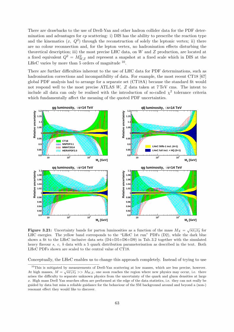
There are drawbacks to the use of Drell-Yan and other hadron collider data for the PDF deter-mination and advantages for ep scattering: i) DIS has the ability to prescribe the reaction typeand the kinematics (x, Q2) through the reconstruction of solely the leptonic vertex; ii) thereare no colour reconnection and, for the lepton vertex, no hadronisation effects disturbing thetheoretical description; iii) the most precise LHC data, on W and Z production, are located ata fixed equivalent Q2 = M2

W,Z and represent a snapshot at a fixed scale which in DIS at the

LHeC varies by more than 5 orders of magnitude 10.

There are further difficulties inherent to the use of LHC data for PDF determinations, such ashadronisation corrections and incompatibility of data. For example, the most recent CT18 [67]global PDF analysis had to arrange for a separate set (CT18A) because the standard fit wouldnot respond well to the most precise ATLAS W, Z data taken at 7 TeV cms. The intent toinclude all data can only be realised with the introduction of so-called χ2 tolerance criteriawhich fundamentally affect the meaning of the quoted PDF uncertainties.

[GeV]XM10 210 310

Rel

ativ

e u

nce

rtai

nty

0.8

0.85

0.9

0.95

1

1.05

1.1

1.15

1.2=14 TeVsgg luminosity,

CT18 NNPDF3.1 MMHT2014 HERAPDF2.0

[GeV]XM10 210 310

Rel

ativ

e u

nce

rtai

nty

0.8

0.85

0.9

0.95

1

1.05

1.1

1.15

1.2=14 TeVs luminosity, qq

LHeC 50fb-1 incl. (4+1)

LHeC full incl. + HQ (5+1)

[GeV]XM10 210 310

Rel

ativ

e u

nce

rtai

nty

0.9

0.92

0.94

0.96

0.98

1

1.02

1.04

1.06

1.08

1.1=14 TeVsqq luminosity,

[GeV]XM10 210 310

Rel

ativ

e u

nce

rtai

nty

0.9

0.92

0.94

0.96

0.98

1

1.02

1.04

1.06

1.08

1.1=14 TeVsqg luminosity,

Figure 3.21: Uncertainty bands for parton luminosities as a function of the mass MX =√sx1x2 for

LHC energies. The yellow band corresponds to the “LHeC 1st run” PDFs (D2), while the dark blueshows a fit to the LHeC inclusive data sets (D4+D5+D6+D9) in Tab. 3.2 together with the simulatedheavy flavour s, c, b data with a 5 quark distribution parameterisation as described in the text. BothLHeC PDFs shown are scaled to the central value of CT18.

Conceptually, the LHeC enables us to change this approach completely. Instead of trying to use

10This is mitigated by measurements of Drell-Yan scattering at low masses, which are less precise, however.At high masses, M =

√sx1x2 >> MW,Z , one soon reaches the region where new physics may occur, i.e. there

arises the difficulty to separate unknown physics from the uncertainty of the quark and gluon densities at largex. High mass Drell Yan searches often are performed at the edge of the data statistics, i.e. they can not really beguided by data but miss a reliable guidance for the behaviour of the SM background around and beyond a (non-)resonant effect they would like to discover.

63

all previous and current PDF sensitive data, to which nowadays one has no alternative, it replacesthese by pure ep collider DIS data. Then one will bring order back into the PDF field: partondistributions, completely resolved, and from a single process, extending over nearly six ordersof magnitude and calculated from NLO pQCD up to probably even N4LO (see Sect. 4.4.1).These PDFs will be applicable for i) identifying new dynamics and symmetries; ii) testingfactorisation; iii) confronting other PDF analsyses at that time; iv) performing high precisionHiggs and electroweak analyses, and v) interpreting any peculiar HL-LHC signal for BSM usingthat independent PDF. higg It has been customary, which is obvious from Eqs. 3.15, 3.20 and3.21, to express the usefulness of various PDF determinations and prospects for the LHC, andsimilarly the FCC, with four so-called parton luminosities which are defined as

Lab(MX) =

∫dxadxb

∑q

Fab δ(M2X − sxaxb) (3.22)

where Fab for (a, b) = (qq) is defined in Eq. 3.15 and (a, b) could also be (g, q), (g, q) and(gg), without a sum over quarks in the latter case. The expectations for the quark and gluonrelated four parton luminosities are presented in Fig. 3.21. The LHeC provides very preciseparton luminosity predictions in the complete range of MX up to the high mass edge of thesearch range at the LHC. This eliminates the currently sizeable PDF uncertainty of precisionelectroweak measurements at the LHC, as for example for the anticipated measurement of MW

to within 10−4 uncertainty, see below. One may also notice that the gluon-gluon luminosity(left top in Fig. 3.21) is at a per cent level for the Higgs mass MX = MH ' 125 GeV. This isevaluated further in the chapter on Higgs physics with the LHeC.

3.4 The 3D Structure of the Proton

As is evident from the discussion in the previous Sections, the LHeC machine will be able tomeasure the collinear parton distribution functions with unprecedented accuracy in its extendedrange of x and Q2. Thus, it will provide a new insight into the details of the one-dimensionalstructure of the proton and nuclei, including novel phenomena at low x. In addition to collineardynamics, the LHeC opens a new window into proton and nuclear structure by allowing a preciseinvestigation of the partonic structure in more than just the one dimension of the longitudinalmomentum. Precision DIS thus gives access to multidimensional aspects of hadron structure.This can be achieved by accurately measuring processes with more exclusive final states likeproduction of jets, semi-inclusive production of hadrons and exclusive processes, in particular theelastic diffractive production of vector mesons and deeply virtual Compton (DVCS) scatteringthat were explored in the 2012 LHeC CDR [1]. These processes have the potential to provideinformation not only on the longitudinal distribution of partons in the proton or nucleus, but alsoon the dependence of the parton distribution on transverse momenta and momentum transfer.Therefore, future, high precision DIS machines like the LHeC or the Electron Ion Collider (EIC)in the US [101], open a unique window into the details of the 3D structure of hadrons. Notethat the measurement of these processes requires a detector with large acceptance, |η| < 4, seee.g. [1, 102]. The current LHeC central detector design covers |η| . 4.5, see Chapter 12.

The most general quantity that can be defined in QCD, that would contain very detailed infor-mation about the partonic content of the hadron, is the Wigner distribution [103]. This functionW (x,k,b) is a 1+4 dimensional function. One can think of it as the “mother” or “master” par-ton distribution, from which lower-dimensional distributions can be obtained. In the definitionof the Wigner function, k is the transverse momentum of the parton and b is the 2-dimensionalimpact parameter, which can be defined as a Fourier conjugate to the momentum transfer of

64

the process. The other, lower dimensional parton distributions can be obtained by integratingout different variables. Thus, transverse momentum dependent (TMD) parton distributions(or unintegrated parton distribution functions) fTMD(x,k) can be obtained by integrating outthe impact parameter b in the Wigner function, while the generalised parton densities (GPD),fGPD(x,b), can be obtained from the Wigner function through the integration over the trans-verse momentum k. In the regime of small x, or high energy, a suitable formalism is that ofthe dipole picture [104–109], where the fundamental quantity which contains the details of thepartonic distribution is the dipole amplitude N(x, r,b). This object contains the dependenceon the impact parameter b as well as another transverse size r, the dipole size, which can berelated to the transverse momentum of the parton k through a Fourier transform. The impor-tant feature of the dipole amplitude is that it should obey the unitarity limit N ≤ 1. The dipoleamplitude N within this formalism can be roughly interpreted as a Wigner function in the highenergy limit, as it contains information about the spatial distribution of the partons in additionto the dependence on the longitudinal momentum fraction x.

W

t

V

γ∗(q)

p(p) Y (p′)

γ∗

N

p p′

V

Figure 3.22: Left: diagram for the quasi-elastic production of the vector meson. Right: schematicillustration of the same process, quasi-elastic vector meson production, within the framework of thedipole picture (taken from [110]). The initial virtual photon, fluctuates into a quark-antiquark pair whichthen scatters off the hadronic target and forms the vector meson. The details of the hadronic interactionof the dipole with the target are encoded in the dipole amplitude N .

Detailed simulations of elastic J/ψ vector meson production were performed for the LHeCkinematic region and beyond [1], using the formalism of the dipole picture. This particularprocess is shown in Fig. 3.22, left plot. The proton is scattered elastically with momentumtransfer t, and the vector meson is produced, which is separated from the final state protonby a rapidity gap. Of particular importance is the measurement of the t slope of this process,since it can be related directly to the impact parameter distribution and is thus sensitive to thetransverse variation of the partonic density in the target. The first type of analysis like this,in the context of elastic scattering, was performed by Amaldi and Schubert [111], where it wasdemonstrated that the Fourier transform of the elastic cross section yields access to the impactparameter profile of the scattering amplitude. This method can be used in the context of vectormeson scattering in DIS, where the transverse distribution of partons, in the perturbative regime,can be extracted through the appropriate Fourier transform [112]. The additional advantage ofstudying diffractive vector meson production is the fact that the partonic distributions can bestudied as a function of the hard scale in this process given by the mass of the vector meson M2

V

in the photoproduction case or Q2 (or more precisely a combination of Q2 and M2V ) in the case

of the diffractive DIS production of vector mesons, as well as the energy W of the photon-protonsystem available in the process which is closely related to x.

The differential cross section for elastic vector meson production can be expressed in the following

65

form:dσγ

∗p→J/ψp

dt=

1

16π|A(x,Q,∆)|2 , (3.23)

where the amplitude for the process of elastic diffractive vector meson production in the highenergy limit, in the dipole picture, is given by

A(x,Q,∆) =∑hh

∫d2r

∫dzΨ∗hh(z, r, Q)N (x, r,∆) ΨV

hh(z, r) . (3.24)

In the above formula, Ψ∗hh

(z, r, Q) is the photon wave function which describes the splittingof the virtual photon γ∗ into a qq pair. This wave funtion can be calculated in perturbativeQCD. The function ΨV

hh(z, r) is the wave function of the vector meson. Finally, N (x, r,∆) is the

dipole amplitude which contains all the information about the interaction of the quark-antiquarkdipole with the target. The formula (3.24) can be interpreted as the process of fluctuation of thevirtual photon into a qq pair, which subsequently interacts with the target through the dipoleamplitude N and then forms the vector meson, given by the amplitude ΨV , see Fig. 3.22, rightplot. The two integrals in the definition Eq. (3.24) are performed over the dipole size which isdenoted by r, and z which is the longitudinal momentum fraction of the photon carried by thequark. The scattering amplitude depends on the value of the momentum transfer ∆, which isrelated to the Mandelstam variable t = −∆2. The sum is performed over the helicity states ofthe quark and antiquark.

The dipole amplitude N (x, r,∆) can be related to the dipole amplitude in coordinate spacethrough the appropriate Fourier transform

N(x, r,b) =

∫d2∆ ei∆·bN (x, r,∆) . (3.25)

We stress that r and b are two different transverse sizes here. The dipole size r is conjugateto the transverse momentum of the partons k, whereas the impact parameter is roughly thedistance between the centre of the scattering target to the centre-of-mass of the quark-antiquarkdipole and is related to the Fourier conjugate variable, the momentum transfer ∆.

The dipole amplitude N(x, r,b) contains rich information about the dynamics of the hadronicinteraction. It is a 5-dimensional function and it depends on the longitudinal momentum frac-tion, and two two-dimensional coordinates. The dependence on the longitudinal momentumfraction is obviously related to the evolution with the centre-of-mass energy of the process,while the dependence on b provides information about the spatial distribution of the partons inthe target. The dipole amplitude is related to the distribution of gluons in impact parameterspace. The dipole amplitude has a nice property that its value should be bounded from aboveby the unitarity requirement N ≤ 1. The complicated dependence on energy, dipole size andimpact parameter of this amplitude can provide a unique insight into the dynamics of QCD,and on the approach to the dense partonic regime. Besides, from Eqs. (3.23),(3.24) and (3.25) itis evident that the information about the spatial distribution in impact parameter b is relatedthrough the Fourier transform to the dependence of the cross section on the momentum transfert = −∆2.

To see how the details of the distribution, and in particular the approach to unitarity, canbe studied through the VM elastic production, calculations based on the dipole model wereperformed [113], and extended to energies which can be reached at the LHeC as well as theFCC-eh. The parameterisations used in the calculation were the so-called IP-Sat [114, 115]

66

and b-CGC [116] models. In both cases the impact parameter dependence has to be modelledphenomenologically. In the IP-Sat model the dipole amplitude has the following form

N(x, r,b) = 1− exp

[−π

2r2

2Ncαs(µ

2)xg(x, µ2)TG(b)

], (3.26)

where xg(x, µ2) is the collinear gluon density, evolved using LO DGLAP (without quarks), froman initial scale µ2

0 up to the scale µ2 set by the dipole size µ2 = 4r2 + µ2

0. αs(µ2) is the strong

coupling. The parameterisation of the gluon density at the initial scale µ20 is given by

xg(x, µ20) = Agx

−λg(1− x)5.6 , (3.27)

and the impact parameter profile for the gluon by

TG(b) =1

2πBGexp(−b2/2BG) . (3.28)

An alternative parameterisation is given by the b-CGC model [116] which has the form

N(x, r,b) =

N0

(rQs

2

)2γeff

for rQs ≤ 2 ,

1− exp(−A ln2(BrQs)) for rQs > 2 .(3.29)

Here the effective anomalous dimension γeff and the saturation scale Qs of the proton explicitlydepend on the impact parameter and are defined as

γeff = γs +1

κλ ln 1/xln

(2

rQs

),

Qs(x, b) =(x0

x

)λ/2exp

[− b2

4γsBCGC

]GeV , (3.30)

where κ = χ′′(γs)/χ′(γs), with χ(γ) being the leading-logarithmic BFKL kernel eigenvaluefunction [117]. The parameters A and B in Eq.(3.29) are determined uniquely from the matchingof the dipole amplitude and its logarithmic derivatives at the limiting value of rqs = 2. Theb-CGC model is constructed by smoothly interpolating between two analytically known limitingcases [116], namely the solution of the BFKL equation in the vicinity of the saturation line forsmall dipole sizes r < 2/Qs, and the solution of the BK equation deep inside the saturationregion for large dipole sizes r > 2/Qs.

The parameters µ0, Ag, λg of the IP-Sat model and N0, γs, x0λ of the b-CGC model were fittedto obtain the best description of the inclusive data for the structure function F2 at HERA. Theslope parameters Bg and BCGC, which control the b -dependence in both models, were fitted toobtain the best description of elastic diffractive J/ψ production, in particular its t-dependence,at small values of t.

In Figs. 3.23 and 3.24 we show the simulated differential cross section dσ/dt as a function of |t|and study its variation with energy and virtuality, and its model dependence. First, in Fig. 3.23we show the differential cross section as a function of t for fixed energy W = 1 TeV, in the case ofthe photoproduction of J/ψ (left plot) and for the case of DIS with Q2 = 10 GeV2 (right plot).The energy W corresponds to the LHeC kinematics. There are three different calculations ineach plot, using the IP-sat model, the b-CGC model and the 1-Pomeron approximation. Thelast one is obtained by keeping just the first non-trivial term in the expansion of the eikonalisedformula of the IP-Sat amplitude (3.26). First, let us observe that all three models coincide

67

0 1 2 3 4|t| [GeV2]

10-6

10-3

100

103

106dσ/d

t (n

b/G

eV2 )

IP-Sat (Saturation)IP-Sat (1-Pomeron)b-CGC (Saturation)

γ∗ + p J/ψ+p

Q = 0, Wγp= 1 TeV

0 1 2 3 4|t| [GeV2]

10-6

10-3

100

103

106

dσ/d

t (n

b/G

eV2 )

IP-Sat (Saturation)IP-Sat (1-Pomeron)b-CGC (Saturation)

γ∗ + p J/ψ+p

Q2 = 10 GeV2, Wγp= 1 TeV

Figure 3.23: Differential cross section for the elastic J/ψ production as a function of |t| within theIP-Sat (saturation), b-CGC and 1-Pomeron models at a fixed Wγp = 1 TeV, which corresponds to theLHeC kinematics, and for two different values of photon virtuality Q = 0 and Q2 = 10 GeV2. Thethickness of points includes the uncertainties associated with the freedom to choose different values forthe charm quark mass within the range mc = 1.2− 1.4 GeV.

for very low values of t, where the dependence on t is exponential. This is because for low|t|, relatively large values of impact parameter are probed in Eq. (3.24) where the amplitudeis small, and therefore the tail in impact parameter is Gaussian in all three cases. Since theFourier transform of the Gaussian in b is an exponential in t, the result at low t follows. Onthe other hand, the three scenarios differ significantly for large values of |t|. In the case of the1-Pomeron approximation the dependence is still exponential, without any dips, which is easilyunderstood since the impact parameter profile is perfectly Gaussian in this case. For the twoother scenarios, dips in dσ/dt as a function in t emerge. They signal the departure from theGaussian profile in b for small values of b where the system is dense. A similar pattern can beobserved when performing the Fourier transform of the Wood-Saxon distribution, which is thetypical distribution used for the description of the matter density in nuclei. When Q2 is increasedthe pattern of dips also changes. This is illustrated in Fig. 3.23. It is seen that the dips move tohigher values of |t| for DIS than for photoproduction. This can be understood from the dipoleformula Eq. (3.24) which contains the integral over the dipole size. Larger values of Q2 selectsmaller values of dipole size r, where the amplitude is smaller and thus in the dilute regime,where the profile in b is again Gaussian. On the other hand, small scales select large dipole sizesfor which the dipole amplitude is larger and thus the saturation effects more prominent, leadingto the distortion of the impact parameter profile and therefore to the emergence of dips in thedifferential cross section dσ/dt when studied as a function of t.

In Fig. 3.24 we show the same calculation but for even higher energy W = 2.5 TeV, which couldbe explored in the FCC-eh. In this case we see that the dips move to lower values of |t|. Thiscan be easily understood, as with increasing energy the dipole scattering amplitude increases,and thus the dilute-dense boundary shifts to larger values of b, meaning that the deviation fromthe exponential fall off occurs for smaller values of |t|. Similar studies [113] show also the changeof the position of the dips with the mass of the vector meson: for lighter vector mesons like

68

0 1 2 3 4|t| [GeV2]

10-6

10-3

100

103

106dσ/d

t (n

b/G

eV2 )

IP-Sat (Saturation)IP-Sat (1-Pomeron)b-CGC (Saturation)

γ∗ + p J/ψ+p

Q = 0, Wγp= 2.5 TeV

0 1 2 3 4|t| [GeV2]

10-6

10-3

100

103

106

dσ/d

t (n

b/G

eV2 )

IP-Sat (Saturation)IP-Sat (1-Pomeron)b-CGC (Saturation)

γ∗ + p J/ψ+p

Q2 = 10 GeV2, Wγp= 2.5 TeV

Figure 3.24: Differential cross section for elastic J/ψ production as a function of |t| within the IP-Sat(saturation), b-CGC and 1-Pomeron models at a fixed Wγp = 2.5 TeV, which corresponds to the regionthat can be explored by FCC-eh, and for two different values of photon virtuality Q = 0 (left plot) andQ2 = 10 GeV2 (right plot). The thickness of points includes the uncertainties associated with the freedomto choose different values for the charm quark mass within the range mc = 1.2− 1.4 GeV .

ρ, ω, φ the dips occur at smaller t than for the heavier vector mesons J/ψ or Υ. We note that,of course, the positions of the dips depend crucially on the details of the models, which arecurrently not constrained by the existing HERA data. We also note the sizeable uncertaintiesdue to the charm quark mass (the fits to inclusive HERA data from which parameters of themodels have been extracted are performed at each fixed value of the charm mass that is thenused to compute exclusive J/ψ production).

We thus see that the precise measurement of the t-slope in the elastic production of vector mesonsat the LHeC, and its variation with x and scales, provide a unique opportunity to explore thetransition between the dilute and dense partonic regimes. As mentioned earlier, elastic diffractiveproduction is one among several different measurements which can be performed to explore the3D structure of the hadron. Another one is Deeply Virtual Compton Scattering which is aprocess sensitive to the spatial distribution of quarks inside the hadron. Previous preliminaryanalyses [1] indicate a huge potential of LHeC for the measurement of DVCS. Another exampleof a process that could be studied at the LHeC, is diffractive exclusive dijet production. Ithas been suggested [118] that this process is sensitive to the Wigner function, and that thetransverse momentum and spatial distribution of partons can be extracted by measuring thisprocess. The transverse momentum of jets would be sensitive to the transverse momentum ofthe participating partons, whereas the momentum transfer of the elastically scattered protonwould give a handle on the impact parameter distribution of the partons in the target [119–121],thus giving a possibility to extract information about the Wigner distribution.

So far we have referred to coherent diffraction, i.e. to a scenario in which the proton remainsintact after the collision. There also exists incoherent diffraction, where the proton gets excitedinto some state with the quantum numbers of the proton and separated from the rest of theevent by a large rapidity gap. In order to apply the dipole formalism to the incoherent case,see Sec. 6.3.1 where the formulae applicable for both protons and nuclei are shown. Here one

69

must consider a more involved structure of the proton (e.g. as composed by a fixed [122–125]or a growing number with 1/x of hot spots [126–128]). As discussed in Sec. 6.3.1, coherentdiffraction is sensitive to the gluon distribution in transverse space, while incoherent diffractionis particularly sensitive to fluctuations of the gluon distribution. A prediction of the model witha growing number of hot spots, both in models where this increasing number is implementedby hand [126–128] and in those where it is dynamically generated [125] from a fixed numberat larger x, is that the ratio of incoherent to coherent diffraction will decrease with W , andthat this decrease is sensitive to the details of the distribution of hot spots, and thus, to thefluctuations of the gluon distribution in transverse space. In order to check these ideas, boththe experimental capability to separate coherent from incoherent diffraction and a large leverarm in W , as available at the LHeC, are required.

In conclusion, measurements at the LHeC (particularly exclusive diffractive production of vectormesons, photons and other final states like dijets) will offer unprecedented opportunities tounravel the three-dimensional structure of hadrons in a kinematic region complementary to thatat the EIC. Note that, such structure varies with x or energy, so its measurement at smallenough x is key as input for both analytic calculations and Monte Carlo simulators at highenergy hadron colliders. And the large lever arms both in x and Q2, as those offered by theLHeC, are required to understand the perturbative evolution of such quantities, as much as itis required for collinear PDFs. Ultraperipheral collisions at the LHC, see Refs. [129, 130] andreferences therein, offer an alternative albeit less precise and for photoproduction.

70

Chapter 4

Exploration of QuantumChromodynamics

The gauge theory formalism of Quantum Chromodynamics (QCD) provides a very successfuldescription of strong interactions between confined partons. Despite the undoubted success ofQCD, the strong force still remains one of the least known fundamental sectors of (particle)physics which needs to be explored much deeper.

For an improved understanding of strong interactions and to answer a variety of those openquestions additional measurements with highest precision have to be performed. At the LHeC,deep-inelastic electron-proton and lepton-nucleus reactions will extend tests of QCD phenomenato a new and yet unexplored domain up to the TeV scale and to x values as low as 10−6, andQCD measurements can be performed with very high experimental precision. This is becausethe proton is a strongly bound system and in deep-inelastic scattering (DIS) the exchangedcolourless photon (or Z) between the electron and the parton inside the proton acts as a neutralobserver with respect to the phenomena of the strong force. In addition, the over-constrainedkinematic system in DIS allows for precise (in-situ) calibrations of the detector to measure thekinematics of the scattered lepton, and, more importantly here, also the hadronic final state. InDIS, in many cases, the virtuality of the exchanged γ/Z boson often provides a reasonable scaleto stabilise theoretical predictions.

In this Chapter, selected topics of QCD studies at the LHeC are discussed.

4.1 Determination of the strong coupling constant

Quantum Chromodynamics (QCD) [131, 132] has been established as the theory of strong in-teractions within the Standard Model of particle physics. While there are manifold aspectsboth from the theoretical and from the experimental point-of-view, by far the most importantparameter of QCD is the coupling strength which is most commonly expressed at the mass ofthe Z boson, MZ , as αs(MZ). Its (renormalisation) scale dependence is given by the QCD gaugegroup SU(3) [133,134]. Predictions for numerous processes in e+e−, pp or ep collisions are thencommonly performed in the framework of perturbative QCD, and (the lack of) higher-orderQCD corrections often represent limiting aspects for precision physics. Therefore, the deter-mination of the strong coupling constant αs(MZ) constitutes one of the most crucial tasks forfuture precision physics, while at the same time the study of the scale dependence of αs providesan inevitable test of the validity of QCD as the theory of strong interactions and the portal for

71

GUT theories.

Different processes and methodologies can be considered for a determination of αs(MZ) (see e.g.reviews [135–137]). Since QCD is an asymptotically free theory, with free behaviour at high scalesbut confinement at low scales, a high sensitivity to the value of αs(MZ) is naturally obtainedfrom low-scale measurements. However, the high-scale behaviour must then be calculated bysolving the renormalisation group equation, which implies the strict validity of the theory andan excellent understanding of all subleading effects, such as the behaviour around quark-massthresholds.

Precision measurements at the LHeC offer the unique opportunity to exploit many of theseaspects. Measurements of jet production cross sections or inclusive NC and CC DIS crosssections provide a high sensitivity to the value of αs(MZ), since these measurements can beperformed at comparably low scales and with high experimental precision. At the same time,the LHeC provides the opportunity to test the running of the strong coupling constant over alarge kinematic range. In this Section, the prospects for a determination of the strong couplingconstant with inclusive jet cross sections and with inclusive NC/CC DIS cross sections arestudied.

4.1.1 Strong coupling from inclusive jet cross sections

The measurement of inclusive jet or di-jet production cross sections in NC DIS provides a highsensitivity to the strong coupling constant and to the gluon PDF of the proton. This is becausejet cross sections in NC DIS are measured in the Breit reference frame [138], where the virtualboson γ∗ or Z collides head-on with the struck parton from the proton and the outgoing jets arerequired to have a non-zero transverse momentum in that reference frame. The leading orderQCD diagrams are QCD Compton and boson-gluon fusion and are both O(αs), see Fig. 4.1.

Q2

e

q

e’

p

(a)

xBj·P

Q2

q

g

ee’

p

(b)

ξ·P

Q2

e

q

q

e’

p

(c)

ξ·P

Figure 4.1: Leading order diagrams for inclusive DIS (a) and jet production (b,c) in the Breit frame(taken from Ref. [139]).

At HERA, jets are most commonly defined by the longitudinally invariant kt jet algorithm [140]with a distance parameter R = 1.0 [139, 141–157]. This provides an infrared safe jet definitionand the chosen distance parameter guarantees a small dependence on non-perturbative effects,such as hadronisation. Differently than in pp at the LHC [158–161], jet algorithms at the LHeCdo not require any pile-up subtraction and any reduction of the dependence on minimum biasor underlying event, due to the absence of such effects. Therefore, for this study we adopt thechoices made at HERA.

In Fig. 4.2 the next-to-next-to-leading order QCD (NNLO) predictions [162, 163] for cross sec-tions for inclusive jet production in NC DIS as a function of the transverse momentum of the jetsin the Breit frame are displayed. The calculations are performed for an electron beam energy of

72

5−10

4−10

3−10

2−10

1−10

1

10

210

310

410

510

610

710

[pb/G

eV

]T

/dp

σd

LHeC pseudo data

[NNLOJET]

NNLO predictions

NNLO QCDNNPDF31_nnlo_as_0118

2+Q2

T=p2

Fµ = 2

Rµ

10 210 [GeV]

Tp

0

0.05

0.1

0.15

rel. e

rro

rs Jet energy scale uncertainty (0.5%)Jet energy scale uncertainty (1.0%)Scale / total theo. error

Figure 4.2: Inclusive jet cross sections calculated in NNLO QCD as a function of the jet transversemomentum in the Breit frame, pT. The shaded area indicates NNLO scale uncertainties and the yellowband shows the estimated experimental jet energy scale uncertainty (JES) of 0.5 %. The blue band showsa very conservative assumption on the JES of 1 %.

Ee = 60 GeV and include γ/Z and Z exchange terms and account for the electron polarisationPe = −0.8. The NC DIS kinematic range is set to Q2 > 4 GeV2. The calculations are performedusing the NNLOJET program [164] interfaced to the APPLfast library [165–167] which providesa generic interface to the APPLgrid [168,169] and fastNLO [170,171] interpolation grid code.

The kinematically accessible range in jet-pT ranges over two orders of magnitude, 4 < pT .400 GeV. The size of the cross section extends over many orders in magnitude, thus imposingchallenging demands on LHeC experimental conditions, triggers and DAQ bandwidth, calibra-tion, and data processing capabilities. The scale uncertainty of the NNLO predictions is about10 % at low values of pT and significantly decreases with increasing values of pT. Future improvedpredictions will further reduce these theoretical uncertainties.

For the purpose of estimating the uncertainty of αs(MZ) in a determination from inclusive jetcross sections at the LHeC, double-differential cross sections as a function of Q2 and pT witha full set of experimental uncertainties are generated. Altogether 509 cross section values arecalculated in the kinematic range 8 < Q2 < 500 000 GeV2 and 4 < pT < 512 GeV, and the bingrid is similar to the ones used by CMS, H1 or ZEUS [44,158,167,172]. The various error sourcesconsidered are summarised in Tab. 4.1. The uncertainties related to the reconstruction of theNC DIS kinematic variables, Q2, y and xbj , are similar to the estimates for the inclusive NC DIScross sections (see section 3.2). For the reconstruction of hadronic final state particles which arethe input to the jet algorithm, jet energy scale uncertainty (JES), calorimetric noise and the polarangle uncertainty are considered. The size of the uncertainties is gauged with achieved values byH1, ZEUS, ATLAS and CMS [148,156,173,174]. The size of the dominant JES one is assumedto be 0.5 % for reconstructed particles in the laboratory rest frame, yielding an uncertainty of0.2–4.4 % on the cross section after the boost to the Breit frame. A JES uncertainty of 0.5 %is well justified by improved calorimeters, since already H1 and ZEUS reported uncertaintiesof 1 % [148, 156, 175], and ATLAS and CMS achieved 1 % over a wide range in pT [173, 174],

73

albeit the presence of pile-up and the considerably more complicated definition of a referenceobject for the in-situ calibration. The size of the JES uncertainty is also displayed in Fig. 4.2.The calorimetric noise of ±20 MeV on every calorimeter cluster, as reported by H1, yields anuncertainty of up to 0.7 % on the jet cross sections. A minimum size of the statistical uncertaintyof 0.15 % is imposed for each cross section bin. An overall normalisation uncertainty of 1.0 %is assumed, which will be mainly dominated by the luminosity uncertainty. In addition, anuncorrelated uncertainty component of 0.6 % collects various smaller error sources, such as forinstance radiative corrections, unfolding or model uncertainties. Studies on the size and thecorrelation model of these uncertainties are performed below.

Exp. uncertainty Shift Size on σ [%]

Statistics with 1 ab−1 min. 0.15 % 0.15 –5Electron energy 0.1 % 0.02 –0.62Polar angle 2 mrad 0.02 –0.48Calorimeter noise ±20 MeV 0.01 –0.74Jet energy scale (JES) 0.5 % 0.2 –4.4Uncorrelated uncert. 0.6 % 0.6Normalisation uncert. 1.0 % 1.0

Table 4.1: Anticipated uncertainties of inclusive jet cross section measurements at the LHeC.

The value and uncertainty of αs(MZ) is obtained in a χ2-fit of NNLO predictions [162, 163] tothe simulated data with αs(MZ) being a free fit parameter. The methodology follows closelyanalyses of HERA jet data [167,172] and the χ2 quantity is calculated from relative uncertainties,i.e. those of the right column of Tab. 4.1. The predictions for the cross section σ account forboth αs-dependent terms in the NNLO calculations, i.e. in the DGLAP operator and the hardmatrix elements, by using

σ = fµ0 ⊗ Pµ0→µF (αs(Mz))⊗ σ(αs(Mz), µ) , (4.1)

where fµ0 are the PDFs at a scale of µ0 = 30 GeV, and Pµ0→µF denotes the DGLAP operator,which is dependent on the value of αs(MZ). The αs uncertainty is obtained by linear errorpropagation and is validated with a separate study of the ∆χ2 = 1 criterion.

In the fit of NNLO QCD predictions to the simulated double-differential LHeC inclusive jet crosssections an uncertainty of

∆αs(MZ)(jets) = ±0.00013(exp) ± 0.00010(PDF) (4.2)

is found. The PDF uncertainty is estimated from a PDF set obtained from LHeC inclusive DISdata (see Sec. 3.3). These uncertainties promise a determination of αs(MZ) with the highestprecision and would represent a considerable reduction of the current world average value witha present uncertainty of ±0.00110 [136].

The uncertainty of αs is studied for different values of the experimental uncertainties for theinclusive jet cross section measurement and for different assumption on bin-to-bin correlations,expressed by the correlation coefficient ρ, of individual uncertainty sources, as shown in Fig. 4.3.It is observed that, even for quite conservative scenarios, αs(MZ) will be determined with anuncertainty smaller than 2 ‰. For this, it is important to keep the size of the uncorrelateduncertainty or the uncorrelated components of other systematic uncertainties under good con-trol. This is also visible from Fig. 4.3 (bottom right), where the contributions of the individualuncertainty sources to the total uncertainty of αs(MZ) are displayed, and it is seen that the

74

0 0.2 0.4 0.6 0.8 1

ρCorrelation coefficient

0

0.5

1

1.5

2

2.5

3

3.5

4

4.5

54 x

10

sα

δ

NNLO QCD

NNPDF31_nnlo_as_0118

)2+Q2

T = (p2

Rµ = 2

Fµ

JESCalorimeter noiseElectron energy

θElectron angle

0 0.2 0.4 0.6 0.8 1

JES uncertainty [%]

0

0.5

1

1.5

2

2.5

3

3.5

4

4.5

54 x

10

sα

δ

NNLO QCD

NNPDF31_nnlo_as_0118

)2+Q2

T = (p2

Rµ = 2

Fµ

Correlation coefficient 1.0

Correlation coefficient 0.8

Correlation coefficient 0.5

0 0.2 0.4 0.6 0.8 1 1.2 1.4 1.6 1.8 2

Uncertainty [%]

0

0.5

1

1.5

2

2.5

3

3.5

4

4.5

54 x

10

sα

δ

NNLO QCD

NNPDF31_nnlo_as_0118

)2+Q2

T = (p2

Rµ = 2

Fµ

Uncorrelated uncertainty

Luminosity uncertainty

0 0.2 0.4 0.6 0.8 1 1.2 1.4 1.6

sαδ

uncor.

norm.

θE

eE

Noise

JES

stat.

4 10× sαδ

error budget (approx.)sα LHeC

Figure 4.3: Studies of the size and correlations of experimental uncertainties impacting the uncertaintyof αs(MZ). Top left: Study of the value of the correlation coefficient ρ for different systematic uncer-tainties. Common systematic uncertainties are considered as fully correlated, ρ = 1. Top right: Size ofthe JES uncertainty for three different values of ρJES. Bottom left: Impact of the uncorrelated and nor-malisation uncertainties on ∆αs(MZ). Bottom right: Contribution of individual sources of experimentaluncertainty to the total experimental uncertainty of αs(MZ).

uncorrelated and the normalisation uncertainty are the largest individual uncertainty compo-nents. It is further observed, that the size of the statistical uncertainty (stat.) is non-negligible,which is, however, strongly dependent on the ad hoc assumption on the minimum size of 0.15 %.The noise uncertainty contributes mainly to jets at low-pT, and since these have a particularhigh sensitivity to αs(MZ), due to their low scale µR. It is of great importance to keep thisexperimental uncertainty well under control, or make better use of track-based information forthe measurment of jets.

In the present formalism theoretical uncertainties from scale variations of the NNLO predictionsamount to about ∆αs(MZ) = 0.0035 (NNLO). These can be reduced with suitable cuts in pT orQ2 to about ∆αs(MZ) ≈ 0.0010. However, it is expected that improved predictions, e.g. withresummed contributions or N3LO predictions will significantly reduce these uncertainties in thefuture. Uncertainties on non-perturbative hadronisation effects will have to be considered aswell, but these will be under good control due to the measurements of charged particle spectraat the LHeC and improved phenomenological models.

75

4.1.2 Pinning Down αs with Inclusive and Jet LHeC Data

The dependence of the coupling strength as a function of the renormalisation scale µR is predictedby QCD, which is often called the running of the strong coupling. Its study with experimentaldata represents an important consistency and validity test of QCD. Using inclusive jet crosssections the running of the strong coupling can be tested by determining the value of αs atdifferent values of µR by grouping data points with similar values of µR and determining thevalue of αs(µR) from these subsets of data points. The assumptions on the running of αs(µR)are then imposed only for the limited range of the chosen interval, and not to the full measuredinterval as in the previous study. Here we set µ2

R = Q2 + p2T

1. The experimental uncertaintiesfrom the fits to subsets of the inclusive jet pseudodata are displayed in Fig. 4.4. These results

[GeV]R

µ

6 10 20 100 200 1000

)Rµ(

s α

0.1

0.15

0.2

[PDG18]World average (expcd. exp. uncert.)LHeC inclusive jets

[NNLO]H1 inclusive jets [NNLO]HERA inclusive jets

[NNLO+NLLA+K]JADE 3-jet rate [NNLO]

23OPAL y

LO]3[NGFitter EW fit [NLO]CMS inclusive jets 8TeV

LHeC experimental uncertainties onlyLHeC

[GeV]R

µ6 10 20 100 200 1000

)

Z(M

s α

0.11

0.115

0.12

0.125

Figure 4.4: Uncertainties of αs(MZ) and corresponding αs(µR) in a determination of αs using LHeCinclusive jet cross sections at different values of µ2

R = Q2 +p2T . Only experimental uncertainties are shown

for LHeC and are compared with a number of presently available measurements and the world averagevalue.

demonstrate a high sensitivity to αs over two orders of magnitude in renormalisation scale upto values of about µR ≈ 500 GeV. In the range 6 < µR . 200 GeV the experimental uncertaintyis found to be smaller than the expectation from the world average value [183]. This region is ofparticular interest since it connects the precision determinations from lattice calculations [184]or τ decay measurements [185], which are at low scales O(GeV), to the measurements at theZ pole [186] and to the applications to scales which are relevant for the LHC, e.g. for Higgs

1The choice of the scales follows a conventional scale setting procedure and uncertainties for the scale choiceand for unknown higher order terms are estimated by varying the scales. Such variations are sensitive only to theterms which govern the behaviour of the running coupling, and may become unreliable due to renormalons [176].An alternative way to fix the scales is provided by the Principle of Maximum Conformality (PMC) [177–181].The PMC method was recently applied to predictions of event shape observables in e+e− → hadrons [182]. Whenapplying the PMC method to observables in DIS, the alternative scale setting provides a profound alternative toverify the running of αs(µR). Such a procedure could be particularly relevant for DIS event shape observables,where the leading-order terms are insensitive to αs and conventional scale choices may not be adequately relatedto the αs-sensitive higher order QCD corrections.

76

or top-quark physics or high-mass searches. This kinematic region of scales O(10 GeV) cannotbe accessed by (HL-)LHC experiments because of limitations due to pile-up and underlyingevent [187].

Inclusive DIS cross sections are sensitive to αs(MZ) through higher-order QCD corrections,contributions from the FL structure function and the scale dependence of the cross section athigh x (scaling violations). The value of αs(MZ) can then be determined in a combined fitof the PDFs and αs(MZ) [172]. While a simultaneous determination of αs(MZ) and PDFs isnot possible with HERA inclusive DIS data alone due to its limited precision and kinematiccoverage [44,172], the large kinematic coverage, high precision and the integrated luminosity ofthe LHeC data will allow for the first time such an αs analysis.

For the purpose of the determination of αs(MZ) from inclusive NC/CC DIS data, a combinedPDF+αs fit to the simulated data is performed, similar to the studies presented above, inChapter 3. Other technical details are outlined in Ref. [172]. In this fit, however, the numbersof free parameters of the gluon parameterisation is increased, since the gluon PDF and αs(MZ)are highly correlated and LHeC data are sensitive to values down to x < 10−5, which requiresadditional freedom for the gluon parameterisation. The inclusive data are restricted to Q2 ≥5 GeV2 in order to avoid a region where effects beyond fixed-order perturbation theory maybecome sizeable [44,188].

Exploiting the full LHeC inclusive NC/CC DIS data with Ee = 50 GeV, the value of αs(MZ) canbe determined with an uncertainty ∆αs(MZ) = ±0.00038. With a more optimistic assumptionon the dominant uncorrelated uncertainty of δσ(uncor.) = 0.25 %, an uncertainty as small as

∆αs(MZ)(incl. DIS) = ±0.00022(exp+PDF) (4.3)

is achieved. This would represent a considerable improvement over the present world averagevalue. Given these small uncertainties, theoretical uncertainties from missing higher orders orheavy quark effects have to be considered in addition. In a dedicated study, the fit is repeatedwith a reduced data set which can be accumulated already during a single year of operation 2,corresponding to about L ∼ 50 fb−1. Already these data will be able to improve the worldaverage value. These studies are displayed in Fig. 4.5.

High sensitivity to αs(MZ) and an optimal treatment of the PDFs is obtained by using inclusivejet data together with inclusive NC/CC DIS data in a combined determination of αs(MZ) andthe PDFs. The jet data will provide an enhanced sensitivity to αs(MZ), while inclusive DIS datahas the highest sensitivity to the determination of the PDFs. In such combined QCD analyses,also heavy quark data may be further analysed to determine mc and mb. However, since jetcross sections have sufficiently high scale (pT mb) these are fairly insensitive to the actualvalue of the heavy quark masses. Contrary, heavy quark data is predominantly sensitive to thequark mass parameters rather than to αs(MZ), and their correlation is commonly found to besmall in such combined analyses, see e.g. Ref [52]. Infact, at LHeC the masses of charm andbottom quarks can be determined with high precision and uncertainties of 3 MeV and 10 MeVare expected, respectively [1]. Therefore, for our sole purpose of estimating the uncertainty ofαs(MZ) from LHeC data, we do not consider heavy quark data, nor free values of mc or mb

in the analysis, and we leave the outcome of such a complete QCD analysis to the time whenreal data are available and the actual value of the parameters are of interest. At this time, alsobetter theoretical predictions will be used, including higher order corrections, heavy quark masseffects or higher-twist terms, as can be expected from steady progress [189–194].

2Two different assumptions are made. One fit is performed with only electron data corresponding to L ∼50 fb−1, and an alternative scenario considers further positron data corresponding to L ∼ 1 fb−1.

77

Uncorr. uncertainty (DIS) [%]

1−10 1−10×2 1

4 1

0×

sα

δ

0

2

4

6

8

10

12

14

16

18

20 from inclusive DIS and jetssαLHeC-50:

)-

e-1

(50fbDIS alone )+ e

-1, 1fb

- e

-1(50fbDIS alone (full lumi.)DIS alone

)-

e-1

(50fbjets + DIS(full lumi.)jets + DIS

PDG18

Figure 4.5: Uncertainties of αs(MZ) from simultaneous fits of αs(MZ) and PDFs to inclusive NC/CCDIS data as a function of the size of the uncorrelated uncertainty of the NC/CC DIS data. The full linesindicate the uncertainties obtained with different assumptions on the data taking scenario and integratedluminosity. The dashed lines indicate results where, additionally to the inclusive NC/CC DIS data,inclusive jet cross section data are considered.

For this study, the double-differential inclusive jet data as described above, and additionallythe inclusive NC/CC DIS data with Ee = 50 GeV as introduced in Sec. 3.2, are employed.Besides the normalisation uncertainty, all sources of systematic uncertainties are considered asuncorrelated between the two processes. A fit of NNLO QCD predictions to these data sets isthen performed, and αs(MZ) and the parameters of the PDFs are determined. The methodologyfollows closely the methodology sketched in Sect. 3. Using inclusive jet and inclusive DIS datain a single analysis, the value of αs(MZ) is determined with an uncertainty of

∆αs(MZ)(incl. DIS & jets) = ±0.00018(exp+PDF) . (4.4)

This result will improve the world average value considerably. However, theoretical uncertaintiesare not included and new mathematical tools and an improved understanding of QCD willbe needed in order to achieve small values similar to the experimental ones. The dominantsensitivity in this study arises from the jet data. This can be seen from Fig. 4.5, where ∆αs(MZ)changes only moderately with different assumptions imposed on the inclusive NC/CC DIS data.Assumptions made for the uncertainties of the inclusive jet data have been studied above, andthese results can be translated easily to this PDF+αs fit.

The expected values for αs(MZ) obtained from inclusive jets or from inclusive NC/CC DIS dataare compared in Fig. 4.6 with present determinations from global fits based on DIS data (calledPDF fits) and the world average value [136]. It is observed that LHeC will have the potentialto improve considerably the world average value. Already after one year of data taking, theexperimental uncertainties of the NC/CC DIS data are competitive with the world averagevalue. The measurement of jet cross sections will further improve that value (not shown).

Furthermore, LHeC will be able to address a long standing puzzle. All αs determinations fromglobal fits based on NC/CC DIS data find a lower value of αs(MZ) than determinations in thelattice QCD framework, from τ decays or in a global electroweak fit. With the expected precisionfrom LHeC this discrepancy will be resolved.

78

0.11 0.115 0.12)

Z(Ms α

[2018] World average

run)st(1LHeC incl. DIS LHeC DIS+jetsLHeC incl. jets

=50GeV)e

(ELHeC incl. DIS

HERA incl. jetsH1

MMHTNNPDFJRBBGABMPABM

Figure 4.6: Summary of αs(MZ) values in comparison with present values.

4.1.3 Strong coupling from other processes

A detailed study for the determination of αs(MZ) from NC/CC DIS and from inclusive jet datawas presented in the previous paragraphs. However, a large number of additional processesand observables that are measured at the LHeC can also be considered for a determination ofαs(MZ). Suitable observables or processes are di-jet and multi-jet production, heavy flavourproduction, jets in photoproduction or event shape observables. These processes all exploitthe αs dependence of the hard interaction. Using suitable predictions, also softer processescan be exploited for an αs determination. Examples could be jet shapes or other substructureobservables, or charged particle multiplicities.

Since αs(MZ) is a parameter of a phenomenological model, the total uncertainty of αs(MZ) isalways a sum of experimental and theoretical uncertainties which are related to the definition ofthe observable and to the applied model, e.g. hadronisation uncertainties, diagram removal/sub-traction uncertainties or uncertainties from missing higher orders. Therefore, credible prospectsfor the total uncertainty of αs(MZ) from other observables or processes altogether are difficultto predict, even more since LHeC will explore a new kinematic regime that was previouslyunmeasured.

In a first approximation, for any process the sensitivity to αs(MZ) scales with the order n of αs

in the leading-order diagram, αns . The higher the power n the higher the sensitivity to αs(MZ).Consequently, the experimental uncertainty of an αs fit may reduce with increasing power n.Already at HERA three-jet cross section were proven to have a high sensitivity to αs(MZ) albeittheir sizeable statistical uncertainties [139, 149]. At the LHeC, due to the higher

√s and huge

integrated luminosity, as well as the larger acceptance of the detector, three-, four- or five-jetcross sections represent highly sensitive observables for a precise determination of αs(MZ), andhigh experimental precision can be achieved. In these cases, fixed order pQCD predictions maybecome limiting factors, since they are more complicated for large n.

Di-jet observables are expected to yield a fairly similar experimental uncertainty than inclusive

79

jet cross sections, as studied in the previous paragraphs, since both have n = 1 at LO. How-ever, their theoretical uncertainties may be smaller, since di-jet observables are less sensitive toadditional higher-order radiation, in particular at lower scales where αs(µR) is larger.

Event shape observables in DIS exploit additional radiation in DIS events (see e.g. review [195]or HERA measurements [196, 197]). Consequently, once measured at the LHeC the experi-mental uncertainties of αs(MZ) from these observables are expected to become very similarto that in Eq. (4.4), since both the event sample and the process is similar to the inclusivejet cross sections 3. However, different reconstruction techniques of the observables may yieldreduced experimental uncertainties, and the calculation of event shape observables allow forthe resummation of large logarithms, and steady theoretical advances promise small theoreticaluncertainties [198–204].

Jet production cross sections in photoproduction represents a unique opportunity for anotherprecision determination of αs(MZ). Such measurements have been performed at HERA [205–208]. The sizeable photoproduction cross section provides a huge event sample, which is statis-tically independent from NC DIS events, and already the leading-order predictions are sensitiveto αs(MZ) [209]. Also its running can be largely measured since the scale of the process is wellestimated by the transverse momentum of the jets µR ∼ pjet

T . Limiting theoretical aspects aredue to the presence of a quasi-real photon and the poorly known photon PDF [210,211].

A different class of observables represent heavy flavour (HF) cross sections, which are discussed inSec. 3.3.5. Due to flavour conservation, these are commonly proportional to O(α1

s ) at leading-order. However, when considering inclusive HF cross sections above the heavy quark massthreshold heavy quarks can be factorised into the PDFs, and the leading structure functionsF c,b2 are sensitive to αs only beyond the LO approximation (see reviews [81, 82], recent HERAmeasurements [65, 212] and references therein). The presence of the heavy quark mass as anadditional scale stabilises perturbative calculations, and reduced theoretical uncertainties areexpected.

At the LHeC the structure of jets and the formation of hadrons can be studied with unprece-dented precision. This is so because of the presence of a single hadron in the initial state.Therefore, limiting effects like the underlying event or pile-up are absent or greatly diminished.Precise measurements of jet shape observables, or the study of jet substructure observables [213],are highly sensitive to the value of αs(MZ), because parton shower and hadronisation take placeat lower scales where the strong coupling becomes large and an increased sensitivity to αs(MZ)is attained [165,214].

Finally, also the determination of αs(MZ) from inclusive NC DIS cross sections can be improved.For NC DIS the dominant sensitivity to αs arises from the FL structure function and from scalingviolations of F2 at lower values of Q2 but at very high values of x. Dedicated measurements ofthese kinematic regions will further improve the experimental uncertainties from the estimatedvalues in Eq. (4.3).

4.2 Discovery of New Strong Interaction Dynamics at Small x

The LHeC machine will offer access to a completely novel kinematic regime of DIS characterisedby very small values of x. From the kinematical plane in (x,Q2) depicted in Fig. 1.1, it is clearthat the LHeC will be able to probe Bjorken-x values as low as 10−6 for perturbative values of

3It shall be noted, that event shape observables in NC DIS can be defined in the laboratory rest frame or theBreit frame.

80

Q2. At low values of x various phenomena may occur which go beyond the standard collinearperturbative description based on DGLAP evolution. Since the seminal works of Balitsky,Fadin, Kuraev and Lipatov [117, 215, 216] it has been known that, at large values of centre-of-mass energy

√s or, to be more precise, in the Regge limit, there are large logarithms of energy

which need to be resummed. Thus, even at low values of the strong coupling αs, logarithms ofenergy ln s may be sufficiently large, such that terms like (αs ln s)n will start to dominate thecross section.

In addition, other novel effects may appear in the low x regime, which are related to the highgluon densities. At large parton densities the recombination of the gluons may become importantin addition to the gluon splitting. This is known as the parton saturation phenomenon in QCD,and is deeply related to the restoration of the unitarity in QCD. As a result, the linear evolutionequations will need to be modified by the additional nonlinear terms in the gluon density. In thenext two subsections we shall explore the potential and sensitivity of the LHeC to these smallx phenomena in ep collisions. Note also that, being a density effect, the non-linear phenomenaleading to parton saturation are enhanced by increasing the mass number of the nucleus in eA.Chapter 6, devoted to the physics opportunities with eA collisions at the LHeC, discusses thisaspect, see also Ref. [1].

4.2.1 Resummation at small x

The calculation of scattering amplitudes in the high-energy limit and the resummation of(αs ln s)n series in the leading logarithmic order was performed in Refs. [117, 215, 216] and itresulted in the famous BFKL evolution equation. This small x evolution equation, written forthe so-called gluon Green’s function or the unintegrated gluon density, is a differential equationin ln 1/x. An important property of this equation is that it keeps the transverse momenta un-ordered along the gluon cascade. This has to be contrasted with DGLAP evolution which isdifferential in the hard scale Q2 and relies on the strong ordering in the transverse momenta ofthe exchanged partons in the parton cascade. The solution to the BFKL equation is a gluondensity which grows sharply with decreasing x, as a power i.e. ∼ x−ωIP , where ωIP is the hardPomeron intercept, and in the leading logarithmic approximation equals Ncαs

π 4 ln 2, which givesa value of about 0.5 for typical values of the strong coupling. The leading logarithmic (LLx)result yielded a growth of the gluon density which was too steep for the experimental data atHERA. The next-to-leading logarithmic (NLLx) calculation performed in the late 90s [217,218]resulted in large negative corrections to the LLx value of the hard Pomeron intercept and yieldedsome instabilities in the cross section [219–222] and it is important to account for subleadingeffects, since these are large [223,224].

The appearance of the large negative corrections at NLLx motivated the search for the appro-priate resummation which would stabilize the result. It was understood very early that the largecorrections which appear in BFKL at NLLx are mostly due to the kinematics [225–227] as well asDGLAP terms and the running of the strong coupling. First attempts at combining the BFKLand DGLAP dynamics together with the proper kinematics [228–230] yielded encouraging re-sults, and allowed a description of HERA data on structure functions with good accuracy. Thecomplete resummation program was developed in a series of works [231–247]. In these worksthe resummation for the gluon Green’s function and the splitting functions was developed.

The low-x resummation was recently applied to the description of structure function data atHERA using the methodology of NNPDF [248]. It was demonstrated that the resummed fitsprovide a better description of the structure function data than the pure DGLAP based fits atfixed NNL order. In particular, it was shown that the χ2 of the fits does not vary appreciably

81

when more small x data are included in the case of the fits which include the effects of the small-xresummation. On the other hand, the fits based on NNLO DGLAP evolution exhibit a worseningof their quality in the region of low x and low to moderate values of Q2. This indicates thatthere is some tension in the fixed order fits based on DGLAP, and that resummation alleviatesit. In addition, it was shown that the description of the longitudinal structure function FLfrom HERA data is improved in the fits with the small x resummation. This analysis suggeststhat the small x resummation effects are indeed visible in the HERA kinematic region. Sucheffects will be strongly magnified at the LHeC, which probes values of x more than one orderof magnitude lower than HERA. The NNPDF group also performed simulation of the structurefunctions F2 and FL with and without resummation in the LHeC range as well as for the nextgeneration electron-hadron collider FCC-eh [248]. The predictions for the structure functions asa function of x for fixed values of Q2 are shown in Figs. 4.7.

10−6 10−5 10−4 10−3

x

0

1

2

3

4

5

Fp 2

LHeC kinematic range

FCC-eh kinematic range

NNPDF3.1sx, Q2 = 5 GeV2

NNLO

NNLO+NLLx

Pseudo-Data

10−4 10−30.6

0.8

1.0

1.2

1.4

10−6 10−5 10−4 10−3

x

−0.5

0.0

0.5

1.0

1.5

Fp L

LHeC kinematic range

FCC-eh kinematic range

NNPDF3.1sx, Q2 = 5 GeV2

NNLO

NNLO+NLLx

Figure 4.7: Predictions for the F2 and FL structure functions using the NNPDF3.1sx NNLO andNNLO+NLLx fits at Q2 = 5 GeV2 for the kinematics of the LHeC and FCC-eh. In the case of F2, wealso show the expected total experimental uncertainties based on the simulated pseudodata, assuming theNNLO+NLLx values as the central prediction. A small offset has been applied to the LHeC pseudodataas some of the values of x overlap with the FCC-eh pseudodata points. The inset in the left plot shows amagnified view in the kinematic region x > 3× 10−5, corresponding to the reach of HERA data. Figuretaken from Ref. [248].

The simulations were done using APFEL [249] together with the HELL package [250] whichimplements the small x resummation. From Fig. 4.7 it is clear that LHeC will have much highersensitivity to discriminate between fixed order and resummed scenarios than the HERA collider,with even better discrimination at the FCC-eh. The differences between the central values forthe two predictions are of the order of 15% for the case of F2 and this is much larger thanthe projected error bar on the reduced cross section or structure function F2 which could bemeasured at LHeC. For comparison, the simulated pseudodata for F2 are shown together withthe expected experimental uncertainties. The total uncertainties of the simulated pseudodataare at the few percent level at most, and are therefore much smaller than the uncertaintiescoming from the PDFs in most of the kinematic range.

It is evident that fits to the LHeC data will have power to discriminate between the differentframeworks. In the right plot in Fig. 4.7, the predictions for the longitudinal structure functionare shown. We see that in the case of the FL structure function, the differences between thefixed order and resummed predictions are even larger, consistently over the entire range of x.This indicates the importance of the measurement of the longitudinal structure function FL

82

which can provide further vital constraints on the QCD dynamics in the low x region due to itssensitivity to the gluon density in the proton.

To further illustrate the power of a high energy DIS collider like the LHeC in exploring thedynamics at low x, fits which include the simulated data were performed. The NNLO+NLLxresummed calculation was used to obtain the simulated pseudodata, both for the LHeC, in ascenario of a 60 GeV electron beam on a 7 TeV proton beam as well as in the case of the FCC-ehscenario with a 50 TeV proton beam. All the experimental uncertainties for the pseudodata havebeen added in quadrature. Next, fits were performed to the DIS HERA as well as LHeC andFCC-eh pseudodata using the theory with and without the resummation at low x. Hadronicdata like jet, Drell-Yan or top, were not included for this analysis but, as demonstrated in [248],these data do not have much of the constraining power at low x, and therefore the results ofthe analysis at low x are independent of the additional non-DIS data sets. The quality of thefits characterised by the χ2 was markedly worse when the NNLO DGLAP framework was usedto fit the HERA data and the pseudodata from LHeC and/or FCC-eh than was the case withresummation. To be precise, the χ2 per degree of freedom for the HERA data set was equal to1.22 for the NNLO fit, and 1.07 for the resummed fit. For the case of the LHeC/FCC-eh the χ2

per degree of freedom was equal to 1.71/2.72 and 1.22/1.34 for NNLO and NNLO+resummationfits, respectively. These results demonstrate the huge discriminatory power of the new DISmachines between the DGLAP and resummed frameworks, and the large sensitivity to the lowx region while simultaneously probing low to moderate Q2 values.

10−8 10−7 10−6 10−5 10−4 10−3 10−2 10−1 100

x

0.7

0.8

0.9

1.0

1.1

1.2

1.3

g(x,Q

2)/g

(x,Q

2)[

ref]

NNPDF31sx, Q = 100 GeV

NNLO+NLLx HERA only, global

NNLO+NLLx HERA+LHeC+FCC-eh, DIS-only

NNLO HERA+LHeC+FCC-eh, DIS-only

10−8 10−7 10−6 10−5 10−4 10−3 10−2 10−1 100

x

0.7

0.8

0.9

1.0

1.1

1.2

1.3

Σ(x,Q

2)/Σ

(x,Q

2)[

ref]

NNPDF31sx, Q = 100 GeV

NNLO+NLLx HERA only, global

NNLO+NLLx HERA+LHeC+FCC-eh, DIS-only

NNLO HERA+LHeC+FCC-eh, DIS-only

Figure 4.8: Comparison between the gluon (left plot) and the quark singlet (right plot) PDFs in theNNPDF3.1sx NNLO+NNLx fits without (blue hatched band) and with the LHeC+FCC-eh pseudodata(orange band) on inclusive structure functions. For completeness, we also show the results of the corre-sponding NNPDF3.1sx NNLO fit with LHeC+FCC-eh pseudodata (green hatched band). Figure takenfrom Ref. [248].

In Fig. 4.8 the comparison of the gluon and quark distributions from the NNLO + NLLx fits isshown at Q = 100 GeV as a function of x, with and without including the simulated pseudodatafrom LHeC as well as FCC-eh. The differences at large x are due to the fact that only DISdata were included in the fits, and not the hadronic data. The central values of the extractedPDFs using only HERA or using HERA and the simulated pseudodata coincide with eachother, but a large reduction in uncertainty is visible when the new data are included. Theuncertainties from the fits based on the HERA data only increase sharply already at x ∼ 10−4.On the other hand, including the pseudodata from LHeC and/or FCC-eh can extend this regimeby order(s) of magnitude down in x. Furthermore, fits without resummation, based only onNNLO DGLAP, were performed to the HERA data and the pseudodata. We see that in thiscase the extracted gluon and singlet quark densities differ significantly from the fits using the

83

NNLO+NLLx. Already at x = 10−4 the central values of the gluon differ by 10% and atx = 10−5, which is the LHeC regime, the central values for the gluon differ by 15%. Thisdifference is much larger than the precision with which the gluon can be extracted from the DISdata, which is of the order of ∼ 1%.

The presented analysis demonstrates that the fixed order prediction based on the DGLAPevolution would likely fail to describe accurately the structure function data in the new DISmachines and that in that regime new dynamics including resummation are mandatory forquantitative predictions. Therefore, the LHeC machine has an unprecedented potential to pindown the details of the QCD dynamics at low values of Bjorken x.

4.2.2 Disentangling non-linear QCD dynamics at the LHeC

As mentioned previously the kinematic extension of the LHeC will allow unprecedented tests ofthe strong interaction in the extremely low x region, and allow for the tests of the novel QCDdynamics at low x. The second effect, in addition to resummation, that may be expected isthe parton saturation phenomenon, which may manifest itself as the deviation from the linearDGLAP evolution, and the emergence of the saturation scale.

In particular, it has been argued that the strong growth of the gluon PDF at small-x shouldeventually lead to gluon recombination [251] to avoid violating the unitary bounds. The onsetof such non-linear dynamics, also known as saturation, has been extensively searched but sofar there is no conclusive evidence of its presence, at least within the HERA inclusive structurefunction measurements. In this context, the extended kinematic range of the LHeC providesunique avenues to explore the possible onset of non-linear QCD dynamics at small-x. Thediscovery of saturation, a radically new regime of QCD, would then represent an importantmilestone in our understanding of the strong interactions.

The main challenge in disentangling saturation lies in the fact that non-linear corrections areexpected to be moderate even at the LHeC, since they are small (if present at all) in the regioncovered by HERA. Therefore, great care needs to be employed in order to separate such effectsfrom those of standard DGLAP linear evolution. Indeed, it is well known that HERA data atsmall-x in the perturbative region can be equally well described, at least at the qualitative level,both by PDF fits based on the DGLAP framework as well as by saturation-inspired models.However, rapid progress both in theory calculations and methodological developments havepushed QCD fits to a new level of sophistication, and recently it has been shown that subtle butclear evidence of BFKL resummation at small-x is present in HERA data, both for inclusive andfor heavy quark structure functions [252, 253]. Such studies highlight how it should be possibleto tell apart non-linear from linear dynamics using state-of-the-art fitting methods even if theseare moderate, provided that they are within the LHeC reach.

Here we want to assess the sensitivity of the LHeC to detect the possible onset of non-linearsaturation dynamics. This study will be carried out by generalising a recent analysis [59] thatquantified the impact of LHeC inclusive and semi-inclusive measurements on the PDF4LHC15PDFs [254,255] by means of Hessian profiling [256]. There, the LHeC pseudodata was generatedassuming that linear DGLAP evolution was valid in the entire LHeC kinematic range using thePDF4LHC15 set as input. To ascertain the possibility of pinning down saturation at the LHeC,here we have revisited this study but now generating the LHeC pseudodata by means of asaturation-inspired calculation. By monitoring the statistical significance of the tension thatwill be introduced (by construction) between the saturation pseudodata and the DGLAP theoryassumed in the PDF fit, we aim to determine the likelihood of disentangling non-linear from

84

linear evolution effects at the LHeC. See also [257] for previous related studies along the samedirection.

Analysis settings

In this study we adopt the settings of [59, 258], to which we refer the interested reader forfurther details. In Ref. [59] the impact on the proton PDFs of inclusive and semi-inclusiveneutral-current (NC) and charged current (CC) DIS structure functions from the LHeC wasquantified. These results were then compared with the corresponding projections for the PDFsensitivity of the High-Luminosity upgrade of the LHC (HL-LHC). In Fig. 3.4 the kinematicrange in the (x,Q2) plane of the LHeC pseudodata employed in that analysis is displayed, whichillustrated how the LHeC can provide unique constraints on the behaviour of the quark andgluon PDFs in the very small-x region.

Since non-linear dynamics are known to become sizeable only at small-x, for the present analysisit is sufficient to consider the NC e−p inclusive scattering cross sections from proton beamenergies of Ep = 7 TeV and Ep = 1 TeV. In Fig. 4.9 we show the bins in (x,Q2) for whichLHeC pseudodata for inclusive structure functions has been generated according to a saturation-based calculation. Specifically, we have adopted here the DGLAP-improved saturation modelof Ref. [259], in which the scattering matrix is modelled through eikonal iteration of two gluonexchanges. This model was further extended to include heavy flavour in Ref. [260]. The specificparameters that we use were taken from Fit 2 in Ref. [261], where parameterisations are providedthat can be used for x < 0.01 and Q2 < 700 GeV2. These parameters were extracted from a fitto the HERA legacy inclusive structure function measurements [44] restricted to x < 0.01 and0.045 < Q2 < 650 GeV2. In contrast to other saturation models, the one we assume here [261]provides a reasonable description for large Q2 in the small x region, where it ensure a smoothtransition to standard fixed-order perturbative results.

10 6 10 5 10 4 10 3 10 2 10 1 100

x

101

102

103

104

105

106

107

Q2

LHeC760NCEM DGLAPSaturation

Figure 4.9: The kinematic coverage of the NC e−p scattering pseudodata at the LHeC, where the blue(red) points indicate those bins for which DGLAP (saturation) predictions are available.

Note that the above discussion refers only to the generated LHeC pseudodata: all other aspectsof the QCD analysis of Ref. [59] are left unchanged. In particular, the PDF profiling will be

85

carried out using theory calculations obtained by means of DGLAP evolution with the NNLOPDF4LHC15 set (see also Ref. [262]), with heavy quark structure functions evaluated by means ofthe FONLL-B general-mass variable flavour number scheme [89]. In order to ensure consistencywith the PDF4LHC15 prior, here we will replace the DGLAP pseudodata by the saturationcalculation only in the kinematic region for x ∼< 10−4, rather than for all the bins indicated inred in Fig. 4.9. The reason for this choice is that PDF4LHC15 already includes HERA datadown to x ' 10−4 which is successfully described via the DGLAP framework, and therefore if weassume departures from DGLAP in the LHeC pseudodata this should only be done for smallervalues of x.

Results and discussion

Using the analysis settings described above, we have carried out the profiling of PDF4LHC15with the LHeC inclusive structure function pseudodata, which for x ≤ 10−4 (x > 10−4) hasbeen generated using the GBW saturation (DGLAP) calculations, and compare them with theresults of the profiling where the pseudodata follows the DGLAP prediction. We have generatedNexp = 500 independent sets LHeC pseudodata, each one characterised by different randomfluctuations (determined by the experimental uncertainties) around the underlying central value.

To begin with, it is instructive to compare the data versus theory agreement, χ2/ndat, betweenthe pre-fit and post-fit calculations, in order to assess the differences between the DGLAP andsaturation cases. In the upper plots of Fig. 4.10 we show the distributions of pre-fit and post-fitvalues of χ2/ndat for the Nexp = 500 sets of generated LHeC pseudodata. We compare the resultsof the profiling of the LHeC pseudodata based on DGLAP calculations in the entire range ofx with those where the pseudodata is based on the saturation model in the region x < 10−4.Then in the bottom plot we compare of the post-fit χ2 distributions between the two scenarios.Note that in these three plots the ranges in the x axes are different.

From this comparison we can observe that for the case where the pseudodata is generated usinga consistent DGLAP framework (PDF4LHC15) as the one adopted for the theory calculationsused in the fit, as expected the agreement is already good at the pre-fit level, and it is furtherimproved at the post-fit level. However the situation is rather different in the case where asubset of the LHeC pseudodata is generated using a saturation model: at the pre-fit level theagreement between theory and pseudodata is poor, with χ2/ndat ' 7. The situation markedlyimproves at the post-fit level, where now the χ2/ndat distributions peaks around 1.3. This resultimplies that the DGLAP fit manages to absorb most of the differences in theory present inthe saturation pseudodata. This said, the DGLAP fit cannot entirely fit away the non-linearcorrections: as shown in the lower plot of Fig. 4.10, even at the post-fit level one can still tellapart the χ2/ndat distributions between the two cases, with the DGLAP (saturation) pseudodatapeaking at around 0.9 (1.3). This comparison highlights that it is not possible for the DGLAPfit to completely absorb the saturation effects into a PDF redefinition.

In order to identify the origin of the worse agreement between theory predictions and LHeCpseudodata in the saturation case, it is illustrative to take a closer look at the pulls defined as

P (x,Q2) =Fdat(x,Q

2)−Ffit(x,Q2)

δexpF(x,Q2), (4.5)

where Ffit is the central value of the profiled results for the observable F (in this case the reducedneutral current DIS cross section), Fdat is the corresponding central value of the pseudodata,and δexpF represents the associated total experimental uncertainty. In Fig. 4.11 we display thepulls between the post-fit prediction and the central value of the LHeC pseudodata for different

86

0.4 0.6 0.8 1 1.2 1.4 1.6 dat / N

LHeC2χ

0

0.05

0.1

0.15

0.2

0.25

0.3

0.35

0.4

Dis

trib

utio

n

DGLAP-based LHeC pseudo-data (PDF4LHC15)

pre-fit

post-fit

DGLAP-based LHeC pseudo-data (PDF4LHC15)

0 1 2 3 4 5 6 7 8 9 dat / N

LHeC2χ

0

0.1

0.2

0.3

0.4

0.5

0.6

0.7

0.8

0.9

Dis

trib

utio

n

)-4Saturation LHeC pseudo-data (for x < 10

pre-fit

post-fit

)-4Saturation LHeC pseudo-data (for x < 10

0.6 0.8 1 1.2 1.4 1.6 1.8 dat / N

LHeC2χ

0

0.05

0.1

0.15

0.2

0.25

0.3

0.35

0.4

0.45

0.5

Dis

trib

utio

n

Post-fit results to LHeC (500 pseudo-experiments)

DGLAP pseudo-data

Saturation pseudo-data

Post-fit results to LHeC (500 pseudo-experiments)

Figure 4.10: Upper plots: the distribution of pre-fit and post-fit values of χ2/ndat for the Nexp = 500sets of generated LHeC pseudodata. We compare the results of the profiling of the LHeC pseudodatabased on DGLAP calculations in the entire range of x (left) with those where the pseudodata is basedon the saturation model in the region x < 10−4 (right plot). Bottom plot: comparison of the post-fitχ2/ndat distributions between these two scenarios for the pseudodata generation.

bins in Q2. We compare the cases where the pseudodata has been generated using a consistenttheory calculation (DGLAP) with that based on the GBW saturation model.

The comparisons in Fig. 4.11 show first of all that in the DGLAP case the pulls are O(1) inthe entire kinematical range. This is of course expected, given that the LHeC pseudodata isgenerated using the same theory as the one subsequently used for the fit. In the case wherethe pseudodata has been partially generated with the saturation calculation, on the other hand,one finds a systematic tension between the theory used for the fit (DGLAP) and the one usedto generate the pseudodata (saturation). Indeed, we find that at the smallest values of x thetheory prediction overshoots the data by a significant amount, while at higher x the oppositebehaviour takes place. One can also see that in the region 10−4 ∼< x ∼< 10−3 the fit undershootsthe pseudodata by a large amount.

These comparisons highlight how a QCD fit to the saturation pseudodata is obtained as acompromise between opposite trends: the theory wants to overshoot the data at very small xand undershoot it at larger values of x. These tensions result in a distorted fit, explaining thelarger χ2/ndat values as compared to the DGLAP case. Such a behaviour can be partially tracedback by the different scaling in Q2 between DGLAP and GBW: while a different x dependencecould eventually be absorbed into a change of the PDFs at the parameterisation scale Q0, thisis not possible with a Q2 dependence.

The pull analysis of Fig. 4.11 highlights how in order to tell apart linear from non-linear QCDevolution effects at small-x it would be crucial to ensure a lever arm in Q2 as large as possiblein the perturbative region. This way it becomes possible to disentangle the different scaling

87

5−10 4−10 3−10 2−10 x

6−

4−

2−

0

2

4

6

( P

seud

oDat

a -

Fit

)/ E

xpE

rror

2 = 5 GeV2LHeC pseudo-data, Q

DGLAP

Saturation

2 = 5 GeV2LHeC pseudo-data, Q

5−10 4−10 3−10 2−10 x

6−

4−

2−

0

2

4

6

( P

seud

oDat

a -

Fit

)/ E

xpE

rror

2 = 10 GeV2LHeC pseudo-data, Q

DGLAP

Saturation

2 = 10 GeV2LHeC pseudo-data, Q

5−10 4−10 3−10 2−10 x

6−

4−

2−

0

2

4

6

( P

seud

oDat

a -

Fit

)/ E

xpE

rror

2 = 20 GeV2LHeC pseudo-data, Q

DGLAP

Saturation

2 = 20 GeV2LHeC pseudo-data, Q

5−10 4−10 3−10 2−10 x

6−

4−

2−

0

2

4

6

( P

seud

oDat

a -

Fit

)/ E

xpE

rror

2 = 50 GeV2LHeC pseudo-data, Q

DGLAP

Saturation

2 = 50 GeV2LHeC pseudo-data, Q

Figure 4.11: The pulls between the central value of the LHeC pseudodata and post-fit prediction,Eq. (4.5), for four different bins in Q2. We compare the results of the profiling where the LHeC pseudo-data has been generated using a consistent DGLAP theory with that partially based on the saturationcalculations.

in Q2 for the two cases. The lack of a sufficiently large lever arm in Q2 at HERA at small xcould explain in part why both frameworks are able to describe the same structure functionmeasurements at the qualitative level. Furthermore, we find that amplifying the significanceof these subtle effects can be achieved by monitoring the χ2 behaviour in the Q2 bins moreaffected by the saturation corrections. The reason is that the total χ2, such as that reportedin Fig. 4.10, is somewhat less informative since the deviations at small-Q are washed out bythe good agreement between theory and pseudodata in the rest of the kinematical range of theLHeC summarised in Figs. 3.4 and 4.9.

To conclude this analysis, in Fig. 4.12 we display the comparison between the PDF4LHC15baseline with the results of the PDF profiling of the LHeC pseudodata for the gluon (left) andquark singlet (right) for Q = 10 GeV. We show the cases where the pseudodata is generatedusing DGLAP calculations and where it is partially based on the GBW saturation model (forx ∼< 10−4). We find that the distortion induced by the mismatch between theory and pseudodatain the saturation case is typically larger than the PDF uncertainties expected once the LHeCconstraints are taken into account. While of course in a realistic situation such a comparisonwould not be possible, the results of Fig. 4.12 show that saturation-induced effects are expectedto be larger than the typical PDF errors in the LHeC era, and thus that it should be possible totell them apart using for example tools such as the pull analysis of Fig. 4.11 or other statisticalmethods.

Summary

Here we have assessed the feasibility of disentangling DGLAP evolution from non-linear effects atthe LHeC. By means of a QCD analysis where LHeC pseudodata is generated using a saturationmodel, we have demonstrated that the LHeC should be possible to identify non-linear effectswith large statistical significance, provided their size is the one predicted by current calculations

88

6−10 5−10 4−10 3−10 2−10 x

0.85

0.9

0.95

1

1.05

1.1

1.15

1.2g

( x,

Q )

/ g

( x,

Q )

[ref

] Baseline

DGLAP pseudo-data

Saturation pseudo-data

PDF4LHC15 baseline + LHeC pseudo-data [ Q = 10 GeV ]

6−10 5−10 4−10 3−10 2−10 x

0.85

0.9

0.95

1

1.05

1.1

1.15

1.2

( x

, Q )

[ref

] Σ

( x

, Q )

/ Σ

Baseline

DGLAP pseudo-data

Saturation pseudo-data

PDF4LHC15 baseline + LHeC pseudo-data [ Q = 10 GeV ]

Figure 4.12: Comparison between the PDF4LHC15 baseline (green band) with the results of theprofiling of the LHeC pseudodata for the gluon (left) and quark singlet (right) for Q = 10 GeV. We showthe cases where the pseudodata is generated using DGLAP calculations (red hatched band) and whereit is partially based on the GBW saturation model (blue curve).

such as the that of [261] that have been tuned to HERA data. A more refined analysis wouldrequire to study whether or not small-x BFKL resummation effects can partially mask theimpact of non-linear dynamics, though this is unlikely since the main difference arises in theirQ2 scaling. The discovery of non-linear dynamics would represent an important milestone forthe physics program of the LHeC, demonstrating the onset of a new gluon-dominated regime ofthe strong interactions and paving the way for detailed studies of the properties of this new stateof matter. Such discovery would have also implications outside nuclear and particle physics, forinstance it would affect the theory predictions for the scattering of ultra-high energy neutrinoswith matter [263].

4.2.3 Low x and the Longitudinal Structure Function FL

DIS Cross Section and the Challenge to Access FL

The inclusive, deep inelastic electron-proton scattering cross section at low Q2 M2Z ,

Q4x

2πα2Y+· d2σ

dxdQ2= σr ' F2(x,Q2)− f(y) · FL(x,Q2) = F2 ·

(1− f(y)

R

1 +R

)(4.6)

is defined by two proton structure functions, F2 and FL, with y = Q2/sx, Y+ = 1 + (1 − y)2

and f(y) = y2/Y+. The cross section may also be expressed [264] as a sum of two contributions,σr ∝ (σT + εσL), referring to the transverse and longitudinal polarisation state of the exchangedboson, with ε characterising the ratio of the longitudinal to the transverse polarisation. Theratio of the longitudinal to transverse cross sections is termed

R(x,Q2) =σLσT

=FL

F2 − FL, (4.7)

which is related to F2 and FL as given above. Due to the positivity of the cross sections σL,Tone observes that FL ≤ F2. The reduced cross section σr, Eq. (4.6), is therefore a direct measureof F2, apart from a limited region of high y where a contribution of FL may be sizeable. Toleading order, for spin 1/2 particles, one expected R = 0. The initial measurements of R atSLAC [265, 266] showed that R was indeed small, R ' 0.18, which was taken as evidence forquarks to carry spin 1/2.

The task to measure FL thus requires to precisely measure the inclusive DIS cross section nearto y = 1 and to then disentangle the two structure functions by exploiting the f(y) = y2/Y+

89

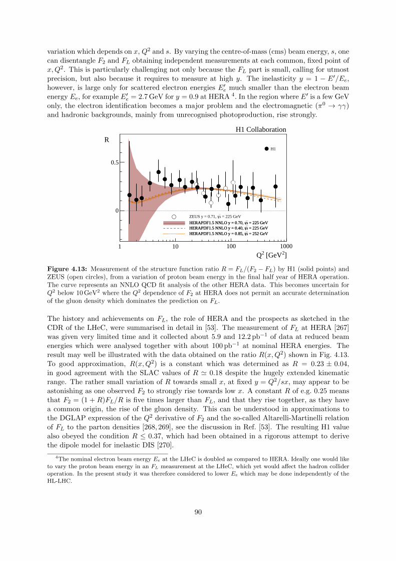
variation which depends on x, Q2 and s. By varying the centre-of-mass (cms) beam energy, s, onecan disentangle F2 and FL obtaining independent measurements at each common, fixed point ofx,Q2. This is particularly challenging not only because the FL part is small, calling for utmostprecision, but also because it requires to measure at high y. The inelasticity y = 1 − E′/Ee,however, is large only for scattered electron energies E′e much smaller than the electron beamenergy Ee, for example E′e = 2.7 GeV for y = 0.9 at HERA 4. In the region where E′ is a few GeVonly, the electron identification becomes a major problem and the electromagnetic (π0 → γγ)and hadronic backgrounds, mainly from unrecognised photoproduction, rise strongly.

1 10 100 1000

0

0.5

H1 Collaboration

R

]2 [GeV2Q

= 225 GeVsZEUS y = 0.71,

= 225 GeVsHERAPDF1.5 NNLO y = 0.70, = 225 GeVsHERAPDF1.5 NNLO y = 0.40, = 252 GeVsHERAPDF1.5 NNLO y = 0.85,

= 225 GeVsHERAPDF1.5 NNLO y = 0.70, = 225 GeVsHERAPDF1.5 NNLO y = 0.40, = 252 GeVsHERAPDF1.5 NNLO y = 0.85,

H1

Figure 4.13: Measurement of the structure function ratio R = FL/(F2 − FL) by H1 (solid points) andZEUS (open circles), from a variation of proton beam energy in the final half year of HERA operation.The curve represents an NNLO QCD fit analysis of the other HERA data. This becomes uncertain forQ2 below 10 GeV2 where the Q2 dependence of F2 at HERA does not permit an accurate determinationof the gluon density which dominates the prediction on FL.

The history and achievements on FL, the role of HERA and the prospects as sketched in theCDR of the LHeC, were summarised in detail in [53]. The measurement of FL at HERA [267]was given very limited time and it collected about 5.9 and 12.2 pb−1 of data at reduced beamenergies which were analysed together with about 100 pb−1 at nominal HERA energies. Theresult may well be illustrated with the data obtained on the ratio R(x,Q2) shown in Fig. 4.13.To good approximation, R(x,Q2) is a constant which was determined as R = 0.23 ± 0.04,in good agreement with the SLAC values of R ' 0.18 despite the hugely extended kinematicrange. The rather small variation of R towards small x, at fixed y = Q2/sx, may appear to beastonishing as one observed F2 to strongly rise towards low x. A constant R of e.g. 0.25 meansthat F2 = (1 + R)FL/R is five times larger than FL, and that they rise together, as they havea common origin, the rise of the gluon density. This can be understood in approximations tothe DGLAP expression of the Q2 derivative of F2 and the so-called Altarelli-Martinelli relationof FL to the parton densities [268, 269], see the discussion in Ref. [53]. The resulting H1 valuealso obeyed the condition R ≤ 0.37, which had been obtained in a rigorous attempt to derivethe dipole model for inelastic DIS [270].

4The nominal electron beam energy Ee at the LHeC is doubled as compared to HERA. Ideally one would liketo vary the proton beam energy in an FL measurement at the LHeC, which yet would affect the hadron collideroperation. In the present study it was therefore considered to lower Ee which may be done independently of theHL-LHC.

90

Parton Evolution at Low x

Parton distributions are to be extracted from experiment as their x dependence and flavoursharing are not predicted in QCD. They acquire a particular meaning through the theoreticalprescription of their kinematic evolution. PDFs, as they are frequently used for LHC analyses,are predominantly defined through the now classic DGLAP formalism, in which the Q2 depen-dence of parton distributions is regulated by splitting functions while the DIS cross section,determined by the structure functions, is calculable by folding the PDFs with coefficient func-tions. Deep inelastic scattering is known to be the most suited process to extract PDFs fromthe experiment, for which the HERA collider has so far delivered the most useful data. Throughfactorisation theorems the PDFs are considered to be universal such that PDFs extracted in epDIS shall be suited to describe for example Drell-Yan scattering cross sections in pp at the LHC.This view has been formulated to third order pQCD already and been quite successful in theinterpretation of LHC measurements, which by themselves also constrain PDFs in parton-partonscattering sub-processes.

As commented in Sec. 4.2.1, the question has long been posed about the universal validity ofthe DGLAP formalism, especially for the region of small Bjorken x where logarithms ∝ ln(1/x)become very sizeable. This feature of the perturbation expansion is expected to significantlymodify the splitting functions. This in turn changes the theory underlying the physics of partondistributions, and predictions for the LHC and its successor will correspondingly have to bealtered. This mechanism, for an equivalent Q2 of a few GeV2, is illustrated in Fig. 4.14, takenfrom Ref. [253]. It shows the x dependence of the gluon-gluon and the quark-gluon splittingfunctions, Pgg and Pqg, calculated in DGLAP QCD. It is observed that at NNLO Pgg stronglydecreases towards small x, becoming smaller than Pqg for x below 10−4. Resummation ofthe large ln(1/x) terms, see Ref. [253], here performed to next-to-leading log x, restores thedominance of the gg splitting over the qg one. Consequently, the gluon distribution in theresummed theory exceeds the one derived in pure DGLAP. While this observation has beensupported by the HERA data, it yet relies on limited kinematic coverage and precision. TheLHeC will examine this in detail, at a hugely extended range and is thus expected to resolve thelong known question about the validity of the BFKL evolution and the transition from DGLAPto BFKL as x decreases while Q2 remains large enough for pQCD to apply.

Kinematics of Higgs Production at the HL-LHC

The clarification of the evolution and the accurate and complete determination of the partondistributions is of direct importance for the LHC. This can be illustrated with the kinematics ofHiggs production at HL-LHC which is dominated by gluon-gluon fusion. With the luminosityupgrade, the detector acceptance is being extended into the forward region to pseudorapidityvalues of |η| = 4, where η = ln tan θ/2 is a very good approximation of the rapidity. In Drell-Yanscattering of two partons with Bjorken x values of x1,2 these are related to the rapidity via therelation x1,2 = exp (±η) ·M/

√s where

√s = 2Ep is the cms energy and M the mass of the

produced particle. It is interesting to see that η = ±4 corresponds to x1 = 0.5 and x = 0.00016for the SM Higgs boson of mass M = 125 GeV. Consequently, Higgs physics at the HL-LHCwill depend on understanding PDFs at high x, a challenge resolved by the LHeC too, and onclarifying the evolution at small x. At the FCC-hh, in its 100 TeV energy version, the small xvalue for η = 4 will be as low as 2 ·10−5. Both the laws of QCD and the resulting phenomenologyof particle production at the HL-LHC and its successor demand to clarify the evolution of theparton contents at small x as a function of the resolution scale Q2 [271–273]. This concerns inparticular the unambiguous, accurate determination of the gluon distribution, which dominatesthe small-x parton densities and as well the production of the Higgs boson in pp scattering.

91

0

0.1

0.2

0.3

0.4

0.5

10-510-410-310-210-11

x P(x)

x

αs = 0.28, nf = 4

LONLO

NNLONNLO+NLLx

PggPqg

Figure 4.14: Calculation of splitting functions Pgg (top, blue) and Pqg (bottom, brown) in resummedNNLO (solid) as compared to non-resummed calculations at LO (dotted), NLO (dashed) and NNLO(dashed-dotted) as functions of x for nf = 4 at a large value of αs corresponding to a Q2 of a few GeV2,from Ref. [253]. The resummed calculation is seen to restore the dominance of Pgg over Pqg as x becomessmall (towards the right side), which is violated at NNLO.

Indications for Resummation in H1 FL Data

The simultaneous measurement of the two structure functions F2 and FL is the cleanest wayto establish new parton dynamics at low x. This holds because their independent constraintson the dominating gluon density at low x ought to lead to consistent results. In other words,one may constrain all partons with a complete PDF analysis of the inclusive cross section inthe kinematic region where its FL part is negligible and confront the FL measurement withthis result. A significant deviation from FL data signals the necessity to introduce new, non-DGLAP physics in the theory of parton evolution, especially at small x. The salient value of theFL structure function results from its inclusive character enabling a clean theoretical treatmentas has early on been recognised [268, 269]. This procedure has recently been illustrated [253]using the H1 data on FL [274] which are the only accurate data from HERA at smallest x. Theresult is shown in Fig. 4.15. One observes the trend described above: the resummed predictionis higher than the pure NNLO curve, and the description at smallest x, below 5 · 10−4, appearsto be improved. The difference between the two curves increases as x decreases. However, dueto the peculiarity of the DIS kinematics, which relates x to Q2/sy, one faces the difficulty ofQ2 decreasing with x at fixed s for large y ≥ 0.6, which is the region of sensitivity to FL. Thusone not only wishes to improve substantially the precision of the FL data but also to increasesubstantially s in order to avoid the region of non-perturbative behaviour while testing theoryat small x. This is the double and principal advantage which the LHeC offers - a much increasedprecision and more than a decade of extension of kinematic range.

The Longitudinal Structure Function at the LHeC

Following the method described above, inclusive cross section data have been simulated forEp = 7 TeV and three electron beam energies Ee of 60, 30 and 20 GeV. The assumed integrated

92

101 102 103Q2 [GeV2]

0.2

0.1

0.0

0.1

0.2

0.3

0.4

0.5

0.6

F L(x

,Q2 )

x=8.77

105

x=1.29

104

x=1.69

104

x=2.24

104

x=3.19

104

x=4.02

104

x=5.40

104

x=6.87

104

x=9.58

104

x=1.21

103

x=1.57

103

x=2.43

103

x=3.03

103

x=4.02

103

x=5.41

103

x=7.36

103

x=9.86

103

x=1.84

102

H1 FL

NNLONNLO+NLLxData

Figure 4.15: Measurement of the longitudinal structure function FL, obtained as an average results overa number of x dependent points at fixed Q2, plotted vs Q2 with the corresponding x values indicatedin grey. Red curve: NNLO fit to the H1 cross section data; green curve: NNLO fit including NLLxresummation, from Ref. [253].

luminosity values are 10, 1 and again 1 fb−1, respectively. These are about a factor of a hundredlarger than the corresponding H1 luminosities. At large y, the kinematics is best reconstructedusing the scattered electron energy, E′e, and polar angle, θe. The experimental methods tocalibrate the angular and energy measurements are described in [267]. For the present studysimilar results are assumed: for E′e a scale uncertainty of 0.5 % at small y (compared to 0.2 %with H1) rising linearly to 1.2 %, in the range of y = 0.4 to 0.9. For the polar angle, giventhe superior quality of the anticipated LHeC Silicon tracker as compared to the H1 tracker,it is assumed that θe may be calibrated to 0.2 mrad, as compared to 0.5 mrad at H1. Theresidual photo-production background contamination is assumed to be 0.5 % at largest y, twicebetter than with H1. There is further an assumption made on the radiative corrections whichare assumed to be uncertain to 1 % and treated as a correlated error. The main challenge is toreduce the uncorrelated uncertainty, which here was varied between 0.2 and 0.5 %. This is aboutten to three times more accurate than the H1 result which may be a reasonable assumption: thehundred fold increase in statistics sets a totally different scale to the treatment of uncorrelateduncertainties, as from imperfect simulations, trigger efficiency or Monte Carlo statistics. Itis very difficult to transport previous results to the modern and future conditions. It could,however, be an important fix point if one knows that the most precise measurement of Z bosonproduction by ATLAS at the LHC had a total systematic error of just 0.5 % [275].

The method here used is that of a simple straight-line fit of σr = F2 − f(y)FL (Eq. (4.6)), inwhich FL is obtained as the slope of the f(y) dependence 5. The predictions for F2 and FL wereobtained using LO formulae for the PDF set of MSTW 2008. In this method any common factordoes not alter the absolute uncertainty of FL. This also implies that the estimated absolute erroron FL is independent of whether FL is larger or smaller than here assumed. For illustration,FL was scaled by a factor of two. Since f(y) ∝ y2, the accuracy is optimised with a non-linearchoice of lowered beam energies. The fit takes into account cross section uncertainties and their

5Better results were achieved by H1 using a χ2 minimisation technique, see Ref. [276], which for the roughestimate on the projected FL uncertainty at the LHeC has not been considered.

93

LHeC

H1

<H1>

FL

FL

FL

Figure 4.16: H1 measurement and LHeC simulation of data on the longitudinal structure functionFL(x,Q2). Green: Data by H1, for selected Q2 intervals from Ref. [274]; Blue: Weighted average of the(green) data points at fixed Q2; Red: Simulated data from an FL measurement at the LHeC with varyingbeam energy, see text. The H1 error bars denote the total measurement uncertainty. The LHeC innererror bars represent the data statistics, visible only for Q2 ≥ 200 GeV2, while the outer error bars are thetotal uncertainty. Since the FL measurement is sensitive only at high values of inelasticity, y = Q2/sx,each Q2 value is sensitive only to a certain limited interval of x values which increase with Q2. Thus eachpanel has a different x axis. The covered x range similarly varies with s, i.e. H1 x values are roughlytwenty times larger at a given Q2. There are no H1 data for high Q2, beyond 1000 GeV2, see Ref. [274].

correlations, calculated numerically following [58, 277], by considering each source separatelyand adding the results of the various correlated sources to one correlated systematic error whichis added quadratically to the statistical and uncorrelated uncertainties to obtain one total error.

The result is illustrated in Fig. 4.16 presenting the x-dependent results, for some selected Q2

values, of both H1, with their average over x, and the prospect LHeC results. It reflects thehuge extension of kinematic range, towards low x and high Q2 by the LHeC as compared toHERA. It also illustrates the striking improvement in precision which the LHeC promises toprovide. The FL measurement will cover an x range from 2 · 10−6 to above x = 0.01. Surely,when comparing with Fig. 4.15, one can safely expect that any non-DGLAP parton evolutionwould be discovered with such data, in their combination with a very precise F2 measurement.

A few comments are in order on the variation of the different error components with the kine-matics, essentially Q2 since the whole FL sensitivity is restricted to high y which in turn for eachQ2 defines a not wide interval of x values covered. One observes in Fig. 4.16 that the precisionis spoiled towards large x ∝ 1/y, see e.g. the result for Q2 = 8.5 GeV2. The assumptions on

94

the integrated luminosity basically define a Q2 range for the measurement. For example, thestatistical uncertainty for Q2 = 4.5 GeV2 and x = 10−5, a medium x value at this Q2 interval,is only 0.6 % (or 0.001 in absolute for FL = 0.22). At Q2 = 2000 GeV2 it rises to 21 % (or 0.012for FL = 0.064). One thus can perform the FL measurement at the LHeC, with a focus on onlysmall x, with much less luminosity than the 1 fb−1 here used. The relative size of the varioussystematic error sources also varies considerably, which is due to the kinematic relations betweenangles and energies and their dependence on x and Q2. This is detailed in [58]. It implies, for ex-ample, that the 0.2 mrad polar angle scale uncertainty becomes the dominant error at small Q2,which is the backward region where the electron is scattered near the beam axis in the directionof the electron beam. For large Q2, however, the electron is more centrally scattered and theθe calibration requirement may be more relaxed. The E′e scale uncertainty has a twice smallereffect than that due to the θe calibration at lowest Q2 but becomes the dominant correlatedsystematic error source at high Q2. The here used overall assumptions on scale uncertaintiesare therefore only rough first approximations and would be replaced by kinematics and detectordependent requirements when this measurement may be pursued. These could also exploit thecross calibration opportunities which result from the redundant determination of the inclusiveDIS scattering kinematics through both the electron and the hadronic final state. This had beennoted very early at HERA times, see Ref. [55,57,277] and was worked out in considerable detailby both H1 and ZEUS using independent and different methods. A feature used by H1 in theirFL measurement includes a number of decays such as π0 → γγ and J/ψ → e+e− for calibratingthe low energy measurement or K0

s → π+π− and Λ→ pπ for the determination of tracker scales,see Ref. [267].

It is obvious that the prospect to measure FL as presented here is striking. For nearly a decade,Guido Altarelli was a chief theory advisor to the development of the LHeC. In 2011, he publishesan article [276], in honour of Mario Greco, about The Early Days of QCD (as seen from Rome)in which he describes one of his main achievements [268], and persistent irritation, regardingthe longitudinal structure function, FL, and its measurement: . . . The present data, recentlyobtained by the H1 experiment at DESY, are in agreement with our [!this] LO QCD predictionbut the accuracy of the test is still far from being satisfactory for such a basic quantity. TheLHeC developments had not been rapid enough to let Guido see results of much higher qualityon FL with which the existence of departures from the DGLAP evolution, to high orders pQCD,may be expected to most safely be discovered.

4.2.4 Associated jet final states at low x

The dynamical effects from resummation or nonlinear corrections which we have discussed abovecan arise at the LHeC not only in the inclusive structure functions, as we have illustrated so far,but also in more exclusive observables describing the structure of the jet final states associatedto low-x DIS.

Baseline predictions for jet final states in DIS are obtained from perturbative finite-order calcu-lations (see e.g. [203, 278] for third-order calculations), supplemented by parton-shower MonteCarlo generators for realistic event simulation (as e.g. in [202]). But owing to the large phasespace opening up at LHeC energies and the complex kinematics possibly involving multiple hardscales, jet events are potentially sensitive to soft-gluon coherence effects of initial-state radia-tion [225, 279–281], which go beyond finite-order perturbative evaluations and collinear partonshowers, and show up as logarithmic x → 0 corrections to all orders of perturbation theory.These corrections can be resummed, and combined with large-x contributions, via CCFM exclu-sive evolution equations [225, 279], and affect the structure of jet multiplicities and angular jetcorrelations [281] as well as heavy quark distributions [280]. Observables based on forward jets,

95

transverse energy flow, angle and momentum correlations constitute probes of low-x dynamicsin DIS final states [282–284]. Phenomenological studies started with HERA [285–287] and willcontinue with the LHeC.

Computational tools are being developed to address the structure of multi-jet final states byincluding low-x dynamical effects. These include CCFM Monte Carlo tools [288, 289], off-shellmatrix element parton-level generators [290, 291], BFKL Monte Carlo generators [292–294].Fig. 4.17 gives an example of transverse momentum correlations in DIS di-jet and three-jet finalstates computed with the Monte Carlo [288], compared with the measurements [295].

b

b

b

b

HZToolAnalysis/hz07062 datab

JH 2013 set1JH 2013 set20.0005 < x < 0.001

1

10 1

10 2

10 3

10 4

10 5

10 6tri-jet (ZEUS Nuclear Physics B 786 (2007) 152)

dσ

/d

∑~p

jet

1,2

td

x

1 10 1 10 20

0.5

1

1.5

2

| ∑~pjet 1,2t |(GeV)

MC

/D

ata

b

b

b

b

HZToolAnalysis/hz07062 datab

JH 2013 set1JH 2013 set20.0005 < x < 0.001

10 2

10 3

10 4

10 5

10 6

10 7

10 8di-jet (ZEUS Nuclear Physics B 786 (2007) 152)

dσ

/d|∆

~pje

t1

,2t

|/(2

Eje

t1T

)dx

0 0.2 0.4 0.6 0.8 10

0.5

1

1.5

2

|∆~pjet 1,2t |/(2E

jet1T )

MC

/D

ata

Figure 4.17: Momentum correlations in DIS multi-jet final states at low x computed from the CCFMMonte Carlo [288] with TMD parton densities JH2013 [296], compared with the measurements [295]:(left) tri-jets; (right) di-jets.

Furthermore, exclusive parton branching formalisms are being proposed in which not only gluondistributions but also quark distributions are treated at unintegrated level in transverse momen-tum [297–299]. This is instrumental in connecting low-x approaches with DGLAP approachesto parton showers beyond leading order [300,301]. Applications of these new developments haveso far been mostly carried out for final states in hadron-hadron collisions, while extensions tolepton-hadron collisions are underway. Fig. 4.18 gives examples of transverse momentum spectrain low-mass Drell-Yan lepton pair production computed in [302] by the parton branching (PB)method [298], compared with the measurements [303] and [304].

4.2.5 Relation to Ultrahigh Energy Neutrino and Astroparticle physics

The small-x region probed by the LHeC is also very important in the context of ultra-high energyneutrino physics and astroparticle physics. Highly energetic neutrinos provide a unique windowinto the Universe, due to their weak interaction with matter, for a review see for example [305].They can travel long distances from distant sources, undeflected by the magnetic fields insideand in between galaxies, and thus provide complementary information to cosmic rays, gammarays and gravitational wave signals. The IceCube observatory on Antarctica [306] is sensitiveto neutrinos with energies from 100 GeV up (above 10 GeV with the use of their Deep Coredetector). Knowledge about low-x physics becomes indispensable in two contexts: neutrinointeractions and neutrino production. At energies beyond the TeV scale the dominant part of thecross section is due to the neutrino DIS CC and NC interaction with the hadronic targets [305].

96

b bb b

b b

bb

b

b

b

b NuSeaMCatNLO PB-NLO-2018-Set2 (exp+mod)MCatNLO PB-NLO-2018-Set2 (scale)4.2 < M

µ+µ− < 5.2 GeV

10−2

10−1

1

10 1

10 2

NuSea: Drell-Yan√

s = 38.8 GeV, −0.05 < xF < 0.15(2

E)/

(π√

s)dσ

/dx

Fdp

2 T(p

b/G

eV)

b b b b b b b b b b b

0 0.5 1 1.5 2 2.5 3 3.50.50.60.70.80.9

11.11.21.31.4

pT (GeV)

MC

/Dat

a

b b

bb

b

b

b

b b

b bb

b PHENIXMCatNLO PB-NLO-2018-Set2 (exp+mod)MCatNLO PB-NLO-2018-Set2 (scale)4.8 < m

µ+µ− < 8.2 GeV

10−2

10−1

1

10 1

10 2

PHENIX: Drell-Yan√

s = 200 GeV, 1.2 < |y| < 2.2

1/(2

πp T

)d2 σ

/dy

/dp

T(p

b/G

eV2 )

b b b b b b b b b b b b

1 2 3 4 5 6

0.51

1.52

2.53

3.54

pT (GeV)

MC

/Dat

a

Figure 4.18: Transverse momentum spectra in low-mass Drell-Yan lepton pair production [302] fromthe parton branching (PB) method, compared with (left) NuSea measurements [303] and (right) PHENIXmeasurements [304].

10-8

10-7

10-6

10-5

10-4

10-3

10-2

10-1

1

10 2 10 3 10 4 10 5 10 6 10 7 10 8 10 9 10 10 10 11

Total CC cross section

valence quarks

ud sea quarks

cs quarks

bt quarks

Eν [GeV]

σC

C(ν

N) [µ

b]

Figure 4.19: Charged current cross section for the neutrino - nucleon interaction on a isoscalar targetas a function of neutrino energy. The total CC cross section is broken down into several contributionsdue to valence, up-down,strange-charm and bottom-top quarks. The calculation was based on Ref. [307].

In Fig. 4.19 we show the charged current neutrino cross section as a function of the neutrinoenergy for an isoscalar target (in the laboratory frame where the target is at rest), using acalculation [307] based on the resummed model in [230]. We see that at energies below ∼ 50 TeVthe cross section grows roughly linearly with energy, and in this region it is dominated bycontributions from the large-x valence region. Beyond that energy the neutrino cross sectiongrows slower, roughly as a power ∼ Eλν with λ ' 0.3. This high energy behaviour is totally

97

controlled by the small-x behaviour of the parton distributions. The dominance of the seacontributions to the cross section is clearly seen in Fig. 4.19. To illustrate more precisely thecontributing values of x and Q2, in Fig. 4.20 we show the differential cross section for the CCinteraction xQ2dσCC/dxdQ2 for a neutrino energy Eν = 1011 GeV (in the frame where thehadronic target is at rest). We see a clear peak of the cross section at roughly a value ofQ2 = M2

W and an x value

x ' M2W

2MEν, (4.8)

which in this case is about 3×10−8. We note that IceCube extracted the DIS cross section from

Figure 4.20: Differential charged current neutrino cross section 105 ·xQ2dσCC/dxdQ2 [nb] as a functionof Q2 and x for fixed neutrino energy Eν = 1011 GeV. Left: surface plot; right: contour plot.

neutrino observations [308] in the region of neutrino energies 10 − 1000 TeV. The extractionis consistent, within the large error bands, with the predictions based on the QCD, like thoseillustrated in Fig. 4.19. It is important to note that the IceCube extraction is limited to theseenergies by the statistics due to the steeply falling flux of neutrinos at high energy. We thussee that the neutrino interaction cross section at high energies is sensitive to a region which iscurrently completely unconstrained by existing precision DIS data.

Another instance where dynamics at low x are crucial for neutrino physics is in understand-ing the mechanisms of ultra-high energy neutrino production. The neutrinos are produced ininteractions which involve hadrons, either in γp or in pp interactions. They emerge as decayproducts of pions, kaons and charmed mesons, and possibly beauty mesons if the energy is highenough [309]. For example, in the atmosphere neutrinos are produced in the interactions of thehighly energetic cosmic rays with nitrogen and oxygen nuclei. The lower energy part of theatmospheric neutrino spectrum, up to about 100 TeV or so, is dominated by the decay of pionsand kaons. This is called the conventional atmospheric neutrino flux. Above that energy theneutrino flux is dominated by the decay of the shorter-lived charmed mesons. Thus, this part ofthe neutrino flux is called the prompt-neutrino flux. The reason why the prompt-neutrino fluxdominates at high energies is precisely related to the life-time of the intermediate mesons (andalso baryons like Λc). The longer lived pions and kaons have a high probability of interactingbefore they decay, thus degrading their energy and leading to a steeply falling neutrino flux.The cross section for the production of charmed mesons is smaller than that for pions and kaons,but the charmed mesons D±, D0, Ds and baryon Λc live shorter than pions and kaons, and thus

98

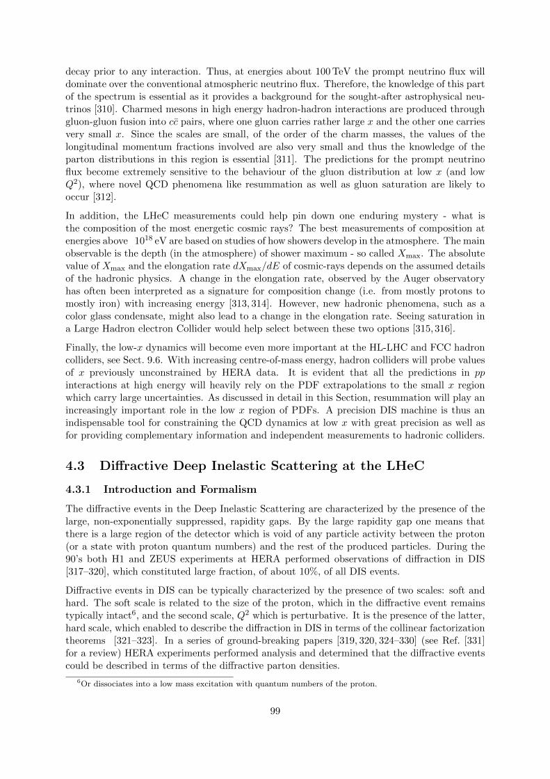
decay prior to any interaction. Thus, at energies about 100 TeV the prompt neutrino flux willdominate over the conventional atmospheric neutrino flux. Therefore, the knowledge of this partof the spectrum is essential as it provides a background for the sought-after astrophysical neu-trinos [310]. Charmed mesons in high energy hadron-hadron interactions are produced throughgluon-gluon fusion into cc pairs, where one gluon carries rather large x and the other one carriesvery small x. Since the scales are small, of the order of the charm masses, the values of thelongitudinal momentum fractions involved are also very small and thus the knowledge of theparton distributions in this region is essential [311]. The predictions for the prompt neutrinoflux become extremely sensitive to the behaviour of the gluon distribution at low x (and lowQ2), where novel QCD phenomena like resummation as well as gluon saturation are likely tooccur [312].

In addition, the LHeC measurements could help pin down one enduring mystery - what isthe composition of the most energetic cosmic rays? The best measurements of composition atenergies above 1018 eV are based on studies of how showers develop in the atmosphere. The mainobservable is the depth (in the atmosphere) of shower maximum - so called Xmax. The absolutevalue of Xmax and the elongation rate dXmax/dE of cosmic-rays depends on the assumed detailsof the hadronic physics. A change in the elongation rate, observed by the Auger observatoryhas often been interpreted as a signature for composition change (i.e. from mostly protons tomostly iron) with increasing energy [313, 314]. However, new hadronic phenomena, such as acolor glass condensate, might also lead to a change in the elongation rate. Seeing saturation ina Large Hadron electron Collider would help select between these two options [315,316].

Finally, the low-x dynamics will become even more important at the HL-LHC and FCC hadroncolliders, see Sect. 9.6. With increasing centre-of-mass energy, hadron colliders will probe valuesof x previously unconstrained by HERA data. It is evident that all the predictions in ppinteractions at high energy will heavily rely on the PDF extrapolations to the small x regionwhich carry large uncertainties. As discussed in detail in this Section, resummation will play anincreasingly important role in the low x region of PDFs. A precision DIS machine is thus anindispensable tool for constraining the QCD dynamics at low x with great precision as well asfor providing complementary information and independent measurements to hadronic colliders.

4.3 Diffractive Deep Inelastic Scattering at the LHeC

4.3.1 Introduction and Formalism

The diffractive events in the Deep Inelastic Scattering are characterized by the presence of thelarge, non-exponentially suppressed, rapidity gaps. By the large rapidity gap one means thatthere is a large region of the detector which is void of any particle activity between the proton(or a state with proton quantum numbers) and the rest of the produced particles. During the90’s both H1 and ZEUS experiments at HERA performed observations of diffraction in DIS[317–320], which constituted large fraction, of about 10%, of all DIS events.

Diffractive events in DIS can be typically characterized by the presence of two scales: soft andhard. The soft scale is related to the size of the proton, which in the diffractive event remainstypically intact6, and the second scale, Q2 which is perturbative. It is the presence of the latter,hard scale, which enabled to describe the diffraction in DIS in terms of the collinear factorizationtheorems [321–323]. In a series of ground-breaking papers [319, 320, 324–330] (see Ref. [331]for a review) HERA experiments performed analysis and determined that the diffractive eventscould be described in terms of the diffractive parton densities.

6Or dissociates into a low mass excitation with quantum numbers of the proton.

99

The precise measurement of the diffractive DIS in wide kinematic range can provide uniqueinsights into many facets of the strong interaction dynamics. Because of the presence of the largerapidity gap, it has been understood that the diffractive process proceeds through the exchange ofthe composite object which preserves color neutrality, and has quantum numbers of the vacuum.Thus the mechanism through which a composite object interacts perturbatively [332–338] canoffer information about the confinement and in general about emergent phenomena in stronginteraction. It has been established some time ago [339–342] that the diffractive phenomenaare closely related to the low-x dynamics, and in particular to the partonic structure of theproton in this regime. Therefore an investigation of diffraction can offer unique insights into therole and importance of the higher twists and the non-linear parton evolution. It has been alsoknown [343] that there is a relation between the diffraction in ep and nuclear shadowing. Thisrelation has been used for example to successfully predict the amount of the shadowing in someprocesses at LHC ultra peripheral collisions [344, 345]. Finally, precise measurements of thediffractive structure functions in the extended kinematic range of LHeC with respect to HERAwill allow for the accurate extraction of diffractive parton distribution functions and providemore stringent constraints on the uncertainties. This in turn will facilitate the tests of the rangeof validity of perturbative factorisation [321–323] and potential importance of the higher twisteffects.

In the following we will present the studies of inclusive diffraction that will be possible at theLHeC. The detailed analysis was performed in Ref. [346], and we shall summarize these results inthis and two following subsections. The LHeC will substantially extend the kinematic coverageof the HERA analyses, leading to much more detailed tests of theoretical ideas than have beenpossible hitherto. Although the analysis done in [346] and summarized here was done at NLOof QCD, it is worth noting that similar analyses in the HERA context have recently extendedto NNLO [347].

X

kk'

p p'

(ξ)

(β)

(Q2)

(t)

qe

pY

Figure 4.21: A diagram of a diffractive NC event in DIS together with the corresponding variables, inthe one-photon exchange approximation. The incoming proton scatters elastically or is dissociated intoa low mass excitation Y . The system of particles denoted by X is then separated from the proton (or itsexcitation Y ) by a large rapidity gap. Double line indicates a diffractive exchange in the t channel.

Diffractive deep inelastic event is schematically depicted in the diagram shown in Fig. 4.21. It isassumed that the process proceeds through the neutral current exchange. Charged currents couldalso be considered and were measured at HERA [326] but with large statistical uncertaintiesand in a very restricted region of phase space. The LHeC and the FCC-eh will allow to measurecharge currents in diffractive DIS with larger statistics and more extended kinematics than atHERA. However, in the study [346] summarized here, only neutral currents were considered,hence we shall also limit ourselves to that case.

100

The incoming electron or positron, with four momentum k, scatters off the proton, with fourmomentum p. Here, we only consider protons, though in principle one could also have nuclei.The inclusive diffraction in the nuclear case will be considered in Chapter 6. The interactionproceeds through the exchange of a virtual photon with four-momentum q and the diffractiveexchange in the t channel (indicated by the double line in Fig. 4.21). The kinematic variablesfor such an event include the standard deep inelastic variables

Q2 = −q2 , x =−q2

2p · q , y =p · qp · k , (4.9)

where Q2 is the (minus) photon virtuality, x is the Bjorken variable and y the inelasticity of theprocess. In addition, the variables

s = (k + p)2 , W 2 = (q + p)2 , (4.10)

are the electron-proton centre-of-mass energy squared and the photon-proton centre-of-massenergy squared, respectively. A diffractive event ep→ eXY is uniquely characterized by thepresence of the large rapidity gap between the diffractive system, with the invariant mass MX

and the final proton (or its low-mass excitation) Y with four momentum p′. Therefore in orderto fully describe the diffractive event in DIS, additional set of variables is necessary. They aredefined as

t = (p− p′)2 , ξ =Q2 +M2

X − tQ2 +W 2

, β =Q2

Q2 +M2X − t

. (4.11)

In the above t is the squared four-momentum transfer at the proton vertex, ξ (alternativelydenoted by xIP ) can be interpreted as the momentum fraction of the diffractive exchange withrespect to the incoming hadron, and β is the momentum fraction of the struck parton withrespect to the diffractive exchange. The two diffractive momentum fractions are constrained togive Bjorken-x, x = βξ.

The kinematic range in (β,Q2, ξ) that we consider at the LHeC is restricted by the followingcuts:

• Q2 ≥ 1.8 GeV2: due to the fact that the initial distribution for the DGLAP evolution isparameterised at µ2

0 = 1.8 GeV2. The renormalisation and factorisation scales are takento be equal to Q2.

• ξ < 0.4: constrained by physical and experimental limitations. This rather high ξ value isan experimental challenge and physically enters the phase-space region where the Pomeroncontribution should become negligible compared with sub-leading exchanges. Within thetwo-component model, see Eq. (4.16) below, at high ξ the cross section is dominated by thesecondary Reggeon contribution, which is poorly fixed by the HERA data. Nevertheless,we present this high ξ (> 0.1) region for illustrative purpose and for the sake of discussionof the fit results below. It is also worth mentioning that with appropriate detector designit might be possible to reach this region of high ξ which would be highly interesting andprovide new constraints on the Pomeron and Reggeon contributions with respect to HERA.

In Fig. 4.22 the accessible kinematic range in (x,Q2) is shown for four machines: HERA, EIC,LHeC and FCC-eh [346]. For the LHeC design the range in x is increased by a factor ∼ 20 overHERA and the maximum available Q2 by a factor ∼ 100. The FCC-eh machine would furtherincrease this range with respect to LHeC by roughly one order of magnitude in both x and Q2.We also show the EIC kinematic region for comparison, which could cover high x as well as lowQ2 range. The three different machines are clearly complementary in their kinematic coverage,with LHeC and EIC adding sensitivity at lower and higher x than HERA, respectively.

101

θ > 1°0.001 < y < 0.96β < 1ξ < 0.4

Q2

[GeV

2 ]

x = βξ

ZEUS-LRGH1-LRGHERA-FLPS

10-2

10-1

100

101

102

103

104

105

106

107

10-8 10-7 10-6 10-5 10-4 10-3 10-2 10-1

FCC-eh50 TeV60 GeV

FCC-eh50 TeV60 GeV

Q2

[GeV

2 ]

x = βξ

10-2

10-1

100

101

102

103

104

105

106

107

10-8 10-7 10-6 10-5 10-4 10-3 10-2 10-1

LHeC7 TeV

60 GeV

LHeC7 TeV

60 GeV

Q2

[GeV

2 ]

x = βξ

10-2

10-1

100

101

102

103

104

105

106

107

10-8 10-7 10-6 10-5 10-4 10-3 10-2 10-1

EIC0.25 TeV21 GeV

EIC0.25 TeV21 GeV

Q2

[GeV

2 ]

x = βξ

10-2

10-1

100

101

102

103

104

105

106

107

10-8 10-7 10-6 10-5 10-4 10-3 10-2 10-1

HERA0.92 TeV27.5 GeV

HERA0.92 TeV27.5 GeV

Figure 4.22: Kinematic phase space for inclusive diffraction in (x,Q2) for the Electron Ion Collider(EIC) (magenta region), the LHeC (orange region) and the FCC-eh (dark blue region) as compared withthe HERA data (light blue region, ZEUS-LRG [327], H1-LRG [330], HERA-FLPS [348]). The acceptancelimit for the electron in the detector design has been assumed to be 1, and we take ξ < 0.4 (see text fordetails). Figure taken from [346].

In Fig. 4.23 the phase space specific to diffractive processes in (β,Q2) is shown for fixed ξ forthe LHeC [346]. Thanks to the high center of mass energy the LHeC machine probes very smallvalues of ξ, reaching 10−4 with a wide range of β, and for the perturbative values of Q2. Ofcourse, the ranges in β and ξ are correlated since x = βξ. Therefore, for small values of ξ onlylarge values of β are accessible while for large ξ the range in β extends to very small values.The two horizontal lines denote Q2 = 5 GeV2 and m2

t threshold. The first value is the scalecorresponding to the lowest data in the DGLAP fit and DPDF extraction discussed later. Thedashed line corresponds to the kinematic limit of the tt production.

In analogy to the inclusive case, the diffractive cross sections in the neutral current case can berepresented in the form of the reduced cross sections [326]:

d3σD(3)

dξdβdQ2=

2πα2em

βQ4Y+ σ

D(3)red , (4.12)

where Y+ = 1+(1−y)2 and the reduced cross sections can be expressed in terms of two diffractivestructure functions FD

2 and FDL . In the one-photon approximation, the relations are

σD(3)red = F

D(3)2 (β, ξ,Q2)− y2

Y+F

D(3)L (β, ξ,Q2) . (4.13)

In the above, both cross sections and structure functions are integrated over the momentum

transfer t. This is indicated by σD(3), FD(3)2 , F

D(3)L notation where ‘3’ means that the cross

section or structure function depends on three variables, (β, ξ,Q2). Depending on the detector

setup and luminosity it could also be possible to measure σD(4), FD(4)2 , F

D(4)L which depend on

four variables (β, ξ,Q2, t). Also in principle, for the neutral current case, one needs to considerZ0 exchange in addition to photon, but in the analysis [346] presented here it was neglected.

102

Ep = 7 TeV, Ee = 60 GeV, ymin = 0.001, ymax = 0.96

10-2

10-1

100

101

102

103

104

105

10-6 10-5 10-4 10-3 10-2 10-1

Q2

[GeV

2 ]

β

ξ = 0.1

bins MX = 2 mt

5 GeV2

m2t

10-2

10-1

100

101

102

103

104

105

10-5 10-4 10-3 10-2 10-1

Q2

[GeV

2 ]

β

ξ = 0.01

5 GeV2

m2t

10-2

10-1

100

101

102

103

104

105

10-4 10-3 10-2 10-1

Q2

[GeV

2 ]

β

ξ = 0.001

5 GeV2

m2t

10-2

10-1

100

101

102

103

104

105

10-3 10-2 10-1

Q2

[GeV

2 ]

β

ξ = 0.0001

5 GeV2

m2t

10-2

10-1

100

101

102

103

104

105

10-2 10-1

Q2

[GeV

2 ]

β

ξ = 1e-05

5 GeV2

m2t

Figure 4.23: Kinematic phase space for the inclusive diffraction in (β,Q2) for fixed values of ξ for theLHeC design. The horizontal lines indicate correspondingly, Q2 = 5 GeV2, the lowest data value for theDGLAP fit performed in this study and m2

t the 6-flavour threshold. The dashed line marks the kinematiclimit for tt production. Figure taken from [346].

Both σD(3)red and σ

D(4)red have been measured at the HERA collider [319,320,324–330] and used to

obtain QCD-inspired parameterisations.

The standard perturbative QCD approach to diffractive cross sections is based on the collinearfactorisation [321–323]. In these works it was demonstrated that, similarly to the inclusive DIScross section, the diffractive cross section can be written, up to terms of order O(Λ2/Q2), whereΛ is the hadronic scale, in a factorised form

dσep→eXY (β, ξ,Q2, t) =∑i

∫ 1

βdz dσei

(β

z,Q2

)fDi (z, ξ,Q2, t) , (4.14)

where the sum is performed over all parton flavours (gluon, d-quark, u-quark, etc.). The hardscattering partonic cross section dσei, corresponding to the short distance physics, can be com-puted order by order in perturbative QCD and is the same as in the inclusive deep inelastic scat-tering case. The long distance part fD

i is the diffractive parton distribution function (DPDF).These functions can be interpreted as conditional probabilities for finding partons in the pro-ton provided the latter is scattered into the final state system Y with specified 4-momentump′. They are evolved using the DGLAP evolution equations [349–352] similarly to the inclusivecase. The analogous formula to 4.14 for the t-integrated structure functions reads

FD(3)2/L (β, ξ,Q2) =

∑i

∫ 1

β

dz

zC2/L,i

(βz

)f

D(3)i (z, ξ,Q2) , (4.15)

where the coefficient functions C2/L,i are the same as in inclusive DIS, and can be computedperturbatively in QCD.

103

Fits to the diffractive structure functions usually [326,328] parameterise the diffractive PDFs ina two component model, which is a sum of two diffractive exchange contributions, IP and IR:

fD(4)i (z, ξ,Q2, t) = fpIP (ξ, t) f IPi (z,Q2) + fpIR(ξ, t) f IRi (z,Q2) . (4.16)

For both of these terms proton vertex factorisation is separately assumed, meaning that thediffractive exchange can be interpreted as colourless objects called a Pomeron or a Reggeonwith parton distributions f IP ,IRi (β,Q2). Note that, this factorization is completely differentthan the collinear factorization for the structure functions mentioned above. It is an additionalassumption motivated by the Regge theory and supported by the fits to the diffractive data.The flux factors fpIP ,IR(ξ, t) represent the probability that a Pomeron/Reggeon with given valuesξ, t couples to the proton. They are parameterised using the form motivated by Regge theory,

fpIP ,IR(ξ, t) = AIP ,IReBIP ,IRt

ξ2αIP ,IR(t)−1, (4.17)

with a linear trajectory αIP ,IR(t) = αIP ,IR(0) + α′IP ,IR t, BIP ,IR being the t slope and normalizationfactors AIP ,IR. One can also introduce the diffractive PDFs which correspond to the t-integratedcross sections

fD(3)i (z, ξ,Q2) = φ p

IP (ξ) f IPi (z,Q2) + φ pIR(ξ) f IRi (z,Q2) , (4.18)

with

φ pIP ,IR(ξ) =

∫dt fpIP ,IR(ξ, t) . (4.19)

Note that, the notions of Pomeron and Reggeon used here to model hard diffraction in DIS are,in principle, different from those describing the soft hadron-hadron interactions; in particular,the parameters of the fluxes may be different.

As is usual for the DGLAP evolution one needs to specify suitable initial conditions (see [346] fordetails). The diffractive parton distributions of the Pomeron at the initial scale µ2

0 = 1.8 GeV2

are parameterised aszf IPi (z, µ2

0) = AizBi(1− z)Ci , (4.20)

as in ZEUS-SJ parametrisation, and where i is a gluon or a light quark and the momentumfraction z = β in the case of quarks. In the diffractive parameterisations the contributionsof all the light quarks (anti-quarks) are assumed to be equal. For the treatment of heavyflavours, a variable flavour number scheme (VFNS) is adopted, where the charm and bottomquark DPDFs are generated radiatively via DGLAP evolution, and no intrinsic heavy quarkdistributions are assumed. The structure functions are calculated in a General-Mass VariableFlavour Number scheme (GM-VFNS) [353,354] which ensures a smooth transition of F2,L acrossthe flavour thresholds by including O(m2

h/Q2) corrections. The parton distributions for the

Reggeon component are taken from a parameterisation which was obtained from fits to the pionstructure function [355,356].

In Eq. (4.16) the normalisation factors of fluxes, AIP ,IR and of DPDFs, Ai enter in the product.In order to resolve the ambiguity7 the normalization AIP was fixed and f IRi (z,Q2) was normalisedto the pion structure function. This resulted in Ai and AIR being well defined free fit parameters.For full details of the parametrisations, see Ref. [346].

7Here, as in the HERA fits, AIP is fixed by normalizing φ pIP (0.003) = 1.

104

4.3.2 Pseudodata for the reduced cross section

In order to generate the pseudodata for the LHeC one needs to use certain model which ex-trapolates the data from HERA. In the study [346] described here, the reduced cross sectionswere extrapolated using the ZEUS-SJ DPDFs. Following the scenario of the ZEUS fit [328] wework within the VFNS scheme at NLO accuracy. As mentioned before, there exists calculationsat NNLO accuracy, however for the purposes of this analysis it is sufficient to work at NLOaccuracy. The transition scales for DGLAP evolution are fixed by the heavy quark masses,µ2 = m2

h and the structure functions are calculated in the Thorne–Roberts GM-VFNS [357].The Reggeon PDFs are taken from the GRV pion set [356], the numerical parameters are takenfrom Tables 1 and 3 of Ref. [328], the heavy quark masses are mc = 1.35 GeV,mb = 4.3 GeV,and αs(M

2Z) = 0.118.

The pseudodata were generated [346] using the extrapolation of the fit to HERA data, whichprovides the central values, amended with a random Gaussian smearing with standard deviationcorresponding to the relative error δ. An uncorrelated 5% systematic error was assumed givinga total uncertainty

δ =√δ2

sys + δ2stat . (4.21)

The statistical error was computed assuming a very modest integrated luminosity of 2 fb−1, seeRef. [35,36]. For the binning adopted in the study [346], the statistical uncertainties have a verysmall effect on the uncertainties in the extracted DPDFs. Obviously, a much larger luminositywould allow a denser binning that would result in smaller DPDF uncertainties. An extendedanalysis in principle could be performed for the σD(4) which would include t dependence, providedthe latter could be extracted by using proper forward instrumentation.

In Fig. 4.24 we show a subset of the simulated data for the diffractive reduced cross section ξσred

as a function of β in selected bins of ξ and Q2 for the LHeC [346]. For the most part the errorsare very small, and are dominated by the systematics. The breaking of Regge factorisation,evident at large ξ, comes from the large Reggeon contribution in that region, whose validitycould be further investigated at the LHeC.

We see that for the LHeC parameters, the integrated luminosity is sufficient for the precisemeasurement of the diffractive reduced cross section. The study could be further refined byimplementing more information about the potential sources of the systematic errors includingcorrelations. In addition, by varying the centre-of-mass energy one could extract also longi-

tudinal structure function FD(3)L . Pioneering measurement of this quantity was performed at

HERA [358], albeit with very limited precision. Longitudinal diffractive structure function couldbe extremely valuable information, as it is an independent diffractive structure function andprovides with an additional constraint on the diffractive PDFs. It also may be more sensitivequantity to the higher twist contribution. More detailed analysis need to be however performedto determine the feasibility and precision of such measurement at the LHeC.

4.3.3 Potential for constraining diffractive PDFs at the LHeC

We next proceed to discuss the prospects for the extraction and constraining the diffractive PDFsfrom the future experimental data obtained at the LHeC. The strategy to assess the constrainingpotential was developed in [346] which we summarize below. First, the central values of thepseudodata using the central set of the ZEUS-SJ fit are generated, that are distributed accordingto a Gaussian with experimental width given by Eq. (4.21), that also provides the uncertaintyin the pseudodata. After that, the pseudodata in a fit are included alongside the existing HERAdata using the same functional form of the initial parametrisation. The quality of the resulting

105

e p Ep = 7 TeV, Ee = 60 GeV, L = 2 fb-1

0

0.05

0.1

0.15

0.2

0.25

0.3

Q2 = 10 GeV2

ξσre

d

ξ = 0.1ξ = 0.01ξ = 0.001ξ = 0.0001

Q2 = 100 GeV2

ξ = 0.1ξ = 0.01ξ = 0.001ξ = 0.0001

0

0.05

0.1

0.15

0.2

0.25

0.0001 0.001 0.01 0.1

Q2 = 1000 GeV2

ξσre

d

β

ξ = 0.1ξ = 0.01ξ = 0.001

0.0001 0.001 0.01 0.1 1

Q2 = 10000 GeV2

β

ξ = 0.1ξ = 0.01

Figure 4.24: Selected subset of the simulated data for the diffractive reduced cross section as a functionof β in bins of ξ and Q2 for ep collisions at the LHeC. Based on the extrapolation of the ZEUS-SJ fitto HERA data. The curves for ξ = 0.01, 0.001, 0.0001 are shifted up by 0.04, 0.08, 0.12, respectively.Integrated luminosity is taken to be 2 fb−1. Figure taken from [346].

fit was very good, as it was expected, and χ2/ndf ∼ 1 was obtained, which demonstrated theconsistency of the approach.

To evaluate the experimental precision with which the DPDFs can be determined, several pseu-dodata sets, corresponding to independent random error samples, were generated [346]. Eachpseudodata set was fitted separately. The minimal value of Q2 for the data considered in thefits was set to Q2

min = 5 GeV2. The reason for this cut-off is to show the feasibility of thefits including just the range in which standard twist-2 DGLAP evolution is expected to betrustable. At HERA, the Q2

min values giving acceptable DGLAP (twist-2) fits were 8 GeV2 [326]and 5 GeV2 [327] for H1 and ZEUS, respectively. Below these values the fits were deteriorating.The maximum value of ξ was set by default to ξmax = 0.1, above which the cross section startsto be dominated by the Reggeon exchange. The binning adopted in the study [346] correspondsroughly to 4 bins per order of magnitude in each of ξ, β,Q2. For Q2

min = 5 GeV2, ξmax = 0.1and below the top threshold this results in 1229 pseudodata points for the LHeC. The top-quarkregion adds 17 points for the LHeC. The LHeC offers window to study top quark contribution indiffraction in limited range of kinematics, going further to FCC-eh would expand that possibilitygreatly. Lowering Q2

min down to 1.8 GeV2 we get 1589 pseudodata points, while increasing ξ upto 0.32 adds around 180 points for the LHeC machine. Of course, in the case of the lower valueof Q2 the collinear formalism with leading twist contribution may become questionable. Giventhe fact that the ZEUS and H1 fits based on DGLAP did not desrcibe well the data in the lowQ2 region may indicate that other effects may start playing important role. In Ref. [359] it wasargued that this deviation from the leading twist DGLAP evolution might be an indication forhigher twist effects. Larger lever arm in x, and high precision of the data from the LHeC willbe extremely helpful in mapping out the region of validity of the leading twist description andshould help to constrain the higher twist effects in diffraction. Dedicated studies of the LHeC

106

potential in this area will need to be performed,

The potential for determination of the gluon DPDF was investigated by fitting the inclusivediffractive DIS pseudodata with two models with different numbers of parameters, named Sand C (see Ref. [346] for details) with αIP,IR(0) fixed, in order to focus on the shape of thePomeron’s PDFs. At HERA, both S and C fits provide equally good descriptions of the datawith χ2/ndf = 1.19 and 1.18, respectively, despite different gluon DPDF shapes. The LHeCpseudodata are much more sensitive to gluons, resulting in χ2/ndf values of 1.05 and 1.4 for theS and C fits, respectively. It also shows clearly the potential of the LHeC to better constrainthe low-x gluon and, therefore, unravel eventual departures from standard linear evolution.Gluon DPDFs from the 5% simulations

Ep = 7 TeV, Q2 > 4.2 GeV2, 1229 data points.

0 0.5

1 1.5

2 2.5

3 3.5

4

10-5 10-4 10-3 10-2 10-1 100

zg

z

ZEUS-SJABC

0 0.5

1 1.5

2 2.5

3 3.5

4

10-5 10-4 10-3 10-2 10-1 100

μ2 = 6 GeV2

0

2

4

6

8

10

10-5 10-4 10-3 10-2 10-1 100

z

0

2

4

6

8

10

10-5 10-4 10-3 10-2 10-1 100

μ2 = 20 GeV2

0 2 4 6 8

10 12 14 16

10-5 10-4 10-3 10-2 10-1 100

zg

z

0 2 4 6 8

10 12 14 16

10-5 10-4 10-3 10-2 10-1 100

μ2 = 60 GeV2

0

5

10

15

20

10-5 10-4 10-3 10-2 10-1 100

z

0

5

10

15

20

10-5 10-4 10-3 10-2 10-1 100

μ2 = 200 GeV2

Quark DPDFs from the 5% simulationsEp = 7 TeV, Q2 > 4.2 GeV2, 1229 data points.

0

0.2

0.4

0.6

0.8

1

10-5 10-4 10-3 10-2 10-1 100

zΣz

ZEUS-SJABC

0

0.2

0.4

0.6

0.8

1

10-5 10-4 10-3 10-2 10-1 100

μ2 = 6 GeV2

0

0.5

1

1.5

2

2.5

10-5 10-4 10-3 10-2 10-1 100

z

0

0.5

1

1.5

2

2.5

10-5 10-4 10-3 10-2 10-1 100

μ2 = 20 GeV2

0 0.5

1 1.5

2 2.5

3 3.5

4

10-5 10-4 10-3 10-2 10-1 100

zΣ

z

0 0.5

1 1.5

2 2.5

3 3.5

4

10-5 10-4 10-3 10-2 10-1 100

μ2 = 60 GeV2

0

1

2

3

4

5

10-5 10-4 10-3 10-2 10-1 100

z

0

1

2

3

4

5

10-5 10-4 10-3 10-2 10-1 100

μ2 = 200 GeV2

Figure 4.25: Diffractive PDFs for gluon and quark in the LHeC kinematics as a function of momentumfraction z for fixed values of scale µ2. Results of fits to three (A,B,C) pseudodata replicas are showntogether with the experimental error bands. For comparison, the extrapolated ZEUS-SJ fit is also shown(black) with error bands marked with the hatched pattern. The vertical dotted lines indicate the HERAkinematic limit. The bands indicate only the experimental uncertainties. The shaded band indicatesregion not accessible to LHeC. Figure taken from [346].

In Fig. 4.25 the diffractive gluon and quark distributions are shown for the LHeC, as a function oflongitudinal momentum fraction z for fixed scales µ2 = 6, 20, 60, 200 GeV2, see [346]. The bandslabelled A,B,C denote fits to three statistically independent pseudodata replicas, obtained fromthe same central values and statistical and systematic uncertainties. Hereafter the uncertaintybands shown correspond to ∆χ2 = 2.7 (90 % CL). Also the extrapolated ZEUS-SJ DPDFs areshown with error bands marked by the ‘/’ hatched area. Note that the depicted uncertaintybands come solely from experimental errors, neglecting theoretical sources, such as fixed inputparameters and parameterisation biases. The extrapolation beyond the reach of LHeC is markedin grey and the HERA kinematic limit is marked with the vertical dotted line. The low x DPDFdetermination accuracy improves with respect to HERA by a factor of 5–7 for the LHeC andcompletely new kinematic regimes are accessed.

For a better illustration of the precision, in Fig. 4.26 the relative uncertainties are shown forparton distributions at different scales, see [346]. The different bands show the variation withthe upper cut on the available ξ range, from 0.01 to 0.32. In the best constrained region ofz ' 0.1, the precision reaches the 1% level. We observe only a modest improvement in theachievable accuracy of the extracted DPDFs with the change of ξ by an order of magnitudefrom 0.01 to 0.1. An almost negligible effect is observed when further extending the ξ range

107

up to 0.32. This is very encouraging, since the measurement for the very large values of ξ ischallenging. It reflects the dominance of the secondary Reggeon in this region.

We stress again that only experimental errors are included in our uncertainty bands. Neithertheoretical uncertainties nor the parameterisation biases are considered. Of course such studiescould be expanded to obtain more precise estimates on the potential of the LHeC measurementsto constrain and detect the deviations from the factorization of the importance of the highertwists, as an example. For a detailed discussion of this and other aspects of the fits, see Ref. [346].Gluon DPDF error bands from 5% simulations

Ep = 7 TeV, Q2min ≈ 5 GeV2

-0.1

-0.05

0

0.05

0.1

10-5 10-4 10-3 10-2 10-1 100

zg

z

ξmax = 0.01ξmax = 0.03ξmax = 0.10ξmax = 0.32

-0.1

-0.05

0

0.05

0.1

10-5 10-4 10-3 10-2 10-1 100

μ2 = 6 GeV2-0.1

-0.05

0

0.05

0.1

10-5 10-4 10-3 10-2 10-1 100

z

-0.1

-0.05

0

0.05

0.1

10-5 10-4 10-3 10-2 10-1 100

μ2 = 20 GeV2

Figure 4.26: Relative uncertainties on the diffractive gluon PDFs for the LHeC kinematics. Two differ-ent choices of scales are considered µ2 = 6 and µ2 = 20 GeV2. The blue, red, green bands and magentaline correspond to different maximal values of ξ = 0.01, 0.03, 0.1, 0.32, respectively. The cross-hatchedareas show kinematically excluded regions. The bands indicate only the experimental uncertainties, seethe text. Figure taken from [346].

4.3.4 Hadronic Final States in Diffraction and hard rapidity gap processes

Various diffractive processes offer unique opportunity to investigate the factorisation propertiesand can help to disentangle DGLAP vs BFKL dynamics.

The factorisation properties of diffractive DIS were a major topic of study at HERA [331] andare highly relevant to the interpretation of diffractive processes at the LHC [360]. A general the-oretical framework is provided by the proof [321] of a hard scattering collinear QCD factorisationtheorem for semi-inclusive DIS scattering processes such as ep → epX. This implies that theDPDFs extracted in fits to inclusive diffractive DIS may be used to predict perturbative crosssections for hadronic final state observables such as heavy flavour or jet production. Testing thisfactorisation pushes at the boundaries of applicability of perturbative QCD and will be a majortopic of study at the LHeC.

Tests of diffractive factorisation at HERA are strongly limited by the kinematics. The mass ofthe dissociation system X is limited to approximately MX < 30 GeV, which implies for examplethat jet transverse momenta cannot be larger than about 15 GeV and more generally leaves verylittle phase space for any studies at perturbative scales. As well as restricting the kinematic rangeof studies, this restriction also implied large hadronisation and scale uncertainties in theoreticalpredictions, which in turn limit the precision with which tests can be made.

The higher centre-of-mass energy of the LHeC opens up a completely new regime for diffractivehadronic final state observables in which masses and transverse momenta are larger and theo-retical uncertainties are correspondingly reduced. For example, MX values in excess of 250 GeVare accessible, whilst remaining in the region ξ < 0.05 where the leading diffractive (pomeron)

108

exchange dominates. The precision of tests is also improved by the development of techniquesfor NNLO calculations for diffractive jets [361].

Fig. 4.27 shows a simulation of the expected diffractive jet cross section at the LHeC, assumingDPDFs extrapolated from H1 at HERA [326], using the NLOJET++ framework [362]. Anintegrated luminosity of 100 fb−1 is assumed and the kinematic range considered is Q2 > 2 GeV2,0.1 < y < 0.7 and scattered electron angles larger than 1. Jets are reconstructed using the kTalgorithm with R = 1. The statistical precision remains excellent up to jet transverse momentaof almost 50 GeV and the theoretical scale uncertainties (shaded bands) are substantially reducedcompared with HERA measurements. Comparing a measurement of this sort of quality withpredictions refined using DPDFs from inclusive LHeC data would clearly provide an exactingtest of diffractive factorisation.

Figure 4.27: Simulated diffractive dijet cross section as a function of leading jet transverse momentumin the kinematic range Q2 > 2 GeV2 and 0.1 < y < 0.7, with scattered electron angles in excess of 1.The error bars indicate predicted statistical uncertainties for a luminosity of 100 fb−1. The colouredbands correspond to theoretical uncertainties when varying the renormalisation and factorisation scalesby factors of 2.

Further interesting hadronic final state observables that were studied at HERA and could beextended at the LHeC include open charm production, thrust and other event shapes, chargedparticle multiplicities and energy flows. In addition, the LHeC opens up completely new chan-nels, notably diffractive beauty, W and Z production, the latter giving complementary sensitivityto the quark densities to that offered by inclusive diffraction.

Of separate interest are hard rapidity gap processes, for example γ∗p→ J/ψ+rapidity gap(∆y)+Y at large −t 1 GeV2. In such processes DGLAP evolution is strongly suppressed andtherefore this is an ideal laboratory to investigate BFKL dynamics. The dependence of theprocess on ∆y is expected to be given by σ ∼ ∆y2ωP (t). Here, the effective pomeron trajectoryis parameterized as αP (t) = 1 + ω(t). The current models give ω between 0.5 (LO BFKL) andω = 0.2− 0.3 for the resummed BFKL. With a proper large acceptance detector one would beable to study dependence on ∆y in a wide rapidity interval as well as the dependence on themomentum transfer t. Hence this process offers a powerful test for the theoretical predictionsof the properties of the BFKL pomeron.

109

4.4 Theoretical Developments

4.4.1 Prospects for Higher Order pQCD in DIS

With its large anticipated luminosity, the LHeC will be able to perform highly precise mea-surements for a wide variety of final states in deep inelastic scattering, often exploring novelkinematical ranges, challenging the theory of QCD at an unprecedented level of accuracy, andenabling precision determinations of QCD parameters and of the proton’s parton structure. Forthis program to succeed, it will be mandatory to be able to confront the LHeC precision datawith equally precise theoretical predictions.

In the Standard Model, these predictions can be obtained through a perturbative expansionto sufficiently high order. These calculations are performed in the larger framework of QCDfactorisation [38] and exploit the process-independence of parton distributions, whose evolutionis controlled by the DGLAP equations. The DGLAP splitting functions are known to NNLOlevel for already quite some time [363, 364], and important progress has been made recentlytowards their N3LO terms [93,94]. Moreover, mixed QCD/QED corrections to them have beenderived [365], enabling a consistent combination of QCD and electroweak effects.

The physics opportunities that are offered already by the HERA legacy data set have motivatedsubstantial recent activity in precision QCD calculations for deeply inelastic processes. At theinclusive level, the QCD coefficients for the inclusive DIS structure functions are known to threeloops (N3LO) for some time [366], they were improved upon recently by the computation of heavyquark mass effects [367, 368]. Fully differential predictions for final states with jets, photons,heavy quarks or hadrons are generally available to NLO in QCD, often dating back to the HERAepoch. Technical developments that were made in the context of fully differential higher-orderQCD calculations for LHC processes have enabled substantial advances in the theory precisionof DIS jet cross sections. Fully differential predictions for single jet production are now availableto NNLO [201] and N3LO [203, 278] for neutral-current and charged current DIS, and two-jetproduction [162, 163, 369] has been computed to NNLO. The latter calculations are performedwith fully differential parton-level final state information, thereby allowing their extension to jetproduction in diffractive DIS [361] and to DIS two-parton event shapes [204]. The newly derivedNNLO jet cross sections were partly used in the projections for LHeC precision jet studies inSections 4.1.2 and 4.3.4 above.

NLO calculations have been largely automated in QCD [370–372] and the electroweak the-ory [373, 374], and are now available in multi-purpose event generator programs [375–377] forprocesses of arbitrary multiplicity. These can be combined with parton shower approximationsto provide NLO-accurate predictions for fully exclusive final states. Although most of the ap-plications of these tools were to hadron collider observables, they are also ready to be used forDIS processes [202], thereby offering novel opportunities for precision studies for LHeC. In thiscontext, electroweak corrections may become particularly crucial for high-mass final states atthe LHeC, and have been largely unexplored up to now. A similar level of automation has notyet been reached so far at NNLO, where calculations are performed on a process-by-process ba-sis. For DIS processes, fully differential NNLO calculations for three-jet final states or for heavyquark production could become feasible in the near-term future. Moreover, a whole set of cal-culations at this order for specific final states (involving jets, vector bosons or heavy quarks) inphotoproduction could be readily taken over by adapting the respective hadron collider results.

The all-order resummation of large logarithmic corrections to hadron collider processes hasmade very substantial advances in the recent past, owing to the emergence of novel systematicframeworks from soft-collinear effective theory, or in momentum space resummation. As a

110

result, threshold logarithms and transverse-momentum logarithms in benchmark hadron colliderprocesses can now be resummed up to the third subleading logarithmic order (N3LL). A similaraccuracy has been reached for selected event shapes in electron-position annihilation. For DISevent shapes, currently available predictions include only up to NLL resummation [378]. Withthe newly available frameworks, they could be improved by two more logarithmic orders, asdemonstrated in exploratory work on the DIS one-jettiness event shape [199,200]. Applicationsof this framework to final states in DIS the small-x limit (see Section 4.2) are largely unexplored,and may provide important novel insights into the all-order dynamics in the high-energy limit.

The full exploitation of future LHeC data will require novel precision calculations for a varietyof benchmark processes, often combining fixed-order, resummation and parton shower eventgeneration to obtain theory predictions of matching accuracy. Recent advances in calculationaltechniques and an increasing degree of automation will help to enable this progress. A closeinterplay between experiment and theory will then be crucial to combine data and predictionsinto precision measurements of physics parameters and into probes of fundamental particledynamics.

4.4.2 Theoretical Concepts on the Light Cone

Intrinsic Heavy Quark Phenomena

One of the most interesting nonperturbative quantum field theoretic aspects of hadron light frontwavefunctions in QCD are the intrinsic heavy-quark Fock states [379–381]. Consider a heavy-quark loop insertion to the proton’s self-energy. The heavy-quark loop can be attached by gluonsto just one valence quark. The cut of such diagrams yields the standard DGLAP gluon splittingcontribution to the proton’s heavy quark structure function. In this case, the heavy quarks areproduced at very small x. However, the heavy quark loop can also be attached to two or morevalence quarks in the proton self-energy. In the case of QED this corresponds to the light-by-light lepton loop insertion in an atomic wavefunction. In the case of QCD, the heavy quarkloop can be attached by three gluons to two or three valence quarks in the proton self-energy.This is a non-Abelian insertion to the hadron’s self-energy. The cut of such diagrams gives theintrinsic heavy-quark contribution to the proton’s light-front wavefunction. In the case of QCD,the probability for an intrinsic heavy QQ pair scales as 1

M2Q

; this is in contrast to heavy `¯ lepton

pairs in QED where the probability for heavy lepton pairs in an atomic wavefunction scales as1M4`

. This difference in heavy-particle scaling in mass distinguishes Abelian from non-Abelian

theories.

A basic property of hadronic light-front wavefunctions is that they have strong fall-off with theinvariant mass of the Fock state. For example, the Light-Front Wave Functions (LFWFs) of thecolour-confining AdS/QCD models [382] M2 = [

∑i k

µi ]2 of the Fock state constituents. This

means that the probability is maximised when the constituents have equal true rapidity, i.e.xi ∝ (~k2

⊥i +m2i )

1/2. Thus the heavy quarks carry most of the momentum in an intrinsic heavyquark Fock state. For example, the charm quark in the intrinsic charm Fock state |uudcc〉 of aproton carries about 40 % of the proton’s momentum: xc ∼ 0.4. After a high-energy collision,the co-moving constituents can then recombine to form the final state hadrons. along the proton.Thus, in a ep collision the comoving udc quarks from the |uudcc〉 intrinsic 5-quark Fock state canrecombine to a Λc, where xΛc = xc+xu+xd ∼ 0.5. Similarly, the comoving dcc in the |uudcccc〉intrinsic 7-quark Fock state can recombine to a Ξ(ccd)+, with xΞ(ccd) = xc + xc + xd ∼ 0.9.

Therefore, in the intrinsic heavy quark model the wavefunction of a hadron in QCD can be rep-resented as a superposition of Fock state fluctuations, e.g. |nV 〉, |nV g〉, |nVQQ〉, . . . components

111

where nV ≡ dds for Σ−, uud for proton, ud for π− and ud for π+. Charm hadrons can beproduced by coalescence in the wavefunctions of the moving hadron. Doubly-charmed hadronsrequire fluctuations such as |nV cccc〉. The probability for these Fock state fluctuations to comeon mass shell is inversely proportional to the square of the quark mass, O(m−2n

Q ) where n

is the number of QQ pairs in the hadron. Thus the natural domain for heavy hadrons pro-duced from heavy quark Fock states is ~k2

⊥Q ∼ m2Q and high light-front momentum fraction

xQ [379, 380, 380, 381]. For example, the rapidity regime for double-charm hadron productionyccd ∼ 3 at low energies is well within the kinematic experiment domain of a fixed target ex-periment such as SELEX at the Tevatron [383]. Note that the intrinsic heavy-quark mechanismcan account for many previous observations of forward heavy hadron production single anddouble J/ψ production by pions observed at high xF > 0.4 in the low energy fixed target NA3experiment, the high xF production of pp → Λc,+X and pp → Λb + X observed at the ISR;single and double Υ(bb) production, as well as quadra-bottom tetraquark [bbbb] production ob-served recently by the AnDY experiment at RHIC [384]. In addition the EMC collaborationobserved that the charm quark distribution in the proton at x = 0.42 and Q2 = 75 GeV2 is 30times larger that expected from DGLAP evolution. All of these experimental observations arenaturally explained by the intrinsic heavy quark mechanism. The SELEX observation [383] ofdouble charm baryons at high xF reflects production from double intrinsic heavy quark Fockstates of the baryon projectile. Similarly, the high xF domain – which would be accessible atforward high xF – is the natural production domain for heavy hadron production at the LHeC.

The production of heavy hadrons based on intrinsic heavy quark Fock states is thus remarkableefficient and greatly extends the kinematic domain of the LHeC, e.g. for processes such asγ∗b → Z0b. This is in contrast with the standard production cross sections based on gluonsplitting, where only a small fraction of the incident momentum is effective in creating heavyhadrons.

Light-Front Holography and Superconformal Algebra

The LHeC has the potential of probing the high mass spectrum of QCD, such as the spectroscopyand structure of hadrons consisting of heavy quarks. Insights into this new domain of hadronphysics can now be derived by new non-perturbative colour-confining methods based on light-front (LF) holography. A remarkable feature is universal Regge trajectories with universalslopes in both the principal quantum number n and internal orbital angular momentum L. Akey feature is di-quark clustering and supersymmetric relations between the masses of meson,baryons, and tetraquarks. In addition the running coupling is determined at all scales, includingthe soft domain relevant to rescattering corrections to LHeC processes. The combination oflightfront holography with superconformal algebra leads to the novel prediction that hadronphysics has supersymmetric properties in both spectroscopy and dynamics.

Light-front holography and recent theoretical advances Five-dimensional AdS5 spaceprovides a geometrical representation of the conformal group. Remarkably, AdS5 is holograph-ically dual to 3 + 1 spacetime at fixed LF time τ [385]. A colour-confining LF equation formesons of arbitrary spin J can be derived from the holographic mapping of the soft-wall modelmodification of AdS5 space for the specific dilaton profile e+κ2z2

, where z is the fifth dimensionvariable of the five-dimensional AdS5 space. A holographic dictionary maps the fifth dimensionz to the LF radial variable ζ, with ζ2 = b2⊥(1 − x). The same physics transformation mapsthe AdS5 and (3 + 1) LF expressions for electromagnetic and gravitational form factors to eachother [386].

112

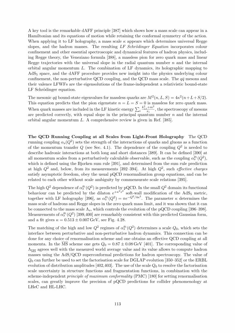
A key tool is the remarkable dAFF principle [387] which shows how a mass scale can appear in aHamiltonian and its equations of motion while retaining the conformal symmetry of the action.When applying it to LF holography, a mass scale κ appears which determines universal Reggeslopes, and the hadron masses. The resulting LF Schrodinger Equation incorporates colourconfinement and other essential spectroscopic and dynamical features of hadron physics, includ-ing Regge theory, the Veneziano formula [388], a massless pion for zero quark mass and linearRegge trajectories with the universal slope in the radial quantum number n and the internalorbital angular momentum L. The combination of LF dynamics, its holographic mapping toAdS5 space, and the dAFF procedure provides new insight into the physics underlying colourconfinement, the non-perturbative QCD coupling, and the QCD mass scale. The qq mesons andtheir valence LFWFs are the eigensolutions of the frame-independent a relativistic bound-stateLF Schrodinger equation.

The mesonic qq bound-state eigenvalues for massless quarks are M2(n,L, S) = 4κ2(n+L+S/2).This equation predicts that the pion eigenstate n = L = S = 0 is massless for zero quark mass.

When quark masses are included in the LF kinetic energy∑

ik2⊥i+m

2

xi, the spectroscopy of mesons

are predicted correctly, with equal slope in the principal quantum number n and the internalorbital angular momentum L. A comprehensive review is given in Ref. [385].

The QCD Running Coupling at all Scales from Light-Front Holography The QCDrunning coupling αs(Q

2) sets the strength of the interactions of quarks and gluons as a functionof the momentum transfer Q (see Sec. 4.1). The dependence of the coupling Q2 is needed todescribe hadronic interactions at both long and short distances [389]. It can be defined [390] atall momentum scales from a perturbatively calculable observable, such as the coupling αg1

s (Q2),which is defined using the Bjorken sum rule [391], and determined from the sum rule predictionat high Q2 and, below, from its measurements [392–394]. At high Q2, such effective chargessatisfy asymptotic freedom, obey the usual pQCD renormalisation group equations, and can berelated to each other without scale ambiguity by commensurate scale relations [395].

The high Q2 dependence of αg1s (Q2) is predicted by pQCD. In the small Q2 domain its functional

behaviour can be predicted by the dilaton e+κ2z2soft-wall modification of the AdS5 metric,

together with LF holography [396], as αg1s (Q2) = πe−Q

2/4κ2. The parameter κ determines the

mass scale of hadrons and Regge slopes in the zero quark mass limit, and it was shown that it canbe connected to the mass scale Λs, which controls the evolution of the pQCD coupling [396–398].Measurements of αg1

s (Q2) [399,400] are remarkably consistent with this predicted Gaussian form,and a fit gives κ = 0.513± 0.007 GeV, see Fig. 4.28.

The matching of the high and low Q2 regimes of αg1s (Q2) determines a scale Q0, which sets the

interface between perturbative and non-perturbative hadron dynamics. This connection can bedone for any choice of renormalisation scheme and one obtains an effective QCD coupling at allmomenta. In the MS scheme one gets Q0 = 0.87± 0.08 GeV [401]. The corresponding value ofΛMS agrees well with the measured world average value and its value allows to compute hadronmasses using the AdS/QCD superconformal predictions for hadron spectroscopy. The value ofQ0 can further be used to set the factorisation scale for DGLAP evolution [350–352] or the ERBLevolution of distribution amplitudes [402,403]. The use of the scale Q0 to resolve the factorisationscale uncertainty in structure functions and fragmentation functions, in combination with thescheme-independent principle of maximum conformality (PMC) [180] for setting renormalisationscales, can greatly improve the precision of pQCD predictions for collider phenomenology atLHeC and HL-LHC.

113

Figure 4.28: Prediction for the running coupling αg1s (Q2) at all scales. At lower Q2 predictions are

obtained from LF Holography and at higher Q2 from perturbative QCD. The magnitude and derivativeof the perturbative and non-perturbative coupling are matched at the scale Q0. This matching connectsthe perturbative scale ΛMS to the non-perturbative scale κ which underlies the hadron mass scale.

Superconformal Algebra and Hadron Physics with LHeC data If one generalises LFholography using superconformal algebra the resulting LF eigensolutions yield a unified Reggespectroscopy of mesons, baryons and tetraquarks, including remarkable supersymmetric relationsbetween the masses of mesons and baryons of the same parity 8 [404, 405]. This generalisationfurther predicts hadron dynamics, including vector meson electroproduction, hadronic LFWFs,distribution amplitudes, form factors, and valence structure functions [406, 407]. Applicationsto the deuteron elastic form factors and structure functions are given in Refs. [408,409]

The eigensolutions of superconformal algebra predict the Regge spectroscopy of mesons, baryons,and tetraquarks of the same parity and twist as equal-mass members of the same 4-plet repre-sentation with a universal Regge slope [410–412]. A comparison with experiment is shown inFig. 4.29. The qq mesons with orbital angular momentum LM = LB + 1 have the same mass astheir baryonic partners with orbital angular momentum LB [410,413].

The predictions from LF holography and superconformal algebra can also be extended to mesons,baryons, and tetraquarks with strange, charm and bottom quarks. Although conformal symme-try is strongly broken by the heavy quark masses, the basic underlying supersymmetric mech-anism, which transforms mesons to baryons (and baryons to tetraquarks), still holds and givesremarkable mass degeneracy across the entire spectrum of light, heavy-light and double-heavyhadrons.

The 4-plet symmetry of quark-antiquark mesons, quark-diquark baryons, and diquark-antidiquarktetraquarks are important predictions by superconformal algebra [401,404]. Recently the AnDYexperiment at RHIC has reported the observation of a state at 18 GeV which can be identifiedwith the [bb][bb] tetraquark [384]. The states with heavy quarks such as the [bb][bb] tetraquark

8QCD is not supersymmetrical in the usual sense, since the QCD Lagrangian is based on quark and gluonicfields, not squarks or gluinos. However, its hadronic eigensolutions conform to a representation of superconformalalgebra, reflecting the underlying conformal symmetry of chiral QCD and its Pauli matrix representation.

114

!

!

!

!!

!!

!!!!!!

"

"

"

"

#

#

#

#

M2 !GeV2"

LM ! LB ! 1Ρ, Ω

a2, f2

Ρ3, Ω3

a4, f4

$32

!

$12

%

, $32

%

$12

!

, $32

!

, $52

!

, $72

!

$112

!

0 1 2 3 4 50

1

2

3

4

5

6

superpartner trajectoriesSuperpartner Trajectories

Superconformal Quantum Mechanics

de Tèramond, Dosch, Lorce, sjb

Figure 4.29: Comparison of the ρ/ω meson Regge trajectory with the J = 3/2 ∆ baryon trajectory.Superconformal algebra predicts the mass degeneracy of the meson and baryon trajectories if one identifiesa meson with internal orbital angular momentum LM with its superpartner baryon with LM = LB + 1.See Refs. [410,413].

can be produced at the LHeC, especially at high xF along the proton beam direction. Newmeasurements at the LHeC are therefore inevitable to manifest the superconformal nature ofhadronic bound states.

115

Chapter 5

Electroweak and Top Quark Physics

5.1 Electroweak Physics with Inclusive DIS data

With the discovery of the Standard Model (SM) Higgs boson at the CERN LHC experimentsand subsequent measurements of its properties, all fundamental parameters of the SM have nowbeen measured directly and with remarkable precision. To further establish the validity of thetheory of electroweak interactions [25,414–417], validate the mechanism of electroweak symmetrybreaking and the nature of the Higgs sector [418–420], new electroweak measurements have tobe performed at highest precision. Such high-precision measurements can be considered as aportal to new physics, since non-SM contributions, as for instance loop-insertions, may causesignificant deviations for some precisely measurable and calculable observables. At the LHeC,the greatly enlarged kinematic reach to higher mass scales in comparison to HERA [421–423]and the large targeted luminosity will enable electroweak measurements in ep scattering withhigher precision than ever before.

In this section the sensitivity of inclusive DIS cross sections to electroweak parameters is dis-cussed. An extended analysis and a more comprehensive discussion is found in Ref. [424], andsome aspects are described in the following. The direct production of W and Z bosons isdiscussed in the subsequent section.

5.1.1 Electroweak effects in inclusive NC and CC DIS cross sections

Electroweak NC interactions in inclusive e±p DIS are mediated by exchange of a virtual photon(γ) or a Z boson in the t-channel, while CC DIS is mediated exclusively by W -boson exchangeas a purely weak process. Inclusive NC DIS cross sections are expressed in terms of generalisedstructure functions F±2 , xF±3 and F±L at EW leading order (LO) as

d2σNC(e±p)dxdQ2

=2πα2

xQ4

[Y+F

±2 (x,Q2)∓ Y−xF±3 (x,Q2)− y2F±L(x,Q2)

], (5.1)

where α denotes the fine structure constant. The terms Y± = 1 ± (1 − y)2, with y = Q2/sx,describe the helicity dependence of the process. The generalised structure functions are separatedinto contributions from pure γ- and Z-exchange and their interference [97,136]:

F±2 = F2 − (geV ± PegeA)κZFγZ2 + [(geV g

eV + geAg

eA)± 2Peg

eV g

eA]κ2

ZFZ2 , (5.2)

F±3 = −(geA ± PegeV )κZFγZ3 + [2geV g

eA ± Pe(geV geV + geAg

eA)]κ2

ZFZ3 . (5.3)

116

Similar expressions hold for FL. In the naive quark-parton model, which corresponds to the LOQCD approximation, the structure functions are calculated as[

F2, FγZ2 , FZ2

]= x

∑q

[Q2q , 2Qqg

qV , g

qV g

qV + gqAg

qA

]q + q , (5.4)

x[F γZ3 , FZ3

]= x

∑q

[2Qqg

qA, 2g

qV g

qA

]q − q , (5.5)

representing two independent combinations of the quark and anti-quark momentum distribu-tions, xq and xq. In Eq. (5.3), the quantities gfV and gfA stand for the vector and axial-vectorcouplings of a fermion (f = e or f = q for electron or quark) to the Z boson, and the coefficientκZ accounts for the Z-boson propagator including the normalisation of the weak couplings. Bothparameters are fully calculable from the electroweak theory. The (effective) coupling parame-ters depend on the electric charge, Qf and the third component of the weak-isospin, I3

L,f . Using

sin2θW = 1− M2W

M2Z

, one can write

gfV =√ρNC,f

(I3

L,f − 2QfκNC,f sin2θW

), and (5.6)

gfA =√ρNC,f I

3L,f with f = (e, u, d) . (5.7)

The parameters ρNC,f and κNC,f are calculated as real parts of complex form factors whichinclude the higher-order loop corrections [425–427]. They contain non-leading flavour-specificcomponents.

Predictions for CC DIS are written in terms of the CC structure functions W2, xW3 and WL andhigher-order electroweak effects are collected in two form factors ρCC,eq and ρCC,eq [428,429].

In this study, the on-shell scheme is adopted for the calculation of higher-order corrections.This means that the independent parameters are chosen as the fine structure constant α andthe masses of the weak bosons, the Higgs boson and the fermions. The weak mixing angle isthen fixed and GF is a prediction, whose higher-order corrections are included in the well-knowncorrection factor ∆r [430–432] (see discussion of further contributions in Ref. [136]).

The predicted single-differential inclusive NC and CC DIS cross sections for polarised e−p scat-tering as a function of Q2 are displayed in Fig. 5.1. For NC DIS and at higher Q2, electroweakeffects are important through γZ interference and pure Z-exchange terms and the polarisationof the LHeC electron beam of Pe = ±0.8 will considerably alter the cross sections. For CC DIS,the cross section scales linearly with Pe. Two different electron beam energies are displayed inFig. 5.1, and albeit the impact of a reduction from Ee = 60 to 50 GeV appears to be small, alarger electron beam energy would yield higher precision for the measurement of electroweakparameters, since these are predominantly sensitive to the cross sections at highest scales, aswill be shown in the following.

5.1.2 Methodology of a combined EW and QCD fit

A complete electroweak analysis of DIS data has to consider PDFs together with electroweakparameters [434]. In this study, the uncertainties of electroweak parameters are obtained ina combined fit of electroweak parameters and the PDFs, and the inclusive NC and CC DISpseudodata (see Sec. 4.3.2) are explored as input data. The PDFs are parameterised with 13parameters at a starting scale Q2

0 and NNLO DGLAP evolution is applied [47, 48]. In thisway, uncertainties from the PDFs are taken into account, which is very reasonable, since thePDFs will predominantly be determined from those LHeC data in the future. The details of

117

]2 [GeV2Q

310 410 510

]2 [p

b/G

eV2

/dQ

σd

-910

-810

-710

-610

-510

-410

-310

-210

-1101

10

p cross section−

LHeC polarised e

p−

LHeC eNC -0.8) =60GeV , P=

e(ECC

NC =60GeV , P=+0.8)e

(ECC NC -0.8) =50GeV , P=

e(ECC

NC =50GeV , P=+0.8)e

(ECC NC (P=0%)CC HERA-H1

Figure 5.1: Single differential cross sections for polarised e−p NC and CC DIS at LHeC for two differentelectron beam energies (Ee). Cross sections for longitudinal electron beam polarisations of Pe = −0.8and +0.8 are displayed. For comparison also measurements at centre-of-mass energies of

√s = 920 GeV

by H1 at HERA for unpolarised (Pe = 0 %) electron beams are displayed [433].

the PDF fit are altogether fairly similar to the PDF fits outlined in Chapter. 3. Noteworthydifferences are that additionally EW effects are included into the calculation by considering thefull set of 1-loop electroweak corrections [435], and the χ2 quantity [148], which is input to theminimisation and error propagation, is based on normal-distributed relative uncertainties. Inthis way, a dependence on the actual size of the simulated cross sections is avoided. The size ofthe pseudodata are therefore set equivalent to the predictions [436].

5.1.3 Weak boson masses MW and MZ

The expected uncertainties for a determination of the weak boson masses, MW and MZ, aredetermined in the PDF+EW-fit, where one of the masses is determined together with the PDFs,while the other mass parameter is taken as external input. The expected uncertainties for MW

are

∆MW(LHeC-60) = ±8(exp) ± 5(PDF) MeV = 10(tot) MeV and (5.8)

∆MW(LHeC-50) = ±9(exp) ± 8(PDF) MeV = 12(tot) MeV

for LHeC with Ee = 60 GeV or 50 GeV, respectively. The breakdown into experimental and PDFuncertainties is obtained by repeating the fit with PDF parameters fixed. These uncertaintiesare displayed in Fig. 5.2 and compared to the values obtained by LEP2 [438], Tevatron [437],ATLAS [439] and the PDG value [183]. The LHeC measurement will become the most precisemeasurement from one single experiment and will greatly improve over the best measurementachieved by H1, which was MW(H1) = 80.520±0.115 GeV [423]. If the dominating uncorrelated

118

[GeV]Wm80.35 80.4

[2019] PDG

=0.25%)unc.δ=50GeV, e

(ELHeC =0.5%)unc.δ=50GeV,

e(ELHeC

=0.25%)unc.δ=60GeV, e

(ELHeC =0.5%)unc.δ=60GeV,

e(ELHeC

ATLAS TevatronLEP2

W-boson mass

Uncorrelated uncertainty [%]

1−10 1−10×2 1

[MeV

]W

M∆

0

5

10

15

20

25W-boson mass uncertainty

GeV) 60 = e

(ELHeC GeV) 50 =

e(ELHeC

PDG19

Figure 5.2: Left: Measurements of the W -boson mass assuming fixed values for the top-quark andZ-boson masses at the LHeC for different scenarios in comparison with today’s measurements [437–439]and the world average value (PDG19) [183]. For LHeC, prospects for Ee = 60 GeV and 50 GeV aredisplayed, as well as results for the two scenarios with 0.5 % or 0.25 % uncorrelated uncertainty (see text).Right: Comparison of the precision for MW for different assumptions of the uncorrelated uncertainty ofthe pseudodata. The uncertainty of the world average value is displayed as horizontal line. The nominal(and alternative) size of the uncorrelated uncertainty of the inclusive NC/CC DIS pseudodata is indicatedby the vertical line (see text).

uncertainties can be reduced from the prospected 0.5 % to 0.25 % 1, a precision for MW of up to

∆MW(LHeC-60) = ±5(exp) ± 3(PDF) MeV = 6(tot) MeV and (5.9)

∆MW(LHeC-50) = ±6(exp) ± 6(PDF) MeV = 8(tot) MeV

for LHeC-60 and LHeC-50 may be achieved, respectively. A complete dependence of the expectedtotal experimental uncertainty ∆MW on the size of the uncorrelated uncertainty component isdisplayed in Fig. 5.2, and with a more optimistic scenario an uncertainty of up to ∆MW ≈ 5 MeVcan be achieved. In view of such a high accuracy, it will be important to study carefullytheoretical uncertainties. For instance the parameteric uncertainty due to the dependence onthe top-quark mass of 0.5 GeV will yield an additional error of ∆MW = 2.5 MeV. Also higher-order corrections, at least the dominating 2-loop corrections in DIS will have to be studied andkept under control. Then, the prospected determination of the W -boson mass from LHeC datawill be among the most precise determinations and significantly improve the world average valueof MW. It will also become competitive with its prediction from global EW fits with presentuncertainties of about ∆MW = 7 MeV [183,440,441].

While the determination of MW from LHeC data is competitive with other measurements, theexperimental uncertainties of a determination of MZ are estimated to be about 11 MeV and13 MeV for LHeC-60 and LHeC-50, respectively. Therefore, the precision of the determinationof MZ at LHeC cannot compete with the precise measurements at the Z-pole by LEP+SLD andfuture e+e− colliders may even improve on that.

A simultaneous determination of MW and MZ is displayed in Fig. 5.3 (left). Although theprecision of these two mass parameters is only moderate, a meaningful test of the high-energy

1Due to performance reasons, the pseudodata are generated for a rather coarse grid. With a binning which isclosely related to the resolution of the LHeC detector, much finer grids in x and Q2 are feasible. Already such achange would alter the uncertainties of the fit parameters. However, such an effect can be reflected by a changeduncorrelated uncertainty, and a value of 0.25 % appears like an optimistic, but achievable, alternative scenario.

119

[GeV]Wm80.3 80.35 80.4 80.45

[GeV

]Z

m

91.1

91.2

91.3

LHeC-60=0.25%)uncorr.δ(LHeC-60

LHeC-50 as additional constraint)

F(with G LHeC-60

PDG

FG WΘ2sin

C.L. 68

[GeV]tM160 170 180 190

[GeV

]W

M

80.3

80.4

80.5

LHeC-60=0.25%)uncorr.δ(LHeC-60

LHeC-50LEP1+SLDGlobal EW fitPDG

C.L. 68

Figure 5.3: Simultaneous determination of the top-quark mass Mt and W -boson mass MW from LHeC-60 or LHeC-50 data (left). Simultaneous determination of the W -boson and Z-boson masses from LHeC-60 or LHeC-50 data (right).

behaviour of electroweak theory is obtained by using GF as additional input: The high precisionof the GF measurement [442] yields a very shallow error ellipse and a precise test of the SMcan be performed with only NC and CC DIS cross sections alone. Such a fit determines andsimultaneously tests the high-energy behaviour of electroweak theory, while using only low-energy parameters α and GF as input (plus values for masses like Mt and MH needed for loopcorrections).

5.1.4 Further mass determinations

Inclusive DIS data are sensitive to the top-quark mass Mt indirectly through radiative correc-tions. Mt-dependent terms are dominantly due to corrections from the gauge boson self-energycorrections. They are contained in the ρ and κ parameters and in the correction factor ∆r.The leading contributions are proportional to M2

t . This allows for an indirect determinationof the top-quark mass using LHeC inclusive DIS data, and a determination of Mt will yield anuncertainty of ∆Mt = 1.8 GeV to 2.2 GeV. Assuming an uncorrelated uncertainty of the DISdata of 0.25 % the uncertainty of Mt becomes as small as

∆Mt = 1.1 to 1.4 GeV (5.10)

for 60 and 50 GeV electron beams, respectively. This would represent a very precise indirectdetermination of the top-quark mass from purely electroweak corrections and thus being fullycomplementary to measurements based on real t-quark production, which often suffer fromsizeable QCD corrections. The precision achievable in this way will be competitive with indirectdeterminations from global EW fits after the HL-LHC [443].

More generally, and to some extent depending on the choice of the renormalisation scheme, the

leading self-energy corrections are proportional toM2t

M2W

and thus a simultaneous determination

of Mt and MW is desirable. The prospects for a simultaneous determination of Mt and MW isdisplayed in Fig. 5.3 (right). It is remarkable that the precision of the LHeC is superior to that ofthe LEP+SLD combination [444]. In an optimistic scenario an uncertainty similar to the globalelectroweak fit [441] can be achieved. In a fit without PDF parameters similar uncertaintiesare found (not shown), which illustrates that the determination of EW parameters is to a largeextent independent of the QCD phenomenology and the PDFs.

120

uA

g0.4 0.5 0.6

u Vg

0.1

0.2

0.3

0.4

LHeC-50H1LEP & SLDD0Standard model expectation

C.L. 68

dA

g0.6− 0.5− 0.4−

d Vg

0.6−

0.4−

0.2−

0LHeC-50H1LEP & SLDD0Standard model expectation

C.L. 68

Figure 5.4: Weak NC vector and axial-vector couplings of u-type (left) and d-type quarks (right) at 68 %confidence level (C.L.) for simulated LHeC data with Ee = 50 GeV. The LHeC expectation is comparedwith results from the combined LEP+SLD experiments [444], a single measurement from D0 [445] andone from H1 [423]. The standard model expectations are diplayed by a red star, partially hidden by theLHeC prospects.

The subleading contributions to self-energy corrections have a Higgs-boson mass dependence

and are proportional to logM2H

M2W

. When fixing all other EW parameters the Higgs boson mass

could be constrained indirectly through these loop corrections with an experimental uncertaintyof ∆mH =+29

−23 to +24−20 GeV for different LHeC scenarios, which is again similar to the indirect

constraints from a global electroweak fit [441], but not competitive with direct measurements.

5.1.5 Weak Neutral Current Couplings

The vector and axial-vector couplings of up-type and down-type quarks to the Z, gqV and gqA,see Eq. (5.7), are determined in a fit of the four coupling parameters together with the PDFs.

Coupling PDG Expected uncertainties

parameter value LHeC-60 LHeC-60 (δuncor.=0.25 %) LHeC-50

guA 0.50 +0.04−0.05 0.0022 0.0015 0.0035

gdA −0.514 +0.050−0.029 0.0055 0.0034 0.0083

guV 0.18 ±0.05 0.0015 0.0010 0.0028gdV −0.35 +0.05

−0.06 0.0046 0.0027 0.0067

Table 5.1: Light-quark weak NC couplings (guA,gdA,guV ,gdV ) and their currently most precise values fromthe PDG [183] compared with the prospected uncertainties for different LHeC scenarios. The LHeCprospects are obtained in a simultaneous fit of the PDF parameters and all four coupling parametersdetermined at a time.

The resulting uncertainties are collected in Tab. 5.1. The two-dimensional uncertainty contoursat 68 % confidence level obtained from LHeC data with Ee = 50 GeV are displayed in Fig. 5.4for the two quark families and compared with available measurements. While all the currentdeterminations from e+e−, ep or pp data have a similar precision, the future LHeC data willgreatly improve the precision of the weak neutral-current couplings and expected uncertaintiesare an order of magnitude smaller than the currently most precise ones [183]. An increased

121

NC,f'ρ

0.995 1 1.005

NC

,f'κ

0.995

1

1.005

1.01All fermions

LHeC-60=0.25%)uncorr.δ(LHeC-60

LHeC-50leptons (uncertainty only)LEP+SLD

SM

C.L. % 68

NC,u'ρ

0.96 0.98 1 1.02 1.04

NC

,u'κ

0.95

1

1.05

1.1up-type quarks (u=c)

LHeC-60=0.25%)uncorr.δ(LHeC-60

LHeC-50c-quarks (uncertainty only)LEP+SLD

SM

C.L. % 68

NC,d'ρ

0.95 1 1.05

NC

,d'κ

0.9

1

1.1

1.2down-type quarks (d=s=b)

LHeC-60=0.25%)uncorr.δ(LHeC-60

LHeC-50b-quarks (uncertainty only)LEP+SLD

SM

C.L. % 68

Figure 5.5: Expectations at 68 % confidence level for the determination of the ρ′NC and κ′NC parametersassuming a single anomalous factor equal for all fermions (left). The results for three different LHeCscenarios are compared with the achieved uncertainties from the LEP+SLD combination [444] for thedetermination the respective leptonic quantities. Right: uncertainties for the simultaneous determinationof the anomalous form factors for u and d-type quarks, assuming known values for the electron parameters.The values are compared with uncertainties reported by LEP+SLD for the determination of the values

ρNC,(c,b) and sin θeff,(c,b)W for charm or bottom quarks, respectively.

electron beam energy of Ee = 60 GeV or improved experimental uncertainties would furtherimprove this measurement.

The determination of the couplings of the electron to the Z boson, geV and geA, can be determinedat the LHeC with uncertainties of up to ∆geV = 0.0013 and ∆geA = ±0.0009, which is similarto the results of a single LEP experiment and about a factor three larger than the LEP+SLDcombination [444].

5.1.6 The neutral-current ρNC and κNC parameters

Beyond Born approximation, the weak couplings are subject to higher-order loop corrections.These corrections are commonly parameterised by quantities called ρNC, κNC and ρCC. They aresensitive to contributions beyond the SM and the structure of the Higgs sector. It is importantto keep in mind that these effective coupling parameters depend on the momentum transferand are, indeed, form factors rather than constants. It is particularly interesting to investigatethe so-called effective weak mixing angle defined as sin2 θeff

W = κNCsin2θW. At the Z-pole itis well accessible through asymmetry measurements in e+e− collisions. In DIS at the LHeC,the scale dependence of the effective weak mixing angle is not negligible. It can be determinedonly together with the ρ parameter due to the Q2 dependence and the presence of the photonexchange terms. Therefore, we introduce (multiplicative) anomalous contributions to thesefactors, denoted as ρ′NC,CC and κ′NC, and test their agreement with unity (for more details seeRef. [423]), and uncertainties of these parameters are obtained in a fit together with the PDFs.The two-dimensional uncertainty contours of the anomalous form factors ρ′NC,f and κ′NC,f aredisplayed for three different LHeC scenarios in Fig. 5.5 (left), and compared with uncertaintiesfrom the LEP+SLD combination 2 [444]. It is found that these parameters can be determinedwith very high experimental precision.

Assuming the couplings of the electron are given by the SM, the anomalous form factors for

2Since in the LEP+SLD analysis the values of ρNC and κNCsin2θW are determined, we compare only thesize of the uncertainties in these figures. Furthermore it shall be noted, that LEP is mainly sensitive to theparameters of leptons or heavy quarks, while LHeC data is more sensitive to light quarks (u,d,s), and thus theLHeC measurements are highly complementary.

122

[GeV]2Q

100 1000

NC

,f'ρ

0.95

1

1.05

1.1LHeC-50 H1 data

LHeC-60 SM

[GeV]2Q

100 1000

NC

,f'κ

0.98

1

1.02

1.04LHeC-50 H1 data

LHeC-60 SM

Figure 5.6: Test of the scale dependence of the anomalous ρ and κ parameters for two different LHeCscenarios. For the case of LHeC-60, i.e. Ee = 60 GeV, we assume an uncorrelated uncertainty of 0.25 %.The uncertainties of the parameter κ′NC,f can be interpreted as sensitivity to the scale-dependence of the

weak mixing angle, sin θeffW(µ).

the two quark families can be determined and results are displayed in Fig. 5.5 (right). Sincethese measurements represent unique determinations of parameters sensitive to the light-quarkcouplings, we can compare only with nowadays measurements of the parameters for heavy-quarksof the same charge and it is found that the LHeC will provide high-precision determinations ofthe ρ′NC and κ′NC parameters.

A meaningful test of the SM can be performed by determining the effective coupling parametersas a function of the momentum transfer. In case of κ′NC, this is equivalent to measuring therunning of the effective weak mixing angle, sin θeff

W(µ) (see also Sec. 5.1.7). However, DIS is quitecomplementary to other measurements since the process is mediated by space-like momentumtransfer, i.e. q2 = −Q2 < 0 with q being the boson four-momentum. Prospects for a determi-nation of ρ′NC or κ′NC at different Q2 values are displayed in Fig. 5.6 and compared to resultsobtaind by H1. The value of κ′NC(µ) can be easily translated to a measurement of sin θeff

W(µ).From Fig. 5.6 one can conclude that this quantity can be determined with a precision of up to0.1 % and better than 1 % over a wide kinematic range of about 25 <

√Q2 < 700 GeV.

5.1.7 The effective weak mixing angle sin2 θeff,`W

The leptonic effective weak mixing angle is defined as sin2 θeff,`W (µ2) = κNC,`(µ

2)sin2θW. Due toits high sensitivity to loop corrections it represents an ideal quantity for precision tests of theStandard Model. Its value is scheme dependent and it exhibits a scale dependence. Near theZ pole, µ2 = M2

Z, its value was precisely measured at LEP and at SLD. Those analyses werebased on the measurement of asymmetries and their interpretation in terms of the leptonic weakmixing angle was simplified by the fact that many non-leptonic corrections and contributionsfrom box graphs cancel or can be taken into account by subtracting their SM predictions. Thehighest sensitivity to sin2 θeff,`

W (MZ) to date arises from a measurement of A0,bfb [444], where

the non-universal flavour-specific corrections to the quark couplings are taken from the SMand consequently these measurements are interpreted to be sensitive only to the universal, i.e.

123

Fit parameters Parameter SM Expected uncertainties

of interest value LHeC-50 LHeC-60 LHeC-50 LHeC-60(δuncor. = 0.50 %) (δuncor. = 0.25 %)

κ′NC,f , PDFs sin2 θeff,`W (M2

Z) 0.23154 0.00033 0.00025 0.00022 0.00015

κ′NC,f , ρ′NC,f , PDFs sin2 θeff,`W (M2

Z) 0.23154 0.00071 0.00036 0.00056 0.00023

κ′NC,e, PDFs sin2 θeff,eW (M2

Z) 0.23154 0.00059 0.00047 0.00038 0.00028

κ′NC,e, κ′NC,u, κ′NC,d, PDFs sin2 θeff,e

W (M2Z) 0.23154 0.00111 0.00095 0.00069 0.00056

κ′NC,f sin2 θeff,`W (M2

Z) 0.23154 0.00028 0.00023 0.00017 0.00014

Table 5.2: Determination of sin2 θeff,`W (M2

Z) with inclusive DIS data at the LHeC for different scenarios.Since the value of the effective weak mixing angle at the Z pole cannot be determined directly in DIS, a fitof the κ′NC,f parameter is performed instead and its uncertainty is translated to sin2 θeff,`

W (M2Z). Different

assumptions on the fit parameters are studied, and results include uncertainties from the PDFs. Onlythe last line shows results where the PDF parameters are kept fixed. See text for more details.

flavour-independent 3, non-SM contributions to κNC. Applying this assumption also to the DIScross sections, the determination of κ′NC,f can directly be interpreted as a sensitivity study of

the leptonic effective weak mixing angle sin2 θeff,`W .

The prospects for a determination of sin2 θeff,`W are listed in Tab. 5.2. Two fits have been studied:

one with a fixed parameter ρ′NC and one where sin2 θeff,`W is determined together with ρ′NC (see

Fig. 5.5 (left)). At the LHeC, it will be possible to determine the value of sin2 θeff,`W (M2

Z) withan experimental uncertainty of up to

∆ sin2 θeff,`W = ±0.00015 , (5.11)

where PDF uncertainties are already included. If the PDF parameters are artificially kept fixed,the uncertainties are of very similar size, which demonstrates that these measurements are fairlyinsensitive to the QCD effects and the PDFs. The uncertainties are compared 4 to recent averagevalues in Fig. 5.7. One can see that the LHeC measurement has the potential to become themost precise single measurement in the future with a significant impact to the world averagevalue. It is obvious that a conclusive interpretation of experimental results with such a highprecision will require correspondingly precise theoretical predictions, and the investigation oftwo-loop corrections for DIS will become important.

This LHeC measurement will become competitive with measurements at the HL-LHC [187].Since in pp collisions one of the dominant uncertainties is from the PDFs [448, 449, 452–454],future improvements can (only) be achieved with a common analysis of LHeC and HL-LHCdata. Such a study will yield highest experimental precision and the challenging theoreticaland experimental aspects for a complete understanding of such an analysis will deepen ourunderstanding of the electroweak sector.

It may be further of interest, to determine the value of the effective weak mixing angle of theelectron separately in order to compare with measurements in pp and test furthermore lepton-

3Flavour-specific tests have been discussed to some extent in the previous Section.4It shall be noted, that in order to compare the LHeC measurements with the Z-pole measurements at µ2 = M2

Z

in a conclusive way, one has to assume the validity of the SM framework. In particular the scale-dependence ofκNC,` must be known in addition to the flavour-specific corrections. On the other hand, the scale dependencecan be tested itself with the LHeC data which cover a large range of space-like Q2. In this aspect, DIS providesa unique opportunity for precision measurements in the space-like regime (µ2 < 0) as has been discussed in theprevious Section, see Fig. 5.6 (right).

124

eff,lept.Wθ2sin

0.231 0.232

[2019] World Average

=0.5%)unc.δ=50GeV, e

(ELHeC =0.25%)unc.δ=60GeV,

e(ELHeC

LHCTevatronLEP+SLC

eff,lept.Wθ2sin

Figure 5.7: Comparison of the determination of sin2 θeff,`W (M2

Z) from LHeC inclusive DIS data with recentaveraged values. Results from LEP+SLC [444], Tevatron [446], LHC [447–450] and the world averagevalue [450] are all obtained from a combination of various separate measurements (not shown individually)(see also Ref. [451] for additional discussions). For LHeC, the experimental and PDF uncertainties aredisplayed.

specific contributions to κNC,lept.. Such fits are summarised in Table 5.2 and a reasonableprecision is achieved with LHeC.

The measurement of the weak mixing angle can be performed in sub-regions of Q2 due to thewide kinematic range accessible at the LHeC. The relative uncertainties for the determination ofthe weak mixing angle for different Q2 intervals is displayed in Fig. 5.8. We find that the weakmixing angle can be determined in the range of about 25 <

√Q2 < 700 GeV with a precision

better than 0.1 %. If a calculation of DIS cross sections including higher-order EW correctionsin the MS scheme is available, these relative uncertainties can be mapped into a test of therunning of the weak mixing angle. Note, that in DIS the scattering process is mediated byboson exchange with spacelike momenta and is therefore complementary to other measurementssince the scale is µ2 = −Q2.

5.1.8 Electroweak effects in charged-current scattering

The charged-current sector of the SM can be uniquely measured at high scales over many ordersof magnitude in Q2 at the LHeC, due to the excellent tracking detectors, calorimetry, and high-bandwidth triggers. Similarly as in the NC case, the form factors of the effective couplings ofthe fermions to the W boson can be measured. In the SM formalism, only two of these formfactors are present, ρCC,eq and ρCC,eq. We thus introduce two anomalous modifications to them,ρCC,(eq/eq) → ρ′CC,(eq/eq)ρCC,(eq/eq) (see Ref. [423]). The prospects for the determination of theseparameters are displayed in Fig. 5.9, and it is found, that with the LHeC these parameters canbe determined with a precision up to 0.2–0.3 %. Also their Q2 dependence can be uniquelystudied with high precision up to

√Q2 values of about 400 GeV.

125

[GeV]2Q

10 100 1000

rela

tive

unce

rtai

nty

0

0.02

0.04

0.06Wθ2sin LHeC-50

=0.25%)un.δ(LHeC-60

SM

Figure 5.8: Expected uncertainties of the weak mixing angle determined in sub-regions of Q2. Twoscenarios for the simulation of LHeC inclusive NC/CC DIS data are considered.

CC,eq'ρ

0.99 1 1.01 1.02

qC

C,e

'ρ

0.99

1

1.01

1.02

LHeC-60=0.25%)uncorr.δ(LHeC-60

LHeC-50H1SM

C.L. % 68

10 100 1000

[GeV]2Q

0.98

0.99

1

1.01

1.02

1.03

CC

,f'ρ

LHeC-50 LHeC-60

H1 data SM

Figure 5.9: Left: anomalous modifications of the charged current form factors ρ′CC,eq and ρ′CC,eq

for different LHeC scenarios in comparison with the H1 measurement [423]. Right: scale dependentmeasurement of the anomalous modification of the charged current form factor ρ′CC(Q2), assumingρ′CC,eq = ρ′CC,eq = ρ′CC.

5.1.9 Conclusion

With LHeC inclusive NC and CC DIS data, unique measurements of electroweak parameters canbe performed with highest precision. Since inclusive DIS is mediated through space-like momen-tum transfer (t-channel exchange) the results are often complementary to other experiments,such as pp or e+e− collider experiments, where measurements are performed in the time-likeregime and most often at the Z peak. Among many other quantities, measurements of the weakcouplings of the light quarks, u and d, or their anomalous form factors ρ′NC,u/d and κ′NC,u/d,

126

can be performed uniquely due to the important contributions of valence quarks in the initialstate. Also scale dependent measurements of weak interactions can be performed over a largerange in

√Q2, which provides an interesting portal to BSM physics. The W boson mass can be

determined with very small experimental uncertainties, such that theoretical uncertainties areexpected to become more important than experimental uncertainties. While the parameters ofthe PDFs are determined together with the EW parameters in the present study, it is foundthat the PDFs do not induce a limitation of the uncertainties. Considering the dominatingtop-quark mass dependence of higher-order electroweak effects, one can realise that the LHeCwill be competitive with the global electroweak fit after the HL-LHC era [187,443].

Besides proving its own remarkable prospect on high-precision electroweak physics, the LHeCwill further significantly improve the electroweak measurements in pp collisions at the LHC byreducing the presently sizeable influence of PDF and αs uncertainties. This is discussed in Sec. 9.

5.2 Direct W and Z Production and Anomalous Triple GaugeCouplings

5.2.1 Direct W and Z Production

The direct production of single W and Z bosons as a crucial signal represents an importantchannel for EW precision measurements. The production of W bosons has been measured at√s ' 320 GeV at HERA [455–457]. With the full e±p data set collected by the H1 and ZEUS

experiments together, corresponding to an integrated luminosity of about L ∼ 1 fb−1, a fewdozens of W boson event candidates have been identified in the e, µ or τ decay channel.

Detailed studies of direct W/Z production in ep collisions at higher centre-of-mass energies havebeen presented in the past, see Refs. [458–460]. These theoretical studies were performed fora proton beam energy of Ep = 8 TeV and electron beam energies of Ee = 55 GeV or 100 GeV,which correspond to a very similar centre-of-mass energy as the LHeC. Measurements at theLHeC will benefit considerably from the large integrated luminosity, in comparison to earlierprojections.

The W or Z direct production in e−p collisions can be classified into five processes

e−p→ e−W+j, e−p→ e−W−j,

e−p→ ν−e W−j, e−p→ ν−e Zj (5.12)

and

e−p→ e−Zj, (5.13)

where j denotes the hadronic the final state (i.e. the forward jet). According to the aboveclassification, the four processes in Eq. (5.12) can be used to study Tripe Gauge Couplings(TGCs), e.g. WWγ and WWZ couplings, since some contributing diagrams represent VectorBoson Fusion (VBF) processes. The process shown in Eq. (5.13) does not contain any TGCvertex. The processes for positron-proton collisions can be easily derived from Eqs. (5.12)and (5.13), but are not discussed further here due to the small integrated luminosity of theLHeC e+p data.

The MadGraph5 v2.4.2 program [375] is employed for matrix element calculation and event gen-eration and the PDF NNPDF23 nlo as 0119 qed [461] is used. Technical cuts on the transversemomentum of the outgoing scattered lepton, p`T , of 10 GeV or alternatively 5 GeV, are imposed

127

and other basic cuts are pjT > 20 GeV, |ηe,j | < 5 and ∆Rej < 0.4. The resulting Standard Modeltotal cross sections of the above processes are listed in Tab. 5.3.

Process Ee = 50 GeV, Ep = 7 TeV Ee = 60 GeV, Ep = 7 TeV Ee = 60 GeV, Ep = 7 TeVpeT > 10 GeV peT > 10 GeV peT > 5 GeV

e−W+j 1.00 pb 1.18 pb 1.60 pbe−W−j 0.930 pb 1.11 pb 1.41 pbν−e W

−j 0.796 pb 0.956 pb 0.956 pbν−e Zj 0.412 pb 0.502 pb 0.502 pbe−Zj 0.177 pb 0.204 pb 0.242 pb

Table 5.3: The SM predictions of direct W and Z production cross sections in e−p collisions for differentcollider beam energy options, Ee, and final state forward electron transverse momentum cut, peT . Twodifferent electron beam energy options are considered, Ee = 50 GeV and 60 GeV.

The process with the largest production cross section in e−p scattering is the single W+ bosonproduction. This will be the optimal channel of both the SM measurement and new physicsprobes in the EW sector. Also, this channel is experimentally preferred since the W+ is producedin NC scattering, so the beam electron is measured in the detector, and theW -boson has oppositecharge to the beam lepton and thus in a leptonic decay an opposite charge lepton and missingtransverse momentum is observed. Altogether, it is expected that a few million of direct W -boson events are measured at LHeC.

Several 105 direct Z events are measured, which corresponds approximately to the size of theevent sample of the SLD experiment [444], but at the LHeC these Z bosons are predominantlyproduced in VBF events.

All these total cross sections increase significantly with smaller transverse momentum of theoutgoing scattered lepton. Therefore it will become important to decrease that threshold withdedicated electron taggers, see Chapter 12.

5.2.2 Anomalous Triple Gauge Couplings

The measurement of gauge boson production processes provides a precise measurement of thetriple gauge boson vertex. The measurement is sensitive to new physics contributions in anoma-lous Tripe Gauge Couplings (aTGC). The LHeC has advantages of a higher centre-of-massenergy and easier kinematic analysis in the measurement of aTGCs.

In the effective field theory language, aTGCs in the Lagrangian are generally parameterised as

LTGC/gWWV = ig1,V (W+µνW

−µ Vν −W−µνW+

µ Vν) + iκVW+µ W

−ν Vµν +

iλVM2W

W+µνW

−νρVρµ

+gV5 εµνρσ(W+µ

←→∂ ρW

−ν )Vσ − gV4 W+

µ W−ν (∂µVν + ∂νVµ)

+iκVW+µ W

−ν Vµν +

iλVM2W

W+λµW

−µν Vνλ, (5.14)

where V = γ, Z. The gauge couplings gWWγ = −e, gWWZ = −e cot θW and the weak mixing

angle θW are from the SM. Vµν and A←→∂ µB are defined as Vµν = 1

2εµνρσVρσ, A←→∂ µB = A(∂µB)−

(∂µA)B, respectively. There are five aTGCs (g1,Z , κV , and λV ) conserving the C and CPcondition with electromagnetic gauge symmetry requires g1,γ = 1. Only three of them areindependent because λZ = λγ and ∆κZ = ∆g1,Z − tan2 θW∆κγ [462–464]. The LHeC can setfuture constraints on ∆κγ and λγ .

128

In the direct Z/γ production process, the anomalous WWZ and WWγ couplings can be sep-arately measured without being influenced by their interference [465, 466]. In the direct Wproduction process, both the deviation in signal cross section and the kinematic distributionscan effectively constrain the WWγ aTGC, while anomalous WWZ contribution in this channelis insensitive as a result of the suppression from Z boson mass [467–469].

-1.0 -0.5 0.0 0.5 1.00.05

0.10

0.50

1

λγ

σ()

Ee=60 GeV

Δκγ=0

-1.0 -0.5 0.0 0.5 1.00.05

0.10

0.50

1

Δκγ

σ()

Ee=60 GeV

λγ=0

Figure 5.10: Total cross sections of the e−p → e−µ+νµj process with varying λγ (left plot) and∆κγ (right plot).

The W decay into muon channel is the expected optimal measurement for the anomalous WWγcoupling because of the discrimination of final states and mistagging efficiencies [467]. Fig. 5.10shows the cross section of single W+ production process followed by W+ → µ+νµ decay, withdifferent λγ and ∆κγ values. Large anomalous coupling leads to measurable deviation to theSM prediction. The cross section increases monotonically with ∆κγ and the absolute value ofλγ within the region of −1.0 ≤ λγ/∆κγ ≤ 1.0.

Kinematic analysis is necessary for the precise aTGC measurement. At LHeC, the e−p →e−W±j process with leptonic W boson decay can be fully reconstructed because the unde-tected neutrino information is reconstructed either with energy-momentum conservation or therecoil mass method. This allows to use angular correlation observables, which are sensitive tothe W boson polarisation. Helicity amplitude calculation indicates that a non-SM value of λγleads to a significant enhancement in the transverse polarisation fraction of the W boson in thee−p→ e−W+j process, while a non-SM value of ∆κγ leads to enhancement in the longitudinalcomponent fraction [458]. The angle θ`W is defined as the angle between the decay productlepton ` in the W rest frame and W moving direction in the collision rest frame. Making useof the energetic final states in the forward direction, a second useful angle ∆φej is defined asthe separation of final state jet and electron on the azimuthal plane. In an optimised analysis,assuming an integrated luminosity of 1 ab−1, the observable ∆φej can impose stringent con-straints on both λγ and ∆κγ , and uncertainties within [−0.007, 0.0056] and [−0.0043, 0.0054]are achieved, respectively. The cos θµW observable is also sensitive to ∆κγ at the same order,but fails to constrain λγ . The analysis is described in detail in Ref. [467].

Fig. 5.11 shows the two-parameter aTGC constraint on the λγ–∆κγ plane based on a χ2 analysisof ∆φej at parton-level and assuming an electron beam energy of Ee = 60 GeV. When comparingwith the current LHC (blue and green) and LEP (red) bounds, the LHeC has the potentialto significantly improve the constraints, in particular on the ∆κγ parameter. The polarisedelectron beam is found to improve the aTGC measurement [466, 469]. In consideration of the

129

-0.10 -0.05 0.00 0.05 0.10

-0.10

-0.05

0.00

0.05

0.10

0.15

λγ

Δκ γ

LHeC(Ee=60 GeV)

LHC(13 TeV)

LHC(8 TeV)

LEP

Figure 5.11: The 95% C.L. exclusion limit on the ∆κγ-λγ plane. The purple dashed contour is theprojected LHeC exclusion limit with 1 ab−1 integrated luminosity [467]. The blue, green and red contoursare current bounds from LHC [470,471] and LEP [472].

realistic analysis at detector level, one expects 2-3 ab−1 integrated luminosity to achieve sameresults [467].

One uncertainty in the aTGC measurement at the (HL-)LHC comes from the PDF uncertainty.Future LHeC PDF measurement will improve the precision of aTGC measurement in the x 'O(10−2) region.

5.3 Top Quark Physics

SM top quark production at a future ep collider is dominated by single top quark production,mainly via CC DIS production. A leading-order Feynman diagram is displayed in Fig. 5.12(left). The total cross section for single top quark production is 1.89 pb at the LHeC [473] anda centre-of-mass energy of 1.3 TeV, i.e. with an electron beam energy of 60 GeV and an LHCproton beam of 7 TeV. The second important production mode for top quarks at the LHeC isphotoproduction of top-antitop quark pairs (tt), where a total cross section of 0.05 pb is expectedat the LHeC [474]. Figure 5.12 (right) shows an example Feynman diagram. This makes a futureLHeC a top quark factory and an ideal tool to study top quarks with a high precision, and toanalyse in particular their electroweak interaction. Selected highlights in top quark physics aresummarised here.

5.3.1 Wtq Couplings

The top quark couplings to gauge bosons can be modified significantly in models with new top (orthird generation) partners, such as in some extensions of the minimal supersymmetric standardmodel, in little Higgs models, top-color models, top seesaw, top compositeness, and others.Testing them is therefore of utmost importance to find out whether there are other sources ofelectroweak symmetry breaking that are different from the standard Higgs mechanism.

One highlight at the LHeC is the direct measurement of the CKM matrix element |Vtb|. Sucha measurement can be done without making any model assumptions, like for instance on theunitarity of the CKM matrix or the number of quark generations. An elaborate analysis of the

130

Figure 5.12: Example graphs for top quark production in CC DIS (left) and for tt photoproduction(right).

single top quark CC DIS process at the LHeC, which makes use of a detailed detector simulationusing the DELPHES package [475], shows that already at 100 fb−1 of integrated luminosity anuncertainty of 1% can be expected. This compares to a total uncertainty of 4.1 % of the currentlymost accurate result at the LHC Run-I performed by the CMS experiment [476].

The same process is also highly sensitive to the search for anomalous left- and right-handed Wtbvector (fL1 , fR1 ) and tensor (fL2 , fR2 ) couplings [473]. These are given by an effective Lagrangian,

LWtb = − g√2bγµVtb(f

L1 PL − fR1 PR)tW−µ −

g√2biσµνqνMW

(fL2 PL − fR2 PR)tW−µ + h.c. (5.15)

In the SM formalism fL1 = 1 and fR1 = fL2 = fR2 = 0. The effect of anomalous Wtb couplings isconsistently evaluated in the production and the decay of the antitop quark, cf. Fig. 5.12 (left).5

The expected limits for the anomalous couplings at 95 % confidence level from a measurement ofsingle top quark production in CC DIS at the LHeC, is displayed in Fig. 5.13. This analysis onlyexploits hadronic top quark decays [473]. The coupling parameters are expected to be measuredwith accuracies of 1 % for the SM fL1 coupling determining |Vtb| (as discussed above) and of 4 %for fL2 , 9 % for fR2 , and 14% for fR1 at 1 ab−1.

In a similar way, through W boson and bottom (light) quark associated production, the CKMmatrix elements |Vtx| (x = d, s) can be extracted with very high precision utilizing a parameter-isation of the deviations from the respective SM values. Here, the W boson and the b-jet (lightjet j = d, s) are produced via t-channel top quark exchange, or via s-channel single top quarkdecay, as outlined in [478]. As an example, the processes

Signal 1: pe− → νet→ νeW−b→ νe`

−ν`b

Signal 2: pe− → νeW−b→ νe`

−ν`b

Signal 3: pe− → νet→ νeW−j → νe`

−ν`j

are analyzed in an elaborate study, where a detailed detector simulation is performed withthe DELPHES package [475]. Fig. 5.14 shows the resulting accuracies at the 2σ confidencelevel (C.L.) for an expected measurement of |Vtd| and |Vts|, respectively, as a function of theintegrated luminosity. At 1 ab−1 of integrated luminosity and an electron polarisation of 80 %,the 2σ limits improve on existing limits from the LHC [479] (interpreted by [480]) by a factor of≈ 3.5. Analyzing Signal 3 alone, and even more when combining Signals 1, 2 and 3, will allow for

5Further studies of the top quark charged current coupling can be found in [477]. There, a more generalframework is employed using the full basis of SU(2)L ×U(1) operators, including the relevant four-fermion ones.

131

the first time to achieve an accuracy of the order of the actual SM value of |V SMts | = 0.04108+0.0030

−0.0057

as derived from an indirect global CKM matrix fit [481], and will therefore represent a directhigh precision measurement of this important top quark property. In these studies, upper limitsat the 2σ level down to |Vts| < 0.06, and |Vtd| < 0.06 can be achieved.

5.3.2 Top Quark Polarisation

Single top quarks produced via the e+p→ tν processes possess a high degree of spin polarisationin terms of a basis which decomposes the top quark spin in its rest frame along the direction ofthe incoming e beam [482]. It has been investigated for

√s = 1.6 TeV in e+p scattering, that the

spin fraction defined as the ratio of the polarised cross section to the unpolarised one, reaches96% allowing a detailed study of the polarisation and the spin of the top quark. Exploring theangle between the momentum direction of the charged lepton from top quark decay and the spinquantisation axis in the top quark rest frame, anomalous Wtb couplings can be tested. Assuminga total systematic uncertainty of 10% the expected sensitivity for

√s = 1.6 TeV reaches ±3%

for fL2 , and ±7% for fR2 as defined in Eq. (5.15).

5.3.3 Top-γ and Top-Z Couplings

The LHeC is particularly well suited to measure the ttγ vertex, since in photoproducton of topquark pairs (see Fig. 5.12, right) the highly energetic incoming photon only couples to the topquark, and therefore the cross section directly depends on the ttγ vertex. This provides a directmeasurement of the coupling between the top quark and the photon and therefore of anotherimportant top quark property, the top quark charge. In contrast, at the LHC the ttγ vertexvertex is probed in ttγ production, where the final state photon can also be produced from othervertices than the ttγ vertex, such as from initial state radiation or from radiation off chargedtop quark decay products.

The LHeC also provides a high potential for measuring the ttγ magnetic and electric dipolemoments (MDM and EDM, respectively) in tt production [474]. In an effective Lagrangian

Figure 5.13: Expected sensitivities on the SM and anomalous Wtb couplings, as a function of theintegrated luminosity [473].

132

Figure 5.14: Expected sensitivities on |Vtd| (left) and |Vts| (right), as a function of the integratedluminosity [478].

framework, effective ttγ couplings can be written in terms of form factors:

LWtb = e t

(Qtγ

µAµ +1

4mtσµνFµν (κ+ iκγ5)

)t + h.c. (5.16)

with the anomalous MDM of the top quark, κ, and the EDM of the top quark, κ. The top quarkcharge is given by eQt.

By solely measuring the tt production cross section, remarkably tight bounds can be derived on

Figure 5.15: Allowed region of the magnetic dipole moment κ and the electric dipole moment κ of thetop quark as expected in a measurement of the photoproduction cross section σ(e(γ)p(g)→ tt) in semilep-tonic final states, assuming an experimental uncertainty of 8% (dark grey), and of 16% (dark+mediumgrey) [474]. Light gray area: region allowed by the measurements of the branching ratio (solid graylines) and the CP asymmetry (dashed gray lines) of B → Xsγ [483]. Black dashed line: region allowedby a hypothetical experimental result for σ(pp → ttγ) utilizing semileptonic final states at the LHC at√s = 14 TeV with phase-space cuts as defined in equations (5), (6) of Ref. [483] (including EγT > 10 GeV),

and assuming an experimental uncertainty of 5%.

133

the MDM and the EDM of the top quark as presented in Fig. 5.15. In this parton level study,for the computation of the cross section a set of appropriate phase-space cuts are imposed on thefinal-state momenta. Applying further cuts to remove the background will result in a substantialreduction of the signal. It is therefore assumed that this would lead to a statistical uncertaintyof about 8%, represented by the dark inner ring in Fig. 5.15. To include uncertainties due tomistagging and to allow for other unspecified sources of systematic uncertainty, it is assumedthat the total uncertainty will be about 16% corresponding to the full ring in Fig. 5.15. Thiswould yield bounds of −0.13 < κ < 0.18, and |κ| < 0.38, respectively, at the 2σ C.L. Figure 5.15shows that the LHeC could greatly improve the limits imposed by the indirect constraints fromb→ sγ, and even the limits imposed by a future measurement of ttγ production at the LHC at√s = 14 TeV.

Furthermore, the deep inelastic scattering (DIS) regime of tt production will allow to probe thettZ coupling, albeit with less sensitivity [474].

5.3.4 Top-Higgs Coupling

The CP-nature of the top-Higgs coupling can be analysed at the LHeC in ep→ tH productionexploring the top quark polarisation and other angular variables such as the difference in rapiditybetween the antitop quark and the Higgs boson. Measuring just the fiducial inclusive productioncross section gives already a powerful probe of the CP properties of the ttH coupling [484].Further details are given in Section 7.5.

5.3.5 Top Quark PDF and the Running of αs

Parton distributions are usually released in a variable-flavor number scheme, where the numberof active flavors changes as the scale is raised [254]. However, nf = 5 is normally taken by defaultas a maximum number of flavors, even though in some PDF releases nf = 6 PDF sets are alsomade available [485]. The top PDF is unlikely to be required for precision phenomenology, evenat very high scales, because the top threshold is high enough that collinear resummation is not

necessary up to extremely large scales: indeedαs(M2

t )π ln Q2

m2t∼ 1

2 only for Q & 106mt. On the

other hand, the use of nf = 6 active flavors in the running of αs is important for precisionphenomenology, since the value of αs with five and six active flavors already differ by about2% at the TeV scale [486]. Investigations of the top quark structure inside the proton are alsodiscussed in Refs. [1, 40].

5.3.6 FCNC Top Quark Couplings

Like all the Flavour Changing Neutral Currents (FCNCs) the top quark FCNC interactionsare also extremely suppressed in the SM, which renders them a good test of new physics. Thecontributions from FCNC to top interactions can be parameterised via an effective theory andstudied by analysing specific processes.

NC DIS production of single top quarks can be explored to search for FCNC tuγ, tcγ, tuZ, andtcZ couplings [487,488] as represented by the Lagrangian

LFCNC =∑q=u,c

(ge

2mttσµν(λLq PL + λRq PR)qAµν +

gW4cWmZ

tσµν(κLq PL + κRq PR)qZµν

)+ h.c. .

(5.17)Here, the electromagnetic (weak) coupling constant is denoted as ge (gW ), while cW is the cosineof the weak mixing angle, λL,Rq and κL,Rq are the anomalous top FCNC coupling strengths.

134

Figure 5.16: Example graphs for single top quark production via FCNC tqγ (left) and tuZ (right)couplings.

The values of these couplings vanish at the lowest order in the SM. The study assumes thatλLq = λRq = λq and κLq = κRq = κq. Top FCNC couplings as introduced in Eq. (5.17) would leadto Feynman graphs as shown in Fig. 5.16.

In an elaborate analysis, events are selected that include at least one electron and three jetsfrom hadronic top quark decay, with high transverse momentum, and within the detector’spseudorapidity acceptance range. The invariant mass of two jets, reconstructing the W bosonmass, and an additional jet tagged as b-jet, are used to reconstruct the top quark mass. Therespective distribution is used to further enhance signal over background events, mainly givenby W + jets production. Interference effects between signal and background are included. TheDELPHES package [475] is used to simulate the detector.

Figure 5.17 (left) presents expected limits on the branching ratios BR(t→ qγ) and BR(t→ qZ)at the 2σ C.L., as a function of the integrated luminosity. Assuming an integrated luminosityof 1 ab−1, limits of BR(t→ qγ) < 1 · 10−5 and BR(t→ qZ) < 4 · 10−5 are expected. This levelof precision is close to concrete predictions by new phenomena models, that have the actualpotential to produce FCNC top quark couplings, such as SUSY, little Higgs, and technicolour.These limits are expected to improve on existing limits from the LHC by one order of mag-nitude [14], and will be similar to limits expected from the High Luminosity-LHC (HL-LHC)with 3000 fb−1 [187]. They will also improve limits from the International Linear Collider (ILC)with an integrated luminosity of 500 fb−1 at a centre-of-mass energy of

√s = 250 GeV [489,490]

by an order of magnitude (see also Fig. 5.19). The expected sensitivities on BR(t → qγ) andBR(t → qZ) are presented in Fig. 5.17 (right), as a function of the centre-of-mass energy. Ata future FCC-ep [14] with a 60 GeV electron beam energy, and a 50 TeV proton beam energy,leading to a centre-of-mass energy of 3.5 TeV, the sensitivity to FCNC tqγ couplings are expectedto exceed sensitivities from the HL-LHC with 3000 fb−1 at

√s = 14 TeV [187].

A further search for top quark FCNC tuZ and tcZ couplings has been performed [491] ina detailed analysis including a DELPHES [475] detector simulation. The effective couplingsinvestigated are of vector and tensor nature, the latter corresponding to those in Eq. (5.17).The effect of these couplings is probed in single top quark production (see Fig. 5.16 right). Itis shown that the polar angle θ of the scattered initial state electron in association with topquark polarisation asymmetries constructed from angular distributions of the lepton from topquark decay, allow to distinguish the Lorentz structure of the couplings. From a multi-parameteranalysis, a reach of the order O(10−2) in case of vector couplings and 0.1 − 0.5 TeV−1 in caseof tensor couplings are obtained at the 95% C.L. for an integrated luminosity of 2 ab−1. Thiscorresponds to respective limits on the branching ratio BR(t→ uZ) of 9 ·10−5 (15 ·10−5) for theleft-(right-)handed vector coupling, and of 4 · 10−5 (6 · 10−5) for the left-(right-)handed tensor

135

Figure 5.17: Expected sensitivities on FCNC t → qV branching ratios (left), as a function of theintegrated luminosity [487,488]. Right: the expected upper limits on FCNC t→ qV branching ratios areshown dependent on the centre-of-mass-energy.

coupling.

Another sensitive search for FCNC tqH couplings as defined in

LFCNC = κtuH tuH + κtcH tcH + h.c. (5.18)

can be performed in CC DIS production as shown in Fig. 5.18 (left). Here, singly produced topanti-quarks could decay via such couplings into a light up-type anti-quark and a Higgs bosonwhich further decays into a bottom quark-antiquark pair, e−p → νet → νeHq → νebbq [492].Another signal process is given by the appearance of the FCNC tqH coupling in the productionvertex, involving a light quark from the proton interacting via t-channel top quark exchangewith a W boson, which is radiated from the initial electron, and produces a b quark and a Higgsboson decaying into a bottom quark-antiquark pair, e−p → νeHb → νebbb [492]. This channelhas a similar sensitivity as the previous one because of the clean experimental environmentthat can be achieved by requiring three jets to be identified as b-jets. The most importantbackgrounds are expected to be Z → bb, SM H → bb, and single top quark production wherethe top quark decays hadronically. In order to account for the limited accuracy of the backgroundyield calculations, 5 % of systematic uncertainty is added. In this analysis, parameterisations forthe resolutions of electrons, photons, muons, jets and unclustered energy are applied utilizingtypical parameter values as measured at the ATLAS experiment. Furthermore, it is assumedthat the b-tag rate is 60 %, the c-jet fake rate is 10%, and the light-jet fake rate is 1%. Forthe different signal contributions, separate selections are established and optimised. As a result,the expected upper limits on the branching ratio Br(t → Hu) with 1σ, 2σ, 3σ, and 5σ C.L.are presented in Fig. 5.18 (right), as a function of the integrated luminosity. The signal processe−p→ νet→ νeHq → νebb is presented. Upper limits of Br(t→ Hu) < 1.5 · 10−3 are expectedat the 2σ C.L. for an integrated luminosity of 1 ab−1.

In Fig. 5.19 the different expected limits on various FCNC top quark couplings from the LHeCare summarised, and compared to results from the LHC and the HL-LHC. This documentsthe competitiveness of the LHeC results, and clearly shows the complementarity of the resultsgained at different colliders.

136

Figure 5.18: Example Feynman graph for associated single top quark and Higgs boson production viaFCNC tqH couplings (left). Expected sensitivities on FCNC t → uH branching ratios are given as afunction of the integrated luminosity [492] (right).

5.3.7 Summary of Top Quark Physics

Top quark physics at the LHeC represents a very rich and diverse field of research involvinghigh precision measurements of top quark properties, and sensitive searches for new physics.In particular the top couplings to the photon, the W boson and possible FCNC interactionscan be studied in a uniquely clean environment. One signature analysis is the expected directmeasurement of the CKM matrix element |Vtb| with a precision of less than 1 % in CC DIS. Intop quark pair photoproduction the magnetic and electric dipole moments of the top quark canbe probed directly with higher sensitivity than indirect limits from b → sγ and the potentiallimits from the LHC through ttγ production. Furthermore, FCNC top quark couplings canbe studied with a precision high enough to explore those couplings in a regime that might beaffected by actual new phenomena models, such as SUSY, little Higgs, and technicolour.

It has been shown [14], that results from future e+e−-colliders, eh-colliders, and hh-collidersdeliver complimentary information and will therefore give us a more complete understanding ofthe properties of the heaviest elementary particle known to date, and of the top quark sector ingeneral.

137

Figure 5.19: Summary of 95% C.L. limits on top quark branching fractions in searches for FCNC intop quark production or decays. The LHeC results (black lines) are compared to current LHC limits(blue and red dots), to HL-LHC predictions with 3000 fb−1 at

√s = 14 TeV [187] (magenta lines), and

to predictions from a future ILC collider with 500 fb−1 at√s = 250 GeV [489, 490] (green lines). The

results are also compared to various theory predictions (hached areas).

138

Chapter 6

Nuclear Particle Physics withElectron-Ion Scattering at the LHeC

6.1 Introduction

The LHeC accelerator, in addition to being a powerful machine for exploring proton structure,will allow for the first time studies of DIS off nuclei in a collider mode at the energy frontier. Thenuclear structure has been previously studied in fixed target experiments with charged leptonand neutrino beams, see [69–71, 493–502] and references therein. Due to the energy limitationsof the machines operating in this mode, the kinematic range covered by these experiments israther narrow, mostly limited to relatively large values of x ≥ 0.01 and low to moderate Q2,in the range Q2 < 100 GeV2. The precise kinematic range covered by experiments is shownin Fig. 6.1, where the DIS experiments overlap to a large degree with the data from hadroniccollisions using the Drell-Yan (DY) process. These fixed target DIS and DY data dominate thedata sets used in the fits for the nuclear parton distribution functions. In addition, in someanalyses of nuclear PDFs, data on inclusive single hadron production in dAu collisions at RHICand on EW bosons and dijets in pPb collisions at the LHC are included.

As is clear from Fig. 6.1, the LHeC will be able to cover a very large range in (x,Q2) in eA,previously unexplored in experiments. It will extend the range in x down to ∼ 10−6 and havea huge lever arm in Q2 from very low values up to ∼ 106 GeV2. It will also be complementaryto the EIC [101] machine, extending the range in x and Q2 by about two orders of magnitudewith respect to it. The extension of these ranges will be even larger at the FCC-eh.

Due to large statistics and modern, specialised detectors, it will be possible to study nuclearstructure at the LHeC with unprecedented precision in a kinematical range far wider thanpreviously possible and with the controlled systematics of one single experiment. There are alarge number of important physics topics that can be addressed in eA collisions at the LHeC:

• A precise determination of nuclear parton densities for a single nucleus (lead, and eventu-ally lighter ions) will be possible. In particular, the current huge uncertainties in nucleargluon and sea quark densities at low x will be dramatically improved using the data fromthe LHeC. In analogy to the proton PDF extraction described in previous sections, fullflavour decomposition in the nuclear case could be achieved using both NC and CC datawith heavy flavour identification.

• Precision measurement of semi-inclusive and exclusive processes will enable an exploration

139

Ax

8−10 7−10 6−10 5−10 4−10 3−10 2−10 1−10 1

)2 (

GeV

2Q

1−10

1

10

210

310

410

510

610

710

Au(100)+e(20)197

Pb(2750)+e(50)208

Pb(7885)+e(60)208

Pb(19700)+e(60)208

(x)2sat,PbQ

PresentνDIS+DY+

dAu@

RHIC

pPb@LHC

Figure 6.1: Kinematic regions in the x−Q2 plane explored by different data sets (charged lepton andneutrino DIS, DY, dAu at RHIC and pPb at the LHC) used in present nPDF analyses [503], comparedto the ones achievable at the EIC (red), the LHeC (ERL against the HL-LHC beams, dark blue) and twoFCC-eh versions (with Pb beams corresponding to proton energies Ep = 20 TeV - green and Ep = 50 TeV- light blue). Acceptance of the detector for the electrons is taken to be 1 < θ < 179, and 0.01(0.001) <y < 1 for the EIC (all other colliders). The saturation scale Qsat shown here for indicative purposesonly, see also [504], has been drawn for a Pb nucleus considering an uncertainty ∼ 2 and a behaviourwith energy following the model in [505]. Note that it only indicates a region where saturation effects areexpected to be important but there is no sharp transition between the linear and non-linear regimes.

of new details of the nuclear structure. Similarly to the proton case, DVCS and exclusivevector-meson production will provide unique insight into 3D nuclear structure.

• The LHeC will offer unprecedented opportunities to extract diffractive parton densitiesin nuclei for the first time. A first detailed analysis [346] indicates that the achievableprecision on diffractive PDFs in nuclei will be comparable to that possible in the protoncase. The measurements of diffraction on protons and nuclei as well as the inclusivestructure functions in the nuclear case will allow us to explore the very important relationbetween nuclear shadowing and diffraction [344].

• The LHeC will be able to test and establish or exclude the phenomenon of parton saturationat low x in protons and nuclei. According to the Color Glass Condensate framework [506,507], parton saturation is a density effect that can be achieved in two ways, either bydecreasing the value of x or by increasing the size of the target by increasing A. TheLHeC will be a unique machine to address both of their variations, such that the ideas ofsaturation could be precisely tested. It will be possible to search for parton saturation in

140

a variety of ways which include, among others, the search for tensions in DGLAP fits, thestudy of the diffraction, in particular the ratios of diffractive to inclusive cross sections,and the study of particle azimuthal de-correlations.

• Finally, the LHeC machine in eA mode will have a huge impact onto physics explored inpA and AA collisions, see Sec. 9.7, where it will provide vital input and constraints on the‘baseline’ initial state in nuclear collisions, measurements of the impact of a cold nuclearmedium on hard probes and effects of hadronisation. It will also explore the initial statecorrelations on the final state observables relevant for understanding collectivity in smallsystems explored in pp or pA collisions.

As commented below, these aims will require an experimental apparatus with large rapiditycoverage and associated forward and backward electron, photons, hadron and nuclear detectors.In addition the detector design should allow to precisely measure diffractive events in eA andallow the clean separation of radiative events, most important for the case of DVCS and exclusivediffraction.

Photonuclear interactions at high energies can also be studied through ultraperipheral collisionsat RHIC and the LHC [129,130,316,508] that offer an alternative although with less precision.This is briefly discussed in Chapter 9 where the relation between the LHeC and the HL-LHC ispresented.

In this Chapter we do not address issues on the nuclear modification on jet yields and fragmen-tation that are expected to show dramatic effects and to be of great importance for heavy-ioncollisions. All these aspects were previously discussed in Ref. [1]. Besides, electron-deuteroncollisions that offer additional possibilities for determining proton and neutron parton densities,and for studying weak interactions with neutron targets at high energies, are not consideredhere, see Ref. [1] where an analysis of parton densities in eD collisions can be found.

6.2 Nuclear Parton Densities

PDFs are essential ingredients in our understanding of the dynamics of the strong interaction.First, they encode important information about the structure of hadrons [509,510]. Second, theyare indispensable for the description of hadronic collisions within standard collinear factorisa-tion [38]. Concerning nuclei, it has been known for more than 40 years that structure functionsare strongly affected by the nuclear environment [501,502] so that they cannot be interpreted asa simple superposition of structure functions of free nucleons. In the standard approach, withincollinear factorization, the nuclear modification is included in the parametrisation of the partondensities. This means that the parton densities in a bound nucleon are different from those ina free nucleon, and the difference is encoded in the non-perturbative initial conditions of theparton densities at some low, initial scale Q2

0. The present status of nuclear parton densities(nPDFs), see for example [511,512], can be summarised as follows:

• Modern analyses [503,513–515] are performed at next-to-leading order (NLO) and next-to-next-to-leading order (NNLO) [516,517]. Differences between the different groups mainlyarise from the different sets of data included in the analyses 1 and from the differentfunctional forms employed for the initial conditions.

1The main difference lies in the use or not of neutrino-Pb cross sections (whose usage has been controver-sial [518–520], particularly the NuTeV data [70] from the Fe nucleus) from CHORUS and π0,± transverse mo-mentum spectra from dAu collisions at the Relativistic Heavy Ion Collider (RHIC).

141

• Many sets of data are presented as ratios of cross section for a given nucleus over that indeuterium, which is loosely bound and isoscalar. Therefore, it has become customary towork in terms of ratios of nPDFs:

Ri(x,Q2) =

fAi (x,Q2)

Afpi (x,Q2), i = u, d, s, c, b, g, . . . , (6.1)

with fp(A)i (x,Q2) the corresponding parton density in a free proton p or in nucleus A.

These nuclear modification factors are parametrised at initial scale Q20 (assuming isospin

symmetry to hold). The nPDFs are then obtained multiplying the nuclear modificationfactors by some given set of free proton PDFs.

• The available data come from a large variety of nuclei and the number of data points forany of them individually is very small compared to the proton analyses. In particular,for the Pb nucleus there are less than 50 points coming from the fixed target DIS andDY experiments and from particle production data in pPb collisions at the LHC. The fitfor a single nucleus is therefore impossible and the modelling of the A-dependence of theparameters in the initial conditions becomes mandatory [503, 515]. The most up to dateanalyses include between 1000 and 2000 data points for 14 nuclei.

• The kinematic coverage in Q2 and x with existing data is very small compared to thatof present hadronic colliders. The ultimate precision and large coverage of the kinematicplane for nPDFs can only be provided by a high energy electron-ion collider. Meanwhile,the only experimental collision system where nPDFs can be currently constrained arehadronic and ultraperipheral collisions (UPCs). It is important to stress that extractingPDFs from these collisions presents many theoretical challenges. These are related to thequestion of applicability of collinear factorization for nuclear collisions, higher twist effects,scale choices and other theoretical uncertainties.

All parton species are very weakly constrained at small x < 10−2 [521], gluons are poorlyknown at large x > 0.2, and the flavour decomposition is largely unknown - a natural factfor u and d due to the approximate isospin symmetry in nuclei 2. The impact of presentlyavailable LHC data, studied using reweighting [256, 522] in [523, 524] and included in the fitin [503], is quite modest with some constrains on the gluon and the strange quark in the region0.01 < x < 0.3. On the other hand, theoretical predictions for nuclear shadowing of quark andgluon PDFs based on s-channel unitarity and diffractive nucleon PDFs are available down tox ∼ 10−4 − 10−5 [344, 525–527]. Predictions on the flavour dependence of nuclear effects in theantishadowing region [528] cannot be confirmed with present data.

Future runs at the LHC will offer some further possibilities for improving our knowledge onnPDFs [508]. However, the ideal place to determine parton densities is DIS, either at the ElectronIon Collider (EIC) [101] in the USA or, in a much larger kinematic domain (see Fig. 6.1), at theLHeC. DIS measurements in such configurations offer unprecedented possibilities to enlarge ourknowledge of parton densities through a complete unfolding of all flavours.

In the following, we show the possibilities for constraining the PDFs for a Pb nucleus at theLHeC. In the next subsection, Subsec. 6.2.1, we discuss the corresponding pseudodata for theinclusive cross section in electron-nucleus scattering. Next, in Subsec. 6.2.2 we discuss how thepseudodata will be introduced in a global nPDF fit. Finally, in Subsec. 6.2.3 it is demonstratedhow the PDFs of Pb can be extracted with a very good precision from the LHeC data only,without requiring any other set of data.

2The u-d difference is suppressed by a factor 2Z/A− 1.

142

6.2.1 Pseudodata

eA scattering at the LHeC provides measurements of inclusive neutral and charged currentcross sections in the deep inelastic scattering region 1 < Q2 < 5 · 105 GeV2 and x from a fewtimes 10−6 to near x = 1, see Ref. [63] which contains the material that is summarised in thisSubsection. Achieving Q2 much larger than the W -boson mass squared, CC measurementstogether with the NC contribution from photon and Z-boson exchange will be most importantfor flavour separation. In CC, charm tagging will determine the anti-strange quark contributionto 10 − 20 % accuracy. In NC, charm and beauty tagging will precisely constrain nuclear xcand xb. The use of data from a single experiment will allow nPDF uncertainties to follow froma straightforward ∆χ2 = 1 criterion. As often emphasised, the knowledge of the heavy quarkdensities is of key importance for our understanding nuclear structure and for the developmentof QCD.

The subsequent QCD analyses of LHeC cross section pseudodata employ sets of simulated NCand CC measurements. The corresponding assumptions on precision are summarised in Ta-ble 6.1, see Ref. [63]. The cross section simulations were done employing derivative formulaefrom [58]. They compare well to detailed Monte Carlo simulations for the conditions of theH1 experiment. The assumptions made, reasonable when compared to the H1 achievements,leave room for further improvements if new detector techniques and higher statistics would beconsidered. A special challenge is the control of radiative corrections which in eA scatteringgrow ∝ Z2. Therefore, the LHeC detector requires to be equipped with photon detectors. Theexploitation of energy-momentum conservation, via E−pz cuts, should further reduce the effectof photon radiation to a few per cent level. Note that semi-inclusive measurements of the s, cand b quark distributions contain further uncertainties for tagging, acceptance and backgroundinfluences.

Source of uncertainty Error on the source or cross section

Scattered electron energy scale 0.1 %Scattered electron polar angle 0.1 mradHadronic energy scale 0.5 %Calorimeter noise (y < 0.01) 1–3 %Radiative corrections 1–2 %Photoproduction background 1 %Global efficiency error 0.7 %

Table 6.1: Summary of assumed systematic uncertainties for future inclusive cross section measurementsat the LHeC. Taken from Ref. [63].

Fig. 6.2 illustrates the kinematic reach of the NC+CC pseudodata at the LHeC and the FCC-eh,in ep and ePb collisions (for per nucleon integrated luminosities ≤ 1 and 10 fb−1 respectively). Inaddition to inclusive data, semi-inclusive measurements with flavour sensitivity are also included.A determination of the strange, charm, beauty and even top PDFs will thus become possible.The main technique required for flavour studies is charm (in CC for xs, in NC for xc) andbeauty tagging (in NC for xb), for which the following consideration are in order, see Ref. [63].The transverse extension of the LHeC beam spot of the LHeC is about (7µm)2. Typical decaylengths of charm and beauty particles are of hundreds of µm, to be compared with the resolutionof a few microns for modern Si detectors. The experimental challenges are then the forwardtagging acceptance, similar to the situation at the HL-LHC, and the beam pipe radius, copingat the LHeC with strong synchrotron radiation effects.

143

7−10 6−10 5−10 4−10 3−10 2−10 1−10 1

1−10

1

10

210

310

410

510

610

710

x

)2 (GeV2Q

HERA

LHeC NC+CC, xFitter, p

FCC-eh NC+CC, xFitter, p

7−10 6−10 5−10 4−10 3−10 2−10 1−10 1

1−10

1

10

210

310

410

510

610

710

x

)2 (GeV2Q

LHeC NC+CC, EPPS16*, Pb

LHeC charm, EPPS16*, Pb

LHeC NC+CC, xFitter, Pb

FCC-eh NC+CC, xFitter, Pb

PresentνDIS+DY+

dAu@

RHIC

pPb@LHC

Figure 6.2: Left: kinematic x − Q2 plot of the NC+CC pseudodata on a proton at the LHeC (redsymbols) and the FCC-eh (green symbols) used in the xFitter analysis in Section 6.2.3; data used inanalysis at HERA (black symbols) are shown for comparison. Right: kinematic x − Q2 plot of thepseudodata on Pb used in the EPPS16 analysis at the LHeC (NC+CC, light blue symbols, and charm,dark blue symbols) in Section 6.2.2, and in the xFitter analysis in Subsec. 6.2.3 (at the LHeC, red symbols,and the FCC-eh, green symbols); the regions explored by currently available data sets (charged leptonand neutrino DIS, DY, dAu at RHIC and pPb at the LHC) used in present nPDF analyses [503] areshown for comparison.

A study was made, Ref. [63], of the possibilities for measurements of the nuclear anti-strangedensity (see Fig. 6.3) through impact parameter tagging in eA CC scattering, and of the charmand beauty cross sections in NC (see Fig. 6.4). Charm and beauty tagging efficiencies were

Q2/GeV2

xs(x

,Q2)

[3j ]

.

LHeC

102 103 104

102

103

104

105

106

107

Q2/GeV2

xs(x

,Q2)

[3j ]

.

LHeC eA: 60 GeV * 2.75 TeV

102 103 104

102

103

104

105

106

107

1 fb-1, e-px=0.0001-0.1εc=0.1, bgdq=0.01strange quark distribution

Figure 6.3: Simulation of the measurement of the (anti)-strange quark distribution xs(x,Q2) in chargedcurrent eA scattering through the t-channel reaction W−s→ c. The data are plotted with full systematicand statistical errors added in quadrature. Taken from Ref. [63].

assumed to be 10 % and 60 %, respectively, following experience on heavy flavour tagging atHERA and ATLAS. Control of the light quark background in the charm analysis and of thecharm background in the beauty tagging sample is assumed to be 1 and 10 %, respectively.

144

Q2/GeV2

F2c (x

,Q2)

[5j ]

.

LHeC

100 101 102 103 104101

102

103

104

105

106

107

108

109

1010

1011

1012

1013

Q2/GeV2

F2c (x

,Q2)

[5j ]

.

LHeC eA: 60 GeV x 2.75 TeV

100 101 102 103 104101

102

103

104

105

106

107

108

109

1010

1011

1012

1013

1 fb-1, e-px=0.000005-0.1εc=0.1, bgdq=0.01charm structure function

Q2/GeV2

F2b(x

,Q2)

[5j ]

.

LHeC

102 103 104100

101

102

103

104

105

106

107

108

109

1010

Q2/GeV2

F2b(x

,Q2)

[5j ]

.

LHeC eA: 60 GeV x 2.75 TeV

102 103 104100

101

102

103

104

105

106

107

108

109

1010

1 fb-1, e-px=0.0001-0.1εb=0.6, bgdc=0.1beauty structure function

Figure 6.4: Left: Simulation of the measurement of the charm quark distribution expressed as F c2 =e2cx(c + c) in neutral current eA scattering; Right: Simulation of the measurement of the bottom quark

distribution expressed as F b2 = e2bx(b+ b) in neutral current eA scattering. The data are plotted with full

systematic and statistical errors added in quadrature. Taken from Ref. [63].

Tagging efficiencies and background contaminations affect the statistical error. Besides, anadditional systematic error of 3 (5) % is assumed in the simulated NC (CC) measurements.These assumptions result in very promising measurements of the heavier quark distributions, toabout 10− 20 % (3− 5 %) total uncertainty on the strange (charm and beauty) measurements,for 10−4 < x < 0.1 and Q2 extending from below threshold m2

Q up to a few times 104 GeV2.

6.2.2 Nuclear gluon PDFs in a global-fit context

To illustrate the impact of the LHeC ePb pseudodata in the global context, they have beenadded [529] into the EPPS16 global analysis of nuclear PDFs [503]. The EPPS16 strategy is

to parametrise the nuclear modification ratios Ri(x,Q2) between the bound-proton PDFs f

p/Pbi

and proton PDFs fpi ,

Ri(x,Q2) ≡ f

p/Pbi (x,Q2)

fpi (x,Q2)

, (6.2)

at the charm mass threshold Q2 = m2charm = (1.3 GeV)2. At higher Q2 the nuclear PDFs are

obtained by solving the standard DGLAP evolution equations at next-to-leading order in QCD.As the LHeC pseudodata reach to significantly lower x than the data that were used in theEPPS16 analysis, an extended small-x parametrisation was used for gluons, see Figure 6.5. Theframework is almost identical to that in Ref. [530]. The introduced functional form allows forrather wild – arguably unphysical – behaviour at small-x where e.g. significant enhancement isallowed. This is contrary to the theoretical expectations from the saturation conjecture and looksalso to be an improbable scenario given the recent LHCb D and B meson measurements [531,532]which impressively indicate [533] gluon shadowing down to x ∼ 10−5 at interaction scales as lowas Q2 ∼ m2

charm. On the other hand, given that there are no prior DIS measurements in thiskinematic range for nuclei other than the proton, and that the D and B meson production inpPb collisions could be affected by strong final-state effects (which could eventually be resolvedby e.g. measurements of forward prompt photons [534] in pPb), we hypothesise that any kindof behaviour is possible at this stage. Anyway, with the extended parametrisation – calledhere EPPS16* – the uncertainties in the small-x regime get significantly larger than in the

145

standard EPPS16 set. This is reflected as significantly larger PDF error bands in comparisonto the projected LHeC pseudodata. It is shown in Figure 6.6 where EPPS16* predictions arecompared with the LHeC pseudodata for inclusive NC and CC reactions, as well as charmproduction in neutral-current scattering. The uncertainties are estimated using the Hessianmethod [535] and the same overall tolerance ∆χ2 = 52 as in the EPPS16 analysis has been usedwhen defining the error bands. Because there are no small-x data constraints for gluons, thegluon uncertainty is enormous and the Hessian method used for estimating the uncertainties isnot particularly accurate, i.e. the true ∆χ2 = 52 error bands are likely to be even larger. Atsome point the downward uncertainty will be limited by positivity constraints e.g. for FL, butwill depend strongly on which Q2 is used to set the positivity constraints (e.g. in the EPPS16analysis FL is required to remain positive at Q2 = m2

charm).

0.0

0.2

0.4

0.6

0.8

1.0

1.2

1.4

0.0

0.2

0.4

0.6

0.8

1.0

1.2

1.4

10-4

10-3

10-2

10-1

1

xa xe

x

REPPS16

0.0

0.2

0.4

0.6

0.8

1.0

1.2

1.4

0.0

0.2

0.4

0.6

0.8

1.0

1.2

1.4

10-4

10-3

10-2

10-1

1

xa xe

x

Rnew

Figure 6.5: Left: Illustration of the functional behaviours allowed at small x in the EPPS16 analysis.Right: Illustration of the possible functional variations at small x in the extended parametrisation thatwe employ here.

Upon including the LHeC ePb pseudodata in the fit, the new nPDFs adapt to reproduce thepseudodata and their uncertainties are greatly reduced, as shown in Figure 6.7. The overalltolerance has been kept fixed to the default value ∆χ2 = 52. The impact on the nuclearmodification of the gluon PDF is illustrated in Figure 6.8 at two values of Q2: Q2 = 1.69 GeV2

(the parametrisation scale) and Q2 = 10 GeV2. Already the inclusive pseudodata are able toreduce the small-x gluon uncertainty quite significantly, and the addition of the charm datapromises an even more dramatic reduction in the errors. The analysis indicates that the LHeCwill nail the nuclear gluon PDF to a high precision down to x of at least 10−5.

6.2.3 nPDFs from DIS on a single nucleus

Another approach that becomes possible with the large kinematic coverage and volume of datafor a single nucleus, Pb, at the LHeC and FCC-eh, is to perform a fit to only Pb data in orderto extract the Pb PDFs, removing the need to interpolate between different nuclei. Then thecorresponding ratios or nuclear modification factors for each parton species can be obtainedusing either a proton PDF set from a global fit or, as we do here (see [14, 536, 537]), from afit to proton LHeC and FCC-eh pseudodata. In this way, there will be no need to introduce anuclear size dependence in the parameters for the initial condition for DGLAP evolution. SuchnPDFs can then be used for comparing to those obtained from global fits and for precision testsof collinear factorisation in nuclear collisions.

The fits are performed using xFitter [538], where 484 (150) NC+CC Pb data points at the LHeC(FCC-eh) have been used in the fitted region Q2 > 3.5 GeV2, see Fig. 6.2. A HERAPDF2.0-

146

0.6

0.8

1.0

1.2

0.6

0.8

1.0

1.2

0.4

0.6

0.8

1.0

1.2

10-6

10-4

10-2

1 10-4

10-2

1 10-4

10-2

1 10-4

10-2

1 10-4

10-2

1

EPPS16*

LHeC projection

Q2 = 2GeV2 Q2 = 5GeV2

Q2 = 10GeV2 Q2 = 20GeV2 Q2 = 50GeV2

Q2 = 102GeV2 Q2 = 2× 102GeV2 Q2 = 5× 102GeV2 Q2 = 103GeV2 Q2 = 2× 103GeV2

x

Q2 = 5× 103GeV2

x

Q2 = 104GeV2

x

Q2 = 2× 104GeV2

x

Q2 = 5× 104GeV2

x

Q2 = 105GeV2

σPb

r,NC/σ

p r,NC

0.6

0.8

1.0

1.2

0.6

0.8

1.0

1.2

10-6

10-4

10-2

1 10-4

10-2

1 10-4

10-2

1 10-4

10-2

1 10-4

10-2

1

EPPS16*

LHeC projection

Q2 = 100GeV2 Q2 = 200GeV2 Q2 = 500GeV2 Q2 = 1000GeV2 Q2 = 2000GeV2

x

Q2 = 50002GeV2

x

Q2 = ×104GeV2

x

Q2 = 2× 104GeV2

x

Q2 = 5× 104GeV2

x

Q2 = 105GeV2

σPb

r,CC/σ

p r,CC

0.2

0.6

1.0

1.4

0.2

0.6

1.0

0.2

0.6

1.0

10-6

10-4

10-2

1 10-4

10-2

1 10-4

10-2

1

EPPS16*LHeCprojection

Q2 = 2GeV2 Q2 = 5GeV2 Q2 = 10GeV2 Q2 = 20GeV2 Q2 = 50GeV2

Q2 = 102GeV2 Q2 = 2× 102GeV2 Q2 = 5× 102GeV2 Q2 = 103GeV2 Q2 = 2× 103GeV2

x

Q2 = 5× 103GeV2

x

Q2 = 104GeV2

x

Q2 = 2× 104GeV2

σPb

r(charm)/σp r(charm)

Figure 6.6: Top: Simulated ratios of neutral-current reduced cross sections between ePb and ep colli-sions compared with the predictions from a EPPS16-type global fit of nuclear PDFs using an extendedparametrisation for gluons. Middle: Charged-current cross section ratios. Bottom: Neutral-currentcharm-production cross section ratios.

147

0.6

0.8

1.0

1.2

0.6

0.8

1.0

1.2

0.4

0.6

0.8

1.0

1.2

10-6

10-4

10-2

1 10-4

10-2

1 10-4

10-2

1 10-4

10-2

1 10-4

10-2

1

full fit

LHeC projection

Q2 = 2GeV2 Q2 = 5GeV2

Q2 = 10GeV2 Q2 = 20GeV2 Q2 = 50GeV2

Q2 = 102GeV2 Q2 = 2× 102GeV2 Q2 = 5× 102GeV2 Q2 = 103GeV2 Q2 = 2× 103GeV2

x

Q2 = 5× 103GeV2

x

Q2 = 104GeV2

x

Q2 = 2× 104GeV2

x

Q2 = 5× 104GeV2

x

Q2 = 105GeV2

σPb

r,NC/σ

p r,NC

0.6

0.8

1.0

1.2

0.6

0.8

1.0

1.2

10-6

10-4

10-2

1 10-4

10-2

1 10-4

10-2

1 10-4

10-2

1 10-4

10-2

1

full fit

LHeC projection

Q2 = 100GeV2 Q2 = 200GeV2 Q2 = 500GeV2 Q2 = 1000GeV2 Q2 = 2000GeV2

x

Q2 = 50002GeV2

x

Q2 = ×104GeV2

x

Q2 = 2× 104GeV2

x

Q2 = 5× 104GeV2

x

Q2 = 105GeV2

σPb

r,CC/σ

p r,CC

0.2

0.6

1.0

1.4

0.2

0.6

1.0

0.2

0.6

1.0

10-6

10-4

10-2

1 10-4

10-2

1 10-4

10-2

1

full fit

LHeCprojection

Q2 = 2GeV2 Q2 = 5GeV2 Q2 = 10GeV2 Q2 = 20GeV2 Q2 = 50GeV2

Q2 = 102GeV2 Q2 = 2× 102GeV2 Q2 = 5× 102GeV2 Q2 = 103GeV2 Q2 = 2× 103GeV2

x

Q2 = 5× 103GeV2

x

Q2 = 104GeV2

x

Q2 = 2× 104GeV2

σPb

r(charm)/σp r(charm)

Figure 6.7: As Figure 6.6 but with fit results after including the LHeC pseudodata in the global analysis.

148

x

EPPS16*

RPb

g(x,Q

2=1.69

GeV

2)

x

LHeC fit no charm

RP

bg(x,Q

2=1.69

GeV

2)

x

LHeC fit full

RP

bg(x,Q

2=1.69

GeV

2)

x

EPPS16*

RPb

g(x,Q

2=10

GeV

2)

x

LHeC fit no charm

RP

bg(x,Q

2=10

GeV

2)

x

LHeC fit full

RP

bg(x,Q

2=10

GeV

2)

Figure 6.8: Upper panels: The gluon nuclear modification for the Pb nucleus at Q2 = 1.69 GeV2 inEPPS16* (left), LHeC analysis without charm pseudodata (middle), and full LHeC analysis (right). Theblue bands mark the total uncertainty and the green dotted curves correspond to individual Hessian errorsets. Lower panels: As the upper panels but at Q2 = 10 GeV2.

type parametrisation [44] has been employed to provide both the central values for the reducedcross sections (therefore, the extracted nuclear modification factors are centered at 1) and thefit functional form; in this way, neither theory uncertainties (treatment of heavy flavours, valueof αs, order in the perturbative expansion) nor the uncertainty related to the functional formof the initial condition – parametrisation bias – are considered in our study, in agreementwith our goal of estimating the ultimate achievable experimental precision in the extraction ofnPDFs. We have worked at NNLO using the Roberts-Thorne improved heavy quark scheme,and αs(m

2Z) = 0.118. The treatment of systematics and the tolerance ∆χ2 = 1 are identical to

the approach in the HERAPDF2.0 fits, as achievable in a single experiment.

The results for the relative uncertainties in the nuclear modification factors are shown in Figs. 6.9,6.10 and 6.11 for valence, sea and gluon, respectively. The uncertainties in these plots reflectthe assumed uncertainties in the pseudodata, both statistics (mainly at large x) and systematicsfrom detector efficiencies, radiative corrections, etc., see Sec. 6.2.1. As expected, the uncertaintyin the extraction of the valence at small x is sizeably larger than that for the sea and gluon.

While a very high precision looks achievable at the LHeC and the FCC-eh, for the comparisonwith EPPS16 (or any other global fit) shown in the plots and with previous results includingLHeC pseudodata in that setup, see Sect. 6.2.2 and [529,530], some caution is required. First, theeffective EPPS16 tolerance criterion ∆χ2 ' 52 implies that naively the uncertainty bands shouldbe compared after rescaling by a factor

√52. Second, the treatment of systematics is rather

different, considering correlations in the xFitter exercise and taking them as fully uncorrelated(and added quadratically to the statistical ones) in the EPPS16 approach. Finally, EPPS16uses parametrisations for the nuclear modification factors for different parton species while in

149

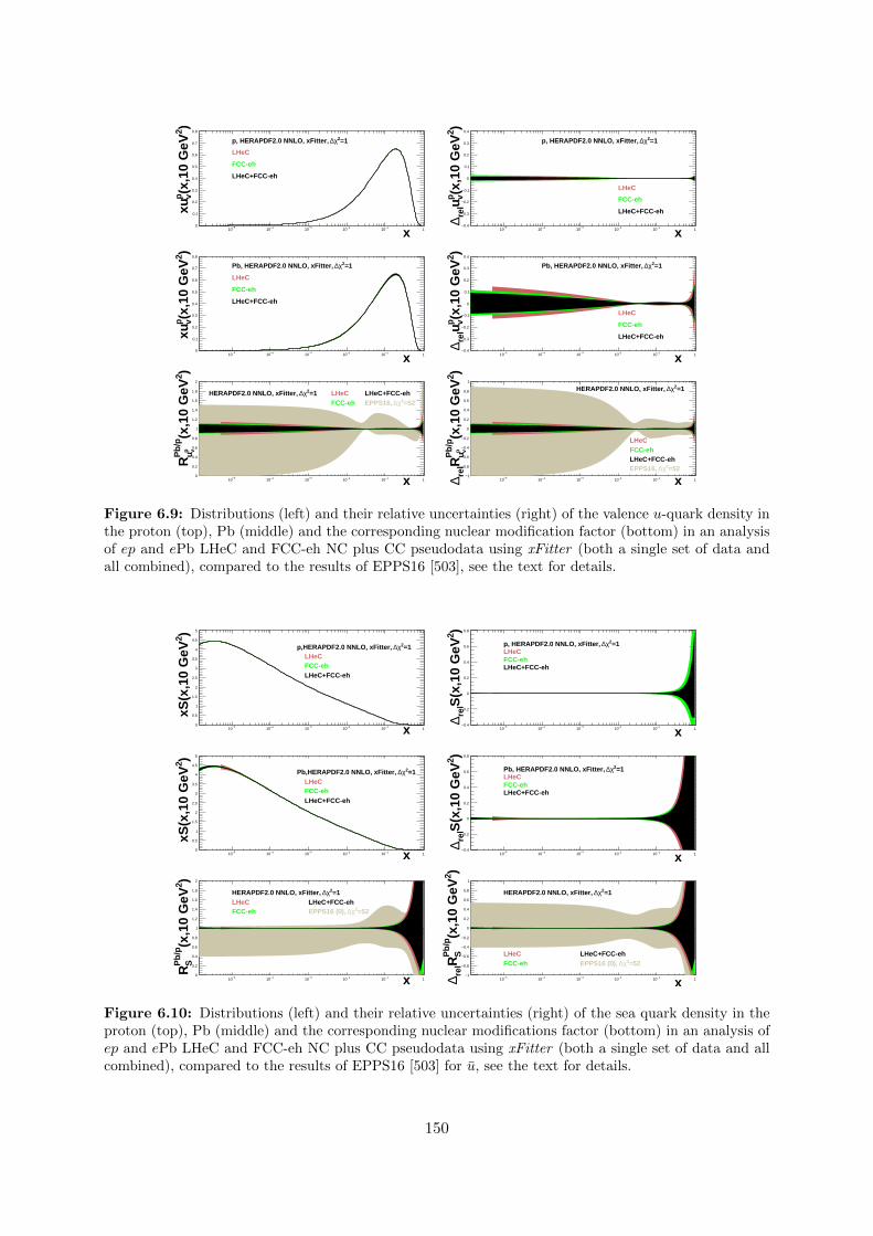
5−10 4−10

3−10 2−10 1−10 1

0

0.1

0.2

0.3

0.4

0.5

0.6

0.7

0.8

x

)2(x

,10

GeV

p vxu

=12χ∆p, HERAPDF2.0 NNLO, xFitter,

LHeC

FCC-eh

LHeC+FCC-eh

5−10 4−10

3−10 2−10 1−10 1

0

0.1

0.2

0.3

0.4

0.5

0.6

0.7

0.8

x

)2(x

,10

GeV

p vxu

=12χ∆Pb, HERAPDF2.0 NNLO, xFitter,

LHeC

FCC-eh

LHeC+FCC-eh

5−10 4−10

3−10 2−10 1−10 1

0

0.2

0.4

0.6

0.8

1

1.2

1.4

1.6

1.8

2

x

)2(x

,10

GeV

p vuPb

/pR

=12χ∆HERAPDF2.0 NNLO, xFitter, LHeCFCC-eh

LHeC+FCC-eh=522χ∆EPPS16,

5−10 4−10

3−10 2−10 1−10 1

0.4−

0.3−

0.2−

0.1−

0

0.1

0.2

0.3

0.4

x

)2(x

,10

GeV

p vure

l∆

=12χ∆p, HERAPDF2.0 NNLO, xFitter,

LHeC

FCC-eh

LHeC+FCC-eh

5−10 4−10

3−10 2−10 1−10 1

0.4−

0.3−

0.2−

0.1−

0

0.1

0.2

0.3

0.4

x

)2(x

,10

GeV

p vure

l∆

=12χ∆Pb, HERAPDF2.0 NNLO, xFitter,

LHeC

FCC-eh

LHeC+FCC-eh

5−10 4−10

3−10 2−10 1−10 1

1−

0.8−

0.6−

0.4−

0.2−

0

0.2

0.4

0.6

0.8

1

x

)2(x

,10

GeV

p vuPb

/pR

rel

∆

=12χ∆HERAPDF2.0 NNLO, xFitter,

LHeCFCC-ehLHeC+FCC-eh

=522χ∆EPPS16,

Figure 6.9: Distributions (left) and their relative uncertainties (right) of the valence u-quark density inthe proton (top), Pb (middle) and the corresponding nuclear modification factor (bottom) in an analysisof ep and ePb LHeC and FCC-eh NC plus CC pseudodata using xFitter (both a single set of data andall combined), compared to the results of EPPS16 [503], see the text for details.

5−10 4−10

3−10 2−10 1−10 1

0

0.5

1

1.5

2

2.5

3

3.5

4

4.5

5

x

)2xS

(x,1

0 G

eV =12χ∆p,HERAPDF2.0 NNLO, xFitter, LHeCFCC-ehLHeC+FCC-eh

5−10 4−10

3−10 2−10 1−10 1

0

0.5

1

1.5

2

2.5

3

3.5

4

4.5

5

x

)2xS

(x,1

0 G

eV

=12χ∆Pb,HERAPDF2.0 NNLO, xFitter, LHeCFCC-ehLHeC+FCC-eh

5−10 4−10

3−10 2−10 1−10 1

0

0.2

0.4

0.6

0.8

1

1.2

1.4

1.6

1.8

2

x

)2(x

,10

GeV

SPb

/pR

=12χ∆HERAPDF2.0 NNLO, xFitter, LHeCFCC-eh

LHeC+FCC-eh=522χ∆), uEPPS16 (

5−10 4−10

3−10 2−10 1−10 1

0.4−

0.2−

0

0.2

0.4

0.6

0.8

x

)2S

(x,1

0 G

eVre

l∆

=12χ∆p, HERAPDF2.0 NNLO, xFitter, LHeCFCC-ehLHeC+FCC-eh

5−10 4−10

3−10 2−10 1−10 1

0.4−

0.2−

0

0.2

0.4

0.6

0.8

x

)2S

(x,1

0 G

eVre

l∆

=12χ∆Pb, HERAPDF2.0 NNLO, xFitter, LHeCFCC-ehLHeC+FCC-eh

5−10 4−10

3−10 2−10 1−10 1

1−

0.8−

0.6−

0.4−

0.2−

0

0.2

0.4

0.6

0.8

1

x

)2(x

,10

GeV

SPb

/pR

rel

∆

=12χ∆HERAPDF2.0 NNLO, xFitter,

LHeCFCC-eh

LHeC+FCC-eh=522χ∆), uEPPS16 (

Figure 6.10: Distributions (left) and their relative uncertainties (right) of the sea quark density in theproton (top), Pb (middle) and the corresponding nuclear modifications factor (bottom) in an analysis ofep and ePb LHeC and FCC-eh NC plus CC pseudodata using xFitter (both a single set of data and allcombined), compared to the results of EPPS16 [503] for u, see the text for details.

150

5−10 4−10

3−10 2−10 1−10 1

0

2

4

6

8

10

12

x

)2xg

(x,1

0 G

eV =12χ∆p, HERAPDF2.0 NNLO, xFitter, LHeCFCC-ehLHeC+FCC-eh

5−10 4−10

3−10 2−10 1−10 1

0

2

4

6

8

10

12

x

)2xg

(x,1

0 G

eV =12χ∆Pb, HERAPDF2.0 NNLO, xFitter, LHeCFCC-ehLHeC+FCC-eh

5−10 4−10

3−10 2−10 1−10 1

0

0.2

0.4

0.6

0.8

1

1.2

1.4

1.6

1.8

2

x

)2(x

,10

GeV

gPb

/pR

=12χ∆HERAPDF2.0 NNLO, xFitter, LHeCFCC-eh

LHeC+FCC-eh=522χ∆EPPS16,

5−10 4−10

3−10 2−10 1−10 1

0.4−

0.2−

0

0.2

0.4

0.6

0.8

x

)2g

(x,1

0 G

eVre

l∆

=12χ∆p, HERAPDF2.0 NNLO, xFitter, LHeCFCC-ehLHeC+FCC-eh

5−10 4−10

3−10 2−10 1−10 1

0.4−

0.2−

0

0.2

0.4

0.6

0.8

x

)2g

(x,1

0 G

eVre

l∆

=12χ∆Pb, HERAPDF2.0 NNLO, xFitter, LHeCFCC-ehLHeC+FCC-eh

5−10 4−10

3−10 2−10 1−10 1

1−

0.8−

0.6−

0.4−

0.2−

0

0.2

0.4

0.6

0.8

1

x)2

(x,1

0 G

eVgP

b/p

Rre

l∆

=12χ∆HERAPDF2.0 NNLO, xFitter, LHeCFCC-eh

LHeC+FCC-eh=522χ∆EPPS16,

Figure 6.11: Distributions (left) and their relative uncertainties (right) of the gluon density in theproton (top), Pb (middle) and the corresponding nuclear modifications factor (bottom) in an analysis ofep and ePb LHeC and FCC-eh NC plus CC pseudodata using xFitter (both a single set of data and allcombined), compared to the results of EPPS16 [503], see the text for details.

xFitter just the (n)PDF combinations that enter the reduced cross sections are parametrisedand employed for the fit 3. With all these considerations in mind, the results shown in thisSection are fully compatible with those in the previous one.

6.3 Nuclear diffraction

In Sec. 3.4 we have discussed specific processes which will probe the details of the 3D structureof the proton. The same processes can be studied in the context of electron-ion scatteringand used to learn about the partonic structure of nuclei. Inclusive diffraction on nuclei canprovide important information about the nuclear diffractive parton distribution similarly to thediffraction on the proton, see Sec. 4.3. Diffractive vector meson production can be studied inthe nuclear case as well, e.g. within the framework of the dipole model suitable for high energyand including non-linear effects in density. In the nuclear case though, one needs to make adistinction between coherent and incoherent diffraction. In the coherent process, the nucleusscatters elastically and stays intact after the collision. In incoherent diffraction, the nucleusbreaks up, and individual nucleons can be set free. Still, there will be a large rapidity gap betweenthe produced diffractive system and the dissociated nucleus. It is expected that this process willdominate the diffractive cross section for medium and large values of momentum transfer. It isonly in the region of small values of momentum transfer where elastic diffraction is the dominantcontribution. Dedicated instrumentation in the forward region must be constructed in order toclearly distinguish between the two scenarios, see Chapter 10.

3In this respect let us note that, in analogy to proton PDFs, a full flavour decomposition can be achievedusing both NC and CC with heavy flavour identification that will verify the existing ideas on flavour dependenceof nuclear effects on parton densities [528].

151

6.3.1 Exclusive vector meson diffraction

Calculations for the case of Pb for the coherent diffractive J/ψ production were performedusing the dipole model [124], see Sec. 3.4. In order to apply the dipole model calculation to thenuclear case, one takes the independent scattering approximation that is Glauber theory [539].The dipole amplitude can then be represented in the form

NA(x, r,b) = 1−A∏i=1

[1−N(x, r,b− bi)] . (6.3)

Here N(x, r,b − bi) is the dipole amplitude for the nucleon (see Sec. 3.4) and bi denotes thetransverse positions of the nucleons in the nucleus. The interpretation of Eq. (6.3) is that 1−Nis the probability not to scatter off an individual nucleon, and thus

∏Ai=1 [1−N(r,b− bi, x)] is

the probability not to scatter off the entire nucleus.

In addition, the following simulation includes the fluctuations of the density profile in the proton,following the prescription given in [122–124]. To include these proton structure fluctuations oneassumes that the gluonic density of the proton in the transverse plane is distributed aroundthree constituent quarks (hot spots). These hot spots are assumed to be Gaussian. In practicalterms one replaces the proton profile Tp(b)

Tp(b) =1

2πBpe−b

2/(2Bp) , (6.4)

that appears in each individual nucleon scattering probability N(x, r,b− bi) by the function

Tp(b) =

3∑i=1

Tq(b− bq,i) , (6.5)

where the ‘quark’ density profile is given by

Tq(b) =1

2πBqe−b

2/(2Bq) . (6.6)

Here bq,i are the location of the hotspots that are sampled from a two dimensional Gaussiandistribution whose width is given by parameter Bqc. The free parameters Bq and Bqc wereobtained in [123] by comparing with HERA data on coherent and incoherent J/ψ production ata photon-proton centre-of-mass energy W = 75 GeV, corresponding to fractional hadronic targetenergy loss xIP = 10−3. The proton fluctuation parameters obtained are Bqc = 3.3 GeV−2 andBq = 0.7 GeV−2.

The results for the differential cross section at t = 0 for coherent production of J/ψ as afunction of (virtual) photon-proton energy W for fixed values of Q2 are shown in Figs. 6.12and Figs. 6.13. The calculations for Pb are compared to those on the proton target. We seethat the cross sections for the nuclear case increase with energy slower than for the proton caseand are always smaller. Note that, we have already rescaled the diffractive cross section bya factor A2, as appropriate for comparison of the diffractive cross section on the proton andnucleus. In the absence of nuclear corrections their ratio should be equal to 1. The differencesbetween the scattering off a nucleus and a proton are also a function of Q2. They are largerfor smaller values of Q2 and for photoproduction. This is understood from the dipole formulae,see Eqs. (3.23), (3.24), (3.25). As explained previously, larger values of scale Q2 select smallersize dipoles, for which the density effects are smaller. Similarly, the differences between the leadand proton cases are larger for higher energies. This is because the dipole amplitude grows with

152

0 1000 2000 3000 4000 5000!

"!!

#!!!

#"!!

$!!!

$"!!

%!!!

%"!!

ePb

ep

1/A2 d

σ/dt

(t=0)

[nb/

GeV

2 ]

W [GeV]

e+p(Pb) e+p(Pb)+J/ψQ2=0.1 GeV2

0 1000 2000 3000 4000 5000!

"!!

#!!!

#"!!

$!!! e+p(Pb) e+p(Pb)+J/ψQ2=2-5 GeV2

ep

ePb

W [GeV]

1/A2 d

σ/dt

(t=0)

[nb/

GeV

2 ]

Figure 6.12: Cross section for the coherent diffractive production of the vector meson J/ψ in ePb (redsolid curves) and ep (black solid curves) collisions, as a function of the energy W . Left: photoproductioncase Q2 ' 0, right: Q2 = 2− 5 GeV2

0 1000 2000 3000 4000 5000!

"!!

#!!

$!!

%!!

&!!!

&"!! e+p(Pb) e+p(Pb)+J/ψQ2=5-10 GeV2

ep

ePb

W [GeV]

1/A2 d

σ/dt

(t=0)

[nb/

GeV

2 ]

0 1000 2000 3000 4000 5000!

"!

#!

$!

%!

&!!

&"!

&#!

&$! e+p(Pb) e+p(Pb)+J/ψQ2=10-100 GeV2

epePb

1/A2 d

σ/dt

(t=0)

[nb/

GeV

2 ]

W [GeV]

Figure 6.13: Cross section for the coherent diffractive production of the vector meson J/ψ in ePb (redsolid curves) and ep (black solid curves) collisions, as a function of the energy W . Left: Q2 = 5−10 GeV2,right: Q2 = 10− 100 GeV2.

decreasing values of x which are probed when the energy is increased, and thus the non-lineardensity effects are more prominent at low values of x and Q2.

These findings can be summarised by inspecting the ratio of the cross sections, presented as afunction of x defined as4

x =Q2 +m2

J/ψ

Q2 +W 2 +m2J/ψ −m2

N

(6.7)

which is shown in Fig. 6.14. We observe that the ratio is smaller for smaller values of Q2,and it decreases for decreasing values of x. The results from the dipole model calculations arecompared with the ratio of the gluon density squared (evaluated at x and Q2) obtained from thenuclear PDFs using the EPPS16 set [503]. The reason why one can compare the diffractive crosssection ratios with the ratios for the gluon density squared can be understood from Eqs. (3.23)and (3.24). The diffractive amplitude is proportional to the gluon density xg(x,Q2). On theother hand the diffractive cross section is proportional to the amplitude squared, thus havingenhanced sensitivity to the gluon density. The nuclear PDFs have large uncertainties, which isindicated by the region between the two sets of dotted lines. The EPPS16 parametrisation ispractically unconstrained in the region below x = 0.01. Nevertheless, the estimate based on the

4This choice to translate W and Q2 into x in the dipole model calculations differs from others in the literaturebut the difference is only significative at large x where the dipole model is not applicable.

153

1x10-6 0.00001 0.0001 0.001 0.01 0.1

!.#

!.$

!.%

!.&

'

'.#

'.$

'.%

'.&Dipole, Q#=!.' GeV#Dipole, Q#='!-'!! GeV#EPPS'%, Q#=mJ/psi^#EPPS'%, Q#=mJ/psi^#, upperEPPS'%, Q#=mJ/psi^#, lowerEPPS'%, Q#='!! GeV#EPPS'%, Q#='!! GeV#, upperEPPS'%, Q#='!! GeV#, lower

x=(Q2+mJ/ψ2)/(W2+Q2+mJ/ψ

2-mN2)

σ(ePb)/[2082 σ(ep)]

[Rg(x,Q2)]2

Figure 6.14: Ratio of coherent J/ψ production diffractive cross sections for Pb and proton as a functionof the variable x (defined in Eq. (6.7) for the dipole model results). Solid lines: dipole model calcula-tion, for Q2 = 0.1 GeV2 (black) and Q2 = 10 − 100 GeV2 (red). Dotted and dashed lines correspondto the nuclear ratio for the gluon density squared using the EPPS16 parametrisation [503] of the nu-clear parton distribution functions. Black and red dashed lines are the central sets for Q2 = M2

J/ψ and

Q2 = 100 GeV2. The dotted lines correspond to the low and high edges of the Hessian uncertaintyin the EPPS16 parametrisation. The difference between the two dotted lines is thus indicative of theparametrisation uncertainty for the nuclear ratio. These ratios, that can also be measured in ultrape-ripheral collisions [129], are larger that the values 0.2−0.4 at x ' 10−5 predicted by the relation betweendiffraction and nuclear shadowing [344].

dipole model calculation and the central value of the EPPS16 parametrisation are consistentwith each other. This strongly suggests that it will be hard to disentangle nuclear effects fromsaturation effects and that only through a detailed combined analysis of data on the proton andthe nucleus firm conclusions can be established on the existence of a new non-linear regime ofQCD.

The differential cross section dσ/dt as a function of the negative four momentum transfer squared−t for the case of coherent and incoherent production is shown in Fig. 6.15. Coherent and inco-herent diffraction cross sections are computed from the dipole model in the following way. Thecoherent diffractive cross section is obtained by averaging the diffractive scattering amplitudeover the target configurations and taking the square

dσ

dt=

1

16π|〈A(x,Q,∆)〉|2 . (6.8)

Here the brackets 〈. . . 〉 refer to averages over different configurations of the target. The incoher-ent cross section is obtained by subtracting the coherent cross section from the total diffractivecross section. It is standardly assumed that it takes the form of a variance of the diffractivescattering amplitude

dσ

dt=

1

16π

(〈|A(x,Q,∆)|〉2 − |〈A(x,Q,∆)〉|2

), (6.9)

which should be valid for small |t|. The t dependence, and the relation between the impactparameter and t through the Fourier transform, makes diffractive scattering a sensitive probe

154

0.00 0.05 0.10 0.15 0.20 0.25 0.30 0.35 0.40

|t| [GeV2]

102

103

104

105

106

107

dσ/dt

[nb/G

eV2]

With nucleon substructure fluctuationsNo nucleon substructure

γ + Pb→ J/Ψ + Pb, Q2 = 0 GeV2

Figure 6.15: The differential cross sections for coherent and incoherent production of J/ψ in ePb as afunction of the negative four momentum transfer squared −t, for photoproduction, Q2 = 0. The linesshowing dips are for coherent production, and those extending to large |t| are for incoherent. The solid(dashed) lines are the results with (without) nucleon substructure fluctuations. Black, blue, red are forW = 0.1, 0.813, 2.5 TeV, respectively.

of the internal geometric structure of hadrons and nuclei, see Ref. [540] for an extraction ofthe transverse profile of the nucleus in ultraperipheral collisions at RHIC; also Ref. [541] for anstudy for the EIC. In particular, because the incoherent cross section has the form of a varianceof the amplitude, it is sensitive to the amount of fluctuations in impact parameter space.

The results in Fig. 6.15 (results for higher Q2 are very similar) indicate that the incoherentproduction is dominant for most values of −t, except for the very small momentum transfers,about |t| < 0.02 GeV2. Thus, dedicated instrumentation which will allow us to distinguishbetween the two cases is essential if one wants to measure the coherent process in a reasonablywide range of |t|. As in the proton case, the coherent t distribution exhibits characteristic dips.However, in the case of the nuclear targets the dips occur for much smaller values of t. This isrelated to the much larger value of the dipole amplitude for a wide range of impact parametersin the case of nuclear targets compared to the proton case.

Another interesting aspect, see Sec. 3.4, is the effect of the transverse structure of the targetin nuclear coherent and incoherent diffraction [542]. For example, in the formulation shownabove [124] a fixed number of hot spots was considered, while in [128] (see also [125] for arealisation using small-x evolution) a growing number with 1/x is implemented. In both cases,the ratio of incoherent to coherent diffraction decreases with W , being smaller for larger nuclei.This decrease is sensitive to the details of the distribution of hot spots - thus, to the fluctuationsof the gluon distribution in transverse space. It also shows interesting dependencies on themass of the produced vector meson and on Q2, resulting in the ratio being smaller for lightervector mesons and for lower Q2. Besides, the hot spot treatment also has some effects on thedistributions in momentum transfer, see Fig. 6.15. In order to check these ideas, both theexperimental capability to separate coherent form incoherent diffraction, and a large lever armin W and Q2 as available at the LHeC, are required.

155

We thus conclude that by investigating coherent and incoherent diffractive scattering on nuclei,one gets unique insight into the spatial structure of matter in nuclei. On the one hand, thecoherent cross section, which is obtained by averaging the amplitude before squaring it, issensitive to the average spatial density distribution of gluons in transverse space. On the otherhand, the incoherent cross section, which is governed by the variance of the amplitude withrespect to the initial nucleon configurations of the nucleus, measures fluctuations of the gluondensity inside the nucleus. In the case of a nucleus, the diffractive production rate is controlled bytwo different scales related to the proton and nucleus size. At momentum scales correspondingto the nucleon size |t| ∼ 1/R2

p the diffractive cross section is almost purely incoherent. Thet-distribution in coherent diffractive production off the nucleus gives rise to a dip-type structurefor both saturation and non-saturation models, while in the case of incoherent production atsmall |t|, both saturation and non-saturation models do not lead to dips [124]. This is in drasticcontrast to the diffractive production off the proton where only saturation models lead to adip-type structure in the t-distribution at values of |t| that can be experimentally accessible.Therefore, diffractive production offers a unique opportunity to measure the spatial distributionof partons in the protons and nuclei. It is also an excellent tool to investigate the approach tounitarity in the high energy limit of QCD.

While we have focused here on J/ψ production, lighter vector mesons like ρ, ω, φ could also bestudied. They should show a different Q2 dependence and their larger sizes would make themlie closer to the black disk regime. Also the dominance of two-jet events in photoproductionwould provide sensitivity to the approach to the unitarity limit [344].

6.3.2 Inclusive diffraction on nuclei

In Sec. 4.3, a study of the prospects for extracting diffractive parton densities in the proton waspresented following [346]. Diffraction in eA is similar to that in ep, the main difference being asmaller contribution from incoherent e+A→ e+X+A∗ than from coherent e+A→ e+X+Adiffraction, with A∗ denoting a final state where the nucleus dissociates into at least two hadronsbut the event still shows a rapidity gap. Incoherent diffraction dominates for |t| larger than a fewhundredths of a GeV2. Forward detectors [1] will allow the separation of coherent diffraction,on which we focus in the following, summarising the study in Ref. [346].

Assuming that the same framework (collinear factorization for hard diffraction, Eq. (4.14), andRegge factorization, Eq. (4.16)) introduced in Sec. 4.3 for ep also holds for eA, nuclear diffractivePDFs (nDPDFs) can be extracted from the diffractive reduced cross sections. Note that suchnDPDFs have never been measured. For an electron energy Ee = 60 GeV and nuclear beamswith EN = 2.76 TeV/nucleon, the kinematic coverage at the LHeC is very similar to that shownin Fig. 4.22. For details, see Ref. [346].

Defining, in analogy to Eq. (6.1), the diffractive nuclear modification factor

RAk (β, ξ,Q2) =fD(3)k/A (β, ξ,Q2)

AfD(3)k/p (β, ξ,Q2)

, (6.10)

we show in Fig. 6.16 the results for FD(3)2 and F

D(3)L from the FGS models [344]. These models

are based on Gribov inelastic shadowing [343] which relates diffraction in ep to nuclear shadowingfor total and diffractive eA cross sections. The nuclear wave function squared is approximatedby the product of one-nucleon densities, the t-dependence of the diffractive γ∗-nucleon amplitudeis neglected compared to the nuclear form factor, and a real part in the amplitudes [543] andcolour fluctuations for the inelastic intermediate nucleon states [544] are introduced. There are

156

Pb208 FGS-2018 F2 FL nucl. suppr. at Q2 = 10

0

0.2

0.4

0.6

0.8

1

10-4 10-3 10-2 10-1 100

ξ = 10-5

β

F2 FGS-HF2 FGS-LFL FGS-HFL FGS-L

0

0.2

0.4

0.6

0.8

1

10-4 10-3 10-2 10-1 100

ξ = 0.0001

β

0

0.2

0.4

0.6

0.8

1

10-4 10-3 10-2 10-1 100

ξ = 0.001

β

0

0.2

0.4

0.6

0.8

1

10-4 10-3 10-2 10-1 100

ξ = 0.01

β

0

0.2

0.4

0.6

0.8

1

10-4 10-3 10-2 10-1 100

ξ = 0.05

β

0

0.2

0.4

0.6

0.8

1

10-4 10-3 10-2 10-1 100

ξ = 0.1

β

Figure 6.16: Nuclear modification factor, Eq. (6.10), for FD(3)2 and F

D(3)L in 208Pb versus β, at Q2 =

10 GeV2 and for different ξ, for the models H and L in [344]. The ‘\’ and ‘/’ hatched areas showkinematically excluded regions for E = 2.76 and 19.7 TeV/nucleon, respectively. Taken from Ref. [346].

two models, named H and L, that correspond to different strengths of the colour fluctuationsand result in larger and smaller probabilities for diffraction in nuclei with respect to that inproton, respectively. In Figs. 6.16 and 6.17 we show results [346] for both models.

e Pb EPb/A = 2.76 TeV, Ee = 60 GeV, L = 2 fb-1

0

0.02

0.04

0.06

0.08

0.1

Q2 = 10 GeV2

FGS18-L

ξσre

d

ξ = 0.1ξ = 0.01ξ = 0.001ξ = 0.0001

Q2 = 100 GeV2

FGS18-Lξ = 0.1ξ = 0.01ξ = 0.001

0

0.02

0.04

0.06

0.08

0.1

0.0001 0.001 0.01 0.1

Q2 = 1000 GeV2

FGS18-L

ξσre

d

β

ξ = 0.1ξ = 0.01

0.0001 0.001 0.01 0.1 1

Q2 = 10000 GeV2

FGS18-L

β

ξ = 0.1

e Pb EPb/A = 2.76 TeV, Ee = 60 GeV, L = 2 fb-1

0

0.02

0.04

0.06

0.08

0.1

Q2 = 10 GeV2

FGS18-H

ξσre

d

ξ = 0.1ξ = 0.01ξ = 0.001ξ = 0.0001

Q2 = 100 GeV2

FGS18-Hξ = 0.1ξ = 0.01ξ = 0.001

0

0.02

0.04

0.06

0.08

0.1

0.0001 0.001 0.01 0.1

Q2 = 1000 GeV2

FGS18-H

ξσre

d

β

ξ = 0.1ξ = 0.01

0.0001 0.001 0.01 0.1 1

Q2 = 10000 GeV2

FGS18-H

β

ξ = 0.1

Figure 6.17: An indicative subset of simulated data for the diffractive reduced cross section as afunction of β in bins of ξ and Q2 for e 208Pb collisions at the LHeC, in the models in [344]. The curvesfor ξ = 0.01, 0.001, 0.0001 are shifted up by 0.01, 0.02, 0.03, respectively. Taken from Ref. [346].

157

A subset of the simulated pseudodata for the reduced cross sections is shown in Fig. 6.17 [346].They are generated assuming 5 % systematic error and statistic errors calculated for an integratedluminosity of 2 fb−1. Compared to Fig. 4.24, the comparably large kinematic coverage and small(systematics-dominated) uncertainty illustrated in Fig. 6.17 show clearly that an extraction ofnDPDFs in 208Pb analogous to that shown in Figs. 4.25 and 4.26 for the DPDFs, will be possiblewith similar accuracy in an extended kinematic region.

6.4 New Dynamics at Small x with Nuclear Targets

As discussed in Sec. 4.2.1, theoretical expectations [507] indicate that fixed-order perturbationtheory leading to the DGLAP evolution equations should eventually fail. When x decreases,αs ln 1/x becomes large and these large logarithms must be resummed, leading to the BFKLequation. Furthermore, when the parton density becomes large, the linear approximation thatunderlies both DGLAP and BFKL breaks, and non-linear processes must be taken into accountto compute parton evolution. The CGC [506] offers a non-perturbative but weak couplingeffective theory to treat dense parton systems in a systematic and controlled way. One of theimportant predictions of the CGC is that in a dense parton system saturation occurs leading tothe emergence of a new dynamical scale – the saturation scale Qsat, which increases with theenergy.

The parton density in a hadron becomes high both through evolution – when energy or 1/xbecomes large, and/or when partons are accumulated by overlapping nucleons – when massnumber A becomes large in a nucleus. In the nucleus rest frame, the virtual photon fluctuationsat small x < (2mNRA)−1, with mN the nucleon mass and RA the nuclear radius, acquirea lifetime larger than the time taken to traverse the nucleus and, thus, all partons within atransverse area ∼ 1/Q2 are simultaneously probed. Actually, the parameter determining thetransition between linear and non-linear dynamics is the parton density and, therefore, the onsetof this new regime of QCD and its explanation must be tested, as commented in [1], exploringboth decreasing values of x and increasing values of A in a kinematic x − Q2 region where,in order to be sensitive to differences in evolution, enough lever arm in Q2 Λ2

QCD at smallx is available. The saturation scale Qsat that characterises the typical gluon momentum ina saturated hadron wave function increases with nuclear size, Q2

sat ∝ A1/3. Therefore, in eAcollisions the perturbatively saturated regime is achieved at parametrically larger x than in aproton – a prediction not only of the CGC but of all multiple scattering models that anticipatean approach to the black disk, unitarity limit.

The opportunities to establish the existence of saturation in lepton-nucleus collisions are nu-merous. They include inclusive observables, both total and diffractive cross sections, and lessinclusive ones like correlations:

• Tension in DGLAP fits for inclusive observables: As discussed in [1,257] and in Sec. 4.2.2,deviations from fixed-order perturbation theory can be tested by the tension that wouldappear in the description within a DGLAP fit of observables with different sensitivities tothe sea and the glue, for example F2 and FL (or reduced cross sections at different energies)

or F inclusive2 and F heavy quarks

2 . In [545], such an exercise was performed considering F2 andFL pseudodata for eAu collisions at the EIC [101] using reweighting techniques. While theresults for EIC energies are shown not to be conclusive due to the reduced lever arm inQ2 > Q2

sat Λ2QCD, the much larger centre-of-mass energies at the LHeC (and FCC-eh)

should make possible a search for tensions between different observables.

• Saturation effects in diffraction: A longstanding prediction of saturation [107, 546, 547]

158

is a modification of the diffractive cross section in nuclei with respect to protons, witha suppression (enhancement) at small (large) β due to the approach of the nucleus tothe black disk limit, where elastic and diffractive scattering become maximal, and thebehaviour of the different Fock components of the virtual photon wave function. Sucheffects can also be discussed in terms of a competition of nuclear shadowing with theprobability that the event remains diffractive in the multiple scattering process [344]. Thisleads to the generic expectation of an enhancement of the ratio of the coherent diffractivecross section in nucleus over that in protons, in non-linear approaches with respect tolinear ones [101].

• Correlations: Correlations have been considered for a long time as sensitive probes of theunderlying production dynamics. For example, the cross section for the production oftwo jets with the same hardness and widely separated in rapidity, called Mueller-Naveletjets [548], was proposed as a test of BFKL versus DGLAP dynamics, but the effect ofsaturation has not been widely studied although it has the large potentiality of differ-entiating linear resummation from non-linear saturation where non-trivial nuclear effectscould appear. Correlations between jets were analysed in [1] for the LHeC kinematics,both in inclusive and diffractive events, see the formalism in [549]. On the other hand, theazimuthal decorrelation of particles and jets when saturation effects are at work – at smallx, studied by the difference between collisions involving proton and nuclei, was proposedlong ago in dAu collisions at the Relativistic Hadron Collider [550, 551]. It was studiedin [1] for the LHeC kinematics, see recent developments in [552] and the extension toforward dijet production in [553]. It could also be analysed in ultraperipheral collisions atthe LHC, see Sec. 9.7.

6.5 Collective effects in dense environments – the ‘ridge’

One of the most striking discoveries [554] at the LHC is, that in all collision systems, fromsmall (pp and pA) to large (AA), many of the features that are considered as indicative of theproduction of a dense hot partonic medium are observed (see e.g. reviews [555–557] and referencestherein). The most celebrated of such features is the long rapidity range particle correlationscollimated in azimuth, named the ‘ridge’, shown in Fig. 6.18. The dynamics underlying thisphenomena, either the formation of QGP and the existence of strong final state interactions, orsome initial state dynamics that leaves imprint on the final observables, is under discussion [558].While observed in photoproduction on Pb in UPCs at the LHC [559], its existence in smallersystems like e+e− [560] at LEP and ep at HERA [561] has been scrutinised, but the results arenot conclusive.

In this respect, measurements in ep and eA collisions at the LHeC at considerable centre-of-mass energies will offer crucial additional information. For example, the collision of the virtualphoton with the proton at the LHeC can be considered as a high energy collision of two jets or‘flux tubes’, as discussed in Refs. [564, 565] and illustrated in Fig. 6.18. This can lead to theproduction of ‘ridges’ and other novel configurations of gluons and quarks and will be measureduniquely at the LHeC.

6.6 Novel QCD Nuclear Phenomena at the LHeC

Beyond the topics discussed above there are many novel phenomena which can be explored in eAcollisions at LHeC or FCC-eh, in a high energy regime and using dedicated instrumentation. We

159

Figure 6.18: Left and top right: Collective effects seen in high-multiplicity two-particle azimuthalcorrelation, as observed by CMS in PbPb, pPb [562], and pp [563] collisions. Bottom right: Schematicillustration for the production of ridge-like effects in ep or eA scattering at the LHeC [564].

shall briefly review some of these phenomena, which can be understood utilizing the light-frontframework of QCD, for a review see [566].

One of the most important theoretical tools in high energy physics is Dirac’s light-front (LF)time: τ = x+ = t + z/c, the time along the light-front [567], a concept which allows all of thetools and insights of Schrodinger’s quantum mechanics and the Hamiltonian formalism to beapplied to relativistic physics [566]. When one takes a photograph, the object is observed at afixed LF time. Similarly, Compton γp → γ′p′′ and deep-inelastic lepton-proton scattering aremeasurements of proton structure at fixed LF time. Unlike ordinary instant time t, physics atfixed τ is Poincare invariant; i.e. independent of the observer’s Lorentz frame. Observationsat fixed τ are made within the causal horizon. LF time τ reduces to ordinary time t in thenonrelativistic limit c→∞.The LF wavefunctions (LFWF) of hadrons are superpositions of ΨH

n (xi,~k⊥i,λi) =< ΨH |n >,the Fock state projections of the eigensolution of the QCD LF Hamiltonian HQCD|ΨH >=M2HΨH >. They encode the underlying structure of bound states in quantum field theory and

underlie virtually every observable in hadron physics. Hadronic LFWFs can also be measureddirectly by the Ashery method [568], the coherent diffractive dissociation of high energy hadronsinto jets [569,570]. In the diffractive dissociation of a high energy hadron into quark and gluonjets by two-gluon exchange, the cross-section measures the square of the second transversederivative of the projectile LFWF. Similarly, the dissociation of a high energy atom such aspositronium or true muonium ([µ+µ−]) can be used to measure the transverse derivative of itsLFWFs.

160

Hadronic LFWFs are defined at fixed τ = −x+ = t + z/c; they are thus off-shell in the totalP− = P 0 − P z, not energy P 0 [566]. Thus LFWFs are also off-shell in M2 = P+P− − P 2

⊥ =

[∑

i kµi ]2 =

∑ik2⊥+m2

x i, the invariant mass squared of the constituents in the n-particle Fock

state. LFWFs are thus functions of the invariant mass squared of the constituents in the

Fock state. For a two-particle Fock state, M2 =k2⊥+m2

x(1−x) . Thus, the constituent transverse

momenta k2⊥i do appear alone as a separate factor in the LFWF; the transverse momenta are

always coupled to the longitudinal LF momentum fractions xi. This is the light-front versionof rotational invariance. Only positive k+

i = k0i + kzi ≥ 0 and 0 ≤ xi = k+−

P+ ≤ 1 appear,

where∑

i xi = 1. In addition, Jz =∑

i Lzi + Szi , as well as P+ =

∑i k

+i and ~P⊥ =

∑i~k⊥i are

conserved at every vertex – essential covariant kinematical constraints. A remarkable property:the anomalous gravitomagnetic moment of every LF Fock state vanishes at Q2 = 0. TheLFWFs of bound states are off-shell in P− =

∑i k−i , but they tend to be maximal at minimal

off-shellness; i.e. minimal invariant mass. In fact, in the holographic LFWFs where colour isconfined, the LFWFs of hadrons have fast Gaussian fall-off in invariant mass. This feature alsounderlie intrinsic heavy quark Fock states: the LFWFs have maximal support when all of the

constituents have the same rapidity yi; i.e. xi ∝√m2i + k2

⊥i. Thus the heavy quarks have the

highest momentum fractions xi.

Conversely, light-front wavefunctions provide the boost-invariant transition amplitude whichconvert the free quark and gluons into the hadronic eigenstates of QCD. Thus, knowing theLFWFs allows one to compute hadronization at the amplitude level – how the coloured quarksand gluons produced in a deep inelastic scattering event ep → e′X at the LHeC are confinedand emerge as final-state hadrons.

The LF formalism leads to many novel nuclear phenomena, such as hidden colour [571] colourtransparency [572], nuclear-bound quarkonium [573], nuclear shadowing and antishadowing ofnuclear structure functions, etc. For example, there are five distinct colour-singlet QCD Fockstate representations of the six colour-triplet quarks of the deuteron. These hidden-colour Fockstates become manifest when the deuteron fluctuates to a small transverse size, as in mea-surements of the deuteron form factor at large momentum transfer. One can also probe thehidden-colour Fock states of the deuteron by studying the final state of the dissociation of thedeuteron in deep inelastic lepton scattering at the LHeC eD → e′X, where X can be ∆++ +∆−,six quark jets, or other novel colour-singlet final states.

The LF wave functions provide the input for scattering experiments at the amplitude level,encoding the structure of a projectile at a single light-front time τ [566]. For example, considerphoton-ion collisions. The incoming photon probes the finite size structure of the incomingnucleus at fixed LF time, like a photograph – not at a fixed instant time, which is acausal.Since the nuclear state is an eigenstate of the LF Hamiltonian, its structure is independent ofits momentum, as required by Poincare invariance. One gets the same answer in the ion restframe, the CM frame, or even if the incident particles move in the same direction, but collidetransversely. There are no colliding pancakes using the LF formalism.

The resulting photon-ion cross-section is not point-like; it is shadowed: σ(γA→ X) = Aασ(γN →X), where A is the mass number of the ion, N stands for a nucleon, and the power α ≈ 0.8reflects Glauber shadowing [574]. The shadowing stems from the destructive interference oftwo-step and one-step amplitudes, where the two-step processes involve diffractive reactions ona front-surface nucleon which shadows the interior nucleons. Thus the photon interacts primar-ily on the front surface. Similarly, a high energy ion-ion collision A1 + A2 → X involves theoverlap of the incident frame-independent LFWFs. The initial interaction on the front surface

161

of the colliding ions can resemble a shock wave.

In the case of a deep inelastic lepton-nucleus collision γ∗A→ X, the two-step amplitude involvesa leading-twist diffractive deep inelastic scattering (DDIS) γ∗N1 → V ∗N1 on a front surfacenucleon N1 and then the on-shell propagation of the vector system V ∗ to a downstream nucleonN2 where it interacts inelastically: V ∗N2 → X. If the DDIS involves Pomeron exchange, the two-step amplitude interferers destructively with the one-step amplitude γ∗N1 → X thus producingshadowing of the nuclear parton distribution function at low x < 0.1. On the other hand, ifthe DDIS process involves I = 1 Reggeon exchange, the interference is constructive, producingflavour-dependent leading-twist antishadowing [574] in the domain 0.1 < x < 0.2.

One can also show that the Gribov-Glauber processes, which arise from leading-twist diffractivedeep inelastic scattering on nucleons and underly the shadowing and antishadowing of nuclearstructure functions [574], prevent the application of the operator product expansion to thevirtual Compton scattering amplitude γ∗A→ γ∗A on nuclei and thus negate the validity of themomentum sum rule for deep inelastic nuclear structure functions [575].

162

Chapter 7

Higgs Physics with LHeC

7.1 Introduction

The Higgs boson was discovered in 2012 by ATLAS [576] and CMS [577] at the Large HadronCollider (LHC). It is the most recently discovered and least explored part of the Standard Model.The Higgs Boson (H) is of fundamental importance. It is related to the mechanism predictedby [419, 420, 578] and independently by [579]], in which the intermediate vector bosons of thespontaneously broken electroweak symmetry acquire masses 1 while the photon remain massless.Fermions obtain a mass via the Yukawa couplings with the Higgs field. Following the discoveryof the Higgs boson, its physics and thorough exploration has become a central theme of thephysics programme at the LHC. Any high-energy future collider project, beginning with thehigh luminosity upgrade of the Large Hadron Collider, the HL-LHC, underway to collect datain a decade hence, has put the potential to precisely study the properties of the Higgs boson intoits center of attention, for understanding its characteristics and hoping to open a new windowinto physics extending beyond the Standard Model, see for example [580, 581]. In this sectionwe present the potential to explore the SM Higgs physics at the LHeC and to certain extent atFCC-eh also.

A first challenge on the physics of the Higgs boson is to establish whether it indeed satisfies theproperties inherent to the Standard Model (SM) regarding its production and decay mechanisms.The SM neutral H boson decays into pairs of fermions, ff . The dominant decay is H → bbwith a branching fraction of about 58 %. The branching scales with the square of the fermionmass, m2

f . The next prominent fermionic decay therefore is H → τ+τ− with 6.3 % followed bythe charm decay with a predicted branching fraction of 2.9 %. The Higgs boson also decays intopairs of W and Z bosons at a rate of 21.5 % and 2.6 %, respectively. Loop diagrams enable thedecay into gluon and photon pairs with a branching of 8.2 and 0.2 %, respectively. The sevenmost frequent decay channels, ordered according to descending branching fractions, thus areinto bb, W+W−, gg, τ+τ−, cc, ZZ and γγ. Together these are predicted to represent a totalSM branching fraction of 99.9 %. At the LHC these and rarer decays can be reconstructed,with the exception of the charm decay for reasons of prohibitive combinatorial background. Themain purpose of this paper is to evaluate the prospects for precisely measuring these channels

1The mass of the W boson, MW , is generated through the vacuum expectation value, η, of the Higgs field (Φ)and given by the simple relation MW = gη/

√2 where g is the weak interaction coupling. Here η =

√−µ2/2λ

with the two parameters of the Higgs potential that is predicted to be V = −µ2Φ+Φ − λ(Φ+Φ)2. The Higgsmass is given as MH = 2η

√λ while the mass of the Z boson is related to MW with the electroweak mixing angle,

MZ = MW / cos ΘW .

163

in electron-proton scattering.

7.2 Higgs Production in Deep Inelastic Scattering

In deep inelastic electron-proton scattering, the Higgs boson is predominantly produced throughWW fusion in charged current DIS (CC) scattering, Fig. 1. The next large Higgs productionmode in ep is ZZ → H fusion in neutral current DIS (NC) scattering, Fig. 1, which has a smallerbut still sizable cross section. These ep Higgs production processes are very clean for a number

q q′

W+

W−

H

e− νe

q q′

Z

Z

H

e− e−

Figure 7.1: Higgs boson production in charged (left) and neutral (right) current deep inelastic electron-proton scattering to leading order.

of reasons:

• even at the high luminosity of 1034 cm−2s−1 the inclusive pileup is only 0.1 (1) for theLHeC (FCC-eh) and the final state signature therefore free from event overlap, in contrastto the HL-LHC where it will typically be 150;

• in ep, contrary to pp, there is no initial nor final state colour (re)connection;

• the higher-order corrections are small. For the total CC process they were estimated [582]to be of the order of only 1 % for the QCD part, subject to cut dependencies yieldingshape changes up to 20 %, and −5 % for the QED part (with a weak dependence onthe PDF choice). The smallness of the QCD corrections was attributed mainly to theabsorption of gluon and quark radiation effects in the evolution of the parton distributions(PDFs) [582]. The PDFs will be measured with very high precision at any of the epcolliders here considered, see Chapter 3, thus allowing a unique self-consistency of Higgscross section measurements.

The NC reaction is even cleaner than the CC process as the scattered electron fixes the kinematicsmore accurately than the missing energy. While in pp both WW and ZZ processes are hardlydistinguishable, in ep they uniquely are, which provides an important, precise constraint on theWWH and ZZH couplings.

7.2.1 Kinematics of Higgs Production

At HERA the kinematics was conveniently reconstructed through event-wise measurements ofQ2 and y. The reconstruction of the kinematics in charged currents uses the inclusive hadronicfinal state measurements. Based on the energies E′e and Eh and the polar angles Θe and Θh

of the scattered electron and the hadronic final state, respectively, one obtains a redundantdetermination of the kinematics in neutral current scattering. This permits a cross calibrationof calorimetric measurements, of the electromagnetic and hadronic parts and of different regions

164

of the detector, which is a major means to achieve superb, sub-percent precision in ep collidermeasurements. Methods have been developed to optimise the kinematics reconstruction andmaximise the acceptance by exploiting the redundant determination of the scattering kinematics,see for example [56]. The basic DIS kinematic distributions of Q2, x and y for Higgs productionat√s = 3.5 TeV are illustrated in Fig. 7.2. The average Q2 and x values probed are Q2 ≈

]2 [GeV2 Q10

log0 1 2 3 4 5 6

Eve

nts

0

100

200

300

400

500

600

700

800

y10

log-3 -2.5 -2 -1.5 -1 -0.5 0

Eve

nts

0

100

200

300

400

500

x10

log-7 -6 -5 -4 -3 -2 -1 0

Eve

nts

0

100

200

300

400

500

600

700

Figure 7.2: Distributions for ep→ νHX events, at parton-level, for the negative 4-momentum transfersquared, Q2 (top left), Bjorken x (bottom left) and the inelasticity y = Q2/sx (top right) at

√s = 3.5 TeV

(FCC-eh). Events generated with MadGraph [375], see Tab. 7.1.

2000 GeV2, x ≈0.02 at LHeC and Q2 ≈ 6500 GeV2, x ≈0.0016 at FCC-eh.

As is described in this paper elsewhere, constraints for a large pseudorapidity or polar angle,η = ln tan θ/2, acceptance of the apparatus arise i) for the backward region (the polar angleis defined w.r.t. the proton beam direction) from the need to reconstruct electrons at low Q2

enabling low x physics and ii) for the forward region to cover a maximum region towards largex at medium Q2 with the reconstruction of the hadronic final state. The acceptance thereforeextends, for the LHeC, to pseudorapidities of η = ±5, which for the FCC-eh case is extended toη = ±6. The large acceptance is in particular suitable for the reconstruction of Vector-Boson-Fusion Higgs boson event signatures, see Fig. 7.3 for the typical pseudorapidity distributions ofHiggs boson event signature in DIS at the most asymmetric FCC-eh collider configuration.

Geometric acceptances due to kinematic constraints in the pseudorapidity on the Higgs decayproducts for both LHeC and FCC-eh are further illustrated in Fig. 7.4. The acceptances arecalculated for a basic selection of all final states with pT > 15 GeV and a coverage of the forwardjet up to η = 5 and η = 6, respectively, for both colliders. As seen from Fig. 7.4, the acceptancesare higher for the less asymmetric LHeC beam configuration and about the same for hadroniccalorimetry up to η = 5 and η = 6. Hence, the LHeC calorimeter is designed for η = 5. Theoptimal hadronic calorimetry coverage for FCC-eh is clearly η = 6 yielding significantly higheracceptances in comparison to an η = 5 calorimetry. From Fig. 7.4, it is apparent that for bothcollider configurations the Higgs decay products would require tagging capabilities up η = 3.5,e.g. for heavy flavour and tau decays. Suitably designed muon detectors covering η = 4 appearfeasible for both collider configurations, those would result in high H → µµ acceptances of about72 % (63 %) for LHeC (FCC-eh) for selecting all final states with pT > 15 GeV and a coverage

165

η-6 -4 -2 0 2 4 6 8 10

Eve

nts

0

100

200

300

400

500

Higgs

Decay particles

Struck Quark

Scattered lepton

Figure 7.3: Pseudorapidity (η) distributions, at parton-level, characterising the Vector-Boson-Fusionproduction and decay of the Higgs boson to WW in DIS scattering at FCC-eh. The scattered lepton(blue) in the NC case (or missing energy for CC) has an average η of about −0.5, i.e. it is scatteredsomewhat backwards (in electron beam direction). The pseudorapidity distributions of the generatedHiggs boson (red) and its decay particles (black) are very similar and peak at η ' 2. The struck quark,especially at the FCC-eh as compared to LHeC, generates a very forward jet requiring forward calorimetryup to η ' 6 as is foreseen in the FCC-eh detector design. Events are generated with MadGraph, seesetup in Tab. 7.1.

of the forward jet up to η = 5 (η = 6). A further extension to a 1 muon acceptance, wouldchange the acceptances marginally to 72.9 % (67.5 %) for LHeC (FCC-eh).

7.2.2 Cross Sections and Rates

The cross sections for Higgs production in CC and NC DIS e− scattering of a 60 GeV electronbeam with protons at three different energies, for LHeC, HE-LHeC and FCC-eh, are summarisedin Tab. 7.1. The cross sections are calculated to leading order with MadGraph (MG5 v2.5.1)using the CTEQ6L1 proton PDF and MH = 125 GeV. The CC e−p cross section is directly pro-portional to the beam polarisation, P , as σCC ∝ (1−P ) while the NC cross section only weaklydepends on the polarisation [97]. It is observed that the CC Higgs production cross section atLHeC is comparable to that of a 250 GeV e+e− collider. One thus expects, roughly, results ofcomparable sensitivity. The difference being that e+e− favours the H to ZZ couplings while epis dominantly sensitive to WW → H production. This provides a fundamental complementaritybetween e+e− and ep collider Higgs physics.

The CC e−p cross section is enlarged with the (negative) electron beam polarisation, Pe, whilethe NC cross section is less sensitive to Pe. The cross section at FCC-eh reaches values of pb.Combined with long operation time one reaches sub-permille precision of the Higgs couplings.Similarly, the HH cross section approaches 0.5 fb values only with the highest energy as expectedfor√s > 3 TeV FCC-eh or CLIC-ee colliders. A first cut-based study to access the Higgs self-

coupling at FCC-eh within 20% is detailed in Ref. [584]. Further prospects are not discussed heresince measuring the HH coupling is one of the foremost tasks of HL-LHC and the FCC-hh [585].

The polarised e+p cross section is calculated to be significantly smaller than the e−p value, by afactor of 197/58 ' 6 at the LHeC, mainly because the W−u→ d reaction is more frequent than

166

LHeC ηjet < 5LHeC ηjet < 6FCC-eh ηjet < 6FCC-eh ηjet < 5

η cut on Higgs decay products

acce

pta

nce

(%

)

0

10

20

30

40

50

60

70

80

90

100

1 1.5 2 2.5 3 3.5 4 4.5 5

Figure 7.4: Acceptance of DIS Higgs candidates (y axis) in dependence on the pseudorapidity (η) cutrequirement on the Higgs decay products (x axis) for two scenarios of the coverage of the hadronic finalstates. All final states are selected with pT > 15 GeV. The forward jet is accepted up to η = 5 andη = 6 for LHeC (full and dashed-dotted lines), and FCC-eh (dotted and dashed lines), respectively.Calculations are at parton-level using MadGraph.

W+d → u. Furthermore, positron sources are currently considered to be much less intense (bya factor of about ten or even a hundred) than electron sources. It is desirable to take e+p dataat future ep colliders for electroweak physics but in the linac-ring version their amount will belimited and unlikely suitable for precision Higgs physics.

Table 7.2 provides an illustration of the statistics which is expected to be available in chargedand neutral current scattering for nine decay channels ordered by their branching ratios for thenominal LHeC and FCC-eh configurations. The statistics at LHeC would be about ten timeslower than that at FCC-eh since the cross section is diminished by ' 1/5 and due to a shorterexpected running time, i.e. the integrated luminosity is assumed to be half of that at FCC-eh.Accessing rarer SM Higgs decay channels is the particular strength of luminous pp scattering athighest energies rather than that of anticipated ep or e+e− colliders. The signal strength andcoupling analyses subsequently presented deal with the seven most frequent decays representing99.9 % of the SM Higgs decays. In addition, there is a significant potential for a measurementof the H → µµ decay at the FCC-eh, which, as is seen in Tab. 7.2, may provide about 500(45) events, from CC and NC DIS at FCC-eh (LHeC). Thus one may be able to measure thisprocess to about 6 % precision at the FCC-eh and 18 % at LHeC.

7.3 Higgs Signal Strength Measurements

Standard Model Higgs production in deep inelastic ep scattering proceeds via Vector-Boson-Fusion in either charged or neutral current scattering as it is illustrated in Fig. 1. The scatteringcross sections, including the decay of the Higgs boson into a pair of particles AiAi can be written

167

Parameter Unit LHeC HE-LHeC FCC-eh FCC-eh

Ep TeV 7 13.5 20 50√s TeV 1.30 1.77 2.2 3.46

σCC (P = −0.8) fb 197 372 516 1038σNC (P = −0.8) fb 24 48 70 149σCC (P = 0) fb 110 206 289 577σNC (P = 0) fb 20 41 64 127

HH in CC fb 0.02 0.07 0.13 0.46

Table 7.1: Total cross sections, in fb, for inclusive Higgs production, MH = 125 GeV, in charged andneutral current deep inelastic e−p scattering for an unpolarised (P = 0) and polarised (P = −0.8)Ee = 60 GeV electron beam and four different proton beam energies, Ep, for LHeC, HE-LHeC and twoFCC-eh versions. The c.m.s. energy squared in ep is s = 4EeEp. The last row shows the double-HiggsCC production cross sections in fb. The calculations are at LO QCD using the CTEQ6L1 PDF [583] andthe default scale of MadGraph [375] with dependencies due to scale choices of 5-10 %.

Number of Events

Charged Current Neutral Current

Channel Fraction LHeC FCC-eh LHeC FCC-eh

bb 0.581 114 500 1 208 000 14 000 175 000W+W− 0.215 42 300 447 000 5 160 64 000gg 0.082 16 150 171 000 2000 25 000τ+τ− 0.063 12 400 131 000 1 500 20 000cc 0.029 5700 60 000 700 9 000ZZ 0.026 5 100 54 000 620 7 900

γγ 0.0023 450 5 000 55 700Zγ 0.0015 300 3 100 35 450µ+µ− 0.0002 40 410 5 70

σ [pb] 0.197 1.04 0.024 0.15

Table 7.2: Total event rates, and cross sections, for SM Higgs decays in the charged (ep→ νHX) andneutral (ep→ eHX) current production in polarised (P = −0.8) electron-proton deep inelastic scatteringat LHeC (

√s = 1.3 TeV) and FCC-eh (

√s = 3.5 TeV), for an integrated luminosity of 1 and 2 ab−1,

respectively. The branching fractions are taken from [586]. The estimates are at LO QCD using theCTEQ6L1 PDF and the default scale of MadGraph, see setup in Tab. 7.1.

as

σiCC = σCC ·Γi

ΓHand σiNC = σNC ·

Γi

ΓH. (7.1)

Here the ratio of the partial to the total Higgs decay width defines the branching ratio, bri,for each decay into AiAi. The ep Higgs production cross section and the O(1) ab−1 luminosityprospects enable to consider the seven most frequent SM Higgs decays, i.e. those into fermions(bb, cc, τ+τ−) and into gauge particles (WW, ZZ, gg, γγ) with high precision at the LHeCand its higher energy versions.

In ep one obtains constraints on the Higgs production characteristics from CC and NC scattering,which probe uniquely either the HWW and the HZZ production, respectively. Event by eventvia the selection of the final state lepton which is either an electron (NC DIS) or missing energy(CC DIS) those production vertices can be uniquely distinguished, in contrast to pp. In e+e−,at the ILC, one has considered operation at 250 GeV and separately at 500 GeV to optimise

168

the HZZ versus the HWW sensitive production cross section measurements [587]. For CLICthe c.m.s. energy may be set to 380 GeV as a compromise working point for joint NC and CCmeasurements, including access to top production [588]. The salient advantage of the e+e−

reaction, similarly considered for the more recent circular collider proposals, CEPC [18] andFCC-ee [15], stems from the kinematic constraint of the Higgs-strahlung, e+e− → Z∗ → ZH,which determines the total Higgs production cross section independently of its decay.

The sum of the branching ratios for the seven Higgs decay channels here under study for ep addsup to 99.87 % of the total SM width [589]. As is discussed in Sect. 7.6, significant constraintsof the H → invisible decay can be set with ep also albeit not being able to exclude exotic,unnoticed Higgs decays. The accurate reconstruction of all decays considered here will presenta severe constraint on the total cross section and with that of the total decay width of theHiggs boson in the SM. For the evaluation of the measurement accuracy, the cross sectionmeasurement prospects for a decay channel i are presented here as relative signal strengthsµi(NC,CC), obtained from division by the SM cross section.

Initially, detailed simulations and Higgs extraction studies for LHeC were made for the dominantH → bb [590–594] and the challenging H → cc [594–596] channels. The focus on the H → bbdecay has been driven not only by its dominance but as well by the difficulty of its accuratereconstruction at the LHC. It has been natural to extend this to the H → cc which currently isconsidered to not be observable at the HL-LHC, for permutation and large background reasons.The results of the updated b and c decay studies, using cuts and boosted decision tree (BDT)techniques, are presented below.

A next detailed analysis has been performed for the H →W+W− decay. The total of the WWdecays represents 21.5 % of the Higgs branching into SM particles. There is a special interestin its reconstruction in the DIS charged current reaction as this channel uniquely determinesthe HWW coupling to its fourth power. A complete signal and background simulation andeventual BDT analysis of the H → W+W− decay in charged currents has been performedwhich is subsequently described. Unlike at LHC, this uses the purely hadronic decays which inpp are very difficult to exploit.

Finally, as summarised below, an analysis using acceptance, efficiency and signal-to-backgroundscale factors has been established for the residual four of the seven dominant decay channels,Tab. 7.2. This estimate could be successfully benchmarked with the detailed simulations forheavy quark and W decays. The present study therefore covers more than 99 % of the SM Higgsdecays, which in ep are redundantly measured, in both neutral and charged current reactions.This opens interesting prospects for precision Higgs physics in ep, but as well in combinationwith pp, i.e. of LHeC with HL-LHC, and later of FCC-eh with FCC-hh.

7.3.1 Higgs Decay into Bottom and Charm Quarks

The Higgs boson decays dominantly into bb with a 58 % branching ratio in the SM. Its reconstruc-tion at the LHC has been complicated by large combinatorial background. Recently this decaywas established with signal strengths, relatively to the SM, of µbb = 1.01± 0.12(stat)±0.16

0.15 (exp)by ATLAS [597] with a luminosity of 79.8 fb−1 and of µbb = 1.01 ± 0.22 by CMS [598] witha luminosity of 41.3 fb−1. This is a remarkable experimental LHC achievement since for longone expected to not be able to measure this decay to better than about 10 % at the futureHL-LHC. Meanwhile this expectation has become more optimistic with the updated HL-LHCprospects [599], however, the most hopeful assumption for the H → cc decay is a limit to twotimes the SM expectation.

169

Because of the special importance of determining the frequent bb decay most accurately, andwith it the full set of SM branchings, the prime attention of the LHeC Higgs prospect studieshas been given to those two channels. The first PGS detector-level study was published withthe CDR [1] before the announcement of the discovery of the Higgs boson and assuming MH =120 GeV. This and subsequent analyses use samples generated by MadGraph5 [375], for bothsignal and background events with fragmentation and hadronization via PYTHIA 6.4 [600] in anep customised programme version2. Subsequent analyses have been updated to MH = 125 GeVand to state-of-the art fast detector simulation with DELPHES 3 [602] as testbed for ep detectorconfigurations. Both cut-based and boosted decision tree (BDT) analyses were performed inindependent evaluations.

As shown in the CDR, the H → bb decay could be measured via applying classical kinematicselection requirements as follows:

• CC DIS kinematic cuts of Q2h > 500 GeV2, yh < 0.9, missing energy Emiss

T > 30 GeV, andno electrons in the final state to reject NC DIS;

• at least three anti-kt R = 0.7 jets with pT > 20 GeV which are subject to further b-taggingrequirements;

• a Higgs candidate from two b-tagged jets with b-tagging efficiencies of 60 to 75 %, charm(light quark) misidentification efficiencies of 10 to 5 % (1 %) ;

• rejection of single-top events via requiring a dijet W candidate mass of greater than130 GeV and a three-jet top candidate mass of larger than 250 GeV using a combina-tion with one of the b-jets of the Higgs mass candidate;

• a forward scattered jet with η > 2, and a large ∆φb,MET > 0.2 between the b-tagged jetand the missing energy.

The dominant backgrounds are CC DIS multijet and single top production, while CC Z, W andNC Z contributions are small. The background due to multijets from photoproduction, whereQ2 ∼ 0, can be reduced considerably due to the tagging of the small angle scattered electronwith an electron tagger. The result of a cut-based analysis is shown in Fig. 7.5 where clear Zand H → bb peaks are seen. Assuming that the photoproduction background is vetoed with a90 % efficiency, the resulting signal is shown in Fig. 7.5 corresponding to a SM H → bb signalstrength δµ/µ of 2 % for an integrated luminosity of 1000 fb−1 and Pe = −0.8. This result isconsistent with earlier analysis and robust w.r.t. the update of the Higgs mass from 120 to125 GeV confirming the high S/B > 1 (see also Ref. [593] where an alternative approach toestimate the multijet photoproduction background gives a similar signal strength uncertainty).The result illustrates that even with harsh kinematic requirements and already a small luminosityof 100 fb−1, this important decay channel could be measured to an uncertainty of about 6 %.

The stability of the cut-based results has been further shown for different hadronic calorimeterresolution setups

σ

E=

a√E⊕ b for |η| < |ηmin| , (7.2)

σ

E=

c√E⊕ d for |ηmin| < |η| < 5 , (7.3)

2The hadronic showering is not expected to change the kinematics of the DIS scattered lepton. This has beenshown, see page 11 of Ref. [601], with the very good level of agreement of NC DIS electron kinematics with andwithout the ep-customized Pythia showering. Specifically, for 99.8 % of events the kinematics in the momentumvector components and for 98 % of the events the energy of the scattered electron remain unchanged.

170

(GeV)jjM0 20 40 60 80 100 120 140 160 180 200

/10G

eV-1

Eve

nts/

1ab

0

500

1000

1500

2000

2500higgs+bkg

CCjjj no top

CC single top

CC Z

NC Z

PAjjj

signal

Figure 7.5: Invariant dijet mass distribution at DELPHES detector-level expected for 1 ab−1 and -80 %electron polarisation at LHeC. The S/B is about 2.9 for the events in the Higgs mass range of 100 to130 GeV. Events are generated with MadGraph using MH = 125 GeV and showered with PYTHIA6.4, and subject to cut-based event selection criteria, see text for further details. Note that samples aregenerated with a minimum dijet mass cut of 60 GeV.

where for ηmin = 3 the parameter b (d) is varied within 1 (3) and 7 (9) % for two resolutionparameters a (c) of either 30 (60) and 35 (45) %. Alternatively, the central range was restrictedto ηmin = 2 with parameter b (d) of 3 (5) % for resolution parameters a (c) of 35 (45) %. Whileusing the same analysis cuts, the signal yields varied within 34 %, it could be shown that withadjusted set of cuts (notably the choices of cuts for Higgs mass range, ∆φb,MET , and forwardη) the SM H → bb signal strength δµ/µ varied with a fractional uncertainty of at most 7 %.

The cut-based H → bb signal strength analyses are suffering from rather low acceptance timesselection efficiencies in the range of 3 to 4 % only. Modern state-of-the-art analysis techniques,e.g. as performed for finding H → bb at the LHC regardless of the overwhelming QCD jetbackground, are based on neural networks in the heavy flavour tagging as well as in the analysis.

Boosted Decision Tree (BDT) H → bb and H → cc analyses using the Toolkit for MultivariateData Analysis with ROOT (TMVA) [603] are performed using independently produced signaland background samples based on the same setup as for the cut-based analyses, see Fig. 7.5.Those analyses start with loose preselections of at least three anti-kt jets with pT > 15 GeVwithout any further heavy flavour tagging in addition to the CC DIS kinematic cuts of Q2

h > 400GeV2, yh < 0.9, and missing energy Emiss

T > 20 GeV. The invariant mass distributions usinganti-kt R = 0.5 jets are illustrated in Fig. 7.6, where the mass distributions in the upper plotsillustrate in particular the single top contributions and the subsequent significant Higgs signalloss if simple anti-top cuts would be applied. In the lower plot of Fig. 7.6 the invariant dijetmass distribution of untagged Higgs signal candidates is seen clearly above the backgroundcontributions in the expected mass range of 100 to 130 GeV. It is observed that the remainingbackground is dominated by CC multi-jets. The quantities represented in the three distributionsof Fig. 7.6 are important inputs for the BDT neural network in addition to further variablesdescribing e.g. the pseudorapidities of the Higgs and forward jet candidates including jet andtrack heavy flavour probabilities, see details below and further in Ref. [596].

As a novel element in these analyses, heavy flavour tagging based on track and jet probabilities

171

[GeV]jjM50 100 150 200 250 300 350 400 450 500

Eve

nts

0

0.2

0.4

0.6

0.8

1

1.2

1.4

310×

b b→CC h c c→CC h

jj→CC Z p jjjγ

CC jjj

tCC jj→NC Z

[GeV]before topmass cuts

jjj,rec cutsM

50 100 150 200 250 300 350 400 450 500

Eve

nts

0100200300400500600700800900

b b→CC h c c→CC h

jj→CC Z p jjjγ

CC jjj

tCC jj→NC Z

[GeV]before topmass cuts

jjM

20 40 60 80 100 120 140 160 180 200

Eve

nts

0

1

2

3

4

5

310×

b b→CC h c c→CC h

jj→CC Z p jjjγ

CC jjj

tCC jj→NC Z

Figure 7.6: Invariant mass distributions at DELPHES detector level for an integrated luminosity of100 fb−1 and −80 % electron polarisation. Events passed preselection cuts of Q2

h > 400 GeV2, yh < 0.9,EmissT > 20 GeV and at least three, flavour-untagged anti-kt R = 0.5 jets with pT > 15 GeV. The different

colours show the contributions per process, the photoproduction background (γp jjj) is assumed to bevetoed with 90 %. Note that samples are generated with a minimum dijet mass cut of 60 GeV. Upper left:Invariant dijet mass, showing W candidates from single top production (blue), based on combining jetswith second and third lowest |η| values per event. Upper right: Invariant mass distribution combiningthe three highest pT jets per event showing single top mass candidates (blue). Lower middle: Invariantdijet mass, showing Higgs candidates (black dots, including background), combining jets with the twolowest |η| values per event.

has been implemented into the DELPHES detector analysis following the Tevatron D0 experi-mental ansatz described e.g. in Ref. [604]. The resulting b and c-jet efficiency versus the light jetmisidentification efficiencies are illustrated in Fig. 7.7 for assumed nominal impact parameterresolution of 10 (5) µm for tracks with 0.5 < pT < 5 (> 5) GeV and three choices of distanceparameter R = 0.5, 0.7, 0.9 for the anti-kt jets. In particular for the charm tagging, impactparameters are studied with resolutions of 5 (2.5) µm (Half Vertex Resolution), 20 (10) µm(Double Vertex Resolution) for tracks with 0.5 < pT < 5 (> 5) GeV within |η| < 3.5. For aconservative light jet efficiency of 5 %, the b-jet tagging efficiency is rather robust around 60 %for the considered nominal impact parameter performance and the three considered anti-kt dis-tance parameters, in slight favour of the anti-kt R = 0.5 choice. For the expected charm tagging,however, an excellent impact parameter resolution and R = 0.5 jets give the best tagging effi-ciency of around 30 %. This means a significant improvement e.g. w.r.t. a 23 % charm taggingefficiency for R = 0.9 jets at a nominal impact parameter resolution. These tagging efficienciescan be considered as realistic but rather conservative in particular for the remaining light jetefficiency which is expected to be about 0.1 % at a b-jet efficiency of 60 % using LHC-style neuralnetwork based taggers.

A series of BDT score tests has been performed using the preselected signal samples and CCmulti-jet as the main background sample to determine the optimal combination of the impactresolution parameters while resolving the two jets from the Higgs decay in dependence of R.

172

0 0.05 0.1 0.15 0.2 0.25 0.3 0.35 0.4 0.45 0.50

0.1

0.2

0.3

0.4

0.5

0.6

0.7

0.8

0.9

1Legend

Jet Parameter R=0.5

Jet Parameter R=0.9Jet Parameter R=0.7Half Vertex Resolution (R=0.7)Half Vertex Resolution (R=0.9)

B-jet efficiency vs light-jet efficincy

0 0.05 0.1 0.15 0.2 0.25 0.3 0.35 0.4 0.45 0.50

0.1

0.2

0.3

0.4

0.5

0.6

0.7

0.8

0.9

1Legend

Jet Parameter R=0.5

Jet Parameter R=0.9Jet Parameter R=0.7Half Vertex Resolution (R=0.7)Half Vertex Resolution (R=0.9)

C-jet efficiency vs light-jet efficincy

Figure 7.7: Expected average efficiency to tag a b-jet (upper plot) and charm-jet (lower plot) versus thelight-jet efficiency (x-axis) based on Tevatron-style jet tagging [604]. Events are selected at DELPHESdetector level using a CC multi-jet sample and for an integrated luminosity of 100 fb−1. The colouredlines correspond to the choice of the anti-kt distance parameter R and different assumptions in theimpact parameter resolution of 10 (5) µm (nominal, no text added in legend), 5 (2.5) µm (Half VertexResolution), 20 (10) µm (Double Vertex Resolution) for tracks with 0.5 < pT < 5 (> 5) GeV within|η| < 3.5.

The resulting number of H → bb(cc) signal events versus the BDT score is illustrated in Fig. 7.8,which shows the evident interplay between detector performance and the choice of jet parametersR, where the R = 0.9 anti-kt jets show the worst performance. At a score of BDT=0, the highestnumber of signal events are achieved for R = 0.5 anti-kt jets for both charm and beauty decays,where the effect of the impact resolution is much more stringent for the charm than for the beautytagging. Following Fig. 7.8, the complete BDT-based H → bb(cc) analyses are performed foranti-kt R = 0.5 jets and impact parameter resolution of 5 (2.5) µm (Half Vertex Resolution) fortracks with 0.5 < pT < 5 (> 5) GeV within |η| < 3.5. The acceptance times efficiency values areabout 28 % for the H → bb and about 11 % for the H → cc channel at BDT=0.

The results of the BDT H → bb and H → cc analyses, assuming that each background contri-bution is understood at the 2 % level via control regions and negligible statistical Monte Carlouncertainties for the background predictions for the signal region, are shown in Fig. 7.9. Us-ing these assumptions, the resulting signal strengths are 0.8 % for the H → bb and 7.4 % forthe H → cc channel. For the latter, the SM Higgs decays, in particular H → bb, representalso a part of the cc background contribution but can be controlled by the high precision ofthe genuine bb result. Advanced analysis strategies to distinguish bb and cc SM Higgs decays

173

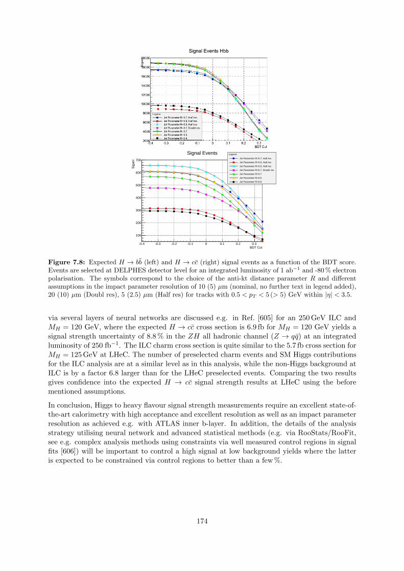
BDT Cut-0.4 -0.3 -0.2 -0.1 0 0.1 0.2 0.3

Sig

anl

100

200

300

400

500

600

700

Legend

Jet Parameter R=0.7, Half res

Jet Parameter R=0.9, Half res

Jet Parameter R=0.5, Half res

Jet Parameter R=0.7, Doublr res

Jet Parameter R=0.7

Jet Parameter R=0.5

Jet Parameter R=0.9

Signal Events

Figure 7.8: Expected H → bb (left) and H → cc (right) signal events as a function of the BDT score.Events are selected at DELPHES detector level for an integrated luminosity of 1 ab−1 and -80 % electronpolarisation. The symbols correspond to the choice of the anti-kt distance parameter R and differentassumptions in the impact parameter resolution of 10 (5) µm (nominal, no further text in legend added),20 (10) µm (Doubl res), 5 (2.5) µm (Half res) for tracks with 0.5 < pT < 5 (> 5) GeV within |η| < 3.5.

via several layers of neural networks are discussed e.g. in Ref. [605] for an 250 GeV ILC andMH = 120 GeV, where the expected H → cc cross section is 6.9 fb for MH = 120 GeV yields asignal strength uncertainty of 8.8 % in the ZH all hadronic channel (Z → qq) at an integratedluminosity of 250 fb−1. The ILC charm cross section is quite similar to the 5.7 fb cross section forMH = 125 GeV at LHeC. The number of preselected charm events and SM Higgs contributionsfor the ILC analysis are at a similar level as in this analysis, while the non-Higgs background atILC is by a factor 6.8 larger than for the LHeC preselected events. Comparing the two resultsgives confidence into the expected H → cc signal strength results at LHeC using the beforementioned assumptions.

In conclusion, Higgs to heavy flavour signal strength measurements require an excellent state-of-the-art calorimetry with high acceptance and excellent resolution as well as an impact parameterresolution as achieved e.g. with ATLAS inner b-layer. In addition, the details of the analysisstrategy utilising neural network and advanced statistical methods (e.g. via RooStats/RooFit,see e.g. complex analysis methods using constraints via well measured control regions in signalfits [606]) will be important to control a high signal at low background yields where the latteris expected to be constrained via control regions to better than a few %.

174

Figure 7.9: Result of the joint H → bb and H → cc analysis for an integrated luminosity of 1 ab−1

and -80 % electron polarisation at the LHeC. Left: Invariant mass distributions for the two channels withsignal and background, see text. Right: Expected Higgs signal distributions after background subtraction.The background is assumed to be at the 2 % level via control region measurements.

7.3.2 Higgs Decay into WW

Inclusive charged current scattering, the CC production of the Higgs boson with a WW decayand the main backgrounds are illustrated in Fig. 7.10. The ep → νHX → νW ∗WX processwith hadronic W decays, see Fig. 7.10 a, causes a final state which to lowest order comprises4 + 1 jets and the escaping neutrino identified via missing energy (MET). The pure hadronicWW Higgs decay has a branching ratio of about 45 %. Using MadGraph (MG5) and a versionof PYTHIA, customised for ep DIS, events have been generated and analysed after passing aDELPHES description of the FCC-eh detector. The present study has been performed for themost asymmetric beam configuration of Ee = 60 GeV and Ep = 50 TeV yielding

√s = 3.5 TeV.

The analysis has been focussed on requiring four fully resolved jets from the Higgs decay and atleast one forward jet, where the jets are reconstructed using the anti-kT algorithm with R = 0.7.Further event categories where the jets from the Higgs decay products may merge and yieldeither three or only two large-R jets in the final state have been not considered yet. However,as shown from state-of-the art LHC-style studies, those event categories and the use of e.g.dedicated top and W-tagging based on large-R jet substructures may give additional access tomeasure Higgs signal strengths.

The analysis requiring fully resolved jets from the H → W ∗W → 4j decay and at least oneforward jet proceeds in the following steps:

• Study of the reconstructed event configuration and recognition of its characteristics fordefining a set of loose cuts. These are: the pT of any jet has to be larger than 6 GeV, therapidity difference between the forward jet and the reconstructed 4-jet Higgs candidateto be larger than 1.5, the azimuthal difference between that Higgs candidate and either

175

j

(a) (b) (c)

(e)(d)

j

W

Wu

e

d

H

j

jW

W

W

u

e

u

W

Z

j

j

W

Wu

e

d

j

jZ

g

W

e

W

b

b

b

t

j

j

g

W

e

d

uug

g

Figure 7.10: Typical lepton-parton diagrams relevant to the H → W ∗W analysis: a) signal: CC DISwith a Higgs produced in the t-channel and its decay into a pair of W bosons which generates a four-jetfinal state, besides the forward jet. The other diagrams are examples to illustrate background channelswhich at higher orders, with extra emissions, may mimic the signal configuration: b) single W -bosonproduction; c) single Z-boson production; d) single top-quark production; e) QCD multi-jet production.

the forward jet or the scattered lepton (MET) to be larger than 1, two-jet masses of thevirtual and the real W boson candidate to be larger than 12 GeV and below 90 GeV (Zmass).

• Verification of truth matching to check that the combinatorial association of jets reproducesthe Higgs candidate (four jets) and its W (two jets) decays (see Fig. 7.11 and text).

• Application of this algorithm to the simulated background samples. The MadGraph singleW , top and Z production samples are turned to multi-jet background through PYTHIA.The cross sections are reliably calculated as there is a hard scale available. The initialcuts reduce this background to about 3 % for single vector boson production and to 9 %for top.

• Due to the size of the Hbb decay and jet radiation, there occurs a residual backgroundfrom the Higgs itself which is also reduced to 3 % through the cuts.

• The final background is due to multi-jets. The MadGraph cross section for a 4+1 jetCC configuration is considered much too large in view of the cross section measurementresults as a function of the jet number, both at HERA and the LHC, see for example [607].The sample was thus scaled using a conservative αs renormalisation to the inclusive crosssection. The initial cuts reduce the multi-jet background to about 13 %.

• Following a detailed training study, a BDT analysis was used. This determined a finalevent number of about 12k for to a signal-to-background ratio of 0.23.

The result of this analysis translates to an estimated uncertainty on µWW of 1.9 % at FCC-eh. The 4-jet mass distribution after the BDT requirement exhibits a clear WW Higgs peak(see Fig. 7.11) which illustrates the suitability to use the electron-proton environment for Higgsmeasurements in indeed challenging final state configurations.

176

[GeV]invM20 40 60 80 100 120 140

Eve

nts

0

50

100

150

200

250

TMHiggs

TMon-shell W

TMoff-shell W

[GeV]invM20 40 60 80 100 120 140

Eve

nts

0

50

100

150

200

250

combHiggs

combon-shell W

comboff-shell W

Figure 7.11: Reconstructed signal mass distributions (at DELPHES detector level) of truth matchedevents (left) and after the just combinatorial association of jets to the two W bosons forming Higgs can-didates (right). Green: virtual W ∗ boson; blue: W boson; red: Higgs signal from W ∗W reconstruction.It is observed that the combination causes some background while the respective signal peaks are clearlypreserved with a purity of 68 % that the correct forward jet is identified.

7.3.3 Accessing Further Decay Channels

Following the detailed studies of the bb and cc decay channels, presented above, a coarser anal-ysis was established for other frequent decay channels both in NC and CC. Here acceptancesand backgrounds were estimated with MadGraph, and efficiencies, distinguishing leptonic andhadronic decay channels for W, Z, and τ , were taken from prospective studies on Higgs cou-pling measurements at the LHC [608]. This provided a systematic scale factor, f , on the purestatistical error δs, which comprised the signal-to-background ratio, S/B, and the product ofacceptance, A, and extra reconstruction efficiency ε, according to

f =

√1 + B

S

A · ε (7.4)

The error on the signal strength µi for each of the Higgs decay channels i is determined asδµi/µi = fi · δs.

Parameter bb WW gg ττ cc ZZ γγ

Branching fraction 0.581 0.215 0.082 0.063 0.029 0.026 0.0023Statistical error (δs) [%] 0.09 0.15 0.24 0.28 0.41 0.43 1.41

Acceptance (A) 0.14 0.10 0.40 0.40 0.11 0.10 0.40Signal/background (S/B) 9 0.2 0.1 0.2 0.43 0.33 0.5Extra efficiency (ε) 1 0.3 0.5 0.43 1 0.5 0.7Scale factor f 2.8 16 7.4 5.9 5.5 9.0 3.3

Table 7.3: Statistical uncertainty for the seven most abundant Higgs decay channels, for the chargedcurrent Higgs measurement prospects with the FCC-eh, together with their systematic scale factor f ,Eq. 7.4, resulting from acceptance, background and efficiency effects as given. Note that the results forbb and cc are taken from the BDT analysis (Sect. 7.3.1) with efficiency 1. The WW result is replaced bythe BDT analysis (Sect. 7.3.2) for quoting the expected signal strength uncertainty.

To good approximation these factors apply to LHeC, HE-LHeC and FCC-eh because the de-tector dimensions and acceptances scale with the proton energy, conceptually using the sametechnology and very similar resolution assumptions. Therefore there is one main matrix used

177

for the subsequent experimental deterioration of the pure statistics precision, both for CC andNC. Future detailed analyses will lead to refining this expectation which for the current purposewas beyond the scope of the study. The results of the analysis of uncertainties are summarisedin Tab. 7.3 for the CC channel at the FCC-eh. The resulting signal strength uncertainty values

Setup bb bb⊕ Thy WW gg ττ cc ZZ γγ

LHeC NC 2.3 2.4 17 16 15 20 35 42LHeC CC 0.80 0.94 6.2 5.8 5.2 7.1 12 15HE-LHeC NC 1.15 1.25 8.9 8.3 7.5 10 17 21HE-LHeC CC 0.41 0.65 3.2 3.0 2.7 3.6 6.2 7.7FCC-eh NC 0.65 0.82 5.0 4.7 4.2 5.8 10 12FCC-eh CC 0.25 0.56 1.9 1.8 1.6 2.2 3.8 4.6

Table 7.4: Summary of estimates on the experimental uncertainty of the signal strength µ, in per cent,for the seven most abundant Higgs decay channels, in charged and neutral currents for the LHeC, theHE-LHeC and the FCC-eh. The bb channel is the one which is most sensitive to theoretical uncertaintiesand for illustration is given two corresponding columns, see Sect. 7.3.4.

are provided in Tab. 7.4. Note that for the beauty, charm and WW channels the table containsthe BDT analysis 3 results of Sect. 7.3.1 and Sect. 7.3.2, resp. The beauty and charm CC resultsstem from the BDT analysis for LHeC and are applied to FCC-eh with a factor of about 1/3.The CC WW results are due to the FCC-eh BDT analysis and are used for LHeC, enlarged bya factor of 3.2, determined by the different cross sections and luminosities. For HE-LHC, thevalues are about twice as precise as the LHeC values because the cross section is enlarged byabout a factor of two, see Tab. 7.1, and the integrated luminosity with 2 ab−1 twice that of theLHeC. All signal strength uncertainties, in both CC and NC, for the three collider configurationsare shown in Fig. 7.12.

0

10

20

30

40

50

bbWWgg ττ cc ZZ γγ bbWWgg ττ cc ZZ γγ

LHeC

HELHeC

FCCeh

ChargedCurrents:epàνHX

NeutralCurrents:epàeHX

δμ/μ[%]

preliminary

Figure 7.12: Uncertainties of signal strength determinations in the seven most abundant SM Higgsdecay channels for the FCC-eh (green, 2 ab−1), the HE LHeC (brown, 2 ab−1) and LHeC (blue, 1 ab−1),in charged and neutral current DIS production.

3This is in very good agreement with the scale factor method: for example, the WW result in Tab. 7.3 leadsto a value of 2.1 % slightly worse than the BDT analysis.

178

7.3.4 Systematic and Theoretical Errors

The signal strength is expressed relatively to a theoretical calculation of the charged currentHiggs cross section, including its decay into a chosen channel, according to

µ =σexpσthy

=σexp

σHty · br. (7.5)

Consequently one can decompose the (relative) error of µ into the genuine measurement er-ror, denoted as δσexp, including a possible systematic error contribution, E, and two furthercomponents

δµ

µ=

(δσexpσexp

)2

· (1⊕ E) +

(δσHtyσHty

)2

+

(δbr

br

)21/2

, (7.6)

which are due to imperfections to theoretically model the Higgs production cross section, σHty,and uncertainties on the branching ratio, br, in the channel under study. Note, that the experi-mental uncertainty takes into account possible variations of the backgrounds which are estimatedconservatively and thus represent more than genuine statistics.

The channel dependent signal strength uncertainties quoted in Tab. 7.4 are estimates of thefirst, experimental term in Eq. 7.6 neglecting extra systematic error effects. They are derived asstated above from the purely statistical error (δs = 1/

√N), its increase due to acceptance (A)

and efficiency (ε) effects and, further, the modulation caused by the background-to-signal ratio(B/S). These factors are all involved in the BDT analysis but the scale factor equation, Eq. 7.4,may be used to estimate further systematic effects for any channel. From the relation

δσexpσexp

= δs ·√

1 +B/S

A · ε (7.7)

the combined systematic error contribution, E, caused by variations ∆ of A, ε and the back-ground B can be estimated as

E =1

2

(∆A

A

)2

+

(∆ε

ε

)2

+

(∆B

B· B/S

1 +B/S

)21/2

. (7.8)

The formula shows that if the background-to-signal ratio is very small, then the backgroundeffect is suppressed ∝ B/S. If it is larger than 1, the relative uncertainty of the backgroundenters as an additional component of the signal strength error.

Given the fact that the experimental H → bb result in the CC reaction is especially precise,compare Tab. 7.4, an estimate was performed of the systematic error in this channel. Thefollowing effects were included: a variation of the light-quark misidentification by a factor 3, avariation of the reduction of the photo-production via tagging between 2 % and 10 %, a variationof the combined acceptance times efficiency effect by 10 % and a variation of the hadronic energyresolution, studied in Ref. [591], leading to a 7 % signal variation. The overall effect of thesecontributions determines a systematic error of about 10 % on µbb, i.e. δµ/µ = 0.80 ± 0.09 forH → bb at the LHeC in the CC channel. Similar levels of uncertainty are expected to occur forother channels but have not been estimated to such detail as those channels are measured lessprecisely.

A separate effect arises from the measurement of the luminosity. While that will be measuredabout as accurate as 0.5 %, based on Bethe-Heitler scattering and its accurate description tohigher-order QEDC [1], additionally it will be negligible to a good approximation: the LHeC,

179

and its successors, will provide a very precise, determination of all parton distributions fromthe ep data alone. Any systematic mistake in the normalisation will therefore affect both themeasured and the calculated cross section and drop out in their ratio µ.

A next uncertainty on the signal strength arises from the theoretical description of σCCH to whichthe measured cross section is normalised. From a simulation of the systematic uncertaintiesdue to imperfect calibrations and extra efficiencies one may expect the cross section to beknown to better than 1 %. The prediction will be available to N3LO, αs be determined to0.1− 0.2 % precision, and it can be gauged with the inclusive cross section measurement. Thisuncertainty, following Eq. 7.8, enters directly as a contribution to the µ measurement result. A0.5 % uncertainty, as can be seen in Tab. 7.4, becomes noticeable in most of the bb results butis negligible for all other channels. In the present analysis values of 0.5 % and 1 % uncertaintyhave been considered and their effect on the κ result been evaluated, see Sect. 7.4.

A final uncertainty is caused by the branching fractions and their uncertainty. A recent un-certainty estimate [586] quotes on the here most relevant H → bb branching ratio a theorycontribution due to missing higher orders of 0.65 %, a parameterisation uncertainty dependingon the quark masses of 0.73 %, and an αs induced part of 0.78 %. The LHeC, or similarly thehigher energy ep colliders, will determine the b mass (in DIS) to about 10 MeV and αs to permille precision [1] which would render corresponding uncertainty contributions to brbb negligible.The genuine theoretical uncertainty would also be largely reduced with an extra order pQCD.In the subsequent study the contribution from the branching fraction uncertainty has been ne-glected. This may also be justified by the programme here sketched, and similarly for otherfuture colliders: the ep colliders will measure the couplings, especially of the WW , bb and ZZvery precisely, which will enable an iterative treatment of the branching ratio uncertainties.

It may be noticed [586] that the αs contribution to the H → gg branching fraction uncertaintyis about 3.7 %, i.e. twice as large as the estimated signal strength measurement uncertainty ofthis channel at the FCC-eh. There arises another important benefit of the future ep collidersand their high precision DIS programme for precision Higgs physics at the combined ep & ppfacilities.

7.4 Higgs Coupling Analyses

In order to quantify possible deviations from the SM expectation one may use the κ parameter-isation framework, introduced in Ref. [609], which enables easy comparisons between differentcollider configurations independently of their ability to access the total Higgs decay width. Itshould be noted that there are differences between the results in the EFT and in the κ formal-ism [610]. Therefore, it would be very interesting to go beyond the κ framework also for theep colliders here presented because out of the 2499 dimension-6 Wilson coefficients altogether13 ·n4

g = 1053 involve leptons and quarks [611], for ng = 3 generations. This, however, has beenbeyond the scope of this study. In the following results are presented for the various ep colliderconfigurations (Sect. 7.2.2).

The κ parameters are factors to the various Higgs couplings, equal to one in the SM, which scaleσNC/CC with κ2

Z/W , the width Γi for a channel i with κ2i and lead to replacing ΓH by the sum

ΣjκjΓj , where we have assumed no non-SM H decays. This defines the following modifications

of the cross sections (Eq. 7.1)

σiCC = σCC bri · κ2Wκ

2i

1∑j κ

2jbrj

and σiNC = σNC bri · κ2Zκ

2i

1∑j κ

2jbrj

. (7.9)

180

Dividing these expressions by the SM cross section predictions one obtains the variations of therelative signal strengths, µi, for charged and neutral currents and their κ dependence

µiCC = κ2Wκ

2i

1∑j κ

2jbrj

and µiNC = κ2Zκ

2i

1∑j κ

2jbrj

. (7.10)

With seven decay channels considered in CC and NC, one finds that for each of the ep colliderconfigurations there exist eight constraints on κW and κZ and two on the other five κ parameters.Using the signal strength uncertainties as listed in Tab. 7.4 fits to all seven channels, in NC andCC, are performed in a minimisation procedure to determine the resulting uncertainties forthe κ parameters. These are done separately for each of the ep collider configurations withresults listed in Tab. 7.5. A naive expectation would have been that δκ ' δµ/2. Comparing theresults, for example for LHeC (top rows), of the signal strengths (Tab. 7.4) with the κ fit results(Tab. 7.5) one observes that this relation holds approximately for the gg, ττ, cc, γγ channels.However, due to the dominance of H → bb in the total H width and owing to the presence of theWWH and ZZH couplings in the initial state, there occurs a reshuffling of the precisions in thejoint fit: κb is relatively less precise than µbb while both κW and κZ become more precise thannaively estimated, even when one takes into account that the H →WW decay in CC measuresκ4W . The seven channel results are displayed in Fig. 7.13.

0.00

1.00

2.00

3.00

4.00

5.00

6.00

7.00

8.00

WW ZZ gg γγ cc bb ττ

LHeC

FCC-eh(2.2)

FCC-eh(3.5)

kapp

a/ %

Figure 7.13: Summary of uncertainties of Higgs couplings from ep for the seven most abundant decaychannels, for LHeC (gold), FCC-eh at 20 TeV proton energy (brown) and for Ep = 50 TeV (blue).

Setup bb WW gg ττ cc ZZ γγ

LHeC 1.9 0.70 3.5 3.1 3.8 1.2 6.8HE-LHeC 1.0 0.38 1.8 1.6 1.9 0.6 3.5FCC-eh 0.60 0.22 1.1 0.93 1.2 0.35 2.1

Table 7.5: Summary of κ uncertainty values as obtained from separate fits to the signal strengthuncertainty estimates for the seven most abundant Higgs decay channels, in charged and neutral currentsfor the LHeC, the HE-LHeC and the FCC-eh, see text.

In the electroweak theory there is an interesting relation between the ratio of the W and Z

181

couplings and the mixing angle,

σ(WW → H → AA)

σ(ZZ → H → AA)=κ2W

κ2Z

= (1− sin2 θW )2 (7.11)

This relation can be particularly well tested with the ep colliders as they measure both WWHand ZZH in one experiment and common theoretical environment. If one assumes the WWand ZZ measurements to be independent, the resulting error on sin2 θW ' 0.23 is 0.003 for theLHeC and 0.001 for FCC-eh. However, this probably is smaller because there exist correlationsin the measurements which a genuine data based analysis would have to evaluate and take intoaccount.

The effect of the theory uncertainties has been studied for the FCC-eh where the experimentalprecision is highest. Tab. 7.6 presents the results of a κ analysis using the CC and NC FCC-eh signal strength input (Tab. 7.4) neglecting the theoretical uncertainty and adding 0.5 % or1 % in quadrature, to only µbb where it matters. This results in an about linear increase ofthe uncertainty for bb (by a factor of 1.5), WW (by 1.7) and ZZ (by 1.5), while all other κuncertainties only slightly deteriorate. The effect of such uncertainties for LHeC is much smalleras the µ uncertainties are three times those of FCC-eh, see Tab. 7.4. Therefore, in the LHeCcase, the theory uncertainties are neglected.

Setup bb WW gg ττ cc ZZ γγ

FCC-eh (no thy) 0.60 0.22 1.1 0.93 1.2 0.35 2.1FCC-eh (0.5 % thy) 0.72 0.28 1.1 1.0 1.2 0.41 2.2FCC-eh (1.0 % thy) 0.91 0.37 1.1 1.0 1.3 0.53 2.3

Table 7.6: Summary of κ uncertainty values as obtained from separate fits to the signal strengthuncertainty estimates for the seven most abundant Higgs decay channels, in charged and neutral currentsfor the FCC-eh, with no theoretical uncertainty, half a per cent and one per cent uncertainty added.

An interesting question regards the role of the electron beam polarisation. Assuming a maximumpolarisation of P = −0.8, the CC (NC) Higgs cross section is calculated to be 1.8 (1.09) timeslarger than that in unpolarised scattering. Therefore the signal CC and NC strength uncertain-ties scale like 1.34 and 1.09, respectively. This is studied for the LHeC. If the default fit is made,then the κ uncertainties quoted in Tab. 7.5 for bb, WW, gg, ττ and cc are enhanced by a factorof 1.28. This is due to the combined effect of CC and NC which diminishes the deterioration abit, from 1.34 to 1.28. Thus, for example, the κW uncertainty moves from 0.7 to 0.9 % in theunpolarised case. The uncertainty on κZ is enhanced only by a factor of 1.14, becoming 1.38instead of 1.21 because the NC channel has a particularly strong effect on the ZZH coupling.Since the prospect to detect the γγ channel in NC is very poor, the κγ uncertainty is enlargedby the full CC factor of 1.34. It is for maximum precision very desirable to have the beampolarised. This, together with electroweak physics, represents an important reason to continueto develop high current polarised electron sources.

7.5 Measuring the Top-quark–Higgs Yukawa Coupling

Electron-proton collisions at high energy are known to provide a unique window of opportunityto perform precision measurements in the top sector [473]. This is due to the large cross-sectionsof the production of single top, which amounts to about 2 pb for Ee = 60 GeV and Ep = 7 TeV,where clean signatures are provided without the challenges posed by pile-up. As a result, the

182

cross-section of the SM in association with a single top in e−p collisions is large enough toperform competitive measurements. This includes the measurement of the absolute value of thetop-Yukawa coupling and, most prominently, its CP-phase [484].

page 1/1

Diagrams made by MadGraph5_aMC@NLO

t~4

b~

1

w+

e-

2

ve

3

w+ h

5

diagram 1

NP=0, QCD=0, QED=3

b~

1

h5

b~

e-

2

ve

3

w+ t~

4

diagram 2

NP=0, QCD=0, QED=3

b~

1

h5

b~

e-

2

ve

3

w+ t~

4

diagram 3

NP=1, QCD=0, QED=3

t~ 4

h

5

t~

e-2

ve

3

w+

b~

1 diagram 4

NP=0, QCD=0, QED=3

t~ 4

h

5

t~

e-2

ve

3

w+

b~

1 diagram 5

NP=1, QCD=0, QED=3

page 1/1

Diagrams made by MadGraph5_aMC@NLO

t~

4

b~

1

w+

e-2 ve

3

w+

h 5

diagram 1 NP=0, QCD=0, QED=3

b~

1h

5

b~

e-2 ve

3

w+

t~ 4

diagram 2 NP=0, QCD=0, QED=3

b~

1h

5

b~

e-2 ve

3

w+

t~ 4

diagram 3 NP=1, QCD=0, QED=3

t~

4

h

5

t~

e-2

ve3

w+

b~

1

diagram 4 NP=0, QCD=0, QED=3

t~

4

h

5

t~

e-2

ve3

w+

b~

1

diagram 5 NP=1, QCD=0, QED=3

b tW+

e

h

W+

page 1/1

Diagrams made by M

adGraph5_aMC@NLO

t~

4

b~

1

w+

e-

2

ve

3

w+h

5

diagram 1

NP=0, QCD=0, Q

ED=3

b~

1

h

5

b~

e-

2

ve

3

w+t~

4

diagram 2

NP=0, QCD=0, Q

ED=3

b~

1

h

5

b~

e-

2

ve

3

w+t~

4

diagram 3

NP=1, QCD=0, Q

ED=3

t~ 4

h

5

t~

e-2

ve

3

w+

b~

1 diagram 4

NP=0, QCD=0, Q

ED=3

t~ 4

h

5

t~

e-2

ve

3

w+

b~

1 diagram 5

NP=1, QCD=0, Q

ED=3

b t

e

h

e

W

W

page 1/1

Diagrams made by MadGraph5_aMC@NLO

t~

4

b~

1

w+

e-2 ve

3

w+

h 5

diagram 1 NP=0, QCD=0, QED=3

b~

1h

5

b~

e-2 ve

3

w+

t~ 4

diagram 2 NP=0, QCD=0, QED=3

b~

1h

5

b~

e-2 ve

3

w+

t~ 4

diagram 3 NP=1, QCD=0, QED=3

t~

4

h

5

t~

e-2

ve3

w+

b~

1

diagram 4 NP=0, QCD=0, QED=3

t~

4

h

5

t~

e-2

ve3

w+

b~

1

diagram 5 NP=1, QCD=0, QED=3

e

b

t

e

h

W+

b

page 1/1

Diagrams made by M

adGraph5_aMC@NLO

t~4

b~

1

w+

e-

2

ve

3

w+ h

5

diagram 1

NP=0, QCD=0, Q

ED=3

b~

1

h

5

b~

e-

2

ve

3

w+ t~

4

diagram 2

NP=0, QCD=0, Q

ED=3

b~

1

h

5

b~

e-

2

ve

3

w+ t~

4

diagram 3

NP=1, QCD=0, Q

ED=3

t~ 4

h

5

t~

e-2

ve

3

w+

b~

1 diagram 4

NP=0, QCD=0, Q

ED=3

t~ 4

h

5

t~

e-2

ve

3

w+

b~

1 diagram 5

NP=1, QCD=0, Q

ED=3

b

tb

e

W

e

h

page 1/1

Diagrams made by MadGraph5_aMC@NLO

t~

4

b~

1

w+

e-2 ve

3

w+

h 5

diagram 1 NP=0, QCD=0, QED=3

b~

1h

5

b~

e-2 ve

3

w+

t~ 4

diagram 2 NP=0, QCD=0, QED=3

b~

1h

5

b~

e-2 ve

3

w+

t~ 4

diagram 3 NP=1, QCD=0, QED=3

t~

4

h

5

t~

e-2

ve3

w+

b~

1

diagram 4 NP=0, QCD=0, QED=3

t~

4

h

5

t~

e-2

ve3

w+

b~

1

diagram 5 NP=1, QCD=0, QED=3

e

bt

e

hW+

t

page 1/1

Diagrams made by MadGraph5_aMC@NLO

t~

4

b~

1

w+

e-2

ve3

w+

h 5

diagram 1 NP=0, QCD=0, QED=3

b~

1h

5

b~

e-2

ve3

w+

t~ 4

diagram 2 NP=0, QCD=0, QED=3

b~

1h

5

b~

e-2

ve3

w+

t~ 4

diagram 3 NP=1, QCD=0, QED=3

t~

4

h

5

t~

e-

2

ve3

w+

b~

1

diagram 4 NP=0, QCD=0, QED=3

t~

4

h

5

t~

e-

2

ve3

w+

b~

1

diagram 5 NP=1, QCD=0, QED=3

b

W

e e

h

t

Figure 7.14: Leading order Feynman diagrams contributing to the process p e− → t h νe in high energye−p collisions. The full circle in the right diagram shows the top-quark–Higgs coupling of interest in thissection.

To investigate top Yukawa coupling, the SM interaction can be modified in terms of mixtures ofCP-even and CP-odd states. In terms of a CP-phase (ζt) generalised Lagrangian can be writtenas [612]:

L =− mt

vt [κ cos ζt + iγ5 sin ζt]t h. (7.12)

Here, ζt = 0 or ζt = π correspond to a pure scalar state while ζt = π2 to a pure pseudo scalar

state. Therefore, the ζt-ranges 0 < ζt < π/2 or π/2 < ζt < π represent a mixture of the differentCP-states, and the case ζt = 0 with κ = 1 corresponds to the SM.

In e−p collisions, the top-quark–Higgs couplings is accessed via associated production of theHiggs boson with an anti-top quark through the process e−p → t h νe, where 5-flavour protoninclude the b-quark parton distribution. In Fig. 7.14, the Feynman diagrams for the processof interest are displayed. Interestingly this process involves three important couplings, namelyhWW , Wtb and the top-Higgs (tth). A detailed study of hWW and Wtb couplings at the e−pcollider have been performed in Refs. [473,613], respectively.

At the LHC [612], quantitatively an interesting feature can be observed: in the pure SM casethere is constructive interference between the diagrams shown in Fig. 7.14, left and middle, forζt > π/2 resulting in an enhancement in the total production cross section of associated top-Higgs significantly. This is also true for ζt < π/2 - however the degree of enhancement is muchsmaller owing to the flipped sign of the CP-even part of the coupling.

A study of the sensitivity to the top-quark–Higgs couplings in terms of ζt a model was presentedin Ref. [484]. In the following the methodology and results are briefly described. In order toassess the sensitivity to the top-quark–Higgs couplings, a model file built in FeynRules [614]which incorporates the Lagrangian, c.f. Eq. (7.12). The associated top-Higgs production in thecharged-current channel p e− → t h νe is then simulatend (c.f. Fig. 7.14), where it is assumedthat h decays into a bb pair, and the anti-top quark decays leptonically. An electron-protoncentre of mass energy of

√s ≈ 1.3 TeV is assumed. In this study [484], the analysis is performed

at the parton level. For signal and background event generation the Monte Carlo event gener-ator package MadGraph5 [375] is employed together with NNPDF23 lo as 0130 qed [615] partondistribution functions. The renormalisation and factorisation scales for the signal sample arechosen to be µF = µR = (mt +mh)/4. The background samples are generated using the default

183

0.01

0.1

1

10

50 100 150 200 250 300

σ [

fb]â

Ee [GeV]

Unpol.

80% Pol.

Leptonic

Hadronic

Figure 7.15: Cross-sections of the Higgs boson produced in association with a top quark in e−p collisionswith Ep = 7 TeV for different electron beam energies (taken from Ref [484]). The dotted and solid blacklines correspond to p e− → t h νe with and without longitudinal polarisation of the electron beam,respectively. The dotted red and blue lines correspond to σ×BR for the leptonic and hadronic decaymodes of t where for this estimation we use basic cuts (see text and Ref. [484]).

MadGraph5 [375] dynamic scales. The longitudinal polarisation of the electron beam is asumedto be -0.8.

In Fig. 7.15 we present the variation of the total cross section against the electron beam energyfor the signal process p e− → thνe, by considering un-polarised and polarised e− beam. Also,the effect of branchings of h → bb and the t decay for both leptonic and hadronic modesare shown. Possible background events typically arise from W+ multi-jet events, Wbbb withmissing energy which comes by considering only top-line, only Higgs-line, and without top- norHiggs-line, in charged and neutral current deep-inelastic scattering and in photo-production byfurther decaying W into leptonic mode. To estimate the cross sections for signal and all possiblebackgrounds only basic cuts on rapidity |η| ≤ 10 for light-jets, leptons and b-jets, the transversemomentum cut pT ≥ 10 GeV and ∆Rmin=0.4 for all particles considered.

Estimation of the sensitivity of the associated top-Higgs production cross-section, σ(ζt), as afunction of the CP phase of the tth-coupling is shown in Fig. 7.16. In this study, the eletronand proton beams are assumed to have an energy of 60 GeV and 7 TeV, respectively. The scaleuncertainties are obtained by varying the nominal scale, µF = µR ≤ (mt +mh)/4, by factors of0.5 and 2. It is observed that the size of the cross section is strongly dependent on the valueof ζt, in particular in the region ζt >

π2 where the interference between the diagrams becomes

constructive. At lower values of ζt the interference is still constructive, but it decreases withdecreasing ζt. Note, ζt = 0 represents the cross section in the strict SM formalism.

At ζt = π2 , which corresponds to the pure CP-odd case, the cross section is increased by about

a factor of five in comparison to the SM expectation. At ζt = π, which corresponds to the pureCP-even case with opposite sign of tth-coupling, the cross section can be enhanced by a factorof up to 24 times. In the while range of ζt, the scale uncertainty is found to be about 7 %.

To evaluate sensitivity to the measurement of the top-Yukawa coupling and its CP-phase, fol-lowing criteria of fiducial selection taken [484]:

184

0.1

1

10

0 π/4 π/2 3π/4 π

σ[f

b]

ζt

Ee = 60 GeV

Ee = 120 GeV

Figure 7.16: Total cross section of the Higgs boson produced in association with a single top as afunction of ζt, including scale uncertainties (taken from Ref. [484]). The black solid and blue dotted linescorrespond to Ee = 60 and 120 GeV, respectively. These are obtained for fixed Ep = 7 TeV and scalesµF = µR = (mt +mh)/4.

• pT ≥ 20 GeV for b-tagged jets and light-jets, and pT ≥ 10 GeV for leptons.

• b-jets must be within −2 ≤ η ≤ 5

• light jets and the scattered lepton must be identified within 2 ≤ η ≤ 5

• all final state particles must be separated by a distance ∆R greater than 0.4.

• the missing transverse energy must exceed 10 GeV

• the invariant mass windows for the Higgs through b-tagged jets and the top are requiredto be 115 < mbb < 130 GeV and 160 < mt < 177 GeV.

In these selections the b-tagging efficiency is assumed to be 70%, with fake rates from c-initiatedjets and light jets to the b-jets to be 10% and 1%, respectively. The last requirement is importantto reduce background processes.

Using the Poisson formula S =√

2[(S +B) log(1 + S/B)− S], where S and B are the number ofexpected signal and background events at particular luminosity (L in fb−1), the exclusion regionsregions of ζt as a function of L are estimated. Here, 10 % systematic uncertainty is expected forthe background yields. Fig. 7.17, displays the exclusion contours at different confidence levels.It is observed that the shape of the exclusion limit changes at around ζt = π/2. Therefore,in order to obtain significant exclusion limits in the region 0 < ζt < π/2 a larger integratedluminosity is required. This is in keeping with the feature exhibited in As it is visible fromFig. 7.16, for ζt values where constructive interference between the signal diagrams enhances thecross-section over the SM value, i.e. for ζt > π/2, less integrated luminosity is requried in order toobtain precise exclusion limits. For example, for L = 100 fb−1, regions above π/5 < ζt ≤ π and3π/10 < ζt ≤ π are excluded at a confidence limit of 2σ and 3σ, respectively. With L = 400 fb−1,regions above π/6 < ζt ≤ π and π/4 < ζt ≤ π are excluded at 4σ and 5σ C.L., respectively.The asymmetry studies at the HL-LHC [612] help probe up to ζt = π/6 for a total integratedluminosity of 3 ab−1. However, LHeC provides a better environment to test the CP nature of

185

Figure 7.17: Exclusion contours for ζt as a function of integrated luminosity for√s = 1.3 TeV (from

Ref. [484]). The shaded areas under a contour-line are excluded. The blue and black lines represent the4σ and 3σ regions. Results are obtained based on fiducial cross-sections (see text).

Higgs boson couplings. For the targeted integrated luminosity of L = 1 ab−1, almost all valuesof ζt can be excluded with at a confidence level of at least 4σ.

While investigating the overall sensitivity of ζt by applying these two observables, it is alsoimportant to measure the accuracy of SM tth coupling κ at the LHeC energies. By using thethe formula

√(S +B)/(2S) at a selected luminosity of L = 1 ab−1, the value of κ can be

determined with an uncertainty of about pm0.17. In this estimate, 10% systematic uncertaintyis been taken for the background yields.

These results are obtained based on the evaluation of the fiducial cross-sections alone. Aspointed out in Ref. [484], a number of other observables carry sensitivity to the structure of thetop-Higgs Yukawa coupling, such as the rapidity difference between the top quark and the Higgsboson and a number of angular variables. While the fiducial rate studied here is the single mostsensitive observable, it is evident that a multi-variate approach will significantly enhance thesensitivity reported here.

7.6 Higgs Decay into Invisible Particles

The Higgs decay into invisible particles could be a key to BSM physics. The SM branchingratio of H → ZZ → 4ν is only 0.1%. Any sizable decay rate into invisible particles wouldthus indicate an exotic decay, for example to dark matter particles. Its non-observation wouldgive the SM cross section measurement, reconstructing more than 99 % of the ordinary decaysa higher meaning for constraining the total Higgs decay width.

For the LHeC at a luminosity of 1 ab−1, initial parton-level studies of this decay were presentedin Ref. [616], with the estimate of a two σ sensitivity to a branching fraction of 6 %. For thisstudy, NC production via ZZ fusion eq → eqZZ → eqH was used, which has a cross sectionof about 25 fb at the LHeC. The CC production via WW fusion has a larger cross section,but entails a missing energy signal by itself which requires further study of potentially quitesome gain in precision. This channel, when employed for the invisible decay study, results in amono-jet signature which is hard to separate from the SM DIS CC background.

186

The neutral current study has been repeated using the LHeC Higgs WG analysis tools, intro-duced above: MadGraph, Pythia and Delphes. Similar to [616], an electron beam of 60 GeVwith a polarization of -80% is assumed. The basic event topology contains the scattered electron,jet and missing transverse energy. Its main background results from SM W and Z productions(followed by W → `ν and Z → νν). In the study NC and CC W production and NC Z produc-tion are considered, while single-top, NC multijets and W photoproduction were all found to benegligible. Requiring missing transverse energy of 60 GeV, exactly one electron and one jet, andno other leptons (including τ), as well as imposing several selection criteria on the kinematics ofelectron, jet and missing transverse momentum, we get a two σ sensitivity to a branching ratioof 7.2 %, which is similar to the earlier result [616]. Fig. 7.18 shows the electron-jet invariantmass distribution after the selection for the signal (normalized to a 100 % branching ratio) andthe background.

[GeV]ejm

0 100 200 300 400 500 600 700 800 900 10000

50

100

150

200

250

300

350

400­1

Ldt=1ab∫=7TeV, protonE

Cut Based

Signal (Br=100%)

νWj

Zje

je+

W

je­

W

Other

Figure 7.18: Electron-jet invariant mass distribution for the Higgs to invisible decay signal (normalizedto 100% branching ratio) and the stacked backgrounds for an integrated luminosity of 1 ab−1 at theLHeC after all selection cuts.

The analysis has been further refined with a usage of multivariate analysis (Boosted DecisionTree in TVMA package). Basically the set of selection variables used in the cut-based analysisabove was used as inputs to the multivariate analysis, tuned to yield the best output score todiscriminate the signal from backgrounds. Fig. 7.19 shows the distribution of the discriminantvariable for the signal and background (both area normalised). An optimization on the statisticalsignificance is found at the BDT score > 0.25, and the resulting mass distribution is shownin Fig. 7.20. With 1 ab−1 of integrated luminosity, a two σ sensitivity of 5.5% is obtainedconsistent with the previous results. For a comparison, an estimate of 3.5 % is given for a HL-LHC sensitivity study on this channel [617]. The result on the LHeC may be further improvedin the future with a refined BDT analysis when one introduces extra parameters, beyond thoseinitially introduced with the cut based analysis.

In these initial studies no systematic uncertainties were considered. This may be justified withthe very a clean environment of electron-hadron collider, in which precise measurements of Wand Z production will be made, for example in their decays to muons, for accurately controlling

187

BDT score

0.6− 0.4− 0.2− 0 0.2 0.40

0.02

0.04

0.06

0.08

0.1

0.12

=7TeVprotonE

Training sample

Test sample

Signal

νWj

Zje

je+

W

je­

W

Other

Figure 7.19: BDT output score distribution forthe Higgs to invisible decay signal and the stackedbackgrounds (both area normalized) at the LHeC.

[GeV]ejm

0 100 200 300 400 500 600 700 800 900 10000

50

100

150

200

250

300

350

400

450

­1Ldt=1ab∫=7TeV, protonE

BDT score > 0.25

Signal (Br=100%)

νWj

Zje

je+

W

je­

W

Other

Figure 7.20: Electron-jet invariant mass distri-bution for the Higgs to invisible decay signal (nor-malized to 100% branching ratio) and the stackedbackgrounds for an integrated luminosity of 1 ab−1

at the LHeC after the BDT score cut of 0.25.

the systematics in the background prediction to a negligible level.

The BDT analysis was repeated for higher proton energies. At the HE-LHeC (Ep=13.5 TeV)the NC production cross section increases to 45 fb and the branching ratio sensitivity improvesto 3.4 % because the luminosity is doubled in the configurations here assumed. At the FCC-eh,the cross section rises to 120 fb and the sensitivity of the branching ratio reaches about 1.7 %.

188

Chapter 8

Searches for Physics Beyond theStandard Model

8.1 Introduction

The LHC was originally envisioned as the ultimate machine to search for physics beyond theStandard Model at the TeV scale. Since electrons and quarks share only electroweak interac-tions, an electron-proton collider could allow to measure the same phenomena in a differentenvironment with generally higher precision. It could add complementary search channels orlead to the discovery of a weak signal. The possibility of undiscovered New Physics (NP) belowthe TeV scale could thus be also addressed by the LHeC, which is projected to operate whenthe LHC will be in its high luminosity phase, in spite of the lower centre-of-mass energy. Exoticphenomena that can be studied at ep colliders have been reviewed, for example, in [618]. Morerecently, but when the LHC was only beginning to yield data in Run I, an overview of thepotential of the LHeC for probing physics beyond the Standard Model has been given in theConceptual Design Report [1]. Since then, stringent constraints on NP phenomena have beenobtained from the LHC and the absence of hints from NP to date is presently changing thisparadigm to two alternative scenarios: NP may actually reside at an even larger energy scale;NP may be at or below the TeV scale, but more weakly coupled, and thus hidden in the SMbackgrounds [619].

A similar pp-ep synergy could be envisaged with higher proton beam energies at the FCC 100 kmtunnel. With an electron beam of 60 GeV, the expected centre-of-mass energies for ep couldbe 2.9 TeV for Ep = 19 TeV (Low-Energy FCC) and 3.5 TeV for Ep = 50 TeV (FCC). Below welist recent developments which discuss new physics opportunities at the LHeC and its potentialfuture high-energy upgrades.

8.2 Extensions of the SM Higgs Sector

Presently, given the precision of measurements in the Higgs sector, it appears that the discovered125 GeV scalar is indeed the SM Higgs boson. The question remains, however, if the scalarpotential is truly that of the SM or if it should be extended, possibly with additional degrees offreedom. Several extensions of the Higgs sector have been proposed and can be studied at theep colliders with results often complementary to those of pp colliders and other future facilities.

189

8.2.1 Modifications of the Top-Higgs interaction

In electron-proton collisions the heavy top-quarks can be produced in association with a Higgsboson, which allows us to study the sensitivity of the LHeC or the FCC-eh to the top-Higgs(tH) interaction. In Ref. [484] the sensitivity of the process pe− → tHνe to the CP nature ofthe tH coupling is investigated by considering a CP phase ζt at the ttH and bbH vertices. Theauthors conclude, based on several observables and with appropriate error fitting methodology,that better limits on ζt are obtained at the LHeC than at the HL-LHC. At the design luminosityof 1 ab−1, almost all values of ζt are excluded up to 4σ C.L. and the SM top-Higgs couplingcould be measured relative to its SM value with a precision of κ = 1.00± 0.17.

Flavour changing neutral currents (FCNC) are completely absent at tree-level in the SM andstrongly constrained, especially by low energy experiments. Anomalous flavour changing neutralcurrent Yukawa interactions between the top quark, the Higgs boson, and either an up or charmquark are documented in Chapter 3, Sec. 5.3.6. Among other studies, in Ref. [620] the authorsconsider the Higgs decay modes H → γγ, bb and ττ and Ee = 150 GeV. The results are updatedin Ref. [492] for Ee = 60 GeV, including estimates for lower electron beam energies, and the 2σsensitivity on the branching ratio Br(t → uh) is found to be 0.15 × 10−2. Making use of thepolarisation of the electron beam and multivariate techniques, Ref. [621] shows that limits onthe branching ratio Br(t→ uh) of O(0.1) % can be obtained, an improvement over present LHClimits of 0.19 % [622,623]. These results vary with Ee and Ep.

8.2.2 Charged scalars

The prospects to observe a light charged Higgs boson through the decay H+ → cb are inves-tigated within the framework of the Two Higgs Doublet Model (2HDM) Type III, assuminga four-zero texture in the Yukawa matrices and a general Higgs potential [624]. The chargedcurrent production processes e−p → νH+q are considered. The analysed signature stems fromthe subsequent decay H+ → cb. The parton level analysis accounts for irreducible SM back-grounds and considers scenarios up to a mass of 200 GeV, consistent with present limits fromHiggs and flavour physics. The authors show that for L = 100 fb−1 a charged Higgs bosoncould be observed with about 3 − 4σ significance. This is to be compared with results frompresent LHC searches in which strong limits are set on the branching fraction B(t → H+b),assuming B(H+ → cb) = 1.0 or B(H+ → cs) = 1.0 for the charged Higgs boson mass range∼ 90− 160 GeV [625,626].

A similar study, H± → sc+su, for the FCC-eh (with√s ≈ 3.5 TeV) is presented in Ref. [627], in

the context of a next-to-minimal supersymmetric model (NMSSM). Using dedicated optimisationtechniques, the authors show that a light charged boson H± can be observed with maximalsignificance of 4.4 (2.2)σ provided its mass is at most mH± = 114(121) GeV, for the totalluminosity of 1 ab−1.

The Georgi-Machacek (GM) model extends the Higgs sector by including higher multiplet stateswhile preserving custodial symmetry. The physical states include, besides the SM Higgs, aheavier singlet H, a triplet (H+

3 , H03 , H

−3 ) and a quintuplet (H+

5 +, H+5 , H

05 , H

−5 , H

−5 −). The H5

scalars do not couple to fermions and can therefore only be produced by vector boson fusion. Ananalysis for the prospects to discover the doubly charged Higgs bosons in the GM model at theLHeC and the FCC-eh is presented in Ref. [628]. Therein the production of a doubly-chargedmember of five-plet Higgs-bosons (H±±5 ), produced from W±W± fusion is studied. The authorsfind that 2 to 3σ limits can be obtained for mixings sin(θH) as low as 0.2, for M(H5) < 300 GeV.The prospects can be improved at the FCC-eh collider, where doubly charged Higgs bosons canbe tested for masses MH5 < 400 GeV, also for small scalar mixing angles (Fig. 8.1 (left)).

190

7TeV Ä 60GeV unpol. LHeC

L = 1 ab-1

∆sys =10%Boundary.A

Boundary.B

5Σ 1Σ2Σ3Σ

200 300 400 500 600

0.1

0.2

0.3

0.4

0.5

0.6

M H5

sin

Θ H

Figure 8.1: Left: Discovery contour with respect to sin θH and M(H++/−−5 ) at LHeC with unpolarized

beam; Right: Limit Contours for the case of singly charged Higgs for FCC-eh and LHeC. The blue

dotted curve and the blue dashed curves give the 95% CL limit from CMS for H+/−5 and for H++/−−

respectively [630, 631]. An unpolarized beam of integrated luminosity of 1 ab−1 and a 10% systematicuncertainty for background yields is assumed in both plots.

The discovery prospects for the singly charged Higgs, H±5 of the Georgi-Machacek model, pro-duced in W±Z fusion, are evaluated in Ref. [629]. The authors perform a multivariate analysis,including a fast detector simulation, and consider the LHeC and the FCC-eh for a mass rangefrom 200–1000 GeV. They find that the LHeC can improve over current LHC limits on H±5 formasses up to about 400 GeV and scalar mixing angles sin θH ∼ 0.5 (Fig. 8.1 (right)).

8.2.3 Neutral scalars

Neutral scalar bosons generally appear in many extensions of the scalar sector. They can beadded directly, as SU(1) singlets, or be part of higher representation SU(2) multiplets. Theygenerally mix with the SM Higgs boson, from which they inherit a Higgs-like phenomenology.

The potential of testing the heavier CP-even scalar that is contained in the 2HDM Type-I ispresented in Ref. [632]. Therein, the lighter scalar particle is considered to be a SM-like Higgsboson and the properties of a heavy scalar, assumed to have the specific mass 270 GeV, isdiscussed. The authors state that the final state H → Sh, where S is a scalar singlet with amass around 100 GeV, is of particular interest, as it connects to the findings in Ref. [619].

The prospects to search for a generic heavy neutral scalar particle are presented in detailRef. [633]. The model is a minimal extension of the SM with one additional complex scalarsinglet that mixes with the SM Higgs doublet, which governs its production and decay mode.The heavy scalar is produced via vector-boson fusion and decays into two vector bosons. A mul-tivariate analysis is performed and detector simulation is taken into account. Masses between200 and 800 GeV and scalar mixings as small as sin2 α ∼ 10−3 are considered. The resultingsensitivity for a total luminosity of 1 ab−1 is shown in Fig. 8.2, including existing bounds fromthe LHC and future HL-LHC projections. A significant improvement over existing LHC limitsis found, with the LHeC probing scalar boson masses below ∼ 500 GeV, a region which remainsdifficult at the HL-LHC.

The scalar bosons from the 2HDM Type-III framework may give rise to flavour violating signa-tures, as discussed in Ref. [636]. The prospects to observe the light and heavy CP-even neutralHiggs bosons via their decays into flavour violating bs channels were studied with specific Yukawa

191

[GeV]HM200 400 600 800

2 )θ95% CL Limit (sin

2−10

10

210

Observed LHC 95% CL Expected HL-LHC 95% CL Expected median 95% CL

σ 1±Expected σ 2±Expected

LHeC

Combined Limits

Figure 8.2: Expected exclusion limits (green and yellow bnds) for a heavy scalar search at the LHeC, as-suming a systematic uncertainty on the SM background of 2 % (from Ref. [633]). The blue line representsthe current LHC limit at 95 % CL as extracted from [634], the red line the forecast of the HL-LHC sen-sitivity via h2 → ZZ searches from Ref. [635]. The LHeC results correspond to an integrated luminosityof 1 ab−1.

textures and a general Higgs potential. The signature consists of one jet originating from b-hadron fragmentation (b-tagged jets) and one light-flavour jet in the central rapidity region, witha remaining jet in the forward region. Relevant SM backgrounds were considered and it is foundthat flavour violating decays of the SM-like Higgs boson would be accessible with L = 100 fb−1

at ep colliders.

The prospects of observing the light CP-even neutral Higgs bosons of the NMSSM framework,the MSSM with an additional singlet superfield, via their decays into b-quarks and in the neutraland charged current production processes, are studied in Ref. [637]. In this work the followingconstraints are incorporated into the spectrum: neutralino relic density corresponding to theobserved dark matter relic density; direct and indirect mass bounds from searches for specificsparticles; the SM-like Higgs boson has a mass around 126 GeV and an invisible branching ratiobelow 0.25. The signal is given by three jets plus an electron or missing transverse momentum(EmissT ) arising from the neutral (charged) current interaction, where two jets are required to beoriginating from a b-quark and the remaining jet is required to be in the forward region. For thecut-based analysis a number of reducible and irreducible SM backgrounds, generated with a fastdetector simulation with an adaptation of the LHeC detector, are considered. It is found thatthe boson h1 could be observable for some of the NMSSM benchmark points, at up to 2.5σ levelin the e+ 3j channel up to masses of 75 GeV; in the 3j +EmissT channel h1 could be discoveredat 2.4σ level up to masses of 88 GeV with L = 100 fb−1, and a 5σ observation is possible withL = 1 ab−1 for masses up to 90 GeV.

8.2.4 Modifications of Higgs self-couplings

As in the chapter on Higgs physics above, the e−p collisions are a very convenient environmentto study the property of the SM Higgs boson itself. The latter is produced through vector-bosonfusion processes and the precise measurement of its properties provides a unique opportunityto probe the interaction HV V , (V = W±, Z). These interactions are in general sensitive tocertain classes of beyond the SM physics, which can be parameterized, for instance, via higherdimensional operators and their coefficients, cf. Refs. [584,613,638–640].

192

The prospects of inferring the strengths of the two couplings HWW and HZZ were studied inRefs. [613, 639] in the context of electron-proton collisions. The authors find that the higher-dimensional operator coefficients can be tested for values around O(10−1) at the LHeC. Thissensitivity is improved at the FCC-eh due to larger centre-of-mass energies, which in generalenhance the vector-boson fusion cross sections.

The Higgs self-coupling itself HHH can be tested through the measurement of the di-Higgsproduction cross section as was shown in Ref. [584]. With appropriate error fitting methodologythis study illustrates that the Higgs boson self-coupling could be measured with an accuracy of

g(1)HHH = 1.00

+0.24(0.14)−0.17(0.12) of its expected SM value at

√s = 3.5(5.0) TeV, considering an ultimate

10 ab−1 of integrated luminosity.

An analysis presented in Ref. [640] evaluates the LHeC sensitivity to dimension-six operators.The authors employ jet substructure techniques to reconstruct the boosted Higgs boson in thefinal state. A shape analysis on the differential cross sections shows in some cases improvementswith respect to the high-luminosity LHC forecasts.

8.2.5 Exotic Higgs boson decays

The LHeC sensitivity to an invisibly decaying Higgs boson was investigated in Ref. [616]. Thereinthe focus is on the neutral current production channel due to the enhanced number of observ-ables compared to the charged current counterpart. The signal contains one electron, one jetand large missing energy. A cut-based parton level analysis yields the estimated sensitivity ofBr(h→invisible) = 6 % at 2σ level. Exotic decays of the Higgs boson into a pair of light spin-0particles referred to as Φ was discussed in Ref. [641]. The studied signature is a final state with4 b-quarks, which is well motivated in models where the scalars can mix with the Higgs doublet,and suffers from multiple backgrounds at the LHC. The analysis is carried out at the partonlevel, where simple selection requirements render the signature nearly free of SM backgroundand makes Φ with masses in the range [20, 60] GeV testable for a hV V (V = W,Z) couplingstrength relative to the SM at a few per-mille level and at 95 % confidence level.

The prospects of testing exotic Higgs decays into pairs of light long-lived particles at the LHeCwere studied in Ref. [642] where it was shown that proper lifetimes as small as µm could betested, which is significantly better compared to the LHC. This is shown in Fig. 8.3 (left). Thisinformation can be interpreted in a model where the long-lived particles are light scalars that mixwith the Higgs doublet, where both, production and decay, are governed by this scalar mixingangle. The area in the mass-mixing parameter space that give rise to at least 3 observableevents with a displaced vertex are shown in Fig. 8.3. It is apparent that mixings as small assin2 α ∼ 10−7 can be tested at the LHeC for scalar masses between 5 and 15 GeV [642].

8.3 Searches for supersymmetry

Several SUSY scenarios might remain still elusive in searches performed at pp colliders. Whilethe null results from current searches by the LHC experiments have produced impressive con-straints on the SUSY coloured sector (squarks and gluinos) because of their large productioncross sections in strong interactions, less stringent constraints have been placed on weakly-produced SUSY particles, namely neutralinos χ0, charginos χ±, and sleptons ˜±. Some of thesescenarios where ep colliders might have discovery potential complementary to that of the HL-LHC are discussed below. These include R-parity conserving SUSY models, e.g. motivated bydark matter, or R-parity violating SUSY models, e.g. including single production of bottom andtop squarks and low mass gluinos.

193

10-8 10-6 10-4 0.01 1 100

10-6

10-5

10-4

0.001

0.010

0.100

1

cτ (m)

ExcludedBr(h→XX)

ep: 1 ab-1

pp: 3 ab-1

=

LHeC

FCC-eh (60)

FCC-eh (240)

ℓ + ( = μ)

HL-LHC

FCC-hh

+ ( = )

HL-LHC

FCC-hh

FCC-heLHeC

5 10 15 20 25 30 35-9

-8

-7

-6

-5

-4

-3

mh2 [GeV]

Log 10sin2α

Figure 8.3: Sensitivity contours for displaced vertex searches for Higgs decays into long-lived scalarparticles (LLP), which are pair produced from decays of the Higgs boson, and which themselves decayvia scalar mixing into fully visible final states. Left: As a function of the LLP lifetime for a fixed massfrom Ref. [642]. Right: For a specific model, where lifetime and production rate of the LLP are governedby the scalar mixing angle. The contours are for 3 events and consider displacements larger than 50µmto be free of background.

8.3.1 Search for the SUSY Electroweak Sector: prompt signatures

Electroweakino scenarios where charginos, neutralinos, and sleptons are close in mass can becharacterised by the neutralino mass m and the mass splitting between charginos and neutralinos∆m. We here refer to scenarios with ∆m < 50GeV as compressed. A subtlety arises for∆m ≤ 1 GeV, when the χ±1 /χ

02 becomes long lived and its decays are displaced. For ∆m > 1 GeV

the decays are prompt, the visible decay products from ˜ and χ±1 /χ02 have very soft transverse

momenta (pT ) and the SM backgrounds are kinematically similar to the signal. The analysestherefore become challenging and sensitivities decrease substantially. Two SUSY scenarios areconsidered in Ref. [643] and depicted in Fig. 8.4 where the LSP χ0

1 is Bino-like, χ±1 and χ02

are Wino-like with almost degenerate masses, and the mass difference between χ01 and χ±1 is

small. The signal is produced via the process “p e− → j e− χχ”, where χ = χ01, χ±1 or χ0

2.

Figure 8.4: Representative production diagrams for the signal processes considered in Ref. [643]. Thedecoupled-slepton scenario includes only the first two diagrams, while the compressed-slepton scenarioincludes all four diagrams.

Conservative leading order cross sections are considered for the SUSY signal models. Thekinematic observables are input to the TMVA package to perform a multivariate analysis at thedetector level.

In the compressed-slepton scenario, the case where the left-handed slepton ˜L and sneutrino

ν are slightly heavier than χ±1 or χ02 is considered. When fixing the mass difference ∆m =

m˜−mχ±1 ,χ02

= 35 GeV and ignoring the systematic uncertainty on the background, the analysis

indicates that the 2 (5)σ limits on the χ±1 , χ02 mass are 616 (517) GeV for 2.5 ab−1 luminosity at

the FCC-eh, and 266 (227) GeV for 1 ab−1 luminosity at the LHeC, respectively. An illustrationof the model assumptions in terms of sleptons and neutralino masses and the current constraintsat the LHC is presented in Fig. 8.5 (left). Results are illustrated in Fig. 8.5 (right). The effects

194

Figure 8.5: Left: Benchmark assumption on slepton masses and 2019 reach of current ATLAS searchesfor sleptons (figure adapted from Ref. [644]). Right: Significances as varying the masses of χ±1 and χ0

2 forthe compressed-slepton scenario at the LHeC with unpolarised beams and 1 ab−1 luminosity. For dashed(solid) curve, a systematic uncertainty of 0 % (5 %) on the background is considered. The figure is fromRef. [643].

of varying ∆m are investigated: fixing mχ±1 ,χ02

to be 400 GeV, it is found that at the FCC-eh

the significance is maximal when ∆m is around 20 GeV.

In the decoupled-slepton scenarios where only χ01, χ±1 and χ0

2 are light and other SUSY particlesare heavy and decoupled, the 2σ limits obtained on the χ±1 , χ0

2 mass are 230 GeV for 2.5 ab−1

luminosity at the FCC-eh when neglecting the systematic uncertainty on the background. Largesystematic uncertainties on the SM background processes can substantially affect the sensitivity,hence good control of experimental and theoretical sources of uncertainties is very important.

Finally, it is also found that the possibility of having a negatively polarised electron beam(Pe = 80 %) could potentially extend the sensitivity to electroweakinos by up to 40 %.

Overall, since the sensitivity to the electroweak SUSY sector depends on the mass hierarchyof χ±1 , χ0

1, χ02 and sleptons, and given the difficulty to probe efficiently small ∆m regions at

the current LHC and possibly at the HL-LHC, measurements at ep colliders may prove to offercomplementary or additional reaches, in particular for the compressed scenarios.

8.3.2 Search for the SUSY Electroweak Sector: long-lived particles

Studies on Higgsinos (χ) with masses O(100) GeV are motivated by natural SUSY theories andhelp to avoid large fine-tuning on the Higgs boson mass. In these scenarios the low energycharginos (χ+)/neutralinos(χ0) are all Higgsino-like and their masses are nearly degenerate,only slightly above the neutralino.

As mentioned above, a compressed spectrum with nearly degenerate masses results in a kinematicsuppression of the heavier χ+ decays into W±χ0, which has twofold consequences: it yields finalstates without hard leptons; it enhances the χ+ lifetime up to O(1) mm. At the LHC the absenceof hard leptons with sizable transverse momentum makes this signature difficult to investigate.One possibility is to search for the tracks from χ+, which effectively disappear once it decaysand are thus called disappearing tracks.

The discovery prospects for prompt signatures of electroweakino decays in electron-proton col-lisions are presented in Ref. [645]. The light χ+ (and χ0) can be produced in pairs via in vectorboson fusion of the charged or neutral currents. A cut-based analysis of these processes at theLHeC, assuming prompt χ+ decays, yields 2σ discovery prospects for masses up to 120 GeV.

Taking into account the finite lifetime of the charginos, two comments are in order: first, the

195

100 120 140 160 180 200 22010-810-710-610-510-410-310-210-1

0.30.5

1

2

345

mχ+ (GeV)

cτ(m

)

Δm

(GeV

)

LHeC

1ab-1

μ > 0

N1+LLP > 10N1+LLP > 100

Figure 8.6: Exclusion limits on Higgsino masses as a function of their lifetime from Ref. [642]. Colouredregions denote where 10 or 100 events with at least one LLP decay are observed. Light shading indicatesthe uncertainty in the predicted number of events due to different hadronisation and LLP reconstruc-tion assumptions. The black curves are the optimistic and pessimistic projected bounds from HL-LHCdisappearing track searches.

lifetimes and boosts of the χ+ are in general too small to resolve a disappearing track; second,the soft final state is not a problem per se and can in principle be observed.

Instead of searching for a disappearing track, the long lifetimes of the χ+ can be exploitedvia the measurement of the impact parameter of the soft hadronic final, as is discussed inRef. [642]. The crucial machine performance parameters are the tracking resolution, which isas good as O(10)µm, and the absence of pile up, which allows to identify and measure a singlesoft pion’s impact parameter. In this way the LHeC can test χ with masses up to 200 GeV. Thecorresponding sensitivity is shown in Fig. 8.6, and the bounds on disappearing track searchesat the HL-LHC are shown as black lines in the figure. By considering non-prompt decaysof Higgsinos, the discovery prospects compared to the prompt analysis is thus significantlyimproved. Further means of improving the prospects is an increased centre-of-mass energy,which enhances the production rate of the Higgsinos.

8.3.3 R-parity violating signatures

Supersymmetry typically evokes the so-called R-parity, which implies that each fundamentalvertex contains an even number of sparticles and helps preventing rapid proton decays. Ingeneral, R-parity need not be an exact symmetry of the theory, such that interactions can bepresent that allow for sparticles to decay into SM particles and include the possibility to violatelepton and/or baryon number.

R-partiy violating interactions are particularly interesting in electron-proton collisions, wheresingle superpartners might be produced resonantly, and detected via the corresponding 2 → 2process. This is discussed in Refs. [646, 647] for the case of the sbottom, showing that a goodlevel of precision could be achieved at LHeC compared with all the knowledge derived fromindirect measurements.

Single (anti-)top quark production associated with a lightest neutralino in the MSSM with R-parity breaking coupling is investigated in Ref. [648] for the LHeC. The study, which includescalculations of QCD contributions at NLO, concludes that the available constraints would allowa notable production rate.

196

Certain SUSY scenarios might produce prompt signals of multiple soft jets, which generallyresemble QCD backgrounds at the LHC and are thus notoriously difficult to test. The largelyQCD-free environment of electron-proton collisions allows to test this class of signatures. Oneexample of this signal can come from gluinos, which are tested at the LHC via signatures thatinvolve large amounts of missing energy. If the gluino has an all-hadronic decay – as in R-parityviolating scenarios or Stealth SUSY models – the current experimental searches have a gap insensitivity for masses between about 50 to 70 GeV [649]. Gluinos within this gap can be tested atthe LHeC [650], where a three sigma exclusion sensitivity was demonstrated with simple signalselection cuts.

8.4 Feebly Interacting Particles

New physics may interact with the SM via the so-called portal operators, including the vector,scalar, pseudoscalar, or neutrino portal. In these scenarios, the SM is often extended by anentire sector of new physics, comprising new forces and several particle species, which may beconnected to the big open questions of Dark Matter or the origin of neutrino mass.

These hypothetical new sectors derive their typically very feeble interaction strength with theknown particles from mass mixing with a SM particle that shares their quantum numbers. Someexamples are being discussed below.

8.4.1 Searches for heavy neutrinos

The observation of neutrino oscillations requires physics beyond the SM that gives rise to the lightneutrino masses. One well-motivated class of models for this purpose is the so-called symmetryprotected type I seesaw scenario, which features heavy neutrinos with signatures that are inprinciple observable at colliders, cf. Ref. [651] and references therein. A comprehensive overviewover collider searches for the heavy and mostly sterile neutrinos can be found in Ref. [652], wherethe promising signatures for such searches at electron-proton colliders have been identified.

In electron-proton collisions heavy neutrinos can be produced via the charged current (see theleft panel of Fig. 8.7). The heavy neutrino production cross section is dependent on the active-sterile neutrino mixing with the electron flavour called |θe|2. The most promising searches atthe LHeC are given by processes with lepton flavour violating final states and displaced vertices,the prospects of which are evaluated in Ref. [653] and are shown in the right panel of Fig. 8.7. Itis remarkable, that the prospects to detect heavy neutrinos with masses above about 100 GeVare much better in electron-proton collisions compared to proton-proton or electron-positron,due to the much smaller reducible backgrounds.

The prospects of heavy neutrino detection can be further enhanced with jet substructure tech-niques when the W boson in the decay N → eW, W → jj is highly boosted. Ref. [654] showsthat these techniques can help to distinguish the heavy neutrino signal from the few SM back-grounds. A considerable improvement in the bounds of |VeN |2 over present limits from LHC,0v2β experiments and from electroweak precision data is obtained with 1 ab−1 of integratedluminosity at the LHeC.

An alternative approach is employed in Ref. [659] where the dominant sterile neutrino inter-actions with the SM are taken to be higher dimension effective operators (parameterizing awide variety of UV-complete new physics models) while contributions from neutrino mixing isneglected. The study shows prospects of Majorana neutrino detection for masses lower than700 and 1300 GeV can be discovered at the LHeC with Ee = 50 and 150 GeV, respectively, for

197

e−

p j

W−

N

ℓ−α

J

5 10 50 100 500 100010-9

10-8

10-7

10-6

10-5

10-4

10-3

MN [GeV]

Θ2

MEG: Θ2=|θeθμ|

DELPHI: Θ2=|θ 2

ATLAS: Θ2=|θμ2

LHCb: Θ2=|θμ2

LHeC (LFV): Θ2=|θeθμ|

FCC-he (LFV): Θ2=|θeθμ|

LHeC (displaced): Θ2=|θe2

FCC-he (displaced): Θ2=|θe2

Figure 8.7: Left: Dominant tree-level production mechanism for sterile neutrinos at the LHeC. Thesterile neutrino decay via the charged current gives rise to the so-called lepton flavor violating lepton-trijet signature. Right: Sensitivity of the LFV lepton-trijet searches (at 95 % C.L.) and the displacedvertex searches (at 95 % C.L.) from Ref. [653] compared to the current exclusion limits from ATLAS [655],LHCb [656], LEP [657], and MEG [658].

Ep = 7 TeV. Recently the influence of vector and scalar operators on the angular distribution ofthe final anti-lepton was investigated. The forward-backward asymmetry is studied in Ref. [660],wherein, in particular, the feasibility of initial electron polarisation as a discriminator betweendifferent effective operators is studied.

Prospects of testing left-right symmetric models, featuring additional charged and neutral gaugebosons and heavy neutrinos, were studied in the context of electron-proton collisions in Refs. [661,662]. The authors show that the production of heavy right-handed neutrinos of mass O(102-103) GeV at the LHeC, with a lepton number violating final state, can yield information onthe parity breaking scale in left-right symmetric theories. Heavy neutrinos of sub-TeV mass ininverse see-saw model with Yukawa coupling ofO(0.1) are investigated for the LHeC in Ref. [663].

8.4.2 Fermion triplets in type III seesaw

Another technically natural way of generating the light neutrino masses is the so-called TypeIII seesaw mechanism, which extends the SM with a fermion SU(2) triplet. In minimal versionsof these models the neutral and charged triplet fermions have almost degenerate masses aroundthe TeV scale.

In the three generation triplet extension of the type-III seesaw, the role of mixings betweenactive neutrinos and neutral triplet fermions has been investigated in Ref. [664]. Dependingupon the choices of Dirac Yukawa coupling, the mixing angles can take many possible values,from very small to large. With very small mixings, decay length of the triplet fermion can bevery large. It can show a displaced decay inside the detector or outside the detector of thehigh energy colliders. The proper decay length as a function of the lightest light neutrino massm1(m3) for the Normal (Inverted) hierarchy case are shown in Fig. 8.8.

The prospects of probing this mechanism via searches for the new fermions are evaluated inRef. [666], wherein signatures from long-lived particles at various experiments were considered.The triplet fermions are primarily produced through their gauge interactions, as shown in theleft panel of Fig. 8.9, and can be observed via displaced vertices and disappearing track searchesfor masses of a few hundred GeV. The authors find that the LHeC can observe displaced verticesfrom the decays of the charged fermion triplet components via the soft pion impact parame-ters for triplet masses up to about 220 GeV and has a complementary sensitivity to the light

198

Figure 8.8: Proper decay length of Σ0i (Σ±i ) with respect to the lightest light neutrino mass in the upper

(lower) panel for 1 TeV triplet. The Normal (Inverted) hierarchy case is shown in the left (right) panel.The first generation triplet is represented by the red band, the second generation is represented by theblue band and the third generation is represented by the green band respectively. The shaded region isexcluded by the PLANCK data [665].

199

HL-LHC exclusion (improved tracker)

HL-LHC exclusion (standard tracker)

Figure 8.9: Left: Dominant production diagram of triplet fermion pairs via their gauge interactions.Right: Prospects of displaced vertex searches from charged fermion triplet Σ±. The blue and green shadedregions denote the expected observability of 10 (100) events, dashed lines denote HL-LHC exclusionsensitivity, and the red line is connected to the light neutrino properties. For details, see text andRef. [666].

neutrino mass scale, which governs the lifetime of the neutral fermion, compared the LHC andMATHUSLA. The final results from Ref. [666] for the LHeC are shown in the right panel ofFig. 8.9.

If the mixing becomes sufficiently large, and/or if the masses areO(100) GeV, the triplet fermionsdecay promptly. Also in this case, the heavy triplets can show a variety of interesting collidersignatures including fat jets. The latter have been studied for FCC-he in Ref. [667].

8.4.3 Dark photons

Minimal extensions of the SM often involve additional gauge factors. In particular the U(1)X ex-tensions are interesting, because they are often connected to a dark charge that can be associatedwith the dark matter.

An SM-extending U(1)X predicts an additional gauge boson that naturally mixes with the U(1)Yfactor of the SM kinetically [668]. This kinetic mixing lets the SM photon couple to fermions thatcarry the dark charge X, and the other gauge boson to the electric charge. Both interactionsare suppressed by the mixing parameter ε. In most models the additional gauge boson alsoreceives a mass, possibly from spontaneous breaking of the U(1)X , and the corresponding masseigenstate is called a dark photon. Dark photons typically have masses around the GeV scaleand their interactions are QED-like, scaled with the small mixing parameter ε. It can decay topairs of leptons, hadrons, or quarks, which can give rise to a displaced vertex signal due to itslong lifetime.

The prospects for the dark photon searches via their displaced decays in ep collisions are pre-sented in Ref. [669]. The dark photon production process targeted in this search is depicted inFig. 8.10. The signal is given by the process e−p → e−Xγ′, where X denotes the final statehadrons, and the dark photon γ′ decays into two charged fermions or mesons.

The most relevant performance characteristics of the LHeC are the very good tracking resolutionand the very low level of background, which allow the detection of a secondary vertex with adisplacement of O(0.1) mm.

The resulting sensitivity contours in the mass-mixing parameter space are shown in Fig. 8.11,

200

p

e−

X

γ ′

e−

γ

p X

e−

e−

γ ′

Figure 8.10: Feynman diagrams for the dark photon production processes in electron-proton collisions.Here X denotes the final state hadrons after the scattering process.

0.1 0.2 0.3 0.4 0.5 0.6 0.7 0.81.×10-5

5.×10-5

1.×10-4

5.×10-4

0.001

mγ ' [GeV]

ϵ

Present exclusion

LHeC, Pt(X) = 5 GeV

LHCb

Nbkg=0, signal efficiency = 100%

Nbkg=0, signal efficiency = 20%

Nbkg=100, signal efficiency = 100%

Nbkg=100, signal efficiency = 20%

Figure 8.11: Projected sensitivity of dark photon searches at the LHeC via displaced dark photondecays from Ref. [669]. The sensitivity contour lines are at the 90 % confidence level after a transversemomentum cut on the final state hadrons of 5 GeV. The blue and red areas denote the assumption ofzero and 100 background events, respectively, the solid and dashed lines correspond to a reconstructionefficiency of 100 % and 20 %, respectively. See Ref. [669] for details.

where the different colours correspond to different assumptions on the irreducible backgroundand the solid and dashed lines consider different signal reconstruction efficiencies. Also shownfor comparison are existing exclusion limits from different experiments, and the region that iscurrently investigated by the LHCb collaboration [670].

The domain in parameter space tested in electron-proton collisions is complementary to otherpresent and planned experiments. In particular for masses below the di-muon threshold, searchesat the LHC are practically impossible. It is remarkable that dark photons in this mass range canbe part of a dark sector that explains the observed Dark Matter in the Universe via a freeze-inmechanism, cf. e.g. Ref. [671].

8.4.4 Axion-like particles

The axion is the Goldstone boson related to a global U(1) symmetry, which is spontaneouslybroken at the so-called Peccei-Quinn scale, assumed to be around the GUT scale. Its mass,being inversely proportional to the Peccei-Quinn scale, is therefore usually in the sub-eV regimeand the axion provides a dynamical solution to the strong CP problem of the standard model.Axions are a very attractive candidate for cold dark matter, despite their tiny mass.

201

p

e−

e−

j

a

γ

γ

LHeC

HE-LHeC

FCC-eh

109 1010 1011 1012 101310-6

10-5

10-4

10-3

10-2

10-1

Ma [eV]

gaγ

γ[GeV

-1]

L3

LHC

Flavour

Figure 8.12: Left: Production of axion-like particles (ALPs) via photon fusion. Right: Projectedsensitivity of the LHeC to ALPs coupling with photons at 95% CL. The existing exclusion limits areshown with the green regions. See Ref. [672] for details.

Axion-like particles (ALP) are motivated by the original idea of the QCD axion and similarly,they are good dark matter candidates. ALPs are pseudoscalar particles that are usually assumedto be relatively light (i.e. with masses around and below one GeV) and couple to the QCD fieldstrength. In addition, they may have a number of further interactions, for instance they caninteract with the other fields of the SM and also mix with the pion. Particularly interesting isthe possibility to produce ALPs via vector boson fusion processes.

A recent study [672] has evaluated the prospects of detecting ALPs at the LHeC via the processe−γ → e−a, as shown in the left panel of Fig. 8.12, in a model independent fashion. Theinvestigated signature is the decay a → γγ, which allows to test the effective ALP-photoncoupling for ALPs with masses in the range of 10 GeV < ma < 3 TeV. It was found thatsensitivities can improve current LHC bounds considerably, especially for ALP masses below100 GeV, as shown in the right panel of Fig. 8.12. The authors state that ALP searches at epcolliders might become an important handle on this class of new physics scenarios [672].

8.5 Anomalous Gauge Couplings

New physics beyond the SM can modify SM interactions, for instance at the loop level. Suchcontributions could either modify the interaction strength of SM particles or introduce additionalinteractions that are not present in the SM, like flavour changing neutral couplings.

Searches for anomalous couplings of top quarks are summarised in Section 5.3. They areparametrised via an effective Lagrangian and are studied by analysing specific processes. Forexample, anomalous Wtb couplings are studied in e−p → νet, and anomalous ttγ and ttZ cou-plings are studied in top quark pair production. In addition FCNC tuγ and tuZ couplings areanalysed in NC DIS single top quark production, and FCNC tHu couplings are investigated inCC DIS single top quark production. Limits on the corresponding FCNC branching ratios arediscussed in Section 5.3.6 and summarised and compared to different colliders in Fig. 5.19.

Triple gauge boson couplings (TGC) W+W−V , V = γ, Z are precisely defined in the SM and any

202

significant deviation from the predicted values could indicate new physics. Present constraintson anomalous triple vector boson couplings are dominated by LEP (but they are not free ofassumptions) and the WWZ and WWγ vertices can be tested at LHeC in great detail.

The search for anomalous WWγ and WWZ couplings with polarised electron beam were studiedin Ref. [466] via the processes ep → νqγX and ep → νqZX. It was found that the LHeCsensitivity with Ee = 60 GeV and L = 100/fb is comparable with existing experimental limitsfrom lepton and hadron colliders, and that the sensitivity to anomalous Z couplings mightbe better, reaching (∆κγ,Z , λγ,Z) as small as O(10−1, 10−2). In general, beam polarisationand larger electron beam energies improve the sensitivity, and the LHeC was found to givecomplementary information on the anomalous couplings compared to the LHC.

The prospects of testing anomalous triple gauge couplings are also investigated in Ref. [465].Therein the authors study the kinematics of an isolated hard photon and a single jet with asubstantial amount of missing transverse momentum. They show that the LHeC is sensitiveto anomalous triple gauge couplings via the azimuthal angle differences in the considered finalstate. It is pointed out that, in such an analysis, it is possible to probe the WWγ vertexseparately with no contamination from possible BSM contributions to the WWZ coupling. Theestimations consider Ee = 100, 140, 200 GeV and it is claimed that, while higher energies yieldbetter sensitivities, the differences are not very large. For an integrated luminosity of 200 fb−1

and Ee = 140 GeV the exclusion power of the LHeC is superior to all existing bounds, includingthose from LEP.

The process e−p→ e−µ+νj is investigated in Ref. [467]. The analysis is carried out at the partonlevel and includes the cross section measurement and a shape analysis of angular variables, inparticular of the distribution of the azimuthal angle between the final state forward electron andjet. It is shown that the full reconstruction of leptonic W decay can be used for W polarizationwhich is another probe of anomalous triple gauge couplings. The results show that the LHeCcould reach a sensitivity to λγ and ∆kγ as small as O(10−3) for L = 2− 3/ab.

8.5.1 Radiation Amplitude Zero

The LHeC is ideal for testing a novel feature of the Standard Model: the radiation amplitudezero [673–676] of the amplitude γW− → cb and related amplitudes, see Fig. 8.13. The Bornamplitude is predicted to vanish and change sign at cos θCM =

ebe−W

= −1/3. This LHeC mea-

surement tests the compositeness of the W boson and its zero anomalous magnetic moment atleading order, where one has gW = 2, κW = 1, as well as gq = 2 for the quarks. More gener-ally, one can also test the radiation amplitude zero for the top quark from measurements of theprocess γb→W−t.

8.6 Theories with heavy resonances and contact interaction

In many other BSM scenarios, new physics will manifest itself by the presence of new reso-nances. Although the high centre-of-mass energy of pp colliders allow for a better reach in mostof these scenarios, the LHeC and FCC-eh, thanks to the clean collision environment and thevirtual absence of pileup, can complement the LHC in the search for these new phenomena.Deviations from Standard Model predictions could signal new physics even if it is at an energyscale beyond the centre-of-mass energy of the collider. In this case, the effective four-fermioncontact interaction could be explained by the exchange of a virtual heavy particle, such as aleptoquark, a heavy boson or elementary constituents of quarks and leptons in composite mod-els. The effective contact interaction scale then represents the typical mass scale of the new

203

Figure 8.13: The radiation amplitude zero of the Standard Model in γW+ → cb and γu → W+d. Aprediction for the angular distribution dσ

dcos(θCM ) (γu→W+d) is provided in Ref. [676].

500 1000 1500 2000 2500 30003−10

2−10

1−10

lambda_FCCeh.dat

LHeC FCCehl

MLQ

L= 1 ab−1

𝑒#$ + 𝑝 → 𝑆) → 𝑒#$ + 𝑞

Figure 8.14: Estimated 2σ significance for the coupling λ at LHeC and FCC-eh for the scalar lepto-quarkS1 as a function of its mass, assuming 1 ab−1 luminosity and no systematic uncertainty.

particles. Relevant studies on various topics including scalar and vector leptoquarks and excitedleptons, are collected in this section.

8.6.1 Leptoquarks

In recent years the experiments that study heavy flavoured mesons have revealed intriguing hintsfor new physics in semileptonic decays of B mesons. A violation of lepton flavour universalityat the level of 3 to 5σ is apparent in both the charged current and neutral current mediatedprocesses [677]. In this context BSM theories involving leptoquarks (LQs) have gained renewedinterest as they can give rise to lepton universality violating decays of heavy mesons at tree level,provided they couple to the second and third generation of quarks. Leptoquarks first appearedin Ref. [678] in Pati and Salam’s SU(4) model, where lepton number was considered to be thefourth colour. They also appear in Grand Unified theories, extended technicolor models andcompositeness models. The nomenclature and classification are based on their transformationproperties under the SM gauge groups [679,680].

204

Figure 8.15: Left: Feynman diagram for the e-τ (and e-µ) conversion processes pe− → τ− + j (andpe− → µ− + j) mediated by a Z ′ with flavour-violating couplings to charged leptons at the LHeC [688].Right: Limits on the coupling parameter |V |2 for signal hypothesis compared with the existing limitsfrom experimental constraints on the relevant flavour conserving and flavour violating processes. Theblack line is the LHeC sensitivity for the process pe− → τj. For the other limits, see text.

In ep collisions LQs can be produced in an s-channel resonance via their coupling to the firstgeneration of quarks, the signature being a peak in the invariant mass of the outgoing `q system.Contrary to what is achievable in the LHC environment, it has been shown that at the LHeCmany properties of the LQs can be measured with high precision [1].

The search for LQs at the LHC is essentially insensitive to the coupling LQ-e-q, characterizedby the parameter λ, since the dominant process is pair production via the strong interaction.Recent searches have therefore been able to exclude LQs of the first generation of mass up to 1.4TeV, assuming a branching ratio to charged leptons = 1.0. For other generations, the boundsare ∼ 1 TeV. (for the latest results, see, for example Ref. [681, 682]). Under the assumptionthat the LQ has O(0.1) branching ratios to a number of tested final states, there remains someparameter space where the LHeC can make a significant contribution in the search for LQs.

For LQs with masses below the centre-of-mass energy of the collider, suitable searches promisea sensitivity to λ as small as O(10−3). As shown in [683], production of the first generationscalar leptoquarks at LHeC can have a much higher cross section than at the LHC. The authors

also show that a sensitivity to the Yukawa coupling, for the LQs called R5/32 ∼(3,2,7/6) and

R2/32 ∼(3,2,1/6), better than the electromagnetic strength (∼ 0.3) of 5σ can be reached up to a

mass of 1.2 TeV.

For the S1 scalar leptoquark (3,1,1/3), an estimate of the sensitivity of the LHeC and the FCC-eh as a function of the LQ mass and LL Yukawa coupling is shown in Fig. 8.14, assuming 1 ab−1

of integrated luminosity. Here, the signal was generated at leading order using MadGraph withthe model files from Ref. [684], with hadronisation performed by Herwig7 [376,685] and detectorsimulation with Delphes [475]. The SM background e−p → e−j was also generated at leadingorder. A simple set of cuts on the pT of the leading electron and jet and a window on theinvariant mass of the e-jet system was applied.

The R2/32 scalar LQ allows for coupling to right-handed neutrinos, providing interesting search

channels. Its signatures at ep colliders have been investigated recently [686,687]. In the lepton +jet final state, it is found that LHeC can probe up to 1.2 TeV at 3σ significance with an e− beam,and at 5σ discovery with an e+ beam and 1 ab−1 of integrated luminosity. At FCC-eh, a 5σdiscovery can be reached with an e− beam up to ∼ 2.3 TeV and 1 ab−1 of integrated luminosity.

205

8.6.2 Z’ mediated charged lepton flavour violation

Charged lepton flavour violating signatures are well tested involving electrons and muons, butless so when they involve tau leptons. Interestingly, in many extensions of the SM lepton flavouris much more strongly violated in the tau sector whilst weaker experimental constraints at lowenergy exist. In Ref. [688] the Z ′ mediated e − τ (and e − µ) conversion processes are studiedat the LHeC, considering the lepton flavour violating processes pe− → τ−j (and pe− → µ−j).

For this LHeC study, a 60-GeV electron beam with up to 80% polarization is considered, toachieve a centre-of-mass energy close to 1.3 TeV with a total of 1 ab−1 integrated luminosity.Several backgrounds featuring tau leptons are considered, a parameterised reconstruction effi-ciency and mis-identification for tau jets is included in the analysis. To distinguish between thesignal events and all relevant backgrounds, 31 kinematic variables (at the reconstruction levelafter the detector simulation) are used as input to a tool for Multi-Variate Analysis (TMVA).A BDT algorithm is used to separate the signal events from the background events. Systematicuncertainties are evaluated and are found to be around 2%.

Asuming equal couplings |V ijR | = |V

ijL | ≡ |V | of the Z ′ to quark-quark or lepton-lepton flavours

i, j, the LHeC is found to be sensitive to Z ′ masses up to O(10) TeV, as depicted in Fig. 8.15 bythe black line. Included in the Figure are also the existing limits from ATLAS searches for Z ′

decays into eτ [689] and the search for same flavour final states [690]. The experimental limitsbased on the branching ratio BR(τ → eγ) [691] and BR(τ → eee) [692] are also reported.

Overall, lepton flavour violation in the tau sector can be tested extremely well at the LHeC,surpassing the sensitivity of the LHC and low energy experiments in the whole considered massrange by more than two orders of magnitude. This is particularly interesting for very heavy Z’that are not accessible for direct production, where the LHeC provides an exciting new discoverychannel for this kind of lepton flavour violating processes.

8.6.3 Vector-like quarks

In composite Higgs models, new vector-like quarks are introduced. The third generation isfavored, in particular the top-partner (T ) with charge 2/3. The prospects of detecting T at theLHeC are discussed in Ref. [693]. For this search a simplified model is considered where T isproduced from positron proton scattering via intergenerational mixing and decays as T → tZ,with the final state νe`

+`−bjj′, considering Ee = 140 GeV. The authors find that for L = 1/abmasses for the top partner T around 800 GeV can be tested when the model-related couplingconstants are O(0.1) and that mixing between T and the first generation quarks can significantlyenhance the LHeC sensitivity.

Another search strategy for singly produced top partners is given by their decays T →Wb andT → th, which is presented in Ref. [694]. The analysis is based on a simplified model wherethe top partner is an SUL(2) singlet and interacts only with the third generation of quarks. Itconsiders collisions of positrons and protons with Ee = 140 GeV. The analysis, carried out atthe parton level, investigates the kinematic distributions of the final states. Useful kinematicvariables for the bW final state were found to be the transverse momentum of the lepton, b-jetmissing energy, while for the th final state the most useful observable is the transverse hadronicenergy. For masses of O(1) TeV the LHeC is found to be sensitive to the new interactions whenthey are O(0.1) for L = 1/ab, in agreement with [693]. A very similar analysis was performedfor the T →Wb signal channel with comparable results [695].

206

8.6.4 Excited fermions (ν∗, e∗, u∗)

The potential of searches for excited spin-1/2 and spin-3/2 neutrinos are discussed in Ref. [696].For the analysis the authors consider effective currents that describe the interactions betweenexcited fermions, gauge bosons, and SM leptons. For the signature, the production of the excitedelectron neutrino ν∗ and its subsequent decay ν∗ →We with W → jj was chosen. The analysis,carried out at the parton level, considers Ee = 60 GeV, and consists in a study of the kinematicdistributions of the final states. It is concluded that the signature can be well distinguishedfrom backgrounds, and that other lepton-hadron colliders would be required to test the excitedneutrinos of different flavours.

Analyses in similar models, considering electron-proton collisions at energies of the FCC-eh andbeyond, were carried out for excited electron neutrinos and are presented in Ref. [697]. Ananalysis for the reach for testing excited electrons is discussed in Ref. [698], and for excitedquarks in a composite model framework in Ref. [699].

8.6.5 Colour octet leptons

Unresolved issues of the SM, like family replication and quark-lepton symmetry, can be addressedby composite models, where quarks, leptons, and gauge bosons are composite particles made upof more basic constituents. One general class of particles, predicted in most composite models,are colour octet leptons, which are bound states of a heavy fermion and a heavy scalar particlethat is assumed to be colour-charged. In this scenario each SM lepton is accompanied by a colouroctet lepton, which may have spin 1/2 or 3/2. Since they are unobserved, the compositenessscale is expected to be at least O(1) TeV.

At the LHeC, the colour octet partner of the electron e8 can be produced through the processe−p→ e8g+X and studied via its decays products. An analysis including the study of kinematicdistributions that were obtained at the parton level is presented in Ref. [700]. It was shown thatdiscovery prospects exist for masses of O(TeV). A similar analysis is performed for the FCC-ehat much higher energies in Ref. [701].

8.6.6 Quark substructure and Contact interactions

Several long-standing questions arise in the SM, such as those enumerated in Section 1.1. Perhapsmost seriously, the SM does not appear to provide a clear, dynamical raison d’etre for theexistence of quarks. Leptons and quarks appear in the Standard Model in a symmetric way,sharing electromagnetic interaction with the same charge quantization and with a cancellation ofanomaly in the family structure. This strongly suggests that they may be composed of the samefundamental constituents, or that they form a representation of an extended gauge symmetrygroup of a Grand Unified Theory.

Assuming that the electron is a point-like particle, the quark substructure can be investigatedby introducing a form factor fq(Q

2) to describe deviations of the ep scattering cross section:

dσ

dQ2=dσSM

dQ2f2q (Q2) (8.1)

f2q (Q2) ' 1− R2

6Q2 (8.2)

Here, R is the rms electric charge quark radius. The present limit from HERA is 4.3 × 10−19

m [702] while it is estimated that LHeC will be sensitive up to ∼ 10−19 m [703].

207

Figure 8.16: Form factor effect in the e-p interaction produced by substructure according to Model IIof Hofstadter [707] with the model parameters given in the text.

An electric precursor to QCD was formulated in 1969 that assumed that hadron constituentsare highly electrically charged and where the strong attraction between positive and negativeconstituents was assumed to bind them together [704]. Neither the electric model nor Schwinger’scomparable model of monopoles [705] reproduce the observed particle spectrum of hadrons, orthe observed pattern of weak interactions. The ATLAS Collaboration has recently reportedsearches for free magnetic monopoles and free highly electrically charged particles produced inpp collisions at 13 TeV [706]. No candidates were detected with one or two Dirac magneticcharges or with electric charges 20e < |z| < 100e. This extends the results of previous searchesmade at lower energies and in cosmic rays or bulk matter. A simple picture of what might emergewith highly electrically charged constituents is obtained by modeling the proton’s substructureby a charge of (say) 21|e| smeared uniformly over a region of radius 10−19 m, and two chargesof −10|e| smeared over a larger region of radius 2× 10−19 m. The model II by Hofstadter [707]predicts the form factor results shown in Fig. 8.16, consistent the HERA upper limit.

More generally [708], contact interactions can be parameterized in the Lagrangian by couplingcoefficients ηqij where the indices i, j indicate the left-handed or right-handed fermion helicitiesand q the quark flavor. The interaction can be of a scalar, vector or tensor nature and theinterference with SM currents can be constructive or destructive. It has been estimated thatthe LHeC can be sensitive to a scale of contact interaction of ∼ 40 − 60 TeV with 100 fb−1 ofintegrated luminosity [703] while the present LHC limits are between 20 and 40 TeV, dependingon the sign of the interference [709,710].

8.7 Summary and conclusion

The lack of new physics at the LHC to date forces the community to develop new theoreticalideas as well as to explore the complementarities of pp machines with other possible futurefacilities. In the context of ep colliders, several studies are being carried out to understand thepotential to search for new physics, considering that many interactions can be tested at highprecision that are otherwise not easily accessible.

At ep colliders, most BSM physics is accessed via vector-boson fusion, which suppresses theproduction cross section quickly with increasing mass. Nonetheless, scalar extensions of the SM

208

as well as neutrino-mass related BSM physics can be well tested at ep due to the smallness andreducibility of the SM backgrounds. The absence of pile up and complicated triggering makessearches for soft-momenta final state particles feasible, so that results for BSM theories forexample characterised by the presence of non-prompt, long-lived particles are complementary tothose at the LHC. Additionally, the excellent angular acceptance and resolution of the detectoralso renders the LHeC a very suitable environment for displaced vertex searches. An increasein the centre-of-mass energy as high as the one foreseen at the FCC would naturally boost thereach in most scenarios considerably.

Finally, it is worth noting that the LHeC can offer different or indirect ways to search fornew physics. It was shown recently that Lorentz invariance violation in the weak vector-bosonsector can be studied in electron-proton scattering [711] via a Fourier-analysis of the parityviolating asymmetry in deep inelastic scattering. Moreover, New Physics could be related tonucleon, nuclear, and top structure functions as discussed in Refs. [40, 712, 713]. Investigating

of the B(∗)c meson and doubly heavy baryon also was shown to have discovery potential for New

Physics [714–716].

209

Chapter 9

Influence of the LHeC on Physics atthe HL-LHC

After almost 10 years of scientific exploitation of the LHC and about 175 fb−1 of proton-protoncollision data delivered to each of the ATLAS and CMS experiments, the sensitivity of a signifi-cant fraction of leading measurements and searches becomes limited by systematic uncertainties.Uncertainties induced by the strong interaction, in particular related to the proton structure,play a prominent role and tend to saturate the physics reach of the experiments. This contextwill only become more evident when the LHC enters its high-luminosity era.

With high precision PDFs measured independently from the other LHC experiments, the LHeCproject can resolve this situation. It allows a clean study of the pure QCD effects it aims at mea-suring, resolving the ambiguity between new physics effects at high mass and PDF uncertaintiesthat intrinsically affects the interpretation of proton-proton data alone. At the weak scale,improved PDFs provide a significant boost to the achievable precision of measurements of theHiggs boson properties and of fundamental electroweak parameters. The LHeC is thus a perfectcompanion machine for the HL-LHC, allowing a full exploitation of the data and significantlyextending its reach.

The present chapter illustrates this with a few selected examples in the domain of precisionmeasurements of the W -, Z- and Higgs boson properties. The impact of precise PDFs onsearches for TeV-scale new physics is also illustrated. Besides, the complementarity of PDFstudies at the LHeC and the HL-LHC and the impact of new QCD dynamics at small x onmeasurements at hadronic colliders, as well as the impact of electron-nucleus scattering data onheavy-ion physics at the LHC, are presented.

9.1 Precision Electroweak Measurements at the HL-LHC

9.1.1 The effective weak mixing angle

Prospective studies for the measurement of the effective weak mixing angle using the forward-backward asymmetry, AFB, in Drell-Yan di-lepton events at the HL-LHC were performed atATLAS [717], CMS [718] and LHCb [719] and reported in the CERN report on Standard Modelphysics at the HL-LHC [187]. A brief summary is given here, focusing on the impact of theLHeC on this measurement.

At leading order, lepton pairs are produced through the annihilation of a quark and antiquark

210

via the exchange of a Z boson or a virtual photon. The definition of AFB is based on the angleθ∗ between the initial- and final-state fermions:

AFB =σF − σB

σF + σB, (9.1)

where σF and σB are the cross sections in the forward (cos θ∗ > 0) and backward (cos θ∗ < 0)hemispheres, respectively.

A non-zero AFB in dilepton events arises from the vector and axial-vector couplings of elec-troweak bosons to fermions. At tree level, the vector and axial-vector couplings of the Z bosonto a fermion f are

gfV = T f3 − 2Qf sin2θW , gfA = T f3 . (9.2)

The coupling ratio, gfV /gfA = 1− 4|Qf | sin2θW , generates the asymmetry. Defining

Af = 2gfV /g

fA

1 + (gfV /gfA)2

(9.3)

one finds, for a given sub-process qq → Z → `+`−,

AFB =3

4AqA`. (9.4)

As discussed in Sects. 5.1 and 9.1.3 below, Eq. (9.2) is subject to radiative corrections introducingthe effective weak mixing angle sin2θ`eff in replacement of the leading order observable sin2θW .The asymmetry definitions downstream are however unchanged.

The angle θ∗ is uniquely defined in e+e− collisions, where the directions of the e+ and e−

beams are known. In proton-antiproton collisions, at the Tevatron, the incoming quarks andanti-quarks also have preferred directions, and a non-zero asymmetry exists for all lepton-pairrapidities. At the LHC the beams are symmetric, and a non-zero asymmetry only appears forhigh-rapidity events, as the direction of the longitudinal boost reflects, on average, the directionof the incoming valence quark. While the expected Z-boson statistics are very large, withO(3 × 109) events expected in ATLAS and CMS, the measuremend is thus highly affected byPDF uncertainties, and in particular by the u and d valence and sea distributions.

Prospective studies were performed by ATLAS, CMS and LHCb, including a discussion ofexpected PDF uncertainties. The impact of LHeC PDFs was evaluated by ATLAS and isdiscussed further. Tab. 9.1 compares the published ATLAS result [448] with the prospects for3 ab−1, for a variety of PDF sets. The statistical uncertainty is at the level of 3×10−5 with thissample, and the experimental systematic uncertainties are improved by 10− 25 % depending onthe PDF scenario considered. While MMHT2014 [720] and CT14 [721] claim comparable PDFuncertainties, the size of the PDF uncertainty is reduced at the HL-LHC thanks to the increasedsample size, which helps constraining this component in situ. The HL-LHC PDF set [258], whichincorporates the expected constraints from present and future LHC data, further decreases theassociated uncertainty by about 20%. The LHeC projection [54] results from a QCD fit to1 ab−1 of ep scattering pseudodata, with Ee = 60 GeV and Ep = 7 TeV; in this case, the PDFuncertainty is subleading compared to the experimental systematics.

Fig. 9.1 compares the ATLAS sensitivity studies of sin2θ`eff to previous measurements from theLHC experiments [447–449, 722], and to the legacy measurements by the experiments at LEPand SLC [444] and the Tevatron [446]. The precision of the measurement of the weak mixingangle in Z-boson events, using 3000 fb−1 of pp collision data at

√s = 14 TeV, exceeds the

precision achieved in all previous single-experiments to date. The LHeC is thus essential inexploiting the full potential of the HL-LHC data for this measurement.

211

Parameter Unit ATLAS (Ref. [448]) HL-LHC projection

MMHT2014 CT14 HL-LHC PDF LHeC PDF

Centre-of-mass energy,√s TeV 8 14 14 14

Int. luminosity, L fb−1 20 3000 3000 3000

Experimental uncert. 10−5 ± 23 ± 9 ± 7 ± 7PDF uncert. 10−5 ± 24 ± 16 ± 13 ± 3Other syst. uncert. 10−5 ± 13 – – –

Total uncert., ∆ sin2θW 10−5 ± 36 ± 18 ± 15 ± 8

Table 9.1: The breakdown of uncertainties of sin2θW from the ATLAS preliminary results at√s = 8 TeV

with 20 fb−1 [448] is compared to the projected measurements with 3000 fb−1 of data at√s = 14 TeV

for two PDF sets considered in this note. All uncertainties are given in units of 10−5. Other sources ofsystematic uncertainties, such as the impact of the MC statistical uncertainty, evaluated in Ref. [448] arenot considered in the HL-LHC prospect analysis.

efflθ2sin

0.23 0.231 0.232

0.00008±0.23153 HL-LHC ATLAS PDFLHeC: 14 TeV

0.00015±0.23153 : 14 TeVHL-LHCHL-LHC ATLAS PDF4LHC15

0.00018±0.23153 HL-LHC ATLAS CT14: 14 TeV

0.00036±0.23140 ATLAS Preliminary: 8 TeV

0.00120±0.23080 ATLAS: 7 TeV

0.00053±0.23101 CMS: 8 TeV

0.00106±0.23142 LHCb: 7+8 TeV

0.00033±0.23148 Tevatron

0.00026±0.23098 lSLD: A

0.00029±0.23221 0,bFBLEP-1 and SLD: A

0.00016±0.23152 LEP-1 and SLD: Z-pole average

ATLAS Simulation Preliminary

Figure 9.1: Comparison of measurements or combinations of sin2θ`eff with the world average value(orange band) and the projected uncertainties of measurements at the HL-LHC from Ref. [717]. For theHL-LHC the central values are set to the world average value and uncertainties are displayed for differentassumptions of the available PDF sets, similar to Tab. 9.1.

9.1.2 The W -boson mass

This section summarises a study describing prospects for the measurement of mW with theupgraded ATLAS detector, using low pile-up data collected during the HL-LHC period [723].Similar features and performance are expected for CMS.

Proton-proton collision data at low pile-up are of large interest for W boson physics, as the lowdetector occupancy allows an optimal reconstruction of missing transverse momentum, and theW production cross section is large enough to achieve small statistical uncertainties in a moderaterunning time. At

√s = 14 TeV and for an instantaneous luminosity of L ∼ 5 × 1032 cm−2s−1,

corresponding to two collisions per bunch crossing on average at the LHC, about ×107 W bosonevents can be collected in one month. Such a sample provides a statistical sensitivity at thepermille level for cross section measurements, at the percent level for measurements of the Wboson transverse momentum distribution, and below 4 MeV for a measurement of mW .

Additional potential is provided by the upgraded tracking detector, the ITk, which extends the

212

coverage in pseudorapidity beyond |η| < 2.5 to |η| < 4. The increased acceptance allows W -boson measurements to probe a new region in Bjorken x at Q2 ∼ m2

W . This will in turn allowfurther constraints on the parton density functions (PDFs) from cross section measurements,and reduce PDF uncertainties in the measurement of mW . A possible increase of the LHCcentre-of-mass energy, such as the HE-LHC program with

√s = 27 TeV [724], could play a

similar role on a longer timescale.

Leptonic W boson decays are characterised by an energetic, isolated electron or muon, and sig-nificant missing transverse momentum reflecting the decay neutrino. The hadronic recoil, uT, isdefined from the vector sum of the transverse momenta of all reconstructed particles in the eventexcluding the charged lepton, and provides a measure of the W boson transverse momentum.Lepton transverse momentum, p`T, missing transverse momentum, Emiss

T , and the hadronic recoil

are related through ~EmissT = −(~p`T + ~uT). The p`T and Emiss

T distributions have sharp peaks at

p`T ∼ EmissT ∼ mW /2. The transverse mass mT, defined as mT =

√2p`TE

missT cos(φ` − φmiss),

peaks at mT ∼ mW .

Events are selected applying the following cuts to the object kinematics, after resolution correc-tions:

• p`T > 25 GeV, EmissT > 25 GeV, mT > 50 GeV and uT < 15 GeV;

• |η`| < 2.4 or 2.4 < |η`| < 4.

The first set of cuts select the range of the kinematic peaks of the W boson decay products,restricting to the region of small pWT to maximise the sensitivity of the distributions to mW .Two pseudorapidity ranges are considered, corresponding to the central region accessible withthe current ATLAS detector, and to the forward region accessible in the electron channel withthe ITk.

The W -boson mass is determined comparing the final state kinematic peaks in the simulationto those observed in the data, and adjusting the value of mW assumed in the former to optimisethe agreement. The shift in the measured value of mW resulting from a change in the assumedPDF set is estimated using a set of template distributions obtained for different values of mW

and a given reference PDF set, and “pseudo-data” distributions obtained for an alternate setrepresenting, for example, uncertainty variations with respect to the reference set. The PDFuncertainty for a given set is calculated by summing the shifts obtained for all uncertaintyvariations in quadrature.

The PDF uncertainty is calculated for the CT14 [721], MMHT2014 [720], HL-LHC [258] andLHeC [54] PDF sets and their associated uncertainties. Compared to current sets such asCT14 and MMHT2014, the HL-LHC set incorporates the expected constraints from present andfuture LHC data; it starts from the PDF4LHC convention [254] and comes in three scenarioscorresponding to more or less optimistic projections of the experimental uncertainties.

The expected statistical and PDF uncertainties are illustrated in Tab. 9.2 and Fig. 9.2. TheCT10 and CT14 sets yield comparable uncertainties. The MMHT2014 uncertainties are about30 % lower. The three projected HL-LHC PDF sets give very similar uncertainties; scenario 2is the most conservative and shown here. Compared to CT10 and CT14, a reduction in PDFuncertainty of about a factor of two is obtained in this case.

The LHeC sample can be collected in about three years, synchronously with the HL-LHC op-eration. In this configuration, the neutral- and charged-current DIS samples are sufficient todisentangle the first (d, u) and second (s, c) generation parton densities without ambiguity, and

213

reduce the PDF uncertainty below 2 MeV, a factor 5–6 compared to present knowledge. Alsoin this case the mW measurement will benefit from the large W boson samples collected at theLHC, and from the combination of the central and forward categories. In this context, PDFuncertainties would be sub-leading even with 1 fb−1 of low pile-up LHC data.

Parameter Unit ATLAS (Ref. [439]) HL-LHC projection

CT10 CT14 HL-LHC LHeC LHeC

Centre-of-mass energy,√s TeV 7 14 14 14 14

Int. luminosity, L fb−1 5 1 1 1 1Acceptance |η| < 2.4 |η| < 2.4 |η| < 2.4 |η| < 2.4 |η| < 4

Statistical uncert. MeV ± 7 ± 5 ± 4.5 ± 4.5 ± 3.7PDF uncert. MeV ± 9 ± 12 ± 5.8 ± 2.2 ± 1.6Other syst. uncert. MeV ± 13 - - -

Total uncert. ∆mW MeV ± 19 13 7.3 5.0 4.1

Table 9.2: Measurement uncertainty of the W -boson mass at the HL-LHC for different PDF sets (CT14,HL-LHC PDF and LHeC PDF) and lepton acceptance regions in comparison with a measurement byATLAS [439]. The HL-LHC projections are obtained from a combined fit to the simulated p`T and mT

distributions.

CT10 CT14 MMHT2014 HL-LHC LHeC

[MeV

]W

m∆

0

2

4

6

8

10

12

14

16

18

20ATLAS Simulation Preliminary

-1 PDF 200 pb⊕Stat. -1 PDF 1 fb⊕Stat.

PDF

> = 2µ = 14 TeV, <s

| < 4l

η, |lT

& pT from mWm

Figure 9.2: Measurement uncertainty of mW at the HL-LHC with 200 pb−1 (dark blue) and 1 fb−1

(pink) of collected low pile-up data for different present and future PDF sets from Ref. [723]. The greenarea indicates the PDF uncertainty from those sets alone. The projections are obtained from a combinedfit to the simulated p`T and mT distributions in the acceptance |η| < 4.

.

9.1.3 Impact on electroweak precision tests

The theoretical expressions for the electroweak parameters discussed above are functions of theother fundamental constants of the theory. In the Standard Model, an approximate expressionfor mW , valid at one loop for mH > mW , is [444]

214

m2W =

m2Z

2

1 +

√1−√

8παemGFm2

Z

1

1−∆r

, (9.5)

∆r = ∆αem −cos2θWsin2θW

∆ρ, (9.6)

∆ρ =3GFm

2W

8√

2π2

[m2

top

m2W

− sin2θWcos2θW

(lnm2H

m2W

− 5

6

)+ · · ·

]. (9.7)

∆r includes all radiative corrections to mW , ∆αem is the difference between the electromagneticcoupling constant evaluated at q2 = 0 and q2 = m2

Z , and ∆ρ is the quantum correction to thetree-level relation ρ ≡ m2

W /(m2Z cos2θW ) = 1, defined as ρ = 1 + ∆ρ.

Similarly, approximate one-loop expressions for the vector and axial-vector couplings betweenthe Z boson and the fermions, gV and gA, are

gV =√

1 + ∆ρ(T3 − 2Q(1 + ∆κ) sin2θW

), (9.8)

gA =√

1 + ∆ρ T3 , (9.9)

where

∆κ =3GFm

2W

8√

2π2

[cos2θWsin2θW

m2top

m2W

− 10

9

(lnm2H

m2W

− 5

6

)+ · · ·

]. (9.10)

At two loops, also the strong coupling constant enters.

A large class of theories beyond the SM predict particles that contribute to the W - and Z-bosonself-energies, modifying the above expressions. From the point of view of on-shell observablesof the W and Z, these modifications are usually parameterized using the so-called obliqueparameters, called S, T and U [725]. Their values are by definition 0 in the SM and, forexample, a significant violation of the relation between mW , mH and mtop would translate intonon-zero values for S and T .

A typical application of this formalism consists in using the measured properties of the Wand Z bosons, the top quark mass, and the values of coupling constants, to derive an indirectdetermination of the Higgs boson mass in the SM and compare the latter to the measured value.Beyond the SM, the measured values can be used to derive allowed contours in the (S, T ) plane.

Present and future measurement uncertainties for the most relevant electroweak parameters aresummarised in Tab. 9.3, and are used to evaluate the impact of the improved measurements onelectroweak precision tests. Specifically, we consider the effect of improved measurements of mW

and sin2θ`eff discussed in this chapter, and of the improved precision of αs discussed in Chapter 4.In addition, we consider an ultimate precision of 300 MeV for the top quark mass measured atthe LHC.

The results are illustrated in Figs. 9.3 and 9.4. The former results from a fit performed usingthe GFitter framework [441], and compares the indirect determinations of the Higgs boson massfor the present and expected measurement precisions. The indirect uncertainty in mH reducesfrom about 20 % to 10 %.

Fig. 9.4 was performed using HEPfit [726], and compares allowed contours for the S and Tparameters. Here also, the allowed region is reduced by a factor of about two from the improvedmeasurements of mW , sin2θ`eff, mtop and αs. Improved theoretical calculations in the SM willprovide an additional reduction of 10-15 %.

215

Parameter Unit Value Uncertainty

Present Expected

mZ MeV 91187.6 2.1 2.1mW MeV 80385 15 5sin2θ`eff 0.23152 0.00016 0.00008mtop GeV 173.1 0.7 0.3αs(MZ) 0.1179 0.0010 0.0001

Table 9.3: Present uncertainties for the relevant EW precision observables [136, 183, 444], and theirexpected precision in the LHeC and HL-LHC era.

80 90 100 110 120 130 140 150 [GeV]HM

1

2

3

4

5

6

7

8

9

102 χ ∆

HIndirect Determination of M

Measurement

EWK Fit (2018)

EWK Fit (Projection HL-LHC + LHeC)

Figure 9.3: Comparisons of χ2 distributions for different Higgs boson mass values, using present andfuture experimental uncertainties. The theoretical uncertainties are indicated by the filled areas. TheGfitter program [441] was used for this analysis.

In summary, the LHeC data promises significant improvements in the measurement precisionof fundamental electroweak parameters such as mW and sin2θ`eff. The improved measurementsenhance the sensitivity of electroweak tests by a factor of two or more.

9.2 Higgs Physics

9.2.1 Impact of LHeC data on Higgs cross section predictions at the LHC

A detailed analysis of Higgs boson production cross sections was given in the report on HiggsPhysics at the HL-LHC and HE-LHC [727]. Central values at

√s = 14 TeV and the corre-

sponding uncertainties are reported in Tab. 9.4. Perturbative uncertainties (labelled ∆σscales inTab. 9.4) generally dominate compared to the contributions of αs and the PDFs. This is espe-cially true for gluon fusion, where the residual theoretical uncertainties correspond to missingcorrections beyond N3LO in QCD, and for ttH production which is known to NLO QCD+EWaccuracy. The weak boson fusion, WH and ZH cross sections are known to NNLO QCD + NLOEW accuracy; residual theoretical uncertainties are smaller for these weak interaction processes.

In Ref. [727], αs-related uncertainties are propagated assuming αs = 0.118 ± 0.0015, and theassumed PDF uncertainties reflect the HL-LHC prospects [258]. They are in excess of 3 % forgluon fusion and ttH, below 2 % for WH and ZH, and 0.4% for weak boson fusion. The LHeC

216

STU fit: 68% prob. regionCurrent (SM)

HL+LHeC

Future ThIntrHL+LHeC

-0.2 -0.1 0.0 0.1 0.2

-0.2

-0.1

0.0

0.1

0.2

T

SSTU fit: 68% prob. region

Current (SM)

HL+LHeC

Future ThIntrHL+LHeC

-0.2 -0.1 0.0 0.1 0.2

-0.2

-0.1

0.0

0.1

0.2

U

S

STU fit: 68% prob. regionCurrent (SM)

HL+LHeC

Future ThIntrHL+LHeC

-0.2 -0.1 0.0 0.1 0.2

-0.2

-0.1

0.0

0.1

0.2

U

T

Figure 9.4: Allowed regions in the (S,T ,U) plane showing all three combinations: S vs T (top-left), S vsU (top-right), T vs U (bottom). The grey and green areas indicate the currently allowed region and theLHeC projection, respectively. The dashed line indicates the effect of expected theoretical improvements.The HEPfit program [726] was used for this analysis.

uncertainties in Tab. 9.4 are calculated using MCFM [728], interfaced to PDFs determined fromLHeC pseudodata as described in Chapter 3. Assuming the prospects for αs and PDFs describedin Chapters 3 and 4, and with the exception of weak-boson fusion production, the correspondinguncertainties decrease by a factor 5 to 10.

Process σH [pb] ∆σscales ∆σPDF+αs

HL-LHC PDF LHeC PDF

Gluon-fusion 54.7 5.4 % 3.1 % 0.4 %Vector-boson-fusion 4.3 2.1 % 0.4 % 0.3 %pp→WH 1.5 0.5 % 1.4 % 0.2 %pp→ ZH 1.0 3.5 % 1.9 % 0.3 %pp→ ttH 0.6 7.5 % 3.5 % 0.4 %

Table 9.4: Predictions for Higgs boson production cross sections at the HL-LHC at√s = 14 TeV and

its associated relative uncertainties from scale variations and two PDF projections, HL-LHC and LHeCPDFs, ∆σ. The PDF uncertainties include uncertainties of αs.

The important, beneficial role of ep PDF information for LHC Higgs physics can also be illus-trated using the predictions for the total cross section, pp→ HX at the LHC. This has recentlybeen calculated [729] to N3LO pQCD. In Fig. 9.5 calculations of this cross section are shownfor several recent sets of parton distributions, calculated with the iHix code [730], including theLHeC set.

217

NNNLO pp-Higgs Cross Sections at 14 TeV

42

43

44

45

46

47

48

49

50

51

52

0 0.1 0.2 0.3 0.4 0.5 0.6 0.7 0.8 0.9 1arbitrary

Cro

ss S

ecti

on

(p

b)

Figure 9.5: Cross sections of Higgs production calculated to N3LO using the iHix program [730] for existingPDF parameterisation sets (left side) and for the LHeC PDFs (right side). The widths of the areas correspondto the uncertainties as quoted by the various sets, having rescaled the CT14 uncertainties from 90 to 68 % C.L.Results (left) are included also for different values of the strong coupling constant αs(M

2Z), from 0.114 to 0.120.

The inner LHeC uncertainty band (red) includes the expected systematic uncertainty due to the PDFs while theouter box illustrates the expected uncertainty resulting from the determination of αs with the LHeC.

The effect of these improvements on Higgs boson coupling determination at the HL-LHC is atpresent modest, due to the combined effect of still significant perturbative uncertainties andof the expected experimental systematic uncertainties. The influence of the LHeC on thesemeasurements is further discussed in the next section.

9.2.2 Higgs Couplings from a simultaneous analysis of pp and ep collisiondata

The LHC data collected during the Runs I and II have provided a first exploration of theproperties of the Higgs boson. The so-called κ framework [731] – which allows modificationsof the SM-like couplings of the Higgs boson to each SM particle i, parameterised by couplingmodifiers κi – has been widely used for the interpretation of these measurements. With currentdata, the κ parameters associated to the main couplings of the Higgs can be determined toa precision of roughly 10-20 %, see e.g. [732].1 This knowledge will be further improved atthe high-luminosity phase of the LHC, reaching a precision in many cases well below the 10 %level [727]. Even at the HL-LHC it will however, be difficult to obtain sensible measurements ofcertain Higgs interactions, especially the coupling to charm quarks. Such gap would be covered

1Note that at the LHC one can only determine coupling ratios.

218

by the precise measurements of that channel at the LHeC, as described in Sect. 7. Channelsmeasured to a few percent accuracy at both HL-LHC and LHeC would provide important crosschecks and additional physics information because of the different dominant Higgs productionmechanisms, gg → H in pp and WW → H in ep. There follows a remarkable complementaritybetween the measurements from both machines and a joint precision that is comparable to thatat ILC or CLIC [733], which yet have the important possibility to determine the total crosssection through the e+e− → Z∗ → ZH reaction. Furthermore, as also explained in Sect. 7,the LHeC environment allows very precise determinations of certain interactions, well beyondof what will be possible at the high-luminosity pp collider. In this subsection we briefly describethe complementarity between the Higgs measurements at the pp and ep colliders, illustrated viaa combined fit to the HL-LHC and LHeC projections in the κ framework.

For a detailed description of the Higgs physics program at the LHeC we refer to Chapter 7. Theonly information not included in the fit presented in this section is that of the determinationof the top Yukawa coupling, since projections from that study are performed assuming anycoupling other than κt to be SM like. Comments in this regard will be made, when necessary,below.

For the HL-LHC inputs of the combined fit we rely on the projections presented in Ref. [727],as used in the comparative study in Ref. [733]. These HL-LHC inputs include projections forthe total rates in the main production (ggF, VBF, V H and ttH) and decay channels (H →bb, ττ, µµ, ZZ∗, WW ∗, γγ, Zγ). They are available both for ATLAS and CMS. Regardingthe theory systematics in these projections, we assume the scenario S2 described in [727], wherethe SM theory uncertainties are reduced by roughly a factor of two with respect to their currentvalues, a reduction to which LHeC would contribute by eliminating the PDF and αs parts ofthe uncertainty, see Fig. 9.5. Theory systematics are assumed to be fully correlated betweenATLAS and CMS. These projections are combined with LHeC ones, where, as in Ref. [733],we use the future projections for the SM theory uncertainties in the different production crosssections and decay widths. In the κ fit performed here we assume: (1) no Higgs decays intoparticles other than the SM ones; (2) heavy particles are allowed to modify the SM loops, so weuse effective κ parameters to describe the SM loop-induced processes, i.e. we use κg, κγ , κZγ asfree parameters. The total list of free parameters considered for this combined HL-LHC+LHeCκ fit is, therefore,

κb, κt, κτ , κc, κµ, , κZ , κW , κg, κγ , κZγ , (9.11)

for a total of 10 degrees of freedom. Coupling modifiers associated to any other SM particlesare assumed to be SM-like, κi = 1.

The results of the HL-LHC+LHeC fit, which has been performed using the HEPfit code [726], areshown in Tab. 9.5, and Fig. 9.6 and its zoomed version Fig. 9.7 2. The increment in constrainingpower after adding the LHeC measurements is especially apparent for the couplings to W bosonsand b quarks, bringing an improvement with respect to the HL-LHC result of a factor ' 3. Asexplained at the beginning of this section, the LHeC measurements also bring the possibilityof setting sensible constraints on the Higgs interactions with charm quarks, with a precision ofroughly 4%. The HL-LHC measurements, in turn, fill some of the gaps in the fit at the LHeC,where there is little sensitivity to the couplings involved in rare Higgs decays, e.g. H → µµ andH → Zγ. This makes apparent the complementarity between the measurements at ep and ppmachines, with the former leading in terms of precision in the largest Higgs couplings, while thehigh-luminosity of the latter brings sensitivity to the smaller interactions.

2The κ analysis of the LHeC has been performed independently using a MINUIT based fit program leading toperfect agreement with the HEPfit result.

219

Parameter Uncertainty

HL-LHC LHeC HL-LHC+LHeC

κW 1.7 0.75 0.50κZ 1.5 1.2 0.82κg 2.3 3.6 1.6κγ 1.9 7.6 1.4κZγ 10 – 10κc – 4.1 3.6κt 3.3 – 3.1κb 3.6 2.1 1.1κµ 4.6 – 4.4κτ 1.9 3.3 1.3

Table 9.5: Results of the combined HL-LHC + LHeC κ fit. The output of the fit is compared with theresults of the HL-LHC and LHeC stand-alone fits. The uncertainties of the κ values are given in per cent.

κW κZ κg κγ κZγ κc κt κb κμ κτκW κZ κg κγ κZγ κc κt κb κμ κτκW κZ κg κγ κZγ κc κt κb κμ κτ

0

1

2

3

4

5

6

7

8

9

10

11

0

1

2

3

4

5

6

7

8

9

10

11

κi[%]

HL-LHC LHeC HL-LHC + LHeC

Model-Dependent κ fit

κW κZ κg κγ κZγ κc κt κb κμ κτκW κZ κg κγ κZγ κc κt κb κμ κτκW κZ κg κγ κZγ κc κt κb κμ κτ

01234

01234

κi[%]

Improvement wrt. HL-LHC

Figure 9.6: Top: Uncertainty of the determination of the scale factor κ in the determination of theHiggs couplings, in per cent. Results are given of the combined HL-LHC + LHeC κ fit (dark blue) and ofthe HL-LHC (blue) and LHeC (gold) stand-alone fits. There is no accurate measurement expected of κcat the LHC. Likewise the precision of the rare channels Zγ, tt and µµ will be very limited at the LHeC.Bottom: Improvement of the κ determinations through the addition of the ep information (gold) and bythe combined ep + pp analysis (dark blue), calculated with respect to the HL-LHC prospects. Strongimprovements are seen for the W , Z and b couplings, while that for charm cannot be illustrated here asκc is considered to be not measurable at the HL-LHC.

220

0.00

0.50

1.00

1.50

2.00

2.50

3.00

3.50

4.00

bb WW gg tau cc ZZ

HL-LHC LHeC pp+ep!!

"#/%

Figure 9.7: Uncertainty of the determination of the scale factor κ in the determination of the Higgscouplings, in per cent. Zoom of Fig. 9.6 into the six most frequent H decay channels. Results are given ofthe combined HL-LHC + LHeC κ fit (dark blue) and of the HL-LHC (blue) and LHeC (gold) stand-alonefits. There is no accurate measurement expected of κc at the LHC.

Finally, as mentioned at the beginning, we did not include in this combined ep+pp fit theprojections for top Yukawa interactions at the LHeC from Section 7.5, as these were not derivedin a global setup, but rather setting all other interactions involved in tHνe product to their SMvalues. However, the main uncertainty from the other κ parameters is expected to come fromthe W and b couplings, κW and κb, which are determined with an overall precision of ∼ 0.8%and 2%. Therefore one expects the LHeC result, δκt ∼ 17% for L = 1 ab−1, to be minimallyaffected. This number is to be compared with the HL-LHC projection of ∼ 4%, which is expectedto dominate in a combined result.

9.3 Further precision SM measurements at the HL-LHC

The LHeC measurements and the results from their phenomenological interpretations will havean important impact on many areas of the HL-LHC physics programme. This goes far beyondthe precision electroweak and the Higgs physics, as discussed at hand of dedicated analyses inthe previous sections, and BSM or eA physics as discussed in the subsequent sections. In thissection a few further selected topics of the Standard Model (SM) physics programme at the LHCand HL-LHC are discussed, where substantial improvements due to the LHeC can be expected.

In general, two distinct aspects can be considered for any SM measurement in that respect 3:

• improvements of the analysis of the recorded event data, and• improvements of the phenomenological interpretation of the measurements.

In order to assess the impact of the LHeC for the first bullet, one must recollect that an essentialkey ingredient of the analysis of any hadron collider data is the utilisation of phenomenologicalmodels, and commonly QCD inspired Monte Carlo (MC) event generators are employed. These

3In some cases, a model- or physics parameter is directly extracted from the experiment data and the twoapplications are merged into a single analysis workflow, for instance in many LHC top-quark mass analyses.Additionally to these two aspects, of course, the complementarity of the physics case of ep collisions enhances ourunderstanding of the fundamental laws of physics.

221

are used for calibration, corrections of limited acceptance and resolution effects (unfolding),training of machine learning algorithms for event or object classification, extrapolations fromthe fiducial to the full phase space, estimates of different background sources and also signalextraction. Although the implemented models are derived from more fundamental equations likethe QCD Lagrangian, a number of model parameters remain poorly known and have to be tunedwith data. Also, since most models involve approximations and may be numerically limited, anymodel needs to be validated, or invalidated, with independent measurements prior to its usage,of course. With more and more data being recorded at the (HL-)LHC, statistical uncertaintiesbecome very small and systematic uncertainties are reduced due to improved calibration andanalysis algorithms, so that uncertainties associated to the MC event models become importantand are limiting the accuracy of the HL-LHC measurements. It must be noted, that the MCparameters should be tuned with data from another experiment in order to avoid a potentialbias of the actual measurement due to experimental correlations.

For the second bullet, the phenomenological interpretation of hadron collider measurements, likefor instance tests of pQCD or the determination of SM parameters (e.g. αs(MZ), sin2θ`eff, mW ,the κ parameters, . . . ), the proton PDFs and SM parameter which are input to the predictionmust be known with high accuracy, most noteworthy the value of αs(MZ).

The most important inputs of the LHeC to the HL-LHC measurements are of course the precisedetermination of the PDFs and αs(MZ), see Chapter 3. These will improve both, the dataanalysis and its interpretation. Beyond that, the measurements of charged particle spectra, jetshape and jet substructure observables, jet cross sections and event shape observables or heavyflavor cross sections will help to improve MC models further, for instance with the determinationof charm and bottom-quark masses, heavy quark (c, b) fragmentation functions and fragmen-tation fractions, finding optimal choices for all scales involved in a MC model, or determiningthe optimal parameters for the parton shower. Such measurements can be performed with highprecision at the LHeC, since DIS represents a superior QCD laboratory. This is because in thefinal state there is always a lepton, which is used for trigger and vertexing, and simultaneouslya hadronic system which is then subject of interest. In addition, the overconstrained kinematicsystem allows for the precise calibration of hadronic final state objects, and furthermore limitingeffects like minimum bias definition or pile-up are absent.

In the following, a few selected subjects are discussed at hand of LHC analyses performed withRun-I data at

√s = 8 or 13 TeV, and thus giving a tangible indication about challenges at future

HL-LHC measurements:

• The measurement of the integrated top-quark pair cross section represents an outstand-ing benchmark quantity for the entire field of top-quark physics. Its measurement fortop-transverse momenta ptT > 400 GeV in the lepton+jets decay channel yields a highexperimental precision with both, small statistical and systematic uncertainties. However,its measurement precision is limited by theoretical uncertainties (also called modelling un-certainties), and the largest individual source stems from the PDFs [183, 735]. A relatedstudy of PDF effects on the acceptance correction for the integrated top-pair productioncross section and single-top production Wt is displayed in Fig. 9.8. The acceptance correc-tion changes by up to 0.5–1 % for different PDF sets, and can become as large as 2.5 % fordifferent PDF sets and eigenvectors. Another very important uncertainty for top-quarkmeasurements is from the modelling of the parton shower. Both uncertainties from thePDFs and from parton shower modelling, are expected to be significantly reduced withLHeC data.

• The determination of the top-quark mass mt from LHC data requires the precise modelling

222

2 jets [%]≥Acceptance variation, 1.5− 1− 0.5− 0 0.5 1 1.5

Cro

ss-s

ectio

n va

riatio

n [%

]

6−

4−

2−

0

2

4

6

8

10 ATLAS Simulation Preliminary t = 8 TeV, ts

CT10MMHT2014NNPDF3.0

Acceptance variation, =1 jet [%]2− 1.5− 1− 0.5− 0 0.5 1 1.5 2

Cro

ss-s

ectio

n va

riatio

n [%

]

10−

5−

0

5

10ATLAS Simulation Preliminary

= 8 TeV, Wt sCT10MMHT2014NNPDF3.0

Figure 9.8: Impact of PDF uncertainty from CT10 and MMHT2014 eigenvectors or NNPDF3.0 repli-cas, on the cross section and the acceptance correction for top pair production tt (left) and single topproduction Wt (right) (taken from Ref. [734]). Events are selected with at least two jets or with exactlyone jet, respectively. Depending on the PDF set and eigenvector employed, the cross sections varies byup to 5–7 % for top-pair and more than 10 % for single-top production. Also the acceptance correctionvaries by about 0.5–1 % for different PDF sets, and can become as large as 2.5 % for different PDF setsand eigenvectors. Since the acceptance correction has to be imposed for the measurement, the limitedknowledge of the PDFs introduces a sizeable modelling uncertainty on the measurement.

of the physics and all background processes with suitable MC models. Today, the valueof mt is determined most precisely from a combination of such individual analyses, anduncertainties of 0.4–0.8 GeV are reported [183,736–740]. Any of these individual precisiondeterminations are limited by model uncertainties, and therefore improvements at theHL-LHC cannot be obtained with more data, but only with improved models. Some ofthe model uncertainties, e.g. PDF, parton shower, hadronisation or fragmentation relateduncertainties can expected to be reduced with LHeC data.

• At the HL-LHC also rare decay channels can be exploited for precision measurements. Forexample, the top-quark mass can be determined from top-quark pair production with a sub-sequent decay, where one b-quark hadronises into a B-hadron which then decays througha J/ψ-meson into a pair of muons, tt→W+bW−b→ `ν`J/ψ(→ µ+µ−)Xqq′b [741]. Sucha measurement requires the precise knowledge of b-quark fragmentation, which can be wellmeasured at the LHeC, and will thus improve the HL-LHC measurement.

• The value of the strong coupling constant αs(MZ) is one of the least known fundamentalparameters in physics and an improved determination with new measurement constitutesa real challenge for LHC an HL-LHC experiments. A large number of observables at theLHC are per-se sensitive to αs(MZ), and its value was determined in the past from var-ious definitions of jet cross section observables (see e.g. [158, 159, 742, 743]) or transverseenergy-energy correlations [744], Z+jet cross sections [745], integrated [746] or differen-tial top-quark cross sections [747], inclusive W or Z production [748,749], prompt photondata [750], and many other observables (see Ref. [183] for a review). Although the harsh en-vironment in high-luminosity hadron-hadron collisions requires sophisticated analysis tech-niques and dedicated measurements, small experimental uncertainties for αs(MZ) could beachieved. Hence, αs determinations are nowadays limited due to theoretical uncertaintiesand the dominant uncertainties are most commonly PDF related [745,746,748,749] (onlyfor observables where NNLO predictions are not yet applicable, the scale uncertaintiesmay overshoot the PDF uncertainties). Therefore, already today the knowledge of the

223

Z Wfid.σ / Z W

fid.σ1.2 1.3 1.4 1.5 1.6 1.7 1.8

combined

µµµ

µµe

eeµ

eee

+ -

ATLAS

Data

MATRIX, NNPDF3.0PDF uncertainty

-1 = 13 TeV, 36.1 fbs

0.13±1.64

0.10±1.47

0.10±1.43

0.08±1.41

0.05±1.47

Figure 9.9: Measurement of the ratio of di-boson σ(W+Z)/σ(W−Z) integrated cross sections in afiducial phase space for four different decay channels and their combination at

√s = 13 TeV in comparison

with NNLO predictions [751,752] (taken from Ref. [753]). The total uncertainties of the data points aredominated by statistical uncertainties and will be reduced in the future. The shaded violet band indicatesthe size of the PDF uncertainties that limits the overall interpretation of the measurement.

PDFs represent the limiting factor, and a significant reduction of the total uncertainty forαs(MZ) can (only) be achieved with PDFs determined at the LHeC.

• The production of W±Z pairs in pp collisions provides a crucial test of the electroweaksector of the SM, since di-boson production is sensitive to the gauge-boson self-interactions.Already small deviations in the observed distributions could provide indications for newphysics. The process can be well measured in a high-pile up environment and can be wellseparated from its huge QCD background. However, due to the relatively small W±Zcross sections high statistical precision can only be achieved with high luminosity. Recentmeasurement of W±Z pairs at

√s = 13 TeV based on 36 fb−1 of integrated luminosity

have been performed by ATLAS and CMS [753,754]. In Fig. 9.9 the ratio of fiducial crosssections σW+Z/σW−Z is displayed. The largest individual uncertainty is the statisticaluncertainty and therefore future measurements at the LHC and HL-LHC are of greatimportance in order to reach higher precision. Nontheless, already today, the overallphenomenological interpretation is limited by PDF uncertainties, as visible from Fig. 9.9,and these can be improved best with PDFs from LHeC.

In the situation of the absence of indications for new physics, an important goal of the futureLHC and HL-LHC physics programme has to be devoted to precision measurements. From theexamples discussed above (W -boson mass and Higgs measurements are discussed in previoussections), it becomes obvious that limiting factors of such measurements arise from the signaland MC modelling, where PDF uncertainties constitute a limiting factor, and also improvedunderstandings of parton shower, hadronisation and fragmentation processes are of importance.These aspects can all be ameliorated with independent precision measurements at the LHeC.

Similarly, the phenomenological interpretation of many processes is already today limited byPDF uncertainties, and as outlined, αs determinations, di-boson processes, top-mass or top-cross section measurements, and many other topics, require a higher precision for PDFs. In theHL-LHC era, where data and predictions are more precise, the detailed knowledge of the PDFswill become of even greater importance.

224

9.4 High Mass Searches at the LHC

9.4.1 Strongly-produced supersymmetric particles

The potential of the HL- and HE-LHC to discover supersymmetry was extensively discussedin Ref. [755]. Here we focus on searches for gluinos within MSSM scenarios. Gluino pairs areproduced through the strong interaction, and their production cross section is relatively large;naturalness considerations indicate that gluino masses should not exceed a few TeV and lie nottoo far above the EW scale. Hence, they are certainly among the first particles that could bediscovered at the HL-LHC.

In the following we assume that a simplified topology dominates the gluino decay chain, culmi-nating in jets plus missing energy originating from a massless LSP, χ0. Ref. [755] evaluated thesensitivity of the HL- and HE-LHC to gluino pair production with gluinos decaying exclusivelyto qqχ0, through off-shell first and second generation squarks, using a standard search for eventswith jets and missing transverse energy. Currently, the reach for this simplified model with36 fb−1 of 13 TeV data is roughly 2 TeV gluinos, for a massless LSP [756, 757]. Extrapolatingto 3 ab−1 at 14 TeV, the limit grows to 3.2 TeV. For 15 ab−1 at 27 TeV, a limit of 5.7 TeV wasfound.

When deriving limits, an overall systematic uncertainty of 20% was assumed on the SM back-ground contributions, and a generic 10 % uncertainty was assumed on the signal normalisation,not taking into account PDF-related uncertainties which are as large as 50% for gluinos around3 TeV. The effect of this additional source of uncertainty was found to induce a variation in themass limit by ±200 GeV at the HL-LHC, and as much as ±500 GeV at the HE-LHC.

We can revert this argument, and claim that with present PDF knowledge, mass limits couldbe as low as 3.0 TeV and 5.3 TeV at the HL- and HE-LHC, respectively. Data from the LHeCwould make this contribution negligible compared to other sources of uncertainty. Comparedto the most conservative scenario, the increase in sensitivity would correspond to an increase incentre-of-mass energy by approximately 5 to 10 %.

9.4.2 Contact interactions

New, high-mass gauge bosons are most often searched for in resonant final states. Peaks in theinvariant-mass distributions of electron, muon or jet pairs directly reflect the presence of suchnew particles; the accessible mass range is limited by the available centre-of-mass energy.

Particles with a mass beyond the kinematic limit generally interfere with the Z boson and thephoton, generating non-resonant deviations in the invariant mass distributions. Such modelscan be parameterised as contact interactions (CI) between two initial-state quarks and twofinal-state leptons of given chirality:

LCI =g2

Λ2ηij(qiγµqi)(¯

iγµ`i), (9.12)

where i, j = L or R (for left- or right-handed chirality), g is a coupling constant set to be 4π byconvention, and Λ is the CI scale. The sign of ηij determines whether the interference betweenthe SM Drell–Yan (DY) process, qq → Z/γ∗ → `+`−, is constructive or destructive.

The size and sign of the observed deviation with respect to the SM probes the scale and in-terference pattern of the interaction. The sensitivity of the search is limited by experimentaluncertainties (finite statistics and experimental systematic uncertainties) and by uncertaintiesin the theoretical modelling of the DY background.

225

The most recent results of the ATLAS and CMS Collaborations [709, 710] are based on e+e−

and µ+µ− final states in 36 fb−1 of data, and probe CI’s up to a typical scale of 25 TeV, de-pending on the chirality and sign of the interaction coupling parameter. The limits derived byATLAS, summarised in Tab. 9.6, accounted for theoretical uncertainties induced by the PDFsand by αs. The dominant PDF uncertainty was estimated from the 90% CL uncertainty inthe CT14nnlo PDF set, adding an envelope from the comparison of the CT14nnlo, MMHT2014and NNPDF3.0 [758] central sets. The strong coupling constant uncertainty was propagatedassuming αs = 0.118± 0.003, with a subleading effect.

The present study evaluates the sensitivity of this search at the HL-LHC. The increase insensitivity is estimated using samples of Standard-Model like pseudo data, corresponding to theintegrated luminosity of 3 ab−1. In a first step, both the experimental and theoretical systematicuncertainties are kept in the publication. In this regime, the extrapolated statistical uncertaintyis typically a factor 5 to 10 smaller than the theoretical uncertainty. Improvements from theLHeC in αs and in the proton PDFs are incorporated in a second step. Assuming the prospectsdescribed in Chapter 3, αs and PDF uncertainties are smaller than the statistical fluctuationsand can be neglected in a first approximation.

The results are summarised in Tab. 9.6. Everything else equal, increasing the sample size from36 fb−1 to 3 ab−1 enhances the CI reach by a typical factor of two. Accounting for the improve-ment in the theoretical modelling of the DY process brought by the LHeC brings another factorof 1.5–1.8 in the limits. In the last case, the limits reach well into range directly accessible withproton-proton collisions at

√s = 100 TeV, as envisioned at the FCC-hh.

Model ATLAS (Ref. [709]) HL-LHC

L = 36 fb−1 (CT14nnlo) L = 3 ab−1 (CT14nnlo) L = 3 ab−1 (LHeC)

LL (constr.) 28 TeV 58 TeV 96 TeVLL (destr.) 21 TeV 49 TeV 77 TeVRR (constr.) 26 TeV 58 TeV 84 TeVRR (destr.) 22 TeV 61 TeV 75 TeVLR (constr.) 26 TeV 49 TeV 81 TeVLR (destr.) 22 TeV 45 TeV 62 TeV

Table 9.6: Contact interaction limits from ATLAS based on 36 fb−1 of data [709], and extrapolatedto the full HL-LHC dataset (3 ab−1). The extrapolation is performed assuming the same PDF and αs

uncertainties as in Ref. [709], and assuming the improved uncertainties as obtained from the LHeC.

9.5 PDFs and the HL-LHC and the LHeC

As discussed in the previous Sections, a precise determination of PDFs is an essential ingredientfor the success of the HL-LHC. Conversely, the HL-LHC itself offers a significant opportunity toimprove our understanding of proton structure. In this Section we will discuss the possibilitiesthat the combination of HL-LHC ad LHeC measurements offer for the determination of PDFsin the proton.

9.5.1 PDF Prospects with the HL-LHC and the LHeC

In Ref. [258] the HL-LHC potential to constrain PDFs was analysed in detail, focussing on SMprocesses that are expected to have the most impact at higher x. In particular, projections forthe production of top quark pairs, inclusive jets, forward W + charm quark and direct photons,

226

as well as forward and high–mass Drell-Yan and the Z boson p⊥ distribution were included. Itwas found that PDF uncertainties on LHC processes can be reduced by a factor between twoand five, depending on the specific flavour combination and on the optimistic assumptions aboutthe reduction of the (experimental) systematic uncertainties.

It is of interest to compare these constraints with those expected to come from the LHeC itself, aswell as potential improvements from a combined PDF fit to the HL-LHC and LHeC datasets; thiswas studied in [59]. The basic procedure consists in generating HL-LHC and LHeC pseudodatawith the PDF4LHC15 set [254] and then applying Hessian PDF profiling [256, 759], in otherwords a simplified version of a full refit, to this baseline to assess the expected impact of thedata. While the HL-LHC datasets are described above, the LHeC pseudodata correspond tothe most recent publicly available official LHeC projections, see Section 3.2, for electron andpositron neutral-current (NC) and charged-current (CC) scattering. As well as inclusive dataat different beam energies (Ep = 1, 7 TeV), charm and bottom heavy quark NC and charmproduction in e−p CC scattering are included.

5−10 4−10 3−10 2−10 1−10 x

0.9

0.95

1

1.05

1.1

1.15

g (

x, Q

) /

g (

x, Q

) [r

ef]

PDF4LHC15

+ LHeC

+ HL-LHC

+ LHeC + HL-LHC

PDFs at the HL-LHC ( Q = 10 GeV )

5−10 4−10 3−10 2−10 1−10 x

0.9

0.95

1

1.05

1.1

1.15

d (

x, Q

) /

d (

x, Q

) [r

ef]

PDF4LHC15

+ LHeC

+ HL-LHC

+ LHeC + HL-LHC

PDFs at the HL-LHC ( Q = 10 GeV )

5−10 4−10 3−10 2−10 1−10 x

0.9

0.95

1

1.05

1.1

1.15

( x

, Q )

[ref

] u

( x

, Q )

/ u

PDF4LHC15

+ LHeC

+ HL-LHC

+ LHeC + HL-LHC

PDFs at the HL-LHC ( Q = 10 GeV )

5−10 4−10 3−10 2−10 1−10 x

0.8

0.9

1

1.1

1.2

1.3

( x

, Q )

[ref

] +

( x

, Q )

/ s

+ s

PDF4LHC15

+ LHeC

+ HL-LHC

+ LHeC + HL-LHC

PDFs at the HL-LHC ( Q = 10 GeV )

Figure 9.10: Impact of LHeC on the 1-σ relative PDF uncertainties of the gluon, down quark, anti–upquark and strangeness distributions, with respect to the PDF4LHC15 baseline set (green band). Resultsfor the LHeC (red), the HL-LHC (blue) and their combination (violet) are shown.

The expected impact of the HL-LHC, LHeC and their combination on the PDF uncertainties ofthe gluon, down quark, anti–up quark and strangeness distributions are shown in Fig. 9.10. Oneobserves that at low x the LHeC data place in general by far the strongest constraint, in partic-ular for the gluon, as expected from its greatly extended coverage at small x. At intermediatex the impact of the HL-LHC and LHeC are more comparable in size, but nonetheless the LHeCis generally expected to have a larger impact. At higher x the constraints are again comparablein size, with the HL-LHC resulting in a somewhat larger reduction in the gluon and strangenessuncertainty, while the LHeC has a somewhat larger impact for the down and anti–up quarkdistributions. Thus, the combination of both HL-LHC and LHeC pseudodata nicely illustrate

227

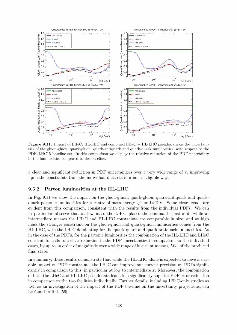
10 210 310 ( GeV )XM

0

0.2

0.4

0.6

0.8

1

1.2

1.4

1.6

Glu

on-G

luon

Lum

i (ra

tio to

bas

elin

e) PDF4LHC15

+ LHeC

+ HL-LHC

+ LHeC + HL-LHC

=14 TeVsUncertanties in PDF luminosities @

10 210 310 ( GeV )XM

0

0.2

0.4

0.6

0.8

1

1.2

1.4

1.6

Qua

rk-G

luon

Lum

i (ra

tio to

bas

elin

e) PDF4LHC15

+ LHeC

+ HL-LHC

+ LHeC + HL-LHC

=14 TeVsUncertanties in PDF luminosities @

10 210 310 ( GeV )XM

0

0.2

0.4

0.6

0.8

1

1.2

1.4

1.6

Qua

rk-A

ntiq

uark

Lum

i (ra

tio to

bas

elin

e)

PDF4LHC15

+ LHeC

+ HL-LHC

+ LHeC + HL-LHC

=14 TeVsUncertanties in PDF luminosities @

10 210 310 ( GeV )XM

0

0.2

0.4

0.6

0.8

1

1.2

1.4

1.6

Qua

rk-Q

uark

Lum

i (ra

tio to

bas

elin

e) PDF4LHC15

+ LHeC

+ HL-LHC

+ LHeC + HL-LHC

=14 TeVsUncertanties in PDF luminosities @

Figure 9.11: Impact of LHeC, HL-LHC and combined LHeC + HL-LHC pseudodata on the uncertain-ties of the gluon-gluon, quark-gluon, quark-antiquark and quark-quark luminosities, with respect to thePDF4LHC15 baseline set. In this comparison we display the relative reduction of the PDF uncertaintyin the luminosities compared to the baseline.

a clear and significant reduction in PDF uncertainties over a very wide range of x, improvingupon the constraints from the individual datasets in a non-negligible way.

9.5.2 Parton luminosities at the HL-LHC

In Fig. 9.11 we show the impact on the gluon-gluon, quark-gluon, quark-antiquark and quark-quark partonic luminosities for a centre-of-mass energy

√s = 14 TeV. Some clear trends are

evident from this comparison, consistent with the results from the individual PDFs. We canin particular observe that at low mass the LHeC places the dominant constraint, while atintermediate masses the LHeC and HL-LHC constraints are comparable in size, and at highmass the stronger constraint on the gluon-gluon and quark-gluon luminosities comes from theHL-LHC, with the LHeC dominating for the quark-quark and quark-antiquark luminosities. Asin the case of the PDFs, for the partonic luminosities the combination of the HL-LHC and LHeCconstraints leads to a clear reduction in the PDF uncertainties in comparison to the individualcases, by up to an order of magnitude over a wide range of invariant masses, MX , of the producedfinal state.

In summary, these results demonstrate that while the HL-LHC alone is expected to have a size-able impact on PDF constraints, the LHeC can improve our current precision on PDFs signifi-cantly in comparison to this, in particular at low to intermediate x. Moreover, the combinationof both the LHeC and HL-LHC pseudodata leads to a significantly superior PDF error reductionin comparison to the two facilities individually. Further details, including LHeC-only studies aswell as an investigation of the impact of the PDF baseline on the uncertainty projections, canbe found in Ref. [59].

228

9.5.3 PDF Sensitivity: Comparing HL-LHC and LHeC

While the experimental reach of each facility in the x,Q2 kinematic plane provides a usefulcomparison, there are more factors to consider – especially when we are striving for ultra-highprecision measurements. One measure that provides a dimension beyond the x,Q2 plane is thesensitivity ; this is a combination of the correlation coefficient times a scaled residual [760, 761].This provides an extra dimension of information in comparison to a simple x,Q2 map andrepresents a measure of the impact of the data.

Figure 9.12: Sensitivity for a sample flavour d(x,Q) in the x,Q2 kinematic plane for the LHeC(left) and the HL-LHC (right) calculated with pseudodata [761]. We observe the LHeC is particularlysensitive in both the high and low x regions, and the HL-LHC covers the intermediate x region out tolarge Q scales.

In Fig. 9.12 this PDF sensitivity for a sample PDF flavour is displayed for the LHeC and theHL-LHC pseudo-data. In particular, one observe that the LHeC provides strong sensitivity inthe high-x region, which is of great importance for BSM searches, and also in the low-x region,which is relevant for QCD phenomena such as saturation. The HL-LHC provides constraintscoming from W/Z production (Q ∼MW/Z) as well as from jets at high scales. The combinationof these measurements will provide strongest constraints on the various PDF flavours across thebroad x,Q2 kinematic plane.

9.6 Impact of New Small-x Dynamics on Hadron Collider Physics

As discussed in Subsections 4.2.1 and 4.2.3, the presence of new dynamics at small x as claimed inRefs. [248,252,253] will have impact on hadronic observables. The impact is stronger for largerenergies, therefore more important for the FCC-hh than for the LHC. But it may competewith other uncertainties and thus become crucial for precision studies even at LHC energies.Studies on the impact of non-linear dynamics at hadron colliders have been devoted mainlyto photoproduction in UPCs, see e.g. [762–764] and Refs. therein for the case of gauge bosonproduction. In this section we focus on the effect of resummation at small x.

While hadronic data like jet, Drell-Yan or top production at existing energies do not have muchconstraining power at low x [248] and thus need not be included in the extraction of PDFsusing resummed theoretical predictions, this fact does not automatically mean that the impactof resummation is not visible at large scales for large energies. Indeed the PDFs obtained with

229

small-x resummation may change at low energies in the region of x relevant for hadronic data,thereby giving an effect also at higher energies after evolving to those scales. A consistentinclusion of resummation effects on hadronic observables is thus crucial for achieving precision.The difficulty for implementing resummation on different observables lies in the fact that not onlyevolution equations should include it but also the computation of the relevant matrix elementsfor the observable must be performed with matching accuracy.

Until present, the only observable that has been examined in detail is Higgs production crosssection through gluon fusion [765]. Other observables like Drell-Yan [766] or heavy quark [767]production are under study and they will become available in the near future.

For gg → H, the LL resummation of the matrix elements matched to fixed order at N3LO wasdone in Refs. [273, 765] and the results are shown in Figs. 9.13 and 9.14. Fig. 9.13 shows theincreasing impact of resummation on the cross section with increasing energy. It also illustratesthe fact that the main effect of resummation comes through the modification of the extractionof parton densities and their extrapolation, not through the modification of the matrix elementsor the details of the matching.

0.98

1

1.02

1.04

1.06

1.08

1.1

1.12

1.14

2 7 8 13 14 2710 100

f.o. PDFs: NNPDF31sx_nnlo_as_0118res PDFs: NNPDF31sx_nnlonllx_as_0118

band: PDF uncertainty

mH = 125 GeVµF = µR = mH/2

ratio

toN3LO

s [TeV]

ggH production cross section --- effect of small-x resummation

N3LO using f.o. PDFsN3LO using res PDFs

N3LO+LL using res PDFsN3LO+LL(LL') using res PDFs

Figure 9.13: Ratio of the N3LO Higgs cross section with and without resummation to the N3LO fixed-order cross section, as a function of the collider centre-of-mass energy. “f.o.” denotes fixed order, “res”denotes resummed and “LL′” a different anomalous dimension matching at leading logarithmic accuracy,see the legend on the plot and Ref. [765] for details. The PDFs used are from the global dataset ofRef. [252]. Figure taken from Ref. [765].

Fig. 9.14 indicates the size of the different uncertainties on the absolute values of the cross sectionwith increasing accuracy of the perturbative expansion, at HL-LHC and FCC-hh energies. ForN3LO(+LL) it can be seen that while at the HL-LHC, the effect of resummation is of the sameorder as other uncertainties like those coming scale variations, PDFs and subleading logarithms,this is not the case for the FCC where it can be clearly seen that it will be the dominant one.Resummation should also strongly affect the rapidity distributions, a key need for extrapolationof observed to total cross sections. In particular, rapidity distributions are more directly sensitiveto PDFs at given values of momentum fraction x, and therefore in regions where this momentumfraction is small (large rapidities) the effect of resummation may be sizeable also at lower colliderenergies. These facts underline the need of understanding the dynamics at small x for any kind

230

of precision physics measurements at future hadronic colliders, with increasing importance forincreasing energies.

30

35

40

45

50

55

60

NLONLO+LL

NNLONNLO+LL

N 3LON 3LO+LL

µF = µR = mH/2mH = 125 GeV

[pb]

s = 14 TeV

PDFsPDFs+subl.logsPDFs+subl.logs+scale

450

500

550

600

650

700

750

800

850

900

950

NLONLO+LL

NNLONNLO+LL

N 3LON 3LO+LL

µF = µR = mH/2mH = 125 GeV

[pb]

s = 100 TeV

PDFsPDFs+subl.logsPDFs+subl.logs+scale

Figure 9.14: Perturbative progression of the Higgs cross section for two collider energies√s =

14, 100 TeV. In each plot the NLO, NLO+LL, NNLO, NNLO+LL, N3LO and N3LO+LL results areshown. The results are supplemented by uncertainty bands from PDF, subleading logarithms and scaleuncertainties. Figure taken from Ref. [765].

Finally, it should be mentioned that a different kind of factorisation, called transverse momentum(TMD) factorisation [38,510,768–771], may have an effect on large scale observables in hadroniccolliders. The extension of the TMD evolution equations towards small x [772] and the relation ofsuch factorisation with new dynamics at small x, either through high-energy factorisation [773–776] or with the CGC [506,507], is under development [777].

9.7 Heavy Ion Physics with eA Input

The study of hadronic collisions at RHIC and the LHC, proton-proton, proton-nucleus andnucleus-nucleus, has produced several observations of crucial importance for our understandingof QCD in complex systems where a large number of partons is involved [778,779]. The differentstages of a heavy ion collision, as we presently picture it, are schematically drawn in Fig 9.15.

Figure 9.15: Sketch of a heavy ion collision with time running left to right, going from the approachof two ultrarelativistic Lorentz-contracted nuclei, the collision and parton creation in the central ra-pidity region, the beginning of expansion and formation of the QGP, the expansion of the QGP untilhadronisation, and, finally, the expansion of the hadronic gas.

231

First, the hot and dense partonic medium created in heavy ion collisions, the quark-gluon plasma(QGP), experiences a collective behaviour of which azimuthal asymmetries and transverse spec-tra with a specific ordering in particle masses are the most prominent observables. This collec-tivity can be very well described by relativistic hydrodynamics [780]. For this description, thesystem has to undergo some dynamics leading to rough isotropisation in a short time, . 1 fm/c,for which both strong and weak coupling explanations have been proposed [558].

Second, collisions between smaller systems, pp and pA, show many of the features [555–557] thatin heavy ion collisions are taken as indicative of the production of a dense hot partonic medium.The most celebrated of such features, the long rapidity range particle correlations collimated inazimuth, named the ridge (see Sect. 6.5), has been found in all collisions systems. The dynamicsunderlying this phenomena, either the formation of QGP and the existence of strong final stateinteractions, or some initial state dynamics that leaves imprint on the final observables, is underdiscussion [558].

Finally, the QGP is extremely opaque to both highly energetic partons [781] and quarkonia [782]traversing it. These observables, whose production in pp can be addressed through perturba-tive methods, are called hard probes [783]. The quantification of the properties of the QGPextracted through hard probes is done by a comparison with predictions based on assuming anuclear collision to be a superposition of collisions among free nucleons. Such predictions containuncertainties coming both from nuclear effects other than those in QGP (named cold nuclearmatter effects), and from uncertainties in the dynamics determining the interaction between theenergetic parton or bound state and the medium. In the case of partons, this has motivated thedevelopment of sophisticated jet studies in heavy ion collisions [784].

eA collisions studied in the energy range relevant for the corresponding hadronic accelerator – theLHeC for the LHC – would substantially improve our knowledge on all these aspects and, indeed,on all stages of a heavy ion collisions depicted in Fig. 9.15. Besides, they can reduce sizeably theuncertainties in the extracted QGP parameters, the central goal of the heavy program for theunderstanding of the different phases of QCD. Here we provide three examples of such synergies:

• Nuclear parton densities: The large lack of precision presently existing in the deter-mination of parton densities induce large uncertainties in the understanding of severalsignatures of the QGP. For example, for J/ψ suppression, its magnitude at midrapidityat the LHC is compatible with the sole effect of nuclear shadowing on nPDFs [782], seeFig. 9.16. While from data at lower energies and at forward and backward rapidities it isclear that this is not the only effect at work, only a reduction on the nPDF uncertaintyas feasible at the LHeC , see Sect. 6.2, will make possible a precise quantification of thedifferent mechanisms producing either suppression (screening, gluon dissociation, energyloss) or enhancement (recombination or coalescence), that play a role for this observable.

• Initial conditions for the collective expansion and the small system problem: At present,the largest uncertainty in the determination of the transport coefficients of the partonicmatter created in heavy ion collisions [786, 787] (see Fig. 9.17), required in hydrodynamiccalculations, and in our understanding of the speed of the approach to isotropisation andof the dynamics prior to it [788], comes from our lack of knowledge of the nuclear wavefunction and of the mechanism of particle production at small to moderate scales – i.e. thesoft and semihard regimes. Both aspects determine the initial conditions for the applicationof relativistic hydrodynamics. This is even more crucial in the discussion of small systems,where details of the transverse structure of protons are key [789] not only to providesuch initial conditions but also to establish the relative role of initial versus final statedynamics. For example, the description of azimuthal asymmetries in pp and pPb collisions

232

y

0 0.5 1 1.5 2 2.5 3 3.5 4

AA

R

0

0.2

0.4

0.6

0.8

1

1.2

1.4 = 2.76 TeV

NNsALICE (PLB 734 (2014) 314) Pb­Pb

c>0 GeV/T

p90%, , centrality 0%­e+ e→ ψJ/

8%± global syst.= c<8 GeV/T

p90%, 0< , centrality 0%­µ+µ → ψJ/

= 2.76 TeVNN

sCold nuclear matter effects in Pb­Pb

EPS09 shadowing (PRC 81 (2010) 044903)

nDSg shadowing (NPA 855 (2011) 327)

ALI−DER−65282

Figure 9.16: ALICE inclusive J/ψ nuclear modification factor versus rapidity [785], compared to nPDFcalculations. Taken from [782].

at the LHC demands that the proton is modelled as a collection of constituent quarks orhot spots [780, 789]. ep and eA collisions at the LHeC can constrain both aspects in thepertinent kinematic region, see Sects. 3.4 and 6.3. Besides, they can clarify the mechanismsof particle production and the possible relevance of initial state correlations on the finalstate observables as suggested e.g. by CGC calculations, see Sects. 4.2.1 and 6.4, whoseimportance for LHC energies can be established at the LHeC.

0 10 20 30(1/S) dN

ch/dy (fm

-2)

0

0.05

0.1

0.15

0.2

0.25

v2/!

0 10 20 30 40(1/S) dN

ch/dy (fm

-2)

hydro ("/s) + UrQMD hydro ("/s) + UrQMDMC-GlauberMC-KLN0.0

0.08

0.16

0.24

0.0

0.08

0.16

0.24

"/s"/s

v22 / #!

2

part$1/2

Gl

(a) (b)

#v2$ / #!

part$Gl

v22 / #!

2

part$1/2

KLN

#v2$ / #!

part$KLN

Figure 9.17: Comparison of the universal v2(η/s)/ε vs. (1/S)(dNch/dy) curves with experimental datafor 〈v2〉 [790], v22 [791], and dNch/dy [792] from the STAR Collaboration. The experimental data usedin (a) and (b) are identical, but the normalisation factors 〈εpart〉 and S used on the vertical and horizontalaxes, as well as the factor 〈ε2

part〉1/2 used to normalize the v22 data, are taken from the MC-KLN modelin (a) and from the MC-Glauber model in (b). Theoretical curves are from simulations with MC-KLNinitial conditions in (a) and with MC-Glauber initial conditions in (b). Taken from [786].

• Impact on hard probes: Besides the improvement in the determination of nPDFs thataffects the quantification of hard probes, commented above, eA collisions can help to un-derstand the dynamics of the probes by analysing the effects of the nuclear medium onthem. As two examples, the abundant yields of jets and large transverse momentum parti-

233

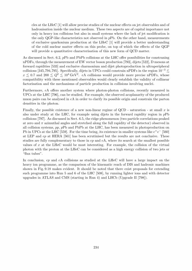
cles at the LHeC [1] will allow precise studies of the nuclear effects on jet observables and ofhadronisation inside the nuclear medium. These two aspects are of capital importance notonly in heavy ion collisions but also in small systems where the lack of jet modification isthe only QGP-like characteristics not observed in pPb. On the other hand, measurementsof exclusive quarkonium production at the LHeC [1] will provide a better understandingof the cold nuclear matter effects on this probe, on top of which the effects of the QGPwill provide a quantitative characterisation of this new form of QCD matter.

As discussed in Sect. 6.2, pPb and PbPb collisions at the LHC offer possibilities for constraningnPDFs, through the measurement of EW vector boson production [793], dijets [522], D mesons atforward rapidities [533] and exclusive charmonium and dijet photoproduction in ultraperipheralcollisions [345,794,795]. Specifically, dijets in UPCs could constrain nPDFs in the region 10−3 .x . 0.7 and 200 . Q2 . 104 GeV2. eA collisions would provide more precise nPDFs, whosecompatibility with these mentioned observables would clearly establish the validity of collinearfactorisation and the mechanisms of particle production in collisions involving nuclei.

Furthermore, eA offers another system where photon-photon collisions, recently measured inUPCs at the LHC [796], can be studied. For example, the observed acoplanarity of the producedmuon pairs can be analysed in eA in order to clarify its possible origin and constrain the partondensities in the photon.

Finally, the possible existence of a new non-linear regime of QCD - saturation - at small x isalso under study at the LHC, for example using dijets in the forward rapidity region in pPbcollisions [797]. As discussed in Sect. 6.5, the ridge phenomenon (two particle correlations peakedat zero and π azimuthal angles and stretched along the full rapidity of the detector) observed inall collision systems, pp, pPb and PbPb at the LHC, has been measured in photoproduction onPb in UPCs at the LHC [559]. For the time being, its existence in smaller systems like e+e− [560]at LEP and ep at HERA [561] has been scrutinised but the results are not conclusive. Thesestudies are fully complementary to those in ep and eA, where its search at the smallest possiblevalues of x at the LHeC would be most interesting. For example, the collision of the virtualphoton with the proton at the LHeC can be considered as a high energy collision of two jets or“flux tubes”.

In conclusion, ep and eA collisions as studied at the LHeC will have a large impact on theheavy ion programme, as the comparison of the kinematic reach of DIS and hadronic machinesshown in Fig. 9.18 makes evident. It should be noted that there exist proposals for extendingsuch programme into Run 5 and 6 of the LHC [508], by running lighter ions and with detectorupgrades in ATLAS and CMS (starting in Run 4) and LHCb (Upgrade II [798]).

234

Ax

8−10 7−10 6−10 5−10 4−10 3−10 2−10 1−10 1

)2 (

GeV

2Q

1−10

1

10

210

310

410

510

610

710

Au(100)+e(20)197

Pb(2750)+e(50)208

Pb(7885)+e(60)208

Pb(19700)+e(60)208

(x)2sat,PbQ

PresentνDIS+DY+

dAu@

RHIC

pPb@LHC

7+2.75 TeV

=0,...,6.6lab

y

50+19.7 TeV

=0,...,6.6lab

y

Figure 9.18: Kinematic regions in the x−Q2 plane explored by data sets (charged lepton and neutrinoDIS, DY, dAu at RHIC and pPb at the LHC) used in present nPDF analyses [503], compared to the onesachievable at the EIC (red), the LHeC (ERL against the HL-LHC beams, dark blue) and two FCC-ehversions (with Pb beams corresponding to proton energies of 20 TeV - green and 50 TeV - light blue).Acceptance is taken to be 1 < θ < 179, and 0.01(0.001) < y < 1 for the EIC (all other colliders).The areas delimitated by thick brown and black lines show the regions accessible in pPb collisions atthe LHC and the FCC-hh (50 TeV) respectively, while the thin lines represent constant rapidities from 0(right) to 6.6 (left) for each case. The saturation scale Qsat shown here for indicative purposes only, seealso [504], has been drawn for a Pb nucleus considering an uncertainty ∼ 2 and a behaviour with energyfollowing the model in [505]. Note that it only indicates a region where saturation effects are expectedto be important but there is no sharp transition between the linear and non-linear regimes.

235

Chapter 10

The Electron Energy Recovery Linac

We studied different options for the electron accelerator for LHeC in Ref. [1], of which the EnergyRecovery Linac (ERL) option is retained in this update of the CDR. This is due to the higherachievable luminosity of the Linac-Ring option, as compared to the Ring-Ring option, as well asthe interference of the installation of an electron ring in the LHC tunnel with its operation [799].The clear advantage of the ERL compared to its contenders in 2012 is the possibility to keepthe overall energy consumption at bay, albeit, in its baseline configuration and size of the returnarcs, operation is still limited to lepton energies below 70 GeV to avoid excessive synchrotronradiation losses. Since there is no fundamental beam loading in an ERL by its principle, higheraverage currents and thus higher luminosities would not lead to larger power consumption.

10.1 Introduction – Design Goals

The main guidelines for the design of the Electron ERL and the Interaction Region (IR) withthe LHC are:

• electron-hadron operation in parallel with high luminosity hadron-hadron collisions inLHC/HL-LHC;

• centre-of-mass collision energy in the TeV scale;

• power consumption of the electron accelerator smaller than 100 MW;

• peak luminosity approaching 1034 cm−2s−1;

• integrated luminosity exceeding by at least two orders of magnitude that achieved byHERA at DESY.

The electron energy Ee chosen in the previous version of the CDR [1] was 60 GeV. This could beachieved with an ERL circumference of 1/3 of that of the LHC. Cost considerations and machine–detector performance aspects, in particular the amount of synchrotron radiation losses in theIR, have led to define a new reference configuration with Ee = 49.2 GeV and a circumference of≈ 5.4 km, 1/5 of that of the LHC.

The ERL consists of two superconducting (SC) linacs operated in CW connected by at leastthree pairs of arcs to allow three accelerating and three decelerating passes (see Fig. 10.1). Thelength of the high energy return arc following the interaction point should be such as to providea half RF period wavelength shift to allow the deceleration of the beam in the linac structuresin three passes down to the injection energy and its safe disposal. SC Cavities with an unloaded

236

quality factor Q0 exceeding 1010 are required to minimise the requirements on the cryogeniccooling power and to allow an efficient ERL operation. The choice of having three acceleratingand three decelerating passes implies that the circulating current in the linacs is six times thecurrent colliding at the Interaction Point (IP) with the hadron beam.

Figure 10.1: Schematic layout of the LHeC design based on an Energy Recovery Linac.

The choice of an Energy Recovery Linac offers the advantage of a high brightness beam and itavoids performance limitations due to the beam-beam effect seen by the electron beam [800],which was a major performance limitation in many circular lepton colliders (e.g. LEP) and forthe LHeC Ring-Ring option. The current of the ERL is limited by its source and an operationalgoal of Ie = 20 mA has been set, corresponding to a bunch charge of 500 pC at a bunch frequencyof 40 MHz. This implies operating the SRF cavities with the very high current of 120 mA for avirtual beam power (product of the beam current at the IP times the maximum beam energy) of1 GW. The validation of such performance in terms of source brightness and ERL 3-turn stableand efficient operation in the PERLE facility [11] is a key milestone for the LHeC design.

A small beam size at the IP is required to maximize luminosity and approach peak luminositiesof 1034 cm−2s−1 and integrated luminosities of 1 ab−1 in the LHeC lifetime. In particular β∗ <10 cm needs to be achieved for the colliding proton beam compatibly with the optics constraintsimposed by the operation in parallel to proton-proton physics in the other IPs during the HL-LHC era [3]. The peak luminosity values quoted above exceed those at HERA by 2-3 orders ofmagnitude. The operation of HERA in its first, extended running period 1992–2000, providedand integrated luminosity of about 0.1 fb−1 for the H1 and ZEUS experiments, correspondingto the expected integrated luminosity collected over 1 day of LHeC operation.

10.2 The ERL Configuration of the LHeC

The main parameters of the LHeC ERL are listed in Tab. 10.1; their choices and optimisationcriteria will be discussed in the following sections.

237

Parameter Unit Value

Injector energy GeV 0.5Total number of linacs 2Number of acceleration passes 3Maximum electron energy GeV 49.19Bunch charge pC 499Bunch spacing ns 24.95Electron current mA 20Transverse normalized emittance µm 30Total energy gain per linac GeV 8.114Frequency MHz 801.58Acceleration gradient MV/m 19.73Cavity iris diameter mm 130Number of cells per cavity 5Cavity length (active/real estate) m 0.918/1.5Cavities per cryomodule 4Cryomodule length m 7Length of 4-CM unit m 29.6Acceleration per cryomodule (4-CM unit) MeV 289.8Total number of cryomodules (4-CM units) per linac 112 (28)Total linac length (with with spr/rec matching) m 828.8 (980.8)Return arc radius (length) m 536.4 (1685.1)Total ERL length km 5.332

Table 10.1: Parameters of LHeC Energy Recovery Linac (ERL).

10.2.1 Baseline Design – Lattice Architecture

The ERL, as sketched in Fig. 10.1, is arranged in a racetrack configuration; hosting two su-perconducting linacs in the parallel straights and three recirculating arcs on each side. Thelinacs are 828.8 m long and the arcs have 536.4 m radius, additional space of 76 m is taken up byutilities like Spreader/Recombiner (Spr/Rec), matching and energy loss compensating sectionsadjacent to both ends of each linac (total of 4 sections) [801]. The total length of the racetrackis 5.332 km: 1/5 of the LHC circumference 2 · (828.8 + 2 · 76 + 536.4π) m. Each of the two linacsprovides 8.114 GV accelerating voltage, therefore a 49.19 GeV energy is achieved in three turns.After the collision with the protons in the LHC, the beam is decelerated in the three subsequentturns. The injection and dump energy has been chosen at 0.5 GeV.

Injection into the first linac is done through a fixed field injection chicane, with its last magnet(closing the chicane) being placed at the beginning of the linac. It closes the orbit bump at thelowest energy, injection pass, but the magnet (physically located in the linac) will deflect thebeam on all subsequent linac passes. In order to close the resulting higher pass bumps, the so-called re-injection chicane is instrumented, by placing two additional opposing bends in front ofthe last chicane magnet. The chosen arrangement is such that, the re-injection chicane magnetsare only visible by the higher pass beams. The second linac in the racetrack is configured exactlyas a mirror image of the first one, with a replica of the re-injection chicane at its end, whichfacilitates a fixed-field extraction of energy recovered beam to the dump.

Linac Configuration and Multi-pass Optics

Appropriate choice of the linac optics is of paramount importance for the transverse beamdynamics in a multi-pass ERL. The focusing profile along the linac (quadrupole gradients) need

238

Figure 10.2: Layout of a half-cell composed out of four cryomodules (each hosting four, 5-cell cavities:top insert) and a focusing quad. Beta functions reflect 130° FODO optics.

to be set (and they stay constant), so that multiple pass beams within a vast energy range maybe transported efficiently. The chosen arrangement is such that adequate transverse focusing isprovided for a given linac aperture. The linac optics is configured as a strongly focusing, 130°FODO. In a basic FODO cell a quadrupole is placed every four cryomodules, so that the full cellcontains two groups of 16 RF cavities and a pair of quads (F, D) as illustrated in Fig. 10.2. Theentire linac is built out of 14 such cells. Energy recovery in a racetrack topology explicitly requiresthat both the accelerating and decelerating beams share the individual return arcs [802]. Thisin turn, imposes specific requirements for TWISS function at the linacs ends: TWISS functionshave to be identical for both the accelerating and decelerating linac passes converging to thesame energy and therefore entering the same arc. There is an alternative scheme, proposed byPeter Williams [803], who has argued that it would be beneficial to separate the accelerating anddecelerating arcs. This would simplify energy compensation systems and linac-to-arc matching,but at an higher cost of the magnetic system of the arcs. However, doubling number of arcs isa very costly proposition. On the other hand, C-BETA experiment is pioneering a multi-passarcs to transport a vast energy range through the same beam-line and it still intends to usethem for energy recovery. Our approach, based on proven, CEBAF-like, RLA technology [804]is somewhere in the ’middle’.

To visualize beta functions for multiple accelerating and decelerating passes through a givenlinac, it is convenient to reverse the linac direction for all decelerating passes and string themtogether with the interleaved accelerating passes, as illustrated in Fig. 10.3. This way, thecorresponding accelerating and decelerating passes are joined together at the arc’s entrance/exit.Therefore, the matching conditions are automatically built into the resulting multi-pass linacbeamline. One can see that both linacs uniquely define the TWISS functions for the arcs: Linac1 fixes input to all odd arcs and output to all even arcs, while Linac 2 fixes input to all evenarcs and output to all odd arcs. The optics of the two linacs are mirror-symmetric; They wereoptimised so that, Linac 1 is periodic for the first accelerating pass and Linac 2 has this featurefor last decelerating one. In order to maximize the BBU threshold current [805], the optics istuned so that the integral of β/E along the linac is minimised. The resulting phase advance percell is close to 130°. Non-linear strength profiles and more refined merit functions were tested,but they only brought negligible improvements.

239

Figure 10.3: Beta function in the optimised multi-pass linacs (3 accelerating passes and 3 deceleratingpasses in each of two linacs). The matching conditions are automatically built into the resulting multi-passlinac beamline.

Recirculating Arcs – Emittance Preserving Optics

Synchrotron radiation effects on beam dynamics, such as the transverse emittance dilutioninduced by quantum excitations have a paramount impact on the collider luminosity. All sixhorizontal arcs are accommodated in a tunnel of 536.4 m radius. The transverse emittancedilution accrued through a given arc is proportional to the emittance dispersion function, H,averaged over all arc’s bends [806]:

∆ε =2π

3Cqr0 < H >

γ5

ρ2, (10.1)

where

Cq =55

32√

3

~mc

(10.2)

and r0 is the classical electron radius and γ is the Lorentz boost. Here, H = (1 + α2)/β ·D2 + 2α DD′ + β · D′2 where D,D′ are the bending plane dispersion and its derivative, with< ... > = 1

π

∫bends ... dθ.

Therefore, emittance dilution can be mitigated through appropriate choice of arc optics (valuesof α, β,D,D′ at the bends). In the presented design, the arcs are configured with a FMC(Flexible Momentum Compaction) optics to ease individual adjustment of, < H >, in variousenergy arcs.

Optics design of each arc takes into account the impact of synchrotron radiation at differentenergies. At the highest energy, it is crucial to minimise the emittance dilution due to quantumexcitations; therefore, the cells are tuned to minimise the emittance dispersion, H, in the bendingsections, as in the TME (Theoretical Minimum Emittance) lattice. On the other hand, at thelowest energy, it is beneficial to compensate for the bunch elongation with isochronous optics.The higher energy arcs (4,5 and 6) configured with the TME cells are still quasi-isochronous. Tofully compensate remnant bunch elongation one could set higher pass linacs slightly off-crest tocompress the bunches, since one has full control of gang-phases for individual linac passes. Allstyles of FMC lattice cells, as illustrated in Fig. 10.4, share the same footprint for each arc. This

240

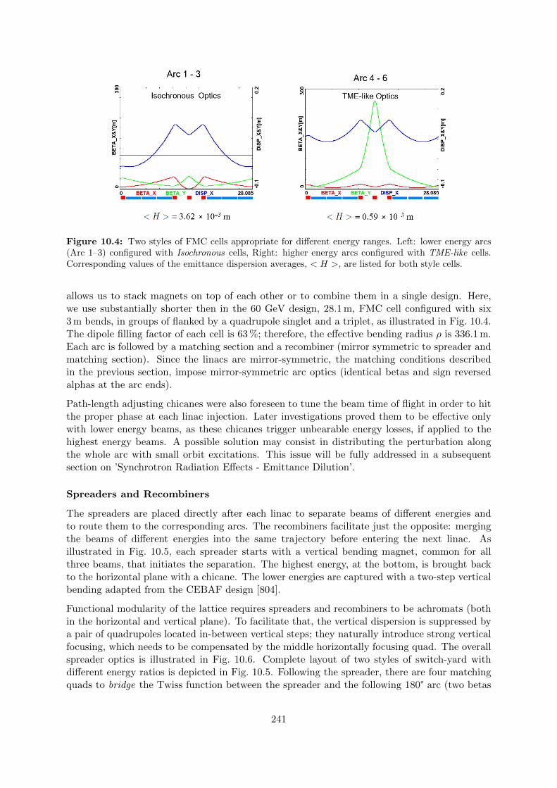
Figure 10.4: Two styles of FMC cells appropriate for different energy ranges. Left: lower energy arcs(Arc 1–3) configured with Isochronous cells, Right: higher energy arcs configured with TME-like cells.Corresponding values of the emittance dispersion averages, < H >, are listed for both style cells.

allows us to stack magnets on top of each other or to combine them in a single design. Here,we use substantially shorter then in the 60 GeV design, 28.1 m, FMC cell configured with six3 m bends, in groups of flanked by a quadrupole singlet and a triplet, as illustrated in Fig. 10.4.The dipole filling factor of each cell is 63 %; therefore, the effective bending radius ρ is 336.1 m.Each arc is followed by a matching section and a recombiner (mirror symmetric to spreader andmatching section). Since the linacs are mirror-symmetric, the matching conditions describedin the previous section, impose mirror-symmetric arc optics (identical betas and sign reversedalphas at the arc ends).

Path-length adjusting chicanes were also foreseen to tune the beam time of flight in order to hitthe proper phase at each linac injection. Later investigations proved them to be effective onlywith lower energy beams, as these chicanes trigger unbearable energy losses, if applied to thehighest energy beams. A possible solution may consist in distributing the perturbation alongthe whole arc with small orbit excitations. This issue will be fully addressed in a subsequentsection on ’Synchrotron Radiation Effects - Emittance Dilution’.

Spreaders and Recombiners

The spreaders are placed directly after each linac to separate beams of different energies andto route them to the corresponding arcs. The recombiners facilitate just the opposite: mergingthe beams of different energies into the same trajectory before entering the next linac. Asillustrated in Fig. 10.5, each spreader starts with a vertical bending magnet, common for allthree beams, that initiates the separation. The highest energy, at the bottom, is brought backto the horizontal plane with a chicane. The lower energies are captured with a two-step verticalbending adapted from the CEBAF design [804].

Functional modularity of the lattice requires spreaders and recombiners to be achromats (bothin the horizontal and vertical plane). To facilitate that, the vertical dispersion is suppressed bya pair of quadrupoles located in-between vertical steps; they naturally introduce strong verticalfocusing, which needs to be compensated by the middle horizontally focusing quad. The overallspreader optics is illustrated in Fig. 10.6. Complete layout of two styles of switch-yard withdifferent energy ratios is depicted in Fig. 10.5. Following the spreader, there are four matchingquads to bridge the Twiss function between the spreader and the following 180° arc (two betas

241

Figure 10.5: Layout of a three-beam switch-yard for different energy ratios: 1 : 3 : 5 and 1 : 2 : 3 corre-sponding to specific switch-yard geometries implemented on both sides of the racetrack

Figure 10.6: Spreader 3 (24.8 GeV) optics; featuring a vertical achromat with three dispersion suppress-ing quads in-between the two steps, a pair of path-length adjusting dogleg chicanes and four betatronmatching quads, interleaved with three energy loss compensating sections (2-nd harmonic RF cavitiesmarked in green).

and two alphas). Combined spreader-arc-recombiner optics, features a high degree of modularfunctionality to facilitate momentum compaction management, as well as orthogonal tunabilityfor both the beta functions and dispersion, as illustrated in Fig. 10.7.

Alternative design of the spreader/recombiner

The desire to reduce the number of elements included in the spreader led to the reduction ofthe number of steps required to separate vertically the different beams and route them intotheir specific arcs. In particular, this alternative spreader design uses a single vertical stepinstead of two. Although the concept has been briefly discussed in [1] it was not retained dueto the superconducting technology needed for the quadrupoles that must be avoided in thishighly radiative section. Nevertheless, recent studies have been pursuing a one step spreaderversion, based on normal conducting magnet technology. It assumes a pole tip field of less than1 T for an aperture radius of 30 mm, allowing the use of thin quadrupoles and thus minimisepotential overlap with the other beamlines. With respect to the previous study, the use of normalconductors was made possible by increasing the overall spreader length and reducing the number

242

Figure 10.7: Complete Optics for Arc 3 (including switch-yard); featuring: low emittance 180° arcbased on isochronous cells (30 cells flanked by dispersion suppression cell with missing dipoles on eachside), spreaders and recombiners with matching sections and doglegs symmetrically placed on each sideof the arc proper.

Figure 10.8: Optics and layout of Arc 4 including the detector bypass. The lattice (top insert) featuresa vertical spreader, an initial horizontal bending, a straight section, a modified dispersion suppressor,seven junction cells, and four regular cells. The bypass geometry (bottom insert), features a long IP line,AB, which for visual reasons has been purposely stretched, being actually about 1/5 of the arc radius.All geometric dependencies of the bypass parameters are summarized in the inserted formulae.

243

of quadrupoles. In particular, the focusing magnets are limited to two outer quadrupoles for theachromatic function and one quadrupole in the middle, where the dispersion is zero, to controlthe beta function in the defocusing plane. Two visualisations are given Fig 10.9 and 10.10.

Figure 10.9: 3D visualisation of the spreader 1,3,5 inserted between the end of the linac and routingthe different beamlines into their respective dispersion suppresors.

Both spreader types start with a first dipole that separates vertically the different beamlines ina 1-3-5 ratio for the odd number spreaders and in a 1-2-3 ratio for the even number spreaders.Theses ratios are defined by the beam energies of the corresponding turn. Therefore by fixingthe length of the longest beamline for each spreaders (odd and even numbers) one obtains therequired angle to get a 50 cm vertical offset between each beamlines. The equations belowrepresent the required bending angle in the dipole and beamline lengths in order to meet therequirements,

θ3 =0.5

l3 − Ll1 =

2E1

E3(l3 − L) + L (10.3)

θ2 =1

l2 − Ll4 =

1

2

E4

E2(l2 − L) + L (10.4)

where the index i corresponds to the beamline number associated to an energy Ei. L is thedipole length and l is the whole spreader beamline length.

For the beam line 2 and 4 we obtain l4 ≈ l2 according to the energy ratio of 1.97. On the otherhand, l3 will be longer than l1 because the energy ratio is 2.88. One can therefore tune theangle of the even number spreaders by defining l2 as it will be the longest. However the angleof the odd number spreaders will be determined by the length of l3. Regarding the chicaneused for the highest energy only a minimum separation between the highest energy and theintermediate energy allows the introduction of the opposite bending dipole. It constraints inreturn the placement of the quadrupoles of the intermediate energy. The location of the magnetsis the main limitation towards a minimization of the spreader length: the shorter the latticegets, the stronger the quadrupoles need to be in order to preserve the achromatic function.

As a result, a one step spreader halves the number of dipoles present in the lattice and relaxesthe constraint on magnets interference and overlap favorable for compactness. Dividing by twothe number of dipoles has a noticeable effect on the synchrotron power radiated in the spreaderwhich is, in addition, beneficial for the emittance growth. The dipole fields required, for amaximal length of 50 m, are 226 mT for the odd number spreaders and 326 mT for the evennumber spreaders. The multipass linac optics Fig. 10.3 shows that the even number spreaders,i.e. 2, 4 and 6, have the highest beta functions at their entrance which is detrimental from theperspective of minimizing the emittance growth within the spreader lattice. A solution to solvethis issue is to insert a doublet of quadrupoles at the exit of the linac. All three energies will

244

go through the doublet and, therefore, a compromise has to be found for the gradients. Finally,the reduction of the H function over the length of the spreader and specifically in the dipolescontributes to a further reduction of the emittance growth.

The energy loss for spreader 1 is low due to the low beam energy; spreader 2 and 3 have similarvalues that are acceptable as well as the one of spreader 4. Spreader 5 and 6 have the highestbeam energies and therefore the largest energy loss. In addition, the dipoles used to produce thechicane need double the field strength compared to the other dipoles for the same length, i.e.half the bending radius, in order to save space for the other elements in the other beamlines.The vertical emittance growth is well controlled just as in the even number spreaders. Onlyspreader 6 has an order of magnitude higher contribution but one has to keep in mind thatthe even number spreaders will only act as recombiner since there will be the horizontal bypassdoing the separation with the detector and a vertical separation will only occur for arc 2 and 4.Consequently spreader 6 should not be taken into account for the emittance growth contributionuntil the interaction point.

Figure 10.10: 3D visualisation of the spreader 2,4,6 inserted between the end of the linac and routingthe different beamlines into their respective dispersion suppressors.

The optics for the Spreader/Recombiner of arc 2 and 4 are presented Fig. 10.11, it shows theachromatic function supported by the outer quadrupoles while the control of the horizontal betafunction is provided by the ”middle” quadrupole. One sees that the lattice of the arc 2 requiresto split the ”middle” quadrupole in two, in order to avoid overlap with the other beamline (arc4), see Fig.10.10. These two optics are the most challenging as they have high beta functions atthe entrance of their lattices, due to the multi pass linac optics as previously explained.

Figure 10.11: Left : Spreader/Recombiner optics of the arc 2 for the 16.73 GeV electron beam. Right: Spreader/Recombiner optics of the arc 4 for the 32.96 GeV electron beam.

245

IR Bypasses

After the last spreader the 49.19 GeV beam goes straight to the interaction region. However thelower energy beams; at 16.7 and 33.0 GeV, need to be further separated horizontally in orderto avoid interference with the detector. Different design options for the bypass section wereexplored [807] and the one that minimises the extra bending has been chosen and implementedin the lattice.

Ten arc-like dipoles are placed very close to the spreader, to provide an initial bending, θ, whichresults in X = 10 m separation from the detector located 120 m downstream. The straightsection of the bypass is approximately 240 m long. After the bypass, in order to reconnect tothe footprint of Arc 6, 7 of 30 standard cells in Arc 2 and Arc 4 are replaced with 7 higher field,junction cells. The number of junction cells is a compromise between the field strength increaseand the length of additional bypass tunnel, as can be inferred from the scheme summarised inFig. 10.8. The stronger bending in the junction cells creates a small mismatch, which is correctedby adjusting the strengths of the quadrupoles in the last junction cell and in the first regularcell.

Synchrotron Radiation Effects – Emittance Dilution

ERL efficiency as a source of multi-GeV electrons for a high luminosity collider is limited by theincoherent synchrotron radiation effects on beam dynamics; namely the transverse emittancedilution and the longitudinal momentum spread (induced by quantum excitations). The firsteffect, the transverse emittance increase, will have a paramount impact on the collider luminosity,due to stringent limits on the allowed emittance increase. The second one, accrued momentumspread, governs asymmetries of accelerated and decelerated beam profiles. These asymmetriessubstantially complicate multi-pass energy recovery and matching, and ultimately they limit theenergy reach of the ERLs due to recirculating arc momentum acceptance.

Arc optics was designed to ease individual adjustment of momentum compaction (needed for thelongitudinal phase-space control, essential for operation with energy recovery) and the horizontalemittance dispersion, H, in each arc. Tab. 10.2 lists arc-by-arc dilution of the transverse, ∆ε, andlongitudinal, ∆σ∆E

E, emittance due to quantum excitations calculated using analytic formulas,

Eqs. (10.5), (10.6) and (10.7), introduced by M. Sands [806]:

∆E =2π

3r0 mc

2 γ4

ρ(10.5)

∆εN =2π

3Cqr0 < H >

γ6

ρ2, (10.6)

∆ε2EE2

=2π

3Cqr0

γ5

ρ2, (10.7)

where Cq is given by Eq. (10.2). Here, ∆ε2E is an increment of energy square variance, r0 isthe classical electron radius, γ is the Lorentz boost and Cq ≈ 3.832 · 10−13 m for electrons (orpositrons).

Apart from the horizontal 180° arcs, there are other sources of emittance dilution due to syn-chrotron radiation, namely vertical Spreaders and Recombiners, as well as horizontal ’Doglegs’used to compensate seasonal variation of path-length. To minimise their contribution to the ver-tical emittance dilution, special optics with small vertical < H > has been introduced in Spr/Recsections. The effects on vertical emittance dilution coming from these beamlines (Spr/Rec) are

246

Beamline Beam energy ∆E ∆εxN ∆σ∆EE

[GeV] [MeV] [mm mrad] [%]

arc 1 8.62 0.7 0.0016 0.0005arc 2 16.73 10 0.085 0.0027arc 3 24.85 49 0.91 0.0072arc 4 32.96 152 0.81 0.015arc 5 41.08 368 3.03 0.026arc 6 49.19 758 8.93 0.040

Table 10.2: Energy loss and emittance dilution (horizontal and longitudinal) due to synchroton radiation

generated by all six 180° arcs (not including Spreaders, Recombiners and Doglegs). Here, ∆σ∆EE

=

√∆ε2EE2

.

Beamline Beam energy ∆E ∆εyN ∆σ∆EE

[GeV] [MeV] [mm mrad] [%]

Spr/Rec 1 8.62 0.2 0.035 0.0008Spr/Rec 2 16.73 3.0 0.540 0.0044Spr/Rec 3 24.85 6.0 0.871 0.0066Spr/Rec 4 32.96 21.6 5.549 0.0143Spr/Rec 5 41.08 7.1 0.402 0.0062Spr/Rec 6 49.19 39.2 3.92 0.0205

Table 10.3: Energy loss and emittance dilution (vertical and longitudinal) due to synchroton radiation

generated by the two step Spreader, or Recombiner design of a given arc. Here, ∆σ∆EE

=

√∆ε2EE2

.

summarized in Tab. 10.3 for the two-step spreaders and in Tab. 10.4 for the alternative versionof a one-step spreader.

Beam Energy ∆E ∆εyN ∆σ∆EE

[GeV] [MeV] [mm.mrad] [%]

Spreader 1 8.62 0.04 0.004 0.0002Spreader 2 16.73 0.31 0.004 0.0007Spreader 3 24.85 0.32 0.012 0.0006Spreader 4 32.96 1.18 0.112 0.0013Spreader 5 41.08 2.64 0.083 0.0019Spreader 6 49.19 7.92 1.060 0.0040

Table 10.4: Energy loss and emittance dilution (vertical and longitudinal) due to synchroton radiation

generated by a one-step Spreader, or Recombiner design of a given arc. Here, ∆σ∆EE

=

√∆ε2EE2

Similarly, the horizontal emittance dilution induced by the Doglegs (four dogleg chicanes perarc) in various arcs is summarized in Tab. 10.5. Each dogleg chicane is configured with four 1meter bends (1 Tesla each), so that they bend the lowest energy beam at 8.6 GeV by 2 degrees.The corresponding path-lengths gained in the Doglegs of different arcs are also indicated.

As indicated in Tab. 10.5, the Doglegs in the highest energy arcs, Arc 5 and Arc 6, provide onlysub mm path-length gain with large synchrotron radiation effects. They are not very effectiveand generate strong, undesired emittance dilution. Therefore, it is reasonable to eliminate themfrom both Arc 5 and 6. Instead, one could resort to an alternative path-length control via

247

Beamline Beam energy ∆E ∆εxN ∆σ∆EE

path-length

[GeV] [MeV] [mm mrad] [%] [mm]

Doglegs 1 8.62 2 0.201 0.007 7.32Doglegs 2 16.73 9 0.667 0.009 1.96Doglegs 3 24.85 19 5.476 0.014 0.84Doglegs 4 32.96 33 5.067 0.014 0.52Doglegs 5 41.08 52 12.067 0.028 0.36Doglegs 6 49.19 74 2.836 0.011 0.28

Table 10.5: Energy loss and emittance dilution (horizontal and longitudinal) due to synchroton radiation

generated by the Doglegs (four dogleg chicanes) of a given arc. Here, ∆σ∆EE

=

√∆ε2EE2

.

appropriate orbit steering with both horizontal and vertical correctors present at every girderand distributed evenly throughout the arc.

Combining all three contributions: (180° arc, Spreader, Recombiner and Doglegs (no Doglegs inArcs 5 and 6), the net cumulative emittance dilution is summarized in Tab. 10.6 for the case ofthe two-step spreader.

Beamline Beam energy ∆E ∆cumεxN ∆cumεyN ∆cumσ∆EE

[GeV] [MeV] [mm mrad] [mm mrad] [%]

Arc 1 8.62 3 0.2 0.1 0.01Arc 2 16.73 25 1.0 1.2 0.03Arc 3 24.85 80 7.3 2.9 0.06Arc 4 32.96 229 13.2 14.0 0.12Arc 5 41.08 383 16.2 14.8 0.16IR 49.19 39 16.2 18.7 0.18Arc 6 49.19 797 25.2 22.6 0.24Arc 5 41.08 383 28.2 23.4 0.28Arc 4 32.96 229 34.1 34.5 0.33Arc 3 24.85 80 40.5 36.3 0.37Arc 2 16.73 25 41.2 37.4 0.39Arc 1 8.62 3 41.4 37.4 0.40Dump 0.5 41.4 37.4 0.40

Table 10.6: Energy loss and cumulative emittance dilution (transverse and longitudinal) due to synchro-ton radiation at the end of a given beam-line (complete Arc including: 180° arc, Spreader, Recombinerand Doglegs in arcs 1-4). The table covers the entire ER cycle: 3 passes ’up’ + 3 passes ’down’. Cu-mulative emittance dilution values just before the IP (past Arc 5 and Spr 6), which are critical for theluminosity consideration are highlighted in ’bold’. That row accounts for contributions from Spr 6 (thelast bending section before the IR) to energy loss, as well as the vertical and longitudinal emittance

dilutions. Here, ∆σ∆EE

=

√∆ε2EE2

.

Tab. 10.6 shows, the LHeC luminosity requirement of total transverse emittance dilution ineither plane (normalized) at the IP (at the end of Arc 5), not to exceed 20 mm mrad (hor:16.2 mm mrad and ver: 18.7 mm mrad) is met by-design, employing presented low emittancelattices in both the arcs and switch-yards. In the case of the optimised one-step spreader design,another reduction - mainly of the vertical emittance budget - is obtained, providing a comfortablesafety margin of the design.

Finally, one can see from Eqs. (10.6) and (10.7) an underlying universal scaling of the transverse

248

(unnormalized) and longitudinal emittance dilution with energy and arc radius; they are bothproportional to γ5/ρ2. This in turn, has a profound impact on arc size scalability with energy;namely the arc radius should scale as γ5/2 in order to preserve both the transverse and longi-tudinal emittance dilutions, which is a figure of merit for a synchrotron radiation dominatedERL.

10.2.2 30 GeV ERL Options

One may think of an upgrade path from 30 to 50 GeV ERL, using the same 1/5 of the LHCcircumference (5.4 km), footprint. In this scenario, each linac straight (front end) would initiallybe loaded with 18 cryomodules, forming two 5.21 GV linacs. One would also need to decreasethe injector energy by a factor of 5.21/8.11. The top ERL energy, after three passes, would reach31.3 GeV. Then for the upgrade to 50 GeV, one would fill the remaining space in the linacs withadditional 10 cryomodules each; 2.9 GV worth of RF in each linac. This way the energy ratioswould be preserved for both 30 and 50 GeV ERL options, so that the same switch-yard geometrycould be used. Finally, one would scale up the entire lattice; all magnets (dipoles and quads)by 8.11/5.21 ratio.

If one wanted to stop at the 30 GeV option with no upgrade path, then a 1/14 of the LHCcircumference (1.9 km) would be a viable footprint for the racetrack, featuring: two linacs,503 m each, (17 cryomodules) and arcs of 94.5 m radius. Again, assuming 0.32 GeV injectionenergy, the top ERL energy would reach 30.2 GeV. Such a configuration may become of interestif time and funds may permit a small version of the LHeC or none. This version of the LHeCwould have a reduced Higgs, top and BSM physics potential. Yet, owing to the high protonbeam energy, this configuration would still have a TeV in the centre-of-mass such that the coreQCD, PDF and electroweak programme would still be striking.

10.2.3 Component Summary

This closing section will summarise active accelerator components: magnets (bends and quads)and RF cavities for the 50 GeV baseline ERL. The bends (both horizontal and vertical) arecaptured in Tab. 10.7, while the quadrupole magnets and RF cavities are collected in Tab. 10.8.

One would like to use a combined aperture (3-in-one) arc magnet design with 50 cm verticalseparation between the three apertures, proposed by Attilo Milanese [808]. That would reducenet arc bend count from 2112 to 704. As far as the Spr/Rec vertical bends are concerned, thedesign was optimised to include an additional common bend separating the two highest passes.So, there are a total of 8 trapezoid B-com magnets, with second face tilted by 3° and large 10 cmvertical aperture, the rest are simple rectangular bends with specs from the summary Tab. 10.7.

10.3 Electron-Ion Collisions

Besides colliding proton beams, the LHC also provides collisions of nuclear (fully-stripped ion)beams with each other (AA collisions) or with protons (pA). Either of these operating modesoffers the possibility of electron-ion (eA) collisions in the LHeC configuration1

Here we summarise the considerations leading to the luminosity estimates given in Tab. 2.4 forcollisions of electrons with 208Pb82+ nuclei, the nominal heavy ion species collided in the LHC.

1In pA operation of the LHC the beams may be reversed (Ap) for some part of the operating time. Only onedirection (ions in Beam 2) would provide eA collisions while the other would provide ep collisions at significantlyreduced luminosity compared to the pp mode, since there would be fewer proton bunches of lower intensity.

249

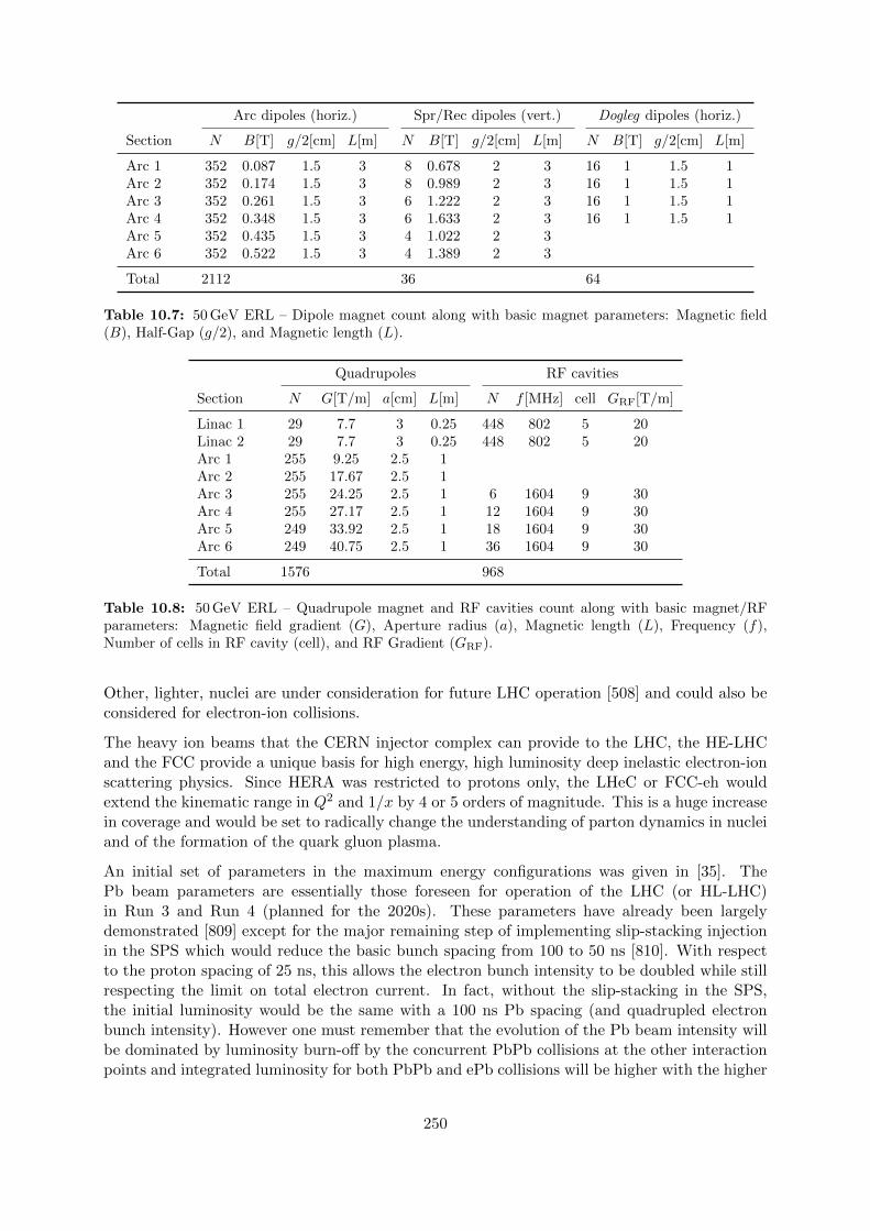
Arc dipoles (horiz.) Spr/Rec dipoles (vert.) Dogleg dipoles (horiz.)

Section N B[T] g/2[cm] L[m] N B[T] g/2[cm] L[m] N B[T] g/2[cm] L[m]

Arc 1 352 0.087 1.5 3 8 0.678 2 3 16 1 1.5 1Arc 2 352 0.174 1.5 3 8 0.989 2 3 16 1 1.5 1Arc 3 352 0.261 1.5 3 6 1.222 2 3 16 1 1.5 1Arc 4 352 0.348 1.5 3 6 1.633 2 3 16 1 1.5 1Arc 5 352 0.435 1.5 3 4 1.022 2 3Arc 6 352 0.522 1.5 3 4 1.389 2 3

Total 2112 36 64

Table 10.7: 50 GeV ERL – Dipole magnet count along with basic magnet parameters: Magnetic field(B), Half-Gap (g/2), and Magnetic length (L).

Quadrupoles RF cavities

Section N G[T/m] a[cm] L[m] N f [MHz] cell GRF[T/m]

Linac 1 29 7.7 3 0.25 448 802 5 20Linac 2 29 7.7 3 0.25 448 802 5 20Arc 1 255 9.25 2.5 1Arc 2 255 17.67 2.5 1Arc 3 255 24.25 2.5 1 6 1604 9 30Arc 4 255 27.17 2.5 1 12 1604 9 30Arc 5 249 33.92 2.5 1 18 1604 9 30Arc 6 249 40.75 2.5 1 36 1604 9 30

Total 1576 968

Table 10.8: 50 GeV ERL – Quadrupole magnet and RF cavities count along with basic magnet/RFparameters: Magnetic field gradient (G), Aperture radius (a), Magnetic length (L), Frequency (f),Number of cells in RF cavity (cell), and RF Gradient (GRF).

Other, lighter, nuclei are under consideration for future LHC operation [508] and could also beconsidered for electron-ion collisions.

The heavy ion beams that the CERN injector complex can provide to the LHC, the HE-LHCand the FCC provide a unique basis for high energy, high luminosity deep inelastic electron-ionscattering physics. Since HERA was restricted to protons only, the LHeC or FCC-eh wouldextend the kinematic range in Q2 and 1/x by 4 or 5 orders of magnitude. This is a huge increasein coverage and would be set to radically change the understanding of parton dynamics in nucleiand of the formation of the quark gluon plasma.

An initial set of parameters in the maximum energy configurations was given in [35]. ThePb beam parameters are essentially those foreseen for operation of the LHC (or HL-LHC)in Run 3 and Run 4 (planned for the 2020s). These parameters have already been largelydemonstrated [809] except for the major remaining step of implementing slip-stacking injectionin the SPS which would reduce the basic bunch spacing from 100 to 50 ns [810]. With respectto the proton spacing of 25 ns, this allows the electron bunch intensity to be doubled while stillrespecting the limit on total electron current. In fact, without the slip-stacking in the SPS,the initial luminosity would be the same with a 100 ns Pb spacing (and quadrupled electronbunch intensity). However one must remember that the evolution of the Pb beam intensity willbe dominated by luminosity burn-off by the concurrent PbPb collisions at the other interactionpoints and integrated luminosity for both PbPb and ePb collisions will be higher with the higher

250

total Pb intensity. The details of this will depend on the operating scenarios, number of activeexperiments, etc, and are not considered further here. The time-evolution of eA luminosity willbe determined by that of PbPb and pPb collisions, as discussed, for example, in Ref. [16,508,811].

Combining these assumptions with the default 50 GeV electron ERL for LHeC and 60 GeV forFCC-eh, yields the updated parameter sets and initial luminosities given in Tab. 2.4, earlier inthe present report.

Radiation damping of Pb beams in the hadron rings is about twice as fast as for protons and canbe fully exploited since it takes longer to approach the beam-beam limit at the PbPb collisionspoints. For the case of the FCC-hh [16], one can expect the emittance values in Tab. 2.4 to bereduced during fills [16, 508,811].

The Pb beam will be affected by ultraperipheral collision effects, mainly bound-free pair pro-duction and Coulomb dissociation of the nuclei, induced by the electromagnetic fields of theelectrons, seen as pulses of virtual photons. The relevant cross-sections will be similar to thosein pPb collisions which are down by a factor of Z2 compared to those in PbPb collisions andcan be neglected in practice.

10.4 Beam-Beam Interactions

In the framework of the Large Hadron electron Collider, the concept of an Energy RecirculatingLinac (ERL) allows to overcome the beam-beam limit that one would face in a storage ring. Theelectron beam can be heavily disturbed by the beam collision process, while the large acceptanceof the ERL will still allow for a successful energy recovery during the deceleration of the beamso that the power consumption is minimised. In order to compare the relevant beam-beamparameters and put them into the context of other colliders, two tables are shown highlighting,on the one hand, the parameters from LEP and LHC runs in Tab. 10.9, and on the other hand,the parameters planned for LHeC at HL-LHC in Tab. 10.10.

Parameter Unit LEP LHC

Beam sizes σx / σy µm 180 / 7 16.6 / 16.6Intensity 1011 particles/bunch 4.00 1.15Energy GeV 100 7000β∗x/β

∗y cm 125/5 55/55

Crossing angle µrad 0 0/285Beam-beam tune shift ∆Qx/∆Qy 0.0400/0.0400 0.0037/0.0034Beam-beam parameter ξ 0.0700 0.0037

Table 10.9: Comparison of parameters for the LEP collider and LHC. Taken from CDR 2012, p.286.

In the case of LHeC, the β-functions at the interaction point are chosen such that the transversebeam sizes of the e- and p- beams are equal in both transverse planes. Although the proton andelectron emittances are different, the beta functions at the interaction point are set accordinglyso that the two beams conserve σex = σpx and σey = σpy .

10.4.1 Effect on the electron beam

The disruption parameter for the electron beam is of the order of 14.5 which corresponds, inlinear approximation, to almost 2 oscillations of the beam envelope within the proton bunch.The non linearity of the interaction creates a distortion of the phase space and a mismatch from

251

Beam parameter Unit LHeC at HL-LHC

Proton beam Electron beam

Energy GeV 7000 49.19Normalized emittance mm·mrad 2.5 50Beam sizes σx,y µm 5.8 5.8Intensity 109 particles/bunch 220.00 3.1Bunch length σs mm 75.5 0.6β∗x,y cm 10.00 6.45Disruption factor 1.2× 10−5 14.5Beam-beam parameter ξ 1.52× 10−4 0.99

Table 10.10: Comparison of parameters for the LHeC at HL-LHC. The parameters presented correspondto the default design.

the design optics (see Fig. 10.12). The mismatch and distortion can be minimized by tuning theTwiss parameters (α∗, β∗) at the interaction point.

Figure 10.12: Left: Electron beam sizes with (blue) and without (black) the beam-beam forces exertedon the electron beam. The geometric emittance is represented in red and the effective emittance that takesinto account the mismatch from the original optics is illustrated in green. Right: The horizontal phasespace of the spent electron distribution backtracked to the interaction point. 3σ Gaussian distributionare highlighted for the post-collided distribution (solid line) and the design optics (dashed line).

In a series of studies the optics parameters of the electron beam were tracked back to theinteraction point in presence of the beam-beam forces in order to show the impact of the beam-beam effect for different values of the electron Twiss parameters at the IP. In addition, theinfluence of a waist shift from the IP (proportional to α∗), similar to changing the foci of theinteracting beams, has been studied and allows to keep the electron beam for a longer timewithin the proton bunch, thus optimizing the luminosity. The modification of the electronbeta function (β∗) leads to more freedom and gives access, among all the possibilities, to twodifferent optima regarding the luminosity and the mismatch from the design optics. The resultsare summarized in the contour plots of Fig. 10.13.

As a consequence, the Twiss parameters at the interaction point can be set in a way, to minimizethe mismatch of the optics (i.e. the effective emittance) or to maximize the luminosity. In casethe optimization of the luminosity is chosen (see the circle marker in Fig. 10.13), a modifiedcapture optics in the beam transfer to the arc structure will be needed to re-match the modifiedTwiss functions perturbed by the non-linear beam-beam effects.

252

Figure 10.13: Left : Contour plot describing the effective emittance post collision as a function of thealfa and beta functions at IP. Right : Contour plot describing the luminosity as a function of the alfaand beta functions at the IP. The diamond marker represents the initial Twiss parameters, the circleshows the luminosity optimum, the cross symbolizes the smallest mismatch from the original optics andthe star illustrates the minimal geometric emittance growth.

The effect of possible offsets between the two colliding beams has been characterized in previousbeam-beam studies [812], and – if uncorrected – might lead to an electron beam emittancegrowth. The parameters for these studies have been updated and the results are presented inFig. 10.14. As any offset between the two beams is amplified, it results in a larger increase of thebeam envelope. As a solution, a fast feed-forward system is proposed, across the Arc 6, whichwould aim at damping the transverse motion so that the beam emittance can be recovered.Using two sets of kickers placed at the center and at the end of the arc, an offset of 0.16σ can bedamped. A single set cutting across the whole arc can correct a 1σ offset with approximately4.4 kV.

Figure 10.14: Electron bean emittance relative change with respect to its centroid (blue) and withrespect to the vacuum chamber center (orange).

Additionally, the coupling of the beam-beam effect with long range wakefields has been ad-dressed [812]. Assuming a misaligned bunch injected among a train of nominal bunches, thecoupling of the beam-beam effect with the wakefields leads to a reduction of the damping ofthe excitation created by the misaligned bunch. Nevertheless it can be shown that the beamstability is conserved and the total amplification remains acceptable with respect to the studythat was not considering the coupling.

253

10.4.2 Effect on the proton beam

The beam-beam interaction between the electron and proton beams is asymmetric in terms ofbeam rigidities. Although the less energetic 49.19 GeV electron beam is heavily distorted by thestrong 7 TeV proton beam, the proton beam will suffer from an emittance growth adding upturn by turn [812] due to the build up of the tiny disruption created by the offset between thebeams. In fact, the previous studies gave a growth rate of around 0.01 %/s for a jitter of 0.2 σx.As long as an adequate control of the bunches is preserved, this effect should lie in the shadowof other effects leading to emittance blow-up in the LHC (e.g. IBS). Since the electron beamenergy decreased from 60 GeV to 49.19 GeV this study needs to be updated and the resultsshould remain in agreement with the previous statement.

10.5 Arc Magnets

In this section, a conceptual design of the main magnets needed for the Linac-Ring (LR) ac-celerator at 50 GeV is described. The number and types of magnets is listed in Tabs. 10.7and 10.8.

10.5.1 Dipole magnets

The bending magnets are used in the arcs of the recirculator. Each of the six arcs needs 352horizontal bending dipoles. Additional dipoles are needed in the straight sections: 36 verticalbending dipoles in the spreader/recombiner and 64 horizontal bending dipoles for the “dogleg”.These magnets are not considered at the moment.

In the CDR issued in 2012 for a 60 GeV lepton ring (LR) , a design based on three independentdipoles stacked on top of each other was proposed. A post-CDR design with three aperturesdipoles was introduced in 2014 [808]. This solution allows reducing the Ampere-turns and theproduction cost of the dipoles. For a 50 GeV LR, the three apertures dipole design is adaptedto fulfil new magnetic field requirements.

The 352 horizontal bending dipoles needed for each arc, combined in three apertures dipoles re-sult in a total of 704 units. These magnets are 3 m long and provide a field in the 30 mm apertureranging from 0.087 T to 0.522 T depending on the arc energy, from 8.62 GeV to 49.19 GeV.

In the proposed design, the three apertures are stacked vertically but offset transversely. Thisallows recycling the Ampere-turns from one aperture to the other. The coils are centrally locatedon the yoke and are made of simple aluminium bus-bars all powered in series. A current densityof 1 A/mm2 in the coils is sufficiently low to not have water-cooling but in order to limit thetemperature in the tunnel it may be required. Trim coils can be added on two of the aperturesto provide some tuning. Alternatively, each stage could be powered separately. The dipole yokesare made of low carbon steel plates. The relevant parameters are summarised in Tab. 10.11 andthe cross section is illustrated in Fig. 10.15 for 500 mm between consecutive arcs.

10.5.2 Quadrupole magnets

Quadrupoles for recirculator arcs

In total 1518 quadrupoles are needed for the recirculator arcs: 255 for each of the arcs one to fourand 249 for each of the arcs five and six. The required integrated gradients, comprised between9.25 T and 40.75 T, can be achieved using one type of quadrupole one meter long. However,instead of operating the magnets at low current for lower arcs energy, it can be considered to

254

Parameter Unit Value

Beam energy GeV 8.62 to 49.19Magnetic field T 0.087 to 0.522Magnetic length m 3Vertical aperture mm 30Pole width mm 90Number of apertures 3Distance between apertures mm 500Mass 8000 kgNumber of magnets 704Current A 4250Number of turns per magnet 4Current density A/mm2 1Conductor material aluminumMagnet resistance mΩ 0.17Power kW 3Total power consumption six arcs MW 2.1Cooling air

Table 10.11: 50 GeV ERL – Main parameters of the three apertures bending magnets.

Figure 10.15: 50 GeV ERL - Cross section of the three apertures bending magnet, arc 2, 4 and 6 with500 mm between consecutive arcs - Finite Element Method (FEM).

have a shorter model 0.6 meter long for arcs one to three. These quadrupoles require water-cooling for the coils. The relevant parameters are summarised in Tab. 10.12 and the cross sectionis illustrated in Fig. 10.16 (left).

In order to reduce the power consumption, it could be envisaged to use a hybrid configurationfor the quadrupoles, with most of the excitation given by permanent magnets. The gradientstrength could be varied by trim coils or by mechanical methods.

255

Parameter Unit Value

Beam energy GeV 8.62 to 49.19Field gradient T/m 9.25 to 40.75Magnetic length m 1Aperture radius mm 25Mass kg 550Number of magnets 1518Current at 40.75 T/m A 560Number of turns per pole 17Current density at 40.75 T/m A/mm2 6.7Conductor material copperMagnet resistance mΩ 33Power at 8.62 GeV kW 0.5Power at 16.73 GeV kW 1.9Power at 24.85 GeV kW 3.7Power at 32.96 GeV kW 4.6Power at 41.08 GeV kW 7.2Power at 49.19 GeV kW 10.3Total power consumption six arcs MW 7.1Cooling water

Table 10.12: 50 GeV ERL – Main parameters of the arc quadrupoles.

Figure 10.16: 50 GeV ERL. Left: Cross section of the arc quadrupole magnets. Right: Cross sectionof the linac quadrupole magnets.

Quadrupoles for the two 8.1 GeV linacs

In the two 8.1 GeV linacs, 29 + 29 quadrupoles, each providing 1.93 T integrated strength arerequired. The present design solution considers 30 mm aperture radius magnets. The relevantparameters are summarised in Tab. 10.13 and the cross section is illustrated in Fig. 10.16 (right).

256

Parameter Unit Value

Beam energy GeV 8.62 to 49.19Field gradient T/m 7.7Magnetic length m 0.25Aperture radius mm 30Mass kg 110Number of magnets 56Current at 7.7 T/m A 285Number of turns per pole 10Current density at 7.7 T/m A/mm2 3Conductor material copperMagnet resistance mΩ 6Power at 8.1 GeV kW 0.5Total power consumption 2 linacs MW 0.03Cooling water

Table 10.13: 50 GeV ERL – Main parameters of the linac quadrupoles.

10.6 LINAC and SRF

Each of the two main linacs has an overall length of 828.8 m and provides an acceleration of8.114 GV. Each linac consists of 112 cryomodules, arranged in 28 units of 4 cryomodules withtheir focussing elements – each cryomodule contains four 5-cell cavities, optimised to operate withlarge beam current (up to 120 mA at the High Order Mode – HOM – frequencies). The operatingtemperature is 2 K; the cavities are based on modern SRF technology and are fabricated frombulk Nb sheets; they are described in detail in section 10.6.2 below. The nominal accelerationgradient is 19.73 MV/m.

In addition to the main linacs, the synchrotron losses in the arcs will make additional linacsnecessary, referred to here as the loss compensation linacs. These will have to provide differentaccelerations in the different arcs, depending on the energy of the beams as shown in Tab. 10.14.The quoted beam energies are at entry into the arc. Their natural placement would be at theend of the arcs just before the combiner, where the different energy beams are still separate.The largest of these linacs would have to compensate the SR losses at the highest energy,requiring a total acceleration of about 700 MV. The loss compensation linacs will be detailed insection 10.6.6 below.

Section Beam energy [GeV] ∆E [MeV]

Arc 1 8.62 3Arc 2 16.73 25Arc 3 24.85 80Arc 4 32.96 229Arc 5 41.08 383Arc 6 49.19 836

Table 10.14: Synchroton radiation losses for the different arc energies

Through all arcs but Arc 6, the beam passes twice, once while accelerated and once while decel-erated. It is planned to operate these additional loss compensation linacs at 1603.2 MHz, whichallows energy compensation of both the accelerated and the decelerated beam simultaneously.This subject will be discussed in detail in a subsequent section 10.6.6.

257

10.6.1 Choice of Frequency

The RF frequency choice primarily takes into account the constraints of the LHC bunch repeti-tion frequency, f0, of 40.079 MHz, while allowing for a sufficiently high harmonic, h, for a flexiblesystem. For an ERL with npass = 3 recirculating passes and in order to enable equal bunchspacing for the 3 bunches – though not mandatory – it was originally considered to suppress allharmonics that are not a multiple of npass · f0 = 120.237 MHz. Initial choices for instance were721.42 MHz (h = 18) and 1322.61 MHz (h = 33) in consideration of the proximity to the frequen-cies used for state-of-the-art SRF system developments worldwide [813]. In synergy with otherRF system developments at CERN though, the final choice was 801.58 MHz (h = 20), wherethe bunching between the 3 recirculating bunches can be made similar but not exactly equal.Note that this frequency is also very close to the 805 MHz SRF proton cavities operating at theSpallation Neutron Source (SNS) at ORNL, so that one could leverage from the experience inregard to cryomodule and component design at this frequency.

Furthermore, in the frame of an independent study for a 1 GeV CW proton linac, a capitalplus operational cost optimisation was conducted [814]. This optimisation took into accountthe expenditures for cavities, cryomodules, the linac tunnel as well as the helium refrigeratorexpenses as a function of frequency and thus component sizes. Labor costs were included basedon the existing SNS linac facility work breakdown structure. It was shown that capital plusoperating costs could be minimised with a cavity frequency between 800 MHz and 850 MHz,depending also on the choice of the operating He bath temperature (1.8 K to 2.1 K). Clear benefitof operating in this frequency regime are the comparably small dynamic RF losses per installationlength due to a relatively small BCS surface resistance as well as low residual resistance ofthe niobium at the operating temperature. This could be principally verified as part of theprototyping effort detailed in the next sub-section. Note that the cost optimum also favorscavities operating at rather moderate field levels (< 20 MV/m). This comes as a benefit inconcern of field emission and associated potential performance degradations.

10.6.2 Cavity Prototype

Given the RF frequency of 801.58 MHz, JLab has collaborated with CERN, and consequentlyproposed a five-cell cavity design that was accepted for prototyping, see Fig. 10.17. The cavityshape has also been adopted for PERLE. Tab. 10.15 summarises the relevant cavity parameters.

Figure 10.17: Bare 802 MHz five-cell cavity design (RF vacuum) with a 130 mm iris and beam tubeaperture.

The cavity exhibits a rather large iris and beam tube aperture (130 mm) to consider beam-dynamical aspects such as HOM-driven multi-bunch instabilities. Despite the comparably largeaperture, the ratio of the peak surface electric field, Epk, respectively the peak surface magneticfield, Bpk, and the accelerating field, Eacc, are reasonably low, while the factor R/Q · G iskept reasonably high, concurrently to limit cryogenic losses. This is considered as a generically

258

Paramater Unit Value

Frequency MHz 801.58Number of cells 5active length lact mm 917.9loss factor V pC−1 2.742R/Q (linac convention) Ω 523.9R/Q ·G per cell Ω2 28788Cavity equator diameter mm 327.95Cavity iris diameter mm 130Beam tube inner diameter mm 130diameter ratio equator/iris 2.52Epeak/Eacc 2.26Bpeak/Eacc mT/(MV/m) 4.2cell-to-cell coupling factor kcc % 3.21TE11 cutoff frequency GHz 1.35TM01 cutoff frequency GHz 1.77

Table 10.15: Parameter table of the 802 MHz prototype five-cell cavity.

well balanced cavity design [815]. The cavity cell shape also avoids that crucial HOMs willcoincide with the main spectral lines (multiples of 801.58 MHz), while the specific HOM couplerdevelopment is pending.

Figure 10.18: Real monopole impedance spectrum of the five-cell 802 MHz cavity prototype (red)together with the considered beam current lines (green) for the 3-pass PERLE machine (25 mA injectedcurrent). The numbers associated with the spectral lines denote the power dissipation (in Watt).

Furthermore, as shown in Fig. 10.18 for the case of the bunch recombination pattern consideredfor PERLE originally, the much denser intermediate beam current lines (green) are not coincidingwith cavity HOMs. Here the figure plots the real part of the beam-excited cavity monopoleimpedance spectrum up to 6 GHz, and denotes the power deposited at each spectral line (inWatt) for an injected beam current of 25 mA. For instance, the summation of the power inthis spectral range results in a moderate 30 W. This covers the monopole modes with thehighest impedances residing below the beam tube cutoff frequency. The HOM-induced heat has

259

to be extracted from the cavity and shared among the HOM couplers attached to the cavitybeam tubes. The fraction of the power escaping through the beam tubes above cutoff can beintercepted by beam line absorbers.

Note that for Fig. 10.18 a single HOM-coupler end-group consisting of three scaled TESLA-type coaxial couplers was assumed to provide damping. Instead of coaxial couplers, waveguidecouplers could be utilized, which for instance have been developed at JLab in the past for highcurrent machines. These are naturally broadband and designed for high power capability, thoughsome penalty is introduced as this will increase the complexity of the cryomodule. Ultimately,the aim is to efficiently damp the most parasitic longitudinal and transverse modes (each polar-ization). The evaluation of the total power deposition is important for LHeC to decide whichHOM coupler technology is most appropriate to cope with the dissipated heat and whetheractive cooling of the couplers is a requirement.

Though the prototype efforts focused on the five-cell cavity development, JLab also producedsingle-cell cavities, i.e. one further Nb cavity and two OFE copper cavities. The former has beenshipped to FNAL for N-doping/infusion studies, whereas the latter were delivered to CERN forNb thin-film coating as a possible alternative to bulk Nb cavities. In addition, a copper cavitywas built for low power bench measurements, for which multiple half-cells can be mechanicallyclamped together. Presently, a mock-up can be created with up to two full cells. This cavityhas been produced in support of the pending HOM coupler development. The ensemble ofmanufactured cavities resonating at 802 MHz is shwon in Fig. 10.19.

Figure 10.19: Ensemble of 802 MHz cavities designed and built at JLab for CERN. The Nb cavitieshave been tested vertically at 2 Kelvin in JLab’s vertical test area.

Results for the Nb cavities - made from fine grain high-RRR Nb - were encouraging since bothcavities reached accelerating fields, Eacc, slightly above 30 MV/m ultimately limited by thermalbreakdown (quench). Moreover, the RF losses were rather small as a benefit of the relativelylow RF frequency as anticipated. The residual resistance extracted from the measurement dataupon cooldown of the cavity was 3.2 Ω ± 0.8 Ω. This resulted in unloaded quality factors,Q0, well above 4× 1010 at 2 K at low field levels, while Q0-values beyond 3× 1010 could bemaintained for the five-cell cavity up to ∼27 MV/m (see Fig. 10.20). Only standard interiorsurface post-processing methods were applied including bulk buffered chemical polishing, hightemperature vacuum annealing, light electropolishing, ultrapure high-pressure water rinsing,

260

and a low temperature bake-out. While the vertical test results indicate generous headroom fora potential performance reduction once a cavity is equipped with all the ancillary componentsand installed in a cryomodule, clean cavity assembly procedure protocols must be establishedfor the cryomodules to minimise the chance of introducing field-emitting particulates.

Figure 10.20: Vertical test result of the five-cell 802 MHz niobium cavity prototype.

10.6.3 Cavity-Cryomodule

The ERL cryomodules hosting the superconducting RF cavities are a key component of theaccelerator. They should provide the proper mechanical, vacuum and cryogenic environment tothe SRF cavities equipped with their ancillaries systems: helium tank, power coupler and HOMcouplers. Each cryomodule is containing 4 superconducting 801.58 MHz 5-cells elliptical cavitiesdescribed in the previous chapters.

Recently, several projects worldwide have designed cryomodules for elliptical cavities with acavity configuration (number, length and diameter) quite close to the one required by LHeCERL:

• SNS [816]: two different sized cryomodules host either 4 elliptical 6-cells 805 MHz cavitiesof β = 0.81 or 4 elliptical 6-cells 805 MHz of β = 0.61;

• SPL [817]: the cryomodule is designed to integrate 4 elliptical 5-cells 704 MHz cavities ofβ = 1;

• ESS [818]: two cryomodules of the same length can host either 4 elliptical 6-cells 704 MHzcavities of β = 0.67 or 4 elliptical 5-cells 704 MHz cavities of β = 0.85.

These three cryomodule designs are based on two completely different concepts for the cavitystring support structure. SNS and ESS cryomodules are based on an intermediate supportsystem, called the spaceframe, which is horizontally translated inside the cryomodule vacuumvessel. The low pressure cryogenic line is located above the cavities string and connected to thecryogenic transfer line by a double angled connection, the jumper. RF waveguides are connectedunderneath the cryomodule, using door-knob transition to the couplers. All the hanging andalignment operations of the cavities string and shielding are implemented outside the vacuumtank, using the spaceframe. In the ESS case, each cavity is hanged by 2 sets of 4 cross rods. The

261

thermal shield is also hanged to these rods by the mean of an aluminium “elastic boxes” thatallow the thermal shrinkage while maintaining the transverse stability. The thermal shield ismade of 2.5 mm thick aluminium and wrapped with multi-layer insulation. It is fastened directlyto the support rods of the cavities string.

Figure 10.21: SPL cryomodule general assembly view

In the SPL cryomodule, the cavity string is directly supported by the power coupler and withdedicated inter-cavity support features. Moreover, the SPL cryomodule integrates a full lengthdemountable top lid, enabling the cavity string assembly from the cryomodule top (Fig. 10.21).The thermal shield is made of rolled aluminium sheets, and is composed of four main partsassembled before the vertical insertion of the string of cavities. The shield, wrapped with multi-layer insulation, is suspended to the vacuum vessel via adjustable tie rods in titanium alloy whichalso cope, by angular movements, with its thermal contractions. The cavity stainless steel heliumtanks are connected by a 100-mm-diameter two-phase pipe placed above the cavities. This pipeensures liquid feeding to the cavities by gravity, and is also used as a pumping line for gaseoushelium.

Figure 10.22: Cross-view of the SPL cryomodule

With the aim of minimizing static heat loads from room temperature to 2 K by solid thermalconduction, the number of mechanical elements between the two extreme temperatures is re-duced to the strict minimum: the cavities are supported directly via the external conductor of

262

the RF coupler (Fig. 10.22), the double-walled tube (DWT). The latter is made out of a stain-less steel tube with an internal diameter of 100 mm, which is actively cooled by gaseous heliumcirculating inside a double-walled envelope in order to improve its thermal efficiency.

An additional supporting point to keep cavity straightness and alignment stability within re-quirements is obtained by supporting each cavity on the adjacent one via the inter-cavity support,which is composed of a stem sliding inside a spherical bearing. As a result, a pure vertical sup-porting force is exchanged by adjacent cavities whereas all other degrees of freedom remain unre-strained allowing thermal contraction movements to occur unhindered. The thermo-mechanicalbehaviour of this supporting system has been extensively studied on a dedicated test bench atCERN, proving its efficiency and reliability.

There are some specific additional constraints or requirements for a cryomodule to be used inan ERL, and some of them are quite challenging, The first set of constraints is linked to the CWoperation of the cryomodules (contrary to SNS, SPL and ESS which are pulsed accelerators),where dynamic heat loads are much larger than the static ones. Thus, reaching high Q0 (lowcryogenic losses) is a main objective in these machines and beside specific optimization on cavitydesign and preparation (such as N-doping), magnetic shielding should be carefully studied:material, operating temperature, numbers of layers, active and/or passive shielding. Anotherimportant constraint is linked to relative high power to be extracted by the HOM couplers:thermal analysis should be carefully performed to have an optimized evacuation of the HOMthermal load not to degrade the cryogenic performances of the cryomodule.

We recently decided to push further away the analysis to use the SPL cryomodule for the LHeCERL, thanks to its geometrical compatibility with the LHeC ERL superconducting cavities,but also because it fits quite well the overall ERL requirements. One of the clear advantagesof the SPL configuration is a much simplified assembly procedure (Fig. 10.23), with its top-lidconfiguration which also allows an easier maintenance.

Figure 10.23: Cryomodule assembly procedure main steps

The first study performed was to analyse the possibility to integrate the ERL cavities insteadof the SPL ones. The 802 MHz cavities are a little bit shorter than the SPL ones and the cellsare also smaller in diameter. The beam port internal diameter is about the same, as well asthe power coupler port. As a result, the SPL cryomodule is well fitted to the ERL 802 MHzsuperconducting cavities from the geometrical point of view, and they could be easily integratedproviding minor mechanical features adaptations.

The second analysed point is the beam vacuum. As the SPL cryomodule existing design wasdone for a prototype, intended for RF and cryogenic test only, without beam, the vacuum valveis a VAT CF63 “vatterfly” valve with viton seal and manual actuator, which is not adapted for areal operating cryomodule. Integration of an all-metal gate valve instead is not an issue and wealso designed a specific solution based on a two stages valves (Fig. 10.24) to adapt the already

263

fabricated SPL prototype cryomodule in order to be able to integrate the 802 MHz cavities.

Figure 10.24: The two stages vacuum valve solution for adapting the SPL cryomodule prototype to the802 MHz cavities of the LHeC ERL.

The third study performed is the compatibility of the SPL cryogenic features with the ERLrequirements. SPL was designed to operate 702 MHz cavities at 25 MV/m with a Q0 of 5× 109

with a 8.2 % duty cycle. The LHeC ERL will operate SRF cavities in CW regime, but at a lowerfield (20 MV/m) and with a higher expected Q0 at the nominal gradient (about 1.5 × 1010).As a result, and despite the different duty cycle, the dynamic cryogenic losses are estimated tobe only about 30 % more in the ERL case. The overall cryogenic dimensioning is then fullycompatible, providing some unavoidable adaptation of a few internal cryogenic piping. Themain issue still to address is the need and consequences of the HOM coupler cooling. Even ifthe present engineering analysis showed that this point will not be a showstopper, it might havean impact on some cryogenic piping and cooling circuit.

Detailed engineering studies are being pursued to transform the SPL cryomodule prototype intoan ERL LHeC cryomodule prototype. We are taking benefit of all the design and fabricationwork previously performed on the SPL, and also on the fact some parts, such as the thermal andmagnetic shielding, are not yet fabricated and could be exactly adapted to the ERL requirements.This will give the possibility to have an earlier full prototype cryomodule RF and cryogenic test ascompared to a standard experimental plan where the complete study and fabrication is startingfrom scratch.

10.6.4 Electron sources and injectors

Specification of electron sources

Operation of the LHeC with an electron beam, delivered by a full energy ERL imposes specificrequirements on the electron source. It should deliver a beam with the charge and temporalstructure required at the Interaction Point. Additionally as during acceleration in a high energyERL both longitudinal and transverse emittances of the beam are increased due to SynchrotronRadiation (SR), the 6D emittance of the beam delivered by electron source should be smallenough to mitigate this effect. The general specification of the electron source are shown inTab. 10.16. Some parameters in this table such as RMS bunch length, uncorrelated energyspread and normalised transverse emittance are given on the basis of the requirements for the

264

acceleration in ERL and to pre-compensate the effects of SR. The most difficult of the parametersto specify is injector energy. It should be as low as possible to reduce the unrecoverable powerused to accelerate the beam before injection into the ERL while still being high enough to delivershort electron bunches with high peak current. Another constraint on the injection energy isthe average energy and energy spread of the returned beam. The average energy cannot beless than the energy of electron source, but the maximum energy in the spectrum should notexceed 10 MeV the neutron activation threshold. An injection energy of 7 MeV is a reasonablecompromise to meet this constraint.

Parameter Unit Value

Booster energy MeV 7*Bunch repetition rate MHz 40.1Average beam current mA 20Bunch charge pC 500RMS bunch length mm 3Normalised transverse emittance π·mm·mrad <6Uncorrelated energy spread keV 10Beam polarisation Unpolarised/Polarised

Table 10.16: General specification of the LHeC ERL electron source.

The required temporal structure of the beam and the stringent requirements for beam emittancedo not allow the use of conventional thermionic electron sources for the LHeC ERL without usinga bunching process involving beam losses. While this option cannot completely be excluded as asource of unpolarised electrons. The additional requirement to deliver polarised beam can onlybe met with photoemission based electron sources.

There are now four possible designs of electron sources for delivering unpolarised beams and(potentially) three for delivering polarised beams:

1. A thermionic electron source with RF modulated grid or gate electrode with following(multi)stage compression and acceleration. The electron source could be either a DCelectron gun or an RF electron source in this case. Although these sources are widely usedin the injectors of Infra-Red FELs [819] their emittance is not good enough to meet thespecification of the LHeC injector. Moreover, thermionic sources cannot deliver polarisedelectrons.

2. A VHF photoemission source. This is a type of normal conducting RF source whichoperates in the frequency range 160 MHz – 200 MHz. The relatively low frequency of thesesources means that they are large enough that sufficient cooling should be provided topermit CW operation. This type of source has been developed for the new generationof CW FELs such as LCLS-II [820], SHINE [821] and a back-up option of the EuropeanXFEL upgrade [822], but they have not yet demonstrated the average current requiredfor the LHeC injector. The possibility of generating polarised electrons with this type ofsource has not investigated yet.

3. A superconducting RF photoemission source. This type of sources are under developmentfor different applications such as CW FEL’s (ELBE FEL [823], SRF option of LCLS-IIinjector [824], European XFEL upgrade [825]), as a basis of injectors for ERL’s (bERLin-Pro [826]) and for electron cooling (BNL [827]). Though this type of sources has alreadydemonstrated the possibility of delivering the average current, required for the LHeC withunpolarised beams (BNL), and has the potential for operation with GaAs type photocath-

265

odes (HZDR) which are required for delivery of polarised beams, the current technologyof SRF photoelectron source cannot be considered as mature enough for use in the LHeC.

4. A DC photoemission source. In this type of source the electrons are accelerated imme-diately after emission by a potential difference between the source cathode and anode.This type of source is the most common for use in ERL injectors. It has been used in theprojects which are already completed (JLAB [828], DL [829]), is being used for ongoingprojects (KEK [830], Cornell/CBeta [831]) and is planned to be used in new projects suchas the LHeC prototype PERLE [832]. The technology of DC photoemission sources iswell-developed and has demonstrated the average current and beam emittance requiredfor the LHeC ERL (Cornell). Another advantage of the photoelectron source with DCacceleration is the possibility of operation with GaAs based photocathodes for deliver-ing of polarised beam. Currently it’s the only source, which can deliver highly polarisedelectron beams with the current of several mA’s which is already in the range of LHeCspecifications (JLab [833]).

Based on this analysis at CDR stage we consider the use of DC photoemission source as a basicoption, keeping in mind that in the course of the injector development other types of electronsources may be considered, especially for providing of unpolarised beam.

The LHeC unpolarised injector

The injector layout follows the scheme depicted in Fig. 10.25. Its design will be similar to the

Figure 10.25: The layout of the unpolarised injector.

unpolarised variant of the PERLE injector [832]. The electron source with DC accelerationdelivers a CW beam with the required bunch charge and temporal structure. Immediatelyafter the source is a focusing and bunching section consisting of two solenoids with a normalconducting buncher placed between them. The solenoids have two purposes. Firstly to controlthe transverse size of the space charge dominated beam which will otherwise rapidly expandtransversely. This ensures that the beam will fit through all of the apertures in the injectorbeamline. Secondly the solenoids are used for emittance compensation to counter the spacecharge induced growth in the projected emittance. This is then followed by a superconductingbooster linac. This accelerates the beam up to its injection energy, provides further longitudinalbunch compression and continues the emittance compensation process.

The DC electron source will have an accelerating voltage of 350 kV using a high quantum ef-ficiency antimonide based photocathode such as Cs2KSb. The photoinjector laser required forthis cathode type will be a 532 nm green laser. There will be a load lock system to allow pho-tocathodes to be replaced without breaking the source vacuum. This significantly reduces the

266

down time required for each replacement which is a major advantage in a user facility such asthe LHeC where maximising uptime is very important. The cathode electrode will be mountedfrom above similar to the Cornell [834] and KEK [835] sources. This electrode geometry makesthe addition of a photocathode exchange mechanism much easier as the photocathode can beexchanged through the back of the cathode electrode. In addition the cathode electrode will beshaped to provide beam focusing. The operational voltage of 350 kV for the source was chosenas practical estimate of what is achievable. A higher voltage would produce better performancebut would be challenging to achieve in practice. The highest operational voltage successfullyachieved is 500 kV by the DC electron source that is used for the cERL injector [836]. However350 kV is sufficient to achieve the required beam quality [832].

Polarised electron source for ERL

Providing polarised electrons has always been a challenging process, especially at relatively highaverage current as required for the LHeC. The only practically usable production mechanismof polarised electrons is the illumination of activated to Negative Electron Affinity (NEA) stateGaAs based photocathodes with circularly polarised laser light. The vacuum requirements forthese cathodes mean that this must be done in a DC electron source only. In the course of thelast 30 years significant progress has been achieved in improving the performance of polarisedelectron sources. The maximum achievable polarisation has reached 90 % and the maximumQuantum Efficiency (QE) of the photocathode at the laser wavelength of maximum polarisationhas reached 6 %. Meanwhile the implementation of a polarised electron source into the LHeCremains a challenge as the practical operational charge lifetime of the GaAs based photocathodedoes not exceed hundreds Coulombs (JLAB [837]) at an operational current in mA range.

In Fig. 10.26 a preliminary design of the LHeC polarised injector is shown. In general, the design

Figure 10.26: The layout of the polarised injector.

of the polarised electrons injector is close to that of the unpolarised injector and is based on aDC electron source where a photocathode is illuminated by a pulsed laser beam. The choice of aDC source is dictated by the necessity of achieving extra high vacuum, with a pressure at a levelof 10−12 mbar, in the photocathode area. This level of vacuum is neccesary for providing longlifetime of the photocathode. In order to reduce photocathode degradation caused by electronstimulated gas desorption, the accelerating voltage in the source is reduced to 220 kV. The maindifferences with unpolarised injector are the presence of a photocathode preparation system,permanently attached to the source, and a Wien filter based spin manipulator between the sourceand the buncher. In order to reduce depolarisation of the beam in the spin manipulator, causedby the space charge induced energy spread of the beam, an RF dechirper is installed between

267

the source and the spin manipulator. The injector is also equipped with a Mott polarimeter tocharacterise the polarisation of the beam delivered by the source.

An important consideration of the operation with interchangeable photocathodes is minimisationof the down time required for the photocathode exchange. It typically takes few hours to replacethe photocathode and to characterise polarisation of the beam. For large facility like LHeC thisis unacceptable. A practical solution could be operation with 2 or more electron sources whichoperate in rotation similar to the way which was proposed at BNL [838]. Another motivationfor using multi-source injector is the nonlinear dependence of photocathode charge lifetime onaverage beam current (JLAB [833]), which reduces with increasing of the average current. Forexample in case of 3 electron sources 2 of them can be operated with half operation frequency20.05 MHz in opposite phase delivering average current of 10 mA each, while the third is in standby regime with freshly activated photocathode. The only time which is necessary to switch iton is the time required for rising the high voltage. Another advantage of using a multi-sourcescheme is the reduction of the average laser power deposited on the photocathode and as resultrelaxing requirements for the photocathode cooling. In order to implement the multi-sourcepolarised electron injector, development of a deflection system which is able to merge the beamsfrom different sources before the spin rotator is required.

Lasers for electron sources

In the proposed design of the LHeC injection system at least 2 lasers must be used. In theunpolarised electron injector, which is going to operate with antimionide-based photocathode,a laser with a wavelength of 532 nm is required. Typical initial QE of these photocathodes is10% and for practical application reduction of QE up to 1 % may be expected. For polarisedelectron source typical QE varies from 1 % down to 0.1 % and laser with a wavelength of 780 nmis required. The optimised parameters of the required lasers are summarised in Tab. 10.17. Lasertemporal profile and spot size on the photocathode are given on the basis of source optimisationfor operation at 350 kV for unpolarised regime and 220 kV for polarised.

Laser beam parameter Unit Unpolarised Polarisedmode mode

Laser wavelength nm 532 780Laser pulse repetition rate MHz 40.1 40.1Energy in the single pulse at photocathode QE=1 % µJ 0.12Average laser power at photocathode QE=1 % W 4.7*Energy in the single pulse at photocathode QE=0.1 % µJ 0.79Average laser power at photocathode Qe=0.1 % W 32*Laser pulse duration ps FWHM 118 80Laser pulse rise time ps 3.2 3.2Laser pulse fall time ps 3.2 3.2Spot diameter on the photocathode surface mm 6.4 8Laser spot shape on the photocathode surface Flat top

Table 10.17: Parameters of the electron source drive laser.

10.6.5 Positrons

Physics and Intensity Considerations

Variation of the beam conditions (energies, lepton charge and polarisation, hadron types) pro-vides a considerable extension of the physics programme of the LHeC. The LHC permits a

268

variation of the proton beam energy between about 1 and 7 TeV. It is a proton collider withoptions for heavy ions, primarily Pb and possibly lighter ones. The electron beam energy maybe varied between about 10 and the maximum of 50 (or eventually 60) GeV. Highly intensepolarised electron beam sources are under development which shall allow detailed investigationsof weak interactions and searches for new physics to be performed through variations of theelectron beam helicity, P. It is an advantage of the linac to achieve very high values of P, as com-pared to a ring electron accelerator where the polarisation build up due to the Sokolov-Ternoveffect [839] runs into serious difficulties at higher energies. The electron beam polarisation atHERA was limited to about 40 %. Positrons are the genuine challenge for the LHeC and as wellfor future e+e− linear colliders. The reason is the difficulty to generate intense beams as wasdiscussed for the LHeC in quite some detail already in the 2012 CDR [1].

The physics reasons for positrons at the LHeC are somehow obvious: positrons permit to es-tablish, exploit and question the existence of charge symmetry which may lead to discovery.For example, the charm tagging process in electron initiated charged current scattering mea-sures the anti-strange quark density xs(x,Q2) in the proton. There are expectations that thedifference x(s − s) may be different from zero, i.e. that there existed a strange-quark valencecomponent. That requires a precision measurement of also xs(x,Q2) for which one needs about1 fb−1 of integrated e+p luminosity, desirably of course more. Further reasons, presented inthe CDR [1] regard the nature of excited leptons, the origin of contact interactions, the spec-troscopy of lepto-quarks, the understanding of DIS, as for the measurement of FL where thesignal is charge sensitive but background at high inelasticity dominantly charge symmetric, thethorough resolution of the parton contents of hadrons etc. Thus, yes, one has many reasons tooperate LHeC as a positron-hadron collider also.

However, from today’s perspective, one has to be realistic in one’s assumptions about whatintensity may be realistically achievable and required in the positron linac - proton ring config-uration. The current luminosity goal of the LHeC had been set with the observation that theHiggs production cross section in ep is about 200 fb, comparable to that of the e+e− colliders,and the LHeC could become a Higgs factory [840]. Higgs production at the LHeC is dominantlydue to e−p→ νHX scattering, i.e. the LHeC has a competitive Higgs physics potential which iscomplementary to e+e− and pp as the dominant production mechanisms are WW −H, Z∗−HZand gg −H, respectively. The electron-proton CC Higgs cross section is much larger than theone in positron-proton scattering which is related to the dominance of up quarks as comparedto down quarks in the proton. Much of the running optimisation used in this paper has targetedto maximise the number of Higgs events and preferred electron over positron operation.

The target electron current to achieve 1034 cm−2s−1 luminosity has been set to 20 mA. Thisorigins from a 500 pC gun which for 40 MHz LHC operation frequency leads to a charge of 3 ·109

electrons per bunch corresponding to 1.2 ·1017 e−/s. Given the current and near future status ofpositron intensity requirements, one may set an LHeC target of order 1015−16 e+/s. Note thatthe normalised transverse emittance of of the electron beam is 50 mm mrad and the longitudinalemittance 5 MeV mm.

The intensity above would potentially provide a luminosity of order of 1−10 fb−1 within one year.With a drastic difference in the electron and positron intensities, later operation would favoure−p over e+p running to maximise the statistics. We thus assumed e+p would operate for aboutone year, somehow comparable to the heavy ion operation of the LHC. In the physics studies,as on PDF and electroweak measurements, we have used values of integrated e+p luminositiescorresponding to these assumptions. It was also assumed the positrons were not polarised. Thelinac-ring ep configuration thus has a highly polarised, intense electron beam and a less intense

269

unpolarised positron beam. The ring-ring configuration, a still possible back-up for the LHeCat HE-LHC, has intense electron and positron beams but with rather lower polarisations.

Positron Sources

One can compare the LHeC e+ intensity target with the goals for CLIC and ILC as listed inTab. 10.18. One finds that the chosen LHeC value is more demanding than that of CLIC andILC. Recently the interest in very intense e+ production has been renewed with the revival of the

Parameter CLIC ILC LHeC

Energy [GeV] 1500 250 50e+/bunch [109] 3.7 20 2Norm. emittance [mm.mrad] 0.66 (H) 10 (H) 50

0.02 (V) 0.04 (V) 50Norm. emittance [eV.m] 5000 60000 5000Repetition rate [Hz] 50 10 CWBunches / s 15600 26250 2 · 107

e+ flux [1015 e+/s] 0.1 0.4 1-10

Table 10.18: Characteristics of positron beams for CLIC, ILC and LHeC. Note that the muon collidertarget value in the LEMMA scheme is about 4 · 1016 e+/s.

muon collider studies and the so-called LEMMA proposal [841] to generate muons from e+e−

pairs, i.e. not from pion decays to achieve small emittance beams. This requires to generate anintense, 45 GeV energy positron beam annihilating with electrons from a target for muon pairproduction near threshold. In a study following the LEMMA idea, a target positron intensityof 3.9 1016 e+/s was set [842] which requires considerable R+D efforts.

A conventional positron source uses only a single amorphous target. An electron beam hits thetarget where Bremstrahlung and pair-production take place. Downstream the target, particulardevices (Quarter Wave Transformer QWT or Adiabatic Matching Device AMD) allow capturingas many positrons as possible, with a large emittance. The CLIC e+ source [843] takes advantageof a hybrid target design. A thin crystal target allows reducing the peak power deposition andenhances photon production via a channelling process. An amorphous target converting thephotons into positrons follows it. In between, a magnet sweeps out charged particles.

The ILC e+ source [844] takes advantage of a long helical undulator using the high-energyelectron beam of the collider. The electron beam passing through the undulator producespolarised photons by impinging on a moving target the design of which is still to be finalised.This target converts photons into positrons. The ILC-type positron source is not an option forthe LHeC since it requires an electron beam energy above 100 GeV

One option considered for the initial LHeC e+ source [1] was using ten hybrid targets in parallel.Bunch intensity and density could be enhanced by a tri-ring transformer system converting fromCW to pulsed mode for accumulation, and again back to CW.

To evaluate the performance of e+ sources, one defines a positron yield parameter. This pa-rameter is the number of positrons, at a given place along the production channel, per electronimpinging onto the target. It is crucial to improve the positron yield while keeping the peakenergy density deposition PEDD and the shockwave inside the target within acceptable limits.The target lifetime suffers from the cyclic thermal loads and stresses due to the beam pulses.The evacuation of the average power (kW to MW) from the target is challenging and shouldbe investigated for the reliability of the target. Heat dissipation in the amorphous target may

270

be improved by replacing it with a granular target (experiment at KEK). The capture and ac-celerating sections should also be optimised. Peak magnetic field and its shape, aperture andaccelerating gradient of the RF structures are important parameters. Given the large emit-tance of the e+ beam, a damping ring is mandatory. Due to the high requested e+ flux, anaccumulation process should be considered. The e+ flux is

dN+

dt= a · y ·N− · f , (10.8)

where a is the accumulation efficiency and is a function of the damping time, y is the yield asdefined above depending on the electron beam energy E−, further N− is the number of electronimpinging on the target, and f the linac repetition rate. This accumulation could be realisedby means of a tri-ring system as presented in the CDR.

Approaches towards LHeC Positrons

It is to be mentioned that positrons have not been in the focus of our recent LHeC design activitysuch that basic discussions as presented in the CDR [1] still hold.

The CLIC positron source was studied in great detail and many pertinent simulations were per-formed. Based on the expected flux of the CLIC e+ source, we have identified three possibilitiesfor the LHeC:

• Option 1: Keep the CW mode and the bunch spacing of 25 ns. This implies a bunchcharge of 2.5× 106 e+/bunch and a current of 16µA;

• Option 2: Keep the CW mode with a bunch charge of 2.5× 109 e+/bunch. This implies abunch spacing of 25µs and a current of 16µA;

• Option 3: Keep the bunch spacing of 25 ns with a bunch charge of 1× 109 e+/bunch. Thisimplies a pulsed mode with a repetition rate of 50 Hz. The beam current is now 6.4 mA.

The CLIC source, however, just provides O(1014) e+/s which would provide maximally 100 pb−1

ep luminosity in an efficient year.

One notes that the ILC luminosity upgrade foresees a positron rate up to eight times higher thanthe CLIC rate. A recent ILC status report cites novel concepts for high intense and polarisedpositron beams, obtained in an electron beam driven configuration [845].

Two alternative options, not yet studied in greater detail, promise to deliver a still much higherpositron rate, indeed close to that of the electrons, providing 1000 times more positron persecond than a CLIC-based source: One possibly may i) convert high-energy photons from theLHC-based gamma factory [846] for producing a positron rate of up to 1017 e+/s [847] or ii)using the photons from an LHeC based FEL [848] to generate a similarly high rate of positrons,which in both cases would already be at the correct bunch spacing. These two options rely oneither the LHC hadron or the LHeC lepton-beam infrastructure, and thus do not need other,possibly additional investments.

Depending on how challenging the parameter requirements are, a more or less radical changeof paradigm is necessary. There is no easy path even to 1014 e+/s. As to LHeC, it may profitfrom recent and forthcoming developments for lepton colliders for which higher intense positronsources and beams are a matter of existence. When approved, however, serious R+D effortswill be inevitable also for LHeC, and later FCC-he, for which positron beams may even be moreimportant, if, for example, lepto-quarks or SUSY particles in the few TeV range were found andto be examined in e±p scattering at the FCC.

271

10.6.6 Compensation of Synchrotron Radiation Losses

Depending on energy, each arc exhibits fractional energy loss due to the synchrotron radiation,which scales as γ4/ρ (see Eq. (10.5)). Arc-by-arc energy loss was previously summarised inTab. 10.14. That energy loss has to be replenished back to the beam, so that at the entrance ofeach arc the accelerated and decelerated beams have the same energy, unless separate arcs areused for the accelerated and decelerated beams. Before or after each arc, a matching sectionadjusts the optics from and to the linac. Adjacent to these, additional cells are placed, hostingthe RF compensating sections. The compensation makes use of a second harmonic RF at1603.2 MHz to replenish the energy loss for both the accelerated and the decelerated beams,therefore allowing them to have the same energy at the entrance of each arc, as shown inFig. 10.27.

Figure 10.27: The second-harmonic RF restores the energy loss in both the accelerating and deceleratingpasses.

Parameters of the RF compensation cryomodules, shown in Table 10.19, have been extrapolatedfrom the ILC cavity design, expecting that the higher frequency and lower gradient wouldsupport continuous operation.

Parameter Unit Value

Frequency MHz 1603.2Gradient MV/m 30Design Nine cellsCells length mm 841Structure length m 1Cavity per cryomodule 6Cryomodule length m 6Cryomodule voltage MV 150

Table 10.19: A tentative list of parameter for the compensating RF cryomodules extrapolated from theILC design.

As illustrated schematically in Fig. 10.27, there are two beams in each arcs (with exceptionof Arc 6) one needs to replenish energy loss for: the accelerated and the decelerated beams.Assuming nominal beam current of 20 mA, the net current for two beams doubles. Therefore,40 mA current in Arcs 1-5, was used to evaluated power required to compensate energy loss by2-nd harmonic RF system, as summarized in Table 10.20.

The compensating cryomodules are placed into Linac 1 side of the racetrack, before the bendingsection of Arc 1, Arc 3, and Arc 5 and after the bending section of Arc 2, Arc 4, and Arc 6.

272

Section ∆E [MeV] P [MW] Cryomodules

Arc 1 3 0.12 0Arc 2 25 1.0 0Arc 3 80 3.2 1Arc 4 229 9.16 2Arc 5 383 15.32 3Arc 6 836 16.7 6

Table 10.20: Arc-by-arc synchrotron radiated power for both the accelerated and decelerated beams(only one beam in Arc 6) along with a number of 2-nd harmonic RF cryomodules required to compensateenergy loss.

This saves space on Linac 2 side to better fit the IP line and the bypasses. Note that with thecurrent vertical separation of 0.5 m it will not be possible to stack the cryomodules on top ofeach other; therefore, they will occupy 36 m on the Arc 4 and Arc 6 side and 18 m on the Arc 3and Arc 5 side of the racetrack. Each of the compensating cavities in Arc 5 needs to transferup to 1 MW to the beam. Although a 1 MW continuous wave klystron are available [849], thecryomodule integration and protection system will require a careful design. Tab. 10.20 shows theenergy loss for each arc and the corresponding synchrotron radiated power, along with numberof cryomodules at 1603.2 MHz RF frequency required to replenish the energy loss.

10.6.7 LINAC Configuration and Infrastructure

Since the power supplied to the beam in the main linacs will be recovered, the average RF powerrequirements at 802 MHz are relatively small and determined by the needs to handle transientsand microphonics.

The RF power required for the second-harmonic RF system however is substantial – it can beestimated from Tab. 10.14 with the nominal current of 20 mA. Tab. 10.20 above summarizesthe estimated power lost in each arc depending on beam energy; these power values must besupplied by the 6 2-nd harmonic RF systems.

The RF infrastructure required at 802 MHz

10.7 Interaction Region

The design of the LHeC Interaction region has been revised with respect to the LHeC CDR totake into account the reduction of the electron energy from 60 GeV to 50 GeV and the latestdesign of the HL-LHC optics and it has been optimized to minimize synchrotron radiation powerand critical energy at the IP.

10.7.1 Layout

The basic principle of the Linac-Ring IR design remains unchanged and it is shown in Fig. 10.28:the two proton beams are brought onto intersecting orbits by strong separation and recombina-tion dipoles. A collision of the proton beams at the IP is avoided by selecting appropriately itslocation, i.e. by displacing it longitudinally with respect to the point where the two counter-rotating proton beams would collide. The large crossing angle keeps the long range beam-beameffect small and separates the beams enough to allow septum quadrupoles to focus only thecolliding beam (the anti-clockwise rotating LHC beam – Beam 2). The non-colliding beam (theclockwise rotating LHC beam – Beam 1) is unfocused and passes the septum quadrupoles in a

273

Magnet Gradient [T/m] Length [m] Free aperture radius [mm]

Q1A 252 3.5 20Q1B 164 3.0 32Q2 type 186 3.7 40Q3 type 175 3.5 45

Table 10.21: Parameters of the final focus quadrupole septa. The parameters of Q1A/B and Q2 arecompatible with the Nb3Sn based designs from [851] assuming the inner protective layer of Q2 can bereduced to 5 mm thickness.

field free aperture. The electron beam is brought in with an even larger angle, partly sharingthe field free aperture of the septum quadrupoles with the non-colliding beam. A weak dipolein the detector region bends the electron beam into head-on collisions with the colliding protonbeam. The two proton beams are also exposed to the dipole field but, due to the large beamrigidity, they are barely affected. After the interaction point a dipole with opposite polarityseparates the orbits of the electron and proton beam.

−150 −100 −50 0 50 100 150

Distance from IP s [m]

−0.3

−0.2

−0.1

0.0

0.1

0.2

0.3

x[m

] p+-Beam 1

p+-Beam 2

e−-Beam

Figure 10.28: Geometry of the interaction region with 10σ envelopes. The electron beam is collidingwith the focussed anti-clockwise rotating LHC beam (Beam 2) while the clockwise rotating LHC beamis unfocussed and passes the Interaction Region without interacting with the other two beams

The high electron current (cf. Tab. 10.1) required to approach the goal peak luminosity of1034cm−2s−1 poses a potential problem for the interaction region (IR) as it increases the alreadyhigh synchrotron radiation.

The ERL parameters are not the only major change the new IR design has to account for.The first design of the quadrupole septa featured a separation of 68 mm for the two protonbeams. However, this design focused strongly on providing a field free region for the non-colliding beam. Unfortunately, this lead to a poor field quality for the strongly focused collidingbeam. The first quadrupole Q1 was a half quadrupole design effectively acting as a combinedfunction magnet with a dipole component of 4.45 T [850]. The sextupole field component wasalso prohibitively high. Consequently, a new design approach focusing on the field quality in thequadrupole aperture was necessary. The parameters relevant for the interaction region designare summarised in Tab. 10.21.

274

Magnet Field strength [T] Interbeam distance [mm] Length [m] Number

D1 5.6 ≥ 496 mm 9.45 6D2 4.0 ≥ 194 mm 9.45 4IP Dipole 0.21 - 10 -

Table 10.22: Parameters of the separation and recombination dipoles. The respective interbeam dis-tances are given for the magnet with the lowest value.

It is noteworthy that the minimum separation of the two beams at the entrance of the firstquadrupole Q1A increased from 68 mm to 106 mm requiring a stronger bending of the electronbeam. This would increase the already high synchrotron radiation in the detector region evenmore. In order to compensate this increase, it was decided to increase L∗ (i.e. the distance fromthe IP to the first superconducting septum quadrupole focussing Beam 2) to 15 m, an approachthat was shown to have a strong leverage on the emitted power [852].

The increased separation of the two proton beams, the longer L∗ and the overall longer finalfocus triplet make longer and stronger separation and recombination dipoles necessary. Thedipoles differ from the arc dipoles in that the magnetic field in both apertures has the samedirection. Consequently the cross talk between both apertures is significant and the maximumreachable field is lower. The new geometry keeps the required field below 5.6 T. The requiredlengths and strength of these dipoles are listed in Tab. 10.22. It should be noted that the inter–beam distance is different for each of the five magnets per side, so each magnet will likely requirean individual design. The design of the D1 dipoles is further complicated by the fact that anescape line for neutral collision debris traveling down the beam pipe will be necessary [1], as wellas a small angle electron tagger. These issues have not been addressed so far, further studieswill require detailed dipole designs.

The first design of the LHeC interaction region featured detector dipoles occupying almost theentire drift space between the interaction point and first quadrupole. The approach was to havethe softest synchrotron radiation possible to minimise the power. However, since the purposeof the dipoles is to create a spacial separation at the entrance of the first quadrupole, it ispossible to make use of a short drift between dipole and quadrupole to increase the separationwithout increasing the synchrotron radiation power. A dipole length of 2

3L∗ is the optimum in

terms of synchrotron radiation power [853]. Compared to the full length dipole it reduces thepower by 15.6 % at the cost of a 12.5 % higher critical energy. With an L∗ of 15 m the optimumlength of the detector dipoles is 10 m. A magnetic field of 0.21 T is sufficient to separate theelectron and proton beams by 106 mm at the entrance of the first quadrupole. With thesedipoles and an electron beam current of 20 mA at 49.19 GeV the total synchrotron radiationpower is 38 kW with a critical energy of 283 keV to be compared with a power of 83 kW and acritical energy of 513 keV for the electron beam energy of 60 GeV. More detailed studies on thesynchrotron radiation for different options and including a beam envelope for the electron beamare summarised in Tab. 10.25 below.

A schematic layout of the LHeC interaction region with the dipoles discussed above is shown inFig. 10.29. The corresponding beam optics will be discussed in the following sections.

10.7.2 Proton Optics

As discussed above, the L∗ was increased to 15 m in order to compensate the increased syn-chrotron radiation due to the larger separation. The final focus system is a triplet consistingof the quadrupoles Q1A and Q1B (see Tab. 10.21), three elements of the Q2 type and two of

275

−100 −75 −50 −25 0 25 50 75 100

Distance from IP s [m]

−0.3

−0.2

−0.1

0.0

0.1

0.2

0.3

x[m

]

p+-Beam 1 (12.3 σ)

p+-Beam 2 (12.3 σ)

e−-Beam (5.0-10.0 σ)

γ

106 mm

190 mm

310 mm

Figure 10.29: Schematic layout of the LHeC interaction region. The colliding proton beam and theelectron beam are shown at collision energy while the non-colliding beam is shown at injection energywhen its emittance is the largest.

the Q3 type. Between the elements a drift space of 0.5 m was left to account for the magnetinterconnects in a single cryostat. Between Q1 and Q2 as well as Q2 and Q3 a longer drift of5 m is left for cold-warm transitions, Beam Position Monitors (BPMs) and vacuum equipment.Behind Q3, but before the first element of the recombination dipole D1, another 16 m of driftspace are left to allow for the installation of non-linear correctors in case the need arises, as wellas a local protection of the triplet magnets from asynchronous beam dumps caused by failuresof the beam dump kickers (MKD) as discussed below.

As the recombination dipoles D1 and D2 for the LHeC interaction region require more spacethan the current ALICE interaction region, the quadrupoles Q4 and Q5 had to be moved furtheraway from the IP. The position of Q6 is mostly unchanged but due to a need for more focusingthe length was increased by replacing it with two elements of the MQM magnet class of LHC.

With the triplet quadrupole parameters provided in Tab. 10.21 we were able to match optics witha minimum β∗ of 10 cm. The corresponding optics are shown in Fig. 10.30 and feature maximumβ functions in the triplet in the order of 20 km. With these large β functions, the free aperturesof the quadrupoles leave just enough space for a beam stay clear of 12.3σ, the specification of theLHC. This is illustrated in Fig 10.30. However, since the LHeC is supposed to be incorporatedin the HL-LHC lattice, this minimum beam stay clear requires specific phase advances from theMKD kicker to the protected aperture as detailed later. The large β functions not only drivethe aperture need in the final focus system, but also the required chromaticity correction inthe adjacent arcs. To increase the leverage of the arc sextupoles, the Achromatic TelescopicSqueezing scheme (ATS) developed for HL-LHC [854] was extended to the arc upstream ofIP2 for the colliding beam (Beam 2) (see Fig. 10.31). This limited the optical flexibility inthe matching sections of IR2, specifically of the phase advances between arc and IP2. As aconsequence, the optical solution that has been found (Fig. 10.30) still has a residual dispersionof 15 cm at the IP and the polarities of the quadrupoles Q4 and Q5 on the left side of theIP break up the usual sequence of focusing and defocusing magnets. It needs to be studiedwhether this is compatible with the injection optics. The latest optics designs can be found atthe webpage [855].

The free apertures given in Tab. 10.21 include a 10 mm thick shielding layer in Q1 and 5 mm in

276

0

5

10

15

20

β[k

m]

βx

βy

Dx

−400 −200 0 200 400

Distance from IP [m]

0

10

20

bea

mst

ay

clea

r[σ

]

−4

−2

0

2

Dis

per

sion

[m]

Figure 10.30: Optics (top) and beam stay clear (bottom) of the colliding beam with β∗ = 10 cm.

103

104

LHeC ATLASCMS

LHCb

βx

βy

−10000 −5000 0 5000 10000

Distance from IP2 [m]

0

100

200

300

400

500

600

700

β[m

]

Figure 10.31: Optics of full ring of the colliding LHC proton beam (Beam 2).

Q2 and Q3. This is necessary to protect the superconducting coils from synchrotron radiationentering the magnets as can be seen in Fig. 10.29. The absorber must also protect the magnetsfrom collision debris. Simulations of both synchrotron radiation and collision debris are yet tobe conducted in order to confirm the feasibility of this design.

A separation between the two proton beams in time is currently foreseen, i.e. while the orbitsof the two proton beams do cross, the bunches do not pass through the IP at the same time.This approach is complicated by the fact that the timing of the bunches in the other threeinteraction points should not be affected. The easiest way to accomplish this is by shifting theinteraction point of LHeC by a quarter of a bunch separation, i.e. 6.25 ns× c ≈ 1.87 m upstreamor downstream of the current ALICE IP, similar to what has been done for the LHCb detectorin Point 8 of the LHC. This will of course have an impact in the integration of the detector inthe underground cavern [856], however it seems feasible [857].

The LHC protected aperture in the event of an asynchronous beam dump significantly depends

277

on the phase advance between the MKD kicker and the local aperture protection [858]. Thisis due to the oscillation trajectory of bunches deflected during the kicker rise time. With aphase advance of 0 or 180 from the kicker to the protected aperture, a direct hit should beunlikely, so aperture bottlenecks should be close to that. For a beam stay clear of 12.3σ a phaseadvance of less than 30° from either 0 or 180 was calculated to be acceptable [858]. The majorcomplication comes from the fact that not only the final focus system of LHeC, but also of thetwo main experiments ATLAS and CMS need to have to correct phase advances and since thephase advances between IP2 (LHeC) and IP1 (ATLAS) are locked in the achromatic telescopicsqueezing scheme there are few degrees of freedom to make adaptations.

The Achromatic Telescopic Squeezing (ATS) scheme [854] is a novel optical solution proposedfor the HL-LHC to strongly reduce the β∗ while controlling the chromatic aberrations induced,among other benefits.

The principles of the ATS as implemented for the HL-LHC are as follows: first, in the presqueezestage, a standard matching procedure is performed in the interaction regions to obtain a value ofβ∗ which is achievable in terms of quadrupole strengths and chromaticity correction efficiency,in the case of HL-LHC this corresponds to IR1 and IR5. A further constraint at this point isto match the arc cell phase advance on the regions adjacent to the low β∗ interaction regions toexactly π/2. Later, at the collision stage, the low β∗ insertions remain unchanged and insteadthe adjacent interaction regions contribute to the reduction of β∗, that is IR8 and IR2 for IR1,and IR4 and IR6 for IR5. The π/2 phase advance allows the propagation of β-waves in thearc. If phased correctly with the IP, these β-waves will reach their maximum at every othersextupoles, increasing the β function at their location at the same rate that the decrease in β∗.The increase of the β function at the location of the sextupoles will result in an increase of theirefficiency, allowing the system to correct the high chromaticity produced by the high-β functionin the inner triplet. This way, the ATS allows a further reduction of the β∗ at the same timethat correcting the chromaticity aberrations produced in the low β insertions.

Following the experience for HL-LHC, the ATS scheme was proposed for the LHeC project toovercome some of the challenges of this design in terms of limits in the quadrupole strengths ofthe interaction region and in the chromaticity correction.

A first integration of the LHeC IR into the HL-LHC lattice using the ATS scheme for theprevious nominal case with β∗ = 10 cm and L∗ = 10 m was presented by extending the β waveinto the arc 23 [852]. The flexibility of this design was later explored to study the feasibilityof minimising β∗, to increase the luminosity, and increasing L∗, to minimise the synchrotronradiation. It was found that increasing L∗ to 15 m provided a good compromise but keeping theβ∗ to 10 cm.

The changes made to the HLLHCV1.3 lattice [859] to obtain the LHeC lattice and the detailedmatching procedure are described in Ref. [860]. At the end of this process a lattice for therequired collision optics in all IRs (β∗=15 cm for IR1 and IR5 and β∗=10 cm for IR2) hasbeen obtained, with the appropriate corrections (crossing, dispersion, tune and chromaticity).The phases between the MKD kicker in IR6 and the different low β∗ triplets were also checked,resulting in 15 from the horizontal for IR1, 22 for IR2 and 26 for IR5, therefore fulfilling the< 30 requirement for all three IRs.

Similarly the chromaticity correction for the LHeC lattice further develops from the HL-LHCchromaticity correction scheme [860] allowing to correct the chromaticity for the case withβ∗ = 10 cm in IP2 within the available main sextupole strength. Lattices with β∗= 7, 8 and9 cm and L∗ = 15 m were also successfully matched in terms of both the β∗ and the chromaticity

278

correction. It must be noted however that these cases require a larger aperture in the innertriplet.

Dynamic aperture (DA) studies were performed to analyze the stability of the lattice designsusing SixTrack [861] on a thin-lens version of the LHeC lattice at collision (β∗ = 0.15 m inIP1 and IP5, β∗ = 10 cm in IP2) over 105 turns with crossing angles on, 30 particles pairs peramplitude step of 2σ, 5 angles in the transverse plane and a momentum offset of 2.7× 10−4.The energy was set to 7 TeV and the normalised emittance of the proton beam to ε = 2.5 µm.No beam-beam effects were included in this study.

Previous DA studies had been performed for an earlier version of the LHeC lattice [852]. Thesestudies did not include triplet errors of either of the low-β interaction regions, as these errorswere not available at that stage. These studies were updated for the newer version of the LHeClattice described in the previous sections and included errors on the triplets of IR1 and IR5. Forthe case of IR2 errors tables for the new triplet are not yet available but it was estimated thatthe same field quality than the triplets for the HL-LHC IR can be achieved for these magnets,and therefore the same field errors were applied but adjusted to the LHeC triplet apertures.

The initial DA resulted in 7σ but following the example of HL-LHC and FCC studies [862] twofurther corrections were implemented: the use of non-linear correctors to compensate for the nonlinear errors in the LHeC IR, and the optimisation of the phase advance between IP1 and IP5.With these corrections the DA was increased to 10.2σ, above the target of 10σ. The case forlower β∗, particularly for the case of interest with β∗ = 7 cm proved to be more challenging, asexpected, when adding errors on the LHeC IR; however with the use of the latest corrections aDA of 9.6σ was achieved, that is not far off from the target. The DA versus angle for both thesecases are shown in Fig. 10.32. It is important to point out that the challenge for the β∗=7 cmcase comes instead from the quadrupole aperture and gradient requirements, particularly in thefirst magnet.

Figure 10.32: Dynamic aperture vs angle for 60 seeds for the LHeC lattice at collision for the casesβ∗ = 10 cm (red) and β∗ = 5 cm in IP2.

β∗ values lower than 10 cm require a completely different final focus system as the lower β∗ meansthe beam size in the triplet will become larger. Larger apertures are required and consequentlythe gradients in the quadrupoles will decrease. However similar integrated focusing strengthswill be required so the overall length of the triplet will increase. As this will in turn increase theβ functions in the triplet further it is imperative to optimise the use of the available space. Anexample of available space is the drift between the detector region dipoles and the triplet magnets

279

as shown in Fig. 10.33. The optimum dipole lengths in terms of synchrotron radiation power

0 5 10 15 20 25 30

Distance from IP s [m]

−0.3

−0.2

−0.1

0.0

0.1

0.2

0.3

x[m

]

Dipoles

Triplet

Figure 10.33: Empty space between the detector dipole and the superconducting quadrupoles of thefinal focus triplet.

was determined to be 2/3 ·L∗ so a drift of 5 m is left. Now it is immediately clear that this regioncannot be occupied by a superconducting quadrupole septum as that would effectively decreaseL∗ and thus increase the synchrotron radiation power as a stronger separation is necessary.Instead it is thinkable that a normal conducting quadrupole septum can be built that eitherdoes not require a yoke or similar structure between the beams or has a very thin yoke, or aseptum that has a very limited and controlled field in the region of the electron beam trajectory.In the later case it might even be used as part of the final focus system of the electron beam.Either way, it is clear that such a normal conducting septum must have a pole tip field way belowthe saturation limit of iron. The section on electron optics shows that a normal quadrupole ofthis kind can also have benefits in terms of synchrotron radiation, but studies remained to bedone to make sure the parameters work for both cases. For our calculation a pole tip field of1 T was assumed. For β∗ = 5 cm an aperture radius of 20 mm is required at a distance of 14 mfrom the IP, resulting in a pole tip field of 50 T/m for the normal conducting septum called Q0.Possible ratios of apertures and gradients for the remaining triplet magnets were approximatelybased on the quadrupole parameters shown in Tab. 10.21, however these parameters wouldrequire a magnet design for confirmation. With the quadrupole parameters shown in Tab. 10.23we were able to obtain triplet optics that can accommodate a beam with a minimum β∗ of 5 cm.

Magnet Gradient [T/m] Length [m] Aperture radius [mm]

Q0 (nc) 50 3.0 20Q1A 110 3.5 27Q1B 162 5.0 37Q2 123 5.0 62Q3 123 4.5 62

Table 10.23: Parameters of the final focus quadrupole septa required to accommodate a β∗ of 5 cm.The normal conducting quadrupole is called Q0 although it has the same polarity as Q1A/B.

The corresponding optics are shown in Fig. 10.34. So from the triplet point of view it appearspossible to reach lower β∗, however many assumptions need verification: First the magneticdesign for the normal conducting quadrupole septum must be shown to be possible. If there

280

0

20

40β

[km

]

βx

βy

0 50 100 150 200 250

Distance from IP [m]

0

10

20

bea

mst

ay

clea

r[σ

]

Figure 10.34: Optics (top) and beam stay clear (bottom) in the triplet region of colliding beam withB∗ = 5 cm.

is a residual field in the space of the electron beam trajectory, the impact on the electronbeam and the synchrotron radiation power must be evaluated. The parameters of the modifiedsuperconducting triplet quadrupole septa, although scaled conservatively, must be confirmed.Furthermore the larger aperture radius of Q1 might require a larger separation at the entrance ofQ1, increasing the synchrotron power that is already critical. Thus a full design of such magnetsis required. Lastly, the interaction region must be integrated into the full ring to verify thatchromaticity correction is possible. Studies in Ref. [860] that were conducted on the normaltriplet without regard for aperture constraints suggest that a chromaticity correction is onlypossible for a β∗ down to around 7 cm.

So far, the optics of the final focus system featured asymmetrically powered triplets on the twosides of the IP. This is inherited from the ALICE final focus system where the aperture is sharedand the antisymmetry guarantees the same optics for both beams and similar chromaticities inboth horizontal and vertical planes. In the LHeC final focus system however, the apertures of thequadrupoles are not shared between both beams, so the antisymmetry is not strictly necessary,although it eases the integration in the full ring. An alternative approach that is worth studyingis a symmetric doublet. Doublets feature a large β function in one plane and a relatively low onein the other plane for equal β functions at the IP. Since the non-colliding proton beam is of noconcern for LHeC it makes sense to create doublets on each side of the IP that have the peak βfunction in the horizontal plane as the chromaticity correction was limited in the vertical plane.Furthermore, in a doublet the integrated focusing strength needed is lower as fewer quadrupolesact against each other. This further reduces the chromaticity and should also reduce the overalllength of the final focus system. With the space saved by the doublet it is possible to either shiftthe recombination dipoles D1 and D2 closer to the IP, reducing the needed integrated strengths,or even to increase L∗ to further reduce the synchrotron radiation power and critical energy.In order to make best use of the available doublet quadrupole aperture, it is also thinkable tocollide with flat beams. The main disadvantage of symmetric doublets is the breaking of the

281

sequence of focusing and defocusing quadrupoles. As no changes should be made to the arcs,the left-right symmetry needs to be broken up again in one of the matching sections, either byintroducing another quadrupole on one side of the IP, or by overfocusing the beam.

At collision energy the non-colliding beam has no optics specification within the straight section.Consequently the optics should transfer the beam from the left arc to the right arc without hittingthe aperture and at a specific phase advance. The same is true at injection energy, but with alarger emittance, making the satisfaction of the aperture constraint more difficult. Thus it issufficient to find working injection optics, as no squeeze will be required for this beam. Thisapproach of course will require some tuning as at least one arc will apply the ATS scheme atcollision, but as the aperture constraint is less tight at higher energy there should be enoughdegrees of freedom available.

Finding injection optics appears trivial at first but is complicated by the fact that the distancebetween the IP and the first quadrupole magnet Q4 is larger than 159 m. A total distanceof 318 m needs to be bridged without any focusing available. A solution has been found withβ∗ = 92 m and α∗ = ±0.57 with the required beam size in the quadrupole septa and Q4 [860].The corresponding optics are shown in Fig. 10.35. For the magnets Q4 and Q5 LHC quadrupoles

0

500

1000

1500

β[m

]

βx

βy

Dx

−400 −200 0 200 400

Distance from IP [m]

0

10

20

bea

mst

ay

clea

r[σ

]

0

1

2

3

Dis

per

sion

[m]

Figure 10.35: Optics (top) and beam stay clear of the non-colliding beam at injection energy. The Q5quadrupole magnets on either side of the IP currently are aperture bottlenecks. It should be possible tomitigate this problem by replacing the magnets with longer, larger aperture magnets.

of the large aperture MQY type with 70 mm aperture diameter and a 160 T/m gradient wereassumed. As can be seen in the aperture plot, the triplet quadrupole septa and Q4 are just belowthe minimum beam stay clear at injection of 12.6σ but it is expected that nominal aperture canbe achieved With some minor optimisation. However the Q5 magnets only have a beam stayclear of about 9.2σ with little chance of decreasing the beam size without increasing it bothin Q4 and in the quadrupole septa. Consequently it will be necessary to use quadrupoles withapertures larger than 106 mm and make up for the lower gradient by increasing the length or byusing Nb3Sn technology. At injection energy the remaining magnets in the IR have strengthsaccording to the HL-LHC specification and thus do not pose any problems. However the injectionoptics shown in Fig. 10.35 will require some changes during the ramp as Q4, Q5 and Q6 would

282

become too strong at collision energy. This is not considered a problem though, as the emittanceshrinking will ease the aperture requirements.

The non-colliding proton beam does not need to be focused and consequently passes the quadrupolesepta of the colliding beam in the field free region.

The large angle of 7200 µrad between the two beams (compared to 590 µrad in the high lumi-nosity IPs) should suffice to mitigate long range beam-beam effects, considering that the sharedaperture is only 30 m long as opposed to the main experiments where the shared aperture exceedsa length of 70 m.

10.7.3 Electron Optics

First ideas of a possible layout and design of the LHeC IR have already been presented in Ref. [1].Based on the principles explained there, a further optimisation of the beam separation schemehas been established, with the ultimate goal of lowest synchrotron radiation power and criticalenergy in the direct environment of the particle detector. Depending on the requests from theactual detector geometry and shielding, the flexibility of the new IR layout allows to optimisefor either side.

The basic principle is – as before – based on the large ratio (approximately 140) of the protonto electron beam momentum (or beam rigidity, Bρ = p/e) that makes a magnetic field basedseparation scheme the straightforward solution to the problem, using effective dipole fields.

Boundary conditions are set however due to the limited longitudinal space, resulting from thedistance of the first focusing elements of the proton lattice, located at L∗ = 15 m, and the need forsufficient transverse separation, defined by the technical design of this first proton quadrupole.The size of the two beams and – clear enough – the power of the emitted synchrotron radiationPsyn and the critical energy Ecrit have to be taken into account in addition. The well knowndependencies of these two parameters on the beam energy Ee = mec

2γ and bending radius ρare given by

Psyn =e2c

6πε0

γ4

ρ2and Ecrit =

3

2

~cγ3

ρ. (10.9)

The schematic layout of the original design of the electron interaction region shown in Fig. 10.29is reproduced in Fig. 10.36 (a). The long dipole magnet B, used to deflect the electron beam, isembedded inside the detector structure which is ranging from −6 m to 4 m around the interactionpoint, extended by ±1.65 m of muon chamber. Basic interaction region designs with and withoutchromaticity correction were presented [863,864] but were not fully integrated in the ERL. Theelectron final quadrupoles were placed at 30 m from the IP [865], compatible with the protonlayout described above. While this approach is straightforward, the only parameter that can beused to minimise the power of the emitted synchrotron radiaton is the length of the separator-dipole field [853]. In addition, the installation of the first focusing elements of the electron beamdownstream of the triplet focussing the colliding proton beam leads to a considerable increaseof the electron beam size in the separation plane.

Lattices including chromaticity correction had a significant length of 150 m. However, the wholestraight section between Linac and arc is only 290 m long [1] and the IR design did not include amatching and splitting section or a focus system for the spent, outgoing electron beam. Withoutchromaticity correction in the electron final focus, aberrations at the IP decrease luminosity byabout 20% [866].

283

Figure 10.36: Separation scheme based on a long dipole magnet B (a) and improved layout using Q0,a normal conducting half-quadrupole as first focusing element of the proton beam (b). The last designfeatures a doublet of off-centered quadrupoles to minimise the electron beam size at the entrance of Q1A(d).

Investigations have been launched to minimise critical energy and emitted synchrotron radiationpower by reducing the separation in two main steps:

• introduce a compact mirror-plate half quadrupole (QNC) in front of Q1A (on the IP side)to focus the colliding proton beam and provide a field free region for the electron and non-interacting proton beam. This reduces the required bending field of the separation dipoleB for the same separation at Q1A. In addition, the normal conducting magnet QNC willact as shielding of the superconducting triplet magnets that would otherwise be subject todirect synchrotron radiation. Additional shielding is foreseen, to protect the SC magnetsand avoid as much as possible backshining to the detector. In addition, sufficient spacewill be provided to correct the vertical orbit and coupling of the electrons coming fromthe solenoid.

• reduce the beam size of the electron beam by a very early focusing of the beam. As positiveside effect this leads to a considerable reduction of the chromaticity of the electron lattice.

The first step is sketched in Fig. 10.36 (b) and the corresponding electron beam trajectory isshown in Fig. 10.36 (c).

The introduction of the mirror plate half quadrupole QNC allows to reduce the length of theQ1A quadrupole while conserving the total integrated gradient, therefore leaving the overallfocusing properties of the proton lattice quasi untouched. The entry of Q1A is therefore movedaway from the IP to relax the separation fields.

Scanning the Q1A entry position leads to either an optimum of the critical energy or to aminimum of the emitted synchrotron power. Both cases are shown in Fig. 10.37 and for eachof them the new Q1A entry position has been determined. The power of the emitted radiationis reduced by up to 28 %. The colliding proton beam, passing through this half quadrupolewith a certain offset to guarantee sufficient beam stay clear, will receive a deflecting kick in thehorizontal plane of about 90 µrad. It supports the dipole based beam separation, provided bythe so-called D1 / D2 magnets in LHC, and will be integral part of the LHC design orbit.

284

Figure 10.37: Improved critical energy and power of the synchrotron radiation for the half quadrupolebased proton lattice. Left side: critical energy, right side: synchrotron radiation power. The horizontalaxis refers to the shift ∆L∗ of the position of the first proton superconducting magnet Q1A.

The resulting beam optics of the protons differs only marginally from the original version andonly a slight re-match is needed. However by carefully choosing the gradient of the new magnetthe parameters of the superconducting proton quadrupoles are untouched and the phase advanceat the end of the interaction region lattice is conserved in both planes.

Improved Electron lattice

A further improvement of the emitted synchrotron power and critical energy is obtained byintroducing an early focusing scheme of the electrons, which leads to a reduced electron beamsize and thus to softer separation requirements.

The reduction of the electron beam size is obtained by installing a quadrupole doublet in theelectron lattice between the separation dipole and the QNC (half-) quadrupole. A carefullymatched focusing strength of this doublet will minimise the β function of the electrons at thelocation of Q1A. At the same time an effective dipole field, that is needed to maintain theseparation of proton and electron beams, is provided by shifting the magnet centres of thedoublet lenses off axis. The horizontal offset of these quadrupoles has been chosen to providethe same bending radius as the separation dipole, thus leading in first order to the same criticalenergy of the emitted light in all separation fields. A detailed calculation of the divergence of thephotons, the geometry of the radiation fan and the position of the absorbers and collimators willbe one of the essential next steps within the so-called machine-detector-interface considerations.

Fig. 10.36 (d) shows the new layout – compared to the previous version. The doublet providingthe early focusing of the electron beam is embedded in the separator dipole, i.e. it is positionedat s = 6.3 m and acts in combination with the separation dipole. The quadrupole gradients havebeen chosen for optimum matching conditions of the electron beam and the transverse shift ofthe field centres provide the same separation dipole effect as used in the long dipole.

The early focusing of the electron beam allows for a softer separation of the beams, and leadstherefore directly to a reduced critical energy Ecrit and power Psyn of the emitted radiation.Fig. 10.38 shows the dependence of Ecrit and Psyn on the β-function at s = L∗ for the electronoptics for different values of the required electron beam stay-clear expressed in units of theelectron beam size σ. The beam separation has been re-calculated and the critical energy

285

and radiation power are plotted. The graphs include different assumptions for the beam sizeconsidered. Including orbit tolerances, a beam stay-clear of 20 σ is considered as the mostrelevant case, which refers to the red curve in the graph.

Figure 10.38: Relative difference with respect to the single dipole separation scheme for different valuesof the required beam stay-clear expressed in σ. Left : for the power of the emitted radiation, as functionof the β-function of the electron beam at position s=15m. Left: for the critical energy of the emittedradiation, as function of the β-function of the electron beam at position s=15m. The early focusing ofthe electron beam allows for a much reduced separation field and thus to a reduced critical energy andpower of the emitted radiation. The initial beta value is 2250 m.

In order to provide a complete study with the lattice featuring the off-centered quadrupoles, thenew interaction region has been embedded in between the high energy end of the accelerationpart of the linac and the Arc 6 of the ERL, which marks the start of the energy recovery lattice.An optimum has been found for a beam optics with a beta function in the plane of the beamseparation (i.e. horizontal) of βx = 90 m at L∗ ≈ 15 m

An improvement of about 9 % for the critical energy and close to 25 % of the radiated power isobtained, if an electron beam optics with βx = 90 m at the entrance of Q1A is used. For thismost promising case the matched beam optics is shown in Fig. 10.39.

The lower β-function of the electron beam at the focusing elements has the additional positivefeature of reducing considerably the chromaticity of the new lattice, which is a crucial parameterfor the performance of the energy recovery process (details are described below in the chapteron tracking calculations). Compared to the dipole based separation and a late focusing, Q′ isreduced to a level of 13 % horizontally and to a level of 11 % in the vertical plane. The detailsare listed in Tab. 10.24. Further studies will investigate the orbit correction scheme of the newIR, and an eventual interplay of the solenoid fringe field and the quadrupoles.

Dipole based separation Early focusing scheme

ξx -116 -15ξy -294 -32

Table 10.24: Chromaticity of the dipole based separation scheme and the new lattice based on earlyfocusing, off-axis quadrupole lenses.

The influence of the electron doublet magnets on the proton optics is marginal – as can beexpected due to the large difference in beam rigidity: If uncorrected, the electron doublet creates

286

Figure 10.39: Electron beam optics for the new lattice including the early focusing scheme. The offsetof the new doublet quadrupoles are chosen to provide the same separation field as in the dipole. Thenew optics is matched on the left side of the plot to the end of the acceleration linac. The right handside is connected to Arc 6, the beginning of the decelerating ERL part. At the position of the firstsuperconducting proton magnet the β-function in the (horizontal) separation plane of the electron beamis reduced to 90 m for lowest possible synchrotron radiation load.

a distortion (a so-called beta-beat) of the proton optics of roughly 1 %. Still it has been calculatedand taken into account in the context of a re-match of the proton beam optics.

Combining the two improvement factors, namely the effective lengthening of L∗ due to theuse of a half quadrupole in front of the superconducting triplet, and the early focusing schemein the lattice of the electrons, leads to an overall improvement of the interaction region withrespect to synchrotron radiation power and critical energy that is shown in Fig. 10.40. Theoverall improvement factor is plotted with reference to the baseline dipole separation designwith originally β = 2250 m at the separation point s = L∗. Using a normal conducting halfquadrupole in combination with the early focusing scheme, the power of the emitted synchrotronradiation is reduced by 48 % for an electron beam stay-clear of 20σ.

The estimated synchrotron radiation power and critical energy for the different optimisationsare plotted in Fig. 10.40 and the results are summarised in Tab. 10.25. Referring to a beamenergy of 49.19 GeV and the design current of 20 mA an overall power of 16.2 kW is emittedwithin one half of the interaction region.

Optimised scheme Synchrotron radiation Critical energy

Radiation Critical Radiation Criticalpower [kW] energy [keV] power [kW] energy [keV]

Reference design 30.8 300 30.8 300Dipole length optimum 26.8 336 30.8 300Half quadrupole optimum 22.2 331 26.1 295Off-centered quadrupoles opti. 19.3 290 22.1 259Half quad. + Off-centered quad. opti. 16.2 265 17.4 255

Table 10.25: Synchrotron radiation power and critical energy for the different optimised separationschemes.

287

Figure 10.40: Relative differences with respect to the original single dipole separation scheme. Thesynchrotron radiated power is plotted as a function of the critical energy for different optimisation results:only optimising the dipole length (blue), only using a mirror quadrupole (orange), only using off-centeredquadrupoles (green) and combining the mirror quadrupole with an earlier focusing (red).

Depending on the boundary conditions imposed by the integration of the particle detector, oneof the two optimum layouts can be chosen – or a combination of both, i.e. an overall minimumdefined by critical energy and radiated power.

The basic main parameters of the proton mirror plate half quadrupole are summarised inTab. 10.26 for the two optimum scenarios explained above: the optimum found for smallestsynchrotron radiation power and the optimum for smallest critical energy of the emitted radia-tion. The values result from the optics studies of the previous sections. The presented gradientslead to a pole tip field of Bp ≈ 1.3 T.

Half quadrupole Unit Minimum synchrotron Minimum criticalparameter radiation power energy

γεp mm·mrad 2.50 2.50Gradient T/m 48.2 50.7Aperture radius mm 27.0 25.6Length m 6.84 2.08

Table 10.26: Magnet gradient of the proposed half quadrupole for lowest synchrotron radiaton powerand lowest critical energy. An aperture of 15σ + 20 % beta-beating + 2 mm orbit tolerances has beenassumed.

In both cases, the proton aperture radius has been chosen to include an orbit tolerance of 2 mm,a 10 % tolerance on the beam size due to optics imperfections (beta-beating) and a beam sizethat corresponds to n = 15σ for a proton beam normalised emittance εp = 2.50µm. A valuethat is comfortably larger than the requirements of the HL-LHC standard lattice. The injectionproton optics has been taken into account and although it features a larger emittance it clearlyfit in the aperture, see the red dashed line in Fig. 10.41. The electron beam and the non-colliding

288

proton beam will pass through the field free region delimited by the mirror plate.

Figure 10.41: The position of the three beams at the entrance (blue) and exit (green) of the halfquadrupole. The colliding proton beam is centered inside the main magnet aperture, while the secondproton beam and the electrons are located in the field free region. The dashed red line represents theinjection proton beam at the output of the half quadrupole.

The aperture requirements inside the half quadrupole are determined on one side by the collidingproton beam optics in the main aperture of the magnet. The beam separation scheme and opticsof electron and non-colliding proton beam on the other side have to fit into the field free regionbeyond the mid plane of the mirror plate. As described below, a crossing angle of 7 mrad isassumed for the non-colliding protons. These requirements are illustrated in Fig. 10.41. Forthe case of smallest synchrotron radiation power, the three beams are plotted at the entranceand exit of the quadrupole lens. For both proton beams the beam size shown in the graphcorresponds to 15 sigma plus 2 mm orbit tolerance and 10 % beam size beating. Due to themini-beta optics the colliding proton beam fills nearly the given aperture of the magnet. Thenon-colliding proton beam follows a relaxed optics with very limited aperture need. The envelopeof the electron beam is shown for 20 σ beam size in both transverse planes.

In contrast to the proton half quadrupole, the doublet magnets of the early focusing schemewill house the three beams in one single aperture. In addition to the beam envelopes, the offsetthat has been chosen to provide the beam separation effect has to be taken into account andincluded in the aperture considerations.

In Fig. 10.42 the situation is visualised. On the left side the first off-center quadrupole (poweredas focusing lens) is presented. Following the field direction, the electron beam is offset towardsthe outer side of the ring (right side of the plot) as defined by the proton beam closed orbit.The right part of the figure shows the second quadrupole (powered as defocusing lens) withthe electron beam offset shifted to the other direction. In order to provide sufficient aperturefor the three beams, an elliptical shape has been chosen for the vacuum chamber. It definesenough space for the beam envelopes and the off-centre design trajectories. The black ellipsescorrespond to the beams at the entrance of the magnet while the red shapes represent the beamsat the exit. From left to right the three beams are respectively the non colliding proton beam(tiny circles), electron beam (squeezed ellipses) and the colliding proton beam. As defined beforewe refer to a beam size of 20σ in case of the electrons and 15 sigma plus beta-beating plus 2mm orbit tolerance for the colliding and non-colliding proton beam.

In this context it should be pointed out that the non-colliding proton beam, travelling in the

289

Figure 10.42: The position of the three beams at the entrance (black) and exit (red) of the electrondoublet magnets. Following the internal convention, 15σ plus 20 % beta beating plus 2 mm orbit tol-erances beam envelopes are chosen for the proton beams. The beam size of the electrons refer to 20σ.From left to right the three beams are respectively the non colliding proton beam (tiny circles), electronbeam (squeezed ellipses) and the colliding proton beam.

same direction as the electrons, is shifted in time by half the bunch spacing. While the projectedbeam envelopes in Figs. 10.42 and 10.41 seem to overlap in the transverse plane, they are wellseparated by 12.5 ns, corresponding to 3.75 m, in the longitudinal direction.

The minimum required gradients and pole tip radius of the quadrupoles of the doublet are listedin Tab. 10.27. Following the increasing beam size after the IP, the two quadrupoles are optimised

Parameter Unit Q0F Q0D

γεe mm·mrad 50 50γεp mm·mrad 2.50 2.50Gradient T/m 36.2 26.1Min. pole-tip radius mm 28.9 38.1Length m 1.86 1.86

Table 10.27: Magnet gradient and pole tip aperture of the quadrupoles of the doublet for the synchrotronpower optimum.

for sufficient free aperture for the collidng beams and their design orbits. Accordingly a differentlayout has been chosen for the magnets, to provide the best conditions for the radiation powerand critical energy. An alternative approach has been studied, based on a single quadrupoledesign for both lenses of the doublet. While an optics solution still is possible, it does howevernot allow for minimum radiation power and sets more stringent requirements on the shieldingand absorption of the synchrotron light fan.

The chromatic effect of the two lattice versions as a function of the momentum spread is shownin Fig. 10.44. The lattice based on a single dipole magnet and late focusing of the electronbeam shows an increase of the β function of up to 40% in the vertical plane for particles with amomentum deviation up to the design value of ∆p

p = 2.6 ·10−4 (vertical cursor line in the graph)and a corresponding luminosity loss of 20% for those particles (see Fig. 10.45). The optimiseddesign, based on the early focusing scheme, shows a much reduced chromatic effect and the

290

Figure 10.43: Possible optimised design featuring a 1.0 m drift between the off-centered quadrupolesand the half quadrupole in order to leave space for shielding material.

Figure 10.44: Beta function at the IP as a function of the momentum spread. Left : Situation for thesingle dipole based separation scheme. Right : With the design featuring an earlier focusing. The graphsshow the increase of β∗ due to the chromaticity of the lattice.

resulting off-momentum beta-beating at the IP is limited to a few percent. As direct consequencethe luminosity loss is well below the 1.5% level. A special local chromaticity correction scheme,therefore, dealing with the aberrations at IP, is thus not considered as necessary. Further studieswill include the recirculation of the beam post-collision and the energy recovery performance andmight nevertheless highlight the need of explicit sextupoles to mitigate the growing momentumspread through the deceleration process and to avoid beam losses.

10.7.4 Interaction Region Magnet Design

Triplet Magnet Design

While the Q1 magnets remain in the range achievable with the well proven Nb-Ti superconduc-tors, operated at 1.8 K, the Q2 magnets require Nb3Sn technology at an operation temperatureof 4.2 K. The working points on the load-line are given for both superconducting technologies inFig. 10.46.

The thickness of a coil layer is limited by the flexural rigidity of the cable, which will make thecoil-end design difficult. Therefore multi-layer coils must be considered. However, a thicker,multi-layer coil will increase the beam separation between the proton and the electron beams.

291

Figure 10.45: Luminosity as a function of the momentum spread for the single dipole based separationscheme (blue circles) and the design featuring an earlier focusing (green triangles).

0 2 4 6 8 10 12 140

500

1000

1500

2000

2500

3000

3500

4000

0 2 4 6 8 10 12 140

500

1000

1500

2000

2500

3000

3500

4000

0 2 4 6 8 10 12 140

500

1000

1500

2000

2500

3000

3500

4000

0 2 4 6 8 10 12 140

500

1000

1500

2000

2500

3000

3500

4000

0 2 4 6 8 10 12 140

500

1000

1500

2000

2500

3000

3500

4000

0 2 4 6 8 10 12 140

500

1000

1500

2000

2500

3000

3500

4000

0 2 4 6 8 10 12 140

500

1000

1500

2000

2500

3000

3500

4000

0 2 4 6 8 10 12 140

500

1000

1500

2000

2500

3000

3500

4000

A/mm2

T

B

J

outer layer

inner layer

Nb-Ti @ 1.8 K Nb3Sn @ 4.2 K

Figure 10.46: Working points on the load-line for both Nb-Ti and Nb3Sn variants of Q1A.

The results of the field computation are given in Tab. 10.28.

Magnet parameter Unit Magnet type

Q1A Q1B Q2 type Q3 type

Superconductor type Nb-Ti Nb-Ti Nb3Sn Nb3SnCoil aperture radius R mm 20 32 40 45Nominal current Inom A 7080 6260 7890 9260Nominal gradient g T/m 252 164 186 175Percentage on the load line % 78 64 71 75Beam separation distance Sbeam mm 106-143 148-180 233-272 414-452

Table 10.28: Main triplet magnet parameters

Unlike with the design proposed in the CDR of 2012 [1], the increased beam separation distancebetween the colliding proton beam and the electron beam makes it possible to neglect the fringefields in the electron beam pipe. For the Q2 and Q3 magnets, the electron beam is outside

292

of the quadrupole cold-mass and consequently, an HL-LHC inner-triplet magnet design can beadapted.

For the Nb3Sn material we assume composite wire produced with the internal Sn process (Nbrod extrusions) [867]. The non-Cu critical current density is 2900 A/mm2 at 12 T and 4.2 K.The filament size of 46 µm in Nb3Sn strands give rise to higher persistent current effects inthe magnet. The choice of Nb3Sn would impose a considerable R&D and engineering designeffort, which is however, not more challenging than other accelerator magnet projects, such asthe HL-LHC.

The conceptual design of the mechanical structure of the Q1 magnets is shown in Fig. 10.47(right). The necessary prestress in the coil-collar structure, which must be high enough to

Collars

Yoke (floating)

Yoke (structural)

Yoke keys

Collar keys

Figure 10.47: Conceptual design of the final focus septa Q1. Left: Magnetic vector potential (fieldlines). Right: Sketch of the mechanical structure.

avoid unloading at full excitation, cannot be exerted with the stainless-steel collars alone. Twointerleaved sets of yoke laminations (a large one comprising the area of the yoke keys anda smaller, floating lamination with no structural function) provide the necessary mechanicalstability of the magnet during cooldown and excitation. Preassembled yoke packs are mountedaround the collars and put under a hydraulic press, so that the keys can be inserted. The sizingof these keys and the amount of prestress before the cooldown will have to be calculated usingmechanical FEM programs. This also depends on the elastic modulus of the coil, which has tobe measured with a short-model equipped with pressure gauges. Special care must be taken toavoid nonallowed multipole harmonics because the four-fold symmetry of the quadrupole willnot entirely be maintained.

For the Q2 and Q3 magnets, a HL-LHC inner triplet desing using a bladder and key mechanicalstructure can be adapted.

Normal-Conducting Magnet Design

The proposed mini-beta doublet of the electron lattice, providing an early focusing of the beam,and the normal conducting proton-half quadrupole are new magnet concepts. These have beenstudied conceptually to determine their technical feasibility. The geometry of the QNC magnetis shwon in Fig. 10.48 (left). Left of the mirror plate, the field free region will provide space forthe electron beam and the non-colliding proton beam. The thickness of the mirror plate at themagnet mid-plane is 20 mm, allowing for sufficient mechanical stability at the minimal beamseparation between the electron and proton beams.

293

Figure 10.48: Left: Mechanical layout of the new half quadrupole for the proton beam. Right : Fielddistribution in the half quadrupole for the proton beam.

Field calculations, using the magnet design code ROXIE [868] are presented in Fig. 10.48 (right).The achieved field gradient is 50 T/m for a current of 400 A, assuming a current density of21.14 A/mm2. This is in line with conductor geometries used for normal conducting magnetsinstalled in the CERN injector complex, for example, ID: PXMQNDD8WC, which is rated at860 A corresponding to 45.45 A/mm2. A more comprehensive design study must also include afurther reduction of the multipole field components.

The geometry of the Q0F and Q0D quadrupoles are given in Fig. 10.42 and the main specifi-cations are provided in Tab. 10.27. A maximum magnetic field of 1.2 T at the pole tip is wellwithin reach for a normal conducting quadrupole.

10.8 Civil Engineering

Since the beginning of the LHeC study which proposes a electron-hadron collider, various shapesand sizes of the eh collider were studied around CERN region. Two main options were initiallyconsidered, namely the Ring-Ring and the Linac-Ring. For civil engineering, these optionswere studied taking into account geology, construction risks, land features as well as technicalconstraints and operations of the LHC. The Linac-Ring configuration was selected, favouringa higher achievable luminosity. This chapter describes the civil engineering infrastructure re-quired for an Energy Recovery Linac (ERL) injecting into the ALICE cavern at Point 2 LHC.Fig. 10.49 shows three options for the ERL of different sizes, represented as fractions of the LHCcircumference, respectively 1/3, 1/4 and 1/5 of the LHC circumference.

10.8.1 Placement and Geology

The proposed siting for the LHeC is in the North-Western part of the Geneva region at theexisting CERN laboratory. The proposed Interaction Region is fully located within existingCERN land at LHC Point 2, close to the village of St. Genis, in France. The CERN area isextremely well suited to housing such a large project, with well understood ground conditionshaving several particle accelerators in the region for over 50 years. Extensive geological recordsexist from previous projects such as LEP and LHC and more recently, further ground inves-tigations have been undertaken for the High-Luminosity LHC project. Any new undergroundstructures will be constructed in the stable molasse rock at a depth of 100–150 m in an area withlow seismic activity.

The LHeC is situated within the Geneva basin, a sub-basin of the large molassic plateau

294

Figure 10.49: Racetrack options proposed for LHeC at Point 2 of the LHC. The color coding illustrateddifferent options with 1/3, 1/4 and 1/5 of the LHC circumference, resulting in different electron beamenergies.

(Fig. 10.50). The molasse is a weak sedimentary rock which formed from the erosion of theAlps. It comprises of alternating layers of marls and sandstones (and formations of interme-diate compositions), which show a high variety of strength parameters [869]. The molasse isoverlaid by the Quaternary glacial moraines. A simplified geological profile of the LHC is shownin Fig. 10.51. Although placed mainly within the molasse plateau, one sector of the LHC issituated in the Jura limestone.

The physical positioning of the LHeC has been developed based on the assumption that themaximum underground volume should be placed within the molasse rock and should avoid asmuch as possible any known geological faults or environmentally sensitive areas. Stable and dry,the molasse is considered a suitable rock type for Tunnel Boring Machines (TBM) excavation.In comparison, CERN has experienced significant issues with the underground construction ofsector 3-4 in the Jura limestone. There were major issues with water ingress at and behind thetunnel face [870]. Another challenging factor for limestone is the presence of karsts. These areformed by chemical weathering of the rock and often they are filled with water and sediment,which can lead to water infiltration and instability of the excavation.

The ERL will be positioned inside the LHC layout, in order to ensure that new surface facilitiesare located on existing CERN land. The proposed underground structures for the LHeC withan electron beam energy of 60 GeV are shown in Fig. 10.52. The LHeC tunnel will be tiltedsimilarly to the LHC at a slope of 1.4% to follow a suitable layer of molasse rock.

10.8.2 Underground infrastructure

The underground structures proposed for LHeC option 1/3 LHC require a 9 km long tunnelincluding two LINACs. The internal diameter of the tunnel is 5.5 m. Parallel to the LINACs, at10m distance apart, there are the RF galleries, each 1070 m long. Waveguides of 1 m diameter

295

Figure 10.50: Simplified map of Swiss geology.

Figure 10.51: Geological profile of the LHC tunnel.

296

Figure 10.52: 3D Schematic showing proposed underground structures of LHeC (shwon in yellow). TheHL-LHC structures are highlighted in blue.

and four connection tunnels are connecting the RF galleries and LINACs. These structures arelisted in Tab. 10.29. Two additional caverns, 25 m wide and 50 m long are required for cryogenics

Structure Quantities Span [m] 1/3 LHC 1/5 LHC

Length [m] Length [m]

Machine tunnels - 5.5 9000 5400Service caverns 2 25 50 50Service shafts 2 9 80 80Injection caverns 1 25 50 50Dump cavern 1 16.8 90 90Junction caverns 3 16.8 20 20RF galleries 2 5.5 1070 830Waveguide connections 50 1 10 10Connection tunnels 4 3 10 10

Table 10.29: List of underground structures for LHeC for two different options with 1/3 or 1/5 of theLHC circumference.

and technical services. These are connected to the surface via two 9 m diameter shafts, providedwith lifts to allow access for equipment and personnel. Additional caverns are needed to houseinjection facilities and a beam dump. As shown in Tab. 10.29, the underground structuresproposed for LHeC options 1/5 LHC and 1/3 LHC are similar with the exception of the maintunnel and the RF galleries which have different lengths.

Shaft locations were chosen such that the surface facilities are located on CERN land. The scopeof work for surface sites is still to be defined. New facilities are envisaged for housing technicalservices such as cooling and ventilation, cryogenics and electrical distribution.

297

Figure 10.53: ERL injection area into IP2 and junction cavern

In addition to the new structures, the existing LHC infrastructure requires some modifications.To ensure connection between LHC and LHeC tunnels, the junction caverns UJ22 and UJ27need to be enlarged. Fig. 10.53 shows the location of these caverns. Localised parts of thecavern and tunnel lining will be broken out to facilitate the excavation of the new spaces andthe new connections, requiring temporary support.

Infrastructure works for LEP were completed in 1989, for which a design lifespan of 50 yearswas specified. If the LHC infrastructure is to be re-used, refurbishment and maintenance worksare needed.

10.8.3 Construction Methods

A TBM would be utilised for the excavation of the main tunnel to achieve the fastest construc-tion. When ground conditions are good and the geology is consistent, TBMs can be two to fourtimes faster than conventional methods. A double shield TBM could be employed, installingpre-cast segments as primary lining, and injecting grouting behind the lining.

For the excavation of the shafts, caverns and connection tunnels, typical conventional techniquescould be used. Similar construction methods used during HL-LHC construction can be adoptedfor LHeC, for example using roadheaders and rockbreakers. This machinery is illustrated inFig. 10.54, showing the excavation works at Point 1. One main constraint that dictated whatequipment to be used for the HL-LHC excavation, was the vibration limit. Considering thesensitivity of the beamline, diesel excavators have been modified and equipped with an electricmotor in order to reduce vibrations that could disrupt LHC operation. Similar equipment couldbe required for LHeC, if construction works are carried out during operation of the LHC.

Existing boreholes data around IP2 shows that the moraines layer is approximately 25–35 m deepbefore reaching the molasse. Temporary support of the excavation, for example using diaphragmwalls is recommended. Once reaching a stable ground in dry conditions, common excavationmethods can be adopted. The shaft lining will consist of a primary layer of shortcrete withrockbolts and an in-situ reinforced concrete secondary lining, with a waterproofing membranein between the two linings.

298

Figure 10.54: Left: Roadheader being used for shaft excavation at HL-LHC Point 1. Right: Rockbreakerused for new service tunnels excavation at HL-LHC Point 5 (Credit: Z. Arenas).

10.8.4 Civil Engineering for FCC-eh

A facility allowing collisions between protons and electrons was considered in the study for theFuture Circular Collider (FCC). Fig. 10.55 shows the baseline position for FCC and the lepronring located at Point L.

During FCC feasibility stage, a bespoke GIS based tool (the Tunnel Optimisation Tool – TOT)was used to optimise the placement and layout of the FCC ring. The current baseline locationwas chosen such that the FCC tunnel is placed in preferable geology (90 % of the tunnel is inmolasse), the depth of the shafts and the overburden is minimised and tunnel under the GenevaLake goes through the lake bed, passing though reasonably stable ground. More investigationsare needed to determine the feasibility of tunnelling under the Geneva Lake. The baselineposition also allows connections to the LHC. Fig. 10.56 shows the geological profile of the tunnelin baseline position. TOT was used to evaluate different layouts and positions for the FCCring and assess the impact on the location of the lepton ring. The candidate locations for theeh IR were the experimental points A, B, G and L. Point L was selected because it providesgood geological conditions, being fully housed in the molasse layer at a depth of around 180 m.In comparison, Point G is much deeper, Point A is challenging due to proximity of the LHCand Point B is located in a congested urban area. Similarly to LHeC, the lepton ring will belocated inside the FCC ring, in this instance to avoid the Jura limestone. The entire FCC-ehinfrastructure is located in the molasse.

The geological data captured within the TOT tool was collected from various sources includ-ing previous underground projects at CERN, the French Bureau de Recherches Geologiques etMinieres (BRGM), and existing geological maps and boreholes for geothermal and petroleumexploration. The data was processed to produce rock-head maps and to create the geologicallayers. No ground investigations have been conducted specifically for the FCC project [16]. Inorder to validate its baseline alignment and determine the geotechnical parameters required forthe detailed design, site investigation campaigns will need to be carried out. Some boreholesexist in the region where the tunnel for the lepton ring will be built, reducing the uncertaintyof the ground conditions. However, further ground investigations are needed in order to verifythe boundary between geological layers. The geological features of interest in this region are theAllondon Fault and possible zones of poor rock and level of limestone, which should be avoided.

The IP will be in the experimental cavern at point L, defined as an experimental point for FCC-hh. The layout of the ERL and the underground infrastructure for the FCC-eh is similar toLHeC (see Table 10.29), with the exception of the shafts which are 180 m deep. The schematiclayout and proposed civil engineering structures are shown in Fig. 10.57.

299

Figure 10.55: Baseline position and layout for FCC. The lepton ring location is shown at Point L.

Figure 10.56: Geological profile along FCC tunnel circumference

300

Figure 10.57: Schematic layout showing the proposed underground structures for FCC-eh

The upper excavation for each shaft will be through the moraines. Based on available geologicaldata, the moraines layer should be approximately 30 m deep. Similar construction methods asdescribed in Section 8.8.3 could be used. For FCC, the alternative technology that has beenconsidered for deep shafts is using a Vertical Shaft Sinking Machine. The junction cavernsconnecting the ERL tunnel with the FCC tunnel must be designed such that they fit the re-quirements for the new collider and the lepton machine. The junction caverns near Point Lwill connect three tunnels, the FCC main tunnel, the ERL tunnel and the RF galleries. Thesecaverns will have a 25 m span and 50 m length.

For the FCC TBM excavations, different lining designs have been developed corresponding toconditions of the rock [16]. Good ground conditions have been assumed based on availablegeological information in the area where the ERL tunnels are positioned and a single-pass pre-cast lining is proposed.

10.8.5 Cost estimates

The cost for underground civil engineering for FCC-eh facility was estimated to be approximately430 MCHF. The construction programme for the lepton accelerator tunnels, caverns and shaftsis currently integrated into the overall FCC construction schedule.

A detailed cost estimate was prepared for a 9 km ERL located at Point 2 of LHC, using thesame unit prices as for FCC. More recently for LHeC, the cost figures were adapted to fit thesmaller version, the 5.4 km racetrack at Point 2 (option 1/5 LHC). The civil engineering costsamount to about 25 % of the total project costs. For the 9 km ERL (1/3 LHC option) the civilengineering was estimated to 386 MCHF and for a 5.4 km configuration (1/5 LHC) the costs

301

would be 289 MCHF. These costs do not include surface structures. Where possible, existingsurface infrastructure will be re-used.

The cost estimates include the fees for preliminary design, approvals and tender documents(12 %), site investigations (2 %) and contractor’s profit (3 %). The accuracy range of the costestimates at feasibility stage is ± 30 %.

10.8.6 Spoil management

As with all construction projects, environmental aspects play an important role. A detailed studyis being conducted at CERN to find a potential re-use for of the spoil that will be generatedfrom the FCC underground excavations. The total amount of spoil calculated is approximately10 million cubic meters, of which 778,000 cubic metres of spoil would be generated from thelepton ring tunnel construction.

302

Chapter 11

Technology of ERL and PERLE

Energy recovery has been proposed in 1965 [871] as a means for efficient colliding beam in-teractions. It has been demonstrated to indeed work at a number of laboratories, at BINPNovosibirsk, at Daresbury, at Jefferson Lab and very recently at Cornell. The striking tech-nology developments of high quality superconducting cavities of the last decades and the needfor high collider intensities at economic use of power have now lead to a wider recognition ofERL applications as one of the most promising and fundamental developments of energy frontieraccelerator physics. For the LHeC, it had become clear already with and before the CDR, thatERL was the only way to achieve high luminosity in ep within the given power limit of 100 MWwall plug for the linac-ring ep collider configuration. For FCC-ee it has been promoted as an al-ternative to conventional synchrotron technology for extending the energy range and increasingthe luminosity in the WW and top mass ranges [32]. A high current electron ERL is designedto reach high lumosities with proton beam cooling at the EIC [872]. High energy particle andnuclear physics colliders do await high current ERLs to become available.

Following the LHeC CDR it became increasingly clear, much emphasised by the IAC of theLHeC, that the basic concept, of high current, multi-turn ERL, needed a smaller size facilityfor gaining experience and developing the technology. This lead to the development of thePERLE concept as was described in a Conceptual Design Report published in 2017 [7]. PERLEimported the main characteristics of the LHeC, the 802 MHz frequency and the 3-turn racetrackconfiguration of two oppositely positioned linacs. With the 20 mA current goal and a 500 MeVbeam it represents a first ERL facility in the 10 MW power range. Its intensity, exceedingthat of ELI by 2-3 orders of magnitude, is the base for novel low energy experiments whichare envisaged to follow the first years of dedicated accelerator design study and technologydevelopment. PERLE therefore has a physics and technical programme which reaches beyondsupporting the LHeC design and possible future operation.

An international collaboration has recently been established with the aim to realise PERLE in afew stages at IJC Laboratory at Orsay near Paris within the next years. The following chapterhas two parts, the first describing challenges and status of ERL developments and the secondone briefly summarising PERLE. It has to be noted that crucial parts of PERLE are describedabove in the LHeC Linac part, such as the choice of frequency, the electron source, and thesuccessful design, construction and test of the first 5-cell SC Niobium cavity, because all thesecharacteristics are shared between the LHeC and its development facility.

303

11.1 Energy Recovery Linac Technology - Status and Prospects

In instances where high beam power is required, the concept of energy recovery presents anattractive solution. Energy recovering linacs (ERLs) are a class of novel accelerators whichare uniquely qualified to meet the demands for a wide variety of applications by borrowingfeatures from traditional architectures to generate linac quality beams with near storage ringefficiency [873]. After acceleration through a linac section, the electrons in an ERL are returned180 out of phase with respect to the radio frequency (RF) accelerating field for energy recovery.The beam deposits energy into cavity fields, which can then accelerate newly injected bunches,thereby effectively canceling the beam loading effects of the accelerated beam. Therefore ERLscan accelerate very high average currents with only modest amounts of RF power. Becausethe beam is constantly being renewed, it never reaches an equilibrium state. Consequently thisprovides flexibility to manipulate the phase space and tailor the beam properties for a specificapplication. Further, since the energy of the decelerated beam is approximately equal to theinjection energy, the dump design becomes considerably easier.

11.1.1 ERL Applications

Historically, nearly all ERLs built and operated were used to drive a free-electron laser (FEL).The requirement for high peak current bunches necessitated bunch compression and handlingthe attendant beam dynamical challenges. In recent years, ERLs have turned from being driversof light sources toward applications for nuclear physics experiments, Compton backscatteringsources and strong electron cooling. Unlike an FEL, these latter use cases require long, highcharge bunches with small energy spread. Where once a short bunch length was the key perfor-mance metric, now there is a premium on maintaining a small correlated energy spread (with acommensurately long bunch).

11.1.2 Challenges

Energy recovery linacs are not without their own set of challenges. In the following sections abrief survey of some of the most relevant are given. These include collective effects, such as spacecharge, the multipass beam breakup (BBU) instability, coherent synchrotron radiation (CSR)and the microbunching instability (µBI), beam dynamic issues such as halo, the interaction ofthe beam with the RF system and other environmental impedances as well as issues related tocommon transport lines.

Space Charge

The role of space charge forces (both transverse and longitudinal) often dictate many operationalaspects of the machine. Maintaining beam brightness during the low energy injection stage isvitally important. In addition to the low energy, ERL injectors must also preserve beam qualitythrough the merger system that directs the beam to the linac axis. Once injected into thelinac, the beam energy at the front end is often still low enough that space charge forces cannotbe neglected. Just as important is the longitudinal space charge (LSC) force which manifestsitself by an energy spread asymmetry about the linac on-crest phase [874]. The LSC wake actsto accelerate the head of the bunch while decelerating the tail. Operating on the rising partof the waveform leads to a decrease in the correlated energy spread, while accelerating on thefalling side leads to an increase. These observations inform where acceleration, and how thelongitudinal match, is performed.

304

Beam Breakup Instability

The beam breakup instability is initiated when a beam bunch passes through an RF cavityoff-axis, thereby exciting dipole higher-order modes (HOMs). The magnetic field of an excitedmode deflects following bunches traveling through the cavity. Depending on the details of themachine optics, the deflection produced by the mode can translate into a transverse displacementat the cavity after recirculation. The recirculated beam induces, in turn, an HOM voltage whichdepends on the magnitude and direction of the beam displacement. Thus, the recirculated beamcompletes a feedback loop which can become unstable if the average beam current exceeds thethreshold for stability [875]. Beam breakup is of particular concern in the design of high averagecurrent ERLs utilizing superconducting RF (SRF) technology. If not sufficiently damped by theHOM couplers, dipole modes with quality factors several orders of magnitude higher than innormal conducting cavities can exist, providing a threat for BBU to develop. For single passERLs, beam optical suppression techniques – namely, interchanging the horizontal and verticalphase spaces to break the feedback loop between the beam and the offending HOM – are effectiveat mitigating BBU [876].

Coherent Synchrotron Radiation

Coherent synchrotron radiation poses a significant challenge for accelerators utilizing high bright-ness beams. When a bunch travels along a curved orbit, fields radiated from the tail of the bunchcan overtake and interact with the head. Rather than the more conventional class of head-tailinstabilities where the tail is affected by the actions of the head, CSR is a tail-head instability.The net result is that the tail loses energy while the head gains energy leading to an undesirableredistribution of particles in the bunch. Because the interaction takes place in a region of dis-persion, the energy redistribution is correlated with the transverse positions in the bend planeand can lead to projected emittance growth. While there has been much progress in recent yearsto undo the effects of CSR in the bend plane with an appropriate choice of beam optics [877],it is more difficult to undo the gross longitudinal distortion caused by the CSR wake. This isparticularly true in applications where the intrinsic energy spread is small and/or where theeffect can accumulate over multiple recirculations. One possible mitigation is shielding the CSRwake using an appropriately sized beam pipe [878].

Microbunching Instability

Microbunching develops when an initial density modulation, either from shot noise or from thedrive laser, is converted to energy modulations through short-range wakefields such as spacecharge and CSR. The energy modulations are then transformed back to density modulationsthrough the momentum compaction of the lattice. Danger arises when a positive feedback isformed and the initial modulations are enhanced. This phenomenon has been studied exten-sively, both theoretically and experimentally, in bunch compressor chicanes [879, 880]. Onlyrecently has there been a concerted effort to study the microbunching instability in recirculatingarcs [881–883]. Because the beam is subject to space charge and/or CSR throughout an ERL,density modulations can be converted to energy modulations. And because of the native mo-mentum compaction of the lattice (in arcs, spreaders/recombiners, chicanes, etc.) those energymodulations may be converted back to density modulations. Therefore, ERLs offer potentiallyfavorable conditions for seeding the microbunching instability, which requires careful attentionin the early design stages.

305

Halo

Halo is defined as the relatively diffuse and potentially irregularly distributed components ofbeam phase space that can reach large amplitudes. It is of concern because ERL beams aremanifestly non-Gaussian and can have beam components of significant intensity beyond thebeam core [884]. Though sampling large amplitudes, halo responds to the external focusing ofthe accelerator transport system in a predictable manner. It is therefore not always at largespatial amplitude, but will at some locations instead be small in size but strongly divergent.Halo can therefore present itself as hot spots in a beam distribution, and thus may be thoughtof as a lower-intensity, co-propagating beam that is mismatched to the core beam focusing,timing, and energy. Beam loss due to halo scraping is perhaps the major operational challengefor higher-power ERLs. Megawatt-class systems must control losses at unshielded locations tobetter than 100 parts-per-million to stay within facility radiation envelopes. Scaling to 100 MWsuggests that control must be at the part-per-million level. This has been demonstrated – butonly at specific locations within an ERL [885].

RF Transients

Dynamic loading due to incomplete energy recovery is an issue for all ERLs [886]. In somemachines it is due to unintentional errors imposed on the energy recovered beam; for instance,path length errors in large-scale systems. In other machines, such as high power ERL-based FELdrivers, it is done intentionally. In cases where there is the potential for rapid changes in therelative phase of the energy recovered beam, dynamic loading would be difficult to completelycontrol using fast tuners. In such cases adequate headroom in the RF power will have tobe designed into the system. These transient beam-loading phenomena are widely unrecognizedand/or neglected, however studies have been exploring these issues and the dependence on factorssuch as the bunch injection pattern [887]. RF drive requirements for an ERL are often viewed asminimal, because in steady-state operation the recovered beam notionally provides RF power foracceleration. It has however been operationally established that RF drive requirements for ERLsare defined not by the steady-state, but rather by beam transients and environmental/designfactors such as microphonics [888]. As a result, the RF power required for stable ERL operationcan differ dramatically from naıve expectations.

Wakefields and Interaction of Beam with Environment

As with other system architectures intended to handle high-brightness beams, ERLs can beperformance-limited by wakefield effects. Not only can beam quality be compromised by in-teraction of the beam with environmental impedances, there is also significant potential forlocalized power deposition in beamline components. Resistive wall and RF heating have provenproblematic during ERL operation in the past [889]. Extrapolation of this experience to higherbunch charges and beam powers leads to serious concern regarding heating effects. Carefulanalysis and management of system component impedances is required.

Multi-turn, Common Transport

Future systems must evolve to utilize multiple turns; it is a natural cost optimization method [890]and multi-turn systems can in principle provide performance equal to that of 1-pass up/downERLs at significantly lower cost. In addition to the use of multiple turns, cost control motivatesuse of extended lengths of common transport, in which both accelerated and recovered passesare handled simultaneously using the same beam lines. This presents unique challenges for highenergy ERLs, like LHeC in particular, where energy loss due to synchrotron radiation cannot

306

be ignored and causes an energy mismatch for common transport lines. But addressing thesechallenges will open up exciting new opportunities for ERLs. In addition to PERLE and LHeC,a multi-turn ERL design from Daresbury illustrates the manner in which the cost/complexityoptimum lies toward shorter linacs, more turns, and multiple beams in fewer beam lines [803].This also drives the use of multiple turns in stacking rings for hadron cooling; the more turnsthe cooling beam can be utilized, the lower the current required from the driver ERL, whichmitigates challenges associated with source lifetime [891].

11.1.3 ERL Landscape

One way to view the current state of ERLs globally is the so-called ERL landscape shown inFig. 11.1 [892]. Every data point represents a machine that demonstrated energy recovery and ispositioned in (maximum) energy and (average) current parameter space. For clarity, the plot isrestricted to continuous-wave (CW), SRF-based ERLs only and includes legacy machines, thoseunder construction and currently in operation as well as the LHeC and PERLE (proposed).The size of the marker is indicative of the charge per bunch while a black line around themarker indicates it was/is a true ERL. That is, where the beam power exceeds the installedRF power (they are represented in the plot by the three FEL drivers that were designed, built,commissioned and operated at Jefferson Laboratory).

Figure 11.1: The ERL landscape, where data points are restricted to CW, SRF-based ERLs. Thedashed lines represent lines of constant beam power – starting from 10 W in the lower left and going to10 GW in the upper right. Note that both axes use a log scale.

A cursory look at Fig. 11.1 illustrates several of the challenges facing the next generation ofERLs. While getting from the current state-of-the-art to the LHeC requires only a modestincrease in average current, it requires a significant increase in bunch charge and addressingthe consequent collective effects [893]. Most significantly, however, is the leap in energy fromsystems that have operated in the 100 MeV range to several tens of GeV. Note that PERLE isstrategically positioned to address incremental changes in both average current, bunch chargeand energy. As such, it provides a convenient test bed facility to address the issues describedpreviously [894]. Several ERLs are still in the nascent stages and as they ramp up beam power,

307

will also be valuable in advancing the state-of-the-art. For instance, though it uses a Fixed FieldAlternating Gradient (FFAG) arc, the Cornell/Brookhaven ERL Test Accelerator (CBETA)will address multi-turn energy recovery for the first time in an SRF system [5]. Note that withonly minor modifications Jefferson Laboratory’s Continuous Electron Beam Accelerator Facility(CEBAF) could be operated with multi-pass energy recovery at several GeV using commontransport with the same topology as LHeC (i.e. bisected linacs of equal energy gain with arcsvertically separated by energy using spreaders and recombiners) [895].

11.2 The ERL Facility PERLE

PERLE is a compact three-pass ERL based on SRF technology, a new generation machineuniquely covering the 10 MW power regime of beam current and energy. Its Conceptual DesignReport appeared recently [7]. Apart from low energy experiments it could host, thanks to itsbeam characteristics, PERLE will serve as a hub for the validation of a broad range of accel-erator phenomena and the development of ERL technology for future colliders as introducedabove. Particularly, the basic 3-turn configuration, design challenges and beam parameters(see Tab. 11.1) are chosen to enable PERLE as a testbed for the injection line and SRF tech-nology development, as well as multi-turn and high current ERL operation techniques for theLarge Hadron electron Collider. While the concept and promise of ERL’s has been kick-startedby demonstration machines based on existing accelerator technology, PERLE will be the firstmachine designed from the ground up to use fully optimised ERL-specific designs and hardware.

The PERLE collaboration involves today CERN, Jefferson Laboratory, STFC-Daresbury (AsTECwith Cockcroft), University of Liverpool, BINP-Novosibirsk and the newly formed Irene Joliot-Curie Lab (IJCLab) at Orsay. Four of these international partners have been pioneering thedevelopment of ERL technology, the other are leading laboratories on SRF technology and accel-erator physics. The Orsay Lab, belonging to CNRS and IN2P3, is leading the effort to developand host PERLE at the Orsay campus in close collaboration with the LHeC coordination.

The following PERLE summary focuses on the power challenge, the lattice, site and time sched-ule. PERLE uses a cryo-module with four 5-cell cavities like the LHeC. The prototype cavityproduction and test as well as the design status of the cryo-module are described in the LHeClinac chapter. Above one also finds a section on the source and injector and as well arc magnets,dipoles of a 3-in-1 design and quadrupoles, which are foreseen to also be used, mutatis mutandis,for PERLE.

11.2.1 Configuration

In the final PERLE configuration, a high current electron beam (20 mA) is accelerated throughthree passes to the maximum energy (500 MeV) in the superconducting RF CW linear acceleratorcryo-cavity units. The 3-passes up in energy do increase the energy spread and emittance whilethe major part of the beam power remains. The beam is then sent back through the acceleratorsagain only this time roughly 180 degrees off the accelerating RF phase such that the beam isdecelerated through the same number of passes and may be sent to a beam dump at the injectionenergy. Several benefits arise from this configuration: the required RF power (and its capitalcost and required electricity) is significantly reduced to that required to establish the cavityfield; the beam power that must be dissipated in the dump is reduced by a large factor, andoften the electron beam dump energy can be reduced below the photo-neutron threshold so thatactivation of the dump region can be reduced or eliminated.

308

11.2.2 Importance of PERLE towards the LHeC

PERLE is an important and necessary step accompanying the LHeC realisation. Together withother ERL facilities, CBETA, hopefully bERLin-Pro and possibly others, it will bridge the gapof power level between the currently reached maximum (CEBAF-ER at 1 MW) and the targetedperformances of LHeC (1 GW) by exploring a next higher operational power regime of around10 MW. Moreover, sharing the same conceptual design with the LHeC, a racetrack configurationwith 3 acceleration and 3 deceleration passes, identical injection line and the same SRF system,as well as the same beam current in the SRF cavities will allow to acquire with PERLE anenormous insight on multiple pass operation and common transport from full energy, before andpossibly during LHeC operation.

Up to date, existing SRF systems have demonstrated stability at only a modest fraction (≤ 20 %)of the current envisaged for the LHeC. Though threshold currents have been indirectly measuredat higher values, there is no direct evidence that multi-pass systems will be sufficiently resistantto BBU at the higher current, nor has the sensitivity of the instability threshold to linac length,dynamic range, and number of passes been directly or systematically measured as yet. PERLEwill provide a single datum on linac length, and can directly measure the dependence on thenumber of passes and the turn-to-turn transfer matrix.

The dynamic range (which is the ratio of injected/extracted energy to full energy) is a criticaldesign parameter, in as much as it defines the sensitivity of the overall system to magneticfield errors. Errors at full energy drive phase/energy errors that are magnified by adiabaticanti-damping during recovery, can exceed the dump acceptance should the errors be too large.Thus, the field quality needed is inversely proportional to the ratio of full energy to dumpenergy: that is, a very high energy machine (or one with very low dump energy) needs veryhigh-quality magnets. For PERLE, the dynamic range is 70 : 1 (7 MeV injected and 490 MeV fullenergy). This implies a need of ∆B/Bdipole ' 0.001 % field flatness (extrapolated from JLABERL needs) to recover cleanly enough. This implies a tight constraint on magnet performancesand also affects their cost, even when it is the SRF which drives the overall cost of the facility,for LHeC. PERLE has a very large dynamic range and a transport system with considerablesymmetry and flexibility. It is therefore a suitable tool to explore this issue and evaluate thecost implications for larger scale systems.

Existing systems have operated at maximum 1 MW full beam power. This is too low for a preciseunderstanding and control of beam halo. Extrapolation to 10 MW will demand suppression oflocalised losses to, or below, parts per million. Higher power requires a lower fractional loss.It is not yet well understood how to do this - in particular, collimation systems require a moreoptimised control of CW losses at rates observed in linacs. PERLE will provide a platformon which the next step in understanding can be taken. Other halo effects may become visibleat only the higher CW powers under consideration in PERLE (including Touschek and intra-beam scattering, beam-gas scattering, and ion trapping). These lead to scattering events thatadiabatically anti-damp and result in intolerable loss in the back end of the machine, limitingdynamic range. There is no experience with these phenomena, although theoretical studiessuggest they are problematic. PERLE will be the first system capable of directly exploringthese issues.

There are many collective effects that have proven challenging at lower beam powers - includingRF heating, resistive wall heating, THz emission heating... - that will have greater impact atboth higher power and higher energy. There are at present no operating ERL systems that canstudy these. PERLE is the only system proposed or under construction that combines sufficientbeam power with sufficient operational flexibility to study and test mitigation algorithms and

309

Figure 11.2: PERLE facility layout featuring two parallel linacs each hosting a cryomodule housing 4five-cell SC cavities, achieving 500 MeV in three passes, see text.

methods. Without PERLE, higher energy/power machines will have very little insight regardingthese problems and lack the ability to test solutions.

Beam quality preservation in the presence of collective effects is a significant challenge for modernmachines. In particular, Longitudinal Space Charge (LCS), Coherent Synchrotron Radiation(CSR), and the micro-bunching instability have serious deleterious impact on performance, andcan prevent a machine from producing beam consistent with user requirements - or, worse, frombeing able to operate at significant powers. PERLE probes the regions of parameter spacewhere these effects are observable, and offers an opportunity to benchmark models and exploremitigation methods.

11.2.3 PERLE Layout and Beam Parameters

The PERLE accelerator complex is arranged in a racetrack configuration hosting two cryo-modules (containing 4 five-cell cavities operating at 801.6 MHz frequency), each located in oneof two parallel straights completed with a vertical stack of three recirculating arcs on each side.The straights are 10 m long and the 180 arcs are 5.5 m across. Additional space is taken by4 m long spreaders/recombiners, including matching sections. As illustrated in Fig. 11.2, thePERLE footprint, excluding shielding and experiments, is: 24 × 5.5 × 0.8 m3, accounting for40 cm vertical separation between arcs. Each of the two cryo-modules provides up to 82 MeVenergy boost per path. Therefore, in three turns, a 492 MeV energy beam is generated. Addingthe initial injection energy of 7 MeV yields the total energy of approximately 500 MeV. The mainbeam parameters of PERLE facility are summarised in Tab. 11.1

As mentioned in the introduction, the essential PERLE parameters are the same as the LHeC.The frequency choice, emittance, beam current and the time structure are chosen regarding therequirements of the electron-proton collisions in the LHeC.

310

Target parameter Unit Value

Injection energy MeV 7Electron beam energy MeV 500Norm. emittance γεx,y mm·mrad 6Average beam current mA 20Bunch charge pC 500Bunch length mm 3Bunch spacing ns 25RF frequency MHz 801.6Duty factor CW

Table 11.1: Summary of main PERLE beam parameters.

Figure 11.3: PERLE spreader design and matching to three circulating arcs.

11.2.4 PERLE Lattice

Multi-pass energy recovery in a racetrack topology explicitly requires that both the acceleratingand decelerating beams share the individual return arcs (Fig. 11.2). Therefore, the TWISSfunctions at the linac ends have to be identical, for both the accelerating and decelerating linacpasses converging to the same energy and therefore entering the same arc.

Injection at 7 MeV into the first linac is done through a fixed field injection chicane, with itslast magnet (closing the chicane) being placed at the beginning of the linac. It closes the orbitbump at the lowest energy, injection pass, but the magnet (physically located in the linac) willdeflect the beam on all subsequent linac passes. In order to close the resulting higher passbumps, the so-called re-injection chicane is instrumented, by placing two additional bends infront of the last chicane magnet. This way, the re-injection chicane magnets are only visible bythe higher pass beams. The spreaders are placed directly after each linac to separate beams ofdifferent energies and to route them to the corresponding arcs. The recombiners facilitate justthe opposite: merging the beams of different energies into the same trajectory before enteringthe next linac. The current spreader design (Fig. 11.3) consists of a vertical bending magnet,common for all three beams, that initiates the separation. The highest energy, at the bottom, isbrought back to the horizontal plane with a chicane. The lower energies are captured with a two-step vertical bending. The vertical dispersion introduced by the first step bends is suppressed bythe three quadrupoles located appropriately between the two steps. The lowest energy spreaderis configured with three curved bends following the common magnet, because of a large bendingangle (45) the spreader is configured with. This minimises adverse effects of strong edge focusingon dispersion suppression in the spreader. Following the spreader there are four matching quads

311

to bridge the TWISS function between the spreader and the following 180 arc (two betas andtwo alphas). All six, 180 horizontal arcs are configured with Flexible Momentum Compaction(FMC) optics to ease individual adjustment of M56 in each arc (needed for the longitudinalphase-space reshaping, essential for operation with energy recovery). The lower energy arcs (1,2, 3) are composed of four 45.6 cm long curved 45 bends and of a series of quadrupoles (twotriplets and one singlet), while the higher arcs (4, 5, 6) use double length, 91.2 cm long, curvedbends. The usage of curved bends is dictated by a large bending angle (45). If rectangularbends were used, their edge focusing would have caused significant imbalance of focusing, whichin turn, would have had adverse effect on the overall arc optics. Another reason for using curvedbends is to eliminate the problem of magnet sagitta, which would be especially significant forlonger, 91.2 cm, bends. Each arc is followed by a matching section and a recombiner (bothmirror symmetric to previously described spreader and matching segments). As required in caseof identical linacs, the resulting arc features a mirror symmetric optics (identical betas and signreversed alphas at the arc ends).

The presented arc optics with modular functionality facilitates momentum compaction manage-ment (isochronicity), as well as orthogonal tunability for both beta functions and dispersion.The path-length of each arc is chosen to be an integer number of RF wavelengths except for thehighest energy pass, arc 6, whose length is longer by half of the RF wavelength to shift the RFphase from accelerating to decelerating, switching to the energy recovery mode.

11.2.5 The Site

The IJCLab Orsay intends to host PERLE. The footprint of this facility occupies a rectangle of24×5.5 m2. This area should be enclosed by shielding at a sufficient distance to allow passage andmaintenance operations. We estimate the required passage and half thickness of the acceleratorcomponent to 2 m. A concrete shielding is assumed here to stop photons and neutrons producedby halo electrons. A more detailed study of the radiation generated by the impinging electronwill be necessary at a following stage. An increase of the shielding required could be alleviatedby the use of denser materials.

The PERLE operation at the design beam parameters (Tab. 11.1) required an in-depth studyof the machine failure scenario to estimate the power left in the machine during operation afterbeam losses and how to handle and control it. The study aimed at looking if the PERLE facilitywill be classified as INB (Infrastructure Nucleaire de Base) or not, with respect to the Frenchradioprotection and nuclear safety rules. This conclusion is crucial for the decision of hostingPERLE at Orsay as such INB facilities require heavy regulation procedures and a very highinvestment to fulfil the requirements and ensure the safety provisions to be implemented. Theoutcome of the study had concluded that PERLE shall not be considered as INB, even if thebeam parameters are quite demanding, because for several failure scenarios the energy of thebeam is brought back to the injection energy and safely dumped, in a few tenths of micro secondsthanks to the recovery mode. For other scenarios, hard interlocks and the machine safety systemare fast enough to manage the situations. The complete report of this study has been deliveredby the IRSD team at Orsay.

Besides the central area required for machine implementation, space needs to be allocated for theauxiliary systems (power converters for magnets, septa and kickers, RF power, Water cooling,Cryogenics, Electron source, Dump). One has also to consider sufficient space for experimentsthat may use the PERLE beam. These have been sketched in the PERLE CDR [7]. As a roughestimate one would need to triple the area of the accelerator itself to accommodate all services,with shielding included. The building that is foreseen to host this version of PERLE is a former

312

experimental hall (Super ACO). It is equipped with cranes and electricity. The ground of thebuilding is made of concrete slabs with variable ground resistance. More than half of the hallarea has a sufficient resistance to allow the installation PERLE. Being next to the tunnel of theold Orsay Linac and close to the Iglooo, where new accelerators are being installed currently, thebuilding is partially shielded and some equipment (water-cooling circuits, electrical transformer)can be shared with the other machines. The building gives the possibility to install the RF sourceand the power supplies at a different level than the accelerator. An existing control room thatoverlooks the experimental hall may be used for PERLE. Since all the accelerators installednearby are based on warm technology, a cryogenic plant will be built. All the needed supportfor infrastructure could be assured by the CPER program. Altogether, this appears to be a wellsuitable place which has the great advantage to be available.

11.2.6 Building PERLE in Stages

The PERLE realisation starts with a design and prototyping phase that ends with the PERLETDR. This phase will include the design, the simulations and the test of the main componentprototypes allowing to define the technical choices and needs prior to the construction phases.The PERLE configuration (cf. Fig. 11.2) entails the possibility to construct PERLE in sub-sequent stages. Three phases of construction, commissioning and exploitation are foreseen toachieve the final configuration. Briefly these are characterised as follows:

• Phase 0: Installation of the injection line with a beam dump at its end: The injectionline includes the DC gun, the load lock photocathode system, solenoids, buncher, booster,merger and required beam instrumentations to qualify the generated beam. The commis-sioning of the injection line will require the installation of cryogenics, RF power source,power supplies for the optics, photocathode laser, beam dump, control-command, vacuumsystems, site shielding, safety control system, fluids, etc. Many of these installations mustbe already sized according to the final configuration of PERLE.

• Phase 1: 250 MeV Version of PERLE, see Fig. 11.4: Installation of a single linac in thefirst straight and installation of beam pipe and complete return arcs. The switchyardshave to be chosen according to the beam energy at each end (energy acceptance ratio:1:2:3 for the spreader and combiner). This version of the race track is connected to theinjection line built in phase 0, via the merger. This particular staging is determined bythe existence of the SPL cryomodule at CERN (see the discussion in Chapter 10) whichwill permit a rather rapid realisation of a 250 MeV machine likely still using the ALICEgun which resides already at IJCLab. This will permit first tests with beam of the variousSRF components, to explore the multi-turn ERL operation and to gain essential operationexperience.

• Phase 2: 500 MeV version of PERLE: This phase is for the realisation of PERLE at itsdesign parameters, as a 10 MW power machine which requires the nominal electron current,i.e. the upgraded electron gun and the completion of the production of a dedicated furthercryomodule. Also, a second spreader and recombiner at the required acceptance ratio needto be installed on both sides of the second cryomodule.

The PERLE collaboration is currently developing a detailed time schedule for the project atits different phases, which depends on the suitability to use the SPL cryomodule adapted forPERLE and the availability of further essential components. In relation to the LHeC it maybe noticed that PERLE offers to gain the experience one would have to gain with LHeC, yearsbefore it starts. LHeC cannot begin before early thirties while PERLE will operate in thetwenties.

313

Figure 11.4: PERLE-Phase 1 layout featuring a single Linac in the first straight and beam line in thesecond straight, achieving 250 MeV in three passes.

11.2.7 Concluding Remark

Currently the focus of the planning for PERLE is on the development of ERL as a means for highpower, large energy accelerator design, technology and realisation. PERLE has a considerablepotential for low energy particle and nuclear physics too. Its intensity is orders of magnitudehigher than that of ELI. This opens a huge field of physics and industrial applications for auser facility once the machine has been understood and operates close to its design in a reliablemanner. With recent increased interest in energy recovery technology applications at LHeC,but also FCC and EIC, PERLE may become an important cornerstone for future high energyand nuclear physics. The re-use of power is a per se green technology which is an example as tohow science may react to the low power requirements of our time.

314

Chapter 12

Experimentation at the LHeC

12.1 Introduction

The LHeC Conceptual Design Report [1] contained a very detailed description of a core detectorconcept for the LHeC. At the time of writing, the target luminosity was of order 1033 cm−2s−1

and, whilst evidence was building, the Higgs boson had yet to be discovered. A detector designbased on established technologies either in use by the LHC General Purpose Detectors, ATLASand CMS, or being developed for their upgrades was found to be adequate to realise the physicspriorities of the project at the time and could comply with the ep machine constraints at anaffordable cost, provided the angular acceptance was sufficient (nominally to within 1 of thebeamline). A salient feature of experimentation at the LHeC, as compared to the LHC, is thecomplete absence of pile-up which can be estimated 1 to be around 0.1 in ep at the LHeC ascompared to ' 150 in pp at HL-LHC. Similarly, there is a reduced level of radiation in ep, byorders of magnitude lower than in pp, which enables to also consider novel technologies that areless radiation hard than conventional ones, with HV CMOS Silicon detectors as an example.

This chapter provides a short overview of a partially revised LHeC detector design, with moredetail on those aspects which have developed significantly since the 2012 version (notably thecentral tracking). To a large extent, the considerations in the CDR are still valid and are takenforward here. However, this update also profits from the evolution of the design in the subsequentyears, the updated and long term physics priorities with the higher achievable luminosities. Italso introduces new technologies where they are becoming available. In more detail, the majorconsiderations which motivate an update of the detector with respect to the 2012 baseline are:

• The increased luminosity and the confirmation of a Higgs boson discovery at a massof around 125 GeV opens the opportunity for the LHeC to provide a set of precisionmeasurements of the Higgs properties, in particular, percent-level measurements of severalof its couplings. The possibility of obtaining world-leading measurements of couplingsto beauty and charm place a heavy emphasis on the inner tracking and vertexing. The

1The pile-up is given as the number of events per bunch crossing, which is obtained from the instantaneousluminosity, L = 1034 cm−2s−1, the total cross section, σtot ' σ(γp)·Φγ , and the bunch distance of 25 ns. The totalphoto-production cross section, with a minimum Q2 = (Me ·y)2/(1−y), is estimated as 220 (260)µb at the LHeC(FCC-he) using the parameterisation given in Ref. [896]. Here y is the inelasticity variable and Me the electronmass. The photon flux factor in the Weizsacker-Williams approximation is calculated as Φγ = 1.03 (1.25) forW =

√ys > 1 GeV. The hadronic final state at very small scattering angles, θh ≤ 0.7 or |η| ≥ 5 , is not reaching

the central detector acceptance such that at the LHeC Wmin would be larger, about 10 GeV, which reduces theflux to about 0.6. A conservative estimate is to use W > 1 GeV. This translates to an estimated pile-up of 0.06at the LHeC and 0.09 at the FCC-eh which favourably compares with an estimated pile-up of 150 at HL-LHC.

315

tracking region has therefore been extended radially with an also increased segmentation.The requirement to maximise the acceptance for Higgs decays places an even heavierrequirement on angular coverage than was the case in 2012, with forward tracking andvertexing being of particular importance.

• The fast development of detector technologies and related infrastructure in some areas ne-cessitates a fresh look at the optimum choices. Most notably, silicon detector technologieshave advanced rapidly in response to both commercial and particle physics requirements.The low material budget, potential high granularity, and cost-effectiveness offered by mono-lithic active pixel sensor (MAPS) solutions such as HV-CMOS are particularly attractiveand can reasonably be assumed to be in wide use in future particle physics collider detectorcontexts.

• The long term, high energy hadron collider physics program, including FCC and possi-bilities in Asia, as well as the ultimate use of the LHC for two more decades, require theprecise, independent, and comprehensive measurements to determine PDFs, over a widerrange of x and Q2 than has previously been possible. The implication for the LHeC is aneed to further improve and extend the detector acceptance and overall performance.

• Options in which the ep centre-of-mass energy is increased, at HE LHC or FCC-eh, requirea further reinforcement of the detector design in the forward (outgoing proton) direction,increasing the overall size of the detector. In particular, the calorimeter depth scaleslogarithmically with Ep so as to fully contain particles from very high energy forward-going hadronic showers and to allow for precise measurements of actual and missing energy.Using such scaling considerations, the LHeC design has been applied also to the post LHChadron beam configurations.

The design described in the following addresses the points above. The updated detector require-ments point in the tracking region to the need for higher spatial resolution, improved precisionin momentum measurements and enhanced primary and secondary vertexing capabilities. Themost significant change compared with 2012 is therefore a more ambitious tracking detectordesign. The detector must also provide accurate measurements of hadronic jets and missingtransverse energy, as well as isolated electrons and photons. As an option compared to the CDR,the liquid argon (LAr) choice for the main electromagnetic barrel calorimeter sampling materialis here changed to a scintillator-based solution. Both options are subsequently compared, andas expected the long term stability and resolution performance favour a LAr calorimeter whilethe modularity and installation aspects are easier solved with a warm crystal calorimeter.

Both the overall event kinematics (much larger proton than electron beam energy) and thespecific acceptance requirements for the key Higgs production process imply an asymmetricdesign with enhanced hadronic final state detection capabilities in the forward direction wherethe deposited hadronic and electromagnetic energies are much higher than in the backward (theelectron beam) direction, see Fig. 3.2 in Sect. 3.2.

A dipole magnet bends the electron beam into head-on collision with the colliding proton beamand after the interaction point a further dipole with opposite polarity separates the orbits ofthe electron and proton beam. These weak bending dipoles are placed outside of the trackerand electromagnetic calorimeter regions. The total length is 10 m or 2/3L∗ as explained in theIR section. The resulting synchrotron radiation fan has to be given free space and the beampipe geometry is designed specifically to accommodate it. The residual synchrotron radiationbackground poses a constraint to the inner detector components.

The 2012 and 2020 versions of the LHeC detector design are both realisable in terms of technology

316

readiness. It has been a goal of this conceptual design to study the feasibility, performance andintegration of the detector, which will eventually be designed by a future ep/eA experimentcollaboration. The two designs, albeit being still similar, can be considered as two examplesolutions to the LHeC requirements with differences in where the emphasis is placed in termsof performance and cost. The current design is performed using the DD4hep [897] softwareframework.

12.2 Overview of Main Detector Elements

A side projection overview of the current detector design is shown in Fig. 12.1, illustrating themain detector components. The overall size remains compact by recent standards, with overalldimensions of approximately 13 m in length and 9 m in diameter, small compared with ATLAS(45×25 m2) and even CMS (21×15 m2). The inner silicon tracker contains a central barrel com-ponent (‘Tracker’), with additional disks in the forward and backward directions (‘Tracker Fwd’and ‘Tracker Bwd’, respectively). It is surrounded at larger radii by the Electromagnetic Barrel(‘EMC-Barrel’) and in the forward and backward directions by the electromagnetic forward andbackward plug calorimeters (‘FEC-Plug-Fwd’ and ‘BEC-Plug-Bwd’, respectively). The solenoidmagnet is placed at radii immediately outside the EMC-Barrel, and is housed in a cryostat,which it shares with the weak dipole magnet that ensures head-on collisions. It is the dipole andcost considerations which suggest to place the solenoid there instead of surrounding the HCALwhich in terms of performance surely would have been preferable.

The Hadronic-Barrel calorimeter (HCAL-Barrel) is located at radii beyond the solenoid anddipole, whilst the forward and backward hadronic plug detectors (FHC-Plug-Fwd and BHC-Plug-Bwd, respectively) lie beyond their electromagnetic counterparts in the longitudinal coor-dinate. The Muon Detector forms a near-hermetic envelope around all other parts of the maindetector. It uses similar technologies to those employed by ATLAS, at much smaller surface,see below.

A magnified view of the inner part of the detector, including the magnet elements, is shown inFig. 12.2. The solenoid and steering dipoles enclose the electromagnetic calorimeters and thetracker setup completely, the steering dipoles extending over the full 10 m length of the innerdetector and forward and backward plugs. If liquid argon is chosen for the sensitive materialin the EMC as in the 2012 design, the EMC will be mounted inside the cryostat, alongside thesolenoid and dipoles. The hadronic calorimeter components remain outside the cryostat andmagnet elements in all circumstances.

Exploiting the current state of the art, the beam pipe is constructed of berylium of 2.5–3 mmthickness. As in the 2012 CDR, the beam pipe has an asymmetric shape in order to accommodatethe synchrotron radiation fan from the dipole magnets. It is thus 2.2 cm distant from theinteraction region, comparable to the HL-LHC beam pipes of the GPDs, except in the directionof the synchrotron fan, where it is increased to 10.0 cm, giving rise to an overall circular-ellipticalprofile ( illustration of the profile at IP in Fig. 12.3 ). The beam pipe shape has implicationsfor the design of the inner detector components, as illustrated in Fig. 12.4. The first layer ofthe barrel tracker follows the circular-elliptical beam pipe shape as closely as possible, with theprofiles of subsequent layers reverting to a circular geometry.

317

Figure 12.1: Side view of the updated baseline LHeC detector concept, providing an overview of themain detector components and their locations. The detector dimensions are about 13 m length and 9 mdiameter. The central detector is complemented with forward (p, n) and backward (e, γ) spectrometersmainly for diffractive physics and for photo-production and luminosity measurements, respectively. Seetext for details.

Figure 12.2: Side projection of the central part of the LHeC detector, illustrating also the solenoid andelectron-beam-steering dipoles. See text for further details.

12.3 Inner Tracking

12.3.1 Overview and Performance

A schematic view of the updated tracking region is shown in Fig. 12.5. The layouts in thecentral, forward and backward directions have been separately optimised using the tkLayoutperformance estimation tool for silicon trackers [899]. The result is seven concentric barrellayers with the innermost layer approximately 3 cm from the beam line at its closest distanceand with approximately equal radial spacing thereafter. The tracker barrel is supplemented byseven forward wheels and five backward wheels of which three in each direction comprise thecentral tracker end-cap and, respectively, four and two, respectively, are mounted beyond thecentral tracker enclosure.

318

Figure 12.3: The simulation of synchrotron radiation profile at the IP using GEANT4 [1,898].

Figure 12.4: End-on view of the arrangement of the inner barrel tracker layers around the beam pipe.

319

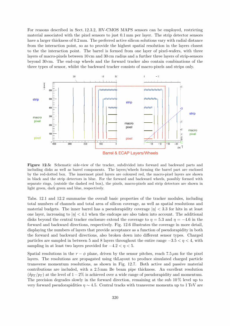
For reasons described in Sect. 12.3.2, HV-CMOS MAPS sensors can be employed, restrictingmaterial associated with the pixel sensors to just 0.1 mm per layer. The strip detector sensorshave a larger thickness of 0.2 mm. The preferred active silicon solutions vary with radial distancefrom the interaction point, so as to provide the highest spatial resolution in the layers closestto the the interaction point. The barrel is formed from one layer of pixel-wafers, with threelayers of macro-pixels between 10 cm and 30 cm radius and a further three layers of strip-sensorsbeyond 30 cm. The end-cap wheels and the forward tracker also contain combinations of thethree types of sensor, whilst the backward tracker consists of macro-pixels and strips only.

Figure 12.5: Schematic side-view of the tracker, subdivided into forward and backward parts andincluding disks as well as barrel components. The layers/wheels forming the barrel part are enclosedby the red-dotted box. The innermost pixel layers are coloured red, the macro-pixel layers are shownin black and the strip detectors in blue. For the forward and backward wheels, possibly formed withseparate rings, (outside the dashed red box), the pixels, macro-pixels and strip detectors are shown inlight green, dark green and blue, respectively.

Tabs. 12.1 and 12.2 summarise the overall basic properties of the tracker modules, includingtotal numbers of channels and total area of silicon coverage, as well as spatial resolutions andmaterial budgets. The inner barrel has a pseudorapidity coverage |η| < 3.3 for hits in at leastone layer, increasing to |η| < 4.1 when the endcaps are also taken into account. The additionaldisks beyond the central tracker enclosure extend the coverage to η = 5.3 and η = −4.6 in theforward and backward directions, respectively. Fig. 12.6 illustrates the coverage in more detail,displaying the numbers of layers that provide acceptance as a function of pseudorapidity in boththe forward and backward directions, also broken down into different sensor types. Chargedparticles are sampled in between 5 and 8 layers throughout the entire range −3.5 < η < 4, withsampling in at least two layers provided for −4.2 < η < 5.

Spatial resolutions in the r − φ plane, driven by the sensor pitches, reach 7.5µm for the pixellayers. The resolutions are propagated using tkLayout to produce simulated charged particletransverse momentum resolutions, as shown in Fig. 12.7. Both active and passive materialcontributions are included, with a 2.5 mm Be beam pipe thickness. An excellent resolution(δpT /pT ) at the level of 1− 2% is achieved over a wide range of pseudorapidity and momentum.The precision degrades slowly in the forward direction, remaining at the sub 10 % level up tovery forward pseudorapidities η ∼ 4.5. Central tracks with transverse momenta up to 1 TeV are

320

Tracker (LHeC) Inner Barrel ECAP

pix pixmacro strip pix pixmacro strip

ηmax,ηmin 3.3,−3.3 2.1,−2.1 1.4,−1.4 ±[4.1, 1.8] ±[2.4, 1.5] ±[2.0, 0.9]Layers (Barrel) 1 3 3Wheels (ECAP) 2 1 1-3Modules/Sensors 320 4420 3352 192 192 552Total Si area [m2] 0.3 4.6 17.6 0.8 5.6 3.3Read-out-Channels [106] 224.5 1738 20.6 322.4 73.3 17.0pitchr−φ [µm] 25 100 100 25 100 100pitchz [µm] 50 400 50k 2) 50 400 10k 1)

AverageX0/ΛI [%] 7.2 / 2.2 2.2 / 0.71) Reaching pitchr−φ when using two wafer layers rotated by 20 mrad is achievable.

Table 12.1: Summary of the main properties of the Barrel and Endcap tracker modules based oncalculations performed using tkLayout [899]. For each module, the rows correspond to the pseudorapiditycoverage, numbers of barrel and disk layers, numbers of sensors, total area covered by silicon sensors,numbers of readout channels, the hardware pitches affecting the (r−φ) and the z resolution, respectively,and the average material budget in terms of radiation lengths and interaction lengths. Where appropriate,the numbers are broken down into separate contributions from pixels, macro-pixels and strips. SeeTab. 12.2 for a sum of all tracker components.

Tracker (LHeC) Fwd Tracker Bwd Tracker Total

pix pixmacro strip pixmacro strip (incl. Tab. 12.1)

ηmax,ηmin 5.3,2.6 3.5,2.2 3.1,1.6 −4.6,−2.5 −2.9,−1.6 5.3,−4.6Wheels 2 1 3 2 4Modules/Sensors 180 180 860 72 416 10736Total Si area [m2] 0.8 0.9 4.6 0.4 1.8 40.7Read-out-Channels [106] 404.9 68.9 26.4 27.6 10.6 2934.2pitchr−φ [µm] 25 100 100 100 100pitchz [µm] 50 400 50k 2) 400 10k 1)

AverageX0/ΛI [%] 6.7 / 2.1 6.1 / 1.9incl. beam pipe [%] 40 / 25

1) Reaching pitchr−φ when using two wafer layers rotated by 20 mrad is achievable.

Table 12.2: Summary of the main properties of the forward and backward tracker modules in the revisedLHeC detector configuration based on calculations performed using tkLayout [899]. For each module,the rows correspond to the pseudorapidity coverage, numbers of disk layers, numbers of sensors, totalarea covered by silicon sensors, numbers of readout channels, the hardware pitches affecting the (r − φ)and the z resolution, respectively, and the average material budget in terms of radiation lengths andinteraction lengths. The polar angle dependence and decomposition of X0 and ΛI are shown in Fig. 12.9.Where appropriate, the numbers are broken down into separate contributions from pixels, macro-pixelsand strips. The column Total contains the sum of corresponding values in tables 12.1 and 12.2.

321

Figure 12.6: Numbers of silicon layers that provide acceptance for charged particles as a function ofabsolute value of pseudorapidity in the forward (left) and backward (right) directions, summed acrossthe central, forward and backward trackers. The distributions are broken down according to sensor type,with colour coding of red for pixels, light or dark green for macro-pixels, blue for strips and black for thesum.

measured with 10− 20 % precision. Similar results are achieved in the (negative η) backwarddirection (not shown).

A major requirement of the tracking detectors will be the precise determination of vertex co-ordinates and track impact parameters relative to the primary vertex in order to give the bestpossible sensitivity to secondary vertices from heavy flavour decays, for example for the study ofthe Higgs in its dominant bb decay mode. The simulated results for longitudinal and transversetrack impact parameter resolutions using the full new tracking layout are shown in Fig. 12.8.The transverse spatial resolutions are at the level of 10− 50µm over a wide range of transversemomentum and pseudorapidity, extending well into the forward direction.

The material budget contributions from the sensors summed across all layers are given inTabs. 12.1 and This is largest for the inner barrel, where it amounts to 7.2 % of a radiationlength. The sensors in the central tracker endcap and the forward and backward tracking ringscontribute 2.2 %, 6.7 % and 6.1 % of a radiation length, respectively. The material budget simula-tions, propagated for the full system and including passive contributions, are shown in Fig. 12.9.The use of thin sensors keeps the total material to the level of 0.2−0.4X0 throughout the entiretracking region up to η ∼ 4.5. At the most forward (and backward) pseudorapidities, particlestravel through a large effective thickness of material as they pass through the beam pipe; thisbecomes the dominant contribution for η > 3.5.

12.3.2 Silicon Technology Choice

Being developed for several High Luminosity-LHC (HL-LHC) upgrades and the proposed CLIChigh-energy linear collider we envisage depleted CMOS sensor technology, also known as De-pleted Monolithic Active Pixel Sensors (DMAPS), to be used as position sensitive detectors inindustry standard CMOS processes or High Voltage-CMOS (HV-CMOS) processes [900]. Thesesensors are extremely attractive for experiments in particle physics as they integrate the sensingelement and the readout ASIC in a single layer of silicon, which removes the need for inter-connection with complex and expensive solder bump technology. Depleted CMOS sensors alsobenefit from faster turnaround times and lower production costs when compared to hybrid sil-icon sensors. To achieve fast charge collection and high radiation tolerance, DMAPS can beimplemented following two different approaches known as low fill-factor and large fill-factor.

322

Figure 12.7: Simulated transverse momentum track resolution using all modules in the revised LHeCtracking system. Results are shown in terms of fractional pT resolution as a function of pseudorapidityfor several constant momenta, p = 100 MeV (Black, bottom, obscured), 1 GeV (Dark Blue, obscured),2 GeV (Light Blue, obscured), 5 GeV (Red), 10 GeV (Light Green), 100 GeV (Magenta), 1 TeV (DarkGreen) and 10 TeV (Black, top).

Low fill-factor DMAPS benefit from High Resistivity (HR) substrates and thick epitaxial layersaccessible from large-scale CMOS imaging processes, while large fill-factor DMAPS exploit theHigh Voltage (HV) option developed by commercial CMOS foundries for power electronics. Re-cently, HR wafers have become available in the production line of foundries that manufactureHV-CMOS processes, thus DMAPS in HR/HV-CMOS are also possible to further improve theperformance of the sensor. Today’s most performant DMAPS detectors are 50µm thin and have50µm x 50µm cell size with integrated mixed analogue and digital readout electronics, 6ns timeresolution and 2x10151MeV neq/cm2 radiation tolerance. The typical cross-section of a largefill-factor DMAPS in a HV-CMOS process is shown in Fig. 12.10.

DMAPS in HR/HV-CMOS have been adopted as a world first as the sensor technology of choicefor the Mu3e experiment at the Paul Scherrer Institute (PSI) in Switzerland [901]. MuPix,the DMAPS detector for Mu3e, implements active pixels that amplify the collected charge inthe collecting electrode and peripheral readout electronics that discriminate and process theamplified signals. MuPix10, the first reticle size detector for Mu3e (' 2× 2 cm2) and currentlyin production, features 250× 256 pixels with an 80× 80µm2 pixel size, 11-bit time-stamp, 6-bitTime-over-Threshold (ToT) and continuous readout. Its peripheral readout electronics includereadout buffers, a state machine, a Phase Locked Loop (PLL) and Voltage-Controlled Oscillator(VCO), 8/10-bit encoders and 3 serialisers for data transmission with a rate of up to 1.6 Gbit/s.Previous MuPix prototypes have been thinned to 50µm successfully and tested to achieve a6 ns time resolution after time-walk correction [902]. ATLASPix, the DMAPS development inHR/HV-CMOS that was originally aimed at providing an alternative sensor technology for theoutermost pixel layer of the new ATLAS Inner Tracker (ITk) upgrade, has been tested to havean approximate 150 mW/cm2 power consumption and be radiation tolerant up to 2 ·1015 1 MeVneq/cm2 fluences [903] DMAPS in HR-CMOS, such as the MALTA development originally aimedat the new ATLAS ITk upgrade as well, have achieved full efficiency after 1·1015 1 MeV neq/cm2

fluences [904]. However, further research is still needed to demonstrate reticle size DMAPS inHR-CMOS. Research to further develop DMAPS to meet the extreme requirements of futureexperiments in particle physics is on-going.

323

Figure 12.8: Simulated longitudinal (left) and transverse (right) impact parameter resolutions usingall modules in the revised LHeC tracking system. Results are shown as a function of pseudorapidity forseveral constant momenta, p = 100 MeV (Black, top), 1 GeV (Dark Blue), 2 GeV (Light Blue), 5 GeV(Red), 10 GeV (Light Green), 100 GeV (Magenta, obscureed), 1 TeV (Dark Green, obscured) and 10 TeV(Black, bottom).

Figure 12.9: Material contributions from the tracking modules as a function of pseudorapidity. Resultsare given in terms of radiation lengths (left) and hadronic interaction lengths (right). The results arebroken down into contributions from barrel modules (yellow) and endcap / additional disk modules (red)and are compared with the contribution from the 2.5 mm beam pipe (green).

324

Figure 12.10: Typical sensor cross-section of a DMAPS detector in a HV-CMOS process [900].

The here presented tracker design of the LHeC utilises pixel detectors for high resolution trackingin the inner barrel and as well the barrel endcaps and the forward tracker. The number of readoutchannels is close to 109, with a high transverse and longitudinal segmentation provided by a pitchof 25 × 50µm2. One can expect that such a fine segmentation is in reach for a detector whichwould be built in a decade hence. The radiation level in electron-proton scattering is by ordersof magnitude lower than in proton-proton interactions at the LHC and is indeed in a rangeof 1015 MeV neq/cm2 for which radiation hardness has been proven as indicated above. Themonolithic CMOS detector technology leads to a significant simplification of the production ofthese detectors and a considerably reduced cost. We thus conclude that the LHeC pixel trackerrepresents a particularly suitable device for a large scale implementation of HV CMOS Siliconin a forthcoming collider detector.

12.4 Calorimetry

The 2012 CDR detector design leaned on technologies employed by ATLAS for calorimetry in thebarrel region, adopting a lead / liquid argon sampling electromagnetic calorimeter with an ac-cordion geometry and a steel / scintillating tile sampling hadronic component. For the version ofthe LHeC detector described here, an alternative solution of a lead / scintillator electromagneticcalorimeter has been investigated. This has the advantage of removing the need for cryogenics,whilst maintaining an acceptable performance level. Comparing the lead-scintintillator designsfor the electromagnetic barrel calorimeter for the 2012 CDR with the updated setup, the a-termfor shower fluctuations and transverse leakages and the b-term describing the back-leakagesof the calorimeter the resolution performance of the updated design is better (a= 20% andb= 0.14% in the 2012 CDR and a= 12.4% and b= 1.9% in the new design). Although it isnot discussed here, the liquid argon solution very much remains the favorable option due to itshigh level of performance and stability / radiation hardness. The fit-results in CDR 2012 theLAr calorimeter option show a slightly better resolution performance than the lead-scintillatorvariant. Due to the accordion shaped absorber it forces more energy deposit in the calorimetervolume. The CDR values for comparison: a= 8.47% and b= 0.318%. The hadronic calorime-ter retains the steel and scintillating tile design, similar to ATLAS. As in the 2012 CDR, plugsampling calorimeters are also incorporated at large |η|, the forward and backward componentsusing tungsten and lead absorber material, respectively, with both using silicon based sensitivereadout layers. The steel structures in the central and plug calorimetry close the outer fieldof the central solenoid. The solenoid and the dipoles are placed between the Electromagnetic-Barrel and the Hadronic-Calorimeter. The HCAL-Barrel sampling calorimeter using steel and

325

Figure 12.11: Three-dimensional view of the arrangement of Hadronic-Calorimeter, experimental mag-nets (solenoid and dipoles), the electromagnetic calorimeter and tracking detector layers.

Figure 12.12: The coil arrangement of the solenoid and dipoles system housing in a common cryostat.

326

scintillating tiles as absorber and active material, respectively, provides the mechanical stabilityfor the Magnet/Dipole cryostat and the tracking system Fig. 12.11. How the solenoid/dipoles-system would look like has been discussed in more detail in [1] and is illustrated by Fig. 12.12.(and the LAr cryostat in a cold EMC version) along with the iron required for the return flux ofthe solenoidal field. The main features of the new calorimeter layout are summarised in Tab. 12.3and 12.4. The pseudorapidity coverage of the electromagnetic barrel is −1.4 < η < 2.4, whilstthe hadronic barrel and its end cap cover −1.5 < η < 1.9. Also including the forward andbackward plug modules, the total coverage is very close to hermetic, spanning −5.0 < η < 5.5.The total depth of the electromagnetic section is 30 radiation lengths in the barrel and backwardregions, increasing to almost 50X0 in the forward direction where particle and energy densitiesare highest. The hadronic calorimeter has a depth of between 7.1 and 9.6 interaction lengths,with the largest values in the forward plug region.

Calo (LHeC) EMC HCAL

Barrel Ecap Fwd Barrel Ecap Bwd

Readout, Absorber Sci,Pb Sci,Fe Sci,Fe Sci,FeLayers 38 58 45 50Integral Absorber Thickness [cm] 16.7 134.0 119.0 115.5ηmax, ηmin 2.4, −1.9 1.9, 1.0 1.6, −1.1 −1.5, −0.6

σE/E = a/√E ⊕ b [%] 12.4/1.9 46.5/3.8 48.23/5.6 51.7/4.3

ΛI /X0 X0 = 30.2 ΛI = 8.2 ΛI = 8.3 ΛI = 7.1Total area Sci [m2] 1174 1403 3853 1209

Table 12.3: Basic properties and simulated resolutions of barrel calorimeter modules in the new LHeCdetector configuration. For each of the modules, the rows indicate the absorber and sensitive materials,the number of layers and total absorber thickness, the pseudorapidity coverage, the contributions to thesimulated resolution from the sampling (a) and material (b) terms in the form a/b, the depth in termsor radiation or interaction lengths and the total area covered by the sensitive material. GEANT4 [898]simulation based fits using crystal ball function [905–907].

Calo (LHeC) FHC FEC BEC BHCPlug Fwd Plug Fwd Plug Bwd Plug Bwd

Readout, Absorber Si,W Si,W Si,Pb Si,CuLayers 300 49 49 165Integral Absorber Thickness [cm] 156.0 17.0 17.1 137.5ηmax, ηmin 5.5, 1.9 5.1, 2.0 −1.4, −4.5 −1.4, −5.0

σE/E = a/√E ⊕ b [%] 51.8/5.4 17.8/1.4 14.4/2.8 49.5/7.9

ΛI /X0 ΛI = 9.6 X0 = 48.8 X0 = 30.9 ΛI = 9.2Total area Si [m2] 1354 187 187 745

Table 12.4: Basic properties and simulated resolutions of forward and backward plug calorimeter mod-ules in the new LHeC detector configuration. For each of the modules, the rows indicate the absorberand sensitive materials, the number of layers and total absorber thickness, the pseudorapidity coverage,the contributions to the simulated resolution from the sampling (a) and material (b) terms in the forma/b, the depth in terms or radiation or interaction lengths and the total area covered by the sensitivematerial. GEANT4 [898] simulation based fits using crystal ball function [905–907].

The performance of the new calorimeter layout has been simulated by evaluating the mean sim-ulated response to electromagnetic (electron) and hadronic (pion) objects with various specificenergies using GEANT4 [898] and interpreting the results as a function of energy in terms ofsampling (a) and material / leakage (b) terms in the usual form σE/E = a/

√E ⊕ b. Example

results from fits are shown for the barrel electromagnetic and hadronic calorimeters in Fig. 12.13

327

and for the forward plug electromagnetic and hadronic calorimeters in Fig. 12.14. The resultsfor the a and b parameters are summarised in Tabs. 12.3 and 12.4. The response of the barrelelectromagnetic calorimeter to electrons in terms of both sampling (a = 12.4 %) and material(b = 1.9 %) terms is only slightly worse than that achieved with liquid argon sampling in the2012 CDR. The resolutions of the forward and backward electromagnetic plug calorimeters arecomparable to those achieved in the 2012 design. A similar pattern holds for the hadronic re-sponse, with sampling terms at the sub-50 % level and material terms of typically 5 % throughoutthe barrel end-caps and forward and backward plugs.

Figure 12.13: Crystal Ball fitted energy dependent resolution for the barrel electromagnetic (left) andbarrel hadronic (right) calorimeters EMC and HCAL, respectively. The first (a) term includes showerfluctuations and transverse leakages and the second (b) term includes leakages from the calorimeter volumelongitudinally.

Figure 12.14: Crystal Ball fitted energy dependent resolution for the forward electromagnetic (left)and forward hadronic (right) plug calorimeters FEC and FHC, respectively. The first (a) term includesshower fluctuations and transverse leakages and the second (b) term includes leakages from the calorimetervolume longitudinally.

12.5 Muon Detector

Muon identification is an important aspect for any general purpose HEP experiment. At theLHeC the muon detector can widen the scope and the spectrum of many measurements, of which

328

only a few are listed here:

• Higgs decay,

• Semi-leptonic decays of heavy flavoured hadrons,

• Vector meson production,

• Direct W and Z production,

• Di-muon production,

• Leptoquarks, lepton flavour violation, and other BSM phenomena.

The primary target of the muon detector at the LHeC is to provide a reliable muon tag signaturewhich can be uniquely used in conjunction with the central detector for muon identification,triggering and precision measurements. This specification is appropriate to the constraints oflimited space 2 and the lack of a dedicated magnetic field as in the baseline design. The muonchambers surround the central detector and cover the maximum possible solid angle. They havea compact multi-layer structure, providing a pointing trigger and a precise timing measurementwhich is used to separate muons coming from the interaction point from cosmics, beam halo andnon prompt particles. This tagging feature does not include the muon momentum measurementwhich is performed only in conjunction with the central detector. A trigger candidate in themuon detector is characterised by a time coincidence over a majority of the layers in a rangeof η and φ, compatible with an ep interaction of interest in the main detector. The muoncandidates are combined with the trigger information coming from the central detector (mainlythe calorimetry at Level 1 trigger) to reduce the fake rate or more complex event topologies.

In terms of technology choices, the options in use in ATLAS and CMS and their planned upgradesare adequate for LHeC. Generally, muon and background rates in LHeC are expected to belower than in pp. The option of an LHeC muon detector composed by layers of ResistivePlate Chambers (RPC), providing the Level 1 trigger and a two coordinate (η, φ) measurementpossibly aided by Monitored Drift Tubes (MDT) for additional precision measurements, aschosen for the 2012 CDR, is still valid. Recent developments as presented in the LHC Phase 2Upgrade Technical Design Reports [908, 909] further strengthen this choice. A new thin-RPC(1 mm gas gap) operated with lower HV, provides a sharper time response (few ns), a higherrate capability (tens of kHz/cm2), and extends the already good aging perspective. Advances inlow-noise, high-bandwidth front-end electronics can improve the performance of older detectors.Similar arguments also hold for smaller tube MDTs (15 mm diameter) which provide loweroccupancy and higher rate capability.

Fig. 12.15 shows an adaptation for LHeC of an RPC-MDT assembly as will be implemented forthe inner muon layer of ATLAS already during the Phase-1 upgrade as a pilot for Phase-2. Atriplet of thin gap RPCs, each with 2 coordinate measurement, is combined with two superlayersof small MDTs. It is also important to note the reduced volume of this structure, in particularthe RPC part which would provide the muon tag. For the LHeC a baseline would be to haveone or two such stations forming a near-hermetic envelope around the central detector.

Finally, as already presented in the 2012 CDR, detector extensions, with a dedicated magneticfield in the muon detector, be this a second solenoid around the whole detector or extra dipoleor toroid in the forward region are, at this stage, left open as possible developments only forupgrade scenarios.

2As in the 2012 CDR, the baseline LHeC detector including the muon system and all of the services andsupports is expected to fit into the octagonal shape envelope of the L3 magnet (11.6 m minimum diameter).

329

Figure 12.15: A transverse view of a RPC-MDT assembly as adapted from a drawing of the ATLASPhase-1 muon upgrade [908]. In this case a station is composed of an RPC triplet for trigger andtw0-coordinate readout and two MDT superlayers for precise track measurements.

12.6 Forward and Backward Detectors

In the 2012 CDR, initial plans for beamline instrumentation were provided for the LHeC. In thebackward direction, low angle electron and photon calorimeters were included with the primaryintention of measuring luminosity via the Bethe-Heitler process ep → eXp, also offering anelectron tagger to identify photoproduction (γp → X) processes at intermediate y values. Thecurrent design carries forward the 2012 version of this backward instrumentation.

In the forward direction, Roman pot detectors were included in the region of z ∼ 420 m, capableof detecting scattered protons over a range of fractional energy loss 10−3 < ξ < 3 × 10−2 andwide transverse momentum acceptance, based on extensive previous work in the LHC context bythe FP420 group [910]. This also forms the basis of forward proton tagging in the revised design.However, as is the case at ATLAS and CMS / TOTEM, further Roman pot detectors in theregion of 200 m and (with HL-LHC optics) perhaps around 320 m would extend the acceptancetowards higher ξ values up to around 0.2 allowing the study of diffractive processes ep → eXpwhere the dissociation system X has a mass extending into the TeV regime. It is worth notingthat Roman pot technologies have come of age at the LHC, with the TOTEM collaborationoperating 14 separate stations at its high point. Silicon sensor designs borrowed from theinnermost regions of the ATLAS and CMS vertexing detectors have been used, providing highspatial resolution and radiation hardness well beyond the needs of LHeC. Very precise timingdetectors based on fast silicon or Cherenkov radiation signals from traversing protons in quartzor diamond have also been deployed. It is natural that these advances and the lessons from theirdeployment at the LHC will be used to inform the next iteration of the LHeC design.

The forward beamline design also incorporates a zero angle calorimeter, designed primarilyto detect high energy leading neutrons from semi-inclusive processes in ep scattering and todetermine whether nuclei break up in eA events. This component of the detector was notconsidered in detail in 2012 and is therefore discussed here.

12.6.1 Zero-Degree (Neutron) Calorimeter

The Zero-Degree Calorimeter (ZDC) measures final state neutral particles produced at anglesnear the incoming hadron beam direction. They typically have large longitudinal momentum(xF 10−2), but with transverse momentum of order of ΛQCD. Such a calorimeter has beeninstrumented in experiments for ep collisions (H1 and ZEUS) and for pp, pA and AA collisions atRHIC (STAR and PHENIX) and at the LHC (ATLAS, CMS, ALICE and LHCf at the ATLASIP). The detector’s main focus is to study the soft-hard interplay in the QCD description of epand eA collisions by studying the dependence of forward-going particles with small transversemomentum on variables such as Q2 and x that describe the hard scattering. The detector alsoallows the tagging of spectator neutrons to detect nuclear breakup in eA collisions and enables

330

the precise study of the EMC effect by using neutron-tagged DIS on small systems, such ase 3He → ed + n → eX + n. For heavier ions, several tens of neutrons may enter within theaperture of the ZDC. Inclusive π0 production has been measured by the LHCf experiments forpp collisions. It is of great interest to compare with DIS measurements at the same protonenergies. Precise understanding of the inclusive spectrum of the forward-going particles is a keyingredient in simulating air showers from ultra-high energy cosmic rays.

Physics requirement for forward neutron and π0 production measurement

It is known from various HERA measurements that the slope parameter b is about 8 GeV−2 in theexponential parameterisation ebt of the t distribution of leading neutrons. In order to preciselydetermine the slope parameter it is necessary to measure the transverse momentum of theneutrons up to or beyond 1 GeV. The aperture for forward neutral particles does not have to bevery large, thanks to the large energy of the proton and heavy ion beam. For example, collisionswith Ep = 7 TeV need 0.14 mrad for pT = 1 GeV neutrons at Eparticle/Ebeam ≡ xF = 1.0, or0.56 mrad for xF = 0.25.

The energy or xF resolution for neutrons will not be a dominant factor thanks to the high energyof the produced particles. The energy resolution of a neutron with xF = 0.1 is about 2% forcutting-edge hadron calorimeters with σE/E = 50 %/

√E, where E is in GeV. Such a resolution

can be achieved if non-unity e/h can be compensated either by construction of the calorimeteror by software weighting, and if the size of the calorimeter is large enough so that shower leakageis small.

On the other hand, the resolution requirement on the transverse momentum is rather stringent.For example, 1 mm resolution on hadronic showers from the neutron measured at 100 m down-stream from the interaction point corresponds to 0.01 mrad or 70 MeV, which is rather moderate(≤ 10 % resolution for large pT hadrons with pT > 700 MeV). For smaller pT it is more appro-priate to evaluate the resolution in terms of t ' −(1 − xF )p2

T i.e. ∆t ' 2(∆pT )pT at xF = 1.At t = 0.1 GeV2 or pT ' 300 MeV, ∆t is about 50 %. A shower measurement with significantlybetter than 1 mm position resolution, therefore, would improve the t-distribution measurementsignificantly.

According to the current LHC operation conditions with β∗ = 5 cm, the beam spread is8× 10−5 rad or 0.56 GeV. This is much larger than the required resolution in pT . It is thereforeneither possible to measure the particle flow nor to control the acceptance of the forward aper-ture. For precision measurement of forward particles, it is necessary to have runs with β∗ ≥ 1 m,corresponding to σ(pT ) < 70 MeV.

The calorimeter should be able to measure more than 30 neutrons of 5 TeV to tag spectatorneutrons from heavy-ion collisions. The dynamic range of the calorimeter should exceed 100 TeVwith good linearity.

As for π0 measurements, the LHCf experiment has demonstrated that a position resolution of200µm on electromagnetic showers provides good performance for the inclusive photon spectrummeasurements [911]. This also calls for fine segmentation sampling layers.

ZDC location

According to the IP design, a possible location for the ZDC is after the first bending of theoutgoing colliding proton beam at around Z = 110 m, where no beam magnet is placed (seeFig. 12.16). It is anyhow planned to place a neutral particle dump around this location in order

331

to protect accelerator components. A ZDC could serve as the first absorbing layer at zerodegrees.

Figure 12.16: Possible location for a ZDC for the linac–ring IR design of LHeC as shown in Fig. 10.28.The solid rectangle represents the potential location and magnets overlaid.

The aperture to the ZDC would be determined by the last quadruple magnet at around z = 50 m.Assuming a typical aperture for the LHC magnets of 35 mm, the aperture could be as large as0.7 mrad. The horizontal aperture of the dipole magnets between 75 and 100 m would be larger,since otherwise the magnets receive significant radiation from neutral particles produced fromthe collisions at the IP. Even if the aperture is limited by the vertical aperture of the last dipoleat z = 100 m, the aperture is 0.35 mrad, corresponding to 2.4 GeV in pT for 7 GeV particles.This fulfills the physics requirement.

The space for the ZDC location in the transverse direction should be at least ±2λI to avoidlarge leakage of hadronic showers. This can be achieved if the proton beam passes inside thecalorimeter, about 20 cm from the centre of the calorimeter. The total size of the calorimetercould then be 60 × 60 × 200 cm3 or larger according to the current layout of the beam andaccelerator components. This would provide about ±3λI in the transverse direction and about10λI in depth.

Radiation requirement for the ZDC

It can safely be assumed that the energy spectrum of the forward neutral particles produced inep and pp events are very similar. According to the LHCf simulation, their tungsten–scintillatorsandwich calorimeter receives about 30 Gy/nb−1 or 108 events/nb−1 assuming σtot

pp = 100 mb,i.e. 3× 10−7 Joule/event. This means that about 1/4 of the total proton beam energy (7 TeV '1.12× 10−6 Joule/event) is deposited in 1 kg material in pp collisions. The ep total cross sectionis expected to be approximately 68µb or 680 kHz at 1034 cm2s−1. A 7 TeV beam or 1.12 ×

332

10−6 Joule/event corresponds to 0.76 Joule/s at this instantaneous luminosity. A quarter of thetotal dose is then about 0.2 Gy/sec or 0.02 Gy/nb. The contribution from beam-gas interactionsis estimated to be much smaller (O(100 kHz)).

Assuming that the ZDC is always operational during LHeC running, one year of ep operationamounts to 2.5 MGy/year assuming 107 sec operation, or O(10 MGy) throughout the lifetime ofthe LHeC operation. This approximately corresponds to 1014 − 1015 1 MeV neutron equivalent.

Possible calorimeter design

The high dose of O(10 MGy) requires calorimeters based on modern crystals (e.g. LYSO) orsilicon as sampling layers, at least for the central part of the calorimeter where the dose isconcentrated. Since we also need very fine segmentation for photons, it is desirable to use finelysegmented silicon pads of order of 1 mm. As for the absorbers, tungsten should be used for goodposition resolution of photons and the initial part of hadronic showers.

In the area outside the core of the shower i.e. well outside the aperture, the dose may be muchsmaller and small scintillator tiles could be used for absorbers, which allows measurements withgood e/h ratio. If we choose a uniform design using silicon across the detector, the segmentationof the outer towers could be order of a few cm, which still makes it possible to use softwarecompensation technology, as developed for example for the calorimeters in the ILC design. Itmay also be possible to use lead instead of tungsten for outer towers to reduce the cost.

12.7 Detector Installation and Infrastructure

The usual constraints that apply to HEP detector integration and assembly studies also applyto the LHeC. In places, they are even tighter since the detector has to be installed in a relativelyshort time, as given by the duration of an LHC machine shutdown, which is typically two years.For the purposes of this report, it is assumed that the LHeC detector will be installed at IP2, seeFig. 12.17. The magnet formerly used by L3 and now in use by ALICE is already present at IP2and its support structure will be used once again my LHeC. However, the time needed to removethe remainder of the existing detector and its services has to be included to the overall schedule.Thus the only realistic possibility to accomplish the timely dismantling of the old detector andthe installation of the new one is to complete as much as possible of the assembly and testingof the LHeC detector on the surface, where the construction can proceed without impacting onthe LHC physics runs. The condition for doing this is the availability of equipped free spaceat the LHC-P2 surface, namely a large assembly hall with one or two cranes. To save time,most of the detector components have been designed to match the handling means availableon site, i.e. a bridge crane in the surface hall and experiment cavern. Nevertheless, a heavylifting facility (about 300 tons capacity) will be rented for the time needed to lower the heaviestdetector components, such as the HCal barrel and plug modules. Large experience with thiswill be acquired during LHC Long Shutdown 3, when a significant part of the ATLAS and CMSdetectors will be replaced by new elements. At CMS, for instance, a new Endcap Calorimeterweighting about 220 tons will be lowered into the experiment cavern, a scenario very close towhat is envisaged for the LHeC detector assembly.

The detector has been split into the following main parts for assembly purposes:

• Coil cryostat, including the superconducting coil, the two integrated dipoles and eventuallythe EMCal.

• Five HCal tile calorimeter barrel modules, fully instrumented and cabled (5).

333

Figure 12.17: View of the surface infrastructure at Point 2, near St. Genis [912].

• Two HCal plugs modules, forward and backward (2).

• Two EMCal plugs, forward and backward (2).

• Innner Tracking detector (1).

• Beam-pipe (1).

• Central Muon detector (1 or 2).

• Endcaps Muon detector (2).

The full detector, including the Muon chambers, fits inside the former L3 detector Magnet Yoke,once the four large doors are taken away. The goal is to prevent losing time in dismantling theL3 Magnet barrel yoke and to make use of its sturdy structure to hold the detector central parton a platform supported by the magnet crown, whilst the Muon chambers are inserted intolightweight structures (space-frames) attached to the inner surface of the octagonal L3 magnet.

The assembly of the main detector elements on the surface can start at any time, withoutsensible impact on the LHC run, providing that the surface facilities are available. The Coilsystem commissioning on site is estimated to require three months and preparation for loweringa further three months, including some contingency. In the same time window, the L3 Magnetwill be freed up and prepared for the new detector 3. Lowering of the main detector componentsinto the cavern, illustrated in Fig. 12.18, is expected to take one week per piece (15 pieces intotal). Underground integration of the central detector elements inside the L3 Magnet wouldrequire about 6 months, cabling and connection to services some 8 to 10 months, in parallelwith the installation of the Muon chambers, the Tracker and the Calorimeter Plugs. Fig. 12.19shows the installed complete detector housed in the L3 magnet support.

The total estimated time, from the starting of the testing of the Coil system on surface to thecommissioning of the detector underground is thus 20 months. The beam-pipe bake out andvacuum pumping could take another 3 months and the final detector check-out one additional

3The actual delay depends on the level of activation and the procedure adopted for dismantling the existingdetector. Here again the experience acquired during the long shutdown LS2 with the upgrades of ALICE andLHCb and later with the ATLAS and CMS upgrades during LS3 will provide important insight for definingprocedures and optimising the schedule.

334

Figure 12.18: View of the cavern infrastructure at Point 2 [913]. The support structure of the magnetof the L3 experiment (at the centre) will house and support the LHeC detector.

Crane bridge 2x20tons

LHC magnets

External dipole

Detector installation complete underground.

PX24 shaft

UX25 cavern

L3 magnet

Figure 12.19: View of the LHeC detector, housed in the L3 magnet support structure, after installationat the interaction point.

month. Some contingency (2–3 months in total) is foreseen at the beginning and the end of theinstallation period. A sketch of the installation schedule is provided in Fig. 12.20

Concerning the detector infrastructures, not much can be said at this stage. The LHeC detectorsuperconducting coil will need cryogenic services and a choice has to be made between purchas-ing a dedicated liquid helium refrigeration plant or profiting from the existing LHC cryogenicinfrastructure to feed the detector magnet. The electrical and water-cooling networks present atLHC-P2 are already well sized for the new detector and only minor interventions are expected

335

Figure 12.20: Time schedule of the sequential installation of the LHeC detector at point 2, as describedin the text.

there.

336

12.8 Detector Design for a Low Energy FCC-eh

Although not the primary focus of this report, a full detector design has also been carriedout for an ep facility based on an FCC tunnel with proton-ring magnet strengths limited suchthat the proton energy is 20 TeV. For ease of comparison, the basic layout and the technologychoices are currently similar to those of the LHeC detector. Similar or improved performance isobtained compared with the LHeC, provided that additional disks are included in the forwardand backward trackers and the calorimeter depths are scaled logarithmically with the beamenergies.

Figure 12.21: Side view of a low energy FCCeh (Ep = 20 TeV) concept detector, designed using theDD4hep framework [897], showing the essential features. The solenoid is again placed between the ECAL-Barrel and Hadronic-Barrel calorimeters and is housed in a cryostat in common with the beam steeringdipoles extending over the full length of the barrel and plug hadronic calorimeters. The sizes have beenchosen such that the solenoid/dipoles and ECAL-Barrel systems as well as the whole tracker are alsosuitable to operate after an upgrade of the beam energy to Ep = 50 TeV.

The basic layout is shown in Fig. 12.21. The barrel and end-caps of the central tracker areidentical to those of the LHeC design, as given in table 12.1. The design parameters for theFCC-eh versions of the forward and backward trackers, the barrel calorimeters and the plugcalorimeters are given in tables 12.5, 12.6 and 12.7, respectively. Comparing the performance of”warm” solution (Pb-Sctillator) with the ”cold” variant (Pb-LAr) for the barrel electromagneticcalorimeter (EMC) the superior performance of the ”cold” calorimeter setup again favorises thePb-LAr option for the lowE-FCCeh detector (see figure 12.22 and table 12.6).

337

Tracker (lowE-FCCeh) 1) Fwd Tracker Bwd Tracker Total

pix pixmacro strip pixmacro strip (incl. Tab. 12.1)

ηmax,ηmin 5.6,2.6 3.8,2.2 3.5,1.6 −4.6,−2.6 −2.8,−1.6 5.3,−4.6Wheels 2 1 3 3 3Modules/Sensors 288 288 1376 216 1248 12444Total Si area [m2] 1.35 1.45 7.35 1.0 6.5 49.85Read-out-Channels [106] 647.9 110.2 42.3 82.7 38.3 3317.2pitchr−φ [µm] 25 100 100 100 100pitchz [µm] 50 400 50k 2) 400 10k 2)

AverageX0/ΛI [%] 6.7 / 2.1 6.1 / 1.9incl. beam pipe [%] 40 / 25

1) Based on tklayout calculations [899]2) Reaching pitchr−φ when using two wafer layers rotated by 20 mrad is achievable.

Table 12.5: Summary of the main properties of the forward and backward tracker modules in thelow energy FCC-eh detector configuration, based on calculations performed using tkLayout. For eachmodule, the rows correspond to the pseudorapidity coverage, the numbers of disk layers and of sensors, thetotal area covered by silicon sensors, the numbers of readout channels, the hardware pitches affecting the(r−φ) and the z resolution, and the average material budget in terms of radiation lengths and interactionlengths. The numbers are broken down into separate contributions from pixels, macro-pixels and strips.The column Total contains the sum of corresponding values of barrel tracker modules (identical to theLHeC barrel layout, table 12.1)and the forward and backward trackers in this table, 12.5.

Calo (lowE-FCCeh) EMC HCAL

Barrel Ecap Fwd Barrel Ecap Bwd

Readout, Absorber Sci,Pb Sci,Fe Sci,Fe Sci,FeLayers 49 91 68 78Integral Absorber Thickness [cm] 36.6 206.0 184.0 178.0ηmax, ηmin 2.8, −2.5 2.0, 0.8 1.6, −1.4 −0.7, −1.8

σE/E = a/√E ⊕ b [%] 12.6/1.1 38.9/3.3 42.4/4.2 40.6/3.5

ΛI /X0 X0 = 66.2 ΛI = 12.7 ΛI = 11.3 ΛI = 11.0Total area Sci [m2] 2915 4554 12298 3903

Table 12.6: Basic properties and simulated resolutions of barrel calorimeter modules in a scaled config-uration, suitable for a low energy FCC detector. For each of the modules, the rows indicate the absorberand sensitive materials, the numbers of layers and the total absorber thickness, the pseudorapidity cov-erage, the contributions to the simulated resolution from the sampling (a) and material (b) terms in theform a/b, the depth in terms or radiation or interaction lengths and the total area covered by the sensitivematerial. The resolutions are obtained from a GEANT4 [898] simulation, with fits using a crystal ballfunction [905–907].

338

Calo (lowE-FCCeh) FHC FEC BEC BHCPlug Fwd Plug Fwd Plug Bwd Plug Bwd

Readout, Absorber Si,W Si,W Si,Pb Si,CuLayers 296 49 59 238Integral Absorber Thickness [cm] 256.9 29.6 27.9 220.8ηmax, ηmin 5.8, 1.8 5.4, 1.8 −1.5, −5.2 −1.5, −5.6

σE/E = a/√E ⊕ b [%] 61.9/0.5 26.5/0.4 24.7/0.4 46.7/4.4

ΛI /X0 ΛI = 15.5 X0 = 84.7 X0 = 50.2 ΛI = 14.7Total area Si [m2] 2479 364 438 1994

Table 12.7: Basic properties and simulated resolutions of forward and backward plug calorimeter mod-ules in a scaled configuration, suitablle for a low energy FCC detector. For each of the modules, the rowsindicate the absorber and sensitive materials, the numbers of layers and the total absorber thickness,the pseudorapidity coverage, the contributions to the simulated resolution from the sampling (a) andmaterial (b) terms in the form a/b, the depth in terms or radiation or interaction lengths and the totalarea covered by the sensitive material. The resolutions are obtained from a GEANT4 [898] simulation,with fits using a crystal ball function [905–907].

Figure 12.22: For comparison the achievable resolution of a cold version of an EM-calorimeter stack isshown. The sampling calorimeter setup (ATLAS type) is characterised by lead as absorber 2.2 mm thickand 3.8 mm gaps filled with liquid argon as detecting medium, a cartesian accordion geometry and stackfolds having a length of 40.1 mm and an inclination angle of ±45°to each other. The radiation length forthe setup described is estimated from geantino scans using GEANT4 [898]. The simulated calorimeterstack has a depth of 83.7 cm (approximately 58 X0). The fits have been performed as for Fig. 12.13.

339

Chapter 13

Conclusion

The Large Hadron Collider determines the energy frontier of experimental collider physics for thenext two decades. Following the current luminosity upgrade, the LHC can be further upgradedwith a high energy, intense electron beam such that it becomes a twin-collider facility, in whichep collisions are registered concurrently with pp. A joint ECFA, CERN and NuPECC initiativeled to a detailed conceptual design report (CDR) [1] for the Large Hadron Electron Colliderpublished in 2012. The present paper represents an update of the original CDR in view of newphysics and technology developments.

The LHeC uses a novel, energy recovery linear electron accelerator which enables TeV energyelectron-proton collisions at high luminosity, of O(1034) cm−2s−1, exceeding that of HERA bynearly three orders of magnitude. The discovery of the Higgs boson and the surprising absenceof BSM physics at the LHC demand to extend the experimental base of particle physics suitableto explore the energy frontier, beyond pp collisions at the LHC. The LHC infrastructure is thelargest single investment the European and global particle physics community ever assembled,and the addition of an electron accelerator a seminal opportunity way to build on it, and tosustain the HL-LHC programme by adding necessary elements which are provided by high energydeep inelastic scattering. As has been shown in this paper, the external DIS input transformsthe LHC to a much more powerful facility, with a new level of resolving matter substructure,a more precise Higgs programme, challenging and complementing that of a next e+e− collider,and with a hugely extended potential to discover physics beyond the Standard Model.

The very high luminosity and the substantial extension of the kinematic range in deep inelasticscattering, compared to HERA, make the LHeC on its own a uniquely powerful TeV energycollider. Realising the Electrons for LHC programme developed with the previous and thepresent “white” papers, will create the cleanest, high resolution microscope accessible to theworld, which one may term the “CERN Hubble Telescope for the Micro-Universe”. It is directedto unravel the substructure of matter encoded in the complex dynamics of the strong interaction,and to provide the necessary input for precision and discovery physics at the HL-LHC and forfuture hadron colliders.

This programme, as has been described in this paper, comprises the complete resolution of thepartonic densities in an unexplored range of kinematics, the foundations for new, generalisedviews on proton structure and the long awaited clarification of the QCD dynamics at highdensities, as are observed at small Bjorken x. New high precision measurements on diffractionand vector mesons will shed new light on the puzzle of confinement. As a complement to the LHCand a possible future e+e− machine, the LHeC would scrutinise the Standard Model deeper than

340

ever before, and possibly discover new physics in the electroweak and chromodynamic sectorsas is outlined in the paper.

Through the extension of the kinematic range by about three orders of magnitude in lepton-nucleus (eA) scattering, the LHeC is the most powerful electron-ion research facility one canbuild in the next decades, for clarifying the partonic substructure and dynamics inside nucleifor the first time and elucidating the chromodynamic origin of the Quark-Gluon-Plasma.

The Higgs programme at the LHeC is astonishing in its precision. It relies on CC and NCprecision measurements for which an inverse atobarn of luminosity is desirable to achieve. Theprospective results on the Higgs couplings from the HL-LHC, when combined with those herepresented from the LHeC, will determine the couplings in the most frequent six Higgs decaychannels to one per cent level accuracy. This is as precise as one expects measurements fromlinear e+e− colliders but obtained dominantly from gg and WW fusion respectively, as comparedto Higgs-strahlung in electron-positron scattering which has the advantage of providing a Higgswidth determination too. The combined pp+ep LHC facility at CERN may then be expectedto remain the centre of Higgs physics for two more decades.

Searches for BSM physics at the LHeC offer great complementarity to similar searches at theHL-LHC. The core advantage of the LHeC is the clean, QCD-background and pileup-free en-vironment of an electron-proton collider with a cms energy exceeding a TeV. This enables dis-coveries of signatures that could be lost in the hadronic noise at pp or possibly unaccessible dueto the limited com energy at ee. Prominent examples for discovery enabled with ep are heavyneutral leptons (or sterile neutrinos) that mix with the electron flavour, dark photons below thedi-muon threshold, which are notoriously difficult to detect in other experiments, long-lived newparticles in general or new physics scenarios with a compressed mass spectrum, such as SUSYelectrowikinos and heavy scalar resonances with masses around and below 500 GeV, which mayexist but literally be buried in di-top backgrounds at the LHC.

The LHeC physics programme reaches far beyond any specialised goal which underlines theunique opportunity for particle physics to build a novel laboratory for accelerator based energyfrontier research at CERN. The project is fundable within the CERN budget, and not preventingmuch more massive investments into the further future. It offers the possibility for the currentgeneration of accelerator physicists to build a new collider using and developing novel technologywhile preparations proceed for the next grand step in particle physics for generations ahead.

The main technical innovation through the LHeC is the first ever high energy application ofenergy recovery technology, based on high quality superconducting RF developments, a majorcontribution to the development of green collider technology which is an appropriate responseto demands of our time. The ERL technique is more and more seen to have major furtherapplications, beyond ep at HE-LHC and FCC-eh, such as for FCC-ee, as a γγ Higgs facility or,beyond particle physics, as the highest energy XFEL of hugely increased brightness.

The paper describes the plans and configuration of PERLE, the first 10 MW power ERL facility,which is being prepared in international collaboration for built at Irene Joliot-Curie Laboratoryat Orsay. PERLE has adopted the 3-pass configuration, cavity and cryomodule technology,source and injector layout, frequency and electron current parameters from the LHeC. Thisqualifies it to be the ideal machine to accompany the development of the LHeC. However,through its technology innovation and its challenging parameters, such as an intensity exceedingthat of ELI by orders of magnitude, PERLE has an independent, far reaching low energy nuclearand particle physics programme with new and particularly precise measurements. It also has apossible program on industrial applications, which has not been discussed in the present paper.

341

The LHeC provides an opportunity for building a novel collider detector which is sought for asthe design of the HL-LHC detector upgrades is approaching completion. A novel ep experimentenables modern detection technology, such as HV CMOS Silicon tracking, to be further developedand exploited in a new generation, 4π acceptance, no pile-up, high precision collider detector inthe decade(s) hence. This paper presented an update of the 2012 detector design, in response todevelopments of physics, especially Higgs and BSM, and of technology in detectors and analysis.The LHeC requires to be installed at IP2 at the LHC for there is no other interaction regionavailable while the heavy ion programme at the LHC is presently limited to the time until LS4.In the coming years it will have to be decided whether this or alternative proposals for usingIP2 during the final years of LHC operation are considered attractive enough and realistic to berealised.

The next steps in this development are rather clear: the emphasis on ERL, beyond LHeC,requires the PERLE development to rapidly proceed. Limited funds are to be found for essentialcomponents with the challenging IR quadrupole as the main example. ECFA is about to establisha detector and physics series of workshops, including possible future Higgs facilities, and ep,which is a stimulus for further developing the organisational base of the LHeC towards a detectorproto-Collaboration. These developments shall include preparations for FCC-he and provide anecessary basis when in a few years time, as recommended by the IAC, a decision on buildingthe LHeC at CERN may be taken.

The recent history teaches a lesson about the complementarity required for energy frontierparticle physics. In the seventies and eighties, CERN hosted the pp energy frontier, with UA1and UA2, and the most powerful DIS experiments with muons (EMC, BCDMS, NMC) andneutrinos (CDHSW, CHARM), while e+e− physics was pursued at PEP, PETRA and alsoTRISTAN. Following this, the Fermi scale could be explored with the Tevatron, HERA andLEP. The here advertised next logical step is to complement the HL-LHC by a most powerfulDIS facility, the LHeC, while preparations will take shape for a next e+e− collider, currently atCERN and in Asia. Hardly a decision on LHeC may be taken independently of how the grandfuture unfolds. Still, this scenario would give a realistic and yet exciting base for completing theexploration of TeV scale physics which may not be achieved with solely the LHC.

The ERL concept and technology here presented has the potential to accompany the FCC forrealising the FCC-eh machine when the time comes for the next, higher energy hadron collider,and the search for new physics at the O(10) TeV scale.

Acknowledgement

The analyses and developments here presented would not have been possible without the CERNDirectorate and other laboratories, universities and groups supporting this study. We admirethe skills of the technicians who successfully built the first 802 MHz SC cavity. We thank manyof our colleagues for their interest in this work and a supportive attitude when time constraintscould have caused lesser understanding. Special thanks are also due to the members and Chair ofthe International Advisory Committee for their attention and guidance to the project. From thebeginning of the LHeC study, it has been supported by ECFA and its chairs, which was a greathelp and stimulus for undertaking this study performed outside our usual duties. During thetime, a number of students, in Master and PhD courses, have made very essential contributionsto this project for which we are especially grateful. This also extends to colleagues with whom

342

we have been working closely but who meanwhile left this development, perhaps temporarily, orwork at non-particle physics institutions while wishing LHeC success. The current situation ofparticle physics reminds us on the potential we have when resources and prospects are combined,for which this study is considered to be a contribution.

The authors would like to thank the Institute of Particle Physics Phenomenology (IPPP) atDurham for the award of an IPPP Associateship to support this work, and gratefully acknowl-edges support from the state of Baden-Wurttemberg through bwHPC and the German ResearchFoundation (DFG) through grant no INST 39/963-1 FUGG. Financial support by Ministeriode Ciencia e Innovacion of Spain under projects FPA2017-83814-P and Unidad de ExcelenciaMarıa de Maetzu under project MDM-2016-0692, and by Xunta de Galicia (project ED431C2017/07 and Centro singular de investigacion de Galicia accreditation 2019-2022) and the Eu-ropean Union (European Regional Development Fund – ERDF), is gratefully acknowledged. Ithas been performed in the framework of COST Action CA 15213 “Theory of hot matter andrelativistic heavy-ion collisions” (THOR), MSCA RISE 823947 “Heavy ion collisions: collectiv-ity and precision in saturation physics” (HIEIC) and has received funding from the EuropeanUnion’s Horizon 2020 research and innovation programme under grant agreement No. 824093.

343

Appendix A

Statement of the InternationalAdvisory Committee

End of 2014, the CERN Directorate appointed an International Advisory Committee (IAC) foradvice on the direction of energy frontier electron-hadron scattering at CERN, for their mandatesee below. The committee and its chair, em. DG of CERN Herwig Schopper, was reconfirmedwhen a new DG had been appointed. The IAC held regular sessions at the annual LHeCworkshops in which reports were heard by the co-coordinators of the project, Oliver Bruningand Max Klein. Its work and opinion shaped the project development considerably and it waspivotal for the foundation of the PERLE project. The committee was in close contact andadvised especially on the documents, on the LHeC [8, 10] and PERLE [11], submitted end of2018 to the update of the European strategy on particle physics. In line with the present updatedLHeC design report and the strategy process, the IAC formulated a brief report to the CERNDG, in which its observations and recommendations have been summarised. This report wasalso sent to the members of the European particle physics strategy group. It is reproduced here.

Report by the IAC on the LHeC to the DG of CERN

The development of the LHeC project was initiated by CERN and ECFA, in cooperationwith NuPECC. It culminated in the publication of the Conceptual Design Report (CDR),arXiv:1206.2913 in 2012, which received by now about 500 citations. In 2014, the CERN Di-rectorate invited our committee to advise the CERN Directorate, and the Coordination Group,on the directions of future energy frontier electron-hadron scattering as are enabled with theLHC and the future FCC (for the mandate see below). In 2016, Council endorsed the HL-LHC,which offers a higher LHC performance and strengthened the interest in exploring the Higgsphenomenon. In view of the imminent final discussions for the European Road Map for particlephysics, a short summary report is here presented.

Main Developments 2014–2019

A series of annual workshops on the LHeC and FCC-eh was held, and this report is givenfollowing the latest workshop https://indico.cern.ch/event/835947 , October 24/25, 2019.

Based on recent developments concerning the development of the LHC accelerator and physics,and the progress in technology, a new default configuration of the LHeC and FCC-eh has been

344

worked out with a tenfold increased peak luminosity goal, of 1034 cm−2s−1, as compared to theCDR. A comprehensive paper, “The LHeC at the HL-LHC”, is being finalised for publicationthis year.

Within this work, it has been shown that the LHeC represents the cleanest, high resolutionmicroscope the world can currently build, a seminal opportunity to develop and explore QCD,to study high precision Higgs and electroweak physics and to substantially extend the rangeand prospects for accessing BSM physics, on its own and in combination of pp with ep. TheLHeC, in eA scattering mode, has a unique discovery potential on nuclear structure, dynamicsand QGP physics.

Intense eh collisions with LHeC and FCC-eh are enabled through a special electron-beam race-track arrangement with energy recovery linac (ERL) technology. If LHeC were to be consideredeither on its own merits, or as a bridge project to FCC-eh, it seemed important to find a config-uration, which could be realised within the existing CERN budget. Several options were studiedand found.

Before a decision on such a project can be taken, the ERL technology has to be further developed.Considerable progress has been made in the USA, and a major effort is now necessary to developit further in Europe. An international collaboration (ASTeC, BINP, CERN, Jefferson Lab,Liverpool, Orsay) has been formed to realise the first multi-turn 10 MW ERL facility, PERLEat Orsay, with its main parameters set by the LHeC and producing the first encouraging resultson 802 MHz cavity technology, for the CDR see arXiv:1705.08783.

This radically new accelerator technology, ERL, has an outstanding technical (SRF), physics(nuclear physics) and industrial (lithography, transmutations, ..) impact, and offers possibleapplications beyond ep (such as a racetrack injector or ERL layout for FCC-ee, a high energyFEL or γγ collider).

In conclusion it may be stated

• The installation and operation of the LHeC has been demonstrated to be commensuratewith the currently projected HL-LHC program, while the FCC-eh has been integrated intothe FCC vision;

• The feasibility of the project as far as accelerator issues and detectors are concerned hasbeen shown. It can only be realised at CERN and would fully exploit the massive LHCand HL-LHC investments;

• The sensitivity for discoveries of new physics is comparable, and in some cases superior,to the other projects envisaged;

• The addition of an ep/A experiment to the LHC substantially reinforces the physics pro-gram of the facility, especially in the areas of QCD, precision Higgs and electroweak aswell as heavy ion physics;

• The operation of LHeC and FCC-eh is compatible with simultaneous pp operation; forLHeC the interaction point 2 would be the appropriate choice, which is currently used byALICE;

• The development of the ERL technology needs to be intensified in Europe, in nationallaboratories but with the collaboration of CERN;

• A preparatory phase is still necessary to work out some time-sensitive key elements, es-pecially the high power ERL technology (PERLE) and the prototyping of IntersectionRegion magnets.

345

Recommendations

i) It is recommended to further develop the ERL based ep/A scattering plans, both at LHCand FCC, as attractive options for the mid and long term programme of CERN, resp. Beforea decision on such a project can be taken, further development work is necessary, and shouldbe supported, possibly within existing CERN frameworks (e.g. development of SC cavities andhigh field IR magnets).

ii) The development of the promising high-power beam-recovery technology ERL should be in-tensified in Europe. This could be done mainly in national laboratories, in particular with thePERLE project at Orsay. To facilitate such a collaboration, CERN should express its interestand continue to take part.

iii) It is recommended to keep the LHeC option open until further decisions have been taken.An investigation should be started on the compatibility between the LHeC and a new heavy ionexperiment in Interaction Point 2, which is currently under discussion.

After the final results of the European Strategy Process will be made known, the IAC considersits task to be completed. A new decision will then have to be taken for how to continue theseactivities.

Herwig Schopper, Chair of the Committee, Geneva, November 4, 2019

Mandate of the International Advisory Committee

Advice to the LHeC Coordination Group and the CERN directorate by following the develop-ment of options of an ep/eA collider at the LHC and at FCC, especially with: Provision ofscientific and technical direction for the physics potential of the ep/eA collider, both at LHCand at FCC, as a function of the machine parameters and of a realistic detector design, as wellas for the design and possible approval of an ERL test facility at CERN. Assistance in buildingthe international case for the accelerator and detector developments as well as guidance to theresource, infrastructure and science policy aspects of the ep/eA collider. (December 2014)

Members of the Committee

Sergio Bertolucci (U Bologna) Max Klein (U Liverpool, coordinator)Nichola Bianchi (INFN, now Singapore) Shin-Ichi Kurokawa (KEK)Frederick Bordy (CERN) Victor Matveev (JINR Dubna)Stan Brodsky (SLAC) Aleandro Nisati (Rome I)Oliver Bruning (CERN, coordinator) Leonid Rivkin (PSI Villigen)Hesheng Chen (IHEP Beijing) Herwig Schopper (CERN, em.DG, Chair)Eckhard Elsen (CERN) Jurgen Schukraft (CERN)Stefano Forte (U Milano) Achille Stocchi (IJCLab Orsay)Andrew Hutton (Jefferson Lab) John Womersley (ESS Lund)Young-Kee Kim (U Chicago)

346

Appendix B

Membership of CoordinationCoordinating GroupGianluigi Arduini (CERN)Nestor Armesto (University of Santiago de Compostela)Oliver Bruning (CERN) – Co-ChairAndrea Gaddi (CERN)Erk Jensen (CERN)Walid Kaabi (IJCLab Orsay)Max Klein (University of Liverpool) – Co-ChairPeter Kostka (University of Liverpool)Bruce Mellado (University of Witwatersrand)Paul R. Newman (University of Birmingham)Daniel Schulte (CERN)Frank Zimmermann (CERN)

Physics ConvenorsParton Distributions and QCDClaire Gwenlan (University of Oxford)Fred Olness (Texas University, Dallas)Physics at Small xPaul R. Newman (University of Birmingham)Anna M. Stasto (Pennsylvania State University)Top and Electroweak PhysicsOlaf Behnke (DESY Hamburg)Daniel Britzger (MPI Munich)Christian Schwanenberger (DESY Hamburg)Electron− Ion PhysicsNestor Armesto (University of Santiago de Compostela)Higgs PhysicsUta Klein (University of Liverpool)Masahiro Kuze (Institute of Technology Tokyo)BSM PhysicsGeorges Azuelos (University of Montreal)Monica D’Onofrio (University of Liverpool)Oliver Fischer (MPIK Heidelberg)Detector DesignPeter Kostka (University of Liverpool)Alessandro Polini (INFN Bologna)

347

Bibliography

[1] LHeC Study Group, J. L. Abelleira et al., J. Phys. G39 (2012) 075001, arXiv:1206.2913.

[2] H. Burkhardt, ICFA Beam Dyn. Newslett. 58 (2012) 76.

[3] G. Apollinari, I. Bejar Alonso, O. Bruning, P. Fessia, M. Lamont, L. Rossi and L. Tavian (eds.),High-Luminosity Large Hadron Collider (HL-LHC), vol. 4. CERN Yellow Rep. Monogr.,CERN-2017-007-M, 2017.

[4] L. Rossi and O. Bruning, “Progress with the High Luminosity LHC project at CERN,” in Proceedings,10th International Particle Accelerator Conference (IPAC2019): Melbourne, Australia, May 19-24, 2019,Jun 2019.

[5] G. Hoffstaetter et al., arXiv:1706.04245.

[6] A. Bartnik et al., Phys. Rev. Lett. 125 (2020) 044803.

[7] D. Angal-Kalinin et al., J. Phys. G45 (2018) 065003, arXiv:1705.08783.

[8] LHeC Study Group, O. Bruning, M. Klein et al., “Exploring the Energy Frontier with Deep InelasticScattering at the LHC,” A Contribution to the Update of the European Strategy on Particle Physics,CERN-ACC-NOTE-2018-0084, Dec 2018. http://cds.cern.ch/record/2652313.

[9] LHeC and PERLE Collaborations, O. Bruning, M. Klein et al., J. Phys. G46 (2019) 123001.

[10] LHeC Study Group, O. Bruning, M. Klein et al., “Addendum. Exploring the Energy Frontier with DeepInelastic Scattering at the LHC,” A Contribution to the Update of the European Strategy on ParticlePhysics, CERN-ACC-NOTE-2018-0085, Dec 2018.

[11] PERLE Collaboration, M. Klein, A. Stocchi et al., “PERLE: A High Power Energy Recovery Facility forEurope,” A Contribution to the Update of the European Strategy on Particle Physics,CERN-ACC-NOTE-2018-0086, Dec 2018. https://cds.cern.ch/record/2652336.

[12] G. Altarelli, Frascati Phys. Ser. 58 (2014) 102, arXiv:1407.2122.

[13] J. De Hondt, “Talk on the Future of Particle Physics and on ECFA Matters,” Plenary Session, ECFA,CERN, November, 2019.

[14] FCC Collaboration, A. Abada et al., Eur. Phys. J. C79 (2019) 474.

[15] FCC Collaboration, A. Abada et al., Eur. Phys. J. ST 228 (2019) 261.

[16] FCC Collaboration, A. Abada et al., Eur. Phys. J. ST 228 (2019) 755.

[17] CEPC-SPPC Study Group, M. Ahmad et al., “CEPC-SPPC Preliminary Conceptual Design Report. 2.Accelerator,” IHEP-CEPC-DR-2015-01, IHEP-AC-2015-01, 2015.

[18] CEPC Study Group, M. Dong et al., “CEPC Conceptual Design Report: Volume 2 - Physics & Detector,”2018. arXiv:1811.10545.

[19] R. P. Feynman, Photon-hadron interactions. Westview Press, Reading, MA, 1972.

[20] E. D. Bloom et al., Phys. Rev. Lett. 23 (1969) 930.

[21] M. Breidenbach et al., Phys. Rev. Lett. 23 (1969) 935.

[22] R. P. Feynman, Phys. Rev. Lett. 23 (1969) 1415.

[23] J. D. Bjorken and E. A. Paschos, Phys. Rev. 185 (1969) 1975.

[24] C. Y. Prescott et al., Phys. Lett. 77B (1978) 347.

[25] S. Weinberg, Phys. Rev. Lett. 19 (1967) 1264.

[26] B. H. Wiik, Acta Phys. Polon. B16 (1985) 127.

348

[27] M. Klein and R. Yoshida, Prog. Part. Nucl. Phys. 61 (2008) 343, arXiv:0805.3334.

[28] A. De Rujula, S. L. Glashow, H. D. Politzer et al., Phys. Rev. D10 (1974) 1649.

[29] J. Dainton, M. Klein, P. Newman, E. Perez and F. Willeke, JINST 1 (2006) P10001,arXiv:hep-ex/0603016.

[30] FCC Collaboration, A. Abada et al., Eur. Phys. J. ST 228 (2019) 1109.

[31] F. Marhauser et al., “802 MHz ERL Cavity Design and Development,” in Proceedings, 9th InternationalParticle Accelerator Conference (IPAC 2018): Vancouver, BC Canada, April 29-May 4, 2018, 2018.

[32] V. N. Litvinenko, T. Roser and M. Chamizo-Llatas, Phys. Lett. B 804 (2020) 135394, arXiv:1909.04437.

[33] O. Bruning, “FCC-eh Cost Estimate,” CERN-ACC-NOTE-2018-0061, 2018.

[34] A. Bogacz, “The LHeC ERL - Optics and Performance Optimisation,” Talk given at ERL Workshop,Berlin, 2019.

[35] O. Bruning, J. Jowett, M. Klein, D. Pellegrini, D. Schulte and F. Zimmermann, “Future Circular ColliderStudy FCC-eh Baseline Parameters,” 2017. CERN FCC-ACC-RPT-012.

[36] F. Bordry et al., “Machine Parameters and Projected Luminosity Performance of Proposed FutureColliders at CERN,” 2018. arXiv:1810.13022.

[37] C. Quigg, PoS DIS2013 (2013) 034, arXiv:1308.6637.

[38] J. C. Collins, D. E. Soper and G. F. Sterman, Factorization of Hard Processes in QCD, vol. 5, pp. 1–91.1989. arXiv:hep-ph/0409313.

[39] LHeC Study Group, J. L. Abelleira et al., “On the Relation of the LHeC and the LHC,” 2012.arXiv:1211.5102.

[40] G. R. Boroun, Phys. Lett. B744 (2015) 142, arXiv:1503.01590.

[41] T. J. Hobbs, J. T. Londergan, D. P. Murdock and A. W. Thomas, Phys. Lett. B698 (2011) 123,arXiv:1101.3923.

[42] M. Klein, “The structure of the proton and HERA,” in International Conference on the Structure andInteractions of the Photon and 18th International Workshop on Photon-Photon Collisions andInternational Workshop on High Energy Photon Linear Colliders, Jan 2010.

[43] H1 and ZEUS Collaborations, F. Aaron et al., JHEP 1001 (2010) 109, arXiv:0911.0884.

[44] H1 and ZEUS Collaborations, H. Abramowicz et al., Eur. Phys. J. C75 (2015) 580, arXiv:1506.06042.

[45] HERAFitter Group, S. Alekhin et al., Eur. Phys. J. C75 (2015) 304, arXiv:1410.4412.

[46] H1 Collaboration, F. Aaron et al., Eur. Phys. J. C64 (2009) 561, arXiv:0904.3513.

[47] M. Botje, Comput. Phys. Commun. 182 (2011) 490, arXiv:1005.1481.

[48] M. Botje, “Erratum for the time-like evolution in QCDNUM,” 2016. arXiv:1602.08383.

[49] R. Thorne, Phys. Rev. D 73 (2006) 054019, arXiv:0601245.

[50] R. Thorne, Phys. Rev. D 86 (2012) 074017, arXiv:1201.6180.

[51] S. Alekhin, J. Blumlein and S. Moch, Phys. Rev. D86 (2012) 054009, arXiv:1202.2281.

[52] S. Alekhin, J. Blumlein, S.-O. Moch and R. Placakyte, Phys. Rev. D 96 (2017) 014011, arXiv:1701.05838.

[53] M. Klein, “Future Deep Inelastic Scattering with the LHeC,” in From My Vast Repertoire ...: GuidoAltarelli’s Legacy, A. Levy, S. Forte and G. Ridolfi (eds.), p. 303. 2019. arXiv:1802.04317.

[54] M. Klein and V. Radescu, “Partons from the LHeC,” CERN-LHeC-Note-2013-002, Jul 2013.https://cds.cern.ch/record/1564929.

[55] S. Bentvelsen, J. Engelen and P. Kooijman, “Reconstruction of (x, Q**2) and extraction of structurefunctions in neutral current scattering at HERA,” in Workshop on Physics at HERA Hamburg, Germany,October 29-30, 1991, 1992.

[56] U. Bassler and G. Bernardi, Nucl. Instrum. Meth. A361 (1995) 197, arXiv:hep-ex/9412004.

[57] U. Bassler and G. Bernardi, Nucl. Instrum. Meth. 426 (1999) A583, arXiv:hep-ex/9801017.

[58] J. Blumlein and M. Klein, “Kinematics and resolution at future e p colliders,” in 1990 DPF SummerStudy on High-energy Physics: Research Directions for the Decade (Snowmass 90) Snowmass, Colorado,June 25-July 13, 1990, 1990.

[59] R. Abdul Khalek, S. Bailey, J. Gao, L. Harland-Lang and J. Rojo, SciPost Phys. 7 (2019) 051,arXiv:1906.10127.

349

[60] S. J. Brodsky and G. R. Farrar, Phys. Rev. Lett. 31 (1973) 1153.

[61] S. J. Brodsky and G. R. Farrar, Phys. Rev. D11 (1975) 1309.

[62] V. A. Matveev, R. M. Muradian and A. N. Tavkhelidze, Lett. Nuovo Cim. 7 (1973) 719.

[63] M. Klein, EPJ Web Conf. 112 (2016) 03002.

[64] ATLAS Collaboration, G. Aad et al., Eur. Phys. J. C 79 (2019) 970, arXiv:1907.05120.

[65] H1 and ZEUS Collaborations, H. Abramowicz et al., Eur. Phys. J. C78 (2018) 473, arXiv:1804.01019.

[66] J. Kuti and V. F. Weisskopf, Phys. Rev. D 4 (1971) 3418.

[67] T.-J. Hou et al., arXiv:1912.10053.

[68] W. G. Seligman et al., Phys. Rev. Lett. 79 (1997) 1213, arXiv:hep-ex/9701017.

[69] NuTeV Collaboration, M. Tzanov et al., Phys. Rev. D74 (2006) 012008, arXiv:hep-ex/0509010.

[70] CHORUS Collaboration, G. Onengut et al., Phys. Lett. B632 (2006) 65.

[71] J. P. Berge et al., Z. Phys. C49 (1991) 187.

[72] NOMAD Collaboration, O. Samoylov et al., Nucl. Phys. B876 (2013) 339, arXiv:1308.4750.

[73] ATLAS Collaboration, G. Aad et al., Phys. Rev. Lett. 109 (2012) 012001, arXiv:1203.4051.

[74] CMS Collaboration, S. Chatrchyan et al., JHEP 02 (2014) 013, arXiv:1310.1138.

[75] ATLAS Collaboration, G. Aad et al., JHEP 05 (2014) 068, arXiv:1402.6263.

[76] ATLAS Collaboration, M. Aaboud et al., Eur. Phys. J. C77 (2017) 367, arXiv:1612.03016.

[77] S. Alekhin, J. Blumlein and S.-O. Moch, Phys. Lett. B777 (2018) 134, arXiv:1708.01067.

[78] A. M. Cooper-Sarkar and K. Wichmann, Phys. Rev. D98 (2018) 014027, arXiv:1803.00968.

[79] S. Alekhin, J. Blumlein, S. Kulagin, S.-O. Moch and R. Petti, PoS DIS2018 (2018) 008,arXiv:1808.06871.

[80] xFitter Developers’ Team Collaboration, H. Abdolmaleki et al., Eur. Phys. J. C79 (2019) 864,arXiv:1907.01014.

[81] O. Behnke, A. Geiser and M. Lisovyi, Prog. Part. Nucl. Phys. 84 (2015) 1, arXiv:1506.07519.

[82] O. Zenaiev, Eur. Phys. J. C77 (2017) 151, arXiv:1612.02371.

[83] M. A. G. Aivazis, F. I. Olness and W.-K. Tung, Phys. Rev. Lett. 65 (1990) 2339.

[84] M. A. G. Aivazis, F. I. Olness and W.-K. Tung, Phys. Rev. D50 (1994) 3085, arXiv:hep-ph/9312318.

[85] M. A. G. Aivazis, J. C. Collins, F. I. Olness and W.-K. Tung, Phys. Rev. D50 (1994) 3102,arXiv:hep-ph/9312319.

[86] R. S. Thorne and R. G. Roberts, Eur. Phys. J. C19 (2001) 339, arXiv:hep-ph/0010344.

[87] S. Alekhin, J. Blumlein and S. Moch, Phys. Rev. D89 (2014) 054028, arXiv:1310.3059.

[88] S. Alekhin, J. Blumlein, S. Klein and S. Moch, Phys. Rev. D81 (2010) 014032, arXiv:0908.2766.

[89] S. Forte, E. Laenen, P. Nason and J. Rojo, Nucl. Phys. B834 (2010) 116, arXiv:1001.2312.

[90] A. D. Martin, W. J. Stirling, R. S. Thorne and G. Watt, Eur. Phys. J. C70 (2010) 51, arXiv:1007.2624.

[91] R. D. Ball, V. Bertone, F. Cerutti, L. Del Debbio, S. Forte, A. Guffanti, J. I. Latorre, J. Rojo andM. Ubiali, Nucl. Phys. B849 (2011) 296, arXiv:1101.1300.

[92] R. D. Ball, M. Bonvini and L. Rottoli, JHEP 11 (2015) 122, arXiv:1510.02491.

[93] S. Moch, B. Ruijl, T. Ueda, J. A. M. Vermaseren and A. Vogt, JHEP 10 (2017) 041, arXiv:1707.08315.

[94] F. Herzog, S.-O. Moch, B. Ruijl, T. Ueda, J. A. M. Vermaseren and A. Vogt, Phys. Lett. B790 (2019) 436,arXiv:1812.11818.

[95] G. Das, S.-O. Moch and A. Vogt, arXiv:1912.12920.

[96] R. D. Ball, AIP Conf. Proc. 1819 (2017) 030002, arXiv:1612.03790.

[97] M. Klein and T. Riemann, Z. Phys. C24 (1984) 151.

[98] A. Argento et al., Phys. Lett. 140 (1984) B142.

[99] S. Drell and T.-M. Yan, Phys. Rev. Lett. 25 (1970) 316. [Erratum: Phys. Rev. Lett. 25 (1970) 902].

[100] J. Kubar, M. Le Bellac, J. Meunier and G. Plaut, Nucl. Phys. B 175 (1980) 251.

[101] A. Accardi et al., Eur. Phys. J. A52 (2016) 268, arXiv:1212.1701.

350

[102] M. Lomnitz and S. Klein, Phys. Rev. C 99 (2019) 015203, arXiv:1803.06420.

[103] A. V. Belitsky, X.-d. Ji and F. Yuan, Phys. Rev. D69 (2004) 074014, arXiv:hep-ph/0307383.

[104] N. N. Nikolaev and B. G. Zakharov, Z. Phys. C49 (1991) 607.

[105] N. Nikolaev and B. G. Zakharov, Z. Phys. C53 (1992) 331.

[106] N. N. Nikolaev and B. G. Zakharov, J. Exp. Theor. Phys. 78 (1994) 598. [Zh. Eksp. Teor. Fiz. 105 (1994)1117].

[107] N. N. Nikolaev, B. G. Zakharov and V. R. Zoller, Z. Phys. A351 (1995) 435.

[108] A. H. Muller, Nucl. Phys. B415 (1994) 373.

[109] A. H. Muller and B. Patel, Nucl. Phys. B425 (1994) 471, arXiv:hep-ph/9403256.

[110] J. Berger and A. M. Stasto, JHEP 01 (2013) 001, arXiv:1205.2037.

[111] U. Amaldi and K. R. Schubert, Nucl. Phys. B166 (1980) 301.

[112] S. Munier, A. M. Stasto and A. H. Muller, Nucl. Phys. B603 (2001) 427, arXiv:hep-ph/0102291.

[113] N. Armesto and A. H. Rezaeian, Phys. Rev. D90 (2014) 054003, arXiv:1402.4831.

[114] H. Kowalski and D. Teaney, Phys. Rev. D68 (2003) 114005, arXiv:hep-ph/0304189.

[115] H. Kowalski, L. Motyka and G. Watt, Phys. Rev. D74 (2006) 074016, arXiv:hep-ph/0606272.

[116] G. Watt and H. Kowalski, Phys. Rev. D78 (2008) 014016, arXiv:0712.2670.

[117] L. N. Lipatov, Sov. Phys. JETP 63 (1986) 904. [Zh. Eksp. Teor. Fiz. 90 (1986) 1536].

[118] Y. Hatta, B.-W. Xiao and F. Yuan, Phys. Rev. Lett. 116 (2016) 202301, arXiv:1601.01585.

[119] T. Altinoluk, N. Armesto, G. Beuf and A. H. Rezaeian, Phys. Lett. B758 (2016) 373, arXiv:1511.07452.

[120] H. Mantysaari, N. Muller and B. Schenke, Phys. Rev. D99 (2019) 074004, arXiv:1902.05087.

[121] F. Salazar and B. Schenke, Phys. Rev. D100 (2019) 034007, arXiv:1905.03763.

[122] H. Mantysaari and B. Schenke, Phys. Rev. Lett. 117 (2016) 052301, arXiv:1603.04349.

[123] H. Mantysaari and B. Schenke, Phys. Rev. D94 (2016) 034042, arXiv:1607.01711.

[124] H. Mantysaari and B. Schenke, Phys. Lett. B772 (2017) 832, arXiv:1703.09256.

[125] H. Mantysaari and B. Schenke, Phys. Rev. D98 (2018) 034013, arXiv:1806.06783.

[126] J. Cepila, J. G. Contreras and J. D. Tapia Takaki, Phys. Lett. B766 (2017) 186, arXiv:1608.07559.

[127] D. Bendova, J. Cepila and J. G. Contreras, Phys. Rev. D99 (2019) 034025, arXiv:1811.06479.

[128] M. Krelina, V. P. Goncalves and J. Cepila, Nucl. Phys. A989 (2019) 187, arXiv:1905.06759.

[129] A. J. Baltz, Phys. Rept. 458 (2008) 1, arXiv:0706.3356.

[130] S. R. Klein, Nucl. Phys. A 967 (2017) 249, arXiv:1704.04715.

[131] G. Zweig, “An SU(3) model for strong interaction symmetry and its breaking. Version 1,” 1964.CERN-TH-401.

[132] H. Fritzsch, M. Gell-Mann and H. Leutwyler, Phys. Lett. 47B (1973) 365.

[133] D. J. Gross and F. Wilczek, Phys. Rev. Lett. 30 (1973) 1343.

[134] H. D. Politzer, Phys. Rev. Lett. 30 (1973) 1346.

[135] G. Dissertori, Adv. Ser. Direct. High Energy Phys. 26 (2016) 113, arXiv:1506.05407.

[136] Particle Data Group, M. Tanabashi et al., Phys. Rev. D98 (2018) 030001.

[137] D. d’Enterria et al., PoS ALPHAS2019 (2019) 001, arXiv:1907.01435.

[138] K. H. Streng, T. F. Walsh and P. M. Zerwas, Z. Phys. C2 (1979) 237.

[139] H1 Collaboration, F. D. Aaron et al., Eur. Phys. J. C67 (2010) 1, arXiv:0911.5678.

[140] S. D. Ellis and D. E. Soper, Phys. Rev. D48 (1993) 3160, arXiv:hep-ph/9305266.

[141] H1 Collaboration, C. Adloff et al., Eur. Phys. J. C13 (2000) 397, arXiv:hep-ex/9812024.

[142] H1 Collaboration, C. Adloff et al., Eur. Phys. J. C19 (2001) 289, arXiv:hep-ex/0010054.

[143] H1 Collaboration, C. Adloff et al., Phys. Lett. B542 (2002) 193, arXiv:hep-ex/0206029.

[144] H1 Collaboration, A. Aktas et al., Eur. Phys. J. C33 (2004) 477, arXiv:hep-ex/0310019.

[145] H1 Collaboration, A. Aktas et al., Eur. Phys. J. C37 (2004) 141, arXiv:hep-ex/0401010.

351

[146] H1 Collaboration, A. Aktas et al., Phys. Lett. B653 (2007) 134, arXiv:0706.3722.

[147] H1 Collaboration, F. D. Aaron et al., Eur. Phys. J. C65 (2010) 363, arXiv:0904.3870.

[148] H1 Collaboration, V. Andreev et al., Eur. Phys. J. C75 (2015) 65, arXiv:1406.4709.

[149] H1 Collaboration, V. Andreev et al., Eur. Phys. J. C77 (2017) 215, arXiv:1611.03421.

[150] ZEUS Collaboration, J. Breitweg et al., Phys. Lett. B479 (2000) 37, arXiv:hep-ex/0002010.

[151] ZEUS Collaboration, S. Chekanov et al., Eur. Phys. J. C23 (2002) 13, arXiv:hep-ex/0109029.

[152] ZEUS Collaboration, S. Chekanov et al., Phys. Lett. B547 (2002) 164, arXiv:hep-ex/0208037.

[153] ZEUS Collaboration, S. Chekanov et al., Eur. Phys. J. C35 (2004) 487, arXiv:hep-ex/0404033.

[154] ZEUS Collaboration, S. Chekanov et al., Nucl. Phys. B765 (2007) 1, arXiv:hep-ex/0608048.

[155] ZEUS Collaboration, S. Chekanov et al., Phys. Lett. B649 (2007) 12, arXiv:hep-ex/0701039.

[156] ZEUS Collaboration, H. Abramowicz et al., Eur. Phys. J. C70 (2010) 965, arXiv:1010.6167.

[157] ZEUS Collaboration, H. Abramowicz et al., Phys. Lett. B691 (2010) 127, arXiv:1003.2923.

[158] CMS Collaboration, V. Khachatryan et al., JHEP 03 (2017) 156, arXiv:1609.05331.

[159] K. Rabbertz, Springer Tracts Mod. Phys. 268 (2017) 1.

[160] ATLAS Collaboration, M. Aaboud et al., JHEP 09 (2017) 020, arXiv:1706.03192.

[161] ATLAS Collaboration, M. Aaboud et al., JHEP 05 (2018) 195, arXiv:1711.02692.

[162] J. Currie, T. Gehrmann and J. Niehues, Phys. Rev. Lett. 117 (2016) 042001, arXiv:1606.03991.

[163] J. Currie, T. Gehrmann, A. Huss and J. Niehues, JHEP 07 (2017) 018, arXiv:1703.05977.

[164] T. Gehrmann et al., PoS RADCOR2017 (2018) 074, arXiv:1801.06415.

[165] J. R. Andersen et al., “Les Houches 2017: Physics at TeV Colliders Standard Model Working GroupReport,” 2018. arXiv:1803.07977.

[166] S. Amoroso et al., “Les Houches 2019: Physics at TeV Colliders: Standard Model Working GroupReport,” in 11th Les Houches Workshop on Physics at TeV Colliders: PhysTeV Les Houches, Mar 2020.arXiv:2003.01700.

[167] D. Britzger et al., Eur. Phys. J. C79 (2019) 845, arXiv:1906.05303.

[168] T. Carli, G. P. Salam and F. Siegert, “A Posteriori inclusion of PDFs in NLO QCD final-statecalculations,” in HERA and the LHC: A Workshop on the Implications of HERA for LHC Physics,CERN, Geneva, Switzerland, October 11-13, 2004, 2005. arXiv:hep-ph/0510324.

[169] T. Carli et al., Eur. Phys. J. C 66 (2010) 503, arXiv:0911.2985.

[170] T. Kluge, K. Rabbertz and M. Wobisch, “FastNLO: Fast pQCD calculations for PDF fits,” in Proceedings,14th International Workshop of deep inelastic scattering (DIS 2006), Tsukuba, Japan, April 20-24, 2006,2006. arXiv:hep-ph/0609285.

[171] D. Britzger, K. Rabbertz, F. Stober and M. Wobisch, “New features in version 2 of the fastNLO project,”in Proceedings, 20th International Workshop on Deep-Inelastic Scattering and Related Subjects (DIS2012): Bonn, Germany, March 26-30, 2012, 2012. arXiv:1208.3641.

[172] H1 Collaboration, V. Andreev et al., Eur. Phys. J. C77 (2017) 791, arXiv:1709.07251.

[173] CMS Collaboration, V. Khachatryan et al., JINST 12 (2017) P02014, arXiv:1607.03663.

[174] ATLAS Collaboration, M. Aaboud et al., “Determination of jet calibration and energy resolution inproton-proton collisions at

√s = 8 TeV using the ATLAS detector,” 2019. arXiv:1910.04482.

[175] R. Kogler, Measurement of jet production in deep-inelastic e p scattering at HERA. PhD thesis, HamburgU., 2011.

[176] J. R. Ellis, E. Gardi, M. Karliner and M. A. Samuel, Phys. Lett. B366 (1996) 268, arXiv:hep-ph/9509312.

[177] S. J. Brodsky and X.-G. Wu, Phys. Rev. D85 (2012) 034038, arXiv:1111.6175. [Erratum: Phys. Rev. D86(2012) 079903].

[178] S. J. Brodsky and X.-G. Wu, Phys. Rev. Lett. 109 (2012) 042002, arXiv:1203.5312.

[179] S. J. Brodsky and L. Di Giustino, Phys. Rev. D86 (2012) 085026, arXiv:1107.0338.

[180] M. Mojaza, S. J. Brodsky and X.-G. Wu, Phys. Rev. Lett. 110 (2013) 192001, arXiv:1212.0049.

[181] S. J. Brodsky, M. Mojaza and X.-G. Wu, Phys. Rev. D89 (2014) 014027, arXiv:1304.4631.

352

[182] S.-Q. Wang, S. J. Brodsky, X.-G. Wu, J.-M. Shen and L. Di Giustino, Phys. Rev. D100 (2019) 094010,arXiv:1908.00060.

[183] Particle Data Group, M. Tanabashi et al., “2019 Update of the Review of Particle Physics,”.http://pdg.lbl.gov/2019/. To be published in Prog. Theor. Exp. Phys. 083C01 (2020).

[184] Flavour Lattice Averaging Group, S. Aoki et al., arXiv:1902.08191.

[185] D. Boito, M. Golterman, K. Maltman, J. Osborne and S. Peris, Phys. Rev. D91 (2015) 034003,arXiv:1410.3528.

[186] Gfitter Group, M. Baak et al., Eur. Phys. J. C74 (2014) 3046, arXiv:1407.3792.

[187] P. Azzi et al., CERN Yellow Rep. Monogr. 7 (2019) 1, arXiv:1902.04070.

[188] I. Abt, A. M. Cooper-Sarkar, B. Foster, V. Myronenko, K. Wichmann and M. Wing, Phys. Rev. D96(2017) 014001, arXiv:1704.03187. [Phys. Rev.D96,014001(2017)].

[189] J. Ablinger, J. Blumlein, S. Klein, C. Schneider and F. Wissbrock, Nucl. Phys. B844 (2011) 26,arXiv:1008.3347.

[190] J. Ablinger, J. Blumlein, A. De Freitas, A. Hasselhuhn, A. von Manteuffel, M. Round, C. Schneider andF. Wissbrock, Nucl. Phys. B882 (2014) 263, arXiv:1402.0359.

[191] J. Ablinger, A. Behring, J. Blumlein, A. De Freitas, A. von Manteuffel and C. Schneider, Nucl. Phys.B890 (2014) 48, arXiv:1409.1135.

[192] A. Behring, I. Bierenbaum, J. Blumlein, A. De Freitas, S. Klein and F. Wißbrock, Eur. Phys. J. C74(2014) 3033, arXiv:1403.6356.

[193] J. Ablinger, J. Blumlein, A. De Freitas, C. Schneider and K. Schonwald, Nucl. Phys. B927 (2018) 339,arXiv:1711.06717.

[194] J. Ablinger, J. Blumlein, A. De Freitas, A. Goedicke, C. Schneider and K. Schonwald, Nucl. Phys. B932(2018) 129, arXiv:1804.02226.

[195] M. Dasgupta and G. P. Salam, J. Phys. G30 (2004) R143, arXiv:hep-ph/0312283.

[196] H1 Collaboration, A. Aktas et al., Eur. Phys. J. C46 (2006) 343, arXiv:hep-ex/0512014.

[197] ZEUS Collaboration, S. Chekanov et al., Nucl. Phys. B767 (2007) 1, arXiv:hep-ex/0604032.

[198] D. Kang, C. Lee and I. W. Stewart, Phys. Rev. D88 (2013) 054004, arXiv:1303.6952.

[199] Z.-B. Kang, X. Liu and S. Mantry, Phys. Rev. D90 (2014) 014041, arXiv:1312.0301.

[200] D. Kang, C. Lee and I. W. Stewart, PoS DIS2015 (2015) 142.

[201] G. Abelof, R. Boughezal, X. Liu and F. Petriello, Phys. Lett. B763 (2016) 52, arXiv:1607.04921.

[202] S. Hoche, S. Kuttimalai and Y. Li, Phys. Rev. D98 (2018) 114013, arXiv:1809.04192.

[203] J. Currie, T. Gehrmann, E. W. N. Glover, A. Huss, J. Niehues and A. Vogt, JHEP 05 (2018) 209,arXiv:1803.09973.

[204] T. Gehrmann, A. Huss, J. Mo and J. Niehues, Eur. Phys. J. C 79 (2019) 1022, arXiv:1909.02760.

[205] H1 Collaboration, C. Adloff et al., Eur. Phys. J. C29 (2003) 497, arXiv:hep-ex/0302034.

[206] H1 Collaboration, A. Aktas et al., Phys. Lett. B639 (2006) 21, arXiv:hep-ex/0603014.

[207] ZEUS Collaboration, S. Chekanov et al., Phys. Rev. D76 (2007) 072011, arXiv:0706.3809.

[208] ZEUS Collaboration, H. Abramowicz et al., Nucl. Phys. B864 (2012) 1, arXiv:1205.6153.

[209] M. Klasen, Rev. Mod. Phys. 74 (2002) 1221, arXiv:hep-ph/0206169.

[210] M. Gluck, E. Reya and A. Vogt, Phys. Rev. D46 (1992) 1973.

[211] K. Sasaki, T. Ueda and T. Uematsu, CERN Proc. 1 (2018) 7.

[212] H1 and ZEUS Collaborations, H. Abramowicz et al., JHEP 09 (2015) 149, arXiv:1503.06042.

[213] A. J. Larkoski, I. Moult and B. Nachman, Phys. Rept. 841 (2020) 1–63, arXiv:1709.04464.

[214] F. Ringer, PoS ALPHAS2019 (2019) 010.

[215] I. I. Balitsky and L. N. Lipatov, Sov. J. Nucl. Phys. 28 (1978) 822. [Yad. Fiz. 28 (1978) 1597].

[216] E. A. Kuraev, L. N. Lipatov and V. S. Fadin, Sov. Phys. JETP 45 (1977) 199. [Zh. Eksp. Teor. Fiz. 72(1977) 377].

[217] V. S. Fadin and L. N. Lipatov, Phys. Lett. B429 (1998) 127, arXiv:hep-ph/9802290.

[218] M. Ciafaloni and G. Camici, Phys. Lett. B430 (1998) 349, arXiv:hep-ph/9803389.

353

[219] D. A. Ross, Phys. Lett. B431 (1998) 161, arXiv:hep-ph/9804332.

[220] Y. V. Kovchegov and A. H. Muller, Phys. Lett. B439 (1998) 428, arXiv:hep-ph/9805208.

[221] E. Levin, Nucl. Phys. B545 (1999) 481, arXiv:hep-ph/9806228.

[222] N. Armesto, J. Bartels and M. A. Braun, Phys. Lett. B442 (1998) 459, arXiv:hep-ph/9808340.

[223] J. Blumlein and A. Vogt, Phys. Lett. B370 (1996) 149, arXiv:hep-ph/9510410.

[224] J. Blumlein and A. Vogt, Phys. Rev. D58 (1998) 014020, arXiv:hep-ph/9712546.

[225] M. Ciafaloni, Nucl. Phys. B296 (1988) 49.

[226] B. Andersson, G. Gustafson and J. Samuelsson, Nucl. Phys. B467 (1996) 443.

[227] J. Kwiecinski, A. D. Martin and P. J. Sutton, Z. Phys. C71 (1996) 585, arXiv:hep-ph/9602320.

[228] R. Ellis, Z. Kunszt and E. Levin, Nucl. Phys. B 420 (1994) 517. [Erratum: Nucl. Phys. B433 (1995) 498].

[229] R. Ellis, F. Hautmann and B. Webber, Phys. Lett. B348 (1995) 582, arXiv:hep-ph/9501307.

[230] J. Kwiecinski, A. D. Martin and A. M. Stasto, Phys. Rev. D56 (1997) 3991, arXiv:hep-ph/9703445.

[231] S. Catani, M. Ciafaloni and F. Hautmann, Phys. Lett. B307 (1993) 147.

[232] S. Catani and F. Hautmann, Phys. Lett. B315 (1993) 157.

[233] S. Catani and F. Hautmann, Nucl. Phys. B 427 (1994) 475, arXiv:hep-ph/9405388.

[234] G. P. Salam, JHEP 07 (1998) 019, arXiv:hep-ph/9806482.

[235] M. Ciafaloni, D. Colferai and G. P. Salam, JHEP 10 (1999) 017, arXiv:hep-ph/9907409.

[236] M. Ciafaloni, D. Colferai and G. P. Salam, Phys. Rev. D60 (1999) 114036, arXiv:hep-ph/9905566.

[237] M. Ciafaloni, D. Colferai, G. P. Salam and A. M. Stasto, Phys. Lett. B576 (2003) 143,arXiv:hep-ph/0305254.

[238] M. Ciafaloni, D. Colferai, G. P. Salam and A. M. Stasto, Phys. Lett. B587 (2004) 87,arXiv:hep-ph/0311325.

[239] M. Ciafaloni, D. Colferai, G. P. Salam and A. M. Stasto, Phys. Rev. D68 (2003) 114003,arXiv:hep-ph/0307188.

[240] M. Ciafaloni, D. Colferai, G. P. Salam and A. M. Stasto, JHEP 08 (2007) 046, arXiv:0707.1453.

[241] G. Altarelli, R. D. Ball and S. Forte, Nucl. Phys. B575 (2000) 313, arXiv:hep-ph/9911273.

[242] G. Altarelli, R. D. Ball and S. Forte, Nucl. Phys. B599 (2001) 383, arXiv:hep-ph/0011270.

[243] G. Altarelli, R. D. Ball and S. Forte, Nucl. Phys. B621 (2002) 359, arXiv:hep-ph/0109178.

[244] G. Altarelli, R. D. Ball and S. Forte, Nucl. Phys. B674 (2003) 459, arXiv:hep-ph/0306156.

[245] G. Altarelli, R. D. Ball and S. Forte, Nucl. Phys. B799 (2008) 199, arXiv:0802.0032.

[246] R. S. Thorne, Phys. Rev. D64 (2001) 074005, arXiv:hep-ph/0103210.

[247] A. Sabio Vera, Nucl. Phys. B722 (2005) 65, arXiv:hep-ph/0505128.

[248] M. Bonvini, S. Marzani and T. Peraro, Eur. Phys. J. C76 (2016) 597, arXiv:1607.02153.

[249] V. Bertone, S. Carrazza and J. Rojo, Comput. Phys. Commun. 185 (2014) 1647, arXiv:1310.1394.

[250] M. Bonvini, S. Marzani and C. Muselli, JHEP 12 (2017) 117, arXiv:1708.07510.

[251] A. H. Muller, Nucl. Phys. B335 (1990) 115.

[252] R. D. Ball, V. Bertone, M. Bonvini, S. Marzani, J. Rojo and L. Rottoli, Eur. Phys. J. C78 (2018) 321,arXiv:1710.05935.

[253] H. Abdolmaleki et al., Eur. Phys. J. C78 (2018) 621, arXiv:1802.00064.

[254] J. Butterworth et al., J. Phys. G43 (2016) 023001, arXiv:1510.03865.

[255] S. Carrazza, S. Forte, Z. Kassabov, J. I. Latorre and J. Rojo, Eur. Phys. J. C75 (2015) 369,arXiv:1505.06736.

[256] H. Paukkunen and P. Zurita, JHEP 12 (2014) 100, arXiv:1402.6623.

[257] J. Rojo and F. Caola, “Parton distributions and small-x QCD at the Large Hadron Electron Collider,” in17th International Workshop on Deep-Inelastic Scattering and Related Subjects (DIS 2009): Madrid,Spain, April 26-30, 2009, Berlin, Germany, 2009. arXiv:0906.2079.

[258] R. Abdul Khalek, S. Bailey, J. Gao, L. Harland-Lang and J. Rojo, Eur. Phys. J. C78 (2018) 962,arXiv:1810.03639.

354

[259] J. Bartels, K. J. Golec-Biernat and H. Kowalski, Phys. Rev. D66 (2002) 014001, arXiv:hep-ph/0203258.

[260] K. J. Golec-Biernat and S. Sapeta, Phys. Rev. D74 (2006) 054032, arXiv:hep-ph/0607276.

[261] K. J. Golec-Biernat and S. Sapeta, JHEP 03 (2018) 102, arXiv:1711.11360.

[262] J. Gao, L. Harland-Lang and J. Rojo, Phys. Rept. 742 (2018) 1, arXiv:1709.04922.

[263] V. Bertone, R. Gauld and J. Rojo, JHEP 01 (2019) 217, arXiv:1808.02034.

[264] L. N. Hand, D. G. Miller and R. Wilson, Rev. Mod. Phys. 35 (1963) 335.

[265] G. Miller et al., Phys. Rev. D5 (1972) 528.

[266] E. M. Riordan et al., Phys. Rev. Lett. 33 (1974) 561.

[267] H1 Collaboration, F. D. Aaron et al., Eur. Phys. J. C71 (2011) 1579, arXiv:1012.4355.

[268] G. Altarelli and G. Martinelli, Phys. Lett. 76B (1978) 89.

[269] M. Gluck, E. Hoffmann and E. Reya, Z. Phys. C13 (1982) 119.

[270] C. Ewerz and O. Nachtmann, Annals Phys. 322 (2007) 1670, arXiv:hep-ph/0604087.

[271] F. Hautmann, Phys. Lett. B535 (2002) 159, arXiv:hep-ph/0203140.

[272] S. Marzani, R. D. Ball, V. Del Duca, S. Forte and A. Vicini, Nucl. Phys. B 800 (2008) 127,arXiv:0801.2544.

[273] M. Bonvini and S. Marzani, Phys. Rev. Lett. 120 (2018) 202003, arXiv:1802.07758.

[274] H1 Collaboration, V. Andreev et al., Eur. Phys. J. C74 (2014) 2814, arXiv:1312.4821.

[275] ATLAS Collaboration, G. Aad et al., Phys. Rev. D85 (2012) 072004, arXiv:1109.5141.

[276] G. Altarelli, Nuovo Cim. C035N1 (2012) 1, arXiv:1106.3189.

[277] J. Blumlein and M. Klein, Nucl. Instrum. Meth. A329 (1993) 112.

[278] T. Gehrmann, A. Huss, J. Niehues, A. Vogt and D. Walker, Phys. Lett. B792 (2019) 182,arXiv:1812.06104.

[279] S. Catani, F. Fiorani and G. Marchesini, Nucl. Phys. B336 (1990) 18.

[280] G. Marchesini and B. Webber, Nucl. Phys. B 386 (1992) 215.

[281] F. Hautmann and H. Jung, JHEP 10 (2008) 113, arXiv:0805.1049.

[282] A. H. Mueller, J. Phys. G 17 (1991) 1443.

[283] J. R. Forshaw, A. Sabio Vera and B. Webber, J. Phys. G 25 (1999) 1511, arXiv:hep-ph/9812318.

[284] F. Hautmann, Acta Phys. Polon. B 40 (2009) 2139.

[285] J. Bartels, V. Del Duca, A. De Roeck, D. Graudenz and M. Wusthoff, Phys. Lett. B 384 (1996) 300,arXiv:hep-ph/9604272.

[286] J. Kwiecinski, A. D. Martin and A. Stasto, Phys. Lett. B 459 (1999) 644, arXiv:hep-ph/9904402.

[287] B. Andersson, G. Gustafson, H. Kharraziha and J. Samuelsson, Z. Phys. C 71 (1996) 613.

[288] H. Jung et al., Eur. Phys. J. C 70 (2010) 1237, arXiv:1008.0152.

[289] F. Hautmann, H. Jung and S. T. Monfared, Eur. Phys. J. C 74 (2014) 3082, arXiv:1407.5935.

[290] A. van Hameren, Comput. Phys. Commun. 224 (2018) 371, arXiv:1611.00680.

[291] A. van Hameren, PoS DIS2019 (2019) 139.

[292] G. Chachamis and A. Sabio Vera, Phys. Rev. D 93 (2016) 074004, arXiv:1511.03548.

[293] S. Hoeche, F. Krauss and T. Teubner, Eur. Phys. J. C 58 (2008) 17, arXiv:0705.4577.

[294] J. R. Andersen, H. M. Brooks and L. Lonnblad, JHEP 09 (2018) 074, arXiv:1712.00178.

[295] ZEUS Collaboration, S. Chekanov et al., Nucl. Phys. B 786 (2007) 152, arXiv:0705.1931.

[296] F. Hautmann and H. Jung, Nucl. Phys. B 883 (2014) 1, arXiv:1312.7875.

[297] F. Hautmann, H. Jung, A. Lelek, V. Radescu and R. Zlebcik, Phys. Lett. B 772 (2017) 446,arXiv:1704.01757.

[298] F. Hautmann, H. Jung, A. Lelek, V. Radescu and R. Zlebcik, JHEP 01 (2018) 070, arXiv:1708.03279.

[299] A. Bermudez Martinez, P. Connor, H. Jung, A. Lelek, R. ˇ Zlebˇ cık, F. Hautmann and V. Radescu,Phys. Rev. D 99 (2019) 074008, arXiv:1804.11152.

[300] S. Hoche, F. Krauss and S. Prestel, JHEP 10 (2017) 093, arXiv:1705.00982.

355

[301] S. Hoche and S. Prestel, Phys. Rev. D 96 (2017) 074017, arXiv:1705.00742.

[302] A. Bermudez Martinez et al., Eur. Phys. J. C 80 (2020) 598, arXiv:2001.06488.

[303] NuSea Collaboration, J. Webb et al., arXiv:hep-ex/0302019.

[304] PHENIX Collaboration, C. Aidala et al., Phys. Rev. D 99 (2019) 072003, arXiv:1805.02448.

[305] R. Gandhi, C. Quigg, M. H. Reno and I. Sarcevic, Phys. Rev. D58 (1998) 093009, arXiv:hep-ph/9807264.

[306] IceCube Collaboration, M. G. Aartsen et al., JINST 12 (2017) P03012, arXiv:1612.05093.

[307] J. Kwiecinski, A. D. Martin and A. M. Stasto, Phys. Rev. D59 (1999) 093002, arXiv:astro-ph/9812262.

[308] IceCube Collaboration, M. G. Aartsen et al., Nature 551 (2017) 596, arXiv:1711.08119.

[309] T. K. Gaisser, Cosmic rays and particle physics. 1990.http://www.cambridge.org/uk/catalogue/catalogue.asp?isbn=0521326672.

[310] IceCube Collaboration, M. G. Aartsen et al., Phys. Rev. Lett. 113 (2014) 101101, arXiv:1405.5303.

[311] G. Gelmini, P. Gondolo and G. Varieschi, Phys. Rev. D61 (2000) 056011, arXiv:hep-ph/9905377.

[312] A. Bhattacharya, R. Enberg, Y. S. Jeong, C. S. Kim, M. H. Reno, I. Sarcevic and A. Stasto, JHEP 11(2016) 167, arXiv:1607.00193.

[313] Pierre Auger Collaboration, A. Aab et al., Phys. Rev. D 90 (2014) 122006, arXiv:1409.5083.

[314] Pierre Auger Collaboration, A. Aab et al., Phys. Rev. D 90 (2014) 122005, arXiv:1409.4809.

[315] H. Drescher, A. Dumitru and M. Strikman, Phys. Rev. Lett. 94 (2005) 231801, arXiv:hep-ph/0408073.

[316] S. R. Klein and H. Mantysaari, Nature Rev. Phys. 1 (2019) 662, arXiv:1910.10858.

[317] ZEUS Collaboration, M. Derrick et al., Phys. Lett. B 315 (1993) 481–493.

[318] H1 Collaboration, T. Ahmed et al., Nucl. Phys. B 429 (1994) 477–502.

[319] H1 Collaboration, C. Adloff et al., Z. Phys. C76 (1997) 613, arXiv:hep-ex/9708016.

[320] ZEUS Collaboration, J. Breitweg et al., Eur. Phys. J. C1 (1998) 81, arXiv:hep-ex/9709021.

[321] J. C. Collins, Phys. Rev. D57 (1998) 3051, arXiv:hep-ph/9709499. [Erratum: Phys. Rev. D61 (2000)019902].

[322] A. Berera and D. E. Soper, Phys. Rev. D53 (1996) 6162, arXiv:hep-ph/9509239.

[323] L. Trentadue and G. Veneziano, Phys. Lett. B323 (1994) 201.

[324] ZEUS Collaboration, S. Chekanov et al., Nucl. Phys. B713 (2005) 3, arXiv:hep-ex/0501060.

[325] H1 Collaboration, A. Aktas et al., Eur. Phys. J. C48 (2006) 749, arXiv:hep-ex/0606003.

[326] H1 Collaboration, A. Aktas et al., Eur.Phys.J. C48 (2006) 715, arXiv:hep-ex/0606004.

[327] ZEUS Collaboration, S. Chekanov et al., Nucl.Phys. B816 (2009) 1, arXiv:0812.2003.

[328] ZEUS Collaboration, S. Chekanov et al., Nucl.Phys. B831 (2010) 1, arXiv:0911.4119.

[329] H1 Collaboration, F. Aaron et al., Eur.Phys.J. C71 (2011) 1578, arXiv:1010.1476.

[330] H1 Collaboration, F. Aaron et al., Eur.Phys.J. C72 (2012) 2074, arXiv:1203.4495.

[331] P. Newman and M. Wing, Rev. Mod. Phys. 86 (2014) 1037, arXiv:1308.3368.

[332] G. Ingelman and P. Schlein, Phys. Lett. B152 (1985) 256.

[333] W. Buchmuller, T. Gehrmann and A. Hebecker, Nucl. Phys. B 537 (1999) 477, arXiv:hep-ph/9808454.

[334] F. Hautmann, Z. Kunszt and D. Soper, Phys. Rev. Lett. 81 (1998) 3333, arXiv:hep-ph/9806298.

[335] F. Hautmann, Z. Kunszt and D. Soper, Nucl. Phys. B 563 (1999) 153, arXiv:hep-ph/9906284.

[336] S. J. Brodsky, R. Enberg, P. Hoyer and G. Ingelman, Phys. Rev. D 71 (2005) 074020,arXiv:hep-ph/0409119.

[337] G. Ingelman, R. Pasechnik and D. Werder, Phys. Rev. D 93 (2016) 094016, arXiv:1511.06317.

[338] C. O. Rasmussen and T. Sjostrand, JHEP 02 (2016) 142, arXiv:1512.05525.

[339] J. Bjorken, Phys. Rev. D 47 (1993) 101.

[340] J. Bartels, J. R. Ellis, H. Kowalski and M. Wusthoff, Eur. Phys. J. C 7 (1999) 443,arXiv:hep-ph/9803497.

[341] F. Hautmann and D. Soper, Phys. Rev. D 63 (2001) 011501, arXiv:hep-ph/0008224.

[342] F. Hautmann and D. E. Soper, Phys. Rev. D 75 (2007) 074020, arXiv:hep-ph/0702077.

356

[343] V. N. Gribov, Sov. Phys. JETP 29 (1969) 483. [Zh. Eksp. Teor. Fiz. 56 (1969) 892].

[344] L. Frankfurt, V. Guzey and M. Strikman, Phys. Rept. 512 (2012) 255, arXiv:1106.2091.

[345] V. Guzey and M. Zhalov, JHEP 10 (2013) 207, arXiv:1307.4526.

[346] N. Armesto, P. R. Newman, W. Slominski and A. M. Stasto, Phys. Rev. D100 (2019) 074022,arXiv:1901.09076.

[347] H. Khanpour, Phys. Rev. D99 (2019) 054007, arXiv:1902.10734.

[348] H1 and ZEUS Collaborations, F. D. Aaron et al., Eur. Phys. J. C72 (2012) 2175, arXiv:1207.4864.

[349] V. N. Gribov and L. N. Lipatov, Sov. J. Nucl. Phys. 15 (1972) 675. [Yad. Fiz. 15 (1972) 1218].

[350] V. N. Gribov and L. N. Lipatov, Sov. J. Nucl. Phys. 15 (1972) 438. [Yad. Fiz. 15 (1972) 781].

[351] G. Altarelli and G. Parisi, Nucl. Phys. B126 (1977) 298.

[352] Y. L. Dokshitzer, Sov. Phys. JETP 46 (1977) 641. [Zh. Eksp. Teor. Fiz. 73 (1977) 1216].

[353] J. C. Collins and W.-K. Tung, Nucl. Phys. B278 (1986) 934.

[354] R. S. Thorne and W. K. Tung, Conf. Proc. C08-05-26.4 (2008) 332, arXiv:0809.0714.

[355] J. F. Owens, Phys. Rev. D30 (1984) 943.

[356] M. Gluck, E. Reya and A. Vogt, Z. Phys. C53 (1992) 651.

[357] R. S. Thorne and R. G. Roberts, Phys. Rev. D57 (1998) 6871, arXiv:hep-ph/9709442.

[358] H1 Collaboration, F. Aaron et al., Eur. Phys. J. C 71 (2011) 1836, arXiv:1107.3420.

[359] L. Motyka, M. Sadzikowski and W. Slominski, Phys. Rev. D86 (2012) 111501, arXiv:1203.5461.

[360] ATLAS Collaboration, G. Aad et al., Phys. Lett. B754 (2016) 214, arXiv:1511.00502.

[361] D. Britzger, J. Currie, T. Gehrmann, A. Huss, J. Niehues and R. Zlebcık, Eur. Phys. J. C78 (2018) 538,arXiv:1804.05663.

[362] Z. Nagy, Phys. Rev. D68 (2003) 094002, arXiv:hep-ph/0307268.

[363] S. Moch, J. Vermaseren and A. Vogt, Nucl. Phys. B 688 (2004) 101, arXiv:hep-ph/0403192.

[364] A. Vogt, S. Moch and J. Vermaseren, Nucl. Phys. B 691 (2004) 129, arXiv:hep-ph/0404111.

[365] D. de Florian, G. F. Sborlini and G. Rodrigo, JHEP 10 (2016) 056, arXiv:1606.02887.

[366] J. Vermaseren, A. Vogt and S. Moch, Nucl. Phys. B 724 (2005) 3, arXiv:hep-ph/0504242.

[367] J. Ablinger, A. Behring, J. Blumlein, A. De Freitas, A. Hasselhuhn, A. von Manteuffel, M. Round,C. Schneider and F. Wißbrock, Nucl. Phys. B 886 (2014) 733, arXiv:1406.4654.

[368] J. Ablinger, J. Blumlein, A. De Freitas, A. Hasselhuhn, C. Schneider and F. Wißbrock, Nucl. Phys. B 921(2017) 585, arXiv:1705.07030.

[369] J. Niehues and D. Walker, Phys. Lett. B788 (2019) 243, arXiv:1807.02529.

[370] V. Hirschi, R. Frederix, S. Frixione, M. V. Garzelli, F. Maltoni and R. Pittau, JHEP 05 (2011) 044,arXiv:1103.0621.

[371] F. Cascioli, P. Maierhofer and S. Pozzorini, Phys. Rev. Lett. 108 (2012) 111601, arXiv:1111.5206.

[372] G. Cullen et al., Eur. Phys. J. C 74 (2014) 3001, arXiv:1404.7096.

[373] R. Frederix, S. Frixione, V. Hirschi, D. Pagani, H.-S. Shao and M. Zaro, JHEP 07 (2018) 185,arXiv:1804.10017.

[374] F. Buccioni, J.-N. Lang, J. M. Lindert, P. Maierhofer, S. Pozzorini, H. Zhang and M. F. Zoller, Eur. Phys.J. C 79 (2019) 866, arXiv:1907.13071.

[375] J. Alwall, R. Frederix, S. Frixione, V. Hirschi, F. Maltoni, O. Mattelaer, H. S. Shao, T. Stelzer, P. Torrielliand M. Zaro, JHEP 07 (2014) 079, arXiv:1405.0301.

[376] J. Bellm et al., Eur. Phys. J. C76 (2016) 196, arXiv:1512.01178.

[377] Sherpa Collaboration, E. Bothmann et al., SciPost Phys. 7 (2019) 034, arXiv:1905.09127.

[378] M. Dasgupta and G. P. Salam, JHEP 08 (2002) 032, arXiv:hep-ph/0208073.

[379] S. J. Brodsky, P. Hoyer, C. Peterson and N. Sakai, Phys. Lett. 93B (1980) 451.

[380] S. J. Brodsky, A. Kusina, F. Lyonnet, I. Schienbein, H. Spiesberger and R. Vogt, Adv. High Energy Phys.2015 (2015) 231547, arXiv:1504.06287.

[381] S. J. Brodsky and S. Gardner, Phys. Rev. Lett. 116 (2016) 019101, arXiv:1504.00969.

357

[382] G. F. de Teramond and S. J. Brodsky, Phys. Rev. Lett. 102 (2009) 081601, arXiv:0809.4899.

[383] SELEX Collaboration, A. Ocherashvili et al., Phys. Lett. B628 (2005) 18, arXiv:hep-ex/0406033.

[384] ANDY Collaboration, L. C. Bland et al., arXiv:1909.03124.

[385] S. J. Brodsky, G. F. de Teramond, H. G. Dosch and J. Erlich, Phys. Rept. 584 (2015) 1, arXiv:1407.8131.

[386] G. F. de Teramond, H. G. Dosch and S. J. Brodsky, Phys. Rev. D87 (2013) 075005, arXiv:1301.1651.

[387] V. de Alfaro, S. Fubini and G. Furlan, Nuovo Cim. A34 (1976) 569.

[388] G. Veneziano, Nuovo Cim. A57 (1968) 190.

[389] A. Deur, S. J. Brodsky and G. F. de Teramond, Prog. Part. Nucl. Phys. 90 (2016) 1, arXiv:1604.08082.

[390] G. Grunberg, Phys. Lett. 95B (1980) 70. [Erratum: Phys. Lett. B110 (1982) 501].

[391] J. D. Bjorken, Phys. Rev. 148 (1966) 1467.

[392] A. Deur et al., Phys. Rev. Lett. 93 (2004) 212001, arXiv:hep-ex/0407007.

[393] A. Deur, Y. Prok, V. Burkert, D. Crabb, F. X. Girod, K. A. Griffioen, N. Guler, S. E. Kuhn andN. Kvaltine, Phys. Rev. D90 (2014) 012009, arXiv:1405.7854.

[394] A. Deur et al., Phys. Rev. D78 (2008) 032001, arXiv:0802.3198.

[395] S. J. Brodsky and H. J. Lu, Phys. Rev. D51 (1995) 3652, arXiv:hep-ph/9405218.

[396] S. J. Brodsky, G. F. de Teramond and A. Deur, Phys. Rev. D81 (2010) 096010, arXiv:1002.3948.

[397] A. Deur, S. J. Brodsky and G. F. de Teramond, Phys. Lett. B750 (2015) 528, arXiv:1409.5488.

[398] S. J. Brodsky, G. F. de Teramond, A. Deur and H. G. Dosch, Few Body Syst. 56 (2015) 621,arXiv:1410.0425.

[399] A. Deur, V. Burkert, J.-P. Chen and W. Korsch, Phys. Lett. B650 (2007) 244, arXiv:hep-ph/0509113.

[400] A. Deur, V. Burkert, J. P. Chen and W. Korsch, Phys. Lett. B665 (2008) 349, arXiv:0803.4119.

[401] S. J. Brodsky, J. Phys. Conf. Ser. 1137 (2019) 012027.

[402] G. P. Lepage and S. J. Brodsky, Phys. Lett. 87B (1979) 359.

[403] A. V. Efremov and A. V. Radyushkin, Phys. Lett. 94B (1980) 245.

[404] S. J. Brodsky, G. F. De Teramond and H. G. Dosch, Phys. Lett. B729 (2014) 3, arXiv:1302.4105.

[405] S. J. Brodsky, Few Body Syst. 57 (2016) 703, arXiv:1601.06328.

[406] R. S. Sufian, G. F. de Teramond, S. J. Brodsky, A. Deur and H. G. Dosch, Phys. Rev. D95 (2017) 014011,arXiv:1609.06688.

[407] HLFHS Collaboration, G. F. de Teramond, T. Liu, R. S. Sufian, H. G. Dosch, S. J. Brodsky and A. Deur,Phys. Rev. Lett. 120 (2018) 182001, arXiv:1801.09154.

[408] T. Gutsche, V. E. Lyubovitskij, I. Schmidt and A. Vega, Phys. Rev. D91 (2015) 114001,arXiv:1501.02738.

[409] T. Gutsche, V. E. Lyubovitskij and I. Schmidt, Phys. Rev. D94 (2016) 116006, arXiv:1607.04124.

[410] H. G. Dosch, G. F. de Teramond and S. J. Brodsky, Phys. Rev. D91 (2015) 085016, arXiv:1501.00959.

[411] S. J. Brodsky, G. F. de Teramond, H. G. Dosch and C. Lorce, Int. J. Mod. Phys. A31 (2016) 1630029,arXiv:1606.04638.

[412] M. Nielsen, S. J. Brodsky, G. F. de Teramond, H. G. Dosch, F. S. Navarra and L. Zou, Phys. Rev. D98(2018) 034002, arXiv:1805.11567.

[413] G. F. de Teramond, H. G. Dosch and S. J. Brodsky, Phys. Rev. D91 (2015) 045040, arXiv:1411.5243.

[414] S. L. Glashow, Nucl. Phys. 22 (1961) 579.

[415] S. Weinberg, Phys. Rev. Lett. 27 (1971) 1688.

[416] S. Weinberg, Phys. Rev. D5 (1972) 1412.

[417] A. Salam and J. C. Ward, Phys. Lett. 13 (1964) 168.

[418] P. W. Higgs, Phys. Lett. 12 (1964) 132.

[419] P. W. Higgs, Phys. Rev. Lett. 13 (1964) 508.

[420] F. Englert and R. Brout, Phys. Rev. Lett. 13 (1964) 321.

[421] H1 Collaboration, A. Aktas et al., Phys. Lett. B632 (2006) 35, arXiv:hep-ex/0507080.

[422] ZEUS Collaboration, H. Abramowicz et al., Phys. Rev. D93 (2016) 092002, arXiv:1603.09628.

358

[423] H1 Collaboration, V. Andreev et al., Eur. Phys. J. C78 (2018) 777, arXiv:1806.01176.

[424] D. Britzger, M. Klein and H. Spiesberger, Eur. Phys. J. C80 (2020) 831, arXiv:2007.11799.

[425] M. Bohm and H. Spiesberger, Nucl. Phys. B294 (1987) 1081.

[426] D. Yu. Bardin, C. Burdik, P. C. Khristova and T. Riemann, Z. Phys. C42 (1989) 679.

[427] Hollik, W. and Bardin, D. Yu. and Blumlein, J. and Kniehl, B. A. and Riemann, T. and Spiesberger, H.,“Electroweak parameters at HERA: Theoretical aspects,” in Workshop on physics at HERA Hamburg,Germany, October 29-30, 1991, 1992.

[428] M. Bohm and H. Spiesberger, Nucl. Phys. B304 (1988) 749.

[429] D. Yu. Bardin, K. C. Burdik, P. K. Khristova and T. Riemann, Z. Phys. C44 (1989) 149.

[430] A. Sirlin, Phys. Rev. D22 (1980) 971.

[431] M. Bohm, H. Spiesberger and W. Hollik, Fortsch. Phys. 34 (1986) 687.

[432] W. F. L. Hollik, Fortsch. Phys. 38 (1990) 165.

[433] H1 Collaboration, F. D. Aaron et al., JHEP 09 (2012) 061, arXiv:1206.7007.

[434] D. Britzger and M. Klein, PoS DIS2017 (2018) 105.

[435] H. Spiesberger, “EPRC: A program package for electroweak physics at HERA,” in Future physics atHERA. Proceedings, Workshop, Hamburg, Germany, September 25, 1995-May 31, 1996. Vol. 1, 2, 1995.

[436] G. Cowan, K. Cranmer, E. Gross and O. Vitells, Eur. Phys. J. C71 (2011) 1554, arXiv:1007.1727.[Erratum: Eur. Phys. J. C73 (2013) 2501].

[437] CDF and D0 Collaborations, “2012 Update of the Combination of CDF and D0 Results for the Mass ofthe W Boson,” 2012. arXiv:1204.0042.

[438] ALEPH, DELPHI, L3, OPAL, LEP Electroweak Collaboration, S. Schael et al., Phys. Rept. 532 (2013)119, arXiv:1302.3415.

[439] ATLAS Collaboration, M. Aaboud et al., Eur. Phys. J. C78 (2018) 110, arXiv:1701.07240. [Erratum:Eur. Phys. J. C78 (2018) 898].

[440] J. de Blas, M. Ciuchini, E. Franco, S. Mishima, M. Pierini, L. Reina and L. Silvestrini, JHEP 12 (2016)135, arXiv:1608.01509.

[441] J. Haller, A. Hocker, R. Kogler, K. Monig, T. Peiffer and J. Stelzer, Eur. Phys. J. C78 (2018) 675,arXiv:1803.01853.

[442] MuLan Collaboration, V. Tishchenko et al., Phys. Rev. D87 (2013) 052003, arXiv:1211.0960.

[443] M. Schott, “Global EW fits: experimental and theoretical issues,” Talk presented at the UltimatePrecision at Hadron Colliders, Sarclay, France, 2019.

[444] ALEPH, DELPHI, L3, OPAL, SLD Collaborations, LEP Electroweak Working Group, SLD ElectroweakHeavy Flavour Groups, S. Schael et al., Phys. Rept. 427 (2006) 257, arXiv:hep-ex/0509008.

[445] D0 Collaboration, V. M. Abazov et al., Phys. Rev. D84 (2011) 012007, arXiv:1104.4590.

[446] CDF and D0 Collaborations, T. A. Aaltonen et al., Phys. Rev. D97 (2018) 112007, arXiv:1801.06283.

[447] LHCb Collaboration, R. Aaij et al., JHEP 11 (2015) 190, arXiv:1509.07645.

[448] ATLAS Collaboration, “Measurement of the effective leptonic weak mixing angle using electron and muonpairs from Z-boson decay in the ATLAS experiment at

√s = 8 TeV,” 2018. ATLAS-CONF-2018-037.

[449] CMS Collaboration, A. M. Sirunyan et al., Eur. Phys. J. C78 (2018) 701, arXiv:1806.00863.

[450] J. Erler, “Global fits of the SM parameters,” in 7th Large Hadron Collider Physics Conference (LHCP2019) Puebla, Puebla, Mexico, May 20-25, 2019, 2019. arXiv:1908.07327.

[451] J. Erler and M. Schott, Prog. Part. Nucl. Phys. 106 (2019) 68, arXiv:1902.05142.

[452] E. Accomando et al., JHEP 10 (2019) 176, arXiv:1907.07727.

[453] E. Accomando, J. Fiaschi, F. Hautmann and S. Moretti, Eur. Phys. J. C 78 (2018) 663,arXiv:1805.09239. [Erratum: Eur.Phys.J. C79 (2019) 453].

[454] E. Accomando, J. Fiaschi, F. Hautmann and S. Moretti, Phys. Rev. D 98 (2018) 013003,arXiv:1712.06318. [Erratum: Phys. Rev. D99 (2019) 079902].

[455] ZEUS Collaboration, S. Chekanov et al., Phys. Lett. B672 (2009) 106, arXiv:0807.0589.

[456] H1 Collaboration, F. D. Aaron et al., Eur. Phys. J. C64 (2009) 251, arXiv:0901.0488.

[457] H1 and ZEUS Collaborations, F. D. Aaron et al., JHEP 03 (2010) 035, arXiv:0911.0858.

359

[458] U. Baur and D. Zeppenfeld, Nucl. Phys. B325 (1989) 253.

[459] U. Baur, B. A. Kniehl, J. A. M. Vermaseren and D. Zeppenfeld, “Single W and Z production at LEP /LHC,” in ECFA Large Hadron Collider Workshop, Aachen, Germany, 4-9 Oct 1990: Proceedings.2., 1990.

[460] U. Baur, J. A. M. Vermaseren and D. Zeppenfeld, Nucl. Phys. B375 (1992) 3.

[461] NNPDF Collaboration, R. D. Ball et al., Nucl. Phys. B877 (2013) 290, arXiv:1308.0598.

[462] K. Hagiwara, S. Ishihara, R. Szalapski and D. Zeppenfeld, Phys. Rev. D48 (1993) 2182.

[463] K. Hagiwara, S. Ishihara, R. Szalapski and D. Zeppenfeld, Phys. Lett. B283 (1992) 353.

[464] A. De Rujula, M. B. Gavela, P. Hernandez and E. Masso, Nucl. Phys. B384 (1992) 3.

[465] S. S. Biswal, M. Patra and S. Raychaudhuri, arXiv:1405.6056.

[466] I. T. Cakir, O. Cakir, A. Senol and A. T. Tasci, Acta Phys. Polon. B45 (2014) 1947, arXiv:1406.7696.

[467] R. Li, X.-M. Shen, K. Wang, T. Xu, L. Zhang and G. Zhu, Phys. Rev. D97 (2018) 075043,arXiv:1711.05607.

[468] M. Koksal, A. A. Billur, A. Gutierrez-Rodrıguez and M. A. Hernandez-Ruız, arXiv:1910.06747.

[469] A. Gutierrez-Rodrıguez, M. Koksal, A. A. Billur and M. A. Hernandez-Ruız, arXiv:1910.02307.

[470] CMS Collaboration, A. M. Sirunyan et al., Phys. Lett. B772 (2017) 21, arXiv:1703.06095.

[471] CMS Collaboration, A. M. Sirunyan et al., arXiv:1907.08354.

[472] S. Villa, Nucl. Phys. Proc. Suppl. 142 (2005) 391, arXiv:hep-ph/0410208.

[473] S. Dutta, A. Goyal, M. Kumar and B. Mellado, Eur. Phys. J. C75 (2015) 577, arXiv:1307.1688.

[474] A. O. Bouzas and F. Larios, Phys. Rev. D88 (2013) 094007, arXiv:1308.5634.

[475] S. Ovyn, X. Rouby and V. Lemaitre, “DELPHES, a framework for fast simulation of a generic colliderexperiment,” 2009. arXiv:0903.2225.

[476] CMS Collaboration, V. Khachatryan et al., JHEP 06 (2014) 090, arXiv:1403.7366.

[477] I. A. Sarmiento-Alvarado, A. O. Bouzas and F. Larios, J. Phys. G42 (2015) 085001, arXiv:1412.6679.

[478] H. Sun, PoS DIS2018 (2018) 167.

[479] CMS Collaboration, V. Khachatryan et al., Phys. Lett. B736 (2014) 33, arXiv:1404.2292.

[480] J. A. Aguilar-Saavedra, Acta Phys. Polon. B35 (2004) 2695, arXiv:hep-ph/0409342.

[481] J. Charles et al., Phys. Rev. D91 (2015) 073007, arXiv:1501.05013.

[482] S. Atag and B. Sahin, Phys. Rev. D73 (2006) 074001.

[483] A. O. Bouzas and F. Larios, Phys. Rev. D 87 (2013) 074015, arXiv:1212.6575.

[484] B. Coleppa, M. Kumar, S. Kumar and B. Mellado, Phys. Lett. B770 (2017) 335, arXiv:1702.03426.

[485] NNPDF Collaboration, R. D. Ball et al., Eur. Phys. J. C 77 (2017) 663, arXiv:1706.00428.

[486] F. Demartin, S. Forte, E. Mariani, J. Rojo and A. Vicini, Phys. Rev. D 82 (2010) 014002,arXiv:1004.0962.

[487] I. Turk Cakir, A. Yilmaz, H. Denizli, A. Senol, H. Karadeniz and O. Cakir, Adv. High Energy Phys. 2017(2017) 1572053, arXiv:1705.05419.

[488] O. Cakir, A. Yilmaz, I. Turk Cakir, A. Senol and H. Denizli, Nucl. Phys. B944 (2019) 114640,arXiv:1809.01923.

[489] J. A. Aguilar-Saavedra and T. Riemann, “Probing top flavor changing neutral couplings at TESLA,” in5th Workshop of the 2nd ECFA, Obernai, France, October 16-19, 1999, 2001. arXiv:hep-ph/0102197.

[490] Top Quark Working Group, K. Agashe et al., “Working Group Report: Top Quark,” in CommunitySummer Study on the Future of U.S. Particle Physics: Minneapolis, MN, USA, July 29-August 6, 2013,2013. arXiv:1311.2028.

[491] S. Behera, R. Islam, M. Kumar, P. Poulose and R. Rahaman, Phys. Rev. D 100 (2019) 015006,arXiv:1811.04681.

[492] H. Sun and X. Wang, Eur. Phys. J. C78 (2018) 281, arXiv:1602.04670.

[493] European Muon Collaboration, J. J. Aubert et al., Phys. Lett. 123B (1983) 275.

[494] J. Gomez et al., Phys. Rev. D49 (1994) 4348.

[495] New Muon Collaboration, P. Amaudruz et al., Nucl. Phys. B441 (1995) 3, arXiv:hep-ph/9503291.

360

[496] New Muon Collaboration, M. Arneodo et al., Nucl. Phys. B441 (1995) 12, arXiv:hep-ex/9504002.

[497] New Muon Collaboration, M. Arneodo et al., Nucl. Phys. B481 (1996) 3.

[498] European Muon Collaboration, J. Ashman et al., Z. Phys. C57 (1993) 211.

[499] New Muon Collaboration, M. Arneodo et al., Nucl. Phys. B481 (1996) 23.

[500] New Muon Collaboration, P. Amaudruz et al., Nucl. Phys. B371 (1992) 3.

[501] M. Arneodo, Phys. Rept. 240 (1994) 301.

[502] D. F. Geesaman, K. Saito and A. W. Thomas, Ann. Rev. Nucl. Part. Sci. 45 (1995) 337.

[503] K. J. Eskola, P. Paakkinen, H. Paukkunen and C. A. Salgado, Eur. Phys. J. C77 (2017) 163,arXiv:1612.05741.

[504] C. A. Salgado et al., J. Phys. G39 (2012) 015010, arXiv:1105.3919.

[505] K. J. Golec-Biernat and M. Wusthoff, Phys. Rev. D59 (1998) 014017, arXiv:hep-ph/9807513.

[506] F. Gelis, E. Iancu, J. Jalilian-Marian and R. Venugopalan, Ann. Rev. Nucl. Part. Sci. 60 (2010) 463,arXiv:1002.0333.

[507] Y. V. Kovchegov and E. Levin, Camb. Monogr. Part. Phys. Nucl. Phys. Cosmol. 33 (2012) 1.

[508] Z. Citron et al., “Future physics opportunities for high-density QCD at the LHC with heavy-ion andproton beams,” in HL/HE-LHC Workshop: Workshop on the Physics of HL-LHC, and Perspectives atHE-LHC Geneva, Switzerland, June 18-20, 2018, 2018. arXiv:1812.06772.

[509] B. L. Ioffe, V. S. Fadin and L. N. Lipatov, Quantum chromodynamics: Perturbative and nonperturbativeaspects, vol. 30. Cambridge Univ. Press, 2010.

[510] J. Collins, Foundations of perturbative QCD, vol. 32. Cambridge University Press, Nov 2013.

[511] H. Paukkunen, Nucl. Phys. A967 (2017) 241, arXiv:1704.04036.

[512] H. Paukkunen, PoS HardProbes2018 (2018) 014, arXiv:1811.01976.

[513] K. J. Eskola, H. Paukkunen and C. A. Salgado, JHEP 04 (2009) 065, arXiv:0902.4154.

[514] D. de Florian, R. Sassot, P. Zurita and M. Stratmann, Phys. Rev. D85 (2012) 074028, arXiv:1112.6324.

[515] K. Kovarik et al., Phys. Rev. D93 (2016) 085037, arXiv:1509.00792.

[516] H. Khanpour and S. Atashbar Tehrani, Phys. Rev. D93 (2016) 014026, arXiv:1601.00939.

[517] NNPDF Collaboration, R. Abdul Khalek, J. J. Ethier and J. Rojo, Eur. Phys. J. C79 (2019) 471,arXiv:1904.00018.

[518] H. Paukkunen and C. A. Salgado, JHEP 07 (2010) 032, arXiv:1004.3140.

[519] K. Kovarik, I. Schienbein, F. I. Olness et al., Phys. Rev. Lett. 106 (2011) 122301, arXiv:1012.0286.

[520] H. Paukkunen and C. A. Salgado, Phys. Rev. Lett. 110 (2013) 212301, arXiv:1302.2001.

[521] N. Armesto, J. Phys. G32 (2006) R367, arXiv:hep-ph/0604108.

[522] K. J. Eskola, P. Paakkinen and H. Paukkunen, Eur. Phys. J. C79 (2019) 511, arXiv:1903.09832.

[523] N. Armesto, H. Paukkunen, J. M. Penın, C. A. Salgado and P. Zurita, Eur. Phys. J. C76 (2016) 218,arXiv:1512.01528.

[524] A. Kusina, F. Lyonnet, D. B. Clark, E. Godat et al., Eur. Phys. J. C77 (2017) 488, arXiv:1610.02925.

[525] N. Armesto, A. Capella, A. B. Kaidalov, J. Lopez-Albacete and C. A. Salgado, Eur. Phys. J. C29 (2003)531, arXiv:hep-ph/0304119.

[526] N. Armesto, A. B. Kaidalov, C. A. Salgado and K. Tywoniuk, Eur. Phys. J. C68 (2010) 447,arXiv:1003.2947.

[527] M. Krelina and J. Nemchik, arXiv:2003.04156.

[528] S. J. Brodsky, I. Schmidt and J.-J. Yang, Phys. Rev. D70 (2004) 116003, arXiv:hep-ph/0409279.

[529] LHeC Study Group, H. Paukkunen, PoS DIS2017 (2018) 109, arXiv:1709.08342.

[530] E. C. Aschenauer, S. Fazio, M. A. C. Lamont, H. Paukkunen and P. Zurita, Phys. Rev. D96 (2017)114005, arXiv:1708.05654.

[531] LHCb Collaboration, R. Aaij et al., JHEP 10 (2017) 090, arXiv:1707.02750.

[532] LHCb Collaboration, R. Aaij et al., Phys. Rev. D99 (2019) 052011, arXiv:1902.05599.

[533] K. J. Eskola, I. Helenius, P. Paakkinen and H. Paukkunen, JHEP 05 (2020) 037, arXiv:1906.02512.

361

[534] I. Helenius, K. J. Eskola and H. Paukkunen, JHEP 09 (2014) 138, arXiv:1406.1689.

[535] J. Pumplin, D. Stump, R. Brock et al., Phys. Rev. D65 (2001) 014013, arXiv:hep-ph/0101032.

[536] N. Armesto, “Nuclear pdfs.” 2nd FCC Physics Workshop (CERN, January 15th-19th 2018), 2018.

[537] N. Armesto, PoS HardProbes2018 (2019) 123.

[538] HERAFitter Group, S. Alekhin et al., Eur. Phys. J. C75 (2015) 304, arXiv:1410.4412.

[539] T. Lappi and H. Mantysaari, Phys. Rev. C87 (2013) 032201, arXiv:1301.4095.

[540] STAR Collaboration, L. Adamczyk et al., Phys. Rev. C 96 (2017) 054904, arXiv:1702.07705.

[541] T. Toll and T. Ullrich, Phys. Rev. C 87 (2013) 024913, arXiv:1211.3048.

[542] H. Mantysaari, arXiv:2001.10705.

[543] V. N. Gribov and A. A. Migdal, Sov. J. Nucl. Phys. 8 (1969) 583. [Yad. Fiz. 8 (1968) 1002].

[544] L. L. Frankfurt, G. A. Miller and M. Strikman, Ann. Rev. Nucl. Part. Sci. 44 (1994) 501,arXiv:hep-ph/9407274.

[545] C. Marquet, M. R. Moldes and P. Zurita, Phys. Lett. B772 (2017) 607, arXiv:1702.00839.

[546] L. L. Frankfurt and M. I. Strikman, Phys. Lett. B382 (1996) 6.

[547] H. Kowalski, T. Lappi, C. Marquet and R. Venugopalan, Phys. Rev. C78 (2008) 045201, arXiv:0805.4071.

[548] A. H. Muller and H. Navelet, Nucl. Phys. B282 (1987) 727.

[549] M. Deak, F. Hautmann, H. Jung and K. Kutak, Eur. Phys. J. C72 (2012) 1982, arXiv:1112.6354.

[550] J. L. Albacete and C. Marquet, Phys. Rev. Lett. 105 (2010) 162301, arXiv:1005.4065.

[551] T. Lappi and H. Mantysaari, Nucl. Phys. A908 (2013) 51, arXiv:1209.2853.

[552] A. Stasto, S.-Y. Wei, B.-W. Xiao and F. Yuan, Phys. Lett. B784 (2018) 301, arXiv:1805.05712.

[553] A. van Hameren, P. Kotko, K. Kutak, C. Marquet, E. Petreska and S. Sapeta, JHEP 12 (2016) 034,arXiv:1607.03121. [Erratum: JHEP 02 (2019) 158].

[554] CMS Collaboration, V. Khachatryan et al., JHEP 09 (2010) 091, arXiv:1009.4122.

[555] S. Schlichting and P. Tribedy, Adv. High Energy Phys. 2016 (2016) 8460349, arXiv:1611.00329.

[556] C. Loizides, Nucl. Phys. A956 (2016) 200, arXiv:1602.09138.

[557] B. Schenke, Nucl. Phys. A967 (2017) 105, arXiv:1704.03914.

[558] P. Romatschke, Eur. Phys. J. C77 (2017) 21, arXiv:1609.02820.

[559] ATLAS Collaboration, “Two-particle azimuthal correlations in photo-nuclear ultra-peripheral Pb+Pbcollisions at 5.02 TeV with ATLAS,” ATLAS-CONF-2019-022, 2019.

[560] A. Badea, A. Baty, P. Chang, G. M. Innocenti, M. Maggi, C. Mcginn, M. Peters, T.-A. Sheng, J. Thalerand Y.-J. Lee, Phys. Rev. Lett. 123 (2019) 212002, arXiv:1906.00489.

[561] ZEUS Collaboration, “Two-particle azimuthal correlations as a probe of collective behaviour in deepinelastic ep scattering at HERA,” 2019. arXiv:1912.07431.

[562] CMS Collaboration, S. Chatrchyan et al., Phys. Lett. B724 (2013) 213, arXiv:1305.0609.

[563] CMS Collaboration, V. Khachatryan et al., Phys. Lett. B765 (2017) 193, arXiv:1606.06198.

[564] S. D. Glazek, S. J. Brodsky, A. S. Goldhaber and R. W. Brown, Phys. Rev. D97 (2018) 114021,arXiv:1805.08847.

[565] J. D. Bjorken, S. J. Brodsky and A. Scharff Goldhaber, Phys. Lett. B726 (2013) 344, arXiv:1308.1435.

[566] S. J. Brodsky, H.-C. Pauli and S. S. Pinsky, Phys. Rept. 301 (1998) 299, arXiv:hep-ph/9705477.

[567] P. A. M. Dirac, Rev. Mod. Phys. 21 (1949) 392.

[568] D. Ashery, Nucl. Phys. Proc. Suppl. 161 (2006) 8, arXiv:hep-ex/0511052.

[569] G. Bertsch, S. J. Brodsky, A. S. Goldhaber and J. F. Gunion, Phys. Rev. Lett. 47 (1981) 297.

[570] L. Frankfurt, G. A. Miller and M. Strikman, Phys. Rev. D65 (2002) 094015, arXiv:hep-ph/0010297.

[571] S. J. Brodsky, C.-R. Ji and G. P. Lepage, Phys. Rev. Lett. 51 (1983) 83.

[572] S. J. Brodsky and A. H. Muller, Phys. Lett. B206 (1988) 685.

[573] S. J. Brodsky, I. A. Schmidt and G. F. de Teramond, Phys. Rev. Lett. 64 (1990) 1011.

[574] S. J. Brodsky and H. J. Lu, Phys. Rev. Lett. 64 (1990) 1342.

362

[575] S. J. Brodsky, I. Schmidt and S. Liuti, arXiv:1908.06317.

[576] ATLAS Collaboration, G. Aad et al., Phys. Lett. B716 (2012) 1, arXiv:1207.7214.

[577] CMS Collaboration, S. Chatrchyan et al., Phys. Lett. B716 (2012) 30, arXiv:1207.7235.

[578] G. S. Guralnik, C. R. Hagen and T. W. B. Kibble, Phys. Rev. Lett. 13 (1964) 585. [,162(1964)].

[579] A. A. Migdal and A. M. Polyakov, Sov. Phys. JETP 24 (1967) 91. [Zh. Eksp. Teor. Fiz. 51 (1966) 135].

[580] S. Gori, C. Grojean, A. Juste and A. Paul, JHEP 01 (2018) 108, arXiv:1710.03752.

[581] T. Cohen, N. Craig, G. F. Giudice and M. McCullough, JHEP 05 (2018) 091, arXiv:1803.03647.

[582] J. Blumlein, G. J. van Oldenborgh and R. Ruckl, Nucl. Phys. B395 (1993) 35, arXiv:hep-ph/9209219.

[583] J. Pumplin, D. R. Stump, J. Huston, H. L. Lai, P. M. Nadolsky and W. K. Tung, JHEP 07 (2002) 012,arXiv:hep-ph/0201195.

[584] M. Kumar, X. Ruan, R. Islam, A. S. Cornell, M. Klein, U. Klein and B. Mellado, Phys. Lett. B764 (2017)247, arXiv:1509.04016.

[585] E. by M. Benedikt et al., .

[586] LHC Higgs Cross Section Working Group, D. de Florian et al., arXiv:1610.07922.

[587] D. M. Asner et al., “ILC Higgs White Paper,” in Proceedings, 2013 Community Summer Study on theFuture of U.S. Particle Physics: Snowmass on the Mississippi (CSS2013): Minneapolis, MN, USA, July29-August 6, 2013, 2013. arXiv:1310.0763.http://www.slac.stanford.edu/econf/C1307292/docs/submittedArxivFiles/1310.0763.pdf.

[588] H. Abramowicz et al., Eur. Phys. J. C77 (2017) 475, arXiv:1608.07538.

[589] Higgs Cross Section Working Group, https://twiki.cern.ch/twiki/bin/view/LHCPhysics/CERNYellowReportPageBR .

[590] T. Han and B. Mellado, Phys. Rev. D82 (2010) 016009, arXiv:0909.2460.

[591] M. Tanaka, “Study of the higgs measurements at the lhec,” in Bachelor of Science Thesis, Tokyo Instituteof Technology, and Talk at DIS Workshop 2017, 2014.https://indico.cern.ch/event/568360/contributions/2523555/.

[592] E. Kay, “Higgs Studies at a High Luminosity LHeC,” in Master Thesis, University of Liverpool, 2014.

[593] U. Klein, Poster at 37th International Conference on High Energy Physics (ICHEP), Valencia (2014) .https://indico.ific.uv.es/event/2025/contributions/937/.

[594] U. Klein, Talk at LHeC Workshop, CERN and Chavannes-de-Bogis (2015) .https://indico.cern.ch/event/356714/contributions/844946/.

[595] D. Hampson, “Precision Higgs coupling measurements at a high luminosity LHeC,” in Master Thesis,University of Liverpool, 2016.

[596] I. Harris, “Finding higgs to charm decays in electron-proton collisions,” in Bachelor of Science Theses,University of Liverpool, 2017.

[597] ATLAS Collaboration, M. Aaboud et al., Phys. Lett. B786 (2018) 59, arXiv:1808.08238.

[598] CMS Collaboration, A. M. Sirunyan et al., Phys. Rev. Lett. 121 (2018) 121801, arXiv:1808.08242.

[599] ATLAS and CMS Collaborations, CERN Yellow Rep. Monogr. 7 (2019) Addendum, arXiv:1902.10229.

[600] T. Sjostrand, S. Mrenna and P. Skands, JHEP 05 (2006) .

[601] U. Klein, Talk at Workshop on the LHeC, Chavannes-de-Bogis (2014) .https://indico.cern.ch/event/278903/contributions/631181.

[602] J. de Favereau, C. Delaere, P. Demin, A. Giammanco, V. Lematre, A. Mertens and M. Selvaggi, Journalof High Energy Physics 02 (2014) .

[603] A. Hocker et al., “TMVA - Toolkit for Multivariate Data Analysis,” CERN-OPEN-2007-007, 2007.arXiv:physics/0703039.

[604] S. Greder, b quark tagging and cross-section measurement in quark pair production at D0. PhD thesis,Louis Pasteur U., Strasbourg I, 2004.

[605] Y. Banda, T. Lastovicka and A. Nomerotski, “Measurement of the Higgs boson decay branching ratio tocharm quarks at the ILC,” 2009. arXiv:0909.1052.

[606] ATLAS Collaboration, G. Aad et al., Phys. Rev. D100 (2019) 032007, arXiv:1905.07714.

[607] ATLAS Collaboration, M. Aaboud et al., Eur. Phys. J. C77 (2017) 361, arXiv:1702.05725.

363

[608] C. Englert, R. Kogler, H. Schulz and M. Spannowsky, Eur. Phys. J. C76 (2016) 393, arXiv:1511.05170.

[609] LHC Higgs Cross Section Working Group Collaboration, S. Dittmaier et al., arXiv:1101.0593.

[610] T. Barklow, K. Fujii, S. Jung, R. Karl, J. List, T. Ogawa, M. E. Peskin and J. Tian, Phys. Rev. D97(2018) 053003, arXiv:1708.08912.

[611] M. Trott, Invited Talk at the LHeC Workshop, Chavannes (2014) .https://indico.cern.ch/event/278903/contributions/631177/.

[612] S. D. Rindani, P. Sharma and A. Shivaji, Phys. Lett. B761 (2016) 25, arXiv:1605.03806.

[613] S. S. Biswal, R. M. Godbole, B. Mellado and S. Raychaudhuri, Phys. Rev. Lett. 109 (2012) 261801,arXiv:1203.6285.

[614] A. Alloul, N. D. Christensen, C. Degrande, C. Duhr and B. Fuks, Comput. Phys. Commun. 185 (2014)2250, arXiv:1310.1921.

[615] R. D. Ball et al., Nucl. Phys. B867 (2013) 244, arXiv:1207.1303.

[616] Y.-L. Tang, C. Zhang and S.-h. Zhu, Phys. Rev. D94 (2016) 011702, arXiv:1508.01095.

[617] C. Bernaciak, T. Plehn, P. Schichtel and J. Tattersall, Phys. Rev. D91 (2015) 035024, arXiv:1411.7699.

[618] R. J. Cashmore et al., Phys. Rept. 122 (1985) 275.

[619] S. Buddenbrock, A. S. Cornell, Y. Fang, A. Fadol Mohammed, M. Kumar, B. Mellado and K. G. Tomiwa,JHEP 10 (2019) 157, arXiv:1901.05300.

[620] W. Liu, H. Sun, X. Wang and X. Luo, Phys. Rev. D92 (2015) 074015, arXiv:1507.03264.

[621] X. Wang, H. Sun and X. Luo, Adv. High Energy Phys. 2017 (2017) 4693213, arXiv:1703.02691.

[622] ATLAS Collaboration, M. Aaboud et al., Phys. Rev. D98 (2018) 032002, arXiv:1805.03483.

[623] CMS Collaboration, V. Khachatryan et al., JHEP 02 (2017) 079, arXiv:1610.04857.

[624] J. Hernandez-Sanchez, O. Flores-Sanchez, C. G. Honorato, S. Moretti and S. Rosado, PoSCHARGED2016 (2017) 032, arXiv:1612.06316.

[625] CMS Collaboration, A. M. Sirunyan et al., JHEP 11 (2018) 115, arXiv:1808.06575.

[626] CMS Collaboration, V. Khachatryan et al., JHEP 12 (2015) 178, arXiv:1510.04252.

[627] S. P. Das, J. Hernandez-Sanchez, S. Moretti and A. Rosado, arXiv:1806.08361.

[628] H. Sun, X. Luo, W. Wei and T. Liu, Phys. Rev. D96 (2017) 095003, arXiv:1710.06284.

[629] G. Azuelos, H. Sun and K. Wang, Phys. Rev. D97 (2018) 116005, arXiv:1712.07505.

[630] CMS Collaboration, A. M. Sirunyan et al., Phys. Rev. Lett. 119 (2017) 141802, arXiv:1705.02942.

[631] CMS Collaboration, A. M. Sirunyan et al., Phys. Rev. Lett. 120 (2018) 081801, arXiv:1709.05822.

[632] C. Mosomane, M. Kumar, A. S. Cornell and B. Mellado, J. Phys. Conf. Ser. 889 (2017) 012004,arXiv:1707.05997.

[633] L. Delle Rose, O. Fischer and A. Hammad, Int. J. Mod. Phys. A34 (2019) 1950127, arXiv:1809.04321.

[634] CMS Collaboration, A. M. Sirunyan et al., JHEP 06 (2018) 127, arXiv:1804.01939. [Erratum: JHEP 03(2019) 128].

[635] CMS Collaboration, “Search for a new scalar resonance decaying to a pair of Z bosons at theHigh-Luminosity LHC,” CMS-PAS-FTR-18-040, 2019.

[636] S. P. Das, J. Hernandez-Sanchez, S. Moretti, A. Rosado and R. Xoxocotzi, Phys. Rev. D94 (2016) 055003,arXiv:1503.01464.

[637] S. P. Das and M. Nowakowski, Phys. Rev. D96 (2017) 055014, arXiv:1612.07241.

[638] A. Senol, Nucl. Phys. B873 (2013) 293, arXiv:1212.6869.

[639] I. T. Cakir, O. Cakir, A. Senol and A. T. Tasci, Mod. Phys. Lett. A28 (2013) 1350142, arXiv:1304.3616.

[640] H. Hesari, H. Khanpour and M. Mohammadi Najafabadi, Phys. Rev. D97 (2018) 095041,arXiv:1805.04697.

[641] S. Liu, Y.-L. Tang, C. Zhang and S.-h. Zhu, Eur. Phys. J. C77 (2017) 457, arXiv:1608.08458.

[642] D. Curtin, K. Deshpande, O. Fischer and J. Zurita, JHEP 07 (2018) 024, arXiv:1712.07135.

[643] G. Azuelos, M. D’Onofrio, S. Iwamoto and K. Wang, Phys. Rev. D101 (2020) 095015, arXiv:1912.03823.

[644] ATLAS Collaboration, “SUSY July 2019 Summary Plot Update,” 2019.http://cds.cern.ch/record/2682063.

364

[645] C. Han, R. Li, R.-Q. Pan and K. Wang, Phys. Rev. D98 (2018) 115003, arXiv:1802.03679.

[646] S. Kuday, J. Korean Phys. Soc. 64 (2014) 1783, arXiv:1304.2124.

[647] R.-Y. Zhang, H. Wei, L. Han and W.-G. Ma, Mod. Phys. Lett. A29 (2014) 1450029, arXiv:1401.4266.

[648] X.-P. Li, L. Guo, W.-G. Ma, R.-Y. Zhang, L. Han and M. Song, Phys. Rev. D88 (2013) 014023,arXiv:1307.2308.

[649] J. A. Evans and D. Mckeen, “The Light Gluino Gap,” 2018. arXiv:1803.01880.

[650] D. Curtin, K. Deshpande, O. Fischer and J. Zurita, Phys. Rev. D99 (2019) 055011, arXiv:1812.01568.

[651] S. Antusch and O. Fischer, JHEP 05 (2015) 053, arXiv:1502.05915.

[652] S. Antusch, E. Cazzato and O. Fischer, Int. J. Mod. Phys. A32 (2017) 1750078, arXiv:1612.02728.

[653] S. Antusch, O. Fischer and A. Hammad, JHEP 03 (2020) 110, arXiv:1908.02852.

[654] A. Das, S. Jana, S. Mandal and S. Nandi, Phys. Rev. D99 (2019) 055030, arXiv:1811.04291.

[655] ATLAS Collaboration, G. Aad et al., arXiv:1905.09787.

[656] S. Antusch, E. Cazzato and O. Fischer, Phys. Lett. B774 (2017) 114, arXiv:1706.05990.

[657] DELPHI Collaboration, P. Abreu et al., Z. Phys. C74 (1997) 57. [Erratum: Z. Phys. C75 (1997) 580].

[658] MEG Collaboration, J. Adam et al., Phys. Rev. Lett. 110 (2013) 201801, arXiv:1303.0754.

[659] L. Duarte, G. A. Gonzalez-Sprinberg and O. A. Sampayo, Phys. Rev. D91 (2015) 053007,arXiv:1412.1433.

[660] L. Duarte, G. Zapata and O. A. Sampayo, Eur. Phys. J. C78 (2018) 352, arXiv:1802.07620.

[661] S. Mondal and S. K. Rai, Phys. Rev. D93 (2016) 011702, arXiv:1510.08632.

[662] M. Lindner, F. S. Queiroz, W. Rodejohann and C. E. Yaguna, JHEP 06 (2016) 140, arXiv:1604.08596.

[663] S. Mondal and S. K. Rai, Phys. Rev. D94 (2016) 033008, arXiv:1605.04508.

[664] A. Das and S. Mandal, arXiv:2006.04123.

[665] Planck Collaboration, N. Aghanim et al., Astron. Astrophys. 641 (2020) A6, arXiv:1807.06209.

[666] S. Jana, N. Okada and D. Raut, arXiv:1911.09037.

[667] A. Das, S. Mandal and T. Modak, Phys. Rev. D102 (2020) 033001, arXiv:2005.02267.

[668] B. Holdom, Phys. Lett. 166B (1986) 196.

[669] M. D’Onofrio, O. Fischer and Z. S. Wang, Phys. Rev. D 101 (2020) 015020, arXiv:1909.02312.

[670] LHCb Collaboration, R. Aaij et al., Phys. Rev. Lett. 120 (2018) 061801, arXiv:1710.02867.

[671] S. Heeba and F. Kahlhoefer, “Probing the freeze-in mechanism in dark matter models with U(1)′ gaugeextensions,” 2019. arXiv:1908.09834.

[672] C.-X. Yue, M.-Z. Liu and Y.-C. Guo, Phys. Rev. D100 (2019) 015020, arXiv:1904.10657.

[673] K. O. Mikaelian, M. A. Samuel and D. Sahdev, Phys. Rev. Lett. 43 (1979) 746.

[674] S. J. Brodsky and R. W. Brown, Phys. Rev. Lett. 49 (1982) 966.

[675] R. W. Brown, K. L. Kowalski and S. J. Brodsky, Phys. Rev. D28 (1983) 624. [Addendum: Phys.Rev.D29,2100(1984)].

[676] M. A. Samuel and J. H. Reid, Prog. Theor. Phys. 76 (1986) 184.

[677] HFLAV Collaboration, Y. S. Amhis et al., arXiv:1909.12524.

[678] J. C. Pati and A. Salam, Phys. Rev. D10 (1974) 275. [Erratum: Phys. Rev. D11 (1975) 703].

[679] W. Buchmuller, R. Ruckl and D. Wyler, Phys. Lett. B191 (1987) 442. [Erratum: Phys. Lett. B448 (1999)320].

[680] I. Dorsner, S. Fajfer, A. Greljo, J. F. Kamenik and N. Kosnik, Phys. Rept. 641 (2016) 1,arXiv:1603.04993.

[681] ATLAS Collaboration, “ATLAS Exotics Searches,”. https://atlas.web.cern.ch/Atlas/GROUPS/

PHYSICS/CombinedSummaryPlots/EXOTICS/ATLAS_Exotics_Summary/ATLAS_Exotics_Summary.pdf.

[682] CMS Collaboration, “Overview of CMS Exo Results,”.http://cms-results.web.cern.ch/cms-results/public-results/publications/EXO/index.html.

[683] J. Zhang, C.-X. Yue and Z.-C. Liu, Mod. Phys. Lett. A33 (2018) 1850039.

[684] I. Dorsner and A. Greljo, JHEP 05 (2018) 126, arXiv:1801.07641.

365

[685] M. Bahr et al., Eur. Phys. J. C58 (2008) 639, arXiv:0803.0883.

[686] S. Mandal, M. Mitra and N. Sinha, Phys. Rev. D98 (2018) 095004, arXiv:1807.06455.

[687] R. Padhan, S. Mandal, M. Mitra and N. Sinha, arXiv:1912.07236.

[688] S. Antusch, A. Hammad and A. Rashed, Phys. Lett. B 810 (2020) 135796, arXiv:2003.11091.

[689] ATLAS Collaboration, M. Aaboud et al., Phys. Rev. D98 (2018) 092008, arXiv:1807.06573.

[690] ATLAS Collaboration, G. Aad et al., Phys. Lett. B796 (2019) 68, arXiv:1903.06248.

[691] BaBar Collaboration, B. Aubert et al., Phys. Rev. Lett. 104 (2010) 021802, arXiv:0908.2381.

[692] K. Hayasaka et al., Phys. Lett. B687 (2010) 139, arXiv:1001.3221.

[693] Y.-J. Zhang, L. Han and Y.-B. Liu, Phys. Lett. B768 (2017) 241.

[694] Y.-B. Liu, Nucl. Phys. B923 (2017) 312, arXiv:1704.02059.

[695] L. Han, Y.-J. Zhang and Y.-B. Liu, Phys. Lett. B771 (2017) 106.

[696] A. Ozansoy, V. Arı and V. Cetinkaya, Adv. High Energy Phys. 2016 (2016) 1739027, arXiv:1607.04437.

[697] A. Caliskan, Adv. High Energy Phys. 2017 (2017) 4726050, arXiv:1706.09797.

[698] A. Caliskan and S. O. Kara, Int. J. Mod. Phys. A33 (2018) 1850141, arXiv:1806.02037.

[699] Y. O. Gunaydın, M. Sahin and S. Sultansoy, Acta Phys. Polon. B49 (2018) 1763, arXiv:1707.00056.

[700] M. Sahin, Acta Phys. Polon. B45 (2014) 1811, arXiv:1302.5747.

[701] Y. C. Acar, U. Kaya, B. B. Oner and S. Sultansoy, J. Phys. G44 (2017) 045005, arXiv:1605.08028.

[702] ZEUS Collaboration, H. Abramowicz et al., Phys. Lett. B757 (2016) 468, arXiv:1604.01280.

[703] A. F. Zarnecki, “Leptoquarks and Contact Interactions at LeHC,” in Proceedings, 16th InternationalWorkshop on Deep Inelastic Scattering and Related Subjects (DIS 2008): London, UK, April 7-11, 2008,2008. arXiv:0809.2917.

[704] P. C. M. Yock, Int. J. Theor. Phys. 2 (1969) 247.

[705] J. S. Schwinger, Science 165 (1969) 757.

[706] ATLAS Collaboration, G. Aad et al., Phys. Rev. Lett. 124 (2020) 031802, arXiv:1905.10130.

[707] R. Hofstadter, Rev. Mod. Phys. 28 (1956) 214.

[708] A. F. Zarnecki, Eur. Phys. J. C11 (1999) 539, arXiv:hep-ph/9904334.

[709] ATLAS Collaboration, M. Aaboud et al., JHEP 10 (2017) 182, arXiv:1707.02424.

[710] CMS Collaboration, A. M. Sirunyan et al., JHEP 04 (2019) 114, arXiv:1812.10443.

[711] A. Michel and M. Sher, Phys. Rev. D100 (2019) 095011, arXiv:1909.10627.

[712] G. R. Boroun, Chin. Phys. C41 (2017) 013104, arXiv:1510.02914.

[713] G. R. Boroun, B. Rezaei and S. Heidari, Int. J. Mod. Phys. A32 (2017) 1750197, arXiv:1606.02864.

[714] H.-Y. Bi, R.-Y. Zhang, H.-Y. Han, Y. Jiang and X.-G. Wu, Phys. Rev. D95 (2017) 034019,arXiv:1612.07990.

[715] K. He, H.-Y. Bi, R.-Y. Zhang, X.-Z. Li and W.-G. Ma, J. Phys. G45 (2018) 055005, arXiv:1710.11508.

[716] H.-Y. Bi, R.-Y. Zhang, X.-G. Wu, W.-G. Ma, X.-Z. Li and S. Owusu, Phys. Rev. D95 (2017) 074020,arXiv:1702.07181.

[717] ATLAS Collaboration, “Prospect for a measurement of the Weak Mixing Angle in pp→ Z/γ∗ → e+e−

events with the ATLAS detector at the High Luminosity Large Hadron Collider,”ATL-PHYS-PUB-2018-037, CERN, Geneva, Nov 2018. https://cds.cern.ch/record/2649330.

[718] CMS Collaboration, “A proposal for the measurement of the weak mixing angle at the HL-LHC,”CMS-PAS-FTR-17-001, CERN, Geneva, 2017. https://cds.cern.ch/record/2294888.

[719] W. J. Barter, “Prospects for measurement of the weak mixing angle at LHCb,” LHCb-PUB-2018-013.CERN-LHCb-PUB-2018-013, CERN, Geneva, Nov 2018. https://cds.cern.ch/record/2647836.

[720] L. A. Harland-Lang, A. D. Martin, P. Motylinski and R. S. Thorne, Eur. Phys. J. C75 (2015) 204,arXiv:1412.3989.

[721] S. Dulat et al., Phys. Rev. D93 (2016) 033006, arXiv:1506.07443.

[722] ATLAS Collaboration, G. Aad et al., JHEP 09 (2015) 049, arXiv:1503.03709.

366

[723] ATLAS Collaboration, “Prospects for the measurement of the W-boson mass at the HL- and HE-LHC,”ATL-PHYS-PUB-2018-026, CERN, Geneva, Oct 2018. http://cds.cern.ch/record/2645431.

[724] F. Zimmermann, ICFA Beam Dynamics Newsletter 72 (2017) 138.

[725] M. E. Peskin and T. Takeuchi, Phys. Rev. D46 (1992) 381.

[726] J. De Blas et al., Eur. Phys. J. C80 (2020) 456, arXiv:1910.14012.

[727] M. Cepeda et al., CERN Yellow Rep. Monogr. 7 (2019) 221, arXiv:1902.00134.

[728] J. Campbell and T. Neumann, JHEP 12 (2019) 034, arXiv:1909.09117.

[729] B. Mistlberger, JHEP 05 (2018) 028, arXiv:1802.00833.

[730] F. Dulat, A. Lazopoulos and B. Mistlberger, Comput. Phys. Commun. 233 (2018) 243, arXiv:1802.00827.

[731] LHC Higgs Cross Section Working Group Collaboration, A. David et al., “LHC HXSWG interimrecommendations to explore the coupling structure of a Higgs-like particle,” 2012. arXiv:1209.0040.

[732] ATLAS Collaboration, G. Aad et al., Phys. Rev. D101 (2020) 012002, arXiv:1909.02845.

[733] J. de Blas et al., JHEP 01 (2020) 139, arXiv:1905.03764.

[734] ATLAS Collaboration, “Study of correlation of PDF uncertainty in single top and top pair production atthe LHC,” ATL-PHYS-PUB-2015-010, Geneva, May 2015. http://cds.cern.ch/record/2020601.

[735] CMS Collaboration, V. Khachatryan et al., Phys. Rev. D94 (2016) 072002, arXiv:1605.00116.

[736] Tevatron Electroweak Working Group, T. Aaltonen et al., “Combination of CDF and D0 results on themass of the top quark using up 9.7 fb−1 at the Tevatron,” 2016. arXiv:1608.01881.

[737] CMS Collaboration, V. Khachatryan et al., Phys. Rev. D93 (2016) 072004, arXiv:1509.04044.

[738] ATLAS Collaboration, M. Aaboud et al., Phys. Lett. B761 (2016) 350, arXiv:1606.02179.

[739] CMS Collaboration, A. M. Sirunyan et al., Eur. Phys. J. C77 (2017) 354, arXiv:1703.02530.

[740] CMS Collaboration, A. M. Sirunyan et al., Eur. Phys. J. C78 (2018) 891, arXiv:1805.01428.

[741] ATLAS Collaboration, “Prospects for measurement of the top quark mass using tt events withJ/ψ → µ+µ− decays with the upgraded ATLAS detector at the High Luminosity LHC,”ATL-PHYS-PUB-2018-042, Geneva, Dec 2018. http://cds.cern.ch/record/2649882.

[742] D. Britzger, K. Rabbertz, D. Savoiu, G. Sieber and M. Wobisch, Eur. Phys. J. C79 (2019) 68,arXiv:1712.00480.

[743] ATLAS Collaboration, M. Aaboud et al., Phys. Rev. D98 (2018) 092004, arXiv:1805.04691.

[744] ATLAS Collaboration, M. Aaboud et al., Eur. Phys. J. C77 (2017) 872, arXiv:1707.02562.

[745] M. Johnson and D. Maıtre, Phys. Rev. D97 (2018) 054013, arXiv:1711.01408.

[746] T. Klijnsma, S. Bethke, G. Dissertori and G. P. Salam, Eur. Phys. J. C77 (2017) 778, arXiv:1708.07495.

[747] CMS Collaboration, A. M. Sirunyan et al., Submitted to: Eur. Phys. J. (2019) , arXiv:1904.05237.

[748] CMS Collaboration, A. M. Sirunyan et al., JHEP 06 (2020) 018, arXiv:1912.04387.

[749] D. d’Enterria and A. Poldaru, JHEP 06 (2020) 016, arXiv:1912.11733.

[750] B. Bouzid, F. Iddir and L. Semlala, arXiv:1703.03959.

[751] M. Grazzini, S. Kallweit, D. Rathlev and M. Wiesemann, Phys. Lett. B761 (2016) 179, arXiv:1604.08576.

[752] M. Grazzini, S. Kallweit and M. Wiesemann, Eur. Phys. J. C78 (2018) 537, arXiv:1711.06631.

[753] ATLAS Collaboration, M. Aaboud et al., Eur. Phys. J. C79 (2019) 535, arXiv:1902.05759. Auxiliaryfigure.

[754] CMS Collaboration, A. M. Sirunyan et al., JHEP 04 (2019) 122, arXiv:1901.03428.

[755] X. Cid Vidal et al., CERN Yellow Rep. Monogr. 7 (2019) 585, arXiv:1812.07831.

[756] ATLAS Collaboration, M. Aaboud et al., Phys. Rev. D97 (2018) 112001, arXiv:1712.02332.

[757] CMS Collaboration, A. M. Sirunyan et al., JHEP 05 (2018) 025, arXiv:1802.02110.

[758] NNPDF Collaboration, R. D. Ball et al., JHEP 04 (2015) 040, arXiv:1410.8849.

[759] C. Schmidt, J. Pumplin, C. P. Yuan and P. Yuan, Phys. Rev. D98 (2018) 094005, arXiv:1806.07950.

[760] B.-T. Wang, T. J. Hobbs, S. Doyle, J. Gao, T.-J. Hou, P. M. Nadolsky and F. I. Olness, Phys. Rev. D98(2018) 094030, arXiv:1803.02777.

[761] T. J. Hobbs, B.-T. Wang, P. M. Nadolsky and F. I. Olness, PoS DIS2019 (2019) 247, arXiv:1907.00988.

367

[762] C. Brenner Mariotto and M. Machado, Phys. Rev. D 86 (2012) 033009, arXiv:1208.5685.

[763] R. Coelho and V. Goncalves, arXiv:2002.10713.

[764] R. Coelho and V. Goncalves, Nucl. Phys. B 956 (2020) 115013.

[765] M. Bonvini, Eur. Phys. J. C 78 (2018) 834, arXiv:1805.08785.

[766] M. Bonvini, R. Gauld, T. Giani and S. Marzani in preparation.

[767] M. Bonvini and F. Silvetti in preparation.

[768] J. C. Collins, D. E. Soper and G. F. Sterman, Nucl. Phys. B 250 (1985) 199.

[769] R. Angeles-Martinez et al., Acta Phys. Polon. B 46 (2015) 2501, arXiv:1507.05267.

[770] M. Diehl, Eur. Phys. J. A 52 (2016) 149, arXiv:1512.01328.

[771] T. C. Rogers, Eur. Phys. J. A 52 (2016) 153, arXiv:1509.04766.

[772] I. Balitsky and A. Tarasov, JHEP 06 (2016) 164, arXiv:1603.06548.

[773] S. Catani, M. Ciafaloni and F. Hautmann, Phys. Lett. B242 (1990) 97.

[774] S. Catani, M. Ciafaloni and F. Hautmann, Nucl. Phys. B 366 (1991) 135.

[775] J. C. Collins and R. Ellis, Nucl. Phys. B 360 (1991) 3.

[776] E. Levin, M. Ryskin, Y. Shabelski and A. Shuvaev, Sov. J. Nucl. Phys. 53 (1991) 657.

[777] T. Altinoluk and R. Boussarie, JHEP 10 (2019) 208, arXiv:1902.07930.

[778] N. Armesto and E. Scomparin, Eur. Phys. J. Plus 131 (2016) 52, arXiv:1511.02151.

[779] W. Busza, K. Rajagopal and W. van der Schee, Ann. Rev. Nucl. Part. Sci. 68 (2018) 339,arXiv:1802.04801.

[780] P. Romatschke and U. Romatschke, Relativistic Fluid Dynamics In and Out of Equilibrium. CambridgeMonographs on Mathematical Physics. Cambridge University Press, 2019. arXiv:1712.05815.

[781] Y. Mehtar-Tani, J. G. Milhano and K. Tywoniuk, Int. J. Mod. Phys. A28 (2013) 1340013,arXiv:1302.2579.

[782] A. Andronic et al., Eur. Phys. J. C76 (2016) 107, arXiv:1506.03981.

[783] “Proceedings, 9th International Conference on Hard and Electromagnetic Probes of High-Energy NuclearCollisions: Hard Probes 2018 (HP2018),” SISSA, 2018. https://pos.sissa.it/345.

[784] H. A. Andrews et al., arXiv:1808.03689.

[785] ALICE Collaboration, B. B. Abelev et al., Phys. Lett. B734 (2014) 314, arXiv:1311.0214.

[786] H. Song, S. A. Bass, U. Heinz, T. Hirano and C. Shen, Phys. Rev. Lett. 106 (2011) 192301,arXiv:1011.2783. [Erratum: Phys. Rev. Lett. 109 (2012) 139904].

[787] H. Niemi, K. J. Eskola and R. Paatelainen, Phys. Rev. C93 (2016) 024907, arXiv:1505.02677.

[788] J. Liu, C. Shen and U. Heinz, Phys. Rev. C91 (2015) 064906, arXiv:1504.02160. [Erratum: Phys. Rev.C92 (2015) 049904].

[789] B. Schenke, P. Tribedy and R. Venugopalan, Phys. Rev. Lett. 108 (2012) 252301, arXiv:1202.6646.

[790] J.-Y. Ollitrault, A. M. Poskanzer and S. A. Voloshin, Phys. Rev. C80 (2009) 014904, arXiv:0904.2315.

[791] STAR Collaboration, J. Adams et al., Phys. Rev. C72 (2005) 014904, arXiv:nucl-ex/0409033.

[792] STAR Collaboration, B. I. Abelev et al., Phys. Rev. C79 (2009) 034909, arXiv:0808.2041.

[793] CMS Collaboration, A. M. Sirunyan et al., arXiv:1905.01486.

[794] J. G. Contreras, Phys. Rev. C96 (2017) 015203, arXiv:1610.03350.

[795] V. Guzey and M. Klasen, Eur. Phys. J. C79 (2019) 396, arXiv:1902.05126.

[796] ATLAS Collaboration, M. Aaboud et al., Phys. Rev. Lett. 121 (2018) 212301, arXiv:1806.08708.

[797] ATLAS Collaboration, M. Aaboud et al., Phys. Rev. C100 (2019) 034903, arXiv:1901.10440.

[798] R. Aaij et al., “Expression of Interest for a Phase-II LHCb Upgrade: Opportunities in flavour physics, andbeyond, in the HL-LHC era,” CERN-LHCC-2017-003, CERN, Geneva, Feb 2017.

[799] O. Bruning, “Accelerator design.” Presented at the lhec workshop, June 2015.https://indico.cern.ch/event/356714/contributions/844912/.

[800] D. Brandt, H. Burkhardt, M. Lamont, S. Myers and J. Wenninger, Rept. Prog. Phys. 63 (2000) 939.

[801] D. Pellegrini, A. Latina, D. Schulte and S. A. Bogacz, Phys. Rev. ST Accel. Beams 18 (2015) 121004.

368

[802] S. A. Bogacz et al., ICFA Beam Dynamics Newsletter 71 (2017) 135.

[803] P. Williams, “A Staged, Multi-User X-Ray Free Electron Laser and Nuclear Physics Facility based on aMulti-Pass Recirculating Superconducting CW Linac,” in Proceedings, Future Light Sources 2018,Shanghai, 2018.

[804] 12 GeV CEBAF Upgrade, Reference Design: www.jlab.org/physics/GeV/accelerator (2012).

[805] G. H. Hoffstaetter and I. V. Bazarov, Phys. Rev. ST Accel. Beams 7 (2004) 054401,arXiv:physics/0405106.

[806] J. S. Schwinger, Phys. Rev. 70 (1946) 798.

[807] D. Pellegrini, Ph.D. Thesis, EPFL, Switzerland (2016) .

[808] A. Milanese, Talk presented at the LHeC workshop at CERN (2014) .

[809] J. Jowett et al., “The 2018 heavy-ion run of the LHC,” in Proceedings, 10th International ParticleAccelerator Conference (IPAC2019): Melbourne, Australia, May 19-24, 2019, 2019.

[810] T. Argyropoulos, T. Bohl, A. Lasheen, G. Papotti, D. Quartullo and E. Shaposhnikova, “Momentumslip-stacking in CERN SPS for the ion beams,” in Proceedings, 10th International Particle AcceleratorConference (IPAC2019): Melbourne, Australia, May 19-24, 2019, 2019.

[811] M. Schaumann, Phys. Rev. ST Accel. Beams 18 (2015) 091002, arXiv:1503.09107.

[812] O. Bruning et al., ICFA Beam Dynamics Newsletter 68 (2015) 46.

[813] R. Calaga and E. Jensen, “A Proposal for an ERL Test Facility at CERN,” in Proceedings, 4thInternational Particle Accelerator Conference (IPAC 2013): Shanghai, China, May 12-17, 2013, 2013.http://JACoW.org/IPAC2013/papers/wepwo049.pdf.

[814] F. Marhauser, “Cost Rationales for an SRF Proton Linac,” in Proceedings, 5th International ParticleAccelerator Conference (IPAC 2014): Dresden, Germany, June 15-20, 2014, 2014.

[815] F. Marhauser, “Recent results on a multi-cell 802 mhz bulk nb cavity.” Presented at fcc week 2018,https://indico.cern.ch/event/656491/contributions/2932251/attachments/1629681/2597650/5_

cell_Cavity_Marhauser.pdf, 2018.

[816] W. Schneider, I. Campisi, E. Daly et al., “Design of the sns cryomodule,” in Proceedings, the 2001 ParticleAccelerator Conference (PACS2001), 2001.

[817] V. Parma et al., “Conceptual design of the superconducting proton linac short cryo-module,” inProceedings of the SRF2011, Chicago, July, 2011.

[818] G. Olivier, J. Thermeau and P. Bosland, “Ess cryomodules for elliptical cavities,” in Proceedings of the2013 Superconducting Radio Frequency Conference, 2013.

[819] H. Bluem, D. Dowell, A. Todd and L. Young, “High Brightness Thermionic Electron Gun Performance,”in Procings, 50th Advanced ICFA Beam Dynamics Workshop on Energy Recovery Linacs (ERL’11),Tsukuba, Japan, Oct. 2011, 2011.

[820] F. Sannibale et al., “The VHF-Gun, the LBNL High-Brightness Electron Photo-Injector for MHz-ClassRepetition-Rate Applications,” in High-Brightness Sources and Light-Driven Interactions, Optical Societyof America, 2016.

[821] Z. Wang, Q. Gu, G. Wang and M. Zhao, “Injector Physics Design at SHINE,” in Proceedings, 10thInternational Particle Accelerator Conference (IPAC’19), Melbourne, Australia, 19-24 May 2019, JACoWPublishing, Geneva, Switzerland, Jun. 2019.

[822] G. Shu, Y. Chen, S. Lal, H. Qian, H. Shaker and F. Stephan, “FIRST DESIGN STUDIES OF A NC CWRF GUN FOR EUROPEAN XFEL,” in Proceedings, 10th International Particle Accelerator Conference(IPAC’19), Melbourne, Australia, 19-24 May 2019, JACoW Publishing, Geneva, Switzerland, Jun. 2019.

[823] J. Teichert et al., Nuclear Instruments and Methods in Physics Research Section A: Accelerators,Spectrometers, Detectors and Associated Equipment 743 (2014) 114.

[824] J. Bisognano et al., “Wisconsin srf electron gun commisioning,” in Proceedings, North American ParticleAccelerator Conf. (NAPAC’13), Pasadena, CA, USA, Sep.-Oct. 2013, 09 2013.http://accelconf.web.cern.ch/AccelConf/PAC2013/papers/tupma19.pdf.

[825] E. Vogel et al., “SRF Gun Development at DESY,” JACoW, Geneva, Sep 2018.

[826] A. Neumann, and others, “Status of SRF Gun for bERLinPro,” in Proceedings, ERL’19, Berlin,Germany, Sept. 2019, 2019.

[827] Belomestnykh, S.A. and others, “Commissioning of the 112 MHz SRF Gun,” in Proceedings, 17th Int.Conf. RF Superconductivity, Whistler, Canada, Sep. 2015, 2015.

369

[828] Hernandez-Garcia, C. and others, “JLab FEL DC Gun,” in Proceedings, 45th ICFA Advanced BeamDynamics Workshop on Energy Recovery LINAC Workshop (ERL’09), Ithaca, NY, USA, June 2009 ,2009.

[829] L. B. Jones, J. W. McKenzie, K. J. Middleman, B. L. Militsyn, Y. M. Saveliev and S. L. Smith, Journal ofPhysics: Conference Series 298 (2011) 012007.

[830] R. Kato, Y. Honda, H. Kawata, T. Miyajima, N. Nakamura, H. Sakai, M. Shimada, Y. Tanimoto, K.Tsuchiya, “Ir-fel project at the cerl and future euv-fel lithography,” in Presented at the 39th Int. FreeElectron Laser Conf. (FEL’19), Hamburg, Germany, Aug. 2019, 2019.

[831] Hoffstaetter, G.H. and others, “CBETA: The Cornell/BNL 4-turn ERL with FFAG Return Arcs foreRHIC Prototyping,” in Proceedings, 28th Linear Accelerator Conf. (LINAC’16), East Lansing, MI, USA,2016.

[832] B. Hounsell, W. Kaabi, M. Klein, B. Militsyn and C. Welsch, “Optimisation of the PERLE injector,” inProceedings, ERL’19, Berlin, Germany, Sept. 2019, 2019.

[833] R. Suleiman, P. Adderley, J. Grames, J. Hansknecht, M. Poelker and M. Stutzman, AIP ConferenceProceedings 1970 (2018) 050007, https://aip.scitation.org/doi/pdf/10.1063/1.504022.

[834] C. K. Sinclair et al., “Performance of a very high voltage photoemission electron gun for a high brightness,high average current ERL injector,” in Proceedings, 22nd Particle Accelerator Conf. (PAC’07),Albuquerque, NM, USA, 2007. https://accelconf.web.cern.ch/AccelConf/p07/PAPERS/TUPMS021.PDF.

[835] N. Nishimori, R. Nagai, S. Matsuba, R. Hajima, M. Yamamoto, T. Miyajima, Y. Honda, H. Iijima,M. Kuriki and M. Kuwahara, Applied Physics Letters 102 (2013) 234103.

[836] N. Nishimori, R. Nagai, R. Hajima, M. Yamamoto, Y. Honda, T. Miyajima and T. Uchiyama, Phys. Rev.Accel. Beams 22 (2019) 053402.

[837] W. Liu, Y. Chen, W. Lu, A. Moy, M. Poelker, M. Stutzman and S. Zhang, Applied Physics Letters 109(2016) 252104, https://doi.org/10.1063/1.4972180.

[838] E. Wang, AIP Conference Proceedings 1970 (2018) 050008,https://aip.scitation.org/doi/pdf/10.1063/1.5040227.

[839] A. Sokolov and I. Ternov, Sov. Phys. Dokl. 8 (1964) 1203.

[840] F. Zimmermann, O. Bruning and M. Klein, “The LHeC as a Higgs Boson Factory,” in 4th InternationalParticle Accelerator Conference, 2013.

[841] M. Antonelli, M. Boscolo, R. Di Nardo and P. Raimondi, Nucl. Instrum. Meth. A 807 (2016) 101,arXiv:1509.04454.

[842] M. Boscolo, M. Antonelli, O. Blanco-Garcia, S. Guiducci, S. Liuzzo, P. Raimondi and F. Collamati, Phys.Rev. Accel. Beams 21 (2018) 061005, arXiv:1803.06696.

[843] M. Aicheler, P. Burrows, M. Draper, T. Garvey, P. Lebrun, K. Peach, N. Phinney, H. Schmickler,D. Schulte and N. Toge, “A Multi-TeV Linear Collider Based on CLIC Technology: CLIC ConceptualDesign Report,” CERN-2012-007, Oct 2012.

[844] C. Adolphsen et al., “The International Linear Collider Technical Design Report - Volume 3.II:Accelerator Baseline Design,” Jun 2013. arXiv:1306.6328.

[845] P. Bambade et al., “The International Linear Collider: A Global Project,” Mar 2019. arXiv:1903.01629.

[846] M. W. Krasny, “The Gamma Factory proposal for CERN,” An Executive Summary of the GammaFactory proposal addressed to the CERN management, Nov 2015. arXiv:1511.07794.

[847] F. Zimmermann, J. Phys. Conf. Ser. 1067 (2018) 022017.

[848] F. Zimmermann, H. Aksakal, A. Aksoy and Z. Nergiz, “Free electron laser driven by a high-energyhigh-current energy-recovery linac,” in 10th International Particle Accelerator Conference, 2019.

[849] A. Zaltsman and R. Lambiase, Proceedings of the 24-th Particle Accelerator Conference, PAC-2011,TUP125 (2011) .

[850] B. Parker, “Latest Developments and Progress on the IR magnet design.” presented at the LHeC andFCC-eh Workshop, Sept 2017.

[851] B. Parker, “Superconducting Magnet Concepts for Electron Hadron Collider IRs.” Presented at theelectrons for the lhc - lhec/fcceh and perle workshop, Sept 2018.

[852] E. Cruz-Alaniz, D. Newton, R. Tomas and M. Korostelev, Phys. Rev. ST Accel. Beams 18 (2015) 111001.

[853] R. Martin and R. Tomas Garcia, “Length optimization of the detector region dipoles in LHeC andFCC-eh,” CERN-ACC-2018-0042, CERN, Geneva, Oct 2018. http://cds.cern.ch/record/2644892.

370

[854] S. Fartoukh, Phys. Rev. ST Accel. Beams 16 (2013) 111002.

[855] “Lattice repository.” https://gitlab.cern.ch/lhec-optics/lhec-lattice, 2019.

[856] A. Gaddi, “Installation Issues of eh Detectors (LHC and FCC),” Talk presented at the LHeC and FCC-ehWorkshop, CERN, Sept 2017.

[857] A. Gaddi. Private communication, Jan 2019.

[858] R. Bruce, C. Bracco, R. De Maria, M. Giovannozzi, S. Redaelli, R. Tomas Garcia, F. M. Velotti andJ. Wenninger, “Updated parameters for HL-LHC aperture calculations for proton beams,”CERN-ACC-2017-0051, CERN, Geneva, Jul 2017. https://cds.cern.ch/record/2274330.

[859] R. De Maria et al., “HLLHCV1.3 Optics repository.”http://lhc-optics.web.cern.ch/lhc-optics/HLLHCV1.3/.

[860] E. Cruz-Alaniz, R. Martin and R. Tomas, “LHeC optics with β∗ = 10 cm and L∗ = 15 m,”CERN-ACC-NOTE-2019-0049, CERN, Geneva, 2019. https://cds.cern.ch/record/2701426.

[861] Sixtrack web site: http://sixtrack.web.cern.ch/SixTrack/.

[862] E. Cruz-Alaniz, J. L. Abelleira, L. van Riesen-Haupt, A. Seryi, R. Martin and R. Tomas, “Methods toincrease the dynamic aperture of the fcc-hh lattice,” in Proceedings. International Particle AcceleratorConference (IPAC’18), Vancouver, Canada, 2018, JACoW, Geneva, Switzerland, May 2018.https://accelconf.web.cern.ch/AccelConf/ipac2018/papers/thpak145.pdf.

[863] F. Zimmermann et al., “Interaction-Region Design Options for a Linac-Ring LHeC,” in Proceedings,International Particle Accelerator Conference (IPAC’10), Kyoto, Japan, May 23-28, 2010, JACoW,Geneva, Switzerland, May 2010.

[864] J. L. Abelleira, H. Garcia, R. Tomas and F. Zimmermann, “Final-Focus Optics for the LHeC ElectronBeam Line,” in Proceedings, International Particle Accelerator Conference (IPAC’12), New Orleans,Louisiana, USA, May 20-25, 2012, JACoW, Geneva, Switzerland, May 2012.

[865] LHeC Study Group, FCC-eh Study Group, PERLE Collaboration, G. Arduini, O. Bruning and M. Klein,PoS DIS2018 (2018) 183.

[866] R. Tomas, “LHeC interaction region,” Talk presented at DIS 2012 Workshop, Bonn, 2012.

[867] J. A. Parrell, M. B. Field, Y. Zhang and S. Hong, AIP Conf. Proc. 711 (2004) 369–375.

[868] S. Russenschuck, Field computation for accelerator magnets: analytical and numerical methods forelectromagnetic design and optimization. Wiley, Weinheim, 2010.

[869] E. Fern, V. Di Murro, K. Soga, Z. Li, J. Osborne and L. Scibile, Tunnelling and Underground SpaceTechnology 77 (2018) 249.

[870] C. Laughton, Int. J. of Mining and Geological Engineering 6 (1988) 353.

[871] M. Tigner, Nuovo Cim. 37 (1965) 1228.

[872] V. Litvinenko et al., “Coherent Electron Cooling Experiment at RHIC: Status and Plans,” in 12thInternational Workshop on Beam Cooling and Related Topics, 2019.

[873] C. Tennant, “Energy Recovery Linacs,” in Challenges and Goals for Accelerators in the XXI Century,O. Bruning and S. Myers (eds.), World Scientific, 2016.

[874] C. Tennant, “Progress at the Jefferson Laboratory FEL,” in Particle accelerator. Proceedings, 23rdConference, PAC’09, Vancouver, Canada, May 4-8, 2009, 2010.http://www1.jlab.org/Ul/publications/view_pub.cfm?pub_id=8641.

[875] G. H. Hoffstaetter and I. V. Bazarov, Phys. Rev. ST Accel. Beams 7 (2004) 054401.

[876] D. R. Douglas et al., Phys. Rev. ST Accel. Beams 9 (2006) 064403.

[877] S. Di Mitri, M. Cornacchia and S. Spampinati, Phys. Rev. Lett. 110 (2013) 014801.

[878] M. G. Fedurin, D. Kayran, V. Yakimenko, A. V. Fedotov, V. Litvinenko and P. Muggli, Conf. Proc.C110328 (2011) 1677.

[879] S. Heifets, G. Stupakov and S. Krinsky, Phys. Rev. ST Accel. Beams 5 (2002) 064401.

[880] Z. Huang and K.-J. Kim, Phys. Rev. ST Accel. Beams 5 (2002) 074401.

[881] S. Di Mitri and M. Cornacchia, EPL (Europhysics Letters) 109 (2015) 62002.

[882] C.-Y. Tsai, D. Douglas, R. Li and C. Tennant, Phys. Rev. Accel. Beams 19 (2016) 114401.

[883] C.-Y. Tsai, S. Di Mitri, D. Douglas, R. Li and C. Tennant, Phys. Rev. Accel. Beams 20 (2017) 024401.

[884] D. Douglas et al. Jefferson Laboratory Technical Note 12-017, 2012.

371

[885] R. Alarcon et al., Phys. Rev. Lett. 111 (2013) 164801.

[886] T. Powers and C. Tennant, “Implications of incomplete energy recovery in srf-based energy recoverylinacs,” in Proceedings of the 2007 ICFA Workshop on Energy Recovery Linacs, Daresbury, UK, 2007.

[887] S. Setiniyaz, R. Apsimon and P. Williams, Phys. Rev. Accel. Beams 23 (2020) 072002, arXiv:2001.04156.

[888] T. Powers, “Control of Microphonics for Narrow Control Bandwidth Cavities,” Talk presented at the 2017International Conference on RF Superconductivity, Lanzhou, China, 2017.

[889] S. Benson et al., Conf. Proc. C070625 (2007) 79.

[890] T. Powers, “Optimization of SRF Linacs,” in Proceedings of the 2013 International Conference on RFSuperconductivity, Paris, France, 2013.

[891] S. Benson et al., “Development of a Bunched-Beam Electron Cooler for the Jefferson Lab Electron-IonCollider,” in Proceedings, 9th International Particle Accelerator Conference (IPAC 2018), Vancouver, BCCanada, 2018.

[892] C. Tennant. https://userweb.jlab.org/~tennant/.

[893] C. Tennant, “Analysis of the Baseline PERLE Lattice,” Jefferson Laboratory Technical Note 18-031, 2018.

[894] D. Douglas et al., “”Why PERLE?” Historical Context and Technological Motivation,” JeffersonLaboratory Technical Note 18-014, 2018.

[895] T. Satogata et al., “ER@CEBAF: A test of 5-pass energy recovery at CEBAF,” Program AdvisoryCommittee Proposal, Jun 2016.

[896] A. Donnachie and P. Landshoff, Phys. Lett. B296 (1992) 227, arXiv:hep-ph/9209205.

[897] M. Frank, F. Gaede, M. Petric and A. Sailer, “Aidasoft/dd4hep,,” Oct. 2018.

[898] GEANT4 Collaboration, S. Agostinelli et al., Nucl. Instrum. Meth. A506 (2003) 250.

[899] CMS Collaboration, G. Bianchi, JINST 9 (2014) C03054.

[900] I. Peric, Nucl. Instrum. Meth. A582 (2007) 876.

[901] A. Blondel et al., “Research Proposal for an Experiment to Search for the Decay µ→ eee,” Jan 2013.arXiv:1301.6113.

[902] A. Schoning et al., “MuPix and ATLASPix - Architectures and Results,” in 28th International Workshopon Vertex Detectors, Feb 2020. arXiv:2002.07253.

[903] M. Prathapan et al., PoS TWEPP2019 (2020) 010.

[904] M. Dyndal et al., JINST 15 (2020) P02005, arXiv:1909.11987.

[905] M. Oreglia, A Study of the Reactions ψ′ → γγψ. PhD thesis.https://search.proquest.com/docview/303269954.

[906] J. E. Gaiser, Charmonium Spectroscopy From Radiative Decays of the J/ψ and ψ′. PhD thesis.https://search.proquest.com/docview/303269954.

[907] T. Skwarnicki, A study of the radiative CASCADE transitions between the Upsilon-Prime and Upsilonresonances. PhD thesis, Cracow, INP, 1986.http://www-library.desy.de/cgi-bin/showprep.pl?DESY-F31-86-02.

[908] ATLAS Collaboration, “Technical Design Report for the Phase-II Upgrade of the ATLAS MuonSpectrometer,” 2017. http://cds.cern.ch/record/2285580.

[909] CMS Collaboration, “The Phase-2 Upgrade of the CMS Muon Detectors,” 2017.

[910] FP420 R&D Collaboration, M. G. Albrow et al., JINST 4 (2009) T10001, arXiv:0806.0302.

[911] LHCf Collaboration, O. Adriani et al., Phys. Lett. B780 (2018) 233, arXiv:1703.07678.

[912] CERN. Screenshot from MapCERN, Dec 2019. maps.web.cern.ch.

[913] ALICE Collaboration, G. Dellacasa et al., “ALICE technical design report of the time-of-flight system(TOF),” 2 2000. https://cds.cern.ch/record/430132.

372