fluid dynamics
TRANSCRIPT
DEPARTMENT OF MATHEMATICS FACULTY OF SCIENCE AND HUMANITIES
M.Sc (MATHEMATICS) REGULAR 2019 SYLLABUS
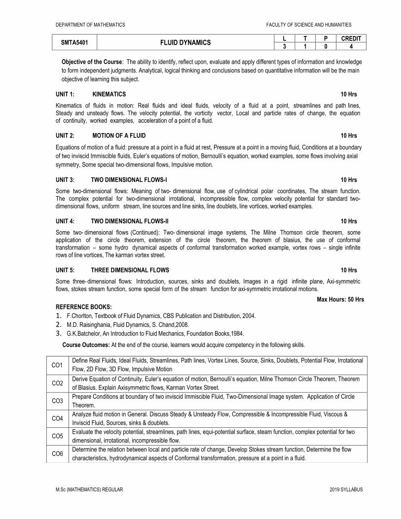
Objective of the Course: The ability to identify, reflect upon, evaluate and apply different types of information and knowledge
to form independent judgments. Analytical, logical thinking and conclusions based on quantitative information will be the main
objective of learning this subject.
UNIT 1: KINEMATICS 10 Hrs
Kinematics of fluids in motion: Real fluids and ideal fluids, velocity of a fluid at a point, streamlines and path lines, Steady and unsteady flows. The velocity potential, the vorticity vector, Local and particle rates of change, the equation of continuity, worked examples, acceleration of a point of a fluid. UNIT 2: MOTION OF A FLUID 10 Hrs
Equations of motion of a fluid: pressure at a point in a fluid at rest, Pressure at a point in a moving fluid, Conditions at a boundary
of two inviscid Immiscible fluids, Euler’s equations of motion, Bernoulli’s equation, worked examples, some flows involving axial
symmetry, Some special two-dimensional flows, Impulsive motion.
UNIT 3: TWO DIMENSIONAL FLOWS-I 10 Hrs
Some two-dimensional flows: Meaning of two- dimensional flow, use of cylindrical polar coordinates, The stream function. The complex potential for two-dimensional irrotational, incompressible flow, complex velocity potential for standard two-dimensional flows, uniform stream, line sources and line sinks, line doublets, line vortices, worked examples. UNIT 4: TWO DIMENSIONAL FLOWS-II 10 Hrs
Some two- dimensional flows (Continued): Two- dimensional image systems, The Milne Thomson circle theorem, some application of the circle theorem, extension of the circle theorem, the theorem of blasius, the use of conformal transformation – some hydro dynamical aspects of conformal transformation worked example, vortex rows – single infinite rows of line vortices, The karman vortex street. UNIT 5: THREE DIMENSIONAL FLOWS 10 Hrs
Some three- dimensional flows: Introduction, sources, sinks and doublets, Images in a rigid infinite plane, Axi-symmetric flows, stokes stream function, some special form of the stream function for axi-symmetric irrotational motions.
Max Hours: 50 Hrs REFERENCE BOOKS:
1. F.Chorlton, Textbook of Fluid Dynamics, CBS Publication and Distribution, 2004.
2. M.D. Raisinghania, Fluid Dynamics, S. Chand,2008.
3. G.K.Batchelor, An Introduction to Fluid Mechanics, Foundation Books,1984.
Course Outcomes: At the end of the course, learners would acquire competency in the following skills.
SMTA5401 FLUID DYNAMICS L T P CREDIT
3 1 0 4
CO1 Define Real Fluids, Ideal Fluids, Streamlines, Path lines, Vortex Lines, Source, Sinks, Doublets, Potential Flow, Irrotational
Flow, 2D Flow, 3D Flow, Impulsive Motion
CO2 Derive Equation of Continuity, Euler’s equation of motion, Bernoulli’s equation, Milne Thomson Circle Theorem, Theorem
of Blasius. Explain Axisymmetric flows, Karman Vortex Street.
CO3 Prepare Conditions at boundary of two inviscid Immiscible Fluid, Two-Dimensional Image system. Application of Circle
Theorem.
CO4 Analyze fluid motion in General. Discuss Steady & Unsteady Flow, Compressible & Incompressible Fluid, Viscous &
Inviscid Fluid, Sources, sinks & doublets.
CO5 Evaluate the velocity potential, streamlines, path lines, equi-potential surface, steam function, complex potential for two
dimensional, irrotational, incompressible flow.
CO6 Determine the relation between local and particle rate of change, Develop Stokes stream function, Determine the flow
characteristics, hydrodynamical aspects of Conformal transformation, pressure at a point in a fluid.

SCHOOL OF SCIENCE & HUMANITIES
DEPARTMENT OF MATHEMATICS
UNIT – I - KINEMATICS – SMTA5401
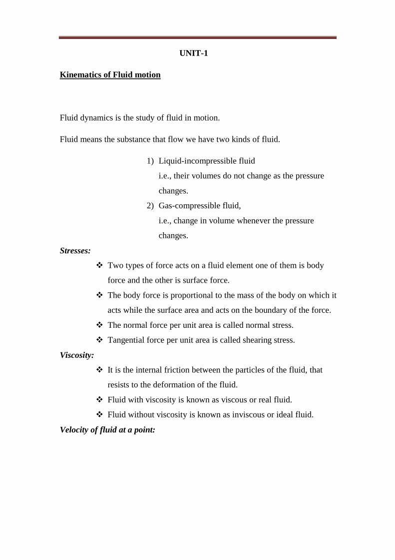
UNIT-1
Kinematics of Fluid motion
Fluid dynamics is the study of fluid in motion.
Fluid means the substance that flow we have two kinds of fluid.
1) Liquid-incompressible fluid
i.e., their volumes do not change as the pressure
changes.
2) Gas-compressible fluid,
i.e., change in volume whenever the pressure
changes.
Stresses:
Two types of force acts on a fluid element one of them is body
force and the other is surface force.
The body force is proportional to the mass of the body on which it
acts while the surface area and acts on the boundary of the force.
The normal force per unit area is called normal stress.
Tangential force per unit area is called shearing stress.
Viscosity:
It is the internal friction between the particles of the fluid, that
resists to the deformation of the fluid.
Fluid with viscosity is known as viscous or real fluid.
Fluid without viscosity is known as inviscous or ideal fluid.
Velocity of fluid at a point:

Let at time t the particle be at the point P. OP r and at the time t. t t
the particle P’ such that rOP' r .In the interval t ,moment of the particle is
rPP' Then, the particle r 0 r
t drq
dtlim
,q is dependent on both r and t
Streamlines:
It is the curve drawn in the fluid such that direction of the tangent to it at
any point coincides with the direction of fluid velocity at that point.
Derivation of streamlines:
At any point P, let q [u, v, w] be the velocity at the point P(x,y,z) of
the fluid. The direction ratios of the tangent to the curve at P(x,y,z) are
dr [dx,dy,dz]
Since, the tangent and the velocity at P have the same direction, we have
q dr 0
i.e., (vdw wdy)i (udz wdx) j (udy vdx)k 0
vdw wdy 0
dz dy
w v
udz wdx 0
dz dx
w u
udy vdx 0
dy dx
v u
i.e., dx dy dz
u v w
These are the differential equation for the streamlines. i.e., their solution gives
the streamlines

1 2 3q ,q ,q ,..... denote the velocities at neighbouring points 1 2P ,P ,..... then, the
small straight line segments 1 2 2 3 3 4PP ,P P ,P P ..... collectively give the approximate
form of streamline.
Pathlines:
When the fluid motion is steady, so that pattern of flow does not very
with time. The paths of the fluid particle coincide with the streamlines, though
the streamline through any point P does touch the pathline through P.
In case of unsteady motion, the flow pattern varies with time and the
paths of the particle do not coincide with the streamline.
In case of unsteady motion, the flow pattern varies with time and the paths of
the particle do not coincide with the streamline.
Pathlines are the curve described by the fluid particles during their motion.
i.e., these are the paths of the particle the differential equation of
pathlines are,
drq
dt
dxu
dt ,
dyv
dt ,
dzw
dt
where x,y,z are the Cartesian co-ordinates of the fluid and not a fixed point of
space.
Notes:
Streamlines give motion of a particle at a given instant, whereas the pathlines
gives the motion of a given particle at each instant.
Streamtube:
If we draw the streamline through every point of a closed curve in the fluid we
obtain streamtube.

Velocity potential:
Let the fluid velocity at time t is q=[u,v,w] in Cartesian form.
The equation of streamlines at one instant is dx dy dz
u v w
The curve cut the surface udx vdy wdz 0
Suppose, the expression udx vdy wdz 0 is an exact differential say(-dφ)
i.e., dx dy dz dt udx vdy wdzx y t t
where φ is φ(x,y,z,t) is some scalar function, uniform throughout the entire
field.
Therefore, u , v , w , 0x y t t
(x, y, z)
q ui v j wk
i j k
x y z
Note:
q , the negative sign is a convention and it ensures a flow takes
place from higher or lower potential.
The level surface φ(x,y,xz,t)=constant are called equi-potentials or equi-
potential surfaces.
When curl q=0, the flow is said to be irrotational of potential kind. For
such flow, the field of q is conservated and q is lamellar vector.
Vorticity:
q=[u v w] be the velocity vector of a fluid particle then the vector
q is called vortex vector or vorticity.
The components are 1 2 3, ,

1
2
3
w vi.e.,
y z
u w
z x
v u
x y
Note:
The fluid motion is said to be rotational if q 0
If q 0 then the fluid motion is irrotational or of potential kind.
Vortex line:
It is the curve in the fluid there exist the tangent at any point on the curve has
the direction of vorticity vector.
Vortex tube:
It is the surface formed by drawing vortex lines through each point of the
closed curve in the fluid.
A vortex tube with small cross-section called a vortex filament.
Problem:
At the point in an incompressible fluid having spherical
polar co-ordinates(r,φ,ψ), the velocity component are
3 32 r cos , r sin ,0 where M is a constant. Show that velocity is of
potential kind. Find the velocity potential and the equations of streamlines.
Solution:
Taking ˆˆ ˆds drr rd r sind
3 3 ˆˆq 2 r cos r r sin 0
We obtain curl q ⇨ q

2
3 3
ˆˆ ˆr r r sin1
rr sin
2 r cos r sin 0
q =0.
Thus, the flow is of potential kind. Let r, , be the approximate velocity
potential.
Then, 3 32 r cos , r sin , 0r r r sin
d dr d dr
3 2(2Mr cos )dr (Mr sin )d 0d
32Mr cos
The streamlines are given by 3 2
dr r d r sin d
2Mr cos M r sin 0
d 0
12cot d dr
r
Int, cost
2r Asin
Equation of continuity:
When a region of a fluid contains neither source nor sinks i.e.,when
there is no inlets and outlets through which the fluid can enter or have the

region the mass contained inside a given volume of fluid remains constant
throughout the motion.
Let ∆ be a closed surface drawn in the fluid and taken fixed in space.
Let it contains a volume ∆v of the fluid and let ρ=ρ(x,y,z,t) be the fluid density
at any point (x,y,z) of the fluid in ∆v at any time t.
Let n be unit outward drawn normal at any surface element δs of∆s. δs ≤∆s.
Then if q is the fluid velocity at the element δs , the normal component of q
measured outward from ∆v is n.q .
We consider the mass of fluid which leaves ∆v by flowing across an element δs
of∆s in time δt.
This quantity is exactly that which is contained in a small cylinder of cross
section δs of length ˆ(q.n) t
Mass of the fluid=density*volume
= ˆ(q.n) t. s
Hence, the rate of at which fluid leaves ∇v by flowing across the element δs is
ˆ(q.n) s
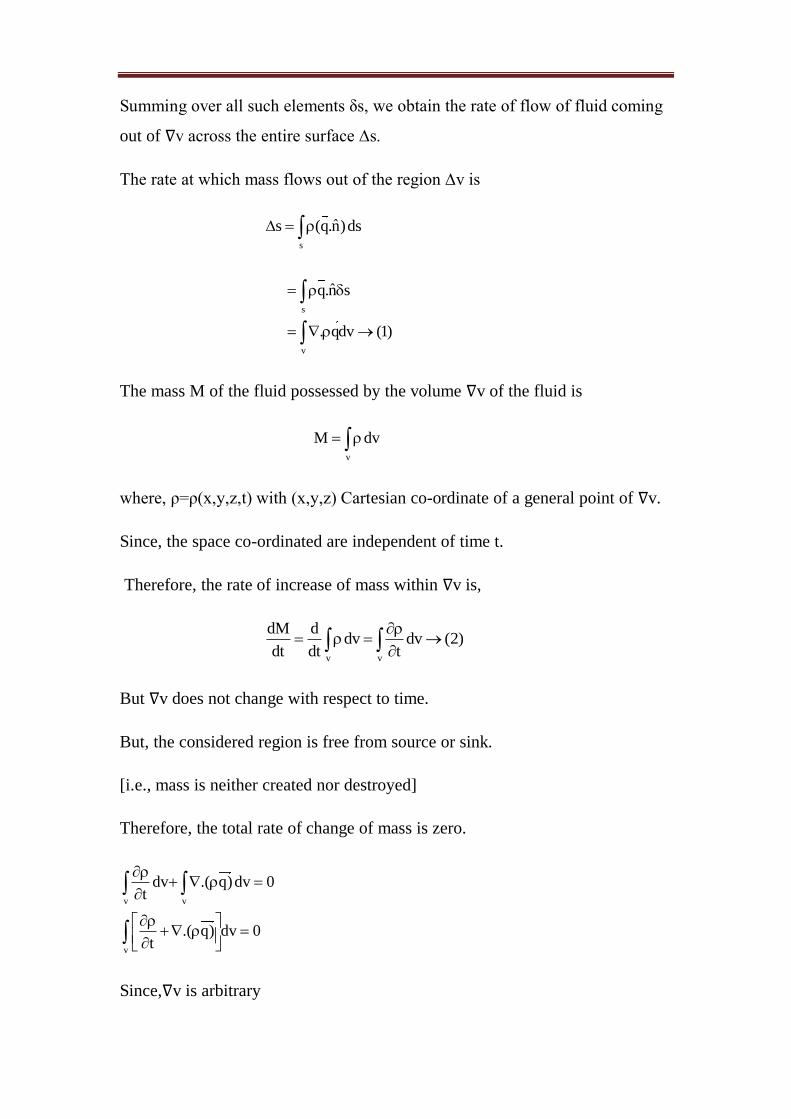
Summing over all such elements δs, we obtain the rate of flow of fluid coming
out of ∇v across the entire surface ∆s.
The rate at which mass flows out of the region ∆v is
s
ˆs (q.n)ds
s
v
ˆq.n s
. qdv (1)
The mass M of the fluid possessed by the volume ∇v of the fluid is
v
M dv
where, ρ=ρ(x,y,z,t) with (x,y,z) Cartesian co-ordinate of a general point of ∇v.
Since, the space co-ordinated are independent of time t.
Therefore, the rate of increase of mass within ∇v is,
v v
dM ddv dv (2)
dt dt t
But ∇v does not change with respect to time.
But, the considered region is free from source or sink.
[i.e., mass is neither created nor destroyed]
Therefore, the total rate of change of mass is zero.
v v
v
dv .( q)dv 0t
.( q) dv 0t
Since,∇v is arbitrary

.( q) 0 (3)t
This is known as equation of continuity which must always hold at any points
of a fluid free from sources and sinks.
Other form of equation of continuity
1) q q. 0 (4)t
2) q 0t
We consider the differential following fluid motion
From equation(4)
The equation of continuity
( .q) (q. ) 0t
q. (q. ) 0t
D(q. ) 0...............(5)
Dt
3) Equation (5) can be written as
1 D. .q 0
Dt
D(log ) .q 0
Dt
4) When the motion of fluid steady
0t
From (5) the equation of continuity
. q 0
Here ρ is a function of time
i.e. ρ=ρ(x,y,z)

5) When the fluid is incompressible then ρ=constant and thus D
0Dt
From (5) equation of continuity
. q 0
q 0
The same is for homogenous and incompressible fluid.
6) If the fluid is homogenous, incompressible and the flow is of potential
kind.
i.e., q
then, the equation of continuity becomes
q 0
2
( ) 0
0
This is Laplace equation.
Example:
Text whether the motion specified by 2
j i
2 2
K (x y )q
x y
, k is constant
is a possible motion for incompressible fluid. If so determine the equation of
the streamlines. Also test whether the motion is of the potential kind and if so
determine the velocity potential.
Solution:
To prove the given velocity is possible motion of Incompressible fluid
i.e to prove ∇.q=0

2 2 2
2 2 2 2 2 2
i j kx y z
K (x j yi) K yi K x jq or
x y x y x y
2
2 2
K (x j yi).q i j k
x y z x y
2 2
2 2 2 2
K y K x
x x y y x y
2 2
2 22 2 2 2
K y 2x ( 2x)K y
x y x y
0
.q 0
Therefore the given velocity is possibly the motion of incompressible
fluid.
Streamlines
The equation of streamlines are given by
2 2
2 2 2 2
dx dy dz
x y z
dx dy dz
K y K x 0
x y x y
dx dy dz
y x 0
xdx ydy …………1
dz 0 …………………..2
Integrating we get
From 1
2 2x y c …………….3
From2
Z = constant
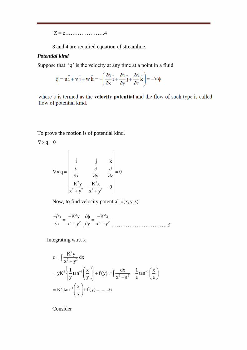
Z = c………………….4
3 and 4 are required equation of streamline.
Potential kind
Suppose that ‘q’ is the velocity at any time at a point in a fluid.
To prove the motion is of potential kind.
q 0
2 2
2 2 2 2
i j k
q 0x y z
K y K x0
x y x y
Now, to find velocity potential (x, y, z)
2
2 2
K y
x x y
,
2
2 2
K x
y x y
…………………………..5
Integrating w.r.t x
2
2 2
2 1 1
2 2
2 1
K ydx
x y
1 x dx 1 xyK tan f (y) tan
y y x a a a
xK tan f (y)...........6
y
Consider
2 1
222
22
22 2
2
2 2
xK tan f (y)yy y
1 xK f '(y)y
x1y
y xK f '(y)yx y
K xf '(y)..........................7
x y
From 7 and 5
f '(y) 0
f (y) cons tan t
2 1 xK tan c
y
The equipotential is thus given by the plane x=cy through z.
Example
For an incompressible fluid q=[-wy,wx,0],w=constant. Discuss the nature
of flow.
The flow is said to be of potential kind if q 0
q wyi wx j ok
i j k
qx y z
wy wx 0
wx i wy j wx wy k
z z x y
k(w w) 2wk 0
which it is rotational.
The flow is not of potential kind. It is a rigid body rotating about the z-axis
with constant vector angular velocity wk .
i.e., for the velocity at (x,y,z) in the body is wyi wx j
Equation of streamlines are
dx dy dz
wy wx 0
Therefore, the streamlines are the circle
x2+y2=c and z=c
Example
For a fluid moving in a fine tube of variable section prove from 1st
principle that the equation of continuity is A A v 0t s
where v is the
speed at the point P of the fluid and s is the length of the tube upto P.
What does this become for the steady incompressible fluid.
Solution:
Let OPP’ be the central streamline of the tube.
Let S and S+δS be the arc length of OP and OP’.
Let v be the velocity of the fluid at P.
Let A be the area of the section at P. We assume the conditions are constant
over the section A.
So that rate of mass flux over A in the sense of S increasing is ρvA.
At the neighbouring section, A’ through P’ the mass flux per unit time in the
direction of S increasing is vA s. vAs

At the same instant of time t . Thus, the net rate of flow of mass into the
element between the section A and A+δA.
vA* s ( vA) vAs
s ( vA)s
But at time t, the mass between the sections is A s
Rate of increases, ( A s)t
A st
In the absence of sources and sinks
s ( vA) A ss t
i.e.,A vA 0t s
For steady incompressible flow, the ρ is constant
A ( vA) 0t s
c
(vA) 0s
di.e., (vA) 0
ds
vA=constant
i.e., volume of fluid crossing every section per unit time is
constant.

Liquid flows through a pipe whose surface is the surface of revolution of
the curve 2Kxy a
a about x-axis (-a≤x≤a). If the liquid enters at the end
x=-a of the pipe with velocity v. Show that the time taken by liquid particle
to traverse the entire length of the pipe from x=-a to x=a is
2
2
2a 2 11 k k3 5v(1 k)
Solution:
Let v0 be the velocity at the section at the section x=0
The area of the section x=-a 22a 1 k
The area of the section x=0 2a
The area of the section distant x from 0
22kx
aa
By equation of continuity
22
22 2 0
0
kxa 1 k a v a .x
a
Since, x0 is the velocity across the plane distant x from o
22
2
2a 2
2
0
kx dxdt a .
a (1 k) v
2 kxt a dx
v(1 k) a
Which gives the stated result.
Local and particle rate of change.

Suppose a particle of fluid moves form p(x,y,z) at time t to
P '(x x, y y,z z) at time t+δt.Let f(x,y,z,t) be a scalar function associated
with some properties of fluid.Then, the motion of the particle from p to p’ the
total change of is
f f f ff x y z t
x y z t
Thus, the total rate of change of f at a point P at a time t.
In the motion of the particle,
t 0
df flim
dt x
f dx f dy f dz f
x dt y dt z dt t
f f f fu v w
x y z t
If q=[u,v,w] is the velocity of the fluid particle at P
df fq. f (1)
dt t
Similiarlly, for a velocity function F(x,y,z,t) associtated with
some property of a fluid.
dF F
q. F (2)dt t
Hence, both the scalar and vector function of position and time,
By operation equality d
q. (3)dt t
,provided that those functions are
associated with the properties of the moving fluid.
In the obtaining equation (1) and (2), we considered total change.
When the fluid particle moves from p(x,y,z) to P '(x x, y y,z z) in time
δt.

Thus, df dF
,dt dt
are a total differentiation following the fluid particles are
called particle rates of change.
On the other hand, partical time derivative f F
,t t
are only the time rates
of change at the point p(x,y,z)
Consider fixed in space at a point p(x,y,z) they are the local rates of
change. It follows that q. f or q. F
We presents the rate of change due to the motion of particle along it
path.
Then, nothing the arc length of the a path by S and PP’ by δS.
Simillarly, for a function F Here we use, s.s
Conditions at a rigid boundary
P is the point on the boundary where the fluid velocity is q, boundary has the
velocity U.
If n specifies a unit normal direction at P then q.n=U.n .Since, there is no
relative normal velocity at P between boundary and fluid.
Note:
for invicous fluid the above condition exist.
For viscous fluid, there is no slip, tangential components must be equal.
If the boundary is at rest, q.n=0. Every point of boundary.
UNIT -2
SCHOOL OF SCIENCE & HUMANITIES
DEPARTMENT OF MATHEMATICS
UNIT – II – MOTION OF A FLUID – SMTA5401

Let P be a point in a fluid moving with velocity q . We insert an elementary
rigid plane area A into this fluid at point P. This Plane area also moves with
the velocity q of the local fluid at P
If F denotes the force exited on one side of A by the fluid particles on the
other side, then this is will act normal to A
We assume that 0
lt
A
F
A
exists uniquely.
Then, this limit is called the (hydrodynamic) fluid pressure at point P and is
denoted by P.
1. Pressure P at a point P in a moving fluid is some in all direction.
Or
Pressure p at P in a moving fluid is independent of the orientation of A
Let q be the velocity of the fluid. We consider an elementary tetrahedron.
PQRS of the fluid at a point P of the moving fluid.
Let the edges of the tetrahedron be PQ= x , PR= y , PS= z at time t, where
, ,x y z are taken along the co-ordinate axes ox,oy,oz resp. This tetrahedron
is also moving with the velocity q of the local fluid at P.
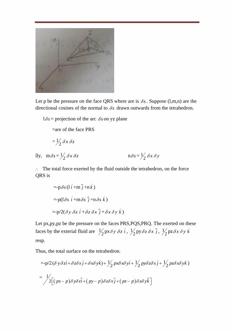
Let p be the pressure on the face QRS where are is s . Suppose (l,m,n) are the
directional cosines of the normal to s drawn outwards from the tetrahedron.
l s = projection of the arc s on yz plane
=are of the face PRS
= 12
x z
lly, m s = 12
x z n s = 12
x y
The total force exerted by the fluid outside the tetrahedron, on the force
QRS is
=-p s (l i +m j +n k )
=-p(l s i +m s j +n s k )
=-p/2( y z i + z x j + x y k )
Let px,py,pz be the pressure on the faces PRS,PQS,PRQ. The exerted on these
faces by the exterial fluid are 12
px y z i , 12
py z x j , 12
pz x y k
resp.
Thus, the total surface on the tetrahedron.
=-p/2 1 1 1( y )2 2 2
zi z x j x yk px x yi py z x j pz x yk )
=
12 px p y zi py p z x j pz p x yk
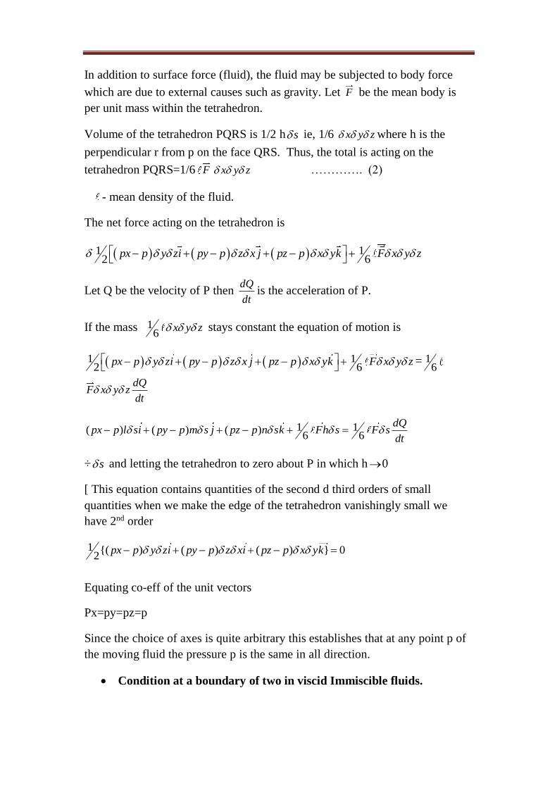
In addition to surface force (fluid), the fluid may be subjected to body force
which are due to external causes such as gravity. Let F be the mean body is
per unit mass within the tetrahedron.
Volume of the tetrahedron PQRS is 1/2 h s ie, 1/6 x y z where h is the
perpendicular r from p on the face QRS. Thus, the total is acting on the
tetrahedron PQRS=1/6 F x y z …………. (2)
- mean density of the fluid.
The net force acting on the tetrahedron is
1 12 6
px p y zi py p z x j pz p x yk F x y z
Let Q be the velocity of P then dQ
dtis the acceleration of P.
If the mass 16
x y z stays constant the equation of motion is
1 12 6
px p y zi py p z x j pz p x yk F x y z
= 16
dQF x y z
dt
1 1( ) ( ) ( )6 6
dQpx p l si py p m s j pz p n sk Fh s F s
dt
÷ s and letting the tetrahedron to zero about P in which h0
[ This equation contains quantities of the second d third orders of small
quantities when we make the edge of the tetrahedron vanishingly small we
have 2nd order
1 {( ) ( ) ( ) } 02
px p y zi py p z xi pz p x yk
Equating co-eff of the unit vectors
Px=py=pz=p
Since the choice of axes is quite arbitrary this establishes that at any point p of
the moving fluid the pressure p is the same in all direction.
Condition at a boundary of two in viscid Immiscible fluids.
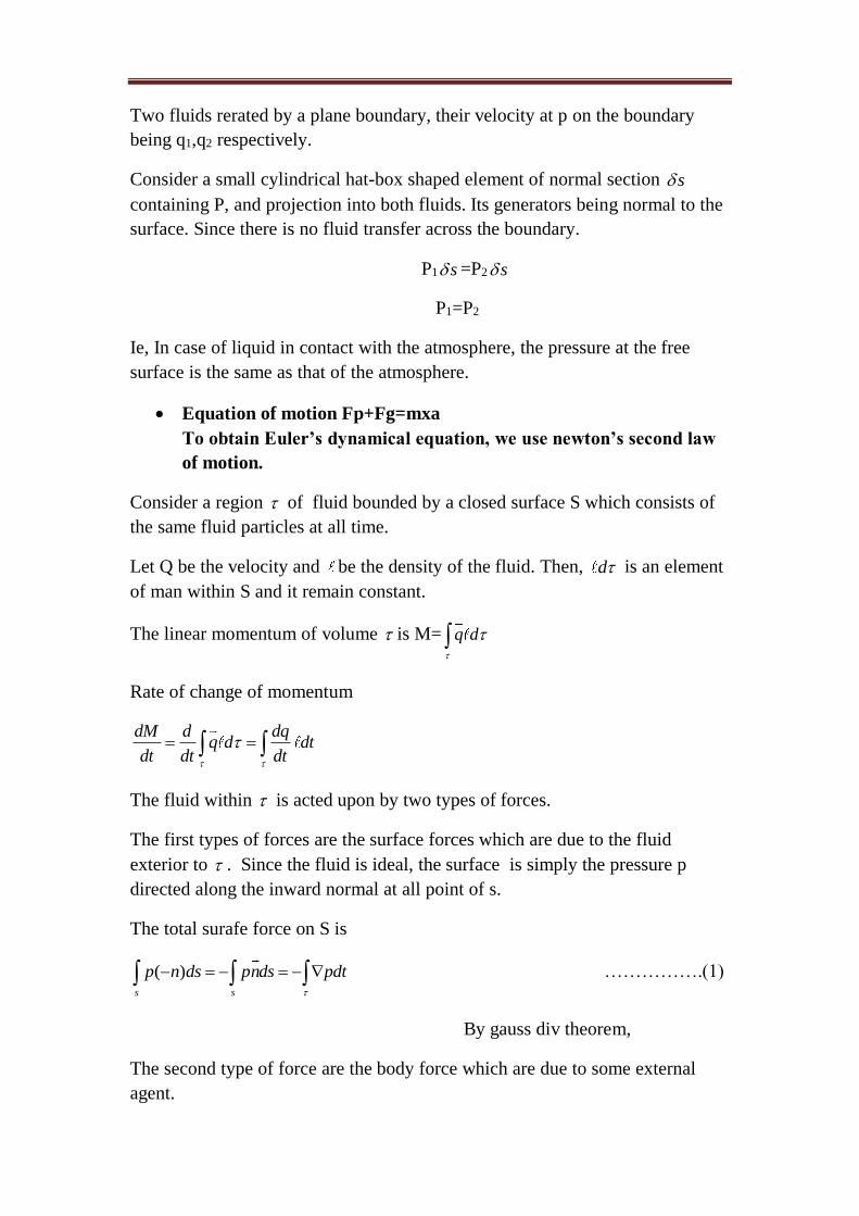
Two fluids rerated by a plane boundary, their velocity at p on the boundary
being q1,q2 respectively.
Consider a small cylindrical hat-box shaped element of normal section s
containing P, and projection into both fluids. Its generators being normal to the
surface. Since there is no fluid transfer across the boundary.
P1 s =P2 s
P1=P2
Ie, In case of liquid in contact with the atmosphere, the pressure at the free
surface is the same as that of the atmosphere.
Equation of motion Fp+Fg=mxa
To obtain Euler’s dynamical equation, we use newton’s second law
of motion.
Consider a region of fluid bounded by a closed surface S which consists of
the same fluid particles at all time.
Let Q be the velocity and be the density of the fluid. Then, d is an element
of man within S and it remain constant.
The linear momentum of volume is M= q d
Rate of change of momentum
dM d dqq d dt
dt dt dt
The fluid within is acted upon by two types of forces.
The first types of forces are the surface forces which are due to the fluid
exterior to . Since the fluid is ideal, the surface is simply the pressure p
directed along the inward normal at all point of s.
The total surafe force on S is
( )s s
p n ds pnds pdt
…………….(1)
By gauss div theorem,
The second type of force are the body force which are due to some external
agent.
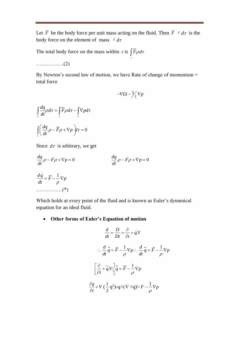
Let F be the body force per unit mass acting on the fluid. Then F d is the
body force on the element of mass d
The total body force on the mass within is F d
…………….(2)
By Newton’s second law of motion, we have Rate of change of momentum =
total force
1 p
dqd F d pd
dt
0dq
F p ddt
Since d is arbitrary, we get
0dq
F pdt
0dq
F pdt
1dqF p
dt
……………(*)
Which holds at every point of the fluid and is known as Euler’s dynamical
equation for an ideal fluid.
Other forms of Euler’s Equation of motion
.d D
qdt Dt t
1d
q F pdt
1d
q F pdt
1
.q q F pt
q
t
(
1
2q2)-q˄(˄q)=
1F p
.q (1
2q2)-(X q )X q
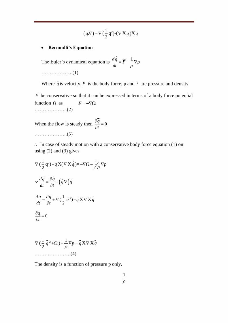
Bernoulli’s Equation
The Euler’s dynamical equation is 1dq
F pdt
……………….(1)
Where q is velocity, F is the body force, p and are pressure and density
F be conservative so that it can be expressed in terms of a body force potential
function as F
………………..(2)
When the flow is steady then 0q
t
………………..(3)
In case of steady motion with a conservative body force equation (1) on
using (2) and (3) gives
(1
2q2) q X(X q )= 1 p
.dq q
q qdt t
d q q
dt t
(1
2q 2) q XX q
0q
t
(1
2q 2 )
1p
q XX q
………………….(4)
The density is a function of pressure p only.
1

1
p
dp
Using in (4), we get
[ 12
q 2dp
q
X(X q )
……………………..(5)
Multiplying (5) scalarly by q
q .( q X curl q )=( q X q ).curl q =0
q . [1
2q 2 dp
=0
…..………………(6)
If s is a unit vector along the streamline through general point of the fluid and
S measure distance along this streamline, then since S is parallel to q
eqn (6) gives s
[
1
2q 2 dp
]=0 s q
q ks
ss
Hence along any particular streamline, we have
1
2q 2 dp
c
………………..(7)
Where c is constant which takes different values for different streamlines. (7) is
called Bernoulli’s equation
Some potential theorem.
An irrotational motion is called acyclic if the velocity potential is a
single valued function.
ie, when at every field point, a unique velocity potential exists, otherwise the
irrotational motion is said to be cyclic.

For a possible fluid motion, ever if is multivalued at a particular point, the
velocity at that point must be single valued.
We prove number of theorems for steady irrotational incompressible flows for
which the velocity potential satisfies 2 0 .
Mean value of velocity potential over spherical surface.
THEOREM:
The mean value of a over any spherical surface S drawn in the fluid
throughout whose interior
2 0 , is equal to the value of at the center of the sphere.
If S is the boundary of a spherical surface lying wholly within the fluid, then
the mean value of the velocity potential is equal to its value at the center of the
sphere.
Let p be the value of at the center P of a spherical surface S of radius r,
wholly lying in the liquid. Let denotes the mean value of over S.
Let us draw another concentric sphere of unit radius.. Then, a cone with
vertex P which intercepts are ds form the sphere S intercepts an area d from
the sphere .
2
21
ds r
dw ds=r2 d
Now by definition
2
1
4
s
s
s
ds
dsrds
2
1
4c
dsr r r
Since the normal n
to the surface is along the radius r
on s, we have .nr n

2
1.
4s
n dsr r
2
1.
4s
ndr
(Gauss theorem)
2
2
10
4d
r
0 0
Where is the volume enclosed by surface S Thus 0r
constant
Hence, is independent of r, so that the mean value of is the same over all
sphere having the same center and therefore is equal to its value at the center.
THEOREM:
If is the solid boundary of a large spherical surface of radius R, containing
fluid in motion and also enclosing one or more closed surface, then the mean
value of on is of the form
= M CR
Where M and C are constant , provided that the fluid extends to infinitely and
is at rest there
(or)
If the liquid of infinite extent is in irrotational motion and is bounded internally
by of one or more closed surfaces s, the mean value of over a large sphere ,
of radius R, which enclose S is of the form M
CR
where M and C are
constants provided that the liquid is at rest at infinity.
PROOF:
Suppose that the volume of fluid acrossing each of internal surface contained
within , per unit time is a finite quantity say 4 m [ 4 m represent the flux
of fluid across or s]
Since the fluid velocity at any point of is R
radially outwards, the equation
f continuity gives
4d MR
2d R dw
21
4R dw m
R
2
1
4
mdw
R R
2
1
4
mdw
R R
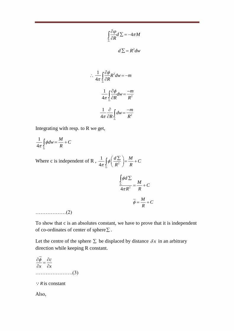
Integrating with resp. to R we get,
1
4
Mdw C
R
Where c is independent of R , 2
1
4
d MC
R R
24
dM
CR R
M
CR
………………(2)
To show that c is an absolutes constant, we have to prove that it is independent
of co-ordinates of center of sphere .
Let the centre of the sphere be displaced by distance x in an arbitrary
direction while keeping R constant.
c
x x
………………….(3)
R is constant
Also,

1 1
4 4dw dw
x x x
0
From, (3) we get,
0
cc
x
is an absolute constant.
Hence,
M
CR
where M and C are constant.
*THEOREM:
With the radiation of theorem 3, if the fluid is at rest at infinity and if each
surface m is rigid, then the kinetic energy of the moving fluid is
2
1
1 1 .2 2
k
mv m
T q dv dsn
(or)
If is the solid boundary of a large spherical surface of Radius R, containing
fluid in motion and also enclosing one or more closed surface, is p
denotes
the potential at any point P of the fluid, if the fluid is at rest and if each
surface ,m mX S is rigid then the kinetic energy of the moving fluid is
2
1
1 1 .2 2
k
mv m
T q dv dsn
PROOF:
Kinetic energy, from of energy that an object or a particle has by reason
T=1/2 of its motion is
K.E 21
2mv
Kinetic energy of a fluid particle of mass v is 21
2svq
21
2dv q q
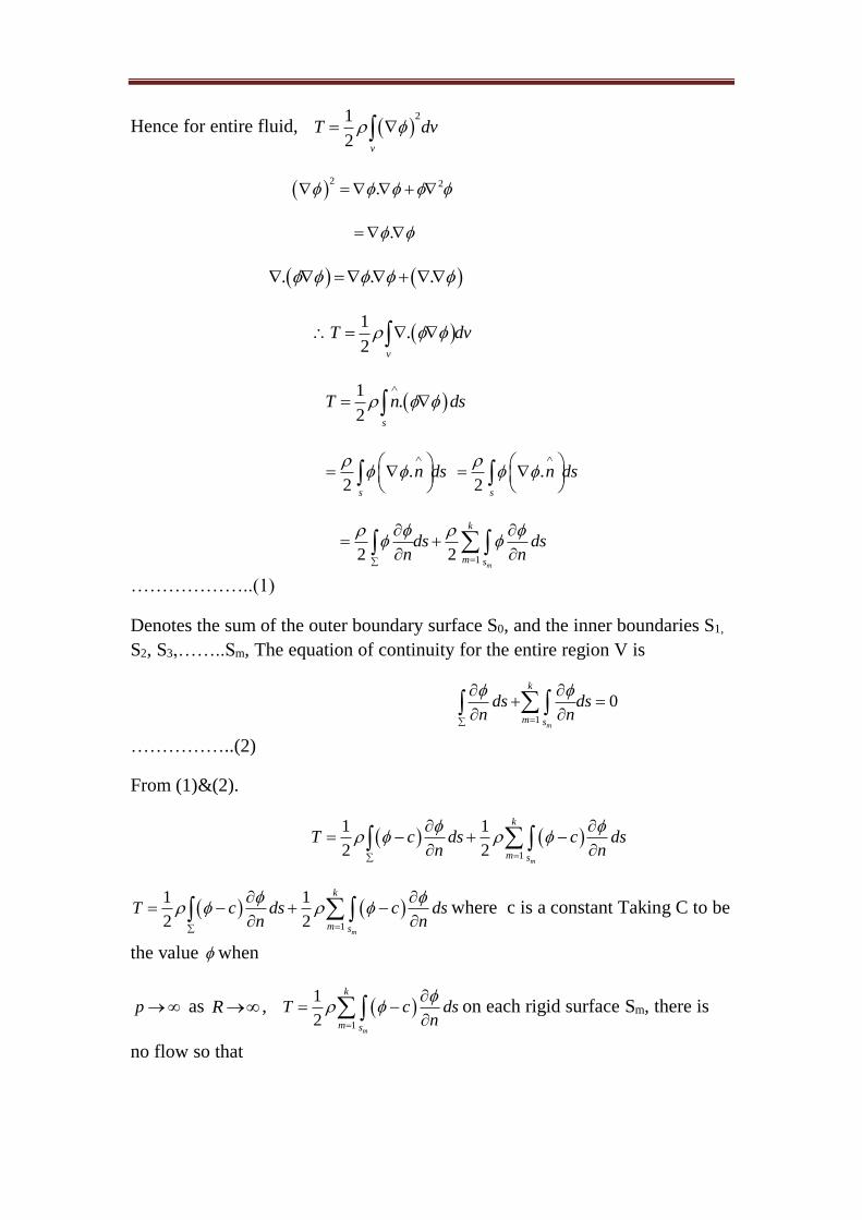
Hence for entire fluid, 21
2v
T dv
2 2.
.
. . .
1
.2
v
T dv
1
.2
s
T n ds
.2
s
n ds
.2
s
n ds
12 2
m
k
m s
ds dsn n
………………..(1)
Denotes the sum of the outer boundary surface S0, and the inner boundaries S1,
S2, S3,……..Sm, The equation of continuity for the entire region V is
1
0
m
k
m s
ds dsn n
……………..(2)
From (1)&(2).
1
1 1
2 2m
k
m s
T c ds c dsn n
1
1 1
2 2m
k
m s
T c ds c dsn n
where c is a constant Taking C to be
the value when
p as R , 1
1
2m
k
m s
T c dsn
on each rigid surface Sm, there is
no flow so that

0
ms
dsn
,
Then, 1
1
2m
k
m s
T dsn
Hence Proved
UNIQUENESS THEOREM:1
If is the solid boundary of large spherical surface of Radius R, cont. fluid in
motion and enclosing one or more closed surface then M
cR
provided the
fluid extends to infinity and is at rest, if each surface Sm is rigid and K.E of the
moving fluid.
2
1
1
2 2m
k
mv s
T q dv dsn
2
1
1
2 2m
k
mv s
T q dv dsn
Then, if either or n
is prescribed on each surface Sm, then, is determine
uniquely through an arbitrary constant.
PROOF:
From previous theorem, 2
1m
k
mv s
dv dsn
………………(1)
Within v 2
1m
k
mv s
dv dsn
2 0
………………..(2)
Suppose 1 2, are the two solutions of (2) subject to (1).
Write, 1 2 then. 2 2 2
1 2 0 in V
Thus, is a harmonic function satisfying similar condition to 1 2,
Hence, 2
1m
k
mv s
dv dsn
……………(3)

On each Sm, either 1 2 or 1 2
n n
ie, either 0 or 0
n
thus in all
cases 0n
On each Sm, so that the RHS of (3) is zero. 2
0v
dv
…….…………(4)
Since, 2
0 , the condition (4) holds only if, 0 in V
………………(5)
(5) gives is constant 1 2 constant
* UNIQUENESS THEOREM:2
If the fluid of theorem V is in uniform motion at infinity and if v
is
prescribed on each surface Sm then is uniquely determined throughout V.
Let V be the velocity of the fluid at infinity suppose a velocity –v on the entire
system so as to reduce the velocity of the fluid at infinity to rest. Then the
condition of then V prevails in which the velocity at all points of each Sm are
known in a fluid which is at rest at infinity. This leads to a unique value of
at each point of v
If the region occupied b the fluid is infinite and fluid is at rest at infinity, prove
that only one irrotational motion is possible when internal boundaries have
prescribed velocities.
Let there be two irrotational motions gives by two different velocity potential
1 2,
The condition are boundaries are 1 2
n n
…………………(1)
1 2 0q q at infinity
……………….(2)
1 2
…………………(3)
2 2 2
1 2 0 0 0

Motion given by is also irrotational
Further from (3) we get
1 2 0n n n
. 0q n q n on the surface .
Also,
1 2q
1 2 0q q at using ( 2)
0q everyone on the surface and also at infinity .
Hence we get constant
1 2 constant
…………………(4)
We can take the constant on RHS (4) to be zero (it gives no motion) and thus
we get, 1 2
Some flows involving axial symmetry
If the region occupied by the fluid is infinite then only one irrotational motion
of the fluid exists when the boundaries have prescribed velocities .
(or)
Show that there cannot be 2 different forms of a cyclic irrotational motion of a
given liquid whose boundaries have prescribed velocities . Let 1 and 2 be
two different velocity potentials representing two motions then
2 2
1 20
Since , the kinetic conditions at the boundaries are satisfied by both flows
therefore at each point of s 1 2
n n
Let 1 2

2 2 2
1 2 0 at each point of fluid 2 2 2
1 2 0 at each point of
S.
Kinetic energy is given by
2 02 2
s
q d dsn
0n
0q at each point of fluid.
1 2
1 2
0
0
1 2
1 2
0
0
Which shows that the motion are the same. Moreover is unique apart from an
additive constant which gives vise be no velocity and thus can be taken as zero.
Some flows involving axial symmetry.
Let , ,r be the velocity potential at any point having spherical polar co-
ordinates , ,r in a fluid of steady irrotational incompressible flow laplace
equation 2 =0
Since,
22
2
1sin sin 0
sinr
r r
when there is symmetric about the line 0 then ,r and the becomes
2sin sin 0rr r
special solution of (1) are
2
1cos , cosr
r
Thus the move general solution,
2, cosr Ar Br
Stationary sphere in a uniform stream sphere at rest in a uniform
stream.
Consider an impermeable solid of radius a at rest with its center and at the pole
of system of spherical polar co-ordinates , ,r
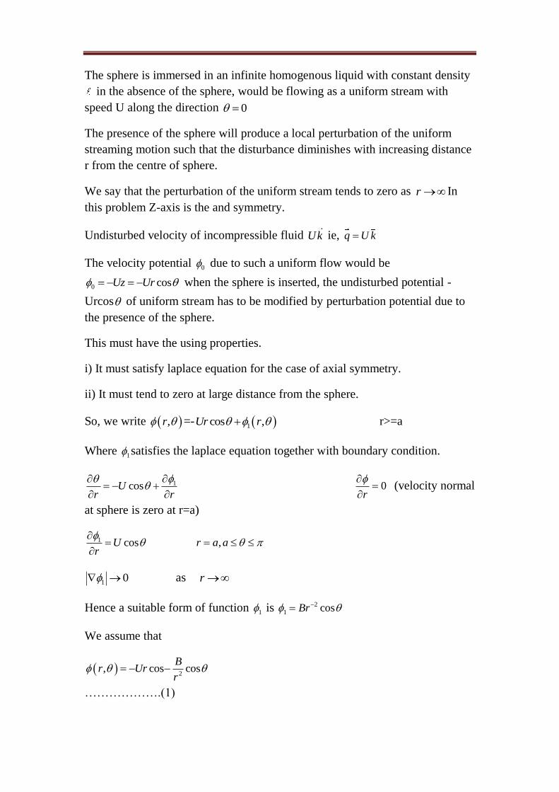
The sphere is immersed in an infinite homogenous liquid with constant density
in the absence of the sphere, would be flowing as a uniform stream with
speed U along the direction 0
The presence of the sphere will produce a local perturbation of the uniform
streaming motion such that the disturbance diminishes with increasing distance
r from the centre of sphere.
We say that the perturbation of the uniform stream tends to zero as r In
this problem Z-axis is the and symmetry.
Undisturbed velocity of incompressible fluid Uk ie, q U k
The velocity potential 0 due to such a uniform flow would be
0 cosUz Ur when the sphere is inserted, the undisturbed potential -
Urcos of uniform stream has to be modified by perturbation potential due to
the presence of the sphere.
This must have the using properties.
i) It must satisfy laplace equation for the case of axial symmetry.
ii) It must tend to zero at large distance from the sphere.
So, we write ,r =- 1cos ,Ur r r>=a
Where 1 satisfies the laplace equation together with boundary condition.
1cosUr r
0
r
(velocity normal
at sphere is zero at r=a)
1 cosUr
,r a a
1 0 as r
Hence a suitable form of function 1 is 12 cosBr
We assume that
2, cos cos
Br Ur
r
……………….(1)
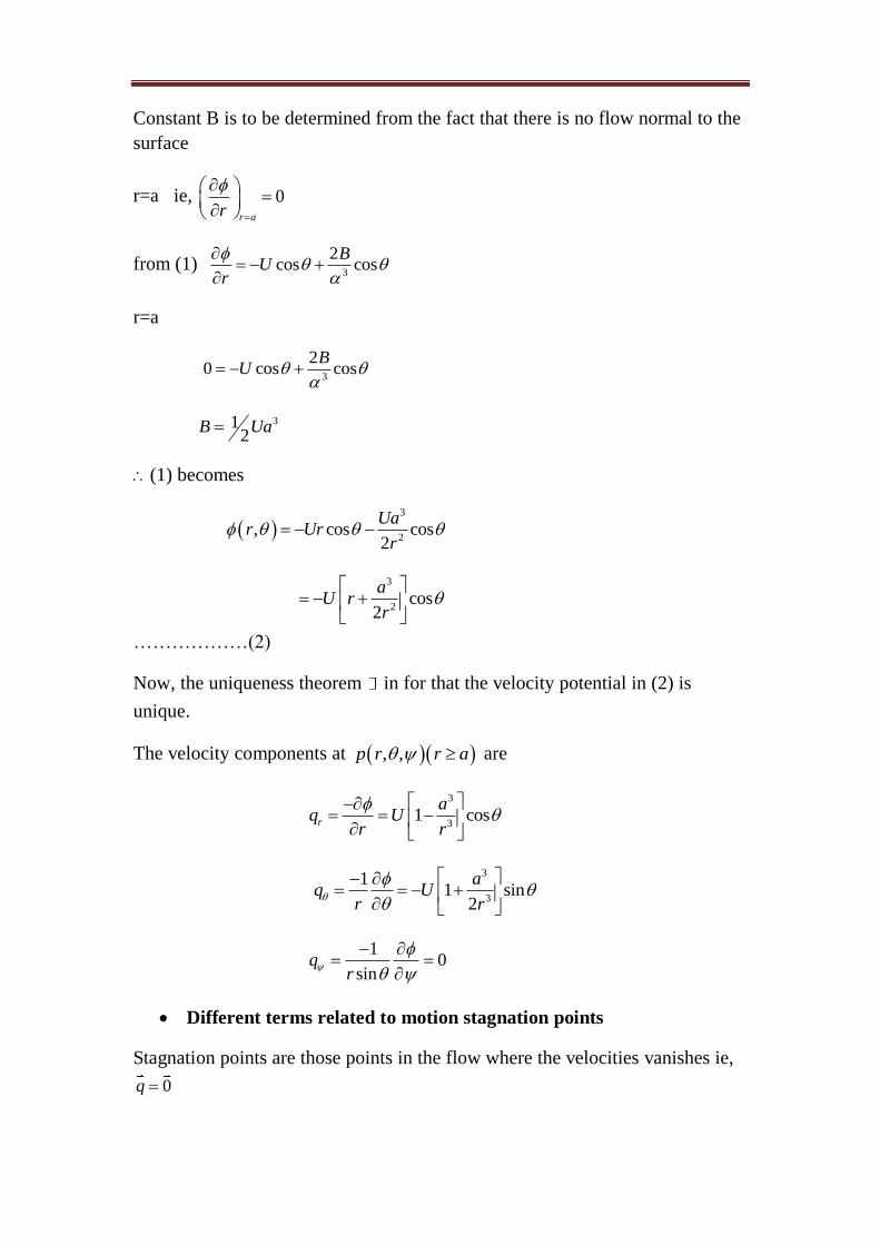
Constant B is to be determined from the fact that there is no flow normal to the
surface
r=a ie, 0r ar
from (1) 3
2cos cos
BU
r
r=a
3
20 cos cos
BU
31
2B Ua
(1) becomes
3
2, cos cos
2
Uar Ur
r
3
2cos
2
aU r
r
………………(2)
Now, the uniqueness theorem in for that the velocity potential in (2) is
unique.
The velocity components at , ,p r r a are
3
31 cosr
aq U
r r
3
3
11 sin
2
aq U
r r
1
0sin
qr
Different terms related to motion stagnation points
Stagnation points are those points in the flow where the velocities vanishes ie,
0q
Thus, these points are obtained by solving the equations
3
3
3
3
1 cos 0
1 sin 02
aU
r
aU
r
………………….(4)
Which are satisfied only by r=a, 0, . Thus the stagnation points are
, 0 ,r a and r a on the sphere There are referred to respectively
as the near and forward stagnation points.
Stream lines
The equation of streamlines sin
r
dr rd r d
q q q
3 3
3 3
sin
01 cos 1 sin
2
dr rd r d
a aU U
r r
r a
0d
=constant
3 3
3 31 cos 1 sin
2
a ar d dr
r r
3 3 3 3
3 3
2cos sin
2
r a r ar d dr
r r
32
32
21
2cot
ar
r dr dar
rr
32
2
32
21
2cot
ar
rr dr dar
rr
Integrating we get,
2 3 1log 2logsin logr a r c
3 32log logsin log
r ac
r
2
3 3sin 0
crc
r a
For each value of C1, above equation given a streamline in the plane
=constant.
The choice of C=0 corresponds to the sphere and axis of symmetric.
Pressure at any point (stagnation pressure)
We find stagnation pressure at any point by applying Bernoulli’s equation
along the streamline.
The pressure at any point of the fluid is obtained by applying Bernoulli’s
equation along the streamline through the point, taking the pressure at to be
of constant value p Thus in the absence of body force, the Bernoulli’s
equation for homogeneous steady flow is
23 3
2 2
3 3
11 cos 1 sin 1
2 2
a ap p U
r r
23 3
2 2
3 3
11 cos 1 sin 1
2 2
a ap p U
r r
21
2
pC
…..…………(a)
At infinity P p and U k we get 21
2
pC U
……………..(b)
From (a) and (b)
2 21 1
2 2
ppU

221 1
2 2p p U
2
3 32 2 2
3 3
1 11 cos 1 sin
2 2 2
a ap U U
r r
q
23 3
2 2
3 3
11 cos 1 sin 1
2 2
a ap p U
r r
…..……..(5)
Which gives the pressure at any point of the fluid of particular interest is the
distribution of pressure on the boundary of the sphere. It is obtained by putting
r=a in (5)
23
2 2
3
11 sin 1
2 2
ap p U
a
23
2 2
5
1 3sin 1
2 2
ap U
a
2 21 9sin 1
8 4p U
2 214 9sin
8p U
2 219cos 5
8p U
The maximum pressure occurs at the stagnation point where 0 or
2
max
1
2p p U maxp
maxp is also called stagnation pressure.

The minimum pressure occurs along the equation circle of sphere where 2
2
min5
8p p pu
A fluid is pressured to be incapable of sustaining a negative pressure then
min
80
5
pp U
. At this stage the fluid will tend to break away from the
surface of the sphere and cavitation is said to occur.
Ie, vaccum is formed.
Thrust on the hemisphere
We find thrust (force) on the hemisphere on which the liquid impinges r=a,
02
Let s be a small element at 0 , ,p a of the hemisphere bounded by circles
at r=a and at angular distance and from the axis of symmetry (z-axis)
The component of the thrust on s is cos sp . Hence total thrust on the
hemisphere is along Z’o and is given by
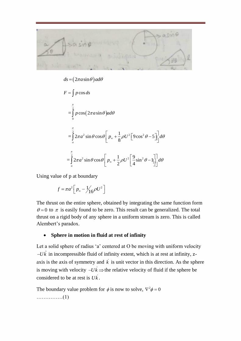
2 sinds a ad
cosF p ds
= 2
0
cos 2 sinp a ad
=2
2 2 212 sin cos 9cos 5
8o
a p U d
=2
2 2 21 92 sin cos sin 1
2 4o
a p U d
Using value of p at boundary
2 2116
f a p U
The thrust on the entire sphere, obtained by integrating the same function form
0 to is easily found to be zero. This result can be generalized. The total
thrust on a rigid body of any sphere in a uniform stream is zero. This is called
Alembert’s paradox.
Sphere in motion in fluid at rest of infinity
Let a solid sphere of radius ‘a’ centered at O be moving with uniform velocity
U k in incompressible fluid of infinity extent, which is at rest at infinity, z-
axis is the axis of symmetry and k is unit vector in this direction. As the sphere
is moving with velocity Uk the relative velocity of fluid if the sphere be
considered to be at rest is Uk .
The boundary value problem for is now to solve, 2 0
……………(1)

Such that cosUr
(r=a)
……………(2)
And 0 r
…………….(3)
The present case is also a problem with axial symmetry about the axis 0,
so, ,r
Also, Since, 1(cos ) cosp
Legendre function and the boundary condition (2) implies that the dependence
of an must be like cos ,
has the form
12( ) (cos )
BAr p
r
2
( ) cosB
Arr
To satisfy (3), it is necessary that A=0 and then from (2) we get 312
B Ua
Thus, the solution for is
3
2cos
2
Ua
r
From here, the velocity component are obtained to be
3
3cosr
Uaq
r r
3
3
1sin
2
Uaq
r r r
0q 0q
Where ( , , )r are spherical polar co-ordinates the various terms of particular
importance related to this motion.
Streamline

The differential equations for streamlines are sin
r
dr rd r d
q q q
3 3
3 3
sin
0cos sin
2
dr rd r d
Ua Ua
r r
0d =constant
2cotdr
dr
, log 2logsin logr C
2sinr c
Streamline, line are 2sinr c , =constant.
Kinetic energy of the liquid.
Let S be the surface of sphere and be the density of liquid, then kinetic energy
is given by
12
s
T dsn
Where n is the outward unit normal. But for the sphere n is along radius
vector
sn r
(r=a)
=1
cos cos2
Ua U
= 2 21cos
2U a
2 2
1
1cos
2 2s
T v a ds
= 2
2
0
cos 2 sin4
ava ad
= 3 2
2 2
0
cos sin2
a vd

= 3 2 3
0
cos
2 3
a v
= 2
3 2 31 433 4
va v a
= 1 21
4m v
……………….(6)
Where 1 34
3m a is the mass of the liquid displaced by the sphere.
Also, F.E of the sphere moving with speed v is given by, 2
2
1
2T mv
…………………(7)
34
3M a is the mass of the sphere being the density of the material of the
sphere.
From (6) and (7), Total Kinetic Energy T is 1 2T T T
1
2
mm
1 21 1[ m ]U
2 2T m t
121
[ ]U2 2
mT m he quantity
1
2
mm is called the virtual
mass of the sphere.
Accelerating sphere moving in a fluid at rest at infinity
The solution derived above for is applicable when the sphere translates
unsteadily along a stream line
( )U U and the velocity potential has 3
2, , cos
2
U t ar t
r
…………….(1)
The instantaneous values of velocity comp and F.E at time t are given by
3
3cosr
U t aq
r
,
3
3sin
2
U t aq
r
, 0q (similar to steady case)
1 21 1[ m ]U
2 2T m t
……………..(2)
The pressure at any point of the fluid is obtained by using Bernoulli’s equation
for unsteady flow of a homogenous liquid, in the absence of body force an,
21
2
pU f t
t
………………….(3)21
2
ppU
t
Where f(t) is a function of time t only let to be the presence at infinity where
the fluid is at rest
From (3) we get,
( )p
f tt
cos
rU
t
21
2
ppU
t
……………..(4)
To find t
U Uk U t k is the velocity of sphere the velocity potential given in (1)
can be expressed in the from 3
3
.1
2
a u r
r ……………….(5)
Since r is the position vector of a fixed point P of the fluid relative to the
moving centre O of the sphere, it is the U rt
………………(6)
2 . .r r
r r r r r r ut t
using (6)
.r uk
.ru r k

cosru
cosr
Ut
……………...(7)
Diff (5) with respect to ‘t’
2 2
3 2
3 2 3
1 cos 3[ cos ]
2
U U Ua
t r r t r
3 2 2
2
2 3 3
U cos 3[ cos ]
2
a U U
r r r
uU
t
Also,
2 6 2 62
2 2 2 2
6 6cos sin
4r
U a U aU q q
r r
2 62 2
6
1[cos sin ]
4
U a
r
=2 6
2 2
6
1[cos sin ]
4
U a
r
The pressure at any point of the fluid can be obtained from equation (4)u
Ut
In particular at a point on the sphere r=a
2 2 21[ cos 3 cos ]
2Ua U U
t
2
2 2[4cos sin ]4
UU
And the corresponding pressure is given by
2 21 1cos (9cos 5)2 8
ppUa U
………………(5)
The forces (thrust) acting on the sphere is given by
0
cos (2 sin )F p a ad k
2 21 1cos (9cos 5)2 8
ppUa U
2
2 2[4cos sin ]4
UU
.2 2 2
0
1 12 [ cos (9cos 5)]cos sin2 8
a k p U a pU d
3 32 41 ( )23 3
a U k a U k
11
2m U k
34
3m a is mass of the liquid displaced.
This shows that the force acts in the direction appointing the sphere’s motion.
Sphere moving with constant velocity which is otherwise at rest.
We consider a solid sphere with centre O moving with uniform velocity iU in
incompressible fluid of infinite extent which is at rest at infinity OX is the axis
of symmetry and the direction of unit vector i. We take to be finite at infinity
then, the velocity potential at , ,P r where r>=a will be in the form
2( , ) Ar cosr
……………….(1)
This satisfies the axiom symmetric form of laplace equation in spherical polar
co-ordinates are
1 1
sinr r r
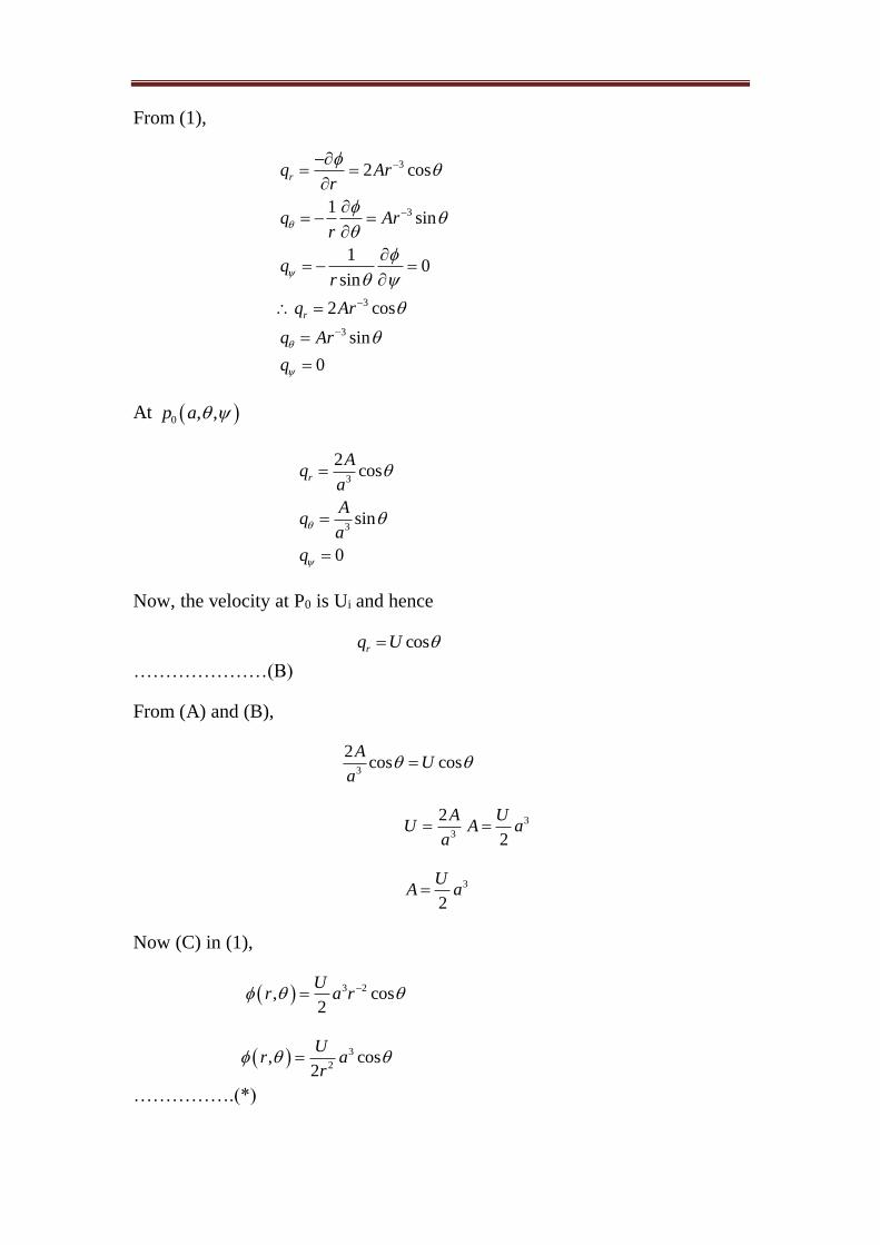
From (1),
3
3
3
3
2 cos
1sin
10
sin
2 cos
sin
0
r
r
q Arr
q Arr
qr
q Ar
q Ar
q
At 0 , ,p a
3
3
2cos
sin
0
r
Aq
a
Aq
a
q
Now, the velocity at P0 is Ui and hence
cosrq U
…………………(B)
From (A) and (B),
3
2cos cos
AU
a
3
2AU
a 3
2
UA a
3
2
UA a
Now (C) in (1),
3 2, cos2
Ur a r
3
2, cos
2
Ur a
r
…………….(*)
To find kinetic energy of a fluid
We consider,
1
2s
T dsr
1
( )2
s
dsr
From (*)
3
3cos
Ua
r r
1
2s
T dsr
3 3
2 3cos cos
2
Ua Ua
r r r
2 6
2
5cos
2
U a
r
r=a
2
2cos2
U a
2
21cos
2 2s
U aT ds
2
2cos4
s
U ads
2
2 2cos (2 sin )4
s
aUa d
3 2
2cos sin2
s
a Ud
3 2
2
0
cos (cos )2
a Ud
3 2 3
0
cos
2 3
a U
3 2 1 1
2 3 3
a U
3 2 2
2 3
a U
3 2
3
a U
Accelerating sphere moving in fluid at ret at infinity
(or)
A sphere of centre I and radius a moves through an infinite liquid of
constant density at rest at infinity O describes a straight lines with
velocity V(t) if there are no body force show that the pressure P at points
on the surface of sphere in a plane perpendicular to the straight lines at a
distance x from O measure positively in a direction of v given by.
2
2 2
2
5 9 1( )
8 8 2o
x dvP p v v x
a dt
op is pressure at infinity reduce that the thrust on sphere is 11
2
dvM
dt where
M1 is the man of liquid having the volume of sphere.
Sol:
Let , ,p r be a point such that, at P is given by
2, , ( ) cosr A t r which satisfies the spherical polar form of laplace
equation.
3[ ( )( 2 cos )]rq A t rr
32 ( ) cosA t r
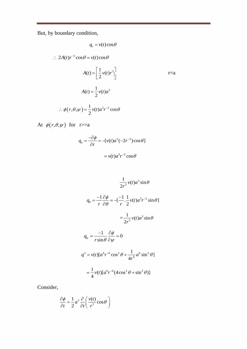
But, by boundary condition,
( )cosrq v t
32 ( ) cos ( )cosA t r v t
31( ) ( )
2A t v t r
r=a
31( ) ( )
2A t v t a
3 21, , ( ) cos
2r v t a r
At , ,r for r>=a
3 3[ ( ) ( 2 )cos ]oq v t a rr
3 3( ) cosv t a r
3
3
1( ) sin
2v t a
r
3 21 1 1[ . ( ) sin ]
2q v t a r
r r
= 3
3
1( ) sin
2v t a
r
1
0sin
qr
2 6 6 2 6 2
6
1( )[ cos sin ]
4q v t a r a
r
6 6 2 21( )[ (4cos sin )]
4v t a r
Consider,
3
2
1 ( )cos
2
v ta
t t r

3
2 2
1 cos cos[
2
dva v
r dt t r
2 3
cos .r i
t r t r
3.r i rt
3 4. ( 3 )r r
i r r t rt t
po r
( )r
t
vel of O =Vi
i
rv
t
2 2r r
2 2
r rr r
t t
1,i
rv r
t r
2
2 3
cos( 1 3cos )
v
t r r
The Bernoulli’s equation,
21( )
2 2a f t
t
3
6 6 2 2 2 2 3
3
1( )a (4 sin ) [ cos 3 cos ]
8 2
p a dvv t r cos r v v d
r dt
Putting , r a , cosx a
22 2
2
5 9 1
8 8 2o
x dvp p v v x
a dt
SCHOOL OF SCIENCE & HUMANITIES
DEPARTMENT OF MATHEMATICS
UNIT – III – TWO DIMENSIONAL FLOWS-I – SMTA5401

UNIT-III
Some two dimensional flow use of cyclindrical polar co-ordinates.
For an incompressible irrotational flow of uniform density, the
equation of continuity 2 0 for the velocity potential r, , z in cylindrical
polar co-ordinates r, , z is 2 2
2 2 2
1 1r 0 1
r r r r z
If the flow is two dimensional and the co-ordinate axes are to so
chosen that all physical quantities associated with the fluid are independent of z
then r,
∴ (1) becomes,
2
2 2
1 1r 0 2
r r r r
Let r, f (r)g( ) be the solution of equ (2) for separation of
variables.
Thus, we get 2
1 d 1g( ) [rf '(r)] f (r)g''( ) 0
r dr r
dr [rf '(r)]
g''( )dr 4f (r) g( )
Thus, L.H.S of (4) is a function of r only and RHS is a function of θ
only.
As r,θ are independent variables. So, each side of equ(4) is a
constant say λ.
2r f ''(r) rf'(r) g''( )
f (r) g( )
i.e. , 2r f ''(r) rf'(r) f (r) 0 5
g''( ) g( ) 0 6
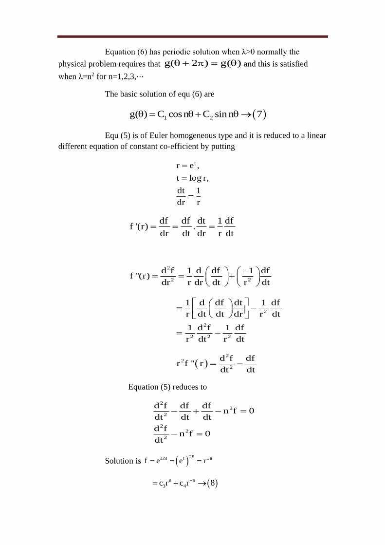
Equation (6) has periodic solution when λ>0 normally the
physical problem requires that g( 2 ) g( ) and this is satisfied
when λ=n2 for n=1,2,3,⋯
The basic solution of equ (6) are
1 2g( ) C cosn C sin n 7
Equ (5) is of Euler homogeneous type and it is reduced to a linear
different equation of constant co-efficient by putting
tr e ,
t log r,
dt 1
dr r
df df dt 1 dff '(r) .
dr dt dr r dt
2
2 2
d f 1 d df 1 dff ''(r)
dr r dr dt r dt
2
2
2 2 2
1 d df dt 1 df
r dt dt dr r dt
1 d f 1 df
r dt r dt
2
2
2
d f dfr f '' r
dt dt
Equation (5) reduces to
22
2
22
2
d f df dfn f 0
dt dt dt
d fn f 0
dt
Solution is n
nt t nf e e r
n n
3 4c r c r 8
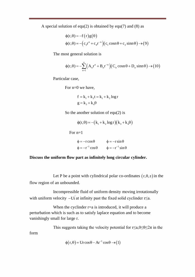
A special solution of equ(2) is obtained by equ(7) and (8) as
n n
3 4 1 2
(r, ) f r g
(r, ) c r c r c cosn c sinn 9
The most general solution is
n n
n n n n
n 1
(r, ) A r B r C cosn D sinn 10
Particular case,
For n=0 we have,
1 2 1 2
3 4
f k k t k k log r
g k k
So the another solution of equ(2) is
1 2 3 4(r, ) k k logr k k
For n=1
1
r cos
r cos
1
r sin
r sin
Discuss the uniform flow part as infinitely long circular cylinder.
Let P be a point with cylindrical polar co-ordinates r, , z in the
flow region of an unbounded.
Incompressible fluid of uniform density moving irrotationally
with uniform velocity Ui at infinity past the fixed solid cyclinder r≤a.
When the cyclinder r=a is introduced, it will produce a
perturbation which is such as to satisfy laplace equation and to become
vanishingly small for large r.
This suggests taking the velocity potential for r≤a,0≤θ≤2π in the
form
1r, Urcos Ar cos 1
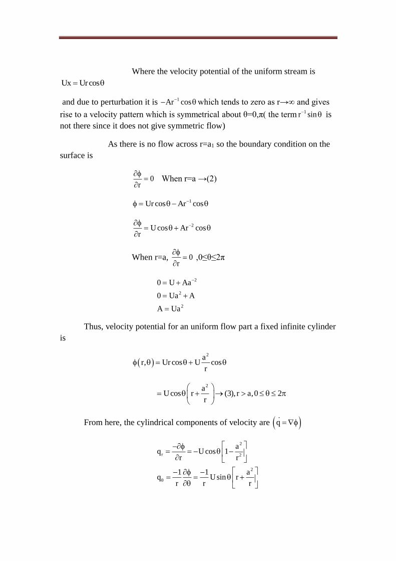
Where the velocity potential of the uniform stream is
Ux Urcos
and due to perturbation it is 1Ar cos which tends to zero as r→∞ and gives
rise to a velocity pattern which is symmetrical about θ=0,π( the term 1r sin is
not there since it does not give symmetric flow)
As there is no flow across r=a1 so the boundary condition on the
surface is
0r
When r=a →(2)
1Ur cos Ar cos
2U cos Ar cosr
When r=a,
0r
,0≤θ≤2π
2
2
2
0 U Aa
0 Ua A
A Ua
Thus, velocity potential for an uniform flow part a fixed infinite cylinder
is
2a
r, Ur cos U cosr
2a
Ucos r (3), r a,0 2r
From here, the cylindrical components of velocity are q
2
r 2
2
aq U cos 1
r r
1 1 aq Usin r
r r r

2
2
aUsin 1
r
zq 0z
We note that as r→∞, rq Ucos ,q Usin which are consistent with
the velocity at infinity Ui of the uniform stream.
Stream function:
When motion is the same in all planes parallel to xy plane and there is
no velocity parallel to the x-axis i.e., when u,v are function of x,y,t and w=0.
The motion is regarded as two-dimensional.
Now to consider the flow across a curve in this plane, we mean the flow
across unit length of a cylinder where trace on the xy plane is the curve in
question, the generations of the cylinder being parallel to the z-axis.
For a two-dimensional motion in x-y plane, q is a function of x,y,t only
and the differential equation of the streamline are
dx dy
i.e., vdx udy 0 1u v
and corresponding equation of continuity
u v
0 2x y
Equation (2) is condition of exactness of (1)
It is that (1) must be exact differential vdx udy d dx dyx y
u , v
y x
This function ψ is called the stream function or the current
function or lagranges stream function. Then streamlines are given by the
solution of (1) is dψ=0, i.e, ψ=constant.
Thus, the stream function is constant along a streamlines.
Note:
It is clear that the existence of stream function is merely a consequence
of the continuity and incompressibility of fluid.
The stream function always exists is all types of two dimensional motion
whether rotational or irroational.
Physical interpretation of stream function.
Let P be a point on a curve C in x-y plane. Let an element ds of
the curve makes an angle θ with x-axis. The direction cosines of the normal at
P are
cos 90 ,cos ,0
i.e., sin ,cos ,0
The flow across the curve C from right to left is
C
ˆq.nds where n sin i cos j
q ui v j
C
C
C
C
B A
C
u sin vcos ds
sin cos ds u , vy x y x
dx dy dx dyds cos ,sin
y ds x ds ds ds
dx dyy x
d
Where A Band are the values of ψ at the initial and final
points of the curve.
Thus, the difference of the values of a stream function at any two
points represents the flow across the curve, joining the two points.
Corolloary:
Suppose that the curve C be the streamline, then no fluid crosses its
boundary, then B A B A0
Ψ is constant along C.
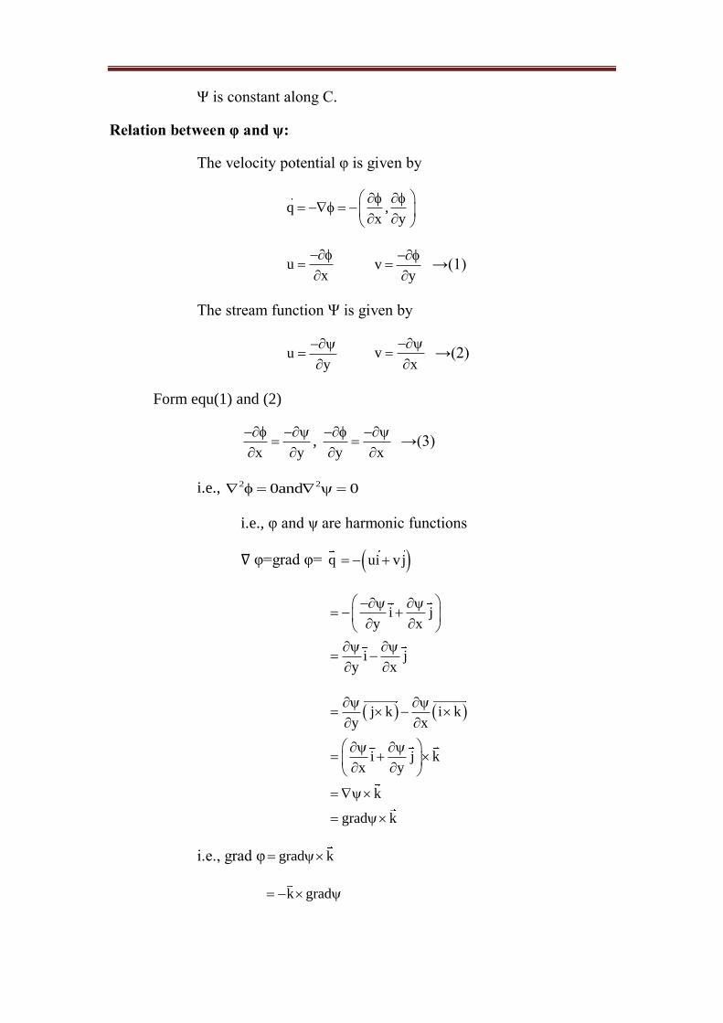
Relation between φ and ψ:
The velocity potential φ is given by
q ,x y
ux
v
y
→(1)
The stream function Ψ is given by
uy
v
x
→(2)
Form equ(1) and (2)
x y
,
y x
→(3)
i.e., 2 20and 0
i.e., φ and ψ are harmonic functions
∇ φ=grad φ= q ui vj
i jy x
i jy x
j k i ky x
i j kx y
k
grad k
i.e., grad φ grad k
k grad

k 4
Again from (3), we have
.x x y y
. . 0x x y y
. 0
Thus for irrotational incompressible two-dimensional flow
(steady or unsteady). x, y , x, y are harmonic functions and family of
curves
φ=constant(equipotential)
ψ=constant(streamlines) intersect
orthogonally.
Complex potential
We consider irrotational plane flows of incompressible fluid of uniform
density for which the velocity potential x, y and the stream function x, y
exist.
(x.y) specify two dimensional Cartesian co-ordinates in a plane of flow
w x, y i x, y 1
All four first order partial derivatives of φ and ψ with respect to
x,y exist and are continuous throughout the plane of flow.
Velocity q =(u,v) has components satisfying q
ux y
v
y x
→(2)
Thus, φ and ψ satisfy the C-R equations and so w must be an
analytic function of z=x+iy.
Therefore, we can write (1) as
w f(z) i 3

The function w=f(z) is called complex potential of the plane flow.
Complex velocity differential partially with respect to x
w i
z x iy
w
ix x x
i
x y
u iv
z x iy
z1
x
but cos iqsin
therefore, dw
u ivdz
,dw
u ivdz
i
q cos iqsin
q cos isin
qe
The combination u-iv is known as complex velocity.
Speed 2 2dwq u v
dz
and for stagnation points
dw0
dz .
Discuss the flow for which complex potential is w=z2
We have w=z2
=(x+iy)2
=x2-y2+2ixy
2 2x, y x y
x, y 2xy

The equtipotentials φ=constant are the rectangular hyperbola x2-
y2=constant having asymptotes y=±x.
The streamline ψ=constant are the rectangular hyperbola xy=constant
having the axes x=0 and y=0 as asymptotes.
Considerdw
2zdz
, therefore the only stagnation point is the
origin.
The two tamilips of curves cut each other orthogonally. Both φ
and ψ are harmonic and the flow is irroational.
Complex velocity potential for standard two-dimensional flows.
We consider flow patterns due to a uniform stream, a line source
and sink and a line labels.
Complex potential for a uniform tream we first consider the
uniform stream having velocity Ui
This gives rise to a velocity potential xU
w Uz U x iy
The stream function ψ=imaginary(w). So that the lines
y=constant are the streamlines.
Secondly, Let the uniform stream advance with a velocity having
magnitude U and being inclined at angle α, to the positive direction of x-axis.
u Ucos v Usin
dw
u ivdz
i
U cos iUsin
Ue
The simplest form of w, ignoring the constant of integrating is iw Uze
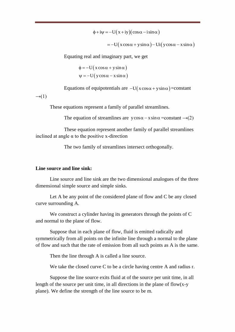
i U x iy cos isin
U xcos ysin Ui ycos xsin
Equating real and imaginary part, we get
U x cos ysin
U ycos x sin
Equations of equipotentials are U xcos ysin =constant
→(1)
These equations represent a family of parallel streamlines.
The equation of streamlines are ycos x sin =constant →(2)
These equation represent another family of parallel streamlines
inclined at angle α to the positive x-direction
The two family of streamlines intersect orthogonally.
Line source and line sink:
Line source and line sink are the two dimensional analogues of the three
dimensional simple source and simple sinks.
Let A be any point of the considered plane of flow and C be any closed
curve surrounding A.
We construct a cylinder having its generators through the points of C
and normal to the plane of flow.
Suppose that in each plane of flow, fluid is emitted radically and
symmetrically from all points on the infinite line through a normal to the plane
of flow and such that the rate of emission from all such points as A is the same.
Then the line through A is called a line source.
We take the closed curve C to be a circle having centre A and radius r.
Suppose the line source exits fluid at of the source per unit time, in all
length of the source per unit time, in all directions in the plane of flow(x-y
plane). We define the strength of the line source to be m.
A line source of strength –m is called a line sink.
Complex potential for a line source:
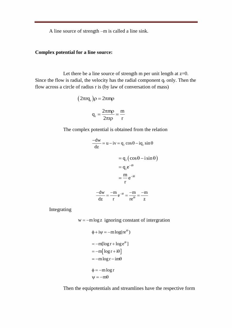
Let there be a line source of strength m per unit length at z=0.
Since the flow is radial, the velocity has the radial component qr only. Then the
flow across a circle of radius r is (by law of conversation of mass)
r2 rq 2 m
r
2 m mq
2 r r
The complex potential is obtained from the relation
r r
dwu iv q cos iq sin
dz
r
i
r
i
q cos isin
q e
me
r
i
i
dw m m me
dz r re z
Integrating
w m log z ignoring constant of intergration
ii mlog(re )
im[log r log e ]
m log r i
mlog r im
mlog r
m
Then the equipotentials and streamlines have the respective form

2 2
2 2
1
i.e., x y cons tan t
x y C
1
1
yi.e., tan cons tan t
x
y C x
Thus, the equipotential are circles and streamlines are
straight lines passing through origin.
If the line source is at z=z0 instead of z=0 then the complex
potential is
0w mlog z z
If there are a number of line source at 1 2 nz z ,z , , z of respective
strengths 1 2 nm ,m , ,m per unit length then the complex potential is
1 1 2 2 n nz m log z z m log z z m log z z
Complex potential for a line doublet:
The combination of a line source and a line sink of equal strength
when placed close to each other gives a line doublet.
Let us take a line source of strength m per unit length at iz ae
and a line sink of strength m per unit length at z=0.
∴ The complex potential due to the combination is
iw mlog z ae mlog(z 0)
i
i
1i
i 2 2i
2
z aemlog
z
aemlog 1
z
aem log 1
z
ae a em
z z

Suppose m become vary large and the distance between
source and sink ‘a’ becomes small.
Then ma→μ
i.e., m→∞ and a→0, ma→μ
ie
wz
If the line sink is situated at z=z0 then the complex potential is i
0
ew
z z
Notes:
If α=0 then the line source is an x-axis and thus 0
wz z
If there are number of line doublets of strength 1 2 n, , , per unit
length with line sinks at points 1 2 nz ,z , , z and their axis being inclined
at angles 1 2 n, , , with the positive direction of x-axis then the
complex potential is given by
1 2 ni i i
1 2 n
1 2 n
e e ew
z z z z z z
Example:
Discuss the flow due to a uniform line doublet at origin of strength 𝛍 per
unit length and its axis being along x-axis.
Solution:
We know that the complex potential for a doublet is i
0
ew
z z
.
when the doublet is at origin having its axis along z-axis then α=0,z=0
2 2
(x iy)w
z x iy x y
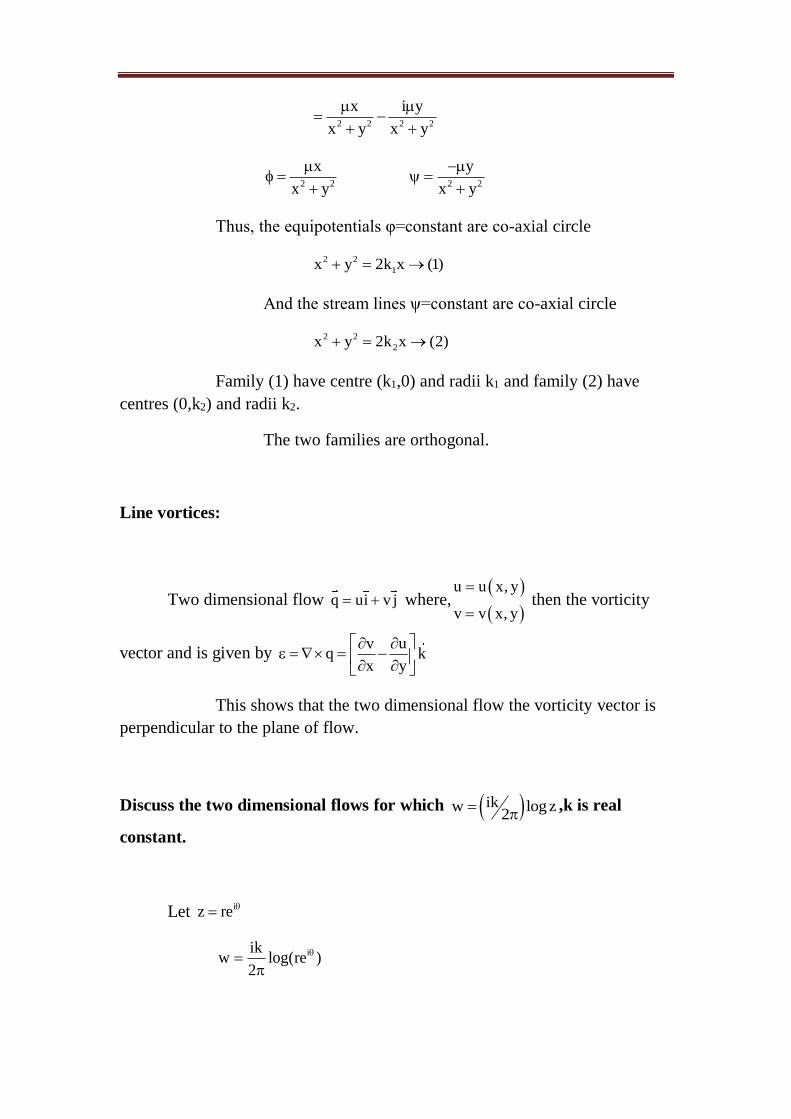
2 2 2 2
x i y
x y x y
2 2
x
x y
2 2
y
x y
Thus, the equipotentials φ=constant are co-axial circle
2 2
1x y 2k x (1)
And the stream lines ψ=constant are co-axial circle
2 2
2x y 2k x (2)
Family (1) have centre (k1,0) and radii k1 and family (2) have
centres (0,k2) and radii k2.
The two families are orthogonal.
Line vortices:
Two dimensional flow q ui v j where,
u u x, y
v v x, y
then the vorticity
vector and is given by v u
q kx y
This shows that the two dimensional flow the vorticity vector is
perpendicular to the plane of flow.
Discuss the two dimensional flows for which ikw log z2
,k is real
constant.
Let iz re
iikw log(re )
2

ik k
w log r2 2
k
2
klog r
2
Thus the streamlines in the plane of flow are the concentric
circles r=constant.
Equipotentials are the radii vectors θ=constant through the origin.
The two families are mutually orthogonal and φ,ψ are both
harmonic function.
The radial and transverse velocity components are
rq 0r
r
1 kq
r 2 r
The circulation round any closed curve and surrounding the
origin and in the plane of flow is given by q.ds
kq
2 r
ds dr.r rd .
k
q.ds d2
k k
d 2 k2 2
If ε does not surround, then is easily shown to be zero.
Hence, a two dimensional distribution having a complex velocity
potentialik
w logz2
gives a circulation round any closed curve ε in the plane
and enclosing the origin O of amount K.
Also,round any other curve in the plane of flow which does not enclose
O the circulation is zero.
The streamlines are the concentric circles r=constant and the
equipotentials the lines θ=constant.
Uniform line vortex.
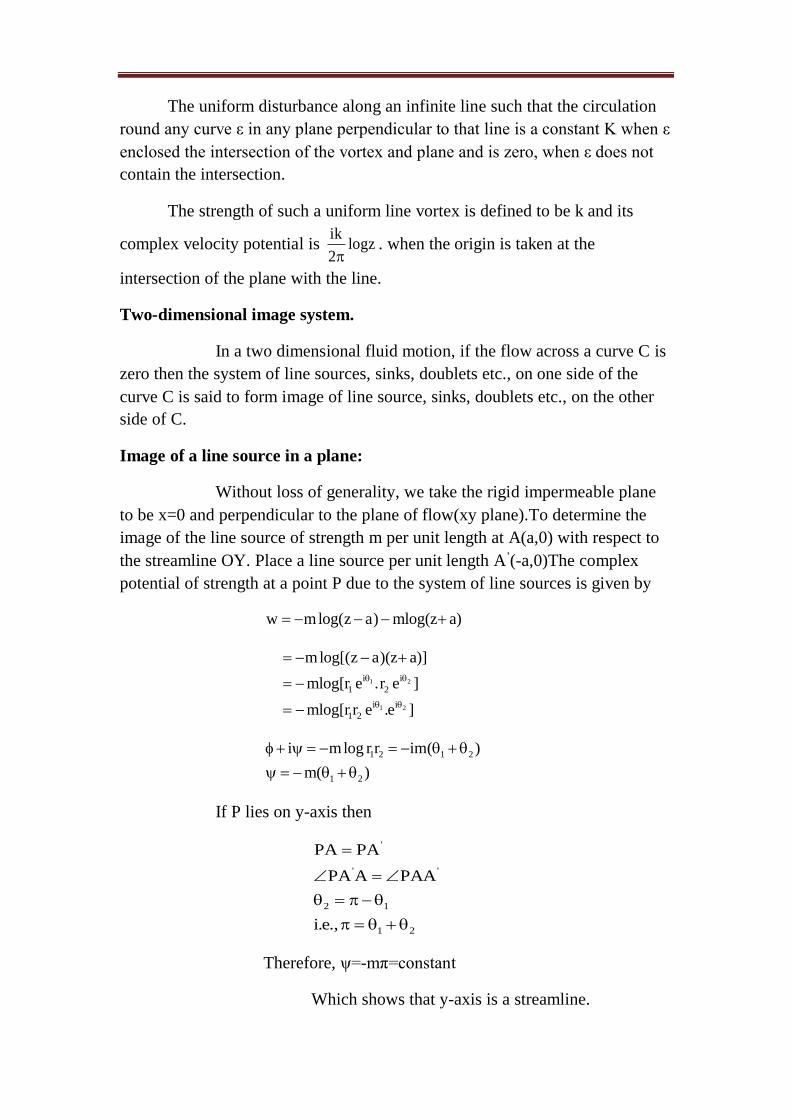
The uniform disturbance along an infinite line such that the circulation
round any curve ε in any plane perpendicular to that line is a constant K when ε
enclosed the intersection of the vortex and plane and is zero, when ε does not
contain the intersection.
The strength of such a uniform line vortex is defined to be k and its
complex velocity potential is ik
logz2
. when the origin is taken at the
intersection of the plane with the line.
Two-dimensional image system.
In a two dimensional fluid motion, if the flow across a curve C is
zero then the system of line sources, sinks, doublets etc., on one side of the
curve C is said to form image of line source, sinks, doublets etc., on the other
side of C.
Image of a line source in a plane:
Without loss of generality, we take the rigid impermeable plane
to be x=0 and perpendicular to the plane of flow(xy plane).To determine the
image of the line source of strength m per unit length at A(a,0) with respect to
the streamline OY. Place a line source per unit length A’(-a,0)The complex
potential of strength at a point P due to the system of line sources is given by
w mlog(z a) mlog(z a)
1 2
1 2
i i
1 2
i i
1 2
mlog[(z a)(z a)]
mlog[r e .r e ]
mlog[r r e .e ]
1 2 1 2
1 2
i mlog r r im( )
m( )
If P lies on y-axis then
'
' '
2 1
1 2
PA PA
PA A PAA
i.e.,
Therefore, ψ=-mπ=constant
Which shows that y-axis is a streamline.

Hence, the image of a line source of strength m per unit length of
a line at A(a,0) is a source of strength m per unit length at A’(-a,0).
In other words, image of line source with respect to a plane (a
streamline) is a line source of equal strength situated on opposite side of the
plane (streamline) at an equal distance.
Image of a line doublets in a plane:
Consider the rigid plane x=0 and perpendicular to the plane of
flow (xy-plane).
Thus, to determine the image of a line doublet with respect to the
streamlines OY.
Let there be line sources at the points A and B, taken close
together, of strength –m and m per unit length.
Their respective image in OY are –m at A’, m at B’ where A’ and
B’ are the reflections of A,B in OY.
The line AB makes angle α with OX . Thus A 'B'makes angle with OX.
In the limiting case, as m→∞,AB→0, we have equal line
doublets at A and A’ with their axes inclined at α,(π-α) to OX .
Image of vortex in a plane:
Let us consider two line vortices of strength K and –K per unit
length at 1A(z z ) and 2B(z z ) respectively.
The complex potential due to there line vortices.
1 2w ik log(z z ) ik log(z z )
1
2
z zik log
z z
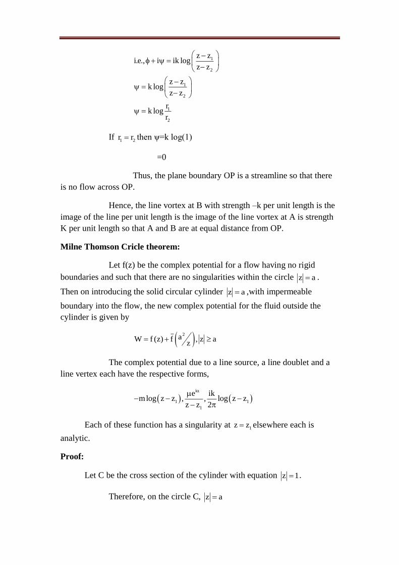
1
2
1
2
1
2
z zi.e., i ik log
z z
z zk log
z z
rk log
r
If 1 2r r then ψ=k log(1)
=0
Thus, the plane boundary OP is a streamline so that there
is no flow across OP.
Hence, the line vortex at B with strength –k per unit length is the
image of the line per unit length is the image of the line vortex at A is strength
K per unit length so that A and B are at equal distance from OP.
Milne Thomson Cricle theorem:
Let f(z) be the complex potential for a flow having no rigid
boundaries and such that there are no singularities within the circle z a .
Then on introducing the solid circular cylinder z a ,with impermeable
boundary into the flow, the new complex potential for the fluid outside the
cylinder is given by
2aW f (z) f , z az
The complex potential due to a line source, a line doublet and a
line vertex each have the respective forms,
i
1 1
1
e ikmlog z z , , log z z
z z 2
Each of these function has a singularity at 1z z elsewhere each is
analytic.
Proof:
Let C be the cross section of the cylinder with equation z 1 .
Therefore, on the circle C, z a
2
2 azz a zz
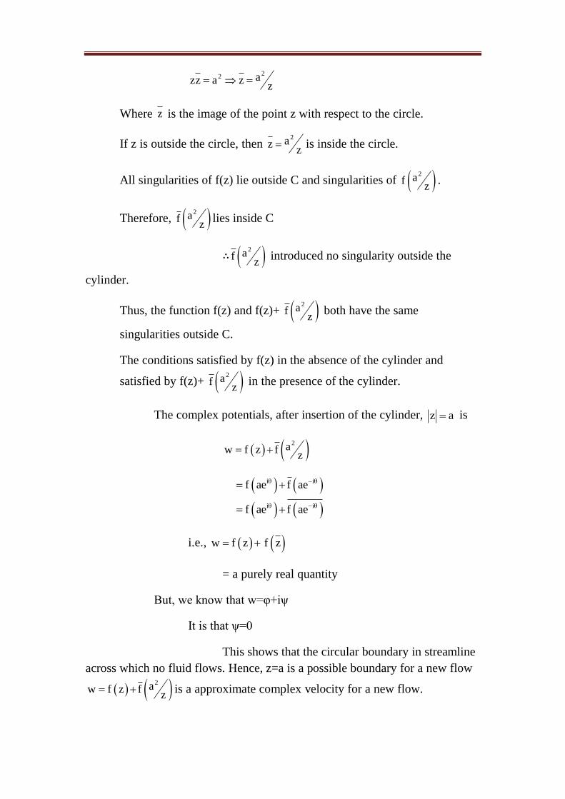
Where z is the image of the point z with respect to the circle.
If z is outside the circle, then 2az
z is inside the circle.
All singularities of f(z) lie outside C and singularities of 2afz
.
Therefore, 2afz
lies inside C
∴ 2afz
introduced no singularity outside the
cylinder.
Thus, the function f(z) and f(z)+ 2afz
both have the same
singularities outside C.
The conditions satisfied by f(z) in the absence of the cylinder and
satisfied by f(z)+ 2afz
in the presence of the cylinder.
The complex potentials, after insertion of the cylinder, z a is
2
w f z afz
i i
i i
ae f ae
ae ae
f
f f
i.e., w f z f z
= a purely real quantity
But, we know that w=φ+iψ
It is that ψ=0
This shows that the circular boundary in streamline
across which no fluid flows. Hence, z=a is a possible boundary for a new flow
2
w f z afz
is a approximate complex velocity for a new flow.

Uniform flow part a stationary cylinder
Uniform stream having velocity =Ui gives rise to a complex potential
Uz
f(z)=Uz
then f z Uz
and so 2 2a Ua
fz z
Then, on introducing the cylinder of circular section z 0
into the stream, the complex potential for the region z a becomes
2
w f z afz
2Ua
Uzz
iz re
i 2 1 i
2 1
2 1 2 1
Ure Ua r e
U r(cos isin ) a r (cos isin )
Ucos(r a r )iUsin(r a r )
Uniform stream at incidence 𝛂 toOX
Complex potential for a uniform stream of velocity O at
incidence to 𝛂 to OX ,i.e., iUze
f(z)= iUze
if (z) Uze
2
2 iaaf ( ) U ez z
Hence, when the cylinder of section z a is introduced
the complex potential is z a
2i i
2i i
aw Uze U e
z
aw U ze e
z
Image of a line source in a circular cylinder show that image of line source
in a right circular cylinder is an equal line source through the inverse
point in the circular section in the inverse point in the circular section in
the plane of flow together with an equal line sink through the centre of the
section.
Solution:
Suppose there is a uniform line source of strength m per unit
length through the point z=d,d>a.
Then, the complex potential at a point
2
2
f (z) mlog(z d)
f (z) mlog(z d)
aaf mlog dz z
On introducing the circular cylinder of section z a , the
complex velocity potential in the region z a
2a
w mlog(z d) mlog dz
Alternative form:
2a
w mlog(z d) mlog d mlog z cons tan tz
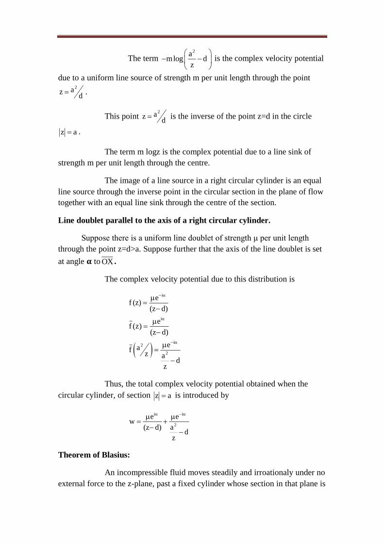
The term 2a
mlog dz
is the complex velocity potential
due to a uniform line source of strength m per unit length through the point 2az
d .
This point 2az
d is the inverse of the point z=d in the circle
z a .
The term m logz is the complex potential due to a line sink of
strength m per unit length through the centre.
The image of a line source in a right circular cylinder is an equal
line source through the inverse point in the circular section in the plane of flow
together with an equal line sink through the centre of the section.
Line doublet parallel to the axis of a right circular cylinder.
Suppose there is a uniform line doublet of strength μ per unit length
through the point z=d>a. Suppose further that the axis of the line doublet is set
at angle 𝛂 to OX .
The complex velocity potential due to this distribution is
i
i
i2
2
ef (z)
(z d)
ef (z)
(z d)
eafz a
dz
Thus, the total complex velocity potential obtained when the
circular cylinder, of section z a is introduced by
i i
2
e ew
a(z d)d
z
Theorem of Blasius:
An incompressible fluid moves steadily and irroationaly under no
external force to the z-plane, past a fixed cylinder whose section in that plane is
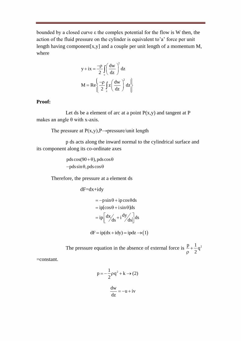
bounded by a closed curve ε the complex potential for the flow is W then, the
action of the fluid pressure on the cylinder is equivalent to’a’ force per unit
length having component[x,y] and a couple per unit length of a momentum M,
where
2
2
dwy ix dz
2 dz
dwM Re z dz
2 dz
Proof:
Let ds be a element of arc at a point P(x,y) and tangent at P
makes an angle θ with x-axis.
The pressure at P(x,y),P→pressure/unit length
p ds acts along the inward normal to the cylindrical surface and
its component along its co-ordinate axes
pdscos(90 ),pdscos
pdssin ,pdscos
Therefore, the pressure at a element ds
dF=dx+idy
psin ipcos ds
ip[cos isin ]ds
dydxip i dsds ds
dF ip(dx idy) ipdz 1
The pressure equation in the absence of external force is 2p 1q
2
=constant.
21p q k (2)
2
dw
u ivdz
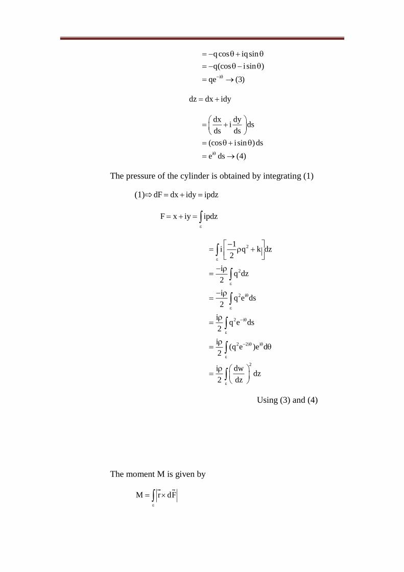
i
q cos iqsin
q(cos isin )
qe (3)
dz dx idy
i
dx dyi ds
ds ds
(cos isin )ds
e ds (4)
The pressure of the cylinder is obtained by integrating (1)
(1)⇨ dF dx idy ipdz
F x iy ipdz
2
2
2 i
2 i
2 2i i
2
1i q k dz
2
iq dz
2
iq e ds
2
iq e ds
2
i(q e )e d
2
i dwdz
2 dz
Using (3) and (4)
The moment M is given by
M r dF

2
2
2
2
2 i
2 2i i
xpdscos ypdssin
dx dyxp ds yp ds
ds ds
p(xdx ydy)
1k q xdx ydy
2
1k xdx ydy p q xdx ydy
2
pq xdx ydy
2
pR.P q (x iy)(cos i sin )ds
2
pR.P q ze ds
2
pR.P z(q e )e ds
2
2p dw
R.P z dz2 dz
Hence proved.
Circulation about a circular cylinder in a uniform stream.
Let a liquid be in motion with a velocity –U along the x-axis. The
complex potential due to the stream is Uz.
If the circular cylinder of radius a is introduced inside the liquid,
then the complex potential , by circle theorem becomes
2Ua
Uzz
Let there be a circulation and about the cylinder. The complex
potential due to circulation is ik(logz).
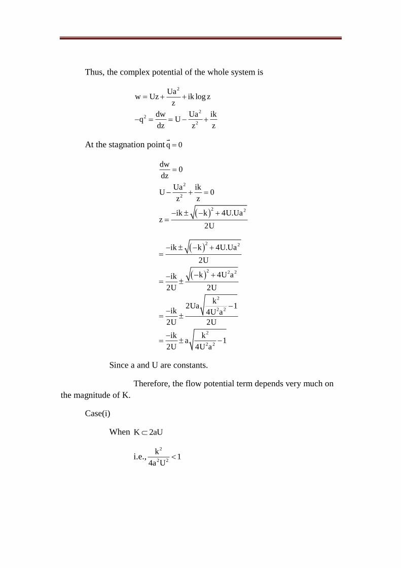
Thus, the complex potential of the whole system is
2
22
2
Uaw Uz ik log z
z
dw Ua ikq U
dz z z
At the stagnation point q 0
2
2
2 2
dw0
dz
Ua ikU 0
z z
ik k 4U.Uaz
2U
2 2
2 2 2
2
2 2
2
2 2
ik k 4U.Ua
2U
k 4U aik
2U 2U
k2Ua 1
ik 4U a
2U 2U
ik ka 1
2U 4U a
Since a and U are constants.
Therefore, the flow potential term depends very much on
the magnitude of K.
Case(i)
When K 2aU
i.e.,2
2 2
k1
4a U

22
2 2
2
2 2
ksin
4a U
ik kz a 1
2U 4a U
2i2aUsin
a 1 sin2U
ia sin a cos
z ia sin a cos z ia sin a cos
i
a[cos isin ]
ae
i
a[cos i sin ]
ae
If the above inequality holds, there are two distinct stagnation points at
1 2z z ,z z on the surface of cylinder.
The diagram shows the pattern of streamlines formed in such a case
A1,A2 be the stagnation points.
At A1,A2 the pressure is a maximum and so the effect produced on the
direction OY .
Then, the force is 2 2 21M Re 2 i k 2U a 0
2
When k=0 the streamlines flow is symmetrical about the
plane y=0 and there is no such tendency.
Circulation may be produced in practice by rotating the cylinder
about its axis.
The viscosity of the real fluid would then produce such circulation. This
lifting effect produced by the circulation is called the magnus effect.
We know that at the stagnation points (critical points) there are
two branches of the streamline which are at right angles to each other.
Thus, the liquid inside the loop formed at the stagnation points will not
be carried by the stream but will circulate round the cylinder.
The pressure (forces) on the circular cylinder.
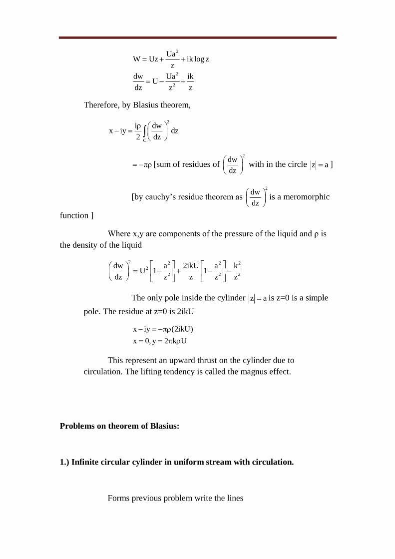
2
2
2
UaW Uz ik log z
z
dw Ua ikU
dz z z
Therefore, by Blasius theorem,
2
C
i dwx iy dz
2 dz
[sum of residues of 2
dw
dz
with in the circle z a ]
[by cauchy’s residue theorem as 2
dw
dz
is a meromorphic
function ]
Where x,y are components of the pressure of the liquid and ρ is
the density of the liquid
2 2 2 22
2 2 2
dw a 2ikU a kU 1 1
dz z z z z
The only pole inside the cylinder z a is z=0 is a simple
pole. The residue at z=0 is 2ikU
x iy (2ikU)
x 0, y 2 k U
This represent an upward thrust on the cylinder due to
circulation. The lifting tendency is called the magnus effect.
Problems on theorem of Blasius:
1.) Infinite circular cylinder in uniform stream with circulation.
Forms previous problem write the lines
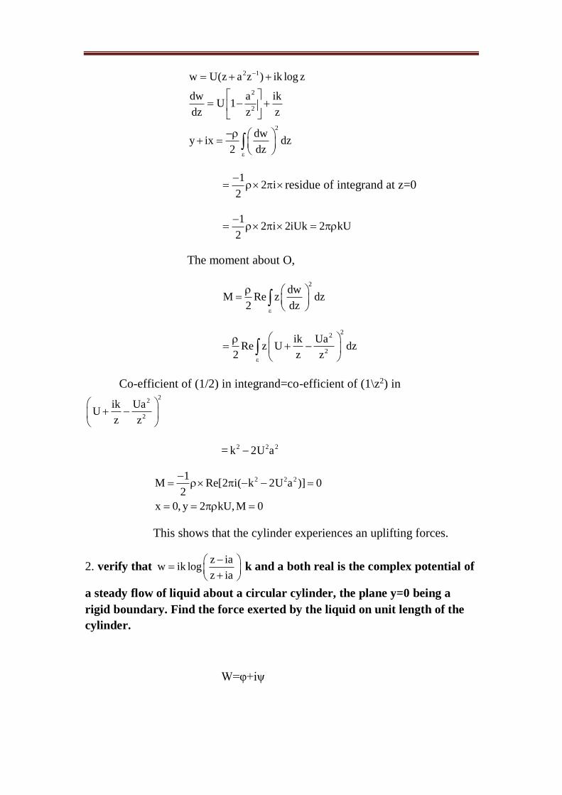
2 1
2
2
2
w U(z a z ) ik log z
dw a ikU 1
dz z z
dwy ix dz
2 dz
1
2 i2
residue of integrand at z=0
1
2 i 2iUk 2 kU2
The moment about O,
2dw
M Re z dz2 dz
22
2
ik UaRe z U dz
2 z z
Co-efficient of (1/2) in integrand=co-efficient of (1\z2) in 2
2
2
ik UaU
z z
= 2 2 2k 2U a
2 2 21
M Re[2 i( k 2U a )] 02
x 0, y 2 kU,M 0
This shows that the cylinder experiences an uplifting forces.
2. verify that z ia
w ik logz ia
k and a both real is the complex potential of
a steady flow of liquid about a circular cylinder, the plane y=0 being a
rigid boundary. Find the force exerted by the liquid on unit length of the
cylinder.
W=φ+iψ

z ia
i ik logz ia
1 1z ia y a y aik log i tan i tan
z ia x x
z ia
k logz ia
The streamlines ψ=constant are given by z ia
z ia
=constant=λ
For λ≠1, there are non-intersecting coaxial of circle having z=±ia
as the limiting points i.e.,circles of zero radius.
In particular, for λ=1, we get a streamlines which is the perpendicular
bisector of the line segment joining the points ±ia and it is the radical axis of
the co-axial system.
Coaxial circle:
A system of circles, every pair of which have the same radical axis.
Radical axis:
The radical axis of two circles is the locus of points at which tangent
drawn to both circles have the same length.
No fluid crosses a streamlines and so a rigid boundary may be
introduced along any circle λ=constant of the coaxial system,including the
perpendicular bisector λ=1.
We note that for λ=1
2 22 2
z ia z ia
x y a x y a
y 0
Hence, we can introduce rigid boundaries along
i. A particular circle λ=constant
ii. Along the plane y=0(λ=1)
This establishes the result of the first part of the question.

SCHOOL OF SCIENCE & HUMANITIES
DEPARTMENT OF MATHEMATICS
UNIT – IV – TWO DIMENSIONAL FLOWS-II – SMTA5401
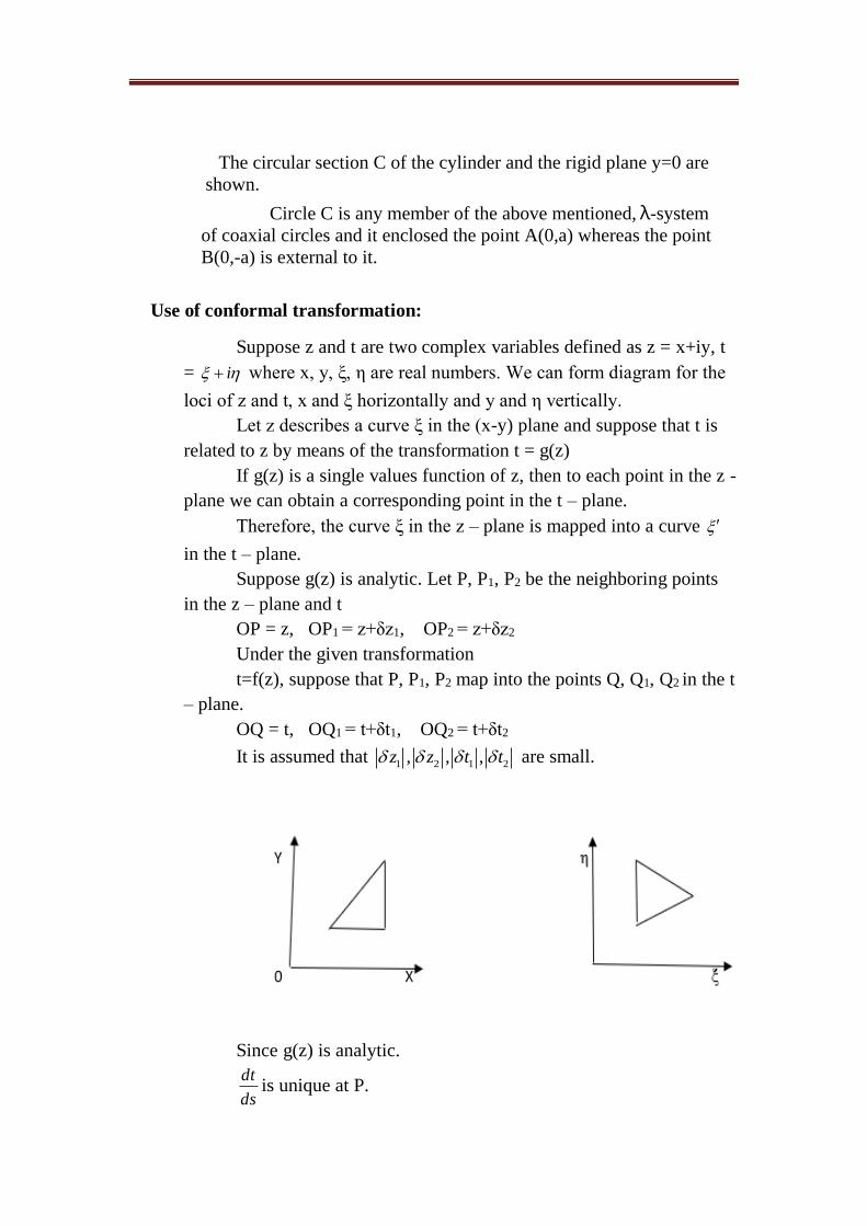
Unit 4
Use of conformal transformation:
Suppose z and t are two complex variables defined as z = x+iy, t
= i where x, y, ξ, η are real numbers. We can form diagram for the
loci of z and t, x and ξ horizontally and y and η vertically.
Let z describes a curve ξ in the (x-y) plane and suppose that t is
related to z by means of the transformation t = g(z)
If g(z) is a single values function of z, then to each point in the z -
plane we can obtain a corresponding point in the t – plane.
Therefore, the curve ξ in the z – plane is mapped into a curve
in the t – plane.
Suppose g(z) is analytic. Let P, P1, P2 be the neighboring points
in the z – plane and t
OP = z, OP1 = z+δz1, OP2 = z+δz2
Under the given transformation
t=f(z), suppose that P, P1, P2 map into the points Q, Q1, Q2 in the t
– plane.
OQ = t, OQ1 = t+δt1, OQ2 = t+δt2
It is assumed that 1 2 1 2, , ,z z t t are small.
Since g(z) is analytic.
dt
dsis unique at P.
The circular section C of the cylinder and the rigid plane y=0 areshown.
Circle C is any member of the above mentioned, λ-systemof coaxial circles and it enclosed the point A(0,a) whereas the pointB(0,-a) is external to it.
Thus, to the first order of smallness
1 2
1 2
t t
x x
1 1
2 2
t x
t x
1 1
2 2
(1)t x
t x
arg δt1 – arg δt2 = arg δz1 – arg δz2 (2)
from (1)
1 1
2 2
(3)QQ PP
QQ PP
From (2) , on reversing the signs of each other
2 1 2 1 (4)Q QQ P PP
The equations (3) and (4) shows that the triangles
Q2QQ1, P2 PP1 are similar.
i.e., within the neighborhood of any point p in the z – plane and
its corresponding mapping in the t – plane, angle remain unaltered.
From (4) the ratios of corresponding linear dimension when the
mapping takes place under a transformation of the form t = f(z), where
f(z) is analytic at p and within its neighborhood.
Such a transformation is said to be conformal.
1) Theorems concerning the conformal transformation of the line
distribution under conformal transformation a uniform line source maps
into another uniform line source of the same length.
Let there be a uniform line source of strength m per unit length
through the point z = z0. Suppose the conformal t = g(z) is made from
the z – plane to the t – plane so that the point z = z0 maps the point t = t0.
Let ξ be a closed curve in the z – plane containing the point z = z0
and suppose ξ maps in the t – plane.
Then t = t0 lies within
The complex velocity potential ω is the same for both systems
and has the forms.
for the z - planei
for the t - planei
Thus , . Since φ is the same at corresponding points of
ξ, .
1d d
Now in the z – plane ω = - m log(z-z0)
dω = -m 0
dz
z z
0
2dz
d m m iz z
Since the integrand has a residue of 1 at z = z0
d d id
2 (2)d m
The numerical value of this is the volume of fluid crossing unit
thickness of ξ per unit t time.
Equation (1) and (2) shows that the same volume crosses unit
thickness of per unit time which implies an equal line source of
strength m per unit length through t = t0.
2) Under conformal transformation a uniform line vortex maps into another
uniform line vortex of the same strength.
Let there be a uniform line vortex of strength k per unit length
through z = z0. Suppose the conformal transformation t = g(z) is made
from the z – plane to t – plane so that the point z = z0 maps into t=t0.
Let be its map in the t – plane then contain t = t0.
The complex velocity potential ω is the same for both systems
and has the forms.
for the z - planei
for the t - planei
Thus , . Since φ is the same at corresponding points of
ξ, .
1d d
In the z – plane the complex potential is
0log( )2
ikz z
0
22 2
ik dz ikd i k
z z
Equating real parts gives,
; - (2)d k d k
The integral on the LHS is the circulation round ξ.
Equation (1) and (2) shows that the circulation round is
also k.
Thus, the line source through z = z0 of strength k per unit
length maps into an equal line source through t = t0.
3) Under conformal transformation a uniform line doublet maps into
another uniform line doublet of the different length.
Let there be a uniform line doublet of strength μ per unit
length through P where z = z0.
Suppose that under the conformal transformation t = g(z), P maps
into Q where
t = t0.
Let the line doublet be replaced by equivalent line sources of
strength -m, m per unit length through P, P where ,PP z m z
PP is in the direction of the axis of the line doublet.
Suppose P maps into Q
Then the line source of strength -m, +m per unit length through
PPmaps into ones of strength -m, +m per unit length through QQ .
If , ( )QQ t t g z z
So that,
( )t g z z
arg t = arg g (z)+ arg z
Hence the two line sources through QQ gives a line doublet at
Q of strength .
( )m t g z
The inclination of the axis of the line doublet to the real axis is
increased by arg ( )g z .
4) Single infinite row of vertices:
To find complex potential of an infinite row of parallel vertices
of strength k and distance ‘a’ apart.
Proof:
Let there be 2n+1 vertex with their centers on x – axis and the
middle vortex having its center at the origin.
The vertices are placed at points z = Ina where n=0,1,2…
symmetrical about y – axis.
The complex potential due to these vertices is
log log( ) log( 2 ) ... log(z na) iklog(z a)
log( 2 ) ... log( )
ik z ik z a ik z a ik
ik z a ik z na
2 2 2 2 2 2 2 2log log( ) log( 2 ) ... log( )ik z ik z a ik z a ik z n a
2 2 2 2 2 2 2 2log log( ) log( 2 ) ... log( )a
ik z ik z a ik z a ik z n aa
2 2 22 2 2 2 2
2 2 2 2 2logz log( ) 1 log( 2 ) 1 ... log( ) 1
2
z z zik ik a ik a ik n a
a a n a
2 2 2
2 2 2 2 2
2 2 2 2 2log 1 1 ... 1 log ( 1) ( )(2 )...( )
2
nz z z z aik ik a a n a
a a a n a
Ignoring constant terms and having z
a

2 2 2
2 2 2 2 2log 1 1 ... 1
2ik as n
n
logsinik
logsin (1)z
ika
The velocity of vertices at origin is given by
logd z
q ikdz a
0
logsin logz
d z zik ik
dz a a
0
cos1
sinz
z
aikza z
a
Indeterminate form as 0z
Hence, velocity at 0z is zero.
Thus, the infinite row of vertices does not induce any velocity by
itself.
The velocity at any point of the fluid other than the vertices is
given by,
cotd ik z
q u ivdz a a
cot ( )ik
x iya a
cos ( )
sin ( )
x iyik a
ax iy
a
2cos ( )sin ( )
2sin ( )sin ( )
x iy x iyik a a
ax iy x iy
a a
2 2sin sin
2 2cos cos
x yi
a aikyi xa
a a
2 2sin sinh
2 2cosh cos
x yi
a aiky xa
a a
2sinh
2 2cosh cos
yk
a auy x
a a
2sin
2 2cosh cos
xk
a avy x
a a
We have,
logsinz
i ika
logsinz
i ika
( ) ( ) logsin logsinz z
i i ik ika a
2 2 logsin sinz z
i ika a
Streamline φ= constant, are found to be 2 2
cosh cosy x
a a
is
constant.
5) Karman vortex street:
This consist of two parallel infinite rows of line vortices arranged
as follows
The first row consists of line vortices of strength k at the points
having cartesian coordinates.
1
( , ) 0 1, 2,...2
na b where n
The second row consists of line vortex of strength -k at the points
1 1
(2 1) , 0, 1, 2,...2 2
n a b where n
Such arrangement is called as Karman vortex street.
Proof:
This consist of two parallel infinite row AA and BB of vortices
of equal spacing ‘a’ so arranged that each vertex of strength k of AA is
exactly above the midpoint of the join of two vertices of BB each of
strength -k.
Therefore, the complex potential
logsin ( ) logsin2 2 2
ik ik az ib z ib
a a
By considering the point z1 = ib, z2 = - ib
The velocity of the vertex at z = ib is

1 1 cot ( )2 2
ik au iv ib ib
a a
2 1
cot2 2
ik iba
a a a
2 1
cot2 2
ik ib
a a
2
cot2 2
ik ib
a a
2
cot2 2
ik ib
a a
2
tan2
ik ib
a a
2
tanh2
k b
a a
1 1
2tanh 0
2
k bu where v
a a
The same can be shown to each of vortices at the row AA and
BB move with the same velocity. This means that the vertex
configuration remains unaltered at all times. Since, both AA and BB
have the same velocity 2
tanh2
k b
a a
in x – direction.
Hence the street moves through the liquid with two velocity.
This shows that Karman vortex street is realized when a flat plate
moves broadside through a liquid.
6) Schwartz – Christoffel transformation:
Fig (i) shows n points 1 2 3,A ,A ,...AnA on the real axis t = ξ+iη, ξ
and η are real.
The points rA are specified by t = ar (r = 1,2,…n)
The ordering is such that,
1 2 3 1... n na a a a a
Now suppose that, t mapped onto the z – plane
1 21 1 1
1 2( ) ( ) ...( ) (1)n
n
dzk t a t a t a
dt
Which is conformal everywhere, save at t = ar (r = 1,2,…n)
The number 1 2, ,... tann are real cons ts
1 21 1 1
1 2( ) ( ) ...( ) (*)n
n
zlet k t a t a t a
t
Where k be the complex constant
t be the changes in t
z the corresponding change in z.
From (*),
1 21 1 1
1 2( ) ( ) ...( ) n
nz tk t a t a t a
Applying argument on both sides,
1 21 1 1
1 2arg( ) arg[ ( ) ( ) ...( ) ] n
nz tk t a t a t a
1 21 2arg( )[arg( ) ( 1)arg( ) ( 1)arg( ) ... ( 1)arg( )] n
nt k t a t a t a
First suppose we say, t travels from 1 to a , along =0
Then, arg( ) 0,t 1 2arg( ) arg( ) ... arg( )nt a t a t a
Hence,
1 1 2(arg ) arg ( ) ( ) ... ( ) tan (2)nz k cons t
Equation (2), z describes the straight line segment.
UA1 as t travels from 1 to a , along =0
Next t travels from 1 2a to a , along =0
Then, arg( ) 0,t
1 2arg( ) 0 and arg( ) ... arg( ) tan (3)nt a t a t a cons t

This shows that, z describes a line segment A1, A2, as t travels
from 1 2a to a , along =0
From (2) and (3),
2 1 1(arg ) (arg z)z
The angle between the direction UA1, A1, A2 is 1 . This
means t travels along the axis =0 from 1 part A , similarly at t
moves from 2 3a to a , along =0
Then, arg( ) 0,t
1 2 3arg( ) 0 , arg( ) 0 and arg(t-a )... arg( ) tan (4)nt a t a t a cons t
Equation (4) shows that z describes a line segment A2, A3, as t
travels from 2 3a to a , along =0
From (3) and (4)
3 2 2(arg ) (arg z)z
This shows that direction z changes by 2A in the positive sense
as z passes through A2.
Continuing in this way, z describes the sides
1 1 2 1, , , . , , n n nA A A A A A of a closed polygon on z – plane , as t
moves along the real axis 1 to a , 1 2a to a , 2 3a to a , ……..
1a to a , to +n n na respectively.
Therefore, the angles turned through in the positive sense at A1,
A2, …. An-1, An are 1 2, ,..... n
So, the internal angles of the polygon at these points are
1 2, ,... n
Suppose that, 1 2 ... ( 2)n n
Then , A1, A2, …. An-1, An is a closed polygon , the portion,
1nA A beast line .
Further, since the half plane, img (t)>0 is along the positive
direction of the axis η=0. The corresponding area in the z plane is the
interior of polygon.
If 1 2 3 1... n na a a a a are the n distinct points on the img (t)
=0 in the t – plane.
If 1 2, ,... n are n real constants 1 2 ... ( 2)n n , where n is
the positive integer.

Then the transformation,
1 21 1 1
1 2( ) ( ) ...( ) n
ndz k t a t a t a dt
On integrating both sides, we get
1 21 1 1
1 2( ) ( ) ...( ) n
nz k t a t a t a dt
Here, k are the constants that maps the entire line img (t) = 0 onto
the boundary
A1, A2, …. An-1, AnA1 of a closed polygon on n – sides.
Such a way, that points t = ak transform into Ak at which the
internal angles are k = 1,2,3,..n and the half plane img (t)>0 transforms
into the interior.
This transformation is called the Schwartz - Christoffel
transformation.
Note;
Suppose the real line t is infinity then, if na
1 21 1 1
1 2( ) ( ) ...( ) n
n
dzk t a t a t a
dt
Put k = 1
A( )n
na
Then ,
1
1
1( ) A 1
n
n
n
tk t a
a
1
A 1 A, as a
n
n
n
t
a
The Schwartz – Christoffel transformation becomes
1 21 1 1
1 2( ) ( ) ...( ) n
n
dzA t a t a t a
dt
This shows an , the factor 1
( )n
nt a
is suppressed. A similar result
for an
Unit 5

SCHOOL OF SCIENCE & HUMANITIES
DEPARTMENT OF MATHEMATICS
UNIT – V – THREE DIMENSIONAL FLOWS – SMTA5401
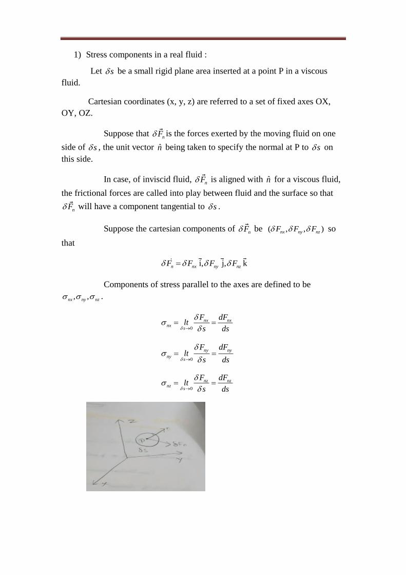
1) Stress components in a real fluid :
Let s be a small rigid plane area inserted at a point P in a viscous
fluid.
Cartesian coordinates (x, y, z) are referred to a set of fixed axes OX,
OY, OZ.
Suppose that nF is the forces exerted by the moving fluid on one
side of s , the unit vector n being taken to specify the normal at P to s on
this side.
In case, of inviscid fluid, nF is aligned with n for a viscous fluid,
the frictional forces are called into play between fluid and the surface so that
nF will have a component tangential to s .
Suppose the cartesian components of nF be ( , , )nx ny nzF F F so
that
i, j, knx ny nzn F F FF
Components of stress parallel to the axes are defined to be
, ,nx ny nz .
0
nx nxnx
s
F dFlt
s ds
0
ny ny
nys
F dFlt
s ds
0
nz nznz
s
F dFlt
s ds
In the components , ,nx ny nz , the first suffix n denote the direction
of the normal to the elements of plane s , second suffix x or y or z denotes the
direction in which components measured.
n in turn with the unit vector , ,i j k in , ,OX OY OZ
which is
achieved by suitably re-orientating s .
Three set of stress components,
xx xy xz
yx yy yz
zx zy zz
The diagonal element , ,xx yy zz of this array are called normal or
direct stresses.
The remaining six elements are called shearing stresses.
For an inviscid fluid,
xx yy zz p
0xy xz yx yz zx zy
We consider the normal stresses as positive when they are tensile and
negative when they are compressive, so that p is the hydrostatic pressure.
The matrix,
xx xy xz
yx yy yz
zx zy zz
are called the stress matrix.
The quantities ij (i, j= x, y, z) are called the components of the
stress tensor where matrix is of above form.
2) Derive the relations between cartesian components of stress:
We consider the motion of a small rectangular parallelepiped of
viscous fluid, its center being P(x, y, z) and its edges of lengths
, ,x y z parallel to fixed cartesian axes. The mass p x y z of the
fluid element remains constant and the element is presumed to move

along with the fluid. In the diagram the points 1 2, PP have coordinates
1 1( , , ), ( , , )
2 2x x y z x x y z
At P(x, y, z) the force components parallel to , ,OX OY OZ
on the
surface of area y z through P and having i as unit normal are
, ,xx xy xzp y z p y z p y z
At 2
1( , , )
2P x x y z , since i is the unit normal measured outwards
from the fluid, the corresponding force components across the parallel plane of
area y z are
1 1 1
2 2 2, ,
xyxx xzxx xy xzy
pp pp x p x p x
xz
xz y z
xy
For the parallel plane through 1
1( , , )
2P x x y z , since -i is the unit
normal drawn outwards from the fluid element, the corresponding
components are,
1 1 1
2 2 2, ,
xyxx xzxx xy xz
pp pp x p x p xy z y z y
xz
x x
The forces on the parallel planes through 1 2, PP are equivalent to a
single force at P with components,
, ,xyxx xz
pp px y z
x x x
Together with couples whose moments (to the third order) are
about oy;
about oz
xz
xy
p x y z
p x y z
Similarly, the pair of faces perpendicular to the y axis gives a force
at P having components
, ,yx yy yzp p p
x y zy y y
Together with couple couples of moments,
about oz;
about ox
yx
yz
p x y z
p x y z
The pair of faces perpendicular to the z axis give a face at P
having components,
, ,zyzx zz
pp px y z
z z z
Together with couple couples of moments,
about ox;
about oy
zy
zx
p x y z
p x y z
Taking into account the surface forces on all six faces of the
cuboid, we see that they reduce to a single force at P having
components,
, ,yx xy yy zy yzxx zx xz zz
p p p p pp p p px y z
x y z x y z x y z
Together with a vector couple having cartesian components,
, ,yz zy zx xz xy yxp p p p p p x y z
Now, suppose the external body forces acting at P are [X, Y, Z]
per unit mass, so that the total body force on the element has
components , ,ZX Y x y z . Take moments about the i direction
through P, then

Total moment of forces =(moment of inertia about axis) *(angular
acceleration)
i.e., 4 50 0yz zyp p x y z
here 0 n satisfies a quantity of thn order of smallness in
, ,x y z . Thus to the third order of smallness,
0yz zyp p x y z
So that as the element becomes vanishingly small, we obtain,
yz zyp p
Similarly,
,zx xz xy yxp p p p
Thus the stress matrix is diagonally symmetric and contains only
six unknowns.
3) Relation between stress and rate of strain :
Using the analysis of a foregoing section, we now link together the
stress and rates of strain in a viscous fluid in motion.
Suppose fig (a) represents a particle of fluid at time t in the shape
of a rectangular parallelepiped of edges x y z , parallel to fixed
cartesian axes.
At the time t the velocity components in the x direction at the
corner (x, y, z) of the bios is u and so that at the corner ( , , )x x y z is
uu x u a x
x

Thus at time (t+δt) , therefore the edge δx has grown to
length x a x t , since aδx is the relation velocity increases between
its two ends.
Similarly, the edges δy, δz have grown to lengths
(1 ), (1 )y b t z c t respectively.
Thus, volumetric increment in the interval δt is
(1 )(1 )(1 ) ( )x y z a t b t c t x y z a b c x y z t
Which gives a dilatation or volumetric strain in time δt
Of (a+b+c) δt.
Hence at time t, the rate of dilatation is Δ (or) volumetric
stress where
u u u
a b cx y z
= dig q
This quantity have been seen to be invariant at each point of the
fluid its volume is also A+B+C in terms of principle rates of strain.
Further, w.k.t, the equation of continuity for an incompressible
fluid is Δ=0, but for a compressible one Δ≠0, we discuss the two cases
separately,
In the case of incompressible fluid, we suppose the principle
stresses p1,p2,p3 differ from this mean value -p by quantities proportional
to the rates of distortion A, B, C in the principal direction.
Thus we write,
1
2
3
2
2 (1)
2
p p A
p p B
p p C
Where μ is a constant.
In the case of compressible fluid we have the additional affect of
the rate of dilatation Δ manifesting itself equally in the directions.
This effect we represent by adding to the R.H.S. of each of the
equation (1) the quantity λΔ, where λ is a constant.
So that in the case
1
2
3
2
2 (2)
2
p p A
p p B
p p C
Adding together equation (2) and using Δ=A+B+C, we find, since
p1+p2+p3=-3p and Δ≠0 and 2
(3)3
The equation (1), (2) link principal stresses with principal rate of
strain.
We next evaluate non principal stress ,... ,...xx yzp p in terms of
non principal rates of strain.
The equation of motion in stress analysis is
2 2 2
1 1 2 2 3 3xxp l p l p l p
Using the equation (2), we obtain,
2 2 2 2 2 2 2 2 2
1 2 3 1 2 3 1 2 3( ) 2 ( C) A( )xxp p l l l l A l B l l l l
2p A
2u
px
Permuting the symbols gives the equation,
1
2
3
2
2 (3)
2
up p
x
vp p
y
wp p
z
Where Δ= div q, Δ=0 for incompressible flow and 2
3 for
the compressible flow. From analysis stress in fluid motion, we get
1 1 1 2 2 2 3 3 3yzp m n p m n p m n p
1 1 2 2 3 3 1 1 2 2 3 3( )( ) 2 ( C)p m n m n m n m n A m n B m n
2 f
w v
y z
Thus we obtain the three equation
(4)
yz zy
zx xz
xy yx
w vp p
y z
u wp p
z x
v up p
x y
Which are true for compressible and incompressible fluid.
4) The Navier- stokes equation of motion of a viscous fluid:
The translational equation of motion in the form,
1 yxxx zxpp pdu
Xdt x y z
On substituting,
2xx
up p
x
yx
zx
v up
x y
u wp
z x
We obtain,
21du p vX V u V
dt x x

Since 2
3 for the compressible fluid and since Δ=0 for
incompressible fluid this equation may be written unambiguously for the
two cases in the form,
21 1
3
du p vX V u V
dt x x
Thus the equation of motion in the three directions may be
written FDX
2
2
2
1 1
3
1 1 (1)
3
1 1
3
du pX V u V
dt x x
dv pY V u V
dt y y
dw pZ V u V
dt z z
The tensor form of these equation is
[ , , Z],q [x, y, z]F X Y the vectoral form of equation (1) is clearly
2 1( . ) (2)
3
dq dpF V q V q
dt
Now,
2
2
1( . ) ( ),
2
( ) ( . ) ,
dq q qq q q q q
dt t t
q q q
So that (2) may also written as
21 4( ) ( ( . ) ( )) (3)
2 3
dq dpq q q F V q V q
dt
any of the forms (1), (2) and (3) are called the Navier- stokes
equation of motion.
, , ,
1 1 (i) writing,
3
ii i i jj i
duX p Vu V
dt
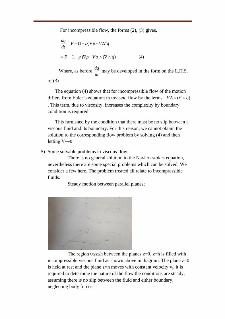
For incompressible flow, the forms (2), (3) gives,
2(1 )dq
F p V qdt
(1 ) ( ) (4)F p V q
Where, as before dq
dt may be developed in the form on the L.H.S.
of (3)
The equation (4) shows that for incompressible flow of the motion
differs from Euler’s equation in inviscid flow by the terms ( )V q
. This term, due to viscosity, increases the complexity by boundary
condition is required.
This furnished by the condition that there must be no slip between a
viscous fluid and its boundary. For this reason, we cannot obtain the
solution to the corresponding flow problem by solving (4) and then
letting V→0
5) Some solvable problems in viscous flow:
There is no general solution to the Navier- stokes equation,
nevertheless there are some special problems which can be solved. We
consider a few here. The problem treated all relate to incompressible
fluids.
Steady motion between parallel planes;
The region 0≤z≤h between the planes z=0, z=h is filled with
incompressible viscous fluid as shown above in diagram. The plane z=0
is held at rest and the plane z=h moves with constant velocity vj. it is
required to determine the nature of the flow the conditions are steady,
assuming there is no slip between the fluid and either boundary,
neglecting body forces.
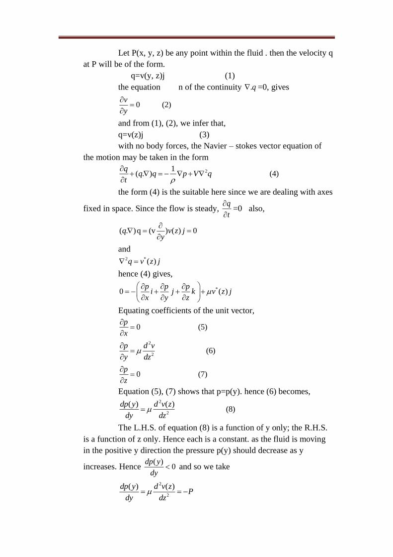
Let P(x, y, z) be any point within the fluid . then the velocity q
at P will be of the form.
q=v(y, z)j (1)
the equation n of the continuity .q =0, gives
0 (2)v
y
and from (1), (2), we infer that,
q=v(z)j (3)
with no body forces, the Navier – stokes vector equation of
the motion may be taken in the form
21( . ) (4)
qq q p V q
t
the form (4) is the suitable here since we are dealing with axes
fixed in space. Since the flow is steady, q
t
=0 also,
( . )q (v ) ( ) 0q v z jy
and
2 *( )q v z j
hence (4) gives,
*0 ( )p p p
i j k v z jx y z
Equating coefficients of the unit vector,
0 (5)p
x
2
2 (6)
p d v
y dz
0 (7)p
z
Equation (5), (7) shows that p=p(y). hence (6) becomes,
2
2
( ) ( ) (8)
dp y d v z
dy dz
The L.H.S. of equation (8) is a function of y only; the R.H.S.
is a function of z only. Hence each is a constant. as the fluid is moving
in the positive y direction the pressure p(y) should decrease as y
increases. Hence ( )
0dp y
dy and so we take
2
2
( ) ( )dp y d v zP
dy dz
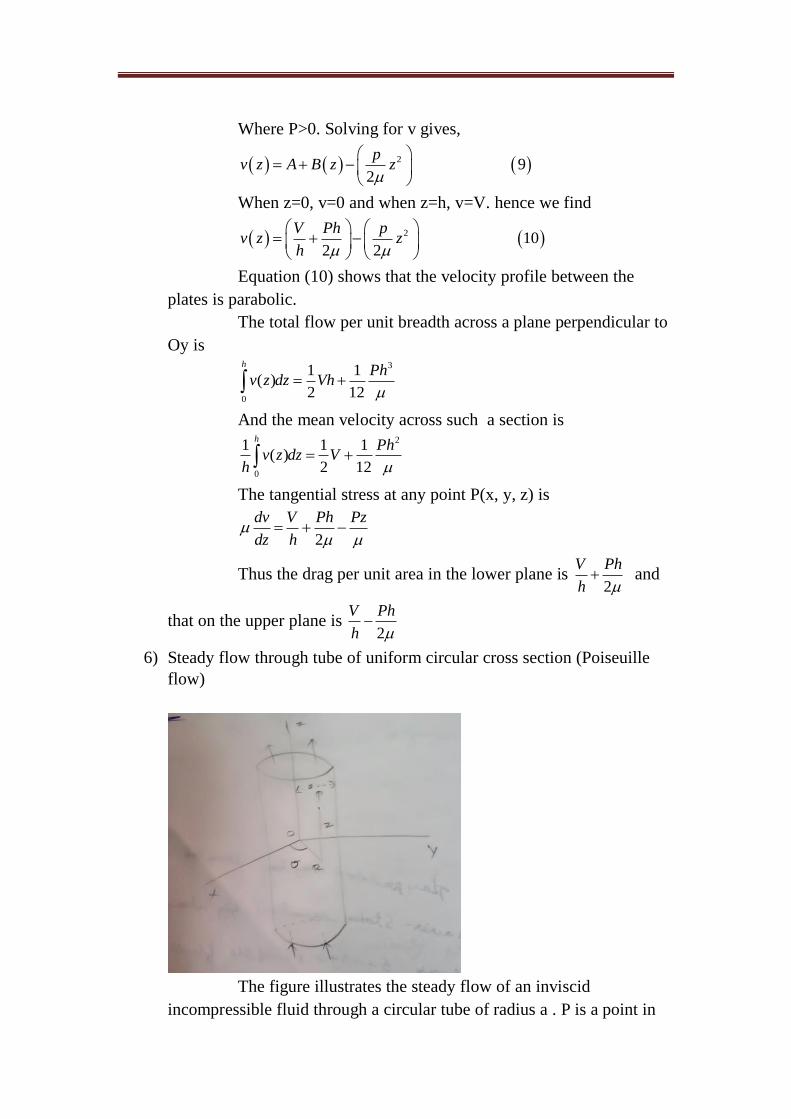
Where P>0. Solving for v gives,
2 92
pv z A B z z
When z=0, v=0 and when z=h, v=V. hence we find
2 022
1p
zV Ph
v zh
Equation (10) shows that the velocity profile between the
plates is parabolic.
The total flow per unit breadth across a plane perpendicular to
Oy is
3
0
1 1( )
2 12
hPh
v z dz Vh
And the mean velocity across such a section is
2
0
1 1 1( )
2 12
hPh
v z dz Vh
The tangential stress at any point P(x, y, z) is
2
dv V Ph Pz
dz h
Thus the drag per unit area in the lower plane is 2
V Ph
h and
that on the upper plane is 2
V Ph
h
6) Steady flow through tube of uniform circular cross section (Poiseuille
flow)
The figure illustrates the steady flow of an inviscid
incompressible fluid through a circular tube of radius a . P is a point in

the fluid having cylindrical polar coordinates (R, θ, z) refereed to the
origin O on the axis of the tube which is taken as the z- axis . we assume
there are no body forces. Then continuity considerations applied to an
annular shaped element of radii R, R+δR of the fluid indicate that the
fluid velocity is of the form
q=w(R)k (1)
let us take the Navier – stokes vector equation in the form
1
( . ) ( ) (2)q
q q p V qt
here this form is adopted with the last term ( )V q and
not 2V q as in the previous case, because the axes are not fixed in
space. For the same reason the form give on the L.H.S. is more useful
than dq
dt then we have,
0 ( )q
steady conditionst
( . ) ( )[w(R) k] 0q q wz
1 ˆˆp p
p R kR R z
in the above ( . )q q is easy to evaluate since the operand involves the
constant unit vector k. also,
ˆˆ
1 ˆ(R)
0 0 ( )
R R k
q wR R z
w R
hence,
ˆˆ
1 1( ) (Rw ) k
0 (R) 0
R R k
dq
R R z R dR
Rw
thus the equation (2), becomes,
1 ( )ˆ0
p p p v d RwR k k
R R z R dR
equating coefficients of the unit vectors gives,
0 (3)p
R
0 (4)p

( )
(5)p d Rw
z R dR
equation (3) and (4) shows that p=p(z) so that (5) becomes
( )
[ ( )] (6)dp z d
Rw Rdz R dR
the L.H.S. of (6) is a function of z only the R.H.S. is a
function of R only. Hence each is constant. As flow is supposes to occur
in the positive direction, we suppose p
z
<0. Take each side of (6) to be
-P where P is a positive constant. Then
( ) d PR
RwdR
or
2
2
Rdw PRA
dR
hence
1
2
dw A PR
dR R
and so, 21
( ) log (7)4
PRw R B A R
now w is finite on R=0. Thus we require A=0. Also on R=a, w=0 since
there is no slip.
Then , Hence
2 21( ) (8)
4
Pw R a R
Then for, (8) shows that the velocity [profile is parabolic. i.e.,
the plot of w against R from R=0 to a is parabolic shape.
The volume of fluid discharged over any section per unit time
is
4
0
( )28
aPa
Q w R RdR
If p denotes the pressure difference at two points on the axis
of the tube distant l apart, then p
Pl
7) Analysis stress in fluid motion:

With a notation of section a plane perpendicular to
xP cuts
the principal axes , ,n n nPx Py Pz of the rate of strain quadric in A,B,C to
form a small tetrahedron of fluid PABC in fig. If A denotes this area
of the face ABC, then 1 2 3, ,l A l A l A are the areas of the faces PBC,
PCA, PAB. Since these last three are principal planes, using the notation
it follows that the only forces on them are the normal forces
1 1 2 2 3 3,p ,pp l A l A l A . The forces on the face ABC are
, p ,pxx xy xzp A A A
in the x-y-z direction.
The equation of motion in the x direction (assuming the element
to be a particle
of fixed mass moving with the fluid) is
1 1 1 2 2 2 3 3 3 30xxp A l p l A l p l A l p l A
Where 30 is a term of the third order. Thus in the limit as the
volume of the element tends to zero, we obtain
2 2 2
1 1 2 2 3 3
2 2 2
1 1 2 2 3 3
2 2 2
1 1 2 2 3 3
(1)
xx
yy
zz
p p l p l p l
and similarly
p p m p m p m
p p n p n p n
Adding the equations (1) together we find
1 2 3( 3 , )xx yy zzp p p p p p p say
Thus the sum of the normal stresses across any three
perpendicular planes at a point is an invariant. We denote this sum by -
3p, so that p denotes the mean pressure at the point.
Resolving in the direction and neglecting third order terms,
1 1 1 2 2 2 3 3 3
1 1 1 2 2 2 3 3 3
1 1 1 2 2 2 3 3 3
(2)
xy
yz
zx
p l m p l m p l m p
and similarly
p m n p m n p m n p
p n l p n l p n l p
The equation (1) and (2) express the six distinct components
of stress matrix in terms of the principal stresses.
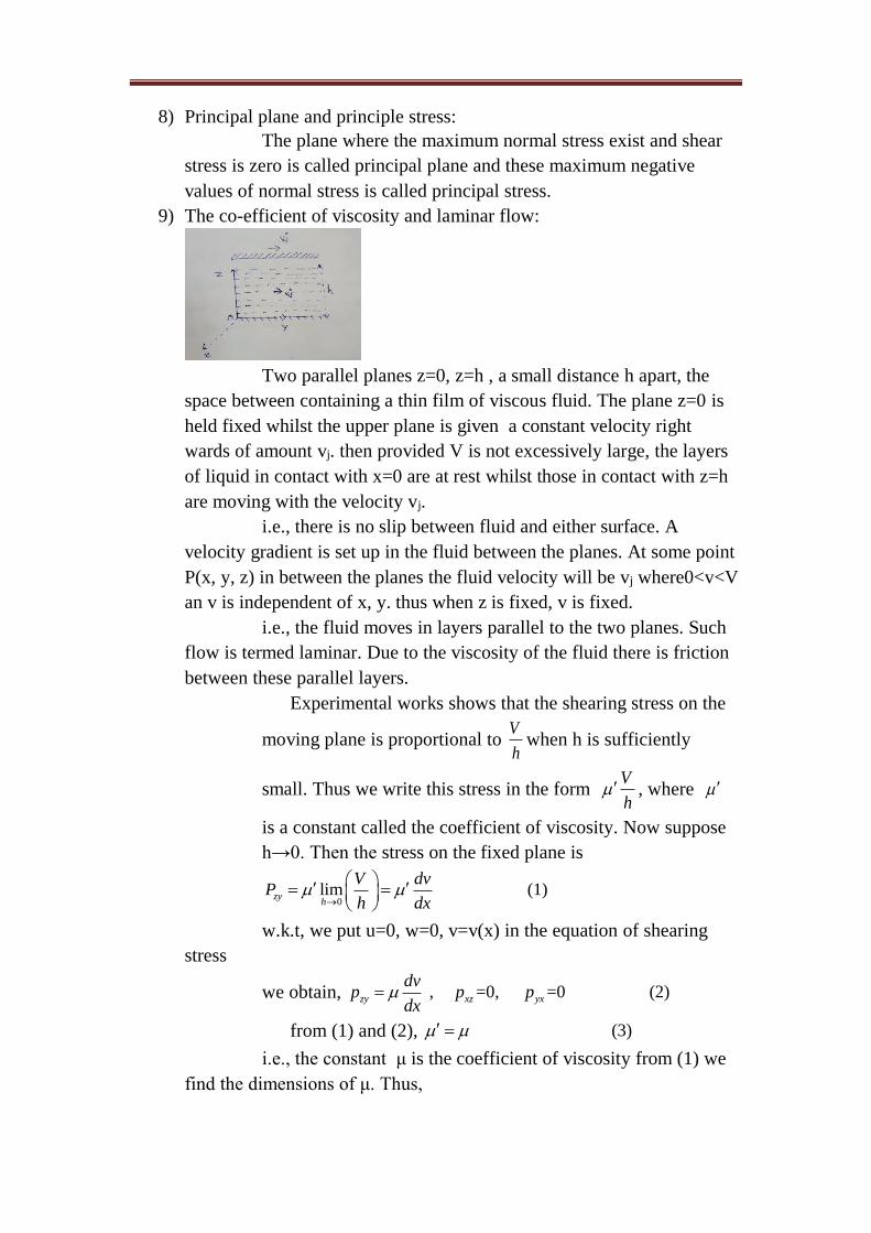
8) Principal plane and principle stress:
The plane where the maximum normal stress exist and shear
stress is zero is called principal plane and these maximum negative
values of normal stress is called principal stress.
9) The co-efficient of viscosity and laminar flow:
Two parallel planes z=0, z=h , a small distance h apart, the
space between containing a thin film of viscous fluid. The plane z=0 is
held fixed whilst the upper plane is given a constant velocity right
wards of amount vj. then provided V is not excessively large, the layers
of liquid in contact with x=0 are at rest whilst those in contact with z=h
are moving with the velocity vj.
i.e., there is no slip between fluid and either surface. A
velocity gradient is set up in the fluid between the planes. At some point
P(x, y, z) in between the planes the fluid velocity will be vj where0<v<V
an v is independent of x, y. thus when z is fixed, v is fixed.
i.e., the fluid moves in layers parallel to the two planes. Such
flow is termed laminar. Due to the viscosity of the fluid there is friction
between these parallel layers.
Experimental works shows that the shearing stress on the
moving plane is proportional to V
hwhen h is sufficiently
small. Thus we write this stress in the form V
h , where
is a constant called the coefficient of viscosity. Now suppose
h→0. Then the stress on the fixed plane is
0
lim (1)zyh
V dvP
h dx
w.k.t, we put u=0, w=0, v=v(x) in the equation of shearing
stress
we obtain, , =0, =0 (2)zy xz yx
dvp p p
dx
from (1) and (2), (3)
i.e., the constant μ is the coefficient of viscosity from (1) we
find the dimensions of μ. Thus,
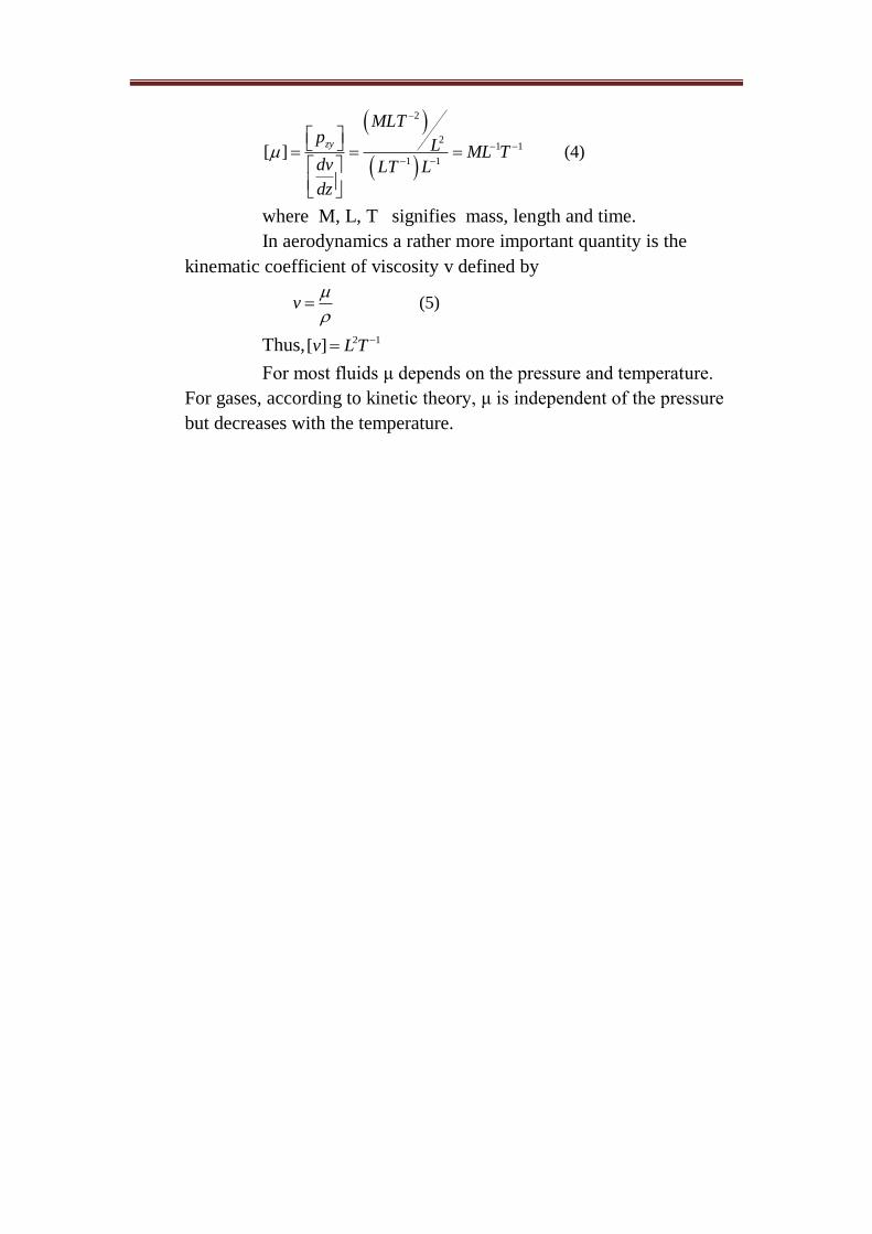
2
21 1
1 1[ ] (4)
zy
MLTp
L ML Tdv LT L
dz
where M, L, T signifies mass, length and time.
In aerodynamics a rather more important quantity is the
kinematic coefficient of viscosity v defined by
(5)v
Thus, 2 1[ ]v L T
For most fluids μ depends on the pressure and temperature.
For gases, according to kinetic theory, μ is independent of the pressure
but decreases with the temperature.