Computational fluid dynamics for physicists and engineers

Ruchi MishraNicolaus Copernicus Astronomical Center

Inverted CERN school of Computing (iCSC), CERN, 28th Sep- 2nd Oct 2020

Content What is Computational Fluid Dynamics?

Applications in different fields

How does CFD work?

Conservation equations

Discretization method

Riemann Problem

Example: Shock tube Problem

Example: KORAL Simulation

2

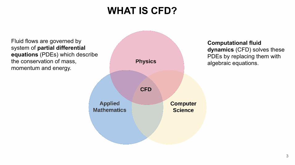
Fluid flows are governed by system of partial differential equations (PDEs) which describe the conservation of mass, momentum and energy.

Computational fluid dynamics (CFD) solves these PDEs by replacing them with algebraic equations.

WHAT IS CFD?

3

4

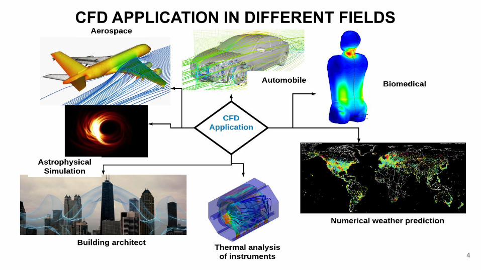
CFD APPLICATION IN DIFFERENT FIELDS

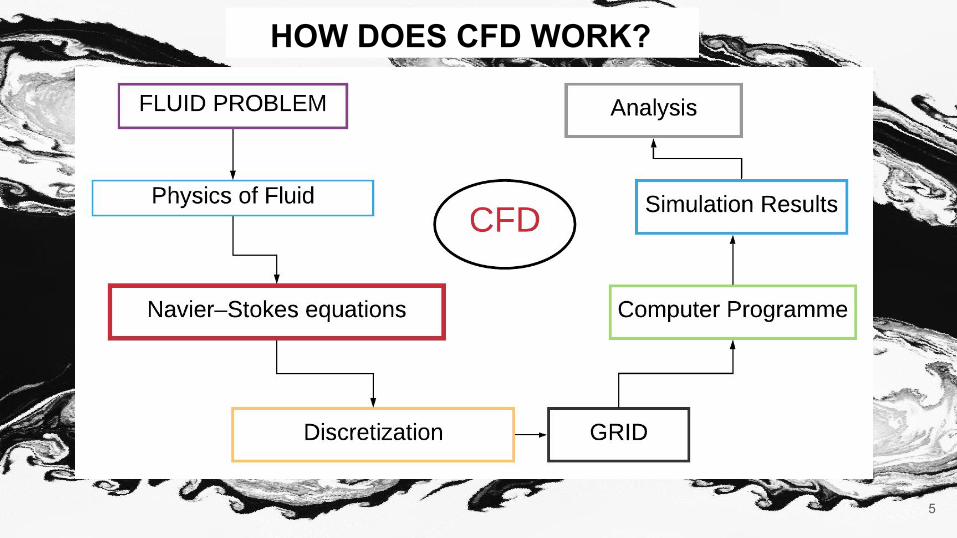
HOW DOES CFD WORK?

5

6

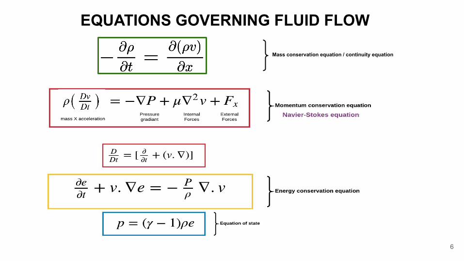
Mass conservation equation / continuity equation

EQUATIONS GOVERNING FLUID FLOW

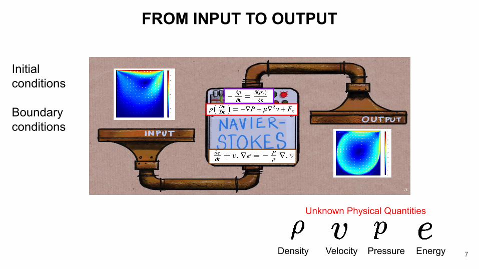
FROM INPUT TO OUTPUT

7

Unknown Physical Quantities

Density Velocity Pressure Energy

Initial conditions

Boundary conditions

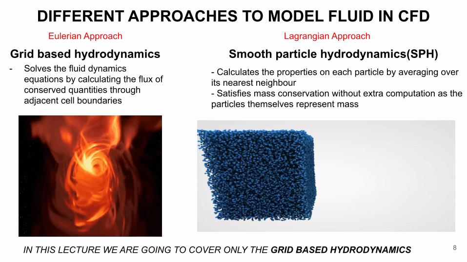
DIFFERENT APPROACHES TO MODEL FLUID IN CFD

Grid based hydrodynamics Smooth particle hydrodynamics(SPH)- Solves the fluid dynamics

equations by calculating the flux of conserved quantities through adjacent cell boundaries

- Calculates the properties on each particle by averaging over its nearest neighbour- Satisfies mass conservation without extra computation as the particles themselves represent mass

Lagrangian ApproachEulerian Approach

8IN THIS LECTURE WE ARE GOING TO COVER ONLY THE GRID BASED HYDRODYNAMICS

9 How to solve it numerically ?

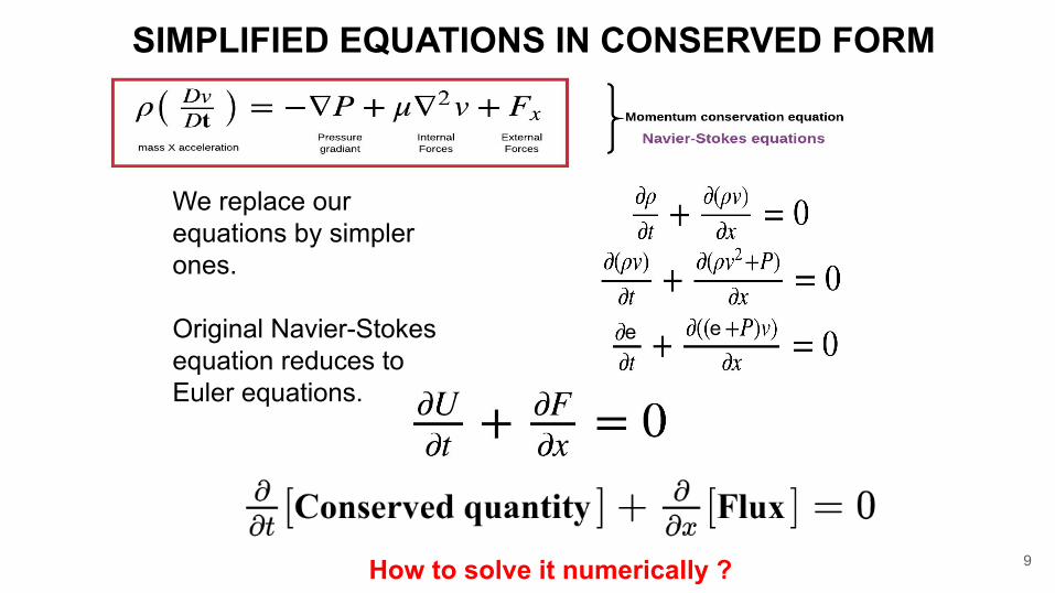
We replace our equations by simpler ones.

Original Navier-Stokes equation reduces to Euler equations.

SIMPLIFIED EQUATIONS IN CONSERVED FORM

e e

10

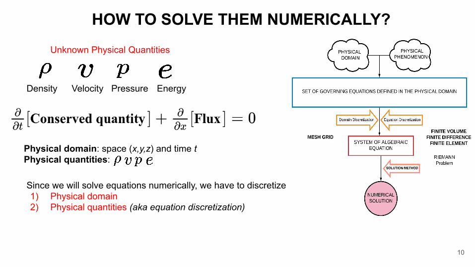
Physical domain: space (x,y,z) and time tPhysical quantities:

Since we will solve equations numerically, we have to discretize:1) Physical domain2) Physical quantities (aka equation discretization)

Unknown Physical Quantities

Density Velocity Pressure Energy

HOW TO SOLVE THEM NUMERICALLY?

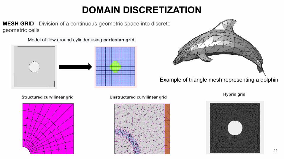
DOMAIN DISCRETIZATIONMESH GRID - Division of a continuous geometric space into discrete geometric cells

Example of triangle mesh representing a dolphin

Model of flow around cylinder using cartesian grid.

Structured curvilinear grid Unstructured curvilinear grid Hybrid grid

11

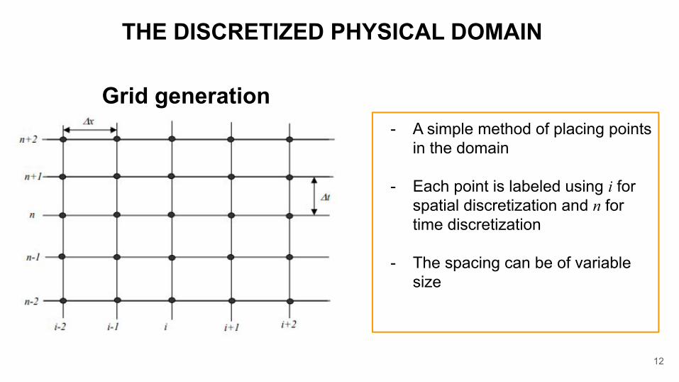
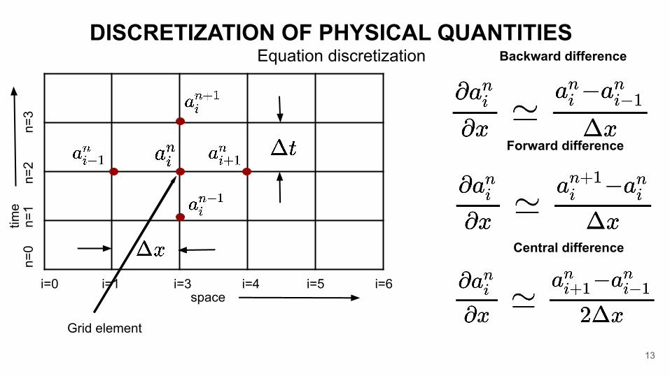
THE DISCRETIZED PHYSICAL DOMAIN

- A simple method of placing points in the domain

- Each point is labeled using i for spatial discretization and n for time discretization

- The spacing can be of variable size

Grid generation

12

space

time

DISCRETIZATION OF PHYSICAL QUANTITIES Equation discretization Backward difference

Central difference

i=0 i=1 i=3 i=4 i=5 i=6

n=0

n

=1

n=

2

n

=3

Grid element

13

Forward difference

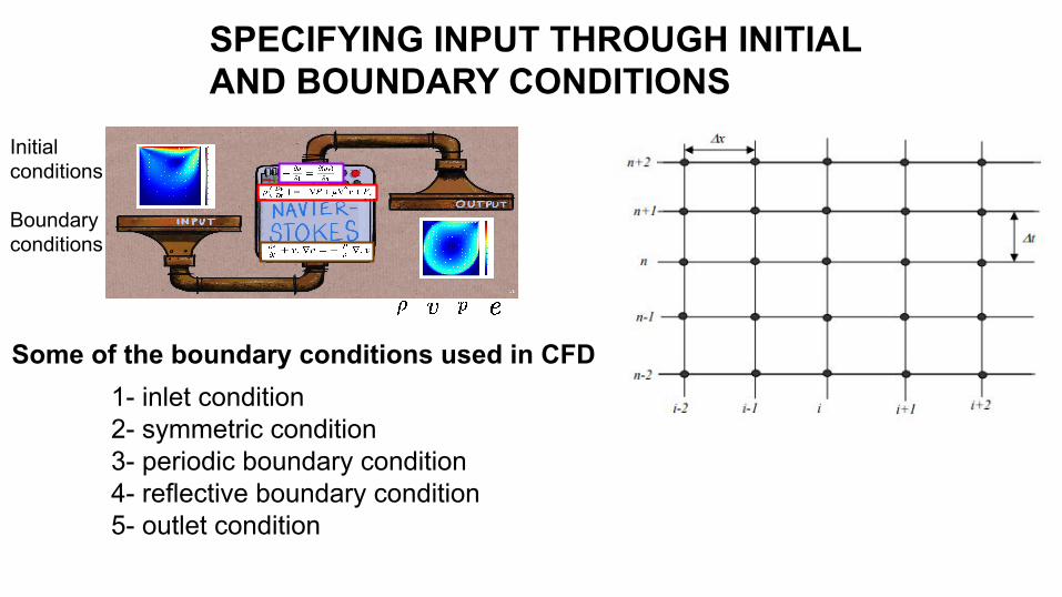
Initial conditions

Boundary conditions

SPECIFYING INPUT THROUGH INITIAL AND BOUNDARY CONDITIONS

1- inlet condition2- symmetric condition3- periodic boundary condition4- reflective boundary condition5- outlet condition

Some of the boundary conditions used in CFD

15

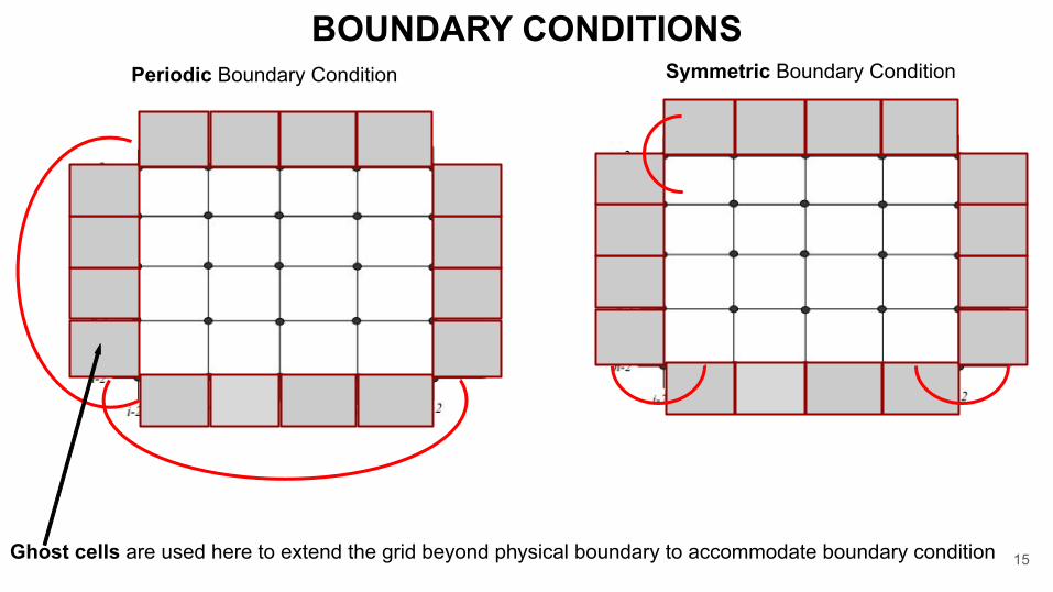
Symmetric Boundary ConditionPeriodic Boundary Condition

Ghost cells are used here to extend the grid beyond physical boundary to accommodate boundary condition

BOUNDARY CONDITIONS

16

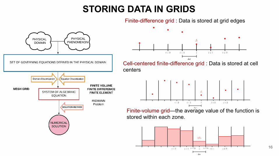
Finite-difference grid : Data is stored at grid edges

Cell-centered finite-difference grid : Data is stored at cell centers

Finite-volume grid—the average value of the function is stored within each zone.

STORING DATA IN GRIDS

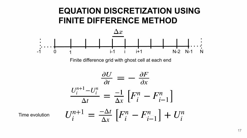
EQUATION DISCRETIZATION USING FINITE DIFFERENCE METHOD

i i+1i-10-1 1 NN-1N-2

Finite difference grid with ghost cell at each end

17

Time evolution

18

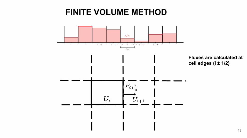
FINITE VOLUME METHOD

Fluxes are calculated at cell edges (i ± 1/2)

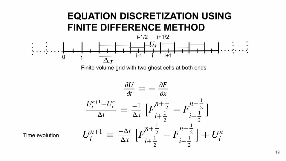
i i+1i-10 1

i-1/2 i+1/2

Finite volume grid with two ghost cells at both ends

19

Time evolution

EQUATION DISCRETIZATION USING FINITE DIFFERENCE METHOD

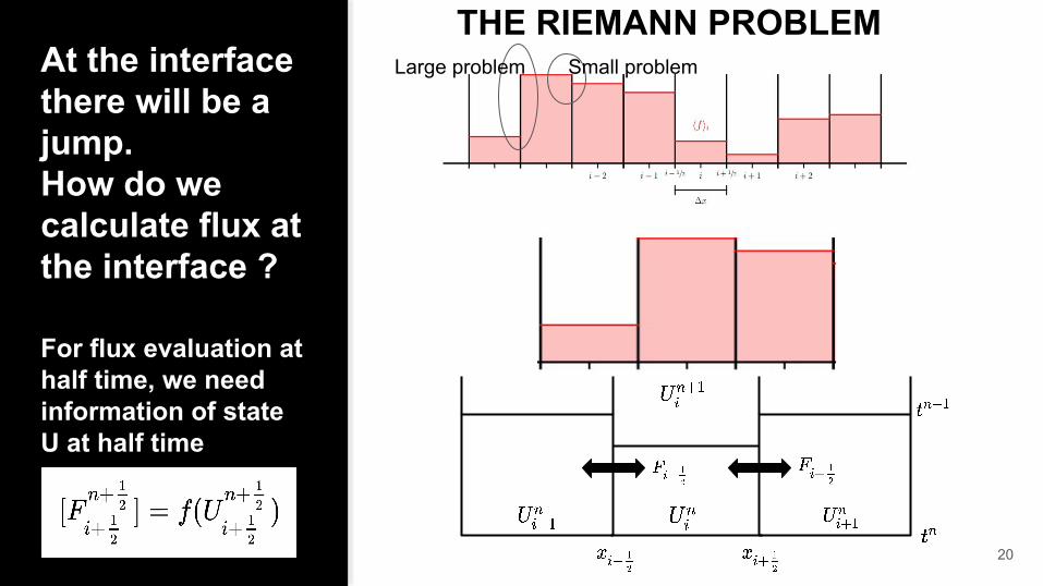
At the interface there will be a jump.How do we calculate flux at the interface ?

THE RIEMANN PROBLEM

20

For flux evaluation at half time, we need information of state U at half time

Small problemLarge problem

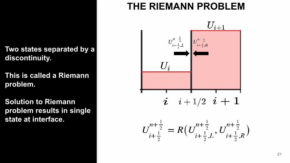
Two states separated by a discontinuity.

This is called a Riemann problem.

Solution to Riemann problem results in single state at interface.

21

THE RIEMANN PROBLEM

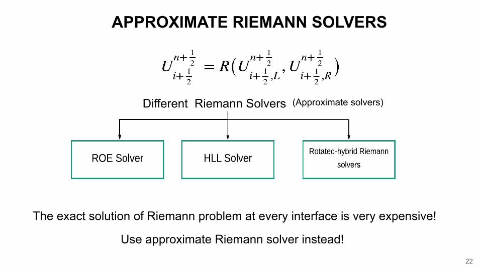
The exact solution of Riemann problem at every interface is very expensive!

Use approximate Riemann solver instead!

22

Different Riemann Solvers (Approximate solvers)

APPROXIMATE RIEMANN SOLVERS

23

Different Riemann Solvers

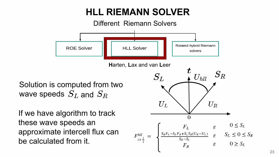
Harten, Lax and van Leer

HLL RIEMANN SOLVER

Solution is computed from two wave speeds and

If we have algorithm to track these wave speeds an approximate intercell flux can be calculated from it.

24

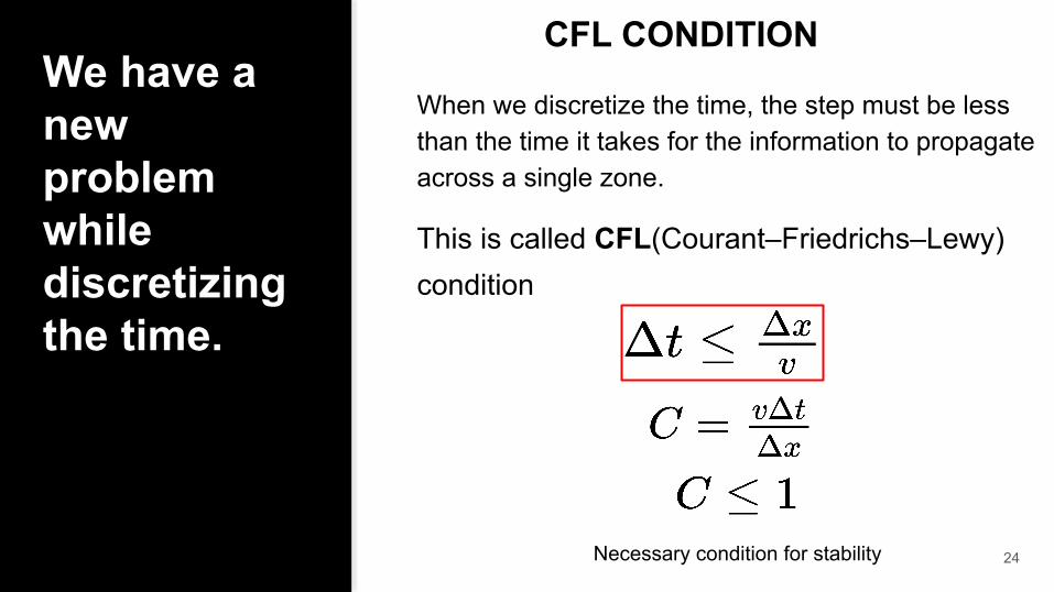
We have a new problem while discretizing the time.

When we discretize the time, the step must be less than the time it takes for the information to propagate across a single zone.

This is called CFL(Courant–Friedrichs–Lewy) conditionion

Necessary condition for stability

CFL CONDITION

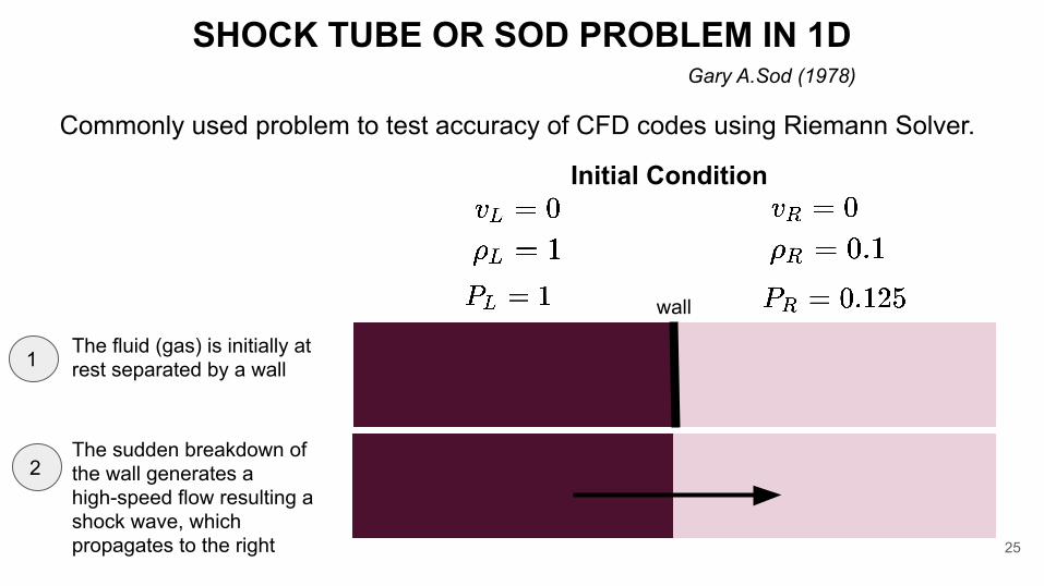
SHOCK TUBE OR SOD PROBLEM IN 1D

Initial Condition

The sudden breakdown of the wall generates a high-speed flow resulting a shock wave, which propagates to the right

Gary A.Sod (1978)

Commonly used problem to test accuracy of CFD codes using Riemann Solver.

25

The fluid (gas) is initially at rest separated by a wall

wall

1

2

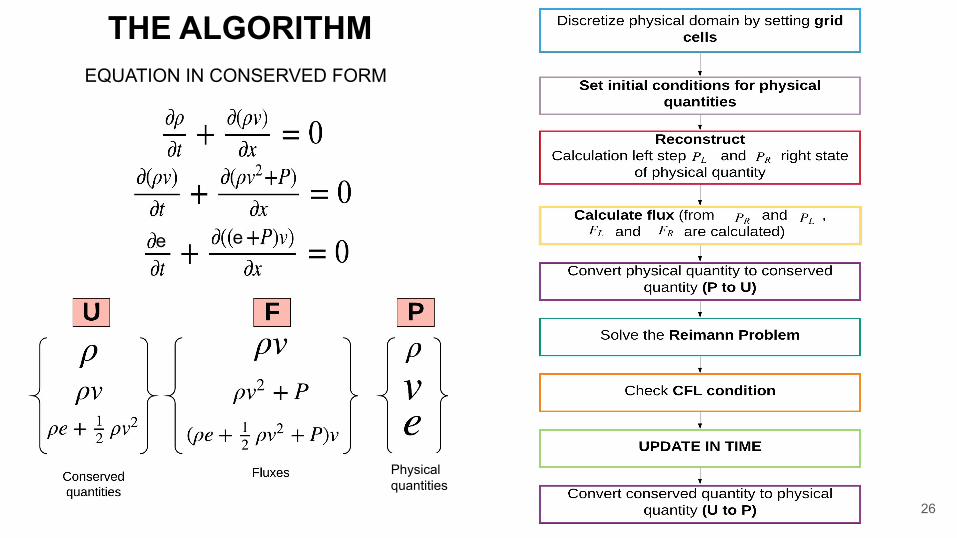
THE ALGORITHM

26

EQUATION IN CONSERVED FORM

Physicalquantities

e e

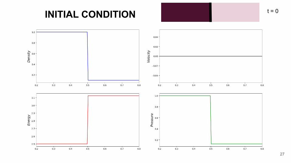
t = 0

27

INITIAL CONDITION

28

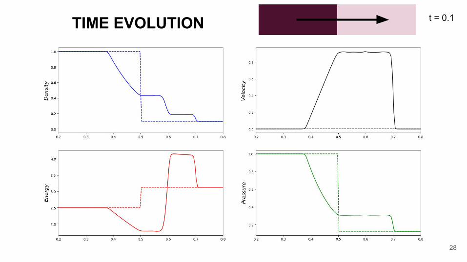
TIME EVOLUTION t = 0.1

29

TIME EVOLUTION t = 0.2

30

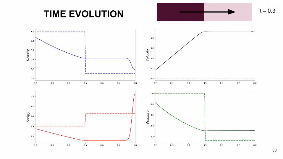
TIME EVOLUTION t = 0.3

Why do we do simulation in

Astrophysics?

31

SIMULATION IN ASTROPHYSICS

Simulation enables us to build a model of a system

It allows us to do virtual experiments to understand how this system reacts to a range of conditions and assumptions

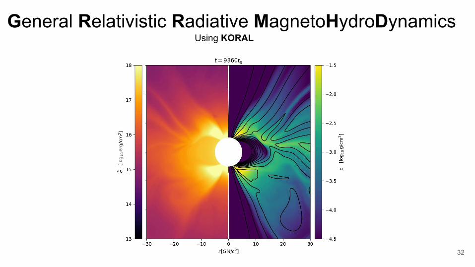
General Relativistic Radiative MagnetoHydroDynamics

32

Using KORAL

33

TAKE HOME MESSAGE :

● CFD enables us to predict fluid flow● The fundamentals of CFD lie in solving the set of partial differential

equations that describe the fluid flow (e.g. Navier-Stokes equation )● In Eulerian grid based approach, the physical domain is discretized into

large number of cells ● In each of these cells, Navier-Stokes equations can be rewritten as algebraic

equations● These equations are then solved numerically● At the end we get the complete description of flow throughout the domain

THANK YOU

34