• Norwegian Society of Chartered Engineers

NORTH SEA FLOW MEASUREMENT WORKSHOP

OCTOBER 22. - 24. 1991 SOI.STRAND FJORD HOTEL, BERGEN - NORWAY

EFFECTS OF FLOW CHARACTERISTICS DOWNSTREAM OF ELBOWS ON ORIFICE ME'I'ER ACCURACY

Lecturer:

Mr. Kamal Botros Nova Husky Research Corporation

Main Index

Reproduction is prohibited wbithout written pennmion from NIF and the author

EFFECTS OF FLOW CHARACTERISTICS DOWNSTREAM OF ELBOW/FLOW CONDITIONER

ON ORIFICE METER

1.0 INTRODUCTION

U. Karnik, W.M. Jungowski and K.K. Botros

NOVA HUSKY Research Corporation 2928 - 16th Street N.E.

calgary, Alberta canada T2E 7K7

Flow conditioners are used upstream of orifice meters to eliminate flow non-uniformities and

swirl and thereby facilitate accurate metering within a shortest possible meter run. The tube ..

bundle is the most commonly used flow conditioner in natural gas metering. The two impo~ant

standards providing specifications on the design and locations of the tube bundles are the

ANSl/API 2530 and the ISO 5167. An important specification is the straight length section

between the piping element generating the disturbance and the flow conditioner (L1), and that

between the flow conditioner and the orifice plate (L2). These specifications are quite different in

the two standards which has led several experimenters and the gas industry to heighten research

to study the effects of tube bundle location on orifice meter accuracy.

The available data produced to date, particularly those dealing with elbows generating the flow

disturbance upstream, are numerous. Almost all of the published reports and papers attempt to

specify a location of the tube bundle between the elbow and orifice meter which gives zero

deviation in the orifice discharge coefficient (Cd). The term 11cross-over point'1 is often used to

define this optimum location; a shorter distance to the orifice causes a negative A.Cd while a

longer distance causes a positive one.

For this cross-over point, contradicting values of L2/D started to appear (D is the pipe diameter).

This was to be expected since the cross-over point is not a unique point for all installations. It

should depend on the flow Reynolds number, total length of the meter run, orifice ~atio, meter

tube roughness, and instrumentation among other factors.

To be presented at the 9TH North Sea Flow Measurement Workshop, October 22 - 24, 1991, Bergen Norway

2

For example, the EC program conducted at Gasunie and NEL for testing the performance of tube

bundles in good flow conditions has revealed that the cross-over point Jies between 10 D and

15 D (1,2). A similar observation has been made by Brennan, et. al. [3] following experiments

performed at NIST (Boul.der). Extensive tests by Mcfaddin, et. al. [4] revealed that, for their meter

run, a cross-over point at 17 D was obtained for alt f>-ratios and was independent of the location

of the bundle w.r.t. the disturbance (two elbows in-plane separated by 12 D). Mean velocity

profiles at 7 D and 27 D were also presented in [4] which show that although the mean profile at

27 D is nearly fully developed, this was not the optimum position and .6.Cd for the 0.67 and 0.73

orifice plates was around +0.5%. Unfortunately, the velocity profile at 17 D (the cross-over

point) was not presented.

Sliding .tube bundle experiments were conducted in the low pressure nitrogen loop (724 kPa,

Re = 9 x 105) of the GRI Meter Research Facility at SwRI [51. The cross-over point for a 0.75

orifice plate was =11 D for 45 D meter run and =15 D for 19 D meter run. Velocity profiles

measured at different locations revealed that .the flow i~ still far from fully developed in the 45 D meter tube length indicating that there are other factors contributing to the zero shift other than a

. . fully developed velocity profile.

Experiments conducted on the .211 water facility at NIST in Gaithersburg [61 showed that with a

tube bundle located at L1 = 5.7 D from elbow outlet, a cross-over point was obtained at =12 D

for three f3-ratios (0.383, 0.5 and 0.75). Measurements of the streamwise and radial mean and

turbulent velocity profiles upstream and downstream of the tube, obtained by LDV, showed that

the tube bundle produces higher turbulence levels immediately downstream and that the levels

reach fully developed (Laufer) values at 27.3 D from tube bundle outlet. Unfortunately, the mean

and turbulent velocity profiles were not presented at the 12 D location which could possibly

illuminate the contribution of the turbulence levels to the zero deviation of Cd.

In this paper an attempt is made not to produce another cross~over point for an elbow/tube

bundle configuration, but to find the underlying mechanistic principles contributing to the

optimum location of the tube bundle w.r.t. the orifice meter. Tests were conducted on NOVA's

high pressure test facility at Didsbury, Alberta, Canada. The flow Reynolds number based on

pipe diameter was =s x 106. Two elbows in-plane separated by 1 O D represented the disturbing

element, and a 2.5 D long tube bundle (19 tubes) sliding along the pipe was used in the

experiments. Mean velocity profiles were obtained by means of a Pitot-static tube traversing in

two planes. Tests on. a similar configuration were conducted in a low pressure air loop where

profiles of the mean velocity and the Reynolds stresses were obtained by hot-wire anemometry.

P-0!<1007

3

Jn this paper, results from both the high pressure and low pressure facilities are presented and a

preliminary conjecture on the effects of turbulence and shear stress distribution downstream of a

tube bundle on the Cd shifts is proposed. An attempt is made to correlate the contribution of the

mean velocity profile, turbulence level, and shear stress to the location of the cross-over point.

2.0 EXPERIMENT AL FACILITIES

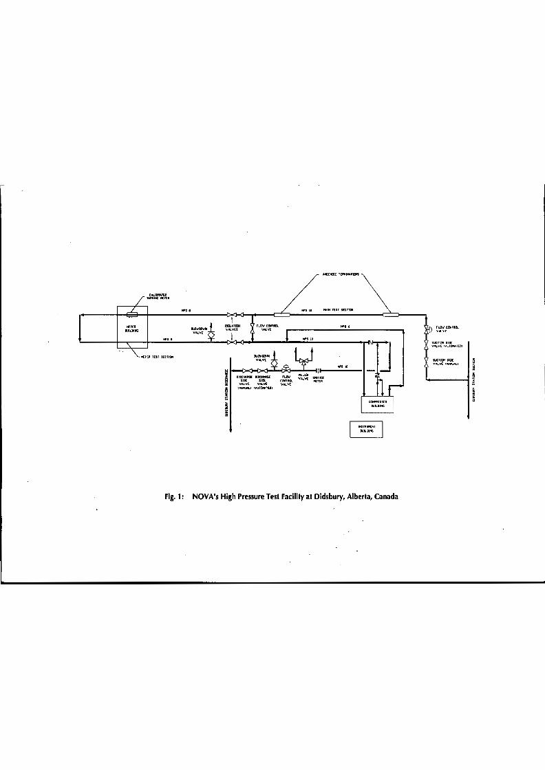
High Pressure Facility

A schematic of NOVA's Gas Dynamic Test Facility at Didsbury, Alberta, Canada is shown in

Figure 1. High pressure natural gas is diverted from the mainline into the test loop by means of a

centrifugal compressor or in a free flow mode. The maximum operating pressure at the facility is

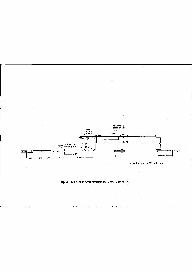
6450 kPa and the maximum Reynolds number in the test section of a 100 mm diameter was = 6 x 1 os. The test section is shown in more detail in Figure 2. Two orifice fittings are installed in

series, the one upstream being the reference meter. This reference orifice meter is preceded by

44 D straight meter run of internal roughness =s.o µm Ra, and two reducers 200 x 150 mm and

150 x 100. mm with 16 D separation. Two elbows in-plane with 10 D separation are shown in

figure 2. Both in-line tube bundle or a sliding tube bundle were used upstream of the second

(tested) orifice meter. The second orifice fitting is replaced with a traversing mechanism holding

a standard Pitot-static tube (PST) when measuring the axial and transverse velocity profiles. High­

accuracy transmitters were used in measuring the differential pressures across the flange-tapped

orifices and also the static pressure to an accuracy of :t0.1 % of span. As for the PST, the .

differential pressure transmitter connected to the stagnation and static holes is calibrated in the

range of 1 to 12.5 kPa, while the static holes (for radial velocity component) differential

transmitter was calibrated between - 1.5 to+ 1.5 kPa. All velocity profiles were normalized by

the instantaneous mean flow velocity obtained by the reference orifice meter upstream.

Temperature accuracy is within ±0.2% of the span. A gas chromatograph is connected on line to

give detailed gas composition of the gas during the course of the experiments.

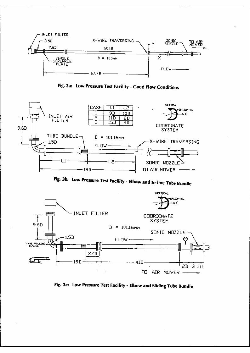
low Pressure Facility

The low pressure test facility consists of a 100 mm diameter test section, calibrated sonic nozzle

and 30 kW blower. Air is driven through the test section in a suction mode as shown in Figure

3a. Experiments were conducted with a sonic nozzle securing mean velocity of approximately

14.7 m/s through the test section, resulting in a Reynolds number of ::::-o.9 x 10s. Mean and

turbulent velocity profiles as well as shear stresses were obtained by x-wire miniature probe with

P.UC.1007

.. ..

4

a TSI anemometer (IFA 100). The x-wire was calibrated in a TSI calibrator. Figure 3a shows the

test section for a fully developed turbulent flow measurements at = 68 D downstream of a

sprenkle plate following the inlet filter. This test section was used to evaluate the performance of

the 19 tube flow conditioner in a good flow condition. Figure 3b shows the test section altered

with an upstream elbow of radius 1.5 D and an in-line tube bundle. The x-wire was traversed

across two perpendicular planes at 19 D from elbow outlet, for different location of the tube

bundle. Figure 3c shows similar configuration with a sliding tube bundle and an orifice meter

located at 19 D from the elbow outlet. The reference flow is measured by the calibrated sonic

nozzle downstream. All pipes used in the low pressure experiments were clear PVC pipes with

internal roughness around 0.25 µm (Ra). The elbow, however, is exactly the same steel elbow

used in the high pressure facility.

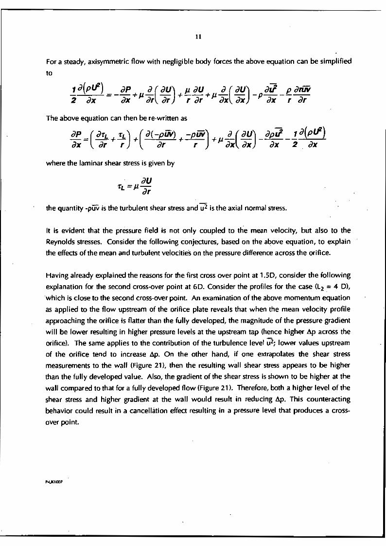
3.0 RESULTS FROM HIGH PRESSURE FACILITY

At the high pressure test facility the Pitot-static tube was traversed in a vertical and horizontal

plane. The measurements were taken at various distances from the second elbow: a) without

any flow conditioner, b) 4 D downstream of the tube bundle outlet . with the tube bundle at

different positions from elbow outlet, c) with fii;c:ed position of the tube bundle inlet at i D from

the elbow and PST at different locations downstream, and d) with fixed position of the PST at 19

D from the elbow and moved tube bundle.

The following observations were made:

re: a) the profiles acquired close to the second elbow outlet were typical for a single elbow

configuration, they became flat at about 16 D and then more elongated at 27.6 D but still

deviating from the reference profile which was measured upstream of the elbows in the

straight pipe (Figure 4);

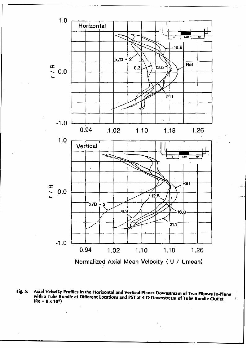
re: b) velocity profiles varied significantly with increasing distance between the elbow and tube

bundle outlets until around 12.5 D and then the pattern was primarily determined by the

distortion by the tube bundle itself (Figure 5);

re: c) the profiles at 6 D from the tube bundle outlet revealed strong distortions and at 27.6 D

became rather uniform but more elongated than the reference profile (figure 6);

P.UC1007

s

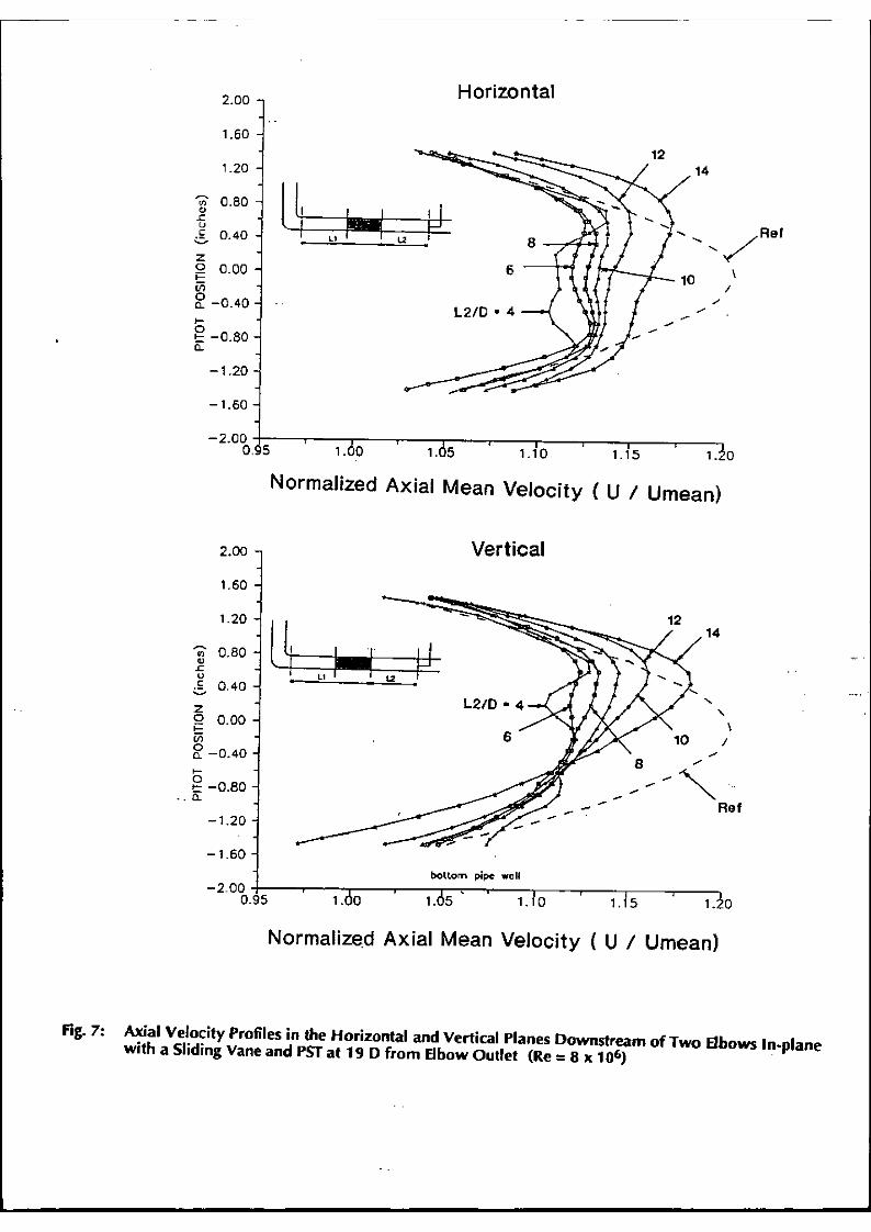
re: d) with decrease in distance from 1 5 to 5 D between the elbow and tube bundle outlets, the

profiles changed from an underdeveloped character to a more elongated one (Figure 7).

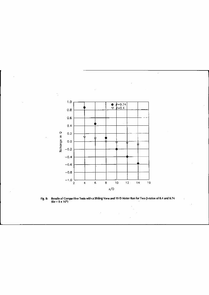
In order to correlate the velocity profiles to the cross-over point, the PST was replaced by an

orifice plate and the flow rate was metered with various positions of the tube bundle as in case

d). As Figure 8 shows, the cross-over occurred around L2 == 8D for both orifice plates (~ = 0.4

and 0.74). However, the corresponding vertical and horizontal profiles were underdeveloped

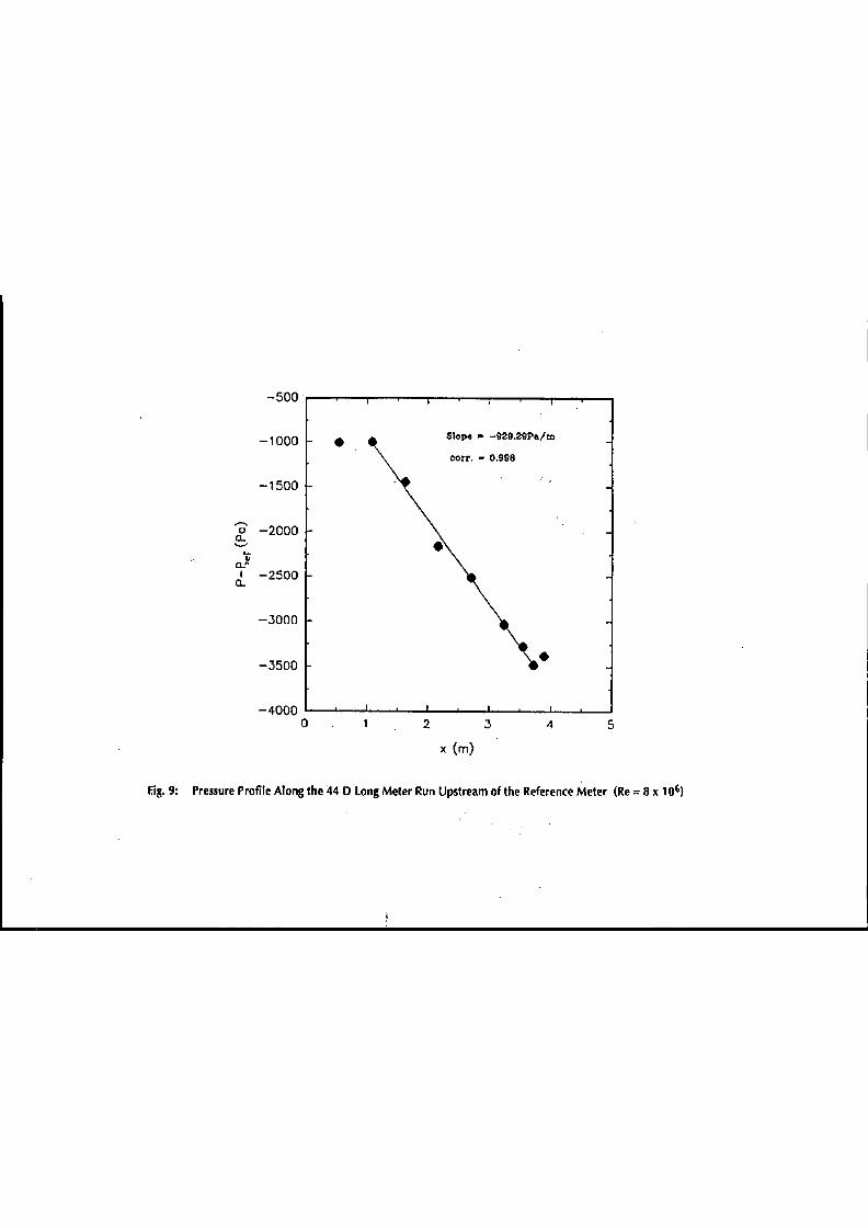
compared to the reference profile. In order to characterize the reference profile, the distribution

of the wall static pressure along the upstream pipe of the reference meter was measured. The

reference profile was found previously when the reference meter was substituted with the pitot

tube. Figure 9 shows a quasi-linear pressure drop along the pipe indicating that the flow is fully

developed. Utilizing Darcy friction factor f = 0.0131 evaluated from the pressure drop and the

approximate relation n = 1 / ..[j (14) between the exponent n characterizing the velocity profile

and f, n = 8.74 was found. This relation, however, overestimates n by about 10%. On the other .

hand, the fit to the experimental reference profile (Figures 4 through 7) gave n :: f .83. Both.

results appear to agree well.

A few conclusions can be drawn from the study performed at the hig~ pressure facility. A

comparison of case a) with c) . indicated that an enhancement of turbulence by the tube bundle

significantly increased the rate of the velocity profile modification, even to the overdevelopment.

case b) showed that at a certain distance, distortion caused by the tube bundle dominates the

effect caused by the elbows. This confirms earlier observations in (2,3,4) that the upstream

distance L1 has less effect than L2 on metering error. How~er, placing the tube bundle close to

the elbow outlet tends to freeze the incoming velocity profile and defeat th~ purpose of the tube

bundle. cased) and metering with the orifice plate revealed that the cross-over point can occur

with different mean velocity profiles. This implies that some other factors contribute to the

outcome of flow metering. The analysis of momentum equations pointed to the distribution of

the Reynolds stresses and therefore gave an incentive to measure turbulence. Preparation for

these measurements at the high pressure facility is currently underway.

In the meantime, in order to simplify experimental procedures and understand the flow

characteristics, tests were conducted on the low pressure test facility. It is believed that these

results could be scaled to the high pressure/high Re flows.

P~007

6

4.0 RESULTS FROM LOW PRESSURE FACILITY

4.1 Reference Profiles

Reference profiles were obtained, following a development length of approximately 680, with

the use of a miniature x-wire probe (see Figure 3a). The average velocity for this flow was around

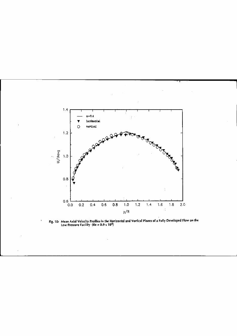
14.7m/s resulting in a Reynolds number of =:: O. 9x1 o5. It can be seen from Figure 10 that the

mean axial velocity profiles are nearly axi-symmetric and that the measurements are compatible

with the power law

~=( Y)11n 4nax R .

A log-log plot of (y/R v/s U/Umax) revealed that the value of n in the above power law is z 7.4.

Measurements close to the wall and near the centerline were excluded for the regression. The 11expected11 value of n for a smooth pipe at Re=O. 9x1 os is around 7.0. Thus, the pres~nt. profile

may be regarded to be slightly under-developed.

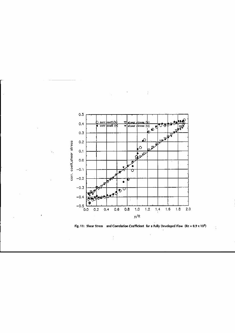
It has been shown, analytically [7] and experimentally 18,9], that for a fully developed flow the

distribution of the turbulent shear stress ('tt) across the pipe diameter is linear and its extrapolation

to the wall would result in an estimation of the wall shear stress. Figure 11 shows our

measurements of the turbulent shear stress uv = 'tt/p. The distribution is clearly linear. This

indicates that, for all practical purposes, the flow is fully developed. The shear stress is zero at the

center as expected and on extrapolating this distribution to the wall, the wall shear stress ('t..Jp) is

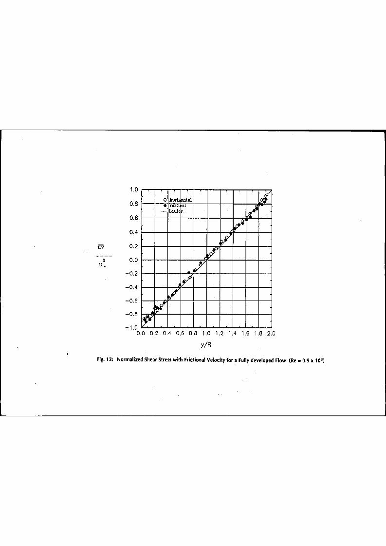
estimated to be approximately 0.42m2/s2 resulting in a friction velocity (u.) of 0.65m/s. Thus, if

the measured wall shear stress is used to normalize the data, the shear stress distribution (Figure

12) is representative of a fully developed flow. Additionally, the distribution of the correlation

coefficient (uv/u'v') is akin to that observed in a fully developed flow [B,91 where u 1 and v' are

the rms values of the fluctuating axial and radial velocities. The correlation coefficient reaches an

asymptotic value of approximately 0.43 near the wall. This value was measured as 0.4 and 0.5 by

(9) and {8] respectively. The correlation coefficient is usually approximated to be around 0.45

for a boundary layer l 1 O].

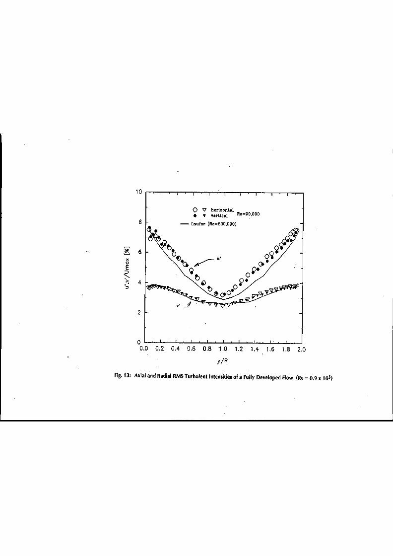
The axial and radial rms turbulent intensities, presented in Figure 13 are found to be comparable

to laufer's -data (8]. The axial intensities appear to be slightly higher, however, a similar

observation was made by Lawn 19], who measured intensities higher than those measured by

Laufer [8] and those measured in the present experiments.

P-UIC1007

1

Thus, ·measurements at the reference location appear to indicate that, for alJ practical purposes

the present flow is fully developed. Apart from providing details of the reference velocity field,

these measurements have also served as a test of credibility for the data acquisition and post

processing of the hot-wire anemometer signals.

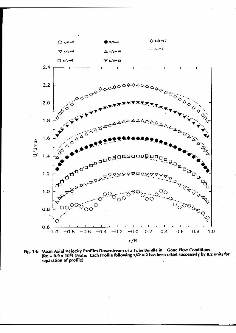
4.2 Measurements Downstream of a Tube Bundle in Good Flow Conditions

Measurements downstream of a 19 tube tube bundle (circular pattern, di=l 8 mm, d0=20 mm,

2.50 long) were obtained with the above reference profile as an input.

The mean axial velocity profiles at various locations downstream of the tube bundle are shown in

Figure 14, normalized by the maximum measured velocity. Allowing for experimental

inaccuracies, these profiles indicate that, after the initial decay of the jets/wakes generated by the

tube bundle, the velocity profiles are nearly compatible with the reference profile (n=7.4) after 6

pipe diameters.

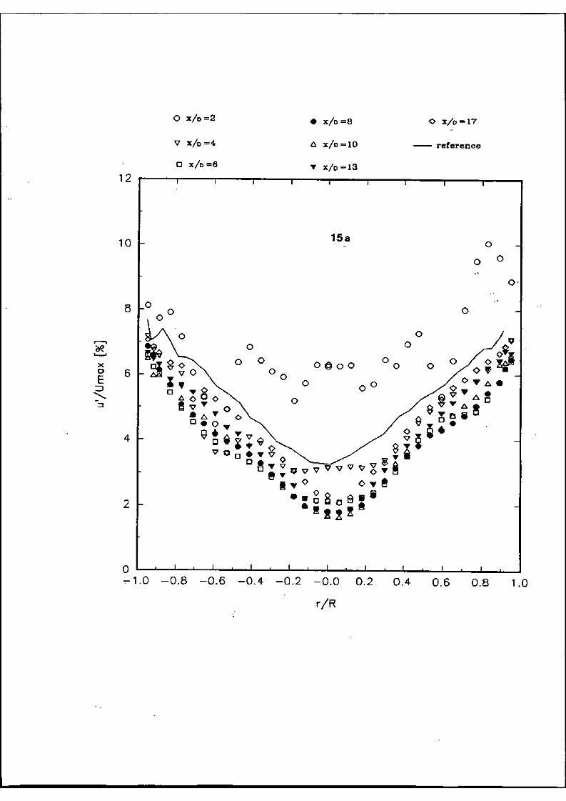
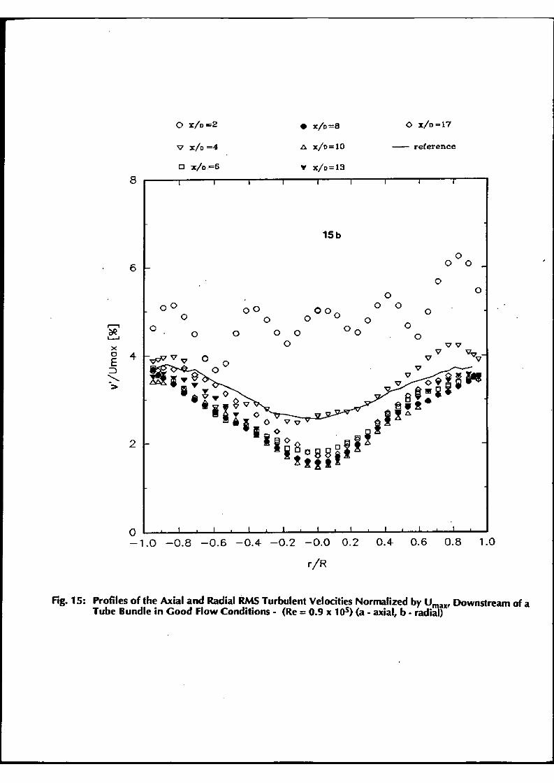
Profiles of the axial and radial rms turbulent velocities (normalized by the maximum velocity), at

locations downstream of the tube bundle, are shown in Figures 1 Sa and 1 Sb, respectively. As

expected, the turbulence intensities are maximum at the location closest to the tube bundle.

These intensities decay at downstreal'T) locations to a level below that at the reference location

and exhibit a growth further downstream. A similar behavior, on the centerline, has been .

observed by Morrow et. al. (17) in their sliding vane measurements. In their case, the tube

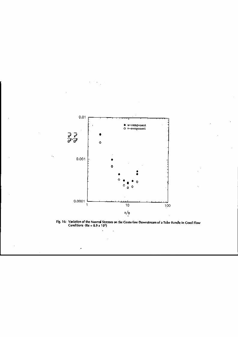
bundle was placed downstream of a single elbow. The variation of the normal stresses on the

centerline with downstream location, shown in Figure 16, indicates that the position of the

minima is at 10 D from tube bundle outlet

This behavior of initiaf decay and subsequent growth of the normal stresses is consistent with the

physics of the flow. Initially, the tube bundle generates high normal stresses (turbulence) due to

the shear of the jets/wakes generat~. As these jets/wakes coalesce, turbulence decays according

to a power law in a manner similar to grid turbulence (Sreenivasan et al. (11 ], and Warhaft, (12)).

This decay dominates the production of the pipe boundary layers until a balance is reached.

Subsequently, turbulence grows and, in the case of a pipe flow, it should be expected to reach

the fully developed magnitude asymptotically. This behavior of initial decay and subsequent

growth in the presence of a uniform shear, has also been documented in the wind tunnel

P.()1(1007

8

experiments of Tavoularis and Kamik [13). However, in their case, due to the presence of a

uniform shear, turbulence continues to grow downstream.

It may be worthwhile to note that the initial rate of decay of grid turbulence is dependent on the

mesh size (M =di in our case) of the grid and on the initial Reynolds number (ReM=UM/u). Since

decay of energy is mainly attributed to the draining of energy from the large eddies towards the

smaller eddies via inertial interactions [14], a smaller mesh size would imply a quicker decay of

energy. Also, in terms of the initial Reynolds number, a higher Reynolds number implies lower

viscous dissipation due to either lower kinematic viscosity or a slower energy transfer due to

larger scales (larger mesh size). This is evident· from the measurements of Batchelor and

Townsend [15) (ReM upto 4.4 x 104) and those of Kistler and Vrebalovich (16J(ReM=2.4x10°).

Measurements of the turbulent shear stress (Figure 17) reveal that the linear distribution of the ··

incoming reference flow has been distorted. Initially, the shear stress changes sign, as expected, ·

at locations of the jets/wakes. The shear stress is high at the locations of the maximum velocity

gradients and the change of sign is at the location where the mean velocity _gradient is zero.

Further downstream, the shear stress begins to re-organize itself. The magnitude of the shear · ·

stress is low in the core of the flow due to a lower mean velocity gradient and increases towards

the pipe walls. Further downstream, at about x/0=13, the shear stress appears to be re-aligning

itself with the reference shear stress distribution (shown as solid line). Hence it is evident that

although the mean velocity profile appears to be fully developed, the non-Hnear shear

·distribution indicates otherwise.

4.3 Measurements Downstream of a Tube Bundle with a Single goo Elbow

As mentioned earlier, these measurements were conducted to simulate the high pressure facility

and understand the contribution of turbulence to metering error. The major differences in the two

facilities are the working pressure, test fluid and the pipe Reynolds number. The present

measurements were taken downstream of a tube bundle, described earlier, with the velocity

profile from a single 900 elbow fr=l.SD) as in input.

Mean axial velocity profiles for the three different locations of the tube bundle with respect to the

elbow in a 19D meter run are shown in Figure 18. The velocity profile at the location of the

orifice plate appears to be dependent on the distance of the tube bundle from the elbow. For

locations closest to the elbow (L2=1 O D), the reminence of the effect of the elbow is evident

r>.UK1007

----- - · -··--·

9

whereas at the location farthest from the elbow (L2=4 D), the velocity profiJe downstream of the

tube bundle js relatively flat indicating that the effects of the elbow are sufficiently diminished.

The above can also be concluded from the velocity profiles obtained at the high pressure facility.

However, it appears that comparison of the velocity profiles in the two situations may not be

possible due to differences in the Reynolds number. As mentioned earlier, the dissipation due to

viscous action is less at higher Reynolds numbers and hence one could speculate that the effects

of the elbow and tube bundle would diminish at downstream distances which are longer than

those in the case of lower Reynolds numbers. This can be seen from the fact that at the high

pressure facility (high Re), for L2=4 0, the wakes/jets of the tube bundle are clearly detected

<Figures 6 and 7), however, in the case of the low pressure facility for a similar configuration,

there is.no evidence of the presence of these wakes/jets.

As observed ;n the case of the tube bundle in good flow conditions and by Morrow et. al. [17),

the axial and radial turbulence intensities in the present case are found to be lower. than the

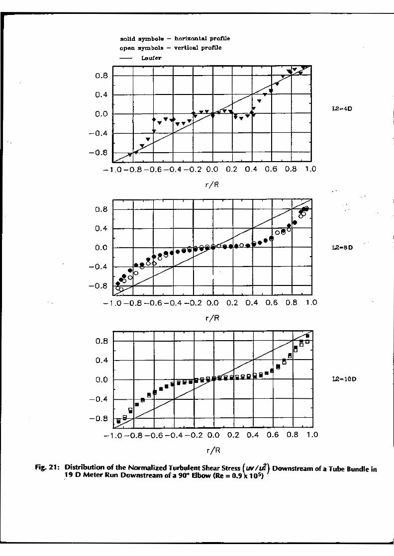
reference values as s.een in Figures 19 and 20. The shear stress (Figure 21) also exhibits a non·

linear distribution similar to that seen in the case of a tube bundle in good flow conditions. It is

worth mentioning at this point that the gradient of the shear stress away from the centerline

appears to be greater than that for the reference flow.

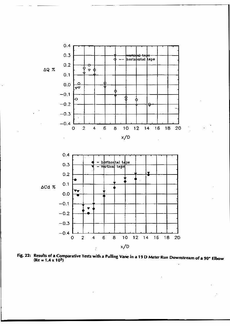
In order to determine the cross over points of the Cd shift, the tube bundle pulling mechanism

used in the high pressure facility was utilized for the present measurements. The orifice plate

(~0.44) was located at 190 from the elbow and the flow was metered by means of a calibrated

sonic nozzle. In order to obtain a pressure drop across the orifice plate within the range

recommended (1 o to 40 kPa) the chosen sonic nozzle resulted in a Reynolds number of

Z'1.4x1 os. The pressure taps for the orifice plate were located in the horizontal and vertical

plane at r/R = · 1.0. For each location of the tube bundle the% error in the flow rate and Cd was

evaluated

Results of the comparative testing, shown in Figure 22., indicate that there exists a cross-over

point at approximately 1.50 and another at around 60. Also, the vertical pressure taps (in the

plane of the elbow) consistently appear to read a lower pressure differential than the horizontal

pressure taps indicating that the plane of location of the pressure taps is important when

considering orifice metering accuracy.

P-uK1007

10

5.0 ANALYSIS OF RESULTS

The first cross-over point at x/D=l .5 of Figure 22 is not surprising. At positions closer than 1.SD,

the pressure has not fully recovered from the pressure drop due to the tube bundle, hence, the

upstream pressure tap is subjected to lower pressure levels resulting in a positive shift in the

discharge coefficient. As the tube bundle is retracted, at around 1.50, pressure recovery takes

place and levels of pressure are akin to the true pressure levels and a zero error (first cross over)

occurs.

With further pulling of the tube bundle, the pressure has fully recovered from the tube bundle

effects, and other parameters must be sought to explain the non-zero er'rors in the discharge

coefficient. Previously, only the mean axial velocity profite ha.s been used to explain this

occurrence. It has been claimed that if the mean velocity profile is close to being fully developed,

then a z~ro error would occur. However, deviations from this claim have been noticed. For

example, measurements at the high pressure facility show that the mean horizontal yelocity

profile at the cross-over point is rather flat. We mention the horizontal profiles since the taps are

on the h0rizontal plane. On the other hand, the profiles presented at 270 downstream of the

tube bundle by NIST [4} indicate that the mean velocity profile is nearly fully developed and yet

an error of +0.5% occurs in the discharge coefficient. Such contradictions have been stimulous to

measure and document the turbulent stresses in the present work and if possible extend the

correlation of the metering error to the turbulent structure of the flow.

Although more "carefully plann.ed and controlled" experiments would be required to establish an

exact relation between metering error and the turbulent structure, at this stage it suffices to show

that there exists such a relationship and we propose what may possibly be viewed as conjectures

based on the limited information in hand in the following.

Consider the mean axial momentum equation which can be written as (14)

ou aP 2 ail p aruv p auw p-=--+µV U-p---------+F.. Dt ax ax r ar r ae x

where U,V and W are the rnean velocities in the axial, radial and azimuthal directions and u,v

and w are the corresponding fluctuating velocities.

P.UC1007

11

For a steady, axisymmetric flow with negligible body forces the above equation can be simplified

to

The above equation can then be re.written as

aP = ( u'f'4 + 'f'L) + ( ac -pw) + -puv) + ~(au)-apt! _ 1 a(p<I) ax ar r ar r µ ax ax ax 2 ax

where the laminar shear stress is given by

au 1'4 = µ­ar

the quantity -puv is the turbulent shear stress and u2 is the axial normal stress.

It is evident that the pressure field is not only coupled to the mean velocity, but also to the

Reynolds stresses. Consider the following conjectures, based on the above equation, to explain

the effects of the mean and turbulent velocitieS on the pressure difference across the orifice.

Having already explained the reasons for the first cross over point at 1.50, consider the following

explanation for the second cross-over point at 60. Consider the profiles for the case (L2 = 4 D),

·which is close to the second cross-over point. An examination of the above momentum equation

as applied to the flow upstream of the orifice plate reveals that when the mean velocity profile

approaching the orifice is flatter than the fully developed, the magnitude of the pressure gradient

will be lower resulting in higher pressure levels at the upstream tap (hence higher dµ across the

orifice). The same applies to the contribution of the turbulence level u2; lower values upstream

of the orifice tend to increase ~· On the other hand, if one extrapolates the shear stress

measurements to the wall (Figure 21), then the resulting wall shear stress appears to be higher

than the fully developed value. Also, the gradient of the shear stress is shown to be higher at the

wall compared to that for a fully developed flow (Figure 21 ). Therefore, both a higher level of the

shear stress and higher gradient at the wall would result in reducing dp. This counteracting

behavior could result in a cancellation effect resulting in a pressure level that produces a cross­

over point.

P.UC:Ulll7

12

For the intermediate location (L2=8 D), the mean velocity profile approaching the orifice plate

appears to be nearly fully developed. Once again, in applying the momentum equation the mean

velocity inertial terms can be neglected. The decay of the normal Reynolds stresses tend to

increase the pressure levels at the upstream tap, however, the gradient of the shear stress which is

considerably greater than its fully developed counter part tends to reduce this pressure. The latter

effects is more severe, resulting in a low differential pressure across the orifice plate and

consequently a positive shift in the discharge coefficient.

In conclusion, as stated before, in the absence of more in·depth measurements, the above

explanations may be viewed as conjectures, at best, however, they seem to adequately explain

metering error which thus far could not be done solely on the basis of the mean velocity field.

Finally, the present measurements and their interpretations most certainly illuminate the fact that

there exists a definite relationship between orifice metering error and the turbulent velocity field.

6.0 FUTURE WORK

It is evident that there exists a need to conduct carefully planned and in·depth measurements to

shed more I ight on the precise interaction between orifice metering errors and the mean and

turbulent velocity field. Apart from the Reynolds stresses, also of interest are the measurements of

the integral length scales and the Taylor (dissipation) microscale. These would provide

information on the effect of initial scale size (due to tube bundle) on the decay of energy. Such

experiments are being planned at the low pressure facility at NHRC. Also, this study is to be

extended to the high pressure facility. Although equipmeni problems have been taken care of

with regards to the functioning of the IFA 1 oo in natural gas application at high pressures,

approval is currently being sought from the appropriate agencies to use this technique at such a

hazardous location. Once this has been achieved, it will then be possible to document the mean

and turbulent velocity flow field for low and high Reynolds numbers. This should go a long way

towards shedding light on the interaction of orifice metering error and the velocity field.

7.0 ACKNOWLEDGEMENT

The authors would like to acknowledge the assistance provided by P.Goldsmith, S.Fry and

P.Tetreau during the experiments. The work presented here is part of a flow metering research

program sponsored by NOVA CORPORATION OF ALBERTA and the permission to publish it is

hereby acknowledged.

1'.UC1007

13

8.0 REFERENCES

1. Smith, D.J.M., uThe Effects of Flow Straighteners on Orifice Plates in Good Flow

Conditions11, Commission of the European Communities, Directorate - General,

Telecommunications, Information Industries and lnnovatton, Batiment Jean Monnet,

Luxembourg, 1986.

2. Sattary, J.A., "EEC Orifice Plate Programme - Installation Effects", Seminar on lnstalfation

Effects on Flow Metering, NEL, Glasgow, 1990.

3. Brennan, J.A., Sindt, C.F ., Lewis, M.A. and Scott, J.L., "Choosing Flow Conditioners and

their Location for Orifice Flow Measurement", Seminar on Installation Effects on flow

Metering, NEL, Glasgow, 1990.

4. Mcfaddin, S.E., Sindt, S.F., and Brennan, J.A., "Optimum Location of Flow Conditioners

in a 411 Orifice Meter", National Institute of Standards and · Technology, Chemical

Engineering Science Division, Boulder, Colorado, 1989.

5. Morrow, T.B., "Determination of Installation Effects from 100 mm Orifice Meter Using a

Sliding Vane Technique", Seminar on Installation Effects on Flow Metering, NEL,

Glasgow, 199_0.

6. Mattingly, G.E., and Yeh, T.T., "Effects of Pipe Elbows and Tube Bundles on 50 mm

Orifice Meters", Seminar on Installation Effects on Flow Metering, NEL, Glasgow, 1990.

7. Tennekes, H., and Lumley, J.L., "A First Course in Turbulence", MIT Press, 1972.

8. Laufer, J., "The Structure of Turbulence in Fully Developed Pipe Flow'', NACA Report

1174,1954.

9. Lawn, C.J., ''The Determination of the Rate of Dissipation in Turbulent Pipe Flow'', J. of

Fluid Mechanics, Vol. 8, Part 3, 477-505, 1971.

10. Schlichting, H., "Boundary-Layer Theory'', McGraw-Hill, New York, 1979.

P.UC1007

14

11. Sreenivasan, K.R., Tavoularis, s., Henry, R., and Corrsin, S., ''Temperature Fluctuations

and Scales in Grid-Generated Turbulence", J. Fluid Mechanics, Vol. 100, Part 3, 597-621,

1980.

12. Warhaft, Z., ''The Interference of Thermal Fields from Line Sources in Grid Turbulence", J. Fluid Mechanics, Vol. 144, 363-387, 1984.

13. Tavoularis, S. and Karnik, U., "Further Experiments on the Evolution of Turbulent Stress

and Scales in Uniformly Sheared Turbulence", J. Fluid Mechanics, Vol. 204, 457-

478, 1989.

14. Hinze, J.O. "Turbulence", 2nd Edition, McGraw Hill, New York, 1975.

15. Batchelor, G.K. and Townsend, A.A., "Decay of Isotropic Turbulence in the Initial Period",

Proc. Roy. Soc. London, 193A, 539, 1948.

16. Kistler, A.L. and Vrebalovich, T., J. Fluid Mechanics, Vol. 26, 37, 1966.

17. Morrow, T.B., Park, J.T., and McKee, R.J., "Determination of Installation Effects for a 100

mm Orifice Meter Using a Sliding Vane Technique". Flow Meas. and Inst., Vol. 2, No. 1,

Jan. 1991.

P-UX1007

.... ISQ.ATD Vilt.VU

DIWWIOI: lltoWIOC nDW SlK SllC COflllQ.

VM..'lt. YAL.'1£ Y-'l.YC c--.iao t&\IT'C>ll t tin

""""' ..... _]

Fig. 1: NOVA's High Pressure Test Facility at Didsbury, Alberta, Canada

l UC U!>ISltlC Y""-vt •.oulCW. ICDI

aJCTDf SIDC -..aLVCl~I

~ ~ ~ ... -----1 =

trQverS1ng pltot-~ta tic

L:_ 19ll----<

FLO\./

Note• The VQne 1$ e.SD In length.

Fig. 2: Test Section Arrangement in the Meter Room of Fig. t

8 JN

1 ~.5

;;

IN3L.SEDT FILTER

X-1./JRE TRAVERSING "°"'\ J~Nff E ~ ~iJ'l

1~

7.6D 60.lD d y

=s=~k=~=~~~t=E=========D====lO=O=MM========~~l==~x==id

t-----PL_A_T_E ____ 67.7D --------1• FLOW'----

Fig. 3a: Low Pressure Test facility - Good Flow Conditions

INLET AIR FILTER

1.5D

CASE L1 L2 1 9D !OD 2 1 lD SD 3 15D 4D

D = 101.16MM

FLO\./----

COORDINATE SYSTEM

X-\./IRE TRAVERSING

~~u F=-~~~~

---------19D~-------~

SONIC NOZZL~ TO AIR MOVER

Fig. lb: Low Pressure Test facility - Elbow and ln-Hne Tube Bundle

FILTER

D = 101.16MM

VCRTICAL.

~~~ZCMAL -~~x

COORDINATE SYSTEM

SONIC

FLO\./----

TO AIR MOVER ---

Fig. Jc: Low Pressure Test Facility- Elbow and Sliding Tube Bundle

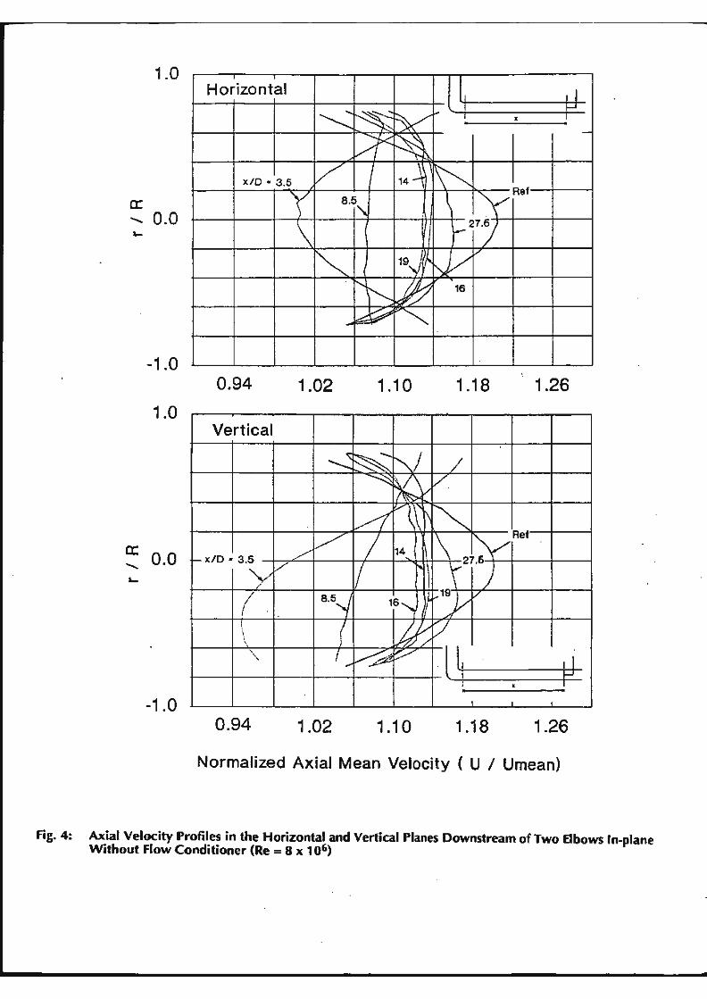
Fig. 4:

LO Horizontal [, _d

~ ~ ~~ ' _t:'" I K I

-

~ N~

a: ....... 0.0

/ I \ ~ x/O • 3 .5 14-1

y 8.5\. \ YRef \ I i-27/

_l

~ 19 l '-../ ~~wv

. r"-

lb ,

~ 16

... ~·

-1.0 0.94 1.02 1.10 1.18 1.26

1.0 Vertical

~ ~ ""'/ / ~ FrQ v . v

a: ....... 0.0 .....

~Y~' l\ ~ I/

/ 14~ \ l:'YRef i-X/0 • 3.5 / ) \27.6) y v I ["

/ 8.5"/ 16 ........ /t "'1Yv J

\ ( ~ v \ ' \

l I: ' \. I ~ v .... 8 I K I

-1.0 I I t

0.94 1.02 1.10 1.18 1.26

Normalized Axial Mean Velocity ( U I Umean)

Axial Velocity Profiles in the Horizontal and Vertical Planes Downstream of Two Ebows In-plane Without Flow Conditioner (Re = 8 x 106)

1.0 Horizontal

a: Ref

...... 0.0

-1 .0 0.94 .1.02 1.10 1.18 1.26

1.0 Vertical

a: ...... 0.0 ....

-1.0 0.94 1.02 1.10 1.18 1.26

Normalized Axial Mean Velocity ( U I Umean)

fig. 5: Axial Veloctty Profiles in the Horizontal and Vertical Planes Downstream of Two Elbows In-Plane with a Tube Bundle at Different locations and PST at 4 D Downstream of Tube Bundle Outlet (Re= ax 1011)

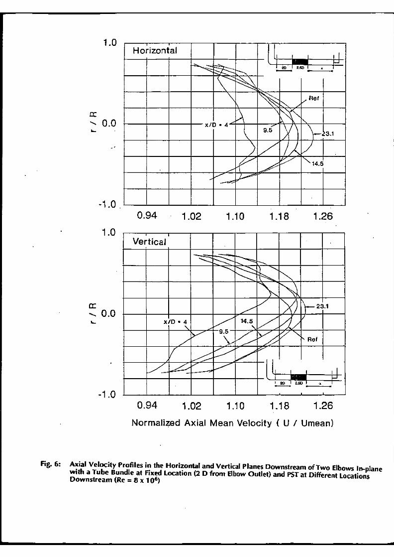
Fig. 6:

1.0 ~H_o-+-riz_o_nt+-a_I --+--+----r--,_ [ II J ,J µ

- -----=---

cc ...... 0.0 ....

3.1

0.94 1.02 1.10 1.18 1.26

1.0 Vertical

a: ....... 0.0 '-

Ref

l~ ~ i 20 ·• --1.0

0.94 i .02 1.10 1.18 1.26

Normali~ed Axial Mean Velocity ( U I Umean)

Axial Velocity Profiles in the Horizontal and Vertical Planes Downstream of Two Elbows In-plane with a Tube Bundle at Fixed Location (2 D from Elbow Outlet) and PST at Different Locations Downstream (Re = 8 x 106)

2.00 Horizontal

1.60

1.20 14

. .... -.. ..._'/Ref

......... 0 .80 ll: I/)

~ .s::. u c: 0.40 f v. z

6 \ 0 0.00 ~ Vi ~ -0.40

I

t-

g -0.80 o_

_, .20

-1.60

-2.00 0 . 5 1. 0 1. 5 1., 0 1. 5 1. 0

Normalized Axial Mean Velocity ( U I Umean)

2.00 Vertical

1.60

1.20 u - 0 .80 {I) (IJ

.s::. I 0

c: 0.40 v. z 0 0.00 ~ Vi :? -0.40 t-

g -0.80 • • o_

-1 .20

-1 .60

-2.00 ...!-----r-----.--,----.--------r---ir--~--.----,.--i 0 .95 1. 0 1. 5 1. 1 0 1. 5 1. 0

bottom pipe wall

Normaliz~d Axial Mean Velocity ( U I Umean)

Fig. 7: Axial Velocity Profiles in the Horizontal and Vertical Planes Downstream of Two Elbows In-plane with a Sliding Vane and PST at 19 D from EJbow Outlet (Re == 8 x 106) ·

1.0

0.8 •i b=0.74

1• \l ~=0.4

0.6

0.4 4t

0 0.2 c: ~11

'~ 4t Cl> 0.0 O> c: 0

I ~ ~17

.r::. u -0.2 ~

-0.4

-0.6 .~

-0.8

-1.0 2 4 6 8 10 12 14 16

x/D

Fig. 8: Results of Comparitive Tests with a Sliding Vane and 19 D Meter Run for Two P-ratios of 0.4 and 0.74 (Re = 8 x 106) ·

-500 .

-1000

-1500

........ -2000 0

a. '-' ... .. Cl!' I -2500 a.

-3000

-3500

-4000 0

•

2

Slope " -929.29Pa/m

corr. - 0.998

3 4

x (m)

5

F.ig. 9: Pressure Profile Along the 44 D Long Meter Run Upstream of the Reference Meter (Re = 8 x 106)

1.4

n•7.4 .., horizon la I

0 vertlcal

1.2

0.8

0.6 ._....._....1-_.__.r...___._---1~i-....;..L-....._..J-_.__,__.,__J~.__J__._-1...._.__J 0.0 0.2 0.4 0.6 0.8 1.0

y/R

1.2 1.4 1.6 1.8 2.0

Fig. 10: Mean Axial Velocity Profiles in the Horizontal and Vertical Planes of a Fully Developed Flow on the Low Pressure Facility (Re= 0.9 x 1 QS)

0.5

0.4

0.3

(I) 0.2 (I) Q) .... ti 0.1 .... c Q) .I:. 0.0 "!. -.... Q)

0 -0.1 ()

..: .... 0 -0.2 ()

-0 . .3

-0.5 .__..._..__....__.__.__,__.__.__.___..__.__...__.__..__..._~~~~-o. o 0.2 o.4 o.s o.a 1.0 1.2 1.4 1.6 , .B 2.0

y/R

Fig. 11: Shear Stress and Correlation Coefficient for a Fully Developed Flow (Re= 0.9 x 1 oS)

1.0

0.8

0.6

0.4

iiV 0 .2

2 0.0 u .

-0.2

-0.4

-0.6

-0.8

O horlz t:inte.l 'ff • ven1 a1

~ Laute

r /

I~ . ~

JV ./

Jf' ~ -1.0

0.0 0.2 0.4 0.6 0.B 1.0 1.2 1.4 1.6 1.8 2.0

y/R

Fig. 12: Normalized Shear Stress with Frictional Velocity for a Fully developed Flow (Re = 0.9 x 1 os)

0 \1 horizontal • ., verUcal Re•S0,000

8 - Laufer (Re=500,000)

,......, ~ 6 ..........

u' x ~ 0

E ::> "-">;. 4 "::::i

2

0 L-..-..l. ......... ......L.. ........ ...1......._..__""--l'--L.......r.._.._ ........ _._....._....._.___..__,

0.0 0.2 0.4 0.6 0.8 1.0 1.2 1.4 1.6 1.8 2.0

y/R

Fig. 13: Axial and Radial RMS Turbulent Intensities of a Fully Developed Flow (Re= 0.9 x 10s)

0 z/o.=2 • x/o•8

'\J 2/D<=4 6 x/o=lO ·· ·· ·n-7.-'

0 x/D•6 Y x/ci•t3

2.4 I I I I I I I ' t

2.2 - -

2 .0 ....

0 .6 I I I I I I I I I •

- 1 .0 -0.8 -0.6 -0.4 - 0 .2 -0.0 0 .2 0.4 0 .6 0 .8 1.0

r/R

Fig. 14: Mean Axial Velocity Profiles Downstream of a Tube Bundle in Good Flow Conditions - . (Re = 0.9 x 1 os) (Note: F.ach P.rofile following x/O = 2 has been offset successivly by 0.2 units for separation of profile)

x 0 E

=:i ...........

:::i

0 x/o=2 • x/o =B

v x/o =4 A x/o = 10

O x/o=6 'Y x/o=13 12

10 15a

0 00

8

6

4

2

00

<> x/o =17

- reference

0 0

0 0

0

0

0

0

0 ·

0 ..__,___..___.____.~--...... ~"'-....... ~"-------'----'----'~..._ ...... ~.......__._~ ...... _.....__,, -:--1 .0 -0.8 -0.6 -0.4 -0.2 -0.0 0 .2 0.4 0 .6 0.8 1.0

r/R

x 0

E ::'.)

':'-:>

8

6

0

4

2

0

O x/0 ... 2

<:7 x/o - 4

D x/o.= 6

oO 0

0 0

oO 0

0

• x/o=8

1::i. x/ o=lO

'I' x/ o=13

15b

0

<> x/o =17

- reference

0 0 0

0 0

0

0

0 0 0

0

-1 .0 -0.8 -0.6 -0.4 -0.2 -0.0 0 .2 0.4 0.6 0.8 1.0

r/R

Fig. 15: Profiles of the Axial and Radial RMs Turbulent Velocities Normalized by UR\U' Downstream of a Tube Bundle in Good Flow Conditions - (Re = 0.9 x 1 oS) (a - axial, b - radial)

--------. -. -

0.01

• 0

0.001 ,_ • 0

• 0

0.0001

I

• u-component O v-component

• • ~ . • 0

0 0

I

10

x/o

100

Fig. 16: Variation of the Normal Stresses on the Centerline Downstream of a Tube Bundle in Good Flow Conditions (Re = O. 9 x 1 QS)

symbols as in Fiiure 15

0 .0 l----it-----t~---t~"T'riih:n::1:8'~1-9-"'-""--+-~+::::~-+-~

-0.4 t-----i~t-=-t....,.......~".::---t-~--......~--t----t-~-;-~;----1 0

-0.B 0

0 0

-1.2 0 .__..__ .......... ....._..__.__..__..__.._.___.___.___.__.__.__....._._ .......... ......_......_.

-1 .0-0.8-0.6-0.4-0.2 0 .0 0 .2 0.4 0.6 0 .8 1 .0

1.0

0 .8

0.6 0.4

0.2 0.0

-0.2

-0.4 -0.6

-0.8 - 1 .0

.

a4

•:!A - A

·4'~ / /

-·· ~~~! / /

/-/ ""r

~ ••' ~

..... ~ .-• -

~ ~

-

-1 .0-0.s-o.6-0.4-o.2 o .o 0 .2 o .4 o .6 o.a 1.o

1.0

0 .8

0 .6 0.4 0.2 0 .0

-0.2 -0.4 -0.6

-0.8

-1.0

'9' - ~

"7'

_,, _ ..... ~

() y tSV" I~

/-~ ~<::"""'"

4 .,,.

~ i.'""

/.~ • ~

-1.0-0.8-0.6-0.4-0.2 0 .0 0 .2 0.4 0 .6 0 .8 1.0

r/R

Fig. 17: Distribution of the Normalized Turbulent Shear Stress (WI cl) Downstream of a Tube Bundle in Good Flow Conditions (Re= 0.9 x 1()5)

1.8 ...--.--. -, ..... ...,....__,.--....... -..,--.,--r-• ...,...--tr--...,....--,,--..,.......,.,--...... -r-,-i---tl""'""'-,---,

1.6 -

1.4 ,_

1.2 .... ~

1.0

. ,,. : . :

0.8 ~

solid symbols - horizontal

open symbols - verticlll

n::;7.,

+ borz. t'epeat

. . " .... \,,,, .

-

-

.

-

I I I I I 1 I I P 0.6 L-..a........l........i...--L.---&.---'L...-.i....-..a....--....i... ........ --.i.~~.i....-..._ ......... __ __._ __ __.

-1 .0 -0.8 -0.6 -0.4 -0.2 0.0

r/R

0.2 0.4 0.6 0.8

Note; Each data set following 12- 4 bas been offset by 0.2 units

1.0

Fig. 18: Mean Axial Velocity Profiles for Three Different Locations of a Tube Bundle Placed in 19 D Meter Run Downstream of a 90° Elbow - Re = 0.9 x 1 os · · · ·

'

..---. ~ ..__.

x 0

E ::::> "'-.. ::l

.--. ~ ..__. x 0

E ::::> "'-.. ::I

10

8

6

4

2

0

solld symbols - horizontal profile

open 111ym bots - vertical profile

reference

-1 _o -o.B -0.6 -o.4 -0.2 o.o 0 .2 0.4 0.6 o.a 1.0

r/ R

10

8

6

4

2 ·

0 -1 .0 -0.8 -0.6 -0.4 -0.2 0 .0 0.2 0.4 0.6 0 .8 1.0

r/R

1.0

8

2

0 L-"'--J.-"'--.L-.i....;..&...-"'--"'--'--'--.__i.......i .................. __.__.__.__...__,

-1.0 -0.8 -0.6 -0.4 -0.2 0 .0 0 .2 0.4 0.6 0 .8 1 .0

r/R

12- 80

L2=10D

fig. 19: Axial Turbulent Intensity (RMS) Downstream of a Tube Bundle Placed in 19 0 Meter Run Downstream of a 90° Elbow (Re = 0.9 x 105)

----------

........, ~

L......J

x 0

E :J

.......... ->

,.--., ~ ..__. x 0

E =>

.......... ->

..., ~

L......J x 0 E

:::> ::--.. >

6

4

2

solld symbols - horizontal protlle

opeo symbols - vertical profile

reference

0 ..._.._...__._ ................. _._ ................................. ...._ ............. _______ ......_ __ _..__.

-1.0 -0.8-0.6 -0.4 -0.2 0.0 0.2 0.4 0.6 0 .8 1.0

r/R

6

4

2

0 ._.._....._...&...........__.__.___.____.,___.~......_..__.._....._ __ _._ ................ _.... ........ __,

-1 .0 -0.8 -0.6 -0.4 -0.2 0 .0 0 .2 0.4 0 .6 0.8 , .0

r/R

4

2

0 ._.._ ....... _.__._ ........ __ _.. ____ ~----....... ------------------- 1. 0 -0.8 -0.6 -0.4-0.2 0 .0 0.2 0.4 0.6 0.8 1.0

r/R

1..2=40

L2-=60

12-100

fig. 20: Radial Turbulent Intensity (RMS) Downstream of a Tube Bundle Placed in 19 D Meter Run Downstream of a 90° ebow (Re = 0.9 x 1 OS) ·

0.8

0.4

0.0

-0.4

-0.8

solid symbols - horizontal protlle

open symbols - vertical profile

Lout er

v ~ . ...

-· ~ ~

......... •7 / ,.., ... ~

• ... .Y

v ~

.. •,,.Z'

~

. -1 .0 -0.8 -0.6 -0.4-0.2 0.0 0.2 0.4 0 .6 0 .8 1.0

r/R

0.8

0 .0

-0.8

-1 .0 -0.8 -0.6 -0.4 -0.2 0.0 0.2 0.4 0 .6 0 .8 1.0

r/R

0.8

0.4

0.0

-0.4

-0.8 l._.Q_JL. __ -!-----+---4-~4-~-t-~-t-~;---;-----1

-1 .0 -0.8 -0.6 -0.4 -0.2 0 .0 0 .2 0 .4 0.6 0 .8 1 .0

r/R

L2=40

. .

12-so

I.2-100

Fig. 21: Distribution of the Normalized Turbulent Shear Stress ( w 1J} Downstream of a Tube Bundle in .19 D Meter Run Downstream of a 90° Elbow (Re = 0.9 x 1 oS)

0.4

0 .3

0 .2 ~Q %

0.1

-cb ; (~ ,.,

0.0 (")

vv

-0.1 K>

-0.2

-0.3

-0.4 0 2 4

0 .4

0.3 ~

'II

0.2

• ~Cd%

0 .1

0.0 .... ,,. •

-0.1 I~ ,,. ••

-0.2 ..... -

-0.3

-0.4 0 2 4

([)

·~

6

- . -· ~- ~· ·-( -- horiz t>ntal taps

0 -,

cD <11 cb

" v -

8 10 12 14 16 18 20

x/D

- h t>riZOI tel l1 ps -v ~ca taps

,. 4 ~

.

6

'I' ..... , .. 4~

.... 0

0

8 1 0 1 2 1 4 1 6 1 8 20

x/D

fig. 22: Results of a Comparative Tests with a Pulling Vane in a 19 D Meter Run Downstream of a 90° Elbow (Re= 1.4 x 10s) .