computational fluid dynamics for engineers
TRANSCRIPT
Computational Fluid Dynamics for Engineers
Computational fluid dynamics (CFD) has become an indispensable tool for many engi-
neers. This book gives an introduction to CFD simulations of turbulence, mixing, reac-
tion, combustion and multiphase flows. The emphasis on understanding the physics
of these flows helps the engineer to select appropriate models with which to obtain
reliable simulations. Besides presenting the equations involved, the basics and limita-
tions of the models are explained and discussed. The book, combined with tutorials,
project and Power-Point lecture notes (all available for download), forms a complete
course. The reader is given hands-on experience of drawing, meshing and simulation.
The tutorials cover flow and reactions inside a porous catalyst, combustion in turbulent
non-premixed flow and multiphase simulation of evaporating sprays. The project deals
with the design of an industrial-scale selective catalytic reduction process and allows
the reader to explore various design improvements and apply best practice guidelines in
the CFD simulations.
Bengt Andersson is a Professor in Chemical Engineering at Chalmers University,
Sweden. His research has focused on experimental studies and modelling of mass
and heat transfer in various chemical reactors ranging from automotive catalysis to
three-phase flow in chemical reactors.
Ronnie Andersson is an Assistant Professor in Chemical Engineering at Chalmers Uni-
versity. He obtained his PhD at Chalmers in 2005 and from 2005 until 2010 he worked
as a consultant at Epsilon HighTech as a specialist in CFD simulations of combustion
and multiphase flows. His research projects involve physical modelling, fluid-dynamic
simulations and experimental methods.
Love Hakansson works as a consultant at Engineering Data Resources – EDR in Oslo,
Norway. His research has been in mass transfer in turbulent boundary layers. He is now
working on simulations of single-phase and multiphase flows.
Mikael Mortensen obtained his PhD at Chalmers University in 2005 in turbulent mixing
with chemical reactions. After two years as a post doc at the University of Sydney, he is
now working with fluid dynamics at the Norwegian Defence Research Establishment in
Lillehammer, Norway.
Rahman Sudiyo is a Lecturer at the University of Gadjah Mada in Yogyakarta, Indonesia.
He received his PhD at Chalmers University in 2006. His research has been in multiphase
flow.
Berend van Wachem is a Reader at Imperial College London in the UK. His research
projects involve multiphase flow modelling, ranging from understanding the behaviour
of turbulence on the scale of individual particles to the large-scale modelling of gas–solid
and gas–liquid flows.
http://ebooks.cambridge.org/ebook.jsf?bid=CBO9781139093590Cambridge Books Online © Cambridge University Press, 2012

http://ebooks.cambridge.org/ebook.jsf?bid=CBO9781139093590Cambridge Books Online © Cambridge University Press, 2012

Computational Fluid Dynamicsfor Engineers
BENGT ANDERSSONChalmers University, Sweden
RONNIE ANDERSSONChalmers University, Sweden
LOVE HAKANSSONEngineering Data Resources – EDR, Norway
MIKAEL MORTENSENNorwegian Defence Research Establishment, Norway
RAHMAN SUDIYOUniversity of Gadjah Mada, Indonesia
BEREND VAN WACHEMImperial College London, UK
http://ebooks.cambridge.org/ebook.jsf?bid=CBO9781139093590Cambridge Books Online © Cambridge University Press, 2012
CAMBRIDGE UNIVERSITY PRESS
Cambridge, New York, Melbourne, Madrid, Cape Town,
Singapore, Sao Paulo, Delhi, Tokyo, Mexico City
Cambridge University Press
The Edinburgh Building, Cambridge CB2 8RU, UK
Published in the United States of America by Cambridge University Press, New York
www.cambridge.org
Information on this title: www.cambridge.org/9781107018952
C© B. Andersson, R. Andersson, L. Hakansson, M. Mortensen, R. Sudiyo, B. van Wachem, L. Hellstrom 2012
This publication is in copyright. Subject to statutory exception
and to the provisions of relevant collective licensing agreements,
no reproduction of any part may take place without the written
permission of Cambridge University Press.
First published 2012
Printed in the United Kingdom at the University Press, Cambridge
A catalogue record for this publication is available from the British Library
Library of Congress Cataloguing in Publication data
Computational fluid dynamics for engineers / Bengt Andersson . . . [et al.].
p. cm.
Includes bibliographical references and index.
ISBN 978-1-107-01895-2 (hardback)
1. Fluid dynamics. 2. Engineering mathematics. I. Andersson, Bengt, 1947 June 15–
TA357.C58776 2011
532′.05 – dc23 2011037992
ISBN 978-1-107-01895-2 Hardback
Additional resources for this publication at
www.cambridge.org/9781107018952
Cambridge University Press has no responsibility for the persistence or
accuracy of URLs for external or third-party internet websites referred to
in this publication, and does not guarantee that any content on such
websites is, or will remain, accurate or appropriate.
http://ebooks.cambridge.org/ebook.jsf?bid=CBO9781139093590Cambridge Books Online © Cambridge University Press, 2012
Contents
Preface page ix
1 Introduction 1
1.1 Modelling in engineering 1
1.2 CFD simulations 1
1.3 Applications in engineering 2
1.4 Flow 2
1.4.1 Laminar flow 3
1.4.2 Turbulent flow 3
1.4.3 Single-phase flow 4
1.4.4 Multiphase flow 4
1.5 CFD programs 4
2 Modelling 8
2.1 Mass, heat and momentum balances 9
2.1.1 Viscosity, diffusion and heat conduction 9
2.2 The equation of continuity 12
2.3 The equation of motion 14
2.4 Energy transport 16
2.4.1 The balance for kinetic energy 16
2.4.2 The balance for thermal energy 18
2.5 The balance for species 18
2.6 Boundary conditions 18
2.6.1 Inlet and outlet boundaries 19
2.6.2 Wall boundaries 19
2.6.3 Symmetry and axis boundary conditions 20
2.6.4 Initial conditions 20
2.6.5 Domain settings 21
2.7 Physical properties 21
2.7.1 The equation of state 22
2.7.2 Viscosity 22
http://ebooks.cambridge.org/ebook.jsf?bid=CBO9781139093590Cambridge Books Online © Cambridge University Press, 2012
vi Contents
3 Numerical aspects of CFD 24
3.1 Introduction 24
3.2 Numerical methods for CFD 25
3.2.1 The finite-volume method 25
3.2.2 Geometrical definitions 26
3.3 Cell balancing 26
3.3.1 The convective term 27
3.3.2 The diffusion term 28
3.3.3 The source term 28
3.4 Example 1 – 1D mass diffusion in a flowing gas 29
3.4.1 Solution 29
3.4.2 Concluding remarks 33
3.5 The Gauss–Seidel algorithm 33
3.6 Example 2 – Gauss–Seidel 34
3.7 Measures of convergence 37
3.8 Discretization schemes 38
3.8.1 Example 3 – increased velocity 39
3.8.2 Boundedness and transportiveness 40
3.8.3 The upwind schemes 40
3.8.4 Taylor expansions 42
3.8.5 Accuracy 43
3.8.6 The hybrid scheme 44
3.8.7 The power-law scheme 45
3.8.8 The QUICK scheme 45
3.8.9 More advanced discretization schemes 46
3.9 Solving the velocity field 47
3.9.1 Under-relaxation 49
3.10 Multigrid 50
3.11 Unsteady flows 51
3.11.1 Example 4 – time-dependent simulation 52
3.11.2 Conclusions on the different time discretization methods 57
3.12 Meshing 58
3.12.1 Mesh generation 58
3.12.2 Adaptation 60
3.12.3 Numerical diffusion 60
3.13 Summary 61
4 Turbulent-flow modelling 62
4.1 The physics of fluid turbulence 62
4.1.1 Characteristic features of turbulent flows 63
4.1.2 Statistical methods 66
4.1.3 Flow stability 69
4.1.4 The Kolmogorov hypotheses 70
http://ebooks.cambridge.org/ebook.jsf?bid=CBO9781139093590Cambridge Books Online © Cambridge University Press, 2012
Contents vii
4.1.5 The energy cascade 72
4.1.6 Sources of turbulence 74
4.1.7 The turbulent energy spectrum 75
4.2 Turbulence modelling 76
4.2.1 Direct numerical simulation 79
4.2.2 Large-eddy simulation 79
4.2.3 Reynolds decomposition 81
4.2.4 Models based on the turbulent viscosity hypothesis 86
4.2.5 Reynolds stress models (RSMs) 96
4.2.6 Advanced turbulence modelling 99
4.2.7 Comparisons of various turbulence models 99
4.3 Near-wall modelling 99
4.3.1 Turbulent boundary layers 101
4.3.2 Wall functions 104
4.3.3 Improved near-wall-modelling 107
4.3.4 Comparison of three near-wall modelling approaches 109
4.4 Inlet and outlet boundary conditions 110
4.5 Summary 112
5 Turbulent mixing and chemical reactions 113
5.1 Introduction 114
5.2 Problem description 115
5.3 The nature of turbulent mixing 117
5.4 Mixing of a conserved scalar 119
5.4.1 Mixing timescales 119
5.4.2 Probability density functions 120
5.4.3 Modelling of turbulent mixing 124
5.5 Modelling of chemical reactions 130
5.5.1 Da ≪ 1 130
5.5.2 Da ≫ 1 131
5.5.3 Da ≈ 1 138
5.6 Non-PDF models 141
5.7 Summary 142
6 Multiphase flow modelling 143
6.1 Introduction 144
6.1.1 Characterization of multiphase flows 144
6.1.2 Coupling between a continuous phase and a dispersed phase 146
6.2 Forces on dispersed particles 147
6.3 Computational models 149
6.3.1 Choosing a multiphase model 150
6.3.2 Direct numerical simulations 151
6.3.3 Lagrangian particle simulations, the point-particle approach 152
http://ebooks.cambridge.org/ebook.jsf?bid=CBO9781139093590Cambridge Books Online © Cambridge University Press, 2012
viii Contents
6.3.4 Euler–Euler models 155
6.3.5 The mixture model 156
6.3.6 Models for stratified fluid–fluid flows 158
6.3.7 Models for flows in porous media 160
6.4 Closure models 161
6.4.1 Interphase drag 161
6.4.2 Particle interactions 163
6.4.3 Heat and mass transfer 168
6.5 Boundaries and boundary conditions 169
6.5.1 Lagrangian dispersed phase 169
6.5.2 Eulerian dispersed phase 170
6.6 Summary 171
6.6.1 Guidelines for selecting a multiphase model 172
7 Best-practice guidelines 174
7.1 Application uncertainty 175
7.1.1 Geometry and grid design 175
7.2 Numerical uncertainty 175
7.2.1 Convergence 175
7.2.2 Enhancing convergence 176
7.2.3 Numerical errors 176
7.2.4 Temporal discretization 177
7.3 Turbulence modelling 177
7.3.1 Boundary conditions 177
7.4 Reactions 178
7.5 Multiphase modelling 178
7.6 Sensitivity analysis 180
7.7 Verification, validation and calibration 180
Appendix 181
References 185
Index 186
http://ebooks.cambridge.org/ebook.jsf?bid=CBO9781139093590Cambridge Books Online © Cambridge University Press, 2012

Cambridge Books Online © Cambridge University Press, 2012
Preface
Computational fluid dynamics (CFD) has become an indispensable tool for engineers.
CFD simulations provide insight into the details of how products and processes work,
and allow new products to be evaluated in the computer, even before prototypes have
been built. It is also successfully used for problem shooting and optimization. The
turnover time for a CFD analysis is continuously being reduced since computers are
becoming ever more powerful and software uses ever more efficient algorithms. Low
cost, satisfactory accuracy and short lead times allow CFD to compete with building
physical prototypes, i.e. ‘virtual prototyping’.
There are many commercial programs available, which have become easy to use, and
with many default settings, so that even an inexperienced user can obtain reliable results
for simple problems. However, most applications require a deeper understanding of fluid
dynamics, numerics and modelling. Since no models are universal, CFD engineers have
to determine which models are most appropriate to the particular case. Furthermore, this
deeper knowledge is required since it gives the skilled engineer the capability to judge
the potential lack of accuracy in a CFD analysis. This is important since the analysis
results are often used to make decisions about what prototypes and processes to build.
Our ambition is that this book will provide sufficient background for CFD engineers
to solve more advanced problems involving advanced turbulence modelling, mixing,
reaction/combustion and multiphase flows. This book presents the equations that are to
be solved, but, more importantly, the essential physics in the models is described, and
the limitations of the models are discussed. In our experience, the most difficult part for
a CFD engineer is not to select the best numerical schemes but to understand the fluid
dynamics and select the appropriate models. This approach makes the book useful as
an introduction to CFD irrespective of the CFD code that is used, e.g. finite-volume,
finite-element, lattice Boltzmann etc.
This book requires a prior knowledge of transport phenomena and some understanding
of computer programming. The book (and the tutorials/project) is primarily intended
for engineering students. The objective is to teach the students how to do CFD analysis
correctly but not to write their own CFD code. Beyond this, the book will give an
understanding of the strengths and weakness of CFD simulations. The book is also
useful for experienced and practicing engineers who want to start using CFD themselves
or, as project managers, purchase these services from consulting firms.
We have added several questions of reflective character throughout the book; it
is recommended that you read these to confirm that the most important parts have
Cambridge Books Online © Cambridge University Press, 2012
x Preface
been understood. However, the book intentionally contains few simulation results and
worked-through examples. Instead we have developed three tutorials and one larger
project that give students the required hands-on experience. The tutorials take 6–8 hours
each to run; the project takes 30 hours to run and write a report. These tutorials and
the project are available from the authors. We have chosen to use a commercial code
(ANSYS/Fluent) in our course, but the problem formulations are written very gener-
ally and any commercial program could be used. Our experience is that commercial
CFD programs can be obtained for teaching purposes at very low cost or even free. An
alternative is to use an open-source program, e.g. OpenFoam. Unfortunately, the user
interface in OpenFoam is not as well developed as are those in the commercial programs,
so students will have additional problems in getting their programs working.
This book has successfully been used in a CFD course at Chalmers University since
2004. Every year approximately 60 chemical and mechanical engineering students take
the course. Over the years this book has also been used for PhD courses and courses in
the industry. The text has been rewritten every year to correct errors and in response to
very valuable suggestions from the students. PowerPoint lecture notes are also available
from the authors.
Scope
Chapter 1 provides an introduction to what can be solved with a CFD program and what
inputs are required from the user. It also gives an insight into what kind of problems are
easy or difficult to solve and how to obtain reliable results.
Chapter 2 contains the equations that are solved by the CFD software. The student
should know these equations from their prior courses in transport phenomena, but we
have included them because they are the basis for CFD and an up-to-date knowledge of
them is essential.
In Chapter 3 the most common numerical methods are presented and the importance
of boundedness, stability, accuracy and convergence is discussed. We focus on the finite
volumes on which most commercial software is based and only a short comparison with
the finite-element method is included. There is no best method available for all simula-
tions since the balance among stability, accuracy and speed depends on the specific task.
Chapter 4 gives a solid introduction to turbulence and turbulence modelling. Since
simulation of turbulent flows is the most common application for engineers, we have
set aside a large part of the chapter to describe the physics of turbulence. With this
background it is easier to present turbulence modelling, e.g. why sources and sinks for
turbulence are important. The k–ε model family, k–ω, Reynolds stress and large-eddy
models are presented and boundary conditions are discussed in detailed.
Chapter 5 carefully analyses turbulent mixing, reaction and combustion. The physics
of mixing is presented and the consequence of large fluctuations in concentration
is discussed. A probability distribution method is presented and methods to solve
instantaneous, fast and slow kinetics are formulated. A simple eddy-dissipation model
is also presented.
Cambridge Books Online © Cambridge University Press, 2012
Preface xi
In Chapter 6 multiphase models are presented. First various tools with which to charac-
terize multiphase flow and forces acting on particles are presented. Eulerian–Lagrangian,
Euler–Euler, mixture (algebraic slip), volume-of-fluid and porous-bed models are pre-
sented and various closures for drag, viscosity etc. are formulated. Simple models for
mass and heat transfer between the phases are also presented.
Finally, Chapter 7 contains a best-practice guideline. It is based on the guidelines
presented by the European Research Community on Flow Turbulence and Combustion,
ERCOFTAC, in 2000 and 2009 for single-phase and multiphase systems, respectively.
In Tutorial 1 reactions inside a spherical porous catalyst particle are studied. The
reaction is exothermic and flow, heat and species must be modelled. The student will
learn how to draw and mesh a two-dimensional (2D) geometry. They will also specify
boundary conditions and select the models to solve. The kinetics is written as a user-
defined function (UDF) and the student will learn how to implement a UDF in a CFD
simulation. Convergence is a problem, and the student will learn about physical reaction
instability, numerical instabilities, under-relaxation and numerical diffusion. In the report
the student is required to show that their simulations fulfil the criteria given in the best
practice guidelines.
In Tutorial 2 turbulent mixing and combustion in a bluff-body stabilized non-premixed
turbulent flame is studied. An instantaneous adiabatic equilibrium reaction, i.e. combus-
tion of methane in air, is simulated. The student should select an appropriate turbulence
model and solve for flow, turbulence, mean mixture fraction, mixture fraction variance,
species and heat with appropriate boundary conditions, e.g. wall functions. Mesh adap-
tation to obtain the proper y+ for the wall functions is introduced. The students should
analyse whether jets and recirculations exist in the flow and whether the reaction is fast
compared with turbulent mixing.
In Tutorial 3 a spray is modelled using an Eulerian–Lagrangian multiphase model.
Continuous phase and spray velocity combined with heat transfer and evaporation are
modelled. The student should analyse the fluid–spray interaction and choose what forces
should be included in the model.
The Project is dedicated to the design of an industrial-scale selective catalytic reduc-
tion (SCR) process. The student generates a three-dimensional (3D) computer-aided
design (CAD) model and mesh, analyses the performance, and suggests and evaluates
design improvements of the SCR reactor.
Acknowledgements
We are very grateful to the students who have given us very valuable feedback and thus
helped us to improve the book. We would also like to thank Mrs Linda Hellstrom, who
did the graphics, and Mr Justin Kamp, who corrected most of our mistakes in the English
language.
Bengt Andersson
Cambridge Books Online © Cambridge University Press, 2012

Cambridge Books Online © Cambridge University Press, 2012

Cambridge Books Online © Cambridge University Press, 2012
1 Introduction
The purpose of this chapter is to explain the input needed to solve CFD problems, e.g.
CAD geometry, computational mesh, material properties, boundary conditions etc. The
difficulty and accuracy of CFD simulations for various applications, such as laminar and
turbulent flows, single-phase and multiphase flows and reactive systems are discussed
briefly.
1.1 Modelling in engineering
Traditional modelling in engineering is heavily based on empirical or semi-empirical
models. These models often work very well for well-known unit operations, but are not
reliable for new process conditions. The development of new equipment and processes
is dependent on the experience of experts, and scaling up from laboratory to full scale is
very time-consuming and difficult. New design equations and new parameters in existing
models must be determined when changing the equipment or the process conditions out-
side the validated experimental database. A new trend is that engineers are increasingly
using computational fluid dynamics (CFD) to analyse flow and performance in the design
of new equipment and processes. CFD allows a detailed analysis of the flow combined
with mass and heat transfer. Modern CFD tools can also simulate transport of chemical
species, chemical reactions, combustion, evaporation, condensation and crystallization.
1.2 CFD simulations
Simple, single-phase laminar flow can be simulated very accurately, and for most single-
phase turbulent flows the simulations are reliable. However, many systems in engineering
are very complex, and simulations of multiphase systems and systems including very
fast reactions are at present not very accurate. For these systems, the traditional models
using well-proven design equations that have been verified over many years are more
accurate than the best CFD simulations. However, design equations are available only for
existing equipment and for a limited range of process conditions, and CFD simulations
can be very useful even when no accurate predictions are possible, e.g. by calibrating
the model to get a solution that is verified experimentally. From this simulation we can
Cambridge Books Online © Cambridge University Press, 2012
2 Introduction
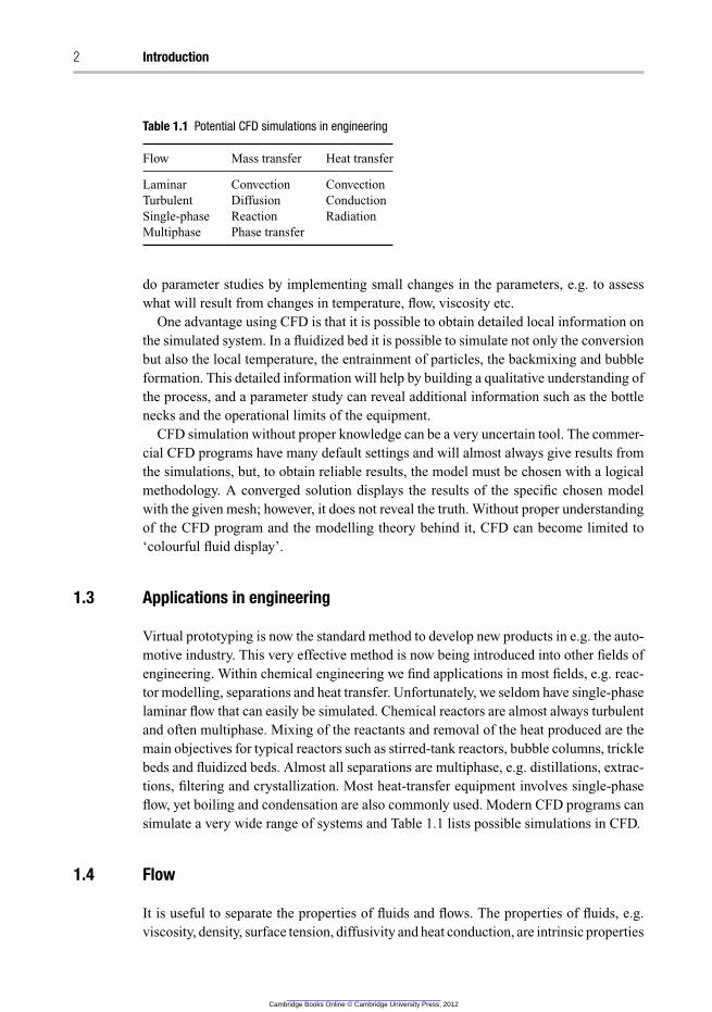
Table 1.1 Potential CFD simulations in engineering
Flow Mass transfer Heat transfer
Laminar Convection Convection
Turbulent Diffusion Conduction
Single-phase Reaction Radiation
Multiphase Phase transfer
do parameter studies by implementing small changes in the parameters, e.g. to assess
what will result from changes in temperature, flow, viscosity etc.
One advantage using CFD is that it is possible to obtain detailed local information on
the simulated system. In a fluidized bed it is possible to simulate not only the conversion
but also the local temperature, the entrainment of particles, the backmixing and bubble
formation. This detailed information will help by building a qualitative understanding of
the process, and a parameter study can reveal additional information such as the bottle
necks and the operational limits of the equipment.
CFD simulation without proper knowledge can be a very uncertain tool. The commer-
cial CFD programs have many default settings and will almost always give results from
the simulations, but, to obtain reliable results, the model must be chosen with a logical
methodology. A converged solution displays the results of the specific chosen model
with the given mesh; however, it does not reveal the truth. Without proper understanding
of the CFD program and the modelling theory behind it, CFD can become limited to
‘colourful fluid display’.
1.3 Applications in engineering
Virtual prototyping is now the standard method to develop new products in e.g. the auto-
motive industry. This very effective method is now being introduced into other fields of
engineering. Within chemical engineering we find applications in most fields, e.g. reac-
tor modelling, separations and heat transfer. Unfortunately, we seldom have single-phase
laminar flow that can easily be simulated. Chemical reactors are almost always turbulent
and often multiphase. Mixing of the reactants and removal of the heat produced are the
main objectives for typical reactors such as stirred-tank reactors, bubble columns, trickle
beds and fluidized beds. Almost all separations are multiphase, e.g. distillations, extrac-
tions, filtering and crystallization. Most heat-transfer equipment involves single-phase
flow, yet boiling and condensation are also commonly used. Modern CFD programs can
simulate a very wide range of systems and Table 1.1 lists possible simulations in CFD.
1.4 Flow
It is useful to separate the properties of fluids and flows. The properties of fluids, e.g.
viscosity, density, surface tension, diffusivity and heat conduction, are intrinsic properties
Cambridge Books Online © Cambridge University Press, 2012
1.4 Flow 3
that can be described as functions of temperature, pressure and composition. Properties
that depend on the flow include pressure, turbulence and turbulent viscosity.
From a CFD modelling point of view it is useful to separate possible flows into the
following categories:
laminar–turbulent
steady–transient
single-phase–multiphase
1.4.1 Laminar flow
In laminar flow the Navier–Stokes equations describe the momentum transport of flow
that is dominated by viscous forces. It is possible with CFD to obtain very accurate
flow simulations for single-phase systems, provided that the flow is always laminar.
The transitions between laminar and turbulent flow, both from turbulent to laminar and
from laminar to turbulent, are difficult to simulate accurately. In this region the flow can
fluctuate between laminar and turbulent and turbulent slugs can frequently appear in
laminar flow far below the critical Reynolds number for transition to turbulent flow.
Simulation of heat transfer is also often very accurate and a good prediction of temper-
ature can easily be obtained. Mass transfer in the gas phase is also quite straightforward.
However, the diffusivities in liquids are about four orders of magnitude lower than those
in the gas phase at atmospheric pressure and accurate mass-transport simulations in
laminar liquids are difficult. An estimation of the transport distance due to diffusion in
laminar flow can be calculated from x =√
Dt . The diffusivity in liquids is of the order
of 10−9 m2 s−1 and the average transport distance in 1 s is about 3 µm, i.e. very dense
grids are required. The corresponding transport distance in the gas phase is 300 µm,
with a gas-phase diffusivity of 10−5 m2 s−1.
1.4.2 Turbulent flow
The Navier–Stokes equations describe turbulent flows, but, due to the properties of
the flow, it is seldom possible to solve the equations for real engineering applications
even with supercomputers. In a stirred-tank reactor the lifetime and size of the smallest
turbulent eddies, the Kolmogorov scales, are about 5 ms and 50 µm, respectively. A very
fine time and space resolution is needed when solving the Navier–Stokes equations and
it is at present not possible. Direct solution of the Navier–Stokes equations (DNS) for
small systems is, however, very useful for developing an understanding of turbulence,
and for developing new models.
A more cost-effective method is to resolve only the large-scale turbulence, by filtering
out the fine-scale turbulence, and model these small scales as flow-dependent effective
viscosity. This method, large-eddy simulation (LES), is growing in popularity since it
makes it possible to simulate simple engineering flows on a fast PC. The simulations
are, however, very time consuming on a PC, and several weeks can often be needed to
obtain good statistical averages even for rather simple flows.
Cambridge Books Online © Cambridge University Press, 2012
4 Introduction
For more complex flows, it is not possible to resolve the turbulence fluctuations at all.
Most engineering simulations are done with Reynolds-averaged Navier–Stokes (RANS)
methods. In these models the turbulent fluctuations are time averaged, yet reasonable
velocity averages can be simulated from these models. However, there are important
properties of the flow that are not resolved. Everything that occurs on a scale below
the size of the grid is not resolved, e.g. mixing of chemical species or the break-up and
coalescence of bubbles and drops in multiphase flow. Additional models must be added
to the RANS models in order to include these phenomena.
1.4.3 Single-phase flow
In single-phase laminar flow we can obtain very accurate solutions and in turbulent flow
we can in most cases obtain satisfactory flow simulations. The main problem is usually
simulation of the mixing of reactants for fast reactions in laminar or turbulent flow.
When the reaction rate is fast compared with mixing, there will be strong concentration
gradients that cannot be resolved in the grid, and a model for mixing coupled with a
chemical reaction must be introduced. Combustion in the gas phase and ion–ion reactions
in the liquid phase belong to this category.
1.4.4 Multiphase flow
Multiphase flow may consist of gas–liquid, gas–solid, liquid–liquid, liquid–solid or gas–
liquid–solid systems. For a multiphase system containing very small particles, bubbles
or drops that follow the continuous phase closely, reasonable simulation results can be
obtained. Systems in which the dispersed phase has a large effect on the continuous
phase are more difficult to simulate accurately, and only crude models are available for
multiphase systems with a high load of the dispersed phase. At the moment, the quality
of the simulations is limited not by the computer speed or memory but by the lack
of good models for multiphase flow. However, multiphase flows are very important in
engineering since many common processes involve multiphase flow.
The mass and heat transfer between the phases are of interest in many applications,
e.g. in boiling, heterogeneous catalysis and distillation. For these simulations we must
introduce empirical or semi-empirical correlations to describe mass and heat transfer.
The mass- and heat-transfer coefficients are usually calculated from the traditional
correlations for the Sherwood, Sh, and Nusselt, Nu, numbers. The advantage with CFD
is that Sh and Nu can be computed using local flow properties. The mass and heat
transfer are also affected by the coalescence and break-up of bubbles and drops. The
phenomenon of break-up and coalescence is not included in this book since only very
simple models are available for simulation of the effect of turbulence and shear rate on
drop or bubble size distributions.
1.5 CFD programs
There are many commercial general-purpose CFD programs available, e.g. Fluent, CFX,
Star-CD, FLOW-3D and Phoenics. There are also some very specialized programs
Cambridge Books Online © Cambridge University Press, 2012
1.5 CFD programs 5
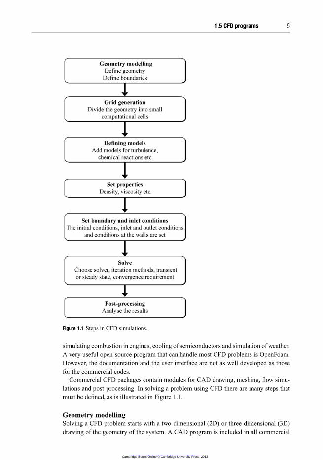
Figure 1.1 Steps in CFD simulations.
simulating combustion in engines, cooling of semiconductors and simulation of weather.
A very useful open-source program that can handle most CFD problems is OpenFoam.
However, the documentation and the user interface are not as well developed as those
for the commercial codes.
Commercial CFD packages contain modules for CAD drawing, meshing, flow simu-
lations and post-processing. In solving a problem using CFD there are many steps that
must be defined, as is illustrated in Figure 1.1.
Geometry modelling
Solving a CFD problem starts with a two-dimensional (2D) or three-dimensional (3D)
drawing of the geometry of the system. A CAD program is included in all commercial
Cambridge Books Online © Cambridge University Press, 2012
6 Introduction
CFD programs but the geometry of the system can usually be drawn in any CAD program
and imported into the grid-generation program. However, CAD programs not designed
for CFD often contains details that cannot be included in CFD drawings, e.g. nuts and
bolts. These drawings must be cleaned before they can be used in a meshing program.
Grid generation (meshing)
The equations for momentum transport are nonlinear, which means that the computa-
tional volume must be discretized properly to obtain an accurate numerical solution of
the equations. Accurate meshing of the computational domain is as important as defining
the physical models. An ill-conditioned mesh can give rise to very inaccurate results,
so the quality of the mesh, e.g. its aspect ratio and skewness, must be evaluated prior
to the simulations. Most CFD programs have also the possibility of adaptation, which,
after a preliminary result has been obtained, enables local refinement of the grid where
necessary.
Define models
For single-phase laminar flow, the Navier–Stokes equations can be solved directly, but
for turbulent and multiphase flows the user must select the most appropriate model.
There are few generally accepted models for turbulence and multiphase flow, but there
are hundreds of models to choose from. For each model there are also several parameters
that must be set. Usually the default values are the best choice, but in some cases the user
can find more suitable parameters. In most commercial CFD programs it is also possible
to write your own model as a user-defined subroutine/function (UDS/UDF) in Fortran
or C. Not all properties are resolved in the CFD program, and many semi-empirical
models must be defined. The momentum, heat and mass transfer between the dispersed
and continuous phases in multiphase flow are defined by empirical models for drag and
Sherwood and Nusselt numbers as functions of the local particle Reynolds number or
turbulence intensity.
Set properties
All physical properties of the fluids must be defined, e.g. the viscosity and density and
their temperature, composition and pressure dependence. Some are built into the CFD
software or easily found in available databases. The programs also provide polynomials
for which you can add your own constants. It is also possible to write a UDS/UDF that
is added to the CFD program for calculating the properties.
Set boundary and initial conditions
All inlet and outlet conditions must be defined, as must conditions on the walls and other
boundaries. Rotational symmetry and other symmetries, e.g. periodic induced boundary
conditions, must also be defined. Periodic boundary conditions are very useful with
rotating equipment, e.g. a turbine, when only a part is modelled. Initial conditions for
transient simulations or an initial guess to start the iterations for steady-state simulations
must also be provided.
Cambridge Books Online © Cambridge University Press, 2012
1.5 CFD programs 7
Solve
For the solver you can choose either a segregated or a coupled solver, pressure- or density-
based, and for unsteady problems you must choose either implicit or explicit time-
stepping methods. Numerical schemes to enhance convergence, e.g. multigrid, upwind
schemes or under-relaxation factors, must be defined. The quality of an acceptable
solution in terms of the convergence criteria must also be defined.
Post-processing/analysis
The first objective in the post-processing is to analyse the quality of the solution. Is
the solution independent of the grid size, the convergence criterion and the numerical
schemes? Have the proper turbulence model and boundary conditions been chosen, and
is the solution strongly dependent on those choices?
Analysis of the final simulation results will then give local information about flow,
concentrations, temperatures, reaction rates etc.
For very complex systems the results are not very accurate, but CFD can still be very
useful in answering the question ‘What if?’. Starting with an adjusted CFD simulation
that fits the available experimental results, a parameter study can reveal how e.g. the
mixing is affected by an increase in molecular viscosity.
Questions
(1) What can be simulated in a CFD program?
(2) Why is it not possible to solve Navier–Stokes equations for turbulent flows for
typical engineering applications?
(3) What steps are involved in solving a typical CFD problem?
Cambridge Books Online © Cambridge University Press, 2012

Cambridge Books Online © Cambridge University Press, 2012
2 Modelling
In CFD the equations for continuity, momentum, energy and species are solved. These
coupled partial nonlinear differential equations are in general not easy to solve numer-
ically and analytical solutions are available for only very few limited cases. The reader
is expected to have a basic knowledge of transport phenomena but, since all CFD is
based on these few equations, they are given here in tensor notation so that the reader
can become familiar with this notation.
A general balance formulation in tensor notation for a scalar, vector or tensor φ can
be formulated as
∂φ
∂t+ Ui
∂φ
∂xi
= D∂
2φ
∂xi∂xi
+ S(φ), (2.1)
where the terms have the following meanings:
{
rate of
accumulation
}
+
{
transport by
convection
}
=
{
transport by
diffusion
}
+
{
source
terms
}
This notation will be used throughout the book and the reader must be familiar with this
notation. In this convention there is an understood summation that is written explicitly
below (see the appendix for further information):
∂φ
∂t+
∑
i
Ui
∂φ
∂xi
=∑
i
D∂
2φ
∂x2i
+ S(φ)
In 3D Cartesian coordinates i can take the values 1, 2 and 3, and for a scalar φ the
equation above becomes
∂φ
∂t+ U1
∂φ
∂x1
+ U2
∂φ
∂x2
+ U3
∂φ
∂x3
= D
(
∂2φ
∂x21
+∂
2φ
∂x22
+∂
2φ
∂x23
)
+ S(φ). (2.2)
Note that since φ is a scalar there is only one equation describing how φ is distributed
in the three dimensions x1, x2 and x3. The easiest way to understand the notation is to
identify whether the dependent variable is a scalar, vector or tensor. When φ is a scalar,
e.g. temperature, T, only one equation is possible, since there is only one temperature at
a given position. When φ is a vector, e.g. φ = [U1U2U3]T, there will be one equation
for each of the three velocities. Equation (2.21) below is a tensor notation of the three
momentum equations written in Eq. (2.20). For a tensor τ ij there will be nine equations
in three dimensions, cf. Eq. (2.7) below.
Cambridge Books Online © Cambridge University Press, 2012
2.1 Mass, heat and momentum balances 9
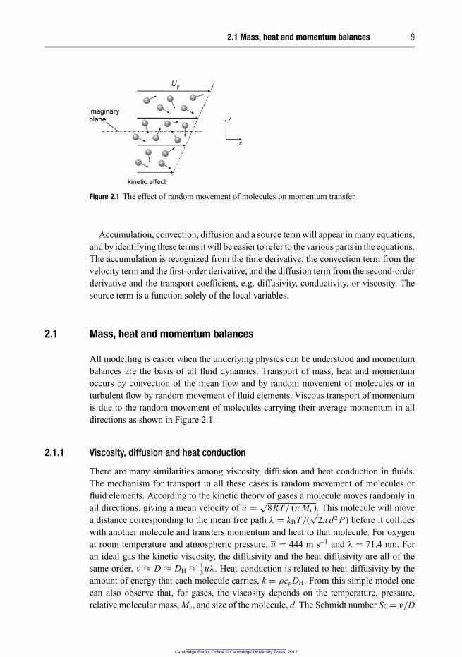
Figure 2.1 The effect of random movement of molecules on momentum transfer.
Accumulation, convection, diffusion and a source term will appear in many equations,
and by identifying these terms it will be easier to refer to the various parts in the equations.
The accumulation is recognized from the time derivative, the convection term from the
velocity term and the first-order derivative, and the diffusion term from the second-order
derivative and the transport coefficient, e.g. diffusivity, conductivity, or viscosity. The
source term is a function solely of the local variables.
2.1 Mass, heat and momentum balances
All modelling is easier when the underlying physics can be understood and momentum
balances are the basis of all fluid dynamics. Transport of mass, heat and momentum
occurs by convection of the mean flow and by random movement of molecules or in
turbulent flow by random movement of fluid elements. Viscous transport of momentum
is due to the random movement of molecules carrying their average momentum in all
directions as shown in Figure 2.1.
2.1.1 Viscosity, diffusion and heat conduction
There are many similarities among viscosity, diffusion and heat conduction in fluids.
The mechanism for transport in all these cases is random movement of molecules or
fluid elements. According to the kinetic theory of gases a molecule moves randomly in
all directions, giving a mean velocity of u =√
8RT/ (π Mv). This molecule will move
a distance corresponding to the mean free path λ = kBT/(√
2πd2 P) before it collides
with another molecule and transfers momentum and heat to that molecule. For oxygen
at room temperature and atmospheric pressure, u = 444 m s−1 and λ = 71.4 nm. For
an ideal gas the kinetic viscosity, the diffusivity and the heat diffusivity are all of the
same order, ν ≈ D ≈ DH ≈ 13uλ. Heat conduction is related to heat diffusivity by the
amount of energy that each molecule carries, k = ρcpDH. From this simple model one
can also observe that, for gases, the viscosity depends on the temperature, pressure,
relative molecular mass, Mv, and size of the molecule, d. The Schmidt number Sc = ν/D
Cambridge Books Online © Cambridge University Press, 2012
10 Modelling
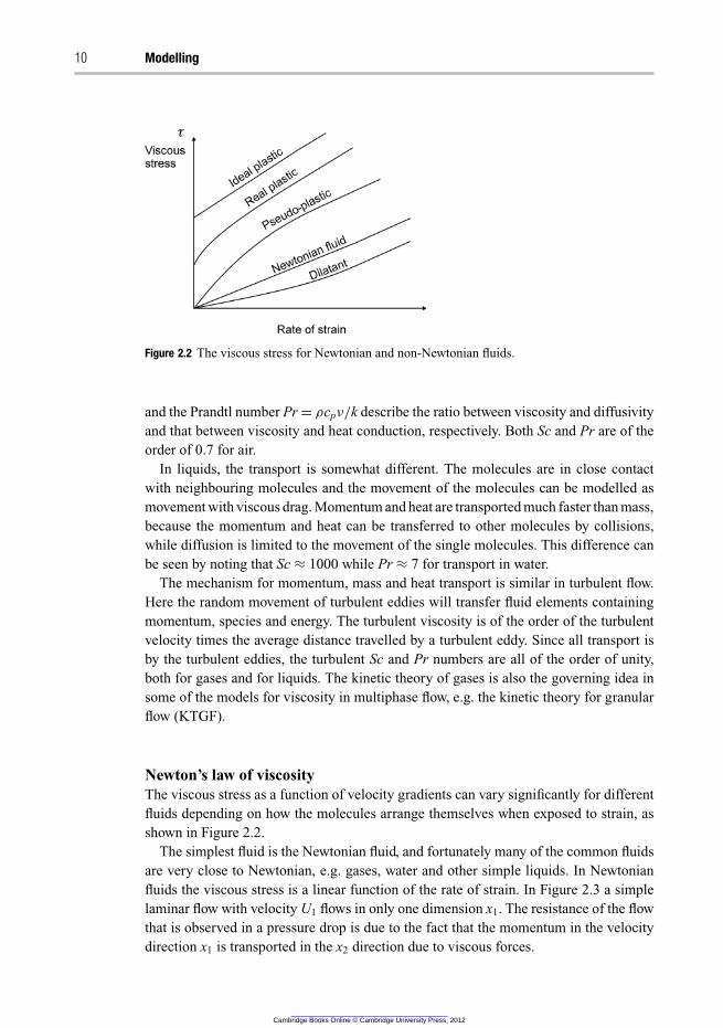
Figure 2.2 The viscous stress for Newtonian and non-Newtonian fluids.
and the Prandtl number Pr = ρcpν/k describe the ratio between viscosity and diffusivity
and that between viscosity and heat conduction, respectively. Both Sc and Pr are of the
order of 0.7 for air.
In liquids, the transport is somewhat different. The molecules are in close contact
with neighbouring molecules and the movement of the molecules can be modelled as
movement with viscous drag. Momentum and heat are transported much faster than mass,
because the momentum and heat can be transferred to other molecules by collisions,
while diffusion is limited to the movement of the single molecules. This difference can
be seen by noting that Sc ≈ 1000 while Pr ≈ 7 for transport in water.
The mechanism for momentum, mass and heat transport is similar in turbulent flow.
Here the random movement of turbulent eddies will transfer fluid elements containing
momentum, species and energy. The turbulent viscosity is of the order of the turbulent
velocity times the average distance travelled by a turbulent eddy. Since all transport is
by the turbulent eddies, the turbulent Sc and Pr numbers are all of the order of unity,
both for gases and for liquids. The kinetic theory of gases is also the governing idea in
some of the models for viscosity in multiphase flow, e.g. the kinetic theory for granular
flow (KTGF).
Newton’s law of viscosity
The viscous stress as a function of velocity gradients can vary significantly for different
fluids depending on how the molecules arrange themselves when exposed to strain, as
shown in Figure 2.2.
The simplest fluid is the Newtonian fluid, and fortunately many of the common fluids
are very close to Newtonian, e.g. gases, water and other simple liquids. In Newtonian
fluids the viscous stress is a linear function of the rate of strain. In Figure 2.3 a simple
laminar flow with velocity U1 flows in only one dimension x1. The resistance of the flow
that is observed in a pressure drop is due to the fact that the momentum in the velocity
direction x1 is transported in the x2 direction due to viscous forces.
Cambridge Books Online © Cambridge University Press, 2012

2.1 Mass, heat and momentum balances 11
Figure 2.3 The distortion of a fluid element due to strain rate dU1/dx2.
Figure 2.4 Translation, rotation and distortion of a fluid element.
For a Newtonian fluid the linear dependence between stress and the velocity gradient
is expressed as
τ21 = μ
dU1
dx2
. (2.3)
Here the first index of τ 21 denotes the direction of transport and the second the
direction of the momentum. Note that the stress tensor is written with a positive sign.
There is a tradition in chemical engineering of viewing the stress tensor as the transport
of momentum and consequently defining it with a negative sign since the direction of
momentum transport is opposite to the direction of the gradient analogous to heat and
mass transfer.
The velocity gradient in itself does not cause the stresses, but rather the stresses arise
due to the distortion of the fluid element. A pure translation or rotation of the element
will not give rise to viscous stress (Figure 2.4).
In a 2D case, the viscous stress will depend on distortion of the fluid element and the
viscous stress becomes a linear function of the strain rate
τ12 = τ21 = μ
(
∂U1
∂x2
+∂U2
∂x1
)
. (2.4)
The expression is symmetric in the two dimensions and the two stresses must be equal,
τ 12 = τ 21.
The normal stresses are also affected by the compression of the fluid elements,
τ11 = 2μ
∂U1
∂x1
−(
23μ − κ
)
(
∂U1
∂x1
+∂U2
∂x2
)
(2.5)
and
τ22 = 2μ
∂U2
∂x2
−(
23μ − κ
)
(
∂U1
∂x1
+∂U2
∂x2
)
. (2.6)
Cambridge Books Online © Cambridge University Press, 2012
12 Modelling
In 3D the nine possible stresses become
τi j = τ j i = μ
(
∂Ui
∂x j
+∂U j
∂xi
)
−(
23μ − κ
)
δi j
(
∂Uk
∂xk
)
, (2.7)
where δi j is the Kronecker delta
δi j = (I)i j =
{
1 if i = j,
0 if i �= j.
Sometimes the pressure is added to the normal stresses and the stress tensor is
written
σi j = μ
(
∂U1
∂x1
+∂U2
∂x2
)
−(
23μ − κ
)
δi j
(
∂Uk
∂xk
)
− δi j P. (2.8)
The dilatational viscosity κ is important only for shock waves and sound waves. From
the kinetic theory of gases it has also been shown that κ is zero for monatomic gases at
low pressure. In this book we will mostly describe non-compressible fluids, for which
the term ∂Uk/∂xk on the right-hand side is zero and the viscous stress for a Newtonian
fluid is described by
τi j = τ j i = μ
(
∂Ui
∂x j
+∂U j
∂xi
)
. (2.9)
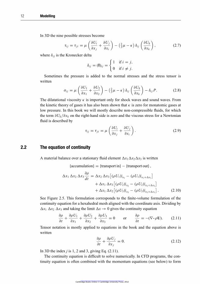
2.2 The equation of continuity
A material balance over a stationary fluid element �x1�x2�x3 is written
{accumulation} = {transport in} − {transport out} ,
�x1 �x2 �x3
∂ρ
dt= �x2 �x3
[
(ρU1)|x1− (ρU1)|x1+�x1
]
+�x1 �x3
[
(ρU2)|x2− (ρU2)|x2+�x2
]
+�x1 �x2
[
(ρU3)|x3− (ρU3)|x3+�x3
]
. (2.10)
See Figure 2.5. This formulation corresponds to the finite-volume formulation of the
continuity equation for a hexahedral mesh aligned with the coordinate axis. Dividing by
�x1 �x2 �x3 and taking the limit �x → 0 gives the continuity equation
∂ρ
∂t+
∂ρU1
∂x1
+∂ρU2
∂x2
+∂ρU3
∂x3
= 0 or∂ρ
∂t= −(∇ ·ρU). (2.11)
Tensor notation is mostly applied to equations in the book and the equation above is
written
∂ρ
∂t+
∂ρU j
∂x j
= 0. (2.12)
In 3D the index j is 1, 2 and 3, giving Eq. (2.11).
The continuity equation is difficult to solve numerically. In CFD programs, the con-
tinuity equation is often combined with the momentum equations (see below) to form
Cambridge Books Online © Cambridge University Press, 2012
2.2 The equation of continuity 13
x3
(ρU1)|x1(ρU1)|x1 + ∆x1
x2
x1
x1 + ∆x1, x2 + ∆x2, x3 + ∆x3
∆x1
∆x2
∆x3
Figure 2.5 A material balance over a fluid element.
a Poisson equation for pressure. For constant density and viscosity the new equation
will be
∂
∂xi
(
∂ P
∂xi
)
= −∂
∂xi
[
∂
(
ρUiU j
)
∂x j
]
. (2.13)
This equation has more suitable numerical properties and can be solved by proper
iteration methods. The Navier–Stokes equations are used for simulation of velocity and
pressure. The Poisson formulation introduces pressure as a dependent variable, and the
momentum equations can be formulated to solve for velocity. The Poisson equation and
other methods to solve the continuity are discussed in Chapter 3.
In many cases it is more convenient to describe the change in flow of a fluid element
that moves with the flow. On performing the derivation in Eq. (2.12) we obtain
∂ρ
∂t+ U1
∂ρ
∂x1
+ U2
∂ρ
∂x2
+ U3
∂ρ
∂x3
= −ρ
(
∂U1
∂x1
+∂U2
∂x2
+∂U3
∂x3
)
. (2.14)
The left-hand side is the substantial derivative of density, i.e. the time derivative for a
fluid element that follows the fluid motion. The equation can be abbreviated as
Dρ
Dt= −ρ
∂Ui
∂xi
(2.15)
and the substantial operator defined as
D
Dt≡
∂
∂t+ U1
∂
∂x1
+ U2
∂
∂x2
+ U3
∂
∂x3
. (2.16)
Incompressible flow is defined by having constant density along the streamline, i.e. the
left-hand side of Eq. (2.15) is zero and
∂Ui
∂xi
= 0. (2.17)
The assumption of incompressible flow will simplify the modelling substantially, and
we will use it throughout the book. Truly incompressible flow does not exist, but the
assumption of incompressible flow is valid for most engineering applications. A local
change in pressure will spread with the speed of sound, and, when modelling phenomena
Cambridge Books Online © Cambridge University Press, 2012
14 Modelling
x3
x2
x1
(x1 + ∆x1, x2 + ∆x2, x3 + ∆x3)
τ31|x3
τ11|x1 + ∆x1
τ31|x3 + ∆x3
τ21|x2 + ∆x2
τ11|x1
τ21|x2
Figure 2.6 Momentum balance over a fluid element.
much slower than the speed of sound, we can safely assume that the new pressure is
reached in each time step, i.e. compressible flows can be characterized by the value of
the Mach number M = U/c. Here, c is the speed of sound in the gas c =√
γ RT , where
γ is the ratio of specific heats cp/cv. At Mach numbers much less than 1.0 (M < 0.1),
compressibility effects are negligible and the variation of the gas density due to pressure
waves can safely be ignored in the flow modelling. The density change due to pressure
drops and temperature variations will automatically be compensated for by the state
equation that describes how the density is related to pressure and temperature.
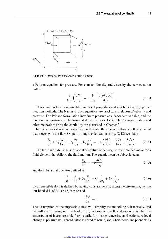
2.3 The equation of motion
The momentum balance for the U1 momentum over the volume �x1�x2�x3 is given by
⎧
⎨
⎩
rate of
momentum
accumulation
⎫
⎬
⎭
=
⎧
⎨
⎩
rate of
momentum
in
⎫
⎬
⎭
−
⎧
⎨
⎩
rate of
momentum
out
⎫
⎬
⎭
+
⎧
⎨
⎩
sum of forces
acting on
the system
⎫
⎬
⎭
.
(2.18)
Newton’s law requires that the change in momentum in each direction should be
balanced by the forces acting in that direction. The arrows in Figure 2.6 describe the
direction of viscous transport of Ui momentum. A balance for the momentum of the
velocity component in the x1 direction, i.e. U1, is written
�x1 �x2 �x3
∂ρU1
∂x1
= �x2 �x3
[
(ρU1U1)|x1− (ρU1U1)|x
1+�x
1
]
− τ11|x1+ τ11|x
1+�x
1
+�x1 �x3
[
(ρU2U1)|x2− (ρU2U1)|x
2+�x
2
]
− τ21|x2+ τ21|x
2+�x
2
+�x1 �x2
[
(ρU3U1)|x3− (ρU3U1)|x
3+�x
3
]
− τ31|x3+ τ31|x
3+�x
3
+�x2 �x3
[
(P)|x1− (P)|x
1+�x
1
]
+ �x1 �x2 �x3 ρg1. (2.19)
Cambridge Books Online © Cambridge University Press, 2012

2.3 The equation of motion 15
From our definition of τ it is –τ that denotes the momentum that is transported
into the fluid element at x. Equation (2.19) corresponds to a finite-volume formulation
of the momentum equations for a hexahedral mesh aligned with the coordinate axis.
Dividing by �x1 �x2 �x3 and taking the limit �x → 0 gives for all three components
the Navier–Stokes equations
∂U1
∂t+ U1
∂U1
∂x1
+ U2
∂U1
∂x2
+ U3
∂U1
∂x3
= −1
ρ
∂ P
∂x1
+1
ρ
∂τ11
∂x1
+1
ρ
∂τ21
∂x2
+1
ρ
∂τ31
∂x3
+ g1,
∂U2
∂t+ U1
∂U2
∂x1
+ U2
∂U2
∂x2
+ U3
∂U2
∂x3
= −1
ρ
∂ P
∂x2
+1
ρ
∂τ12
∂x1
+1
ρ
∂τ22
∂x2
+1
ρ
∂τ32
∂x3
+ g2,
∂U3
∂t+ U1
∂U3
∂x1
+ U2
∂U3
∂x2
+ U3
∂U3
∂x3
= −1
ρ
∂ P
∂x3
+1
ρ
∂τ13
∂x1
+1
ρ
∂τ23
∂x2
+1
ρ
∂τ33
∂x3
+ g3.
(2.20)
These three equations can be rewritten as
∂Ui
∂t+
∑
j
U j
∂Ui
∂x j
= −1
ρ
∂ P
∂xi
+∑
j
1
ρ
∂τ j i
∂x j
+ gi .
Note that there is no summation over i, since i represents the three equations. In tensor
notation these three equations are written
∂Ui
∂t+ U j
∂Ui
∂x j
= −1
ρ
∂ P
∂xi
+1
ρ
∂τ j i
∂x j
+ gi , (2.21)
which for a Newtonian fluid becomes
∂Ui
∂t+ U j
∂Ui
∂x j
= −1
ρ
∂ P
∂xi
+ ν
∂
∂x j
(
∂Ui
∂x j
+∂U j
∂xi
)
+ gi . (2.22)
Equation (2.22) can be written in different forms since
ν
∂
∂x j
(
∂Ui
∂x j
+∂U j
∂xi
)
= ν
∂2Ui
∂x j∂x j
in incompressible flow with constant ρ and ν. In addition to gravity, there are additional
external sources that may affect the acceleration of the fluid, e.g. electrical and magnetic
fields. When reading Eq. (2.21) note that j should be summed over all dimensions, i.e.
j = 1, 2 and 3, and i appears in all terms and for three dimensions, constituting the three
equations as in Eq. (2.20).
Strictly it is the momentum equations that form the Navier–Stokes equations, but
sometimes the continuity and the momentum equations together are called the Navier–
Stokes equations. The Navier–Stokes equations are limited to macroscopic conditions.
In reality the molecules move some distance before they collide, and the kinetic energy
and consequently the velocity of the individual molecules are Boltzmann distributed.
These effects must be accounted for at low pressures and in very small volumes. The
Knudsen number relates the mean free path, λ, to the system dimension, Kn = λ/L.
The average distance between collisions, i.e. the mean free path, in air at 1 atm and
room temperature is ∼80 nm, and a correction of the Navier–Stokes equations and the
Cambridge Books Online © Cambridge University Press, 2012

16 Modelling
boundary conditions is required for Knudsen numbers larger than ∼0.02. Simulation
of microfluids at dimensions below 5 µm at atmospheric pressure will require special
boundary conditions [1].
2.4 Energy transport
Energy is present in many forms in flow, e.g. as kinetic energy due to the mass and
velocity of the fluid, as thermal energy and as chemically bounded energy. We can then
define the enthalpy as
h = hm + hT + hC + � total energy,
hm = 12ρUiUi kinetic energy,
hT =∑
n
mn
T∫
Tref
cp,n dT thermal energy,
hC =∑
n
mnhn chemical energy,
� = ρgi xi potential energy,
where mn is the mass fraction, cp,n the heat capacity and hn the standard state enthalpy
(heat of formation) for species n. The potential energy is often included in the kinetic
energy.
The balance equation for total energy is
∂h
∂t= −
∂
∂x j
[
hU j − keff
∂T
∂xi
+∑
n
mnhn jn − τk jUk
]
+ Sh . (2.23)
Here jn is the diffusional flux of species n,
jn = −Dn
∂Cn
∂x j
.
The couplings between the energy equations and the momentum equations are weak
for incompressible flows, and the equations for kinetic, thermal and chemical energies
can be written separately.
2.4.1 The balance for kinetic energy
An equation for the kinetic energy including the potential energy can be deduced from
the momentum equation by multiplying by velocity Ui:
Ui
∂Ui
∂t+ UiU j
∂Ui
∂x j
= −1
ρ
Ui
∂ P
∂xi
+Ui
ρ
∂τi j
∂x j
+ Ui gi . (2.24)
Cambridge Books Online © Cambridge University Press, 2012
2.4 Energy transport 17
By using
Ui
∂Ui
∂xi
=1
2
∂U 2i
∂xi
and defining e ≡ 12(U 2
1 + U 22 + U 2
3 ) [J kg−1 fluid] we obtain
∂e
∂t+ U j
∂e
∂x j
= −1
ρ
Ui
∂ P
∂xi
+1
ρ
Ui
∂τi j
∂x j
+ Ui gi . (2.25)
Note that this is a scalar equation and the expanded equation is obtained by summation
over i and j. On multiplying by the density of the fluid and defining hm = ρe [J m−3
fluid] and using the relations
∂(PUi )
∂xi
= Ui
∂ P
∂xi
+ P∂Ui
∂xi
and∂(τi jUi )
∂xi
= Ui
∂τi j
∂xi
+ τi j
∂Ui
∂xi
we obtain
∂(hm)
∂t= −U j
∂(hm)
∂x j
+ P∂Ui
∂xi
−∂(PUi )
∂xi
+∂(τi jUi )
∂xi
− τi j
∂Ui
∂xi
+ ρgUi . (2.26)
The accumulation and convection terms (the first two terms on the right-hand side) are
straightforward and need no further comments. The work done by the gravity force
(the sixth term on the right-hand side) is the change in potential energy due to gravity.
Reversible conversion to heat (the third term on the right-hand side) stems from the
thermodynamic cooling when a gas expands or heating when it is compressed. The work
done by viscous forces (the fourth term on the right-hand side) is the accumulation of
strain in some fluids, e.g. a rubber band. The irreversible conversion of kinetic energy
into heat (the fifth term on the right-hand side) is, for Newtonian fluids,
ε = −1
ρ
τi j
∂Ui
∂x j
=1
2ν
[(
∂Ui
∂x j
+∂U j
∂xi
)
−2
3
∂Ui
∂xi
]2
. (2.27)
Owing to the fact that this is a squared term, the viscous dissipation term is always
positive for Newtonian fluids. Heat is actually random movement of molecules or atoms,
i.e. translational, rotational and vibrational movement. The difference between kinetic
energy and heat is that kinetic energy has an average direction of movement whereas heat
is random movement. With this perspective the dissipation term can be seen as viscous
transport of fast molecules into areas with low average velocity and of slow molecules
into areas with high average velocity. The molecules will collide with other molecules,
transferring their average momentum, but will very soon lose their directional average
and the movement is defined as heat.
The dissipation term is usually small and only with a very high velocity gradient
will it be possible to measure the temperature increase due to viscous dissipation. In a
stirred-tank reactor the power input by the impeller is of the order of 1 kW m−3, which
corresponds to a temperature increase of about 1 K h−1. However, in turbulent flow this
Cambridge Books Online © Cambridge University Press, 2012
18 Modelling
term becomes very important since it describes the decay of turbulence when the energy
in the turbulent eddies is transferred into heat.
2.4.2 The balance for thermal energy
A balance for heat can be formulated generally by simply adding the source terms from
the kinetic-energy balance and from chemical reactions:
∂(ρcpT )
∂t= −U j
∂(ρcpT )
∂x j
+ keff
∂2T
∂x j ∂x j
− P∂U j
∂x j
+ τk j
∂Uk
∂x j
+∑
m
Rm(C, T )(−�Hm) + ST , (2.28)
where the terms on the right-hand side are for accumulation, convection, conduction,
expansion, dissipation and the reaction source.
Here the terms in the equation for transformation between thermal and kinetic energy,
i.e. expansion and dissipation, occur as source terms. The relation to change in chemical
energy is seen in the term for heat formation due to chemical reactions. Examples of the
source term ST are absorption and emission of radiation.
2.5 The balance for species
The balance for transport and reaction for species in constant-density fluids is described
by
∂Cn
∂t+ U j
∂Cn
∂x j
=∂
∂x j
(
Dn
∂Cn
∂x j
)
+ R(C, T ) + Sn. (2.29)
In most CFD programs, the concentration is replaced with the mass fraction
yn =Mv,nCn
ρ
. (2.30)
Transport and reaction will be discussed further in Chapter 5.
2.6 Boundary conditions
The 3D Navier–Stokes equations contain four dependent variables, U1, U2, U3 and P.
Depending on the conditions of the flow, we can define the boundary conditions in
many different ways. The boundary conditions are just as important as the differential
equations that determine the system, and the results of the simulations depend on the
inlet and outlet conditions and the conditions at the walls as well as on the differential
equations. We may also introduce boundary conditions due to simplifications of the
computational domain, e.g. symmetry.
Cambridge Books Online © Cambridge University Press, 2012
2.6 Boundary conditions 19
2.6.1 Inlet and outlet boundaries
The inlet velocity can be defined in terms of velocities or mass flow rate. In most CFD
programs it is possible to enter the inlet condition as an average flow perpendicular to the
surface or as a velocity-component distribution over the inlet surface. The way we define
boundaries may affect the results, e.g. defining the inlet by an average velocity or by a
parabolic laminar flow distribution will give the flow different momentum distributions
and the total energy added by the inlet flow will be different in these two cases. An
alternative to defining inlet velocities is the pressure inlet boundary condition that can
be used when the inlet pressure is known without knowledge of the flow rate. The
pressure inlet boundary condition is also useful when it is unknown whether the flow
enters or exits at this position.
The standard outlet boundary condition is the zero-diffusion flux condition applied
at outflow cells, which means that the conditions of the outflow plane are extrapolated
from within the domain and have no impact on the upstream flow, i.e.
φ|L− = φ|L+ . (2.31)
The pressure outlet boundary condition is often the default condition used to define the
static pressure at flow outlets. The use of a pressure outlet boundary condition instead
of an outflow condition often results in a better rate of convergence when backflow
occurs during iteration. Pressure outflow is also useful when there are several outflows.
Specified outflow boundary conditions are used to model flow exits where the details of
the inlet flow velocity and pressure are not known prior to solution of the flow problem.
They are appropriate where the exit flow is close to a fully developed condition, since
the standard outflow boundary condition assumes a normal gradient of zero for all flow
variables except pressure.
Scalars, e.g. temperature and species, are usually defined as temperature and mass
fractions in the inlet flow. Standard outlet conditions are usually the default.
2.6.2 Wall boundaries
The usual boundary condition for velocity at the walls is the ‘no-slip condition’, i.e. the
relative velocity between the wall and the fluid is set to zero. For high-Reynolds-number
turbulent flow the no-slip condition is still valid but the grid resolution is usually too
coarse to specify the no-slip condition. In this case the velocity and shear close to the
wall are modelled using a wall function. (See Chapter 4 for further details.) The no-slip
condition may be inappropriate for non-Newtonian and multiphase flow and at large
Knudsen numbers (Kn > 0.02), i.e. for low pressure or small dimensions.
For heat transfer, walls can be considered insulated or heat may be transferred through
the walls. For heat there are several choices for boundary conditions, e.g. fixed heat flux,
fixed temperature, convective heat transfer, radiation heat transfer or a combination
of these boundary conditions. Heat transfer by radiation occurs mainly between solid
surfaces, and the CFD program must be able also to calculate view angles in order to
obtain accurate radiation boundary conditions.
Cambridge Books Online © Cambridge University Press, 2012
20 Modelling
The boundary conditions for species are usually termed ‘no penetration’, but diffusion
to and reaction at the walls can occur. Evaporation and condensation are also possible
wall boundary conditions.
2.6.3 Symmetry and axis boundary conditions
The time taken for simulations can be reduced significantly by using the geometrical
symmetry of the problem. Mirror symmetry can halve or even further reduce the calcu-
lation region, and rotational symmetry, by defining a rotation axis, reduces a problem
from 3D to 2D, which can decrease the time taken for simulation by several orders of
magnitude. Symmetric initial and boundary conditions do not guarantee that the solution
is symmetric, e.g. buoyancy-driven flows have a tendency to have several possible solu-
tions depending on the initial conditions, and enforced symmetry conditions can produce
erroneous results. Two-dimensional simulations may give very misleading results, e.g.
the bubbles appearing in a simulation of a fluidized bed are cylinders in 2D and toroids
in rotational symmetry. It should also be recognized that no net transport is allowed
across a symmetry plane.
Periodic boundaries are convenient for DNS and LES simulations of turbulent flows
since time-resolved inlet conditions are required. In periodic boundaries the inlet is set
to the outlet. In this way the time-resolved solution will transfer the outlet solution to
the inlet. However, to avoid having the boundary condition affect the simulation results,
the residence time in the simulation domain should be long compared with the lifetime
of the turbulent eddies. Periodic boundaries are also useful for rotating systems when
only a fraction of the tangential direction is resolved, e.g. in simulation of turbines.
2.6.4 Initial conditions
Since the Navier–Stokes equations are nonlinear it is necessary to have an initial guess
from which the solver can start the iterations. The better the initial conditions, the faster
the final solution will convergence. It is also possible that the specified problem has
multiple solutions and that the solution will converge to different solutions depending
on the initial guess. It is always recommended that different initial conditions should be
tested to evaluate convergence and to determine whether there are multiple stationary
solutions. When multiple solutions are possible, the simulations must be transient,
starting from correct initial conditions.
If a time-dependent solution is required, the actual initial conditions must be specified.
Initial conditions for all variables that are to be solved must be specified. For example, in
turbulence modelling the initial conditions for the variables describing the turbulence,
e.g. the turbulence kinetic energy and the rate of dissipation, must also be set.
Owing to the numerical properties in transient simulations, it is in some cases more
efficient to solve a steady-state case by transient simulations. In this case, we are not
interested in accurate simulation of the transient behaviour, but only in obtaining a
reliable steady-state solution. Exact initial conditions are not necessary, and it is possible
to use larger time steps to obtain faster convergence.
Cambridge Books Online © Cambridge University Press, 2012
2.7 Physical properties 21
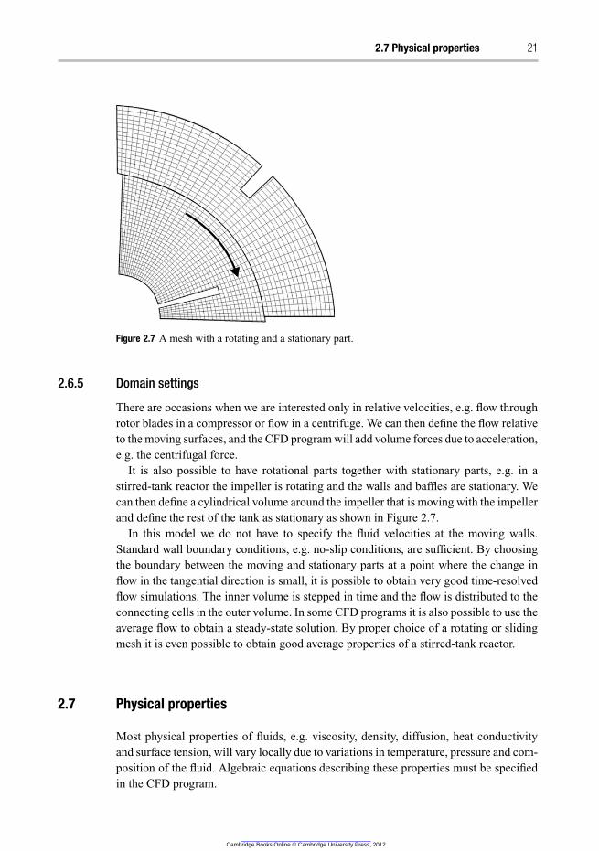
Figure 2.7 A mesh with a rotating and a stationary part.
2.6.5 Domain settings
There are occasions when we are interested only in relative velocities, e.g. flow through
rotor blades in a compressor or flow in a centrifuge. We can then define the flow relative
to the moving surfaces, and the CFD program will add volume forces due to acceleration,
e.g. the centrifugal force.
It is also possible to have rotational parts together with stationary parts, e.g. in a
stirred-tank reactor the impeller is rotating and the walls and baffles are stationary. We
can then define a cylindrical volume around the impeller that is moving with the impeller
and define the rest of the tank as stationary as shown in Figure 2.7.
In this model we do not have to specify the fluid velocities at the moving walls.
Standard wall boundary conditions, e.g. no-slip conditions, are sufficient. By choosing
the boundary between the moving and stationary parts at a point where the change in
flow in the tangential direction is small, it is possible to obtain very good time-resolved
flow simulations. The inner volume is stepped in time and the flow is distributed to the
connecting cells in the outer volume. In some CFD programs it is also possible to use the
average flow to obtain a steady-state solution. By proper choice of a rotating or sliding
mesh it is even possible to obtain good average properties of a stirred-tank reactor.
2.7 Physical properties
Most physical properties of fluids, e.g. viscosity, density, diffusion, heat conductivity
and surface tension, will vary locally due to variations in temperature, pressure and com-
position of the fluid. Algebraic equations describing these properties must be specified
in the CFD program.
Cambridge Books Online © Cambridge University Press, 2012
22 Modelling
2.7.1 The equation of state
The relations among density, temperature, pressure and composition are described by the
equation of state. For gases at low pressure the ideal-gas law can be used for compressible
flows:
ρ =P
RT∑
n
yn/Mw,n
. (2.32)
The ideal-gas law is also an option for incompressible flow if the pressure variation is
moderate. The model will then correctly express the relationship between density and
temperature required for e.g. natural convection problems.
For non-ideal gases many choices can be found in the literature, the most common of
which are the law of corresponding states and the cubic equations of state. The law of
corresponding states is defined as
Z =PV
RT, (2.33)
where Z is a function of the reduced temperature and pressure. The cubic equations are
in the form
P =RT
V − b−
a
V 2 + ubV + wb2, (2.34)
where a, b, u and w are parameters. Depending on the parameters, they form van der
Waals, Redlich–Kwong, Soave and Peng–Robinson equations of state.
For liquids the pressure dependence can often be neglected and a simple polynomial
can describe the temperature dependence:
ρ = A + BT + CT 2 + DT 3 + · · · . (2.35)
2.7.2 Viscosity
At low pressure the viscosity increases slowly with temperature but there is only a small
pressure dependence. The Chapman–Enskog theory provides an expression for the gas
viscosity:
μgas =5
16
√πmkBT
πσ2�T ∗
. (2.36)
A more compressed form is Sutherland’s law,
μ =C1T 3/2
T + C2
, (2.37)
where C1 and C2 are constants. For a multi-component system the total viscosity depends
in a nonlinear fashion on the individual viscosities μi and mole fractions Xi:
μ =∑
i
X iμi∑
j
X iφi j
, (2.38)
Cambridge Books Online © Cambridge University Press, 2012
2.7 Physical properties 23
where
φi j =
[
1 +
(
μi
μ j
)1/2 (
Mw, j
Mw,i
)1/4]2/
[
8
(
1 +Mw,i
Mw, j
)]1/2
. (2.39)
The viscosity increases with temperature for gases, whereas the viscosity decreases expo-
nentially with temperature for liquids. The temperature dependence for liquid viscosity
is often written as
μliq = aeb/T. (2.40)
For non-Newtonian fluids there are several models available. In this book we will cover
only Newtonian fluids, but the interested reader can find additional theories in standard
textbooks [2]. The standard models for turbulent flows assume Newtonian fluids, and
empirical models are required for modelling turbulent viscosity.
Questions
(1) Why are diffusivity, kinematic viscosity and thermal diffusion similar in gases at
low pressure?
(2) What is the molecular mechanism for viscous transport of momentum in gases?
(3) Why is it necessary to rewrite the continuity equation in CFD software?
(4) Why can a gas be treated as incompressible when there is a pressure drop?
(5) Why does viscous dissipation of kinetic energy form heat?
(6) What are standard outlet conditions?
(7) What is a no-slip condition at the wall and when can it be used?
(8) What is a periodic boundary condition?
(9) What are symmetry and axis boundary conditions?
(10) What is an equation of state?
Cambridge Books Online © Cambridge University Press, 2012

Cambridge Books Online © Cambridge University Press, 2012
3 Numerical aspects of CFD
This chapter introduces commonly used numerical methods. The aim is to explain
the various methods so that the reader will be able to choose the appropriate method
with which to perform CFD simulations. There is an extensive literature on numerical
methods, and the interested reader can easily find textbooks. Appropriate references
are [3, 4].
3.1 Introduction
In the previous chapter the physics of fluid flow has been presented. The concepts of how
the flow is modelled, with and without turbulence, have been introduced. The Navier–
Stokes, continuity and pressure equations have been derived, and model equations for
some turbulence quantities will be discussed in following chapters. Expressions for
heat and mass transfer have also been presented. The expressions for velocity, pressure,
turbulence quantities and heat and mass transfer, together with the appropriate boundary
conditions, constitute the core of the CFD problem.
So far there has been no discussion of how these equations are solved. This chapter will
deal with the most fundamental aspects of numerical procedures for solving problems
with CFD. The scope of the chapter is to give the reader a numerical background and
an understanding of some of the numerical problems that can occur. Being aware of the
existence of these problems and being able to avoid them are of crucial importance.
The general transport equation for an arbitrary variable φ in conservative form is
now stated:
ρ
∂φ
∂t+ ρ
∂(U jφ)
∂x j
=∂
∂x j
(
Ŵ
∂φ
∂x j
)
+ Sφ . (3.1)
This equation has been used in the previous chapter, e.g. the Navier–Stokes equations,
Eq. (2.21), which actually are nothing other than transport equations for momentum
(or rather velocity). The equation also appears as the transport equation for various
turbulence quantities in Chapter 4. Unfortunately, it is generally not possible to solve
equations of this type analytically, since they are nonlinear and often contain both spatial
and temporal derivatives. This requires the application of numerical methods.
Cambridge Books Online © Cambridge University Press, 2012
3.2 Numerical methods for CFD 25
3.2 Numerical methods for CFD
The pioneers of CFD employed finite differences to approximate the governing equations
describing fluid mechanics. With finite differences, the partial spatial and temporal
derivatives appearing in the equations are approximated through Taylor series. Although
there is no formal restriction, finite differences are typically employed only on Cartesian
geometries. Since most of the problems engineers tackle do not take place in a square
box, finite differences are not often used for practical problems.
Finite-element methods require a 2D or 3D mesh and are very flexible in terms of
geometry and mesh elements; almost any type of mesh element can be employed. At
each mesh element, a base function is used. This base function should locally describe
the solution of (part of) the governing equation to be approximated. The finite-element
method aims to minimize the difference between the exact solution and the collection
of base functions; this can be done e.g. by a Galerkin method. There is no dispute
that finite-element methods are the preferred method of choice for solid-mechanics
problems.
However, problems in the fluid-mechanics area are generally governed by local con-
servation. For instance, the continuity equation dictates the local conservation of mass.
Local conservation is not necessarily a property of the finite-element method, since the
difference between the base functions and the exact solution is minimized globally. The
adaptation of the finite-element method to reflect local conservation is still very much
the focus of numerical research, therefore the method has historically not been used as
much for CFD.
3.2.1 The finite-volume method
The principle of the finite-volume method is local conservation, and this is the key
reason for its success in CFD. To solve the equations numerically with the finite-
volume method, the entire computational domain is divided into ‘small’ sub-volumes,
so-called cells. Employing Gauss’ law, the partial derivatives expressing a conservation
principle, such as div u, can be rewritten at each cell as an algebraic contribution. The
governing equation, expressed in the partial differential equations, is reformulated, at
each computational cell, into a set of linear algebraic equations
Usually, these equations are solved numerically in an iterative manner. The price
for this so-called discretization of the domain is the introduction of a numerical error
into the solution. It is important to control the magnitude of the error after a solution
has been obtained, and, since it can be shown that this error vanishes as the cell size
approaches zero, a sufficient decrease of the cell size will often reduce the error well
enough. On the other hand, reducing the cell size too much will create an unnecessarily
large number of cells, which will increase the computational effort required and possibly
yield prohibitive simulation times. Finding a fast but still accurate way of solving the
CFD problem is one of the CFD engineer’s most important tasks.
Cambridge Books Online © Cambridge University Press, 2012
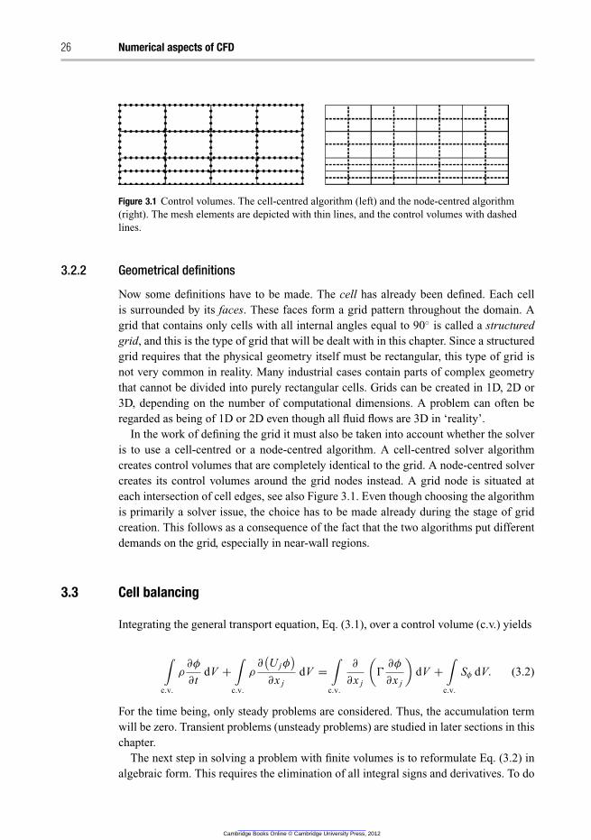
26 Numerical aspects of CFD
Figure 3.1 Control volumes. The cell-centred algorithm (left) and the node-centred algorithm
(right). The mesh elements are depicted with thin lines, and the control volumes with dashed
lines.
3.2.2 Geometrical definitions
Now some definitions have to be made. The cell has already been defined. Each cell
is surrounded by its faces. These faces form a grid pattern throughout the domain. A
grid that contains only cells with all internal angles equal to 90◦ is called a structured
grid, and this is the type of grid that will be dealt with in this chapter. Since a structured
grid requires that the physical geometry itself must be rectangular, this type of grid is
not very common in reality. Many industrial cases contain parts of complex geometry
that cannot be divided into purely rectangular cells. Grids can be created in 1D, 2D or
3D, depending on the number of computational dimensions. A problem can often be
regarded as being of 1D or 2D even though all fluid flows are 3D in ‘reality’.
In the work of defining the grid it must also be taken into account whether the solver
is to use a cell-centred or a node-centred algorithm. A cell-centred solver algorithm
creates control volumes that are completely identical to the grid. A node-centred solver
creates its control volumes around the grid nodes instead. A grid node is situated at
each intersection of cell edges, see also Figure 3.1. Even though choosing the algorithm
is primarily a solver issue, the choice has to be made already during the stage of grid
creation. This follows as a consequence of the fact that the two algorithms put different
demands on the grid, especially in near-wall regions.
3.3 Cell balancing
Integrating the general transport equation, Eq. (3.1), over a control volume (c.v.) yields
∫
c.v.
ρ
∂φ
∂tdV +
∫
c.v.
ρ
∂
(
U jφ
)
∂x j
dV =
∫
c.v.
∂
∂x j
(
Ŵ
∂φ
∂x j
)
dV +
∫
c.v.
Sφ dV. (3.2)
For the time being, only steady problems are considered. Thus, the accumulation term
will be zero. Transient problems (unsteady problems) are studied in later sections in this
chapter.
The next step in solving a problem with finite volumes is to reformulate Eq. (3.2) in
algebraic form. This requires the elimination of all integral signs and derivatives. To do
Cambridge Books Online © Cambridge University Press, 2012
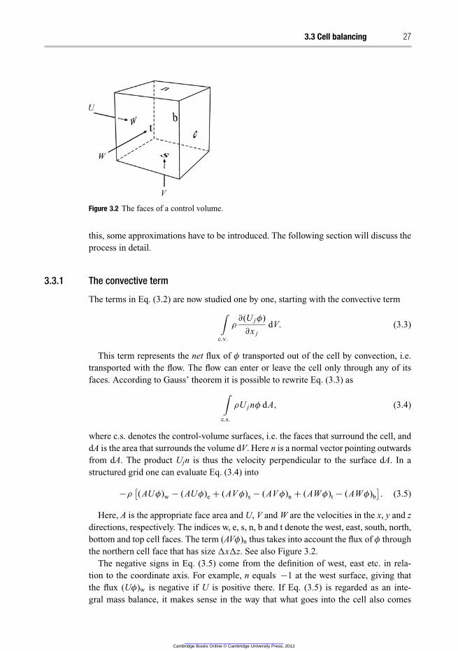
3.3 Cell balancing 27
Figure 3.2 The faces of a control volume.
this, some approximations have to be introduced. The following section will discuss the
process in detail.
3.3.1 The convective term
The terms in Eq. (3.2) are now studied one by one, starting with the convective term
∫
c.v.
ρ
∂(U jφ)
∂x j
dV. (3.3)
This term represents the net flux of φ transported out of the cell by convection, i.e.
transported with the flow. The flow can enter or leave the cell only through any of its
faces. According to Gauss’ theorem it is possible to rewrite Eq. (3.3) as
∫
c.s.
ρU j nφ dA, (3.4)
where c.s. denotes the control-volume surfaces, i.e. the faces that surround the cell, and
dA is the area that surrounds the volume dV. Here n is a normal vector pointing outwards
from dA. The product Ujn is thus the velocity perpendicular to the surface dA. In a
structured grid one can evaluate Eq. (3.4) into
−ρ
[
(AUφ)w − (AUφ)e + (AV φ)s − (AV φ)n + (AWφ)t − (AWφ)b
]
. (3.5)
Here, A is the appropriate face area and U, V and W are the velocities in the x, y and z
directions, respectively. The indices w, e, s, n, b and t denote the west, east, south, north,
bottom and top cell faces. The term (AVφ)n thus takes into account the flux of φ through
the northern cell face that has size �x�z. See also Figure 3.2.
The negative signs in Eq. (3.5) come from the definition of west, east etc. in rela-
tion to the coordinate axis. For example, n equals −1 at the west surface, giving that
the flux (Uφ)w is negative if U is positive there. If Eq. (3.5) is regarded as an inte-
gral mass balance, it makes sense in the way that what goes into the cell also comes
Cambridge Books Online © Cambridge University Press, 2012
28 Numerical aspects of CFD
out for source-free, steady conditions when there is no other means of transport than
convection.
An apparent problem when evaluating the convective term is that the face values of
Uj and φ must be known. As mentioned earlier, the transport equations are not solved
on the faces. Several approaches to overcome this will be discussed later in the section
about discretizing schemes.
3.3.2 The diffusion term
Next, a closer look is taken at the diffusion term,∫
c.v.
∂
∂x j
(
Ŵ
∂φ
∂x j
)
dV . (3.6)
The diffusion term takes into account the transport of φ by diffusion. Equation (3.6) can
be treated in a similar way to the convective term, Eq. (3.3). By making use of Gauss’
theorem,∫
c.s.
Ŵ
∂φ
∂x j
n dA. (3.7)
Using the same notation as in the convective case, Eq. (3.7) can be evaluated to give a
similar expression:
−
[(
AŴ
∂φ
∂x
)
w
−
(
AŴ
∂φ
∂x
)
e
+
(
AŴ
∂φ
∂y
)
s
−
(
AŴ
∂φ
∂y
)
n
+
(
AŴ
∂φ
∂z
)
t
(
AŴ
∂φ
∂z
)
b
]
.
(3.8)
3.3.3 The source term
The last term in the general transport equation is the source term,∫
c.v.
Sφ dV . (3.9)
The source term takes into account any generation or dissipation of φ. The body force
due to gravity in the Navier–Stokes equation for the y momentum is an example of a
source term as discussed previously. The pressure gradient term in the Navier–Stokes
equation is another example. To be able to rewrite Eq. (3.9) without using any integral
signs, simply take a cell mean value of Sφ and move it outside the integral sign. Thus,∫
c.v.
Sφ dV ≈ SφV . (3.10)
Here, Sφ is the mean value of Sφ in the cell.
The original transport equation, Eq. (3.1), is now transformed into equations that
can be solved algebraically, Eqs. (3.5), (3.8) and (3.10). It has also been concluded
Cambridge Books Online © Cambridge University Press, 2012

3.4 Example 1 29
Figure 3.3 The experimental set-up in Example 1.
that the face values of φ, Ŵ and Uj need to be predicted, and the gradient of φ at
the faces is needed. If a source is present, the correct mean values of the sources in
all cells must be created. It must also be remembered that there can be many dif-
ferent scalars, and that they are usually dependent on each other, forcing us to solve
their equations simultaneously in each cell. Hence, the set of equations often becomes
nonlinear.
Equation (3.5), (3.8) and (3.10) will now be used to solve an easy and clarifying 1D
problem, Example 1.
3.4 Example 1 – 1D mass diffusion in a flowing gas
The flow of an inert gas I between two perforated surfaces is simulated. The distance
between the surfaces is 10 cm, and it is assumed that the surface areas are infinite. This
assumption is made so that the problem can be treated as being 1D. The gas velocity is
1 mm s−1. At the west surface the species concentration is 10 moles m−3 of A and at the
east surface the concentration is 100 moles m−3 of A. Assuming that the total density
is 1 kg m−3, the diffusion constant for A in I is 10−4 m2 s−1. The objective is to predict
the profile of A between the surfaces, using ten equidistant cells. See Figure 3.3 for the
simulation set-up.
3.4.1 Solution
This is a 1D problem. The general transport equation, Eq. (3.1), can be evaluated
according to the previous sections with a somewhat simpler expression than for the
general 3D case. By way of illustration, the steps are presented. Here, φ denotes the
molar concentration of A.
Cambridge Books Online © Cambridge University Press, 2012
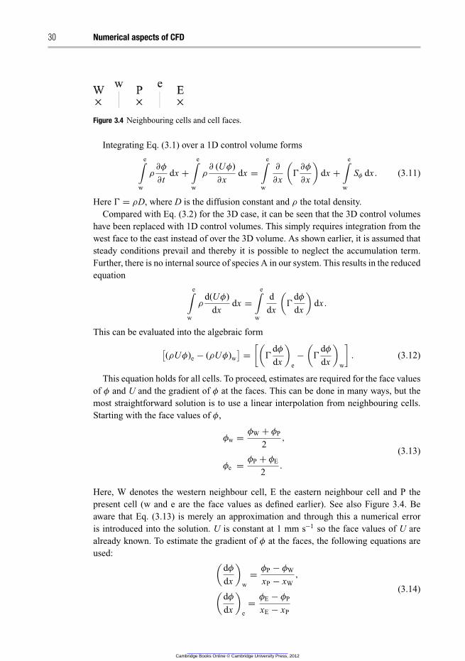
30 Numerical aspects of CFD
Figure 3.4 Neighbouring cells and cell faces.
Integrating Eq. (3.1) over a 1D control volume forms
e∫
w
ρ
∂φ
∂tdx +
e∫
w
ρ
∂ (Uφ)
∂xdx =
e∫
w
∂
∂x
(
Ŵ
∂φ
∂x
)
dx +
e∫
w
Sφ dx . (3.11)
Here Ŵ = ρD, where D is the diffusion constant and ρ the total density.
Compared with Eq. (3.2) for the 3D case, it can be seen that the 3D control volumes
have been replaced with 1D control volumes. This simply requires integration from the
west face to the east instead of over the 3D volume. As shown earlier, it is assumed that
steady conditions prevail and thereby it is possible to neglect the accumulation term.
Further, there is no internal source of species A in our system. This results in the reduced
equation
e∫
w
ρ
d(Uφ)
dxdx =
e∫
w
d
dx
(
Ŵ
dφ
dx
)
dx .
This can be evaluated into the algebraic form
[
(ρUφ)e − (ρUφ)w
]
=
[(
Ŵ
dφ
dx
)
e
−
(
Ŵ
dφ
dx
)
w
]
. (3.12)
This equation holds for all cells. To proceed, estimates are required for the face values
of φ and U and the gradient of φ at the faces. This can be done in many ways, but the
most straightforward solution is to use a linear interpolation from neighbouring cells.
Starting with the face values of φ,
φw =φW + φP
2,
φe =φP + φE
2.
(3.13)
Here, W denotes the western neighbour cell, E the eastern neighbour cell and P the
present cell (w and e are the face values as defined earlier). See also Figure 3.4. Be
aware that Eq. (3.13) is merely an approximation and through this a numerical error
is introduced into the solution. U is constant at 1 mm s−1 so the face values of U are
already known. To estimate the gradient of φ at the faces, the following equations are
used:(
dφ
dx
)
w
=φP − φW
xP − xW
,
(
dφ
dx
)
e
=φE − φP
xE − xP
(3.14)
Cambridge Books Online © Cambridge University Press, 2012
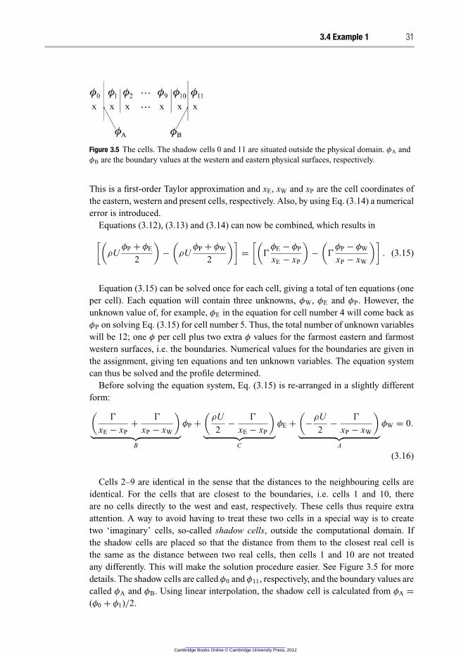
3.4 Example 1 31
Figure 3.5 The cells. The shadow cells 0 and 11 are situated outside the physical domain. φA and
φB are the boundary values at the western and eastern physical surfaces, respectively.
This is a first-order Taylor approximation and xE, xW and xP are the cell coordinates of
the eastern, western and present cells, respectively. Also, by using Eq. (3.14) a numerical
error is introduced.
Equations (3.12), (3.13) and (3.14) can now be combined, which results in
[(
ρUφP + φE
2
)
−
(
ρUφP + φW
2
)]
=
[(
Ŵ
φE − φP
xE − xP
)
−
(
Ŵ
φP − φW
xP − xW
)]
. (3.15)
Equation (3.15) can be solved once for each cell, giving a total of ten equations (one
per cell). Each equation will contain three unknowns, φW, φE and φP. However, the
unknown value of, for example, φE in the equation for cell number 4 will come back as
φP on solving Eq. (3.15) for cell number 5. Thus, the total number of unknown variables
will be 12; one φ per cell plus two extra φ values for the farmost eastern and farmost
western surfaces, i.e. the boundaries. Numerical values for the boundaries are given in
the assignment, giving ten equations and ten unknown variables. The equation system
can thus be solved and the profile determined.
Before solving the equation system, Eq. (3.15) is re-arranged in a slightly different
form:
(
Ŵ
xE − xP
+Ŵ
xP − xW
)
︸ ︷︷ ︸
B
φP +
(
ρU
2−
Ŵ
xE − xP
)
︸ ︷︷ ︸
C
φE +
(
−ρU
2−
Ŵ
xP − xW
)
︸ ︷︷ ︸
A
φW = 0.
(3.16)
Cells 2–9 are identical in the sense that the distances to the neighbouring cells are
identical. For the cells that are closest to the boundaries, i.e. cells 1 and 10, there
are no cells directly to the west and east, respectively. These cells thus require extra
attention. A way to avoid having to treat these two cells in a special way is to create
two ‘imaginary’ cells, so-called shadow cells, outside the computational domain. If
the shadow cells are placed so that the distance from them to the closest real cell is
the same as the distance between two real cells, then cells 1 and 10 are not treated
any differently. This will make the solution procedure easier. See Figure 3.5 for more
details. The shadow cells are called φ0 and φ11, respectively, and the boundary values are
called φA and φB. Using linear interpolation, the shadow cell is calculated from φA =
(φ0 + φ1)/2.
Cambridge Books Online © Cambridge University Press, 2012
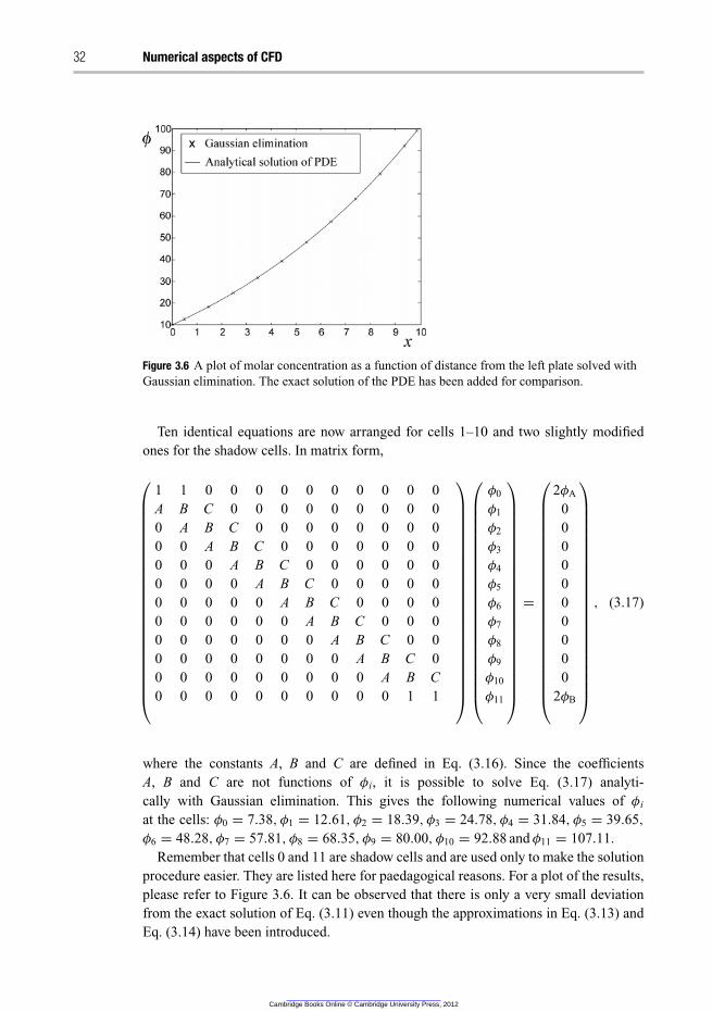
32 Numerical aspects of CFD
Figure 3.6 A plot of molar concentration as a function of distance from the left plate solved with
Gaussian elimination. The exact solution of the PDE has been added for comparison.
Ten identical equations are now arranged for cells 1–10 and two slightly modified
ones for the shadow cells. In matrix form,
⎛
⎜
⎜
⎜
⎜
⎜
⎜
⎜
⎜
⎜
⎜
⎜
⎜
⎜
⎜
⎜
⎜
⎜
⎜
⎜
⎜
⎜
⎜
⎝
1 1 0 0 0 0 0 0 0 0 0 0
A B C 0 0 0 0 0 0 0 0 0
0 A B C 0 0 0 0 0 0 0 0
0 0 A B C 0 0 0 0 0 0 0
0 0 0 A B C 0 0 0 0 0 0
0 0 0 0 A B C 0 0 0 0 0
0 0 0 0 0 A B C 0 0 0 0
0 0 0 0 0 0 A B C 0 0 0
0 0 0 0 0 0 0 A B C 0 0
0 0 0 0 0 0 0 0 A B C 0
0 0 0 0 0 0 0 0 0 A B C
0 0 0 0 0 0 0 0 0 0 1 1
⎞
⎟
⎟
⎟
⎟
⎟
⎟
⎟
⎟
⎟
⎟
⎟
⎟
⎟
⎟
⎟
⎟
⎟
⎟
⎟
⎟
⎟
⎟
⎠
⎛
⎜
⎜
⎜
⎜
⎜
⎜
⎜
⎜
⎜
⎜
⎜
⎜
⎜
⎜
⎜
⎜
⎜
⎜
⎜
⎜
⎜
⎜
⎝
φ0
φ1
φ2
φ3
φ4
φ5
φ6
φ7
φ8
φ9
φ10
φ11
⎞
⎟
⎟
⎟
⎟
⎟
⎟
⎟
⎟
⎟
⎟
⎟
⎟
⎟
⎟
⎟
⎟
⎟
⎟
⎟
⎟
⎟
⎟
⎠
=
⎛
⎜
⎜
⎜
⎜
⎜
⎜
⎜
⎜
⎜
⎜
⎜
⎜
⎜
⎜
⎜
⎜
⎜
⎜
⎜
⎜
⎜
⎜
⎝
2φA
0
0
0
0
0
0
0
0
0
0
2φB
⎞
⎟
⎟
⎟
⎟
⎟
⎟
⎟
⎟
⎟
⎟
⎟
⎟
⎟
⎟
⎟
⎟
⎟
⎟
⎟
⎟
⎟
⎟
⎠
, (3.17)
where the constants A, B and C are defined in Eq. (3.16). Since the coefficients
A, B and C are not functions of φi, it is possible to solve Eq. (3.17) analyti-
cally with Gaussian elimination. This gives the following numerical values of φi
at the cells: φ0 = 7.38, φ1 = 12.61, φ2 = 18.39, φ3 = 24.78, φ4 = 31.84, φ5 = 39.65,
φ6 = 48.28, φ7 = 57.81, φ8 = 68.35, φ9 = 80.00, φ10 = 92.88 and φ11 = 107.11.
Remember that cells 0 and 11 are shadow cells and are used only to make the solution
procedure easier. They are listed here for paedagogical reasons. For a plot of the results,
please refer to Figure 3.6. It can be observed that there is only a very small deviation
from the exact solution of Eq. (3.11) even though the approximations in Eq. (3.13) and
Eq. (3.14) have been introduced.
Cambridge Books Online © Cambridge University Press, 2012
3.5 The Gauss–Seidel algorithm 33
3.4.2 Concluding remarks
The solution strategy for a simple CFD problem has now been demonstrated. However,
it must be kept in mind that the solved example contained many simplifications and was
well defined in many ways. Generally, it is not possible to solve a CFD problem with a
direct method, such as Gaussian elimination. The focus is then turned towards iterative
methods.
Some examples of simplifications in the solved Example 1 are the following.
� The problem could be treated as 1D due to symmetries. A problem in 2D or 3D would,
of course, generate more cells; in this case a 3D treatment would give 1000 cells
instead of 10, assuming that the grid density was kept constant and the computational
domain had a cubic geometry. The cells were placed with constant spacing, generating
a so-called equidistant grid.� Further, the presence of a constant velocity made the solution process easier. Usually,
the velocities cannot be predetermined, and thus one requires a solution to a transport
equation for each velocity component as well. If this is the case, the equation system,
Eq. (3.16), will contain nonlinear terms like ρUφ, where both U and φ are variables.
This means that matrices can no longer be created with constant coefficients like in
Eq. (3.17). The equation system must then be solved by some iterative technique, e.g.
the Gauss–Seidel method (see below for more details).� Another simplification introduced was the linear approximations of the variables and
the gradients at the faces. Obviously, at high positive flow rates, the face values
between, for example, cell 1 and cell 2 must be more dependent on cell 1 than on
cell 2. Thus, linear interpolation, or central differencing, must be used with caution.� The fluid properties were assumed to be constant. In non-isothermal situations, the
temperature must be calculated in order for these entities to be predicted. A transport
equation for temperature has to be solved. However, in order to solve the energy
equation, the fluid properties must be known. This requires iterative methods.
Questions
(1) Propose a general expression for the transport of the entity φ. Give a physical
interpretation and units to the terms.
(2) What is discretization? Is it always a necessary step in the solving of a CFD problem?
(3) How many boundary conditions are required in order to solve a steady diffusion–
convection problem in n computational dimensions? Does this number change if
diffusion is neglected? Give a physical explanation!
(4) What sources of error were introduced in Example 1?
3.5 The Gauss–Seidel algorithm
As discussed earlier, iterative methods are always used in CFD. Most commercial CFD
codes use some variant of the Gauss–Seidel algorithm (GSA). Some basic knowledge
Cambridge Books Online © Cambridge University Press, 2012
34 Numerical aspects of CFD
of the GSA makes it easier to understand how these codes work and also what problems
can occur.
For demonstration, Example 1 will be solved again, this time with the GSA. First,
some general words about the GSA are in order. Starting with Eq. (3.16), it is possible
to isolate φP from the equation:
φP =aEφE + aWφW
aP
, (3.18)
where
aE =
(
−ρU
2+
Ŵ
xE − xP
)
,
aW =
(
ρU
2+
Ŵ
xP − xW
)
,
aP =
(
Ŵ
xE − xP
+Ŵ
xP − xW
)
.
(3.19)
The main difference between using the GSA and Gaussian elimination is that the GSA
is an iterative method. Equation (3.18) is solved for each cell in an iterative manner.
Start with cell 1; to be able to solve for this cell, the numerical value of the variable in
the shadow cell, φ0, and also the numerical value in cell 2, φ2, are needed. Since there is
no numerical value of φ in any cell, a starting guess, an initialization, for all φi must be
made. φ1 is then solved for. Shifting our attention to φ2, Eq. (3.18) is solved for this cell.
In the calculation of φ2, the calculated value of φ1 and the starting guess for φ3 are used.
Thus, the GSA uses the values calculated already in the same iteration sweep, which
makes the solution converge faster. The procedure is then carried out until φi in all cells
have been calculated. But, there is a problem here; since φ1 was calculated as a function
of φ0 and φ2, the equation for φ1 is no longer satisfied since a new value of φ2 has been
calculated. Thus, the procedure must be repeated many times; i.e. it requires iteration.
This is done until convergence is reached, i.e. the numerical values of φi change by less
than a specified threshold amount set by the user. Discussion of how this is usually done
in practice will come later.
3.6 Example 2 – Gauss–Seidel
This time, Example 1 will be solved numerically using the GSA. The procedure given
in Figure 3.7 will be followed.
On looking at the expressions for aW, aE and aP, one may see that they are identical
for all cells and do not change during the iterations. We use the numerical values given
in the assignment, aE = 0.0095, aW = 0.0105 and aP = 0.0200, for all cells. A high
numerical value of e.g. aE means that cell (P) is highly influenced by it, whereas a low
number means the opposite; see Eq. (3.18). As can be seen here, aW is larger than aE,
meaning that the value for cell P is more influenced by its western neighbour than by
its eastern one. This shouldn’t come as any surprise, knowing that the gas is flowing
from west to east and, thus, the western cell should play a more dominant role in the
calculation of cell P.
Cambridge Books Online © Cambridge University Press, 2012
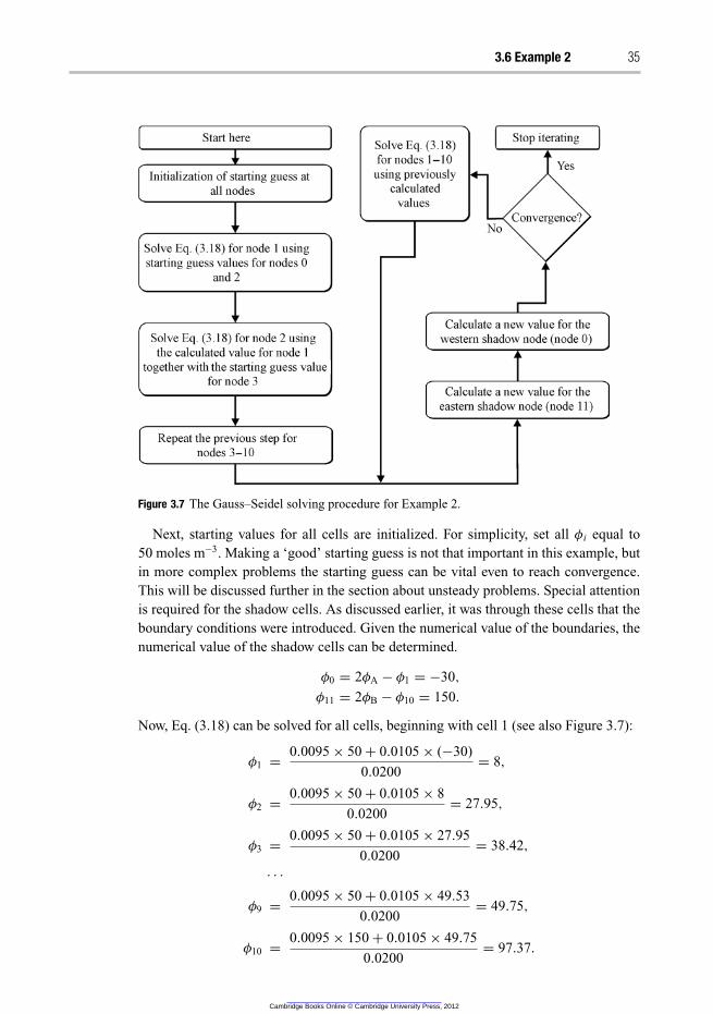
3.6 Example 2 35
Figure 3.7 The Gauss–Seidel solving procedure for Example 2.
Next, starting values for all cells are initialized. For simplicity, set all φi equal to
50 moles m−3. Making a ‘good’ starting guess is not that important in this example, but
in more complex problems the starting guess can be vital even to reach convergence.
This will be discussed further in the section about unsteady problems. Special attention
is required for the shadow cells. As discussed earlier, it was through these cells that the
boundary conditions were introduced. Given the numerical value of the boundaries, the
numerical value of the shadow cells can be determined.
φ0 = 2φA − φ1 = −30,
φ11 = 2φB − φ10 = 150.
Now, Eq. (3.18) can be solved for all cells, beginning with cell 1 (see also Figure 3.7):
φ1 =0.0095 × 50 + 0.0105 × (−30)
0.0200= 8,
φ2 =0.0095 × 50 + 0.0105 × 8
0.0200= 27.95,
φ3 =0.0095 × 50 + 0.0105 × 27.95
0.0200= 38.42,
· · ·
φ9 =0.0095 × 50 + 0.0105 × 49.53
0.0200= 49.75,
φ10 =0.0095 × 150 + 0.0105 × 49.75
0.0200= 97.37.
Cambridge Books Online © Cambridge University Press, 2012
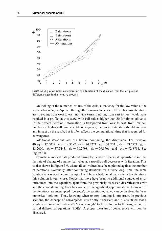
36 Numerical aspects of CFD
Figure 3.8 A plot of molar concentration as a function of the distance from the left plate at
different stages in the iterative process.
On looking at the numerical values of the cells, a tendency for the low value at the
western boundary to ‘spread’ through the domain can be seen. This is because iterations
are sweeping from west to east, not vice versa. Iterating from east to west would have
resulted in a profile, at this stage, with cell values higher than 50 for almost all cells.
In the present iteration, information is transported from west to east, from low cell
numbers to higher cell numbers. At convergence, the mode of iteration should not have
any impact on the result, but it often affects the computational time that is required for
convergence.
Additional iterations are run before continuing the discussion. For iteration
40 φ1 = 12.6027, φ2 = 18.3587, φ3 = 24.7271, φ4 = 31.7741, φ5 = 39.5721, φ6 =
48.2000, φ7 = 57.7443, φ8 = 68.2998, φ9 = 79.9706 and φ10 = 92.8714. See
Figure 3.8.
From the numerical data produced during the iterative process, it is possible to see that
the rate of change of a numerical value at a specific cell decreases with iteration. This
is also shown in Figure 3.9, where all cell values have been plotted against the number
of iterations. Eventually, after continuing iterations for a ‘very long’ time, the same
solution as was obtained in Example 1 will be reached, but already after a few iterations
this solution is very close. Notice that there have been no additional sources of error
introduced into the equations apart from the previously discussed discretization error
and the error stemming from face-value or face-gradient approximations. However, if
the iterations are interrupted ‘too soon’, the solution obtained can be far from the ‘true
numerical’ solution. Thus, knowing when to stop iterating is important. In previous
sections, the concept of convergence was briefly discussed; and it was stated that a
solution is converged when it’s ‘close enough’ to the solution to the original set of
partial differential equations (PDEs). A proper measure of convergence will now be
discussed.
Cambridge Books Online © Cambridge University Press, 2012
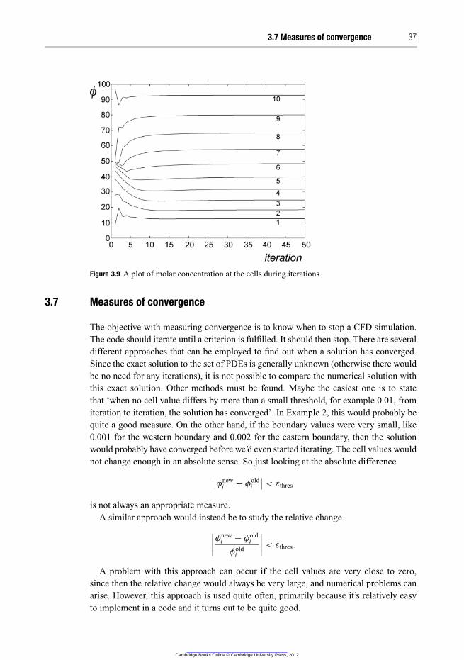
3.7 Measures of convergence 37
Figure 3.9 A plot of molar concentration at the cells during iterations.
3.7 Measures of convergence
The objective with measuring convergence is to know when to stop a CFD simulation.
The code should iterate until a criterion is fulfilled. It should then stop. There are several
different approaches that can be employed to find out when a solution has converged.
Since the exact solution to the set of PDEs is generally unknown (otherwise there would
be no need for any iterations), it is not possible to compare the numerical solution with
this exact solution. Other methods must be found. Maybe the easiest one is to state
that ‘when no cell value differs by more than a small threshold, for example 0.01, from
iteration to iteration, the solution has converged’. In Example 2, this would probably be
quite a good measure. On the other hand, if the boundary values were very small, like
0.001 for the western boundary and 0.002 for the eastern boundary, then the solution
would probably have converged before we’d even started iterating. The cell values would
not change enough in an absolute sense. So just looking at the absolute difference
∣
∣
φnewi − φ
oldi
∣
∣
< εthres
is not always an appropriate measure.
A similar approach would instead be to study the relative change
∣
∣
∣
∣
φnewi − φ
oldi
φoldi
∣
∣
∣
∣
< εthres.
A problem with this approach can occur if the cell values are very close to zero,
since then the relative change would always be very large, and numerical problems can
arise. However, this approach is used quite often, primarily because it’s relatively easy
to implement in a code and it turns out to be quite good.
Cambridge Books Online © Cambridge University Press, 2012
38 Numerical aspects of CFD
A very common approach is to calculate the error in Eq. (3.18),
R =∑
all cells
|aPφP − aWφW − aEφE|. (3.20)
If this error is scaled with an appropriate factor, a dimensionless number on which one
can impose a criterion results. For example, if F is an appropriate scaling factor,
R
F< εthres, e.g. F =
∑
all cells
∣
∣apφp
∣
∣+ |aWφW| + |aEφE|.
In some commercial CFD software the scaling factor is simply set to the highest unscaled
residual obtained within the first iterations. Hence, a bad starting guess makes it easier
to reach convergence, and vice versa.
A completely different way to measure convergence is to check whether the domain
upholds conservativeness. In the previous examples one could check the amount of A
being transported into the domain and subtract the amount that is being transported
out from it. For convergence, this difference should of course be zero, since there are
no sources inside the domain. In mathematical terms, the total flux (convection plus
diffusion) is given as F and this criterion is expressed as
|FW + FE| < εthres.
It must also be mentioned here that εthres can take different numerical values for
different variables. The numerical values of εthres are often in the range 10−3–10−6 for
single precision modes depending on which definition of a convergent solution is used.
Probably, the best way to ensure convergence is a combination of the criteria described
above. Being able to determine convergence is one of the most crucial parts of CFD.
Almost all commercial codes have various built-in functions to check convergence, but
nevertheless it is often worth the extra effort to do some extra manual checks. Remember
that a solution that has not converged is an ‘incorrect’ solution.
More about convergence can be found in Chapter 7.
Question
(1) In Examples 1 and 2 the same problem was solved in two completely different ways.
Which solution procedure puts the highest demand on the computer in terms of
memory usage and processor performance?
3.8 Discretization schemes
Look back at Example 1. When Eq. (3.18) was solved for the cells, the numerical
values of aE, aW and aP were used. These were obtained from Eq. (3.19). In turn,
these expressions relied on the assumptions made in Eqs. (3.13) and (3.14). A linear
interpolation was assumed in order to get accurate face values for φ. On the other hand,
it was later argued that this was an assumption that lacks physical reliability in cases
Cambridge Books Online © Cambridge University Press, 2012
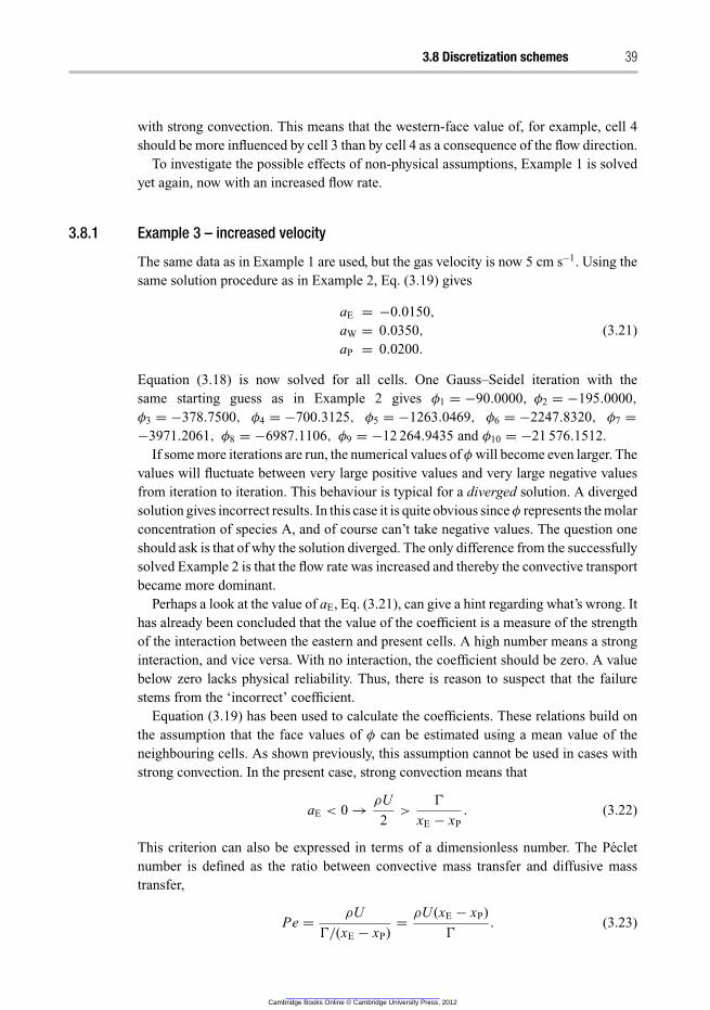
3.8 Discretization schemes 39
with strong convection. This means that the western-face value of, for example, cell 4
should be more influenced by cell 3 than by cell 4 as a consequence of the flow direction.
To investigate the possible effects of non-physical assumptions, Example 1 is solved
yet again, now with an increased flow rate.
3.8.1 Example 3 – increased velocity
The same data as in Example 1 are used, but the gas velocity is now 5 cm s−1. Using the
same solution procedure as in Example 2, Eq. (3.19) gives
aE = −0.0150,
aW = 0.0350,
aP = 0.0200.
(3.21)
Equation (3.18) is now solved for all cells. One Gauss–Seidel iteration with the
same starting guess as in Example 2 gives φ1 = −90.0000, φ2 = −195.0000,
φ3 = −378.7500, φ4 = −700.3125, φ5 = −1263.0469, φ6 = −2247.8320, φ7 =
−3971.2061, φ8 = −6987.1106, φ9 = −12 264.9435 and φ10 = −21 576.1512.
If some more iterations are run, the numerical values of φ will become even larger. The
values will fluctuate between very large positive values and very large negative values
from iteration to iteration. This behaviour is typical for a diverged solution. A diverged
solution gives incorrect results. In this case it is quite obvious since φ represents the molar
concentration of species A, and of course can’t take negative values. The question one
should ask is that of why the solution diverged. The only difference from the successfully
solved Example 2 is that the flow rate was increased and thereby the convective transport
became more dominant.
Perhaps a look at the value of aE, Eq. (3.21), can give a hint regarding what’s wrong. It
has already been concluded that the value of the coefficient is a measure of the strength
of the interaction between the eastern and present cells. A high number means a strong
interaction, and vice versa. With no interaction, the coefficient should be zero. A value
below zero lacks physical reliability. Thus, there is reason to suspect that the failure
stems from the ‘incorrect’ coefficient.
Equation (3.19) has been used to calculate the coefficients. These relations build on
the assumption that the face values of φ can be estimated using a mean value of the
neighbouring cells. As shown previously, this assumption cannot be used in cases with
strong convection. In the present case, strong convection means that
aE < 0 →ρU
2>
Ŵ
xE − xP
. (3.22)
This criterion can also be expressed in terms of a dimensionless number. The Peclet
number is defined as the ratio between convective mass transfer and diffusive mass
transfer,
Pe =ρU
Ŵ/(xE − xP)=
ρU (xE − xP)
Ŵ
. (3.23)
Cambridge Books Online © Cambridge University Press, 2012
40 Numerical aspects of CFD
The criterion for strong convection would then be (cf. Eq. (3.22))
|Pe| > 2. (3.24)
Here, it is assumed that the velocity is always positive, i.e. the flow is from west to
east. However, the flow could just as well go in the opposite direction, giving a negative
value of aW instead. This would also have resulted in a divergent solution. The absolute
sign for Pe in Eq. (3.24) evolves from this fact. In Example 3, Pe = 5, which satisfies
Eq. (3.24) and hence makes the problem diverge.
This example illustrates that it’s important to keep in mind that all assumptions must
have physical reliability. This will always be important in CFD, not only in the numerical
aspects, but also in other parts of the CFD problem. When the various turbulence
models are introduced in following chapters it is stated that each model has its physical
limitations and that overlooking these limitations can result in an incorrect solution.
Bearing in mind the physical background of the problem is thus always important.
3.8.2 Boundedness and transportiveness
A desired property of a discretization scheme is that it should uphold boundedness. A
bounded variable has a value that is neither larger nor smaller than any of the values that
are used to calculate it. In Example 1 central differencing was used to estimate the face
values of φ. The face value was then simply the mean value of the two surrounding cells.
Thus, the face values are bounded. The cell values were calculated using Eq. (3.18),
which actually is nothing other than a weighted mean value of the two neighbouring
cells. This follows from the fact that aW + aE = aP. On the other hand, Eq. (3.18) can
be seen as a mean value only for cases with positive values of the coefficients. If one
of the values is negative, it is no longer possible to say that φP is bounded, since it can
take values that are either larger or smaller than those for any of the neighbouring cells.
Thus, the central-differencing scheme is said to be conditionally bounded. It should be
noted that there are more advanced central-differencing schemes that are bounded, but
they are beyond the scope of this book.
Transportiveness is another desired property of the schemes. It has already been dis-
cussed briefly, but not defined properly. The ability of the numerical scheme to ‘feel’ in
what direction the information is being transported is a description of transportiveness.
As previously discussed, the solution in Example 3 failed partly due to the lack of this
property. Transportiveness is linked to boundedness in this case, since lack of trans-
portiveness gave an unbounded solution. The central-differencing scheme calculates the
face values without taking any notice of the direction of the flow, i.e. the direction of the
information. Thus, the central-differencing scheme does not satisfy the transportiveness
requirement.
3.8.3 The upwind schemes
From Example 3, and the discussion above, it is clear that in cases with strong convection
the face values of φ have to be estimated in some other way than using Eq. (3.13). A
Cambridge Books Online © Cambridge University Press, 2012
3.8 Discretization schemes 41
reasonable line is to suggest that the face values between, for example, cell 4 and cell 5
are dependent only upon cell values from cell 4 or cells further upstream. Schemes that
let face values be dependent only on upstream conditions are called upwind schemes.
We will now examine two of these schemes closer.
First-order upwind
The idea behind the first-order upwind scheme is to have physical reliability for convec-
tive flows simply by letting the face value between two cells be equal to the value for the
nearest upstream cell, i.e.
φw = φW,
φe = φP,(3.25)
or, for negative velocities,
φw = φP,
φe = φE.
(3.26)
The gradients are still estimated using Eq. (3.14).
If we return to our previous examples and use the first-order upwind scheme instead
of the central-differencing scheme, we can rewrite Eq. (3.15) as
[(ρUφP) − (ρUφW)] =
[(
Ŵ
φE − φP
xE − xP
)
−
(
Ŵ
φP − φW
xP − xW
)]
. (3.27)
The physical meaning of the terms in the equation is the same as before; the difference
in convective transport of φ is balanced out by the difference in diffusion. The only
difference from Eq. (3.15) is that face values of φ have been expressed using the first-
order upwind scheme instead of the central-differencing scheme. If we write Eq. (3.27)
in the same form as Eq. (3.18), we get
aE =Ŵ
xE − xP
,
aW =Ŵ
xP − xW
+ ρU,
aP = ρU +Ŵ
xE − xP
+Ŵ
xP − xW
.
(3.28)
Then, 40 iterations with the GSA will yield the following values for the
cells: φ1 = 10.0004, φ2 = 10.0003, φ3 = 10.0003, φ4 = 10.0007, φ5 = 10.0034, φ6 =
10.0199, φ7 = 10.1191, φ8 = 10.7143, φ9 = 14.2858 and φ10 = 35.7143.
The results are as expected; the high flow rate makes the western boundary more
dominant. Almost all cells in the domain, except the most eastern, have much the same
value of φ of approximately 10. Again, this seems reasonable.
From Eq. (3.28) it follows that the first-order upwind scheme is bounded. It also fulfils
the requirement of transportiveness since care is taken regarding the direction of the flow,
cf. Eqs. (3.25) and (3.26). However, it also overestimates the transport of entities in the
flow direction. This gives rise to so-called numerical diffusion.
Cambridge Books Online © Cambridge University Press, 2012
42 Numerical aspects of CFD
Second-order upwind
To improve accuracy – we will discuss accuracy in more detail later – there is an
upwind scheme that predicts the face values using information from two upwind cells.
To estimate the eastern-face value, the scheme assumes that the gradient between the
present cell and the eastern face is the same as that between the western cell and the
present cell. In mathematical terms,
φe − φP
xe − xP
=φP − φW
xP − xW
→ φe =(φP − φW) (xe − xP)
xP − xW
+ φP. (3.29)
For an equidistant grid, Eq. (3.29) gives that
φe = 1.5φP − 0.5φW. (3.30)
A major drawback with the second-order upwind scheme is that it is unbounded. To
avoid the numerical problems that often arise as a result of unbounded schemes, some
bounded second-order schemes have been developed, e.g. the van Leer scheme. The
definitions will be stated here.
The van Leer scheme
If |φE − 2φP + φW| ≤ |φE − φW|, the value of φ at the eastern face is (cf. Eq. (3.29))
φe = φP +(φE − φP) (φP − φW)
φE − φW
. (3.31)
Otherwise (cf. Eq. (3.25)),
φe = φP. (3.32)
The velocity is assumed to be positive. The van Leer scheme implements the unbounded
second-order upwind scheme, Eq. (3.31), if the gradient is ‘smooth’, i.e. the second
derivative of φ is ‘small’. Otherwise, the first-order upwind scheme, Eq. (3.32), is used.
3.8.4 Taylor expansions
Before proceeding, a short mathematical review of Taylor expansions will be given.
Taylor’s theorem for a 1D expansion of a real function f (x) about a point x = x0 is
given without a proof:
f (x) = f (x0) + (x − x0) f ′(x0) +(x − x0)2
2!f ′′(x0) + · · ·
+(x − x0)n
n!f (n)(x0) +
x∫
x0
(x − u)n
n!f (n+1)(u)du. (3.33)
The last term in Eq. (3.33) is called the Lagrange remainder. Taylor’s theorem, except
for the Lagrange remainder, was devised by the English mathematician Brook Taylor
in 1712 and published in Methodus in crementorum directa et inversa in 1715. The
Cambridge Books Online © Cambridge University Press, 2012
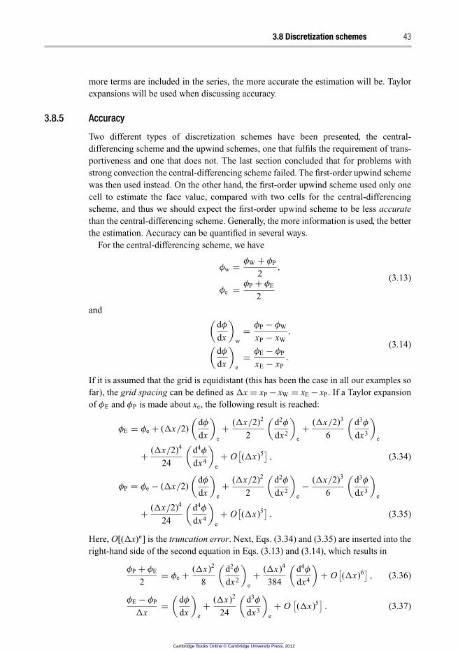
3.8 Discretization schemes 43
more terms are included in the series, the more accurate the estimation will be. Taylor
expansions will be used when discussing accuracy.
3.8.5 Accuracy
Two different types of discretization schemes have been presented, the central-
differencing scheme and the upwind schemes, one that fulfils the requirement of trans-
portiveness and one that does not. The last section concluded that for problems with
strong convection the central-differencing scheme failed. The first-order upwind scheme
was then used instead. On the other hand, the first-order upwind scheme used only one
cell to estimate the face value, compared with two cells for the central-differencing
scheme, and thus we should expect the first-order upwind scheme to be less accurate
than the central-differencing scheme. Generally, the more information is used, the better
the estimation. Accuracy can be quantified in several ways.
For the central-differencing scheme, we have
φw =φW + φP
2,
φe =φP + φE
2
(3.13)
and(
dφ
dx
)
w
=φP − φW
xP − xW
,
(
dφ
dx
)
e
=φE − φP
xE − xP
.
(3.14)
If it is assumed that the grid is equidistant (this has been the case in all our examples so
far), the grid spacing can be defined as �x = xP − xW = xE − xP. If a Taylor expansion
of φE and φP is made about xe, the following result is reached:
φE = φe + (�x/2)
(
dφ
dx
)
e
+(�x/2)2
2
(
d2φ
dx2
)
e
+(�x/2)3
6
(
d3φ
dx3
)
e
+(�x/2)4
24
(
d4φ
dx4
)
e
+ O[
(�x)5]
, (3.34)
φP = φe − (�x/2)
(
dφ
dx
)
e
+(�x/2)2
2
(
d2φ
dx2
)
e
−(�x/2)3
6
(
d3φ
dx3
)
e
+(�x/2)4
24
(
d4φ
dx4
)
e
+ O[
(�x)5]
. (3.35)
Here, O[(�x)n] is the truncation error. Next, Eqs. (3.34) and (3.35) are inserted into the
right-hand side of the second equation in Eqs. (3.13) and (3.14), which results in
φP + φE
2= φe +
(�x)2
8
(
d2φ
dx2
)
e
+(�x)4
384
(
d4φ
dx4
)
+ O[
(�x)6]
, (3.36)
φE − φP
�x=
(
dφ
dx
)
e
+(�x)2
24
(
d3φ
dx3
)
e
+ O[
(�x)5]
. (3.37)
Cambridge Books Online © Cambridge University Press, 2012
44 Numerical aspects of CFD
According to Eqs. (3.13) and (3.14), these expressions should be equal to the face
value of φ and the gradient of φ at the eastern face, respectively, assuming that central
differencing is used. Thus, since the second-order derivative d2φ/dx2 is unknown,
φe = φCDe + O
[
(�x)2]
(3.38)
and
(
dφ
dx
)
e
=
(
dφ
dx
)CD
e
+ O[
(�x)2]
. (3.39)
Before we comment on the results, we repeat the same procedure for the first-order
upwind scheme. Since the face gradient is predicted in the same way as with central
differencing, the face-value estimation, i.e. Eq. (3.25), must be examined. According to
this relation, the face value of the eastern face is simply equal to the cell value in the
present cell. A Taylor expansion of φ about xP gives
φe = φP + (�x/2)
(
dφ
dx
)
P
+(�x/2)2
2
(
d2φ
dx2
)
P
+ O[
(�x)3]
. (3.40)
Here, the first-order derivative is unknown and the outcome is
φe = φ1ue + O(�x). (3.41)
If Eqs. (3.38) and (3.41) are compared, it can be seen that, for a reduction of �x, the
face-value estimation seems to approach the ‘true’ value quicker in the case with the
central-differencing scheme. In other words, this means that, if the grid is made denser,
i.e. more cells are introduced, the error in the central-differencing scheme will be reduced
more quickly than in the case with the first-order upwind scheme. The lowest order of
the grid spacing in the central-differencing scheme is 2, hence the central-differencing
scheme is referred to as second-order accurate. For the first-order upwind scheme, the
corresponding number is 1; hence this scheme is referred to as first-order accurate.
Higher-order schemes are more accurate but this can be at the expense of numerical
stability. When stability is problematic it is recommended that one start with a simple
first-order upwind scheme and change to a higher-order scheme after some iterations.
Going to higher order is always necessary in order to minimize numerical diffusion when
the grids are not aligned with the flow.
3.8.6 The hybrid scheme
An attempt to combine the positive properties of both the central-differencing scheme
and the first-order upwind scheme has been proposed. This scheme is called the hybrid
differencing scheme. This scheme implements the upwind scheme at faces where the
criterion in Eq. (3.24) is fulfilled, and uses central differencing elsewhere. Thus, this
scheme takes advantage of both the high accuracy of the central-differencing scheme
and the more physical properties in terms of boundedness and transportiveness of the
upwind scheme.
Cambridge Books Online © Cambridge University Press, 2012
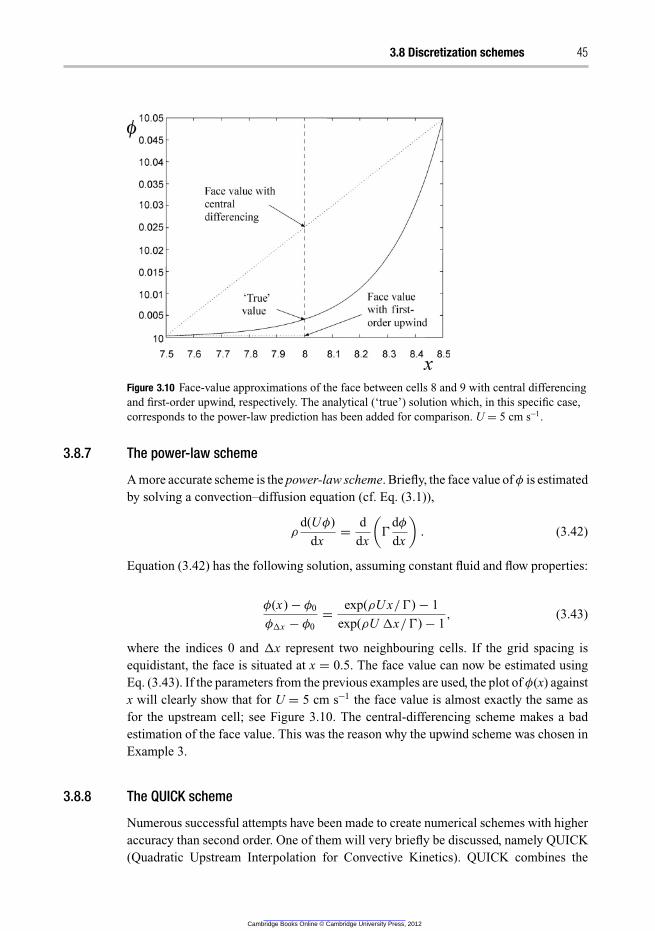
3.8 Discretization schemes 45
Figure 3.10 Face-value approximations of the face between cells 8 and 9 with central differencing
and first-order upwind, respectively. The analytical (‘true’) solution which, in this specific case,
corresponds to the power-law prediction has been added for comparison. U = 5 cm s−1.
3.8.7 The power-law scheme
A more accurate scheme is the power-law scheme. Briefly, the face value of φ is estimated
by solving a convection–diffusion equation (cf. Eq. (3.1)),
ρ
d(Uφ)
dx=
d
dx
(
Ŵ
dφ
dx
)
. (3.42)
Equation (3.42) has the following solution, assuming constant fluid and flow properties:
φ(x) − φ0
φ�x − φ0
=exp(ρU x/Ŵ) − 1
exp(ρU �x/Ŵ) − 1, (3.43)
where the indices 0 and �x represent two neighbouring cells. If the grid spacing is
equidistant, the face is situated at x = 0.5. The face value can now be estimated using
Eq. (3.43). If the parameters from the previous examples are used, the plot of φ(x) against
x will clearly show that for U = 5 cm s−1 the face value is almost exactly the same as
for the upstream cell; see Figure 3.10. The central-differencing scheme makes a bad
estimation of the face value. This was the reason why the upwind scheme was chosen in
Example 3.
3.8.8 The QUICK scheme
Numerous successful attempts have been made to create numerical schemes with higher
accuracy than second order. One of them will very briefly be discussed, namely QUICK
(Quadratic Upstream Interpolation for Convective Kinetics). QUICK combines the
Cambridge Books Online © Cambridge University Press, 2012
46 Numerical aspects of CFD
strengths of both the upwind schemes and of the central differencing; it uses three-
point upstream quadratic interpolation to estimate the face values. For the western and
eastern faces, respectively,
φw =6
8φW +
3
8φP −
1
8φWW, (3.44)
φe =6
8φP +
3
8φE −
1
8φW. (3.45)
It has been assumed here that the velocity is positive. A Taylor expansion of φ around
the eastern face gives
φE = φe + (�x/2)
(
dφ
dx
)
e
+(�x/2)2
2
(
d2φ
dx2
)
e
+ O[
(�x)3]
, (3.34′)
φP = φe − (�x/2)
(
dφ
dx
)
e
+(�x/2)2
2
(
d2φ
dx2
)
e
+ O[
(�x)3]
, (3.35′)
φW = φe − (1.5�x)
(
dφ
dx
)
e
+(1.5�x)2
2
(
d2φ
dx2
)
e
+ O[
(�x)3]
. (3.46)
On inserting Eqs. (3.34′), (3.35′) and (3.46) into Eq. (3.45), we get
φe = φQUICKe + O
[
(�x)3]
. (3.47)
Thus, the QUICK scheme is third-order accurate. Further, it can be shown that it is
unbounded but fulfils the transportiveness criterion. The use of QUICK is restricted to
hexahedral meshes.
3.8.9 More advanced discretization schemes
The discretization schemes mentioned previously are only a few among the many avail-
able. In most commercial CFD codes there are many variations of schemes, and it is
not our intention to provide a complete list in Table 3.1. However, two more will be
mentioned here without going into too much detail.
� MUSCL (Monotone Upstream-centred Schemes for Conservation Laws). The
MUSCL scheme shows a similar degree of accuracy to QUICK, but is not limited to
hexahedral meshes.� HRIC (High-Resolution Interface Capturing). The HRIC scheme is primarily used in
multiphase flows when tracking the interface between the phases. HRIC has proven
to be more accurate than QUICK for VOF simulations (see Chapter 6).
For all of the discretization schemes that have been presented here, the error tends
to zero as the grid spacing is reduced infinitely. Schemes that uphold this property are
said to be consistent. It should also be mentioned that the definitions of some of the
discretization schemes presented here seem to differ in the literature.
Cambridge Books Online © Cambridge University Press, 2012
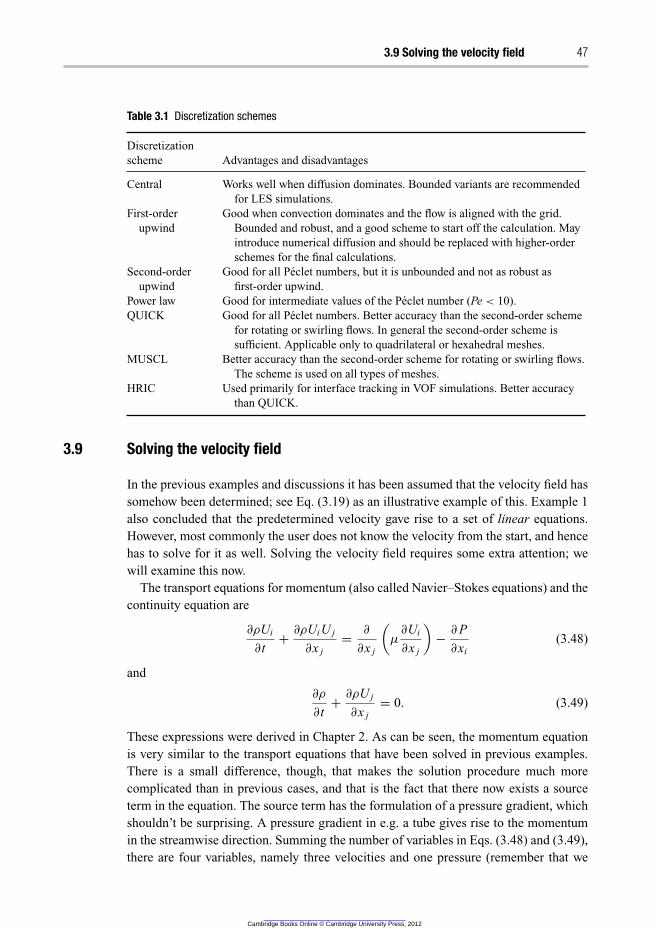
3.9 Solving the velocity field 47
Table 3.1 Discretization schemes
Discretization
scheme Advantages and disadvantages
Central Works well when diffusion dominates. Bounded variants are recommended
for LES simulations.
First-order
upwind
Good when convection dominates and the flow is aligned with the grid.
Bounded and robust, and a good scheme to start off the calculation. May
introduce numerical diffusion and should be replaced with higher-order
schemes for the final calculations.
Second-order
upwind
Good for all Peclet numbers, but it is unbounded and not as robust as
first-order upwind.
Power law Good for intermediate values of the Peclet number (Pe < 10).
QUICK Good for all Peclet numbers. Better accuracy than the second-order scheme
for rotating or swirling flows. In general the second-order scheme is
sufficient. Applicable only to quadrilateral or hexahedral meshes.
MUSCL Better accuracy than the second-order scheme for rotating or swirling flows.
The scheme is used on all types of meshes.
HRIC Used primarily for interface tracking in VOF simulations. Better accuracy
than QUICK.
3.9 Solving the velocity field
In the previous examples and discussions it has been assumed that the velocity field has
somehow been determined; see Eq. (3.19) as an illustrative example of this. Example 1
also concluded that the predetermined velocity gave rise to a set of linear equations.
However, most commonly the user does not know the velocity from the start, and hence
has to solve for it as well. Solving the velocity field requires some extra attention; we
will examine this now.
The transport equations for momentum (also called Navier–Stokes equations) and the
continuity equation are
∂ρUi
∂t+
∂ρUiU j
∂x j
=∂
∂x j
(
μ
∂Ui
∂x j
)
−∂ P
∂xi
(3.48)
and
∂ρ
∂t+
∂ρU j
∂x j
= 0. (3.49)
These expressions were derived in Chapter 2. As can be seen, the momentum equation
is very similar to the transport equations that have been solved in previous examples.
There is a small difference, though, that makes the solution procedure much more
complicated than in previous cases, and that is the fact that there now exists a source
term in the equation. The source term has the formulation of a pressure gradient, which
shouldn’t be surprising. A pressure gradient in e.g. a tube gives rise to the momentum
in the streamwise direction. Summing the number of variables in Eqs. (3.48) and (3.49),
there are four variables, namely three velocities and one pressure (remember that we
Cambridge Books Online © Cambridge University Press, 2012
48 Numerical aspects of CFD
have assumed incompressible flow!). The total number of equations is four (3 + 1), so
it should be possible to solve the system straight away. Normally, Eq. (3.48) is used
for the three velocity components. Unfortunately, Eq. (3.49) cannot be used to solve for
pressure. Hence, the equation must be modified first. Taking the divergence of Eq. (3.48)
gives
∂2
∂xi ∂t(ρUi ) +
∂2
∂xi ∂x j
(
ρUiU j
)
=∂
2
∂xi ∂x j
(
μ
∂Ui
∂x j
)
−∂
2 P
∂xi ∂xi
. (3.50)
The first term on the left-hand side and the first term on the right-hand side can be
rewritten (assuming constant density and viscosity) as
∂
∂xi
(
∂ρUi
∂t
)
=∂
∂t
(
∂ρUi
∂xi
)
,
∂
∂xi
[
∂
∂x j
(
μ
∂Ui
∂x j
)]
=∂
∂x j
[
∂
∂x j
(
μ
∂Ui
∂xi
)]
.
Owing to continuity (see Eq. (3.49)), the right-hand sides of both these expressions are
equal to zero. Equation (3.50) can thus be written in the following way:
∂2 P
∂xi ∂xi
= −∂
2
∂xi ∂x j
(
ρUiU j
)
. (3.51)
Equation (3.51), which is a scalar equation, can be used as a direct equation for pressure.
However, numerical problems are commonly encountered, for reasons that will not be
discussed in this book. Therefore, in almost all commercial CFD software an iterative
procedure for solving Eq. (3.51) is adopted, thereby avoiding the numerical problems.
Some of the most widely used algorithms are SIMPLE, SIMPLEC, SIMPLER and PISO.
The algorithms of the SIMPLE (Semi-Implicit Method for Pressure-Linked Equations)
family use a starting guess for pressure and velocity to solve for the corresponding
velocities via the momentum equations. Since the starting guess of the pressure will
not be correct, the velocities obtained will not satisfy continuity. Hence, correction
factors for pressure and velocity are introduced, and transport equations for these factors
are proposed and solved to give corrected velocities and pressure. The other transport
equations, e.g. for various scalars, are then solved. Then, a check for convergence is made
and the procedure is repeated until convergence is reached. SIMPLER and SIMPLEC
are improved variants of SIMPLE. The PISO algorithm is mostly used for unsteady
flow. It can be seen as an extension of the SIMPLE algorithm, but it uses two levels of
correction instead of one as is the case with SIMPLE.
It is generally not possible to say that a specific scheme is always better than another
with respect to efficiency or robustness. These properties are very dependent on the
flow conditions at hand, but a proper choice of scheme can sometimes speed up the
simulations significantly. The performance and behaviour of the schemes have been
thoroughly examined, and a few conclusions are mentioned here.
For a laminar backward-facing step it has been shown that PISO performs twice as
fast as SIMPLE, while it has been shown to be four times as slow for a case concerning
flow through a heated fin. For steady flow problems, SIMPLER has been shown to need
Cambridge Books Online © Cambridge University Press, 2012
3.9 Solving the velocity field 49
30%–50% less computer time than SIMPLE to solve problems in general. The degree
of coupling between the momentum equations and scalar equations has been shown to
have a significant impact sometimes. In problems where there is only a weak coupling or
no coupling at all between the momentum and scalar equations, PISO has been shown
to have the most robust convergence and is quicker than SIMPLEC and SIMPLER. If
the opposite is valid, i.e. there is a strong coupling between the momentum and scalar
equations, SIMPLER and SIMPLEC have been shown to perform better than PISO.
Further, it has not been possible to claim that either SIMPLER or SIMPLEC is superior
to the other in general. SIMPLEC usually performs better in situations in which the
rate of convergence is limited by the pressure–velocity coupling, such as non-complex
laminar-flow cases.
In order to solve the transport equations for momentum, Eq. (2.21), it is required
that the pressures at the cell faces are known. As in the cases with other transported
quantities, this is achieved by interpolation of the values in the neighbouring cells. Most
commercial CFD software offers a variety of interpolation schemes. Each scheme uses
its own interpolation function.
The standard scheme uses the coefficients ap, ae, etc. to interpolate the pressure on
the cell faces. As long as the pressure variation between the cells is smooth, the scheme
usually works fine. For flows with large body forces the standard scheme has been shown
to be troublesome. In such cases it is recommended that the body force-weighted scheme
be used. This scheme assumes that the normal gradient of the difference between the
body force and pressure is constant. For swirling flows and flows with natural convection,
the PRESTO! scheme should be used. The PRESTO! scheme uses the discrete continuity
equation to calculate the pressure field on a mesh that is geometrically shifted so that the
new cell centres are where the faces of the ordinary mesh are placed. This means that the
pressures on the faces are now known. The PRESTO! scheme is also recommended for
VOF simulations. The second-order pressure scheme is analogous to the second-order
discretization scheme presented earlier and is recommended for compressible flows. The
second-order scheme can be numerically unstable if it is used at the start of a calculation
or on a bad mesh.
3.9.1 Under-relaxation
The momentum equations, Eq. (3.48), contain nonlinear terms, e.g. ρV2 in the momen-
tum equation for V. To avoid divergence due to nonlinearities, so-called under-relaxation
is used in the solving procedure. The under-relaxation factor α is defined as
φnew = αφsolver + (1 − α) φold, (3.52)
where φnew is the new value at the cell, φsolver is the value for the solution to the last
iteration, and φold is the previous value at the cell that is used to compute φsolver. Thus,
a large value of α means that the new value will be very influenced by the solved value,
and vice versa. α lies usually in the range between zero and one. In many cases the
under-relaxation factor can be increased during iterations. Each transport equation or
pressure equation has its ‘own’ corresponding under-relaxation factor. Too low a value
Cambridge Books Online © Cambridge University Press, 2012
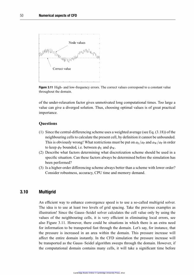
50 Numerical aspects of CFD
Figure 3.11 High- and low-frequency errors. The correct values correspond to a constant value
throughout the domain.
of the under-relaxation factor gives unmotivated long computational times. Too large a
value can give a diverged solution. Thus, choosing optimal values is of great practical
importance.
Questions
(1) Since the central-differencing scheme uses a weighted average (see Eq. (3.18)) of the
neighbouring cells to calculate the present cell, by definition it cannot be unbounded.
This is obviously wrong! What restrictions must be put on aE/aP and aW/aP in order
to keep φP bounded, i.e. between φE and φW.
(2) Describe what factors determining what discretization scheme should be used in a
specific situation. Can these factors always be determined before the simulation has
been performed?
(3) Is a higher-order differencing scheme always better than a scheme with lower order?
Consider robustness, accuracy, CPU time and memory demand.
3.10 Multigrid
An efficient way to enhance convergence speed is to use a so-called multigrid solver.
The idea is to use at least two levels of grid spacing. Take the previous examples as
illustration! Since the Gauss–Seidel solver calculates the cell value only by using the
values of the neighbouring cells, it is very efficient in eliminating local errors, see
also Figure 3.11. However, there could be situations in which there is an extra need
for information to be transported fast through the domain. Let’s say, for instance, that
the pressure is increased in an area within the domain. This pressure increase will
affect the entire domain instantly. In the CFD simulation the pressure increase will
be transported as the Gauss–Seidel algorithm sweeps through the domain. However, if
the computational domain contains many cells, it will take a significant time before
Cambridge Books Online © Cambridge University Press, 2012
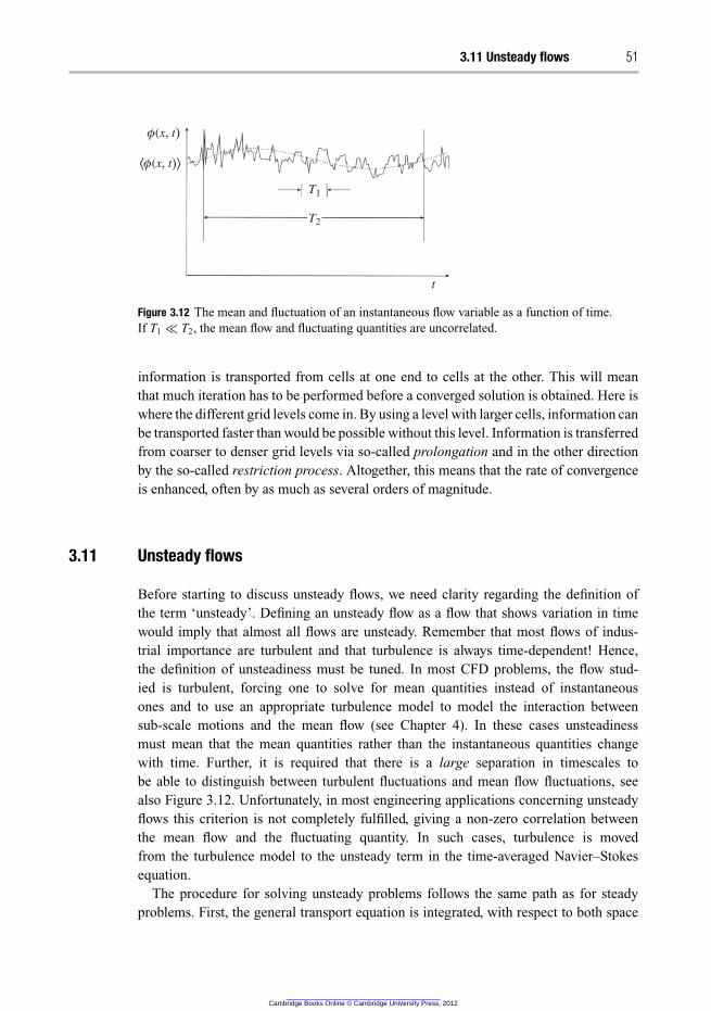
3.11 Unsteady flows 51
φ(x, t)
T1
T2
t
⟨φ(x, t)⟩
Figure 3.12 The mean and fluctuation of an instantaneous flow variable as a function of time.
If T1 ≪ T2, the mean flow and fluctuating quantities are uncorrelated.
information is transported from cells at one end to cells at the other. This will mean
that much iteration has to be performed before a converged solution is obtained. Here is
where the different grid levels come in. By using a level with larger cells, information can
be transported faster than would be possible without this level. Information is transferred
from coarser to denser grid levels via so-called prolongation and in the other direction
by the so-called restriction process. Altogether, this means that the rate of convergence
is enhanced, often by as much as several orders of magnitude.
3.11 Unsteady flows
Before starting to discuss unsteady flows, we need clarity regarding the definition of
the term ‘unsteady’. Defining an unsteady flow as a flow that shows variation in time
would imply that almost all flows are unsteady. Remember that most flows of indus-
trial importance are turbulent and that turbulence is always time-dependent! Hence,
the definition of unsteadiness must be tuned. In most CFD problems, the flow stud-
ied is turbulent, forcing one to solve for mean quantities instead of instantaneous
ones and to use an appropriate turbulence model to model the interaction between
sub-scale motions and the mean flow (see Chapter 4). In these cases unsteadiness
must mean that the mean quantities rather than the instantaneous quantities change
with time. Further, it is required that there is a large separation in timescales to
be able to distinguish between turbulent fluctuations and mean flow fluctuations, see
also Figure 3.12. Unfortunately, in most engineering applications concerning unsteady
flows this criterion is not completely fulfilled, giving a non-zero correlation between
the mean flow and the fluctuating quantity. In such cases, turbulence is moved
from the turbulence model to the unsteady term in the time-averaged Navier–Stokes
equation.
The procedure for solving unsteady problems follows the same path as for steady
problems. First, the general transport equation is integrated, with respect to both space
Cambridge Books Online © Cambridge University Press, 2012
52 Numerical aspects of CFD
and time,
∫
c.v.
⎛
⎝
t+�t∫
t
ρ
∂φ
∂tdt
⎞
⎠ dV +
t+�t∫
t
⎡
⎣
∫
c.v.
ρ
∂
(
U jφ
)
∂x j
dV
⎤
⎦ dt
=
t+�t∫
t
⎡
⎣
∫
c.v.
∂
∂x j
(
Ŵ
∂φ
∂x j
)
dV
⎤
⎦ dt +
t+�t∫
t
⎛
⎝
∫
c.v.
Sφ dV
⎞
⎠ dt. (3.53)
The order of integration is reversed in the accumulation term. To clarify the steps needed,
an example is given.
3.11.1 Example 4 – time-dependent simulation
Using the same experimental set-up as in Example 1, but this time without any con-
vection, the unsteady case is solved. Initially there is no species A in the domain. The
boundary conditions are the same as in the original example.
The integrated transport equation for φ in the present example is
e∫
w
⎛
⎝
t+�t∫
t
ρ
dφ
dtdt
⎞
⎠ dx =
t+�t∫
t
⎡
⎣
e∫
w
d
dx
(
Ŵ
dφ
dx
)
dx
⎤
⎦dt . (3.54)
Using central differencing allows us to rewrite Eq. (3.54) as
e∫
w
⎛
⎝
t+�t∫
t
ρ
dφ
dtdt
⎞
⎠ dx =
t+�t∫
t
(
Ŵe
φE − φP
�x− Ŵw
φP − φW
�x
)
dt . (3.55)
To proceed with the time integration an appropriate temporal discretization scheme is
needed. As in the case with spatial discretization there is a choice of scheme; either
‘earlier’ or ‘later’ times (or a mixture of them) can be used to estimate the temporal
derivative at the ‘present’ time. For now,
ρ[φP (t + �t) − φP (t)]�x =
t+�t∫
t
(
Ŵe
φE − φP
�x− Ŵw
φP − φW
�x
)
dt . (3.56)
To continue, φ on the right-hand side of Eq. (3.56) is evaluated at each time step. φ
changes in time, so there are at least three different ways to get values for φ: (1) let φ be
equal to φ(t), (2) let φ be equal to φ(t + �t), and (3) let φ be a mixture of the two.
We now define the weight factor θ :
t+�t∫
t
φ dt = [θφ(t + �t) + (1 − θ )φ(t)]�t. (3.57)
The case θ = 0 means that only the old value of φ is used when evaluating
Eq. (3.56). This leads to so-called explicit discretization of this equation. The other
extreme, θ = 1, corresponds to a discretization where only the new value of φ is used
Cambridge Books Online © Cambridge University Press, 2012
3.11 Unsteady flows 53
in the discretization, the so-called ( fully) implicit discretization. Of course, θ can take
values also between zero and one; e.g. the Crank–Nicolson scheme for θ = 0.5.
Using Eq. (3.57) to express φi in Eq. (3.56),
ρ
[
φP − φoP
]
�x =
[
θ
(
Ŵe
φE − φP
�x− Ŵw
φP − φW
�x
)
+ (1 − θ)
(
Ŵe
φoE − φ
oP
�x− Ŵw
φoP − φ
oW
�x
)]
�t. (3.58)
Here, φoi means the value for cell i at time t. φi means the value for cell i at time t + �t.
To examine the properties of Eq. (3.58), it is rewritten as[
ρ
�x
�t+ θ
(
Ŵe
�x+
Ŵw
�x
)]
φP
=Ŵe
�x
[
θφE + (1 − θ )φoE
]
+Ŵw
�x
[
θφW + (1 − θ )φoW
]
+
[
ρ
�x
�t− (1 − θ )
Ŵe
�x− (1 − θ)
Ŵw
�x
]
φoP. (3.59)
This leads to (cf. Eq. (3.19))
aPφP = aW
[
θφW + (1 − θ ) φoW
]
+ aE
[
θφE + (1 − θ) φoE
]
+[
aoP − (1 − θ ) aW − (1 − θ ) aE
]
φoP, (3.60)
where
aP = θ (aW + aE) + aoP,
aoP = ρ
�x
�t,
aW =Ŵw
�x,
aE =Ŵe
�x.
(3.61)
An unsteady problem must be solved in a different way from a steady problem. This is as
a consequence of having to solve the set of equations for many different times. Evidently,
Eq. (3.60) must be satisfied within each time step, thus it is necessary to sub-iterate within
each time step. When a convergent solution has been obtained, move forward one time
step and repeat the sub-iterations. This is continued until the appropriate time has been
reached. The starting guess for the next time step is the solution to the previous time
step. In that way, the number of sub-iterations required within each time step usually
decreases with time, provided that the time step is sufficiently small. The presence of a
starting solution instead of a starting guess is required for the initial time step.
The example is finally solved using the different discretization methods.
Cambridge Books Online © Cambridge University Press, 2012
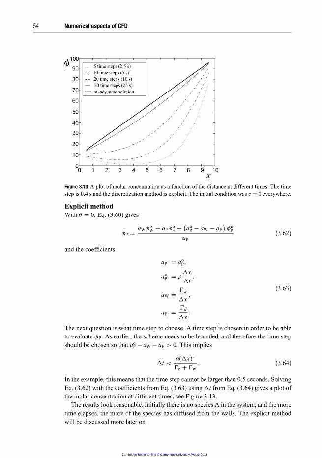
54 Numerical aspects of CFD
Figure 3.13 A plot of molar concentration as a function of the distance at different times. The time
step is 0.4 s and the discretization method is explicit. The initial condition was c = 0 everywhere.
Explicit method
With θ = 0, Eq. (3.60) gives
φP =aWφ
oW + aEφ
oE +(
aoP − aW − aE
)
φoP
aP
(3.62)
and the coefficients
aP = aoP,
aoP = ρ
�x
�t,
aW =Ŵw
�x,
aE =Ŵe
�x.
(3.63)
The next question is what time step to choose. A time step is chosen in order to be able
to evaluate φP. As earlier, the scheme needs to be bounded, and therefore the time step
should be chosen so that aoP − aW − aE > 0. This implies
�t <
ρ(�x)2
Ŵe + Ŵw
. (3.64)
In the example, this means that the time step cannot be larger than 0.5 seconds. Solving
Eq. (3.62) with the coefficients from Eq. (3.63) using �t from Eq. (3.64) gives a plot of
the molar concentration at different times, see Figure 3.13.
The results look reasonable. Initially there is no species A in the system, and the more
time elapses, the more of the species has diffused from the walls. The explicit method
will be discussed more later on.
Cambridge Books Online © Cambridge University Press, 2012
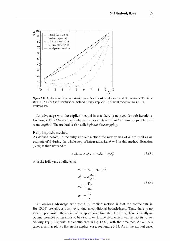
3.11 Unsteady flows 55
Figure 3.14 A plot of molar concentration as a function of the distance at different times. The time
step is 0.5 s and the discretization method is fully implicit. The initial condition was c = 0
everywhere.
An advantage with the explicit method is that there is no need for sub-iterations.
Looking at Eq. (3.62) explains why; all values are taken from ‘old’ time steps. Thus, its
name explicit. The method is also called global time stepping.
Fully implicit method
As defined before, in the fully implicit method the new values of φ are used as an
estimate of φ during the whole step of integration, i.e. θ = 1 in this method. Equation
(3.60) is then reduced to
aPφP = aWφW + aEφE + aoPφ
oP (3.65)
with the following coefficients:
aP = aW + aE + aoP,
aoP = ρ
�x
�t,
aW =Ŵw
�x,
aE =Ŵe
�x.
(3.66)
An obvious advantage with the fully implicit method is that the coefficients in
Eq. (3.66) are always positive, giving unconditional boundedness. Thus, there is no
strict upper limit in the choice of the appropriate time step. However, there is usually an
optimal number of iterations to be used in each time step, which will restrict its value.
Solving Eq. (3.65) with the coefficients in Eq. (3.66) with the time step �t = 0.5 s
gives a similar plot to that in the explicit case, see Figure 3.14. As in the explicit case,
Cambridge Books Online © Cambridge University Press, 2012
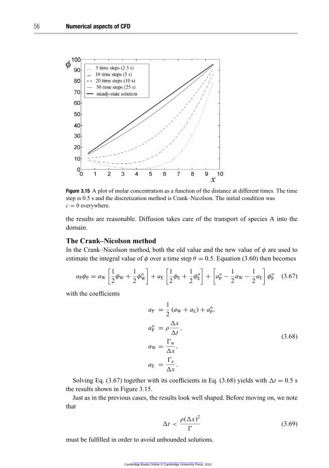
56 Numerical aspects of CFD
Figure 3.15 A plot of molar concentration as a function of the distance at different times. The time
step is 0.5 s and the discretization method is Crank–Nicolson. The initial condition was
c = 0 everywhere.
the results are reasonable. Diffusion takes care of the transport of species A into the
domain.
The Crank–Nicolson method
In the Crank–Nicolson method, both the old value and the new value of φ are used to
estimate the integral value of φ over a time step θ = 0.5. Equation (3.60) then becomes
aPφP = aW
[
1
2φW +
1
2φ
oW
]
+ aE
[
1
2φE +
1
2φ
oE
]
+
[
aoP −
1
2aW −
1
2aE
]
φoP (3.67)
with the coefficients
aP =1
2(aW + aE) + ao
P,
aoP = ρ
�x
�t,
aW =Ŵw
�x,
aE =Ŵe
�x.
(3.68)
Solving Eq. (3.67) together with its coefficients in Eq. (3.68) yields with �t = 0.5 s
the results shown in Figure 3.15.
Just as in the previous cases, the results look well shaped. Before moving on, we note
that
�t <
ρ(�x)2
Ŵ
(3.69)
must be fulfilled in order to avoid unbounded solutions.
Cambridge Books Online © Cambridge University Press, 2012
3.11 Unsteady flows 57
3.11.2 Conclusions on the different time discretization methods
As when the different discretization methods for spatial discretization were presented and
evaluated in earlier sections of this chapter, accuracy, boundedness and transportiveness
will be discussed here. The explicit method as well as the fully implicit method are
first-order accurate, which we state here, without proof,
φ = φex + O(�t) ,
φ = φim + O(�t) .
This follows from the fact that the value of φ in each time step is taken from either
the old value or the new one. The Crank–Nicolson method is second-order accurate, or
in mathematical terms,
φ = φC−N + O
[
(�t)2]
.
The Crank–Nicolson method has major resemblances to the central-differencing
scheme for spatial discretization, cf. Eqs. (3.13) and (3.57) with θ = 0.5. A reduc-
tion of the time-step size thus gives a more significant improvement in the results if
the Crank–Nicolson method is used than for first-order methods. There also exist many
higher-order numerical schemes for time discretization. Figure 3.15 shows a simulation
using the Crank–Nicolson method.
As concluded earlier, the explicit method is only conditionally bounded. This imposes
a constraint on the choice of the time step, cf. Eq. (3.64). If this criterion is violated,
the solution often diverges. On the other hand, being without the need to sub-iterate, the
explicit method is faster than the other two.
The fully implicit method is unconditionally bounded. This is a great advantage with
the method, and, in most commercial CFD codes, the fully implicit method is the default
method for time discretization.
The Crank–Nicolson method is only conditionally bounded, cf. Eq. (3.69). This
constraint is, however, not as restrictive as in the explicit method; it differs by a
factor of 2.
The time step is determined by the Courant number (CFL). Since the time step is
determined by the fluxes in each cell and the general rule is that the time step should be
shorter than the time it takes to transport past the cell,
�t < CFL min
(
ρ(�x)2
Ŵ
,
�x
U
)
, (3.70)
where CFL = 1 for an explicit solver and CFL = 5 or higher for a fully implicit solver.
A fully implicit solver should be stable for all time steps, but, due to nonlinearities in the
equations, it is recommended that one start with a low Courant number (5) and increase
it during the iterations.
Among the most recent transient solvers, the use of the method of lines is very common.
This method reformulates the transient PDE into a transient ordinary differential equation
Cambridge Books Online © Cambridge University Press, 2012
58 Numerical aspects of CFD
(ODE) by discretizing the spatial coordinates only. Then an ordinary ODE solver is used
to solve the equations.
Questions
(1) The first term in Eq. (3.53) can be seen as a convective term for time. Why is there
no diffusion term for time? What would such a term look like?
(2) What does Figure 3.12 tell us? What consequences does it enforce on the dependent
variables?
3.12 Meshing
Finally, a few words will be said about meshing. So far, it has been assumed in all the
examples that a proper mesh has been provided. However, this is generally not the case.
Thus, meshing becomes an important part of the CFD engineer’s work. Bad meshes
often give numerical problems and bad results.
3.12.1 Mesh generation
There are several commercial software packets for mesh generation. To generate a mesh
is in general a very complex procedure, and only some of the basics will be mentioned
here.
Traditionally, grids have been divided into structured grids and unstructured grids.
The structured grids are built up from quadrilateral elements, i.e. four-edged elements,
but not necessarily rectangles, in 2D and hexahedra (elements with six faces) in 3D.
Indexing and finding neighbouring cells is very easy with these elements. CFD pro-
grams using structured grids are usually faster and require less memory than programs
using unstructured grids. Unstructured grids are built from different elements, quadri-
lateral and triangular elements in 2D and tetrahedra, hexahedra, pyramids, prisms and
even dodecahedra in 3D. Usually, a structured grid will require less memory and have
better numerical properties. However, it is not always possible to mesh complex geome-
tries using structured mesh and today most solvers can handle both structured and
unstructured grids. Figure 3.16 shows typical building elements for meshing in 2D
and 3D.
Most meshing programs allow the user to draw the geometry in the program itself, but
most commonly the geometry is imported from a general CAD program. The geometry
is built from single points, lines or 2D and 3D shapes, e.g. rectangles, circles, boxes or
cylinders. The points can be combined to make lines, and lines to 2D shapes etc., so any
geometrical shape can be formed. It is then possible to unite, subtract or intersect these
shapes and form new shapes.
Elements at the walls must be handled carefully. The angle between the wall and the
grid line should be close to 90◦. The easiest way to obtain this is to start the meshing by
forming a regular mesh that is built from the surface. When a fine resolution is needed
Cambridge Books Online © Cambridge University Press, 2012
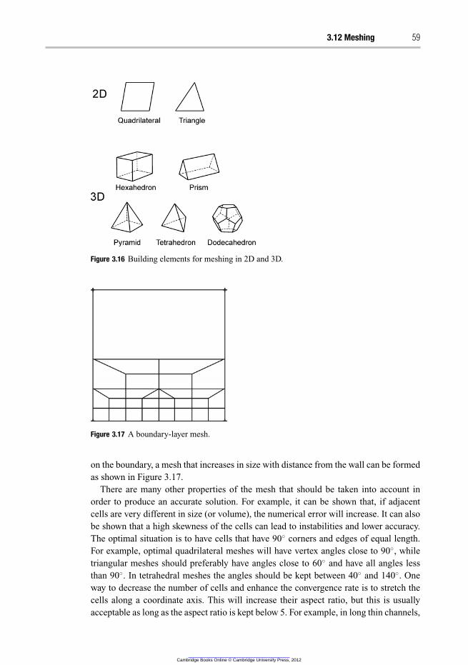
3.12 Meshing 59
Figure 3.16 Building elements for meshing in 2D and 3D.
Figure 3.17 A boundary-layer mesh.
on the boundary, a mesh that increases in size with distance from the wall can be formed
as shown in Figure 3.17.
There are many other properties of the mesh that should be taken into account in
order to produce an accurate solution. For example, it can be shown that, if adjacent
cells are very different in size (or volume), the numerical error will increase. It can also
be shown that a high skewness of the cells can lead to instabilities and lower accuracy.
The optimal situation is to have cells that have 90◦ corners and edges of equal length.
For example, optimal quadrilateral meshes will have vertex angles close to 90◦, while
triangular meshes should preferably have angles close to 60◦ and have all angles less
than 90◦. In tetrahedral meshes the angles should be kept between 40◦ and 140◦. One
way to decrease the number of cells and enhance the convergence rate is to stretch the
cells along a coordinate axis. This will increase their aspect ratio, but this is usually
acceptable as long as the aspect ratio is kept below 5. For example, in long thin channels,
Cambridge Books Online © Cambridge University Press, 2012
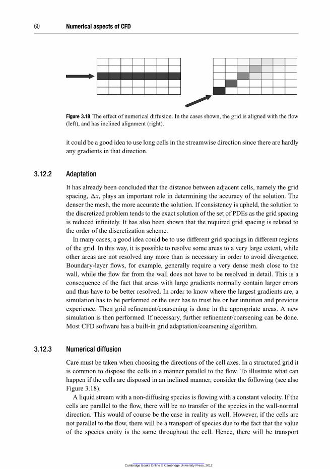
60 Numerical aspects of CFD
Figure 3.18 The effect of numerical diffusion. In the cases shown, the grid is aligned with the flow
(left), and has inclined alignment (right).
it could be a good idea to use long cells in the streamwise direction since there are hardly
any gradients in that direction.
3.12.2 Adaptation
It has already been concluded that the distance between adjacent cells, namely the grid
spacing, �x, plays an important role in determining the accuracy of the solution. The
denser the mesh, the more accurate the solution. If consistency is upheld, the solution to
the discretized problem tends to the exact solution of the set of PDEs as the grid spacing
is reduced infinitely. It has also been shown that the required grid spacing is related to
the order of the discretization scheme.
In many cases, a good idea could be to use different grid spacings in different regions
of the grid. In this way, it is possible to resolve some areas to a very large extent, while
other areas are not resolved any more than is necessary in order to avoid divergence.
Boundary-layer flows, for example, generally require a very dense mesh close to the
wall, while the flow far from the wall does not have to be resolved in detail. This is a
consequence of the fact that areas with large gradients normally contain larger errors
and thus have to be better resolved. In order to know where the largest gradients are, a
simulation has to be performed or the user has to trust his or her intuition and previous
experience. Then grid refinement/coarsening is done in the appropriate areas. A new
simulation is then performed. If necessary, further refinement/coarsening can be done.
Most CFD software has a built-in grid adaptation/coarsening algorithm.
3.12.3 Numerical diffusion
Care must be taken when choosing the directions of the cell axes. In a structured grid it
is common to dispose the cells in a manner parallel to the flow. To illustrate what can
happen if the cells are disposed in an inclined manner, consider the following (see also
Figure 3.18).
A liquid stream with a non-diffusing species is flowing with a constant velocity. If the
cells are parallel to the flow, there will be no transfer of the species in the wall-normal
direction. This would of course be the case in reality as well. However, if the cells are
not parallel to the flow, there will be a transport of species due to the fact that the value
of the species entity is the same throughout the cell. Hence, there will be transport
Cambridge Books Online © Cambridge University Press, 2012
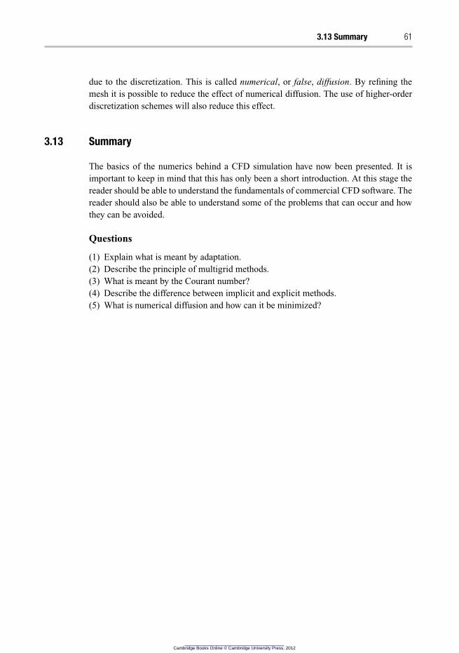
3.13 Summary 61
due to the discretization. This is called numerical, or false, diffusion. By refining the
mesh it is possible to reduce the effect of numerical diffusion. The use of higher-order
discretization schemes will also reduce this effect.
3.13 Summary
The basics of the numerics behind a CFD simulation have now been presented. It is
important to keep in mind that this has only been a short introduction. At this stage the
reader should be able to understand the fundamentals of commercial CFD software. The
reader should also be able to understand some of the problems that can occur and how
they can be avoided.
Questions
(1) Explain what is meant by adaptation.
(2) Describe the principle of multigrid methods.
(3) What is meant by the Courant number?
(4) Describe the difference between implicit and explicit methods.
(5) What is numerical diffusion and how can it be minimized?
Cambridge Books Online © Cambridge University Press, 2012

Cambridge Books Online © Cambridge University Press, 2012
4 Turbulent-flow modelling
This chapter provides an insight into the physical nature of turbulence and the math-
ematical framework that is used in numerical simulations of turbulent flows. The aim
is to explain why turbulence must be modelled and how turbulence can be modelled,
and also to explain what is modelled with different turbulence models. In addition, the
limitations of the turbulence models are discussed. The intention is to give you such an
understanding of turbulence modelling that you can actually suggest appropriate turbu-
lence models for different kinds of turbulent flows depending upon their complexity and
the required level of description.
4.1 The physics of fluid turbulence
Turbulence is encountered in most flows in nature and in industrial applications. Nat-
ural turbulent flows can be found in oceans, in rivers and in the atmosphere, whereas
industrial turbulent flows can be found in heat exchangers, chemical reactors etc. Most
flows encountered in industrial applications are turbulent, since turbulence significantly
enhances heat- and mass-transfer rates. In industry a variety of turbulent multiphase
flows can be encountered. Turbulence plays an important role in these types of flows
since it affects processes such as break-up and coalescence of bubbles and drops, thereby
controlling the interfacial area between the phases. Thus, turbulence modelling becomes
one of the key elements in CFD.
In order to determine which turbulence-modelling approach is best suited to a particu-
lar application, we need to understand the limitations of various turbulence models. This
insight requires a certain level of understanding of fluid turbulence. Probably everyone
has an intuitive understanding of what turbulence is, since turbulence is encountered
daily. From everyday experiences e.g. mixing coffee and milk, we know that turbulence
increases the disorder in a fluid, resulting in an efficient mixing of fluid elements. As
has already been mentioned, turbulence significantly affects mass-, momentum- and
heat-transfer rates. High mass- and heat-transfer rates are positive and crucial aspects
of many processes. In contrast, increased momentum transfer is usually undesirable,
since it results in higher skin friction and hence drag. In other words, turbulence is
an unavoidable feature of many chemical processes because high throughputs imply
turbulent conditions. In this section we will take a closer look at what characterizes
turbulence.
Cambridge Books Online © Cambridge University Press, 2012
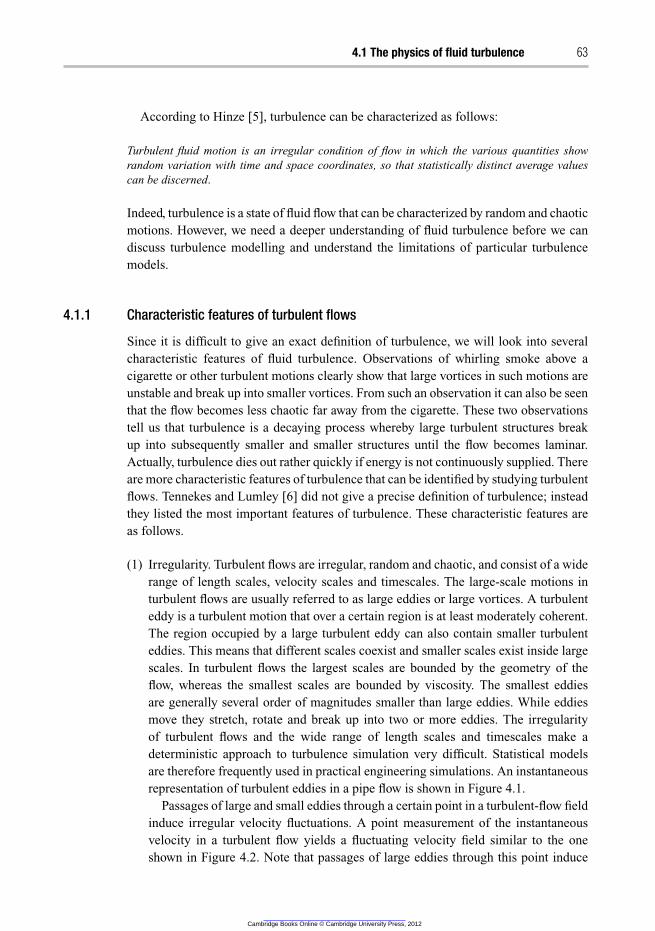
4.1 The physics of fluid turbulence 63
According to Hinze [5], turbulence can be characterized as follows:
Turbulent fluid motion is an irregular condition of flow in which the various quantities show
random variation with time and space coordinates, so that statistically distinct average values
can be discerned.
Indeed, turbulence is a state of fluid flow that can be characterized by random and chaotic
motions. However, we need a deeper understanding of fluid turbulence before we can
discuss turbulence modelling and understand the limitations of particular turbulence
models.
4.1.1 Characteristic features of turbulent flows
Since it is difficult to give an exact definition of turbulence, we will look into several
characteristic features of fluid turbulence. Observations of whirling smoke above a
cigarette or other turbulent motions clearly show that large vortices in such motions are
unstable and break up into smaller vortices. From such an observation it can also be seen
that the flow becomes less chaotic far away from the cigarette. These two observations
tell us that turbulence is a decaying process whereby large turbulent structures break
up into subsequently smaller and smaller structures until the flow becomes laminar.
Actually, turbulence dies out rather quickly if energy is not continuously supplied. There
are more characteristic features of turbulence that can be identified by studying turbulent
flows. Tennekes and Lumley [6] did not give a precise definition of turbulence; instead
they listed the most important features of turbulence. These characteristic features are
as follows.
(1) Irregularity. Turbulent flows are irregular, random and chaotic, and consist of a wide
range of length scales, velocity scales and timescales. The large-scale motions in
turbulent flows are usually referred to as large eddies or large vortices. A turbulent
eddy is a turbulent motion that over a certain region is at least moderately coherent.
The region occupied by a large turbulent eddy can also contain smaller turbulent
eddies. This means that different scales coexist and smaller scales exist inside large
scales. In turbulent flows the largest scales are bounded by the geometry of the
flow, whereas the smallest scales are bounded by viscosity. The smallest eddies
are generally several order of magnitudes smaller than large eddies. While eddies
move they stretch, rotate and break up into two or more eddies. The irregularity
of turbulent flows and the wide range of length scales and timescales make a
deterministic approach to turbulence simulation very difficult. Statistical models
are therefore frequently used in practical engineering simulations. An instantaneous
representation of turbulent eddies in a pipe flow is shown in Figure 4.1.
Passages of large and small eddies through a certain point in a turbulent-flow field
induce irregular velocity fluctuations. A point measurement of the instantaneous
velocity in a turbulent flow yields a fluctuating velocity field similar to the one
shown in Figure 4.2. Note that passages of large eddies through this point induce
Cambridge Books Online © Cambridge University Press, 2012
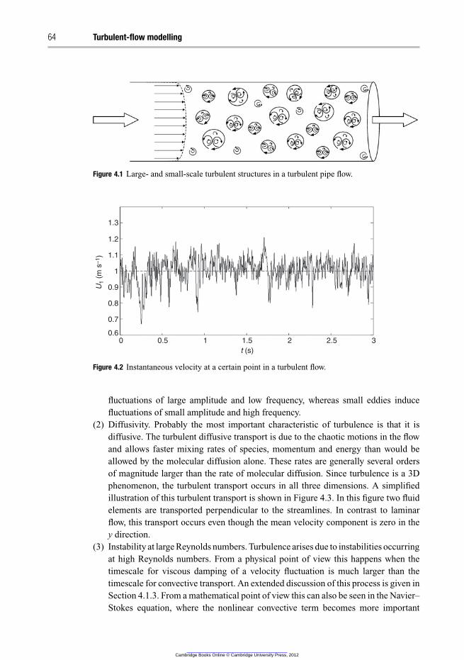
64 Turbulent-flow modelling
Figure 4.1 Large- and small-scale turbulent structures in a turbulent pipe flow.
1.3
1.2
1.1
1
0.9U1 (
m s
–1)
0.8
0.7
0.60 1 2 30.5 1.5
t (s)
2.5
Figure 4.2 Instantaneous velocity at a certain point in a turbulent flow.
fluctuations of large amplitude and low frequency, whereas small eddies induce
fluctuations of small amplitude and high frequency.
(2) Diffusivity. Probably the most important characteristic of turbulence is that it is
diffusive. The turbulent diffusive transport is due to the chaotic motions in the flow
and allows faster mixing rates of species, momentum and energy than would be
allowed by the molecular diffusion alone. These rates are generally several orders
of magnitude larger than the rate of molecular diffusion. Since turbulence is a 3D
phenomenon, the turbulent transport occurs in all three dimensions. A simplified
illustration of this turbulent transport is shown in Figure 4.3. In this figure two fluid
elements are transported perpendicular to the streamlines. In contrast to laminar
flow, this transport occurs even though the mean velocity component is zero in the
y direction.
(3) Instability at large Reynolds numbers. Turbulence arises due to instabilities occurring
at high Reynolds numbers. From a physical point of view this happens when the
timescale for viscous damping of a velocity fluctuation is much larger than the
timescale for convective transport. An extended discussion of this process is given in
Section 4.1.3. From a mathematical point of view this can also be seen in the Navier–
Stokes equation, where the nonlinear convective term becomes more important
Cambridge Books Online © Cambridge University Press, 2012
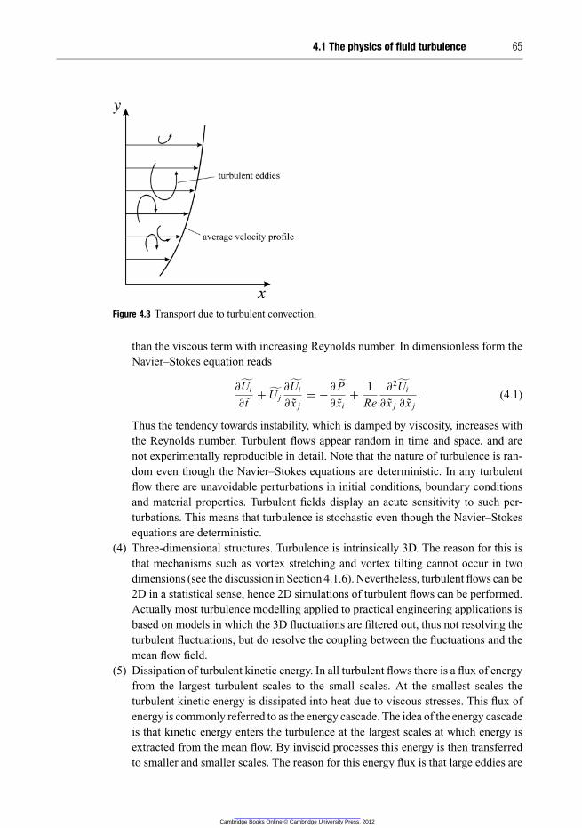
4.1 The physics of fluid turbulence 65
Figure 4.3 Transport due to turbulent convection.
than the viscous term with increasing Reynolds number. In dimensionless form the
Navier–Stokes equation reads
∂˜Ui
∂ t+˜U j
∂˜Ui
∂ x j
= −∂˜P
∂ xi
+1
Re
∂2˜Ui
∂ x j ∂ x j
. (4.1)
Thus the tendency towards instability, which is damped by viscosity, increases with
the Reynolds number. Turbulent flows appear random in time and space, and are
not experimentally reproducible in detail. Note that the nature of turbulence is ran-
dom even though the Navier–Stokes equations are deterministic. In any turbulent
flow there are unavoidable perturbations in initial conditions, boundary conditions
and material properties. Turbulent fields display an acute sensitivity to such per-
turbations. This means that turbulence is stochastic even though the Navier–Stokes
equations are deterministic.
(4) Three-dimensional structures. Turbulence is intrinsically 3D. The reason for this is
that mechanisms such as vortex stretching and vortex tilting cannot occur in two
dimensions (see the discussion in Section 4.1.6). Nevertheless, turbulent flows can be
2D in a statistical sense, hence 2D simulations of turbulent flows can be performed.
Actually most turbulence modelling applied to practical engineering applications is
based on models in which the 3D fluctuations are filtered out, thus not resolving the
turbulent fluctuations, but do resolve the coupling between the fluctuations and the
mean flow field.
(5) Dissipation of turbulent kinetic energy. In all turbulent flows there is a flux of energy
from the largest turbulent scales to the small scales. At the smallest scales the
turbulent kinetic energy is dissipated into heat due to viscous stresses. This flux of
energy is commonly referred to as the energy cascade. The idea of the energy cascade
is that kinetic energy enters the turbulence at the largest scales at which energy is
extracted from the mean flow. By inviscid processes this energy is then transferred
to smaller and smaller scales. The reason for this energy flux is that large eddies are
Cambridge Books Online © Cambridge University Press, 2012
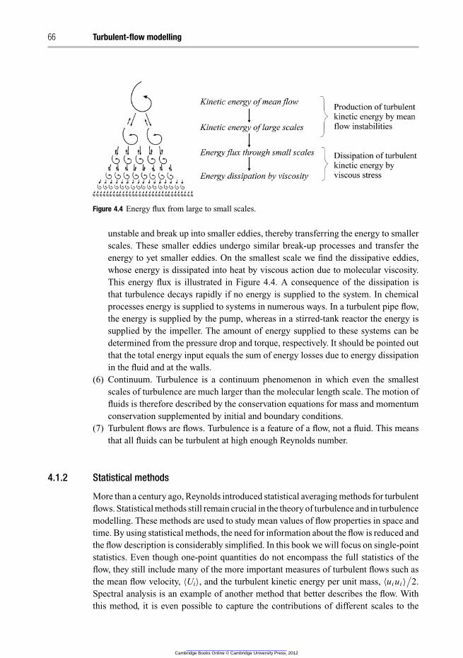
66 Turbulent-flow modelling
Figure 4.4 Energy flux from large to small scales.
unstable and break up into smaller eddies, thereby transferring the energy to smaller
scales. These smaller eddies undergo similar break-up processes and transfer the
energy to yet smaller eddies. On the smallest scale we find the dissipative eddies,
whose energy is dissipated into heat by viscous action due to molecular viscosity.
This energy flux is illustrated in Figure 4.4. A consequence of the dissipation is
that turbulence decays rapidly if no energy is supplied to the system. In chemical
processes energy is supplied to systems in numerous ways. In a turbulent pipe flow,
the energy is supplied by the pump, whereas in a stirred-tank reactor the energy is
supplied by the impeller. The amount of energy supplied to these systems can be
determined from the pressure drop and torque, respectively. It should be pointed out
that the total energy input equals the sum of energy losses due to energy dissipation
in the fluid and at the walls.
(6) Continuum. Turbulence is a continuum phenomenon in which even the smallest
scales of turbulence are much larger than the molecular length scale. The motion of
fluids is therefore described by the conservation equations for mass and momentum
conservation supplemented by initial and boundary conditions.
(7) Turbulent flows are flows. Turbulence is a feature of a flow, not a fluid. This means
that all fluids can be turbulent at high enough Reynolds number.
4.1.2 Statistical methods
More than a century ago, Reynolds introduced statistical averaging methods for turbulent
flows. Statistical methods still remain crucial in the theory of turbulence and in turbulence
modelling. These methods are used to study mean values of flow properties in space and
time. By using statistical methods, the need for information about the flow is reduced and
the flow description is considerably simplified. In this book we will focus on single-point
statistics. Even though one-point quantities do not encompass the full statistics of the
flow, they still include many of the more important measures of turbulent flows such as
the mean flow velocity, 〈Ui〉, and the turbulent kinetic energy per unit mass, 〈ui ui 〉/
2.
Spectral analysis is an example of another method that better describes the flow. With
this method, it is even possible to capture the contributions of different scales to the
Cambridge Books Online © Cambridge University Press, 2012
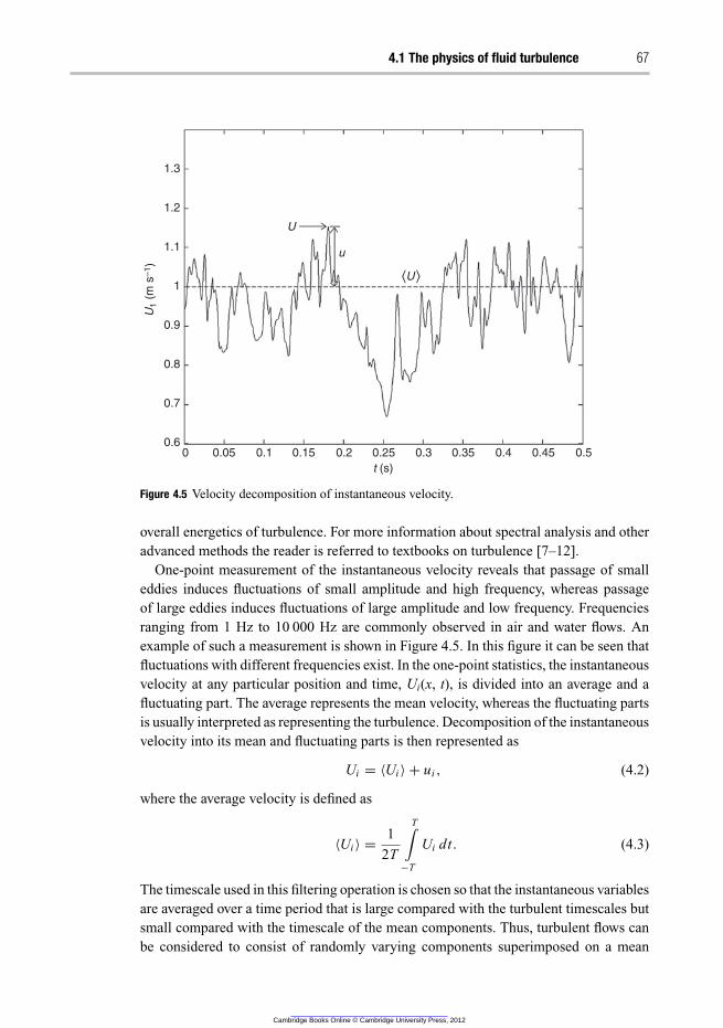
4.1 The physics of fluid turbulence 67
1.3
1.2
1.1
1
0.9
U1 (
m s
–1)
0.8
0.7
0.60 0.05 0.15
U
u
0.1 0.2 0.3 0.4 0.50.25 0.35 0.45
t (s)
u
U
⟨U ⟩
Figure 4.5 Velocity decomposition of instantaneous velocity.
overall energetics of turbulence. For more information about spectral analysis and other
advanced methods the reader is referred to textbooks on turbulence [7–12].
One-point measurement of the instantaneous velocity reveals that passage of small
eddies induces fluctuations of small amplitude and high frequency, whereas passage
of large eddies induces fluctuations of large amplitude and low frequency. Frequencies
ranging from 1 Hz to 10 000 Hz are commonly observed in air and water flows. An
example of such a measurement is shown in Figure 4.5. In this figure it can be seen that
fluctuations with different frequencies exist. In the one-point statistics, the instantaneous
velocity at any particular position and time, Ui(x, t), is divided into an average and a
fluctuating part. The average represents the mean velocity, whereas the fluctuating parts
is usually interpreted as representing the turbulence. Decomposition of the instantaneous
velocity into its mean and fluctuating parts is then represented as
Ui = 〈Ui 〉 + ui , (4.2)
where the average velocity is defined as
〈Ui 〉 =1
2T
T∫
−T
Ui dt. (4.3)
The timescale used in this filtering operation is chosen so that the instantaneous variables
are averaged over a time period that is large compared with the turbulent timescales but
small compared with the timescale of the mean components. Thus, turbulent flows can
be considered to consist of randomly varying components superimposed on a mean
Cambridge Books Online © Cambridge University Press, 2012
68 Turbulent-flow modelling
motion. This decomposition is known as Reynolds decomposition since Reynolds first
introduced the concept in the analysis of turbulent flows. The intensities of velocity
fluctuation in different directions can be measured in terms of the turbulent kinetic
energy per unit mass
k =1
2〈ui ui 〉 =
1
2
3∑
i=1
⟨
u2i
⟩
=1
2
(⟨
u21
⟩
+⟨
u22
⟩
+⟨
u23
⟩)
. (4.4)
Let us now define what we mean by turbulent kinetic energy. The kinetic energy of the
fluid (per unit mass) at a specific point in time is given by
E =1
2UiUi . (4.5)
The mean of the kinetic energy can be decomposed into two parts,
〈E〉 =1
2〈(〈Ui 〉 + ui )(〈Ui 〉 + ui )〉 =
1
2(〈Ui 〉〈Ui 〉 + 〈ui ui 〉)
=1
2〈Ui 〉〈Ui 〉 + k = E + k, (4.6)
where E is the kinetic energy of the mean flow and k is the turbulent kinetic energy per
unit mass, 12〈ui ui 〉.
To solve the Navier–Stokes equations, the pressure is decomposed in a similar way:
P = 〈P〉 + p. (4.7)
For incompressible fluids there is no need for decomposition of any other quantities
than velocity and pressure. However, for compressible fluids the density must also be
decomposed.
Definition of various statistical symmetries
A steady or stationary turbulent flow is defined as one whose statistical properties do
not change with time. Homogeneity implies that, given any number of different spatial
points and times, the statistics will remain unchanged if all positions are shifted by the
same constant displacement. In other words, the statistics of the flow are invariant under
translation. If the statistics are also invariant under rotation and reflection, the flow
is isotropic. Isotropy is therefore a stricter criterion than homogeneity. Assumptions
of homogeneous and isotropic turbulence are often made in theoretical studies, since
these assumptions simplify equations and analysis. We can summarize the statistical
symmetries as
� statistically stationary, if all statistics are invariant under a shift in time;� statistically homogeneous, if all statistics are invariant under a shift in position
(translation);� statistically isotropic, if all statistics are invariant under rotations and reflections.
Even though homogeneous turbulence is rarely encountered in practice it is still possible
to produce laboratory flows close to homogeneity. Grid-generated turbulence is an
example of approximately homogeneous turbulence. These flows are homogeneous in
Cambridge Books Online © Cambridge University Press, 2012
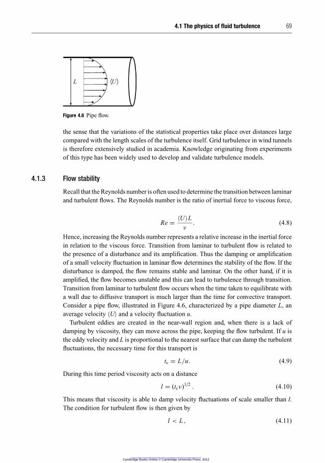
4.1 The physics of fluid turbulence 69
Figure 4.6 Pipe flow.
the sense that the variations of the statistical properties take place over distances large
compared with the length scales of the turbulence itself. Grid turbulence in wind tunnels
is therefore extensively studied in academia. Knowledge originating from experiments
of this type has been widely used to develop and validate turbulence models.
4.1.3 Flow stability
Recall that the Reynolds number is often used to determine the transition between laminar
and turbulent flows. The Reynolds number is the ratio of inertial force to viscous force,
Re =〈U 〉L
ν
. (4.8)
Hence, increasing the Reynolds number represents a relative increase in the inertial force
in relation to the viscous force. Transition from laminar to turbulent flow is related to
the presence of a disturbance and its amplification. Thus the damping or amplification
of a small velocity fluctuation in laminar flow determines the stability of the flow. If the
disturbance is damped, the flow remains stable and laminar. On the other hand, if it is
amplified, the flow becomes unstable and this can lead to turbulence through transition.
Transition from laminar to turbulent flow occurs when the time taken to equilibrate with
a wall due to diffusive transport is much larger than the time for convective transport.
Consider a pipe flow, illustrated in Figure 4.6, characterized by a pipe diameter L, an
average velocity 〈U〉 and a velocity fluctuation u.
Turbulent eddies are created in the near-wall region and, when there is a lack of
damping by viscosity, they can move across the pipe, keeping the flow turbulent. If u is
the eddy velocity and L is proportional to the nearest surface that can damp the turbulent
fluctuations, the necessary time for this transport is
tc = L/u. (4.9)
During this time period viscosity acts on a distance
l = (tcν)1/2. (4.10)
This means that viscosity is able to damp velocity fluctuations of scale smaller than l.
The condition for turbulent flow is then given by
l < L , (4.11)
Cambridge Books Online © Cambridge University Press, 2012
70 Turbulent-flow modelling
or
l = (tcν)1/2< L . (4.12)
Substitution of Eq. (4.9) into Eq. (4.12) leads to the condition
uL
ν
≫ 1. (4.13)
Note that the velocity fluctuations, u, are usually much smaller than the average velocity
in the pipe, 〈U〉. Thus, the criterion for turbulent flow in pipes in terms of the average
velocity is given by
Re =〈U 〉L
ν
≫ 1. (4.14)
This means that, for high-Reynolds-number flows, Re ≫ 1, viscosity cannot damp veloc-
ity fluctuations and the flow becomes turbulent. The first systematic studies regarding
the transition to turbulence were carried out by Osborne Reynolds more than a century
ago. Reynolds studied flow in glass tubes and obtained a critical Reynolds number 2100
at which the flow ceased to be laminar. By eliminating disturbances at the inlet of the
tube, it has been possible to maintain laminar flow even for Reynolds numbers one order
of magnitude larger than that.
Experimental studies have shown that the following Reynolds-number criteria can be
used to predict the transition from laminar to turbulent flow.
(1) For internal flows,� pipe flow, Re > 2100;� flow between parallel plates, Re > 800.
(2) For external flows,� flow around a sphere, Re > 350.
(3) Boundary layers,� flow along surfaces, Re > 500 000.
Note that different characteristic lengths are used in the definitions of the Reynolds
numbers above. It should also be noted that surface roughness affects the transition
as well.
4.1.4 The Kolmogorov hypotheses
In 1941, Kolmogorov stated three prominent hypotheses that are of fundamental impor-
tance for the understanding of turbulence. The first hypothesis concerns the isotropy of
small-scale turbulent motions. Kolmogorov argued that there are reasons to expect that at
high Reynolds number the directional information is lost in the chaotic scale-reduction
process. Whereas the anisotropic large-scale structures, l0, depend on geometry and
boundary conditions, it is assumed that the small scales have small timescales and that
these motions are statistically independent of the large-scale turbulence and of the mean
flow. In other words, somewhere in the process whereby turbulent eddies are reduced in
Cambridge Books Online © Cambridge University Press, 2012
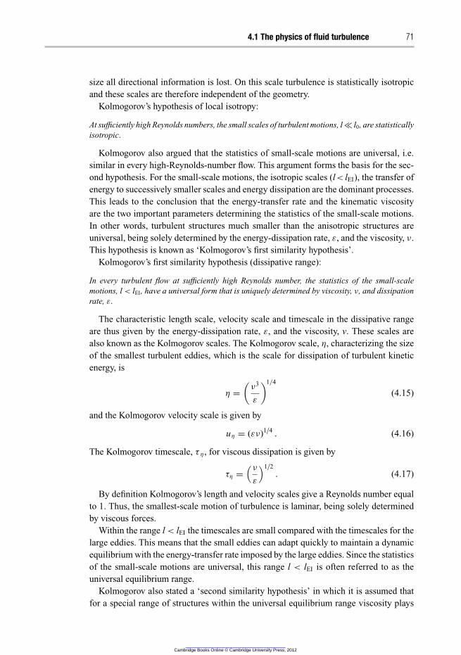
4.1 The physics of fluid turbulence 71
size all directional information is lost. On this scale turbulence is statistically isotropic
and these scales are therefore independent of the geometry.
Kolmogorov’s hypothesis of local isotropy:
At sufficiently high Reynolds numbers, the small scales of turbulent motions, l ≪ l0, are statistically
isotropic.
Kolmogorov also argued that the statistics of small-scale motions are universal, i.e.
similar in every high-Reynolds-number flow. This argument forms the basis for the sec-
ond hypothesis. For the small-scale motions, the isotropic scales (l< lEI), the transfer of
energy to successively smaller scales and energy dissipation are the dominant processes.
This leads to the conclusion that the energy-transfer rate and the kinematic viscosity
are the two important parameters determining the statistics of the small-scale motions.
In other words, turbulent structures much smaller than the anisotropic structures are
universal, being solely determined by the energy-dissipation rate, ε, and the viscosity, ν.
This hypothesis is known as ‘Kolmogorov’s first similarity hypothesis’.
Kolmogorov’s first similarity hypothesis (dissipative range):
In every turbulent flow at sufficiently high Reynolds number, the statistics of the small-scale
motions, l < lEI, have a universal form that is uniquely determined by viscosity, ν, and dissipation
rate, ε.
The characteristic length scale, velocity scale and timescale in the dissipative range
are thus given by the energy-dissipation rate, ε, and the viscosity, v. These scales are
also known as the Kolmogorov scales. The Kolmogorov scale, η, characterizing the size
of the smallest turbulent eddies, which is the scale for dissipation of turbulent kinetic
energy, is
η =
(
ν3
ε
)1/4
(4.15)
and the Kolmogorov velocity scale is given by
uη = (εν)1/4. (4.16)
The Kolmogorov timescale, τ η, for viscous dissipation is given by
τη =
(
ν
ε
)1/2. (4.17)
By definition Kolmogorov’s length and velocity scales give a Reynolds number equal
to 1. Thus, the smallest-scale motion of turbulence is laminar, being solely determined
by viscous forces.
Within the range l < lEI the timescales are small compared with the timescales for the
large eddies. This means that the small eddies can adapt quickly to maintain a dynamic
equilibrium with the energy-transfer rate imposed by the large eddies. Since the statistics
of the small-scale motions are universal, this range l < lEI is often referred to as the
universal equilibrium range.
Kolmogorov also stated a ‘second similarity hypothesis’ in which it is assumed that
for a special range of structures within the universal equilibrium range viscosity plays
Cambridge Books Online © Cambridge University Press, 2012
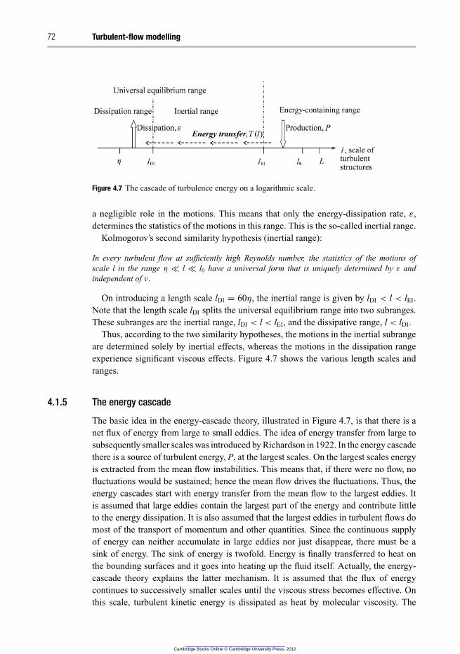
72 Turbulent-flow modelling
Figure 4.7 The cascade of turbulence energy on a logarithmic scale.
a negligible role in the motions. This means that only the energy-dissipation rate, ε,
determines the statistics of the motions in this range. This is the so-called inertial range.
Kolmogorov’s second similarity hypothesis (inertial range):
In every turbulent flow at sufficiently high Reynolds number, the statistics of the motions of
scale l in the range η ≪ l ≪ l0 have a universal form that is uniquely determined by ε and
independent of ν.
On introducing a length scale lDI = 60η, the inertial range is given by lDI < l < lEI.
Note that the length scale lDI splits the universal equilibrium range into two subranges.
These subranges are the inertial range, lDI < l < lEI, and the dissipative range, l < lDI.
Thus, according to the two similarity hypotheses, the motions in the inertial subrange
are determined solely by inertial effects, whereas the motions in the dissipation range
experience significant viscous effects. Figure 4.7 shows the various length scales and
ranges.
4.1.5 The energy cascade
The basic idea in the energy-cascade theory, illustrated in Figure 4.7, is that there is a
net flux of energy from large to small eddies. The idea of energy transfer from large to
subsequently smaller scales was introduced by Richardson in 1922. In the energy cascade
there is a source of turbulent energy, P, at the largest scales. On the largest scales energy
is extracted from the mean flow instabilities. This means that, if there were no flow, no
fluctuations would be sustained; hence the mean flow drives the fluctuations. Thus, the
energy cascades start with energy transfer from the mean flow to the largest eddies. It
is assumed that large eddies contain the largest part of the energy and contribute little
to the energy dissipation. It is also assumed that the largest eddies in turbulent flows do
most of the transport of momentum and other quantities. Since the continuous supply
of energy can neither accumulate in large eddies nor just disappear, there must be a
sink of energy. The sink of energy is twofold. Energy is finally transferred to heat on
the bounding surfaces and it goes into heating up the fluid itself. Actually, the energy-
cascade theory explains the latter mechanism. It is assumed that the flux of energy
continues to successively smaller scales until the viscous stress becomes effective. On
this scale, turbulent kinetic energy is dissipated as heat by molecular viscosity. The
Cambridge Books Online © Cambridge University Press, 2012
4.1 The physics of fluid turbulence 73
Table 4.1 Correlations for various turbulence scales
Scale Length Time Velocity
Large scale l = k3/2/ε τl = k/ε ul =
(
2
3k)
1/2
Smallest scale η = (ν3/ε)1/4
τη = (ν/ε)1/2 uη = (εν)1/4
energy-dissipation process is a result of viscous friction between layers of fluid moving
at different velocities. An important consequence of the viscous stress is that it prevents
the generation of infinitely small eddies. Hence, in all fluid flows there is a minimum
scale of turbulent structures.
Discussions of the energy cascade often refer to the universal equilibrium range. This
terminology is based on the argument that the small eddies will evolve much more
rapidly than the large eddies. Thus eddies in the universal range can adjust so quickly to
changes in external conditions that they can be assumed to be always in a state of local
equilibrium. The transfer of energy in the cascade is given by
TEI = T (lEI) = T (l) = TDI = T (lDI) = ε. (4.18)
In conclusion, the energy-cascade theory places production at the beginning and
dissipation at the end of a sequence of processes. L and l0 in Figure 4.7 are the flow scale
and the scale of the largest eddies, respectively. The length scale l0 is a measure of the
largest turbulent eddies, which contain most of the turbulent kinetic energy. l0 is given
by
l0 =k3/2
ε
. (4.19)
The characteristic timescale for the large eddies, τ l, is the time necessary to decrease
a turbulent structure of size l0, that is the ‘eddy lifetime’. This timescale can also be seen
as the timescale for transfer of turbulent kinetic energy from the scale l0 to η, which
means that it is a measure for the turbulence decay rate. τ l is given by
τl =k
ε
. (4.20)
Since k is defined as 12
(
u21 + u2
2 + u23
)
, the characteristic velocity scale for the large
eddies is given by
ul =
(
2
3k
)1/2
. (4.21)
As a rule of thumb, lEI can be used as a demarcation between anisotropic and isotropic
turbulent eddies, see Figure 4.7. The length scale of the anisotropic large eddies is then
given by l > lEI and that for isotropic eddies by l < lEI. This demarcation requires an
approximation of lEI, which is given by lEI ≈ 16
l0. The relations for the various scales of
turbulent motions are summarized in Table 4.1.
Cambridge Books Online © Cambridge University Press, 2012
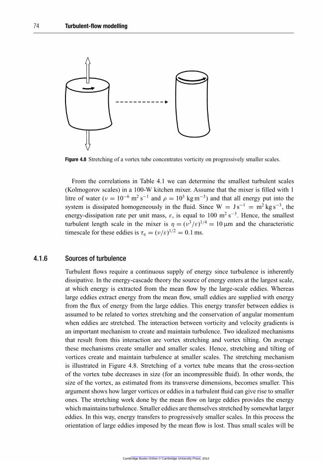
74 Turbulent-flow modelling
Figure 4.8 Stretching of a vortex tube concentrates vorticity on progressively smaller scales.
From the correlations in Table 4.1 we can determine the smallest turbulent scales
(Kolmogorov scales) in a 100-W kitchen mixer. Assume that the mixer is filled with 1
litre of water (ν = 10−6 m2 s−1 and ρ = 103 kg m−3) and that all energy put into the
system is dissipated homogeneously in the fluid. Since W = J s−1 = m2 kg s−3, the
energy-dissipation rate per unit mass, ε, is equal to 100 m2 s−3. Hence, the smallest
turbulent length scale in the mixer is η = (ν3/ε)1/4 = 10 µm and the characteristic
timescale for these eddies is τη = (ν/ε)1/2 = 0.1 ms.
4.1.6 Sources of turbulence
Turbulent flows require a continuous supply of energy since turbulence is inherently
dissipative. In the energy-cascade theory the source of energy enters at the largest scale,
at which energy is extracted from the mean flow by the large-scale eddies. Whereas
large eddies extract energy from the mean flow, small eddies are supplied with energy
from the flux of energy from the large eddies. This energy transfer between eddies is
assumed to be related to vortex stretching and the conservation of angular momentum
when eddies are stretched. The interaction between vorticity and velocity gradients is
an important mechanism to create and maintain turbulence. Two idealized mechanisms
that result from this interaction are vortex stretching and vortex tilting. On average
these mechanisms create smaller and smaller scales. Hence, stretching and tilting of
vortices create and maintain turbulence at smaller scales. The stretching mechanism
is illustrated in Figure 4.8. Stretching of a vortex tube means that the cross-section
of the vortex tube decreases in size (for an incompressible fluid). In other words, the
size of the vortex, as estimated from its transverse dimensions, becomes smaller. This
argument shows how larger vortices or eddies in a turbulent fluid can give rise to smaller
ones. The stretching work done by the mean flow on large eddies provides the energy
which maintains turbulence. Smaller eddies are themselves stretched by somewhat larger
eddies. In this way, energy transfers to progressively smaller scales. In this process the
orientation of large eddies imposed by the mean flow is lost. Thus small scales will be
Cambridge Books Online © Cambridge University Press, 2012
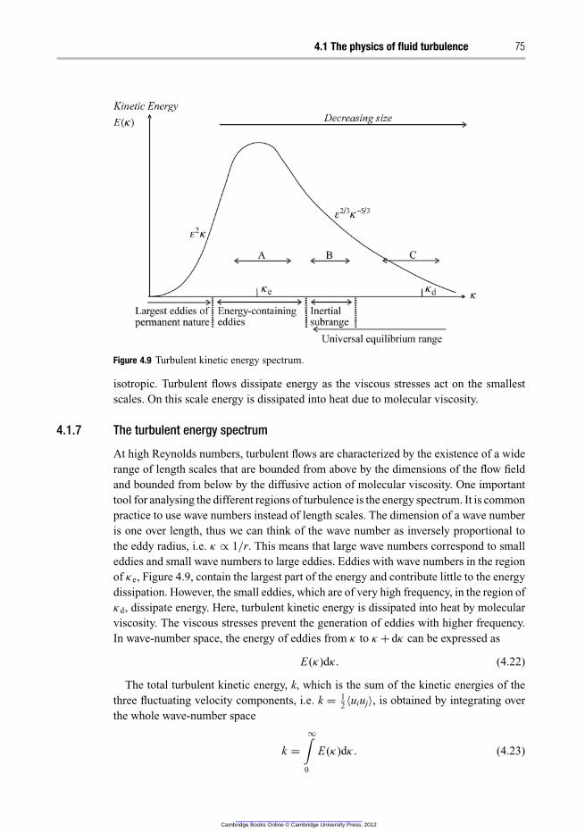
4.1 The physics of fluid turbulence 75
Figure 4.9 Turbulent kinetic energy spectrum.
isotropic. Turbulent flows dissipate energy as the viscous stresses act on the smallest
scales. On this scale energy is dissipated into heat due to molecular viscosity.
4.1.7 The turbulent energy spectrum
At high Reynolds numbers, turbulent flows are characterized by the existence of a wide
range of length scales that are bounded from above by the dimensions of the flow field
and bounded from below by the diffusive action of molecular viscosity. One important
tool for analysing the different regions of turbulence is the energy spectrum. It is common
practice to use wave numbers instead of length scales. The dimension of a wave number
is one over length, thus we can think of the wave number as inversely proportional to
the eddy radius, i.e. κ ∝ 1/r. This means that large wave numbers correspond to small
eddies and small wave numbers to large eddies. Eddies with wave numbers in the region
of κe, Figure 4.9, contain the largest part of the energy and contribute little to the energy
dissipation. However, the small eddies, which are of very high frequency, in the region of
κd, dissipate energy. Here, turbulent kinetic energy is dissipated into heat by molecular
viscosity. The viscous stresses prevent the generation of eddies with higher frequency.
In wave-number space, the energy of eddies from κ to κ + dκ can be expressed as
E(κ)dκ. (4.22)
The total turbulent kinetic energy, k, which is the sum of the kinetic energies of the
three fluctuating velocity components, i.e. k = 12〈uiuj〉, is obtained by integrating over
the whole wave-number space
k =
∞∫
0
E(κ)dκ. (4.23)
Cambridge Books Online © Cambridge University Press, 2012
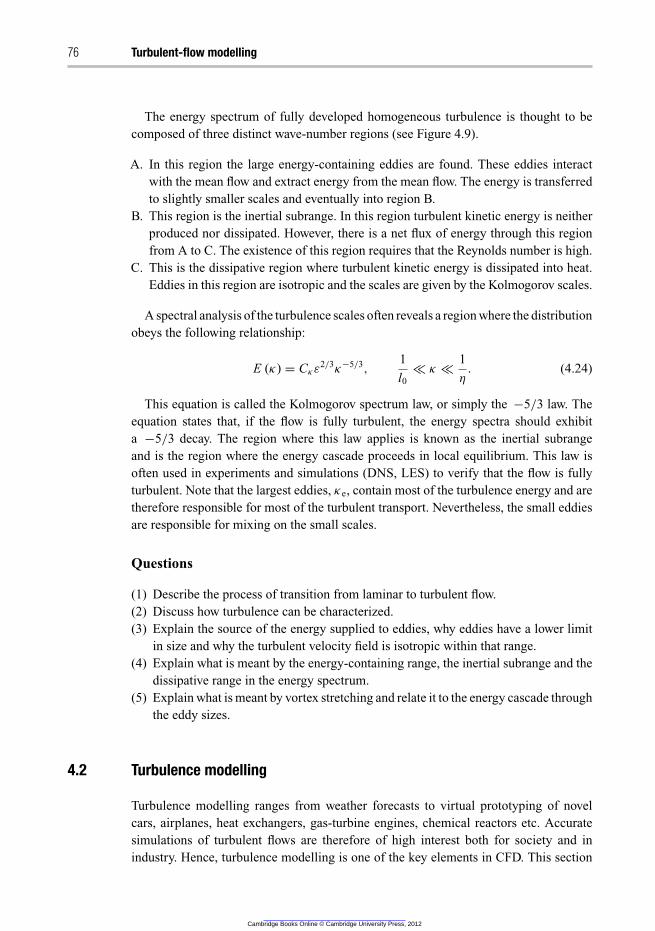
76 Turbulent-flow modelling
The energy spectrum of fully developed homogeneous turbulence is thought to be
composed of three distinct wave-number regions (see Figure 4.9).
A. In this region the large energy-containing eddies are found. These eddies interact
with the mean flow and extract energy from the mean flow. The energy is transferred
to slightly smaller scales and eventually into region B.
B. This region is the inertial subrange. In this region turbulent kinetic energy is neither
produced nor dissipated. However, there is a net flux of energy through this region
from A to C. The existence of this region requires that the Reynolds number is high.
C. This is the dissipative region where turbulent kinetic energy is dissipated into heat.
Eddies in this region are isotropic and the scales are given by the Kolmogorov scales.
A spectral analysis of the turbulence scales often reveals a region where the distribution
obeys the following relationship:
E (κ) = Cκε2/3
κ−5/3
,
1
l0
≪ κ ≪1
η
. (4.24)
This equation is called the Kolmogorov spectrum law, or simply the −5/3 law. The
equation states that, if the flow is fully turbulent, the energy spectra should exhibit
a −5/3 decay. The region where this law applies is known as the inertial subrange
and is the region where the energy cascade proceeds in local equilibrium. This law is
often used in experiments and simulations (DNS, LES) to verify that the flow is fully
turbulent. Note that the largest eddies, κe, contain most of the turbulence energy and are
therefore responsible for most of the turbulent transport. Nevertheless, the small eddies
are responsible for mixing on the small scales.
Questions
(1) Describe the process of transition from laminar to turbulent flow.
(2) Discuss how turbulence can be characterized.
(3) Explain the source of the energy supplied to eddies, why eddies have a lower limit
in size and why the turbulent velocity field is isotropic within that range.
(4) Explain what is meant by the energy-containing range, the inertial subrange and the
dissipative range in the energy spectrum.
(5) Explain what is meant by vortex stretching and relate it to the energy cascade through
the eddy sizes.
4.2 Turbulence modelling
Turbulence modelling ranges from weather forecasts to virtual prototyping of novel
cars, airplanes, heat exchangers, gas-turbine engines, chemical reactors etc. Accurate
simulations of turbulent flows are therefore of high interest both for society and in
industry. Hence, turbulence modelling is one of the key elements in CFD. This section
Cambridge Books Online © Cambridge University Press, 2012
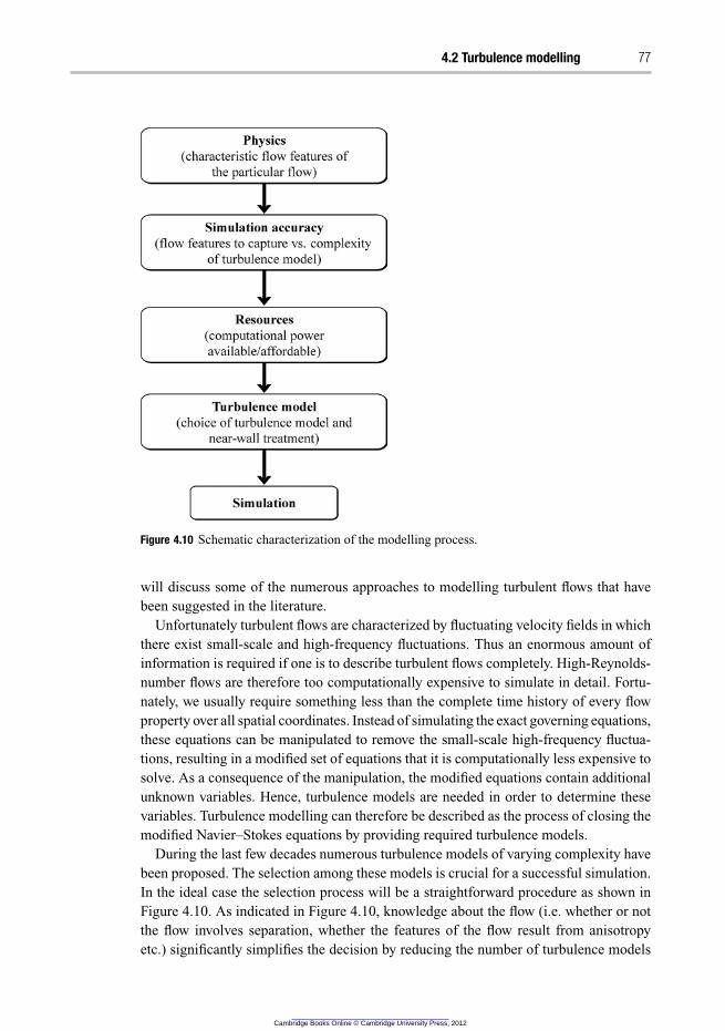
4.2 Turbulence modelling 77
Figure 4.10 Schematic characterization of the modelling process.
will discuss some of the numerous approaches to modelling turbulent flows that have
been suggested in the literature.
Unfortunately turbulent flows are characterized by fluctuating velocity fields in which
there exist small-scale and high-frequency fluctuations. Thus an enormous amount of
information is required if one is to describe turbulent flows completely. High-Reynolds-
number flows are therefore too computationally expensive to simulate in detail. Fortu-
nately, we usually require something less than the complete time history of every flow
property over all spatial coordinates. Instead of simulating the exact governing equations,
these equations can be manipulated to remove the small-scale high-frequency fluctua-
tions, resulting in a modified set of equations that it is computationally less expensive to
solve. As a consequence of the manipulation, the modified equations contain additional
unknown variables. Hence, turbulence models are needed in order to determine these
variables. Turbulence modelling can therefore be described as the process of closing the
modified Navier–Stokes equations by providing required turbulence models.
During the last few decades numerous turbulence models of varying complexity have
been proposed. The selection among these models is crucial for a successful simulation.
In the ideal case the selection process will be a straightforward procedure as shown in
Figure 4.10. As indicated in Figure 4.10, knowledge about the flow (i.e. whether or not
the flow involves separation, whether the features of the flow result from anisotropy
etc.) significantly simplifies the decision by reducing the number of turbulence models
Cambridge Books Online © Cambridge University Press, 2012
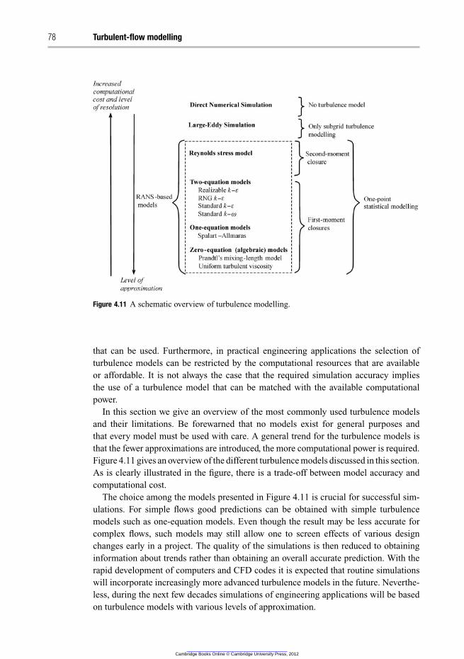
78 Turbulent-flow modelling
Figure 4.11 A schematic overview of turbulence modelling.
that can be used. Furthermore, in practical engineering applications the selection of
turbulence models can be restricted by the computational resources that are available
or affordable. It is not always the case that the required simulation accuracy implies
the use of a turbulence model that can be matched with the available computational
power.
In this section we give an overview of the most commonly used turbulence models
and their limitations. Be forewarned that no models exist for general purposes and
that every model must be used with care. A general trend for the turbulence models is
that the fewer approximations are introduced, the more computational power is required.
Figure 4.11 gives an overview of the different turbulence models discussed in this section.
As is clearly illustrated in the figure, there is a trade-off between model accuracy and
computational cost.
The choice among the models presented in Figure 4.11 is crucial for successful sim-
ulations. For simple flows good predictions can be obtained with simple turbulence
models such as one-equation models. Even though the result may be less accurate for
complex flows, such models may still allow one to screen effects of various design
changes early in a project. The quality of the simulations is then reduced to obtaining
information about trends rather than obtaining an overall accurate prediction. With the
rapid development of computers and CFD codes it is expected that routine simulations
will incorporate increasingly more advanced turbulence models in the future. Neverthe-
less, during the next few decades simulations of engineering applications will be based
on turbulence models with various levels of approximation.
Cambridge Books Online © Cambridge University Press, 2012
4.2 Turbulence modelling 79
4.2.1 Direct numerical simulation
Direct numerical simulation (DNS) of turbulent flows may at first glance seem to be
the most obvious and straightforward approach with which to simulate turbulent flows.
Using DNS, in which the unsteady 3D Navier–Stokes equations are solved directly, there
is no need for a turbulence model since the equations correctly describe fluid flows both
for laminar and for turbulent conditions. The difficulty is actually solving these equations
at high Reynolds number. Recall that a wide range of length scales and timescales exists
in high-Reynolds-number turbulent flows. This means that all these turbulent scales
must be resolved in the simulations. The scale of resolution needed is roughly described
by the Kolmogorov length scale and timescale. Hence, very dense computational grids
and short time steps are required. Add also that the equations are nonlinear and it is
clear that this will challenge the computational solution algorithms, thus making any
simulation very time-consuming. In fact, it will not be possible to perform DNS for
real engineering problems until many more generations of computers have come and
gone. Even if it were possible to perform these simulations for practical engineering
applications, the amount of data would be overwhelming. At the present time DNS is a
research tool rather than an aid to engineering design. The computational cost of DNS
is high and it increases as the cube of the Reynolds number. For the interested reader, it
can be mentioned that the computational cost for DNS of reactive flows is given by
t ∝ Re3Sc2. (4.25)
Note that for gases Sc ∼ 1, for liquids like water Sc ∼ 103 and for very viscous
liquids Sc ∼ 106. DNS is thus mainly used for gaseous flows at moderate Reynolds
numbers due to the high computational cost. Such deterministic simulations are useful
for developing closures for statistical turbulence models and for validation of these
models, but in practical engineering simulations DNS is less useful. Since DNS is of
no use for practical engineering flow simulations, it will not be discussed further in this
chapter.
4.2.2 Large-eddy simulation
Since the main problem in simulating high-Reynolds-number flows is the presence of
very small length scales and timescales, a logical solution is to filter the equations, thus
resolving only intermediate-to-large turbulence scales. Large-eddy simulation (LES)
extends the usefulness of DNS for practical engineering applications by intentionally
leaving the smallest turbulence scales unresolved. In LES the dynamics of the large scales
are computed explicitly. Therefore, LES needs to be 3D and transient. The advantages
of LES arise from the fact that the large eddies, which are hard to model in a universal
way since they are anisotropic, are simulated directly. In contrast, small eddies are more
easily modelled since they are closer to isotropy and adapt quickly to maintain a dynamic
equilibrium with the energy-transfer rate imposed by the large eddies. The effects of the
non-resolved scales, which cannot be neglected, are accounted for with subgrid stress
models. This means that the subgrid models should be universal. In LES the turbulence
Cambridge Books Online © Cambridge University Press, 2012
80 Turbulent-flow modelling
scales are usually resolved down to the inertial subrange, Figure 4.9. As a general rule
of thumb at least 80% of the turbulence energy should be resolved in the calculated
velocities. Substantial savings in computational cost are realized in LES, since a coarser
grid is employed than that required for DNS, Figure 4.11. This allows modelling of
flows at higher Reynolds number. Nevertheless, the computational cost for LES is high
in comparison with those of other turbulence models. The high computational cost
stems from a very fine grid, short time steps and long computational time taken to obtain
reliable statistics.
Filtering of the Navier–Stokes equations
The governing equations for LES are obtained by spatially filtering over small scales. A
generalized filter can be defined by
Ui (x, t) =
∫∫∫
G(x − ξ ; �)Ui(ξ, t)d3ξ, (4.26)
where the filter function is interpreted as acting to keep values of Ui occurring on scales
larger than the filter width �. Basically the filter function, G, is some function that is
effectively zero for values of Ui occurring at the small scales. Thus, filtering eliminates
eddies whose scales are smaller than the filter width. Examples of such filters are the box,
Gaussian and sharp spectral filters etc. [11]. By filtering the Navier–Stokes equations,
the scales which will be modelled are separated from those which will be calculated
directly.
The velocity field has the decomposition,
Ui (x, t) = Ui (x, t) + ui (x, t). (4.27)
An important difference between this decomposition and the Reynolds decomposition,
which is widely used in turbulence modelling, is that U i is a random field and that in
general the filtered residual is not zero,
ui (x, t) �= 0. (4.28)
The filtered continuity equation is
∂U j
∂x j
= 0 (4.29)
and the filtered momentum equation is
∂U i
∂t+
∂U iU j
∂x j
= −1
ρ
∂ P
∂x j
+ ν
∂2U i
∂x j ∂x j
−∂τi j
∂x j
. (4.30)
The closure problem in LES arises from the residual stress tensor, τ ij, which is also
commonly referred to as the subgrid stress tensor. Here the term τ ij describes the transfer
of momentum by turbulence at scales that are smaller than the filter,
τi j = UiU j − U iU j . (4.31)
The filtered velocities U i and U j are solved for but the correlation UiU j is unknown
and a satisfactory subgrid stress model must be provided for τ ij. The simplest models
Cambridge Books Online © Cambridge University Press, 2012
4.2 Turbulence modelling 81
usually involve modelling of a subgrid viscosity. An important difference between the
subgrid viscosity and the traditional eddy viscosity is that it acts as a correction to the
behaviour of the small scales, not as a correction of the entire influence of turbulence on
the mean flow. This means that the subgrid viscosity is small compared with the eddy
viscosity used in the eddy-viscosity models.
One frequently used model is the Smagorinsky–Lilly model. In this model the isotropic
stress is included in the modified filtered pressure
p = p +2
3τi i (4.32)
and the anisotropic part is modelled using a linear eddy-viscosity model,
τi j − 13τkkδi j = −2μt Si j . (4.33)
The subgrid viscosity is then calculated from
μt = ρL2S
∣
∣S∣
∣
, (4.34)
where
∣
∣S∣
∣ =
√
2Si j Si j and L S = min(κd, CSV 1/3), (4.35)
κ is the von Karman constant, d is the distance to the nearest wall and V is the volume
of the computational cell. The Smagorinsky coefficient CS is of the order of 0.17 but
depends, unfortunately, on the flow conditions and grid size. The interested reader is
referred to [7, 11] for more information about LES. More advanced LES models, e.g.
dynamic LES, also estimate the Smagorinsky coefficient by filtering on two different
scales.
4.2.3 Reynolds decomposition
Industrial applications of LES are expected to increase in the near future. However, like
DNS, LES is currently too computationally expensive for routine simulations. In many
cases the industrial and academic communities need even simpler models than LES.
In this chapter we introduce turbulence models that are widely used for simulations of
engineering applications. These models are based on a method by which the scales can
be separated. Recall that in the LES approach the small length scales and timescales
were filtered out. However, even the intermediate-to-large turbulence scales must be
filtered out to obtain a set of equations that can be used for routine simulations. Hence,
the solution of these equations remains the only viable means for routine simulations of
turbulent flows encountered in engineering practice. More than 100 years ago Reynolds
proposed that the instantaneous variables could be split into a mean part and a fluctuating
part,
Ui = 〈Ui 〉 + ui (4.36)
Cambridge Books Online © Cambridge University Press, 2012
82 Turbulent-flow modelling
and
P = 〈P〉 + p. (4.37)
This method is therefore referred to as Reynolds decomposition. All turbulence mod-
els in the following sections of this chapter share the fact that they are mathematically
based on the Reynolds-decomposition concept. With Reynolds decomposition, the flow
is described statistically by the mean flow velocity and the turbulence quantities. By time
averaging over a reasonable time period the turbulence fluctuations are separated from
the non-turbulence quantities. Hence, the set of equations obtained with this method
is called the Reynolds averaged Navier–Stokes equations, or simply the RANS equa-
tions. In many practical cases it is necessary to simulate non-steady flows, where the
instantaneous variables are averaged over a time period that is large compared with the
turbulence timescales but small compared with the timescale of the mean components.
This means that the time derivative of the mean flow in the RANS equations accounts
for variations at timescales larger than those of turbulence.
Recall that for incompressible flows the continuity equation reads
∂U j
∂x j
= 0 (4.38)
and the Navier–Stokes equations read
∂Ui
∂t+ U j
∂Ui
∂x j
= −1
ρ
∂ P
∂xi
+ ν
∂2Ui
∂x j ∂x j
. (4.39)
The equations for the mean variables of these quantities are derived by substituting
the decomposed form into the Navier–Stokes equations and taking the average. Let us
now substitute for the instantaneous variables in Eqs. (4.38) and (4.39) the decomposed
variables. By substituting we obtain
∂(〈Ui 〉 + ui )
∂xi
= 0 (4.40)
and
∂(〈Ui 〉 + ui )
∂t+ (⟨
U j
⟩
+ u j )∂(〈Ui 〉 + ui )
∂x j
= −1
ρ
∂(〈P〉 + p)
∂xi
+ ν
∂2(〈Ui 〉 + ui )
∂x j∂x j
.
(4.41)
After decomposing the dependent variables into mean and fluctuating quantities we
then time-average the equations using the operator
〈φ〉 =1
τ
t+τ∫
t
φ(x, t )dt . (4.42)
Equation (4.40) then reads⟨
∂(〈Ui 〉 + ui )
∂xi
⟩
= 0 (4.43)
Cambridge Books Online © Cambridge University Press, 2012
4.2 Turbulence modelling 83
and Eq. (4.41) becomes⟨
∂(〈Ui 〉 + ui )
∂t
⟩
+
⟨
(⟨
U j
⟩
+ u j
) ∂(〈Ui 〉 + ui )
∂x j
⟩
= −1
ρ
⟨
∂(〈P〉 + p)
∂xi
⟩
+ ν
⟨
∂2(〈Ui 〉 + ui )
∂x j ∂x j
⟩
. (4.44)
Note that all terms linear in fluctuating variables give zero on averaging:
〈ui 〉 =⟨
u j
⟩
= 0. (4.45)
This does not apply for the nonlinear term:
⟨
UiU j
⟩
=⟨
(〈Ui 〉 + ui )(⟨
U j
⟩
+ u j
)⟩
=⟨(
〈Ui 〉⟨
U j
⟩
+ u j 〈Ui 〉 + ui
⟨
U j
⟩
+ ui u j
)⟩
= 〈Ui 〉⟨
U j
⟩
+⟨
u j
⟩
〈Ui 〉 + 〈ui 〉⟨
U j
⟩
+⟨
ui u j
⟩
= 〈Ui 〉⟨
U j
⟩
+⟨
ui u j
⟩
.
(4.46)
Equations (4.43) and (4.44) reduce to
∂〈Ui 〉
∂xi
= 0 (4.47)
and
∂〈Ui 〉
∂t+⟨
U j
⟩ ∂〈Ui 〉
∂x j
+
⟨
∂ui u j
∂x j
⟩
= −1
ρ
∂〈P〉
∂xi
+ ν
∂2〈Ui 〉
∂x j ∂x j
. (4.48)
By re-arranging we obtain the general form of the RANS equation
∂〈Ui 〉
∂t+⟨
U j
⟩ ∂〈Ui 〉
∂x j
= −1
ρ
∂〈P〉
∂xi
+ ν
∂2〈Ui 〉
∂x2j
−∂
⟨
ui u j
⟩
∂x j
, (4.49)
which can be written as
∂〈Ui 〉
∂t+⟨
U j
⟩ ∂〈Ui 〉
∂x j
= −1
ρ
∂
∂x j
{
〈P〉δi j + μ
(
∂〈Ui 〉
∂x j
+∂
⟨
U j
⟩
∂xi
)
− ρ〈ui u j 〉
}
.
(4.50)
This equation was first derived by Reynolds in 1895 and is very similar to the original
Navier–Stokes equations (4.39) apart from the additional term −ρ〈uiuj〉. This term is
referred to as the Reynolds stresses and is very important since it introduces a coupling
between the mean and fluctuating parts of the velocity field. Note that sometimes 〈uiuj〉
is referred to as the Reynold stresses even though the precise definition of the Reynolds
stresses is −ρ〈uiuj〉. Since the Reynolds stress term contains products of the velocity
fluctuations this term must be modelled in order to close Eq. (4.49). This is the sole
purpose of RANS turbulence modelling.
Note that by averaging over all timescales of turbulence one performs averaging over
the longest timescales of turbulence. This means that the only dynamic behaviour that
will be resolved in the simulations is that of the mean flow. For flows that are statistically
steady the Reynolds averaged equations of motion do not resolve any of the dynamics
Cambridge Books Online © Cambridge University Press, 2012
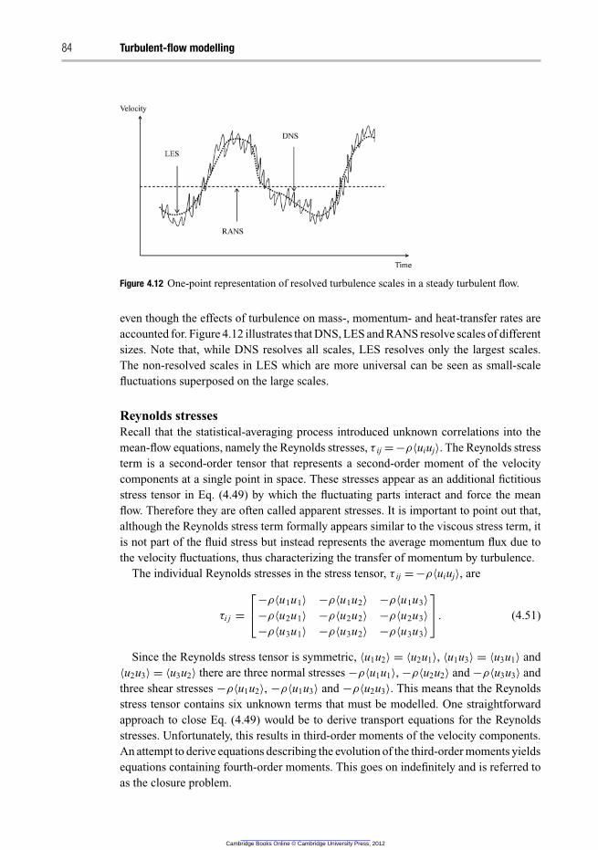
84 Turbulent-flow modelling
Figure 4.12 One-point representation of resolved turbulence scales in a steady turbulent flow.
even though the effects of turbulence on mass-, momentum- and heat-transfer rates are
accounted for. Figure 4.12 illustrates that DNS, LES and RANS resolve scales of different
sizes. Note that, while DNS resolves all scales, LES resolves only the largest scales.
The non-resolved scales in LES which are more universal can be seen as small-scale
fluctuations superposed on the large scales.
Reynolds stresses
Recall that the statistical-averaging process introduced unknown correlations into the
mean-flow equations, namely the Reynolds stresses, τ ij =−ρ〈uiuj〉. The Reynolds stress
term is a second-order tensor that represents a second-order moment of the velocity
components at a single point in space. These stresses appear as an additional fictitious
stress tensor in Eq. (4.49) by which the fluctuating parts interact and force the mean
flow. Therefore they are often called apparent stresses. It is important to point out that,
although the Reynolds stress term formally appears similar to the viscous stress term, it
is not part of the fluid stress but instead represents the average momentum flux due to
the velocity fluctuations, thus characterizing the transfer of momentum by turbulence.
The individual Reynolds stresses in the stress tensor, τ ij =−ρ〈uiuj〉, are
τi j =
⎡
⎣
−ρ〈u1u1〉 −ρ〈u1u2〉 −ρ〈u1u3〉
−ρ〈u2u1〉 −ρ〈u2u2〉 −ρ〈u2u3〉
−ρ〈u3u1〉 −ρ〈u3u2〉 −ρ〈u3u3〉
⎤
⎦. (4.51)
Since the Reynolds stress tensor is symmetric, 〈u1u2〉 = 〈u2u1〉, 〈u1u3〉 = 〈u3u1〉 and
〈u2u3〉 = 〈u3u2〉 there are three normal stresses −ρ〈u1u1〉, −ρ〈u2u2〉 and −ρ〈u3u3〉 and
three shear stresses −ρ〈u1u2〉, −ρ〈u1u3〉 and −ρ〈u2u3〉. This means that the Reynolds
stress tensor contains six unknown terms that must be modelled. One straightforward
approach to close Eq. (4.49) would be to derive transport equations for the Reynolds
stresses. Unfortunately, this results in third-order moments of the velocity components.
An attempt to derive equations describing the evolution of the third-order moments yields
equations containing fourth-order moments. This goes on indefinitely and is referred to
as the closure problem.
Cambridge Books Online © Cambridge University Press, 2012
4.2 Turbulence modelling 85
In high-Reynolds-number flows, the Reynolds stress tensor can easily be 1000 times
larger than the mean viscous stress tensor,
ρ
∥
∥
⟨
ui u j
⟩∥
∥≫ μ
∥
∥
∥
∥
∥
∂〈Ui 〉
∂x j
+∂
⟨
U j
⟩
∂xi
∥
∥
∥
∥
∥
. (4.52)
This means that at high Reynolds numbers the viscous stress may generally be
neglected when compared with the Reynolds stress insofar as the mean flow equations
are concerned. However, this does not apply towards boundaries of the flow. In these
regions (thin layers adjacent to the walls) the turbulence is damped, the mean velocity
gradients grow larger and the viscous stress becomes comparable to the Reynolds stress.
Thus, in this region we have
ρ
∥
∥
⟨
ui u j
⟩∥
∥ ≈ μ
∥
∥
∥
∥
∥
∂〈Ui 〉
∂x j
+∂
⟨
U j
⟩
∂xi
∥
∥
∥
∥
∥
. (4.53)
A discussion about these viscous regions and how they can be modelled is given in
Section 4.3.
The Boussinesq approximation
To summarize, when the RANS equations were derived we introduced the Reynolds
stresses, which are unknown terms, without adding any extra equations. This means that
the Reynolds stresses must be modelled since the total number of unknowns is more than
the total number of equations. Unless some assumptions are made about the Reynolds
stresses it is not possible to solve Eqs. (4.47) and (4.49). One way to model the Reynolds
stresses is to relate them to the dependent variables they are meant to transport. Such
turbulence models make the prediction of turbulence feasible with a reasonable amount
of computer time.
A simple approximation is to express the Reynolds stress tensor, −ρ〈uiuj〉, in terms
of the mean velocity itself. This closure has an approximate character, which means that
the solution of the RANS equations is always an approximation. In what follows we
consider closures that are based on the concept of turbulent eddy viscosity.
The Boussinesq approximation is based on the assumption that the components of the
Reynolds stress tensor are proportional to the mean velocity gradients. The Boussinesq
relation proposes that the transport of momentum by turbulence is a diffusive process and
that the Reynolds stresses can be modelled using a turbulent viscosity (eddy viscosity),
which is analogous to molecular viscosity. The Boussinesq approximation reads
τi j
ρ
= −⟨
ui u j
⟩
= νT
(
∂〈Ui 〉
∂x j
+∂
⟨
U j
⟩
∂xi
)
−2
3kδi j , (4.54)
or
τi j
ρ
= −⟨
ui u j
⟩
= νTSi j −2
3kδi j , (4.55)
Cambridge Books Online © Cambridge University Press, 2012
86 Turbulent-flow modelling
where
Si j =1
2
(
∂〈Ui 〉
∂x j
+∂
⟨
U j
⟩
∂xi
)
is the strain-rate tensor and k is the turbulent kinetic energy per unit mass. The turbulent
kinetic energy per unit mass is defined as half the trace of the Reynolds stress tensor
k = 12〈ui ui 〉. In contrast to the molecular viscosity, the turbulent viscosity is not a fluid
property but depends strongly on the state of turbulence.
The second term on the right-hand side of Eq. (4.54) represents normal stresses. Thus,
a term analogous to the pressure occurs in the usual stress tensor for a viscous fluid,
which can be absorbed into the real pressure term. Hence we finally obtain
∂〈Ui 〉
∂t+⟨
U j
⟩ ∂〈Ui 〉
∂x j
= −1
ρ
∂
(
〈P〉 + 23ρk)
∂xi
+∂
∂x j
[
(ν + νT)∂〈Ui 〉
∂x j
]
, (4.56)
or
∂〈Ui 〉
∂t+⟨
U j
⟩ ∂〈Ui 〉
∂x j
= −1
ρ
∂〈P〉
∂xi
−2
3
∂k
∂xi
+∂
∂x j
[
(ν + νT)
(
∂〈Ui 〉
∂x j
+∂
⟨
U j
⟩
∂xi
)]
.
(4.57)
Thus, if specific details of the turbulence are not important we can interpret the fluid
itself as a pseudo-fluid with an increased viscosity (effective viscosity, νeff = ν + νT)
that roughly approximates the turbulent mixing processes to diffusion of momentum and
other flow properties. This means that diffusion models convection, where ∂
⟨
ui u j
⟩
/∂x j
is transport of 〈Ui〉 in Eq. (4.49).
Regardless of the approach used to determine vT, there are several limitations with
the Boussinesq approximation. Among others, the Boussinesq approximation assumes
that eddies behave like molecules, that turbulence is isotropic and that there exists
local equilibrium between stress and strain. As a consequence of these assumptions,
predictions of simple flows may fail, e.g. in channel flows, where measurements show that
−〈u21〉 �= −〈u2
2〉 �= −〈u23〉. Hence, models that are based on the Boussinesq approximation
are limited to prediction of isotropic flows in local equilibrium. Despite the shortcomings
of the Boussinesq approximation it is one of the cornerstones in several turbulence
models. The reasons for this are the cost of using more elaborate turbulence models and
problems with obtaining closures for higher moments.
4.2.4 Models based on the turbulent viscosity hypothesis
Most models evaluating the Reynolds stress tensor simplify the situation through the
Boussinesq eddy-viscosity concept. Thus, as part of quantitative turbulence modelling
this eddy viscosity, vT, must be determined. So when it comes to turbulence mod-
elling based on the RANS equations and the eddy-viscosity concept, the turbulence
model can be seen as the set of equations that are needed to determine this viscosity.
Cambridge Books Online © Cambridge University Press, 2012
4.2 Turbulence modelling 87
As in the kinetic theory of gases, the viscosity is proportional to velocity times dis-
tance. The turbulent-viscosity models are based on appropriate velocity, u, and length
scales, l, describing the local turbulent viscosity, vT. The dimension of vT is [m2 s−1],
which means that the product of these two scales gives the right dimension; that is,
we have
νT = Cν
l2
t= Cνul. (4.58)
In this expression u and l are the characteristic scales for the large turbulent eddies and
Cν is a proportionality constant. This is reasonable because these scales are responsible
for most of the turbulent transport. The turbulent eddy viscosity, vT, in Eq. (4.57) may
vary with position and time and must be specified before the set of equations can be
closed. A proper turbulence model therefore involves a closed set of equations, i.e. the
total number of unknown variables equals the total number of equations. There exist
numerous methods that provide values for the turbulent viscosity. These methods are
usually categorized by the number of additional transport equations that are required
for closure, i.e. the equations required to determine the velocity and length scales
describing the local turbulence. In the simplest categories of models no additional
transport equations are used. These models are therefore referred to as zero-equation
models. Furthermore, there are one- and two-equation models in which respectively one
and two PDEs are solved together with the RANS equations. The degree of accuracy
of each turbulence model depends on the validity of the assumptions behind it. In what
follows we will discuss some of the zero-, one- and two-equation models that are used
for this purpose. Among these models, the two-equation models are the most widely
used for routine simulation of engineering applications.
Zero-, one- and two-equation models
The number of additional PDEs considered in addition to the RANS and continuity
equations is used to classify the turbulence models. Hence algebraic models are classified
as zero-equation models. One of the most well-known zero-equation models is Prandtl’s
mixing-length model. In this model vT is calculated using an analogy between the chaotic
motions of eddies and the random motion of molecules in gases (kinetic gas theory).
The mixing length, l, depends strongly on the nature of the flow and is generally space-
dependent. This model offers an improvement over the constant-viscosity models and is
capable of predicting some simple flows. The motivation for developing more advanced
models than the zero-equation models is that it is very difficult to estimate the distribution
of the mixing length. Another limitation with this model is that the eddy viscosity is
instantaneously affected by the shear rate and vanishes whenever the velocity gradient
is zero. This does not agree with experimental data. The reason for this is that the
turbulent stresses result not only from events at a single point but also from events in the
region, since they are transported by convection and diffusion and they have a certain
lifetime before the energy is dissipated. Hence, zero-equation models are unsuitable
for general use since they do not account for effects of accumulation and transport
on turbulence.
Cambridge Books Online © Cambridge University Press, 2012

88 Turbulent-flow modelling
Since turbulent eddies have a certain lifetime and are transported by convection,
turbulence is not completely determined by the local conditions but depends also on
the history of the eddies. One way to overcome the limitations of the zero-equation
models is to relate the turbulent viscosity to a transported turbulent quantity instead
of relating it to the mean velocity gradient. In contrast to the zero-equation models
the one-equation models allow history effects to be accounted for. It was independently
suggested by Kolmogorov and Prandtl that the square root of the time-averaged turbulent
kinetic energy, k, should be employed as the characteristic turbulent velocity scale, u.
Examples of such models include Prandtl’s k–l model and the Spalart–Allmaras model.
From the above discussion it can be concluded that transport of the turbulent kinetic
energy is taken into account in one-equation models at the cost of solving one additional
PDE. The problem with one-equation models is that only the characteristic velocity
scale is determined from a transport equation, and the length scale must therefore be
specified algebraically. An obvious solution would then be to determine the length scale
from an additional transport equation. That is actually what is done in two-equation
models.
Two-equation models
Zero- and one-equation models are still used for certain applications but they are rarely
used for general-purpose flow simulations. For general-purpose flow simulations, the
more sophisticated two-equation models are frequently used. As the number of equa-
tions increases, the computational cost increases as well. It should be mentioned that the
two-equation models are sometimes referred to as complete models, since they allow
the turbulent velocity and length scales to be determined independently. For practical
engineering purposes, the most successful models involve two or more transport equa-
tions. This is due to the fact that it takes two quantities to characterize the length and
velocity scales of turbulent flows. Using transport equations to describe these variables
means that the turbulence-production and -dissipation processes can have localized
rates. Without the transport mechanism turbulence has to instantly adjust to local con-
ditions, thereby giving unrealistically large production and dissipation rates. In many
cases a high local value of turbulence is due to convection of upstream-generated
eddies.
A straightforward approach to model the turbulent velocity and length scales is to
solve the k equation for the velocity scale and the l equation for the length scale. Usually
the names of the turbulence models are logical in the sense that they reflect what is
modelled. Hence, a two-equation model that models k and l is simply called a k–l model.
More often the second transport equation describes transport of some property other
than the length scale, l. Obviously it must be possible to determine the length scale
explicitly from this property. Generally we can write an arbitrary property, φ, which is
related to the length scale, l, in the following way:
φ = kαlβ . (4.59)
Cambridge Books Online © Cambridge University Press, 2012

4.2 Turbulence modelling 89
Table 4.2 Commonly used properties for determination of the turbulence length scale
Alternative
α β φ symbol to φ Interpretation of φ
0 1 l l Length scale
1 −2 k/l2ω Vorticity scale
1/2 −1 k1/2/l f Frequency scale
−1/2 1 k−1/2l τ Timescale
3/2 −1 k3/2/l ε Dissipation rate
This means that for the k–l model α = 0 and β = 1, hence φ = l. There are many
possible choices for the second turbulence variable, resulting in different values of α
and β. Some of the proposed variables are given in Table 4.2.
The energy-dissipation rate, ε, is the most commonly used of these variables. As
implied by its name, the k–ε model describes turbulence using two variables, namely the
turbulent kinetic energy, k, and the energy-dissipation rate, ε. The relation between the
turbulence length scale and the energy-dissipation rate is
φ = k3/2/ l = ε. (4.60)
The length scale is simply the turbulent velocity,√
k, times the lifetime of the turbulent
eddies k/ε,
l =√
kk
ε
=k3/2
ε
, (4.61)
and the turbulent viscosity is given by
νT = Cνul = Cνk1/2 k3/2
ε
= Cν
k2
ε
. (4.62)
Two-equation models are widely used for simulation of engineering applications.
Even though these models impose limitations, they continue to be favourable since they
are robust and inexpensive to implement.
The standard k–ε model
The k–ε model has become very popular due to the important role played by ε in the
interpretation of turbulence in addition to the fact that ε appears directly in the transport
equation for k. This turbulence model provides a good compromise between generality
and economy for many CFD problems. Before looking at the modelled transport equa-
tions for k and ε, one should be aware that these equations are actually simplifications
of the exact transport equations for k and ε. This means that the k–ε model is one of
several possible closures by which the RANS equations are simplified even further. In
the following section we will look particularly at the closures introduced to solve the
exact k and ε equations. Note that these types of closures are not unique to the k–ε
model but are in fact required to close all models that are based on statistical averaging,
due the higher-order moments that are introduced. The exact transport equation for the
Cambridge Books Online © Cambridge University Press, 2012
90 Turbulent-flow modelling
turbulent kinetic energy, k, can be deduced from the equation for the kinetic energy
Eq. (2.26) by Reynolds decomposition and reads
∂k
∂t︸︷︷︸
I
+⟨
U j
⟩ ∂k
∂x j︸ ︷︷ ︸
II
= −⟨
ui u j
⟩ ∂〈Ui 〉
∂x j︸ ︷︷ ︸
III
− ν
⟨
∂ui
∂x j
∂ui
∂x j
⟩
︸ ︷︷ ︸
IV
+∂
∂x j
⎛
⎜
⎜
⎜
⎝
ν
∂k
∂x j︸ ︷︷ ︸
V
−
⟨
ui ui u j
⟩
2︸ ︷︷ ︸
VI
−
⟨
u j p⟩
ρ
︸ ︷︷ ︸
VII
⎞
⎟
⎟
⎟
⎠
. (4.63)
The physical interpretation of the terms in the Eq. (4.63) is as follows.
I. Accumulation of k.
II. Convection of k by the mean velocity.
III. Production of k, large eddies extract energy from the mean flow.
IV. Dissipation of k by viscous stress, whereby turbulent kinetic energy is transformed
into heat.
V. Molecular diffusion of k.
VI. Turbulent transport by velocity fluctuations.
VII. Turbulent transport by pressure fluctuations.
In Eq. (4.63) the terms III, IV, VI and VII are unknown and, unless some approxima-
tions are introduced, it is not possible to solve this equation. Hence, closures are required
for the production, dissipation and diffusion terms. The production term represents the
production of turbulent kinetic energy due to the mean flow strain rate. If the equation
for the kinetic energy of the mean flow is considered, this term actually appears as a
sink in the equation. This clearly shows that the production of turbulent kinetic energy is
indeed a result of the mean flow losing kinetic energy, recalling that 〈E〉 = E + k. Note
that the production term is the Reynolds stresses times the shear rates and maximum
production will occur where both are large. This is mainly in the boundary layers close
to the walls, and for flow parallel to the wall the maximum production is at y+ ≈ 12.
The Reynolds stresses can be identified in the production term and it is assumed that the
Boussinesq approximation can be used to model this term by relating it to gradients of
the mean flow
−⟨
ui u j
⟩
= νT
(
∂〈Ui 〉
∂x j
+∂
⟨
U j
⟩
∂xi
)
−2
3kδi j . (4.64)
This means that the production of turbulent kinetic energy can be modelled as
−⟨
ui u j
⟩ ∂〈Ui 〉
∂x j
= νT
(
∂〈Ui 〉
∂x j
+∂
⟨
U j
⟩
∂xi
)
∂〈Ui 〉
∂x j
−2
3k∂〈Ui 〉
∂xi
. (4.65)
Cambridge Books Online © Cambridge University Press, 2012
4.2 Turbulence modelling 91
Note that the last term in Eq. (4.65) is zero for incompressible flow due to continuity.
It is important to recall that the Boussinesq approximation is an isotropic model for the
Reynolds stresses and assumes that the normal stresses are all equal.
The second closure needed to model the k equation is a relation for the energy-
dissipation rate, which is the rate of destruction of turbulent kinetic energy. Note that
the energy dissipation of turbulent kinetic energy is defined as
ε = ν
⟨
∂ui
∂x j
∂ui
∂x j
⟩
. (4.66)
The third closure is required to describe the turbulent transport of k. These higher-
order moments (terms VI and VII) are usually modelled by assuming a gradient-diffusion
transport mechanism. This assumption allows the turbulent transport due to velocity and
pressure fluctuations to be modelled as
−
⟨
ui ui u j
⟩
2−
⟨
u j p⟩
ρ
=νT
σk
∂k
∂x j
. (4.67)
Here, σk is a model coefficient known as the Prandtl–Schmidt number and vT is the
turbulent viscosity. Substituting these closures into the exact transport equation for k
gives the modelled equation for k
∂k
∂t+⟨
U j
⟩ ∂k
∂x j
= νT
[(
∂〈Ui 〉
∂x j
+∂
⟨
U j
⟩
∂xi
)
∂〈Ui 〉
∂x j
]
− ε +∂
∂x j
[(
ν +νT
σk
)
∂k
∂x j
]
.
(4.68)
To close the k equation we need to calculate ε and the turbulent viscosity. Obviously,
the energy-dissipation rate is modelled with a second transport equation. Note that
the production of turbulent kinetic energy is modelled as the product of the turbulent
viscosity and average velocity gradients.
The exact ε equation can be written as
∂ε
∂t︸︷︷︸
I
+⟨
U j
⟩ ∂ε
∂x j︸ ︷︷ ︸
II
= −2ν
(⟨
∂ui
∂xk
∂u j
∂xk
⟩
+
⟨
∂uk
∂xi
∂uk
∂x j
⟩)
∂〈Ui 〉
∂x j︸ ︷︷ ︸
III
− 2ν
⟨
uk
∂ui
∂x j
⟩
∂2 〈Ui 〉
∂xk∂x j︸ ︷︷ ︸
IV
− 2ν
⟨
∂ui
∂xk
∂ui
∂x j
∂uk
∂x j
⟩
︸ ︷︷ ︸
V
− 2νν
⟨
∂2ui
∂xk∂x j
∂2ui
∂xk∂x j
⟩
︸ ︷︷ ︸
VI
+∂
∂x j
⎛
⎜
⎜
⎜
⎝
ν
∂ε
∂x j︸ ︷︷ ︸
VII
− ν
⟨
u j
∂ui
∂x j
∂ui
∂x j
⟩
︸ ︷︷ ︸
VIII
− 2ν
ρ
⟨
∂p
∂x j
∂u j
∂x j
⟩
︸ ︷︷ ︸
IX
⎞
⎟
⎟
⎟
⎠
. (4.69)
Cambridge Books Online © Cambridge University Press, 2012
92 Turbulent-flow modelling
The physical interpretation of some of the terms in Eq. (4.69) is as follows.
I. Accumulation of ε.
II. Convection of ε by the mean velocity.
III and IV. Production of dissipation, due to interactions between the mean flow and the
products of the turbulent fluctuations.
V and VI. Destruction rate of the dissipation, due to turbulent velocity fluctuations.
VII. Viscous diffusion of ε.
VIII. Turbulent transport of ε due to velocity fluctuations.
IX. Turbulent transport of ε due to pressure–velocity fluctuations.
In Eq. (4.69) there are several unknown terms containing correlations of fluctuating
velocities and gradients of fluctuating velocities and pressure, namely terms III, IV, V,
VI, VIII and IX. Again we need several closures for the unknown terms in order to
close the equation. The result of introducing closures is that the modelled equation is
drastically simplified. To avoid tedious manipulation of the exact ε equation we simply
give the general form of the modelled ε equation:
∂ε
∂t︸︷︷︸
I
+⟨
U j
⟩ ∂ε
∂x j︸ ︷︷ ︸
II
= Cε1νT
ε
k
[(
∂〈Ui 〉
∂x j
+∂
⟨
U j
⟩
∂xi
)
∂〈Ui 〉
∂x j
]
︸ ︷︷ ︸
III
− Cε2
ε2
k︸ ︷︷ ︸
IV
+∂
∂x j
[(
ν +νT
σε
)
∂ε
∂x j
]
︸ ︷︷ ︸
V
. (4.70)
The physical interpretation of the terms in Eq. (4.70) is as follows.
I. Accumulation of ε.
II. Convection of ε by the mean velocity.
III. Production of ε.
IV. Dissipation of ε.
V. Diffusion of ε.
The time constant for turbulence is calculated from the turbulent kinetic energy and the
rate of dissipation of turbulent kinetic energy:
τ = k/ε. (4.71)
Note that the source term in the ε equation is the same as that in the k equation divided
by the time constant τ in Eq. (4.71) and the rate of dissipation of ε is proportional to
ε/τ = ε2/k. (4.72)
The turbulent viscosity must be calculated to close the k–ε model. Recall that the
turbulent viscosity is given as the product of the characteristic velocity and length
scales, νT ∝ ul. This means that we have
νT = Cμ
k2
ε
. (4.73)
Cambridge Books Online © Cambridge University Press, 2012
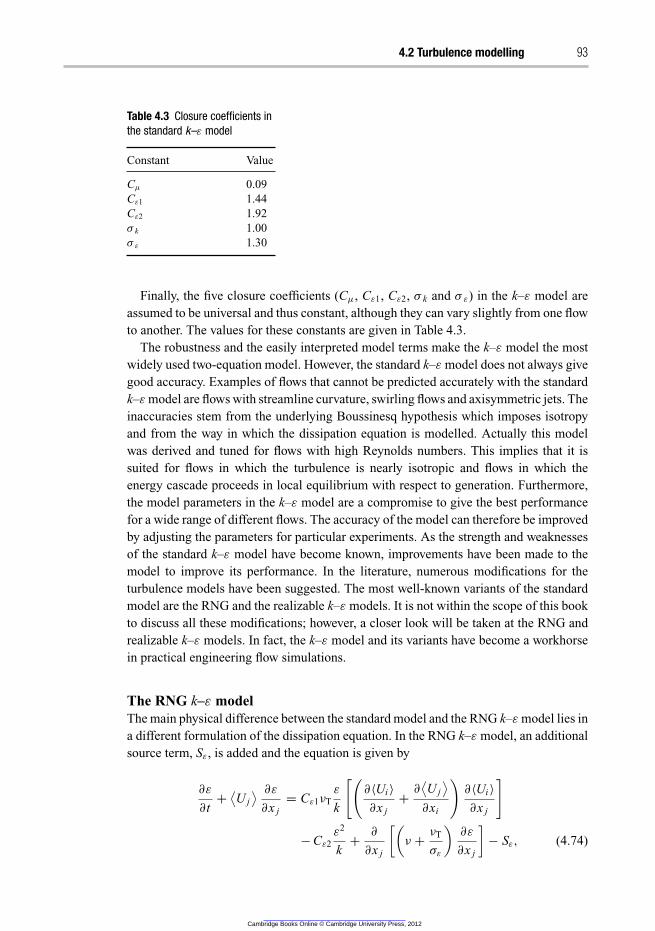
4.2 Turbulence modelling 93
Table 4.3 Closure coefficients in
the standard k–ε model
Constant Value
Cμ 0.09
Cε1 1.44
Cε2 1.92
σ k 1.00
σ ε 1.30
Finally, the five closure coefficients (Cμ, Cε1, Cε2, σ k and σ ε) in the k–ε model are
assumed to be universal and thus constant, although they can vary slightly from one flow
to another. The values for these constants are given in Table 4.3.
The robustness and the easily interpreted model terms make the k–ε model the most
widely used two-equation model. However, the standard k–ε model does not always give
good accuracy. Examples of flows that cannot be predicted accurately with the standard
k–ε model are flows with streamline curvature, swirling flows and axisymmetric jets. The
inaccuracies stem from the underlying Boussinesq hypothesis which imposes isotropy
and from the way in which the dissipation equation is modelled. Actually this model
was derived and tuned for flows with high Reynolds numbers. This implies that it is
suited for flows in which the turbulence is nearly isotropic and flows in which the
energy cascade proceeds in local equilibrium with respect to generation. Furthermore,
the model parameters in the k–ε model are a compromise to give the best performance
for a wide range of different flows. The accuracy of the model can therefore be improved
by adjusting the parameters for particular experiments. As the strength and weaknesses
of the standard k–ε model have become known, improvements have been made to the
model to improve its performance. In the literature, numerous modifications for the
turbulence models have been suggested. The most well-known variants of the standard
model are the RNG and the realizable k–ε models. It is not within the scope of this book
to discuss all these modifications; however, a closer look will be taken at the RNG and
realizable k–ε models. In fact, the k–ε model and its variants have become a workhorse
in practical engineering flow simulations.
The RNG k–ε model
The main physical difference between the standard model and the RNG k–ε model lies in
a different formulation of the dissipation equation. In the RNG k–ε model, an additional
source term, Sε, is added and the equation is given by
∂ε
∂t+⟨
U j
⟩ ∂ε
∂x j
= Cε1νT
ε
k
[(
∂〈Ui 〉
∂x j
+∂
⟨
U j
⟩
∂xi
)
∂〈Ui 〉
∂x j
]
− Cε2
ε2
k+
∂
∂x j
[(
ν +νT
σε
)
∂ε
∂x j
]
− Sε, (4.74)
Cambridge Books Online © Cambridge University Press, 2012
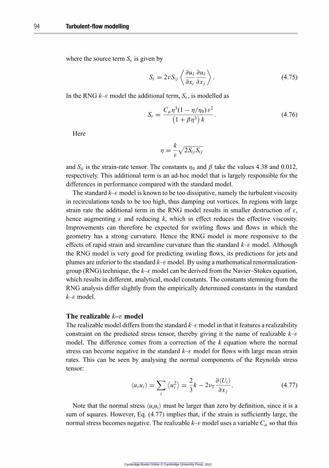
94 Turbulent-flow modelling
where the source term Sε is given by
Sε = 2νSi j
⟨
∂ul
∂xi
∂ul
∂x j
⟩
. (4.75)
In the RNG k–ε model the additional term, Sε, is modelled as
Sε =Cμη
3(1 − η/η0) ε2
(
1 + βη3)
k. (4.76)
Here
η =k
ε
√
2Si j Si j
and Sij is the strain-rate tensor. The constants η0 and β take the values 4.38 and 0.012,
respectively. This additional term is an ad-hoc model that is largely responsible for the
differences in performance compared with the standard model.
The standard k–ε model is known to be too dissipative, namely the turbulent viscosity
in recirculations tends to be too high, thus damping out vortices. In regions with large
strain rate the additional term in the RNG model results in smaller destruction of ε,
hence augmenting ε and reducing k, which in effect reduces the effective viscosity.
Improvements can therefore be expected for swirling flows and flows in which the
geometry has a strong curvature. Hence the RNG model is more responsive to the
effects of rapid strain and streamline curvature than the standard k–ε model. Although
the RNG model is very good for predicting swirling flows, its predictions for jets and
plumes are inferior to the standard k–ε model. By using a mathematical renormalization-
group (RNG) technique, the k–ε model can be derived from the Navier–Stokes equation,
which results in different, analytical, model constants. The constants stemming from the
RNG analysis differ slightly from the empirically determined constants in the standard
k–ε model.
The realizable k–ε model
The realizable model differs from the standard k–ε model in that it features a realizability
constraint on the predicted stress tensor, thereby giving it the name of realizable k–ε
model. The difference comes from a correction of the k equation where the normal
stress can become negative in the standard k–ε model for flows with large mean strain
rates. This can be seen by analysing the normal components of the Reynolds stress
tensor:
〈ui ui 〉 =∑
i
⟨
u2i
⟩
=2
3k − 2νT
∂〈Ui 〉
∂x j
. (4.77)
Note that the normal stress 〈uiui〉 must be larger than zero by definition, since it is a
sum of squares. However, Eq. (4.77) implies that, if the strain is sufficiently large, the
normal stress becomes negative. The realizable k–ε model uses a variable Cμ so that this
Cambridge Books Online © Cambridge University Press, 2012
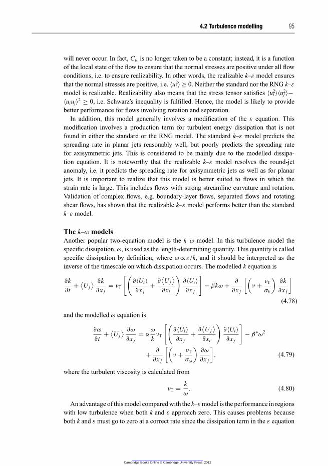
4.2 Turbulence modelling 95
will never occur. In fact, Cμ is no longer taken to be a constant; instead, it is a function
of the local state of the flow to ensure that the normal stresses are positive under all flow
conditions, i.e. to ensure realizability. In other words, the realizable k–ε model ensures
that the normal stresses are positive, i.e. 〈u2i 〉 ≥ 0. Neither the standard nor the RNG k–ε
model is realizable. Realizability also means that the stress tensor satisfies 〈u2i 〉〈u
2j 〉−
〈uiuj〉2 ≥ 0, i.e. Schwarz’s inequality is fulfilled. Hence, the model is likely to provide
better performance for flows involving rotation and separation.
In addition, this model generally involves a modification of the ε equation. This
modification involves a production term for turbulent energy dissipation that is not
found in either the standard or the RNG model. The standard k–ε model predicts the
spreading rate in planar jets reasonably well, but poorly predicts the spreading rate
for axisymmetric jets. This is considered to be mainly due to the modelled dissipa-
tion equation. It is noteworthy that the realizable k–ε model resolves the round-jet
anomaly, i.e. it predicts the spreading rate for axisymmetric jets as well as for planar
jets. It is important to realize that this model is better suited to flows in which the
strain rate is large. This includes flows with strong streamline curvature and rotation.
Validation of complex flows, e.g. boundary-layer flows, separated flows and rotating
shear flows, has shown that the realizable k–ε model performs better than the standard
k–ε model.
The k–ω models
Another popular two-equation model is the k–ω model. In this turbulence model the
specific dissipation, ω, is used as the length-determining quantity. This quantity is called
specific dissipation by definition, where ω ∝ ε/k, and it should be interpreted as the
inverse of the timescale on which dissipation occurs. The modelled k equation is
∂k
∂t+⟨
U j
⟩ ∂k
∂x j
= νT
[(
∂〈Ui 〉
∂x j
+∂
⟨
U j
⟩
∂xi
)
∂〈Ui 〉
∂x j
]
− βkω +∂
∂x j
[(
ν +νT
σk
)
∂k
∂x j
]
(4.78)
and the modelled ω equation is
∂ω
∂t+⟨
U j
⟩ ∂ω
∂x j
= α
ω
kνT
[(
∂〈Ui 〉
∂x j
+∂
⟨
U j
⟩
∂xi
)
∂〈Ui 〉
∂x j
]
− β∗ω
2
+∂
∂x j
[(
ν +νT
σω
)
∂ω
∂x j
]
, (4.79)
where the turbulent viscosity is calculated from
νT =k
ω
. (4.80)
An advantage of this model compared with the k–ε model is the performance in regions
with low turbulence when both k and ε approach zero. This causes problems because
both k and ε must go to zero at a correct rate since the dissipation term in the ε equation
Cambridge Books Online © Cambridge University Press, 2012
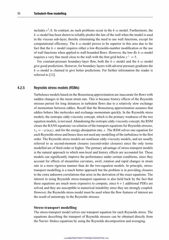
96 Turbulent-flow modelling
includes ε2/k. In contrast, no such problems occur in the k–ω model. Furthermore, the
k–ω model has been shown to reliably predict the law of the wall when the model is used
in the viscous sub-layer, thereby eliminating the need to use wall functions, except for
computational efficiency. The k–ω model proves to be superior in this area due to the
fact that the k–ε model requires either a low-Reynolds-number modification or the use
of wall functions when applied to wall-bounded flows. However, the low-Re k–ω model
requires a very fine mesh close to the wall with the first grid below y+ = 5.
For constant-pressure boundary-layer flow, both the k–ε model and the k–ω model
give good predictions. However, for boundary layers with adverse pressure gradients the
k–ω model is claimed to give better predictions. For further information the reader is
referred to [12].
4.2.5 Reynolds stress models (RSMs)
Turbulence models based on the Boussinesq approximation are inaccurate for flows with
sudden changes in the mean strain rate. This is because history effects of the Reynolds
stresses persist for long distances in turbulent flows due to a relatively slow exchange
of momentum between eddies. Recall that the Boussinesq approximation assumes that
eddies behave like molecules and exchange momentum quickly. In the Reynolds stress
models, the isotropic eddy-viscosity concept, which is the primary weakness of the two
equation models, is not used. Abandoning the isotropic eddy-viscosity concept, the RSM
closes the RANS equations via solution of the transport equations for Reynolds stresses,
τ ij =−ρ〈uiui〉, and for the energy-dissipation rate, ε. The RSM solves one equation for
each Reynolds stress and hence does not need any modelling of the turbulence to the first
order. The Reynolds stress models are nonlinear eddy-viscosity models, and are usually
referred to as second-moment closures (second-order closures) since the only terms
modelled are of third order or higher. The primary advantage of stress-transport models
is the natural approach in which non-local and history effects are accounted for. These
models can significantly improve the performance under certain conditions, since they
account for effects of streamline curvature, swirl, rotation and rapid changes in strain
rate in a more rigorous manner than do the two-equation models. In principle, stress-
transport modelling is a much better approach but the problem is in providing closures
to the extra unknown correlations that arise in the derivation of the exact equations. The
interest in using Reynolds stress-transport equations is also held back by the fact that
these equations are much more expensive to compute, since 6 + 1 additional PDEs are
solved, and they are susceptible to numerical instability since they are strongly coupled.
However, the Reynolds stress model must be used when the flow features of interest are
the result of anisotropy in the Reynolds stresses.
Stress-transport modelling
The stress-transport model solves one transport equation for each Reynolds stress. The
equations describing the transport of Reynolds stresses can be obtained directly from
the Navier–Stokes equations by using the Reynolds decomposition and averaging.
Cambridge Books Online © Cambridge University Press, 2012
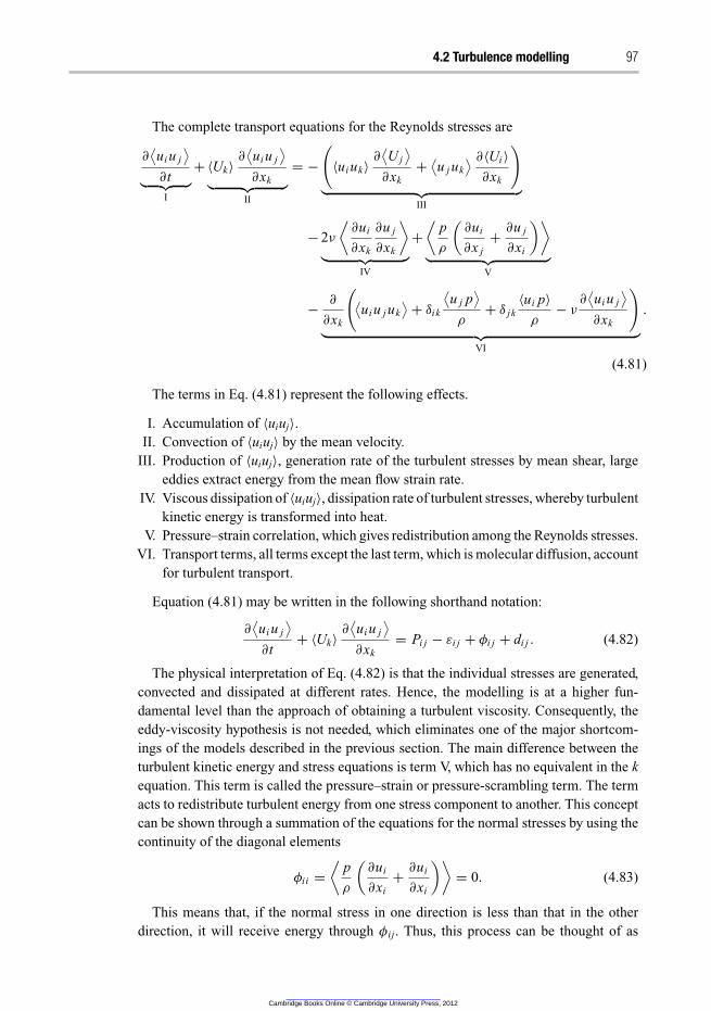
4.2 Turbulence modelling 97
The complete transport equations for the Reynolds stresses are
∂
⟨
ui u j
⟩
∂t︸ ︷︷ ︸
I
+〈Uk〉∂
⟨
ui u j
⟩
∂xk︸ ︷︷ ︸
II
= −
(
〈ui uk〉∂
⟨
U j
⟩
∂xk
+⟨
u j uk
⟩ ∂〈Ui 〉
∂xk
)
︸ ︷︷ ︸
III
− 2ν
⟨
∂ui
∂xk
∂u j
∂xk
⟩
︸ ︷︷ ︸
IV
+
⟨
p
ρ
(
∂ui
∂x j
+∂u j
∂xi
)⟩
︸ ︷︷ ︸
V
−∂
∂xk
(
⟨
ui u j uk
⟩
+ δik
⟨
u j p⟩
ρ
+ δ jk
〈ui p〉
ρ
− ν
∂
⟨
ui u j
⟩
∂xk
)
︸ ︷︷ ︸
VI
.
(4.81)
The terms in Eq. (4.81) represent the following effects.
I. Accumulation of 〈uiuj〉.
II. Convection of 〈uiuj〉 by the mean velocity.
III. Production of 〈uiuj〉, generation rate of the turbulent stresses by mean shear, large
eddies extract energy from the mean flow strain rate.
IV. Viscous dissipation of 〈uiuj〉, dissipation rate of turbulent stresses, whereby turbulent
kinetic energy is transformed into heat.
V. Pressure–strain correlation, which gives redistribution among the Reynolds stresses.
VI. Transport terms, all terms except the last term, which is molecular diffusion, account
for turbulent transport.
Equation (4.81) may be written in the following shorthand notation:
∂
⟨
ui u j
⟩
∂t+ 〈Uk〉
∂
⟨
ui u j
⟩
∂xk
= Pi j − εi j + φi j + di j . (4.82)
The physical interpretation of Eq. (4.82) is that the individual stresses are generated,
convected and dissipated at different rates. Hence, the modelling is at a higher fun-
damental level than the approach of obtaining a turbulent viscosity. Consequently, the
eddy-viscosity hypothesis is not needed, which eliminates one of the major shortcom-
ings of the models described in the previous section. The main difference between the
turbulent kinetic energy and stress equations is term V, which has no equivalent in the k
equation. This term is called the pressure–strain or pressure-scrambling term. The term
acts to redistribute turbulent energy from one stress component to another. This concept
can be shown through a summation of the equations for the normal stresses by using the
continuity of the diagonal elements
φi i =
⟨
p
ρ
(
∂ui
∂xi
+∂ui
∂xi
)⟩
= 0. (4.83)
This means that, if the normal stress in one direction is less than that in the other
direction, it will receive energy through φij. Thus, this process can be thought of as
Cambridge Books Online © Cambridge University Press, 2012
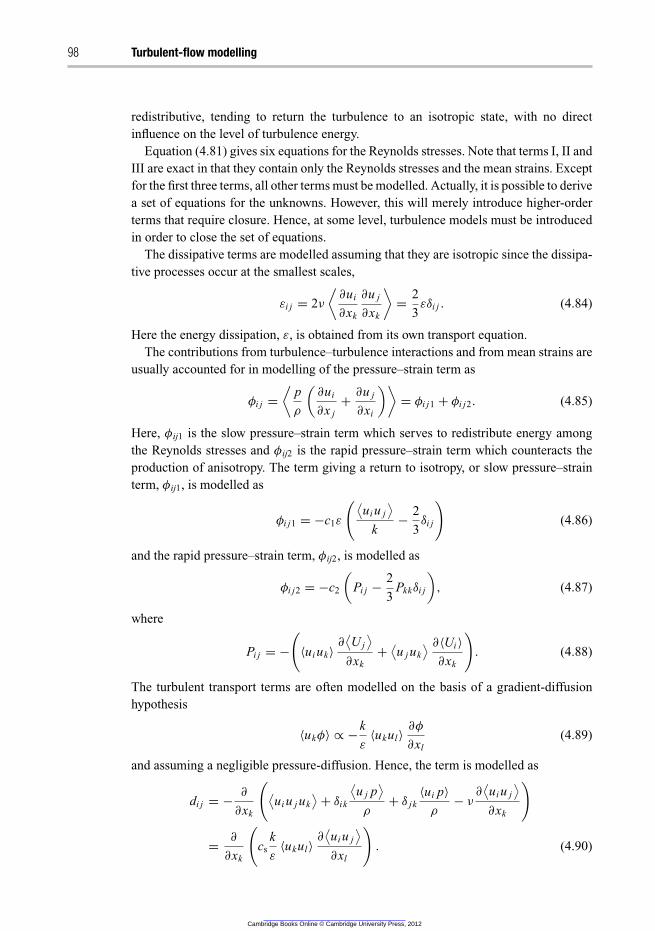
98 Turbulent-flow modelling
redistributive, tending to return the turbulence to an isotropic state, with no direct
influence on the level of turbulence energy.
Equation (4.81) gives six equations for the Reynolds stresses. Note that terms I, II and
III are exact in that they contain only the Reynolds stresses and the mean strains. Except
for the first three terms, all other terms must be modelled. Actually, it is possible to derive
a set of equations for the unknowns. However, this will merely introduce higher-order
terms that require closure. Hence, at some level, turbulence models must be introduced
in order to close the set of equations.
The dissipative terms are modelled assuming that they are isotropic since the dissipa-
tive processes occur at the smallest scales,
εi j = 2ν
⟨
∂ui
∂xk
∂u j
∂xk
⟩
=2
3εδi j . (4.84)
Here the energy dissipation, ε, is obtained from its own transport equation.
The contributions from turbulence–turbulence interactions and from mean strains are
usually accounted for in modelling of the pressure–strain term as
φi j =
⟨
p
ρ
(
∂ui
∂x j
+∂u j
∂xi
)⟩
= φi j1 + φi j2. (4.85)
Here, φij1 is the slow pressure–strain term which serves to redistribute energy among
the Reynolds stresses and φij2 is the rapid pressure–strain term which counteracts the
production of anisotropy. The term giving a return to isotropy, or slow pressure–strain
term, φij1, is modelled as
φi j1 = −c1ε
(
⟨
ui u j
⟩
k−
2
3δi j
)
(4.86)
and the rapid pressure–strain term, φij2, is modelled as
φi j2 = −c2
(
Pi j −2
3Pkkδi j
)
, (4.87)
where
Pi j = −
(
〈ui uk〉∂
⟨
U j
⟩
∂xk
+⟨
u j uk
⟩ ∂〈Ui 〉
∂xk
)
. (4.88)
The turbulent transport terms are often modelled on the basis of a gradient-diffusion
hypothesis
〈ukφ〉 ∝ −k
ε
〈ukul〉∂φ
∂xl
(4.89)
and assuming a negligible pressure-diffusion. Hence, the term is modelled as
di j = −∂
∂xk
(
⟨
ui u j uk
⟩
+ δik
⟨
u j p⟩
ρ
+ δ jk
〈ui p〉
ρ
− ν
∂
⟨
ui u j
⟩
∂xk
)
=∂
∂xk
(
cs
k
ε
〈ukul〉∂
⟨
ui u j
⟩
∂xl
)
. (4.90)
Cambridge Books Online © Cambridge University Press, 2012
4.3 Near-wall modelling 99
Note that it is good practice to include wall correction terms in the modelled equations
to account for wall reflection effects. Note also that an additional transport equation for
the energy-dissipation rate is solved. Thus, we have a solvable set of equations, e.g.
11 equations for 11 unknowns, 〈Ui〉, 〈uiuj〉, 〈P〉 and ε.
4.2.6 Advanced turbulence modelling
Turbulence models that fall beyond the bounds of the categories presented earlier have
been developed. It is difficult to sum up all the progress in this field in a few sentences;
instead, the interested reader is referred to textbooks on advanced turbulence modelling
for further insight into this exciting area. It should also be mentioned that research in
this area still remains active.
4.2.7 Comparisons of various turbulence models
In the previous sections, we have presented turbulence models that are commonly
encountered in commercial CFD codes. In these sections the physical and mathematical
principles underlying the turbulence models were presented together with discussions
about their limitations. Table 4.4 gives a short summary of the advantages and short-
comings of these models.
In general the turbulence models are developed to predict velocities accurately. The
parameters in the models, e.g. k and ε, may very well be off by a factor of 3. Using
these parameters in other models, e.g. for mixing or bubble break-up, should be done
with the awareness that the parameters do not have exact physical relevance but only
show the trend.
4.3 Near-wall modelling
Most flows of engineering interest involve situations in which the flow is constrained
by a solid wall. Ludwig Prandtl was the first to realize that the relative magnitude of
the inertial and viscous forces changed on going from a layer near the wall to a region
far from the wall. In the early 1900s he presented the theory which describes boundary-
layer effects. The wall no-slip condition ensures that, over some region of the wall
layer, viscous effects on the transport processes must be large. Recall that particular
turbulence models such as the k–ε model are not valid in the near-wall region, where
viscous effects are dominant. Furthermore, rapid variation of the flow variables occurs
within this region. This implies that a very fine computational mesh is required in order
to resolve the steep gradients of the flow variables accurately. Representation of these
processes within a CFD model raises problems. Basically, there are two approaches that
can be used to model the near-wall region. In the first approach the viscosity-affected
near-wall region is not resolved. Instead, wall functions are used to obtain boundary
conditions for the mean velocity components and the turbulent quantities at the first
Cambridge Books Online © Cambridge University Press, 2012
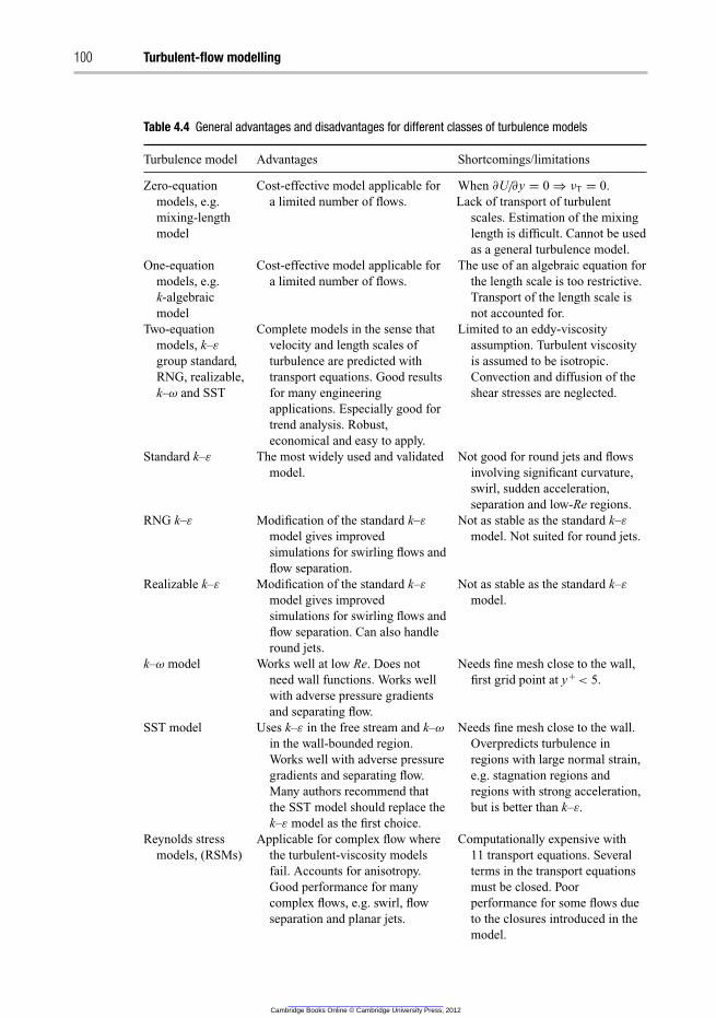
100 Turbulent-flow modelling
Table 4.4 General advantages and disadvantages for different classes of turbulence models
Turbulence model Advantages Shortcomings/limitations
Zero-equation
models, e.g.
mixing-length
model
Cost-effective model applicable for
a limited number of flows.
When ∂U/∂y = 0 ⇒ νT = 0.
Lack of transport of turbulent
scales. Estimation of the mixing
length is difficult. Cannot be used
as a general turbulence model.
One-equation
models, e.g.
k-algebraic
model
Cost-effective model applicable for
a limited number of flows.
The use of an algebraic equation for
the length scale is too restrictive.
Transport of the length scale is
not accounted for.
Two-equation
models, k–ε
group standard,
RNG, realizable,
k–ω and SST
Complete models in the sense that
velocity and length scales of
turbulence are predicted with
transport equations. Good results
for many engineering
applications. Especially good for
trend analysis. Robust,
economical and easy to apply.
Limited to an eddy-viscosity
assumption. Turbulent viscosity
is assumed to be isotropic.
Convection and diffusion of the
shear stresses are neglected.
Standard k–ε The most widely used and validated
model.
Not good for round jets and flows
involving significant curvature,
swirl, sudden acceleration,
separation and low-Re regions.
RNG k–ε Modification of the standard k–ε
model gives improved
simulations for swirling flows and
flow separation.
Not as stable as the standard k–ε
model. Not suited for round jets.
Realizable k–ε Modification of the standard k–ε
model gives improved
simulations for swirling flows and
flow separation. Can also handle
round jets.
Not as stable as the standard k–ε
model.
k–ω model Works well at low Re. Does not
need wall functions. Works well
with adverse pressure gradients
and separating flow.
Needs fine mesh close to the wall,
first grid point at y+< 5.
SST model Uses k–ε in the free stream and k–ω
in the wall-bounded region.
Works well with adverse pressure
gradients and separating flow.
Many authors recommend that
the SST model should replace the
k–ε model as the first choice.
Needs fine mesh close to the wall.
Overpredicts turbulence in
regions with large normal strain,
e.g. stagnation regions and
regions with strong acceleration,
but is better than k–ε.
Reynolds stress
models, (RSMs)
Applicable for complex flow where
the turbulent-viscosity models
fail. Accounts for anisotropy.
Good performance for many
complex flows, e.g. swirl, flow
separation and planar jets.
Computationally expensive with
11 transport equations. Several
terms in the transport equations
must be closed. Poor
performance for some flows due
to the closures introduced in the
model.
Cambridge Books Online © Cambridge University Press, 2012
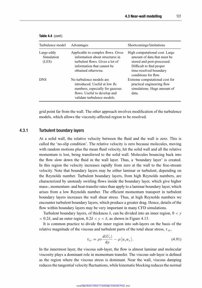
4.3 Near-wall modelling 101
Table 4.4 (cont.)
Turbulence model Advantages Shortcomings/limitations
Large-eddy
Simulation
(LES)
Applicable to complex flows. Gives
information about structures in
turbulent flows. Gives a lot of
information that cannot be
obtained otherwise.
High computational cost. Large
amount of data that must be
stored and post-processed.
Difficult to find proper
time-resolved boundary
conditions for flow.
DNS No turbulence models are
introduced. Useful at low Re
numbers, especially for gaseous
flows. Useful to develop and
validate turbulence models.
Extreme computational cost for
practical engineering flow
simulations. Huge amount of
data.
grid point far from the wall. The other approach involves modification of the turbulence
models, which allows the viscosity-affected region to be resolved.
4.3.1 Turbulent boundary layers
At a solid wall, the relative velocity between the fluid and the wall is zero. This is
called the ‘no-slip condition’. The relative velocity is zero because molecules, moving
with random motions plus the mean fluid velocity, hit the solid wall and all the relative
momentum is lost, being transferred to the solid wall. Molecules bouncing back into
the flow slow down the fluid in the wall layer. Thus, a ‘boundary layer’ is created.
In this region the velocity increases rapidly from zero at the wall to the free-stream
velocity. Note that boundary layers may be either laminar or turbulent, depending on
the Reynolds number. Turbulent boundary layers, from high Reynolds numbers, are
characterized by unsteady swirling flows inside the boundary layer, which give higher
mass-, momentum- and heat-transfer rates than apply to a laminar boundary layer, which
arises from a low Reynolds number. The efficient momentum transport in turbulent
boundary layers increases the wall shear stress. Thus, at high Reynolds numbers we
encounter turbulent boundary layers, which produce a greater drag. Hence, details of the
flow within boundary layers may be very important in many CFD simulations.
Turbulent boundary layers, of thickness δ, can be divided into an inner region, 0 < y
< 0.2δ, and an outer region, 0.2δ < y < δ, as shown in Figure 4.13.
It is common practice to divide the inner region into sub-layers on the basis of the
relative magnitude of the viscous and turbulent parts of the total shear stress, τ xy,
τxy = ρν
d〈Ux 〉
dy− ρ
⟨
ux u y
⟩
. (4.91)
In the innermost layer, the viscous sub-layer, the flow is almost laminar and molecular
viscosity plays a dominant role in momentum transfer. The viscous sub-layer is defined
as the region where the viscous stress is dominant. Near the wall, viscous damping
reduces the tangential velocity fluctuations, while kinematic blocking reduces the normal
Cambridge Books Online © Cambridge University Press, 2012
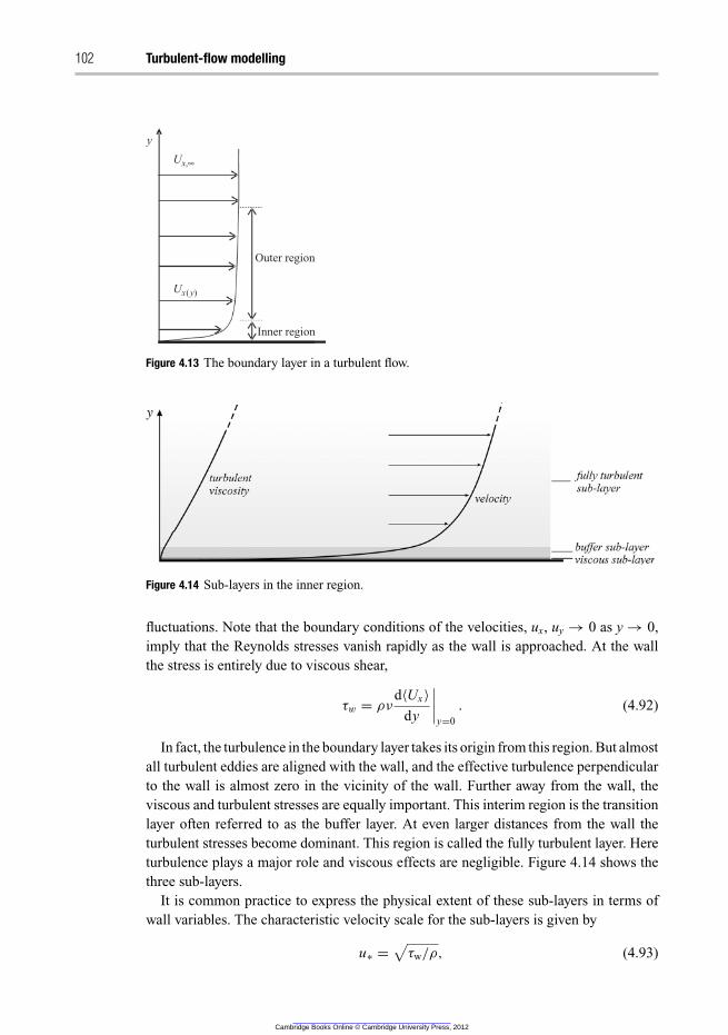
102 Turbulent-flow modelling
y
Ux,∞
Ux(y)
Outer region
Inner region
Figure 4.13 The boundary layer in a turbulent flow.
Figure 4.14 Sub-layers in the inner region.
fluctuations. Note that the boundary conditions of the velocities, ux, uy → 0 as y → 0,
imply that the Reynolds stresses vanish rapidly as the wall is approached. At the wall
the stress is entirely due to viscous shear,
τw = ρν
d〈Ux 〉
dy
∣
∣
∣
∣
y=0
. (4.92)
In fact, the turbulence in the boundary layer takes its origin from this region. But almost
all turbulent eddies are aligned with the wall, and the effective turbulence perpendicular
to the wall is almost zero in the vicinity of the wall. Further away from the wall, the
viscous and turbulent stresses are equally important. This interim region is the transition
layer often referred to as the buffer layer. At even larger distances from the wall the
turbulent stresses become dominant. This region is called the fully turbulent layer. Here
turbulence plays a major role and viscous effects are negligible. Figure 4.14 shows the
three sub-layers.
It is common practice to express the physical extent of these sub-layers in terms of
wall variables. The characteristic velocity scale for the sub-layers is given by
u∗ =√
τw/ρ, (4.93)
Cambridge Books Online © Cambridge University Press, 2012
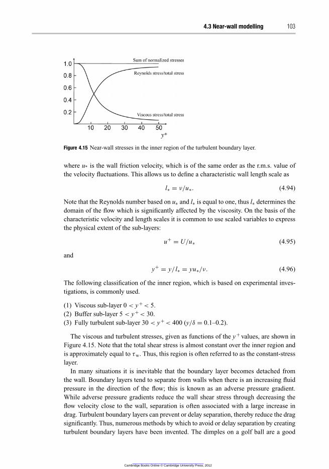
4.3 Near-wall modelling 103
Figure 4.15 Near-wall stresses in the inner region of the turbulent boundary layer.
where u* is the wall friction velocity, which is of the same order as the r.m.s. value of
the velocity fluctuations. This allows us to define a characteristic wall length scale as
l∗ = ν/u∗. (4.94)
Note that the Reynolds number based on u∗ and l∗ is equal to one, thus l∗ determines the
domain of the flow which is significantly affected by the viscosity. On the basis of the
characteristic velocity and length scales it is common to use scaled variables to express
the physical extent of the sub-layers:
u+ = U/u∗ (4.95)
and
y+ = y/ l∗ = yu∗/ν. (4.96)
The following classification of the inner region, which is based on experimental inves-
tigations, is commonly used.
(1) Viscous sub-layer 0 < y+< 5.
(2) Buffer sub-layer 5 < y+< 30.
(3) Fully turbulent sub-layer 30 < y+< 400 (y/δ = 0.1–0.2).
The viscous and turbulent stresses, given as functions of the y+ values, are shown in
Figure 4.15. Note that the total shear stress is almost constant over the inner region and
is approximately equal to τw. Thus, this region is often referred to as the constant-stress
layer.
In many situations it is inevitable that the boundary layer becomes detached from
the wall. Boundary layers tend to separate from walls when there is an increasing fluid
pressure in the direction of the flow; this is known as an adverse pressure gradient.
While adverse pressure gradients reduce the wall shear stress through decreasing the
flow velocity close to the wall, separation is often associated with a large increase in
drag. Turbulent boundary layers can prevent or delay separation, thereby reduce the drag
significantly. Thus, numerous methods by which to avoid or delay separation by creating
turbulent boundary layers have been invented. The dimples on a golf ball are a good
Cambridge Books Online © Cambridge University Press, 2012
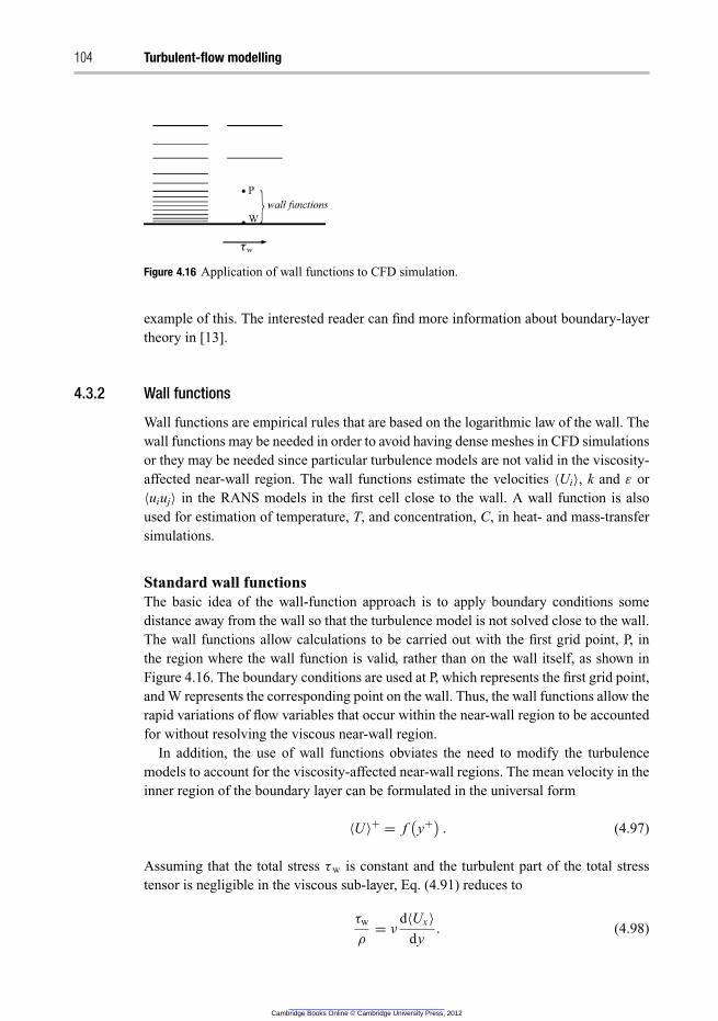
104 Turbulent-flow modelling
Figure 4.16 Application of wall functions to CFD simulation.
example of this. The interested reader can find more information about boundary-layer
theory in [13].
4.3.2 Wall functions
Wall functions are empirical rules that are based on the logarithmic law of the wall. The
wall functions may be needed in order to avoid having dense meshes in CFD simulations
or they may be needed since particular turbulence models are not valid in the viscosity-
affected near-wall region. The wall functions estimate the velocities 〈Ui〉, k and ε or
〈uiuj〉 in the RANS models in the first cell close to the wall. A wall function is also
used for estimation of temperature, T, and concentration, C, in heat- and mass-transfer
simulations.
Standard wall functions
The basic idea of the wall-function approach is to apply boundary conditions some
distance away from the wall so that the turbulence model is not solved close to the wall.
The wall functions allow calculations to be carried out with the first grid point, P, in
the region where the wall function is valid, rather than on the wall itself, as shown in
Figure 4.16. The boundary conditions are used at P, which represents the first grid point,
and W represents the corresponding point on the wall. Thus, the wall functions allow the
rapid variations of flow variables that occur within the near-wall region to be accounted
for without resolving the viscous near-wall region.
In addition, the use of wall functions obviates the need to modify the turbulence
models to account for the viscosity-affected near-wall regions. The mean velocity in the
inner region of the boundary layer can be formulated in the universal form
〈U 〉+ = f(
y+)
. (4.97)
Assuming that the total stress τw is constant and the turbulent part of the total stress
tensor is negligible in the viscous sub-layer, Eq. (4.91) reduces to
τw
ρ
= ν
d〈Ux 〉
dy. (4.98)
Cambridge Books Online © Cambridge University Press, 2012
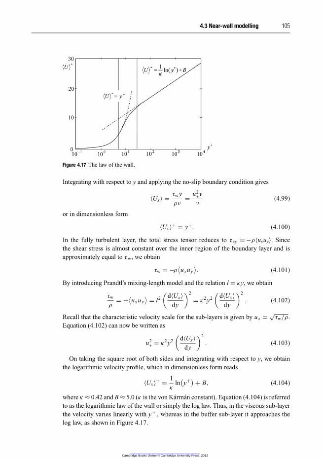
4.3 Near-wall modelling 105
Figure 4.17 The law of the wall.
Integrating with respect to y and applying the no-slip boundary condition gives
〈Ux 〉 =τw y
ρν
=u2
∗y
ν
(4.99)
or in dimensionless form
〈Ux 〉+ = y+
. (4.100)
In the fully turbulent layer, the total stress tensor reduces to τ xy =−ρ〈uxuy〉. Since
the shear stress is almost constant over the inner region of the boundary layer and is
approximately equal to τw, we obtain
τw = −ρ
⟨
ux u y
⟩
. (4.101)
By introducing Prandtl’s mixing-length model and the relation l = κy, we obtain
τw
ρ
= −⟨
ux u y
⟩
= l2
(
d〈Ux 〉
dy
)2
= κ2 y2
(
d〈Ux 〉
dy
)2
. (4.102)
Recall that the characteristic velocity scale for the sub-layers is given by u∗ =√
τw/ρ.
Equation (4.102) can now be written as
u2∗ = κ
2 y2
(
d〈Ux 〉
dy
)2
. (4.103)
On taking the square root of both sides and integrating with respect to y, we obtain
the logarithmic velocity profile, which in dimensionless form reads
〈Ux 〉+ =
1
κ
ln(
y+)
+ B, (4.104)
where κ ≈ 0.42 and B ≈ 5.0 (κ is the von Karman constant). Equation (4.104) is referred
to as the logarithmic law of the wall or simply the log law. Thus, in the viscous sub-layer
the velocity varies linearly with y+ , whereas in the buffer sub-layer it approaches the
log law, as shown in Figure 4.17.
Cambridge Books Online © Cambridge University Press, 2012
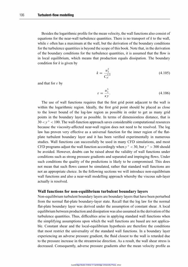
106 Turbulent-flow modelling
Besides the logarithmic profile for the mean velocity, the wall functions also consist of
equations for the near-wall turbulence quantities. There is no transport of k to the wall,
while ε often has a maximum at the wall, but the derivation of the boundary conditions
for the turbulence quantities is beyond the scope of this book. Note that, in the derivation
of the boundary conditions for the turbulence quantities, it is assumed that the flow is
in local equilibrium, which means that production equals dissipation. The boundary
condition for k is given by
k =u2
∗
C1/2μ
(4.105)
and that for ε by
ε =u3
∗
κy. (4.106)
The use of wall functions requires that the first grid point adjacent to the wall is
within the logarithmic region. Ideally, the first grid point should be placed as close
to the lower bound of the log-law region as possible in order to get as many grid
points in the boundary layer as possible. In terms of dimensionless distance, that is
30 < y+< 100. The wall-function approach saves considerable computational resources
because the viscosity-affected near-wall region does not need to be resolved. The log
law has proven very effective as a universal function for the inner region of the flat-
plate turbulent boundary layer and it has been verified experimentally in numerous
studies. Wall functions can successfully be used in many CFD simulations, and most
CFD programs adjust the wall function accordingly when y+< 30, but y+
> 300 should
be avoided. However, doubts can be raised about the validity of wall functions under
conditions such as strong pressure gradients and separated and impinging flows. Under
such conditions the quality of the predictions is likely to be compromised. This does
not mean that such flows cannot be simulated, rather that standard wall functions are
not an appropriate choice. In the following sections we will introduce non-equilibrium
wall functions and also a near-wall modelling approach whereby the viscous sub-layer
actually is resolved.
Wall functions for non-equilibrium turbulent boundary layers
Non-equilibrium turbulent boundary layers are boundary layers that have been perturbed
from the normal flat-plate boundary-layer state. Recall that the log law for the normal
flat-plate boundary layer was derived under the assumption of constant shear. A local
equilibrium between production and dissipation was also assumed in the derivation of the
turbulence quantities. Thus, difficulties arise in applying standard wall functions when
the simplifying assumptions upon which the wall functions are based are not applica-
ble. Constant shear and the local-equilibrium hypothesis are therefore the conditions
that most restrict the universality of the standard wall functions. In a boundary layer
experiencing an adverse pressure gradient, the fluid closest to the wall is retarded due
to the pressure increase in the streamwise direction. As a result, the wall shear stress is
decreased. Consequently, adverse pressure gradients alter the mean velocity profile as
Cambridge Books Online © Cambridge University Press, 2012
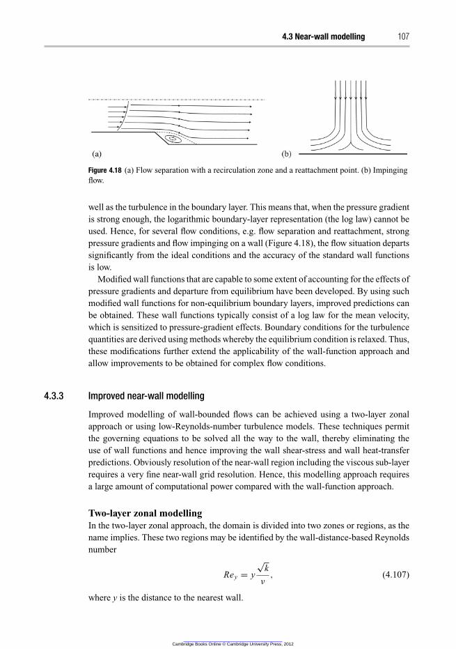
4.3 Near-wall modelling 107
Figure 4.18 (a) Flow separation with a recirculation zone and a reattachment point. (b) Impinging
flow.
well as the turbulence in the boundary layer. This means that, when the pressure gradient
is strong enough, the logarithmic boundary-layer representation (the log law) cannot be
used. Hence, for several flow conditions, e.g. flow separation and reattachment, strong
pressure gradients and flow impinging on a wall (Figure 4.18), the flow situation departs
significantly from the ideal conditions and the accuracy of the standard wall functions
is low.
Modified wall functions that are capable to some extent of accounting for the effects of
pressure gradients and departure from equilibrium have been developed. By using such
modified wall functions for non-equilibrium boundary layers, improved predictions can
be obtained. These wall functions typically consist of a log law for the mean velocity,
which is sensitized to pressure-gradient effects. Boundary conditions for the turbulence
quantities are derived using methods whereby the equilibrium condition is relaxed. Thus,
these modifications further extend the applicability of the wall-function approach and
allow improvements to be obtained for complex flow conditions.
4.3.3 Improved near-wall modelling
Improved modelling of wall-bounded flows can be achieved using a two-layer zonal
approach or using low-Reynolds-number turbulence models. These techniques permit
the governing equations to be solved all the way to the wall, thereby eliminating the
use of wall functions and hence improving the wall shear-stress and wall heat-transfer
predictions. Obviously resolution of the near-wall region including the viscous sub-layer
requires a very fine near-wall grid resolution. Hence, this modelling approach requires
a large amount of computational power compared with the wall-function approach.
Two-layer zonal modelling
In the two-layer zonal approach, the domain is divided into two zones or regions, as the
name implies. These two regions may be identified by the wall-distance-based Reynolds
number
Rey = y
√k
ν
, (4.107)
where y is the distance to the nearest wall.
Cambridge Books Online © Cambridge University Press, 2012
108 Turbulent-flow modelling
The fully turbulent region is normally taken to have Rey > 200 and the viscosity
affected region to have Rey < 200. In the viscosity-affected near-wall region, a one-
equation turbulence model for the turbulent kinetic energy is applied and an algebraic
relation is used to determine the energy-dissipation rate. In contrast, a two-equation
model such as the standard or more advanced k–ε model is employed in the fully
turbulent region. Thus, in the viscous zone the energy dissipation is calculated from
ε =k3/2
lε, (4.108)
where lε is an appropriate length scale.
It is common practice to use a blending function to calculate the turbulent viscosity in
the transition region. This function simply blends the turbulent viscosity in the viscosity-
affected region with the turbulent viscosity in the turbulent region to obtain a smooth
transition. Thus the blending function is defined as unity far from the wall and zero
at the wall. The two-layer zonal approach requires approximately the same boundary-
layer resolution as in the low-Reynolds-number approach. Since the energy dissipation
is calculated from an algebraic equation, this approach may be more stable than the
low-Reynolds-number approach.
Low-Reynolds-number turbulence models
One way of characterizing turbulence models is to distinguish between high- and low-
Reynolds-number models. In the former, wall functions are used to approximate turbu-
lence quantities close to walls. The standard k–ε model is an example of a high-Reynolds-
number model. Whereas high-Reynolds-number models are valid for turbulent core
flows, they are not valid in regions close to walls, where viscous effects predominate
over turbulent ones. Low-Reynolds-number models are examples of models that are
valid also in the viscous wall region and can thus be integrated all the way to the wall.
The low-Reynolds-number modifications typically consist of damping functions for
the source terms in the transport equation for ε and in the expression for the turbulent
viscosity. These modifications allow the equations to be integrated through the turbulent
boundary layer, including the viscous sub-layer, thereby giving better predictions for
near-wall flows. It is important to point out that these models are applicable for flows
with high global Reynolds number wherein the flow is fully turbulent. These models
are not useful for solving flows with low global Reynolds numbers. For that a transition
model is needed. It should also be noted that these models are of ad-hoc nature and cannot
be relied upon to give consistently good results for all types of flows. Low-Reynolds-
number variants of the k–ε model include the Launder–Sharma and Lam–Bremhorst
models.
For low-Reynolds-number models, the general transport equations for k are given by
∂k
∂t+⟨
U j
⟩ ∂k
∂x j
=∂
∂x j
((
ν +νT
σk
)
∂k
∂x j
)
+ νT
[(
∂〈Ui 〉
∂x j
+∂
⟨
U j
⟩
∂xi
)
∂〈Ui 〉
∂x j
]
− ε
(4.109)
Cambridge Books Online © Cambridge University Press, 2012
4.3 Near-wall modelling 109
and the general transport equations for ε are given by
∂ε
∂t+⟨
U j
⟩ ∂ε
∂x j
=∂
∂x j
((
ν +νT
σε
)
∂ε
∂x j
)
+ C1ε f1νT
ε
k
[(
∂〈Ui 〉
∂x j
+∂
⟨
U j
⟩
∂xi
)
∂〈Ui 〉
∂x j
]
− C2ε f2
ε2
k+ E, (4.110)
where the turbulent viscosity is calculated from
νT = fμCμ
k2
ε
(4.111)
and the energy dissipation, ε, is related to ε by
ε = ε0 + ε. (4.112)
The quantities ε0 and E are defined differently for each model; ε0 is the value of ε
at the wall. The difference between these models and the standard k–ε model is the
damping functions f1 and f2 in the transport equation of ε and the damping function fμ.
The damping functions are generally written in terms of specifically defined Reynolds
numbers
Ret =k2
νε
(4.113)
and
Rey =
√ky
ν
. (4.114)
Obviously the global Reynolds number has nothing to do with the low-Reynolds-
number turbulence models. The low Reynolds number comes from the local Reynolds
number.
4.3.4 Comparison of three near-wall modelling approaches
As has already been pointed out, the near-wall treatment determines the accuracy of the
wall stresses and of the near-wall turbulence prediction. Hence, appropriate near-wall
turbulence modelling is crucial in order to capture important flow features such as flow
separation, reattachment and heat- and mass-transfer rates. Figure 4.19 illustrates the
implementation of the three near-wall treatment approaches mentioned in the previous
sections.
The general recommendation for a standard wall function is 30 < y+<100, preferably
in the lower region. At high Re the log law is valid up to higher y+ and the upper limit
may increase to 300–500. For low-Re models and enhanced wall functions the first
grid point should be close to y+ =1, and there should be at least ten grid points in the
viscosity-affected near-wall region, i.e. y+< 20.
The lengths corresponding to y+ =1 and y+ = 30 for pipe flows at various Reynolds
numbers are given in Table 4.5 to give a feeling for the actual dimensions.
Cambridge Books Online © Cambridge University Press, 2012
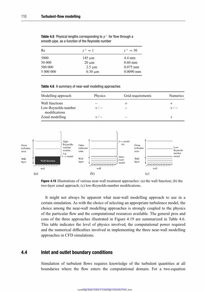
110 Turbulent-flow modelling
Table 4.5 Physical lengths corresponding to y+ for flow through a
smooth pipe, as a function of the Reynolds number
Re y+ = 1 y+ = 30
5000 145 µm 4.4 mm
50 000 20 µm 0.60 mm
500 000 2.5 µm 0.075 mm
5 000 000 0.30 µm 0.0090 mm
Table 4.6 A summary of near-wall modelling approaches
Modelling approach Physics Grid requirements Numerics
Wall functions − + +
Low-Reynolds-number
modifications
+ / − − + / −
Zonal modelling + / − − +
Figure 4.19 Illustrations of various near-wall treatment approaches: (a) the wall function; (b) the
two-layer zonal approach; (c) low-Reynolds-number modifications.
It might not always be apparent what near-wall modelling approach to use in a
certain simulation. As with the choice of selecting an appropriate turbulence model, the
choice among the near-wall modelling approaches is strongly coupled to the physics
of the particular flow and the computational resources available. The general pros and
cons of the three approaches illustrated in Figure 4.19 are summarized in Table 4.6.
This table indicates the level of physics involved, the computational power required
and the numerical difficulties involved in implementing the three near-wall modelling
approaches in CFD simulations.
4.4 Inlet and outlet boundary conditions
Simulation of turbulent flows requires knowledge of the turbulent quantities at all
boundaries where the flow enters the computational domain. For a two-equation
Cambridge Books Online © Cambridge University Press, 2012
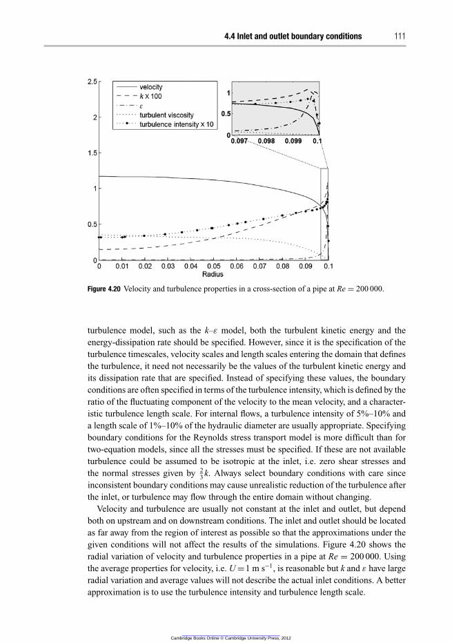
4.4 Inlet and outlet boundary conditions 111
Figure 4.20 Velocity and turbulence properties in a cross-section of a pipe at Re = 200 000.
turbulence model, such as the k–ε model, both the turbulent kinetic energy and the
energy-dissipation rate should be specified. However, since it is the specification of the
turbulence timescales, velocity scales and length scales entering the domain that defines
the turbulence, it need not necessarily be the values of the turbulent kinetic energy and
its dissipation rate that are specified. Instead of specifying these values, the boundary
conditions are often specified in terms of the turbulence intensity, which is defined by the
ratio of the fluctuating component of the velocity to the mean velocity, and a character-
istic turbulence length scale. For internal flows, a turbulence intensity of 5%–10% and
a length scale of 1%–10% of the hydraulic diameter are usually appropriate. Specifying
boundary conditions for the Reynolds stress transport model is more difficult than for
two-equation models, since all the stresses must be specified. If these are not available
turbulence could be assumed to be isotropic at the inlet, i.e. zero shear stresses and
the normal stresses given by 23k. Always select boundary conditions with care since
inconsistent boundary conditions may cause unrealistic reduction of the turbulence after
the inlet, or turbulence may flow through the entire domain without changing.
Velocity and turbulence are usually not constant at the inlet and outlet, but depend
both on upstream and on downstream conditions. The inlet and outlet should be located
as far away from the region of interest as possible so that the approximations under the
given conditions will not affect the results of the simulations. Figure 4.20 shows the
radial variation of velocity and turbulence properties in a pipe at Re = 200 000. Using
the average properties for velocity, i.e. U =1 m s−1, is reasonable but k and ε have large
radial variation and average values will not describe the actual inlet conditions. A better
approximation is to use the turbulence intensity and turbulence length scale.
Cambridge Books Online © Cambridge University Press, 2012
112 Turbulent-flow modelling
The turbulence intensity for a pipe at high Reynolds number can be estimated from
I =u
〈U 〉= 0.16Re−1/8 (4.115)
and the turbulence length scale is given by
l = 0.07L , (4.116)
where L is the hydraulic diameter and U the average velocity. It is then possible to
estimate k and ε from
k =3
2(〈U 〉)2 and ε = C3/4
μ
k3/2
l. (4.117)
4.5 Summary
Turbulence is of considerable importance in most flows of engineering interest, so
turbulence modelling is one of the key elements to successful CFD simulations. In this
chapter the physical and mathematical principles underlying turbulence modelling were
explained. The purpose of this chapter was, besides providing a survey of turbulence
models, also to indicate their validity and limitations in various applications. Even
though we have far from exhausted all aspects, this chapter serves as an overview of
turbulence modelling. Readers who are particularly interested in turbulence modelling
are encouraged to turn their attention to the references given in this book for more
in-depth discussions of this subject.
Questions
(1) Discuss why turbulence has to be modelled.
(2) Explain the origin of the Reynolds stresses in the RANS equations and explain
what is meant by the closure problem.
(3) Explain what is meant by the Boussinesq approximation.
(4) What limitations does the Boussinesq approximation impose on a turbulence
model?
(5) Discuss the application of zero-, one- and two-equation models.
(6) Discuss the differences between Reynolds stress modelling and eddy-viscosity-
based modelling.
(7) Explain what is meant by large-eddy simulations.
(8) Explain what is meant by wall functions, why they are used and when it is appro-
priate to use them.
(9) Discuss how the near-wall treatment can be improved, i.e. when the wall-function
approach is not appropriate.
(10) Discuss what turbulence boundary conditions it is appropriate to use.
Cambridge Books Online © Cambridge University Press, 2012

Cambridge Books Online © Cambridge University Press, 2012
5 Turbulent mixing andchemical reactions
The purpose of this chapter is to give an introduction to problems faced by engineers
wanting to use CFD for detailed modelling of turbulent reactive flows. After reading
this chapter you should be able to describe the physical process of turbulent mixing
and know why this can have an effect on the outcome of chemical reactions, e.g.
combustion. The problem arises when the grid and time resolution is not sufficient to
resolve the concentration and the average concentration in the cells is a poor estimation
of the actual concentration as shown in Figure 5.1. The local concentration changes fast,
and we need models that can predict the space- and time-average reaction rate in each
computational cell.
The average concentration in a computational cell can be used to describe macromix-
ing (large-scale mixing) in the reactor and is relatively straightforward to model. The
concentration fluctuations, on the other hand, can be used to describe micromixing
(small-scale mixing on the molecular level). To quantify micromixing, the variance of
the concentration fluctuations is used. Chemical reactions can take place only at the
smallest scales of the flow, after micromixing has occurred, because reactions occur
only as molecules meet and interact. An expression for the instantaneous rate of chem-
ical reactions is often known for homogeneous mixtures. However, the average rate
of chemical reactions in a reactor subject to mixing will depend also on the rate of
micromixing.
In modelling fast reactions it is not sufficient to know the time-average concentration
since at a specific position only one of the reactants may be present for some fraction
of the time and no reaction will occur. The models for the average reaction rate make
use both of the average concentrations and of the variance. The time average alone will
not tell us whether both reactants were present simultaneously. A large variance tells us
that the instantaneous concentration is far from the average and the probability that both
reactants are present is low, whereas a small variance tells us that the concentrations
of both reactants are close to the average and there is a high probability that both are
present simultaneously. Hence, it is of great importance to understand that the average
and variance represent macromixing and micromixing on the largest and smallest scales
of the flow, respectively. In this chapter we will present the tools required to describe the
flow and simulate concentration variations using probability density functions (PDFs),
and use them to calculate average reaction rates.
Cambridge Books Online © Cambridge University Press, 2012
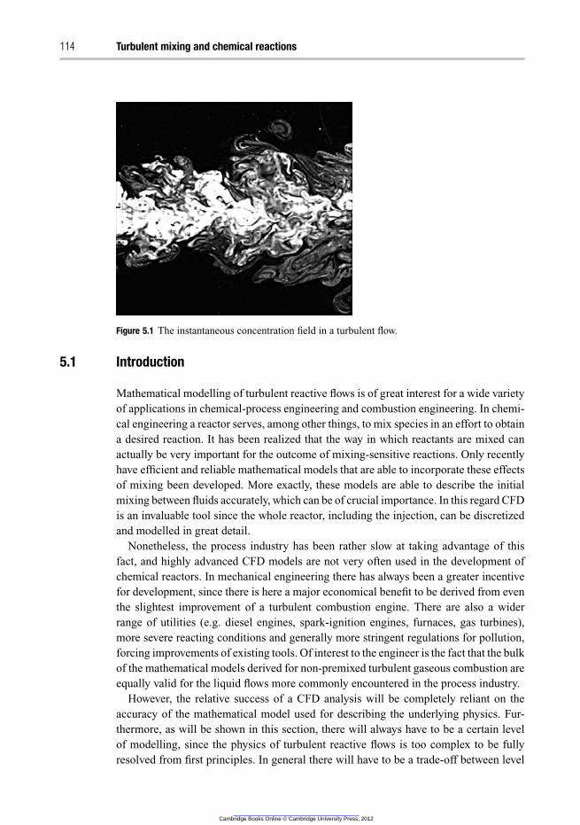
114 Turbulent mixing and chemical reactions
Figure 5.1 The instantaneous concentration field in a turbulent flow.
5.1 Introduction
Mathematical modelling of turbulent reactive flows is of great interest for a wide variety
of applications in chemical-process engineering and combustion engineering. In chemi-
cal engineering a reactor serves, among other things, to mix species in an effort to obtain
a desired reaction. It has been realized that the way in which reactants are mixed can
actually be very important for the outcome of mixing-sensitive reactions. Only recently
have efficient and reliable mathematical models that are able to incorporate these effects
of mixing been developed. More exactly, these models are able to describe the initial
mixing between fluids accurately, which can be of crucial importance. In this regard CFD
is an invaluable tool since the whole reactor, including the injection, can be discretized
and modelled in great detail.
Nonetheless, the process industry has been rather slow at taking advantage of this
fact, and highly advanced CFD models are not very often used in the development of
chemical reactors. In mechanical engineering there has always been a greater incentive
for development, since there is here a major economical benefit to be derived from even
the slightest improvement of a turbulent combustion engine. There are also a wider
range of utilities (e.g. diesel engines, spark-ignition engines, furnaces, gas turbines),
more severe reacting conditions and generally more stringent regulations for pollution,
forcing improvements of existing tools. Of interest to the engineer is the fact that the bulk
of the mathematical models derived for non-premixed turbulent gaseous combustion are
equally valid for the liquid flows more commonly encountered in the process industry.
However, the relative success of a CFD analysis will be completely reliant on the
accuracy of the mathematical model used for describing the underlying physics. Fur-
thermore, as will be shown in this section, there will always have to be a certain level
of modelling, since the physics of turbulent reactive flows is too complex to be fully
resolved from first principles. In general there will have to be a trade-off between level
Cambridge Books Online © Cambridge University Press, 2012

5.2 Problem description 115
of description and computational efficiency, in a hierarchy of models. In fact, the more
of the flow is modelled, the less expensive the computations will be.
The highest-level mathematical descriptions of a turbulent reactive flow use only
first principles and no modelling, i.e. direct numerical simulation (DNS). However, this
approach is completely impractical for all industrial applications due to the enormous
computational cost. The next-level large-eddy simulation (LES) models only the smallest
scales of the flow (molecular mixing and chemical reactions), whereas the lowest level
computes only statistical properties. Except for the highest level, the calculations are in
general still not accurate enough to make experiments superfluous. However, for many
systems there are models available that can give at least reasonably reliable predictions,
completely without the aid of experiments. Still, it is our firm belief that the optimal
design of a chemical reactor or combustion unit will be achieved through a balanced
unification of experience, experiments and simulations.
The most common application area for reactive-mixing models is in turbulent com-
bustion. The problem of mixing and reaction is exactly the same in combustion as in
chemical reactors, but one must also take into account the sometimes large density and
temperature fluctuations in combustion. This complicates the mathematical description
and sometimes requires models that are used only for combustion. In combustion it
is also common for the species to be premixed, whereupon reactions start only after
ignition. This exact problem is not encountered in chemical reactors. In what follows we
will assume that the reactants are initially separated (non-premixed), that the heat release
from the reactions is small (so that the temperature fluctuations will be negligible) and
that the density is constant. We will address only pure reaction-and-mixing problems,
i.e. problems in which turbulent mixing has a direct effect on the outcome of chemi-
cal reactions. This is commonly referred to as the turbulence-chemistry effect. Hence
we will not discuss more classical reaction problems involving more than one phase,
e.g. packed beds, monoliths, reactive distillation etc.
5.2 Problem description
Danckwerts (in 1958) was the first chemical engineer to study the influence of mixing on
the evolution of chemical reactions. Danckwerts established that for some reactions the
way in which species were mixed could severely affect the product selectivity. This was
in sharp contrast to reactor models routinely used by chemical engineers that neglected
the effects of mixing, e.g. ideal batch, perfectly mixed continuously stirred tank reactors
or plug flow. However, far from all reactions are mixing-sensitive, and these reactor
models still serve a purpose in the process industry. In general, if chemical reactions
are slow, mixing has no influence on the mean rate of reaction and the 1D ideal reactor
models suffice. This follows since the reactants will be well mixed on the smallest scales
(micromixing will be complete) before substantial reactions can occur. The only real
problem is then that of how to obtain an accurate rate expression for the chemistry.
When the typical time required for mixing is of the same order as, or longer than, the
typical time required for reactions, mixing models must be introduced to describe the
Cambridge Books Online © Cambridge University Press, 2012

116 Turbulent mixing and chemical reactions
physics and to get realistic results for selectivity calculations. Furthermore, fast reactions
depend very much on how reactants are mixed and on the geometry of the reactor. CFD
simulations are then necessary for sufficient accuracy.
To illustrate the main problem in modelling of reactive flows, consider a single
irreversible reaction leading to some products:
A + B k1−→ products. (5.1)
The chemical reaction rate is now assumed to be second order with rate constant k1.
Mathematically this can be represented as
SA = SB = −k1CACB. (5.2)
In statistical modelling of turbulent reactive flows one is interested in the average, not
the instantaneous, rate of the chemical reactions. For this reason it is common to introduce
Reynolds decomposition (see Section 4.2.3) of the instantaneous concentration into its
mean and fluctuating parts. Representing the average with angle brackets and fluctuation
about the average with primes, the instantaneous concentration can be decomposed as
Cα = 〈Cα〉 + C′α. Inserting for this in Eq. (5.2) and taking the average leads to the
following expression for the average reaction rate:
〈SA〉 = 〈SB〉 = −〈k1CACB〉 = −k1
(
〈CA〉〈CB〉 +⟨
C ′AC ′
B
⟩)
. (5.3)
The time-averaged concentrations 〈CA〉 and 〈CB〉 are easily available in the simulations,
but the covariance of the fluctuating components 〈C′AC′
B〉 is the major problem in mod-
elling of turbulent reactive flows. Note that for slow reactions that term will be zero,
since there will be no fluctuations left when the reactions start to occur, i.e. micromixing
will be complete and the mixture will be homogeneous. Hence for slow reactions there
is no turbulence-chemistry effect and Eq. (5.3) will be closed. Since fast chemical reac-
tions occur during the early stages of mixing, there will during the course of reactions
be large local concentration fluctuations, as illustrated in Figure 5.2. In Figure 5.2 there
are large areas containing only A or only B, where no reactions can occur. The reactions
occur only when A and B are present simultaneously, and here the term 〈C′AC′
B〉 can be
significant.
The term 〈C′AC′
B〉 is the reactive-mixing analogy to the Reynolds stress uiuj. We
know from Chapter 4 that the convective Reynolds stress usually can be modelled as a
diffusion process, due to the chaotic nature of turbulence. In other words, diffusion is
used to model convection. Unfortunately, there is no such analogy known for 〈C′AC′
B〉. In
fact, it has been proven that in general it is not possible to model 〈C′AC′
B〉 using merely
the average (macroscale) concentrations 〈CA〉 and 〈CB〉, their gradients or the rate of
mixing, which complicates matters significantly. In other words, it has been realized that,
for sufficient accuracy in modelling of chemical reactions, greater levels of complexity
are necessary than for pure flow computations. Since the complexity is so high, we will
not go into great detail or give a complete review of the current state of the art. Instead,
we will first discuss the nature of reactive mixing and then discuss the simplest models
that can be incorporated into commercial CFD software.
Cambridge Books Online © Cambridge University Press, 2012
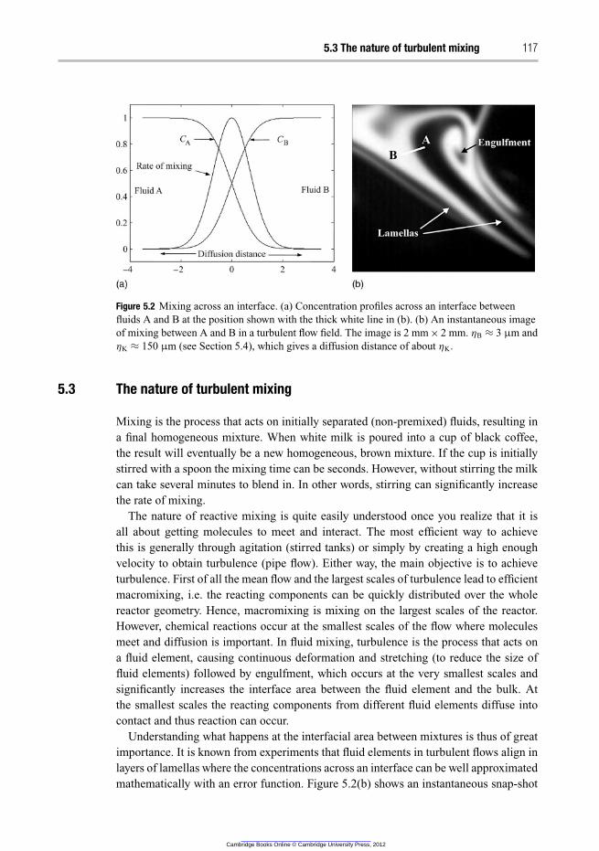
5.3 The nature of turbulent mixing 117
Figure 5.2 Mixing across an interface. (a) Concentration profiles across an interface between
fluids A and B at the position shown with the thick white line in (b). (b) An instantaneous image
of mixing between A and B in a turbulent flow field. The image is 2 mm × 2 mm. ηB ≈ 3 µm and
ηK ≈ 150 µm (see Section 5.4), which gives a diffusion distance of about ηK.
5.3 The nature of turbulent mixing
Mixing is the process that acts on initially separated (non-premixed) fluids, resulting in
a final homogeneous mixture. When white milk is poured into a cup of black coffee,
the result will eventually be a new homogeneous, brown mixture. If the cup is initially
stirred with a spoon the mixing time can be seconds. However, without stirring the milk
can take several minutes to blend in. In other words, stirring can significantly increase
the rate of mixing.
The nature of reactive mixing is quite easily understood once you realize that it is
all about getting molecules to meet and interact. The most efficient way to achieve
this is generally through agitation (stirred tanks) or simply by creating a high enough
velocity to obtain turbulence (pipe flow). Either way, the main objective is to achieve
turbulence. First of all the mean flow and the largest scales of turbulence lead to efficient
macromixing, i.e. the reacting components can be quickly distributed over the whole
reactor geometry. Hence, macromixing is mixing on the largest scales of the reactor.
However, chemical reactions occur at the smallest scales of the flow where molecules
meet and diffusion is important. In fluid mixing, turbulence is the process that acts on
a fluid element, causing continuous deformation and stretching (to reduce the size of
fluid elements) followed by engulfment, which occurs at the very smallest scales and
significantly increases the interface area between the fluid element and the bulk. At
the smallest scales the reacting components from different fluid elements diffuse into
contact and thus reaction can occur.
Understanding what happens at the interfacial area between mixtures is thus of great
importance. It is known from experiments that fluid elements in turbulent flows align in
layers of lamellas where the concentrations across an interface can be well approximated
mathematically with an error function. Figure 5.2(b) shows an instantaneous snap-shot
Cambridge Books Online © Cambridge University Press, 2012
118 Turbulent mixing and chemical reactions
of binary mixing between fluids A and B in a turbulent flow field. The size of the
measured volume corresponds to a computational cell in CFD, and it is evident that
the average concentration in a computational cell will give a poor description of the
concentration during mixing and fast chemical reactions. The theoretical concentrations
and mixing rate (scalar dissipation rate) across an interface are presented in Figure 5.2(a)
with error functions. At the smallest scales in Figure 5.2(a) only diffusion is important
for the mixing process. Turbulence quickly increases the interfacial area between fluid
elements and thus reduces the required diffusion distance, so that the required diffusion
time will be small. If turbulence is intense, diffusion will limit the rate of mixing, and
vice versa if the intensity is too low.
It is of great importance to estimate whether mixing can be a rate-limiting step in
the process. The mixing time must then be compared with a timescale for reaction. A
quantity that compares the timescale of chemical reactions with the timescale of mixing
is the Dahmkohler number (Da):
Da =Typical time required for mixing
Typical time required for chemical reactions. (5.4)
The time for mixing is described in the following equation and the typical time for
chemical reactions can be estimated with Cα as the concentration of the limiting reactant:
τ =Cα
r=
Cα
kCαCβ
=1
kCβ
.
There are three possible outcomes from analysis of the Dahmkohler number:
(1) Da ≪ 1. Reactions are slow compared with the rate of mixing. In other words, the
reactor will have a homogeneous mixture (no segregation) before any substantial
reaction can take place. The concentrations in the computational cells are sufficiently
well described by the average concentration in the cell. For this scenario standard
chemical-reactor models such as the plug-flow reactor or the continuously stirred
tank reactor may suffice.
(2) Da ≫ 1. Reactions are very fast or instantaneous, e.g. acid–base reactions, ion–ion
reactions and some gaseous combustion reactions. This problem often benefits from
CFD modelling since the common reactor models are inapplicable. Furthermore,
since the reactions are instantaneous, it can be shown that studying the evolution
of a conserved scalar suffices to get a complete description of the problem (see
Section 5.5.2). A conserved scalar is an inert, or passive, tracer, and it is is much easier
to study the conserved scalar than reactive species because the (usually nonlinear)
chemical reaction rate need not be modelled.
(3) Da ≈ 1. The timescales for reaction and mixing are of the same order of magnitude.
This scenario is by far the most difficult and requires complex modelling for accurate
predictions of the mean chemical reaction rates. The case cannot be described by
traditional reactor models. Engineers have commonly solved this problem by using
Lagrangian micromixing models. However, these models neglect inhomogeneities
and reactor geometry.
Cambridge Books Online © Cambridge University Press, 2012
5.4 Mixing of a conserved scalar 119
In modelling of cases (2) and (3) the most successful CFD models calculate first the
mixing of a conserved scalar to predict the intensity of segregation of the mixture (the
state of mixedness). This information can further be used to obtain closures for the
mean chemical reaction rate. When reading Section 5.4 it is important to remember that,
even though we are addressing only a conserved scalar, prediction of the mean chemical
reaction rate is the overall main objective.
5.4 Mixing of a conserved scalar
To estimate the Dahmkohler number it is necessary to get an idea of the relevant length
scales and timescales for mixing and reactions in the system concerned. These scales
can be found from simulations of the flow field (the turbulence variables k and ε are
usually sufficient) with some model taken from Section 4.2, or from experiments. It is,
for example, possible to measure the pressure drop over a chemical reactor and from
this estimate the corresponding average rate of energy dissipation. It is also necessary
to gain knowledge of the rate expressions for the chemical reactions (like Eq. (5.2))
and the diffusivity of the reacting species. The smallest length scales and timescales
that are important for chemical reactions are generally not the same as for the flow (see
Chapter 4 about the Kolmogorov scales). This follows since the molecular diffusivity of
species in liquids is usually much lower than the kinematic viscosity of the fluid. The
smallest relevant length scale for reacting flows will be the average distance a molecule
diffuses during the Kolmogorov timescale. This scale is characterized by the Batchelor
length scale ηB, which is represented as
ηB = Sc−1/2ηK. (5.5)
The Schmidt number Sc describes how fast transport of momentum is relative to the
transport of molecules (Sc = ν/D). For gases the Schmidt number is approximately unity
and the Batchelor scale more or less equals the Kolmogorov scale. For water-like liquids
and not-too-large molecules, the Schmidt number is usually close to 1000. The Schmidt
number is high for liquids since momentum can be transported by collisions of molecules,
whereas molecular diffusion represents the movement of individual molecules.
5.4.1 Mixing timescales
The stages of mixing during which fluid elements are deformed and reduced in size
followed by molecular diffusion are referred to in combination as micromixing. The
initial step, i.e. deformation and stretching, is referred to as inertial–convective mix-
ing since the fluid elements are merely transported from large eddies to small eddies
through convection. The timescale for this process is merely the inverse of the rate of
mixing. Hence, modelling of timescales and modelling of mixing rates are equivalent,
the timescale used for describing inertial–convective mixing being
τIC = θ
k
ε
, (5.6)
Cambridge Books Online © Cambridge University Press, 2012
120 Turbulent mixing and chemical reactions
where θ is a constant commonly set to 0.5. There is no Schmidt-number dependence
since viscosity and diffusion are not relevant. For gases (Sc ≈ 1) this single timescale
suffices for a complete description of the mixing process.
At scales just below ηK convective and viscous mixing are of the same order of
magnitude, whereas diffusion is still too slow to interfere for Sc ≫ 1. Mixing on this scale
is commonly referred to as engulfment or viscous–convective mixing. The timescale for
engulfment is often determined by
τVC = 17.25
√
ν
ε
. (5.7)
The final stage of mixing during which all spatial gradients disappear and a homogeneous
mixture is obtained occurs near the Batchelor scale. Mixing at this scale is referred to as
viscous–diffusive mixing since both viscosity and diffusion are important. The timescale
for viscous–diffusive mixing is given as
τVD =τVC
0.303 + 17 050Sc−1, (5.8)
which is proportional to the viscous–convective timescale, but with a Schmidt-number
dependence.
Typical average data for a large stirred-tank reactor with water at room temperature
are k ≈ 0.05 m2 s−2 and ε ≈ 1 W kg−1, giving τ IC = 25 ms, τVC = 17 ms and τVD ≈
1 ms. Only fast reactions in which a noticeable amount has reacted within 1 s need to
be modelled using mixing models. The mixing time for the reactor, i.e. the time taken
to reach the same concentration in the whole reactor, is of the order of minutes, and the
ideal stirred-tank reactor may still be a poor model. The local rate of dissipation around
the impeller is an order of magnitude higher than the average, and good mixing for fast
reactions can be obtained when the reactants are added in the impeller region and the
opposite behaviour is obtained close to the reactor surface.
The characterization of timescales for mixing described in this section is only one
of several suggestions that have appeared in the literature. However, all mixing models
are similar insofar as one must make use of the same parameters that are available from
flow-field computations (ν, k, ε and Sc). The important lesson is that you now have
some tools that can be used to get a first understanding of the problem at hand, through
describing the reactions as slow, fast or instantaneous compared with mixing. You can,
for example, use the knowledge from this section to determine the local rate of mixing
in a stirred tank, which is important for finding the optimal position for injection of a
reactant. Usually it is most efficient to inject where the rate of mixing is fastest, e.g. in
the impeller region.
5.4.2 Probability density functions
In modelling of reactive mixing a very important tool is the probability density function
(PDF) of a mixture fraction (a conserved scalar, i.e. a non-reacting species). The mixture
fraction ξ (x, t) is defined for binary mixtures (mixtures with two inlets) as unity for one
inlet stream and zero for the other. The name mixture fraction is thus logical since it
Cambridge Books Online © Cambridge University Press, 2012
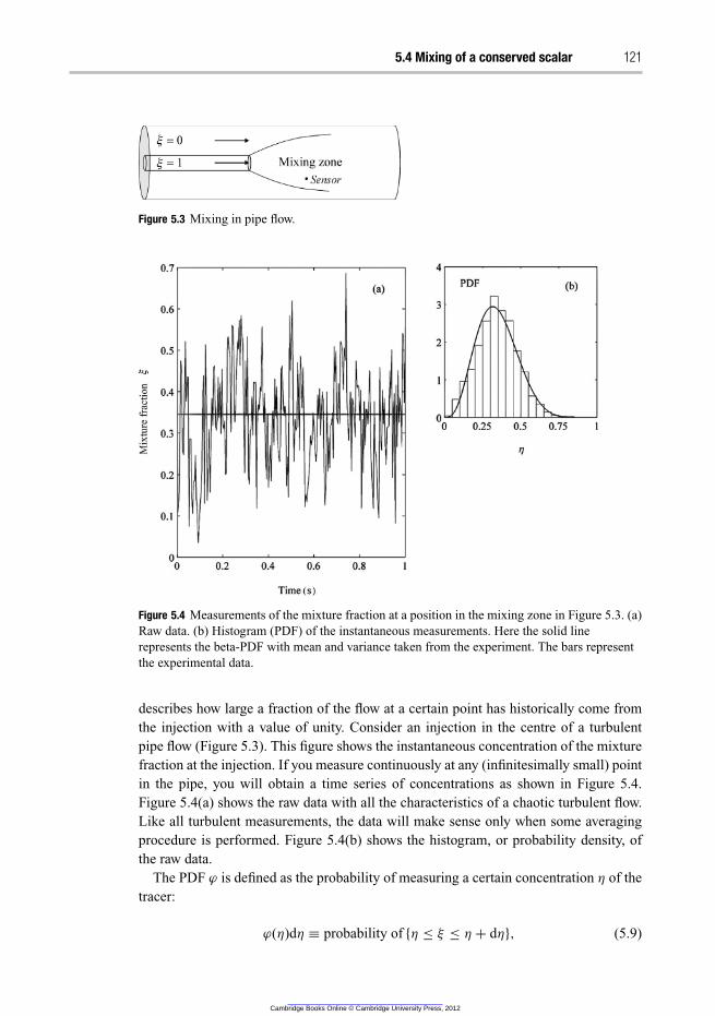
5.4 Mixing of a conserved scalar 121
Figure 5.3 Mixing in pipe flow.
Figure 5.4 Measurements of the mixture fraction at a position in the mixing zone in Figure 5.3. (a)
Raw data. (b) Histogram (PDF) of the instantaneous measurements. Here the solid line
represents the beta-PDF with mean and variance taken from the experiment. The bars represent
the experimental data.
describes how large a fraction of the flow at a certain point has historically come from
the injection with a value of unity. Consider an injection in the centre of a turbulent
pipe flow (Figure 5.3). This figure shows the instantaneous concentration of the mixture
fraction at the injection. If you measure continuously at any (infinitesimally small) point
in the pipe, you will obtain a time series of concentrations as shown in Figure 5.4.
Figure 5.4(a) shows the raw data with all the characteristics of a chaotic turbulent flow.
Like all turbulent measurements, the data will make sense only when some averaging
procedure is performed. Figure 5.4(b) shows the histogram, or probability density, of
the raw data.
The PDF ϕ is defined as the probability of measuring a certain concentration η of the
tracer:
ϕ(η)dη ≡ probability of {η ≤ ξ ≤ η + dη}, (5.9)
Cambridge Books Online © Cambridge University Press, 2012
122 Turbulent mixing and chemical reactions
where η is a sample-space variable for ξ . A sample space is the collection of all possible
outcomes of an event. A variable used to describe a single event in sample space is
a sample-space variable. In mixture-fraction space η is thus the sample-space variable
used to describe the real event ξ .
The sample space of the mixture fraction spans from zero to unity, as shown in
Figure 5.4(b), since these two extremes represent pure mixtures. A logical effect of
mixing is that the mixture fraction cannot take on values outside this range. For a single
bin in the histogram of Figure 5.4(b), dη is chosen to have the discrete value of 0.05, but
for a continuous PDF dη → 0. By definition the integral of the PDF must equal unity:
1∫
0
ϕ(η)dη = 1. (5.10)
For the discrete histogram the integral is defined as the summation over all the bins:∑
bins
ϕ(η)dη = 1. (5.11)
Another way to think of the PDF is that it describes the fraction of time that the mixture
fraction spends in the state η, i.e. the fraction of time a certain concentration or mixture
fraction is observed.
The PDF contains all single-point information of the mixture fraction. Given the PDF,
all mixture fraction moments (mean, variance, skewness etc.) can be found by integration
over mixture-fraction space. The mean 〈ξ 〉 and variance σ2 (second central moment) of
the mixture fraction are defined through the PDF as
〈ξ 〉 =
1∫
0
ηϕ(η)dη and σ2 =
1∫
0
(η − 〈ξ 〉)2ϕ(η)dη. (5.12)
It can be seen from Figure 5.4(b) that for this particular PDF the probability of measuring
a mixture fraction close to the mean is relatively large. In other words, the variance is
small. What happens during mixing is that the variance will gradually decrease until
eventually the mixture is homogeneous, the variance will be zero and the PDF can be
described by a single delta-function. In Figure 5.5 the evolution of the PDF for mixing
in a homogeneous turbulent flow field with a presumed beta-PDF as a model for ϕ (the
mean mixture fraction will be constant and the variance will decrease exponentially in
time) is shown. The beta-PDF uses the mean and variance of the mixture fraction to give
a continuous distribution. The beta-PDF ϕB is defined as
ϕB(η; a, b) =η
a−1 (1 − η)b−1
B(a, b), (5.13)
A semicolon is used to denote that η is a sample-space variable, whereas a and b are fixed
parameters. The coefficients are easily calculated from the average ξ and the variance
σ2 as
a = 〈ξ 〉
[
〈ξ 〉(1 − 〈ξ 〉)
σ2
− 1
]
, b =1 − 〈ξ 〉
〈ξ 〉a (5.14)
Cambridge Books Online © Cambridge University Press, 2012
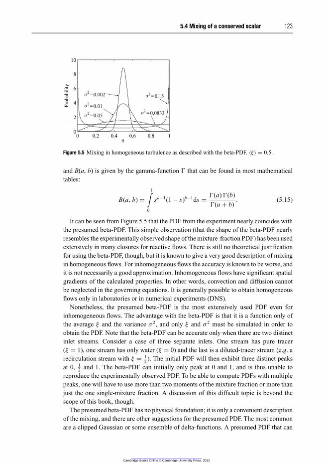
5.4 Mixing of a conserved scalar 123
Figure 5.5 Mixing in homogeneous turbulence as described with the beta-PDF. 〈ξ〉 = 0.5.
and B(a, b) is given by the gamma-function Ŵ that can be found in most mathematical
tables:
B(a, b) =
1∫
0
sa−1(1 − s)b−1ds =Ŵ(a) Ŵ(b)
Ŵ(a + b). (5.15)
It can be seen from Figure 5.5 that the PDF from the experiment nearly coincides with
the presumed beta-PDF. This simple observation (that the shape of the beta-PDF nearly
resembles the experimentally observed shape of the mixture-fraction PDF) has been used
extensively in many closures for reactive flows. There is still no theoretical justification
for using the beta-PDF, though, but it is known to give a very good description of mixing
in homogeneous flows. For inhomogeneous flows the accuracy is known to be worse, and
it is not necessarily a good approximation. Inhomogeneous flows have significant spatial
gradients of the calculated properties. In other words, convection and diffusion cannot
be neglected in the governing equations. It is generally possible to obtain homogeneous
flows only in laboratories or in numerical experiments (DNS).
Nonetheless, the presumed beta-PDF is the most extensively used PDF even for
inhomogeneous flows. The advantage with the beta-PDF is that it is a function only of
the average ξ and the variance σ2, and only ξ and σ
2 must be simulated in order to
obtain the PDF. Note that the beta-PDF can be accurate only when there are two distinct
inlet streams. Consider a case of three separate inlets. One stream has pure tracer
(ξ = 1), one stream has only water (ξ = 0) and the last is a diluted-tracer stream (e.g. a
recirculation stream with ξ = 12). The initial PDF will then exhibit three distinct peaks
at 0, 12
and 1. The beta-PDF can initially only peak at 0 and 1, and is thus unable to
reproduce the experimentally observed PDF. To be able to compute PDFs with multiple
peaks, one will have to use more than two moments of the mixture fraction or more than
just the one single-mixture fraction. A discussion of this difficult topic is beyond the
scope of this book, though.
The presumed beta-PDF has no physical foundation; it is only a convenient description
of the mixing, and there are other suggestions for the presumed PDF. The most common
are a clipped Gaussian or some ensemble of delta-functions. A presumed PDF that can
Cambridge Books Online © Cambridge University Press, 2012
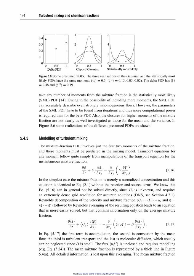
124 Turbulent mixing and chemical reactions
Figure 5.6 Some presumed PDFs. The three realizations of the Gaussian and the statistically most
likely PDFs have the same moments (〈ξ〉 = 0.5, 〈ξ ′2〉 = 0.15, 0.05, 0.02). The delta PDF has 〈ξ〉
= 0.48 and 〈ξ ′2〉 = 0.19.
take any number of moments from the mixture fraction is the statistically most likely
(SML) PDF [14]. Owing to the possibility of including more moments, the SML PDF
can accurately describe even strongly inhomogeneous flows. However, the parameters
of the SML PDF have to be found from iterations and thus more computational power
is required than for the beta-PDF. Also, the closures for higher moments of the mixture
fraction are not nearly as well investigated as those for the mean and the variance. In
Figure 5.6 some realizations of the different presumed PDFs are shown.
5.4.3 Modelling of turbulent mixing
The mixture-fraction PDF involves just the first two moments of the mixture fraction,
and these moments must be predicted in the mixing model. Transport equations for
any moment follow quite simply from manipulations of the transport equation for the
instantaneous mixture fraction:
∂ξ
∂t+ U j
∂ξ
∂x j
=∂
∂x j
(
D∂ξ
∂x j
)
. (5.16)
In the simplest case the mixture fraction is merely a normalized concentration and this
equation is identical to Eq. (2.1) without the reaction and source terms. We know that
Eq. (5.16) can in general not be solved directly, since Ui is unknown, and requires
an extremely dense grid resolution for accurate solutions (DNS, see Section 4.2.1).
Reynolds decomposition of the velocity and mixture fraction (Ui = 〈Ui〉+ ui and ξ =
〈ξ 〉+ ξ′) followed by Reynolds averaging of the resulting equation leads to an equation
that is more easily solved, but that contains information only on the average mixture
fraction:
∂〈ξ 〉
∂t+
⟨
U j
⟩ ∂〈ξ 〉
∂x j
= −∂
∂x j
(
⟨
u jξ′⟩
− D∂〈ξ 〉
∂x j
)
. (5.17)
In Eq. (5.17) the first term is accumulation, the second is convection by the mean
flow, the third is turbulent transport and the last is molecular diffusion, which usually
can be neglected since D is small. The flux 〈ujξ′〉 is unclosed and requires modelling
(e.g. Eq. (5.24)). The mean mixture fraction is represented by a thick line in Figure
5.4(a). All detailed information is lost upon this averaging. The mean mixture fraction
Cambridge Books Online © Cambridge University Press, 2012
5.4 Mixing of a conserved scalar 125
describes macromixing and gives information about the largest scales of the reactor. It is,
however, useless for predicting the level of mixing on the smallest scales (micromixing)
which are important for fast or instantaneous chemical reactions.
Micromixing is often described by the mixture-fraction variance which was previously
defined through the PDF in Eq. (5.12). The variance can be interpreted as a local
average departure from homogeneity, and it is thus a local measure of segregation.
With reference to Figure 5.4(a), the variance can be understood as the intensity of the
fluctuations around the mean. Strong fluctuations mean a large variance (high degree of
segregation). The maximum variance that can be achieved occurs when all measurements
are either zero or unity (the existence of no intermediate values means that no mixing has
occurred). The value of the variance will then equal σ2max = 〈ξ 〉(1 − 〈ξ 〉), which is often
used for normalization. The resulting normalized variance is termed the intensity of
segregation IS:
IS =σ
2
〈ξ 〉(1 − 〈ξ 〉). (5.18)
The intensity of segregation always starts with the value of unity under non-premixed
initial conditions.
A transport equation for σ2 can be found by multiplying Eq. (5.16) by 2ξ , Reynolds
decomposing Ui and ξ , and then taking the Reynolds average of the whole equation:
∂σ2
∂t+
⟨
U j
⟩ ∂σ2
∂x j
= −∂
∂x j
(
⟨
u jξ′2⟩
− D∂σ
2
∂x j
)
− 2⟨
u jξ′⟩ ∂ 〈ξ 〉
∂x j
− 2D
⟨
∂ξ′
∂x j
∂ξ′
∂x j
⟩
.
(5.19)
To derive Eq. (5.19) we have also used Eq. (5.17) and the following identity:
ξ
∂ξ
∂xi
=1
2
∂ξ2
∂xi
. (5.20)
The left-hand side of Eq. (5.19) is accumulation and convection. On the right-hand side
the first term is turbulent transport and molecular diffusion, the second is production
due to interaction between a flux and the gradient of the mean mixture fraction, and
the last term is twice the mean scalar dissipation rate, which we henceforth denote 〈N〉
(see Eq. (5.32)). The mean scalar dissipation rate is the scalar analogue of the mean
energy-dissipation rate ε and is always positive. Physically, this term describes how fast
the mixture-fraction variance is disappearing due to diffusion at the smallest scales.
Note that, even though Eq. (5.19) is an exact equation for the mixture-fraction variance,
problems could arise from its solution. The intensity of segregation cannot, by definition,
be larger than unity. However, with the solution of Eq. (5.19) there is nothing to ensure
that this limit is respected. Problems can arise due to the production term and the closure
for the first-order flux 〈ujξ′〉 (see Eq. (5.24)). There is a nice solution to this problem,
though. Instead of solving for Eq. (5.19) directly, you can solve for the equivalent
Cambridge Books Online © Cambridge University Press, 2012
126 Turbulent mixing and chemical reactions
second raw moment σ2R. The second raw moment is defined as the second moment
around zero:
σ2R =
⟨
ξ2⟩
=
1∫
0
η2ϕ(η)dη. (5.21)
A transport equation for σ2R can be found by exactly the same procedure as for
Eq. (5.19), but without decomposition of ξ . The resulting equation reads
∂σ2R
∂t+
⟨
U j
⟩ ∂σ2R
∂x j
= −∂
∂x j
(
⟨
u jξ2⟩
− D∂σ
2R
∂x j
)
− 2D
⟨
∂ξ
∂x j
∂ξ
∂x j
⟩
. (5.22)
On implementing Eq. (5.22) instead of Eq. (5.19) you will not get any problems of
realizability (unphysical results) since there is no production involved. It also ensures
that the intensity of segregation initially starts out as exactly unity. To obtain the central
variance from the raw moment, simply apply the following formula:
σ2 = σ
2R − 〈ξ 〉2
. (5.23)
In Eqs. (5.17), (5.19) and (5.22) closure is required for 〈ujξ′〉, 〈ujξ
′2〉, 〈ujξ2〉 and 〈N〉,
so these terms will now be discussed further. The first three terms are fluxes, and are
thus required to conserve the mean upon transport (the spatial derivative of the flux is
convection, which is conservative). The only way to achieve this is through gradient-
diffusion models or by deriving completely new transport equations for the fluxes (that
again will contain unknown terms requiring closure). In engineering only the first option
is usually employed. The closures for the fluxes thus become
⟨
u jξ′⟩
= −DT
∂〈ξ 〉
∂x j
, (5.24)
⟨
u jξ′2⟩
= −DT
∂σ2
∂x j
(5.25)
⟨
u jξ2⟩
= −DT
∂σ2R
∂x j
. (5.26)
Here DT is the turbulent diffusivity, which is commonly calculated as
DT =νT
ScT
. (5.27)
The exact form of DT will depend on the turbulence model used for νT (see
Chapter 4). The turbulence Schmidt number ScT is known to vary between approxi-
mately 0.5 and 1.5, but is most commonly set to 0.7. The near-unity value of ScT means
that turbulent transport (macromixing) of momentum and species is almost identical
for most flows. Note that the gradient closures (Eqs. (5.24) − (5.26)) are closely related
to the Boussinesq hypothesis used for modelling of the Reynolds stresses discussed in
Section 4.2.4.
Cambridge Books Online © Cambridge University Press, 2012
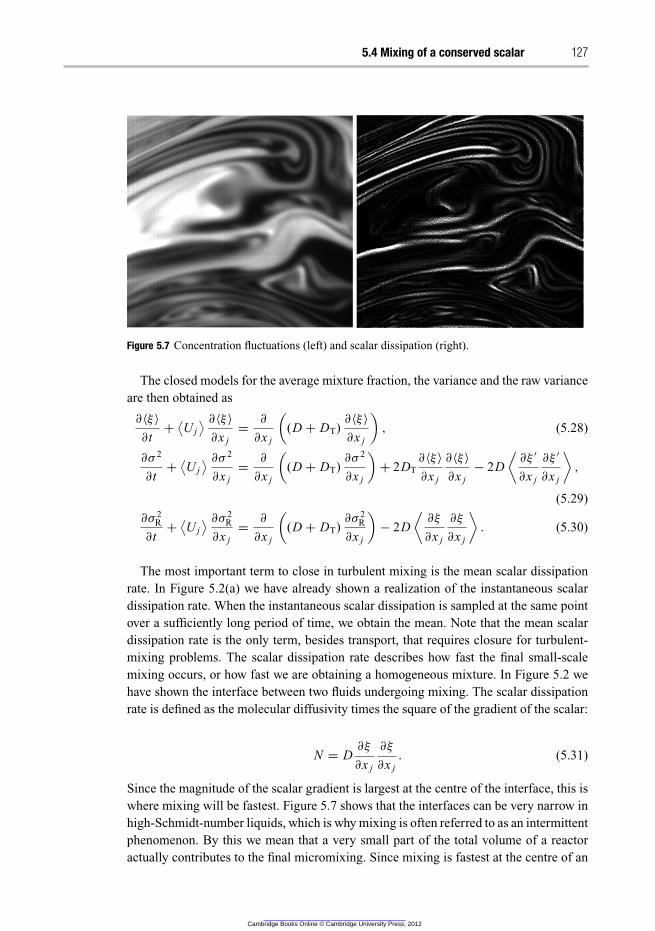
5.4 Mixing of a conserved scalar 127
Figure 5.7 Concentration fluctuations (left) and scalar dissipation (right).
The closed models for the average mixture fraction, the variance and the raw variance
are then obtained as
∂〈ξ 〉
∂t+
⟨
U j
⟩ ∂〈ξ 〉
∂x j
=∂
∂x j
(
(D + DT)∂〈ξ 〉
∂x j
)
, (5.28)
∂σ2
∂t+
⟨
U j
⟩ ∂σ2
∂x j
=∂
∂x j
(
(D + DT)∂σ
2
∂x j
)
+ 2DT
∂〈ξ 〉
∂x j
∂〈ξ 〉
∂x j
− 2D
⟨
∂ξ′
∂x j
∂ξ′
∂x j
⟩
,
(5.29)
∂σ2R
∂t+
⟨
U j
⟩ ∂σ2R
∂x j
=∂
∂x j
(
(D + DT)∂σ
2R
∂x j
)
− 2D
⟨
∂ξ
∂x j
∂ξ
∂x j
⟩
. (5.30)
The most important term to close in turbulent mixing is the mean scalar dissipation
rate. In Figure 5.2(a) we have already shown a realization of the instantaneous scalar
dissipation rate. When the instantaneous scalar dissipation is sampled at the same point
over a sufficiently long period of time, we obtain the mean. Note that the mean scalar
dissipation rate is the only term, besides transport, that requires closure for turbulent-
mixing problems. The scalar dissipation rate describes how fast the final small-scale
mixing occurs, or how fast we are obtaining a homogeneous mixture. In Figure 5.2 we
have shown the interface between two fluids undergoing mixing. The scalar dissipation
rate is defined as the molecular diffusivity times the square of the gradient of the scalar:
N = D∂ξ
∂x j
∂ξ
∂x j
. (5.31)
Since the magnitude of the scalar gradient is largest at the centre of the interface, this is
where mixing will be fastest. Figure 5.7 shows that the interfaces can be very narrow in
high-Schmidt-number liquids, which is why mixing is often referred to as an intermittent
phenomenon. By this we mean that a very small part of the total volume of a reactor
actually contributes to the final micromixing. Since mixing is fastest at the centre of an
Cambridge Books Online © Cambridge University Press, 2012
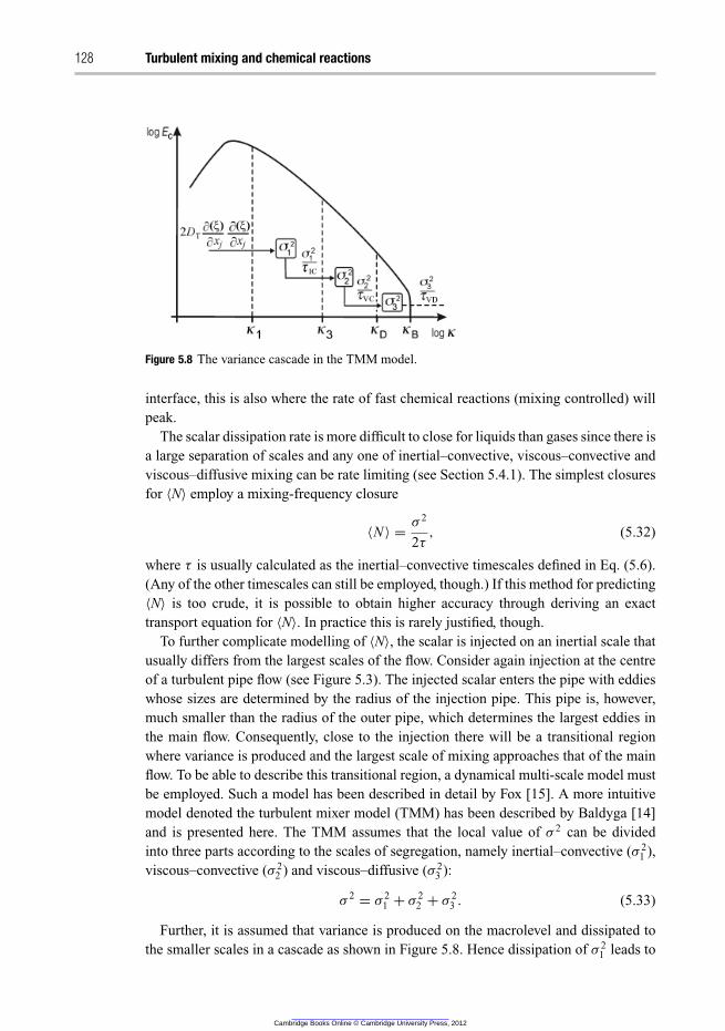
128 Turbulent mixing and chemical reactions
Figure 5.8 The variance cascade in the TMM model.
interface, this is also where the rate of fast chemical reactions (mixing controlled) will
peak.
The scalar dissipation rate is more difficult to close for liquids than gases since there is
a large separation of scales and any one of inertial–convective, viscous–convective and
viscous–diffusive mixing can be rate limiting (see Section 5.4.1). The simplest closures
for 〈N〉 employ a mixing-frequency closure
〈N 〉 =σ
2
2τ
, (5.32)
where τ is usually calculated as the inertial–convective timescales defined in Eq. (5.6).
(Any of the other timescales can still be employed, though.) If this method for predicting
〈N〉 is too crude, it is possible to obtain higher accuracy through deriving an exact
transport equation for 〈N〉. In practice this is rarely justified, though.
To further complicate modelling of 〈N〉, the scalar is injected on an inertial scale that
usually differs from the largest scales of the flow. Consider again injection at the centre
of a turbulent pipe flow (see Figure 5.3). The injected scalar enters the pipe with eddies
whose sizes are determined by the radius of the injection pipe. This pipe is, however,
much smaller than the radius of the outer pipe, which determines the largest eddies in
the main flow. Consequently, close to the injection there will be a transitional region
where variance is produced and the largest scale of mixing approaches that of the main
flow. To be able to describe this transitional region, a dynamical multi-scale model must
be employed. Such a model has been described in detail by Fox [15]. A more intuitive
model denoted the turbulent mixer model (TMM) has been described by Baldyga [14]
and is presented here. The TMM assumes that the local value of σ2 can be divided
into three parts according to the scales of segregation, namely inertial–convective (σ 21 ),
viscous–convective (σ 22 ) and viscous–diffusive (σ 2
3 ):
σ2 = σ
21 + σ
22 + σ
23 . (5.33)
Further, it is assumed that variance is produced on the macrolevel and dissipated to
the smaller scales in a cascade as shown in Figure 5.8. Hence dissipation of σ21 leads to
Cambridge Books Online © Cambridge University Press, 2012
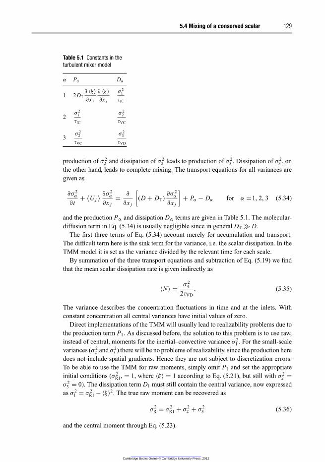
5.4 Mixing of a conserved scalar 129
Table 5.1 Constants in the
turbulent mixer model
α Pα Dα
1 2DT
∂ 〈ξ〉
∂x j
∂ 〈ξ〉
∂x j
σ21
τIC
2σ
21
τIC
σ22
τVC
3σ
22
τVC
σ23
τVD
production of σ22 and dissipation of σ
22 leads to production of σ
23 . Dissipation of σ
23 , on
the other hand, leads to complete mixing. The transport equations for all variances are
given as
∂σ2α
∂t+
⟨
U j
⟩ ∂σ2α
∂x j
=∂
∂x j
[
(D + DT)∂σ
2α
∂x j
]
+ Pα − Dα for α =1, 2, 3 (5.34)
and the production Pα and dissipation Dα terms are given in Table 5.1. The molecular-
diffusion term in Eq. (5.34) is usually negligible since in general DT ≫ D.
The first three terms of Eq. (5.34) account merely for accumulation and transport.
The difficult term here is the sink term for the variance, i.e. the scalar dissipation. In the
TMM model it is set as the variance divided by the relevant time for each scale.
By summation of the three transport equations and subtraction of Eq. (5.19) we find
that the mean scalar dissipation rate is given indirectly as
〈N 〉 =σ
23
2τVD
. (5.35)
The variance describes the concentration fluctuations in time and at the inlets. With
constant concentration all central variances have initial values of zero.
Direct implementations of the TMM will usually lead to realizability problems due to
the production term P1. As discussed before, the solution to this problem is to use raw,
instead of central, moments for the inertial–convective variance σ21 . For the small-scale
variances (σ 22 and σ
23 ) there will be no problems of realizability, since the production here
does not include spatial gradients. Hence they are not subject to discretization errors.
To be able to use the TMM for raw moments, simply omit P1 and set the appropriate
initial conditions (σ 2R1, = 1, where 〈ξ 〉 = 1 according to Eq. (5.21), but still with σ
22 =
σ23 = 0). The dissipation term D1 must still contain the central variance, now expressed
as σ21 = σ
2R1 − 〈ξ 〉2. The true raw moment can be recovered as
σ2R = σ
2R1 + σ
22 + σ
23 (5.36)
and the central moment through Eq. (5.23).
Cambridge Books Online © Cambridge University Press, 2012
130 Turbulent mixing and chemical reactions
In this section we have discussed only pure mixing. By solving the equations above,
we obtain the local mean mixture fraction and variance. The intention has been to obtain
a tool for predicting the turbulence-chemistry effect in order to be able to predict the
average rate of chemical reactions in each computational cell. In the next section we will
discuss how the modelling of a conserved scalar is used in reference to this.
5.5 Modelling of chemical reactions
The modelling hierarchy for reactive flows closely resembles that of pure flows (see
Chapter 4). In general you have to give up information in return for computational
efficiency. In this regard it is important to understand what information you are giving up
and how this can be modelled through simplified relations. As for turbulence modelling
the word ‘simplified’ is actually very misleading. The problem is not easier than direct
numerical simulation (DNS) of the governing equations. However, DNS is possible only
for simple geometries and low Reynolds numbers. Hence, DNS is not an option for
chemical reactors and will most likely remain just a research tool in the foreseeable
future.
The instantaneous equation for reacting species that is solved in DNS consists of
standard accumulation, convection, diffusion and reaction terms:
∂Cα
∂t+ U j
∂Cα
∂x j
=∂
∂x j
(
D∂Cα
∂x j
)
+ Sα(C) . (5.37)
Here C denotes a vector of all the reacting species in the flow, meaning that the source
term for species α, Sα, could depend on any of the other existing species. Since
Eq. (5.37) can be solved only for simple geometries with extremely dense meshes
(DNS), we must introduce some sort of averaging. Here we consider only Reynolds
averaging.
Consider again the reaction described in Eq. (5.1). For a reaction rate r = kCACB the
characteristic chemical-reaction timescale can now be given as either τR = minimum of
1/(k1CA) and 1/(k1CB) or τR = 1/(k1CA + k1CB), where the concentrations are defined
at the inlets. (Note that, since this is only an approximate timescale, the definitions are
not strict.) This timescale should now be used to predict the Dahmkohler number to see
which scenario of Section 5.3 is relevant.
5.5.1 Da ≪ 1
If the Dahmkohler number is small there is no problem, since there is sufficient time for
local mixing and the covariance term in Eq. (5.3) will be zero. The reaction rate can be
expressed merely through the mean concentrations that are already known. The reaction
described in Eqs. (5.1)–(5.3) can now easily be closed by neglecting the covariance in
Eq. (5.3), and we obtain
SA = −k1CACB. (5.38)
Cambridge Books Online © Cambridge University Press, 2012
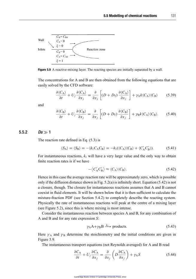
5.5 Modelling of chemical reactions 131
Figure 5.9 A reactive-mixing layer. The reacting species are initially separated by a wall.
The concentrations for A and B are then obtained from the following equations that are
easily solved by the CFD software:
∂〈CA〉
∂t+ U j
∂〈CA〉
∂x j
=∂
∂x j
[
(D + DT)∂〈CA〉
∂x j
]
+ γAk〈CA〉〈CB〉 (5.39)
and
∂〈CB〉
∂t+ U j
∂〈CB〉
∂x j
=∂
∂x j
[
(D + DT)∂〈CB〉
∂x j
]
+ γBk〈CA〉〈CB〉. (5.40)
5.5.2 Da ≫ 1
The reaction rate defined in Eq. (5.3) is
〈SA〉 = 〈SB〉 = −〈k1CACB〉 = −k1(〈CA〉〈CB〉 + 〈C ′AC ′
B〉). (5.41)
For instantaneous reactions, k1 will have a very large value and the only way to obtain
finite reaction rates is if we have
−⟨
C ′AC ′
B
⟩
≈ 〈CA〉〈CB〉. (5.42)
Hence in this case the average reaction rate will be approximately zero, which is possible
only if the diffusion distance shown in Fig. 5.2(a) is infinitely short. Equation (5.42) is not
a closure, though. The closure for instantaneous reactions assumes that A and B cannot
coexist in fluid elements. It will be shown below that it is then sufficient to calculate the
mixture-fraction PDF (see Section 5.4.2) to completely describe the reacting system.
Physically the rate of instantaneous reactions will peak at the centre of a mixing layer
(see Figure 5.2), since this is where mixing is most intense.
Consider the instantaneous reaction between species A and B, for any combination of
A and B and for any rate expression S:
γAA+γBB k1−→ products. (5.43)
Here γ A and γ B determine the stoichiometry and the initial conditions are given in
Figure 5.9.
The instantaneous transport equations (not Reynolds averaged) for A and B read
∂CA
∂t+ U j
∂CA
∂x j
=∂
∂x j
(
D∂CA
∂x j
)
+ γAS (5.44)
Cambridge Books Online © Cambridge University Press, 2012
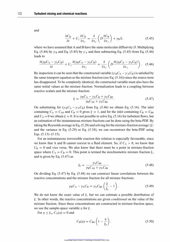
132 Turbulent mixing and chemical reactions
and
∂CB
∂t+ U j
∂CB
∂x j
=∂
∂x j
(
D∂CB
∂x j
)
+ γBS, (5.45)
where we have assumed that A and B have the same molecular diffusivity D. Multiplying
Eq. (5.44) by γ B and Eq. (5.45) by γ A and then subtracting Eq. (5.45) from Eq. (5.44)
leads to
∂(γBCA − γACB)
∂t+ U j
∂(γBCA − γACB)
∂x j
=∂
∂x j
(
D∂(γBCA − γACB)
∂x j
)
. (5.46)
By inspection it can be seen that the constructed variable (γ BCA − γ ACB) is satisfied by
the same transport equation as the mixture fraction (see Eq. (5.16)) since the source term
has disappeared. To be completely identical, the constructed variable must also have the
same initial values as the mixture fraction. Normalization leads to a coupling between
reactive scalars and the mixture fraction:
ξ =γBCA − γACB + γACB0
γBCA0 + γACB0
. (5.47)
On substituting for (γ BCA − γ ACB) from Eq. (5.46) we obtain Eq. (5.16). The inlet
containing CA = CA0 and CB = 0 gives ξ = 1, and for the inlet containing CB = CB0
and CA = 0 we obtain ξ = 0. It is not possible to solve Eq. (5.16) for turbulent flows, but
an estimation of the instantaneous mixture fractions can be done using the beta-PDF. By
taking the Reynolds average in Eq. (5.28) and solving for the mixture-fraction average 〈ξ 〉
and the variance in Eq. (5.29) or Eq. (5.34), we can reconstruct the beta-PDF using
Eqs. (5.13)–(5.15).
For an instantaneous irreversible reaction this relation is especially favourable, since
we know that A and B cannot coexist in a fluid element. So, if CA > 0, we know that
CB = 0 and vice versa. We also know that there must be a point in mixture-fraction
space where CA = CB = 0. This point is termed the stoichiometric mixture fraction ξ s
and is given by Eq. (5.47) as
ξs =γACB0
γBCA0 + γACB0
. (5.48)
On dividing Eq. (5.47) by Eq. (5.48) we can construct linear correlations between the
reactive concentrations and the mixture fraction for all mixture fractions:
γBCA − γACB = γACB0
(
ξ
ξs
− 1
)
. (5.49)
We do not know the exact value of ξ , but we can estimate a possible distribution of
ξ . In other words, the reactive concentrations are given conditional on the value of the
mixture fraction. Since these concentrations are constructed in mixture-fraction space,
we use the sample-space variable η for ξ .
For η ≤ ξ s, CA(η) = 0 and
CB(η) = CB0
(
1 −η
ξs
)
. (5.50)
Cambridge Books Online © Cambridge University Press, 2012
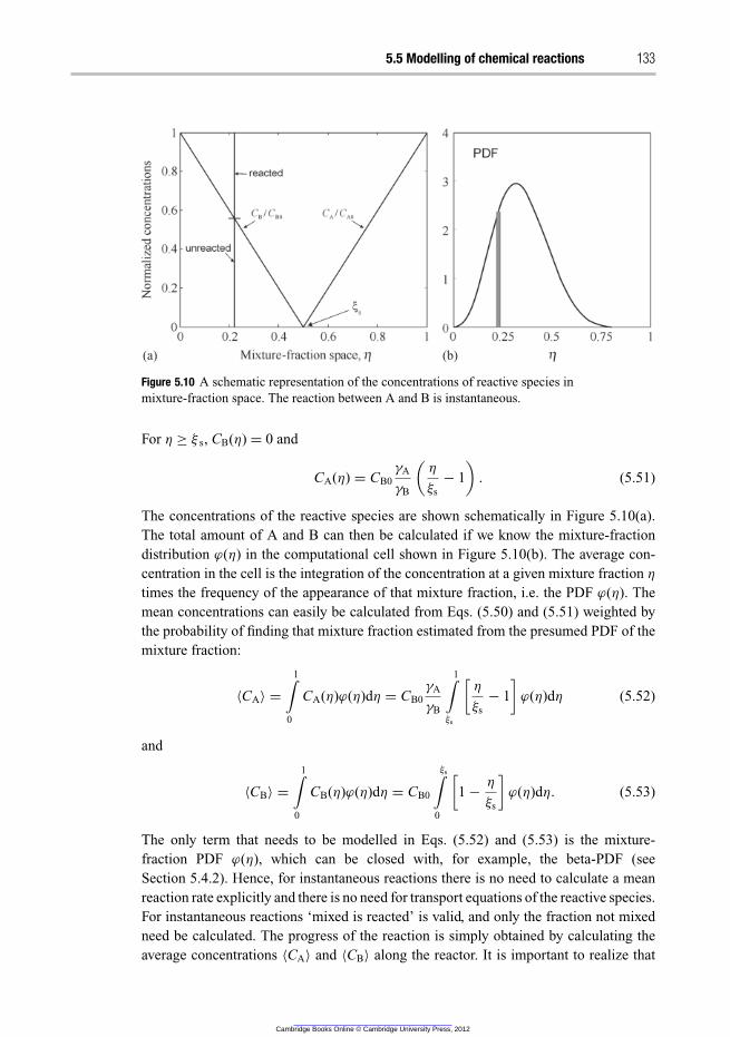
5.5 Modelling of chemical reactions 133
(a) (b)
Figure 5.10 A schematic representation of the concentrations of reactive species in
mixture-fraction space. The reaction between A and B is instantaneous.
For η ≥ ξ s, CB(η) = 0 and
CA(η) = CB0
γA
γB
(
η
ξs
− 1
)
. (5.51)
The concentrations of the reactive species are shown schematically in Figure 5.10(a).
The total amount of A and B can then be calculated if we know the mixture-fraction
distribution ϕ(η) in the computational cell shown in Figure 5.10(b). The average con-
centration in the cell is the integration of the concentration at a given mixture fraction η
times the frequency of the appearance of that mixture fraction, i.e. the PDF ϕ(η). The
mean concentrations can easily be calculated from Eqs. (5.50) and (5.51) weighted by
the probability of finding that mixture fraction estimated from the presumed PDF of the
mixture fraction:
〈CA〉 =
1∫
0
CA(η)ϕ(η)dη = CB0
γA
γB
1∫
ξs
[
η
ξs
− 1
]
ϕ(η)dη (5.52)
and
〈CB〉 =
1∫
0
CB(η)ϕ(η)dη = CB0
ξs∫
0
[
1 −η
ξs
]
ϕ(η)dη. (5.53)
The only term that needs to be modelled in Eqs. (5.52) and (5.53) is the mixture-
fraction PDF ϕ(η), which can be closed with, for example, the beta-PDF (see
Section 5.4.2). Hence, for instantaneous reactions there is no need to calculate a mean
reaction rate explicitly and there is no need for transport equations of the reactive species.
For instantaneous reactions ‘mixed is reacted’ is valid, and only the fraction not mixed
need be calculated. The progress of the reaction is simply obtained by calculating the
average concentrations 〈CA〉 and 〈CB〉 along the reactor. It is important to realize that
Cambridge Books Online © Cambridge University Press, 2012
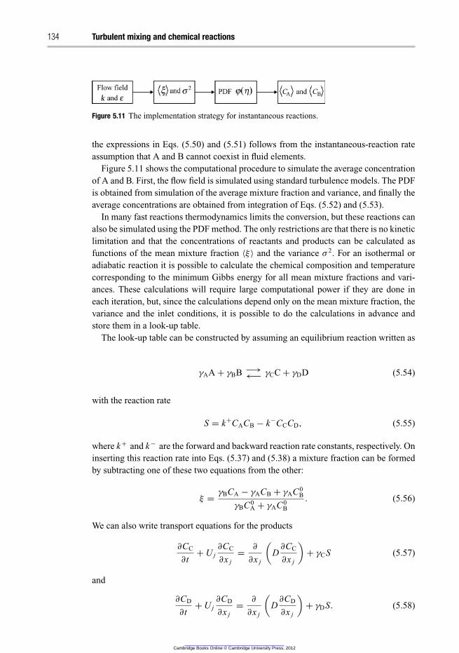
134 Turbulent mixing and chemical reactions
Figure 5.11 The implementation strategy for instantaneous reactions.
the expressions in Eqs. (5.50) and (5.51) follows from the instantaneous-reaction rate
assumption that A and B cannot coexist in fluid elements.
Figure 5.11 shows the computational procedure to simulate the average concentration
of A and B. First, the flow field is simulated using standard turbulence models. The PDF
is obtained from simulation of the average mixture fraction and variance, and finally the
average concentrations are obtained from integration of Eqs. (5.52) and (5.53).
In many fast reactions thermodynamics limits the conversion, but these reactions can
also be simulated using the PDF method. The only restrictions are that there is no kinetic
limitation and that the concentrations of reactants and products can be calculated as
functions of the mean mixture fraction 〈ξ 〉 and the variance σ2. For an isothermal or
adiabatic reaction it is possible to calculate the chemical composition and temperature
corresponding to the minimum Gibbs energy for all mean mixture fractions and vari-
ances. These calculations will require large computational power if they are done in
each iteration, but, since the calculations depend only on the mean mixture fraction, the
variance and the inlet conditions, it is possible to do the calculations in advance and
store them in a look-up table.
The look-up table can be constructed by assuming an equilibrium reaction written as
γAA + γBB −→←− γCC + γDD (5.54)
with the reaction rate
S = k+CACB − k−CCCD, (5.55)
where k+ and k− are the forward and backward reaction rate constants, respectively. On
inserting this reaction rate into Eqs. (5.37) and (5.38) a mixture fraction can be formed
by subtracting one of these two equations from the other:
ξ =γBCA − γACB + γAC0
B
γBC0A + γAC0
B
. (5.56)
We can also write transport equations for the products
∂CC
∂t+ U j
∂CC
∂x j
=∂
∂x j
(
D∂CC
∂x j
)
+ γCS (5.57)
and
∂CD
∂t+ U j
∂CD
∂x j
=∂
∂x j
(
D∂CD
∂x j
)
+ γDS. (5.58)
Cambridge Books Online © Cambridge University Press, 2012
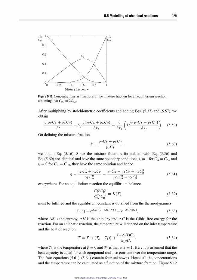
5.5 Modelling of chemical reactions 135
Figure 5.12 Concentrations as functions of the mixture fraction for an equilibrium reaction
assuming that CB0 = 2CA0.
After multiplying by stoichiometric coefficients and adding Eqs. (5.37) and (5.57), we
obtain
∂(γCCA + γACC)
∂t+ U j
∂(γCCA + γACC)
∂x j
=∂
∂x j
(
D∂(γCCA + γACC)
∂x j
)
. (5.59)
On defining the mixture fraction
ξ =γCCA + γACC
γCC0A
, (5.60)
we obtain Eq. (5.16). Since the mixture fractions formulated with Eq. (5.56) and
Eq. (5.60) are identical and have the same boundary conditions, ξ = 1 for CA = CA0 and
ξ = 0 for CB = CB0, they have the same solution and hence
ξ =γCCA + γACC
γCC0A
=γBCA − γACB + γAC0
B
γBC0A + γAC0
B
(5.61)
everywhere. For an equilibrium reaction the equilibrium balance
CγC
C CγD
D
CγA
A CγB
B
= K (T ) (5.62)
must be fulfilled and the equilibrium constant is obtained from the thermodynamics:
K (T ) = e�S/Re−�H/(RT ) = e−�G/(RT ), (5.63)
where �S is the entropy, �H is the enthalpy and �G is the Gibbs free energy for the
reaction. For an adiabatic reaction, the temperature will depend on the inlet temperature
and the heat of reaction:
T = T1 + (T2 − T1)ξ +(−�H )CC
γCρC p
, (5.64)
where T1 is the temperature at ξ = 0 and T2 is that at ξ = 1. Here it is assumed that the
heat capacity is equal for each compound and also constant over the temperature range.
The four equations (5.61)–(5.64) contain four unknowns. Hence all the concentrations
and the temperature can be calculated as a function of the mixture fraction. Figure 5.12
Cambridge Books Online © Cambridge University Press, 2012
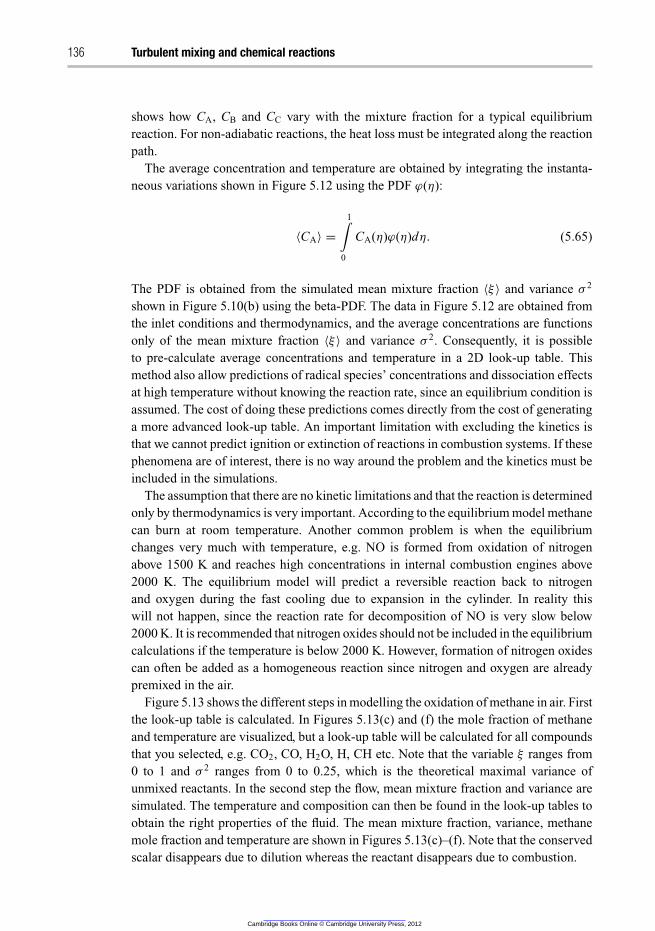
136 Turbulent mixing and chemical reactions
shows how CA, CB and CC vary with the mixture fraction for a typical equilibrium
reaction. For non-adiabatic reactions, the heat loss must be integrated along the reaction
path.
The average concentration and temperature are obtained by integrating the instanta-
neous variations shown in Figure 5.12 using the PDF ϕ(η):
〈CA〉 =
1∫
0
CA(η)ϕ(η)dη. (5.65)
The PDF is obtained from the simulated mean mixture fraction 〈ξ 〉 and variance σ2
shown in Figure 5.10(b) using the beta-PDF. The data in Figure 5.12 are obtained from
the inlet conditions and thermodynamics, and the average concentrations are functions
only of the mean mixture fraction 〈ξ 〉 and variance σ2. Consequently, it is possible
to pre-calculate average concentrations and temperature in a 2D look-up table. This
method also allow predictions of radical species’ concentrations and dissociation effects
at high temperature without knowing the reaction rate, since an equilibrium condition is
assumed. The cost of doing these predictions comes directly from the cost of generating
a more advanced look-up table. An important limitation with excluding the kinetics is
that we cannot predict ignition or extinction of reactions in combustion systems. If these
phenomena are of interest, there is no way around the problem and the kinetics must be
included in the simulations.
The assumption that there are no kinetic limitations and that the reaction is determined
only by thermodynamics is very important. According to the equilibrium model methane
can burn at room temperature. Another common problem is when the equilibrium
changes very much with temperature, e.g. NO is formed from oxidation of nitrogen
above 1500 K and reaches high concentrations in internal combustion engines above
2000 K. The equilibrium model will predict a reversible reaction back to nitrogen
and oxygen during the fast cooling due to expansion in the cylinder. In reality this
will not happen, since the reaction rate for decomposition of NO is very slow below
2000 K. It is recommended that nitrogen oxides should not be included in the equilibrium
calculations if the temperature is below 2000 K. However, formation of nitrogen oxides
can often be added as a homogeneous reaction since nitrogen and oxygen are already
premixed in the air.
Figure 5.13 shows the different steps in modelling the oxidation of methane in air. First
the look-up table is calculated. In Figures 5.13(c) and (f) the mole fraction of methane
and temperature are visualized, but a look-up table will be calculated for all compounds
that you selected, e.g. CO2, CO, H2O, H, CH etc. Note that the variable ξ ranges from
0 to 1 and σ2 ranges from 0 to 0.25, which is the theoretical maximal variance of
unmixed reactants. In the second step the flow, mean mixture fraction and variance are
simulated. The temperature and composition can then be found in the look-up tables to
obtain the right properties of the fluid. The mean mixture fraction, variance, methane
mole fraction and temperature are shown in Figures 5.13(c)–(f). Note that the conserved
scalar disappears due to dilution whereas the reactant disappears due to combustion.
Cambridge Books Online © Cambridge University Press, 2012
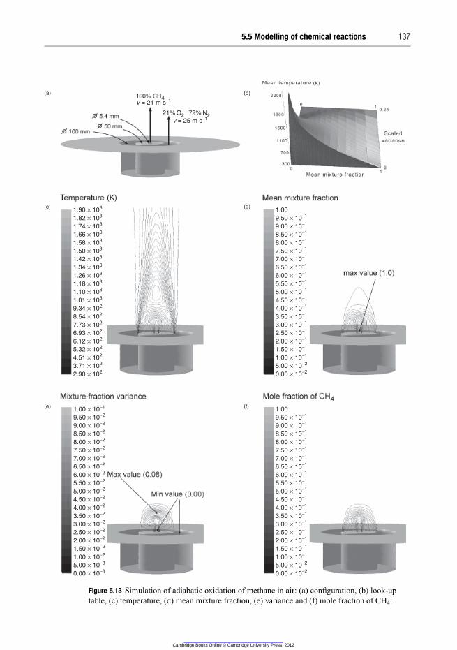
5.5 Modelling of chemical reactions 137
(K)
1.90 × 10³
1.82 × 10³
1.74 × 10³
1.66 × 10³
1.58 × 10³
1.50 × 10³
1.42 × 10³
1.34 × 10³
1.26 × 10³
1.18 × 10³
1.10 × 10³
1.01 × 10³
9.34 × 10²
8.54 × 10²
7.73 × 10²
6.93 × 10²
6.12 × 10²
5.32 × 10²
4.51 × 10²
3.71 × 10²
2.90 × 10²
1.00
9.50 × 10⁻¹
9.00 × 10⁻¹
8.50 × 10⁻¹
8.00 × 10⁻¹
7.50 × 10⁻¹
7.00 × 10⁻¹
6.50 × 10⁻¹
6.00 × 10⁻¹
5.50 × 10⁻¹
5.00 × 10⁻¹
4.50 × 10⁻¹
4.00 × 10⁻¹
3.50 × 10⁻¹
3.00 × 10⁻¹
2.50 × 10⁻¹
2.00 × 10⁻¹
1.50 × 10⁻¹
1.00 × 10⁻¹
5.00 × 10⁻²
0.00 × 10⁻²
1.00
9.50 × 10⁻¹
9.00 × 10⁻¹
8.50 × 10⁻¹
8.00 × 10⁻¹
7.50 × 10⁻¹
7.00 × 10⁻¹
6.50 × 10⁻¹
6.00 × 10⁻¹
5.50 × 10⁻¹
5.00 × 10⁻¹
4.50 × 10⁻¹
4.00 × 10⁻¹
3.50 × 10⁻¹
3.00 × 10⁻¹
2.50 × 10⁻¹
2.00 × 10⁻¹
1.50 × 10⁻¹
1.00 × 10⁻¹
5.00 × 10⁻²
0.00 × 10⁻²
9.50 × 10−21.00 × 10−1
9.00 × 10⁻²
8.50 × 10⁻²
8.00 × 10⁻²
7.50 × 10⁻²
7.00 × 10⁻²
6.50 × 10⁻²
6.00 × 10⁻²
5.50 × 10⁻²
5.00 × 10⁻²
4.50 × 10⁻²
4.00 × 10⁻²
3.50 × 10⁻²
3.00 × 10⁻²
2.50 × 10⁻²
2.00 × 10⁻²
1.50 × 10⁻²
1.00 × 10⁻²
5.00 × 10⁻³
0.00 × 10⁻³
(K)
(b)
(d)
(f)
(a)
(c)
(e)
N2O2 , 79%21%
v = 25 m s−1
v = 21 m s−1
-
Figure 5.13 Simulation of adiabatic oxidation of methane in air: (a) configuration, (b) look-up
table, (c) temperature, (d) mean mixture fraction, (e) variance and (f) mole fraction of CH4.
Cambridge Books Online © Cambridge University Press, 2012
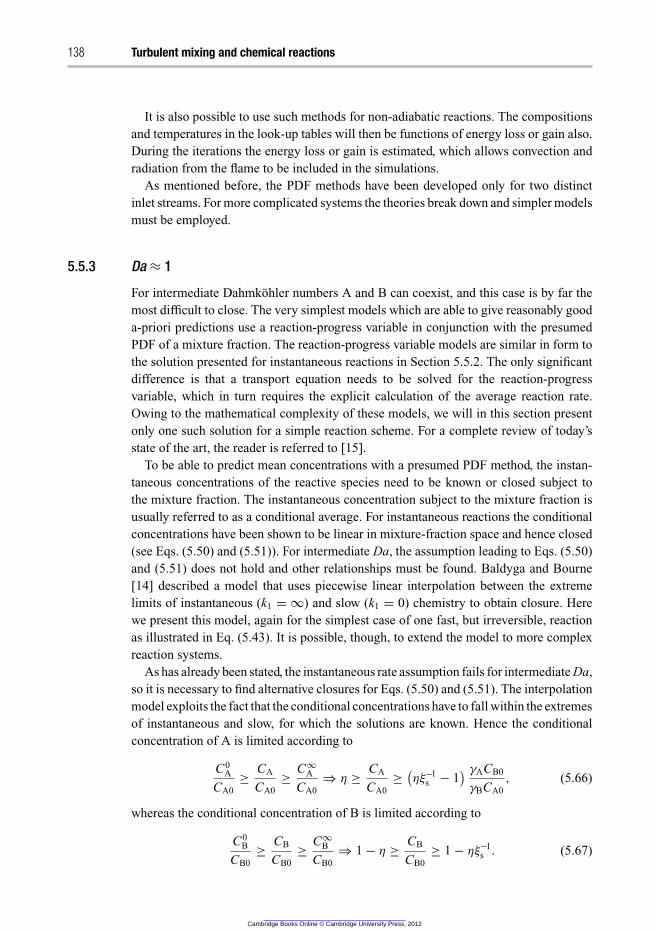
138 Turbulent mixing and chemical reactions
It is also possible to use such methods for non-adiabatic reactions. The compositions
and temperatures in the look-up tables will then be functions of energy loss or gain also.
During the iterations the energy loss or gain is estimated, which allows convection and
radiation from the flame to be included in the simulations.
As mentioned before, the PDF methods have been developed only for two distinct
inlet streams. For more complicated systems the theories break down and simpler models
must be employed.
5.5.3 Da ≈ 1
For intermediate Dahmkohler numbers A and B can coexist, and this case is by far the
most difficult to close. The very simplest models which are able to give reasonably good
a-priori predictions use a reaction-progress variable in conjunction with the presumed
PDF of a mixture fraction. The reaction-progress variable models are similar in form to
the solution presented for instantaneous reactions in Section 5.5.2. The only significant
difference is that a transport equation needs to be solved for the reaction-progress
variable, which in turn requires the explicit calculation of the average reaction rate.
Owing to the mathematical complexity of these models, we will in this section present
only one such solution for a simple reaction scheme. For a complete review of today’s
state of the art, the reader is referred to [15].
To be able to predict mean concentrations with a presumed PDF method, the instan-
taneous concentrations of the reactive species need to be known or closed subject to
the mixture fraction. The instantaneous concentration subject to the mixture fraction is
usually referred to as a conditional average. For instantaneous reactions the conditional
concentrations have been shown to be linear in mixture-fraction space and hence closed
(see Eqs. (5.50) and (5.51)). For intermediate Da, the assumption leading to Eqs. (5.50)
and (5.51) does not hold and other relationships must be found. Baldyga and Bourne
[14] described a model that uses piecewise linear interpolation between the extreme
limits of instantaneous (k1 = ∞) and slow (k1 = 0) chemistry to obtain closure. Here
we present this model, again for the simplest case of one fast, but irreversible, reaction
as illustrated in Eq. (5.43). It is possible, though, to extend the model to more complex
reaction systems.
As has already been stated, the instantaneous rate assumption fails for intermediate Da,
so it is necessary to find alternative closures for Eqs. (5.50) and (5.51). The interpolation
model exploits the fact that the conditional concentrations have to fall within the extremes
of instantaneous and slow, for which the solutions are known. Hence the conditional
concentration of A is limited according to
C0A
CA0
≥CA
CA0
≥C∞
A
CA0
⇒ η ≥CA
CA0
≥(
ηξ−1s − 1
) γACB0
γBCA0
, (5.66)
whereas the conditional concentration of B is limited according to
C0B
CB0
≥CB
CB0
≥C∞
B
CB0
⇒ 1 − η ≥CB
CB0
≥ 1 − ηξ−1s . (5.67)
Cambridge Books Online © Cambridge University Press, 2012
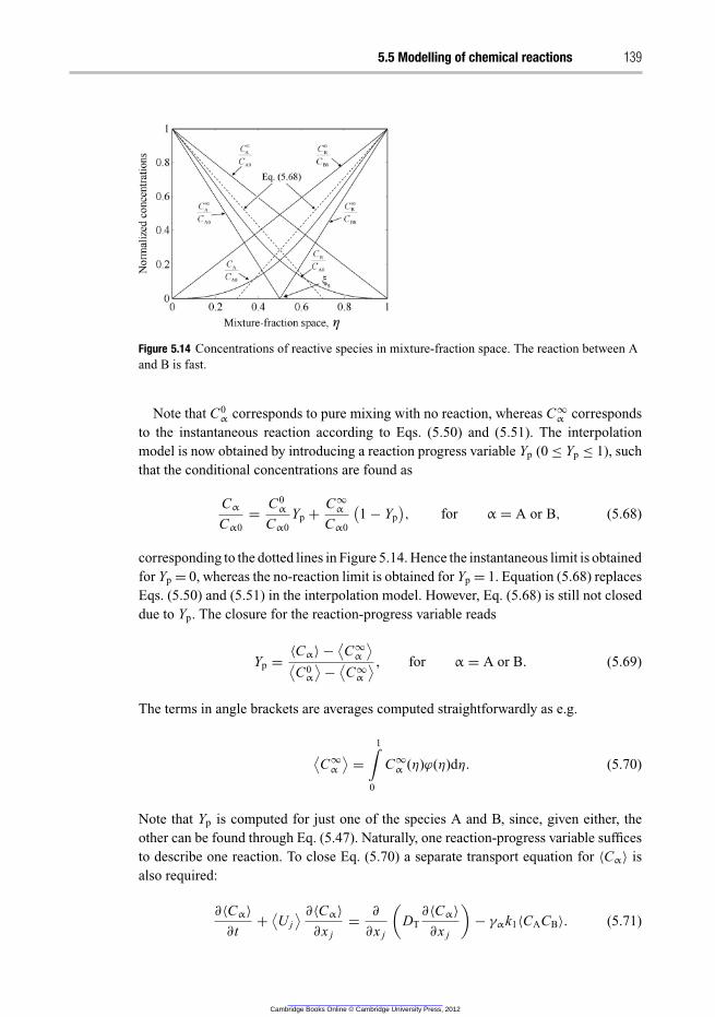
5.5 Modelling of chemical reactions 139
Figure 5.14 Concentrations of reactive species in mixture-fraction space. The reaction between A
and B is fast.
Note that C0α corresponds to pure mixing with no reaction, whereas C∞
α corresponds
to the instantaneous reaction according to Eqs. (5.50) and (5.51). The interpolation
model is now obtained by introducing a reaction progress variable Yp (0 ≤ Yp ≤ 1), such
that the conditional concentrations are found as
Cα
Cα0
=C0
α
Cα0
Yp +C∞
α
Cα0
(
1 − Yp
)
, for α = A or B, (5.68)
corresponding to the dotted lines in Figure 5.14. Hence the instantaneous limit is obtained
for Yp = 0, whereas the no-reaction limit is obtained for Yp = 1. Equation (5.68) replaces
Eqs. (5.50) and (5.51) in the interpolation model. However, Eq. (5.68) is still not closed
due to Yp. The closure for the reaction-progress variable reads
Yp =〈Cα〉 −
⟨
C∞α
⟩
⟨
C0α
⟩
−⟨
C∞α
⟩ , for α = A or B. (5.69)
The terms in angle brackets are averages computed straightforwardly as e.g.
⟨
C∞α
⟩
=
1∫
0
C∞α (η)ϕ(η)dη. (5.70)
Note that Yp is computed for just one of the species A and B, since, given either, the
other can be found through Eq. (5.47). Naturally, one reaction-progress variable suffices
to describe one reaction. To close Eq. (5.70) a separate transport equation for 〈Cα〉 is
also required:
∂〈Cα〉
∂t+
⟨
U j
⟩ ∂〈Cα〉
∂x j
=∂
∂x j
(
DT
∂〈Cα〉
∂x j
)
− γαk1〈CACB〉. (5.71)
Cambridge Books Online © Cambridge University Press, 2012

140 Turbulent mixing and chemical reactions
Figure 5.15 An implementation strategy for the interpolation model.
For the current purpose α can be either A or B. The average reaction rate can be computed
as
k1〈CACB〉 = k1
1∫
0
CA(η)CB(η)ϕ(η)dη. (5.72)
where CA(η) is computed from Eq. (5.68) and CB(η) can be computed from Eq. (5.47)
with ξ = η and γ A = γ B as
CB(η) = CA(η) + CB0 − η(CA0 + CB0). (5.73)
Equation (5.72) closes the problem and the interpolation model can be implemented
using the strategy of Figure 5.15. First (1) the flow field needs to be computed to
provide the turbulent kinetic energy and energy-dissipation rates. These parameters are
then used for calculating the mean and variance of a mixture fraction using e.g. the
TMM model (2) that further can be used to close the mixture fraction PDF from e.g.
Eqs (5.13)–(5.15). With the PDF we can (3) compute the average reaction rate that closes
the transport equation for the average reactive species.
Any model can be used for steps (1) and (2) in Figure 5.15 as long as the
mixture-fraction PDF is delivered to the final step. The final step requires solution of
Eq. (5.71) using Eqs. (5.47), (5.68)–(5.70) and (5.72). The average concentration in the
computational cell is iterated. An initial guess of 〈CA〉 gives the progress variable in Eq.
(5.69) that is used for calculating the reaction rate in Eq. (5.72). This reaction rate is
then used in solving Eq. (5.71), which produces a new value of 〈CA〉. Note that there is
only one more transport equation that needs to be solved in the CFD problem. All the
remaining equations are algebraic and must be solved for in user-defined functions to
provide the reaction rate as input for the transported species.
A more general procedure for implementing reaction-progress variables that can be
more easily extended to multiple reactions has been described by Fox [15].
The state of the art for presumed PDF methods is the conditional moment closure that
actually solves transport equations for the conditional concentrations in mixture-fraction
space, instead of relying on the linear interpolations. The conditional moment closure
has been applied both to combustion and to mixing-sensitive liquid reactions. One
major disadvantage of the conditional moment closure is that the governing transport
equations are five-dimensional (three spatial, one time and one mixture-fraction space)
and thus computationally demanding. The large-dimensionality space is also one of the
major problems of today’s state of the art in modelling of reactive mixing, the full PDF
methods, which solve transport equations for the joint PDF of reactive species. In full
PDF methods the dimensional space is proportional to the number of reacting species,
which can be substantial.
Cambridge Books Online © Cambridge University Press, 2012
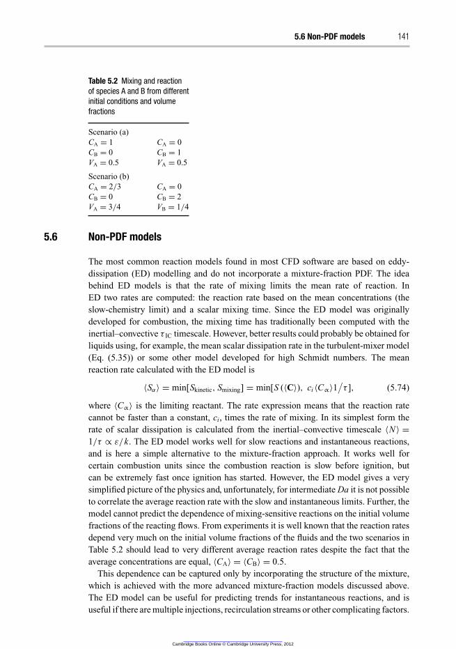
5.6 Non-PDF models 141
Table 5.2 Mixing and reaction
of species A and B from different
initial conditions and volume
fractions
Scenario (a)
CA = 1 CA = 0
CB = 0 CB = 1
VA = 0.5 VA = 0.5
Scenario (b)
CA = 2/3 CA = 0
CB = 0 CB = 2
VA = 3/4 VB = 1/4
5.6 Non-PDF models
The most common reaction models found in most CFD software are based on eddy-
dissipation (ED) modelling and do not incorporate a mixture-fraction PDF. The idea
behind ED models is that the rate of mixing limits the mean rate of reaction. In
ED two rates are computed: the reaction rate based on the mean concentrations (the
slow-chemistry limit) and a scalar mixing time. Since the ED model was originally
developed for combustion, the mixing time has traditionally been computed with the
inertial–convective τ IC timescale. However, better results could probably be obtained for
liquids using, for example, the mean scalar dissipation rate in the turbulent-mixer model
(Eq. (5.35)) or some other model developed for high Schmidt numbers. The mean
reaction rate calculated with the ED model is
〈Sα〉 = min[Skinetic, Smixing] = min[S (〈C〉), ci 〈Cα〉1/
τ ], (5.74)
where 〈Cα〉 is the limiting reactant. The rate expression means that the reaction rate
cannot be faster than a constant, ci, times the rate of mixing. In its simplest form the
rate of scalar dissipation is calculated from the inertial–convective timescale 〈N 〉 =
1/τ ∝ ε/k. The ED model works well for slow reactions and instantaneous reactions,
and is here a simple alternative to the mixture-fraction approach. It works well for
certain combustion units since the combustion reaction is slow before ignition, but
can be extremely fast once ignition has started. However, the ED model gives a very
simplified picture of the physics and, unfortunately, for intermediate Da it is not possible
to correlate the average reaction rate with the slow and instantaneous limits. Further, the
model cannot predict the dependence of mixing-sensitive reactions on the initial volume
fractions of the reacting flows. From experiments it is well known that the reaction rates
depend very much on the initial volume fractions of the fluids and the two scenarios in
Table 5.2 should lead to very different average reaction rates despite the fact that the
average concentrations are equal, 〈CA〉 = 〈CB〉 = 0.5.
This dependence can be captured only by incorporating the structure of the mixture,
which is achieved with the more advanced mixture-fraction models discussed above.
The ED model can be useful for predicting trends for instantaneous reactions, and is
useful if there are multiple injections, recirculation streams or other complicating factors.
Cambridge Books Online © Cambridge University Press, 2012
142 Turbulent mixing and chemical reactions
The ED model is applicable for any initial configuration, which mainly accounts for its
popularity in commercial software.
5.7 Summary
In this chapter we have discussed the problems specific to reactive mixing of turbulent
incompressible, isothermal flows. The major emphasis has been on modelling of a
conserved scalar and the use of a conserved scalar in modelling of chemical reactions,
through presumed PDF methods.
Questions
(1) What is the most important parameter to study when you are first presented with a
reactive-mixing problem?
(2) What is meant by the mixture-fraction PDF? What is a conserved scalar?
(3) What is the physical interpretation of the mixture-fraction variance?
(4) Explain the most important features of the turbulent-mixer model.
(5) What is the smallest relevant length scale for turbulent mixing? What is the physical
interpretation of this scale?
(6) What is described by the Schmidt number? What is described by the turbulent
Schmidt number?
(7) Why is it difficult to solve problems in which Da ≈ 1?
Cambridge Books Online © Cambridge University Press, 2012

Cambridge Books Online © Cambridge University Press, 2012
6 Multiphase flow modelling
Most books on fluid mechanics, especially books on turbulence, will have a statement
along the lines of ‘most important fluid flows are turbulent’. That statement can be made
for multiphase flows as well. Most of the flows around us are multiphase. They exist in
nature, such as rain or snow in the sky, or the flow of a river, which may transport all
kinds of solids and has a large interface with the air above it. Also, the flow of blood
in our veins is a good example of a mixture of a fluid and particles. Such cases prevail
even more so in industry, especially in the processing industry. In the pharmaceutical
industry, pills are made from small particles. Also droplets can be dispersed so that they
can be inhaled into lungs. There is an abundance of multiphase flows in chemical-process
industries, e.g. flow of catalyst particles, fuel, plastics, gases, etc. The energy-producing
industry has many examples too, such as the burning of coal particles and fuel sprays and
the boiling of water. Bubbly flows prevail in the nuclear industry, where the science of
studying multiphase flows all started. These are just a few of the multitude of examples of
multiphase flows. Some examples of multiphase flows and their applications are shown
in Table 6.1.
The word ‘phase’ in multiphase flows refers to the solid, liquid or vapour state of
matter. The prefix ‘multi’ means multiple. So a multiphase flow is the flow of a mixture
of phases such as gases (bubbles) in a liquid, or liquid (droplets) in gases or particles
in liquids and/or gases. This definition should not be taken too strictly; for instance, the
flow of two immiscible liquids does not contain multiple phases in a thermodynamic
sense, yet, because there are multiple different liquids, and this is in fact quite similar to
the situation of a droplet in a gas flow, they are still considered within the research area
of multiphase flow. A more detailed disussion of multiphase flows can be found in [16].
The research area of multiphase flows is extremely broad and not very well defined.
This has led to a very wide field of research, both fundamental and applied. It has also led
to a lot of confusion – so much confusion that, today, there is not even agreement upon
the governing equations which are to be used, let alone all the empirical closure models
obtained from measured data. There are some areas where reliable ab-initio simulations
are possible, whereas in other areas only parameter studies around experimentally vali-
dated simulations are possible. In general simulations of multiphase flows are reliable at
low particle loading with particles that follow the continous phase closely. In contrast,
multiphase systems that are dominated by non-ideal particle–particle collisions are very
difficult so simulate accurately. This chapter tries to give an overview of the modelling
Cambridge Books Online © Cambridge University Press, 2012
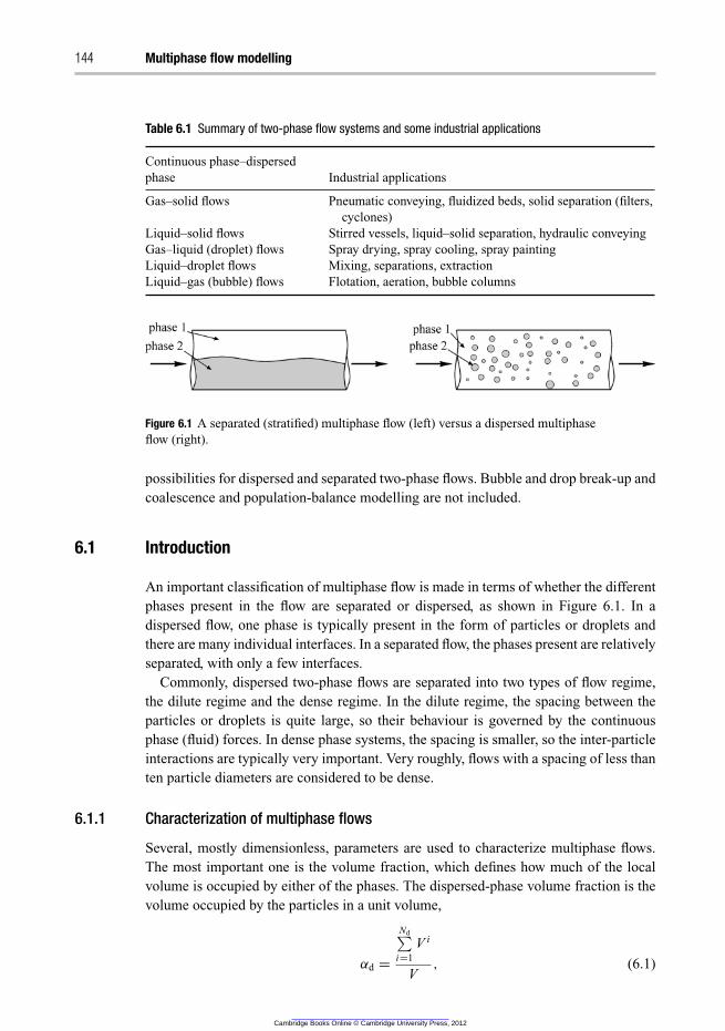
144 Multiphase flow modelling
Table 6.1 Summary of two-phase flow systems and some industrial applications
Continuous phase–dispersed
phase Industrial applications
Gas–solid flows Pneumatic conveying, fluidized beds, solid separation (filters,
cyclones)
Liquid–solid flows Stirred vessels, liquid–solid separation, hydraulic conveying
Gas–liquid (droplet) flows Spray drying, spray cooling, spray painting
Liquid–droplet flows Mixing, separations, extraction
Liquid–gas (bubble) flows Flotation, aeration, bubble columns
Figure 6.1 A separated (stratified) multiphase flow (left) versus a dispersed multiphase
flow (right).
possibilities for dispersed and separated two-phase flows. Bubble and drop break-up and
coalescence and population-balance modelling are not included.
6.1 Introduction
An important classification of multiphase flow is made in terms of whether the different
phases present in the flow are separated or dispersed, as shown in Figure 6.1. In a
dispersed flow, one phase is typically present in the form of particles or droplets and
there are many individual interfaces. In a separated flow, the phases present are relatively
separated, with only a few interfaces.
Commonly, dispersed two-phase flows are separated into two types of flow regime,
the dilute regime and the dense regime. In the dilute regime, the spacing between the
particles or droplets is quite large, so their behaviour is governed by the continuous
phase (fluid) forces. In dense phase systems, the spacing is smaller, so the inter-particle
interactions are typically very important. Very roughly, flows with a spacing of less than
ten particle diameters are considered to be dense.
6.1.1 Characterization of multiphase flows
Several, mostly dimensionless, parameters are used to characterize multiphase flows.
The most important one is the volume fraction, which defines how much of the local
volume is occupied by either of the phases. The dispersed-phase volume fraction is the
volume occupied by the particles in a unit volume,
αd =
Nd∑
i=1
V i
V, (6.1)
Cambridge Books Online © Cambridge University Press, 2012
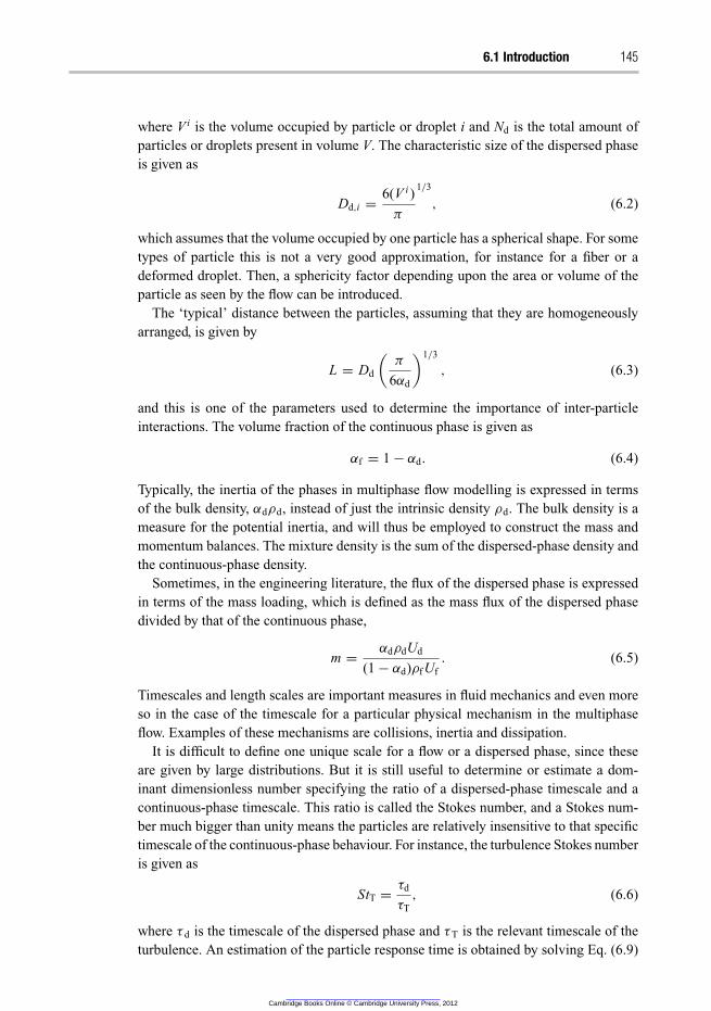
6.1 Introduction 145
where V i is the volume occupied by particle or droplet i and Nd is the total amount of
particles or droplets present in volume V. The characteristic size of the dispersed phase
is given as
Dd,i =6(V i )
π
1/3
, (6.2)
which assumes that the volume occupied by one particle has a spherical shape. For some
types of particle this is not a very good approximation, for instance for a fiber or a
deformed droplet. Then, a sphericity factor depending upon the area or volume of the
particle as seen by the flow can be introduced.
The ‘typical’ distance between the particles, assuming that they are homogeneously
arranged, is given by
L = Dd
(
π
6αd
)1/3
, (6.3)
and this is one of the parameters used to determine the importance of inter-particle
interactions. The volume fraction of the continuous phase is given as
αf = 1 − αd. (6.4)
Typically, the inertia of the phases in multiphase flow modelling is expressed in terms
of the bulk density, αdρd, instead of just the intrinsic density ρd. The bulk density is a
measure for the potential inertia, and will thus be employed to construct the mass and
momentum balances. The mixture density is the sum of the dispersed-phase density and
the continuous-phase density.
Sometimes, in the engineering literature, the flux of the dispersed phase is expressed
in terms of the mass loading, which is defined as the mass flux of the dispersed phase
divided by that of the continuous phase,
m =αdρdUd
(1 − αd)ρfUf
. (6.5)
Timescales and length scales are important measures in fluid mechanics and even more
so in the case of the timescale for a particular physical mechanism in the multiphase
flow. Examples of these mechanisms are collisions, inertia and dissipation.
It is difficult to define one unique scale for a flow or a dispersed phase, since these
are given by large distributions. But it is still useful to determine or estimate a dom-
inant dimensionless number specifying the ratio of a dispersed-phase timescale and a
continuous-phase timescale. This ratio is called the Stokes number, and a Stokes num-
ber much bigger than unity means the particles are relatively insensitive to that specific
timescale of the continuous-phase behaviour. For instance, the turbulence Stokes number
is given as
StT =τd
τT
, (6.6)
where τ d is the timescale of the dispersed phase and τT is the relevant timescale of the
turbulence. An estimation of the particle response time is obtained by solving Eq. (6.9)
Cambridge Books Online © Cambridge University Press, 2012
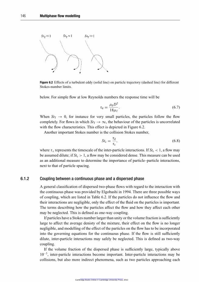
146 Multiphase flow modelling
Figure 6.2 Effects of a turbulent eddy (solid line) on particle trajectory (dashed line) for different
Stokes-number limits.
below. For simple flow at low Reynolds numbers the response time will be
τd =ρd D2
18μf
. (6.7)
When StT → 0, for instance for very small particles, the particles follow the flow
completely. For flows in which StT → ∞, the behaviour of the particles is uncorrelated
with the flow characteristics. This effect is depicted in Figure 6.2.
Another important Stokes number is the collision Stokes number,
Stc =τd
τc
, (6.8)
where τ c represents the timescale of the inter-particle interactions. If Stc < 1, a flow may
be assumed dilute; if Stc > 1, a flow may be considered dense. This measure can be used
as an additional measure to determine the importance of particle–particle interactions,
next to that of particle spacing.
6.1.2 Coupling between a continuous phase and a dispersed phase
A general classification of dispersed two-phase flows with regard to the interaction with
the continuous phase was provided by Elgobashi in 1994. There are three possible ways
of coupling, which are listed in Table 6.2. If the particles do not influence the flow and
their interactions are negligible, only the effect of the fluid on the particles is important.
The terms describing how the particles affect the flow and how they affect each other
may be neglected. This is defined as one-way coupling.
If particles have a Stokes number larger than unity or the volume fraction is sufficiently
large to affect the average denisty of the mixture, their effect on the flow is no longer
negligible, and modelling of the effect of the particles on the flow has to be incorporated
into the governing equations for the continuous phase. If the flow is still sufficiently
dilute, inter-particle interactions may safely be neglected. This is defined as two-way
coupling.
If the volume fraction of the dispersed phase is sufficiently large, typically above
10−3, inter-particle interactions become important. Inter-particle interactions may be
collisions, but also more indirect phenomena, such as two particles approaching each
Cambridge Books Online © Cambridge University Press, 2012
6.2 Forces on dispersed particles 147
Table 6.2 The various types of coupling between the dispersed phase and the continuous phase. The
choice of coupling can be made on the basis of the length scale of the dispersed phase, or on the basis
of the Stokes number
Type of coupling Definition Implementation
One-way Dispersed phase senses continuous
phase, but the continuous phase
is unaffected
Particle tracking may be done in a
post-processor
Two-way Dispersed phase senses continuous
phase and continuous phase
senses dispersed phase
The presence of the dispersed phase
should be reflected in the
governing equations of the fluid
Four-way Dispersed particles interact A model for particle–particle
interactions should be included
other in a viscous liquid. Although they will most probably not collide, their interaction
may still be important. This is defined as four-way coupling (note that one particle
affecting the other and the other affecting the first is counted as two coupling terms).
Note that this classification does not specify how accurate a model should be. The
dispersed phase may be represented by a momentum source in the governing equations
for the continuous phase, or, alternatively, the complete flow around a particle may be
resolved. Although they are very different in terms of the level of detail, both these
models fall into the category of two-way coupling.
6.2 Forces on dispersed particles
Newton’s second law can be applied to the dispersed particles. The main controversy
has been over how to describe the forces acting on the particles. The original work by
Basset (1888), Boussinesq (1885) and Oseen (1927), abbreviated as the BBO equa-
tion, described a few small particles in a uniform flow with particle Reynolds number
ReP ≪ 1. The original work was later adjusted for higher particle Reynolds numbers
and turbulent flows. In a more general framework, the forces on a single particle are
given by
md
dUi,d
dt= Fi,Drag + Fi,Press + Fi,Virt + Fi,History + Fi,Bouy + Fi,Lift + Fi,Therm
+ Fi,Turb + Fi,Brown, (6.9)
where Ui,d is the linear velocity of the particle, md is the mass of the particle, Fi,Drag
is the drag force, Fi,Press is the pressure force due to the pressure gradient, Fi,Virt is the
virtual mass force due to acceleration of the surrounding fluid, Fi,History is the history
or Basset force due to changes in the boundary layer, Fi,Bouy denotes forces due to
gravity, Fi,Lift is the Saffman and Magnus lift force due to the velocity gradient and
particle rotation, Fi,Therm is the thermophoretic force due to a temperature gradient,
Fi,Turb denotes forces due to turbulent fluctuations and Fi,Brown is the Brownian force due
to molecular collisions. These forces are described briefly below and a more detailed
discussion can be found in [17].
Cambridge Books Online © Cambridge University Press, 2012
148 Multiphase flow modelling
The Magnus force is due to the rotation of the particle and a torque balance is required.
This balance between rotational velocity, ωi, inertia, Ii, and torque, Ti, is given by
Ii
dωi
dt= Ti .
However, the Magnus force is usually small and not well defined outside the laminar
region, and the torque balance is not discussed further in this book.
The forces in Eq. (6.9) above are briefly described below. Note that the detailed flow
around the particles is not resolved. The model requires that the particles are much
smaller than the computational cell and that the continuous phase is resolved on a large
scale. The effect of the dispersed phase on the continuous phase is treated as a source
term arriving from all particles in the cell.
For a single particle the drag force is expressed as a function of the relative velocity
between the two phases,
Fi,Drag =1
2AdCDρf |Uf − Ud| (Ui,f − Ui,d) , (6.10)
where Ad is the projected area normal to the flow, i.e. π D2p/4 for a sphere. The drag
coefficient CD is discussed in more detail in Section 6.4.1.
The second term represents the pressure and shear forces from the fluid on the particle.
This is usually expressed in terms of the pressure and shear gradient over the particle
surface. Assuming a constant pressure and shear gradient over the volume of the particle,
this force can be written
Fi,Press = Vd
(
−∂ P
∂xi
+∂τi j
∂x j
)
, (6.11)
where Vd is the volume of the particle.
The third term represents the virtual-, apparent- or added-mass force. This force
arises from the acceleration or deceleration of the fluid surrounding an accelerating or
decelerating particle. The effect of this term is an increase in the apparent mass of the
particle, whence the name added-mass force. This force is written in the form
Fi,Virt = −CVMρf Vd
D
Dt(Ui,d − Ui,f ), (6.12)
where D/Dt is the substantial operator and represents the relative acceleration of the
particle compared with the fluid along the path of the particle. The virtual-mass force
coefficient CVM is usually close to 0.5, which indicates that a volume of the continuous
phase corresponding to half the volume of the particle is accelerated with the particle.
This force can be neglected when the density of the continuous phase is much lower
than the density of the particle and the virtual mass is much less than the mass of the
particle.
The fourth term, the history force, arises from the time required to develop the
boundary layer around the particle when the particle is accelerated or decelerated. This
development leads to a separation of timescales between the fluid and the particle,
thereby creating the necessity for the time integral in the force. This time integral makes
Cambridge Books Online © Cambridge University Press, 2012
6.3 Computational models 149
the history force computationally very expensive – the calculation times may increase
by an order of magnitude.
The fifth term represents the bouyancy force, the volume of the particle multiplied by
the density difference between the phases and the gravitational acceleration constant.
The Saffman and Magnus lift forces are due to the higher velocity on one side of the
particle arising from flow in a velocity gradient (the Saffman lift force) or rotation of the
particle (the Magnus lift force). Accurate models are available only for spherical bodies
at low particle Reynolds numbers. There is very little empirical data for both types of lift
force at higher Reynolds numbers. Owing to boundary-layer separation and deformation
of fluid particles, even the direction of the lift force can be difficult to predict.
The thermophoretic force represents the force due to a temperature gradient in the fluid.
Hot molecules move faster than cold molecules and a large temperature gradient will
give a net force in the direction opposite to the temperature gradient. This thermophoretic
force is important only for very small particles, and will lead to a separation of particles
depending on their size.
The origin of the Brownian force is random collisions of individual molecules. This
force is usually modelled as Gaussian white noise. The momentum transferred by colli-
sion of individual molecules is very small and the Brownian force is important only for
submicrometer particles.
The forces due to turbulence are often modelled as a random addition to the fluid
velocity that is sustained for a time corresponding to the minimum of the lifetime of the
turbulent eddies and the time taken for a particle to pass through a turbulent eddy.
The importance of the terms in the above equation of motion for one particle can
be analysed by dividing all the forces by the particle density. If the particle density is
much larger than the fluid density, as in gas–solid and gas–droplet flows, terms linear
in ρf/ρd may be neglected. This means that only drag, the pressure and shear-stress
gradient, and the buoyancy are important in such flows. If terms containing ρf/ρd may
not be neglected, such as for rising bubbles and liquid–solid flows, the added-mass force
and the history force are typically important. It is much more difficult to calculate the
trajectories of particles in such flows.
The original BBO equation is valid for one (or very few) particles in a homogeneous
flow with particle Re < 1. Most industrial applications do not deal with a few particles
in a homogeneous and low-Reynolds-number flow, so empirical extensions of the forces
from their original derivation are required. For the drag force, this has been a very
successful approach; here the empirical coefficient is called the drag coefficient. The lift
coefficient, virtual-mass coefficient, and history-force coefficient have been found to be
more prone to error, and the form of the terms in Eq. (6.9) may be less suitable. Closure
models for these terms are discussed later.
6.3 Computational models
There are many different kinds of model available for multiphase flow. The models
presented in this book can be subdivided into five main classes:
Cambridge Books Online © Cambridge University Press, 2012
150 Multiphase flow modelling
� the Euler–Lagrange model� the Euler–Euler model� the mixture or algebraic-slip model� the volume-of-fluid (VOF) model� porous-bed models.
In Euler–Lagrange modelling the fluid phase is modelled as a continuum by solving
the Navier–Stokes equations, while for the dispersed phase a large number of individual
particles is modelled. The dispersed phase can exchange momentum, mass and energy
with the fluid phase. Since the particle or droplet trajectories are computed for each
particle or for a bundle of particles that are assumed to follow the same trajectory, the
approach is limited to systems with a low volume fraction of dispersed phase.
In Euler–Euler models the different phases are all treated as continuous phases, and
momentum and continuity equations are solved for each phase. The Euler–Euler model
can handle very complex flows, but does not always give the best results since empirical
information is needed in order to close the momentum equations. Typical applications
are risers and fluidized beds.
In the mixture model (algebraic-slip model) the flows of phases are assumed to interact
strongly and it is not necessary to solve the momentum balances for the different phases
separately. In this model the viscosity is estimated for the mixture. The velocities of the
different phases are thereafter calculated from buoyancy, drag and other forces, giving
the relative velocities in comparison with the mean velocity of the mixture. Typical
applications are bubble columns, fine particle suspensions and stirred-tank reactors.
The volume-of-fluid (VOF) model is an Euler–Euler model whereby the interface
between the different phases is tracked. The model is suitable for stratified flow, free
surface flows and movement of large bubbles in liquids. Since the interface between
the fluids must be resolved, it is not applicable for a system with many small drops or
bubbles.
In the porous-bed model, the pressure drop across a porous bed is modelled. In a
bed containing many particles, it is not possible to resolve the geometry and solve
the Navier–Stokes equations. Instead the pressure drop is calculated from an equation
similar to the Ergun equation for the pressure drop in fixed beds [18].
6.3.1 Choosing a multiphase model
In selecting the most appropriate multiphase model, the physics of the system must be
analysed and understood. Initially, there are some questions that must be asked.
� Are the phases separated or dispersed?� Will the particles follow the continuous phase? What is the Stokes number?� How large are the local volume fractions?� How many particles are there in the system?� What kind of coupling occurs? Is it one-, two- or four-way coupling?
Cambridge Books Online © Cambridge University Press, 2012
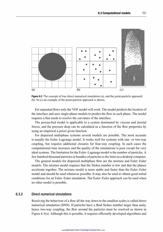
6.3 Computational models 151
Figure 6.3 The concept of true direct numerical simulation (a), and the point-particle approach
(b). In (c) an example of the point-particle approach is shown.
For separated flows only the VOF model will work. The model predicts the location of
the interface and uses single-phase models to predict the flow in each phase. The model
requires a fine mesh to resolve the curvature of the interface.
The porous-bed model is applicable to a system dominated by viscous and inertial
forces, and the pressure drop can be calculated as a function of the flow properties by
using an empirical a-priori given function.
For dispersed multiphase systems several models are possible. The most accurate
is usually the Euler–Lagrange model. It works well for systems with one- or two-way
coupling, but requires additional closures for four-way coupling. In such cases the
computational time increases and the quality of the simulations is poor except for very
ideal systems. The limitation for the Euler–Lagrange model is the number of particles. A
few hundred thousand particles or bundles of particles is the limit on a desktop computer.
The general models for dispersed multiphase flow are the mixture and Euler–Euler
models. The mixture model requires that the Stokes number is low and that the phases
accelerate together. The mixture model is more stable and faster than the Euler–Euler
model and should be used whenever possible. It may also be used to obtain good initial
conditions for an Euler–Euler simulation. The Euler–Euler approach can be used when
no other model is possible.
6.3.2 Direct numerical simulations
Resolving the behaviour of a flow all the way down to the smallest scales is called direct
numerical simulation (DNS). If particles have a fluid Stokes number larger than unity,
hence two-way coupling, the flow around the particles must be resolved as shown in
Figure 6.3(a). Although this is possible, it requires efficiently developed algorithms and
Cambridge Books Online © Cambridge University Press, 2012
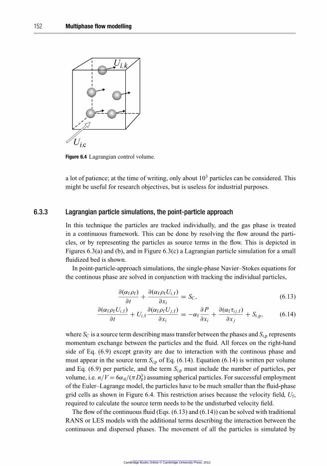
152 Multiphase flow modelling
Figure 6.4 Lagrangian control volume.
a lot of patience; at the time of writing, only about 103 particles can be considered. This
might be useful for research objectives, but is useless for industrial purposes.
6.3.3 Lagrangian particle simulations, the point-particle approach
In this technique the particles are tracked individually, and the gas phase is treated
in a continuous framework. This can be done by resolving the flow around the parti-
cles, or by representing the particles as source terms in the flow. This is depicted in
Figures 6.3(a) and (b), and in Figure 6.3(c) a Lagrangian particle simulation for a small
fluidized bed is shown.
In point-particle-approach simulations, the single-phase Navier–Stokes equations for
the continous phase are solved in conjunction with tracking the individual particles,
∂(αfρf )
∂t+
∂(αfρfUi,f )
∂xi
= SC, (6.13)
∂(αfρfUi,f )
∂t+ Ui,f
∂(αfρfU j,f )
∂xi
= −αf
∂ P
∂xi
+∂(αfτi j,f )
∂x j
+ Si,p, (6.14)
where SC is a source term describing mass transfer between the phases and Si,p represents
momentum exchange between the particles and the fluid. All forces on the right-hand
side of Eq. (6.9) except gravity are due to interaction with the continous phase and
must appear in the source term Si,p of Eq. (6.14). Equation (6.14) is written per volume
and Eq. (6.9) per particle, and the term Si,p must include the number of particles, per
volume, i.e. n/V = 6αd/(πD3p) assuming spherical particles. For successful employment
of the Euler–Lagrange model, the particles have to be much smaller than the fluid-phase
grid cells as shown in Figure 6.4. This restriction arises because the velocity field, Uf,
required to calculate the source term needs to be the undisturbed velocity field.
The flow of the continuous fluid (Eqs. (6.13) and (6.14)) can be solved with traditional
RANS or LES models with the additional terms describing the interaction between the
continuous and dispersed phases. The movement of all the particles is simulated by
Cambridge Books Online © Cambridge University Press, 2012
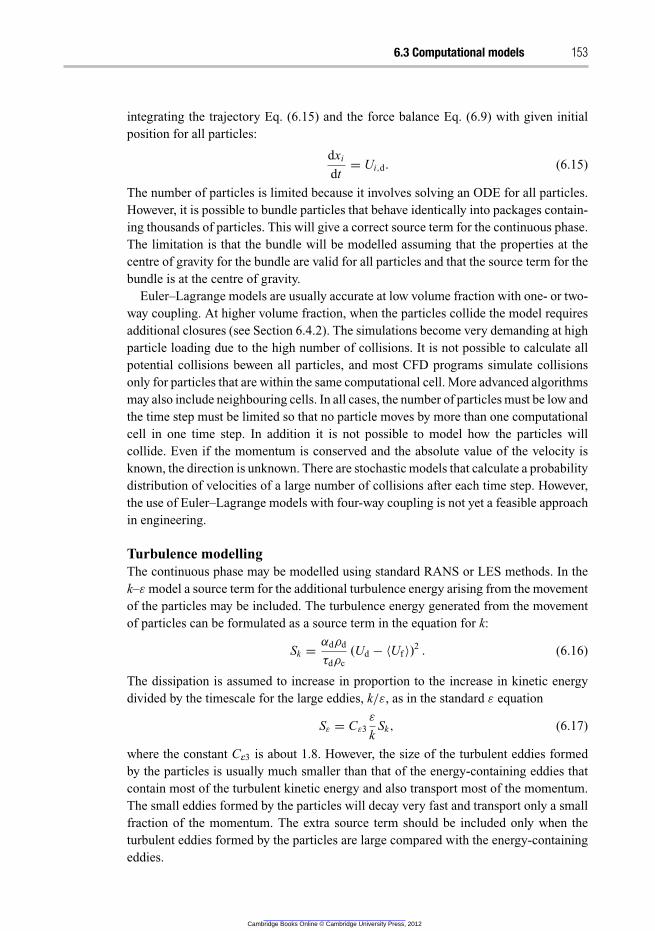
6.3 Computational models 153
integrating the trajectory Eq. (6.15) and the force balance Eq. (6.9) with given initial
position for all particles:
dxi
dt= Ui,d. (6.15)
The number of particles is limited because it involves solving an ODE for all particles.
However, it is possible to bundle particles that behave identically into packages contain-
ing thousands of particles. This will give a correct source term for the continuous phase.
The limitation is that the bundle will be modelled assuming that the properties at the
centre of gravity for the bundle are valid for all particles and that the source term for the
bundle is at the centre of gravity.
Euler–Lagrange models are usually accurate at low volume fraction with one- or two-
way coupling. At higher volume fraction, when the particles collide the model requires
additional closures (see Section 6.4.2). The simulations become very demanding at high
particle loading due to the high number of collisions. It is not possible to calculate all
potential collisions beween all particles, and most CFD programs simulate collisions
only for particles that are within the same computational cell. More advanced algorithms
may also include neighbouring cells. In all cases, the number of particles must be low and
the time step must be limited so that no particle moves by more than one computational
cell in one time step. In addition it is not possible to model how the particles will
collide. Even if the momentum is conserved and the absolute value of the velocity is
known, the direction is unknown. There are stochastic models that calculate a probability
distribution of velocities of a large number of collisions after each time step. However,
the use of Euler–Lagrange models with four-way coupling is not yet a feasible approach
in engineering.
Turbulence modelling
The continuous phase may be modelled using standard RANS or LES methods. In the
k–ε model a source term for the additional turbulence energy arising from the movement
of the particles may be included. The turbulence energy generated from the movement
of particles can be formulated as a source term in the equation for k:
Sk =αdρd
τdρc
(Ud − 〈Uf 〉)2. (6.16)
The dissipation is assumed to increase in proportion to the increase in kinetic energy
divided by the timescale for the large eddies, k/ε, as in the standard ε equation
Sε = Cε3
ε
kSk, (6.17)
where the constant Cε3 is about 1.8. However, the size of the turbulent eddies formed
by the particles is usually much smaller than that of the energy-containing eddies that
contain most of the turbulent kinetic energy and also transport most of the momentum.
The small eddies formed by the particles will decay very fast and transport only a small
fraction of the momentum. The extra source term should be included only when the
turbulent eddies formed by the particles are large compared with the energy-containing
eddies.
Cambridge Books Online © Cambridge University Press, 2012
154 Multiphase flow modelling
The effect of fluid-phase turbulence on the particles may be important, depending
upon the Stokes number. In determining a drag force, the instantaneous drag forces on
each particle are averaged into a drag force, which becomes a function of the mean
or average relative velocity. The turbulent eddies in the continous phase will move the
single particles in all directions and away from the average path. At the end particles
injected at the same point will not end up at the same position due to the turbulence, and
this phenomenon must be taken into account.
The information on the turbulence provided by RANS models is available only in sta-
tistical terms, for instance, in terms of the turbulent kinetic energy and energy-dissipation
rates. To couple the behaviour of the particles effectively with the local fluid properties,
however, instantaneous fluid properties are required. A popular way of determining a
non-unique set of instantaneous fluid properties from the given statistical turbulence
models is use of the so-called random-walk models. The instantaneous fluid velocity at
a particle location is determined from the averaged fluid velocity, which is deterministic,
and a random component for which the magnitude, direction and timescales obey the
statistical (averaged) properties of the local fluid turbulence.
In the discrete-random-walk (DRW) model it is assumed that the effect of turbulence
can be modelled by adding a random velocity to the continuous phase for a specific time
T, where T is the time the particle spent in a turbulent eddy. This time is estimated as
the minimum of the time taken for a particle to pass through the turbulent eddy and
the lifetime of the turbulent eddy. The time taken to pass through the turbulent eddy is
estimated from the size of the turbulent eddy and the slip velocity,
T ≈ −τ ln
(
1 −l
τ |Ud − 〈Uf 〉|
)
, (6.18)
where τ is the particle response time (Eq. (6.7)) and l is the size of the turbulent eddy
(Eq. (4.19)). The lifetime of a turbulent eddy in RANS models is
T ∝k
ε
. (6.19)
The turbulent velocity fluctuations are assumed to have a Gaussian probability distribu-
tion and the turbulent fluctuations are added to the continuous-phase velocity
u′i = ξi
√
u2i , (6.20)
where ξ i is a Gaussian random number.
In isotropic turbulence 〈u21〉 = 〈u2
2〉 = 〈u23〉 = 2k/3 and the continuous-phase velocity
fluctuation is calculated from
ui = ξi
√
2k
3. (6.21)
All three velocity fluctuations are known in Reynolds stress modelling and all the
individual fluctuating components can be calculated. The random velocity u′i is then
added to the average fluid velocity 〈Ui,f〉 and kept constant during the time step defined
by T above. A new random number ξ i is chosen after each time step.
Cambridge Books Online © Cambridge University Press, 2012
6.3 Computational models 155
Figure 6.5 A stratified flow simulation (left) versus a dispersed flow simulation (right).
6.3.4 Euler–Euler models
The Euler–Euler model treats a dispersed multiphase flow as two (or more) fully inter-
penetrating quasi-fluids, and is therefore often referred to as the two-fluid model. The
two-fluid model is derived by ensemble averaging or volume averaging. A very impor-
tant quantity appearing in the equation because of the averaging is the volume fraction
αk. This quantity alone does not say anything about the size or behaviour of the dis-
persed phase, and this generally comes in via closure models. Within the Euler–Euler
framework both stratified and dispersed flow are modelled. In this book we present the
Euler–Euler model as a general model for most kinds of multiphase flow, the mixture
model as a simplification of the Euler–Euler model and the volume-of-fluid model for
stratified flows as shown in Figure 6.5.
Intuitively, it is easiest to imagine the derivation of the two-fluid model in terms
of volume averaging. A small volume, much smaller than that of the large-scale flow
structures, but much larger than that of individual dispersed particles, in which both
phases are present is used in this model. The volume fraction is defined on the basis of the
distribution of phases and the size of the computational volume. The local instantaneous
equations describing both phases may then be averaged in the volume, considering the
bulk density of each of the phases. The two-fluid model equations for each phase are
given by the following equations, where k is not an index but represents a phase:
∑
k
αk = 1, (6.22)
∂αkρk
∂t+
∂αkρkUi,k
∂xi
= −
p∑
l=1
(mkl − mlk), (6.23)
∂αkρkUi,k
∂t+
∂αkρkUi,kU j,k
∂x j
= −αk
∂ P
∂xi
+∂αkτi j,k
∂xk
+ αkρk gi + Fi,k, (6.24)
Cambridge Books Online © Cambridge University Press, 2012
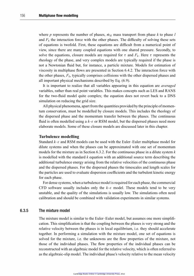
156 Multiphase flow modelling
where p represents the number of phases, mkl mass transport from phase k to phase l
and Fk the interaction force with the other phases. The difficulty of solving these sets
of equations is twofold. First, these equations are difficult from a numerical point of
view, since there are many coupled equations with one shared pressure. Secondly, to
solve the equations, closure models are required for τ and Fk. Here τ represents the
rheology of the phase, and very complex models are typically required if the phase is
not a Newtonian fluid but, for instance, a particle mixture. Models for estimation of
viscosity in multiphase flows are presented in Section 6.4.2. The interaction force with
the other phases, Fk, typically comprises collisions with the other dispersed phases and
all important physical mechanisms described by Eq. (6.9).
It is important to realize that all variables appearing in this equation are averaged
variables, rather than real point variables. This makes concepts such as LES and RANS
for the two-fluid model quite complex; the equation does not revert back to a DNS
simulation on reducing the grid size.
All physical phenomena, apart from the quantities provided by the principle of momen-
tum conservation, must be modelled by closure models. This includes the rheology of
the dispersed phase and the momentum transfer between the phases. The continuous
fluid is often modelled using a k–ε or RSM model, but the dispersed phases need more
elaborate models. Some of these closure models are discussed later in this chapter.
Turbulence modelling
Standard k–ε and RSM models can be used with the Euler–Euler multiphase model for
dilute systems and when the phases can be approximated with one set of momentum
models for the mixture as in Section 6.3.2. For the continuous phase in a dilute system k
is modelled with the standard k equation with an additional source term describing the
additional turbulence energy arising from the relative velocities of the continuous phase
and the dispersed phases. For the dispersed phases the timescales and length scales for
the particles are used to evaluate dispersion coefficients and the turbulent kinetic energy
for each phase.
For dense systems, when a turbulence model is required for each phase, the commercial
CFD software usually includes only the k–ε model. These models tend to be very
unstable, and the quality of the simulations is usually low. The simulations often need
calibration and should be combined with validation experiments in similar systems.
6.3.5 The mixture model
The mixture model is similar to the Euler–Euler model, but assumes one more simplifi-
cation. This simplification is that the coupling between the phases is very strong and the
relative velocity between the phases is in local equilibrium, i.e. they should accelerate
together. In performing a simulation with the mixture model, one set of equations is
solved for the mixture, i.e. the unknowns are the flow properties of the mixture, not
those of the individual phases. The flow properties of the individual phases can be
reconstructed with an algebraic model for the relative velocity, which is often referred to
as the algebraic-slip model. The individual phase’s velocity relative to the mean velocity
Cambridge Books Online © Cambridge University Press, 2012
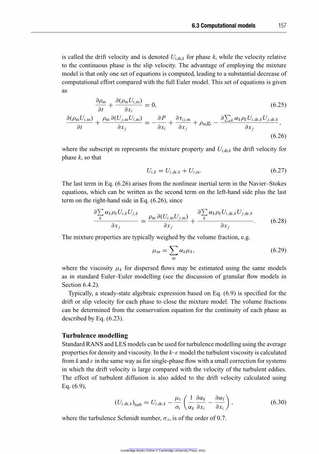
6.3 Computational models 157
is called the drift velocity and is denoted Ui,dr,k for phase k, while the velocity relative
to the continuous phase is the slip velocity. The advantage of employing the mixture
model is that only one set of equations is computed, leading to a substantial decrease of
computational effort compared with the full Euler model. This set of equations is given
as
∂ρm
∂t+
∂(ρmUi,m)
∂xi
= 0, (6.25)
∂(ρmUi,m)
∂t+
ρm ∂(U j,mUi,m)
∂x j
= −∂ P
∂xi
+∂τi j,m
∂x j
+ ρmgi −∂
∑
k αkρkUi,dr,kU j,dr,k
∂x j
,
(6.26)
where the subscript m represents the mixture property and Ui,dr,k the drift velocity for
phase k, so that
Ui,k = Ui,dr,k + Ui,m. (6.27)
The last term in Eq. (6.26) arises from the nonlinear inertial term in the Navier–Stokes
equations, which can be written as the second term on the left-hand side plus the last
term on the right-hand side in Eq. (6.26), since
∂
∑
k
αkρkUi,kU j,k
∂x j
=ρm ∂(Ui,mU j,m)
∂x j
+
∂
∑
k
αkρkUi,dr,kU j,dr,k
∂x j
. (6.28)
The mixture properties are typically weighed by the volume fraction, e.g.
μm =∑
m
αkμk, (6.29)
where the viscosity μk for dispersed flows may be estimated using the same models
as in standard Euler–Euler modelling (see the discussion of granular flow models in
Section 6.4.2).
Typically, a steady-state algebraic expression based on Eq. (6.9) is specified for the
drift or slip velocity for each phase to close the mixture model. The volume fractions
can be determined from the conservation equation for the continuity of each phase as
described by Eq. (6.23).
Turbulence modelling
Standard RANS and LES models can be used for turbulence modelling using the average
properties for density and viscosity. In the k–ε model the turbulent viscosity is calculated
from k and ε in the same way as for single-phase flow with a small correction for systems
in which the drift velocity is large compared with the velocity of the turbulent eddies.
The effect of turbulent diffusion is also added to the drift velocity calculated using
Eq. (6.9),
(Ui,dr,k)turb = Ui,dr,k −μt
σt
(
1
αk
∂αk
∂xi
−∂αf
∂xi
)
, (6.30)
where the turbulence Schmidt number, σ t, is of the order of 0.7.
Cambridge Books Online © Cambridge University Press, 2012
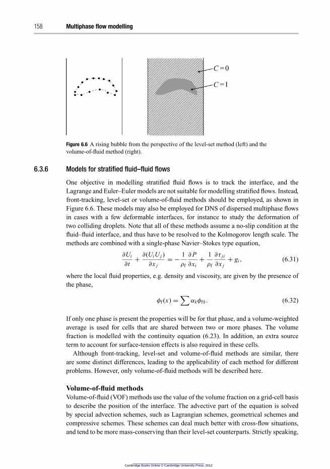
158 Multiphase flow modelling
Figure 6.6 A rising bubble from the perspective of the level-set method (left) and the
volume-of-fluid method (right).
6.3.6 Models for stratified fluid–fluid flows
One objective in modelling stratified fluid flows is to track the interface, and the
Lagrange and Euler–Euler models are not suitable for modelling stratified flows. Instead,
front-tracking, level-set or volume-of-fluid methods should be employed, as shown in
Figure 6.6. These models may also be employed for DNS of dispersed multiphase flows
in cases with a few deformable interfaces, for instance to study the deformation of
two colliding droplets. Note that all of these methods assume a no-slip condition at the
fluid–fluid interface, and thus have to be resolved to the Kolmogorov length scale. The
methods are combined with a single-phase Navier–Stokes type equation,
∂Ui
∂t+
∂(UiU j )
∂x j
= −1
ρf
∂ P
∂xi
+1
ρf
∂τ j i
∂x j
+ gi , (6.31)
where the local fluid properties, e.g. density and viscosity, are given by the presence of
the phase,
φf (x) =∑
αkφfk . (6.32)
If only one phase is present the properties will be for that phase, and a volume-weighted
average is used for cells that are shared between two or more phases. The volume
fraction is modelled with the continuity equation (6.23). In addition, an extra source
term to account for surface-tension effects is also required in these cells.
Although front-tracking, level-set and volume-of-fluid methods are similar, there
are some distinct differences, leading to the applicability of each method for different
problems. However, only volume-of-fluid methods will be described here.
Volume-of-fluid methods
Volume-of-fluid (VOF) methods use the value of the volume fraction on a grid-cell basis
to describe the position of the interface. The advective part of the equation is solved
by special advection schemes, such as Lagrangian schemes, geometrical schemes and
compressive schemes. These schemes can deal much better with cross-flow situations,
and tend to be more mass-conserving than their level-set counterparts. Strictly speaking,
Cambridge Books Online © Cambridge University Press, 2012
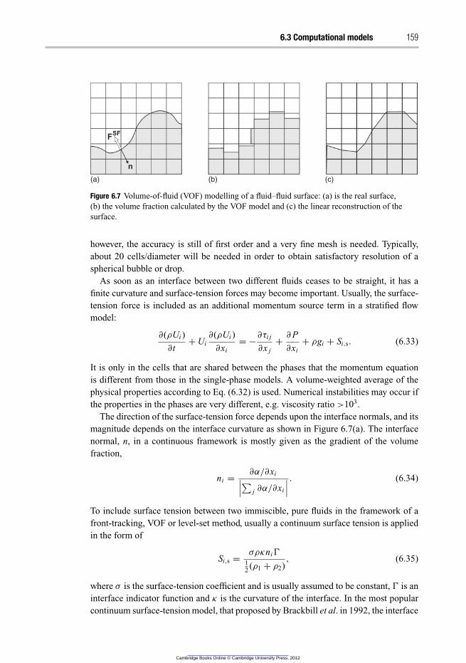
6.3 Computational models 159
(a) (b) (c)
Figure 6.7 Volume-of-fluid (VOF) modelling of a fluid–fluid surface: (a) is the real surface,
(b) the volume fraction calculated by the VOF model and (c) the linear reconstruction of the
surface.
however, the accuracy is still of first order and a very fine mesh is needed. Typically,
about 20 cells/diameter will be needed in order to obtain satisfactory resolution of a
spherical bubble or drop.
As soon as an interface between two different fluids ceases to be straight, it has a
finite curvature and surface-tension forces may become important. Usually, the surface-
tension force is included as an additional momentum source term in a stratified flow
model:
∂(ρUi )
∂t+ Ui
∂(ρUi )
∂xi
= −∂τi j
∂x j
+∂ P
∂xi
+ ρgi + Si,s. (6.33)
It is only in the cells that are shared between the phases that the momentum equation
is different from those in the single-phase models. A volume-weighted average of the
physical properties according to Eq. (6.32) is used. Numerical instabilities may occur if
the properties in the phases are very different, e.g. viscosity ratio >103.
The direction of the surface-tension force depends upon the interface normals, and its
magnitude depends on the interface curvature as shown in Figure 6.7(a). The interface
normal, n, in a continuous framework is mostly given as the gradient of the volume
fraction,
ni =∂α/∂xi
∣
∣
∣
∑
j ∂α/∂xi
∣
∣
∣
. (6.34)
To include surface tension between two immiscible, pure fluids in the framework of a
front-tracking, VOF or level-set method, usually a continuum surface tension is applied
in the form of
Si,s =σρκniŴ
12(ρ1 + ρ2)
, (6.35)
where σ is the surface-tension coefficient and is usually assumed to be constant, Ŵ is an
interface indicator function and κ is the curvature of the interface. In the most popular
continuum surface-tension model, that proposed by Brackbill et al. in 1992, the interface
Cambridge Books Online © Cambridge University Press, 2012
160 Multiphase flow modelling
indicator, the curvature of the interface and the interface normal are directly related to
the volume fraction,
Ŵ =
∣
∣
∣
∣
∑
j
∂α
∂x j
∣
∣
∣
∣
, (6.36)
κ = −∂ni
∂xi
. (6.37)
Hence, the curvature is a measure of how fast (magnitude) and in which direction (sign)
the normal of an interface changes in space. The surface tension aims at minimizing
the interface area. For bubbles or droplets, the minimized interface area is spherical;
for a fully stratified flow, the minimized interface area is a straight line. The influ-
ence from surface tension can be neglected for capillary numbers Ca =μU/σ ≫ 1 or
Weber numbers We = ρLU2/σ ≫ 1. For large interfaces, such as in stratified flows,
but also for interfaces of bubbles or droplets of diameter larger then a few centime-
tres, the surface-tension force may be negligible. However, for very large curvatures,
for example small bubbles with a diameter of a few millimetres, the surface tension
may be dominant and in that case ensures that the interface is spherically shaped at all
times.
One complication with surface tension not dealt with here is that, in mixtures and
with temperature gradients, the surface tension is not constant, and there will appear
tangential to the surface a force aiming at minimizing surface energy globally.
Turbulence modelling
In theory the interface should be resolved to the Kolmogorov length scale. This might
not be possible in all cases, and standard RANS models must be used with caution. The
bulk properties are used, and the damping of turbulence at the interface that is expected
when the properties of the phases are very different might not be modelled corectly. Wall
functions are not possible since the location of the interface is not given a priori. The
k–ω model might be a better choice than the k–ε model, but will require a denser mesh.
Large-eddy simulation works better with VOF since the momentum transport across the
interface on the subgrid level is much less.
6.3.7 Models for flows in porous media
Flow in a porous medium is driven by the pressure drop over the medium. Examples
of such flows occur in fixed-bed reactors, filters and trays in distillation columns. The
pressure drop and the resistance of the medium are the most important terms in the
governing equations for the fluid phase, i.e. the accelerations are usually small. It is
generally not possible to resolve the flow around each object or cavity in a porous
medium, so a rough estimate of the pressure drop over the bed is made. The pressure
drop in a packed bed originates from viscous resistance, which is proportional to the
Cambridge Books Online © Cambridge University Press, 2012
6.4 Closure models 161
viscosity and velocity of the fluid phase, and an inertial resistance that is proportional
to the density and the velocity squared,
dP
dxi
= −AμUi − B
(
1
2ρ|U |Ui
)
. (6.38)
The simplest model for this is called Darcy’s law, wherein inertial effects are neglected
(i.e. B = 0). This is quite frequently used in, for example, simulations of the flow in oil
reservoirs. A is then inversely proportional to the area of the pores in the reservoir.
The model of Ergun (dating from 1952) is valid for flow through packed beds for a
wide range of velocities and includes both a viscous resistance and an inertial resistance,
A =150(1 − α)2
d2pα
3, (6.39)
B =1.75(1 − α)
dpα3
, (6.40)
where α is the void fraction and dp is the particle diameter. Note that these values are
valid only for flow though beds containing rigid spherical particles. For other types of
particles, e.g. fibres and compressible particles, an empirical determination of A and B
is required.
6.4 Closure models
Multiphase flow simulations without the requirement of closure models are either
extremely computationally expensive, or apply only for very simplified situations.
Almost all multiphase flow simulations for engineering applications need closure mod-
els to some extent. Most closure models are empirical, meaning that they are determined
by experiments and are valid only for the conditions under which the experiments were
performed. Some closure models are based upon more theoretical considerations, but
most often require assumptions as well. It is important to verify these assumptions and
determine whether they are applicable to the simulated conditions. Some of the most
popular closure models are discussed here.
6.4.1 Interphase drag
Equation (6.10) is valid for a single particle, i.e. at low volume fraction of the dispersed
phase. To model the drag between a fluid and dispersed particles at high volume fraction
of the dispersed phase, the drag as formulated in Eq. (6.10) must be adjusted,
Fi,D =1
2AdCDρfα
−2.65f |Ui,f − Ui,d| (Ui,f − Ui,d) , (6.41)
where CD represents the drag coefficient. For spherical particles, this coefficient is a
scalar, since it does not depend upon the stream direction of the flow on the particle.
Cambridge Books Online © Cambridge University Press, 2012
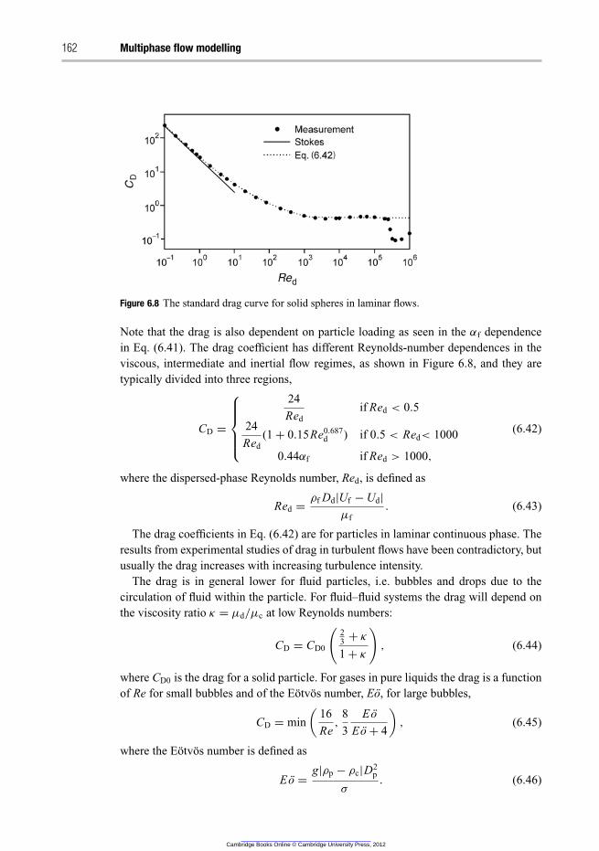
162 Multiphase flow modelling
Figure 6.8 The standard drag curve for solid spheres in laminar flows.
Note that the drag is also dependent on particle loading as seen in the αf dependence
in Eq. (6.41). The drag coefficient has different Reynolds-number dependences in the
viscous, intermediate and inertial flow regimes, as shown in Figure 6.8, and they are
typically divided into three regions,
CD =
⎧
⎪
⎪
⎪
⎨
⎪
⎪
⎪
⎩
24
Red
if Red < 0.5
24
Red
(1 + 0.15Re0.687d ) if 0.5 < Red< 1000
0.44αf if Red > 1000,
(6.42)
where the dispersed-phase Reynolds number, Red, is defined as
Red =ρf Dd|Uf − Ud|
μf
. (6.43)
The drag coefficients in Eq. (6.42) are for particles in laminar continuous phase. The
results from experimental studies of drag in turbulent flows have been contradictory, but
usually the drag increases with increasing turbulence intensity.
The drag is in general lower for fluid particles, i.e. bubbles and drops due to the
circulation of fluid within the particle. For fluid–fluid systems the drag will depend on
the viscosity ratio κ = μd/μc at low Reynolds numbers:
CD = CD0
(
23
+ κ
1 + κ
)
, (6.44)
where CD0 is the drag for a solid particle. For gases in pure liquids the drag is a function
of Re for small bubbles and of the Eotvos number, Eo, for large bubbles,
CD = min
(
16
Re,
8
3
Eo
Eo + 4
)
, (6.45)
where the Eotvos number is defined as
Eo =g|ρp − ρc|D
2p
σ
. (6.46)
Cambridge Books Online © Cambridge University Press, 2012
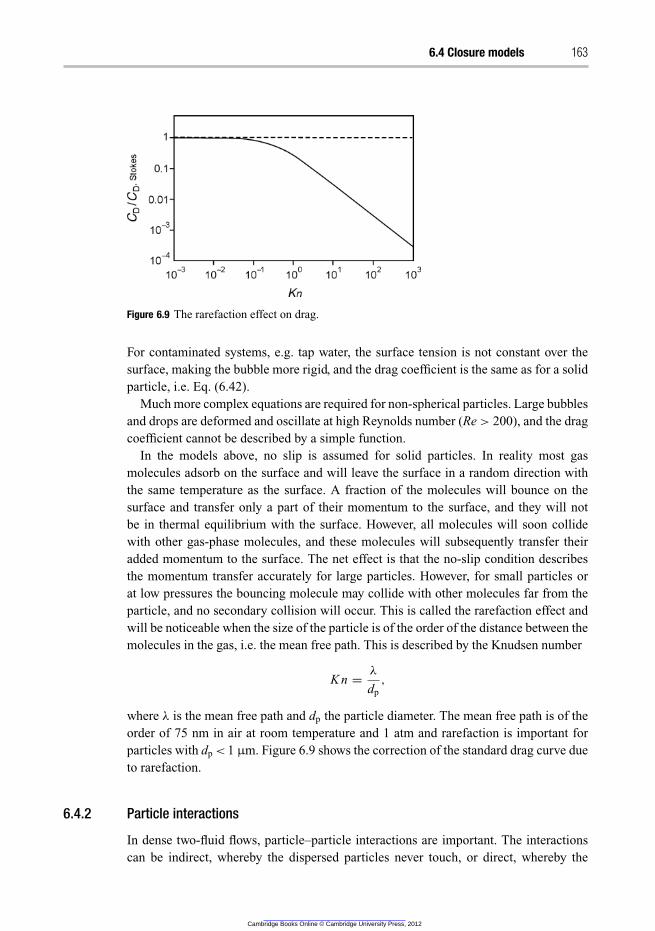
6.4 Closure models 163
Figure 6.9 The rarefaction effect on drag.
For contaminated systems, e.g. tap water, the surface tension is not constant over the
surface, making the bubble more rigid, and the drag coefficient is the same as for a solid
particle, i.e. Eq. (6.42).
Much more complex equations are required for non-spherical particles. Large bubbles
and drops are deformed and oscillate at high Reynolds number (Re > 200), and the drag
coefficient cannot be described by a simple function.
In the models above, no slip is assumed for solid particles. In reality most gas
molecules adsorb on the surface and will leave the surface in a random direction with
the same temperature as the surface. A fraction of the molecules will bounce on the
surface and transfer only a part of their momentum to the surface, and they will not
be in thermal equilibrium with the surface. However, all molecules will soon collide
with other gas-phase molecules, and these molecules will subsequently transfer their
added momentum to the surface. The net effect is that the no-slip condition describes
the momentum transfer accurately for large particles. However, for small particles or
at low pressures the bouncing molecule may collide with other molecules far from the
particle, and no secondary collision will occur. This is called the rarefaction effect and
will be noticeable when the size of the particle is of the order of the distance between the
molecules in the gas, i.e. the mean free path. This is described by the Knudsen number
K n =λ
dp
,
where λ is the mean free path and dp the particle diameter. The mean free path is of the
order of 75 nm in air at room temperature and 1 atm and rarefaction is important for
particles with dp < 1 µm. Figure 6.9 shows the correction of the standard drag curve due
to rarefaction.
6.4.2 Particle interactions
In dense two-fluid flows, particle–particle interactions are important. The interactions
can be indirect, whereby the dispersed particles never touch, or direct, whereby the
Cambridge Books Online © Cambridge University Press, 2012
164 Multiphase flow modelling
particles actually touch. Examples of indirect interactions occur in bubble columns,
between interacting bubbles. However, indirect interactions between two particles may
also occur; this is often referred to as the lubrication effect. When the fluid density and
viscosity are low, interactions are most often direct.
Models for indirect interactions are required when the behaviour of continuous fluid
between the two dispersed particles is not fully resolved. The models depend on how
much of the fluid behaviour between the particles is unresolved, which may vary for each
simulation. Typically, these models have the form of a long-range potential force, 1/rγ ,
where r is the distance between the bodies and γ provides a measure for the strength of
the interaction. Such models are typically empirical.
Direct interactions typically involve solid particles colliding. There are two character-
istic regimes for colliding particles, namely slow granular flow and rapid granular flow.
Slow granular flow is characterized by very high volume fractions of solids, low rela-
tive velocities between the particles and enduring, multi-body contact. Rapid granular
flow is characterized by moderate volume fractions of solids and binary, instantaneous
collisions.
Lagrangian particle collisions
When dealing with particle–particle collisions, two types of collision model are widely
employed, namely the hard-sphere model and the soft-sphere model. Hard-sphere mod-
els describe the dynamics of individual, binary collisions in terms of conservation
of momentum and energy. In an ideal collision the momentum is conserved, and the
momentum transferred during a collision can be quantified as
J = m1(Ud,1 − U ′d,1) = −m2(Ud,2 − U ′
d,2), (6.47)
where m1 represents the mass of particle 1, Ud,1 the velocity prior to collision of particle
1 and U′d,1 the velocity right after the collision. The post-collision velocities U′
d,1 and U′d,2
can be found by making use of the principle of conservation of energy. More advanced
hard-sphere models employ a coefficient of restitution, so part of the kinetic energy of
the particles prior to collision is transferred to thermal energy during the collision.
The restitution coefficient describes the damping of velocity at the collision. It is
defined as
ed =U ′
d,2 − U ′d,1
Ud,1 − Ud,2
. (6.48)
A restitution coefficient of unity corresponds to ideal collision with no energy losses.
Soft-sphere models aim to estimate the local deformation of the particles during colli-
sion. This deformation is due to reversible deformation of the particle. The deformation
is related to a linear ‘overlap’ of the particles during collision. The force resulting from
the deformation is typically written in terms of a so-called spring–slider–dashpot model.
The spring force is typically the dominant contribution, and is formulated as
F = −kδα
n n, (6.49)
Cambridge Books Online © Cambridge University Press, 2012
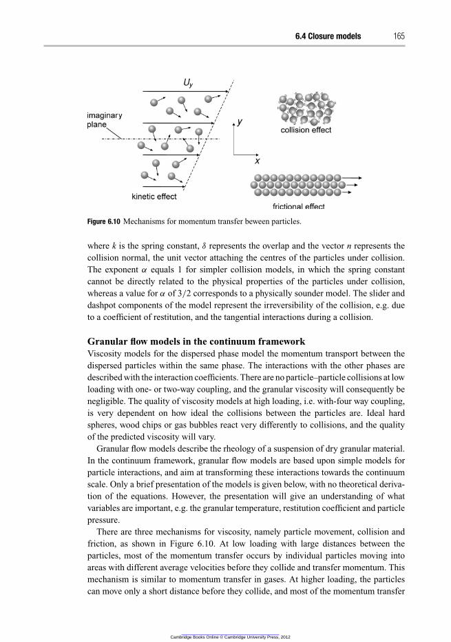
6.4 Closure models 165
Figure 6.10 Mechanisms for momentum transfer beween particles.
where k is the spring constant, δ represents the overlap and the vector n represents the
collision normal, the unit vector attaching the centres of the particles under collision.
The exponent α equals 1 for simpler collision models, in which the spring constant
cannot be directly related to the physical properties of the particles under collision,
whereas a value for α of 3/2 corresponds to a physically sounder model. The slider and
dashpot components of the model represent the irreversibility of the collision, e.g. due
to a coefficient of restitution, and the tangential interactions during a collision.
Granular flow models in the continuum framework
Viscosity models for the dispersed phase model the momentum transport between the
dispersed particles within the same phase. The interactions with the other phases are
described with the interaction coefficients. There are no particle–particle collisions at low
loading with one- or two-way coupling, and the granular viscosity will consequently be
negligible. The quality of viscosity models at high loading, i.e. with-four way coupling,
is very dependent on how ideal the collisions between the particles are. Ideal hard
spheres, wood chips or gas bubbles react very differently to collisions, and the quality
of the predicted viscosity will vary.
Granular flow models describe the rheology of a suspension of dry granular material.
In the continuum framework, granular flow models are based upon simple models for
particle interactions, and aim at transforming these interactions towards the continuum
scale. Only a brief presentation of the models is given below, with no theoretical deriva-
tion of the equations. However, the presentation will give an understanding of what
variables are important, e.g. the granular temperature, restitution coefficient and particle
pressure.
There are three mechanisms for viscosity, namely particle movement, collision and
friction, as shown in Figure 6.10. At low loading with large distances between the
particles, most of the momentum transfer occurs by individual particles moving into
areas with different average velocities before they collide and transfer momentum. This
mechanism is similar to momentum transfer in gases. At higher loading, the particles
can move only a short distance before they collide, and most of the momentum transfer
Cambridge Books Online © Cambridge University Press, 2012
166 Multiphase flow modelling
occurs by frequent collisions. This mechanism is similar to momentum transfer in
liquids. In both these mechanisms, the viscosity depends on the fluctuation motion of
the particles, i.e. the granular temperature defined below. At the highest loading the
particles are in constant contact and slide over each other. Here the mechanism for
momentum transfer is friction, and the viscosity depends on the granular temperature
via the particle pressure pd. Granular flow models are usually divided into two families of
models, the slow granular flow models and the rapid granular flow models. Slow granular
flow is related to momentum transfer by friction and frequent collision of particles in a
dense environment, whereas in rapid granular flow the momentum transport occurs by
movement and collision of particles.
A popular model in the rapid granular flow regime is the kinetic theory for granular
flow [19]. The kinetic theory of granular flow predicts the stresses in moderately dense
flows quite accurately, and it has successfully been employed in many applications in this
regime. In the rapid granular flow regime, the solids stress arises from particle momentum
exchange due to translation and collision. A key parameter in the constitutive closures
for the solids phase is the energy associated with the fluctuating motion of the particles,
the so-called granular temperature. The granular temperature is defined as the random
movement of particles corresponding to how the random movement of molecules in
kinetic theory of gases constitutes temperature,
θ =1
3
(⟨
u21
⟩
+⟨
u22
⟩
+⟨
u23
⟩)
, (6.50)
where u represents the fluctuating velocity of a particle, which has a zero mean by
definition. The kinetic theory of granular flows aims to derive a transport equation for
the granular temperature. The shearing of the particles causes granular temperature to be
produced, and the damping non-ideal component of the collisions, transferring kinetic
energy to heat, causes a dissipative effect in granular temperature. The terms in the
granular temperature balance arise from collisions and the streaming of particles. In this
process, quite a few closures are required, and some of these remain topics for discussion
and further research. The balance for granular temperature is very similar to the balance
for thermal energy, Eq. (2.28) in Chapter 2. The equation is formulated as
3
2
[
∂(ρdαdθ )
∂t+ U j,d
∂(ρdαdθ )
∂x j
]
= κd
∂2θ
∂xi ∂x j
− pd
∂U j,d
∂x j
+ τk j,d
∂Uk,d
∂x j
− γd, (6.51)
where κd is the conductivity of granular temperature and the dissipation of fluctuation
energy is described by
γd = 3(
1 − e2d
)
α2dρdg0
(
4
dd
√
θ
π
−∂Ui,d
∂xi
)
, (6.52)
where ed is the coefficient of restitution for particle collisions. The models presented
below are frequently used, but there is no general agreement on a best model. The
granular temperature conductivity κd is a complex function of granular temperature,
Cambridge Books Online © Cambridge University Press, 2012
6.4 Closure models 167
restitution coefficient etc. that is not given here. The radial distribution function at
particle contact is
g0 =
[
1 −
(
αd
αd,max
)1/3]−1
, (6.53)
where the maximum volume fraction of the dispersed phase αd,max is used to calculate
a dimensionless particle–particle distance. This function (g0) also certifies that the
maximum particle loading is never surpassed by increasing the particle pressure to
infinity when αd → αd,max. The total particle pressure due to the streaming and collisions
of particles is given as
pd = αdρdθ + 2ρd(1 + ed)α2d g0θ. (6.54)
The kinetic and collision parts of the granular viscosity can be formulated as
μd,kin =αdddρd
√θπ
6 (1 − ed)
[
1 +2
5(1 + ed)(3ed − 1)αdg0
]
, (6.55)
μd,coll =4
5αdρdddg0(1 + ed)
(
θ
π
)1/2
. (6.56)
Slow granular flow models are based upon theories of soil mechanics, including a global
inertia effect in the governing equations of the solids. The volume fractions of slow
granular flows are typically very large, just below the maximum packing of the particles.
Therefore, gradients of the volume fraction are typically neglected. The random kinetic
energy of individual particles, the granular temperature, is very low and neglected as
well. The granular flow is dominated by frictional stress, and the classical slow granular
flow models based upon Mohr–Coulomb models have successfully been employed to
predict the particle flow in, for instance, hoppers and chutes. Such models describe how
normal pressure and viscosity depend upon the strain-rate tensor; for instance, for the
frictional viscosity
μd,fr =pd sin φ
2√
I2D
, (6.57)
where I2D is related to the principal strain-rate tensor. Some parameters must be set in
the model, i.e. the coefficient of restitution for particle collisions ed and the angle of
internal friction φ. The angle of internal friction φ is the maximum angle of a stable
slope determined by friction, cohesion and the shapes of the particles.
Although rapid granular flow occurs less often in nature than slow granular flow, there
are much sounder models for this flow regime. The basic assumption for such models
is that particle interactions comprise binary, instantaneous and nearly elastic collisions.
The particle rheology is directly expressed in the granular temperature. Since the number
of particles is strongly dependent upon the solids volume fraction, the particle stresses
have a strong dependence upon the solids volume fraction. When the solids volume
fraction reaches the maximum packing, the number of collisions is infinite, and so are
the predicted particulate stresses. Rapid granular flow models are not very accurate in
this very dense regime, since the inter-particle interaction is no longer instantaneous,
Cambridge Books Online © Cambridge University Press, 2012
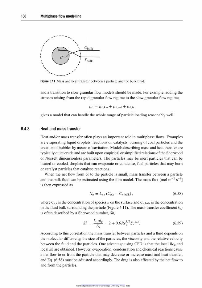
168 Multiphase flow modelling
Figure 6.11 Mass and heat transfer between a particle and the bulk fluid.
and a transition to slow granular flow models should be made. For example, adding the
stresses arising from the rapid granular flow regime to the slow granular flow regime,
μd = μd,kin + μd,col + μd,fr
gives a model that can handle the whole range of particle loading reasonably well.
6.4.3 Heat and mass transfer
Heat and/or mass transfer often plays an important role in multiphase flows. Examples
are evaporating liquid droplets, reactions on catalysts, burning of coal particles and the
creation of bubbles by means of cavitation. Models describing mass and heat transfer are
typically quite crude and are built upon empirical or simplified relations of the Sherwood
or Nusselt dimensionless parameters. The particles may be inert particles that can be
heated or cooled, droplets that can evaporate or condense, fuel particles that may burn
or catalyst particles that catalyse reactions.
When the net flow from or to the particle is small, mass transfer between a particle
and the bulk fluid can be estimated using the film model. The mass flux [mol m−2 s−1]
is then expressed as
Nn = kc,n (Cn,s − Cn,bulk) , (6.58)
where Cn,s is the concentration of species n on the surface and Cn,bulk is the concentration
in the fluid bulk surrounding the particle (Figure 6.11). The mass-transfer coefficient kc,i
is often described by a Sherwood number, Sh,
Sh =kc,i dp
Di
= 2 + 0.6Re1/2d Sc1/3
. (6.59)
According to this correlation the mass transfer between particles and a fluid depends on
the molecular diffusivity, the size of the particles, the viscosity and the relative velocity
between the fluid and the particles. One advantage using CFD is that the local Red and
local Sh are obtained. However, evaporation, condensation and chemical reactions cause
a net flow to or from the particle that may decrease or increase mass and heat transfer,
and Eq. (6.58) must be adjusted accordingly. The drag is also affected by the net flow to
and from the particles.
Cambridge Books Online © Cambridge University Press, 2012
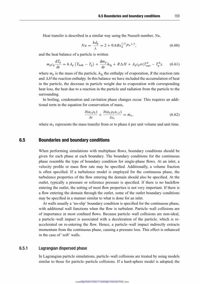
6.5 Boundaries and boundary conditions 169
Heat transfer is described in a similar way using the Nusselt number, Nu,
Nu =hdp
λ
= 2 + 0.6Re1/2d Pr1/3
, (6.60)
and the heat balance of a particle is written
mpcp
dTp
dt= h Ap
(
Tbulk − Tp
)
+dmp
dthfg + R�H + Apεpσ (T 4
surr − T 4p ), (6.61)
where mp is the mass of the particle, hfg the enthalpy of evaporation, R the reaction rate
and �H the reaction enthalpy. In this balance we have included the accumulation of heat
in the particle, the decrease in particle weight due to evaporation with corresponding
heat loss, the heat due to a reaction in the particle and radiation from the particle to the
surrounding.
In boiling, condensation and cavitation phase changes occur. This requires an addi-
tional term in the equation for conservation of mass,
∂(αkρk)
∂t+
∂(αkρkui,k)
∂xi
= mk, (6.62)
where mk represents the mass transfer from or to phase k per unit volume and unit time.
6.5 Boundaries and boundary conditions
When performing simulations with multiphase flows, boundary conditions should be
given for each phase at each boundary. The boundary conditions for the continuous
phase resemble the type of boundary condition for single-phase flows. At an inlet, a
velocity profile or mass flow rate may be specified. Additionally, a volume fraction
is often specified. If a turbulence model is employed for the continuous phase, the
turbulence properties of the flow entering the domain should also be specified. At the
outlet, typically a pressure or reference pressure is specified. If there is no backflow
entering the outlet, the setting of most flow properties is not very important. If there is
a flow entering the domain through the outlet, some of the outlet boundary conditions
may be specified in a manner similar to what is done for an inlet.
At walls usually a ‘no-slip’ boundary condition is specified for the continuous phase,
with additional wall functions when the flow is turbulent. Particle–wall collisions are
of importance in most confined flows. Because particle–wall collisions are non-ideal,
a particle–wall impact is associated with a deceleration of the particle, which is re-
accelerated on re-entering the flow. Hence, a particle–wall impact indirectly extracts
momentum from the continuous phase, causing a pressure loss. This effect is enhanced
in the case of ‘soft’ walls.
6.5.1 Lagrangian dispersed phase
In Lagrangian particle simulations, particle–wall collisions are treated by using models
similar to those for particle–particle collisions. If a hard-sphere model is adopted, the
Cambridge Books Online © Cambridge University Press, 2012
170 Multiphase flow modelling
Figure 6.12 A particle colliding with a rough wall.
particle–wall collision may dissipate kinetic energy as heat that can be estimated from
the coefficient of restitution. The restitution coefficient is defined as the ratio of the
velocity after collision and that before collision. If a soft-sphere model is adopted, the
effect of the wall may be described using a spring–slider–dashpot model based upon
heuristics or upon a number of physical parameters. Note that, in the application both
of hard-sphere and of soft-sphere models, the properties of the wall are not necessarily
the same as the properties of the particles. Most often, a wall can be treated as a particle
with infinite mass and radius.
Rough walls
Experiments and simulations have shown that wall roughness may have a considerable
effect on the particle–wall collision process, and thus on the complete flow characteris-
tics. This has two causes. First, the normal of the actual wall might not be constant across
the wall. This means that the impact normal is a function of the local wall roughness.
This can be modelled by including a ‘random’ component on top of the average wall
normal. Secondly, the so-called shadow effect results in a shift of the effective roughness
distribution for small impact angles. Both effects are shown in Figure 6.12: (1) the local
wall normal changes along the wall, affecting the collision normal; and (2) particles with
small impact angles can no longer collide with parts of the wall, making certain collision
normals more likely than others (this was called the shadow effect by Sommerfeld in
1996).
6.5.2 Eulerian dispersed phase
Boundary conditions for walls in Eulerian models are less obvious than in the Lagrangian
framework. In most simulations, particles are assumed to slip freely along the walls. This
assumption originates from experimental observations, in which most particles seem to
move rather freely along walls. More realistically, a slip condition can be specified at the
walls,
∂Ui,d
∂ni
= f, (6.63)
Cambridge Books Online © Cambridge University Press, 2012
6.6 Summary 171
where f specifies the amount of slip. If f = 0, the free-slip conditions are obtained. It is
generally observed that convergence becomes difficult for higher values of f.
Boundary conditions for the granular temperature at the wall may have a significant
impact on the flow. Various models that mimic the wall functions for single-phase
turbulent flows are available. These have a production term, accounting for the dispersion
effect of the particles, and a dissipation term, accounting for the non-ideal effect of the
collision. In most simulations, specifying a zero gradient of granular temperature at
walls gives satisfactory results.
6.6 Summary
In this chapter the Euler–Lagrange, Euler–Euler, mixture, volume-of-fluid and packed-
bed models are presented. In many cases, it is not evident which model to choose.
Each of the models is based on a number of assumptions and provides a specific level
of detail. Some models describe individual particles or interface segments, whereas
other models are expressed in terms of averaged properties. When selecting a model,
numerical stability and computational cost must also be considered.
The Euler–Euler model is obtained by averaging the flow properties of a multiphase
flow of dispersed particles smaller than the computational cells. The model solves the
momentum and continuity equations for each phase. It is the most general model and
should in principle work for all kinds of multiphase flows. However, it is usually less
stable than the other models, and it requires closure models to describe all interactions
between the phases, so empirical models for the specific system are often required.
The mixture model is a simplification of the Euler–Euler model that is more stable but
requires a strong coupling between the phases, i.e. low Stokes number. It shares with the
Euler–Euler model the problem that empirical closures are required for any interaction
between the phases.
In the Euler–Lagrange model the transport equations for each particle or a bundle
of particles that behave identically are solved. It is most accurate and works very well
for systems with a limited number of particles, often in cases in which particle–particle
collisions can be neglected, i.e. when the particle–particle distance is larger than ten
particle diameters. In principle, inter-particle collisions can be taken into account, but
this is usually very expensive. The upper limit for the number of particles or bundles of
particles is a few hundred thousand when the simulations are done on a PC. The model
tracks the centre of gravity of the bundle, and a limit for the bundle size is that most of
the particles in the bundle should be within one computational cell if one is to describe
the interaction with the continuous phase accurately. The Euler–Lagrange model can
easily take into account particle-size or density distributions. For a large size or density
distribution the Euler–Euler model requires several phases to describe the system and
relations to describe their interactions. In these cases, the Euler–Lagrange model will
be more stable and will predict the flow better.
The volume-of-fluid (VOF) model is intended for gas–liquid and liquid–liquid segre-
gated flows. The model resolves the interface between the phases and requires that the
Cambridge Books Online © Cambridge University Press, 2012
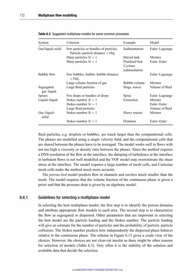
172 Multiphase flow modelling
Table 6.3 Suggested multiphase models for some common processes
System Criterion Example Model
Gas/liquid–solid Few particles or bundles of particles.
Particle–particle distance <10dp
Sedimentation Euler–Lagrange
Many particles St < 1 Stirred tank Mixture
Many particles St > 1 Fluidized bed
Cyclone
sedimentation
Euler–Euler
Bubbly flow Few bubbles, bubble–bubble distance
>10dp
Euler–Lagrange
Large volume fraction of gas Bubble column Mixture
Segregated
gas–liquid
Large fluid particles Slugs, waves Volume of fluid
Sprays Few drops or bundles of drops Spray Euler–Lagrange
Liquid–liquid Stokes number St < 1 Extraction Mixture
Stokes number St > 1 Euler–Euler
Large fluid particles Volume of fluid
Gas–liquid–
solid
Stokes number St > 1 Slurry reactor Mixture
Stokes number St < 1 Flotation Euler–Euler
fluid particles, e.g. droplets or bubbles, are much larger than the computational cells.
The phases are modelled using a single velocity field, and the computational cells that
are shared between the phases have to be averaged. The model works well in flows with
not too high a viscosity or density ratio between the phases. Since the method requires
a DNS resolution of the flow at the interface, the damping of turbulence at the interface
in turbulent flows is not well modelled and the VOF model may overestimate the shear
stress at the interface. The model requires a large number of mesh cells, and Cartesian
mesh cells make the method much more accurate.
The porous-bed model predicts flow in channels and cavities much smaller than the
mesh. The model requires that the volume fraction of the continuous phase is given a
priori and that the pressure drop is given by an algebraic model.
6.6.1 Guidelines for selecting a multiphase model
In selecting the best multiphase model, the first step is to identify the porous domains
and attribute appropriate flow models to each area. The second step is to characterize
the flow as segregated or dispersed. Other parameters that are important in selecting
the best model are the particle loading and the Stokes number. The particle loading
will give an estimate for the number of particles and the probability of particle–particle
collisions. The Stokes number predicts how independently the dispersed phase behaves
relative to the continuous phase. The scheme in Figure 6.13 gives a crude view of the
choices. However, the choices are not clear-cut insofar as there might be other reasons
for selection of models (Table 6.3). Very often it is the stability of the solution and
available data that decide the selection.
Cambridge Books Online © Cambridge University Press, 2012
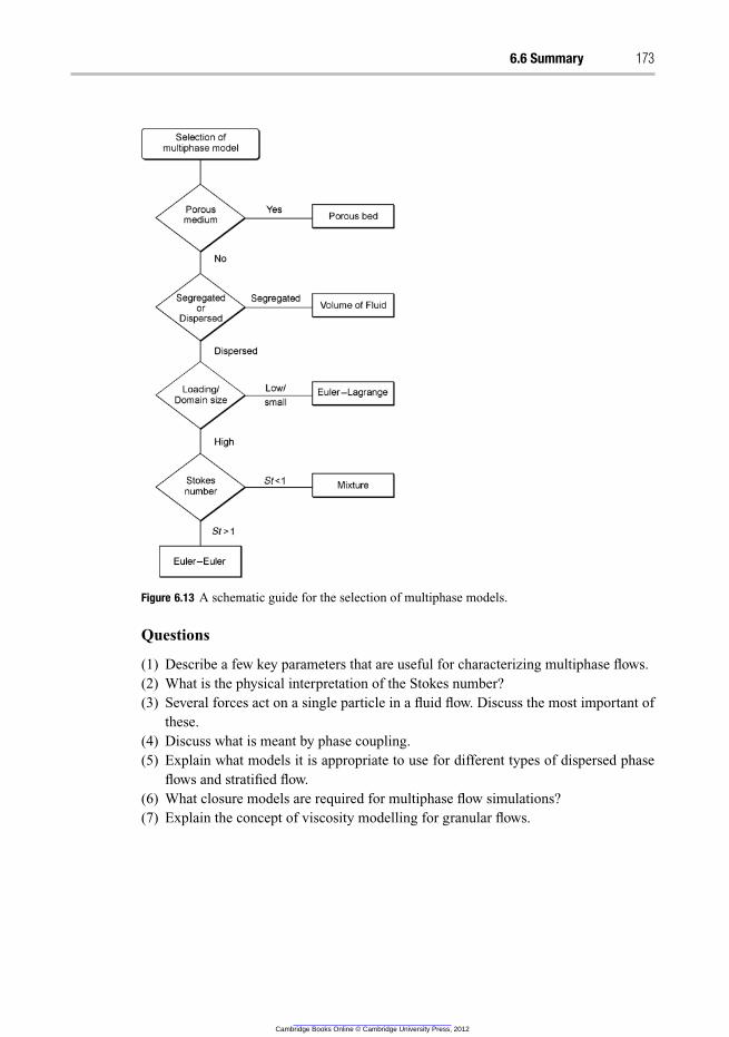
6.6 Summary 173
Figure 6.13 A schematic guide for the selection of multiphase models.
Questions
(1) Describe a few key parameters that are useful for characterizing multiphase flows.
(2) What is the physical interpretation of the Stokes number?
(3) Several forces act on a single particle in a fluid flow. Discuss the most important of
these.
(4) Discuss what is meant by phase coupling.
(5) Explain what models it is appropriate to use for different types of dispersed phase
flows and stratified flow.
(6) What closure models are required for multiphase flow simulations?
(7) Explain the concept of viscosity modelling for granular flows.
Cambridge Books Online © Cambridge University Press, 2012

Cambridge Books Online © Cambridge University Press, 2012
7 Best practice guidelines
Computational fluid dynamics does not provide an exact solution to all problems, but
is in many cases a reliable tool that can provide useful results when it is employed
by an experienced user. An inexperienced user, on the other hand, may obtain very
nice graphs that are very far from being a prediction of the stated problem. Some of
the problems arise from the many default settings in commercial CFD codes, since
the user may obtain results without knowing what the code is doing by accepting set-
tings that are not appropriate for the specific problem. The user must make an active
decision regarding each setting due to the fact that many problems can arise from
a user failing to understand what the proper settings should be. This chapter pro-
vides some guidelines that can help a new user to avoid the most common mistakes.
Many more recomendations selected by experienced CFD users can be found in the
‘Best Practice Guidelines’ for single-phase flows [20] and for dispersed multiphase
flows [21] by the European Research Community on Flow Turbulence and Combustion
(ERCOFTAC).
A CFD simulation contains both errors and uncertainties. An error is defined as a
recognizable deficiency that is not due to a lack of knowledge, whereas an uncertainty
is a potential deficiency that is due to a lack of knowledge.
Poor simulation results may arise for many different reasons; the user may make
mistakes in formulating the problem to solve or in formulating the geometry and mesh-
ing. Numerical errors may occur due to lack of convergence and a poor choice of
discretization methods. The models for turbulence, reactions and multiphase flow are
not exact descriptions of the real world, and poor results may be introduced by not
selecting the best model for the specific case. In the end, the robustness and reliability
of the simulations should be analysed by sensitivity analysis, verification, validation and
calibration.
In general, it is good practice to study the obtained simulation results critically. CFD
is not (yet) at the stage at which it can be treated as a black box. Simulation results
should be verified with experimental findings, fluid-mechanics theory and, sometimes,
instinct. It may also help to understand the limitations of the CFD model if a simulation
is performed for a case regarding which the results are known, prior to exploring new
ground with the model. Some common errors and recommendations for best practice
are given in this chapter.
Cambridge Books Online © Cambridge University Press, 2012
7.2 Numerical uncertainty 175
7.1 Application uncertainty
Many problems in CFD simulations arise from inaccurately stated problems. The actual
problem that is being solved is not always straightforward. It is seldom possible to select
the right settings from the beginning. The properties of the flow are not all known in
advance. The flow can be laminar or turbulent, or laminar in some regions and turbulent
in other regions. The local hold-up in multiphase flow and the local Dahmkohler number
in reacting systems can affect the choice of model. The flow within the system may also
affect the flow at the inlet and the outlet. These are just a few of the possibilities.
7.1.1 Geometry and grid design
A number of general guidelines can be given.
� Make sure that the CAD geometry is complete for the flow simulation. The CAD
drawing should be kept as simple as possible, but it must not be simpler than that. All
details smaller than the computational cells can in most cases be removed, but small
details on the surface can sometimes be important for the flow, e.g. a welded joint may
induce flow separation.� Symmetric boundary conditions restrict the solution to a symmetric solution, and no
transport is allowed across the symmetry plane, e.g. bubble columns and fluidized
beds are poorly described by 2D simulations.� When the inflow and outflow are not known exactly, they should be put far from the
region of interest.� With constant-pressure outflow, specify the direction of the outflow (e.g. normal to
the plane) to minimize the pressure difference across the surface.� Use pressure outflow for multiple outflow boundaries.� Avoid having non-orthogonal cells close to the boundaries. The angle between the
grid lines and the boundary should be close to 90◦. Use body-fitted grids when the
grid cannot be aligned with the surface.� Avoid the use of highly skewed cells. The angles should be kept between 40◦ and 140◦.
The maximum skewness should be <0.95 and the average below 0.33. The aspect
ratio should be below 5, but may be up to 10 inside the boundary layer.� The squish index describes how the cell faces are oriented, where 0 is a perfect cell and
the upper limit is 1. The recommendation is that the maximum squish index should
be below 0.99.� Perform a grid check to avoid problems due to incorrect connectivity. This can often
be done in the mesh-generator software.
7.2 Numerical uncertainty
7.2.1 Convergence
Poor convergence is the most common numerical reason for poor results. Residuals are
defined differently in various programs, and monitoring the residual is in most cases not
sufficient to verify that a converged solution has been reached. Convergence problems
Cambridge Books Online © Cambridge University Press, 2012
176 Best practice guidelines
for steady-state simulations may also indicate that a steady solution does not exist. The
residual should always be combined with other measures of convergence. Keep in mind
that a converged solution is not always a correct one.
� Use different convergence criteria for different variables. Concentration may need a
lower residual than velocity.� Monitor integral quantities of solution-sensitive variables.� Make global balances for mass, momentum and energy.� Monitor the solution at specific important points.� Test for steady state by switching to a transient solver.� Plot the residual to evaluate whether the solution is poor in some regions of the
computational domain.
7.2.2 Enhancing convergence
There are many different methods by which to enhance convergence.
� Use more robust numerical schemes, e.g. initially employ first-order upwind, changing
to a higher order for the final iterations.� Reduce the under-relaxation or CFL number initially.� Examine the local residual. The convergence problem might be localized to one small
region. Use grid adaptation to refine or coarsen the mesh in areas where it is needed.
Using a fine grid throughout may diminish the convergence rate.� Solve steady-state problems transiently.� Try different initial guesses, e.g. obtain an initial guess from a short transient simula-
tion or obtain an initial guess from a steady-state simulation.� Solve for only a few variables at a time, e.g. solve for the flow field first and keep the
velocities constant whilst solving concentration and chemical reactions. Finally solve
for all variables.� Use the coupled solver for high-speed compressible flows, highly coupled flows with
strong body forces or flows being solved on very fine meshes. Keep in mind that the
coupled solver requires 1.5–2 times more memory than needed by a segregated solver.
7.2.3 Numerical errors
The numerical error is the difference between the exact solution and the numerical
solution.
� Avoid the use of first-order schemes. First order can be used initially when you have
convergence problems, but will always lead to problems with numerical diffusion.� Estimate the discretization error by showing that the solution is independent of the
mesh density.� Use node-based gradients with unstructured tetrahedral meshes.� If possible, compare the solutions with different orders of accuracy.
Cambridge Books Online © Cambridge University Press, 2012

7.3 Turbulence modelling 177
� Perform refinement or coarsening of the computational mesh. Ideally, the solution
should become less dependent on the mesh as it is refined. If the results reveal a strong
dependence on the computational mesh spacing, further refinement is required.
7.2.4 Temporal discretization
The choice of time step depends on the flow features being studied. Large-eddy simula-
tion requires very short time steps to resolve the turbulent eddies. Some of the turbulent
structures can also be resolved with RANS models, i.e. unsteady RANS or URANS, but
usually the time step is much larger than the turbulence timescales and only the transient
behaviour of the mean flow is resolved.
� Start with a short time step, i.e. a low CLF number that can increase with time.� The time step should be selected so that fewer than 20 iterations are needed in each
time step with an implicit solver.� Make sure that the solution has converged for each iteration for implicit schemes.� For temporal accuracy, a second-order-accurate discretization scheme is recom-
mended, such as Crank–Nicolson or second-order backward Euler.
7.3 Turbulence modelling
Only DNS is an exact formulation of the Navier–Stokes equations. All other turbulence
models contain model approximations. Table 4.4 contains a comparison of turbulence
models.
� Test different turbulence models. The cost of running a second model starting from
a converged solution is usually not high. Different values of the model constants that
are recommended for specific kinds of flows should also be tested.� Transition between turbulent and laminar flow is very difficult to simulate for all
models. Simulations involving transition must be verified with experimental data.� Be aware of the limitations of the specific model, e.g. the k–ε model will suppress
swirl in a flow and the absence of swirl in a k–ε model does not certify that swirl
would not appear with another turbulence model.� Many physical phenomena are not captured by turbulence models and require under-
standing from the user. Examples include, but are not limited to, transition, separation,
unsteady boundary layers and low-Reynolds-number turbulence.
7.3.1 Boundary conditions
� The exact inlet conditions for the turbulence properties are usually not known exactly.
The value of k/ε times the average velocity gives an order-of-magnitude estimation
of how far into the system the settings at the inlet will survive.� Exact inlet conditions for LES are not possible. Modern CFD programs can generate
simple turbulent eddies at the inlet, but the inlet should be far from the area of
Cambridge Books Online © Cambridge University Press, 2012
178 Best practice guidelines
interest in order to allow a proper statistical distribution of eddies to develop. Periodic
boundary conditions should be used when possible, but may introduce unphysical
correlations. As always, it is important to verify the obtained solution critically.� For RANS models, the lower level of y+ should typically be between 20 and 30 at
the walls. Some commercial CFD programs can be made to accept lower y+ levels
by adjusting the appropriate model. (Check the manual for actual values.) The upper
limit of y+ is usually in the range 80–100.� LES models require additional treatment at no-slip walls.� For low-Re turbulence models the first grid should be at y+
< 4, preferably at y+ ≈ 1
with 5–10 mesh points below y+ = 20.� Standard wall functions are not recommended for flow with a negative pressure
gradient, e.g. with flow separation at the wall.
7.4 Reactions
� Check the Dahmkohler number. Slow chemical reactions with Da ≪ 1 are straightfor-
ward. Very fast, mixing-controlled, isothermal chemical reactions with Da ≫ 1 can
be modelled rather accurately. Most other conditions with Da ≈ 1 and reactions that
lead to heat formation and changes in density will give uncertain results.� Very low residuals as a convergence criterion for concentration are often required,
and monitoring integral quantities for mass balances or steady local concentrations
usually provides more reliable indicators than low residuals.
7.5 Multiphase modelling
Generally speaking, multiphase flows are more challenging than single-phase flows,
and errors in multiphase flow simulations are typically larger than those in single-phase
simulations. These errors may have a number of different origins.
� Not knowing the most important physical mechanisms. Because of the wide variety
of multiphase flow types, there is not one ‘generic’ model for multiphase flows. Before
attempting to model a multiphase flow system, it is very important to understand the
physical mechanisms occurring in the flow system. This includes understanding the
most important forces and mechanisms in the flow and the properties of the fluid(s)
and/or solids, as well as a good estimate of the length scales and timescales of the
physical processes. Only with this knowledge can appropriate models be selected and
their shortcomings in a simulation estimated.� Closure models. Most errors in multiphase flow simulations arise from shortcomings
of the closure models employed. Most closure models are empirically determined,
which makes them applicable, strictly speaking, only under conditions similar to
those for the data they are built from. Analytical closure models are developed for
‘ideal’ conditions, which are hardly ever met in reality. Using closure models for
Cambridge Books Online © Cambridge University Press, 2012
7.5 Multiphase modelling 179
conditions or regimes different from those to which they are applicable may be asking
for trouble.� Timescale and length-scale separation. In the derivation of turbulence models, a
separation between the timescales and length scales of the ‘large’ eddies carrying the
energy and the scale(s) at which energy is dissipated is assumed. Similar assumptions
are required in order to derive governing and closure models for multiphase flows. For
instance, many closure models require the particles to be smaller than the large-scale
flow structures in a flow.� Choice of model and governing equations. It is important to understand the impli-
cations and assumptions of each multiphase model, and under what conditions it may
be employed. For instance, in the derivation of the Euler–Euler or two-fluid model,
the pressure gradient over large interfaces, which is important in separated-flow sit-
uations, is neglected. This means that such a model will not capture the dynamics of
free surfaces very accurately.� Numerical errors. Many numerical errors potentially arising in single-phase calcu-
lations may also arise in multiphase flow calculations. Therefore, it is important to
check the best-practice guidelines for single-phase flow computations. However, there
may be additional problems. Many of the ideas employed in solving multiphase flows
arise from single-phase flows, leading to slow convergence, or, worse, an erroneous
result.
To minimize the potential problems occurring when performing multiphase flow simu-
lations, the following checklist may be employed,
1. If possible, start the simulation with a single-phase flow situation resembling the
system. This simulation can be optimized in terms of grid size, time step, etc. by
using the best-practice guidelines for single-phase flow.
2. Determine the regime of the multiphase flow in terms of dimensionless parameters
(Re, We, St, . . . ). This enables the choice of suitable closure models and may give
insight into the expected flow situation.
3. Make an estimate of the forces acting on bubbles, particles or droplets and under
which conditions these forces will occur.
4. Make a suitable selection of the turbulence model and decide which terms (and
coupling to the dispersed phase) are important.
5. If possible, start with a geometry, flow properties and dispersed-phase properties sim-
ilar to those of a system of which you know the behaviour or for which experimental
data are available. This creates confidence in the models employed.
6. If there is a large size distribution of the dispersed phase, a multi-fluid approach might
be required for the dispersed phase. This allows the use of a range of size classes,
which can be monitored separately. Size distributions can have a big effect on the
flow.
7. First-order-accurate models, such as the VOF model and the surface-tension models,
require a very fine mesh – in these cases a relatively mesh-independent solution is
very important.
Cambridge Books Online © Cambridge University Press, 2012
180 Best practice guidelines
8. Make sure that iterations are well converged. Many popular commercial CFD solvers
will start with a new time step when a specified maximum number of iterations is
reached, regardless of convergence criteria. This may be detrimental in terms of the
quality of results obtained.
7.6 Sensitivity analysis
There are many choices that are uncertain, and sensitivity analysis is one way to examine
the effect of the specific choice. It is good practice to start from a converged solution
and change all uncertain settings in the model.
7.7 Verification, validation and calibration
Verification is a procedure to ensure that the program solves the equations correctly.
Validation is done to test how accurately the model represents reality, and calibration
is often used to adjust the simulation to known experimental data in order to study
parameter sensitivity (‘what if’) in the design process.
Cambridge Books Online © Cambridge University Press, 2012

Cambridge Books Online © Cambridge University Press, 2012
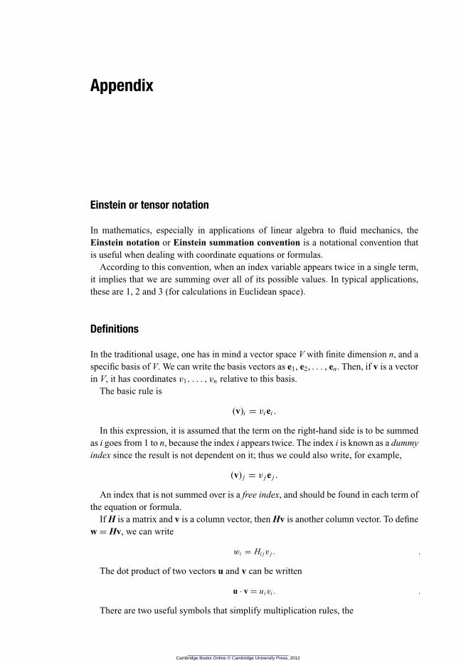
Appendix
Einstein or tensor notation
In mathematics, especially in applications of linear algebra to fluid mechanics, the
Einstein notation or Einstein summation convention is a notational convention that
is useful when dealing with coordinate equations or formulas.
According to this convention, when an index variable appears twice in a single term,
it implies that we are summing over all of its possible values. In typical applications,
these are 1, 2 and 3 (for calculations in Euclidean space).
Definitions
In the traditional usage, one has in mind a vector space V with finite dimension n, and a
specific basis of V. We can write the basis vectors as e1, e2, . . . , en. Then, if v is a vector
in V, it has coordinates v1, . . . , vn relative to this basis.
The basic rule is
(v)i = vi ei .
In this expression, it is assumed that the term on the right-hand side is to be summed
as i goes from 1 to n, because the index i appears twice. The index i is known as a dummy
index since the result is not dependent on it; thus we could also write, for example,
(v) j = v j e j .
An index that is not summed over is a free index, and should be found in each term of
the equation or formula.
If H is a matrix and v is a column vector, then Hv is another column vector. To define
w = Hv, we can write
wi = Hi jv j . .
The dot product of two vectors u and v can be written
u · v = uivi . .
There are two useful symbols that simplify multiplication rules, the
Cambridge Books Online © Cambridge University Press, 2012
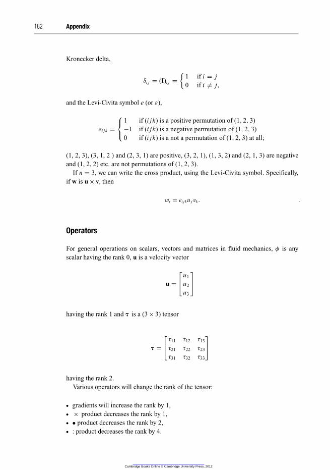
182 Appendix
Kronecker delta,
δi j = (I)i j =
{
1 if i = j
0 if i �= j,
and the Levi-Civita symbol e (or ε),
ei jk =
⎧
⎨
⎩
1 if (i jk) is a positive permutation of (1, 2, 3)
−1 if (i jk) is a negative permutation of (1, 2, 3)
0 if (i jk) is a not a permutation of (1, 2, 3) at all;
(1, 2, 3), (3, 1, 2 ) and (2, 3, 1) are positive, (3, 2, 1), (1, 3, 2) and (2, 1, 3) are negative
and (1, 2, 2) etc. are not permutations of (1, 2, 3).
If n = 3, we can write the cross product, using the Levi-Civita symbol. Specifically,
if w is u × v, then
wi = ei jku jvk . .
Operators
For general operations on scalars, vectors and matrices in fluid mechanics, φ is any
scalar having the rank 0, u is a velocity vector
u =
⎡
⎣
u1
u2
u3
⎤
⎦
having the rank 1 and � is a (3 × 3) tensor
� =
⎡
⎣
τ11 τ12 τ13
τ21 τ22 τ23
τ31 τ32 τ33
⎤
⎦
having the rank 2.
Various operators will change the rank of the tensor:
� gradients will increase the rank by 1,� × product decreases the rank by 1,� • product decreases the rank by 2,� : product decreases the rank by 4.
Cambridge Books Online © Cambridge University Press, 2012
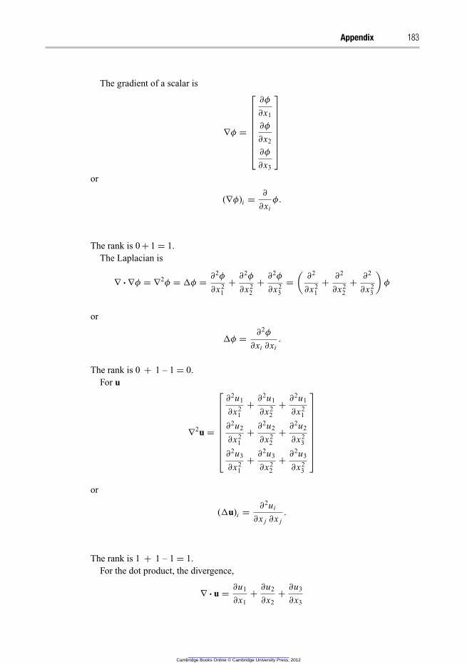
Appendix 183
The gradient of a scalar is
∇φ =
⎡
⎢
⎢
⎢
⎢
⎢
⎢
⎢
⎣
∂φ
∂x1
∂φ
∂x2
∂φ
∂x3
⎤
⎥
⎥
⎥
⎥
⎥
⎥
⎥
⎦
or
(∇φ)i =∂
∂xi
φ.
The rank is 0 + 1 = 1.
The Laplacian is
∇ · ∇φ = ∇2φ = �φ =
∂2φ
∂x21
+∂
2φ
∂x22
+∂
2φ
∂x23
=
(
∂2
∂x21
+∂
2
∂x22
+∂
2
∂x23
)
φ
or
�φ =∂
2φ
∂xi ∂xi
.
The rank is 0 + 1 – 1 = 0.
For u
∇2u =
⎡
⎢
⎢
⎢
⎢
⎢
⎢
⎢
⎢
⎣
∂2u1
∂x21
+∂
2u1
∂x22
+∂
2u1
∂x21
∂2u2
∂x21
+∂
2u2
∂x22
+∂
2u2
∂x23
∂2u3
∂x21
+∂
2u3
∂x22
+∂
2u3
∂x23
⎤
⎥
⎥
⎥
⎥
⎥
⎥
⎥
⎥
⎦
or
(�u)i =∂
2ui
∂x j ∂x j
.
The rank is 1 + 1 – 1 = 1.
For the dot product, the divergence,
∇ · u =∂u1
∂x1
+∂u2
∂x2
+∂u3
∂x3
Cambridge Books Online © Cambridge University Press, 2012
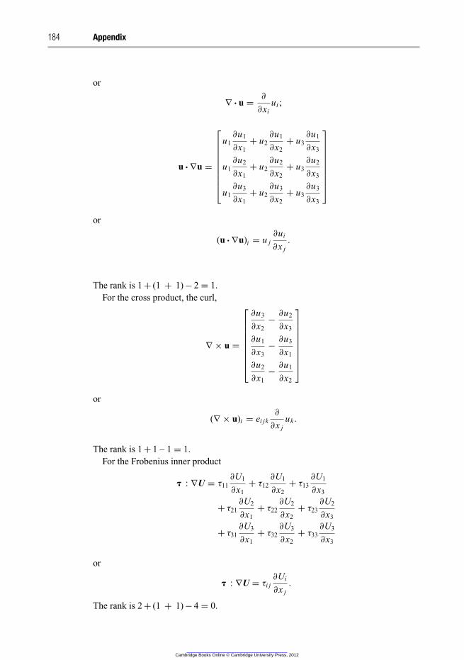
184 Appendix
or
∇ · u =∂
∂xi
ui ;
u · ∇u =
⎡
⎢
⎢
⎢
⎢
⎢
⎢
⎢
⎣
u1
∂u1
∂x1
+ u2
∂u1
∂x2
+ u3
∂u1
∂x3
u1
∂u2
∂x1
+ u2
∂u2
∂x2
+ u3
∂u2
∂x3
u1
∂u3
∂x1
+ u2
∂u3
∂x2
+ u3
∂u3
∂x3
⎤
⎥
⎥
⎥
⎥
⎥
⎥
⎥
⎦
or
(u · ∇u)i = u j
∂ui
∂x j
.
The rank is 1 + (1 + 1) − 2 = 1.
For the cross product, the curl,
∇ × u =
⎡
⎢
⎢
⎢
⎢
⎢
⎢
⎢
⎣
∂u3
∂x2
−∂u2
∂x3
∂u1
∂x3
−∂u3
∂x1
∂u2
∂x1
−∂u1
∂x2
⎤
⎥
⎥
⎥
⎥
⎥
⎥
⎥
⎦
or
(∇ × u)i = ei jk
∂
∂x j
uk .
The rank is 1 + 1 – 1 = 1.
For the Frobenius inner product
� : ∇U = τ11
∂U1
∂x1
+ τ12
∂U1
∂x2
+ τ13
∂U1
∂x3
+ τ21
∂U2
∂x1
+ τ22
∂U2
∂x2
+ τ23
∂U2
∂x3
+ τ31
∂U3
∂x1
+ τ32
∂U3
∂x2
+ τ33
∂U3
∂x3
or
� : ∇U = τi j
∂Ui
∂x j
.
The rank is 2 + (1 + 1) − 4 = 0.
Cambridge Books Online © Cambridge University Press, 2012

Cambridge Books Online © Cambridge University Press, 2012
References
1. Cercignani, C., Rarefied Gas Dynamics: From Basic Concepts to Actual Calculations, 2000,
Cambridge: Cambridge University Press.
2. Chhabra, R. P. and J. F. Richardson, Non-Newtonian Flow and Applied Rheology: Engineering
Applications, 2008, Oxford: Butterworth-Heinemann.
3. Versteeg, H. K. and W. Malalasekera, An Introduction to Computational Fluid Dynamics:
The Finite Volume Method, 1995, New York: Wiley.
4. Chung, T. J., Computational Fluid Dynamics, 2002, New York: Cambridge University Press.
5. Hinze, J. O., Turbulence, 1975, New York: McGraw-Hill.
6. Tennekes, H. and J. L. Lumley, A First Course in Turbulence, 1972, Cambridge, MA: MIT
Press.
7. Pope, S., Turbulent Flows, 2000, Cambrige: Cambridge University Press.
8. Bernard, P. S. and J. M. Wallace, Turbulent Flow, 2002, Hoboken, NJ: John Wiley & Sons
Inc.
9. Garde, R. J., Turbulent Flow, 1994, New Delhi: Wiley Eastern Limited.
10. Mathieu, J. and J. Scott, An Introduction to Turbulent Flow, 2000, Cambridge: Cambridge
University Press.
11. Sagaut, P., Large Eddy Simulation for Incompressible Flows, 2001, Heidelberg: Springer.
12. Wilcox, D. C., Turbulence Modeling for CFD, 2000, La Canada, CA: DCW Industries.
13. Schlichting, H., Boundary Layer Theory, 2000, Berlin: Springer.
14. Baldyga, J. and J. R. Bourne, Turbulent Mixing and Chemical Reactions, 1999, New York:
Wiley.
15. Fox, R. O., Computational Models for Turbulent Reacting Flows, 2003, Cambridge:
Cambridge University Press.
16. Clift, R., J. R. Grace and M. E. Weber, Bubbles, Drops, and Particles, 1978, New York:
Academic Press.
17. Crowe, C., M. Sommerfeld and Y. Tsuji, Multiphase Flows with Droplets and Particles, 1998,
Boca Raton, FL: CRC Press.
18. Kolev, N. I., Multiphase Flow Dynamics. 1, Fundamentals, 2005, Berlin: Springer.
19. Gidaspow, D., Multiphase Flow and Fluidization: Continuum and Kinetic Theory Description,
1994, Boston, MA: Academic Press.
20. European Research Community on Flow, Turbulence and Combustion (ERCOFTAC), Special
Interest Group on Quality and Trust in Industrial CFD Best Practice Guidelines, eds. M. Casey
and T. Wintergerste, 2000, online.
21. European Research Community on Flow, Turbulence and Combustion (ERCOFTAC), Special
Interest Group on Dispersed Turbulent Multi-Phase Flow. Best Practice Guidelines, eds.
M. Sommerfeld, B. van Wachem and R. Oliemans, 2008, online.
Cambridge Books Online © Cambridge University Press, 2012
Index
accuracy, 43, 176
adaptation, 60, 178
algebraic slip model, 150
angular momentum, 74
anisotropic, 70, 71
application uncertainty, 175
aspect ratio, 59
average concentrations, 133
average reaction rate, 116, 140
Batchelor length scale, 119
BBO equation, 147
beta-PDF, 122
boundary conditions, 18–21
axis, 20
best-practice guidelines, 177
inlet, 19, 111
outlet, 19
periodic, 6
symmetry, 20
wall functions, 106
walls, 19
boundary layers, see turbulent boundary layers
boundedness, 40
Boussinesq approximation, 85
bouyancy force, 149
Brownian force, 149
calibration, 180
capillary number, 160
cell-centred, 26
central differencing, 40
chemical energy, 16
chemical reactions, 130–40
best-practice guidelines, 178
collision viscosity, 167
combustion, 137
conditionally bounded, 40
conservativeness, 38
conserved scalar, 119
consistent, 46
continuity equation, 12
control volume, 26
convergence, 37
best-practice guidelines, 175
Courant number (CFL), 57, 176
Crank–Nicolson, 56
Dahmkohler number, 118
dense regime, 144
dilatational viscosity, 12
dilute regime, 144
direct numerical simulation (DNS), 79
discrete random walk (DRW), 154
discretization schemes, 38–46, 176
comparison, 46
dispersed flow, 144
dissipation, 91
dissipative subrange, 73, 76
drag coefficient, 162
drag force, 148
drag models, 161
drift velocity, 157
dynamic LES, 81
eddy dissipation (ED), 141
eddy viscosity, 86
effective viscosity, 86
energy cascade, 72
energy-containing subrange, 73, 76
energy spectrum, 75
energy transport, 16
engulfment, 117
Eotvos number, 162
equation of state, 22
equilibrium reaction, 135
Euler–Euler, 150, 155
Euler–Lagrange, 150, 152
explicit method, 54
face value, 28
film model, 168
filtered residual, 80
filtered velocity, 80
finite differences, 25
finite elements, 25
http://ebooks.cambridge.org/ebook.jsf?bid=CBO9781139093590Cambridge Books Online © Cambridge University Press, 2012
Index 187
finite volumes, 25
first-order accurate, 44
first-order upwind, 41, 176
forces on dispersed particles, 147–9
bouyancy force, 149
Brownian force, 149
drag force, 148
history force, 148
Magnus lift force, 148
pressure force, 148
Saffman lift force, 149
shear force, 148
thermophoretic force, 149
turbulence force, 149
virtual mass force, 148
four-way coupling, 147
friction velocity, 103
frictional viscosity, 167
Gauss theorem, 27
Gauss–Seidel, 34
granular flow models, 165
granular temperature, 166
granular viscosity, 167
collision, 167
friction, 167
kinetic, 167
heat transfer, 168
hexahedral, 58
history force, 148
HRIC scheme, 46
implicit method, 55, 177
incompressible flow, 13
inertial subrange, 73, 76
initial conditions, 20, 34
best-practice guidelines, 176
intensity of segregation, 125
inter-particle distance, 145
isotropic, 68, 71, 75
kinetic energy, 16
kinetic energy balance, 16
kinetic theory of granular flow (KTGF),
166
kinetic viscosity, 167
Knudsen number, 15, 163
Kolmogorov hypotheses, 70
Kolmogorov spectrum law, 76
Kronecker delta, 12
k–ε model, 89
k–ω model, 95
large-eddy simulation (LES), 79
law of the wall, 105
look-up table, 134
low-Reynolds-number models, 108
Mach number, 14
macromixing, 113
Magnus lift force, 148
mass transfer, 168
mean concentrations, 133
mean free path, 9
mesh generation, 58
best practice guidelines, 175
micromixing, 113
mixing segregation, 128
mixing timescales, 119
inertial–convective mixing, 119
viscous–convective mixing, 120
viscous–diffusive mixing, 120
mixture fraction, 119–30, 132
closures, 126
instantaneous, 124
mean, 124
variance, 122, 125
mixture model, 150, 156
momentum balance, 14
multigrid, 50
multiphase flows
characterization, 144
coupling, 146
loading, 145
particle forces, 147
particle spacing, 145
response time, 146
Stokes number, 145
volume fraction, 144
multiphase modelling, 149–69
best-practice guidelines, 178
boundary conditions, 169
Euler–Euler, 150, 155
Euler–Lagrange, 150, 152
guideline, 172
mixture model, 150, 156
porous-bed model, 150, 160
turbulence, 153, 156, 160
volume-of-fluid (VOF) model, 150,
158
MUSCL scheme, 46
Navier–Stokes equations, 15
near-wall modelling, 99–110
Newtonian fluid, 10
node-centred, 26
non-PDF models, 141
normal stress, 11, 84
numerical diffusion, 60, 176
numerical errors, 176
Nusselt number, 169
http://ebooks.cambridge.org/ebook.jsf?bid=CBO9781139093590Cambridge Books Online © Cambridge University Press, 2012
188 Index
one-way coupling, 146
particle collisions, 164
particle interactions, 163
particle pressure, 167
particle response time, 146
particle Reynolds number, 162
particle spacing, 145
particle–particle collisions, 169
Peclet number, 39
phase coupling, 146
PISO, 48
Poisson equation, 13
porous-bed model, 150, 160
potential energy, 16
power-law scheme, 45
Prandtl number, 10
Prandtl’s mixing length, 105
pressure force, 148
pressure-strain, 98
PRESTO!, 49
presumed PDF, 122
probability density function (PDF), 120
QUICK scheme, 45
radial distribution function, 167
RANS equations, 82
rapid granular flow, 166
rarefaction effect, 163
rate of strain, 10
raw moment, 126
reaction-progress variable, 138
realizable k–ε model, 94
residuals, 38
restitution coefficient, 164
Reynolds decomposition, 81
Reynolds number, 69
Reynolds stress models (RSM), 96
Reynolds stress tensor, 84
Reynolds stresses, 84
RNG k–ε model, 93
rotational velocity, 148
Saffman lift force, 149
sample-space variable, 122
scalar dissipation rate, 127
scales of segregation, 128
Schmidt number, 9
second-order accurate, 44
second-order upwind, 42
sensitivity analysis, 180
separated flow, 144
shear force, 148
shear stress, 11, 84, 101
Sherwood number, 168
SIMPLE, 48
SIMPLEC, 48
SIMPLER, 48
size distribution, 179
skewness, 59, 175
slip velocity, 157
slow granular flow, 166
Smagorinsky–Lilly model, 81
species balance, 18
specific dissipation, 95
squish index, 175
statistical methods, 66
stoichiometric mixture fraction, 132
Stokes number, 145
strain rate, 10
stratified flow, 144
structured grid, 26, 58
subgrid stress model, 80
subgrid stress tensor, 80
subgrid viscosity, 81
substantial operator, 13
surface-tension model, 159
Taylor expansion, 42
tensor notation, 8
tetrahedral, 58
thermal energy, 16
thermal energy balance, 18
thermophoretic force, 149
third-order accurate, 46
time step, 177
transportiveness, 40
truncation error, 43
turbulence
characteristics, 63
energy cascade, 72
energy spectrum, 75
kinetic energy, 68, 90
statistics, 66
timescales and length scales, 73
transition, 69
turbulence modelling, 76–99
best-practice guidelines, 177
comparison, 99
direct numerical simulation (DNS), 79
energy dissipation, 91
k–ω model, 95
large-eddy simulation (LES), 79
low-Reynolds-number models, 95, 108
near-wall region, 107
realizable k–ε model, 94
Reynolds stress models (RSM), 96
RNG k–ε model, 93
standard k–ε model, 89
turbulent viscosity, 85, 86
zonal modelling, 107
http://ebooks.cambridge.org/ebook.jsf?bid=CBO9781139093590Cambridge Books Online © Cambridge University Press, 2012
Index 189
turbulent boundary conditions, 99–112
inlet, 111
unsteady, 20
walls, see wall functions
turbulent boundary layers, 101
buffer sub-layer, 102
fully turbulent sub-layer, 102
viscous sub-layer, 101
turbulent diffusivity, 126
turbulent energy dissipation, 91
turbulent intensity, 112
turbulent kinetic energy, 68, 90
turbulent mixer model (TMM), 128
turbulent mixing, 117
turbulent viscosity, 85, 86
two-way coupling, 146
u, 103
unbounded, 46
under-relaxation, 49, 176
universal equilibrium range, 73, 76
unsteady flows, 51, 177
unstructured grid, 58
validation, 180
van Leer scheme, 42
velocity decomposition, 67
verification, 180
virtual mass force, 148
viscosity models, 22
viscous dissipation, 17
viscous stress, 10
volume fraction, 144
volume-of-fluid (VOF) model, 150, 158
von Karman constant, 81
vortex stretching, 74
vorticity, 74
wall friction velocity, 103
wall functions, 104–7
best-practice guidelines, 177
non-equilibrium, 106
standard, 104
wave number, 75
Weber number, 160
y + , 103
http://ebooks.cambridge.org/ebook.jsf?bid=CBO9781139093590Cambridge Books Online © Cambridge University Press, 2012