computational fluid dynamics investigation and ... - dspace cover page
TRANSCRIPT

Computational fluid dynamics investigation and optimisationof marine waterjet propulsion unit inlet design
Author:Seil, Gregory Juergen
Publication Date:1997
DOI:https://doi.org/10.26190/unsworks/5538
License:https://creativecommons.org/licenses/by-nc-nd/3.0/au/Link to license to see what you are allowed to do with this resource.
Downloaded from http://hdl.handle.net/1959.4/57490 in https://unsworks.unsw.edu.au on 2022-05-31

Computational Fluid Dynamics Investigation and Optimisation of Marine Waterjet Propulsion
Unit Inlet Design
by
Gregory Juergen Seil BE (Hons. I)
A thesis submitted to fulfil the requirements for admission to the degree of Doctor of Philosophy
of The University ofNew South Wales
Department of Mechanical and Manufacturing Engineering
The University of New South Wales Sydney, Australia.
December 1997
Abstract The primary objective of the work presented in this thesis was to use computational
fluid dynamics (CFD) to investigate and optimise the design of flush-type marine
waterjet propulsion unit inlets. The CFD methodology used was based on the solution of
the Reynolds-averaged Navier Stokes equations with two-equation RNG k-E turbulence
modelling, on single-block body-fitted-coordinate structured grids.
The accuracy of a commercially-available CFD code (Fluent) was validated against
three different experimental data sets, in order to assess the suitability of CFD as a
reliable tool for the investigation of waterjet inlet design. The validation cases
examined, corresponded to flow in a 90° bend, S-Duct and waterjet inlet. It was
consistently found that the RNG k-E turbulence model gave more accurate flow
predictions than the Standard k-E turbulence model, yielding results in good agreement
with experimental data.
The effect of inlet velocity ratio on the static pressure distribution within the waterjet
inlet and the flow at the duct exit was examined. Due to the variation in possible
boundary layer thicknesses with different hull forms, the effect of hull boundary layer
thickness was investigated and found to have a significant effect on the flow within the
waterjet inlet, by virtue of ingested momentum and energy fluxes.
A generic parametric waterjet inlet geometry was defined and its design hyperspace
investigated, in order to correlate the flow within the waterjet inlet with its underlying
geometry. The parametric geometry was then optimised for maximum static pressure on
the surface of the waterjet inlet. This resulted in a sharp, raised-lip profile. The design
hyperspace investigations and the waterjet inlet optimisation were made with a thick
boundary layer upstream of the inlet, in the absence of a surrounding hull form, at a
vessel cruise condition. It was found that careful attention must be given to the design of
the inlet lip profile and operating conditions, in order to avoid cavitation. The lip must
be designed in such a way as to direct the flow symmetrically over it and so maximise
static pressure on its surface.
i

Acknowledgements I would firstly like to express my deepest sense of gratitude and appreciation to my wife
Elizabeth and my parents for their continual support and encouragement, without which
this work would not have been possible.
I would also like to thank my supervisors Prof. C. A. J. Fletcher and Assoc. Prof. L. J.
Doctors for initiating this interesting research project, which I have enjoyed studying.
Furthermore I would like to thank both gentlemen for their supervision, guidance,
motivation and encouragement during the course of my research. I would also like to
express my appreciation to DrS. Di for his co-supervision.
I thank the Commonwealth Government and the Australian Maritime Engineering
Cooperative Research Centre (AMECRC) for providing both the direct and indirect
financial support that has made this research possible.
I am indebted to Mr J. Roberts for providing me with experimental data so that I could
validate Fluent against an actual waterjet inlet flow. I would also like to thank Dr G.
Walker and Prof. M. Davis for their active enthusiasm and interest in this project as part
of the AMECRC propulsion program.
Finally I would like to thank Mr N. A. Armstrong for sharing his knowledge on the
development of waterjet-propelled high-speed catamarans and Mr B. W. Matthews for
his encouragement.
ii
Table of Contents Abstract..................................................................................................................... 1
Acknowledgements................................................................................................. ii
Table of Contents.................................................................................................... 111
Nomenclature ........................................................................................................... vii
1 Introduction......................................................................................................... 1 1.1 Alternative Waterjet Concepts .... ............... ............. ... ... .... ... .. ........ .......... ... . .. 3 1.2 Historical Development of W aterjet Propulsion Systems . . . .. . . . . . . . . . . . .. . . . . . . . . . . . . 4 1.3 Technical Overview........................................................................................ 4
1.3.1 Inlet.................................................................................................... 5 1.3.2 Pump.................................................................................................. 6 1.3.3 Nozzle................................................................................................ 7 1.3.4 Steering and Reversing Gear.............................................................. 8
1.4 Issues Associated with Waterjet-Propelled Vessels ....................................... 11 1.4.1 Waterjet-Hull Interaction................................................................... 11 1.4.2 Ship Design Optimisation.................................................................. 12
1.5 Research Issues and Objectives ...................................................................... 14 1.6 Overview of Thesis......................................................................................... 16
2 Parametric Model of Waterjet Performance ........................................... 18 2.1 Waterjet Thrust ............................................................................................... 19
2.1.1 Definition ofWaterjet Control-Volume for Thrust Analysis ............. 20 2.1.2 Thrust Relationships .. . . . . . . . .. . . . . . . . . . . . . . . .. . . .. . .. . . . . . . . . . . . . . . . . .. .. . . . . . . . . . .. . . . . . . . . . 21 2.1.3 Waterjet Thrust Model ....................................................................... 25
2.2 Propulsive Efficiency ......... .. ... ................ .. ............. ......... ... ............ ........... ..... 27 2.2.1 Control-Volume Definition for Efficiency Analysis.......................... 27 2.2.2 Development of a Model for Propulsive Efficiency . . . . . . . . . . .. . . . .. . . . . . . . . . 28
2.3 Parametric Study of Waterjet Efficiency........................................................ 31 2.3.1 Parametric Analysis with Boundary Layer Ingestion ........................ 33 2.3.2 Points of Maximum Efficiency .......................................................... 36
2.4 Closure ............................................................................................................ 37
3 Computational Fluid Dynamics Modelling .............................................. 38 3.1 Governing Flow Equations ............................................................................. 41
3 .1.1 N a vier Stokes Equations . . . . . . . . . . . . . . . . . . . . . . . . . . . . . . . . . . . . . . . . . . . . . . . . . . . . . . . . . .. . . . . . . . . . 41 3.1.2 Reynolds-averaged Navier Stokes Equations .................................... 42
3.2 Turbulence Modelling .................................................................................... 43 3.2.1 Standard k-E Turbulence Model.. ....................................................... 46 3.2.2 RNG k-E Turbulence Model .............................................................. 46
iii
3.2.2 Limitations of k-E Turbulence Modelling .......................................... 48 3.3 Modelling of the Near-Wall Flow .................................................................. 51
3.3.1 Boundary Layer Structure .................................................................. 51 3.3.2 The Wall Function Approach ............................................................. 53 3.3.3 Standard (Equilibrium) Wall Function .............................................. 54 3.3.4 Two-Layer-BasedNonequilibrium Wall Function ............................ 56
3.4 Finite-Volume Discretisation of the Governing Equations............................ 58 3.4.1 Finite-Volume Formulation ............................................................... 58
3.5 Convective Differencing ................................................................................. 61 3.5.1 Power-Law Scheme ........................................................................... 63 3.5.2 Higher-Order Convective Differencing ............................................. 64 3.5.3 Numerical Diffusion .......................................................................... 65
3.6 Solution of the Discretised Equations ............................................................ 65 3.6.1 Solution Methodology ........................................................................ 66 3.6.2 Determination of Convergence .......................................................... 69 3.6.3 Iterative Solution of the Discretised Equations .................................. 70
3.7 Closure ............................................................................................................ 73
4 Generic Geometry and Grid Generation .................................................. 76 4.1 Generic Flush-type Waterjet Inlet Geometry .................................................. 80
4.1.1 Geometric Simplifications .......... ..... ........ .... ......... ......... .. .. ... .. ......... .. 80 4.1.2 Parameterisation of the Generic Geometry........................................ 81 4.1.3 Representation of Geometric Features............................................... 84
4.2 Mesh Topology............................................................................................... 85 4.3 Boundary Mesh............................................................................................... 86
4.3.1 Transfinite Interpolation ..................................................................... 86 4.3.2 Stretching Function ............................................................................ 87 4.3.3 Smoothing of the Surface Mesh ......................................................... 88
4.4 Interior Mesh ......... .................................... ...... .............. .. . ... ..... ...................... 89 4.4.1 Transfinite Interpolation..................................................................... 89 4.4.2 Smoothing of the Interior Mesh......................................................... 90
4.5 Quality of the Generic Waterjet Inlet Grid..................................................... 91 4.6 Grid Generation for Bends and S-Ducts ......................................................... 94
4.6.1 Grid Topology.................................................................................... 94 4.6.2 Meshing Procedure ............................................................................ 95 4.6.3 Grid Quality ....................................................................................... 95
4.7 Closure ............................................................................................................ 96
5 Experimental Validation . .. ......................... ...... ......... .. .................................... 98 5.1 Generic Flow Behaviour ................................................................................. 100
5.1.1 Flow in Bends .................................................................................... 101 5.1.2 Flow inS-Shaped Ducts ..................................................................... 102 5.1.3 Flow in Flush-Type Waterjet Inlets ................................................... 104
5.2 Flow in a 90° Bend ......................................................................................... 107 5.2.1 Experimental Configuration ............................................................... 107 5.2.2 Computational Modelling of Experimental Configuration ................ 107
iv
5.2.3 Computational Simulation ................................................................. 110 5.2.4 Experimental and Theoretical Comparisons ...................................... 111
5.3 Flow in an S-Duct. .......................................................................................... l24 5.3.1 Experimental Configuration ............................................................... 126 5.3.2 Computational Modelling of Experimental Configuration ................ 127 5.3.3 Computational Simulation ................................................................. 128 5.3.4 Experimental and Theoretical Comparisons ...................................... 129
5.4 Flow in a W aterjet Inlet .................................................................................. 141 5 .4.1 Experimental Configuration ............................................................... 141 5.4.2 Computational Modelling of Experimental Configuration ................ 143 5.4.3 Computational Simulation ................................................................. 145 5.4.4 Experimental and Theoretical Comparisons ...................................... 147
5.5 Discussion of Results ..................................................................................... 168 5.5.1 Boundary Conditions ......................................................................... 168 5.5.2 Grid Size and Quality ......................................................................... 169 5.5 .3 Turbulence Modelling ........................................................................ 170 5.5.4 Near-Wall Modelling ......................................................................... 172
5.6 Closure ............................................................................................................ 174
6 Boundary Layer Investigations .................................................................... 177 6.1 Assessment of Hydrodynamic Performance ................................................... 178'
6.1.1 Cavitation ........................................................................................... 179 6.1.2 Inlet Total Pressure Losses ................................................................. 181 6.1.3 Flow Distortion at the Duct Exit.. ...................................................... 182 6.1.4 Internal Volume ofWaterjet Inlet.. .................................................... 187 6.1.5 Vertical Forces acting on the Waterjet Inlet.. ..................................... 187 6.1.6 Dimensions of the Inlet Streamtube ................................................... 188
6.2 Computational Modelling and Simulation ..................................................... 188 6.2.1 Waterjet Inlet Geometry ..................................................................... 189 6.2.2 Computational Modelling of Flow Domain ....................................... 190 6.2.3 Computational Simulation ................................................................. 194
6.3 Results ............................................................................................................ 196 6.4 Discussion of Results ..................................................................................... 210 6.5 Closure ............................................................................................................ 215
7 Design Subspace Investigations .................................................................... 218 7.1 Investigation Methodology ............................................................................. 220 7.2 Computational Simulation .............................................................................. 222 7.3 Results ............................................................................................................ 225
7.3.1 Variation of Lip Radius and Inlet Inclination .................................... 225 7.3.2 Variation of Lip Profile ...................................................................... 237 7.3.3 Variation of Lip Radius with Internal Diffusion ................................ 246
7.4 Discussion of Results ..................................................................................... 259 7 .4.1 Hydrodynamics of Inlet Lip ............................................................... 259 7 .4.2 Vertical Forces acting on the Waterjet Inlet.. ..................................... 262
7.5 Closure ............................................................................................................ 266
v

8 Optimisation of Waterjet Inlet Design ....................................................... 268 8.1 Optimisation Methodology ............................................................................. 270
8.1.1 Overview of Optimisation Procedure ................................................ 273 8.1.2 Optimisation Algorithm ..................................................................... 276
8.2 Computational Simulation and Optimisation ................................................. 279 8.3 Results ............................................................................................................ 281 8.4 Discussion of Results ..................................................................................... 292
8.4.1 Correlation between Flow and Geometry .......................................... 292 8.4.2 Convergence Behaviour of the Optimisation Algorithm ................... 298
8.5 Closure ............................................................................................................ 299
9 Conclusions and Recommendations ............................................................ 302 9.1 Conclusions .................................................................................................... 302
9.1.1 Parametric Model ............................................................................... 302 9 .1.2 CFD Modelling .................................................................................. 303 9.1.3 Design Subspace Investigation and Optimisation Methodologies ..... 304 9.1.4 Effect of Upstream Boundary Layer .................................................. 305 9 .1.5 W aterjet Inlet Design ......................................................................... 306
9.2 Recommendations .......................................................................................... 309 9.2.1 CFD Modelling .................................................................................. 309 9.2.2 Waterjet Inlet Design ......................................................................... 310
References .................................................................................................................. 312
Appendix A - Design Subspace Data .............................................................. .323 A.1 Tabulated Results for Design Subspace 1 ..................................................... 323 A.2 Tabulated Results for Design Subspace 2 ..................................................... 324 A.3 Tabulated Results for Design Subspace 3 ..................................................... 324 A.4 Lip Flow and Minimum Lip Static Pressure ................................................. .325 A.5 Lip Flow and Vertical Forces ........................................................................ 325 A.6 Study of Vertical Forces on Waterjet Inlet .................................................... 326
A.6.1 Design Subspace 1 ............................................................................ 326 A.6.2 Design Subspace 2 ............................................................................ 327
Appendix B- Optimisation Data ....................................................................... 329 B.1 Tabulated Results for Optimisation Algorithm ............................................. 329 B.2 Results for Optimum Lip Radius and Lip Profile Inclination ........................ 331
vi
Chapter 1 Introduction
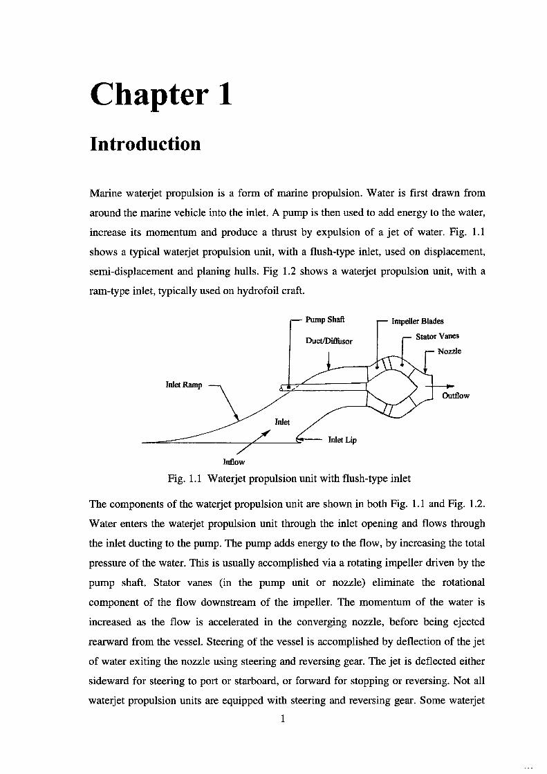
Marine waterjet propulsion is a form of marine propulsion. Water is first drawn from
around the marine vehicle into the inlet. A pump is then used to add energy to the water,
increase its momentum and produce a thrust by expulsion of a jet of water. Fig. 1.1
shows a typical waterjet propulsion unit, with a flush-type inlet, used on displacement,
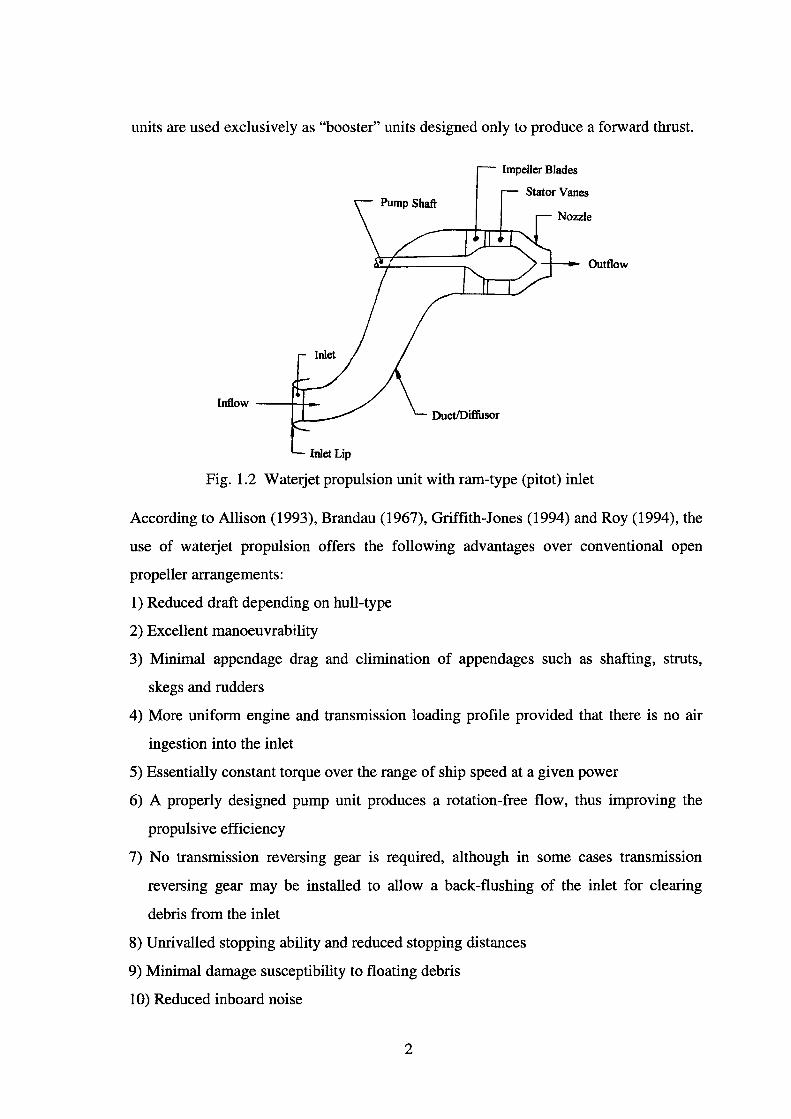
semi-displacement and planing hulls. Fig 1.2 shows a waterjet propulsion unit, with a
ram-type inlet, typically used on hydrofoil craft.
Pump Shaft
Duct/Diffusor Nozzle
Inlet Ramp
Outflow
Inlet Lip
Inflow
Fig. 1.1 Waterjet propulsion unit with flush-type inlet
The components of the waterjet propulsion unit are shown in both Fig. 1.1 and Fig. 1.2.
Water enters the waterjet propulsion unit through the inlet opening and flows through
the inlet ducting to the pump. The pump adds energy to the flow, by increasing the total
pressure of the water. This is usually accomplished via a rotating impeller driven by the
pump shaft. Stator vanes (in the pump unit or nozzle) eliminate the rotational
component of the flow downstream of the impeller. The momentum of the water is
increased as the flow is accelerated in the converging nozzle, before being ejected
rearward from the vessel. Steering of the vessel is accomplished by deflection of the jet
of water exiting the nozzle using steering and reversing gear. The jet is deflected either
sideward for steering to port or starboard, or forward for stopping or reversing. Not all
waterjet propulsion units are equipped with steering and reversing gear. Some waterjet
1
units are used exclusively as "booster" units designed only to produce a forward thrust.
Impeller Blades
Outflow
Fig. 1.2 Waterjet propulsion unit with ram-type (pitot) inlet
According to Allison (1993), Brandau (1967), Griffith-Jones (1994) and Roy (1994), the
use of waterjet propulsion offers the following advantages over conventional open
propeller arrangements:
1) Reduced draft depending on hull-type
2) Excellent manoeuvrability
3) Minimal appendage drag and elimination of appendages such as shafting, struts,
skegs and rudders
4) More uniform engine and transmission loading profile provided that there is no air
ingestion into the inlet
5) Essentially constant torque over the range of ship speed at a given power
6) A properly designed pump unit produces a rotation-free flow, thus improving the
propulsive efficiency
7) No transmission reversing gear is required, although in some cases transmission
reversing gear may be installed to allow a back-flushing of the inlet for clearing
debris from the inlet
8) Unrivalled stopping ability and reduced stopping distances
9) Minimal damage susceptibility to floating debris
1 0) Reduced inboard noise
2

11) Reduced vibration
12) The absence of an externally rotating blade provides a safety benefit.
Other advantages which may be of significance in military applications include:
1) Greatly reduced underwater noise
2) A reduction in the turbulence of the wake downstream of the vessel
3) Reduced magnetic signature.
There are, however, some notable disadvantages inherent in the selection of waterjet
propulsion as a means of ship propulsion. These include:
1) Substantially higher initial cost in terms of engineering, purchase and installation
2) Higher overall fuel consumption, as compared with equivalent propeller installations,
due to reduced efficiency at off-design conditions (such as low speed operation in the
case of a high-speed vessel)
3) The potential for inlet plugging due to the build-up of weeds and other debris on the
inlet grill
4) Corrosion and biological growth within the inlet causes increased pressure loss within
the inlet and hence leads to a degradation of performance
5) Integration of the propulsion unit with the hull form is more complex than with the
equivalent propeller installation on non-hydrofoil applications
6) The ingestion of air into the waterjet when certain hull types, such as planing hulls
and surface effect ships, operate in a seaway
7) Impeller access, when compared with conventional propeller designs is poor, making
inspection and repair, or removal of debris difficult.
1.1 Alternative Waterjet Concepts
The field of waterjet propulsion is not limited to the types of waterjet propulsion units
shown in Fig. 1.1 and Fig. 1.2. Perhaps the most futuristic waterjet concept is that of
magnetohydrodynarnic (MHD) sea water propulsion, where water is electrolysed by an
electric field acted upon by large magnetic fields. The interaction of the electric current
produced by ion movement in the MHD duct and the magnetic field, forces water
through the duct and creates a thrust. Detailed discussions on MHD sea water
3

propulsion can be found in Owen (1962), Doragh (1963), Swallom et al (1991) and
Doss and Geyer (1993). Motora et al (1991) discussed the development of the world's
first MHD-powered ship, the Y amato-1.
Gany (1993) proposed a "bubbly" waterjet, a ramjet-type propulsion unit where thrust is
generated by forming a high-speed two phase exhaust jet flow of water and air, created
by the addition of compressed air into the water flow. Allison (1993) cited references to
water piston propulsors. Roy (1994) cited references to other forms of waterjet
propulsion such as "pulse jet" propulsion. It is clear that there exist a large number of
potential waterjet concepts that can be used for marine propulsion.
1.2 Historical Development of Waterjet Propulsion Systems
There are several papers in the literature discussing the historical development of
waterjet propulsion. Roy's (1994) paper is an excellent and comprehensive overview of
the history of waterjet development and future development possibilities. Allison ( 1993)
briefly reviewed some of the historical developments of waterjet propulsion and Youngs
( 1994) provided an overview of the development of jet boats.
It is interesting to note that the idea of waterjet propulsion dates back to 1661 when
English inventors Toogood and Hayes were granted a patent by King Charles II, 19
years before Hooke suggested the screw propeller (see Roy (1994)). In the latter part of
the twentieth century there has been a rapid increase in the number of waterjet
manufacturers and the number of waterjets produced. There has also been a trend of
increasingly more powerful waterjet propulsion units.
1.3 Technical Overview
In this section the basic components of conventional waterjet propulsion systems which
include the waterjet inlet, the pump, nozzle and steering and reversing gear are
discussed in greater detail.
4
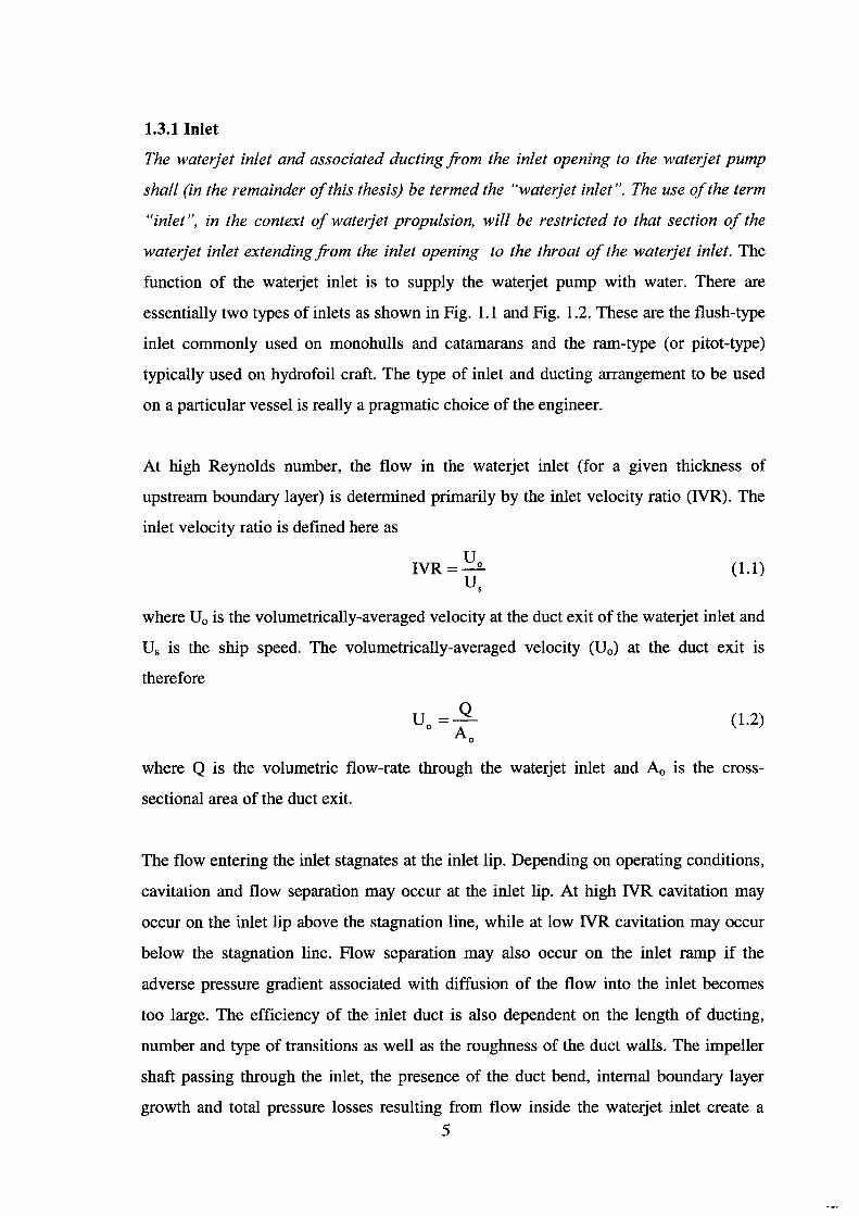
1.3.1 Inlet
The waterjet inlet and associated ducting from the inlet opening to the waterjet pump
shall (in the remainder of this thesis) be termed the "waterjet inlet". The use of the term
"inlet", in the context of waterjet propulsion, will be restricted to that section of the
waterjet inlet extending from the inlet opening to the throat of the waterjet inlet. The
function of the waterjet inlet is to supply the waterjet pump with water. There are
essentially two types of inlets as shown in Fig. 1.1 and Fig. 1.2. These are the flush-type
inlet commonly used on monohulls and catamarans and the ram-type (or pitot-type)
typically used on hydrofoil craft. The type of inlet and ducting arrangement to be used
on a particular vessel is really a pragmatic choice of the engineer.
At high Reynolds number, the flow in the waterjet inlet (for a given thickness of
upstream boundary layer) is determined primarily by the inlet velocity ratio (NR). The
inlet velocity ratio is defined here as
(1.1)
where U0 is the volumetrically-averaged velocity at the duct exit of the waterjet inlet and
Us is the ship speed. The volumetrically-averaged velocity (U0 ) at the duct exit is
therefore
u =_g_ o A
0
(1.2)
where Q is the volumetric flow-rate through the waterjet inlet and Ao is the cross
sectional area of the duct exit.
The flow entering the inlet stagnates at the inlet lip. Depending on operating conditions,
cavitation and flow separation may occur at the inlet lip. At high NR cavitation may
occur on the inlet lip above the stagnation line, while at low NR cavitation may occur
below the stagnation line. Flow separation may also occur on the inlet ramp if the
adverse pressure gradient associated with diffusion of the flow into the inlet becomes
too large. The efficiency of the inlet duct is also dependent on the length of ducting,
number and type of transitions as well as the roughness of the duct walls. The impeller
shaft passing through the inlet, the presence of the duct bend, internal boundary layer
growth and total pressure losses resulting from flow inside the waterjet inlet create a
5
distorted total pressure field at the pump inlet. This distorted total pressure field can
reduce the operating efficiency of the pump and assist in exciting pump vibration.
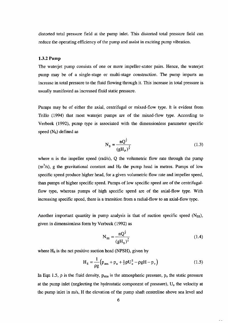
1.3.2 Pump
The waterjet pump consists of one or more impeller-stator pairs. Hence, the waterjet
pump may be of a single-stage or multi-stage construction. The pump imparts an
increase in total pressure to the fluid flowing through it. This increase in total pressure is
usually manifested as increased fluid static pressure.
Pumps may be of either the axial, centrifugal or mixed-flow type. It is evident from
Trillo (1994) that most waterjet pumps are of the mixed-flow type. According to
Verbeek ( 1992), pump type is associated with the dimensionless parameter specific
speed (Ns) defined as
(1.3)
where n is the impeller speed (rad/s), Q the volumetric flow rate through the pump
(m3/s), g the gravitational constant and Hp the pump head in metres. Pumps of low
specific speed produce higher head, for a given volumetric flow rate and impeller speed,
than pumps of higher specific speed. Pumps of low specific speed are of the centrifugal
flow type, whereas pumps of high specific speed are of the axial-flow type. With
increasing specific speed, there is a transition from a radial-flow to an axial-flow type.
Another important quantity in pump analysis is that of suction specific speed (Nss),
given in dimensionless form by Verbeek ( 1992) as
(1.4)
where Hs is the net positive suction head (NPSH), given by
- I ( I u2 ) Hs -- Patm +po +2P o -pgH-pv pg
(1.5)
In Eqn 1.5, p is the fluid density, Patm is the atmospheric pressure, Po the static pressure
at the pump inlet (neglecting the hydrostatic component of pressure), U0 the velocity at
the pump inlet in rn/s, H the elevation of the pump shaft centreline above sea level and
6
Pv the vapour pressure of water. All head quantities are expressed in metres. NPSH is
essentially the total manometric head available at the pump inlet above the vapour
pressure of the fluid as noted by Verbeek (1992). Suction specific speed is an extremely
useful parameter in relating the operating conditions of the pump, such as impeller
speed, volumetric flow-rate and NPSH, to the likelihood of impeller cavitation. From
Eqn 1.4 it is clear that an increase in impeller speed, volumetric flow-rate or a decrease
in NPSH, will result in a higher value of suction specific speed and hence a greater
possibility of impeller cavitation.
Note that an inducer can be used to increase the suction specific speed limit. Allison
(1993) listed the following characteristics as being desirable for a waterjet pump:
1) High hydraulic efficiency at high flow
2) Minimum outside diameter and weight for a given nozzle size
3) Cavitation free operation down to maximum pump speed and low inlet head
4) The capability of sustained operation with some cavitation without noticeable erosion
of blades, stator vanes and nozzle
5) High impeller speed enabling the use of a lighter gearbox
6) Tolerance to flow distortion at the pump inlet
7) Superior mechanical design of bearings, pump lubrication system, shaft seals and
other associated components
8) The use of lightweight corrosion-resistant materials for pump housing and parts
The above characteristics favour pumps of relatively high specific speed and high
suction specific speed.
1.3.3 Nozzle
The waterjet nozzle converts the increase in total pressure (mostly in the form of static
pressure) imparted by the pump into increased fluid momentum. This occurs as the high
pressure water at the nozzle entrance is accelerated in the converging nozzle to a higher
velocity at the nozzle exit, exiting the nozzle at ambient pressure. It is evident from
Trillo ( 1994) that nozzles are usually machined from stainless steel castings with
integral stator vanes. Nozzles generally have very high efficiency and since they carry
fluid of high total pressure they must have high efficiency in order to minimise fluid
7
power losses.
1.3.4 Steering and Reversing Gear
Steering of a waterjet-propelled vessel is typically achieved by deflection of the jet of
water leaving the propulsion unit nozzle. The jet may be deflected by a steering bucket,
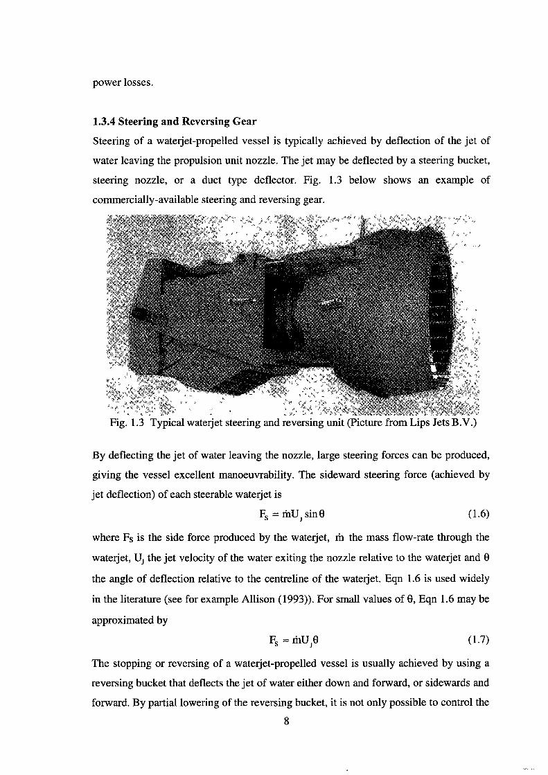
steering nozzle, or a duct type deflector. Fig. 1.3 below shows an example of
commercially-available steering and reversing gear.
' "
Fig. 1.3 Typical waterjet steering and reversing unit (Picture from Lips Jets B.V.)
By deflecting the jet of water leaving the nozzle, large steering forces can be produced,
giving the vessel excellent manoeuvrability. The sideward steering force (achieved by
jet deflection) of each steerable waterjet is
Fs = mUJ sin8 (1.6)
where Fs is the side force produced by the waterjet, m the mass flow-rate through the
waterjet, UJ the jet velocity of the water exiting the nozzle relative to the waterjet and 8
the angle of deflection relative to the centreline of the waterjet. Eqn 1.6 is used widely
in the literature (see for example Allison (1993)). For small values of 8, Eqn 1.6 may be
approximated by
(1.7)
The stopping or reversing of a waterjet-propelled vessel is usually achieved by using a
reversing bucket that deflects the jet of water either down and forward, or sidewards and
forward. By partial lowering of the reversing bucket, it is not only possible to control the
8
amount of forward or reverse thrust available, but also to create zero net thrust. The
prime mover can therefore run the waterjet pump at constant revolutions per minute
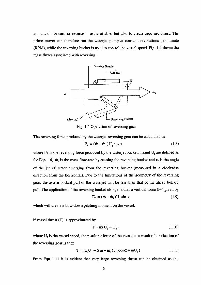
(RPM), while the reversing bucket is used to control the vessel speed. Fig. 1.4 shows the
mass fluxes associated with reversing.
Steering Nozzle
Reversing Bucket
Fig. 1.4 Operation of reversing gear
The reversing force produced by the waterjet reversing gear can be calculated as
FR = (rn- rnl )UJ cosa. (1.8)
where FR is the reversing force produced by the waterjet bucket, rn and U1 are defined as
for Eqn 1.6, rn1 is the mass flow-rate by-passing the reversing bucket and a. is the angle
of the jet of water emerging from the reversing bucket (measured in a clockwise
direction from the horizontal). Due to the limitations of the geometry of the reversing
gear, the astern bollard pull of the waterjet will be less than that of the ahead bollard
pull. The application of the reversing bucket also generates a vertical force (Fy) given by
Fy = (rn- rn1)UJ sina. (1.9)
which will create a bow-down pitching moment on the vessel.
If vessel thrust (T) is approximated by
T = rn(UJ- u.) (1.10)
where Us is the vessel speed, the resulting force of the vessel as a result of application of
the reversing gear is then
(1.11)
From Eqn 1.11 it is evident that very large reversing thrust can be obtained as the
9
reversing thrust is the sum of the force on the reversing bucket and the momentum drag
associated with ingestion of fluid into the waterjet inlet. Since the momentum drag is a
function of vessel speed, it is obvious that the waterjet-propelled vessel will exhibit
excellent stopping characteristics, especially at high-speed.
The zero thrust position of the waterjet bucket under operating conditions may be
determined by setting Eqn 1.11 to zero, resulting in
_1(:rh1 - :rhUs I UJ J ot=cos :rh- :rhl
(1.12)
The mass flow rate deflected by the reversing gear is a direct function of its design and
therefore affects the dynamics of reversing bucket operation according to the above
equations.
Voulon and Wesselink ( 1995) presented an excellent paper discussing the technical
issues associated with manoeuvrability of waterjet-propelled passenger ferries. The use
of the waterjet steering and reversing bucket can be used to execute a variety of vessel
motion such as turning, yawing and transverse motion. When only stem-mounted
waterjets are installed, the vessel's length-to-beam ratio is of prime importance to
manoeuvrability. For large length-to-beam ratios, the possible steering angles for
transverse motion become small, thus resulting in low side forces. The use of bow
thrusters or jet pumps can have a marked influence on the manoeuvrability of vessels
with large length-to-beam ratios. Wave-piercing catamarans with low length-to-beam
ratios therefore possess greater manoeuvrability than monohulls, according to Voulon
and Wesselink (1995) and Torneman (1994).
On nearly all commercially-available steerable waterjet units, the steering and reversing
gear is fitted to the waterjet propulsion unit, usually on the pump or nozzle body. This
type of mounting is acceptable for small and medium sized waterjets. Allison and Dai
(1994) described a new concept for mounting steering and reversing gear on the vessel
hull instead of the pump body. This concept can be used for very large waterjet units,
when it becomes impractical to mount these components on the pump body.
10
1.4 Issues Associated with Waterjet-Propelled Vessels
Technical issues that must be taken into account when designing the waterjet propulsion
system for a vessel are discussed in this section. These issues must be appropriately
addressed if the waterjet-propelled ship is to function successfully.
1.4.1 Waterjet-Hull Interaction
For waterjet-propelled ships, the waterjet inlet duct is an integral part of the hull form and
hydrodynamically it is impossible to separate the two for the purpose of analysis, as the
hull form affects the flow entering the waterjet while the waterjet affects the flow around
the hull form. This mutual interaction is called waterjet-hull interaction in the literature.
W aterjet -hull interaction will change the following hydrodynamic phenomena:
1) Hull boundary layer growth
2) Potential flow around the hull
3) Wavemaking
4) Sinkage and trim effects
relative to the bare hull flow, with consequent effects on thrust deduction and propulsive
efficiency.
Dai et al (1995) stated that the drag can be either augmented or reduced relative to the
bare hull resistance when there is an inlet with impeller operating. This situation is
further complicated by changes in hull pressure distribution due to the interaction
between the inlet and hull which can effectively change the trim of the vessel. Dai et al
(1993) also noted that the inlet flow can also change the boundary layer characteristics
near the stem. There is some flow acceleration ahead of the inlet and the formation of a
"new" boundary layer aft of the stagnation line on the inlet lip. This modification of the
boundary layer ahead and aft of the inlet can have a significant effect on the drag of the
vessel relative to the bare hull resistance. The flow into the inlet may also affect the
boundary layer on the stem adjacent to the inlet area.
The hydrodynamic problem posed is therefore very complex. At present experimental
model testing in towing tanks offers the best means of a systematic investigation into
waterjet-hull interaction effects. The proceedings of the 1987 International Towing Tank
11
Conference (ITTC) offered guidelines for the evaluation of data from self-propulsion
model tests using waterjets. Dyne & Lindell ( 1994) discussed the evolution of wateijet
propelled self-propulsion tests at the SSP A towing tank in Sweden. Steen & Minsaas
( 1995) discussed the testing of waterjet propulsion system models and self-propulsion tests
at MARINTEK in Norway. It is therefore clear that a significant number of waterjet
propelled self-propulsion model tests have been carried out worldwide.
In the literature there has been some systematic work in the area of waterjet-hull
interaction for waterjets with flush-type inlets, most notably by van Terwisga (1996). Van
Terwisga used a combination of experimental and computational work to investigate the
mechanisms influencing waterjet-hull interaction. For planing craft, van Terwisga (1996)
found a large peak in the thrust deduction fraction at low Froude numbers. This was
caused by the clearing of the transom stem which affects the nozzle pressure and hence
thrust. The resistance increment of the hull due to the jet action was found to be dominated
by pressure drag. For Froude numbers below unity, this pressure drag was governed by
transom sinkage, with the trim angle becoming more important at higher Froude numbers.
Other works have included papers by Alexander et al (1994), Alexander and van Terwisga
(1993) and Coop and Bowen (1993). Hoshino and Baba (1984) investigated the effect on
thrust deduction of using a waterjet with twin propellers on a self-propelled semi
displacement craft model. There remains, however, a great deal of work which can be
undertaken in this field, both experimentally and computationally. The interested reader is
referred to van Terwisga (1996) for a comprehensive literature review on the subject of
wateijet -hull interaction.
1.4.2 Ship Design Optimisation
The design of the waterjet propulsion system, i.e. the vessel prime mover, wateijet pump
and inlet ducting, poses another challenge. It is clear from the literature that the wateijet
propulsion system cannot be optimised independently of the total vessel design, but must
be selected on the basis of a total vessel design optimisation, in order to obtain the most
cost-effective design.
12
Venturini ( 1980) noted that an optimal vessel and propulsor arrangement does not
generally coincide with the minimum propulsor power for a given cruising speed.
According to Allison and Goubault ( 1995), there exists a need to optimise the vessel and
waterjet as an integrated entity through a whole ship design synthesis process, rather than
fit available waterjet propulsors into a ship design. Gallin et al ( 1995) for example,
concluded that designing the waterjet propulsor to match the prime mover resulted in a
smaller life-cycle cost than matching a prime mover to an existing waterjet design.
The design of hydrofoil craft provides interesting examples of the need to optimise the
total vessel design rather than individual sub-systems. Schultz (1974a, 1974b) discussed
issues associated with the design of the Boeing Jetfoil, a gas-turbine-powered, waterjet
propelled high-speed passenger ferry, that entered service in the early 1970s. In order to
design the Jetfoil, Boeing conducted extensive parametric analyses looking at issues
such as suitable hydrofoil routes, hydrofoil configuration and size, vehicle performance
and cost and the number and distribution of passengers. Other factors examined
included fares, block-speed, percent of market carried, load factor, hours of utilisation,
required fleet size, profit and return on investment.
A fundamental design consideration for Boeing was to keep the vehicle weight fractions
(structure, propulsion and machinery) as low as was safely possible to achieve the best
payload/performance for the installed power, in order to obtain the most efficient
design. Life-cycle costs such as construction, maintenance and support were also
analysed.
Batte and Davis ( 1967) discussed the methods developed at Boeing during the 1960s for
waterjet propulsion system selection for hydrofoil craft. For waterjet systems, Boeing
consistently found that a higher propulsive efficiency would result in lower overall
system performance because of the effects of parasitic drag and waterjet weight
fractions. Propulsive efficiency therefore proved to be a misleading criterion in
determining the best waterjet system. More applicable criteria were required, such as
range, payload and the efficient use of power. Boeing found that early design analyses
demonstrated performance optimisation of individual subsystem components resulted in
13
relatively poor overall craft performance, thus creating a need for the examination of a
large number of overall craft performance parameters and various sub-system
compromises.
1.5 Research Issues and Objectives
The focus of this research project was the investigation and optimisation of the design of
generic flush-type waterjet inlets using computational fluid dynamics (CFD). Ideally the
total waterjet inlet/hull configuration should be optimised as part of a total vessel design
optimisation process, taking into account the effects of waterjet -hull interaction, as
discussed in Section 1.4. The systematic hydrodynamic optimisation of a waterjet inlet
itself, in the absence of hull form, presents a sufficiently complex problem that must be
addressed prior to any waterjet inlet/hull optimisation. In addition, investigations related
to the design and optimisation of the waterjet inlet allows a large amount of data to be
gathered on how aspects of the inlet design affect inlet hydrodynamic performance. This
is clearly useful in correlating the hydrodynamic performance with the underlying inlet
geometry.
In recent years, there have been an increasing number of publications appearing in the
literature presenting CFD results for flows in waterjet inlets and discussing the use of
CFD as a tool for waterjet inlet design and analysis. Among these publications are the
works of Ff/Srde et al (1991 ), Dai et al (1995), Seil et al (1995) and Seil et al (1997).
Other researchers have concentrated on comparing CFD results with experimental data
obtained from the testing of model waterjet inlets in wind tunnels. Griffith-Jones (1994)
and Roberts (1998) have carried out such studies. The CFD results of Griffith-Jones
( 1994) were not in good agreement with the experimental data, possibly due to
inadequate near-wall flow resolution resulting from the grid used.
Allison ( 1996) discussed the cost savings that were achieved by using CFD as a design
tool for the hydrodynamic design of the waterjet inlet for the US Marine Corps
Advanced Amphibious Assault Vehicle. Costs savings were attributed to a reduction in
the experimental testing required for the development of the propulsor. Indeed, the use
of CFD provides a necessary foundation for practical, cost-effective waterjet inlet
14
optimisation work as Seil et al ( 1997) noted.
The waterjet inlet is likely to spend most of its operational time in a "cruise" (low IVR)
condition and so will tend to be designed by the manufacturer with a bias toward this
condition. The waterjet inlet must also offer adequate hydrodynamic performance at off
design conditions such as when manoeuvring in a harbour or docking (high IVR). Under
these off-design conditions, the NPSH at the pump inlet is low thus limiting the power
input into the pump, the flow-rate through the pump and hence the thrust produced. In
addition, if severe cavitation and flow separation exist in the inlet, the thrust available
for manoeuvring may also drop dramatically thus degrading manoeuvring performance.
This is of special concern for a large vessel attempting to manoeuvre in a crowded
harbour (or dock) while being acted upon by currents, wind and the vessel's own inertia.
As a consequence of the importance of obtaining adequate hydrodynamic performance
from the waterjet inlet in off-design conditions, the hydrodynamic optimisation of a
waterjet inlet must be treated as a multi-point optimisation problem where the resulting
optimised design expresses a compromise between the cruise and manoeuvring
conditions.
There are many other questions and issues that arise in conjunction with the design of
the inlet and its optimisation. These include, but are not limited to the following:
1) The key parameters that are used to evaluate the hydrodynamic performance of the
waterjet inlet
2) The aspects of the inlet geometry which have the greatest effect on hydrodynamic
performance
3) The effect of the upstream hull boundary layer thickness on the flow at the duct exit,
the flow in the vicinity of the inlet lip and its effect on an optimised design
4) The optimality of current commercially-available inlet designs
5) The accuracy of CFD flow computation
6) The ease with which existing CFD technology can be applied to the optimisation of
waterjet inlet design
As a consequence of the above issues, the following research objectives were set and
15
form the basis of the work presented in this thesis. These objectives were:
1) To validate that the accuracy of a commercially-available CFD code (in this case
Fluent) based on the solution of the Reynolds-averaged Navier Stokes equations with
two-equation k-E turbulence modelling, is sufficient to allow it to be used as a
suitable tool for predicting the flow in waterjet inlets.
2) To develop a mathematical model to describe waterjet propulsion system
performance.
3) To develop a mathematical model to describe the hydrodynamic performance of the
waterjet inlet for use with an optimisation methodology.
4) To develop a parametrically-defined generic flush-type waterjet inlet geometry that
can be systematically varied (by varying the defining geometric parameters) in order
to produce different waterjet inlet designs. The systematic variation of the waterjet
inlet geometry is a necessary prerequisite for parametric design subspace
investigation and waterjet inlet optimisation.
5) To investigate the use of CFD and a formal optimisation methodology in order to
optimise the waterjet inlet (in the absence of hull-form) with respect to cavitation
performance and the elimination of flow separation, for a vessel cruise condition.
This corresponds to a single point optimisation and allows the optimised geometries
to be compared with existing commercially-available waterjet inlet designs.
1.6 Overview of Thesis
A theoretical model for the determination of waterjet propulsion unit thrust and
efficiency is presented in Chapter 2, together with a parametric study of the waterjet
efficiency model. The parametric study examines the effect of waterjet component
efficiencies and upstream boundary layer thickness on overall waterjet efficiency and
the point of optimum waterjet efficiency.
The CFD methodology used as the basis of the flow computations presented in this
thesis is presented in Chapter 3. The computational techniques discussed are based on
the solution of the RANS equations with two-equation k-E turbulence modelling, using a
co-located finite volume formulation for discretising the governing equations. Iterative
solution techniques used to solve the discretised governing equations are also discussed.
16
A description of the parametrically-defined generic flush-type waterjet inlet geometry,
used for the purposes of waterjet inlet design and optimisation investigations, is
presented in Chapter 4. The mesh generation techniques used for meshing this geometry
and creating single-block body-fitted-coordinate structured grids for use with Fluent are
also presented. Chapter 4 also describes the mesh generation techniques used for
meshing the 90° bend and S-Duct experimental geometries discussed in Chapter 5.
In Chapter 5 the accuracy of Fluent is validated against three experimental data sets.
These include turbulent flow in the 90° bend of Enayet et al (1982), the 45°-45° S-Duct
of Bansod and Bradshaw ( 1972) and the flush-type waterjet inlet wind tunnel model of
Roberts (1998).
A set of parameters used to assess the hydrodynamic performance of the waterjet inlet is
presented in Chapter 6. These parameters are used in Chapter 6 and subsequent chapters
to assess and compare the hydrodynamic performance of different waterjet inlet designs.
A systematic investigation of the effect of upstream boundary layer thickness on the
flow within the waterjet inlet is then undertaken.
In Chapter 7 three two-parameter design subspaces of the parametric design hyperspace
of the author's parametric waterjet inlet design are investigated for an IVR of 0.6. In
other words, three two-parameter combinations of the generic geometry are varied with
the other parameters held constant. The large amount of hydrodynamic data obtained as
a result of these investigations allows a clear link between the hydrodynamics of the
waterjet inlet flow and the underlying geometry to be established.
In Chapter 8 the author's generic parametrically-defined waterjet inlet is optimised for
an IVR of 0.6, in order to maximise the static pressure on the surface of the waterjet
inlet. The initial and optimum geometries are compared and the hydrodynamics of their
respective flows are correlated with the underlying geometry. This further enhances
knowledge of waterjet inlet design. The conclusions of this research are summarised in
Chapter 9 which also contains a list of recommendations relating to waterjet inlet design
and further CFD research directions in this field.
17
Chapter 2 Parametric Model ofWaterjet Performance
Physically realistic and accurate mathematical models for waterjet thrust and efficiency
are crucial in determining the performance of a waterjet propulsion unit. It is also
necessary to know to what extent changes in the parameters which influence waterjet
propulsion system performance would affect overall system performance. These issues
form the basis of the work contained in this chapter. In this chapter a model for waterjet
thrust and efficiency, that can be used to estimate the performance of a waterjet
propulsion unit from experimental or CFD analysis, shall be presented.
Of the waterjet literature surveyed, van Terwisga (1996) and Coop and Bowen (1993)
provided the most detailed and physically realistic definition of thrust. In fact van
Terwisga (1996) derived a logical and comprehensive model of waterjet thrust and
efficiency and provided a good literature review of the subject. Svensson (1993) gave a
simple and yet effective expression for waterjet thrust applicable to waterjet model
testing in a cavitation tunnel. Etter et al (1982) provided a detailed analysis of waterjet
thrust based on momentum analysis, but demarcated the definition of waterjet and hull
differently from other authors. Dyne and Lindell (1994) used momentum analysis of the
frictional wake behind the vessel to derive their expression for waterjet thrust. Authors
who presented models for waterjet efficiency in the literature have included Allison
(1993), Brandau (1967) and Etter et al (1982). The ITTC 87 suggested a model based
primarily on the work of Etter et al (1980) and Haglund et al (1982).
In Section 2.1, the concept of waterjet propulsion system thrust is defined. Subsequently
a mathematical model for waterjet thrust is developed from a control volume analysis of
the conservation of mass and momentum for flow through the waterjet. The terminology
used is based on that in the aeronautical literature.
A mathematical model for waterjet propulsion system energy efficiency, derived using a
18
control volume approach for the conservation of energy for flow through the waterjet, is
presented in Section 2.2. In addition, formulae for calculating the jet velocity ratio
(JVR) corresponding to maximum waterjet efficiency (for a given set of flow parameters
and component efficiencies) is derived.
A parametric study investigating the effect on overall waterjet propulsion unit efficiency
of variation in the efficiency of sub-system components, is presented in Section 2.3. The
effect on waterjet performance of ingesting fluid from the hull boundary layer is also
examined. Realistic efficiency values for the various propulsion unit sub-system
components, reflecting the current state-of-the-art, are used in the parametric study
presented. The point of optimum operational efficiency, corresponding to the efficiency
of sub-system components and the thickness of ingested boundary layer is also
examined.
2.1 Waterjet Thrust
An accurate determination of waterjet propulsion unit thrust is essential for the
determination not only of the thrust capability of the waterjet propulsor itself, but also of
propulsive efficiency and the effect, both beneficial and adverse, of waterjet-hull
interaction.
Although waterjet propulsion is a hydrodynamic problem, it is in fact analogous to
subsonic aircraft inlet design and hence the aeronautical literature provides a good basis
for obtaining information on flow behaviour and thrust. Information on thrust definition
and subsonic inlet flows (in the aeronautical literature) can be found in Seddon and
Goldsmith (1985). It is surprising that so little reference has been made in the waterjet
literature to aeronautical publications.
The term waterjet shall be defined as the installed waterjet propulsion unit, from the
inlet duct welded to the bottom plating of the hull, to the nozzle exit plane. Any surface
in contact with water and not contained within the waterjet shall be deemed to be the
hull. In the following sections, equations for waterjet thrust are derived from the
equations of conservation of mass and momentum for a finite control-volume.
19
The analysis contained in this section is used to determine correct expressions for
propulsor thrust based on an analysis of a finite control-volume. This type of analysis is
the typical analysis approach used for determining the performance of jet engines and
waterjet propulsors. Initially, detailed expressions for propulsor thrust shall be
determined, followed by simplifications for ease of interpretation of computational or
experimental results.
Expressions for thrust are derived from Newton's Second Law applied to a finite
control-volume. Conceptually, forces due to pressure and shear acting over the surface
of the control volume, in addition to body forces acting on the fluid within the control
volume, effect a net change in momentum of fluid entering and leaving the control
volume. In a conventional jet engine or waterjet propulsor, it is only those solid control
volume surfaces in contact with the fluid that can transmit force to the aircraft or ship.
Magnetohydrodynamic propulsors work on a different principle where the thrust is
transmitted to the ship through the magnet structure, the thrust itself being generated
from the interaction of the magnetic field with ions in the propulsor duct.
2.1.1 Definition ofWaterjet Control-Volume for Thrust Analysis
A control-volume (ABCEFGA) encompassing the waterjet unit, impeller shaft housing,
impeller and a streamtube of fluid external to it, is shown in Fig. 2.1. Area A5 represents
all surfaces inside the waterjet unit exposed to water. This includes the waterjet inlet
duct, impeller shaft housing/fairing, impeller, nozzle and stator vanes. It must be noted
that these surfaces are the only means by which force can be transmitted to the vessel.
Area A2 represents a streamtube surface through which no transport of mass occurs, thus
dividing the flow entering the waterjet unit from the flow by-passing it. The location of
Area At is arbitrarily chosen. Van Terwisga ( 1996) specified the location of AB at a
distance of 10% of the physical intake length DG. Since area A3 represents the portion
of the inlet streamtube in contact with the hull, the location of AB will affect the shear
force acting on A3 and velocity profile over At. For reasons of simplicity, it is therefore
beneficial to locate AB as close to the inlet as possible, but as far upstream as is
necessary to avoid the major effects of the pressure field caused by the inlet ramp. This
may be greater than 10% of the length DG, depending on operating conditions. Point C
20
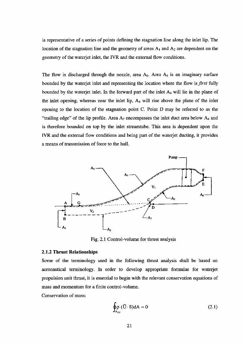
is representative of a series of points defining the stagnation line along the inlet lip. The
location of the stagnation line and the geometry of areas A1 and Az are dependent on the
geometry of the waterjet inlet, the IVR and the external flow conditions.
The flow is discharged through the nozzle, area A6. Area ~ is an imaginary surface
bounded by the waterjet inlet and representing the location where the flow is first fully
bounded by the waterjet inlet. In the forward part of the inlet ~ will lie in the plane of
the inlet opening, whereas near the inlet lip, A4 will rise above the plane of the inlet
opening to the location of the stagnation point C. Point D may be referred to as the
"trailing edge" of the lip profile. Area A7 encompasses the inlet duct area below ~ and
is therefore bounded on top by the inlet streamtube. This area is dependent upon the
IVR and the external flow conditions and being part of the waterjet ducting, it provides
a means of transmission of force to the hull.
A G
~ v2 -----L ~--------l---
AI A2
Fig. 2.1 Control-volume for thrust analysis
2.1.2 Thrust Relationships
Some of the terminology used in the following thrust analysis shall be based on
aeronautical terminology. In order to develop appropriate formulae for waterjet
propulsion unit thrust, it is essential to begin with the relevant conservation equations of
mass and momentum for a finite control-volume.
Conservation of mass:
!P (U · n)dA = o jAcv
(2.1)
21
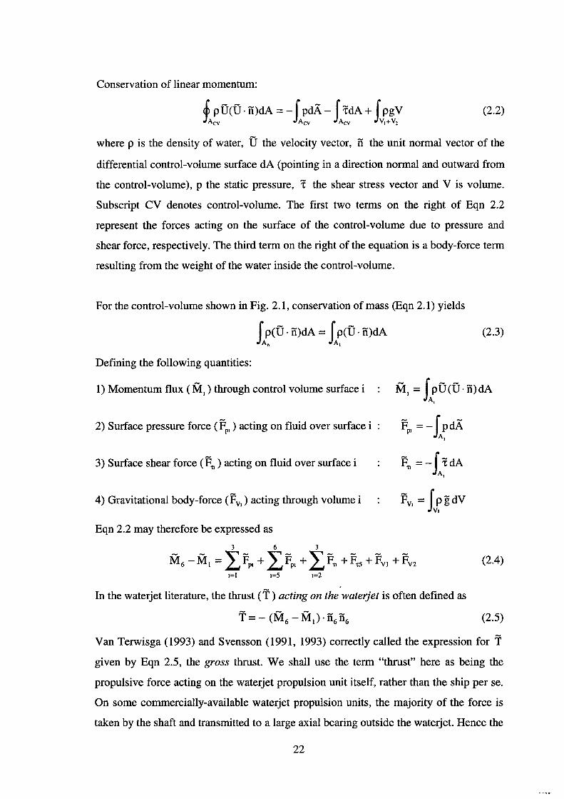
Conservation of linear momentum:
,( pU(U · fi)dA = -JpdA- J:rdA + f pgV jAcv Acv Acv Jv1+V2
(2.2)
where p is the density of water, D the velocity vector, fi the unit normal vector of the
differential control-volume surface dA (pointing in a direction normal and outward from
the control-volume), p the static pressure, 1 the shear stress vector and V is volume.
Subscript CV denotes control-volume. The first two terms on the right of Eqn 2.2
represent the forces acting on the surface of the control-volume due to pressure and
shear force, respectively. The third term on the right of the equation is a body-force term
resulting from the weight of the water inside the control-volume.
For the control-volume shown in Fig. 2.1, conservation of mass (Eqn 2.1) yields
f p(U · fi)dA = f p(U · fi)dA A6 At
Defining the following quantities:
1) Momentum flux ( M1
) through control volume surface i
2) Surface pressure force ( FPI) acting on fluid over surface i
3) Surface shear force ( F"tl) acting on fluid over surface i
4) Gravitational body-force (Fv1
) acting through volume i
Eqn 2.2 may therefore be expressed as
1=1 1=5 1=2
In the waterjet literature, the thrust ('T) acting on the waterjet is often defined as
T = - (M6 - M I) . fi6 fi6
(2.3)
(2.4)
(2.5)
Van Terwisga (1993) and Svensson (1991, 1993) correctly called the expression for T given by Eqn 2.5, the gross thrust. We shall use the term "thrust" here as being the
propulsive force acting on the waterjet propulsion unit itself, rather than the ship per se.
On some commercially-available waterjet propulsion units, the majority of the force is
taken by the shaft and transmitted to a large axial bearing outside the waterjet. Hence the
22
force in the direction of the negative of the nozzle area vector provides a convenient
direction for describing the net propulsive force acting on the waterjet propulsion unit,
as this vector is generally parallel to the shaft centreline. Gross thrust is not, in fact, the
actual thrust generated for the waterjet under consideration. Seddon and Goldsmith
(1985) discussed the various thrust definitions used in the aeronautical literature. The
practical thrust definition in the aeronautical literature is termed the net standard thrust
( T Ns ) • A revised definition of net standard thrust, accounting for body forces (weight of
entrained water) acting inside the control-volume and thus relevant to waterjet
applications, is
(2.6)
It must be noted that in the aeronautical literature FP1 is taken as being equal to ambient
pressure. Since the thrust analysis presented here is applicable to a waterjet unit installed
as part of a hull system, FP1 is non-zero in value due to hydrostatic and hydrodynamic
forces and therefore must be included in the definition of net standard thrust.
The actual expression for the force (thrust) transmitted to area A5, called the intrinsic
thrust, is defined by
Tlntrlnslc = -(Fps + F'ts). n6 n6 = -(M6- M4- (Fp4 + Fp6)- FYI). n6n6 (2.7)
Intrinsic thrust may also be written as
TlntrmSIC = -(M6- Ml- (Fp6 + Fpl + Fp2 + Fp3)- (F't2 + F't3)- FYI- Fy2). n6 n6 (2.8)
The difference in thrust between net standard thrust and the intrinsic thrust, is termed
the "Pre-entry Drag" CDPre) and may be evaluated as
Eqn 2.9 states that the Pre-entry Drag is primarily a function of the geometry of the inlet
streamtube and may be either positive or negative depending on whether the streamtube
pre-diffuses or contracts prior to entry into the propulsor. It is clear that the
determination of net standard thrust, intrinsic thrust and pre-entry drag is by no means
simple, requiring extensive CFD analysis or experimental investigation.
23
While Eqn 2.7 specifies the actual thrust transmitted to the hull via the propulsor, for the
control-volume under consideration, this is not the total thrust force acting on the
propulsor. There is also a force generated by the pressure distribution over area A7. The
total thrust (r Net ) generated by the propulsor is then
(2.10)
with an inlet drag ( Diniet) defined as
(2.11)
Neglecting body forces, Seddon and Goldsmith (1985) stated (for subsonic inlets) that
the drag of the inlet is composed of three components. These are the pre-entry drag,
frictional drag and the pressure drag on the cowl. In an inviscid flow condition, the pre
entry drag is balanced by suction on the cowl lip. In practice, because the boundary layer
on the cowl displaces the potential flow and there are skin frictional effects, the suction
of the cowl lip is insufficient to balance the pre-entry drag and so there is a net drag. In
the case of the waterjet, area A7 is analogous to the inlet cowl of a subsonic aircraft. It
can thus be expected, in the case of inviscid flow, that inlet drag will be zero. The work
of van Terwisga ( 1996) supports this conclusion. In this case Eqn 2.11 becomes
(2.12)
Substitution of Eqn 2.12 into Eqn 2.10 and using the definition of pre-entry drag from
Eqn 2.9 gives
(T Net ) Invtsctd = {T Intnns•c + f) Pre ) lnv•sc•d = T NS (2.13)
It is therefore clear that in the case of in viscid flow, the net thrust produced by the
waterjet is simply equal to the net standard thrust. In the case of viscous flow, the net
thrust becomes
TNet = {TNet )lnvJscJd + {Ft2 + Ft3 - Ft7) · ff6 °6 = {TNS )corrected - Ft7 · ff6 ff6 {2.14)
where
(2.15)
is the corrected net standard thrust, that is the net standard thrust that would be obtained
if AB were moved close to the ramp tangency point. Eqn 2.15 explicitly deals with the
drag contribution of the inlet stream-tube outside of the waterjet. Eqn 2.13 provides a
close approximation to thrust if the pressure losses on A7, A2 and A3 are small.
24
If lip pressure losses due to fluid viscosity (or changes due to cavitation) become
significant, the deviation between net thrust and corrected net standard thrust can be
accounted for by the introduction of a lip loss thrust deduction factor ( 1-q_J, defined by
(2.16)
where tL is the lip loss thrust deduction fraction. The significance of this parameter is
that it gives an indication as to the magnitude of the lack of pressure recovery on the
inlet lip outside of the inlet streamtube. Lip loss thrust deduction factor defined by Eqn
2.16 is similar in form to the jet thrust deduction factor as proposed by van Terwisga
( 1996), but differs in its definition and significance.
Since many authors use gross thrust as their definition of thrust, without taking into
account pre-entry drag or the force contribution of area A7, the effects of inlet drag
inevitably appear in the thrust deduction factor (1-t) defined by
(1- t) = IR.BH 1/ltl (2.17)
where R BH is the bare-hull resistance vector and T the gross thrust vector defined by
Eqn 2.5. With the nozzle and A1 of the inlet streamtube at ambient pressures and, low
lip losses, gross thrust will provide a close approximation to the waterjet thrust.
2.1.3 Waterjet Thrust Model
The equation for the net thrust of a waterjet (Eqn 2.14) was derived in Section 2.1.2. In
order to develop a model for waterjet thrust, it shall be assumed that the direction of the
area vectors representing the nozzle throat area (A6) and the control-volume inlet area
(A1) are parallel to each other and parallel to the horizontal direction. This
simplification eliminates the body force terms in the expression for net thrust.
A simplified expression for net thrust can be derived using the definition of net standard
thrust (Eqn 2.6), corrected net standard thrust (Eqn 2.15), net thrust (Eqn 2.14) and lip
loss thrust deduction factor (Eqn 2.16). The net thrust (T) of the waterjet may now be
written as
(2.18)
where UJ is the average jet velocity through the nozzle throat (with the assumption that
25
the vena contracta of the flow is at the nozzle exit plane) determined on a
volumetrically-averaged basis and :rh the mass flow-rate through the waterjet. The skin
friction force caused by the flow of water on the solid surface A3 is accounted for by the
term incorporating the skin-friction coefficient (Cr) in Eqn 2.18. Pressure losses at the
lip reduce the lip suction and hence the thrust. They are therefore accounted for through
the lip loss thrust deduction factor. The nozzle momentum flux coefficient (Cmn)
accounts for the change in nozzle momentum due to flow non-uniformity over the
nozzle throat and may be defined as
cmn = . 1 Jp(U·n6 )
2dA
(mU) A6
(2.19)
where dA is the differential area and n6 is the unit direction vector of differential area
of the nozzle. The upstream momentum flux coefficient (Cm) accounts for the reduction
in ingested momentum resulting from the ingestion of fluid from an upstream boundary
layer and may be defined as
(2.20)
The negative sign in Eqn 2.20 is required to make Cm a positive quantity, since n1 is
negative. An average static pressure coefficient ( CP) can be defined where
(2.21)
In Eqn 2.21, Prer is the reference static pressure. An average skin-friction coefficient
(2.22)
may be defined to account for the viscous force on A3.
Eqn 2.18 may then be rewritten as
T= (1-tL)(m(CmnUJ -CmUs)+tpu;(CrA3 -CPA 1)) (2.23)
The pressure coefficient term can be written in terms of mass flow-rate so that Eqn 2.23
becomes
26
(2.24)
where CA and C8 are the ratios of A3 and A1 to the streamtube cross sectional area of A 1
under free-stream conditions, respectively.
2.2 Propulsive Efficiency
The development of a theoretical model of waterjet efficiency is outlined below. This
model can be used in conjunction with CFD or experimental results to quantify the
changes in waterjet efficiency resulting from changes in parameters that affect
performance.
With the increasing use of waterjet propulsion as the preferred means of providing high
speed marine propulsion, there is a need to clarify waterjet -hull interaction and
efficiency in a systematic manner. A good mathematical model of waterjet efficiency
should therefore be straightforward to use and should relate the performance of the
waterjet to the performance of individual components of the waterjet propulsion unit
(such as the inlet, pump and nozzle) and the flow conditions upstream of the inlet. This
must be done in a physically correct and consistent manner. The model presented in this
thesis meets all these requirements and can be readily applied to the interpretation of
experimental or CFD results.
2.2.1 Control-Volume Definition for Efficiency Analysis
In order to properly analyse the waterjet propulsion unit, it is necessary to define a
suitable control-volume encompassing the flow through the waterjet. The defined
control-volume (ABCDEFGHA) is shown in Fig. 2.2. This control-volume encompasses
the inlet streamtube, waterjet inlet, impeller and other surfaces in contact with water
contained in the waterjet ducting. Station 1 represents an upstream cross-section of the
inlet streamtube, Station 2 the pump inlet, Station 3 the pump exit and Station 4 the
nozzle throat.
27

Station 3 - Pump Outlet -
Station 2 - Pump Inlet
......::;-- --c D
A
Station 4 - Nozzle Throat
Fig. 2.2 Control-volume for efficiency analysis
2.2.2 Development of a Model for Propulsive Efficiency
The efficiency of a waterjet is often defined in the literature as
(2.25)
where 1lw1 represents the waterjet system efficiency, TNet the net waterjet thrust vector,
D. a vector representing the ship's velocity, W the power output of the vessel prime
mover driving the waterjet pump and TIT the efficiency of power transmission from
prime mover to waterjet pump. Waterjet system efficiency may be also written as
TJ WJ = TJ Rot TJ Pump TJ Duct TJ I (2.26)
where TJPump is the efficiency of the waterjet pump at the required operating point with
spatially uniform inflow conditions, TJRot is the rotative efficiency of the waterjet pump
as installed in the waterjet, TJouct the efficiency of the total waterjet ducting and 111 the
ideal waterjet efficiency derived from momentum considerations as
TII = 2U. I (V. + V) (2.27)
The propulsive efficiency of the total waterjet-hull system, on the other hand, can be
written as
28
(2.28)
In Eqn 2.28, R8H is the bare-hull resistance vector and (1-t) is a thrust deduction factor
linking the waterjet thrust and the bare-hull resistance. It is clear that the value of t will
depend on how the operation of the waterjet modifies the flow around the vessel hull.
For the derivation of a mathematical model for waterjet efficiency, it will be assumed
for simplicity that the vectors for thrust, resistance and ship's velocity are parallel in
direction. Using the result of Eqn 2.24, thrust (T) may be calculated as
(2.29)
A mass-averaged total pressure (P) can be defined as
P= ~L (p+pgH+tpU 2 )dm (2.30)
where p represents static pressure, g the gravitational constant and H is the elevation
above a given reference point. The energy flux (E) may be then expressed as
E= mP p
(2.31)
which is similar in essence to that provided by Haglund et al (1982). The inlet efficiency
can be defined as
(2.32)
and the nozzle efficiency as
(2.33)
Ingestion of fluid from an upstream hull boundary layer will result in the total energy of
the flow passing through these cross-sections being different from the case of uniform
flow. The energy at Station 1 may be expressed as
E -I . C uz AB- 2m e s
where ce is the inlet energy flux coefficient defined by
(2.34)
(2.35)
The negative sign appearing in Eqn 2.35 is required to make Ce a positive quantity, as
29
i'i 1 is negative. A nozzle energy flux coefficient (Cen) can be similarly defined. Waterjet
efficiency can now be determined as
TUS (2.36)
or in other words,
(2.37)
Defining J..L=U/Us as the jet velocity ratio (JVR), waterjet efficiency can be written as
In terms of JVR, ideal efficiency (Eqn 2.27) becomes
Tli = 2/ (1 + J..L)
(2.38)
(2.39)
Waterjet duct efficiency can be determined from Eqn 2.26 by substitution of Eqn 2.38
and Eqn 2.39. The result is
(2.40)
It can be seen from Eqn 2.40 that the duct efficiency of the waterjet is a non-linear
function of JVR and correspondingly of IVR. Duct efficiency is also dependent on the
flow behaviour upstream of the waterjet inlet. Inlet efficiency and nozzle efficiency
themselves are not fixed in value but vary as functions of IVR and JVR. Seddon and
Goldsmith ( 1985) discussed the variation of inlet efficiency with IVR for subsonic
aircraft intakes. To assign a fixed value of duct efficiency over a range of IVR of interest
is clearly erroneous. Similarly, since inlet efficiency will change with IVR, it may be
expected that the pump rotative efficiency will change as a result of the different flow
conditions at the duct exit of the waterjet inlet, therefore affecting propulsive efficiency.
The optimum value of JVR at which waterjet efficiency is maximised can be found be
setting the derivative of Eqn 2.38, with respect to JVR, equal to zero. The resulting
expression is
30
cmncen 2 2Cen I - I -f..l ---(Cm -zCACr +zCsCp)f..l+CmnCellin =0
llN llN (2.41)
The optimum value of JVR is therefore
(2.42)
where A, B and C are the coefficients of the polynomial described by Eqn 2.41 such that
(2.43)
2.3 Parametric Study of W aterjet Efficiency
The development of a model for waterjet thrust and efficiency was presented in Section
2.1 and Section 2.2, respectively. This model incorporates all of the relevant physics
associated with the performance of the waterjet propulsion unit. In order to understand
how changes in model parameters affect the performance of the waterjet, it is necessary
to conduct a parametric study in order to gauge the relative importance of these
parameters.
The parametric study is presented in two parts. The effect of the variation in component
efficiency and upstream boundary layer thickness on the efficiency of the waterjet is first
examined in Section 2.3.1. The optimum value of JVR at which waterjet efficiency is
maximised (for variations in inlet and nozzle efficiency), with different amounts of
boundary layer ingestion will be examined in Section 2.3.2.
For the purposes of investigating the effect of the ingestion of fluid from the hull
boundary layer, it has been assumed for simplicity that the cross-section of the inlet
streamtube is rectangular, thereby allowing the boundary layer to be treated as two
dimensional. In reality the cross-section of the inlet streamtube is more of an
ellipticaVtrapezoidal shape as Griffith-Jones (1994) and Roberts (1998) showed. In this
case evaluation of the inlet momentum flux coefficient (Cm) and the inlet energy flux
coefficient (Ce) would require an integration of the boundary layer velocity and pressure
profile over the cross-sectional area of the inlet streamtube. The assumption of a two
dimensional profile would be more realistic when wide flush-type inlets are used as
noted by Purnell (1976).
31
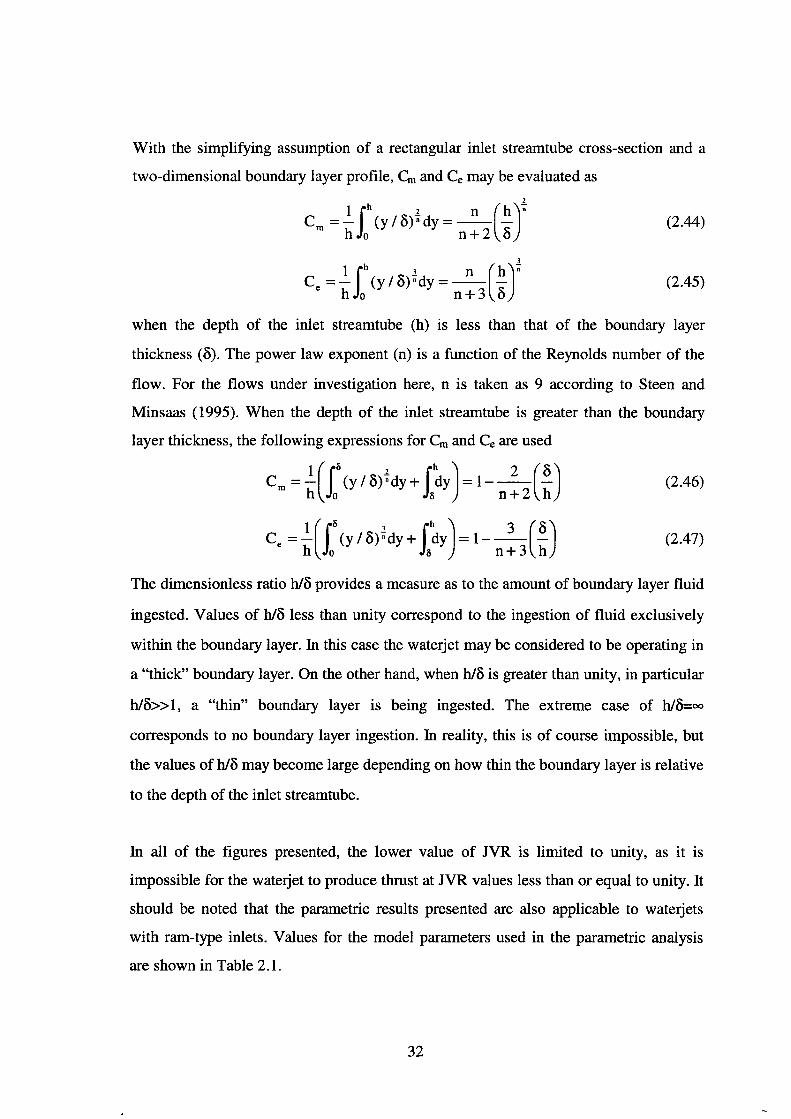
With the simplifying assumption of a rectangular inlet streamtube cross-section and a
two-dimensional boundary layer profile, Cm and Ce may be evaluated as
1 Jh 2 n (h)~ Crn =- (y I 8) 11 dy = - -h o n+2 8
(2.44)
1 Jh ; n (h)~ ce =- (y/8) 11dy=--h o n+3 8
(2.45)
when the depth of the inlet streamtube (h) is less than that of the boundary layer
thickness (8). The power law exponent (n) is a function of the Reynolds number of the
flow. For the flows under investigation here, n is taken as 9 according to Steen and
Minsaas ( 1995). When the depth of the inlet stream tube is greater than the boundary
layer thickness, the following expressions for Cm and Ce are used
(2.46)
(2.47)
The dimensionless ratio h/8 provides a measure as to the amount of boundary layer fluid
ingested. Values of h/8 less than unity correspond to the ingestion of fluid exclusively
within the boundary layer. In this case the waterjet may be considered to be operating in
a "thick" boundary layer. On the other hand, when h/8 is greater than unity, in particular
h/8>>1, a "thin" boundary layer is being ingested. The extreme case of hl8=oo
corresponds to no boundary layer ingestion. In reality, this is of course impossible, but
the values of h/8 may become large depending on how thin the boundary layer is relative
to the depth of the inlet streamtube.
In all of the figures presented, the lower value of JVR is limited to unity, as it is
impossible for the waterjet to produce thrust at JVR values less than or equal to unity. It
should be noted that the parametric results presented are also applicable to waterjets
with ram-type inlets. Values for the model parameters used in the parametric analysis
are shown in Table 2.1.
32
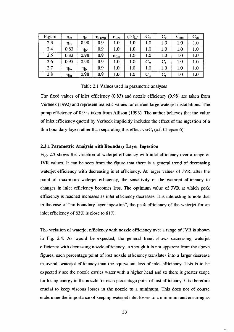
Figure Tlln llN TlPump TlRot (1-tL) Cm Ce Cmn Cen 2.3 Tlln 0.98 0.9 1.0 1.0 1.0 1.0 1.0 1.0 2.4 0.83 llN 0.9 1.0 1.0 1.0 1.0 1.0 1.0 2.5 0.83 0.98 0.9 TlRot 1.0 1.0 1.0 1.0 1.0 2.6 0.95 0.98 0.9 1.0 1.0 Cm Ce 1.0 1.0 2.7 'Tlln llN 0.9 1.0 1.0 1.0 1.0 1.0 1.0 2.8 Tlln 0.98 0.9 1.0 1.0 Cm Ce 1.0 1.0
Table 2.1 Values used in parametric analyses
The fixed values of inlet efficiency (0.83) and nozzle efficiency (0.98) are taken from
Verbeek (1992) and represent realistic values for current large waterjet installations. The
pump efficiency of 0.9 is taken from Allison (1993). The author believes that the value
of inlet efficiency quoted by Verbeek implicitly includes the effect of the ingestion of a
thin boundary layer rather than separating this effect viaCe (c.f. Chapter 6).
2.3.1 Parametric Analysis with Boundary Layer Ingestion
Fig. 2.3 shows the variation of waterjet efficiency with inlet efficiency over a range of
JVR values. It can be seen from the figure that there is a general trend of decreasing
waterjet efficiency with decreasing inlet efficiency. At larger values of JVR, after the
point of maximum waterjet efficiency, the sensitivity of the waterjet efficiency to
changes in inlet efficiency becomes less. The optimum value of JVR at which peak
efficiency is reached increases as inlet efficiency decreases. It is interesting to note that
in the case of "no boundary layer ingestion", the peak efficiency of the waterjet for an
inlet efficiency of 83% is close to 61%.
The variation of waterjet efficiency with nozzle efficiency over a range of JVR is shown
in Fig. 2.4. As would be expected, the general trend shows decreasing waterjet
efficiency with decreasing nozzle efficiency. Although it is not apparent from the above
figures, each percentage point of lost nozzle efficiency translates into a larger decrease
in overall waterjet efficiency than the equivalent loss of inlet efficiency. This is to be
expected since the nozzle carries water with a higher head and so there is greater scope
for losing energy in the nozzle for each percentage point of lost efficiency. It is therefore
crucial to keep viscous losses in the nozzle to a minimum. This does not of course
undermine the importance of keeping waterjet inlet losses to a minimum and ensuring as
33
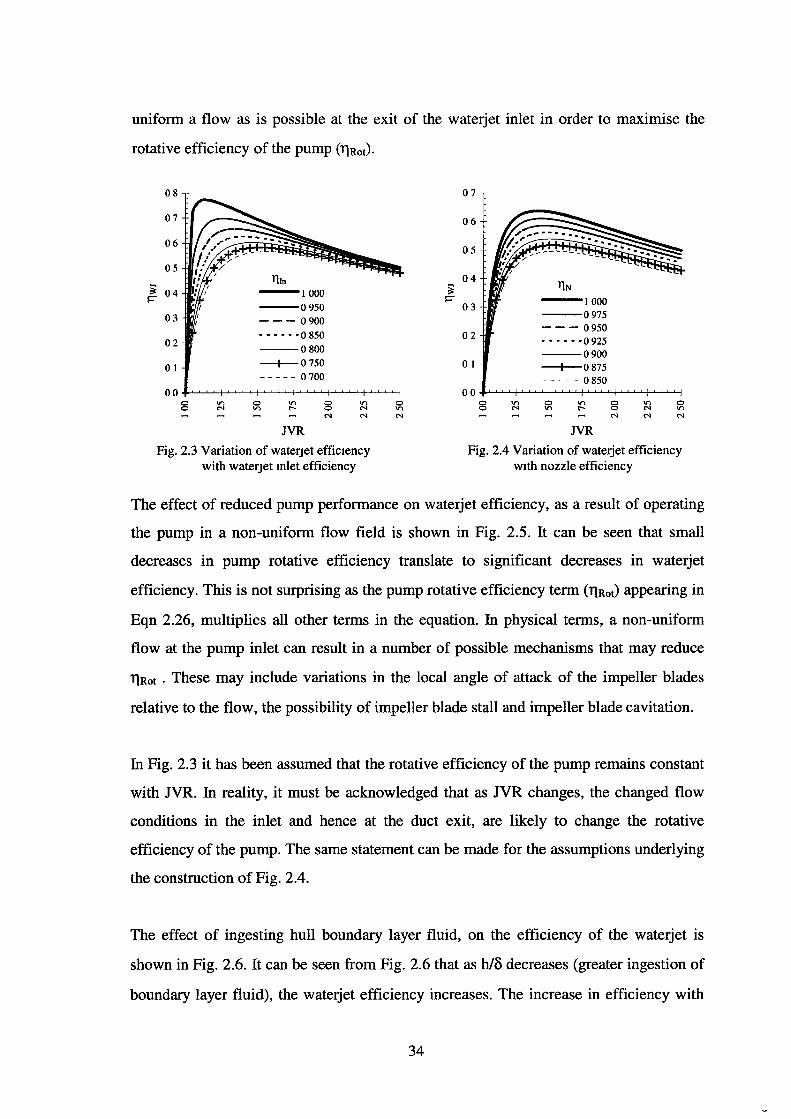
uniform a flow as is possible at the exit of the waterjet inlet in order to maximise the
rotative efficiency of the pump (llRot).
08
07
06
05
~ 04 ~
03
02
0 I
00 0 0 "' N
TIIn -1000 --0950 ---0900 ---···0850 --0800
-+-0750 ----- 0 700
0
"' JVR
8 N
Fig. 2.3 Variation of waterJet efficiency with waterJet mlet efficiency
~ ~
07
06
05
04
03 I 000 --0975 --- 0950
02 ••••• ·0 925 --0900
0 I -l--0875 ----- 0 850
00 0 "' 0 "' 8 "' 0 0 N "' r- N "' - - N N N
JVR
Fig. 2.4 Variation of waterjet efficiency w1th nozzle efficiency
The effect of reduced pump performance on waterjet efficiency, as a result of operating
the pump in a non-uniform flow field is shown in Fig. 2.5. It can be seen that small
decreases in pump rotative efficiency translate to significant decreases in waterjet
efficiency. This is not surprising as the pump rotative efficiency term (llRot) appearing in
Eqn 2.26, multiplies all other terms in the equation. In physical terms, a non-uniform
flow at the pump inlet can result in a number of possible mechanisms that may reduce
llRot . These may include variations in the local angle of attack of the impeller blades
relative to the flow, the possibility of impeller blade stall and impeller blade cavitation.
In Fig. 2.3 it has been assumed that the rotative efficiency of the pump remains constant
with JVR. In reality, it must be acknowledged that as JVR changes, the changed flow
conditions in the inlet and hence at the duct exit, are likely to change the rotative
efficiency of the pump. The same statement can be made for the assumptions underlying
the construction of Fig. 2.4.
The effect of ingesting hull boundary layer fluid, on the efficiency of the waterjet is
shown in Fig. 2.6. It can be seen from Fig. 2.6 that as h/8 decreases (greater ingestion of
boundary layer fluid), the waterjet efficiency increases. The increase in efficiency with
34
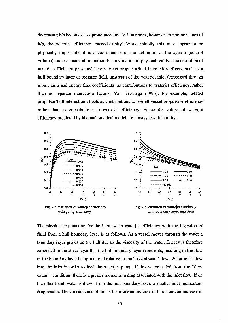
decreasing h/8 becomes less pronounced as JVR increases, however. For some values of
h/8, the waterjet efficiency exceeds unity! While initially this may appear to be
physically impossible, it is a consequence of the definition of the system (control
volume) under consideration, rather than a violation of physical reality. The definition of
waterjet efficiency presented herein treats propulsor/hull interaction effects, such as a
hull boundary layer or pressure field, upstream of the waterjet inlet (expressed through
momentum and energy flux coefficients) as contributions to waterjet efficiency, rather
than as separate interaction factors. Van Terwisga ( 1996), for example, treated
propulsor/hull interaction effects as contributions to overall vessel propulsive efficiency
rather than as contributions to waterjet efficiency. Hence the values of waterjet
efficiency predicted by his mathematical model are always less than unity.
07
06
05
04 ~
!=' 0 3
02
0 I
oo~~~~~~~~~~~~~y
8
Fig. 2.5 Variation of waterjet efficiency with pump efficiency
14
12
I 0
0 8 T ..t'T"fO+o.&._o_' ~ ~ .. -.,...:-~~~
!=' 06 1
I I
04 I
02
h/8 ---o 25 --o so - - - 0 75 - - - - - - I 00 --150 --+-300
----- NoBL
JVR
Fig. 2.6 Variation of waterjet efficiency with boundary layer ingestion
The physical explanation for the increase in waterjet efficiency with the ingestion of
fluid from a hull boundary layer is as follows. As a vessel moves through the water a
boundary layer grows on the hull due to the viscosity of the water. Energy is therefore
expended in the shear layer that the hull boundary layer represents, resulting in the flow
in the boundary layer being retarded relative to the "free-stream" flow. Water must flow
into the inlet in order to feed the waterjet pump. If this water is fed from the "free
stream" condition, there is a greater momentum drag associated with the inlet flow. If on
the other hand, water is drawn from the hull boundary layer, a smaller inlet momentum
drag results. The consequence of this is therefore an increase in thrust and an increase in
35
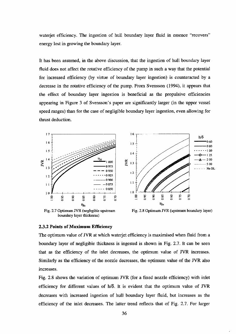
waterjet efficiency. The ingestion of hull boundary layer fluid in essence "recovers"
energy lost in growing the boundary layer.
It has been assumed, in the above discussion, that the ingestion of hull boundary layer
fluid does not affect the rotative efficiency of the pump in such a way that the potential
for increased efficiency (by virtue of boundary layer ingestion) is counteracted by a
decrease in the rotative efficiency of the pump. From Svensson (1994), it appears that
the effect of boundary layer ingestion is beneficial as the propulsive efficiencies
appearing in Figure 3 of Svensson's paper are significantly larger (in the upper vessel
speed ranges) than for the case of negligible boundary layer ingestion, even allowing for
thrust deduction.
17.-----------------------~
16
I 5
~ 14 ~
> ...., I 3
12
II
8 V'l a.. 0
0 a.. 0
'I") 00 0
llin
TJN -1ooo --0975
--- 0950
----- -o 925 --0900
- -0875 ----- 0 850
0 'I") 0 00 ,.... ,.... 0 0 0
Fig. 2.7 Optimum JVR (neghgible upstream boundary layer thickness)
2.3.2 Points of Maximum Efficiency
llin
Fig. 2.8 Optimum JVR (upstream boundary layer)
The optimum value of JVR at which waterjet efficiency is maximised when fluid from a
boundary layer of negligible thickness is ingested is shown in Fig. 2. 7. It can be seen
that as the efficiency of the inlet decreases, the optimum value of JVR increases.
Similarly as the efficiency of the nozzle decreases, the optimum value of the JVR also
increases.
Fig. 2.8 shows the variation of optimum JVR (for a fixed nozzle efficiency) with inlet
efficiency for different values of hi~. It is evident that the optimum value of JVR
decreases with increased ingestion of hull boundary layer fluid, but increases as the
efficiency of the inlet decreases. The latter trend reflects that of Fig. 2. 7. For larger
36
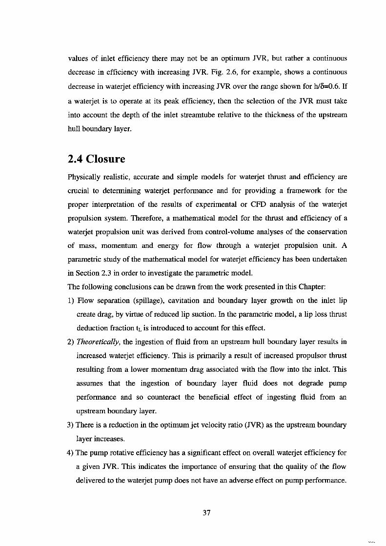
values of inlet efficiency there may not be an optimum JVR, but rather a continuous
decrease in efficiency with increasing JVR. Fig. 2.6, for example, shows a continuous
decrease in waterjet efficiency with increasing JVR over the range shown for h/0=0.6. If
a waterjet is to operate at its peak efficiency, then the selection of the JVR must take
into account the depth of the inlet streamtube relative to the thickness of the upstream
hull boundary layer.
2.4 Closure
Physically realistic, accurate and simple models for waterjet thrust and efficiency are
crucial to determining waterjet performance and for providing a framework for the
proper interpretation of the results of experimental or CFD analysis of the waterjet
propulsion system. Therefore, a mathematical model for the thrust and efficiency of a
waterjet propulsion unit was derived from control-volume analyses of the conservation
of mass, momentum and energy for flow through a waterjet propulsion unit. A
parametric study of the mathematical model for waterjet efficiency has been undertaken
in Section 2.3 in order to investigate the parametric model.
The following conclusions can be drawn from the work presented in this Chapter:
1) Flow separation (spillage), cavitation and boundary layer growth on the inlet lip
create drag, by virtue of reduced lip suction. In the parametric model, a lip loss thrust
deduction fraction tL is introduced to account for this effect.
2) Theoretically, the ingestion of fluid from an upstream hull boundary layer results in
increased waterjet efficiency. This is primarily a result of increased propulsor thrust
resulting from a lower momentum drag associated with the flow into the inlet. This
assumes that the ingestion of boundary layer fluid does not degrade pump
performance and so counteract the beneficial effect of ingesting fluid from an
upstream boundary layer.
3) There is a reduction in the optimum jet velocity ratio (JVR) as the upstream boundary
layer increases.
4) The pump rotative efficiency has a significant effect on overall waterjet efficiency for
a given JVR. This indicates the importance of ensuring that the quality of the flow
delivered to the waterjet pump does not have an adverse effect on pump performance.
37
Chapter 3 Computational Fluid Dynamics Modelling
In the literature there have been several approaches to the computational simulation of
waterjet inlets. These have ranged from potential flow methods, such as the method of
Hess and Smith (1964) used by Kashiwadani (1997), to the solution of the Reynolds
averaged Navier Stokes (RANS) equations with turbulence modelling which Seil et al
( 1995) used. Some workers have used an interesting combination of computational
techniques. F!1Srde et al ( 1991 ), for example, used a combination of the time-dependent
form of the Euler equations with thin-layer RANS equations to calculate the flow in both
ram and flush-type waterjet inlets.
Several authors such as Kashiwadani (1997), have used potential flow methods as
preliminary analysis tools to examine the pressure distribution over the surface of the
waterjet inlet in the immediate vicinity of the inlet. This approach allows the likelihood of
cavitation and flow separation to be determined. Kashiwadani's results were in reasonable
agreement with experimental data possibly due to the thin nature of the boundary layers on
the inlet ramp resulting from his scoop-type inlet. Van Terwisga ( 1996) compared
potential flow predictions with experimental data for flow within a waterjet inlet model.
He found that the use of the potential flow methodology gave relatively large inaccuracies
in the predicted static pressure distribution over the inlet lip and ramp. The discrepancies
can be primarily attributed to the neglect of boundary layer growth within the inlet. Large
differences were evident at the inlet lip as a result of an incorrectly calculated stagnation
line resulting from the neglect of boundary layer effects.
Dai et al ( 1995) and Steen and Minsaas ( 1995) have used potential flow when seeking to
"optimise" an inlet design by examining a large number of prospective designs. These two
sets of authors, however, complement their potential flow analyses with RANS
computations for designs which appear to be promising. This was done in order to provide
38
more accurate computations accounting for the effects of viscosity on flow behaviour.
From the results of van Terwisga ( 1996), it is evident that the assumptions underlying the
use of potential flow computations are clearly violated for conventional flush-type waterjet
inlets, which have relatively shallow inlets and large internal boundary layer growth.
Furthermore, the assumptions of potential flow theory become irrelevant in the presence of
the large boundary layer thicknesses developed on high-speed catamaran ferries. For large
flush-type waterjet inlet installations, upstream boundary layer thicknesses must be
accounted for in the design of these inlets. Therefore computational techniques based on
the solution of the RANS equations offer the only realistic means of solving the flow in
the vicinity of the inlet and inside the waterjet inlet itself.
fu the literature there has been some work towards the computational simulation of the
complete waterjet-hull geometry. Yang et al (1995) used a boundary element method to
calculate the flow around a mathematical hull form in order to provide boundary
conditions for a RANS computation of the flow in a waterjet inlet. Viscous effects
associated with the hull boundary layer development were neglected and this is a clear
limitation of their methodology. Widmark and Gustafsson (1997) of SSPA, used that
organisation's SHIPFLOW code to provide boundary conditions for a RANS simulation
of flow in a waterjet inlet. SHIPFLOW used a combination of potential flow, boundary
layer integral and RANS methodologies to calculate the flow around the vessel hull. No
experimental validation of the methodology was presented in the paper, so the accuracy of
the total methodology could not be determined.
The optimisation of the hydrodynamic design of waterjet inlets is an applied problem,
where the emphasis is on design investigation and optimisation. As a consequence, the
choice was made to use commercially-available CFD software. This allows attention to
be focused on the practicalities of waterjet inlet design investigation and mesh
generation, with CFD used as an analysis tool. This is analogous to the way in which
modem industry uses finite element structural analysis as an analysis tool in the design
of machine parts.
Since interest is directed at the design of the waterjet inlet itself, in the absence of hull
39
form geometry, a simplified flow domain external to the inlet is chosen. This makes the
meshing of the waterjet inlet and flow domain external to the inlet amenable to the
single-block structured grid topology described in Chapter 4. As a result, a structured
mesh can be used to mesh the complete flow domain and consequently a structured CFD
solver can be used to simulate the flow internal and external to the waterjet inlet. This is
a primary reason for the choice of the commercially-available CFD software Fluent. The
good international reputation of this software also favours its use.
An overview of the CFD methodology and techniques that form the foundation of the
numerical work presented in this thesis will be given in this chapter and is applicable to
obtaining flow solutions on body-fitted-coordinate (BFC) structured meshes. The RANS
equations are derived from the isothermal and incompressible form of the continuity and
Navier Stokes equations in Section 3.1. In Section 3.2, the Reynolds stresses that appear
in the RANS equations are modelled using two-equation turbulence models based on
the hypothesis of Boussinesq (1877), where mean velocity gradients are related to the
Reynolds-stresses via an eddy-viscosity formulation. Two, two-equation turbulence
models based on the transport of turbulent kinetic energy (k) and turbulent dissipation
(E) are described. These are the Standard k-E model of Launder and Spalding (1974) and
the RNG k-E model of Yakhot and Orszag (1986) which was extended by Yakhot et al
(1992) to account for the effects of irrotational strain on the turbulence. The relative
merits and limitations of these turbulence models are then discussed. In Section 3.3 the
structure of the turbulent boundary layer is presented and the reasons why wall functions
are used to model the near-wall behaviour of the flow are discussed. Details of the wall
functions used in this work are subsequently given.
The finite-volume discretisation of the governing transport equations is discussed in
Section 3.4. In order to complete the discretisation process, it is necessary to employ
suitable convective differencing schemes to relate the values of the transported quantity
<j> at the control-volume faces to their surrounding finite-volume cell-centre values. This
forms the subject of Section 3.5. The nonlinearity of the governing transport equations
and the present state of computer hardware necessitate the solution of the discretised
equations by iterative means. The manipulation of the discretised equations into a form
40
suitable for use with iterative solution techniques is discussed in Section 3.6. The CFD
methodology used by the author is summarised in Section 3.7. The Dirichlet and
Neumann boundary conditions used in the computational simulations presented in this
thesis will be discussed in later chapters in the context of the description of those
simulations.
3.1. Governing Flow Equations
The flows studied in this thesis may be considered to be steady, isothermal and
incompressible. As a consequence of this, the continuity and Navier Stokes equations
provide a full description of the flow behaviour.
3.1.1 Navier Stokes Equations
The continuity equation and Navier Stokes equations express Eulerian conservation
relationships for mass and momentum respectively. According to Fletcher (1987b,
p.10), the coordinate invariant form of the Navier Stokes equation is
_i_(pu) + (u · V)u = pf- Vp-2
V(J.!V · u) +2V · (J.!D) at 3
(3.1)
In Eqn 3.1 V represents the gradient operator, u the instantaneous fluid velocity, Jl the
molecular viscosity of the fluid, p the fluid density, p the pressure, f the volume force
per unit mass and D is the deformation (rate of strain tensor) whose components can be
written in Cartesian tensor notation as
D,,=~(~: +~:J (3.2)
Using Cartesian tensor notation, the steady-state, incompressible form of the continuity
and N a vier Stokes equations may be written as
a -a (u)=O x.
(3.3)
a a a = p-(uJu.) = _ _£_+2-(J.!D)+pf.
axJ ax. axJ (3.4)
Eqn 3.3 is the continuity equation and Eqn 3.4 is the Navier Stokes equations,
respectively (see Wilcox (1993)). In the above equations, U1 is the instantaneous velocity
and f. the body force per unit mass in the ith coordinate direction (x1), respectively.
41
Following the conventions of tensor notation, repetition of the same index implies a
summation over the range of that index.
As the Reynolds number of a flow increases, the ability of the fluid's viscosity to
suppress instabilities within the flow (and so maintain laminar flow) decreases.
Eventually, at a sufficiently high Reynolds number, the flow becomes unstable and is
then characterised by random fluctuations of the flow quantities. Turbulence is therefore
a random, dissipative, time-dependent phenomenon displaying a large range of excited
length and time-scales. These range in size from the integral scales of the turbulence
down to the Kolmogorov microscale as was discussed by Tennekes and Lumley ( 1972).
The smallest scales of the turbulent fluctuations are many orders of magnitude smaller
than the largest scales present in the flow. Inherent in turbulent flow is a cascading
process whereby, as the turbulence decays, its kinetic energy transfers from larger eddies
to smaller eddies, this being achieved mainly by the process of vortex stretching as was
noted by Wilcox (1993). The apparent fluid stresses that are developed within the
turbulent flow are several orders of magnitude larger than in a corresponding laminar
flow. Since turbulence is a continuum phenomenon, the three-dimensional Navier
Stokes equations contain all of the physics necessary to describe that flow.
3.1.2 Reynolds-averaged Navier Stokes Equations
Turbulence is a random phenomenon which must be handled using a statistical
approach. Therefore, the time averages of the continuity and Navier Stokes equations
are sought. The instantaneous velocity at a point in the flow (u1) can be considered as
being composed of a mean (average) component (U1) and a fluctuating component ( u; ),
such that
The mean velocity is defined by
where T is a characteristic time-scale. The time average of the mean velocity t+T
- 1 J ul = lim - ul dt = u I T-7~ T
(3.5)
(3.6)
(3.7)
is simply the mean velocity. In Eqn 3.7 the overbar denotes an average value. The time-
42
average of the fluctuating component of the instantaneous velocity t+T
u; =lim_.!_ Jcul- UJdt = ul- ul = o T--t~ T
(3.8)
is zero. A limit ofT of oo in the above definitions is appropriate for stationary turbulence
(a turbulent flow that on average does not vary with time). For flows containing very
slow variations of the mean velocity with time, an alternative definition
t+T
UJ = ~ f U 1dt , T1 <<T<<T2 (3.9)
is required. fu Eqn 3.9, T1 is the time scale characteristic of the random velocity
fluctuations associated with the turbulence and T 2 the time scale associated with the
variation of the slowly varying mean flow behaviour. It has been assumed here that T2 is
several orders of magnitude greater than T 1• A more detailed exposition of Reynolds
averaging (time averaging) was given by Wilcox (1993).
Reynolds-averaging of the steady, incompressible form of the continuity and Navier
Stokes equations results in the following equations in Cartesian tensor form
(3.10)
(3.11)
The correlated quantity -pu:u; appearing in Eqn 3.11 is the Reynolds stress tensor
denoted by 't1J • The quantity S is a "source" term and accounts for such effects as body
forces. The Reynolds stress tensor is symmetric and there are therefore six Reynolds
stresses that must be determined in order to close Eqn 3.11. The determination of the
Reynolds stresses in the RANS equations forms the fundamental problem of turbulence
modelling.
3.2 Turbulence Modelling
A brief overview of the theory behind turbulence modelling and the two-equation
turbulence models available in Fluent and used in this research, shall be presented in
this section. Fluent also allows the option of using a Reynolds Stress Model (RSM)
turbulence model which should allow more accurate solutions to be obtained for
43
anisotropic flows. Fluent ( 1996) noted that despite this advantage, more time is required
to obtain converged solutions as there are a larger number of equations being solved and
the model is computationally less robust than the k-E models available. In view of the
fact that a large number of runs would be required for the design space investigation and
optimisation-related work presented in later chapters (where minimal execution time
and robustness of calculation are essential) it was decided to make exclusive use of k-E
models.
The hypothesis of Boussinesq (1877), referred to by Wilcox (1993), can be written for
incompressible flow as
-,-, (au. auJ J 2 k~ -pu.uJ = J..lt -a +-a --p u.J XJ X1 3
(3.12)
can be used to relate the mean strain rate tensor (Dij) to the Reynolds stresses via an
isotropic eddy/turbulent-viscosity (J.11) formulation. In Eqn 3.12, 01J is the Kronnecker
delta and the quantity k is the specific turbulent kinetic energy, commonly called the
turbulent kinetic energy and is defined by
1-- -- 1-k = -(u'u' + v'v' + w'w') = -u'u' 2 2 I I
Dimensional arguments dictate that eddy viscosity is given by
J..l 1 = const · pk112 f
(3.13)
(3.14)
where f is the turbulent length-scale, the determination of which is not unique as was
noted by Wilcox (1993).
The steady form of the transport equation for turbulent kinetic energy can be written as
U ak au. a ( ak 1 , , , -,-,J p -='t ---pE+- J..L---puuu -pu J ax IJ ax ax ax 2 I I J J
J J J J (3.15)
The left-hand-side of Eqn 3.15 represents the convection of turbulent energy by the
mean flow. The terms on the right-hand side of Eqn 3.15 represent the production,
dissipation, molecular diffusion, turbulent transport and the pressure diffusion of
turbulent kinetic energy, respectively. The production term represents the rate at which
kinetic energy is transferred from the mean flow to the turbulence. It is also the rate at
which the mean flow "works" against the Reynolds stresses. The dissipation is the rate
44
at which turbulent kinetic energy is converted into heat. Molecular diffusion represents
the diffusion of turbulence energy as a consequence of natural molecular transport
processes. The turbulent transport term represents the rate at which turbulence energy is
transported through the fluid by turbulent velocity fluctuations. The pressure-diffusion
results from correlated velocity and pressure fluctuations.
The turbulent transport and pressure-diffusion terms are approximated together by a
gradient -diffusion representation
1 ~ ak -pu'u'u' + p'u' = --1
-2 IIJ J crax
k J
(3.16)
as stated by Wilcox (1993). Replacement of the turbulent transport and pressure
diffusion terms in Eqn 3.16 with a gradient-diffusion approximation yields the following
generic equation for k
(3.17)
The turbulent dissipation is defined by the correlation
au: au: E=V--
axJ axJ (3.18)
If R is a turbulent length-scale of effective eddy size, then the velocity scale of the
corresponding eddy is k112• Its turbulent dissipation should scale by dimensional
reasoning as
(3.19)
(see White (1991)), which when substituted into Eqn 3.14 allows the eddy-viscosity to
be directly related to k and E via
(3.20)
Therefore, in order to determine the eddy-viscosity so as to close the RANS equations, it
is necessary to solve two additional transport equations, one for the turbulent kinetic
energy (k) and the other for the turbulent dissipation (E).
The exact equation for E is actually a transport equation for the dissipating eddies. What
45
is actually sought is an equation for the transfer of energy from the energy-containing
eddies, since the length-scale required is that of the energy-containing, Reynolds-stress
bearing eddies (Wilcox (1993)). As a result, the transport equation for turbulent
dissipation is taken as an empirical equation for the rate of energy transfer from the
large eddies (equal to the rate of dissipation of turbulent energy in the small eddies). The
e equation is therefore modelled in an analogous way to the k equation (Wilcox (1993)).
3.2.1 Standard k-e Turbulence Model
Fluent (1996) noted that the Standard k-e model of Launder and Spalding (1974) has
been a popular two-equation turbulence model for over 20 years and derives its
acceptance from its robustness, computational economy and reasonable accuracy. The
Standard k-e turbulence model may be written as
p ae +pU ae =_j_(J..LT ae )+ CEIJ..lTf.(aul + auJ)aul- pCE2£2
at J ax J ax J (j E ax J k ax J ax 1 ax J k
where the eddy viscosity is determined by
k2 II =pC -t"! J.l f.
(3.21)
(3.22)
(3.23)
The empirically determined closure coefficients of the transport equations for k and e
are
cJ.l = o.o9, eEl = 1.45, CE2 = 1.90, crk =to, crE = 1.3 (3.24)
The constants for the Standard k-e model were determined by calibrating the model
against experimental data (Launder and Spalding (1974)). A brief history of the
development of the k -e turbulence model was provided by Wilcox ( 1993).
3.2.2 RNG k-e Turbulence Model
The Renormalisation Group (RNG) k-e turbulence model used by Fluent was originally
developed by Yakhot and Orszag (1986) and extended by Yakhot et al (1992) to account
for the effect of irrotational strain on the production of e. Only the high Reynolds
number form of the model shall be presented, as this is the only form of the model used
46
to obtain the CFD results presented in this thesis. The RNG method is essentially a scale
elimination technique that can be applied to both the Navier Stokes equations and scalar
transport equations. Removal of successively larger scales leads to differential transport
equations. Constants in the model are derived explicitly from theory.
The RNG k-E turbulence model used in Fluent may be summarised as
where the closure coefficients for the transport equations of k and E are
c,1 =1.42, c.2=l.68, a=l.39
The turbulent kinetic energy production term in Eqn 3.25 is
Gk = JlrS2 = 2J.1rS,JSIJ
where S,J is the mean rate of strain tensor
and S is its modulus defined by
s =~S,1S,1
(3.25)
(3.26)
(3.27)
(3.28)
(3.29)
(3.30)
The structure of Eqn 3.25 and Eqn 3.26 are similar in form to that of the Standard k-E
model, but differs due to the addition of a rate of strain term (R) in the transport
equation for E and different closure coefficients. It is this rate of strain term that
sensitises the production (or destruction) of E to the effect of irrotational strains in the
flow and hence improves the model's predictive accuracy. The rate of strain term (R) is
given by
II au' au' r- I I R=2-S --p ljax ax
I j
and is expressed in the model equations as
47
(3.31)
(3.32)

where ll = S k/c is the ratio of the turbulent to mean strain rate time-scales, llo""4.38 and
B=0.012. For the high Reynolds number form of the model, the isotropic eddy-viscosity
is calculated by
(3.33)
where the closure coefficient CJ.1=0.0845. This is close to the value of CJ.1=0.09 of the
Standard k-£ model. The inverse of the Prandtl number (a.), appearing in the turbulent
transport equations is obtained from the effective viscosity by the solution of
a- 1.3929 o 6321 a+ 2.3929 o 3679 = Jlo
a 0 -1.3929 a 0 + 2.3929 Jl 1
(3.34)
where ao= 1.
3.2.3 Limitations of k-£ Turbulence Modelling
A well known deficiency of the Standard k -£ model is the tendency of this model to
over-predict the eddy-viscosity under adverse pressure gradients. This acts to suppress
flow separation and leads to an over-prediction of the skin friction coefficient for wall
bounded flows. Rodi and Scheuerer ( 1986) demonstrated that the limitations of the
Standard k-c model under adverse pressure gradient may be attributed to an over
prediction of the turbulent length-scale by the c equation.
Rodi and Scheuerer ( 1986) noted that the results of Bradshaw ( 1967) suggested that the
turbulent length-scale is essentially independent of pressure gradient over a wide range.
Thus there is a need to modify the c equation so that either the generation of c is
enhanced or the destruction of c is reduced under adverse pressure gradient. Rodi and
Scheuerer ( 1986) adopted the former approach based on augmenting the production of c
using the model of Hanjalic and Launder ( 1980). Hanjalic and Launder ( 1980) modified
the c equation in order to promote higher rates of dissipation for irrotational strains than
for rotational strains, thus suggesting that energy transfer rates across the turbulence
spectrum is promoted by irrotational deformations.
The Boussinesq hypothesis represents another limitation of the Standard k-c model and
48
indeed other two-equation models as well. The notion that the Reynolds stresses can be
related to mean flow gradients via an isotropic eddy-viscosity becomes inaccurate when
the Reynolds-stresses are unrelated to mean flow gradients. Wilcox (1993) noted that
examples of such flows include:
1) Flows subjected to sudden changes in mean strain rate
2) Flows over curved surfaces
3) Flows with boundary layer separation
4) Flows in ducts with secondary motion
5) Secondary flows in the comers of ducts of rectangular cross-section driven by
anisotropy in the turbulence
6) Three-dimensional flows and flows with significant boundary layer cross-flow
7) Flows subjected to rotation
Flows over curved surfaces, flows subjected to rotation, secondary flows (and swirl) and
flows with boundary layer separation are themselves examples of flows subjected to
streamline curvature and what Bradshaw (1973) termed as "extra rates of strain". These
"extra rates of strain" modify the structure of the turbulence to a much greater extent
than the extra production terms that appear in the Reynolds stress equations would
suggest. The phenomenon is related to the higher-order structural parameter of the
turbulence, which causes changes in the Reynolds stresses and therefore modifies the
structure of the turbulence. These processes are unrelated to the mean strain rates of the
flow.
Lakshminarayana ( 1986) reviewed the subject of turbulence modelling for complex
flows. Lakshminarayana ( 1986) stated the following reasons for the limitations of k-E
models:
1) The assumption of isotropic eddy-viscosity
2) Inadequate modelling of the pressure strain terms in the turbulent transport equations
3) The calibration of model constants from two-dimensional flows
4) Gradient-induced diffusion as the only diffusive mechanism
Lakshminarayana (1986) and the references cited therein suggested that a constant value
49
of C~ is inadequate for the prediction of complex shear layers. In order to improve the
predictive accuracy for three-dimensional flows, the k-E model may be modified to
include a vectorial representation of C~ via an Algebraic Reynolds Stress Model
(ARSM). For example, Leschziner and Rodi (1981) used this approach and were able to
obtain closer agreement with experimental data for annular and twin parallel jet flow.
Alternatively, the k-E model should be coupled with either an ARSM or Reynolds Stress
Model when adequate prediction of the mean and turbulence flow field is sought.
There have been numerous attempts to modify two-equation turbulence models to give a
better prediction of flows subjected to streamline curvature. Wilcox and Chambers
( 1977) for example, proposed a curvature correction to the turbulent kinetic energy
equation for their k-ro model and obtained improved predictive accuracy for flow over a
curved surface. They argued that the equation for k should be thought of as an equation
for v'2 for curved flow over a surface. Launder et al (1977) modified the dissipation
term in the E equation to account for the effect of streamline curvature. The constant C£2
was modified using a turbulent Richardson number as the significant curvature
parameter. This yielded an improvement in predictive accuracy.
From the references cited, it is clear that there is a diverse range of modifications to two
equation models to account for adverse pressure gradient and streamline curvature.
These essentially involve the modification of C~ , or the turbulent length-scale obtained
by modification of the production or dissipation terms in the E equation.
The RNG k-E turbulence model offers improved accuracy over the Standard k-E model
due to the rate of strain term (Eqn 3.32) in theE equation. This effectively sensitises the
production (or dissipation) of E to the effect of irrotational strains. Therefore, in regions
of large irrotational strain (Tl>Tlo) R becomes negative and E increases. This leads to
smaller turbulent length-scales and reduced eddy-viscosity. Hence, the tendency of the
flow to separate will be enhanced. For flows over curved surfaces, the reduction in
eddy-viscosity provides a better modelling of the collapse of turbulence phenomena (see
Gillis and Johnston (1983)) for flow over convex surfaces.
50
3.3 Modelling of the Near-Wall Flow
The viscosity of the fluid, irrespective of its magnitude, results in the "no-slip"
condition at a solid boundary (wall). This requires that the velocity of the fluid at a solid
surface be equal to the velocity of the surface, as noted by Tennekes and Lumley (1972).
As a consequence of the no-slip condition, fluid in its flow over a solid boundary is
subject to significant shearing in the streamwise direction. A boundary layer evolves
over the surface of the solid boundary. Solid boundaries therefore act as sources of
turbulence and energy loss.
3.3.1 Boundary Layer Structure
The no-slip (zero velocity) condition at the wall is the essence of the formation of the
turbulent (high flow Reynolds numbers) boundary layer. The difference between the
free-stream velocity and the zero velocity at the wall results in sharp velocity gradients
and hence shearing in the fluid. The consequence of this being the formation and growth
of a boundary layer adjacent to the wall.
The turbulent boundary layer may be described by several layers in accordance with the
behaviour of the turbulence in these "layers". This is ultimately a direct consequence of
the turbulent length-scales involved, since there exists a close analogy between the
spatial structure of a turbulent boundary layer and the spectral structure of turbulence
(Tennekes and Lumley (1972)). The velocity profile of a turbulent boundary layer
consists of an inner layer where viscous effects are predominant, an outer layer (wake
region) where turbulent shear dominates, and an overlap layer providing an asymptotic
matching between the inner and outer layers (see for example White (1991) and Wilcox
(1993)).
The behaviour of the inner layer, or "wall region" is directly affected by the conditions
at the wall and hence by the wall shear stress, the wall roughness, fluid viscosity and the
distance (y) from the wall, but not on free-stream properties as both Hinze (1975) and
White (1991) noted. The functional form of the velocity in the wall region may be
determined from dimensional analysis as
51
where ut is the "friction velocity" defined by
and y + is the dimensionless sublayer-scaled distance from the wall defined by
y+ = pyU-r
J.1
The behaviour in the outer layer follows a "velocity-defect law" of the form
Urer- u = f(x_) ut 8
(3.35)
(3.36)
(3.37)
(3.38)
(Hinze (1975)) where 8 is the boundary layer thickness and Uref the velocity at the edge
of the boundary layer. From Eqn 3.35 and Eqn 3.38 it can be seen that the inner layer
corresponds to small turbulent length-scales of order y, the distance from the wall, down
to the Kolmogorov microscale of dissipative eddies. The outer layer corresponds to
large scale turbulent behaviour in the boundary layer with length-scales of the order of
8. It is possible to find a range of distances (y) from the surface where y+>>1 and y/8<<1
simultaneously. This range covering the transition from small to large-scale turbulence
dynamics corresponds to the overlap layer. This range is also called the logarithmic
region or the inertial sublayer, in an analogous manner to the inertial subrange of the
spectral structure of turbulence as Tennekes and Lumley ( 1972) explained. It is here that
asymptotic matching of the velocity profiles of the inner and outer layers occurs.
Three subregions may be identified in the inner layer. These are the viscous sublayer
(y+<5) , the transition or "buffer" layer (5<y+~30) and a fully turbulent region (y+>30),
(see Hinze (1975)). In the near-wall region, the integral scale of the turbulence is
proportional to the distance from the wall and must be of order y. Sufficiently close to
the wall the length scale of the turbulence becomes less than the Kolmogorov
microscale and hence Reynolds stresses become negligible and viscous effects
dominate. This is the viscous sublayer. As distance from the wall increases, the integral
scale becomes larger than the Kolmogorov microscale and Reynolds stresses
progressively become larger in magnitude until viscous stresses become negligible in
comparison to Reynolds stresses in the fully turbulent region. This region of transition
52
from viscous to Reynolds stresses is the buffer layer. The buffer layer is a region of
vigorous turbulence dynamics, because the turbulent energy production reaches a
maximum where the Reynolds stresses become equal to the viscous stress (y+:::::12) (see
Tennekes and Lumley (1972)).
In the viscous sublayer, velocity scales in a linear manner directly with distance from the
wall as
(3.39)
as noted by White (1991). In the fully turbulent region, the velocity can be described by
a logarithmic velocity distribution
u 1 ( +) -=-In y +B u't K
(3.40)
In Eqn 3.40, K is the von Karman constant and B is an empirical constant. Coles and
Hirst ( 1968) proposed the following values of the two constants
K=0.41 , B=5.0. (3.41)
Note that the above discussion has assumed flow over a smooth surface. In the buffer
layer the velocity profile is neither linear nor logarithmic but rather a smooth transition
from linear to logarithmic. Spalding (1961) proposed the following single composite
profile
(3.42)
for the wall region.
3.3.2 The Wall Function Approach
In order to utilise a two-equation turbulence model for computational simulation of a
wall-bounded flow, it is necessary to specify boundary conditions for velocity, turbulent
kinetic energy (k) and turbulent dissipation (c) at the wall, since the presence of the wall
is the primary source of turbulence formation. Since the Standard k-c model is of a high
Reynolds number form, it fails to predict a satisfactory constant B in the law of the wall
as Wilcox ( 1993) discussed. As a consequence, simply applying the no-slip condition at
the wall and integrating through the viscous sublayer will yield an unsatisfactory result.
53

Apart from the issue of the behaviour of two-equation turbulence models in the near
wall region, there are also issues of computational requirements. As the Reynolds
number of the flow increases, the range of turbulent length-scales also increases and
hence there will be a larger discrepancy in size between the integral scale of eddies and
the Kolmogorov microscale of dissipative eddies. It can thus be expected that as the
Reynolds number of the flow increases, the inner layer of the boundary layer will
decrease in thickness. As a consequence of this fact, if an integration of the governing
equations through the sublayer is sought, a finer grid would be required in order to
adequately resolve the flow down through the viscous sublayer. This increases the
computational requirements, both in terms of memory and execution time.
The above-mentioned problems can be overcome via the use of "wall functions" as a
means of providing suitable boundary conditions for the wall adjacent cells. Launder
and Spalding (1974) noted that the use of wall functions would not only reduce the
computational requirements of the simulation, but also allow the introduction of
additional empirical information in special cases, for example when the wall is rough.
3.3.3 Standard (Equilibrium) Wall Function
Wilcox (1993) and Cebeci and Smith (1974) showed that when pressure gradients are
small or negligible compared to other terms in the momentum equations, the momentum
equations in the inner layer simplify to
(3.43)
where U is the velocity tangent to the surface and y is the perpendicular distance from
the wall. Integration ofEqn 3.43 yields
(3.44)
In other words the sum of the molecular shear stress and the Reynolds stress is constant
in the inner layer, therefore shear stress is constant. Since shear stress is constant in the
inner layer, outside the buffer layer (y+>30), molecular shear stresses become negligible
in comparison to turbulent shear stress, hence the Reynolds stress is z-pU~ and the
mean velocity gradient is given by Uj(Ky) (Tennekes and Lumley (1972)). It follows
54
that the production of turbulent kinetic energy in the inner layer is given by
Gk = -ulvl au= U~ ay Ky
(3.45)
In an equilibrium boundary layer, the rates of turbulence production and dissipation are
in balance, therefore
u3 E=Gk = ~ (3.46)
Applying the Boussinesq hypothesis for the flow in the buffer layer, the Reynolds stress
can be related to the mean velocity gradient by
I I au -pu v = Jlt ay (3.47)
The turbulent kinetic energy may be obtained by substituting Eqn 3.46 into Eqn 3.23
and solving fork, with the mean velocity gradient in Eqn 3.47 being evaluated from the
law of the wall (Eqn 3.40). The resulting expression is
k= u~ ,JC;
Using the result ofEqn 3.48, y+ can be written as
and the following expression for the law of the wall may then be evaluated as
~CI'4kl/2 = ..!_ln(Ey p(C~2kp)It2) 'tw / p 11 p 1( p Jl
(3.48)
(3.49)
(3.50)
where kp is the turbulent kinetic energy at the wall-adjacent cell centres, at a
perpendicular distance of yp from the wall. The production of turbulent kinetic energy
then becomes
and turbulent dissipation can be rewritten (using the result ofEqn 3.48) as
c3'4k312 11 p
Ep =--=---K)'p
(3.51)
(3.52)
Fluent solves the momentum equations throughout the computational domain, including
the wall adjacent cells, with the no-slip condition specified at the wall. The near-wall
55
values of turbulent kinetic energy are determined by solving the complete transport
equation for k in the near-wall control-volumes subject to the boundary condition of a
zero normal gradient assumed for k at the wall. The production term for k in the
transport equation for k is obtained from Eqn 3 .51.
When the Standard (equilibrium) wall function option is specified, the wall shear stress
is determined from Eqn 3.50. Once the wall shear stress has been determined, the
production of k and the turbulent dissipation can then be determined using Eqn 3.51 and
Eqn 3.52, respectively. It is interesting to note that the transport equation forE, unlike
the momentum equations and the transport equation for k, is not solved at the near-wall
cells, but rather the solution fore is obtained via the use ofEqn 3.52.
It has been assumed in the above discussion, that the cell-centre location of the wall
adjacent cells have values of y+ sufficiently large such that the predominant shear
stresses present in the flow are turbulent and that Eqn 3.50 will provide a reasonably
accurate approximation to the velocity profile. In the viscous sublayer, where the
stresses are viscous and in the lower part of the buffer layer where viscous stresses are
predominant (y+s;12), a different form of wall function must be used. In many near-wall
modelling approaches using wall functions, the buffer layer is eliminated by linking the
linear velocity profile in the viscous sublayer to the logarithmic profile in the inertial
sublayer. This causes an abrupt change from purely viscous stress to purely turbulent
stress at y + = 11 as Tennekes and Lumley ( 1972) discussed. Following this approach,
when y +> 11.225 Fluent uses the logarithmic velocity profile of Eqn 3.50 to calculate
wall shear stress. When y+<11.225, the laminar stress-strain relationship ofEqn 3.39 is
used (see Fluent (1996)). The abrupt change from a viscous to a turbulent shear stress
relationship, resulting from the changeover of velocity profile at y + = 11.225 (as a
consequence of the elimination of the buffer layer in the modelling), is clearly a source
of modelling inaccuracy.
3.3.4 Two-Layer-Based Nonequilibrium Wall Function
For complex flows involving separation, reattachment and impingement, where the
mean flow and turbulence are subject to severe pressure gradients and change rapidly,
56
the equilibrium assumptions underlying the development of the Standard wall function
break down. The boundary layer can no longer be considered as being an equilibrium
boundary layer, indeed it is now a nonequilibrium boundary layer. Fluent offers the
option of selecting a Two-Layer-Based Nonequilibrium (TLBN) wall function which
can partly account for nonequilibrium effects neglected by the Standard wall function
(see Fluent (1996)). The discussion of the TLBN wall function presented below is taken
exclusively from Fluent ( 1996).
In the TLBN wall function, the wall function of Launder and Spalding (1974) is
sensitised to the effects of pressure gradient and is modified to the following form
(3.53)
where
(3.54)
and Yv is the physical thickness of the viscous sublayer determined by
* JlYv (3.55)
where y: = 11225. Unfortunately Fluent (1996) does not give the value of K *. For the
cells adjacent to the wall, the following profile assumptions are made for the turbulence
quantities
{
0, 'i =
I 'i W'
k = {(y /Y v t kp, Y < Y v
kp, Y>Yv {
2j.lkj(py 2 ), Y < Yv
e = kat2 j(Cey), y > Yv (3.56)
where Ce = KC~314 , 't1 is the turbulent shear stress and Yv is the dimensional thickness of
the viscous sublayer defined by Eqn 3.55. Using the profiles for 't1 , k and E specified in
Eqn 3.56, the cell-averaged production of k can be approximated by its depth-average
- 1 fYn dU 1 't2
( y ) Gk = -Jc 'tt ::h, dy = -- u: 112 In _n
Y 0 0 v y Ky 0 pC ~ k p Y v
(3.57)
The over-bar on Gk denotes a cell-averaged quantity and Yn is the height of the cell
(yn=2yp). Similarly, the cell-averaged dissipation rate is
57
_ 1 JYn 1 ( 2fJ. k~2 (Y"J] E=- cdy=- -+-In- kp y n 0 y n py v cl y v
(3.58)
The solution procedure for determining velocity, k and E in the wall-adjacent cells is
identical to the case of the Standard wall function, but in the case of the TLBN wall
function, wall shear stress ('tw) is determined by Eqn 3.53. The value of 'tw obtained
from Eqn 3.53 is subsequently used in the calculation of the production term of the
transport equation fork using Eqn 3.57. The turbulent dissipation in the wall-adjacent
cells is then calculated using Eqn 3.58.
3.4 Finite-Volume Discretisation of the Governing Equations
The equations governing fluid flow describe a continuum phenomena. Exact solution of
the governing equations would yield a solution at an infinite number of points in the
flow field. Whereas simple two-dimensional partial differential equations may be solved
analytically, the complexity of the governing equations described in this thesis are only
amenable to numerical solution using powerful computers. In order to solve the
governing equations numerically, it is necessary to replace these partial differential
equations with a system of algebraic equations so that a computational solution can be
obtained as noted by Fletcher (1987a).
A brief overview of the finite-volume method of discretising the governing equations
shall be presented in this section. Much of the discussion is based on Patankar (1980),
Fletcher (1987a) and Fluent (1996). The simple case of the application of the finite
volume formulation to three-dimensional, rectangular grids is used for illustrative
purposes. The extension of the methodology to general curvilinear coordinate systems is
not discussed, but the reader is referred to Naser (1990) and the references cited therein.
3.4.1 Finite-Volume Formulation
Fletcher (1987a) noted that the finite-volume (or control-volume) formulation belongs
to the class of numerical techniques collectively known as the "method of weighted
residuals" (MWR). The MWR may be stated as
JJfvwm (x 1 ,x2 ,x3 )Rdx 1dx 2dx 3 = 0 (3.59)
58
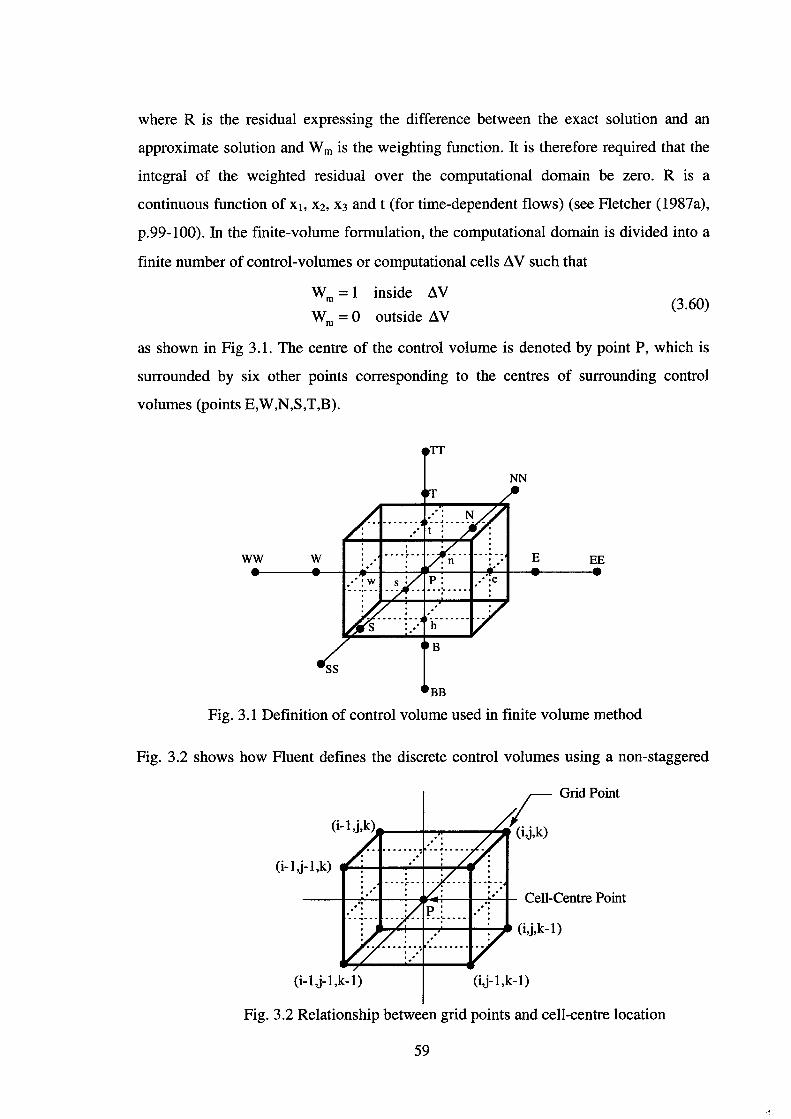
where R is the residual expressing the difference between the exact solution and an
approximate solution and W m is the weighting function. It is therefore required that the
integral of the weighted residual over the computational domain be zero. R is a
continuous function of x1, x2, x3 and t (for time-dependent flows) (see Fletcher (1987a),
p.99-100). In the finite-volume formulation, the computational domain is divided into a
finite number of control-volumes or computational cells ~ V such that
W = 1 inside ~V m
W = 0 outside ~V m
(3.60)
as shown in Fig 3.1. The centre of the control volume is denoted by point P, which is
surrounded by six other points corresponding to the centres of surrounding control
volumes (points E,W,N,S,T,B).
ww w
ss BB
Fig. 3.1 Definition of control volume used in finite volume method
Fig. 3.2 shows how Fluent defines the discrete control volumes using a non-staggered
Cell-Centre Point
(i-1,j-1,k-1) (i,j-1 ,k-1)
Fig. 3.2 Relationship between grid points and cell-centre location
59
grid storage scheme. It is clear that the node points of the computational grid do not
correspond to the control-volume centres, but are used to determine the control-volume
centres and define the cell boundaries. The same control-volume is employed for
integration of all of the conservation equations. All variables are stored at the centre of
the control-volume and therefore Fluent employs a co-located finite-volume
formulation.
The weighted residual inside the control-volume becomes
JffvRdx 1dx 2 dx 3 =0 (3.61)
where R is now the governing equation being discretised, since the governing equations
describe conservation relationships which must reduce R to zero if the correct solution
is obtained. Gauss's theorem (see for example Dubbel (1990))
JJfvv. F(f)dV =JL (F. n)ds (3.62)
can be used to convert the volume integral of a governing equation into a corresponding
surface integral over the six faces of the control-volume as follows
JII V · FdV =JFedA- JFwdA + JF0 dA- JF5dA + JF1dA- JFbdA (3.63) V A 0 Aw A 0 As A1 Ab
Eqn 3.63 may be alternatively expressed as
Ie - Iw +I" -Is + I 1 - Ib = S
where
represents the flux of F across the ith control volume face and
S = Sp .1x 1.1x 2 .1x 3
(3.64)
(3.65)
(3.66)
is the linearised source term obtained by integration of the volumetric source (sp) over
the control volume (Naser (1990)).
The fluxes across each control volume face (Eqn 3.65) are composed of a convective
component and a diffusive component. For the continuity equation, the cell face fluxes
are purely convective (mass fluxes). For the momentum equations, the convective fluxes
are momentum fluxes and the diffusion fluxes are due to viscous stresses. For the
continuity equation, the mass fluxes across the control-volume face are given by
60
II = J (pU)dA = (pUA)I A,
(3.67)
for the control-volume shown in Fig. 3.1. Similarly, the convective fluxes across the
control-volume faces, for a transported quantity<!>, may be written as
II = J (pU<!>)dA = (pU<!>A)I A,
(3.68)
The diffusion fluxes contain both normal-derivative and cross-derivative contributions
as discussed by Naser (1990).
It is clear from the above discussion that the values of the transported variable at the
control-volume faces are sought. Since the finite-volume methodology used by Fluent
solves the value of the transport variables at the control-volume cell-centres, it is
therefore necessary to perform a suitable interpolation in order to express the value of
the transport variables at the control volume faces in terms of the cell-centre values.
This is the underlying motivation behind the development of convective differencing
schemes which are the focus of the next section.
Patankar ( 1980) wrote the finite-volume discretised governing equations in the
following generic form
ap<l>p =I anb<l>nb + b nb
(3.69)
where the value of the dependent variable at point P (<!>P) is a weighted average of the
neighbouring cell-centre values of q,. In Eqn 3.69 the subscript nb denotes neighbouring
points. The coefficients in the discretised equations (a) multiply the cell-centre point
values. The constant, b, is the volume integral of the source term. It is interesting to note
that the coefficients in the discretised equations are nonlinear due to the nonlinearity of
the governing transport equations being solved. As a consequence of this and the large
number of equations to be solved, iterative solution techniques are used to solve the
discretised equations.
3.5 Convective Differencing
As mentioned in the previous section, the finite-volume methodology results in
expressions for the discretised governing equations in terms of cell face values, which
61
must be related to cell-centred values via appropriate local solution interpolation.
Patankar ( 1980) noted two guiding principles that must be adhered to in a finite-volume
discretisation formulation. These are the principles of physically realistic solution
behaviour (or boundedness) and of integral conservation (conservativeness).
Roundedness implies that in the absence of sources, the values of the transported
quantity <1> in the interior of the computational domain, should be restricted to lie within
the limits specified by the boundary conditions as noted by Naser (1990).
Conservativeness implies that overall conservation of transported quantities applies over
any number of control-volumes taken together. This implies an overall integral balance
between fluxes and internal sources. With an inappropriate choice of convective
differencing scheme for a given size of grid, the above guidelines may be violated
resulting in poor or physically unrealistic solutions.
The Peclet number, defined by
Pe= pUL r
(3.70)
where L is a characteristic length and r the diffusion coefficient, describes the relative
strengths between convection and diffusion in a flow (see Patankar (1980)). In the
context of CFD, a cell Peclet number is defined as
Pe= pU(~) r
(3.71)
where the characteristic length is now replaced by the distance between adjacent grid
points (~). For large cell Peclet number where pU(~)>>r the flow is dominated by
convective transport, whereas for very small cell Peclet number r>>pU(Ax) the
transport is largely diffusive. The extreme cases are IPel=oo and Pe=O corresponding to
pure convection and pure diffusion, respectively.
The behaviour of the solution between two cell-centre locations, with Peclet number,
can be understood by examining the solution of a steady one-dimensional convection
diffusion equation in the absence of sources,
j__CpU<!>) = ~cr d<l>) dx dx dx
(3.72)
over an interval L with boundary conditions
62
x=O <1>=<1> 0
x=L <j>=<j>L
as discussed by Patankar (1980). The exact solution to the Eqn 3.72 is
<I>- <l>o exp((Pe)x I L) -1 '----~=-::....C....'--'----'---
<1> L - <1> 0 exp(Pe)
(3.73)
(3.74)
Patankar showed that for the case of pure diffusion a piecewise linear (centred
difference) approximation provides an exact solution of the variation of <1> between 0 and
L. For convection dominated flows, where Pe>>l, the flow is dominated by the
upstream behaviour, so that the value of <1> at the control-volume face could simply be
set as the value of <1> at the upstream node. This forms the basis of the upwinding scheme
(see Patankar (1980) and the references cited therein). Therefore for small Pe (1Pe1~2) a
centred-difference approximation provides an adequate interpolation of face values,
whereas for large Pe>>l an upwind difference scheme provides a good approximation.
For a given application, the cell Peclet number can be reduced by grid refinement, but
this increases the computational requirements.
3.5.1 Power-Law Scheme
In order to provide a convective differencing scheme that is applicable over a wide
range of Peclet numbers, a suitable scheme could use the exact solution of the steady
one-dimensional convection-diffusion equation, or an approximation thereof. Finite
volume discretisation of the steady one-dimensional convection-diffusion equation
yields
aP<I>P = aE<I>E + aw<l>w
where a E = De - Fe I 2
aw = Dw +Fw 12
aP = De +Fe I 2 + Dw - Fw I 2
F = pu , D = r I (Ax)
(3.75)
according to Patankar (1980). Substitution of the exact solution to the one-dimensional
convection diffusion equation into Eqn 3.75 gives
63
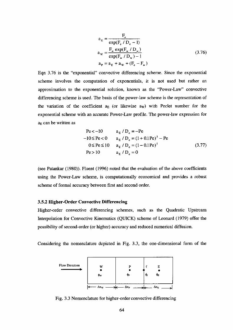
Fe aE = ___ .:::._ __ exp(Fe I De - 1)
Fw exp(Fw I Dw) aw =
exp(F w I D w ) - 1 (3.76)
ap = aE + aw +(Fe - Fw)
Eqn 3.76 is the "exponential" convective differencing scheme. Since the exponential
scheme involves the computation of exponentials, it is not used but rather an
approximation to the exponential solution, known as the "Power-Law" convective
differencing scheme is used. The basis of the power-law scheme is the representation of
the variation of the coefficient aE (or likewise aw) with Peclet number for the
exponential scheme with an accurate Power-Law profile. The power-law expression for
aE can be written as
Pe<-10 aE /De =-Pe
-10 ~ Pe < 0 a E I De = (1 + 0.1 Pe) 5 - Pe
0~ Pe ~ 10 aE I De= (1- 0.1Pe) 5 (3.77)
Pe> 10
(see Patankar (1980)). Fluent (1996) noted that the evaluation of the above coefficients
using the Power-Law scheme, is computationally economical and provides a robust
scheme of formal accuracy between first and second order.
3.5.2 Higher-Order Convective Differencing
Higher-order convective differencing schemes, such as the Quadratic Upstream
Interpolation for Convective Kinematics (QUICK) scheme of Leonard (1979) offer the
possibility of second-order (or higher) accuracy and reduced numerical diffusion.
Considering the nomenclature depicted in Fig. 3.3, the one-dimensional form of the
Flow Direction w p f E • • I •
«<>w cjlp $r <Ill;
Fig. 3.3 Nomenclature for higher-order convective differencing
64
higher-order convective differencing schemes used by Fluent can be written in the
following generic form
<l>r =8(.1,xE<I>P +.1.xP<I>E]/(.1,xp +.1.XE]
+ (1- 8)[(.1.xw + 2.1.xp) <I>P - .1.xp<l>w] I [.1.xw + .1.xP] (3.78)
where <l>r is the value of <1> sought at the desired cell face f and <l>c, <l>w, <!>E represent the
centre cell-centre, upstream cell-centre and downstream cell-centre values of <!>,
respectively.
Variation of the parameter 8 leads to different discretisation schemes. For example the
Second-Order Upwind scheme corresponds to 8=0, whereas the QUICK scheme
corresponds to 8=0.75. Bounding of the higher-order schemes used by Fluent is
necessary to avoid numerical instabilities. Fluent ( 1996) noted that the use of the
Second-Order Upwind or QUICK scheme will produce undershoots or overshoots at
discontinuities. On a uniform grid the QUICK scheme becomes
(3.79)
3.5.3 Numerical Diffusion
Additional numerical diffusion (for a given mesh size) will occur when the flow is
oblique to the gridlines and there is a non-zero gradient of the dependent variable in a
direction normal to the flow. Numerical diffusion enhances the actual diffusion in the
flow and will lead to a "smearing" of the solution. Numerical diffusion is most
pronounced when the flow is aligned at 45° to the gridlines and for convection
dominated (high Pe) flows. It is reduced to zero when the flow is aligned at 0° or 90° to
the gridlines. Higher-order convective differencing schemes such as QUICK are less
susceptible to numerical diffusion than the Power-Law scheme, as more points are used
in the interpolation and hence more flow information is available in the interpolation.
3.6 Solution of the Discretised Equations
Once the governing equations have been discretised as algebraic equations, they can be
solved numerically using a computer. Due to the elliptic and nonlinear nature of the
governing equations in steady-state form, the discretised equations can be assembled
65
into the following matrix form (Fletcher (1987a))
A(V)V=B (3.80)
In this case V is the vector of unknown cell-centre values and A is a matrix of
discretised equation coefficient values which is itself a function of V. B is composed
of algebraic coefficients associated with discretisation of the governing equations,
source terms and boundary condition information.
In order to solve the system of equations denoted by Eqn 3.80, iterative techniques must
be used, due to the dependency of A on the solution vector V . It is therefore possible to
set up an outer iteration where the coefficients in A are "frozen" while the system is
solved for V. Once V is obtained the components of A are updated and the procedure
repeated until convergence. Solution of the system A V = B can only be realistically
achieved using iterative solution techniques, due to the enormous computational
requirements that would otherwise be necessary (in terms of computer memory and
speed) if a direct Gaussian elimination were to be attempted.
3.6.1 Solution Methodology
In Fluent, the discretised governing equations are solved sequentially, with the
momentum and continuity equations being solved prior to solution of the transport
equations for turbulent kinetic energy (k) and turbulent dissipation(£).
In order to solve the momentum equations and the continuity equation, it is necessary to
solve for all the velocity components and the pressure. Since the incompressible form of
the continuity equation does not contain any explicit pressure-related terms, it is
necessary to construct an equation for updating the pressure. Fluent uses the Semi
Implicit Method for Pressure-Linked Equations (SIMPLE) scheme of Patankar and
Spalding ( 1972) to accomplish this. The SIMPLE scheme used in Fluent has been
formulated for use in a co-located finite-volume formulation (rather than on a staggered
grid configuration as presented in the above references). The SIMPLE formulation used
by Fluent overcomes the pressure-velocity decoupling problem (see Patankar (1980))
that was prevalent in early attempts at producing co-located finite-volume formulations
of this scheme.
66
For illustrative purposes, the SIMPLE scheme has been described below for the three
dimensional continuity and momentum equations discretised on a rectangular Cartesian
grid. The discussion is taken largely from Patankar ( 1980) and Fluent ( 1996). If a
"guessed" pressure field (p*) is substituted into the momentum equations an
approximated velocity field (U*, v· ,W*) can be determined. The U momentum equation,
for example, becomes
apu; = L:anbu:b -(p:Ae -p:Aw)+S (3.81) nb
The approximated velocity field does not in general satisfy continuity except when a
converged solution to the discretised equations is obtained. The actual velocity and
pressure fields can be related to the approximated velocity and pressure fields by
up= u; + u;·
vp = v; + v;·
Wp =W; +W;*
p = p* + p**
where u**, v**, w** are the velocity corrections and p** is the pressure correction.
(3.82)
(3.83)
Since the actual velocity and the pressure satisfy the momentum equations, an equation
linking the velocity correction with the pressure correction can be obtained by
substituting Eqn 3.82 and Eqn 3.83 into the momentum equations and subtracting the
equations for the velocity approximations (for example Eqn. 3.81) from the momentum
equations. This results in a momentum balance for the corrections. For example, the
equation for the u** velocity correction is therefore
U** ~ U** ( **A **A ) ap P = .£..Janb nb- Pe e -pw w (3.84) nb
If the term L anb u:~ is omitted from Eqn 3.84, the velocity correction can be directly nb
linked to the pressure correction resulting in the following equation for the velocity
correction
U** =--1 ( **A - **A ) p Pe e Pw w
aP (3.85)
How can such an omission be made? At convergence the omitted term will be zero as
67

the velocity corrections of the neighbouring points will be zero. Therefore this omission
can be made. A pressure correction equation can now be formed from the continuity
equation by substitution of Eqn 3.82, Eqn 3.83 and Eqn 3.85 into the continuity equation
resulting in the following generic form of the pressure correction equation
app;• = :L/nbP:~ + b (3.86) nb
Patankar ( 1980) noted that the coefficient b in this case acts as a "mass source" term
which the pressure corrections must reduce to zero at convergence.
The overall solution methodology used by Fluent for the solution of isothermal and
incompressible turbulent flow can be summarised as follows:
1) Estimate (guess) the pressure field.
2) Solve the discretised momentum equations (Eqn 3.81) in order to obtain the velocity
approximations in the sequence u·' v· 'w·
3) Solve the pressure correction equation (Eqn 3.86) in order to obtain the pressure
. ** correctiOn p .
4) Calculate the pressure using Eqn 3.83
5) Calculate the velocity corrections u**, v**, w** from Eqn 3.85 and subsequently the
velocities from Eqn 3.82.
6) Solve the transport equation for turbulent kinetic energy (k).
7) Solve the transport equation for turbulent dissipation (E).
8) Regard the corrected pressure as the new pressure estimate p, return to step 2 and
repeat the above steps until a converged solution is obtained. It must be noted that the
updated velocity field is treated as the new approximated velocity field when solving
Eqn 3.81.
In practice, the pressure correction and momentum equations are underrelaxed in order
to successfully converge the calculations. In the case of the pressure calculation, the use
of underrelaxation leads to
• ** P = P +app (3.87)
where ap is the underrelaxation factor for pressure correction. In the case of the
momentum equations for the velocity approximations (Eqn 3.81), underrelaxation is
68
applied to the results of the iterative solver so that
(3.88)
The result (U*) n+l of an iteration is therefore a linear combination of the current
solution (U~as) n+l obtained by the Line Gauss-Seidel (LGS) solver and the result of the
previous solution (U*)n at iteration n, where A is the underrelaxation factor.
3.6.2 Determination of Convergence
The calculation of equation residuals allows the convergence behaviour of the
computational simulation to be determined. Equation residuals provide a measure of
how closely each finite-difference equation is balanced given the current state of the
solution. The generic form of the finite-volume discretised governing equations was
stated previously as
ap<l>p = L anb<l>nb +b. nb
(3.89)
Fluent computes the global residual of the particular discretised transport equations by
summing the residual of the discretised equation for each control-volume over the
computational domain. This results in the following expression for the global residual
N
R = L L anb<l>nb + b- ap<l>p (3.90) •=I nb
where N is the total number of cell-centres in the computational domain. According to
Fluent (1996), the global residuals expressed by Eqn 3.90 are dimensional having units
of kg units of <1> per second and can be normalised to make them non-dimensional. The
non-dimensionalised form of the global residual is therefore
N
L L anb<l>nb + b- ap<l>p R = •=I nb (3.91)
The global residual for the pressure is actually the imbalance in the pressure correction
equation (and hence an imbalance in mass conservation) and is calculated by
N
R= LIFw -Fe +Fs -Fn +Fb -F11 (3.92) •=I
(see Fluent (1996)), where F1 in this case is the mass flux through face i. The pressure
69
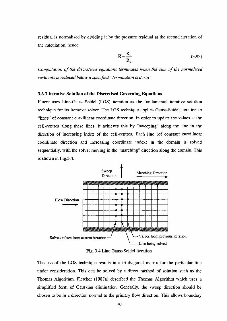
residual is normalised by dividing it by the pressure residual at the second iteration of
the calculation, hence
- R R=-"
R2 (3.93)
Computation of the discretised equations terminates when the sum of the normalised
residuals is reduced below a specified "termination criteria".
3.6.3 Iterative Solution of the Discretised Governing Equations
Fluent uses Line-Gauss-Seidel (LOS) iteration as the fundamental iterative solution
technique for its iterative solver. The LOS technique applies Gauss-Seidel iteration to
"lines" of constant curvilinear coordinate direction, in order to update the values at the
cell-centres along these lines. It achieves this by "sweeping" along the line in the
direction of increasing index of the cell-centres. Each line (of constant curvilinear
coordinate direction and increasing coordinate index) in the domain is solved
sequentially, with the solver moving in the "marching" direction along the domain. This
is shown in Fig.3.4.
Sweep t Direction
Flow Direction
Solved values from current iteration
Marching Direction
Values from previous iteration
Line being solved
Fig. 3.4 Line Gauss Seidel iteration
The use of the LOS technique results in a tri-diagonal matrix for the particular line
under consideration. This can be solved by a direct method of solution such as the
Thomas Algorithm. Fletcher (1987a) described the Thomas Algorithm which uses a
simplified form of Gaussian elimination. Generally, the sweep direction should be
chosen to be in a direction normal to the primary flow direction. This allows boundary
70
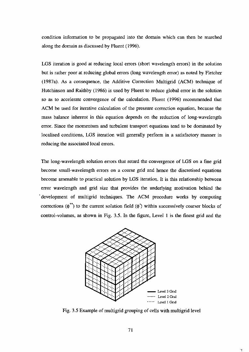
condition information to be propagated into the domain which can then be marched
along the domain as discussed by Fluent (1996).
LGS iteration is good at reducing local errors (short wavelength errors) in the solution
but is rather poor at reducing global errors (long wavelength error) as noted by Fletcher
(1987a). As a consequence, the Additive Correction Multigrid (ACM) technique of
Hutchinson and Raith by ( 1986) is used by Fluent to reduce global error in the solution
so as to accelerate convergence of the calculation. Fluent ( 1996) recommended that
ACM be used for iterative calculation of the pressure correction equation, because the
mass balance inherent in this equation depends on the reduction of long-wavelength
error. Since the momentum and turbulent transport equations tend to be dominated by
localised conditions, LGS iteration will generally perform in a satisfactory manner in
reducing the associated local errors.
The long-wavelength solution errors that retard the convergence of LGS on a fine grid
become small-wavelength errors on a coarse grid and hence the discretised equations
become amenable to practical solution by LGS iteration. It is this relationship between
error wavelength and grid size that provides the underlying motivation behind the
·development of multigrid techniques. The ACM procedure works by computing
corrections (<j>**) to the current solution field (<j)) within successively coarser blocks of
control-volumes, as shown in Fig. 3.5. In the figure, Level 1 is the finest grid and the
- Level3Gnd
- Level2Gnd
····· Levell Gnd
Fig. 3.5 Example of multigrid grouping of cells with multigrid level
71
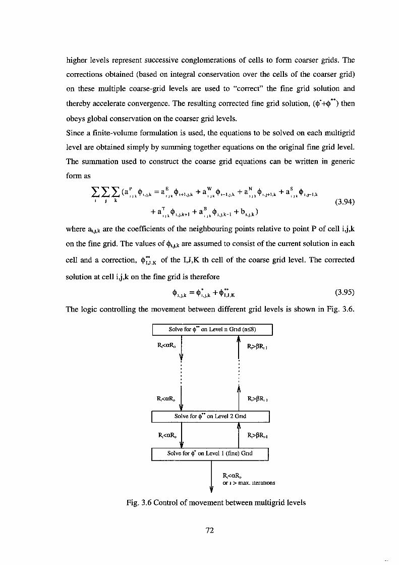
higher levels represent successive conglomerations of cells to form coarser grids. The
corrections obtained (based on integral conservation over the cells of the coarser grid)
on these multiple coarse-grid levels are used to "correct" the fine grid solution and
thereby accelerate convergence. The resulting corrected fine grid solution, (q>*+<l>**) then
obeys global conservation on the coarser grid levels.
Since a finite-volume formulation is used, the equations to be solved on each multigrid
level are obtained simply by summing together equations on the original fine grid level.
The summation used to construct the coarse grid equations can be written in generic
form as
~~~(aP <1> =aE <1> +aw <1> +aN <1> +a5 <1> .£..J .£..J .£..J 0 J k l,j,k o J k t+),j,k 1 J k t-),j,k 0 J k l,j+),k o J k l,j-),k
I J k (3.94)
where a1,J,k are the coefficients of the neighbouring points relative to point P of cell i,j,k
on the fine grid. The values of <I>1,J,k are assumed to consist of the current solution in each
cell and a correction, <I>;~,K of the I,J,K th cell of the coarse grid level. The corrected
solution at cell i,j,k on the fine grid is therefore
(3.95)
The logic controlling the movement between different grid levels is shown in Fig. 3.6.
Solve for cp** on Level n Gnd (n~8)
R,>l3R,1
I Solve for cp** on Level 2 Gnd J R,«XR,
I Solve for cp* on Level I (fine) Gnd I R,<OCR0
or 1 >max. IteratiOns
Fig. 3.6 Control of movement between multigrid levels
72
When the rate of reduction of the residuals is insufficient on the current grid level, the
algorithm moves to the next coarser grid level. In order to move to the next coarser grid
level
R R, p<--
R,_I (3.96)
where~ is the residual reduction rate parameter, R1 the absolute sum of residuals on the
current grid level after the ith iteration of the line solver and R1.1 is the residual from the
previous iteration.
A move is made from a coarser grid level to a finer grid level when either the equations
are sufficiently converged, or a maximum number of iterations of the solver at that level
has been executed. The convergence or termination criteria
(3.97)
states that the residual after the ith iteration of the solver on the current level (R1) has
fallen to some fraction (a) of the residual (R0 ) at the beginning of iteration at the current
level.
3.7 Closure
The use of computational techniques based on the solution of the full Reynolds
averaged Navier Stokes equations provides the only practical means by which
computational simulation of waterjet inlets can be undertaken. This is primarily due to
the necessity to account for viscosity and turbulence in the flow. The decision was made
to use the commercially-available CFD software, Fluent, for the purposes of flow
analysis. The use of existing proven CFD software allows attention to be focused on
grid generation and waterjet inlet design and optimisation-related investigations, rather
than on programming a CFD solver.
An overview of the derivation of the Reynolds-averaged Navier Stokes equations by
Reynolds-averaging of the Navier Stokes equations was presented in this chapter.
Adequate closure of the RANS equations can be effected by relating the Reynolds
stresses inherent in these time-averaged equations, to mean velocity gradients via an
eddy-viscosity formulation according to the hypothesis of Boussinesq (1877). The
73
Standard k-E turbulence model of Launder and Spalding (1974) and the RNG k-E model
of Y akhot and Orszag ( 1986) which was extended by Y akhot et al ( 1992) to account for
the effect of irrotational strain on the turbulence, were described. Both models are used
in the context of work presented in this thesis. The RNG k-E turbulence model contains
an "extra rate of strain" term in the E equation which improves flow prediction for flows
subject to rapid strain and streamline curvature and so represents an improvement over
the Standard k -E model.
The use of wall functions for modelling the near-wall region is a robust and
computationally efficient approach to the modelling of the flow behaviour adjacent to
the wall. The Standard wall function, which assumes an equilibrium boundary layer was
presented together with the Two-Layer-Based Nonequilibrium wall function. This latter
wall function is sensitised to the effect of pressure gradient on boundary layer behaviour
and is meant to represent an improvement over the Standard wall function for flows
experiencing large pressure gradients.
An overview of the co-located finite-volume method, used by Fluent, for discretisation
of the governing equations was presented. The finite-volume method enforces integral
conservation of the transported quantities on a finite control-volume and results in a
balance between fluxes across the faces of the control-volume (cell) and source terms.
Convective differencing schemes such as the Power-Law scheme, outlined in Patankar
(1980), are used to relate the values of the transported quantities at the cell faces (which
appear in the discretised equations) to the values at the cell-centres. Higher-order
convective-differencing schemes such as the QUICK scheme of Leonard ( 1979) offer
greater calculation accuracy and reduced numerical diffusion, but require the use of
limiters in order to retain numerical stability during the course of calculation.
Due to the nonlinearity of the discretised equations and computational requirements
necessary to solve them, the discretised equations are solved by iterative means. Since
the flows analysed in this work are incompressible, the SIMPLE scheme of Patankar and
Spalding (1972) was used to provide a suitable coupling between velocity and pressure
in the solution process. A Line Gauss Seidel iterative solver is used by Fluent to solve
74
the discretised equations and is good at reducing short-wavelength error in the solution,
but is poor at reducing global error. Multigrid acceleration, such as the Additive
Correction Multi grid scheme of Hutchinson and Raithby ( 1986), can be used to reduce
this global error, particularly for the pressure correction equation. The termination
criterion used by the iterative solver for termination of the calculation, is that the sum of
the normalised residuals fall below a specified value. At this point the calculations may
be considered to be converged.
75
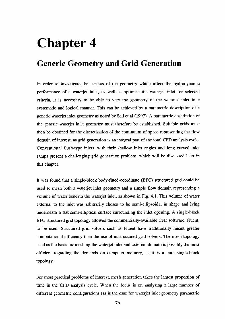
Chapter 4 Generic Geometry and Grid Generation
In order to investigate the aspects of the geometry which affect the hydrodynamic
performance of a waterjet inlet, as well as optimise the waterjet inlet for selected
criteria, it is necessary to be able to vary the geometry of the waterjet inlet in a
systematic and logical manner. This can be achieved by a parametric description of a
generic waterjet inlet geometry as noted by Seil et al (1997). A parametric description of
the generic waterjet inlet geometry must therefore be established. Suitable grids must
then be obtained for the discretisation of the continuum of space representing the flow
domain of interest, as grid generation is an integral part of the total CFD analysis cycle.
Conventional flush-type inlets, with their shallow inlet angles and long curved inlet
ramps present a challenging grid generation problem, which will be discussed later in
this chapter.
It was found that a single-block body-fitted-coordinate (BFC) structured grid could be
used to mesh both a waterjet inlet geometry and a simple flow domain representing a
volume of water beneath the waterjet inlet, as shown in Fig. 4.1. This volume of water
external to the inlet was arbitrarily chosen to be semi-ellipsoidal in shape and lying
underneath a flat semi-elliptical surface surrounding the inlet opening. A single-block
BFC structured grid topology allowed the commercially-available CFD software, Fluent,
to be used. Structured grid solvers such as Fluent have traditionally meant greater
computational efficiency than the use of unstructured grid solvers. The mesh topology
used as the basis for meshing the waterjet inlet and external domain is possibly the most
efficient regarding the demands on computer memory, as it is a pure single-block
topology.
For most practical problems of interest, mesh generation takes the largest proportion of
time in the CFD analysis cycle. When the focus is on analysing a large number of
different geometric configurations (as is the case for waterjet inlet geometry parametric
76
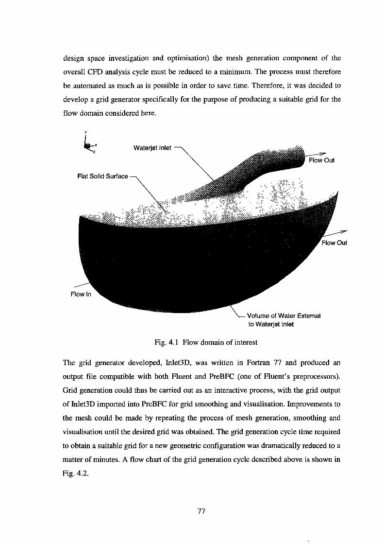
design space investigation and optimisation) the mesh generation component of the
overall CFD analysis cycle must be reduced to a minimum. The process must therefore
be automated as much as is possible in order to save time. Therefore, it was decided to
develop a grid generator specifically for the purpose of producing a suitable grid for the
flow domain considered here.
y
~X z
Flat Solid Surface
Waterjet Inlet
Volume of Water External to Waterjet Inlet
Fig. 4.1 Flow domain of interest
The grid generator developed, Inlet3D, was written in Fortran 77 and produced an
output file compatible with both Fluent and PreBFC (one of Fluent's preprocessors).
Grid generation could thus be carried out as an interactive process, with the grid output
of Inlet3D imported into PreBFC for grid smoothing and visualisation. Improvements to
the mesh could be made by repeating the process of mesh generation, smoothing and
visualisation until the desired grid was obtained. The grid generation cycle time required
to obtain a suitable grid for a new geometric configuration was dramatically reduced to a
matter of minutes. A flow chart of the grid generation cycle described above is shown in
Fig. 4.2.
77
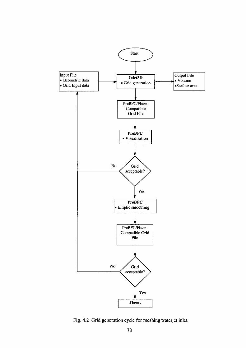
Input File • Geometric data • Grid Input data
No
Inlet3D • Grid generation
PreBFC/Fluent Compatible
Grid File
PreBFC • Visualisation
Yes
PreBFC • Elliptic smoothing
No
PreBFC/Fluent Compatible Grid
File
Yes
Fluent
Output File
1---~· Volume •Surface area
Fig. 4.2 Grid generation cycle for meshing waterjet inlet
78
A clear disadvantage of using the above methodology is that the quality of the resulting
meshes are heavily dependent on the user's experience and understanding. In addition,
extensive grid investigations must be initially undertaken in order to determine the
appropriate number of grid lines in each coordinate direction and their distribution.
Solution-adaptive meshing techniques, described by Thompson et al ( 1985), overcome
these limitations and allow a more optimum grid to be developed during the course of
solution. Solution adaptive meshing is not however, available in Fluent and so the above
limitations apply to the grids generated.
In view of the above discussion, this chapter is devoted to discussing the parametric
description of the author's generic flush-type waterjet inlet geometry. This generic
geometry forms the basis of the design and optimisation-related investigations that are
the focus of the work presented in this thesis. The various grid generation techniques
used to mesh the different geometries presented in later chapters are also discussed.
In Section 4.1 the parametric definition of the author's generic flush-type waterjet inlet
geometry is presented. The grid topology used as the basis of the meshing of the
waterjet inlet and a simplified flow domain external to it is discussed in Section 4.2. The
grid topology establishes the link between physical space (x,y,z) and computational
space (~,T).~) for the flow domain being meshed. The choice of topology used in
computational space will inevitably affect the resultant grid in physical space.
&
In order to generate the computational mesh, it is first necessary to generate the
boundary (surface) mesh that encloses the volume of the flow domain of interest. This is
the subject of Section 4.3. Once the domain boundaries have been meshed, the interior
grid can then be generated. This is discussed in Section 4.4. The relative merits and
limitations of the grid obtained, as a direct consequence of the grid topology used, are
discussed in Section 4.5 within the context of the role played by the grid in obtaining
accurate CFD solutions.
In Section 4.6 a brief discussion of the meshing procedure and mesh topology used for
the meshing of the individual geometries for the first two experimental validation cases
79
of Chapter 5 are presented. The discussion presented is brief because the meshing of
these two geometries is a relatively straightforward process. A summary of the contents
of this chapter will be given in Section 4. 7.
4.1 Generic Flush-type Waterjet Inlet Geometry
The geometric simplifications made in order to mesh the generic waterjet inlet
geometry, using a single-block structured mesh are discussed in Section 4.1.1. The
parameterisation of the geometry is discussed in Section 4.1.2. The simplicity and
effectiveness of using Bezier curves as a means of defining aspects of the waterjet inlet
geometry will be discussed in Section 4.1.3.
4.1.1 Geometric Simplifications
There are practical limits to the amount of geometric modelling required to adequately
describe the waterjet inlet for the purposes of CFD computation. Furthermore, geometric
modelling limitations result directly from the grid topology used to mesh the waterjet
inlet. In addition to modelling the shape of the waterjet inlet itself, it would be desirable
to model such aspects of the geometry as:
1) The impeller shaft or impeller shaft housing/fairing
2) The inlet grille (if fitted)
3) The tubing on which the inspection cover is fitted.
For the purposes of good flow design, the impeller shaft should always be housed in
some type of fairing. The impeller shaft (or housing/fairing) passing through the
waterjet inlet duct, will clearly influence the flow inside the waterjet inlet and therefore
should be represented either geometrically, or its effect on flow behaviour modelled.
The grid topology used for the work presented in this thesis makes geometric
representation of the impeller shaft or impeller shaft housing/fairing impractical and so
the effect of this geometric feature on the flow must be modelled. For the purposes of
investigating and optimising the geometric shape of the waterjet inlet, this issue will not
be given further consideration.
The representation of the inlet grille would require a large number of gridlines in order
80
to represent the individual grille bars. The smaller the pitch of the grille bars, the greater
the number of gridlines required for representation of the grille. It must be noted that not
all waterjets have grilles fitted, as there is a tendency for grilles to 'clog up' with debris.
This feature will not be represented in the computational mesh for two main reasons.
Firstly, the mesh topology makes representation of an inlet grille bar impossible and
secondly, the emphasis of this work is on the geometric shape of the waterjet inlet,
rather than on any effects that can be attributed to an inlet grille. No significant
influence on the flow is expected from the tubing associated with the inspection cover.
Therefore, this geometric feature is omitted from further consideration.
4.1.2 Parameterisation of the Generic Geometry
After careful examination of the shape of several flush-type waterjet inlets used on high
speed catamaran vessels, as described in Trillo (1994), Seil et al (1997) found that the
generic shape of the waterjet inlet could be approximated by eight parameters for a
given inlet throat diameter (D). This assumes, of course, that the following aspects of
the geometry are fixed:
1) Cross-sectional shape of the inlet throat
2) Generic profile of the inlet lip
3) Profile of the inlet ramp
4) Profile of the inlet opening
5) Maximum width of the inlet opening
6) A set variation of the cross-sectional area of the waterjet inlet from the inlet throat to
the duct exit
7) An effective deadrise of the inlet opening
Seil et al ( 1997) used the following eight geometric parameters to describe a generic
waterjet inlet geometry, subject to the above-mentioned geometric assumptions:
1) a - The angle of inclination of the inlet to the horizontal plane
2) RL - Radius of the inlet lip
3) H - Height of the pump centreline above the inlet opening
4) R0 - Radius of curvature of the centreline of the duct bend
5) LH - Length of the horizontal duct section downstream of the bend
81
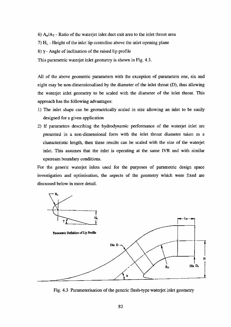
6) AJ AT - Ratio of the waterjet inlet duct exit area to the inlet throat area
7) HL - Height of the inlet lip centreline above the inlet opening plane
8) y- Angle of inclination of the raised lip profile
This parametric waterjet inlet geometry is shown in Fig. 4.3.
All of the above geometric parameters with the exception of parameters one, six and
eight may be non-dimensionalised by the diameter of the inlet throat (D), thus allowing
the waterjet inlet geometry to be scaled with the diameter of the inlet throat. This
approach has the following advantages:
1) The inlet shape can be geometrically scaled in size allowing an inlet to be easily
designed for a given application
2) If parameters describing the hydrodynamic performance of the waterjet inlet are
presented in a non-dimensional form with the inlet throat diameter taken as a
characteristic length, then these results can be scaled with the size of the waterjet
inlet. This assumes that the inlet is operating at the same IVR and with similar
upstream boundary conditions.
For the generic waterjet inlets used for the purposes of parametric design space
investigation and optimisation, the aspects of the geometry which were fixed are
discussed below in more detail.
Parametric Definition of Lip Profile
_____.L.-------l t H
~~ I Fig. 4.3 Parameterisation of the generic flush-type waterjet inlet geometry
82
The variation of the cross-sectional area of the waterjet inlet with distance along the
duct centreline, from the inlet throat to the duct exit, can be described by a third-order
polynomial of the form
(4.1)
where A is cross-sectional area, AT the cross-sectional area at the inlet throat, Ao the
cross-sectional area at the duct exit and u the non-dimension length along the centreline
from the inlet throat to the duct exit, defined on the unit interval by
u=S/STot O~u~1 (4.2)
In Eqn 4.2, S represents the arc length along the duct centreline measured from the inlet
throat and STot is the total centreline arc length between the inlet throat and the duct exit.
The coefficients of the cubic polynomial (a1) must be chosen so that the following
constraints on the variation of A with u are satisfied
At u=O, A=AT A>O for O~u~1 (4.3)
For area ratios greater than unity, a linear variation of cross-sectional area along the inlet
duct centreline between the circular inlet throat and duct exit has been assumed. In this
case Eqn 4.1 is reduced to
(4.4)
The choice of polynomial is worthy of further study in order to find an optimum
streamwise cross-sectional area distribution. The linear variation selected for this work
is unlikely to be the optimum profile.
The raised lip profile of the parametric geometry shown in Fig. 4.3, was chosen as this
type of profile is commonly used in waterjet inlets currently installed in many of today' s
large high-speed catamarans as is evident from a reading of Trillo ( 1994 ). This profile is
economical to fabricate from aluminium by virtue of its simplicity. Aluminium is the
metal which is widely used for the construction of the large high-speed catamarans
produced by Australia, due to its relatively light weight in comparison with steel. The
profile of the inlet ramp is taken as a circular arc, again following the generic design of
inlets used on large high-speed catamarans. There is, however, no reason why other
ramp profiles cannot be used. Ffl)rde et al ( 1991) for example, used Bezier curves to
describe the ramp profile of their waterjet inlets.
83
The profile of the inlet opening was obtained by using two Bezier curves, one for the
forward part of the inlet opening, near the inlet ramp and one for the aft section of the
inlet opening, near the inlet lip. The forward section of the inlet opening was taken to be
rectangular in shape, as flat ramp surfaces are used on conventional inlets due to ease of
fabrication. The aft section of the inlet opening was taken to be semi-elliptical in shape,
again following the generic design of current large inlets. This choice was arbitrary and
alternative profiles could have been used instead. The maximum width of the inlet
opening was taken to be 70/6. For the generic geometry described, no effective deadrise
angle was included. Thus the inlet opening lies flat on the horizontal plane. It is
recognised here that many vessels will have an effective deadrise angle on their hull so
that the plane of the inlet opening will be inclined at an angle to the horizontal in such
cases.
4.1.3 Representation of Geometric Features
The use of Bezier curves to represent geometric features of the inlet allows excellent
geometric flexibility and simplicity of formulation. Other possibilities are the use of
cubic curves, Spline curves or B-Spline curves. F~~Srde et al (1991) made extensive use of
Bezier curves and surfaces in defining their waterjet inlet geometry. Bezier curves are
formulated as
n
r(u) = L ~BI,n(u) U E [0,1] (4.5) 1=0
according to Mortenson (1985). In Eqn 4.5, ~ represent the n+1 vertices of a
characteristic polygon and are called "control points" as they directly control the shape
of the Bezier curve. The Bernstein polynomials (B1,n) provide blending (interpolation)
and are defined by
B =nC U 1 (1-u)n-l 1,n 1
(4.6)
where ncl is the binomial coefficient
nc = n! 1 i!(n-i)!
(4.7)
Two Bezier curves are used to define the profile of the inlet opening. By specifying
multiple coincident points at the vertex of the characteristic polygon for the Bezier
curve, the curve is pulled toward that vertex. This effect increases with an increasing
84
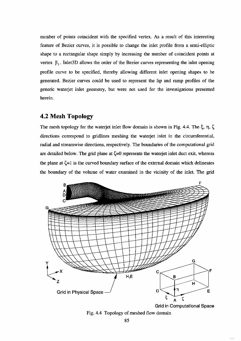
number of points coincident with the specified vertex. As a result of this interesting
feature of Bezier curves, it is possible to change the inlet profile from a semi-elliptic
shape to a rectangular shape simply by increasing the number of coincident points at
vertex p2 • Inlet3D allows the order of the Bezier curves representing the inlet opening
profile curve to be specified, thereby allowing different inlet opening shapes to be
generated. Bezier curves could be used to represent the lip and ramp profiles of the
generic waterjet inlet geometry, but were not used for the investigations presented
herein.
4.2 Mesh Topology
The mesh topology for the waterjet inlet flow domain is shown in Fig. 4.4. The ~. 11, ~
directions correspond to gridlines meshing the waterjet inlet in the circumferential,
radial and streamwise directions, respectively. The boundaries of the computational grid
are detailed below. The grid plane at ~=0 represents the waterjet inlet duct exit, whereas
the plane at ~=1 is the curved boundary surface of the external domain which delineates
the boundary of the volume of water examined in the vicinity of the inlet. The grid
G
~X z
Grid in Physical Space
A s Grid in Computational Space
Fig. 4.4 Topology of meshed flow domain
85
boundary at 11=0 is a cylindrical boundary of zero radius lying on the vertical
centreplane (plane of flow symmetry) of the grid. The grid boundary at 11= 1 represents
the surface of the waterjet inlet and the flat horizontal surface of the external flow
domain. The vertical centreplane of the waterjet inlet and the external flow domain are
represented by grid planes at ~=0 and ~= 1, with the grid plane at ~=0 upstream of the
surface at ~= 1.
4.3 Boundary Mesh
The grid generation techniques used by Inlet3D for the meshing of the boundary
surfaces of the grid are discussed in this section. The boundaries of the computational
domain are meshed using two-directional transfinite interpolation. Depending on the
surface being meshed, a two-dimensional Poisson equation solver (elliptic partial
differential equation solver) is additionally used to effect smoothing of the resultant
surface mesh.
4.3.1 Transfinite Interpolation
The two-directional transfinite interpolation algorithm can be written as the sum of
projectors
F1 = P~r F2 = P
11(r-F1)
r(~, 11) = F1 + F2
(4.8)
where ~ and 11 (in this case), represent any two curvilinear coordinate directions. The
projectors P~ and P11
are idempotent linear operators (see Gordon and Hall (1973))
allowing unidirectional interpolation in each computational coordinate direction. The
order of the unidirectional interpolation is immaterial as noted by Thompson et al
(1985). The projectors used in the grid generator described in this work are of the form
(4.9)
according to Thompson et al ( 1985), where ~ and 11 again represent arbitrary coordinate
directions. The functions <P and '¥ in Eqn 4.9 are blending functions responsible for
providing blending (interpolation) of points and first derivatives in the ~ direction,
86
respectively. It is of course possible to use projectors that interpolate higher-order
derivatives, as discussed by Eriksson ( 1982), Eriksson ( 1985), Smith ( 1982) and
Fletcher ( 1987b ). This allows greater control of the resultant interior mesh. Both linear
and Hermite cubic interpolation are used to effect blending. Linear blending functions
result in the following form for <I> and '¥
<l>z = u
'¥2 = 0
whereas the Hermite cubic interpolant takes the form
<1> 1 =2u3 -3u2 +1
'¥1 = u 3 - 2u 2 + u
<1>2 = 1- <I> I
'¥z=U3-u
(4.10)
(4.11)
The blending function parameter (u) is related to the general computational coordinate
(~1) through a control function of the form
(4.12)
For the waterjet inlet boundary mesh, the following form of the control function was
used
(4.13)
when there is little stretching of gridlines in the ~~ direction. For large stretching in the ~~
direction, h takes the form of the stretching function used, in this case the stretching
function of Vinokur (1983). The control function h(~1) is used as an approximate means
of relating the computational coordinate to the arc length along the gridlines in the ~~
direction. The reader is referred to Smith ( 1982) for a more detailed discussion of the
relationship between the computational coordinate, gridline arc length and the blending
function parameter (u). The grid planes at ~=0 and ~=1 are initially generated by
transfinite interpolation.
4.3.2 Stretching Function
In the context of the grid generation procedures presented in this chapter, there is a need
for a general two-sided stretching function allowing arbitrary grid point clustering to be
specified independently at each end of the interval under consideration. The primary
reason for such a requirement is often the need to resolve different length scales in the
87
flow. This is particularly pertinent in the case of applying grid point clustering in the T\
(radial) direction inside of the waterjet inlet, where the resolution of the near-wall flow
requires the resolution of much smaller length-scales than the flow outside the boundary
layer. The two-sided stretching function of Vinokur (1983) is implemented in Inlet3D.
The interested reader is referred to Vinokur' s paper for a detailed discussion of the
mathematical formulation of this stretching function.
4.3.3 Smoothing of the Surface Mesh
The vert-ical centreplane of the waterjet inlet and external domain (comprising the ~=0,
~=1 and T\=0 boundaries) is initially meshed by using transfinite interpolation and then
subsequently smoothed by iteration of a two dimensional Poisson equation solver. The
two-dimensional Poisson solver solves the following set of equations
a2ll a2ll a2s a2s ox2 + oy2 = P(T\,s) , ox2 + oy2 = Q(T\,s) (4.14)
The source terms on the right-hand side of the equations (P and Q) are "control
functions" used to control the gridline spacing in the interior of the grid. Solution of Eqn
4.14 requires a solution forT\, sin the physical domain. The actual solution of Eqn 4.14
is carried out in the computational domain (T\,s). A transformation from the physical
domain to the computational domain is therefore necessary. This yields the following set
of equations
(4.15)
where gu, g22 and g12 are the components of the covariant metric tensor defined by
The control functions P and Q are chosen as
P=- ~·~11- r;,·r~~ 1~/ l~f
r~ · r~~ r~ · r;,11
Q=- 1~12 - 1~12
88
(4.16)
(4.17)
in order to ensure that the grid is orthogonal at the boundary of the domain, as outlined
in Thompson et al ( 1985). The subscripts appearing in Eqn 4.17 denote partial
differentiation with respect to the subscript. Using this choice of P and Q, an iterative
solution methodology is used to smooth the centreplane grid. The control functions are
initially calculated on the boundary curves from the centreplane grid. The boundary
values of P and Q are then interpolated into the domain using a simple linear
interpolation,
P(Tt.s) = (1- u)P(T\,0) + uP(Tt,l)
Q(T\.s) = (1- v)Q(O,s) + vQ(l,s)
The parametric variables u and v ofEqn 4.18 are
(4.18)
(4.19)
Eqn 4.15 is then solved for the spatial coordinates x and y of the centreplane grid. The
values of P and Q on the domain boundaries are recalculated and the above process is
repeated for the specified number of iterations, or until a convergence criteria is
satisfied. Sorenson ( 1982) used this approach for meshing a two-dimensional
augmentor-wing configuration. Eqn 4.15 is then solved using Gauss-Seidel iteration
with successive over relaxation (SOR).
4.4 Interior Mesh
The interior mesh is initially generated from the boundary mesh using three-directional
transfinite interpolation and subsequently smoothed by several iterations of a Poisson
equation solver which provides elliptic smoothing of the grid.
4.4.1 Transfinite Interpolation
The three directional transfinite interpolant mapping the relationship between the grid in
computational space and the grid in physical space can be written as the sum of
projectors
F1 =P~;r
F2 = PTJ (r- F1 )
F3 = i\ (r- F1 - F2 )
r(~.T\.s)=FI +Fz +F3
89
(4.20)
and is in essence an extension of the case of two-directional transfinite interpolation of
Eqn 4.8. Hermite cubic interpolation is used for all unidirectional interpolations as it is a
simple and effective means of providing blending. The parametric variable (u) used in
the blending functions is related to the computational coordinate (~') through a control
function
u=h(~') (4.21)
For the interior mesh of the flow domain, h is of the same form as Eqn 4.13 when there
is little stretching of gridlines in the ~· direction, whereas for a large stretching in the ~· ,
h takes the form of the stretching function used, in this case the stretching function of
Vinokur (1983).
4.4.2 Smoothing of the Interior Mesh
The smoothing of the grid is carried out in PreBFC, a preprocessor for use with Fluent.
The interior grid generated by transfinite interpolation provides a starting solution for
PreBFC's three-dimensional Poisson equation solver, which is iterated several times
using SOR in order to smooth the grid. The three-dimensional Poisson solver solves the
following equations
a2~ a2~ a2~ ax2 + ()y2 + az2 = P(~. 11.~)
d211 d211 d211 dX 2 + dy2 + dZ2 = Q(~. 11'~) (4.22)
a2~ a2~ a2~ ax2 + ()y2 + ()z2 = R(~, 11.~)
The actual solution of Eqn 4.22 is carried out in the computational domain (~.11.~). The
spatial variation of the control functions P, Q and R must be determined throughout the
interior grid. In order to achieve this, the control functions are determined on the
boundary from the spatial coordinates of the boundary mesh. For a detailed discussion
of the calculation of these control functions on the boundary surfaces, the reader is
referred to Thompson et al ( 1985) and Thomas ( 1982). The control functions
determined on the boundary surface meshes are subsequently interpolated into the
interior using transfinite interpolation with linear blending functions. For example, the
interpolation of the control function R into the interior of the flow domain
90
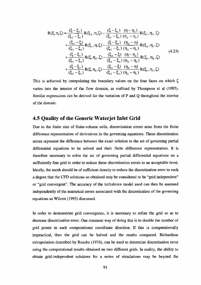
(4.23)
This is achieved by interpolating the boundary values on the four faces on which ~
varies into the interior of the flow domain, as outlined by Thompson et al ( 1985).
Similar expressions can be derived for the variation of P and Q throughout the interior
of the domain.
4.5 Quality of the Generic W aterjet Inlet Grid
Due to the finite size of finite-volume cells, discretisation errors arise from the finite
difference representation of derivatives in the governing equations. These discretisation
errors represent the difference between the exact solution to the set of governing partial
differential equations to be solved and their finite difference representation. It is
therefore necessary to solve the set of governing partial differential equations on a
sufficiently fine grid in order to reduce these discretisation errors to an acceptable level.
Ideally, the mesh should be of sufficient density to reduce the discretisation error to such
a degree that the CFD solutions so obtained may be considered to be "grid independent"
or "grid convergent". The accuracy of the turbulence model used can then be assessed
independently of the numerical errors associated with the discretisation of the governing
equations as Wilcox (1993) discussed.
In order to demonstrate grid convergence, it is necessary to refine the grid so as to
decrease discretisation error. One common way of doing this is to double the number of
grid points in each computational coordinate direction. If this is computationally
impractical, then the grid can be halved and the results compared. Richardson
extrapolation described by Roache (1976), can be used to determine discretisation error
using the computational results obtained on two different grids. In reality, the ability to
obtain grid-independent solutions for a series of simulations may be beyond the
91
capability of the hardware available. Therefore, a compromise must be made between
accuracy, memory requirements and solution time, all of which influence the size of grid
used.
Qualities of a grid considered desirable (in order to facilitate accurate solution of the
governing equations and good calculation convergence behaviour) include good cell
orthogonality, cell aspect ratios close to unity, uniform cell size, grid smoothness and
alignment of the grid with streamlines (see Fluent (1996)). Practical resolution of
boundary layers and other regions of large flow gradients inevitably requires a stretched
grid. This will degrade solution accuracy due to the introduction of diffusive and
dispersive terms in the truncation error for the finite-difference representation of
derivatives in the governing equations as noted by both Fletcher ( 1987b) and Thompson
et al (1985). Therefore, the growth of the grid in any curvilinear coordinate direction
should be minimised. In regions where the solution does not vary appreciably, the rate
of cell size growth is of less concern as Thompson et al ( 1985) noted. Large cell aspect
ratios resulting from the stretching of grid lines may result in problematic calculation
convergence behaviour when the local flow vector has a component across the smallest
dimension of the cell. This may also result in a degradation of calculation accuracy.
Convergence difficulty may also be experienced when there is excessive cell skewness
throughout the domain. Excessive cell skewness near wall boundaries can cause the
accuracy of the boundary condition treatment to deteriorate.
Smoothness of gridlines (curve smoothness along the curves defining the gridlines) is
required for accurate application of convective differencing schemes in the numerical
algorithm, although higher-order convective differencing schemes are less susceptible to
lack of gridline smoothness (see Fluent (1996)). In order to reduce numerical diffusion,
it is desirable to align the gridlines with the general flow direction. Patankar ( 1980)
noted that numerical diffusion can be reduced by the use of higher-order convective
differencing in the discretisation process.
Excessive cell skewness does occur for some cells in the forward lower inlet region and
in parts of the external domain close to the inlet, (close to the surface and near the side
92
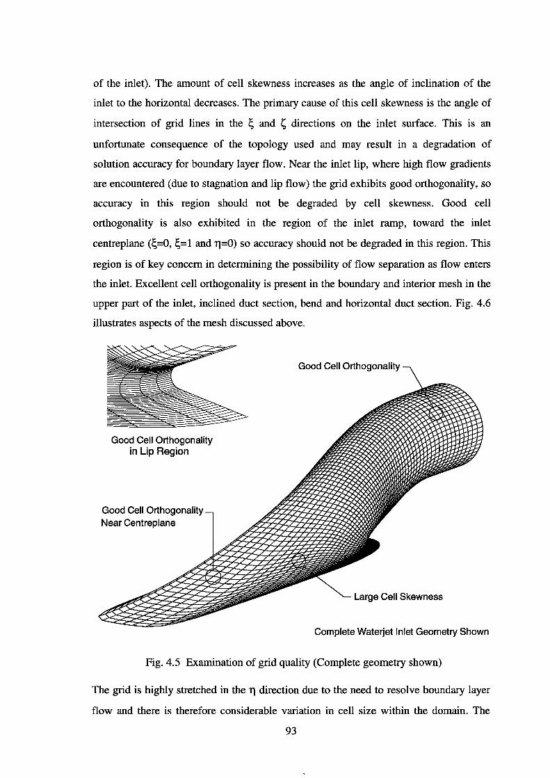
of the inlet). The amount of cell skewness increases as the angle of inclination of the
inlet to the horizontal decreases. The primary cause of this cell skewness is the angle of
intersection of grid lines in the ~ and ~ directions on the inlet surface. This is an
unfortunate consequence of the topology used and may result in a degradation of
solution accuracy for boundary layer flow. Near the inlet lip, where high flow gradients
are encountered (due to stagnation and lip flow) the grid exhibits good orthogonality, so
accuracy in this region should not be degraded by cell skewness. Good cell
orthogonality is also exhibited in the region of the inlet ramp, toward the inlet
centreplane (~=0, ~=1 and 11=0) so accuracy should not be degraded in this region. This
region is of key concern in determining the possibility of flow separation as flow enters
the inlet. Excellent cell orthogonality is present in the boundary and interior mesh in the
upper part of the inlet, inclined duct section, bend and horizontal duct section. Fig. 4.6
illustrates aspects of the mesh discussed above.
Good Cell Orthogonality in Lip Region
Good Cell Orthogonality Near Cent rep lane
Good Cell Orthogonality
Large Cell Skewness
Complete Waterjet Inlet Geometry Shown
Fig. 4.5 Examination of grid quality (Complete geometry shown)
The grid is highly stretched in the 11 direction due to the need to resolve boundary layer
flow and there is therefore considerable variation in cell size within the domain. The
93
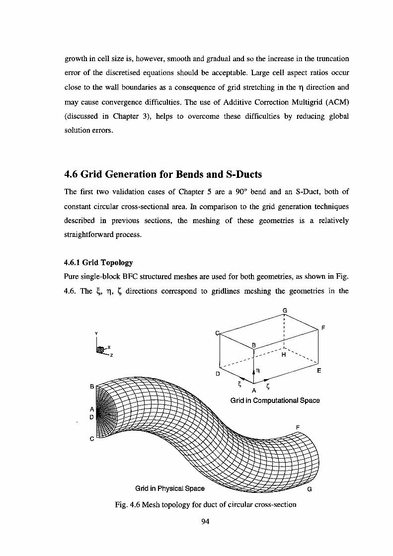
growth in cell size is, however, smooth and gradual and so the increase in the truncation
error of the discretised equations should be acceptable. Large cell aspect ratios occur
close to the wall boundaries as a consequence of grid stretching in the 11 direction and
may cause convergence difficulties. The use of Additive Correction Multigrid (ACM)
(discussed in Chapter 3), helps to overcome these difficulties by reducing global
solution errors.
4.6 Grid Generation for Bends and S-Ducts
The first two validation cases of Chapter 5 are a 90° bend and an S-Duct, both of
constant circular cross-sectional area. In comparison to the grid generation techniques
described in previous sections, the meshing of these geometries is a relatively
straightforward process.
4.6.1 Grid Topology
Pure single-block BFC structured meshes are used for both geometries, as shown in Fig.
4.6. The ~. 11. ~ directions correspond to gridlines meshing the geometries in the
G
F y
~ z
B
Grid in Computational Space
c
Grid in Physical Space
Fig. 4.6 Mesh topology for duct of circular cross-section
94
circumferential, radial and streamwise directions, respectively. From Fig. 4.6 it is
evident that an 0-grid topology is used to mesh the cross-section of these ducts.
4.6.2 Meshing Procedure
The basic idea behind the generation of these grids is to generate an 0-type grid at the
cross-section corresponding to the inlet of the flow domain under investigation and then
sweep this cross-sectional mesh (aligned normal to the tangent to the centreline) along
the centreline of the respective duct in order to generate the complete mesh. Using this
approach, the grid point locations relative to the axis can be written as
x = xc + fs (D I 2) cos9cos~
Y = Yc +fs(D/2)cos9sin~
z = fs (D I 2) sin 9
(4.24)
where D is the diameter of the duct, ~ is the angle of inclination of the cross-section to
the horizontal and 9 is the angle of the radial gridline to the vertical plane of symmetry
of the duct. Subscript c denotes centreline location and fs is the value of the stretching
function (in this case the stretching function of Vinokur (1983)) applied in the 11 (radial)
direction.
The above-mentioned approach is much simpler than specifying the mesh on the domain
boundaries, either by transfinite interpolation or other means and then using transfinite
interpolation to generate the interior mesh. Simple programs were written to accomplish
the meshing of both geometries. The above methodology may be termed "direct grid
point specification".
4.6.3 Grid Quality
The grids produced by "direct grid-point specification" possess excellent orthogonality.
Since the primary flow direction will essentially be aligned with the l; curvilinear
coordinate, additional numerical diffusion caused by flow/grid alignment effects should
be minimised. There will be some additional numerical diffusion associated with
secondary flow behaviour in the cross-stream direction. The stretching of the grid in the
radial direction is necessary in order to resolve the growth of boundary layers on the
duct walls and will increase the truncation error in the discretised equations. The large
95
aspect ratios of the cells near the wall may create convergence difficulties, but as
discussed in Section 4.5, ACM can be used to overcome these problems.
4.7 Closure
In this chapter, a description was given of the generic parametrically-defined flush-type
waterjet inlet geometry used as the basis of the design and optimisation-related
investigations presented in later chapters. The process of mesh generation takes a
significant proportion of the CFD analysis cycle time and therefore must be reduced to a
minimum when a large number of different configurations are to be analysed. It was
therefore decided to develop a grid generator specifically for the purpose of minimising
the time dedicated to grid generation.
A Fortran 77 program, lnlet3D, was written specifically for meshing the generic waterjet
inlet geometry. lnlet3D uses a single-block body-fitted-coordinate (BFC) structured grid
to mesh the geometry of the waterjet inlet and a semi-ellipsoidal external flow domain
below the inlet. lnlet3D uses a combination of transfinite interpolation and elliptic
partial differential equation solution techniques (based on the iteration of a Poisson
equation solver) in order to mesh all flow domain boundaries. The interior of the flow
domain is generated initially by transfinite interpolation and then smoothed by iteration
of a Poisson equation solver in the Fluent preprocessor, PreBFC. The stretching function
of Vinokur ( 1983) is used to effect grid point clustering where required.
The merits and limitations of the grid produced by lnlet3D were discussed. In particular,
the generic grid produced possesses good grid orthogonality in the upper part of the
waterjet inlet and in the inlet lip region. The cell skewness in the lower-forward-side
part of the inlet increases as the angle of inclination of the inlet to the horizontal
decreases. This growth in cell skewness is a direct result of the grid topology used and
the geometry being meshed. It is also a fundamental reason why obtaining suitable
meshes for flush-type waterjet inlet geometries is difficult when BFC meshes are used.
The grid is also highly stretched in the radial direction in order to resolve the wall
boundary layers and this results in large cell aspect ratio variations.
96
The grids used in the first two experimental validation cases presented in Chapter 5 are
generated using a single-block BFC structured grid topology. Owing to the simplicity of
these geometries it is possible to generate these grids directly by specifying their grid
point locations utilising explicit trigonometric relationships. Again, the stretching
function of Vinokur (1983) is used to effect grid-point clustering. The grids produced
possess excellent orthogonality by virtue of the topology used, but large cell aspect
ratios and significant stretching in the radial direction result from the need to resolve
wall boundary layers.
97

Chapter 5 Experimental Validation
A necessary component of any CFD study is an assessment of the accuracy of the
computational solution against relevant experimental data. By "benchmarking" the
computational solution against experimental data, aspects related to the computational
simulation such as the grid size, boundary conditions, or the turbulence model, can be
adjusted in order to improve the agreement with the experimental data, within the
limitations of the modelling used.
Good agreement between theoretical computations and experimental results lends
credibility to the efficacy of the CFD methodology used, therefore justifying the use of
CFD as a reliable analysis tool for the particular application under consideration. This is
of particular importance to design and optimisation-related work.
In this chapter, computational solutions obtained using Fluent are compared with
experimental data in order to assess the accuracy of the CFD modelling methodology
that was outlined in Chapter 3 and used in subsequent chapters of this thesis. Of
particular relevance to the work presented in later chapters are the grid sizes necessary
to reduce discretisation error of the discretised governing equations to an acceptable
level, the accuracy of the two-equation k-e turbulence modelling used and the near-wall
modelling (via wall functions) used to "bridge" the viscosity-affected near-wall region.
Boundary conditions are also of great importance in ensuring accurate solution, as they
reflect the realism of the boundary data, but vary according to the problem analysed.
The flow in a flush-type watetjet inlet is subject to significant streamline curvature as a
result of the different aspects of the waterjet inlet geometry, such as the inlet ramp, lip
and the bend in the waterjet inlet. At the inlet lip there is a line of flow stagnation and
then large pressure gradients as flow accelerates into the inlet or outside of the inlet.
98
Since the work presented in this thesis is based upon the CFD simulation of flush-type
waterjet inlets, it is necessary for the purposes of credibility and completeness, to
validate the accuracy of CFD computation using Fluent against an actual flush-type
waterjet inlet.
In addition to the flow in a flush-type waterjet inlet, experimental data sets for the flow
in S-shaped inlet ducts and pipe (or duct) bends offer rigorous test cases for validation
of a CFD program, as the essential physics of the flow are similar to that in a waterjet
inlet. This is due to the streamline curvature, adverse pressure gradients and secondary
flow behaviour inherent in such flows. Using experimental data for flow in a bend or an
S-shaped duct as a validation case, offers the additional advantage that this type of flow
is essentially equivalent to the flow in a ram-type waterjet inlet. This, therefore, allows
the accuracy of such waterjet inlet flows to be assessed as an additional outcome of the
validations presented herein. No further discussion of this issue is, however, presented.
Three different validation studies were conducted. These were the 90° bend of Enayet et
al (1982), an S-Duct of Bansod and Bradshaw (1972) and a perspex model of a flush
type waterjet inlet tested in the wind tunnel at The University of Tasmania by Roberts
(1998). The model waterjet inlet of Roberts (1998) is based upon generic designs used
in the marine industry for the propulsion of large high-speed catamaran vessels and is
therefore a realistic, industrially-relevant example of a commercially-available waterjet
inlet design.
The generic flow behaviour for flows in bends, S-Ducts and flush-type waterjet inlets is
discussed in Section 5.1 for reasons of completeness and for the benefit of the reader. In
Section 5.2 a validation study of the flow through the 90° bend of Enayet et al (1982)
is presented. Validation studies are also presented for an S-Duct of Bansod and
Bradshaw (1972) and the model waterjet inlet of Roberts (1998), in Section 5.3 and
Section 5.4 respectively. The accuracies of the computational solutions obtained for
each validation case will be discussed in the relevant section. Section 5.5 provides a
general discussion of the results obtained in previous sections, relating the accuracy of
the computational results obtained to the strengths and limitations of the underlying
99
CFD modelling methodology. The conclusions of the experimental validation studies
are presented in Section 5.6.
5.1 Generic Flow Behaviour
An understanding of the generic physical behaviour of a particular flow provides a
necessary foundation for an intelligent interpretation of results obtained from a CFD
simulation of that flow. The generic behaviour of flows in bends, S-Ducts and flush-type
wateljet inlets is presented in this section, since these are the flows which the validation
studies presented in later sections of this chapter are based upon.
Flow development in bends, S-Ducts and flush-type waterjet inlets involves a complex
interaction of pressure gradients, streamline curvature and secondary flow effects. It is
interesting to note that the development of secondary flow within a curved duct is
essentially an inviscid phenomena, given an initial upstream boundary layer, as Bansod
and Bradshaw ( 1972) noted.
An inviscid-flow theory relating the effect of upstream vorticity on the downstream
secondary flow in a cascade of airfoils was developed by Squire and Winter (1951 ).
Using this theory, Squire and Winter related the strength of the axial vorticity of the
flow leaving a cascade to the angle of deflection of the flow by the cascade and the
upstream velocity gradients. The Squire and Winter relationship is
~ =-2eau ~ dZ (5.1)
In Eqn 5.1 ~~ is the streamwise vorticity at the duct exit, 8 the angle of deflection of the
streamwise flow by the duct, U the streamwise velocity at the entrance to the duct and z
the cross-stream direction (which is evident from the geometric definitions of the flow
domains presented later in this chapter). It is clear from Eqn 5.1 that the greater the
cross-stream vorticity ((}U/(}z) upstream of the duct and the larger the deflection of the
flow is, the stronger will be the strength of the streamwise vortex developed in the duct
and hence the secondary flow. The upstream vorticity is equivalent to the boundary layer
thickness in this case.
100
5.1.1 Flow in Bends
In the literature there is a significant number of publications dealing with the subject of
flow in pipe and duct bends of both circular and rectangular cross-section. Papers such
as those by Ward-Smith (1963), Rowe (1970), Enayet et aJ (1982) and Taylor et aJ
(1982a) are examples of such publications. A characteristic which distinguishes flows in
duct bends from those in straight ducts is the generation of stream wise vorticity, or
"secondary motion" within the duct. This results in a pressure loss, the spatial
redistribution of streamwise velocity and increased heat transfer at the duct wall, as
noted by Taylor et al (1982a).
As the flow enters the duct bend cross-stream static pressure gradients develop between
the outside of the bend and the inside of the bend, as a result of the streamline curvature
present. A larger static pressure develops at the outside of the bend than at the inside.
The adjustment of streamwise flow in the bend creates ~ cross-flow in the core region
from the inside of the bend to the outside. The larger static pressure at the outside of the
bend creates an adverse pressure gradient that thickens the boundary layer as a result of
flow deceleration. The boundary layer at the inside of the bend experiences a beneficial
pressure gradient and flow acceleration, thus thinning it. The cross-stream static
pressure gradient causes a flow of boundary layer fluid from the outside of the bend
toward the inside. This creates a secondary flow which convects boundary layer fluid to
the inside of the bend. This results in a build-up of low momentum fluid at the inside of
the bend and the formation of a pair of counter-rotating vortices which further assists in
convecting boundary layer fluid to the inside of the bend. The reversal of the streamwise
pressure gradient over the second half of the bend also assists in the thickening of the
boundary layer at the inside of the bend. Ward-Smith (1963) showed that the effect of
the duct bend is to influence the static pressure distribution both upstream and
downstream of the bend.
As Taylor et aJ (1982a) explained, factors which affect the development of the flow in
the pipe bend and the nature of the secondary flow include: the radius of the pipe bend,
the distribution of the cross-stream vorticity upstream of the bend (the boundary layer
profile) and the flow Reynolds number. Bends of greater curvature experience larger
101
pressure gradients and hence stronger secondary flows. The larger pressure gradients
present cause a greater flow acceleration at the inside of the bend and a greater flow
retardation at the outside of the bend. This has the effect of displacing the core flow
toward the inside of the bend. Larger centrifugal forces are applied to the in viscid core
flow with increasing Reynolds number, due to higher bulk fluid velocities. This will
affect the location of the "inviscid" core flow and hence the overall flow behaviour in
the bend.
5.1.2 Flow in S-Shaped Ducts
Much experimental and CFD work has been presented in the aeronautical literature
dealing with the subject of flow in S-shaped ducts. The S-shaped duct is of particular
relevance to the design of gas turbine inlet ducting, where the engine compressor inlet is
offset from the air inlet. Little and Trimboli ( 1982) for example, presented the results of
an experimental investigation of S-Duct diffusers for high-speed prop-fans. Kitchen and
Sedlock (1983) discussed the development and challenges faced in the design of
diffusers for advanced tactical aircraft.
S-Ducts may be diffusing or non-diffusing depending on the variation of duct cross
sectional area along the duct centreline. Diffusing S-ducts not only have centreline
curvature but also a cross-sectional area increase. As Wellborn et al (1994) noted, the
adverse pressure gradient caused by the increasing cross-sectional area of the duct can
lead to flow separation in the duct.
There are numerous references in the literature presenting experimental data for the flow
inS-Ducts. Among these are the velocity and turbulence measurements (obtained from
experiments) for flow in a diffusing S-Duct by Whitelaw and Yu (1993). Wellborn et al
(1994) provided an extensive set of pressure, velocity and flow visualisation data for
flow in a diffusing S-Duct of circular cross-section. Guo and Seddon (1982), Guo and
Seddon ( 1983a) and Guo and Seddon ( 1983b) investigated the effect of mass flow-rate
and flow incidence on the swirl in S-Ducts. They were able to link the resultant swirl at
the exit of the duct with flow separation effects at the duct inlet caused by flow
incidence and proposed ways of reducing swirl by the use of spoilers.
102
A description of the flow behaviour in S-Ducts of circular cross-section is presented
below and is taken largely from Bansod and Bradshaw (1972) and Wellborn et al
(1994). It must be noted that the flow over the first bend of an S-Duct is essentially the
same as that for an equivalent bend of the same angle. As discussed in Section 5.1.1, the
cross-stream pressure gradients that develop over the first bend create a movement of
the low momentum fluid in the boundary layer toward the inside of the bend.
As the flow enters the second bend, the cross-stream pressure gradient reverses, by
virtue of the adjustment of the streamwise flow in the bend. This results in a greater
static pressure at the outside of the second bend than at the inside. The reversal of the
sign of the cross-stream pressure gradient tends to make the boundary layer fluid
migrate circumferentially to the inside of the duct bend. The boundary layer fluid near
the outside of the duct bend experiences a negligible circumferential component. The
circumferential movement of boundary layer fluid developed over the first bend requires
time to reverse. The combination of this secondary flow behaviour and the presence of a
favourable stream wise pressure gradient on the outside of the bend (after the middle of
the second bend), results in the formation of a pair of strong counter-rotating vortices.
These vortices convect low momentum boundary layer fluid to the inside of the duct
bend. Toward the duct exit, the result is a characteristic region of low total pressure and
velocity at the outside of the second bend.
It is interesting to note that although the mechanisms by which these vortices are formed
in bends and S-Ducts involve a combination of cross-flow, convergence and streamwise
acceleration, the process is basically an inviscid one given an initial boundary layer, as
Harloff et al (1993) showed from the solution of the Euler equations for flow in an S
Duct with an initial upstream boundary layer velocity distribution.
As Wellborn et al (1994) pointed out, the convection of low momentum fluid toward the
centre of the duct by stream wise vortices results in a decrease in both the uniformity and
magnitude of the total pressure at the exit of an S-Duct. This is also applicable to the
flow in bends.
103
5.1.3 Flow in Flush-Type Waterjet Inlets
There have been few publications presenting experimental flow results for flush-type
waterjet inlets available in the literature. Much of the experimental work undertaken has
been by waterjet manufacturers who are reluctant to release commercially sensitive
information to the public domain. Publications appearing in the literature include the
works of Okamoto et al (1993), Griffith-Jones (1994) and Roberts (1998). The design of
condenser scoops (engine cooling inlets) is in many respects similar to that of flush-type
waterjet inlets. Information on the performance of condenser scoop designs can be
found in Hewins and Reilly (1940) and English (1974).
In Section 1.3 .1, aspects of the flow through a flush-type waterjet inlet were briefly
discussed. The flow through a flush-type waterjet can be understood by considering the
underlying geometry. The presence of the inlet ramp causes an acceleration of the flow
into the inlet, with a reduction of static pressure on the ramp surface. Stagnation of the
flow at the inlet lip causes a high static pressure along the stagnation line with
subsequent acceleration of the flow into the inlet (above the stagnation line), or out of
the inlet (below the stagnation line). This causes rapid changes in static pressure in the
vicinity of the inlet lip.
It is interesting to examine how the bend will affect flow behaviour in the inlet. As
discussed in Section 5.1.1, it may be expected that the outside of the bend will
experience an increase in static pressure that will extend both upstream and downstream
of the bend. An adverse pressure gradient experienced by the flow upstream of the bend
undoubtedly affects the boundary layer development. Similarly, the pressure distribution
associated with the inside of the bend will generate a favourable pressure gradient
upstream of the bend. The secondary flow behaviour at the duct exit is dependent, not
only upon the geometry of the bend, but also upon the vorticity upstream of the bend.
The generic centreline static pressure distribution (including the effect of the bend) for a
flush-type waterjet inlet can be seen from the results of Okamoto et al (1993). It is
interesting to note that as the inlet velocity ratio (IVR) increases, there is a general
decrease in static pressure coefficient. It must be further noted that the values of static
104
pressure coefficient presented in the paper are indicative of hull boundary layer
ingestion (due to the decreased dynamic pressure upstream of the inlet) as static pressure
recovery would have been greater had there been no boundary layer ingestion. The
upstream hull boundary layer characteristics will therefore clearly affect the flow in the
waterjet inlet including the location of the lip stagnation line, the total pressure recovery
in the inlet, static pressure distribution over the surface, the velocity, static pressure and
secondary flow behaviour at the duct exit.
Griffith-Jones (1994) used a wind-tunnel to investigate a complete waterjet model
(including fan and nozzle) and the corresponding flush-type waterjet inlet (without
impeller shaft). He found that the presence of the fan shaft and fan had little effect on
the bare duct flow. Consequently it is acceptable to omit the modelling of the pump
shaft and the pump prewhirl when either experimentally or computationally modelling
the flow in the waterjet inlet. An experimental modelling of the complete waterjet is,
however, necessary to determine the effect of flow non-uniformity (at the duct exit) on
pump performance.
The development of the secondary flow within the waterjet inlet is of particular
relevance to the quality of the flow at the duct exit and is therefore discussed below. The
discussion presented below is constructed from the results of Griffith-Jones (1994),
Roberts (1998) and the author's own CFD investigations. The secondary flow present at
the duct exit is qualitatively similar to that in an S-Duct, but the mechanisms responsible
for its formation are in fact different. From the results of Griffith-Jones (1994), it is
evident that the diffusing flow into the inlet creates an upward secondary flow pattern in
both the core flow and the boundary layer flow on the side-walls of the inlet. In addition,
flow diffusion and the physical length of the inlet ramp cause a thickening of the
boundary layer on the ramp surface. Depending on the geometry of the waterjet inlet and
the IVR, the flow may or may not separate on the upper-ramp surface. The formation of
additional secondary flow, as stream wise vortices in the inlet comers (between the ramp
surface and the inlet side-walls) may also occur (depending on the geometry), thus
affecting the development of the boundary layer to some extent. In the absence of
detailed experimental data it is difficult to quantify this effect and its importance, which
105
is probably minor. The behaviour of the secondary flow in the inlet side-wall boundary
layers is equivalent to that in the first bend of an S-Duct. In the wateijet inlet, the
secondary flow in the core is toward the ramp (convex) surface, whereas over the first
bend of the S-Duct it is toward the outer radius of the bend and so the two flows differ
in this regard.
As the flow enters the waterjet inlet duct bend, the secondary flow in the core continues
to be directed toward the top of the duct, in this case from the inside of the bend toward
the outside of the bend. The larger static pressures at the outside of the bend act to direct
the secondary flow in the boundary layer toward the inside of the bend. The boundary
layer fluid near the outside of the bend experiences a negligible circumferential
component. The circumferential movement of boundary layer fluid developed upstream
of the bend requires time to reverse. The combination of this secondary flow behaviour
and the presence of a favourable streamwise pressure gradient at the outside of the bend,
after the middle of the duct bend, results in the formation of a pair of counter-rotating
vortices that convect low momentum boundary layer fluid to the outside of the bend.
This assists in the development in the low total pressure and velocity region at the
outside of the bend.
As mentioned above, the larger static pressures at the outside of the bend act to direct
the secondary flow in the boundary layer toward the inside of the bend. This is certainly
the case for the secondary flow in the boundary layer at the side of the bend, which is
now directed toward the inside of the bend. With the secondary flow in the core directed
toward the outside of the bend and the secondary flow in the boundary layer directed
toward the inside of the bend, a second pair of streamwise vortices appears on the side
of the duct. This vortex acts to convect boundary layer fluid toward the lower part of the
duct.
The secondary flow development over the waterjet inlet bend is thus analogous to
secondary flow development in the second bend of an S-Duct with similar generic
secondary flow behaviour at the duct exit. As discussed above, the mechanisms for the
formation of upstream vorticity are different for the waterjet inlet and an S-Duct. The
106
actual secondary flow behaviour in the waterjet inlet will depend on several factors.
These include the geometry of the waterjet inlet, IVR, upstream boundary layer
thickness and the presence or absence of flow separation in the waterjet inlet.
5.2 Flow in a 90° Bend
In this section the accuracy of the CFD techniques described in Chapter 3 are assessed
and benchmarked against experimental data for flow in the goo bend of Enayet et al
(lg82). Enayet et al (lg82) investigated the laminar and turbulent flow of water in a goo
bend of circular cross-section using Laser-Doppler velocimetry. Their study was focused
on obtaining mean velocity and turbulence profiles at various cross-sections in the bend
and downstream of the bend, as well as wall static pressure measurements. The study of
flow in a goo bend is an interesting and rigorous CFD validation case because of the
combination of streamline curvature, adverse pressure gradient and secondary flow
development. A turbulence model must adequately model all of these features in order
to produce an accurate solution.
5.2.1 Experimental Configuration
The experimental geometry shown in Fig. 5.1 , consists of a goo bend of circular cross
section with an internal diameter of 48 mm and a centreline radius of curvature of 134
mm. The bend is machined from two halves of a perspex block fixed in the horizontal
plane and fitted with upstream and downstream tangents that are 240 mm and 480 mm
long, respectively. The experimental geometry is fitted in a special flow rig through
which water was pumped at a Reynolds number of 43000 (based on the 48 mm duct
diameter and a volumetrically-averaged velocity in the duct of o.g2 mls).
5.2.2 Computational Modelling of Experimental Configuration
The experimental configuration is modelled from the start of the upstream tangent to six
duct diameters downstream of the bend. The topology and techniques used to mesh the
modelled flow domain are discussed in Section 4.6 and shown in Fig. 4.6.
Since the experimental data presented by Enayet et al ( }g82) showed that the flow is
symmetrical about the plane of geometric symmetry, only half of the experimental
107
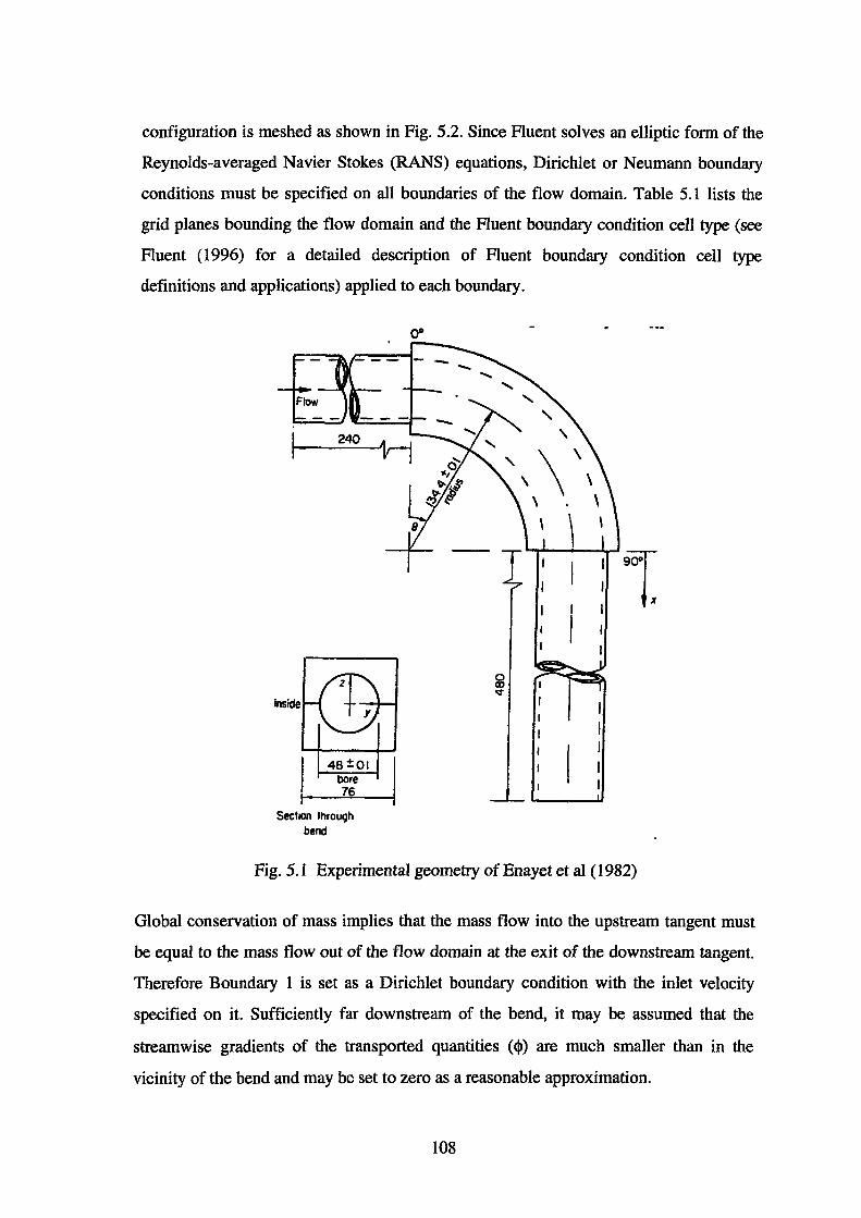
configuration is meshed as shown in Fig. 5.2. Since Fluent solves an elliptic form of the
Reynolds-averaged Navier Stokes (RANS) equations, Dirichlet or Neumann boundary
conditions must be specified on all boundaries of the flow domain. Table 5.1 lists the
grid planes bounding the flow domain and the Fluent boundary condition cell type (see
Fluent ( 1996) for a detailed description of Fluent boundary condition cell type
definitions and applications) applied to each boundary.
48±01 bore 76
Sectaon through bend
0"
Fig. 5.1 Experimental geometry of Enayet et al ( 1982)
Global conservation of mass implies that the mass flow into the upstream tangent must
be equal to the mass flow out of the flow domain at the exit of the downstream tangent.
Therefore Boundary 1 is set as a Dirichlet boundary condition with the inlet velocity
specified on it. Sufficiently far downstream of the bend, it may be assumed that the
stream wise gradients of the transported quantities ( <l>) are much smaller than in the
vicinity of the bend and may be set to zero as a reasonable approximation.
108

y
~ z
Fig. 5.2 41x41x81 surface grid bounding the modelled flow domain
Grid Plane in Computational Space Boundary Plane ~rnm ~max Tlmm Tlmax ~min lmax Fluent
1 ~=0.0 0.0 1.0 0.0 1.0 0.0 0.0 Inlet
2 ~=1.0 0.0 1.0 0.0 1.0 1.0 1.0 Outlet
3 1'}=0.0 0.0 1.0 0.0 0.0 0.0 1.0 Axis 4 11=1.0 0.0 1.0 1.0 1.0 0.0 1.0 Wall
5 ~=0.0 0.0 0.0 0.0 1.0 0.0 1.0 Symmetry
6 ~=1.0 1.0 1.0 0.0 1.0 0.0 1.0 Symmetry
Table 5.1 Relationship between boundary conditions and mesh topology
109
Thus, a Neumann boundary condition of the form
(5.2)
was set for Boundary 2. Boundary 5 and Boundary 6 lie on the plane of flow symmetry
and are therefore set as mixed Dirichlet/Neumann boundary conditions such that
velocities normal to the plane of flow symmetry and normal gradients of transported
quantities are set to zero. In other words
U·n=O cv~)·n =O
(5.3)
where U is the velocity vector, ~ a transported quantity and n a vector normal to the
symmetry plane. Boundary 3 which lies on the centreline of the flow domain, is a
Dirichlet boundary condition obtained by averaging the values of ~ from the cell-centres
of neighbouring cells according to
- 1 ""' ~P = N L.J ~nb nb
(5.4)
In Eqn 5.4, N is the number of neighbouring cell-centre locations surrounding point P.
Boundary 4 represents the wall bounding the flow domain. It is here that the no-slip
condition is applied in conjunction with the near-wall modelling (using wall functions)
as discussed in Section 3.3.
5.2.3 Computational Simulation
A plug-flow velocity profile of 0.92 rnls is specified on Boundary 1 at the entrance to
the modelled flow domain. A water density of 1000 kg/m3 was specified and the
molecular viscosity adjusted to give the appropriate Reynolds number.
All computations were executed on Hewlett Packard K210 workstation servers. In fact,
all computations used to obtain the results presented in this thesis were executed on the
above-mentioned hardware. Calculations are deemed to have converged when the sum
of the normalised residuals of the transport equations and the pressure correction
equation are reduced below lxl0-3 (see Section 3.6.2) which is Fluent's default
convergence criteria.
110
Computations were initially executed using the RNG k-e turbulence model and the
Standard wa11 function on a number of successively finer grids, with progressive
refinement in the circumferential (I), radial (J) and streamwise (K) directions. This was
done in order to determine a suitable grid size necessary to reduce discretisation error to
levels sufficiently low that the solution may be considered to be "grid-independent". For
all intents and purposes, it was found that a reasonably grid-independent solution could
be obtained on a 41 x41 x81 grid.
With discretisation errors reduced to acceptable levels, the effect of turbulence and near
wall modelling on the solution was examined, using both the RNG k-e turbulence model
and the Standard k-£ turbulence model, with the Standard wall function and the Two
Layer-Based Nonequilibrium (TLBN) wall function. The results of the validation study
are presented in the next section.
5.2.4 Experimental and Theoretical Comparisons
In this section, the accuracy of the computational results is assessed against
experimental data obtained from the measurements of Enayet et al ( 1982). The predicted
flow behaviour will be discussed in relation to the underlying physical flow behaviour.
The computed distribution of streamwise velocity and turbulence intensity at 0.58
diameters upstream of the bend is compared with the corresponding experimental data
in Fig. 5.3. The data has been plotted against distance from the wall, along the
centreplane of the duct (y), non-dimensionalised by the duct diameter (D). In all relevant
figures presented in this section, the direction of increasing y is taken to be from the
inside of the bend to the outside. The computational results presented in Fig. 5.3 are
obtained on a 4lx41x81 grid using the RNG k-e turbulence model with the Standard
wall function. From Fig. 5.3a it can be seen that the core velocities are within a relative
error of 7% of the measured values. Since Enayet et al (1982) quoted systematic and
random errors in their laser-Doppler velocimetry (LDV) measurements of U!Urer of
2.5% and ±1.5% respectively, it is possible that the actual error between the measured
and predicted velocities may in fact be less.
111
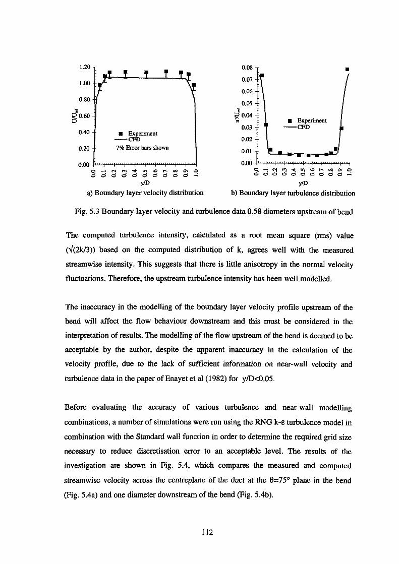
1.20
1.00
0.80
'i! ~ 0.60 ::J
0.40
0.20
• Expenment -CFD 7% Error bars shown
q - N ~ ~ ~ ~ ~ ~ ~ 0 0 d d d d d d d d d ~
y/D
a) Boundary layer velocity distribution
0.08
O.o7
0.06
0.05 'i! ~0.04 -=
0.03
0.02
0.01
• Experiment -CFD
•
0.00 -t'-'-'-"'t'-'-'-'t'-'-'.Lf-'-1-JL.I..f-'-LLL.j-'-LJ.J.fllJ.J.fll.L.I.fJ-'.L.I.fJ-'u.J..j o-N~~~~r-:~~q dddddddodd-
y/D
b) Boundary layer turbulence distribution
Fig. 5.3 Boundary layer velocity and turbulence data 0.58 diameters upstream of bend
The computed turbulence intensity, calculated as a root mean square (rms) value
(V(2k/3)) based on the computed distribution of k, agrees well with the measured
streamwise intensity. This suggests that there is little anisotropy in the normal velocity
fluctuations. Therefore, the upstream turbulence intensity has been well modelled.
The inaccuracy in the modelling of the boundary layer velocity profile upstream of the
bend will affect the flow behaviour downstream and this must be considered in the
interpretation of results. The modelling of the flow upstream of the bend is deemed to be
acceptable by the author, despite the apparent inaccuracy in the calculation of the
velocity profile, due to the lack of sufficient information on near-wall velocity and
turbulence data in the paper of Enayet et al (1982) for y/D<0.05.
Before evaluating the accuracy of various turbulence and near-wall modelling
combinations, a number of simulations were run using the RNG k-e turbulence model in
combination with the Standard wall function in order to determine the required grid size
necessary to reduce discretisation error to an acceptable level. The results of the
investigation are shown in Fig. 5.4, which compares the measured and computed
streamwise velocity across the centreplane of the duct at the 8=75° plane in the bend
(Fig. 5.4a) and one diameter downstream of the bend (Fig. 5.4b).
112
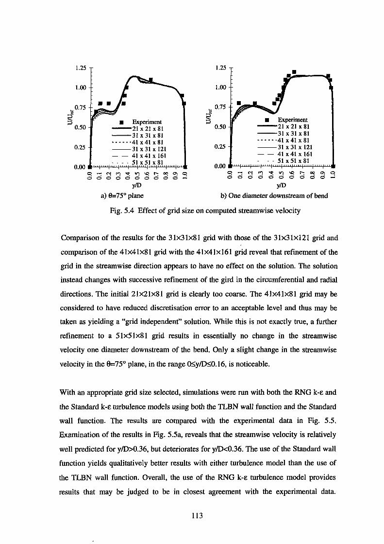
~ ::::>
1.25
1.00
0.75
0.50
0.25
• Experiment -21 x21 x81 -31 x31 x81 ······41 x41 x81 --31 X 31 X 121 - - 41 X 41 X 161 · - - - 51 X 51 X 81
0.00 ll-'-'..l.f-ll'-'+'-'.J.J.fJ-I..I..Lf-'.!.i.Lf-l..llJ..j-J.J..L.1.1f.!-LLLI-'-'-'-'+'-'-'-.
0 Nl"''"'<tlt")\Of"-000\C! 0000000000
y/D
a) &=75° plane
1.25
1.00
... 0.75
ti ::::>
0.50
0.25
•
Experiment --21 x21 x81 --31x31x81 ······41x41x81 --31 X 31 X 121 - - 41 X 41 X 161
- - 51 X 51 X 81
0 N 1"'1 "'<t lt") \0 f"- 00 0\ 0. 0 . o· o· o· · · · · · · 0 0 0 0 0 0
y/D
b) One diameter downstream of bend
Fig. 5.4 Effect of grid size on computed streamwise velocity
Comparison of the results for the 31x31x81 grid with those of the 31x31x121 grid and
comparison of the 41 x41 x81 grid with the 41 x41 x 161 grid reveal that refinement of the
grid in the streamwise direction appears to have no effect on the solution. The solution
instead changes with successive refinement of the gird in the circumferential and radial
directions. The initial 2lx2Ix81 grid is clearly too coarse. The 41x41x81 grid may be
considered to have reduced discretisation error to an acceptable level and thus may be
taken as yielding a "grid independent" solution. While this is not exactly true, a further
refinement to a 51x51x81 grid results in essentially no change in the streamwise
velocity one diameter downstream of the bend. Only a slight change in the streamwise
velocity in the 8=75° plane, in the range Qs;y/Ds;O.l6, is noticeable.
With an appropriate grid size selected, simulations were run with both the RNG k-e and
the Standard k-e turbulence models using both the TLBN wall function and the Standard
wall function. The results are compared with the experimental data in Fig. 5.5.
Examination of the results in Fig. 5.5a, reveals that the streamwise velocity is relatively
well predicted for y/D>0.36, but deteriorates for y/D<0.36. The use of the Standard wall
function yields qualitatively better results with either turbulence model than the use of
the TLBN wall function. Overall, the use of the RNG k-e turbulence model provides
results that may be judged to be in closest agreement with the experimental data.
113
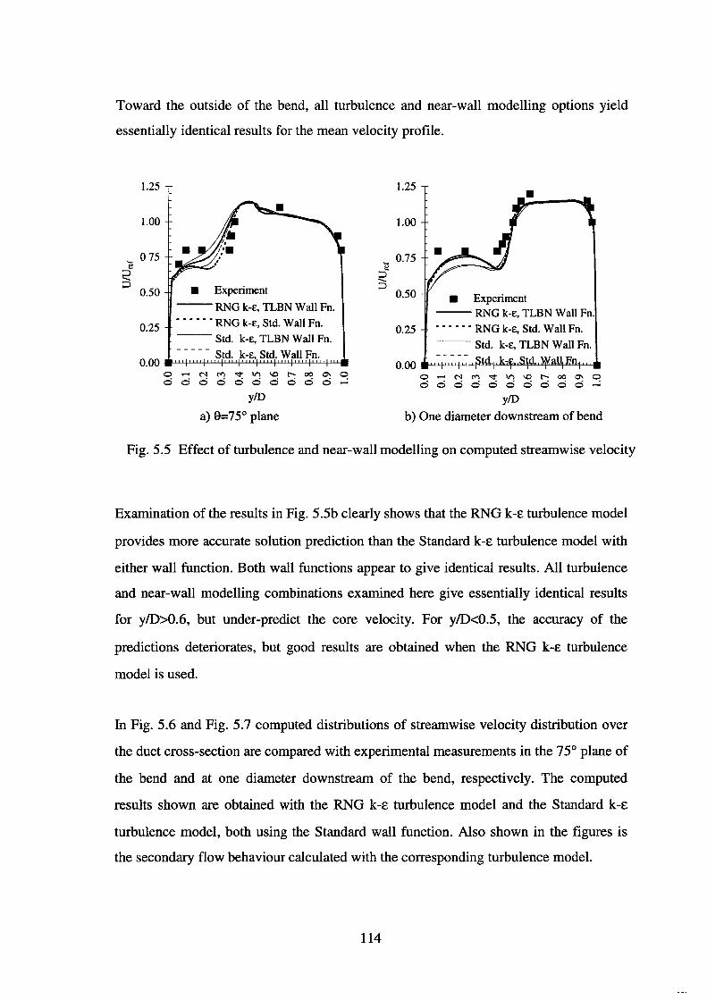
Toward the outside of the bend, all turbulence and near-wall modelling options yield
essentially identical results for the mean velocity profile.
1.25
1.00
- 075 e
2 ::>
0.50
0.25
• Experiment
--RNG k-e, TLBN Wall Fn. • • • • • • RNG k-e, Std. Wall Fn.
--Std. k-e, TLBN Wall Fn.
Std. k-e, Std. Wall Fn. 0. 00 .-w-'-1-'-'--'-'+'-'-'-'-t'-'-'-'+.u..w...I-'-'-'-'-P-'-'-'+'-'-'-'+'-'--'-'+'-.......
0 N M ~ ~ ~ ~ 00 ~ ~ d d d d d d d d d d
y/D
a) 9=75° plane
e ::> ....... ::>
1.25
1.00
0.75
0.50
0.25
• Experiment --RNG k-e, TLBN Wall Fn . •••••• RNG k-e, Std. Wall Fn.
-- Std. k-e, TLBN Wall Fn.
0 N M ~ ~ ~ ~ 00 ~ ~ d d d d d d d d d d
y/D
b) One diameter downstream of bend
Fig. 5.5 Effect of turbulence and near-wall modelling on computed streamwise velocity
Examination of the results in Fig. 5.5b clearly shows that the RNG k-E turbulence model
provides more accurate solution prediction than the Standard k-E turbulence model with
either wall function. Both wall functions appear to give identical results. All turbulence
and near-wall modelling combinations examined here give essentially identical results
for y/D>0.6, but under-predict the core velocity. For y/D<0.5, the accuracy of the
predictions deteriorates, but good results are obtained when the RNG k-E turbulence
model is used.
In Fig. 5.6 and Fig. 5.7 computed distributions of streamwise velocity distribution over
the duct cross-section are compared with experimental measurements in the 75° plane of
the bend and at one diameter downstream of the bend, respectively. The computed
results shown are obtained with the RNG k-E turbulence model and the Standard k-E
turbulence model, both using the Standard wall function. Also shown in the figures is
the secondary flow behaviour calculated with the corresponding turbulence model.
114
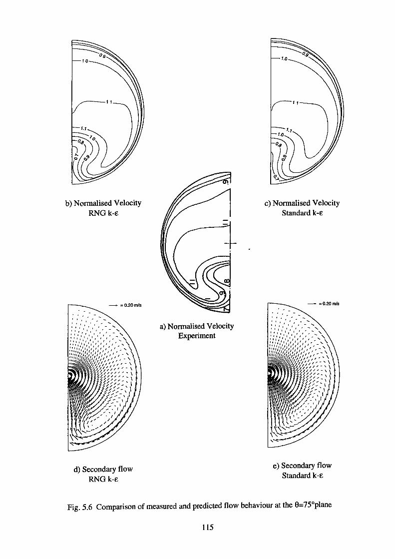
b) Normalised Velocity RNGk-£
- =0.20mls
d) Secondary flow RNGk-£
a) Normalised Velocity Experiment
c) Normalised Velocity Standard k-E
- =0.20m/s
e) Secondary flow Standard k-£
Fig. 5.6 Comparison of measured and predicted flow behaviour at the 8=75°plane
115
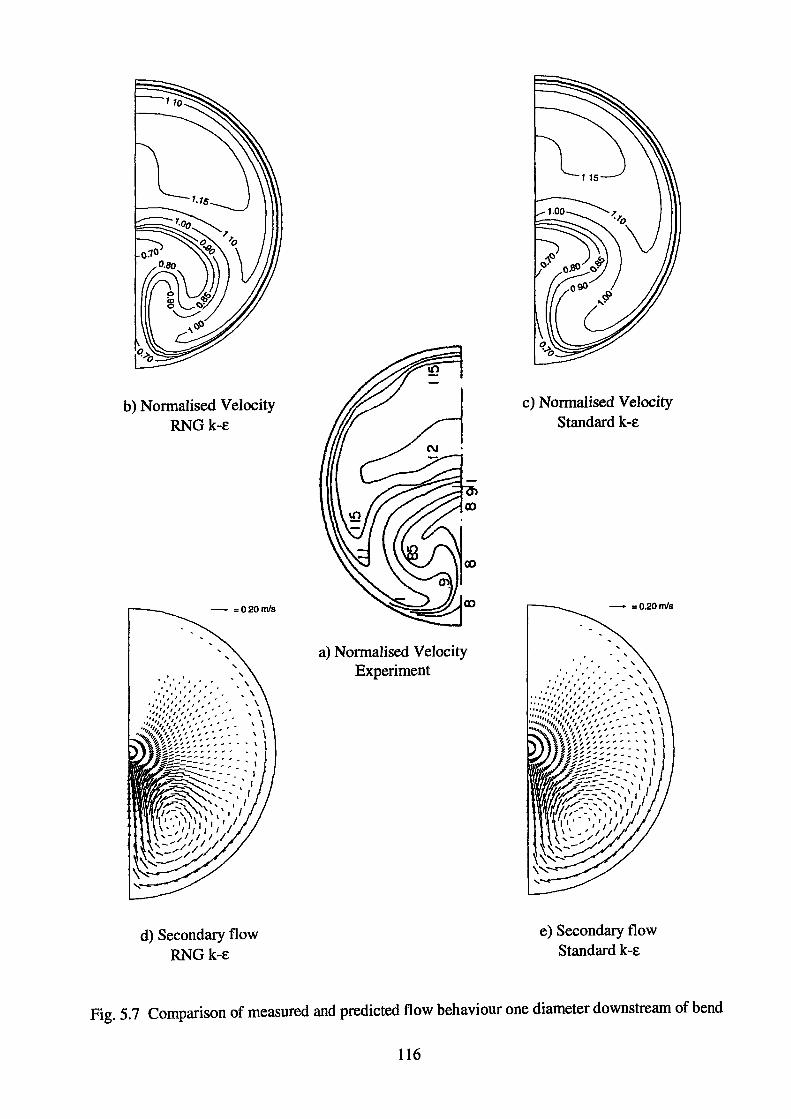
b) Normalised Velocity RNGk-e
- =020rnls
...
d) Secondary flow RNGk-e
a) Normalised Velocity Experiment
c) Normalised Velocity Standard k-e
- =0.20rnls
e) Secondary flow Standard k-e
Fig. 5.7 Comparison of measured and predicted flow behaviour one diameter downstream of bend
116

The results obtained for the streamwise velocity distribution over the duct cross-section
using the RNG k-E turbulence model are in closer agreement with the experimental data
than those of the Standard k-E model. The difference in the computational results for the
different turbulence models can be understood by examining the secondary flow
behaviour at both locations. Both reveal the existence of a streamwise vortex located
toward the inside of the bend (lower duct in the figure) near the duct centreplane. This
results from the interaction of the boundary layer and the transverse pressure gradient
associated with the bend. Both turbulence models predict a reduction in the intensity of
this streamwise vortex and reduced secondary flow one diameter downstream of the
bend (Fig. 5.7) due to the absence of the transverse pressure gradient at this location.
The stronger secondary flows predicted by the RNG k-E turbulence model at both
locations results in a greater convection of boundary layer fluid toward the centreplane
of the duct and hence a greater accumulation and up-welling of low-momentum fluid
from the inside of the bend toward the duct centreline. In fact, the RNG k-E turbulence
model tends to over-predict this secondary flow, whereas the Standard k-E model under
predicts the strength of the secondary flow.
As an interesting study of how the predicted turbulence behaviour follows the measured
trend of streamwise velocity fluctuations, the rms velocity fluctuations .V(2k/3) obtained
from the results of k along the centreplane of the duct are compared with the measured
streamwise velocity fluctuations in Fig. 5.8. If the correct distribution of k can be
calculated across the duct, then differences between the calculated rms turbulence
intensity and the streamwise intensity of the turbulence will indicate anisotropy in the
turbulence.
It can be seen from Fig. 5.8a and Fig. 5.8b that the distribution of calculated rms
turbulent fluctuations follows the trend of the measurements. Quantitative agreement
between computation and experiment appears to be relatively poor. In Fig. 5.8b
agreement between the computation and experiment appears to improve with relatively
good agreement obtained in the range 0.3<y/D<0.6 and y/D>0.9.
Two conclusions may be drawn from the results which indicate an uncertainty in the
117
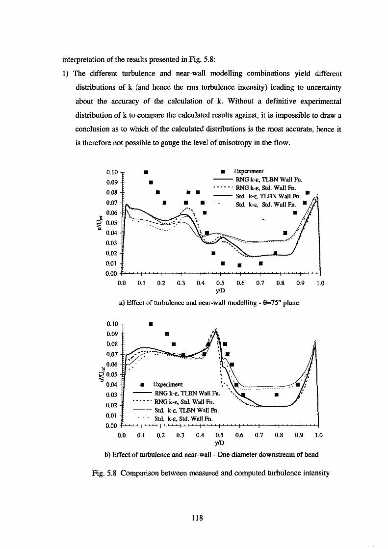
interpretation of the results presented in Fig. 5.8:
1) The different turbulence and near-wall modelling combinations yield different
distributions of k (and hence the rms turbulence intensity) leading to uncertainty
about the accuracy of the calculation of k. Without a definitive experimental
distribution of k to compare the calculated results against, it is impossible to draw a
conclusion as to which of the calculated distributions is the most accurate, hence it
is therefore not possible to gauge the level of anisotropy in the flow.
~ ::s
'i!
0.10 • • Experiment
0.09 • -- RNG k-£, TLBN Wall Fn.
0.08 • • • • • ·- • · RNG k-e, Std. Wall Fn. -- Std. k-£, TLBN Wall Fn.
0.07 • • • Std. k-e, Std. Wall Fn. 0.06 • 0.05
0.04
0.03
0.02 • 0.01 • • • 0.00
0.0 0.1 0.2 0.3 0.4 0.5 0.6 0.7 0.8 0.9 y/D
a) Effect of turbulence and near-wall modelling- 8=75° plane
0.10 •
0.09 •
0.08
0.07
0.06
•
1.0
e o.o5 "::s
0.04
0.03
0.02
0.01
• Experiment
-- RNG k-£, TLBN Wall Fn. • • • - • · RNG k-£, Std. Wall Fn. -- Std. k-e, TLBN Wall Fn.
Std. k-£, Std. Wall Fn. 0.00 -f-'-i..L-'-I--'-'-'--'-+-L..l-L...l....\-'-'-....L..J....+-'-1....L...l-f-'-..J....1..-'-+.L-L.J'-'-f....l-L..L..1..+-'-.L-L.J'-I--'-'-'-..J....!
0.0 0.1 0.2 0.3 0.4 0.5 0.6 0.7 0.8 0.9 1.0 y/D
b) Effect of turbulence and near-wall - One diameter downstream of bend
Fig. 5.8 Comparison between measured and computed turbulence intensity
118

2) If it is assumed that the actual distribution of k lies close to the results obtained using
the RNG k-e turbulence model (for example), then as can be seen from Fig. 5.8b,
there appears to be considerable anisotropy in the turbulence close to the inside of the
bend y/0<0.3 and in the core flow for the range 0.62<y/D<0.9. From Fig. 5.8a, there
appears to be considerable anisotropy across the duct centreplane.
Fig. 5.9 provides a comparison between the measured streamwise turbulent velocity
fluctuations and the rms turbulence intensity calculated using both the RNG k-e
turbulence model and the Standard k-e turbulence model. The two turbulence models
have been used with the Standard wall function. It can be seen from both Fig. 5.9a and
Fig. 5.9b that the measured distributions of streamwise turbulence intensity show the
effect of secondary flow-induced velocity gradients on the turbulence development, with
high levels of velocity fluctuations being associated with steep mean velocity gradients.
The contour patterns obtained using the RNG k-e model are qualitatively in better
agreement with the experimental data than those obtained using the Standard k-e model.
This may be attributed to the greater convection of turbulence by stronger secondary
flow and steeper secondary flow-induced velocity gradients over the cross-section
(which act to increase the production of turbulence).
The plotting of velocity vectors on the duct centreplane provides an understanding of
not only the magnitude and direction of the local flow direction, but also the developing
streamwise velocity profile across the duct. The results obtained using the RNG k-e and
the Standard k-e turbulence models, both using the Standard wall function, are shown in
Fig. 5.10. Examination of the figure reveals the dramatic increase in boundary layer
thickness at the inside of the bend driven by the secondary flow. It is interesting to note
that the growth of the boundary layer at the inside of the bend continues downstream of
the bend as a direct consequence of the secondary flow, but one that is decaying in its
strength as it is no longer driven by a transverse pressure gradient associated with the
bend.
Comparisons between the computed non-dimensional turbulent velocity-scale ('..fklUrer)
and the computed turbulent length-scale ( R E /D) on the duct centreplane, obtained using
119
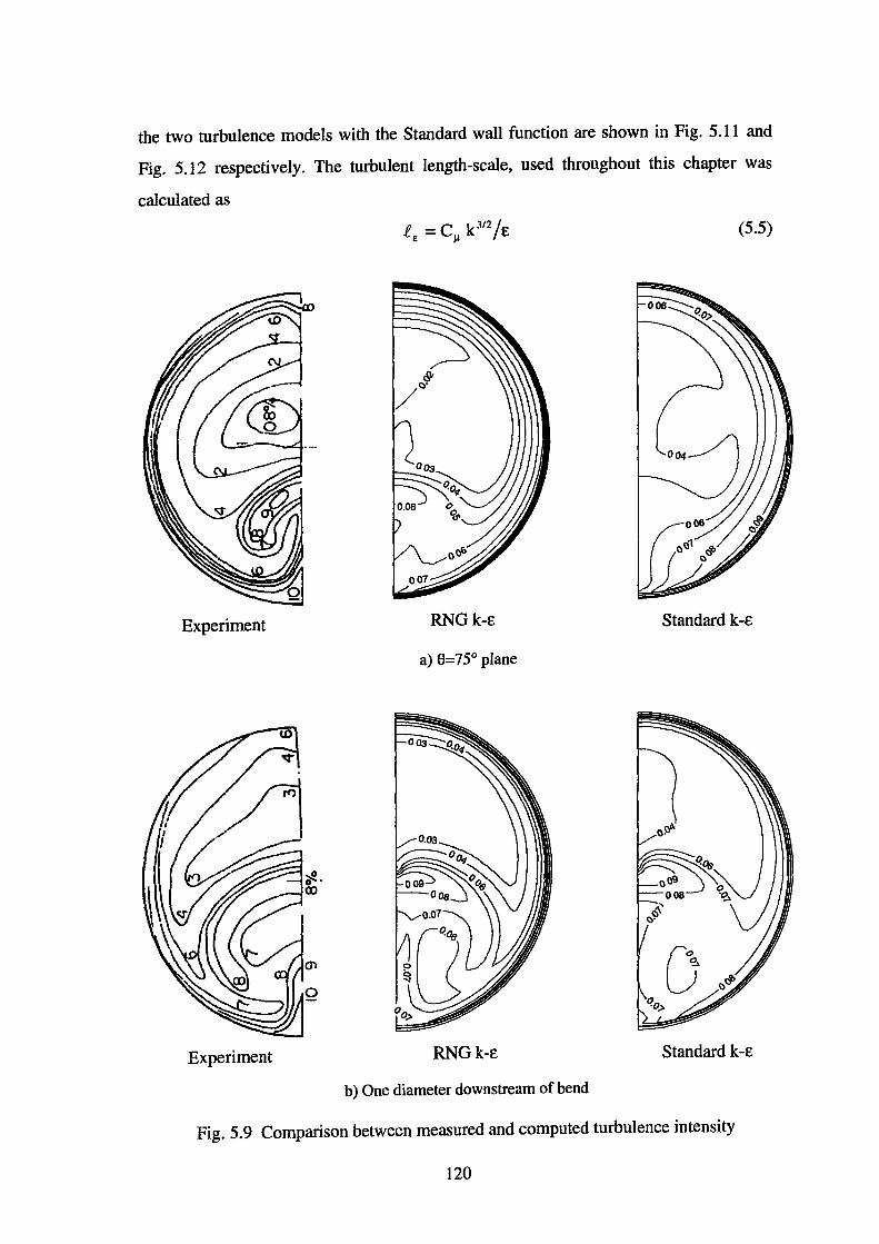
the two turbulence models with the Standard wall function are shown in Fig. 5.11 and
Fig. 5.12 respectively. The turbulent length-scale, used throughout this chapter was
calculated as
.f = C k 312/E E )! (5.5)
Experiment RNGk-E Standard k-E
a) 8=75° plane
Experiment RNGk-E Standard k-E
b) One diameter downstream of bend
Fig. 5.9 Comparison between measured and computed turbulence intensity
120
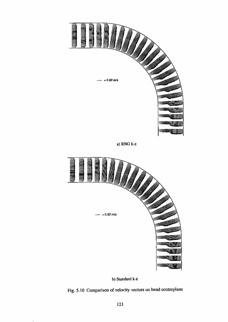
- =0.92m/s
a)RNGk-£
- =0.92m/s
b) Standard k-£
Fig. 5.10 Comparison of velocity vectors on bend centreplane
121
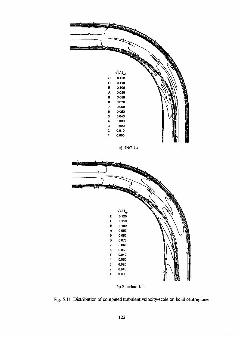
---2:----
-../k/U,e! D 0.120 c 0.110 8 0.100 A 0.090 9 0.080 8 0.070 7 0,060 6 0.050 5 0.040 4 0.030 3 0.020 2 0.010
0.000
a) RNGk-E
-../k/Ure! D 0.120 c 0.110 8 0.100 A 0.090 9 0.080 8 0.070 7 0.060 6 0.050 5 0.040 4 0.030 3 0.020 2 0.010
0.000
b) Standard k-E
Fig. 5.11 Distribution of computed turbulent velocity-scale on bend centreplane
122
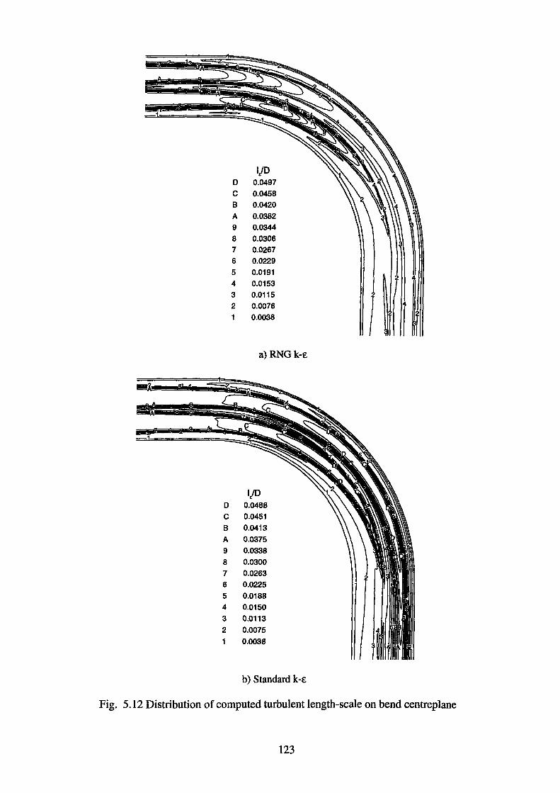
ljD D 0.0497 c 0.0458 B 0.0420 A 0.0382 9 0.0344 8 0.0306 7 0.0267 6 0.0229 5 0.0191 4 0.0153 3 0.0115 2 0.0076
0.0038
a) RNGk-E
IJD D 0.0488 c 0.0451 B 0.0413
A 0.0375 9 0.0338 8 0.0300 7 0.0263 6 0.0225 5 0.0188 4 0.0150 3 0.0113 2 0.0075
0.0038
b) Standard k-E
Fig. 5.12 Distribution of computed turbulent length-scale on bend centreplane
123
It can be seen from both figures that the core flow contains eddies of larger length-scale,
but smaller velocity-scale than those present in the boundary layers. These are the large
energy-containing eddies that are convected with the core flow. The greater turbulence
intensity and smaller length-scales of the eddies in the developing boundary layer at the
inside of the bend suggest smaller more dissipative eddies. Hence, there can be seen to
be a cascade of energy from the large energy-containing eddies in the core flow to the
smaller highly-turbulent dissipative eddies in the boundary layer.
It is evident from Fig. 5.12 that the relatively steep velocity gradients between the
developing boundary layer near the inside of the bend and the core flow lead to
significant turbulence production resulting in increased turbulence levels. Quantitative
differences in rms turbulence levels across the duct can be seen by examining Fig. 5.8. It
is interesting to note the large differences in computed length-scale in the core flow
between the results obtained from the two turbulence models. While the length-scale
predicted by the RNG k-e turbulence model decreases downstream over the bend, the
length-scale predicted by the Standard k-£ model remains high. This suggests that the
length-scale determining procedure (via solution of the £ equation) appears to lack
sensitivity to the effects of the streamline curvature present in the flow (this issue will
be discussed in greater length in Section 5.5). As a consequence, predicted eddy
viscosity, the Reynolds stresses and hence total pressure loss will be higher in the core
flow when the Standard k-e model is used to model the flow.
5.3 Flow in an S-Duct
The accuracy of the CFD techniques described in Chapter 3 are assessed and
benchmarked against experimental data for flow in an S-Duct of Bansod and Bradshaw
(1972) who investigated the flow in three S-shaped ducts. Their primary objective was
to investigate and explain the formation of a region of low-velocity fluid at the duct exit.
Numerous workers have used CFD to investigate the flow in S-Ducts, but they have
adopted different approaches to the governing equations solved and the turbulence
modelling used. Among these are papers originating from the NASA Lewis group and
include the work of Towne (1984), Vakili et al (1984) and Anderson et al (1994). Other
124
works include papers by Jenkins and Loeffler (1991) and Zhao (1997). Jenkins and
Loeffler (1991) used the algebraic turbulence model of Baldwin and Lomax (1978) to
examine the flow in a compact diffusing S-Duct. Although qualitative features of the
flow were reproduced, overall agreement with experimental data was relatively poor,
especially with regard to wall static pressure distributions. The primary cause of the
poor agreement may be attributed to the limitations of the turbulence model in
modelling flow separation behaviour and other flow effects within the duct.
Towne (1984) used a parabolised form of the Navier-Stokes equations (based on the
assumption that streamwise viscous diffusion is negligible) with algebraic turbulence
modelling. Results in good quantitative agreement with experimental data for flow in
the 22.5°-22.5° S-Duct of circular cross-section of Taylor et al (1984) and the 22.5°-
22.50 S-Duct of square cross-section of Taylor et al (1982b) were obtained. The
corresponding Reynolds numbers of the flows, based on duct diameter, were 48000 and
40000 respectively. Since an algebraic mixing-length turbulence model was used, the
good agreement between the computation and experiment may be attributed to two main
factors. The first being the absence of flow separation in the inlet, due to the mild
curvature of the duct (RID=7) and hence, relatively mild streamwise pressure gradients.
The second reason is the fact that since secondary flow development is to a large extent
an inviscid-flow phenomena, therefore the relatively large boundary layer thicknesses at
the entrance to the S-Duct (ranging from 0.10 to 0.20 of the duct diameter) will have a
predominant influence on the corresponding secondary flow development. Thus the
good agreement with the experiment is not surprising.
Vakili et al ( 1984) compared computational and experimental results for flow in a 30°-
30° non-diffusing S-Duct of circular cross-section using the same parabolised Navier
Stokes code as that of Towne ( 1984 ). The entrance Mach number of flow entering the S
Duct was 0.6 and algebraic turbulence modelling was used. Agreement between theory
and experiment was generally good. No separation was present in the duct. Boundary
layers were thin (relative to the duct diameter) in the straight duct section upstream of
the entrance to the S-Duct and the radius of curvature of the bend (RID=5) was smaller
than that of Towne (1984). As a consequence, the accuracy of prediction is more reliant
125
on the accuracy of prediction of the boundary layer development and the effect of
streamwise pressure gradients on the development of turbulence and mean flow
structure. Therefore the limitations of the turbulence modelling used are apparent.
Zhao (1997) investigated the flow in the same non-diffusing S-Duct of circular cross
section examined by Vakili et al (1984), but using a low-Reynolds number k-e
turbulence model. Overall agreement was reasonable, but wall static pressure
predictions deteriorated over the second bend. This was attributed to the limitations of
the k-e model in handling streamwise curvature and adverse pressure gradient. Zhao
(1997) also investigated the flow in a diffusing S-Duct using the experimental data from
the AGARD Fluid Dynamics Panel Working Group 13 numerical subgroup test case 3.
In this case, the wall static pressure was well predicted despite the failure of the
turbulence model to predict separation in the second bend of the duct at the outer wall.
This is most likely due to the diffusing nature of the flow and rising duct static
pressures, which tends to minimise the effects of flow separation on the static pressure
distribution on the duct surface. The calculated total pressure distribution at the duct exit
was in poor agreement with the experimental data. This was attributed to the poor
performance of the k-E turbulence modelling under the effects of streamline curvature
and large adverse pressure gradient (see Section 3.2.3).
It is thus evident, from the brief literature review presented above, that the application of
CFD to the prediction of the flow in S-Ducts has met with various degrees of success,
depending on the actual flow under consideration and the computational modelling used
to predict that flow.
5.3.1 Experimental Configuration
The geometry of S-Duct configuration three of Bansod and Bradshaw (1972) is shown
in Fig. 5.13b. The duct has a diameter of 150 mm and consists of two 45° bends, with
the upstream bend having RID=2.25 and the downstream bend having RID=3.5, where
R is the radius of curvature of the duct centreline and D the duct diameter. A straight
duct section of 0.5 D length separates the two bends and the downstream bend is
followed by a straight duct section of 0.5 D.
126
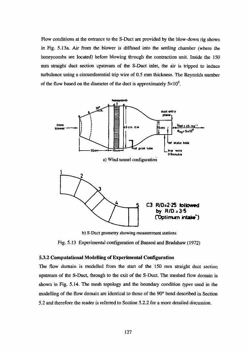
Flow conditions at the entrance to the S-Duct are provided by the blow-down rig shown
in Fig. 5.13a. Air from the blower is diffused into the settling chamber (where the
honeycombs are located) before blowing through the contraction unit. Inside the 150
mm straight duct section upstream of the S-Duct inlet, the air is tripped to induce
turbulence using a circumferential trip wire of 0.5 mm thickness. The Reynolds number
of the flow based on the diameter of the duct is approximately 5x 10⁵•
duct e"ltry plane
stat1c hole
trtp w.re O·Srnrn.d 1a
a) Wind tunnel configuration
C3 R/0:2·25 followwd by R/0 =3·5 \Optinun intat.•)
b) S-Duct geometry showing measurement stations
Fig. 5.13 Experimental configuration ofBansod and Bradshaw (1972)
5.3.2 Computational Modelling of Experimental Configuration
The flow domain is modelled from the start of the 150 mm straight duct section
upstream of the S-Duct, through to the exit of the S-Duct. The meshed flow domain is
shown in Fig. 5.14. The mesh topology and the boundary condition types used in the
modelling of the flow domain are identical to those of the 90° bend described in Section
5.2 and therefore the reader is referred to Section 5.2.2 for a more detailed discussion.
127
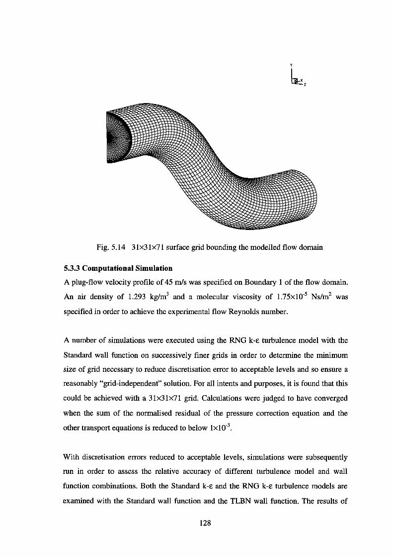
y
~z
Fig. 5.14 31x31x71 surface grid bounding the modelled flow domain
5.3.3 Computational Simulation
A plug-flow velocity profile of 45 m/s was specified on Boundary 1 of the flow domain.
An air density of 1.293 kg/m3 and a molecular viscosity of 1.75x10⁻⁵ Ns/m2 was
specified in order to achieve the experimental flow Reynolds number.
A number of simulations were executed using the RNG k-£ turbulence model with the
Standard wall function on successively finer grids in order to determine the minimum
size of grid necessary to reduce discretisation error to acceptable levels and so ensure a
reasonably "grid-independent" solution. For all intents and purposes, it is found that this
could be achieved with a 31x31x71 grid. Calculations were judged to have converged
when the sum of the normalised residual of the pressure correction equation and the
other transport equations is reduced to below 1xl0-3•
With discretisation errors reduced to acceptable levels, simulations were subsequently
run in order to assess the relative accuracy of different turbulence model and wall
function combinations. Both the Standard k-£ and the RNG k-£ turbulence models are
examined with the Standard wall function and the TLBN wall function. The results of
128
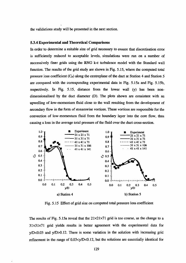
the validations study will be presented in the next section.
5.3.4 Experimental and Theoretical Comparisons
In order to determine a suitable size of grid necessary to ensure that discretisation error
is sufficiently reduced to acceptable levels, simulations were run on a number of
successively finer grids using the RNG k-E turbulence model with the Standard wall
function. The results of the grid study are shown in Fig. 5.15, where the computed total
pressure loss coefficient (Cp) along the centreplane of the duct at Station 4 and Station 5
are compared with the corresponding experimental data in Fig. 5.15a and Fig. 5.15b,
respectively. In Fig. 5.15, distance from the lower wall (y) has been non
dimensionalised by the duct diameter (D). The plots shown are consistent with an
upwelling of low-momentum fluid close to the wall resulting from the development of
secondary flow in the form of streamwise vortices. These vortices are responsible for the
convection of low-momentum fluid from the boundary layer into the core flow, thus
causing a loss in the average total pressure of the fluid over the duct cross-section.
1.0
0.9
0.8
0.7
0.6 ... 0.5 u
0.4
0.3
0.2
0.1
0.0
0.0
• Experiment -21 x21 x71 --31 x31 x71 ······41x41x71 --31 x31 x 106
41 X 41 X 141
0.1 0.2 0.3 0.4 0.5 y/D
a) Station 4
1.0
0.9
0.8
0.7
0.6
u 0.5
0.4
0.3
0.2
0.1
• Experiment 21 X 21 X 71
--31 x31 x71 ••• · ··41 x41 x 71 --31 x31 x 106
- 41 X 41 X 141
0.0 +--<--L..L.J...+-'-'-.1-l--f--'--L-L-L-J.--L-'-_,_y~~
0.0 0.1 0.2 0.3 0.4 0.5 y/D
b) Station 5
Fig. 5.15 Effect of grid size on computed total pressure loss coefficient
The results of Fig. 5.15a reveal that the 21x2lx71 grid is too coarse, as the change to a
3lx31x71 grid yields results in better agreement with the experimental data for
y/D<0.03 and y/D>0.12. There is some variation in the solution with increasing grid
refinement in the range of 0.03<y/D<0.12, but the solutions are essentially identical for
129
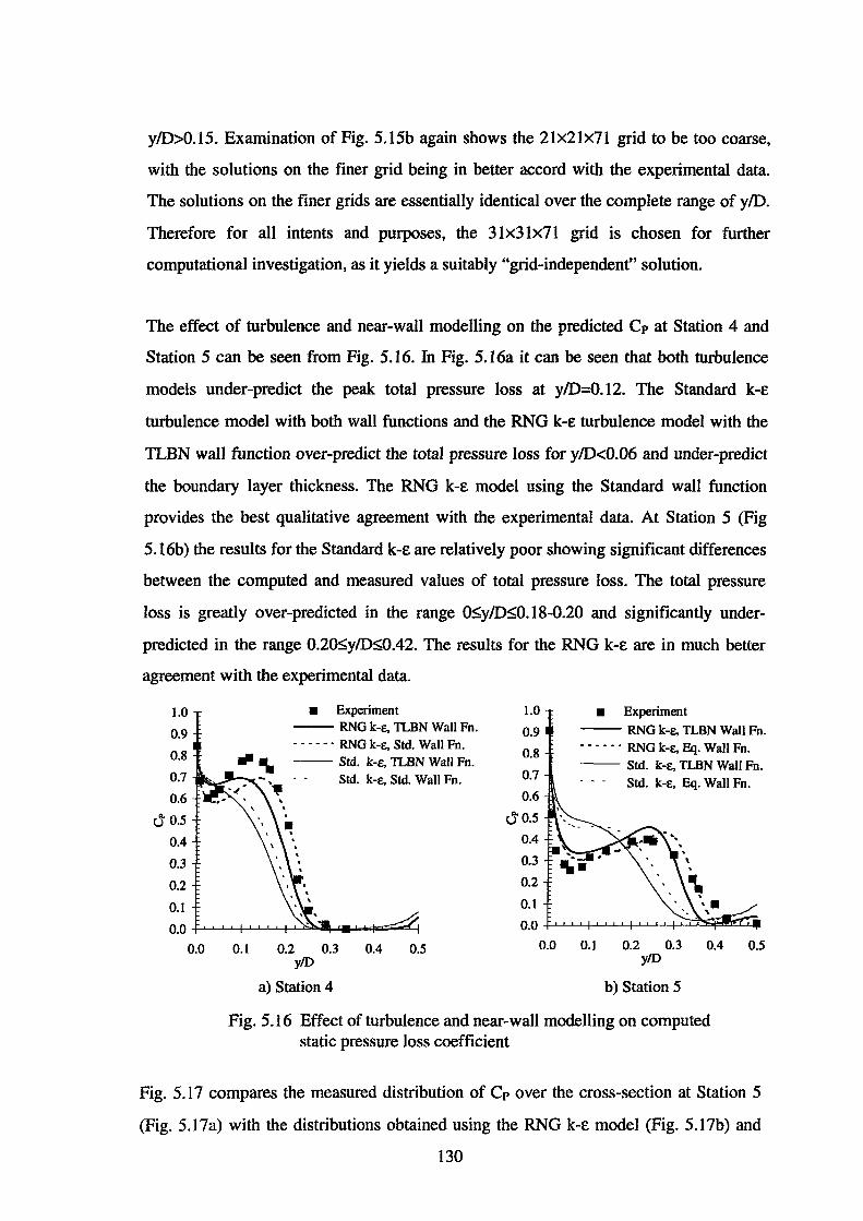
y/D>0.15. Examination of Fig. 5.15b again shows the 21x21x71 grid to be too coarse,
with the solutions on the finer grid being in better accord with the experimental data.
The solutions on the finer grids are essentially identical over the complete range of y/D.
Therefore for all intents and purposes, the 31x31x71 grid is chosen for further
computational investigation, as it yields a suitably "grid-independent" solution.
The effect of turbulence and near-wall modelling on the predicted Cp at Station 4 and
Station 5 can be seen from Fig. 5.16. In Fig. 5.16a it can be seen that both turbulence
models under-predict the peak total pressure loss at y/D=0.12. The Standard k-£
turbulence model with both wall functions and the RNG k-£ turbulence model with the
TLBN wall function over-predict the total pressure loss for y/D<0.06 and under-predict
the boundary layer thickness. The RNG k-£ model using the Standard wall function
provides the best qualitative agreement with the experimental data. At Station 5 (Fig
5.16b) the results for the Standard k-£ are relatively poor showing significant differences
between the computed and measured values of total pressure loss. The total pressure
loss is greatly over-predicted in the range 0$;y/D$;0.18-0.20 and significantly under
predicted in the range 0.20~y/D~0.42. The results for the RNG k-£ are in much better
agreement with the experimental data.
1.0
0.9
0.8
0.7
0.6
u 0.5
0.4
0.3
0.2
0.1
• Experiment -- RNG k-e, TLBN Wall Fn. • • • • • · RNG k-e, Std. Wall Fn. -- Std. k-e, TLBN Wall Fn.
Std. k-e, Std. Wall Fn.
0.0 +-c-.L.L-'-i---'-'-'-'--+~~!1-J.i ....... '*"'::W<~
0.0 0.1 0.2 0.3 0.4 0.5 y/D
a) Station 4
1.0
0.9
0.8
0.7
0.6
c)0.5
0.4
0.3
0.2
0.1
• Experiment
-- RNG k-e, TLBN Wall Fn. • • - • • · RNG k-e, Eq. Wall Fn. -- Std. k-t, TLBN Wall Fn.
Std. k-t, Eq. Wall Fn.
0.0 -f--.-.--'---'--1f--L--'-~..L-.1-14~~Pi!:r;~ 0.0 0.1 0.2 0.3 0.4 0.5
y/D
b) Station 5
Fig. 5.16 Effect of turbulence and near-wall modelling on computed static pressure loss coefficient
Fig. 5.17 compares the measured distribution of Cp over the cross-section at Station 5
(Fig. 5.17a) with the distributions obtained using the RNG k-£ model (Fig. 5.17b) and
130
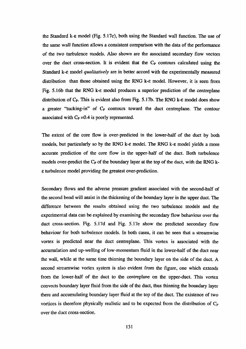
the Standard k-E model (Fig. 5.17c), both using the Standard wall function. The use of
the same wall function allows a consistent comparison with the data of the performance
of the two turbulence models. Also shown are the associated secondary flow vectors
over the duct cross-section. It is evident that the Cp contours calculated using the
Standard k-E model qualitatively are in better accord with the experimentally measured
distribution than those obtained using the RNG k-E model. However, it is seen from
Fig. 5.16b that the RNG k-E model produces a superior prediction of the centreplane
distribution of Cp. This is evident also from Fig. 5.17b. The RNG k-E model does show
a greater "tucking-in" of Cp contours toward the duct centreplane. The contour
associated with Cp =0.4 is poorly represented.
The extent of the core flow is over-predicted in the lower-half of the duct by both
models, but particularly so by the RNG k-E model. The RNG k-E model yields a more
accurate prediction of the core flow in the upper-half of the duct. Both turbulence
models over-predict the Cp of the boundary layer at the top of the duct, with the RNG k
E turbulence model providing the greatest over-prediction.
Secondary flows and the adverse pressure gradient associated with the second-half of
the second bend will assist in the thickening of the boundary layer in the upper duct. The
difference between the results obtained using the two turbulence models and the
experimental data can be explained by examining the secondary flow behaviour over the
duct cross-section. Fig. 5.17d and Fig. 5.17e show the predicted secondary flow
behaviour for both turbulence models. In both cases, it can be seen that a streamwise
vortex is predicted near the duct centreplane. This vortex is associated with the
accumulation and up-welling of low-momentum fluid in the lower-half of the duct near
the wall, while at the same time thinning the boundary layer on the side of the duct. A
second streamwise vortex system is also evident from the figure, one which extends
from the lower-half of the duct to the centreplane on the upper-duct. This vortex
convects boundary layer fluid from the side of the duct, thus thinning the boundary layer
there and accumulating boundary layer fluid at the top of the duct. The existence of two
vortices is therefore physically realistic and to be expected from the distribution of Cp
over the duct cross-section.
131
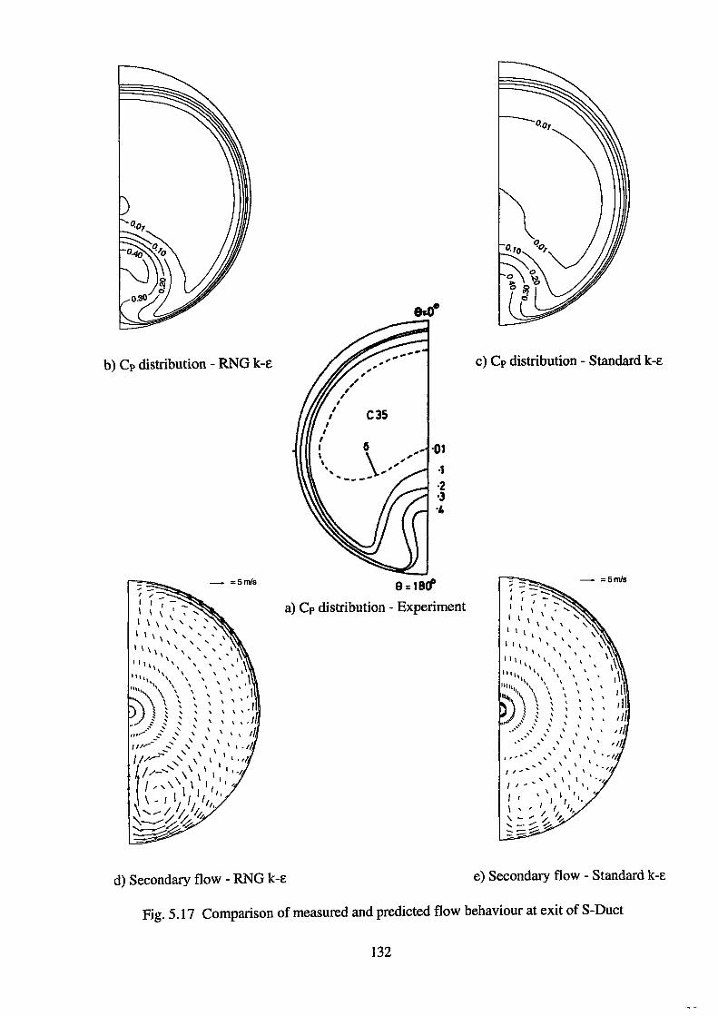
b) Cp distribution- RNG k-e
-- - =5mls ~::-:;-' I -I I I-
I \ ' ' I I 1 \ ' ' '
\ .... ' ' I I 1 1 ' , ' , 1 \'i
\ ' ' .\ l I \ I \ \ ' ' ' \ \1 I \ \ \ ' ' ... I\ ,,,, ', ' ' ' ... ~
\\ \ \ \ I
"''',, \ \ ' ' '' ' .. ,,,, ,, \ \ ' ' ' ' I I "" \ \ ' ' \ , 0 ' ' \ '' ' ' ' \ ~ ~ ' \ \ \ ' '~',
... ' ' ' l/1 ,/ .. ..:- ~ ~ \ ~ \ \ \ -,,,,~- _....... ' ' \ \ \ Jl
- ' ' \ \ f/// ,' \ \ I I .//, -- ' \ \ \ /I/.,.,- ,' \ I I,,~.
lf/-'' \\ I ,''•·t.
{
\ \ I ,,,\ 1\ If I
I ,, I,
,. \ - I I I I t,, ,, ....... ;I 1.~,: '\-.......-~~ ~ ~
,,' , I
, _...,.-
""',"'
/ C3S I
I I
~ 6\ ...... ·01 \ ,""' '..., ,' ·1 .... ___ ..
·2 ·3 .,
9 = 18cf
a) Cp distribution - Experiment
d) Secondary flow - RNG k-E
c) Cp distribution- Standard k-E
- =5mls
. '-I '•
e) Secondary flow- Standard k-E
Fig. 5.17 Comparison of measured and predicted flow behaviour at exit of S-Duct
132
The Standard k-E model under-predicts the intensity of the streamwise vortex in the
lower-duct resulting in insufficient accumulation of low-momentum fluid there. The
RNG k-E model on the other hand, tends to over-predict the strength of the secondary
flow resulting in the "tucking-in" of the total pressure contours toward the duct
centreplane. Both turbulence models most likely over-predict the secondary flow
associated with the upper vortex. This results in excessive accumulation of low
momentum fluid at the top of the duct. This is particularly evident for the RNG k-E
model (Fig. 5.17b and Fig. 5.17d) which shows larger secondary flow vectors close to
the wall than the Standard k-E model.
Fig. 5.18 shows the comparison between measured static pressure coefficient (Cp) and
that calculated using the RNG k-E turbulence model with the Standard wall function, on
the duct centreplane, at the top and bottom of the duct. Cp has been plotted against arc
length along the duct centreline (S) non-dimensionalised by the duct diameter (D). fu
fact, the other turbulence and near-wall modelling combinations used give essentially
identical results when plotted in the form of Fig. 5.18. It can be seen that good
agreement has been obtained between the computational results and the experimental
data over the first bend. The static pressure is also well predicted over the top of the first
half of the second bend, but deteriorates thereafter, with static pressure under-predicted
by Cp =0.08 at the duct exit. The static pressure over the bottom of the second bend is
over-predicted as a consequence of the failure to adequately predict the onset of the
region of separation/near-separation measured by Bansod and Bradshaw ( 1972).
Further insight into the inaccuracy in calculated static pressure distribution may be
obtained by considering the distribution of calculated and measured skin friction
coefficient (Cr) at the top and bottom of the duct centreplane, as we11 as the calculated
and measured mass-weighted total pressure loss coefficient ( Cp ) over the duct cross-
section. Calculated and measured CP is tabulated in Table 5.2 for the different
turbulence model and wall function combinations examined.
133

u
u
0.4
0.3
0.2
0.1
0.0
u"" -0.1
-0.2
-0.3
-0.4
-0.5
• Experiment - Top A Experiment - Bottom
--CFD-Top - CFD- Bottom
-0. 6 ..P....L...L.J...f-'-'--L..L..j-'-'-'-'-t-'-L...I...J...f-'-'--L..L..j-L..L..L.'-t-'-.L..L.J...f-'-'-.L...L.f-L.W..'-t-'-.L..L.J...f-'-'-.L...L.f-J...J...L.J...j
6.0E-03
5.0E-03
4.0E-03
3.0E-03
2.0E-03
I.OE-03
O.OE+OO
?.OE-03
6.0E-03
5.0E-03
4.0E-03
3.0E-03
2.0E-03
I.OE-03
O.OE+OO
0.0 0.5 1.0 1.5 2.0 2.5 3.0 3.5 4.0 4.5 5.0 5.5 6.0 SID
q 0
0 d
Fig. 5.18 Distribution of static pressure overS-Duct centreplane
Vl q "1 q Vl 0 Vl 0 Vl d N c-4 rri rri -o:i -o:i
SID
a) Top of S-Duct
Vl q "1 0 Vl q Vl 0 Vl d C'i C'i ('f'l <"i -o:i ...j
SID
b) Bottom of S-Duct
• Experiment - Top - RNG k-£, TLBN Wall Fn. • • • • • · RNG k-£, Std. Wall Fn. -- Std. k-e, TLBN Wall Fn.
- - Std. k-e, Std. Wall Fn.
• q "1 0
..0 Vl Vl
• Experiment
-- RNG k-£, TLBN Wall Fn. • • • • • · RNG k-e, Std. Wall Fn. -- Std. k-£, TLBN Wall Fn.
Std. k-£, Std. Wall Fn.
q "1 0 Vl Vl ..0
Fig. 5.19 Distribution of skin friction on S-Duct centreplane
134
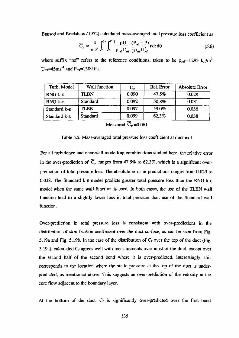
Bansod and Bradshaw ( 1972) calculated mass-averaged total pressure loss coefficient as
- 4 i21tlDn pU (P - P) Cp = --2 1
ret 2
rdrd8 1tD 0 0 PrerUref 2PrerUref
(5.6)
where suffix "ref' refers to the reference conditions, taken to be PreF 1.293 kglm3,
UreF45ms-1 and PreF1309 Pa.
Turb. Model Wall function Cp Rei. Error Absolute Error
RNGk-e TLBN 0.090 47.5% 0.029
RNGk-e Standard 0.092 50.8% 0.031
Standard k -e TLBN 0.097 59.0% 0.036
Standard k -e Standard 0.099 62.3% 0.038
Measured Cp =0.061
Table 5.2 Mass-averaged total pressure loss coefficient at duct exit
For all turbulence and near-wall modelling combinations studied here, the relative error
in the over-prediction of Cp ranges from 47.5% to 62.3%, which is a significant over
prediction of total pressure loss. The absolute error in predictions ranges from 0.029 to
0.038. The Standard k-e model predicts greater total pressure loss than the RNG k-e
model when the same wall function is used. In both cases, the use of the TLBN wall
function lead to a slightly lower loss in total pressure than use of the Standard wall
function.
Over-prediction in total pressure loss is consistent with over-predictions in the
distribution of skin friction coefficient over the duct surface, as can be seen from Fig.
5.19a and Fig. 5.19b. In the case of the distribution of Cr over the top of the duct (Fig.
5.19a), calculated Cr agrees well with measurements over most of the duct, except over
the second half of the second bend where it is over-predicted. Interestingly, this
corresponds to the location where the static pressure at the top of the duct is under
predicted, as mentioned above. This suggests an over-prediction of the velocity in the
core flow adjacent to the boundary layer.
At the bottom of the duct, Cr is significantly over-predicted over the first bend
135
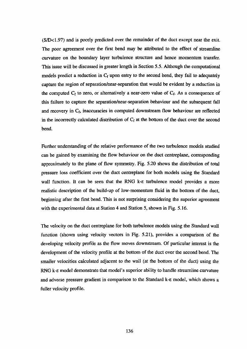
(S/0<1.97) and is poorly predicted over the remainder of the duct except near the exit.
The poor agreement over the first bend may be attributed to the effect of streamline
curvature on the boundary layer turbulence structure and hence momentum transfer.
This issue will be discussed in greater length in Section 5.5. Although the computational
models predict a reduction in Cr upon entry to the second bend, they fail to adequately
capture the region of separation/near-separation that would be evident by a reduction in
the computed Cr to zero, or alternatively a near-zero value of Cr. As a consequence of
this failure to capture the separation/near-separation behaviour and the subsequent fall
and recovery in Cr, inaccuracies in computed downstream flow behaviour are reflected
in the incorrectly calculated distribution of Cr at the bottom of the duct over the second
bend.
Further understanding of the relative performance of the two turbulence models studied
can be gained by examining the flow behaviour on the duct centreplane, corresponding
approximately to the plane of flow symmetry. Fig. 5.20 shows the distribution of total
pressure loss coefficient over the duct centreplane for both models using the Standard
wall function. It can be seen that the RNG k-E turbulence model provides a more
realistic description of the build-up of low-momentum fluid in the bottom of the duct,
beginning after the first bend. This is not surprising considering the superior agreement
with the experimental data at Station 4 and Station 5, shown in Fig. 5.16.
The velocity on the duct centreplane for both turbulence models using the Standard wall
function (shown using velocity vectors in Fig. 5.21), provides a comparison of the
developing velocity profile as the flow moves downstream. Of particular interest is the
development of the velocity profile at the bottom of the duct over the second bend. The
smaller velocities calculated adjacent to the wall (at the bottom of the duct) using the
RNG k-E model demonstrate that model's superior ability to handle streamline curvature
and adverse pressure gradient in comparison to the Standard k-E model, which shows a
fuller velocity profile.
136
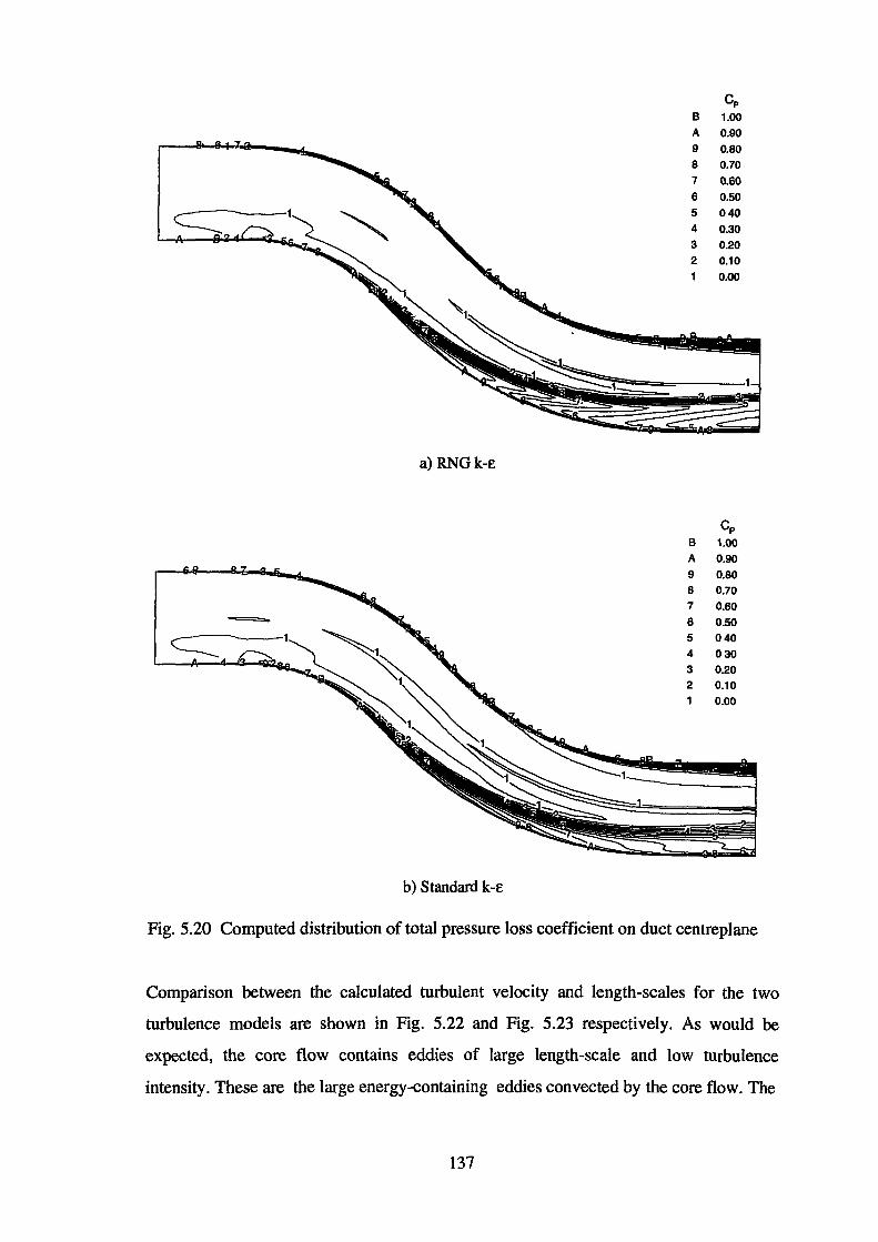
CP B 1.00 A 0.90 9 0.80 8 0.70 7 0.60 6 0.50 5 040 4 0.30 3 0.20 2 0.10
0.00
a)RNGk-E
Cp B 1.00 A 0.90 9 0.80 8 0.70 7 0.60 6 0.50 5 040 4 030 3 0.20 2 0.10
0.00
b) Standard k -£
Fig. 5.20 Computed distribution of total pressure loss coefficient on duct centreplane
Comparison between the calculated turbulent velocity and length-scales for the two
turbulence models are shown in Fig. 5.22 and Fig. 5.23 respectively. As would be
expected, the core flow contains eddies of large length-scale and low turbulence
intensity. These are the large energy-containing eddies convected by the core flow. The
137
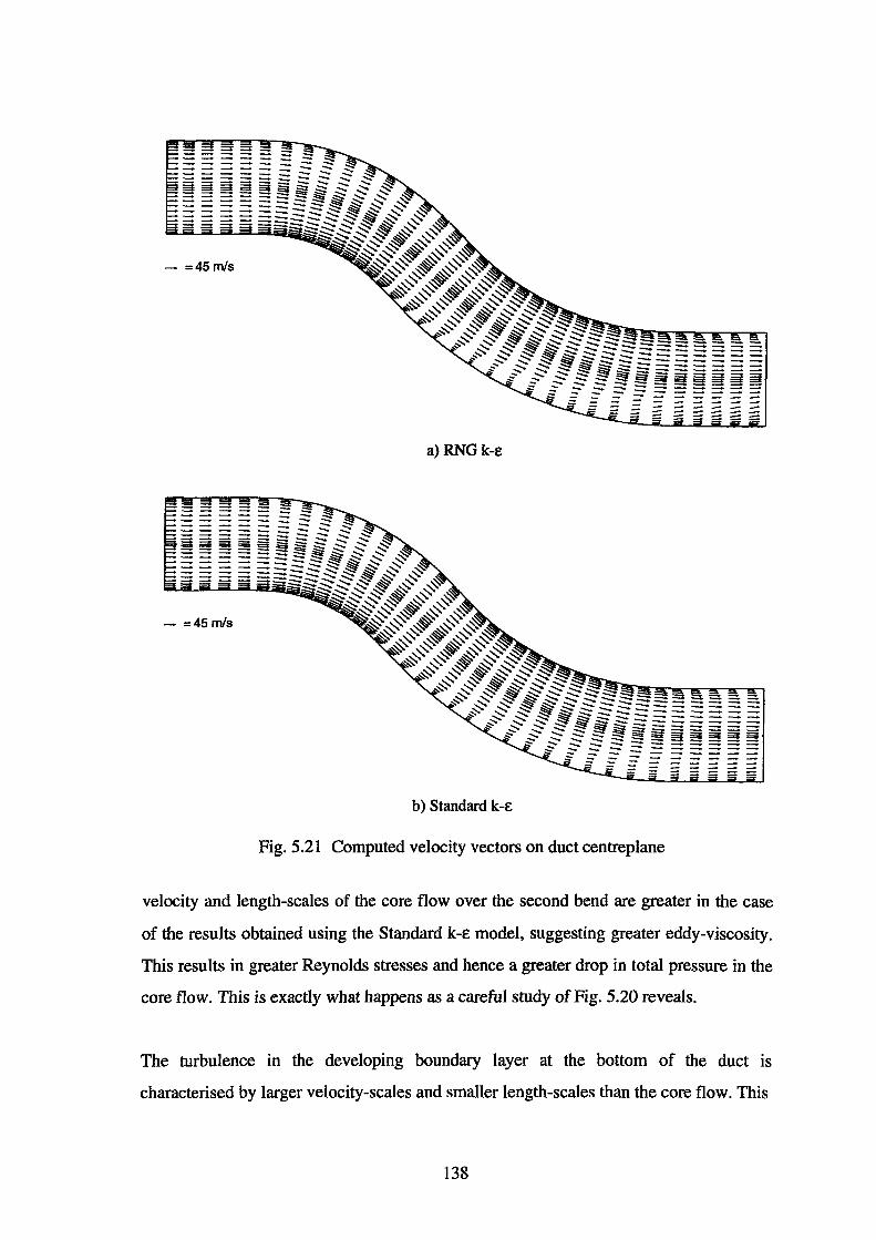
a)RNGk-E
b) Standard k-E
Fig. 5.21 Computed velocity vectors on duct centreplane
velocity and length-scales of the core flow over the second bend are greater in the case
of the results obtained using the Standard k-E model, suggesting greater eddy-viscosity.
This results in greater Reynolds stresses and hence a greater drop in total pressure in the
core flow. This is exactly what happens as a careful study of Fig. 5.20 reveals.
The turbulence in the developing boundary layer at the bottom of the duct is
characterised by larger velocity-scales and smaller length-scales than the core flow. This
138
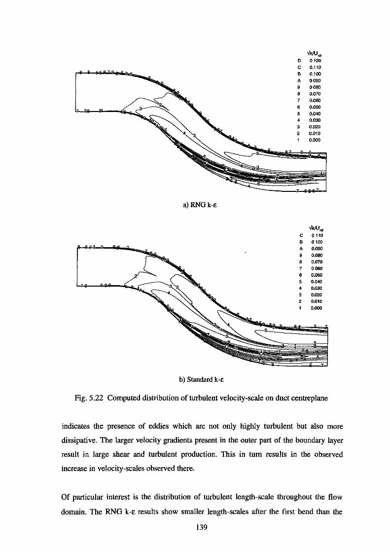
..Jk/Uref 0 0120 c 0.110
0.100 0090 0080 0.070 0.060 0.050 0.040 0.030 0.020 0.010 0.000
a)RNGk-E
..Jk/Urer c 0110 B 0100 A 0.090 9 0.080 8 0.070 7 0060 6 0.050 5 0.040 4 0.030 3 0.020 2 0.010
0.000
b) Standard k-E
Fig. 5.22 Computed distribution of turbulent velocity-scale on duct centreplane
indicates the presence of eddies which are not only highly turbulent but also more
dissipative. The larger velocity gradients present in the outer part of the boundary layer
result in large shear and turbulent production. This in turn results in the observed
increase in velocity-scales observed there.
Of particular interest is the distribution of turbulent length-scale throughout the flow
domain. The RNG k-£ results show smaller length-scales after the first bend than the
139
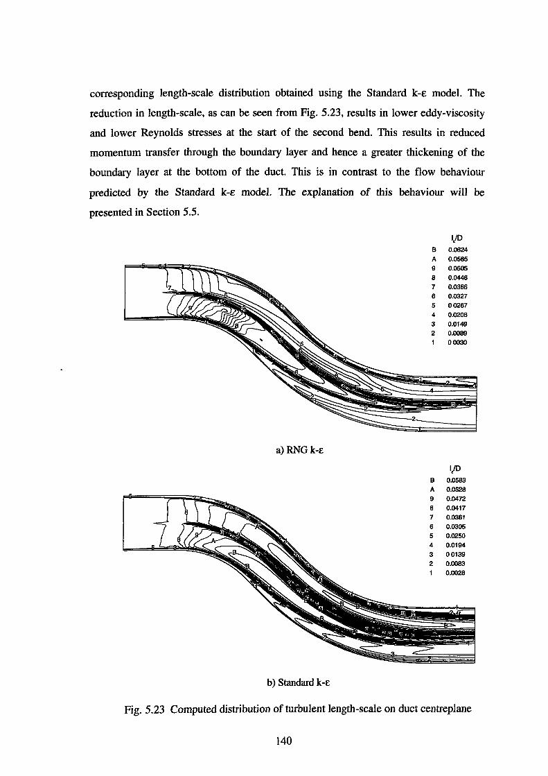
corresponding length-scale distribution obtained using the Standard k-E model. The
reduction in length-scale, as can be seen from Fig. 5.23, results in lower eddy-viscosity
and lower Reynolds stresses at the start of the second bend. This results in reduced
momentum transfer through the boundary layer and hence a greater thickening of the
boundary layer at the bottom of the duct. This is in contrast to the flow behaviour
predicted by the Standard k-E model. The explanation of this behaviour will be
presented in Section 5.5.
1/D B 0.0624 A 0.0565 9 0.0505 8 0.0446 7 0.0386 6 0.0327 5 00267 4 0.0208 3 0.0149 2 0.0089
00030
a)RNGk-E
1/D B 0.0583 A 0.0528 9 0.0472 8 0.0417 7 0.0361 6 0.0305 5 0.0250 4 0.0194 3 00139 2 0.0083
0.0028
b) Standard k-E
Fig. 5.23 Computed distribution of turbulent length-scale on duct centreplane
140
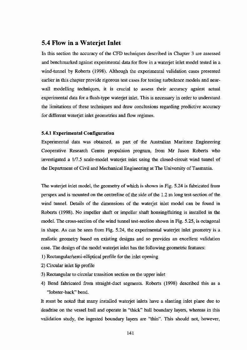
5.4 Flow in a W aterjet Inlet
In this section the accuracy of the CFD techniques described in Chapter 3 are assessed
and benchmarked against experimental data for flow in a waterjet inlet model tested in a
wind-tunnel by Roberts (1998). Although the experimental validation cases presented
earlier in this chapter provide rigorous test cases for testing turbulence models and near
wall modelling techniques, it is crucial to assess their accuracy against actual
experimental data for a flush-type waterjet inlet. This is necessary in order to understand
the limitations of these techniques and draw conclusions regarding predictive accuracy
for different waterjet inlet geometries and flow regimes.
5.4.1 Experimental Configuration
Experimental data was obtained, as part of the Australian Maritime Engineering
Cooperative Research Centre propulsion program, from Mr Jason Roberts who
investigated a 117.5 scale-model waterjet inlet using the closed-circuit wind tunnel of
the Department of Civil and Mechanical Engineering at The University of Tasmania.
The waterjet inlet model, the geometry of which is shown in Fig. 5.24 is fabricated from
perspex and is mounted on the centreline of the side of the 1.2 m long test -section of the
wind tunnel. Details of the dimensions of the waterjet inlet model can be found in
Roberts (1998). No impeller shaft or impeller shaft housing/fairing is installed in the
model. The cross-section of the wind tunnel test-section shown in Fig. 5.25, is octagonal
in shape. As can be seen from Fig. 5.24, the experimental waterjet inlet geometry is a
realistic geometry based on existing designs and so provides an excellent validation
case. The design of the model waterjet inlet has the following geometric features:
1) Rectangular/semi-elliptical profile for the inlet opening
2) Circular inlet lip profile
3) Rectangular to circular transition section on the upper inlet
4) Bend fabricated from straight-duct segments. Roberts (1998) described this as a
"lobster-back" bend.
It must be noted that many installed waterjet inlets have a slanting inlet plane due to
deadrise on the vessel hull and operate in "thick" hull boundary layers, whereas in this
validation study, the ingested boundary layers are "thin". This should not, however,
141
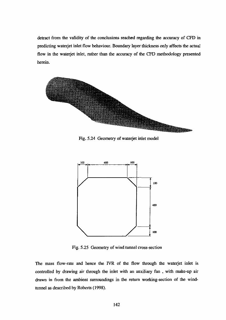
detract from the validity of the conclusions reached regarding the accuracy of CFD in
predicting waterjet inlet flow behaviour. Boundary layer thickness only affects the actual
flow in the waterjet inlet, rather than the accuracy of the CFD methodology presented
herein.
Fig. 5.24 Geometry of waterjet inlet model
100 400 100
100
400
100
Fig. 5.25 Geometry of wind tunnel cross-section
The mass flow-rate and hence the IVR of the flow through the waterjet inlet is
controlled by drawing air through the inlet with an auxiliary fan , with make-up air
drawn in from the ambient surroundings in the return working-section of the wind
tunnel as described by Roberts ( 1998).
142
5.4.2 Computational Modelling of Experimental Configuration
Inlet3D was modified to mesh the experimental geometry. In particular, the main
modifications are made to incorporate the polynomial ramp profile and the specific
rectangular to circular transition geometry on the upper part of the inlet. In these two
respects, the model waterjet inlet differed from that of the generic parametric geometry
described in Chapter 4. A smooth bend is used to represent the segmented ("lobster
back") bend geometry present in the experimental model.
An obvious limitation of the mesh topology used by Inlet3D is the difficulty in
representing the geometry of the wind tunnel test-section (domain external to the
waterjet inlet). The mesh topology used by Roberts (1998) meshes the test-section
geometry in a more natural manner, but suffers from other limitations. It was therefore
decided to use the generic external domain produced by Inlet3D, with the underlying
assumption that the flow around the inlet is affected by the geometry and flow
conditions "close" to the inlet, that is in the immediate vicinity of the waterjet inlet. The
validity of this assumption therefore, also has an effect on the choice of boundary
conditions applied to the flow domain.
Since the flow in the waterjet inlet and external domain may be considered to be
symmetrical about the vertical plane of symmetry of the waterjet inlet, only half of the
external domain is meshed. It will be shown in later sections that the flow in the inlet
exhibits a gross swirl (evident from the data supplied for IVR=0.61) at the duct exit and
the reason for this behaviour will be explained. Since the distortion of the total pressure
distribution at the duct exit is relatively small in circumferential deviation from the
vertical centreplane of the duct, meshing only one-half of the waterjet inlet and external
domain is justified. In addition, this approach requires half of the grid size that would
otherwise be required for a given spatial discretisation of the flow domain.
The topology used by Inlet3D to mesh a wateijet inlet and a simplified flow domain
external to it was discussed in Section 4.2. Since the flow under consideration here
exhibits "stationary turbulence", the RANS equations assume an elliptic form thus
requiring the specification of Dirichlet or Neumann boundary conditions on all surfaces
143
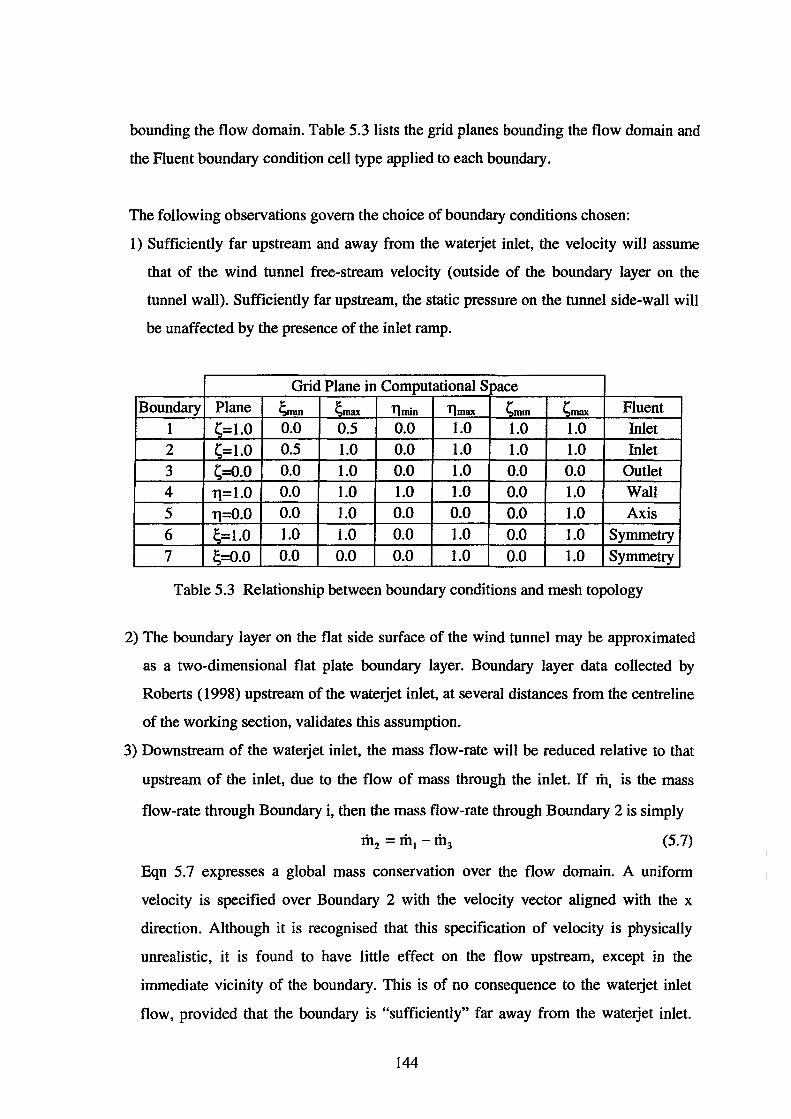
bounding the flow domain. Table 5.3 lists the grid planes bounding the flow domain and
the Fluent boundary condition cell type applied to each boundary.
The following observations govern the choice of boundary conditions chosen:
1) Sufficiently far upstream and away from the waterjet inlet, the velocity will assume
that of the wind tunnel free-stream velocity (outside of the boundary layer on the
tunnel wall). Sufficiently far upstream, the static pressure on the tunnel side-wall will
be unaffected by the presence of the inlet ramp.
Grid Plane in Computational Space Boundary Plane ~IDln ~max Tlmin Tlmax ~IDJD ~max Fluent
1 ~=1.0 0.0 0.5 0.0 1.0 1.0 1.0 Inlet 2 ~=1.0 0.5 1.0 0.0 1.0 1.0 1.0 Inlet 3 ~=0.0 0.0 1.0 0.0 1.0 0.0 0.0 Outlet 4 11=1.0 0.0 1.0 1.0 1.0 0.0 1.0 Wall 5 TJ=O.O 0.0 1.0 0.0 0.0 0.0 1.0 Axis 6 ~=1.0 1.0 1.0 0.0 1.0 0.0 1.0 Symmetry 7 ~=0.0 0.0 0.0 0.0 1.0 0.0 1.0 Symmetry
Table 5.3 Relationship between boundary conditions and mesh topology
2) The boundary layer on the flat side surface of the wind tunnel may be approximated
as a two-dimensional flat plate boundary layer. Boundary layer data collected by
Roberts ( 1998) upstream of the waterjet inlet, at several distances from the centreline
of the working section, validates this assumption.
3) Downstream of the waterjet inlet, the mass flow-rate will be reduced relative to that
upstream of the inlet, due to the flow of mass through the inlet. If m. is the mass
flow-rate through Boundary i, then the mass flow-rate through Boundary 2 is simply
(5.7)
Eqn 5.7 expresses a global mass conservation over the flow domain. A uniform
velocity is specified over Boundary 2 with the velocity vector aligned with the x
direction. Although it is recognised that this specification of velocity is physically
unrealistic, it is found to have little effect on the flow upstream, except in the
immediate vicinity of the boundary. This is of no consequence to the waterjet inlet
flow, provided that the boundary is "sufficiently" far away from the waterjet inlet.
144
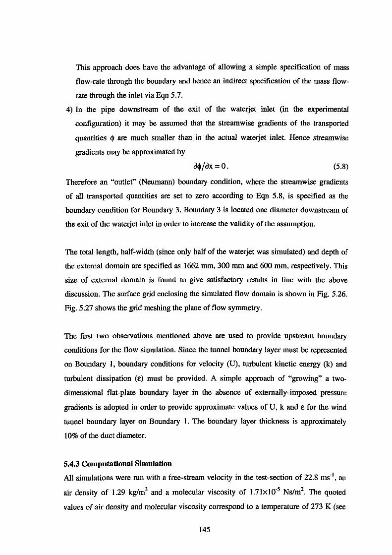
This approach does have the advantage of allowing a simple specification of mass
flow-rate through the boundary and hence an indirect specification of the mass flow
rate through the inlet via Eqn 5.7.
4) In the pipe downstream of the exit of the waterjet inlet (in the experimental
configuration) it may be assumed that the streamwise gradients of the transported
quantities <P are much smaller than in the actual waterjet inlet. Hence streamwise
gradients may be approximated by
aq,jax = 0. (5.8)
Therefore an "outlet" (Neumann) boundary condition, where the streamwise gradients
of all transported quantities are set to zero according to Eqn 5.8, is specified as the
boundary condition for Boundary 3. Boundary 3 is located one diameter downstream of
the exit of the waterjet inlet in order to increase the validity of the assumption.
The total length, half-width (since only half of the waterjet was simulated) and depth of
the external domain are specified as 1662 mm, 300 mm and 600 mm, respectively. This
size of external domain is found to give satisfactory results in line with the above
discussion. The surface grid enclosing the simulated flow domain is shown in Fig. 5.26.
Fig. 5.27 shows the grid meshing the plane of flow symmetry.
The first two observations mentioned above are used to provide upstream boundary
conditions for the flow simulation. Since the tunnel boundary layer must be represented
on Boundary 1, boundary conditions for velocity (U), turbulent kinetic energy (k) and
turbulent dissipation (E) must be provided. A simple approach of "growing" a two
dimensional flat-plate boundary layer in the absence of externally-imposed pressure
gradients is adopted in order to provide approximate values of U, k and E for the wind
tunnel boundary layer on Boundary 1. The boundary layer thickness is approximately
10% of the duct diameter.
5.4.3 Computational Simulation
All simulations were run with a free-stream velocity in the test-section of 22.8 ms-1, an
air density of 1.29 kg/m3 and a molecular viscosity of 1.7lxl0-5 Ns/m2. The quoted
values of air density and molecular viscosity correspond to a temperature of 273 K (see
145
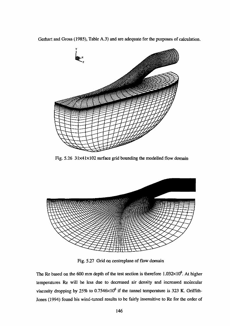
Gerhart and Gross (1985), Table A.3) and are adequate for the purposes of calculation.
v
~X z
Fig. 5.26 31x41xl02 surface grid bounding the modelled flow domain
Fig. 5.27 Grid on centreplane of flow domain
TheRe based on the 600 mm depth of the test section is therefore 1.032x10⁶• At higher
temperatures Re will be less due to decreased air density and increased molecular
viscosity dropping by 25% to 0.7546x10⁶ if the tunnel temperature is 323 K. Griffith
Jones (1994) found his wind-tunnel results to be fairly insensitive toRe for the order of
146
magnitude of the Re (order of 1 05) used in his experiments. The tunnel free-stream
velocity is deduced from static pressure and static pressure coefficient data supplied to
the author by Mr Roberts assuming the above air density.
Computations were initially performed on a 31x41x102 grid for a nominal IVR of 0.61
using the RNG k-e turbulence model with the TLBN wall function. The grid was
subsequently separately doubled in each computational coordinate direction in order to
determine the effect of grid refinement on the solution. The solutions obtained on the
31x41xl02 grid were used as starting solutions for these cases. Due to the limitations of
the hardware it was not possible to double the grid in all computational coordinate
directions simultaneously. Therefore it was not possible to obtain a definitive conclusion
as to how close the solutions (on the 31x41x102 grid) are to grid-independency.
Calculations are deemed to have converged when the sum of the normalised residuals of
the transport equations and the pressure correction equation fall below lx10-3.
In order to compare the effect of turbulence and near-wall modelling on the solution,
calculations were run using the Standard wall function. The effect of the choice of
turbulence model (at an IVR value of 0.61) is examined by repeating the computations
using the Standard k-e model with the TLBN wall function. Computations were then
made for IVR values of 0.68, 0.80 and 0.97 using the RNG k-e turbulence model with
the TLBN wall function in order to assess the accuracy of CFD calculation at these
values of IVR.
5.4.4 Experimental and Theoretical Comparisons
Comparison between experimental data and CFD calculations are presented for a test
case having a nominal IVR of 0.61. Comparison between measured and calculated static
pressure distributions for higher IVR are then presented. Results have been presented for
the above-mentioned range of values of IVR in order to analyse the trends in predicted
flow behaviour over the range of IVR examined.
Fig. 5.28 shows a comparison between the measured boundary layer velocity and
turbulence intensity profiles 0.5D upstream of the ramp tangency point. It can be seen
147
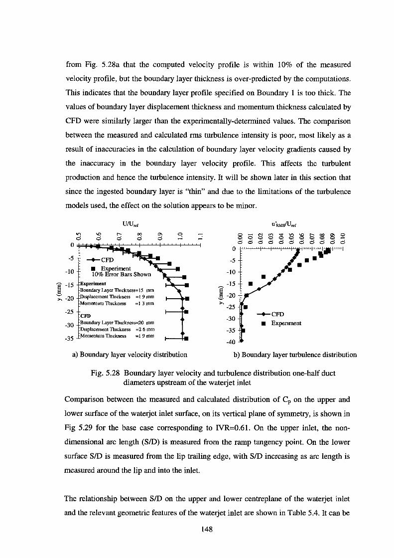
s E '-'
from Fig. 5.28a that the computed velocity profile is within 10% of the measured
velocity profile, but the boundary layer thickness is over-predicted by the computations.
This indicates that the boundary layer profile specified on Boundary 1 is too thick. The
values of boundary layer displacement thickness and momentum thickness calculated by
CFD were similarly larger than the experimentally-determined values. The comparison
between the measured and calculated rms turbulence intensity is poor, most likely as a
result of inaccuracies in the calculation of boundary layer velocity gradients caused by
the inaccuracy in the boundary layer velocity profile. This affects the turbulent
production and hence the turbulence intensity. It will be shown later in this section that
since the ingested boundary layer is "thin" and due to the limitations of the turbulence
models used, the effect on the solution appears to be minor.
II) 00 0 0
ot¥~~~~~~~~~
-5 -+-CFD
-10 • Experiment 10% Error Bars Shown
-15 xperiment Boundary Layer Thickness= 15 mm
0
-5
-10
-15 ,...... E
0 0 0 0 0
s 0
8 ~ ~ 8 8 ~ 8 s 0 0 0 0 0 0 0 0
1splacement Thickness =19mm >. -20 E -20 '-'
Momentum Thickness =13mm >. -25
-25 CFD
-30 Boundary Layer Thlckness=20 mm Displacement Thickness =26mm
-+-CFD
• Expenment -30
-35 -35 Momentum Thickness =19mm
-40
a) Boundary layer velocity distribution b) Boundary layer turbulence distribution
Fig. 5.28 Boundary layer velocity and turbulence distribution one-half duct diameters upstream of the waterjet inlet
Comparison between the measured and calculated distribution of Cp on the upper and
lower surface of the waterjet inlet surface, on its vertical plane of symmetry, is shown in
Fig 5.29 for the base case corresponding to IVR=0.61. On the upper inlet, the non
dimensional arc length (SID) is measured from the ramp tangency point. On the lower
surface SID is measured from the lip trailing edge, with SID increasing as arc length is
measured around the lip and into the inlet.
The relationship between SID on the upper and lower centreplane of the waterjet inlet
and the relevant geometric features of the waterjet inlet are shown in Table 5.4. It can be
148
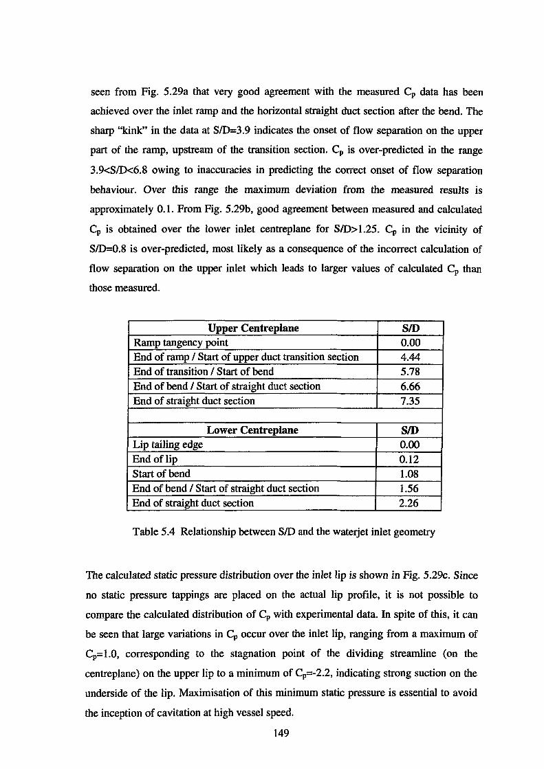
seen from Fig. 5.29a that very good agreement with the measured Cp data has been
achieved over the inlet ramp and the horizontal straight duct section after the bend. The
sharp "kink" in the data at SID=3.9 indicates the onset of flow separation on the upper
part of the ramp, upstream of the transition section. Cp is over-predicted in the range
3.9<SID<6.8 owing to inaccuracies in predicting the correct onset of flow separation
behaviour. Over this range the maximum deviation from the measured results is
approximately 0.1. From Fig. 5.29b, good agreement between measured and calculated
Cp is obtained over the lower inlet centreplane for SID> 1.25. Cp in the vicinity of
SID=0.8 is over-predicted, most likely as a consequence of the incorrect calculation of
flow separation on the upper inlet which leads to larger values of calculated Cp than
those measured.
Upper Centreplane SID Ramp tangency point 0.00 End of ramp I Start of upper duct transition section 4.44 End of transition I Start of bend 5.78 End of bend I Start of straight duct section 6.66 End of straight duct section 7.35
Lower Centreplane SID Lip tailing edge 0.00 End of lip 0.12 Start of bend 1.08 End of bend I Start of straight duct section 1.56 End of straight duct section 2.26
Table 5.4 Relationship between SID and the waterjet inlet geometry
The calculated static pressure distribution over the inlet lip is shown in Fig. 5.29c. Since
no static pressure tappings are placed on the actual lip profile, it is not possible to
compare the calculated distribution of Cp with experimental data. In spite of this, it can
be seen that large variations in Cp occur over the inlet lip, ranging from a maximum of
Cp= 1.0, corresponding to the stagnation point of the dividing streamline (on the
centreplane) on the upper lip to a minimum of Cp=-2.2, indicating strong suction on the
underside of the lip. Maximisation of this minimum static pressure is essential to avoid
the inception of cavitation at high vessel speed.
149
In order to test the sensitivity of the solution to changes in grid size, the grid is doubled
in each computational coordinated direction. No notable change in the solution occurred
as can be seen from Fig. 5.29c and Fig. 5.32a. A complete doubling of the gird in two or
all coordinate directions simultaneously would have been beyond the capability of the
hardware and was therefore not undertaken. While it cannot be claimed that the
computational solution is by any means "grid-independent", it appears from the above
mentioned grid investigation and the results presented in this section, that a reasonable
level of discretisation error has been achieved.
Fig. 5.30 shows the effect of turbulence and near-wall modelling on the calculated
distribution of Cp on the inlet centreplane for an IVR of 0.61. It can be seen that the
Standard k-E turbulence model yields results that are inferior to those obtained using the
RNG k-E turbulence model, although the differences between the two results are not
large. The static pressure distributions appear to be insensitive to the wall function used.
The cross-sectional distribution of total pressure and secondary flow at the duct exit of
the waterjet inlet is of particular relevance to pump operation as it defines the operating
environment of the pump and hence the effect on pump performance and operational
efficiency of the waterjet unit. The measured distribution of total pressure coefficient
(Cp) at the duct exit is shown in Fig. 5.31a, together with the computed distribution of
Cp in Fig. 5.31c, both at an IVR of 0.61. It is interesting to note that the measured Cp
distribution is asymmetrical about the vertical plane of symmetry of the waterjet inlet,
thus indicating a slight gross swirling motion of the flow. The rotation of the total
pressure distribution about the centreplane is approximately 15° and is therefore small in
circumferential extent. This gross swirl occurs as a result of a combination of the
interaction between flow asymmetries in the inflow to the side-mounted waterjet inlet
(Roberts ( 1998) attributed this to thermal convection in the vertical direction within the
wind tunnel, caused by temperature differentials in the tunnel air), bend pressure
gradients and flow separation. Guo and Seddon (1983a) found that an S-shaped inlet
duct (centreplane lying in the horizontal plane) operating with flow separation at the
inlet lip due to an angle of incidence in the vertical plane, would develop a gross
swirling pattern.
150
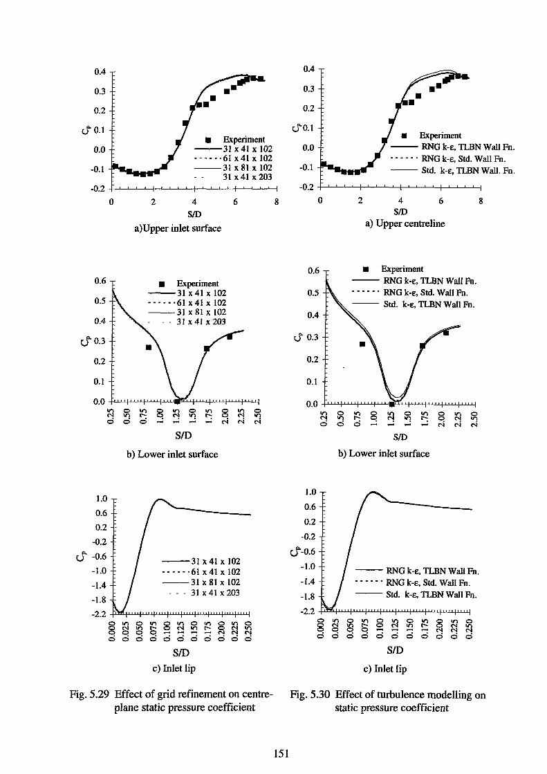
0.4
0.3
0.2
uc. 0.1
0.0
-0.1
-0.2
0.6
0.5
0.4
uc. 0.3
0.2
0.1
1.0
0.6
0.2
-0.2
u -0.6
-1.0
-1.4
-1.8
-2.2
0
0 0 0 0
• Experiment --31 X 41 X 102 • • • • • · 61 X 41 X 102 --31 X 81 X 102
31 X 41 X 203
2 4
SID
a) Upper inlet surface
• Experiment --31 X 41 X 102 • • • • • • 61 X 41 X 102 --31 X 81 X 102
- - 31 X 41 X 203
lf'l 0 C'! 111 - -SID
6
b) Lower inlet surface
lf'l 0 C'l lf'l 0 q 0 0
lf'l s 0
--31 x41 x 102 • • • • • · 61 X 41 X 102 --31 X 81 X 102
- - - 31 X 41 X 203
0 lf'l 0 lf'l 0 lf'l 0 C'l lf'l r- 0 C'l - -- - C'l C'l 0 0 0 0 0 0
SID
c) Inlet lip
0 lf'l C'l 0
Fig. 5.29 Effect of grid refinement on centreplane static pressure coefficient
8
151
0.4
0.3
0.2
d'"0.1
0.0
-0.1
-0.2
0
0.6
0.5
0.4
uc. 0.3
0.2
0.1
1.0
0.6
0.2
-0.2
uc.-0.6
-1.0
-1.4
-1.8
-2.2 0
8 0
• Experiment -- RNGk-E, TLBNWallFn. • • • • • · RNG k-E, Std. Wall Fn. -- Std. k-E, TLBN Wall. Fn.
2 4 SID
6
a) Upper centreline
• Experiment -- RNG k-E, TLBN Wall Fn. • • • - • · RNG k-E, Std. Wall Fn. -- Std. k-E, TLBN Wall Fn.
SID
8
b) Lower inlet surface
lf'l 0 C'l lf'l 0 q 0 0
-- RNG k-E, TLBN Wall Fn. • • • • • · RNG k-E, Std. Wall Fn. -- Std. k-E, TLBN Wall Fn.
lf'l 0 lf'l 0 lf'l 0 lf'l 0 r- 0 C'l lf'l r- 0 C'l lf'l 0 - - - - C'l C'l C'l 0 0 0 0 0 0 0 0
SID
c) Inlet lip
Fig. 5.30 Effect of turbulence modelling on static pressure coefficient
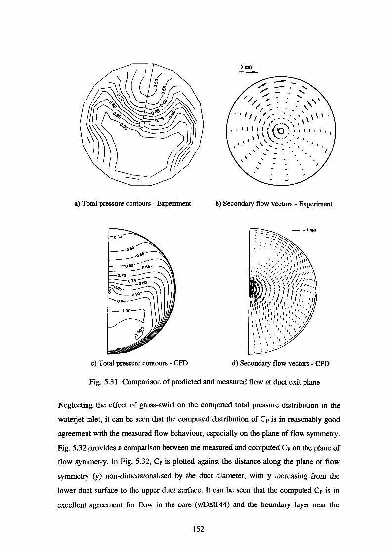
a) Total pressure contours - Experiment
c) Total pressure contours - CFD
Sm!s -~
"/ /- ..... / / ..... ,,, // "' . . . '
• I I I ; "'. . . . . '' \ \ \ ,,,_ .. _, \ 1/--,•,\
, , I I I I I { (o ~ ', , t 1 I 1
\ \ \ \ ' --·· ... \\ ,'' ....... •', •I
' .. . .
' '
' .. -' ... -... ...
b) Secondary flow vectors - Experiment
d) Secondary flow vectors - CFD
Fig. 5.31 Comparison of predicted and measured flow at duct exit plane
Neglecting the effect of gross-swirl on the computed total pressure distribution in the
waterjet inlet, it can be seen that the computed distribution of Cp is in reasonably good
agreement with the measured flow behaviour, especially on the plane of flow symmetry.
Fig. 5.32 provides a comparison between the measured and computed Cp on the plane of
flow symmetry. In Fig. 5.32, Cp is plotted against the distance along the plane of flow
symmetry (y) non-dimensionalised by the duct diameter, with y increasing from the
lower duct surface to the upper duct surface. It can be seen that the computed Cp is in
excellent agreement for flow in the core (y/Ds;0.44) and the boundary layer near the
152
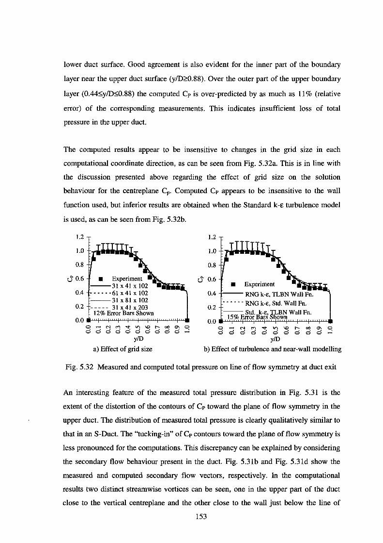
lower duct surface. Good agreement is also evident for the inner part of the boundary
layer near the upper duct surface (y/D;:::0.88). Over the outer part of the upper boundary
layer (0.44:s;y/D::;0.88) the computed Cp is over-predicted by as much as 11% (relative
error) of the corresponding measurements. This indicates insufficient loss of total
pressure in the upper duct.
The computed results appear to be insensitive to changes in the grid size in each
computational coordinate direction, as can be seen from Fig. 5.32a. This is in line with
the discussion presented above regarding the effect of grid size on the solution
behaviour for the centreplane Cp. Computed Cp appears to be insensitive to the wall
function used, but inferior results are obtained when the Standard k-E turbulence model
is used, as can be seen from Fig. 5.32b.
1.2
1.0
0.8
u 0.6 • Experiment ~---31 X 41 X 102
0.4 ·····61x41x102 ~--- 31 X 81 X 102
0.2 - - - - - 31 X 41 X 203 12% Error Bars Shown
0 N ~ ~ ~ ~ ~ 00 ~ ~ 0 0 0 0 0 0 0 0 0 0
y/D
a) Effect of grid size
1.2
1.0
0.8
u 0.6 • Experiment
0.4 -+--- RNG k-E, TLBN Wall Fn.
0 - N ~ ~ ~ ~ ~ 00 ~ 0 0 0 0 0 0 0 0 0 0 0 ~
y/D
b) Effect of turbulence and near-wall modelling
Fig. 5.32 Measured and computed total pressure on line of flow symmetry at duct exit
An interesting feature of the measured total pressure distribution in Fig. 5.31 is the
extent of the distortion of the contours of Cp toward the plane of flow symmetry in the
upper duct. The distribution of measured total pressure is clearly qualitatively similar to
that in an S-Duct. The "tucking-in" of Cp contours toward the plane of flow symmetry is
less pronounced for the computations. This discrepancy can be explained by considering
the secondary flow behaviour present in the duct. Fig. 5.31b and Fig. 5.31d show the
measured and computed secondary flow vectors, respectively. In the computational
results two distinct streamwise vortices can be seen, one in the upper part of the duct
close to the vertical centreplane and the other close to the wall just below the line of
153
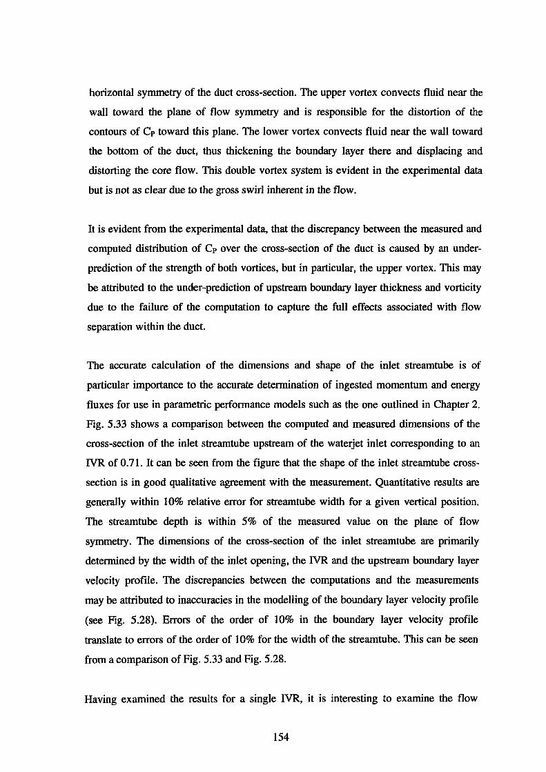
horizontal symmetry of the duct cross-section. The upper vortex convects fluid near the
wall toward the plane of flow symmetry and is responsible for the distortion of the
contours of Cp toward this plane. The lower vortex convects fluid near the wall toward
the bottom of the duct, thus thickening the boundary layer there and displacing and
distorting the core flow. This double vortex system is evident in the experimental data
but is not as clear due to the gross swirl inherent in the flow.
It is evident from the experimental data, that the discrepancy between the measured and
computed distribution of Cp over the cross-section of the duct is caused by an under
prediction of the strength of both vortices, but in particular, the upper vortex. This may
be attributed to the under-prediction of upstream boundary layer thickness and vorticity
due to the failure of the computation to capture the full effects associated with flow
separation within the duct.
The accurate calculation of the dimensions and shape of the inlet streamtube is of
particular importance to the accurate determination of ingested momentum and energy
fluxes for use in parametric performance models such as the one outlined in Chapter 2.
Fig. 5.33 shows a comparison between the computed and measured dimensions of the
cross-section of the inlet streamtube upstream of the waterjet inlet corresponding to an
IVR of 0.71. It can be seen from the figure that the shape of the inlet streamtube cross
section is in good qualitative agreement with the measurement. Quantitative results are
generally within 10% relative error for streamtube width for a given vertical position.
The streamtube depth is within 5% of the measured value on the plane of flow
symmetry. The dimensions of the cross-section of the inlet streamtube are primarily
determined by the width of the inlet opening, the IVR and the upstream boundary layer
velocity profile. The discrepancies between the computations and the measurements
may be attributed to inaccuracies in the modelling of the boundary layer velocity profile
(see Fig. 5.28). Errors of the order of 10% in the boundary layer velocity profile
translate to errors of the order of 10% for the width of the streamtube. This can be seen
from a comparison of Fig. 5.33 and Fig. 5.28.
Having examined the results for a single IVR, it is interesting to examine the flow
154
behaviour over a range of IVR values for two main reasons. The first is to assess the
accuracy of CFD calculation at other IVR values, especially when little or no flow
separation is present. The second is to gain an understanding of the change in flow
behaviour with IVR. Therefore simulations were carried out for IVR values of 0.68,
0.80 and 0.97, since experimental data was available for these values. For the range of
IVR values considered, the RNG k-e turbulence model is used with the TLBN wall
function, as it was shown previously that the RNG k-e turbulence model produces
results superior to those of the Standard k-e turbulence model.
0 20 40 60 80 100 120 140 160
0
-10 • Experiment --CFD
,-., -20 I 0 % Horizontal Error Bars e e -30 5 % Vertical Error Bars Shown '-' ;:>,
-40
-50
-60 z(mm)
Fig. 5.33 Computed and measured inlet streamtube cross-section at IVR=0.71
Fig. 5.34 shows comparisons between the measured and calculated static pressure
distribution over the centreplane of the waterjet inlet with variation of IVR. It is
apparent from Fig. 5.34a and Fig. 5.34b that as IVR is increased, there is a general
decrease in static pressure within the inlet. This is of no real surprise, as higher IVR
results in higher velocities within the duct and hence decreased flow diffusion. This
results in lower average static pressures within the waterjet inlet. Agreement between
the computational results and the measurements improves with increasing IVR. This is
primarily a result of the diminishing extent of flow separation within the duct as a
consequence of the reduced diffusion of the flow. Therefore, with increasing IVR, the
limitations of the turbulence model in handling flow separation become less apparent,
hence predictive accuracy "improves".
Inaccuracies in the static pressure distribution on the upper duct centreplane at
IVR=0.80 and IVR=0.97 are the likely result of a difference in bend geometry between
155
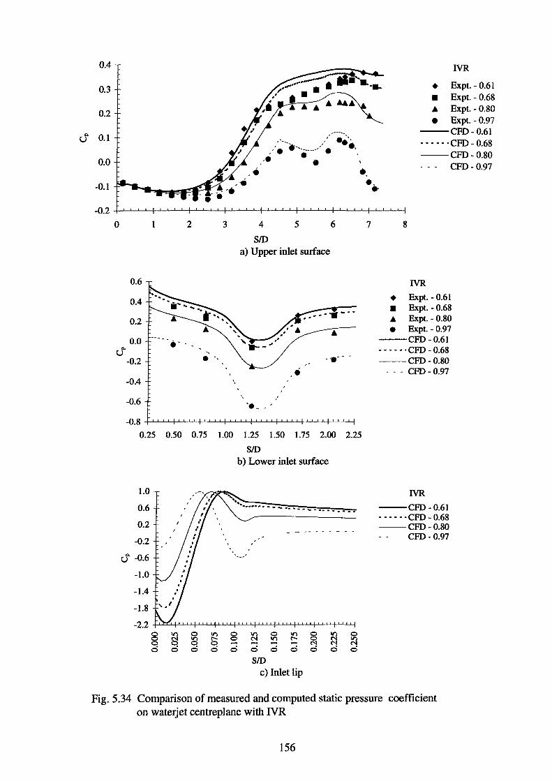
c. u
0.4
0.3
0.2
0.1
0.0
-0.1
-0.2
0
U,.
1 2 3
0.6
0.4
0.2
0.0
-0.2
-0.4 \
-0.6
,, .............. , ,·........ _/ ..•. ,'. ·---- . -· .
4
SID
5
a) Upper inlet surface
.. _-'
6
-0.8 +'--'--'---"'-+-'--'-'--4-''-L-l.-'+-'-'-'---'---+-'-'--'-'-i-'-'--'-'---i-'--J-"-'-+'-J.....LJ.....j
•• •• •
7 8
IVR
• Expt. - 0.61 • Expt. - 0.68 .. Expt. - 0.80 • Expt. - 0.97
--CFD-0.61 - - - - - · CFD - 0.68 --CFD-0.80
CFD-0.97
IVR
• Expt. - 0.61 • Expt. - 0.68 .. Expt. - 0.80 • Expt. - 0.97
--CFD-0.61 - - - • • · CFD - 0.68 --CFD-0.80
- - - CFD - 0.97
0.25 0.50 0.75 1.00 1.25 1.50 1.75 2.00 2.25
SID
1.0
0.6
0.2
-0.2
b) Lower inlet surface
. -... --- .... -.. - .. IVR
--CFD-0.61 - - - - - · CFD - 0.68 --CFD-0.80
CFD-0.97
U,. -0.6
-1.0
-1.4
-1.8
-2.2 +'-l::LJ...j-LW-'-j-1-L..I....L+'-L..L..L..j-__LLl_-J...I-l...L.W.+'-L..L..L..j-.J....L..L..Lj-L.J....L..L+'-L..LL.l
§ 0 :g ~ 8
0 -
lf"l 0 lf"l 0 lf"l 0 N lf"l 1:'- 0 N lf"l
N N N 0 0 0 0 0 0 0 0 0 0
SID c) Inlet lip
Fig. 5.34 Comparison of measured and computed static pressure coefficient on waterjet centreplane with IVR
156
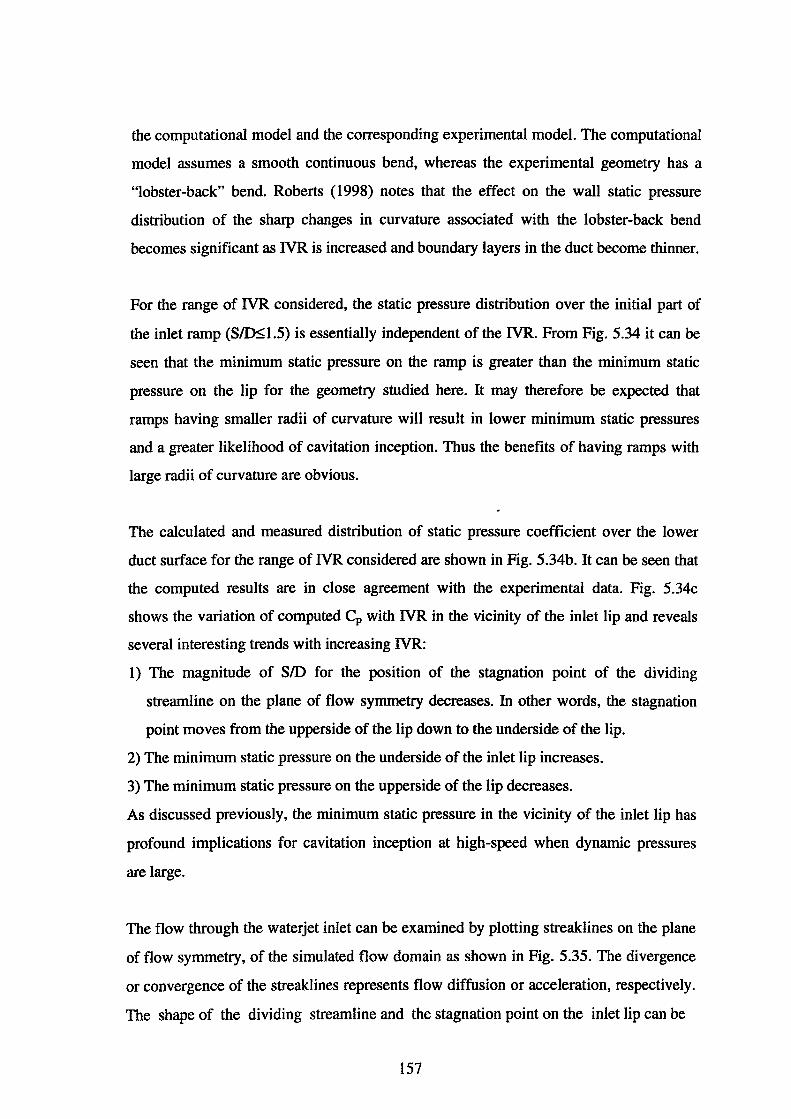
the computational model and the corresponding experimental model. The computational
model assumes a smooth continuous bend, whereas the experimental geometry has a
"lobster-back" bend. Roberts (1998) notes that the effect on the wall static pressure
distribution of the sharp changes in curvature associated with the lobster-back bend
becomes significant as IVR is increased and boundary layers in the duct become thinner.
For the range of IVR considered, the static pressure distribution over the initial part of
the inlet ramp (S/DS1.5) is essentially independent of the IVR. From Fig. 5.34 it can be
seen that the minimum static pressure on the ramp is greater than the minimum static
pressure on the lip for the geometry studied here. It may therefore be expected that
ramps having smaller radii of curvature will result in lower minimum static pressures
and a greater likelihood of cavitation inception. Thus the benefits of having ramps with
large radii of curvature are obvious.
The calculated and measured distribution of static pressure coefficient over the lower
duct surface for the range of IVR considered are shown in Fig. 5.34b. It can be seen that
the computed results are in close agreement with the experimental data. Fig. 5.34c
shows the variation of computed Cp with IVR in the vicinity of the inlet lip and reveals
several interesting trends with increasing IVR:
1) The magnitude of SID for the position of the stagnation point of the dividing
streamline on the plane of flow symmetry decreases. In other words, the stagnation
point moves from the upperside of the lip down to the underside of the lip.
2) The minimum static pressure on the underside of the inlet lip increases.
3) The minimum static pressure on the upperside of the lip decreases.
As discussed previously, the minimum static pressure in the vicinity of the inlet lip has
profound implications for cavitation inception at high-speed when dynamic pressures
are large.
The flow through the waterjet inlet can be examined by plotting streaklines on the plane
of flow symmetry, of the simulated flow domain as shown in Fig. 5.35. The divergence
or convergence of the streaklines represents flow diffusion or acceleration, respectively.
The shape of the dividing streamline and the stagnation point on the inlet lip can be
157

a) IVR=0.61
b) IVR=0.68
c)IVR=0.80
d)IVR=0.97
Fig. 5.35 Computed streaklines on centreplane
158
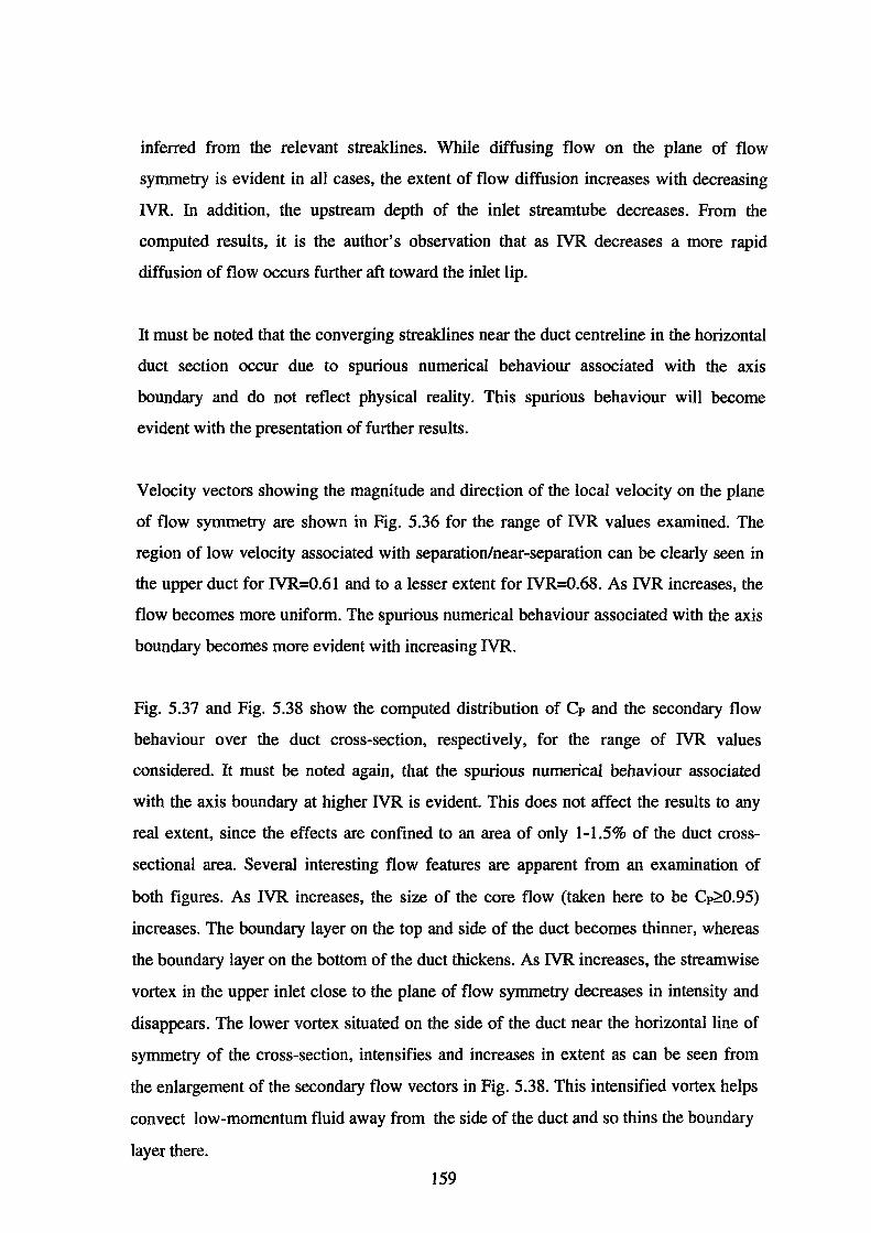
inferred from the relevant streaklines. While diffusing flow on the plane of flow
symmetry is evident in all cases, the extent of flow diffusion increases with decreasing
IVR. In addition, the upstream depth of the inlet streamtube decreases. From the
computed results, it is the author's observation that as IVR decreases a more rapid
diffusion of flow occurs further aft toward the inlet lip.
It must be noted that the converging streaklines near the duct centreline in the horizontal
duct section occur due to spurious numerical behaviour associated with the axis
boundary and do not reflect physical reality. This spurious behaviour will become
evident with the presentation of further results.
Velocity vectors showing the magnitude and direction of the local velocity on the plane
of flow symmetry are shown in Fig. 5.36 for the range of IVR values examined. The
region of low velocity associated with separation/near-separation can be clearly seen in
the upper duct for IVR=0.61 and to a lesser extent for IVR=0.68. As IVR increases, the
flow becomes more uniform. The spurious numerical behaviour associated with the axis
boundary becomes more evident with increasing IVR.
Fig. 5.37 and Fig. 5.38 show the computed distribution of Cp and the secondary flow
behaviour over the duct cross-section, respectively, for the range of IVR values
considered. It must be noted again, that the spurious numerical behaviour associated
with the axis boundary at higher IVR is evident. This does not affect the results to any
real extent, since the effects are confined to an area of only 1-1.5% of the duct cross
sectional area. Several interesting flow features are apparent from an examination of
both figures. As IVR increases, the size of the core flow (taken here to be C~0.95)
increases. The boundary layer on the top and side of the duct becomes thinner, whereas
the boundary layer on the bottom of the duct thickens. As IVR increases, the streamwise
vortex in the upper inlet close to the plane of flow symmetry decreases in intensity and
disappears. The lower vortex situated on the side of the duct near the horizontal line of
symmetry of the cross-section, intensifies and increases in extent as can be seen from
the enlargement of the secondary flow vectors in Fig. 5.38. This intensified vortex helps
convect low-momentum fluid away from the side of the duct and so thins the boundary
layer there.
159
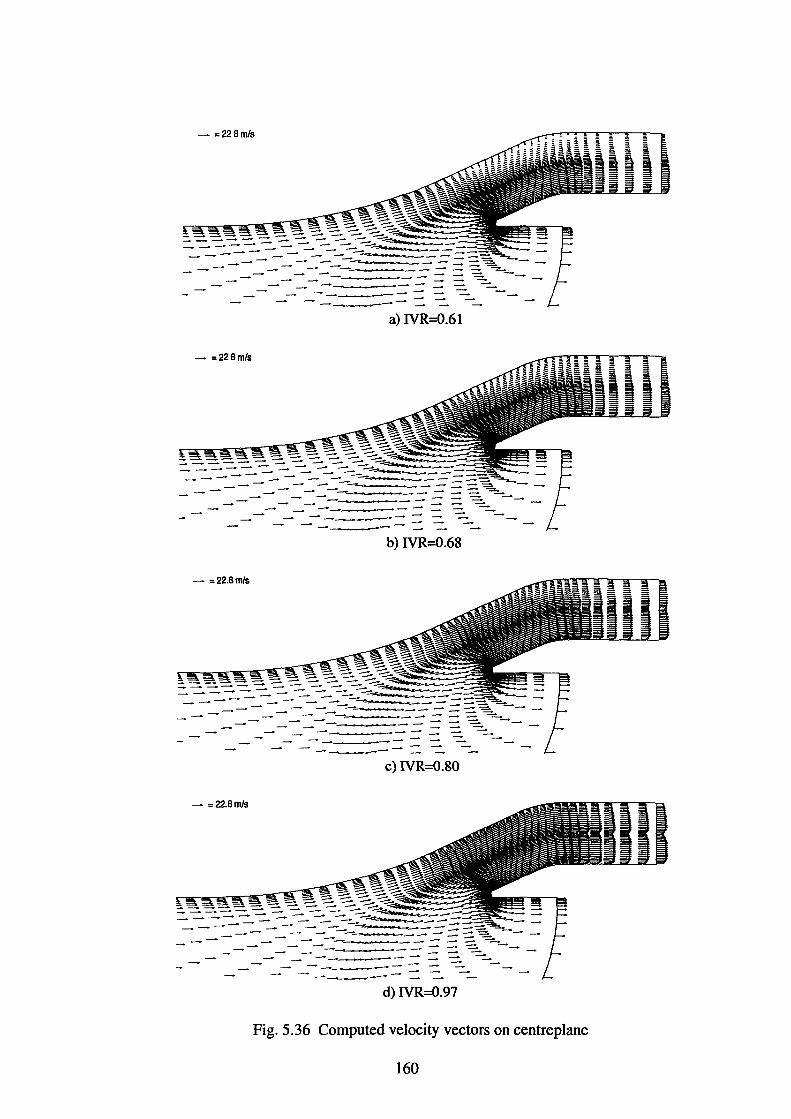
- =228m/s
------a)NR=0.61
- =228m/s
--b) IVR=0.68
- =22.8m/s
--
c)NR=0.80
- =22.8m/s
---
d)NR=0.97
Fig. 5.36 Computed velocity vectors on centreplane
160
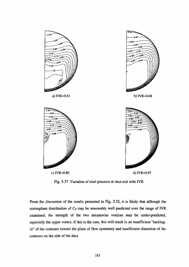
a) IVR=0.61 b) IVR=0.68
c) IVR=0.80 d)IVR=0.97
Fig. 5.37 Variation of total pressure at duct exit with IVR
From the discussion of the results presented in Fig. 5.32, it is likely that although the
centreplane distribution of Cp may be reasonably well predicted over the range of IVR
examined, the strength of the two streamwise vortices may be under-predicted,
especially the upper vortex. If this is the case, this will result in an insufficient "tucking
in" of the contours toward the plane of flow symmetry and insufficient distortion of the
contours on the side of the duct.
161
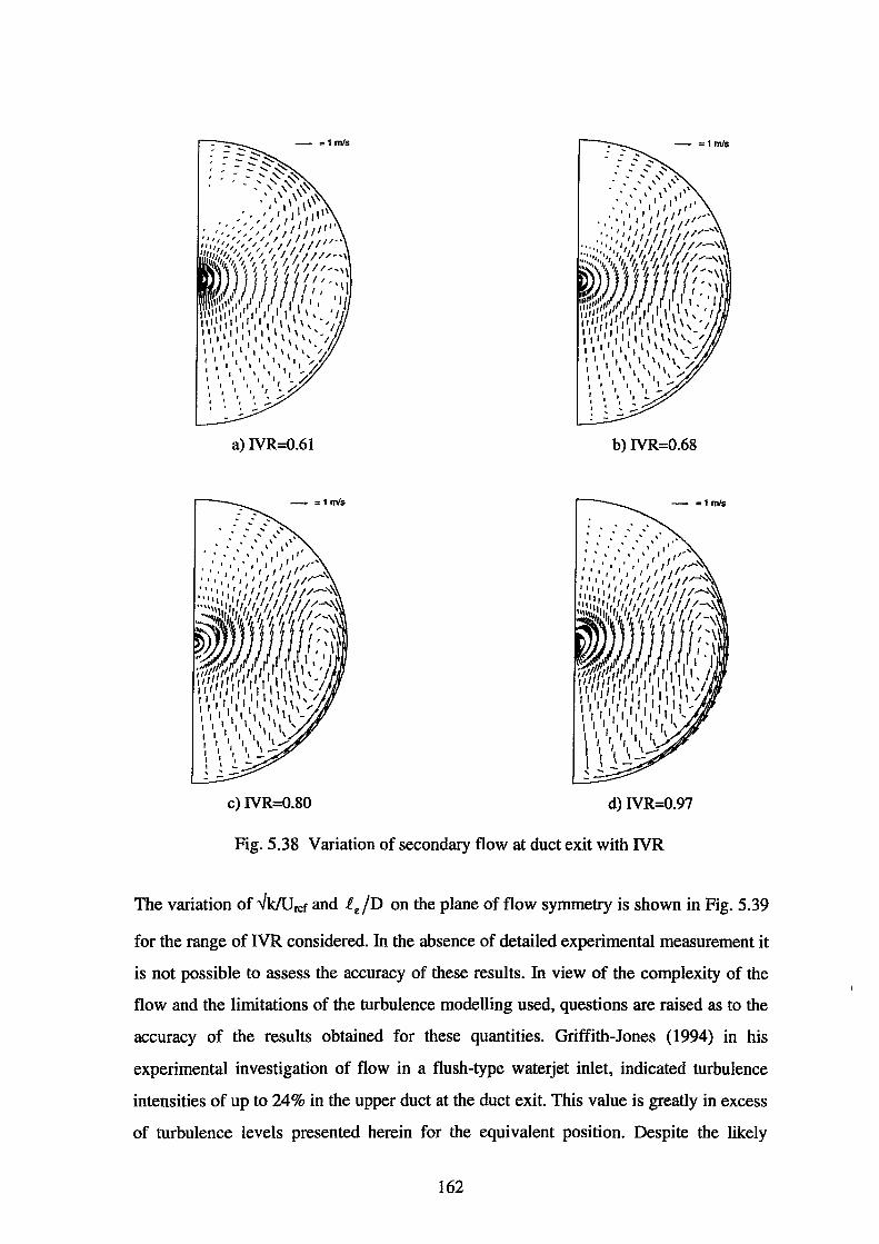
- -- -'-.::- ....... " - ..... ' I .; -- ......
' ' : - ::-::::-'
-=1mls
' - ' ' ' '' I\ \\
I 1 ,, '' I I I ,,
' ' ' ' ' I I // ' ' ' I I I ,,,,
,, ' I I I I 111,,',,", /I ;I II''
,, I I I I I ',,,',,,'~~ ~~ '; J I I/
, I I I /_ I I I/~-,
/ ll!'/f { { :-:, 11 11 1 I 1111, I
IIIII II ,, , ,, I I I \ - I I I 11 I I I 1 I \ '!
1111 r' Ill I\\'·-1 I I I I I I I I \ \' I I I I II I II I I I I I\ -, I t I t I ' \ \1 ',.... I I
11
I 1
1 ' 1 1 t
1
1.,.
1 I I 1 I I I 1 1 I -1 I I I "' ' 0 I . ' .
a) NR=0.61
c)NR=0.80
b)NR=0.68
d)NR=0.97
Fig. 5.38 Variation of secondary flow at duct exit with IVR
The variation of "k!Urer and Rr./D on the plane of flow symmetry is shown in Fig. 5.39
for the range of IVR considered. In the absence of detailed experimental measurement it
is not possible to assess the accuracy of these results. In view of the complexity of the
flow and the limitations of the turbulence modelling used, questions are raised as to the
accuracy of the results obtained for these quantities. Griffith-Jones (1994) in his
experimental investigation of flow in a flush-type waterjet inlet, indicated turbulence
intensities of up to 24% in the upper duct at the duct exit. This value is greatly in excess
of turbulence levels presented herein for the equivalent position. Despite the likely
162
inaccuracies inherent in Fig. 5.39, much can still be learned about the generic turbulence
behaviour and the trends in turbulence behaviour with IVR. Unfortunately, spurious
numerical behaviour in the vicinity of the axis boundary and near the outlet boundary
act to distort the results in the vicinity of these locations and therefore care must be
taken in interpreting these results. The following conclusions can be reached regarding
the turbulence behaviour in the waterjet inlet:
1) Large turbulence levels occur in the vicinity of the inlet lip due to the large viscous
shear forces that exist there, resulting in large production of k and hence large values
of turbulence intensity. The peak levels of turbulence occur on the underside of the
lip for IVR values of 0.61, 0.68 and 0.80. For IVR=0.97, peak turbulence levels occur
on both the underside and upperside of the inlet lip. Large velocity gradients exist as
a result of the acceleration of the flow away from the stagnation point, resulting in a
highly sheared boundary layer whose turbulence intensity is increased significantly
on encountering an adverse pressure gradient after the static pressure minima on the
lip surface (Fig. 5.34).
2) Downstream of the inlet lip in the external flow, the boundary layer thickens more
rapidly with decreasing IVR due to greater adverse pressure gradient. This is evident
from the increasing area covered by the contours of turbulent velocity-scales.
Turbulent length-scales remain small as the eddies in the boundary layer are small
and dissipative.
3) As flow diffuses into the inlet from the upstream boundary layer, the turbulence
spreads as a result of flow diffusion and turbulent diffusion. Turbulence is intensified
as a result of the adverse pressure gradients encountered in the upper part of the
waterjet inlet resulting from flow diffusion and the bend. Overall turbulence levels
inside the waterjet inlet decrease with increasing IVR. This is due to the presence of
more favourable pressure gradients resulting in a reduction of length-scales and
turbulence intensity. The large velocity and length-scales present in the upper part of
the inlet imply large highly turbulent energy-containing eddies creating large eddy
viscosity and therefore large losses in total pressure.
4) The flow in the lower-half of the duct above the wall boundary layer features low
levels of turbulence and small turbulent length-scales, this region may be considered
to be the "potential core".
163
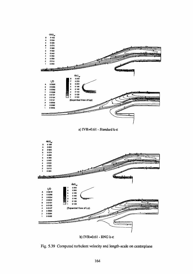
.Jklu,., B 0100 A 0090 9 0080 8 0070 7 0080 6 0050 5 0040 4 0030 3 0020 2 0010
0000
.Jk!U,.,
I! 0240
ljD 0220
c:::: A 00328 0200
9 00295 0180
8 00262 0160
7 00229 0140
6 00197 0120
5 00164 0100
4 00131 (Expanded V1ew of L1p) 3 00098 2 00066
00033
a) NR=0.61- Standard k-E
.JkiU .. , B 0100 A 0090 9 0080 8 0070 7 0.080 6 0050 5 0040 4 0030 3 0020 2 0010
0000
.Jk!U,.,
I,!D
li 0220 c 0200
A 00318 0180
9 00286 0160 8 00254
0140 7 00222
0120 6 00191
0100 5 00159 4 00127 (Expanded V1ew of L1p)
00095 2 00064
00032
b) IVR=0.61 - RNG k-E
Fig. 5.39 Computed turbulent velocity and length-scale on centreplane
164

..Jk!U,., B 0100 A 0090 9 0080 8 0070 7 0080 6 0050 5 0040 4 0030 3 0020 2 0010
0000
1/1)
~~ 0.220 c: 0.200
A 00322 0180 9 00290 0180 8 00257
0140 7 0.0225 0120 6 00193
0100 5 00161 4 00129 (Expanded V1ew of L1p) 3 00097 2 00064
00032
c) IVR=0.68
..Jk!U,., B 0100 A 0090 9 0080 8 0070 7 0060 6 0050 5 0040 4 0030 3 0020 2 0010
0000
..Jk!U,.,
1/D [ 0.220 c: 0.200
A 00305 0180 9 00275 0160 8 00244
0140 7 00214
0120 6 00183
0100 00153
4 00122 (Expanded View of Up) 3 00092 2 00061
00031
=-=
d) IVR=0.80
Fig. 5.39 (cont.)
165
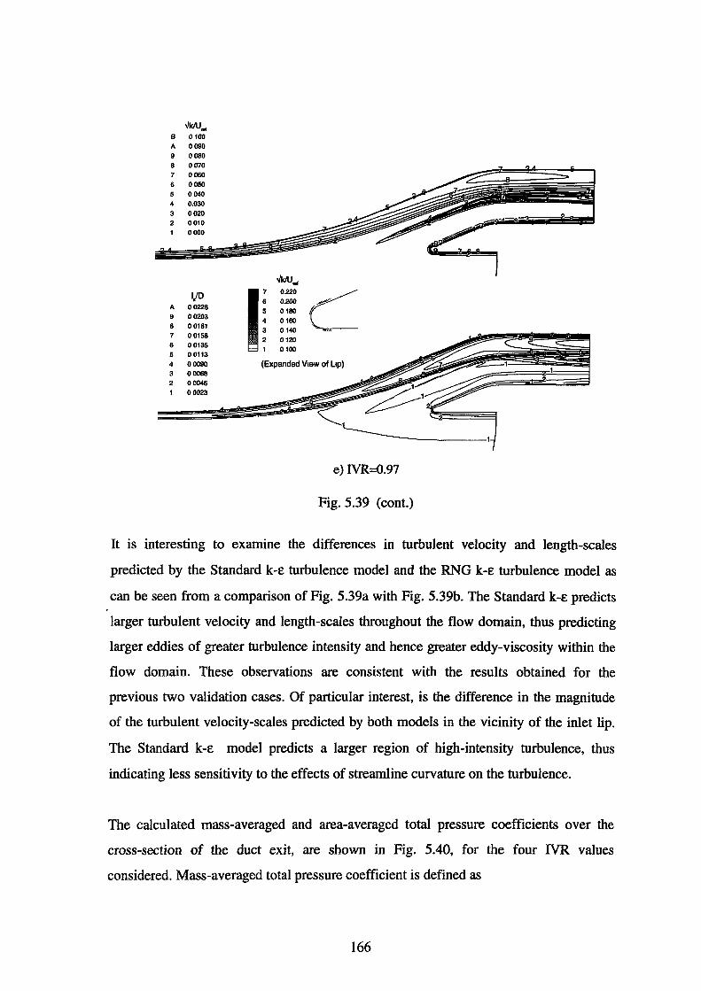
vklu,., B 0100 A 0090 9 0090 8 0070 7 0080 6 0050 5 0040 4 0.030 3 0020 2 0010
0000
1/D [ 0.220 c 0.200
A 00226 0180 9 00203
0160 8 00181
0140 7 00158
0120 6 00135
0100 5 00113 4 00090 (Expanded Vrew of Lrp) 3 00068 2 00045
00023
e) IVR=0.97
Fig. 5.39 (cont.)
It is interesting to examine the differences in turbulent velocity and length-scales
predicted by the Standard k-E turbulence model and the RNG k-E turbulence model as
can be seen from a comparison of Fig. 5.39a with Fig. 5.39b. The Standard k-E predicts
larger turbulent velocity and length-scales throughout the flow domain, thus predicting
larger eddies of greater turbulence intensity and hence greater eddy-viscosity within the
flow domain. These observations are consistent with the results obtained for the
previous two validation cases. Of particular interest, is the difference in the magnitude
of the turbulent velocity-scales predicted by both models in the vicinity of the inlet lip.
The Standard k-E model predicts a larger region of high-intensity turbulence, thus
indicating less sensitivity to the effects of streamline curvature on the turbulence.
The calculated mass-averaged and area-averaged total pressure coefficients over the
cross-section of the duct exit, are shown in Fig. 5.40, for the four IVR values
considered. Mass-averaged total pressure coefficient is defined as
166

_ 2 11t1D/2 U p Cp = --
2 -- 1 2
rdrd8 1tD o o Urer 2PUrer
The area-averaged total pressure coefficient is defined as
Cp = ~ rlt rD/2 I p 2 rdrde 1tD Jo Jo 2 pU ref
(5.9)
(5.10)
It can be seen that as IVR increases, the average total pressure over the cross-section
increases, thus indicating a reduction in the total pressure lost in the duct. This is
expected, since the losses associated with flow separation disappear at higher IVR
values. The values of mass-averaged Cp are higher than the corresponding area
averaged value because the regions of higher Cp (and higher streamwise velocity) carry
more of the mass flow and hence a more energetic flow. This of course results in a
higher Cp over the cross-section.
Mass-averaged Cp is of particular interest for use in waterjet parametric performance
models (see Chapter 2) as it in essence describes an energy recovery efficiency, whereas
area-averaged Cp may be preferred for design purposes as it implicitly contains a
measure of the non-uniformity of the total pressure distribution at the duct exit. It is
interesting to note that there is relatively little variation in mass-averaged CP , while the
change in area-averaged Cp is more significant.
0.86
0.84
u 0.82
~ 0.80
-+---Mass -Averaged 0.78 -A- Area -Averaged
0.76 0 10 0 10 0 10 0 10 0
"' "' 1'- 1'- 00 00 0\ 0\ C! 0 0 0 0 0 0 0 0
IVR
Fig. 5.40 Change in average total pressure coefficient over duct exit with IVR
167
5.5 Discussion of Results
In this section the accuracy of the computational results presented in the preceding
sections for the three validation studies undertaken, will be discussed in relation to the
capabilities and limitations of the computational modelling used.
Since the same turbulence and near-waH modelling are used in all three validation cases
and the same general trends in results observed, it was decided that it is more
appropriate to discuss the accuracy of the computational results in a unified manner and
refer to each validation case as appropriate, for reasons of compactness and to avoid
repetition of the discussion.
Discussion shaH be focused on three main issues associated with computational
simulation of the experimental configurations examined. These are the boundary
conditions used, the size and quality of the numerical grid and the turbulence and near
wall modelling adopted. It is principally this latter issue of turbulence and near-wall
modelling which will be shown to have the greatest impact on the accuracy of the
solutions obtained, as a consequence of the limitations of the models used.
5.5.1 Boundary Conditions
Inaccuracies in representing the velocity upstream of the duct in the case of the 90° bend
of Enayet et al (1982) and the waterjet inlet of Roberts (1998) will affect the
development of streamwise vorticity in the duct and hence the downstream flow
behaviour. This can be qualitatively deduced from the Squire-Winter formula (Eqn 5.1).
Therefore in these cases, inaccurate boundary condition representation is clearly a
source of error which will be reflected in the results obtained, although the magnitude of
these errors is difficult to quantify in view of the other sources of error present in the
computational modelling procedure.
In the modelling of the 90° bend, it is likely that the under-prediction of the core
velocity by all turbulence and near-wall modelling options examined (as can be seen
from Fig. 5.5, Fig. 5.6 and Fig. 5.7) may be directly attributed to inaccuracies in the
velocity profile upstream of the bend. It is difficult to quantify the error associated with
168
incorrectly modelled boundary conditions in the case of flow in the waterjet inlet, but
inaccuracies in the dimensions of the cross-section of the inlet streamtube are reflective
of this. There was insufficient data available in Bansod and Bradshaw (1972) to allow
the accuracy of the boundary conditions adopted in the study presented in Section 5.3 to
be assessed.
In the case of the waterjet inlet of Roberts (1998), inaccurate representation of the
geometry is another source of error. An obvious example of this is the representation of
the "lobster-back" bend with a smooth bend. This is found to lead to inaccuracies in the
static pressure distribution over the duct bend at larger IVR, when flow separation is
absent.
5.5.2 Grid Size and Quality
The solutions obtained on the 4lx4lx81 grid for the 9~0 bend and the 31x3lx71 grid
for the S-Duct are deemed to be "grid-independent" and so errors associated with the
discretisation of the governing equations should have a negligible effect on the solution.
Both grids possess excellent orthogonality and the gridlines in the streamwise (K)
coordinate direction are aligned with the primary flow, therefore minimising cross
stream diffusion. In the case of the 90° bend, gridlines are spaced evenly in the radial (J)
direction. This was done in order to place the cell-centre of the wall-adjacent cells in the
range of y + =30 at entry to the duct and so allow optimum use of wall functions to be
made.
Larger variations in the spacing of radial gridlines are necessary for the S-Duct in order
to resolve the greater range of turbulent length-scales present in the flow. Since the
solution obtained for the S-Duct may be considered to be "grid-independent", errors
associated with the variation in radial gridline spacing and hence variation in cell size,
may be considered to be negligible. Care was also taken to ensure that the cell-centres of
the wall-adjacent cells were placed in the range of y+=30-40 so that appropriate use of
wall functions could be made. It may thus be concluded that the meshes for the 90° bend
and the S-Duct are of a high quality and are in essence a negligible source of solution
error.
169
The situation is however different for the 31 x41 x 102 grid used for simulation of the
flow domain associated with the waterjet inlet. Section 5.4.4 shows that although the
refinement of the grid in each computation coordinate direction does not result in a
change in solution, it cannot be claimed that the solutions obtained on this grid are
"grid-independent". Therefore errors arising from discretisation and associated with
growth in cell size may be present in the solution. Other sources of errors arising from
cross-stream diffusion and cell non-orthogonality will be present, particularly in areas of
extreme cell skewness. The magnitude of these errors is difficult to quantify but must be
considered when examining the solution. The quality of the grid produced by Inlet3D
was discussed in greater detail in Section 4.5.
5.5.3 Turbulence Modelling
In all of the three validation cases considered, the use of the RNG k-e turbulence model
produced results in better accord with the experimental data than those obtained using
the Standard k-e turbulence model, although the limitations of the RNG k-e model are
also apparent. The flows considered in this chapter contain the following features:
1) Adverse pressure gradient in the stream wise direction
2) Streamline curvature
3) Flow separation/near-separation.
It is well known from the literature that the Standard k-e model performs poorly under
adverse pressure gradient. Wilcox ( 1993) used perturbation analysis to show that the
length-scale predicted by the Standard k-e model under adverse pressure gradient tends
to be too large in the near-wall region. Rodi and Scheuerer (1986) showed that under
adverse pressure gradient, the coefficient of the rate of production of e, Ce1 in the e
equation is under-predicted and must therefore be increased in value if the predicted
length-scale is to be made independent of pressure gradient. As a consequence, the
production of e is under-predicted and the length-scale determined by the e equation
rises more steeply near the wall than in the case of zero pressure gradient. Eddy
viscosity is therefore over-predicted and the tendency of the flow to separate suppressed.
Flows with streamline curvature contain what Bradshaw (1973) termed "extra rates of
170
strain" which modify the structure of the turbulence to a much greater extent than
suggested by the extra production terms that appear in the Reynold stress equations.
Bradshaw (1973) noted that "extra rates of strain", unrelated to mean strain rates, cause
changes in the higher-order structural parameters of the turbulence, which subsequently
cause changes in the Reynolds stresses and so modify the structure of the turbulence.
Therefore in "complex" turbulent flows, such as those studied here which contain "extra
rates of strain" due to curvature and flow separation, the Boussinesq hypothesis must
necessarily fail, as Wilcox (1993) noted.
Interesting phenomena associated with streamline curvature include the "collapse of
turbulence" for flow over a convex surface and the augmentation of turbulence for flow
over a concave surface, accompanied by the formation of streamwise longitudinal
vortices in the boundary layer (see Bradshaw (1973)). Gillis and Johnston (1983)
building on previous efforts, investigated two-dimensional flow affected by strong
convex curvature and demonstrated the "collapse of turbulence" phenomenon as well as
a substantial reduction in skin friction coefficient (relative to the corresponding flat plate
boundary layer value) on the convex surface.
The over-prediction of the skin friction coefficient on the first bend, at the bottom of the
S-Duct, by all turbulence and near-wall modelling combinations (Fig. 5.19b) may be
directly attributed to a failure of the turbulence modelling to properly account for the
effects of streamline curvature on the development of the turbulent boundary layer over
this convex surface. This, therefore, results in a failure to predict the general decrease in
Cr relative to the corresponding flat plate value.
The flows considered in the validation study presented here contain a combination of
streamline curvature, adverse pressure gradient in the streamwise direction and/or flow
separation. Therefore the k-E turbulence modelling has to account for all of these effects
simultaneously, rather than individually. Comparison between the centreplane
distributions of turbulent velocity and length-scales obtained using the Standard k-E and
RNG k-E turbulence models for the three validation cases, clearly show that the
distributions obtained using the RNG k-E turbulence model exhibit a greater sensitivity
171
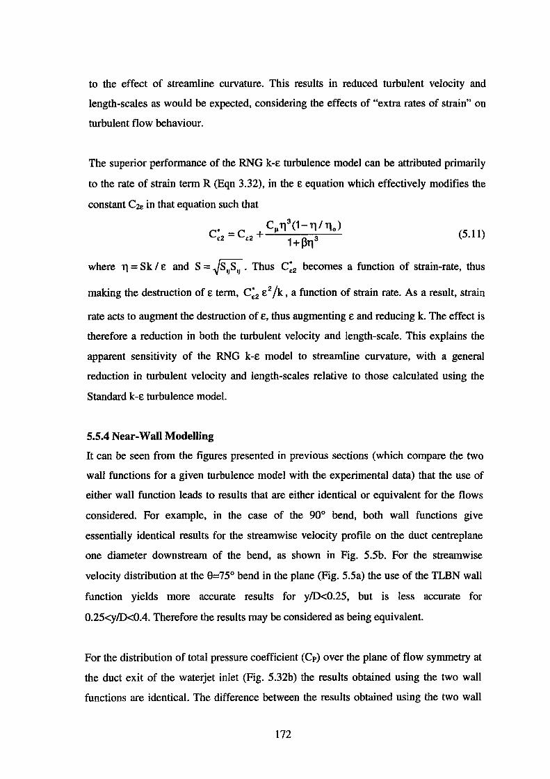
to the effect of streamline curvature. This results in reduced turbulent velocity and
length-scales as would be expected, considering the effects of "extra rates of strain" on
turbulent flow behaviour.
The superior performance of the RNG k-E turbulence model can be attributed primarily
to the rate of strain term R (Eqn 3.32), in theE equation which effectively modifies the
constant C2£ in that equation such that
C* = C +ell 113(1- 11 I 'Tio) £2 £2 1+~113
(5.11)
where 11 =SkI E and S = ~s.Js•J . Thus c:2 becomes a function of strain-rate, thus
making the destruction of E term, c:2 £2 /k, a function of strain rate. As a result, strain
rate acts to augment the destruction of E, thus augmenting E and reducing k. The effect is
therefore a reduction in both the turbulent velocity and length-scale. This explains the
apparent sensitivity of the RNG k-E model to streamline curvature, with a general
reduction in turbulent velocity and length-scales relative to those calculated using the
Standard k-E turbulence model.
5.5.4 Near-Wall Modelling
It can be seen from the figures presented in previous sections (which compare the two
wall functions for a given turbulence model with the experimental data) that the use of
either wall function leads to results that are either identical or equivalent for the flows
considered. For example, in the case of the 90° bend, both wall functions give
essentially identical results for the streamwise velocity profile on the duct centreplane
one diameter downstream of the bend, as shown in Fig. 5.5b. For the streamwise
velocity distribution at the 8=75° bend in the plane (Fig. 5.5a) the use of the TLBN wall
function yields more accurate results for y/D<0.25, but is less accurate for
0.25<y/D<0.4. Therefore the results may be considered as being equivalent.
For the distribution of total pressure coefficient (Cp) over the plane of flow symmetry at
the duct exit of the waterjet inlet (Fig. 5.32b) the results obtained using the two wall
functions are identical. The difference between the results obtained using the two wall
172
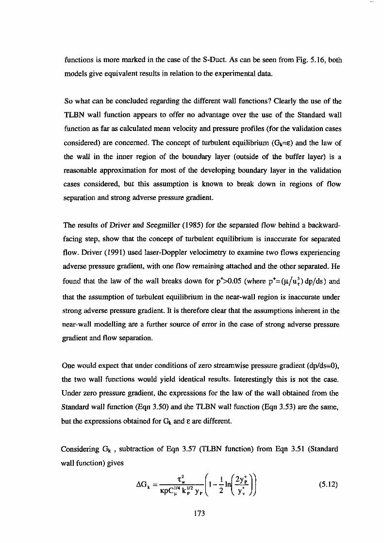
functions is more marked in the case of the S-Duct. As can be seen from Fig. 5.16, both
models give equivalent results in relation to the experimental data.
So what can be concluded regarding the different wall functions? Clearly the use of the
TLBN wall function appears to offer no advantage over the use of the Standard wall
function as far as calculated mean velocity and pressure profiles (for the validation cases
considered) are concerned. The concept of turbulent equilibrium (Gk=E) and the law of
the wall in the inner region of the boundary layer (outside of the buffer layer) is a
reasonable approximation for most of the developing boundary layer in the validation
cases considered, but this assumption is known to break down in regions of flow
separation and strong adverse pressure gradient.
The results of Driver and Seegmiller (1985) for the separated flow behind a backward
facing step, show that the concept of turbulent equilibrium is inaccurate for separated
flow. Driver (1991) used laser-Doppler velocimetry to examine two flows experiencing
adverse pressure gradient, with one flow remaining attached and the other separated. He
found that the law of the wall breaks down for p+>0.05 (where p+=(Jl/u~) dp/ds) and
that the assumption of turbulent equilibrium in the near-wall region is inaccurate under
strong adverse pressure gradient. It is therefore clear that the assumptions inherent in the
near-wall modelling are a further source of error in the case of strong adverse pressure
gradient and flow separation.
One would expect that under conditions of zero streamwise pressure gradient (dp/ds=O),
the two wall functions would yield identical results. Interestingly this is not the case.
Under zero pressure gradient, the expressions for the law of the wall obtained from the
Standard wall function (Eqn 3.50) and the TLBN wall function (Eqn 3.53) are the same,
but the expressions obtained for Gk and E are different.
Considering Gk , subtraction of Eqn 3.57 (TLBN function) from Eqn 3.51 (Standard
wall function) gives
(5.12)
173
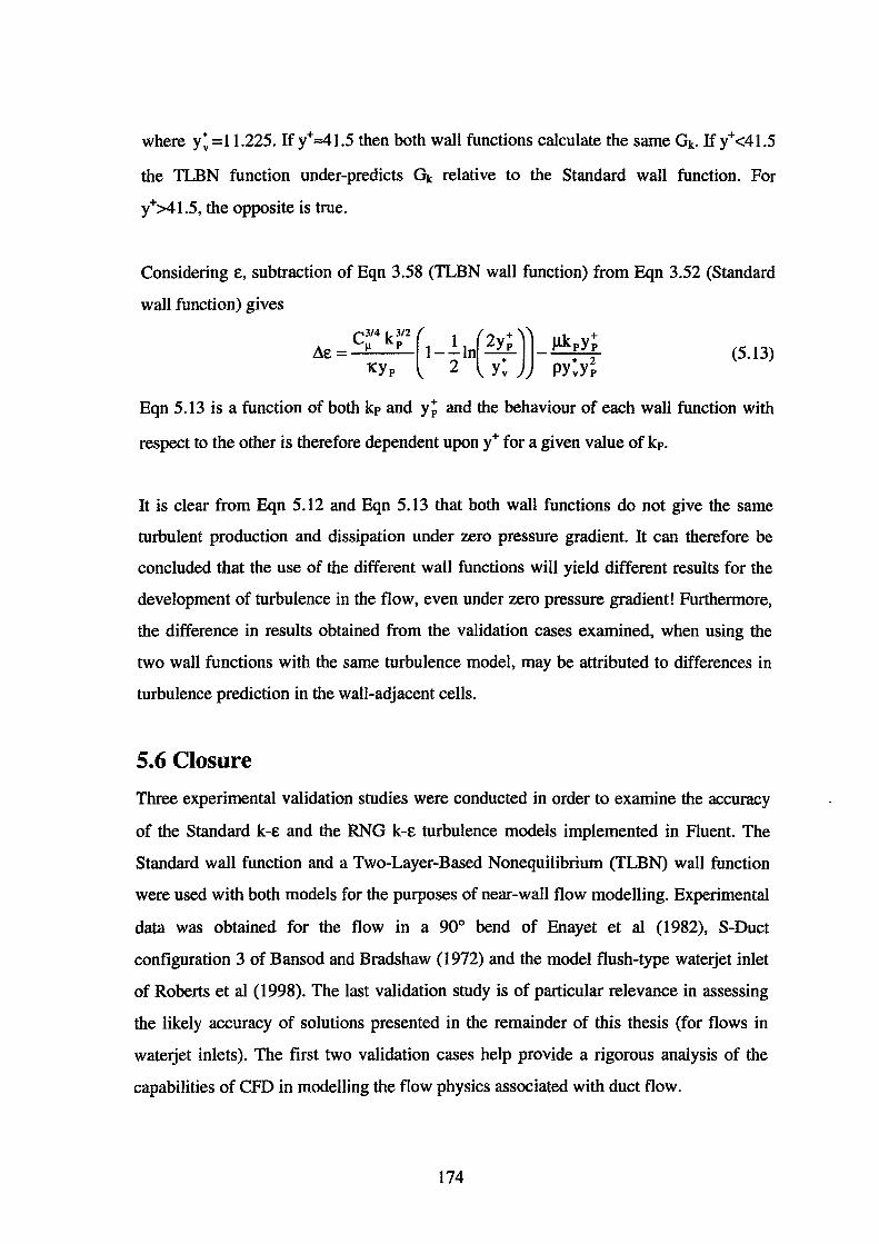
where y: =11.225. If y+=41.5 then both wall functions calculate the same Gk. If y+<41.5
the TLBN function under-predicts Gk relative to the Standard wall function. For
y+>41.5, the opposite is true.
Considering E, subtraction of Eqn 3.58 (TLBN wall function) from Eqn 3.52 (Standard
wall function) gives
(5.13)
Eqn 5.13 is a function of both kp and y; and the behaviour of each wall function with
respect to the other is therefore dependent upon y+ for a given value of kp.
It is clear from Eqn 5.12 and Eqn 5.13 that both wall functions do not give the same
turbulent production and dissipation under zero pressure gradient. It can therefore be
concluded that the use of the different wall functions will yield different results for the
development of turbulence in the flow, even under zero pressure gradient! Furthermore,
the difference in results obtained from the validation cases examined, when using the
two wall functions with the same turbulence model, may be attributed to differences in
turbulence prediction in the wall-adjacent cells.
5.6 Closure
Three experimental validation studies were conducted in order to examine the accuracy
of the Standard k-E and the RNG k-E turbulence models implemented in Fluent. The
Standard wall function and a Two-Layer-Based Nonequilibrium (TLBN) wall function
were used with both models for the purposes of near-wall flow modelling. Experimental
data was obtained for the flow in a 90° bend of Enayet et al (1982), S-Duct
configuration 3 of Bansod and Bradshaw ( 1972) and the model flush-type waterjet inlet
of Roberts et al (1998). The last validation study is of particular relevance in assessing
the likely accuracy of solutions presented in the remainder of this thesis (for flows in
waterjet inlets). The first two validation cases help provide a rigorous analysis of the
capabilities of CFD in modelling the flow physics associated with duct flow.
174
The following conclusions may be drawn as to the modelling approaches examined:
1) In all of the cases examined, the RNG k-E turbulence model provides solutions of
superior accuracy to the Standard k-E turbulence model. The deficiencies of the
Standard k-E turbulence model are well known from the literature. The rate of strain
term (R) in the E equation of the RNG k-E turbulence model provides a better
modelling of flows containing "extra rates of strain" such as streamline curvature,
thus leading to more accurate results.
2) For the validation cases considered, both the Standard wall function and the TLBN
wall function lead to either identical results or results of comparable accuracy for
mean flow quantities such as velocity and pressure.
3) The failure of both models to adequately handle flow separation is due to an
inaccurate prediction of the onset of flow separation and the "extra rates of strain"
phenomenon, as well as a break-down of the assumptions underlying the use of wall
functions in separated flow. This leads to inaccuracies in the computed flow and is
particularly evident in the computational results obtained for the S-Duct and waterjet
inlet.
4) Additional sources of error include the modelling of the boundary conditions for the
goo bend and the waterjet inlet. An additional source of error is the quality of the grid
used for simulation of the waterjet inlet. It is also possible that discretisation error
may be another source of error in the results obtained for the waterjet inlet on the
31x4lxl02 grid. The 41x41x81 grid used for simulation of the experimental
geometry associated with the goo bend and the 31x31x71 grid used for simulation of
the S-Duct provide reasonably "grid-independent" solutions.
5) The computed turbulence behaviour was discussed for the purposes of comparing the
two turbulence models examined. While it is thought that the results reflect the
qualitative flow behaviour, the accuracy of the computed velocity and length-scale
profiles obtained could not be validated due to a lack of experimental data.
Overall, reasonably good agreement between computed velocity and pressure
distributions and the experimental data was obtained for the three cases considered
when the RNG k-E model is used. The agreement between computed results and the
experimental data improves when flow separation is absent from the flow.
175
It can thus be concluded that CFD can be used as an effective analysis tool for
simulating the flow in flush-type waterjet inlets, producing credible results of
reasonably good accuracy for pressure and velocity distributions within the waterjet
inlet. Care must be exercised in the interpretation of results when it appears that flow
separation may be present.
Finally, due to its superior accuracy to the Standard k-E model, the RNG k-E turbulence
model is chosen for use in the simulation of waterjet inlet flow on a 31 x41 x 102 grid in
combination with the TLBN wall function, for the work presented in the remainder of
this thesis.
176

Chapter 6 Boundary Layer Investigations
Two main issues will be addressed in this chapter. The first is the issue of selecting
suitable parameters necessary for quantifying various aspects of the hydrodynamic
performance of the waterjet inlet. This provides the basis for quantifying the effect of
geometric design variations on the hydrodynamic performance of the waterjet inlet and
so provides a necessary foundation for the work presented in this chapter, the parametric
design space investigations in Chapter 7 and the waterjet inlet optimisation example in
Chapter 8.
The second issue involves the effect of the thickness of the upstream boundary layer on
the flow within the waterjet inlet. It will be shown in this chapter, that the thickness of
an upstream boundary layer has a significant influence on the flow inside the waterjet
inlet and hence on its hydrodynamic performance. It may thus be expected that the same
waterjet inlet installed in different vessels will exhibit differing hydrodynamic
performance. This is due to the differences in ingested momentum and energy fluxes
resulting from the upstream hull boundary layer, amongst other factors.
In Chapter 2, a parametric model of waterjet thrust and efficiency was developed.
Subsequently, a parametric analysis was presented which examined the effect of
ingested hull boundary layer fluid on waterjet performance. It was concluded that
ingestion of fluid from the hull boundary layer has a beneficial effect on overall waterjet
efficiency. In this chapter, the emphasis is on a detailed analysis of how ingestion of
varying amounts of boundary layer fluid can affect the internal hydrodynamics of the
waterjet inlet and the quality of flow delivered to the pump.
Furthermore, the issue of upstream boundary layer thickness is also of relevance to
waterjet inlet optimisation, as an inlet optimised for a particular thickness of upstream
boundary layer may give inferior performance when the flow conditions upstream of the
177
inlet change. Therefore, the hydrodynamic performance of a waterjet inlet and hence an
optimised waterjet inlet design is a function of the boundary conditions of the flow
domain of interest. In other words, the optimum waterjet inlet shape may change
depending on the flow conditions in the vicinity of the inlet and the mass flow-rate
through the waterjet inlet.
In Section 6.1 parameters used to quantify the various aspects of the hydrodynamic
performance of the waterjet inlet (which shall be termed the "hydrodynamic
performance parameters" in the remainder of this thesis) are presented and the rationale
behind their selection discussed. The waterjet inlet geometry, CFD modelling and CFD
simulation used for the investigations presented in this chapter are outlined in Section
6.2. The CFD modelling methodology outlined in Section 6.2 also fonp.s the basis of the
generic flow modelling used in subsequent chapters. In Section 6.3, results are presented
of an investigation of the effect of the thickness of the upstream boundary layer on the
hydrodynamic performance of the waterjet inlet. The results of this investigation are
discussed in detail in Section 6.4. A summary of the main points of this chapter and the
conclusions of the boundary layer investigation are presented in Section 6.5, together
with their implications for propulsion system design.
6.1 Assessment of Hydrodynamic Performance
In order to determine the hydrodynamic performance of the waterjet inlet, it is necessary
to identify the most important parameters affecting hydrodynamic performance and
quantify them. This systematic approach is a fundamental requirement for optimisation
of the waterjet inlet, as it allows the objective function of the optimisation problem to be
appropriately related to the hydrodynamic performance of thewaterjet inlet design.
Of hydrodynamic importance are:
1) The presence of flow separation in the inlet
2) The presence of cavitation in the waterjet inlet
3) The recovery of total pressure at the duct exit
4) The distortion of the flow field at the duct exit
5) The turbulent velocity and length-scales at the duct exit
178
6) Drag forces acting on the inlet (Section 2.1.2)
7) The volume of water entrained in the waterjet inlet
8) The vertical forces acting on the waterjet inlet
9) The dimensions of the inlet streamtube
These aspects of hydrodynamic performance are described below.
6.1.1 Cavitation
When the static pressure in the waterjet inlet falls below the vapour pressure of water,
water will cavitate (boil) forming a two-phase liquid/gas flow of water and water vapour
(steam) bubbles. These bubbles of water vapour are convected downstream with the
mean flow and implode as the static pressure increases above the vapour pressure of the
water. The implosion of these water vapour bubbles cause localised pressure waves
which can pit and erode metal surfaces. Cavitation is therefore an undesirable
phenomenon that must be avoided, or at least minimised, through careful geometric
design of the waterjet inlet.
Other undesirable effects of cavitation will manifest themselves through reduced
waterjet efficiency via the terms of Eqn 2.38. Cavitation at the inlet lip below the
stagnation line, will cause an increased lip loss thrust fraction ( t L) as a consequence of
the altered pressure field. Cavitation inside the waterjet inlet will reduce the inlet
efficiency (Tlin) and may lead to a reduction in the pump's rotative efficiency (TlRot).
Further complications arise due to the unsteady time-dependent nature of the cavitating
flow.
Areas of inlet cavitation can be identified primarily by an examination of the cavitation
number distribution over the surface of the waterjet inlet. The inception of cavitation
could also occur in the interior of the flow domain, such as in the cores of strong
vortices, located for example in the comers of rectangular duct sections. However, for
all intents and purposes, the primary sources of cavitation are generally likely to be low
pressure regions in the vicinity of the duct surface resulting from high velocity flow over
these surfaces. Hence examination of the pressure distribution over the duct surface
alone, may be deemed to be an acceptable approach to identifying areas of cavitation
179
inception. Cavitation number is defined here as
cr= Patm -pgH+p-pv 1 uz 2P ref
(6.1)
where cr is the cavitation number, Patm the atmospheric pressure, Uref the reference (free
stream) velocity, p the static pressure calculated by Fluent (which neglects the
contribution to the pressure field arising from hydrostatic pressure), H the height above
the water-level for the point under consideration, g the gravitational constant and Pv the
vapour pressure of water for a given ambient temperature.
An alternative approach for examining the likelihood of waterjet inlet cavitation, is to
use the distribution of the static pressure coefficient over the surface of the waterjet inlet
in order to determine the corresponding pressure distribution. Eqn 6.1 can then be
applied to calculate the cavitation number distribution. The static pressure coefficient is
defined in the usual manner as
C = p-Pref p 1 u2
2P ref (6.2)
where Cp is the static pressure coefficient and Prer the reference static pressure. This
approach allows the results to be extended more easily to other vessel speeds. For the
purpose of inlet optimisation for a given vessel speed, it is only necessary to consider
the cavitation number distribution, rather than the static pressure coefficient distribution.
In this chapter, however, attention will be focused mainly on the use of Cp in order to
generalise the results obtained to other vessel speeds.
Since the governing equations solved by Fluent do not account for the cavitation
phenomenon, the flow behaviour predicted by the governing equations will not be in
accord with reality when cr becomes negative. This may be viewed as either
advantageous or disadvantageous, depending on the perspective adopted. The clear
disadvantage of the flow modelling used, is that the actual extent of cavitation in a flow
cannot be determined. Therefore, the severity and extent of flow disruption caused by
cavitation cannot be quantified. On the other hand, what is actually sought is not the
extent or severity of waterjet inlet cavitation, but rather whether cavitation will occur in
the first place, since it is desirable that the waterjet inlet be free from cavitation. In
180
addition, since the governing equations are solved for a continuous single-phase flow,
the static pressure distribution (unmodified by cavitation) over the waterjet inlet allows
areas of peak negative pressures to be identified and correlated with the underlying
geometry. Indeed, one of the advantages of computational simulation is that physically
impossible situations can be examined.
6.1.2 Inlet Total Pressure Losses
The loss of total pressure in the waterjet inlet provides a measure of its total pressure
recovery efficiency. A non-dimensional total pressure recovery efficiency (11) may be
defined as
(6.3)
where Pref is the average reference total pressure, P0
the average total pressure at the
duct exit and the overbar denotes an average quantity. The average total pressure at the
duct exit may be determined either on a mass-averaged basis as
1 i21t rDo/2 Po = Jc PU rdrdO
AOUO 0 0 (6.4)
or on an area-averaged basis as
(6.5)
where Uo is the volumetrically-averaged velocity flowing through the duct exit, P the
total-pressure at a point on the cross-section and the subscript o denotes the duct exit
location. The integrations of Eqn 6.4 and Eqn 6.5 are formulated in polar coordinates as
this provides for the most convenient evaluation of the double integrals over the cross
section of the duct exit. Similarly, a mass-averaged or area-averaged total pressure loss
coefficient (~) may be defined as
~=1-11 (6.6)
The reference total pressure is taken to be the total pressure of the free-stream condition.
With a reference static pressure of 0 Pa the reference total pressure is then given by
(6.7)
It must be noted that as a consequence of using this definition of reference total
pressure, the value of ~ will not only be affected by the actual viscous losses within the
181
waterjet inlet itself, but also by the ingestion of boundary layer fluid. The greater the
quantity of boundary layer fluid ingested into the inlet, the greater ~will appear to be.
The alternative approach would be to determine a mass-averaged or area-averaged
reference total pressure by performing an integration of the total pressure over the cross
section of the inlet streamtube at the ramp tangency point. This reference total pressure
may be evaluated on a mass-averaged basis as
2 JhJW/2 Pref = -- PU dzdy A1U1 o o
(6.8)
or alternatively on an area-averaged basis as
_ 2 JhJW/2 pref = - p dzdy
A1 o o (6.9)
where U 1 is the volumetrically-averaged velocity of the mass flux through the cross
section of the inlet streamtube and A1 is the total cross-sectional area of the inlet
streamtube (see Fig. 2.2) of maximum depth hand total width W at the ramp tangency
point.
For a given thickness of upstream boundary layer and vessel speed, the total pressure at
the duct exit is of interest since this is the total pressure which affects the net positive
suction head (NPSH) of the flow available to the pump. It is therefore simpler and more
logical to base the reference total pressure on the free-stream condition rather than to
evaluate the reference total pressure by performing an integration of the total pressure
over the cross-section of the inlet streamtube. This latter approach would require a
detailed investigation of the dimensions and shape of the cross-section of the inlet
streamtube, which is clearly impractical for design and optimisation studies, where a
large number of simulations are required.
6.1.3 Flow Distortion at the Duct Exit
Distortion of the velocity and static pressure field upstream of the impeller can lead to
impeller vibration, cavitation (see Aartojarvi (1995)) and possibly fatigue failure of the
impeller shaft due to the cyclic nature of the non-uniform blade loading as the shaft
rotates. All of these effects can be directly attributed to the flow behaviour in the
immediate vicinity of individual blades, as the blades pass through a non-uniform flow
182
field. There are essentially three main causes for a distorted flow field at the pump inlet
in a turbulent flow field. These are:
1) Time-averaged (steady-state) distortiOn of the pressure field and the axial velocity
field resulting directly from the geometry of the waterjet inlet and upstream boundary
conditions.
2) Time-averaged secondary flow velocities (swirl), resulting from the geometry of the
waterjet inlet acting upon the upstream vorticity caused by boundary layer flow (see
Chapter 5).
3) Distortion of the flow field about its time-average due to the level of turbulent
fluctuations present in the flow.
The interaction of the distorted turbulent flow field with the pump will cause a reduction
in the rotative efficiency of the pump (llRot) and hence a reduction in overall waterjet
efficiency (Chapter 2).
Analogues can be made between the above-mentioned problem and:
1) The performance of pumps in a non-uniform flow-field
2) The interaction of ship propellers in a hull wake
3) Aircraft inlet flow and gas turbine compressor interaction
On the subject of the interaction of ship propellers in a hull wake, Tsakonas et al (1967)
and Breslin (1970) expressed the wake upstream of a ship's propeller as a Fourier Series
of axial and tangential velocities in their study of propeller-induced vibratory forces in
ships. Lewis (1963) also examined the subject of propeller-induced vibratory forces in
the hull structure resulting from the operation of a propeller in the non-uniform wake aft
of the hull. It is clear from the literature, that a rotating propeller or impeller operating in
a non-uniform flow field will excite vibratory harmonics, not only in itself, but also in
the surrounding structure. In the case of a waterjet, it may thus be expected that
vibratory harmonics will be induced in the impeller and the waterjet inlet duct. The
amplitude and frequency of these harmonics will depend on many factors and requires a
detailed study, which is beyond the scope of the work presented in this thesis.
There are many references in the aeronautical literature dealing with the subject of non-
183
uniform inlet duct flow upstream of a gas turbine compressor and its relationship to
compressor stall and engine surge. Momentary total pressure distortion levels caused by
the turbulent nature of the inlet flow can be of a magnitude and duration sufficient to
cause compressor stall. Seddon & Goldsmith ( 1985) provided a brief review of the
subject and cited relevant references. Melick et al (1975) also discussed this issue.
Melick and his co-workers modelled the inlet turbulence as a random distribution of
discrete vortices being convected downstream by the mean flow. Tangential velocity
and local pressure gradients associated with each vortex, when superimposed on the
mean flow, produce the measured pressure fluctuations. In order to use the theory of
Melick et al (1975), it is necessary to obtain the root mean square (rms) level and power
spectral density (PSD) function of the inlet total pressure fluctuations from experimental
data. The most probable maximum distortion level under particular operating conditions
is stated as being dependent on:
1) Rms level of total pressure fluctuations
2) PSD function of the total pressure fluctuations
3) Steady-state distortion level
4) Length of time at the operating condition
5) Frequency response characteristics of the engine.
The work of Melick et al (1975) was further extended by Brilliant & Bauer (1977) and
Melick et al (1978). Brilliant & Bauer found the work of Melick et al (1975) to be in
good agreement with experimental results.
Angular swirl in S-shaped inlet ducts is another flow problem that can arise. Again there
has been a significant amount of work on this subject in the aeronautical literature. The
angle of swirl (in the absence of compressor inlet guide vanes) can become sufficiently
large to stall the aircraft gas turbine compressor, resulting in engine surge (see Seddon
and Goldsmith (1985)). Seddon described how swirl has been shown (by wind tunnel
testing) to be a secondary effect of flow separation. Swirl behaviour in S-shaped ducts is
caused by a complex interaction of pressure gradients associated with bends, pressure
gradients associated with incidence, flow separation and the duct geometry, as Guo and
Seddon (1983a) and Guo and Seddon (1983b) demonstrated experimentally.
184
It must be noted that high inlet total pressure recovery is not a guarantee of low flow
distortion at the duct exit and low inlet total pressure recovery does not necessarily
entail a high distortion level. Distortion, therefore, is a feature of inlet flow that must be
evaluated parallel to the mean pressure recovery.
The uniformity of the pressure and velocity fields at the duct exit can be quantified via
the use of distortion coefficients, many definitions of which are presented in the
aeronautical literature. According to Seddon and Goldsmith ( 1985), the usual definition
of distortion coefficient in the United Kingdom is
(6.10)
where P is the mean total pressure at the engine face and P9 the mean total pressure in
the 'worst' sector of angular width e of the engine face. Dc(S) does allow some degree
of circumferential distortion to be assessed, but does not allow assessment of the degree
of radial distortion. An alternate form of distortion coefficient is
(6.11)
where P max , P mm and Po are the maximum, minimum and mean total pressures at the
cross-section under consideration, respectively.
Rather than using the definitions for inlet distortion present in the aeronautical literature,
it is decided to use a statistical approach and define inlet distortion in terms of the
standard deviation of the quantity under consideration, whether this be static pressure,
total pressure, or velocity. This approach suffers from the disadvantage that there is no
distinction made between radial and circumferential distortion. Ideally, however, a
uniform distribution of total pressure is sought at the duct exit, so it can be argued that
both radial and circumferential distortion are equally unacceptable. A clear advantage of
this approach is that it provides (in a single number) a concise statistical representation
of the level of distortion about the mean flow at the duct exit. The standard deviation of
total pressure over the cross-section of the duct exit of the waterjet inlet is therefore
defined as
185
(6.12)
In Eqn 6.12, the square of the deviation between the total pressure measured at point i
on the cross-section (P1) and the average total pressure acting over the cross-section (P0 )
is weighted by the incremental area (A1) surrounding point i. The square of the total
pressure deviations are summed over the N measuring points on the cross-section. For
the purposes of practical CFD evaluation of De, the N measuring points correspond to
grid cell-centre locations, with the total pressure being evaluated from the value of total
pressure stored at the corresponding cell-centre location.
Distortion coefficient may therefore be defined in terms of total pressure coefficient as
according to Seil et al ( 1997), where the total pressure coefficient Cp is defined as
C = P-Pref p 1 u2
2P ref
(6.13)
(6.14)
From the results and discussion presented in Chapter 5, it is clear that the pump will
ingest a distorted flow field. Therefore, it is likely that the distortion of total pressure at
the pump inlet will have the greatest impact on pump performance. As a consequence of
this, no measure is made of the amount of swirl in the inlet. The standard deviation of
total pressure distortion can be related to the distortion coefficient by
1 2 O"p =Dc(-pUref)
2 (6.15)
It should be noted that the distortion coefficient defined by Eqn 6.13 is based on the
time-averaged flow behaviour assuming "stationary turbulence". An understanding of
the magnitude of the rms turbulent velocity fluctuations present in the flow can be
determined from the CFD solution by examining the distribution of turbulent kinetic
energy over the duct exit. The rms turbulent velocity fluctuations can be determined as
u' =Jfk (6.16)
It must be noted that the rms value of the turbulent velocity fluctuation is only an rms
value and does not reflect a maximum or minimum value, which relies on the
"statistics" of the turbulence, as discussed previously.
186
6.1.4 Internal Volume ofWaterjet Inlet
The weight of water entrained in the waterjet inlet may be considered as representing
either a loss of vessel buoyancy or an additional mass that must be carried by the vessel.
Apart from the consideration of the weight of water entrained in the waterjet inlet, the
size of the waterjet inlet also affects the weight of the inlet ducting and the weight of the
structure surrounding the waterjet inlet. Larger waterjet inlets take up more space in the
vessel, space that could be utilised for other purposes. The internal volume of the
waterjet inlet thus primarily affects the hydrodynamic performance of the vessel. Since
there exists a distinct link between the volume of the waterjet inlet and the vessel
hydrodynamics, it is necessary to keep waterjet inlet volume to a minimum. Hence it
may be argued that large waterjet inlet volumes should be considered as representing
poor hydrodynamic performance, as the hydrodynamic performance of the vessel is
ultimately affected. The volume of the waterjet inlet may be non-dimensionalised by the
inlet throat diameter as
V* = V /D 3 (6.17)
thus allowing the volume of the waterjet inlet to be scaled with throat diameter.
6.1.5 Vertical Forces acting on the Waterjet Inlet
The net vertical force (Fv) acting on the waterjet inlet duct is composed of forces due to
static pressure and shear stress and may be evaluated as
(6.18)
where p is the static pressure, dA the differential surface area vector, ::C the shear stress
vector and ] the unit vector in the vertical (y) direction of a Cartesian coordinate
system. The vertical force may be expressed in non-dimensional form as a lift
coefficient
(6.19)
where Cpy is the lift coefficient, AT the area of the inlet throat and Q the volumetric
flow-rate through the inlet. A positive lift coefficient implies a net lifting force on the
waterjet inlet, whereas a negative lift coefficient implies a "suck-down" effect. The
vertical force acting on the waterjet inlet will affect the trim of the vessel and thus
187
constitutes a waterjet-hull interaction effect, if insufficient bottom plating is present on
the vessel hull to counter the lifting force. Van Terwisga ( 1996) discussed the issue of
so-called "lifting forces" caused by the waterjet inlet and showed that for a waterjet
mounted on an infinite flat plate in a potential flow, there is no net lifting force on the
combined waterjet inlet and plate. Van Terwisga ( 1996) noted that lifting forces could
arise from a reduction in bottom plating on the vessel hull, but showed this effect to be
small (under free-stream conditions) for the geometry he investigated. Despite this, a
study of the vertical forces acting on the waterjet inlet duct is still worthwhile, in order
to examine changes in the vertical momentum of the fluid ingested by the waterjet inlet.
6.1.6 Dimensions of the Inlet Streamtube
Knowledge of the dimensions and cross-sectional shape of the inlet streamtube allows
the flux of mass, momentum and energy ingested by the inlet to be determined and
hence provides for accurate calculation of the waterjet thrust and efficiency. A
knowledge of the dimensions of the inlet streamtube is also essential, in order to avoid
the placement of vessel appendages within the volume of the inlet streamtube upstream
of the inlet. This is due to the fact that appendages will generate a turbulent wake and so
affect the quality of the flow entering the inlet.
6.2 Computational Modelling and Simulation
In this section the CFD modelling which forms the basis of the flow simulations used to
obtain the results presented in Section 6.3 is discussed, together with the geometry of
the waterjet inlet investigated. It must be noted that Section 6.2.2 and Section 6.2.3
describe the generic flow simulation methodology used in subsequent chapters, although
it must be emphasised that the CFD simulations used to obtain the results presented in
Chapter 7 and Chapter 8 are for the same thickness of upstream boundary layer.
At the cruise condition, where the vessel is expected to spend most of its time during
transit, a flush-type waterjet inlet will ingest fluid from the boundary layer of the vessel
hull. As discussed in Chapter 2, the ingestion of boundary layer fluid reduces the
momentum drag associated with the inlet. This leads to an increase in vessel thrust and
waterjet efficiency. Due to the length of modem large high-speed vessels (see Trillo
188
(1994)), it can be expected that the boundary layer thickness upstream of the waterjet
inlet will be of the order of the throat diameter (D) of the inlet. This contrasts with
subsonic aircraft inlet flows, where the upstream boundary layer is thin in comparison
with the dimensions of the inlet opening. The amount of boundary layer fluid ingested
will depend on the width of the inlet and the volumetric flow-rate through the waterjet.
At the cruise condition, which is currently likely to be in the range of 35-55 knots,
(Trillo (1994)), there is a significant net positive suction head available at the pump
inlet. This is caused by the large dynamic pressure resulting from the motion of the
vessel. Waterjet inlets operate at IVR values less than unity in order to allow significant
static pressure recovery. Since many large waterjet installations are of approximately
constant cross-sectional area from the inlet throat to the pump inlet, significant diffusion
of the flow will occur upstream of the inlet throat. The static pressure at the pump inlet
and therefore the amount of flow diffusion from the flow conditions upstream of the
waterjet inlet to the pump inlet will depend, of course, on IVR. The determination of a
suitable IVR is therefore of importance to the design of the waterjet propulsion system.
Van Terwisga (1996) stated a cruise IVR of 0.62, while Griffith-Jones (1994) suggested
a design IVR of 0.7 for the Hamilton 211 jet unit. Kashiwadani (1997) optimised his
waterjet inlet for an IVR of 0.75. The ultimate choice of cruise IVR depends on a design
compromise based on the requirements of the pump, the vessel speed, constraints on the
inlet geometry and the hydrodynamic performance of the waterjet inlet. The choice is
therefore somewhat arbitrary, usually over a range between 0.6 and 0.8. It was therefore
decided to focus on the lower end of this range and so an IVR of 0. 6 was taken as being
representative of the cruise condition.
6.2.1 Waterjet Inlet Geometry
The geometry of the waterjet inlet used for the simulations presented herein is based on
the author's generic geometry described in Chapter 4 and is shown in Fig. 6.1. The
values of the geometric parameters describing this geometry, as well as attributes of the
geometry, are listed in Table 6.1. For a description of the generic parametric geometry,
the reader is referred to Fig. 4.3. The geometry of the waterjet inlet design described
here, is based on a duct diameter of 600 mrn, which is a realistic size used in modem
189
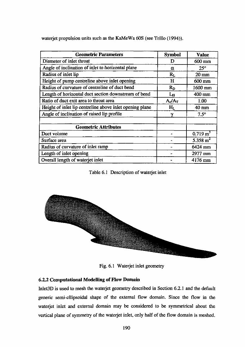
waterjet propulsion units such as the KaMeWa 60S (see Trillo (1994)).
Geometric Parameters Symbol Value Diameter of inlet throat D 600mm Angle of inclination of inlet to horizontal plane a 25° Radius of inlet lip RL 20mm Height of pump centreline above inlet opening H 600mm Radius of curvature of centreline of duct bend Ro 1600mm Length of horizontal duct section downstream of bend LH 400mm Ratio of duct exit area to throat area NAT 1.00 Height of inlet lip centreline above inlet opening plane HL 40mm Angle of inclination of raised lip profile 'Y 7.5°
Geometric Attributes Duct volume - 0.719 m3
Surface area - 5.358 m2
Radius of curvature of inlet ramp - 6424mm Length of inlet opening - 2977mm Overall length of waterjet inlet - 4176mm
Table 6.1 Description of waterjet inlet
Fig. 6.1 Waterjet inlet geometry
6.2.2 Computational Modelling of Flow Domain
Inlet3D is used to mesh the waterjet geometry described in Section 6.2.1 and the default
generic semi-eiJipsoidal shape of the external flow domain. Since the flow in the
waterjet inlet and external domain may be considered to be symmetrical about the
vertical plane of symmetry of the waterjet inlet, only half of the flow domain is meshed.
190
This follows the same approach used in Chapter 5 and neglects the possibility of there
being any gross swirl in the flow as is the case for the waterjet inlet model of Roberts
( 1998) at an NR=0.61. This is a reasonable assumption, as the gross swirl measured by
Roberts is coincidental and a function of the construction of the model. The gross swirl
present, therefore, cannot be generalised to arbitrary waterjet inlet geometries.
Unlike the validation study of the model waterjet inlet presented in Chapter 5, where
there is a need to adjust the boundary conditions to account for the wind tunnel cross
section, the computational simulations presented in this and subsequent chapters are
based upon a full-scale waterjet operating on a flat plate in a large expanse of water.
Hence, the boundary conditions of the flow domain are thus driven by slightly different
considerations.
The topology used by Inlet3D to mesh a waterjet inlet and a simplified flow domain
external to it, has already been discussed in Section 4.2 and is the same as that used for
meshing the waterjet inlet and external flow domain in Chapter 5. Since the flow under
consideration here exhibits "stationary turbulence", the RANS equations assume an
elliptic form, thus requiring the specification of Dirichlet or Neumann boundary
conditions on all surfaces bounding the flow domain. Table 6.2 lists the grid planes
bounding the flow domain and the Fluent boundary condition cell type applied to each
boundary.
Grid Plane in Computational Space Boundary Plane ~mm ~max 11mm 11max Smm l:max Fluent
1 l;=l.O 0.0 0.5 0.0 1.0 1.0 1.0 Inlet 2 l;=l.O 0.5 1.0 0.0 1.0 1.0 1.0 Inlet
3 l;=O.O 0.0 1.0 0.0 1.0 0.0 0.0 Inlet
4 11=1.0 0.0 1.0 1.0 1.0 0.0 1.0 Wall
5 11=0.0 0.0 1.0 0.0 0.0 0.0 1.0 Axis
6 ~=1.0 1.0 1.0 0.0 1.0 0.0 1.0 Symmetry
7 ~=0.0 0.0 0.0 0.0 1.0 0.0 1.0 Symmetry
Table 6.2 Relationship between boundary conditions and flow domain mesh for generic waterjet inlet simulation
The following assumptions and considerations govern the choice of boundary conditions
191
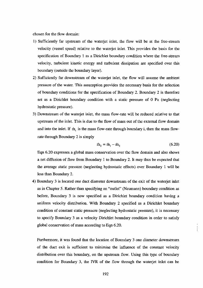
chosen for the flow domain:
1) Sufficiently far upstream of the waterjet inlet, the flow will be at the free-stream
velocity (vessel speed) relative to the waterjet inlet. This provides the basis for the
specification of Boundary 1 as a Dirichlet boundary condition where the free-stream
velocity, turbulent kinetic energy and turbulent dissipation are specified over this
boundary (outside the boundary layer).
2) Sufficiently far downstream of the waterjet inlet, the flow will assume the ambient
pressure of the water. This assumption provides the necessary basis for the selection
of boundary conditions for the specification of Boundary 2. Boundary 2 is therefore
set as a Dirichlet boundary condition with a static pressure of 0 Pa (neglecting
hydrostatic pressure).
3) Downstream of the waterjet inlet, the mass flow-rate will be reduced relative to that
upstream of the inlet. This is due to the flow of mass out of the external flow domain
and into the inlet. If Ih, is the mass flow-rate through boundary i, then the mass flow
rate through Boundary 2 is simply
(6.20)
Eqn 6.20 expresses a global mass conservation over the flow domain and also shows
a net diffusion of flow from Boundary 1 to Boundary 2. It may thus be expected that
the average static pressure (neglecting hydrostatic effects) over Boundary 1 will be
less than Boundary 2.
4) Boundary 3 is located one duct diameter downstream of the exit of the waterjet inlet
as in Chapter 5. Rather than specifying an "outlet" (Neumann) boundary condition as
before, Boundary 3 is now specified as a Dirichlet boundary condition having a
uniform velocity distribution. With Boundary 2 specified as a Dirichlet boundary
condition of constant static pressure (neglecting hydrostatic pressure), it is necessary
to specify Boundary 3 as a velocity Dirichlet boundary condition in order to satisfy
global conservation of mass according to Eqn 6.20.
Furthermore, it was found that the location of Boundary 3 one diameter downstream
of the duct exit is sufficient to minimise the influence of the constant velocity
distribution over this boundary, on the upstream flow. Using this type of boundary
condition for Boundary 3, the NR of the flow through the waterjet inlet can be
192
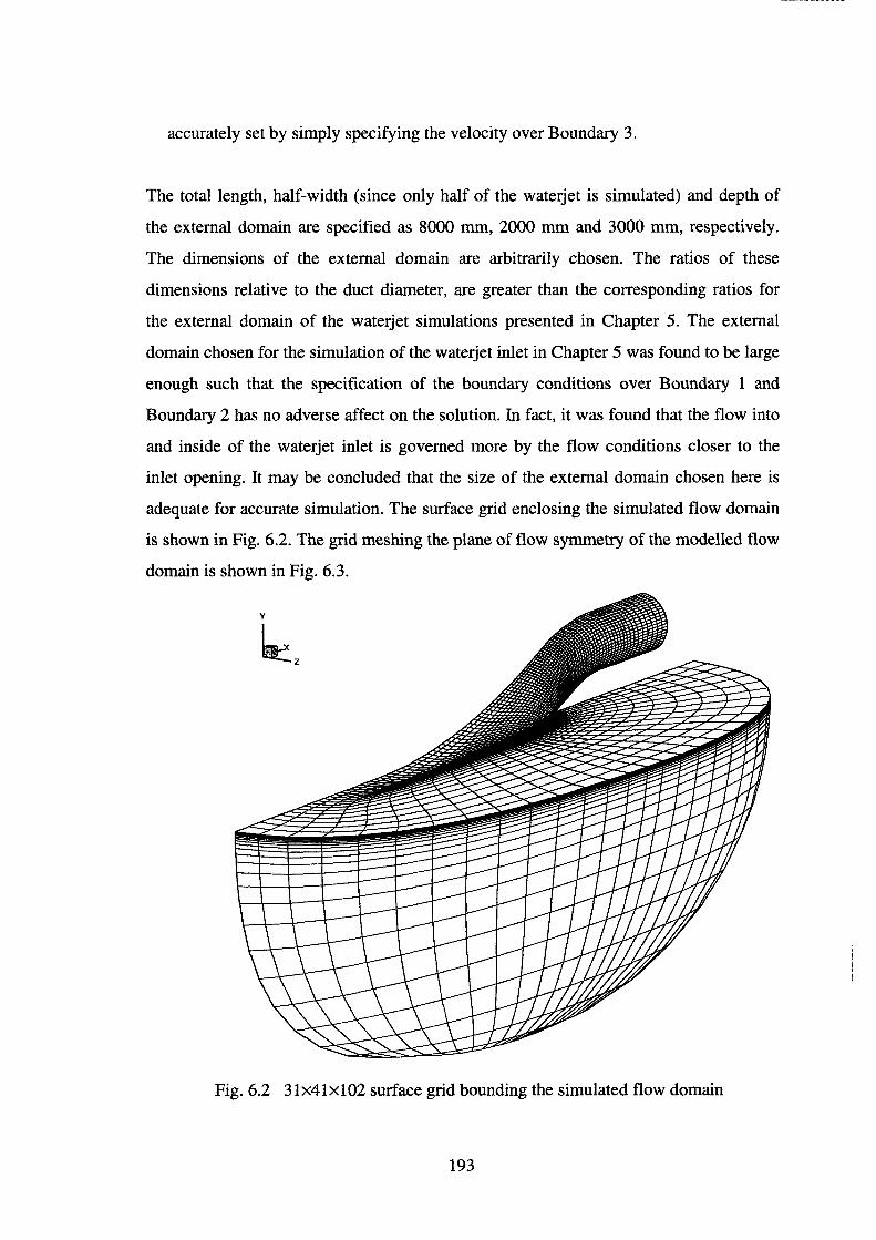
accurately set by simply specifying the velocity over Boundary 3.
The total length, half-width (since only half of the waterjet is simulated) and depth of
the external domain are specified as 8000 mm, 2000 mm and 3000 mm, respectively.
The dimensions of the external domain are arbitrarily chosen. The ratios of these
dimensions relative to the duct diameter, are greater than the corresponding ratios for
the external domain of the waterjet simulations presented in Chapter 5. The external
domain chosen for the simulation of the waterjet inlet in Chapter 5 was found to be large
enough such that the specification of the boundary conditions over Boundary 1 and
Boundary 2 has no adverse affect on the solution. In fact, it was found that the flow into
and inside of the waterjet inlet is governed more by the flow conditions closer to the
inlet opening. It may be concluded that the size of the external domain chosen here is
adequate for accurate simulation. The surface grid enclosing the simulated flow domain
is shown in Fig. 6.2. The grid meshing the plane of flow symmetry of the modelled flow
domain is shown in Fig. 6.3.
y
~z
Fig. 6.2 31x41x102 surface grid bounding the simulated flow domain
193
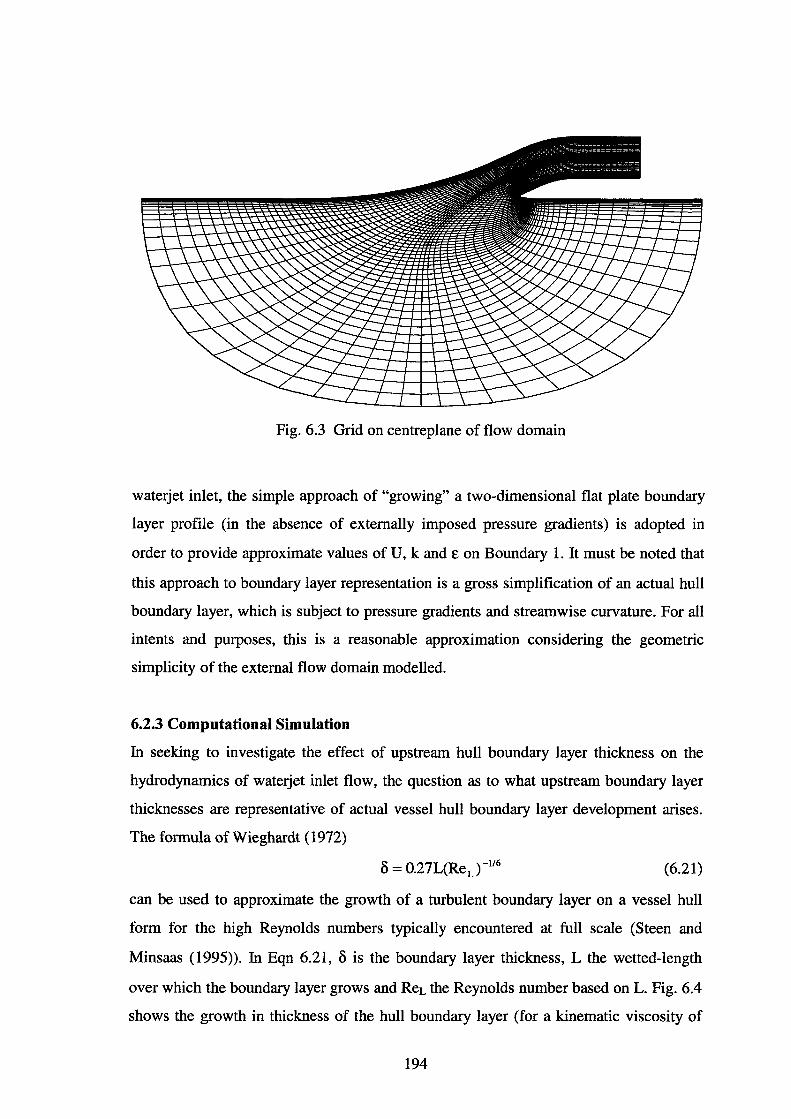
Fig. 6.3 Grid on centreplane of flow domain
waterjet inlet, the simple approach of "growing" a two-dimensional flat plate boundary
layer profile (in the absence of externally imposed pressure gradients) is adopted in
order to provide approximate values of U, k and E on Boundary 1. It must be noted that
this approach to boundary layer representation is a gross simplification of an actual hull
boundary layer, which is subject to pressure gradients and streamwise curvature. For all
intents and purposes, this is a reasonable approximation considering the geometric
simplicity of the external flow domain modelled.
6.2.3 Computational Simulation
In seeking to investigate the effect of upstream hull boundary layer thickness on the
hydrodynamics of waterjet inlet flow, the question as to what upstream boundary layer
thicknesses are representative of actual vessel hull boundary layer development arises.
The formula of Wieghardt ( 1972)
8 = 0.27L(ReL)-116 (6.21)
can be used to approximate the growth of a turbulent boundary layer on a vessel hull
form for the high Reynolds numbers typically encountered at full scale (Steen and
Minsaas (1995)). In Eqn 6.21, 8 is the boundary layer thickness, L the wetted-length
over which the boundary layer grows and ReL the Reynolds number based on L. Fig. 6.4
shows the growth in thickness of the hull boundary layer (for a kinematic viscosity of
194
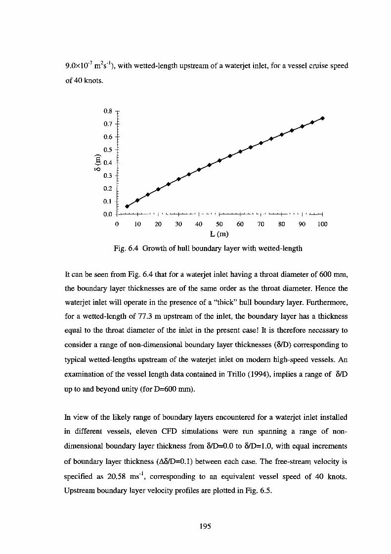
9.0x10⁻⁷ m2s-1), with wetted-length upstream of a waterjet inlet, for a vessel cruise speed
of 40 knots.
0.8
0.7
0.6
0.5 ,..-... s '-' 0.4 t-0
0.3
0.2
0.1
0.0
0 10 20 30 40 50 60 70 80 90 100
L(m)
Fig. 6.4 Growth of hull boundary layer with wetted-length
It can be seen from Fig. 6.4 that for a waterjet inlet having a throat diameter of 600 mm,
the boundary layer thicknesses are of the same order as the throat diameter. Hence the
waterjet inlet will operate in the presence of a "thick" hull boundary layer. Furthermore,
for a wetted-length of 77.3 m upstream of the inlet, the boundary layer has a thickness
equal to the throat diameter of the inlet in the present case! It is therefore necessary to
consider a range of non-dimensional boundary layer thicknesses (OlD) corresponding to
typical wetted-lengths upstream of the waterjet inlet on modern high-speed vessels. An
examination of the vessel length data contained in Trillo (1994 ), implies a range of o/D
up to and beyond unity (for D=600 mm).
In view of the likely range of boundary layers encountered for a waterjet inlet installed
in different vessels, eleven CFD simulations were run spanning a range of non
dimensional boundary layer thickness from 0/D=O.O to 0/D=l.O, with equal increments
of boundary layer thickness (.!\0/D=O.l) between each case. The free-stream velocity is
specified as 20.58 ms-1, corresponding to an equivalent vessel speed of 40 knots.
Upstream boundary layer velocity profiles are plotted in Fig. 6.5.
195
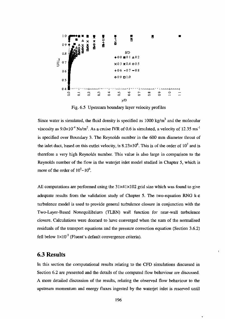
I 0
09
0.8
"!! ~ 07 -.. ~
06
05
04 0 0
• • !II! I X lK 0
+
Ai I ~ ~
-0
t • li!i i5
l>!D +00.01A02
X 0 3 X 0.4 0 0 5
+06 -07-08
0 0 9 [] 1.0
\1)
0
y/D
"' 0 r-0
00 0
Fig. 6.5 Upstream boundary layer velocity profiles
•
0
Since water is simulated, the fluid density is specified as 1000 kg/m3 and the molecular
viscosity as 9.0xl0·4 Ns/m2• As a cruise IVR of 0.6 is simulated, a velocity of 12.35 ms·1
is specified over Boundary 3. The Reynolds number in the 600 mm diameter throat of
the inlet duct, based on this outlet velocity, is 8.23x10⁶• This is of the order of 107 and is
therefore a very high Reynolds number. This value is also large in comparison to the
Reynolds number of the flow in the waterjet inlet model studied in Chapter 5, which is
more of the order of 105-106.
All computations are performed using the 31x41xl02 grid size which was found to give
adequate results from the validation study of Chapter 5. The two-equation RNG k-E
turbulence model is used to provide general turbulence closure in conjunction with the
Two-Layer-Based Nonequilibrium (TLBN) wall function for near-wall turbulence
closure. Calculations were deemed to have converged when the sum of the normalised
residuals of the transport equations and the pressure correction equation (Section 3.6.2)
fell below 1x10·3 (Fluent's default convergence criteria).
6.3 Results
In this section the computational results relating to the CFD simulations discussed in
Section 6.2 are presented and the details of the computed flow behaviour are discussed.
A more detailed discussion of the results, relating the observed flow behaviour to the
upstream momentum and energy fluxes ingested by the waterjet inlet is reserved until
196
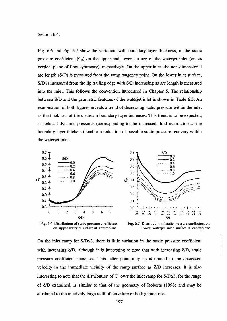
Section 6.4.
Fig. 6.6 and Fig. 6.7 show the variation, with boundary layer thickness, of the static
pressure coefficient (Cp) on the upper and lower surface of the waterjet inlet (on its
vertical plane of flow symmetry), respectively. On the upper inlet, the non-dimensional
arc length (SID) is measured from the ramp tangency point. On the lower inlet surface,
SID is measured from the lip trailing edge with SID increasing as arc length is measured
into the inlet. This follows the convention introduced in Chapter 5. The relationship
between SID and the geometric features of the waterjet inlet is shown in Table 6.3. An
examination of both figures reveals a trend of decreasing static pressure within the inlet
as the thickness of the upstream boundary layer increases. This trend is to be expected,
as reduced dynamic pressures (corresponding to the increased fluid retardation as the
boundary layer thickens) lead to a reduction of possible static pressure recovery within
the waterjet inlet.
"-u
0.7
0.6
0.5
0.4
0.3
0.2
0.1
0.0
-0.1
-0.2
0
BID --o.o --0.2 - - - - - - 0.4 --0.6 --0.8 ----- 1.0
2 3 4 5 6 7 SID
Fig. 6.6 DistributiOn of static pressure coefficient on upper waterjet surface at centreplane
0.8
0.7
0.6
0.5
u"" 0.4
0.3
0.2
0.1
--o.o --0.2 - - - - - • 0.4 --0.6 --0.8 ----- 1.0
0. 0 +'-'--'---f-'--'-'+.LL.Lf-W-I..j-J-J~-'-'-f..L..J-L+-'-L-4-'-'-'--f-J'-'-'--l
~ ~ 00 ~ ~ ~ ~ 00 0 N ~ 0 0 0 ~ ~ - - ~ N N N
SID Ftg. 6.7 Distribution of static pressure coefficient on
lower waterjet mlet surface at centreplane
On the inlet ramp for SID~3, there is little variation in the static pressure coefficient
with increasing BID, although it is interesting to note that with increasing BID, static
pressure coefficient increases. This latter point may be attributed to the decreased
velocity in the immediate vicinity of the ramp surface as BID increases. It is also
interesting to note that the distribution of Cp over the inlet ramp for SID~3, for the range
of BID examined, is similar to that of the geometry of Roberts (1998) and may be
attributed to the relatively large radii of curvature of both geometries.
197
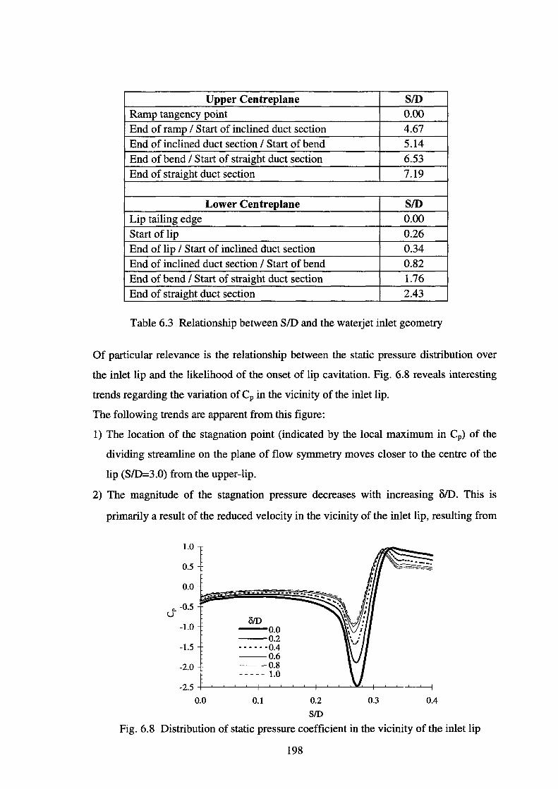
Upper Centreplane SID
Ramp tangency point 0.00 End of ramp I Start of inclined duct section 4.67 End of inclined duct section I Start of bend 5.14 End of bend I Start of straight duct section 6.53 End of straight duct section 7.19
Lower Centreplane SID
Lip tailing edge 0.00 Start of lip 0.26 End of lip I Start of inclined duct section 0.34 End of inclined duct section I Start of bend 0.82 End of bend I Start of straight duct section 1.76 End of straight duct section 2.43
Table 6.3 Relationship between SID and the waterjet inlet geometry
Of particular relevance is the relationship between the static pressure distribution over
the inlet lip and the likelihood of the onset of lip cavitation. Fig. 6.8 reveals interesting
trends regarding the variation of Cp in the vicinity of the inlet lip.
The following trends are apparent from this figure:
1) The location of the stagnation point (indicated by the local maximum in Cp) of the
dividing streamline on the plane of flow symmetry moves closer to the centre of the
lip (S/0=3.0) from the upper-lip.
2) The magnitude of the stagnation pressure decreases with increasing 8/D. This is
primarily a result of the reduced velocity in the vicinity of the inlet lip, resulting from
1.0
0.5
c. -0.5 u
-1.0
-1.5
-2.0
0.0
BID --o.o --0.2 •••••• 0.4 --0.6 --0.8 ----- 1.0
0.1 0.2
SID
0.3 0.4
Fig. 6.8 Distribution of static pressure coefficient in the vicinity of the inlet lip
198
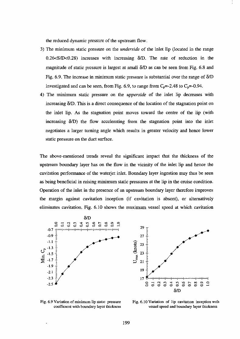
the reduced dynamic pressure of the upstream flow.
3) The minimum static pressure on the underside of the inlet lip (located in the range
0.26<SID<0.28) increases with increasing 8/D. The rate of reduction in the
magnitude of static pressure is largest at small 8/D as can be seen from Fig. 6.8 and
Fig. 6.9. The increase in minimum static pressure is substantial over the range of 8/D
investigated and can be seen, from Fig. 6.9, to range from Cp=-2.48 to Cp=-0.94.
4) The minimum static pressure on the uppers ide of the inlet lip decreases with
increasing 8/D. This is a direct consequence of the location of the stagnation point on
the inlet lip. As the stagnation point moves toward the centre of the lip (with
increasing 8/D) the flow accelerating from the stagnation point into the inlet
negotiates a larger turning angle which results in greater velocity and hence lower
static pressure on the duct surface.
The above-mentioned trends reveal the significant impact that the thickness of the
upstream boundary layer has on the flow in the vicinity of the inlet lip and hence the
cavitation performance of the waterjet inlet. Boundary layer ingestion may thus be seen
as being beneficial in raising minimum static pressures at the lip in the cruise condition.
Operation of the inlet in the presence of an upstream boundary layer therefore improves
the margin against cavitation inception (if cavitation is absent), or alternatively
eliminates cavitation. Fig. 6.10 shows the maximum vessel speed at which cavitation
-0.7
-0.9
-1.1
Q. -1.3 u
-1.5 s:: ~ -1.7
-1.9
-2.1
-2.3
-2.5
0 d d
8/D ~ ~ v ~ ~ ~ 00 ~ q d d d d d d d d
Fig. 6.9 Variation of minimum lip static pressure coefficient with boundary layer thickness
199
29
27 ,....._ "' 25 ..... 0 s:: ~
23 '-"
~ s ~ 21
19
17 0 ~ ~ v ~ ~ ~ 00 ~ q d d d d d d d d d d
8/D
Fig. 6.10 Variation of lip cavitation inception with vessel speed and boundary layer thickness

will begin for a given upstream boundary layer thickness and reveals a greater speed
range for cavitation-free operation (of the waterjet inlet) when the upstream boundary
layer is thick. Cavitation inception was calculated from Eqn. 6.1 by setting the
cavitation number to zero and solving for the reference velocity using the static pressure
data of Fig. 6.9. It must be noted that Reynolds number effects have been neglected in
the calculation of the data plotted in Fig. 6.9.
The variation of the dimensions and shape of the cross-section of the inlet streamtube,
upstream of the waterjet inlet, is shown in Fig. 6.11 for four upstream boundary layer
thicknesses corresponding to 6/D=O, 0.3, 0.7, 1.0. This range is chosen as it spans the
range of BID investigated with approximately equal differences between the values.
Indeed, these four cases are investigated in greater detail in the remainder of this
chapter. It can be seen that as the thickness of the upstream boundary layer grows, so do
the dimensions of the inlet streamtube. The cross-sectional shape is retained, but the
depth and width of the cross-section grow with increasing 6/D. It is interesting to note
that the rate of growth of the width of the streamtube cross-section decreases with
increasing 6/D and it appears that the widths for the cases of 6/0=0.7 and 6/D=l.O are
identical. This will be discussed at greater length in the next section.
0 r- 00
d 0 d 0.00
-0.05 BID -0.10 ---0.0
--0.3 -0.15 --0.7
e -0.20 ----- 1.0 >.
-0.25
-0.30
-0.35 -- --___ _ -0.40
ziD
Fig. 6.11 Growth of the cross-section of the inlet streamtube with boundary layer thickness
The streakline plot of Fig. 6.12 shows the generic diffusing flow into the waterjet inlet
for the geometry consideration here. In this case the flow corresponding to 6/D=O has
been shown.
200
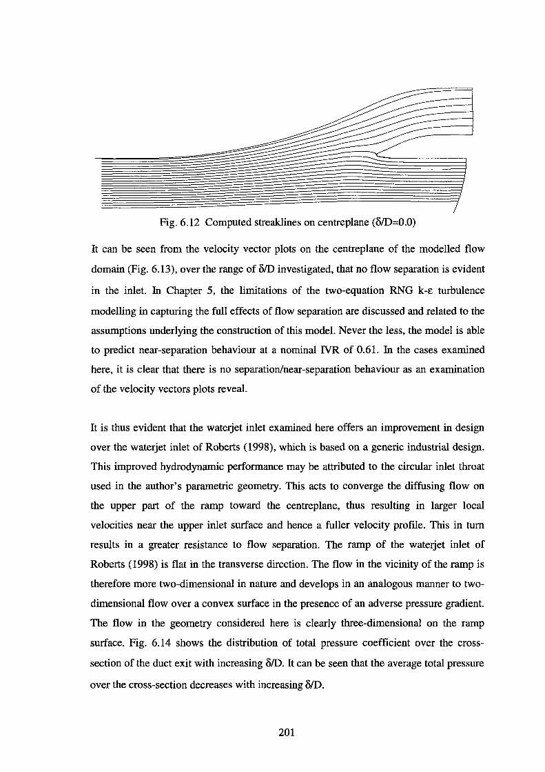
Fig. 6.12 Computed streaklines on centreplane (OID=O.O)
It can be seen from the velocity vector plots on the centreplane of the modelled flow
domain (Fig. 6.13), over the range of OlD investigated, that no flow separation is evident
in the inlet. In Chapter 5, the limitations of the two-equation RNG k-E turbulence
modelling in capturing the full effects of flow separation are discussed and related to the
assumptions underlying the construction of this model. Never the less, the model is able
to predict near-separation behaviour at a nominal IVR of 0.61. In the cases examined
here, it is clear that there is no separation/near-separation behaviour as an examination
of the velocity vectors plots reveal.
It is thus evident that the waterjet inlet examined here offers an improvement in design
over the waterjet inlet of Roberts (1998), which is based on a generic industrial design.
This improved hydrodynamic performance may be attributed to the circular inlet throat
used in the author's parametric geometry. This acts to converge the diffusing flow on
the upper part of the ramp toward the centreplane, thus resulting in larger local
velocities near the upper inlet surface and hence a fuller velocity profile. This in tum
results in a greater resistance to flow separation. The ramp of the waterjet inlet of
Roberts ( 1998) is flat in the transverse direction. The flow in the vicinity of the ramp is
therefore more two-dimensional in nature and develops in an analogous manner to two
dimensional flow over a convex surface in the presence of an adverse pressure gradient.
The flow in the geometry considered here is clearly three-dimensional on the ramp
surface. Fig. 6.14 shows the distribution of total pressure coefficient over the cross
section of the duct exit with increasing OlD. It can be seen that the average total pressure
over the cross-section decreases with increasing OlD.
201
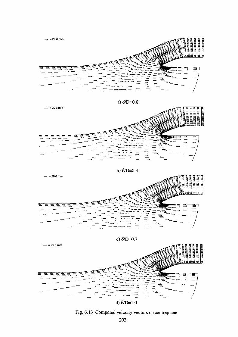
- =206m/s
---
- =206m/s
---
- =206m/s
---
- =206m/s
---
------------- --- - ------~-----~-- ------------------------
a) o/D=O.O
--------~-
b) o/D=0.3
-~~----~----------
c) o/D=0.7
-~-
d) o/D=l.O
Fig. 6.13 Computed velocity vectors on centreplane
202
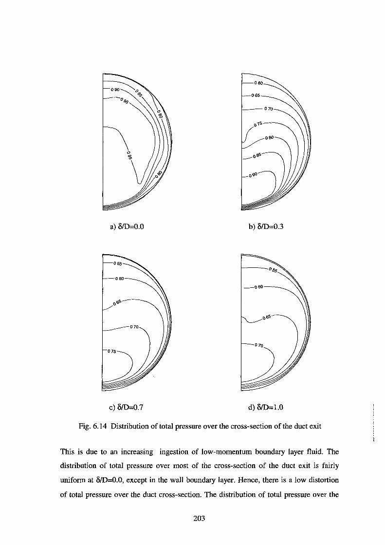
a) OID=O.O b) o/D=0.3
c) o/D=0.7 d) o/D=l.O
Fig. 6.14 Distribution of total pressure over the cross-section of the duct exit
This is due to an increasing ingestion of low-momentum boundary layer fluid. The
distribution of total pressure over most of the cross-section of the duct exit is fairly
uniform at 0/D=O.O, except in the wall boundary layer. Hence, there is a low distortion
of total pressure over the duct cross-section. The distribution of total pressure over the
203
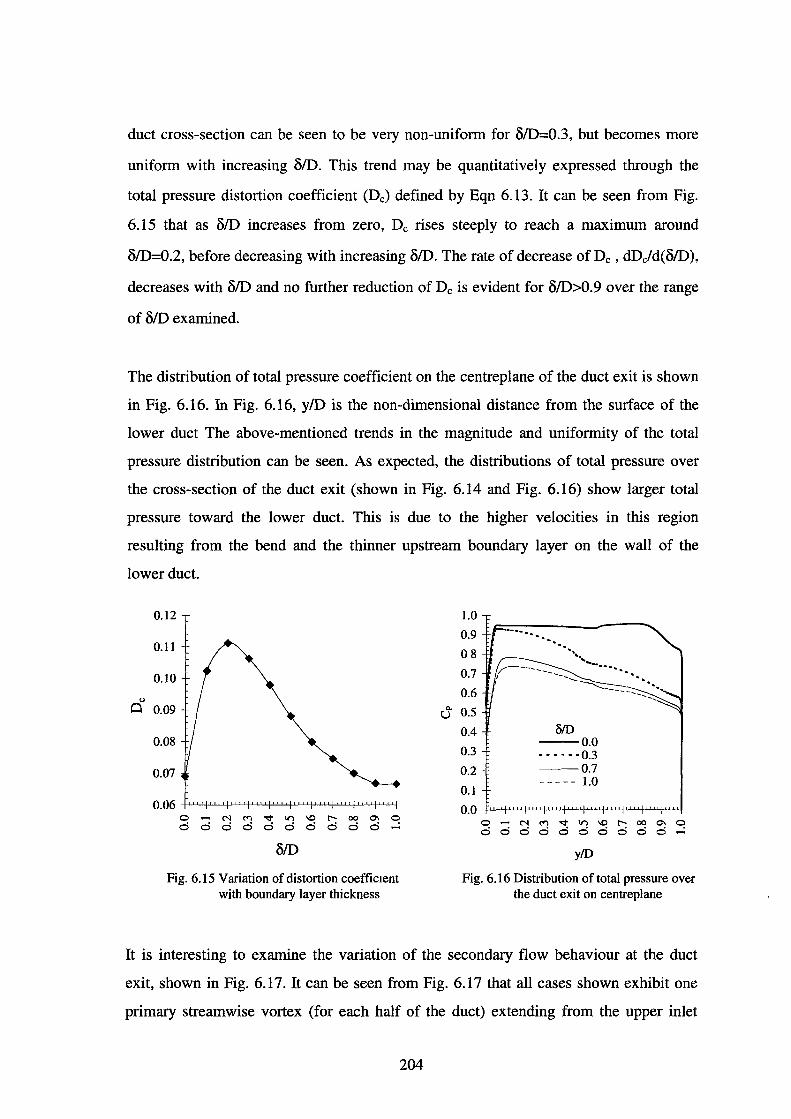
duct cross-section can be seen to be very non-uniform for 8/D=0.3, but becomes more
uniform with increasing 8/D. This trend may be quantitatively expressed through the
total pressure distortion coefficient (De) defined by Eqn 6.13. It can be seen from Fig.
6.15 that as 8/D increases from zero, De rises steeply to reach a maximum around
8/D=0.2, before decreasing with increasing 8/D. The rate of decrease of De, dDcfd(8/D),
decreases with 8/D and no further reduction of De is evident for 8/D>0.9 over the range
of 8/D examined.
The distribution of total pressure coefficient on the centreplane of the duct exit is shown
in Fig. 6.16. In Fig. 6.16, y/D is the non-dimensional distance from the surface of the
lower duct The above-mentioned trends in the magnitude and uniformity of the total
pressure distribution can be seen. As expected, the distributions of total pressure over
the cross-section of the duct exit (shown in Fig. 6.14 and Fig. 6.16) show larger total
pressure toward the lower duct. This is due to the higher velocities in this region
resulting from the bend and the thinner upstream boundary layer on the wall of the
lower duct.
0.12
0.11
0.10
0
0 0.09
0.08
0.07
0 N M V ~ ~ ~ 00 ~ ~ 0 0 0 0 0 0 0 0 0 0 -
BID
Fig. 6.15 Variation of distortion coefficient with boundary layer thickness
1.0
0.9
08
0.7
0.6
u 0.5
0.4
0.3
0.2
0.1
0.0 0 0
··. .. .. .. ~ .............. ..
BID --0.0 - ••. - • 0.3 --0.7 ----- 1.0
N M V ~ ~ ~ 00 ~ ~ 0 0 0 0 0 0 0 0 0
y/D
Fig. 6.16 Distribution of total pressure over the duct exit on centreplane
It is interesting to examine the variation of the secondary flow behaviour at the duct
exit, shown in Fig. 6.17. It can be seen from Fig. 6.17 that all cases shown exhibit one
primary streamwise vortex (for each half of the duct) extending from the upper inlet
204
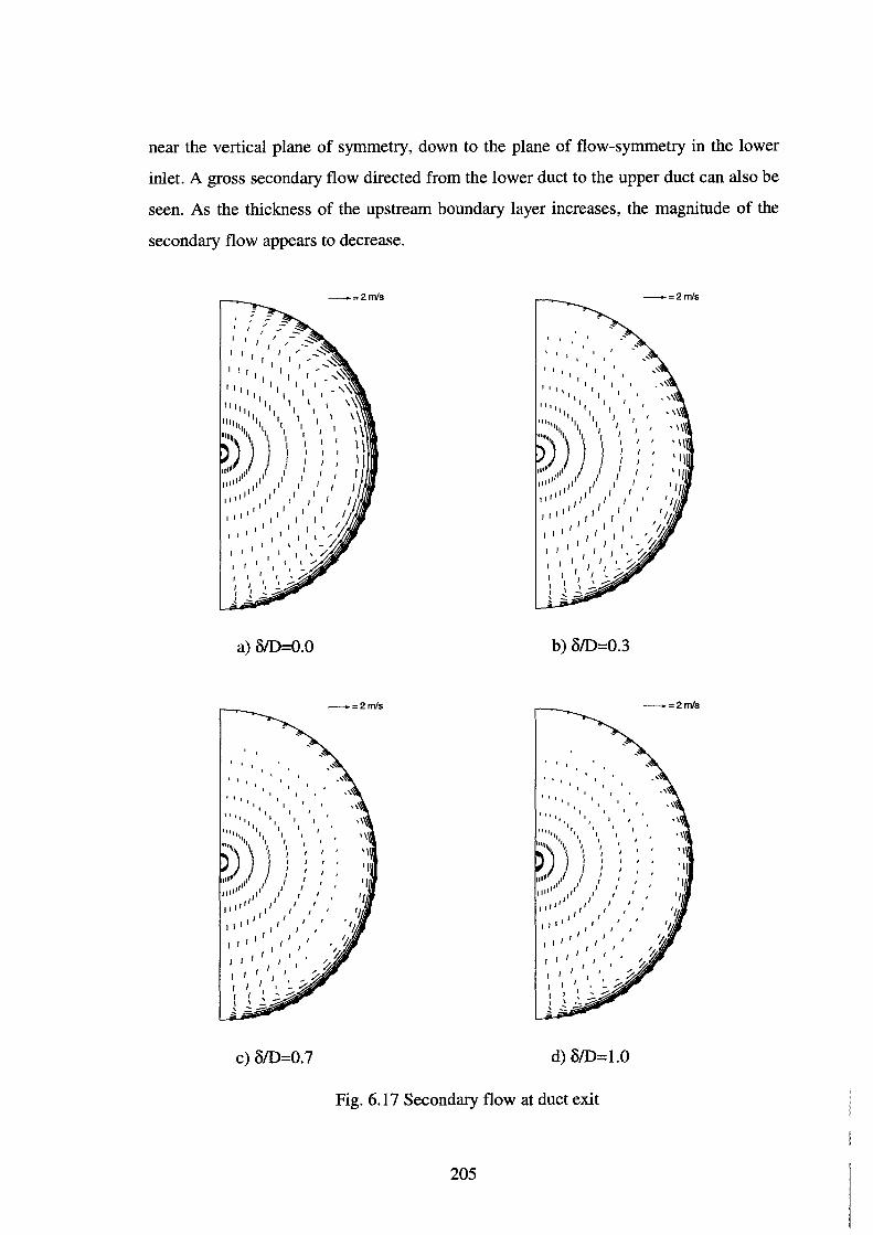
near the vertical plane of symmetry, down to the plane of flow-symmetry in the lower
inlet. A gross secondary flow directed from the lower duct to the upper duct can also be
seen. As the thickness of the upstream boundary layer increases, the magnitude of the
secondary flow appears to decrease.
a) BID=O.O b) BID=0.3
-=2mls
' '
'' '' I I
11
'''I I Ill I
"'•• ., ', ""•·)''')' \, '': 1111 11 I ) / I
Jlllllll Ill ,' I /1 I I
If(// II / I
II I I
1111 II ,'
1 1 I 11
I I I I
c) BID=0.7 d) BID=l.O
Fig. 6.17 Secondary flow at duct exit
205
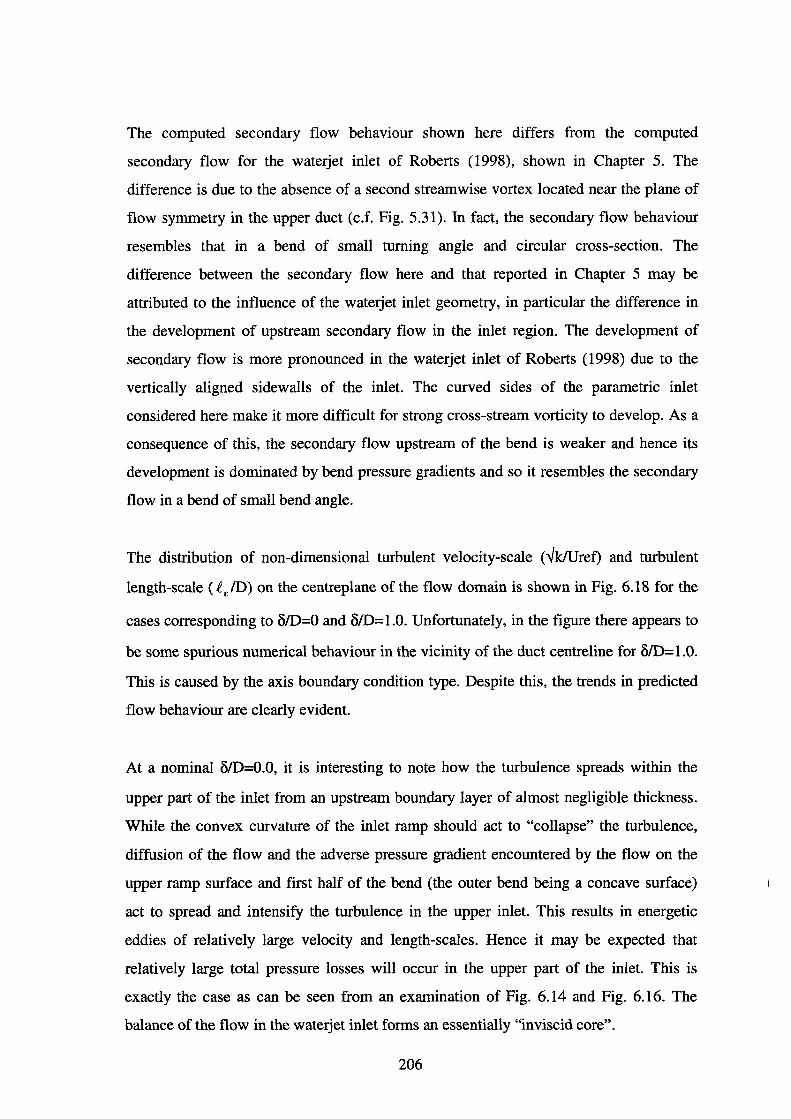
The computed secondary flow behaviour shown here differs from the computed
secondary flow for the waterjet inlet of Roberts (1998), shown in Chapter 5. The
difference is due to the absence of a second streamwise vortex located near the plane of
flow symmetry in the upper duct (c.f. Fig. 5.31). In fact, the secondary flow behaviour
resembles that in a bend of small turning angle and circular cross-section. The
difference between the secondary flow here and that reported in Chapter 5 may be
attributed to the influence of the waterjet inlet geometry, in particular the difference in
the development of upstream secondary flow in the inlet region. The development of
secondary flow is more pronounced in the waterjet inlet of Roberts (1998) due to the
vertically aligned sidewalls of the inlet. The curved sides of the parametric inlet
considered here make it more difficult for strong cross-stream vorticity to develop. As a
consequence of this, the secondary flow upstream of the bend is weaker and hence its
development is dominated by bend pressure gradients and so it resembles the secondary
flow in a bend of small bend angle.
The distribution of non-dimensional turbulent velocity-scale (Vk!Uref) and turbulent
length-scale (ReiD) on the centreplane of the flow domain is shown in Fig. 6.18 for the
cases corresponding to ()/D=O and <>ID=l.O. Unfortunately, in the figure there appears to
be some spurious numerical behaviour in the vicinity of the duct centreline for <>ID= 1.0.
This is caused by the axis boundary condition type. Despite this, the trends in predicted
flow behaviour are clearly evident.
At a nominal <>ID=O.O, it is interesting to note how the turbulence spreads within the
upper part of the inlet from an upstream boundary layer of almost negligible thickness.
While the convex curvature of the inlet ramp should act to "collapse" the turbulence,
diffusion of the flow and the adverse pressure gradient encountered by the flow on the
upper ramp surface and first half of the bend (the outer bend being a concave surface)
act to spread and intensify the turbulence in the upper inlet. This results in energetic
eddies of relatively large velocity and length-scales. Hence it may be expected that
relatively large total pressure losses will occur in the upper part of the inlet. This is
exactly the case as can be seen from an examination of Fig. 6.14 and Fig. 6.16. The
balance of the flow in the waterjet inlet forms an essentially "in viscid core".
206

"k/U"' A 0100
9 0090
8 0080 7 0070
6 0060
5 0050 4 0040
3 0030
2 0020
0010
"k!U,.,
~~ 0060 0050 0040 0030 0020 0010
ljD (Expanded V1ew of L1p) A 00129
9 00116 8 00103 7 00090
6 00077
5 00064 4 00051
3 00039
2 00026
00013
a) 3/D=O.O
,Jw, .. A 0100
9 0090
8 0080 7 0070 6 0060 5 0050 4 0040 3 0030
2 0020 2 2
0010
"k!U .. ,
[ 0200 0183 0167 0150 0133 0117 0100
1/D (Expanded V1ew of L1p) A 00475
9 00427 8 00380
7 00332
6 00285
5 00237 :A;..: 4 00190 - • 3 00142 9
2 00095
00047 ---b) 3/D=l.O
Fig. 6.18 Computed turbulent velocity and length-scales on waterjet centreplane
207

What is particularly interesting is the behaviour of the turbulence in the vicinity of the
inlet lip, where new boundary layers will grow on the surface of the inlet lip
downstream from the stagnation point. A question of interest is the ability of the
turbulence model to accurately predict the correct laminar-to-turbulent transition
behaviour of the developing boundary layers on the lip. It is not possible to quantify the
accuracy of the turbulence model in predicting boundary layer transition without a
detailed and comprehensive experimental validation study. It is however likely that the
turbulence model will predict transition behaviour at Reynolds numbers at least an order
of magnitude too low (see Wilcox (1993)). Never-the-less, examination of the predicted
behaviour of the turbulence in the vicinity of the inlet lip provides valuable qualitative
insight.
The extremely small length-scales in the vicinity of the inlet lip indicate highly
dissipative eddies. An initial examination of the turbulent velocity-scales in the vicinity
of the inlet lip in Fig. 6.18a appears to show lower levels of turbulence than is the case
in Fig. 5.39b. This is, however, deceptive. The Reynolds number of the flow in the
present case is of the order of 107 whereas for the simulations of Chapter 5, the
Reynolds number is more of the order of 105-106• Hence there is a greater separation of
length-scales between the integral scale of the turbulence and the Kolmogorov
microscale of the dissipative eddies. Thus the region of greatest turbulent production
and hence velocity-scale, is closer to the wall and is less easily seen. It therefore appears
as though the turbulent velocity-scale in the vicinity of the inlet lip is smaller than for
the waterjet inlet flow of Chapter 5. In addition, at higher Reynolds number, developing
boundary layers are generally thinner as can be seen from a comparison of flow in the
lip region for Fig. 6.18 and Fig. 5.39b. It is also evident that the adverse pressure
gradient on the underside of the inlet lip acts to increase the turbulence intensity.
The following trends in the turbulence behaviour may be noted as the thickness of the
upstream boundary layer increases:
1) The flow throughout the waterjet inlet becomes turbulent and the overall magnitude
of the turbulent velocity-scale increases as a result of the diffusion of the upstream
turbulence into the inlet.
208
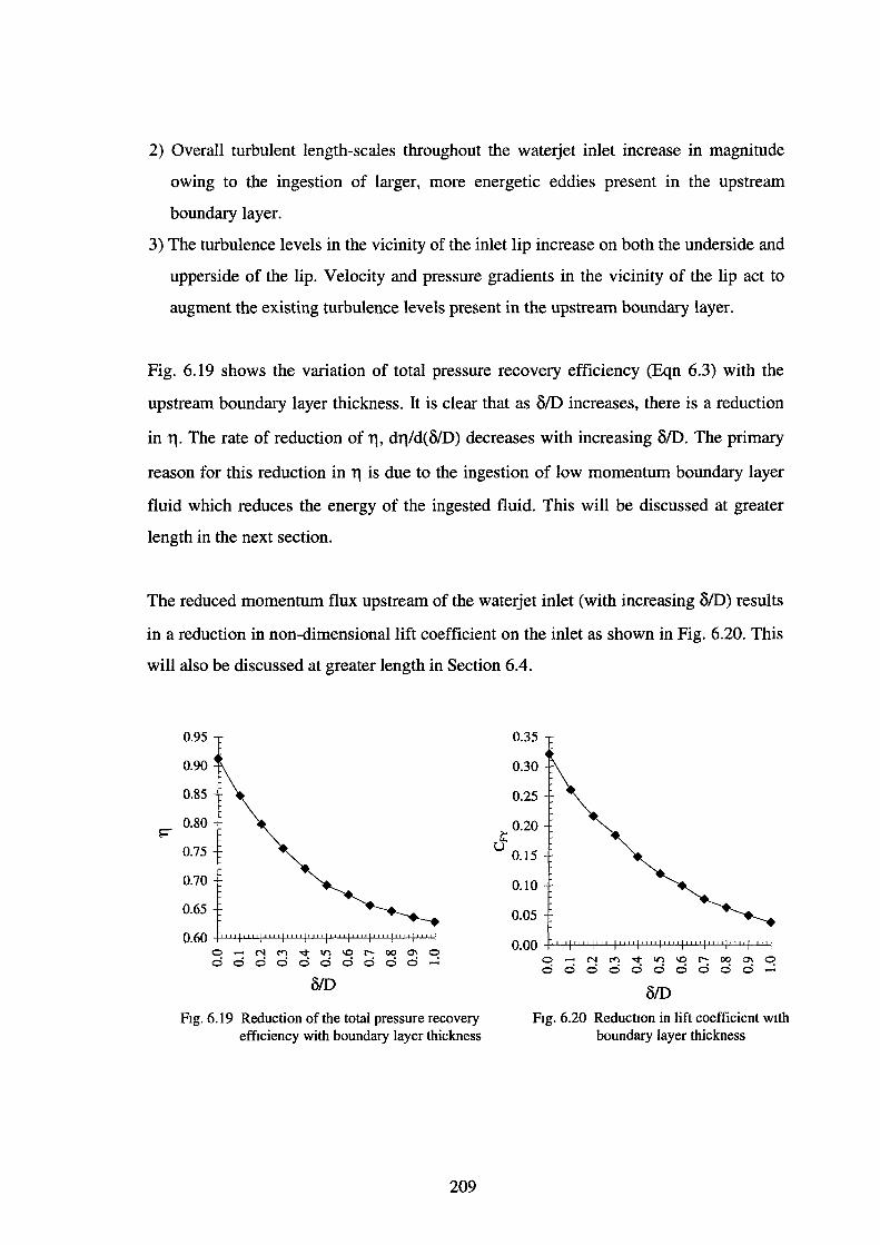
2) Overall turbulent length-scales throughout the waterjet inlet increase in magnitude
owing to the ingestion of larger, more energetic eddies present in the upstream
boundary layer.
3) The turbulence levels in the vicinity of the inlet lip increase on both the underside and
upperside of the lip. Velocity and pressure gradients in the vicinity of the lip act to
augment the existing turbulence levels present in the upstream boundary layer.
Fig. 6.19 shows the variation of total pressure recovery efficiency (Eqn 6.3) with the
upstream boundary layer thickness. It is clear that as o/D increases, there is a reduction
in 11· The rate of reduction of 11, d11/d(o/D) decreases with increasing o/D. The primary
reason for this reduction in 11 is due to the ingestion of low momentum boundary layer
fluid which reduces the energy of the ingested fluid. This will be discussed at greater
length in the next section.
The reduced momentum flux upstream of the waterjet inlet (with increasing o/D) results
in a reduction in non-dimensional lift coefficient on the inlet as shown in Fig. 6.20. This
will also be discussed at greater length in Section 6.4.
0.95
0.90
0.85
0.80
0.75
0.70
0.65
0. 60 -j-LW..Lj-l-1-'-'-j-U..L.L.j-L.l..U.f'U-U..f-'-'-'-'-J-U-U+'-'-'-'-f-'--W"+'-'-'-'-1
0 ~ ~ ~ ~ ~ ~ 00 ~ q d d d d d d d d d d
Fig. 6.19 Reduction of the total pressure recovery efficiency with boundary layer thickness
209
0.35
0.30
0.25
~ 0.20
u 0.15
0.10
0.05
0. 00 -j-LWU-j-I-L.J..J..f-L.LL.Lf-l..LL.Lj-'-'--'-'-f-U-'-'-J-'-U"+'-'-'-'-1-'-l.W.fJ-'-'-'-l
0 ~ ~ ~ ~ ~ ~ 00 ~ q d d d d d d d d d d
BID F1g. 6.20 ReductiOn in lift coefficient With
boundary layer thickness
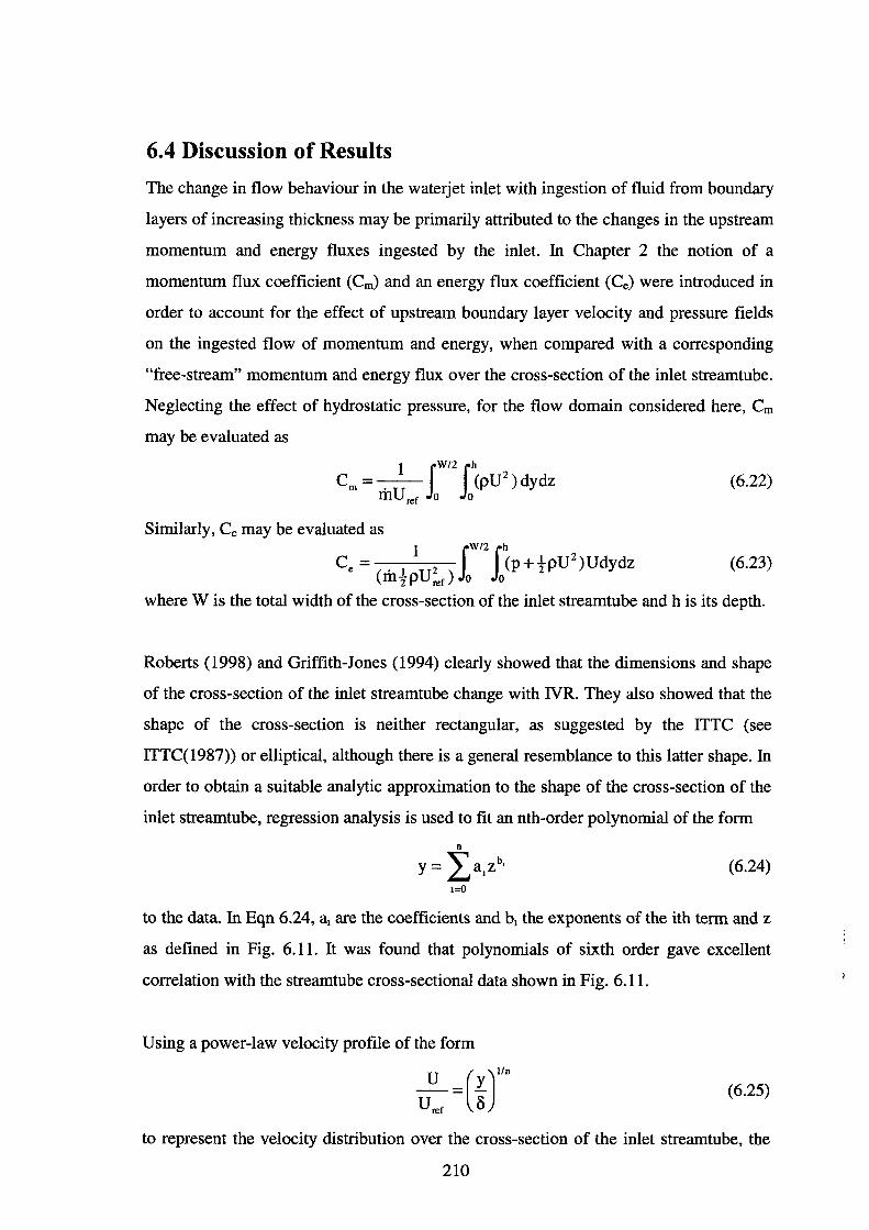
6.4 Discussion of Results
The change in flow behaviour in the waterjet inlet with ingestion of fluid from boundary
layers of increasing thickness may be primarily attributed to the changes in the upstream
momentum and energy fluxes ingested by the inlet. In Chapter 2 the notion of a
momentum flux coefficient (Cm) and an energy flux coefficient (Ce) were introduced in
order to account for the effect of upstream boundary layer velocity and pressure fields
on the ingested flow of momentum and energy, when compared with a corresponding
"free-stream" momentum and energy flux over the cross-section of the inlet streamtube.
Neglecting the effect of hydrostatic pressure, for the flow domain considered here, Cm
may be evaluated as
1 JW/2Jh Cm = . (pU 2) dydz
mUrer o o (6.22)
Similarly, Ce may be evaluated as
1 JW/2Jh ce = . I 2 (p+fpU2 )Udydz (m-zpUrer) o o
(6.23)
where W is the total width of the cross-section of the inlet streamtube and h is its depth.
Roberts (1998) and Griffith-Jones (1994) clearly showed that the dimensions and shape
of the cross-section of the inlet streamtube change with IVR. They also showed that the
shape of the cross-section is neither rectangular, as suggested by the ITTC (see
ITTC( 1987)) or elliptical, although there is a general resemblance to this latter shape. In
order to obtain a suitable analytic approximation to the shape of the cross-section of the
inlet streamtube, regression analysis is used to fit an nth-order polynomial of the form
(6.24)
to the data. In Eqn 6.24, a1 are the coefficients and b1 the exponents of the ith term and z
as defined in Fig. 6.11. It was found that polynomials of sixth order gave excellent
correlation with the streamtube cross-sectional data shown in Fig. 6.11.
Using a power-law velocity profile of the form
~=(r)l'n uref 0
(6.25)
to represent the velocity distribution over the cross-section of the inlet streamtube, the
210
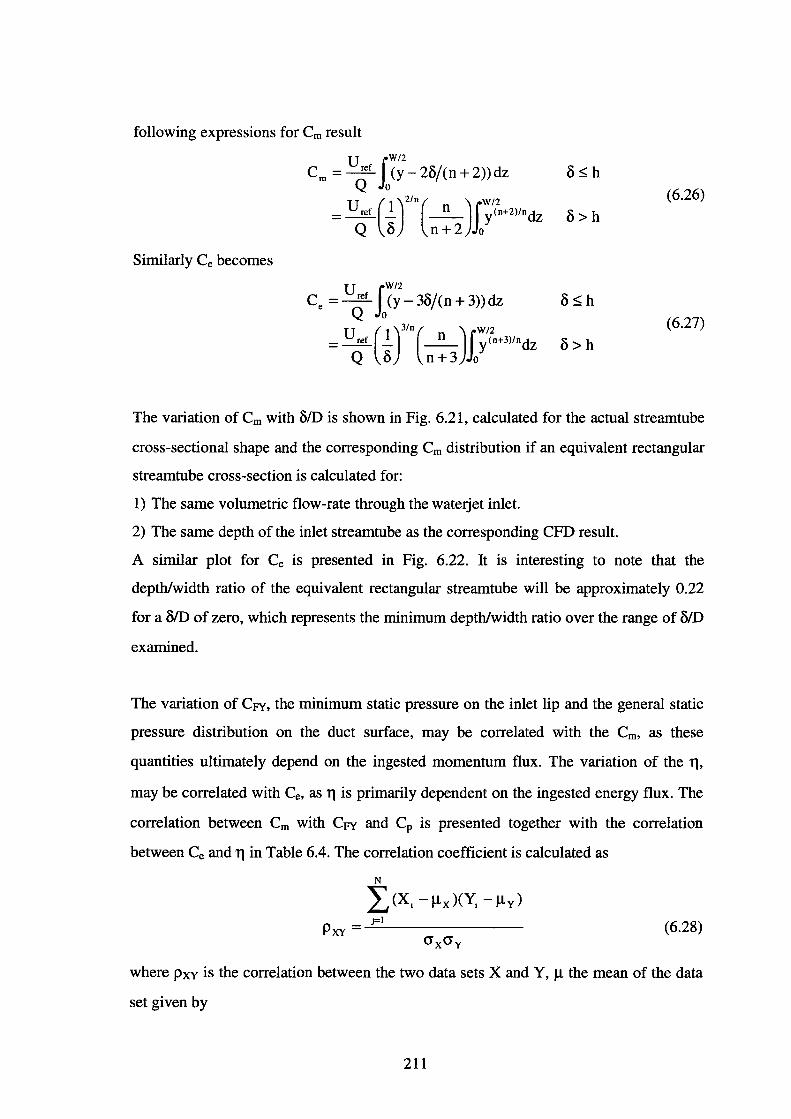
following expressions for Cm result
U JW/2 em=~ (y-28/(n+2))dz Q 0
U ( )2/n( ) W/2 = ~ _! _n_ f y<n+2)/ndz Q 8 n+2 Jo
(6.26)
Similarly Ce becomes
U JW/2 ce =~ (y-38/(n+3))dz Q 0
U ( 1 )3/n ( ) W/2 = ~ - _n_ f y<n+3)/ndz
Q 8 n+3 Jo
8:s;h
(6.27)
8>h
The variation of Cm with 8/D is shown in Fig. 6.21, calculated for the actual streamtube
cross-sectional shape and the corresponding Cm distribution if an equivalent rectangular
streamtube cross-section is calculated for:
1) The same volumetric flow-rate through the waterjet inlet.
2) The same depth of the inlet streamtube as the corresponding CFD result.
A similar plot for Ce is presented in Fig. 6.22. It is interesting to note that the
depth/width ratio of the equivalent rectangular streamtube will be approximately 0.22
for a 8/D of zero, which represents the minimum depth/width ratio over the range of 8/D
examined.
The variation of Cpy, the minimum static pressure on the inlet lip and the general static
pressure distribution on the duct surface, may be correlated with the Cm, as these
quantities ultimately depend on the ingested momentum flux. The variation of the 11.
may be correlated with Ce. as 11 is primarily dependent on the ingested energy flux. The
correlation between Cm with Cpy and Cp is presented together with the correlation
between Ce and 11 in Table 6.4. The correlation coefficient is calculated as
N L (X, - Jlx )(Y, - Jlv) j=l Pxv =....:...._ _______ _ (6.28)
where PxY is the correlation between the two data sets X and Y, Jl the mean of the data
set given by
211
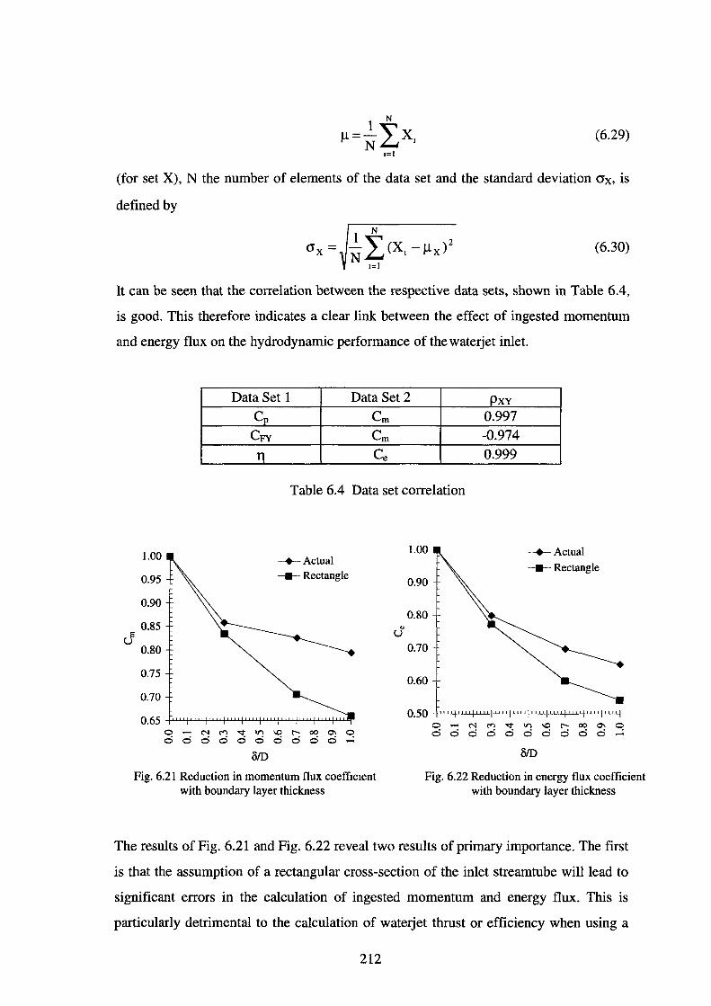
(6.29)
(for set X), N the number of elements of the data set and the standard deviation crx, is
defined by
(6.30)
It can be seen that the correlation between the respective data sets, shown in Table 6.4,
is good. This therefore indicates a clear link between the effect of ingested momentum
and energy flux on the hydrodynamic performance of the waterjet inlet.
Data Set 1 Data Set 2 PxY Cp Cm 0.997
Cpy Cm -0.974
11 Ce 0.999
Table 6.4 Data set correlation
1.00 1.00 ~Actual
~Actual -Rectangle
0.95 -Rectangle 0.90
0.90 0.80
0.85 " e u u
0.80
0.75
0.70
0 N ~ ~ ~ ~ ~ ~ ~ 0. d d d d d d d d d d
BID Fig. 6.21 Reduction in momentum flux coefficient
with boundary layer thickness
0.70
0.60
0 N ~ v ~ ~ ~ ~ ~ ~ d d d d d d d d d d
Fig. 6.22 Reduction in energy flux coefficient with boundary layer thickness
The results of Fig. 6.21 and Fig. 6.22 reveal two results of primary importance. The first
is that the assumption of a rectangular cross-section of the inlet streamtube will lead to
significant errors in the calculation of ingested momentum and energy flux. This is
particularly detrimental to the calculation of waterjet thrust or efficiency when using a
212
parametric model, such as the one presented in Chapter 2. These results therefore
highlight the necessity of an accurate determination of the shape of the cross-section of
the inlet streamtube so that an accurate integration of the velocity profile can be made
and hence accurate calculation of ingested momentum and energy flux.
The second trend that is apparent is the decreasing rate of change of Cm and Ce with olD.
fu other words, both dC.Jd(O/D) and dCJd(o/D) decrease with increasing BID. This is
evident from Fig. 6.21 for Cm and Fig. 6.22 for Ce , where these quantities decrease in an
almost linear manner for O<h, but then follow a much reduced rate of decrease driven by
a power-law. The reader is also referred to Eqn 2.44 to Eqn 2.47, which further
illustrates this point for an inlet streamtube of rectangular cross-section. Since there
exists a good correlation between Cm , Ce and the data, it is therefore of no surprise that
the greatest change in the results occurs for small o/D (eg. O/D<0.3), with a decreasing
rate of change in the results as olD increases. fu a similar manner, the rate of change of
the dimensions of the inlet streamtube, in particular its width, decrease as olD increases.
This is evident from Fig. 6.11.
So what causes this decreasing variation of Cm and Ce with BID? The primary reason
may be attributed to the boundary layer velocity profile becoming "fuller" with
increasing boundary layer thickness. Since the cross-section of the inlet streamtube will
be completely immersed in the boundary layer fluid for o/h~l, the change in velocity
across the cross-section decreases with increasing boundary layer thickness. Assuming
o/h~1 and a power-law velocity profile (Eqn 6.25), the rate of change of the streamwise
velocity with boundary layer thickness may be given by
acu;u ref) = _..:!._1_(~)1
--vn ()() n ()2 y
Alternatively Eqn 6.31 may be written as
()(U/U ref) = -Cjo~+lfn ()()
(6.31)
(6.32)
where C is a constant dependent on n and the selected y position. Therefore as the
boundary layer thickens, the rate of decrease of the streamwise velocity is reduced and
hence the rate of reduction of Cm and Ce decreases.
213
This also helps to explain the variation of distortion coefficient with 8/D, as shown in
Fig. 6.15. The distortion coefficient grows rapidly to reach a maximum at 8/D:::::0.2,
before falling at a reducing rate. At low 8/D (Oih<0.6) the waterjet inlet ingests a
combination of free-stream fluid with a growing proportion of boundary layer fluid,
hence Qb1/Q increases. If one considers the velocity profile across the cross-section of
the inlet streamtube, there is a large variation in the y direction. It may be considered
that the waterjet inlet ingests two "layers" of fluid. Although there is some mixing of
these two "layers" by the secondary flow present in the duct, a large distortion of the
total pressure at the duct exit is a direct result of the large variation in streamwise
velocity profile over the cross-section of the inlet streamtube. For 8/h~0.6, Qb1/Q tends
to unity and for Qbi/Q=1, d(U/Urer )/dO decreases over the whole cross-section of the
inlet streamtube as 8/D increases. Hence the waterjet inlet will ingest a more uniform
distribution of fluid, resulting in a more uniform distribution of total pressure at the duct
exit, albeit with a lower average value.
The results for 11, shown in Fig. 6.19, show how crucial it is that the thickness of the
boundary layer be accounted for when quoting this efficiency, otherwise quoted results
will be misleading. The discrepancy between 11 and Ce may be accounted for as viscous
losses within the waterjet inlet. This may be denoted as 111n according to the definition of
Eqn 2.32 for the parametric model of waterjet efficiency presented in Chapter 2. The
variation of 111n with 8/D is shown in Fig. 6.23. The figure reveals that there is little
variation over the range of 8/D examined. This is possibly due to the lack of flow
separation within the waterjet inlet, with 111n varying between 0.912 and 0.965. There is,
however, some uncertainty in these values, due to an uncertainty in the calculation of Ce.
The power-law velocity profile fit to the actual velocity profile over the cross-section of
the inlet streamtube was within 2% relative error. Inaccuracies are therefore translated to
a maximum possible relative error of 6% in the calculation of Cm, thus leading to an
uncertainty in the results presented in Fig. 6.23.
If it is assumed that these values are reasonably accurate, then the values of 11 quoted in
the literature, typically around 0.8 (Verbeek (1992) quotes 0.83), either account for very
214

large viscous losses (eg. flow separation in the waterjet inlet) or the ingestion of
boundary layer fluid causing a reduction in Ce and hence 11·
0.98
0.96
0.94
~ 092
0.90
0.88 6% Error bars shown
0 N M v ~ ~ ~ 00 ~ 0 0 0 0 0 0 0 0 0 0 0
0/D
Fig. 6.23 Variation of inlet efficiency with boundary layer thickness
6.5 Closure
Parameters that can be used to assess the hydrodynamic performance of the waterjet
inlet were presented in Section 6.2. These provide the basis, not only for interpreting the
results of the boundary layer investigations presented in this chapter, but also for the
design and optimisation-related investigations presented in Chapter 7 and Chapter 8,
respectively. Of particular interest are:
1) Minimum static pressure, expressed either as a cavitation number by Eqn 6.1, or as a
static pressure coefficient by Eqn 6.2
2) Total pressure recovery efficiency (Eqn 6.3) which can be expressed either on a mass
averaged or an area-averaged basis
3) Distortion coefficient, quantifying the non-uniformity of the total pressure at the duct
exit, can be calculated using Eqn 6.13
4) Turbulent velocity and length-scales at the duct exit.
5) Drag forces acting on the inlet.
6) Internal volume of the waterjet inlet, Eqn 6.17.
7) Vertical forces acting on the waterjet inlet, Eqn 6.19.
8) Dimensions and shape of the cross-section of the inlet streamtube.
215
The generic CFD modelling methodology outlined in Section 6.2, forms the basis of the
computational simulation of this and subsequent chapters. The methodology is based on
the solution of the Reynolds-averaged Navier Stokes equations with two-equation RNG
k-E turbulence modelling and the use of a Two-Layer-Based Nonequilibrium wall
function for near-wall turbulence closure.
The effect of the thickness of the upstream boundary layer on the hydrodynamic
performance of the waterjet inlet was investigated for 11 boundary layer thicknesses
ranging from OID=O to O/D=1, where 0 is the boundary layer thickness and D the
diameter of the throat of the waterjet inlet. The geometry of the simulated waterjet inlet
is described in Section 6.2.1 and has a throat diameter of 600 mm.
The following conclusions may be drawn regarding the effect of increasing boundary
layer thickness on the hydrodynamic performance of the waterjet inlet, for the specific
waterjet inlet geometry and IVR investigated:
1) There is an overall reduction in static pressure within the duct
2) The minimum static pressure on the surface of the waterjet inlet occurs on the
underside of the inlet lip and increases significantly with o, thus reducing the
likelihood of cavitation inception
3) The stagnation point moves closer to the centre of the lip
4) Vertical forces acting on the waterjet inlet decrease
5) The width and depth of the inlet streamtube grow
6) Total pressure recovery decreases
7) The distortion coefficient (Eqn 6.13) increases rapidly from 0/D=O, reaches a
maximum around O/D=0.2 and then decreases, indicating an increasingly uniform
distribution of total pressure at the duct exit.
8) There is an overall reduction in the magnitude of the secondary flow at the duct exit
due to a reduction in upstream secondary flow caused by a decrease in flow diffusion
upstream of the inlet throat.
9) Overall turbulent velocity and length-scales increase in the duct
1 0) A lack of flow separation within the waterjet inlet for the range of boundary layer
thicknesses examined, may be attributed to the use of a throat of circular cross-
216
section and is thus an improvement over conventional waterjet inlet geometries, such
as the waterjet inlet geometry examined in Chapter 5.
The first four points may be correlated with the reduction in upstream momentum flux
flowing across the cross-section of the inlet streamtube (with increasing boundary layer
thickness), while the sixth point may be correlated with the reduction in energy flux
across this boundary. The behaviour of the distortion coefficient is linked to the rate of
change of the boundary layer velocity distribution over the cross-section of the inlet
streamtube. The greatest rate of change of the results presented in this chapter occurs
when upstream boundary layer thicknesses are small. This is because the rate of change
of ingested momentum and energy fluxes are greatest for these values.
Therefore in conclusion, it is clear that the upstream boundary layer thickness can have a
marked influence on the hydrodynamics of a waterjet inlet, affecting such aspects as
cavitation inception and the quality of the flow (total pressure distribution and swirl
characteristics) delivered to the waterjet pump and hence the pump performance. It is
therefore necessary to design the waterjet propulsion unit to give adequate
hydrodynamic performance, not only over a range of operating IVR values, but also over
a range of possible upstream boundary layer thicknesses. This issue is particularly
relevant when installing a given waterjet propulsion unit design in different hull forms.
It also highlights the fact that the waterjetlhull system should really be designed as an
integral unit rather than separately.
217
Chapter 7 Design Subspace Investigations
The parametrically-defined generic flush-type waterjet inlet presented in Chapter 4
represents an infinite number of possible waterjet inlet geometries and, hence, flow
solutions. It would be ideal if the hydrodynamic performance parameters (\j11) presented
in Chapter 6, are known analytic functions of the waterjet inlet geometry such that
\j11=f{ X )=f{XJ,X2, ... ,X0 ) {7.1)
where X1 are the components of X , the vector of design variables and f is an explicit
function linking \j11 with X . If this were the case, investigation of the hydrodynamic
performance of the waterjet inlet would be a simple process allowing easy optimisation
of the waterjet inlet geometry. This unfortunately is not the case, as the \j11 are unknown
functions of X and hence the hydrodynamic performance of the waterjet inlet over its
design hyperspace is unknown.
Since \j11 are unknown functions of X , one approach may be to attempt to find an
analytic relationship between \j11 and X . If flow computation were fast and inexpensive,
it could be possible to compute the \j11 at several points in each direction of the design
hyperspace, attempt to fit an analytic approximation to the data (using regression
analysis) and so establish the link between \j11 and X . With m design points in each
dimension, the total number of computations required would be
(7.2)
where N is the total number of computations and n is the number of components of X . For the generic waterjet inlet geometry presented in Chapter 4, n is 8. If 5 points are
investigated in each dimension of the design hyperspace, 390625 computations would
be required. Clearly the total number of computations required quickly becomes
prohibitive for anything but the smallest values of m and n. This approach is therefore
infeasible.
218
On the other hand, investigation of a two-dimensional subspace of the design
hyperspace is a manageable problem. Since such an investigation is limited to the
variation of only two components of X , with the other components held at constant
values, the total number of computations is thus reduced to
(7.3)
Therefore, two-dimensional subspaces of the design hyperspace can be investigated and
an explicit analytic relationship between 'tf1 and X established. For a generic geometry
described by n parameters, there are
N - n! 2-
(n-2)!2! (7.4)
possible two-dimensional subspace combinations that can be investigated. For the
generic geometry presented in Chapter 4 (n=8), there are 28 possible two parameter
subspace combinations. Of particular relevance are those subspaces containing
geometric components that have the greatest effect on flow performance. This issue will
be discussed at greater length in Section 7 .2.
The focus of this chapter is dedicated to the investigation of three two-dimensional
subspaces of the design hyperspace at the vessel cruise condition (IVR=0.60) with a
boundary layer upstream of the waterjet inlet. The motivations behind this study are:
1) The large amount of data collected from such investigations allows the flow
behaviour in the waterjet inlet to be correlated with the underlying geometry via an
understanding of the physical mechanisms governing the flow behaviour.
2) The examination of the sensitivity of the flow in the waterjet inlet to variations in
parameter values.
3) To illuminate the most important hydrodynamic issues associated with inlet design.
4) The design data collected for a two-dimensional design subspace allow an
optimisation to be made in that subspace. In other words, the waterjet inlet could be
designed from a "two-parameter series".
It must be noted from the outset, that the data presented in this chapter is dependent
upon IVR and the upstream boundary layer thickness (Chapter 6) and is therefore not
219
applicable to other NR values or different upstream boundary layer profiles. Griffith
Jones (1994) noted that the Hamilton Jet model 211 operates at a cruise NR of 0.70.
Therefore for the cruise NR of 0.60 considered here, it may be expected that suction on
the underside of the inlet lip is greater (especially in the case of no internal flow
diffusion) and hence the elimination of cavitation at this location at high vessel speeds
poses a more challenging problem.
An overview of this chapter is presented below. In Section 7.1 the methodology used to
investigate two-dimensional subspaces of the design hyperspace is discussed. The
computational modelling and simulation procedure is outlined in Section 7 .2.
Computational results are presented for the three two-parameter design subspaces
investigated in Section 7 .3. The physical mechanisms underlying the trends in flow
behaviour are investigated in detail in Section 7.4. Finally, the conclusions of the design
subspace investigations are summarised in Section 7.5.
7.1 Investigation Methodology
The basic aim of the investigation methodology presented herein is to find an explicit
relationship between \jl1 and X over an examined two-dimensional subspace of the
design hyperspace. The methodology may be summarised as:
1) CFD flow solutions are obtained for a "grid" of design points. In other words, two
components of the vector of design variables are varied with the other components
held constant. The grid is composed of equi-spaced points in each component
direction.
2) The \jl1 are determined from the flow solutions corresponding to the respective design
points.
3) Non-linear least-squares regression is used to fit a bicubic patch surface to the data
obtained for \jl1 in order to construct an explicit relationship between \jl1 and X .
4) The correlation coefficient is calculated in order to examine whether a good
correlation has been obtained between the surface fit to the data and the data itself.
The approach to non-linear least-squares regression is described in greater detail below.
It was originally thought that a bicubic patch of the form
220
(7.5)
would provide a suitable analytic approximation to the data over the range of parameter
values considered. As will be shown later, this was indeed the case. In Eqn 7.5, u and w
represent coordinates on a unit square such that
(7.6)
Furthermore, if x1 and x2 represent any two components of X comprising the sub-space
under investigation, then u and w may be defined as
x1- X nun u = _.:______::::::...._ xmax- X nun
x2 -X nun w = ----:=--__....;;;;=--
X max -X nun
(7.7)
where subscripts min and max denote the lower and upper values of x1 and x2 on the
grid of design points investigated in that subspace.
It must be noted that the bicubic surface patch also accounts for surface fits of order less
than three and so can be used to represent biquadratic and bilinear surfaces. Non-linear
least -squares regression is used to determine the numerical coefficients of Eqn 7.5. Non
linear least-squares regression involves the minimisation of the least square error
between '1'1 and '¥1 over the range of data examined. The least-square error between '1'1
and 'Pi may be written as
1 N 2
E = 2 L ('I'.,J- 'P.) j=l
(7.8)
where E is the least-square error and N the number of data points (N can be calculated
using Eqn 7.3).
In order to minimise the least-square error represented by Eqn 7.8, any optimisation
technique can be used. Minimisation of E is essentially an unconstrained optimisation
for the vector ofbicubic patch coefficients (ak,I) which may be written as
(7.9)
The unconstrained quasi-Newton algorithm of Liu and Nocedal (1989) is used to effect
the minimisation of E. Information relating to quasi-Newton methods can be found in
Gillet al (1981).
221
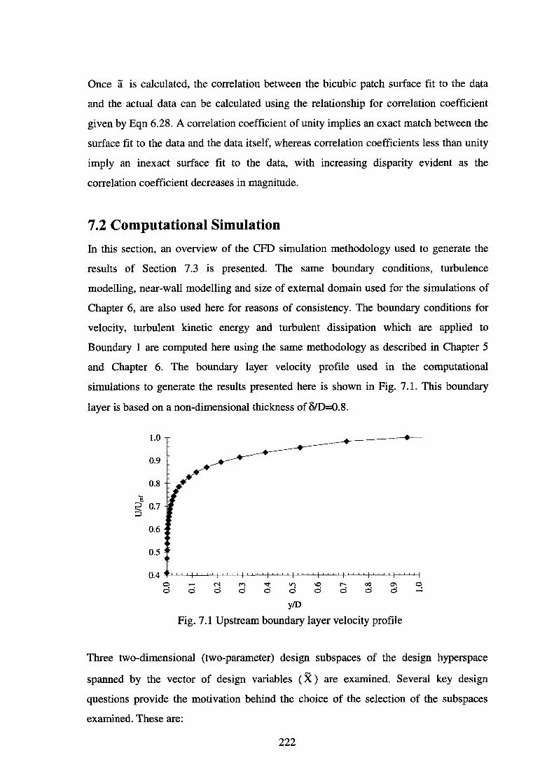
Once a is calculated, the correlation between the bicubic patch surface fit to the data
and the actual data can be calculated using the relationship for correlation coefficient
given by Eqn 6.28. A correlation coefficient of unity implies an exact match between the
surface fit to the data and the data itself, whereas correlation coefficients less than unity
imply an inexact surface fit to the data, with increasing disparity evident as the
correlation coefficient decreases in magnitude.
7.2 Computational Simulation
In this section, an overview of the CFD simulation methodology used to generate the
results of Section 7.3 is presented. The same boundary conditions, turbulence
modelling, near-wall modelling and size of external domain used for the simulations of
Chapter 6, are also used here for reasons of consistency. The boundary conditions for
velocity, turbulent kinetic energy and turbulent dissipation which are applied to
Boundary 1 are computed here using the same methodology as described in Chapter 5
and Chapter 6. The boundary layer velocity profile used in the computational
simulations to generate the results presented here is shown in Fig. 7 .1. This boundary
layer is based on a non-dimensional thickness of 0/0=0.8.
1.0
0.9
0.8
'i! ::J 0.7 ..... ::J
0.6
0.5
0.4 0 C'l (<) v lrl \0 r-- 00 0\ ~ d d d d d d d d d d
y/D
Fig. 7.1 Upstream boundary layer velocity profile
Three two-dimensional (two-parameter) design subspaces of the design hyperspace
spanned by the vector of design variables ( X ) are examined. Several key design
questions provide the motivation behind the choice of the selection of the subspaces
examined. These are:
222
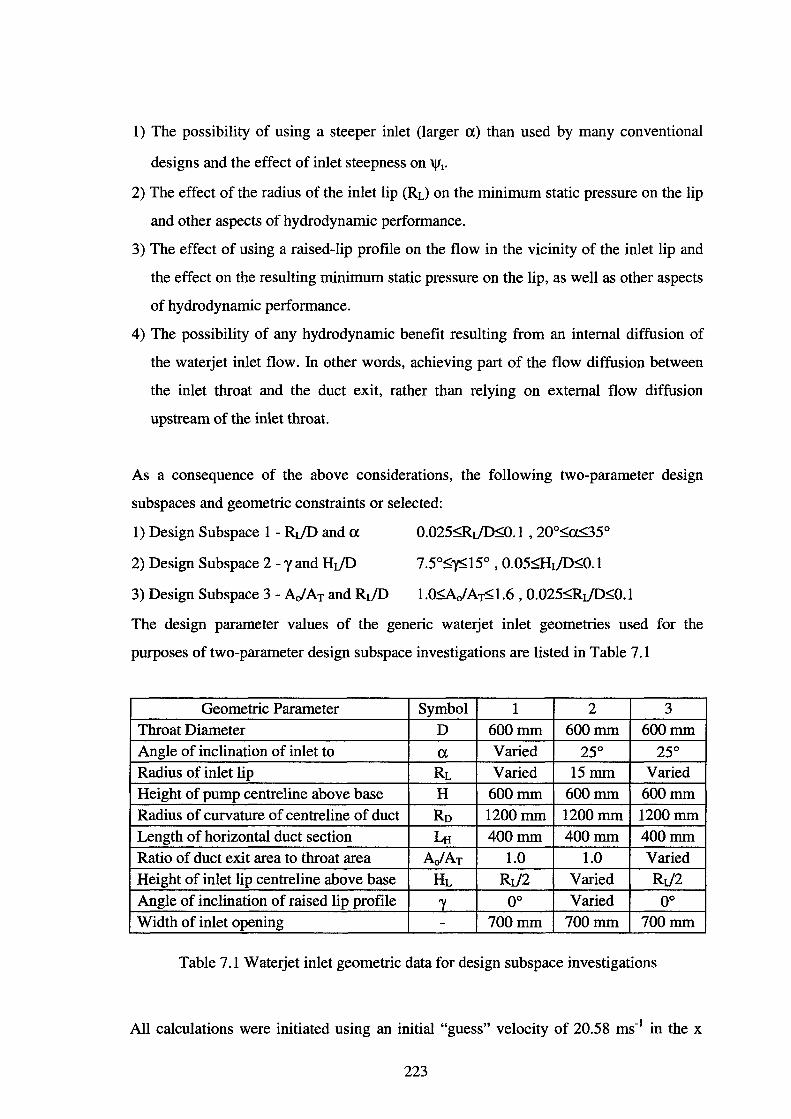
1) The possibility of using a steeper inlet (larger a) than used by many conventional
designs and the effect of inlet steepness on 'lf1•
2) The effect of the radius of the inlet lip (RL) on the minimum static pressure on the lip
and other aspects of hydrodynamic performance.
3) The effect of using a raised-lip profile on the flow in the vicinity of the inlet lip and
the effect on the resulting minimum static pressure on the lip, as well as other aspects
of hydrodynamic performance.
4) The possibility of any hydrodynamic benefit resulting from an internal diffusion of
the waterjet inlet flow. In other words, achieving part of the flow diffusion between
the inlet throat and the duct exit, rather than relying on external flow diffusion
upstream of the inlet throat.
As a consequence of the above considerations, the following two-parameter design
subspaces and geometric constraints or selected:
1) Design Subspace 1 - RUD and a
2) Design Subspace 2 - y and HUD
3) Design Subspace 3 - AJ AT and RUD
0.025~UD:::;0.1 , 20o:::;a:::;35°
7.5o:::;y:::;15°, o.o5:::;Huo:::;o.1
1.0:::;AJAT:::;1.6, 0.025:::;RUD:::;0.1
The design parameter values of the generic waterjet inlet geometries used for the
purposes of two-parameter design subspace investigations are listed in Table 7.1
Geometric Parameter Symbol 1 2 3 Throat Diameter D 600mm 600mm 600mm Angle of inclination of inlet to a Varied 25° 25° Radius of inlet lip RL Varied 15mm Varied Height of pump centreline above base H 600mm 600mm 600mm Radius of curvature of centreline of duct Ro 1200mm 1200mm 1200mm Length of horizontal duct section LH 400mm 400mm 400mm Ratio of duct exit area to throat area AJAT 1.0 1.0 Varied Height of inlet lip centreline above base HL Rt.!2 Varied Rt.!2 Angle of inclination of raised lip profile 'Y oo Varied oo
Width of inlet opening - 700mm 700mm 700mm
Table 7.1 Waterjet inlet geometric data for design subspace investigations
All calculations were initiated using an initial "guess" velocity of 20.58 ms-1 in the x
223
direction throughout the flow domain, thus allowing the computations to be run as batch
processes after initial problem set-up. Once all computations have converged, the 'lf1 are
calculated and the methodology outlined in Section 7.1 is used to determine a suitable
bicubic patch fit to the data. In all cases, a correlation coefficient of unity was obtained
thus indicating a perfect match between the bicubic-patch approximation to the data and
the data itself.
In order to investigate the first design subspace (Section 7.3.1), a total of sixteen CFD
computations was executed, with four computations run in each parameter direction. For
the second design subspace (Section 7.3.2) a total of twelve computations was executed,
with four computations in the y parameter direction and three in the HL parameter
direction. A total of sixteen computations was executed for the investigation of the third
design subspace (Section 7.3.3), with four computations run in each parameter direction.
The total number of computations executed for each design subspace is deemed to be
adequate provided that the variation of the '1'1 over the design subspaces investigated is
smooth. From the results obtained in Section 7.3, this does appear to be the case.
Furthermore, the expectation will be for a smooth variation of the 'lf1 over the design
subspaces in the absence of any major flow separation effects.
If the 'lf1 are not smoothly varying over the range of parameter values comprising the
subspace under investigation, a significantly larger number of computations will be
required to resolve any potential discontinuities, as a result of the larger number of
simulations required in each parameter direction. Due to the quadratic nature ofEqn 7.3,
it is obvious that a doubling of the number of computations in each parameter direction
leads to a four-fold increase in the total number of computations required. The presence
of discontinuities also complicates the form of the analytic surface required to provide a
good correlation with the data. If discontinuitiues are suspected in the 'lf17 an alternative
approach may be to select points in the vicinity of the suspected discontinuity, determine
the values of the '1'1 and then progressively resolve the discontinuity by further addition
of points in the appropriate locations.
224
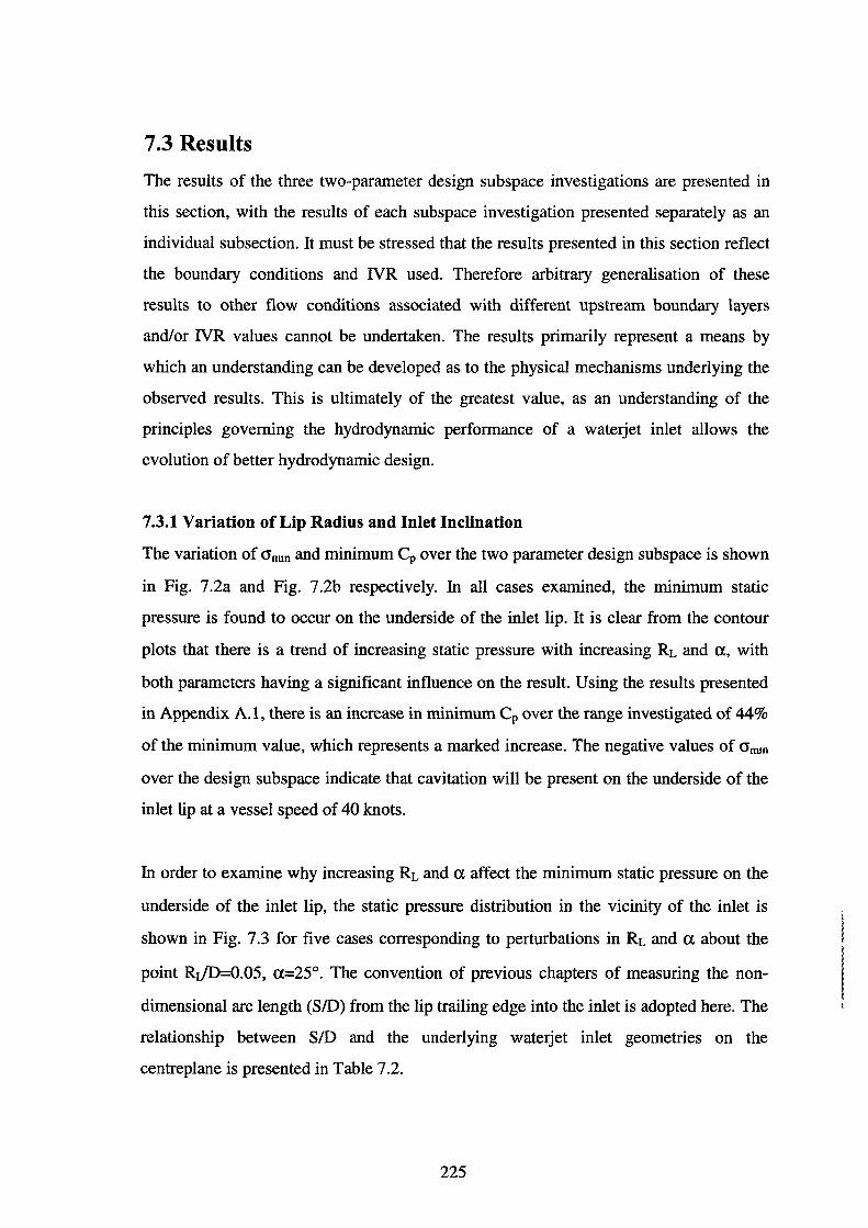
7.3 Results
The results of the three two-parameter design subspace investigations are presented in
this section, with the results of each subspace investigation presented separately as an
individual subsection. It must be stressed that the results presented in this section reflect
the boundary conditions and IVR used. Therefore arbitrary generalisation of these
results to other flow conditions associated with different upstream boundary layers
and/or IVR values cannot be undertaken. The results primarily represent a means by
which an understanding can be developed as to the physical mechanisms underlying the
observed results. This is ultimately of the greatest value, as an understanding of the
principles governing the hydrodynamic performance of a waterjet inlet allows the
evolution of better hydrodynamic design.
7.3.1 Variation of Lip Radius and Inlet Inclination
The variation of O'mm and minimum Cp over the two parameter design subspace is shown
in Fig. 7 .2a and Fig. 7 .2b respectively. In all cases examined, the minimum static
pressure is found to occur on the underside of the inlet lip. It is clear from the contour
plots that there is a trend of increasing static pressure with increasing RL and a., with
both parameters having a significant influence on the result. Using the results presented
in Appendix A.l, there is an increase in minimum Cp over the range investigated of 44%
of the minimum value, which represents a marked increase. The negative values of O'mm
over the design subspace indicate that cavitation will be present on the underside of the
inlet lip at a vessel speed of 40 knots.
In order to examine why increasing RL and a. affect the minimum static pressure on the
underside of the inlet lip, the static pressure distribution in the vicinity of the inlet is
shown in Fig. 7.3 for five cases corresponding to perturbations in RL and a. about the
point Rr/1)=0.05, a.=25°. The convention of previous chapters of measuring the non
dimensional arc length (SID) from the lip trailing edge into the inlet is adopted here. The
relationship between SID and the underlying waterjet inlet geometries on the
centreplane is presented in Table 7 .2.
225
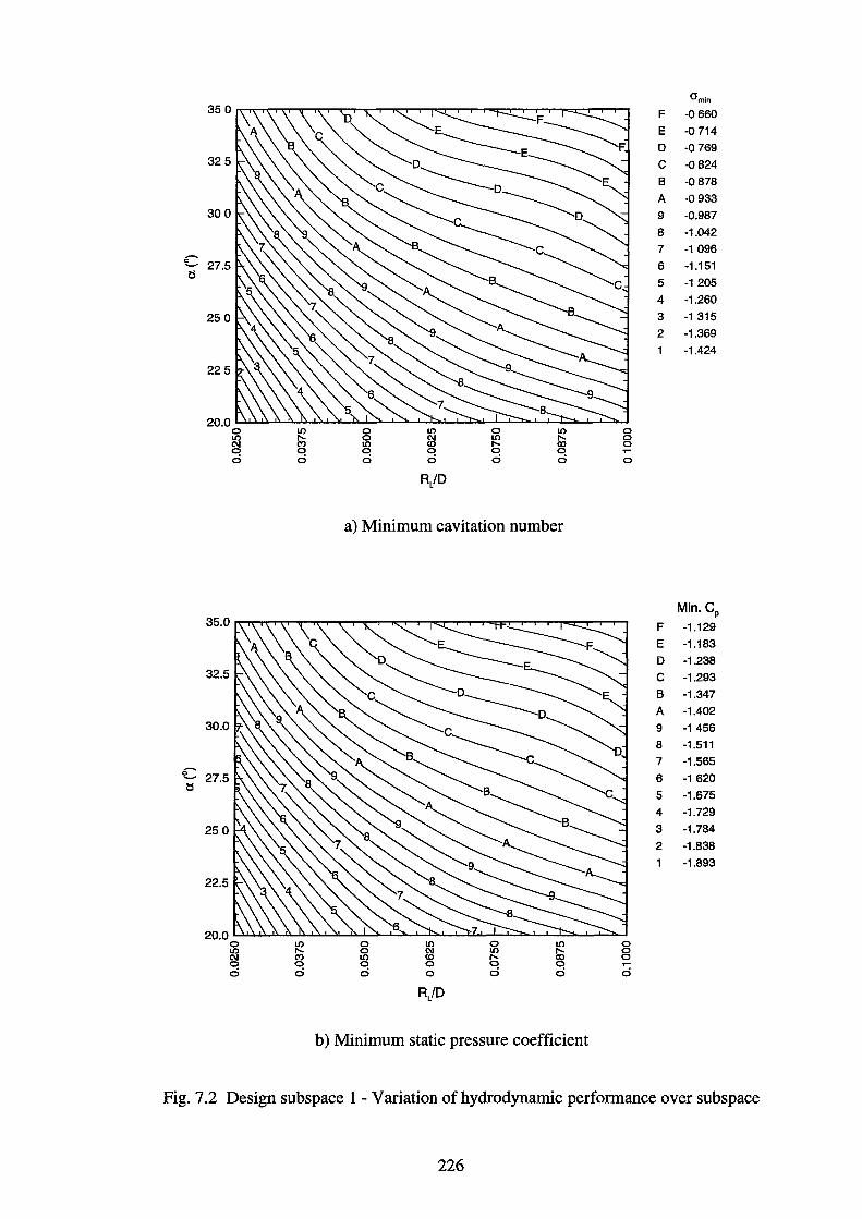
35 0
325
30 0
~
'<.-- 27.5 i:$
25 0
22 5
20.0 0 LO 0 LO 0 LO LO ,.._ 0 C\1 LO ,.._ C\1 C') LO <0 ,.._ CX) 0 0 0 0 0 0 ci ci ci ci ci ci
RJD
a) Minimum cavitation number
35.0
32.5
30.0
c 27.5 i:$
25 0
22.5
20.0 0 LO 0 LO 0 LO LO ,.._ 0 C\1 LO !Xi C\1 C') LO <0 ,.._ 0 0 0 0 0 0 ci ci ci 0 ci ci
RJD
b) Minimum static pressure coefficient
0 0 0 .... 0
0 g .... ci
F
E D
c B
A
9
8
7
6
5
4
3
2
F
E D c B
A 9
8
7
6
5
4
3
2
crmln
-0660
-o 714
-0769
-0824
-0878
-0933
-0.987
-1.042
-1 096
-1.151
-1 205
-1.260
-1 315
-1.369
-1.424
Min.CP -1.129
-1.183
-1.238
-1.293
-1.347
-1.402
-1 456
-1.511
-1.565
-1 620
-1.675
-1.729
-1.784
-1.838
-1.893
Fig. 7.2 Design subspace 1 - Variation of hydrodynamic performance over subspace
226
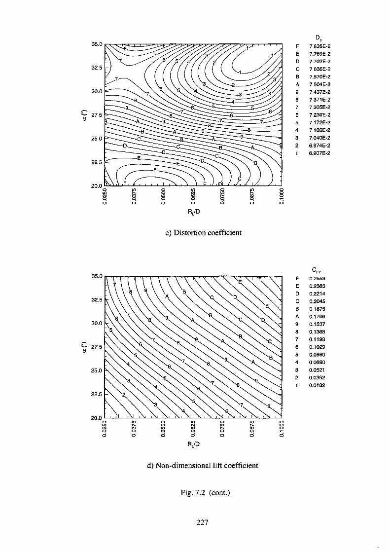
DC F 7 835E-2
E 7.769E-2
D 7 702E-2
c 7 636E-2
B 7.570E-2
A 7 504E-2
9 7 437E-2
8 7 371E-2
7 7 305E-2 c 6 7 239E-2 ts
5 7.172E-2
4 7106E-2
3 7.040E-2
2 6.974E-2
6.907E-2
225
RJD
c) Distortion coefficient
CFY F 0.2553
E 0.2383
D 0.2214
c 0.2045
B 01875
A 0.1706
9 0.1537
8 0.1368
7 0.1198
6 0.1029
5 0.0860
4 00690
3 0.0521
2 0.0352
0.0182
RJD
d) Non-dimensional lift coefficient
Fig. 7.2 (cont.)
227
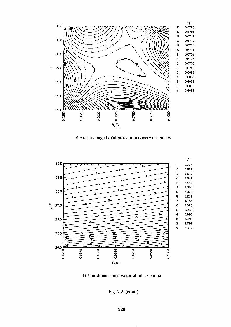
e) Area-averaged total pressure recovery effi . ICiency
350-1-~---------..-11
I l
~..---~ - ........... 0 LO 0
:e ..... CXI
0 0
0 0 ci ci ci
RJD
f) Non-dimensional . waterJet inlet volume
F I g. 7.2 (cont.)
228
ll F 06723
E 06721
D 0.6718
c 06716
8 06713
A 06711
9 0.6708
8 06706
7 0.6703
6 0.6700
5 0.6698
4 0.6695
3 0.6693
2 06690
0.6688
v· F 3.774
E 3.697
D 3.619
c 3.541
B 3.464
A 3.386
9 3308
8 3.231
7 3.153
6 3075
5 2.998
4 2.920
3 2.842
2 2.765
2.687
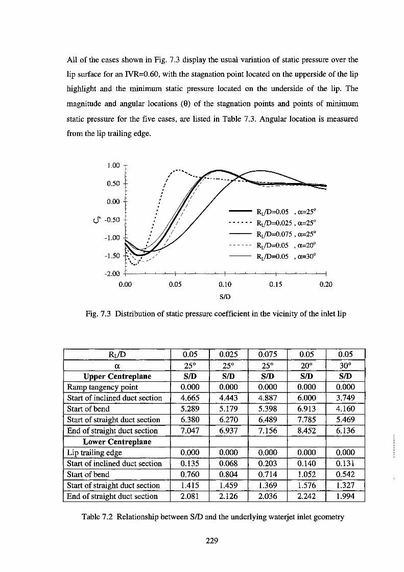
All of the cases shown in Fig. 7.3 display the usual variation of static pressure over the
lip surface for an NR=0.60, with the stagnation point located on the upperside of the lip
highlight and the minimum static pressure located on the underside of the lip. The
magnitude and angular locations (9) of the stagnation points and points of minimum
static pressure for the five cases, are listed in Table 7.3. Angular location is measured
from the lip trailing edge.
1.00
0.50
0.00
u"'" -0.50
-1.00
-1.50
. . .
I . . . . . . . . . --- RdD=0.05 , a=25°
RdD=0.025 , a=25°
-- RdD=0.075 , a=25°
RdD=0.05 , a=20°
RdD=0.05 , a=30°
-2.00 +--'---'-------'---'--t----'----'------'----'--t-----'---'-L--....___-t---'---'---'-------'---1
0.00 0.05 0.10
SID
0.15 0.20
Fig. 7.3 Distribution of static pressure coefficient in the vicinity of the inlet lip
Rr/D 0.05 0.025 0.075 0.05 0.05
a 25° 25° 25° 20° 30° Upper Centreplane SID SID SID SID SID
Ramp tangency point 0.000 0.000 0.000 0.000 0.000 Start of inclined duct section 4.665 4.443 4.887 6.000 3.749 Start of bend 5.289 5.179 5.398 6.913 4.160 Start of straight duct section 6.380 6.270 6.489 7.785 5.469 End of straight duct section 7.047 6.937 7.156 8.452 6.136
Lower Centreplane Lip trailing edge 0.000 0.000 0.000 0.000 0.000 Start of inclined duct section 0.135 0.068 0.203 0.140 0.131 Start of bend 0.760 0.804 0.714 1.052 0.542 Start of straight duct section 1.415 1.459 1.369 1.576 1.327 End of straight duct section 2.081 2.126 2.036 2.242 1.994
Table 7.2 Relationship between SID and the underlying waterjet inlet geometry
229
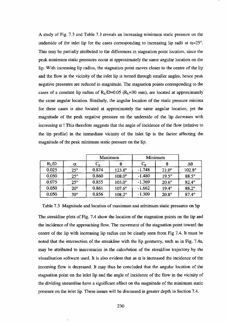
A study of Fig. 7.3 and Table 7.3 reveals an increasing minimum static pressure on the
underside of the inlet lip for the cases corresponding to increasing lip radii at a=25°.
This may be partially attributed to the differences in stagnation point location, since the
peak minimum static pressures occur at approximately the same angular location on the
lip. With increasing lip radius, the stagnation point moves closer to the centre of the lip
and the flow in the vicinity of the inlet lip is turned through smaller angles, hence peak
negative pressures are reduced in magnitude. The stagnation points corresponding to the
cases of a constant lip radius of Rr./D=0.05 (RL=30 mm), are located at approximately
the same angular location. Similarly, the angular location of the static pressure minima
for these cases is also located at approximately the same angular location, yet the
magnitude of the peak negative pressure on the underside of the lip decreases with
increasing a ! This therefore suggests that the angle of incidence of the flow (relative to
the lip profile) in the immediate vicinity of the inlet lip is the factor affecting the
magnitude of the peak minimum static pressure on the lip.
Maximum Minimum
Rr./D a Cp 9 Cp 9 89 0.025 25° 0.874 123.8° -1.748 21.0° 102.8° 0.050 25° 0.860 108.0° -1.480 19.5° 88.5° 0.075 25° 0.855 103.0° -1.369 20.6° 82.4° 0.050 20° 0.861 107.6° -1.662 19.4° 88.2° 0.050 30° 0.856 108.2° -1.309 20.8° 87.4°
Table 7.3 Magnitude and location of maximum and minimum static pressures on lip
The streakline plots of Fig. 7.4 show the location of the stagnation points on the lip and
the incidence of the approaching flow. The movement of the stagnation point toward the
centre of the lip with increasing lip radius can be clearly seen from Fig 7 .4. It must be
noted that the intersection of the streakline with the lip geometry, such as in Fig. 7 .4a,
may be attributed to inaccuracies in the calculation of the streakline trajectory by the
visualisation software used. It is also evident that as a is increased the incidence of the
incoming flow is decreased. It may thus be concluded that the angular location of the
stagnation point on the inlet lip and the angle of incidence of the flow in the vicinity of
the dividing streamline have a significant effect on the magnitude of the minimum static
pressure on the inlet lip. These issues will be discussed in greater depth in Section 7 .4.
230

b) RJD=0.025 , a=25° c) RJD=0.075, a=25°
a) RJD=0.050 , a=25°
d) RJD=0.050 , a=20° e) RJD=0.050, a=30°
Fig. 7 4 Streaklines in the vicinity of the inlet lip
231
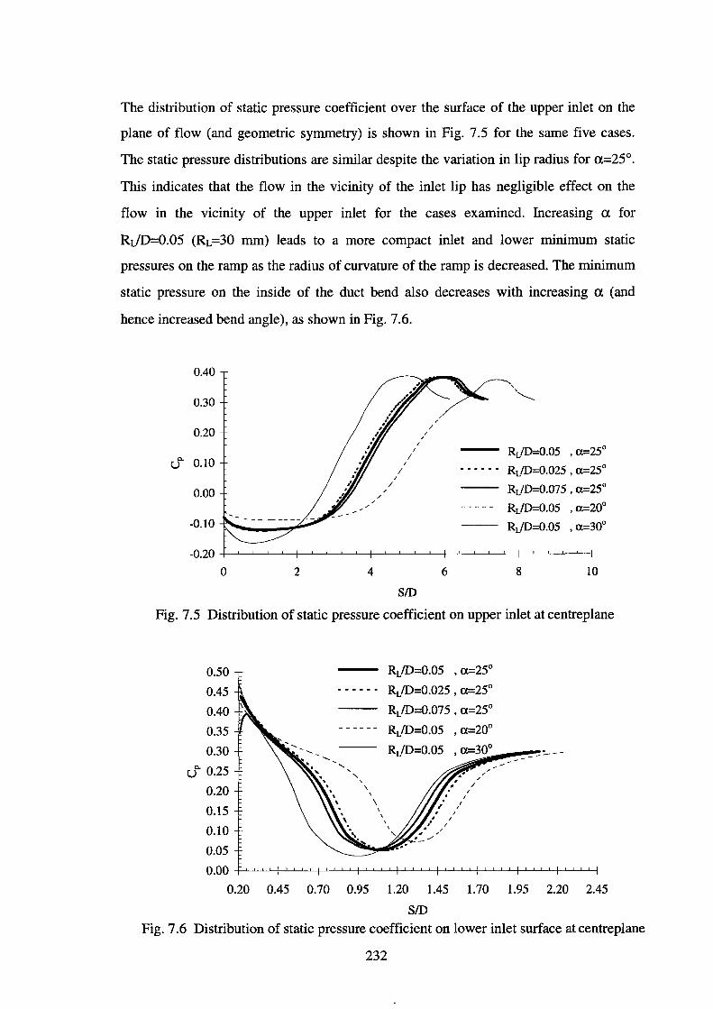
The distribution of static pressure coefficient over the surface of the upper inlet on the
plane of flow (and geometric symmetry) is shown in Fig. 7.5 for the same five cases.
The static pressure distributions are similar despite the variation in lip radius for a=25°.
This indicates that the flow in the vicinity of the inlet lip has negligible effect on the
flow in the vicinity of the upper inlet for the cases examined. Increasing a for
RJD=0.05 (RL=30 rnrn) leads to a more compact inlet and lower minimum static
pressures on the ramp as the radius of curvature of the ramp is decreased. The minimum
static pressure on the inside of the duct bend also decreases with increasing a (and
hence increased bend angle), as shown in Fig. 7 .6.
0.40
0.30
0.20 /
/ /
I
'a=25° / RdD=0.05 "" I
u 0.10 ------ RdD=0.025 , a=25° I /
/ RdD=0.075 , a=25° 0.00 /
/ /
RdD=0.05 'a=20° /
-0.10 -- RdD=0.05 'a=30°
-0.20
0 2 4 6 8 10
SID
Fig. 7.5 Distribution of static pressure coefficient on upper inlet at centreplane
0.50
0.45
0.40
0.35
0.30
u"" 0.25
0.20
0.15
0.10
0.05
0.00
0.20 0.45
' ' ' ' \ \
RL/D=0.05 ' a=25°
RdD=0.025 , a=25°
RdD=0.075 , a=25°
RdD=0.05 , a=20°
RdD=0.05 , a=~3~0°_..~~-:...--
0.70 0.95 1.20 1.45 1.70 1.95 2.20 2.45
SID
Fig. 7.6 Distribution of static pressure coefficient on lower inlet surface at centreplane
232
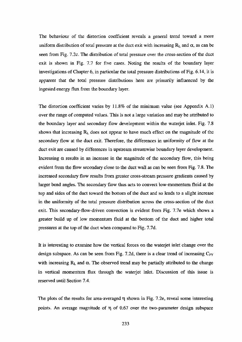
The behaviour of the distortion coefficient reveals a general trend toward a more
uniform distribution of total pressure at the duct exit with increasing RL and a., as can be
seen from Fig. 7 .2c. The distribution of total pressure over the cross-section of the duct
exit is shown in Fig. 7.7 for five cases. Noting the results of the boundary layer
investigations of Chapter 6, in particular the total pressure distributions of Fig. 6.14, it is
apparent that the total pressure distributions here are primarily influenced by the
ingested energy flux from the boundary layer.
The distortion coefficient varies by 11.8% of the minimum value (see Appendix A.1)
over the range of computed values. This is not a large variation and may be attributed to
the boundary layer and secondary flow development within the waterjet inlet. Fig. 7.8
shows that increasing RL does not appear to have much effect on the magnitude of the
secondary flow at the duct exit. Therefore, the differences in uniformity of flow at the
duct exit are caused by differences in upstream streamwise boundary layer development.
Increasing a. results in an increase in the magnitude of the secondary flow, this being
evident from the flow secondary close to the duct wall as can be seen from Fig. 7 .8. The
increased secondary flow results from greater cross-stream pressure gradients caused by
larger bend angles. The secondary flow thus acts to convect low-momentum fluid at the
top and sides of the duct toward the bottom of the duct and so leads to a slight increase
in the uniformity of the total pressure distribution across the cross-section of the duct
exit. This secondary-flow-driven convection is evident from Fig. 7.7e which shows a
greater build up of low momentum fluid at the bottom of the duct and higher total
pressures at the top of the duct when compared to Fig. 7.7d.
It is interesting to examine how the vertical forces on the waterjet inlet change over the
design subspace. As can be seen from Fig. 7 .2d, there is a clear trend of increasing CFY
with increasing RL and a.. The observed trend may be partially attributed to the change
in vertical momentum flux through the waterjet inlet. Discussion of this issue is
reserved until Section 7 .4.
The plots of the results for area-averaged 11 shown in Fig. 7 .2e, reveal some interesting
points. An average magnitude of 11 of 0.67 over the two-parameter design subspace
233

b) RJD=0.025 , a=25° c) RJD=0.075, a=25°
a) RJD=0.05 , a=25°
d) RJD=0.05 , a=20° e) RJD=0.05, a=30°
Fig. 7. 7 Distribution of total pressure coefficient over the cross-section of the duct exit
234
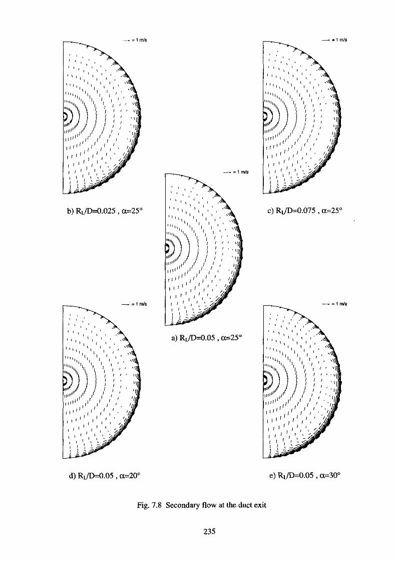
I I I I
I I I I I I
111 I \I I II II
1111 II I I 11 I I
""1 \ II I I Ill I I I I IIIII') Ill Ill II I~ ~
uul11 ))} I/ lfllfll , , / I
11 1 I I I 1111 11 I I
I I I I I I I II I I I
I
I
- =1 m/s
I '
I '
I I I I I I I I I I //
I I I / //, I I , ;,:::;
I I II ~- ~ I I ' /. I I 1 -,_:::........:::;
.:::-«
b) Rr/1)=0.025 , a=25°
I I I
I 1 I I\ I
II II \I \I \
11 II \I I 1\\ I II
I I
I
11111 II II I 111 II I I
) ) ) ) ! ' II Ifill , , I
II I I I 1111, ,I II /
I till II I
I I I II II
I I I I I I
I I I
- =1 m/s
d) Rr/1)=0.05 , a=20°
I I I \
I 1 I\
I 1 11 \1
I\ II II II I II II I I
II II I 1111 1 11 I I 1
111 11 I I ""Ill I) ) I I~ :
,1) ~~ ) I : 1111111 / , / I
-=1m/s
I '
I '
I '
I '
1l 1 I I I 11 11 11 I I 1
II I II II I I II I
I I I I I I I I I I /
1 I I I 1 _, ~ I I I I I , ;..:::;
I 1 - h I I ' /. I
a) Rr/1)=0.05 , a=25°
I I
I I I 1
It I l
I\ I I I I I
'• II II 111
11 I I
II I I
I
'"1' II II I 1111 11 I II I
)) ) ) ; ! lflllll / , / I
1l 1 I I I 11 11 11 I I 1
111 I 1 1 II II I
I I I I I I I
I I I " I I I I' ~ h I I I - h
I ' /.
', ~ .&ii --""
-=1m/s
c) Rr/1)=0.075, a=25°
I I I I
I I 1 I I
It I I I 11 I
It I II I II II II II I
1111 1 11 I I ,,1 II I
""'))Ill II ,, II
111111 I ) ) j Ill I I
lfl 1 I I I 1111 II I
Ill I II
1111 II I I I I
I I I I I I I I I
I I I I I I I I I 1 I I I ~ ~-.
- =1 m/s
e) Rr/1)=0.05, a=30°
Fig. 7.8 Secondary flow at the duct exit
235
indicates that the effect of boundary layer ingestion is the primary source of total
pressure loss (see Chapter 6). The dimensions and shape of the cross-section of the inlet
streamtubes, shown in Fig. 7.9 for the five cases examined in detail, are essentially
identical. This suggests that the dimensions of the cross-section of the inlet streamtube
are governed by the width of the waterjet inlet, the mass flow-rate through the inlet and
the upstream boundary layer. Since the widths of the waterjet inlet geometries examined
here are identical and since the same upstream boundary layer is used as a boundary
condition for all simulations, it may be concluded that the energy flux coefficient (Ce) is
the same for all cases. Ce is calculated as 0.708 using Eqn 6.27. Furthermore, the lack of
significant variation in 11 over the range of RL and a suggests that viscous losses within
the waterjet inlet are essentially identical for the different geometries examined.
It can be seen from Fig. 7.2f that increasing a and decreasing RL results in a smaller,
more compact waterjet inlet, as would be expected. A decrease in volume of 27% is
achievable by moving from Rr./1)=0.1, a=20° to Rr./1)=0.05, a=35°. This represents a
dramatic decrease in waterjet inlet volume and therefore highlights the necessity of
ensuring the absence of flow separation on the inlet ramp, in order to achieve a more
compact waterjet inlet design.
0 0
0.00
-0.05
-0.10
-0.15 e -0.20 >.
-0.25
-0.30
-0.35
-0.40
RdD=0.05 , a=25°
- - - - - - RdD=0.025 , a.=25°
RdD=0.075 , a.=25° ------
RdD=0.05 , a.=20° ---
R,/0=0.05 , a=30°
00 0
ziD
Fig. 7.9 Cross-section of the inlet streamtube
236
7.3.2 Variation of Lip Profile
The variation of O'mm and minimum Cp over the two-parameter design subspace is
shown in Fig. 7.10a and Fig. 7.10b respectively. As was noted in Section 7.3.1 for all
cases examined, the minimum static pressure is found to occur on the underside of the
inlet lip. It is clear from the contour plots that there is a trend of increasing static
pressure with increasing y and HL, with both parameters having a significant influence
on the results obtained. Using the results presented in Appendix A.2, there is an increase
in the minimum Cp over the range investigated of 57.6% of the minimum value. This
represents a large increase. In fact, a minimum Cp of -1.33 represents a marked increase
over a minimum Cp of -1.75 for a lip radius of 15 mm but without the raised-lip profile.
The benefits of using a raised lip profile, are therefore clearly evident. This further
highlights the importance that must be given to the design of the inlet lip. The negative
values of O'mm over the two-parameter design space indicate that cavitation will be
present on the underside of the inlet lip at a vessel speed of 40 knots, although the
maximum value of O"mm of -0.096 is close to a cavitation-free operation.
In order to examine how changing the shape of the lip profile (by increasing y and HL)
affects the minimum static pressure on the underside of the inlet lip, the static pressure
distribution in the vicinity of the inlet region is shown in Fig. 7.11 for five cases
corresponding to perturbations in y and HL about the point y=10°, Hr./D=0.075. The
relationship between SID and the underlying waterjet inlet geometry on the upper and
lower centreplane locations is presented in Table 7 .4. The trend of increasing minimum
static pressure on the underside of the inlet lip, with increasing y and HL can clearly be
seen from the pressure distributions of Fig. 7 .11. It is interesting to note that there is
relatively little variation in Cp over most of the inclined surface downstream of the lip,
except in the immediate vicinity of the lip itself, or at the "inlet/hull" interface. The
increasingly sharp decrease in Cp at the inlet/hull interface with increasing y, may be
attributed to the sudden change in geometry at this location.
237
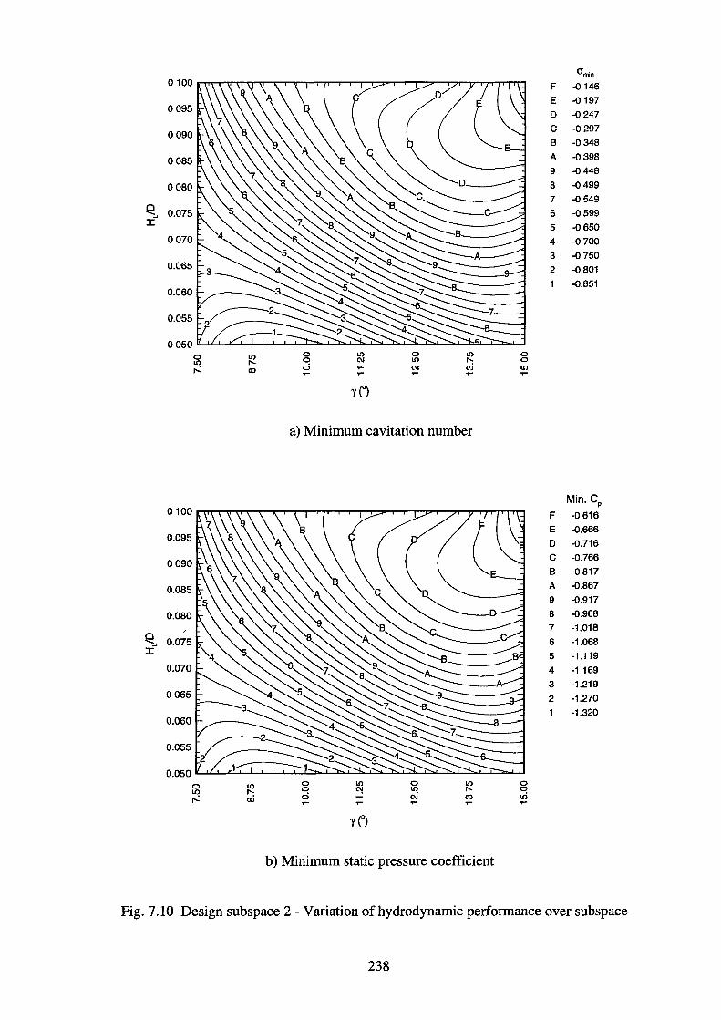
crmln 0100 F -o 146
E -0197 0095
D -0247
0090 c -0297
B -0348
0085 A -Q398
9 -0.448
0080 8 -0499
7 -0549 0
0.075 ~ 6 -Q599 :c 5 -o.650
0070 4 -0.700
3 -0750 0.065 2 -0 801
-0.851 0.060
0.055
0050 0 LO ,...:
a) Minimum cavitation number
Min. CP 0100 F -0 616
E -Q.666 0.095
D -0.716
0090 c -0.766 B -o 817
0.085 A -0.867
9 -0.917
0.080 8 -0.968
7 -1.018 0
0.075 ~ 6 -1.068 :c 5 -1.119
0.070 4 -1 169
3 -1.219 0065 2 -1.270
1 -1.320 0.060
0.055
0.050 0 LO ,...:
b) Minimum static pressure coefficient
Fig. 7.10 Design subspace 2 - Variation of hydrodynamic performance over subspace
238
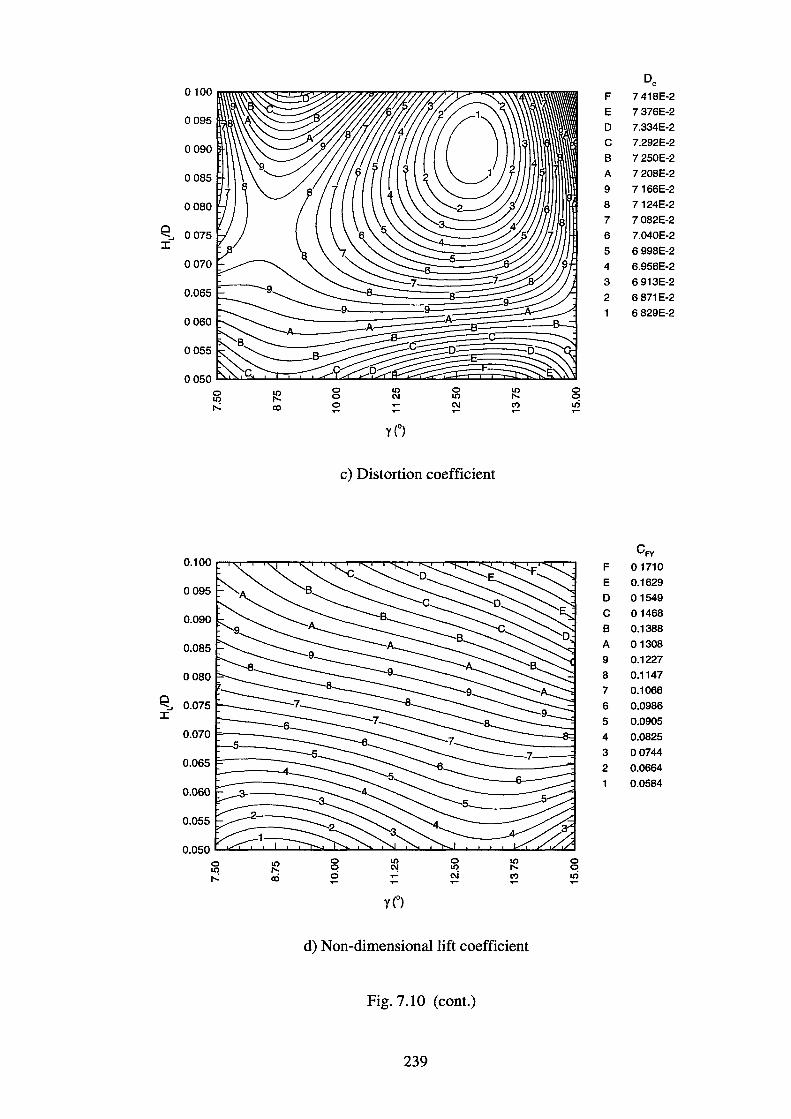
0 ~ J:
0 ~ J:
c) Distortion coefficient
d) Non-dimensional lift coeff" . tctent
Fig. 7.10 (cont.)
239
F
E
D
c B
A
9
8
7
6
5
4
3
2
F
E
D
c B A
9
8
7
6
5
4
3
2
DC 7 418E-2
7 376E-2
7.334E-2
7.292E-2
7 250E-2
7 208E-2
7166E-2
7124E-2
7 082E-2
7.040E-2
6 998E-2
6.956E-2
6 913E-2
6 871E-2
6 829E-2
CFY 01710
0.1629
01549
01468
0.1388
01308
0.1227
0.1147
0.1066
0.0986
0.0905
0.0825
00744
0.0664
0.0584
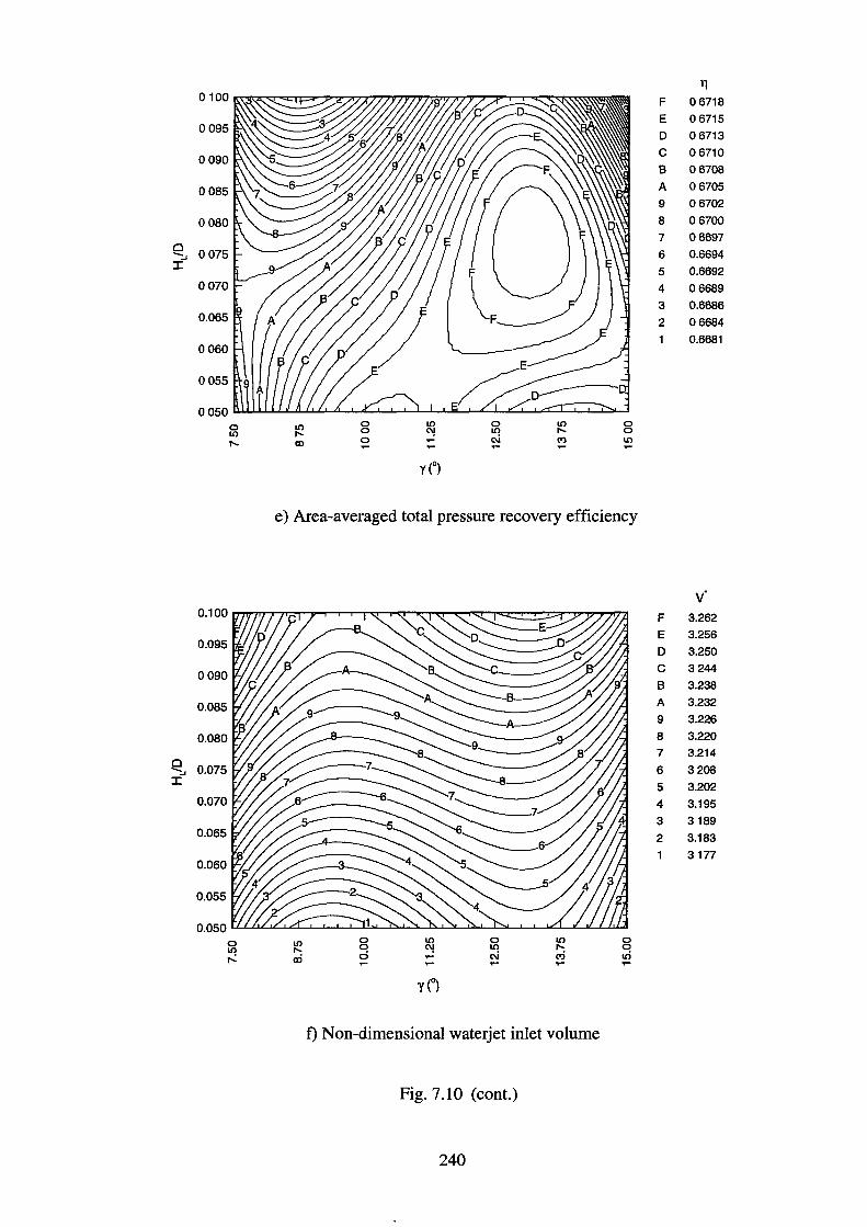
11 0100 F 06718
E 06715 0095
D 06713
0090 c 06710
B 06708
0085 A 06705
9 06702
0080 8 06700
7 06697 Cl
6 0.6694 -:.. 0075 :c 5 0.6692
4 06689
3 0.6686
2 06684
1 0.6681
y (0)
e) Area-averaged total pressure recovery efficiency
v . 0.100 F 3.262
E 3.256 0.095
D 3.250
0090 c 3 244
8 3.238
0.085 A 3.232
9 3.226
0.080 8 3.220
7 3.214 Cl
6 3208 -:.. 0.075 :c 5 3.202
4 3.195
3 3189
2 3.183
1 3177
y (0)
f) Non-dimensional waterjet inlet volume
Fig. 7.10 (cont.)
240
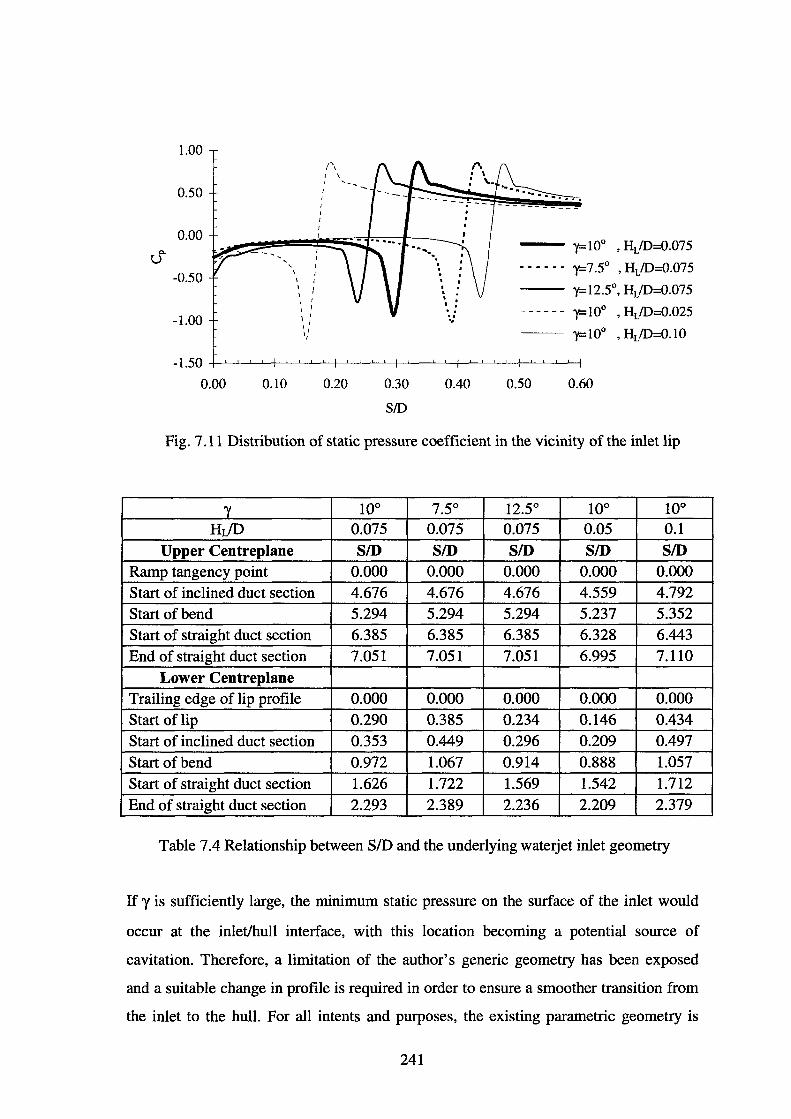
1.00
0.50
0.00 c. u
-0.50
-1.00
-1.50
0.00
'
0.10
' I \ I
I
I I I I I I
I I I I
1/
/\ I \ I ,_
I I I I I I I
0.20 0.30
SID
.. .. ..
0.40
-- y=l0° 'HdD=0.075
· · • ·- • y=7.5° , HdD=0.075
-- y=12.5°, HdD=0.075
- - - - - - y= 10° , HdD=0.025
-- y=10° , HdD=O.lO
0.50 0.60
Fig. 7.11 Distribution of static pressure coefficient in the vicinity of the inlet lip
'Y 100 7.50 12.5° 100 100
HJD 0.075 0.075 0.075 0.05 0.1 Upper Centreplane SID SID SID SID SID
Ramp tangency point 0.000 0.000 0.000 0.000 0.000 Start of inclined duct section 4.676 4.676 4.676 4.559 4.792 Start of bend 5.294 5.294 5.294 5.237 5.352 Start of straight duct section 6.385 6.385 6.385 6.328 6.443 End of straight duct section 7.051 7.051 7.051 6.995 7.110
Lower Centreplane Trailing edge of lip profile 0.000 0.000 0.000 0.000 0.000 Start of lip 0.290 0.385 0.234 0.146 0.434 Start of inclined duct section 0.353 0.449 0.296 0.209 0.497 Start of bend 0.972 1.067 0.914 0.888 1.057 Start of straight duct section 1.626 1.722 1.569 1.542 1.712 End of straight duct section 2.293 2.389 2.236 2.209 2.379
Table 7.4 Relationship between SID and the underlying waterjet inlet geometry
If y is sufficiently large, the minimum static pressure on the surface of the inlet would
occur at the inlet/hull interface, with this location becoming a potential source of
cavitation. Therefore, a limitation of the author's generic geometry has been exposed
and a suitable change in profile is required in order to ensure a smoother transition from
the inlet to the hull. For all intents and purposes, the existing parametric geometry is
241
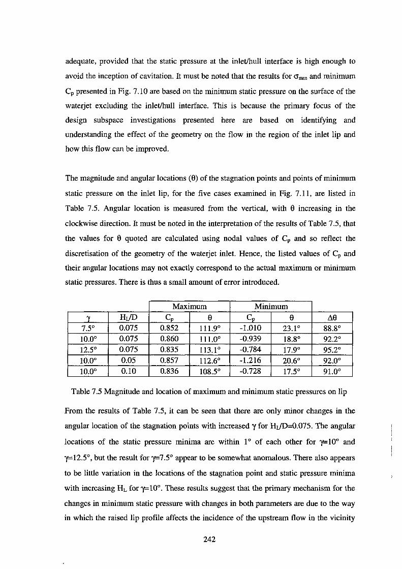
adequate, provided that the static pressure at the inlet/hull interface is high enough to
avoid the inception of cavitation. It must be noted that the results for CJmm and minimum
Cp presented in Fig. 7.10 are based on the minimum static pressure on the surface of the
waterjet excluding the inlet/hull interface. This is because the primary focus of the
design subspace investigations presented here are based on identifying and
understanding the effect of the geometry on the flow in the region of the inlet lip and
how this flow can be improved.
The magnitude and angular locations (8) of the stagnation points and points of minimum
static pressure on the inlet lip, for the five cases examined in Fig. 7.11, are listed in
Table 7.5. Angular location is measured from the vertical, with 8 increasing in the
clockwise direction. It must be noted in the interpretation of the results of Table 7.5, that
the values for 8 quoted are calculated using nodal values of Cp and so reflect the
discretisation of the geometry of the waterjet inlet. Hence, the listed values of Cp and
their angular locations may not exactly correspond to the actual maximum or minimum
static pressures. There is thus a small amount of error introduced.
Maximum Minimum
'Y Hr/D Cp 8 Cp 8 ~8
7.5° 0.075 0.852 111.9° -1.010 23.1° 88.8° 10.0° 0.075 0.860 111.0° -0.939 18.8° 92.2° 12.5° 0.075 0.835 113.1° -0.784 17.9° 95.2° 10.0° 0.05 0.857 112.6° -1.216 20.6° 92.0° 10.0° 0.10 0.836 108.5° -0.728 17.5° 91.0°
Table 7.5 Magnitude and location of maximum and minimum static pressures on lip
From the results of Table 7.5, it can be seen that there are only minor changes in the
angular location of the stagnation points with increased y for Hr/D=0.075. The angular
locations of the static pressure minima are within 1 ° of each other for y= 1 oo and
y=-12.5°, but the result for y=7.5° appear to be somewhat anomalous. There also appears
to be little variation in the locations of the stagnation point and static pressure minima
with increasing HL for y= 10°. These results suggest that the primary mechanism for the
changes in minimum static pressure with changes in both parameters are due to the way
in which the raised lip profile affects the incidence of the upstream flow in the vicinity
242
of the inlet lip. The effect of the profile of the lip on the flow in the vicinity of the inlet
lip (with changes in y and HL) can be seen from the streakline plots of Fig. 7.12. Fig.
7.12 shows how a lip profile with increasing values of y and HL appear to direct the flow
upstream of the lip in such a way as to minimise the perturbation of the lip on the
surrounding flow. This whole issue will be discussed at greater length in Section 7 .4.
The distribution of static pressure coefficient over the surface of the upper inlet on the
plane of flow symmetry is shown in Fig. 7.13 for the above five cases. The static
pressure distributions are essentially identical, with slight variations being due to the
small differences in geometry. It is therefore evident that the profile of the inlet lip has a
negligible influence on the pressure distribution in the upper part of the waterjet inlet,
for the cases examined here. This indicates that the profile of the inlet lip region affects
only the flow in its vicinity. The profile of the inlet lip does not appear to affect the
minimum static pressure on the inside of the duct bend either, as can be seen from Fig.
7.14.
It is difficult to discern any clear trends in the behaviour of the distortion coefficient
from the contour plot of Fig. 7.10c. There does appear, however, to be a region of
minimum distortion centred around "(=12.75°, HJD=0.90. The distortion coefficient
varies by 8.1% over the two parameter design space, but this is not a large variation. It is
therefore thought that the distortion coefficient is influenced by the streamwise
boundary layer development within the waterjet inlet, resulting from the geometry of the
inlet region.
An examination of Fig.7.10d reveals a clear trend in the non-dimensional lift
coefficient. Increasing either y or HL results in a greater vertical force on the waterjet
inlet, although the trend tends to be more pronounced in the HL direction. As was found
to be the case for the first design subspace examined in Section 7.3.1, the trend in Cpy
may be attributed to the change in the vertical momentum of flow through the waterjet
propulsion unit. Again, a detailed discussion of this issue is reserved until Section 7 .4.
The plot of area-averaged 11 is shown in Fig. 7 .lOe. There is a variation of less than
0.3% about an average-value of 11 of0.67. In Section 7.3.1 it is shown that the ingestion
243
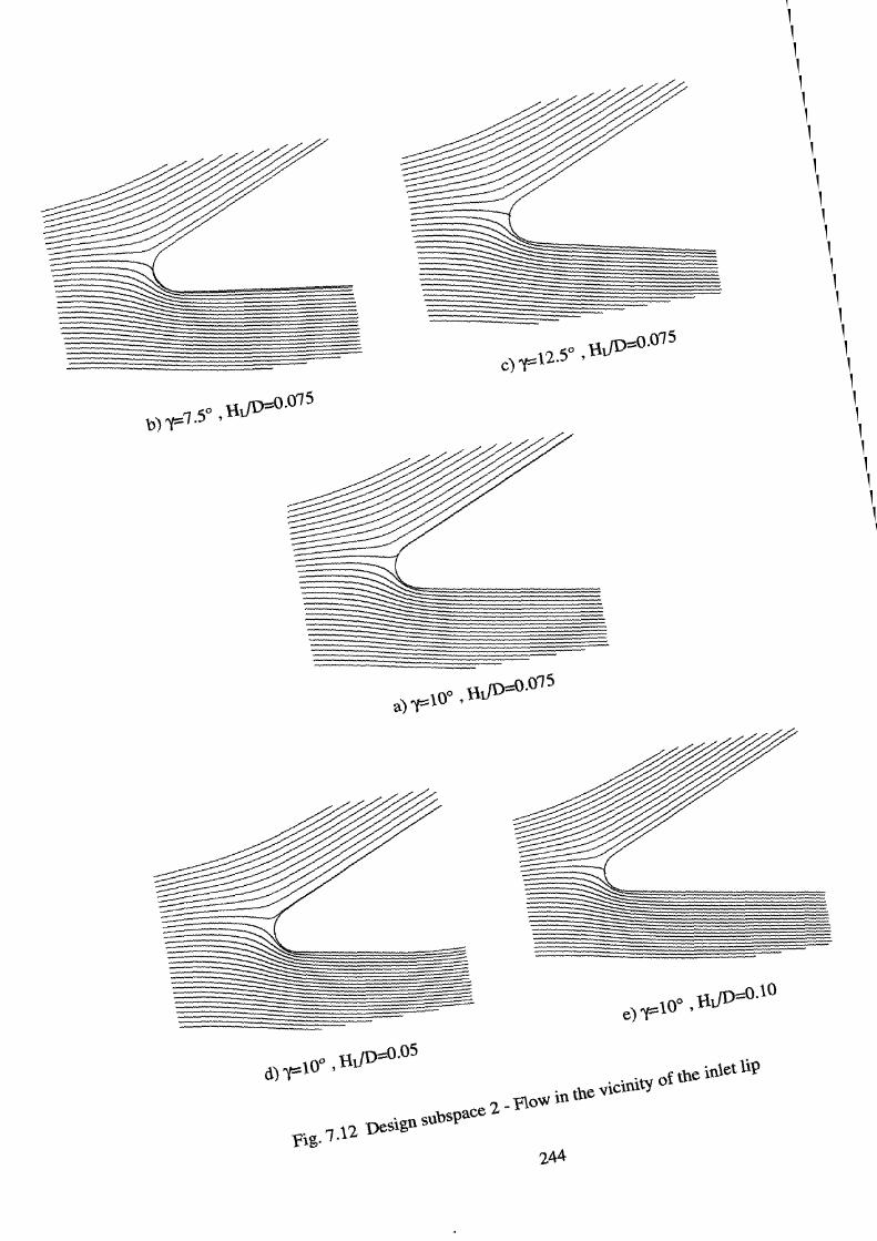
1 1 1 1 1 1 1 1 1 1 1 1 1 1 1 1 1 1 1 1 1 1 1 1 1 1 1 1 1 1 1 1 1 1 1 1 1 1 1 1 1 1 1 1 1 1 1 1 1 1 1 1 1 1 1 1 1 1 1 1 1 1 1 1 1 1 1 1 1 1 1 1 1
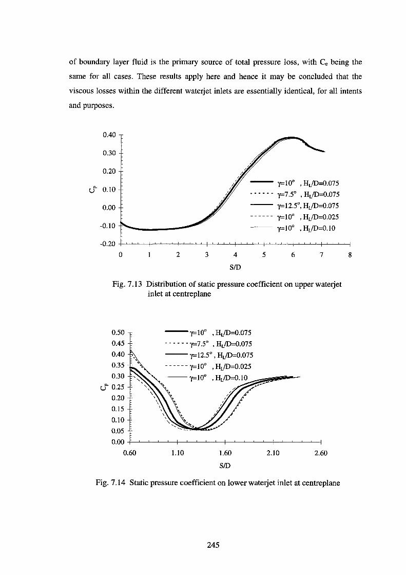
of boundary layer fluid is the primary source of total pressure loss, with Ce being the
same for all cases. These results apply here and hence it may be concluded that the
viscous losses within the different waterjet inlets are essentially identical, for all intents
and purposes.
c. u
0.40
0.30
0.20
y=100 ,HdD=0.075 0.10
· · · • · • y=7 .5° , HdD=0.075
0.00 y=12.S0, HdD=0.075 ------ y=10° ,HdD=0.025
-0.10 y=10° ,HdD=0.10
-0.20
0 2 3 4 5 6 7
SID
Fig. 7.13 Distribution of static pressure coefficient on upper waterjet inlet at centreplane
0.50
0.45
0.40
0.35
0.30
uc. 0.25
0.20
0.15
0.10
0.05
--y=10° ,HdD=0.075
------ y=7S 'HLID=0.075
--- y=12.5°' HLID=0.075
------ y=10° , HdD=0.025
--y=10°
0.00 -j--'----L.--'--'------t-----'---'-----'---'--+---'----'---'-~--t~-'--'---'---1
0.60 1.10 1.60
SID
2.10 2.60
Fig. 7.14 Static pressure coefficient on lower waterjet inlet at centreplane
245
8
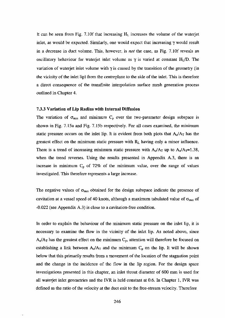
It can be seen from Fig. 7.1 Of that increasing HL increases the volume of the waterjet
inlet, as would be expected. Similarly, one would expect that increasing y would result
in a decrease in duct volume. This, however, is not the case, as Fig. 7.1 Of reveals an
oscillatory behaviour for waterjet inlet volume as y is varied at constant HU:O. The
variation of waterjet inlet volume with y is caused by the transition of the geometry (in
the vicinity of the inlet lip) from the centreplane to the side of the inlet. This is therefore
a direct consequence of the transfinite interpolation surface mesh generation process
outlined in Chapter 4.
7.3.3 Variation of Lip Radius with Internal Diffusion
The variation of O"mm and minimum Cp over the two-parameter design subspace is
shown in Fig. 7.15a and Fig. 7.15b respectively. For all cases examined, the minimum
static pressure occurs on the inlet lip. It is evident from both plots that AJ AT has the
greatest effect on the minimum static pressure with RL having only a minor influence.
There is a trend of increasing minimum static pressure with AJAT up to AJAT=l.38,
when the trend reverses. Using the results presented in Appendix A.3, there is an
increase in minimum Cp of 72% of the minimum value, over the range of values
investigated. This therefore represents a large increase.
The negative values of O"mm obtained for the design subspace indicate the presence of
cavitation at a vessel speed of 40 knots, although a maximum tabulated value of O"mm of
-0.022 (see Appendix A.3) is close to a cavitation-free condition.
In order to explain the behaviour of the minimum static pressure on the inlet lip, it is
necessary to examine the flow in the vicinity of the inlet lip. As noted above, since
AJ AT has the greatest effect on the minimum Cp, attention will therefore be focused on
establishing a link between AJ AT and the minimum Cp on the lip. It will be shown
below that this primarily results from a movement of the location of the stagnation point
and the change in the incidence of the flow in the lip region. For the design space
investigations presented in this chapter, an inlet throat diameter of 600 mm is used for
all waterjet inlet geometries and the IVR is held constant at 0.6. In Chapter 1, IVR was
defined as the ratio of the velocity at the duct exit to the free-stream velocity. Therefore
246
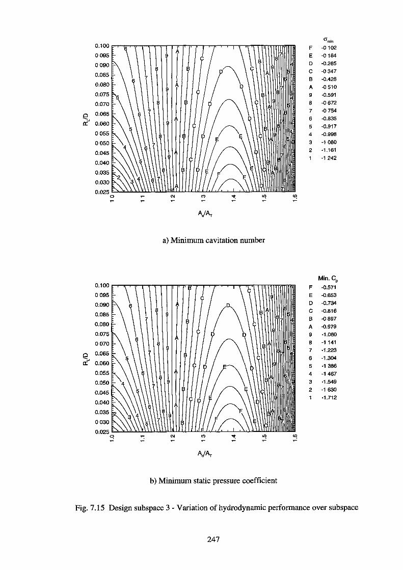
crmln 0.100 F -0102 0095 E -0184
0090 D -0.265
0.085 c -0347
B -0.428 0.080 A -0 510 0.075 9 -0.591
0.070 8 -Q672
0 0.065 "":...
7 -0754
6 -0.835 a: 0.060 5 -0.917
0055 4 -0.998
0050 3 -1 080
0.045 2 -1.161
-1 242 0.040
0.035
0.030
0.025 0
a) Minimum cavitation number
Min.CP 0.100 F -0.571 0095 E -o.653
0.090 D -0.734
0.085 c -0.816
B -Q897 0.080 A -0.979 0.075 9 -1.060
0070 8 -1 141
0 0.065 "":...
7 -1.223
6 -1.304 a: 0.060 5 -1 386
0.055 4 -1 467
0.050 3 -1.549
0.045 2 -1 630 -1.712
0.040
0.035
0030
0.025 q
AJAr
b) Minimum static pressure coefficient
Fig. 7.15 Design subspace 3 - Variation of hydrodynamic performance over subspace
247
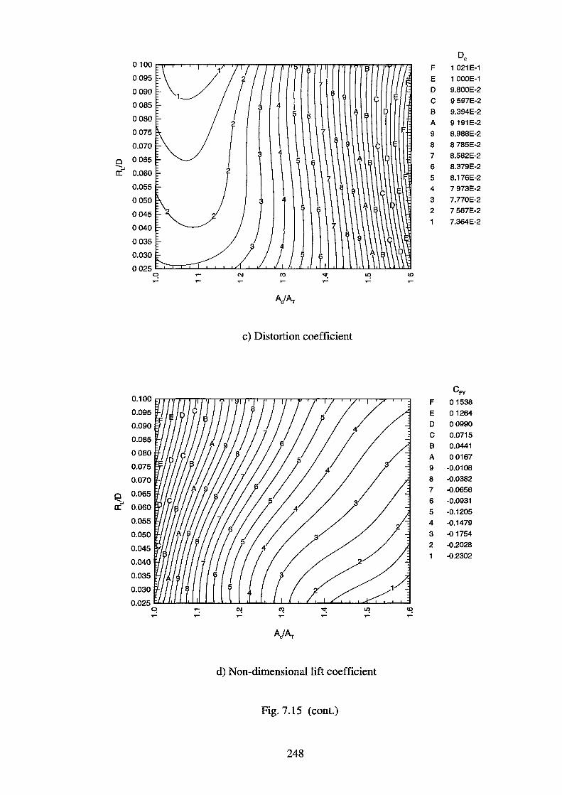
0 ~ a:
0100
0095
0090
0085
0 080
0075
0.070
0065
0.060
0.055
0050
0045
0040
0035
0.030
0025 ~ .....
AJAr
c) Distortion coefficient
0.025 I:.I....L.J.J..L...I-LU...LL...L..I.....IL....I.....L....I.L....L.J..I..-11.....1.-A......L-'--L-L...<I'--I-I......I...o.::t........I_..L.-1-..L....:I
~ ..... ..... .....
d) Non-dimensional lift coefficient
Fig. 7.15 (cont.)
248
DC F 1 021E-1
E 1 OOOE-1
D 9.800E-2
C 9 597E-2
B 9.394E-2
A 9191E-2
9 8.988E-2
8 8 785E-2
7 8.582E-2
6 8.379E-2
5 8.176E-2
4 7 973E-2
3 7.770E-2
2 7 567E-2
7.364E-2
CFY F 0 1538
E 0 1264
D 00990
c 0.0715
B 0.0441
A 00167
9 -O.D108
8 -0.0382
7 -0.0656
6 -0.0931
5 -0.1205
4 -0.1479
3 -0 1754
2 -0.2028
1 -0.2302
0025~~~ 0 ~ ~ M V ~ ~ ~ ~ ~ ~ ~ ~ ~
AjAr
e) Area-averaged total pressure recovery efficiency
0.025~~~
~ ~ ~ ~ ~ ~ ~ ~ ~ ~ ~ ~ ~ ~
AjAr
f) Non-dimensional waterjet inlet volume
Fig. 7.15 (cont.)
249
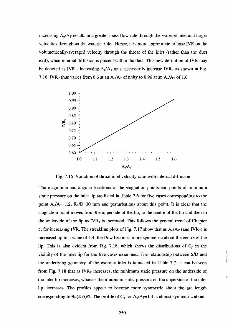
increasing AJ AT results in a greater mass flow-rate through the waterjet inlet and larger
velocities throughout the waterjet inlet. Hence, it is more appropriate to base NR on the
volumetrically-averaged velocity through the throat of the inlet (rather than the duct
exit), when internal diffusion is present within the duct. This new definition of NR may
be denoted as NRT. Increasing AJAT must necessarily increase NRT as shown in Fig.
7.16. IVRT thus varies from 0.6 at an AofAT of unity to 0.96 at an AofAT of 1.6.
1.00
0.95
0.90
0.85
!! 0.80 .......
0.75
0.70
0.65
0.60
1.0 1.1 1.2 1.4 1.5 1.6
Fig. 7.16 Variation of throat inlet velocity ratio with internal diffusion
The magnitude and angular locations of the stagnation points and points of minimum
static pressure on the inlet lip are listed in Table 7.6 for five cases corresponding to the
point AofAT=l.2, Rr/D=30 mm and perturbations about this point. It is clear that the
stagnation point moves from the upperside of the lip, to the centre of the lip and then to
the underside of the lip as NRT is increased. This follows the general trend of Chapter
5, for increasing NR. The streakline plots of Fig. 7.17 show that as AJAT (and NRT) is
increased up to a value of 1.4, the flow becomes more symmetric about the centre of the
lip. This is also evident from Fig. 7 .18, which shows the distributions of Cp in the
vicinity of the inlet lip for the five cases examined. The relationship between SID and
the underlying geometry of the waterjet inlet is tabulated in Table 7.7. It can be seen
from Fig. 7.18 that as NRT increases, the minimum static pressure on the underside of
the inlet lip increases, whereas the minimum static pressure on the upperside of the inlet
lip decreases. The profiles appear to become more symmetric about the arc length
corresponding to 8=(1t-a)/2. The profile ofCp for AJAT=l.4 is almost symmetric about
250
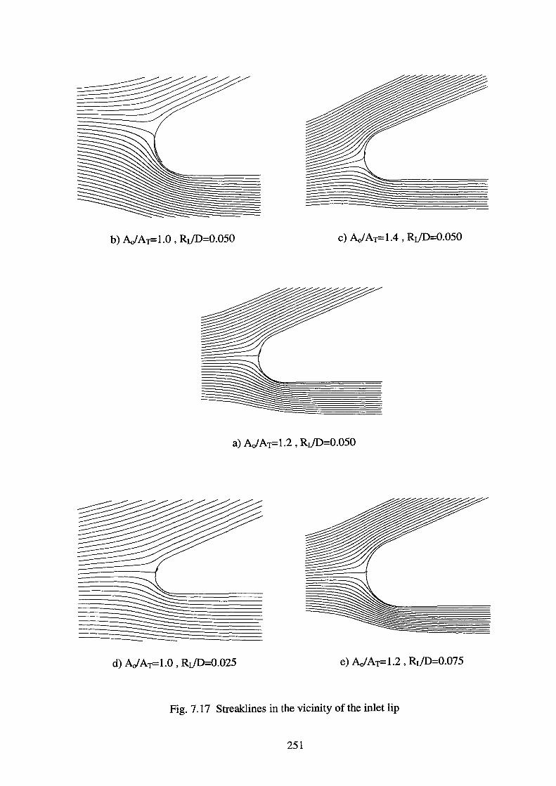
c) AJAT=l.4, Rt/D=0.050
a) AJAT=l.2, Rt/D=0.050
e) AJAr-1.2, Rt/D=0.075
Fig. 7.17 Streaklines in the vicinity of the inlet lip
251
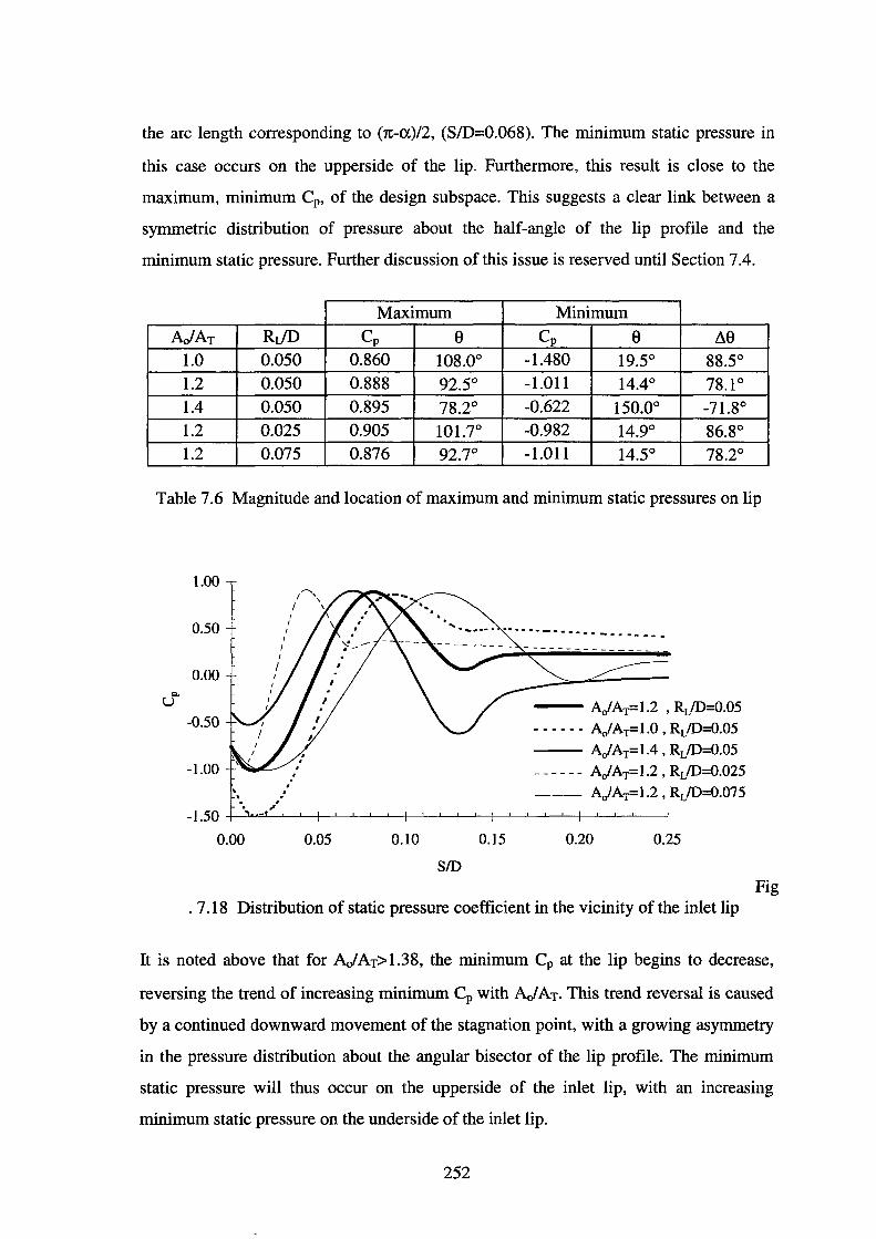
the arc length corresponding to (1t-a)/2, (S/0=0.068). The minimum static pressure in
this case occurs on the upperside of the lip. Furthermore, this result is close to the
maximum, minimum Cp, of the design subspace. This suggests a clear link between a
symmetric distribution of pressure about the half-angle of the lip profile and the
minimum static pressure. Further discussion of this issue is reserved until Section 7 .4.
Maximum Minimum
AJAr Rr}D Cp e Cp e L\8 1.0 0.050 0.860 108.0° -1.480 19.5° 88.5° 1.2 0.050 0.888 92.5° -1.011 14.4° 78.1° 1.4 0.050 0.895 78.2° -0.622 150.0° -71.8° 1.2 0.025 0.905 101.7° -0.982 14.9° 86.8° 1.2 0.075 0.876 92.7° -1.011 14.5° 78.2°
Table 7.6 Magnitude and location of maximum and minimum static pressures on lip
1.00
0.50 I
I
0.00 c..
u --- AofAT=l.2 'RLID=0.05 -0.50 - - - - - - AJAT=1.0 ' RLID=0.05
--- AofArl.4 , RLID=0.05 -1.00 ------ AJAT=l.2, RJD=0.025 . , , . , ·. .. -1.50
-- AJArl.2, RLID=0.075
0.00 0.05 0.10 0.15 0.20 0.25
SID Fig
. 7.18 Distribution of static pressure coefficient in the vicinity of the inlet lip
It is noted above that for AJAr> 1.38, the minimum Cp at the lip begins to decrease,
reversing the trend of increasing minimum Cp with AJAr. This trend reversal is caused
by a continued downward movement of the stagnation point, with a growing asymmetry
in the pressure distribution about the angular bisector of the lip profile. The minimum
static pressure will thus occur on the upperside of the inlet lip, with an increasing
minimum static pressure on the underside of the inlet lip.
252
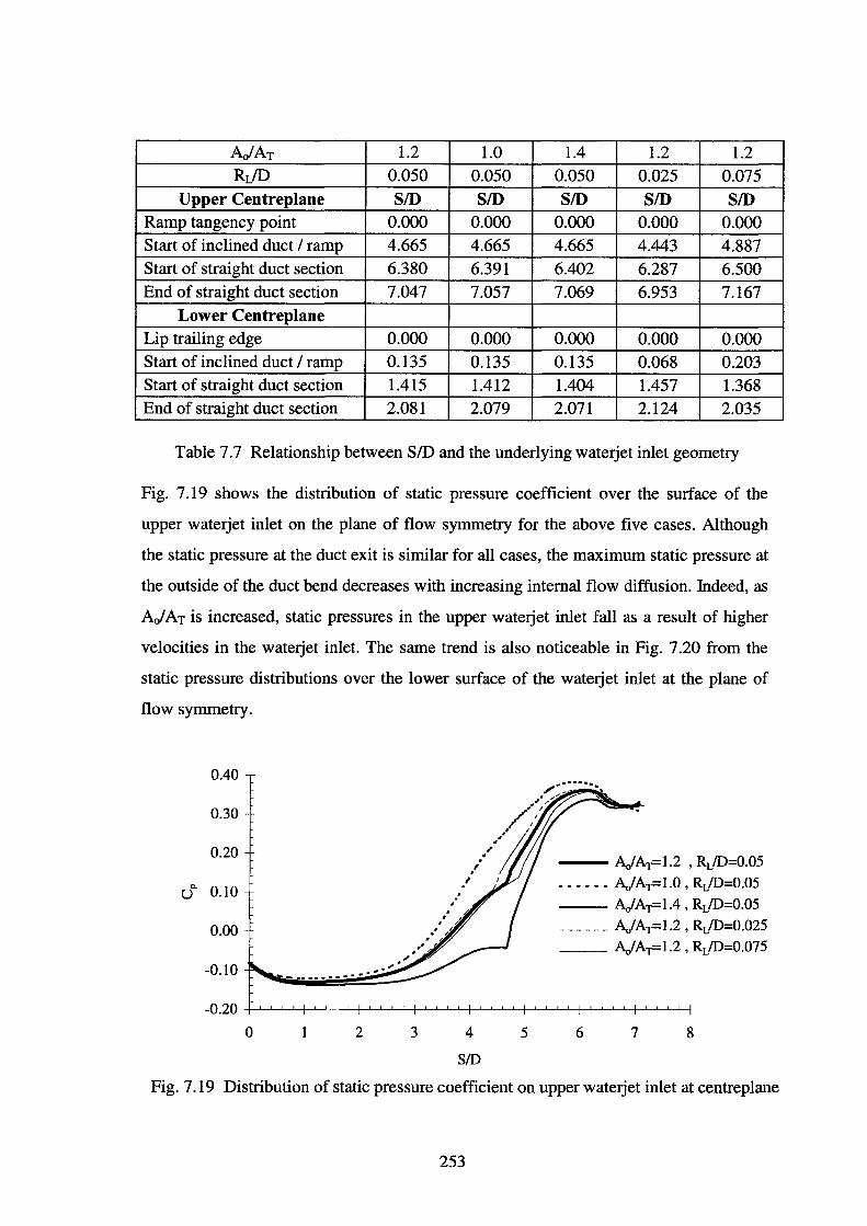
A/AT 1.2 1.0 1.4 1.2 1.2 RUD 0.050 0.050 0.050 0.025 0.075
Upper Centreplane SID SID SID SID SID Ramp tangency point 0.000 0.000 0.000 0.000 0.000 Start of inclined duct I ramp 4.665 4.665 4.665 4.443 4.887 Start of straight duct section 6.380 6.391 6.402 6.287 6.500 End of straight duct section 7.047 7.057 7.069 6.953 7.167
Lower Centreplane Lip trailing edge 0.000 0.000 0.000 0.000 0.000 Start of inclined duct I ramp 0.135 0.135 0.135 0.068 0.203 Start of straight duct section 1.415 1.412 1.404 1.457 1.368 End of straight duct section 2.081 2.079 2.071 2.124 2.035
Table 7.7 Relationship between SID and the underlying waterjet inlet geometry
Fig. 7.19 shows the distribution of static pressure coefficient over the surface of the
upper waterjet inlet on the plane of flow symmetry for the above five cases. Although
the static pressure at the duct exit is similar for all cases, the maximum static pressure at
the outside of the duct bend decreases with increasing internal flow diffusion. Indeed, as
AJ AT is increased, static pressures in the upper waterjet inlet fall as a result of higher
velocities in the waterjet inlet. The same trend is also noticeable in Fig. 7.20 from the
static pressure distributions over the lower surface of the waterjet inlet at the plane of
flow symmetry.
0.40
0.30
0.20
c. 0.10 u
0.00
-0.10 -----------0.20
0 2 3
I
4
SID
5
-- AJAT=l.2 , RJD=0.05
- - - - - - AJAT=l.O , RJD=0.05 -- AJArl.4, RJD=0.05 ______ AJAT=l.2, RJD=0.025
__ AJAT=l.2 , RdD=0.075
6 7 8
Fig. 7.19 Distribution of static pressure coefficient on upper waterjet inlet at centreplane
253
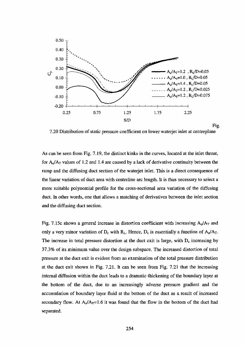
0.50
0.40 . . . . . 0.30
0.20 c. u
0.10
0.00
-0.10
-0.20
0.25
· .. . ' "•, .
', ' ' . '\ '·.. .. \ .. ·- -· -·.
\
0.75 1.25
SID
--- AJAT=l.2 , RdD=0.05 --- ·-- AJArl.O, RdD=0.05 --- AJAT=l.4, RdD=0.05 ------ A0 /AT=l.2, RdD=0.025 __ AJAT=l.2, RdD=0.075
1.75 2.25
Fig. 7.20 Distribution of static pressure coefficient on lower waterjet inlet at centreplane
As can be seen from Fig. 7.19, the distinct kinks in the curves, located at the inlet throat,
for AJAT values of 1.2 and 1.4 are caused by a lack of derivative continuity between the
ramp and the diffusing duct section of the waterjet inlet. This is a direct consequence of
the linear variation of duct area with centreline arc length. It is thus necessary to select a
more suitable polynomial profile for the cross-sectional area variation of the diffusing
duct. In other words, one that allows a matching of derivatives between the inlet section
and the diffusing duct section.
Fig. 7.15c shows a general increase in distortion coefficient with increasing AJAT and
only a very minor variation of De with RL. Hence, De is essentially a function of AJAT.
The increase in total pressure distortion at the duct exit is large, with De increasing by
37.3% of its minimum value over the design subspace. The increased distortion of total
pressure at the duct exit is evident from an examination of the total pressure distribution
at the duct exit shown in Fig. 7 .21. It can be seen from Fig. 7.21 that the increasing
internal diffusion within the duct leads to a dramatic thickening of the boundary layer at
the bottom of the duct, due to an increasingly adverse pressure gradient and the
accumulation of boundary layer fluid at the bottom of the duct as a result of increased
secondary flow. At AJAT=l.6 it was found that the flow in the bottom of the duct had
separated.
254
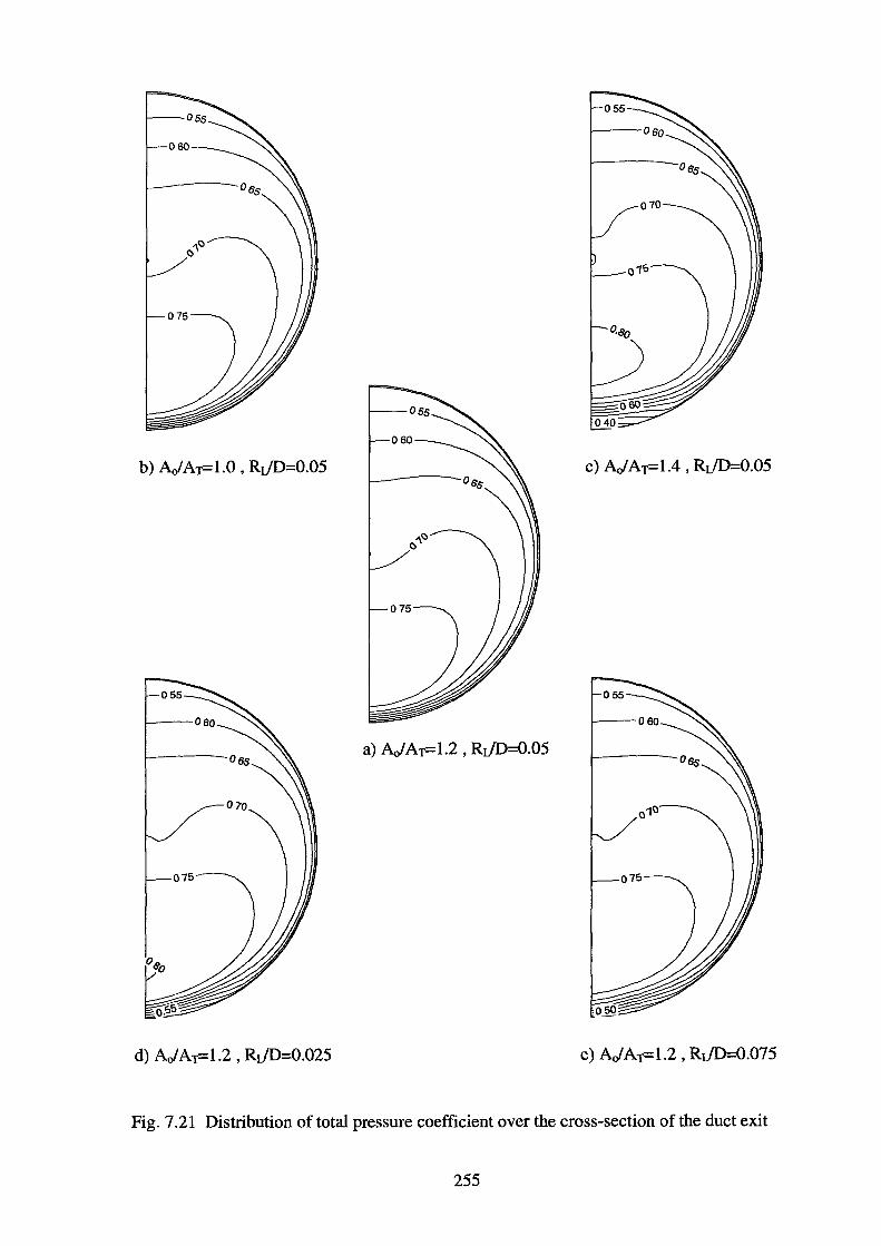
c) AJAT=1.4, RrJD=0.05
Fig. 7.21 Distribution of total pressure coefficient over the cross-section of the duct exit
255

Fig. 7.22 shows the secondary flow at the duct exit for the five cases examined. The
effect of flow diffusion is evident from the increased sideward component of the
secondary flow vectors. With increasing AJ AT the secondary flow is significantly
intensified as a consequence of greater cross-stream pressure gradients associated with
the duct bend. For AJAT values greater than unity, the outer radius of the bend is
increased relative to the outer radius of the bend at an AJAT of unity, whereas the inner
radius is decreased relative to its value at an AJ AT of unity. These changes in bend radii
are the fundamental cause for the increase in cross-stream pressure gradients associated
with the duct bend and hence the stronger secondary flow at the duct exit.
The thickening of the boundary layer at the bottom of the duct partially accounts for the
increase in total pressure distortion. The other factor accounting for the increased
distortion is related to the quality of the flow ingested by the inlet. An increase in AJAT,
results in an increased mass flux across the cross-section of the inlet streamtube and
hence the depth of the cross-section grows while there is only a slight increase in its
width, as can be seen for the three cases examined in Fig. 7.23. This results in a greater
variation of velocity across the depth of the cross-section of the inlet streamtube and
hence the ingestion of a less uniform flow. This causes a greater distortion of total
pressure at the duct exit. This is a corollary of the argument put forward in Chapter 6
(c.f. Section 6.4), explaining the reduction of De with the ingestion of fluid from
upstream boundary layers of increasing thickness.
There is a clear trend in CFY with RL or AJ AT. As RL is increases CFY is also increased
over the design subspace. This follows the same trend as was noted for the design
subspace investigated in Section 7.3.1. Increasing AJAT leads to a "suck-down" effect
where CFY becomes negative and then increasingly negative, although the rate of change
of CFY, d(CFY)Id(AJAT), can be seen to decrease with increasing AJAT. Increasing
AJ AT results in a greater mass flow-rate through the waterjet inlet. This in effect
increases the velocity throughout the waterjet inlet, thus leading to lower static pressures
on the duct surface, as is evident from an examination of Fig. 7.19 and Fig. 7 .20. Thus a
suck-down effect results for sufficiently largeAJAT.
256
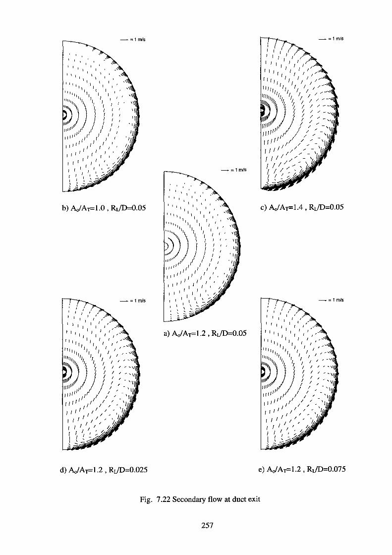
- =1 m/s
I I
I I I I
I I I I I I I
I I I I I I I I I I
111 II I I 11 1 1 I I
IIIII Ill II II I I ' 11 1 11 I I 1
)));'') i: 1111
111 11 I / I
1111
11 I I 111 II 1 1 1
I I 1 1 1111 I
1 1 I I
I I I I I I I I I I I I I I
I I
I I
I I I 1 I
I I I I I I
I I 1 I 1 I
- =1 m/s
I I I I II I II I I -'~
II 1 I 11 I I 1 ' I 11 1 I I , - '\l
lilrrr Ill II II I I II I I , _,~
IIIII) 1)111 Ill ~ II I~
1111111 II ) )l ; : '\\ ""II 1/ I / : : _- ''I 1111 II" / I '- 'll I I I I II / /- 'It
1 111 II/-.,, I I t- 1 /A Ill 1,.1
I I I I I I I I I I /,
I I I I ' /
I I " I ' ' _;;.dii l~-
I I
I I I I
I 1 I I I I I
I I II I II I I 1 I
111 11
I I ''I I I
.... ,, \ ,, II
- =1 m/S
)\, II I
·;;,))}), ,,
1111
" I I I 111
11 I I 1/ I I I
I 1 1 1 1 I 1
I I I I I II I
I I I I II ~ 1 I I I 1 , ~
I 1 1
1 I \ :_ ~
I I \ -.....::;:
~~~ ---a) AJAr=l.2, Rr/D=0.05
Fig. 7.22 Secondary flow at duct exit
257
-=1m/s
I I I I ,' I I I I I I I
I I I I I I I I I I 11 11 1 1 I I 1 .--
1 1 I I I --IIIII II 11 11 1
1
II I I _, -~ 111111 II II I I /
IIIIIIIII;IIIJIJ~ )\ /~ ~ j / / --<
""'''l /l ; : / IIIII ,, I / -' J1 till ;I I / _, - ' \
I I / _, \ ,,,,, / / / -- '1
;I / _, ' l tll /---1
I / - 'L I I I I /, - 'I
I/ - ' I•
~j/"_--:_tt I I ' _, .II ' -~-_.,.;;
c) AJAr= 1.4 , Rr}D=0.05
I
I I I
, I
I
I I I I II II I
II I I II II 'rl I
I Iii If II II II
- =1 m/s
""'')'lilt Ill II I
)
~ I I
!IIIII Iff/ ) jl j I , ''I 1111 II I I -,\1
11/ / I I ' -I I I II I I , 'lJ IIIII / I '--'11
II I ' 1 II I I I I I - IJ
I ,, / -I'~ I JII 1,1~
I I , IJ. I I I I ~;Zoi
I I • I £IIi I I I I ... ~ I ( , _;;~ l --
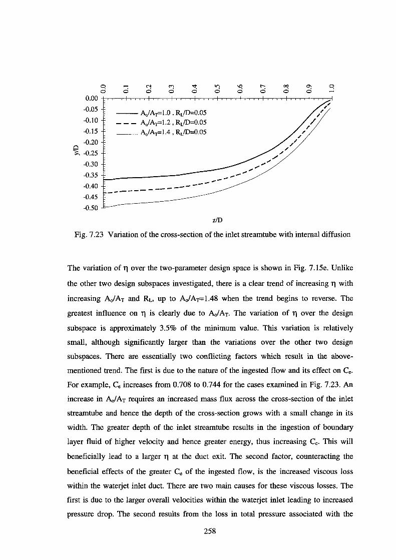
0 c:i
00 c:i
0. 00 +--r-..-r-.+-r-r-r-r--t--T---r-o---.--t-.---r-.---.-h-,--,....--1-r-..-r+-r-r-r-r-+-r--,-,-..-+.,..,.-.,..,.-+-r..-r~
-0.05
-0.10
-0.15
-0.20
~ -0.25
-0.30
-0.35
-0.40
-0.45
-0.50
--- A0/AT=l.0, RdD=0.05
AJAT=l.2 , RdD=0.05 ___ AJAT=l.4 , RdD=0.05
ziD
Fig. 7.23 Variation of the cross-section of the inlet streamtube with internal diffusion
The variation of 11 over the two-parameter design space is shown in Fig. 7.15e. Unlike
the other two design subspaces investigated, there is a clear trend of increasing 11 with
increasing Aol AT and RL, up to AJ AT= 1.48 when the trend begins to reverse. The
greatest influence on 11 is clearly due to AoiAT. The variation of 11 over the design
subspace is approximately 3.5% of the minimum value. This variation is relatively
small, although significantly larger than the variations over the other two design
subspaces. There are essentially two conflicting factors which result in the above
mentioned trend. The first is due to the nature of the ingested flow and its effect on Ce.
For example, Ce increases from 0.708 to 0.744 for the cases examined in Fig. 7.23. An
increase in AoiAT requires an increased mass flux across the cross-section of the inlet
streamtube and hence the depth of the cross-section grows with a small change in its
width. The greater depth of the inlet streamtube results in the ingestion of boundary
layer fluid of higher velocity and hence greater energy, thus increasing Ce. This will
beneficially lead to a larger 11 at the duct exit. The second factor, counteracting the
beneficial effects of the greater Ce of the ingested flow, is the increased viscous loss
within the waterjet inlet duct. There are two main causes for these viscous losses. The
first is due to the larger overall velocities within the waterjet inlet leading to increased
pressure drop. The second results from the loss in total pressure associated with the
258
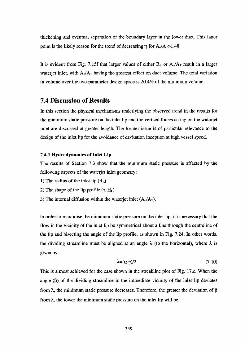
thickening and eventual separation of the boundary layer in the lower duct. This latter
point is the likely reason for the trend of decreasing 11 for A/ AT> 1.48.
It is evident from Fig. 7 .15f that larger values of either RL or A/ AT result in a larger
waterjet inlet, with AJ AT having the greatest effect on duct volume. The total variation
in volume over the two-parameter design space is 20.4% of the minimum volume.
7.4 Discussion of Results
In this section the physical mechanisms underlying the observed trend in the results for
the minimum static pressure on the inlet lip and the vertical forces acting on the waterjet
inlet are discussed at greater length. The former issue is of particular relevance to the
design of the inlet lip for the avoidance of cavitation inception at high vessel speed.
7.4.1 Hydrodynamics of Inlet Lip
The results of Section 7.3 show that the minimum static pressure is affected by the
following aspects of the waterjet inlet geometry:
1) The radius of the inlet lip (RL)
2) The shape of the lip profile (y, HL)
3) The internal diffusion within the waterjet inlet (AJAT).
In order to maximise the minimum static pressure on the inlet lip, it is necessary that the
flow in the vicinity of the inlet lip be symmetrical about a line through the centreline of
the lip and bisecting the angle of the lip profile, as shown in Fig. 7 .24. In other words,
the dividing streamline must be aligned at an angle A (to the horizontal), where A is
given by
A=( a-y)/2 (7.10)
This is almost achieved for the case shown in the streakline plot of Fig. 17 .c. When the
angle (~) of the dividing streamline in the immediate vicinity of the inlet lip deviates
from A, the minimum static pressure decreases. Therefore, the greater the deviation of ~
from A, the lower the minimum static pressure on the inlet lip will be.
259
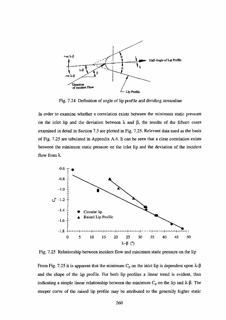
+ve A-13 Half-Angle ofL1p Profile
Lip Profile
Fig. 7.24 Definition of angle of lip profile and dividing streamline
In order to examine whether a correlation exists between the minimum static pressure
on the inlet lip and the deviation between A and ~. the results of the fifteen cases
examined in detail in Section 7.3 are plotted in Fig. 7.25. Relevant data used as the basis
of Fig. 7.25 are tabulated in Appendix A.4. It can be seen that a clear correlation exists
between the minimum static pressure on the inlet lip and the deviation of the incident
flow from A.
-0.6 • -0.8
-1.0
c. -1.2 u
-1.4 • Circular lip
-1.6 A Raised Lip Profile
0 5 10 15 35 40 45 50
Fig. 7.25 Relationship between incident flow and minimum static pressure on the lip
From Fig. 7.25 it is apparent that the minimum Cp on the inlet lip is dependent upon A-~
and the shape of the lip profile. For both lip profiles a linear trend is evident, thus
indicating a simple linear relationship between the minimum Cp on the lip and A-~. The
steeper curve of the raised lip profile may be attributed to the generally higher static
260
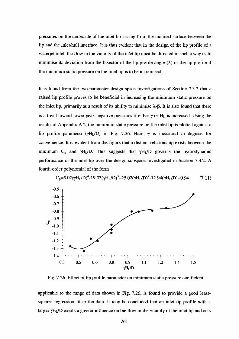
pressures on the underside of the inlet lip arising from the inclined surface between the
lip and the inlet/hull interface. It is thus evident that in the design of the lip profile of a
waterjet inlet, the flow in the vicinity of the inlet lip must be directed in such a way as to
minimise its deviation from the bisector of the lip profile angle (A.) of the lip profile if
the minimum static pressure on the inlet lip is to be maximised.
It is found from the two-parameter design space investigations of Section 7.3.2 that a
raised lip profile proves to be beneficial in increasing the minimum static pressure on
the inlet lip, primarily as a result of its ability to minimise A.-~. It is also found that there
is a trend toward lower peak negative pressures if either y or HL is increased. Using the
results of Appendix A.2, the minimum static pressure on the inlet lip is plotted against a
lip profile parameter (yHr/D) in Fig. 7 .26. Here, y is measured in degrees for
convenience. It is evident from the figure that a distinct relationship exists between the
minimum Cp and yHr/D. This suggests that yHr/D governs the hydrodynamic
performance of the inlet lip over the design subspace investigated in Section 7.3.2. A
fourth-order polynomial of the form
Cp=5.02(yHr/D)4 -19.03(yHr}D)3 +25.02(yHr}D)2 -12.94(yHr/D)+0.94 (7.11)
-0.5
-0.6
-0.7
-0.8
-0.9 c.
u -1.0
-1.1
-1.2
-1.3 • -1.4
0.3 0.5 0.6 0.8 0.9 1.1 1.2 1.4 1.5 yl-ldD
Fig. 7.26 Effect of lip profile parameter on minimum static pressure coefficient
applicable to the range of data shown in Fig. 7 .26, is found to provide a good least
squares regression fit to the data. It may be concluded that an inlet lip profile with a
larger yHr/D exerts a greater influence on the flow in the vicinity of the inlet lip and acts
261

to direct the flow over the lip in such a way as to minimise A.-~ and thereby increase the
minimum static pressure on the lip.
It is found from the two-parameter design space investigations of Section 7 .3.3, that
increasing the internal diffusion within the waterjet inlet (via AJAT) leads to increased
minimum Cp on the inlet lip for AJAr<l.38, after which the trend is reversed.
Increasing AJAT and hence IVRT, changes the shape of the inlet streamtube, due to the
greater mass flux ingested and so acts to direct the flow in such a way as to minimise A.-
~- At an AJ AT of 1.38, where the minimum Cp on the lip is maximised over the design
subspace, IVRT is 0.828. For a waterjet having an AofAT of unity, IVR and IVRT are
identical. It was found from the results presented herein, that increasing IVRT can have a
beneficial effect on the cavitation performance of the inlet lip. This therefore suggests
that operating a waterjet inlet having an Aof AT of unity at a higher IVR can have a
beneficial effect on the cavitation performance of the inlet lip.
7.4.2 Vertical Forces acting on the Waterjet Inlet
The vertical forces acting on the waterjet inlet may be partially attributed to the net
changes in vertical momentum of the flow through it. In the following discussion,
reference is made to the control volume of Fig. 7.27, which is similar to the one used for
F
Fig. 7.27 Control volume for vertical force analysis
262
the derivation of waterjet thrust in Chapter 2. fu this case A1 has been moved to
correspond with the ramp tangency point (hence A3=0) of the inlet and A6 is positioned
at the duct exit.
If the waterjet inlet is not inclined to the horizontal, then the net vertical force caused by
momentum changes acting on the control volume must necessarily balance the weight of
the entrained water. Mathematically this may be expressed as
(7.12)
where } is the unit vector in the vertical direction, V the volume of the control volume,
dA the differential surface area and subscript CV denotes the control volume.
Alternatively Eqn 7.12 may be written as
(7.13)
where the force vectors, F. , represent the integral contributions of static pressure and
shear stress over the control volume area and may be evaluated as
F. =-JpdA-f ~dA A, A,
(7.14)
fu Eqn 7.14 dA represents the differential surface area vector pointing out of the control
volume and ~ is the shear stress vector. Thus, the hydrodynamic forces acting on the
solid surface of the control volume in the vertical direction may be written as
(7.15)
The total vertical force acting on the waterjet inlet, however, includes the contribution
of the area associated with the inlet lip and is given by
(7.16)
where Fy is the total vertical force acting on the waterjet inlet. Using Eqn 7.15, Eqn 7.16
may be also be written as
(7.17)
Thus the vertical force acting on the waterjet inlet is a function of the vertical forces
acting on the inlet streamtube and the inlet lip.
The vertical forces acting on the inlet streamtube and inlet lip are however implicit
functions of the geometry of the waterjet inlet. The work presented in this thesis has
263
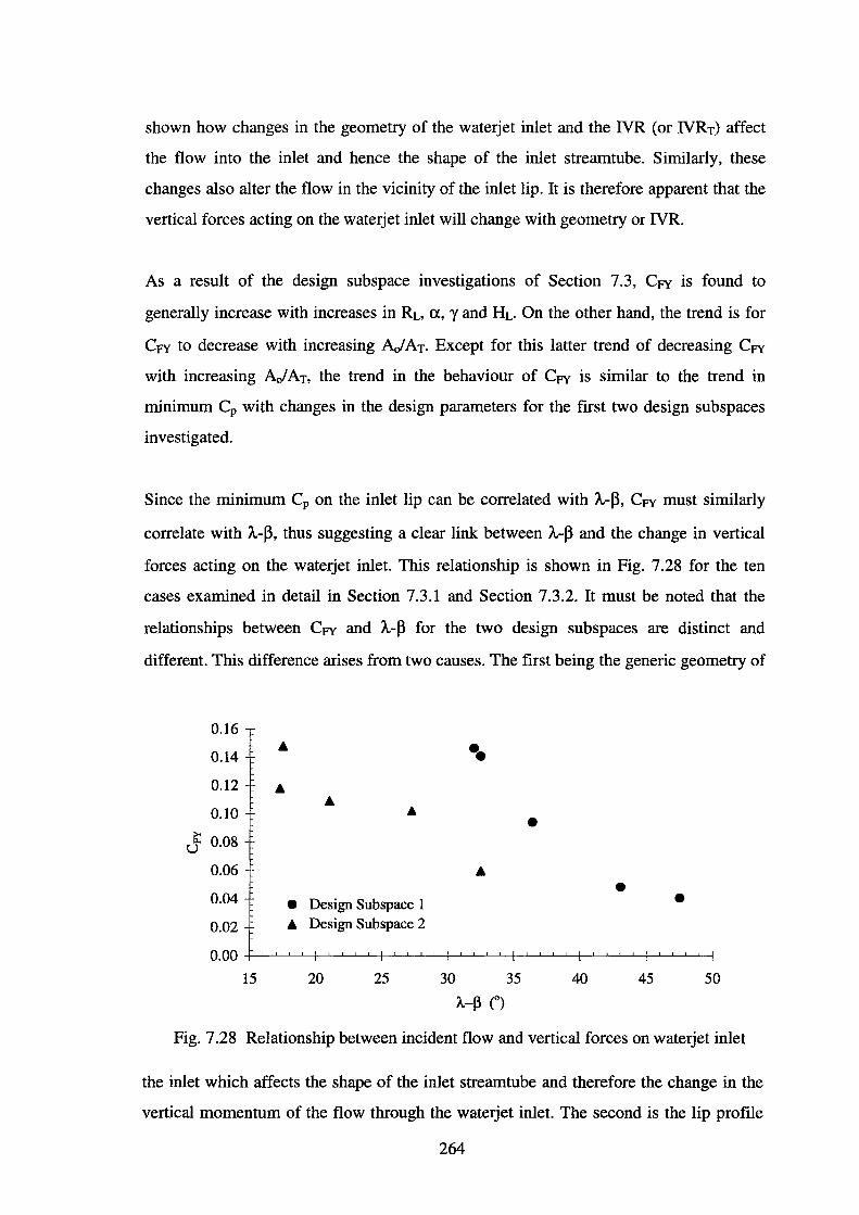
shown how changes in the geometry of the waterjet inlet and the IVR (or IVRT) affect
the flow into the inlet and hence the shape of the inlet streamtube. Similarly, these
changes also alter the flow in the vicinity of the inlet lip. It is therefore apparent that the
vertical forces acting on the waterjet inlet will change with geometry or IVR.
As a result of the design subspace investigations of Section 7.3, Cpy is found to
generally increase with increases in RL, a, y and HL. On the other hand, the trend is for
Cpy to decrease with increasing AofAT. Except for this latter trend of decreasing Cpy
with increasing AofAT, the trend in the behaviour of Cpy is similar to the trend in
minimum Cp with changes in the design parameters for the first two design subspaces
investigated.
Since the minimum Cp on the inlet lip can be correlated with A.-~, Cpy must similarly
correlate with A-~, thus suggesting a clear link between A-~ and the change in vertical
forces acting on the waterjet inlet. This relationship is shown in Fig. 7.28 for the ten
cases examined in detail in Section 7.3.1 and Section 7.3.2. It must be noted that the
relationships between Cpy and A.-~ for the two design subspaces are distinct and
different. This difference arises from two causes. The first being the generic geometry of
0.16
• •• 0.14
0.12 • 0.10 •
i::: 0.08 u 0.06
• 0.04 • Design Subspace 1 • 0.02 • Design Subspace 2
0.00
15 20 25 30 35 40 45 50
A.-~ (o)
Fig. 7.28 Relationship between incident flow and vertical forces on waterjet inlet
the inlet which affects the shape of the inlet streamtube and therefore the change in the
vertical momentum of the flow through the waterjet inlet. The second is the lip profile
264
used, as the geometry of the inlet lip profile will inevitably affect F7 in Eqn 7.17. The
relevant data used as the basis of the plot of Fig. 7.28 is tabulated in Appendix A.S.
A qualitative investigation of the vertical forces acting on the waterjet inlet, the results
of which are presented in Appendix A.6, was undertaken in order to determine the
relative contributions of the components of the waterjet inlet to the overall force
balance. The waterjet inlet is treated as being two-dimensional and the pressure forces
acting on the upper and lower waterjet inlet are calculated according to
(7.18)
where (Fy )1 is the net vertical force (per unit width) acting on the ith section of the
waterjet inlet geometry, Sx the component of arc length in the X direction and s2 and sl
are the upper and lower limits of the range of arc lengths over which the integration is
carried, respectively. Note that the contribution to the vertical force arising from skin
friction has been omitted, as the primary interest here is on the changes in the pressure
forces.
The following conclusions can be drawn from the study:
1) For all cases examined, the net vertical force on the inlet ramp is negative
2) The net vertical force on the inlet lip is negative and represents between 10%-20% of
the net vertical force acting on the lower waterjet inlet for the design subspaces
investigated in Section 7.3.1 and Section 7.3.2.
3) The outside of the duct bend represents the largest contribution to the vertical force
on the upper waterjet inlet.
4) For the design subspaces investigated in Section 7.3.1 and Section 7.3.2, the relative
change in vertical force is greatest in the lower waterjet inlet, thus adding weight to
the argument that it is the angle of the flow into the waterjet inlet that affects the
vertical force via changes in the vertical momentum of the flow and lip suction.
265
7.5 Closure
Three two-parameter subspaces of the design hyperspace spanned by the vector of
design variables of the author's parametric waterjet inlet geometry are investigated in
order to examine how changes in the geometry of the waterjet inlet affect its
hydrodynamic performance.
The design subspaces investigated are:
1) RJD and a - Radius of the inlet lip with inlet steepness
2) y and Hr/D - Profile of the inlet lip
3) A/AT and Rr/D -Internal diffusion with radius of the inlet lip
All CFD simulations were run for a waterjet inlet operating at an IVR of 0.6 with a free
stream velocity of 20.58ms-1 (40 knots vessel speed) corresponding to a vessel cruise
condition. A boundary layer of non-dimensional thickness of BID=O.S was used to
simulate the ingestion of fluid from a thick upstream hull boundary layer.
The following conclusions may be drawn from the investigations presented herein:
1) The minimum static pressures on the surface of the waterjet inlet occurred in the
vicinity of the inlet lip and are sufficiently low to cause cavitation in all cases
examined.
2) The minimum static pressure on the inlet lip is largely dependent on the angle
between the angle of the bisector of the profile of the inlet lip (A) and the angle of the
dividing streamline in the vicinity of the inlet lip (~). Large A.-~ results in low
minimum static pressure on the inlet lip. When A.=~, the flow is symmetrical about
the inlet lip profile and the minimum Cp on the lip is maximised.
3) A raised lip profile acts to direct the flow in the vicinity of the inlet lip more
symmetrically over the lip and so tends to minimise A.-~. Larger values of the
parameter yHr/D are beneficial in increasing the minimum Cp on the inlet lip when a
raised lip is used.
4) The net vertical force acting on the waterjet inlet results from a net change in the
vertical momentum of the flow through the waterjet inlet and vertical forces acting
on the inlet lip below the stagnation line. This was shown to be a function of the
266
geometry of the inlet streamtube, the inlet lip and is found to correlate with A.-~.
Generally, larger RL, HL and a resulted in greater positive vertical forces on the
waterjet inlet. The lower overall static pressures in the waterjet inlet, due to the
increased mass flow-rate as a result of from internal diffusion (AoiAT), lead to a
"suck-down" effect.
5) There are no distinct trends and little overall variation in the area-averaged 11 for the
first two design subspaces investigated, thus suggesting that viscous losses within the
waterjet inlet are approximately equal. The overall level of 11 is determined primary
by the energy flux coefficient (Ce) of the ingested flow. For the third design subspace,
there is a noticeable trend of increasing 11 with AoiAT up to Ao1AT=l.48 when the
trend reverses. This trend reflects a conflict between the increasing Ce of the ingested
flow (primarily by virtue of increased streamtube depth) and the increasing viscous
losses within the waterjet inlet.
6) Variation of RL, a, HL or y leads only to relatively small variations in the distortion
coefficient (De) at the duct exit. Increasing the internal diffusion (AJ AT) lead to
significant changes in De. This is due to a combination of the quality of the ingested
flow and the thickening of the boundary layer in the bottom of the duct by virtue of
adverse pressure gradients and secondary flow.
7) Smaller, more compact waterjet inlets are favoured by large a, small RL and small
HL. Increasing the internal diffusion (AoiAT) within the waterjet inlet leads to an
increase in duct volume at constant throat diameter.
267
Chapter 8 Optimisation of Waterjet Inlet Design
In this chapter a methodology for the optimisation of a parametrically-defined generic
flush-type waterjet inlet (in the absence of hull form) is presented. The methodology is
applied to the optimisation of an inlet for the maximisation of cavitation number on the
surface of the inlet at the cruise condition (selected IVR of 0.60). The main aim of this
chapter is to outline the optimisation methodology and to demonstrate its effectiveness
in improving the hydrodynamic performance of a genericwaterjet inlet geometry.
Seil et al ( 1997) noted the following qualities of an ideal waterjet inlet:
"An ideal waterjet inlet would be free of cavitation and flow separation in the inlet,
deliver a spatially uniform distribution of velocity and pressure to the pump with the
minimum of total pressure losses and contain the minimum weight of entrained water.
An ideal inlet should also affect the flow around the vessel hull in such a way as to
minimise the thrust deduction factor".
In addition, turbulence present in the flow should have no adverse effect on pump
performance. Implicit in the above statement by Seil et al ( 1997) is the notion that the
"idealised" waterjet inlet must perform well over the complete range of IVR
encountered in its operation.
The performance of the ideal inlet can be expressed mathematically usmg the
hydrodynamic performance parameters introduced in previous chapters as
O"mm>>O, tJ=O, t$;0, (~, Dc,V*, ...JkiUref, lJD)-70 (8.1)
where O"mm is the minimum cavitation number on the surface of the waterjet inlet, tj is
the lip loss thrust deduction fraction (see Chapter 2), t the thrust deduction fraction of
the waterjet-hull system, ~ the total pressure loss factor of the waterjet inlet, De the
distortion of total pressure at the duct exit, v* the non-dimensional duct volume of the
waterjet inlet, ...JkiUrer the velocity-scale of turbulence in the inlet and fJD the
268
corresponding turbulent length-scale.
In reality of course, flush-type waterjet inlets do not possess the characteristics of the
ideal waterjet inlet and therefore there must be a compromise between the various
aspects of the hydrodynamic performance of the waterjet inlet, in order to achieve a
practical waterjet inlet design. Since a parametric description of a flush-type waterjet
inlet involves of the order of ten parameters (8 for the author's geometry), one cannot
possibly achieve an "optimum" (the term being used loosely in this case) waterjet inlet
design based purely on experience. Even if one is to achieve a practical waterjet inlet
design of superior hydrodynamic performance, it cannot be claimed that the best
possible design has been achieved. The question is thus posed as to what the optimum
shape of the waterjet inlet is, for a given set of criteria and what the means are to
achieve this shape. Herein lie the issues at the heart of waterjet inlet optimisation.
As noted in Chapter 1, the optimisation of the hydrodynamic performance of waterjet
propelled vessels requires an optimisation of the complete waterjet inlet/hull geometry
over a range of NR values. This poses a very complex hydrodynamic problem.
Therefore, the simplified problem of waterjet inlet optimisation in the absence of hull
form, but with the effect of hull form being represented by a boundary layer upstream of
the waterjet inlet, is examined in this chapter.
The optimisation methodology presented here is based on the approach of treating the
waterjet inlet optimisation as a formal mathematical optimisation problem where a
mathematical objective function, expressing favourable design criteria, is to be
minimised (or maximised) within a set of constraints placed upon the geometry of the
waterjet inlet. The actual approach to optimisation used here is what Frank and Shubin
(1992) call a "Black-Box Method", in which an optimisation routine is coupled with an
existing CFD code (Fluent). The CFD code provides the flow solution data necessary
for calculation of the objective function. One advantage of this approach is that the CFD
analysis code can be used without modification and hence there is no need to modify
complicated discretisation schemes within the code. The disadvantage of such an
approach is, however, that there is a high associated computational cost. This cost grows
linearly as the number of design variables increases. Frank and Shubin ( 1992) further
269
noted that one mitigating factor of this limitation is that the solution of perturbed
analysis problems is considerably less computationally expensive than solving arbitrary
problems. It will be shown in Section 8.2 that this approach does result in significant
computational savings.
As discussed in Chapter 1, the use of CFD provides a necessary foundation for the cost
effective optimisation of waterjet inlet design. Furthermore, the flow in the waterjet inlet
can only be simulated realistically using computational techniques that account for
viscosity and turbulence. Thus it is necessary to solve the Reynolds-averaged Navier
Stokes (RANS) equations with a suitable turbulence closure. From the experimental
validation studies presented in Chapter 5, it is clear that the RNG k-£ turbulence model
can be used to provide suitable turbulence closure of the RANS equations. Thus, the
optimisation methodology presented in this chapter is under-pinned by flow simulations
in which the RANS equations are solved using the RNG k-£ turbulence model.
In Section 8.1 the optimisation methodology used for the optimisation of flush-type
waterjet inlets is presented. The computational modelling of the flow domain and a
discussion of the simulations undertaken to optimise the generic flush-type waterjet inlet
geometry are presented in Section 8.2. It must be noted that the optimisation undertaken
is for constant NR, but not constant flow-rate. In Section 8.3, the hydrodynamics of the
optimised waterjet inlet geometry (with respect to cavitation performance at the cruise
condition) are compared with the hydrodynamics of the initial geometry. The results of
the waterjet inlet optimisation are discussed in Section 8.4. The conclusions of the work
presented in this chapter are summarised in Section 8.5 and the hydrodynamic design of
the optimised waterjet inlet is compared with current industrial designs.
8.1 Optimisation Methodology
The optimisation methodology presented in this section is based on a formal
mathematical approach to optimisation where an objective function describing the
hydrodynamic performance of the waterjet inlet is to be minimised (or maximised, since
this is the equivalent problem), subject to a set of linear and non-linear constraints on
the geometry of the waterjet inlet. This may be mathematically expressed as
270
minimise f(X), X e 9\" subject to the constraints
c.(X)=O, i=1,2, ... ,m'
c.(X)~O, i=m'+1, ... ,m
(8.2)
using the generic form outlined in Gillet al (1981). Eqn 8.2 states that the mathematical
objective function (f) is to be minimised by finding a suitable set of variables (X ) of
which f is either an explicit or implicit function, subject to a set of constraints (c1) on the
components of X .
In the work presented herein, X represents a vector of design variables
(8.3)
whose components are the geometric parameters of the generic flush-type waterjet inlet
geometry described in Chapter 4. The description of this generic geometry X may thus
be written as
(8.4)
where:
1) a. - The angle of inclination of the inlet to the horizontal plane
2) RL- Radius of the inlet lip
3) H - Height of the pump centreline above the base of the inlet
4) R0 - Radius of curvature of the centreline of the duct bend
5) LH - Length of the horizontal duct section downstream of the bend
6) AJ AT - Ratio of duct exit area to throat area
7) HL- Height of the centreline of the inlet lip above the inlet opening plane
8) y - Angle of inclination of the raised-lip profile
In order to allow an optimal shape of waterjet inlet to be geometrically scaled arbitrarily
(provided that Reynolds number effects on the inlet flow are small) so as to increase the
applicability of an optimum waterjet inlet shape to other sizes of waterjet inlet, the
components of X may be non-dimensionalised to give
271
X= [a, RL/D, H/D, R 0 /D, LH/D, A 0 /AT, HL/D, yf (8.5)
where Dis the diameter of the circular throat section of the generic inlet and a and"{ are
measured in radians. This approach does not however, guarantee scaling for 0", as the
static pressure varies linearly with elevation due to gravitational effects. Concerns
about Froude number scaling are unnecessary since attention is focused purely on an
isolated waterjet inlet flow here.
The geometric constraints on the components of X are
a:
RUD:
HID:
RoiD:
LHID:
AofAT:
HLID:
y:
(a)I:s;a:s;(a)z
(RiiD)I:s;RUD:s;(RUD)z
HID=(HID)I
(Ro/D)I:s; RofD:s;(Ro/D)z
(LH/D)I:s; LHID:s;( LH/D)z (8.6)
(AJAT)I:s; AJAT:s;(AJAT)z
(HiiD)I:s; HUD:s;(H-Ro(l-cosa)-(RL +D/2)sin(7t/2-a))/D
("{)J:s;y:s;(y)z
where subscripts 1 and 2 refer to the lower and upper constraints on the particular
geometric parameter.
The objective function (f) describing the hydrodynamic performance of the waterjet inlet
may be written as
(8.7)
where f is an explicit function of the hydrodynamic performance parameters ('1ft) which
provide a measure of the different aspects of the hydrodynamic performance of the
waterjet inlet. The 'lf1 are, however, unknown functions of the inlet geometry, hence
(8.8)
Therefore, f is an implicit function of X1 and so f is ultimately a function of the waterjet
inlet geometry,
f = f('lf 1(XpX 2 , ••• ,xn),'lf 1(XpX2 , ••• ,xn), ... ,'lfN(xpX2 , ••• ,xn)) (8.9)
The choice of explicit relationship between f and 'lf1 is arbitrary, but a suitable choice is
272
N
f = :Laz,-J(az,'I'Jb, (8.10) 1=1
where a2,_ 1, a2, and b, are constants. Clearly f is a non-linear function of 'I'• which
becomes linear if b,=l. Eqn 8.10 is the generic form adopted in Seil et al (1997). Other
functional relationships between f and 'I'• are of course possible, but it is the author's
view that the generic form used in Eqn 8.10 offers the greatest generic usefulness.
Since the focus of this chapter is on the optimisation of the waterjet inlet geometry with
the aim of eliminating cavitation on the underside of the inlet lip and maximising
overall static pressure on the duct surface for the cruise condition, Eqn 8.10 takes the
following form
f = -crmm. (8.11)
Minimisation of Eqn 8.11 actually corresponds to a maximisation of O"mm· Optimisation
based on Eqn 8.11 clearly ignores other factors of hydrodynamic performance, but
focuses attention on the issue of inlet cavitation. This allows a greater understanding of
how a synergistic combination of design parameters can improve cavitation performance
and facilitates a greater understanding of how the waterjet inlet geometry affects the
flow within it.
An alternative approach to the optimisation of the waterjet inlet, with regard to its
cavitation performance, is to solve the inverse design problem. Given the desired static
pressure distribution on the duct surface (for example, the pressure distribution on the
duct centreplane), a suitable geometry is found that minimises an objective function of
the form
(8.12)
is found. In Eqn 8.12, c represents the least-square error between the computed static
pressure distribution on the duct surface (p) and the desired distribution (Pspec). Jameson
(1995) suggested this approach for the optimisation of airfoil shapes.
8.1.1 Overview of Optimisation Procedure
In this section the sequence of steps involved in waterjet inlet optimisation are
273
discussed. The overall optimisation cycle is shown in Fig. 8.1 and is described below. In
order to begin the optimisation, an initial design that satisfies the geometric constraints
on its geometry is selected. The mesh bounding the modelled flow domain containing
the waterjet inlet geometry is then generated.
The mesh generation procedure follows that outlined in Chapter 4 and is performed
manually, as the process of obtaining a suitable grid is necessarily iterative, guided by
the experience of the user. Since waterjet inlet optimisation requires the examination of
a large number of different geometries, the mesh must be suitably modified for each
new geometry in order to ensure that sufficient cells are placed in regions of large flow
gradients and features of the waterjet inlet geometry (in particular the inlet lip) are
adequately represented.
Note that Fig. 8.1 does not imply that only one mesh is generated during the grid
generation process. The number of meshes generated depends on the number of
evaluations of the objective function for each iteration of the optimisation routine. If an
optimisation algorithm based on the evaluation of gradients of the objective function is
used (eg. quasi-Newton methods, see Gillet al (1981)), evaluation of the gradient vector
would require n+ 1 or 2n flow simulations depending on whether the gradients are
calculated using forward differences or central differences, respectively. Calculation of
second derivatives using central differences for evaluation of the Hessian matrix in
Newton methods requires 2n+ 1 function evaluations. If direct search methods are used
(see Gottfried and Weisman (1973), Section 3.3), such as in this thesis, the results of
only one flow simulation are required during each iteration of the optimisation cycle
shown in Fig. 8.1.
After the mesh generation cycle, a CFD analysis using Fluent is undertaken in order to
obtain a converged solution for the flow in the modelled domain. The results analysis
program (Analysis) reads flow data extracted from Fluent and data relating to the cell
face area vector components of the surface of the waterjet inlet mesh produced by
Inlet3D. Output from Analysis contains such 'lf1 as crmm. De. 11 and Cpy. Using the values
of '1'1 , the optimisation routine calculates the value of the objective function (f) decides
whether the criteria for convergence of the optimisation algorithm has been met and
274
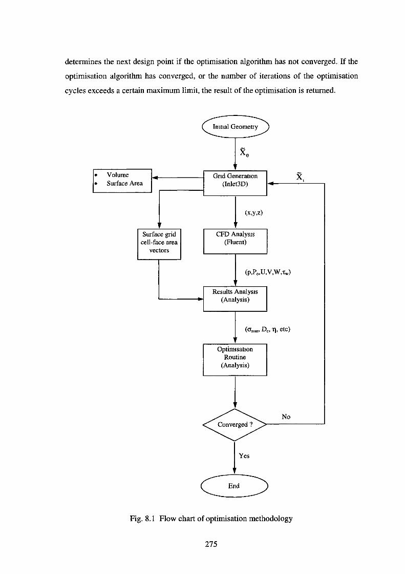
determines the next design point if the optimisation algorithm has not converged. If the
optimisation algorithm has converged, or the number of iterations of the optimisation
cycles exceeds a certain maximum limit, the result of the optimisation is returned.
• •
Volume Surface Area
Surface grid cell-face area
vectors
l X,
Gnd GeneratiOn (lnlet3D)
l (x,y,z)
CFD Analysis (Fluent)
l (p,P0 ,U,V,W,tw)
Results Analysis (Analysis)
Optimisation Routine
(Analysis)
l Converged?
No
Fig. 8.1 Flow chart of optimisation methodology
275
x.

8.1.2 Optimisation Algorithm
The optimisation algorithm chosen for use in the optimisation of the waterjet inlet is the
algorithm of Sherif and Boice (1993), which is essentially a development of the "Pattern
Search" algorithm of Hooke and Jeeves (1961). The Sherif-Boice Algorithm (SBA) is a
direct-search method which does not rely on the calculation of either the gradient vector
or the Hessian in determining the next suitable design point. It rather relies purely on the
calculation and comparison of values of the objective function. The SBA is simple,
robust, computationally efficient and allows easy implementation of constraints.
Furthermore, since it does not involve the calculation of partial derivatives of the
objective function, it can be used effectively when the objective function contains
discontinuities, thus furthering its appeal. There is, however, no guarantee that the
solution obtained using the SBA does in fact correspond to the global minimum of the
objective function. This is the case for most optimisation algorithms.
The SBA is presented in the form of a flow-chart in Fig. 8.2. In the SBA there are
essentially two types of movements made in the design hyperspace. The first is termed
an "exploratory move", where a perturbation in the components of X is made about a
base point and the objective function is evaluated. This is done in order to determine
whether a reduction in f has occurred and so determine a direction of decreasing f.
Should a reduction in f occur, then the location where this reduction occurs becomes the
new base point. The second type of move is termed a "pattern" move and is essentially
an extrapolation from the current and previous base points. The rationale behind this
being that the vector describing the difference between the base points describes a
direction of decreasing f and so moving in this direction should result in a reduction of f.
The SBA shall be explained in greater detail below and proceeds as follows:
Initialisation
An initial solution vector X0 , satisfying the constraints of the problem, is first chosen
and the value of the objective function f(X 0 ) is then determined at this point. A
perturbation vector
(8.13)
276
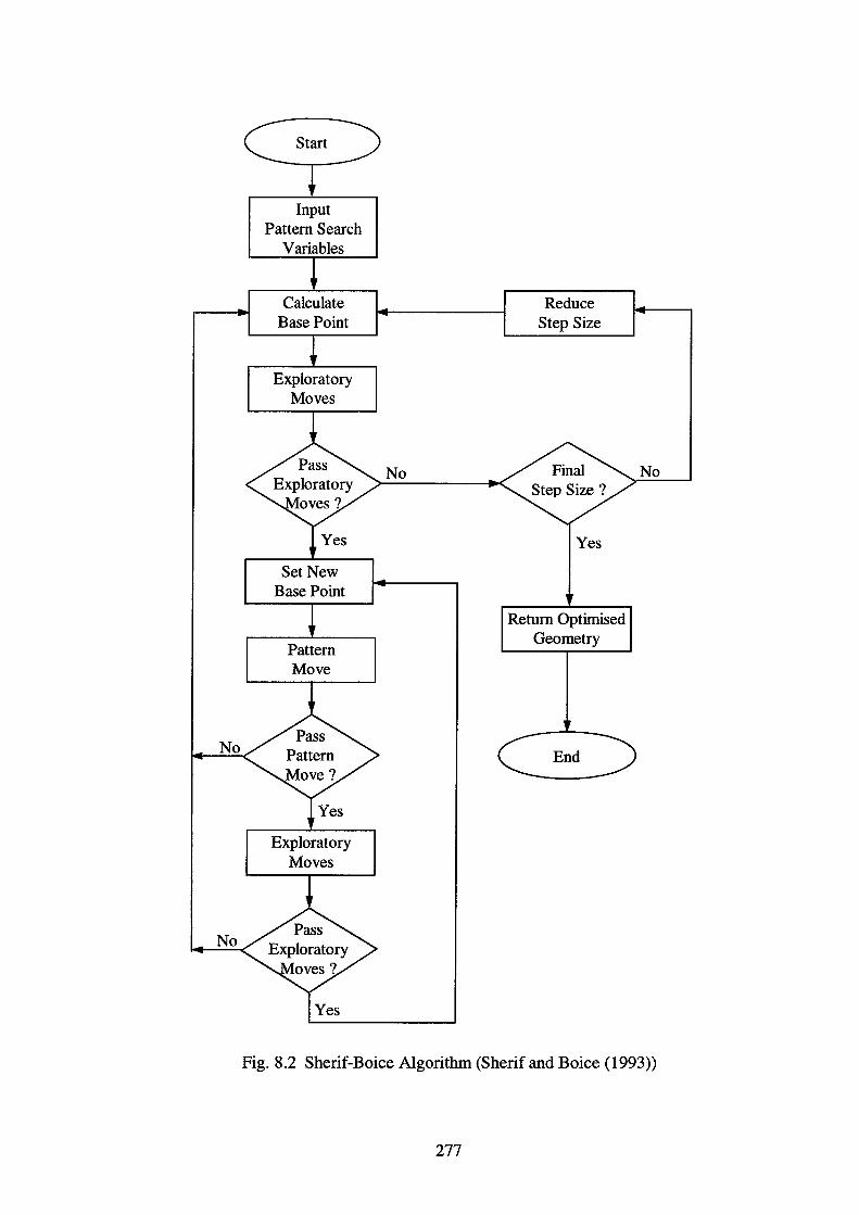
No
No
Input Pattern Search
Calculate Base Point
Exploratory Moves
Set New Base Point
Pattern Move
Exploratory Moves
No
Reduce Step Size
Yes
Return Optimised Geometry
No
Fig. 8.2 Sherif-Boice Algorithm (Sherif and Boice (1993))
277
is defined where the components of this vector correspond to the size of the
perturbations in the corresponding components of X , such that
(8.14)
Exploratory Move
A perturbation is made in X I of the ith base point, such that X = [X I + f. I ' X 2 ' ••• 'X n r and the objective function is evaluated at this point. If f(X) < f(X.), then this X
becomes the new base point. If f(X) ~ f(X.), then another perturbation is made in x1,
but in the opposite direction, such that X = [X I - tp Xz ' ••• 'X n r. If f (X) < f (X.) then
this new value of X becomes the base point, otherwise the above procedure is repeated
for each component of x. until f is minimised. If a new base point cannot be found
after perturbation of all components of x. , then the step sizes of the components of the
perturbation vector are halved, i.e. e -7 E"/2 and the above process is repeated.
Pattern Move
If a base point is found after an exploratory move, then a pattern move is made in which
a new solution vector is determined from an extrapolation of the current and previous
base points. The new solution is calculated as
x = x.-1 +2(X. -x.-1) (8.15)
where X is the new point resulting from the pattern move, x. the current base point
determined from the exploratory move and X1
_ 1 the previous base point. The value of f
is determined at X. Should f(X) < f(X.) then X is taken as the new base point and
exploratory moves are made around the new base point. If on the other hand,
f(X) ~ f(X.), then the pattern move is judged to have failed and x. is retained as the
current base point. An exploratory move is then made around X. in search of a new
base point.
Termination
When exploratory moves around a base point continually fail and every component of
e is reduced below the convergence criterion (limiting step size), the algorithm
278

terminates. The objective function has found a local minima and X is at its local
optimum value.
Depending on the characteristics of the solution space, one may expect that the initial
rate of convergence of the SBA will be relatively large when the starting solution is far
from the solution vector corresponding to a minimum of f and the step size ( £1) of each
component of the perturbation vector is large. It is, however, clear that as the local
minimum value of f is approached, the rate of convergence will become slower and will
require a large number of exploratory moves and hence evaluations of f to obtain a
converged solution ( £, = ec)2, where £c,1 is the limiting step size). The stricter the
convergence criterion (minimum step size) is, the larger will be the number of
exploratory moves that may be expected before convergence is achieved. While this
presents no problem when finding the location of minima for analytic functions, this
issue assumes great importance here due to the computational expense involved in
obtaining RANS solutions (in order to evaluate the objective function). Therefore some
liberty must be taken and the criteria associated with convergence relaxed. In other
words, the tolerance or minimum step size associated with convergence must
necessarily be increased in order to avoid an excessive number of exploratory moves in
the vicinity of the optimum solution. For the purposes of practical design, this may be
deemed to be an acceptable approach.
8.2 Computational Simulation and Optimisation
In this section an overview of the actual optimisation, carried out in order to maximise
the minimum static pressure on the surface of the waterjet inlet, is presented. The same
boundary conditions, external domain size and turbulence modelling as used for the
CFD flow simulations presented in Chapter 6, are also used for the flow simulations
here. The same upstream boundary layer velocity and turbulence data applied to
Boundary 1 of the simulations of Chapter 7, is also applied on Boundary 1 for the
optimisation-related CFD simulations presented herein.
The flow solution from the previous exploratory move or base point is used as an initial
flow solution for subsequent simulation, as each new flow computation generally
279
corresponds to a minor perturbation of the previous geometry. This leads to a dramatic
decrease in computational time and it was found that converged flow solutions could
generally be obtained within 50-100 iterations, which was significantly less than the
600-700 iteration necessary to obtain a converged solution ab initio (with an initial
solution for the velocity field specified as the free-stream velocity). When it is found
that an exploratory move corresponds to a point that has already been evaluated, the
objective function was evaluated using the previously calculated objective function
value for that point. This therefore saves computational effort and hence time. Since the
SBA is essentially a sequential algorithm moving from point to point, it is therefore
impossible to run several computations in parallel. This contrasts with gradient-based
methods where flow simulations used for the evaluation of objective function gradients
can be run in parallel. Thus while total computational effort may be comparable for both
methods, the sequential nature of the SBA will result in a longer overall time taken for
the optimisation process. This is a clear disadvantage of the SBA.
All computations were performed using the dimensional form of X given by Eqn 8.4. A
five-parameter optimisation is carried out using the SBA. In other words, five geometric
parameters are given the freedom to vary while the others are held constant. The
parameters held constant are H, LH and R0 . In an actual waterjet installation, the height
of the pump centreline above the inlet opening (H) is likely to be determined by the
draught of the vessel and is therefore set equal to one duct diameter. This appears to be a
typical dimension for most installed waterjet (see Trillo (1994)). For the purposes of
maximising the minimum static pressure on the surface of the waterjet inlet, the length
of the horizontal duct section downstream of the duct bend (LH) is unlikely to have any
impact on the flow in the inlet region (where the minimum static pressures occur).
Furthermore, although an increase in LH does reduce the distortion of total pressure at
the pump inlet, it may be argued that the extra duct volume incurred (with attendant
structural weight, lost internal space within the vessel and reduced vessel buoyancy)
does not justify increasing LH beyond about one duct diameter downstream of the bend.
The radius of the duct bend (Ro) is fixed in order to focus the attention of the analysis
(presented in Section 8.4) on the geometric parameters associated specifically with the
inlet region, as well as to reduce the computational effort required for the optimisation.
The influence of R0 on the optimum solution is therefore unknown.
280
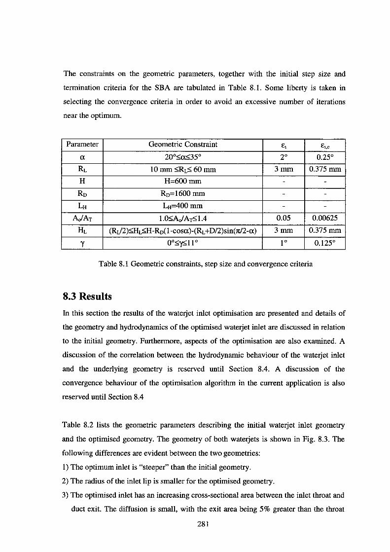
The constraints on the geometric parameters, together with the initial step size and
termination criteria for the SBA are tabulated in Table 8.1. Some liberty is taken in
selecting the convergence criteria in order to avoid an excessive number of iterations
near the optimum.
Parameter Geometric Constraint £1 CJ,C
a 2oo::;;a::;;35° 20 0.25°
RL 10 mm ::;;R~ 60 mm 3mm 0.375 mm
H H=600mm - -
Ro Ro=1600mm - -LH LH=400mm - -
AofAT l.O::;;AJAT::;;l.4 0.05 0.00625
HL (Rv2)::;;H~H-Ro(l-cosa)-(RL +D/2)sin(1t/2-a) 3mm 0.375 mm
'Y oo::;;-y::;; 11 ° 10 0.125°
Table 8.1 Geometric constraints, step size and convergence criteria
8.3 Results
In this section the results of the waterjet inlet optimisation are presented and details of
the geometry and hydrodynamics of the optimised waterjet inlet are discussed in relation
to the initial geometry. Furthermore, aspects of the optimisation are also examined. A
discussion of the correlation between the hydrodynamic behaviour of the waterjet inlet
and the underlying geometry is reserved until Section 8.4. A discussion of the
convergence behaviour of the optimisation algorithm in the current application is also
reserved until Section 8.4
Table 8.2 lists the geometric parameters describing the initial waterjet inlet geometry
and the optimised geometry. The geometry of both waterjets is shown in Fig. 8.3. The
following differences are evident between the two geometries:
1) The optimum inlet is "steeper" than the initial geometry.
2) The radius of the inlet lip is smaller for the optimised geometry.
3) The optimised inlet has an increasing cross-sectional area between the inlet throat and
duct exit. The diffusion is small, with the exit area being 5% greater than the throat
281
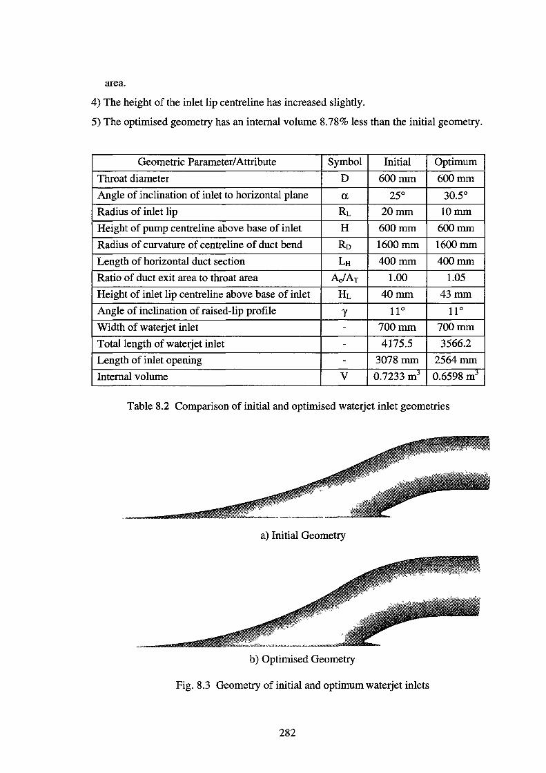
area.
4) The height of the inlet lip centreline has increased slightly.
5) The optimised geometry has an internal volume 8.78% less than the initial geometry.
Geometric Parameter/ Attribute Symbol Initial Optimum
Throat diameter D 600mm 600mm
Angle of inclination of inlet to horizontal plane a. 25° 30.5°
Radius of inlet lip RL 20mm lOmm
Height of pump centreline above base of inlet H 600mm 600mm
Radius of curvature of centreline of duct bend Ro 1600mm 1600mm
Length of horizontal duct section LH 400mm 400mm
Ratio of duct exit area to throat area AJAT 1.00 1.05
Height of inlet lip centreline above base of inlet HL 40mm 43mm
Angle of inclination of raised-lip profile y 110 110
Width of waterjet inlet - 700mm 700mm
Total length of waterjet inlet - 4175.5 3566.2
Length of inlet opening - 3078mm 2564mm
Internal volume v 0.7233 m3 0.6598 m3
Table 8.2 Comparison of initial and optimised waterjet inlet geometries
a) Initial Geometry
b) Optimised Geometry
Fig. 8.3 Geometry of initial and optimum waterjet inlets
282
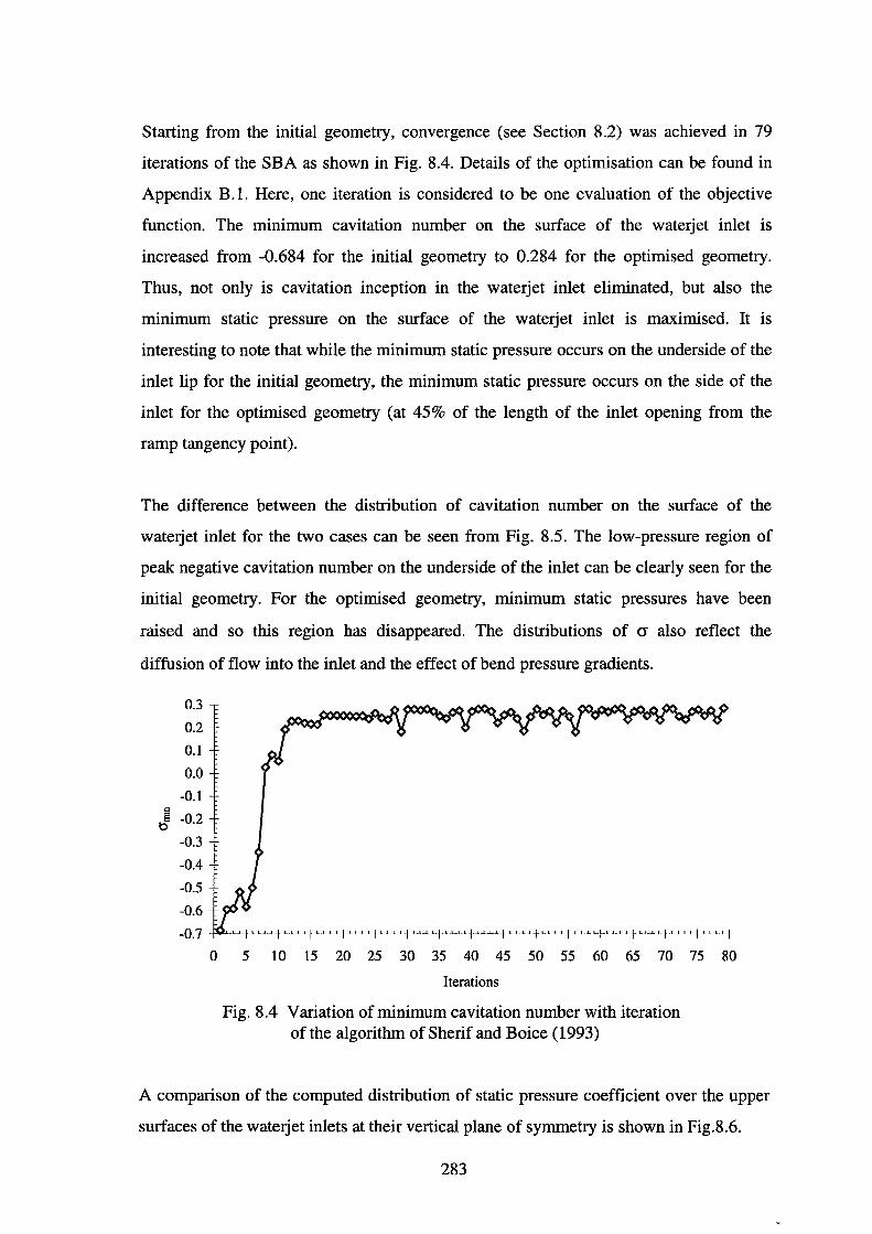
Starting from the initial geometry, convergence (see Section 8.2) was achieved in 79
iterations of the SBA as shown in Fig. 8.4. Details of the optimisation can be found in
Appendix B.l. Here, one iteration is considered to be one evaluation of the objective
function. The minimum cavitation number on the surface of the waterjet inlet is
increased from -0.684 for the initial geometry to 0.284 for the optimised geometry.
Thus, not only is cavitation inception in the waterjet inlet eliminated, but also the
minimum static pressure on the surface of the waterjet inlet is maximised. It is
interesting to note that while the minimum static pressure occurs on the underside of the
inlet lip for the initial geometry, the minimum static pressure occurs on the side of the
inlet for the optimised geometry (at 45% of the length of the inlet opening from the
ramp tangency point).
The difference between the distribution of cavitation number on the surface of the
waterjet inlet for the two cases can be seen from Fig. 8.5. The low-pressure region of
peak negative cavitation number on the underside of the inlet can be clearly seen for the
initial geometry. For the optimised geometry, minimum static pressures have been
raised and so this region has disappeared. The distributions of cr also reflect the
diffusion of flow into the inlet and the effect of bend pressure gradients.
0.3
0.2
0.1
0.0
-0.1
~ -0.2 ~
-0.3
-0.4
-0.5
-0.6
-0.7
0 5 10 15 20 25 30 35 40 45 50 55 60 65 70 75 80
Iterations
Fig. 8.4 Variation of minimum cavitation number with iteration of the algorithm of Sherif and Boice ( 1993)
A comparison of the computed distribution of static pressure coefficient over the upper
surfaces of the waterjet inlets at their vertical plane of symmetry is shown in Fig.8.6.
283
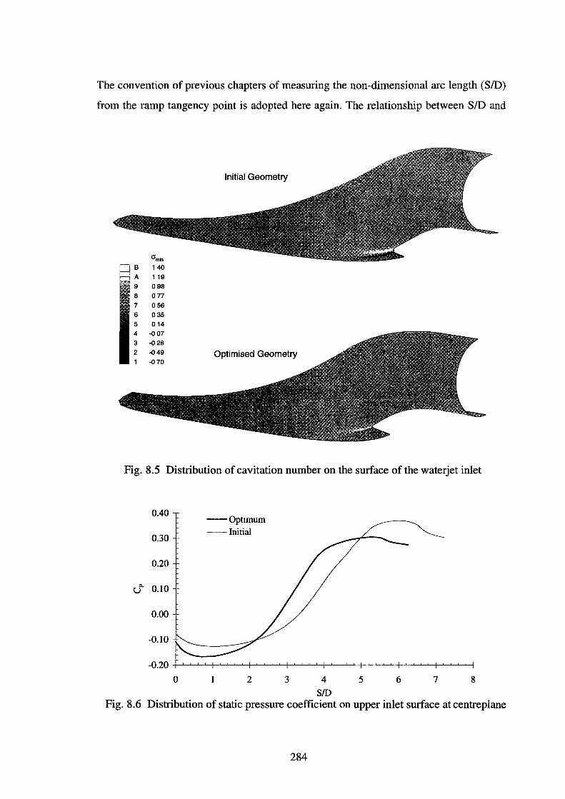
The convention of previous chapters of measuring the non-dimensional arc length (SID)
from the ramp tangency point is adopted here again. The relationship between SID and
Initial Geometry
crmln
=jB 140
A 119
9 098
8 077
7 056
6 035
5 014
4 -007
3 -Q28
2 -049 Optimised Geometry -Q70
Fig. 8.5 Distribution of cavitation number on the surface of the waterjet inlet
c.. u
0.40 --Optimum
0.30 --Initial
0.20
0.10
0.00
-0.10
-0.20 +-'-~'-'--/-'--'--'----'-1-'--'-'--'-lf--'-..L..L--'-----t---'-"-'-~--'--'--'--'-+-'-'----'-'-l--'-'--'--'-l
0 2 3 4
SID 5 6 7 8
Fig. 8.6 Distribution of static pressure coefficient on upper inlet surface at centreplane
284
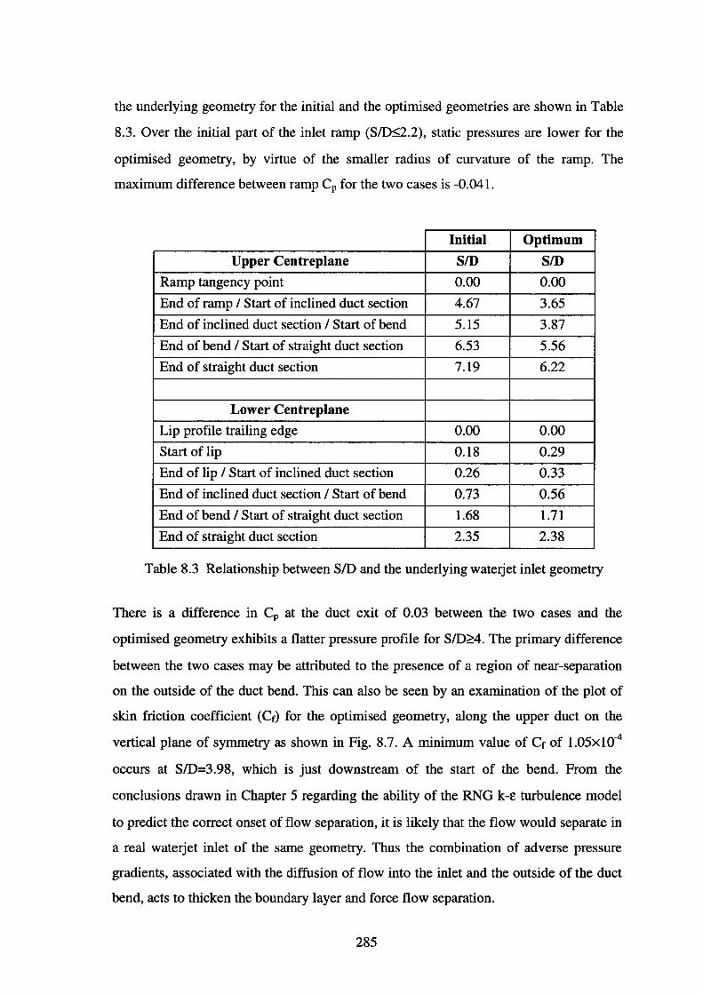
the underlying geometry for the initial and the optimised geometries are shown in Table
8.3. Over the initial part of the inlet ramp (S/D:s;2.2), static pressures are lower for the
optimised geometry, by virtue of the smaller radius of curvature of the ramp. The
maximum difference between ramp Cp for the two cases is -0.041.
Initial Optimum
Upper Centreplane SID SID
Ramp tangency point 0.00 0.00
End of ramp I Start of inclined duct section 4.67 3.65
End of inclined duct section I Start of bend 5.15 3.87
End of bend I Start of straight duct section 6.53 5.56
End of straight duct section 7.19 6.22
Lower Centreplane
Lip profile trailing edge 0.00 0.00
Start of lip 0.18 0.29
End of lip I Start of inclined duct section 0.26 0.33
End of inclined duct section I Start of bend 0.73 0.56
End of bend I Start of straight duct section 1.68 1.71
End of straight duct section 2.35 2.38
Table 8.3 Relationship between SID and the underlying waterjet inlet geometry
There is a difference in Cp at the duct exit of 0.03 between the two cases and the
optimised geometry exhibits a flatter pressure profile for S/D;:::4. The primary difference
between the two cases may be attributed to the presence of a region of near-separation
on the outside of the duct bend. This can also be seen by an examination of the plot of
skin friction coefficient (Cr) for the optimised geometry, along the upper duct on the
vertical plane of symmetry as shown in Fig. 8.7. A minimum value of Cr of 1.05x10⁴
occurs at S/D=3.98, which is just downstream of the start of the bend. From the
conclusions drawn in Chapter 5 regarding the ability of the RNG k-E turbulence model
to predict the correct onset of flow separation, it is likely that the flow would separate in
a real waterjet inlet of the same geometry. Thus the combination of adverse pressure
gradients, associated with the diffusion of flow into the inlet and the outside of the duct
bend, acts to thicken the boundary layer and force flow separation.
285
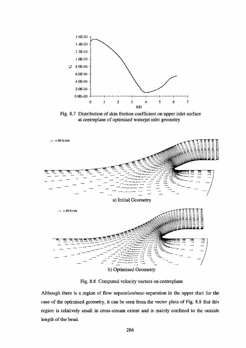
I 6E-03
I 4E-03
I 2E-03
I OE-03
u 8 OE-04
6.0E-04
40E-04
2.0E-04
OOE+OO
0 2 3 4 5 6 7 SID
Fig. 8.7 Distribution of skin friction coefficient on upper inlet surface at centreplane of optimised waterjet inlet geometry
- =206m/s
--~-----~-- -- --::::...
------a) Initial Geometry
- =206m/s
----b) Optimised Geometry
Fig. 8.8 Computed velocity vectors on centreplane
Although there is a region of flow separation/near-separation in the upper duct for the
case of the optimised geometry, it can be seen from the vector plots of Fig. 8.8 that this
region is relatively small in cross-stream extent and is mainly confined to the outside
length of the bend.
286
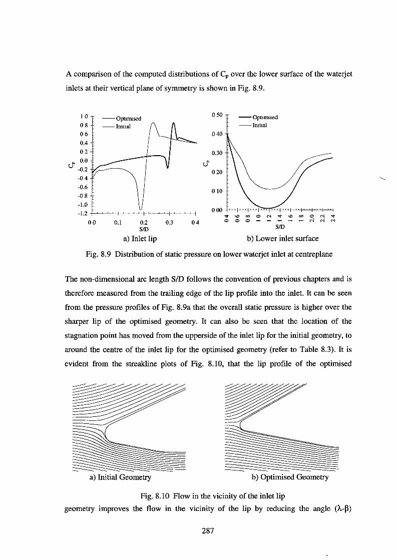
A comparison of the computed distributions of Cp over the lower surface of the waterjet
inlets at their vertical plane of symmetry is shown in Fig. 8.9.
c. u
I 0 --Optnrused 08 -lmttal 06
0.4
02
0.0
-0.2
-04
-0.6
-0 8
-1.0
-1.2
00 0.1 0.2 SID
a) Inlet lip
050
040
0.30 c.
u 020
010
0.3 04
--Optmused -lmttal
~ ~ 00 0 N ~ ~ 00 0 N ~
0 0 0 - - - - - ~ ~ ~ SID
b) Lower inlet surface
Fig. 8.9 Distribution of static pressure on lower waterjet inlet at centreplane
The non-dimensional arc length SID follows the convention of previous chapters and is
therefore measured from the trailing edge of the lip profile into the inlet. It can be seen
from the pressure profiles of Fig. 8.9a that the overall static pressure is higher over the
sharper lip of the optimised geometry. It can also be seen that the location of the
stagnation point has moved from the upperside of the inlet lip for the initial geometry, to
around the centre of the inlet lip for the optimised geometry (refer to Table 8.3). It is
evident from the streakline plots of Fig. 8.10, that the lip profile of the optimised
a) Initial Geometry b) Optimised Geometry
Fig. 8.10 Flow in the vicinity of the inlet lip
geometry improves the flow in the vicinity of the lip by reducing the angle (A.-B)
287
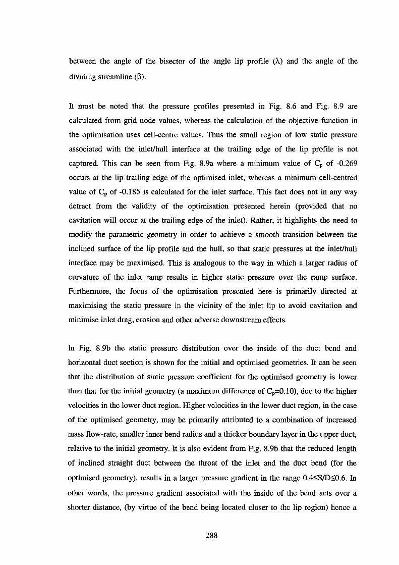
between the angle of the bisector of the angle lip profile (A) and the angle of the
dividing streamline (p).
It must be noted that the pressure profiles presented in Fig. 8.6 and Fig. 8.9 are
calculated from grid node values, whereas the calculation of the objective function in
the optimisation uses cell-centre values. Thus the small region of low static pressure
associated with the inlet/hull interface at the trailing edge of the lip profile is not
captured. This can be seen from Fig. 8.9a where a minimum value of Cp of -0.269
occurs at the lip trailing edge of the optimised inlet, whereas a minimum cell-centred
value of Cp of -0.185 is calculated for the inlet surface. This fact does not in any way
detract from the validity of the optimisation presented herein (provided that no
cavitation will occur at the trailing edge of the inlet). Rather, it highlights the need to
modify the parametric geometry in order to achieve a smooth transition between the
inclined surface of the lip profile and the hull, so that static pressures at the inlet/hull
interface may be maximised. This is analogous to the way in which a larger radius of
curvature of the inlet ramp results in higher static pressure over the ramp surface.
Furthermore, the focus of the optimisation presented here is primarily directed at
maximising the static pressure in the vicinity of the inlet lip to avoid cavitation and
minimise inlet drag, erosion and other adverse downstream effects.
In Fig. 8.9b the static pressure distribution over the inside of the duct bend and
horizontal duct section is shown for the initial and optimised geometries. It can be seen
that the distribution of static pressure coefficient for the optimised geometry is lower
than that for the initial geometry (a maximum difference of Cp=O.lO), due to the higher
velocities in the lower duct region. Higher velocities in the lower duct region, in the case
of the optimised geometry, may be primarily attributed to a combination of increased
mass flow-rate, smaller inner bend radius and a thicker boundary layer in the upper duct,
relative to the initial geometry. It is also evident from Fig. 8.9b that the reduced length
of inclined straight duct between the throat of the inlet and the duct bend (for the
optimised geometry), results in a larger pressure gradient in the range 0.4~S/D~0.6. In
other words, the pressure gradient associated with the inside of the bend acts over a
shorter distance, (by virtue of the bend being located closer to the lip region) hence a
288
larger gradient results.
The dimensions and shape of the cross-section of the inlet streamtube for the initial
geometry and the optimised geometry are shown in Fig. 8.11. The width of the cross
section of the inlet stream tube is identical for both cases, but the depth of the streamtube
is greater for the optimised geometry as a result of the greater mass flux through the
cross-section. The equal widths of the inlet streamtube for the two geometries, again
suggest that the width of the inlet streamtube is a function of the width of the inlet
opening and the boundary layer thickness (see Chapter 6). This is supported by the
results of Chapter 6 and Chapter 7.
0 0
0.00
-0.05
-0.10
-0.15
e -0.20 >.
-0.25
-0.30
-0.35
-0.40
Fig. 8.11
Geometry
--Imtla1 --Optimum
00 0
z/D
Dimensions and shape of cross-section of inlet streamtube
The improvement in static pressure distribution over the surface of the optimised
geometry does however, come at the expense of a decrease in total pressure recovery at
the duct exit and an increase in the distortion coefficient. The mass-averaged total
pressure recovery efficiency for the initial geometry is 0.676 whereas that for the
optimised geometry is 0.670. This represents a relative decrease of 0.89% and may be
attributed primarily to the effects of flow separation/near-separation within the
optimised geometry. For all intents and purposes, such a difference may be considered
to be negligible.
The distribution of total pressure coefficient over the cross-section of the duct exit is
shown in Fig. 8.12 for the initial and optimised geometries. It can be seen from the
figure that the optimised inlet exhibits a greater distortion of total pressure over the duct
289
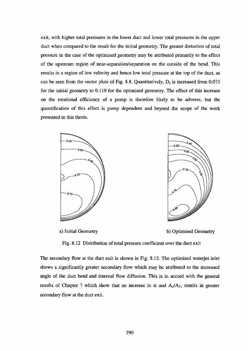
exit, with higher total pressures in the lower duct and lower total pressures in the upper
duct when compared to the result for the initial geometry. The greater distortion of total
pressure in the case of the optimised geometry may be attributed primarily to the effect
of the upstream region of near-separation/separation on the outside of the bend. This
results in a region of low velocity and hence low total pressure at the top of the duct, as
can be seen from the vector plots of Fig. 8.8. Quantitatively, De is increased from 0.073
for the initial geometry to 0.119 for the optimised geometry. The effect of this increase
on the rotational efficiency of a pump is therefore likely to be adverse, but the
quantification of this effect is pump dependent and beyond the scope of the work
presented in this thesis.
a) Initial Geometry b) Optimised Geometry
Fig. 8.12 Distribution of total pressure coefficient over the duct exit
The secondary flow at the duct exit is shown in Fig. 8.13. The optimised waterjet inlet
shows a significantly greater secondary flow which may be attributed to the increased
angle of the duct bend and internal flow diffusion. This is in accord with the general
results of Chapter 7 which show that an increase in a. and AJAT, results in greater
secondary flow at the duct exit.
290
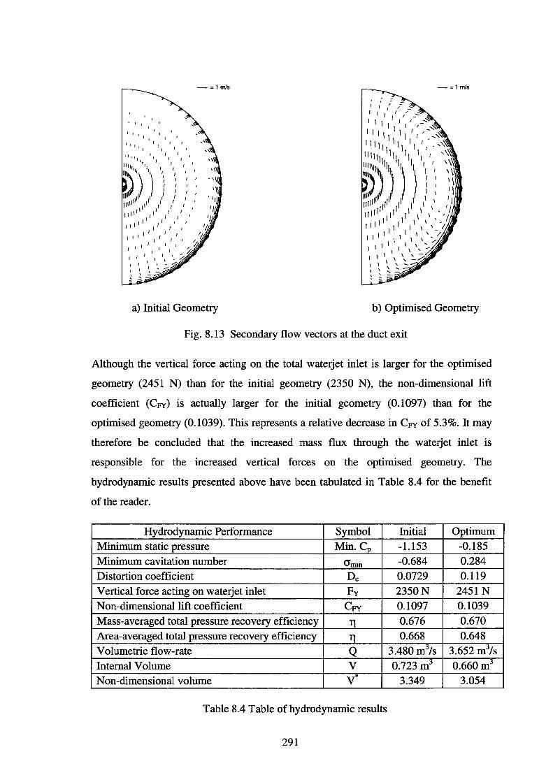
-=1rnls
' '
' '' I o
I I I
I IJI
II
'''•,, '•, ', ', IIJ,,, '•, ', ', I I
"'Dill II I I I '
)
11 1/ 1 I I
} I I I '
nut tl"' ,1 / : ; • 1/illll 11 I I '
1111 II I I ' 1111 Ill II II ' I
I I I I ' I Ill II I I /~ I I I I I I I I Jtfi
I ' ~~
/.;
I ' I o
a) Initial Geometry
-=1rnls
' :: ' : .:
I I , ,:-I I I I ,~ _.:::< I I I I I I _.:::::
I I I ' ~ I I I I -I 1 I I I / ,,'\l 1111 II II I' ... ,~
II I I -IIIII II II II I '\~
111111 1111 Ill II I I ,,~
;Y) ll': ': w ""''llrrl II II 11 I I I I "" 11 r 11 1 1 1 11 I I I I I ,II 11 II I ' /I
11 1 1 1 ' , I II I I I 1 ' I I I I I I I I I '- -/
I I I /
I 1 I 1
1 I
11 \ ':...
I I I I\~~ \ \ ' -_..,.;; ,~.::_--' - ~ ;:::;;:
b) Optimised Geometry
Fig. 8.13 Secondary flow vectors at the duct exit
Although the vertical force acting on the total waterjet inlet is larger for the optimised
geometry (2451 N) than for the initial geometry (2350 N), the non-dimensional lift
coefficient (CFY) is actually larger for the initial geometry (0.1097) than for the
optimised geometry (0.1039). This represents a relative decrease in CFY of 5.3%. It may
therefore be concluded that the increased mass flux through the waterjet inlet is
responsible for the increased vertical forces on the optimised geometry. The
hydrodynamic results presented above have been tabulated in Table 8.4 for the benefit
of the reader.
Hydrodynamic Performance Symbol Initial Optimum Minimum static pressure Min. Cp -1.153 -0.185 Minimum cavitation number O'mm -0.684 0.284 Distortion coefficient De 0.0729 0.119 Vertical force acting on waterjet inlet Fv 2350N 2451 N Non-dimensional lift coefficient CFY 0.1097 0.1039 Mass-averaged total pressure recovery efficiency T) 0.676 0.670 Area-averaged total pressure recovery efficiency T) 0.668 0.648 Volumetric flow-rate Q 3.480 m3/s 3.652 m3/s Internal Volume v 0.723 m3 0.660m3
Non-dimensional volume v* 3.349 3.054
Table 8.4 Table of hydrodynamic results
291
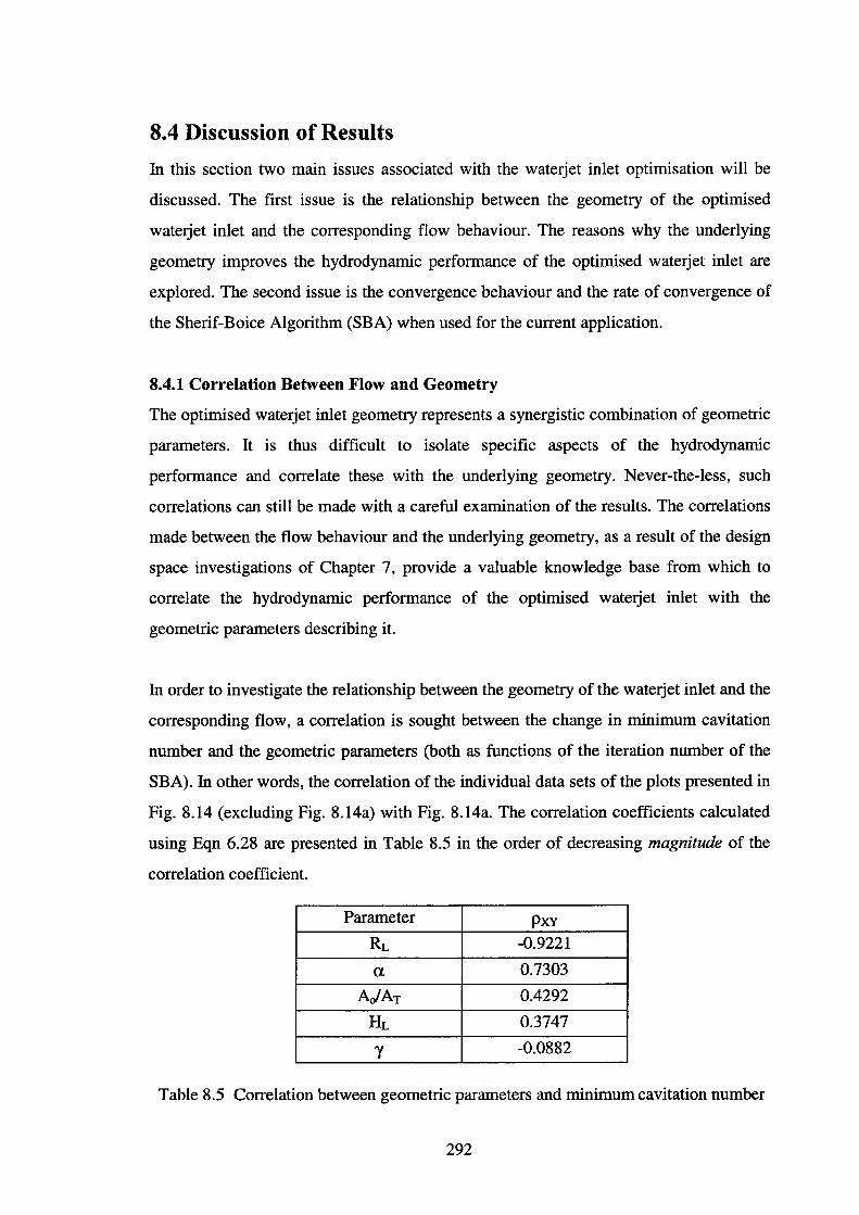
8.4 Discussion of Results
In this section two main issues associated with the waterjet inlet optimisation will be
discussed. The first issue is the relationship between the geometry of the optimised
waterjet inlet and the corresponding flow behaviour. The reasons why the underlying
geometry improves the hydrodynamic performance of the optimised waterjet inlet are
explored. The second issue is the convergence behaviour and the rate of convergence of
the Sherif-Boice Algorithm (SBA) when used for the current application.
8.4.1 Correlation Between Flow and Geometry
The optimised waterjet inlet geometry represents a synergistic combination of geometric
parameters. It is thus difficult to isolate specific aspects of the hydrodynamic
performance and correlate these with the underlying geometry. Never-the-less, such
correlations can still be made with a careful examination of the results. The correlations
made between the flow behaviour and the underlying geometry, as a result of the design
space investigations of Chapter 7, provide a valuable knowledge base from which to
correlate the hydrodynamic performance of the optimised waterjet inlet with the
geometric parameters describing it.
In order to investigate the relationship between the geometry of the waterjet inlet and the
corresponding flow, a correlation is sought between the change in minimum cavitation
number and the geometric parameters (both as functions of the iteration number of the
SBA). In other words, the correlation of the individual data sets of the plots presented in
Fig. 8.14 (excluding Fig. 8.14a) with Fig. 8.14a. The correlation coefficients calculated
using Eqn 6.28 are presented in Table 8.5 in the order of decreasing magnitude of the
correlation coefficient.
Parameter PxY RL -0.9221
a. 0.7303
AJAT 0.4292
HL 0.3747
y -0.0882
Table 8.5 Correlation between geometric parameters and minimum cavitation number
292
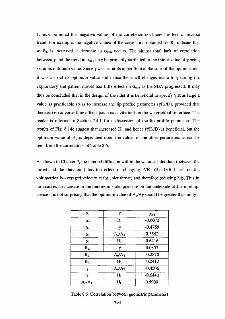
It must be noted that negative values of the correlation coefficient reflect an inverse
trend. For example, the negative values of the correlation obtained for RL indicate that
as RL is increased, a decrease in O"mm occurs. The almost total lack of correlation
between y and the trend in O"rmn may be primarily attributed to the initial value of y being
set at its optimum value. Since y was set at its upper limit at the start of the optimisation,
it was also at its optimum value and hence the small changes made to y during the
exploratory and pattern moves had little effect on O"mm as the SBA progressed. It may
thus be concluded that in the design of the inlet it is beneficial to specify y at as large a
value as practicable so as to increase the lip profile parameter (yHJD), provided that
there are no adverse flow effects (such as cavitation) on the waterjetlhull interface. The
reader is referred to Section 7.4.1 for a discussion of the lip profile parameter. The
results of Fig. 8.14e suggest that increased HL and hence (yHJD) is beneficial, but the
optimum value of HL is dependent upon the values of the other parameters as can be
seen from the correlations of Table 8.6.
As shown in Chapter 7, the internal diffusion within the waterjet inlet duct (between the
throat and the duct exit) has the effect of changing NRT (the NR based on the
volumetrically-averaged velocity at the inlet throat) and therefore reducing A.-~. This in
turn causes an increase in the minimum static pressure on the underside of the inlet lip.
Hence it is not surprising that the optimum value of A/AT should be greater than unity.
X y Pxv a RL -0.6072
a 'Y -0.4759
a A/AT 0.5562
a HL 0.6416
RL 'Y 0.0357
RL AJAT -0.2870
RL HL -0.2412
'Y AJAT -0.4506
'Y HL -0.6440
AJAT HL 0.5909
Table 8.6 Correlation between geometric parameters
293
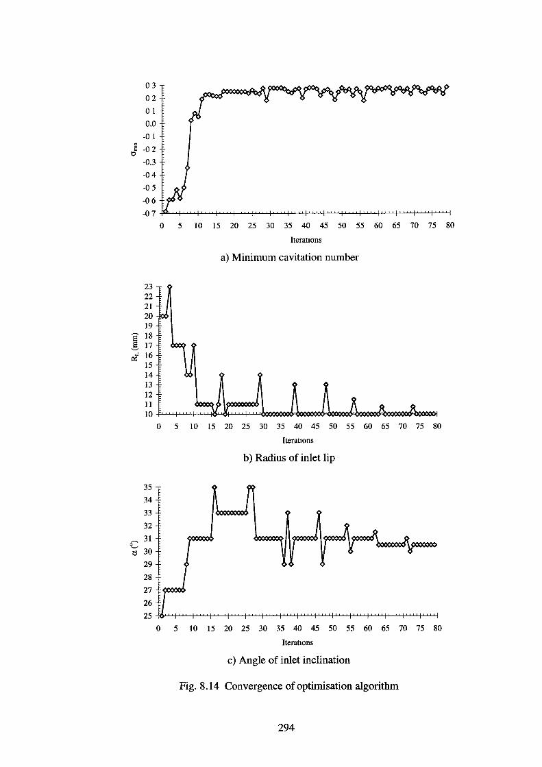
03
02
0 I
0.0
-0 I c e -0 2 t)
-0.3
-04
-0 5
-0 6
-0 7
0 5 10 15 20 25 30 35 40 45 50 55 60 65 70 75 80
Iterations
a) Minimum cavitation number
23 22 21 20 19
8 18 g 17
..J 16 ~
15 14 13 12 11 10
0 5 10 15 20 25 30 35 40 45 50 55 60 65 70 75 80
lteratmns
b) Radius of inlet lip
35
34
33
32
c 31
c::s 30
29
28
27
26
25
0 5 10 15 20 25 30 35 40 45 50 55 60 65 70 75 80
Iterations
c) Angle of inlet inclination
Fig. 8.14 Convergence of optimisation algorithm
294
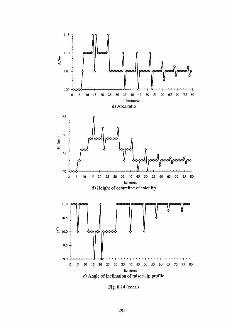
1 15
1 10
1 05
100~~~~~~~~~~~~~~~~~~~~~~~~~
0 5 10 15 20 25 30 35 40 45 50 55 60 65 70 75 80
lterattons
d) Area ratio
0 5 10 15 20 25 30 35 40 45 50 55 60 65 70 75 80
lterattons
d) Height of centreline of inlet lip
11.0
10.5
6' -;:::: 10.0
9.5
0 5 10 15 20 25 30 35 40 45 50 55 60 65 70 75 80
lterattons
e) Angle of inclination of raised-lip profile
Fig. 8.14 (cont.)
295
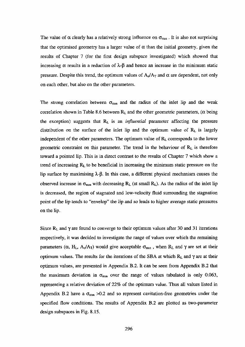
The value of a. clearly has a relatively strong influence on O'mm • It is also not surprising
that the optimised geometry has a larger value of a. than the initial geometry, given the
results of Chapter 7 (for the first design subspace investigated) which showed that
increasing a. results in a reduction of A.-13 and hence an increase in the minimum static
pressure. Despite this trend, the optimum values of AJ AT and a. are dependent, not only
on each other, but also on the other parameters.
The strong correlation between O'rrun and the radius of the inlet lip and the weak
correlation shown in Table 8.6 between RL and the other geometric parameters, (a. being
the exception) suggests that RL is an influential parameter affecting the pressure
distribution on the surface of the inlet lip and the optimum value of RL is largely
independent of the other parameters. The optimum value of RL corresponds to the lower
geometric constraint on this parameter. The trend in the behaviour of RL is therefore
toward a pointed lip. This is in direct contrast to the results of Chapter 7 which show a
trend of increasing RL to be beneficial in increasing the minimum static pressure on the
lip surface by maximising A.-j3. In this case, a different physical mechanism causes the
observed increase in O'mm with decreasing RL (at small RL). As the radius of the inlet lip
is decreased, the region of stagnated and low-velocity fluid surrounding the stagnation
point of the lip tends to "envelop" the lip and so leads to higher average static pressures
on the lip.
Since RL and yare found to converge to their optimum values after 30 and 31 iterations
respectively, it was decided to investigate the range of values over which the remaining
parameters (a., HL, A/AT) would give acceptable O'mm , when RL andy are set at their
optimum values. The results for the iterations of the SBA at which RL and y are at their
optimum values, are presented in Appendix B.2. It can be seen from Appendix B.2 that
the maximum deviation in O'mm over the range of values tabulated is only 0.063,
representing a relative deviation of 22% of the optimum value. Thus all values listed in
Appendix B.2 have a O'rrun >0.2 and so represent cavitation-free geometries under the
specified flow conditions. The results of Appendix B.2 are plotted as two-parameter
design subspaces in Fig. 8.15.
296
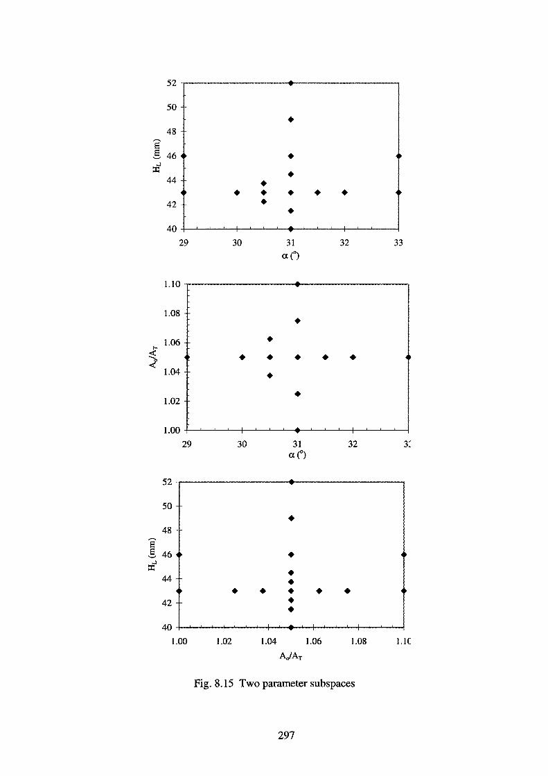
52
50
• 48
,....._ e § 46 • ...l ::r: • 44 • • • • • •
42 • • 40
29 30 31 32 33 an
1.10 ..... T
1.08 • 1.06 •
E-
~ • • • • • < 1.04 • • 1.02
1.00 ....
29 30 31 32 3: a (o)
52
50
• 48
,....._ e § 46 • =f • 44 • • • • • •
42 • • 40
1.00 1.02 1.04 1.06 1.08 1.1(
A./AT
Fig. 8.15 Two parameter subspaces
297
It can be seen from the relative location of the points in Fig. 8.15 that the following
ranges of values should give good cavitation-free performance:
1) a : 29°~a~33°
2) HL : 40mm~HL~52 mm
3) AJAT : l.OO~AJAT~l.lO
It is therefore evident that there is a certain design tolerance and flexibility that can be
made in selecting the dimensions of the waterjet inlet geometry, resulting from the use
of a lip of small RL.
8.4.2 Convergence Behaviour of the Optimisation Algorithm
The convergence behaviour of the SBA can be seen from Fig. 8.14a. The convergence
of the geometric parameters toward their optimum values is also evident from the other
plots presented in Fig. 8.14. The initial rate of convergence of the SBA is large during
the first 12 iterations, but then decreases dramatically as the geometry moves from a
region where O"mm changes rapidly, to a region where there is a much smaller variation in
O"mm with further changes in the waterjet inlet geometry. Since a and RL are well
correlated with O"mm , these two geometric parameters essentially "drive" the rapid
change of O"mm over the first 12 iterations, with the other parameters having a lesser
effect.
It is interesting to note (from Fig. 8.14) when the geometric parameters reached their
final values (excluding unsuccessful exploratory and pattern moves). The number of
iterations before the geometric parameters reached their optimum values is:
1) AJ AT : 25 iterations
2)RL : 30 iterations
3) 'Y : 31 iterations
4) HL : 42 iterations
5) a : 63 iterations
Hence the last 38 iterations are taken up primarily by exploratory moves resulting from
two reductions in step size and a final adjustment in a. Had the convergence criteria
been stricter, the number of iterations to convergence would have been increased. It is
thus evident that the selection of the minimum step-size can have a marked effect on the
298
number of iterations required before convergence is achieved. This issue has already
been briefly discussed in Section 8.1.2 for the general application of the SBA to CFD
related optimisation.
8.5 Closure
The optimisation algorithm of Sherif and Boice ( 1993) was used to maxnmse the
minimum cavitation number (Eqn 6.1) on the surface of the author's parametric waterjet
inlet geometry (Chapter 4). A waterjet inlet of 600 mm was optimised at a free-stream
velocity of 20.58 ms-1 (40 knots vessel speed) with a boundary layer of non-dimensional
thickness OID=0.8 upstream of the inlet. From the optimisation study presented in this
chapter, conclusions may be drawn regarding the design of waterjet inlets for the
avoidance of inlet cavitation and the suitability of the Sherif-Boice algorithm (SBA) as
an optimisation tool.
An analysis of the results of the optimisation study presented in this chapter provides
valuable information regarding the influence of the different aspects of the waterjet inlet
geometry on the pressure distribution on the surface of the inlet, in particular in the
vicinity of the inlet lip and ramp. Thus building on the foundational work presented in
Chapter 7, useful conclusions can be made to guide the design of waterjet inlets at the
cruise condition. The following conclusions are thus drawn from the optimisation study
presented herein:
1) The optimised waterjet inlet design represents a synergistic combination of geometric
design parameters.
2) The increase in minimum cavitation number on the surface of the inlet is driven
largely by RL, a and the lip profile and there exists a range of parameter values at
which acceptable performance can be obtained.
3) Increasing the lip profile parameter (yHr./D) favours large static pressures on the inlet
lip by virtue of a reduction in the angle (A.-P) between the angle of the bisector of the
angle of the lip profile (A.) and the angle of the dividing streamline <P) relative to A..
Decreasing RL at smaller values of RL can increase the static pressure on the inlet lip.
This is due to the fact that there is a tendency for the region of stagnated or low
velocity flow to "envelop" the lip, thus increasing overall static pressures on the lip.
299
4) A small amount of effective internal flow diffusion from the inlet throat to the duct
exit will increase the NR at the throat and hence reduce A.-~. This can be beneficial.
Alternatively an inlet with no internal flow diffusion can be run at higher NR to
achieve the same effect.
5) Although previous chapters have shown that the author's generic design offers an
improvement over conventional industrial designs, by virtue of the employment of a
circular inlet throat, if a becomes too large the flow in the inlet will begin to
separate. This will degrade the total pressure recovery efficiency and the uniformity
of flow at the duct exit. Therefore there is an effective hydrodynamic limit on a.
It is interesting to note that the conclusions drawn above relate well with the better
designs of waterjet inlet used in industry, in particular those conclusions relating to the
design of the inlet lip (RL,HL,y). Perhaps the reluctance to move to steeper inlets from
the range of a (20°-25°) typically used by industry, is due to the greater likelihood of
ramp flow separation on conventional designs. Although conventional inlet designs are
easy to fabricate, they do not offer the best resistance to ramp flow separation.
The hydrodynamic performance of the waterjet inlet is also a function of NR. Since
NR affects A.-f3 and hence the pressure distribution over the inlet lip, simply increasing
the operational NR of an existing inlet may eliminate cavitation (if it exists), improve
the margin against lip cavitation (if absent), or minimise the extent of cavitation on the
inlet lip. For conventional flush-type waterjet inlet designs, the relatively large radius of
curvature of the inlet ramp makes ramp cavitation unlikely.
It must be noted that the conclusions presented above are only applicable to the cruise
condition (NR=0.60). The manoeuvring condition (NR=oo) may give a totally different
shape of waterjet inlet, most likely having a larger radius of inlet lip. Roberts (1998)
used CFD to show that the use of an inlet lip of larger radius increased the total pressure
at the duct exit for the manoeuvring condition. The optimised waterjet inlet design with
its relatively sharp lip is likely to result in spillage at lower NR or significant internal
flow separation in the manoeuvring condition. Therefore an actual waterjet inlet must
reflect a compromise between the cruise and manoeuvring conditions, or at least give
300

adequate performance for manoeuvring. What is really required is a lip profile optimised
for both the cruise and manoeuvring conditions.
The following conclusions are made regarding the suitability of the SBA for waterjet
inlet optimisation:
1) The algorithm allows easy implementation of geometric constraints and is robust.
2) A marked improvement in minimum cavitation number is evident with only a few
iterations of the algorithm.
3) The use of the flow solution from a previous exploratory point or base point, as an
initial solution for a subsequent CFD computation, can dramatically decrease the
time required to obtain a flow solution and hence the computational effort of the
optimisation process.
4) The employment of strict convergence criteria will result in an excessive number of
iterations (and CFD computations) before convergence is finally achieved.
5) The sequential nature of the algorithm extends the time taken for the overall
optimisation process (on multi-processor machines) as CFD computations cannot be
run in parallel, as is the case for gradient-based optimisation methods. On single
processor machines this point is irrelevant.
It is therefore concluded that the optimisation algorithm of Sherif and Boice ( 1993) is an
effective tool for optimising the hydrodynamic design of waterjet inlets on a single
processor computer, provided that the number of design variables to be varied during
the optimisation process is small (eg. 5-10).
301
Chapter 9 Conclusions and Recommendations
The objective of this research was to use computational fluid dynamic (CFD) as a tool
for analysing and optimising the design of marine waterjet propulsion unit inlets, in
order to gain a greater understanding of the hydrodynamics of waterjet inlet design. CFD
has been used effectively as a tool to develop a greater understanding of how the
geometric design of a flush-type waterjet inlet affects the resultant flow. This therefore
allows possible improvements in design to be identified. The design of the inlet lip was
found to be of particular importance to the elimination of cavitation at the cruise
condition (low inlet velocity ratio).
The conclusions of this research are therefore summarised in Section 9 .1. Section 9.2
contains a list of recommendations relating to the improvement of waterjet inlet design,
as well as recommendations for future CFD investigation of waterjet inlet flows.
9.1 Conclusions
The conclusions, of the research presented in this thesis, are summarised below.
9.1.1 Parametric Model
1) A lip loss thrust deduction fraction (tL) is introduced into the equation for waterjet
thrust to account for drag on the inlet lip resulting from flow separation and
cavitation, both of which act to decrease lip suction and hence thrust.
2) Theoretically, the ingestion of fluid from an upstream hull boundary layer acts to
increase the efficiency of the waterjet. This is primarily a result of increased
propulsor thrust resulting from a lower momentum drag associated with flow into the
inlet.
302
3) The optimum jet velocity ratio (JVR) for maximum efficiency decreases with the
ingestion of fluid from a boundary layer of greater thickness.
4) Pump rotative efficiency appears to have a significant effect on overall waterjet
efficiency for a given JVR. This indicates the importance of ensuring that the quality
of the flow delivered to the waterjet pump does not have an adverse effect on pump
operation and so decrease propulsive efficiency.
9.1.2 CFD Modelling
1) Good agreement has been obtained between CFD prediction and experimental data
for the three validation cases considered, particularly when flow separation is absent
from the flow. When flow separation is present, the predictive accuracy of the flow
computations was decreased.
2) CFD computations based on the solution of the Reynolds-averaged Navier Stokes
equations, with two-equation k-E turbulence modelling, can therefore be used as an
effective analysis tool for use in the design of waterjet inlets. The limitations of the
CFD modelling, in particular the turbulence and near-wall modelling, must be
recognised and considered in the interpretation of computational results.
3) Inaccuracies in the computational results obtained for the three validation cases are
influenced by a number of factors. These include inaccuracies in the modelling of the
boundary conditions, possible discretisation error (for the case of the waterjet inlet)
and the turbulence and near-wall modelling used.
4) The use of the RNG k-E turbulence model consistently gave more accurate results
than the Standard k-E model for the three validation cases considered. This
improvement in flow prediction, obtained via use of the RNG k-E model, is primarily
attributed to the rate of strain term in the equation for E. When the flow is subject to
rapid shear and streamline curvature, the inclusion of the rate of strain term results in
smaller predicted eddy-viscosity than when using the Standard k-E model. Therefore,
the effects of streamline curvature are more accurately modelled. This results in an
303
improvement in the prediction of mean flow behaviour.
5) The limitations of the turbulence models examined and their underlying assumption
of isotropic eddy-viscosity, arising from the hypothesis of Boussinesq, become
apparent when flow separation effects are modelled. This leads to inaccuracies in
predicted mean flow quantities. The assumptions underlying the use of conventional
wall functions breakdown under strong adverse pressure gradient and flow
separation. This clearly adds further inaccuracy to the modelling of the onset of flow
separation and separated flow behaviour.
6) The topology of the structured grid used for meshing the waterjet inlet and a simple
flow domain external to it, produces a good quality of mesh in terms of minimising
the number of skewed cells in the flow domain and ensuring orthogonality of grid
lines at the wall. The use of a single-block structured mesh does, however, impose
limitations on the detail of the geometry that can be meshed. In other words, the
geometry to be meshed must be simplified and features such as the impeller shaft
housing/fairing omitted. Furthermore, extension of the flow domain to include the
vessel hull becomes difficult.
9.1.3 Design Subspace Investigation and Optimisation Methodologies
1) CFD offers the only cost-effective means by which awaterjet inlet can be optimised.
2) Systematic investigation of the hydrodynamic design of the waterjet inlet and its
optimisation require a parametric description of a generic waterjet inlet geometry.
This allows a systematic and logical variation of the geometry in order to correlate
the hydrodynamics of the flow with the underlying geometry.
3) Grid generation typically represents the "bottle-neck" in the CFD analysis cycle.
Since design and optimisation-related work require a large number of CFD
computations, it is therefore necessary to automate the mesh generation process as
much as is possible. This is necessary in order to minimise the amount of time
devoted to mesh generation.
304
4) Investigation of two-parameter subs paces of the parametric hyperspace associated
with a generic parametrically-defined waterjet inlet geometry allows useful
hydrodynamic information (relevant to that generic design) to be gathered.
Furthermore, a direct correlation between the hydrodynamics and the underlying
geometry becomes apparent, once sufficient data has been accumulated and analysed.
5) The direct-search optimisation algorithm of Sherif and Boice (1993) can be used as a
tool for the optimisation of waterjet inlet design. This is due to the algorithm's
robustness, relative efficiency and the ease by which geometric constraints (placed on
the generic parametric geometry) can be implemented. Some liberty must be taken in
the specification of the convergence criteria of this algorithm, in order to avoid an
excessive number of iterations. This algorithm is best suited for use on single
processor machines due to its sequential nature.
6) The computational expense of the large number of CFD computations required for
waterjet inlet optimisation, is partially mitigated by using previous solutions as initial
solutions for new calculations.
9.1.4 Effect of Upstream Boundary Layer
1) The thickness of the boundary layer upstream of the inlet was found to have a
significant effect on the flow in the waterjet inlet.
2) The minimum static pressure at the inlet lip increases in the presence of thicker
upstream boundary layers. This is primarily attributed to the decreased momentum of
the flow in the vicinity of the inlet lip.
3) For a given mass flux ingested by the inlet, both the width and the depth of the cross
section of the inlet streamtube increase, as a result of lower average velocities over
the streamtube cross-section.
4) There is a decrease in the total pressure of the fluid at the duct exit with increasing
upstream boundary layer thickness. This is correlated with a reduction in the ingested
305
energy flux across the cross-section of the inlet streamtube.
5) The distortion of the total pressure distribution at the duct exit is strongly dependent
on the thickness of the upstream boundary layer. Except for relatively thin upstream
boundary layers, there is a general trend toward decreasing distortion with increasing
boundary layer thickness for the author's generic waterjet inlet geometry. This result
may not necessarily apply to other geometries.
6) Accurate representation of the actual shape and dimensions of the cross-section of the
inlet streamtube is essential for accurate calculation of ingested momentum and
energy fluxes. The assumption of a rectangular or semi-elliptical profile will lead to
inaccurate calculation of these quantities.
9.1.5 Waterjet Inlet Design
The conclusions presented below are obtained from an analysis of data for waterjet
inlets simulated at an inlet velocity ratio (IVR) of 0.6 in the presence of a thick upstream
boundary layer. Therefore, care must be taken when seeking to generalise these results
to other IVR values.
1) At low IVR values (eg. IVR=0.60) the minimum static pressure occurs on the
underside of the inlet lip, with a risk of flow cavitation.
2) The minimum static pressure on the inlet lip is largely dependent upon the deviation
between the angle of the bisector of the lip profile (A) and the angle of the dividing
streamline (~), as discussed in Chapter 7. Therefore, the larger the magnitude of A.-~,
the lower the minimum static pressure on the lip will be. An objective of inlet lip
design must therefore be to minimise the magnitude of the angle of attack of the local ?
flow relative to the lip (ie. minimise A.-~).
3) The use of a raised-lip profile (where the bottom of the inlet lip is raised above the
base of the inlet opening) was found to be a beneficial design feature for increasing
the minimum static pressure on the lip, by virtue of directing the flow over the lip in
306
such a way as to decrease A-~. The minimum static pressure on the lip is found to
correlate with a lip profile parameter, yHt/D.
4) Increasing the steepness of the inlet (a) was also found to be an effective means of
reducing the magnitude of A-~ and leads to a smaller, more compact inlet. The
disadvantage of this is a greater likelihood of flow separation on the upper inlet ramp
if a becomes too large.
5) When A-~ is minimised (by virtue of a raised-lip profile), inlet lips of smaller radii
appear to be beneficial in raising the minimum static pressure on the lip. This effect
arises because the region of stagnated and low velocity fluid surrounding the
stagnation point on the lip tends to envelop the inlet lip and so leads to higher static
pressures on the lip surface. At high IVR, as in a low-speed or manoeuvring
condition, a sharper lip profile is likely to be detrimental to inlet performance leading
to flow separation within the inlet. Furthermore, at very low IVR, a sharper lip profile
is likely to lead to flow separation on the outside of the inlet lip (spillage drag). These
issues have not been explored and so no further comments can be made.
6) A moderate increase in the IVR of the inlet (for example from 0.6 to 0.8) can provide
an effective means of minimising the magnitude of A-~, thus increasing the minimum
static pressure on the lip.
7) The author's generic waterjet inlet geometry requires a smoother transition between
the inlet and hull (downstream of the lip near the centreplane) when a raised lip
profile is used, in order that this location does not become a potential source of
cavitation at high vessel speed.
8) The author's generic waterjet inlet design, which employs a circular inlet throat,
offers greater resistance to flow separation in the upper inlet than conventional inlet
designs (which use a flat curved ramp surface). The author's generic geometry,
however, is likely to be more difficult to fabricate than conventional designs by
virtue of the doubly-curved nature of the inlet surface.
307
9) A larger radius of curvature of an inlet ramp results in a higher static pressure on the
ramp surface and hence a greater resistance to flow cavitation. This is beneficial at
high vessel speed, but comes at the expense of a greater volume of the waterjet inlet.
10) The distortion of total pressure at the duct exit appears to depend on the influence of
the duct bend or internal flow diffusion (if present) acting on the boundary layer
developed upstream of the bend. In all cases examined, a region of low total pressure
occurs in the upper part of the duct at the duct exit, whereas a region of higher total
pressure occurs in the lower duct. It is therefore doubtful whether a synergistic
combination of geometric parameters can be found that can significantly reduce the
distortion of total pressure at the duct exit, within acceptable geometric limits. The
effect of these distributions on pump performance is unknown and beyond the scope
of the work presented in this thesis.
11) Partial diffusion of the flow inside the waterjet inlet, between the inlet throat and
duct exit, appears to offer no hydrodynamic advantage, except as a means of
minimising A.-p. The adverse effects of internal flow diffusion include boundary
layer thickening, flow separation (with sufficiently large internal diffusion) and
increased distortion of total pressure at the duct exit. Another adverse effect is a
stronger secondary flow within the duct, by virtue of greater cross-stream pressure
gradients associated with the duct bend.
12) The dimensions of the cross-section of the inlet streamtube were shown to be
dependent upon the width of the inlet opening, the mass flux ingested by the
waterjet inlet, as well as the thickness of the upstream boundary layer.
13) The vertical forces acting on the waterjet inlet were shown to be dependent upon the
change in the vertical momentum of the flow through the waterjet inlet, vertical
forces acting on the inlet lip (below the stagnation line), and hydrostatic forces
arising from the volume of water entrained by the waterjet inlet. The change in the
vertical momentum of flow through the waterjet inlet is related to the geometry of
the inlet streamtube which is influenced by such factors as the geometry of the inlet,
308
the ingested mass flux and the upstream boundary layer profile.
9.2 Recommendations
The recommendations for future research and waterjet inlet design, arising from the
conclusions reached as a result of the work presented in this thesis, are summarised
below.
9.2.1 CFD Modelling
1) The ability to mesh the complete geometry of the waterjet inlet, without geometric
simplifications and the omission of components (such as the impeller shaft
housing/fairing), necessitates the use of CFD techniques that solve the Reynolds
averaged Navier Stokes equations on unstructured grids. The use of unstructured grid
technology also allows the meshing of any waterjet-hull system. It is therefore
recommended that future research be directed toward the application of unstructured
CFD technology to waterjet inlet analysis, in order to include the impeller shaft
housing/fairing in the flow simulation. Furthermore, unstructured CFD technology
also offers the possibility of a complete waterjet flow simulation including the
impeller shaft housing, pump impeller, stator blades and the nozzle itself.
2) Although the RNG k-E turbulence model represents an improvement over the
Standard k-E model, there is scope for using turbulence models that offer greater
predictive accuracy for flows subject to adverse pressure gradients and turbulent flow
behaviour unrelated to mean strain rates (such as streamline curvature and separated
flow).
3) The benefits of using an automated approach to the meshing of the flow domain were
discussed as a means of reducing the CFD analysis cycle time. This is crucial when a
large number of computations are required. It is therefore recommended that future
work with unstructured grid technology be focused on automating the grid generation
process as far as is practicable, in order to obtain suitable meshes for CFD
simulation.
309
9.2.2 Waterjet Inlet Design
1) The waterjet inlet was optimised for maximum static pressure on the inlet surface at a
cruise condition corresponding to an IVR of 0.6 (Chapter 8). The performance of this
optimised waterjet inlet at the low speed/manoeuvring condition (IVR>>1) is
unknown. It is however likely that there will be significant flow separation at the inlet
lip as flow enters the inlet from underneath the lip. Satisfactory hydrodynamic
performance at this condition may give a totally different lip profile and inlet shape.
Therefore, an actual waterjet inlet must ideally reflect a compromise between the
cruise and low speed/manoeuvring condition, or at least give adequate performance
for manoeuvring. Investigation into this issue is therefore recommended.
2) A single generic lip profile was investigated. The generic profile investigated
essentially consisted of a circular lip vertically offset from the inlet opening. This
generic profile is by no means optimum and its limitations were shown. It is therefore
recommended that further research be undertaken in order to develop generic inlet lip
profiles offering improved resistance to the inception of cavitation.
3) In order to minimise the angle of attack of the local flow in the vicinity of the inlet
lip, relative to the inlet lip (ie. minimise A.-p), over a range of cruise IVR values, an
adjustable (moveable) inlet lip design could be used. An auxiliary inlet area could be
used for the low-speed manoeuvring condition (in order to minimise flow separation
at the inlet lip). Barr and Etter (1974) suggested the use of a variable-area inlet with a
movable inlet lip and ramp in order to provide satisfactory operation over a range of
IVR values. They noted that by using a moveable lip, the angle of attack of the flow
relative to the lip can be minimised thus leading to reduced lip drag and the use of
smaller lip radii.
4) In view of the conclusions reached regarding the distortion of total pressure at the
duct exit, it is the author's view that the only effective means of reducing the
distortion of the total pressure distribution at the duct exit is by mechanical means.
English (1994) suggested a freely-rotating turbine positioned on the impeller shaft
housing/fairing as a means of effecting a "homogenisation" of the velocity field
310
upstream of the pump. Seddon and Goldsmith ( 1985) discussed a similar idea for
aeronautical applications. While this idea theoretically sounds good, there are,
however, concerns about turbine cavitation. Further investigation of different
mechanical means of effecting flow homogenisation upstream of the waterjet pump
is therefore recommended.
5) The use of a circular inlet throat and a waterjet inlet shape that tends to "converge"
the flow toward the throat of the inlet should offer better resistance to flow separation
on the inlet ramp than conventional inlet designs. This was shown to be the case for
the author's generic geometry. Such an inlet design does, however, come with greater
fabrication difficulty. Since conventional inlet designs (used on large high-speed
vessels) tend to be easier to fabricate, an alternative approach for use on conventional
inlets with a curved flat ramp, would be to use a boundary layer re-energisation
technique such as tangential blowing. Burley and Hwang (1983) discussed this
approach as a means of increasing the separation-free operation of subsonic V/STOL
aircraft inlets. Griffith-Jones (1994) suggested further investigation into the potential
of this method of boundary layer control.
Therefore research into boundary layer re-energisation techniques is recommended,
as this can ultimately lead to improvements in the hydrodynamic performance of
existing designs or to steeper, more compact waterjet inlet designs.
311
References
Aartojarvi, R. (1995) "Noise from Waterjet Propulsion," Proceedings of the Third International Conference on Fast Sea Transportation (FAST'95), Ltibeck-Travemtinde, Germany, vol.2, 1157-1166.
Alexander, K. V. and van Terwisga, T. (1993) "Recent Work on Waterjet-Hull Interaction Effects," Proceedings of the 9th International High Speed Surface Craft Conforence, Singapore.
Alexander, K., Coop, H. and van Terwisga, T. (1994) "Waterjet-Hull Interaction: Recent Experimental Results," Transactions of the Society of Naval Architects and Marine Engineers (SNAME), vol. 102, 87-105.
Allison, J. L. (1993) "Marine Waterjet Propulsion," Transactions of the Society of Naval, Architects and Marine Engineers (SNAME), vol. 101,275-335.
Allison, J. L. ( 1996) "CFD Simulation Saves $100,000 in Design of New marine Landing Craft," BLA Quarterly Digest, Band, Lavis & Associates, Inc., vol. 6, Sept 1996.
Allison, J. and Dai, C. (1994) "Steering and Reversing Gear for Very Large Waterjets," Proc. RINA International Symposium on Waterjet Propulsion-Latest Developments, The Royal Institute of Naval Architects (RINA), London, 1-2 Dec, paper no. 7.
Allison, J. Land Goubault, P. (1995) "Waterjet Propulsion for Fast Craft- Optimized Integration of Hull and Propulsor," Proceedings of the Third International Conference on Fast Sea Transportation (F AST'95), Lubeck-Travemtinde, Germany, vol.2, 1117-1130.
Anderson, B. H., Reddy, D. R.and Kapoor, K. (1994) "Study on Computing Separating Flows within a Diffusing InletS-Duct," Journal of Propulsion and Power, vol. 10, no. 5, Sept-Oct 1994, 661-667.
Baldwin, B.S. and Lomax, H. (1978) 'Thin-Layer Approximation and Algebraic Model for Separated Turbulent Flows," AIAA Paper 78-257, Huntsville, AL.
Bansod, P. and Bradshaw, P. (1972) "The Flow in S-shaped Ducts," The Aeronautical Quarterly, The Royal Aeronautical Society, vol. 23, May 1972, 131-140.
Barr, R. A. and Etter, R. J. (1974) "Selection of Propulsion Systems for High Speed Advanced Marine Vehicles," AIAA, 74-334.
Boussinesq, J. (1877) "Theorie de l'Ecoulement Tourbillant," Mem. Presentes par Divers Savants A cad Sci. Inst. Fr., vol. 23, 46-50.
312
Bradshaw, P. (1967) "The Turbulence Structure of Equilibrium Boundary Layers," J Fluid Mechanics, vol. 29, part 4, 625-645.
Bradshaw, P. (1973) "Effect of Streamline Curvature on Turbulent Flow", AGARD-AG-169.
Brandau, J. H. ( 1967) "Aspects of Performance Evaluation of Waterjet Propulsion Systems and a Critical Review of the State-of-the-Art," AIAAISNAME Advance Marine Vehicle Meeting, Norfolk, Virginia, May 22-24.
Breslin, J. P. (1970) "Theoretical and Experimental Techniques for Practical Estimation of Propeller-Induced Vibratory Forces," Transactions of the Society of Naval Architects and Marine Engineers (SNAME), vol. 78,23-40.
Brilliant, H. M. and Bauer, C. A. (1977) "Comparison of Estimated with Measured Maximum Instantaneous Distortion using Flight Data from an Axisymmetric Mixed Compression Inlet," AIAA 77-876.
Burley, R. R. and Hwang, D.P. (1983) "Investigation of Tangential Blowing Applied to a Subsonic V/STOL Inlet,", J of Aircraft, vol. 20, no. 11, Nov. 1983, 926-934.
Cebeci T. and Smith, A.M. 0. (1974) "Analysis of Turbulent Boundary Layers," Ser. in Appl. Math. & Mech., vol. XV. New York: Academic Press.
Chambers, T. L. and Wilcox, D. C. (1977) "Critical Examination of Two-Equation Turbulence Closure Models for Boundary Layers," AIAA Journal, vol. 15, no. 6, 821-828.
Coles, D. E. and Hirst, E. A. (1968) Computation ofTurbulent Boundary Layers- 1968 AFOSR-IFP-Stanford Conference. Vol. 11 California: Stanford University.
Coop, H. G. and Bowen, A. J. (1993) "Hull-Waterjet Interaction Mechanisms: Theory and Validation," Proceedings of the 2nd International Conference on Fast Sea Transportation (FAST'93), Yokohama, Japan, vol.1, 855-866.
Dai, C., Kerr, C., Nguyen, P. and Wang, H. C. (1995), "A Novel Flush Inlet Design Design Methodology for Waterjet Propulsion," Proceedings of the Third International Conference on Fast Sea Transportation (FAST'95), Ltibeck-Travemtinde, Germany, vol.2, 1367-1378.
Doragh, R. A. (1963) "Magnetohydrodynamic Ship Propulsion using Superconducting Magnets," Transactions of the Society of Naval Architects and Marine Engineers (SNAME), vol. 71, 370-386.
Doss, E. D. and Geyer, H. K. (1993) "MHD Seawater Propulsion," Journal of Ship Research, vol. 37, no. 1, Mar 1993, 49-57.
Driver, D. M. (1991) "Reynolds Shear Stress Measurements in a Separated Boundary Layer," A.IAA-91-1787.
313
Driver, D. M. and Seegmiller, H. L. (1985) "Features of a Reattaching Turbulent Shear Layer in Divergent Channel Flow," AIAA Journal, vol. 23, no. 2, Feb 1985, 163-171.
Dubbel- Taschenbuch fur den Maschinenbau (1990), edited by W. Beitz and K.-H. KUttner, 17 Edition. Berlin: Springer-Verlag.
Dyne, G. and Lindell, P. (1994) "Waterjet Testing in the SSPA Towing Tank," Proc. RINA International Symposium on Waterjet Propulsion - Latest Developments, The Royal Institute of Naval Architects (RINA), London, 1-2 Dec, 1994, paper no. 2.
Enayet, M. M., Gibson, M. M., Taylor, A.M. K. P. and Yianneskis, M. (1982) "LaserDoppler Measurements of Laminar and Turbulent Flow in a Pipe Bend," International Journal of Heat and Fluid Flow, vol. 3, no. 4, Sept. 1982, 213-219.
English, J. W. (1974) "Hydrodynamic Considerations in the Design of Condenser Cooling Water Systems for Large Ships," Trans. RINA, vol. 116, 31-46.
English, J. W. (1994) "Practical Considerations on Waterjet Inlets with Flush Intakes," Proc. RINA International Symposium on Waterjet Propulsion -Latest Developments, The Royal Institute of Naval Architects (RINA), London, 1-2 Dec, 1994, paper no. 11.
Eriksson, L. E. (1982) "Generation of Boundary-Conforming Grids around Wing-Body Configurations using Transfinite Interploation," AIAA Journal, vol. 20, no. 10, Oct 1985, 1313-1320.
Eriksson, L. E. (1985) "Practical Three-Dimensional Mesh Generation using Transfinite Interpolation," SIAM J. Sci. Stat. Comput., Society for Industrial and Applied Mathematics (SIAM), vol. 6, no. 3, July 1985,712-741.
Eriksson, L. E. and Orbekk, E. ( 1989) "Application of Mesh Generation to Complex 3-D Configurations," AGARD CP 464.
Etter, R. J., Krishnamoorthy, V. and Scherer, J. 0. (1982) "Model Testing of Waterjet Propelled Craft," Proceedings of the 19th American Towing Tank Committee (ATTC), 783-806.
Fletcher, C. A. J. (1987a) Computational Techniques for Fluid Dynamics. Vol. 1. Berlin: Springer Verlag.
Fletcher, C. A. J. (1987b) Computational Techniques for Fluid Dynamics. Vol. 2. Berlin: Springer Verlag.
Fluent Inc. (1996) Fluent V4.4 Users Guide. Lebanon, New Hampshire: Fluent Inc.
F~rde, M., 0rbekk, E. and Kubberud, N. (1991) "Computational Fluid Dynamics Applied to High Speed Craft with Special Attention to Water Intake for Water Jets," Proceedings of the 1st International Conference on Fast Sea Transportation (FAST'91), Trondheim, Norway, vol.1, 69-89.
314
Frank, P. D. and Shubin, G. R. (1992) "A Comparison of Optimization-Based Approaches for a Model Computational Aerodynamics Design Problem,", Journal of Computational Physics, vol. 98, 74-89.
Gallin, C. M., Phipps, J. H., Stevenson, J. and van Terwisga, T. (1995) "Technically and Economically Optimized Fast Ships Propulsion Systems from 18000 to 30000 kW," Proceedings of the Third International Conference on Fast Sea Transportation (FAST'95), Liibeck-Travemiinde, Germany, vol.2, 725-753.
Gany, A. (1993) "The Bubbly Waterjet - a Promising High Speed Marine Propulsion Concept," Proceedings- The Ninth High Speed Surface Craft Conference, 9-11 Mar. High Speed Surface Craft Associates.
Gerhart, P. M. and Gross, R. J. (1985) Fundamentals of Fluid Dynamics. Reading, Massachusetts: Addison-Wesley.
Gill, P. E., Murray, W. and Wright, M. H. (1981) Practical Optimization. New York: Academic Press.
Gillis, J. C. and Johnston, J. P. (1983) "Turbulent Boundary-Layer Flow and Structure on a Convex Wall and its Redevelopment on a Flat Wall," Journal of Fluid Mechanics, vol. 135, 123-153.
Gordon, W. J. and Hall, C. A. (1973) "Construction of Curvilinear Co-ordinate Systems and Applications to Mesh Generation," International Journal for Numerical Methods in Engineering, vol. 7, 461-477.
Gottfried, B. S. and Weisman, J. (1973) Introduction to Optimization Theory. Englewood Cliffs, New Jersey: Prentice-Hall.
Griffith-Jones, G. J. (1994) Investigation of Incompressible Flow through an Intake Duct with Applications to Waterjet Propulsion. Christchurch, New Zealand: University of Canterbury, Dept. of Mechanical Engineering.
Guo, R. W. and Seddon, J. (1982) "An Investigation of the Swirl in an S-Duct," Aeronautical Quarterly, Feb 1982, 25-58.
Guo, R. W. and Seddon, J. (1983a) "The Swirl in an S-duct of Typical Air Intake Proportions," Aeronautical Quaterly, Royal Aeronautical Society, vol. 34, part 2, May 1983, 99-129.
Guo, R. W. and Seddon, J. (1983b) "Swirl Characteristics of an S-shaped Air Intake with Horizontal and Vertical Offsets," Aeronautical Quaterly, Royal Aeronautical Society, vol. 34, part 2, May 1983, 130-146.
Haglund, K., Svensson, R. and Bjorheden, 0. (1982) "Design and Testing of a HighPerformance Water Jet Propulsion," Proceedings of the Second Symposium on Small Fast Warships and Security Vessels, The Royal Institute of Naval Architects, paper 17, May 1982, 223-237.
315
Hanjalic, K. and Launder, B. E. (1980) "Sensitizing the Dissipation Equation to Irrotational Strains," Transactions of the ASME, Journal of Fluids Engineering, vol. 102, Mar 1980, 34-40.
Harloff, G. J., Smith, C. F., Bruns, J. E. and DeBonis, J. R. (1993) "Navier-Stokes Analysis of Three-Dimensional S-Ducts," Journal of Aircraft, vol. 30, no. 4, Jul-Aug. 1993, 526-533.
Ratte, R. and Davis, H. J. ( 1967) "Selection of Hydrofoil Waterjet Propulsion Systems," Journal ofHydronautics, vol. 1, no. 1, 12-22.
Hess, J. L. and Smith, A.M. 0. (1964) "Calculation ofNonlifting Potential Flow about Arbitrary Three-Dimensional Bodies," Journal ofShip Research., vol. 8, no. 2, 22-44.
Hewins, E. F. and Reilly, J. R. (1940) "Condensor Scoop Design," Transactions ofthe Society of Naval Architects and Marine Engineers (SNAME), vol. 48,277-304.
Hinze, J. 0. (1975) Turbulence. Second Edition. New York: McGraw-Hill.
Hooke, R. and Jeeves, T. A. (1961) "Direct Search Solution of Numerical and Statistical Problems," Journal of the Association/or Computing Machinery, vol. 8, no. 2, 212-229.
Hoshino, T. and Baba, E. (1984) "Self-propulsion Test of a Semi-Displacement Craft Model with a Waterjet Propulsor," Journal ofthe Society of Naval Architects of Japan, vol.155, 50-57.
Hutchinson, B. R. and Raithby, G. D. (1986) "A Multigrid Method Based on the Additive Correction Strategy," Numerical Heat Transfer, vol. 9, 511-537.
ITTC (1987) "Report of the High-Speed Marine Vehicle Committee - Waterjet Test Procedures," International Towing Tank Confernece 1987, 275-313.
Jameson, A. (1995) "Optimum Aerodynamic Design Using Control Theory," Department of Mechancial and Aerospace Engineering, Princeton University, Princeton, New Jersey.
Jenkins, R. C. and Loeffler, A. L. (1991) "Modelling of Subsonic Flow Through a Compact Offset Inlet Diffuser," AIAA Journal, vol. 29, no. 3, Mar 1993,401-408.
Jones, W. P. and Launder, B. E. (1972) "The Prediction of Laminarization with a TwoEquation Model of Turbulence," International Journal of Heat and Mass Transfer, vol. 15, 301-314.
Kashiwadani, T. (1985) "The Study on the Configuration ofWaterjet Inlet (1st Report)," Journal of the Society of Naval Architects of Japan, vol. 157, 121-140.
Kashiwadani, T. (1986) "The Study on the Configuration of Waterjet Inlet (2nd Report)," vol. 159, 118-128.
316

Kashiwadani, T. (1997) "On the Design Method of Waterjet Inlet for SES 'Meguro 2' ," Proceedings of the Fourth International Conference on Fast Sea Transportation (FAST'97), Sydney, Australia, vol.2, 677-684.
Kitchen, R. A. and Sedlock, D. (1983) "Subsonic Diffuser Development of Advanced Tactical Aircraft," AIAA-83-1168.
Lakshminarayana, B. (1986) "Turbulence Modeling for Complex Shear Flows," AIAA Journal, vol. 24, no. 2, 1900-1917.
Launder, B. E. and Spalding, D. B. (1974) "The Numerical Computation of Turbulent Flows," Computer Methods in Applied Mechanics and Engineering, vol. 3, 269-289.
Launder, B. E., Priddin, C. H. and Sharma, B. I. (1977) "The Calculation of Turbulent Boundary Layers on Spinning and Curved Surfaces," Transactions of ASME, Journal of Fluids Engineering, vol. 99, Mar 1977,231-239.
Leonard, B. P. (1979) "A Stable and Accurate Convective Modelling Procedure Based on Quadratic Upstream Interpolation," Computer Methods in Applied Mechanics and Engineering, vol. 19, 59-98.
Leschziner, M.A. and Rodi, W. (1981) "Calculation of Annular and Twin Parallel Jets using Various Discretisation Schemes and Turbulence-Model Variations," Tansactions of ASME, Journal of Fluids Engineering, vol. 103, Jun 1981, 352-360.
Levy, J. (1965) "The Design of Water-Jet Propulsion Systems for Hydrofoil Craft," Marine Technology, vol. 2, Jan 1965, 15-25,41.
Lewis, F. M. (1963) "Propeller Vibratory Forces," Transactions of the Society of Naval, Architects and Marine Engineers (SNAME), vol. 71,293-326.
Little, B. H. and Trimboli, W. S. (1982) "An Experimental Investigation of S-Duct Diffusers for High-Speed Prop Fans," AIAA-82-1123.
Liu, D. C. and Nocedal, J. (1989) "On the Limited Memory BFGS Method for Large Scale Optimization," Mathematical Programming, vol. 45, no. 3, 503-528.
Melick, H. C., Ybarra, A. H. and Bencze, D. P. (1975) "Estimating Maximum Instantaneous Distortion from Inlet Total Pressure RMS and PSD Measurements," AIAA 75-1213.
Melick, H. C., Ybarra, A. H. and Bencze, D. P. (1978) "Estimating Maximum Instantaneous Distortion from Inlet Total Pressure RMS Measurements," AIAA 78-970.
Mortenson, M. E. (1985) Geometric Modelling. New York: John Wiley & Sons Inc.
Motora, S., Takezawa, S. and Tamama, H. (1991) "Research and Development of Superconducting Magnetohydrodynamic Ship Propulsion," !MAS 91 High Speed Marine Transportation, 11-13 Nov 1991, Paper 6, 49-58.
317
Mount, J. S. (1965) "Effect of Inlet Additive Drag on Aircraft Performance," Journal of Aircraft, American Institute of Aeronautics and Astronautics, vol. 2, no. 5, May 1965, 374-378.
Naser, J. A. (1990) Flow Prediction in Valve/Port Assemblies, PhD Thesis, Dept. of Mechanical Engineering, Imperial College of Science, Technology and Medicine, The University of London.
Okamoto, Y., Sugioka, H. and Kitamura, Y. (1993) "On the Pressure Distribution of a Water Jet Intake Duct in Self Propulsion Conditions," Proceedings of the 2nd International Conference on Fast Sea Transportation (FAST'93), Yokohama Japan, vol.1, 843-854.
Owen, P. M. (1962) "The Prospects for Magnetohydrodynamic Ship Propulsion," Journal of Ship Research, vol. 5, no. 4, Mar 1962,43-51.
Patankar, S. V. (1980) Numerical Heat Transfer and Fluid Flow. New York: Hemisphere.
Patankar, S. V. and Spalding, D. B. (1972) "A Calculation Procedure for Heat, Mass and Momentum Transfer in Three-Dimensional Parabolic Flows," International Journal of Heat and Mass Transfer, vol. 15, 1787-1806.
Purnell J. G. (1976) "The Performance Gains of using Wide, Flush Boundary Layer Inlets on Water-Jet Propelled Craft," Research and Development Report (Report PAS-75-45), Propulsion and Auxiliary Systems Department, David W. Taylor Naval Ship Research and Development Center, Annapolis.
Roache, P. J. (1976) Computational Fluid Dynamics. Albuquerque, New Mexico: Hermosa Publishers.
Roberts, J. L. (1998), The Influence of Hull Boundary Layers on Waterjet Intake Performance, PhD Thesis to be submitted in 1998. Department of Civil and Mechanical Engineering, The University of Tasmania.
Rodi, W. and Scheuerer, G. (1986) "Scrutinizing the k-E Turbulence Model under Adverse Pressure Gradient Conditions," Transactions of ASME, Journal of Fluids Engineering, vol. 108, Jun 1986, 174-179.
Rowe, M. ( 1970) "Measurements and Computations of Flow in Pipe Bends," J Fluid Mechanics, vol. 43, part 4, 771-783.
Roy, S. M. (1994) "The Evolution of the Modem Waterjet Marine Propulsion Unit," Proc. RINA International Symposium on Waterjet Propulsion -Latest Developments, The Royal Institute of Naval Architects (RINA), London, 1-2 Dec, paper no.1.
Schlichting, H. (1979) Boundary Layer Theory. Seventh Edition. New York: McGrawHill.
318
Schultz, W. B. (1974a) "Boeing Jetfoil Progress Report," International Hydrofoil Society, 291-299.
Schultz, W. B. (1974b) "Key Problems Associated with Developing the Boeing Model 929-100 Commercial Passenger Jetfoil," International Hydrofoil Society, 301-306.
Seddon, J. (1984) "Understanding and Countering the Swirl in S-ducts: Tests on the Sensitivity of Swirl to Fences," Aeronautical Journal, Royal Aeronautical Society, vol. 88, no. 874, Apr 1984, 117-127.
Seddon, J. and Goldsmith E. L. (1985) Intake Aerodynamics. London: Collins Professional and Technical Books.
Seil, G. J., Fletcher, C. A. J. and Doctors, L. J. (1995) "The Application of Computational Fluid Dynamics to Practical Waterjet Propulsion System Design and Analysis," Proceedings of the Third International Conference on Fast Sea Transportation (FAST'95), Liibeck-Travemiinde, Germany, vol.2, 1379-1390.
Seil, G. J., Fletcher, C. A. J., and Doctors, L. J. (1997) "Optimisation of Waterjet Inlets using Computational Fluid Dynamics," Proceedings of the Fourth International Conference on Fast Sea Transportation (FAST'97), Sydney, Australia, vol.1, 59-64.
Sherif, Y. S. and Boice, B. A. (1993) "An Efficient Algorithm for Solving the Unconstrained Nonlinear Multivariable Minimization Problems," Advances in Engineering Software, vol. 17, 29-37.
Smith, R. E. (1982) "Algebraic Grid Generation," Numerical Grid Generation editied by J. Thompson, 137-170.
Sorenson, R. L. (1982) "Grid Generation by Elliptic Partial Differential Equations for a Tri-Element Augmentor-Wing Airfoil," Numerical Grid Generation edited by J. Thompson, 653-665.
Spalding, D. B. (1961) "A Single Formula for 'the Law of the Wall'," Journal of Applied Mechanics, vol. 28, Sept 1961,455-457.
Squire, H. B. and Winter, K. G. (1951) "The Secondary Flow in a Cascade of Airfoils in a Nonuniform Stream," Journal of the Aeronautical Sciences, Apr 1951, 271-277.
Steen, S. and Minsaas, K. J. (1995) "Experiences from Design and Testing of Waterjet Inlets for High Speed Craft," Proceedings of the Third International Conference on Fast Sea Transportation (FAST'95), Liibeck-Travemiinde, Germany, vol.2, 1255-1270.
Svensson, R. (1987) "Water Jets- Propulsion for Naval Vessels,", Navy International, Jul/Aug 1987,411-417.
Svensson, R. (1991) "A Description of the Water Jets Selected for Destriero," Proceedings ofthe 1st International Conference on Fast Sea Transportation (FAST'91), Trondheim, Norway, vol.2, 1169-1184.
319
Svensson, R. (1993) "Experience from Operation of Large Water Jet Units," Proceedings of the 2nd International Conference on Fast Sea Transportation (FAST'93), Yokohama, Japan, vol.2, 1409-1421.
Svensson, R. (1994) "Water Jet Propulsion of High-Speed Passenger Vessels," Shipbuilding Technology International '94, edited by R. Burnett, London, Sterling Publications Limited, 155-160.
Swallom, D. W., Sadovnik, I., Gibbs, J, Gurol, H, Nguyen, L. V. and van den Bergh, H. H. (1991) "Magnetohydrodynamic Submarine Propulsion Systems," Naval Engineers Journal, The Society of Naval Engineers, vol. 103, no. 3, May 1991, 141-157.
Taylor, A.M. K. P., Whitelaw, J. H. and Yianneskis, M. (1982a) "Curved Ducts with Strong Secondary Motion: Velocity Measurements of Developing Laminar and Turbulent Flow," Trans. ASME, Journal of Fluids Engineering, vol. 104, Sept 1982, 350-359.
Taylor, A.M. K. P., Whitelaw, J. H. and Yianneskis, M. (1982b) "Developing Flow in S-Shaped Ducts I- Square Cross-Section Duct," NASA CR 3550.
Taylor, A.M. K. P., Whitelaw, J. H. and Yianneskis, M. (1984) "Developing Flow inSShaped Ducts II- Circular Cross-Section Duct,", NASA CR 3759.
Tennekes, H. and Lumley, J. L. (1972) A First Course in Turbulence. Massachusetts: MIT Press.
Thomas, P. D. (1982) "Numerical Generation of Composite Three Dimensional Grids by Quasilinear Elliptic Systems," Numerical Grid Generation edited by J. Thompson, 667-686.
Thompson, J. F., Warsi, Z. U. A. and Mastin, W. C. (1985) Numerical Grid Generation -Foundations and Applications. New York: Elsevier.
Tomeman, G. (1994) "The Importance of High Manoeuvrability for Efficient Operation", Proc. RINA International Symposium on Waterjet Propulsion - Latest Developments, The Royal Institute of Naval Architects (RINA), London, 1-2 Dec., 1994, paper no. 13.
Towne, C. E. (1984) "Computation of Viscous Flow in Curved Ducts and Comparison with Experimental Data," AIAA-84-053I.
Trillo, R. L. (1994) Jane's High-Speed Marine Craft 1993-94. Twenty-Sixth edition. Surrey, Coulsdon: Jane's Information Group.
Tsakonas, S., Breslin, J. and Miller M. (1967) "Correlation and Application of an Unsteady Flow Theory for Propeller Forces," Transactions of the Society of Naval, Architects and Marine Engineers (SNAME), vol. 75 158-193.
320
Vakili, A., Wu, J. M., Hingst, W. R. and Towne, C. E. (1984) "Comparison of Experimental and Computational Flow in aS-Duct," AIAA-84-0033.
Van Terwisga, T. (1996) Waterjet-Hu/1 Interaction, PhD Thesis, Technical University of Delft.
Venturini, G. (1980) "Waterjet Propulsion in High Speed Surface Craft," High-Speed Surface Craft Confernece, Sussex, UK, June 24-27, 1980, 125-142.
Verbeek, R. (1992) "Application of Waterjets in High-Speed Craft," Hydrodynamics: Computations, Model Tests and Reality. Elsevier Science Publishers B.V. 1992, 133-138.
Vinokur, M. (1983) "On One-Dimensional Stretching Functions for Finite-Difference Calculations," Journal ofComputational Physics, vol. 50, 215-234.
Voulon, S. and Wesselink, A. F. (1995) "Manoeuvrability of Waterjet-Propulsed Passenger Ferries," Proceedings of the Third International Conference on Fast Sea Transportation (FAST'95), Liibeck-Travemiinde, Germany, vol.2, 1131-1156.
Wald, Q. R. (1970) "Analysis of the Integral Pumpjet," Journal of Ship Research, vol. 14, Dec 1970, 307-316.
Ward-Smith, A. J. (1963) "The Flow and Pressure Losses in Smooth Pipe Bends of Constant Cross Section," Journal ofthe Royal Aeronautical Society, vol. 67, Jul 1963, 437-450.
Wellborn, S. R., Reichert, B. A. and Okiishi, T. H. (1994) "Study of the Compressible Flow in a Diffusing S-Duct," Journal of Propulsion and Power, vol. 10, no. 5, Sept-Oct 1994, 668-675.
White, F. M. (1991) Viscous Fluid Flow. Second edition. New York: McGraw-Hill.
Whitelaw, J. H. and Yu, S. C. M. (1993) "Velocity Measurements in an S-Shaped Diffusing Duct," Experiments in Fluids, vol. 15, 364-367.
Widmark, C. and Gustafsson, L. T. (1997) "3-Dimensional CFD Calculations on a Complete Watetjet Unit," Proc. RINA International Conference Power, Performance & Operability ofSma/1 Craft, The Royal Institute of Naval Architects (RINA), 15-16 Sept 1997, Southamton, paper no. 5.
Wieghardt, K. (1972) "Viscous Resistance," Resistance Session, International Towing Tank Conference, edited by S. Schuster and M. Scmiechen, vol. 1, 83-95, Berlin.
Wilcox, D. C. (1993) Turbulence Modelling for CFD. La Caiiada, California: DCW Industries, Inc.
Wilcox, D. C. and Sharma, T. L. (1977) "Streamline Curvature Effects on Turbulent Boundary Layers," AIAA Journal, vol. 15, no. 4, Apr 1977, 574-580.
321
Y akhot, V. and Orszag, S. A. ( 1986) "Renormalization Group Analysis of Turbulence," Journal ofScientific Computing, vol. 1, no. 1, 3-51.
Yakhot, V., Orszag, S. A., Thangam, S., Gatski, T.B. and Speziale, C. G. (1992) "Development of Turbulence Models for Shear Flows by a Double Expansion Technique," Phys. Fluids A, vol. 4, no. 7, 1510-1520.
Yang, C. K., Lee, Y. B. and Choi, H. S. (1995) "A Numerical Analysis of the Flow Around the Waterjet Inlet," Proceedings ofthe Third International Conference on Fast Sea Transportation (FAST'95), Liibeck-Travemiinde, Germany, vol. 2, 1391-1401.
Youngs, J. (1994) "The Jet Age," Popular Mechanics, Feb 1994.
Zhao, Y. (1997) "Computational Modelling of 3D Compressible Flows with a LRN k-E Turbulence Model," Computational Fluid Dynamics Journal, vol. 5, no. 4, Jan 1997, 487-508.
322
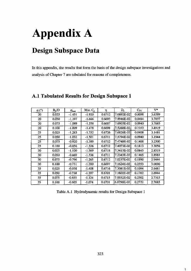
Appendix A Design Subspace Data
In this appendix, the results that form the basis of the design subspace investigations and
analysis of Chapter 7 are tabulated for reasons of completeness.
A.l Tabulated Results for Design Subspace 1
(X (0) RJD O"mm Mm.Cp TJ De CFY V* 20 0.025 -1.451 -1.920 0.6712 7.6892E-02 0.0098 3.6389
20 0.050 -1.197 -1.666 0.6693 7.8946E-02 0.0484 3.7037
20 0.075 -1.089 -1.558 0.6687 7.6903E-02 0.0940 3.7685
20 0.100 -1.009 -1.478 0.6698 7.5260E-02 0.1353 3.8519
25 0.025 -1.283 -1.752 0.6726 7.6826E-02 0.0408 3.1481
25 0.050 -1.032 -1.501 0.6711 7.5794E-02 0.0940 3.1944
25 0.075 -0.920 -1.389 0.6712 7.4748E-02 0.1408 3.2500
25 0.100 -0.856 -1.326 0.6712 7.4073E-02 0.1813 3.3056
30 0.025 -1.100 -1.569 0.6718 7.3413E-02 0.0845 2.8519
30 0.050 -0.869 -1.338 0.6711 7.2343E-02 0.1465 2.8981
30 0.075 -0.796 -1.265 0.6712 7.0237E-02 0.1890 2.9444
30 0.100 -0.731 -1.200 0.6697 7.1624E-02 0.2353 3.0000
35 0.025 -0.938 -1.408 0.6716 7.3081E-02 0.1094 2.6481
35 0.050 -0.738 -1.207 0.6701 7.3802E-02 0.1762 2.6944
35 0.075 -0.655 -1.124 0.6715 7.0552E-02 0.2302 2.7315
35 0.100 -0.605 -1.074 0.6701 6.8790E-02 0.2722 2.7685
Table A. I Hydrodynamic results for Design Subspace 1
323
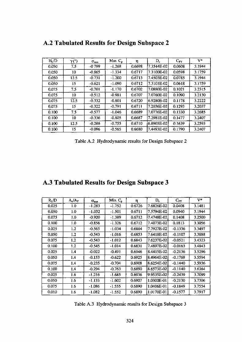
A.2 Tabulated Results for Design Subspace 2
HJD y(o) O"mm Mm Cp 11 De CFY V* 0.050 7.5 -0799 -1.268 0.6698 7.3544E-02 0.0608 3.1944
0.050 10 -0.865 -1.334 0.6717 7.3100E-02 0.0598 3.1759
0.050 12.5 -0.731 -1.200 0.6713 7.4503E-02 0.0785 3.1944
0.050 15 -0.621 -1.090 0.6712 7.3101E-02 0.0618 3.1759
0.075 7.5 -0.701 -1.170 0.6702 7.0880E-02 0.1021 3.2315
0.075 10 -0.512 -0.981 0.6707 7.0760E-02 0.1090 3.2130
0.075 12.5 -0.332 -0.801 0.6720 6.9280E-02 0.1178 3.2222
0.075 15 -0.322 -0.791 0.6711 7.2036E-02 0.1293 3.2037
0.100 7.5 -0.577 -1.046 0.6689 7.0776E-02 0.1330 3.2685
0.100 10 -0.336 -0.805 0.6687 7.2981E-02 0.1477 3.2407
0.100 12.5 -0.286 -0.755 0.6710 6.8903E-02 0.1639 3.2593
0.100 15 -0.096 -0.565 0.6680 7.4493E-02 0.1790 3.2407
Table A.2 Hydrodynamic results for Design Subspace 2
A.3 Tabulated Results for Design Subspace 3
RdD AJAT O"mm Min. Cp 11 De CFY V* 0.025 1.0 -1.283 -1.752 0.6726 7.6826E-02 0.0408 3.1481
0.050 1.0 -1.032 -1.501 0.6711 7.5794E-02 0.0940 3.1944
0.075 1.0 -0.920 -1.389 0.6712 7.4748E-02 0.1408 3.2500
0.100 1.0 -0.856 -1.326 0.6712 7.4073E-02 0.1813 3.3056
0.025 1.2 -0.565 -1.034 0.6864 7.7927E-02 -0.1336 3.3497
0.050 1.2 -0.543 -1.016 0.6853 7.6418E-02 -0.1107 3.3888
0.075 1.2 -0.543 -1.012 0.6843 7.6237E-02 -0.0521 3.4323
0.100 1.2 -0.545 -1.014 0.6831 7.4897E-02 -0.0163 3.4843
0.025 1.4 -0.022 -0.491 0.6946 8.4415E-02 -0.2136 3.5296
0.050 1.4 -0.153 -0.622 0.6925 8.4964E-02 -0.1769 3.5594
0.075 1.4 -0.235 -0.704 0.6908 8.6254E-02 -0.1440 3.5936
0.100 1.4 -0.294 -0.763 0.6890 8.6573E-02 -0.1140 3.6364
0.025 1.6 -1.216 -1.685 0.6936 9.9535E-02 -0.2439 3.7099
0.050 1.6 -1.133 -1.602 0.6907 1.0300E-01 -0.2130 3.7306
0.075 1.6 -1.086 -1.555 0.6890 1.0406E-01 -0.1849 3.7554
0.010 1.6 -1.082 -1.552 0.6890 1.0170E-01 -0.1577 3.7917
Table A.3 Hydrodynamic results for Design Subspace 3
324
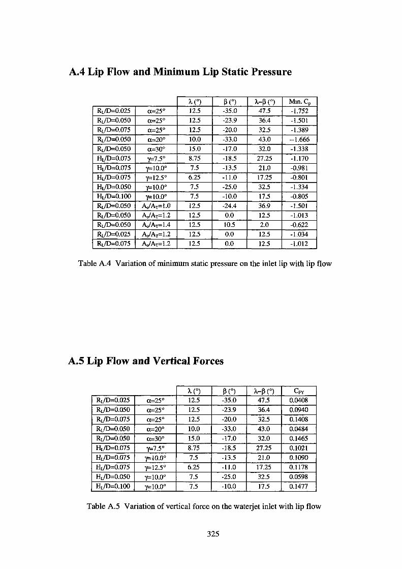
A.4 Lip Flow and Minimum Lip Static Pressure
A (o) ~ (0) A-~ (o) Mm.CP
RV0=0.025 a=25° 12.5 -35.0 47.5 -1.752
RdD=0.050 a=25° 12.5 -23.9 36.4 -1.501
RV0=0.075 a=25° 12.5 -20.0 32.5 -1.389
RdD=0.050 a=20° 10.0 -33.0 43.0 --1.666
RdD=0.050 <X=30° 15.0 -17.0 32.0 -1.338
HV0=0.075 y=7.5° 8.75 -18.5 27.25 -1.170
HdD=0.075 y=10.0° 7.5 -13.5 21.0 -0.981
Htf0=0.075 y=12.5° 6.25 -11.0 17.25 -0.801
HdD=0.050 y=10.0° 7.5 -25.0 32.5 -1.334
Htf0=0.100 y=10.0° 7.5 -10.0 17.5 -0.805
RdD=0.050 AJAT=l.O 12.5 -24.4 36.9 -1.501
RdD=0.050 AJAT=l.2 12.5 0.0 12.5 -1.013
RdD=0.050 AJAT=l.4 12.5 10.5 2.0 -0.622
RV0=0.025 AJAT=l.2 12.5 0.0 12.5 -1.034
RV0=0.075 AJAT=l.2 12.5 0.0 12.5 -1.012
Table A.4 Variation of minimum static pressure on the inlet lip with lip flow
A.5 Lip Flow and Vertical Forces
A (o) ~ (0) A-~ (o) CFY RdD=0.025 a=25° 12.5 -35.0 47.5 0.0408
RdD=0.050 <X=25° 12.5 -23.9 36.4 0.0940
RdD=0.075 <X=25° 12.5 -20.0 32.5 0.1408
RdD=0.050 a=20° 10.0 -33.0 43.0 0.0484
RV0=0.050 <X=30° 15.0 -17.0 32.0 0.1465
HV0=0.075 y=7.5° 8.75 -18.5 27.25 0.1021
HdD=Q.075 y=10.0° 7.5 -13.5 21.0 0.1090
HdD=0.075 y=12.5° 6.25 -11.0 17.25 0.1178
HdD=0.050 y=10.0° 7.5 -25.0 32.5 0.0598
HVO=O.IOO y=l0.0° 7.5 -10.0 17.5 0.1477
Table A.S Variation of vertical force on the waterjet inlet with lip flow
325
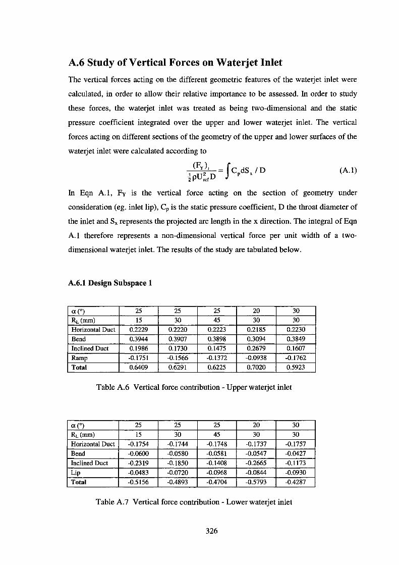
A.6 Study of Vertical Forces on Waterjet Inlet
The vertical forces acting on the different geometric features of the waterjet inlet were
calculated, in order to allow their relative importance to be assessed. In order to study
these forces, the waterjet inlet was treated as being two-dimensional and the static
pressure coefficient integrated over the upper and lower waterjet inlet. The vertical
forces acting on different sections of the geometry of the upper and lower surfaces of the
waterjet inlet were calculated according to
(Fy ), = fc dS I D 1 u2 D p x 2P ref
(A.l)
In Eqn A.l, Fy is the vertical force acting on the section of geometry under
consideration (eg. inlet lip), Cp is the static pressure coefficient, D the throat diameter of
the inlet and Sx represents the projected arc length in the x direction. The integral of Eqn
A.l therefore represents a non-dimensional vertical force per unit width of a two
dimensional waterjet inlet. The results of the study are tabulated below.
A.6.1 Design Subspace 1
a. (0) 25 25 25 20 30
RL(mm) 15 30 45 30 30
Horizontal Duct 0.2229 0.2220 0.2223 0.2185 0.2230
Bend 0.3944 0.3907 0.3898 0.3094 0.3849
Inclined Duct 0.1986 0.1730 0.1475 0.2679 0.1607
Ramp -0.1751 -0.1566 -0.1372 -0.0938 -0.1762
Total 0.6409 0.6291 0.6225 0.7020 0.5923
Table A.6 Vertical force contribution- Upper waterjet inlet
a. (0) 25 25 25 20 30
RL(mm) 15 30 45 30 30
Horizontal Duct -0.1754 -0.1744 -0.1748 -0.1737 -0.1757
Bend -0.0600 -0.0580 -0.0581 -0.0547 -0.0427
Inclined Duct -0.2319 -0.1850 -0.1408 -0.2665 -0.1173
Lip -0.0483 -0.0720 -0.0968 -0.0844 -0.0930
Total -0.5156 -0.4893 -0.4704 -0.5793 -0.4287
Table A.7 Vertical force contribution- Lower waterjet inlet
326
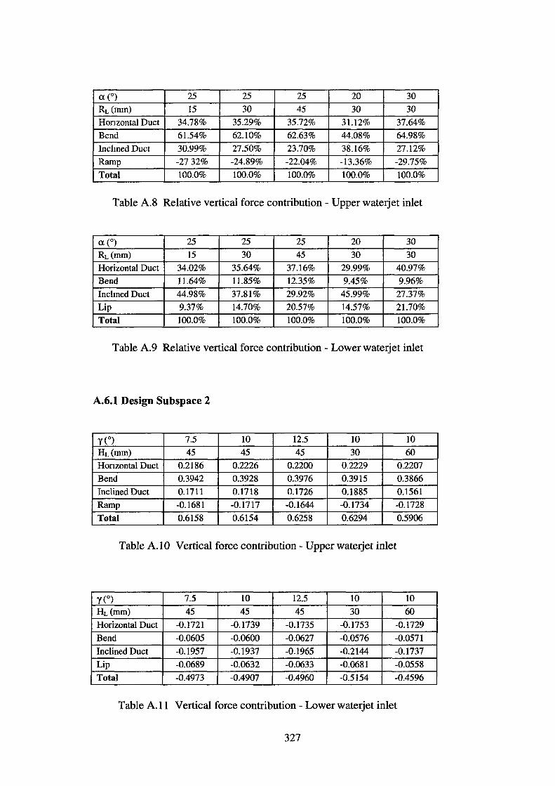
a (o) 25 25 25 20 30
RL(mm) 15 30 45 30 30
Honzonta1 Duct 34.78% 35.29% 35.72% 31.12% 37.64%
Bend 61.54% 62.10% 62.63% 44.08% 64.98%
Inclmed Duct 30.99% 27.50% 23.70% 38.16% 27.12%
Ramp -27 32% -24.89% -22.04% -13.36% -29.75%
Total 100.0% 100.0% 100.0% 100.0% 100.0%
Table A.8 Relative vertical force contribution - Upper waterjet inlet
a (o) 25 25 25 20 30
RL(mm) 15 30 45 30 30
Horizontal Duct 34.02% 35.64% 37.16% 29.99% 40.97%
Bend 11.64% 11.85% 12.35% 9.45% 9.96%
Inchned Duct 44.98% 37.81% 29.92% 45.99% 27.37%
Lip 9.37% 14.70% 20.57% 14.57% 21.70%
Total 100.0% 100.0% 100.0% 100.0% 100.0%
Table A.9 Relative vertical force contribution - Lower waterjet inlet
A.6.1 Design Subspace 2
y(o) 7.5 10 12.5 10 10
HL(mm) 45 45 45 30 60
Honzontal Duct 0.2186 0.2226 0.2200 0.2229 0.2207
Bend 0.3942 0.3928 0.3976 0.3915 0.3866
Inclined Duct 0.1711 0.1718 0.1726 0.1885 0.1561
Ramp -0.1681 -0.1717 -0.1644 -0.1734 -0.1728
Total 0.6158 0.6154 0.6258 0.6294 0.5906
Table A.IO Vertical force contribution- Upperwaterjet inlet
y(o) 7.5 10 12.5 10 10
HL(mm) 45 45 45 30 60
Horizontal Duct -0.1721 -0.1739 -0.1735 -0.1753 -0.1729
Bend -0.0605 -0.0600 -0.0627 -0.0576 -0.0571
Inclined Duct -0.1957 -0.1937 -0.1965 -0.2144 -0.1737
Lip -0.0689 -0.0632 -0.0633 -0.0681 -0.0558
Total -0.4973 -0.4907 -0.4960 -0.5154 -0.4596
Table A. II Vertical force contribution - Lower waterjet inlet
327
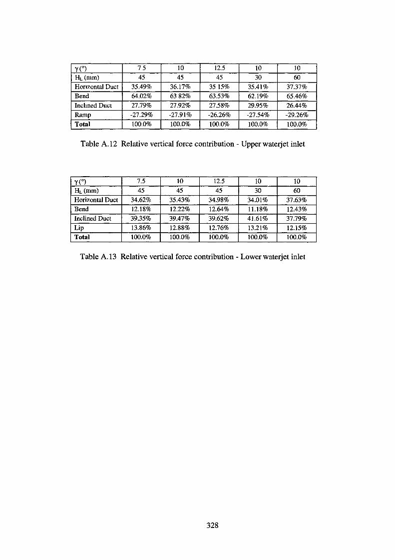
y(o) 75 10 12.5 10 10
HL(mm) 45 45 45 30 60
Honzontal Duct 35.49% 36.17% 3515% 35.41% 37.37%
Bend 64.02% 6382% 63.53% 62.19% 65.46%
Inclined Duct 27.79% 27.92% 27.58% 29.95% 26.44%
Ramp -27.29% -27.91% -26.26% -27.54% -29.26%
Total 100.0% 100.0% 100.0% 100.0% 100.0%
Table A.l2 Relative vertical force contribution - Upper waterjet inlet
y(o) 7.5 10 12.5 10 10
HL(mm) 45 45 45 30 60
Horizontal Duct 34.62% 35.43% 34.98% 34.01% 37.63%
Bend 12.18% 12.22% 12.64% 11.18% 12.43%
Inclined Duct 39.35% 39.47% 39.62% 41.61% 37.79%
Lip 13.86% 12.88% 12.76% 13.21% 12.15%
Total 100.0% 100.0% 100.0% 100.0% 100.0%
Table A.13 Relative vertical force contribution - Lower waterjet inlet
328
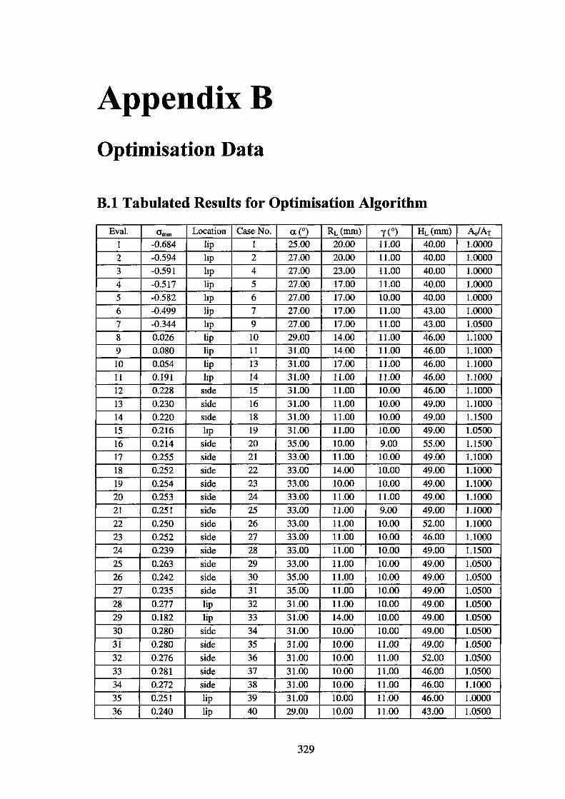
AppendixB Optimisation Data
B.l Tabulated Results for Optimisation Algorithm
Eva!. Gmm Location Case No. a (o) RL(mm) 'Y (0) HL(mm) AJAT I -0.684 lip I 25.00 20.00 11.00 40.00 1.0000
2 -0.594 hp 2 27.00 20.00 11.00 40.00 1.0000
3 -0.591 hp 4 27.00 23.00 11.00 40.00 1.0000
4 -0.517 lip 5 27.00 17.00 11.00 40.00 1.0000
5 -0.582 hp 6 27.00 17.00 10.00 40.00 1.0000
6 -0.499 lip 7 27.00 17.00 11.00 43.00 1.0000
7 -0.344 hp 9 27.00 17.00 11.00 43.00 1.0500
8 0.026 lip 10 29.00 14.00 11.00 46.00 1.1000
9 0.080 lip 11 31.00 14.00 11.00 46.00 1.1000
10 0.054 lip 13 31.00 17.00 11.00 46.00 1.1000
II 0.191 hp 14 31.00 11.00 11.00 46.00 1.1000
12 0.228 side 15 31.00 11.00 10.00 46.00 1.1000
13 0.230 side 16 31.00 11.00 10.00 49.00 1.1000
14 0.220 side 18 31.00 11.00 10.00 49.00 1.1500
15 0.216 hp 19 31.00 11.00 10.00 49.00 1.0500
16 0.214 side 20 35.00 10.00 9.00 55.00 1.1500
17 0.255 side 21 33.00 11.00 10.00 49.00 1.1000
18 0.252 side 22 33.00 14.00 10.00 49.00 1.1000
19 0.254 side 23 33.00 10.00 10.00 49.00 1.1000
20 0.253 side 24 33.00 11.00 11.00 49.00 1.1000
21 0.251 side 25 33.00 11.00 9.00 49.00 1.1000
22 0.250 side 26 33.00 11.00 10.00 52.00 1.1000
23 0.252 side 27 33.00 11.00 10.00 46.00 1.1000
24 0.239 side 28 33.00 11.00 10.00 49.00 1.1500
25 0.263 side 29 33.00 11.00 10.00 49.00 1.0500
26 0.242 side 30 35.00 11.00 10.00 49.00 1.0500
27 0.235 side 31 35.00 11.00 10.00 49.00 1.0500
28 0.277 lip 32 31.00 11.00 10.00 49.00 1.0500
29 0.182 lip 33 31.00 14.00 10.00 49.00 1.0500
30 0.280 side 34 31.00 10.00 10.00 49.00 1.0500
3I 0.280 side 35 31.00 10.00 I I.OO 49.00 1.0500
32 0.276 side 36 31.00 10.00 I 1.00 52.00 1.0500
33 0.281 side 37 31.00 10.00 11.00 46.00 1.0500
34 0.272 side 38 31.00 10.00 11.00 46.00 1.1000
35 0.251 lip 39 31.00 10.00 11.00 46.00 1.0000
36 0.240 lip 40 29.00 10.00 11.00 43.00 1.0500
329
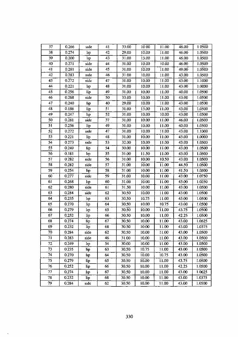
37 0.266 side 4I 33.00 1000 II.OO 46.00 I 0500
38 0.274 hp 42 29.00 10.00 II.OO 46.00 I.0500
39 0.200 hp 43 3I.OO 13.00 II.OO 46.00 I.0500
40 0.27I side 44 31.00 10.00 10.00 46.00 1.0500
4I 0.28I side 45 31.00 10.00 11.00 49.00 1.0500
42 0.283 side 46 31.00 10.00 11.00 43.00 1.0500
43 0.272 side 47 31.00 10.00 11.00 43.00 1.1000
44 0.221 hp 48 31.00 10.00 11.00 43.00 1.0000
45 0.256 lip 49 31.00 10.00 Il.OO 40.00 1.0500
46 0.268 side 50 33.00 10.00 11.00 43.00 1.0500
47 0.240 lip 40 29.00 10.00 11.00 43.00 1.0500
48 0.186 lip 51 31.00 13.00 11.00 43.00 1.0500
49 0.247 hp 52 31.00 10.00 10.00 43.00 1.0500
50 0.281 side 37 31.00 10.00 11.00 46.00 1.0500
51 0.256 lip 49 31.00 10.00 11.00 40.00 1.0500 52 0.272 side 47 31.00 10.00 11.00 43.00 1.1000
53 0.221 lip 48 31.00 10.00 11.00 43.00 I.OOOO
54 0.273 side 53 32.00 10.00 11.00 43.00 1.0500
55 0.249 lip 54 30.00 10.00 I 1.00 43.00 1.0500
56 0.181 hp 55 31.00 11.50 I1.00 43.00 1.0500
57 0.282 side 56 31.00 10.00 10.50 43.00 1.0500
58 0.282 side 57 31.00 10.00 11.00 44.50 1.0500
59 0.254 lip 58 31.00 10.00 11.00 41.50 1.0500
60 0.277 side 59 31.00 10.00 I 1.00 43.00 1.0750
61 0.268 hp 60 31.00 10.00 11.00 43.00 1.0250 62 0.280 side 61 31.50 10.00 11.00 43.00 1.0500
63 0.284 side 62 30.50 10.00 11.00 43.00 1.0500
64 0.235 hp 63 30.50 10.75 11.00 43.00 1.0500
65 0.270 lip 64 30.50 10.00 10.75 43.00 I.0500
66 0.279 hp 65 30.50 10.00 11.00 43.75 1.0500
67 0.252 lip 66 30.50 10.00 11.00 42.25 1.0500
68 0.274 lip 67 30.50 10.00 11.00 43.00 1.0625
69 0.232 lip 68 30.50 10.00 11.00 43.00 1.0375
70 0.284 side 62 30.50 10.00 11.00 43.00 1.0500
71 0.283 side 46 31.00 IO.OO 11.00 43.00 1.0500
72 0.249 hp 54 30.00 10.00 11.00 43.00 1.0500
73 0.235 lip 63 30.50 10.75 11.00 43.00 I.0500
74 0.270 hp 64 30.50 10.00 10.75 43.00 I.0500
75 0.279 lip 65 30.50 10.00 11.00 43.75 1.0500
76 0.252 lip 66 30.50 10.00 11.00 42.25 1.0500
77 0.274 hp 67 30.50 10.00 11.00 43.00 1.0625
78 0.232 lip 68 30.50 10.00 11.00 43.00 1.0375
79 0.284 side 62 30.50 10.00 11.00 43.00 1.0500
330
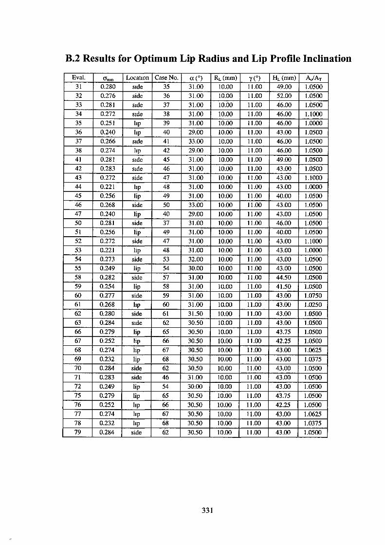
B.2 Results for Optimum Lip Radius and Lip Profile Inclination
Eva!. <Jmm LocatiOn Case No. a (o) RL(mm) 'Y (0) HL(mm) AJAT 31 0.280 Side 35 31.00 10.00 11.00 49.00 1.0500 32 0.276 side 36 31.00 10.00 11.00 52.00 1.0500
33 0.281 side 37 31.00 10.00 11.00 46.00 1.0500
34 0.272 Side 38 31.00 10.00 11.00 46.00 1.1000
35 0.251 hp 39 31.00 10.00 11.00 46.00 1.0000
36 0.240 hp 40 29.00 10.00 11.00 43.00 1.0500
37 0.266 Side 41 33.00 10.00 11.00 46.00 1.0500
38 0.274 hp 42 29.00 10.00 11.00 46.00 1.0500
41 0.281 side 45 31.00 10.00 11.00 49.00 1.0500
42 0.283 side 46 31.00 10.00 11.00 43.00 1.0500 43 0.272 side 47 31.00 10.00 11.00 43.00 1.1000
44 0.221 hp 48 31.00 10.00 11.00 43.00 1.0000
45 0.256 lip 49 31.00 10.00 11.00 40.00 1.0500 46 0.268 side 50 33.00 10.00 11.00 43.00 1.0500
47 0.240 lip 40 29.00 10.00 11.00 43.00 1.0500
50 0.281 side 37 31.00 10.00 11.00 46.00 1.0500 51 0.256 lip 49 31.00 10.00 11.00 40.00 1.0500 52 0.272 side 47 31.00 10.00 11.00 43.00 1.1000
53 0.221 lip 48 31.00 10.00 11.00 43.00 1.0000
54 0.273 side 53 32.00 10.00 11.00 43.00 1.0500 55 0.249 lip 54 30.00 10.00 11.00 43.00 1.0500
58 0.282 side 57 31.00 10.00 11.00 44.50 1.0500
59 0.254 lip 58 31.00 10.00 11.00 41.50 1.0500
60 0.277 side 59 31.00 10.00 11.00 43.00 1.0750 61 0.268 hp 60 31.00 10.00 11.00 43.00 1.0250
62 0.280 side 61 31.50 10.00 11.00 43.00 1.()500
63 0.284 side 62 30.50 10.00 11.00 43.00 1.0500
66 0.279 lip 65 30.50 10.00 11.00 43.75 1.0500
67 0.252 lip 66 30.50 10.00 11.00 42.25 1.0500
68 0.274 lip 67 30.50 10.00 11.00 43.00 1.0625
69 0.232 lip 68 30.50 10.00 11.00 43.00 1.0375
70 0.284 side 62 30.50 10.00 11.00 43.00 1.0500
71 0.283 side 46 31.00 10.00 11.00 43.00 1.0500
72 0.249 lip 54 30.00 10.00 11.00 43.00 1.0500
75 0.279 lip 65 30.50 10.00 11.00 43.75 1.0500
76 0.252 hp 66 30.50 10.00 11.00 42.25 1.0500
77 0.274 hp 67 30.50 10.00 11.00 43.00 1.0625
78 0.232 hp 68 30.50 10.00 11.00 43.00 1.0375
79 0.284 side 62 30.50 10.00 11.00 43.00 1.0500
331