PSFC/RR-06-4 Development of an Experiment to Study the Effects of

Transverse Stress on the Critical Current of a Niobium-Tin Superconducting Cable

Luisa Chiesa

February, 2006

Plasma Science and Fusion Center Massachusetts Institute of Technology

Cambridge MA 02139 USA

This work was supported by the U.S. Department of Energy, Grant No. DE-FC02-93ER54186. Reproduction, translation, publication, use and disposal, in whole or in part, by or for the United States government is permitted.

DEVELOPMENT OF AN EXPERIMENT TO STUDY THE EFFECTS OF TRANSVERSE STRESS ON THE CRITICAL CURRENT OF A NIOBIUM-TIN

SUPERCONDUCTING CABLE

By Luisa Chiesa

Submitted to the Department of Nuclear Science and Engineering in Partial Fulfillment of the Requirements for the Degree of

Master of Science in Nuclear Science and Engineering

at the

Massachusetts Institute of Technology February 2006

© 2006 Massachusetts Institute of Technology All right reserved

Signature of Author

Department of Nuclear Science and Engineering

January 10, 2006

Certified by

Joseph V. Minervini

Senior Research Engineer, MIT Plasma Science and Fusion Center

Nuclear Science and Engineering Department

Thesis Supervisor

Certified by

Jeffrey P. Freidberg

Professor of Nuclear Science and Engineering

Thesis Reader

Accepted by

Jeffrey A. Coderre

Associate Professor of Nuclear Science and Engineering

Chairman, Department Committee on Graduate Students

2

3

DEVELOPMENT OF AN EXPERIMENT TO STUDY THE EFFECTS OF TRANSVERSE STRESS ON THE CRITICAL CURRENT OF A NIOBIUM-TIN SUPERCONDUCTING CABLE

by

Luisa Chiesa

Submitted to the Department of Nuclear Science and Engineering in February 2006

in Partial Fulfillment of the Requirements for the Degree of Master of Science in Nuclear Science and Engineering

ABSTRACT

Superconducting magnets will play a central role for the success of the International Thermonuclear Experimental Reactor (ITER). ITER is a current driven plasma experiment that could set a milestone towards the demonstration of fusion as a source of energy in the future.

Cable-in-Conduit is the typical geometry for the conductor employed in superconducting magnets for fusion application. The cable is composed of over 800 strands. Once energized, the magnets produce an enormous electromagnetic force defined by the product of the current and the magnetic field. The strands move under the effect of this force, and the force accumulates against one side of the conduit thereby pressing transversally against the strands.

The experiment proposed here has the goal of assessing the functionality of the apparatus designed to study the effect of transverse load on a cable composed of 36 superconducting strands (with a 3x3x4 pattern) by mechanically simulating the ITER Lorentz stress condition.

The apparatus was assembled at MIT and preliminary tests at 77 K and room temperature were made to improve the design prior to carrying out the actual experiments. These were done at the National High Magnetic Field Laboratory (NHMFL) located in Florida. Ideally, the transverse conditions simulating the ITER conditions should be created by Lorentz forces due to current and magnetic field. Unfortunately to create such a high level of stress, currents higher than the power supply capability at NHMFL (10 kA) would be required. This is the driving reason to have an apparatus simulating the same stress condition mechanically.

The first test was conducted in October 2005. It was possible to test the structure and its range of operation. Critical current measurements were made as a function of different fields. However during the first measurement, under the loading conditions, the sample was irreversibly damaged and no other measurements were possible.

The successful test of the structural behavior of the apparatus motivated a second test carried out in January 2006. With the improvements made between the two experiments, it was possible to successfully measure the degradation of the cable as a function of the

4

transverse pressure applied, measuring degradation as high as 50% with a transverse load of 100 MPa.

The ultimate goal of these studies is to characterize the critical current behavior as a function of transverse load in order to predict the response of a full sized Cable-in-Conduit. The work in this thesis was used to explore a setup for measurements and measurement technique. A set of empirical equations describing the behavior of full size cables is needed and should be addressed with a new project that extends the work done so far. Luisa Chiesa Thesis Supervisor: Dr. Joseph V. Minervini Title: PSFC Technology and Engineering Division Head Thesis Reader: Dr. Jeffrey P. Freidberg Title: Professor of Nuclear Science and Engineering

5

ACKNOWLEDGEMENTS

I would like to express my deep gratitude to my supervisor Dr. Joseph Minervini, to his constant support and for being always so positive under any circumstance (also when asking money again and again and again for the experiment).

Thanks to Prof. Jeff Friedberg and the patience in reading this thesis despite being so experimental oriented.

A very special thank to the Master, Dr. Makoto-San Takayasu. I learned many things

working next to him…what it is possible but more so what it is impossible and it will never work…just kidding. He is a very patient man who always finds time to explain things and never gets tired of looking for things to improve to have a successful experiment. Arigato gozaimasu Makoto!!! In exchange he learned how to confuse right and left from me. Fair exchange I believe.

Another very special thank to Dave Tracey and his smiling face any time I asked him to modify things for the second…third time. Without his technical skills and his contribution I would not be here writing acknowledgements.

Again to Valery Fishman and his great help in preparing the drawing package and explaining me what M6-1 means and how to consult a machinery catalogue.

Thank to Dr. Chen-Yu Gung and his help in the experimental set up and all the work done to prepare the furnace for heat treatment.

Another thank to Peter Stahle because he had the patience to explain the basic of mechanical engineering especially because he is not even part of our group but he helped us whenever possible. I bet he never amused himself so much about my ignorance on screws size and inches.

Thank to everyone in the group especially Peter Titus and his ANSYS expertise, Phil Michael for his precious comments during the design and experimental phase, Darlene Marble for the constant assistance and Dave Harris for his help and support.

A portion of this work was performed at the National High Magnetic Field Laboratory, which is supported by NSF Cooperative Agreement No. DMR-0084173, by the State of Florida, and by the DOE. Many thanks to all the people that helped us with the experiment at the NHMFL facility.

Thanks to my family, my mum and dad and my wonderful brother. Thanks to all my special friends in Boston. My parents are really grateful to you

because you all took the burden of being next to me during exams and experiment preparation. Thanks Antonio and the wonderful chats and coffees, Chudi and his never ending support in any circumstances, Ksusha for her friendship, chats and company, Matteo because he lets me sing in the office, Jen, Matt for being wonderful roommates, Greg for the great hikes in the Whites, Darwin for always listening with patience.

Also thanks to all the special friends far away… Michela because she is a wonderful, truthful and sincere friend, Paolo, Jackie and their support and advice from the other side of the country, Peter, Shlomo, Silvia, Francesca, Alessandra, Marco, Daniela, Cristian, Rainer, Gianni, Carrie, Federico, Giovanni, Rocco, Keshini, Sejal and her support during my first year at MIT and her being always present, Chris and whomever I forgot…

THANK YOU

6

INDEX Title Page 1 Abstract 3 Acknowledgements 5 Index 6 List of Figures 8 List of Tables 15 Glossary 16 Chapter 1: Introduction 17 1.1 Background of Superconductivity 17 1.2 Superconductivity Application 26 1.3 Magnet types and Cable-in-Conduit Conductor 27 1.4 ITER and fusion energy 30 1.5 Scope of thesis 32 Chapter 2: Strain characteristics of superconducting wires and cable 34 2.1 Introduction 34 2.2 Axial strain effect 35

2.2.1 Single strand in uniaxial strain 38 2.1.2 Single strand under pinching and bending loads 40 2.1.3 Tests of sub-size cables under axial strain 43

2.3 Transverse strain effect 47 2.3.1 Single strand under transverse load 47 2.3.2 Tests on sub-sized cables under transverse load 52

2.4 Motivation for further investigations and challenges 55

Chapter 3: Description of the experiment and the FEM model 57

3.1 Introduction 57 3.2 Cable Design 57 3.3 Structure Design 62 3.3.1 Parts description 62 3.3.2 Strain requirements 68 3.4 Electromagnetic and Mechanical forces 70

3.4.1 Radial electromagnetic force and dewar tail stress calculations 70 3.4.2 Mechanical and structural forces 73 3.4.2.1 Rotational method 73 3.4.2.2 Linear Actuator method 77

3.5 Finite Element Analysis 78

7

Chapter 4: Experimental results and discussions 88

4.1 Introduction 88 4.2 Measurement technique 88 4.3 Preliminary tests done at MIT 91 4.4 Test Facility at NHFML 98 4.5 Results of the first experiment campaign 104 4.6 Further tests performed at MIT after the test at NHMFL 118 4.7 Helium consumption 125 4.8 Changes made after the first experiment 126 4.9 Preliminary results for the second test campaign 128 4.10 Remarks and conclusions 132 Appendix I: Drawings 135 Appendix II: Cabling machine 163 II.1 Machine Description 163 II.2 Typical operation to make a cable 166 II.3 Summary 176 Appendix III: Pictures 179 III.1 Cabling 179 III.2 Parts and Assembly of the first sample 180 III.3 After heat treatment and mounting of strain gages 185 III.4 Experiment of the first sample 188 References 197

8

List of Figures Chapter 1 Fig. 1 Critical surface for superconducting materials. 18 Fig. 2 (a) Critical surface for NbTi, 18 (b) Critical current dependence on axial strain for Nb3Sn strands. 19 Fig. 3 Critical field as a function of temperature for Type I and II superconductors. 19 Fig. 4 Normal cores representation in a Type II superconductors slab. Surface currents flow to maintain the bulk of the slab diamagnetic. 20 Fig. 5 Properties of normal cores in a Type II superconductor [1.5]. 20 Fig. 6 Normal cores and pinning centers in a Type II superconductors. 21 Fig. 7 Critical field as a function of temperature for selected LTS, HTS superconductors. 23 Fig. 8 Critical current density at 4.2 K for different superconducting materials candidates for magnet design. 24 Fig. 9 Cross section of the cable used for ITER. 25 Fig. 10 (a) Rutherford cable used for adiabatic magnets. 27 Fig. 10 (b) NbTi Impregnated coil used in one of the LHC quadrupoles. 28 Fig. 10 (c) Nb3Sn racetrack coil impregnated with epoxy showing some voids after impregnation. 28 Fig. 11 (a) Multiple stage CICC for ITER (3x3x4x4x6). (b) Cut-out of a superconducting cable. 29 Fig. 12 Cut-away of ITER and the magnets system of the machine. 30 Fig. 13 Central Solenoid stack up and CICC used for the coils winding. 31 Fig. 14 Lorentz force due to electromagnetic interaction of current and field in a CICC cable. 32 Fig. 15 (a) Schematic view of the device, (b) pressure pattern applied to the cable (top view). 33 Chapter 2 Fig. 1 Critical current measurements for Nb3Sn cable used in our device. 35 Fig. 2 U-spring strain device. 38 Fig. 3 Pacman strain device. 39 Fig. 4 The Walters Springs (WASP) device. 39 Fig. 5 TARSIS experiment setup. 40 Fig. 6 Fixed bending strain behavior strand configuration. 41 Fig. 7 Maximum bending applied to the support beam at room temperature during preliminary setup. 41 Fig. 8 Pure bending device components. 42 Fig. 9 (a) Schematic of pull test setup. (b) Ratio of critical current to maximum critical current as a function of strain at 4.2K, 12T. (c) Pull test conductor sample prepared for testing. 44

9

Fig.10 (a) Test setup. (b) Critical current as a function of magnetic field for different sample. (c) Typical strain behavior for a single strand at 13T. (d) Strain measurement for the braid subcable. 45 Fig.11 (a) Critical current as a function of magnetic field with no strain applied. (b) Ratio of critical current to maximum critical current as a function of strain at 4.2K, 12T for different samples. 46 Fig. 12 (a) Field dependence of critical current without applied strain for CICC with SS or Ti jacket. (b) Critical current as a function of strain for Nb3Sn conductors containing different internal reinforcement. 47 Fig.13 (a) Schematic view of test setup. (b) Cross section of the two samples used (round and flat). (c) Critical current degradation for transverse and axial compressive stress for ROUND sample. (d) Critical current degradation for transverse and axial compressive stress for FLAT sample. 49 Fig.14 (a) Test setup. (b) Normalized critical current as a function of transverse compression (σt) and axial tension (σa). 50 Fig.15 (a) Cross section of bronze process wire. (b) Cross section of internal tin wire. (c) Critical current degradation as a function of transverse stress and magnetic field for the two different samples. 51 Fig.16 (a) Test setup of crossover effect. (b) Critical current degradation as a function of transverse stress and magnetic field for uniform and cross over stress. 52 Fig.17 Sample arrangement within the test magnet and the transverse load cage. 53 Fig.18 (a) Critical current degradation as a function of transverse stress for the CICC tested. Also plotted the single strand behavior normalized at 12T. (b) Cross section of a 40% void fraction CICC before and after loading. 54 Chapter 3 Fig. 1 Critical currents for a 36 strands cable as a function of field and at constant pressure levels. 58 Fig. 2 (a) Cable ready to be mounted. Voltage taps wires are visible (b) “Sewing” the stainless steel wire for voltage tap. 59 (c) Another view of the cable and the voltage tap wound around it. 60 Fig. 3 Copper terminations soldered to the current leads connection. 60 Fig. 4 Heat treatment schedule for the Nb3Sn sample. 61 Fig. 5 (a) Cross section of the entire probe used for the experiment. 62

10

Fig. 5 (b) Cross section of the probe head structure used for the experiment. 63 Fig. 6 (a) Structure seen from the bottom. The cable is between the Incoloy 908® ring and the expanding collet. (b) Detail of the expanding collet and the cable enclosed. 64 (c) Stainless steel cone used during heat treatment to maintain the proper void fraction of the cable. (d) Cable mounted and detail about how the cable comes out of the structure. (e) Sample and structure ready before heat treatment. 65 Fig. 7 COE as a function of temperature for different materials used in the experiment. 67 Fig. 8 Strain gages mounted on the Incoloy 908® rings. 68 Fig. 9 Stress dependence of single Nb3Sn strand. Strands are much more sensitive to transverse stress. 68 Fig. 10 Critical current variation as a function of uni-axial longitudinal strain applied. 69 Fig. 11 Sources of radial electromagnetic force: missing section of the cable and joint area where the sample is soldered to the copper current leads. 70 Fig. 12 Summary of radial electromagnetic force effect. 71 Fig. 13 Dewar’s schematic with the position of the cable and where the stress was estimated. 72 Fig. 14 (a) Three major sources of friction: threaded brass and nut (CSX-007/CSX-017), nut and brass halves (CSX-017/CSX-011), brass cone and expanding collet (CSX-007/CSX-005). (b) Estimation of the vertical force required to produce 10 MPa on the cable. 74 Fig. 15 (a) Torque created by the first term of Eq. 6 for different friction coefficients (µ) as a function of the friction coefficient between brass conical wedge (CSX-007) and expanding collet (CSX-005). (b) Torque created by the second term of Eq. 6 for different friction coefficients (µc) as a function of the friction coefficient between brass conical wedge (CSX-007) and expanding collet (CSX-005). 76 Fig. 16 Linear actuator and support structure sitting before mounting on the top flange and mounted on top of the dewar with the probe attached to the current leads. 77 Fig. 17 Connector pieces: load cell position and ¾” high strength threaded rod. 78 Fig. 18 (a) 2D geometry and constraints applied, (b) 3D expansion of the model. 79 Fig. 19 Expansion of the 2D model. 80 Fig. 20 Lines defining the different pieces of the model. 81 Fig. 21 Results of Ansys simulation at step 40. 82 Fig. 22 Close up to the cable and Incoloy 908® rings at step 40 of the analysis. 83 Fig. 23 (a) y and z strain in the cable, (b) y and z strain in the Incoloy 908® rings, 84 (c) close up to the strain on the Incoloy 908® ring hosting the cable, (d) z strain distribution in the Incoloy 908® ring when the friction coefficients between the two rings is 0.7. 85 Fig. 24 Strain gages patter used during the test. 86 Fig. 25 Expected values of axial and hoop strain on the Incoloy 908® ring and their relation with the transverse pressure on the cable. 87

11

Fig. 26 Expected values of hoop strain on the Incoloy 908® ring (ANSYS® simulation) compared with measurements taken with the strain gages. 87 Chapter 4 Fig. 1 Schematic view of voltage taps on the cable. 88 Fig. 2 Strain gage pattern for the gages used in the experiment. 89 Fig. 3 Strain gage installation setup (left) and at the end of curing cycle (right). 90 Fig. 4 Strain gage circuit. Inside the box four identical circuits are wired. 90 Fig. 5 Room temperature setup: assembled pieces (left), strain gage (right), exploded view of the assembly (bottom). 91 Fig. 6 Hoop strain results and comparison with ANSYS® simulations. 92 Fig. 7 Axial strain results and comparison with ANSYS® simulations. 93 Fig. 8 (a) Rotating knob and shaft mounted for preliminary tests, (b) probe head and connection shaft-nut, (c) brass cone, its movement expands the collet and reduce the gap. 94 Fig. 9 (a) Experimental setup for the INSTRON test. The probe head is mounted upside down and the load is applied to the bottom area of the brass cone. (b) Gap reduction after the INSTRON test. 95 Fig. 10 Results of INSTRON test, strain gages and load as a function of time. 96 Fig. 11 Strain and load results as a function of the vertical displacement with the INSTRON machine. 97 Fig. 12 Circuit setup of the experiment at NHMFL. 98 Fig. 13 Variation as a function of axial coordinate z of the axial and radial components of the field evaluated at r = 0.056 m [4.1]. 99 Fig. 14 Restoring force acting on the Incoloy 908® rings. 100 Fig. 15 20 T solenoid at NHMFL (units mm). 100 Fig. 16 T solenoid and cryostat. 101 Fig. 17 Experiment setup. Data acquisition system and instrumentation used (top), current leads and position of water cooled resistors (bottom). 102 Fig. 18 Strain gages positions on the two Incoloy 908® ring and their typical wiring. 104 Fig. 19 Details of the probe before being inserted inside the dewar and positions of liquid level sensors. 106 Fig. 20 Voltage across the joints as a function of current. 107 Fig. 21 Voltage trace for voltage tap 1 at 4.2 K, 10 T. 108 Fig. 22 Measured values of critical current compared with estimate from single strand measurements (current cable = single strand value x 35 strands). 109 Fig. 23 Measured n-values as a function of the measured current per strand. 110 Fig. 24 Strain as a function of electromagnetic load at fixed field 10 T. 111 Fig. 25 Strain experienced by gage SG5hs during the measurements made at different fields. 112 Fig. 26 (a) Critical current measurements as a function of field for the three different loads. (b) n- values as a function of current per strand. 114

12

Fig. 27 (a) Different gages recorded at 10 T for the third load as a function of electromagnetic load. (b) Voltage measurements of SG5hs for the different measurements made. 115 Fig. 28 Strain gages readings and their variation while applying load. 116 Fig. 29 SG5hs strain measurement as a function of turn number. 117 Fig. 30 Load (in kg) as a function of turn number. 119 Fig. 31 Strain gages as test setup as a function of vertical load during loading and unloading. 120 Fig. 32 Strain gages as test setup as a function of vertical load during loading for same loading as Fig. 31 and after loosing up the compressive force holding the structure together. 120 Fig. 33 Strain gages in position 3 during loading and unloading. 121 Fig. 34 Probe head before the test (top) and section of the cable severely damaged during the test (bottom). 122 Fig. 35 Strain gages in position 3 and 4 as a function of the load. 123 Fig. 36 All hoop gages as a function of time. 124 Fig. 37 All hoop gages in the four different positions, as a function of load. 124 Fig. 38 Helium consumption as a function of time during the two days of test. 125 Fig. 39 Motor drive connected to the linear actuator during the second test performed in January. 127 Fig. 40 Voltage taps and strain gages positions during the test. 128 Fig. 41 Critical current as a function of magnetic field for the two experiments performed and compared with the expected values calculated form single strand data. 128 Fig. 42 n-values as a function of current per strand for the two different experiments. 129 Fig. 43 Critical currents normalized to the critical current at zero load, with a background field of 12 T, as a function of the transverse load. 130 Fig. 44 Strain gages signals as a function of transverse load and compared with the 2D ANSYS® model described in Chapter 3. 131 Fig. 45 Comparisons between the measurement taken during the experiment, single strand data taken by Ekin and sub-sized measurements made by Summers and Miller. 132 Fig. 46 Modified expanding collet to apply a more uniform load on the cable. 133 Appendix II Fig.1 shows the main components of the machine. 163 Fig. 2 Spinner with 6 spool capability and a single strand spool mounted on the spinner. 164 Fig. 3 Traverser and torque controls and take up and torque switches. 165 Fig. 4 Ratio and speed controls (to the left) and stop-start operation buttons. 166 Fig. 5 Re-spooling station. The strand is re-spooled from a big spool to an appropriate size spool which fits inside the cabling machine. 167

13

Fig. 6 Strand location on the guide wheels which direct the strand towards the cabling spool. 167 Fig. 7 (a) Traverser used to translate the strand guide wheels during spooling to produce uniform layers on the pay-off spool. (b) Counter to measure the length of the strand/cable wound on the cabling spool (measured in feet) (c) Speed and traverse controls. 168 Fig. 8 The copper leader helps to indicate a stop of the machine once a spool is finished. 169 Fig. 9 (a) Device used to estimate the tension on the spool holder and positioning of the spools on the machine. 170 Fig. 9 (b) Details for one of the shafts which support the spool in the cabling machine. 171 Fig. 11 Other views of cabling operation. 172 Fig. 12 As the subcables become larger in diameter, pass through the cabling die becomes increasingly difficult. 173 Fig. 13 Preparation of the connection between the 36 strands cable and the triplet take-up leader at a point just after the cabling die. 174 Fig. 14 View of the connection between the 36 strands cable and the triplet take-up leader as it approaches the first guide wheel. 174 Fig. 15 Measuring the twist pitch by inserting a piece of wire between the higher cable stages. 175 Fig. 16 36-strand cable collected on the take-up spool. The triplet leader is also visible to the left side of the take-up spool. 175 Appendix III Fig. 1 36-strands cable ready after cabling. 179 Fig. 2 Nb3Sn cable inside groove of Incoloy 908® ring. 180 Fig. 3 Expanding collet with stainless steel cone used during heat treatment. 180 Fig. 4 Cable used for the experiment. 181 Fig. 5 Assembly of the first sample. 181 Fig. 6 Mounting of stainless steel “fingers” to enclose the cable between Incoloy 908® ring and expanding collet. 182 Fig. 7 Stainless steel cone used to maintain void fraction of the cable to the desired level during heat treatment. 182 Fig. 8 Structure ready for heat treatment. 183 Fig. 9 Sample and witness strand ready to be put in the oven for heat treatment. 184 Fig. 10 Sample area after heat treatment. 185 Fig. 11 Sample after heat treatment. Incoloy 908® looks more shiny that stainless steel because it contains less chrome than stainless steel. 185 Fig. 12 Another view of the sample after heat treatment. 186

14

Fig. 13 Mounting setup for strain gages. 186 Fig. 14 Bottom gage after heat treatment of the glue used to attach them to a surface. 187 Fig. 15 Strain gages after mounting and heat treatment. 187 Fig. 16 Dewar at NHFML while inserted in the bore of 20 T magnet. 188 Fig. 17 Probe before being inserted in the dewar The tail of the probe is where the sample is located. 189 Fig. 18 Sample area with transfer line ad liquid level sensor mounted. 189 Fig. 19 Sample area with strain gages wires and Hall sensor. 190 Fig. 20 Sample area and wiring used during experiment (strain gages and voltage taps). 190 Fig. 21 Linear actuator and connection box to connect linear actuator and rod going to the sample. 191 Fig. 22 Probe ready to be inserted in the dewar. 191 Fig. 23 Relocation of the probe from wooden box to the dewar. 192 Fig. 24 Probe in the dewar. 10 kA current leads hooked to the top flange. 193 Fig. 25 10 kA current leads hooked to the top flange. 193 Fig. 26 Instrumentation setup. 194 Fig. 27 20 kA cables and water cooled resistor to improve the stability of the voltage power supply. 194 Fig. 28 (a) Burned area of the sample. (b) Burned area of the sample once removed from the dewar. 195 Fig. 29 Burned area of the sample. The sample partially melted on the right side. 196 Fig. 30 Burned area of the sample. 196

15

List of Tables Chapter 1 Table 1 Critical temperatures and fields for Type I and II superconductors. 22 Chapter 3 Table 1 List of constrains considered during the design. 66 Table 2 Radial electromagnetic force due to cable and joints. 71 Chapter 4 Table 1 Instrumentations used during experiment. 101 Table 2 List of diagnostic mounted on the probe. 104 Table 3 Critical current measurements at zero mechanical load. 109 Table 4 Critical current measurements for three different loads. 113 Table 5 Different configuration of strain gages tests at room temperature. 118 Appendix II Table 1 36 strands 3x3x4 measurements of twist pitch for different machine paramenters. 175

16

Glossary of Terms CIC Cable-in-Conduit CICC Cable-in-Conduit Conductor ITER International Thermonuclear Experimental Reactor CSMC Central Solenoid Model Coil NET Next European Torus J Current density B Magnetic field intensity T Temperature Jc Critical current density Bc Critical magnetic field Tc Critical temperature Bc1 Lower critical magnetic field Bc2 Upper critical magnetic field LTS Low Temperature Superconductors HTS High Temperature Superconductors MRI Magnetic Resonance Imaging NMR Nuclear Magnetic Resonance V Voltage Φ Magnetic flux τ Pressure F Force I Current dstrand Diameter of a strand dcable Diameter of a cable Ic Critical current Icm Maximum critical current Vc Critical voltage Ec Critical electric field n n-value of a superconductor ε Strain εm Maximum strain εa Axial strain COE Coefficient of expansion SS Stainless steel σ Stress E Young modulus S Section modulus I Moment of inertia T Torque µ Friction coefficient α Half thread angle

17

CHAPTER 1: Introduction

Since its discovery in 1911, superconductivity has been playing an increasingly important role in different fields especially for magnet technology. The non-resistive characteristic of superconductor materials made them very attractive to achieve performances too demanding for conventional resistive materials. Even though superconductivity is a characteristic common to many metals, the engineering challenge is to obtain a material suitable for magnet design.

There are four key magnet issues to be considered in the context of balancing cost and difficulty of assembly:

• Stability against mechanical, electromagnetic, thermal or nuclear disturbances, • Cryogenics and efficiency of the coolant used, • Protection of the conductor against events which would lead to a complete loss

of superconductive properties (quench), • Mechanical stability of the conductor and the supporting structure.

The principal characteristics of superconducting materials and their application with

focus on magnets for fusion energy application are described in the following sections. In Section 1.1 a general background on superconductivity is given with a description of the critical state model. A list of superconductors available for magnets application will be given with focus on the type of strand and cable used for fusion magnet applications. In Section 1.2 the possible applications for superconductor materials are described. The following section (Section 1.3) describes the differences between magnets design for different applications. A general description of International Thermonuclear Experimental Reactor and the conductors used for the central solenoid is described in Section 1.4. Section 1.5 concludes the chapter with the motivations for this thesis work and the scientific interest of the project developed with this work. 1.1 Background of Superconductivity

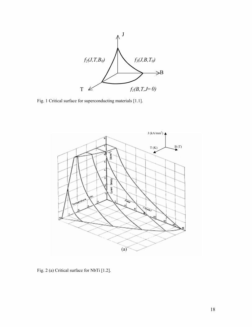
A material is said to be superconductive if it shows virtually no resistance against the

passage of current. This property is usually obtained by sufficiently lowering the temperature of the material. Many metals possess this property, but very few of them have all the characteristics suitable for magnet design. Superconductivity is determined by three properties that describe a surface under which the material does not show any resistance. These are current density, field and temperature. It has also been found that axial and transverse strains affect the material performance (discussed in more details in Chapter 2). If all but one of these properties are kept fixed, once the variable property reaches its critical value the superconductive behavior will be lost. A schematic representation of the critical surface for a superconducting material is shown in Fig. 1. In Fig. 2 NbTi critical surface and critical current dependence on axial strain for Nb3Sn are represented.

18

Fig. 1 Critical surface for superconducting materials [1.1].

Fig. 2 (a) Critical surface for NbTi [1.2].

J (kA/mm2)

T (K) B (T)

(a)

f3(J,B,T0) f2(J,T,B0)

f1(B,T,J=0)

J

B

T )0)

19

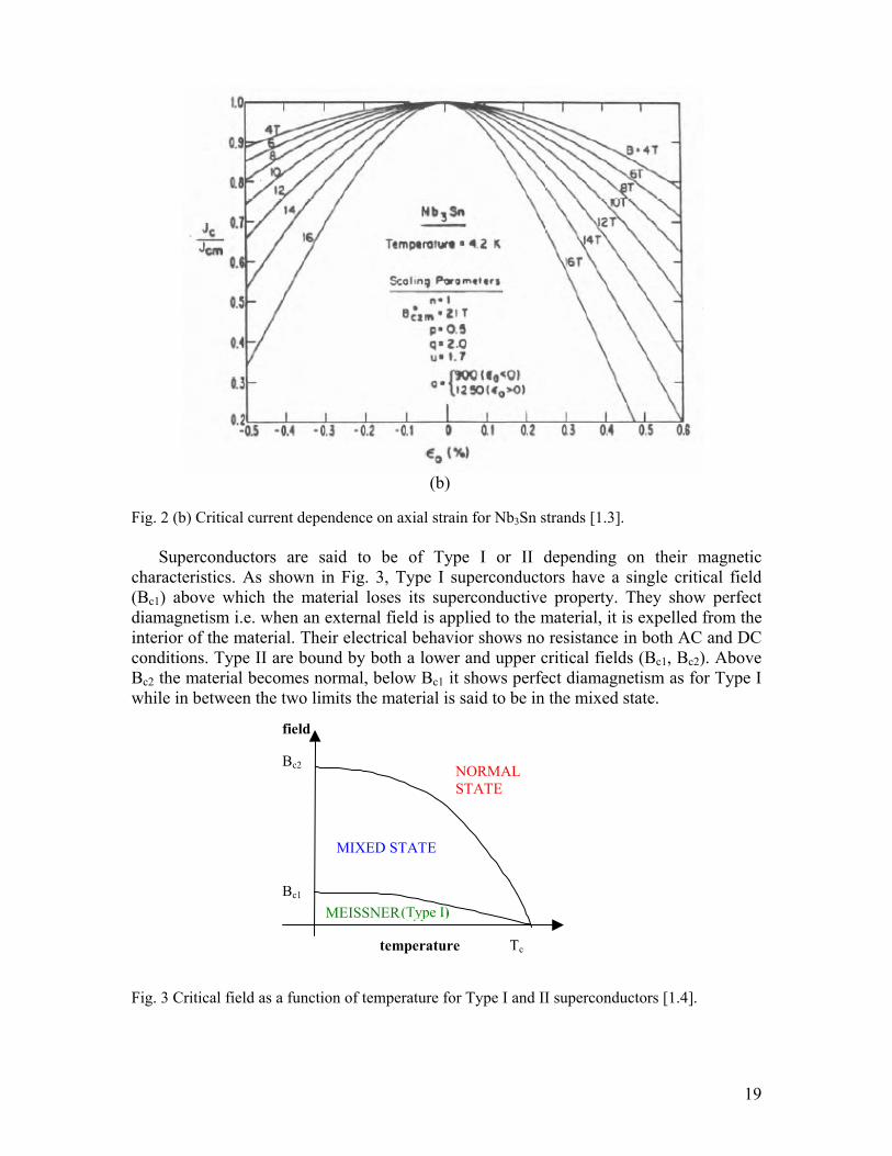
Fig. 2 (b) Critical current dependence on axial strain for Nb3Sn strands [1.3].

Superconductors are said to be of Type I or II depending on their magnetic characteristics. As shown in Fig. 3, Type I superconductors have a single critical field (Bc1) above which the material loses its superconductive property. They show perfect diamagnetism i.e. when an external field is applied to the material, it is expelled from the interior of the material. Their electrical behavior shows no resistance in both AC and DC conditions. Type II are bound by both a lower and upper critical fields (Bc1, Bc2). Above Bc2 the material becomes normal, below Bc1 it shows perfect diamagnetism as for Type I while in between the two limits the material is said to be in the mixed state.

Fig. 3 Critical field as a function of temperature for Type I and II superconductors [1.4].

field

Bc2

Bc1

Tctemperature

NORMALSTATE

MIXED STATE

MEISSNER (type I)(Type I)

(b)

20

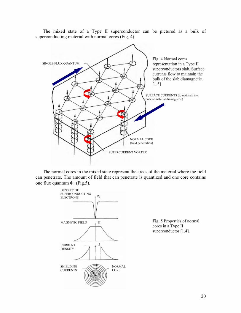
The mixed state of a Type II superconductor can be pictured as a bulk of superconducting material with normal cores (Fig. 4).

The normal cores in the mixed state represent the areas of the material where the field

can penetrate. The amount of field that can penetrate is quantized and one core contains one flux quantum Φ0 (Fig.5).

SINGLE FLUX QUANTUM

NORMAL CORE (field penetration)

SUPERCURRENT VORTEX

SURFACE CURRENTS (to maintain the bulk of material diamagnetic)

Fig. 4 Normal cores representation in a Type II superconductors slab. Surface currents flow to maintain the bulk of the slab diamagnetic. [1.5]

DENSITY OF SUPERCONDUCTING ELECTRONS

MAGNETIC FIELD

CURRENT DENSITY

NORMAL CORE

SHIELDING CURRENTS

ns

H

J

Fig. 5 Properties of normal cores in a Type II superconductor [1.4].

21

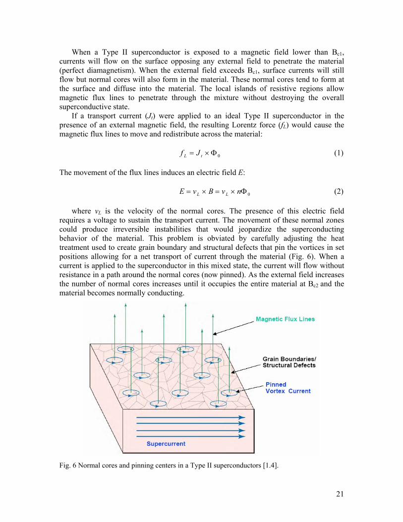
When a Type II superconductor is exposed to a magnetic field lower than Bc1, currents will flow on the surface opposing any external field to penetrate the material (perfect diamagnetism). When the external field exceeds Bc1, surface currents will still flow but normal cores will also form in the material. These normal cores tend to form at the surface and diffuse into the material. The local islands of resistive regions allow magnetic flux lines to penetrate through the mixture without destroying the overall superconductive state.

If a transport current (Jt) were applied to an ideal Type II superconductor in the presence of an external magnetic field, the resulting Lorentz force (fL) would cause the magnetic flux lines to move and redistribute across the material:

0Φ×= tL Jf (1)

The movement of the flux lines induces an electric field E:

0Φ×=×= nvBvE LL (2)

where vL is the velocity of the normal cores. The presence of this electric field

requires a voltage to sustain the transport current. The movement of these normal zones could produce irreversible instabilities that would jeopardize the superconducting behavior of the material. This problem is obviated by carefully adjusting the heat treatment used to create grain boundary and structural defects that pin the vortices in set positions allowing for a net transport of current through the material (Fig. 6). When a current is applied to the superconductor in this mixed state, the current will flow without resistance in a path around the normal cores (now pinned). As the external field increases the number of normal cores increases until it occupies the entire material at Bc2 and the material becomes normally conducting.

Fig. 6 Normal cores and pinning centers in a Type II superconductors [1.4].

22

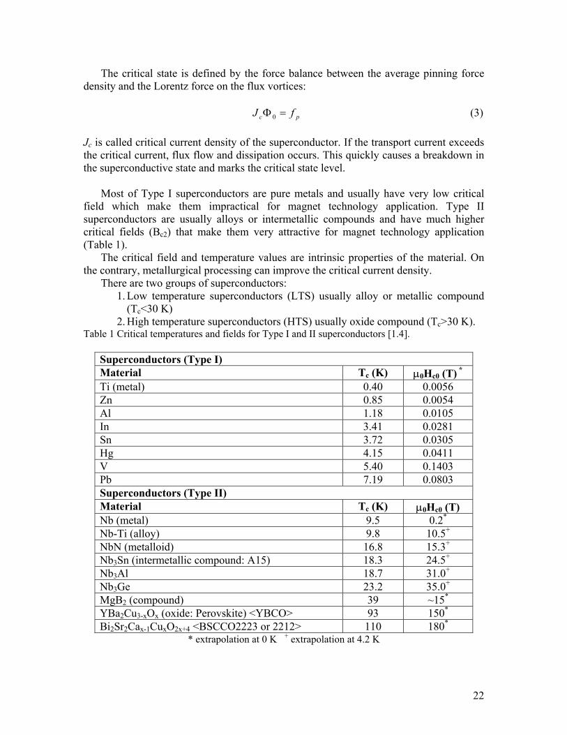
The critical state is defined by the force balance between the average pinning force density and the Lorentz force on the flux vortices:

pc fJ =Φ0 (3) Jc is called critical current density of the superconductor. If the transport current exceeds the critical current, flux flow and dissipation occurs. This quickly causes a breakdown in the superconductive state and marks the critical state level.

Most of Type I superconductors are pure metals and usually have very low critical field which make them impractical for magnet technology application. Type II superconductors are usually alloys or intermetallic compounds and have much higher critical fields (Bc2) that make them very attractive for magnet technology application (Table 1).

The critical field and temperature values are intrinsic properties of the material. On the contrary, metallurgical processing can improve the critical current density.

There are two groups of superconductors: 1. Low temperature superconductors (LTS) usually alloy or metallic compound

(Tc<30 K) 2. High temperature superconductors (HTS) usually oxide compound (Tc>30 K).

Table 1 Critical temperatures and fields for Type I and II superconductors [1.4].

Superconductors (Type I) Material Tc (K) µ0Hc0 (T) * Ti (metal) 0.40 0.0056 Zn 0.85 0.0054 Al 1.18 0.0105 In 3.41 0.0281 Sn 3.72 0.0305 Hg 4.15 0.0411 V 5.40 0.1403 Pb 7.19 0.0803 Superconductors (Type II) Material Tc (K) µ0Hc0 (T) Nb (metal) 9.5 0.2* Nb-Ti (alloy) 9.8 10.5+ NbN (metalloid) 16.8 15.3+ Nb3Sn (intermetallic compound: A15) 18.3 24.5+ Nb3Al 18.7 31.0+ Nb3Ge 23.2 35.0+ MgB2 (compound) 39 ~15* YBa2Cu3-xOx (oxide: Perovskite) <YBCO> 93 150* Bi2Sr2Cax-1CuxO2x+4 <BSCCO2223 or 2212> 110 180*

* extrapolation at 0 K + extrapolation at 4.2 K

23

Several remarks can be made regarding the different materials and their applications: • HTS conductors have much higher critical field and temperature but their

application have been limited due to their recent discovery, the lower critical current density at high fields and the high cost.

• For stability and protection purposes LTS strands contain copper while BSCCO (HTS) uses silver. This makes BSCCO strands much more expensive.

• YBCO and BSCCO-2212 are available only in tape geometry • BSCCO-2212 is competitive with other materials only at 4.2 K, limiting its high

temperature capability (Fig. 7) • Magnet grade conductors are presently limited to three materials: NbTi, Nb3Sn

and BSCCO-2223 • NbTi magnet technology is well established but the limited performance at high

fields is driving attention to other materials • LTS conductors are used by the High Energy Physics, Fusion Energy and

NMR/MRI communities • HTS conductors have a niche application for electric utility application

In Fig. 7 critical magnetic fields as a function of temperature are reported for

different superconducting materials.

Fig. 7 Critical field as a function of temperature for selected LTS and HTS superconductors, the critical field at 0 K is an extrapolation from values at 4.2 K [1.4].

24

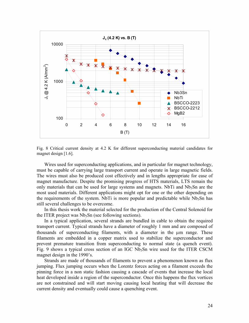
Fig. 8 Critical current density at 4.2 K for different superconducting material candidates for magnet design [1.6].

Wires used for superconducting applications, and in particular for magnet technology, must be capable of carrying large transport current and operate in large magnetic fields. The wires must also be produced cost effectively and in lengths appropriate for ease of magnet manufacture. Despite the promising progress of HTS materials, LTS remain the only materials that can be used for large systems and magnets. NbTi and Nb3Sn are the most used materials. Different applications might opt for one or the other depending on the requirements of the system. NbTi is more popular and predictable while Nb3Sn has still several challenges to be overcome.

In this thesis work the material selected for the production of the Central Solenoid for the ITER project was Nb3Sn (see following sections).

In a typical application, several strands are bundled in cable to obtain the required transport current. Typical strands have a diameter of roughly 1 mm and are composed of thousands of superconducting filaments, with a diameter in the µm range. These filaments are embedded in a copper matrix used to stabilize the superconductor and prevent premature transition from superconducting to normal state (a quench event). Fig. 9 shows a typical cross section of an IGC Nb3Sn wire used for the ITER CSCM magnet design in the 1990’s.

Strands are made of thousands of filaments to prevent a phenomenon known as flux jumping. Flux jumping occurs when the Lorentz forces acting on a filament exceeds the pinning force in a non static fashion causing a cascade of events that increase the local heat developed inside a region of the superconductor. Once this happens the flux vortices are not constrained and will start moving causing local heating that will decrease the current density and eventually could cause a quenching event.

Jc (4.2 K) vs. B (T)

100

1000

10000

0 2 4 6 8 10 12 14 16

B (T)

J c @

4.2

K (A

/mm

2 )

Nb3SnNbTiBSCCO-2223BSCCO-2212MgB2

25

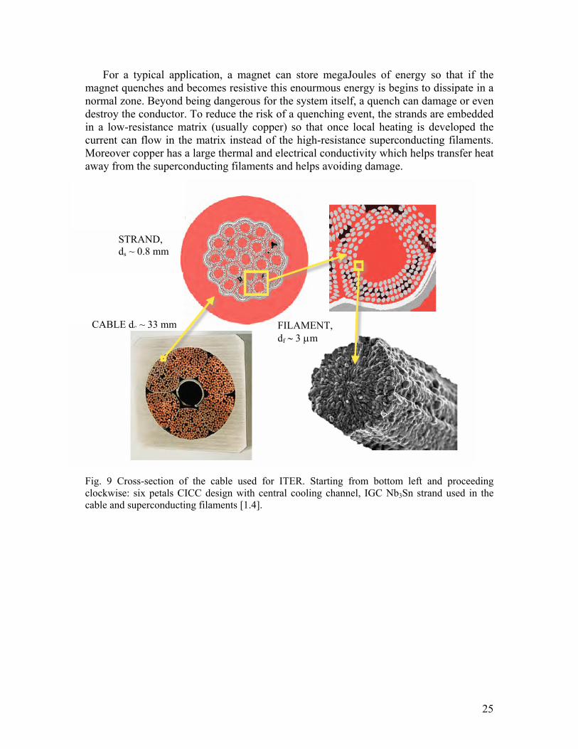
For a typical application, a magnet can store megaJoules of energy so that if the magnet quenches and becomes resistive this enourmous energy is begins to dissipate in a normal zone. Beyond being dangerous for the system itself, a quench can damage or even destroy the conductor. To reduce the risk of a quenching event, the strands are embedded in a low-resistance matrix (usually copper) so that once local heating is developed the current can flow in the matrix instead of the high-resistance superconducting filaments. Moreover copper has a large thermal and electrical conductivity which helps transfer heat away from the superconducting filaments and helps avoiding damage.

Fig. 9 Cross-section of the cable used for ITER. Starting from bottom left and proceeding clockwise: six petals CICC design with central cooling channel, IGC Nb3Sn strand used in the cable and superconducting filaments [1.4].

CABLE dc ~ 33 mm

STRAND, ds ~ 0.8 mm

FILAMENT, df ∼ 3 µm

26

1.2 Superconductivity Applications

Superconducting materials have their largest application in electromagnets. In fact they can achieve higher fields with less power consumption than normal conducting magnets. Though cryogenic systems are required, the overall cost for superconducting magnets is lower.

There are five major fields where superconductivity can be applied:

1. Fusion Energy

Fusion energy is one of the most promising sources of clean and abundant energy for the future. The International Thermonuclear Experimental Reactor (ITER) is the most immediate step towards the goal of demonstrating the feasibility of fusion energy. All the magnets in this tokamak are made of superconducting materials (NbTi and Nb3Sn). This thesis concerns one of the issues related to the superconducting cables of the machine and more details will be given in the following sections regarding the machine and the engineering challenges.

2. High Energy Physics

High field requirements turned the attention of high energy physics to superconducting magnets. In a particle accelerator, magnets are used to accelerate, focus and analyze beams of energetic particles. The project Large Hadron Collider (LHC) in Geneva will be operational in 2007 and contains over 1500 superconducting magnets to reach the designed collision energy of 14 TeV (the Tevatron in Fermilab is the world largest accelerator so far with a collision energy of “just” 1 TeV).

3. Magnetic Resonance Imaging (MRI)

Imaging techniques using magnetic resonance greatly improved the capabilities in diagnosing and treating medical problems. Superconducing magnets are widely used since they produce a very stable DC field with minimal power consumption. Moreover the magnetic fields required for MRI are well within the safe margin of operation for superconductors and avoid any quenching event and provide for magnetic field accuracy.

4. Superconducting Power Transmission Cables and Magnetic Energy Storage (SMES)

Since the energy in superconducting magnets can be virtually stored indefinitely, they are considered good energy storage devices. SMES are now commercially available and compatible with standard storage device for some application. Improvements for power grids are envisioned for the future. To

27

improve the power-handling capabilities of existing underground circuits even further, HTS power could substitute for the standard high-voltage cables. HTS transformers would also decrease the environmental contamination caused by spilling from oil-filled high voltage transformers.

5. Magnetic Levitation

The use of superconducting magnets would allow levitating trains on tracks in transportation applications. The main advantage of this is that these trains will not have the standard mechanical moving parts, which reduces part wear and maintenance.

1.3 Magnet Types and Cable-In-Conduit Conductor

Magnets can be divided in two categories depending on the type of cooling technique used:

1. Adiabatic Magnets

In these magnets the local coolant is eliminated and the entire winding space

unoccupied by the conductor is impregnated with epoxy, rendering the entire winding as one monolithic structure. The coolant is necessary but the conductor does not require direct contact with it. Rutherford cables (Fig. 10a-c) are usually used in these magnets. Epoxy impregnation is a critical operation. If the winding is not properly filled with epoxy, the magnet could be more susceptible to mechanical instabilities due to conductor movements (Fig. 10c). Adiabatic magnets are used for NMR, MRI and High Energy Physics dipoles and quadrupoles where the product RxJxB (force per unit area) is controllable using a composite conductor as a monolith entity.

Fig. 10 (a) Rutherford cable used for adiabatic magnets [1.7].

28

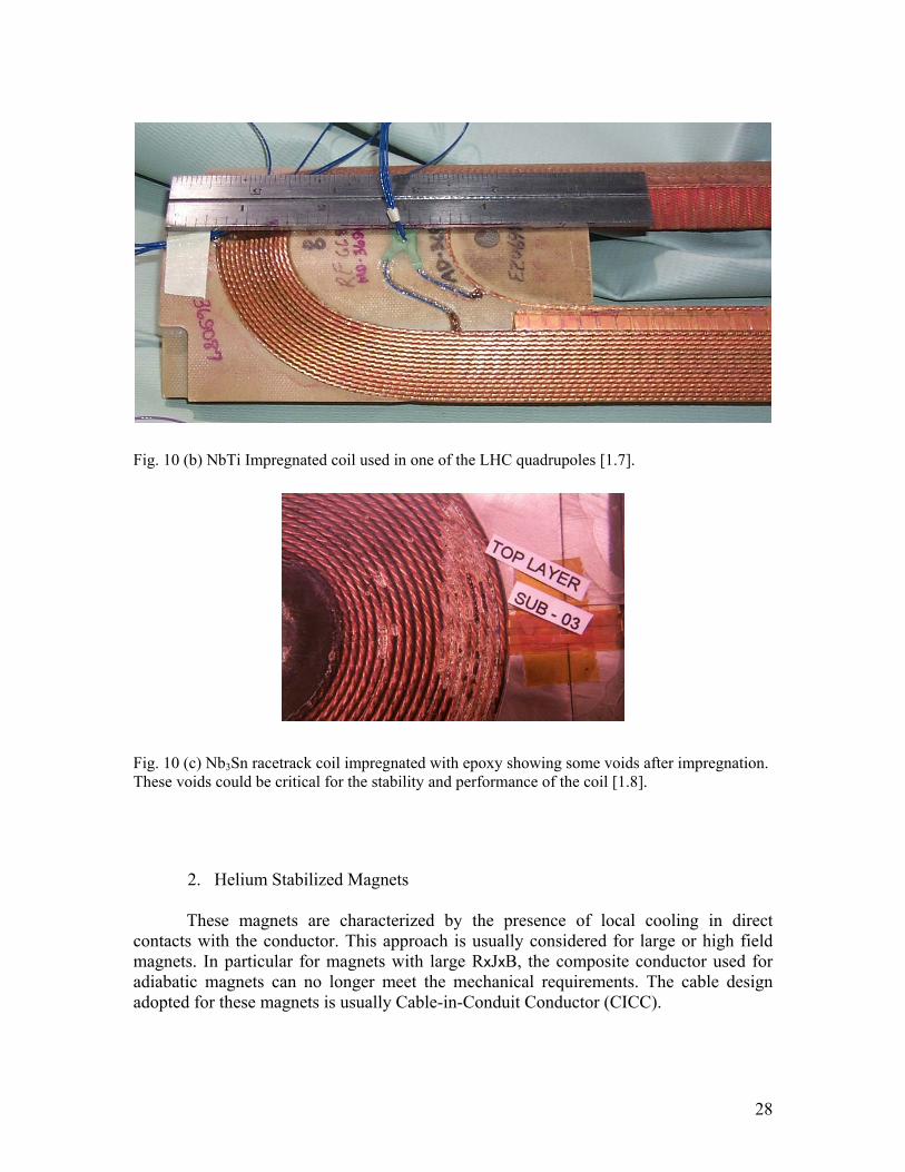
Fig. 10 (b) NbTi Impregnated coil used in one of the LHC quadrupoles [1.7].

Fig. 10 (c) Nb3Sn racetrack coil impregnated with epoxy showing some voids after impregnation. These voids could be critical for the stability and performance of the coil [1.8].

2. Helium Stabilized Magnets

These magnets are characterized by the presence of local cooling in direct contacts with the conductor. This approach is usually considered for large or high field magnets. In particular for magnets with large RxJxB, the composite conductor used for adiabatic magnets can no longer meet the mechanical requirements. The cable design adopted for these magnets is usually Cable-in-Conduit Conductor (CICC).

29

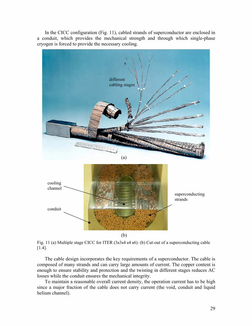
In the CICC configuration (Fig. 11), cabled strands of superconductor are enclosed in a conduit, which provides the mechanical strength and through which single-phase cryogen is forced to provide the necessary cooling.

Fig. 11 (a) Multiple stage CICC for ITER (3x3x4 x4 x6). (b) Cut-out of a superconducting cable [1.4].

The cable design incorporates the key requirements of a superconductor. The cable is

composed of many strands and can carry large amounts of current. The copper content is enough to ensure stability and protection and the twisting in different stages reduces AC losses while the conduit ensures the mechanical integrity.

To maintain a reasonable overall current density, the operation current has to be high since a major fraction of the cable does not carry current (the void, conduit and liquid helium channel).

cooling channel

conduit

superconducting strands

different cabling stages

(a)

(b)

30

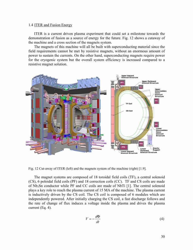
1.4 ITER and Fusion Energy

ITER is a current driven plasma experiment that could set a milestone towards the demonstration of fusion as a source of energy for the future. Fig. 12 shows a cutaway of the machine and a cross section of the magnets system.

The magnets of this machine will all be built with superconducting material since the field requirements cannot be met by resistive magnets, without an enormous amount of power to sustain the currents. On the other hand, superconducting magnets require power for the cryogenic system but the overall system efficiency is increased compared to a resistive magnet solution.

Fig. 12 Cut-away of ITER (left) and the magnets system of the machine (right) [1.9].

The magnet systems are composed of 18 toroidal field coils (TF), a central solenoid (CS), 6 poloidal field coils (PF) and 18 correction coils (CC). TF and CS coils are made of Nb3Sn conductor while PF and CC coils are made of NbTi [1]. The central solenoid plays a key role to reach the plasma current of 15 MA of the machine. The plasma current is inductively driven by the CS coil. The CS coil is composed of 6 modules which are independently powered. After initially charging the CS coil, a fast discharge follows and the rate of change of flux induces a voltage inside the plasma and drives the plasma current (Eq. 4).

dtdV Φ

−= (4)

31

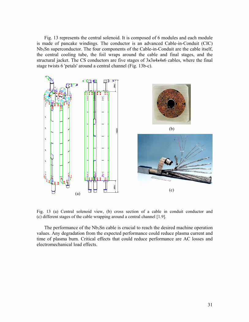
Fig. 13 represents the central solenoid. It is composed of 6 modules and each module

is made of pancake windings. The conductor is an advanced Cable-in-Conduit (CIC) Nb3Sn superconductor. The four components of the Cable-in-Conduit are the cable itself, the central cooling tube, the foil wraps around the cable and final stages, and the structural jacket. The CS conductors are five stages of 3x3x4x4x6 cables, where the final stage twists 6 'petals' around a central channel (Fig. 13b-c).

Fig. 13 (a) Central solenoid view, (b) cross section of a cable in conduit conductor and (c) different stages of the cable wrapping around a central channel [1.9].

The performance of the Nb3Sn cable is crucial to reach the desired machine operation values. Any degradation from the expected performance could reduce plasma current and time of plasma burn. Critical effects that could reduce performance are AC losses and electromechanical load effects.

(b)

(c)(a)

32

1.5 Scope of Thesis

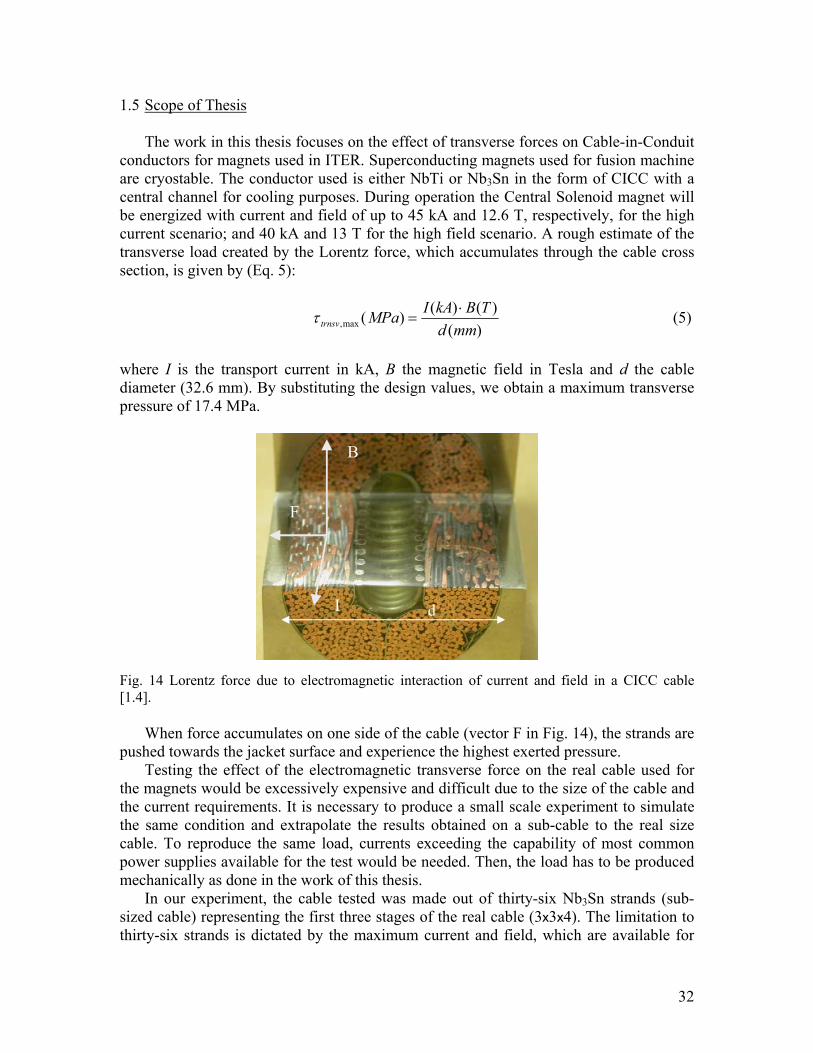
The work in this thesis focuses on the effect of transverse forces on Cable-in-Conduit conductors for magnets used in ITER. Superconducting magnets used for fusion machine are cryostable. The conductor used is either NbTi or Nb3Sn in the form of CICC with a central channel for cooling purposes. During operation the Central Solenoid magnet will be energized with current and field of up to 45 kA and 12.6 T, respectively, for the high current scenario; and 40 kA and 13 T for the high field scenario. A rough estimate of the transverse load created by the Lorentz force, which accumulates through the cable cross section, is given by (Eq. 5):

)()()()(max, mmd

TBkAIMPatrnsv⋅

=τ (5)

where I is the transport current in kA, B the magnetic field in Tesla and d the cable diameter (32.6 mm). By substituting the design values, we obtain a maximum transverse pressure of 17.4 MPa. Fig. 14 Lorentz force due to electromagnetic interaction of current and field in a CICC cable [1.4].

When force accumulates on one side of the cable (vector F in Fig. 14), the strands are pushed towards the jacket surface and experience the highest exerted pressure.

Testing the effect of the electromagnetic transverse force on the real cable used for the magnets would be excessively expensive and difficult due to the size of the cable and the current requirements. It is necessary to produce a small scale experiment to simulate the same condition and extrapolate the results obtained on a sub-cable to the real size cable. To reproduce the same load, currents exceeding the capability of most common power supplies available for the test would be needed. Then, the load has to be produced mechanically as done in the work of this thesis.

In our experiment, the cable tested was made out of thirty-six Nb3Sn strands (sub-sized cable) representing the first three stages of the real cable (3x3x4). The limitation to thirty-six strands is dictated by the maximum current and field, which are available for

B

I

F

B

I

F

d

33

our experiment. The test was performed at NHMFL with a probe with 10 kA current leads and a solenoid of 20 T maximum field.

Since the Lorentz force created during operation is not electromagnetically reproducible in the experimental set up, we designed a probe so that an artificial mechanical transverse stress could be applied.

The scope of this work is to apply a known transverse pressure on the cable and record any visible degradation of its superconducting properties (in particular degradation in the expected critical current).

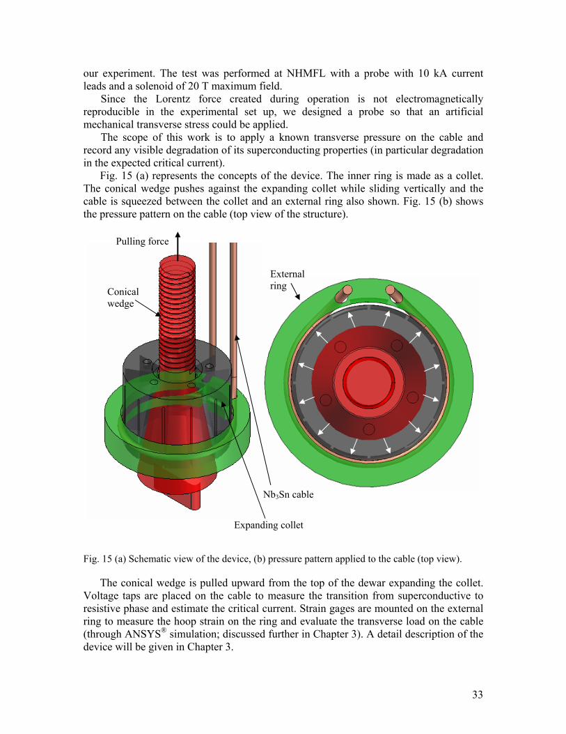
Fig. 15 (a) represents the concepts of the device. The inner ring is made as a collet. The conical wedge pushes against the expanding collet while sliding vertically and the cable is squeezed between the collet and an external ring also shown. Fig. 15 (b) shows the pressure pattern on the cable (top view of the structure).

Fig. 15 (a) Schematic view of the device, (b) pressure pattern applied to the cable (top view).

The conical wedge is pulled upward from the top of the dewar expanding the collet. Voltage taps are placed on the cable to measure the transition from superconductive to resistive phase and estimate the critical current. Strain gages are mounted on the external ring to measure the hoop strain on the ring and evaluate the transverse load on the cable (through ANSYS® simulation; discussed further in Chapter 3). A detail description of the device will be given in Chapter 3.

Nb3Sn cable

Expanding collet

Pulling force

Conical wedge

External ring

34

CHAPTER 2: Strain characteristics of superconducting wires and cables

As seen in Chapter 1, superconductivity depends on three main parameters that describe a critical surface underneath which the material is superconducting. Later discoveries showed that superconductors are also sensitive to strain effects.

A lot of work has been done on the subject of strain effect on superconductor strands beginning about two decades ago. The attention was mainly focused on axial strain effect on the critical current of single strands. Later on the transverse strain effect on a single strand was studied, showing a much sharper degradation due to this effect than that of axial strain. Less attention has been paid in understanding the axial and transverse strain effects on a cable. In particular, the transverse strain effect is dominant for fusion type of magnets (having a void fraction of ~35-40%) but it is not an issue for high energy physics application where magnets are usually impregnated [2.1].

This chapter summarizes the previous work by other researchers to study this effect. After a brief introduction regarding the strain effects on superconducting strands and cables, a summary of different experiments done so far will be given starting with uniaxial strain effect on single strand, pinching and bending loads on single strands, tests of sub-size cables under axial strain, transverse load effect on single strand and tests on sub-sized cables under transverse load. The background given with this summary is relevant to explain the importance of the experiment carried out with this work, since very little has been done so fare and even more its unique setup. 2.1 Introduction

In this chapter a brief history of experiments dealing with the axial and transverse

effects on superconductors performances is reported. Besides the dependence on current density, field and temperature, the performance of a superconductor strand or cable is affected by axial and transverse strain. The latter has a more accentuated effect and the degradation due to transverse strain is up to one order of magnitude greater than the degradation due to axial strain (at the same level of strain) [2.3].

The sensitivity of a Nb3Sn superconductor to transverse loading is dependent on a large number of factors, including the copper/non-copper ratio (quantity that defines the amount of copper over the total amount of material in a strand), the ratio of distance between contact points to the strand diameter, void fraction constraints on strand deflection, pre-compression strain, heat treatment, and the exact material composition of the non-copper region. A monolith or single strand is expected to be an order of magnitude more sensitive to transverse load than to longitudinal load (Fig. 13 later this chapter) and a cable to be two orders of magnitude more sensitive [2.2-2.3].

The larger degradation, for a single strand, caused by transverse load (a factor of 10 larger than the longitudinal case) is believed to be due to the multiplier of deviatoric strain in a composite, in which the transverse compression on a composite with a stiff, unyielding component and a soft, yielding component is translated into a longitudinal tensile strain in the stiffer. In fact, a superconducting strand is composed of copper (the

35

soft component) and non-copper material (the stiff component), which includes Nb3Sn, a barrier (usually tantalum) and bronze. The copper is the low resistance stabilizer where the current flows during a transition to the normal state. The barrier is needed to separate high purity copper from the rest of the composite, which contains bronze, Nb and Sn.

In a cable the degradation due to transverse loads is even more accentuated (~100 times larger than the longitudinal case) [2.2]. A possible explanation for this behavior is the presence of an additional bending effect of each strand inside a cable due to the twisting of the strands around each other [2.2-2.4].

2.2 Axial strain effect

Before summarizing the results of different studies, a series of definition is required. Experiments are usually done with a fixed temperature (usually 4.2 K for Nb3Sn) and a fixed background field. Critical currents are usually measured and a so-called “critical current criterion” is used to determine the critical current. The definition can be understood considering an example.

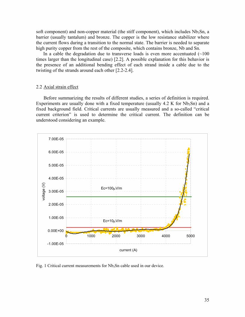
Fig. 1 Critical current measurements for Nb3Sn cable used in our device.

-1.00E-05

0.00E+00

1.00E-05

2.00E-05

3.00E-05

4.00E-05

5.00E-05

6.00E-05

7.00E-05

0 1000 2000 3000 4000 5000

current (A)

volta

ge (V

)

Ec=100µV/m

Ec=10µV/m

36

Fig. 1 represents the typical voltage-current curve during a critical current measurement. In this particular case the temperature was 4.2 K and the background field was 10 T. As the current is increased, the voltage is zero and within the noise level (resistance at this stage is zero as expected from a superconductor) up to a level when the cable starts showing a resistive component (in the Fig. shown around 4 kA). The growth of the voltage as a function of a current is usually described as an exponential [2.5]:

n

cc II

VV

=

(1)

where V and I are the voltage and current to pre-chosen critical values Vc and Ic. The exponent of this relationship is n called “n-value”, often used to describe the sharpness of the transition from superconductive to resistive state. More often two different criterions are used to evaluate the n-value:

n

c

c

c

c

II

VV

=

2

1

2

1 (2)

=

2

1

2

1 lnlnc

c

c

c

II

VV

n (3)

Usually the criteria used are Ec1=100 µV/m, Ec2=10 µV/m, with the corresponding

voltages calculated by multiplying by the distance between the two points from which the voltage is recorded (voltage tap length). The higher the criterion, the less accurate the calculated critical current. In our example, the voltage data were filtered and the offset of the measurement was taken out. The data points are fitted with a polynomial and the intersections of this curve with the two chosen criteria give the two critical currents and permit the determination of the n-value.

A superconducting strand is usually purchased with a specific critical current and n-value provided by the vendor so that expectation values of critical currents can be estimated before the experiment is set up. More details on how all these parameters are evaluated will be given in following chapters during the description of the device and the data taken during the experiment.

Now that a few necessary definitions are given, a summary of the experiments done so far will follow.

Ekin [2.6], carried out a formal relationship for strain scaling based on experimental results using an apparatus which applied simultaneously tensile strain, current and a perpendicular field to a short conductor. Studies were done at a fixed current while varying the other variables. The dependence on field, strain and temperature effects were empirically determined from these measurements.

The sample was secured at either end by soldering it onto two copper blocks. One of the two copper blocks could be moved allowing for the application of tension on the pull rod attached to a lever arm.

The strain was directly measured with a four-strain-gauge extensometer. The critical current criterion used was 200 µV/m and the accuracy in the measurements was 0.5%.

37

Several different specimens were used and it was possible to find a “universal” relationship describing the behavior of strands under axial strain:

)()]([)()( *2 bfBbfKF n

c εε == (4) where F is the pinning force density and b is the reduced field b = B/B*

c2 with B*c2 strain

dependent bulk upper-critical field. The strain dependence of B*

c2 was found to be

)1()( *2

*2

ummcc aBB εεε −−= (5)

where the maximum value, B*

c2m, occurs at εm. For highly reacted Nb3Sn conductors u ≅ 1.7 and a ≅ 900 for ε < εm and a ≅ 1250 for

ε > εm. For insitu (external tin diffusion) and partially reacted Nb3Sn conductors a is smaller (less sensitivity to strain).

This strain scaling relationship can then be combined with the temperature scaling relationship to get the general scaling law for the dependence of F on both strain and temperature:

)()1()1(),,( 2 bftaTBF num

νεεε −−−= (6) with n ≅ 1, ν ≅ 2.5, t = T/T*

c (ε). This equation can be found by postulating the dependence of B*

c2 on temperature and strain as:

wumcmc

cw

cc

aTT

TTTTB/1**

2***2

)1()(

)](/[1)]([),(

εεε

εεε

−−=

−= (7)

where w ≅ 3.

Several measurements were done by Ekin and used to develop and verify the validity of this equation for uniaxial strain in a single strand.

Most of the experiments (especially at the University of Twente) focus on the axial strain dependence of single strands hoping to find better universal scaling laws describing the dependence of critical parameters on axial strain. Unfortunately extrapolations from single strand results to a prediction for a cable are not easily carried out and are very much dependent on the application for which the strand is used.

38

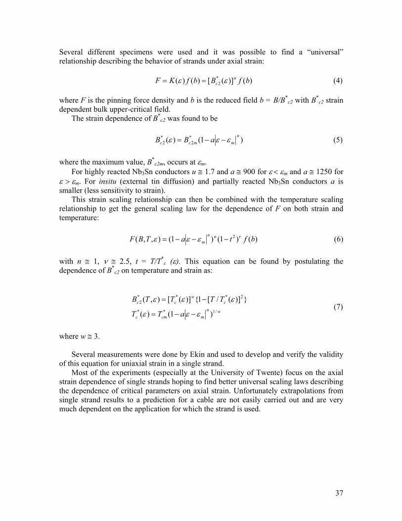
2.2.1 Single strand in uniaxial strain

There are three devices that are most used in studying the strain behavior of superconductors: the U-spring holder, the device called “Pacman”, and the Walters springs. These devices are the most common used to improve the scaling laws used to estimate the critical current of single strand under the effect of uniaxial strain (tension r compression).

In the U-spring device (Fig. 2) the sample is mounted across a bridge that can be in the tensile or compressive regime depending on the movement of the device’s legs. It is really reliable but limited by the length of the sample measured [2.7]. The longer the sample the easier is to measure the critical current because the distance between voltage taps can be longer reducing the voltage to noise ratio in the signal.

Fig. 2 U-spring strain device [2.7].

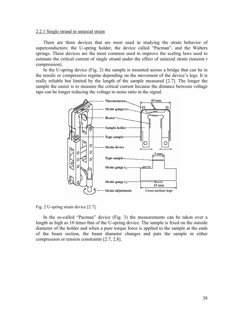
In the so-called “Pacman” device (Fig. 3) the measurements can be taken over a

length as high as 10 times that of the U-spring device. The sample is fixed on the outside diameter of the holder and when a pure torque force is applied to the sample at the ends of the beam section, the beam diameter changes and puts the sample in either compression or tension constraints [2.7, 2.8].

39

Fig. 3 Pacman strain device [2.7, 2.8].

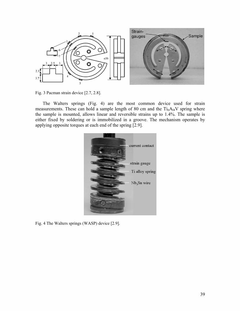
The Walters springs (Fig. 4) are the most common device used for strain measurements. These can hold a sample length of 80 cm and the Ti6Al4V spring where the sample is mounted, allows linear and reversible strains up to 1.4%. The sample is either fixed by soldering or is immobilized in a groove. The mechanism operates by applying opposite torques at each end of the spring [2.9].

Fig. 4 The Walters springs (WASP) device [2.9].

40

2.1.2 Single strand under pinching and bending loads

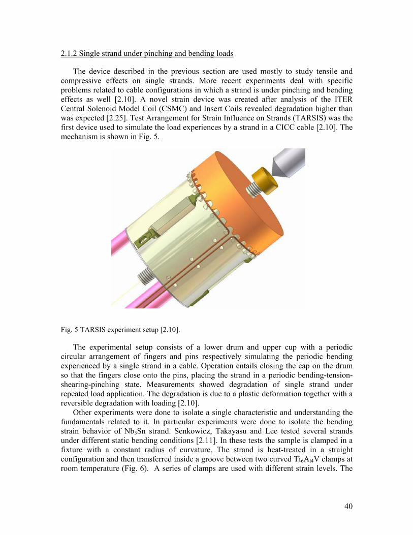
The device described in the previous section are used mostly to study tensile and compressive effects on single strands. More recent experiments deal with specific problems related to cable configurations in which a strand is under pinching and bending effects as well [2.10]. A novel strain device was created after analysis of the ITER Central Solenoid Model Coil (CSMC) and Insert Coils revealed degradation higher than was expected [2.25]. Test Arrangement for Strain Influence on Strands (TARSIS) was the first device used to simulate the load experiences by a strand in a CICC cable [2.10]. The mechanism is shown in Fig. 5.

Fig. 5 TARSIS experiment setup [2.10].

The experimental setup consists of a lower drum and upper cup with a periodic circular arrangement of fingers and pins respectively simulating the periodic bending experienced by a single strand in a cable. Operation entails closing the cap on the drum so that the fingers close onto the pins, placing the strand in a periodic bending-tension-shearing-pinching state. Measurements showed degradation of single strand under repeated load application. The degradation is due to a plastic deformation together with a reversible degradation with loading [2.10].

Other experiments were done to isolate a single characteristic and understanding the fundamentals related to it. In particular experiments were done to isolate the bending strain behavior of Nb3Sn strand. Senkowicz, Takayasu and Lee tested several strands under different static bending conditions [2.11]. In these tests the sample is clamped in a fixture with a constant radius of curvature. The strand is heat-treated in a straight configuration and then transferred inside a groove between two curved Ti6Al4V clamps at room temperature (Fig. 6). A series of clamps are used with different strain levels. The

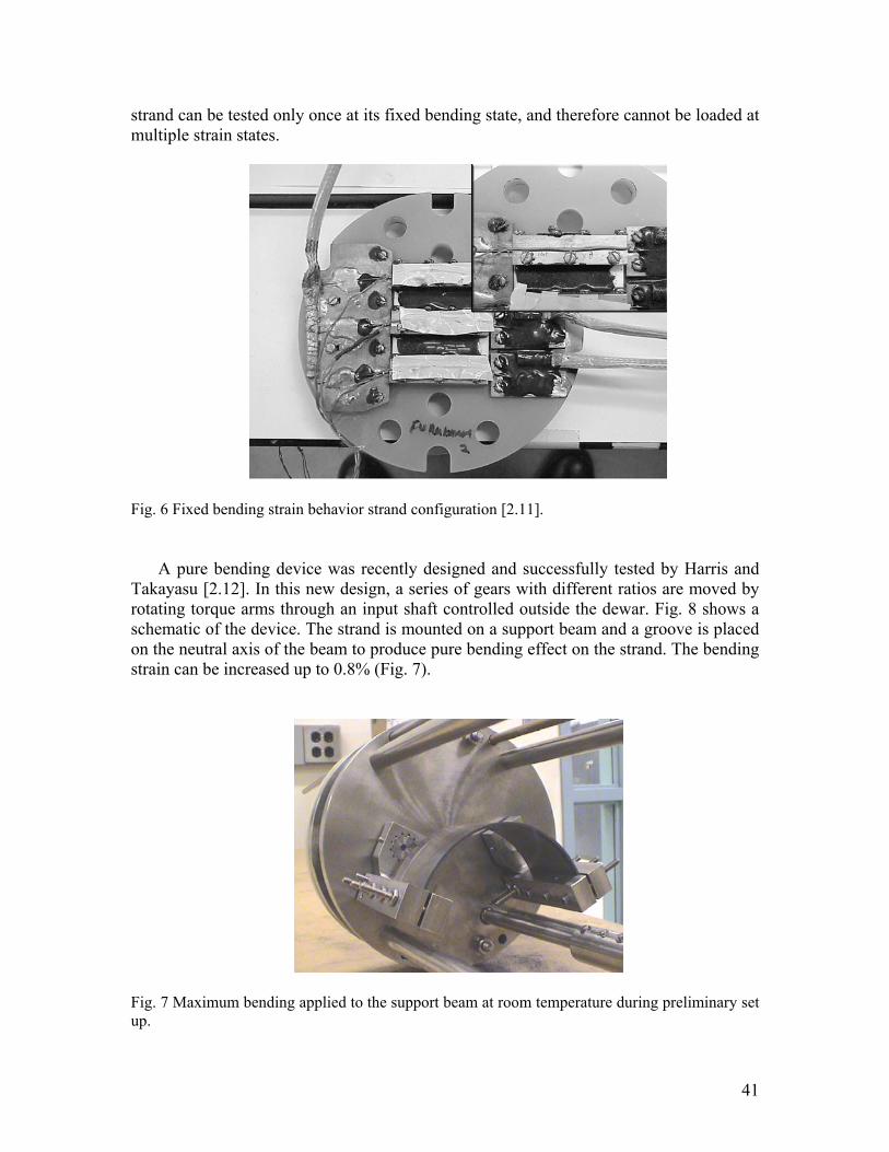
41

strand can be tested only once at its fixed bending state, and therefore cannot be loaded at multiple strain states.

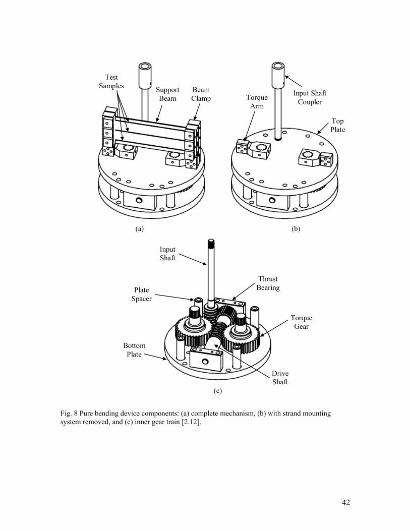
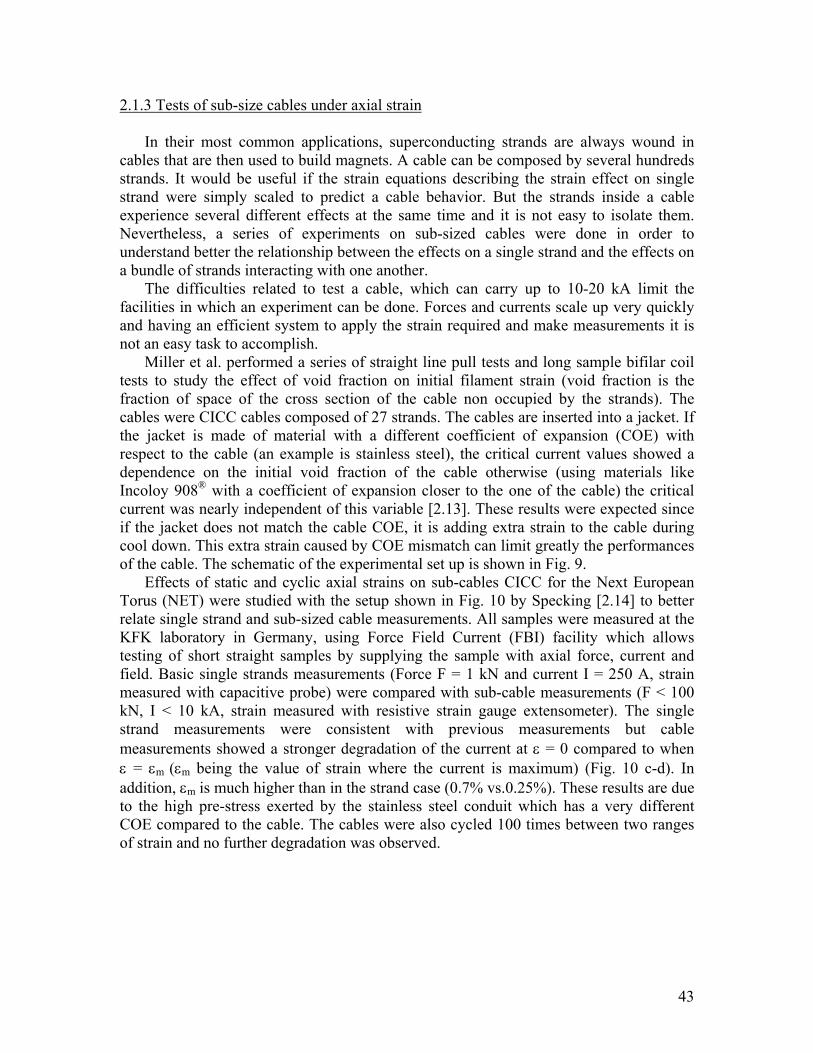
Fig. 6 Fixed bending strain behavior strand configuration [2.11]. A pure bending device was recently designed and successfully tested by Harris and

Takayasu [2.12]. In this new design, a series of gears with different ratios are moved by rotating torque arms through an input shaft controlled outside the dewar. Fig. 8 shows a schematic of the device. The strand is mounted on a support beam and a groove is placed on the neutral axis of the beam to produce pure bending effect on the strand. The bending strain can be increased up to 0.8% (Fig. 7).

Fig. 7 Maximum bending applied to the support beam at room temperature during preliminary set up.

42

(a) (b)

(c)

Beam Clamp

Test Samples Support

Beam Input Shaft

Coupler Torque Arm

Top Plate

Input Shaft

Drive Shaft

Plate Spacer

Bottom Plate

Torque Gear

Thrust Bearing

Fig. 8 Pure bending device components: (a) complete mechanism, (b) with strand mounting system removed, and (c) inner gear train [2.12].

43

2.1.3 Tests of sub-size cables under axial strain

In their most common applications, superconducting strands are always wound in cables that are then used to build magnets. A cable can be composed by several hundreds strands. It would be useful if the strain equations describing the strain effect on single strand were simply scaled to predict a cable behavior. But the strands inside a cable experience several different effects at the same time and it is not easy to isolate them. Nevertheless, a series of experiments on sub-sized cables were done in order to understand better the relationship between the effects on a single strand and the effects on a bundle of strands interacting with one another.

The difficulties related to test a cable, which can carry up to 10-20 kA limit the facilities in which an experiment can be done. Forces and currents scale up very quickly and having an efficient system to apply the strain required and make measurements it is not an easy task to accomplish.

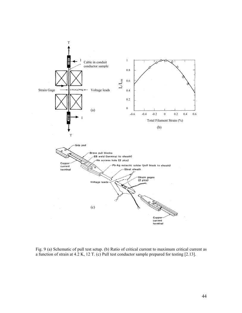
Miller et al. performed a series of straight line pull tests and long sample bifilar coil tests to study the effect of void fraction on initial filament strain (void fraction is the fraction of space of the cross section of the cable non occupied by the strands). The cables were CICC cables composed of 27 strands. The cables are inserted into a jacket. If the jacket is made of material with a different coefficient of expansion (COE) with respect to the cable (an example is stainless steel), the critical current values showed a dependence on the initial void fraction of the cable otherwise (using materials like Incoloy 908® with a coefficient of expansion closer to the one of the cable) the critical current was nearly independent of this variable [2.13]. These results were expected since if the jacket does not match the cable COE, it is adding extra strain to the cable during cool down. This extra strain caused by COE mismatch can limit greatly the performances of the cable. The schematic of the experimental set up is shown in Fig. 9.

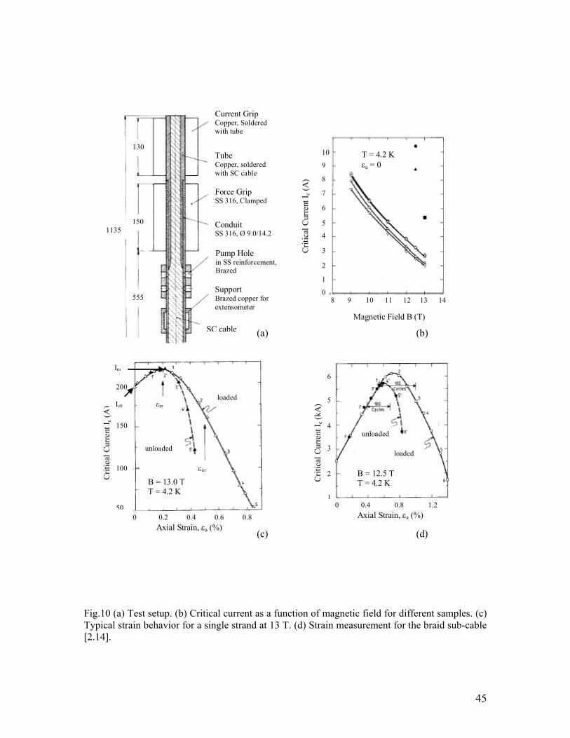
Effects of static and cyclic axial strains on sub-cables CICC for the Next European Torus (NET) were studied with the setup shown in Fig. 10 by Specking [2.14] to better relate single strand and sub-sized cable measurements. All samples were measured at the KFK laboratory in Germany, using Force Field Current (FBI) facility which allows testing of short straight samples by supplying the sample with axial force, current and field. Basic single strands measurements (Force F = 1 kN and current I = 250 A, strain measured with capacitive probe) were compared with sub-cable measurements (F < 100 kN, I < 10 kA, strain measured with resistive strain gauge extensometer). The single strand measurements were consistent with previous measurements but cable measurements showed a stronger degradation of the current at ε = 0 compared to when ε = εm (εm being the value of strain where the current is maximum) (Fig. 10 c-d). In addition, εm is much higher than in the strand case (0.7% vs.0.25%). These results are due to the high pre-stress exerted by the stainless steel conduit which has a very different COE compared to the cable. The cables were also cycled 100 times between two ranges of strain and no further degradation was observed.

44

Fig. 9 (a) Schematic of pull test setup. (b) Ratio of critical current to maximum critical current as a function of strain at 4.2 K, 12 T. (c) Pull test conductor sample prepared for testing [2.13].

(a)

(b)

(c)

Voltage leads

Cable in conduit conductor sample

Strain Gage

I

I

T

T

Total Filament Strain (%) I c/

I cm

-0.6 -0.4 -0.2 0 0.2 0.4 0.6

1 0.8 0.6 0.4

0.2

0

-0.6

45

Fig.10 (a) Test setup. (b) Critical current as a function of magnetic field for different samples. (c) Typical strain behavior for a single strand at 13 T. (d) Strain measurement for the braid sub-cable [2.14].

(a) (b)

(c) (d)

Current Grip Copper, Soldered with tube

Tube Copper, soldered with SC cable

Force Grip SS 316, Clamped

Conduit SS 316, Ø 9.0/14.2

Pump Holein SS reinforcement, Brazed

Support Brazed copper for extensometer

SC cable

130

150 1135

555

T = 4.2 K εa = 0

Magnetic Field B (T)

10

9

8

7 6 5

4 3 2

1

0 8 9 10 11 12 13 14

Axial Strain, εa (%) Axial Strain, εa (%)

Crit

ical

Cur

rent

I c (A

)

Crit

ical

Cur

rent

I c (k

A)

200

150 100

500 0.2 0.4 0.6 0.8

0 0.4 0.8 1.2

6 5 4

3 2 1

loaded

unloaded

εm

Im

Ic0

εirr

B = 13.0 T T = 4.2 K

B = 12.5 TT = 4.2 K

loaded

unloaded

Criti

cal C

urre

nt I c

(A)

46

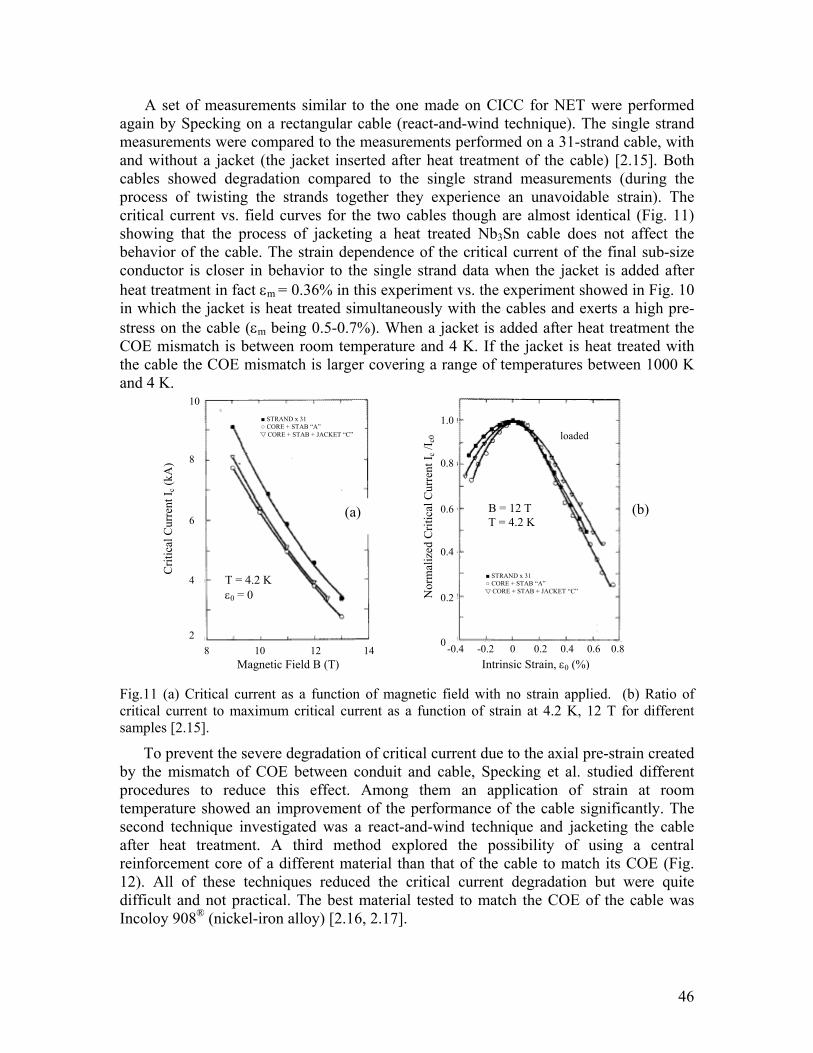
A set of measurements similar to the one made on CICC for NET were performed again by Specking on a rectangular cable (react-and-wind technique). The single strand measurements were compared to the measurements performed on a 31-strand cable, with and without a jacket (the jacket inserted after heat treatment of the cable) [2.15]. Both cables showed degradation compared to the single strand measurements (during the process of twisting the strands together they experience an unavoidable strain). The critical current vs. field curves for the two cables though are almost identical (Fig. 11) showing that the process of jacketing a heat treated Nb3Sn cable does not affect the behavior of the cable. The strain dependence of the critical current of the final sub-size conductor is closer in behavior to the single strand data when the jacket is added after heat treatment in fact εm = 0.36% in this experiment vs. the experiment showed in Fig. 10 in which the jacket is heat treated simultaneously with the cables and exerts a high pre-stress on the cable (εm being 0.5-0.7%). When a jacket is added after heat treatment the COE mismatch is between room temperature and 4 K. If the jacket is heat treated with the cable the COE mismatch is larger covering a range of temperatures between 1000 K and 4 K.

Fig.11 (a) Critical current as a function of magnetic field with no strain applied. (b) Ratio of critical current to maximum critical current as a function of strain at 4.2 K, 12 T for different samples [2.15].

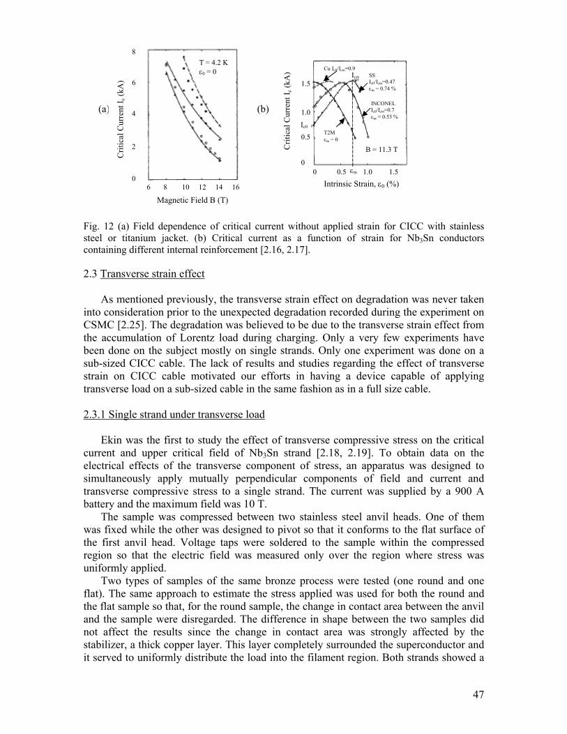
To prevent the severe degradation of critical current due to the axial pre-strain created by the mismatch of COE between conduit and cable, Specking et al. studied different procedures to reduce this effect. Among them an application of strain at room temperature showed an improvement of the performance of the cable significantly. The second technique investigated was a react-and-wind technique and jacketing the cable after heat treatment. A third method explored the possibility of using a central reinforcement core of a different material than that of the cable to match its COE (Fig. 12). All of these techniques reduced the critical current degradation but were quite difficult and not practical. The best material tested to match the COE of the cable was Incoloy 908® (nickel-iron alloy) [2.16, 2.17].

(b) (a)

Crit

ical

Cur

rent

I c (k

A)

Nor

mal

ized

Crit

ical

Cur

rent

I c /I

c0

Magnetic Field B (T) Intrinsic Strain, ε0 (%)

10

8

6

4 2

8 10 12 14 -0.4 -0.2 0 0.2 0.4 0.6 0.8

1.0

0.8

0.6

0.4 0.2

0

T = 4.2 K ε0 = 0

B = 12 T T = 4.2 K

loaded

STRAND x 31 CORE + STAB “A” CORE + STAB + JACKET “C”

STRAND x 31 CORE + STAB “A” CORE + STAB + JACKET “C”

47

Fig. 12 (a) Field dependence of critical current without applied strain for CICC with stainless steel or titanium jacket. (b) Critical current as a function of strain for Nb3Sn conductors containing different internal reinforcement [2.16, 2.17].

2.3 Transverse strain effect

As mentioned previously, the transverse strain effect on degradation was never taken into consideration prior to the unexpected degradation recorded during the experiment on CSMC [2.25]. The degradation was believed to be due to the transverse strain effect from the accumulation of Lorentz load during charging. Only a very few experiments have been done on the subject mostly on single strands. Only one experiment was done on a sub-sized CICC cable. The lack of results and studies regarding the effect of transverse strain on CICC cable motivated our efforts in having a device capable of applying transverse load on a sub-sized cable in the same fashion as in a full size cable. 2.3.1 Single strand under transverse load

Ekin was the first to study the effect of transverse compressive stress on the critical current and upper critical field of Nb3Sn strand [2.18, 2.19]. To obtain data on the electrical effects of the transverse component of stress, an apparatus was designed to simultaneously apply mutually perpendicular components of field and current and transverse compressive stress to a single strand. The current was supplied by a 900 A battery and the maximum field was 10 T.

The sample was compressed between two stainless steel anvil heads. One of them was fixed while the other was designed to pivot so that it conforms to the flat surface of the first anvil head. Voltage taps were soldered to the sample within the compressed region so that the electric field was measured only over the region where stress was uniformly applied.

Two types of samples of the same bronze process were tested (one round and one flat). The same approach to estimate the stress applied was used for both the round and the flat sample so that, for the round sample, the change in contact area between the anvil and the sample were disregarded. The difference in shape between the two samples did not affect the results since the change in contact area was strongly affected by the stabilizer, a thick copper layer. This layer completely surrounded the superconductor and it served to uniformly distribute the load into the filament region. Both strands showed a

(a) (b)

Magnetic Field B (T) 6 8 10 12 14 16

Crit

ical

Cur

rent

I c (k

A)

8

6

4

2 0

T = 4.2 Kε0 = 0

0 0.5 1.0 1.5

Intrinsic Strain, ε0 (%)

1.5

1.0

0.5 0

Crit

ical

Cur

rent

I c (k

A)

B = 11.3 T

Cu Ic0/Icm=0.9 SS Ic0/Icm=0.47 εm = 0.74 %

INCONEL Ic0/Icm=0.7 εm = 0.53 %

εm

T2M εm = 0

Icm

Ic0

48

strong degradation as a function of transverse stress applied and the effect was much more severe than in the case of uniaxial strain. A simplified explanation for this difference was that, under axial strain, the axial force is apportioned among the various composite materials because they occupied parallel load-bearing paths while, in the transverse case, all the components of the composite experienced the same stress which was transferred from one material to the next in a serial load chain. For the transverse stress at 10 T, the degradation was 10% under a compressive pressure of 50 MPa. This degradation rises to nearly 30% at 100 MPa. For the axial strain, the degradation was less than 2% at up to about 200 MPa. The stress, which causes a given amount of critical current degradation at 10 T, was usually seven times less for transverse stress than for axial stress (and was greater at higher fields). The critical current degradation was noted to be reversible in character.

The main difference between the two samples tested was that while the round sample had a curve centered at zero-stress value (it had its maximum at this value), the flat sample critical current was somewhat shifted and had its maximum value at a small but finite compressive value. This peak is caused by anisotropic pre-compression from the thermal contraction of the matrix material. After cool down from reacting the Nb3Sn, this result in a less compression by the bronze matrix along the shorter axis than along the longer axis. Thus the Nb3Sn filaments in the flat sample are under more thermal pre-compression along their width than their narrow dimension. This can be easily seen from the distortional strain expression (eq. 8):

2/122212/1 ])()()[()1(2 xzzyyx εεεεεενε −+−+−+= − (8)

where ν is the Poisson ratio. This represents the distorsional strain state of the material. Anisotropic thermal pre-compression along the horizontal (x) and vertical (y) axes of the flat sample leads to a compressive pre-strain along the y axis which is less than along the x axis, so that the first term in eq. 8 is finite. As external pressure is applied along the y axis, the initial effect is to remove the distortional strain between the x and y axes reducing the difference between εx and εy. This effect reduces the distortional geometric average strain and increases the critical current. As more transverse stress is applied the critical current eventually passes through a maximum and then decreases.

The authors claimed that a possible explanation for the differences in behavior under axial or transversal stress could be due to a preferred crystal growth orientation in the Nb3Sn reaction layer. In fact the growth pattern in multifilamentary samples was radial within each filament, which would define anisotropy between axial and transverse properties. They underlined the importance of having a 3-D treatment of strain through deviatoric strain to better study the connection of axial and transverse strain, which usually acted simultaneously.

It has to be noticed that the transverse stress effect is usually about an order of magnitude greater that axial strain effect, but its relative importance is tempered by the fact that axial stresses in Nb3Sn filaments can accumulate to much higher values. This is due to the fact that the axial stress on the conductor is concentrated in the Nb3Sn filaments with the majority of the conductor cross section (copper and bronze) not bearing much of the load. The paper also proposed law scales for axial and transverse stress, which helped determine the limitation on the size of the cable and the conductor.

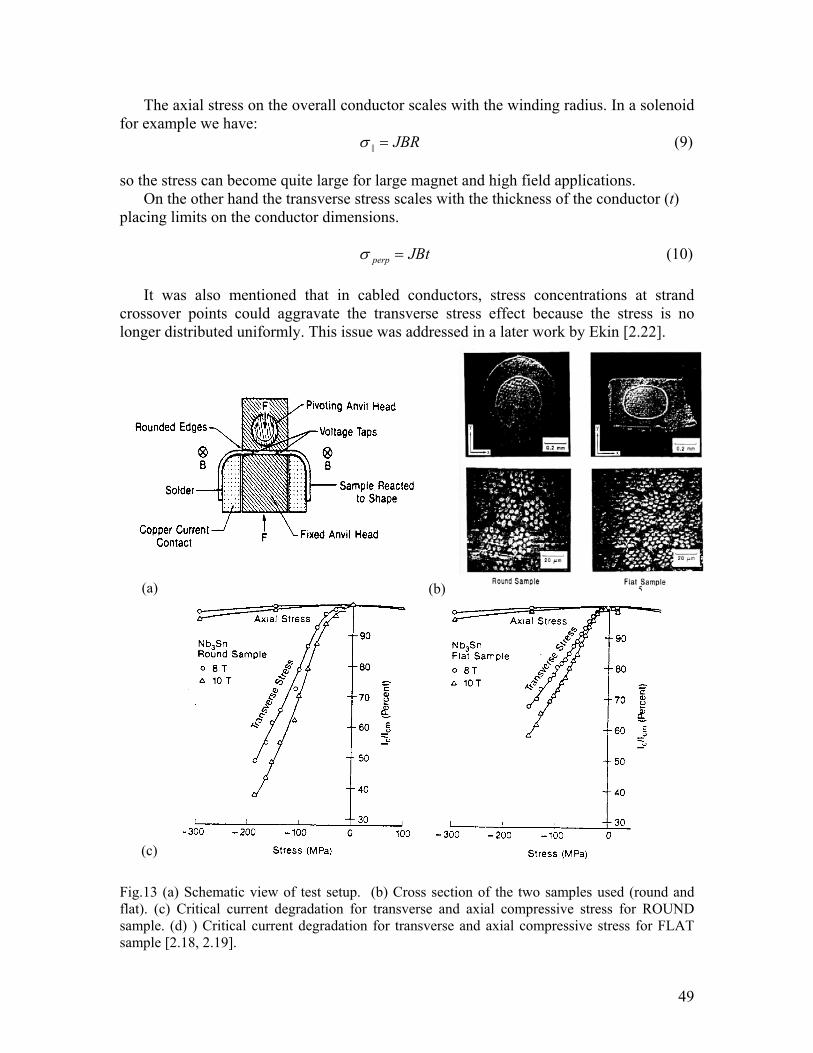
49

The axial stress on the overall conductor scales with the winding radius. In a solenoid for example we have:

σ || = JBR (9)

so the stress can become quite large for large magnet and high field applications. On the other hand the transverse stress scales with the thickness of the conductor (t)

placing limits on the conductor dimensions.

σ perp JBt= (10) It was also mentioned that in cabled conductors, stress concentrations at strand

crossover points could aggravate the transverse stress effect because the stress is no longer distributed uniformly. This issue was addressed in a later work by Ekin [2.22].

Fig.13 (a) Schematic view of test setup. (b) Cross section of the two samples used (round and flat). (c) Critical current degradation for transverse and axial compressive stress for ROUND sample. (d) ) Critical current degradation for transverse and axial compressive stress for FLAT sample [2.18, 2.19].

(a) (b)

(c)

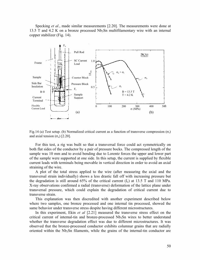
50

Specking et al., made similar measurements [2.20]. The measurements were done at 13.5 T and 4.2 K on a bronze processed Nb3Sn multifilamentary wire with an internal copper stabilizer (Fig. 14).

Fig.14 (a) Test setup. (b) Normalized critical current as a function of transverse compression (σt) and axial tension (σa) [2.20].

For this test, a rig was built so that a transversal force could act symmetrically on both flat sides of the conductor by a pair of pressure bocks. The compressed length of the sample was 10 mm and to avoid bending due to Lorentz forces the upper and lower part of the sample were supported at one side. In this setup, the current is supplied by flexible current leads with terminals being movable in vertical direction in order to avoid an axial straining of the wire.

A plot of the total stress applied to the wire (after measuring the axial and the transversal strain individually) shows a less drastic fall off with increasing pressure but the degradation is still around 65% of the critical current (Ic) at 13.5 T and 110 MPa. X-ray observations confirmed a radial (transverse) deformation of the lattice plane under transversal pressure, which could explain the degradation of critical current due to transverse strain.

This explanation was then discredited with another experiment described below where two samples, one bronze processed and one internal tin processed, showed the same behavior under transverse stress despite having different microstructures.

In this experiment, Ekin et al [2.21] measured the transverse stress effect on the critical current of internal-tin and bronze-processed Nb3Sn wires to better understand whether the transverse degradation effect was due to different microstructures. It was observed that the bronze-processed conductor exhibits columnar grains that are radially oriented within the Nb3Sn filaments, while the grains of the internal-tin conductor are

(a) (b)

Fa

Pull Rod

SC Current Lead

Counter Block

Pressure Block

Ft

Sample Support

Frame

Sample

Current Terminal

Flexible Current Lead

Side Bar Insulation

B ⊗ B = 13.5 T T = 4.2 K

σ (MPa)

σa

σt

σa + σt

I/Icm

1.0 0.5

0 100 200 300 400 500

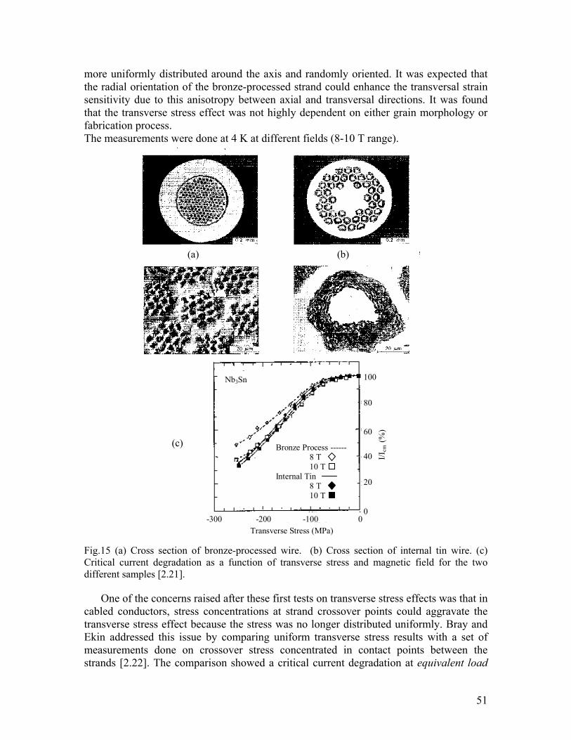
51

more uniformly distributed around the axis and randomly oriented. It was expected that the radial orientation of the bronze-processed strand could enhance the transversal strain sensitivity due to this anisotropy between axial and transversal directions. It was found that the transverse stress effect was not highly dependent on either grain morphology or fabrication process. The measurements were done at 4 K at different fields (8-10 T range).

Fig.15 (a) Cross section of bronze-processed wire. (b) Cross section of internal tin wire. (c) Critical current degradation as a function of transverse stress and magnetic field for the two different samples [2.21].

One of the concerns raised after these first tests on transverse stress effects was that in cabled conductors, stress concentrations at strand crossover points could aggravate the transverse stress effect because the stress was no longer distributed uniformly. Bray and Ekin addressed this issue by comparing uniform transverse stress results with a set of measurements done on crossover stress concentrated in contact points between the strands [2.22]. The comparison showed a critical current degradation at equivalent load

(a) (b)

(c)

Nb3Sn

Bronze Process ------ 8 T ? 10 T ? Internal Tin

8 T ? 10 T ?

-300 -200 -100 0 Transverse Stress (MPa)

I/Icm

(%

) 100 80 60

40

20 0

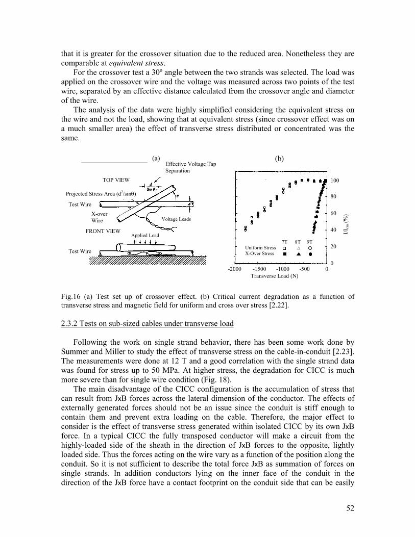
52

that it is greater for the crossover situation due to the reduced area. Nonetheless they are comparable at equivalent stress.

For the crossover test a 30º angle between the two strands was selected. The load was applied on the crossover wire and the voltage was measured across two points of the test wire, separated by an effective distance calculated from the crossover angle and diameter of the wire.

The analysis of the data were highly simplified considering the equivalent stress on the wire and not the load, showing that at equivalent stress (since crossover effect was on a much smaller area) the effect of transverse stress distributed or concentrated was the same. Fig.16 (a) Test set up of crossover effect. (b) Critical current degradation as a function of transverse stress and magnetic field for uniform and cross over stress [2.22]. 2.3.2 Tests on sub-sized cables under transverse load

Following the work on single strand behavior, there has been some work done by Summer and Miller to study the effect of transverse stress on the cable-in-conduit [2.23]. The measurements were done at 12 T and a good correlation with the single strand data was found for stress up to 50 MPa. At higher stress, the degradation for CICC is much more severe than for single wire condition (Fig. 18).

The main disadvantage of the CICC configuration is the accumulation of stress that can result from JxB forces across the lateral dimension of the conductor. The effects of externally generated forces should not be an issue since the conduit is stiff enough to contain them and prevent extra loading on the cable. Therefore, the major effect to consider is the effect of transverse stress generated within isolated CICC by its own JxB force. In a typical CICC the fully transposed conductor will make a circuit from the highly-loaded side of the sheath in the direction of JxB forces to the opposite, lightly loaded side. Thus the forces acting on the wire vary as a function of the position along the conduit. So it is not sufficient to describe the total force JxB as summation of forces on single strands. In addition conductors lying on the inner face of the conduit in the direction of the JxB force have a contact footprint on the conduit side that can be easily

(a) (b) Effective Voltage Tap Separation

Projected Stress Area (d2/sinθ)

Test Wire

X-over Wire

Test Wire

TOP VIEW

FRONT VIEW Applied Load

Voltage Leads

7T 8T 9T Uniform Stress ? ? X-Over Stress ? ? ?

Transverse Load (N)

I/Icm

(%)

-2000 -1500 -1000 -500 0

100

80

60

40

20

0

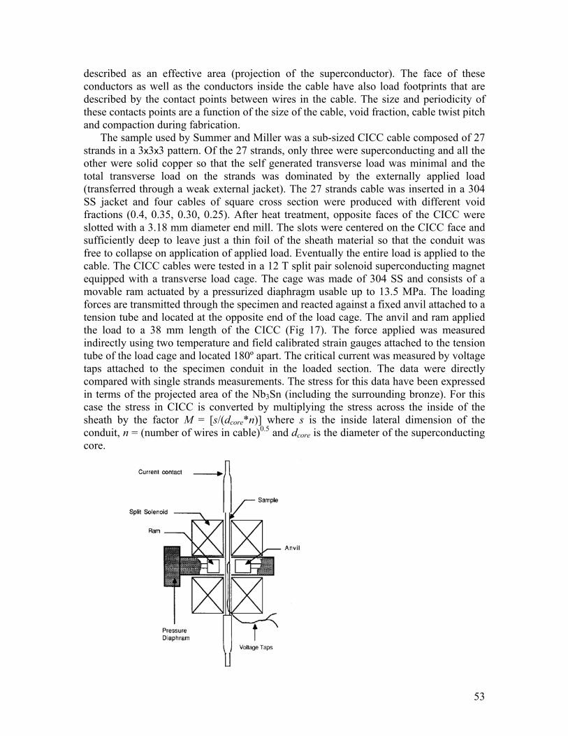
53

described as an effective area (projection of the superconductor). The face of these conductors as well as the conductors inside the cable have also load footprints that are described by the contact points between wires in the cable. The size and periodicity of these contacts points are a function of the size of the cable, void fraction, cable twist pitch and compaction during fabrication.

The sample used by Summer and Miller was a sub-sized CICC cable composed of 27 strands in a 3x3x3 pattern. Of the 27 strands, only three were superconducting and all the other were solid copper so that the self generated transverse load was minimal and the total transverse load on the strands was dominated by the externally applied load (transferred through a weak external jacket). The 27 strands cable was inserted in a 304 SS jacket and four cables of square cross section were produced with different void fractions (0.4, 0.35, 0.30, 0.25). After heat treatment, opposite faces of the CICC were slotted with a 3.18 mm diameter end mill. The slots were centered on the CICC face and sufficiently deep to leave just a thin foil of the sheath material so that the conduit was free to collapse on application of applied load. Eventually the entire load is applied to the cable. The CICC cables were tested in a 12 T split pair solenoid superconducting magnet equipped with a transverse load cage. The cage was made of 304 SS and consists of a movable ram actuated by a pressurized diaphragm usable up to 13.5 MPa. The loading forces are transmitted through the specimen and reacted against a fixed anvil attached to a tension tube and located at the opposite end of the load cage. The anvil and ram applied the load to a 38 mm length of the CICC (Fig 17). The force applied was measured indirectly using two temperature and field calibrated strain gauges attached to the tension tube of the load cage and located 180º apart. The critical current was measured by voltage taps attached to the specimen conduit in the loaded section. The data were directly compared with single strands measurements. The stress for this data have been expressed in terms of the projected area of the Nb3Sn (including the surrounding bronze). For this case the stress in CICC is converted by multiplying the stress across the inside of the sheath by the factor M = [s/(dcore*n)] where s is the inside lateral dimension of the conduit, n = (number of wires in cable)0.5 and dcore is the diameter of the superconducting core.

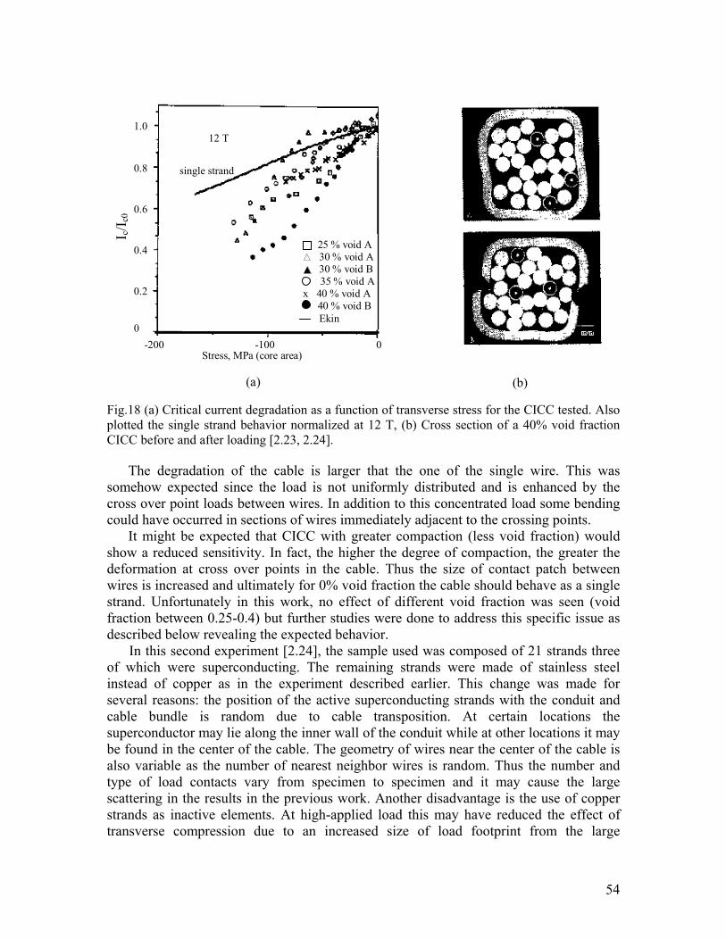
54

Fig.18 (a) Critical current degradation as a function of transverse stress for the CICC tested. Also plotted the single strand behavior normalized at 12 T, (b) Cross section of a 40% void fraction CICC before and after loading [2.23, 2.24].

The degradation of the cable is larger that the one of the single wire. This was somehow expected since the load is not uniformly distributed and is enhanced by the cross over point loads between wires. In addition to this concentrated load some bending could have occurred in sections of wires immediately adjacent to the crossing points.

It might be expected that CICC with greater compaction (less void fraction) would show a reduced sensitivity. In fact, the higher the degree of compaction, the greater the deformation at cross over points in the cable. Thus the size of contact patch between wires is increased and ultimately for 0% void fraction the cable should behave as a single strand. Unfortunately in this work, no effect of different void fraction was seen (void fraction between 0.25-0.4) but further studies were done to address this specific issue as described below revealing the expected behavior.

In this second experiment [2.24], the sample used was composed of 21 strands three of which were superconducting. The remaining strands were made of stainless steel instead of copper as in the experiment described earlier. This change was made for several reasons: the position of the active superconducting strands with the conduit and cable bundle is random due to cable transposition. At certain locations the superconductor may lie along the inner wall of the conduit while at other locations it may be found in the center of the cable. The geometry of wires near the center of the cable is also variable as the number of nearest neighbor wires is random. Thus the number and type of load contacts vary from specimen to specimen and it may cause the large scattering in the results in the previous work. Another disadvantage is the use of copper strands as inactive elements. At high-applied load this may have reduced the effect of transverse compression due to an increased size of load footprint from the large

(a) (b)

25 % void A 30 % void A 30 % void B 35 % void A x 40 % void A 40 % void B Ekin

12 T

Stress, MPa (core area)

I c/I c0

-200 -100 0

1.0

0.8

0.6

0.4

0.2 0

single strand

55

deformation of copper. In this new experiment, the investigators used a cable composed of 21 strands divided in three bundles of 7 strands, of which 6 strands were made of stainless steel. These strands were surrounding one strand of the superconductor. The total active elements are still three superconductor strands. The hard stainless steel does not easily deform under applied load and will tend to minimize the size of the load footprint (increasing the crossover strain localized effect). Secondly, the 6x1 cable first element with the active strand in the middle will mitigate geometry effects as the superconductor will always have 6 wires nearest neighbors and no contact with the inner face of the conduit.

The test procedure was the same as in the first experiment. (the same apparatus was used) and the superconducting strand used was a 0.9 mm diameter, modified jelly roll, binary Nb3Sn with a non-copper volume fraction of 0.65. The 21 strands were inserted in a 304 SS tube and processed with a combination of swaging and rolling to produce a cable with square cross section. Two different void fractions were considered 0.30 and 0.40. Also in this case the jacket had a slot to remove the effect of support material and to apply the stress directly on the cable.

The data from tests (A, B in Fig. 18) at 30% and 40% void fractions were compared with the single strand data. While there is good agreement between the data for the two tests done on the 40 % void fraction for load below 50 MPa), there is a lot of scatter for the data at 30%. As noticed in the previous test, the strands position inside CICC varies as a function of position along the CICC so that the 30% cable was even less sensitive to stress than a single wire.

Regardless of the variation in the data, the effect of void fraction is clear. The 40% void fraction specimens receive less compaction than the 30% void specimen during processing. As a result, the crossover points between wires in the higher-void sample do not deform as much as in the low-void specimen. The load footprint is smaller in high-void samples and the higher contact loading results in increased susceptibility to applied transverse load. Even if stainless steel wires were used as non-active elements of the cable, the results are similar to the ones taken with non-active copper strands.

This was probably due to the fact that during fabrication, the superconductor deforms more than the stainless steel and during the test stainless steel helps to minimize the size of the load footprint and revealed the void fraction dependence. On the other hand during the fabrication process with copper strands, the copper strands deform similarly to the superconductor and even under load, they deform with the superconductor so that the final effect of the two designs were alike.

2.4 Motivation for further investigations and challenges

In recent years, most of the experiments concentrated on further axial strain effect on superconductors. Very little has been done on transverse strain effect on superconductors especially on cables and the only experiments done on sub-sized cables were the two described at the end of the previous section (2.23, 2.24). The fusion community is especially interested in this aspect because CICC cables are more sensitive to this effect due to their design. Tests of the ITER TF Model Coil and ITER CS Model coil showed measurable degradation of the cable and it is believed that this degradation is caused by

56

the transverse strain created by the accumulation of electromagnetic force (JxB) across the cable cross section [2.25]. Besides practical reasons, having a larger data set of measurements, would help elucidate the causes of degradation. The scope of this thesis is to have a device to take these measurements and future work could include a model to predict such behavior.

As mentioned earlier, tests on sub-sized cables are really challenging due to the high current required to test critical current. The measurements try to simulate the magnetic Lorentz force in a cable. This force accumulates over the cross section of the cable and creates a pressure against the strands. The range of pressures of interest is between 10 MPa and 20 MPa. As will be explained in the following chapters, it is not possible to obtain this level of pressures using only the electromagnetic force so it is necessary to simulate the pressure mechanically.

The design and the measurement technique of our new experiment setup are very unique making the work of this thesis challenging but also very stimulating.

Chapter 3 will describe in the details the device and the challenges addressed to ensure a successful test. In Chapter 4 the measurements done to test the device and the measurements technique will be described.

57

CHAPTER 3: Description of the experiment and the FEM model 3.1 Introduction

In this chapter a detailed description of the experimental setup is presented. As

presented in Chapter 1, the goal of this experiment is to measure the effect of transverse load on the critical current of a 36 strands superconducting cable. The load is applied mechanically by pulling a conical wedge that expands a collet which, ultimately, applies the load o the cable located between the collet and an external ring (see Fig. 15 Chapter 1). The experiment has some challenging features and the choices made to address these difficulties are discussed. The measurement technique relies on strain gage measurements and an FEM model performed with ANSYS® to estimate the pressure applied on the cable. A load cell was mounted outside the dewar to measure the vertical load applied externally to the cable. From these measurements the transverse pressure on the cable can be evaluated. The FEM model and the strain gage measurements technique are described in this chapter. 3.2 Cable design

The cable is composed of 36 superconducting Nb3Sn strands with the following parameters:

Strand manufacturer IGC Strand Type Internal Tin Filament Material Nb3Sn

Jc (12 T, 4.2 K) 682 A/mm2 Diameter 0.808 mm Copper\non-copper ratio 1.5:1 Number of strands 36 Average cable diameter 6.25 mm Single turn length 350 mm Cable pattern 3x3x4

The cable was wound with a cabling machine in our laboratory and a detailed description of the operations is given in Appendix II.

One of the critical parameters for the cable is the void fraction, which are empty spaces between the strands when they are twisted together in a pattern of 3x3x4. As discussed for one of the experiments in Chapter 2, it was found that a high void fraction reduces the performance of the cable. An optimal void fraction has been found to be between 35 and 40%. If the void fraction is too low the strands could be damaged during cabling and generate higher AC losses; if it is too high, the space between strands is so big that after reaction (when Nb3Sn is brittle) any little displacement or vibration could irreversibly damage the single strands. For our cable, we aimed for a void fraction of 36-37%, similar to the one of the ITER Model Coil cable. This void fraction is dictated by

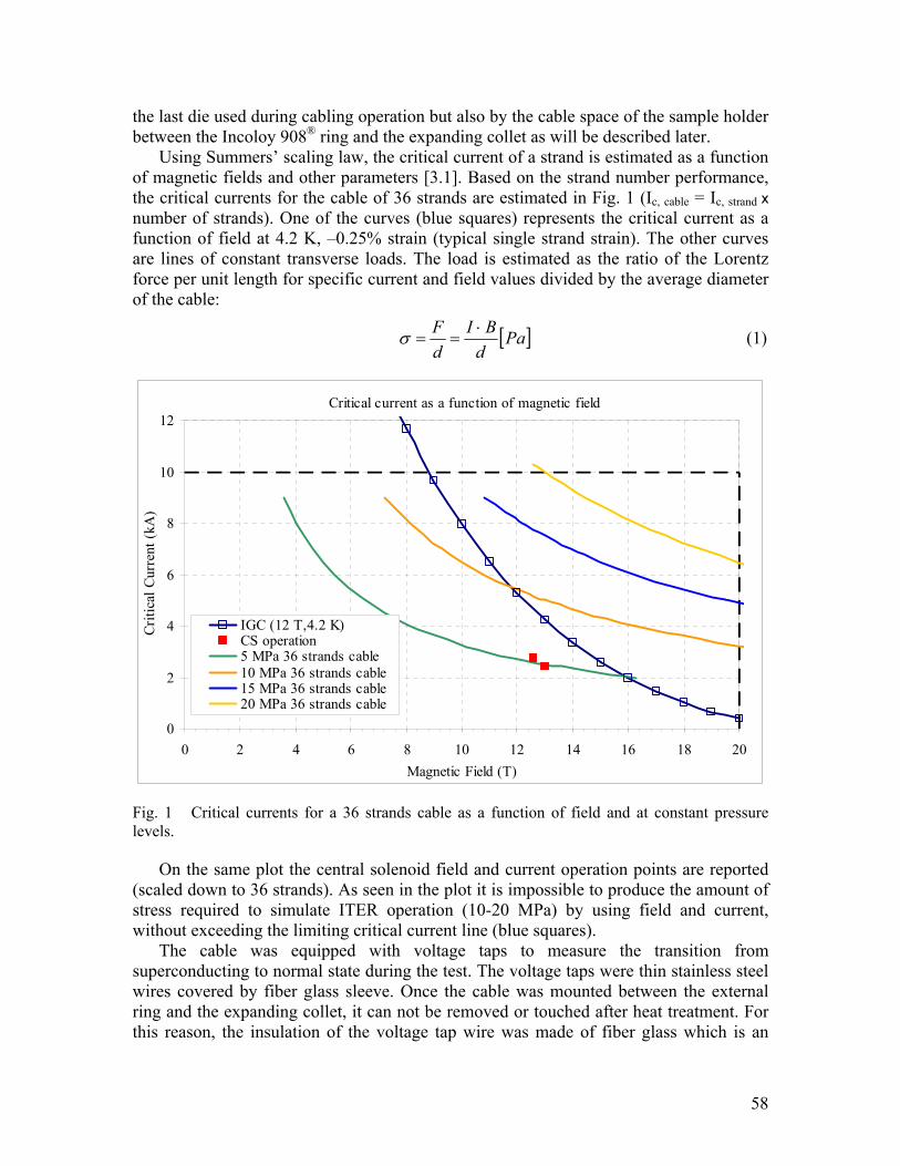
58

the last die used during cabling operation but also by the cable space of the sample holder between the Incoloy 908® ring and the expanding collet as will be described later.

Using Summers’ scaling law, the critical current of a strand is estimated as a function of magnetic fields and other parameters [3.1]. Based on the strand number performance, the critical currents for the cable of 36 strands are estimated in Fig. 1 (Ic, cable = Ic, strand x number of strands). One of the curves (blue squares) represents the critical current as a function of field at 4.2 K, –0.25% strain (typical single strand strain). The other curves are lines of constant transverse loads. The load is estimated as the ratio of the Lorentz force per unit length for specific current and field values divided by the average diameter of the cable:

[ ]Pad

BIdF ⋅==σ (1)

Fig. 1 Critical currents for a 36 strands cable as a function of field and at constant pressure levels.

On the same plot the central solenoid field and current operation points are reported (scaled down to 36 strands). As seen in the plot it is impossible to produce the amount of stress required to simulate ITER operation (10-20 MPa) by using field and current, without exceeding the limiting critical current line (blue squares).

The cable was equipped with voltage taps to measure the transition from superconducting to normal state during the test. The voltage taps were thin stainless steel wires covered by fiber glass sleeve. Once the cable was mounted between the external ring and the expanding collet, it can not be removed or touched after heat treatment. For this reason, the insulation of the voltage tap wire was made of fiber glass which is an

Critical current as a function of magnetic field

0

2

4

6

8

10

12

0 2 4 6 8 10 12 14 16 18 20Magnetic Field (T)

Criti

cal C

urre

nt (k

A)

IGC (12 T,4.2 K)CS operation5 MPa 36 strands cable10 MPa 36 strands cable15 MPa 36 strands cable20 MPa 36 strands cable

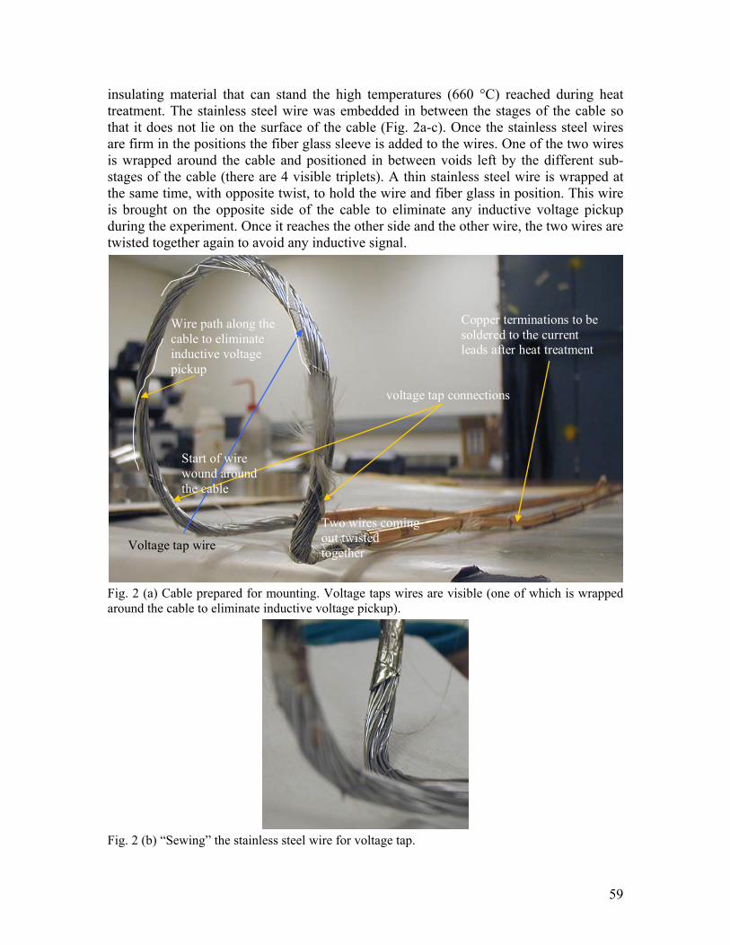
59

insulating material that can stand the high temperatures (660 °C) reached during heat treatment. The stainless steel wire was embedded in between the stages of the cable so that it does not lie on the surface of the cable (Fig. 2a-c). Once the stainless steel wires are firm in the positions the fiber glass sleeve is added to the wires. One of the two wires is wrapped around the cable and positioned in between voids left by the different sub-stages of the cable (there are 4 visible triplets). A thin stainless steel wire is wrapped at the same time, with opposite twist, to hold the wire and fiber glass in position. This wire is brought on the opposite side of the cable to eliminate any inductive voltage pickup during the experiment. Once it reaches the other side and the other wire, the two wires are twisted together again to avoid any inductive signal.

Fig. 2 (a) Cable prepared for mounting. Voltage taps wires are visible (one of which is wrapped around the cable to eliminate inductive voltage pickup).

Fig. 2 (b) “Sewing” the stainless steel wire for voltage tap.

Voltage tap wire

voltage tap connections

Copper terminations to be soldered to the current leads after heat treatment

Start of wire wound around the cable

Two wires coming out twisted together

Wire path along the cable to eliminate inductive voltage pickup

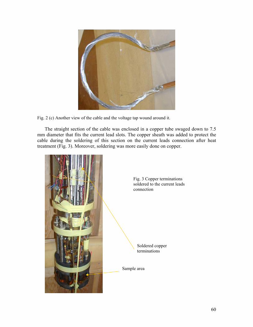
60

Fig. 2 (c) Another view of the cable and the voltage tap wound around it.

The straight section of the cable was enclosed in a copper tube swaged down to 7.5 mm diameter that fits the current lead slots. The copper sheath was added to protect the cable during the soldering of this section on the current leads connection after heat treatment (Fig. 3). Moreover, soldering was more easily done on copper.

Fig. 3 Copper terminations soldered to the current leads connection

Sample area

Soldered copper terminations

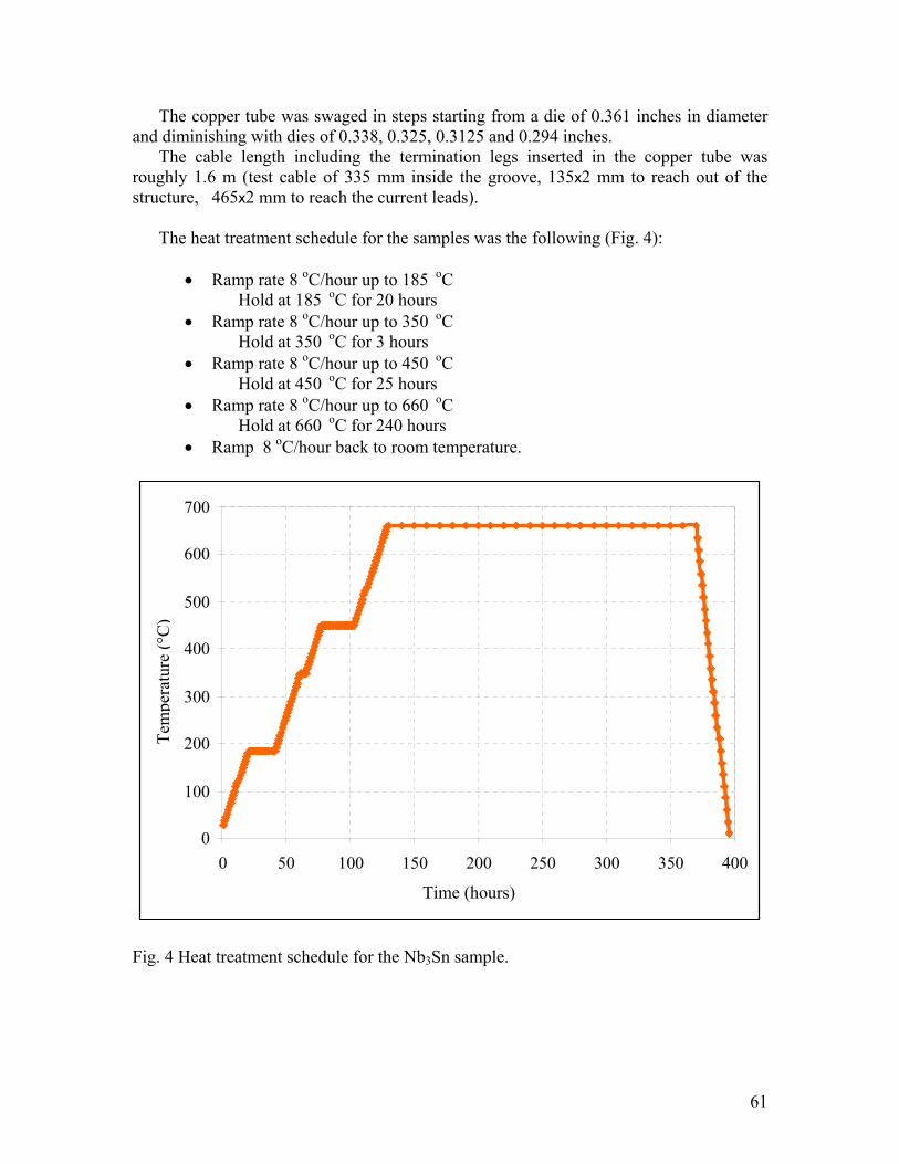
61

The copper tube was swaged in steps starting from a die of 0.361 inches in diameter and diminishing with dies of 0.338, 0.325, 0.3125 and 0.294 inches.

The cable length including the termination legs inserted in the copper tube was roughly 1.6 m (test cable of 335 mm inside the groove, 135x2 mm to reach out of the structure, 465x2 mm to reach the current leads).

The heat treatment schedule for the samples was the following (Fig. 4):

• Ramp rate 8 oC/hour up to 185 oC Hold at 185 oC for 20 hours

• Ramp rate 8 oC/hour up to 350 oC Hold at 350 oC for 3 hours

• Ramp rate 8 oC/hour up to 450 oC Hold at 450 oC for 25 hours

• Ramp rate 8 oC/hour up to 660 oC Hold at 660 oC for 240 hours

• Ramp 8 oC/hour back to room temperature.

Fig. 4 Heat treatment schedule for the Nb3Sn sample.

0

100

200

300

400

500

600

700

0 50 100 150 200 250 300 350 400

time (hours)

tem

pera

ture

(Cel

sius)

Time (hours)

Tem

pera

ture

(°C

)

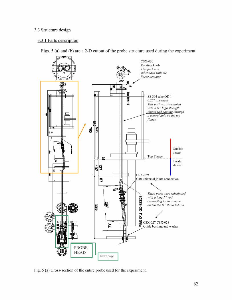
62

3.3 Structure design

3.3.1 Parts description

Figs. 5 (a) and (b) are a 2-D cutout of the probe structure used during the experiment. Fig. 5 (a) Cross-section of the entire probe used for the experiment.

CSX-029 G10 universal joints connection

CSX-027 CSX-028 Guide bushing and washer

SS 304 tube OD 1” 0.25” thickness This part was substituted with a ¾” high strength thread rod passing through a central hole on the top flange

CSX-030 Rotating knob This part was substituted with the linear actuator

Top Flange

Outside dewar

Inside dewar

Next page

These parts were substituted with a long 1” rod connecting to the sample and to the ¾” threaded rod

PROBE HEAD

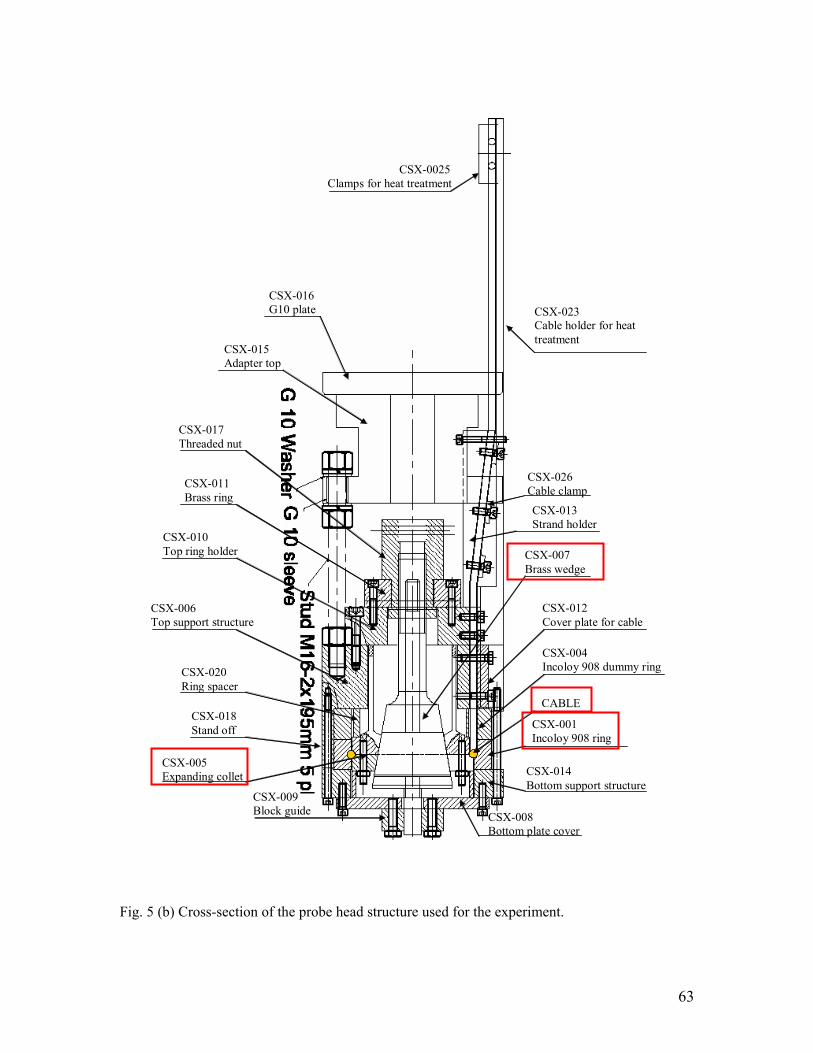
63

Fig. 5 (b) Cross-section of the probe head structure used for the experiment.

CSX-0025 Clamps for heat treatment

CSX-016 G10 plate CSX-023

Cable holder for heat treatment

CSX-015 Adapter top

CSX-026 Cable clamp CSX-013 Strand holder

CSX-007 Brass wedge

CSX-012 Cover plate for cable

CSX-004 Incoloy 908 dummy ring

CABLE

CSX-001 Incoloy 908 ring

CSX-014 Bottom support structure

CSX-017 Threaded nut

CSX-011 Brass ring

CSX-010 Top ring holder

CSX-006 Top support structure

CSX-020 Ring spacer

CSX-018 Stand off

CSX-005 Expanding collet

CSX-009 Block guide CSX-008

Bottom plate cover

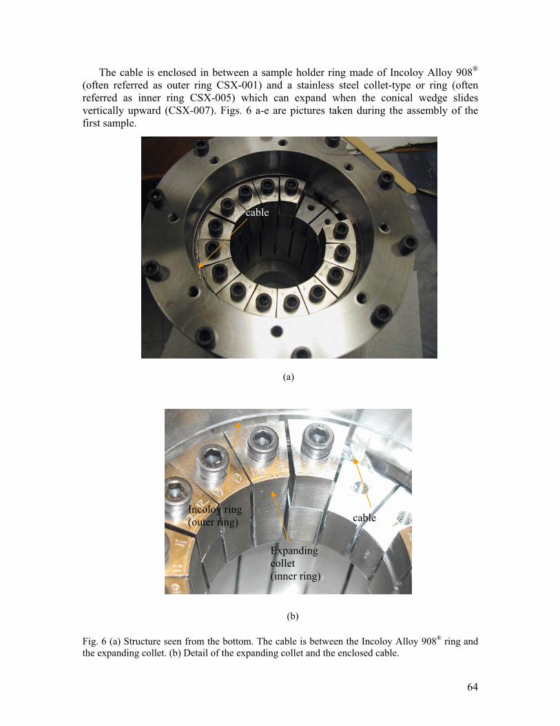
64

The cable is enclosed in between a sample holder ring made of Incoloy Alloy 908® (often referred as outer ring CSX-001) and a stainless steel collet-type or ring (often referred as inner ring CSX-005) which can expand when the conical wedge slides vertically upward (CSX-007). Figs. 6 a-e are pictures taken during the assembly of the first sample.

Fig. 6 (a) Structure seen from the bottom. The cable is between the Incoloy Alloy 908® ring and the expanding collet. (b) Detail of the expanding collet and the enclosed cable.

(a)

(b)

cable

cable

Expanding collet (inner ring)

Incoloy ring (outer ring)

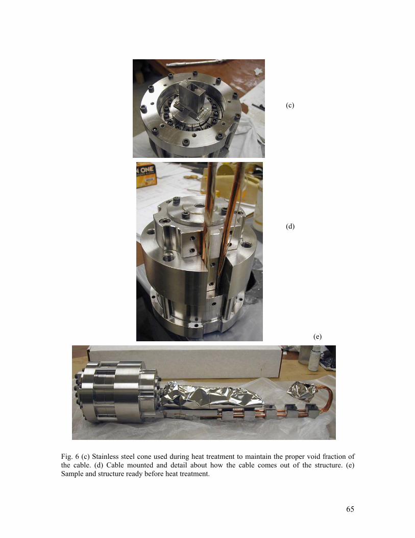
65

Fig. 6 (c) Stainless steel cone used during heat treatment to maintain the proper void fraction of the cable. (d) Cable mounted and detail about how the cable comes out of the structure. (e) Sample and structure ready before heat treatment.

(c)

(d)

(e)

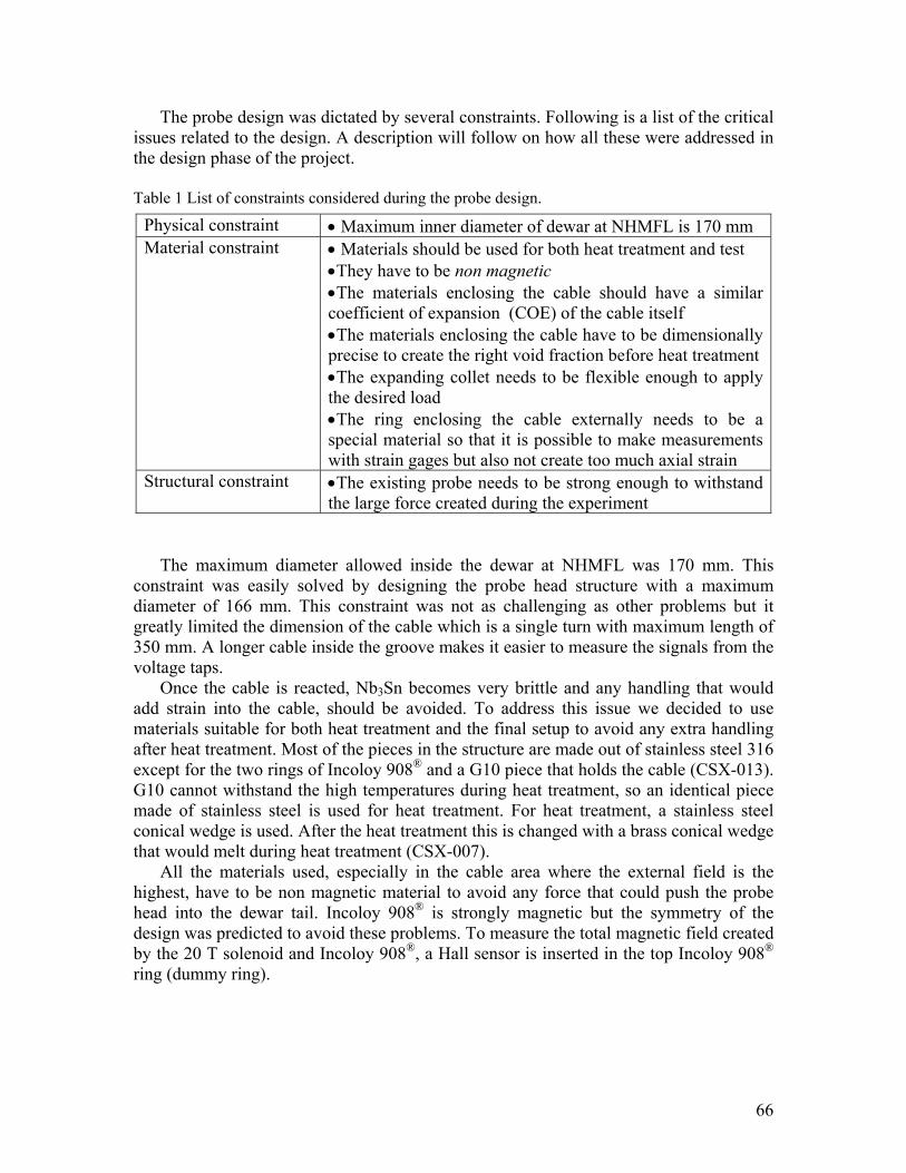
66

The probe design was dictated by several constraints. Following is a list of the critical issues related to the design. A description will follow on how all these were addressed in the design phase of the project.

Table 1 List of constraints considered during the probe design.

Physical constraint • Maximum inner diameter of dewar at NHMFL is 170 mm Material constraint • Materials should be used for both heat treatment and test

•They have to be non magnetic •The materials enclosing the cable should have a similar coefficient of expansion (COE) of the cable itself •The materials enclosing the cable have to be dimensionally precise to create the right void fraction before heat treatment •The expanding collet needs to be flexible enough to apply the desired load •The ring enclosing the cable externally needs to be a special material so that it is possible to make measurements with strain gages but also not create too much axial strain

Structural constraint •The existing probe needs to be strong enough to withstand the large force created during the experiment

The maximum diameter allowed inside the dewar at NHMFL was 170 mm. This

constraint was easily solved by designing the probe head structure with a maximum diameter of 166 mm. This constraint was not as challenging as other problems but it greatly limited the dimension of the cable which is a single turn with maximum length of 350 mm. A longer cable inside the groove makes it easier to measure the signals from the voltage taps.

Once the cable is reacted, Nb3Sn becomes very brittle and any handling that would add strain into the cable, should be avoided. To address this issue we decided to use materials suitable for both heat treatment and the final setup to avoid any extra handling after heat treatment. Most of the pieces in the structure are made out of stainless steel 316 except for the two rings of Incoloy 908® and a G10 piece that holds the cable (CSX-013). G10 cannot withstand the high temperatures during heat treatment, so an identical piece made of stainless steel is used for heat treatment. For heat treatment, a stainless steel conical wedge is used. After the heat treatment this is changed with a brass conical wedge that would melt during heat treatment (CSX-007).

All the materials used, especially in the cable area where the external field is the highest, have to be non magnetic material to avoid any force that could push the probe head into the dewar tail. Incoloy 908® is strongly magnetic but the symmetry of the design was predicted to avoid these problems. To measure the total magnetic field created by the 20 T solenoid and Incoloy 908®, a Hall sensor is inserted in the top Incoloy 908® ring (dummy ring).

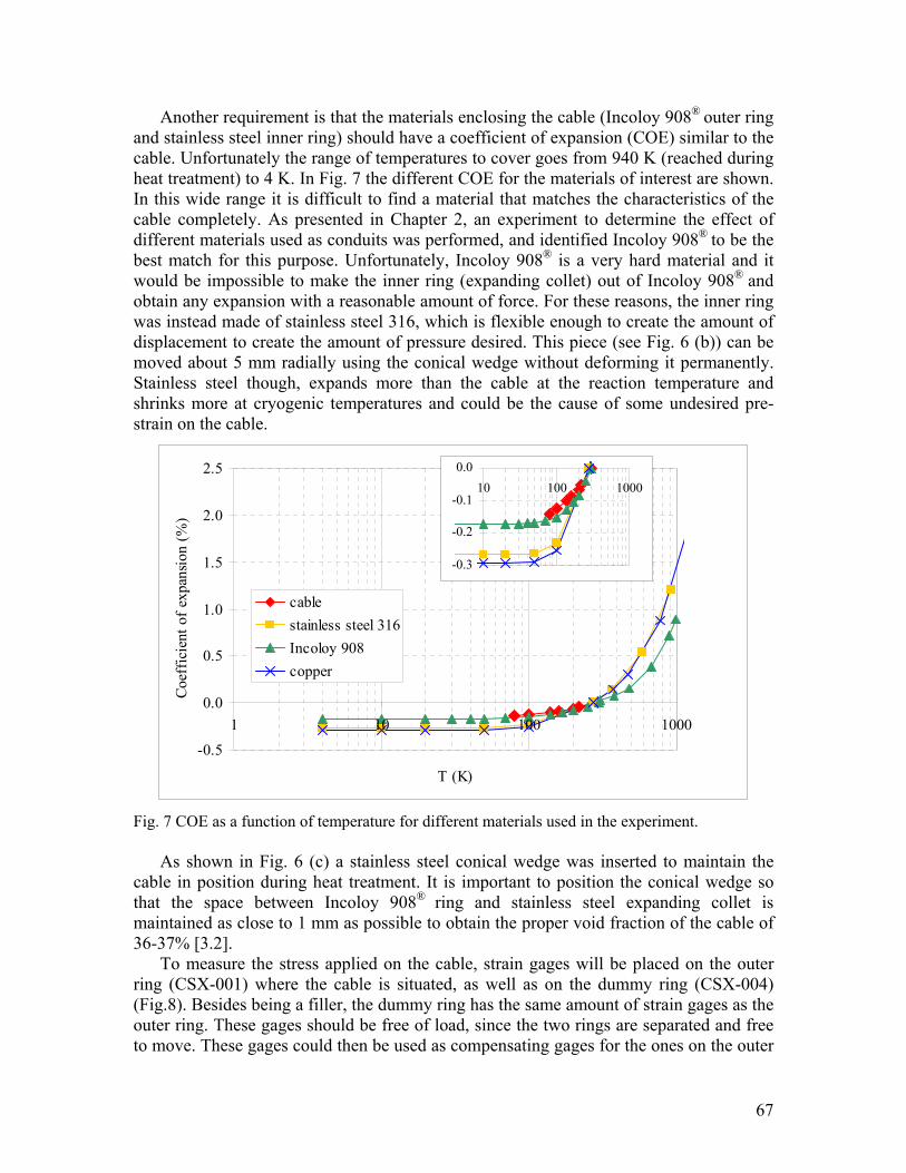
67

Another requirement is that the materials enclosing the cable (Incoloy 908® outer ring and stainless steel inner ring) should have a coefficient of expansion (COE) similar to the cable. Unfortunately the range of temperatures to cover goes from 940 K (reached during heat treatment) to 4 K. In Fig. 7 the different COE for the materials of interest are shown. In this wide range it is difficult to find a material that matches the characteristics of the cable completely. As presented in Chapter 2, an experiment to determine the effect of different materials used as conduits was performed, and identified Incoloy 908® to be the best match for this purpose. Unfortunately, Incoloy 908® is a very hard material and it would be impossible to make the inner ring (expanding collet) out of Incoloy 908® and obtain any expansion with a reasonable amount of force. For these reasons, the inner ring was instead made of stainless steel 316, which is flexible enough to create the amount of displacement to create the amount of pressure desired. This piece (see Fig. 6 (b)) can be moved about 5 mm radially using the conical wedge without deforming it permanently. Stainless steel though, expands more than the cable at the reaction temperature and shrinks more at cryogenic temperatures and could be the cause of some undesired pre-strain on the cable.

Fig. 7 COE as a function of temperature for different materials used in the experiment.

As shown in Fig. 6 (c) a stainless steel conical wedge was inserted to maintain the cable in position during heat treatment. It is important to position the conical wedge so that the space between Incoloy 908® ring and stainless steel expanding collet is maintained as close to 1 mm as possible to obtain the proper void fraction of the cable of 36-37% [3.2].

To measure the stress applied on the cable, strain gages will be placed on the outer ring (CSX-001) where the cable is situated, as well as on the dummy ring (CSX-004) (Fig.8). Besides being a filler, the dummy ring has the same amount of strain gages as the outer ring. These gages should be free of load, since the two rings are separated and free to move. These gages could then be used as compensating gages for the ones on the outer

-0.5

0.0

0.5

1.0

1.5

2.0

2.5

1 10 100 1000

T (K)

Coef

ficie

nt o

f exp

ansio

n (%

)

cablestainless steel 316Incoloy 908copper

-0.3

-0.2

-0.1

0.010 100 1000

68

ring under the transverse load. It turned out that the two rings are not independent as designed, since the glue used to attach the gages onto the material actually diffused between the two rings and glued them to one another (the curing temperature for this glue is up to 60o C and the glue can easily flow inside the gaps present). We then decided to add a load-free, dummy gage for each gage on the rings. This operation doubled the amount of the strain gages, but it would have been misleading to use the dummy ring gages as compensation since they also record stress. This fact defeats the purpose of having two Incoloy 908® rings and in the future the dummy Incoloy 908® ring will be replaced with a filler stainless steel ring.

Fig. 8 Strain gages mounted on the Incoloy 908® rings.

3.3.2 Strain requirements

As shown in Fig. 9 superconducting strands are sensitive to both longitudinal and transverse applied strain [3.3].

Fig. 9 Stress dependence of single Nb3Sn strand. Strands are much more sensitive to transverse stress.

Surface glued during the curing of the gages

Dummy ring

Ring where cable is seated

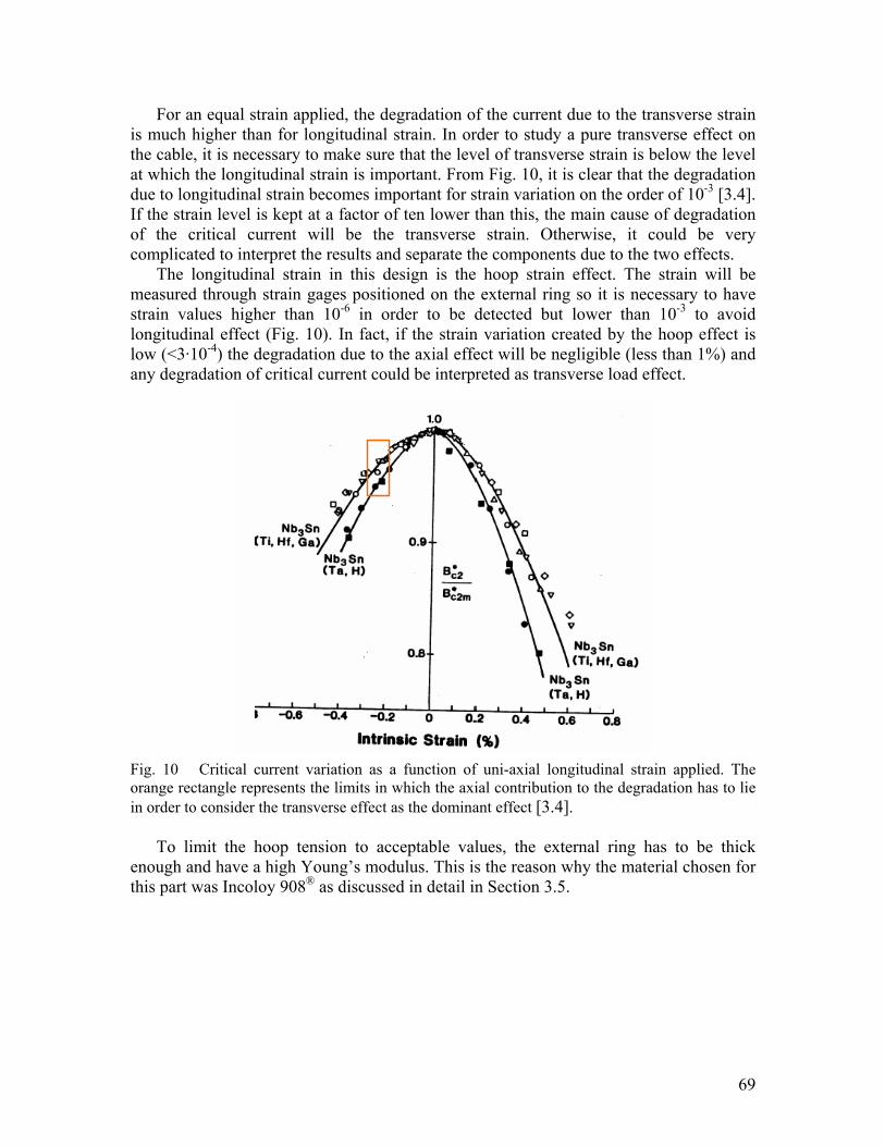
69

For an equal strain applied, the degradation of the current due to the transverse strain is much higher than for longitudinal strain. In order to study a pure transverse effect on the cable, it is necessary to make sure that the level of transverse strain is below the level at which the longitudinal strain is important. From Fig. 10, it is clear that the degradation due to longitudinal strain becomes important for strain variation on the order of 10-3 [3.4]. If the strain level is kept at a factor of ten lower than this, the main cause of degradation of the critical current will be the transverse strain. Otherwise, it could be very complicated to interpret the results and separate the components due to the two effects.

The longitudinal strain in this design is the hoop strain effect. The strain will be measured through strain gages positioned on the external ring so it is necessary to have strain values higher than 10-6 in order to be detected but lower than 10-3 to avoid longitudinal effect (Fig. 10). In fact, if the strain variation created by the hoop effect is low (<3·10-4) the degradation due to the axial effect will be negligible (less than 1%) and any degradation of critical current could be interpreted as transverse load effect.

Fig. 10 Critical current variation as a function of uni-axial longitudinal strain applied. The orange rectangle represents the limits in which the axial contribution to the degradation has to lie in order to consider the transverse effect as the dominant effect [3.4].

To limit the hoop tension to acceptable values, the external ring has to be thick enough and have a high Young’s modulus. This is the reason why the material chosen for this part was Incoloy 908® as discussed in detail in Section 3.5.

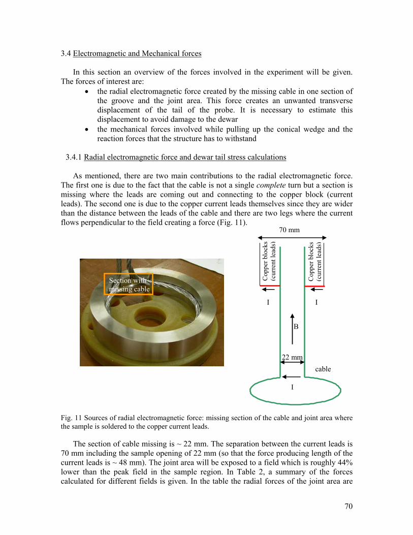
70

3.4 Electromagnetic and Mechanical forces

In this section an overview of the forces involved in the experiment will be given. The forces of interest are:

• the radial electromagnetic force created by the missing cable in one section of the groove and the joint area. This force creates an unwanted transverse displacement of the tail of the probe. It is necessary to estimate this displacement to avoid damage to the dewar

• the mechanical forces involved while pulling up the conical wedge and the reaction forces that the structure has to withstand

3.4.1 Radial electromagnetic force and dewar tail stress calculations

As mentioned, there are two main contributions to the radial electromagnetic force. The first one is due to the fact that the cable is not a single complete turn but a section is missing where the leads are coming out and connecting to the copper block (current leads). The second one is due to the copper current leads themselves since they are wider than the distance between the leads of the cable and there are two legs where the current flows perpendicular to the field creating a force (Fig. 11).

Fig. 11 Sources of radial electromagnetic force: missing section of the cable and joint area where the sample is soldered to the copper current leads.

The section of cable missing is ~ 22 mm. The separation between the current leads is

70 mm including the sample opening of 22 mm (so that the force producing length of the current leads is ~ 48 mm). The joint area will be exposed to a field which is roughly 44% lower than the peak field in the sample region. In Table 2, a summary of the forces calculated for different fields is given. In the table the radial forces of the joint area are

Section with missing cable

Cop

per b

lock

s (c

urre

nt le

ads)

B

I

I I C

oppe

r blo

cks

(cur

rent

lead

s)

cable 22 mm

70 mm

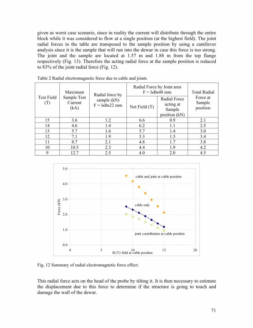
71

given as worst case scenario, since in reality the current will distribute through the entire block while it was considered to flow at a single position (at the highest field). The joint radial forces in the table are transposed to the sample position by using a cantilever analysis since it is the sample that will run into the dewar in case this force is too strong. The joint and the sample are located at 1.57 m and 1.88 m from the top flange respectively (Fig. 13). Therefore the acting radial force at the sample position is reduced to 83% of the joint radial force (Fig. 12). Table 2 Radial electromagnetic force due to cable and joints

Radial Force by Joint area F = IxBx48 mm

Test Field (T)

Maximum Sample Test

Current (kA)

Radial force by sample (kN)

F = IxBx22 mm Net Field (T)

Radial Force acting at Sample

position (kN)

Total Radial Force at Sample position

15 3.6 1.2 6.6 0.9 2.1 14 4.6 1.4 6.2 1.1 2.5 13 5.7 1.6 5.7 1.4 3.0 12 7.1 1.9 5.3 1.5 3.4 11 8.7 2.1 4.8 1.7 3.8 10 10.5 2.3 4.4 1.9 4.2 9 12.7 2.5 4.0 2.0 4.5

Fig. 12 Summary of radial electromagnetic force effect. This radial force acts on the head of the probe by tilting it. It is then necessary to estimate the displacement due to this force to determine if the structure is going to touch and damage the wall of the dewar.

0.0

1.0

2.0

3.0

4.0

5.0

0 5 10 15 20B (T) field at cable position

Forc

e (k

N)

cable only

cable and joint at cable position

joint contribution at cable position

72

Fig. 13 Dewar’s schematic showing the positioning of the cable and the estimated stress range.

The stress applied at position A of the dewar (where the straight section of the dewar ends) can be estimated by using a cantilever model:

SlF ⋅

=σ (2)

where

- F is the force created by the cable (roughly 6000 N at 15 T and 10 kA) - l is the distance between the end of the straight section of the dewar (point A in Fig. 13) and the position of the cable - S is the section modulus of the dewar

The section modulus can be estimated from the moment of inertia I, given by

)(4

44innerouter RRI −⋅=

π (3)

outerRIS = (4)

A

F=6000N

Sample position at center field

2400 mm

1328 mm

811 mm

1570 mm To leads position

Current leads position

498 mm

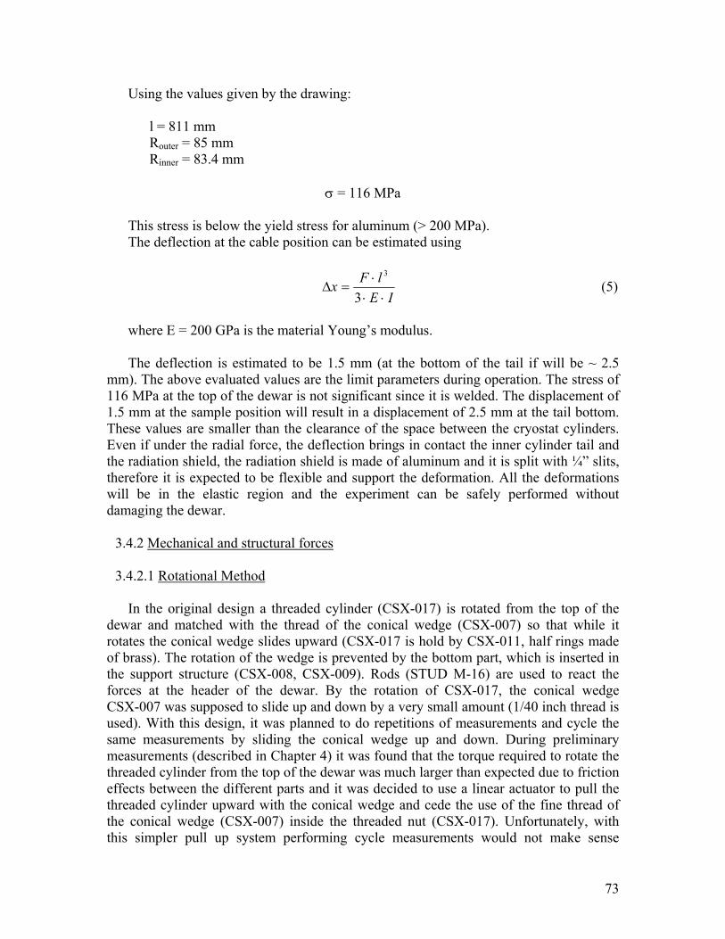
73

Using the values given by the drawing:

l = 811 mm Router = 85 mm Rinner = 83.4 mm

σ = 116 MPa

This stress is below the yield stress for aluminum (> 200 MPa). The deflection at the cable position can be estimated using

IElFx⋅⋅

⋅=∆

3

3

(5)

where E = 200 GPa is the material Young’s modulus.

The deflection is estimated to be 1.5 mm (at the bottom of the tail if will be ~ 2.5

mm). The above evaluated values are the limit parameters during operation. The stress of 116 MPa at the top of the dewar is not significant since it is welded. The displacement of 1.5 mm at the sample position will result in a displacement of 2.5 mm at the tail bottom. These values are smaller than the clearance of the space between the cryostat cylinders. Even if under the radial force, the deflection brings in contact the inner cylinder tail and the radiation shield, the radiation shield is made of aluminum and it is split with ¼” slits, therefore it is expected to be flexible and support the deformation. All the deformations will be in the elastic region and the experiment can be safely performed without damaging the dewar.

3.4.2 Mechanical and structural forces 3.4.2.1 Rotational Method

In the original design a threaded cylinder (CSX-017) is rotated from the top of the dewar and matched with the thread of the conical wedge (CSX-007) so that while it rotates the conical wedge slides upward (CSX-017 is hold by CSX-011, half rings made of brass). The rotation of the wedge is prevented by the bottom part, which is inserted in the support structure (CSX-008, CSX-009). Rods (STUD M-16) are used to react the forces at the header of the dewar. By the rotation of CSX-017, the conical wedge CSX-007 was supposed to slide up and down by a very small amount (1/40 inch thread is used). With this design, it was planned to do repetitions of measurements and cycle the same measurements by sliding the conical wedge up and down. During preliminary measurements (described in Chapter 4) it was found that the torque required to rotate the threaded cylinder from the top of the dewar was much larger than expected due to friction effects between the different parts and it was decided to use a linear actuator to pull the threaded cylinder upward with the conical wedge and cede the use of the fine thread of the conical wedge (CSX-007) inside the threaded nut (CSX-017). Unfortunately, with this simpler pull up system performing cycle measurements would not make sense

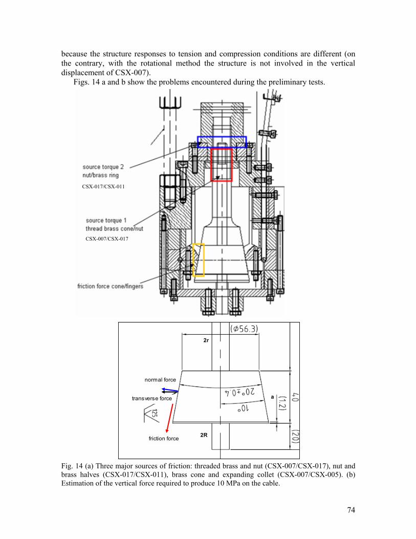
74

because the structure responses to tension and compression conditions are different (on the contrary, with the rotational method the structure is not involved in the vertical displacement of CSX-007).

Figs. 14 a and b show the problems encountered during the preliminary tests.

Fig. 14 (a) Three major sources of friction: threaded brass and nut (CSX-007/CSX-017), nut and brass halves (CSX-017/CSX-011), brass cone and expanding collet (CSX-007/CSX-005). (b) Estimation of the vertical force required to produce 10 MPa on the cable.

a

2r

2R

transverse force

normal force

friction force

CSX-017/CSX-011

CSX-007/CSX-017

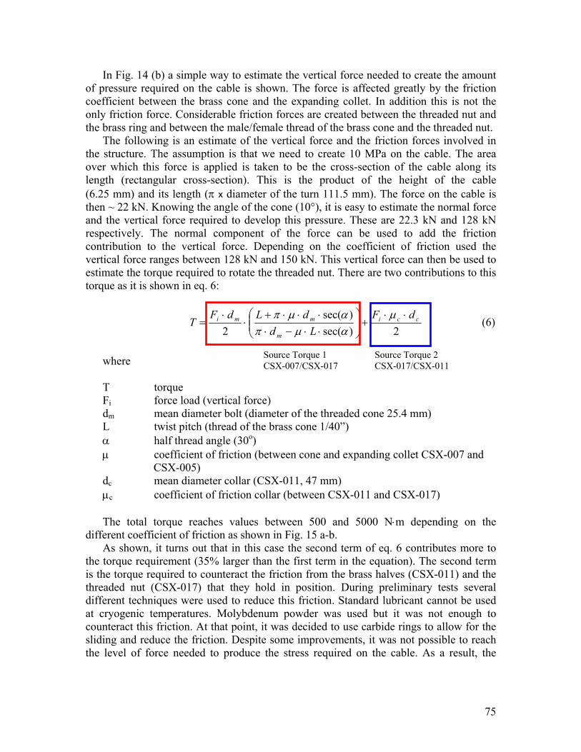
75

In Fig. 14 (b) a simple way to estimate the vertical force needed to create the amount of pressure required on the cable is shown. The force is affected greatly by the friction coefficient between the brass cone and the expanding collet. In addition this is not the only friction force. Considerable friction forces are created between the threaded nut and the brass ring and between the male/female thread of the brass cone and the threaded nut.

The following is an estimate of the vertical force and the friction forces involved in the structure. The assumption is that we need to create 10 MPa on the cable. The area over which this force is applied is taken to be the cross-section of the cable along its length (rectangular cross-section). This is the product of the height of the cable (6.25 mm) and its length (π x diameter of the turn 111.5 mm). The force on the cable is then ~ 22 kN. Knowing the angle of the cone (10°), it is easy to estimate the normal force and the vertical force required to develop this pressure. These are 22.3 kN and 128 kN respectively. The normal component of the force can be used to add the friction contribution to the vertical force. Depending on the coefficient of friction used the vertical force ranges between 128 kN and 150 kN. This vertical force can then be used to estimate the torque required to rotate the threaded nut. There are two contributions to this torque as it is shown in eq. 6:

2)sec()sec(

2cci

m

mmi dFLd

dLdFT

⋅⋅+

⋅⋅−⋅⋅⋅⋅+

⋅⋅

=µ

αµπαµπ

(6)

where T torque Fi force load (vertical force) dm mean diameter bolt (diameter of the threaded cone 25.4 mm) L twist pitch (thread of the brass cone 1/40”) α half thread angle (30o) µ coefficient of friction (between cone and expanding collet CSX-007 and

CSX-005) dc mean diameter collar (CSX-011, 47 mm) µc coefficient of friction collar (between CSX-011 and CSX-017)

The total torque reaches values between 500 and 5000 N⋅m depending on the

different coefficient of friction as shown in Fig. 15 a-b. As shown, it turns out that in this case the second term of eq. 6 contributes more to

the torque requirement (35% larger than the first term in the equation). The second term is the torque required to counteract the friction from the brass halves (CSX-011) and the threaded nut (CSX-017) that they hold in position. During preliminary tests several different techniques were used to reduce this friction. Standard lubricant cannot be used at cryogenic temperatures. Molybdenum powder was used but it was not enough to counteract this friction. At that point, it was decided to use carbide rings to allow for the sliding and reduce the friction. Despite some improvements, it was not possible to reach the level of force needed to produce the stress required on the cable. As a result, the

Source Torque 1 CSX-007/CSX-017

Source Torque 2 CSX-017/CSX-011

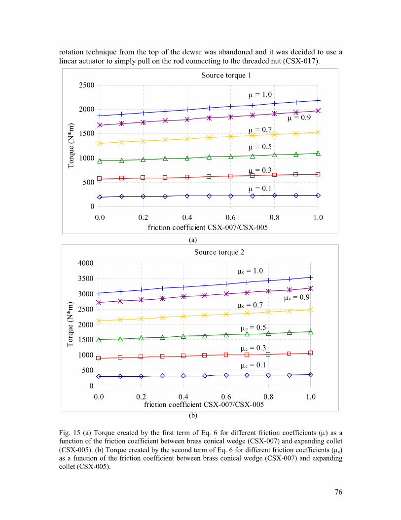
76

rotation technique from the top of the dewar was abandoned and it was decided to use a linear actuator to simply pull on the rod connecting to the threaded nut (CSX-017).

Fig. 15 (a) Torque created by the first term of Eq. 6 for different friction coefficients (µ) as a function of the friction coefficient between brass conical wedge (CSX-007) and expanding collet (CSX-005). (b) Torque created by the second term of Eq. 6 for different friction coefficients (µc) as a function of the friction coefficient between brass conical wedge (CSX-007) and expanding collet (CSX-005).

(a)

Source torque 1

0

500

1000

1500

2000

2500

0.0 0.2 0.4 0.6 0.8 1.0friction coefficient CSX-007/CSX-005

Torq

ue (N

*m)

µ = 0.1

µ = 0.3

µ = 0.5

µ = 0.7µ = 0.9

µ = 1.0

Source torque 2

0

500

1000

1500

2000

2500

3000

3500

4000

0.0 0.2 0.4 0.6 0.8 1.0friction coefficient CSX-007/CSX-005

Torq

ue (N

*m)

µc = 0.1

µc = 0.3

µc = 0.5

µc = 0.7µc = 0.9

µc = 1.0

(b)

77

3.4.2.2 Linear Actuator method The linear actuator is mounted on a plate mounted on the top of the dewar (Fig. 16).

Linear actuator

Supporting plate

Supporting rods

Movable section of the linear actuator

Connection to the center rod attached to the sample area

Linear actuator

Support structure Connection to center rod

Current leads

Dewar top flange

Fig. 16 Linear actuator and support structure sitting before mounting on the top flange (top), and mounted on top of the dewar with the probe attached to the current leads (left).

78

The rods supporting the plate where the actuator was mounted are ½” rods (6 of them) and ¾” rods (2 of them). Of the ½” rods, four of them are inserted in ¾” tube to enhance their strength. The rods are made to withstand a total force of ~ 100 kN.

As shown in Fig. 17 the linear actuator is connected to a hollow cylinder. On the bottom side of the cylinder a ¾”, high strength threaded rod is attached (Fig. 17). A load cell is mounted inside the cylinder so that an absolute measure of the vertical load can be taken during the experiment. The ¾” threaded rod is screwed for 2” inside a 1” rod. The 1” rod is roughly 2 m long and is connected to CSX-017 (threaded nut) through a screw. The brass cone (CSX-007) is screwed inside CSX-017. By pulling the linear actuator upward, the ¾” rod, 1” rod, CSX-017 and CSX-007 all move upward. The vertical movement of CSX-007 expands the collet and applies pressure on the cable.

Fig. 17 Connector pieces: load cell position and ¾” high strength threaded rod. Besides reinforcing the supporting plate where the linear actuator is sitting, the

structure inside the dewar also needed to be reinforced through threaded rods and tubes surrounding them. The choice of using threaded rod inserted in a tube was mainly dictated by the simplicity of the modification of the existing probe structure used for the experiment. 3.5 Finite Element Analysis

An ANSYS® 2-D-axisymmetric model was created to simulate the loading effects for the experiment of transverse stress on a sub-cable composed of 36 superconducting strands. An analysis is given for the strain level on the outside surface of the outer ring of the structure under the transverse load, in order to estimate the strain and stress value on the cable itself.

load cell

¾” rod

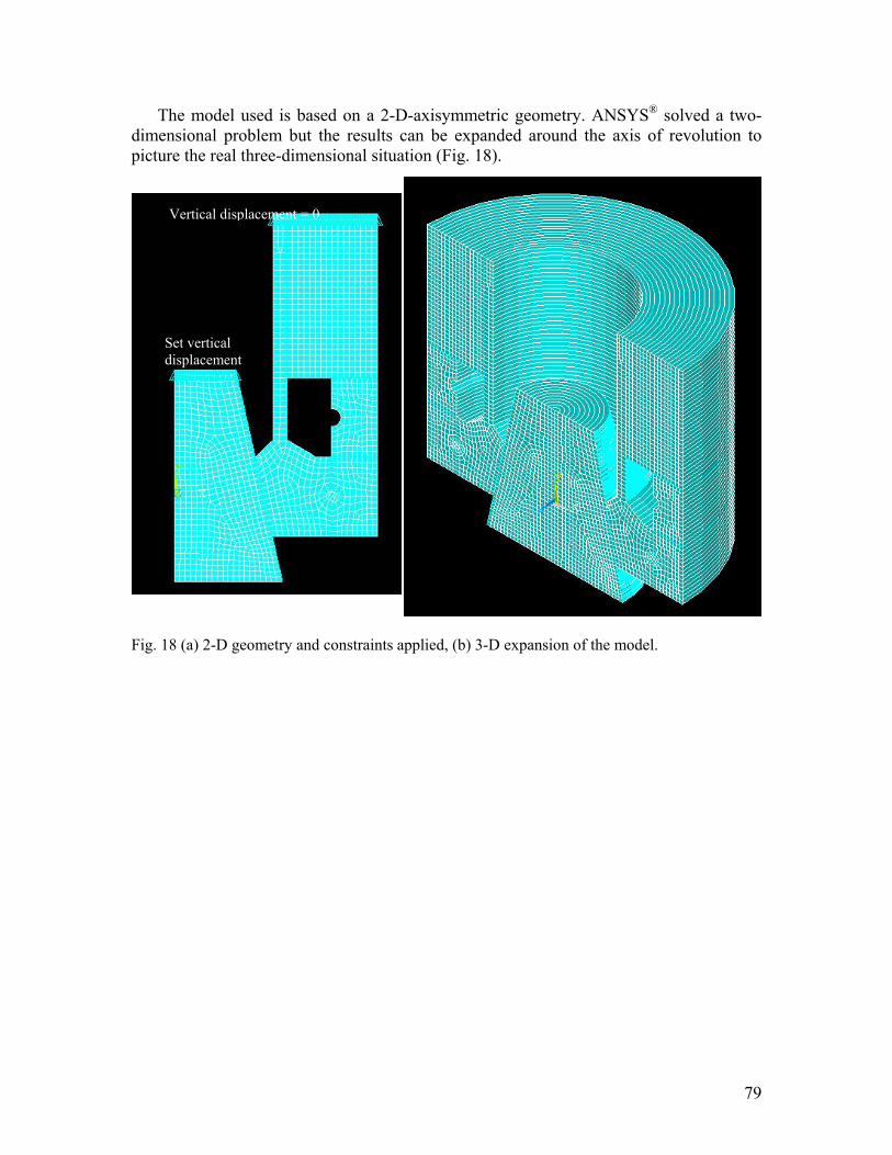
79

The model used is based on a 2-D-axisymmetric geometry. ANSYS® solved a two-dimensional problem but the results can be expanded around the axis of revolution to picture the real three-dimensional situation (Fig. 18).

Fig. 18 (a) 2-D geometry and constraints applied, (b) 3-D expansion of the model.

Vertical displacement = 0

Set vertical displacement

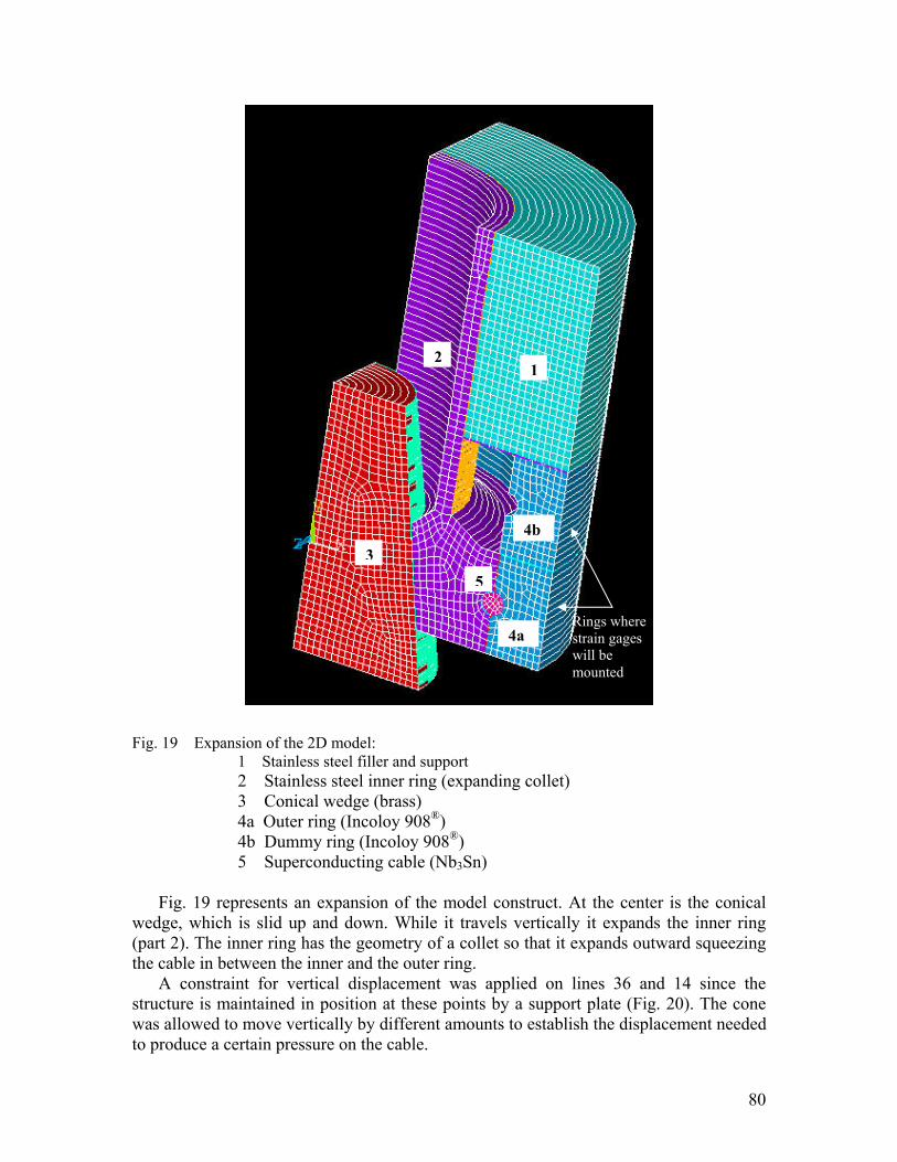
80

Fig. 19 Expansion of the 2D model: 1 Stainless steel filler and support 2 Stainless steel inner ring (expanding collet) 3 Conical wedge (brass) 4a Outer ring (Incoloy 908®) 4b Dummy ring (Incoloy 908®) 5 Superconducting cable (Nb3Sn)

Fig. 19 represents an expansion of the model construct. At the center is the conical

wedge, which is slid up and down. While it travels vertically it expands the inner ring (part 2). The inner ring has the geometry of a collet so that it expands outward squeezing the cable in between the inner and the outer ring.

A constraint for vertical displacement was applied on lines 36 and 14 since the structure is maintained in position at these points by a support plate (Fig. 20). The cone was allowed to move vertically by different amounts to establish the displacement needed to produce a certain pressure on the cable.

4b

12

35

4aRings where strain gages will be mounted

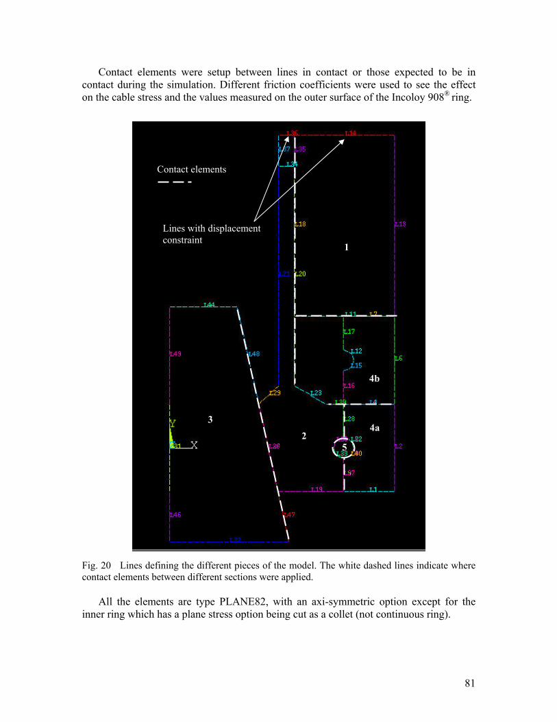
81

Contact elements were setup between lines in contact or those expected to be in contact during the simulation. Different friction coefficients were used to see the effect on the cable stress and the values measured on the outer surface of the Incoloy 908® ring.

Fig. 20 Lines defining the different pieces of the model. The white dashed lines indicate where contact elements between different sections were applied.

All the elements are type PLANE82, with an axi-symmetric option except for the

inner ring which has a plane stress option being cut as a collet (not continuous ring).

Contact elements

1

23

4a

4b

5

Lines with displacement constraint

82

The values of Young’s modulus used for the different materials are:

Stainless steel 207 GPa Brass 110 GPa Incoloy 908® 182 GPa Nb3Sn cable 2 GPa

The Young’s modulus for the Nb3Sn cable has a very low value of 2 GPa after heat

treatment, as Nb3Sn is a very soft material. This value was estimated in a set of experiments made at Twente [3.5].

The coefficient of friction was varied from 0.1 up to 1. Since the interfaces between the conical wedge/inner ring and the outer ring/dummy ring were the most critical, the study was done by varying the coefficient of friction only for these two interfaces. The nominal separation between the Incoloy 908® ring and the expanding collet was 1 mm.

In this configuration the axial strain is the y component while the hoop component is the z component. The transverse pressure is represented by the x component of the stress. There needs to be a relationship between the strain in the z component (hoop strain measured in the experiment) and the transverse stress (x component) on the cable. With this relationship, during the test, it will be possible to estimate the transverse stress by measuring the hoop strain.

Fig. 21 Results of ANSYS® simulation at step 40. The plot is for the transverse stress (x-component). As expected the minimum value (~ -21 MPa, compressive stress) is recorded at the cable position.

83

Fig. 21 shows the typical results for one of the steps during the simulation. In the figure the transverse stress (x-component) is shown. Since the vertical movement of the cone serves the purpose of applying transverse stress to the cable, the minimum value of pressure is contained within the cable (~ -21 MPa compressive stress), showing that the model was working properly.Fig. 22 is a close up of Fig. 21 showing the cable and the two Incoloy 908® rings.

Fig. 22 Close up view of the cable and Incoloy 908® rings at step 40 of the analysis. The plot illustrates the transverse stress.

Fig. 23 (a-d) show the strain level inside the cable and on the Incoloy 908® ring for the same analysis step as the figures above (step at which the transverse stress on the cable is ~ -21 MPa). On the left of each pair of plots, the y-component of the strain is shown. This strain is measured by the axial component of the strain gages used for the experiment. On the right, the z-component of the strain is shown. This strain is measured by the hoop component of the strain gages (Fig. 24). The y-component of the strain on the Incoloy 908® rings is much smaller than the hoop component. The presence of the dummy Incoloy 908® ring (on the top) is creating a non-uniform pattern of the strain on the other ring as well. Averaged values will be used as a comparison with the measurements. Parametric studies on the effect of the coefficient of fiction between the cone and the expanding collet and between the two Incoloy 908® rings were performed. These studies showed that the difference in strain level between the case in which all the friction coefficients are 0.1 and the case where the friction coefficients are varied from 0.3 to 1, is less than 3%. The pattern of the strain level in the Incoloy 908® increases in symmetry for higher friction coefficients between the two rings (Fig. 23 (d)).

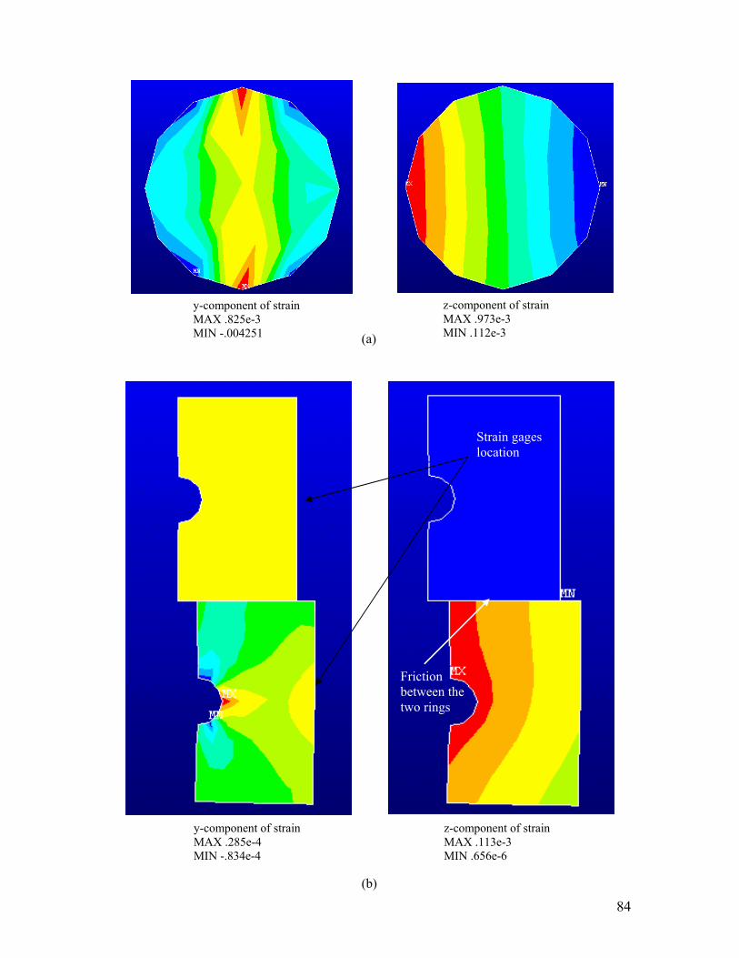
84

y-component of strain MAX .825e-3 MIN -.004251

z-component of strain MAX .973e-3 MIN .112e-3

y-component of strain MAX .285e-4 MIN -.834e-4

z-component of strain MAX .113e-3 MIN .656e-6

(a)

(b)

Friction between the two rings

Strain gages location

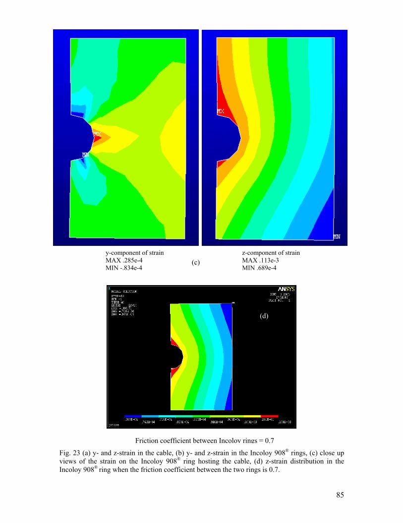
85

Fig. 23 (a) y- and z-strain in the cable, (b) y- and z-strain in the Incoloy 908® rings, (c) close up views of the strain on the Incoloy 908® ring hosting the cable, (d) z-strain distribution in the Incoloy 908® ring when the friction coefficient between the two rings is 0.7.

y-component of strain MAX .285e-4 MIN -.834e-4

z-component of strain MAX .113e-3 MIN .689e-4

Friction coefficient between Incoloy rings = 0.7

(c)

(d)

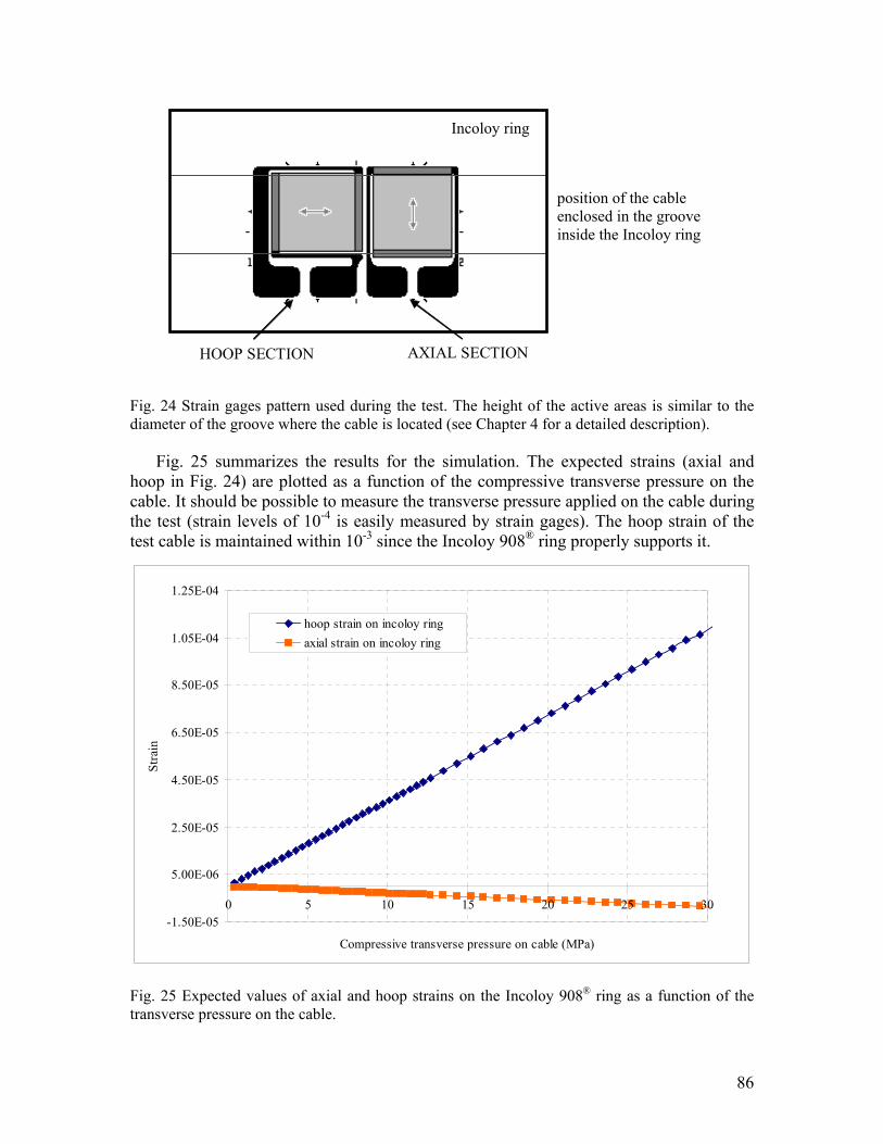
86

Fig. 24 Strain gages pattern used during the test. The height of the active areas is similar to the diameter of the groove where the cable is located (see Chapter 4 for a detailed description).

Fig. 25 summarizes the results for the simulation. The expected strains (axial and hoop in Fig. 24) are plotted as a function of the compressive transverse pressure on the cable. It should be possible to measure the transverse pressure applied on the cable during the test (strain levels of 10-4 is easily measured by strain gages). The hoop strain of the test cable is maintained within 10-3 since the Incoloy 908® ring properly supports it.

Fig. 25 Expected values of axial and hoop strains on the Incoloy 908® ring as a function of the transverse pressure on the cable.

HOOP SECTION AXIAL SECTION

position of the cable enclosed in the groove inside the Incoloy ring

Incoloy ring

-1.50E-05

5.00E-06

2.50E-05

4.50E-05

6.50E-05

8.50E-05

1.05E-04

1.25E-04

0 5 10 15 20 25 30

Compressive transverse pressure on cable (MPa)

Stra

in

hoop strain on incoloy ringaxial strain on incoloy ring

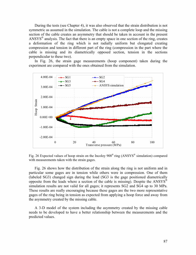
87

During the tests (see Chapter 4), it was also observed that the strain distribution is not symmetric as assumed in the simulation. The cable is not a complete loop and the missing section of the cable creates an asymmetry that should be taken in account in the present ANSYS® analysis. The fact that there is an empty space in one section of the ring, creates a deformation of the ring which is not radially uniform but elongated creating compression and tension in different part of the ring (compression in the part where the cable is missing and its diametrically opposed section, tension in the sections perpendicular to these two).

In Fig. 26, the strain gage measurements (hoop component) taken during the experiment are compared with the ones obtained from the simulation.

Fig. 26 Expected values of hoop strain on the Incoloy 908® ring (ANSYS® simulation) compared with measurements taken with the strain gages.

Fig. 26 shows how the distribution of the strain along the ring is not uniform and in particular some gages are in tension while others were in compression. One of them (labeled SG3) changed sign during the load (SG3 is the gage positioned diametrically opposite from the leads where a section of the cable is missing). Despite the ANSYS® simulation results are not valid for all gages; it represents SG2 and SG4 up to 30 MPa. These results are really encouraging because these gages are the two more representative gages of the ring being in tension as expected from applying a hoop force and away from the asymmetry created by the missing cable.

A 3-D model of the system including the asymmetry created by the missing cable

needs to be developed to have a better relationship between the measurements and the predicted values.

-2.00E-04

-1.00E-04

0.00E+00

1.00E-04

2.00E-04

3.00E-04

4.00E-04

0 20 40 60 80 100Transverse pressure (MPa)

Hoo

p S

train

SG1 SG2SG3 SG4SG5 ANSYS simulation

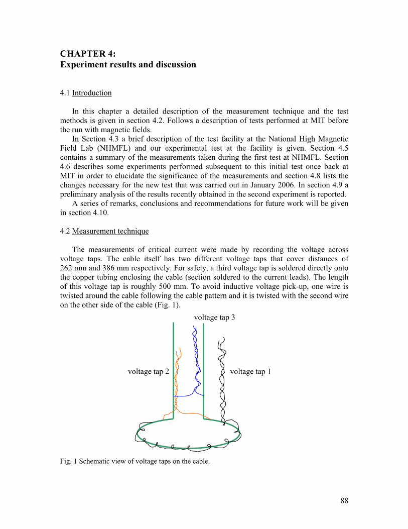
88

CHAPTER 4: Experiment results and discussion 4.1 Introduction

In this chapter a detailed description of the measurement technique and the test

methods is given in section 4.2. Follows a description of tests performed at MIT before the run with magnetic fields.

In Section 4.3 a brief description of the test facility at the National High Magnetic Field Lab (NHMFL) and our experimental test at the facility is given. Section 4.5 contains a summary of the measurements taken during the first test at NHMFL. Section 4.6 describes some experiments performed subsequent to this initial test once back at MIT in order to elucidate the significance of the measurements and section 4.8 lists the changes necessary for the new test that was carried out in January 2006. In section 4.9 a preliminary analysis of the results recently obtained in the second experiment is reported.

A series of remarks, conclusions and recommendations for future work will be given in section 4.10.

4.2 Measurement technique

The measurements of critical current were made by recording the voltage across voltage taps. The cable itself has two different voltage taps that cover distances of 262 mm and 386 mm respectively. For safety, a third voltage tap is soldered directly onto the copper tubing enclosing the cable (section soldered to the current leads). The length of this voltage tap is roughly 500 mm. To avoid inductive voltage pick-up, one wire is twisted around the cable following the cable pattern and it is twisted with the second wire on the other side of the cable (Fig. 1).

Fig. 1 Schematic view of voltage taps on the cable.

voltage tap 3

voltage tap 2 voltage tap 1

89

The Incoloy 908® rings were equipped with strain gages which were used to estimate the load applied on the cable using the ANSYS® model described in Chapter 3. Furthermore a load cell was mounted on the top of the dewar to measure the vertical load applied on the system. Knowing the vertical load it is possible to estimate the force and the pressure on the cable.

The strain gages used were purchased from Vishay Micro-Measurements Group. The gages used for the experiment are model SK-06-250TM-350. The strain gages have a biaxial rosette pattern since it was desirable to know the hoop strain and also any axial component present.

The SK series gages are a family of fully encapsulated in glass fiber reinforced epoxy-phenolic resin. This particular material acts as an insulation barrier that helps diffuse the electrical heat generated before it reaches the helium on the surface. The foil alloy (K) is a nickel-chromium alloy. The number 250 corresponds to the active length in mils (250 mils = 6.35 mm). TM corresponds to the particular pattern of the gage chosen while the 350 refers to the nominal resistance (Ω) of the gage chosen to limit the amount of power generated while still providing enough sensitivity. It is also important that the excitation voltage for the gages be kept low enough to prevent heating of the gages. This voltage was set at 2 V for our measurements (Fig. 2).

Fig. 2 Strain gage pattern for the gages used in the experiment.

Micro-Measurements supplies gages with a self-temperature compensating property. The gages can be chosen to have an approximate thermal coefficient of expansion that matches the test material at the testing temperature. This self-temperature compensation (STC) property changes in a nonlinear fashion with temperature and so a material match at one temperature may not be applicable at another temperature. The gages selected for the measurements have an STC property that correlates to stainless steel (closest material to Incoloy 908® property available).

The Gage Factor (GF) of the strain gage changes also with temperature. At room temperature the nominal value of GF is 1.98 for the hoop section and 2.01 for the axial section. Literature included with the gages, showed that the GF changed linearly with temperature according to a temperature coefficient of GF equal to -1.0%/100 °C. Lowering from room temperature to the -269 °C testing environment meant that the appropriate GF for the strain gages was 2.93% greater, or equal to 2.04 and 2.07 for the hoop and axial section, respectively.

The adhesive selected to install the gages was Micro-Measurements M-Bond AE-15. This is a two-component epoxy-phenolic adhesive that must be cured at relatively

HOOP SECTION AXIAL SECTION

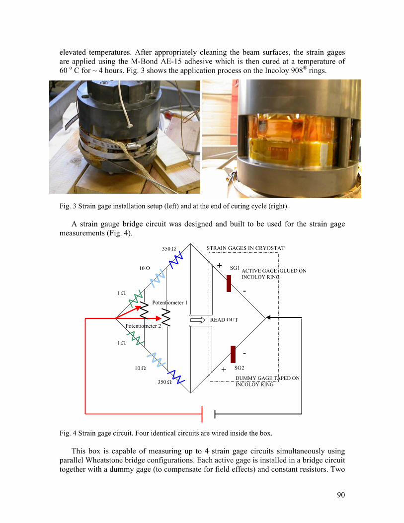
90

elevated temperatures. After appropriately cleaning the beam surfaces, the strain gages are applied using the M-Bond AE-15 adhesive which is then cured at a temperature of 60 o C for ~ 4 hours. Fig. 3 shows the application process on the Incoloy 908® rings.

Fig. 3 Strain gage installation setup (left) and at the end of curing cycle (right).

A strain gauge bridge circuit was designed and built to be used for the strain gage measurements (Fig. 4).

Fig. 4 Strain gage circuit. Four identical circuits are wired inside the box.

This box is capable of measuring up to 4 strain gage circuits simultaneously using parallel Wheatstone bridge configurations. Each active gage is installed in a bridge circuit together with a dummy gage (to compensate for field effects) and constant resistors. Two

ACTIVE GAGE GLUED ON INCOLOY RING

DUMMY GAGE TAPED ON INCOLOY RING

10 Ω

10 Ω

350 Ω

350 Ω

1 Ω

1 Ω

Potentiometer 1

SG1

SG2

-

-

+

+

READ OUTPotentiometer 2

STRAIN GAGES IN CRYOSTAT

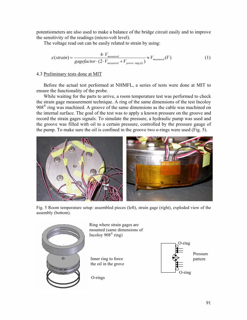
91

potentiometers are also used to make a balance of the bridge circuit easily and to improve the sensitivity of the readings (micro-volt level).

The voltage read out can be easily related to strain by using:

)()2(

4)(sup

VVVVgagefactor

Vstrain measuredplypowermeasured

measured ≈+⋅⋅

⋅=

−

ε (1)

4.3 Preliminary tests done at MIT

Before the actual test performed at NHMFL, a series of tests were done at MIT to ensure the functionality of the probe.

While waiting for the parts to arrive, a room temperature test was performed to check the strain gage measurement technique. A ring of the same dimensions of the test Incoloy 908® ring was machined. A groove of the same dimensions as the cable was machined on the internal surface. The goal of the test was to apply a known pressure on the groove and record the strain gages signals. To simulate the pressure, a hydraulic pump was used and the groove was filled with oil to a certain pressure, controlled by the pressure gauge of the pump. To make sure the oil is confined in the groove two o-rings were used (Fig. 5).

Fig. 5 Room temperature setup: assembled pieces (left), strain gage (right), exploded view of the assembly (bottom).

Ring where strain gages are mounted (same dimensions of Incoloy 908® ring)

Inner ring to force the oil in the grove

O-rings

Pressure pattern

O-ring

O-ring

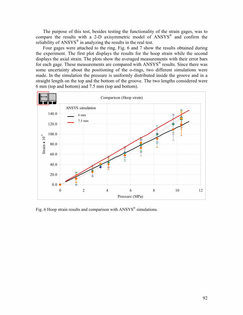
92

The purpose of this test, besides testing the functionality of the strain gages, was to compare the results with a 2-D axisymmetric model of ANSYS® and confirm the reliability of ANSYS® in analyzing the results in the real test.

Four gages were attached to the ring. Fig. 6 and 7 show the results obtained during the experiment. The first plot displays the results for the hoop strain while the second displays the axial strain. The plots show the averaged measurements with their error bars for each gage. These measurements are compared with ANSYS® results. Since there was some uncertainty about the positioning of the o-rings, two different simulations were made. In the simulation the pressure is uniformly distributed inside the groove and in a straight length on the top and the bottom of the groove. The two lengths considered were 6 mm (top and bottom) and 7.5 mm (top and bottom).

Fig. 6 Hoop strain results and comparison with ANSYS® simulations.

Comparison (Hoop strain)

0.0

20.0

40.0

60.0

80.0

100.0

120.0

140.0

160.0

0 2 4 6 8 10 12Pressure (MPa)

Stra

in x

10-6

ANSYS simulation

6 mm

7.5 mm

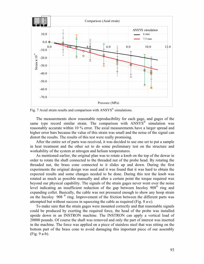
93

Fig. 7 Axial strain results and comparison with ANSYS® simulations.

The measurements show reasonable reproducibility for each gage, and gages of the same type record similar strain. The comparison with ANSYS® simulation was reasonably accurate within 10 % error. The axial measurements have a larger spread and higher error bars because the value of this strain was small and the noise of the signal can distort the results. The results of this test were really promising.

After the entire set of parts was received, it was decided to use one set to put a sample in heat treatment and the other set to do some preliminary test on the structure and workability of the system at nitrogen and helium temperatures.

As mentioned earlier, the original plan was to rotate a knob on the top of the dewar in order to rotate the shaft connected to the threaded nut of the probe head. By rotating the threaded nut, the brass cone connected to it slides up and down. During the first experiments the original design was used and it was found that it was hard to obtain the expected results and some changes needed to be done. During this test the knob was rotated as much as possible manually and after a certain point the torque required was beyond our physical capability. The signals of the strain gages never went over the noise level indicating an insufficient reduction of the gap between Incoloy 908® ring and expanding collet. Basically, the cable was not pressured enough to show any hoop strain on the Incoloy 908 ® ring. Improvement of the friction between the different parts was attempted but without success in squeezing the cable as required (Fig. 8 a-c).

To make sure that the strain gages were mounted correctly and that reasonable signals could be produced by exerting the required force, the head of the probe was installed upside down in an INSTRON machine. The INSTRON can apply a vertical load of 20000 pounds. Of course the shaft was removed and only the part of interest was inserted in the machine. The force was applied on a piece of stainless steel that was sitting on the bottom part of the brass cone to avoid damaging this important piece of our assembly (Fig. 9 a-b).

Comparison (Axial strain)

-70.0

-60.0

-50.0

-40.0

-30.0

-20.0

-10.0

0.0

10.0

20.0

0.0 2.0 4.0 6.0 8.0 10.0 12.0

Pressure (MPa)

Stra

in x

10-6

ANSYS simulation 6 mm

7.5 mm

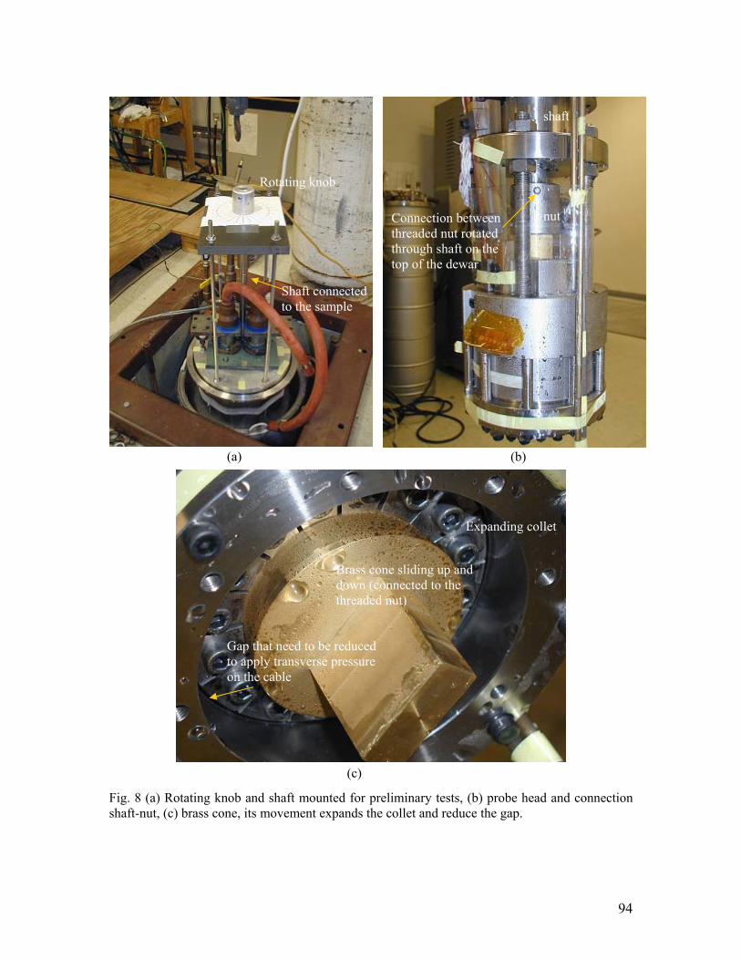
94

Fig. 8 (a) Rotating knob and shaft mounted for preliminary tests, (b) probe head and connection shaft-nut, (c) brass cone, its movement expands the collet and reduce the gap.

Rotating knob

Shaft connected to the sample

d

Connection between threaded nut rotated through shaft on the top of the dewar

shaft

nut

Brass cone sliding up and down (connected to the threaded nut)

Gap that need to be reduced to apply transverse pressure on the cable

(a) (b)

(c)

Expanding collet

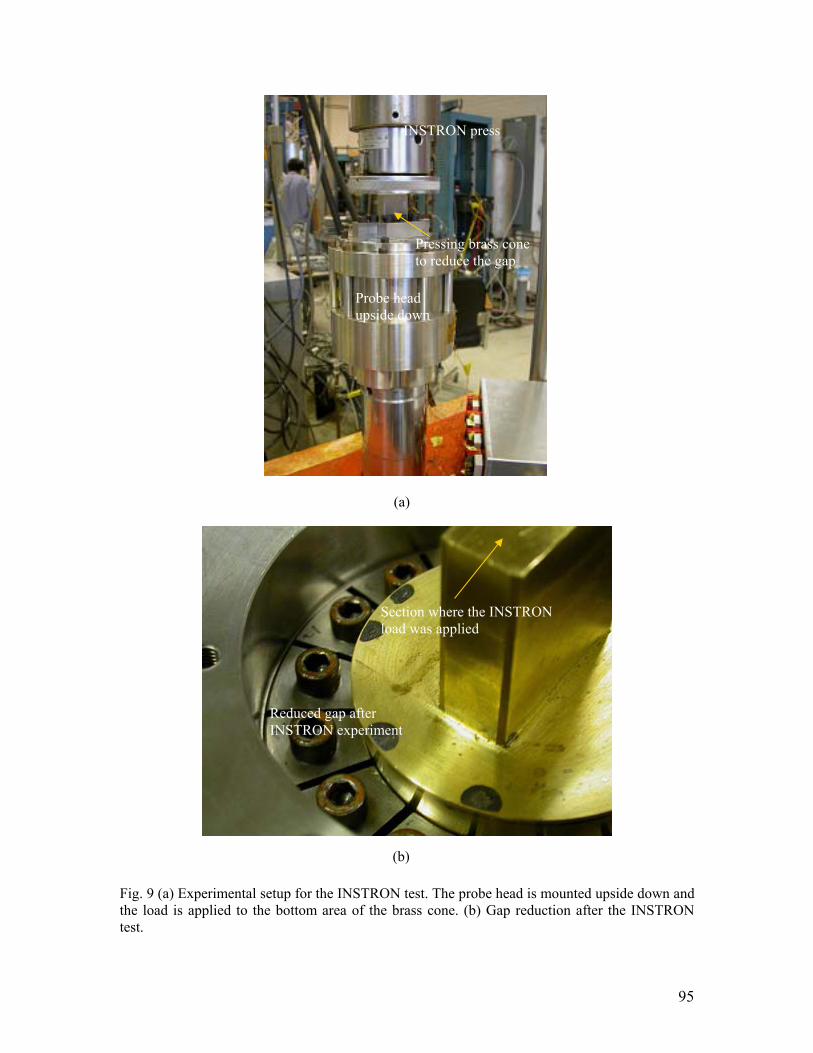
95

Fig. 9 (a) Experimental setup for the INSTRON test. The probe head is mounted upside down and the load is applied to the bottom area of the brass cone. (b) Gap reduction after the INSTRON test.

INSTRON press

Probe head upside down

Pressing brass cone to reduce the gap

Reduced gap after INSTRON experiment

Section where the INSTRON load was applied

(a)

(b)

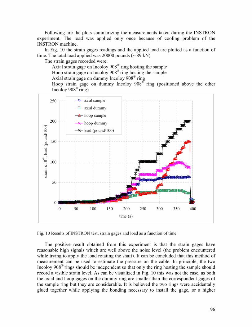
96

Following are the plots summarizing the measurements taken during the INSTRON experiment. The load was applied only once because of cooling problem of the INSTRON machine.

In Fig. 10 the strain gages readings and the applied load are plotted as a function of time. The total load applied was 20000 pounds (~ 89 kN).

The strain gages recorded were: Axial strain gage on Incoloy 908® ring hosting the sample

Hoop strain gage on Incoloy 908® ring hosting the sample Axial strain gage on dummy Incoloy 908® ring Hoop strain gage on dummy Incoloy 908® ring (positioned above the other Incoloy 908® ring)

Fig. 10 Results of INSTRON test, strain gages and load as a function of time.

The positive result obtained from this experiment is that the strain gages have reasonable high signals which are well above the noise level (the problem encountered while trying to apply the load rotating the shaft). It can be concluded that this method of measurement can be used to estimate the pressure on the cable. In principle, the two Incoloy 908® rings should be independent so that only the ring hosting the sample should record a visible strain level. As can be visualized in Fig. 10 this was not the case, as both the axial and hoop gages on the dummy ring are smaller than the correspondent gages of the sample ring but they are considerable. It is believed the two rings were accidentally glued together while applying the bonding necessary to install the gage, or a higher

0

50

100

150

200

250

0 50 100 150 200 250 300 350 400

time (s)

strai

n x

10-6

, loa

d (p

ound

/100

)

axial sample

axial dummy

hoop sample

hoop dummy

load (pound/100)

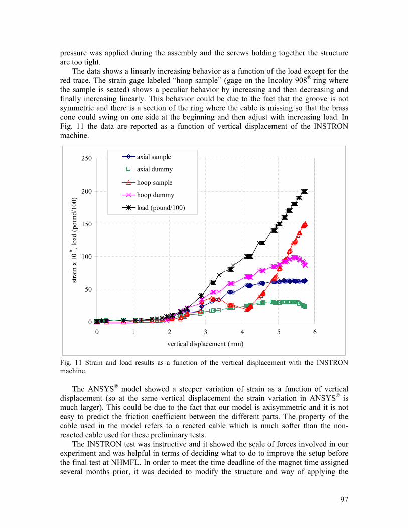
97

pressure was applied during the assembly and the screws holding together the structure are too tight.

The data shows a linearly increasing behavior as a function of the load except for the red trace. The strain gage labeled “hoop sample” (gage on the Incoloy 908® ring where the sample is seated) shows a peculiar behavior by increasing and then decreasing and finally increasing linearly. This behavior could be due to the fact that the groove is not symmetric and there is a section of the ring where the cable is missing so that the brass cone could swing on one side at the beginning and then adjust with increasing load. In Fig. 11 the data are reported as a function of vertical displacement of the INSTRON machine.

Fig. 11 Strain and load results as a function of the vertical displacement with the INSTRON machine.

The ANSYS® model showed a steeper variation of strain as a function of vertical displacement (so at the same vertical displacement the strain variation in ANSYS® is much larger). This could be due to the fact that our model is axisymmetric and it is not easy to predict the friction coefficient between the different parts. The property of the cable used in the model refers to a reacted cable which is much softer than the non-reacted cable used for these preliminary tests.

The INSTRON test was instructive and it showed the scale of forces involved in our experiment and was helpful in terms of deciding what to do to improve the setup before the final test at NHMFL. In order to meet the time deadline of the magnet time assigned several months prior, it was decided to modify the structure and way of applying the

0

50

100

150

200

250

0 1 2 3 4 5 6

vertical displacement (mm)

strai

n x

10-6

, loa

d (p

ound

/100

)

axial sample

axial dummy

hoop sample

hoop dummy

load (pound/100)

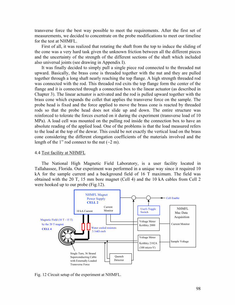
98

transverse force the best way possible to meet the requirements. After the first set of measurements, we decided to concentrate on the probe modifications to meet our timeline for the test at NHMFL.

First of all, it was realized that rotating the shaft from the top to induce the sliding of the cone was a very hard task given the unknown friction between all the different pieces and the uncertainty of the strength of the different sections of the shaft which included also universal joints (see drawing in Appendix I).

It was finally decided to simply pull a single piece rod connected to the threaded nut upward. Basically, the brass cone is threaded together with the nut and they are pulled together through a long shaft nearly reaching the top flange. A high strength threaded rod was connected with the rod. This threaded rod exits the top flange form the center of the flange and it is connected through a connection box to the linear actuator (as described in Chapter 3). The linear actuator is activated and the rod is pulled upward together with the brass cone which expands the collet that applies the transverse force on the sample. The probe head is fixed and the force applied to move the brass cone is reacted by threaded rods so that the probe head does not slide up and down. The entire structure was reinforced to tolerate the forces exerted on it during the experiment (transverse load of 10 MPa). A load cell was mounted on the pulling rod inside the connection box to have an absolute reading of the applied load. One of the problems is that the load measured refers to the load at the top of the dewar. This could be not exactly the vertical load on the brass cone considering the different elongation coefficients of the materials involved and the length of the 1” rod connect to the nut (~2 m).

4.4 Test facility at NHMFL

The National High Magnetic Field Laboratory, is a user facility located in

Tallahassee, Florida. Our experiment was performed in a unique way since it required 10 kA for the sample current and a background field of 16 T maximum. The field was obtained with the 20 T, 15 mm bore magnet (Cell 4) and the 10 kA cables from Cell 2 were hooked up to our probe (Fig.12).

Fig. 12 Circuit setup of the experiment at NHMFL.

Single Turn, 36 Strand Superconducting Cable with Externally Loaded Transverse Force

NHMFL Magnet Power SupplyCELL 2

Water cooled resistors 3.1mΩ each

NHMFL Mac Data Acquisition

Current Monitor

10 kA CurrentCurrent Monitor

Magnetic Field (10 T - 15 T) by the 20 T magnet

CELL 4

Sample Voltage Keithley 2182A

Voltage Meter

Keithley 2000Voltage Meter

Quench Detector

Cell Enable

(100 micro-V)

User's ToggleSwitch

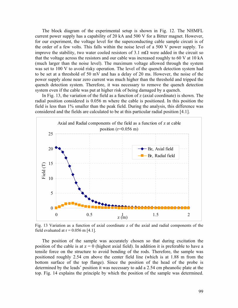
99

The block diagram of the experimental setup is shown in Fig. 12. The NHMFL current power supply has a capability of 20 kA and 500 V for a Bitter magnet. However, for our experiment, the voltage level for the superconducting cable sample circuti is of the order of a few volts. This falls within the noise level of a 500 V power supply. To improve the stability, two water cooled resistors of 3.1 mΩ were added in the circuit so that the voltage across the resistors and our cable was increased roughly to 60 V at 10 kA (much larger than the noise level). The maximum voltage allowed through the system was set to 100 V to avoid risky operation. The level of the quench detection system had to be set at a threshold of 50 mV and has a delay of 20 ms. However, the noise of the power supply alone near zero current was much higher than the threshold and tripped the quench detection system. Therefore, it was necessary to remove the quench detection system even if the cable was put at higher risk of being damaged by a quench.

In Fig. 13, the variation of the field as a function of z (axial coordinate) is shown. The radial position considered is 0.056 m where the cable is positioned. In this position the field is less than 1% smaller than the peak field. During the analysis, this difference was considered and the fields are calculated to be at this particular radial position [4.1].

Fig. 13 Variation as a function of axial coordinate z of the axial and radial components of the field evaluated at r = 0.056 m [4.1].

The position of the sample was accurately chosen so that during excitation the

position of the cable is at z = 0 (highest axial field). In addition it is preferable to have a tensile force on the structure to avoid bending of the rods. Therefore, the sample was positioned roughly 2.54 cm above the center field line (which is at 1.88 m from the bottom surface of the top flange). Since the position of the head of the probe is determined by the leads’ position it was necessary to add a 2.54 cm pheanolic plate at the top. Fig. 14 explains the principle by which the position of the sample was determined.

Axial and Radial components of the field as a function of z at cable position (r=0.056 m)

0

5

10

15

20

25

0 0.5 1 1.5 2z (m)

Fiel

d (T

)

Bz, Axial fieldBr, Radial field

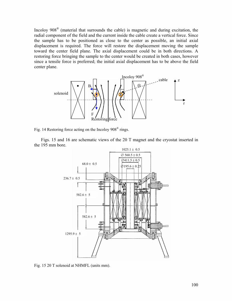
100

Incoloy 908® (material that surrounds the cable) is magnetic and during excitation, the radial component of the field and the current inside the cable create a vertical force. Since the sample has to be positioned as close to the center as possible, an initial axial displacement is required. The force will restore the displacement moving the sample toward the center field plane. The axial displacement could be in both directions. A restoring force bringing the sample to the center would be created in both cases, however since a tensile force is preferred; the initial axial displacement has to be above the field center plane.

Fig. 14 Restoring force acting on the Incoloy 908® rings.

Figs. 15 and 16 are schematic views of the 20 T magnet and the cryostat inserted in the 195 mm bore.

Fig. 15 20 T solenoid at NHMFL (units mm).

1025.1 ± 0.5∅ 560.5 ± 0.5∅411.5 ± 0.5

∅195.6 ± 0.2568.0 ± 0.5

236.7 ± 0.5

582.6 ± 5

582.6 ± 5

1295.9 ± 5

⊗•

• ⊗

Br

solenoid

Incoloy 908® cable z

r

F Restoring force

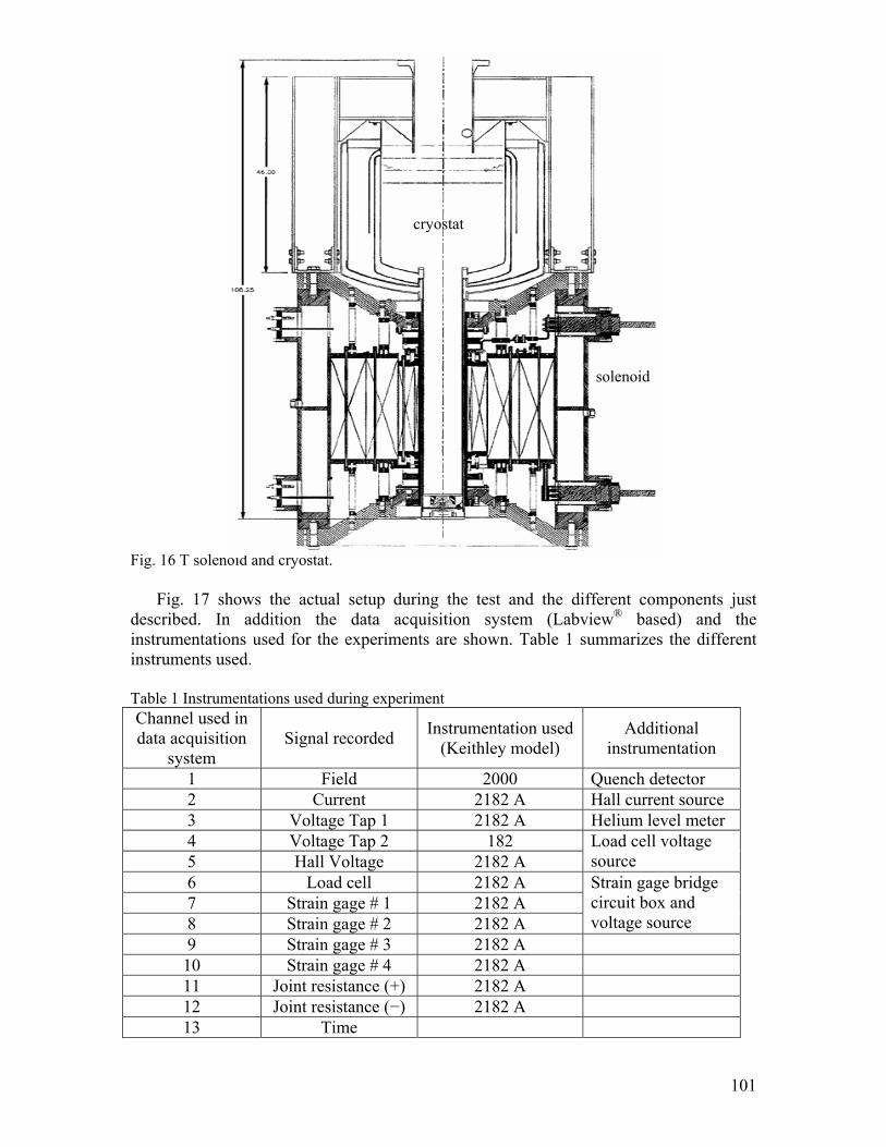
101

Fig. 16 T solenoid and cryostat. Fig. 17 shows the actual setup during the test and the different components just

described. In addition the data acquisition system (Labview® based) and the instrumentations used for the experiments are shown. Table 1 summarizes the different instruments used.

Table 1 Instrumentations used during experiment Channel used in data acquisition

system Signal recorded Instrumentation used

(Keithley model) Additional

instrumentation

1 Field 2000 Quench detector 2 Current 2182 A Hall current source 3 Voltage Tap 1 2182 A Helium level meter 4 Voltage Tap 2 182 5 Hall Voltage 2182 A

Load cell voltage source

6 Load cell 2182 A 7 Strain gage # 1 2182 A 8 Strain gage # 2 2182 A

Strain gage bridge circuit box and voltage source

9 Strain gage # 3 2182 A 10 Strain gage # 4 2182 A 11 Joint resistance (+) 2182 A 12 Joint resistance (−) 2182 A 13 Time

solenoid

cryostat

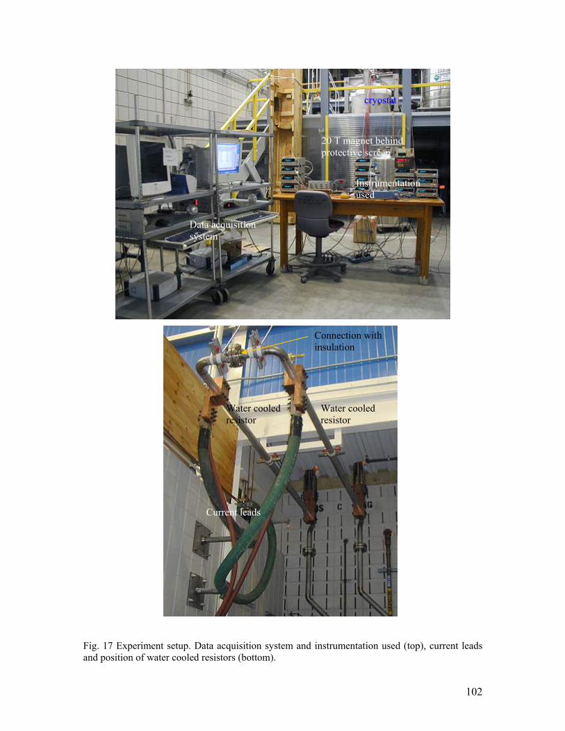
102

Fig. 17 Experiment setup. Data acquisition system and instrumentation used (top), current leads and position of water cooled resistors (bottom).

Data acquisition system

Instrumentation used

cryostat

20 T magnet behind protective screen

Water cooled resistor

Current leads

Water cooled resistor

Connection with insulation

103

The 20 T solenoid is comprised of three coils and for each of them current, voltage and temperature are controlled to make sure the system is protected.

A fault control system keeps the magnets from being damaged. Anything that causes the parameters of each coil to go beyond their tolerance limits trips the system. The fault control system is sensitive to fluctuations in the coil voltages. The users’ experiment must be insulated from the solenoid magnet so that a current from an external power supply does not trip the system. A small amount of noise in the magnet power supply may also trip the fault system and since the power supplies are designed to operate over a large range of voltages, the zero setting is very difficult to achieve and the noise level can be high enough to trip the system.

As a safety precaution, the user must reduce the magnetic field intensity before walking on the platform where the top of the dewar and probe are located. To avoid tripping the system, the magnet can be set to a field level where it is low enough so that it is safe to stay on the platform but high enough so that the power supply has a very low voltage noise. For the 20 T, 195 mm bore magnet this setting is a field of 0.054 T.

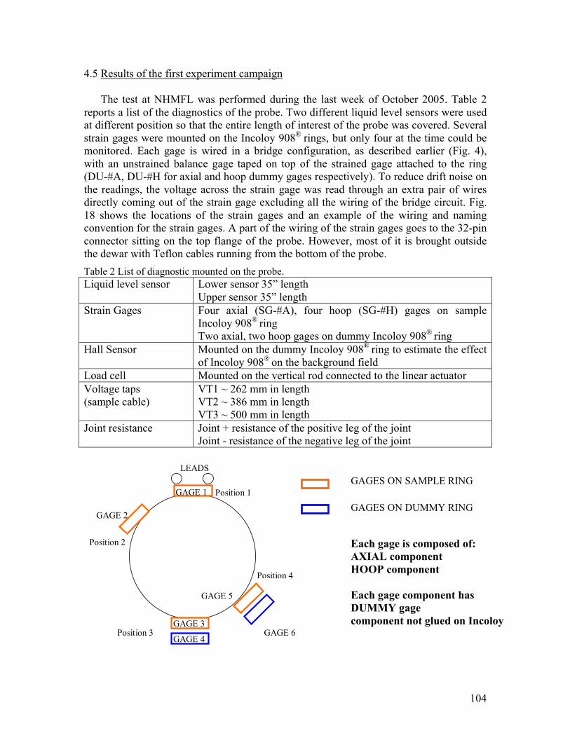
104

4.5 Results of the first experiment campaign

The test at NHMFL was performed during the last week of October 2005. Table 2 reports a list of the diagnostics of the probe. Two different liquid level sensors were used at different position so that the entire length of interest of the probe was covered. Several strain gages were mounted on the Incoloy 908® rings, but only four at the time could be monitored. Each gage is wired in a bridge configuration, as described earlier (Fig. 4), with an unstrained balance gage taped on top of the strained gage attached to the ring (DU-#A, DU-#H for axial and hoop dummy gages respectively). To reduce drift noise on the readings, the voltage across the strain gage was read through an extra pair of wires directly coming out of the strain gage excluding all the wiring of the bridge circuit. Fig. 18 shows the locations of the strain gages and an example of the wiring and naming convention for the strain gages. A part of the wiring of the strain gages goes to the 32-pin connector sitting on the top flange of the probe. However, most of it is brought outside the dewar with Teflon cables running from the bottom of the probe.

Table 2 List of diagnostic mounted on the probe. Liquid level sensor Lower sensor 35” length

Upper sensor 35” length Strain Gages Four axial (SG-#A), four hoop (SG-#H) gages on sample

Incoloy 908® ring Two axial, two hoop gages on dummy Incoloy 908® ring

Hall Sensor Mounted on the dummy Incoloy 908® ring to estimate the effect of Incoloy 908® on the background field

Load cell Mounted on the vertical rod connected to the linear actuator Voltage taps (sample cable)

VT1 ~ 262 mm in length VT2 ~ 386 mm in length VT3 ~ 500 mm in length

Joint resistance Joint + resistance of the positive leg of the joint Joint - resistance of the negative leg of the joint

LEADS

Position 1

Position 2

Position 3

Position 4

GAGE 3

GAGE 4

GAGE 1

GAGE 2

GAGE 5

GAGE 6

GAGES ON SAMPLE RING

GAGES ON DUMMY RING Each gage is composed of: AXIAL component HOOP component Each gage component has DUMMY gage component not glued on Incoloy

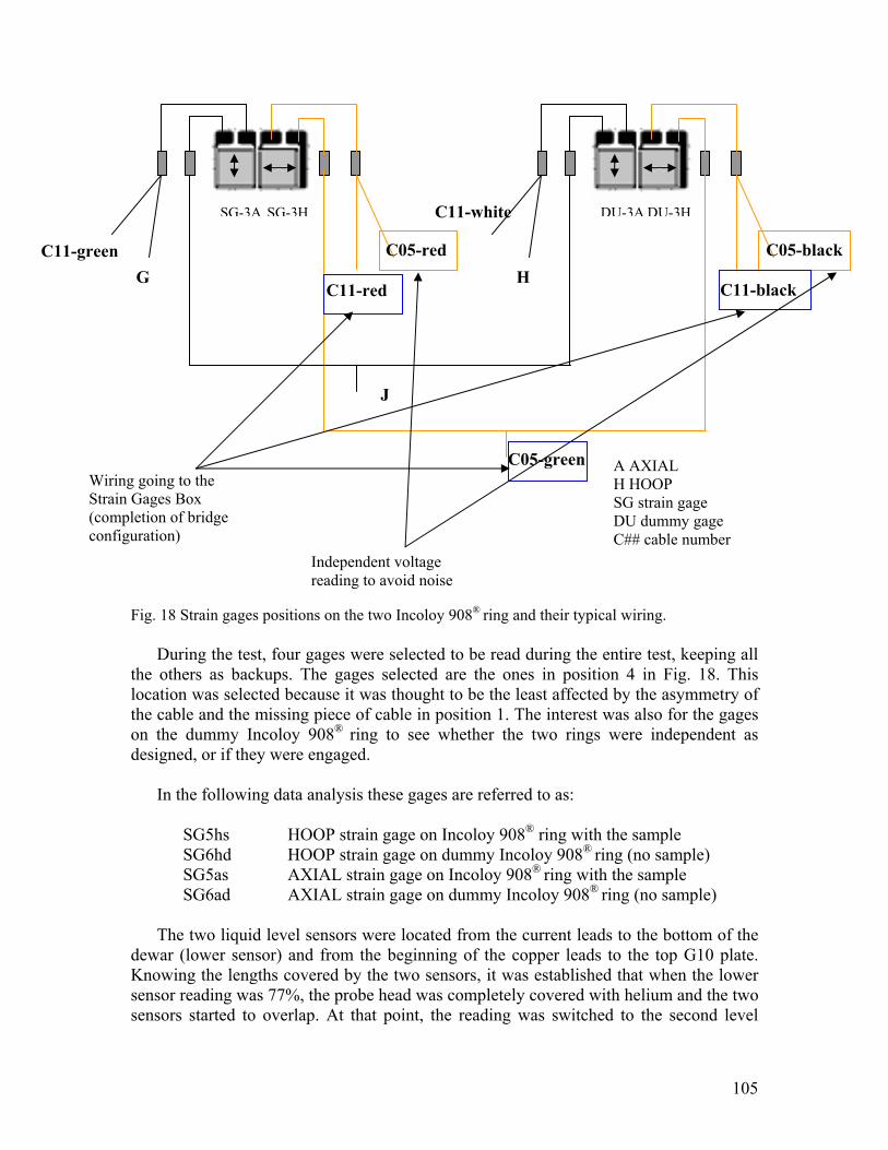
105

Fig. 18 Strain gages positions on the two Incoloy 908® ring and their typical wiring.

During the test, four gages were selected to be read during the entire test, keeping all the others as backups. The gages selected are the ones in position 4 in Fig. 18. This location was selected because it was thought to be the least affected by the asymmetry of the cable and the missing piece of cable in position 1. The interest was also for the gages on the dummy Incoloy 908® ring to see whether the two rings were independent as designed, or if they were engaged.

In the following data analysis these gages are referred to as: SG5hs HOOP strain gage on Incoloy 908® ring with the sample SG6hd HOOP strain gage on dummy Incoloy 908® ring (no sample) SG5as AXIAL strain gage on Incoloy 908® ring with the sample SG6ad AXIAL strain gage on dummy Incoloy 908® ring (no sample) The two liquid level sensors were located from the current leads to the bottom of the

dewar (lower sensor) and from the beginning of the copper leads to the top G10 plate. Knowing the lengths covered by the two sensors, it was established that when the lower sensor reading was 77%, the probe head was completely covered with helium and the two sensors started to overlap. At that point, the reading was switched to the second level

G

J

SG-3A SG-3H

H

DU-3A DU-3H

C05-red C05-black

C05-green

C11-red C11-black

C11-green

C11-white

Wiring going to the Strain Gages Box (completion of bridge configuration)

Independent voltage reading to avoid noise

A AXIAL H HOOP SG strain gage DU dummy gage C## cable number

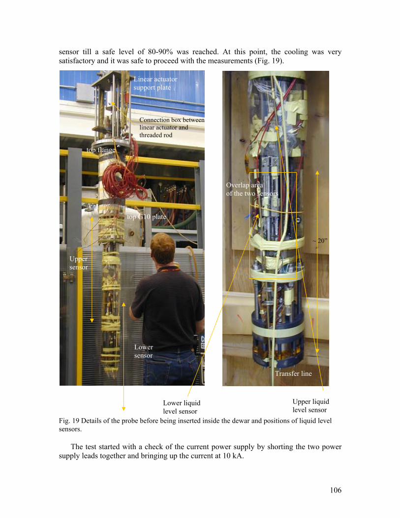
106

sensor till a safe level of 80-90% was reached. At this point, the cooling was very satisfactory and it was safe to proceed with the measurements (Fig. 19).

Fig. 19 Details of the probe before being inserted inside the dewar and positions of liquid level sensors.

The test started with a check of the current power supply by shorting the two power supply leads together and bringing up the current at 10 kA.

top flange

Linear actuator support plate

Connection box between linear actuator and threaded rod

top G10 plate

Transfer line

Overlap area of the two sensors

Lower liquid level sensor

Upper liquid level sensor

~ 20”

Upper sensor

Lower sensor

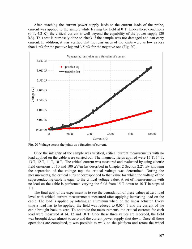
107

After attaching the current power supply leads to the current leads of the probe, current was applied to the sample while leaving the field at 0 T. Under these conditions (0 T, 4.2 K), the critical current is well beyond the capability of the power supply (20 kA). This test is purposely done to check if the sample was not damaged and can carry current. In addition, it was verified that the resistances of the joints were as low as less than 1 nΩ for the positive leg and 3.5 nΩ for the negative one (Fig. 20).

Fig. 20 Voltage across the joints as a function of current.

Once the integrity of the sample was verified, critical current measurements with no load applied on the cable were carried out. The magnetic fields applied were 15 T, 14 T, 13 T, 12 T, 11 T, 10 T. The critical current was measured and evaluated by using electric field criterions of 10 and 100 µV/m (as described in Chapter 2 Section 2.2). By knowing the separation of the voltage tap, the critical voltage was determined. During the measurements, the critical current corresponded to that value for which the voltage of the superconducting cable is equal to the critical voltage value. A set of measurements with no load on the cable is performed varying the field from 15 T down to 10 T in steps of 1 T.

The final goal of the experiment is to see the degradation of these values at zero load level with critical current measurements measured after applying increasing load on the cable. The load is applied by rotating an aluminum wheel on the linear actuator. Every time a load has to be applied, the field was reduced to 0.054 T and the current of the cable brought back to zero. To optimize the measurements, the critical currents for each load were measured at 14, 12 and 10 T. Once these three values are recorded, the field was brought down almost to zero and the current power supply shut down. Once all these operations are completed, it was possible to walk on the platform and rotate the wheel

Voltages across joints as a function of current

0.0E+00

5.0E-06

1.0E-05

1.5E-05

2.0E-05

2.5E-05

3.0E-05

3.5E-05

0 2000 4000 6000 8000 10000Current (A)

Vol

tage

(V)

positive legnegative leg

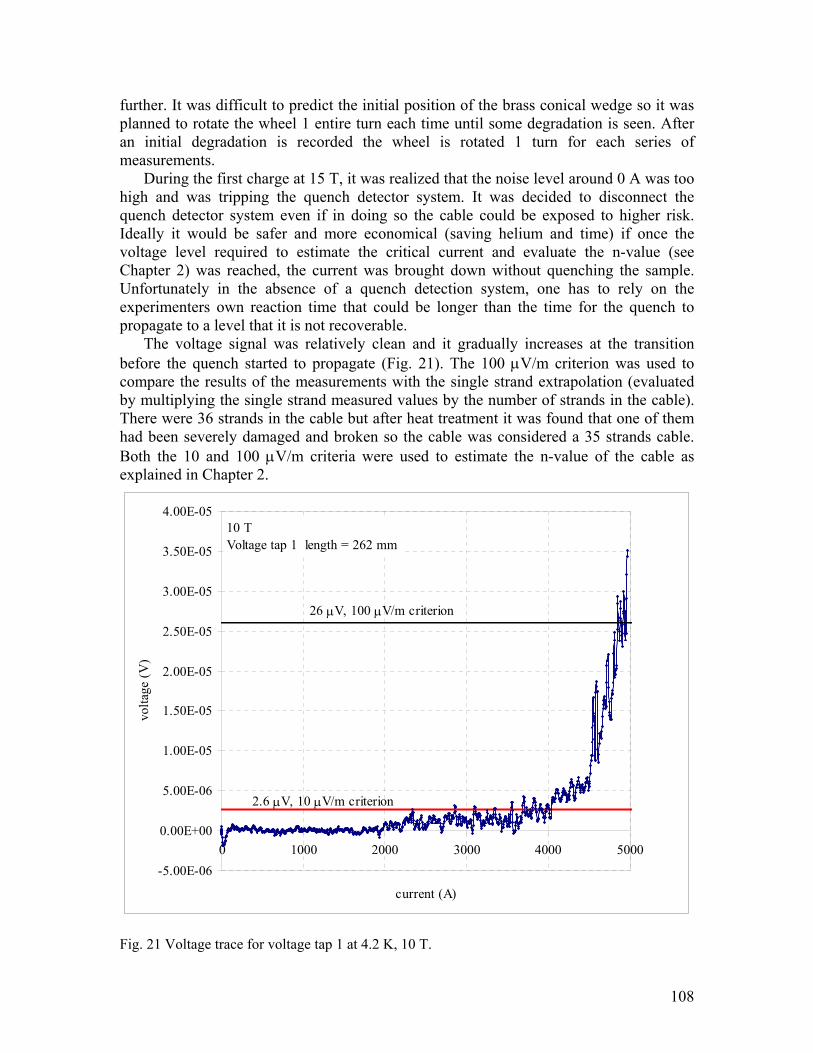
108

further. It was difficult to predict the initial position of the brass conical wedge so it was planned to rotate the wheel 1 entire turn each time until some degradation is seen. After an initial degradation is recorded the wheel is rotated 1 turn for each series of measurements.

During the first charge at 15 T, it was realized that the noise level around 0 A was too high and was tripping the quench detector system. It was decided to disconnect the quench detector system even if in doing so the cable could be exposed to higher risk. Ideally it would be safer and more economical (saving helium and time) if once the voltage level required to estimate the critical current and evaluate the n-value (see Chapter 2) was reached, the current was brought down without quenching the sample. Unfortunately in the absence of a quench detection system, one has to rely on the experimenters own reaction time that could be longer than the time for the quench to propagate to a level that it is not recoverable.

The voltage signal was relatively clean and it gradually increases at the transition before the quench started to propagate (Fig. 21). The 100 µV/m criterion was used to compare the results of the measurements with the single strand extrapolation (evaluated by multiplying the single strand measured values by the number of strands in the cable). There were 36 strands in the cable but after heat treatment it was found that one of them had been severely damaged and broken so the cable was considered a 35 strands cable. Both the 10 and 100 µV/m criteria were used to estimate the n-value of the cable as explained in Chapter 2.

Fig. 21 Voltage trace for voltage tap 1 at 4.2 K, 10 T.

-5.00E-06

0.00E+00

5.00E-06

1.00E-05

1.50E-05

2.00E-05

2.50E-05

3.00E-05

3.50E-05

4.00E-05

0 1000 2000 3000 4000 5000

current (A)

volta

ge (V

)

10 TVoltage tap 1 length = 262 mm

26 µV, 100 µV/m criterion

2.6 µV, 10 µV/m criterion

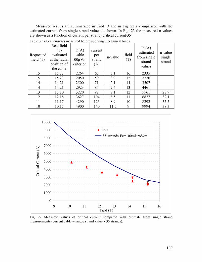
109

Measured results are summarized in Table 3 and in Fig. 22 a comparison with the estimated current from single strand values is shown. In Fig. 23 the measured n-values are shown as a function of current per strand (critical current/35).

Table 3 Critical currents measured before applying mechanical loads.

Requested field (T)

Real field (T)

evaluated at the radial position of the cable

Ic(A) cable

100µV/m criterion

current per

strand (A)

n-value field (T)

Ic (A) estimated

from single strand values

n-value single strand

15 15.23 2264 65 3.1 16 2335 15 15.23 2050 59 3.9 15 2720 14 14.21 2500 71 2.1 14 3507 14 14.21 2923 84 2.4 13 4461 13 13.20 3220 92 7.1 12 5561 28.9 12 12.18 3627 104 8.5 11 6827 32.1 11 11.17 4290 123 8.9 10 8292 35.5 10 10.15 4900 140 11.5 9 9994 38.3

0

1000

2000

3000

4000

5000

6000

7000

8000

9000

10000

9 10 11 12 13 14 15 16Field (T)

Criti

cal C

urre

nt (A

)

test35-strands Ec=100microV/m

Fig. 22 Measured values of critical current compared with estimate from single strand measurements (current cable = single strand value x 35 strands).

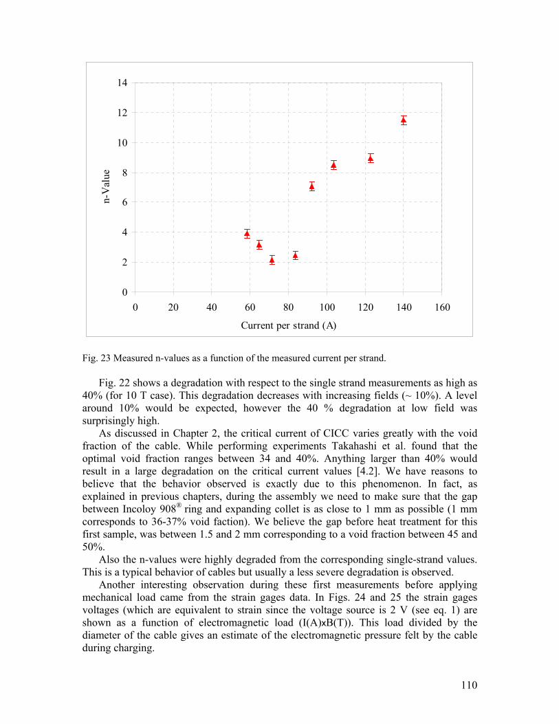
110

Fig. 23 Measured n-values as a function of the measured current per strand.

Fig. 22 shows a degradation with respect to the single strand measurements as high as 40% (for 10 T case). This degradation decreases with increasing fields (~ 10%). A level around 10% would be expected, however the 40 % degradation at low field was surprisingly high.

As discussed in Chapter 2, the critical current of CICC varies greatly with the void fraction of the cable. While performing experiments Takahashi et al. found that the optimal void fraction ranges between 34 and 40%. Anything larger than 40% would result in a large degradation on the critical current values [4.2]. We have reasons to believe that the behavior observed is exactly due to this phenomenon. In fact, as explained in previous chapters, during the assembly we need to make sure that the gap between Incoloy 908® ring and expanding collet is as close to 1 mm as possible (1 mm corresponds to 36-37% void faction). We believe the gap before heat treatment for this first sample, was between 1.5 and 2 mm corresponding to a void fraction between 45 and 50%.

Also the n-values were highly degraded from the corresponding single-strand values. This is a typical behavior of cables but usually a less severe degradation is observed.

Another interesting observation during these first measurements before applying mechanical load came from the strain gages data. In Figs. 24 and 25 the strain gages voltages (which are equivalent to strain since the voltage source is 2 V (see eq. 1) are shown as a function of electromagnetic load (I(A)xB(T)). This load divided by the diameter of the cable gives an estimate of the electromagnetic pressure felt by the cable during charging.

0

2

4

6

8

10

12

14

0 20 40 60 80 100 120 140 160

Current per strand (A)

n-V

alue

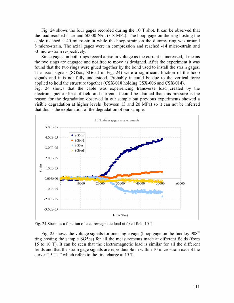
111

Fig. 24 shows the four gages recorded during the 10 T shot. It can be observed that the load reached is around 50000 N/m (~ 8 MPa). The hoop gage on the ring hosting the cable reached ~ 40 micro-strain while the hoop strain on the dummy ring was around 8 micro-strain. The axial gages were in compression and reached -14 micro-strain and -3 micro-strain respectively.

Since gages on both rings record a rise in voltage as the current is increased, it means the two rings are engaged and not free to move as designed. After the experiment it was found that the two rings were glued together by the bond used to install the strain gages. The axial signals (SG5as, SG6ad in Fig. 24) were a significant fraction of the hoop signals and it is not fully understood. Probably it could be due to the vertical force applied to hold the structure together (CSX-018 holding CSX-006 and CSX-014). Fig, 24 shows that the cable was experiencing transverse load created by the electromagnetic effect of field and current. It could be claimed that this pressure is the reason for the degradation observed in our sample but previous experiments showed a visible degradation at higher levels (between 13 and 20 MPa) so it can not be inferred that this is the explanation of the degradation of our sample.

Fig. 24 Strain as a function of electromagnetic load at fixed field 10 T.

Fig. 25 shows the voltage signals for one single gage (hoop gage on the Incoloy 908® ring hosting the sample SG5hs) for all the measurements made at different fields (from 15 to 10 T). It can be seen that the electromagnetic load is similar for all the different fields and that the strain gage signals are reproducible in within 10 microstrain except the curve “15 T a” which refers to the first charge at 15 T.

10 T strain gages measurements

-3.00E-05

-2.00E-05

-1.00E-05

0.00E+00

1.00E-05

2.00E-05

3.00E-05

4.00E-05

5.00E-05

0 10000 20000 30000 40000 50000 60000

Ix B (N/m)

Stra

in

SG5hsSG6hdSG5asSG6ad

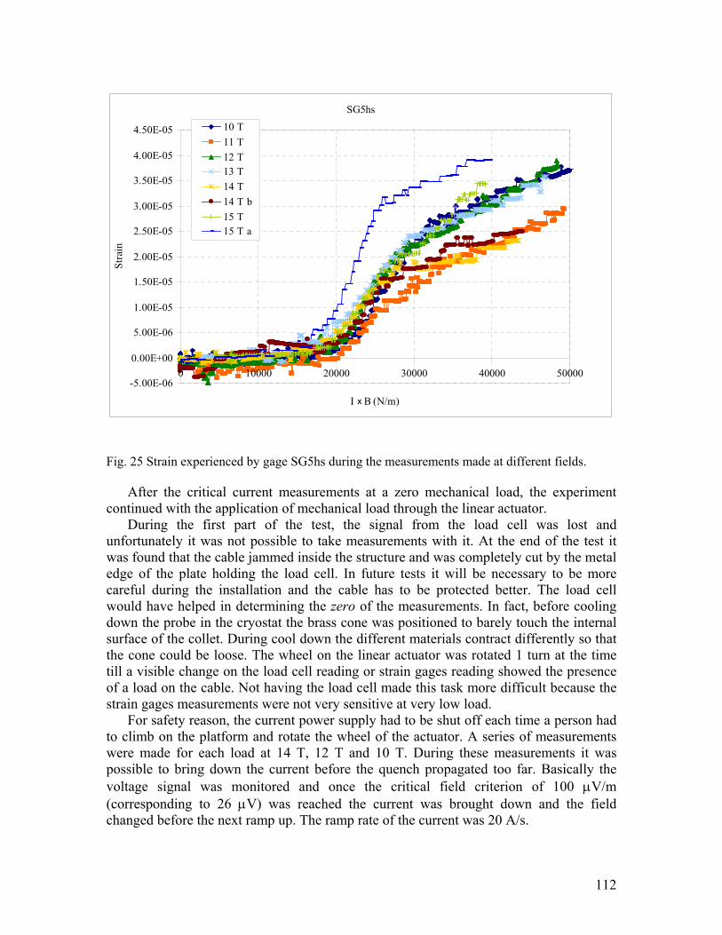
112

Fig. 25 Strain experienced by gage SG5hs during the measurements made at different fields.

After the critical current measurements at a zero mechanical load, the experiment continued with the application of mechanical load through the linear actuator.

During the first part of the test, the signal from the load cell was lost and unfortunately it was not possible to take measurements with it. At the end of the test it was found that the cable jammed inside the structure and was completely cut by the metal edge of the plate holding the load cell. In future tests it will be necessary to be more careful during the installation and the cable has to be protected better. The load cell would have helped in determining the zero of the measurements. In fact, before cooling down the probe in the cryostat the brass cone was positioned to barely touch the internal surface of the collet. During cool down the different materials contract differently so that the cone could be loose. The wheel on the linear actuator was rotated 1 turn at the time till a visible change on the load cell reading or strain gages reading showed the presence of a load on the cable. Not having the load cell made this task more difficult because the strain gages measurements were not very sensitive at very low load.

For safety reason, the current power supply had to be shut off each time a person had to climb on the platform and rotate the wheel of the actuator. A series of measurements were made for each load at 14 T, 12 T and 10 T. During these measurements it was possible to bring down the current before the quench propagated too far. Basically the voltage signal was monitored and once the critical field criterion of 100 µV/m (corresponding to 26 µV) was reached the current was brought down and the field changed before the next ramp up. The ramp rate of the current was 20 A/s.

SG5hs

-5.00E-06

0.00E+00

5.00E-06

1.00E-05

1.50E-05

2.00E-05

2.50E-05

3.00E-05

3.50E-05

4.00E-05

4.50E-05

0 10000 20000 30000 40000 50000

I x B (N/m)

Stra

in10 T11 T12 T13 T14 T14 T b15 T15 T a

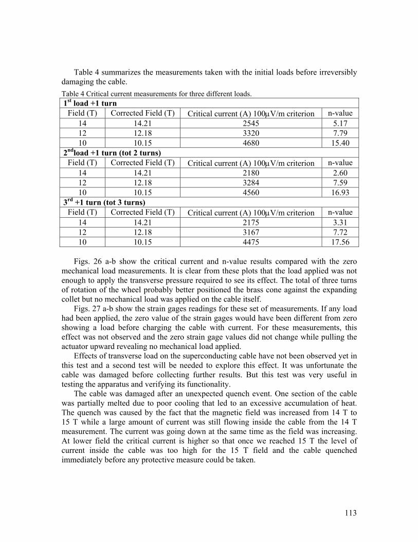
113

Table 4 summarizes the measurements taken with the initial loads before irreversibly damaging the cable.

Table 4 Critical current measurements for three different loads. 1st load +1 turn

Field (T) Corrected Field (T) Critical current (A) 100µV/m criterion n-value 14 14.21 2545 5.17 12 12.18 3320 7.79 10 10.15 4680 15.40

2ndload +1 turn (tot 2 turns) Field (T) Corrected Field (T) Critical current (A) 100µV/m criterion n-value

14 14.21 2180 2.60 12 12.18 3284 7.59 10 10.15 4560 16.93

3rd +1 turn (tot 3 turns) Field (T) Corrected Field (T) Critical current (A) 100µV/m criterion n-value

14 14.21 2175 3.31 12 12.18 3167 7.72 10 10.15 4475 17.56

Figs. 26 a-b show the critical current and n-value results compared with the zero

mechanical load measurements. It is clear from these plots that the load applied was not enough to apply the transverse pressure required to see its effect. The total of three turns of rotation of the wheel probably better positioned the brass cone against the expanding collet but no mechanical load was applied on the cable itself.

Figs. 27 a-b show the strain gages readings for these set of measurements. If any load had been applied, the zero value of the strain gages would have been different from zero showing a load before charging the cable with current. For these measurements, this effect was not observed and the zero strain gage values did not change while pulling the actuator upward revealing no mechanical load applied.

Effects of transverse load on the superconducting cable have not been observed yet in this test and a second test will be needed to explore this effect. It was unfortunate the cable was damaged before collecting further results. But this test was very useful in testing the apparatus and verifying its functionality.

The cable was damaged after an unexpected quench event. One section of the cable was partially melted due to poor cooling that led to an excessive accumulation of heat. The quench was caused by the fact that the magnetic field was increased from 14 T to 15 T while a large amount of current was still flowing inside the cable from the 14 T measurement. The current was going down at the same time as the field was increasing. At lower field the critical current is higher so that once we reached 15 T the level of current inside the cable was too high for the 15 T field and the cable quenched immediately before any protective measure could be taken.

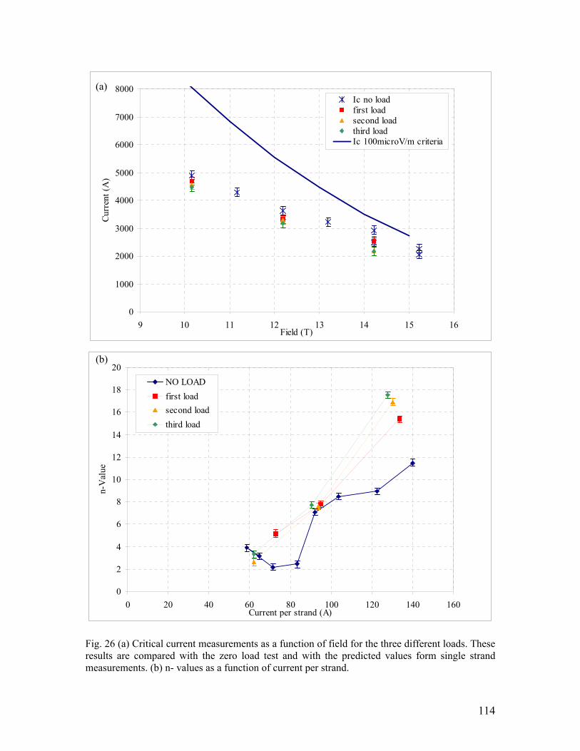
114

Fig. 26 (a) Critical current measurements as a function of field for the three different loads. These results are compared with the zero load test and with the predicted values form single strand measurements. (b) n- values as a function of current per strand.

0

2

4

6

8

10

12

14

16

18

20

0 20 40 60 80 100 120 140 160Current per strand (A)

n-V

alue

NO LOADfirst loadsecond loadthird load

0

1000

2000

3000

4000

5000

6000

7000

8000

9 10 11 12 13 14 15 16Field (T)

Curr

ent (

A)

Ic no loadfirst loadsecond loadthird loadIc 100microV/m criteria

(a)

(b)

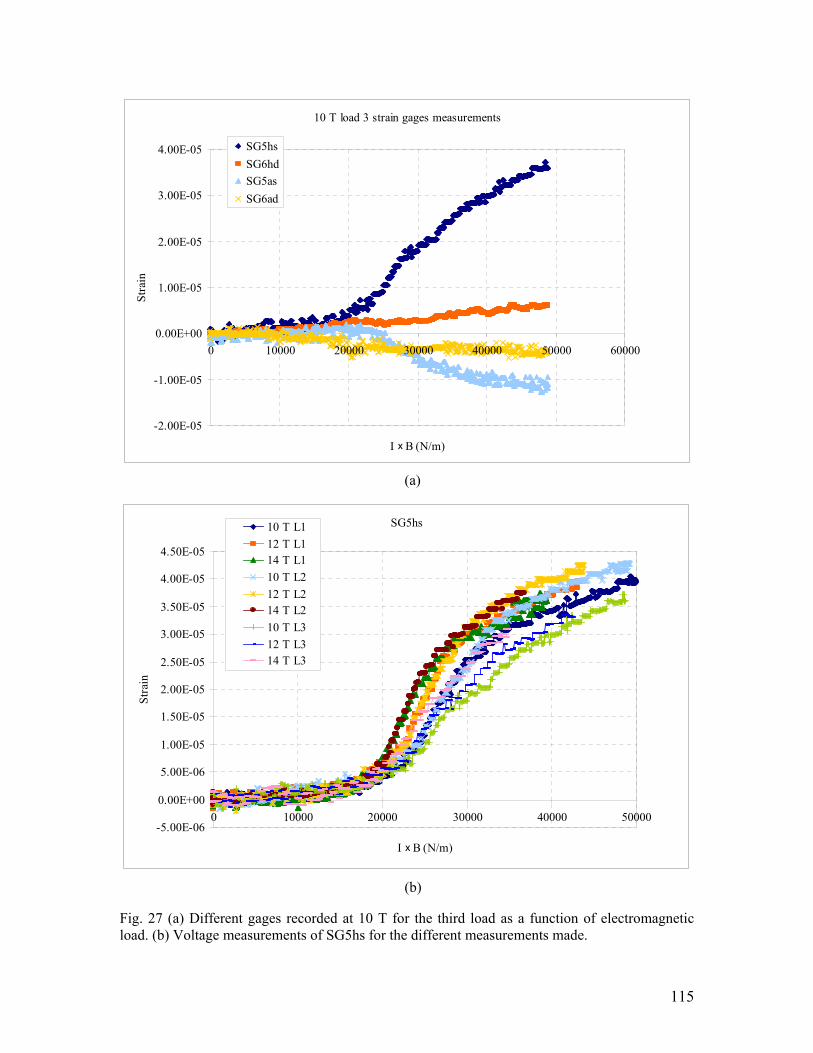
115

Fig. 27 (a) Different gages recorded at 10 T for the third load as a function of electromagnetic load. (b) Voltage measurements of SG5hs for the different measurements made.

10 T load 3 strain gages measurements

-2.00E-05

-1.00E-05

0.00E+00

1.00E-05

2.00E-05

3.00E-05

4.00E-05

0 10000 20000 30000 40000 50000 60000

I x B (N/m)

Stra

inSG5hsSG6hdSG5asSG6ad

SG5hs

-5.00E-06

0.00E+00

5.00E-06

1.00E-05

1.50E-05

2.00E-05

2.50E-05

3.00E-05

3.50E-05

4.00E-05

4.50E-05

0 10000 20000 30000 40000 50000

I x B (N/m)

Stra

in

10 T L112 T L114 T L110 T L212 T L214 T L210 T L312 T L314 T L3

(b)

(a)

116

The electromagnetic load caused by the current and the field reached values around 50000 N/m which corresponds to a pressure of ~ 8 MPa on the cable which is not enough to create visible degradation of the critical current as discussed earlier.

It was decided to also bring down the field, and just test the strain gages and the structure by rotating the wheel on the linear actuator 25 turns, and see if it was possible to measure any change in the strain gages values. Fig 28 shows the strain gages reading as a function of time while Fig. 29 shows the single gage SG5hs as a function of the turns applied to the wheel to pull up the brass cone connected through the shaft to the linear actuator.

It can be seen that the change over the 25 turns is on the order of 160 micro-strain for the hoop gage on the Incoloy 908® ring enclosing the sample. The gage in the dummy ring also showed a change of 100 micro-strain. The axial gages have lower values on the order of 50 micro-strain. When the wheel was turned in the opposite direction to unload the system and return it to the original position, all the gages showed hysteresis and not one of them went back to the original starting value. This could be due to a buckling effect of the structure when one tries to push down the shaft. From Fig. 29 it can be seen that the gage started to measure some significant change after 5 turns. If we had been able to continue our experiment it would have taken us probably about 5 more turns to see any cable degradation.

Fig. 28 Strain gages readings and their variation while applying load.

-100

-50

0

50

100

150

200

0 500 1000 1500 2000 2500

Time (s)

Stra

in x

10-6

SG5hsSG6hdSG5asSG6ad

17 turns

23 turns

24 turns25 turns

reducing load

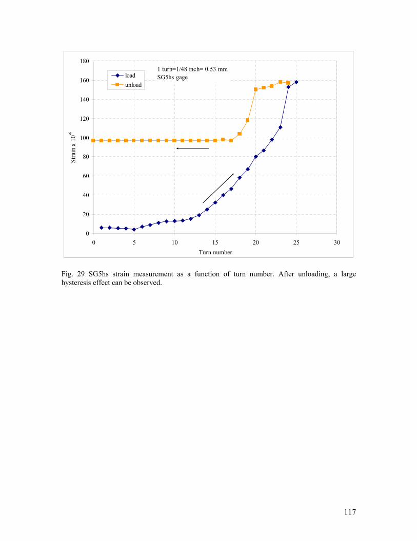
117

0

20

40

60

80

100

120

140

160

180

0 5 10 15 20 25 30Turn number

Stra

in x

10-6

loadunload

1 turn=1/48 inch= 0.53 mmSG5hs gage

Fig. 29 SG5hs strain measurement as a function of turn number. After unloading, a large hysteresis effect can be observed.

118

4.6 Further tests performed at MIT after the test at NHMFL

After the probe was shipped back to MIT, several tests at room temperature were performed in order to obtain a better understanding of the strain gage signals and their behavior under loading conditions. The strain distribution on the Incoloy 908® is not symmetric. The tests carried out at MIT were a series of tests with different strain gage configurations and conditions. After using the same configuration as in the NHMFL test, the dummy Incoloy 908® ring was removed since, being glued with the other, showed interference with the sample holder ring. Moreover it was decided that for future experiments this Incoloy 908® ring should be substituted with a stainless steel filler with a shape that leaves more space for the Incoloy 908® ring where the cable is seated.

Table 5 summarizes the different tests performed:

Table 5 Different configuration of strain gages tests at room temperature. Nomenclature: SG-gage number-h hoop or a axial-s sample ring or d dummy ring Strain gages used Comments SG5hs, SG6hd, SG5as, SG6ad Strain gages used in the test SG5hs, SG6hd, SG5as, SG6ad Strain gages used in the test loosing screws holding

structure SG3hs, SG4hd, SG3as, SG4ad Strain gages in position 3 Removing DUMMY INCOLOY 908® RING Strain gages used Comments SG3hs, SG3as, SG5hs, SG5as Strain gages in position 3 and 4 on Incoloy 908® ring

enclosing the cable SG3hs, SG3as, SG5hs, SG5as Strain gages in position 3 and 4 on Incoloy 908® ring

enclosing the cable SG1hs, SG2hs, SG5hs, SG5hd Hoop strain gages in position 1, 2 and 4 on Incoloy 908®

ring enclosing the cable Axial strain gage in position 4 on Incoloy 908® ring enclosing the cable

SG1hs, SG2hs, SG3hs, SG5hs Hoop strain gages in position 1, 2, 3 and 4 on Incoloy 908® ring enclosing the cable

The reproducibility of the loading as a function of turn number was very good as

shown in Fig. 30. The number of turns to reach ~ 3000 kg was 15. This load should be enough to apply the desired transverse pressure on the cable during the next test.

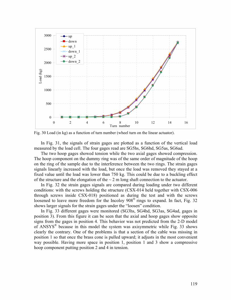
119

0

500

1000

1500

2000

2500

3000

0 2 4 6 8 10 12 14 16Turn number

Load

(kg)

updownup_1down_1up_2down_2

Fig. 30 Load (in kg) as a function of turn number (wheel turn on the linear actuator).

In Fig. 31, the signals of strain gages are plotted as a function of the vertical load measured by the load cell. The four gages read are SG5hs, SG6hd, SG5as, SG6ad.

The two hoop gages showed tension while the two axial gages showed compression. The hoop component on the dummy ring was of the same order of magnitude of the hoop on the ring of the sample due to the interference between the two rings. The strain gages signals linearly increased with the load, but once the load was removed they stayed at a fixed value until the load was lower than 750 kg. This could be due to a buckling effect of the structure and the elongation of the ~ 2 m long shaft connection to the actuator.

In Fig. 32 the strain gages signals are compared during loading under two different conditions: with the screws holding the structure (CSX-014 held together with CSX-006 through screws inside CSX-018) positioned as during the test and with the screws loosened to leave more freedom for the Incoloy 908® rings to expand. In fact, Fig. 32 shows larger signals for the strain gages under the “loosen” condition.

In Fig. 33 different gages were monitored (SG3hs, SG4hd, SG3as, SG4ad, gages in position 3). From this figure it can be seen that the axial and hoop gages show opposite signs from the gages in position 4. This behavior was not predicted from the 2-D model of ANSYS® because in this model the system was axisymmetric while Fig. 33 shows clearly the contrary. One of the problems is that a section of the cable was missing in position 1 so that once the brass cone is pulled upward; it adjusts in the most convenient way possible. Having more space in position 1, position 1 and 3 show a compressive hoop component putting position 2 and 4 in tension.

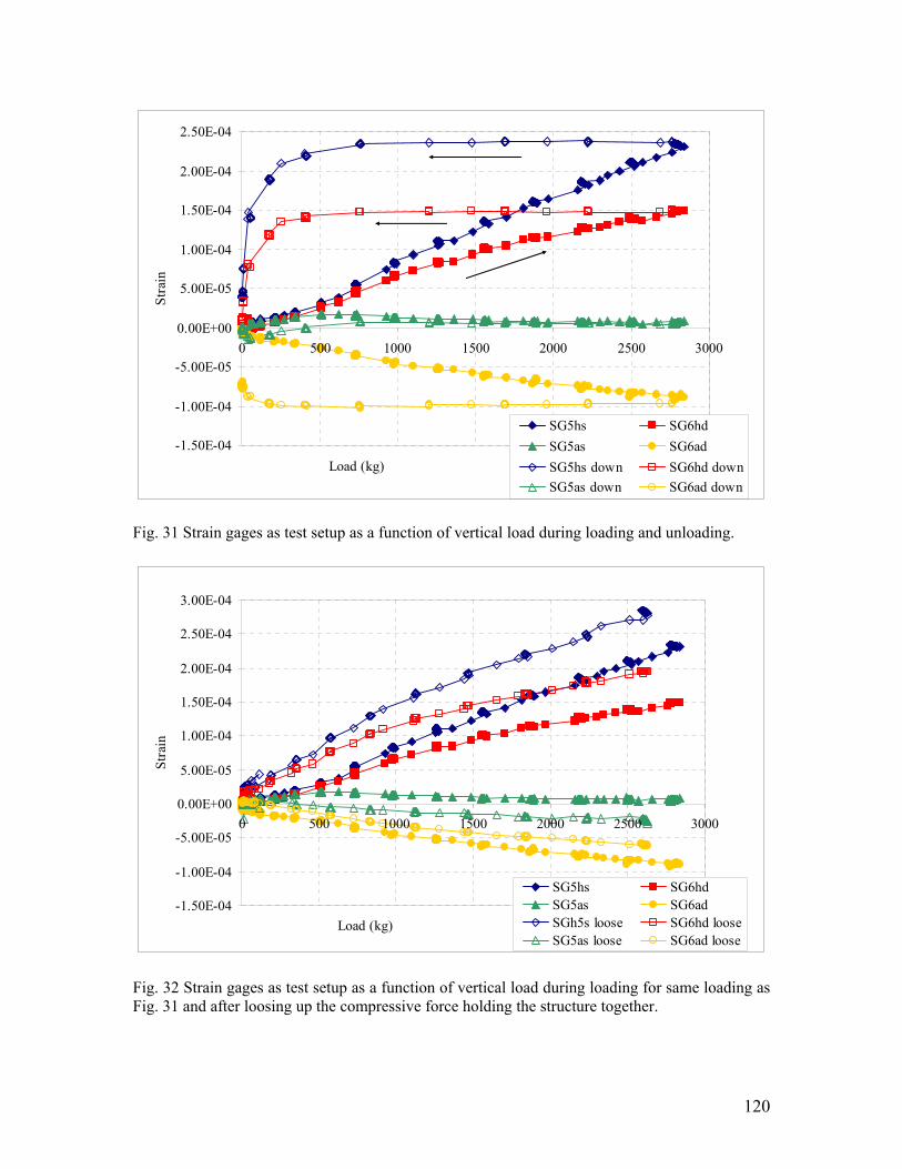
120

Fig. 31 Strain gages as test setup as a function of vertical load during loading and unloading.

Fig. 32 Strain gages as test setup as a function of vertical load during loading for same loading as Fig. 31 and after loosing up the compressive force holding the structure together.

-1.50E-04

-1.00E-04

-5.00E-05

0.00E+00

5.00E-05

1.00E-04

1.50E-04

2.00E-04

2.50E-04

0 500 1000 1500 2000 2500 3000

Load (kg)

Stra

in

SG5hs SG6hdSG5as SG6adSG5hs down SG6hd downSG5as down SG6ad down

-1.50E-04

-1.00E-04

-5.00E-05

0.00E+00

5.00E-05

1.00E-04

1.50E-04

2.00E-04

2.50E-04

3.00E-04

0 500 1000 1500 2000 2500 3000

Load (kg)

Stra

in

SG5hs SG6hdSG5as SG6adSGh5s loose SG6hd looseSG5as loose SG6ad loose

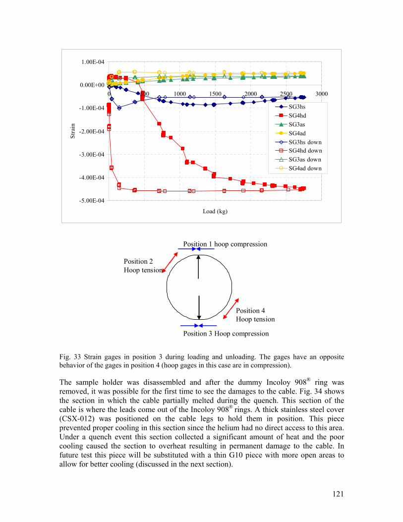
121

Fig. 33 Strain gages in position 3 during loading and unloading. The gages have an opposite behavior of the gages in position 4 (hoop gages in this case are in compression). The sample holder was disassembled and after the dummy Incoloy 908® ring was removed, it was possible for the first time to see the damages to the cable. Fig. 34 shows the section in which the cable partially melted during the quench. This section of the cable is where the leads come out of the Incoloy 908® rings. A thick stainless steel cover (CSX-012) was positioned on the cable legs to hold them in position. This piece prevented proper cooling in this section since the helium had no direct access to this area. Under a quench event this section collected a significant amount of heat and the poor cooling caused the section to overheat resulting in permanent damage to the cable. In future test this piece will be substituted with a thin G10 piece with more open areas to allow for better cooling (discussed in the next section).

Position 1 hoop compression

Position 3 Hoop compression

Position 4 Hoop tension

Position 2 Hoop tension

-5.00E-04

-4.00E-04

-3.00E-04

-2.00E-04

-1.00E-04

0.00E+00

1.00E-04

0 500 1000 1500 2000 2500 3000

Load (kg)

Stra

in

SG3hsSG4hdSG3asSG4adSG3hs downSG4hd downSG3as downSG4ad down

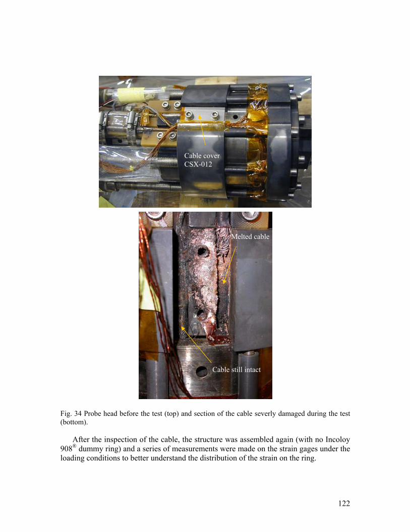
122

Fig. 34 Probe head before the test (top) and section of the cable severly damaged during the test (bottom).

After the inspection of the cable, the structure was assembled again (with no Incoloy 908® dummy ring) and a series of measurements were made on the strain gages under the loading conditions to better understand the distribution of the strain on the ring.

Cable cover CSX-012

Melted cable

Cable still intact

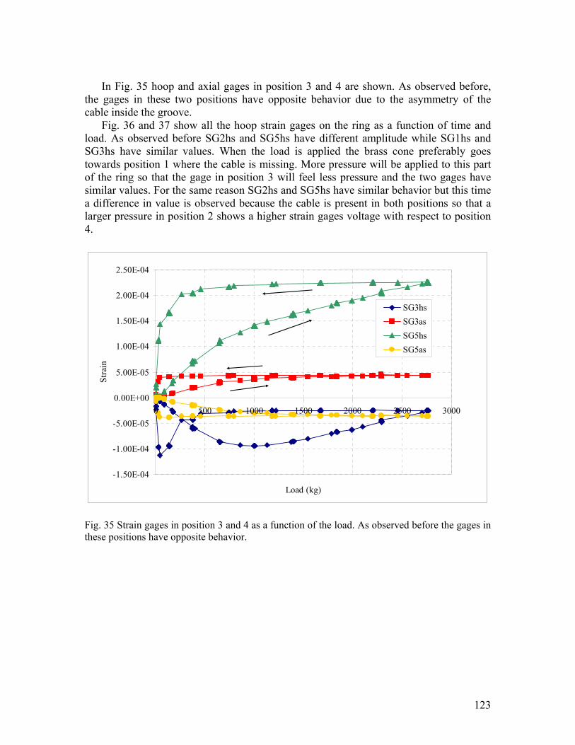
123

In Fig. 35 hoop and axial gages in position 3 and 4 are shown. As observed before,

the gages in these two positions have opposite behavior due to the asymmetry of the cable inside the groove.

Fig. 36 and 37 show all the hoop strain gages on the ring as a function of time and load. As observed before SG2hs and SG5hs have different amplitude while SG1hs and SG3hs have similar values. When the load is applied the brass cone preferably goes towards position 1 where the cable is missing. More pressure will be applied to this part of the ring so that the gage in position 3 will feel less pressure and the two gages have similar values. For the same reason SG2hs and SG5hs have similar behavior but this time a difference in value is observed because the cable is present in both positions so that a larger pressure in position 2 shows a higher strain gages voltage with respect to position 4.

Fig. 35 Strain gages in position 3 and 4 as a function of the load. As observed before the gages in these positions have opposite behavior.

-1.50E-04

-1.00E-04

-5.00E-05

0.00E+00

5.00E-05

1.00E-04

1.50E-04

2.00E-04

2.50E-04

0 500 1000 1500 2000 2500 3000

Load (kg)

Stra

in

SG3hsSG3asSG5hsSG5as

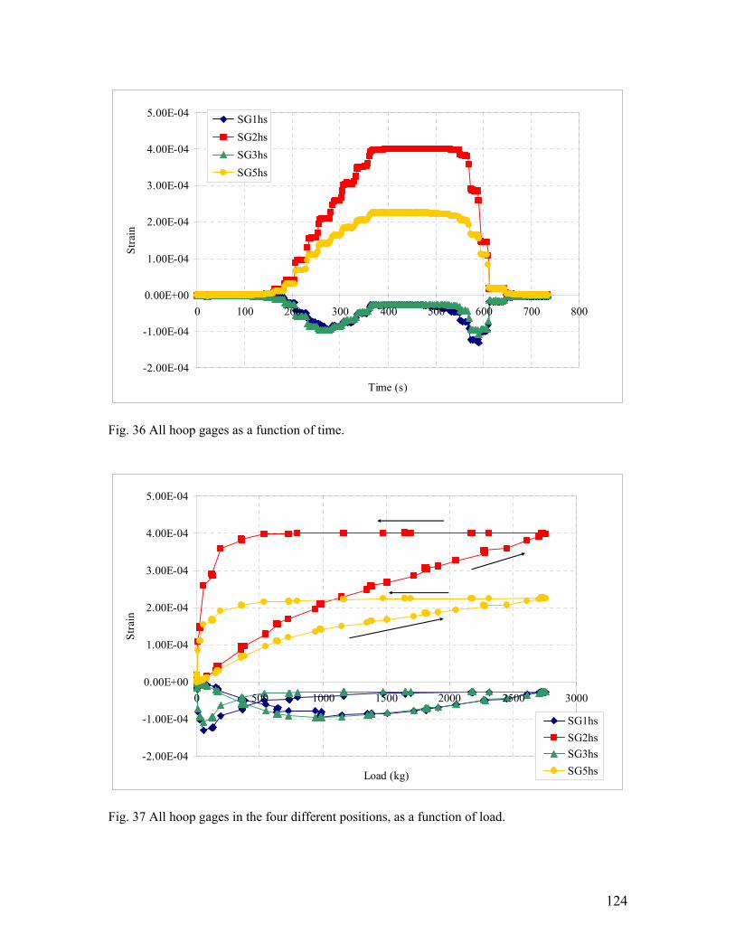
124

-2.00E-04

-1.00E-04

0.00E+00

1.00E-04

2.00E-04

3.00E-04

4.00E-04

5.00E-04

0 100 200 300 400 500 600 700 800

Time (s)

Stra

inSG1hsSG2hsSG3hsSG5hs

Fig. 36 All hoop gages as a function of time.

Fig. 37 All hoop gages in the four different positions, as a function of load.

-2.00E-04

-1.00E-04

0.00E+00

1.00E-04

2.00E-04

3.00E-04

4.00E-04

5.00E-04

0 500 1000 1500 2000 2500 3000

Load (kg)

Stra

in

SG1hsSG2hsSG3hsSG5hs

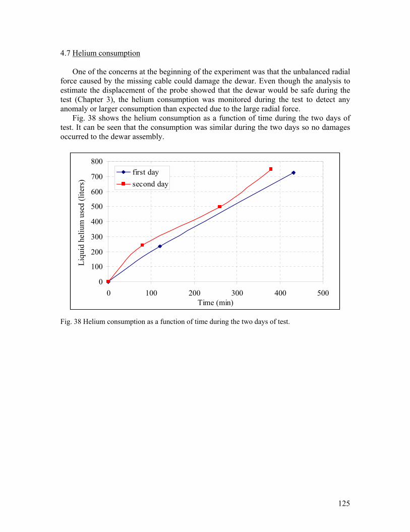
125

4.7 Helium consumption

One of the concerns at the beginning of the experiment was that the unbalanced radial force caused by the missing cable could damage the dewar. Even though the analysis to estimate the displacement of the probe showed that the dewar would be safe during the test (Chapter 3), the helium consumption was monitored during the test to detect any anomaly or larger consumption than expected due to the large radial force.

Fig. 38 shows the helium consumption as a function of time during the two days of test. It can be seen that the consumption was similar during the two days so no damages occurred to the dewar assembly. Fig. 38 Helium consumption as a function of time during the two days of test.

0

100

200

300

400

500

600

700

800

0 100 200 300 400 500Time (min)

first daysecond day

Liqu

id h

eliu

m u

sed

(lite

rs)

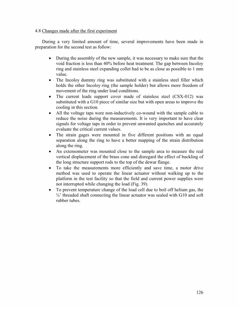
126

4.8 Changes made after the first experiment

During a very limited amount of time, several improvements have been made in preparation for the second test as follow:

• During the assembly of the new sample, it was necessary to make sure that the

void fraction is less than 40% before heat treatment. The gap between Incoloy ring and stainless steel expanding collet had to be as close as possible to 1 mm value.

• The Incoloy dummy ring was substituted with a stainless steel filler which holds the other Incoloy ring (the sample holder) but allows more freedom of movement of the ring under load conditions.

• The current leads support cover made of stainless steel (CSX-012) was substituted with a G10 piece of similar size but with open areas to improve the cooling in this section.

• All the voltage taps were non-inductively co-wound with the sample cable to reduce the noise during the measurements. It is very important to have clear signals for voltage taps in order to prevent unwanted quenches and accurately evaluate the critical current values.

• The strain gages were mounted in five different positions with an equal separation along the ring to have a better mapping of the strain distribution along the ring.

• An extensometer was mounted close to the sample area to measure the real vertical displacement of the brass cone and disregard the effect of buckling of the long structure support rods to the top of the dewar flange.

• To take the measurements more efficiently and save time, a motor drive method was used to operate the linear actuator without walking up to the platform in the test facility so that the field and current power supplies were not interrupted while changing the load (Fig. 39).

• To prevent temperature change of the load cell due to boil off helium gas, the ¾’ threaded shaft connecting the linear actuator was sealed with G10 and soft rubber tubes.

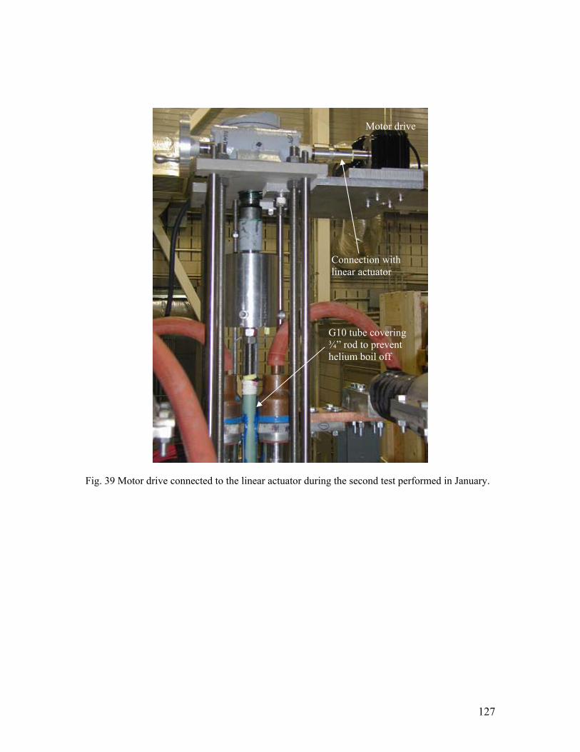
127

Fig. 39 Motor drive connected to the linear actuator during the second test performed in January.

Motor drive

Connection with linear actuator

G10 tube covering ¾” rod to prevent helium boil off

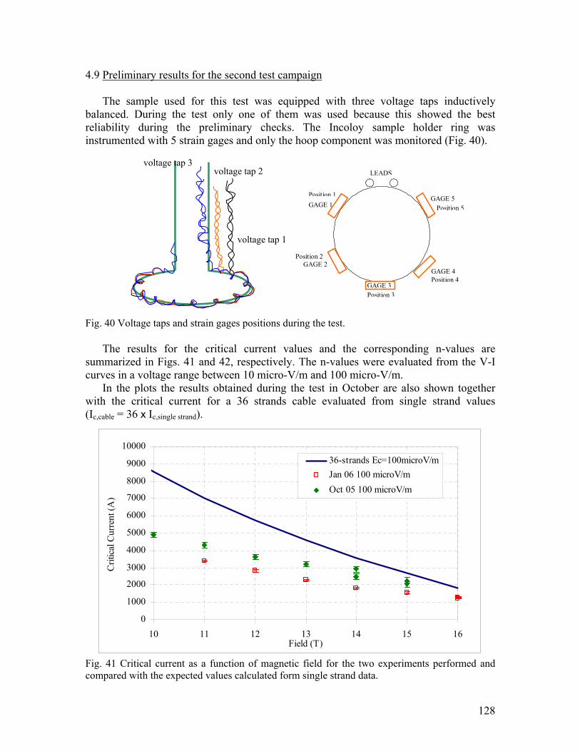
128

4.9 Preliminary results for the second test campaign

The sample used for this test was equipped with three voltage taps inductively balanced. During the test only one of them was used because this showed the best reliability during the preliminary checks. The Incoloy sample holder ring was instrumented with 5 strain gages and only the hoop component was monitored (Fig. 40). Fig. 40 Voltage taps and strain gages positions during the test.

The results for the critical current values and the corresponding n-values are summarized in Figs. 41 and 42, respectively. The n-values were evaluated from the V-I curves in a voltage range between 10 micro-V/m and 100 micro-V/m.

In the plots the results obtained during the test in October are also shown together with the critical current for a 36 strands cable evaluated from single strand values (Ic,cable = 36 x Ic,single strand).

Fig. 41 Critical current as a function of magnetic field for the two experiments performed and compared with the expected values calculated form single strand data.

LEADS

Position 1

Position 2

Position 3GAGE 3

GAGE 1 GAGE 5

GAGE 2 GAGE 4 Position 4

Position 5

voltage tap 1

voltage tap 2 voltage tap 3

0

1000

2000

3000

4000

5000

6000

7000

8000

9000

10000

10 11 12 13 14 15 16Field (T)

Crit

ical

Cur

rent

(A)

36-strands Ec=100microV/mJan 06 100 microV/mOct 05 100 microV/m

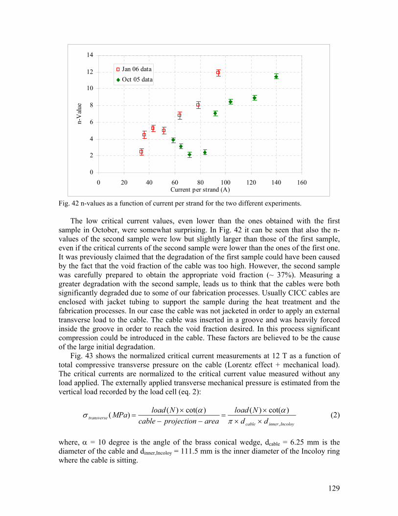
129

Fig. 42 n-values as a function of current per strand for the two different experiments.

The low critical current values, even lower than the ones obtained with the first sample in October, were somewhat surprising. In Fig. 42 it can be seen that also the n-values of the second sample were low but slightly larger than those of the first sample, even if the critical currents of the second sample were lower than the ones of the first one. It was previously claimed that the degradation of the first sample could have been caused by the fact that the void fraction of the cable was too high. However, the second sample was carefully prepared to obtain the appropriate void fraction (~ 37%). Measuring a greater degradation with the second sample, leads us to think that the cables were both significantly degraded due to some of our fabrication processes. Usually CICC cables are enclosed with jacket tubing to support the sample during the heat treatment and the fabrication processes. In our case the cable was not jacketed in order to apply an external transverse load to the cable. The cable was inserted in a groove and was heavily forced inside the groove in order to reach the void fraction desired. In this process significant compression could be introduced in the cable. These factors are believed to be the cause of the large initial degradation.

Fig. 43 shows the normalized critical current measurements at 12 T as a function of total compressive transverse pressure on the cable (Lorentz effect + mechanical load). The critical currents are normalized to the critical current value measured without any load applied. The externally applied transverse mechanical pressure is estimated from the vertical load recorded by the load cell (eq. 2):

Incoloyinnercabletransverse dd

Nloadareaprojectioncable

NloadMPa,

)cot()()cot()()(×××

=−−

×=

παασ (2)

where, α = 10 degree is the angle of the brass conical wedge, dcable = 6.25 mm is the diameter of the cable and dinner,Incoloy = 111.5 mm is the inner diameter of the Incoloy ring where the cable is sitting.

0

2

4

6

8

10

12

14

0 20 40 60 80 100 120 140 160Current per strand (A)

n-V

alue

Jan 06 dataOct 05 data

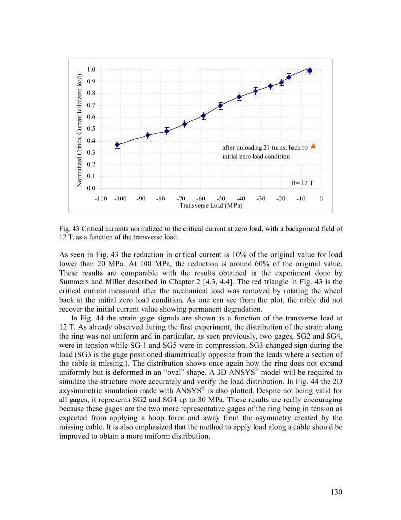
130

Fig. 43 Critical currents normalized to the critical current at zero load, with a background field of 12 T, as a function of the transverse load. As seen in Fig. 43 the reduction in critical current is 10% of the original value for load lower than 20 MPa. At 100 MPa, the reduction is around 60% of the original value. These results are comparable with the results obtained in the experiment done by Summers and Miller described in Chapter 2 [4.3, 4.4]. The red triangle in Fig. 43 is the critical current measured after the mechanical load was removed by rotating the wheel back at the initial zero load condition. As one can see from the plot, the cable did not recover the initial current value showing permanent degradation.

In Fig. 44 the strain gage signals are shown as a function of the transverse load at 12 T. As already observed during the first experiment, the distribution of the strain along the ring was not uniform and in particular, as seen previously, two gages, SG2 and SG4, were in tension while SG 1 and SG5 were in compression. SG3 changed sign during the load (SG3 is the gage positioned diametrically opposite from the leads where a section of the cable is missing.). The distribution shows once again how the ring does not expand uniformly but is deformed in an “oval” shape. A 3D ANSYS® model will be required to simulate the structure more accurately and verify the load distribution. In Fig. 44 the 2D axysimmetric simulation made with ANSYS® is also plotted. Despite not being valid for all gages, it represents SG2 and SG4 up to 30 MPa. These results are really encouraging because these gages are the two more representative gages of the ring being in tension as expected from applying a hoop force and away from the asymmetry created by the missing cable. It is also emphasized that the method to apply load along a cable should be improved to obtain a more uniform distribution.

0.0

0.1

0.2

0.3

0.4

0.5

0.6

0.7

0.8

0.9

1.0

-110 -100 -90 -80 -70 -60 -50 -40 -30 -20 -10 0Transverse Load (MPa)

Nor

mal

ized

Crit

ical

Cur

rent

Ic/Ic

(zer

o lo

ad)

after unloading 21 turns, back to initial zero load condition

B= 12 T

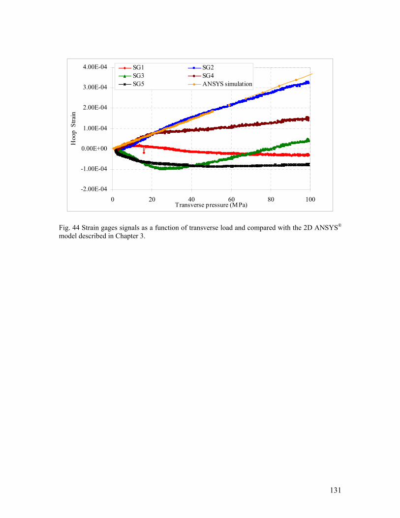
131

Fig. 44 Strain gages signals as a function of transverse load and compared with the 2D ANSYS® model described in Chapter 3.

-2.00E-04

-1.00E-04

0.00E+00

1.00E-04

2.00E-04

3.00E-04

4.00E-04

0 20 40 60 80 100Transverse pressure (MPa)

Hoo

p S

train

SG1 SG2SG3 SG4SG5 ANSYS simulation

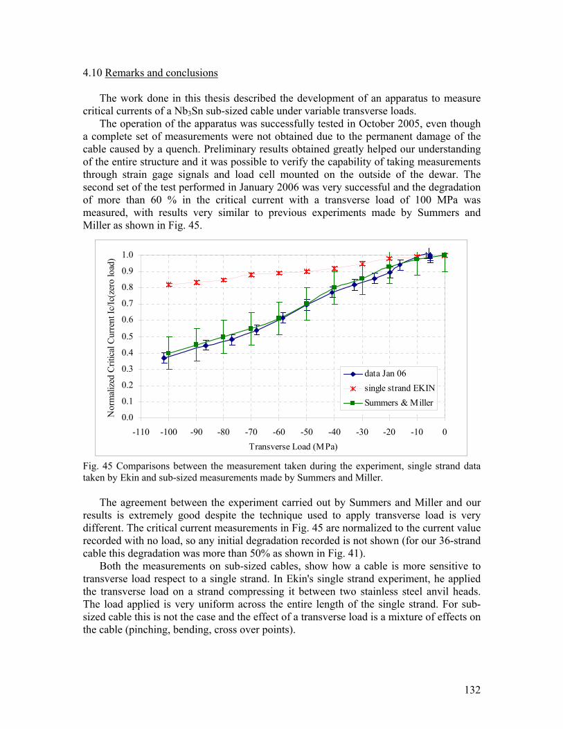
132

4.10 Remarks and conclusions

The work done in this thesis described the development of an apparatus to measure critical currents of a Nb3Sn sub-sized cable under variable transverse loads.

The operation of the apparatus was successfully tested in October 2005, even though a complete set of measurements were not obtained due to the permanent damage of the cable caused by a quench. Preliminary results obtained greatly helped our understanding of the entire structure and it was possible to verify the capability of taking measurements through strain gage signals and load cell mounted on the outside of the dewar. The second set of the test performed in January 2006 was very successful and the degradation of more than 60 % in the critical current with a transverse load of 100 MPa was measured, with results very similar to previous experiments made by Summers and Miller as shown in Fig. 45.

Fig. 45 Comparisons between the measurement taken during the experiment, single strand data taken by Ekin and sub-sized measurements made by Summers and Miller.

The agreement between the experiment carried out by Summers and Miller and our

results is extremely good despite the technique used to apply transverse load is very different. The critical current measurements in Fig. 45 are normalized to the current value recorded with no load, so any initial degradation recorded is not shown (for our 36-strand cable this degradation was more than 50% as shown in Fig. 41).

Both the measurements on sub-sized cables, show how a cable is more sensitive to transverse load respect to a single strand. In Ekin's single strand experiment, he applied the transverse load on a strand compressing it between two stainless steel anvil heads. The load applied is very uniform across the entire length of the single strand. For sub-sized cable this is not the case and the effect of a transverse load is a mixture of effects on the cable (pinching, bending, cross over points).

0.0

0.1

0.2

0.3

0.4

0.5

0.6

0.7

0.8

0.9

1.0

-110 -100 -90 -80 -70 -60 -50 -40 -30 -20 -10 0Transverse Load (MPa)

Nor

mal

ized

Crit

ical

Cur

rent

Ic/Ic

(zer

o lo

ad)

data Jan 06single strand EKINSummers & Miller

133

There are still several improvements for the present apparatus that could be recommended in a future test:

• To reduce the initial degradation of the critical current, the cable should be

jacketed with a thin sheath. The sheath should not disturb the application of the transverse load to the cable. It will be a difficult task and that is why a sheath was not used in this experiment in first place. However, by using the proper thickness and material of the tube it should be possible to insert the cable inside the sheath and mounted inside the groove.

• A better ANSYS® analysis is needed to understand the structure. A 3-D model including the missing cable simulation would help in better understanding the strain data and the asymmetric distribution of stress and strain and it would help to better relate the actual pressure on the cable with the reading through strain gages.

• Voltage taps installation has to be improved to increase reliability during the measurements.

• It is desired to apply transverse pressure uniformly along the test cable. The test cable is not a complete one-turn, but missing a part of it for the current leads. To improve the load application method, it will be suggested to modify the expanding collet by using three sections of the collet instead of the present continuous circular all-around arrangements, as shown in Fig. 46.

The missing section of the cable does not have the force cone fingers so additional missing cone finger sections will be created in other two locations (every 120 degrees). In this way the force applying cone faces uniformly to the three groups of the expanding collet fingers so that the applied transverse load could be uniform. The two portions missing the expanding collet fingers (4 and 8 o’clock) will not have the transverse load and will show a normal critical current behavior (no loading condition). It will not be a critical issue to study the effect of transverse loads on a cable.

Test cable

Force applying cone

Force cone fingersExpanding collet fingers

Fig. 46 Modified expanding collet to apply a more uniform load on the cable. The fingers used to apply pressure on the cable will be removed in two sections to balance the section where the cable is missing.

134

In conclusion, an experimental apparatus to study the effect of transverse load on the critical currents of superconducting cables, has been successfully developed and tested.

The apparatus can apply the large transverse pressure of 100 MPa to a superconducting sub-cable coil. The transverse load can be estimated using the load cell measurements and the load distribution can be evaluated by strain gages.

The final goal of this experiment is to be able to predict the behavior of a full size CICC cable from sub-sized cable experiments. The data obtained with the tests just made, are not conclusive in the prediction of the behavior of a full size cable because the high initial degradation increases the difficulty of relating the results with the CSMC and CS Insert Coil.

This work is the first step towards the ultimate goal to characterize the critical current behavior of Nb3Sn cables as a function of transverse load. Several tests could be done with the device developed:

• Test different types of strand (bronze, internal tin, modified jelly roll) under

the same load conditions to observe any different behavior caused by the different fabrication process used for the strands.

• Vary the twist pitch length of the cable. • Study the void fraction effect on the sensitivity of the cable to transverse load. • Test the sensitivity to transverse load of a hybrid cable (pure copper strands +

superconductive strands).

These studies together with an empirical model to predict the behavior of a full size CICC should be pursued.

135

APPENDIX I: Drawings

This appendix contains the technical drawings of the head of the probe (sample area). The upper part of the probe already existed and was used for a previous experiment of AC losses measurements on CICC cables (AI.1). The upper part, as designed for this previous experiment, could not meet the required strength so it was necessary to make minor modification to reinforce the supporting structure (as described in Chapter 3). The top plate was also modified and a center hole was added to insert the center rod connected to the sample area (inside the dewar) and to the linear actuator (outside the dewar).

As discussed in Chapter 3, to overcome the enormous force required to fight the friction of the structure, the original design was modified to meet these requirements. Instead of using the universal joint to rotate the bottom of the probe, a center hole on the top flange was added. A high strength threaded rod was used as connection between the linear actuator used in the top of the dewar to pull the solid rod connected to the sample area inside the dewar.

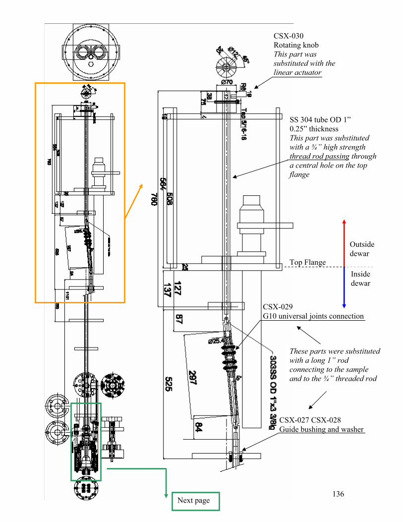
136

CSX-029 G10 universal joints connection

CSX-027 CSX-028 Guide bushing and washer

SS 304 tube OD 1” 0.25” thickness This part was substituted with a ¾” high strength thread rod passing through a central hole on the top flange

CSX-030 Rotating knob This part was substituted with the linear actuator

Top Flange

Outside dewar

Inside dewar

Next page

These parts were substituted with a long 1” rod connecting to the sample and to the ¾” threaded rod

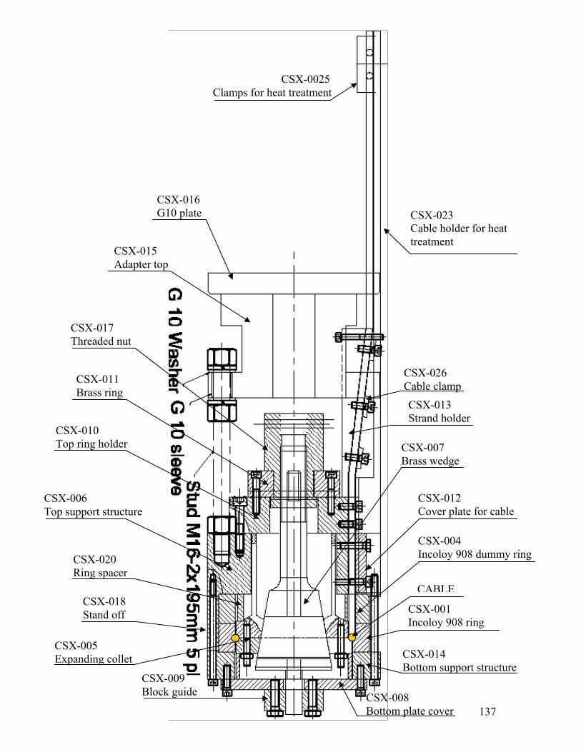
137

CSX-0025Clamps for heat treatment

CSX-016 G10 plate CSX-023

Cable holder for heat treatment

CSX-015 Adapter top

CSX-026 Cable clamp CSX-013 Strand holder

CSX-007 Brass wedge

CSX-012 Cover plate for cable

CSX-004 Incoloy 908 dummy ring

CABLE

CSX-001 Incoloy 908 ring

CSX-014 Bottom support structure

CSX-017 Threaded nut

CSX-011 Brass ring

CSX-010 Top ring holder

CSX-006 Top support structure

CSX-020 Ring spacer

CSX-018 Stand off

CSX-005 Expanding collet

CSX-009 Block guide CSX-008

Bottom plate cover

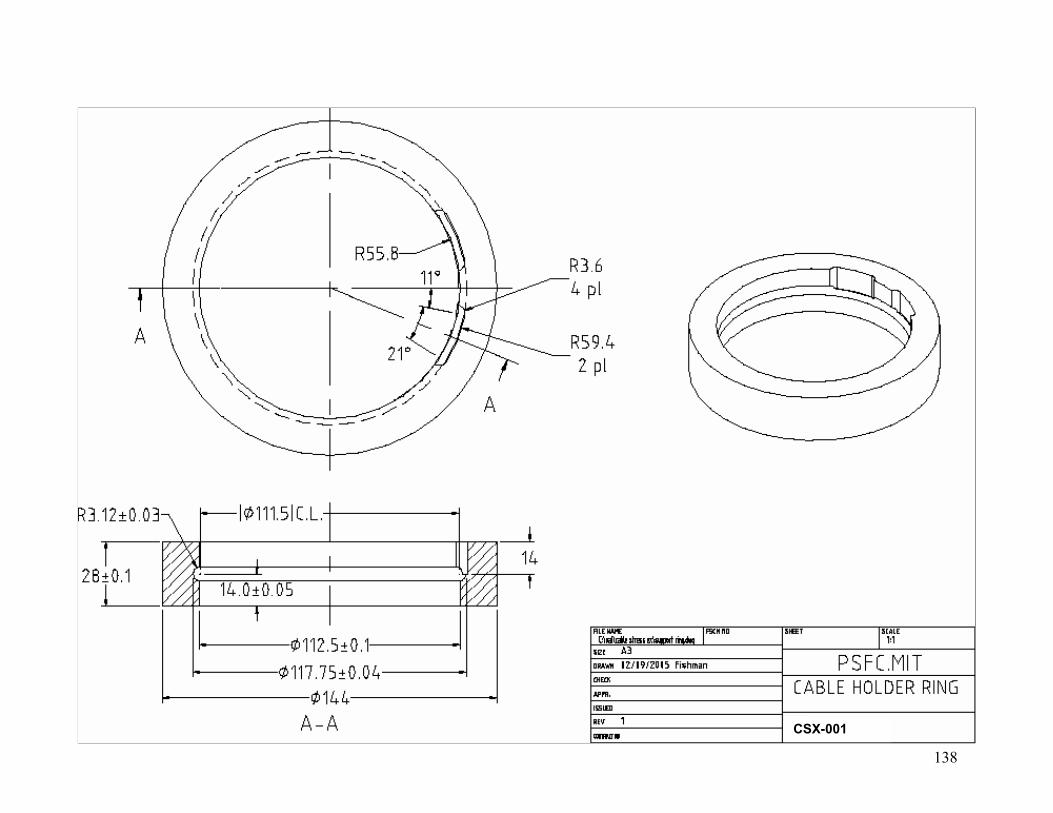
138

CSX-001

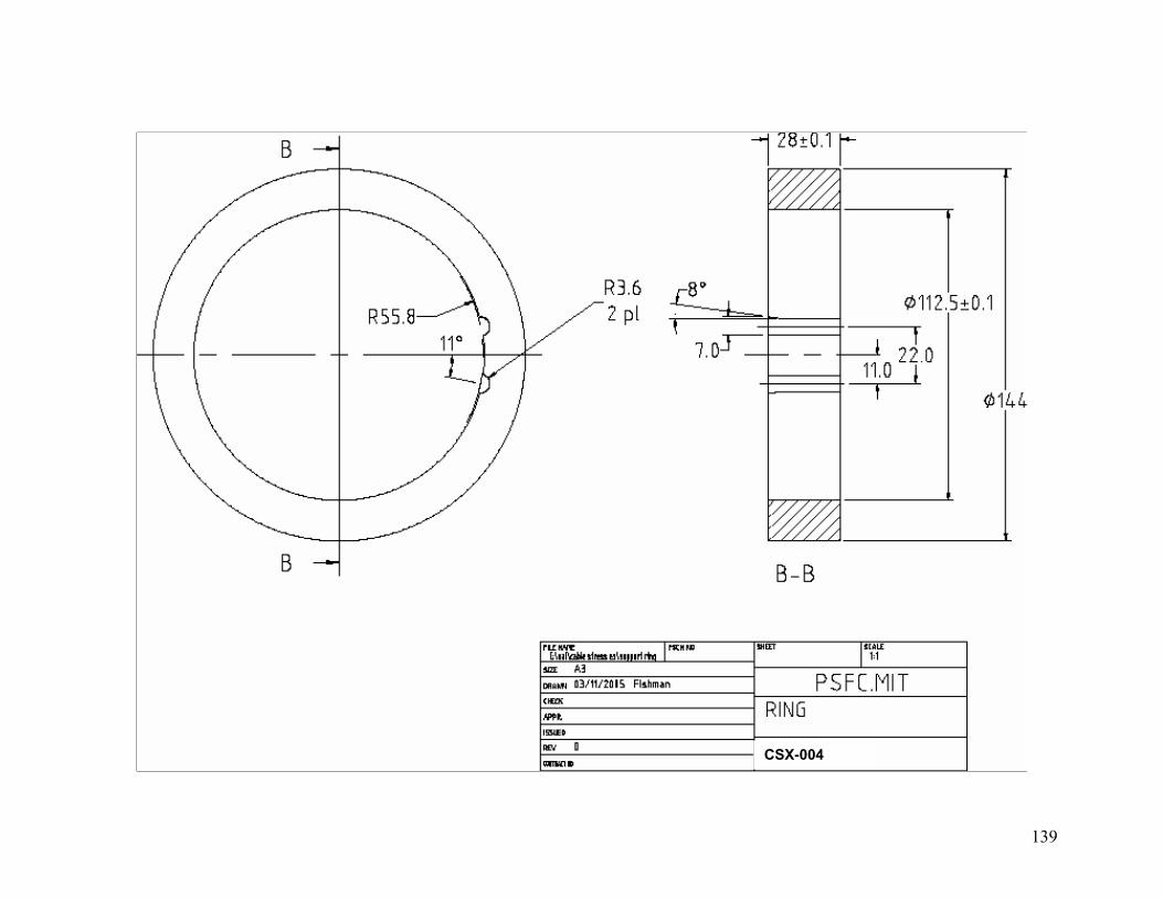
139

CSX-004

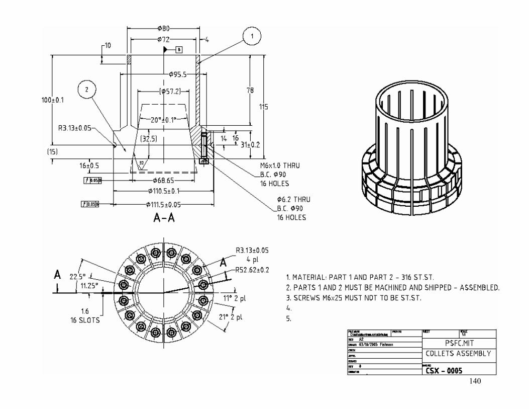
140

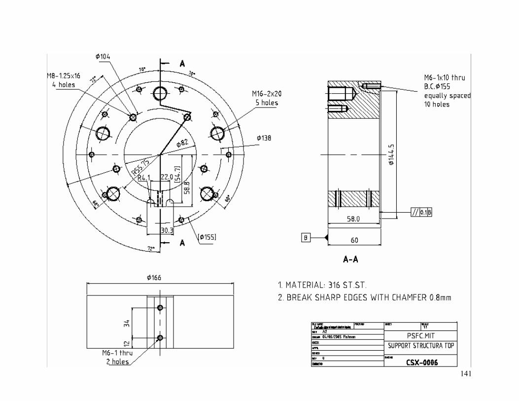
141

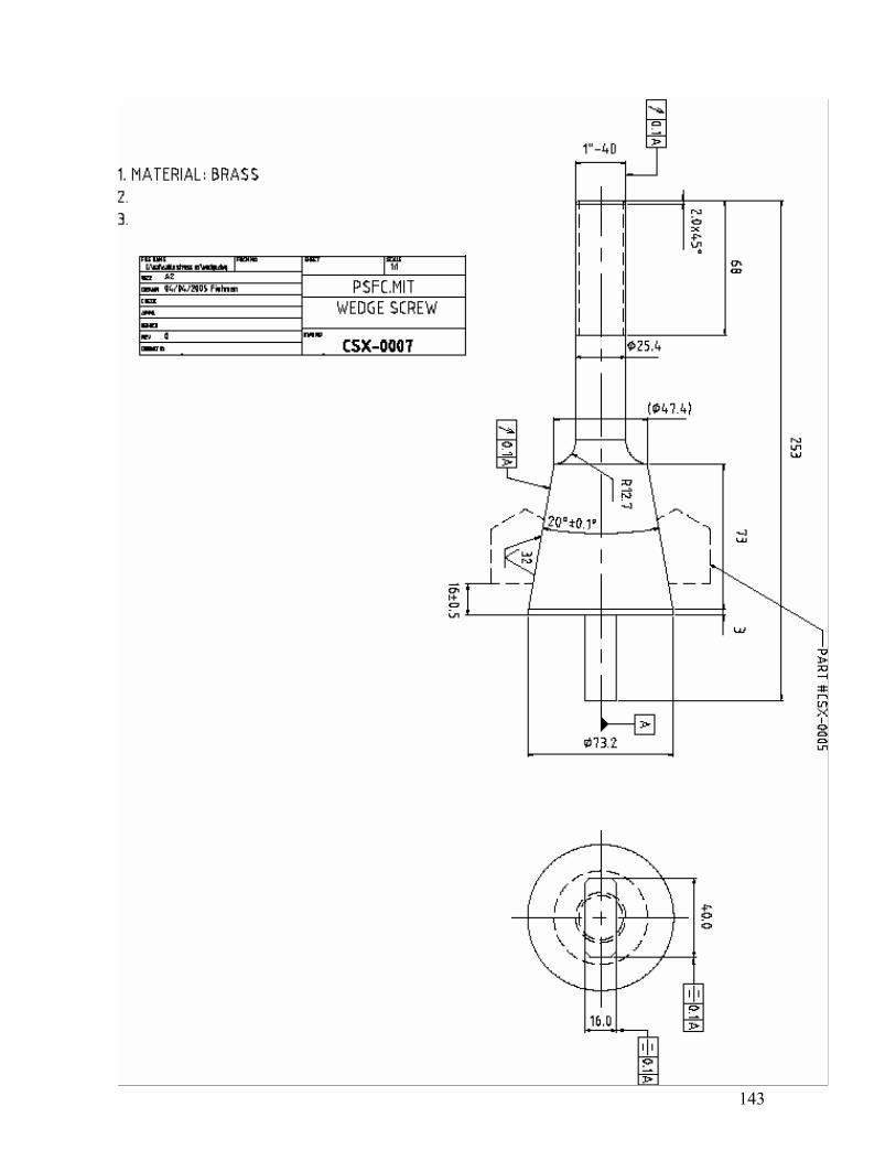
143

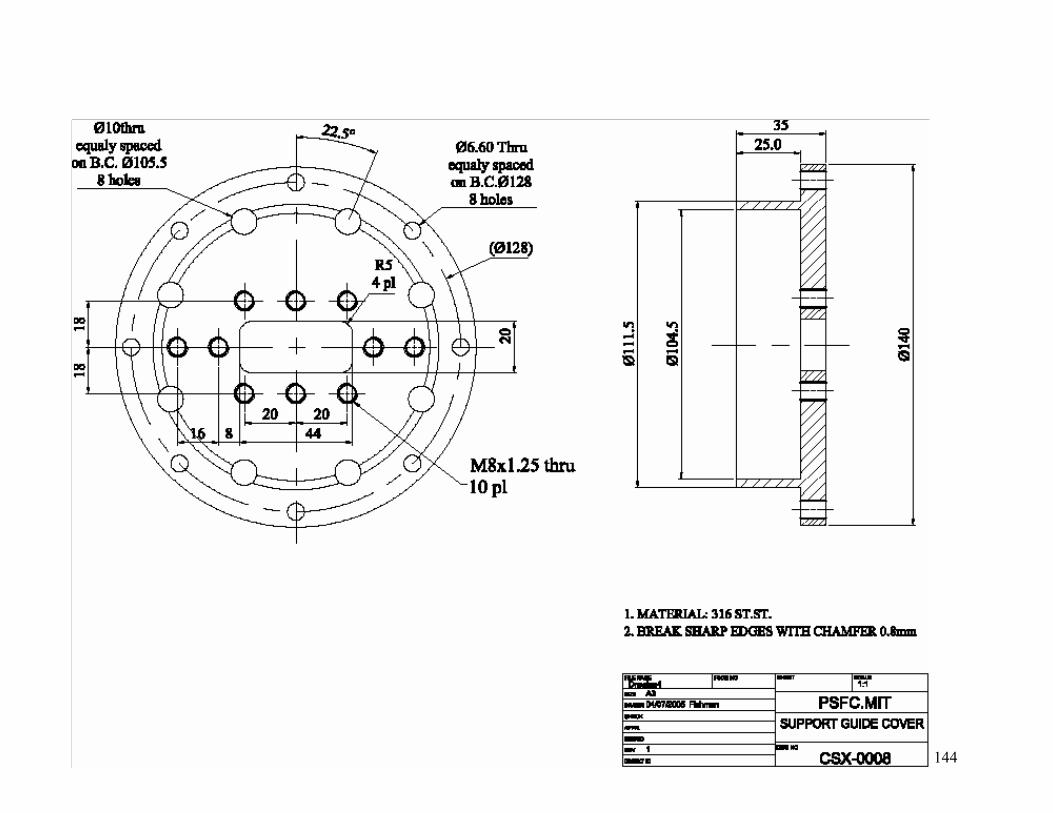
144

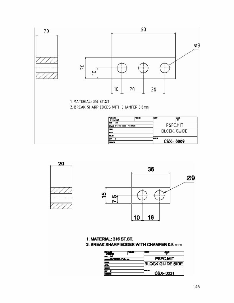
146

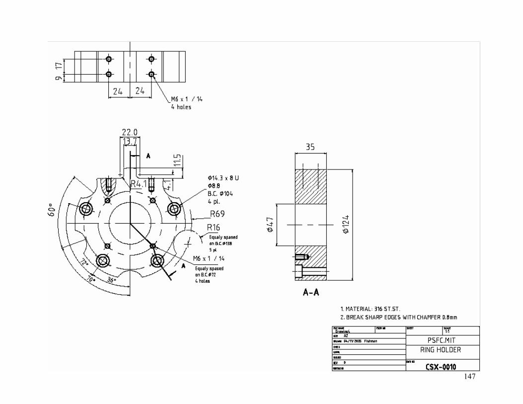
147

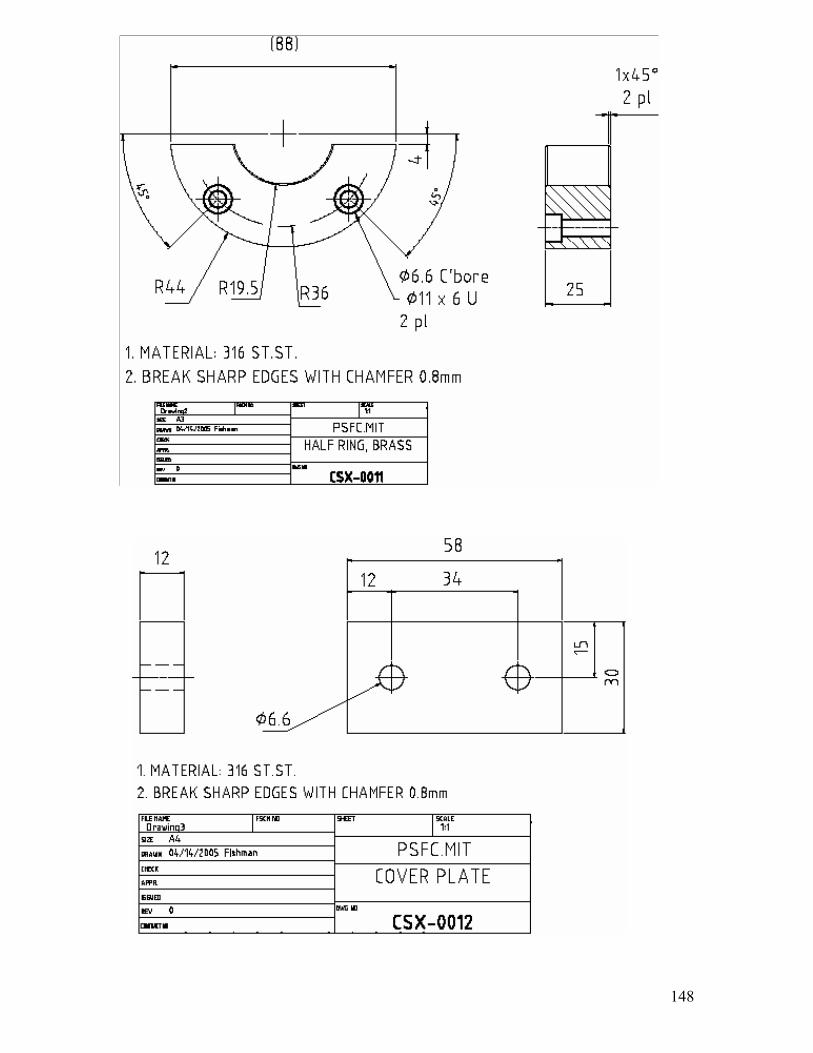
148

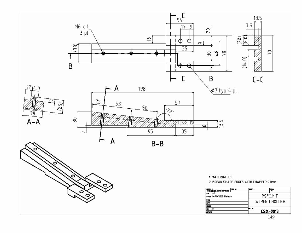
149

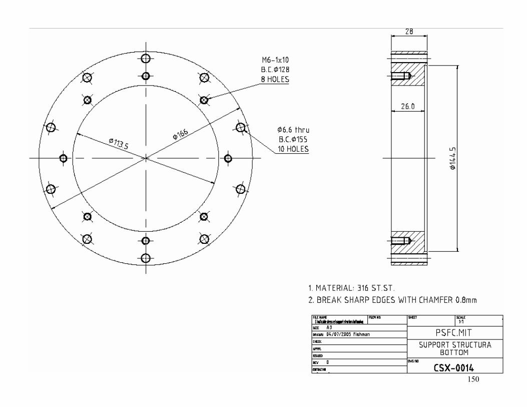
150

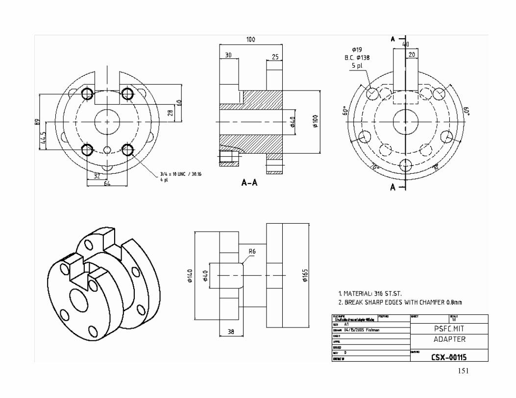
151

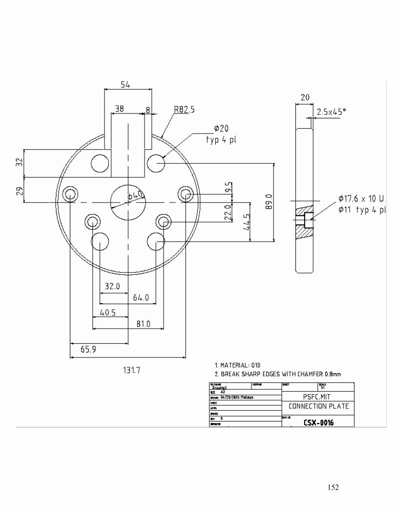
152

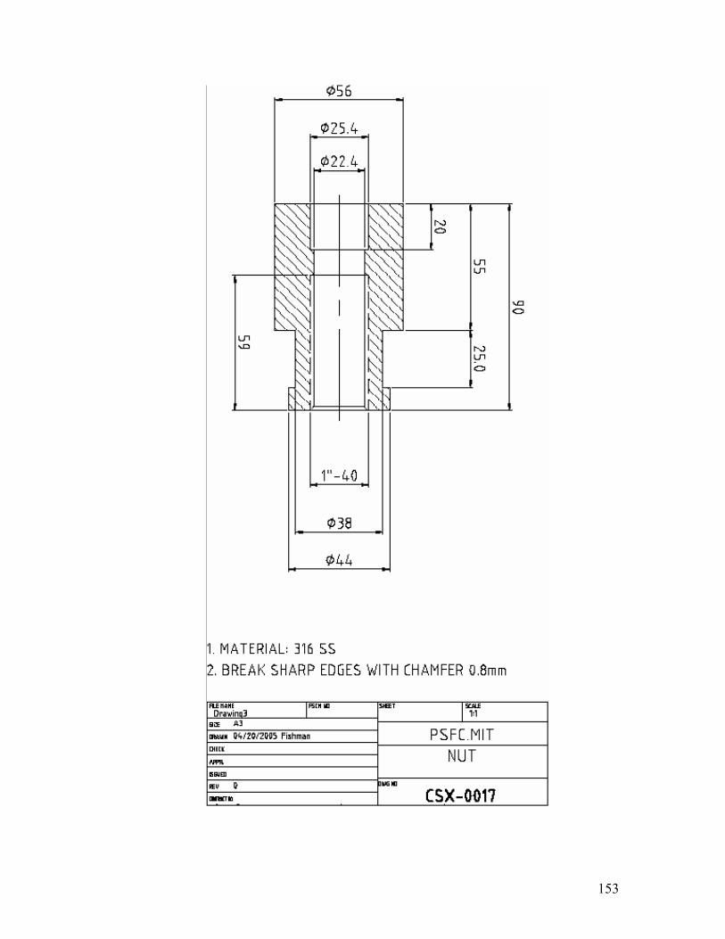
153

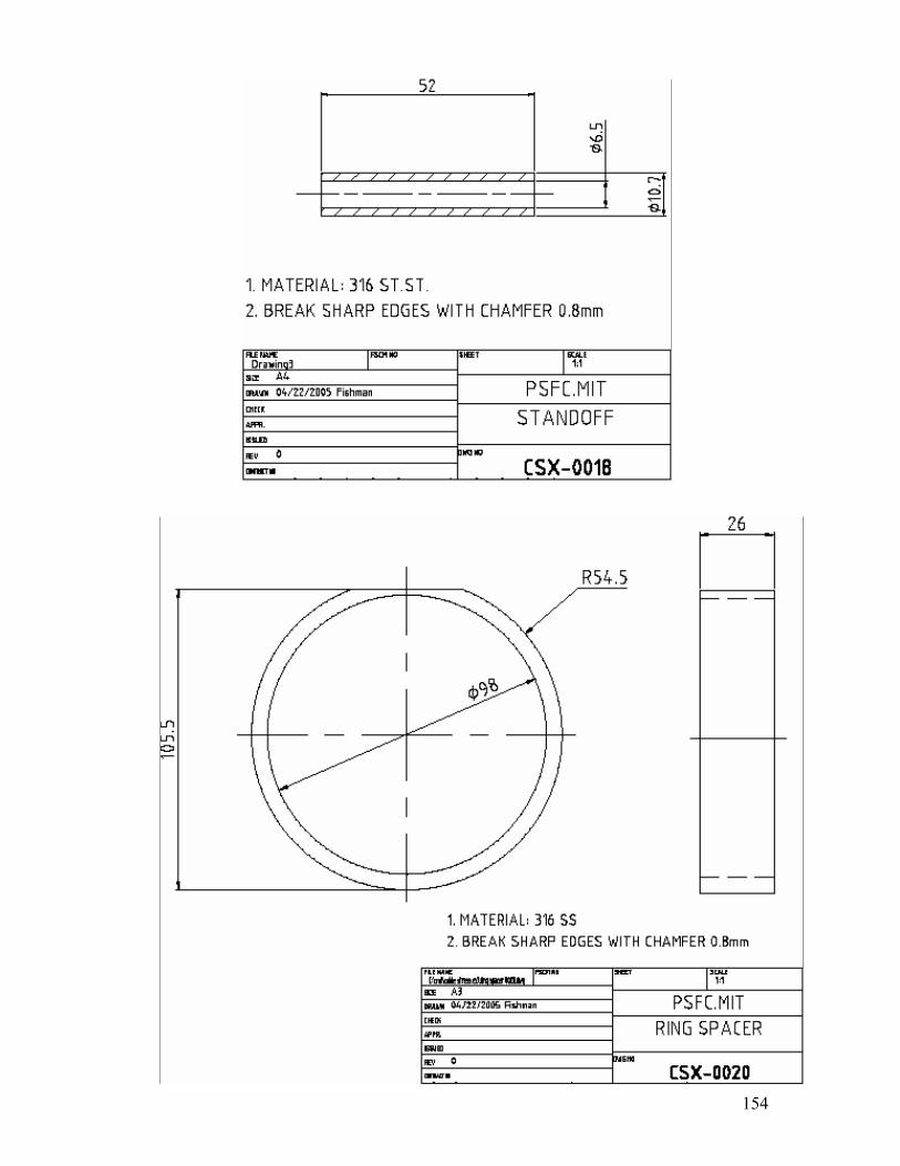
154

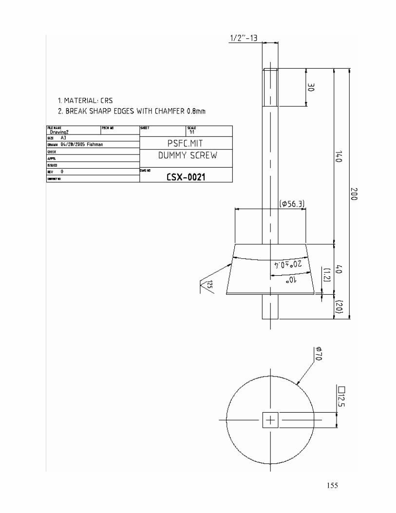
155

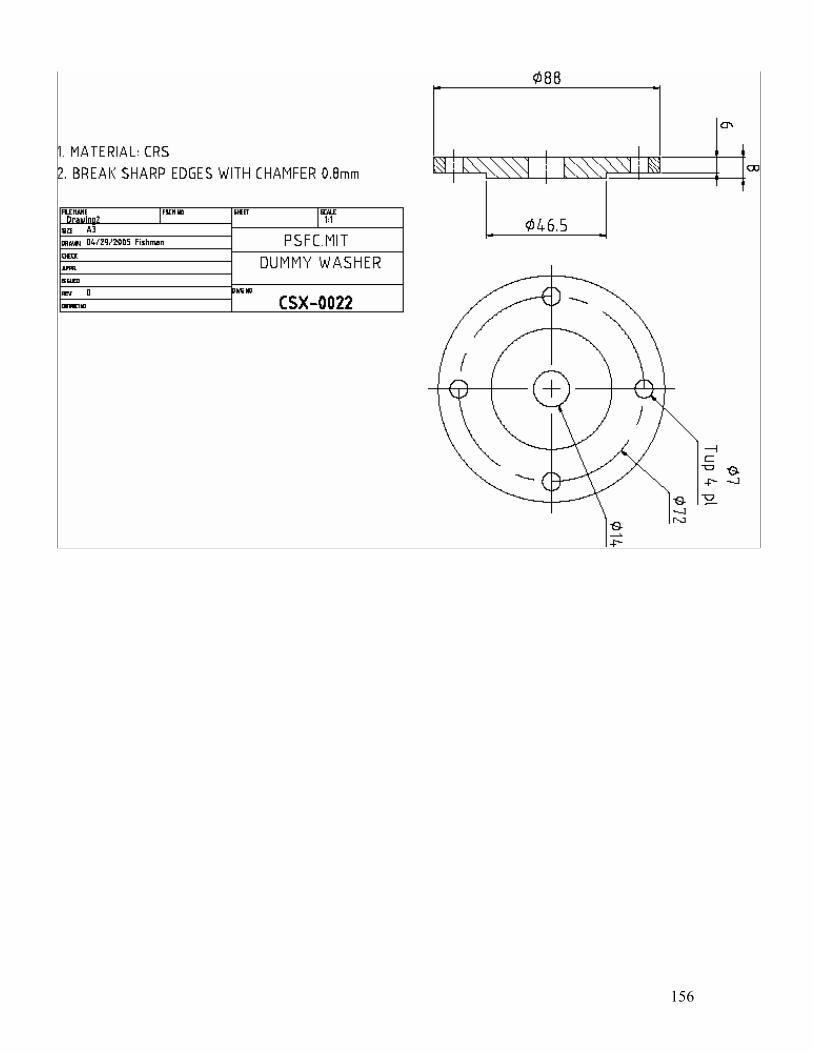
156

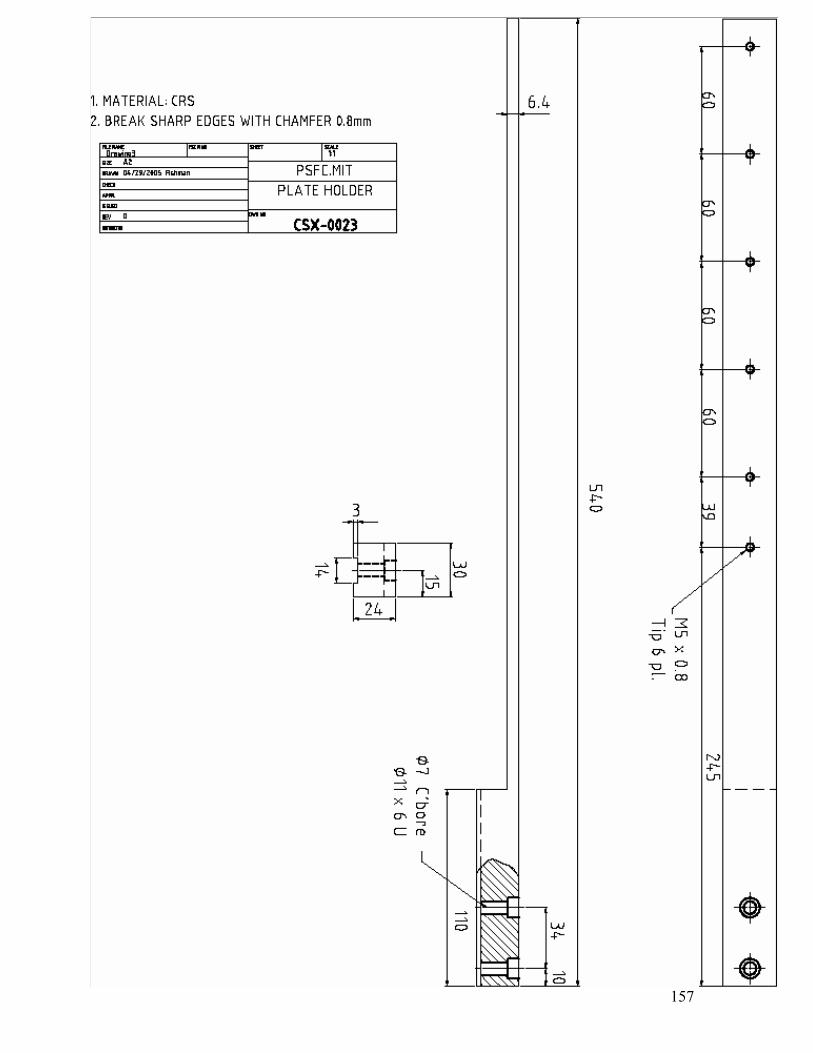
157

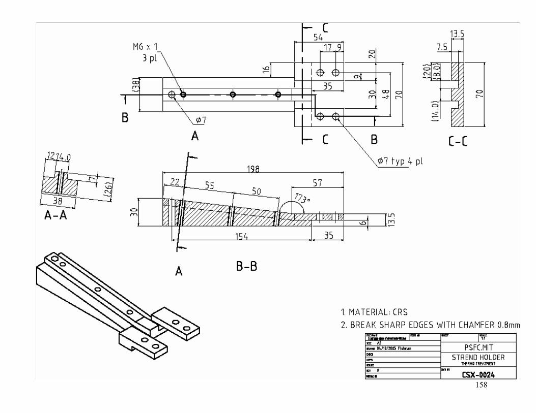
158

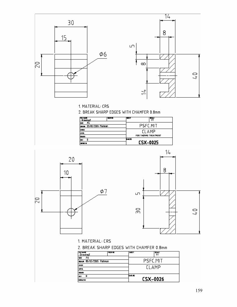
159

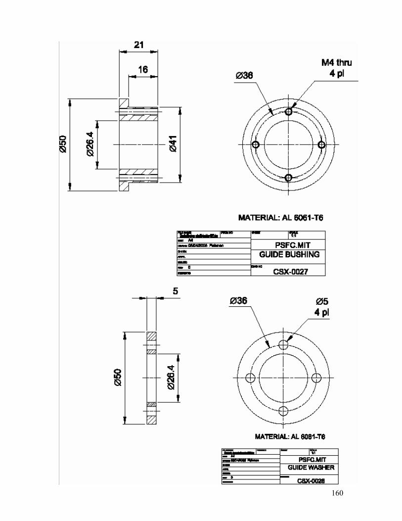
160

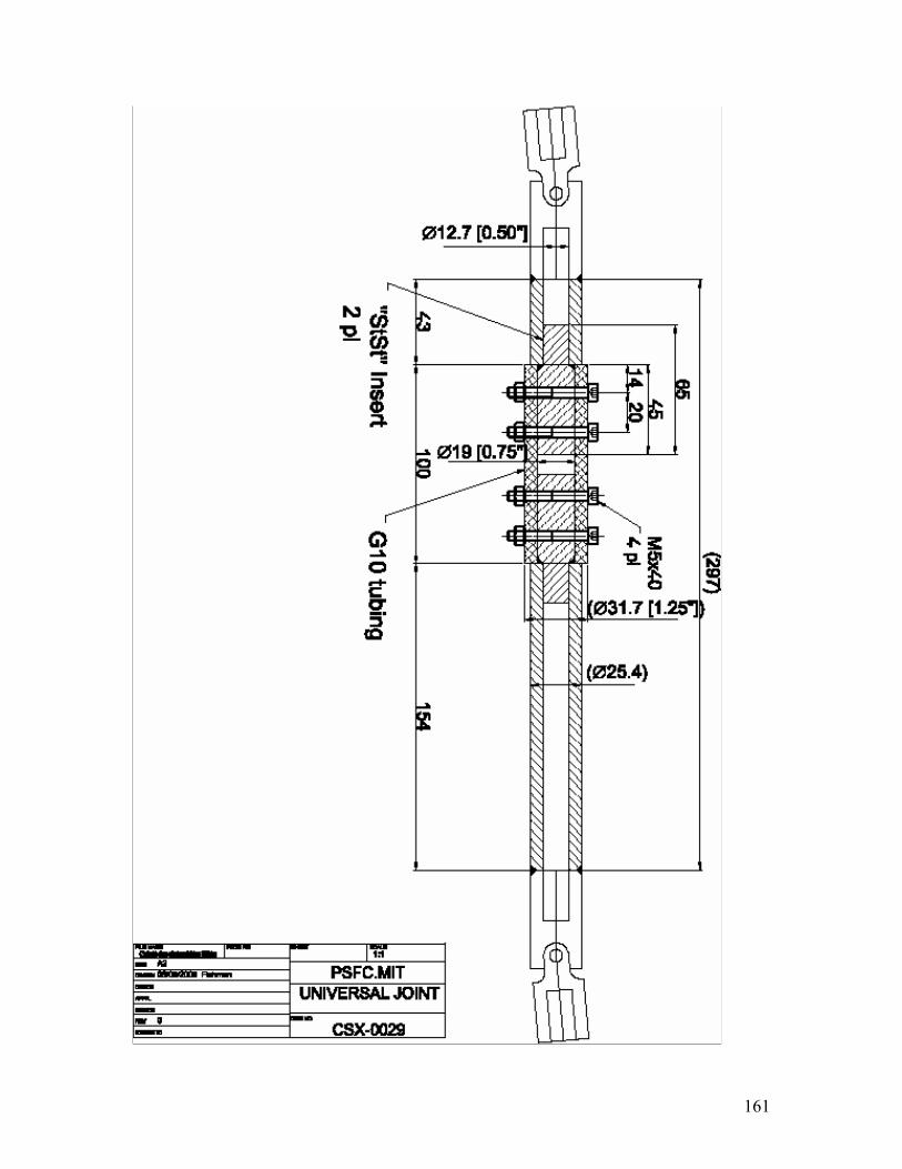
161

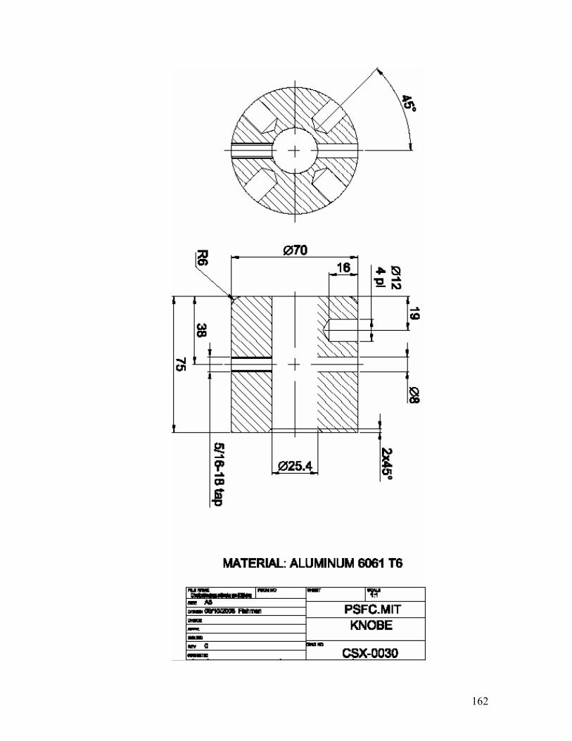
162

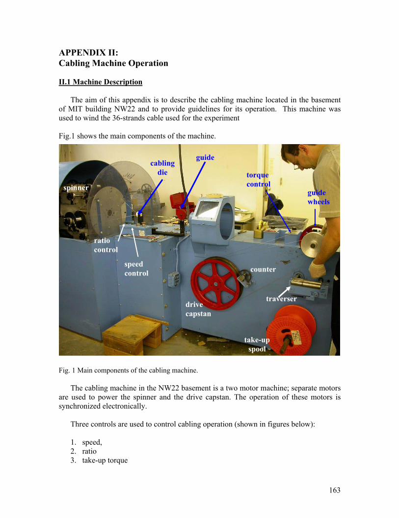
163

APPENDIX II: Cabling Machine Operation II.1 Machine Description

The aim of this appendix is to describe the cabling machine located in the basement of MIT building NW22 and to provide guidelines for its operation. This machine was used to wind the 36-strands cable used for the experiment Fig.1 shows the main components of the machine. Fig. 1 Main components of the cabling machine.

The cabling machine in the NW22 basement is a two motor machine; separate motors are used to power the spinner and the drive capstan. The operation of these motors is synchronized electronically.

Three controls are used to control cabling operation (shown in figures below):

1. speed, 2. ratio 3. take-up torque

spinner

drive capstan

ratio control

speed control

torque control

take-up spool

traverser

counter

cablingdie

guide

guide wheels

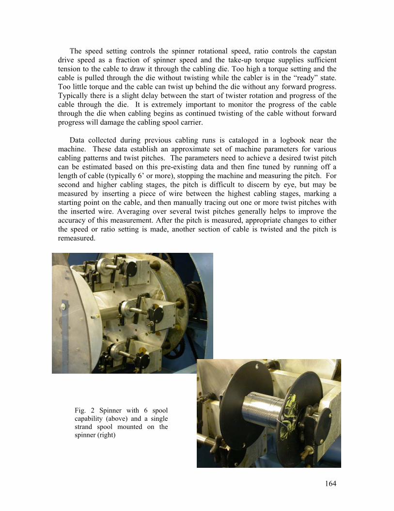
164

The speed setting controls the spinner rotational speed, ratio controls the capstan drive speed as a fraction of spinner speed and the take-up torque supplies sufficient tension to the cable to draw it through the cabling die. Too high a torque setting and the cable is pulled through the die without twisting while the cabler is in the “ready” state. Too little torque and the cable can twist up behind the die without any forward progress. Typically there is a slight delay between the start of twister rotation and progress of the cable through the die. It is extremely important to monitor the progress of the cable through the die when cabling begins as continued twisting of the cable without forward progress will damage the cabling spool carrier.

Data collected during previous cabling runs is cataloged in a logbook near the machine. These data establish an approximate set of machine parameters for various cabling patterns and twist pitches. The parameters need to achieve a desired twist pitch can be estimated based on this pre-existing data and then fine tuned by running off a length of cable (typically 6’ or more), stopping the machine and measuring the pitch. For second and higher cabling stages, the pitch is difficult to discern by eye, but may be measured by inserting a piece of wire between the highest cabling stages, marking a starting point on the cable, and then manually tracing out one or more twist pitches with the inserted wire. Averaging over several twist pitches generally helps to improve the accuracy of this measurement. After the pitch is measured, appropriate changes to either the speed or ratio setting is made, another section of cable is twisted and the pitch is remeasured.

Fig. 2 Spinner with 6 spool capability (above) and a single strand spool mounted on the spinner (right)

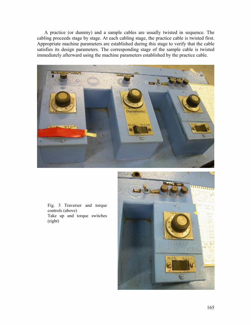
165

A practice (or dummy) and a sample cables are usually twisted in sequence. The cabling proceeds stage by stage. At each cabling stage, the practice cable is twisted first. Appropriate machine parameters are established during this stage to verify that the cable satisfies its design parameters. The corresponding stage of the sample cable is twisted immediately afterward using the machine parameters established by the practice cable.

Fig. 3 Traverser and torque controls (above) Take up and torque switches (right)

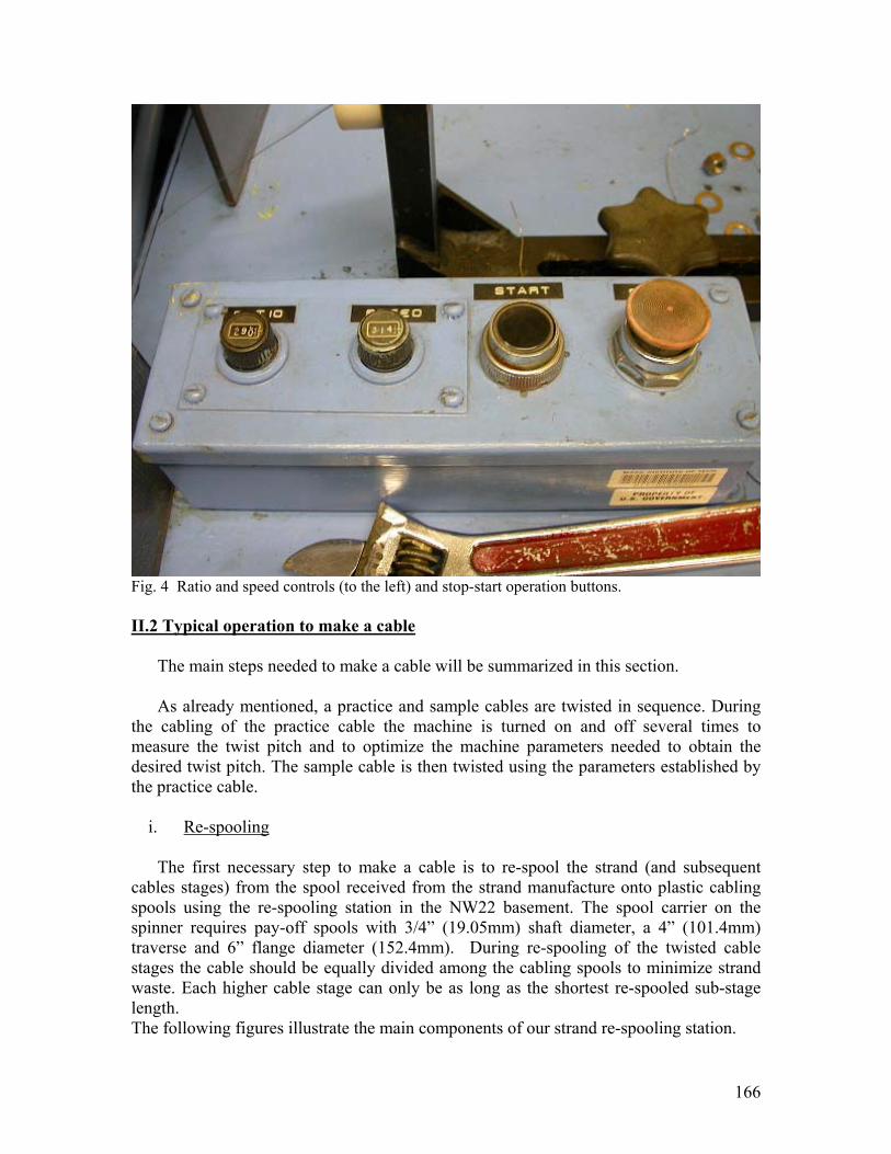
166

Fig. 4 Ratio and speed controls (to the left) and stop-start operation buttons. II.2 Typical operation to make a cable

The main steps needed to make a cable will be summarized in this section.

As already mentioned, a practice and sample cables are twisted in sequence. During the cabling of the practice cable the machine is turned on and off several times to measure the twist pitch and to optimize the machine parameters needed to obtain the desired twist pitch. The sample cable is then twisted using the parameters established by the practice cable.

i. Re-spooling

The first necessary step to make a cable is to re-spool the strand (and subsequent cables stages) from the spool received from the strand manufacture onto plastic cabling spools using the re-spooling station in the NW22 basement. The spool carrier on the spinner requires pay-off spools with 3/4” (19.05mm) shaft diameter, a 4” (101.4mm) traverse and 6” flange diameter (152.4mm). During re-spooling of the twisted cable stages the cable should be equally divided among the cabling spools to minimize strand waste. Each higher cable stage can only be as long as the shortest re-spooled sub-stage length. The following figures illustrate the main components of our strand re-spooling station.

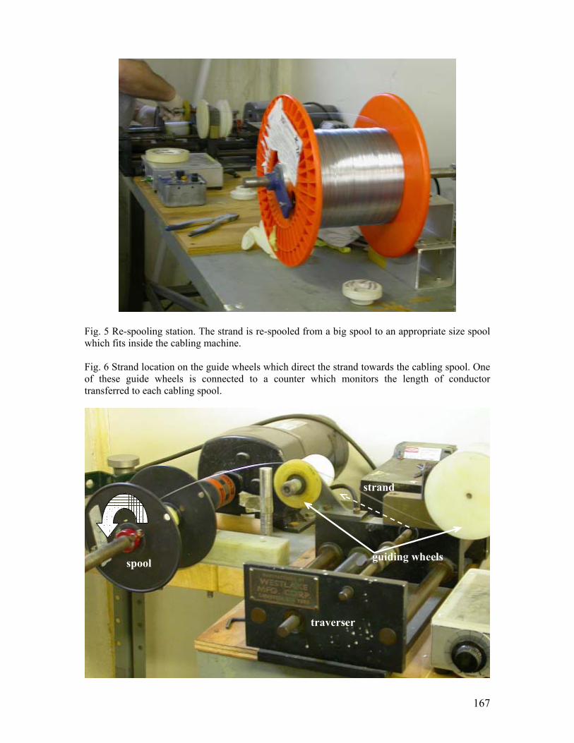
167

Fig. 5 Re-spooling station. The strand is re-spooled from a big spool to an appropriate size spool which fits inside the cabling machine. Fig. 6 Strand location on the guide wheels which direct the strand towards the cabling spool. One of these guide wheels is connected to a counter which monitors the length of conductor transferred to each cabling spool.

strand

guiding wheels

traverser

spool

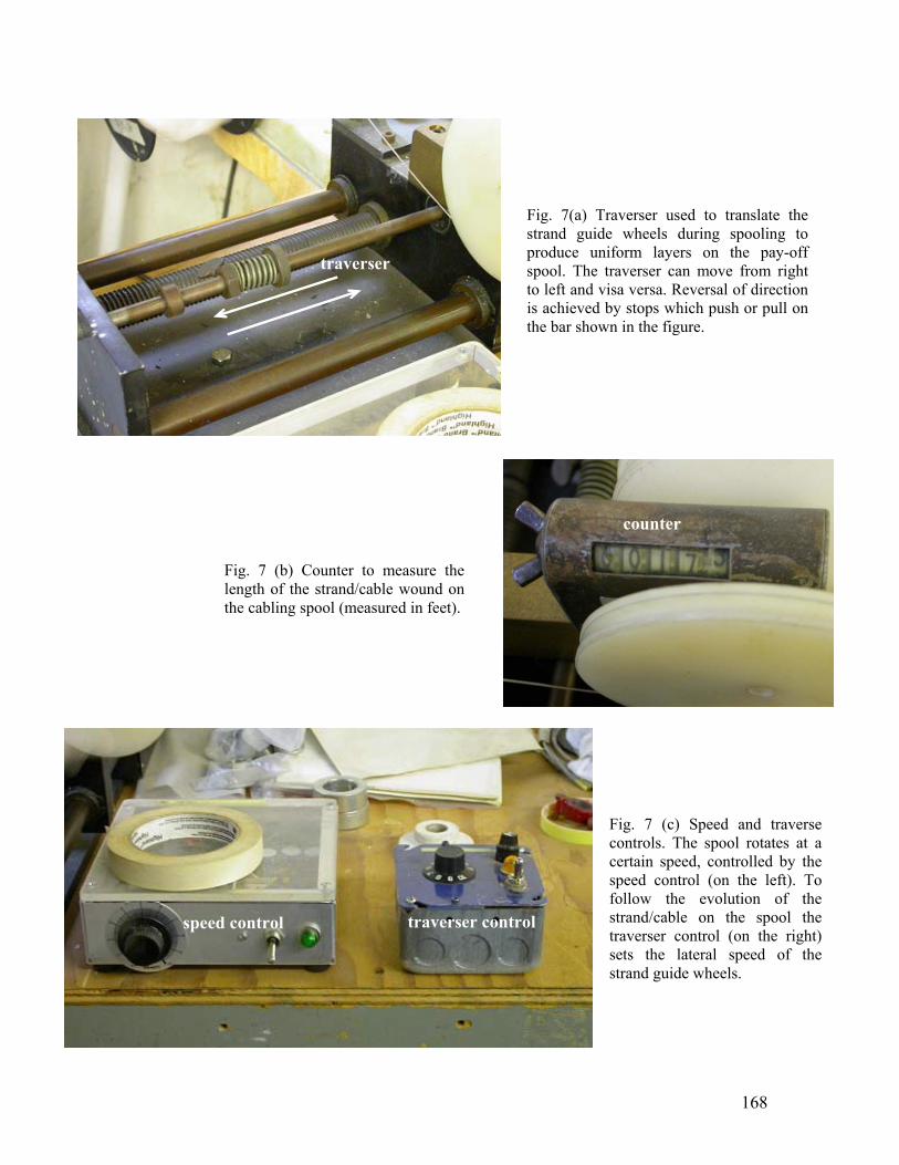
168

Fig. 7 (b) Counter to measure the length of the strand/cable wound on the cabling spool (measured in feet).

Fig. 7(a) Traverser used to translate the strand guide wheels during spooling to produce uniform layers on the pay-off spool. The traverser can move from right to left and visa versa. Reversal of direction is achieved by stops which push or pull on the bar shown in the figure.

Fig. 7 (c) Speed and traverse controls. The spool rotates at a certain speed, controlled by the speed control (on the left). To follow the evolution of the strand/cable on the spool the traverser control (on the right) sets the lateral speed of the strand guide wheels.

traverser

counter

speed control traverser control

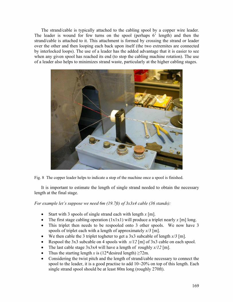
169

The strand/cable is typically attached to the cabling spool by a copper wire leader. The leader is wound for few turns on the spool (perhaps 6’ length) and then the strand/cable is attached to it. This attachment is formed by crossing the strand or leader over the other and then looping each back upon itself (the two extremites are connected by interlocked loops). The use of a leader has the added advantage that it is easier to see when any given spool has reached its end (to stop the cabling machine rotation). The use of a leader also helps to minimizes strand waste, particularly at the higher cabling stages.

Fig. 8 The copper leader helps to indicate a stop of the machine once a spool is finished.

It is important to estimate the length of single strand needed to obtain the necessary length at the final stage. For example let’s suppose we need 6m (19.7ft) of 3x3x4 cable (36 stands):

• Start with 3 spools of single strand each with length x [m]. • The first stage cabling operation (1x1x1) will produce a triplet nearly x [m] long. • This triplet then needs to be respooled onto 3 other spools. We now have 3

spools of triplet each with a length of approximately x/3 [m]. • We then cable the 3 triplet togheter to get a 3x3 subcable of length x/3 [m]. • Respool the 3x3 subcable on 4 spools with x/12 [m] of 3x3 cable on each spool. • The last cable stage 3x3x4 will have a length of roughly x/12 [m]. • Thus the starting length x is (12*desired length) ≥72m. • Considering the twist pitch and the length of strand/cable necessary to connect the

spool to the leader, it is a good practise to add 10~20% on top of this length. Each single strand spool should be at least 80m long (roughly 270ft).

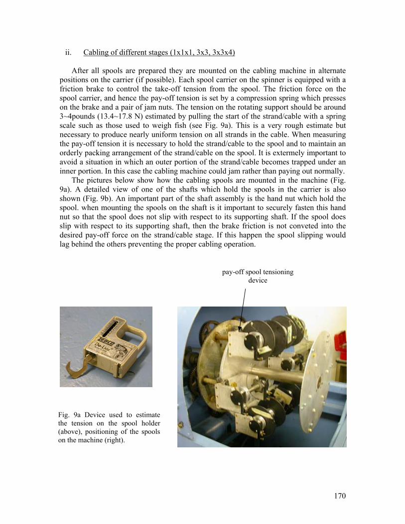
170

ii. Cabling of different stages (1x1x1, 3x3, 3x3x4)

After all spools are prepared they are mounted on the cabling machine in alternate positions on the carrier (if possible). Each spool carrier on the spinner is equipped with a friction brake to control the take-off tension from the spool. The friction force on the spool carrier, and hence the pay-off tension is set by a compression spring which presses on the brake and a pair of jam nuts. The tension on the rotating support should be around 3~4pounds (13.4~17.8 N) estimated by pulling the start of the strand/cable with a spring scale such as those used to weigh fish (see Fig. 9a). This is a very rough estimate but necessary to produce nearly uniform tension on all strands in the cable. When measuring the pay-off tension it is necessary to hold the strand/cable to the spool and to maintain an orderly packing arrangement of the strand/cable on the spool. It is extermely important to avoid a situation in which an outer portion of the strand/cable becomes trapped under an inner portion. In this case the cabling machine could jam rather than paying out normally.

The pictures below show how the cabling spools are mounted in the machine (Fig. 9a). A detailed view of one of the shafts which hold the spools in the carrier is also shown (Fig. 9b). An important part of the shaft assembly is the hand nut which hold the spool. when mounting the spools on the shaft is it important to securely fasten this hand nut so that the spool does not slip with respect to its supporting shaft. If the spool does slip with respect to its supporting shaft, then the brake friction is not conveted into the desired pay-off force on the strand/cable stage. If this happen the spool slipping would lag behind the others preventing the proper cabling operation.

Fig. 9a Device used to estimate the tension on the spool holder (above), positioning of the spools on the machine (right).

pay-off spool tensioning device

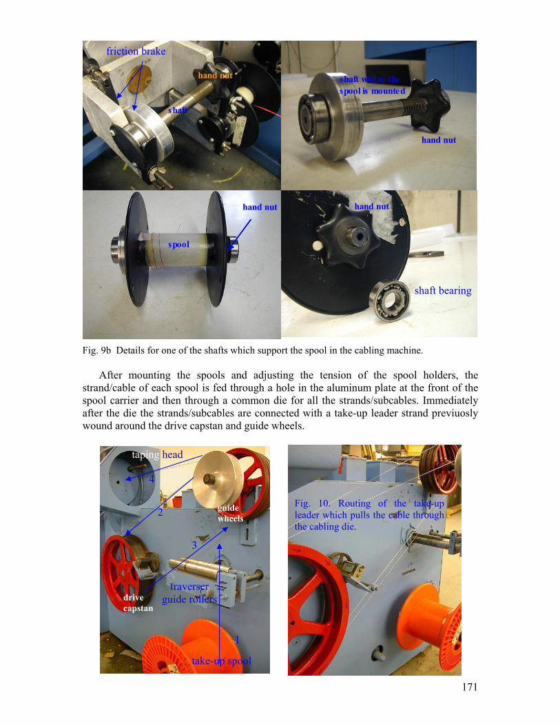
171

Fig. 9b Details for one of the shafts which support the spool in the cabling machine.

After mounting the spools and adjusting the tension of the spool holders, the strand/cable of each spool is fed through a hole in the aluminum plate at the front of the spool carrier and then through a common die for all the strands/subcables. Immediately after the die the strands/subcables are connected with a take-up leader strand previuosly wound around the drive capstan and guide wheels.

shaft

hand nut

hand nut

hand nut

spool

hand nut

shaft where the spool is mounted

friction brake

shaft bearing

Fig. 10. Routing of the take-up leader which pulls the cable through the cabling die.

1

2

3

4

drive capstan

guide wheels

take-up spool

traverser guide rollers

taping head

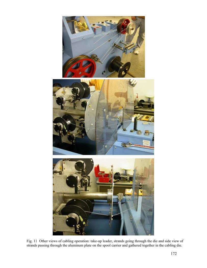
172

Fig. 11 Other views of cabling operation: take-up leader, strands going through the die and side view of strands passing through the aluminum plate on the spool carrier and gathered together in the cabling die.

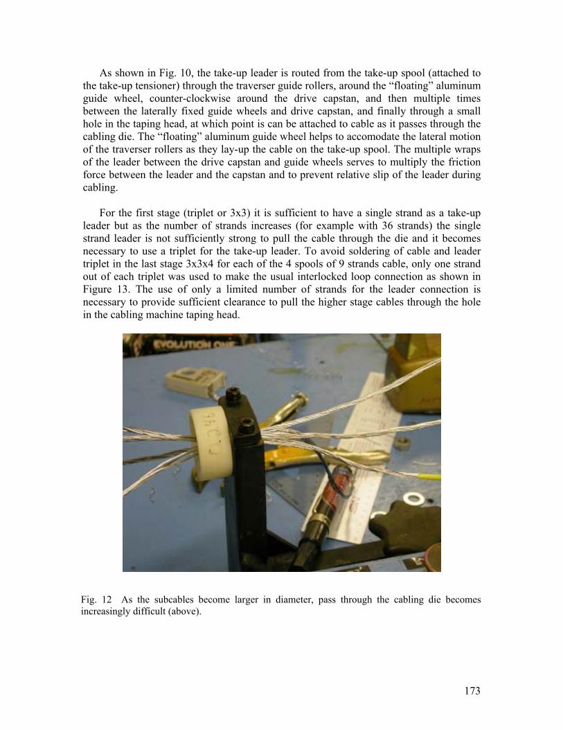
173

As shown in Fig. 10, the take-up leader is routed from the take-up spool (attached to the take-up tensioner) through the traverser guide rollers, around the “floating” aluminum guide wheel, counter-clockwise around the drive capstan, and then multiple times between the laterally fixed guide wheels and drive capstan, and finally through a small hole in the taping head, at which point is can be attached to cable as it passes through the cabling die. The “floating” aluminum guide wheel helps to accomodate the lateral motion of the traverser rollers as they lay-up the cable on the take-up spool. The multiple wraps of the leader between the drive capstan and guide wheels serves to multiply the friction force between the leader and the capstan and to prevent relative slip of the leader during cabling.

For the first stage (triplet or 3x3) it is sufficient to have a single strand as a take-up leader but as the number of strands increases (for example with 36 strands) the single strand leader is not sufficiently strong to pull the cable through the die and it becomes necessary to use a triplet for the take-up leader. To avoid soldering of cable and leader triplet in the last stage 3x3x4 for each of the 4 spools of 9 strands cable, only one strand out of each triplet was used to make the usual interlocked loop connection as shown in Figure 13. The use of only a limited number of strands for the leader connection is necessary to provide sufficient clearance to pull the higher stage cables through the hole in the cabling machine taping head.

Fig. 12 As the subcables become larger in diameter, pass through the cabling die becomes increasingly difficult (above).

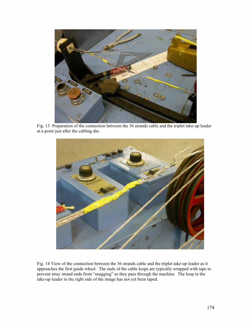
174

Fig. 13 Preparation of the connection between the 36 strands cable and the triplet take-up leader at a point just after the cabling die.

Fig. 14 View of the connection between the 36 strands cable and the triplet take-up leader as it approaches the first guide wheel. The ends of the cable loops are typically wrapped with tape to prevent stray strand ends from “snagging” as they pass through the machine. The loop in the take-up leader to the right side of the image has not yet been taped.

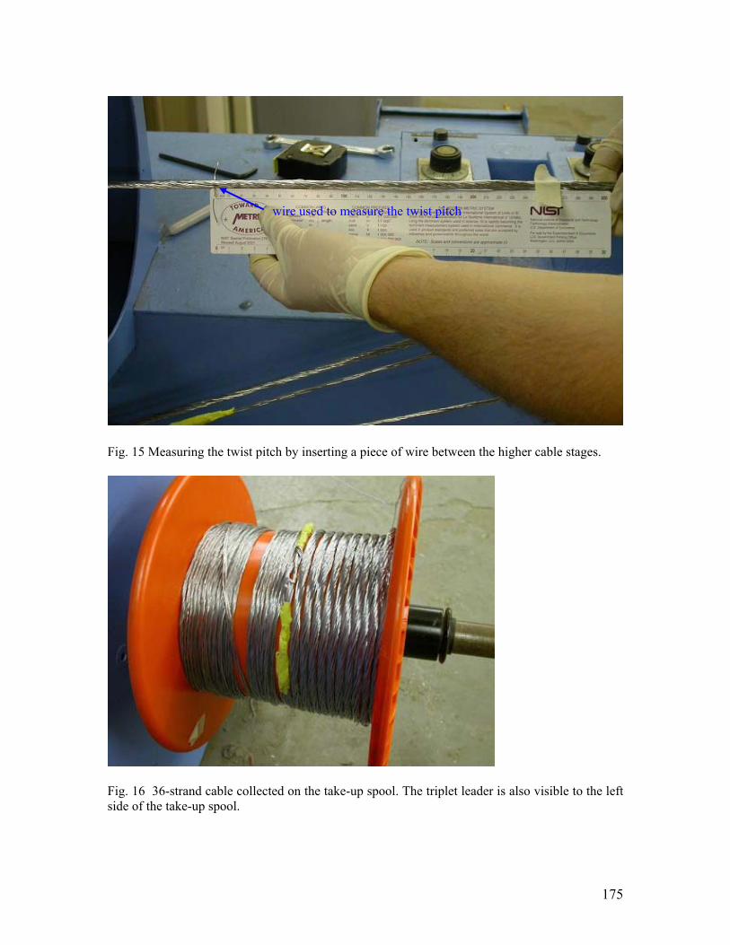
175

Fig. 15 Measuring the twist pitch by inserting a piece of wire between the higher cable stages.

Fig. 16 36-strand cable collected on the take-up spool. The triplet leader is also visible to the left side of the take-up spool.

wire used to measure the twist pitch

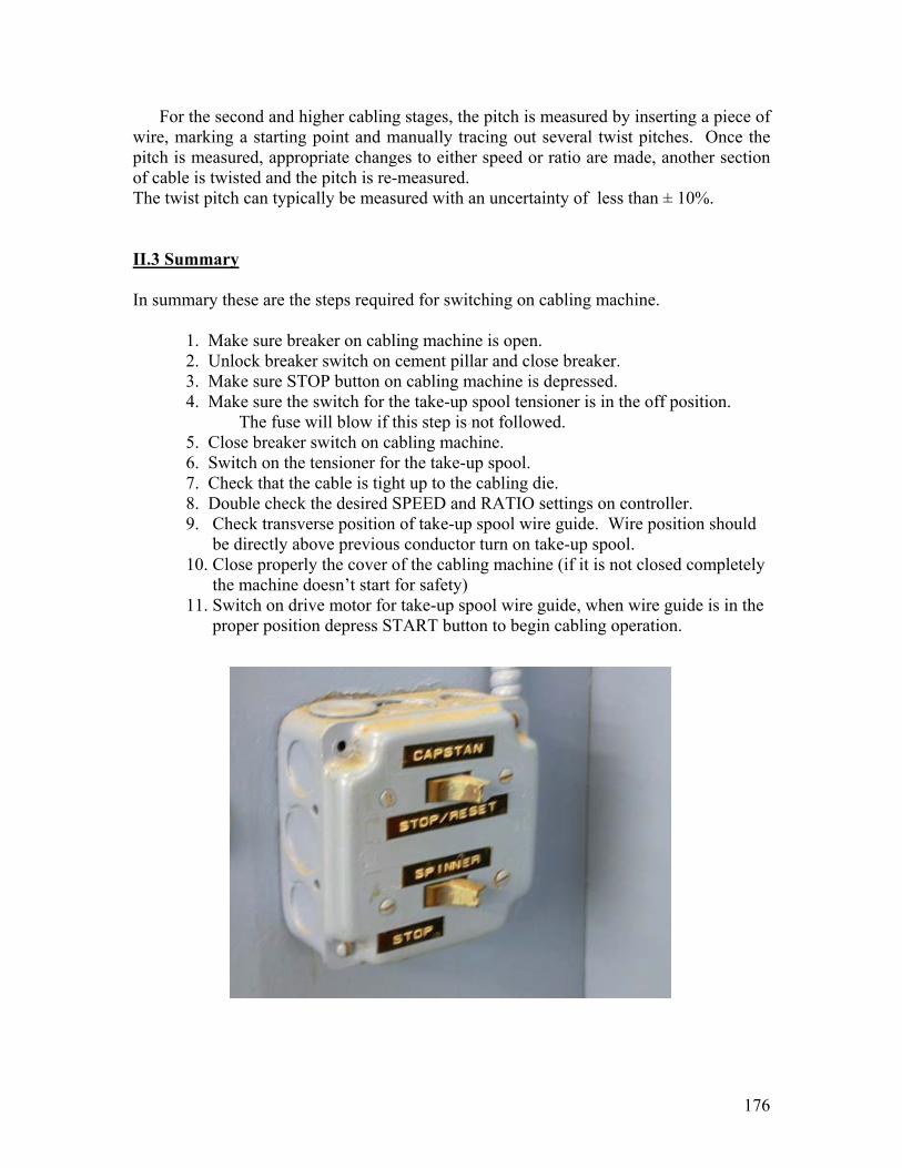
176

For the second and higher cabling stages, the pitch is measured by inserting a piece of wire, marking a starting point and manually tracing out several twist pitches. Once the pitch is measured, appropriate changes to either speed or ratio are made, another section of cable is twisted and the pitch is re-measured. The twist pitch can typically be measured with an uncertainty of less than ± 10%. II.3 Summary In summary these are the steps required for switching on cabling machine.

1. Make sure breaker on cabling machine is open. 2. Unlock breaker switch on cement pillar and close breaker. 3. Make sure STOP button on cabling machine is depressed. 4. Make sure the switch for the take-up spool tensioner is in the off position. The fuse will blow if this step is not followed. 5. Close breaker switch on cabling machine. 6. Switch on the tensioner for the take-up spool. 7. Check that the cable is tight up to the cabling die. 8. Double check the desired SPEED and RATIO settings on controller. 9. Check transverse position of take-up spool wire guide. Wire position should

be directly above previous conductor turn on take-up spool. 10. Close properly the cover of the cabling machine (if it is not closed completely

the machine doesn’t start for safety) 11. Switch on drive motor for take-up spool wire guide, when wire guide is in the

proper position depress START button to begin cabling operation.

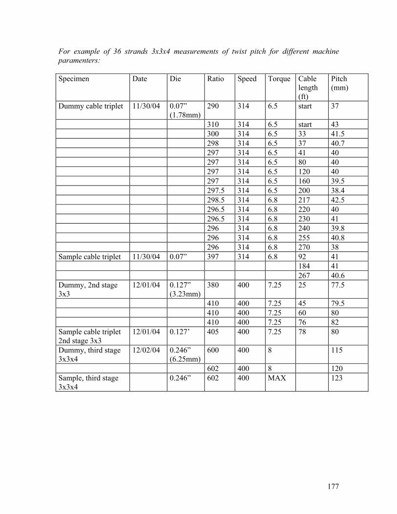
177

For example of 36 strands 3x3x4 measurements of twist pitch for different machine paramenters: Specimen Date Die Ratio Speed Torque Cable

length (ft)

Pitch (mm)

Dummy cable triplet 11/30/04 0.07” (1.78mm)

290 314 6.5 start 37

310 314 6.5 start 43 300 314 6.5 33 41.5 298 314 6.5 37 40.7 297 314 6.5 41 40 297 314 6.5 80 40 297 314 6.5 120 40 297 314 6.5 160 39.5 297.5 314 6.5 200 38.4 298.5 314 6.8 217 42.5 296.5 314 6.8 220 40 296.5 314 6.8 230 41 296 314 6.8 240 39.8 296 314 6.8 255 40.8 296 314 6.8 270 38 Sample cable triplet 11/30/04 0.07” 397 314 6.8 92 41 184 41 267 40.6 Dummy, 2nd stage 3x3

12/01/04 0.127” (3.23mm)

380 400 7.25 25 77.5

410 400 7.25 45 79.5 410 400 7.25 60 80 410 400 7.25 76 82 Sample cable triplet 2nd stage 3x3

12/01/04 0.127’

405 400 7.25 78 80

Dummy, third stage 3x3x4

12/02/04 0.246” (6.25mm)

600 400 8 115

602 400 8 120 Sample, third stage 3x3x4

0.246”

602 400 MAX 123

178

Notes on a recent 3x3x4 cable fabrication effort: • In the future, the dummy cable length should be significantly larger (perhaps 50%)

than the required sample cable length so that it is possible to investigate several sets of cabling parameters to achieve the desired twist pitch length especially at the higher cabling stages.

• Whenever the cabling machine is stopped and restarted there is a slight lag between the spinner rotation and the capstan rotation. Due to occasional slip between the take-up leader and the capstan it is possible that the FINAL CABLE LENGTH on the indicator overestimates the real length. Excessive slip can also damage the spinner if the cable twisting were to continue with no forward cable progress through the die. Machine operation should be closely monitored whenever the cabling machine is restarted.

• The torque on the spool holders was reduced at 3 pounds at the last stage. (This reduction in the pay-off force was probably a mistake. The higher cabling stages get increasingly stiff, so that to maintain a good pay-off arrangement we should probably increase the pay-off tension slightly as we move to the higher cable stages, rather than to reduce it.)

• For the last cable stage it was necessary to use a triplet as the take-up leader due to breakage of the single strand leader at a take-up torque below that needed to pull the 36-strand cable through the cabling die.

• The error in the twist pitch measurements was well within ± 10%.

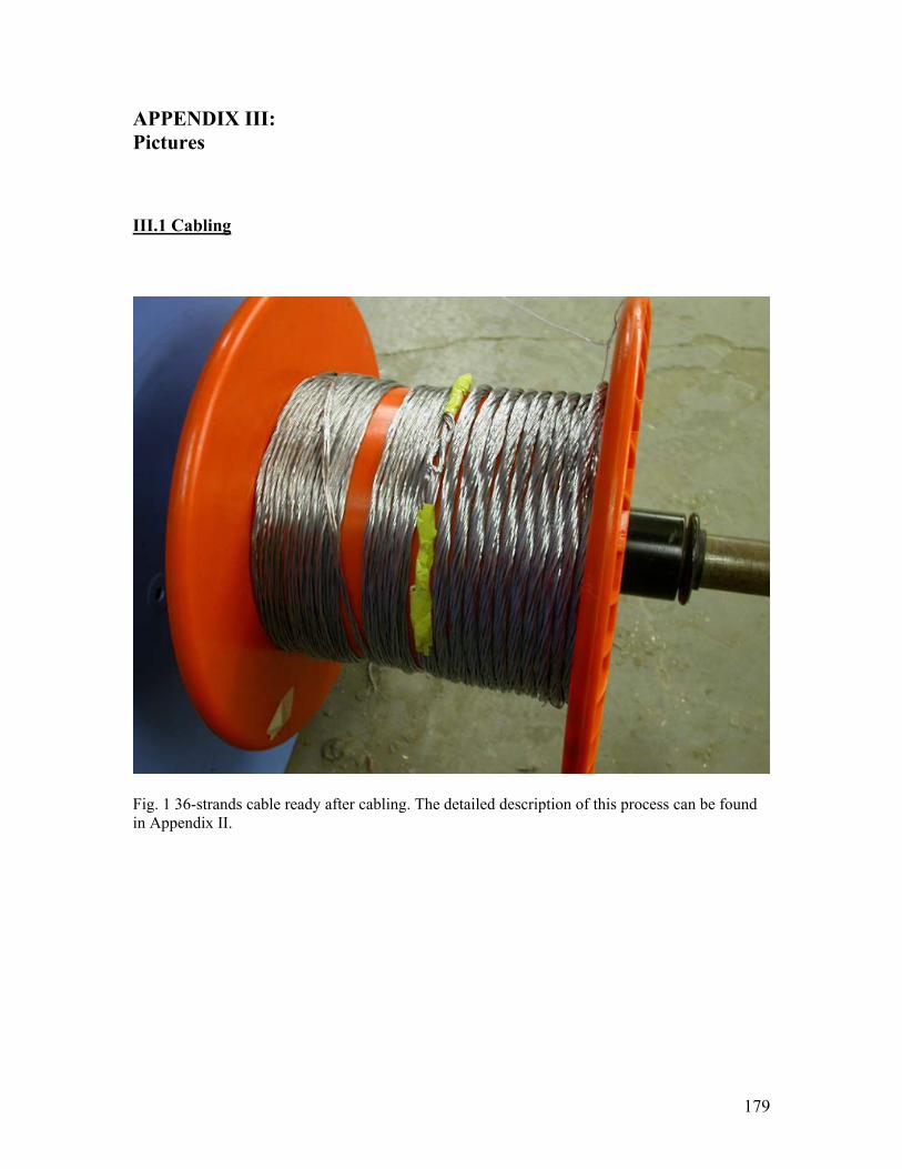
179

APPENDIX III: Pictures III.1 Cabling

Fig. 1 36-strands cable ready after cabling. The detailed description of this process can be found in Appendix II.

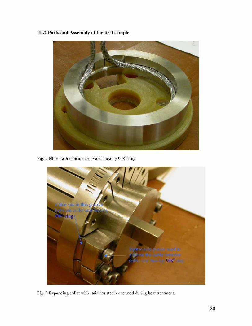
180

III.2 Parts and Assembly of the first sample

Fig. 2 Nb3Sn cable inside groove of Incoloy 908® ring.

Fig. 3 Expanding collet with stainless steel cone used during heat treatment.

Cable sits in this groove between collet and Incoloy 908® ring

Removable pieces used to enclose the cable between collet and Incoloy 908® ring

181

Fig. 4 Cable used for the experiment. Fig. 5 Assembly of the first sample. On the right an upside down view shows hoe the cable is enclosed in the ring.

Voltage tap wire

voltage tap connections

Copper terminations to be soldered to the current leads after heat treatment

Incoloy 908® rings. The cable is sitting in the groove of the bottom ring

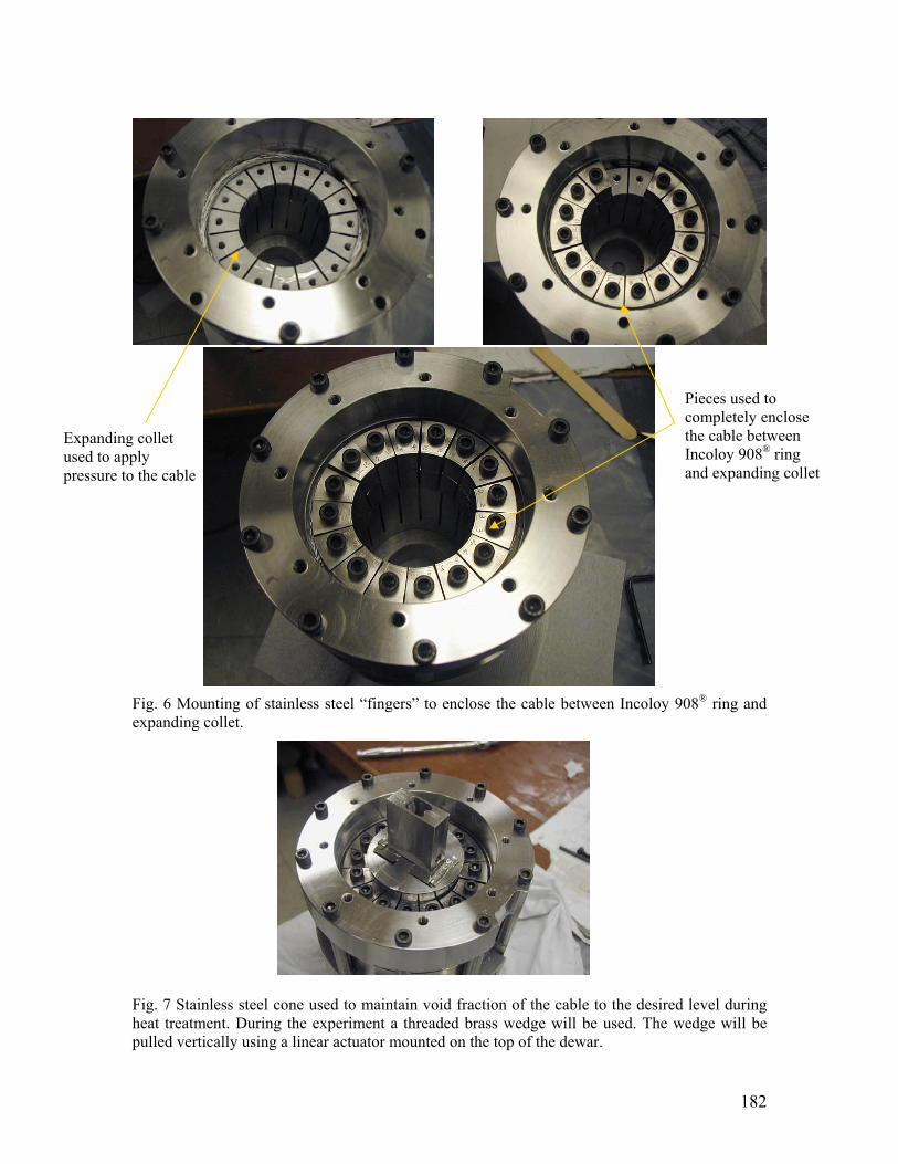
182

Fig. 6 Mounting of stainless steel “fingers” to enclose the cable between Incoloy 908® ring and expanding collet. Fig. 7 Stainless steel cone used to maintain void fraction of the cable to the desired level during heat treatment. During the experiment a threaded brass wedge will be used. The wedge will be pulled vertically using a linear actuator mounted on the top of the dewar.

Expanding collet used to apply pressure to the cable

Pieces used to completely enclose the cable between Incoloy 908® ring and expanding collet

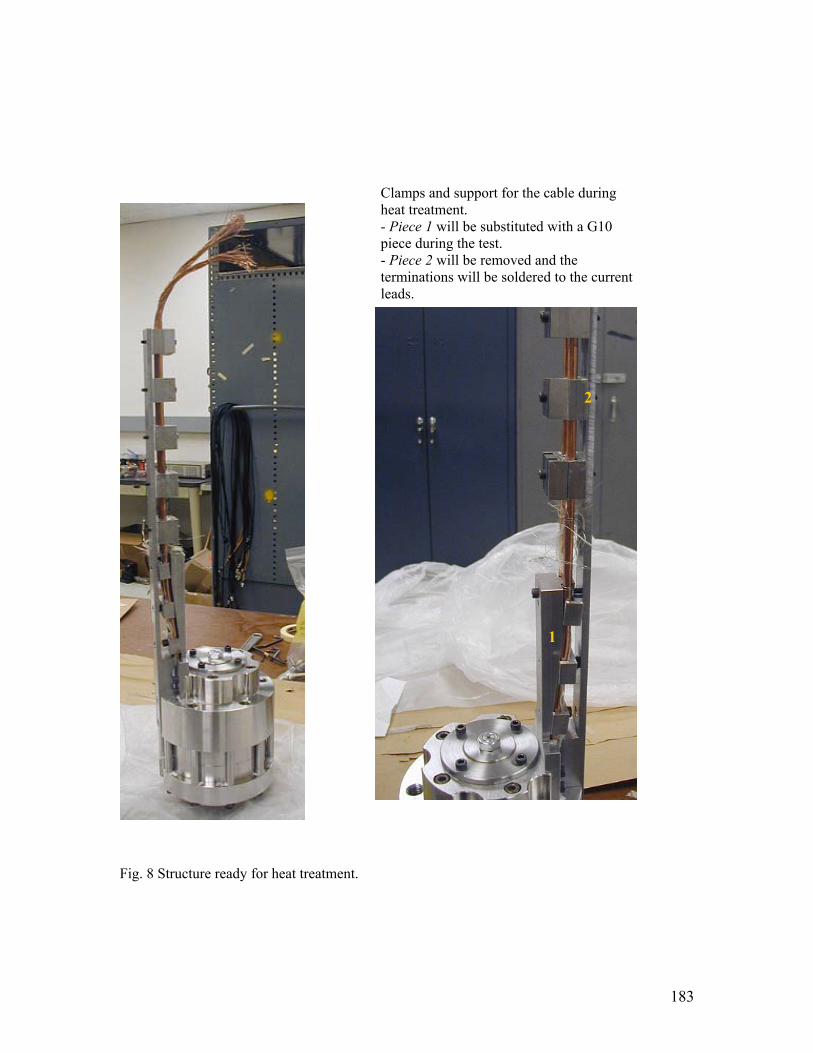
183

Fig. 8 Structure ready for heat treatment.

Clamps and support for the cable during heat treatment. - Piece 1 will be substituted with a G10 piece during the test. - Piece 2 will be removed and the terminations will be soldered to the current leads.

1

2

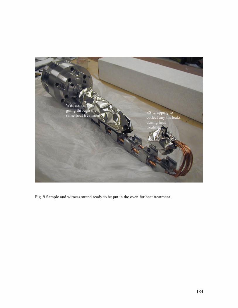
184

Fig. 9 Sample and witness strand ready to be put in the oven for heat treatment .

Witness samples going through the same heat treatment

SS wrapping to collect any tin leaks during heat treatment

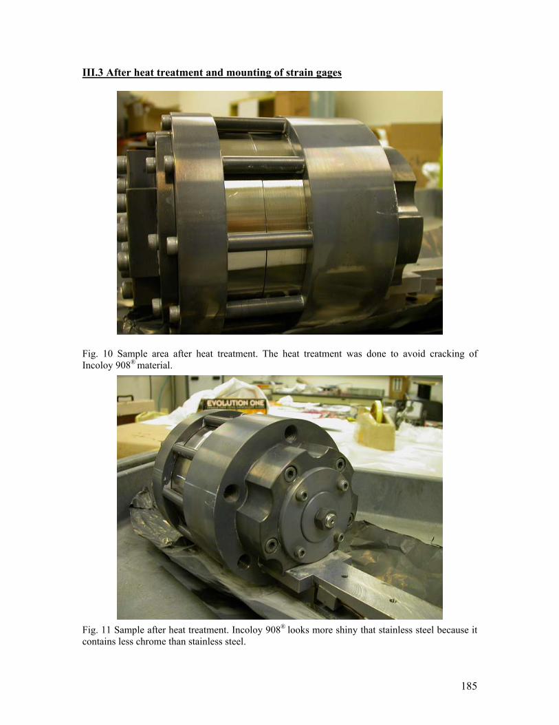
185

III.3 After heat treatment and mounting of strain gages

Fig. 10 Sample area after heat treatment. The heat treatment was done to avoid cracking of Incoloy 908® material.

Fig. 11 Sample after heat treatment. Incoloy 908® looks more shiny that stainless steel because it contains less chrome than stainless steel.

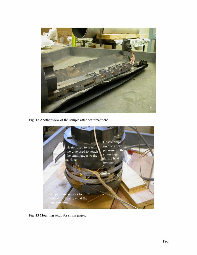
186

Fig. 12 Another view of the sample after heat treatment.

Fig. 13 Mounting setup for strain gages.

Heater used to react the glue used to attach the strain gages to the surface

Hose clamps used to apply pressure on the strain gage during heat treatment

Temperature sensors to control the heat level at the gage position

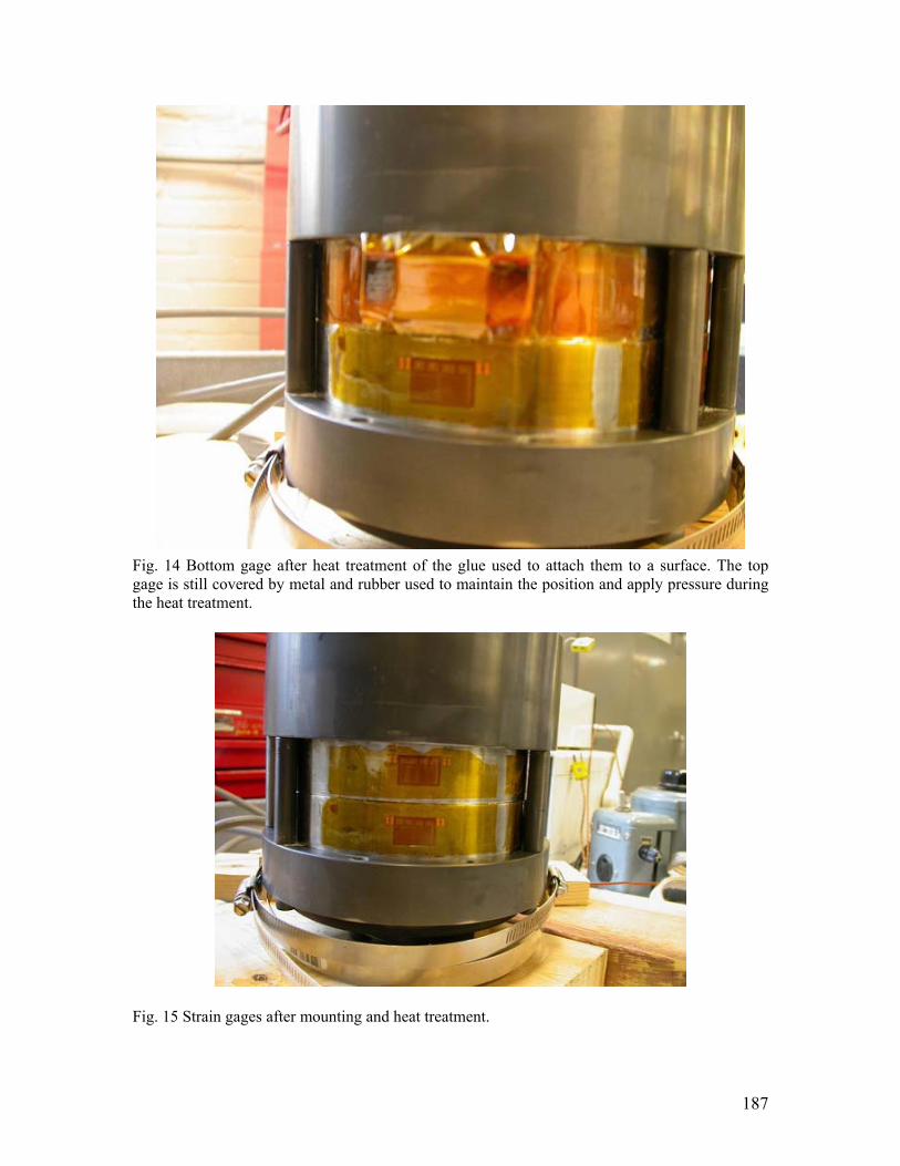
187

Fig. 14 Bottom gage after heat treatment of the glue used to attach them to a surface. The top gage is still covered by metal and rubber used to maintain the position and apply pressure during the heat treatment.

Fig. 15 Strain gages after mounting and heat treatment.

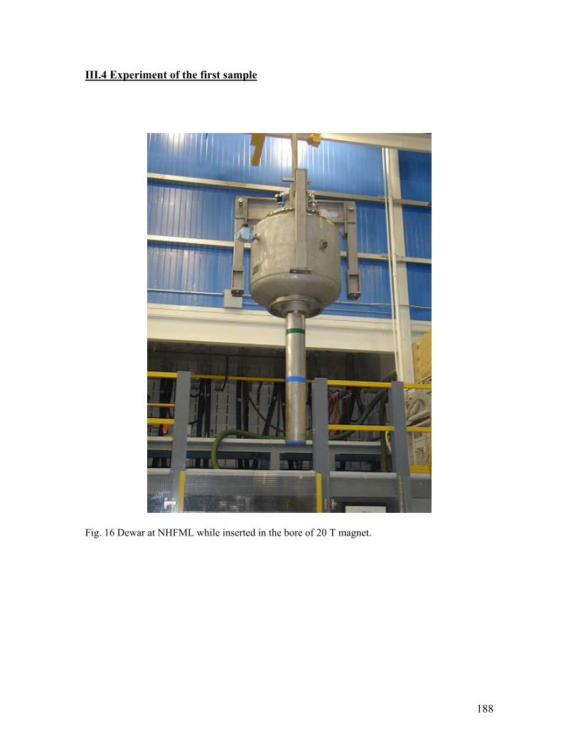
188

III.4 Experiment of the first sample

Fig. 16 Dewar at NHFML while inserted in the bore of 20 T magnet.

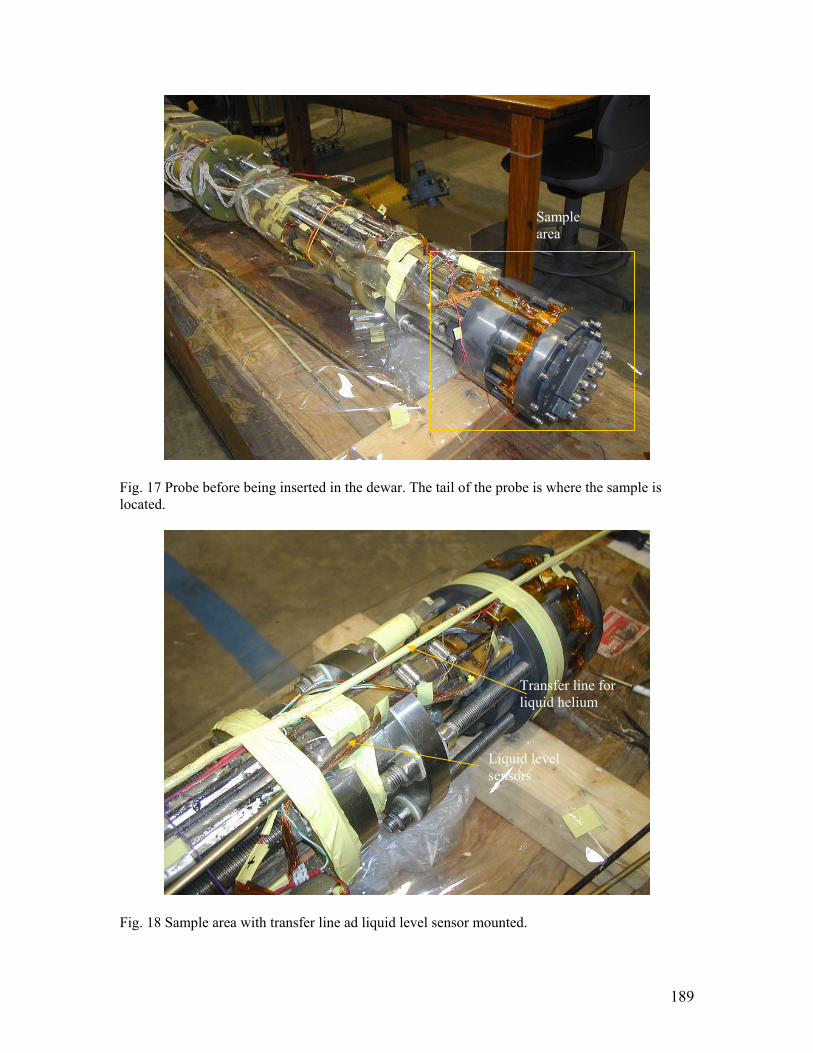
189

Fig. 17 Probe before being inserted in the dewar. The tail of the probe is where the sample is located.

Fig. 18 Sample area with transfer line ad liquid level sensor mounted.

Sample area

Transfer line for liquid helium

Liquid level sensors

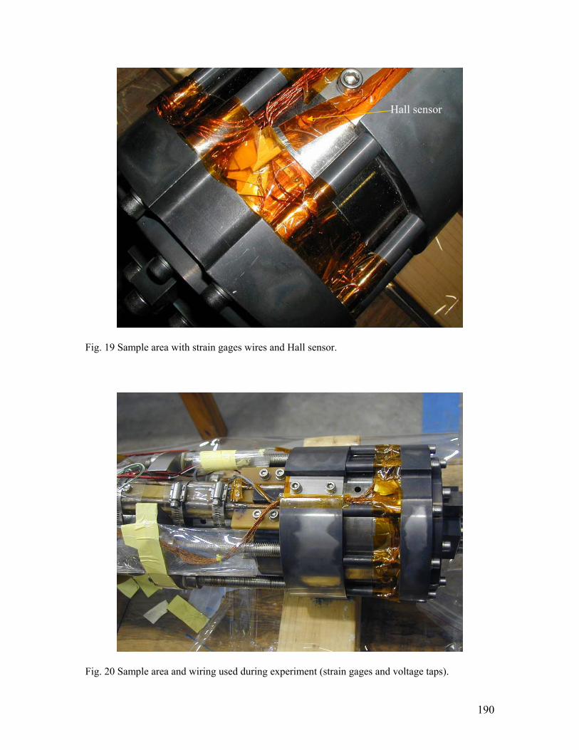
190

Fig. 19 Sample area with strain gages wires and Hall sensor.

Fig. 20 Sample area and wiring used during experiment (strain gages and voltage taps).

Hall sensor

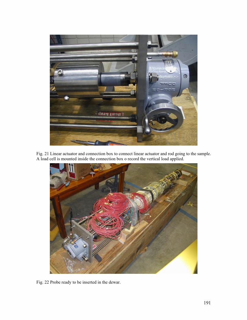
191

Fig. 21 Linear actuator and connection box to connect linear actuator and rod going to the sample. A load cell is mounted inside the connection box o record the vertical load applied.

Fig. 22 Probe ready to be inserted in the dewar.

192

Fig. 23 Relocation of the probe from wooden box to the dewar.

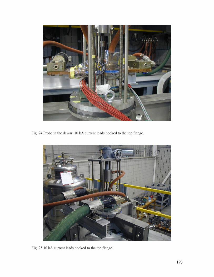
193

Fig. 24 Probe in the dewar. 10 kA current leads hooked to the top flange.

Fig. 25 10 kA current leads hooked to the top flange.

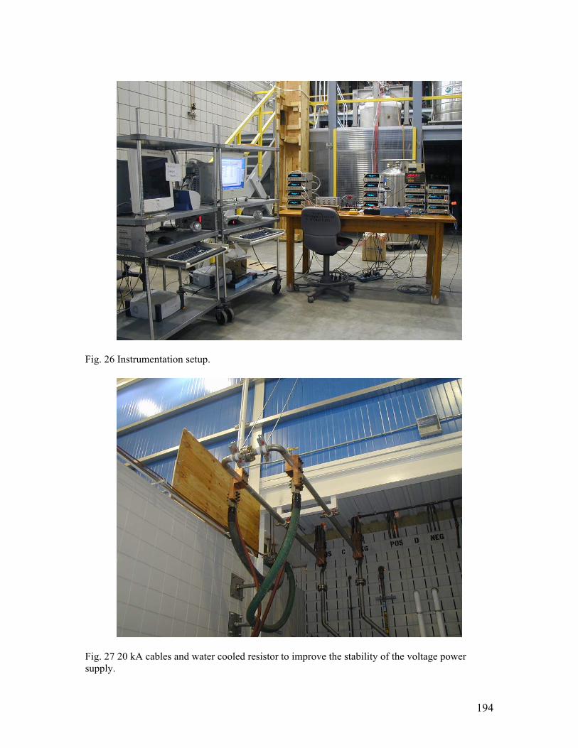
194

Fig. 26 Instrumentation setup.

Fig. 27 20 kA cables and water cooled resistor to improve the stability of the voltage power supply.

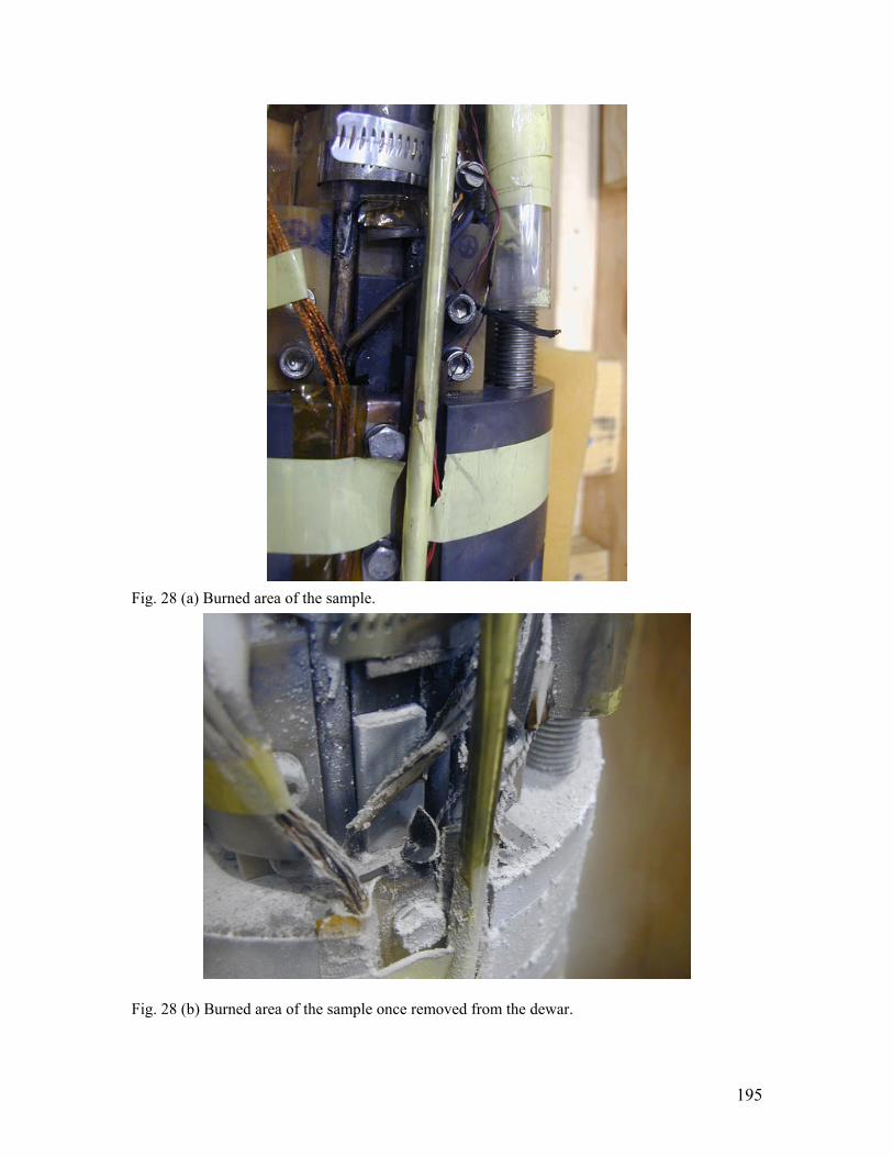
195

Fig. 28 (a) Burned area of the sample.

Fig. 28 (b) Burned area of the sample once removed from the dewar.

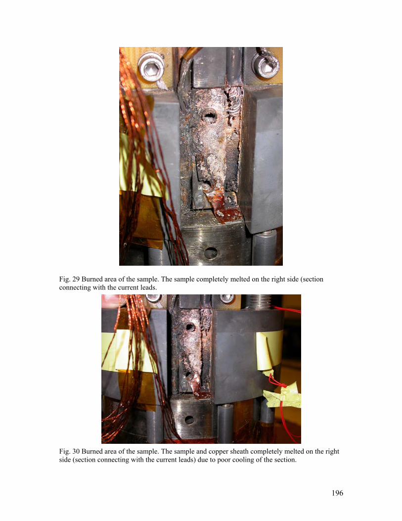
196

Fig. 29 Burned area of the sample. The sample completely melted on the right side (section connecting with the current leads.

Fig. 30 Burned area of the sample. The sample and copper sheath completely melted on the right side (section connecting with the current leads) due to poor cooling of the section.

197

REFERENCES Chapter 1 [1.1] Y. Iwasa “Case Studies in superconducting Magnets Design and Operational Issues” Plenum Press, New York, 1994. [1.2] M.N. Wilson “Superconducting Materials for Magnets”, CERN Accelerator School, Superconductivity in Particle Accelerators, Hamburg, May 1995. [1.3] J.W. Ekin “Strain scaling law for flux pinning in practical superconductors. Part I: Basic relationship and application to Nb3Sn conductors”, Cryogenics, 20 1980, p. 611-624. [1.4] Y. Iwasa and J.V. Minervini “Class 22.68j Superconducting Magnets”, Spring 2005 [1.5] J.V. Minervini “Analysis of Loss Mechanism in Superconducting Windings for Rotating Electric Generators”, PhD Thesis, Massachusetts Institute of Technology, U.S.A. 1981. [1.6] J.H. Schultz “The Medium Temperature Superconductor (MTS) Design Phylosophy”, IEEE Trans. On Applied Superconductivity, Vol. 13, No. 2, June 2003, p. 1604-1607. [1.7] L. Chiesa “Quench Protection Analysis for the Superconducting Quadrupoles Q2a/Q2b for the Inner Triplet of LHC”, Laurea Thesis, Universita’ degli Studi di Milano, February 2001. [1.8] File access to Lawrence Berkeley National Lab, Supercon Group, S. A. Gourlay. [1.9] ITER technical basis, “The plant description document: Chapter 2.1 Magnets”, ITER website http://www.iter.org/index.htm. Chapter 2 [2.1] D. R. Dietderich et al. “Critical Current of Superconducting Rutherford Cable in High Magnetic Fields with Transverse Pressure” IEEE Trans. On Applied Superconductivity, Vol. 9, No. 2, June 1999, p.122-125. [2.2] Joel H. Schultz and Peter Titus, “Transverse Load Degradation of ITER-class Nb3Sn CICC Performance”, ITER-USMIT-JSchultz-050403-01, May 4, 2003. [2.3] J.W. Ekin, “Transverse stress effect on multifilamentary Nb3Sn superconductor”, Adv in Cryo Eng (Materials), Vol. 34, p. 547, Ed. A.F. Clark and R.P. Reed, Plenum Press, NY, 1988. [2.4] N. Mitchell, “Summary, assessment and implications of the ITER model coils test results”, Fusion Engineering and Design, Vol. 66–68, p. 971–993, 2003. [2.5] J. W. Ekin, “Irregularity in Nb-Ti filament area and electric field versus current characteristics”, Cryogenics, Vol. 27, November 1987, p. 603-607. [2.6] J.W. Ekin “Strain scaling law for flux pinning in practical superconductors. Part I: Basic relationship and application to Nb3Sn conductors”, Cryogenics, 20 1980, p. 611-624. [2.7] H.J.N. van Eck et al., “Critical current versus strain research at the University of Twente”, Superconductor Science and Technology, v16, n9, Sept. 2003, p.1026-1030.

198

[2.8] A. Godeke et al., “A device to investigate the axial strain dependence of the critical current density in superconductors”, Review of Scientific Instruments, v75, n12, Dec. 2004, p 5112-5118. [2.9] D. Uglietti et al., “Critical Current vs. Strain Measurements of Long Length Nb3Sn Wires up to 1000A and 17T using a modified Walters Spring”, IEEE Transactions on Applied Superconductivity, v.13, n2, June 2003, p 3544-3547. [2.10] W.A.J. Wessel et al., “A novel ‘test arrangement for strain influence on strands’ (TARSIS): mechanical and electrical testing of ITER Nb3Sn strands”, AIP Conference Proceedings, n711, pt.2, 2004, p 466-73. [2.11] B. J. Senkowicz et al., “Effects of bending on cracking and critical current of Nb3Sn ITER wires”, IEEE Transactions on Applied Superconductivity, v15, n2, pt. III, June, 2005, p 3470-3473. [2.12] D. L. Harris, “Characterization of Nb3Sn Superconducting Strand Under Pure Bending”, M.S. in Mechanical Engineering, Massachusetts Institute of Technology, U.S.A. 2005. [2.13] J.R. Miller et al. “The initial filament strain state of cable in conduit superconductors and relation of this strain to large-bore, high-field magnet design”, IEEE Trans. Mag., Vol. MAG-23. March 1987, p. 1547-1551. [2.14] W. Specking et al. “The effect of static and cyclic axial strain on Ic of cable in conduit NET subcables”, IEEE Trans. Mag., Vol. MAG-27. March 1991, p. 1825-1828. [2.15] W. Specking et al. “Performance of a react and wind 12T KFK-NET-TF subsize conductor under static and cyclic axial strain”, IEEE Trans. Mag., Vol. MAG-27. March 1991, p. 1912-1915. [2.16] W. Specking et al. “Improvement of Ic in Nb3Sn conductors by reduction of axial prestrain”, IEEE Trans. Appl. Superconductivity, Vol. 5, June 1995, p. 845-848. [2.17] W. Specking et al. “Drastic improvement of Ic of Nb3Sn CIC Conductor by pre straining at room temperature”, 15th IEEE/NPSS Symposium on Fusion Engineering, Vol. 2, Oct. 1993, p. 1166-1169. [2.18] J.W. Ekin, “Effect of transverse compressive stress on the critical current and upper critical field of Nb3Sn”, J. Appl. Phys., vol. 62, Dec. 1987, p. 4829 [2.19] J.W. Ekin, “Transverse stress effect on multifilamentary Nb3Sn superconductor”, Adv. Cryogenics Eng., vol. 34, 1988, p. 547-552 [2.20] W. Specking et al., “Effect of transverse compression on Ic of Nb3Sn multifilamentary wire”, Adv. Cryogenics Eng., vol. 34, 1988, p. 569 [2.21] J.W. Ekin et al., “Effect of transverse stress on the critical current of bronze-process and internal-tin Nb3Sn”, J. Appl. Phys., vol. 69, Apr. 1991, p. 4436 [2.22] J.W. Ekin and S.L. Bray, “Critical current degradation in Nb3Sn composite wires due to locally concentrated transverse stress”, Adv. Cryogenics Eng., vol. 38, 1992 [2.23] L.T. Summers and J.R. Miller, “The effect of transverse stress on the critical current of Nb3Sn cable in conduit superconductors”, IEEE Trans. Mag., Vol. 25. March 1989, p. 1835-1838 [2.24] L.T. Summers and J.R. Miller, “Further studies of transverse stress effects in cable in conduit conductors”, internal note LLNL. [2.25] P. Michael et al., “Test of the ITER Central Solenoid Model Coil and CS Insert”, IEEE Trans. Appl. Superconductivity, Vol. 12, No. 1, March 2002, p. 600-605.

199

Chapter 3 [3.1] L.T. Summers et al., “A Model for the prediction of Nb3Sn Critical Current as a Function of Field, Temperature, Strain and Radiation Damage”, IEEE Trans. Mag., Vol. 27, March 1991, p. 2041-2044. [3.2] L.T. Summers and J.R. Miller, “Further studies of transverse stress effects in cable in conduit conductors”, internal note LLNL [3.3] J.W. Ekin, “Transverse stress effect on multifilamentary Nb3Sn superconductor”, Adv in Cryo Eng (Materials), Vol. 34, p. 547, Ed. A.F. Clark and R.P. Reed, Plenum Press, NY, 1988. [3.4] J. W. Ekin, “Strain Effects in Superconducting Compounds”, Adv. Cryo. Eng. 30, 823-836 (1984). [3.5] A. Nijhuis et al.,”Performance of an ITER CS1 Model Coil Conductor under Transverse Cyclic Loading up to 40000 cycles” , IEEE Trans. on Applied Superconductivity, Vol. 14, No. 2, June 2004, p.1489-1494. Chapter 4 [4.1] National High Magnetic Field website, Cell 4 data http://www.magnet.fsu.edu/users/facilities/dcfield/cell4/BrBzBtotal.html [4.2] Y. Takahashi, “AC loss Measurements of 46 kA-13 T Nb3Sn Conductor for ITER”, IEEE Trans. on Applied Superconductivity, Vol. 1, No. 1, March 2001, p.1546-1549. [4.3] L.T. Summers and J.R. Miller, “The effect of transverse stress on the critical current of Nb3Sn cable in conduit superconductors”, IEEE Trans. Mag., Vol. 25. March 1989, p. 1835-1838 [4.4] L.T. Summers and J.R. Miller, “Further studies of transverse stress effects in cable in conduit conductors”, internal note LLNL. Appendix I [AI.1] Timothy D. Alvey, “Calorimetric Measurement of Energy Dissipation in Superconducting Cables”, M.S. in Nuclear Engineering, Massachusetts Institute of Technology, U.S.A. 2000.