1

Heave Plate Design with Computational Fluid Dynamics*

by

Samuel Holmes, Applied Research Associates, Inc.1

830 E. Evelyn Ave. Suite C Palo Alto, CA

Shankar Bhat2 and Pierre Beynet, BP Amoco Corp.

Anil Sablok and Igor Prislin Deep Oil Technology, Inc.

Houston, TX

Abstract Computational fluid dynamics (CFD) methods are used to predict the hydrodynamic loads on heave plates. A series of numerical simulations for plates undergoing simple harmonic motion is used to determine the force and moment resultant histories. A least mean squares method is used to obtain the appropriate Morison coefficients for the plates under a variety of sea conditions. Finally, force and moment histories are predicted for a plate on a floating platform excited by a random sea stated. INTRODUCTION Computational fluid dynamics (CFD) methods are used to predict the dynamic loads on heave plates. The plates are used to stabilize the SPAR type platform shown in Figure 1. As is typical of “SPAR” platform designs, this platform is much taller than it is wide to increase stability in heavy seas. In the design shown in Figure 1, the platform floatation is provided by a large vertical cylindrical hull with a height to diameter ratio of about 2. In order to reduce vertical or heave motions a series of square horizontal heave plates are suspended beneath the platform at varying depths. The heave plates are supported by a system of four vertical tubular members along with some additional truss structure. In evaluating this design it is important to predict both vertical motions of the platform and the load distribution on the platform under a variety of sea states. Resolution of both maximum loads and load history is important so that the probability of failure under maximum stress conditions and fatigue loads can be evaluated. Furthermore, it is important to know the stabilizing resultant forces produced by the plates in order to determine the motions of the platform. Because the heave plates themselves are built up structures with a system of stiffeners supporting a steel deck, it is also desirable to predict the load distribution on the plates in order to create an efficient design. * JOMAE, Vol. 123 February 2001 1 Formerly with Centric Engineering Systems, Inc. 2 Now with ABB

2

It is common practice to design floating platforms using computer codes based on the solution of Morison’s equations in which the resultant forces on a submerged body are expressed in terms of the body’s velocity and acceleration relative to the fluid. On a submerged object undergoing only heave motion, this approach gives rise to a single non-linear ordinary differential equation expressing the vertical force zF in terms of the motion dynamics.

zmzzdz uLCuuLCF &32

21 ρρ += (1)

Here, ρ is fluid density, L is the characteristic dimension of the object, u and u& are the velocity and acceleration of the body relative to the fluid and dC and mC are coefficients of drag and

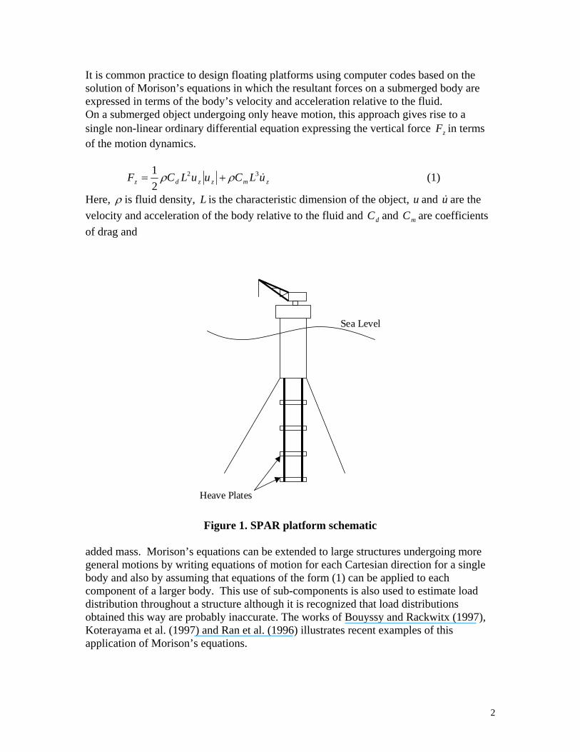
Sea Level

Heave Plates

Figure 1. SPAR platform schematic added mass. Morison’s equations can be extended to large structures undergoing more general motions by writing equations of motion for each Cartesian direction for a single body and also by assuming that equations of the form (1) can be applied to each component of a larger body. This use of sub-components is also used to estimate load distribution throughout a structure although it is recognized that load distributions obtained this way are probably inaccurate. The works of Bouyssy and Rackwitx (1997), Koterayama et al. (1997) and Ran et al. (1996) illustrates recent examples of this application of Morison’s equations.

3

In most applications of Morison’s equation the drag and added mass coefficients are usually assumed constant although it is known that, even for simple harmonic motions, the appropriate values of the coefficients are functions of the motion velocity, amplitude and period. A common way to express this dependence is to plot the coefficients as functions of the Keulegin-Carpenter number (Kc) defined by:

LTU

K ooc = (2)

where oU and oT are the velocity amplitude and period of the motion. Characterizing a new shape to be used in a platform design often requires many experiments to determine

dC and mC over a range of Kc. In addition, the implicit assumption in Eq. (1) is that the resultant force on an object is a function of only the immediate kinematics of the flow without regard to its recent history. This lack of a transient effect can be a serious shortcoming under some flow conditions. For example, the effect of using constant coefficients in Morison’s equation was identified by Natvig and Teigen (1993) as a significant problem to be resolved in tension leg platform design. OBJECTIVE AND APPROACH With these problems in mind, the objective in this study is to predict the loads and resultant forces on the heave plates used to stabilize the SPAR platform under a variety of sea conditions. We especially wanted an accurate prediction of the load history on the plates and the load distribution so that the design could be optimized for fatigue life. We chose to model the plates using computational fluid dynamics (CFD) and a commercial Navier-Stokes flow solver.3 An approach to predicting the fluid structure interaction (FSI) in a floating platform is to perform a coupled fluid and structure analysis in which fluid flow and solid motion or deformation equations are solved simultaneously. This type of approach is computationally expensive and difficult to complete successfully. A recent illustration of research on this problem is given by Farhat and Lesoinne (1998). To avoid solving the FSI problem, we chose instead to specify the motion of the platform for our solutions and solve for the fluid flow only. This is straightforward for simple harmonic motions. For more general problems we either used experimentally determined platform motion histories to generate boundary conditions for the CFD problem or we used a platform motion simulation code to predict the motion in advance of the CFD solution. This predicted motion was then used to set up the CFD problem. In the following sections we first simulate a scale model experiment to predict heave forces on a simple plate. Comparison of the measured and predicted force history is used to validate the CFD solution. CFD solutions are then used to predict the Morison coefficients for the heave plates under a variety of simple harmonic motions. These coefficients are then used to solve for platform motion using a proprietary simulation

3 SPECTRUMTM, Centric Engineering Systems, Inc.

4

code TDSIM.4 TDSIM is based on Morison’s equations and can be used to predict the platform motion and force resultants on platform components under a variety of sea conditions. It is, of course, subject to the limitations of Morison simulations discussed earlier. With the platform motions thus determined, CFD solutions are constructed using the kinematics of the sea and platform predicted by TDSIM. The CFD predicted force resultants are compared with those from the Morison simulation. In addition, the load distribution on the heave plates is predicted directly in the CFD solution. NUMERICAL METHOD All of the CFD analyses were completed using a second order accurate finite element method based on the Galerkin least squares (GLS) formulation (Hughes et al. 1989). The linear equations were solved with the generalized minimum residual (GMRES) method and conjugate gradient (CG) linear solvers in a ‘segregated’ solution strategy where each non-linear iteration consists if two ‘staggers’ or phases. In this strategy, the consistent left hand side of the continuity equation and momentum equations is solved for velocity in the first stagger (with the pressure held fixed) using GMRES. In the second stagger, a symmetric system is formed from the continuity equation, the pressure gradient term from the momentum equations and a diagonal approximation of the remaining terms in the momentum equations. Four nonlinear iterations are taken within each step. This system is advanced in time using the Hilber-Hughes-Taylor (HHT) algorithm (Hilbert et al. 1977). The HHT parameters are chosen to maintain second order accuracy and the time step is chosen corresponding to a Courant-Friedrichs-Lewy number of about 10 based on fluid velocity across an element. Each solution is generated by modeling a large volume of the fluid surrounding the heave plate and moving the plate boundaries to create the effect of plate motion as if the plate were enclosed in the center of a large tank. An arbitrary Langrangian-Eulerian (ALE) mesh moment strategy was used to accommodate the motion of the plate with respect to the volume of fluid. An implicit assumption in the method used here is that the ocean wavelengths are long compared with the plate length so that variations in wave particle motion along the plate can be neglected. In addition, we assume that the plate is far from the free surface so that surface effects can be neglected. These assumptions are not essential to obtaining a CFD solution but they simplify the problem set up and reduce solution time. An inertial reference frame fixed to the fluid boundaries is used in problems without wave motion. Thus the buoyant force on the plate is constant and can be calculated separately. In order to introduce the effect of waves without needing to alter the boundary conditions, we fixed the reference frame in these problems to the free field fluid particle motion so that the plate motion is now specified with respect to the fluid. Because the reference frame is no longer fixed and accelerates with the wave particle

4 TDSIM is a propriety simulation code of Deep Oil Technology.

5

motion, the buoyant force varies with time. The effect on resultant forces is small and is easily corrected. We were also concerned with the effect of Reynolds number and viscous drag on plate hydrodynamics. Both full-scale and 1:49 scale plates were modeled in this study and Reynolds Numbers varied from 0.1 million to 10 million. The meshes used here are too coarse to resolve the boundary layer on the plates accurately for these Reynolds Numbers and we expect that the viscous drag may not be accurately predicted. However, for thin plates where the flow is predominately in a direction normal to the plate, the viscous drag is a very small part of the total drag and errors are negligible as discussed by Gerhart and Gross (1989). Thus the total drag is dominated by the form drag and there is little or no Reynolds number effect over the range of Reynolds numbers studied here. We used the Smagorinsky large eddy simulation turbulence model (Smagorinsky 1965) to simulate turbulence effects in the flow problems. In this model, the components of the subgrid scale Reynolds stress tensor is related to the large-scale strain rate by

,21

⎟⎟⎠

⎞⎜⎜⎝

⎛

∂∂

+∂∂

==i

j

j

iTijTji x

uxuSuu υυ (3)

where

( ) ( )21

2ijijsT SSC ∆=υ (4)

and ∆ is a length scale associated with the grid. In our implementation of the model, the length scale is taken to be the cube root of the element volume. Thus the model captures the large eddies in the flow while adjusting the local fluid viscosity to model the effects of turbulence scales smaller than the grid size. We chose to use LES rather than a Reynolds averaged Navier-Stokes turbulence model because we wanted to capture the eddy effects in the oscillating flow. However, it is recognized that the Smagorinsky model is unlikely to model viscous tractions at the surface of the plate accurately. It should be noted that only single plates are modeled in all of the solutions presented here even though the plates are stacked in the SPAR platform design. This simplification was made to speed the computations and is thought to be permissible because the interference effects between plates is negligible as plate spacing approaches the plate as is the case here length (Prislin et al. 1998). Although the actual heave plates are stiffened structures with rough surfaces, we also simplified the plate geometry by assuming that the plates are smooth with a thickness to length ratio of about 1:100. Several different finite element meshes were used to generate solutions and a typical finite element mesh of hexehedral elements is shown in Figure 2. Note the mesh models a large rectangular brick of fluid surrounding the heave plate. In all cases, the mesh is concentrated around the plate to better capture the details of the flow in this area. Typically, about fifty elements are used along the plate length

6

and about 10 elements through the plate thickness. The element lengths are biased with the smallest elements at the plate edges and corners of the plate. The mesh shown in Figure 2 is used to model simple heave motions and takes advantage of the two planes of symmetry that pass through the plate’s principal axes. Problems with one plane of symmetry, such as heave combined with pitch or when a current is present, were modeled by reflecting the mesh shown about the non-symmetric plane. The meshes used for problems with one plane of symmetry typically had 100,000 or more nodes. Note that the use of symmetry planes can prevent certain asymmetric fluid responses such as certain types of vortex shedding, For problems with no current, the outer boundaries of the fluid are fixed and fluid velocity normal to the mesh is set to zero. The distance from the plate to the fluid boundary is ten times the plate half-length in all directions. For problems with current, a mesh with one plane of symmetry is used and flow is introduced at the inflow boundary using a Dirichlet boundary condition. A von-Neumann pressure boundary condition is used at the outflow boundary. Because the flow is incompressible, the static head can be neglected and a constant pressure assigned to the outflow. Most of the simulations were run on a six processor HP-Convex Exemplar computer although a variety of computer platforms were used during the course of this study. Most simulations were run for 500 or more time steps with at least 100 time steps used to model each plate motion cycle in simple harmonic motion. Simulations of random wave response used several thousand time steps. The computer time required for each solution was generally two or three minutes per time step but varied with the machine used, the mesh size, and other problem factors. Typical problem run times were thus on the order of 16 to 20 hours. We believe that these timings should improve significantly for later generation computer platforms and codes.

7

Figure 2. Finite element mesh using quarter symmetry.

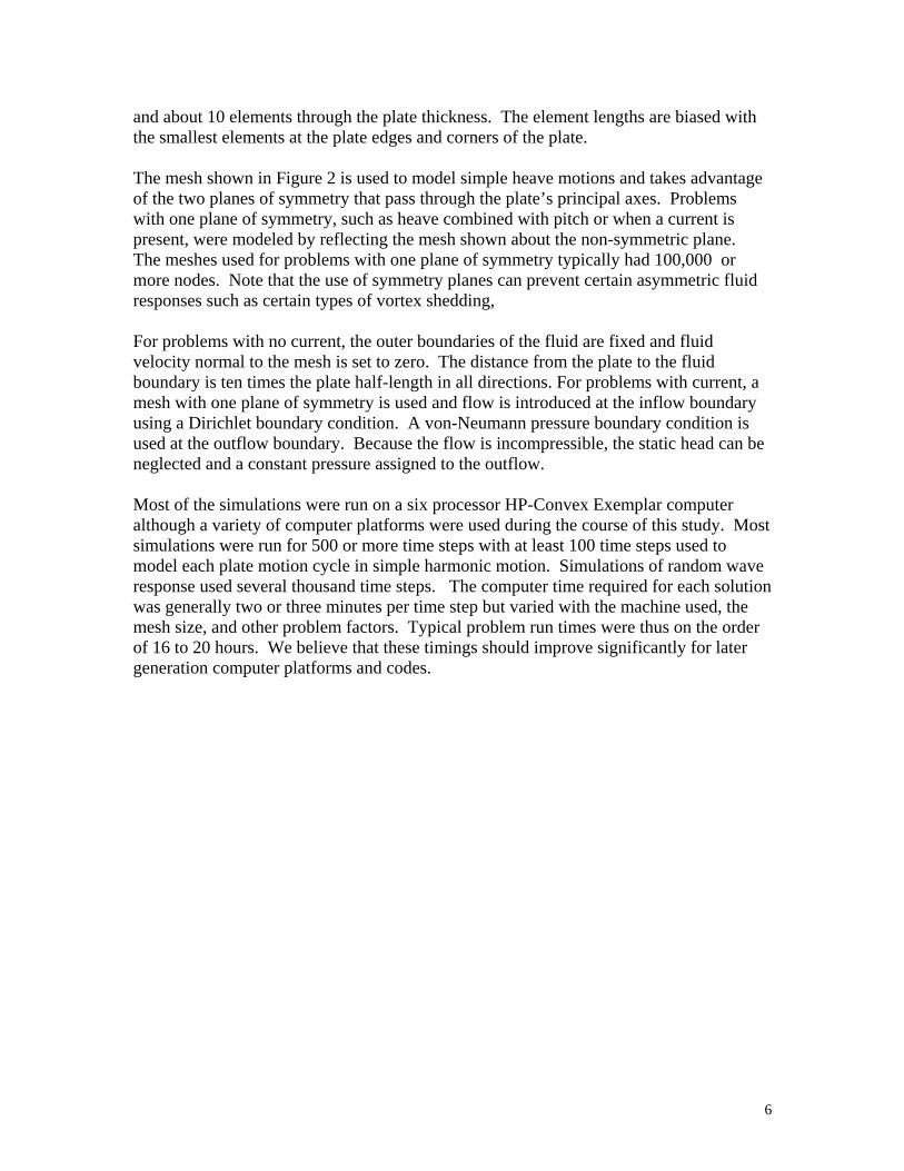
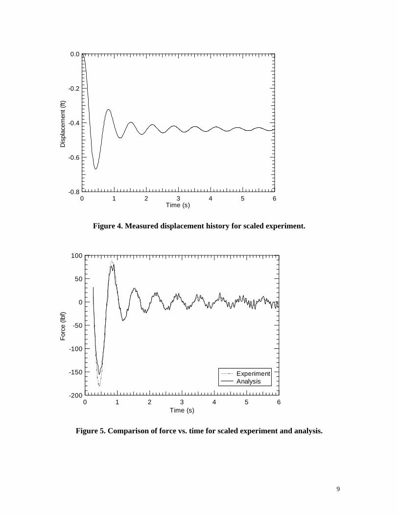
COMPARISON OF ANALYSIS AND EXPERIMENT In order to test the accuracy of the CFD solution, we compared force resultants measured in a scale-model experiment with those predicted by the numerical model. The test set up is described by Prislin et al. (1998). In the model test, a two-foot square plywood plate was submerged in a wave tank and supported by two identical springs as shown in Figure 3. An arrangement of supports confined the plate motion to heave motion only. The load exerted on the plate from one of the springs was measured by a load cell and plate acceleration was measured with an accelerometer. The total load on the plate was estimated by doubling the measured load and the displacement history of the plate was calculated by integrating the measured acceleration of the plate. In the experiment analyzed here, the plate was displaced vertically and released giving the under-damped motion shown in the displacement history in Figure 4.

8

Spring

Load Cell

Plate

Figure 3. Scale model experiment schematic.

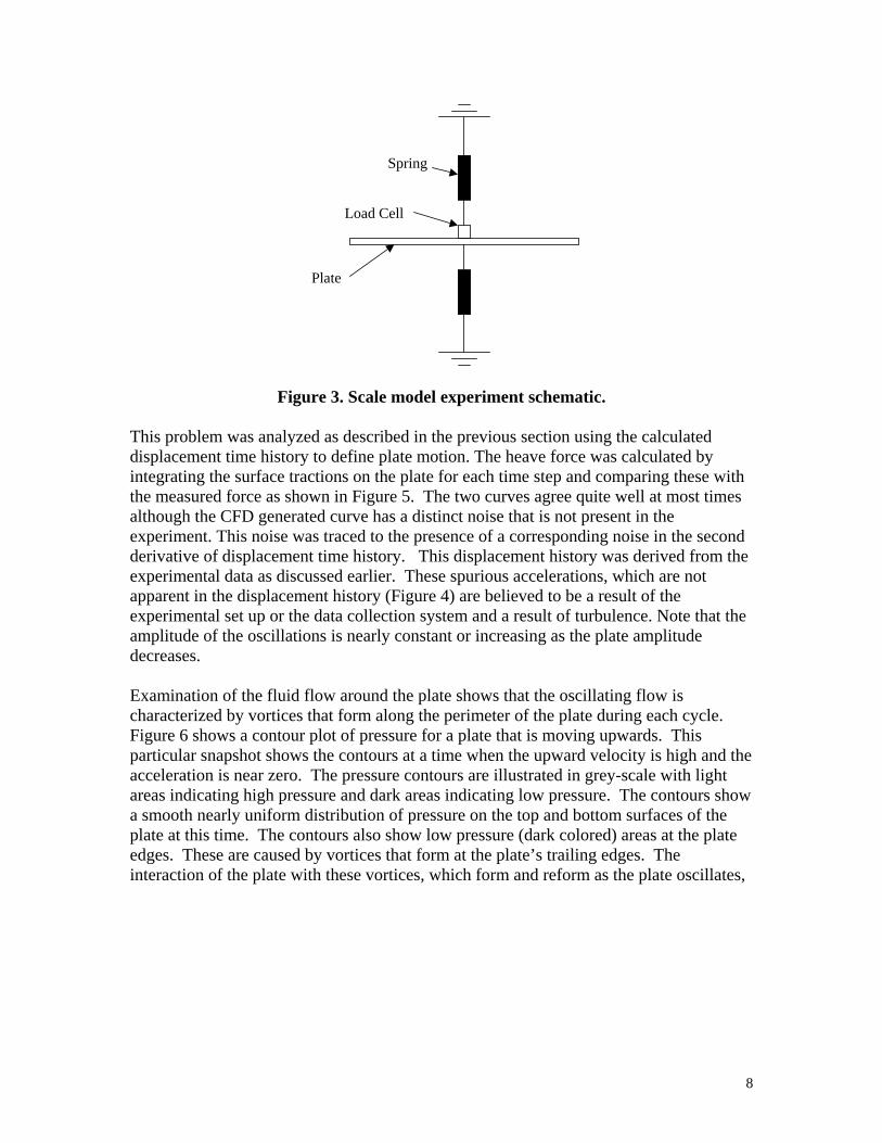
This problem was analyzed as described in the previous section using the calculated displacement time history to define plate motion. The heave force was calculated by integrating the surface tractions on the plate for each time step and comparing these with the measured force as shown in Figure 5. The two curves agree quite well at most times although the CFD generated curve has a distinct noise that is not present in the experiment. This noise was traced to the presence of a corresponding noise in the second derivative of displacement time history. This displacement history was derived from the experimental data as discussed earlier. These spurious accelerations, which are not apparent in the displacement history (Figure 4) are believed to be a result of the experimental set up or the data collection system and a result of turbulence. Note that the amplitude of the oscillations is nearly constant or increasing as the plate amplitude decreases. Examination of the fluid flow around the plate shows that the oscillating flow is characterized by vortices that form along the perimeter of the plate during each cycle. Figure 6 shows a contour plot of pressure for a plate that is moving upwards. This particular snapshot shows the contours at a time when the upward velocity is high and the acceleration is near zero. The pressure contours are illustrated in grey-scale with light areas indicating high pressure and dark areas indicating low pressure. The contours show a smooth nearly uniform distribution of pressure on the top and bottom surfaces of the plate at this time. The contours also show low pressure (dark colored) areas at the plate edges. These are caused by vortices that form at the plate’s trailing edges. The interaction of the plate with these vortices, which form and reform as the plate oscillates,

9

-0.8

-0.6

-0.4

-0.2

0.0D

ispl

acem

ent (

ft)

6543210Time (s)

Figure 4. Measured displacement history for scaled experiment.

-200

-150

-100

-50

0

50

100

Forc

e (lb

f)

6543210Time (s)

Experiment Analysis

Figure 5. Comparison of force vs. time for scaled experiment and analysis.

10

cause strong local variations in load distribution at certain times during the loading cycle. For simple harmonic motions, the vortices are strong when the plate velocity is high and dissipate when the plate changes direction and acceleration is high. The effect of vortices is reflected in the pressure distribution on and around the plate as will be shown later in plots of load distribution.

Figure 6. Pressure contours in fluid surrounding plate at a time of high velocity. APPLICATION TO SPAR PLATFORM DESIGN A series of calculations were made for a full-scale heave plate in support of the SPAR platform design. Four of these calculations are listed in Table 1 and are used here to illustrate the process. The first two calculations are for simple harmonic motions at different values of Kc. These are used to estimate added mass and drag coefficients for the heave plate. The third calculation is for a simple harmonic motion with a constant pitch angle and a current. This calculation is used here to illustrate the fact that the introduction of asymmetry in the problem can produce quite asymmetric load distributions on the plate. The final calculation uses a general random wave sea condition. In this problem, we first used TDSIM to calculate the motion of the SPAR platform under a 100-year storm condition. We used added mass and drag coefficients for the heave plates derived from the CFD solution for Case 1 in this Morison type simulation. The TDSIM predicted platform motion and the random wave particle motion at the heave plate depth were then used to define the boundary conditions for the CFD solution in Case 4. Case 4 is thus a simulation of the heave plate under realistic sea conditions.

11

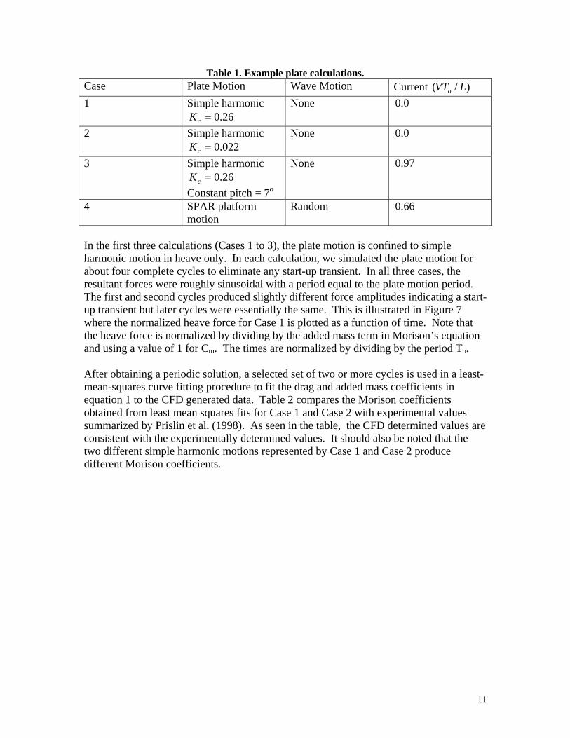
Table 1. Example plate calculations. Case Plate Motion Wave Motion Current )/( LVTo 1 Simple harmonic

26.0=cK None 0.0

2 Simple harmonic 022.0=cK

None 0.0

3 Simple harmonic 26.0=cK

Constant pitch = 7o

None 97.0

4 SPAR platform motion

Random 66.0

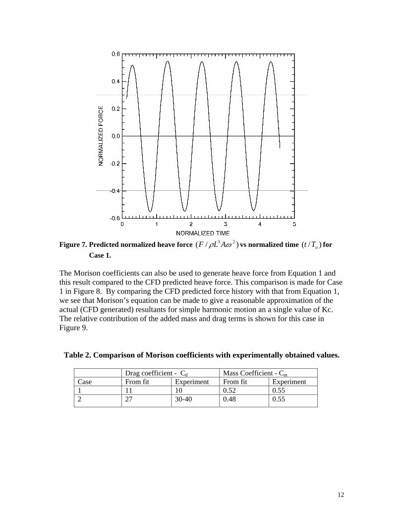
In the first three calculations (Cases 1 to 3), the plate motion is confined to simple harmonic motion in heave only. In each calculation, we simulated the plate motion for about four complete cycles to eliminate any start-up transient. In all three cases, the resultant forces were roughly sinusoidal with a period equal to the plate motion period. The first and second cycles produced slightly different force amplitudes indicating a start-up transient but later cycles were essentially the same. This is illustrated in Figure 7 where the normalized heave force for Case 1 is plotted as a function of time. Note that the heave force is normalized by dividing by the added mass term in Morison’s equation and using a value of 1 for Cm. The times are normalized by dividing by the period To. After obtaining a periodic solution, a selected set of two or more cycles is used in a least-mean-squares curve fitting procedure to fit the drag and added mass coefficients in equation 1 to the CFD generated data. Table 2 compares the Morison coefficients obtained from least mean squares fits for Case 1 and Case 2 with experimental values summarized by Prislin et al. (1998). As seen in the table, the CFD determined values are consistent with the experimentally determined values. It should also be noted that the two different simple harmonic motions represented by Case 1 and Case 2 produce different Morison coefficients.

12

Figure 7. Predicted normalized heave force )/( 23 ωρ ALF vs normalized time )/( oTt for

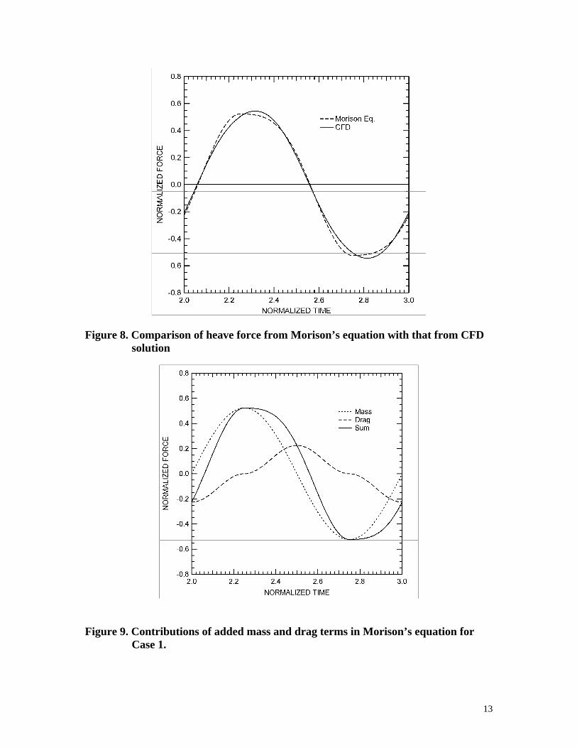
Case 1. The Morison coefficients can also be used to generate heave force from Equation 1 and this result compared to the CFD predicted heave force. This comparison is made for Case 1 in Figure 8. By comparing the CFD predicted force history with that from Equation 1, we see that Morison’s equation can be made to give a reasonable approximation of the actual (CFD generated) resultants for simple harmonic motion an a single value of Kc. The relative contribution of the added mass and drag terms is shown for this case in Figure 9.

Table 2. Comparison of Morison coefficients with experimentally obtained values.

Drag coefficient - Cd Mass Coefficient - Cm Case From fit Experiment From fit Experiment 1 11 10 0.52 0.55 2 27 30-40 0.48 0.55

13

Figure 8. Comparison of heave force from Morison’s equation with that from CFD solution

Figure 9. Contributions of added mass and drag terms in Morison’s equation for

Case 1.

14

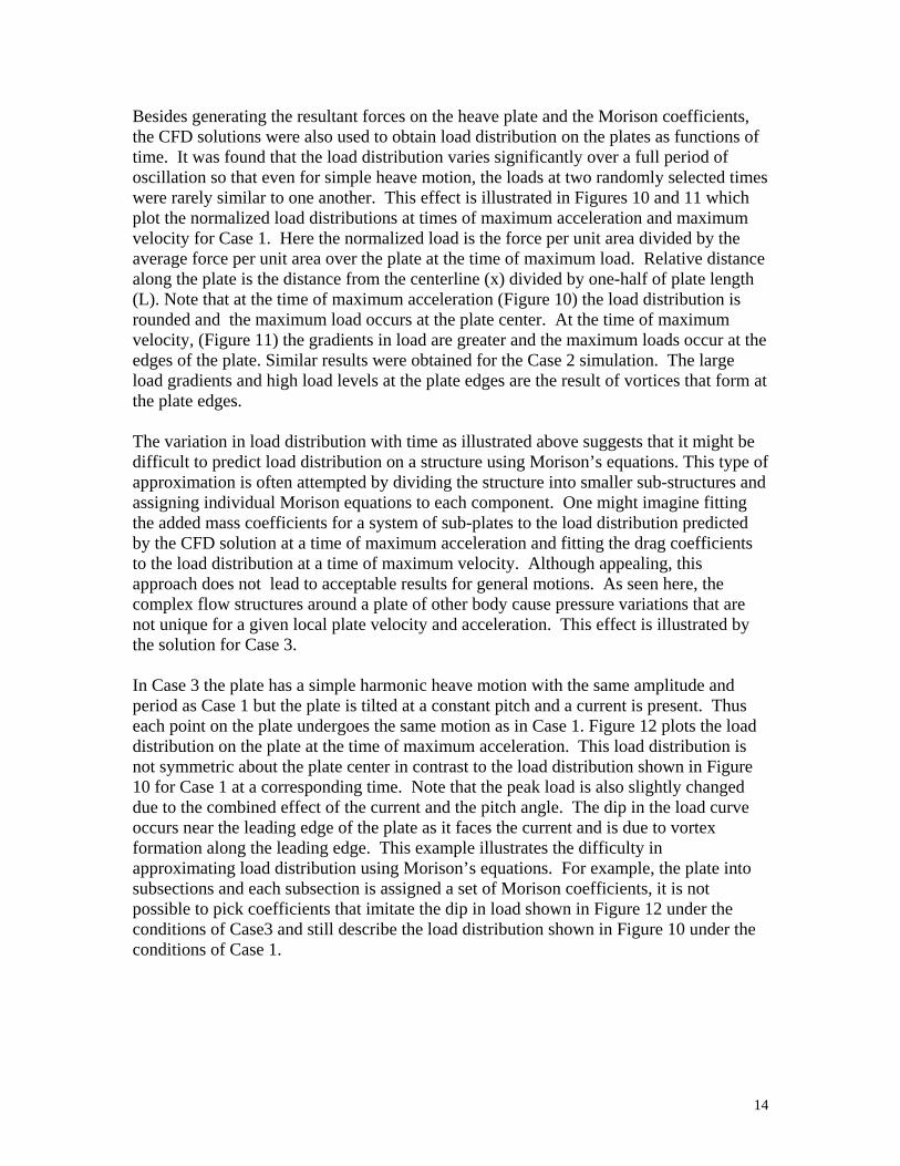
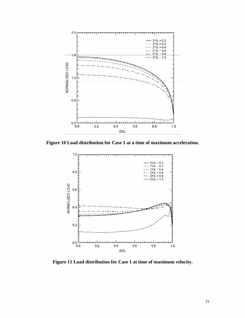
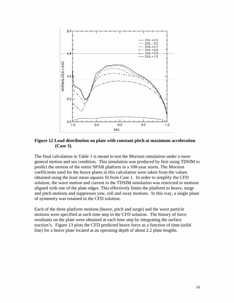
Besides generating the resultant forces on the heave plate and the Morison coefficients, the CFD solutions were also used to obtain load distribution on the plates as functions of time. It was found that the load distribution varies significantly over a full period of oscillation so that even for simple heave motion, the loads at two randomly selected times were rarely similar to one another. This effect is illustrated in Figures 10 and 11 which plot the normalized load distributions at times of maximum acceleration and maximum velocity for Case 1. Here the normalized load is the force per unit area divided by the average force per unit area over the plate at the time of maximum load. Relative distance along the plate is the distance from the centerline (x) divided by one-half of plate length (L). Note that at the time of maximum acceleration (Figure 10) the load distribution is rounded and the maximum load occurs at the plate center. At the time of maximum velocity, (Figure 11) the gradients in load are greater and the maximum loads occur at the edges of the plate. Similar results were obtained for the Case 2 simulation. The large load gradients and high load levels at the plate edges are the result of vortices that form at the plate edges. The variation in load distribution with time as illustrated above suggests that it might be difficult to predict load distribution on a structure using Morison’s equations. This type of approximation is often attempted by dividing the structure into smaller sub-structures and assigning individual Morison equations to each component. One might imagine fitting the added mass coefficients for a system of sub-plates to the load distribution predicted by the CFD solution at a time of maximum acceleration and fitting the drag coefficients to the load distribution at a time of maximum velocity. Although appealing, this approach does not lead to acceptable results for general motions. As seen here, the complex flow structures around a plate of other body cause pressure variations that are not unique for a given local plate velocity and acceleration. This effect is illustrated by the solution for Case 3. In Case 3 the plate has a simple harmonic heave motion with the same amplitude and period as Case 1 but the plate is tilted at a constant pitch and a current is present. Thus each point on the plate undergoes the same motion as in Case 1. Figure 12 plots the load distribution on the plate at the time of maximum acceleration. This load distribution is not symmetric about the plate center in contrast to the load distribution shown in Figure 10 for Case 1 at a corresponding time. Note that the peak load is also slightly changed due to the combined effect of the current and the pitch angle. The dip in the load curve occurs near the leading edge of the plate as it faces the current and is due to vortex formation along the leading edge. This example illustrates the difficulty in approximating load distribution using Morison’s equations. For example, the plate into subsections and each subsection is assigned a set of Morison coefficients, it is not possible to pick coefficients that imitate the dip in load shown in Figure 12 under the conditions of Case3 and still describe the load distribution shown in Figure 10 under the conditions of Case 1.

15

Figure 10 Load distribution for Case 1 at a time of maximum acceleration.

Figure 11 Load distribution for Case 1 at time of maximum velocity.

16

Figure 12 Load distribution on plate with constant pitch at maximum acceleration

(Case 3). The final calculation in Table 1 is meant to test the Morison simulation under a more general motion and sea condition. This simulation was produced by first using TDSIM to predict the motion of the entire SPAR platform in a 100-year storm. The Morison coefficients used for the heave plates in this calculation were taken from the values obtained using the least mean squares fit from Case 1. In order to simplify the CFD solution, the wave motion and current in the TDSIM simulation was restricted to motions aligned with one of the plate edges. This effectively limits the platform to heave, surge and pitch motions and suppresses yaw, roll and sway motions. In this way, a single plane of symmetry was retained in the CFD solution. Each of the three platform motions (heave, pitch and surge) and the wave particle motions were specified at each time step in the CFD solution. The history of force resultants on the plate were obtained at each time step by integrating the surface traction’s. Figure 13 plots the CFD predicted heave force as a function of time (solid line) for a heave plate located at an operating depth of about 2.2 plate lengths.

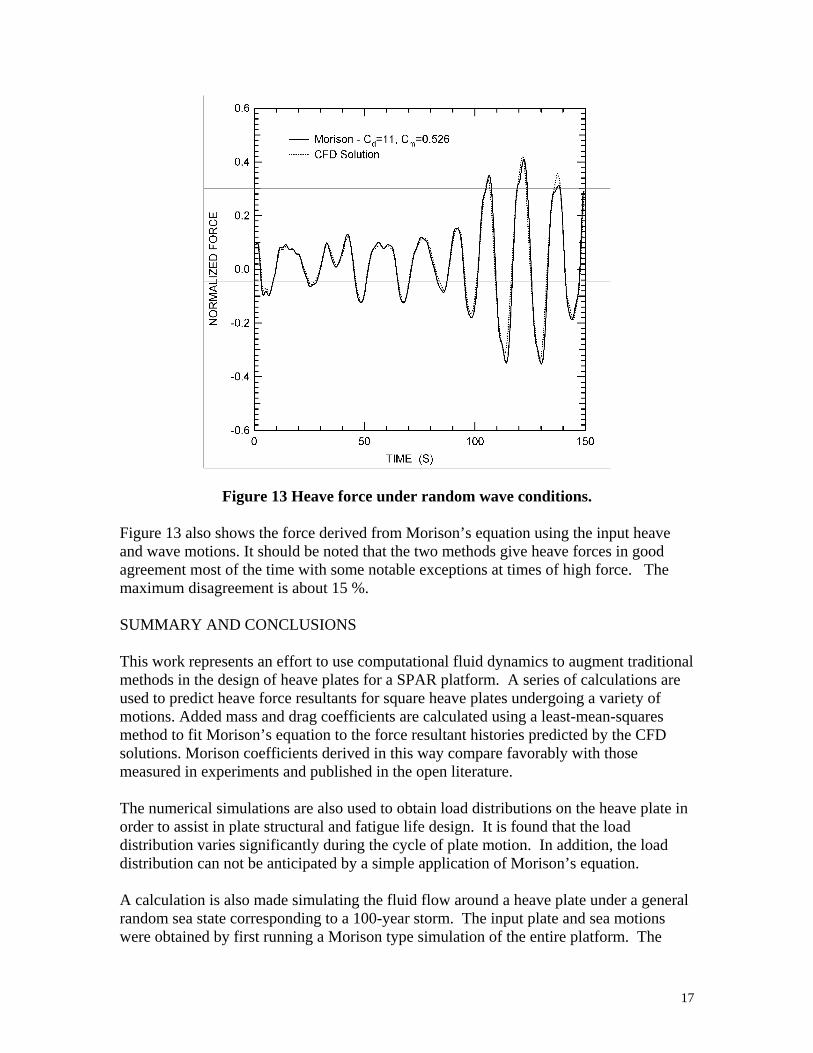
17

Figure 13 Heave force under random wave conditions. Figure 13 also shows the force derived from Morison’s equation using the input heave and wave motions. It should be noted that the two methods give heave forces in good agreement most of the time with some notable exceptions at times of high force. The maximum disagreement is about 15 %. SUMMARY AND CONCLUSIONS This work represents an effort to use computational fluid dynamics to augment traditional methods in the design of heave plates for a SPAR platform. A series of calculations are used to predict heave force resultants for square heave plates undergoing a variety of motions. Added mass and drag coefficients are calculated using a least-mean-squares method to fit Morison’s equation to the force resultant histories predicted by the CFD solutions. Morison coefficients derived in this way compare favorably with those measured in experiments and published in the open literature. The numerical simulations are also used to obtain load distributions on the heave plate in order to assist in plate structural and fatigue life design. It is found that the load distribution varies significantly during the cycle of plate motion. In addition, the load distribution can not be anticipated by a simple application of Morison’s equation. A calculation is also made simulating the fluid flow around a heave plate under a general random sea state corresponding to a 100-year storm. The input plate and sea motions were obtained by first running a Morison type simulation of the entire platform. The

18

resultant heave forces on the plate predicted by the CFD solution compare favorably with those generated by the Morison simulation indicating that the assumed plate motions are essentially correct. Thus the CFD solution should provide good estimates of load distribution. In conclusion, these results suggest that direct solution of the Navier-Stokes equations can be an efficient and effective supplement to Morison type simulations in platform design, at least for flat angular plates. These solutions may be used to directly determine Morison coefficients without recourse to expensive experiments and they can also be used to determine load distribution on floating platforms under general sea states. Further work may be needed to validate this approach for more general submerged shapes.

19

REFERENCES Bouyssy, V. and Rackwitx,” Polynomial Aproximation of Morison Wave Loading,” Trans. Of the ASME Vol. 119, Feb 1997 pp. 30-36 Farhat, C. and M. Lesoinne, “Higher-Order Staggered and Subiteration Free Algorithms for Coupled Dynamic Aeroelasticity Problems,” AIAA 98-0516 Gerhart, P.M. and R. J. Gross, “Fundemental of Fluid Mechanics,” Addison Wesley Co. Reading, MA, 1989, pp 520. Hilber, H. M., T.J.R. Hughes and R. L. Taylor, “Improved numerical dissipation for time integration algorithms in structural dynamics,” Earthquake Eng. Struct. Dyn. %, (1977) pp. 283-292 Hughes, T.J.R., L. P. Franca, G.M. Gilbert, “A new finite element formulation for computational fluid dynamics: VII. The Galerkin/least squares method for advective diffusive equations,” Comp. Methods Appld. Mech. Eng., 73, (1989) pp 173-189 Koterayama, W., H. Mizouka, N. Takatsu, T. Ikebuchi, “Field Experiments and Numerical Prediction on Dynamics of a Light Floating Structure moored in Deep Ocean,” Int. J. of Offshore and Polar Eng. Vol. 7, No. 4, pp. 254-261 Dec.1997 Natvig, B.J. Teigen, P., “Review of Hydrodynamic Challenges in TLP Design,” J. of Offshore and Polar Eng. Vol. ?, No. 4, pp. 241-249 Dec.1993 Prislin, I., Robert D. Blevins, and John E. Halkyard, “Viscous Damping and Added Mass of a Square Plate,” OMAE-98-316 Ran, Z., M.H. Kim, J.M. Niedzwecki and R. P. Johnson, “Responses of a SPAR Platform in Random Waves and Currents,” Int. J. of Offshore and Polar Eng. Vol. 6, No. 1, pp. 27-34 March 1996 Smagorinsky, j. “General circulation experiments with the primitive equations: I The basic experiment,” Mon. Weather Rev. 91, 99-164 (1963) Townsend, M. and N. Haritos, “Dynamically Responding Vertical Cylinders in the Morison Regime – The Influence of Structural Damping,” ,” Int. J. of Offshore and Polar Eng. Vol. 7, No. 3, Sep.1997

20

LIST OF TABLES 1. Example plate calculations. 2. Comparison of Morison coefficients with experimentally obtained values.

21

LIST OF FIGURES

1. SPAR platform schematic.

2. Finite element mesh using quarter symmetry.

3. Scale model experiment schematic.

4. Measured displacement history for scaled experiment

5. Comparison of force vs. time for scaled experiment and analysis.

6. Pressure contours in fluid surrounding a plate at time of high velocity.

7. Predicted normalized heave force )/( 23 ωρ ALF vs. normalized time )/( oTt for Case 1..

8. Comparison of heave force from Morison equation with that from CFD solution.

9. Contribution of added mass and drag terms in Morison’s equation for Case 1.

10. Load distribution for Case 1 at time of maximum acceleration.

11. Load distribution for Case 1 at time of maximum velocity.

12. Load distribution on plate with constant pitch at maximum acceleration (Case 3).

13. Heave force under random wave conditions.