a computational fluid dynamics micro-model parametric study

AIRAH and IBPSA’s Australasian Building Simulation 2017 Conference, Melbourne, November 15-16.

1

A COMPUTATIONAL FLUID DYNAMICS MICRO-MODEL

PARAMETRIC STUDY ASSESSING OPTIMUM RIBLET

GEOMETRY FOR USE IN COOLING COILS

JAMES PATON, BEng(Hons) ESD Engineer

AECOM

420 George St

Sydney NSW 2000

[email protected]

ABOUT THE AUTHOR

James is a first class honours mechanical engineering graduate from UNSW that undertook this

research for his final year thesis topic. James now works for AECOM in the Buildings Applied

Research and Sustainability team that specialises in designing sustainable and environmentally

friendly buildings around the world.

ABSTRACT

Riblets were implemented into a cooling coil to determine what the optimum geometry is for

reducing viscous drag and the associated pressure loss. A computational fluid dynamics micro-

model was built and an extensive parametric simulation study was undertaken. Riblets are thin

blades that run parallel to the flow of fluid. By trapping a small amount of fluid at the surface of a

wall they reduce the viscous drag for the remaining body of fluid. Riblets have successfully been

implemented elsewhere in buildings, such as air ducts. A parametric process was developed to

understand the factors that influence and constrain riblet performance for a given application and

flow type. Simulation results showed a maximum reduction in pressure loss of 5% could be

achieved. The formation of the trapped fluid between the riblets was found to be the sole driver in

determining optimum dimensions for reducing viscous drag and the associated pressure loss. Due to

the constraints in length and the cross-sectional area for fluid flow, energy savings may not be large

enough to warrant the implementation of riblets in cooling coils. The trapped air is also expected to

have a negative effect on the rate of heat transfer and will need to be further investigated. Using this

newly developed parametric method however, all applications of riblets can be optimised for peak

performance.

1. INTRODUCTION

Through many years of iterative design and testing the cooling coil geometry with a high rate of

heat transfer has been thoroughly established [1]. Though its heat transfer is high, the viscous drag

across the geometry is significant, causing losses in air pressure [2]. Air conditioning systems are

one of the largest users of energy in a commercial building and a slight increase in performance of

the cooling coil could contribute to significant energy savings for buildings [3].

Riblets are a potential solution for increasing the efficiency of cooling coils even further by

reducing their viscous drag. A large amount of research and experimentation has been done on


2

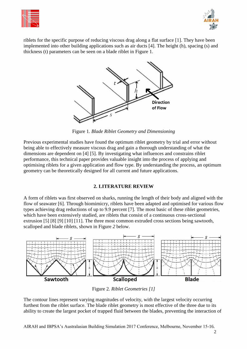
riblets for the specific purpose of reducing viscous drag along a flat surface [1]. They have been

implemented into other building applications such as air ducts [4]. The height (h), spacing (s) and

thickness (t) parameters can be seen on a blade riblet in Figure 1.

Figure 1. Blade Riblet Geometry and Dimensioning

Previous experimental studies have found the optimum riblet geometry by trial and error without

being able to effectively measure viscous drag and gain a thorough understanding of what the

dimensions are dependent on [4] [5]. By investigating what influences and constrains riblet

performance, this technical paper provides valuable insight into the process of applying and

optimising riblets for a given application and flow type. By understanding the process, an optimum

geometry can be theoretically designed for all current and future applications.

2. LITERATURE REVIEW

A form of riblets was first observed on sharks, running the length of their body and aligned with the

flow of seawater [6]. Through biomimicry, riblets have been adapted and optimised for various flow

types achieving drag reductions of up to 9.9 percent [7]. The most basic of these riblet geometries,

which have been extensively studied, are riblets that consist of a continuous cross-sectional

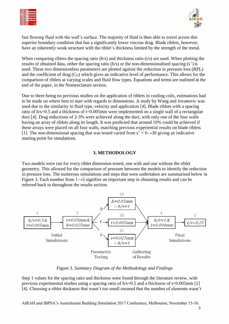
extrusion [5] [8] [9] [10] [11]. The three most common extruded cross sections being sawtooth,

scalloped and blade riblets, shown in Figure 2 below.

Figure 2. Riblet Geometries [1]

The contour lines represent varying magnitudes of velocity, with the largest velocity occurring

furthest from the riblet surface. The blade riblet geometry is most effective of the three due to its

ability to create the largest pocket of trapped fluid between the blades, preventing the interaction of


3

fast flowing fluid with the wall’s surface. The majority of fluid is then able to travel across this

superior boundary condition that has a significantly lower viscous drag. Blade riblets, however,

have an inherently weak structure with the riblet’s thickness limited by the strength of the metal.

When comparing riblets the spacing ratio (h/s) and thickness ratio (t/s) are used. When plotting the

results of obtained data, either the spacing ratio (h/s) or the non-dimensionalised spacing (s+) is

used. These two dimensionless parameters are plotted against the reduction in pressure loss (RPL)

and the coefficient of drag (CD) which gives an indicative level of performance. This allows for the

comparison of riblets at varying scales and fluid flow types. Equations and terms are outlined at the

end of the paper, in the Nomenclature section.

Due to there being no previous studies on the application of riblets in cooling coils, estimations had

to be made on where best to start with regards to dimensions. A study by Wang and Jovanovic was

used due to the similarity in fluid type, velocity and application [4]. Blade riblets with a spacing

ratio of h/s=0.5 and a thickness of t=0.005mm were implemented on a single wall of a rectangular

duct [4]. Drag reductions of 2-3% were achieved along the duct, with only one of the four walls

having an array of riblets along its length. It was predicted that around 10% could be achieved if

these arrays were placed on all four walls, matching previous experiential results on blade riblets

[1]. The non-dimensional spacing that was tested varied from s+ = 6→30 giving an indicative

starting point for simulations.

3. METHODOLOGY

Two models were run for every riblet dimension tested, one with and one without the riblet

geometry. This allowed for the comparison of pressure between the models to identify the reduction

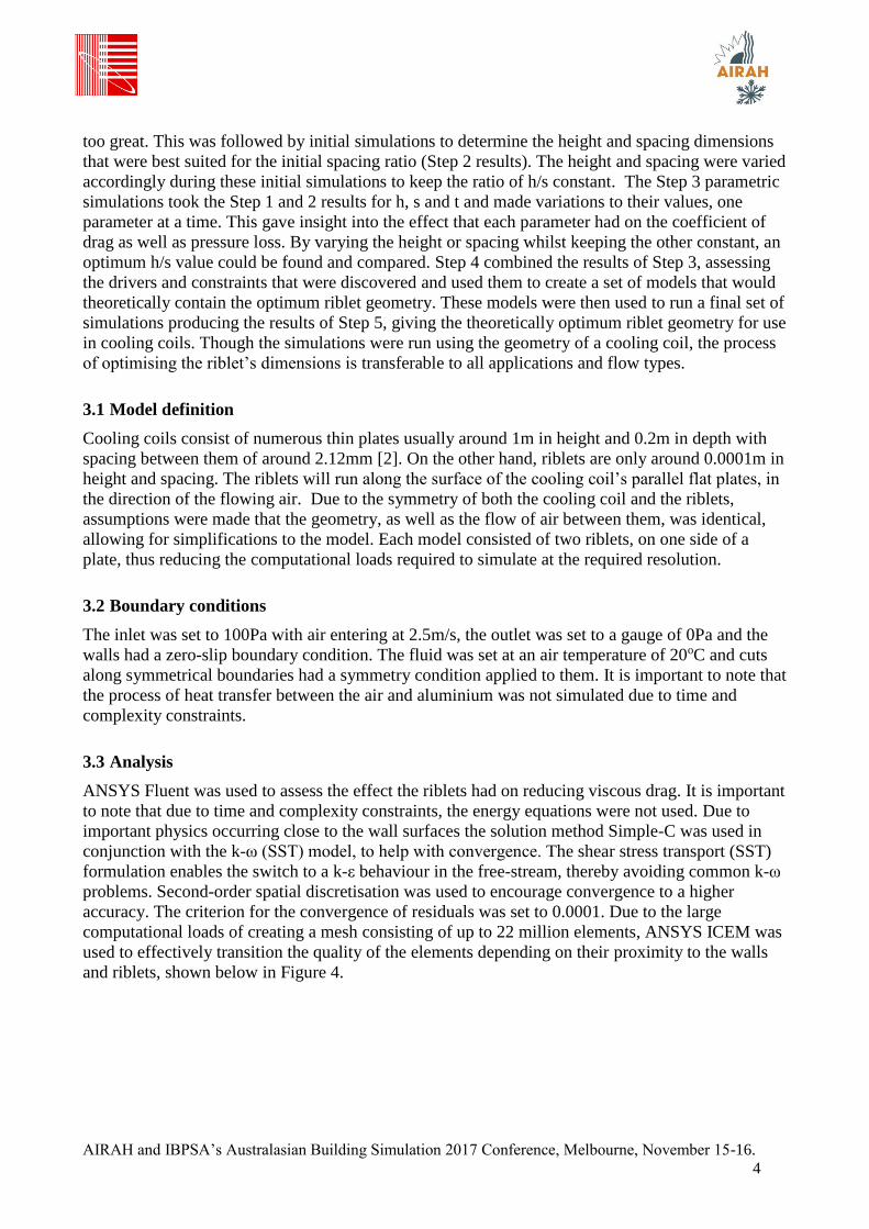
in pressure loss. The numerous simulations and steps that were undertaken are summarised below in

Figure 3. Each number from 1→5 signifies an important step in obtaining results and can be

referred back to throughout the results section.

Figure 3. Summary Diagram of the Methodology and Findings

Step 1 values for the spacing ratio and thickness were found through the literature review, with

previous experimental studies using a spacing ratio of h/s=0.5 and a thickness of t=0.005mm [1]

[4]. Choosing a riblet thickness that wasn’t too small ensured that the number of elements wasn’t


4

too great. This was followed by initial simulations to determine the height and spacing dimensions

that were best suited for the initial spacing ratio (Step 2 results). The height and spacing were varied

accordingly during these initial simulations to keep the ratio of h/s constant. The Step 3 parametric

simulations took the Step 1 and 2 results for h, s and t and made variations to their values, one

parameter at a time. This gave insight into the effect that each parameter had on the coefficient of

drag as well as pressure loss. By varying the height or spacing whilst keeping the other constant, an

optimum h/s value could be found and compared. Step 4 combined the results of Step 3, assessing

the drivers and constraints that were discovered and used them to create a set of models that would

theoretically contain the optimum riblet geometry. These models were then used to run a final set of

simulations producing the results of Step 5, giving the theoretically optimum riblet geometry for use

in cooling coils. Though the simulations were run using the geometry of a cooling coil, the process

of optimising the riblet’s dimensions is transferable to all applications and flow types.

3.1 Model definition

Cooling coils consist of numerous thin plates usually around 1m in height and 0.2m in depth with

spacing between them of around 2.12mm [2]. On the other hand, riblets are only around 0.0001m in

height and spacing. The riblets will run along the surface of the cooling coil’s parallel flat plates, in

the direction of the flowing air. Due to the symmetry of both the cooling coil and the riblets,

assumptions were made that the geometry, as well as the flow of air between them, was identical,

allowing for simplifications to the model. Each model consisted of two riblets, on one side of a

plate, thus reducing the computational loads required to simulate at the required resolution.

3.2 Boundary conditions

The inlet was set to 100Pa with air entering at 2.5m/s, the outlet was set to a gauge of 0Pa and the

walls had a zero-slip boundary condition. The fluid was set at an air temperature of 20oC and cuts

along symmetrical boundaries had a symmetry condition applied to them. It is important to note that

the process of heat transfer between the air and aluminium was not simulated due to time and

complexity constraints.

3.3 Analysis

ANSYS Fluent was used to assess the effect the riblets had on reducing viscous drag. It is important

to note that due to time and complexity constraints, the energy equations were not used. Due to

important physics occurring close to the wall surfaces the solution method Simple-C was used in

conjunction with the k-ω (SST) model, to help with convergence. The shear stress transport (SST)

formulation enables the switch to a k-ε behaviour in the free-stream, thereby avoiding common k-ω

problems. Second-order spatial discretisation was used to encourage convergence to a higher

accuracy. The criterion for the convergence of residuals was set to 0.0001. Due to the large

computational loads of creating a mesh consisting of up to 22 million elements, ANSYS ICEM was

used to effectively transition the quality of the elements depending on their proximity to the walls

and riblets, shown below in Figure 4.


5

Figure 4. Cross Section of a Meshed Model

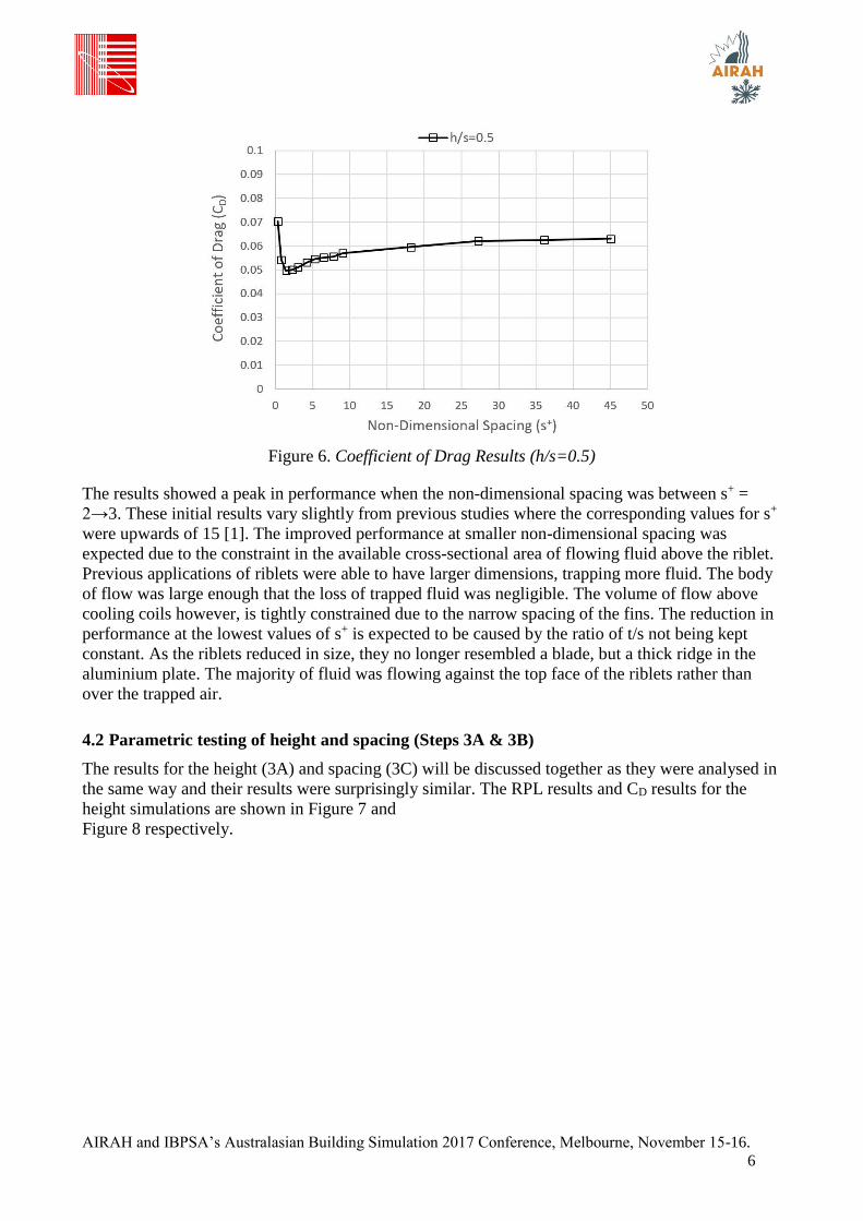
3.4 Mesh verification

Initial simulations were unable to converge due to the length of the model being too small. The

model length was increased until the flow could normalise, allowing the residuals to reach the

required level. An iterative process of increasing the number of mesh elements was then used to

ensure the results were converging to a constant value, as seen in Figure 5 below.

Figure 5. H Convergence of Drag Coefficient

4. RESULTS AND DISCUSSION

4.1 Initial simulations (Step 2)

The Step 1 results were found via the literature review. Using the spacing ratio of h/s=0.5 and a

thickness of t=0.005mm, initial simulations were run. The results showed that the coefficient of

drag steadily reduced as the dimensions of the riblet became smaller. As the s+ values became too

small however, the value of CD spiked backed up, shown below in Figure 6.


6

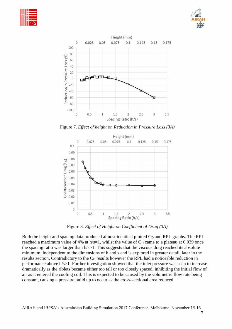
Figure 6. Coefficient of Drag Results (h/s=0.5)

The results showed a peak in performance when the non-dimensional spacing was between s+ =

2→3. These initial results vary slightly from previous studies where the corresponding values for s+

were upwards of 15 [1]. The improved performance at smaller non-dimensional spacing was

expected due to the constraint in the available cross-sectional area of flowing fluid above the riblet.

Previous applications of riblets were able to have larger dimensions, trapping more fluid. The body

of flow was large enough that the loss of trapped fluid was negligible. The volume of flow above

cooling coils however, is tightly constrained due to the narrow spacing of the fins. The reduction in

performance at the lowest values of s+ is expected to be caused by the ratio of t/s not being kept

constant. As the riblets reduced in size, they no longer resembled a blade, but a thick ridge in the

aluminium plate. The majority of fluid was flowing against the top face of the riblets rather than

over the trapped air.

4.2 Parametric testing of height and spacing (Steps 3A & 3B)

The results for the height (3A) and spacing (3C) will be discussed together as they were analysed in

the same way and their results were surprisingly similar. The RPL results and CD results for the

height simulations are shown in Figure 7 and

Figure 8 respectively.


7

Figure 7. Effect of height on Reduction in Pressure Loss (3A)

Figure 8. Effect of Height on Coefficient of Drag (3A)

Both the height and spacing data produced almost identical plotted CD and RPL graphs. The RPL

reached a maximum value of 4% at h/s=1, whilst the value of CD came to a plateau at 0.039 once

the spacing ratio was larger than h/s>1. This suggests that the viscous drag reached its absolute

minimum, independent to the dimensions of h and s and is explored in greater detail, later in the

results section. Contradictory to the CD results however the RPL had a noticeable reduction in

performance above h/s>1. Further investigation showed that the inlet pressure was seen to increase

dramatically as the riblets became either too tall or too closely spaced, inhibiting the initial flow of

air as it entered the cooling coil. This is expected to be caused by the volumetric flow rate being

constant, causing a pressure build up to occur as the cross-sectional area reduced.


8

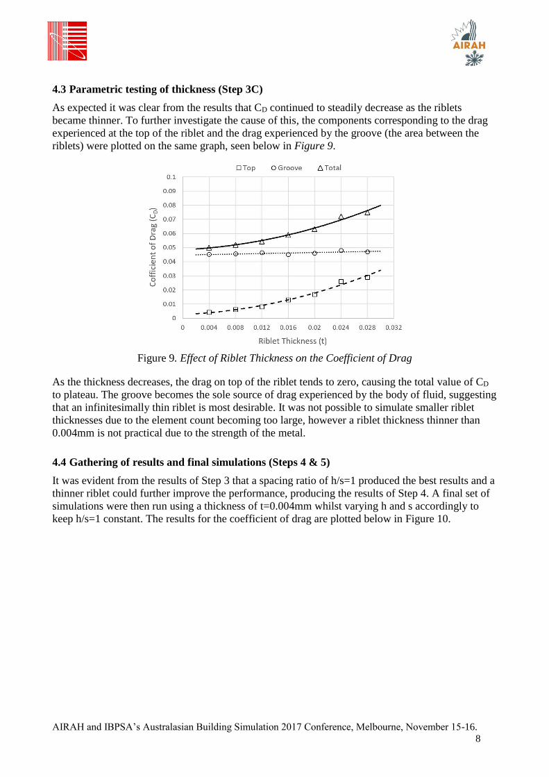
4.3 Parametric testing of thickness (Step 3C)

As expected it was clear from the results that CD continued to steadily decrease as the riblets

became thinner. To further investigate the cause of this, the components corresponding to the drag

experienced at the top of the riblet and the drag experienced by the groove (the area between the

riblets) were plotted on the same graph, seen below in Figure 9.

Figure 9. Effect of Riblet Thickness on the Coefficient of Drag

As the thickness decreases, the drag on top of the riblet tends to zero, causing the total value of CD

to plateau. The groove becomes the sole source of drag experienced by the body of fluid, suggesting

that an infinitesimally thin riblet is most desirable. It was not possible to simulate smaller riblet

thicknesses due to the element count becoming too large, however a riblet thickness thinner than

0.004mm is not practical due to the strength of the metal.

4.4 Gathering of results and final simulations (Steps 4 & 5)

It was evident from the results of Step 3 that a spacing ratio of h/s=1 produced the best results and a

thinner riblet could further improve the performance, producing the results of Step 4. A final set of

simulations were then run using a thickness of t=0.004mm whilst varying h and s accordingly to

keep h/s=1 constant. The results for the coefficient of drag are plotted below in Figure 10.


9

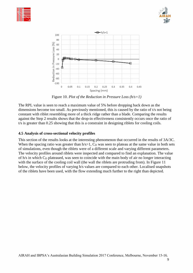
Figure 10. Plot of the Reduction in Pressure Loss (h/s=1)

The RPL value is seen to reach a maximum value of 5% before dropping back down as the

dimensions become too small. As previously mentioned, this is caused by the ratio of t/s not being

constant with riblet resembling more of a thick ridge rather than a blade. Comparing the results

against the Step 2 results shows that the drop-in effectiveness consistently occurs once the ratio of

t/s is greater than 0.25 showing that this is a constraint in designing riblets for cooling coils.

4.5 Analysis of cross-sectional velocity profiles

This section of the results looks at the interesting phenomenon that occurred in the results of 3A/3C.

When the spacing ratio was greater than h/s>1, CD was seen to plateau at the same value in both sets

of simulations, even though the riblets were of a different scale and varying different parameters.

The velocity profiles around riblets were inspected and compared to find an explanation. The value

of h/s in which CD plateaued, was seen to coincide with the main body of air no longer interacting

with the surface of the cooling coil wall (the wall the riblets are protruding from). In Figure 11

below, the velocity profiles of varying h/s values are compared to each other. Localised snapshots

of the riblets have been used, with the flow extending much further to the right than depicted.


10

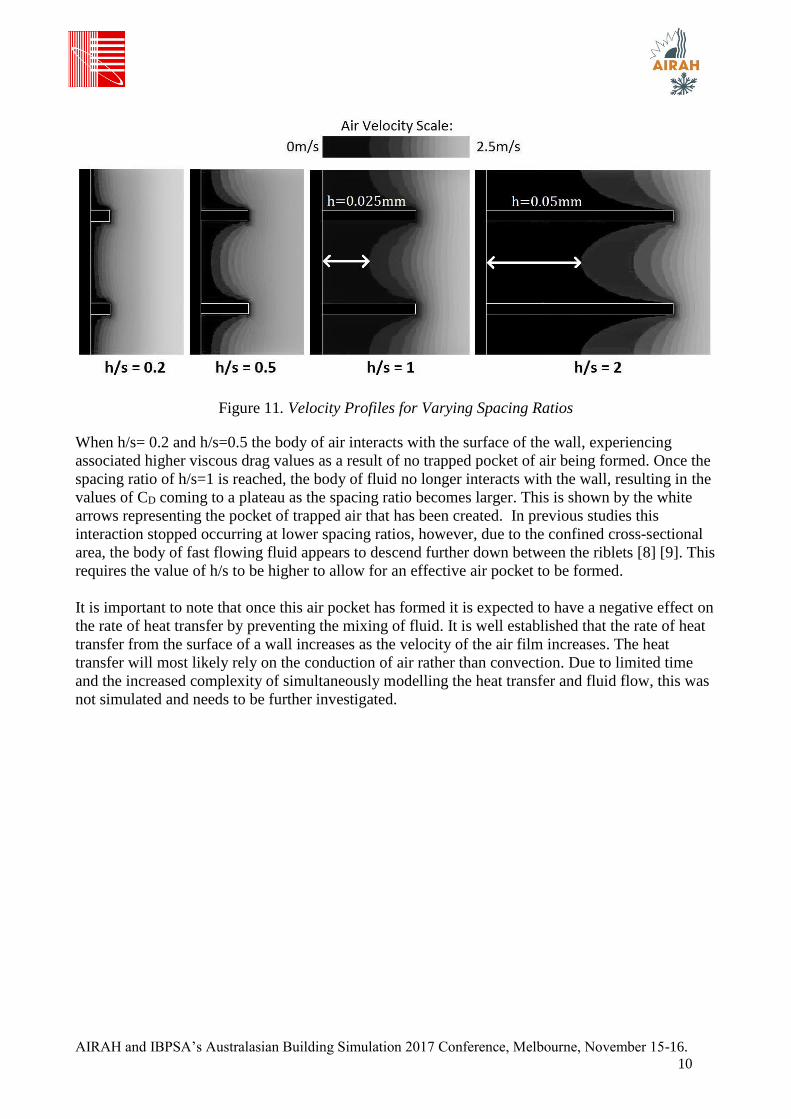
Figure 11. Velocity Profiles for Varying Spacing Ratios

When h/s= 0.2 and h/s=0.5 the body of air interacts with the surface of the wall, experiencing

associated higher viscous drag values as a result of no trapped pocket of air being formed. Once the

spacing ratio of h/s=1 is reached, the body of fluid no longer interacts with the wall, resulting in the

values of CD coming to a plateau as the spacing ratio becomes larger. This is shown by the white

arrows representing the pocket of trapped air that has been created. In previous studies this

interaction stopped occurring at lower spacing ratios, however, due to the confined cross-sectional

area, the body of fast flowing fluid appears to descend further down between the riblets [8] [9]. This

requires the value of h/s to be higher to allow for an effective air pocket to be formed.

It is important to note that once this air pocket has formed it is expected to have a negative effect on

the rate of heat transfer by preventing the mixing of fluid. It is well established that the rate of heat

transfer from the surface of a wall increases as the velocity of the air film increases. The heat

transfer will most likely rely on the conduction of air rather than convection. Due to limited time

and the increased complexity of simultaneously modelling the heat transfer and fluid flow, this was

not simulated and needs to be further investigated.


11

5. CONCLUSION

The viscous drag across a cooling coil is significant, causing losses in pressure and velocity. HVAC

systems make up a significant amount of a building’s energy use. A slight increase in the

performance of a cooling coil could have a significant impact in reducing the energy consumption.

This technical paper was written to assess the feasibility of implementing riblets into cooling coils.

The aim was to find the optimum geometry for reducing viscous drag and pressure loss,

determining the practicality of implementing riblets. In conjunction with this, a parametric method

was developed to elucidate what the drivers and constraints are for designing riblets for various

applications and flow types.

Literature has shown that blade riblets are the superior riblet geometry, successfully implemented

elsewhere in buildings, such as air ducts. The fast-flowing fluid’s degree of descent between the

blades was discovered as the sole driver in determining the optimum dimensions. The spacing ratio

needs to be specifically dimensioned to prevent minimal interaction between the wall and fast

flowing fluid. At smaller dimensions, a spacing ratio of h/s=1 could do this whilst not sacrificing

too much fluid and not effecting the inlet pressure of the cooling coil. The constraint in designing

these blade riblets is primarily the material’s strength and secondly by the ratio of the thickness to

the spacing (t/s<0.25). Whilst it was proved an infinitesimally thin thickness is the limit of

efficiency, blade riblets have an inherently weak structure with the thickness limited by the strength

of the metal. Practically the thickness needs to be no less than around 0.004mm otherwise the riblets

will simply bend and break. The thickness to spacing ratio of t/s<0.25 is then used to determine the

minimum allowable spacing for the given riblet thickness. This corresponds to a spacing value of

0.016mm and finally combining this with the spacing ratio of h/s=1 gives the optimum dimensions

of the riblet geometry.

Simulation results showed pressure savings of up to 5% could be achieved, validated by previous

experimental studies. However, due to the constraints in length and the cross-sectional area for fluid

flow, the energy savings may not be large enough to warrant the implementation of riblets in

cooling coils. With a pressure drop of 100Pa, only 5Pa of pressure would be saved. Due to the

nature of how riblets work, it is believed that the effect on heat transfer will be negative. Whilst the

riblets are effectively doubling the surface area, they are also preventing the mixing of fluid close to

the wall’s surface and this will need to be further investigated. Despite this, the newly developed

parametric process, results and findings help to further expand what is known of riblets and how to

optimise them for a given application and flow type. Using this newly developed parametric

method, all applications of riblets can be optimised for peak performance.

6. ACKNOWLEDGEMENTS

Firstly, I’d like to thank Assoc. Prof. Tracie Barber for helping me with this research, giving me her

invaluable time and help. Secondly, I’d like to thank my father Doug Paton, as well as my

colleagues Jack Blackwell and Tim Dunn for their time spent reviewing this paper.


12

7. NOMENCLATURE

Non-Dimensionalised

Spacing (s+) √𝐶𝐷 2⁄ (𝑠𝑢∞/𝑣)

CD = Coefficient of Drag

S = Riblet Spacing (m)

u∞ = Freestream Velocity (m/s)

v = Kinematic Viscosity (m2/s)

Coefficient of Drag

(CD)

𝐹𝐷12⁄ 𝜌𝑉2𝐴

FD = Drag Force

𝜌 = Density of the Fluid (kg/m3)

V = Velocity of the Fluid (m/s)

A = 'Wetted' Surface Area (m2)

Reduction in Pressure

Loss (RPL)

∆𝑃 − ∆𝑃𝑅∆𝑃

× 100

∆𝑃 = Pressure Loss, Non-Riblet Model

(Pa)

∆𝑃𝑅 = Pressure Loss, Riblet Model (Pa)

Cooling Coil - Refers to a coil that both heats and cools

refrigerant.

8. REFERENCES

[1] B. Dean and B. Bhushan, “Shark-Skin Surfaces for Fluid-Drag Reduction in Turbulant

Flow; A Review,” Philisophil Transactions of the Royal Society A, 2010.

[2] M. Mansour and M. Hassab, Thermal Design of Cooling and Dehumidifying Coils,

INTECH Open Access Publisher, 2012.

[3] AIRAH, Technical Handbook 5th Edition, Melbourne, 2013.

[4] Z. Y. Wang and J. Jovanovic, “Drag Characteristics of Extra-Thin- Fin-Riblets in an

Air Flow Conduit,” Journal of Fluids Engineering, vol. 115, 1993.

[5] D. Bechert, G. Hoppe and W. Reif, “On the drag reduction of the shark skin,” AIAA

Shear Flow Control Conference, pp. 1-18, 1985.

[6] B. Bhushan, “Biomimetics: Lessons from Nature - an overview,” Philosophical

Transactions of the Royal Society A: Mathematical, Physical and Engineering

Sciences, vol. 367, pp. 1445-1486, 2009.

[7] D. Bechert, M. Bruse, W. Hage, J. Van Der Hoeven and G. Hoppe, “Experiments on

drag-reducing surfaces and their optimization with an adjustable geometry,” Journal of

Fluid Mechanics, vol. 338, pp. 59-87, 1997.

[8] M. Walsh, “Turbulent boundary layer drag reduction using riblets,” AIAA Paper, pp.

82-169, 1982.

[9] M. Walsh and A. Lindemann, “Optimization and Application of Riblets for Turbulent

Drag Reduction,” AIAA 22nd Aerospace Sciences Meeting, pp. 1-10, 1984.

[10] D. Bechert, M. Bruse and W. Hage, “Experiments with three-dimensional riblets as an

idealized model of shark skin,” Experiments in Fluids, vol. 28, pp. 403-412, 2000.

[11] D. Bechert, M. Bruse, W. Hage and R. Meyer, “Fluid mechanics of biological surfaces

and their technological application,” Naturwissenschaften, vol. 87, pp. 157-171, 2000.

[12] R. Deissler, Turbulent Fluid Motion, New York: Taylor & Francis, 1998.

a computational fluid dynamics micro-model parametric study

Documents