Parametric and Nonparametric Granger Causality

Testing: Linkages Between International Stock

Markets

Jan G. De Gooijer1∗ and Selliah Sivarajasingham2

1 Department of Quantitative Economics and Tinbergen Institute, University of Amsterdam

Roetersstraat 11, 1018 WB Amsterdam, The Netherlands

e-mail: j.g.degooijer@uva.nl

2 Department of Economics, University of Peradeniya, Peradeniya, Sri Lankae-mail: ssivaraj@pdn.ac.lk

Abstract: This study investigates long-term linear and nonlinear causal linkages among eleven stockmarkets, six industrialized markets and five emerging markets of South-East Asia. We cover the period1987—2006, taking into account the on-set of the Asian financial crisis of 1997. We first apply a testfor the presence of general nonlinearity in vector time series. Substantial differences exist between thepre- and post-crisis period in terms of the total number of significant nonlinear relationships. We thenexamine both periods, using a new nonparametric test for Granger non-causality and the conventionalparametric Granger non-causality test. One major finding is that the Asian stock markets have becomemore internationally integrated after the Asian financial crisis. An exception is the Sri Lankan marketwith almost no significant long-term linear and nonlinear causal linkages with other markets. To ensurethat any causality is strictly nonlinear in nature, we also examine the nonlinear causal relationships ofVAR filtered residuals and VAR filtered squared residuals for the post-crisis sample. We find quite a fewremaining significant bi- and uni-directional causal nonlinear relationships in these series. Finally, afterfiltering the VAR-residuals with GARCH-BEKK models, we show that the nonparametric test statisticsare substantially smaller in both magnitude and statistical significance than those before filtering. Thisindicates that nonlinear causality can, to a large part, be explained by simple volatility effects.

Key words and phrases: GARCH-BEKK; Granger causality; hypothesis testing; nonparametric; stockmarket linkages

∗This paper has been published in Physica A 387 (2008), 2547-2560; see also the URL link

http://dx.doi.org/10.1016/j.physa.2008.01.033

1 Introduction

Since the late 1980s many national stock exchange markets in industrial countries have become

aware of the increased competitiveness among these markets. This, in conjunction with a less

restrictive climate toward capital movements has brought about the view among economists that

the major financial markets of the world are systematically interrelated. This interrelationship

may indicate a growing similarity in reactions toward external developments in macroeconomic

policies and in the world financial environment. In addition, it may also reflect a temporary, or

perhaps more lasting, causal relationship between various individual stock exchanges.

Causal linkages among stock markets have important implications for securities pricing,

hedging and trading strategies, and financial market regulations. Also the presence of long-term

linear and nonlinear relationships may be used to achieve financial gains from international

portfolio diversification and to reduce systematic local risks. Consequently, there exists a large

body of literature examining the presence of causal linkages between developed (less risky)

markets. They typically find that the US market leads other developed markets (e.g. King and

Wadhwani [1]). However, there is substantially less literature on stock market linkages between

developed markets and emerging markets; see Section 2 for a selective overview. Moreover, quite

a few studies relied on the restrictive assumption of a causal linear relationship between stock

markets through the use of Granger’s [2], parametric, causality test. But, as noted by Hsieh [3, 4]

and many others, financial time series exhibit significant nonlinear features. Indeed, Hiemstra

and Jones [5] argue that a nonlinear and nonparametric Granger causality test (hereafter HJ

test), based on the work of Baek and Brock [6], is more effective in uncovering certain nonlinear

causal relationships in daily stock prices.

The HJ causality test seems to be one most used in economics and finance. Examples include

stock price volume relationships (Hiemstra and Jones [5]; Silvapulle and Choi [7]), futures and

cash markets (Dwyer et al. [8]), stock price dividend relationships (Kanas [9]), fundamentals

and exchange rates (Ma and Kanas [10]), equity volatility returns (Brooks and Henry [11]).

However, Diks and Panchenko [12, 13] demonstrate that the HJ test can severely over-reject if

the null hypothesis of non-causality is not true. In addition, with instantaneous dependence,

the HJ test has serious size distortion problems. As an alternative Diks and Panchenko [13]

(hereafter DP) develop a new test statistic which does not suffer from these limitations. Their

empirical results suggest that some of the rejections of the Granger non-causality hypothesis,

using the HJ causality test, may be spurious.

1

The objective of the current paper is two-fold. First, to explore the existence of linear

and nonlinear causal relationships among eleven stock markets. Six of these (Germany, Hong

Kong, Japan, Singapore, UK, and US) belong to the group of world’s major stock markets,

while five markets (India, Malaysia, South Korea, Sri Lanka, and Taiwan) are emerging stock

markets in South-East Asia. Clearly South-East Asia as a region has undergone rapid market

liberalization in the past decade, resulting in increased investment flows. A possible consequence

of this financial openness is an increase in the causal linkages between these emerging markets

and the worlds major financial markets. In particular, the time period after the 1997 Asian

financial crisis may have changed the direction and strength of the causal relationships among

the markets under study. A second objective is to explore the ability of the DP test to detect

nonlinear causal relationships.

The paper has five remaining sections. Section 2 presents a brief overview of the relevant

literature. Also we point out some limitations of the reviewed studies. In Section 3 we present

some selected stock market indicators jointly with a discussion of the eleven stock market indices.

Section 4, entitled “Testing methodology”, introduces (i) a multivariate test of nonlinearity; and

(ii) the nonparametric DP causality test. The empirical findings are reported in Section 5. The

final section closes the paper by discussing some of the main implications of the results and

providing directions for future research.

2 Literature review

There is a wealth of literature on stock market interdependence and integration. However,

depending on the data, methodology, and theoretical models used there is no clear resolution

of the issue yet. Some previous work has have found that international stock markets are

integrated; see, e.g., Arshanapalli and Doukas [14], and Hamao et al. [15]. Others have found

that stock markets are not interlinked; see, e.g., Roca [16], and Smyth and Nandha [17].

Most of the studies on stock market interdependence in emerging markets have been done on

geographical groups of markets, such as markets in Central and Eastern Europe (Gilmore and

McManus [18]; Gündüz and Hatemi-J [19], Latin America (Choudhry [20]; Christofi and Pericli

[21]; Chen et al. [22]), and in Asian countries. Since stock markets in South-East Asia form a

substantial part of the set of markets considered here, we summarize some of the most recent

findings.

Masih and Masih[23, 24] found cointegration in the pre-financial crisis period of October

2

1987 among the stock markets of Thailand, Malaysia, the US, the UK, Japan, Hong Kong and

Singapore. But there was no long-run relationships between these markets for the period after

the global stock market crash of 1987. By contrast, Phylaktis and Ravazzolo [25] found no

linkages and dynamic interactions amongst a group of Pacific-Basin stock markets (Hong Kong,

South Korea, Malaysia, Singapore, Taiwan and Thailand) and the industrialized countries of

Japan and US for the period 1980-1998. Further, Arshanapalli et al. [26] noted an increase in

stock market interdependence after the 1987 crisis for the emerging markets of Malaysia, the

Philippines, Thailand, and the developed markets of Hong Kong, Singapore, the US and Japan

for the period 1986 to 1992. Likewise, when testing for causality-in-variance, Caporale et al. [27]

found some empirical evidence on the bi-directional causal relationships between stock prices

and exchange rates volatility in the case of Indonesia and Thailand for the post-crisis period

1987-2000. Also, Najand [28], using linear state space models, detected stronger interactions

among the stock markets of Japan, Hong Kong, and Singapore after the 1987 stock market

crash.

Linkages among national stock markets before and during the period of the Asian financial

crisis in 1997/98 were explored by Sheng and Tu [29]. In particular, adopting multivariate

cointegration and error-correction tests, these authors focused on 11 major stock markets in the

Asian-Pacific region (Australia, China, Hong Kong, Indonesia, Japan, Malaysia, Philippines,

Singapore, South Korea, Taiwan and Thailand) and the US. Using daily closing prices, they

found empirical evidence that cointegration relationships among the national stock indices has

increased during, but not before, the period of the financial crises. More recently, Weber [30]

revealed various causality-in-variance effects between the volatilities in the national financial

markets in the Asian-Pacific region (Australia, Hong Kong, Indonesia, India, Japan, South

Korea, New Zealand, Philippines, Singapore, Taiwan and Thailand) for the post-crises period

1999-2006. Also, allowing for structural breaks such as the Asian financial crisis, Narayan et al.

[31] found that stock prices in Bangladesh, India and Sri Lanka Granger-cause stock prices in

Pakistan for the period 1995-2001.

All above studies rely on the restrictive assumption of linearity either through the use of

linear causality tests or via linear time series methodology. Moreover, some of these studies

fail to notice that parametric linear Granger causality tests have low power against nonlinear

alternatives; see Baek and Brock [6]. Recognition of the nonlinear property of stock prices, and

subsequently exploring for possible long-run nonlinear relations among national stock markets,

came after publication of the study by Hiemstra and Jones [5]. For instance, using the HJ

3

causality test, Hunter [32] focuses on the emerging markets of Argentina, Chile, and Mexico.

Similarly, Ozdemir and Cakan [33] examine the dynamic relationships between the stock market

indices of the US, Japan, France, and the UK. This latter study reports that there is a strong

bi-directional nonlinear causal relationship between the US and the other countries, which has

also been documented in the literature using linear causality tests. But, as explained in Section

1, the HJ test may lead to false inference. Clearly the causality and nonlinearity tests to be

introduced in Section 4 provide a useful way to extend and update much of the above empirical

knowledge on causal (non)linear relationships.

3 Data

Data consists of eleven time series of daily closing (5 days) stock market price indices, measured

in domestic currencies. The data covers two periods: P1, from November 2, 1987 June 30,

1997, denoting the pre-Asian financial crisis period (2521 observations), and P2, the post-Asian

financial crisis period, with data from June 1, 1998 December 1, 2006 (2220 observations). Recall

that the on-set of the Asian financial crisis started with a 15—20% devaluation of Thailand’s Baht

which took place on July 2, 1997. Subsequently followed by devaluations of the Philippine Peso,

the Malaysian Ringgit, the Indonesian Rupiah, and the Singaporean Dollar. In addition, the

currencies of South Korea and Taiwan suffered. Further in October, 1997 the Hong Kong stock

market collapsed with a 40% loss. In January 1998, the currencies of most South-East Asian

countries regained parts of the earlier losses. The data are taken from ‘DataStream’.

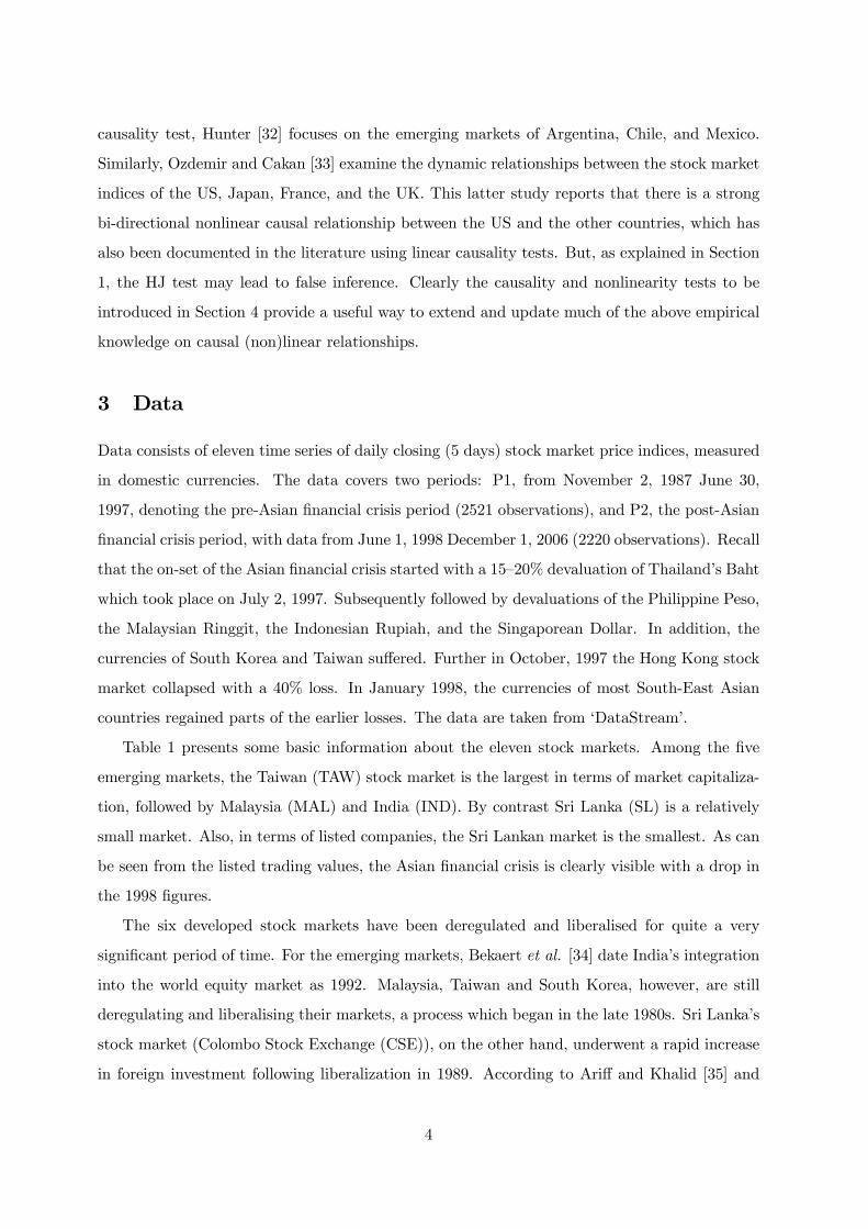
Table 1 presents some basic information about the eleven stock markets. Among the five

emerging markets, the Taiwan (TAW) stock market is the largest in terms of market capitaliza-

tion, followed by Malaysia (MAL) and India (IND). By contrast Sri Lanka (SL) is a relatively

small market. Also, in terms of listed companies, the Sri Lankan market is the smallest. As can

be seen from the listed trading values, the Asian financial crisis is clearly visible with a drop in

the 1998 figures.

The six developed stock markets have been deregulated and liberalised for quite a very

significant period of time. For the emerging markets, Bekaert et al. [34] date India’s integration

into the world equity market as 1992. Malaysia, Taiwan and South Korea, however, are still

deregulating and liberalising their markets, a process which began in the late 1980s. Sri Lanka’s

stock market (Colombo Stock Exchange (CSE)), on the other hand, underwent a rapid increase

in foreign investment following liberalization in 1989. According to Ariff and Khalid [35] and

4

Table 1: Some selected stock market indicators

Country 1997 1998 1999 2000 2001 2002 2003 2004

Number of listed companiesGER 700 741 933 1,022 749 715 684 660HNG 671 693 717 779 657 968 1,027 1,086JAP∗ 2,387 2,416 2,470 2,561 2,471 // 3,058 3,116 3,220SNG 303 321 355 418 386 434 456 489UK 2,157 2,087 1,945 1,904 1,923 2,405 2,311 2,486US 8,851 8,450 7,651 7,524 6,355 5,685 5,295 5,231

IND 5,843 5,860 5,863 5,937 5,795 5,650 5,644 4,730SL 239 233 239 239 238 238 244 245MAL 708 736 757 795 809 865 897 962SK 1,135 1,079 1,178 1,308 1,409 1,518 1,563 1,573TAW 404 437 462 531 584 638 689 697

Market capitalization as a % of GDPGER 39.1 51.0 68.1 68.1 57.8 34.8 44.2 43.6HNG 241.7 211.2 385.1 383.4 310.8 289.5 460.7 528.5JAP∗ 51.4 63.3 101.2 66.3 54.1 53.5 70.9 79.6SNG 112.5 114.9 240.1 164.8 138.3 115.4 158.0 160.6UK 91.4 166.7 201.2 180.3 151.3 119.2 136.8 132.6US 137.0 154.3 180.7 154.0 137.9 106.4 130.2 139.4

IND 30.5 24.5 41.5 32.4 23.1 25.7 46.5 56.1SL 13.9 10.9 10.1 6.6 8.5 10.2 14.9 18.2MAL 93.4 136.0 184.0 130.4 136.4 130.0 162.0 160.6SK 9.7 37.8 97.4 37.5 45.7 45.6 54.2 63.1TAW 101.6 99.8 130.6 79.8 104.1 90.4 132.4 144.5

Trading value ($USm)GER 535,745 761,888 814,740 1,069,120 1,419,579 1,233,056 1,147,209 1,406,055HNG 489,365 205,918 247,428 377,866 196,361 210,662 331,615 438,966JAP† 1,251,750 948,522 1,849,228 2,693,856 1,826,230 1,573,279 2,272,989 3,430,420SNG 63,954 50,735 97,985 91,485 63,385 56,129 87,864 81,314UK 829,131 1,167,382 1,377,859 1,835,278 1,861,131 1,909,716 2,211,533 3,707,191US 10,216,074 13,148,480 18,574,100 31,862,485 29,040,739 25,371,270 15,547,431 19,354,899

IND 158,301 148,239 278,828 509,812 249,298 197,118 284,802 39,085SL 309 281 209 144 153 318 769 582MAL 153,292 29,889 48,512 58,500 20,772 27,623 50,135 59,878SK 172,019 145,572 825,828 1,067,999 703,960 792,165 682,706 638,891TAW 1,291,524 890,491 910,016 983,491 544,808 631,931 592,012 718,619

∗ From 2002 figures include data from both the Tokyo Stock Exchange and JASDAQ. † Figuresinclude data from the Tokyo Stock Exchange and Osaka Stock Exchange. From 2002, JASDAQfigures are included. // Indicates a break in the series.Source: Standard & Poors [37].

5

Elyasiani et al. [36] the CSE was one of the best performing markets in the 1989—1994 period,

with a 15-fold increase in annual turnover and an 8-fold increase in market capitalization.

The trading hours of the eleven stock exchanges are not perfectly synchronized, though there

are several overlapping hours in each trading day for the developed markets. But, within the

group of emerging markets, the trading activity is to a large extent concurrent. Nevertheless,

the differences in closing times could cause sequential price responses to common information

that could be mistaken for causal linkages. Intra-day market data may be used to distangle

these sequential responses from causal transmissions within a particular day. Regrettably these

data are not available for the emerging markets under study.

In the first part of the study, we analyse daily returns Rt = lnPt − lnPt−1, where Pt is theclosing price of an index on day t. In the second part, we focus on the squared and unsquared

residuals from linear VAR models fitted to {Rt}. The squared residuals may be considered asa useful proxy of volatility. Application of three augmented Dickey-Fuller tests (no trend and

no intercept, intercept, and trend plus intercept) indicated that the series {Rt} are integratedof order zero, i.e. stationary, with p-values less than 0.01. The appropriate lag lengths for the

tests were selected by minimizing AIC. The Jarque-Bera test for normality indicated that the

returns are not normally distributed.

Initial exploratory analysis of the sample cross-correlation matrix at lag 0 (contemporaneous

correlation) indicated that almost all series are positively correlated, and significantly different

from zero at the 1% level, for the series {Rt}, and for both time periods. Very low (insignificant)cross-correlations at lag 0 were obtained for the pairs SL-JAP, SL-TAW, SL-UK, and SL-US.

Significant sample cross-correlations at lag 1 were noted for the UK and US stock markets

having uni-directional links with almost all other stock markets. However, it is well-known

that correlations cannot fully capture the long-term dynamic linkages between the markets in

a reliable way. Hence, these results should be interpreted with caution. Consequently, they are

not included in the paper. Indeed, what is needed is a long-term causality analysis between the

markets.

Empirical experience indicates that it is rather hard to absorb simultaneously large tables

with numbers. To overcome this difficulty, and to save space, we use the following simplifying

notation: “∗∗” means that the corresponding p-value of a particular test (causality and nonlin-earity) is smaller than 1%; “∗” means that the corresponding p-value of a test is in the range

1—5%; and “−” denotes that the corresponding p-value of a test is larger than 5%.1 Bi- and uni-1The actual p-values of all tests used in the paper are available upon request.

6

directional causalities will be denoted by the functional representations ↔ and →, respectively.

4 Testing methodology

4.1 A multivariate test of nonlinearity

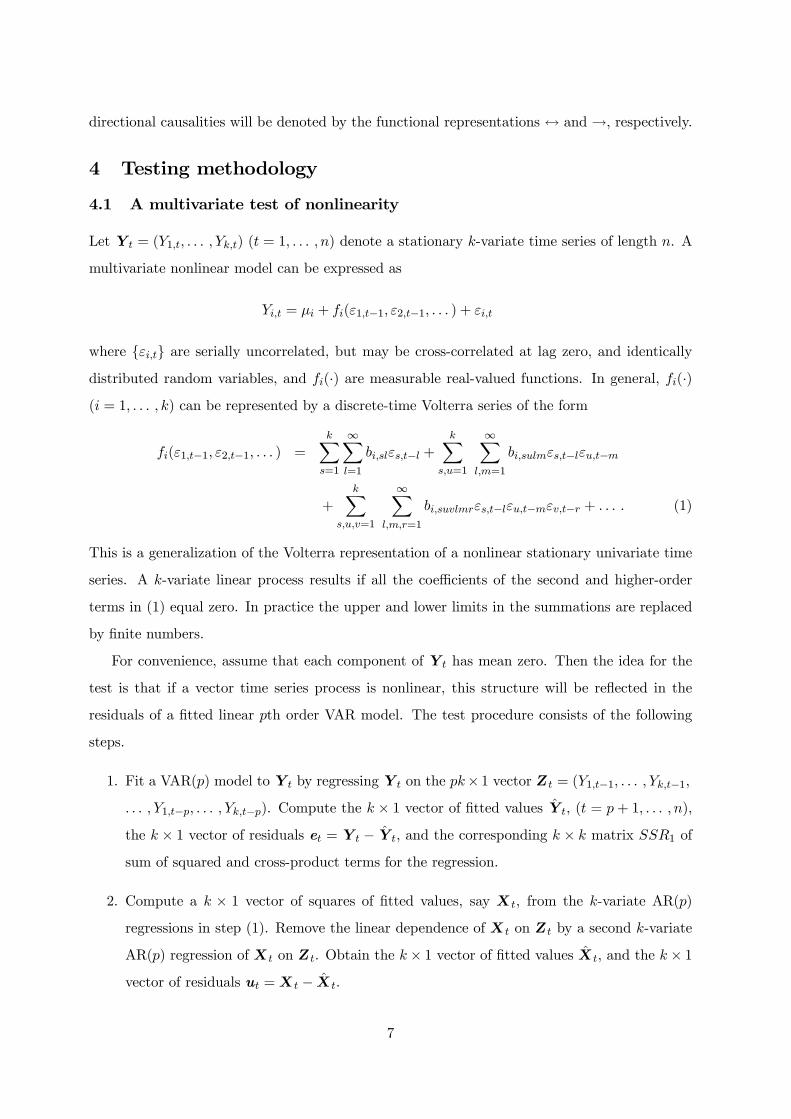
Let Y t = (Y1,t, . . . , Yk,t) (t = 1, . . . , n) denote a stationary k-variate time series of length n. A

multivariate nonlinear model can be expressed as

Yi,t = µi + fi(ε1,t−1, ε2,t−1, . . . ) + εi,t

where {εi,t} are serially uncorrelated, but may be cross-correlated at lag zero, and identicallydistributed random variables, and fi(·) are measurable real-valued functions. In general, fi(·)(i = 1, . . . , k) can be represented by a discrete-time Volterra series of the form

fi(ε1,t−1, ε2,t−1, . . . ) =kX

s=1

∞Xl=1

bi,slεs,t−l +kX

s,u=1

∞Xl,m=1

bi,sulmεs,t−lεu,t−m

+kX

s,u,v=1

∞Xl,m,r=1

bi,suvlmrεs,t−lεu,t−mεv,t−r + . . . . (1)

This is a generalization of the Volterra representation of a nonlinear stationary univariate time

series. A k-variate linear process results if all the coefficients of the second and higher-order

terms in (1) equal zero. In practice the upper and lower limits in the summations are replaced

by finite numbers.

For convenience, assume that each component of Y t has mean zero. Then the idea for the

test is that if a vector time series process is nonlinear, this structure will be reflected in the

residuals of a fitted linear pth order VAR model. The test procedure consists of the following

steps.

1. Fit a VAR(p) model to Y t by regressing Y t on the pk× 1 vector Zt = (Y1,t−1, . . . , Yk,t−1,

. . . , Y1,t−p, . . . , Yk,t−p). Compute the k × 1 vector of fitted values Y t, (t = p+ 1, . . . , n),

the k × 1 vector of residuals et = Y t − Y t, and the corresponding k × k matrix SSR1 of

sum of squared and cross-product terms for the regression.

2. Compute a k × 1 vector of squares of fitted values, say Xt, from the k-variate AR(p)

regressions in step (1). Remove the linear dependence of Xt on Zt by a second k-variate

AR(p) regression of Xt on Zt. Obtain the k × 1 vector of fitted values Xt, and the k × 1vector of residuals ut =Xt − Xt.

7

3. Regress the vector of residuals et from step (1) on the vector of residuals ut from step (2).

4. Compute the corresponding k × k sum of squared regressions matrix, SSR2, and sum of

squared errors matrix, SSE2. Let SSR2|1 = SSR2 − SSR1, i.e. SSR2|1 is the extra sum

of squares due to the addition of the second-order term to the model.

5. Compute the F -statistic F :

F =³n− p− pk − k

k

´³1− Λ1/2Λ1/2

´, (2)

where Λ = |SSE2|/|SSR2|1 + SSE2| is Wilks’ lambda statistic. Under the assumption thatY t follows a zero-mean Gaussian VAR(p) process, and if the sample size n is large, F follows

approximately an Fν1,ν2 distribution with degrees of freedom ν1 = k and ν2 = (n− p)− pk− k.2

Harvill and Ray’s [38] simulation results indicate that, in general, the multivariate version of

Keenan’s [39] test is more powerful than the univariate tests for at least one of the component

series, in particular when the nonlinearity in one series of the vector process is due solely to

terms from the other series.

4.2 The nonparametric DP causality test

The general setting for a causality test is as follows. Assume {Xt, Yt; t ≥ 1} are two scalar-valued strictly stationary time series. Then {Xt} is a strictly Granger cause of {Yt} if past andcurrent values of Xt contain additional information on future values of Yt that is not contained

in the past and current Yt-values alone. More formally, let FX,t and FY,t denote the information

sets consisting of past observations of Xt and Yt up and including time t, and let ‘∼’ denoteequivalence in distribution. Then {Xt} is a Granger cause of {Yt} if, for some k ≥ 1,

(Yt+1, . . . , Yt+k)|(FX,t,FY,t) 6∼ (Yt+1, . . . , Yt+k)|FY,t. (3)

This definition is general and does not involve model assumptions. In practice one often assumes

k = 1, i.e. testing for Granger non-causality comes down to comparing the one-step-ahead

conditional distribution of {Yt} with and without past and current observed values of {Xt},which will also be the case considered here.

Note the testing framework introduced above concerns conditional distributions given an

infinite number of past observations. In practice, however, tests are usually confined to finite

orders in {Xt} and {Yt}. To this end, define the delay vectors X Xt = (Xt− X+1, . . . ,Xt), and

2FORTRAN-code for computing F can be obtained from the first author.

8

Y Yt = (Yt− Y +1, . . . , Yt), ( X , Y ≥ 1). If past observations of X X

t contain no information

about future values, it follows from (3) that the null hypothesis of interest is given by

H0 : Yt+1|(X Xt ;Y

Yt ) ∼ Yt+1|Y Y

t . (4)

For a strictly stationary bivariate time series, (4) comes down to a statement about the invariant

distribution of the X + Y +1-dimensional vector (X Xt ,Y Y

t , Zt) where Zt = Yt+1. To simplify

notation we drop the time index t. Further, it is assumed that X = Y = 1. Hence, under

the null, the conditional distribution of Z given (X,Y ) = (x, y) is the same as that of Z given

Y = y. Then (4) can be restated in terms of ratios of joint distributions. Specifically, the

joint probability density function fX,Y,Z(x, y, z) and its marginals must satisfy the relationship

fX,Y,Z(x, y, z)/fY (y) = (fX,Y (x, y)/fY (y))(fY,Z(y, z)/fY (y)). Thus X and Z are independent

conditionally on Y = y, for each fixed value of y. DP [13] show that this reformulated H0 implies

q ≡ E[fX,Y,Z(X,Y,Z)fY (Y )− fX,Y (X,Y )fY,Z(Y,Z)] = 0.

Let fW (Wi) denote a local density estimator of a dW -variate random vectorW atWi defined

by fW (Wi) = (2εn)−dW (n − 1)−1Pj,j 6=i I

Wij , where I

Wij = I(k Wi −Wj k< εn) with I(·) the

indicator function and εn the bandwidth, depending on the sample size n. Given this estimator,

the test statistic of interest is given by

Tn(εn) =n− 1

n(n− 2)Xi

f2Y (Yi)(fX,Z|Y (Xi, Zi|Yi)− fX|Y (Xi|Yi)fZ|Y (Zi|Yi)). (5)

Suppose that εn = Cn−β (C > 0, 14 < β < 13). Then DP [13] prove that (5) satisfies

√n(Tn(εn)− q)

Sn

D→ N(0, 1), (6)

where D→ denotes convergence in distribution, and Sn is an estimator of the asymptotic variance

of Tn(·) as discussed in detail by DP ([13], Appendix A).3

5 Empirical results

5.1 Multivariate nonlinearity test

Before investigating specific linear and nonlinear causal relationships between pairs of bivariate

time series, it is desirable to test for general vector nonlinear structure. Using linear VAR(p)

models having p = 0, 1, . . . , 10, the AIC model selection criterion was used to select the “best”3C-code for computing the Tn(·) test statistic can be downloaded from: http://www1.fee.uva.nl/cendef/upload

/15/GCTtest.zip

9

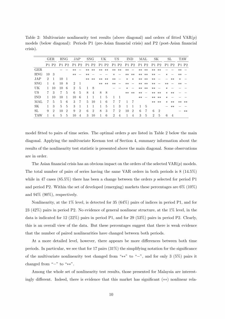
Table 2: Multivariate nonlinearity test results (above diagonal) and orders of fitted VAR(p)models (below diagonal): Periods P1 (pre-Asian financial crisis) and P2 (post-Asian financialcrisis).

GER HNG JAP SNG UK US IND MAL SK SL TAW

P1 P2 P1 P2 P1 P2 P1 P2 P1 P2 P1 P2 P1 P2 P1 P2 P1 P2 P1 P2 P1 P2GER − − ∗∗ − ∗∗ ∗∗ ∗∗ ∗∗ ∗∗ ∗∗ ∗∗ − ∗∗ ∗∗ ∗∗ ∗∗ − − ∗∗ −HNG 10 3 ∗∗ − ∗∗ − − − ∗ − ∗∗ ∗∗ ∗∗ ∗∗ ∗∗ − ∗ − ∗∗ −JAP 2 1 10 1 ∗∗ ∗∗ ∗∗ ∗∗ ∗∗ − ∗ ∗ ∗∗ ∗∗ ∗∗ − − ∗∗ ∗ −SNG 1 4 10 8 2 1 ∗∗ ∗∗ ∗∗ − ∗∗ − ∗∗ ∗∗ ∗∗ − ∗∗ − ∗∗ −UK 1 10 10 6 2 5 1 8 − − ∗ − ∗∗ ∗∗ ∗∗ − ∗ − − −US 7 3 7 5 6 5 8 4 8 8 ∗∗ ∗∗ ∗∗ − ∗∗ ∗∗ ∗ ∗∗ − −IND 1 10 10 1 10 6 1 1 1 5 1 1 ∗∗ − ∗∗ ∗∗ ∗ − − −MAL 7 5 5 6 3 7 5 10 1 6 7 7 1 7 ∗∗ ∗∗ ∗ ∗∗ ∗∗ ∗∗SK 1 3 5 5 3 1 1 1 1 5 1 3 1 1 1 5 − ∗∗ − −SL 9 2 10 2 9 2 6 2 8 3 7 2 10 2 6 7 6 2 − ∗∗TAW 1 4 5 5 10 4 3 10 1 6 2 4 1 4 3 5 2 5 6 4

model fitted to pairs of time series. The optimal orders p are listed in Table 2 below the main

diagonal. Applying the multivariate Keenan test of Section 4, summary information about the

results of the nonlinearity test statistic is presented above the main diagonal. Some observations

are in order.

The Asian financial crisis has an obvious impact on the orders of the selected VAR(p) models.

The total number of pairs of series having the same VAR orders in both periods is 8 (14.5%)

while in 47 cases (85.5%) there has been a change between the orders p selected for period P1

and period P2. Within the set of developed (emerging) markets these percentages are 6% (10%)

and 94% (90%), respectively.

Nonlinearity, at the 1% level, is detected for 35 (64%) pairs of indices in period P1, and for

23 (42%) pairs in period P2. No evidence of general nonlinear structure, at the 1% level, in the

data is indicated for 12 (22%) pairs in period P1, and for 29 (53%) pairs in period P2. Clearly,

this is an overall view of the data. But these percentages suggest that there is weak evidence

that the number of paired nonlinearities have changed between both periods.

At a more detailed level, however, there appears be more differences between both time

periods. In particular, we see that for 17 pairs (31%) the simplifying notation for the significance

of the multivariate nonlinearity test changed from “∗∗” to “−”, and for only 3 (5%) pairs itchanged from “−” to “∗∗”.

Among the whole set of nonlinearity test results, those presented for Malaysia are interest-

ingly different. Indeed, there is evidence that this market has significant (∗∗) nonlinear rela-

10

tionships with almost all other markets. Moreover, these relationships remain fairly persistent

across both time periods.

Broadly, the significant nonlinearity test results reported in Table 2 motivate the search for

causal and persistent nonlinear linkages between pairs of stock indices by a nonparametric test.

Nevertheless these results should be interpreted with caution since high kurtosis in the returns

may affect the null distribution of the test.

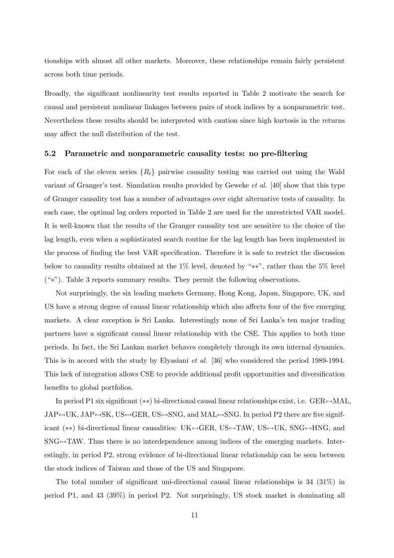
5.2 Parametric and nonparametric causality tests: no pre-filtering

For each of the eleven series {Rt} pairwise causality testing was carried out using the Waldvariant of Granger’s test. Simulation results provided by Geweke et al. [40] show that this type

of Granger causality test has a number of advantages over eight alternative tests of causality. In

each case, the optimal lag orders reported in Table 2 are used for the unrestricted VAR model.

It is well-known that the results of the Granger causality test are sensitive to the choice of the

lag length, even when a sophisticated search routine for the lag length has been implemented in

the process of finding the best VAR specification. Therefore it is safe to restrict the discussion

below to causality results obtained at the 1% level, denoted by “∗∗”, rather than the 5% level

(“∗”). Table 3 reports summary results. They permit the following observations.Not surprisingly, the six leading markets Germany, Hong Kong, Japan, Singapore, UK, and

US have a strong degree of causal linear relationship which also affects four of the five emerging

markets. A clear exception is Sri Lanka. Interestingly none of Sri Lanka’s ten major trading

partners have a significant causal linear relationship with the CSE. This applies to both time

periods. In fact, the Sri Lankan market behaves completely through its own internal dynamics.

This is in accord with the study by Elyasiani et al. [36] who considered the period 1989-1994.

This lack of integration allows CSE to provide additional profit opportunities and diversification

benefits to global portfolios.

In period P1 six significant (∗∗) bi-directional causal linear relationships exist, i.e. GER↔MAL,JAP↔UK, JAP↔SK, US↔GER, US↔SNG, and MAL↔SNG. In period P2 there are five signif-icant (∗∗) bi-directional linear causalities: UK↔GER, US↔TAW, US↔UK, SNG↔HNG, andSNG↔TAW. Thus there is no interdependence among indices of the emerging markets. Inter-estingly, in period P2, strong evidence of bi-directional linear relationship can be seen between

the stock indices of Taiwan and those of the US and Singapore.

The total number of significant uni-directional causal linear relationships is 34 (31%) in

period P1, and 43 (39%) in period P2. Not surprisingly, US stock market is dominating all

11

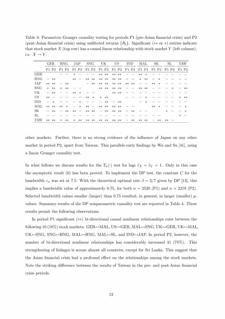
Table 3: Parametric Granger causality testing for periods P1 (pre-Asian financial crisis) and P2(post-Asian financial crisis) using unfiltered returns {Rt}. Significant (∗∗ or ∗) entries indicatethat stock marketX (top row) has a causal linear relationship with stock market Y (left column),i.e. X → Y .

GER HNG JAP SNG UK US IND MAL SK SL TAW

P1 P2 P1 P2 P1 P2 P1 P2 P1 P2 P1 P2 P1 P2 P1 P2 P1 P2 P1 P2 P1 P2GER − − ∗ − − − ∗∗ ∗∗ ∗∗ ∗∗ − − ∗∗ ∗ − − − − − −HNG − ∗∗ ∗∗ − ∗∗ ∗∗ ∗∗ ∗∗ ∗∗ ∗∗ − − ∗ ∗∗ − ∗ − − − −JAP ∗∗ ∗∗ − ∗∗ − ∗∗ ∗∗ ∗∗ ∗∗ ∗∗ ∗∗ ∗∗ − − ∗∗ ∗ − − − −SNG ∗ ∗∗ ∗ ∗∗ − − ∗∗ ∗∗ ∗∗ ∗∗ − − ∗∗ ∗∗ − − − ∗ − ∗∗UK − ∗∗ − − ∗∗ ∗ − − ∗∗ ∗∗ − − − − − − − − − −US ∗∗ − − − − − ∗∗ ∗ ∗ ∗∗ − − − ∗ − − − − ∗ ∗∗IND − ∗ − − − ∗ − − − ∗∗ − ∗∗ − ∗ − − − − − −MAL ∗∗ ∗∗ ∗∗ ∗ − ∗ ∗∗ − ∗∗ ∗∗ ∗∗ ∗∗ − − ∗∗ ∗ − − − ∗SK − ∗∗ − ∗∗ ∗∗ − ∗∗ ∗∗ − ∗∗ ∗∗ ∗∗ − ∗∗ − − ∗ − − ∗SL − − − − − − − − − − − − − − − − − − ∗ −TAW ∗∗ ∗∗ ∗ ∗∗ ∗ ∗∗ ∗∗ ∗∗ ∗∗ ∗∗ ∗∗ ∗∗ − ∗∗ ∗∗ ∗∗ − ∗∗ ∗∗ −

other markets. Further, there is no strong evidence of the influence of Japan on any other

market in period P2, apart from Taiwan. This parallels early findings by Wu and Su [41], using

a linear Granger causality test.

In what follows we discuss results for the Tn(·) test for lags X = Y = 1. Only in this case

the asymptotic result (6) has been proved. To implement the DP test, the constant C for the

bandwidth εn was set at 7.5. With the theoretical optimal rate β = 2/7 given by DP [13], this

implies a bandwidth value of approximately 0.75, for both n = 2520 (P1) and n = 2219 (P2).

Selected bandwidth values smaller (larger) than 0.75 resulted, in general, in larger (smaller) p-

values. Summary results of the DP nonparametric causality test are reported in Table 4. These

results permit the following observations.

In period P1 significant (∗∗) bi-directional causal nonlinear relationships exist between thefollowing 10 (18%) stock markets: GER↔MAL, US↔GER, MAL↔SNG, UK↔GER, UK↔MAL,UK↔SNG, SNG↔HNG, MAL↔HNG, MAL↔SL, and IND↔JAP. In period P2, however, thenumber of bi-directional nonlinear relationships has considerably increased 41 (75%). This

strengthening of linkages is across almost all countries, except for Sri Lanka. This suggest that

the Asian financial crisis had a profound effect on the relationships among the stock markets.

Note the striking difference between the results of Taiwan in the pre- and post-Asian financial

crisis periods.

12

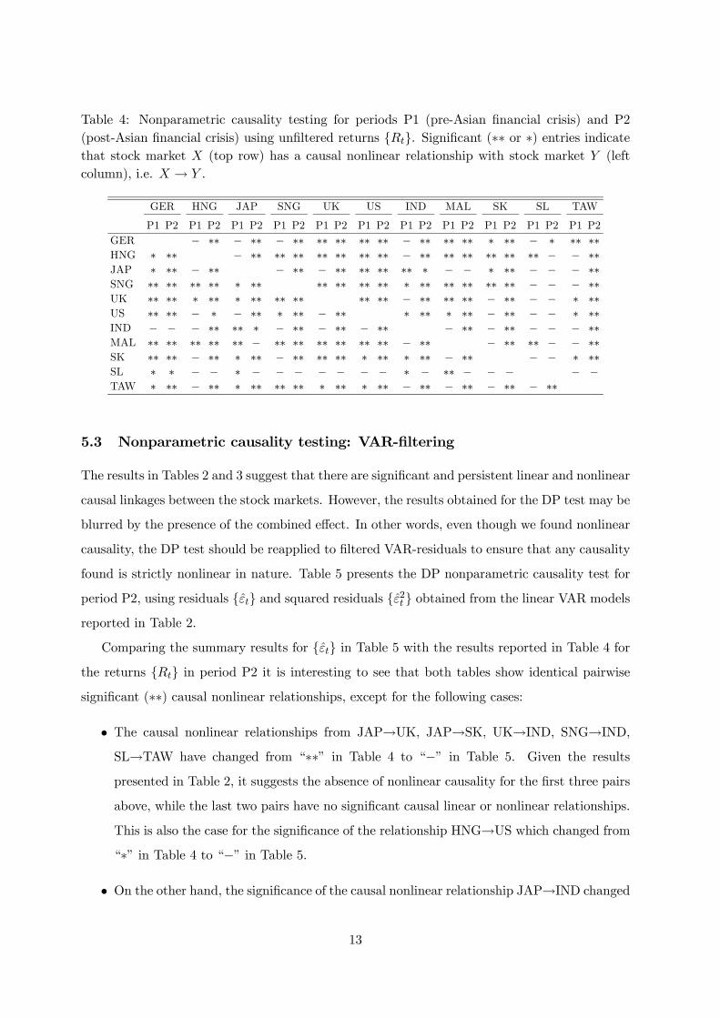
Table 4: Nonparametric causality testing for periods P1 (pre-Asian financial crisis) and P2(post-Asian financial crisis) using unfiltered returns {Rt}. Significant (∗∗ or ∗) entries indicatethat stock market X (top row) has a causal nonlinear relationship with stock market Y (leftcolumn), i.e. X → Y .

GER HNG JAP SNG UK US IND MAL SK SL TAW

P1 P2 P1 P2 P1 P2 P1 P2 P1 P2 P1 P2 P1 P2 P1 P2 P1 P2 P1 P2 P1 P2GER − ∗∗ − ∗∗ − ∗∗ ∗∗ ∗∗ ∗∗ ∗∗ − ∗∗ ∗∗ ∗∗ ∗ ∗∗ − ∗ ∗∗ ∗∗HNG ∗ ∗∗ − ∗∗ ∗∗ ∗∗ ∗∗ ∗∗ ∗∗ ∗∗ − ∗∗ ∗∗ ∗∗ ∗∗ ∗∗ ∗∗ − − ∗∗JAP ∗ ∗∗ − ∗∗ − ∗∗ − ∗∗ ∗∗ ∗∗ ∗∗ ∗ − − ∗ ∗∗ − − − ∗∗SNG ∗∗ ∗∗ ∗∗ ∗∗ ∗ ∗∗ ∗∗ ∗∗ ∗∗ ∗∗ ∗ ∗∗ ∗∗ ∗∗ ∗∗ ∗∗ − − − ∗∗UK ∗∗ ∗∗ ∗ ∗∗ ∗ ∗∗ ∗∗ ∗∗ ∗∗ ∗∗ − ∗∗ ∗∗ ∗∗ − ∗∗ − − ∗ ∗∗US ∗∗ ∗∗ − ∗ − ∗∗ ∗ ∗∗ − ∗∗ ∗ ∗∗ ∗ ∗∗ − ∗∗ − − ∗ ∗∗IND − − − ∗∗ ∗∗ ∗ − ∗∗ − ∗∗ − ∗∗ − ∗∗ − ∗∗ − − − ∗∗MAL ∗∗ ∗∗ ∗∗ ∗∗ ∗∗ − ∗∗ ∗∗ ∗∗ ∗∗ ∗∗ ∗∗ − ∗∗ − ∗∗ ∗∗ − − ∗∗SK ∗∗ ∗∗ − ∗∗ ∗ ∗∗ − ∗∗ ∗∗ ∗∗ ∗ ∗∗ ∗ ∗∗ − ∗∗ − − ∗ ∗∗SL ∗ ∗ − − ∗ − − − − − − − ∗ − ∗∗ − − − − −TAW ∗ ∗∗ − ∗∗ ∗ ∗∗ ∗∗ ∗∗ ∗ ∗∗ ∗ ∗∗ − ∗∗ − ∗∗ − ∗∗ − ∗∗

5.3 Nonparametric causality testing: VAR-filtering

The results in Tables 2 and 3 suggest that there are significant and persistent linear and nonlinear

causal linkages between the stock markets. However, the results obtained for the DP test may be

blurred by the presence of the combined effect. In other words, even though we found nonlinear

causality, the DP test should be reapplied to filtered VAR-residuals to ensure that any causality

found is strictly nonlinear in nature. Table 5 presents the DP nonparametric causality test for

period P2, using residuals {εt} and squared residuals {ε2t } obtained from the linear VAR modelsreported in Table 2.

Comparing the summary results for {εt} in Table 5 with the results reported in Table 4 forthe returns {Rt} in period P2 it is interesting to see that both tables show identical pairwisesignificant (∗∗) causal nonlinear relationships, except for the following cases:

• The causal nonlinear relationships from JAP→UK, JAP→SK, UK→IND, SNG→IND,SL→TAW have changed from “∗∗” in Table 4 to “−” in Table 5. Given the results

presented in Table 2, it suggests the absence of nonlinear causality for the first three pairs

above, while the last two pairs have no significant causal linear or nonlinear relationships.

This is also the case for the significance of the relationship HNG→US which changed from“∗” in Table 4 to “−” in Table 5.

• On the other hand, the significance of the causal nonlinear relationship JAP→IND changed

13

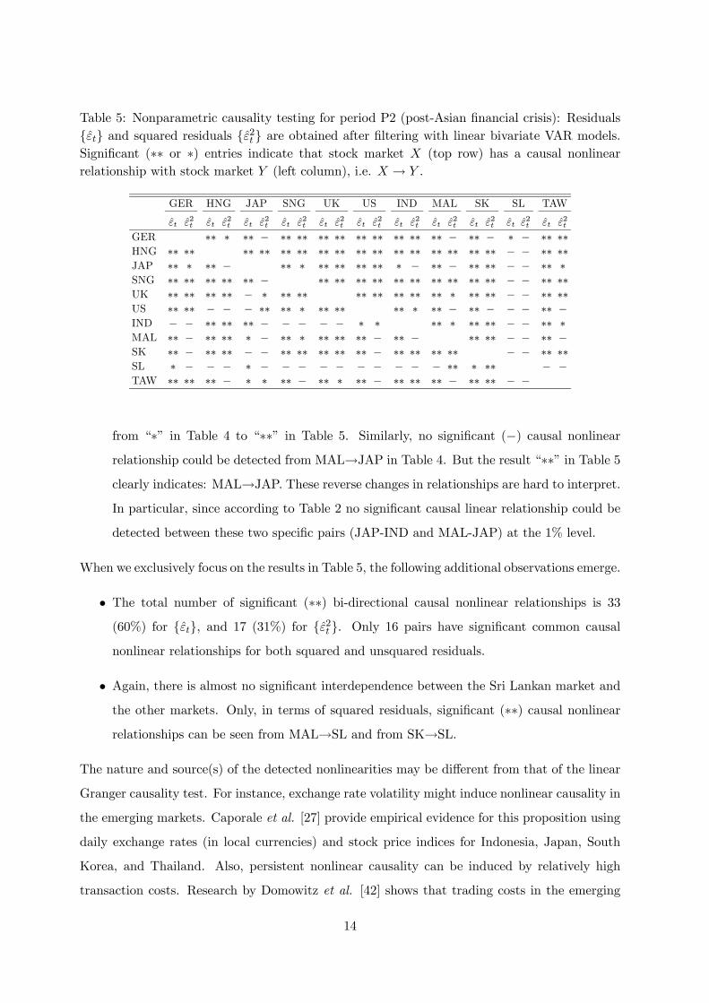
Table 5: Nonparametric causality testing for period P2 (post-Asian financial crisis): Residuals{εt} and squared residuals {ε2t } are obtained after filtering with linear bivariate VAR models.Significant (∗∗ or ∗) entries indicate that stock market X (top row) has a causal nonlinearrelationship with stock market Y (left column), i.e. X → Y .

GER HNG JAP SNG UK US IND MAL SK SL TAW

εt ε2t εt ε2t εt ε2t εt ε2t εt ε2t εt ε2t εt ε2t εt ε2t εt ε2t εt ε2t εt ε2tGER ∗∗ ∗ ∗∗ − ∗∗ ∗∗ ∗∗ ∗∗ ∗∗ ∗∗ ∗∗ ∗∗ ∗∗ − ∗∗ − ∗ − ∗∗ ∗∗HNG ∗∗ ∗∗ ∗∗ ∗∗ ∗∗ ∗∗ ∗∗ ∗∗ ∗∗ ∗∗ ∗∗ ∗∗ ∗∗ ∗∗ ∗∗ ∗∗ − − ∗∗ ∗∗JAP ∗∗ ∗ ∗∗ − ∗∗ ∗ ∗∗ ∗∗ ∗∗ ∗∗ ∗ − ∗∗ − ∗∗ ∗∗ − − ∗∗ ∗SNG ∗∗ ∗∗ ∗∗ ∗∗ ∗∗ − ∗∗ ∗∗ ∗∗ ∗∗ ∗∗ ∗∗ ∗∗ ∗∗ ∗∗ ∗∗ − − ∗∗ ∗∗UK ∗∗ ∗∗ ∗∗ ∗∗ − ∗ ∗∗ ∗∗ ∗∗ ∗∗ ∗∗ ∗∗ ∗∗ ∗ ∗∗ ∗∗ − − ∗∗ ∗∗US ∗∗ ∗∗ − − − ∗∗ ∗∗ ∗ ∗∗ ∗∗ ∗∗ ∗ ∗∗ − ∗∗ − − − ∗∗ −IND − − ∗∗ ∗∗ ∗∗ − − − − − ∗ ∗ ∗∗ ∗ ∗∗ ∗∗ − − ∗∗ ∗MAL ∗∗ − ∗∗ ∗∗ ∗ − ∗∗ ∗ ∗∗ ∗∗ ∗∗ − ∗∗ − ∗∗ ∗∗ − − ∗∗ −SK ∗∗ − ∗∗ ∗∗ − − ∗∗ ∗∗ ∗∗ ∗∗ ∗∗ − ∗∗ ∗∗ ∗∗ ∗∗ − − ∗∗ ∗∗SL ∗ − − − ∗ − − − − − − − − − − ∗∗ ∗ ∗∗ − −TAW ∗∗ ∗∗ ∗∗ − ∗ ∗ ∗∗ − ∗∗ ∗ ∗∗ − ∗∗ ∗∗ ∗∗ − ∗∗ ∗∗ − −

from “∗” in Table 4 to “∗∗” in Table 5. Similarly, no significant (−) causal nonlinearrelationship could be detected from MAL→JAP in Table 4. But the result “∗∗” in Table 5clearly indicates: MAL→JAP. These reverse changes in relationships are hard to interpret.In particular, since according to Table 2 no significant causal linear relationship could be

detected between these two specific pairs (JAP-IND and MAL-JAP) at the 1% level.

When we exclusively focus on the results in Table 5, the following additional observations emerge.

• The total number of significant (∗∗) bi-directional causal nonlinear relationships is 33(60%) for {εt}, and 17 (31%) for {ε2t }. Only 16 pairs have significant common causalnonlinear relationships for both squared and unsquared residuals.

• Again, there is almost no significant interdependence between the Sri Lankan market andthe other markets. Only, in terms of squared residuals, significant (∗∗) causal nonlinearrelationships can be seen from MAL→SL and from SK→SL.

The nature and source(s) of the detected nonlinearities may be different from that of the linear

Granger causality test. For instance, exchange rate volatility might induce nonlinear causality in

the emerging markets. Caporale et al. [27] provide empirical evidence for this proposition using

daily exchange rates (in local currencies) and stock price indices for Indonesia, Japan, South

Korea, and Thailand. Also, persistent nonlinear causality can be induced by relatively high

transaction costs. Research by Domowitz et al. [42] shows that trading costs in the emerging

14

markets are significantly higher than in more developed markets, with South Korea one of the

most expensive markets. This result still holds after correcting for factors affecting costs such

as market capitalization and volatility. Consequently, investors in these markets pool their

information until it is profitable to trade. Needless to say, there may be other sources of the

observed nonlinearities.

5.4 Nonparametric causality testing: GARCH-BEKK filtered VAR-residuals

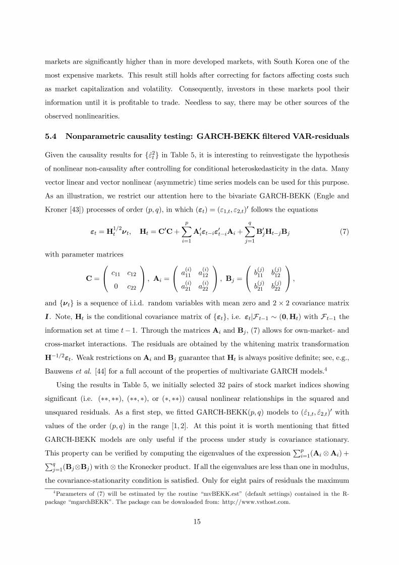
Given the causality results for {ε2t } in Table 5, it is interesting to reinvestigate the hypothesisof nonlinear non-causality after controlling for conditional heteroskedasticity in the data. Many

vector linear and vector nonlinear (asymmetric) time series models can be used for this purpose.

As an illustration, we restrict our attention here to the bivariate GARCH-BEKK (Engle and

Kroner [43]) processes of order (p, q), in which (εt) = (ε1,t, ε2,t)0 follows the equations

εt = H1/2t νt, Ht = C0C+

pXi=1

A0iεt−iε0t−iAi +

qXj=1

B0jHt−jBj (7)

with parameter matrices

C =

c11 c12

0 c22

, Ai =

a(i)11 a

(i)12

a(i)21 a

(i)22

, Bj =

b(j)11 b

(j)12

b(j)21 b

(j)22

,

and {νt} is a sequence of i.i.d. random variables with mean zero and 2 × 2 covariance matrixI. Note, Ht is the conditional covariance matrix of {εt}, i.e. εt|F t−1 ∼ (0,Ht) with F t−1 the

information set at time t− 1. Through the matrices Ai and Bj , (7) allows for own-market- and

cross-market interactions. The residuals are obtained by the whitening matrix transformation

H−1/2εt. Weak restrictions on Ai and Bj guarantee that Ht is always positive definite; see, e.g.,

Bauwens et al. [44] for a full account of the properties of multivariate GARCH models.4

Using the results in Table 5, we initially selected 32 pairs of stock market indices showing

significant (i.e. (∗∗, ∗∗), (∗∗, ∗), or (∗, ∗∗)) causal nonlinear relationships in the squared andunsquared residuals. As a first step, we fitted GARCH-BEKK(p, q) models to (ε1,t, ε2,t)0 with

values of the order (p, q) in the range [1, 2]. At this point it is worth mentioning that fitted

GARCH-BEKK models are only useful if the process under study is covariance stationary.

This property can be verified by computing the eigenvalues of the expressionPp

i=1(Ai ⊗Ai) +Pqj=1(Bj⊗Bj) with ⊗ the Kronecker product. If all the eigenvalues are less than one in modulus,

the covariance-stationarity condition is satisfied. Only for eight pairs of residuals the maximum4Parameters of (7) will be estimated by the routine “mvBEKK.est” (default settings) contained in the R-

package “mgarchBEKK”. The package can be downloaded from: http://www.vsthost.com.

15

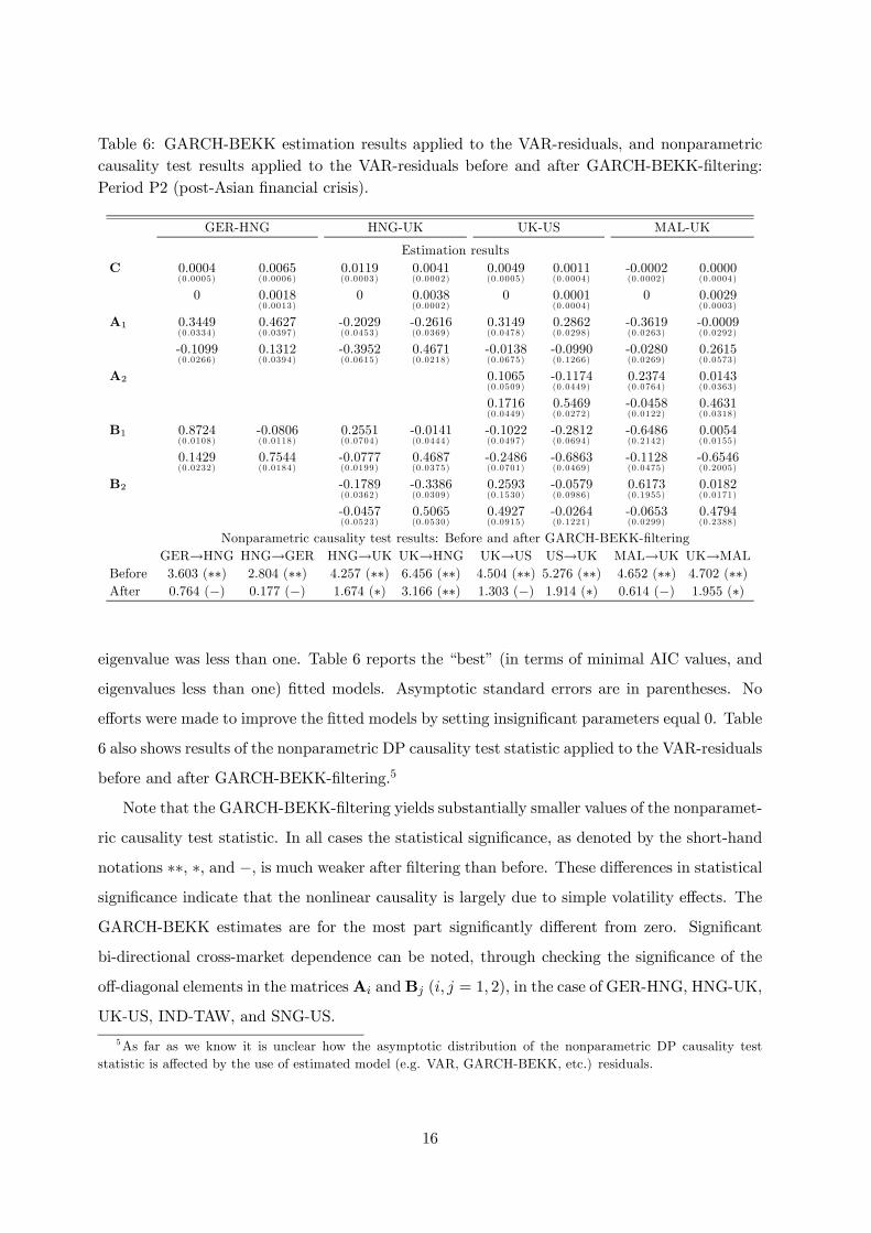
Table 6: GARCH-BEKK estimation results applied to the VAR-residuals, and nonparametriccausality test results applied to the VAR-residuals before and after GARCH-BEKK-filtering:Period P2 (post-Asian financial crisis).

GER-HNG HNG-UK UK-US MAL-UK

Estimation resultsC 0.0004 0.0065 0.0119 0.0041 0.0049 0.0011 -0.0002 0.0000

(0.0005) (0.0006) (0.0003) (0.0002) (0.0005) (0.0004) (0.0002) (0.0004)

0 0.0018 0 0.0038 0 0.0001 0 0.0029(0.0013) (0.0002) (0.0004) (0.0003)

A1 0.3449 0.4627 -0.2029 -0.2616 0.3149 0.2862 -0.3619 -0.0009(0.0334) (0.0397) (0.0453) (0.0369) (0.0478) (0.0298) (0.0263) (0.0292)

-0.1099 0.1312 -0.3952 0.4671 -0.0138 -0.0990 -0.0280 0.2615(0.0266) (0.0394) (0.0615) (0.0218) (0.0675) (0.1266) (0.0269) (0.0573)

A2 0.1065 -0.1174 0.2374 0.0143(0.0509) (0.0449) (0.0764) (0.0363)

0.1716 0.5469 -0.0458 0.4631(0.0449) (0.0272) (0.0122) (0.0318)

B1 0.8724 -0.0806 0.2551 -0.0141 -0.1022 -0.2812 -0.6486 0.0054(0.0108) (0.0118) (0.0704) (0.0444) (0.0497) (0.0694) (0.2142) (0.0155)

0.1429 0.7544 -0.0777 0.4687 -0.2486 -0.6863 -0.1128 -0.6546(0.0232) (0.0184) (0.0199) (0.0375) (0.0701) (0.0469) (0.0475) (0.2005)

B2 -0.1789 -0.3386 0.2593 -0.0579 0.6173 0.0182(0.0362) (0.0309) (0.1530) (0.0986) (0.1955) (0.0171)

-0.0457 0.5065 0.4927 -0.0264 -0.0653 0.4794(0.0523) (0.0530) (0.0915) (0.1221) (0.0299) (0.2388)

Nonparametric causality test results: Before and after GARCH-BEKK-filteringGER→HNG HNG→GER HNG→UK UK→HNG UK→US US→UK MAL→UK UK→MAL

Before 3.603 (∗∗) 2.804 (∗∗) 4.257 (∗∗) 6.456 (∗∗) 4.504 (∗∗) 5.276 (∗∗) 4.652 (∗∗) 4.702 (∗∗)After 0.764 (−) 0.177 (−) 1.674 (∗) 3.166 (∗∗) 1.303 (−) 1.914 (∗) 0.614 (−) 1.955 (∗)

eigenvalue was less than one. Table 6 reports the “best” (in terms of minimal AIC values, and

eigenvalues less than one) fitted models. Asymptotic standard errors are in parentheses. No

efforts were made to improve the fitted models by setting insignificant parameters equal 0. Table

6 also shows results of the nonparametric DP causality test statistic applied to the VAR-residuals

before and after GARCH-BEKK-filtering.5

Note that the GARCH-BEKK-filtering yields substantially smaller values of the nonparamet-

ric causality test statistic. In all cases the statistical significance, as denoted by the short-hand

notations ∗∗, ∗, and −, is much weaker after filtering than before. These differences in statisticalsignificance indicate that the nonlinear causality is largely due to simple volatility effects. The

GARCH-BEKK estimates are for the most part significantly different from zero. Significant

bi-directional cross-market dependence can be noted, through checking the significance of the

off-diagonal elements in the matricesAi andBj (i, j = 1, 2), in the case of GER-HNG, HNG-UK,

UK-US, IND-TAW, and SNG-US.

5As far as we know it is unclear how the asymptotic distribution of the nonparametric DP causality teststatistic is affected by the use of estimated model (e.g. VAR, GARCH-BEKK, etc.) residuals.

16

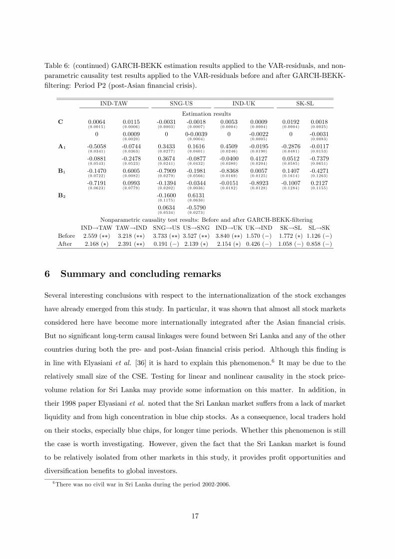
Table 6: (continued) GARCH-BEKK estimation results applied to the VAR-residuals, and non-parametric causality test results applied to the VAR-residuals before and after GARCH-BEKK-filtering: Period P2 (post-Asian financial crisis).

IND-TAW SNG-US IND-UK SK-SL

Estimation resultsC 0.0064 0.0115 -0.0031 -0.0018 0.0053 0.0009 0.0192 0.0018

(0.0015) (0.0006) (0.0003) (0.0007) (0.0004) (0.0004) (0.0004) (0.0025)

0 0.0009 0 0-0.0039 0 -0.0022 0 -0.0031(0.0020) (0.0004) (0.0005) (0.0083)

A1 -0.5058 -0.0744 0.3433 0.1616 0.4509 -0.0195 -0.2876 -0.0117(0.0341) (0.0363) (0.0277) (0.0401) (0.0246) (0.0190) (0.0481) (0.0153)

-0.0881 -0.2478 0.3674 -0.0877 -0.0400 0.4127 0.0512 -0.7379(0.0543) (0.0523) (0.0241) (0.0432) (0.0380) (0.0204) (0.0585) (0.0651)

B1 -0.1470 0.6005 -0.7909 -0.1981 -0.8368 0.0057 0.1407 -0.4271(0.0722) (0.0082) (0.0279) (0.0566) (0.0169) (0.0125) (0.1614) (0.1263)

-0.7191 0.0993 -0.1394 -0.0344 -0.0151 -0.8923 -0.1007 0.2127(0.0623) (0.0779) (0.0202) (0.0036) (0.0182) (0.0128) (0.1284) (0.1155)

B2 -0.1600 0.6131(0.1175) (0.0630)

0.0634 -0.5790(0.0534) (0.0273)

Nonparametric causality test results: Before and after GARCH-BEKK-filteringIND→TAW TAW→IND SNG→US US→SNG IND→UK UK→IND SK→SL SL→SK

Before 2.559 (∗∗) 3.218 (∗∗) 3.733 (∗∗) 3.527 (∗∗) 3.840 (∗∗) 1.570 (−) 1.772 (∗) 1.126 (−)After 2.168 (∗) 2.391 (∗∗) 0.191 (−) 2.139 (∗) 2.154 (∗) 0.426 (−) 1.058 (−) 0.858 (−)

6 Summary and concluding remarks

Several interesting conclusions with respect to the internationalization of the stock exchanges

have already emerged from this study. In particular, it was shown that almost all stock markets

considered here have become more internationally integrated after the Asian financial crisis.

But no significant long-term causal linkages were found between Sri Lanka and any of the other

countries during both the pre- and post-Asian financial crisis period. Although this finding is

in line with Elyasiani et al. [36] it is hard to explain this phenomenon.6 It may be due to the

relatively small size of the CSE. Testing for linear and nonlinear causality in the stock price-

volume relation for Sri Lanka may provide some information on this matter. In addition, in

their 1998 paper Elyasiani et al. noted that the Sri Lankan market suffers from a lack of market

liquidity and from high concentration in blue chip stocks. As a consequence, local traders hold

on their stocks, especially blue chips, for longer time periods. Whether this phenomenon is still

the case is worth investigating. However, given the fact that the Sri Lankan market is found

to be relatively isolated from other markets in this study, it provides profit opportunities and

diversification benefits to global investors.

6There was no civil war in Sri Lanka during the period 2002-2006.

17

The leading role of the US market in the world stock market is clearly visible throughout all

causality tests and in both time periods. This is consistent with earlier findings by Eun and Shim

[45]. In the post-Asian period the US market is influenced by Germany, Japan, Singapore, the

UK, India, Malaysia, South Korea, and Taiwan; see Tables 4 and 5. This confirms the increased

financial links between the US and the world economy. On the other hand, the Japanese market

explains relatively little of the stock price movements in other markets once linear effects have

been removed through VAR-filtering; see Table 5. This finding gives further support to an earlier

study by Malliaris and Urrutia [46] who concluded that the Japanese market plays a passive

role in transmitting information to other stock markets.

Another finding is that no major differences exist between the persistence and strength of the

bi-directional causal linkages among the industrialized markets and the emerging markets in the

post-Asian financial crisis period. These results, apart from offering a much better understanding

of the dynamic linear and nonlinear relationships underlying the movements of emerging Asian

stock markets than has been noted until now, have many implications for market efficiency. For

instance, they may be useful in future research to quantify the process of financial integration

of emerging markets. Also, the presence of causal nonlinear relationships may influence the

greater predictability of these markets. This may, for instance, be investigated through a trading

strategy using multivariate (non)parametric methodology.

Another topic for future research concerns the source(s) or cause(s) of the nonlinear causal

linkages. Previously we conjectured that volatility effects might induce nonlinear causality. The

fitted GARCH-BEKK models provide some guidance on this matter, but only in some special

cases. Alternative specific parametrized structural models may be employed. Related to this,

is a need for determining the economic factors driving the interdependence of emerging stock

markets. Pretorius [47] studies this topic empirically by using cross-section and linear time-series

regression models. But more research is needed.

Finally, the empirical finding of nonlinear causal relationships between emerging stock mar-

kets may be analyzed in terms of their implications for the efficiency of these markets. The

fact that there are long-term links between various markets may imply that excess (risk- and

transactions cost-adjusted) returns exist. Given such inefficiency, authorities in emerging mar-

kets may then reconsider their policies regarding, for instance, brokerage fees, stock exchange

charges, and other equity trading costs.

18

Acknowledgments

We acknowledge comments from a referee which were very useful in improving the presentation.

Selliah Sivarajasingham’s research was supported in part by a grant from the National Center for

Advanced Studies in Humanities and Social Sciences (NCAS), Sri Lanka, and the Department

of Quantitative Economics, University of Amsterdam. He would like to thank the members of

the Department for their hospitality during his stay.

References

[1] M. King, S. Wadhwani, Transmission of volatility between stock markets, Rev. Finan. Stud.

3 (1990) 5-33.

[2] C.W.J. Granger, Investigating causal relations by econometric models and cross-spectral

methods, Econometrica 37 (1969) 424-438.

[3] D.A. Hsieh, Testing of non-linear dependence in daily foreign exchange rates, J. Business

62 (1989) 339-368.

[4] D.A. Hsieh, Chaos and non-linear dynamics; application to financial markets, J. Finan. 5

(1991) 1839-1877.

[5] C. Hiemstra, J.D. Jones, Testing for linear and nonlinear Granger causality in the stock

price-volume relation, J. Finan. 49 (1994) 1639-1664.

[6] E. Baek, W. Brock, A general test for non-linear Granger causality: Bivariate model,

Working paper, Iowa State University and University of Wisconsin, Madison, WI, 1992.

[7] P. Silvapulle, J-S. Choi, Testing for linear and nonlinear Granger causality in the stock

price-volume relation: Korean evidence, Quarterly Rev. Econ. Finan. 39 (1999) 59-76.

[8] G.P. Dwyer, P. Locke, W. Yu, Index arbitrage and nonlinear dynamics between the S&P

500 futures and cash, Rev. Finan. Stud. 9 (1996) 301-332.

[9] A. Kanas, Nonlinearity in the stock price - dividend relation, J. Int. Money and Finance

24 (2005) 583-606.

[10] Y. Ma, A. Kanas, Testing for nonlinear relationship among fundamentals and exchange

rates in the ERM, J. Finan. Econ. 19 (2000) 135-152.

19

[11] C. Brooks, T. Henry, Linear and non-linear transmission of equity return volatility: Evi-

dence from the US, Japan, and Australia, Econ. Modeling, 17 (2000) 497-513.

[12] C. Diks, V. Panchenko, A note on the Hiemstra-Jones test for Granger non-causality, Stud.

Nonlinear Dynamics and Econometrics 9 (2005), art. 4.

[13] C. Diks, V. Panchenko, A new statistic and practical guidelines for nonparametric Granger

causality testing, J. Econ. Dynamics & Control 30 (2006) 1647-1669.

[14] B. Arshanapalli, J. Doukas, International stock market linkages: Evidence from the pre-

and post October 1987 period, J. Banking and Finance 17 (1993) 193-208.

[15] Y. Hamao, R. Masulis, V. Ng, Correlation in price changes and volatility across international

stock markets, Rev. Finan. Stud. 3 (1990) 281-307.

[16] E. Roca, Short-term and long-term price linkages between the equity markets of Australia

and its major trading partners, Appl. Finan. Econ. 9 (1999) 501-511.

[17] R. Smyth, M. Nandha, Bivariate causality between exchange rates and stock prices in South

Asia, Appl. Econ. Lett. 10 (2003) 699-704.

[18] C.G. Gilmore, G.M. McManus, International portfolio diversification: US and Central Eu-

ropean equity markets, Emerging Markets Rev. 3 (2002) 69-83.

[19] L. Gündüz, A. Hatemi-J, “Stock price and volume relation in emerging markets, Emerging

Markets Finance and Trade 41 (2005) 29-44.

[20] T. Choudhry, Stochastic trends in stock prices: Evidence from Latin American markets, J.

Macroeconomics 19 (1997) 285-304.

[21] A. Christofi, A. Pericli, Correlation in price changes and volatility of major Latin American

stock markets, J. Multinational Finan. Manage. 9 (1999) 79-93.

[22] G. Chen, M. Firth, O.M. Rui, Stock market linkages: Evidence from Latin America, J.

Banking and Finan. 26 (2002) 1113-1141.

[23] A.M. Masih, R. Masih, Dynamic linkages and the propagation mechanism driving major

international stock markets: an analysis of the pre- and post-crash eras, Quart. Rev. Econ.

Finan. 37 (1997) 859-885.

20

[24] A.M. Masih, R. Masih, Are Asian stock market fluctuations due mainly to intra-regional

contagion effect? Evidence based on Asian emerging stock markets, Pacific-Basin Finan. J.

7 (1999) 251-282.

[25] K. Phylaktis, F. Ravazzolo, Stock market linkages in emerging markets: im-

plications for international portfolio diversification, 2003. Downloadable from:

http://www.cass.city.ac.uk/emg/workingpapers/stock−market−linkages.pdf

[26] B. Arshanapalli, J. Doukas, J., L.H.P. Lang, Pre- and post-October 1987 stock market

linkages between US and Asian makets, Pacific-Basin Finan. J. 3 (1995) 57-73.

[27] G.M. Caporale, N. Pittis, N. Spagnolo, Testing for causality-in-variance: An application

the East Asian markets, Int. J. Finan. Econ. 7 (2002) 235-245.

[28] M. Najand, A causality test of the October crash of 1987: evidence from Asian stock

markets, J. Business Finan.& Accounting 23 (1996) 439-448.

[29] H.C. Sheng, A.H. Tu, A study of cointegration and variance decomposition among national

equity indices before and after the period of the Asian financial crisis J. Multinational

Finan. Manage. 10 (2000) 345-365.

[30] E. Weber, Volatility and causality in Asia Pacific financial markets, SFB 649 Discussion

paper 2007-004, 2007. Downloadable from: http://sfb649.wiwi.hu-berlin.de.

[31] P. Narayan, R. Smyth, M. Nandha, Interdependence and dynamic linkages between the

emerging stock markets of South Asia, Accounting and Finan. 44 (2004) 419-439.

[32] D.M. Hunter, Linear and nonlinear dynamic linkages between emerging market ADRs and

their underlying stocks, 2003. Downloadable as: SSRN-ID586542-code97395.pdf.

[33] Z.A. Ozdemir, E. Cakan, Non-linear dynamic linkages in the international stock markets,

Physica A 377 (2007) 173-180.

[34] G. Bekaert, C.R. Harvey, R. Lumsdaine, Dating the integration of world equity markets,

Working paper, Stanford University, Stanford, CA, 2001.

[35] M. Ariff, A. Khalid, Liberalization, growth and the Asian financial crisis, Cheltenham:

Edward Elgar, 2004.

21

[36] E. Elyasiani, P. Perera, T.N. Puri, Interdependence and dynamic linkages between stock

markets of Sri Lanka and its trading partners, J. Multinational Finan. Manage. 8 (1998)

89-101.

[37] Standard and Poors, Global Stock Markets Factbook, New York, 2005.

[38] J.L. Harvill, B.K. Ray, A note on tests for nonlinearity in a vector time series, Biometrika

86 (1999) 728-734.

[39] D.M. Keenan, A Tukey nonadditivity-type test for time series nonlinearity, Biometrika 72

(1985) 39-44.

[40] J. Geweke, R. Meese, W. Dent, Comparing alternative tests of causality in temporal sys-

tems, J. Econometrics 21 (1983) 161-194.

[41] C. Wu, Y. Su, Dynamic relations among international stock markets, Int. Rev. Econ. Finan.

7 (1998) 63-84.

[42] I. Domowitz, J. Glen, A. Madhavan, Liquidity, volatility, and equity trading costs across

countries and over time, Working paper 322, William Davidson Institute and Int. Finance

4 (2001) 221-55.

[43] R.F. Engle, F.K. Kroner, Multivariate simultaneous generalized ARCH, Econometric The-

ory 11 (1995) 122-150.

[44] L. Bauwens, S. Laurent, J.V. Rombouts, Multivariate GARCH models: A survey, J. Appl.

Econometrics 21 (2006) 79-109.

[45] C. Eun, S. Shim, International transmission of stock market movements, J. Finan. Quant.

Anal. 24 (1989) 241-256.

[46] A.G. Malliaris, J.L. Urrutia, The international crash of October 1987: Causality tests, J.

Finan. Quant. Anal. 27 (1992) 353-364.

[47] E. Pretorius, Economic determinants of emerging stock market interdependence, Emerging

Markets Rev. 3 (2002) 84-105.

22