This article was downloaded by: [Dogu Akdeniz University]On: 16 July 2015, At: 05:54Publisher: RoutledgeInforma Ltd Registered in England and Wales Registered Number: 1072954 Registered office: 5 HowickPlace, London, SW1P 1WG

Click for updates

Regional StudiesPublication details, including instructions for authors and subscription information:http://www.tandfonline.com/loi/cres20

Causal Relationship between Asset Prices and Outputin the United States: Evidence from the State-LevelPanel Granger Causality TestFurkan Emirmahmutoglua, Mehmet Bacilarb, Nicholas Apergisc, Beatrice D. Simo-Kengneb,Tsangyao Changd & Rangan Guptab

a Department of Econometrics, Gazi University, Ankara, Turkeyb Department of Economics, University of Pretoria, 0002 Pretoria, South Africac Northumbria University, Newcastle upon Tune, UKd Department of Finance, Feng Chia University, No. 100 Wenhua Road, 40724 Taichung,TaiwanPublished online: 16 Jul 2015.

To cite this article: Furkan Emirmahmutoglu, Mehmet Bacilar, Nicholas Apergis, Beatrice D. Simo-Kengne, Tsangyao Chang& Rangan Gupta (2015): Causal Relationship between Asset Prices and Output in the United States: Evidence from theState-Level Panel Granger Causality Test, Regional Studies, DOI: 10.1080/00343404.2015.1055462

To link to this article: http://dx.doi.org/10.1080/00343404.2015.1055462

PLEASE SCROLL DOWN FOR ARTICLE

Taylor & Francis makes every effort to ensure the accuracy of all the information (the “Content”) containedin the publications on our platform. However, Taylor & Francis, our agents, and our licensors make norepresentations or warranties whatsoever as to the accuracy, completeness, or suitability for any purpose ofthe Content. Any opinions and views expressed in this publication are the opinions and views of the authors,and are not the views of or endorsed by Taylor & Francis. The accuracy of the Content should not be reliedupon and should be independently verified with primary sources of information. Taylor and Francis shallnot be liable for any losses, actions, claims, proceedings, demands, costs, expenses, damages, and otherliabilities whatsoever or howsoever caused arising directly or indirectly in connection with, in relation to orarising out of the use of the Content.

This article may be used for research, teaching, and private study purposes. Any substantial or systematicreproduction, redistribution, reselling, loan, sub-licensing, systematic supply, or distribution in anyform to anyone is expressly forbidden. Terms & Conditions of access and use can be found at http://www.tandfonline.com/page/terms-and-conditions

Causal Relationship between Asset Prices andOutput in the United States: Evidence from the

State-Level Panel Granger Causality Test

FURKAN EMIRMAHMUTOGLU†, MEHMET BACILAR‡, NICHOLAS APERGIS§,BEATRICE D. SIMO-KENGNE‡, TSANGYAO CHANG¶ and RANGAN GUPTA‡*

†Department of Econometrics, Gazi University, Ankara, Turkey. Email: emirfurkan@gmail.com‡Department of Economics, University of Pretoria, 0002 Pretoria, South Africa. Emails: mehmet@mbalcilar.net,

beatrice.simo_kengne@up.ac.za and rangan.gupta@up.ac.za§Northumbria University, Newcastle upon Tune, UK. Email: nicholas.apergis@northumbria.ac.uk

¶Department of Finance, Feng Chia University, No. 100Wenhua Road, 40724 Taichung, Taiwan. Email: tychang@fcu.edu.tw

(Received April 2014; in revised form May 2015)

EMIRMAHMUTOGLU F., BACILAR M., APERGIS N., SIMO-KENGNE B. D., CHANG T. and GUPTA R. Causal relationshipbetween asset prices and output in the United States: evidence from the state-level panel Granger causality test, RegionalStudies. This paper investigates the causal relationship between asset prices and output across US states using a bootstrap panelGranger causality approach which allows not only for heterogeneity and cross-sectional dependence to be accounted for butalso interdependency between asset markets. Empirical results from a trivariate vector autoregression (VAR) comprising realhouse prices, real stock prices and real per capita personal income over 1975–2012 reveal the existence of a unidirectional causalityrunning from both asset prices to output. This confirms the leading indicator property of asset prices for the real economy, whilealso substantiating the wealth and/or collateral transmission mechanism.

House prices Stock prices Output Granger causality

EMIRMAHMUTOGLU F., BACILAR M., APERGIS N., SIMO-KENGNE B. D., CHANG T. and GUPTA R.美国资产价格与产出之间的因果关係：州层级的面板格兰杰因果关係检定证据，区域研究。本文运用自助面板格兰杰因果关係方法，探讨

美国各州的资产价格和产出之间的因果关係。该方法不仅能够考量异质性与跨部门依赖，亦可同时考量资产市场之间的相互依赖性。包含 1975年至 2012年间真实住宅价格、真实股票价格与真实人均所得的三元向量自迴归（VAR）模型的经验结果，显示出从资产价格到产出，单一方向的因果关係同时存在。此一结果，确认了资产价格之于实际经济所扮演的先导指标属性，并同时证实了财富与／或抵押传递机制。

住宅价格 股票价格 产出 格兰杰因果关係

EMIRMAHMUTOGLU F., BACILAR M., APERGIS N., SIMO-KENGNE B. D., CHANG T. et GUPTA R. Le lien de causalité entre lesprix des actifs et la production aux États-Unis: des résultats provenant du test de causalité au sens de Granger par panel à l’échelle del’état, Regional Studies. Cet article examine le lien de causalité entre les prix des actifs et la production à travers les états aux É-Uemployant une méthode de causalité au sens de Granger par panel étendu au modèle bootstrap qui tient compte non seulement del’hétérogénéité et de la dépendance transversale mais aussi de l’interdépendance entre les marchés des actifs. Les résultats empiriquesprovenant d’un modèle autorégressif multivarié (VAR) qui comprend les prix réels de l’immobilier, les prix réels des actifs et lerevenu personnel réel par tête entre 1975 et 2012 laissent voir la présence d’une causalité unidirectionnelle allant des prix des actifs àla production. Cela confirme la caractéristique principale du prix des actifs comme indicateur de l’économie réelle, tout en justifiantégalement le mécanisme de transmission de la richesse et/ou du nantissememnt.

Prix de l’immobilier Valeur des actions Production Causalité au sens de Granger

EMIRMAHMUTOGLU F., BACILAR M., APERGIS N., SIMO-KENGNE B. D., CHANG T. und GUPTA R. Kausale Beziehungzwischen Vermögenspreisen und Produktion in den USA: Belege eines Granger-Kausalitätstests für ein Panel auf Bundesstaatse-bene, Regional Studies. In diesem Beitrag wird die kausale Beziehung zwischen Vermögenspreisen und Produktion in den verschie-denen US-Bundesstaaten mithilfe eines grangerschen Bootstrap-Panel-Kausalitätsansatzes untersucht, der nicht nur eineBerücksichtigung der Heterogenität und Querschnittsdependenz, sondern auch der Interdependenz zwischen

*Corresponding author.

Regional Studies, 2015

http://dx.doi.org/10.1080/00343404.2015.1055462

© 2015 Regional Studies Associationhttp://www.regionalstudies.org

Dow

nloa

ded

by [

Dog

u A

kden

iz U

nive

rsity

] at

05:

54 1

6 Ju

ly 2

015

Vermögensmärkten ermöglicht. Die empirischen Ergebnisse einer trivariaten Vektorautoregression (VAR) mit realen Hauspreisen,realen Aktienkursen und realem persönlichen Pro-Kopf-Einkommen im Zeitraum von 1975 bis 2012 verdeutlichen die Existenzeiner unidirektionalen Kausalität, die von beiden Vermögenspreisen zur Produktion verläuft. Dies bestätigt die Eigenschaft derVermögenspreise als führende Indikatoren für die Realwirtschaft und dient zugleich als Beleg für den Mechanismus zurÜbertragung von Vermögen und/oder Sicherheiten.

Hauspreise Aktienkurse Produktion Granger-Kausalität

EMIRMAHMUTOGLU F., BACILAR M., APERGIS N., SIMO-KENGNE B. D., CHANG T. y GUPTA R. Relación causal entre losprecios de los activos y la producción en los Estados Unidos: evidencia de la prueba de causalidad de Granger en un panel deámbito estatal, Regional Studies. En este artículo investigamos la relación causal entre los precios de los activos y la producciónen los Estados de EE.UU. mediante un enfoque de bootstrap de causalidad de Granger en un panel que nos permite tener encuenta no solo la heterogeneidad y la dependencia transversal sino también la interdependencia entre los mercados de activos.Los resultados empíricos de una autorregresión vectorial (VAR) trivariada que consta de precios reales de la vivienda, cotizacionesbursátiles reales y los ingresos personales reales per capita durante el periodo de 1975 a 2012 indican la existencia de una causalidadunidireccional que va de los precios de ambos activos a la producción. Esto confirma la propiedad de los precios de los activos comoindicador líder para la economía real, pero también sirve como evidencia para el mecanismo de transmisión de riqueza y/ogarantías.

Precios de la vivienda Cotizaciones bursátiles Producción Causalidad de Granger

JEL classifications: C33, G10, O18

INTRODUCTION

With the ‘Great recession’, it has become increasinglyclear that asset prices constitute a class of leading indi-cators of the real economy. Forward-looking assetprices may provide useful information about the paceof future economic activity, specifically the futurechanges in output and/or inflation (STOCK andWATSON, 2003; FORNI et al., 2003; GUPTA andHARTLEY, 2013). Despite the evidence of this leadingindicator property, the causal relationships betweenoutput and asset prices appear to be complicated andempirically difficult to identify (INTERNATIONAL

MONETARY FUND (IMF), 2000). One strand of the lit-erature emphasizes that asset prices influence currentexpenditure solely to the extent that they are ‘leadingindicators’ of the future variations in economic activity.Considering that current prices represent the discountedvalue of the expected dividend growth, to the extentthat asset prices are traded in fully and well-informedauction markets, expectation about the future dividendgrowth tend to be rational. From this valuation modelhypothesis, there is no causal relationship runningfrom asset prices to the real economy; asset marketsbeing essentially a ‘side show’ of the causal linkbetween current and future output growth (IMF, 2000).

Differently from the ‘side show’ perspective, the per-manent income hypothesis supports a behavioural causalrelationship running from asset prices to economicactivity through the traditional wealth and/or collateraleffects. Rather than restricted to the single leading indi-cators role, increasing asset prices have a direct effect onagents’ lifetime wealth which in turn may affect theconsumption behaviour and, henceforth, the output.

Indirectly, changes in asset prices may also influencethe borrowing capacity of households and firms withsignificant implications on the consumption and invest-ment plans which in turn stimulate the productionprocess. Consequently, the causality, if any, is expectedto run from asset prices to output; with consumptioneffect serving as a key link between the two variables.However, some researchers including BAJARI et al.(2005), LI and YAO (2007) and BUITER (2008) indicatethat asset price changes do not necessary have a signifi-cant net effect on aggregate consumption; hence, advo-cating the absence of any causal relationship betweenasset prices and output.

Besides the wealth and/or collateral mechanisms,DEMARY (2010) documents a direct mechanismthrough which economic activity may impact houseprices. When there is a positive shock on output, firmsincrease the labour demand that raises households’labour revenue. The subsequent increase in incomecan be either invested in assets or consumed (inhousing and non-housing goods). When the economyis in upswing, having a job qualifies for a cheap mort-gage loan and firms need more office space. This willtrigger the demand for housing which will translateinto an increase in house prices. Similarly, economicexpansion may signal appropriate time for investing instocks, resulting in an increase in stock prices. Conse-quently, the causality may also run from economicactivity to asset prices, making the relationshipbetween the financial and real sectors a bidirectionalone. Given the difficulty of practically disentanglingbetween the above transmission mechanisms, the

2 Furkan Emirmahmutoglu et al.

Dow

nloa

ded

by [

Dog

u A

kden

iz U

nive

rsity

] at

05:

54 1

6 Ju

ly 2

015

nature of the causal linkages between asset prices andoutput should be investigated empirically.

Housing and stock are the two widely held assets inthe United States. Based on IACOVIELLO (2011), non-housing wealth (housing wealth) was calculated to be41.04% (37.78%) of a US household’s total assets and52.07% (47.93%) of a US household’s total net worth.Given the relative importance of equities and housingin the US households’ total wealth, the dynamics ofasset prices are likely to be correlated with the businesscycle fluctuations. In fact, the average growth rate ofreal per capita personal income of 1.12% in 1980s isassociated with an average annual growth rate of−0.71% in real house prices and 5.70% in real stockprices. In 1990s, these growth rates increase and reach1.32%, 0.07% and 11.08%, respectively. In the lastdecade, while real house prices grow faster at anaverage growth rate of 1.50%, there is a slowdown inthe evolution of both real per capita personal incomeand real stock prices which record an annual growthof 0.86% and −3.89%, respectively. However, thisapparent co-movement of asset prices with income (asdepicted by Fig. A1 in Appendix A in the Supplementaldata online) does not prove that fluctuations in assetprices cause changes in income, or vice versa. Thepresent study tests the existence of the causal relationshipbetween housing/stock market prices and output across50 US states and the District of Columbia (DC) over theperiod 1975–2012. Understanding the causal directionbetween asset prices and income is important, sincethis determines possible policy interventions in case ofshocks to each of these variables.

Empirically, there is strong evidence that changes inasset prices affect the US economic activity, particularlyconsumption (see SIMO-KENGNE et al., 2013, 2015, fordetailed literature reviews). However, there are fewexceptions that focus on the output effect of assetprices. These include MAURO (2000), CARLSTROM

et al. (2002), DEMARY (2010), MILLER et al. (2011),APERGIS et al. (2015) and NYAKABAWO et al. (2014).While MAURO (2000) finds a positive impact of stockreturns on output growth, MILLER et al. (2011) depicta positive impact of house price appreciation on econ-omic growth – with both these studies suggesting a uni-directional causality running from asset prices to output.Unlike these authors, DEMARY (2010) identifies impor-tant feedbacks from macroeconomic variables (includ-ing output) to house prices, hence suggesting abidirectional relationship between house prices andthe macro-economy. This finding was in line withCARLSTROM et al. (2002), who document a two-waycausality between stock market and output. Morerecently, APERGIS et al. (2015) explicitly investigatethe causality between house prices and output acrossUS metropolitan areas and finds bidirectional causality,as in the national-level analysis of NYAKABAWO et al.(2014), based on time-varying causality. However,both Apergis et al. and Nyakabawo et al. fail to

account for interdependency between asset markets(house and stock) with possible implications on thecausal linkages with the real sector. More importantly,Apergis et al. rely on a panel vector error correctionmethodology (VECM), which requires pre-testing forstationarity and co-integration and is, therefore,subject to pre-test bias. To mitigate the issue of pre-test bias, EMIRMAHMUTOGLU and KOSE (2011)recently proposed a bootstrap panel causality algorithmthat does not entail pre-testing of the time-series prop-erties but which requires the size of the time series (T ) tobe greater than the number of cross-sections (N ).Therefore, the present application makes use of thebootstrap methodology to analyse the causal relationshipbetween asset markets and output across individual USstates, categorized as agricultural and industrial,1 andfor the entire panels of agricultural and industrialstates. This, in turn, helps one understand which statesare specifically driving the causal relationships for theagricultural and industrial states taken together. To thebest of the authors’ knowledge, this is the first attemptto analyse causal relationships between asset prices andoutput for US states, at individual and aggregate levels,by accounting for cross-sectional dependence andheterogeneity.2

A modified version of the panel causality developedby EMIRMAHMUTOGLU and KOSE (2011), originallyto analyse causality in a bivariate setting, is employed,which allows one to control not only for heterogeneityand cross-sectional dependence across states, but also forinteractions between housing and stock markets. SinceUS states are subject to significant spatial effects giventheir high level of integration, PESARAN (2006) pointsout that ignoring cross-sectional dependency may leadto substantial bias and size distortions. Furthermore,unlike traditional causality approaches that rely on co-integration techniques, the bootstrap methodologydoes not require testing for integration and co-inte-gration, hence preventing the issue of pre-test bias(EMIRMAHMUTOGLU and KOSE, 2011).

The paper is structured as follows. The next sectionsets out the empirical procedure and discusses the esti-mation results. The last section concludes.

EMPIRICAL ANALYSIS

The analysis in this paper is based on annual data for 50US states, as well as DC, over the period 1975–2012. Alltransaction-based (estimated using sales prices andappraisal data) house price data are obtained from theFederal Housing Finance Agency (FHFA), while stockprice, measured by the S&P500, is acquired from theFRED database of the Federal Reserve bank ofSt. Louis. Following the extant literature on regional(state and metropolitan statistical area (MSA) levels) ana-lyses, output is proxied by the per capita personalincome drawn from the Bureau of Economic Analysis

Causal Relationship between Asset Prices and Output in the United States 3

Dow

nloa

ded

by [

Dog

u A

kden

iz U

nive

rsity

] at

05:

54 1

6 Ju

ly 2

015

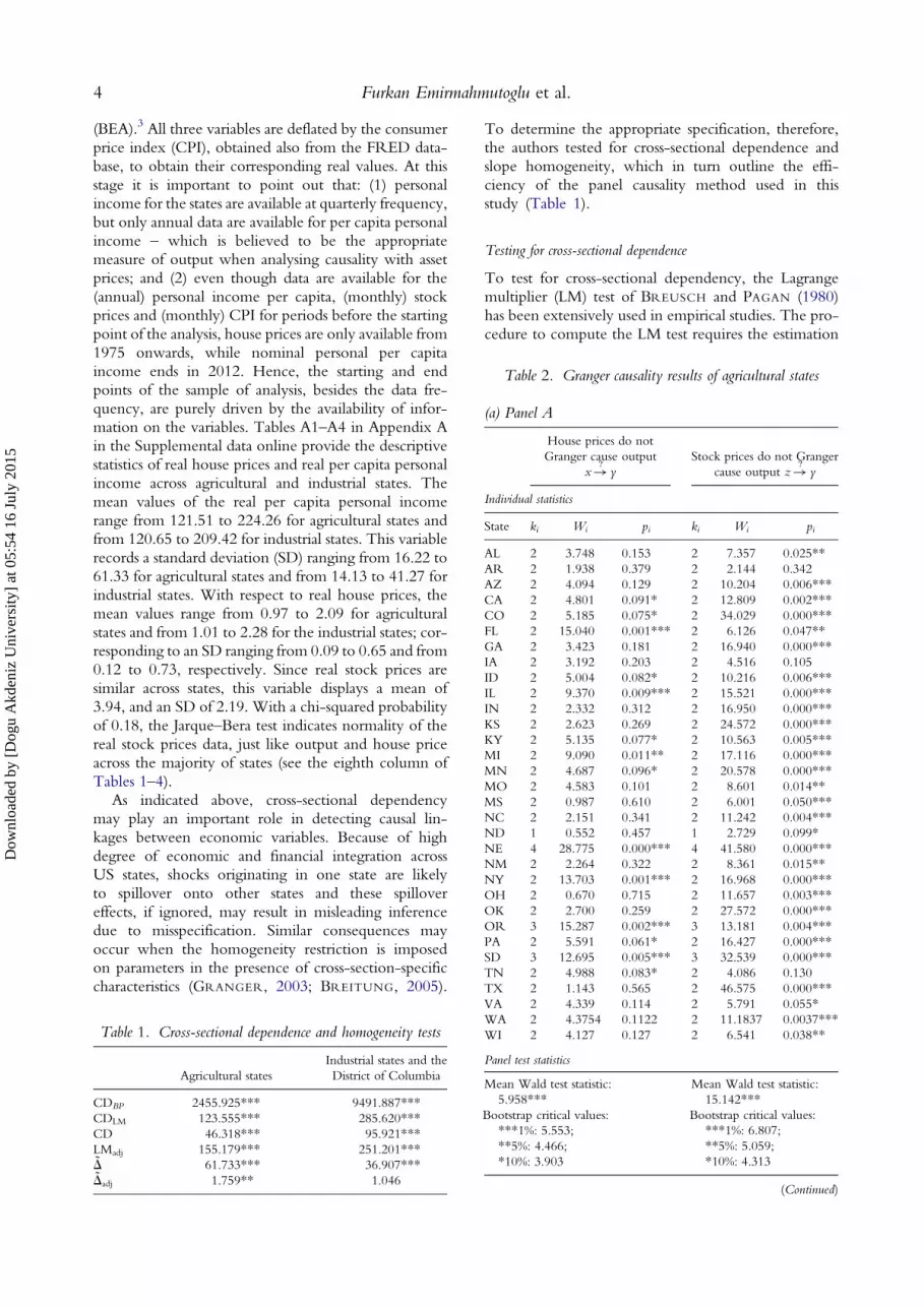
(BEA).3 All three variables are deflated by the consumerprice index (CPI), obtained also from the FRED data-base, to obtain their corresponding real values. At thisstage it is important to point out that: (1) personalincome for the states are available at quarterly frequency,but only annual data are available for per capita personalincome – which is believed to be the appropriatemeasure of output when analysing causality with assetprices; and (2) even though data are available for the(annual) personal income per capita, (monthly) stockprices and (monthly) CPI for periods before the startingpoint of the analysis, house prices are only available from1975 onwards, while nominal personal per capitaincome ends in 2012. Hence, the starting and endpoints of the sample of analysis, besides the data fre-quency, are purely driven by the availability of infor-mation on the variables. Tables A1–A4 in Appendix Ain the Supplemental data online provide the descriptivestatistics of real house prices and real per capita personalincome across agricultural and industrial states. Themean values of the real per capita personal incomerange from 121.51 to 224.26 for agricultural states andfrom 120.65 to 209.42 for industrial states. This variablerecords a standard deviation (SD) ranging from 16.22 to61.33 for agricultural states and from 14.13 to 41.27 forindustrial states. With respect to real house prices, themean values range from 0.97 to 2.09 for agriculturalstates and from 1.01 to 2.28 for the industrial states; cor-responding to an SD ranging from 0.09 to 0.65 and from0.12 to 0.73, respectively. Since real stock prices aresimilar across states, this variable displays a mean of3.94, and an SD of 2.19. With a chi-squared probabilityof 0.18, the Jarque–Bera test indicates normality of thereal stock prices data, just like output and house priceacross the majority of states (see the eighth column ofTables 1–4).

As indicated above, cross-sectional dependencymay play an important role in detecting causal lin-kages between economic variables. Because of highdegree of economic and financial integration acrossUS states, shocks originating in one state are likelyto spillover onto other states and these spillovereffects, if ignored, may result in misleading inferencedue to misspecification. Similar consequences mayoccur when the homogeneity restriction is imposedon parameters in the presence of cross-section-specificcharacteristics (GRANGER, 2003; BREITUNG, 2005).

To determine the appropriate specification, therefore,the authors tested for cross-sectional dependence andslope homogeneity, which in turn outline the effi-ciency of the panel causality method used in thisstudy (Table 1).

Testing for cross-sectional dependence

To test for cross-sectional dependency, the Lagrangemultiplier (LM) test of BREUSCH and PAGAN (1980)has been extensively used in empirical studies. The pro-cedure to compute the LM test requires the estimation

Table 2. Granger causality results of agricultural states

(a) Panel A

House prices do notGranger cause output

x�? yStock prices do not Granger

cause output z�? y

Individual statistics

State ki Wi pi ki Wi pi

AL 2 3.748 0.153 2 7.357 0.025**AR 2 1.938 0.379 2 2.144 0.342AZ 2 4.094 0.129 2 10.204 0.006***CA 2 4.801 0.091* 2 12.809 0.002***CO 2 5.185 0.075* 2 34.029 0.000***FL 2 15.040 0.001*** 2 6.126 0.047**GA 2 3.423 0.181 2 16.940 0.000***IA 2 3.192 0.203 2 4.516 0.105ID 2 5.004 0.082* 2 10.216 0.006***IL 2 9.370 0.009*** 2 15.521 0.000***IN 2 2.332 0.312 2 16.950 0.000***KS 2 2.623 0.269 2 24.572 0.000***KY 2 5.135 0.077* 2 10.563 0.005***MI 2 9.090 0.011** 2 17.116 0.000***MN 2 4.687 0.096* 2 20.578 0.000***MO 2 4.583 0.101 2 8.601 0.014**MS 2 0.987 0.610 2 6.001 0.050***NC 2 2.151 0.341 2 11.242 0.004***ND 1 0.552 0.457 1 2.729 0.099*NE 4 28.775 0.000*** 4 41.580 0.000***NM 2 2.264 0.322 2 8.361 0.015**NY 2 13.703 0.001*** 2 16.968 0.000***OH 2 0.670 0.715 2 11.657 0.003***OK 2 2.700 0.259 2 27.572 0.000***OR 3 15.287 0.002*** 3 13.181 0.004***PA 2 5.591 0.061* 2 16.427 0.000***SD 3 12.695 0.005*** 3 32.539 0.000***TN 2 4.988 0.083* 2 4.086 0.130TX 2 1.143 0.565 2 46.575 0.000***VA 2 4.339 0.114 2 5.791 0.055*WA 2 4.3754 0.1122 2 11.1837 0.0037***WI 2 4.127 0.127 2 6.541 0.038**

Panel test statistics

Mean Wald test statistic:5.958***

Bootstrap critical values:***1%: 5.553;**5%: 4.466;*10%: 3.903

Mean Wald test statistic:15.142***

Bootstrap critical values:***1%: 6.807;**5%: 5.059;*10%: 4.313

(Continued)

Table 1. Cross-sectional dependence and homogeneity tests

Agricultural statesIndustrial states and theDistrict of Columbia

CDBP 2455.925*** 9491.887***CDLM 123.555*** 285.620***CD 46.318*** 95.921***LMadj 155.179*** 251.201***D 61.733*** 36.907***Dadj 1.759** 1.046

4 Furkan Emirmahmutoglu et al.

Dow

nloa

ded

by [

Dog

u A

kden

iz U

nive

rsity

] at

05:

54 1

6 Ju

ly 2

015

of the following panel data model:

yit = ai + b′ixit + uit

for i = 1, 2, . . . ,N ; t = 1, 2, . . . ,T (1)

where i is the cross-section dimension; t is the timedimension; xit is a k× 1 vector of explanatory variables;and ai and bi are the individual intercepts and slopecoefficients that are allowed to vary across states

respectively. In the LM test the null hypothesis of nocross-section dependence:

H0 : Cov(uit, u jt) = 0 for all t and i = j

is tested against the alternative hypothesis of cross-section dependence:

H1 : Cov(uit, u jt) = 0

Table 2. Continued

(b) Panel B

Output does not Grangercause house prices y�? x

Stock prices do notGranger cause house

prices z�? x

Individual statistics

State ki Wi pi ki Wi pi

AL 2 0.2349 0.8892 2 0.2217 0.8951AR 2 2.8215 0.2440 2 0.3551 0.8373AZ 2 1.5114 0.4697 2 0.7403 0.6906CA 2 0.7084 0.7017 2 2.5452 0.2801CO 2 4.3725 0.1123 2 4.2581 0.1189FL 2 1.6044 0.4484 2 2.3267 0.3124GA 2 2.6460 0.2663 2 2.7581 0.2518IA 2 1.4586 0.4822 2 1.0473 0.5923ID 2 0.4116 0.8140 2 0.2806 0.8691IL 2 3.1294 0.2091 2 1.0862 0.5809IN 2 0.2622 0.8771 2 0.3404 0.8435KS 2 2.9709 0.2264 2 0.9979 0.6072KY 2 0.4129 0.8135 2 0.8022 0.6696MI 2 0.5092 0.7752 2 0.5644 0.7541MN 2 0.3010 0.8603 2 4.3455 0.1139MO 2 1.3140 0.5184 2 0.1264 0.9388MS 2 1.8910 0.3885 2 0.6690 0.7157NC 2 0.6479 0.7233 2 3.8353 0.1469ND 1 0.5059 0.4769 1 0.0405 0.8405NE 4 5.7872 0.2156 4 8.7860 0.0667*NM 2 0.4986 0.7794 2 1.1037 0.5759NY 2 1.7205 0.4231 2 0.0498 0.9754OH 2 0.4115 0.8140 2 1.9459 0.3780OK 2 5.6833 0.0583* 2 2.3691 0.3059OR 3 0.7615 0.8586 3 5.2300 0.1557PA 2 0.9569 0.6197 2 0.6430 0.7251SD 3 4.7128 0.1941 3 1.8799 0.5977TN 2 0.1655 0.9206 2 1.0832 0.5818TX 2 6.8918 0.0319** 2 0.9949 0.6081VA 2 0.3209 0.8518 2 1.5347 0.4642WA 2 0.4214 0.8100 2 0.0054 0.9973WI 2 0.1280 0.9380 2 0.1953 0.9070

Panel test statistics

Mean Wald test statistic:1.780

Bootstrap critical values:***1%: 5.948;**5%: 4.673;*10%: 4.099

Mean Wald test statistic:1.775

Bootstrap critical values:***1%: 6.516;**5%: 4.981;*10%: 4.108

(Continued)

Table 2. Continued

(c) Panel C

Output does not Grangercause stock prices y�? z

House prices do notGranger cause stock prices

x�? z

Individual statistics

State ki Wi pi ki Wi pi

AL 2 4.9701 0.0833* 2 0.8594 0.6507AR 2 2.2573 0.3235 2 0.5246 0.7693AZ 2 6.3086 0.0427** 2 6.2042 0.0450**CA 2 1.0775 0.5835 2 2.6281 0.2687CO 2 4.8611 0.0880* 2 1.3332 0.5135FL 2 4.2752 0.1179 2 6.5256 0.0383**GA 2 3.4949 0.1742 2 2.0734 0.3546IA 2 3.4872 0.1749 2 0.1012 0.9506ID 2 4.7139 0.0947* 2 4.4685 0.1071IL 2 1.7871 0.4092 2 0.0981 0.9522IN 2 0.9014 0.6372 2 0.1602 0.9230KS 2 0.9449 0.6235 2 0.2545 0.8805KY 2 0.7141 0.6997 2 0.3152 0.8542MI 2 1.1115 0.5736 2 1.9705 0.3733MN 2 2.0445 0.3598 2 0.0428 0.9788MO 2 3.1872 0.2032 2 0.0984 0.9520MS 2 6.6251 0.0364** 2 2.4630 0.2919NC 2 4.2830 0.1175 2 1.2801 0.5273ND 1 0.6056 0.4364 1 0.2833 0.5945NE 4 2.5536 0.6351 4 2.2616 0.6878NM 2 7.2903 0.0261** 2 3.4492 0.1782NY 2 2.1833 0.3357 2 0.5499 0.7596OH 2 0.6424 0.7253 2 0.2734 0.8722OK 2 1.5950 0.4505 2 0.1351 0.9347OR 3 5.3434 0.1483 3 7.7971 0.0504*PA 2 3.4716 0.1763 2 0.1010 0.9508SD 3 2.3828 0.4968 3 0.4497 0.9298TN 2 1.8368 0.3992 2 0.9343 0.6268TX 2 3.5560 0.1690 2 1.6174 0.4454VA 2 3.3318 0.1890 2 1.3373 0.5124WA 2 1.6357 0.4414 2 2.1714 0.3377WI 2 0.5751 0.7501 2 0.0165 0.9918

Panel test statistics

Mean Wald test statistic:3.122

Bootstrap critical values:***1%: 6.717;**5%: 5.303;*10%: 4.389

Mean Wald test statistic:1.588

Bootstrap critical values:***1%: 6.253;**5%: 4.910;*10%: 4.201

Note: x, Real house prices; y, real per capita personal income; z, realstock prices.

Causal Relationship between Asset Prices and Output in the United States 5

Dow

nloa

ded

by [

Dog

u A

kden

iz U

nive

rsity

] at

05:

54 1

6 Ju

ly 2

015

for at least one pair of i = j. In order to test thenull hypothesis, Breusch and Pagan developed the LMtest as:

LM = T∑N−1

i=1

∑Nj=i+1

r2ij (2)

where rij is the sample estimate of the pairwise corre-lation of the residuals from ordinary least squares(OLS) estimation of equation (1) for each i. Under thenull hypothesis, the LM statistic has an asymptoticchi-square with (N(N − 1)/2) degrees of freedom.Note that the test is valid for a relatively small N and asufficiently large T.

However, the cross-sectional dependence (CD) testis subject to decreasing power in certain situations inwhich the population average pairwise correlations arezero, although the underlying individual populationpairwise correlations are non-zero (PESARAN et al.,2008). Furthermore, in stationary dynamic panel datamodels the CD test fails to reject the null hypothesis

when the factor loadings have zero mean in thecross-sectional dimension. In order to deal with theseproblems, PESARAN et al. (2008) propose a bias-adjustedtest which is a modified version of the LM test by usingthe exact mean and variance of the LM statistic. Thebias-adjusted LM test is:

LMadj =���������������

2TN(N − 1)

( )√ ∑N−1

i=1

∑Nj=i+1

r ij

(T − k) _r2ij −mTij����n2Tij

√(3)

where mTij and n2Tij are respectively the exact mean andvariance of (T − k) _

r2ij, which are provided by Pesaranet al. Under the null hypothesis with first T → ∞ andthenN→∞, the LMadj test is asymptotically distributedas standard normal.

Table 3. Granger causality results of industrial states and theDistrict of Columbia

(a) Panel A

House prices do notGranger cause output x�? y

Stock prices do not Grangercause output z�? y

Individual statistics

State ki Wi pi ki Wi pi

AK 1 4.3269 0.0375** 1 3.8365 0.0501*CT 2 18.2740 0.0001*** 2 16.2394 0.0003***DC 2 6.4500 0.0400** 2 15.0660 0.0010***DE 2 2.3358 0.3110 2 4.6296 0.0988*HI 2 5.9618 0.0507* 2 2.4669 0.2913LA 2 1.7724 0.4122 2 3.4033 0.1824MA 2 16.0911 0.0003*** 2 20.9696 0.0000***MD 2 1.6228 0.4442 2 8.8869 0.0118**ME 2 2.1036 0.3493 2 4.1260 0.1271MT 2 5.5805 0.0614* 2 13.1308 0.0014***NH 2 10.7936 0.0045*** 2 9.2972 0.0096***NJ 2 7.9579 0.0187** 2 14.0451 0.0009***NV 2 1.3388 0.5120 2 11.8773 0.0026***RI 2 4.0776 0.1302 2 0.1599 0.9232SC 1 0.4263 0.5138 1 7.6069 0.0058***UT 2 9.7624 0.0076*** 2 23.4064 0.0000***VT 1 2.4841 0.1150 1 4.2052 0.0403**WV 1 1.5899 0.2073 1 3.7851 0.0517*WY 2 0.9598 0.6188 2 16.7487 0.0002***

Panel test statistics

Mean Wald test statistic:5.360***

Bootstrap critical values:***1%: 4.863;**5%: 3.945;*10%: 3.429

Mean Wald test statistic:9.474***

Bootstrap critical values:***1%: 5.733;**5%: 4.324;*10%: 3.634

(Continued)

Table 3. Continued

(b) Panel B

Output does not Grangercause house prices y�? x

Stock prices do notGranger cause house

prices z�? x

Individual statistics

State ki Wi pi ki Wi pi

AK 1 1.3763 0.2407 1 0.2568 0.6123CT 2 0.6797 0.7119 2 0.1050 0.9489DC 2 1.2031 0.5480 2 3.6282 0.1630DE 2 0.6131 0.7360 2 3.0736 0.2151HI 2 3.6552 0.1608 2 2.1372 0.3435LA 2 0.3063 0.8580 2 0.4134 0.8133MA 2 0.3128 0.8552 2 0.1827 0.9127MD 2 0.2011 0.9044 2 2.8447 0.2412ME 2 0.6593 0.7192 2 0.4654 0.7924MT 2 3.3035 0.1917 2 0.7988 0.6707NH 2 0.8965 0.6387 2 1.4585 0.4823NJ 2 1.5297 0.4654 2 0.2834 0.8679NV 2 1.0422 0.5939 2 3.0184 0.2211RI 2 1.4020 0.4961 2 2.4263 0.2973SC 1 0.0864 0.7688 1 0.1480 0.7004UT 2 0.1407 0.9321 2 0.1959 0.9067VT 1 0.6125 0.4338 1 0.8239 0.3641WV 1 3.8704 0.0491** 1 0.0845 0.7712WY 2 12.7908 0.0017*** 2 4.6254 0.0990*

Panel test statistics

Mean Wald test statistic:1.784

Bootstrap critical values:***1%: 5.203;**5%: 4.037;*10%: 3.474

Mean Wald test statistic:1.229

Bootstrap critical values:***1%: 5.344;**5%: 4.089;*10%: 3.549

(Continued)

6 Furkan Emirmahmutoglu et al.

Dow

nloa

ded

by [

Dog

u A

kden

iz U

nive

rsity

] at

05:

54 1

6 Ju

ly 2

015

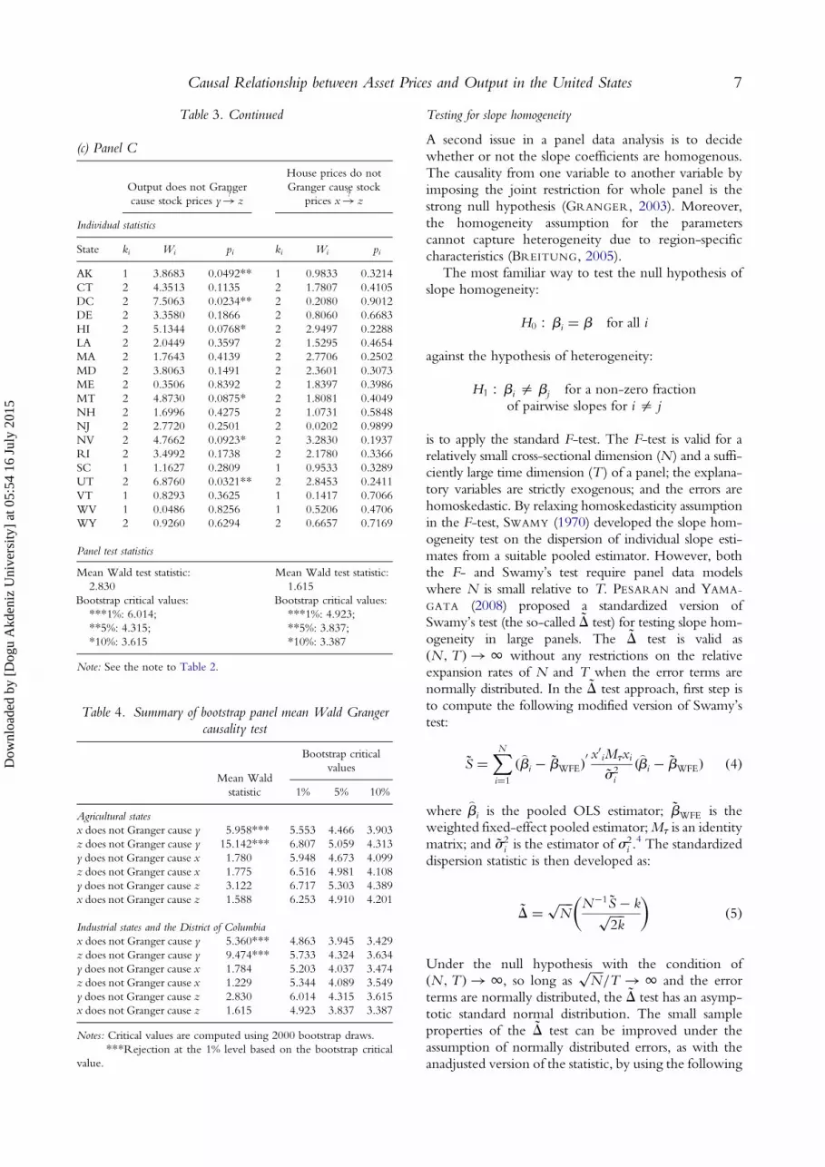
Testing for slope homogeneity

A second issue in a panel data analysis is to decidewhether or not the slope coefficients are homogenous.The causality from one variable to another variable byimposing the joint restriction for whole panel is thestrong null hypothesis (GRANGER, 2003). Moreover,the homogeneity assumption for the parameterscannot capture heterogeneity due to region-specificcharacteristics (BREITUNG, 2005).

The most familiar way to test the null hypothesis ofslope homogeneity:

H0 : bi = b for all i

against the hypothesis of heterogeneity:

H1 : bi = bj for a non-zero fractionof pairwise slopes for i = j

is to apply the standard F-test. The F-test is valid for arelatively small cross-sectional dimension (N ) and a suffi-ciently large time dimension (T ) of a panel; the explana-tory variables are strictly exogenous; and the errors arehomoskedastic. By relaxing homoskedasticity assumptionin the F-test, SWAMY (1970) developed the slope hom-ogeneity test on the dispersion of individual slope esti-mates from a suitable pooled estimator. However, boththe F- and Swamy’s test require panel data modelswhere N is small relative to T. PESARAN and YAMA-

GATA (2008) proposed a standardized version ofSwamy’s test (the so-called D test) for testing slope hom-ogeneity in large panels. The D test is valid as(N,T ) � 1 without any restrictions on the relativeexpansion rates of N and T when the error terms arenormally distributed. In the D test approach, first step isto compute the following modified version of Swamy’stest:

S =∑Ni=1

(_bi − bWFE)′x′iMtxis2i

(_bi − bWFE) (4)

where_

bi is the pooled OLS estimator; bWFE is theweighted fixed-effect pooled estimator;Mt is an identitymatrix; and s2

i is the estimator of s2i .4 The standardized

dispersion statistic is then developed as:

D = ���N

√ N−1S − k���2k

√( )

(5)

Under the null hypothesis with the condition of(N,T ) � 1, so long as

���N

√/T � 1 and the error

terms are normally distributed, the D test has an asymp-totic standard normal distribution. The small sampleproperties of the D test can be improved under theassumption of normally distributed errors, as with theanadjusted version of the statistic, by using the following

Table 3. Continued

(c) Panel C

Output does not Grangercause stock prices y�? z

House prices do notGranger cause stock

prices x�? z

Individual statistics

State ki Wi pi ki Wi pi

AK 1 3.8683 0.0492** 1 0.9833 0.3214CT 2 4.3513 0.1135 2 1.7807 0.4105DC 2 7.5063 0.0234** 2 0.2080 0.9012DE 2 3.3580 0.1866 2 0.8060 0.6683HI 2 5.1344 0.0768* 2 2.9497 0.2288LA 2 2.0449 0.3597 2 1.5295 0.4654MA 2 1.7643 0.4139 2 2.7706 0.2502MD 2 3.8063 0.1491 2 2.3601 0.3073ME 2 0.3506 0.8392 2 1.8397 0.3986MT 2 4.8730 0.0875* 2 1.8081 0.4049NH 2 1.6996 0.4275 2 1.0731 0.5848NJ 2 2.7720 0.2501 2 0.0202 0.9899NV 2 4.7662 0.0923* 2 3.2830 0.1937RI 2 3.4992 0.1738 2 2.1780 0.3366SC 1 1.1627 0.2809 1 0.9533 0.3289UT 2 6.8760 0.0321** 2 2.8453 0.2411VT 1 0.8293 0.3625 1 0.1417 0.7066WV 1 0.0486 0.8256 1 0.5206 0.4706WY 2 0.9260 0.6294 2 0.6657 0.7169

Panel test statistics

Mean Wald test statistic:2.830

Bootstrap critical values:***1%: 6.014;**5%: 4.315;*10%: 3.615

Mean Wald test statistic:1.615

Bootstrap critical values:***1%: 4.923;**5%: 3.837;*10%: 3.387

Note: See the note to Table 2.

Table 4. Summary of bootstrap panel mean Wald Grangercausality test

Mean Waldstatistic

Bootstrap criticalvalues

1% 5% 10%

Agricultural statesx does not Granger cause y 5.958*** 5.553 4.466 3.903z does not Granger cause y 15.142*** 6.807 5.059 4.313y does not Granger cause x 1.780 5.948 4.673 4.099z does not Granger cause x 1.775 6.516 4.981 4.108y does not Granger cause z 3.122 6.717 5.303 4.389x does not Granger cause z 1.588 6.253 4.910 4.201

Industrial states and the District of Columbiax does not Granger cause y 5.360*** 4.863 3.945 3.429z does not Granger cause y 9.474*** 5.733 4.324 3.634y does not Granger cause x 1.784 5.203 4.037 3.474z does not Granger cause x 1.229 5.344 4.089 3.549y does not Granger cause z 2.830 6.014 4.315 3.615x does not Granger cause z 1.615 4.923 3.837 3.387

Notes: Critical values are computed using 2000 bootstrap draws.***Rejection at the 1% level based on the bootstrap critical

value.

Causal Relationship between Asset Prices and Output in the United States 7

Dow

nloa

ded

by [

Dog

u A

kden

iz U

nive

rsity

] at

05:

54 1

6 Ju

ly 2

015

bias adjusted version:

Dadj =���N

√ N−1S − E(zit)��������var(zit)

√( )

(6)

where the mean E(zit) = k and the variance:

var(zit) = 2k(T − k− 1)/T + 1

The results of these selected tests are summarized inTable 1. The null hypothesis of slope homogeneityand cross-sectional independence are rejected, henceconfirming the evidence of heterogeneity as well asspatial effects across US states. These results motivatethe decision to rely on the methodology for causalanalysis in heterogeneous panels. Two alternativeapproaches are used. The first approach is based on thehomogenous non-causality test of DUMITRESCU andHURLIN (2012) that takes into account both heterogen-eity of the slope coefficients and that of the causalityhypothesis. As the second approach, the approach pro-posed by EMIRMAHMUTOGLU and KOSE (2011),based on meta-analysis in heterogeneous-mixed panelswhich accounts for cross-sectional dependence, is alsoused.

Causality analysis

Following DUMITRESCU and HURLIN (2012) andEMIRMAHMUTOGLU and KOSE (2011), the hetero-geneous panel vector autoregressive (VAR) modelwith three variables, y, x and z, where y is real percapita personal income, x is real house prices and z isreal stock prices, is considered:

yit = a1i +∑ki+dmaxi

j=1

b1ijyi,t−j +∑ki+dmaxi

j=1

g1ijxi,t−j

+∑ki+dmaxi

j=1

d1ijzi,t−j + 11it (7)

xit = a2i +∑ki+dmaxi

j=1

b2ijyi,t−j +∑ki+dmaxi

j=1

g2ijxi,t−j

+∑ki+dmaxi

j=1

d2ijzi,t−j + 12it (8)

Table 5. Summary of p-values of individual Granger causality test (agricultural states)

Statesx does not Granger

cause yz does not Granger

cause yy does not Granger

cause xz does not Granger

cause xy does not Granger

cause zx does not Granger

cause z

AL 0.153 0.025** 0.8892 0.8951 0.0833* 0.6507AR 0.379 0.342 0.2440 0.8373 0.3235 0.7693Z 0.129 0.006*** 0.4697 0.6906 0.0427** 0.0450**CA 0.091* 0.002*** 0.7017 0.2801 0.5835 0.2687CO 0.075* 0.000*** 0.1123 0.1189 0.0880* 0.5135FL 0.001*** 0.047** 0.4484 0.3124 0.1179 0.0383**GA 0.181 0.000*** 0.2663 0.2518 0.1742 0.3546IA 0.203 0.105 0.4822 0.5923 0.1749 0.9506ID 0.082* 0.006*** 0.8140 0.8691 0.0947* 0.1071IL 0.009*** 0.000*** 0.2091 0.5809 0.4092 0.9522IN 0.312 0.000*** 0.8771 0.8435 0.6372 0.9230KS 0.269 0.000*** 0.2264 0.6072 0.6235 0.8805KY 0.077* 0.005*** 0.8135 0.6696 0.6997 0.8542MI 0.011** 0.000*** 0.7752 0.7541 0.5736 0.3733MN 0.096* 0.000*** 0.8603 0.1139 0.3598 0.9788MO 0.101 0.014** 0.5184 0.9388 0.2032 0.9520MS 0.610 0.050*** 0.3885 0.7157 0.0364** 0.2919NC 0.341 0.004*** 0.7233 0.1469 0.1175 0.5273ND 0.457 0.099* 0.4769 0.8405 0.4364 0.5945NE 0.000*** 0.000*** 0.2156 0.0667* 0.6351 0.6878NM 0.322 0.015** 0.7794 0.5759 0.0261** 0.1782NY 0.001*** 0.000*** 0.4231 0.9754 0.3357 0.7596OH 0.715 0.003*** 0.8140 0.3780 0.7253 0.8722OK 0.259 0.000*** 0.0583* 0.3059 0.4505 0.9347OR 0.002*** 0.004*** 0.8586 0.1557 0.1483 0.0504*PA 0.061* 0.000*** 0.6197 0.7251 0.1763 0.9508SD 0.005*** 0.000*** 0.1941 0.5977 0.4968 0.9298TN 0.083* 0.130 0.9206 0.5818 0.3992 0.6268TX 0.565 0.000*** 0.0319** 0.6081 0.1690 0.4454VA 0.114 0.055* 0.8518 0.4642 0.1890 0.5124WA 0.1122 0.0037*** 0.8100 0.9973 0.4414 0.3377WI 0.127 0.038** 0.9380 0.9070 0.7501 0.9918

Note: See the note to Table 2.

8 Furkan Emirmahmutoglu et al.

Dow

nloa

ded

by [

Dog

u A

kden

iz U

nive

rsity

] at

05:

54 1

6 Ju

ly 2

015

zit = a3i +∑ki+dmaxi

j=1

b3ijyi,t−j +∑ki+dmaxi

j=1

g3ijxi,t−j

+∑ki+dmaxi

j=1

d3ijzi,t−j + 13it (9)

where, in the present case, zi, the real stock price, is thesame for all I, and the null hypotheses are as follows:

H0 : g1i1 = g1i2 = · · · = g1i,ki = 0

for all i = 1, 2, . . . ,N(10)

H0 : d1i1 = d1i2 = · · · = d1i,ki = 0

for all i = 1, 2, . . . ,N(11)

H0 : b2i1 = b2i2 = · · · = b2i,ki = 0

for all i = 1, 2, . . . ,N(12)

H0 : d2i1 = d2i2 = · · · = d2i,ki = 0

for all i = 1, 2, . . . ,N(13)

H0 : b3i1 = b3i2 = · · · = b3i,ki = 0

for all i = 1, 2, . . . ,N(14)

H0 : g3i1 = g3i2 = · · · = g3i,ki = 0

for all i = 1, 2, . . . ,N(15)

Under the null (10), x does not Granger cause y for all i.Under the null (11), z does not Granger cause y for all i.Under the null (12), y does not Granger cause x for all i.Under the null (13), z does not Granger cause x for all i.Put simply, causality is tested from x to y and from z to yin equation (7). A similar procedure is applied for caus-ality from y to x and from z to x in equation (8) or fromy to z and from x to z in equation (9).

The alternative allows slope coefficients to differ acrossthe groups in order to account for model heterogeneity.Additionally, based on the general non-causality testingapproach in DUMITRESCU and HURLIN (2012), some,but not all, coefficients specified under the null hypoth-eses in equations (10–15) are allowed to be equal tozero. For instance, N1 , N individual processes areallowed with no causality from x to y under alternativeH1 specified for equation (10). This can be specified as:

H1 : g1i1 =g1i2 = · · · = g1i,ki = 0 for i = 1, 2, . . . ,N1

g1i1 = 0,g1i2 = 0, · · · , g1i,ki = 0

for i = N1 + 1,N1 + 2, . . . ,N (16)

An analogous alternative can be specified for each of thenull statements in equations (11–15).

Dumitrescu and Hurlin proposed a test-an-averageWald test based on the average of the individualWald stat-istics associated with testing the Granger non-causality inequations (10–15) for each of the units i = 1, 2, . . . ,N .The average Wald statistic is calculates as:

WHncN,T = 1

N

∑Ni=1

Wi,T (17)

whereWi,T denotes the individual Wald statistics calcu-lated by imposing the non-causality null restriction inequations (10–15) only for the ith cross-section.

This structure of the average Wald statistics is similarto the unit root testing approach of IM et al. (2003). Inorder illustrate this test, consider the non-causality nullin equation (10) with the corresponding alternative inequation (16). If the null is not rejected using theaverage Wald statistic in equation (17), then variable xdoes not Granger cause variable y for all cross-sectionalunits of the panel. If the null is rejected and N1 = 0,then one has homogenous causality result for all cross-sectional units, but the regression model may not behomogenous, allowing slopes to differ across individualunits. If, on the other hand, N1 . 0, then the causalityrelationship is heterogeneous. In this last case, the caus-ality relationship varies from one unit to another andfrom one sample to another.

DUMITRESCU and HURLIN (2012) show that theaverage Wald test sequentially converges to a standardGaussian distribution. The present authors additionallybase the analysis on the critical values of the meanWald statistic obtained from the bootstrap proceduresince the mean Wald test does not converge for fixedN and fixed T and empirical distribution must be used.The bootstrap procedure is also used for the meta-analy-sis. As an example for testing the non-causality hypothesisthat x does not Granger cause y in equation (10), the stepsof the bootstrap procedure proceed as follows:

. Step 1. In order to determine the maximal order ofintegration of three variables (dmaxi) in the VARsystem for each cross-sectional unit, a multiple unitroot test proposed by DICKEY and PANTULA

(1987) is used. The regression (1) is then estimatedby OLS for each individual and the lag order ki’s viaSchwarz information criterion (SIC) is selected bystarting with kmax = 4.

. Step 2. By using ki and dmaxi from Step 1, equation(7) is re-estimated by OLS under the null in equation(10). Thus, the residuals for each individual unit areobtained:

11it = yit − a1i −∑ki+dmaxi

j=1

b 1ijyi,t−j

−∑ki+dmaxi

j=1

d 1ijzi,t−j (18)

Causal Relationship between Asset Prices and Output in the United States 9

Dow

nloa

ded

by [

Dog

u A

kden

iz U

nive

rsity

] at

05:

54 1

6 Ju

ly 2

015

12it = xit − a2i −∑ki+dmaxi

j=1

b 2ijyi,t−j

−∑ki+dmaxi

j=1

g2ijxi,t−j −∑ki+dmaxi

j=ki+1

d 2ijzi,t−j (19)

13it = zit − a3i −∑ki+dmaxi

j=1

b 3ijyi,t−j

−∑ki+dmaxi

j=1

g3ijxi,t−j −∑ki+dmaxi

j=ki+1

d 3ijzi,t−j (20)

. Step 3. STINE (1987) suggests that residuals have to becentred with:

1 jt = 1 jt − T − k− l − 2( )−1∑Tk+l+2

1 jt,

j = 1, 2, 3

(21)

where:

1 jt = (1 j1t, 1 j2t, . . . , 1 jNt)′, k = max (ki)

and l = max (dmaxi)

Furthermore:

1 jit

[ ]N×T

is developed from these residuals. A full column withreplacement from the matrix at a time is selected ran-domly to preserve the cross-covariance structure ofthe errors. The bootstrap residuals are denoted as1∗jit , where t = 1, 2, . . . ,T .

. Step 4. As recursively the bootstrap sample of y∗it, x∗it ,

and z∗it is generated under the null in equation (10):

y∗it = a1i +∑ki+dmaxi

j=1

b 1ijy∗i,t−j +

∑ki+dmaxi

j=1

d 1ijz∗i,t−j

+ 1∗1it (22)

x∗it = a2i +∑ki+dmaxi

j=1

b 2ijy∗i,t−j +

∑ki+dmaxi

j=1

g2ijx∗i,t−j

+∑ki+dmaxi

j=ki+1

d 2ijz∗i,t−j + 1∗2it (23)

z∗it = a3i +∑ki+dmaxi

j=1

b 3ijy∗i,t−j +

∑ki+dmaxi

j=1

g3ijx∗i,t−j

+∑ki+dmaxi

j=ki+1

d 3ijz∗i,t−j + 1∗3it (24)

where a1i, b1ij, g1ij and d1ij are obtained from Step 2for all i and j.

. Step 5. Substitute y∗it , x∗it and z

∗it respectively for yit , xit

and zit and estimate (7) without imposing any par-ameter restrictions on it and then the individualWald statistics are calculated to test the non-causalitynull hypothesis separately for each individual. Usingthese individual Wald statistics, which have an asymp-totic chi-square distribution with ki degrees offreedom, individual p-values are computed. Themean Wald test statistic is then obtained.

Based on the above steps, the bootstrap empirical dis-tribution of the mean Wald test statistic is generatedby repeating Steps 3–5 a total of 2000 times and spe-cifying the bootstrap critical values by selecting theappropriate percentiles of these sampling distributions.

Causality test results are reported in Tables 2 and 3 foragricultural and industrial states (including DC), respect-ively. The first panel (panel A) of these tables tests thecausality from asset prices to output. The bootstrappedvalues of the mean Wald test appear to be considerablyhigher than the bootstrap critical values at the 1% levelof significance. This suggests that house prices andstock prices cause Granger output, which corroboratesthe individual state results with small p-values in themajority of states. It is worth noting that individualresults are more consistent for the stock price-outputcausality than the house price-output causality and thisis true across both categories of states. For the agricul-tural states, only three states out of 32 display insignifi-cant Wald statistics (high p-values) for stock price-output causality, namely Arkansas (AR), Indiana (IA)and Tennessee (TN) (abbreviations for the other stateswill now not be given for reasons of space), with thenon-rejection of the null of no causality holdingbarely for IA. For the house price-output causality,there are 14 states, namely CA, CO, FL, ID, IL, KY,MI, MN, NE, NY, OR, PA, SD and TN, for whichthe null of no causality is rejected. On the other hand,15 (AK, CT, DC, DE, MA, MD, MT, NH, NJ, NV,SC, UT, VT, WV and WY) out of 19 industrial stateshave low p-values for the null of no causality runningfrom stock price to output, compared with nine states(AK, CT, DC, HI, MA, MT, NH, NJ and UT) forthe case of causality running from house price tooutput (Table 6).

Panel B of these tables test the causality running fromoutput to housing and stock prices. The null hypothesisof no Granger causality is rejected, as the bootstrap criti-cal values at the 10%, 5% and 1% levels of significanceare substantially higher than the bootstrapped values ofthe mean Wald test. A similar story holds for state-level results, with the exception of a few states thatindeed have significant Wald statistics, but mostly atthe 10% level of significance across both agriculturaland industrial states. This is the case for OK and TX(WV and WY) for agricultural (industrial) states for

10 Furkan Emirmahmutoglu et al.

Dow

nloa

ded

by [

Dog

u A

kden

iz U

nive

rsity

] at

05:

54 1

6 Ju

ly 2

015

which the causality runs from output to house prices,compared with AL, AZ, CO, ID, MS and NM (AK,DC, HI, MT, NV and UT) for agricultural (industrial)states, in which cases the outputs of these causes thestock price. These findings suggest that output doesnot Granger cause housing and stock prices. Further,based on Panel C of Tables 2 and 3, irrespective ofthe categorization of the states, there is no evidence ofthe causality between housing prices and stock prices;5

suggesting that house prices cannot predict stockprices, and vice versa (Table 5).6

In contrast to APERGIS et al. (2015), who report abidirectional causality between house prices andoutput at the metropolitan level, the findings (summar-ized in Table 6) support a unidirectional causalityrunning from asset prices (housing and stock prices) tooutput at the state level. The observed differencecould be attributed to the pre-test bias as the panelVECM methodology used by Apergis et al. requirespre-testing for co-integration and stationarity. Such aline of thinking was corroborated when bidirectionalcausality was discovered between asset prices andoutput for industrial and agricultural states, as well asall the states taken together, based on a panel VECMapproach similar to that of Apergis et al. – results ofwhich are available from the authors upon request. Insummary, the results substantiate the important role ofasset prices in driving business cycle fluctuations, butno feedback from the real economy onto bothhousing and stock prices.7 The results confirm theleading indicator abilities of asset prices at the regionallevel, something that has been widely shown to existat the aggregate level (e.g., by FORNI et al., 2003;STOCK and WATSON, 2003; and RAPACH andWEBER, 2004).8

CONCLUSIONS

This study implements a newly developed bootstrappanel causality approach to investigate the causal lin-kages between asset prices and output per capita acrossthe 50 US states and DC over the period 1975–2012.Empirical results indicate that when cross-state depen-dency, heterogeneity and asset market interconnectionsare controlled for, the causality runs from asset prices(both housing and stock prices) to output, not only atthe level of individual states, but also taking togetherall the agricultural and industrial states.

Whilst the unidirectional causality running from assetprices to output substantiates the wealth and/or collateraltransmission mechanism, the reverse causation found byAPERGIS et al. (2015) at the metropolitan level disappearsat the state level using the present methodology. The factthat, bidirectional causality was also observed betweenasset prices and output – using a panel VECM as inApergis et al. applied to the data on agricultural and indus-trial states – possibly highlights, though this cannot beconfirmed due to differences in observational units(MSA versus states), the ability of the bootstrap method-ology in alleviating the issue of pre-test bias in causalitytesting, and, in the process, the possible influence assetmarkets interdependency may exert on causal linkageswith the real sector (APERGIS et al., 2015).

The findings here provide important policy impli-cations. First, they show that asset market developmentmight be an efficient tool to stimulate economicgrowth. Conversely, business cycle dynamics are lesslikely to determine asset price fluctuations, at least atthe state level. Second, policy-makers have to identifyany asset bubble at an early stage to avoid a muchlarger bubble burst in future. Third, it is necessary to

Table 6. Summary of p-values of individual Granger causality test (industrial states and the District of Columbia)

Statesx does not Granger

cause yz does not Granger

cause yy does not Granger

cause xz does not Granger

cause xy does not Granger

cause zx does not Granger

cause z

AK 0.0375** 0.0501* 0.2407 0.6123 0.0492** 0.3214CT 0.0001*** 0.0003*** 0.7119 0.9489 0.1135 0.4105DC 0.040** 0.001*** 0.548 0.163 0.0234** 0.9012DE 0.311 0.0988* 0.736 0.2151 0.1866 0.6683HI 0.0507* 0.2913 0.1608 0.3435 0.0768* 0.2288LA 0.4122 0.1824 0.858 0.8133 0.3597 0.4654MA 0.0003*** 0.0000*** 0.8552 0.9127 0.4139 0.2502MD 0.4442 0.0118** 0.9044 0.2412 0.1491 0.3073ME 0.3493 0.1271 0.7192 0.7924 0.8392 0.3986MT 0.0614* 0.0014*** 0.1917 0.6707 0.0875* 0.4049NH 0.0045*** 0.0096*** 0.6387 0.4823 0.4275 0.5848NJ 0.0187** 0.0009*** 0.4654 0.8679 0.2501 0.9899NV 0.512 0.0026*** 0.5939 0.2211 0.0923* 0.1937RI 0.1302 0.9232 0.4961 0.2973 0.1738 0.3366SC 0.5138 0.0058*** 0.7688 0.7004 0.2809 0.3289UT 0.0076*** 0.0000*** 0.9321 0.9067 0.0321** 0.2411VT 0.115 0.0403** 0.4338 0.3641 0.3625 0.7066WV 0.2073 0.0517* 0.0491** 0.7712 0.8256 0.4706WY 0.6188 0.0002*** 0.0017*** 0.099* 0.6294 0.7169

Note: See the note to Table 2.

Causal Relationship between Asset Prices and Output in the United States 11

Dow

nloa

ded

by [

Dog

u A

kden

iz U

nive

rsity

] at

05:

54 1

6 Ju

ly 2

015

prevent overheating of the economy in response to anypositive asset price shock that may raise the volatility offuture gross domestic product (GDP) growth. Fourth,the property (real estate) market should receive priorityfrom policy-makers since the housing price effect plays asignificant role. As part of future research, if state-leveldata on consumption (proxied by retail sales) can beobtained, it would be interesting to conduct not onlypanel causality tests between consumption and assetprices, but also use panel co-integration techniques toobtain state-level consumption functions to determinethe importance of the wealth effect at a regional levelfor the US economy. This is important, since, asshown, national-level policies for the states cannot begeneralized.

However, it is also important to acknowledge alimitation of this study: The rejection of the null ofhomogenous non-causality for the entire panel (basedon the meta-analysis) does not tend to provide exactguidance with respect to the number or the identityof the particular panel units for which the null ofnon-causality is rejected, since the individual Grangercausality tests are actually purely time-series based,which in turn disregards cross-sectional dependence(even though the meta-analysis does account forcross-sectional dependence based on a bootstrappedprocedure). Hence, the suggestions of specific cross-sections driving the aggregate panel based on themeta-analysis cannot be considered as conclusive evi-dence. Note that this limitation is not only specificto the modelling approach, but also is applicable tothe works of DUMITRESCU and HURLIN (2012) andEMIRMAHMUTOGLU and KOSE (2011) – the twostudies followed in this paper. In light of this, futureanalysis should be aimed at developing a meta-analysisfor panel Granger causality tests, which also controls forcross-sectional dependence when obtaining cross-sec-tional-level causality results. This, in turn, will allowaccurate information on the cross-sections to beobtained that might be driving the result for theentire panel.

Acknowledgement – The authors thank two anonymousreferees for their many helpful comments that markedlyimproved the quality of the paper. However, any remainingerrors are solely the authors’ alone.

Disclosure statement – No potential conflict of interestwas reported by the authors.

Supplemental data – Supplemental data for this articlecan be accessed at http://dx.doi.org/10.1080/00343404.2015.1055462

NOTES

1. Based on data from the US Department of Agriculture(USDA)-Economic Research Service, if the total agricul-tural production in a particular state as a percentage ofthe total agricultural production of the US is less than(greater than) 1%, the state is categorized as industrial (agri-cultural). See Appendix A in the Supplemental data onlinefor agricultural versus industrial states.

2. The only study that can be considered related to this workis CHANG et al. (2014). This study, based on an approachproposed by KÓNYA (2006), is a different panel causalitytest based on a seemingly unrelated regressions (SUR) esti-mator that yields a Wald test with country-specific boot-strap critical values, analysed bivariate causality betweenhouse prices and output for the nine provinces of SouthAfrica. This test too does not require pre-testing for unitroots and co-integration apart from the lag structure.However, this approach does not provide a meta-analysisto help one conclude whether and which cross-sectionalunits drive the results for the entire panel.

3. As defined in the BEA regional accounts (see http://www.bea.gov/regional/definitions/):

Personal income is the income received by persons fromparticipation in production, plus transfer receipts fromgovernment and business, plus government interest(which is treated like a transfer receipt). It is defined asthe sum of wages and salaries, supplements to wagesand salaries, proprietors’ income with inventory valua-tion and capital consumption adjustments, rentalincome of persons with capital consumption adjust-ment, personal dividend income, personal interestincome, and personal current transfer receipts, less con-tributions for government social insurance. Because thepersonal income of an area represents the income that isreceived by, or on behalf of, all the persons who live inthat area, and because the estimates of some componentsof personal income (wages and salaries, supplements towages and salaries, and contributions for governmentsocial insurance) are made on a place-of-work basis,state personal income includes an adjustment for resi-dence. The residence adjustment represents the netflow of compensation (less contributions for govern-ment social insurance) of interstate commuters.

Note that data on state-level GDP are available from theregional database of the BEA. But there is a break in1997 in the way the GDP data is measured. In light ofthis, the BEA has a cautionary note (see http://www.bea.gov/regional/docs/product/):

There is a discontinuity in the GDP-by-state time seriesat 1997, where the data change from SIC [StandardIndustrial Classification] industry definitions to NAICS[North American Industry Classification System] industrydefinitions. This discontinuity results from many sources.The NAICS-based statistics of GDP by state are consist-ent with U.S. gross domestic product (GDP) while theSIC-based statistics of GDP by state are consistent withU.S. gross domestic income (GDI). With the compre-hensive revision of June 2014, the NAICS-based statisticsof GDP by state incorporated significant improvements

12 Furkan Emirmahmutoglu et al.

Dow

nloa

ded

by [

Dog

u A

kden

iz U

nive

rsity

] at

05:

54 1

6 Ju

ly 2

015

to more accurately portray the state economies. Twosuch improvements were recognizing research and devel-opment expenditures as capital and the capitalization ofentertainment, literary, and other artistic originals.These improvements have not been incorporated inthe SIC-based statistics. In addition, there are differencesin source data and different estimation methodologies.This data discontinuity may affect both the levels andthe growth rates of GDP by state. Users of GDP bystate are strongly cautioned against appending the twodata series in an attempt to construct a single time seriesfor 1963 to 2013.

In light of this, the present authors, as in the existing litera-ture, prefer the usage of personal income as a proxy foroutput at the state level.

4. In order to save space, see PESARAN and YAMAGATA

(2008) for details of estimators and for Swamy’s test.5. Though few agricultural states, namely, AZ, FL and OR,

display relatively low p-values, indicating causality running

from housing prices in these states to stock price, whilestock price is found to cause house price only in NE.For the industrial states, stock price only causes houseprice in WY, with no evidence of reverse causality fromhouse price to stock price.

6. All the results of the meta-analysis based on theaverage Wald test statistic also continue to hold based onthe Fisher statistic, as developed and used byEMIRMAHMUTOGLU and KOSE (2011). Completedetails of these results are available from the authorsupon request. Furthermore, Appendix B in theSupplemental data online discusses results using real GDPper capita as the proxy of state-level output.

7. To account for structural breaks, Appendix C in theSupplemental data online provides results from the sub-sample analysis.

8. These results are inconsistent with the aggregate-level-basedcausality discussed in Appendix D in the Supplemental dataonline, hence justifying the importance of not derivingstate-level inference from the aggregate level results.

REFERENCES

APERGIS N., SIMO-KENGNE B. D., GUPTA R. and CHANG T. (Forthcoming 2015) The dynamic relationship between house pricesand output: evidence from US metropolitan areas, International Journal of Strategic Property Management.

BAJARI P., BENKARD C. L. and KRAINER J. (2005) House prices and consumer welfare, Journal of Urban Economics 58, 474–487.doi:10.1016/j.jue.2005.08.008

BREITUNG J. (2005) A parametric approach to the estimation of cointegration vectors in panel data, Econometric Reviews 24, 151–173. doi:10.1081/ETC-200067895

BREUSCH T. S. and PAGAN A. R. (1980) The Lagrange multiplier test and its applications to model specification in econometrics,Review of Economic Studies 47, 239–253. doi:10.2307/2297111

BUITER W. H. (2008) Housing Wealth isn’t Wealth. Working Paper No. 14204. National Bureau of Economic Research (NBER),Cambridge, MA.

CARLSTROM C. T., FUERST T. S. and LOANNIDOU V. P. (2002) Stock Prices and Output Growth: An Examination of the Credit Channel.Federal Reserve Bank of Cleveland, Cleveland, OH.

CHANG T., SIMO-KENGNE B. D. and GUPTA R. (Forthcoming 2014) The causal relationship between house prices and growth inthe nine provinces of South Africa: evidence from panel-Granger causality tests, International Journal of Sustainable Economy 6,345–358.

DEMARY M. (2010) The interplay between output, inflation, interest rates and house prices: International evidence, Journal ofProperty Research 27, 1–17. doi:10.1080/09599916.2010.499015

DICKEY D. A. and PANTULA S. G. (1987) Determining the order of differencing in autoregressive processes, Journal of Business andEconomic Statistics 5, 455–461.

DUMITRESCU E. I. and HURLIN C. (2012) Testing for Granger non-causality in heterogeneous panels, Economic Modelling29, 1450–1460. doi:10.1016/j.econmod.2012.02.014

EMIRMAHMUTOGLU F. and KOSE N. (2011) Testing for Granger causality in heterogeneous mixed panels, Economic Modelling28, 870–876. doi:10.1016/j.econmod.2010.10.018

FORNI M., HALLIN M., LIPPI M. and REICHLIN L. (2003) Do financial variables help forecasting inflation and real activity in the euroarea?, Journal of Monetary Economics 50, 1243–1255. doi:10.1016/S0304-3932(03)00079-5

GRANGER C. W. J. (2003) Some aspects of causal relationships, Journal of Econometrics 112, 69–71. doi:10.1016/S0304-4076(02)00148-3

GUPTA R. and HARTLEY F. (2013) The role of asset prices in forecasting inflation and output in South Africa, Journal of EmergingMarket Finance 12, 239–291. doi:10.1177/0972652713512913

IACOVIELLO M. (2011) Housing Wealth and Consumption. International Finance Discussion Paper No. 1027. Federal Reserve Board,Washington, DC.

IM K. S., PESARAN M. H. and SHIN Y. (2003) Testing for unit roots in heterogeneous panels, Journal of Econometrics 54, 91–115.INTERNATIONAL MONETARY FUND (IMF) (2000) World Economic Outlook. Asset Prices and the Business Cycle. World Economic

and Financial Surveys. IMF, Washington, DC.KÓNYA L. (2006) Exports and growth: Granger causality analysis on OECD countries with a panel data approach, Economic

Modelling 23, 978–992. doi:10.1016/j.econmod.2006.04.008LI W. and YAO R. (2007) The life cycle effects of house price changes, Journal of Money, Credit and Banking 39, 1376–1409.MAURO P. (2000) Stock Returns and Output Growth in Emerging and Advanced Economies. IMF Working Paper No. WP/00/89.

International Monetary Fund (IMF), Washington, DC.

Causal Relationship between Asset Prices and Output in the United States 13

Dow

nloa

ded

by [

Dog

u A

kden

iz U

nive

rsity

] at

05:

54 1

6 Ju

ly 2

015

MILLER N., PENG L. and SKLARZ M. (2011) House prices and economic growth, Journal of Real Estate Finance and Economics42, 522–541. doi:10.1007/s11146-009-9197-8

NYAKABAWO W., MILLER S. M., BALCILAR M., DAS S. and GUPTA R. (Forthcoming 2014) Temporal causality between house pricesand output in the U.S.: a bootstrap rolling-window approach, North American Journal of Economics and Finance 33, 55–73.

PESARAN M. H. (2006) Estimation and inference in large heterogeneous panels with multifactor error structure, Econometrica74, 967–1012. doi:10.1111/j.1468-0262.2006.00692.x

PESARAN M. H., ULLAH A. and YAMAGATA T. (2008) A bias-adjusted LM test of error cross-section independence, EconometricsJournal 11, 105–127. doi:10.1111/j.1368-423X.2007.00227.x

PESARAN M. H. and YAMAGATA T. (2008) Testing slope homogeneity in large panels, Journal of Econometrics 142, 50–93. doi:10.1016/j.jeconom.2007.05.010

RAPACH D. E. and WEBER C. E. (2004) Financial variables and the simulated out-of-sample forecastability of U.S. output growthsince 1985: an encompassing approach, Economic Inquiry 42, 717–738. doi:10.1093/ei/cbh092

SIMO-KENGNE B. D., BITTENCOURT M. and GUPTA R. (2013) The impact of house prices on consumption in South Africa:evidence from provincial-level panel VARs, Housing Studies 28, 1133–1154. doi:10.1080/02673037.2013.804492

SIMO-KENGNE B. D., MILLER S. M. and GUPTA R. (2015) Time varying effects of housing and stock prices on US consumption,Journal of Real Estate Finance and Economics 50, 339–354

STINE R. A. (1987) Estimating properties of autoregressive forecasts, Journal of the American Statistical Association 82, 1072–1078.doi:10.1080/01621459.1987.10478542

STOCK J. H. and WATSON M. W. (2003) Forecasting output and inflation: the role of asset prices, Journal of Economic Literature41, 788–829. doi:10.1257/jel.41.3.788

SWAMY P. A. V. B. (1970) Efficient inference in a random coefficient regression model, Econometrica 38, 311–323. doi:10.2307/1913012

14 Furkan Emirmahmutoglu et al.

Dow

nloa

ded

by [

Dog

u A

kden

iz U

nive

rsity

] at

05:

54 1

6 Ju

ly 2

015