lectures on computational fluid dynamics and heat transfer
TRANSCRIPT

Lectures on computational fluid
dynamics and heat transfer
with applications to human
thermodynamics
Prof. Dr.-Ing. habil. Nikolai Kornev
Prof. Dr.-Ing. habil. Irina Cherunova
Rostock2013
Preface
The present book is used for lecture courses Computational heat and masstransfer, Mathematical models of turbulence and Design of special cloth givenby the authors at the University of Rostock, Germany and Don State Tech-nical University, Russia. Each of lecture courses contains about 14 lectures.The lecture course Compuational heat and mass transfer was written pro-ceeding from the idea to present the complex material as easy as possible.We considered derivation of numerical methods, particularly of the finite vol-ume method, in details up to final expressions which can be programmed.Turbulence is a big and a very complicated topic which is difficult to coverwithin 14 lectures. We selected the material combining the main physi-cal concepts of the turbulence with basic mathematical models necessary tosolve practical engineering problems. The course Design of special cloth usesthe material of two parts of this book partially. The material for the thirdpart was gathered from research projects done by the authors of this bookwithin some industrial projects and research works supported by differentfoundations. We express our gratitude to Andreas Gross, Gunnar Jacobiand Stefan Knochenhauer who carried out CFD calculations for the thirdpart of this book.
2
Contents
I Introduction into computational methods for so-lution of transport equations 17
1 Main equations of the Computational Heat and Mass Trans-fer 191.1 Fluid mechanics equations . . . . . . . . . . . . . . . . . . . . 19
1.1.1 Continuity equation . . . . . . . . . . . . . . . . . . . . 191.1.2 Classification of forces acting in a fluid . . . . . . . . . 20
1.1.2.1 Body forces . . . . . . . . . . . . . . . . . . 201.1.2.2 Surface forces . . . . . . . . . . . . . . . . . 211.1.2.3 Properties of surface forces . . . . . . . . . . 21
1.1.3 Navier Stokes Equations . . . . . . . . . . . . . . . . . 231.2 Heat conduction equation . . . . . . . . . . . . . . . . . . . . 26
2 Finite difference method 292.1 One dimensional case . . . . . . . . . . . . . . . . . . . . . . . 292.2 Two dimensional case . . . . . . . . . . . . . . . . . . . . . . . 322.3 Time derivatives. Explicit versus implicit . . . . . . . . . . . . 332.4 Exercises . . . . . . . . . . . . . . . . . . . . . . . . . . . . . . 34
3 Use of boundary conditions in Finite Difference Method 353.1 Zero boundary conditions . . . . . . . . . . . . . . . . . . . . 353.2 Extension to arbitrary non zero boundary conditions . . . . . 36
4 Stability and artificial viscosity of numerical methods 394.1 Artificial viscosity . . . . . . . . . . . . . . . . . . . . . . . . 394.2 Stability. Courant Friedrich Levy criterion (CFL) . . . . . . . 414.3 Exercise . . . . . . . . . . . . . . . . . . . . . . . . . . . . . . 43
5 Simple explicit time advance scheme for solution of the NavierStokes Equation 455.1 Theory . . . . . . . . . . . . . . . . . . . . . . . . . . . . . . . 45
3

5.2 Mixed schemes . . . . . . . . . . . . . . . . . . . . . . . . . . 465.3 Staggered grid . . . . . . . . . . . . . . . . . . . . . . . . . . . 47
5.4 Approximation of − δuni unj
δxj. . . . . . . . . . . . . . . . . . . . . 50
5.4.1 Approximation of −∂uxux∂x− ∂uxuy
∂y= −ux ∂ux∂x − uy
∂ux∂y
. . 51
5.4.2 Approximation of −∂uxuy∂x− ∂uyuy
∂y= −ux ∂uy∂x − uy
∂uy∂y
. . 52
5.5 Approximation of δδxj
δuniδxj
. . . . . . . . . . . . . . . . . . . . . 53
5.6 Calculation of the r.h.s. for the Poisson equation (5.6) . . . . 535.7 Solution of the Poisson equation (5.6) . . . . . . . . . . . . . . 535.8 Update the velocity field . . . . . . . . . . . . . . . . . . . . . 535.9 Boundary conditions for the velocities . . . . . . . . . . . . . . 545.10 Calculation of the vorticity . . . . . . . . . . . . . . . . . . . . 54
6 Splitting schemes for solution of multidimensional problems 556.1 Splitting in spatial directions. Alternating direction implicit
(ADI) approach . . . . . . . . . . . . . . . . . . . . . . . . . . 556.2 Splitting according to physical processes. Fractional step
methods . . . . . . . . . . . . . . . . . . . . . . . . . . . . . . 566.3 Increase of the accuracy of time derivatives approximation us-
ing the Lax-Wendroff scheme . . . . . . . . . . . . . . . . . . 59
7 Finite Volume Method 617.1 Transformation of the Navier-Stokes Equations in the Finite
Volume Method . . . . . . . . . . . . . . . . . . . . . . . . . . 617.2 Sample . . . . . . . . . . . . . . . . . . . . . . . . . . . . . . . 62
7.2.1 Pressure and unsteady terms . . . . . . . . . . . . . . . 627.2.2 Convection term of the x-equation . . . . . . . . . . . . 637.2.3 Convection term of the y-equation . . . . . . . . . . . . 637.2.4 X-equation approximation . . . . . . . . . . . . . . . . 647.2.5 Y-equation approximation . . . . . . . . . . . . . . . . 65
7.3 Explicit scheme . . . . . . . . . . . . . . . . . . . . . . . . . . 657.4 Implicit scheme . . . . . . . . . . . . . . . . . . . . . . . . . . 667.5 Iterative procedure for implicit scheme . . . . . . . . . . . . . 677.6 Pressure correction method . . . . . . . . . . . . . . . . . . . 707.7 SIMPLE method . . . . . . . . . . . . . . . . . . . . . . . . . 70
7.7.1 Pressure correction equation . . . . . . . . . . . . . . . 717.7.2 Summary of the SIMPLE algorithm . . . . . . . . . . . 73
8 Overview of pressure correction methods 758.1 SIMPLE algorithm . . . . . . . . . . . . . . . . . . . . . . . . 758.2 SIMPLE algorithm in OpenFOAM . . . . . . . . . . . . . . . 76
4

8.3 PISO algorithm . . . . . . . . . . . . . . . . . . . . . . . . . 768.3.1 First iteration . . . . . . . . . . . . . . . . . . . . . . . 768.3.2 Second iteration . . . . . . . . . . . . . . . . . . . . . . 768.3.3 Correction . . . . . . . . . . . . . . . . . . . . . . . . . 778.3.4 Summary . . . . . . . . . . . . . . . . . . . . . . . . . 778.3.5 PISO algorithm in OpenFOAM . . . . . . . . . . . . . 78
8.4 SIMPLEC algorithm . . . . . . . . . . . . . . . . . . . . . . . 78
9 Computational grids 819.1 Grid types . . . . . . . . . . . . . . . . . . . . . . . . . . . . . 819.2 Overset or Chimera grids . . . . . . . . . . . . . . . . . . . . 829.3 Morphing grids . . . . . . . . . . . . . . . . . . . . . . . . . . 82
II Mathematical modelling of turbulent flows 85
10 Physics of turbulence 8710.1 Definition of the turbulence . . . . . . . . . . . . . . . . . . . 8710.2 Vortex dynamics . . . . . . . . . . . . . . . . . . . . . . . . . 87
10.2.1 Vorticity transport equation . . . . . . . . . . . . . . . 8710.2.2 Vorticity and vortices . . . . . . . . . . . . . . . . . . . 8810.2.3 Vortex amplification as an important mechanism of the
turbulence generation . . . . . . . . . . . . . . . . . . . 8910.2.4 Vortex reconnection . . . . . . . . . . . . . . . . . . . 9210.2.5 Richardson poem (1922) . . . . . . . . . . . . . . . . . 9310.2.6 Summary . . . . . . . . . . . . . . . . . . . . . . . . . 94
10.3 Experimental observations . . . . . . . . . . . . . . . . . . . . 9410.3.1 Laminar - turbulent transition in pipe. Experiment of
Reynolds . . . . . . . . . . . . . . . . . . . . . . . . . . 9510.3.2 Laminar - turbulent transition and turbulence in jets . 9710.3.3 Laminar - turbulent transition in wall bounded flows . 10010.3.4 Distribution of the averaged velocity in the turbulent
boundary layer . . . . . . . . . . . . . . . . . . . . . . 103
11 Basic definitions of the statistical theory of turbulence 10911.1 Reynolds averaging . . . . . . . . . . . . . . . . . . . . . . . . 10911.2 Isotropic and homogeneous turbulence . . . . . . . . . . . . . 11011.3 Correlation function. Integral length . . . . . . . . . . . . . . 110
11.3.1 Some relations in isotropic turbulence . . . . . . . . . . 11311.3.2 Taylor microscale λ . . . . . . . . . . . . . . . . . . . 11511.3.3 Correlation functions in the Fourier space . . . . . . . 116
5
11.3.4 Spectral density of the turbulent kinetic energy . . . . 11711.4 Structure functions . . . . . . . . . . . . . . . . . . . . . . . . 118
11.4.1 Probability density function . . . . . . . . . . . . . . . 11811.4.2 Structure function . . . . . . . . . . . . . . . . . . . . 118
12 Kolmogorov theory K41 12312.1 Physical background . . . . . . . . . . . . . . . . . . . . . . . 12312.2 Dissipation rate . . . . . . . . . . . . . . . . . . . . . . . . . 12512.3 Kolmogorov hypotheses . . . . . . . . . . . . . . . . . . . . . . 12612.4 Three different scale ranges of turbulent flow . . . . . . . . . . 12812.5 Classification of methods for calculation of turbulent flows. . . 13112.6 Limitation of K-41. Kolmogorov theory K-62 . . . . . . . . . . 131
12.6.1 Exercises . . . . . . . . . . . . . . . . . . . . . . . . . . 133
13 Reynolds Averaged Navier Stokes Equation (RANS) 137
14 Reynolds Stress Model (RSM) 14314.1 Derivation of the RSM Equations . . . . . . . . . . . . . . . . 143
14.1.1 Step 1 . . . . . . . . . . . . . . . . . . . . . . . . . . . 14314.1.2 Step 2 . . . . . . . . . . . . . . . . . . . . . . . . . . . 14414.1.3 Step 3 . . . . . . . . . . . . . . . . . . . . . . . . . . . 14414.1.4 Analysis of terms . . . . . . . . . . . . . . . . . . . . . 146
15 Two equations RANS models 14915.1 Derivation of the k-Equation . . . . . . . . . . . . . . . . . . . 14915.2 Derivation of the ε-Equation . . . . . . . . . . . . . . . . . . . 15215.3 The k − ε model . . . . . . . . . . . . . . . . . . . . . . . . . 15415.4 Low Reynolds k − ε model . . . . . . . . . . . . . . . . . . . . 15615.5 The k − ω model . . . . . . . . . . . . . . . . . . . . . . . . . 15615.6 The k − ω SST model . . . . . . . . . . . . . . . . . . . . . . 15715.7 Method of wall functions . . . . . . . . . . . . . . . . . . . . . 160
15.7.1 Equilibrium wall functions . . . . . . . . . . . . . . . . 16115.7.2 Non- equilibrium wall functions . . . . . . . . . . . . . 163
16 Large Eddy Simulation (LES) 16516.1 LES filtering . . . . . . . . . . . . . . . . . . . . . . . . . . . 165
16.1.1 Properties of filtering . . . . . . . . . . . . . . . . . . . 16616.2 LES equations . . . . . . . . . . . . . . . . . . . . . . . . . . 16716.3 Smagorinsky model . . . . . . . . . . . . . . . . . . . . . . . 16816.4 Model of Germano ( Dynamic Smagorinsky Model) . . . . . . 17016.5 Scale similarity models . . . . . . . . . . . . . . . . . . . . . . 173
6
16.6 Mixed similarity models . . . . . . . . . . . . . . . . . . . . . 17416.7 A-posteriori and a-priori tests . . . . . . . . . . . . . . . . . . 176
17 Hybrid URANS-LES methods 17917.1 Introduction . . . . . . . . . . . . . . . . . . . . . . . . . . . . 17917.2 Detached Eddy Simulation (DES) . . . . . . . . . . . . . . . 18017.3 Hybrid model based on integral length as parameter switching
between LES and URANS . . . . . . . . . . . . . . . . . . . . 18317.4 Estimations of the resolution necessary for a pure LES on the
example of ship flow . . . . . . . . . . . . . . . . . . . . . . . 186
III CFD applications to human thermodynamics 189
18 Mathematical model of the ice protection of a human bodyat high temperatures of surrounding medium 19118.1 Designations . . . . . . . . . . . . . . . . . . . . . . . . . . . . 192
18.1.1 List of symbols . . . . . . . . . . . . . . . . . . . . . . 19218.1.2 Subscripts . . . . . . . . . . . . . . . . . . . . . . . . . 19318.1.3 Superscripts . . . . . . . . . . . . . . . . . . . . . . . . 193
18.2 Introduction . . . . . . . . . . . . . . . . . . . . . . . . . . . . 19318.3 Human body and ice protection models . . . . . . . . . . . . . 19418.4 Mathematical model . . . . . . . . . . . . . . . . . . . . . . . 19518.5 Results . . . . . . . . . . . . . . . . . . . . . . . . . . . . . . . 199
18.5.1 Design of the protection clothes . . . . . . . . . . . . . 19918.5.2 Experimental proof of numerical prediction . . . . . . . 200
18.6 Discussion . . . . . . . . . . . . . . . . . . . . . . . . . . . . . 204
19 CFD Design of cloth for protection of divers at low temper-atures under current conditions 207
20 CFD application for design of cloth for protection from lowtemperatures under wind conditions. Influence of the windon the cloth deformation and heat transfer from the body. 21120.1 Wind tunnel measurements of pressure distribution . . . . . . 21120.2 Numerical simulations of pressure distribution and comparison
with measurements . . . . . . . . . . . . . . . . . . . . . . . . 21220.3 Comparison of CFD results with measurements . . . . . . . . 21320.4 Change of thermal conductivity caused by wind induced pres-
sures . . . . . . . . . . . . . . . . . . . . . . . . . . . . . . . . 214
21 Simulation of human comfort conditions in car cabins 219
7

Bibliography 227
Index 227
8

List of Tables
5.1 Limiters function for TVD schemes . . . . . . . . . . . . 47
7.1 ~n~u and ui at different sides. x-equation . . . . . . . . . . 637.2 Velocities at different sides. x-equation . . . . . . . . . . 647.3 Convection flux. x-equation . . . . . . . . . . . . . . . . . 647.4 ~n~u and ui at different sides. y-equation . . . . . . . . . . 647.5 Velocities at different sides. y-equation . . . . . . . . . . 647.6 Convection flux. y-equation . . . . . . . . . . . . . . . . . 65
16.1 Properties of large and small scale motions . . . . . . . . . . . 16716.2 Advantages and disadvantages of the Smagorinsky model . . . 170
17.1 Results of the resistance prediction using different methods.CR is the resistance coefficient, CP is the pressure resistanceand CF is the friction resistance . . . . . . . . . . . . . . . . 188
18.1 Sizes of the body used in simulations . . . . . . . . . . . . . . 19518.2 Radii of the elliptical cross sections used in simulations . . . . 19718.3 Radii of layers used in simulations in fraction of the skin thick-
ness ∆ . . . . . . . . . . . . . . . . . . . . . . . . . . . . . . . 19718.4 Thermodynamic coefficients of the body layers used in simu-
lations . . . . . . . . . . . . . . . . . . . . . . . . . . . . . . . 20018.5 Coefficient K depending on the test person feelings and energy
expenditure E = M/A (W/m2). A is the body surface (m2)and M is the work (W ) . . . . . . . . . . . . . . . . . . . . . . 204
19.1 Heat flux from the diver depending on the cloth contamination 209
20.1 Thermal conductivity factor f(z) integrated in circumferentialdirection . . . . . . . . . . . . . . . . . . . . . . . . . . . . . . 216
21.1 Boundary conditions . . . . . . . . . . . . . . . . . . . . . . . 221
9

10
List of Figures
1.1 Body and surface forces acting on the liquid element. . . . . . 201.2 Forces acting on the liquid element. . . . . . . . . . . . . . . . 221.3 Stresses acting on the liquid cube with sizes a. . . . . . . . . . 23
2.1 One dimensional case. . . . . . . . . . . . . . . . . . . . . . . 292.2 A sample of non uniform grid around the profile. . . . . . . . . 33
3.1 Illustration of boundary conditions . . . . . . . . . . . . . . . 38
5.1 Sample of the collocated grid. . . . . . . . . . . . . . . . . . . 495.2 Checkerboard pressure solution on the collocated grid. . . . . 495.3 Grid points of staggered grid. . . . . . . . . . . . . . . . . . . 49
7.1 Staggered arrangement of finite volumes. . . . . . . . . . . . . 627.2 SIMPLE algorithm. . . . . . . . . . . . . . . . . . . . . . . . . 717.3 Control volume used for the pressure correction equation. . . . 74
9.1 Samples of a) structured grid for an airfoil, b) block structuredgrid for cylinder in channel and c) unstructured grid for an airfoil. 81
9.2 Illustration of structured grid disadvantage. . . . . . . . . . . 82
10.1 Vorticity and vortices. . . . . . . . . . . . . . . . . . . . . . . 8910.2 Tornado. . . . . . . . . . . . . . . . . . . . . . . . . . . . . . . 9010.3 Vortices in two-dimensional and three dimensional cases. . . . 9010.4 Velocities induced by vortices. Three dimensional curvilinear
vortices induce self induced velocities. . . . . . . . . . . . . . . 9110.5 Illustration of the vortex folding. . . . . . . . . . . . . . . . . 9210.6 Scenario of vortex amplification. . . . . . . . . . . . . . . . . . 9210.7 Scenario of vortex reconnection. . . . . . . . . . . . . . . . . . 9310.8 Sample of the vortex reconnection of tip vortices behind an
airplane. . . . . . . . . . . . . . . . . . . . . . . . . . . . . . . 9410.9 Most outstanding results in turbulence research according to [1]. 9510.10Sketch of the Reynolds experiment. . . . . . . . . . . . . . . . 96
11

10.11Development of instability during the laminar- turbulent tran-sition in the circular pipe (taken from [1]). . . . . . . . . . . . 96
10.12Development of instability in the jet (taken from [1]). . . . . . 97
10.13Development of instability in the free jet. . . . . . . . . . . . . 98
10.14Development of instability in the free jet. . . . . . . . . . . . . 98
10.15Vortex structures in a free jet in a far field. . . . . . . . . . . . 99
10.16Vortex structures in a free jet with acoustic impact. . . . . . . 99
10.17Vortex structures in a confined jet mixer flow. . . . . . . . . . 100
10.18Fine vortex structures in a confined jet mixer flow. PLIF mea-surements by Valery Zhdanov (LTT Rostock). Spatial resolu-tion is 31µm. . . . . . . . . . . . . . . . . . . . . . . . . . . . 101
10.19Scenario of laminar turbulent transition in the boundary layeron a flat plate. . . . . . . . . . . . . . . . . . . . . . . . . . . . 102
10.20Streaks visualized by hydrogen bubbles in the boundary layeron a flat plate. . . . . . . . . . . . . . . . . . . . . . . . . . . . 102
10.21Conceptual model of the organization of the turbulence closeto the wall proposed by Adrian et al. (2000). . . . . . . . . . . 103
10.22Schematic of streaky boundary layer response to free -streamforcing, secondary instability and onset of the turbulence from[2] . . . . . . . . . . . . . . . . . . . . . . . . . . . . . . . . . 103
10.23Vertical distribution of the velocity ux at three different timeinstants in boundary layer. . . . . . . . . . . . . . . . . . . . . 104
10.24Illustration of the Prandtl derivation. . . . . . . . . . . . . . . 105
10.25Structure of the velocity distribution in the turbulent bound-ary layer. U+ = ux/uτ . . . . . . . . . . . . . . . . . . . . . . . 107
11.1 Autocorrelation function coefficient for scalar fluctuation atthree different points A,B and C across the jet mixer. . . . . 111
11.2 Distribution of the integral length of the scalar field along thejet mixer centerline. . . . . . . . . . . . . . . . . . . . . . . . . 112
11.3 Autocorrelation functions in free jet flow. . . . . . . . . . . . . 113
11.4 Illustrations of velocities used in calculations of the longitudi-nal f and transversal g autocorrelations. . . . . . . . . . . . . 114
11.5 Illustration of the autocorrelation functions f and g and Taylormicroscales. . . . . . . . . . . . . . . . . . . . . . . . . . . . . 115
11.6 Kurtosis of the structure function for the concentration of thescalar field obtained in the jet mixer. . . . . . . . . . . . . . . 119
12
12.1 Andrey Kolmogorov was a mathematician, preeminent in the20th century, who advanced various scientific fields (amongthem probability theory, topology, intuitionistic logic, turbu-lence, classical mechanics and computational complexity). . . . 124
12.2 Illustration of the vortex cascado. . . . . . . . . . . . . . . . . 124
12.3 Turbulent vortices revealed in DNS calculations performed byIsazawa et al. (2007). . . . . . . . . . . . . . . . . . . . . . . . 125
12.4 Distribution of the Kolmogorov scale along the centerline ofthe jet mixer and free jet. The dissipation rate ε is calculatedfrom the k−ε model and the experimental estimatin of Millerand Dimotakis (1991) ε = 48(U3
d/d)((x− x0)/d)−4. . . . . . . 128
12.5 Three typical scale ranges in the turbulent flow at high Reynoldsnumbers. . . . . . . . . . . . . . . . . . . . . . . . . . . . . . . 129
12.6 Three typical ranges of the energy density spectrum in theturbulent flow at high Reynolds number. 1- energy containingrange, 2- inertial subrange, 3- dissipation range. . . . . . . . . 129
12.7 Experimental confirmation of the Kolmogorov law. The com-pensated energy spectrum for different flows. . . . . . . . . . . 130
12.8 Experimental confirmation of the Kolmogorov law for the con-centration fluctuations in the jet mixer. Measurements of theLTT Rostock. . . . . . . . . . . . . . . . . . . . . . . . . . . . 131
12.9 Three main methods of turbulent flows modelling. . . . . . . . 132
12.10Vortex structures resolved by different models. . . . . . . . . . 132
12.11Power of the structure function. Experiments versus predic-tion of Kolmogorov and Obukhov. . . . . . . . . . . . . . . . . 133
15.1 Budget of the turbulent kinetic energy in the channel flow atReτ = 180 [3]. . . . . . . . . . . . . . . . . . . . . . . . . . . . 151
15.2 Ratio of the generation to the dissipation in the channel flow [4].152
15.3 Information flux within the k − ε model. . . . . . . . . . . . . 155
15.4 Schematic distribution of submodels in the k − ωSST model. . 158
16.1 Different filtering functions used in LES. . . . . . . . . . . . . 166
16.2 Illustrations for derivation of the scale similarity model. . . . . 173
17.1 Zones of the Detached Eddy Simulation. . . . . . . . . . . . . 181
17.2 Squires K.D., Detached-eddy simulation: current status andperspectives. . . . . . . . . . . . . . . . . . . . . . . . . . . . . 183
17.3 Squires K.D., Detached-eddy simulation: current status andperspectives. . . . . . . . . . . . . . . . . . . . . . . . . . . . . 183
13
17.4 The division of the computational domain into the URANS(dark) and LES (light) regions at one time instant for hybridcalculation of tanker. . . . . . . . . . . . . . . . . . . . . . . . 184
17.5 The cell parameters. . . . . . . . . . . . . . . . . . . . . . . . 188
18.1 Sketch of the human body used in simulations. A- heart, B-liver, C - kidney. . . . . . . . . . . . . . . . . . . . . . . . . . 194
18.2 Horizontal cross section of the human body represented as anellipse with five layers: 1- inner core, 2- outer core, 3- muscles,4- fat, 5- skin. . . . . . . . . . . . . . . . . . . . . . . . . . . . 196
18.3 Ice protection construction. 1- polyurethane foam, 2- ice bri-quette, 3- human body, 4-special overheating protection clothes,5- polyurethane net (air layer). . . . . . . . . . . . . . . . . . 196
18.4 Overheating protection jacket designed on the base of simula-tions. . . . . . . . . . . . . . . . . . . . . . . . . . . . . . . . . 201
18.5 Temperature distributions around the body with continuousice distribution and with ice briquettes. Results of numericalsimulations after 60 minutes. . . . . . . . . . . . . . . . . . . . 201
18.6 Development of the averaged temperature in the air gap be-tween the underwear and the ice protection on the humanchest. Comparison between the measurement (solid line) andthe numerical simulations (dotted line). . . . . . . . . . . . . . 202
18.7 Test person weared overheating protection jacket (left) anddistribution of the temperature sensors on the human body(right). . . . . . . . . . . . . . . . . . . . . . . . . . . . . . . . 203
18.8 Inner human body temperature versus time. . . . . . . . . . . 205
19.1 Left: Heat transfer coefficient at air speed of 1m/s. Right:Whole body convective heat transfer coefficient hc from vari-ous published works. The figure is taken from [5]. Blue crossesshow results of the present work. . . . . . . . . . . . . . . . . 208
19.2 Heat flux from the diver depending on the cloth contamination 209
20.1 Human body model in wind tunnel of the Rostock university(left). Positions of measurement points (right). . . . . . . . . . 212
20.2 Contrours of torso (left) and pressure coefficient Cp distribu-tion around the body at three different altitudes z = 0.329, 0.418and 0.476m. . . . . . . . . . . . . . . . . . . . . . . . . . . . . 214
14
20.3 Left: Pressure distribution ∆p on the body obtained usingStarCCM+ commercial software. Contours of three cross sec-tions at z = 0.329, 0.418 and 0.476 m are marked by blacklines. Right: Pressure coefficient Cp distribution around thebody at z = 0.418. Points position 1, .., 9 is shown in Fig.20.1. Grey zone is the area of unsteady pressure coefficientoscillations in the laminar solution. Vertical lines indicate thescattering of experimental data at points 5, 6 and 7. . . . . . 215
20.4 Change of thermal conductivity due to pressure induced bywind of 10 m/s (left) and 20 m/s (right). Thermal conductiv-ity without wind is 0.22 W/mK. . . . . . . . . . . . . . . . . . 217
21.1 Sketch of the car cabin studied numerically. . . . . . . . . . . 22021.2 Grids with 6.5 million of cells generated with snappyHexMesh. 22021.3 Results of numerical simulations. . . . . . . . . . . . . . . . . 221
15

16

Part I
Introduction intocomputational methods for
solution of transport equations
17


Chapter 1
Main equations of theComputational Heat and MassTransfer
1.1 Fluid mechanics equations
1.1.1 Continuity equation
We consider the case of uniform density distribution ρ = const. The con-tinuity equation has the following physical meaning: The amount of liquidflowing into the volume U with the surface S is equal to the amount of liquidflowing out. Mathematically it can be expressed in form:∫
S
~u~nds = 0 (1.1)
Expressing the scalar product ~u~n through components∫S
(ux cos(nx) + uy cos(ny) + uz cos(nz)
)ds = 0.
and using the Gauss theorem we get∫U
(∂ux∂x
+∂uy∂y
+∂uz∂z
)dU = 0
Since the integration volume U is arbitrary, the integral is zero only if
∂ux∂x
+∂uy∂y
+∂uz∂z
= 0 (1.2)
19

In the tensor form the continuity equation reads:
∂ui∂xi
= 0 (1.3)
1.1.2 Classification of forces acting in a fluid
The inner forces acting in a fluid are subdivided into the body forces andsurface forces (Fig. 1.1).
Figure 1.1: Body and surface forces acting on the liquid element.
1.1.2.1 Body forces
Let ∆~f be a total body force acting on the volume ∆U . Let us introduce thestrength of the body force as limit of the ratio of the force to the volume:
~F = lim∆U→0
∆~f
ρ∆U(1.4)
which has the unit kgms2
m3
kg1m3 = ms−2. Typical body forces are gravitational,
electrostatic or electromagnetic forces. For instance, we have the followingrelations for the gravitational forces:
∆~f = ρg∆U~k (1.5)
20

where ∆~f is the gravitational force acting on a particle with volume ∆U . Thestrength of the gravitational force is equal to the gravitational acceleration:
~F = lim∆U→0
(−ρg∆U~k
ρ∆U) = −g~k (1.6)
The body forces are acting at each point of fluid in the whole domain.
1.1.2.2 Surface forces
The surface forces are acting at each point at the boundary of the fluidelement. Usually they are shear and normal stresses. The strength of surfaceforces is determined as
~pn = lim∆S→0
∆~Pn∆S
(1.7)
with the unit kgms2
1m2 = kg
ms2. A substantial feature of the surface force is the
dependence of ~pn on the orientation of the surface ∆S.The surface forces are very important because they act on the body fromthe side of liquid and determine the forces ~R arising on bodies moving in thefluid:
~R =
∫S
~pndS
~M =
∫S
(~r × ~pn)dS
(1.8)
1.1.2.3 Properties of surface forces
Let us consider a liquid element in form of the tetrahedron (Fig. 1.2).Its motion is described by the 2nd law of Newton:
ρ∆Ud~u
dt= ρ∆U ~F + ~pn∆S − ~px∆Sx − ~py∆Sy − ~pz∆Sz (1.9)
Dividing r.h.s and l.h.s. by the surface of inclined face ∆S results in:
ρ∆U
∆S
(d~u
dt− ~F
)= ~pn − ~px
∆Sx∆S− ~py
∆Sy∆S− ~pz
∆Sz∆S
(1.10)
Let us find the limit of (1.10) at ∆S → 0:
21

Figure 1.2: Forces acting on the liquid element.
lim∆S→0
∆U
∆S= 0, lim
∆S→0
∆Sx∆S
= cos(nx), (1.11)
lim∆S→0
∆Sy∆S
= cos(ny), lim∆S→0
∆Sz∆S
= cos(nz) (1.12)
Substitution of (1.11) and (1.12) into (1.10) results in the following relationbetween ~pn and ~px, ~py, ~pz:
~pn = ~px cos(nx) + ~py cos(ny) + ~pz cos(nz) (1.13)
Let us write the surface forces through components:
~px =~ipxx +~jτxy + ~kτxz
~py =~iτyx +~jpyy + ~kτyz
~pz =~iτzx +~jτzy + ~kpzz
Here τij are shear stress (for instance τ12 = τxy), whereas pii are normalstress (for instance p11 = pxx). From moment equations (see Fig. 1.3) one canobtain the symmetry condition for shear stresses: τzya−τyza = 0⇒ τzy = τyzand generally:
22

τij = τji (1.14)
Figure 1.3: Stresses acting on the liquid cube with sizes a.
The stress matrix is symmetric and contains 6 unknown elements: pxx τxy τxzτxy pyy τyzτxz τyz pzz
(1.15)
1.1.3 Navier Stokes Equations
Applying the Newton second law to the small fluid element dU with thesurface dS and using the body and surface forces we get:∫
U
d~u
dtρdU =
∫U
~FρdU +
∫S
~pndS (1.16)
The property of the surface force can be rewritten with the Gauss theoremin the following form:
∫S
~pndS =
∫S
(~px cos(nx) + ~py cos(ny) + ~pz cos(nz)) dS
=
∫U
(∂~px∂x
+∂~py∂y
+∂~pz∂z
)dU
23

The second law (1.16) takes the form:
∫U
d~u
dtρdU =
∫U
~FρdU +
∫U
(∂~px∂x
+∂~py∂y
+∂~pz∂z
)dU
∫U
[d~u
dtρ− ρ~F −
(∂~px∂x
+∂~py∂y
+∂~pz∂z
)]dU = 0
Since the volume dU is arbitrary, the l.h.s. in the last formulae is zero onlyif:
d~u
dt= ~F +
1
ρ
(∂~px∂x
+∂~py∂y
+∂~pz∂z
)(1.17)
The stresses in (1.17) are not known. They can be found from the generalizedNewton hypothesis pxx τxy τxz
τxy pyy τyzτxz τyz pzz
= −
p 0 00 p 00 0 p
+ 2µSij (1.18)
where p is the pressure,
S11 = Sxx =∂ux∂x
; S12 = Sxy =1
2
(∂ux∂y
+∂uy∂x
); S13 = Sxz =
1
2
(∂ux∂z
+∂uz∂x
)S21 = S12, S22 = Syy =
∂uy∂y
, S23 = Syz =1
2
(∂uy∂z
+∂uz∂y
)S31 = S13, S32 = S23, S33 = Szz =
∂uz∂z
The liquids obeying (1.18) are referred to as the Newtonian liquids.
The normal stresses can be expressed through the pressure p:
pxx = −p+ 2µ∂ux∂x
, pyy = −p+ 2µ∂uy∂y
, pzz = −p+ 2µ∂uz∂z
The sum of three normal stresses doesn’t depend on the choice of the coor-dinate system and is equal to the pressure taken with sign minus:
24

pxx + pyy + pzz3
= −p (1.19)
The last expression is the definition of the pressure in the viscous flow: Thepressure is the sum of three normal stresses taken with the sign minus. Sub-stitution of the Newton hypothesis (1.18) into (1.17) gives (using the firstequation as a sample):
ρduxdt
= ρFx +∂
∂x
(− p+ 2µ
∂ux∂x
)+
∂
∂y
(µ
(∂uy∂x
+∂ux∂y
))+
∂
∂z
(µ
(∂ux∂z
+∂uz∂x
))=
= ρFx −∂p
∂x+ µ
(∂2ux∂x2
+∂2ux∂y2
+∂2ux∂z2
)+
+ µ∂
∂x
(∂ux∂x
+∂uy∂y
+∂uz∂z
)The last term in the last formula is zero because of the continuity equation.Doing similar transformation with resting two equations in y and z direc-tions, one can obtain the following equation, referred to as the Navier-Stokesequation:
d~u
dt= ~F − 1
ρ∇p+ ν∆~u (1.20)
The full or material substantial derivative of the velocity vector d~udt
is theacceleration of the fluid particle. It consists of two parts: local accelerationand convective acceleration:
d~u
dt=
∂~u
∂t︸︷︷︸local acceleration
+ux∂~u
∂x+ uy
∂~u
∂y+ uz
∂~u
∂z︸ ︷︷ ︸convective acceleration
The local acceleration is due to the change of the velocity in time. Theconvective acceleration is due to particle motion in a nonuniform velocityfield. The Navier-Stokes Equation in tensor form is:
∂ui∂t
+ uj∂ui∂xj
= Fi −1
ρ
∂p
∂xi+ ν
∂
∂xj
(∂
∂xjui
)(1.21)
Using the continuity equation (1.3) the convective term can be written in theconservative form:
25
uj∂ui∂xj
=∂
∂xj
(uiuj
)(1.22)
Finally, the Navier Stokes in the tensor form is:
∂ui∂t
+∂
∂xj(uiuj) = Fi −
1
ρ
∂p
∂xi+ ν
∂
∂xj
(∂
∂xjui
)(1.23)
The Navier Stokes equation together with the continuity equation (1.3) isthe closed system of partial differential equations. Four unknowns velocitycomponents ux, uy, uz and pressure p are found from four equations. Theequation due to presence of the term ∂
∂xj(uiuj) is nonlinear.
The boundary conditions are enforced for velocity components and pressureat the boundary of the computational domain. The no slip condition ux =uy = uz = 0 is enforced at the solid body boundary. The boundary conditionfor the pressure at the body surface can directly be derived from the NavierStokes equation. For instance, if y = 0 corresponds to the wall, the NavierStokes Equation takes the form at the boundary:
∂p
∂x= ρFx + µ
∂2ux∂y2
∂p
∂y= ρFy + µ
∂2uy∂y2
∂p
∂z= ρFz + µ
∂2uz∂y2
Very often the last term in the last formulae is neglected because secondspatial derivatives of the velocity are not known at the wall boundary.Till now, the existence of the solution of Navier Stokes has been not proven bymathematicians. Also, it is not clear whether the solution is smooth or allowssingularity. The Clay Mathematics Institute has called the Navier–Stokesexistence and smoothness problems one of the seven most important openproblems in mathematics and has offered one million dollar prize for itssolution.
1.2 Heat conduction equation
Let q(x, t) be the heat flux vector, U is the volume of fluid or solid body, S isits surface and n is the unit normal vector to S. Flux of the inner energyinto the volume U at any point x ∈ U is
26
−q(x, t) · n(x) (1.24)
Integrating (1.24) over the surface S we obtain:
−∫S
q · ndS (1.25)
and using the Gauss theorem∫S
q(x, t) · n(x)dS =
∫U
∇ · q(x, t)dU (1.26)
From the other side the change of the inner energy in the volume U is equalto∫Uρcp
∂∂tT (x, t)dU , where T is the temperature, cp is the specific heat
capacity and ρ is the density. Equating this change to (1.26) we get:
∫U
ρcp∂
∂tT (x, t)dU = −
∫U
∇ · q(x, t)dU +
∫U
f(x, t)dU (1.27)
Here f is the heat sources within the volume U .Fourier has proposed the following relation between the local heat flux andtemperature difference, known as the Fourier law:
q(x, t) = −λ∇T (x, t) (1.28)
where λ is the heat conduction coefficient.Substitution of the Fourier law (1.28) into the inner energy balance equa-tion (1.27) results in
∫ω
(ρcp
∂
∂tT (x, t)−∇ · (λ∇T (x, t))
)dU =
∫U
f(x, t)dU (1.29)
Since the volume U is arbitrary, (1.29) is reduced to
ρcp∂
∂tT (x, t)−∇ · (λ∇T (x, t)) = f(x, t) (1.30)
The equation (1.30) is the heat conduction equation. The heat conductioncoefficient for anisotropic materials is the tensor
λ =
λ11 λ12 λ13
λ12 λ22 λ23
λ13 λ23 λ33
(1.31)
The following boundary conditions are applied for the heat conduction equa-tion (1.30):
27
Neumann condition:
∇T (x, t) · n(x) = F1(x, t), x ∈ S (1.32)
Dirichlet condition:
T (x, t) = F2(x, t), x ∈ S (1.33)
28
Chapter 2
Finite difference method
2.1 One dimensional case
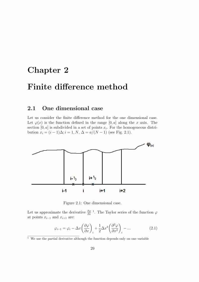
Let us consider the finite difference method for the one dimensional case.Let ϕ(x) is the function defined in the range [0, a] along the x axis. Thesection [0, a] is subdivided in a set of points xi. For the homogeneous distri-bution xi = (i− 1)∆; i = 1, N , ∆ = a/(N − 1) (see Fig. 2.1).
Figure 2.1: One dimensional case.
Let us approximate the derivative ∂ϕ∂x
1. The Taylor series of the function ϕat points xi−1 and xi+1 are:
ϕi−1 = ϕi −∆x
(∂ϕ
∂x
)i
+1
2∆x2
(∂2ϕ
∂x2
)i
− ... (2.1)
1 We use the partial derivative although the function depends only on one variable
29

ϕi+1 = ϕi + ∆x
(∂ϕ
∂x
)i
+1
2∆x2
(∂2ϕ
∂x2
)i
+ ... (2.2)
Expressing the derivative
(∂ϕ∂x
)i
from (2.1) we get the Backward Difference
Scheme (BDS): (∂ϕ
∂x
)i
=1
∆x
(ϕi − ϕi−1
)+O
(∆x
)(2.3)
Expressing the derivative
(∂ϕ∂x
)i
from (2.2) we get the Forward Difference
Scheme (FDS): (∂ϕ
∂x
)i
=1
∆x
(ϕi+1 − ϕi
)+O
(∆x
)(2.4)
Accuracy of both schemes is of the first order. Subtracting (2.1) from (2.2)we get the Central Difference Scheme (CDS)(
∂ϕ
∂x
)i
=1
2∆x
(ϕi+1 − ϕi−1
)+O
(∆x2
)(2.5)
which is of the second order accuracy.
For the approximation of derivatives ui
(∂ϕ∂x
)i
where ui is the flow velocity
one uses the Upwind Difference Scheme (UDS):(∂ϕ
∂x
)i
=
BDS, if u > 0
FDS, if u < 0(2.6)
The accuracy of BDS, FDS and CDS can be improved using the polynomialrepresentation of the function ϕ(x). For instance, consider the approximation
ϕ(x) = ax2 + bx+ c
within the section [xi−1, xi+1].Without loss of generality we assume xi−1 = 0. The coefficient c can beobtained from the condition:
ϕ(0) = ϕi−1 = c
Other two coefficients a and b are determined from the conditions:
30
ϕi = a∆x2 + b∆x+ ϕi−1
ϕi+1 = a4∆x2 + b2∆x+ ϕi−1
a =ϕi+1 − 2ϕi + ϕi−1
2∆x2
b =−ϕi+1 + 4ϕi − 3ϕi−1
2∆x
The first derivative using CDS is then(∂ϕ
∂x
)i
= 2a∆ + b =ϕi+1 − ϕi−1
2∆x
the second derivative:(∂2ϕ
∂x2
)i
= 2a =ϕi+1 − 2ϕi + ϕi−1
∆x2
If the polynomial of the 3rd order ϕ(x) = ax3 + bx2 + cx + d is applied, weget:
(∂ϕ
∂x
)i
=1
6∆x
(2ϕi+1 + 3ϕi − 6ϕi−1 + ϕi−2
)+O
(∆x3
)(2.7)
for the Backward Difference Scheme,
(∂ϕ
∂x
)i
=1
6∆x
(− ϕi+2 + 6ϕi+1 − 3ϕi − 2ϕi−1
)+O
(∆x3
)(2.8)
for the Forward Difference Scheme and
(∂ϕ
∂x
)i
=1
12∆x
(− ϕi+2 + 8ϕi+1 − 8ϕi−1 + ϕi−2
)+O
(∆x4
)(2.9)
for the Central Difference Scheme. As seen the accuracy order is sufficientlyimproved by consideration of more adjacent points.The second derivatives are:(
∂2ϕ
∂x2
)i
=1
∆x2
(ϕi+1 − 2ϕi + ϕi−1
)+O
(∆x2
)(2.10)
for the polynomial of the second order and
31
(∂2ϕ
∂x2
)i
=1
12∆x2
(− ϕi+2 + 16ϕi+1 − 30ϕi + 16ϕi−1 − ϕi−2
)+O
(∆x4
)(2.11)
for the polynomial of the fourth order. The formula (2.10) can also be ob-tained using consequently CDS(
∂2ϕ
∂x2
)i
=1
∆x
(∂ϕ
∂x i+1/2− ∂ϕ
∂x i−1/2
)(2.12)
where i+ 1/2 and i− 1/2 are intermediate points (see Fig. 2.1). Using againthe CDS for the derivatives at intermediate points:(
∂ϕ
∂x
)i+1/2
=ϕi+1 − ϕi
∆x(2.13)
(∂ϕ
∂x
)i−1/2
=ϕi − ϕi−1
∆x(2.14)
we obtain (2.10).
2.2 Two dimensional case
In the two dimensional case the function ϕ is the function of two variables ϕ =ϕ(x, y). A sample of non-uniform grid is given in Fig. (2.2). In next chapterswe will consider different grids and principles of their generation. In thischapter we consider uniform two dimensional grids (xi, yj) with equal spacingin both x and y directions.
The function ϕ at a point (xi, yj) is ϕij. The CDS approximation of thederivative on x at this point is:(
∂ϕ
∂x
)ij
=ϕi+1j − ϕi−1j
2∆x
whereas on y is: (∂ϕ
∂y
)ij
=ϕij+1 − ϕij−1
2∆y
32

Figure 2.2: A sample of non uniform grid around the profile.
2.3 Time derivatives. Explicit versus implicit
Let the unsteady partial differential equation is written in the form:
∂g
∂t= G(g, t) (2.15)
The solution is known at the time instant n. The task is to find the solutionat n+ 1 time instant. Using forward difference scheme we get:
gn+1 = gn +G(g, t)∆t (2.16)
Taking the r.h.s. of (2.15) from the n− th time slice we obtain:
gn+1 = gn +G(gn, t)∆t (2.17)
The scheme (2.17) is the so called explicit scheme (simple Euler approach).Taking the r.h.s. of (2.15) from the n+ 1− th time slice we obtain:
gn+1 = gn +G(gn+1, t)∆t (2.18)
The scheme (2.18) is the implicit scheme. The r.h.s. side of (2.18) depends onthe solution gn+1. With the other words, the solution at the time slice n+ 1,gn+1 can not be expressed explicitly through the solutions known the fromprevious time slices 1, 2, .., n for nonlinear dependence G(g, t).Mix between explicit and implicit schemes is called the Crank-Nicolson Scheme:
gn+1 = gn +1
2(G(gn, t) +G(gn+1, t))∆t
33
2.4 Exercises
1. Using the CDS find the derivative[∂
∂x
(Γ(x)
∂ϕ
∂x
)]i
= ... (2.19)
2. Using the CDS approximate the mixed derivative
∂2ϕ
∂x∂y ij=
∂
∂x
(∂ϕ
∂y
)ij
(2.20)
3. Write the program on the language C to solve the following partialdifferential equation:
∂ϕ
∂x+ α
∂2ϕ
∂x2= f(x)
with the following boundary conditions:
∂ϕ
∂x(x = 0) = C1
ϕ(x = 0) = C2
Use the central difference scheme.
4. Write the program on the language C to solve the following partialdifferential equation:
α∂ϕ
∂t+∂2ϕ
∂x2= f(x, t)
with the following boundary conditions:
∂ϕ
∂x(x = 0) = C1
ϕ(x = 0) = C2
and initial condition ϕ(x, 0) = F (x).
Use the explicit method and the central difference scheme for spatialderivatives.
34

Chapter 3
Use of boundary conditions inFinite Difference Method
3.1 Zero boundary conditions
We consider one dimensional case. ϕ(x) is an unknown function specifiedwithin the interval xε[0, 1]. For the sake of simplicity we consider uniformgrid xi = (i − 1)∆,∆ = 1/(N − 1), i = 1, N . Two dummy nodes x0 = −∆and xN+1 = 1 + ∆ are introduced to take certain boundary conditions intoaccount. Five typical boundary conditions are analyzed:
a). periodic
ϕN+1 = ϕ1, ϕ0 = ϕN (3.1)
Solution is sought at the points i = 1, ..., N.
b). Zero Dirichlet at both ends
ϕ1 = ϕN = 0 (3.2)
Solution is sought at points i = 2, ..., N − 1. At the points i = 1 andi = N the function ϕ is determined by the boundary conditions.
c). Zero Dirichlet at x = 0 and Zero gradient (Neumann) at x = 1
ϕ1 = 0,∂ϕ
∂x(1) = 0⇒ ϕN+1 = ϕN−1 (3.3)
Solution is sought at the points i = 2, ..., N . At the point i = 1 thefunction ϕ is determined by the boundary condition.
35
d). Zero gradient (Neumann) at both ends
∂ϕ
∂x(0) = 0⇒ ϕ0 = ϕ2,
∂ϕ
∂x(1) = 0⇒ ϕN+1 = ϕN−1
(3.4)
Solution is sought at the points i = 1, ..., N .
e). Zero gradient (Neumann) at x = 0 and zero Dirichlet at x = 1
∂ϕ
∂x(0) = 0⇒ ϕ0 = ϕ2, ϕN = 0 (3.5)
Solution is sought at points i = 1, ..., N − 1. At the point i = N thefunction ϕ is determined by the boundary condition.
Boundary conditions are schematically illustrated in Fig 3.1.
3.2 Extension to arbitrary non zero bound-
ary conditions
The equation
∂2ϕ
∂x2+∂ϕ
∂x= f (3.6)
is discretized with central difference scheme
ϕi+1 − 2ϕi + ϕi−1
∆2+ a
ϕi+1 − ϕi−1
2∆= fi
ai+1iϕi+1 + aiiϕi + ai−1iϕi−1 = fi
(3.7)
i = 0 corresponds to x = 0, i = N corresponds to x = 1. ∆ = 1/N, xi = i∆Let us consider the boundary conditions:
ϕ(0) = ψ1
∂ϕ
∂x(x = 1) = ψ2
(3.8)
This case can be reduced to (3.3) by modification of r.h.s. and coefficients aiin (3.7). Equation (3.7) takes at i = 1, x1 = ∆ the form:
36

ϕ2 − 2ϕ1 + ϕ0
∆2+ a
ϕ2 − ϕ0
2∆= f1
ϕ2 − 2ϕ1
∆2+ a
ϕ2
2∆= f1 −
ψ1
∆2+ a
ψ1
2∆
(3.9)
Equation (3.7) takes at xN = 1, i = N the form
ϕN+1 − 2ϕN + ϕN−1
∆2+ a
ϕN+1 − ϕN−1
2∆= fN
From the second condition in (3.8)
ϕN+1 − ϕN−1
2∆= ψ2 ⇒ ϕN+1 = 2∆ψ2 + ϕN−1
−2ϕN + ϕN−1
∆2+ϕN−1
∆2= fN − aψ2 − 2
ψ2
∆
− 2
∆2ϕN +
2
∆2ϕN−1 = fN − aψ2 − 2
ψ2
∆(3.10)
The final approximation of (3.6) reads
ai+1iϕi+1 + aiiϕi + ai−1iϕi−1 = fi (3.11)
where
a21 =1
∆2+
a
2∆, a11 = − 2
∆2, a01 = 0
f1 = f1 −ψ1
∆2+ a
ψ1
2∆
ai+1i =1
∆2+
a
2∆, aii = − 2
∆2, ai−1i =
1
∆2− a
2∆fi = fi i = 2, N − 1
aN+1N = 0, aNN = − 2
∆2, aN−1N =
2
∆2
fN = fN − aψ2 − 2ψ2
∆
System should be solved with homogeneous boundary conditions:
ϕ0 = 0
ϕN+1 + ϕN−1
∆= 0⇒ ϕN+1 = ϕN
37

Figure 3.1: Illustration of boundary conditions
Derive the approximation for the b.c.:
∂ϕ
∂x(0) = ψ1
∂ϕ
∂x(1) = ψ2
38

Chapter 4
Stability and artificial viscosityof numerical methods
4.1 Artificial viscosity
Let us consider the generic linear equation:
∂ξ
∂t+ u
∂ξ
∂x= 0
The numerical upwind scheme (UDS) is:
ξn+1i −ξni
∆t=
−u·ξni −u·ξni−1
∆xu > 0
−u·ξni+1−u·ξni∆x
u < 0
We consider only the case u > 0:
ξn+1i − ξni
∆t= −
u · ξni − u · ξni−1
∆xu > 0 (4.1)
Taylor expansions of the function ξ(x, t) in time and space gives
ξn+1i = ξni +
∂ξ
∂t
∣∣∣∣ni
∆t+∂2ξ
∂t2∆t2
2
∣∣∣∣ni
+ ... (4.2)
ξni = ξni−1 +∂ξ
∂x
∣∣∣∣ni−1
∆x+∂2ξ
∂x2
∣∣∣∣ni−1
∆x2
2+ ... (4.3)
39

Substitution of (4.2) and (4.3) into (4.1) results in
∂ξ
∂t
∣∣∣∣ni
+∂2ξ
∂t2
∣∣∣∣ni
∆t
2=
= − u
∆x
(+∂ξ
∂x
∣∣∣∣ni−1
∆x+∂2ξ
∂x2
∣∣∣∣ni−1
∆x2
2
)(4.4)
The derivatives at i− 1− th point can be expressed through these at i− thpoint:
∂ξ
∂x
∣∣∣∣ni−1
=∂ξ
∂x
∣∣∣∣ni
− ∂2ξ
∂x2
∣∣∣∣ni
∆x+∂3ξ
∂x3
∣∣∣∣ni
∆x2
2− ...,
∂2ξ
∂x2
∣∣∣∣ni−1
=∂2ξ
∂x2
∣∣∣∣ni
− ∂3ξ
∂x3
∣∣∣∣ni
∆x− ...(4.5)
The expressions (4.5) are then used in (4.4)
∂ξ
∂t
∣∣∣∣ni
+∂2ξ
∂t2
∣∣∣∣ni
∆t
2=
= − u
∆x
((∂ξ
∂x
∣∣∣∣ni
− ∂2ξ
∂x2
∣∣∣∣ni
∆x
)∆x+
(∂2ξ
∂x2
∣∣∣∣ni
− ∂3ξ
∂x3
∣∣∣∣ni
∆x
)∆x2
2+ ...
)(4.6)
Finally we have:
∂ξ
∂t
∣∣∣∣ni
+∂2ξ
∂t2
∣∣∣∣ni
∆t
2=
= − u
∆x
∆x
∂ξ
∂x
∣∣∣∣ni
− ∂2ξ
∂x2
∣∣∣∣ni
∆x2
2+ ...
(4.7)
Let us consider the left hand side of the equation (4.7).Differentiating ∂ξ
∂t= −u ∂ξ
∂xon time results in
∂2ξ
∂t2= −u ∂
∂x
(∂ξ
∂t
)= +u2 ∂
2ξ
∂x2(4.8)
40

This allows one to find the derivative ∂2ξ∂t2
:
∂2ξ
∂t2
∣∣∣∣ni
= u2 ∂2ξ
∂x2
∣∣∣∣ni
(4.9)
Using the last result the equation (4.7) is rewritten in form:
∂ξ
∂t
∣∣∣∣ni
= − u
∆x·∆x ∂ξ
∂x
∣∣∣∣ni
+∂2ξ
∂x2
∣∣∣∣ni
∆x2
2
u
∆x− u2 ∂
2ξ
∂x2
∣∣∣∣ni
∆t
2+ ... (4.10)
Finally we have
∂ξ∂t
= −u ∂ξ∂x
+
(u·∆x
2
(1− u·∆t
∆x
)∂2ξ∂x2
)+ ...
Compare now with the original equation:
∂ξ
∂t= −u∂ξ
∂x
The additional term(u·∆x
2
(1− u·∆t
∆x
)∂2ξ∂x2
)describes the error of numerical approximation of derivatives in the originalequation (4.1). It looks like the term describing the physical diffusion ν ∂
2ξ∂x2 ,
where ν is the diffusion coefficient. Therefore, the error term can be in-terpreted as the numerical or artificial diffusion with the diffusion coeffi-cient u·∆x
2(1 − u·∆t
∆x) caused by errors of equation approximation. The pres-
ence of the artificial diffusion is a serious drawback of numerical methods. Itcould be minimised by increase of the resolution ∆x→ 0.
4.2 Stability. Courant Friedrich Levy crite-
rion (CFL)
Let us consider the partial differential equation:
∂ξ
∂t+ u
∂ξ
∂x= 0 (4.11)
41

which is approximated using explicit method and upwind differential schemeat u > 0:
ξn+1i − ξni
∆t= −u
ξni − ξni−1
∆x(4.12)
It follows from (4.12):
ξn+1i − ξni = −u ·∆t
∆x(ξni − ξni−1)
ξn+1i = ξni (1− u ·∆t
∆x) +
u ·∆t∆x
ξni−1
Let us introduce the Courant Friedrich Levy parameter c = u·∆t∆x
:
ξn+1i = ξni (1− c) + cξni−1 (4.13)
We consider the zero initial condition. At the time instant n we introducethe perturbation ε at the point i. The development of the perturbation isconsidered below in time and in x direction:
time instant n:
ξni = ε
time instant n+ 1:
ξn+1i = ξni (1− c) + c · ξni−1 = ε(1− c)ξn+1i+1 = ξni+1(1− c) + c · ξni = c · ε
time instant n+ 2:
ξn+2i = ξn+1
i (1− c) + c · ξn+1i−1 = ε(1− c)2 = ε(1− c)2
ξn+2i+1 = ξn+1
i+1 (1− c) + c · ξn+1i = c · ε(1− c) + c · ε(1− c) = 2c · ε(1− c)
ξn+2i+2 = ξn+1
i+2 (1− c) + c · ξn+1i+1 = c2 · ε
time instant n+ 3:
ξn+3i = ξn+2
i (1− c) + c · ξn+2i−1 = ε(1− c)3
ξn+3i+1 = ξn+2
i+1 (1− c) + c · ξn+2i = 2c · ε(1− c)2 + c · ε(1− c)2
ξn+3i+2 = ξn+2
i+2 (1− c) + c · ξn+2i+1 = c2 · ε(1− c) + c2(2ε)(1− c)
ξn+3i+3 = ξn+2
i+3 (1− c) + c · ξn+2i+2 = c3 · ε
42

time instant n+N :
(ξn+Ni+N ) = cN · ε
..................
As follows from the last formula,the perturbation decays if
c < 1 (4.14)
The condition (4.14) is the Courant Friedrich Levy criterion of the stabilityof explicit numerical schemes. If the velocity is changed within the compu-tational domain, the maximum velocity umax is taken instead of u in for-mula (4.14). Physically the condition umax∆t
∆x< 1 means that the maximum
displacement of the fluid particle within the time step [t, t + ∆t] does notexceed the cell size ∆x. The CFL parameter c can be reduced by decreaseof ∆t (not by increase of ∆x!).
4.3 Exercise
The field of the velocity component ux is given as ux,ij = exp(−((i∆x −0.5)2 + (j∆y − 0.5)2).Calculate uy,ij from continuity equation (1.3) and the ∆t satisfying the CFLcriterion.
43

44

Chapter 5
Simple explicit time advancescheme for solution of theNavier Stokes Equation
5.1 Theory
The unsteady term of the Navier Stokes Equation
∂ui∂t
= −∂uiuj∂xj
− 1
ρ
∂p
∂xi+ ν
∂
∂xj
∂ui∂xj
(5.1)
is written in explicit form:
un+1i = uni + ∆t
[−δuni u
nj
δxj− 1
ρ
δpn
∂xi+ ν
δ
δxj
δuniδxj
](5.2)
where δδxj
is the approximation of the derivative ∂∂xj
. Let us apply the diver-
gence operator δδxi
:
δun+1i
δxi=δuniδxi
+ ∆tδ
δxi
[−δuni u
nj
δxj− 1
ρ
δpn
∂xi+ ν
δ
δxj
δuniδxj
](5.3)
Let uni is the divergence free field, i.e.δuniδxi
= 0. The task is to find thevelocity field at the time moment n+ 1 which is also divergence free
δun+1i
δxi= 0 (5.4)
Substituting (5.4) into (5.3) one obtains:
45
δ
δxi
[−δuni u
nj
δxj− 1
ρ
δpn
∂xi+ ν
δ
δxj
δuniδxj
]= 0 (5.5)
Expressing (5.5) with respect to the pressure results in the Poisson equation:
δ2pn
∂x2i
= ρ
[−δ2uni u
nj
δxjδxi+ ν
δ2
δxiδxj
δuniδxj
](5.6)
The algorithm for time-advancing is as follows:
i) The solution at time n is known and divergence free.
ii) Calculation of the r.h.s. of (5.6) ρ[− δ2uni u
nj
δxjδxi+ ν δ2
δxiδxj
δuniδxj
]iii) Calculation of the pressure pn from the Poisson equation (5.6)
iv) Calculation of the velocity un+1i . This is divergence free.
v) Go to the step ii).
In the following sections we consider the algorithm in details for the twodimensional case.
5.2 Mixed schemes
The high accuracy of the CDS schemes is their advantage. The disadvantageof CDS schemes is their instability resulting in oscillating solutions. On thecontrary, the upwind difference schemes UDS possess a low accuracy and highstability. The idea to use the combination of CDS and UDS to strengthentheir advantages and diminish their disadvantages. Let us consider a simpletransport equation for the quantity ϕ:
∂ϕ
∂t+ u
∂ϕ
∂x= 0 (5.7)
with u > 0. A simple explicit, forward time, central difference scheme forthis equation may be written as
ϕn+1i = ϕni − c([ϕni +
1
2(ϕni+1 − ϕni )]− [ϕni−1 +
1
2(ϕni − ϕni−1)]) =
= ϕni − c([ϕni − ϕni−1] +1
2[ϕni+1 − ϕni ]− 1
2[ϕni − ϕni−1]) (5.8)
46
where c = u∆t∆x
is the CFL parameter. The term c[ϕni − ϕni−1] is the diffusive
1st order upwind contribution. The term c(12[ϕni+1−ϕni ]− 1
2[ϕni −ϕni−1]) is the
anti-diffusive component. With TVD (total variation diminishing) schemesthe anti-diffusive component is limited in order to avoid instabilities andmaintain boundness 0 < ϕ < 1:
ϕn+1i = ϕni − c([ϕni − ϕni−1] +
1
2[ϕni+1 − ϕni ]Ψn
east −1
2[ϕni − ϕni−1]Ψn
west) (5.9)
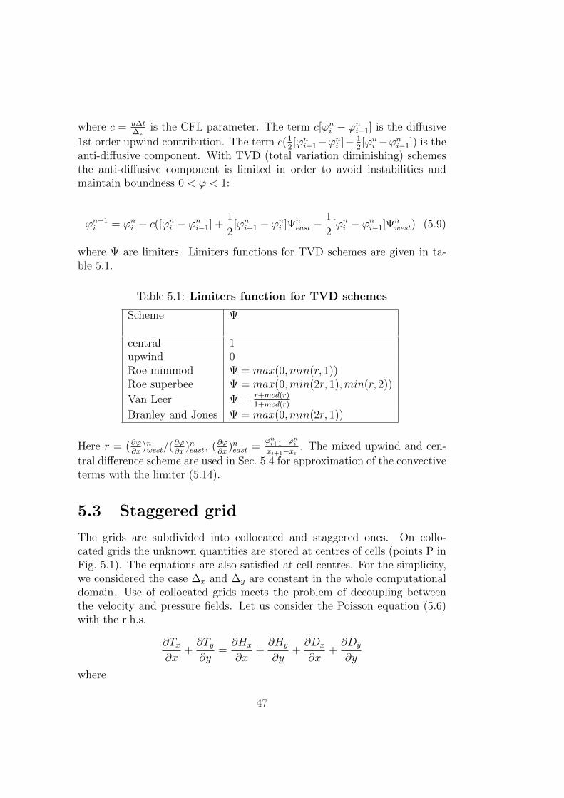
where Ψ are limiters. Limiters functions for TVD schemes are given in ta-ble 5.1.
Table 5.1: Limiters function for TVD schemes
Scheme Ψ
central 1upwind 0Roe minimod Ψ = max(0,min(r, 1))Roe superbee Ψ = max(0,min(2r, 1),min(r, 2))
Van Leer Ψ = r+mod(r)1+mod(r)
Branley and Jones Ψ = max(0,min(2r, 1))
Here r = (∂ϕ∂x
)nwest/(∂ϕ∂x
)neast, (∂ϕ∂x
)neast =ϕni+1−ϕnixi+1−xi . The mixed upwind and cen-
tral difference scheme are used in Sec. 5.4 for approximation of the convectiveterms with the limiter (5.14).
5.3 Staggered grid
The grids are subdivided into collocated and staggered ones. On collo-cated grids the unknown quantities are stored at centres of cells (points P inFig. 5.1). The equations are also satisfied at cell centres. For the simplicity,we considered the case ∆x and ∆y are constant in the whole computationaldomain. Use of collocated grids meets the problem of decoupling betweenthe velocity and pressure fields. Let us consider the Poisson equation (5.6)with the r.h.s.
∂Tx∂x
+∂Ty∂y
=∂Hx
∂x+∂Hy
∂y+∂Dx
∂x+∂Dy
∂y
where
47

Dx = ν∂2ux∂x2
+ ν∂2ux∂y2
Dy = ν∂2uy∂x2
+ ν∂2uy∂y2
Hx = −∂uxux∂x
−−∂uxuy∂y
Hy = −∂uxuy∂x
−−∂uyuy∂y
(5.10)
Application of the central difference scheme to the Poisson equation resultsin
(∂pn
∂x)E − (∂p
n
∂x)W
2∆x
+(∂p
n
∂y)N − (∂p
n
∂y)S
2∆y
=T nx,E − T nx,W
2∆x
+T ny,N − T ny,S
2∆y
or
pnEE−pnP
2∆x− pnP−p
nWW
2∆x
2∆x
+
pnNN−pnP
2∆y− pnP−p
nSS
2∆y
2∆y
=T nx,E − T nx,W
2∆x
+T ny,N − T ny,S
2∆y
= QHP
The last equation is expressed in the matrix form:
ApPpnP +
∑l
Apl pnl = −QH
P (5.11)
where
l = EE,WW,NN, SS, ApEE = ApWW = − 1(2∆x)2 , ApNN = ApSS = − 1
(2∆y)2
and ApP = −∑
lApl
This equation (5.11) has involves nodes which are 2∆ apart (see also [6])!It is a discretized Poisson equation on a grid twice as coarse as the basicone but the equations split into four unconnected systems, one with i and jboth even, one with i even and j odd, one with i odd and j even, andone with both odd. Each of these systems gives a different solution. Fora flow with a uniform pressure field, the checkerboard pressure distributionshown in Fig. 5.2 satisfies these equations and could be produced. However,the pressure gradient is not affected and the velocity field may be smooth.
48
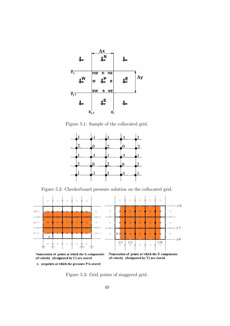
Figure 5.1: Sample of the collocated grid.
Figure 5.2: Checkerboard pressure solution on the collocated grid.
Figure 5.3: Grid points of staggered grid.
49

There is also the possibility that one may not be able to obtain a convergedsteady-state solution.
A possible solution of the problem is the application of the staggered grids(Fig. 5.3). The Poisson equation is satisfied at cell centres designated bycrosses. The ux velocities are stored at points staggered by ∆x/2 in x-direction (filled circles). At these points the first Navier- Stokes equationis satisfied:
∂ux∂t
= −∂uxuj∂xj
− 1
ρ
∂p
∂x+ ν
∂
∂xj
∂ux∂xj
(5.12)
The uy velocities are stored at points staggered by ∆y/2 in y-direction (cir-cles). At these points the second Navier-Stokes equation is satisfied:
∂uy∂t
= −∂uyuj∂xj
− 1
ρ
∂p
∂y+ ν
∂
∂xj
∂uy∂xj
(5.13)
The staggered grid is utilized below.
5.4 Approximation of −δuni unj
δxj
The approximation of the convective term is a very critical point. For fasterflows or larger time steps, the discretization shall be closer to an upwindingapproach [7]. Following to [7] we implement a smooth transition betweencentered differencing and upwinding using a parameter γ ∈ [0, 1]. It is definedas
γ = min(1.2 ·∆t ·max(|ux(i, j)|, |uy(i, j)|), 1) (5.14)
The value of gamma is the maximum fraction of a cells which information cantravel in one time step, multiplied by 1.2, and capped by 1. The factor of 1.2is taken from the experience that often times tending a bit more towardsupwinding can be advantageous for accuracy [8].
γ = 0 corresponds to the central difference scheme (CDS) whereas γ = 1results in the upwind difference scheme (UDS).
50

5.4.1 Approximation of −∂uxux
∂x −∂uxuy
∂y = −ux ∂ux
∂x − uy∂ux
∂y
• Point (i+ 1/2, j) for x-component of velocity:
ux(i+ 1/2, j) = (ux(i+ 1, j) + ux(i, j))/2.0
If ux(i+ 1/2, j) ≥ 0,
then uxux|i+1/2,j = ux(i+ 1/2, j)(1− γ
2ux(i+ 1, j) +
γ + 1
2ux(i, j))
else uxux|i+1/2,j = ux(i+ 1/2, j)(γ + 1
2ux(i+ 1, j) +
1− γ2
ux(i, j))
• Point (i− 1/2, j) for x-component of velocity:
ux(i− 1/2, j) = (ux(i, j) + ux(i− 1, j))/2.0
If ux(i− 1/2, j) ≥ 0,
then uxux|i−1/2,j = ux(i− 1/2, j)(1− γ
2ux(i, j) +
γ + 1
2ux(i− 1, j))
else uxux|i−1/2,j = ux(i− 1/2, j)(γ + 1
2ux(i, j) +
1− γ2
ux(i− 1, j))
• Point (i+ 1/2, j) for y-component of velocity:
uy(i+ 1/2, j) = (uy(i+ 1, j) + uy(i, j))/2.0
If uy(i+ 1/2, j) ≥ 0,
then uxuy|i+1/2,j = uy(i+ 1/2, j)(γ + 1
2ux(i, j) +
1− γ2
ux(i, j + 1))
else uxuy|i+1/2,j = uy(i+ 1/2, j)(1− γ
2ux(i, j) +
γ + 1
2ux(i, j + 1))
• Point (i+ 1/2, j − 1) for y-component of velocity:
uy(i+ 1/2, j − 1) = (uy(i+ 1, j − 1) + uy(i, j − 1))/2.0
If uy(i+ 1/2, j − 1) ≥ 0,
then uxuy|i+1/2,j−1 = uy(i+ 1/2, j − 1)(γ + 1
2ux(i, j − 1) +
1− γ2
ux(i, j))
else uxuy|i+1/2,j−1 = uy(i+ 1/2, j − 1)(1− γ
2ux(i, j − 1) +
γ + 1
2ux(i, j))
Hx(i, j) = −∂uxux∂x
− ∂uxuy∂y
=
−uxux|i+1/2,j − uxux|i−1/2,j
∆x
−uxuy|i+1/2,j − uxuy|i+1/2,j−1
∆y
51

5.4.2 Approximation of −∂uxuy
∂x −∂uyuy
∂y = −ux ∂uy
∂x − uy∂uy
∂y
• Point (i, j + 1/2) for y-component of velocity:
uy(i, j + 1/2) = (uy(i, j) + uy(i, j + 1))/2.0
If uy(i, j + 1/2) ≥ 0,
then uyuy|i,j+1/2 = uy(i, j + 1/2)(1− γ
2uy(i, j + 1) +
γ + 1
2uy(i, j))
else uyuy|i,j+1/2 = uy(i, j + 1/2)(γ + 1
2uy(i, j + 1) +
1− γ2
uy(i, j))
• Point (i, j − 1/2) for y-component of velocity:
uy(i, j − 1/2) = (uy(i, j − 1) + uy(i, j))/2.0
If uy(i, j − 1/2) ≥ 0,
then uyuy|i,j−1/2 = uy(i, j − 1/2)(1− γ
2uy(i, j) +
γ + 1
2uy(i, j − 1))
else uyuy|i,j−1/2 = uy(i, j − 1/2)(γ + 1
2uy(i, j) +
1− γ2
uy(i, j − 1))
• Point (i, j + 1/2) for x-component of velocity:
ux(i, j + 1/2) = (ux(i, j + 1) + ux(i, j))/2.0
If ux(i, j + 1/2) ≥ 0,
then uyux|i,j+1/2 = ux(i, j + 1/2)(γ + 1
2uy(i, j) +
1− γ2
uy(i+ 1, j))
else uyux|i,j+1/2 = ux(i, j + 1/2)(1− γ
2uy(i, j) +
γ + 1
2uy(i+ 1, j))
• Point (i− 1, j + 1/2) for x-component of velocity:
ux(i− 1, j + 1/2) = (ux(i− 1, j + 1) + ux(i− 1, j))/2.0
If ux(i− 1, j + 1/2) ≥ 0,
then uyux|i−1,j+1/2 = ux(i− 1, j + 1/2)(γ + 1
2uy(i− 1, j) +
1− γ2
uy(i, j))
else uyux|i−1,j+1/2 = ux(i− 1, j + 1/2)(1− γ
2uy(i− 1, j) +
γ + 1
2uy(i, j))
Hy(i, j) = −∂uxuy∂x
− ∂uyuy∂y
=
−uyux|i,j+1/2 − uyux|i−1,j+1/2
∆x
−uyuy|i,j+1/2 − uyuy|i,j−1/2
∆y
52
5.5 Approximation of δδxj
δuniδxj
The second derivative is calculated using the Central Difference Scheme(CDS):
Dx(i, j) =ux(i+ 1, j)− 2ux(i, j) + ux(i− 1, j)
∆2x
+ux(i, j + 1)− 2ux(i, j) + ux(i, j − 1)
∆2y
Dy(i, j) =uy(i+ 1, j)− 2uy(i, j) + uy(i− 1, j)
∆2x
+uy(i, j + 1)− 2uy(i, j) + uy(i, j − 1)
∆2y
5.6 Calculation of the r.h.s. for the Poisson
equation (5.6)
The r.h.s. of (5.6) is
−δ2uni u
nj
δxjδxi+ ν
δ2
δxiδxj
δuniδxj
=∂Hx
∂x+∂Hy
∂y+∂Dx
∂x+∂Dy
∂y
The derivatives at the point (i,j) of the pressure storage (designated as X inFig. 5.3) are calculated using CDS
∂Hx
∂x|ij =
Hx(i, j)−Hx(i− 1, j)
∆x,∂Dx
∂x|ij =
Dx(i, j)−Dx(i− 1, j)
∆x,
∂Hy
∂y|ij =
Hy(i, j)−Hy(i, j − 1)
∆y,∂Dy
∂y|ij =
Dy(i, j)−Dy(i, j − 1)
∆y
5.7 Solution of the Poisson equation (5.6)
The numerical solution of the Poisson equation is discussed in [6].
5.8 Update the velocity field
The velocity field is updated according to formula
un+1x (i, j) = unx(i, j) + ∆t(H
nx (i, j) +Dn
x(i, j)− (pn(i+ 1, j)− pn(i, j))/∆x)
un+1y (i, j) = uny (i, j) + ∆t(H
ny (i, j) +Dn
y (i, j)− (pn(i, j + 1)− pn(i, j))/∆y)
53
5.9 Boundary conditions for the velocities
At this stage, the boundary conditions (BC) for the velocity field should betaken into account. The nodes at which the BC are enforced are shown bygrey symbols in Fig. 5.3. Enforcement of the BC is easy, if the ”grey” pointlies exactly at the boundary of the computational domain. If not, two casesshould be considered. If the Neumann condition is enforced ∂u
∂n= C , the
velocity component outside of the boundary u(0) is calculated through theinterior quantity u(1) from
u(1)− u(0)
∆n
= C
If the Dirichlet condition u = C is enforced and the point 0 is outside of thecomputational domain, the value u(0) is calculated from the extrapolationprocedure:
u(0) + u(1)
2= C
5.10 Calculation of the vorticity
The calculation of vorticity ωz = ∂ux∂y− ∂uy
∂xis performed as follows:
ux(i− 1/2, j + 1/2) =1
4(ux(i, j) + ux(i, j + 1) + ux(i− 1, j) + ux(i− 1, j + 1)),
ux(i− 1/2, j − 1/2) =1
4(ux(i, j) + ux(i− 1, j) + ux(i, j − 1) + ux(i− 1, j − 1)),
uy(i+ 1/2, j − 1/2) =1
4(uy(i, j) + uy(i+ 1, j) + uy(i, j − 1) + uy(i+ 1, j − 1)),
uy(i− 1/2, j − 1/2) =1
4(uy(i, j) + uy(i− 1, j) + uy(i, j − 1) + uy(i− 1, j − 1)),
ωz(i, j) =ux(i− 1/2, j + 1/2)− ux(i− 1/2, j − 1/2)
∆y
−
− uy(i+ 1/2, j − 1/2)− uy(i− 1/2, j − 1/2)
∆x
54
Chapter 6
Splitting schemes for solutionof multidimensional problems
6.1 Splitting in spatial directions. Alternat-
ing direction implicit (ADI) approach
Let us consider the two dimensional unsteady heat conduction equation:
∂φ
∂t= λ
(∂2φ
∂x2+∂2φ
∂y2
)(6.1)
We use implicit scheme proposed by Crank and Nicolson and CDS for spatialderivatives:
φn+1 − φn
∆t=λ
2
[(∂2φn
∂x2+∂2φn
∂y2
)+
(∂2φn+1
∂x2+∂2φn+1
∂y2
)](6.2)
(∂2φn
∂x2
)i,j
=φni+1,j − 2φni,j + φni−1,j
(∆x)2(6.3)
(∂2φn
∂y2
)i,j
=φni,j+1 − 2φni,j + φni,j−1
(∆y)2(6.4)
In what follows we use the designations for derivative approximations:
δ2
δx2φn =
φni+1,j − 2φni,j + φni−1,j
(∆x)2(6.5)
δ2
δy2φn =
φni,j+1 − 2φni,j + φni,j−1
(∆y)2(6.6)
55
Using these designations we get from the original heat conduction equation:
(1− λ∆t
2
δ2
δx2
)(1− λ∆t
2
δ2
δy2
)φn+1 =
(1 +
λ∆t
2
δ2
δx2
)(1 +
λ∆t
2
δ2
δy2
)φn+
+(λ∆t)2
4
δ2
δx2
[δ2
δy2
(φn+1 − φn
)](6.7)
The last term is neglected since (φn+1 − φn)(∆t)2 ∼ ∂φ∂t
(∆t)3.Numerical solution is performed in two following steps:
Step 1: Solution of one dimensional problem in x-direction:(1− λ∆t
2
δ2
δx2
)φ∗ =
(1 +
λ∆t
2
δ2
δy2
)φn (6.8)
The numerical solution of (6.8) φ∗ is then substituted as the guesssolution for the next step:
Step 2: Solution of one dimensional problem in y-direction(1− λ∆t
2
δ2
δy2
)φn+1 =
(1 +
λ∆t
2
δ2
δx2
)φ∗ (6.9)
It can be shown that the resulting method is of the second order of accuracyand unconditionally stable.
6.2 Splitting according to physical processes.
Fractional step methods
Within the fractional step method the original equation is split accordingto physical processes. Splitting according to physical processes is used forunsteady problems. The general idea is illustrated for the transport equation:
∂u
∂t= Cu+Du+ P (6.10)
Here
C is the convection operator,
D is the diffusion operator,
56
P is the pressure source operator.
Simple explicit Euler method can be written as
un+1 = un + (Cu+Du+ P )∆t (6.11)
The overall numerical solution is considered as the consequence of numericalsolutions of the following partial problems:
u∗ = un + (Cun)∆t (*) Convection step
u∗∗ = u∗ + (Du∗)∆t (**) Diffusion step
un+1 = u∗∗ + (P )∆t (***) Pressure step
(6.12)
solving sequentially. The sense of this splitting is that the numerical solutionof partial problems (*)-(***) is simpler and more stable than that of thewhole problem. The disadvantage of this procedure is that it is applicable toonly unsteady problem formulation. Another disadvantage is the low orderof accuracy with respect to time derivative approximation. The order of timederivative approximations can be derived using the sample with two physicalprocesses described by operators L1 and L2:
∂u
∂t= L1(u) + L2(u) (6.13)
The splitting of (6.10) results in two steps procedure:
∂u∗
∂t= L1(u∗), u∗|t=tn = un
∂un+1
∂t= L2(un+1), un+1|t=tn = u∗
(6.14)
where
u∗ = un + ∆tL1(un) +O(∆t2),
un+1 = u∗ + ∆tL2(u∗) +O(∆t2) =
= un + ∆tL1(un) + ∆tL2(un + ∆tL1(un)) +O(∆t2) =
= un + ∆t(L1(un) + L2(un)) +O(∆t2).
(6.15)
The accuracy of the final solution un+1 is of the first order in time.Very often the diffusion step is treated implicitly. This is done to diminishthe time step restriction for the diffusion process. Otherwise, the stability
57

requires ∆t to be proportional to the spacial discretization squared, if a pureexplicit scheme is applied. The semi implicit scheme for the two dimensionalNavier Stokes equation reads:
Convection step is treated explicitly:
u∗x − unx∆t
= −δunxu
nx
δx−δunxu
ny
δy(6.16)
u∗y − uny∆t
= −δunyu
nx
δx−δunyu
ny
δy(6.17)
The solutions u∗x,y are used then for the diffusion process which istreated implicitly:
u∗∗x − u∗x∆t
= ν
(δ2u∗∗xδx2
+δ2u∗∗xδy2
)(6.18)
u∗∗y − u∗y∆t
= ν
(δ2u∗∗yδx2
+δ2u∗∗yδy2
)(6.19)
The solutions u∗∗x,y are used then for the next process which is treatedexplicitly:
un+1x − u∗∗x
∆t= −δp
n+1
δx(6.20)
un+1y − u∗∗y
∆t= −δp
n+1
δy(6.21)
where the pressure pn+1 should be pre computed from the continuityequation demanding the velocity at n+ 1 time slice is divergency free:
δun+1x
δx+δun+1
y
δy= 0 (6.22)
Applying the operator∇ to the equations (6.20) and (6.21) we get the Poissonequation for the pressure:
δ2pn+1
δx2+δ2pn+1
δy2=
1
∆t
(δu∗∗xδx
+δu∗∗yδy
)(6.23)
58
6.3 Increase of the accuracy of time deriva-
tives approximation using the Lax-Wendroff
scheme
Let us consider the general transport equation:
∂u
∂t+∂F (u)
∂x= 0 (6.24)
We introduce the following designations:
A =∂F
∂u
utt = −Fxt = −Ftx, Ft = Fuut = −FuFx ≡ −AFx (6.25)
Substitution of these results into the time Taylor series gives the Lax-Wendroffscheme which is of the second order in time:
u(t+ τ) = u(t) + τut(t) +τ 2
2utt(t) +O(τ 3)
= u(t)− τFx(t) +τ 2
2(A(t)Fx(t))x +O(τ 3)
(6.26)
A difficulty arising in the LW approach is the computation of the operator A.One can easy derive that the Lax Wendroff scheme results in the solution ofthe equation:
un+1 − un
τ+∂F n
∂x=τ
2
∂
∂x
(An
∂F n
∂x
)
59

60
Chapter 7
Finite Volume Method
7.1 Transformation of the Navier-Stokes Equa-
tions in the Finite Volume Method
The Navier Stokes equation
∂ui∂t
+∂(uiuj)
∂xj= Fi −
1
ρ
∂p
∂xi+ ν
∂
∂xj
(∂
∂xjui
)(7.1)
is fulfilled within each mesh element (finite volume U) in the integral sense.For that it is integrated over the volume U :
∫U
[∂ui∂t
+∂(uiuj)
∂xj
]dU =
∫U
[Fi −
1
ρ
∂p
∂xi+ ν
∂
∂xj
(∂
∂xjui
)]dU (7.2)
Application of the Gauss theorem results in
∂
∂t
∫U
uidU +
∫S
ui~u~ndS =
∫U
FidU −1
ρ
∫S
p~ei~ndS + ν
∫S
gradui~ndS (7.3)
The same procedure applied to the continuity equation gives∫S
~u~ndS = 0 (7.4)
61

Figure 7.1: Staggered arrangement of finite volumes.
7.2 Sample
Let us consider the two dimensional transport equation without the diffusionterm
∂ui∂t
+∂uiuj∂xj
= − ∂p
∂xi∂uj∂xj
= 0
(7.5)
In the integral form this equation reads
∂
∂t
∫U
uidU +
∫S
ui~u~ndS = −∫S
p~ei~ndS (7.6)
We use the staggered grid (Fig. 14.2). The pressure is stored at the volumecenters. The ux velocity is stored at the centers of vertical faces, whereasthe velocity uy component at centers of horizontal faces. The x- equationis satisfied for volumes displaced in x-direction, whereas the y-equation forthese displaced in y-direction.Below we consider approximations of different terms:
7.2.1 Pressure and unsteady terms
Source (pressure) term for x-equation:
62
Qp1 = −
∫S
p~e1~ndS ≈ −(peSe − pwSw
)= −
(pi+1j − pij
)∆ (7.7)
Unsteady term for x-equation:
∂
∂t
∫U
uxdU = ∆2un+1xij − unxij
∆t(7.8)
Pressure term for y-equation:
Qp2 = −
∫S
p~e2~ndS ≈ −(pnSn − psSs
)= −
(pij+1 − pij
)∆ (7.9)
Unsteady term for y-equation:
∂
∂t
∫U
uydU = ∆2un+1yij − unyij
∆t(7.10)
7.2.2 Convection term of the x-equation
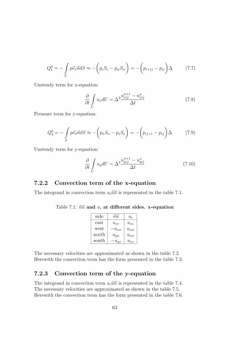
The integrand in convection term ui~u~n is represented in the table 7.1.
Table 7.1: ~n~u and ui at different sides. x-equation
side ~n~u uieast uxe uxewest −uxw uxwnorth uyn uxnsouth −uys uxs
The necessary velocities are approximated as shown in the table 7.2.Herewith the convection term has the form presented in the table 7.3.
7.2.3 Convection term of the y-equation
The integrand in convection term ui~u~n is represented in the table 7.4.The necessary velocities are approximated as shown in the table 7.5.Herewith the convection term has the form presented in the table 7.6.
63

Table 7.2: Velocities at different sides. x-equation
velocity approximationuxe uxe = 1
2(uxij + uxi+1j)
uxw uxw = 12(uxij + uxi−1j)
uxn uxn = 12(uxij + uxij+1)
uxs uxs = 12(uxij + uxij−1)
uyn uyn = 12(uyij + uyi+1j)
uys uys = 12(uyij−1 + uyi+1j−1)
Table 7.3: Convection flux. x-equation
side fluxeast ∆
4(uxij + uxi+1j)
2
west −∆4
(uxij + uxi−1j)2
north ∆4
(uxij + uxij+1)(uyij + uyi+1j)south −∆
4(uxij + uxij−1)(uyi+1j−1 + uyij−1)
Table 7.4: ~n~u and ui at different sides. y-equation
side ~n~u uieast uxe uyewest −uxw uywnorth uyn uynsouth −uys uys
Table 7.5: Velocities at different sides. y-equation
velocity approximationuxe uxe = 1
2(uxij + uxij+1)
uxw uxw = 12(uxi−1j + uxi−1j+1)
uyn uyn = 12(uyij + uyij+1)
uys uys = 12(uyij + uyij−1)
uye uye = 12(uyij + uyi+1j)
uyw uyw = 12(uyij + uyi−1j)
7.2.4 X-equation approximation
∆2un+1xij − unxij
∆t+
64
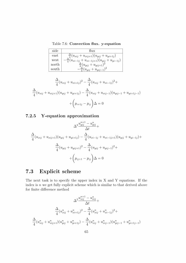
Table 7.6: Convection flux. y-equation
side fluxeast ∆
4(uxij + uxij+1)(uyij + uyi+1j)
west −∆4
(uxi−1j + uxi−1j+1)(uyij + uyi−1j)north ∆
4(uyij + uyij+1)2
south −∆4
(uyij + uyij−1)2
∆
4(uxij + uxi+1j)
2 − ∆
4(uxij + uxi−1j)
2+
∆
4(uxij + uxij+1)(uyij + uyi+1j)−
∆
4(uxij + uxij−1)(uyij−1 + uyi+1j−1)
+
(pi+1j − pij
)∆ = 0
7.2.5 Y-equation approximation
∆2un+1yij − unyij
∆t+
∆
4(uxij + uxij+1)(uyij + uyi+1j)−
∆
4(uxi−1j + uxi−1j+1)(uyij + uyi−1j)+
∆
4(uyij + uyij+1)2 − ∆
4(uyij + uyij−1)2+
+
(pij+1 − pij
)∆ = 0
7.3 Explicit scheme
The next task is to specify the upper index in X and Y equations. If theindex is n we get fully explicit scheme which is similar to that derived abovefor finite difference method
∆2un+1xij − unxij
∆t+
∆
4(unxij + unxi+1j)
2 − ∆
4(unxij + unxi−1j)
2+
∆
4(unxij + unxij+1)(unyij + unyi+1j)−
∆
4(unxij + unxij−1)(unyij−1 + unyi+1j−1)
65

+
(pni+1j − pnij
)∆ = 0 (7.11)
∆2un+1yij − unyij
∆t+
∆
4(unyij + unyi+1j)(u
nxij + unxij+1)− ∆
4(unyij + unyi−1j)(u
nxi−1j + unxi−1j+1)+
∆
4(unyij + unyij+1)2 − ∆
4(unyij + unyij−1)2+
+
(pnij+1 − pnij
)∆ = 0 (7.12)
The Poisson equation for pressure is derived in the same manner as abovefor finite difference method. For that the equations (7.11) is differentiatedon x, whereas the equation (7.12) is differentiated on y. Then both resultsare summed under assumptions that both un+1
ij and unij are divergence free:
δun+1xij
δx+δun+1
yij
δy= 0,
δunxijδx
+δunyijδy
= 0
This equation is coupled with equations (7.11) and (7.12). The explicitscheme has advantage that the solution at the time instant n + 1 is ex-plicitly expressed through the solution at time instant n. The solution oflinear algebraic equations which is the most laborious numerical procedureis necessary only for the solution of the Poisson equation. The momentumequations (7.11) and (7.12) are solved explicitly. Velocities un+1
xij and un+1yij
are computed then from simple algebraic formula (7.11) and (7.12). The bigdisadvantage of the explicit method is the limitation forced by the CourantFriedrich Levy criterion. The time step ∆t should be very small to secure thenumerical stability. This disadvantage can be overcome within the implicitschemes.
7.4 Implicit scheme
If the index is n+ 1 we get implicit scheme
∆2un+1xij − unxij
∆t+
∆
4(un+1
xij + un+1xi+1j)
2 − ∆
4(un+1
xij + un+1xi−1j)
2+
66

∆
4(un+1
xij + un+1xij+1)(un+1
yij + un+1yi+1j)−
∆
4(un+1
xij + un+1xij−1)(un+1
yij−1 + un+1yi+1j−1)
+
(pn+1i+1j − pn+1
ij
)∆ = 0 (7.13)
∆2un+1yij − unyij
∆t+
∆
4(un+1
yij + un+1yi+1j)(u
n+1xij + un+1
xij+1)− ∆
4(un+1
yij + un+1yi−1j)(u
n+1xi−1j + un+1
xi−1j+1)+
∆
4(un+1
yij + un+1yij+1)2 − ∆
4(un+1
yij + un+1yij−1)2+
+
(pn+1ij+1 − pn+1
ij
)∆ = 0 (7.14)
The Poisson equation for pressure is derived in the same manner as abovefor finite difference method. For that the equations (7.13) is differentiatedon x, whereas the equation (7.14) is differentiated on y. Then both resultsare summed under assumptions that both un+1
ij and unij are divergence free:
δun+1xij
δx+δun+1
yij
δy= 0,
δunxijδx
+δunyijδy
= 0
The resulting Poisson equation can not be solved because both the r.h.s.(velocities) and the l.h.s (pressure) depend on n + 1. The term on r.h.s.cannot be computed until the computation of velocity field at time n + 1is completed and vice versa. Other problem is that the equations (7.13)and (7.14) are non linear.
7.5 Iterative procedure for implicit scheme
To solve the nonlinear system and the whole system of equations we use theiterative procedure. Let m be an iteration number. The nonlinear term isrepresented in form:
∂uiuj∂xj
=∂u
(m)i u
(m−1)j
∂xj(7.15)
The velocity uj is taken from the previous iteration (m − 1). The sys-tem (7.11) and (7.12) is rewritten in the form
67

∆2u
(m)xij − unxij
∆t+
∆
4(u
(m)xij + u
(m)xi+1j)(u
(m−1)xij + u
(m−1)xi+1j )− ∆
4(u
(m)xij + u
(m)xi−1j)(u
(m−1)xij + u
(m−1)xi−1j )+
∆
4(u
(m)xij + u
(m)xij+1)(u
(m−1)yij + u
(m−1)yi+1j )− ∆
4(u
(m)xij + u
(m)xij−1)(u
(m−1)yij−1 + u
(m−1)yi+1j−1)
+
(p
(m)i+1j − p
(m)ij
)∆ = 0
∆2u
(m)yij − unyij
∆t+
∆
4(u
(m)yij + u
(m)yi+1j)(u
(m−1)xij + u
(m−1)xij+1 )− ∆
4(u
(m)yij + u
(m)yi−1j)(u
(m−1)xi−1j + u
(m−1)xi−1j+1)+
∆
4(u
(m)yij + u
(m)yij+1)(u
(m−1)yij + u
(m−1)yij+1 )− ∆
4(u
(m)yij + u
(m)yij−1)(u
(m−1)yij + u
(m−1)yij−1 )+
+
(p
(m)ij+1 − p
(m)ij
)∆ = 0
or
qxi−1ju(m)xi−1j + qxiju
(m)xij + qxi+1ju
(m)xi+1j + qxij−1u
(m)xij−1 + qxij+1u
(m)xij+1+ (7.16)
+
(p
(m)i+1j − p
(m)ij
)∆ = rxij
qyi−1ju(m)yi−1j + qyiju
(m)yij + qyi+1ju
(m)yi+1j + qyij−1u
(m)yij−1 + qyij+1u
(m)yij+1+ (7.17)
+
(p
(m)ij+1 − p
(m)ij
)∆ = ryij
where
68

qxij = ∆2/∆t+∆
4[(u
(m−1)xij + u
(m−1)xi+1j )− (u
(m−1)xij + u
(m−1)xi−1j )+
+ (u(m−1)yij + u
(m−1)yi+1j )− (u
(m−1)yij−1 + u
(m−1)yi+1j−1)]
qxi+1j =∆
4(u
(m−1)xij + u
(m−1)xi+1j ), qxi−1j = −∆
4(u
(m−1)xi−1j + u
(m−1)xij ),
qxij+1 =∆
4(u
(m−1)yij + u
(m−1)yi+1j ), qxij−1 = −∆
4(u
(m−1)yij−1 + u
(m−1)yi+1j−1)
qyij =∆2
∆t+
∆
4
[(u
(m−1)yij + u
(m−1)yij+1
)−(u
(m−1)yij + u
(m−1)yij−1
)+
+(u
(m−1)xij + u
(m−1)xij+1
)−(u
(m−1)xi−1j + u
(m−1)xi−1j+1
)]qyi−1j = −∆
4
(u
(m−1)xi−1j + u
(m−1)xi−1j+1
), qyi+1j =
∆
4
(u
(m−1)xij + u
(m−1)xij+1
)qyij−1 = −∆
4
(u
(m−1)yij + u
(m−1)yij−1
), qyij+1 =
∆
4
(u
(m−1)yij + u
(m−1)yij+1
)rxij = ∆2
unxij∆t
, ryij = ∆2unyij∆t
Dividing the equations (7.16) by qxij and (7.17) by qyij we obtain
axi−1ju(m)xi−1j + u
(m)xij + axi+1ju
(m)xi+1j + axij−1u
(m)xij−1 + axij+1u
(m)xij+1+ (7.18)
+
(p
(m)i+1j − p
(m)ij
)∆/qxij = Rxij
ayi−1ju(m)yi−1j + u
(m)yij + ayi+1ju
(m)yi+1j + ayij−1u
(m)yij−1 + ayij+1u
(m)yij+1+ (7.19)
+
(p
(m)ij+1 − p
(m)ij
)∆/qyij = Ryij
where ax,ykl = qx,ykl/qx,yij and Rx,ykl = rx,ykl/qx,yij. In what follows we usethe operator form of equations (7.18) and (7.19):
u = Au+Bp+ C (7.20)
69
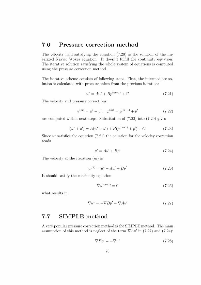
7.6 Pressure correction method
The velocity field satisfying the equation (7.20) is the solution of the lin-earized Navier Stokes equation. It doesn’t fulfill the continuity equation.The iterative solution satisfying the whole system of equations is computedusing the pressure correction method.
The iterative scheme consists of following steps. First, the intermediate so-lution is calculated with pressure taken from the previous iteration:
u∗ = Au∗ +Bp(m−1) + C (7.21)
The velocity and pressure corrections
u(m) = u∗ + u′, p(m) = p(m−1) + p′ (7.22)
are computed within next steps. Substitution of (7.22) into (7.20) gives
(u∗ + u′) = A(u∗ + u′) +B(p(m−1) + p′) + C (7.23)
Since u∗ satisfies the equation (7.21) the equation for the velocity correctionreads
u′ = Au′ +Bp′ (7.24)
The velocity at the iteration (m) is
u(m) = u∗ + Au′ +Bp′ (7.25)
It should satisfy the continuity equation
∇u(m+1) = 0 (7.26)
what results in
∇u∗ = −∇Bp′ −∇Au′ (7.27)
7.7 SIMPLE method
A very popular pressure correction method is the SIMPLE method. The mainassumption of this method is neglect of the term ∇Au′ in (7.27) and (7.24):
∇Bp′ = −∇u∗ (7.28)
70
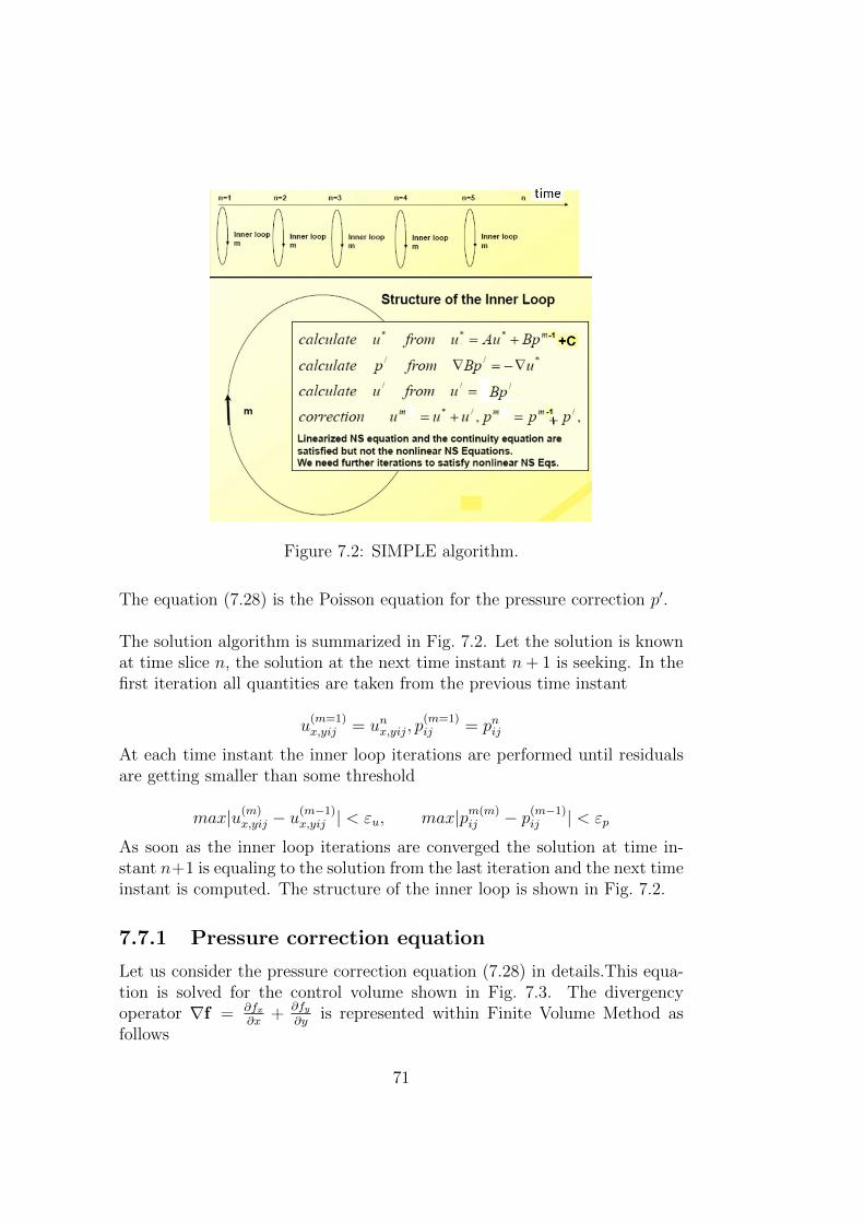
Figure 7.2: SIMPLE algorithm.
The equation (7.28) is the Poisson equation for the pressure correction p′.
The solution algorithm is summarized in Fig. 7.2. Let the solution is knownat time slice n, the solution at the next time instant n+ 1 is seeking. In thefirst iteration all quantities are taken from the previous time instant
u(m=1)x,yij = unx,yij, p
(m=1)ij = pnij
At each time instant the inner loop iterations are performed until residualsare getting smaller than some threshold
max|u(m)x,yij − u
(m−1)x,yij | < εu, max|pm(m)
ij − p(m−1)ij | < εp
As soon as the inner loop iterations are converged the solution at time in-stant n+1 is equaling to the solution from the last iteration and the next timeinstant is computed. The structure of the inner loop is shown in Fig. 7.2.
7.7.1 Pressure correction equation
Let us consider the pressure correction equation (7.28) in details.This equa-tion is solved for the control volume shown in Fig. 7.3. The divergencyoperator ∇f = ∂fx
∂x+ ∂fy
∂yis represented within Finite Volume Method as
follows
71

∫U
∇fdU =
∫U
(∂fx∂x
+∂fy∂y
)dU =
∫S
fndS = (fxe− fxw + fyn− fys)∆ (7.29)
Therefore, the right hand side of the equation (7.28) takes the form
∫U
∇u∗dU =
∫S
u∗ndS = (u∗xij − u∗xi−1j + u∗yij − u∗yij−1)∆ (7.30)
As follows from (7.18) and (7.19) the operator Bp′ has the following valuesat faces of the control volume
(Bp′)xij =
(p′i+1j − p′ij
)∆/qxij, (Bp
′)xi−1j =
(p′ij − p′i−1j
)∆/qxi−1j
(Bp′)yij =
(p′ij+1 − p′ij
)∆/qyij, (Bp
′)yij−1 =
(p′ij − p′ij−1
)∆/qyij−1. (7.31)
Substitution of (7.30) and (7.31) into (7.28) results in
(p′i+1j − p′ij
)/qxij −
(p′ij − p′i−1j
)/qxi−1j +
(p′ij+1 − p′ij
)/qyij
−(p′ij − p′ij−1
)/qyij−1 = −(u∗xij − u∗xi−1j + u∗yij − u∗yij−1) (7.32)
or
βi+1jp′i+1j + βijp
′ij + βi−1jp
′i−1j + βij+1p
′ij+1 + βij−1p
′ij−1 = cij (7.33)
where
cij = −(u∗xij − u∗xi−1j + u∗yij − u∗yij−1), βij = −(
1
qxij+
1
qxi−1j
+1
qyij+
1
qyij−1
),
βi+1j =1
qxij, βi−1j =
1
qxi−1j
, βij+1 =1
qyij, βij−1 =
1
qyij−1
.
72
7.7.2 Summary of the SIMPLE algorithm
We introduce one dimensional numbering instead of two dimensional oneaccording to the rule
α = (i− 1)Ny + j
Let the solution at the time instant n be known. The task is to find thesolution at the time n + 1. At each time instant the guess solution is takenfrom the previous time instant:
u(1)x,yα = unx,yα, p
(1)α = pnα
The solution is found within the next substeps:
i) Calculation of the auxiliary velocity u∗x,yα from two independent sys-tems of linear algebraic equations:
axα−Nyu∗xα−Ny + u∗xα + axα+Nyu
∗xα+Ny + axα−1u
∗xα−1 + axα+1u
∗xα+1+
+
(p
(m−1)α+Ny
− p(m−1)α
)∆/qxα = Rxα
ayα−Nyu∗yα−Ny + u∗yα + ayα+Nyu
∗yα+Ny + ayα−1u
∗yα−1 + ayα+1u
∗yα+1+
+
(p
(m−1)α+1 − p(m−1)
α
)∆/qyα = Ryα
ii) Calculation of the pressure correction p′α from the system of linearalgebraic equations:
βα+Nyp′α+Ny + βαp
′α + βα−Nyp
′α−Ny + βα+1p
′α+1 + βα−1p
′α−1 = cα
iii) Calculation of the velocity correction u′x,yα:
u′xα = −(p′α+Ny − p
′α
)∆/qxα
u′yα = −(p′α+1 − p′α
)∆/qyα
iv) Correction of the velocity and pressure:
u(m)x,yα = u∗x,yα + u′x,yα, p(m)
α = p(m−1)α + p′α
73

Figure 7.3: Control volume used for the pressure correction equation.
v) Check the difference between two iterations:
max|u(m)x,yα − u(m−1)
x,yα | < εu, max|p(m)α − p(m−1)
α | < εp
If these conditions are not fulfilled then
u(m−1)x,yα = u(m)
x,yα, p(m−1)α = p(m)
α
and go to the step i). Otherwise the calculation at the time momentn+ 1 is completed
un+1x,yα = u(m)
x,yα, pn+1α = p(m)
α
and one proceeds to the next time instant n+ 2.
74
Chapter 8
Overview of pressure correctionmethods
8.1 SIMPLE algorithm
The linearized Navier Stokes equation written in operator form is
u = Au+Bp+ C (8.1)
Within the SIMPLE algorithm the solution is seeking at each time step inform of the loop:
Calculation of the auxiliary velocity
u∗ = Au∗ +Bp(m−1) + C (8.2)
Calculation of the pressure correction
∇Bp′ = −∇u∗ (8.3)
Calculation of the velocity correction
u′ = Bp′ (8.4)
Correction
u(m) = u∗ + u′, p(m) = p(m−1) + p′ (8.5)
75
8.2 SIMPLE algorithm in OpenFOAM
SIMPLE algorithm in OpenFOAM is organized is in a slightly different way.First, auxiliary velocity is found from the equation.
u∗ = Au∗ + C (8.6)
The velocity in m-th iteration is calculated as
u(m) = u∗ +Bp(m) (8.7)
u(m) should satisfy the continuity equation:
∇u(m) = ∇(u∗ +Bp(m)) = 0⇒ ∇Bp(m) = −∇u∗ (8.8)
Once p(m) is found from 8.8 it is substituted into (8.7). After that the nextiteration is performed.
8.3 PISO algorithm
In the SIMPLE algorithm we neglected the term ∇Au′ (see 7.25). In PISOalgorithm this term is taken into account. Actually the term ∇Au′ can notbe calculated before the velocity correction is computed. Therefore, the termis taken into account in an iterative way.
8.3.1 First iteration
The term Au′ is neglected, i.e. Au′ = 0. The pressure correction is foundfrom the Poisson equation
∇Bp′ = −∇u∗ (8.9)
The velocity correction is then
u′ = Bp′ (8.10)
8.3.2 Second iteration
The pressure correction within the second iteration is found from the Poissonequation
∇Bp′′ = −∇Au′ (8.11)
The velocity correction within the second iteration is then
u′′ = Au′ +Bp′′ (8.12)
76
8.3.3 Correction
Corrected velocities and pressure are
u(m) = u∗ + u′ + u′′, p(m) = p(m−1) + p′ + p′′ (8.13)
Using formula derived above
∇Bp′ = −∇u∗, u′ = Bp′, u′′ = Au′ +Bp′′,∇Bp′′ = −∇Au′
it is easy to prove that the velocity u(m) satisfies the continuity equation.Now we prove the equation u(m) = Au(m) +Bp(m) + C:
u∗ + u′ + u′′ = A(u∗ + u′ + u′′) +B(p(m−1) + p′ + p′′) + C (8.14)
Sinceu∗ = Au∗ +Bp(m−1) + C, u′ = Bp′, u′′ = Au′ +Bp′′
the equation (8.14) is not satisfied. The residual is Au′′. The residual can bereduced within next iterations. However, usually, PISO algorithm uses onlytwo iterations.
8.3.4 Summary
The PISO algorithm can be summarized as follows:
Calculation of the auxiliary velocity
u∗ = Au∗ +Bp(m−1) + C (8.15)
Calculation of the pressure correction p′:
∇Bp′ = −∇u∗ (8.16)
Calculation of the velocity correction u′
u′ = Bp′ (8.17)
Calculation of the pressure correction p′′:
∇Bp′′ = −∇Au′ (8.18)
Calculation of the velocity correction u′′
u′′ = Au′ +Bp′′ (8.19)
Correction
u(m) = u∗ + u′ + u′′, p(m) = p(m−1) + p′ + p′′ (8.20)
Both algorithms PISO and SIMPLE are widely used in CFD codes.
77

8.3.5 PISO algorithm in OpenFOAM
The PISO algorithm implemented in OpenFOAM consists of the followingsteps:
predictor step
u = Au+Bpn + C u is calculated
corrector step
u = Au+Bp+ C u is calculated
Bp = (Au+ C) p is calculated
8.4 SIMPLEC algorithm
Another way to hold the term ∇Au′ (see 7.25) is implemented in the SIM-PLEC algorithm. The velocity correction at α − th control volume u′α canbe calculated using the interpolation over N adjacent control volumes:
N∑β=1
Aβu′β ≈ u′α
N∑β=1
Aβ (8.21)
where β is the number of adjacent control volumes around the control volumewith the number α.
u′α ≈∑N
β=1 Aβu′β∑N
β=1 Aβ(8.22)
The equation for the velocity correction is
u′ = Au′ +Bp′ (8.23)
or
u′α =N∑β=1
Aβu′β +Bp′ (8.24)
Substitution of (8.22) into (8.24) yields
u′α = u′α
N∑β=1
Aβ +Bp′ (8.25)
78
and
u′α =Bp′
1−∑N
β=1Aβ(8.26)
The pressure correction equation
∇Bp′ = −∇u∗ −∇Au′
takes the form
∇Bp′ = −∇u∗ −∇A Bp′
1−∑N
β=1 Aβ
or
∇(B + A
B
1−∑N
β=1Aβ
)p′ = −∇u∗ (8.27)
The computational steps are the same as these in SIMPLE algorithm withonly difference that the equation (8.27) is solved instead of (8.3).
79

80

Chapter 9
Computational grids
9.1 Grid types
The computational grids are subdivided into:
structured grids (see Fig. 9.1a),
block structured grids (see Fig. 9.1b),
unstructured grids (see Fig. 9.1c).
Disadvantage of the structured grid is shown in Fig. 9.2. Refinement of thegrid close to the wall results in the refinement in areas where this refinement isnot necessary. This disadvantage can be overcome by use of block-structured(Fig. 9.1b) and unstructured grid (Fig. 9.1c).
Figure 9.1: Samples of a) structured grid for an airfoil, b) block structuredgrid for cylinder in channel and c) unstructured grid for an airfoil.
The quality of the grid has a strong impact on the accuracy of numericalprediction. The change of the cell topology within the computational domain
81
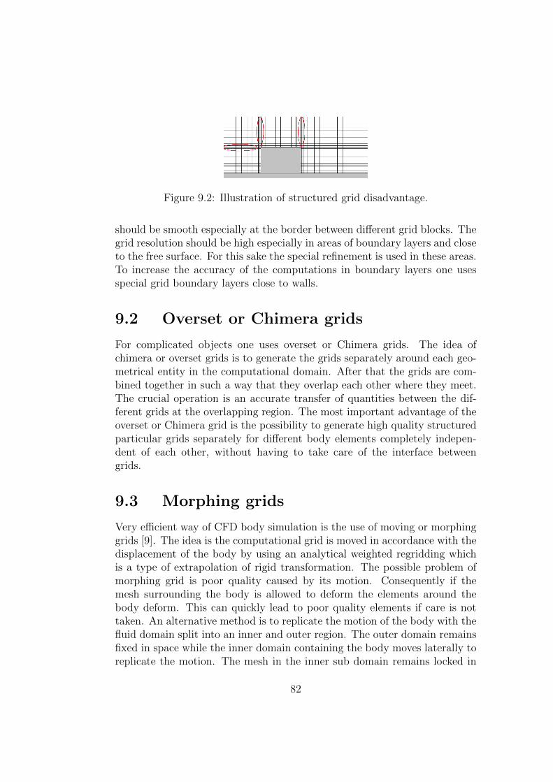
Figure 9.2: Illustration of structured grid disadvantage.
should be smooth especially at the border between different grid blocks. Thegrid resolution should be high especially in areas of boundary layers and closeto the free surface. For this sake the special refinement is used in these areas.To increase the accuracy of the computations in boundary layers one usesspecial grid boundary layers close to walls.
9.2 Overset or Chimera grids
For complicated objects one uses overset or Chimera grids. The idea ofchimera or overset grids is to generate the grids separately around each geo-metrical entity in the computational domain. After that the grids are com-bined together in such a way that they overlap each other where they meet.The crucial operation is an accurate transfer of quantities between the dif-ferent grids at the overlapping region. The most important advantage of theoverset or Chimera grid is the possibility to generate high quality structuredparticular grids separately for different body elements completely indepen-dent of each other, without having to take care of the interface betweengrids.
9.3 Morphing grids
Very efficient way of CFD body simulation is the use of moving or morphinggrids [9]. The idea is the computational grid is moved in accordance with thedisplacement of the body by using an analytical weighted regridding whichis a type of extrapolation of rigid transformation. The possible problem ofmorphing grid is poor quality caused by its motion. Consequently if themesh surrounding the body is allowed to deform the elements around thebody deform. This can quickly lead to poor quality elements if care is nottaken. An alternative method is to replicate the motion of the body with thefluid domain split into an inner and outer region. The outer domain remainsfixed in space while the inner domain containing the body moves laterally toreplicate the motion. The mesh in the inner sub domain remains locked in
82
position relative to the lateral motion of the body. This prevents deformationof the detailed mesh around the body. The outer mesh is deformed due tothe motion of the inner region.
If moving grids are used the Navier Stokes should be transformed to take thevelocity of grid faces ~Ug into account,
∂~u
∂t+(~u− ~Ug
)∇~u = ~f − 1
ρ∇p+ ν∆~u (9.1)
Thomas and Lombard have shown that the function ~Ug can not be arbi-trary rather than they have to be found from the Geometric ConservationLaw
∂
∂t
∫U
dU −∫S
~Ug~ndS = 0 (9.2)
Where U and S are respectively volume and surface of cells. The equa-tion (9.2) is derived from the condition that the computation of the controlvolumes or of the grid velocities must be performed in a such a way thatthe resulting numerical scheme preserves the state of the uniform flow, in-dependently of the deformation of the grid. The equation (9.2) is satisfiedautomatically if the control volumes don’t change their shape. The Geomet-ric conservation law (9.2) should solve coupled with other fluid flow equationsusing the same discretizations schemes.
More detailed information about grid generation can be found in [6], [10]and [11].
83

84

Part II
Mathematical modelling ofturbulent flows
85

Chapter 10
Physics of turbulence
10.1 Definition of the turbulence
Flow motions are subdivided into laminar flows and turbulent ones. Theword
”Laminar“ in Greek means layer. The fluid particles move orderly
in layers without intense lateral mixing. The disruption between layers isabsent. On the contrary the turbulent flow is very chaotic with strong eddiesand intense mixing across the flow.Turbulent motion is the three dimensional unsteady flow motion with
chaotical trajectories of fluid particles,
fluctuations of the velocity and
strong mixing
arisen at large Re numbers due to unstable vortex dynamics.
10.2 Vortex dynamics
The vortex dynamics is the key to understand what happens in the turbulentflow.
10.2.1 Vorticity transport equation
The vector calculus relation reads:
1
2∇(A ·A) = A× (∇×A) + (A∇)A (10.1)
87
Taking u = A we get:
1
2∇(u · u) = u× ω + (u∇)u (10.2)
where ω = ∇× u is the vorticity.Application of the curl operator to (10.2) results in
∇×((u∇)u) = −∇×(u×ω) = −u(∇ω)+ω(∇u)−(ω∇)u+(u∇)ω (10.3)
Here we used the identity ∇× (12∇(u · u)) = 0.
Both vectors u and ω satisfy the continuity equation, i.e. ∇ω = 0 and∇u = 0:
∇× ((u∇)u) = −(ω∇)u + (u∇)ω (10.4)
Let us apply the curl operator to the Navier Stokes equation
∇× (∂u
∂t+ (u∇)u) = ∇× (−1
ρ∇p+ ν∆u) (10.5)
∂ω
∂t+∇× ((u∇)u) = ν∆(∇× u) = ν∆ω (10.6)
Substituting (10.4) into (10.6) results in
∂ω
∂t+ (u∇)ω = (ω∇)u + ν∆ω (10.7)
Dω
Dt= (ω∇)u + ν∆ω (10.8)
The equation (10.8) is the vorticity transport equation.
10.2.2 Vorticity and vortices
The vortices are main players in turbulent flows. Here we would like to em-phasize the difference between the vorticity and vortices. The vorticity isthe curl of the velocity ω = ∇ × u. The vorticity is usually not zero inviscous flows especially in areas close to the walls. Speaking about vorticeswe bear in mind the concentrated structures of the vorticity field ω = ∇×u.The difference between the vorticity and vortices is illustrated in Fig. 10.1.The boundary layer is the flow area with strong but smoothly distributedvorticity (Fig. 10.1a). Due to instabilities, that will be discussed later, theconcentrated vortex structures arise in the smooth vorticity field (Fig. 10.1b).
88

A famous sample of concentrated vortex structures is the tornado (Fig. 10.2).
The vorticity is solenoidal:
∇ω = ∇(∇× u) = 0 (10.9)
The consequence of the condition (10.9) is:
All vortex lines, defined as the lines which are tangential to the vorticityvector ω× dl = 0, are closed in the three dimensional case (Fig. 10.3).
The velocity induced by vorticity ω occupied the volume U are calculatedfrom the Biot-Savart law:
u(x, t) =1
4π
∫U
ω × (x− r)
|x− r|3dU (10.10)
The velocities induced by two dimensional and three dimensional vortexstructures are shown in Fig. 10.4. An important fact is the appearanceof self induced velocities on curvilinear three dimensional vortex structures.They are responsible for leapfrog vortex ring motion (http://www.lemos.uni-rostock.de/galerie/). The self induced velocities is the reason for convectiveinstability of three dimensional vortex structures.
Figure 10.1: Vorticity and vortices.
10.2.3 Vortex amplification as an important mecha-nism of the turbulence generation
As mentioned above the vortices are main players during the laminar- tur-bulent transition. The vorticity can be essentially intensified (amplified) dueto action of neighboring vortices or even due to self induction.
89
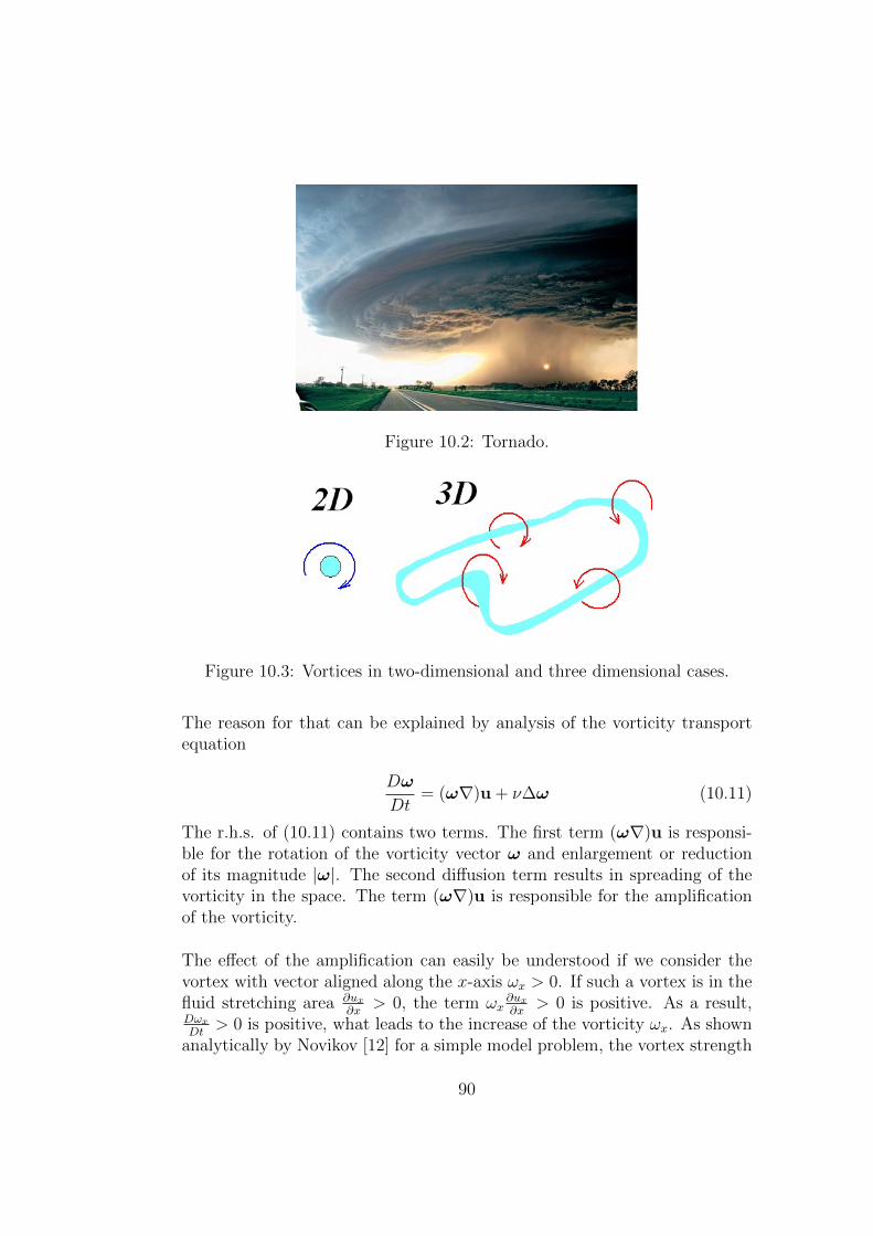
Figure 10.2: Tornado.
Figure 10.3: Vortices in two-dimensional and three dimensional cases.
The reason for that can be explained by analysis of the vorticity transportequation
Dω
Dt= (ω∇)u + ν∆ω (10.11)
The r.h.s. of (10.11) contains two terms. The first term (ω∇)u is responsi-ble for the rotation of the vorticity vector ω and enlargement or reductionof its magnitude |ω|. The second diffusion term results in spreading of thevorticity in the space. The term (ω∇)u is responsible for the amplificationof the vorticity.
The effect of the amplification can easily be understood if we consider thevortex with vector aligned along the x-axis ωx > 0. If such a vortex is in thefluid stretching area ∂ux
∂x> 0, the term ωx
∂ux∂x
> 0 is positive. As a result,DωxDt
> 0 is positive, what leads to the increase of the vorticity ωx. As shownanalytically by Novikov [12] for a simple model problem, the vortex strength
90
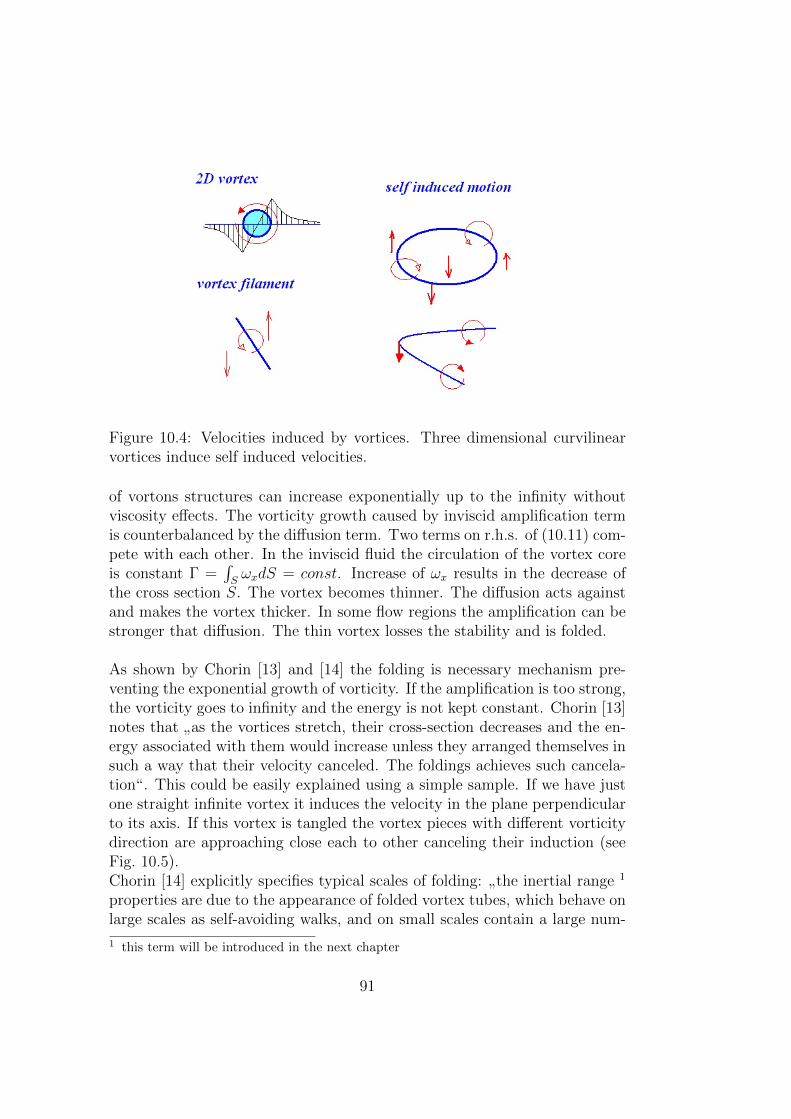
Figure 10.4: Velocities induced by vortices. Three dimensional curvilinearvortices induce self induced velocities.
of vortons structures can increase exponentially up to the infinity withoutviscosity effects. The vorticity growth caused by inviscid amplification termis counterbalanced by the diffusion term. Two terms on r.h.s. of (10.11) com-pete with each other. In the inviscid fluid the circulation of the vortex coreis constant Γ =
∫SωxdS = const. Increase of ωx results in the decrease of
the cross section S. The vortex becomes thinner. The diffusion acts againstand makes the vortex thicker. In some flow regions the amplification can bestronger that diffusion. The thin vortex losses the stability and is folded.
As shown by Chorin [13] and [14] the folding is necessary mechanism pre-venting the exponential growth of vorticity. If the amplification is too strong,the vorticity goes to infinity and the energy is not kept constant. Chorin [13]notes that
”as the vortices stretch, their cross-section decreases and the en-
ergy associated with them would increase unless they arranged themselves insuch a way that their velocity canceled. The foldings achieves such cancela-tion“. This could be easily explained using a simple sample. If we have justone straight infinite vortex it induces the velocity in the plane perpendicularto its axis. If this vortex is tangled the vortex pieces with different vorticitydirection are approaching close each to other canceling their induction (seeFig. 10.5).Chorin [14] explicitly specifies typical scales of folding:
”the inertial range 1
properties are due to the appearance of folded vortex tubes, which behave onlarge scales as self-avoiding walks, and on small scales contain a large num-
1 this term will be introduced in the next chapter
91
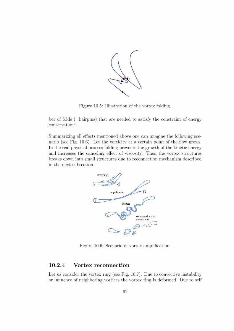
Figure 10.5: Illustration of the vortex folding.
ber of folds (=hairpins) that are needed to satisfy the constraint of energyconservation“.
Summarizing all effects mentioned above one can imagine the following sce-nario (see Fig. 10.6). Let the vorticity at a certain point of the flow grows.In the real physical process folding prevents the growth of the kinetic energyand increases the canceling effect of viscosity. Then the vortex structuresbreaks down into small structures due to reconnection mechanism describedin the next subsection.
Figure 10.6: Scenario of vortex amplification.
10.2.4 Vortex reconnection
Let us consider the vortex ring (see Fig. 10.7). Due to convective instabilityor influence of neighboring vortices the vortex ring is deformed. Due to self
92
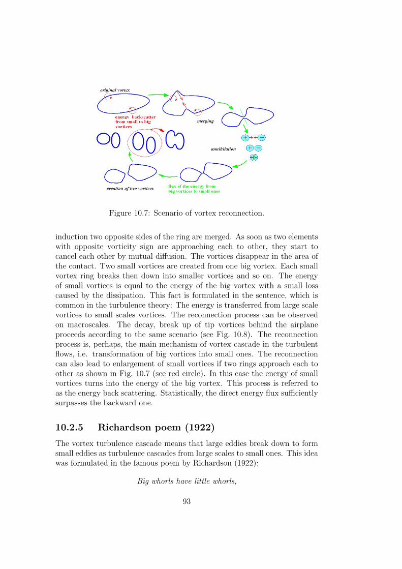
Figure 10.7: Scenario of vortex reconnection.
induction two opposite sides of the ring are merged. As soon as two elementswith opposite vorticity sign are approaching each to other, they start tocancel each other by mutual diffusion. The vortices disappear in the area ofthe contact. Two small vortices are created from one big vortex. Each smallvortex ring breaks then down into smaller vortices and so on. The energyof small vortices is equal to the energy of the big vortex with a small losscaused by the dissipation. This fact is formulated in the sentence, which iscommon in the turbulence theory: The energy is transferred from large scalevortices to small scales vortices. The reconnection process can be observedon macroscales. The decay, break up of tip vortices behind the airplaneproceeds according to the same scenario (see Fig. 10.8). The reconnectionprocess is, perhaps, the main mechanism of vortex cascade in the turbulentflows, i.e. transformation of big vortices into small ones. The reconnectioncan also lead to enlargement of small vortices if two rings approach each toother as shown in Fig. 10.7 (see red circle). In this case the energy of smallvortices turns into the energy of the big vortex. This process is referred toas the energy back scattering. Statistically, the direct energy flux sufficientlysurpasses the backward one.
10.2.5 Richardson poem (1922)
The vortex turbulence cascade means that large eddies break down to formsmall eddies as turbulence cascades from large scales to small ones. This ideawas formulated in the famous poem by Richardson (1922):
Big whorls have little whorls,
93

Figure 10.8: Sample of the vortex reconnection of tip vortices behind anairplane.
Which feed on their velocity;
And little whorls have lessor whorls,
And so on to viscosity (in the molecular sense).
10.2.6 Summary
Vortex arise in the fluid due to viscosity effects. They experience instabilityand amplification. Diffusion counteracts the amplification. If the Reynoldsnumber is large, the vortex structures are strong and concentrated. Theamplification can dominate at some fluid region over the diffusion. Thevortex instability is not damped by viscosity. The flow becomes stochasticdue to mutual interaction of unstable vortices. The big vortices break downinto small ones by means of vortex reconnection. The vortex instabilityprocess is identified as the turbulence.
10.3 Experimental observations
Different regimes of the fluid motion were revealed very early, perhaps, inantique times. Much later, Leonardo da Vinci recognized two states of thefluid motion and introduced the term
”la turbolenza “. Arkady Tsinober
in his book”An informal introduction to turbulence “ [1] presented most
outstanding results in turbulence research in chronological order (Fig. 10.9).
94

Figure 10.9: Most outstanding results in turbulence research according to [1].
10.3.1 Laminar - turbulent transition in pipe. Exper-iment of Reynolds
Quantitative study of turbulence was started by Osborne Reynolds (1842-1912) who performed in 1883 very famous experiment shown in Fig. 10.10.The water flows from the vessel A to the pipe B. The ink injected into thepipe B with the local flow velocity is not mixed in transversal direction andkeeps its identity if the flow velocity is small (Fig. 10.10, right). The flowunder such a condition is laminar. As soon as the flow velocity increases dueto water level raise in the vessel A, the ink jet loses the stability and is mixedwith surrounding water (Fig. 10.10, right). The flow becomes turbulent. Inkjet development at different flow velocities in the circular pipe is shown inFig. 10.11.
The great merit of Reynolds lies in the fact, that he in contrast to his pre-decessors quantified the laminar turbulent transition. He showed that thetransition in pipes occurs if the Reynolds number Re = UbD/ν exceeds thethreshold around ∼ 2400. Here Ub is the bulk velocity in pipe determined asthe ratio of the flow rate to the pipe cross section, i.e. Ub = Q/(πD2/4), D isthe pipe diameter and ν is the kinematic viscosity coefficient (ν ∼ 10−6m2s−1
for water and ν ∼ 10−5m2s−1 for air). Later, it was shown that the transitionstrongly depends on the perturbations presented in the flow. The experimen-tal setup of Reynolds has been preserved at the University of Manchester in
95
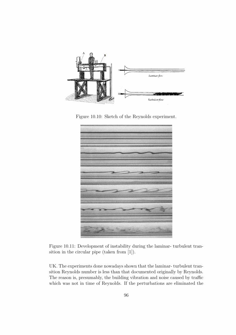
Figure 10.10: Sketch of the Reynolds experiment.
Figure 10.11: Development of instability during the laminar- turbulent tran-sition in the circular pipe (taken from [1]).
UK. The experiments done nowadays shown that the laminar- turbulent tran-sition Reynolds number is less than that documented originally by Reynolds.The reason is, presumably, the building vibration and noise caused by trafficwhich was not in time of Reynolds. If the perturbations are eliminated the
96

transition can be delayed up to Re ∼ 40000...50000.
10.3.2 Laminar - turbulent transition and turbulencein jets
The jet flows experiences also laminar turbulent transition shown in Fig. 10.12.Obviously, the flow can be fully or only partially turbulent. Close to the noz-zle the flow is laminar. The instability is developed downstream. The shearflow at the jet boundary is the area of rapid velocity change from the jetvelocity to zero outside of the jet. The shear flow experiences the so calledKelvin Helmholtz instability (Fig. 10.13) resulting in formation of concen-trated vortices which are approximately circular. It happens close to jetnozzle at x/D < 1 (see Fig. 10.14), where x is the distance from the nozzleand D is the nozzle diameter.
The Kelvin Helmholtz vortices experience then the pairing (see Fig. 10.14).One vortex overtakes the neighbor vortex creating a pair. This processhas an inviscid convective nature and can be explained thinking back tothe famous leapfrog motion of two vortex rings. In the inviscid flow theleapfrog motion is running as long as the convective instability destroysthe vortices. One vortex runs the next down, its radius decreases whereasthe speed increases. The radius of the next vortex increases, the speeddecreases. The first ring moves through the second one. The process isthen repeated. The movie illustrating this process can be downloaded fromhttp://www.lemos.uni-rostock.de/en/gallery/.
The paired vortices experience the azimuthal instability and takes the crudering form. Later they are destroyed downstream in the region 1 < x/D < 6.In far field at large x/D the vortex structures look like a tree with branchesoriented against the main flow direction (see Fig. 10.15).
Figure 10.12: Development of instability in the jet (taken from [1]).
97

Figure 10.13: Development of instability in the free jet.
Figure 10.14: Development of instability in the free jet.
Creation of vortex rings is the reason for the jet noise. The noise produced,for instance, by jet propulsors of airplanes is the action of these vortices.The vortices play a significant positive role in jet mixers widely used in foodindustry, chemical engineering, etc. That is why, one of the most perspectiveway to reduce the noise or to increase mixing is the manipulation of vor-tices arising behind the jet nozzle. To increase the mixing it is necessary tostrengthen the Kelvin Helmholtz vortices. To decrease the noise the vorticesshould be broken down into small ones. Fig. 10.16 shows the effect of theacoustic impact on jet. The original vortices (lower picture) are split intosmall ones (upper picture).
High resolution laser diagnostics methods LIF and PIV allow to get a deepinside into the structure of the turbulent flow. Fig. 10.17 shows the structureof the confined jet mixer flow displayed by Planar Laser Induced Fluores-cence (PLIF) Method. The macrostructure obtained with low resolution isshown in the upper Figure. A small window with sizes 2.08mm × 2.72mm
98
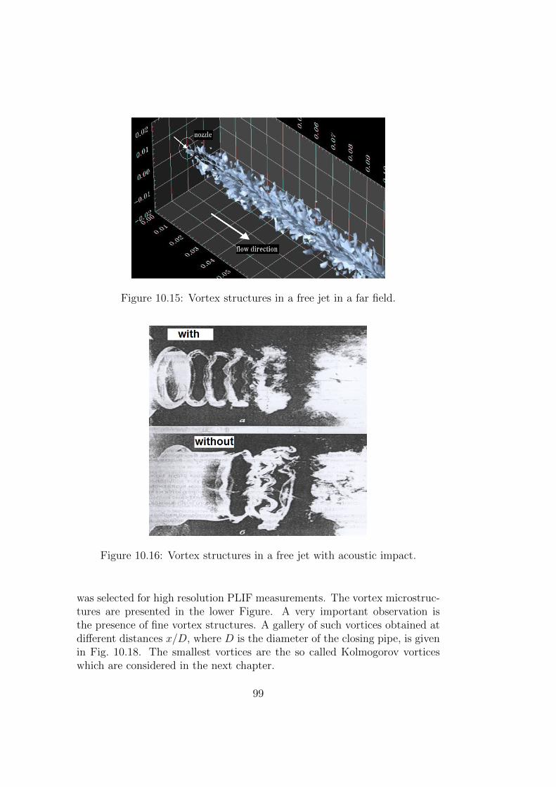
Figure 10.15: Vortex structures in a free jet in a far field.
Figure 10.16: Vortex structures in a free jet with acoustic impact.
was selected for high resolution PLIF measurements. The vortex microstruc-tures are presented in the lower Figure. A very important observation isthe presence of fine vortex structures. A gallery of such vortices obtained atdifferent distances x/D, where D is the diameter of the closing pipe, is givenin Fig. 10.18. The smallest vortices are the so called Kolmogorov vorticeswhich are considered in the next chapter.
99
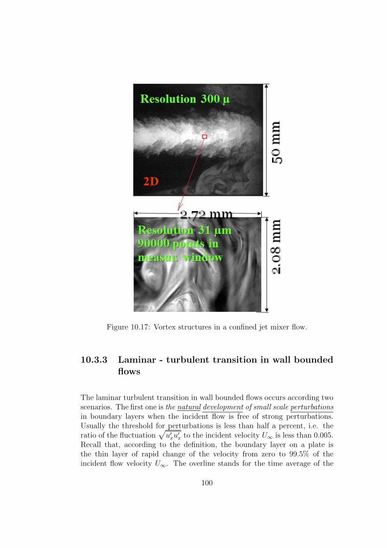
Figure 10.17: Vortex structures in a confined jet mixer flow.
10.3.3 Laminar - turbulent transition in wall boundedflows
The laminar turbulent transition in wall bounded flows occurs according twoscenarios. The first one is the natural development of small scale perturbationsin boundary layers when the incident flow is free of strong perturbations.Usually the threshold for perturbations is less than half a percent, i.e. theratio of the fluctuation
√u′xu
′x to the incident velocity U∞ is less than 0.005.
Recall that, according to the definition, the boundary layer on a plate isthe thin layer of rapid change of the velocity from zero to 99.5% of theincident flow velocity U∞. The overline stands for the time average of the
100

Figure 10.18: Fine vortex structures in a confined jet mixer flow. PLIF mea-surements by Valery Zhdanov (LTT Rostock). Spatial resolution is 31µm.
axial velocity fluctuation squared:
u′xu′x = lim
T→∞
1
T
∫ T
0
u′x(t)u′x(t)dt (10.12)
where T is a sufficiently large average time period. A possible scenario of thelaminar turbulent transition in the boundary layer on a flat plate is shownin Fig. 10.19. First, the transverse vortices are generated in the boundarylayer due to the so- called Tollmien- Schlichting instability [15]. The ini-tial period is characterized by a two-dimensional primary instability whichis described by the Orr-Sommerfeld-Squire theory. The transverse vorticesexperience the secondary three-dimensional instability and form downstreamthe lambda structures. The latter interact each with other and experiencethe tertiary instability. They loss original regular form and become stochas-tic. An important feature of the turbulent boundary layer is the presence ofstreaks (strips) of the low velocity fluid regions (see Fig. 10.20). They arisedue to induction of lambda structures schematically shown in Fig. 10.21.Detailed description of the laminar turbulent transition is outside the scopeof this course. It can be found in [15].
The second scenario takes place when the perturbations in the incidentflow are large. The natural transition stage is bypassed and the scenariois referred to as the bypass transition. For a gradient-free flow in the plateboundary layer, the bypass mode occurs when the initial turbulence inten-
101
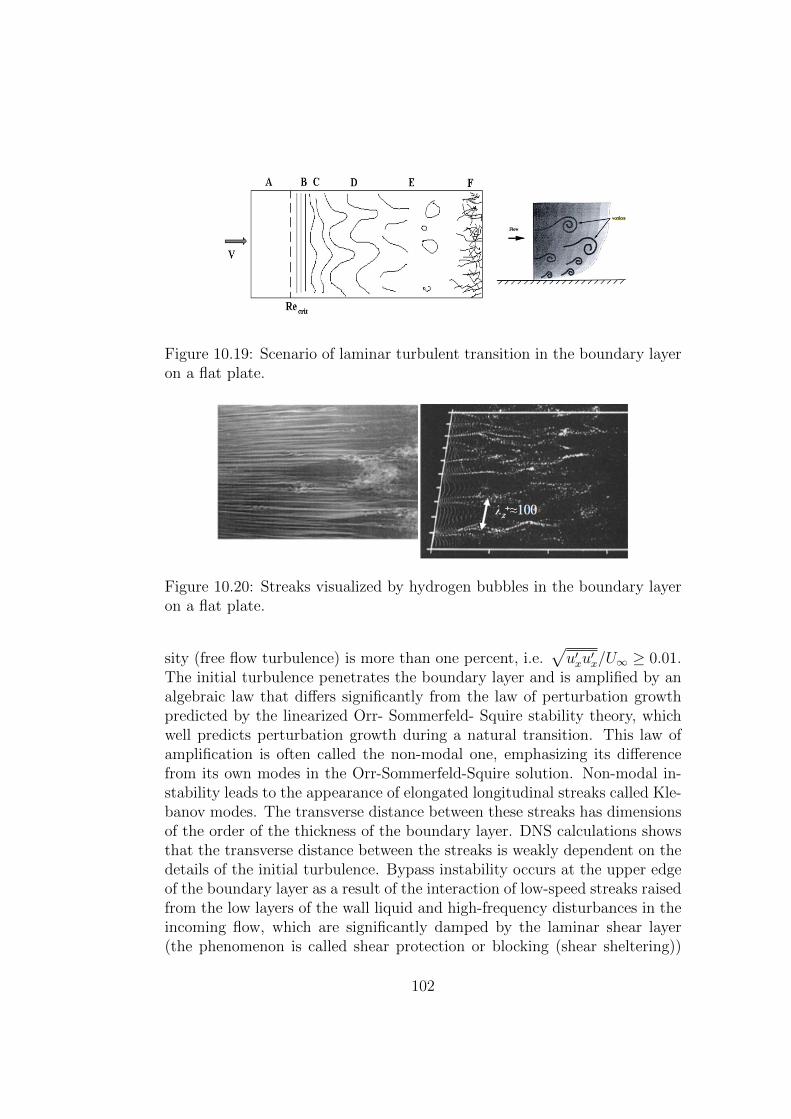
Figure 10.19: Scenario of laminar turbulent transition in the boundary layeron a flat plate.
Figure 10.20: Streaks visualized by hydrogen bubbles in the boundary layeron a flat plate.
sity (free flow turbulence) is more than one percent, i.e.√u′xu
′x/U∞ ≥ 0.01.
The initial turbulence penetrates the boundary layer and is amplified by analgebraic law that differs significantly from the law of perturbation growthpredicted by the linearized Orr- Sommerfeld- Squire stability theory, whichwell predicts perturbation growth during a natural transition. This law ofamplification is often called the non-modal one, emphasizing its differencefrom its own modes in the Orr-Sommerfeld-Squire solution. Non-modal in-stability leads to the appearance of elongated longitudinal streaks called Kle-banov modes. The transverse distance between these streaks has dimensionsof the order of the thickness of the boundary layer. DNS calculations showsthat the transverse distance between the streaks is weakly dependent on thedetails of the initial turbulence. Bypass instability occurs at the upper edgeof the boundary layer as a result of the interaction of low-speed streaks raisedfrom the low layers of the wall liquid and high-frequency disturbances in theincoming flow, which are significantly damped by the laminar shear layer(the phenomenon is called shear protection or blocking (shear sheltering))
102
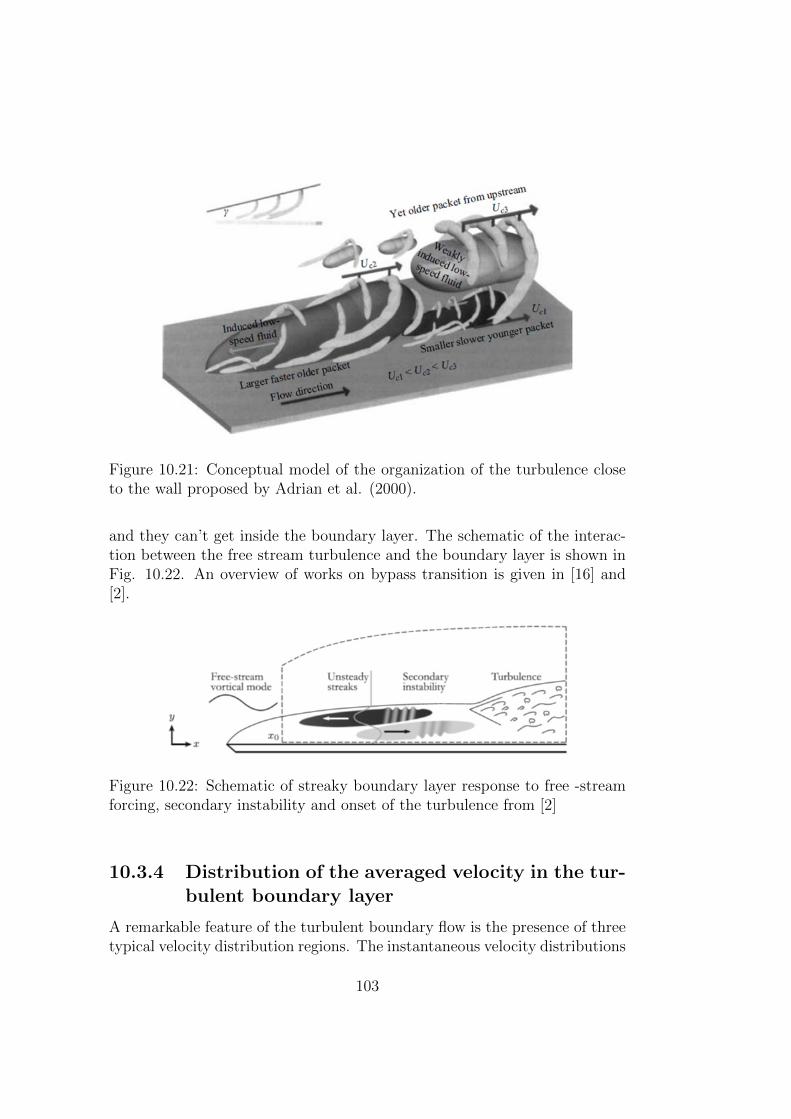
Figure 10.21: Conceptual model of the organization of the turbulence closeto the wall proposed by Adrian et al. (2000).
and they can’t get inside the boundary layer. The schematic of the interac-tion between the free stream turbulence and the boundary layer is shown inFig. 10.22. An overview of works on bypass transition is given in [16] and[2].
Figure 10.22: Schematic of streaky boundary layer response to free -streamforcing, secondary instability and onset of the turbulence from [2]
10.3.4 Distribution of the averaged velocity in the tur-bulent boundary layer
A remarkable feature of the turbulent boundary flow is the presence of threetypical velocity distribution regions. The instantaneous velocity distributions
103

can be quite different (see Fig. 10.25). However, the averaged velocity hastypical distribution close to the wall regardless of the flow type.
Figure 10.23: Vertical distribution of the velocity ux at three different timeinstants in boundary layer.
Let us introduce the following designations:
y is the distance from the wall,
τw is the stress at the wall,
uτ =√
τwρ
is the friction velocity,
y+ = uτyν
is the dimensionless wall distance.
The stress in wall turbulence flow can be considered as the sum of the laminarand turbulent stresses:
τ = τl + τt (10.13)
Close to the wall the turbulent fluctuations are weak. The laminar stressτl dominates over the turbulent one τt, i.e. τ ∼ τl. We consider the thinboundary layer, i.e. the stress is approximately equal to the wall stress τw:
τ ≈ τw (10.14)
Applying the Newton hypothesis (1.18) to the two dimensional wall boundedflow, one gets from (10.14)
τw = ρνduxdy
(10.15)
104

or
uxuτ
= y+ + C (10.16)
From the condition at the wall ux = 0 the unknown constant C is zero, i.e.
uxuτ
= y+ (10.17)
Close to the wall the velocity increases linearly ux ∼ y. This law confirmedin measurements is valid in the range 0 < y+ < 5. This region is reffered toas the viscous sublayer.Far from the wall the laminar stresses are smaller than the turbulent onesτ ∼ τt. The turbulent stress τt can be found from the Prandtl mixing lengthmodel. The instantaneous velocities are presented as the sum of averaged uand fluctuation u
′parts:
ux = ux + u′
x, uy = u′
y, uy = 0 (10.18)
The averaged velocities are defined as
ux = limT→∞
T∫0
ux(t)dt (10.19)
The turbulent stress τ12 = τxy according to the definition is
τ12 = ρu′xu′y (10.20)
Figure 10.24: Illustration of the Prandtl derivation.
105
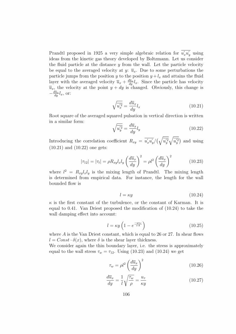
Prandtl proposed in 1925 a very simple algebraic relation for u′xu′y using
ideas from the kinetic gas theory developed by Boltzmann. Let us considerthe fluid particle at the distance y from the wall. Let the particle velocitybe equal to the averaged velocity at y: ux. Due to some perturbations theparticle jumps from the position y to the position y+ lx and attains the fluidlayer with the averaged velocity ux + dux
dylx. Since the particle has velocity
ux, the velocity at the point y + dy is changed. Obviously, this change is−dux
dylx, or: √
u′2x =duxdy
lx (10.21)
Root square of the averaged squared pulsation in vertical direction is writtenin a similar form: √
u′2y =duxdy
ly (10.22)
Introducing the correlation coefficient Rxy = u′xu′y/(√
u′2y
√u′2y)
and using
(10.21) and (10.22) one gets:
|τ12| = |τt| = ρRxylxly
(duxdy
)2
= ρl2(duxdy
)2
(10.23)
where l2 = Rxylxly is the mixing length of Prandtl. The mixing lengthis determined from empirical data. For instance, the length for the wallbounded flow is
l = κy (10.24)
κ is the first constant of the turbulence, or the constant of Karman. It isequal to 0.41. Van Driest proposed the modification of (10.24) to take thewall damping effect into account:
l = κy(
1− e−yuτνA
)(10.25)
where A is the Van Driest constant, which is equal to 26 or 27. In shear flowsl = Const · δ(x), where δ is the shear layer thickness.We consider again the thin boundary layer, i.e. the stress is approximatelyequal to the wall stress τw = τ12. Using (10.23) and (10.24) we get
τw = ρl2(duxdy
)2
(10.26)
duxdy
=1
l
√τwρ
=uτκy
(10.27)
106
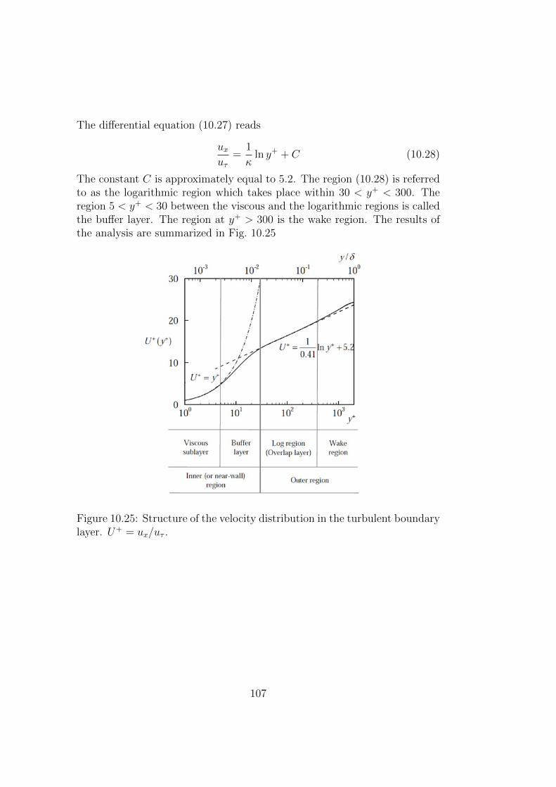
The differential equation (10.27) reads
uxuτ
=1
κln y+ + C (10.28)
The constant C is approximately equal to 5.2. The region (10.28) is referredto as the logarithmic region which takes place within 30 < y+ < 300. Theregion 5 < y+ < 30 between the viscous and the logarithmic regions is calledthe buffer layer. The region at y+ > 300 is the wake region. The results ofthe analysis are summarized in Fig. 10.25
Figure 10.25: Structure of the velocity distribution in the turbulent boundarylayer. U+ = ux/uτ .
107

108
Chapter 11
Basic definitions of thestatistical theory of turbulence
11.1 Reynolds averaging
Reynolds proposed to represent any stochastic quantity in turbulent flow asthe sum of its averaged part and fluctuation. For instance, this representationapplied for velocity components reads
ux = ux + u′x; uy = uy + u′y; uz = uz + u′z; (11.1)
The Reynolds averaged velocities are
ux = limT→∞
1
T
T∫0
uxdt; uy = limT→∞
1
T
T∫0
uydt;
uz = limT→∞
1
T
T∫0
uzdt
(11.2)
The averaged fluctuation is zero
u′x,y,z = 0
The root of the averaged square of fluctuations is called root mean square,or r.m.s.. The quantity averaged twice is equal to quantity averaged onceu = u.
If the turbulence process is statistically unsteady (for instance r.m.s is changedin time), the definition of the Reynolds averaging (11.2) is not applicable and
109

should be extended using the concept of ensemble averaging. Within the en-semble averaging the stochastic process is repeated N times from the initialstate. The turbulent quantity u is measured at a certain time t∗ N times.The ensemble averaged quantity is then:
u(t∗) = limN→∞
1
N
N∑i=1
ui(t∗)
11.2 Isotropic and homogeneous turbulence
The turbulence is isotropic if r.m.s of all three velocity fluctuations are equal
u′2x = u′2y = u′2z (11.3)
The turbulence parameters are invariant with respect to the rotation of thereference system. The turbulence is homogeneous in some fluid volume ifall statistical parameters are the same for all points in this volume, i.e.u′2x,y,z(~x) = u′2x,y,z(~x+ ~r). This equality can be written for all statistical mo-ments. The turbulence parameters are invariant with respect to the transla-tion of the reference system.
11.3 Correlation function. Integral length
The product of two fluctuations is the correlation. The product of two fluc-tuations at two point separated by the distance ~r is the correlation function:
Rij(~x,~r) = u′i(~x)u′j(~x+ ~r) (11.4)
If i = j the correlation function Rii is reffered as to the autocorrelationfunction. In homogeneous turbulence Rii depends only on the separation:
Rij(~r) = u′i(~x)u′j(~x+ ~r) (11.5)
The coefficient of the autocorrelation function is changed between +1 and -1:
ρii(~x,~r) =u′i(~x)u′i(~x+ ~r)
u′2i (~x)(11.6)
A sample of the autocorrealtion function coefficient for scalar fluctuation f ′
ρf (~x,~r) =f ′(~x)f ′(~x+ ~r)
f ′2(~x)(11.7)
110
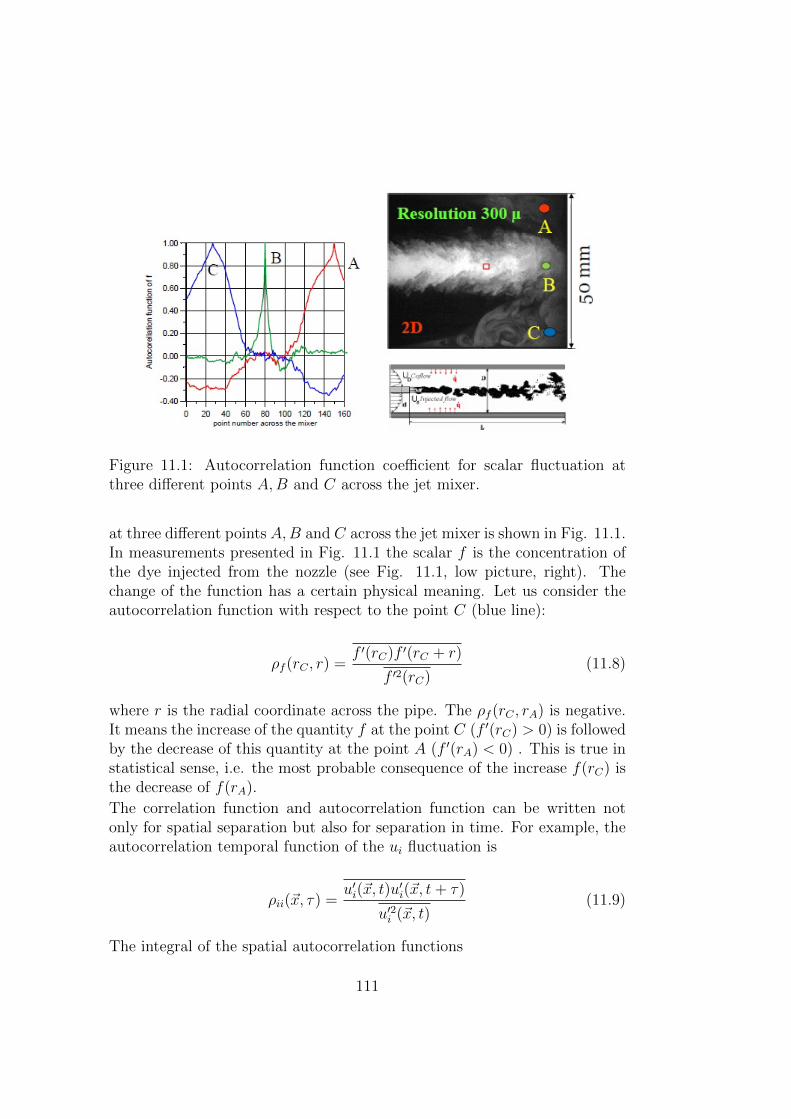
Figure 11.1: Autocorrelation function coefficient for scalar fluctuation atthree different points A,B and C across the jet mixer.
at three different points A,B and C across the jet mixer is shown in Fig. 11.1.In measurements presented in Fig. 11.1 the scalar f is the concentration ofthe dye injected from the nozzle (see Fig. 11.1, low picture, right). Thechange of the function has a certain physical meaning. Let us consider theautocorrelation function with respect to the point C (blue line):
ρf (rC , r) =f ′(rC)f ′(rC + r)
f ′2(rC)(11.8)
where r is the radial coordinate across the pipe. The ρf (rC , rA) is negative.It means the increase of the quantity f at the point C (f ′(rC) > 0) is followedby the decrease of this quantity at the point A (f ′(rA) < 0) . This is true instatistical sense, i.e. the most probable consequence of the increase f(rC) isthe decrease of f(rA).
The correlation function and autocorrelation function can be written notonly for spatial separation but also for separation in time. For example, theautocorrelation temporal function of the ui fluctuation is
ρii(~x, τ) =u′i(~x, t)u
′i(~x, t+ τ)
u′2i (~x, t)(11.9)
The integral of the spatial autocorrelation functions
111
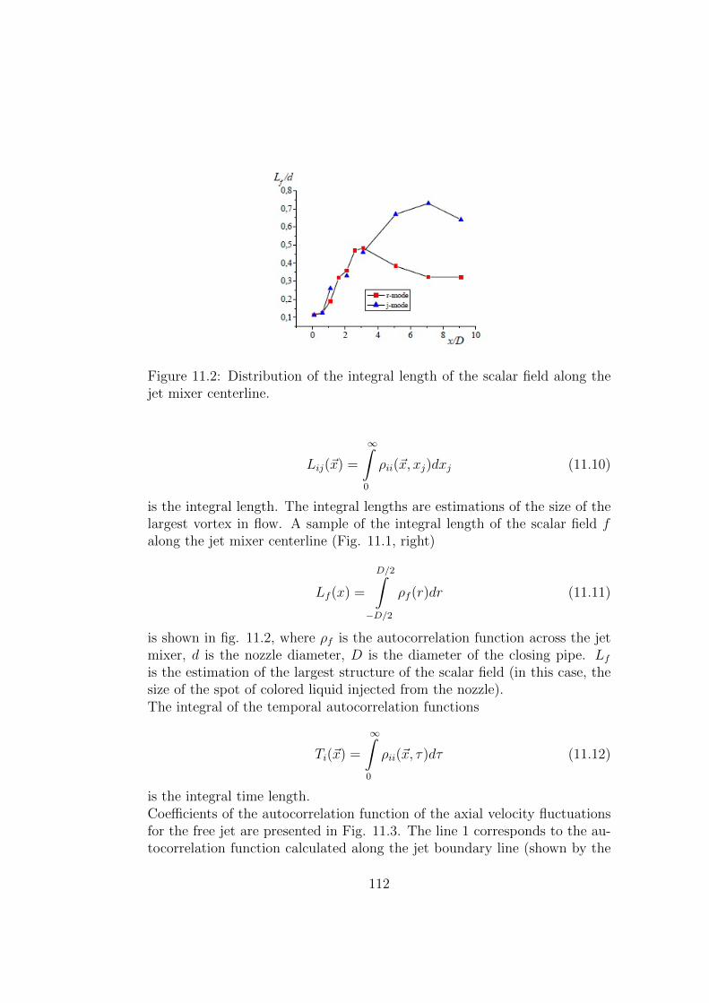
Figure 11.2: Distribution of the integral length of the scalar field along thejet mixer centerline.
Lij(~x) =
∞∫0
ρii(~x, xj)dxj (11.10)
is the integral length. The integral lengths are estimations of the size of thelargest vortex in flow. A sample of the integral length of the scalar field falong the jet mixer centerline (Fig. 11.1, right)
Lf (x) =
D/2∫−D/2
ρf (r)dr (11.11)
is shown in fig. 11.2, where ρf is the autocorrelation function across the jetmixer, d is the nozzle diameter, D is the diameter of the closing pipe. Lfis the estimation of the largest structure of the scalar field (in this case, thesize of the spot of colored liquid injected from the nozzle).The integral of the temporal autocorrelation functions
Ti(~x) =
∞∫0
ρii(~x, τ)dτ (11.12)
is the integral time length.Coefficients of the autocorrelation function of the axial velocity fluctuationsfor the free jet are presented in Fig. 11.3. The line 1 corresponds to the au-tocorrelation function calculated along the jet boundary line (shown by the
112
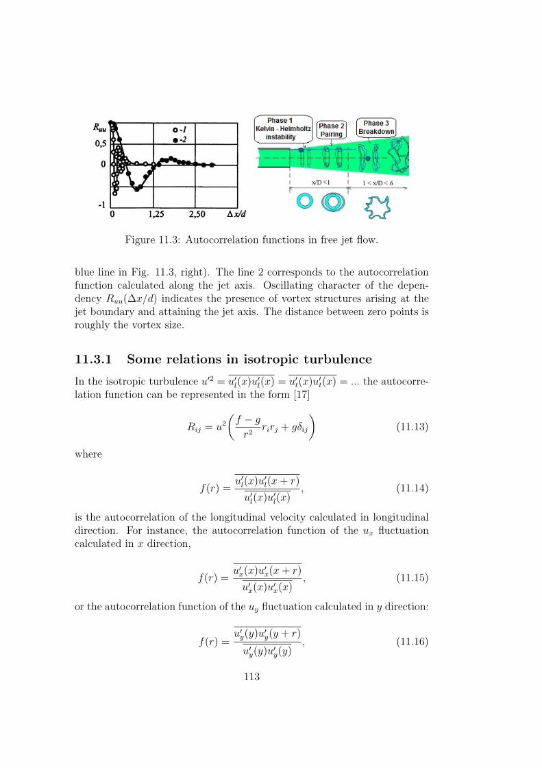
Figure 11.3: Autocorrelation functions in free jet flow.
blue line in Fig. 11.3, right). The line 2 corresponds to the autocorrelationfunction calculated along the jet axis. Oscillating character of the depen-dency Ruu(∆x/d) indicates the presence of vortex structures arising at thejet boundary and attaining the jet axis. The distance between zero points isroughly the vortex size.
11.3.1 Some relations in isotropic turbulence
In the isotropic turbulence u′2 = u′l(x)u′l(x) = u′t(x)u′t(x) = ... the autocorre-lation function can be represented in the form [17]
Rij = u2
(f − gr2
rirj + gδij
)(11.13)
where
f(r) =u′l(x)u′l(x+ r)
u′l(x)u′l(x), (11.14)
is the autocorrelation of the longitudinal velocity calculated in longitudinaldirection. For instance, the autocorrelation function of the ux fluctuationcalculated in x direction,
f(r) =u′x(x)u′x(x+ r)
u′x(x)u′x(x), (11.15)
or the autocorrelation function of the uy fluctuation calculated in y direction:
f(r) =u′y(y)u′y(y + r)
u′y(y)u′y(y), (11.16)
113
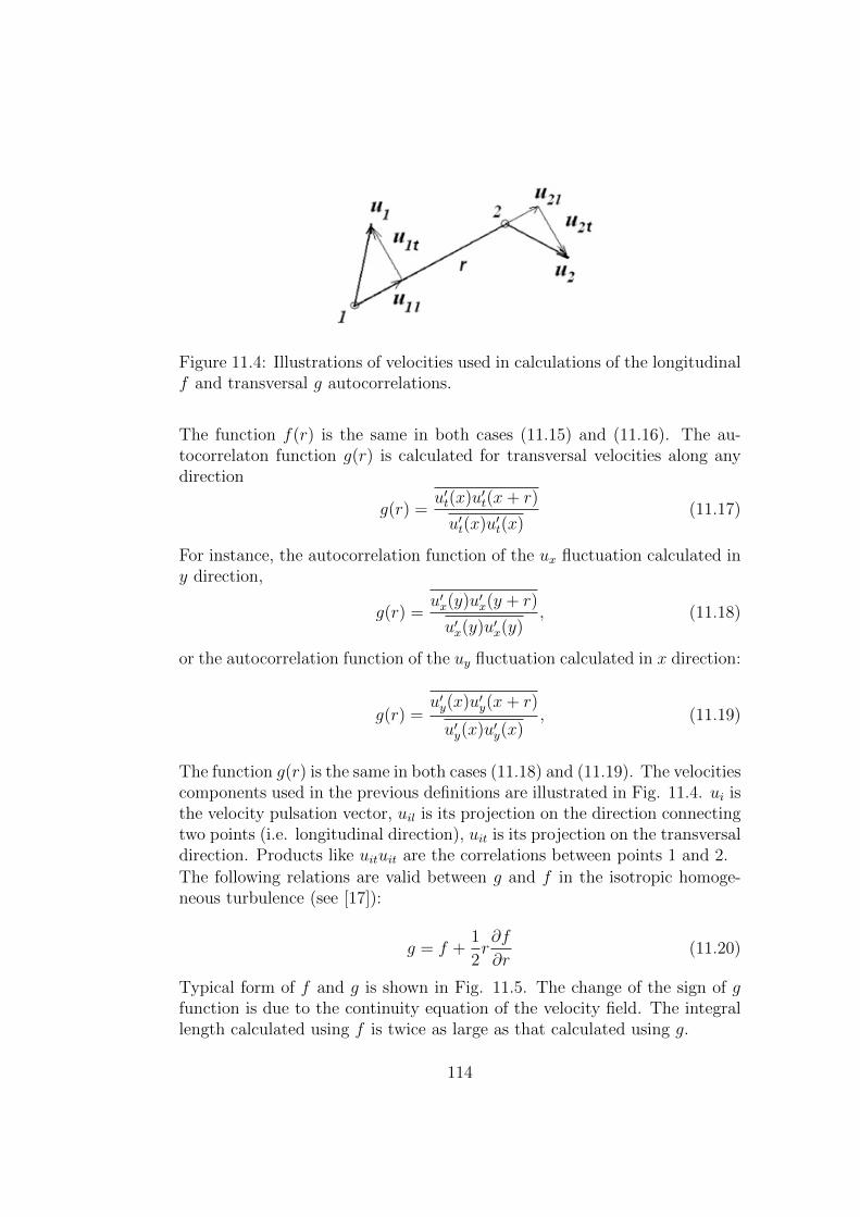
Figure 11.4: Illustrations of velocities used in calculations of the longitudinalf and transversal g autocorrelations.
The function f(r) is the same in both cases (11.15) and (11.16). The au-tocorrelaton function g(r) is calculated for transversal velocities along anydirection
g(r) =u′t(x)u′t(x+ r)
u′t(x)u′t(x)(11.17)
For instance, the autocorrelation function of the ux fluctuation calculated iny direction,
g(r) =u′x(y)u′x(y + r)
u′x(y)u′x(y), (11.18)
or the autocorrelation function of the uy fluctuation calculated in x direction:
g(r) =u′y(x)u′y(x+ r)
u′y(x)u′y(x), (11.19)
The function g(r) is the same in both cases (11.18) and (11.19). The velocitiescomponents used in the previous definitions are illustrated in Fig. 11.4. ui isthe velocity pulsation vector, uil is its projection on the direction connectingtwo points (i.e. longitudinal direction), uit is its projection on the transversaldirection. Products like uituit are the correlations between points 1 and 2.
The following relations are valid between g and f in the isotropic homoge-neous turbulence (see [17]):
g = f +1
2r∂f
∂r(11.20)
Typical form of f and g is shown in Fig. 11.5. The change of the sign of gfunction is due to the continuity equation of the velocity field. The integrallength calculated using f is twice as large as that calculated using g.
114
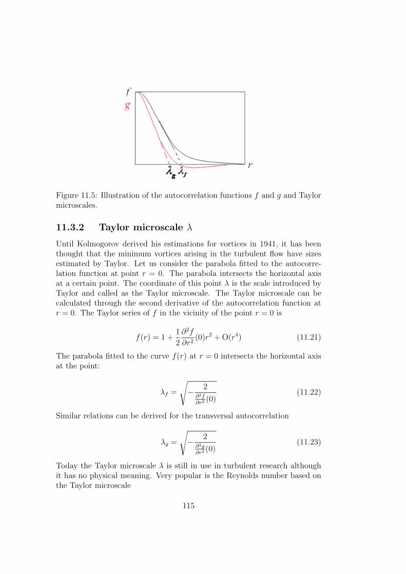
Figure 11.5: Illustration of the autocorrelation functions f and g and Taylormicroscales.
11.3.2 Taylor microscale λ
Until Kolmogorov derived his estimations for vortices in 1941, it has beenthought that the minimum vortices arising in the turbulent flow have sizesestimated by Taylor. Let us consider the parabola fitted to the autocorre-lation function at point r = 0. The parabola intersects the horizontal axisat a certain point. The coordinate of this point λ is the scale introduced byTaylor and called as the Taylor microscale. The Taylor microscale can becalculated through the second derivative of the autocorrelation function atr = 0. The Taylor series of f in the vicinity of the point r = 0 is
f(r) = 1 +1
2
∂2f
∂r2(0)r2 + O(r4) (11.21)
The parabola fitted to the curve f(r) at r = 0 intersects the horizontal axisat the point:
λf =
√− 2
∂2f∂r2 (0)
(11.22)
Similar relations can be derived for the transversal autocorrelation
λg =
√− 2
∂2g∂r2 (0)
(11.23)
Today the Taylor microscale λ is still in use in turbulent research althoughit has no physical meaning. Very popular is the Reynolds number based onthe Taylor microscale
115
Re = u′λ/ν (11.24)
which characterizes the state of the turbulence in the flow.
11.3.3 Correlation functions in the Fourier space
Any continuous function can be represented in the Fourier space:
f(~r, t) =
∞∫−∞
f(~k, t)ei~k~rd~k (11.25)
The new function f(~k, t) is then known as the Fourier transform and/orthe frequency spectrum of the function f . The Fourier transform is also areversible operation:
f(~k, t) =1
8π3
∞∫−∞
f(~r, t)e−i~k~rd~r (11.26)
The Fourier transformation can be also written for the correlation function:
Rij(~r) =
∞∫−∞
Φij(~k)ei~k~rd~k, Φij(~k) =
1
8π3
∞∫−∞
Rij(~r)e−i~k~rd~r (11.27)
Very often one uses one dimensional correlation functions defined as
Θij(k1) =1
2π
∞∫−∞
Rij(r1, 0, 0)e−ik1r1dr1 =
∞∫−∞
∞∫−∞
Φij(k1, k2, k3)dk2dk3
(11.28)
Proof of the formula (11.28) The inverse Fourier transform of the functionRij(r1, 0, 0):
Θij(k1, 0, 0) =1
2π
∞∫−∞
Rij(r1, 0, 0)eik1r1dr1 (11.29)
The inverse transformation reads:
116
Rij(r1, 0, 0) =
∞∫−∞
Θij(k1, 0, 0)e−ik1r1dk1 (11.30)
The general definition is
Rij(r1, r2, r3) =
∞∫−∞
∞∫−∞
∞∫−∞
Φij(k1, k2, k3)ei~k~rdk1dk2dk3 (11.31)
From the last formula we have:
Rij(r1, 0, 0) =
∞∫−∞
( ∞∫−∞
∞∫−∞
Φij(k1, k2, k3)dk2dk3
)eik1r1dk1 (11.32)
Comparison of (11.32) with (11.30) results in the desired formula
Θij(k1, 0, 0) =
∞∫−∞
∞∫−∞
Φij(k1, k2, k3)dk2dk3 (11.33)
11.3.4 Spectral density of the turbulent kinetic energy
According to the definition of the correlation function
Rij(~r) = u′i(~x)u′j(~x+ ~r) (11.34)
the total turbulent kinetic energy is
TKE =1
2Rii(0) =
1
2
∞∫−∞
Φii(~k)d~k =
∞∫0
Φii(~k)d~k (11.35)
The quantity
E(k) =
∫|~k|
Φii(~k)d~k (11.36)
is the spectral density of the turbulent kinetic energy. Physically it is theenergy on the sphere k =
√k2
1 + k22 + k2
3 in the Fourier space. The totalturbulent kinetic energy is then:
117
TKE =
∞∫0
E(k)dk (11.37)
11.4 Structure functions
11.4.1 Probability density function
We take the definitions from Wikipedia: In probability theory, a probabilitydensity function (pdf), or density of a continuous random variable, is a func-tion that describes the relative likelihood for this random variable to takeon a given value. The probability for the random variable to fall within aparticular region is given by the integral of this variables density over theregion. The probability density function is non negative everywhere, and itsintegral over the entire space is equal to one.
11.4.2 Structure function
Kolmogorov introduced the structure function of q order for any stochasticfunction. For instance, for the longitudinal velocity along the longitudinaldirection (see Fig. 11.5) it reads:
Sq(l) = 〈(u2l − u1l)q〉 (11.38)
The standard deviation squared is then σ2 = S2. If the p.d.f. of the structurefunction is described by the Gaussian function
p.d.f.(x) =1√2πσ
e−(x−µ)2
2σ2 (11.39)
where µ is the mean value of the stochastic value, the turbulence is Gaussian.In reality, the most of the turbulence parameters are not Gaussian. Thedeviations from the Gaussian turbulence is characterized by the kurtosisKurt and skewness Sk. The kurtosis
Kurt =〈(u2l − u1l)
4〉(〈(u2l − u1l)2〉)2
(11.40)
is three for the Gaussian turbulence. Big values of the kurtosis means thatthe p.d.f. distribution of the structure function S1(l) = 〈u2l − u1l〉 is veryflat. The kurtosis is also often called as flatness. If kurtosis for small l ∼ 0is big, it means that the field of the stochastic field is very intermittent. Big
118

Figure 11.6: Kurtosis of the structure function for the concentration of thescalar field obtained in the jet mixer.
differences are possible even if the separation between two points l is small.The p.d.f. function has long tails in this case. A sample of kurtosis for thescalar structure function S(x) = f(x+ r)− f(x) is given in Fig.11.6.
The skewness
Sk =〈(u2l − u1l)
3〉(〈(u2l − u1l)2〉)3/2
(11.41)
is zero for the Gaussian process. For the isotropic turbulence the skewnessof the derivative
Sk =〈(∂ul∂l
)3〉[〈(∂ul∂l
)2〉]3/2
(11.42)
is equal to −0.5. Physically it means that negative values of the derivative ∂ul∂l
are more probable than positive ones. Please prove that the skewness (11.42)is the skewness of the structure functions of the first order S1(l) = 〈u2l−u1l〉calculated at l→ 0.
Exercise 1.
Calculate the Reynolds averaged values of the time dependent signals
119
u(t) = cos2 t,
u(t) = sin t,
u(t) =
1− t, t ≤ 1,
0, t > 1.
Solution:
u(t) =1
2,
u(t) = 0,
u(t) = 0.
Exercise 2.Find the Reynolds stresses for the isotropic turbulence. 2 r12 r13
r21 r22 r23
r31 r32 r33
Solution: 2 0 0
0 2 00 0 2
Exercise 3.Calculate the turbulent kinetic energy of the isotropic turbulence, if r33 = 1
Solution:k = 3/2
Exercise 4.Relation between longitudinal autocorrelation function
f(r) =ul(x)ul(x+ r)
u2l (x)
and energy density E(k)is given by formula [17]
120

f(r) =2
u2l
∞∫0
E(k)k−2r−2(sin kr
kr− cos kr)dk (11.43)
Energy density of the isotropic decaying turbulence is described as E(k) =k4Exp[−k2]. Calculate
longitudinal autocorrelation function f ,
integral length and
Taylor microscale
for the isotropic decaying turbulence.
Solution:
f(r) =2
u2l
∞∫0
E(k)k−2r−2(sin kr
kr− cos kr)dk = (11.44)
=2
u2l
∞∫0
Exp[−k2]k2r−2(sin kr
kr− cos kr)dk =
1
4
√πExp[−r2/4]
L =
∞∫0
f(r)dr =π
4
λ =4
π1/4
Exercise 5.Calculate the probability density function of the time dependent signal
time 0 1 2 3 4 5 6 7 8 9 10 11 12 13 14signal 0 0.1 0.9 0.5 0.7 0.5 0.05 0.65 0.2 0.78 0.43 0.98 0.67 0.92 0.55
using the increment 0.2.
Solution:
121
signal 0-0.2 0.2-0.4 0.4-0.6 0.6-0.8 0.8-1.0p.d.f. 3/15 2/15 3/15 4/15 3/15
Exercise 6.The velocity u was measured at N points across the pipe: uki , where i = 1, Nand k = 1, K is the time step number. Write a program to calculate theautocorrelation function of u with respect to point N/2.
Solution:
uk,′i = uki − ui
ui =1
K
K∑k=1
uki
R(i, N/2) =
K∑k=1
uk,′i uk,′N/2
K∑k=1
uk,′2N/2
122
Chapter 12
Kolmogorov theory K41
12.1 Physical background
One of the most outstanding results in turbulence theory was obtained byKolmogorov (s. Fig. 12.1) in 1941. The Kolmogorov theory known as K41is based on the hypothesis of local isotropy of the turbulent motion at smallscales. The physical model behind the Kolmogorov theory is the vortexcascado illustrated in Fig. 12.2. Big vortices with scales L (corresponds tothe wave numbers π/L in the Fourier space) break up to small ones, whichin turn split into even smaller and so on up to the smalles vortices with thescale η. One of the most important vortex break up mechanisms is the vortexreconnection described above. The energy is transferred from big vortices tosmall ones almost without the loss. The massive dissipation ε takes placeat small vortices referred to as the dissipative or the Kolmogorov vortices.The real turbulent vortices are similar to these calculated by Isazawa etal. (Fig. 12.3). Vortices are displayed at three different time instants. Theupper pictures are obtained from the lower ones by filtering out the hightfrequencies. As seen big vortices are revealed in low frequency simulation.If the resolution is increased, more and more small scale vortex filamentsappears on the place of big smooth vortices. Thus, the most importantphysical processes during the vortex break up are:
Transfer energy from large scales to small ones and
Dissipation of the energy in small vortices.
123

Figure 12.1: Andrey Kolmogorov was a mathematician, preeminent in the20th century, who advanced various scientific fields (among them probabil-ity theory, topology, intuitionistic logic, turbulence, classical mechanics andcomputational complexity).
Figure 12.2: Illustration of the vortex cascado.
124

Figure 12.3: Turbulent vortices revealed in DNS calculations performed byIsazawa et al. (2007).
12.2 Dissipation rate
Two parameters, which are of importance during the cascado process, arethe kinematic viscosity ν and the dissipation rate ε. The energy dissipationrate per unit mass of a turbulent fluid is given by
ε =ν
2
∑i,j
(∂u′i∂xj
+∂u′j∂xi
)2= 2νsijsij (12.1)
where sij = 12(∂u′i∂xj
+∂u′j∂xi
) is the fluctuating rate of strain:
sij = Sij − Sij =1
2(∂ui∂xj
+∂uj∂xi
)− 1
2(∂ui∂xj
+∂uj∂xi
) (12.2)
The dissipation ε is a random function of the coordinates and time, whichfluctuates together with the field u(x, t). In what follows we consider themean dissipation rate ε designating it as ε. The energy dissipated by thesmall vortices is generated by large scale vortices. The energy production isdefined as
P = u′iu′j
∂ui∂xj
(12.3)
Based on the dimension analysis, Prandtl and Kolmogorov proposed theestimation of the integral length of the turbulent flow
125

L ∼ k3/2
ε(12.4)
The formula (12.4) is valid for very high Reynolds numbers for the turbulencebeing in the equilibrium, i.e. the production of the turbulence is compensatedby its dissipation, i.e. P = ε.
12.3 Kolmogorov hypotheses
The basis of the Kolmogorov theory are three hypotheses, which are supposedto be valid for high Reynolds numbers Ret = vL
ν, where v =
√TKE =
√k
is the characteristic fluctuation velocity.
The Kolmogorov hypothesis of local isotropy reads:
At sufficiently high Reynolds number Ret, the small-scale turbulent motions(l lEI) are statistically isotropic
Here lEI is the lengthscale as the demarcation between the anisotropic largeeddies and the isotropic small eddies. Kolmogorov argued that all informa-tion about the geometry of the large eddies - determined by the mean flowfield and boundary conditions - is also lost. Directional information at smallscales is lost. With the other words, the direction of the vorticity vector ωof small turbulent vortices is uniformly distributed over the sphere. As aconsequence, the statistics of the small-scale motions are in a sense universal- similar in every high-Reynolds-number turbulent flow (see [18]).
The Kolmogorov first similarity hypothesis reads:
In every turbulent flow at sufficiently high Reynolds number Ret, the statisticsof the small-scale motions (l < lEI) have a universal form that is uniquelydetermined by ν and ε.
For this range of scales we can introduce characteristic size η, characteristicvelocity uη and characteristic time τη which depend only on two parametersν and ε:
η = ναηεβν , uη = ναuεβu , τη = νατ εβτ (12.5)
The analysis of dimension allows one to derive the following dependences:
126
η =
(ν3
ε
)1/4
,
uη = (νε)1/4,
τη = (ν/ε)1/2
(12.6)
Here η is the scale of the smallest dissipative vortices ( Kolmogorov scale),uη is the characteristic velocity of turning of Kolmogorov vortices,τη is characteristic turn over time of Kolmogorov vortices.Using expressions
ε ≈ k3/2
Lu ≈ k1/2 (12.7)
some useful estimations can be derived from (12.6):
η/L ≈ (Ret)−3/4,
uη/u = (Ret)−1/4,
τη/T = (Ret)−1/2
(12.8)
Very remarkable is the first formula defining the ratio between the smallestand largest vortices in the flow. If L is, say one meter, and the fluctu-ation 1m/s, the turbulent Reynolds number in water is Ret = 106. TheKolmogorov scale is in this case 32000 as less as the flow macroscale L. Es-timations of the Kolmogorov scale in the jet mixer with nozzle diameter ofd = 1cm and closing pipe of D = 5cm diameter is shown in Fig. 12.4.
The Kolmogorov second similarity hypothesis reads:
In every turbulent flow at sufficiently high Reynolds number, the statistics ofthe motions of scale l in the range L l η have a universal form that isuniquely determined by ε, independent of ν.
This range is called as the inertial subrange. Since the vortices of this rangeare much larger than Kolmogorov vortices, we can assume that their Reynoldsnumbers lul/ν are large and their motion is little affected by the viscosity.The energy density depends on the wave number k and the dissipation rateε
E(k) = εαkβ (12.9)
127

Figure 12.4: Distribution of the Kolmogorov scale along the centerline ofthe jet mixer and free jet. The dissipation rate ε is calculated from thek − ε model and the experimental estimatin of Miller and Dimotakis (1991)ε = 48(U3
d/d)((x− x0)/d)−4.
The analysis of dimension leads to the Kolmogorov law
E(k) = αε2/3k−5/3 (12.10)
where α ≈ 1.5 is the constant.
12.4 Three different scale ranges of turbulent
flow
Three different ranges can be distinguished in the spectrum of scales in thefull developed turbulence at high Reynolds numbers Ret (Fig.12.5):
Energy containing range at l > lEI (according to Pope [18], lEI ≈ 16L).
Within this range the kinetic energy of turbulence is generated and bigturbulent eddies are created.
Inertial subrange at lDI < l < lEI (according to Pope [18], lDI ≈ 60η).Within this subrange the energy is transferred along the scales towardsdissipative vortices without any significant loss, i.e. ε ∼ 0. The energydensity obeys the Kolmogorov law (12.10).
Dissipation range l < lDI . The dissipation of the energy of big vorticesoccurs within the dissipation range.
128
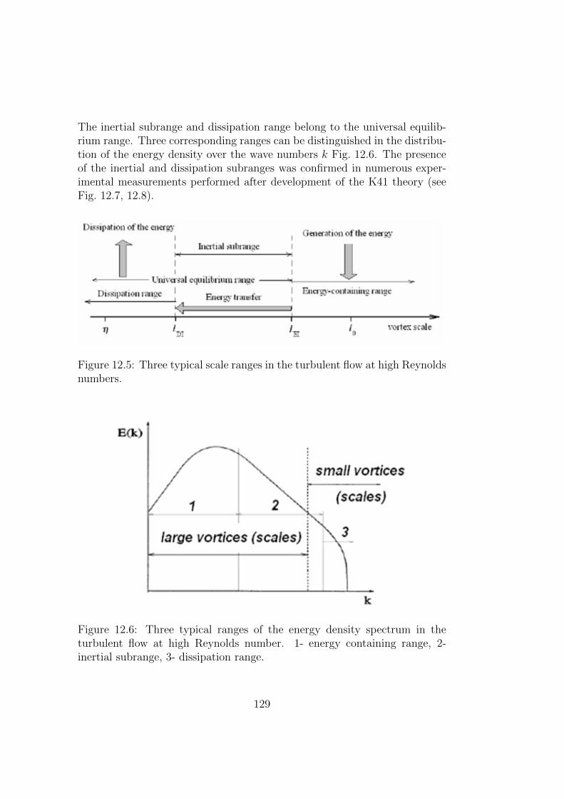
The inertial subrange and dissipation range belong to the universal equilib-rium range. Three corresponding ranges can be distinguished in the distribu-tion of the energy density over the wave numbers k Fig. 12.6. The presenceof the inertial and dissipation subranges was confirmed in numerous exper-imental measurements performed after development of the K41 theory (seeFig. 12.7, 12.8).
Figure 12.5: Three typical scale ranges in the turbulent flow at high Reynoldsnumbers.
Figure 12.6: Three typical ranges of the energy density spectrum in theturbulent flow at high Reynolds number. 1- energy containing range, 2-inertial subrange, 3- dissipation range.
129
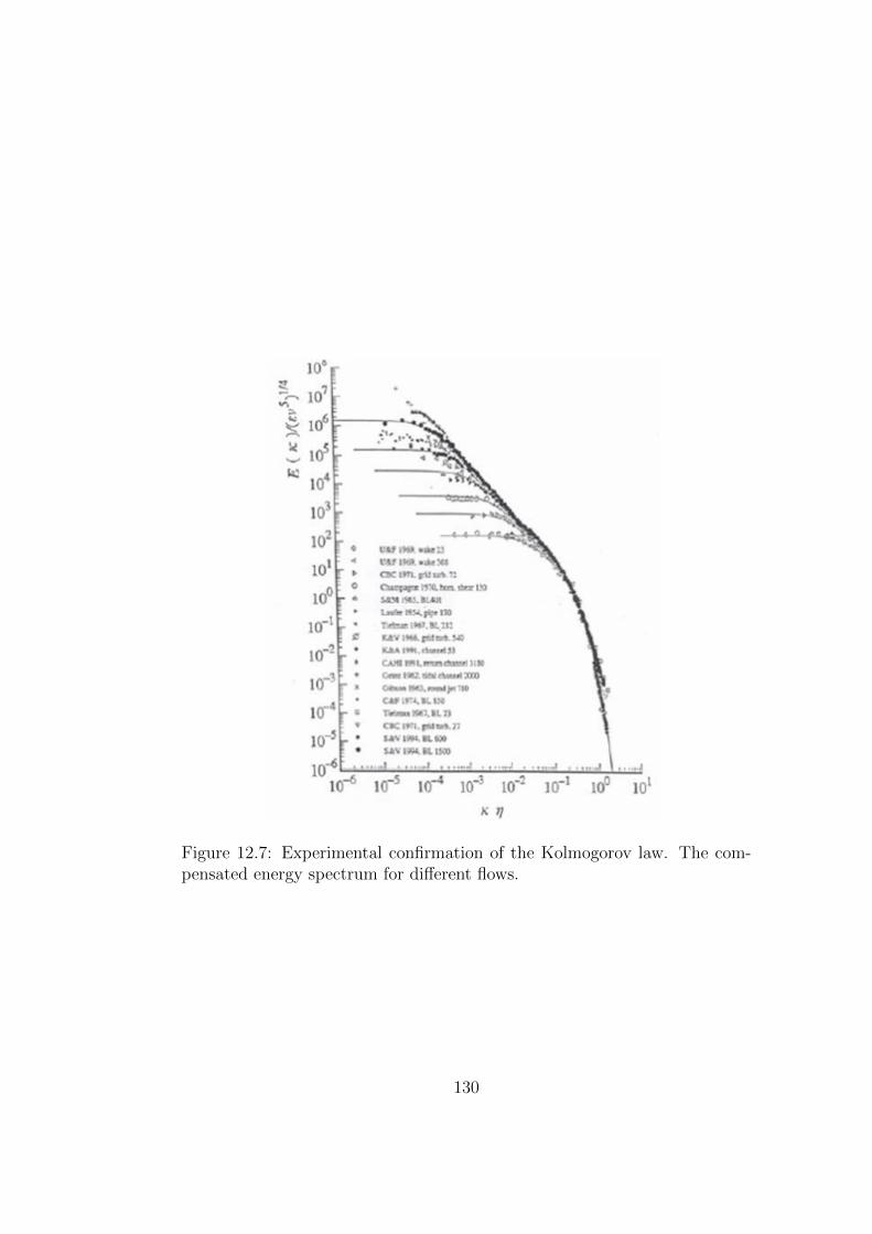
Figure 12.7: Experimental confirmation of the Kolmogorov law. The com-pensated energy spectrum for different flows.
130

Figure 12.8: Experimental confirmation of the Kolmogorov law for the con-centration fluctuations in the jet mixer. Measurements of the LTT Rostock.
12.5 Classification of methods for calculation
of turbulent flows.
The energy spectrum Fig. 12.6 is used to classify three main methods of tur-bulent flows modelling (Fig. 12.9). The most general strategy is the DirectNumerical Simulation (DNS). Within the DNS the whole spectrum of tur-bulent structures is modelled starting from the biggest vortices of the energycontaining range till the smallest dissipative Kolmogorov vortices. The LargeEddy Simulation (LES) models the energy containing vortices and a fractionof vortices corresponding to the inertial subrange. The effect of remain-ing vortices is considered using different approximation models. Since smallvortices are universal, the models are also supposed to be universal. TheReynolds averaged Navier Stokes (RANS) models are dealing with the largevortices corresponding to the energy containing range. The effect of othervortices is taken by different semi- empiric models which are not universal.
12.6 Limitation of K-41. Kolmogorov theory
K-62
The strongest and simultaneously the most questionable assumption of theKolmogorov-41 is: Dissipation rate is an universal constant for each turbulentflow. Already in 1942, during a scientific seminar the Nobel prize winner
131
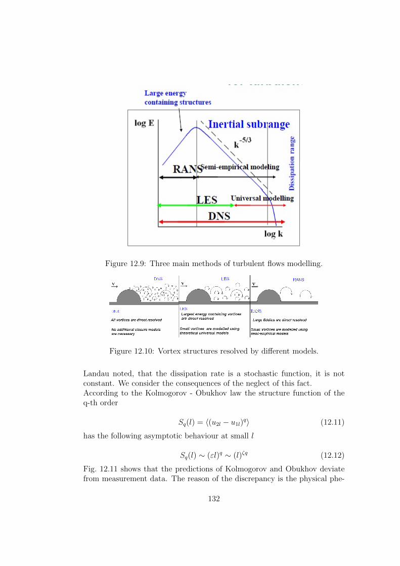
Figure 12.9: Three main methods of turbulent flows modelling.
Figure 12.10: Vortex structures resolved by different models.
Landau noted, that the dissipation rate is a stochastic function, it is notconstant. We consider the consequences of the neglect of this fact.According to the Kolmogorov - Obukhov law the structure function of theq-th order
Sq(l) = 〈(u2l − u1l)q〉 (12.11)
has the following asymptotic behaviour at small l
Sq(l) ∼ (εl)q ∼ (l)ζq (12.12)
Fig. 12.11 shows that the predictions of Kolmogorov and Obukhov deviatefrom measurement data. The reason of the discrepancy is the physical phe-
132

nomenon called the intermittency. The intermittency is caused by the pres-ence of laminar spots in every turbulent flows even at very high Reynoldsnumbers.
Figure 12.11: Power of the structure function. Experiments versus predictionof Kolmogorov and Obukhov.
After the deviation between the K-41 and measurement was documented,Kolmogorov tried to improve his theory. New Kolmogorov theory called asK-62 was published in 1962.New theory is based on two following assumptions:
Assumption 1:
Sq(l) =< δνql >∼< εq/3l > lq/3,
ζq =q
3+ τq/3 < εql >∼ lτq
(12.13)
Assumption 2:
P (εl) = ce(lnε−a)2
2σl2 a = lnε σ2
l = A+ µln(L/l)
τq =µ
2q(1− q) ςq =
q
3+
µ
18q(3− q) < ε2
l >∼ l−µ(12.14)
Unfortunately, various experiments showed later that the second assumptionis proved to be wrong.
12.6.1 Exercises
Exercise 1. Calculate the Reynolds averaged values of the time dependentsignals
u(t) = cos2 t,
133
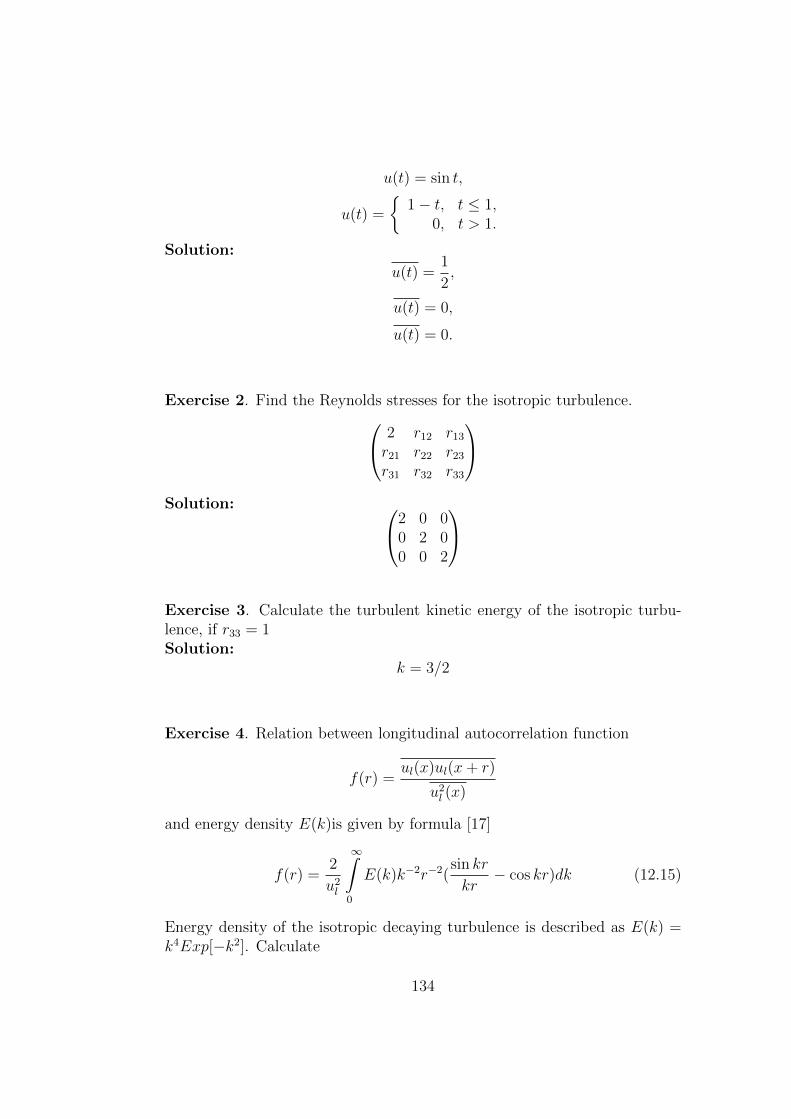
u(t) = sin t,
u(t) =
1− t, t ≤ 1,
0, t > 1.
Solution:
u(t) =1
2,
u(t) = 0,
u(t) = 0.
Exercise 2. Find the Reynolds stresses for the isotropic turbulence. 2 r12 r13
r21 r22 r23
r31 r32 r33
Solution: 2 0 0
0 2 00 0 2
Exercise 3. Calculate the turbulent kinetic energy of the isotropic turbu-lence, if r33 = 1Solution:
k = 3/2
Exercise 4. Relation between longitudinal autocorrelation function
f(r) =ul(x)ul(x+ r)
u2l (x)
and energy density E(k)is given by formula [17]
f(r) =2
u2l
∞∫0
E(k)k−2r−2(sin kr
kr− cos kr)dk (12.15)
Energy density of the isotropic decaying turbulence is described as E(k) =k4Exp[−k2]. Calculate
134

longitudinal autocorrelation function f ,
integral length and
Taylor microscale
for the isotropic decaying turbulence.Solution:
f(r) =2
u2l
∞∫0
E(k)k−2r−2(sin kr
kr− cos kr)dk = (12.16)
=2
u2l
∞∫0
Exp[−k2]k2r−2(sin kr
kr− cos kr)dk =
1
4
√πExp[−r2/4]
L =
∞∫0
f(r)dr =π
4
λ =4
π1/4
Exercise 5. Calculate the probability density function of the time depen-dent signal
time 0 1 2 3 4 5 6 7signal 0 0.1 0.9 0.5 0.7 0.5 0.05 0.65
time 8 9 10 11 12 13 14signal 0.2 0.78 0.43 0.98 0.67 0.92 0.55
using the increment 0.2.
Solution:
signal 0-0.2 0.2-0.4 0.4-0.6 0.6-0.8 0.8-1.0p.d.f. 3/15 2/15 3/15 4/15 3/15
Exercise 6. The velocity u was measured at N points across the pipe: uki ,where i = 1, N and k = 1, K is the time step number. Write a program tocalculate the autocorrelation function of u with respect to point N/2.
Solution:
135

uk,′i = uki − ui
ui =1
K
K∑k=1
uki
R(i, N/2) =
K∑k=1
uk,′i uk,′N/2
K∑k=1
uk,′2N/2
136
Chapter 13
Reynolds Averaged NavierStokes Equation (RANS)
According to the Reynolds averaging each fluctuating quantity is representedas the sum of the averaged value and its fluctuation:
ux = ux + u′x; uy = uy + u′y; uz = uz + u′z (13.1)
where the averaged part is defined as:
ux =1
T
T∫0
uxdt; uy =1
T
T∫0
uydt; uz =1
T
T∫0
uzdt (13.2)
The Reynolds averaging has the following properties:
averaged fluctuation is zero:
f ′ = 0 (13.3)
double averaged quantity is equal to once averaged one:
¯f = f (13.4)
averaged sum is equal to the sum of averaged:
f + g = f + g (13.5)
operators of averaging and differentiation commutate:
∂f
∂t=∂f
∂t,
∂f
∂x=∂f
∂x(13.6)
137
averaged product of two fluctuating quantities is not zero:
f ′g′ 6= 0, fg = f g (13.7)
averaged product of any averaged quantity and fluctuation is zero:
f g′ = f g′ = 0 (13.8)
The starting point of the derivation of the RANS equation is the originalNavier Stokes (NS) equation:
∂ui∂t
+ uj∂ui∂xj
= Fi +1
ρ
∂τji∂xj
(13.9)
Here we use the summation convention of Einstein:
uj∂ui∂xj
= u1∂ui∂x1
+ u2∂ui∂x2
+ u3∂ui∂x3
(13.10)
The NS equation is supplied with the continuity equation, which for the caseof incompressible flow takes the form:
∂ui∂xi
=∂u1
∂x1
+∂u2
∂x2
+∂u3
∂x3
= 0 (13.11)
Using the continuity equation the convective term is written in the conser-vative form:
uj∂ui∂xj
= uj∂ui∂xj
+ ui∂uj∂xj
=∂(uiuj)
∂xj(13.12)
With (13.12) the NS equation reads
∂ui∂t
+∂(uiuj)
∂xj= Fi +
1
ρ
∂τji∂xj
(13.13)
This equation is valid for fluctuating quantities represented in Reynoldsform (13.1)
∂(ui + u′i)
∂t+∂(ui + u′i)(uj + u′j)
∂xj= Fi + F ′ +
1
ρ
∂(τji + τ ′ji)
∂xj(13.14)
Both r.h.s. and l.h.s. are averaged:
∂(ui + u′i)
∂t+∂(ui + u′i)(uj + u′j)
∂xj= Fi + F ′ +
1
ρ
∂(τji + τ ′ji)
∂xj(13.15)
138

Utilization of Reynolds averaging properties results in:
∂ui∂t
+∂(uiuj + u′iu
′j)
∂xj= Fi +
1
ρ
∂τji∂xj
(13.16)
Writing the term u′iu′j on the r.h.s we obtain the Reynolds averaged Navier
Stokes equation (RANS). Its unsteady version is called as the unsteadyReynolds averaged NS equation (URANS):
ρ∂ui∂t
+ ρ∂uiuj∂xj
= ρFi +∂
∂xj(τji − %u′iu′j) (13.17)
There are two important features of URANS in comparison with NS:
The URANS is written for the averaged quantities, whereas the NS forinstantaneous ones,
The URANS has additional term on the r.h.s. −%u′iu′j which is calledthe Reynolds stress Rij.
Generally the Reynolds stress is the matrix with nine terms:
Rij
∣∣∣∣∣∣−ρu′xu′x −ρu′xu′y −ρu′xu′z−ρu′xu′y −ρu′yu′y −ρu′yu′z−ρu′xu′z −ρu′yu′z −ρu′zu′z
∣∣∣∣∣∣ (13.18)
Due to symmetry condtitions the number of unknown stresses is six. Theterm −%u′iu′j is called the stress since it has the same appearance in NSequation as the laminar stress:
τji = ρν
(∂ui∂xj
+∂uj∂xi
)− pδij (13.19)
Laminar stress appears due to viscosity effects whereas the Reynolds stressis caused by flow fluctuations. Now the system of four fluid equations (threeURANS+ continuity) has ten unknowns: three averaged velocity compo-nents ui, averaged pressure p and six Reynolds stresses. The system offluid dynamics is not closed. Additional relations are necessary to expressthe Reynolds stresses through the velocities and pressure. This problem ofdetermination of Reynolds stresses is called as the closure problem of theturbulence. A huge amounts of closure models was developed within theframework of URANS methodology. As said above the URANS methodsmodels the biggest vortices of the flow. The resting scales, which are filteredby the Reynolds avergaing out, are big enough and not universal. This is
139

the reason why the URANS models are not universal. Most of them are ofsemi empirical character. They are based on submodels with few constantsselected for simple canonical flows. Non universality of closure models is thebiggest weakness of URANS turbulence modelling.The majority of URANS models used in engineering are based on the Boussi-nesq hypothesis which is the formal extension of the Newton hypothesis toturbulent flows. Boussinesq proposed to express the Reynolds stress through
the strain rate tensor Sij = 12
(∂uj∂xi
+ ∂ui∂xj
)in the form of the Newton hy-
pothesis with the only difference that instead of the kinematic viscosity νthe turbulent viscosity νt is used
−ρu′iu′j = ρνt
(∂uj∂xi
+∂ui∂xj
)− 2
3ρδijk (13.20)
In the simplest form for flow along the plate with ux(y) and uy = uz = 0 theformula (13.20) reads
−ρu′xu′y = ρνtduxdy
(13.21)
The last term in (13.20) is introduced to keep the consistency. Indeed thesum of three diagonal terms of the Reynolds matrix is equal to the turbulentkinetic energy k = 1
2u′iu′i. Without this term the sum of r.h.s of (13.20)
would result in the sum of the diagonal terms of the strain rate matrixS11 + S22 + S33 which is zero due to the continuity equation. It would bewrong result because k 6= 0. The turbulent closures (13.20) are referred to asthe isotropic because the coefficient νt is equal for all matrix elements Rij.While the kinematic viscosity depends on the liquid, the turbulent kinematicviscosity depends on the turbulent state of the flow. According to estimationof Landau the ratio of the turbulent kinematic viscosity to the kinematic oneis proportional to the ratio of the Reynolds number to that corresponding tothe transition for this type of flow
νt/ν ∼ Re/Recrit (13.22)
The URANS closure models are subdivided into algebraic and differentialones. The most prominent model amount the algebraic models is the Prandtlmodel described in the chapter Physics of turbulence (see the section Dis-tribution of the averaged velocity in the turbulent boundary layer). Thedisadvantages of the algebraic models are:
they are good only for the simplest flow,
140
not suitable for 3D flows,
not suitable for separation flows,
turbulent viscosity depends on averaged values of velocities,
do not consider the flow history.
These disadvantages can be overcome using differential models which aresubdividided into one, two and multi equation models. One and two equa-tion models are usually isotropic based on the Boussinesq approach (13.20).Among the one equation models the most modern and efficient is the modelof Spalart Allmares (SA model) written for the modified kinematic turbulentviscosity υ. The equation for υ reads
∂υ
∂t+ uj
∂υ
∂xj= Cb1ξυ − Cw1fw
(υ
d
)2
+1
σ
∂
∂xk
((ν + υ)
∂υ
∂xk
)+Cb2σ
dυ
dxk
dυ
dxk(13.23)
where
Cb1 = 0, 1355, Cb2 = 0, 622, Cν1 = 7, 1, σ = 2/3,
Cw1 =Cb1k2
+1 + Cb2σ
, Cw2 = 0, 3, Cw3 = 2, 0, k = 0, 41(13.24)
fν1 =χ3
χ3 + C3ν1
, fν2 =χ
1 + χfν1
, fw = g
[1 + C6
w3
g6 + C6w3
]1/6
,
χ = υν, g = r + Cw2(r6 − r), r =υ
ξk2d2
(13.25)
ξ = S +υ
k2d2fν2, S =
√2ΩijΩij, Ωij =
1
2
(∂ui∂xj− ∂uj∂xi
)(13.26)
Two equations RANS models are presented in the next chapter 15.
141

142

Chapter 14
Reynolds Stress Model (RSM)
14.1 Derivation of the RSM Equations
14.1.1 Step 1
The k − th Navier-Stokes equation
∂uk∂t
+∂
∂xj(ujuk) = −1
ρ
∂p
∂xk+
1
ρ
∂
∂xjτjk (14.1)
is multiplied with the velocity component ui
ui
(∂uk∂t
+∂
∂xj(ujuk)
)= ui
(− 1
ρ
∂p
∂xk+
1
ρ
∂
∂xjτjk
)(14.2)
The i− th equation is multiplied with k − th velocity component:
uk
(∂ui∂t
+∂
∂xj(ujui)
)= uk
(− 1
ρ
∂p
∂xi+
1
ρ
∂
∂xjτjk
)(14.3)
Resulting equations (14.2) and (14.3) are then sumed:
∂(ρuiuk)
∂t+∂(ρuiukuj)
∂xj= −ui
∂p
∂xk− uk
∂p
∂xi+ ui
∂τjk∂xj
+ uk∂τji∂xj
(14.4)
Substitution of Reynolds decomposition
ui = ui + u′i, p = p+ p′, τji = τji + τ ′ji (14.5)
into the equation (14.4) results in
143

∂
∂t(ρuiuk) +
∂
∂t(ρu′iu
′k) +
∂
∂xj
(ρuiujuk + ρuiu′ju
′k +
+ρuju′iu′k + ρuku′iu
′j + ρu′iu
′ju′k
)= −ui
∂p
∂xk− u′i
∂p′
∂xk
− uk∂p
∂xi− u′k
∂p′
∂xi+ ui
∂τjk∂xj
+ u′i∂τ ′jk∂xj
+ uk∂τji∂xj
+ u′k∂τ ′ji∂xj
(14.6)
14.1.2 Step 2
The k − th Reynolds averaged Navier Stokes equation
∂ρuk∂t
+∂
∂xj(ρujuk) = − ∂p
∂xk+
∂
∂xj(τjk − ρu′ju′k) (14.7)
is multiplied with the i− th component of averaged velocity
ui
(∂ρuk∂t
+∂
∂xj(ρujuk)
)= ui
(− ∂p
∂xk+
∂
∂xj(τjk − ρu′ju′k)
)(14.8)
Again the i−th Reynolds averaged Navier Stokes equation is multiplied withthe k − th component of averaged velocity
uk
(∂ρui∂t
+∂
∂xj(ρujui)
)= uk
(− ∂p
∂xi+
∂
∂xj(τjk − ρu′ju′i)
)(14.9)
The sum of two last equations reads
∂(ρuiuk)
∂t+∂(ρuiukuj)
∂xj= −ui
∂p
∂xk−uk
∂p
∂xi+ui
∂(τjk − ρu′ju′k)∂xj
+uk∂(τji − ρu′ju′i)
∂xj(14.10)
14.1.3 Step 3
Subtracting the last equation from (14.6) results in
∂
∂t(ρu′iu
′k) +
∂
∂xj(ρuju′iu
′k) +
∂
∂xj(ρu′iu
′ju′k) = −u′i
∂p′
∂xk− u′k
∂p′
∂xi+
+ u′i∂τ ′jk∂xj
+ u′k∂τ ′ji∂xj− ρu′ju′k
∂ui∂xj− ρu′ju′i
∂uk∂xj
(14.11)
144
Using identities (please prove them)
−u′i∂p′
∂xk−u′k
∂p′
∂xi= p′
(∂u′i∂xk
+∂u′k∂xi
)−[δjk
∂
∂xj(u′ip
′)+δij∂
∂xj(u′kp
′)
](14.12)
u′i∂τ ′jk∂xj
+ u′k∂τ ′ji∂xj
= µ
(u′i∂2u′k∂x2
j
+ u′k∂2u′i∂x2
j
)= µ
∂2
∂x2j
u′iu′k − 2µ
∂u′i∂xj
∂u′k∂xj
(14.13)
we get the Reynolds stress model equation
∂
∂t(ρu′iu
′k) +
∂
∂xj(ρuju′iu
′k) +
∂
∂xj(ρu′iu
′ju′k) =
p′(∂u′i∂xk
+∂u′k∂xi
)−[δjk
∂
∂xj(u′ip
′) + δij∂
∂xj(u′kp
′)
]+
+µ∂2
∂x2j
u′iu′k − 2µ
∂u′i∂xj
∂u′k∂xj
−ρu′ju′k∂ui∂xj− ρu′ju′i
∂uk∂xj
which can be written in a compact form
∂
∂t(u′iu
′k) + uj
∂
∂xj(u′iu
′k) =
∂
∂xjDik +Rik + Pik − εik (14.14)
The physical meaning of terms on the r.h.s is as follows
Dik = ν∂(u′iu
′k)
∂xj− u′iu′ju′k +
1
ρ(δjku′i + δiju′k)p
′ → Diffusion (14.15)
Rik =1
ρ
(∂u′i∂xk
+∂u′k∂xi
)p′ → Re distribution (energy exchange) (14.16)
Pik = −u′ju′k∂ui∂xj− u′ju′i
∂uk∂xj
→ Generation (14.17)
εik = 2ν∂u′i∂xj
∂u′k∂xj
→ Dissipation (14.18)
145

14.1.4 Analysis of terms
The diffusion of energy
Dik = ν∂(u′iu
′k)
∂xj− u′iu′ju′k +
1
ρ(δjku′i + δiju′k)p
′ (14.19)
is due to
molecular diffusion, described by the term:
ν∂(u′iu
′k)
∂xj(14.20)
turbulent diffusion, described by the term:
−u′iu′ju′k (14.21)
turbulent diffusion caused by correlation between pressure and velocityfluctuations
1
ρ(δjku′i + δiju′k)p
′ (14.22)
The two last terms are unclosed. Here we face with the famous problemnoted first by Friedman and Keller (1924): Effort to derive the equations forthe second order moments u′iu
′k results in the necessity of determination of
new unclosed terms including third order moments u′iu′ju′k. Using the method
proposed by Friedman and Keller in 1924 it is possible to derive equations formoments of arbitrary order. However, the equation for the m− th order willcontain unclosed moments of the m+1− th order. Impossibility of obtainingof a closed system of equations for a finite number of moments, known as theFriedman-Keller problem is a direct consequence of the nonlinearity of theNavier Stokes equations.
The also unclosed term
Rik =1
ρ
(∂u′i∂xk
+∂u′k∂xi
)p′ (14.23)
describes the redistribution of the energy between different tensor compo-nents u′iu
′k caused by correlation between the stresses and pressure fluctua-
tions.
The term
146
Pik = −u′ju′k∂ui∂xj− u′ju′i
∂uk∂xj
(14.24)
is responsible for the energy generation, i.e. the transport of the energytransfer from averaged (mean) flow to oscillating flow (fluctuations). And,finally,
εik = 2ν∂u′i∂xj
∂u′k∂xj
(14.25)
is the dissipation. This unclosed term is responsible for the transformationof the turbulent kinetic energy into the inner energy of the flow.RSM model based on equations (14.14) is used to determine the Reynoldsstresses from the transport equations. It is not based on the Boussinesqapproach and takes the anisotropy of stresses into account. This model isthe best one among RANS models.
147

148

Chapter 15
Two equations RANS models
15.1 Derivation of the k-Equation
According to definition
k = u′ku′k/2 (15.1)
Assuming i = k in the Reynolds stress model equations (14.14)
∂
∂t(u′iu
′k) + uj
∂
∂xj(u′iu
′k) =
∂
∂xjDik +Rik + Pik − εik (15.2)
ans summing equations for k=1,2 and 3 we obtain the transport equationsfor the total kinetic energy k:
∂k
∂t+ uj
∂k
∂xj=
∂
∂xjDs + P − εS (15.3)
where
DS = ν∂k
∂xj+
1
ρδjku′kp
′ − u′jk′, k′ = u′ku′k/2 Diffusion (15.4)
P = −u′ju′k∂uk∂xj
Generation (15.5)
εS = ν∂u′k∂xj
∂u′k∂xj
Dissipation ( Pseudodissipation) (15.6)
The relation between the true and pseudodissipation is
149
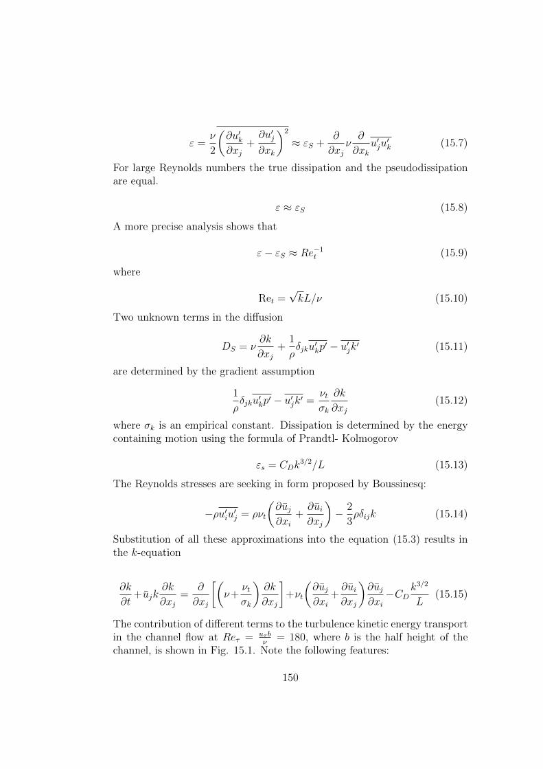
ε =ν
2
(∂u′k∂xj
+∂u′j∂xk
)2
≈ εS +∂
∂xjν∂
∂xku′ju
′k (15.7)
For large Reynolds numbers the true dissipation and the pseudodissipationare equal.
ε ≈ εS (15.8)
A more precise analysis shows that
ε− εS ≈ Re−1t (15.9)
where
Ret =√kL/ν (15.10)
Two unknown terms in the diffusion
DS = ν∂k
∂xj+
1
ρδjku′kp
′ − u′jk′ (15.11)
are determined by the gradient assumption
1
ρδjku′kp
′ − u′jk′ =νtσk
∂k
∂xj(15.12)
where σk is an empirical constant. Dissipation is determined by the energycontaining motion using the formula of Prandtl- Kolmogorov
εs = CDk3/2/L (15.13)
The Reynolds stresses are seeking in form proposed by Boussinesq:
−ρu′iu′j = ρνt
(∂uj∂xi
+∂ui∂xj
)− 2
3ρδijk (15.14)
Substitution of all these approximations into the equation (15.3) results inthe k-equation
∂k
∂t+ujk
∂k
∂xj=
∂
∂xj
[(ν+
νtσk
)∂k
∂xj
]+νt
(∂uj∂xi
+∂ui∂xj
)∂uj∂xi−CD
k3/2
L(15.15)
The contribution of different terms to the turbulence kinetic energy transportin the channel flow at Reτ = uτ b
ν= 180, where b is the half height of the
channel, is shown in Fig. 15.1. Note the following features:
150
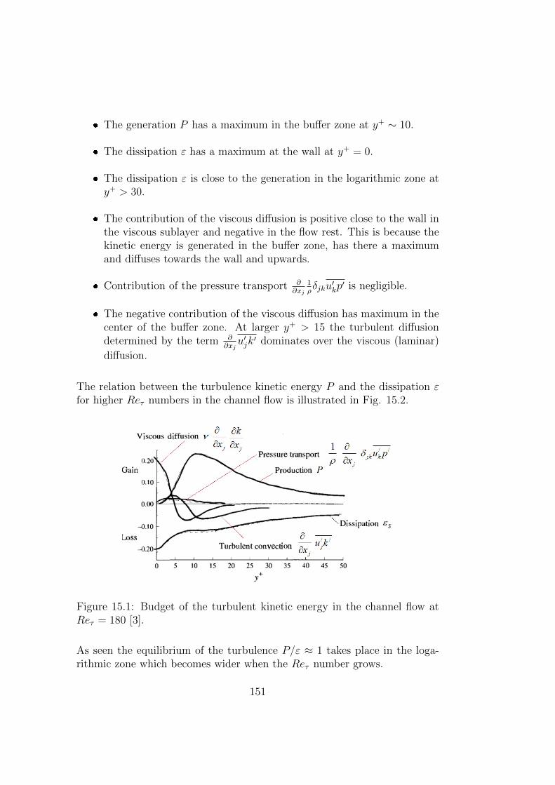
The generation P has a maximum in the buffer zone at y+ ∼ 10.
The dissipation ε has a maximum at the wall at y+ = 0.
The dissipation ε is close to the generation in the logarithmic zone aty+ > 30.
The contribution of the viscous diffusion is positive close to the wall inthe viscous sublayer and negative in the flow rest. This is because thekinetic energy is generated in the buffer zone, has there a maximumand diffuses towards the wall and upwards.
Contribution of the pressure transport ∂∂xj
1ρδjku′kp
′ is negligible.
The negative contribution of the viscous diffusion has maximum in thecenter of the buffer zone. At larger y+ > 15 the turbulent diffusiondetermined by the term ∂
∂xju′jk
′ dominates over the viscous (laminar)
diffusion.
The relation between the turbulence kinetic energy P and the dissipation εfor higher Reτ numbers in the channel flow is illustrated in Fig. 15.2.
Figure 15.1: Budget of the turbulent kinetic energy in the channel flow atReτ = 180 [3].
As seen the equilibrium of the turbulence P/ε ≈ 1 takes place in the loga-rithmic zone which becomes wider when the Reτ number grows.
151
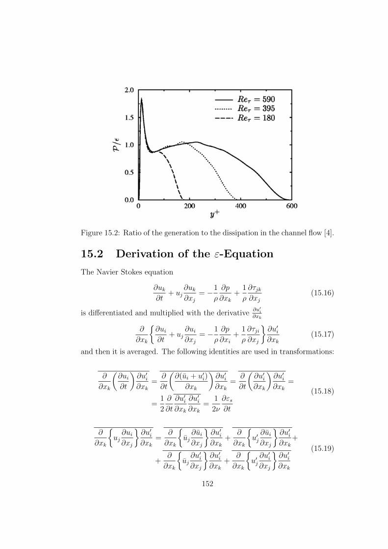
Figure 15.2: Ratio of the generation to the dissipation in the channel flow [4].
15.2 Derivation of the ε-Equation
The Navier Stokes equation
∂uk∂t
+ uj∂uk∂xj
= −1
ρ
∂p
∂xk+
1
ρ
∂τjk∂xj
(15.16)
is differentiated and multiplied with the derivative∂u′i∂xk
∂
∂xk
∂ui∂t
+ uj∂ui∂xj
= −1
ρ
∂p
∂xi+
1
ρ
∂τji∂xj
∂u′i∂xk
(15.17)
and then it is averaged. The following identities are used in transformations:
∂
∂xk
(∂ui∂t
)∂u′i∂xk
=∂
∂t
(∂(ui + u′i)
∂xk
)∂u′i∂xk
=∂
∂t
(∂u′i∂xk
)∂u′i∂xk
=
=1
2
∂
∂t
∂u′i∂xk
∂u′i∂xk
=1
2ν
∂εs∂t
(15.18)
∂
∂xk
uj∂ui∂xj
∂u′i∂xk
=∂
∂xk
uj∂ui∂xj
∂u′i∂xk
+∂
∂xk
u′j∂ui∂xj
∂u′i∂xk
+
+∂
∂xk
uj∂u′i∂xj
∂u′i∂xk
+∂
∂xk
u′j∂u′i∂xj
∂u′i∂xk
(15.19)
152
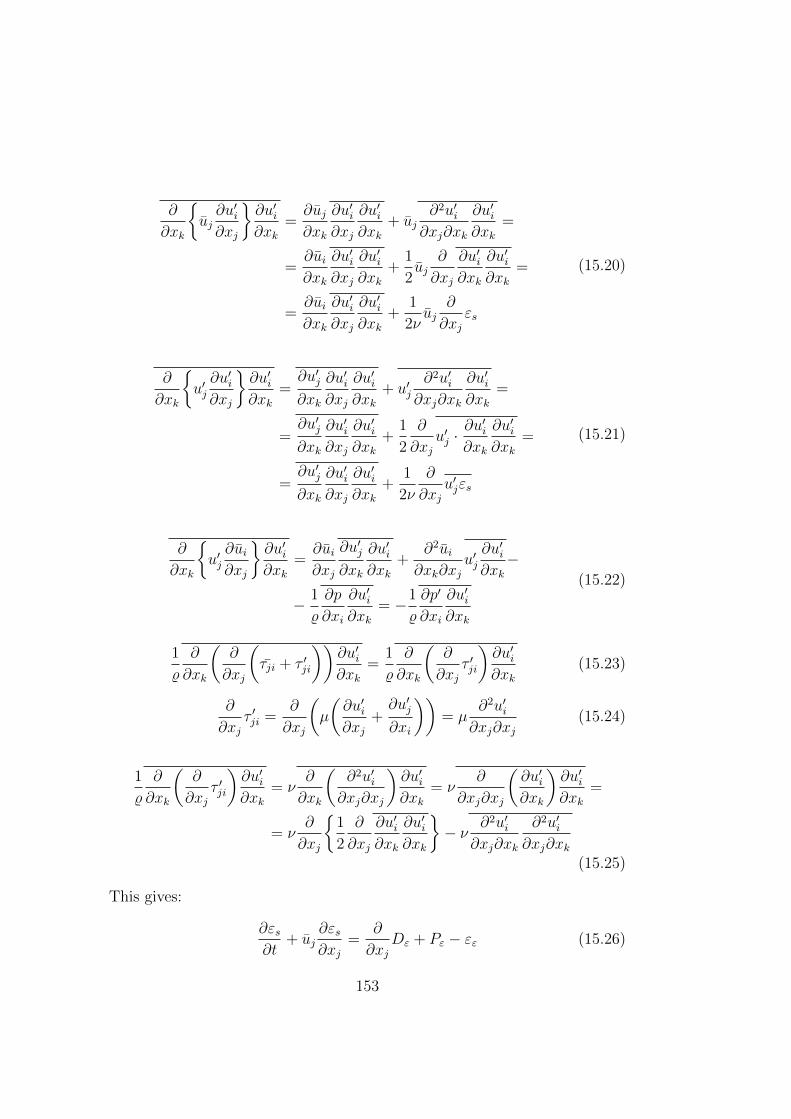
∂
∂xk
uj∂u′i∂xj
∂u′i∂xk
=∂uj∂xk
∂u′i∂xj
∂u′i∂xk
+ uj∂2u′i∂xj∂xk
∂u′i∂xk
=
=∂ui∂xk
∂u′i∂xj
∂u′i∂xk
+1
2uj
∂
∂xj
∂u′i∂xk
∂u′i∂xk
=
=∂ui∂xk
∂u′i∂xj
∂u′i∂xk
+1
2νuj
∂
∂xjεs
(15.20)
∂
∂xk
u′j∂u′i∂xj
∂u′i∂xk
=∂u′j∂xk
∂u′i∂xj
∂u′i∂xk
+ u′j∂2u′i∂xj∂xk
∂u′i∂xk
=
=∂u′j∂xk
∂u′i∂xj
∂u′i∂xk
+1
2
∂
∂xju′j ·
∂u′i∂xk
∂u′i∂xk
=
=∂u′j∂xk
∂u′i∂xj
∂u′i∂xk
+1
2ν
∂
∂xju′jεs
(15.21)
∂
∂xk
u′j∂ui∂xj
∂u′i∂xk
=∂ui∂xj
∂u′j∂xk
∂u′i∂xk
+∂2ui∂xk∂xj
u′j∂u′i∂xk−
− 1
%
∂p
∂xi
∂u′i∂xk
= −1
%
∂p′
∂xi
∂u′i∂xk
(15.22)
1
%
∂
∂xk
(∂
∂xj
(τji + τ ′ji
))∂u′i∂xk
=1
%
∂
∂xk
(∂
∂xjτ ′ji
)∂u′i∂xk
(15.23)
∂
∂xjτ ′ji =
∂
∂xj
(µ
(∂u′i∂xj
+∂u′j∂xi
))= µ
∂2u′i∂xj∂xj
(15.24)
1
%
∂
∂xk
(∂
∂xjτ ′ji
)∂u′i∂xk
= ν∂
∂xk
(∂2u′i∂xj∂xj
)∂u′i∂xk
= ν∂
∂xj∂xj
(∂u′i∂xk
)∂u′i∂xk
=
= ν∂
∂xj
1
2
∂
∂xj
∂u′i∂xk
∂u′i∂xk
− ν ∂2u′i
∂xj∂xk
∂2u′i∂xj∂xk
(15.25)
This gives:
∂εs∂t
+ uj∂εs∂xj
=∂
∂xjDε + Pε − εε (15.26)
153
where
Dε = ν∂εs∂xj− u′jε′s − 2
ν
ρ
∂u′i∂xk
∂p′
∂xi(15.27)
Pε = −2νu′j∂u′i∂xk
∂2ui∂xj∂xk
− 2ν
(∂u′i∂xk
∂u′j∂xk
∂ui∂xj
+∂u′i∂xj
∂u′i∂xk
∂ui∂xk
)− 2ν
∂u′i∂xj
∂u′j∂xk
∂u′i∂xk
(15.28)
εε = 2ν2 ∂2u′i∂xj∂xk
∂2u′i∂xj∂xk
, ε′s = ν∂u′i∂xk
∂u′i∂xk
(15.29)
The terms on the r.h.s. were approximated according to the following for-mula:
∂
∂xjDε =
∂
∂xj
[(ν +
νTσε
)∂ε
∂xj
];Pε =
Cε1ε
kτij∂ui∂xj
; εε =Cε2ε
2
k(15.30)
Constants are taken from planar jet and mixing layer:
Cε1 = 1.44, Cε2 = 1.92, σk = 1, σε = 1.3 (15.31)
Taking the above mentioned similarity between the pseudo dissipation andthe dissipation at large Re numbers (ε ≈ εs) the dissipation equation can bewritten just for ε:
∂ε
∂t+ uj
∂ε
∂xj=
∂
∂xjDε + Pε − εε (15.32)
15.3 The k − ε model
Hereby the full closed system of the k − ε model reads:
∂k
∂t+ uj
∂k
∂xj=
∂
∂xj
((ν +
νtσk
)∂k
∂xj
)+ τij
∂ui∂xj− ε
∂ε
∂t+ uj
∂ε
∂xj=
∂
∂xj
[(ν +
νtσε
)∂ε
∂xj
]+Cε1ε
kτij∂ui∂xj− Cε2ε
2
k
(15.33)
Under assumption that the generation of the turbulent energy equals to theits dissipation (the turbulence is in equilibrium, turbulent scales are in the
154

inertial range) Kolmogorov and Prandtl derived the relation between thekinetic energy, the dissipation rate and the integral lengths L:
ε ≈ k3/2
L(15.34)
From the dimension analysis
νt = Cµ√kL (15.35)
follows
νt = Cµ√kL = Cµ
k2
ε(15.36)
As soon as k and ε are known the turbulent kinematic viscosity νt is computedfrom (15.36) and Reynolds stresses can be calculated from the Boussinesqhypothesis and then substituted into the Reynolds averaged Navier Stokesequations. The problem is mathematically closed. The flux of informationwithin the k − ε model is shown in Fig. 15.3.
Figure 15.3: Information flux within the k − ε model.
The k − ε model is the classical approach, which is very accurate at largeturbulent Reynolds numbers Ret =
√kL/ν, where L is the integral length.
At small Ret number, for instance close to the wall where k ∼ 0, L ∼ 0, theapproximations used in derivation of k− ε model equations are not valid. Toovercome this disadvantage various low Reynolds k−ε models were proposed.
155
15.4 Low Reynolds k − ε model
In the k−ε model the dissipation ε is underestimated and k is overestimatedin the near wall regions at small y+. To artificially increase the dissipation,the ε equation is modified by manipulating two last terms reponsible forthe generation of the dissipation and the dissipation of the dissipation andintroduction of an additional term E:
∂k
∂t+ uj
∂k
∂xj=
∂
∂xj
((ν +
νtσk
)∂k
∂xj
)+ τij
∂ui∂xj− ε
∂ε
∂t+ uj
∂ε
∂xj=
∂
∂xj
[(ν +
νtσε
)∂ε
∂xj
]+ε
k(Cε1f1τij
∂ui∂xj− Cε2εf2) + E
(15.37)
In the traditional model E = 0 and f1 = f2 = 1. To increase the generationof the dissipation, the term ε/kCε1τij
∂ui∂xj
is multiplied with the constant f1
which is larger than one, i.e. f1 > 1. On the contrary, the dissipation ofthe dissipation Cε2ε
2/k is artificially reduced by the multiplication with thecoefficient f2 < 1. In some models, additionally an artificial generation termE > 0 is added on the right hand side of (15.37). In almost all low Reynoldsnumber models the turbulent kinematic viscosity is reduced according toνt = Cµfµk
2/ε, where fµ < 1. The parameters E, f1, f2 and fµ depend onthe flow parameter and are found empirically to match the numerical andexperimental results.
15.5 The k − ω model
The k − ω model was developed as an alternative to the k − ε model toovercome the disadvantages of the latter one in the near wall region. Thefollowing system of equations was proposed by Wilcox in 1998, which includesthe transport equation for the turbulence kinetic energy k and ω which hasdimension of sec−1 and is interpreted as the specific dissipation rate:
∂k
∂t+ uj
∂k
∂xj=
∂
∂xj
((ν +
νtσk
)∂k
∂xj
)+ τij
∂ui∂xj− β∗kω
∂ω
∂t+ uj
∂ω
∂xj=
∂
∂xj
[(ν + σνt
)∂ω
∂xj
]+ α
ω
kτij∂ui∂xj− βω2
(15.38)
with the following closure relations:
α = 13/25, β = β0fβ, β∗ = β∗0fβ∗ , σ = 0.5, σ∗ = 0.5
156

β0 = 9/125, fβ =1 + 70ξω1 + 80ξω
, ξω = |ΩijΩjkSki(β∗ω)3
|
Sij =1
2
(∂ui∂xj
+∂uj∂xi
),Ωij =
1
2
(∂ui∂xj− ∂uj∂xi
)β∗0 = 9/100, fβ∗ =
1 if ξk ≤ 0
1+680χ2k
1+400χ2k
otherwise(15.39)
χk =1
ω2
∂k
∂xj
∂ω
∂xj
Using the dimension analysis the relations between k, νt, ε and the integrallength l were derived
ω = k/νt, ε = β∗ωk, l =√k/ω
The structure of the transport equation (15.38) for ω is the same as forthe ε. The terms ∂
∂xj(ν ∂ω
∂xj) ∂
∂xj(σνt
∂ω∂xj
) are responsible to the molecular
and the turbulent diffusions of ω, respectively. The next term describes thegeneration of the specific dissipation rate and the last one stands for thedissipation of ω.
15.6 The k − ω SST model
The disadvantage of the low Reynolds number model described above is therequirement of a very fine resolution close to the wall. The first node shouldhave the ordinate y+ < 1. Menter [19] proposed a very effective combinationof the k − ε and k − ω models which is applicable in the whole region of theboundary layer. The idea of this development is as follows
The k−ε is accurate far from the wall in the outer part of the boundarylayer and is not applicable close to the wall.
The k − ω is accurate close to the wall, and is not applicable far fromthe wall in the outer part of the boundary layer.
The combination of two models k−ωSST = F1(k−ω)+(1−F1)(k−ε) isthe new model which, if the function F1 is chosen properly, is accuratein the whole boundary layer. F1 tends to 1.0 when y+ → 0 and k −ωSST → (k − ω). F1 tends to 0 when y+ increases and k − ωSST →(k− ε) Schematic distribution of submodels in the k− ωSST model isshown in Fig. 15.4.
157
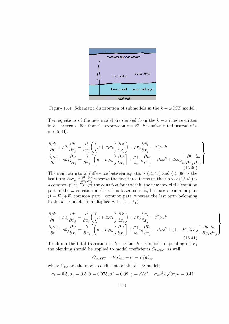
Figure 15.4: Schematic distribution of submodels in the k − ωSST model.
Two equations of the new model are derived from the k − ε ones rewrittenin k − ω terms. For that the expression ε = β∗ωk is substituted instead of εin (15.33):
∂ρk
∂t+ ρuj
∂k
∂xj=
∂
∂xj
((µ+ µtσk
)∂k
∂xj
)+ ρτij
∂ui∂xj− β∗ρωk
∂ρω
∂t+ ρuj
∂ω
∂xj=
∂
∂xj
[(µ+ µtσω
)∂ω
∂xj
]+ργ
νtτij∂ui∂xj− βρω2 + 2ρσω
1
ω
∂k
∂xj
∂ω
∂xj
(15.40)
The main structural difference between equations (15.41) and (15.38) is thelast term 2ρσω2
1ω∂k∂xj
∂ω∂xj
whereas the first three terms on the r.h.s of (15.41) is
a common part. To get the equation for ω within the new model the commonpart of the ω equation in (15.41) is taken as it is, because : common part(1− F1)+F1 common part= common part, whereas the last term belongingto the k − ε model is multiplied with (1− F1)
∂ρk
∂t+ ρuj
∂k
∂xj=
∂
∂xj
((µ+ µtσk
)∂k
∂xj
)+ ρτij
∂ui∂xj− β∗ρωk
∂ρω
∂t+ ρuj
∂ω
∂xj=
∂
∂xj
[(µ+ µtσω
)∂ω
∂xj
]+ργ
νtτij∂ui∂xj− βρω2 + (1− F1)2ρσω
1
ω
∂k
∂xj
∂ω
∂xj
(15.41)
To obtain the total transition to k − ω and k − ε models depending on F1
the blending should be applied to model coefficients CkωSST as well
CkωSST = F1Ckω + (1− F1)Ckε
where Ckω are the model coefficients of the k − ω model:
σk = 0.5, σω = 0.5, β = 0.075, β∗ = 0.09, γ = β/β∗ − σωκ2/√β∗, κ = 0.41
158
and Ckε are the model coefficients of the k − ε model:
σk = 1.0, σω = 0.856, β = 0.0828, β∗ = 0.09, γ = β/β∗ − σωκ2/√β∗, κ = 0.41
The blending function F1 was found empirically from the matching numericalresults with experimental ones for canonical flows:
F1 = tanh(y∗4)
where
y∗ = min
(max
( √k
0.09ωy,500ν
ωy2
),
4ρσωk
CDkωy2
)and
CDkω = max
(2ρσω
1
ω
∂k
∂xj
∂ω
∂xj, 10−20
)The last step in the derivation of the k − ωSST model, which is responsiblefor the abbreviation SST - shear stress transport, is the reformulation of theturbulent viscosity νt expressing it through the shear stress τt. The stress iscalculated from the Bradshow formula for the turbulent shear stress:
τt = ρak (15.42)
where a is an experimental constant. From the other side, from the Boussi-nesq hypothesis we obtain
τt = µt∂ux∂y
= µtΩ (15.43)
where Ω = ∂ux∂y
is the component of the vorticity vector close to the wall.
From comparison of (15.42) and (15.43) we get
νt =ak
Ω(15.44)
This expression is used in a modified form, proposed by Menter
νt =ak
max(a1ω,ΩF2)(15.45)
where
F2 = tanh(y02)
y0 = max
(2√k
0.09ωy,500ν
ωy2
)159
and Ω is calculated as the magnitude of the vorticity vector Ω =√
Ω21 + Ω2
2 + Ω23.
The blending function F2 is chosen to satisfy the following condition:
F2(y0) =
F2 → 1 at the wall y0 →∞F2 → 0 at the wall y0 → 0
(15.46)
Substituting (15.46) into (15.45) results in the following expression for theturbulent kinematic viscosity
νt =
νt → ak
max(aω,Ω)at the wall y0 →∞
νt → k/ω at the wall y0 → 0(15.47)
Far from the wall the turbulent viscosity νt is calculated from the formuladerived from the dimension analysis νt = k/ω which is very inaccurate closeto the wall. It is passed smoothly into the approximation νt = ak
max(aω,Ω)
which is valid at the wall.The Reynolds stress is determined from the Boussinesq formula with k andνt calculated from the k − ωSST model.The model is completed with the following boundary conditions
at the inlet condition:
ω = (1...10)U
L, νt = 10−(2...5)ν, k = νtω
where ν is the kinematic viscosity (laminar), U and L are, respectively, thevelocity and the integral length at the inlet. At the solid boundary thespecific dissipation range satisfies the boundary condition derived by Menter
ω = 106ν
β(∆y)2
where ∆y is the height of the first cell adjacent to the wall.
15.7 Method of wall functions
Basic relations of k − ε model were derived under assumption that the localturbulent Reynolds number Ret =
√kL/ν is very high. This is not the case
in the wall flow. Due to damping effect of the wall, the velocity pulsationsand the turbulent kinetic energy are small. Application of the k − ε modelis not valid. An efficient solution of this problem was proposed by Spaldingwho developed the method of wall functions.
160

The wall function is an analytical representation of the solution close to thewall which is matched with the numerical solution in the resting flow.Below we derive basic relations of the wall function method following to thetextbook [20].
15.7.1 Equilibrium wall functions
It is assumed that the turbulence is in equilibrium, i.e. P = ε:
P = −u′ju′k∂uk∂xj
= ε
This assumption is valid for the gradient less flows when the pressure isconstant along the wall, ∂p/∂x = 0, where x is the coordinate along the wall.Such flows are called in fluid mechanics zero pressure gradient (ZPG) flows.Let us consider two dimensional flow along a plate:
P = −u′xu′y∂ux∂y
= νt
(∂ux∂y
)2
= ε (15.48)
The derivative
(∂ux∂y
)can be expressed from the mixing length model of
Prandtl:
νt = l2(∂ux∂y
)⇒(∂ux∂y
)= νt/l
2 (15.49)
From analysis of dimension we obtain
νt = cµk1/2L (15.50)
Using the Kolmogorov-Prandtl estimation ε ∼ k3/2/L we get
νt =cµk
2
ε(15.51)
From (15.48) and (15.49) it follows
νt = l4/3 · ε1/3
and
ε = c3/4µ k3/2/l
From (15.48) and (15.51) we have:
161
∂ux∂y
=
(ε
νt
)1/2
=
(ε2
cµk2
)1/2
=ε
c1/2µ k
for wall stress:
τw = µt∂ux∂y
= %νtε
c1/2µ k
=
= %cµk
2
ε
ε
c1/2µ k
= %c1/2µ k
and kinetic energy:
k =τw
%c1/2µ
Let yp be the ordinate of the first grid node near the wall.Using approximation of Prandtl for l we obtain the dissipation rate at yp:
εp = c3/4µ k3/2
p /(κyp)
(15.52)
and turbulent kinetic energy
kp =τw
%c1/2µ
τw can be found from the assumption that the first node is in the logarithmicrange:
uxuτ
=1
κlnEy+
uτ =κuxp
lnEy+p√
τw%·√τw%
=
(κuxp
lnEy+p
)1/2
· k1/2p c1/4
µ
τw =%κuxpk
1/2p c
1/4µ
lnEy+p
(15.53)
Values εp (15.52) and τw (15.53) are used within finite volume method whenthe k− ε equations are written for the volumes ∆ν adjacent to the wall. Forinstance the generation term is calculated as
162
∫∆ν
Pdxdy =
∫∆ν
τxy∂ux∂y
dxdy =
∫∆ν
τw∂ux∂y
dxdy = τw∆xuxp (15.54)
The wall functions are applied not only in conjunction with the k − ε butalso in connection with the k − ωSST and other models.
15.7.2 Non- equilibrium wall functions
The wall functions presented above were derived for the turbulence in theequilibrium state. For a more general case of the non- equilibrium turbulenceP 6= ε and non zero gradient (NZPG) ∂p
∂x= 0 the wall functions were pro-
posed, for instance, by Hanjalic and Popovac (2007). The derivation is basedon the momentum (Navier Stokes) equation, written for the wall-tangentialvelocity ux
∂
∂y[(µ+ µt)
∂ux∂y
] = ρ∂ux∂t
+ ρux∂ux∂x
+ ρuy∂ux∂y
+∂p
∂x= Cu (15.55)
The equation (15.55) is integrated over the first wall- adjacent cell, assumingthat the r.h.s. of (15.55) is constant over the cell and
µt =
0, if y < yv
ρκuτy, otherwise(15.56)
where yv is the thickness of the viscous sublayer. After the double integrationone obtains the expression for the wall shear stress τw:
τw =ρux − Cuy
κuτρyvµ
+ ln(y/yv)κuτ
(15.57)
or
uxuτ
=1
κln(Ey+)
1
1− Cuyρuxκuτ
(15.58)
Comparing (15.58) with the classic logarithmic distribution (15.59)
uxuτ
=1
κln(Ey+) (15.59)
one seen that the non- equilibrium effect is taken into account by the coeffi-cient 1
1− Cuyρuxκuτ
which is called the non- equilibrium function. Further deriva-
tions are similar to these for the equilibrium wall functions.
163
The wall functions are widely used for all two equation turbulence modelswhen the near wall flow can not be resolved properly. Especially importantthe wall functions are for the high Reynolds numbers when the real scaleobjects are calculated. Commonly, the wall functions are applied when thewall distance of the first grid node adjacent to the wall satisfies the conditiony+ ≥ 30. This is because the logarithmic velocity distribution is the basicassumption for the most of the wall functions. The wall functions derivedfor a more general velocity distribution, for instance, proposed by Spaldingand which are valid for all y+ can be applied also for y+ < 30.
164

Chapter 16
Large Eddy Simulation (LES)
16.1 LES filtering
Within the LES all vortices are subdivided into large resolved vortices andfine modelled subgrid vortices. The border between vortices should lie withinthe inertial range. The separation of fine scale motions (small fine vortices)from large ones is done using the spatial filtering. Let ϕ be any stochasticfunction which is represented as the sum of filtered part and fluctuation:
ϕ = ϕ+ ϕ′
where the filtered part is defined as
ϕ(~x, t) =
∫ ∞−∞
∫ ∞−∞
∫ ∞−∞
ϕ(~x− ~s, t)F (~s)d~s
Here F(~s) is the filtering function, satisfying the condition
∞∫−∞
∞∫−∞
∞∫−∞
F (~s)d~s = 1
Three different filtering functions shown in Fig. 1: ideal filter, Gauss filterand top hat filter. Ideal filter is applied in Fourier space. High frequenciesare cut off. Low frequencies are simulated directly. The top hat filter is somekind of smoothing applied in physical space. The simplest case is smoothingover three neighboring points
ϕi =1
b(ϕi−1 + aϕi + ϕi+1)
where b = 2 + a.
165

16.1.1 Properties of filtering
The spatial filtering and Reynolds averaging are both filtering operations.LES spatial filtering has properties which differ from these of Reynolds av-eraging. First, the spatialy averaged quantity is not zero. Double filtering isnot equal once filtering:
ϕ′ 6= 0, ˜ϕ 6= ϕ,
Both conditions are compatible because
ϕ′ = ϕ− ϕ = ϕ− ˜ϕ 6= 0
Figure 16.1: Different filtering functions used in LES.
Other important properties are similar to these of RANS averaging:
166

Averaged sum of two quantities is equal to the sum of averaged quan-tities:
ϕ+ g = ϕ+ g
Filtering operator commutes with the differentiation operator, if filter-ing is homogeneous:
∂ϕ
∂t=∂ϕ
∂t
∂ϕ
∂xj=
∂ϕ
∂xj
A very important relation which is the consequence of these properties is
ϕφ = ˜ϕφ+ ˜ϕφ′ + ˜φϕ′ + ϕ′φ′
In the case of Reynolds averaging only the first and the last terms remain.The properties of large and small scale motions are shown in the table 16.1.
Large scale motion Small scale motion
Generated by mean flow Generated by large scale structuresDepends on the flow geometry UniversalRegular StochasticDeterministic description Stochastic descriptionHeterogeneous HomogeneousAnisotrop IsotropExists long time Exists short timeDiffusive DissipativeModelling is complicated Easy to model
Table 16.1: Properties of large and small scale motions
A very important conclusion from this table is the fact that the small scalemotion is universal. Therefore one can expect that the models describing thesmall scale motion in contrast to RANS models are also universal.
16.2 LES equations
The governing equations of LES are derived from the Navier Stokes equation
∂
∂t(ρui) +
∂
∂xj(ρuiuj) =
∂
∂xj
[ρν
(∂uj∂xi
+∂ui∂xj
)]− ∂p
∂xi+ ρgi (16.1)
167

Application of the filter operation to (16.1) results in
˜∂
∂t(ρui) +
∂
∂xj(ρuiuj) =
˜∂
∂xj
[ρν
(∂uj∂xi
+∂ui∂xj
)]− ∂p
∂xi+ ρgi
Averaged sum is equal to the sum of averaged terms:
∂
∂t(ρui) +
˜∂∂xj
(ρuiuj) =˜∂
∂xj
[ρν∂ui∂xj
]− ∂p
∂xi+ ρgi (16.2)
Introducing the term
τSGSij = uiuj − uiujthe equation (16.2) is rewritten in the final form
∂
∂t(ρui) +
∂
∂xj(ρuiuj) =
∂
∂xj
[ρν∂ui∂xj− ρτSGSij
]− ∂p
∂xi+ ρgi
The term τSGSij = uiuj − uiuj is the subgrid stress (SGS) which considersthe effect of small fine vortices on large scale motion directly resolved on thegrid.
16.3 Smagorinsky model
Note that the fine scale vortices are not resolved. They filtered out by thefiltering operation. The effect of these vortices is taken by the term τSGSij
into account. Since the small vortices are not modeled, the subgrid stress arecalculated using phenomenological models. The most recent phenomenolog-ical model was proposed by Smagorinsky in 1963. The Smagorinsky modelis just the extension of the Boussinesq approach
τij −1
3τkkδij ≈ −2νtSij,
Smagorinsky introduced the subgrid viscosity νSGS instead of the turbulentkinematic viscosity
τSGSij − 1
3τSGSkk δij ≈ −2νSGSSij,
Expression for the subgrid viscosity was obtained by Smagorinsky with theuse of idea taken from the Prandtl mixing length theory. According toPrandtl, the turbulent kinematic viscosity is proportional to the mixinglength squared and the velocity gradient close to the wall
168

νt = l2|duxdy|
According to Smagorinsky, the subgrid viscosity is proportional to the mag-nitude of the strain rate tensor Sij and to a certain length lS squared
νSGS = l2S|Sij|, |Sij| =√
2SijSij
Where
Sij =1
2
(∂ui∂xj
+∂uj∂xi
)The length lS is assumed to be proportional to the mesh size
lS = CS∆
where CS is the constant of Smagorinsky.
The Smagorinsky constant was estimated first by Lilly. The main assumptionof the Lilly analysis is the balance between generation
Pr = −τijSij = 2νtSijSij = νt|Sij|2
and dissipation of the turbulent kinetic energy
ε = P = νt|Sij|2 = l2S|Sij|3 (16.3)
Lilly estimated the strain rate tensor magnitude for Kolmogorov spectrum
S2 ≈ 7Cε2/3∆−4/3
Substitution of the last formula into (16.3) results in:
lS =∆
(7C)3/4
(S2
3/2
S3
)1/2
Assuming additionally that S23/2
≈ S3, the length lS and the Smagorinskyconstant are expressed through the Kolmogorov constant C = 1.5:
CS =lS∆
=1
(7C)3/4≈ 0.17
The Smagorinsky constant 0.17 is derived analytically with a few strongassumptions. The experience shows that numerical results agree with mea-surements much better if a reduced value of the Smagorinsky constant is
169
used. Common values are 0.065 and 0.1.
Advantages and disdvantages of the Smagorinsky model are summarized inthe table 20.1.
Advantages DisadvantagesSimple Laminar flow is not modelledLow computational costs Constant of Smagorinsky is constant in time and
spaceStable Actually, the constant is chosen arbitrarily
depending on the problem under considerationGood accuracy in ideal Sensible to gridconditions
Purely dissipativDamping of pulsation is too strong
Table 16.2: Advantages and disadvantages of the Smagorinsky model
We finish this section with a very important comment:
• the LES models are consistent when the resolution increases, i.e. ∆→ 0.
Indeed, if the resolution is increased, ∆ → 0, the SGS stresses disappear.The LES equation is passed to the original Navier Stokes equations. TheLES simulation becomes the DNS simulation if ∆→ 0. On the contrary, theURANS simulation is not consistent when ∆ → 0. The Reynolds stressesdon’t disappear if the resolution is increased ∆→ 0. The turbulence is thentwice resolved.
16.4 Model of Germano ( Dynamic Smagorin-
sky Model)
The classical model of Smagorinsky with the parameter CS being constantfor the whole computational domain is proved to be very diffusive. Germanoproposed to calculate the Smagorinsky constant CS being variable both inspace and in time, i.e. CS = CS(x, t). The constant is determined using thedynamic procedure which is then referred to as the Dynamic SmagorinskyModel (DSM).
According to the definition the subgrid stress is
170
τSGSij = uiuj − uiuj (16.4)
Germano introduces the double filtering or the test filtering designated asau = ˆu. Here the tilde symbol means the first filtering with filter width ∆whereas the hat symbol stands for the second filtering with filter width ∼ 2∆.The symbol means the resulting double filtering. Using the definition (16.4)we can write
T testij =_uiuj −
aui
auj = uiuj − ˆui ˆuj (16.5)
Filtration of (16.4) results in
τSGSij = uiuj − uiuj (16.6)
Subtracting (16.6) from (16.5) yields
T testij − τSGSij = uiuj − ˆui ˆuj (16.7)
We suppose that the double filter width is small. Therefore the Smagorinskymodel is valid for both stresses τSGSij and T testij :
τSGSij − 1
3τSGSkk δij = −2
(C∆s ∆)2|Sij|
(Sij)
= 2CmSGSij ,
T testij −1
3T testkk δij = −2
(C∆s ∆)2| ˆSij|
( ˆSij)
= 2Cmtestij ,
(16.8)
The application of the double filter to τSGSij gives:
τSGSij − 1
3τSGSkk δij = 2CmSGS
ij (16.9)
where C = C2S. Here we supposed that the filtered product of the constant
C with mij is equal to the product of filtered mij with the same constant
Cm ≈ Cm
We introduce the tensor Lij which is equal to the difference between testfilter and once filtered original SGS stress:
Lij = T testij − τSGSij = uiuj − ˆui ˆuj (16.10)
Using this designation we get from (16.8) and (16.9)
2CMij = Lij −1
3Lkkδij (16.11)
171

where
Mij = mtestij − mSGS
ij
The system (16.11) is overdefined (six equations for one unknown coefficientC). To get an unique solution we multiply both the l.h.s. and r.h.s of (16.11)with the tensor Sij. The final result for C is
C =LijSij
2MijSij(16.12)
Use of (16.14) is problematic since the denumerator MijSij can become zero.To overcome this difficulty Lilly proposed to determine the constant from thecondition of the minimum residual of the equation (16.11):
Q =
(Lij −
1
3Lkkδij − 2CMij
)2
→ min (16.13)
The minimum is attained at the point with zero derivative of the functionalQ on the parameter C:
∂Q
∂C= −4Mij
(Lij −
1
3Lkkδij − 2CMij
)= 0 (16.14)
It follows directly from (16.14):
C =MijLij − 1
3LkkδijMij
2MijMij
=MijLij
2MijMij
(16.15)
since δijMij = 0. The solution (16.15) corresponds to the minimum of Q(C)since the second derivative ∂2Q/∂C2 is positive at this point
∂2Q
∂C2= 8MijMij > 0 (16.16)
Theoretically the constant C can become negative. The case C < 0 andνSGS can be considered as the energy backscattering. However, this leads tostrong numerical instability. That is why the dynamic constant is limitedfrom below:
C = max
MijLij
2MijMij
, 0
≥ 0 (16.17)
The subgrid kinematic viscosity is always positive
νSGS = C∆2|Sij| ≥ 0
172
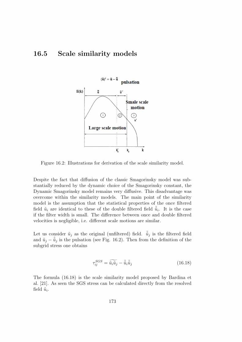
16.5 Scale similarity models
Figure 16.2: Illustrations for derivation of the scale similarity model.
Despite the fact that diffusion of the classic Smagorinsky model was sub-stantially reduced by the dynamic choice of the Smagorinsky constant, theDynamic Smagorinsky model remains very diffusive. This disadvantage wasovercome within the similarity models. The main point of the similaritymodel is the assumption that the statistical properties of the once filteredfield ui are identical to these of the double filtered field ˜ui. It is the caseif the filter width is small. The difference between once and double filteredvelocities is negligible, i.e. different scale motions are similar.
Let us consider uj as the original (unfiltered) field. ˜uj is the filtered fieldand uj − ˜uj is the pulsation (see Fig. 16.2). Then from the definition of thesubgrid stress one obtains
τSGSij = ˜uiuj − ˜ui ˜uj (16.18)
The formula (16.18) is the scale similarity model proposed by Bardina etal. [21]. As seen the SGS stress can be calculated directly from the resolvedfield ui.
173
16.6 Mixed similarity models
The experience shows that diffusion produced by the scale similarity mo-del (16.18) is too low. The numerical calculations are often unstable usingthis model. Taking the fact into account, that the diffusion of the Smagorin-sky model is too high, it was decided to combine the Samgorinsky and scalesimilarity models to get the proper diffusion. The advantages and disadvan-tages of both models are summarized as follows
Dynamic Smagorinsky Model (DSM): energy dissipation is overesti-mated (drawback), energy backscattering is not reproduced (draw-back),
Scale similarity model: energy backscattering is reproduced (advan-tage), energy dissipation is underestimated (drawback).
The idea combine models to strengthen the advantages and to overcome dis-advantages of both models. The hybrid model called as the mixed similaritymodel is written as
τ rij =(˜uiuj − ˜ui ˜uj
)− 2(C∆S ∆)2|S|Sij (16.19)
The mixed model can be derived in a more formal way. For that the velocitydecomposition into filtered and pulsation parts:
uiuj = ˜(ui + u′i)(uj + u′j) = ˜uiuj + u′iuj + u′jui + u′iu′j (16.20)
is substituted into the SGS stress expression:
τSGSij = uiuj − uiuj (16.21)
Finally we have Leonard’s formulation of the mixed model:
τSGSij = Lij + Cij +Rij (16.22)
whereLij = ˜uiuj − uiuj is the Leonard stress
Cij = ˜uiu′j + ˜uju′i is the Cross stress
Rij = u′iu′j is the Reynolds stress
The sum of the cross and Reynolds stresses is calculated via the Smagorinskymodel with the dynamically determined constant CS
174
Cij +Rij = −2(C∆S ∆)2|S|Sij (16.23)
A substantial disadvantage of this formulation is the fact that the Leonardstress does not satisfy the Galilean invariance condition. The Galilean in-variance is the independence of basic formula of mechanics on the speed ofthe reference system.
The classical definition of the SGS stresses possesses the Galilean invariance.Indeed, let V be the speed of the reference system. The velocity relative tothe reference system is
~W = ~u+ ~V (16.24)
The SGS stress does not depend on the reference system speed:
WiWj − WiWj =
= ˜(ui + Vi + u′i)(uj + Vj + u′j)− ˜(ui + Vi + u′i)˜(uj + Vj + u′j) =
= ˜(ui + u′i)(uj + u′j)− ˜(ui + u′i)˜(uj + u′j) = uiuj − uiuj
(16.25)
On the contrary, the Leonard stress is not Galilean invariant:
˜WiWj − WiWj = ˜uiuj − uiuj − Viu′j − Vju′i (16.26)
Germano proposed an alternative formulation
τSGSij = L0ij + C0
ij +R0ij (16.27)
where all stresses are Galilean invariant:
L0ij = ˜uiuj − ˜ui ˜uj is the Leonard stress
C0ij = ˜uiu′j + u′iuj − ˜uiu′j − u′i ˜uj is the Cross stress
R0ij = u′iu
′j − u′iu′j is the Reynolds stress
C0ij +R0
ij = −2(C∆S ∆)2|S|Sij (16.28)
Exercise: Prove the following facts:
175

equivalence of subgrid stresses computed from formulations of Ger-mano (16.27) and the original one proposed by Leonard (16.22),
Galilean invariance of stresses in Germano‘s formulation (16.27).
16.7 A-posteriori and a-priori tests
Two tests are used to verify LES models. The comon way is the a-posterioritest. The LES simulation is performed and then the flow parameters obtainedfrom the simulation are compared with these from measurement. Dependingon comparison results the conclusion about quality of LES models is drawn.The disadvantage of such approach is that the LES results are affected bymodelling errors, errors of approximation of differential operators and round-ing errors. In a-posteriori test they can not be separated.
Direct test of quality of subgrid stresses is the a-priori test. First, the subgridstress is calculated at each time instant from the definition
τSGSdefij = uiuj − uiuj (16.29)
Then the subgrid stress is computed again at each time instant from anymodel, say Smagorinsky one
τSGSmodij − 1
3τSGSmodkk δij = −2(CS∆)2|Sij|Sij (16.30)
The subgrid stresses τSGSdefij and τSGSmodij averaged in time are comparedeach with other. If
τSGSdefij ≈ τSGSmodij
the SGS model is accurate.
A big difficulty of a-priori tests is the determination of velocities ui. Forthat it is necessary first to obtain the unfiltered velocities ui with spatial andtemporal resolutions compared with the Kolmogorov scales. At present thisis a big challenge to measure three components of velocity in a volume withhigh spatial and temporal resolutions. The Particle Image Velocimetry (PIV)measurements are mostly planar measurements within a two dimensionalwindow. Direct Numerical Simulation data are often used as the source fora-priori tests. Three components of velocity in a volume, obtained from DNS,are filtered and utilized for the test. However, it should be noted that DNS
176

simulation is restricted by relatively low Reynolds numbers, whereas mainlaws of LES are valid for high Re numbers.
177

178

Chapter 17
Hybrid URANS-LES methods
17.1 Introduction
As discussed above, the most promising approach to resolve the flow un-steadiness is the Large Eddy Simulation (LES), which is already widely usedfor research purposes. Typical Reynolds numbers in engineering are verylarge even at model scales. The grid resolution necessary for a pure LESis so huge that it makes the direct application of LES impossible (see Sec.17.4). A practical solution of this problem is the use of hybrid URANS-LESmethods, where the near body flow region is treated using URANS and farflow regions are treated with LES.
According to Peng [22] the hybrid techniques can be subdivided into flowmatching and turbulence matching methods. Within the flow matchingmethods the interface between URANS and LES is explicitly defined. LESfiltered equations are solved in the LES region, whereas URANS equationsare solved in the URANS domain. The flow parameters (velocities, kineticenergy) are matched at the interface between the URANS and the LES re-gions. Among the most important contributions to the development of flowmatching methods we mention the works of (Davidson, Dalstroem [23]; Ter-racol [24]; Jakirlic et. al. [25]; Temmerman et. al. [26]) and others. Aserious weakness of this approach is the development of robust proceduresto set the URANS-LES interface for complicated flow geometries. Withinthe framework of the turbulence matching method an universal transportequation is solved in the whole computational domain. The stress termsin this equation are treated in different ways in LES and URANS domains.There are various procedures to distinguish between LES and URANS cells.The most popular hybrid method is Detached Eddy Simulation (DES) pro-
179
posed by (Spalart et al.[27]). The original version of this method is based onthe classic Smagorinsky LES model and the Spalart-Allmaras (SA) URANSapproach. SA is used close to the wall, whereas LES in the rest part ofthe flow. The switching between the two techniques is smooth and occursin a ”gray” subdomain. There are two major improvements of DES, de-veloped recently. The first one, DDES (Delayed DES), has been proposedto detect the boundary layers and to prolong the RANS mode, even if thewall-parallel grid spacing would normally activate the DES limiter (Spalart[28]). The second one, IDDES (Improved DDES), allows one to solve theproblems with modelled-stress depletion and log-layer mismatch. For thedetails see the review (Spalart [28]). In spite of a wide application area DEShas serious principle limitations thoroughly analyzed by (Menter, Egorov [?]). Other versions of the turbulence matching methods using different blend-ing functions to switch the solution between LES and URANS modes wereproposed by (Peng [22]; Davidson, Billson [29]; Abe, Miyata [30]) and others.
A very critical point of the turbulence matching methods is the transitionfrom the time (or ensemble) averaged smooth URANS flow to the oscillat-ing LES flow, see (Menter, Egorov, 2005). The oscillations have to appearwithin a short flow domain in a ”gray zone” between LES and URANS. Ex-perience shows that it is extremely difficult to provide a smooth transitionof the turbulent kinetic energy passing from the URANS to LES domain. Toovercome this problem (Schlueter et al. [31]) and (Benerafa et al. [32]) usedan additional forcing term in the Navier Stokes equation artificially enhanc-ing fluctuations in the gray zone. However, the problem of smooth solutiontransition from URANS to LES still remains as the main challenge for theturbulence matching methods.
17.2 Detached Eddy Simulation (DES)
The most popular hybrid method -detached eddy simulation- was proposedin 1997 by Spalart et al. [27]. The principle of DES is illustrated in Fig. 17.1.Close to the body the solution is calculated using the URANS mode. Farfrom the wall the LES equations are solved. The grey zone between URANSand LES is the mixed solution.
The classical version of the DES approach is based on the Spalart Almaras(SA) model formulated with respect to the modified turbulent viscosity ν =νt/fν1. The transport equation for ν reads
180

Figure 17.1: Zones of the Detached Eddy Simulation.
∂ν
∂t+ vj
∂ν
∂xj= Cb1Sν︸ ︷︷ ︸
Generation
−Cw1fw
(ν
d
)2
︸ ︷︷ ︸Destruction
+
+1
σ
∂
∂xk
((ν + ν)
∂ν
∂xk
)+Cb2σ
∂ν
∂xk
∂ν
∂xk︸ ︷︷ ︸Diffusion
(17.1)
where
Cb1 = 0.1355, Cb2 = 0.622, Cν1 = 7.1,
σ = 2/3, Cw1 =Cb1κ2
+1 + Cb2σ
,
Cw2 = 0.3, Cw3 = 2.0, κ = 0.41,
fν1 =χ3
χ3 + C3ν1
, fν2 = 1− χ
1 + χfν1
,
fw = g
[1 + C6
w3
g6 + C6w3
]1/6
, χ = ν/ν,
g = r + Cw2(r6 − r), r =ν
Sκ2d2,
S = S +ν
κ2d2fν2, S =
√2ΩijΩij,
Ωij =1
2
(∂νi∂xj− ∂νj∂xi
)181
Here d is the distance from the wall. The physical sense of different termsis illustrated in (17.1). Far from the wall the generation and the distructionterms are approaching each to other and the turbulence attains the equilib-rium state:
Cb1Sν︸ ︷︷ ︸Generation
−Cw1fw
(ν
d
)2
︸ ︷︷ ︸Destruction
∼ 0
The kinematic viscosity is then calculated from the formula
ν ∼ Cb1Cw1
Sd2
which is similar to the Smagorinsky one:
νt = l2S|Sij|, |Sij| =√
2SijSij
lS = CS∆
DES inventors proposed to use the following expression for d:
d = mind, CDES∆, ∆ = max∆x,∆y,∆z
where CDES ≈ 1.3 is the DES constant. Now the main idea of the DESbecomes obvious:
• At small wall distance d < CDES∆ the Spalart Almaras URANS model isactive
• At large wall distance d > CDES∆ the Spalart Almaras URANS model issmoothly passed into the Smagorinsky model.
Samples of DES applications are presented in Fig. 17.2 and 17.3.
Despite of the wide application Detached Eddy Simulation technique is notfree of disadvantages. Menter [? ] notes: The essential concern with DESis that it does not continuously change from RANS to LES under grid re-finement. In order for LES structures to appear, the grid spacing and timestep have to be refined beyond a case-dependent critical limit. In addition, asufficiently large instability mechanism has to be present to allow the rapidformation of turbulent structures in regions where the DES limiter is acti-vated. If one of the two, or both requirements are violated, the resultingmodel is undefined and the outcome is largely unpredictable.
182

Figure 17.2: Squires K.D., Detached-eddy simulation: current status andperspectives.
Figure 17.3: Squires K.D., Detached-eddy simulation: current status andperspectives.
17.3 Hybrid model based on integral length
as parameter switching between LES and
URANS
A simple hybrid model proposed in [33] is based on the observation that thebasic transport equations have the same form in LES and RANS
∂ui∂t
+∂(uiuj)
∂xj= −∂p
∗
∂xi+∂(τ lij + τ tij)
∂xj, (17.2)
but the interpretation of the overline differs. In LES it means filtering, butin RANS it stands for the Reynolds, or ensemble, averaging. Here we usedthe standard notation of p∗ for the pseudo-pressure, and τ lij and τ tij for the
183

Figure 17.4: The division of the computational domain into the URANS(dark) and LES (light) regions at one time instant for hybrid calculation oftanker.
laminar and turbulent stresses respectively. Note that the turbulent stressesare calculated in different ways in LES and URANS regions.The computational domain in our model is dynamically (i.e. at each timestep) divided into the LES and URANS regions. A cell of the mesh belongsto one or the other region depending on the relation between the integrallength scale L and the extended LES filter ∆ according to the following rule:
if L > ∆ then the cell is in the LES region,
if L < ∆ then the cell is in the URANS region.(17.3)
The integral length scale is calculated from the known formula of Kolmogorovand Prandtl with the correction factor 0.168 taken from [15]
L = Ck3/2
ε, (17.4)
where k is the turbulent kinetic energy and ε is the dissipation rate. Theconstant C is C ∼ 0.168 close to the wall y/δ < 0.2, C ∼ 0.35 at 0.2 < y/δ <0.7 and C ∼ 1.0 in the outer area of the bounder layer y/δ > 0.7, where δ isthe boundary layer thickness. L varies from one time step to another, whichresults in varying decomposition of the computational domain into the LESand URANS regions. The extended LES filter is computed as
∆ =√d2
max + δ2, (17.5)
where dmax is the maximal length of the cell edges dmax = max(dx, dy, dz)and δ = (the cell volume)1/3 is the common filter width used in LES. Thischoice ensures that very flat cells in the boundary layer (for which δ ≈ 0but dmax > 0) are treated correctly. ∆ depends only on the mesh and it is
184
precomputed only once before the main computation.
As a sample LES and URANS regions are shown in Fig. 17.4 for flow arounda tanker. The URANS region is located close to the ship surface and playsthe role of a dynamic wall function. In areas of bilge vortices formation, theboundary layer is shedding from the hull and penetrates into the outer flowpart. Since the boundary layer is a fine scale flow the procedure (17.3) recog-nizes the bilge vortex formation zones as URANS ones. There is a technicalissue concerning the cells which are far from the ship hull and where bothk and ε are small, so large numerical errors are introduced into the integrallength scale computed according to Eq. (17.4). To avoid an irregular dis-tribution of URANS and LES zones, the general rule (17.3) of the domaindecomposition is corrected in such a way that the LES region is switched toURANS one if k is getting less than some threshold. This procedure has noinfluence on the ship flow parameters since it is used far from the area of theprimary interest.
We have performed several calculations with different combinations of LESand URANS models to find the most efficient one for the problem underconsideration. Among the models we used in our computations are the linearand nonlinear k-ε, k-ω SST and kεv2f URANS models combined with thesimple and dynamic Smagorinsky as well as with the dynamic mixed LESclosure models. The experience shows that the most satisfactory results areobtained using the URANS approach based on the kεv2f turbulent modelof [34] and LES approach based on the Smagorinsky dynamic model. Theturbulent stresses τ tij are calculated from the Boussinesq approximation usingthe concept of the turbulent viscosity. The only difference between LESand URANS is the definition of the kinematic viscosity. Within LES it isconsidered as the subgrid viscosity and calculated according to the dynamicmodel of Smagorinsky:
νSGS = cDδ2|Sij|, Sij =
1
2
(∂uj∂xi
+∂ui∂xj
), (17.6)
where Sij is the strain velocity tensor and cD is the dynamic constant. In theURANS region the viscosity is calculated from the turbulent model of [34]:
νt = min
(0.09
k2
ε, 0.22v2Tt
), (17.7)
where v2 is the wall normal component of the stresses and Tt is the turbulenttime Tt = max(k/ε, 6
√ν/ε).
185

17.4 Estimations of the resolution necessary
for a pure LES on the example of ship
flow
In the CFD community one can observe tendency to use pure LES withoutpaying any attention to resolution problems. Very often LES is running ontypical RANS grids. In fact, such computations can give correct results if theflow structures to be captured are large enough and exist for a long time. Insome cases modeling of such structures does not require detailed resolutionof boundary layers and a thorough treatment of separation regions. As anexample one can mention flows around bluff bodies with predefined separa-tion lines like ship superstructures. Application of underresolved LES forwell streamlined hulls should be considered with a great care. First of all,one should not forget that the basic LES subgrid models are derived underthe assumption that at least the inertial turbulent subrange is resolved. Sec-ond, underresolution of wall region leads to a very inaccurate modeling ofthe boundary layer, prediction of the separation and overall ship resistance.It is clearly illustrated in the Table 17.1. The ship resistance obtained fromunderresolved LES using the wall function of (Werner, Wengle [35]) is lessthan half of the measured one and that obtained from RANS. Obviously, theapplication of modern turbulence LES models, more advanced than RANSmodels, does not improve but even makes the results much worse with thesame space resolution. The change from RANS to LES should definitely befollowed by the increase of the resolution which results in a drastic increaseof the computational costs. These facts underline necessity of further devel-opment towards hybrid methodology. Although in (Alin et al. [36]) it hasbeen shown that the accuracy of the resistance prediction using pure LES ata very moderate resolution with y+ ∼ 30 can be improved using special wallfunctions, the most universal way for the present, to our opinion, is applica-tion of hybrid methods. The impossibility of pure LES is illustrated belowfor flow around the KVLCC2 tanker.
The precise determination of the necessary LES resolution is quite difficult.Estimations presented below are based on the idea that about 80% of theturbulent kinetic energy should be directly resolved and the rest is modeledin a properly resolved LES simulation. Implementation of this idea impliesthe knowledge of the Kolmogorov η and the integral length L scales which areused to draw the typical spectra of the full developed turbulence E(k). Thewave number k∗ separating the resolved and modeled turbulence is foundfrom the condition
186

∫∞k∗E(k)dk∫∞
0E(k)dk
≈ 0.2. (17.8)
The maximum possible cell size is then ∆max = 2π/k∗. The scales L and ηare found from the known expression η = (ν3/ε)1/4 and Eq. (17.4), wherethe kinetic energy k and the dissipation rate ε are taken from RANS simula-tions using k-ε linear model. The ratio λ = ∆max/η is then used as the scaleparameter for grid generation. Both lengths vary in space which makes thegrid generation procedure very complicated. To roughly estimate the size ofthe grid we assume that λ is constant. We performed different calculationsdetermining λ at the two following points: i) the point where L/η is maximalin the ship boundary layer and ii) the point in the propeller disk where thevorticity ~ω is maximal (region of the concentrated vortex structure). The lat-ter is dictated by the wish to resolve the most intensive vortex flow structureswhich have the strongest influence on the propeller operation. Since LES ap-plication is required in the ship stern area only this part of the computationalvolume has been meshed. It covers the boundary layer of the stern regionstarting from the end of the parallel midship section. The thickness of themeshed region has been constant and equal to the maximum boundary layerthickness at the stern δBL. The grid for a pure LES is generated using thefollowing algorithm. The minimum Kolmogorov length ηmin is determinedin the near wall region. The cell sizes in x and z directions along the wallare calculated by multiplication of ηmin with the scale parameter λ. Thesesizes remain constant for all cells row in y direction which is normal to theship surface (see Fig. 17.5). The cells have at least two equal sizes which isdesirable from the point of view of LES accuracy. The choice of the size in ydirection is dictated by proper resolution of the boundary layer. Close to thewall this size is chosen from the condition ∆w = min(yw, ηmin). Since yw ischosen as the ordinate where y+ = 1 the first nodes lay deeply in the viscoussublayer. The size in y direction at the upper border of the boundary layer isequal to ∆∞ = ληδ, where ηδ is the Kolmogorov scale at y = δBL. A simplegrading is used in y direction between ∆w and ∆∞.
Results of the estimations are as follows: the required grid size ranges from∼ 5 M to ∼ 25 M for Re = 2.8 × 10⁶, and from ∼ 7 M to ∼ 60 M forRe = 5.8 × 10⁶. The results vary depending on the value of λ in use, sothey should be considered as very rough estimations. Together with simi-lar estimations for the nonlinear k-ε model these results show that the LESgrid should have the order of tens of millions of nodes. Nowadays, the com-putations with hundred millions and even with a few billions of nodes are
187

d
xy
z
l h· min
l hmin·
l h· d
y=1+
Figure 17.5: The cell parameters.
becoming available in the research community. However, a numerical studyof engineering problems implies usually many computations which have to beperformed within a reasonable time with moderate computational resources.In this sense, the results of the present subsection clearly demonstrate thatthe pure LES is impossible for ship applications so far. To verify that theresolution estimation procedure we used gives meaningful results, it has beenapplied for turbulent boundary layer (TBL) benchmark. We found from me-thodical calculations that the pure LES with 1M cells is quite accurate forprediction of the velocity distribution, TBL thickness, TBL displacementthickness and the wall shear stress. The estimation procedure presentedabove predicted the necessary resolution around 0.5M. Therefore, the esti-mations presented for a ship model are rather lower bound for the resolutionrequired for a pure LES.
CR CP CFKRISO Exp. 4.11× 10⁻³ 15% 85%RANS kεv2f 4.00× 10⁻³ 16% 84%k-ω SST SAS 3.80× 10⁻³ 18% 82%Underresolved LES 1.70× 10⁻³ 81% 19%Hybrid RANS LES 4.07× 10⁻³ 17% 83%
Table 17.1: Results of the resistance prediction using different methods. CR isthe resistance coefficient, CP is the pressure resistance and CF is the frictionresistance
188

Part III
CFD applications to humanthermodynamics
189


191
Chapter 18
Mathematical model of the iceprotection of a human body athigh temperatures ofsurrounding medium
18.1 Designations
18.1.1 List of symbols
A area (m2)cp specific heat capacity (J/(kgK))F density of heat release(W/m3)h sector height (m)K correlation factor of the rectal temperaturek the thermal conductivity (W/(mK))M work done by person (W)m body mass (kg)P body height (cm)Q internal energy (J)
Q heat flux (W)R sector radius (m)T temperature (deg)x radial coordinate along the sector (m)α central sector angle (deg)∆ skin thickness (m)λ thermal diffusivity (m2/s)ρ mass density (kg/m3)φ initial temperature (deg)
192

18.1.2 Subscripts
core human body corehum human bodyi number of human body layerj number of point on the human bodymed surrounding mediummelt melting iceouter outer boundary of clothesskin human body skin
18.1.3 Superscripts
0 degree of Celsius
18.2 Introduction
The heat transfer inside the human body is an extremely complicated prob-lem which is difficult to formulate properly. The body generates the heatwithin certain organs which is then transferred by the thermal diffusionthrough the body substance possessing very non uniform properties. How-ever, the thermal diffusion being complicated is not the main difficulty ofmodeling. A large fraction of the heat generated by internal organs is trans-ported to the body periphery by a complicated net of blood vessels. Thisprocess has still not been modeled with a desirable accuracy. While a fulldetailed model of the human thermodynamics is still remaining the problemof the future, the practical design of protection clothes demands the reliablemodels already now. Such models are necessary to reduce the time and costsconsuming measurements and to avoid dangerous experiments with peopleunder emergency conditions. The models can be only of a semi empiric char-acter and must relay on measurements data to diminish the modelling errors.
Especially interesting is the case of human thermodynamics at high tempera-tures T of surrounding medium. At T > 350 the ability of human thermoreg-ulation is very restricted [37]. The acceptable body temperature variationcan be only one degree of Celsius. If the body temperature exceeds thisthreshold the protecting mechanisms regulating the excessive heat in the or-ganism through the breathing, humidity diffusion of the skin, radiation andtranspiration don’t work [38], [39]. The most effective principle of the protec-tion is the mechanism of the heat absorption through, for instance, the iceembedded into the clothes. This approach being environmentally friendly,
193
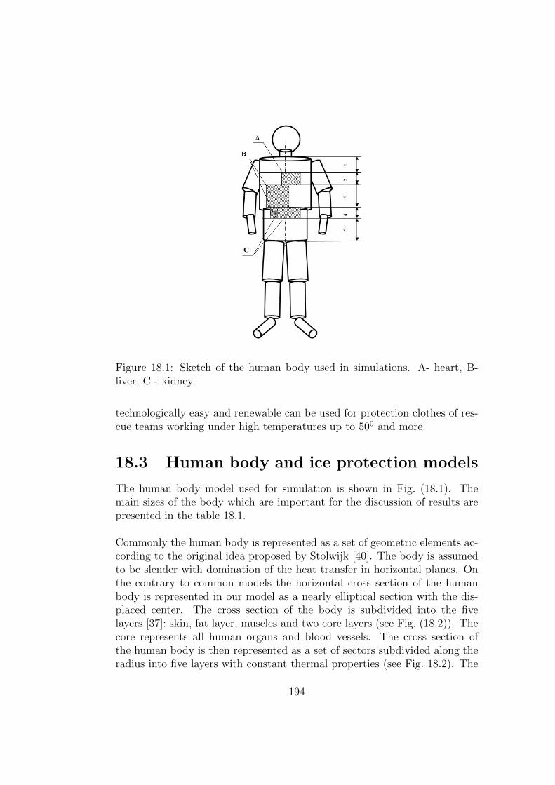
Figure 18.1: Sketch of the human body used in simulations. A- heart, B-liver, C - kidney.
technologically easy and renewable can be used for protection clothes of res-cue teams working under high temperatures up to 500 and more.
18.3 Human body and ice protection models
The human body model used for simulation is shown in Fig. (18.1). Themain sizes of the body which are important for the discussion of results arepresented in the table 18.1.
Commonly the human body is represented as a set of geometric elements ac-cording to the original idea proposed by Stolwijk [40]. The body is assumedto be slender with domination of the heat transfer in horizontal planes. Onthe contrary to common models the horizontal cross section of the humanbody is represented in our model as a nearly elliptical section with the dis-placed center. The cross section of the body is subdivided into the fivelayers [37]: skin, fat layer, muscles and two core layers (see Fig. (18.2)). Thecore represents all human organs and blood vessels. The cross section ofthe human body is then represented as a set of sectors subdivided along theradius into five layers with constant thermal properties (see Fig. 18.2). The
194

Table 18.1: Sizes of the body used in simulations
Element Size in meter
1 0.1272 0.1273 0.2344 0.0905 0.215
radii of each sector R can be found from the table 18.2. The upper ellipticalcylinder is from the neck to the waist, whereas the lower one from the waistto the thing (Fig. 18.1). The skin thickness ∆ is approximately calculated asthe radius R divided by 60.25 [37]. The sizes of different layers inside of thecross section are presented in the table 18.3. At the high temperatures themain part of the heat production occurs in certain organs. The knowledgeabout the heat distribution inside the body allows one to choose the mostefficient design of the ice protection which typical construction is shown inFig. 18.3. In the mathematical model the ice and the clothes layer are mod-elled by additional layers covering the human body (Fig. 18.2). The humanbody model was developed on the base of data taken from [40], [41], [42]and [43].
18.4 Mathematical model
It is assumed, that the heat exchange between the sectors is negligible atevery cross section of the human body. Therefore both the vertical and cir-cumferential heat transfer processes are not taken into account. The heattransfer along the radius x within each sector is described by the one di-mensional heat conduction equation derived from the energy conservationconsideration. The change of the internal energy in the sector element withcoordinates x and x+ dx due to heat transport within the time dt is
dQ1 =
(k(x+ dx)S(x+ dx)
∂T
∂x− k(x)S(x)
∂T
∂x
)dt ≈ ∂
∂x
(k(x)S(x)
∂T
∂x
)dt
(18.1)where T (x, t) is the temperature, k is the thermal conductivity, S(x) = αxhis the sector arc length multiplied with its height h and α is the central angle
195
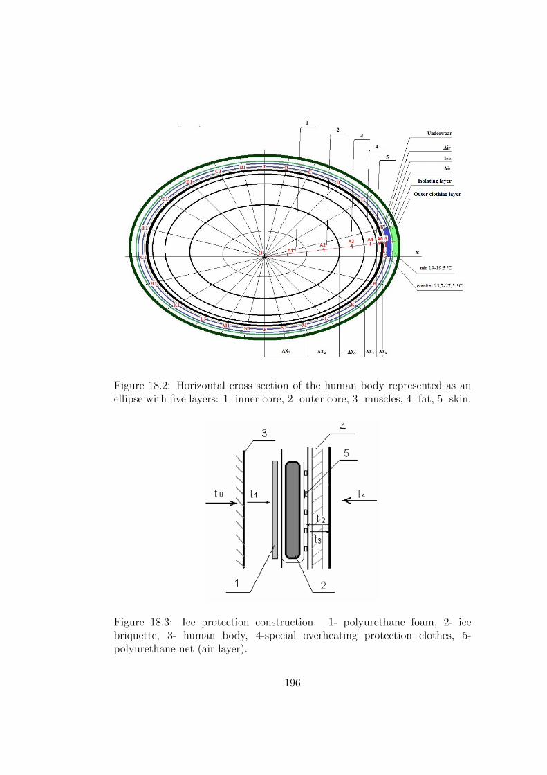
Figure 18.2: Horizontal cross section of the human body represented as anellipse with five layers: 1- inner core, 2- outer core, 3- muscles, 4- fat, 5- skin.
Figure 18.3: Ice protection construction. 1- polyurethane foam, 2- icebriquette, 3- human body, 4-special overheating protection clothes, 5-polyurethane net (air layer).
196

Table 18.2: Radii of the elliptical cross sections used in simulations
radial upper elliptical lower ellipticalline cylinder, m cylinder, m
OJ 0.118 0.109OB, OB1 0.122 0.112OC, OC1 0.137 0.121OD, OD1 0.159 0.135OE, OE1 0.181 0.156OF, OF1 0.195 0.176OG, OG1 0.200 0.190OH, OH1 0.187 0.173OK, OK1 0.163 0.145OL, OL1 0.138 0.121
OM, OM1 0.120 0.106ON, ON1 0.110 0.980
OP 0.106 0.940
Table 18.3: Radii of layers used in simulations in fraction of the skin thickness∆
Elliptical Element Area Layer Radiuscylinder length, m m2
Core 36.15∆upper 0.476 0.489 Muscle 53.70∆
Fat layer 59.25∆Skin 60.25∆Core 36.15∆
lower 0.317 0.293 Muscle 53.70∆Fat layer 59.25∆
Skin 60.25∆
of the sector. Within the material we have additionally the heat release withthe heat density F (heat per unit volume):
dQ2 = SFdxdt (18.2)
197
Due to the heat transfer and heat release the internal energy of the materialis changed by dQ3
dQ3 = cpρS∂T
∂tdxdt (18.3)
where cp is the specific heat capacity and ρ is the mass density of the material.By conservation of energy
dQ1 + dQ2 = dQ3
or
S(x)∂T
∂t= λ
∂
∂x
(S(x)
∂T
∂x
)+ S(x)f(x) (18.4)
where λ(x) = k/(cpρ) is the thermal diffusivity and f(x) = F (x)/(cpρ).The equation (18.4) is solved at the initial condition
T (x, 0) = ϕ(x) (18.5)
and the boundary conditions formulated at the sector center
T (0, t) = Tcore (18.6)
and at the outer boundary of the clothes
T (xouter, t) = Tmed (18.7)
The temperature of the surrounding medium was Tmed = 500. It was as-sumed that the core center (at x = 0) temperature was constant in timeTcore = 36.70.
The heat transfer process is subdivided into three steps. Within the firststep the ice is warmed up to the melting temperature. The melting processis followed by the absorption of the heat coming from both the surroundingmedium Qmed
Qmed = λmed∂T
∂xAmed (18.8)
and the human body Qhum caused by metabolism
Qhum = λskin∂T
∂xAskin (18.9)
where λmed is the thermal diffusivity of the clothing layer adjacent to the icelayer, Amed is the surface between the ice layer and adjacent clothing layer
198
in a sector under consideration, λskin is the thermal diffusivity of the humanskin and Askin is the skin surface in the sector. The second step is the icelayer melting. The phase transition in matter is described by the Stefanproblem [44]. In this paper we used a simplified approach based on the heatbalance conditions. It is assumed that the water and ice mixture is uniformwith the constant temperature of zero degree of Celsius. The dynamics ofthe boundary between the water and ice is not considered. The heat fluxes(18.8) and (18.9) are constant in time. The second step is finished in time t∗
once the ice is melted:
Qmelt = (Qmed + Qskin)t∗ (18.10)
Here Qmelt is the heat necessary to melt the whole ice. After that, within thethird step the water from the melted ice is warming up due to heat fluxes(18.8) and (18.9) continuing in time. The calculations within the third stepare running as long as the comfort conditions are fulfilled.
The equation (18.4) is solved using the finite differential method on the uni-form grid ∆x = const with the constant time step ∆t = const. The numericalimplementation utilizes the central differential scheme for space derivativesand Crank Nicolson implicit representation of the unsteady term. An inhousecode was developed for this purposes.
18.5 Results
18.5.1 Design of the protection clothes
The calculations were performed for five elements of the human body shownin Fig.18.1. Thermodynamic properties of the body layers are given in thetable 18.4. Usually, the ice protection construction consists of the ice layerseparated from the surrounding medium by several layers. In the presentwork we used three layers: outer clothing layer with thickness of 0.001m, iso-lating layer of 0.009m and the air layer of 0.003m. All layers have the initialtemperature T 0
i = 190. The air gap between the ice and the underwear ofthe thickness 0.0025 m was 0.003 m thick. The human body was 180 cm inheight with the mass of 80 kg. The full description of the input data can befound in [45]. It was assumed that the test person does the work at a rate ofabout M = 420 watts. Additional heat release due to this work was takeninto account during numerical simulations in the heat production rate f(x)(see Eq. (18.4)).
199
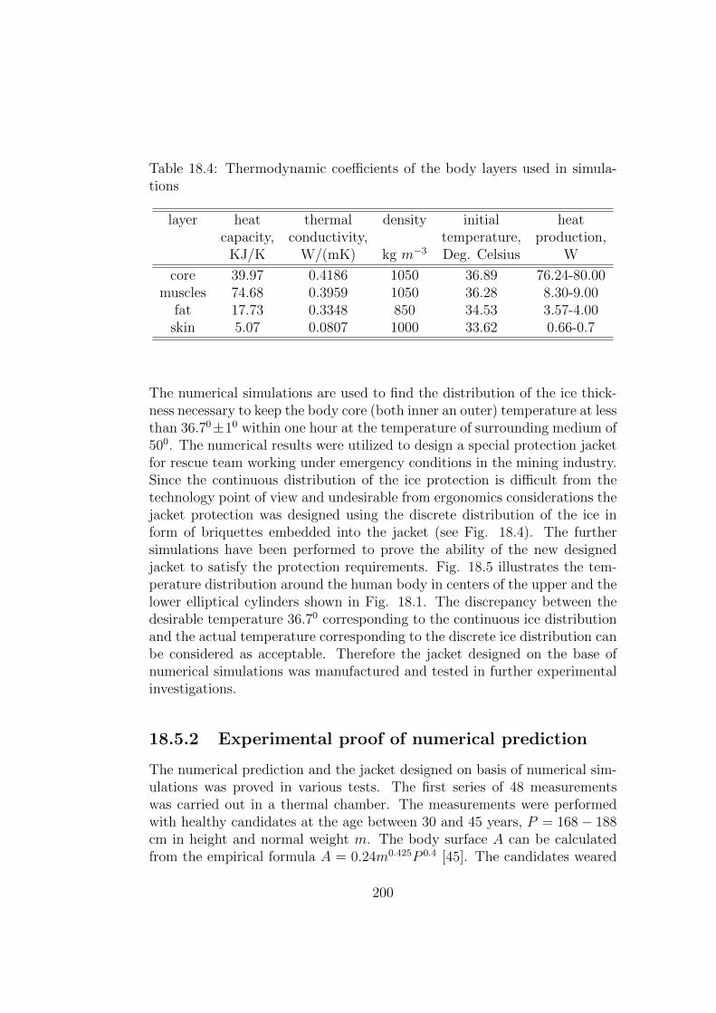
Table 18.4: Thermodynamic coefficients of the body layers used in simula-tions
layer heat thermal density initial heatcapacity, conductivity, temperature, production,
KJ/K W/(mK) kg m−3 Deg. Celsius W
core 39.97 0.4186 1050 36.89 76.24-80.00muscles 74.68 0.3959 1050 36.28 8.30-9.00
fat 17.73 0.3348 850 34.53 3.57-4.00skin 5.07 0.0807 1000 33.62 0.66-0.7
The numerical simulations are used to find the distribution of the ice thick-ness necessary to keep the body core (both inner an outer) temperature at lessthan 36.70±10 within one hour at the temperature of surrounding medium of500. The numerical results were utilized to design a special protection jacketfor rescue team working under emergency conditions in the mining industry.Since the continuous distribution of the ice protection is difficult from thetechnology point of view and undesirable from ergonomics considerations thejacket protection was designed using the discrete distribution of the ice inform of briquettes embedded into the jacket (see Fig. 18.4). The furthersimulations have been performed to prove the ability of the new designedjacket to satisfy the protection requirements. Fig. 18.5 illustrates the tem-perature distribution around the human body in centers of the upper and thelower elliptical cylinders shown in Fig. 18.1. The discrepancy between thedesirable temperature 36.70 corresponding to the continuous ice distributionand the actual temperature corresponding to the discrete ice distribution canbe considered as acceptable. Therefore the jacket designed on the base ofnumerical simulations was manufactured and tested in further experimentalinvestigations.
18.5.2 Experimental proof of numerical prediction
The numerical prediction and the jacket designed on basis of numerical sim-ulations was proved in various tests. The first series of 48 measurementswas carried out in a thermal chamber. The measurements were performedwith healthy candidates at the age between 30 and 45 years, P = 168− 188cm in height and normal weight m. The body surface A can be calculatedfrom the empirical formula A = 0.24m0.425P 0.4 [45]. The candidates weared
200

Figure 18.4: Overheating protection jacket designed on the base of simula-tions.
Figure 18.5: Temperature distributions around the body with continuous icedistribution and with ice briquettes. Results of numerical simulations after60 minutes.
201

Figure 18.6: Development of the averaged temperature in the air gap betweenthe underwear and the ice protection on the human chest. Comparison be-tween the measurement (solid line) and the numerical simulations (dottedline).
the jackets (see Fig. 18.4)were doing the work at a rate of about M = 420watts which corresponds to a hard work typical for the mining industry. Thetemperature of the surrounding medium was T ≈ 500. The temperature hasbeen measured in the air gap between the underwear and the ice at sevenpoints around the chest (section 2 in Fig. 18.1). The temperature averagedover these points is presented in Fig. 18.6. The discrepancy between themeasurement and the numerical simulations does not exceed 14 percent af-ter 60 minutes of the real time. This agreement can be considered as quitesatisfactory taking the simplicity of the used model and complexity of theproblem into account.
The task of this study is the determination of the temperature in the bodycore. It is a difficult problem since the direct measurement is impossible.
202
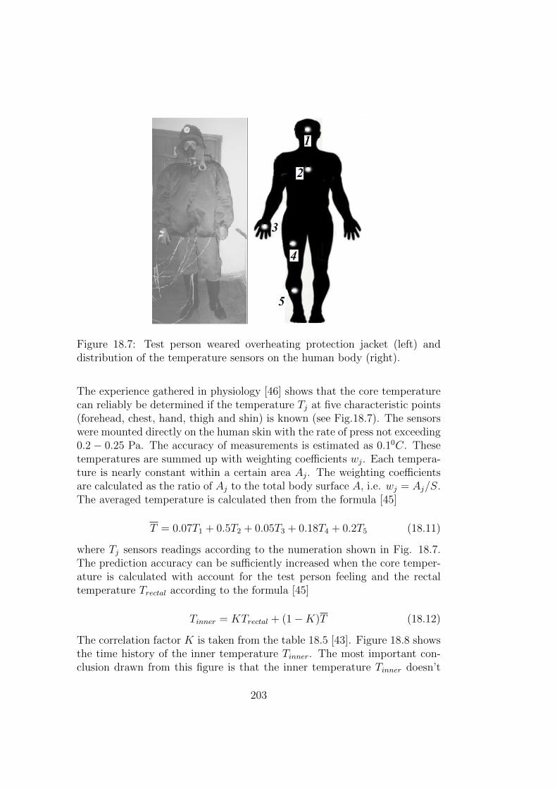
Figure 18.7: Test person weared overheating protection jacket (left) anddistribution of the temperature sensors on the human body (right).
The experience gathered in physiology [46] shows that the core temperaturecan reliably be determined if the temperature Tj at five characteristic points(forehead, chest, hand, thigh and shin) is known (see Fig.18.7). The sensorswere mounted directly on the human skin with the rate of press not exceeding0.2 − 0.25 Pa. The accuracy of measurements is estimated as 0.10C. Thesetemperatures are summed up with weighting coefficients wj. Each tempera-ture is nearly constant within a certain area Aj. The weighting coefficientsare calculated as the ratio of Aj to the total body surface A, i.e. wj = Aj/S.The averaged temperature is calculated then from the formula [45]
T = 0.07T1 + 0.5T2 + 0.05T3 + 0.18T4 + 0.2T5 (18.11)
where Tj sensors readings according to the numeration shown in Fig. 18.7.The prediction accuracy can be sufficiently increased when the core temper-ature is calculated with account for the test person feeling and the rectaltemperature Trectal according to the formula [45]
Tinner = KTrectal + (1−K)T (18.12)
The correlation factor K is taken from the table 18.5 [43]. Figure 18.8 showsthe time history of the inner temperature Tinner. The most important con-clusion drawn from this figure is that the inner temperature Tinner doesn’t
203

exceed the threshold 360 within 60 minutes. Thus, the aim of the design hasbeen achieved.
Table 18.5: Coefficient K depending on the test person feelings and energyexpenditure E = M/A (W/m2). A is the body surface (m2) and M is thework (W )
feeling | E 70 88 113 145 178
cold 0.55 0.57 0.59 0.62 0.64chilly 0.57 0.58 0.60 0.64 0.65
slightly chilly 0.59 0.60 0.63 0.65 0.67comfort 0.62 0.64 0.65 0.67 0.69
slightly warm 0.70 0.70 0.70 0.70 0.70warm 0.79 0.77 0.74 0.72 0.72hot 0.86 0.82 0.79 0.76 0.73
The second series of measurements was carried out directly during the workin a cole mine at the temperature not higher than 600 without fire action.During one year of observations no equipment fault has been documented.The temperature of workers was kept at a prescribed level during at least55 − 60 minutes as predicted both in numerical simulations and thermalchamber tests.
18.6 Discussion
This chapter presents relatively simple and efficient model of the heat trans-fer within the human body at high temperatures of the surrounding medium.The human body cross section is represented as an ellipse with a few lay-ers, modelling the internal organs. The heat generation by internal organsis taken into account. The ice protection and the clothes are modelled asadditional layers covering the human body. Neglecting the heat transfer invertical and circumferential directions the problem is reduced to the solutionof the one dimensional heat conduction equation with variable heat diffu-sivity. The simulations were performed using the finite differential method.Results of simulation were used for calculation of the ice layer thickness nec-essary to prevent the body overheating and to keep the temperature of thebody core at 36.70±10 within one hour. The results of simulations were used
204
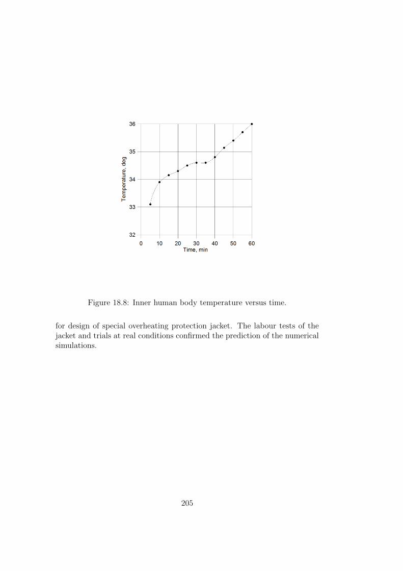
Figure 18.8: Inner human body temperature versus time.
for design of special overheating protection jacket. The labour tests of thejacket and trials at real conditions confirmed the prediction of the numericalsimulations.
205

206
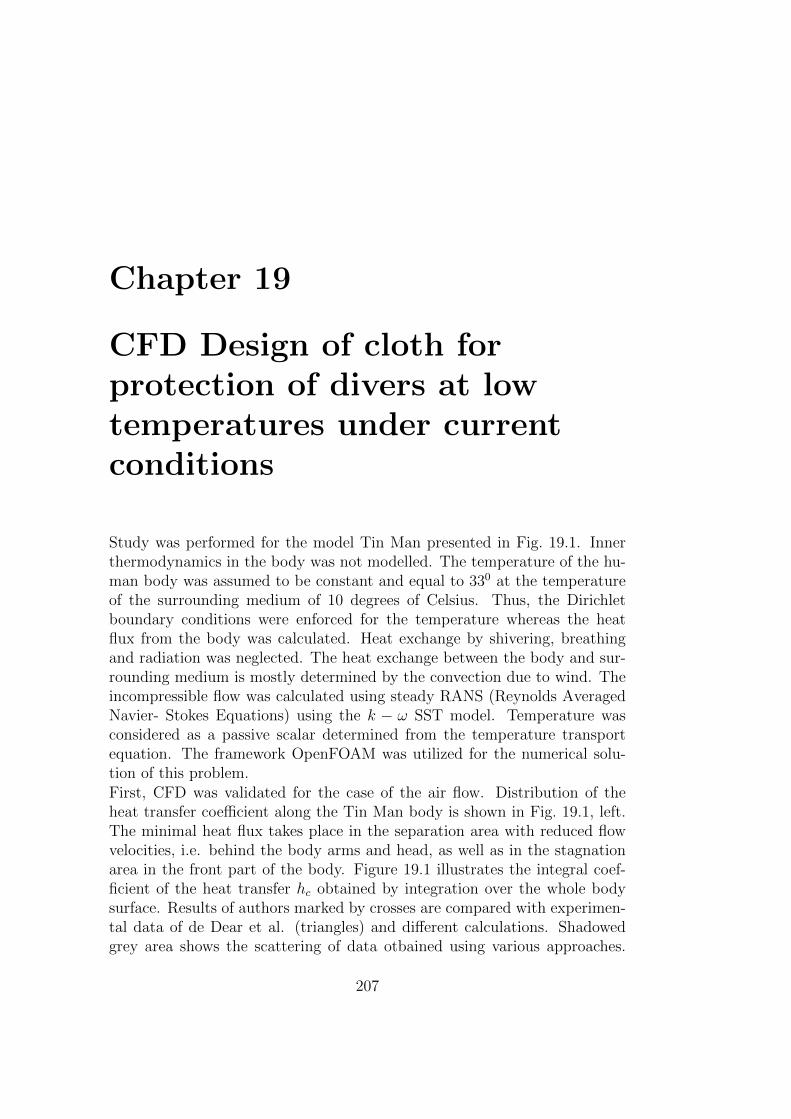
Chapter 19
CFD Design of cloth forprotection of divers at lowtemperatures under currentconditions
Study was performed for the model Tin Man presented in Fig. 19.1. Innerthermodynamics in the body was not modelled. The temperature of the hu-man body was assumed to be constant and equal to 330 at the temperatureof the surrounding medium of 10 degrees of Celsius. Thus, the Dirichletboundary conditions were enforced for the temperature whereas the heatflux from the body was calculated. Heat exchange by shivering, breathingand radiation was neglected. The heat exchange between the body and sur-rounding medium is mostly determined by the convection due to wind. Theincompressible flow was calculated using steady RANS (Reynolds AveragedNavier- Stokes Equations) using the k − ω SST model. Temperature wasconsidered as a passive scalar determined from the temperature transportequation. The framework OpenFOAM was utilized for the numerical solu-tion of this problem.First, CFD was validated for the case of the air flow. Distribution of theheat transfer coefficient along the Tin Man body is shown in Fig. 19.1, left.The minimal heat flux takes place in the separation area with reduced flowvelocities, i.e. behind the body arms and head, as well as in the stagnationarea in the front part of the body. Figure 19.1 illustrates the integral coef-ficient of the heat transfer hc obtained by integration over the whole bodysurface. Results of authors marked by crosses are compared with experimen-tal data of de Dear et al. (triangles) and different calculations. Shadowedgrey area shows the scattering of data otbained using various approaches.
207
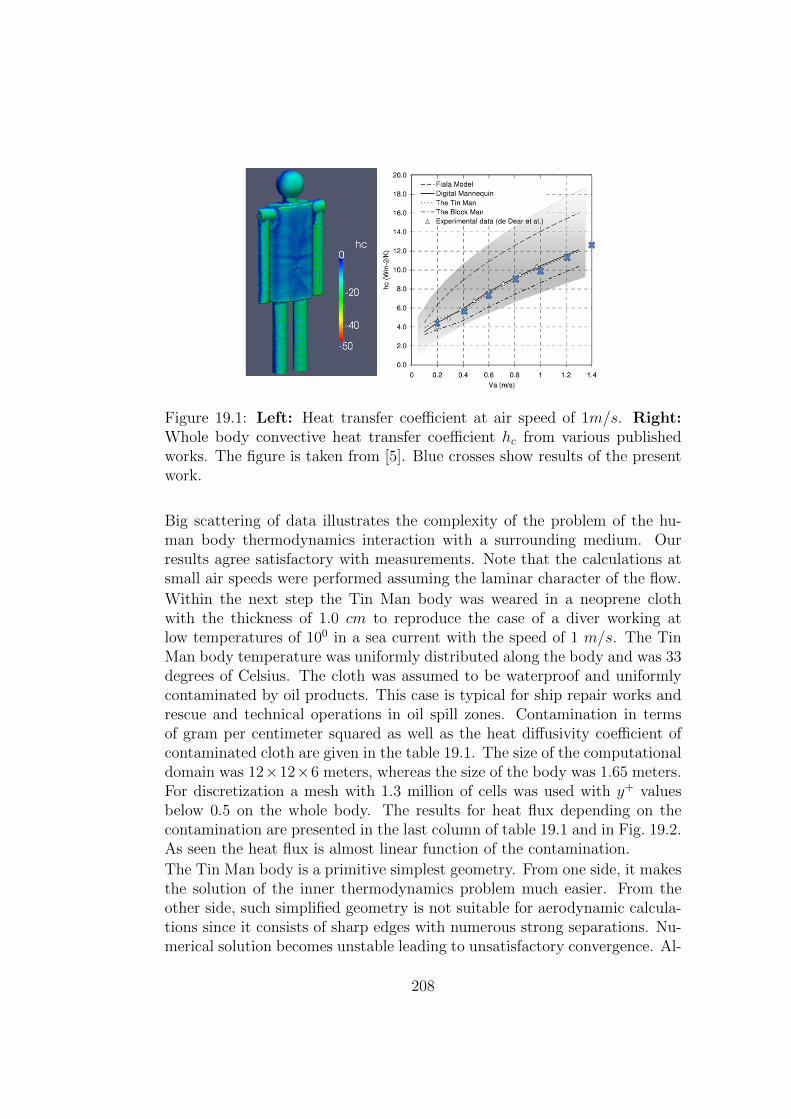
Figure 19.1: Left: Heat transfer coefficient at air speed of 1m/s. Right:Whole body convective heat transfer coefficient hc from various publishedworks. The figure is taken from [5]. Blue crosses show results of the presentwork.
Big scattering of data illustrates the complexity of the problem of the hu-man body thermodynamics interaction with a surrounding medium. Ourresults agree satisfactory with measurements. Note that the calculations atsmall air speeds were performed assuming the laminar character of the flow.
Within the next step the Tin Man body was weared in a neoprene clothwith the thickness of 1.0 cm to reproduce the case of a diver working atlow temperatures of 100 in a sea current with the speed of 1 m/s. The TinMan body temperature was uniformly distributed along the body and was 33degrees of Celsius. The cloth was assumed to be waterproof and uniformlycontaminated by oil products. This case is typical for ship repair works andrescue and technical operations in oil spill zones. Contamination in termsof gram per centimeter squared as well as the heat diffusivity coefficient ofcontaminated cloth are given in the table 19.1. The size of the computationaldomain was 12×12×6 meters, whereas the size of the body was 1.65 meters.For discretization a mesh with 1.3 million of cells was used with y+ valuesbelow 0.5 on the whole body. The results for heat flux depending on thecontamination are presented in the last column of table 19.1 and in Fig. 19.2.As seen the heat flux is almost linear function of the contamination.
The Tin Man body is a primitive simplest geometry. From one side, it makesthe solution of the inner thermodynamics problem much easier. From theother side, such simplified geometry is not suitable for aerodynamic calcula-tions since it consists of sharp edges with numerous strong separations. Nu-merical solution becomes unstable leading to unsatisfactory convergence. Al-
208
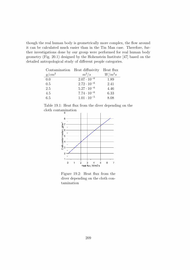
though the real human body is geometrically more complex, the flow aroundit can be calculated much easier than in the Tin Man case. Therefore, fur-ther investigations done by our group were performed for real human bodygeometry (Fig. 20.1) designed by the Hohenstein Institute [47] based on thedetailed antropological study of different people categories.
Contamination Heat diffusivity Heat fluxg/cm2 m2/s W/m2s0.0 2.07 · 10−6 1.890.5 2.72 · 10−6 2.412.5 5.27 · 10−6 4.464.5 7.74 · 10−6 6.336.5 1.01 · 10−5 8.08
Table 19.1: Heat flux from the diver depending on thecloth contamination
Figure 19.2: Heat flux from thediver depending on the cloth con-tamination
209

210

Chapter 20
CFD application for design ofcloth for protection from lowtemperatures under windconditions. Influence of thewind on the cloth deformationand heat transfer from thebody.
Lebedeva and Brink [48] have shown the influence of wind on heat transferdue to cloth deformation caused by wind induced pressures. Experimentalstudy was performed in open type wind tunnel with closed test section upto Reynolds number of 3.6 · 105 based on the air speed and diameter of clothpackages in form of cylinders. The aim of the present work is to get similarestimations for real human body form.
20.1 Wind tunnel measurements of pressure
distribution
The experiment was conducted in the wind tunnel of the Chair of OceanEngineering at the Rostock University. The wind tunnel of the Gottingentype has the test section of lengths of 2.8 m with the square cross sectionof 1.4 × 1.4 m2. The model of the height of 700 mm was manufactured by
211

Figure 20.1: Human body model in wind tunnel of the Rostock university(left). Positions of measurement points (right).
downsizing the real body with the scale factor of 0.39. Within the open testsection the size of the air jet with uniform velocity distribution is estimatedas one meter at least. Since it is one and half times as large as the modelheight, the influence of the jet boundaries on flow around the body can beconsidered as negligible. Two measurement series were performed. In thefirst one the pressure was measured at nine points distributed at three crosssections z = 0.329, 0.418 and 0.476 (see Fig. 20.1 and 20.3) using inclinedmanometers which are very accurate for low pressures measurements. Dueto high inertia of inclined manometers the unsteady pressure oscillationsare not captured. Position of measurement points is shown in Fig. 20.1(points 1, 1′, 1′′, 5, 5′, 5′′ and 9, 9′, 9′′). The measurements were performedwith the air speed of 10m/s at 14 degrees of Celsius. Reynolds numberbased on the maximum transversal body size is around 1.33 · 105. In thesecond series the measurements were performed at nine points 1, ..., 9 shownin Fig. 20.3(right) only at z = 0.418 (waist). This more detailed investigationwas carried out for two air speeds of 10 and 15 m/s.
20.2 Numerical simulations of pressure dis-
tribution and comparison with measure-
ments
Numerical simulations were performed using the commercial software pack-age STAR CCM+ for the air speed of 10 m/s. The boundary layer on thewindward side is supposed to be in transitional state. Due to strong sep-aration the flow on the leeward side of the model and in the wake can beconsidered as a turbulent one. The computational domain has the cross sec-
212

tion of 2.1× 2.1 m2. A length of the domain is 2.1 m in front of the humanbody (0.7 m height) and 4.2 m behind it. The grid consists of 1.2 · 106
polyhedron cells with maximal y+ value of 40. On the model sides the y+
value is varied between 20 and 25. To exclude ambiguity connected to theflow character, simulations were performed both for pure turbulent and purelaminar flows with and without roughness.
20.3 Comparison of CFD results with mea-
surements
Comparison with measurements for the first series is presented in Fig. 20.2.The results of measurements and simulations agree well in the front part ofthe body and in the separation area. Both simulations and measurementspredict the increase of the pressure coefficient in the section z = 0.476 mat angle ≈ 90 degrees caused by the stagnation effect of the shoulder. Onthe side of the model in cross sections z = 0.329 and 0.418 the agreement isnot satisfactory. To clarify this problem, the more detailed second measure-ment series was performed. All results obtained at z = 0.418 are presentedin Fig. 20.3. The big difference takes place around the angle of approx. 90degrees in the area of the separation (point 5 in Fig. 20.1). The experimentdoesn’t predict the strong under pressure region on the side of the model.The minimum experimental pressure coefficient is around −1 whereas thesimulation predicts −2.2 both for laminar and turbulent cases. The differ-ence between the laminar and turbulent solutions is negligible. This mightbe due to two facts. First, the cross section is elliptical (Fig. 20.2, left)and the averaged position of flow separation points is fixed at the widestaxis and doesn’t depend on the flow character. Second, strong unsteadyflow oscillation makes the difference between laminar and turbulent pressuredistributions negligible.
The experimental results raised many questions. Without big error, theflow can be considered as quasi two dimensional in cross sections along thehuman body. Then Cpmin is minus three for the case of two dimensionalcylinder flow. Due to three dimensional effects Cpmin can be smaller, butnot three times smaller like in measurements. The numerical simulationreveals no separation up to angle of 90 degrees. Within the separation zoneat angles larger than 120 degrees the numerical pressure coefficient is nearlyconstant. These facts are in a good agreement with classic knowledge aboutbluff bodies flows. In experiment, Cp slightly increases in the separationarea at angles larger than 90 degrees. Also, a relatively big discrepancy
213

Figure 20.2: Contrours of torso (left) and pressure coefficient Cp distributionaround the body at three different altitudes z = 0.329, 0.418 and 0.476m.
between Cp determined for 10 and 15 m/s seems to be very questionable, atleast within the zone of weak Reynolds number influence, i.e. at angles lessthan 90 degrees. The flow at angles larger than 90 degrees is unsteady. Thescattering of the data due to unsteady effects is shown both for simulationsand measurement. Obviously, the unsteady pressure oscillations can notbe reason for the disagreement between simulation and experiments. Moredetailed experimental study should be carried out in the future to clear thisproblem.
20.4 Change of thermal conductivity caused
by wind induced pressures
Estimations of pressure influence on cloth thermal conductivity was per-formed experimentally in the Thermal laboratory of the Don State TechnicalUniversity. The cloth of 30 mm thickness was manufactured from the Saviourwith Flamestat Cotton (upper sheet), the insulation Thinsulate and Taffetaas a lining. The cloth is used in oil industry for work at very low temperaturesunder oil contamination conditions.It was assumed that the pressure acts only in normal direction and shearstresses are neglected. The cloth has such a structure that it can be pressedbut not stretched. With the other words, the cloth has no deformation ifthe pressure difference ∆p = p− patm is negative. Bearing this in mind, thecloth deformation calculated using numerical pressure data can be considered
214

Figure 20.3: Left: Pressure distribution ∆p on the body obtained us-ing StarCCM+ commercial software. Contours of three cross sections atz = 0.329, 0.418 and 0.476 m are marked by black lines. Right: Pressure co-efficient Cp distribution around the body at z = 0.418. Points position 1, .., 9is shown in Fig. 20.1. Grey zone is the area of unsteady pressure coefficientoscillations in the laminar solution. Vertical lines indicate the scattering ofexperimental data at points 5, 6 and 7.
215

as reliable one since the area of positive Cp is approximately the same inexperiments and simulations. The cloth samples were subjected to pressureand then the thermal conductivity was measured using steady state method.Approximation of measurement points results in the following interpolationformula:
k = 0.22 + c1∆p+ c2∆p2 (20.1)
where k is the thermal conductivity coefficient in W/mK, C1 = 9.322 ·10−4 W
mKPaand C2 = 9.775 · 10−6 W
mKPa2 . Fig. 20.4 shows distribution ofthe thermal conductivity around the body at three sections along the humanbody. As seen the conductivity can increase in the stagnation area at thechest up to four and half times for strong wind of 20 m/s. To estimate theintegral wind influence f the thermal conductivity referred to that withoutwind was integrated over the body at five sections:
f(z) =
∮k(wind 6= 0)/k(wind = 0)r dϑ (20.2)
where ϑ and r are zylindrical coordinates in a cross section. The results aresummarized in the table 20.1. At strong wind of 20 m/s or 72 km/h theintegral increase of thermal conductivity can be up to seventy percent in thechest cross section. At moderate wind of 10 m/s the maximum influence isless than ten percent.
Table 20.1: Thermal conductivity factor f(z) integrated in circumferentialdirection
Body part Wind 10 m/s 20 m/sChest (z = 0.476 m) 1.096 1.729Waist (z = 0.418 m) 1.025 1.199Hip (z = 0.329 m) 1.085 1.668Upper leg (z = 0.25 m) 1.025 1.194Lower leg (z = 0.12 m) 1.018 1.141
216
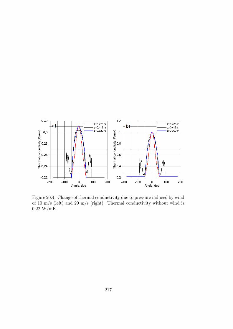
Figure 20.4: Change of thermal conductivity due to pressure induced by windof 10 m/s (left) and 20 m/s (right). Thermal conductivity without wind is0.22 W/mK.
217

218

Chapter 21
Simulation of human comfortconditions in car cabins
The comfort conditions of drivers and passengers is one of the most importantresearch topics in car industry. In this chapter we present a fragment of theresearch conducted in this field at the chair of modelling and simulation ofthe University of Rostock. The calculations presented below were carriedout by Stefan Knochenhauer. A compact car was chosen as the object ofinvestigations. The cabin geometry is represented in Fig. 21.1. The inlet ofthe air stream coming from the ventilation channel is marked by green colorwhereas the air outlet by red one. The grid with 6.5 million of cells is shown inFig. 21.2. The mathematical model is based on the URANS equation (13.17)and temperature transport equation (1.30). The turbulent character of thetemperature transport is taken into account by introduction of the additionalturbulent heat conduction. It means that instead of λ in the equation (1.30)we use the sum λ+ λt, where λt is the turbulent heat conduction coefficient.λt is expressed through the turbulent kinematic viscosity νt and the turbulentPrandtl number Prt
λtρcp
=νtPrt
(21.1)
The turbulent kinematic viscosity is computed from the URANS closure mod-els (see Chapters 13, 14 and 15) whereas the turbulent Prandtl number isassumed to be constant Prt ≈ 0.7. The URANS closure model used in thiswork is the k − ω SST model [49]. Numerical simulations were performedusing the finite volume method (see Chapter 7). Boundary conditions aregiven in the table 20.1.A few selected results of calculations are illustrated in Fig. 21.3. The distri-butions of air velocity and temperature inside of the car cabin are strongly
219

inhomogeneous. In regions of strong velocity the convective heat transferdominates whereas in stagnation areas the heat exchange is mostly due tothe heat conduction.
Figure 21.1: Sketch of the car cabin studied numerically.
Figure 21.2: Grids with 6.5 million of cells generated with snappyHexMesh.
220
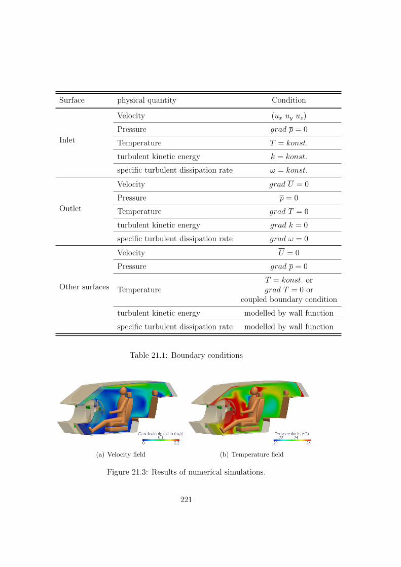
Surface physical quantity Condition
Inlet
Velocity (ux uy uz)
Pressure grad p = 0
Temperature T = konst.
turbulent kinetic energy k = konst.
specific turbulent dissipation rate ω = konst.
Outlet
Velocity grad U = 0
Pressure p = 0
Temperature grad T = 0
turbulent kinetic energy grad k = 0
specific turbulent dissipation rate grad ω = 0
Other surfaces
Velocity U = 0
Pressure grad p = 0
TemperatureT = konst. orgrad T = 0 or
coupled boundary condition
turbulent kinetic energy modelled by wall function
specific turbulent dissipation rate modelled by wall function
Table 21.1: Boundary conditions
(a) Velocity field (b) Temperature field
Figure 21.3: Results of numerical simulations.
221

222
Bibliography
[1] Tsinober A. An informal introduction to turbulence. Kluwer AcademicPublisher, 2004.
[2] T.A. Zaki. From streaks to spots and on to turbulence: Exploring thedynamics of boundary layer transition. Flow, Turbulence and Combus-tion, 91:4, 2013.
[3] Moin P. Kim, J and R. Moser. Turbulence statistics in fully developedchannel flow at low reynolds number.
[4] Kim J. Moser, R. and N. Mansour. Direct numerical simulation of tur-bulent channel flow up to reτ = 590.
[5] Novieto D. Zhang Y. and Yingchun J. Human envoronmental heat trans-fer simulation with cfd- the advances and challenges.building simulation2009. pages 2162–2168. Eleventh International IBPSA Conference, Glas-gow, Scotland, July 27–30, 2009 2009.
[6] Ferziger J. and Peric M. Computational Methods for Fluid Dynamics.Springer, 2002.
[7] Seibold B. A compact and fast matlab code solving the incompress-ible navier-stokes equations on rectangular domains. Applied Mathemat-ics, Massachusetts Institute of Technology, www-math.mit.edu/ seibold,2008.
[8] Dornseifer T. Griebel M. and Neunhoeffer T. Numerical simulation influid dynamics: A practical introduction. Society for Industrial andApplied Mathematics, Philadelphia, PA, USA, 1998.
[9] Phillips A.B. Turnock S.R. and Furlong M. Urans simulations of staticdrift and dynamic manouveres of the KVLCC2 tanker. pages F63–F68.Proceedings of the SIMMAN workshop, 2008.
[10] Liseikin V. Grid Generation Methods. Springer, 2010. 390p.
223

[11] Warsi Z.U.A Thompson I.F. and Mastin C.W. Numerical grid genera-tion. Foundations and applications, 1997.
[12] Novikov E. Generalized dynamics of three-dimensional singularities(vortons). Sov. JETP, 84(3):975 – 981, 1984.
[13] Chorin A. The evolution of a turbulent vortex. Comm. in MathematicalPhysics, 83:517 – 535, 1982.
[14] Chorin A. Constrained random walks and vortex filaments in turbulencetheory. Comm. in Mathematical Physics, 132:519 – 536, 1990.
[15] Schlichting H. Boundary layer theory. Springer, 2000.
[16] P.A. Durbin and X. Wu. Transition beneath vortical disturbances. An-nual Review of Fluid Mechanics, 39:107 – 128, 2007.
[17] Batchelor G. The Theory of Homogeneous Turbulence. Cambridge Uni-versity Press, Cambridge, 1956.
[18] Pope S. Turbulent flows. Cambridge University Press, Cambridge, 2000.
[19] Menter F. and Egorov J. Turbulence models based on the length-scaleequation. pages 941 – 946. Proc. of 4th Int. Symp. Turb. and ShearFlow Phenomena, 2005.
[20] Below I.A. and Isaev S.A. Modelling of turbulent flows. Saint Petersburg,(2001).
[21] Ferziger H. Bardina J. and Reynolds W. Improved subgrid models forlarge eddy simulation. AIAA Paper, pages 80 – 1357, 1980.
[22] Peng S. Hybrid rans-les modeling based on zero- and one- equationmodels for turbulent flow simulation. pages 1159 – 1164. Proc. of 4thInt. Symp. Turb. and Shear Flow Phenomena, 2005.
[23] Davidson L. and Dalstroem S. Hybrid rans-les: An approach to make lesapplicable at high reynolds number. Int. J. of Comp. Fluid Dynamics,19:415 – 427, 2005.
[24] Terracol M. Airframe noise prediction by mean of a zonal rans/les ap-proach. pages 1165 – 1169. In: Proc. of 4th Int. Symp. Turb. and ShearFlow Phenomena, 2005.
224
[25] Kniesner B. Kadavelil G. Basara B. Jakirlic S., Saric S. and Chaouat B.Sgs modelling in les of wall-bounded flows using transport rans models:from a zonal to a seamless hybrid les/rans method. pages 1057 – 1062.Proc. of 6th Int. Symp. Turb. and Shear Flow Phenomena, 2007.
[26] Leschziner M. Temmerman L., Hadziabdec M. and Hanjalic K. A hybridtwo-layer urans-les approach for large-eddy simulation at high reynoldsnumbers. Int. J. of Heat and Fluid, 26:173 – 190, 2005.
[27] Strelets M. Spalart P. R., Jou W. H. and Allmaras S. R. Comments onthe feasibility of les for wings and on a hybrid rans/les approach. pages137 – 148. Advances in LES/DNS: Proc. of the first AFOSR Interna-tional Conf. on DNS/LES, 1997.
[28] Spalart P.R. Detached-eddy simulation. Annu. Rev. Fluid Mech., 41:181– 202, 2009.
[29] Davidson L. and Billson M. Hybrid les-rans using synthesized turbulentfluctuations for forcing in the interface region. Int. J. of Heat and Fluid,27:1028 – 1042, 2006.
[30] Abe K. and Miyata Y. An investigation of hybrid les/rans models forpredicting flow fields with separation. pages 1153 – 1158. Proc. of 4thInt. Symp. Turb. and Shear Flow Phenomena, 2005.
[31] Pitsch H. Schlueter J. U. and Moin P. onsistent boundary conditions forintegrated les/rans simulations: Les outflow conditions. volume 3121,pages 1 – 8. AIAA, 2002.
[32] Ducros F. Benerafa Y. and Sagaut P. Rans/les coupling using a forcingterm approach. pages 1141 – 1146. 4th Int. Symp. Turb. and Shear FlowPhenomena, 2005.
[33] Shchukin E. Kornev N., Taranov A. and Kleinsorge L. Developmentof hybrid urans-les methods for flow simulations in the ship stern area.Ocean Engineering, 38(16):1831 – 1838, 2011.
[34] Durbin P. Near-wall turbulence closure modeling without damping func-tions. J. Theor. Comput. Fluid Dyn, 1991.
[35] Werner H. and Wengle H. Large-eddy simulation of turbulent flow overand around a cube in a plate channel. 8th Symposium on TurbulentShear Flows, 1991.
225
[36] Fureby C. Huuva T. Alin N., Bensow R. and Svennberg U. Currentcapabilities of des and les for submarines at straight course. J. ShipResearch, 54:184 –196, 2010.
[37] Guminer P.K. Thermoregulation studying in hygiene and work physiol-ogy. Medgiz, Moscow, page 147, 1962.
[38] Novieto D. Zhang Y. and Yingchun J. Human environmental heat trans-fer simulation with cfd the advances and challenges. pages 2162 – 2168.Eleventh International IBPSA Conference, Glasgow, Scotland, 2009.
[39] Cherunova I.V. New technologies of heat protection wear design, (inrussian). Technologies of textile industry, pages 51 – 54, 2009.
[40] Palella B.I. Alfano1 F. R. and G. Riccio. Thermode 193: an enhancedstolwijk thermoregulation model of the human body. page 8. 7th Interna-tional Thermal Manikin and Modelling Meeting, University of Coimbra,2008.
[41] Smith T. Anatomie-atlas: Aufbau und Funktionsweise des menschlichenKorpers. Dorling Kindersley, Deutschland, page 448, 2011.
[42] Herman I.P. Physics of a human body. Springer, 860p., 2007.
[43] Zhavoronkov A. Grivina I. and Postnikov N. Pecularities of develop-ments of imitation model ”human-clothes-medium” (in russian) textileindustry. 3:36 – 37, 1988.
[44] Alexiades V. and Solomon A.D. Mathematical modeling of melting andfreezing processes: Basic concepts & applications. Taylor & Francis,1992.
[45] Cherunova I. Theoretical foundations of complex design of special clothesfor protection at high temperatures conditions. PhD thesis, South Rus-sian University of Economics and Service, Shakhty, 2008.
[46] Vitte N.K. Thermal exchange and its hygienic value. State medicalpublishing, Kiev, page 145, 1956.
[47] www.hohenstein.de.
[48] Brink I. and Lebedeva E. Investigation of wind influence on packages ofheat protecting cloth. Textile Industry, 3:34–36 (in Russian), 2005.
226

[49] Menter F.R. Zonal two equation k-ω turbulence models for aerody-namic flows. AIAA 93-2906, 24th Fluid Dynamics Conference, Orlando,Florida, 1993.
227
Index
ε-Equation, 149
a-posteriori test, 166a-priori test, 166alternating direction implicit, 55amplification of the vorticity, 90artificial viscosity, 39autocorrelation function, 108
backward difference scheme, 30Biot-Savart law, 89block structured grids, 81body forces, 20boundary conditions, 26, 28Boussinesq hypothesis, 138buffer layer, 105
central difference scheme, 30collocated grid, 47constant of Karman, 105continuity equation, 19convective acceleration, 25correlation function, 108Courant Friedrich Levy criterion, 43Crank-Nicolson scheme, 33cross stress, 164, 165
density, 27Detached Eddy Simulation, 169, 170Direct Numerical Simulation, 129Dirichlet condition, 28, 54dissipation, 145dissipation range, 126dissipation rate, 123Dynamic Smagorinsky Model, 160
energy containing range, 126energy production, 123ensemble averaged quantity, 108experiment of Reynolds, 95explicit scheme, 33explicit time advance, 45
Finite Volume Method, 61folding, 91forward difference scheme, 30Fourier law, 27fractional step methods, 56friction velocity, 101Friedman-Keller problem, 144
Galilean invariance, 165
heat conduction coefficient, 28heat conduction equation, 27, 28heat flux, 27heat sources, 27homogeneous turbulence, 108hybrid URANS-LES methods, 169
implicit scheme, 33inertial subrange, 125, 126inner energy balance equation, 27integral length, 108isotropic turbulence, 108
k - ε Model, 147k-Equation, 147Kelvin Helmholtz instability, 97Kolmogorov first similarity hypothe-
sis, 124
228

Kolmogorov hypothesis of local isotropy,124
Kolmogorov law, 126Kolmogorov scale, 125Kolmogorov second similarity hypoth-
esis, 125Kolmogorov theory K-62, 129Kolmogorov theory K41, 121kurtosis, 116
lambda structures, 101laminar, 87Large Eddy Simulation, 129, 155Lax-Wendroff scheme, 59Leonard stress, 164, 165LES equations, 157LES filtering, 155limiters function, 47local acceleration, 25logarithmic region, 105
material substantial derivative, 25mixed schemes, 46mixed similarity models, 164morphing grids, 82
Navier Stokes Equation, 23, 88Neumann condition, 28, 54Newton hypothesis, 24Newtonian liquids, 24normal stress, 23
overset or chimera grids, 82
pairing, 97PISO algorithm, 76Poisson equation, 46Prandtl mixing length model, 104pressure, 25pressure correction method, 70probability density function, 116properties of Reynolds averaging, 135
properties of surface forces, 21pseudodissipation, 147
Reynolds averaged Navier Stokes, 129Reynolds averaging, 107Reynolds stress, 137, 164, 165Reynolds Stress Model, 141Richardson poem, 93
scale similarity models, 163shear stress, 23SIMPLE algorithm in OpenFOAM,
76SIMPLE method, 70SIMPLEC algorithm, 78skewness, 116Smagorinsky model, 158Spalart Allmares (SA model), 139specific heat capacity, 27splitting according to physical processes,
56staggered grid, 47streaks, 100, 102structure function, 116structured grids, 81subgrid stress (SGS), 158subgrid viscosity, 158surface forces, 21
Taylor microscale λ, 113time-advancing, 46turbulence, 87turbulent kinematic viscosity, 138turn over time, 125TVD schemes, 47
unstructured grids, 81upwind difference scheme, 30
Van Driest constant, 105viscous sublayer, 103vortex cascado, 122
229
vortex reconnection, 92vorticity, 88vorticity transport equation, 88
wake region, 105
230