fluid dynamics

FLUID DYNAMICSTheory, Computation, and

Numerical Simulation

Accompanied by the software library FDLIB

by

C. PozrikidisUniversity of California, San Diego

La JoIIa9 California 92093-0411U.S.A.

Email: [email protected] URL: http://stokes.ucsd.edu/cjpozrikidis

KLUWER ACADEMIC PUBLISHERSBoston / Dordrecht / London

http://stokes.ucsd.edu/

Distributors for North, Central and South America:Kluwer Academic Publishers101 Philip DriveAssinippi ParkNorwell, Massachusetts 02061 USATelephone (781) 871-6600Fax (781) 681-9045E-Mail < [email protected] >

Distributors for all other countries:Kluwer Academic Publishers GroupDistribution CentrePost Office Box 3223300 AH Dordrecht, THE NETHERLANDSTelephone 3178 6392 392Fax 3178 6546 474E-Mail < services®wkap.nl >

Electronic Services <http://www.wkap.nl>

Library of Congress Cataloging-in-Publication Data

Pozrikidis, C.Fluid dynamics: theory, computation, and numerical simulation / by C. Pozrikidis

p.cm."Accompanied by the software library FDLIB. "Includes bibliographical references and index.ISBN 0-7923-7351-0 (acid-free paper)

1. Fluid dynamics. I. Title

QA911 .P632001532'.05—dc21

2001029458

Copyright © 2001 by Kluwer Academic Publishers

All rights reserved. No part of this publication may be reproduced, stored in aretrieval system or transmitted in any form or by any means, mechanical, photo-copying, recording, or otherwise, without the prior written permission of thepublisher, Kluwer Academic Publishers, 101 Philip Drive, Assinippi Park, Norwell,Massachusetts 02061.

Printed on acid-free paper.

Printed in the United States of America.

Preface

Ready access to computers at an institutional and personal level hasdefined a new era in teaching and learning. The opportunity to extendthe subject matter of traditional science and engineering disciplines intothe realm of scientific computing has become not only desirable, but alsonecessary. Thanks to portability and low overhead and operating costs,experimentation by numerical simulation has become a viable substitute,and occasionally the only alternative, to physical experimentation.

The new environment has motivated the writing of texts and mono-graphs with a modern perspective that incorporates numerical and com-puter programming aspects as an integral part of the curriculum: meth-ods, concepts, and ideas should be presented in a unified fashion thatmotivates and underlines the urgency of the new elements, but does notcompromise the rigor of the classical approach and does not oversimplify.

Interfacing fundamental concepts and practical methods of scientificcomputing can be done on different levels. In one approach, theory andimplementation are kept complementary and presented in a sequentialfashion. In a second approach, the coupling involves deriving compu-tational methods and simulation algorithms, and translating equationsinto computer code instructions immediately following problem formu-lations. The author of this book is a proponent of the second approachand advocates its adoption as a means of enhancing learning: interject-ing methods of scientific computing into the traditional discourse offersa powerful venue for developing analytical skills and obtaining physicalinsight.

The goal of this book is to offer an introductory course in fluid me-chanics, covering traditional topics in a way that unifies theory, computa-tion, computer programming, and numerical simulation. The approachis truly introductory, in the sense that a minimum of prerequisites arerequired. The intended audience includes not only advanced undergrad-uate and entry-level graduate students, but also a broad class of scientistsand engineers with a general interest in scientific computing.

The discourse is distinguished by two features. First, solution pro-cedures and algorithms are developed immediately after problem formu-lations. Second, numerical methods are introduced on a need-to-knowbasis and in increasing order of difficulty: function interpolation, func-tion differentiation, function integration, solution of algebraic equations,finite-difference methods, etc.

A supplement to this book is the FORTRAN software library FDLIBwhose programs explicitly illustrate how computational algorithms trans-late into computer code instructions. The codes of FDLIB range from in-troductory to advanced, and the problems considered span a broad rangeof applications; from laminar channel flows, to vortex flows, to flows inaerodynamics. The input is either entered from the keyboard or readfrom data files. The output is recorded in output files in numerical formso that it can be read and displayed using independent graphics, visu-alization, and animation applications on any computer platform. Com-puter problems at the end of each section ask the student to run theprograms for various flow conditions, and thus study the effect of thevarious parameters characterizing a flow. Instructions for downloadingthe source code and a description of the library contents are given onpage 651.

In concert with the intended usage of this book as a stand-alone textand as a tutorial on numerical fluid dynamics and scientific computing,references are not provided in the text. Instead, a selected compilationof introductory, advanced, and specialized references on fluid dynamics,calculus, numerical methods, and computational fluid dynamics are list-ed in the bibliography on page 666. The reader who wishes to focus ona particular topic is directed to these resources for further details.

I would like to extend special thanks to Vasilis Bontozoglou for hisfriendship and encouragement, and to Yuan Chih-Chung, Rhodalynn De-gracia, Audrey Hill, and Kurt Keller for helping me with the preparationof the manuscript.

C. Pozrikidis

San Diego

January, 2001

Email: [email protected] internet site: http://stokes.ucsd.edu/C-pozrikidis/FD-TCNS

v This page has been reformatted by Knovel to provide easier navigation.

Contents

Preface .................................................................................. ix

1. Fluid Motion: Introduction to Kinematics ................... 1 1.1 Fluids and Solids ............................................................... 1 1.2 Fluid Parcels and Flow Kinematics .................................... 2 1.3 Coordinates, Velocity, and Acceleration ............................ 4 1.4 Fluid Velocity and Streamlines .......................................... 15 1.5 Point Particles and Their Trajectories ................................ 18 1.6 Material Surfaces and Elementary Motions ....................... 27 1.7 Interpolation ....................................................................... 38

2. Fluid Motion: More on Kinematics .............................. 49 2.1 Fundamental Modes of Fluid Parcel Motion ...................... 49 2.2 Fluid Parcel Expansion ...................................................... 61 2.3 Fluid Parcel Rotation and Vorticity ..................................... 62 2.4 Fluid Parcel Deformation ................................................... 68 2.5 Numerical Differentiation ................................................... 72 2.6 Areal and Volumetric Flow Rate ........................................ 77 2.7 Mass Flow Rate, Mass Conservation, and the

Continuity Equation ............................................................ 87 2.8 Properties of Point Particles .............................................. 93 2.9 Incompressible Fluids and Stream Functions .................... 101 2.10 Kinematic Conditions at Boundaries .................................. 106

3. Flow Computation Based on Kinematics .................... 111 3.1 Flow Classification Based on Kinematics .......................... 111

vi Contents

This page has been reformatted by Knovel to provide easier navigation.

3.2 Irrotational Flows and the Velocity Potential ...................... 114 3.3 Finite-Difference Methods .................................................. 122 3.4 Linear Solvers .................................................................... 131 3.5 Two-Dimensional Point Sources and Point-Source

Dipoles ............................................................................... 135 3.6 Three-Dimensional Point Sources and Point-Source

Dipoles ............................................................................... 149 3.7 Point Vortices and Line Vortices ........................................ 154

4. Forces and Stresses ..................................................... 164 4.1 Body Forces and Surface Forces ...................................... 164 4.2 Traction and the Stress Tensor ......................................... 166 4.3 Traction Jump across a Fluid Interface .............................. 173 4.4 Stresses in a Fluid at Rest ................................................. 181 4.5 Viscous and Newtonian Fluids ........................................... 185 4.6 Simple Non-Newtonian Fluids ........................................... 194 4.7 Stresses in Polar Coordinates ........................................... 197 4.8 Boundary Condition on the Tangential Velocity ................. 203 4.9 Wall Stresses in Newtonian Fluids .................................... 205

5. Hydrostatics .................................................................. 208 5.1 Equilibrium of Pressure and Body Forces ......................... 208 5.2 Force Exerted on Immersed Surfaces ............................... 217 5.3 Archimedes' Principle ........................................................ 224 5.4 Shapes of Two-Dimensional Interfaces ............................. 227 5.5 A Semi-Infinite Interface Attached to an Inclined

Plate ................................................................................... 231 5.6 Meniscus between Two Parallel Plates ............................. 235 5.7 A Two-Dimensional Drop on a Horizontal Plane ............... 241 5.8 Axisymmetric Shapes ........................................................ 246

Contents vii


6. Equation of Motion and Vorticity Transport ............... 252 6.1 Newton's Second Law for the Motion of a Parcel .............. 252 6.2 Integral Momentum Balance .............................................. 258 6.3 Cauchy's Equation of Motion ............................................. 263 6.4 Euler's and Bernoulli's Equations ...................................... 270 6.5 The Navier-Stokes Equation .............................................. 281 6.6 Vorticity Transport .............................................................. 288 6.7 Dynamic Similitude, the Reynolds Number, and

Dimensionless Numbers in Fluid Dynamics ...................... 296

7. Channel, Tube, and Film Flows ................................... 306 7.1 Steady Flow in a Two-Dimensional Channel ..................... 306 7.2 Steady Film Flow Down an Inclined Plane ........................ 315 7.3 Steady Flow through a Circular or Annular Tube ............... 319 7.4 Steady Flow through Channels and Tubes with

Various Cross-Sections ..................................................... 327 7.5 Steady Swirling Flow ......................................................... 336 7.6 Transient Flow in a Channel .............................................. 339 7.7 Oscillatory Flow in a Channel ............................................ 347 7.8 Transient and Oscillatory Flow in a Circular Tube ............. 354

8. Finite-Difference Methods ............................................ 364 8.1 Choice of Governing Equations ......................................... 364 8.2 Unidirectional Flow; Velocity/Pressure Formulation ........... 366 8.3 Unidirectional Flow; Velocity/Vorticity Formulation ............ 377 8.4 Unidirectional Flow; Stream Function/Vorticity

Formulation ........................................................................ 382 8.5 Two-Dimensional Flow; Stream Function/Vorticity

Formulation ........................................................................ 386 8.6 Velocity/Pressure Formulation ........................................... 395 8.7 Operator Splitting and Solenoidal Projection ..................... 399

viii Contents


9. Flows at Low Reynolds Numbers ................................ 410 9.1 Flows in Narrow Channels ................................................. 411 9.2 Film Flow on a Horizontal or Down Plane Wall .................. 424 9.3 Two-Layer Channel Flow ................................................... 436 9.4 Flow Due to the Motion of a Sphere .................................. 443 9.5 Point Forces and Point Sources in Stokes Flow ................ 450 9.6 Two-Dimensional Stokes Flow .......................................... 459 9.7 Flow near Corners ............................................................. 465

10. Flows at High Reynolds Numbers ............................... 475 10.1 Changes in the Structure of a Flow with Increasing

Reynolds Number .............................................................. 476 10.2 Prandtl Boundary-Layer Analysis ...................................... 479 10.3 Prandtl Boundary Layer on a Flat Surface ......................... 485 10.4 Von Kàrmàn's Integral Method .......................................... 501 10.5 Instability of Shear Flows ................................................... 512 10.6 Turbulent Motion ................................................................ 525 10.7 Analysis of Turbulent Motion ............................................. 539

11. Vortex Motion ................................................................ 548 11.1 Vorticity and Circulation in Two-Dimensional Flow ............ 549 11.2 Motion of Point Vortices ..................................................... 551 11.3 Two-Dimensional Flow with Distributed Vorticity ............... 566 11.4 Vorticity, Circulation, and Three-Dimensional Flow

Induced by Vorticity ........................................................... 581 11.5 Axisymmetric Flow Induced by Vorticity ............................ 586 11.6 Three-Dimensional Vortex Motion ..................................... 600

12. Aerodynamics ............................................................... 606 12.1 General Features of Flow Past an Aircraft ......................... 607 12.2 Airfoils and the Kutta-Joukowski Condition ........................ 609

Contents ix


12.3 Vortex Panels .................................................................... 612 12.4 Vortex Panel Method ......................................................... 620 12.5 Vortex Sheet Representation ............................................. 629 12.6 Point-Source-Dipole Panels ............................................... 638 12.7 Point-Source Panels and Green's Third Identity ................ 645

FDLIB Software Library ....................................................... 651

FDLIB Directories ................................................................ 653

References ........................................................................... 666

Subject Index ....................................................................... 668

FDLIB Software Library

The software library FDLIB contains a collection of FORTRAN 77 pro-grams and subroutines that solve a broad range of problems in fluiddynamics using a variety of numerical methods. At the time of thisprinting, FDLIB consist of thirteen main directories, each containing amultitude of nested subdirectories. The contents of the subdirectoriesare listed on pages 655-667.

Downloading

The source codes of FDLIB and accompanying User Guide, availablein the pdf format, can be downloaded from the internet site:h t t p : / / s t o k e s . u c s d . e d u / C - p o z r i k i d i s / F D L IB

Installation and compilation on UNIX or LINUX

• The library has been archived using the tar UNIX facility into thefile FDLIB. tar. To unravel the directories on a UNIX or LINUXsystem, please execute the UNIX command:tar xvf FDLIB.tar

• The downloaded package does not contain object files or executa-bles. An application can be built using the makefile provided ineach subdirectory. A makefile is a UNIX script that instructs theoperating system how to compile the main program and subrou-tines, and then link the object files into an executable using an f77compiler.

• To compile the programs using a FORTRAN 90 compiler, simplymake appropriate compiler call substitutions in the makefiles.

• To compile the application named pindos, go to the subdirectorywhere it resides, and type:make pindos

• To remove the object files and output files of the application namedpindos, go to the subdirectory where it resides, and type:make purge

http://stokes.ucsd.edu/pozrikidis/FDLIB/fdlib.shtml

• To remove the object files, output files, and executable of the ap-plication named pindos, go to the subdirectory where it resides,and type:make clean

Installation and compilation on Windows and Macintosh

• To unravel the directories on a Windows or Macintosh platform,double-click on the archived tar file and follow the on-screen in-structions of the invoked application.

• To compile the link the programs, follow the instructions of yourFORTRAN 77 or FORTRAN 90 compiler.

CFDLAB

A subset of FDLIB has been combined with the XIl graphics libraryvogle into an integrated application that visualizes the results of thesimulations. The source code of CFDLAB can be downloaded from theinternet site:http://stokes.ucsd.edu/C-pozrikidis/CFDLAB

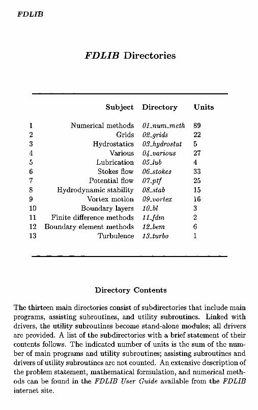
http://stokes.ucsd.edu/pozrikidis/CFDLAB/cfdlab.shtml

FDLIB Directories

Subject Directory Units

1 Numerical methods Ol-num.meth 892 Grids O2.grids 223 Hydrostatics OSJiydrostat 54 Various O4-various 275 Lubrication 05-lub 46 Stokes flow 06-stokes 337 Potential flow #7_p/;/ 258 Hydrodynamic stability 08-stab 159 Vortex motion 09-vortex 1610 Boundary layers ^0.6/ 311 Finite difference methods ll.fdm 212 Boundary element methods 12-bem 613 Turbulence IS.turbo I

Directory Contents

The thirteen main directories consist of subdirectories that include mainprograms, assisting subroutines, and utility subroutines. Linked withdrivers, the utility subroutines become stand-alone modules; all driversare provided. A list of the subdirectories with a brief statement of theircontents follows. The indicated number of units is the sum of the num-ber of main programs and utility subroutines; assisting subroutines anddrivers of utility subroutines are not counted. An extensive description ofthe problem statement, mathematical formulation, and numerical meth-ods can be found in the FDLIB User Guide available from the FDLIBinternet site.

01-numjtneth

General purpose numerical methods in scientific computing. l

Subdirectory

01_num_comp02_lin_calc03_lin_eq04_nl_eq05_eigen06_interp_diff07_integrationOS-approximation09-odeJvp

lO.odeJbvp

ll.pde12_spec_fnc

Topic

General aspects of numerical computation.Linear algebra and linear calculus.Systems of linear algebraic equations.Nonlinear algebraic equations.Eigenvalues and eigenvectors of matrices.Function interpolation and differentiation.Function integration.Function approximation.Ordinary differential equations;initial- value problems.Ordinary differential equations;boundary value problems.Partial differential equations.Computation of special functions.

Units

141110898

108

1

25

10

1ThIs directory accompanies the book: C. Pozrikidis 1998 Numerical Computationin Science and Engineering, Oxford University Press.

Subdirectory

grid_2d

prd_2dprd_3d

prd_ax

rec_2drec_2djstrml

sm_3d_cl_df

sm_3d_cl_tr

trgLoctatrgl_octa_hstrgl_sqr

Topic

Discretization of a planar line into agraded mesh of straight or circular elements.Adaptive parametrization of planar lines.Adaptive parametrizationof three-dimensional lines.Adaptive parametrization of planar linesrepresenting the trace of axisymmetricsurfaces in a meridional plane.Interpolation through a rectangular grid.Streamline pattern by interpolationthrough a rectangular grid.Smoothing of a function on a closed surfaceby surface diffusion.Smoothing of a function on a closed surfaceby Legendre spectrum truncation.Triangulation of a closed surface.Triangulation of an open surface.Triangulation of a square patch.

Units

35

5

31

1

1

1111

02-grids

Adaptive discretization, parametrization, representation, andmeshing of planar lines, three-dimensional lines, and three-dimensional surfaces.

03-hydrostat

Shapes of interfaces in hydrostatics.

Subdirectory

drop_2d

drop_ax

men_2d

men_2d_plate

men_ax

Topic

Shape of a two-dimensional pendantor sessile drop on a plane.Shape of an axisymmetric pendantor sessile drop on a plane.Shape of a two-dimensional meniscusbetween two parallel plates.Shape of a two-dimensional meniscusattached to an inclined plate.Shape of an axisymmetric meniscusin a circular tube.

Units

1

1

1

1

1

04-various

Structure and kinematics of various flows.

Subdirectory

flow.ld

flow_ld_osc

flow_ld_shear

spfstrmlstrmlluniJlow

uni_flow_u

Topic

Steady unidirectional flow in a tubewith arbitrary cross section.Oscillatory unidirectional flow in atube with arbitrary cross section.Unidirectional shear flow over anarray of cylinders.Similarity solutions for stagnation-point flows.Streamline patterns of a broad range of flows.Light version of strml.Steady unidirectional flows withrectilinear or circular streamlines.Unsteady unidirectional flows withrectilinear or circular streamlines.

Units

I

1

1111

15

8

OSJub

Nearly unidirectional lubrication flowsat low Reynolds numbers.

Subdirectory

bear_2d

chan_21_exp

chan_21Jmp

films

Topic

Dynamical simulation of the motionof a slider bearing pressing against a wall.Dynamical simulation of the evolutionof two superposed viscous layersin a horizontal or inclined channel,computed by an explicit finite-diffrence method.Dynamical simulation of the evolutionof two superposed viscous layersin a horizontal or inclined channel,computed by an implicit finite-difference method.Evolution of an arbitrary number of superposedfilms on a horizontal or plane wall.

Units

1

1

1

1

06-stokes

Viscous flows at vanishing Reynolds numbers.

Subdirectory

caps_2d

caps_3d

caps_ax

cop_ax

drop_3d

drop_3dw

em.2d

films

flow_2d

layers

prtcl_2d

Topic

Dynamical simulation of the motion ofa two-dimensional drop or elastic capsule,for a variety of flow configurations.Dynamical simulation of the motion of athree-dimensional elastic capsule.Dynamical simulation of the motion of anaxisymmetric drop or elastic capsule,for a variety of flow configurations.Shear flow over an axisymmetric cavity,orifice, or protrusion.Dynamical simulation of the motion of athree-dimensional drop with constantor varying surface tension.Dynamical simulation of the deformationof a three-dimensional drop adhering toa plane wall.Dynamical simulation of the motion of asuspension of two-dimensional drops orelastic capsules, for a variety of flowconfigurations.Dynamical simulation of the motion ofsuperimposed layers in a channel, ortwo films flowing down a plane wall.Two-dimensional flow in a domain witharbitrary geometry.Dynamical simulation of the motion ofan arbitrary number of layers in a channel,or films flowing down a plane wall.Flow past a fixed bed of two-dimensionalparticles with arbitrary shapes,for a variety of flow configurations,computed by a boundary-element method.

Units

I

1

I

I

I

I

1

I

I

1

1

06-stokes (Continued)

Viscous flows at vanishing Reynolds numbers.

Subdirectory

prtcl_2d_se

prtcLSd

prtcLax

prtcl_sw

sgf_2dsgf_3dsgf_3dax

sgLaxsusp_2d

susp_2d_se

thread_ax

Topic

Flow past a fixed bed of two-dimensionalparticles with arbitrary shapes for a varietyof flow configurations,computed by a spectral-element method.Flow past, or due to the motion of,a three-dimensional particle,for a variety of configurations,computed by a boundary-element method.Flow past, or due to the motion of,a collection of axisymmetric particles,computed by a boundary-element method.Swirling flow produced by the rotationof an axisymmetric particle,computed by a boundary-element method.Green's functions of two-dimensional Stokes flow.Green's functions of three-dimensional Stokes flowGreen's functions of Stokes flowin an axisymmetric domain.Green's functions of axisymmetric Stokes flow.Dynamical simulation of the motionof a suspension of two-dimensionalrigid particles with arbitrary shapes,for a variety of flow configurations,computed by a boundary-element method.Dynamical simulation of the motionof a suspension of two-dimensionalrigid particles with arbitrary shapes,for a variety of flow configurations,computed by a spectral-element method.Dynamical simulation of the evolutionof a fluid thread or annular layer.

Units

1

1

1

165

14

1

1

1

07-ptf

Potential flows.

Subdirectory

airf_2dairf_2d_cdp

airf_2d_csdp

airf_2d_lvp

body_2d

body_ax

bubble_3d

cvt_2d

drop_3d

flow_2d

lgf.2d

lgf_3d

IgLax

tank_2d

Topic

Shapes of airfoils.Flow past an airfoil computed by theconstant-dipole-panel method.Flow past an airfoil computed by theconstant-source-dipole-panel method.Flow past an airfoil computed by thelinear-vortex-panel method.Flow past, or due to the motion of,a two-dimensional body,computed by a boundary element method.Flow past, or due to the motion of,an axisymmetric body,computed by a boundary element method.Dynamical simulation of the deformation,collapse, or oscillations of athree-dimensional bubble.Flow in a rectangular cavity,computed by a finite difference method.Dynamical simulation of the surface-tensioninduced oscillations of a three-dimensionalinviscid drop suspended in vacuum.Two-dimensional flow in an arbitrary domain,computed by a boundary element method.Green and Neumann functions of Laplace'sequation in two dimensions.Green and Neumann functions of Laplace'sequation in three dimensions.Green and Neumann functions of Laplace'sequation in axisymmetric domains.Dynamical simulation of liquid sloshing in arectangular tank, computed by aboundary integral method.

Units

1

I

1

I

I

1

1

1

8

5

3

1

Potential flows.

Subdirectory Topic Units

wave_3d

08-stab

Simulation of gravity and capillary waves 1

Hydrodynamic stability.

Subdirectory

ann_21

chan_21_stk

filmjstkprony

ray_tay_stk

ray.tay_stk_w

sLinv

thread_inv

threadjstk

vlVS

wave-fitting

Topic

Linear stability of two coaxial annular layersplaced between two concentric cylinders.Linear stability of two superposed layersin a channel, in Stokes flow.Linear stability of a viscous film in Stokes flow.Prony fitting of a times serieswith a sum of exponentials.Rayleigh-Taylor instability of an interfaceseparating two semi-infinite fluids in Stokes flow.

r Rayleigh-Taylor instability of an interfaceseparating a layer from a semi-infinite fluidin Stokes flow.Linear instability of an inviscid shear flowwith an arbitrary velocity profile.Linear instability of an inviscid threadsuspended in an inert ambient fluid.Linear instability of a viscous threadsuspended in another viscous fluid, in Stokes flow.Linear instability of a uniform vortex layer.Linear instability of a vortex sheet.Decomposition of linear waves into exponentiallygrowing or decaying normal modes.

Units

4

11

1

1

1

1

1

111

1

09-vortex

Vortex motion.

Subdirectory

IvJia

IvrIvrm

pvpvm

pvm.pr

ring

vl_2d

vp_2d

vs.3d

vp_ax

vs_3d_2p

Topic

Dynamical simulation of the motion of athree-dimensional line vortex, computedby the local-induction approximation (LIA).Velocity induced by line vortex rings.Dynamical simulation of the motionof a collection of coaxial line vortex rings.Velocity induced by point vortices.Dynamical simulation of the motionof a collection of point vortices.Dynamical simulation of the motionof a periodic collection of point vortices.Self-induced velocity of a vortex ringwith core of finite size.Dynamical simulation of the evolution ofcompound periodic vortex layers.Dynamical simulation of the evolution of acollection of two-dimensional vortex patches.Self-induced motion of a closedthree-dimensional vortex sheet.Dynamical simulation of the evolution of acollection of axisymmetric vortex rings andvortex patches.Self-induced motion of a doubly-periodicthree-dimensional vortex sheet.

Units

12

15

1

1

1

1

1

1

1

1

lO.bl

Boundary layers.

Subdirectory

falskankp_cc

pohLpol

Topic

Computation of Falkner-Skan boundary layers.Boundary layer around a circular cylindercomputed by the Karman-Pohlhausen method.Profiles of the Pohlhausen polynomials.

Units

1

11

114dm

Finite difference methods.

Subdirectory

cvt_pm

cvt_sv

Topic

Transient flow in a rectangular cavitycomputed by a projection method.Steady flow in a rectangularcavity computed by the stream function/vorticityformulation.

Units

1

1

12-bem

Boundary element methods.

Subdirectory

ldr.3d

ldr_3d.2p

ldr-3d.ext

ldr_3dJnt

lnm_3d

Topic

Solution of Laplace's equation with Dirichletboundary conditions in the interior or exteri<of a 3D region (boundary-integral formulaticSolution of Laplace's equation with Dirichletboundary conditions in a semi-infiniteregion bounded by a doubly-periodicsurface (double-layer formulation).Solution of Laplace's equation with Dirichletboundary conditions in the exteriorof a 3D region (double-layer formulation).Solution of Laplace's equation with Dirichletboundary conditions in the interiorof a 3D region (double-layer formulation).Solution of Laplace's equation with Neumanboundary conditions in theinterior or exterior of a 3D region(boundary-integral formulation).

13. turbo

Turbulent flows.

Subdirectory

stats

Topic

Statistical analysis of a turbulent time series

Units

orin). 1

1

1

1n

1

Units

I

References

Further discussion on fluid mechanics, applied mathematics, and numer-ical methods can be found in the following highly recommended texts.

Introductory on classical mechanics:

• MARION, J. B. 1970 Classical Dynamics of Particles and Systems,Harcourt Brace.

Introductory on fluid dynamics:

• BIRD, R. B., STEWART, W. E. & LIGHTFOOT, E. N. 1960Transport Phenomena, Wiley.

• PAPANASTASIOU, T. C. 1994 Applied Fluid Mechanics, PrenticeHall.

Advanced on fluid dynamics:

• BATCHELOR G. K. 1967 An Introduction to Fluid Dynamics,Cambridge University Press.

• BRODKEY, R. S. 1967 The Phenomena of Fluid Motions, Dover.

• POZRIKIDIS, C. 1997 Introduction to Theoretical and Computa-tional Fluid Dynamics, Oxford University Press.

• WARSI, Z. U. A. 1993 Fluid Dynamics; Theoretical and Compu-tational Approaches, CRC Press.

• WHITE, F. M. 1974 Viscous Fluid Flow, McGraw Hill.

Computational fluid dynamics:

• FERZIGER, J. H. & PERIC, M. 1996 Computational Methods forFluid Dynamics, Springer-Verlag.

• HIRSCH, C. 1988 Numerical Computation of Internal and ExternalFlows, Volume I and II, Wiley

• POZRIKIDIS, C. 1997 Introduction to Theoretical and Computa-tional Fluid Dynamics, Oxford University Press.

Low-Reynolds-number flow:

• HAPPEL, J. & BRENNER, H. 1973 Low Reynolds Number Hy-drodynamics, Martinus Nijhoff.

• POZRIKIDIS, C. 1992 Boundary Integral and Singularity Methodsfor Linearized Viscous Flow, Cambridge University Press.

Aerodynamics:

• ANDERSON, J. D. 1990 Modern Compressible flow with HistoricalPerspective, McGraw-Hill.

• ANDERSON, J. D. 1991 Fundamentals of Aerodynamics, McGraw-Hill.

• KATZ, J. & PLOTKIN, A. 1991 Low-Speed Aerodynamics; fromWing Theory to Panel Methods, McGraw-Hill.

Numerical methods:

• POZRIKIDIS, C. 1999 Numerical Computation in Science and En-gineering, Oxford University Press.

Calculus:

• BOAS, M. L. 1983 Mathematical Methods in the Physical Sciences,Wiley.

• HILDEBRAND, F. B. 1976 Advanced Calculus for Applications,Prentice-Hall.

Mathematical handbooks:

• ABRAMOWITZ, M. & STEGUN, I. A. 1972 Handbook of Mathe-matical Functions, Dover.

• GRADSHTEYN, I. S. & RYZHIK, I. M. 1980 Table of Integrals,Series, and Products, Academic Press.

• KORN, G. A. & KORN, T. M. 1968 Mathematical Handbook forScientists and Engineers, McGraw-Hill.

1.1 Fluids and solids1.2 Fluid parcels and flow kinematics1.3 Coordinates, velocity, and acceleration1.4 Fluid velocity and streamlines1.5 Point particles and their trajectories1.6 Material surfaces and elementary motions1.7 Interpolation

We begin the study of fluid mechanics by pointing out the differencesbetween fluids and solids, and by describing a flow in terms of the motionof elementary fluid parcels. As the volume of a fluid parcel becomesinfinitesimal, the parcel reduces to a point particle, and the averagevelocity of the parcel reduces to the local fluid velocity computed wellbefore the molecular nature of the fluid becomes apparent. The studyof the motion and deformation of material lines and surfaces consistingof collections of point particles reveals the nature, and illustrates thediversity of motion in the world of fluid mechanics. Numerical methodsallow us to study the kinematical structure of a flow with a specifiedvelocity distribution obtained by analytical, numerical, or experimentalmethods.

1.1 Fluids and solids

Casual observation of the world around us reveals objects that areclassified as solids and fluids; the second category includes gases andliquids. What are the distinguishing features of these two groups? Theanswer may be given on a wide variety of levels; from the molecular levelof the physicist, to the macroscopic level of the engineer and oceanogra-pher, to the cosmic level of the astronomer.

Chapter 1

Fluid Motion: Introduction to Kinematics

Prom the perspective of mainstream fluid mechanics underlying thisbook, the single most important difference between fluids and solids isthat fluids must assume the shape of the container within which they areplaced, whereas solids is able to stand alone sustaining their own shape.As a consequence, a mass of fluid is not able to resist a shearing forceexerted on its surface, that is, a force that is parallel to its boundaries,and must keep deforming forever when subjected to it. In constrast, asolid is able to deform and assume a new stationary shape. A certain classof materials, including polymeric melts and solutions, exhibits propertiesthat are intermediate between those of fluids and solids. This advancedclass, however, will not concern us in this book.

The physicist attributes the differences between fluids and solids tothe intensity of the forces holding the molecules together to form a co-herent piece of material. Indeed, the inability of a fluid to assume itsown shape is due to the weakness of the potential energy associated withthe intermolecular forces relative to the kinetic energy associated withthe vibrations of the individual molecules; the molecules are too busyvibrating to hang onto one another and thus form a long-lived crystal.

Fluids may be transformed into solids, and vice versa, by manipulat-ing the relative magnitude of the potential energy due to intermolecularforces and the kinetic energy due to thermal motion. In practice, this isdone by heating or by changing the pressure of the ambient environment.

Problem

Problem 1.1.1 Nature of a liquid/solid suspension.Fluids containing suspended solid particles abound in nature, phys-

iology, and technology. One example, is blood; another example is aslurry used in the petroleum industry for the fluidic transport of partic-ulates. Discuss whether a suspension should be classified as a fluid orsolid with reference to the volume fraction of the suspended solid phase.

1.2 Fluid parcels and flow kinematics

The motion of a non-deformable solid body, called a rigid body, maybe described in terms of two vectors: the velocity of translation vector,and the angular velocity of rotation vector, where the rotation occursaround a specified center. A rigid body moves as a whole in the direction

of the velocity vector, while rotating as a whole around the angularvelocity vector that is pinned at the designated center of rotation. Incontrast, the motion of a fluid may not generally be described in termsof two vectors alone. A more advanced framework that allows for anextended family of motions is required.

1.2.1 Decomposition of a fluid into parcels

To establish this extended framework, we consider a body of fluid,and subdivide it into parcels. For simplicity, we assume that all moleculescomprising the parcels are identical, that is, the fluid is homogeneous.Each molecule of a certain parcel moves with its own highly fluctuatingvelocity, but if the parcel exhibits a net motion, then the velocities of theindividual molecules must be coordinated to reflect, or more accurately,give rise, to the net motion. A molecule of a gas frequently collides withother molecules after having travelled a distance comparable to the meanfree path.

On a macroscopic level, the motion of a small fluid parcel may bedescribed in terms of its velocity of translation, which can be quantifiedin terms of the average velocity of the individual molecules, as will bediscussed in Section 1.3. If the parcel is sufficiently small, rotation maybe neglected to a first approximation.

1.2.2 Relative parcel motion

A key observation is that the motion of a fluid may be described interms of the relative motion of the individual fluid parcels. For example,if all parcels move with the same velocity, in which case the relativevelocity vanishes, then the fluid translates as a rigid body. Moreover,it is possible that the velocity of the parcels is coordinated so that thefluid rotates as a whole like a rigid body around a designated center orrotation.

Consider now a fluid-filled flexible rubber tube that is closed at bothends, and assume that the tube is stretched, thereby extending the fluidenclosed by it along its length. The fluid has undergone neither trans-lation nor rotation, but rather a new type of motion called pure defor-mation. Combinations of translation, rotation, and pure deformationwhose relative strength varies with position in the fluid gives rise to awide variety of fluid motions.

1.2.3 Kinematics as a field of fluid dynamics

Establishing in quantitative terms the relationship between the rel-ative motion of fluid parcels and the structure of a flow, is the mainobjective of an introductory discipline of fluid mechanics called "flowkinematics". "Kinematics" derives from the Greek work Kivr\ai^ whichmeans "motion". The complementary discipline of "flow dynamics" ad-dresses the forces exerted on a fluid by an ambient force field, such asthe gravitational field, as well as the forces developing in a fluid as theresult of the motion.

1.3 Coordinates, velocity, and acceleration

To describe the motion of a molecule, we work under the auspices ofclassical mechanics. We begin by introducing three mutually orthogonalaxes forming the Cartesian coordinate system (o;,3/,z), as illustrated infigure 1.3.1. A point in the fluid may be identified by its Cartesiancoordinates, that is, by the values of x, y and z, collected into the orderedtriplet

x= (z ,3 / , z ) . (1.3.1)

Each point in the fluid has an associated position vector which starts atthe origin of the Cartesian axes and ends at the point. The Cartesiancoordinates of the point are equal to the components of the position vec-tor, defined as the positive or negative projections of the position vectoronto the corresponding axes. Accordingly, the Cartesian coordinates ofa point have a dual interpretation: they form an ordered triplet of realnumbers, and they represent a geometrical entity associated with theposition vector.

1.3.1 Unit vectors

The three position vectors:

ez = (l,0,0), e,, = (0,1,0), ez = (0,0,1), (1-3.2)

point in the positive directions of the #, y, or z axis, and the end-pointsrepresented by them lie on the x, y, or z axis at distances equal to oneunit of length away from the origin. We say that the vectors ex, ey andez are mutually orthogonal Cartesian unit vectors.

Figure 1.3.1 Three mutually orthogonal axes defining a Cartesian co-ordinate system (x,y,z), and the position vector corresponding tothe point x.

Combining the preceding definitions, we write

x = xex + yey + zez. (1.3.3)

In physical terms, this equation states that, to reach the point x depart-ing from the origin, we may move along each one of the unit vectors ex,C27, e2, by respective distances equal to #, y, or z units of length; theorder of motion along the three directions is immaterial.

1.3.2 Velocity

Because a molecule moves with a highly fluctuating velocity, its po-sition is a rapidly changing function of time. Formally, we say that thecoordinates of the molecule are functions of time t, denoted by

x = X(t), y = Y(t), z = Z(t). (1.3.4)

To economize our notation, we introduce the vector function

X(<) = (X(t),r(t),Z(<)). (1.3.5)

and consolidate expressions (1.3.4) into the form

x = X(t). (1.3.6)

Now, by definition, the velocity of a molecule is equal to the rateof change of its position, displacement per time elapsed. If, during aninfinitesimal period of time dt, the x coordinate of the molecule haschanged by the infinitesimal displacement dX, then Vx = dX/dt. Writingthe counterparts of this equation for the y and z components, we obtain

(1.3.7)

which may be collected into the ordered triplet

(1.3.8)

In vector notation,

(1.3.9)

The velocity of a molecule is a vector described by its three Cartesiancomponents vx, vy, and vz\ these are the positive or negative distancessubtended between the projection of the last and first point of the ve-locity vector onto the x, y, or z axis. The distances are then multipliedby a scaling factor to acquire dimensions of velocity, that is, length di-vided by time. A negative value for Vx indicates that the x coordinateof the last point of the velocity vector is lower than the x value of thefirst point, and the motion occurs toward the negative direction of the xaxis; similarly for the y and z components. In terms of the unit vectorsdefined in equations (1.3.2), the velocity vector is given by

v = vx ex + Vy ey + vz ez. (1.3.10)

It is evident from the preceding definitions that the velocity is a freeCartesian vector, which means that it may be translated in space to anydesired location. In contrast, the first point of the position vector isalways pinned at the origin.

1.3.3 Cylindrical polar coordinates

A point in space may be identified by the values of the ordered triplet(x,<7, </?), where x is the projection of the position vector onto to the

Figure 1.3.2 A system of cylindrical polar coordinces (x,a, (p) definedwith reference to the Cartesian coordinates (x,y,z}.

straight (rectilinear) x axis passing through a designated origin; a isthe distance of the point from the x axis; and (p is the meridional anglemeasured around the x axis. The value (p — O corresponds to the xyplane, as illustrated in figure 1.3.2. The axial coordinate x takes valuesin the range (-00, +00), a takes values in the range [O, oo), and (p takesvalues in the range [0,2Tr).

Using elementary trigonometry, we derive the following relations be-tween the Cartesian and associated polar cylindrical coordinates,

y = acos(p, z = asm(p, (1.3.11)

and the inverse relations

<7 = \fy2 + z2, <^ = arccos(^).

Unit vectors

Considering a point in space, we define three vectors of unit length,denoted by ex, C0-, and e^, pointing, respectively, in the direction of thex axis, normal to the x axis, and in the meridional direction of varyingangle (^, as depicted in figure 1.3.2. Note that the orientation of the

unit vectors ea and e^ changes with position in space; in contrast, theorientation of ex is fixed and independent of position in space. In termsof the local unit vectors ex, ea, the position vector is given by

x = xex + CTe0-. (1.3.13)

where the dependence on the meridional angle (p is mediated throughthe unit vector ea on the right-hand side. The absence of e^ from theright-hand side of (1.3.13) is explained by noting that the distance fromthe origin, expressed by the position vector x, is perpendicular to theunit vector e^.

Correspondingly, the velocity vector v is given by

v = vxex + v a e f f + Vp e^. (1.3.14)

The coefficients vx, va, and v^ are the cylindrical polar components ofthe velocity.

Relation to Cartesian vector components

Using elementary trigonometry, we derive the following relations be-tween the Cartesian and cylindrical polar unit vectors,

S0. = cospey +sin^ez , e^ = - sirup ey + cos ̂ e2, (1.3.15)


ey = cos(pea - sin (^ e^, ez = sin ̂ e0- + cos (p e^>. (1.3.16)

The corresponding relations for the components of the velocity are

V(7 = cos(p Vy + sm(pvz, V^ = -smpvy + cosy? vz, (1.3.17)

and

Vy = cos(p V0- - siny?^, vz = sm<f>va + cosy? v^. (1.3.18)

Rates of change

The counterparts of expressions (1.3.4) for the cylindrical polar co-ordinates are

x = X(t), a = E(t), V = *(t). (L3J9)

The rate of change of the unit vectors following the motion of a moleculeis given by the relations

(1.3.20)

Substituting expressions (1.3.19) into the right-hand side of (1.3.13), tak-ing the time derivative of both sides of the resulting expression, identify-ing the left-hand side with the velocity, expanding out the derivatives ofthe products on the right-hand side, using relations (1.3.20) to eliminatethe time derivatives of the unit vectors, and then comparing the resultwith expression (1.3.14), we find the counterparts of equations (1.3.7),

(1.3.21)

1.3.4 Spherical polar coordinates

Alternatively, a point in space may be identified by the values of theordered triplet (r, #, <p), where r is the distance from a designated origin;6 is the azimuthal angle subtended between the x axis, the origin, andthe chosen point; and (p is the meridional angle measured around thex axis. The value (p — O corresponding to the xy plane, as depicted infigure 1.3.3. The radial distance r takes values in the range [O, oo), theazimuthal angle 9 takes values in the range [O, TT], and the meridionalangle (p takes values in the range [O, 2?r).

Using elementary trigonometry, we derive the following relations be-tween the Cartesian, cylindrical, and spherical polar coordinates,

x — r cos 9, a — r sin ̂ ,

y — a cosip = r sin 9 cos ̂ ,

z = a s'mip = rsin# sin</?, Q 3 22)


(1.3.23)

Figure 1.3.3 A system of spherical polar coordinces (r, #, (p) definedwith reference to the Cartesian coordinates (x,y,z).

Unit vectors

Considering a point in space, we define three vectors of unit length er,e#, and e<p, pointing, respectively, in the radial, azimuthal, and merid-ional direction, as illustrated in figure 1.3.3. Note that the orientation ofall of these unit vectors changes with position in space; in contrast theorientation of the Cartesian unit vectors ex, e^, and ez is fixed.

In terms of the local unit vectors er, e#, and e^, the position vectoris given by

x = re r. (1.3.24)

where the dependence on 9 and (p is mediated through the unit vectorer on the right-hand side. The absence of e# and e^ from the right-handside of (1.3.24) is explained by noting that the distance from the origin,expressed by the position vector x, is perpendicular to the unit vectors60 and e<p. Correspondingly, the velocity vector v is given by

v = vr er + VO e^ + Vy C^, (1.3.25)

where the coefficients vr, VQ, and v^ are the spherical polar componentsof the velocity.


Using elementary trigonometry, we derive the following relations be-tween the spherical polar, cylindrical polar, and Cartesian unit vectors,

er = cos 9 ex + sin 9 cos (p ey + sin O sin (p ez

= cosOex + Sm^e0-,

60 = - sin 9 ex + cos 0 cos (p ey + cos 0 sin (p ez

= -SmOex + cos#e<j,

e^ = -sin<pej, + cos<pez. (1.3.26)


vr — cos 9 vx + sin 6 cos <pvy + sin 9 sin </? ̂

= cos 9 vx + sin# ^0-,

?;0 = — sin 9 Vx + cos # cos <fvy + cos ̂ 8^11 ̂ ^^— — sin9 vx + cos9va,

Vp = -sin y?vy + cos (p vz. (1.3.27)

Rates of change

The counterparts of expressions (1.3.4) for the spherical polar coor-dinates are

r = R(t), 6 = Q(t), <p = *(t). (132g)


(1.3.29)

Figure 1.3.4 A system of plane polar coordinces (r,0) in the xy plane.

Substituting the first of (1.3.28) into the right-hand side of (1.3.24), tak-ing the time derivative of both sides of the resulting equation, identifyingthe left-hand side with the velocity, expanding out the derivatives of theproducts on the right-hand side, using the first relations (1.3.29) to elim-inate the time derivative of the radial unit vector, and then comparingthe result with expression (1.3.25), we find the counterparts of equations(1.3.7),

dR _de . d$vr = -77i VQ = R~JT' Vy = RSmO-.

dt dt * dt (1.3.30)

1.3.5 Plane polar coordinates

A point in the xy plane may be identified by the values of the doublet(r, 0), where r is the distance from the designated origin, and 9 is theangle subtended between the x axis, the origin, and the chosen pointmeasured in the counterclockwise sense, as depicted in figure 1.3.4. Theradial distance r takes values in the range [O, oo), and O takes values inthe range [O, 2 TT).

Using elementary trigonometry, we derive the following relations be-tween the Cartesian and plane polar coordinates,

x = r cos O, y = r s'mO,y (1.3.31)

dR _dQ . d*vr = -77i VQ = R~JT' Vy = RSmO--.at at at


/ yr = \ x2 H- y2, O = arccos -.V r (1.3.32)

[7m'£ vectors

Considering a point in the xy plane, we define two vectors of unitlength er and e# pointing in the radial or polar direction, as depicted infigure 1.3.4. Note that the orientation of these unit vectors changes withposition in the xy plane, whereas the orientation of the Cartesian unitvectors ex and ey is fixed.

In terms of the local unit vectors er and e#, the position vector isgiven by

x — r er, (1.3.33)

and the velocity vector v is given by

v = vrer +veee. (1.3.34)

The coefficients vr and vQ are the plane polar components of the velocity.


Using elementary trigonometry, we derive the following relations be-tween the Cartesian and plane polar unit vectors,

er — cos#ex + smOey, 651 = -sin Oex + cosOey, (1.3.35)


ex = cosO er - sin#e0, ey = sin#er + cos O e#. (1.3.36)


vr = cos O Vx + sin# vy, VQ = — smO Vx + cos$ vy, /., o oy\

andvx = cos O vr — sin O VQ^ vy = smO vr + cos O VQ. (1.3.38)

Rates of change

The counterparts of expressions (1.3.4) for the plane polar coordi-nates are

r = R(t), 9 = <d(t). (1 3 39)


(1.3.40)

Substituting the first of (1.3.39) into the right-hand side of (1.3.33), tak-ing the time derivative of both sides of the resulting equation, identifyingthe left-hand side with the velocity, expanding out the derivatives of theproducts on the right-hand side, using the first of relations (1.3.40) toeliminate the time derivatives of the radial unit vector, and then com-paring the result with expressions (1.3.34), we derive the counterparts ofequations (1.3.7),

(1.3.41)

Problems

Problem 1.3.1 Spherical polar coordinates.Derive the inverse of the transformation rules shown in equation-

s (1.3.27); that is, express the Cartesian components in terms of thespherical polar components of the velocity.

Problem 1.3.2 Acceleration.The acceleration vector, denoted by a, is defined as the rate of change

of the velocity vector,

(1.3.42)

By definition then, the Cartesian components of the acceleration aregiven by

(1.3.43)

(a) Show that the cylindrical polar components of the accelerationare given by

(1.3.44)

(b) Show that the spherical polar components of the acceleration aregiven by

(1.3.45)

(c) Show that the plane polar components of the acceleration aregiven by

(1.3.46)

1.4 Fluid velocity and streamlines

Having prepared the ground for describing the motion of the moleculesin quantitative terms, we turn to considering the motion of fluid parcelsconsisting of large collections of molecules.

Consider a homogeneous fluid consisting of identical molecules, andlabel the TV molecules comprising a fluid parcel using the index i, wherei = 1,2, . . . , 7 V . Let VX, Vy , and VZ be the Cartesian components

of the velocity of the ith molecule at a particular time instant. Thecorresponding components of the mean velocity are defined as

(1.4.1)

where the pointed brackets on the left-hand sides denote averages overall molecules. In compact notation, equations (1.4.1) combine into thevector form

(1.4.2)

Assume now that, at a particular time t, the fluid parcel under con-sideration is centered at the point x. As the size of the parcel becomessmaller, the parcel tends to occupy an infinitesimal volume in space con-taining the point x. In this limit, the components of the parcel velocitydefined in equations (1.4.1) reduce to the corresponding components ofthe fluid velocity, denoted by Ux, uy, and uz, forming the ordered triplet

U = (UX,Uy,UZ).

(1.4.3)

Since different choices for the designated parcel center x at differencetimes t produce different fluid velocities, the components of the velocityvector u are functions of the components of the position vector x =( x , y , z ) and time t. To signify this dependence, we append to Ux, uy,and UZ a set of parentheses enclosing the four independent variables,writing

ux(x, y, z, t), uy(x,y,z,t), uz(x,y,z,t). (1-4.4)

In compact notation,

ux(x, t), %(x,t), uz(x.,i), (1.4.5)

and in full vector notation,u(x, t). (1.4.6)

As an example, the Cartesian components of one particular velocityfield are given by

ux(x, y, z, *) = o, (y2 + z2} + (b + c t) z3y z + c edxt,

%(#, y, 2, *) = a (^2 + ^2) + (& + c *)x y3 z +c edyi->u z ( x , y , z , t ] = a (x2 + y2} + (6 + ct) x y z3 + cedzt,

(1.4.7)

where a, 6, c and d are four constants. Velocity has dimensions of lengthper time -L/T, and the position vector has dimensions of length L. Inorder for both sides of equations (1.4.7) to have the same units, theconstant a must has dimensions of inverse length-time, 1/(LT).

If a flow is steady or time-independent, the components of the velocitydo not depend on time, and we omit t from the list of arguments in(1.4.4)-(1.4.6), writing u(x).

If the fluid translates as a rigid body in a certain direction possi-bly with a time-dependent velocity, we omit x in the list of arguments,writing u(£).

1.4.1 Two-dimensional flow

When the z component of the fluid velocity vanishes while the x andy components depend on the x and y but not on the z coordinate, weobtain a two-dimensional flow in the xy plane. The velocity vector atany point in this two-dimensional flow also lies in the xy plane.

1.4.2 Swirling flow

Consider the system of cylindrical polar coordinates depicted in figure1.3.2. The cylindrical polar components of the velocity, U0- and u^,are related to the Cartesian components by equations (1.3.17), with vreplaced throughout by the fluid velocity u. If the velocity vector pointsin the direction of the meridional angle (p at every point in the flow, thatis, ux and U0- vanish whereas u^ is non-zero and independent of (p, thenwe obtain a swirling flow.

1.4.3 Axisymmetric flow

In contrast, if the meridional component of the velocity u^ vanishes atevery point in the flow, whereas Ux and U0- are non-zero but independentof (p, then we obtain an axially symmetric or axisymmetric flow. The

velocity vector of an axisymmetric flow lies in a meridional plane; thatis, in a plane that passes through the x axis.

Superposing a swirling flow and an axisymmetric flow, we obtaina three-dimensional flow described as axisymmetric flow with swirlingmotion. All three velocity components Ux, ua, and u^ in such a flow aregenerally non-zero but independent of the meridional angle (p.

1.4.4 Streamlines and stagnation points

Consider a flow at a certain time instant, and draw velocity vectors ata large number of points distributed in the domain of flow. The collectionof these vectors defines a vector field called the velocity field. Starting ata certain point in the flow, we may draw a line that is tangential to thevelocity vector at each point, as illustrated in figure 1.4.1. This generallycurved three-dimensional line is called a streamline, and a collection ofstreamlines composes a streamline pattern.

Two or more streamlines may meet at a point called a stagnationpoint, as illustrated in figure 1.4.1. Since the velocity is unique valueat each point in a flow, all velocity components must necessarily vanishat a stagnation point. A streamline is a closed line, extends to infinity,crosses a moving boundary, or terminates at a stagnation point.

Problems

Problem 1.4.1 Dimensions of coefficients.Deduce the dimensions of the coefficients 6, c; d on the right-hand

sides of equations (1.4.7).

Problem 1.4.2 Streamline patterns.Sketch streamline patterns of (a) a two-dimensional flow, (b) a swirling

flow, (c) an axisymmetic flow, and (d) an axisymmetric flow with swirlingmotion.

1.5 Point particles and their trajectories

As the size of a fluid parcel tends to zero, the parcel reduces to anabstract entity called a point particle. By definition, the rate of change

Figure 1.4.1 Illustration of a velocity vector field and associatedstreamline pattern in a two-dimensional flow, involving stagnationpoints denoted as "SP". Stagnation points may occur in the inte-rior of a flow or at the boundaries.

of the position of a point particle is equal to the velocity of the fluidevaluated at- the instantaneous position of the point particle.

If, during an infinitesimal period of time dt, the x coordinate of apoint particle located at the position x = X has changed by the infinites-imal distance dX, then Ux — dX/dt, where the velocity Ux is evaluatedat x=X at the current time t. Writing the counterparts of this equationfor the y and z components, we obtain

^j- = ux(X(t),Y(t),Z(t),t),

^ = %(*(t),y(t),z(t),t),

^ - *,(x(t),y(*),z(<),t),dt (1.5.1)

where the first set of parentheses on the right-hand sides enclose the fourscalar arguments of the velocity.

A conceptual difficulty casts a shadow of ambiguity on the definitionof the fluid velocity based on relations (1.5.1). In the limit as the sizeof a fluid parcel tends to zero, the number of molecules residing inside

the parcel also tends to zero, and the pointed-bracket averages defined inequations (1.4.1) become ill-defined. Consider, for example, a sphericalparticle of radius c. As e tends to zero, a graph of the average molecularvelocity < Vx > plotted against e shows strong fluctuations that aremanifestations of random molecular motions.

To circumvent this difficulty, we adopt the continuum mechanics ap-proximation: as the size of a fluid parcel tends to zero, the limit of theaverage molecular velocity is computed before the discrete nature of thefluid becomes apparent. In the context of continuum mechanics, a pointparticle is large enough to contain a large number of molecules whoseaverage velocity is well-defined, but small enough so that its volume isinfinitesimal; that is, the ratio of the volume of a point particle to thevolume of the fluid to which the point particle belongs is equal to zero.Two consequences of this idealization are:

• A finite fluid parcel is comprised of an infinite number of pointparticles.

• The product of the infinite number of point particles and the in-finitesimal volume of each point particle is finite and non-zero, andequal to the parcel volume.

1.5.1 Point particle motion and path lines

Since a point particle moves with the local fluid velocity, its coor-dinates generally change in time according to equations (1.5.1) even ifthe flow is steady: point particles remain stationary only if the velocityvanishes and the fluid is in a macroscopic state of rest.

Mathematically, equations (1.5.1) comprise a system of three first-order ordinary differential equations, concisely called ODEs. The so-lution of this system subject to an initial condition that specifies theposition of a point particle at a certain time - for example, at a desig-nated origin of time - provides us with the trajectory of a point particlecalled a path line.

If the flow is steady, the system of ODEs is autonomous, meaning thatthere is no explicit time dependence on the right-hand side, whereas ifthe flow is unsteady, the system is non-autonomous. The right-handside of a non-autonomous system depends on time implicitly throughthe arguments of the dependent variables, in this case X(i), Y(i), andZ(t), as well as explicitly through the unsteadiness of the flow.

Assume, for example, that the Cartesian velocity components of acertain steady unidirectional flow are given by

Ux = ay2+ by+ c, uy = 0, uz = O, / I R O A^1.0.ZJ

where a, 6, and c are three constants with appropriate dimensions. Inthis case, the fluid moves along the x axis with velocity that dependson the y coordinate alone. The trajectories of the point particles arestraight lines described by the autonomous system of ODEs

(1.5.3)

The solution of these equations is readily found to be

X(t) = X(t = 0) + (aY2 + bY + c) t,

y(t) = y(t = o), z(t) = z(t = o), (L5>4)

where -X" (O), V(O), and Z(O) are the coordinates of a point particle atthe initial instant, t = O.

In general, however, the solution of the system (1.5.1) may not befound by analytical methods, and the use of numerical methods will beimperative.

1.5.2 Explicit Euler method

A simple algorithm for generating the trajectory of a point particleemerges by considering the change in the position of the point particleover a small time interval At, and replacing the differential equations(1.5.1) with the algebraic equations

(1.5.5)

To obtain these equations, we have replaced the time derivatives on theleft-hand sides of equations (1.5.1) with forward finite differences, whichis a consistent approximation: since, by definition, the first derivativedX/dt is equal to the limit of the ratio [X(t + At) - X ( t ) ] / A t as Attends to zero, we expect that, as long as At is sufficiently small, the errorintroduced by replacing a derivative with a forward finite difference willalso be reasonably small.

In fact, analysis shows that the magnitude of the error associatedwith the approximate forms (1.5.5) is comparable to the magnitude ofAt. For example if At is equal to 0.1 in some units, then the errorassociated with the preceding approximation will be on the order of 0.1multiplied by a constant whose value is on the order of unity; that is, aconstant whose absolute value ranges between 0.5 and 5 in correspondingunits.

In vector notation, the so-called discrete form of the differential sys-tem (1.5.1) expressed by the algebraic system (1.5.5) takes the form

(1.5.6)

where the term O(At) on the right-hand side signifies the order of theerror due to the finite-difference approximation.

Solving the first of equations (1.5.5) for X(t + At), the second equa-tion for Y(t + At), and the third equation for Z(t + At), we obtain

(1.5.7)

In physical terms, equations (1.5.7) state that the position of a pointparticle at time t + At is equal to the position at the previous time tplus a small displacement that is equal to the distance travelled over thesmall time interval At. The velocity of travel has been assumed to beconstant and equal to the point particle or fluid velocity at the beginningof the time step corresponding to time t.

Algorithm

Equations (1.5.7) provide us with a basis for computing the trajectoryof a point particle according to the following algorithm:

1. Specify the initial time; for example, set t = O.

2. Select the size of the time step At.

3. Specify the initial coordinates X(O), Y(O), and Z(O).

4. Evaluate the velocities Ux(X(t),Y(t), Z(t),t), uy(X(t),y(t), Z(t),*),and uz(X(i), Y(t), Z ( t ) , t ) on the right-hand side of equations (1.5.7).

5. Evaluate the right-hand sides of (1.5.7) to obtain the coordinatesof the point particle X(t + At), Y(t + At), and Z(t + At).

6. Reset the time to t + At.

7. Stop if desired, or return to execute steps 4-6.

The procedure just described is the explicit Euler method for solvinga system of ordinary differential equations. The qualifier explicit empha-sizes that the new position of the point particle is computed in terms ofthe old position at a single stage by means of multiplications.

Numerical error

It was mentioned earlier that the finite-difference approximation ofthe derivative dX/rft introduces an error that is comparable to the mag-nitude of At, as shown in equations (1.5.6). Accordingly, the error in theposition of the point particle after it has travelled for the time intervalAt, will be on the order of At2. Based on the value of this exponentof At, we say that the explicit Euler method carries a stepwise error ofsecond order with respect to the size of the time step.

If Nsteps steps are executed from time t = O to time t = t/^na/, thestepwise error will accumulate to an amount that is comparable to theproduct Nsteps x At2. But since, by definition, Nsteps x At = t/ina/, thecummulative error will be on the order of tjinai x At. This expressionshows that the cummulative error is of first order with respect to thesize of the time step. Unless At is sufficiently small, this level of error isnot tolerated in scientific computing.

1.5.3 Explicit modified Euler method

To reduce the magnitude of the error, we implement a simple mod-ification of the explicit Euler method. The new algorithm involves thefollowing steps:

1. Set the initial time; for example, set t — O.

2. Select the size of the time step At.

3. Specify the initial coordinates X(Q), Y(O), and Z(O).

4. Evaluate the velocities Ux (X (t), Y (t), Z (t), t), uy (X (t), Y (t), Z (t), t),a u d u z ( X ( t ) , Y ( t ) , Z ( t ) , t ) on the right-hand side of equations (1.5.7),and save them for future use.

5. Evaluate the right-hand sides of (1.5.7) to obtain the predictedcoordinates of the point particle at time t + At, denoted by Xpred,YPred, and ZPred.

6. Evaluate the following velocities at the predicted position, at timet + At,

(1.5.8)

7. Compute the mean of the initial and predicted velocities

(1.5.9)

8. Compute the coordinates of the point particle at time t + At, byreturning to the position at time t and traveling with the meanvelocity computed at step 7, using the formulae

(1.5.10)

9. Reset the time tot + At.

10. Stop if desired, or returm to execute steps 4-9.

The procedure just described is the explicit modified Euler method.The algorithm is a special member of the inclusive family of second-order Runge-Kutta algorithms for solving systems of ordinary differentialequations.

An error analysis shows that each time step introduces a numericalerror in the position of the point particle that is comparable to thecubic power of time step At3. The cummulative error is on the order oftfinal x At2, which is much smaller than that incurred by the explicitEuler method.

1.5.4 Streaklines

A streakline emerges by connecting the instantaneous positions ofpoint particles that have been released into the flow from a stationary ormoving point at previous times. Alternatively, the point particles mayhave been residing in the flow at all times, but they were colored ortagged as they passed through the tip of a stationary or moving probe.If the flow is steady and the probe is stationary, a streakline is also astreamline.

To compute a streakline, we solve the differential equations describingthe motion of the point particles after they have entered the flow orpassed through the coloring probe, using the methods described earlierfor particle paths. Since the motion of the point particles is independentof their relative position, the trajectory of each point particle may becomputed individually and independently, as though each point particlemoved in isolation.

1.5.5 Streamlines

By definition, a streamline is tangential to the instantaneous velocityvector field at every point. If the flow is steady, a streamline is also apath line.

If the flow is unsteady, an instantaneous streamline is the path de-scribed by a point particle that moves as though the instantaneous ve-locity field were kept frozen at subsequent times.

Problems

Problem 1.5.1 Streamlines by analytical integration.Consider a steady two-dimensional flow with velocity components

Ux = ax+ by, uy = bx-ay. (1.5.11)

Deduce the dimensions of the constants a and 6, and derive analyticalexpressions for the position of a point particle, similar to those shown in(1.5.4).

Problem 1.5.2 Point particle motion in polar coordinates.(a) In the cylindrical polar coordinates depicted in figure 1.3.2, the

position of a point particle is described by the functions x = X(t), a =£(£), and (p = <&(t). Using the transformation rules given in Section 1.3,derive the differential equations

(1.5.12)

(b) In the spherical polar coordinates depicted in figure 1.3.3, theposition of a point particle is described by the functions r = R(t), O =@(t), and (p = &(t). Using the transformation rules given in Section 1.3,derive the differential equations

(1.5.13)

(c) In the plane polar coordinates depicted in figure 1.3.4, the positionof a point particle is described by the functions r = R(t) and 9 = @(t)Using the transformation rules given in Section 1.3, derive the differentialequations

(1.5.14)

Computer problem

Problem c.1.5.1 Streamlines by numerical integration.Directory 04-various/strmll of FDLIB includes the main program

strmll that generates streamlines emanating from a specified collectionof points in the domain of a two-dimensional flow, computed by theexplicit modified Euler method.

(a) Run the program for three velocity fields of your choice imple-mented in the program, generate and discuss the structure of the stream-lines patterns.

(b) Enhance the program with a new flow of your choice, generateand discuss the corresponding streamline pattern.

1.6 Material surfaces and elementary motions

An infinite collection of point particles distributed over a surface thatresides within a fluid or over the boundaries defines a material surface.A cylindrical material surface in a two-dimensional flow can be identifiedby its trace in the xy plane, and an axisymmetric material surface in anaxisymmetric flow can be identified by its trace in a meridional planecorresponding to a certain meridional angle (p.

Any patch on the surface of the ocean is a material surface with adistinct identity. Under most conditions, if a material patch lies at theboundary of a fluid at a certain time, it will remain at the boundary ofthe fluid at all times; that is, the point particles comprising the patchwill not be able to penetrate the fluid.

1.6.1 Material parcels

A closed material surface is the boundary of a material parcel con-sisting of a fixed mass of fluid with a permanent identity. Under mostconditions, if a material surface is located at the boundary of a materialparcel at a certain time, it will remain at the boundary of the parcel atall times. To analyze the evolution of a material parcel and visualize itsmotion, we compute the trajectories of the point particles that lie on itsboundary using analytical or numerical methods.

1.6.2 Fluid parcel rotation

Consider a two-dimensional flow in the xy plane with velocity com-ponents

ux — —r iy , Uy- f ix , (1.6.1)

where Q is a constant with units of inverse time. In vector-matrix nota-tion, equations (1.6.1) are collected into the form

(1.6.2)

According to our discussion in Section 1.5, the trajectory of a pointparticle with Cartesian coordinates (X(t),y(t)), is governed by the dif-ferential equations

(1.6.3)

subject to a specified initial condition Xt=Q = X(t = O) and Yt-Q =Y(t — O). The solution is readily found to be

(1.6.4)

In vector-matrix notation,

(1.6.5)

To deduce the nature of the motion, we refer to plane polar coor-dinates and find that the distance of a point particle from the origin,denoted by R(t) = ^X(t)2 + Y(t)^ remains constant in time and equalto the initial distance R(t = O), whereas the polar angle 9 defined bythe equation tan 9 = Y(t)/X(t) increases linearly in time at the rated9/dt = Q. That is, 0 — 9$ + nt, where #o is the polar angle at t — O.

These results suggest that a circular material line centered at theorigin rotates around the origin as a rigid body with angular velocity fi,maintaining its circular shape. Accordingly, the velocity field associatedwith (1.6.1) expresses rigid-body rotation around the origin in the xyplane.

1.6.3 Fluid parcel deformation

Consider now a different type of two-dimensional flow in the xy planewith velocity components

Ux = Gx, Uy =-Gy, (1.6.6)

where G is a constant with dimensions of inverse time. In vector-matrixnotation,

(1.6.7)

In this case, the trajectory of a point particle is governed by the differ-ential equations

(1.6.8)

subject to a specified initial condition. Note that equations (1.6.8) aredecoupled, in the sense that the first equation contains only X and thesecond equation contains only Y. The solution is readily found to be

X ( t ) = eGt Xt=Q, Y(t) = e~Gt Yt=Q. (L6i9)


(1.6.10)

The evolution of a circular material line centered at the origin isillustrated in figure 1.6.1 for a positive value of G. As soon as the motionbegins, the circular contour deforms into an ellipse with the major andminor axis oriented in the x or y direction. Accordingly, the velocity fieldassociated with the flow (1.6.7) describes pure deformation occurring atan exponential rate; and the constant G is the rate of deformation. Moredetailed consideration reveals that the area enclosed by the deformingcircle remains constant in time: the deformation conserves the area ofthe parcel enclosed by the deforming circle during the motion.

1.6.4 Fluid parcel expansion

As a third case study, we consider a two-dimensional flow in the xyplane with velocity components

Figure 1.6.1 Deformation of a circular material line under the influenceof a two-dimensional elongational flow.

(1.6.11)

where a is a constant with dimensions of inverse time. In vector-matrixnotation,

(1.6.12)

The trajectory of a point particle in this flow is governed by the decoupleddifferential equations

(1.6.13)

subject to a specified initial condition. The solution is found by elemen-tary methods to be

(1.6.14)


(1.6.15)

Based on these expressions, we deduce that a circular material linecentered at the origin expands at an exponential rate, while maintainingits circular shape. Accordingly, the velocity field associated with equa-tions (1.6.11) expresses isotropic expansion. If a(t) is the radius of thecircular material line at time £, and a(t = O) is the radius at the originof time, then

(1.6.16)

Raising both sides of equation (1.6.16) to the second power, and multi-plying the result by TT, we find that the ratio of the areas enclosed by thecircular material lines is given by

(1.6.17)

Accordingly, the constant a. is the rate of areal expansion.

1.6.5 Superposition of rotation, deformation, and expansion

For future convenience, we relabel the Cartesian coordinates from( x , y ) to (x',yf). Superposing the three types of flow discussed in thepreceding sections, we obtain a compound velocity field with components

(1.6.18)

The three matrices on the right-hand side of (1.6.18) express, respec-tively, fluid parcel rotation, pure deformation, and isotropic expansion.Summing corresponding elements, we obtain the synthesized vector form

u' = x ' .A, (1.6.19)

where u' = (ux',uyt), x' — (x',yf), and the matrix A is defined as

(1.6.20)

Because the velocity field (1.6.19) depends linearly on the position vector,the associated flow is linear. Varying the relative magnitudes of the threeparameters fi, G, and a allows us to alter the character of the flow byforming hybrid forms of its three constituents.

Figure 1.6.2 A system of Cartesian axes (xf,yf) arising by rotating the(rr,y) axes by the angle /3.

1.6.6 Rotated coordinates

To this end, we observe that, although fluid parcel rotation, deforma-tion, and expansion have been deduced with reference to the x'y' systemof Cartesian coordinates, as discussed previously in this section, express-ing the position and velocity vectors in a different system of coordinatesshould leave the physical nature of the motion unchanged. Motivated bythis observation, we set out to generalize the velocity field described byequation (1.6.19) in a way that extends its physical interpretation.

Consider a two-dimensional Cartesian system x'y' that has been ro-tated with respect to the xy system by the angle /3, as shown in figure1.6.2. Note that the angle /3 is positive when the system x'y' arises fromthe counter-clockwise rotation of rry, and negative otherwise. A point inthe x'y' or xy plane may be identified by its primed coordinates (o/,y'),or un-primed coordinates (x,y). Using elementary trigonometry, we findthat the two sets of coordinates are related by

x — xl cos/3 — y' sin/3, y = x1 sin/3 + y1 cos/3.(1.6.21)


(1.6.22)

To simplify the notation, we introduce the rotation matrix

(1.6.23)

and express (1.6.22) in the form

x = x ' -R, (1.6.24)

where x' = (xf,yf) and x = (x,y).The rotation matrix R has two important properties. First, its deter-

minant is equal to 1. To explain the second property, we introduce thetranspose of R, which arises by interchanging the off-diagonal elementsRi2 and R^i to form the new matrix

(1.6.25)

Using the rules of matrix multiplication, we find

R-R T = I, R T - R = I, (1.6.26)

where I is the unit or identity matrix defined as

(1.6.27)

Now, the inverse of an arbitrary square matrix A is defined as anothermatrix A"1 with the properties A • A"1 = I and A"1 - A = I. If A"1

is equal to AT, where the superscript T denotes the transpose, thenthe matrix A is called orthogonal. In light of this definition, equations(1.6.26) ensure that the rotation matrix R is orthogonal.

Working in a similar fashion, we find that the components of thevelocity vector in the xy and xryr system of coordinates are related byan equation that is analogous to (1.6.24),

u = u ' -R , (1.6.28)

where u' = (ux^uyt) and u = (ux,uy).Having completed the necessary preparations, we multiply both sides

of equation (1.6.19) by the matrix R, and exploit the first of the orthog-onality properties (1.6.26) to obtain the equivalent form

u' R = x7 A R = x7 I A R = x7 R RTA R. ^ g 29)

Using equations (1.6.24) and (1.6.28), we rewrite equation (1.6.29) in theform

u - x - B , (1-6.30)

where we have introduced the new matrix

B = RT A R. (i.e.si)Substituting (1.6.20), (1.6.23), and (1.6.25) into the right-hand side of

(1.6.31), and using the trigonometric identities cos(2/3) = cos2 /3 — sin2 /3and sin(2/3) = 2 sin /3 cos/3, we derive the explicit form

(1.6.32)

Note that, when /3 — O or TT, the matrix B reduces to the matrix Agiven in equation (1.6.20). The four elements of the matrix B containthe three flow parameters Q, G, and a, and the rotation angle /3.

1.6.7 Flow decomposition

In practice, we are interested in the inverse problem: given the fourelements of the matrix B, obtained by laboratory measurements or nu-merical computation, we want to evaluate the four parameters f£, G, anda, and /3, and thereby deduce, respectively, the rate of rotation, the rateof deformation, the rate of expansion, and the direction of deformation.

To be more specific, we consider a linear flow with velocity compo-nents

(1.6.33)

where a, b, c, and d are four constants with dimensions of inverse time.Setting the components of the matrix on the right-hand side of (1.6.33)equal to the corresponding components of the matrix B on the right-hand side of (1.6.32), we obtain a nonlinear system of four trigonometricequations for the four unknowns fi, G, a, and /3. The solution can befound most readily according to the following steps.

First, we decompose the matrix shown on the right-hand side of(1.6.33) into three constituents, as follows:

(1.6.34)

The first matrix on the right-hand side of (1.6.34) is antisymmetric orskew-symmetric; that is, the 12 component is equal to the negative of the21 component. The second matrix is symmetric and its trace, definedas the sum of the diagonal elements, is equal to zero. The third matrixis diagonal and isotropic, meaning that the two diagonal elements areidentical.

With reference to the first matrix, we set

(1.6.35)

With reference to the third matrix, we set

a = a + d. (1.6.36)

To compute the remaining unknowns G and /3, we consider the secondmatrix on the right-hand side of (1.6.34), defined as

(1.6.37)

[ / 1An eigenvalue A of E and the corresponding eigenvector f = \ * \

L Jy Jsatisfy the equation

E - f = Af, (1.6.38)

or

( E - A I ) . f = 0. (1.6.39)

The eigenvalues of E are found by setting the determinant of the matrixE -AI equal to zero, obtaining the quadratic equation

(1.6.40)

whose roots are found to be

(1.6.41)

The corresponding eigenvectors are found by solving the homogeneoussystem (1.6.39). Having found the eigenvalues and eigenvectors of thematrix E, we recover G and /3 by setting

G = A> (1.6.42)

with the plus or minus sign selected on the right-hand side of (1.6.41),and then identify /3 with the angle subtended between the correspondingeigenvector f and the x axis; that is, we compute the angle /3 from theequation tan /3 — fy/fx-

As an example, consider a two-dimensional velocity field with com-ponents

ux(x, y, i) = w(t) (2 x - y), uy(x, y, i) = w(t) (-3 x + 3 y),(1.6.43)

where w(t) is a function of time. The four time-dependent constantsa, 6, c and d introduced in equation (1.6.33) are given by

a = 2 w(t), b = -3 w(t); c = -w(t), d = 3 w(t). ^ g ̂

Carrying out the decomposition shown in equation (1.6.34), we find

(1.6.45)

Using equations (1.6.35) and (1.6.36), we find that the rate of rotationis given by Jl = —w(t), and the rate of expansion is given by a — 5 w(t).The symmetric matrix E defined in equation (1.6.37) is given by thesecond term on the right-hand side of (1.6.45),

(1.6.46)

The eigenvalues of E are found by setting the determinant of the matrix

(1.6.47)

equal to zero. The roots of the resulting quadratic equation are given by

(1.6.48)

Either one of these values may be identified with the rate of extensionG, as indicated by equation (1.6.42).

Substituting expressions (1.6.48) into the system (1.6.39), we find

(1.6.49)

The two scalar equations comprising system (1.6.49) are, in fact, identi-cal. Using the first equation, we find

(1.6.50)

Executing the instructions given in the paragraph following equation(1.6.41), we finally set tan /3 = fy/fx, and find

(1.6.51)

Problems

Problem 1.6.1 Material lines.A collection of point particles distributed over a line in a three-

dimensional flow defines a material line. Explain why, if the flow issteady, a material line that lies on a streamline at a certain time willremain on the streamline at all times.

Problem 1.6.2 Rotation of coordinates.Derive two equations that relate the old coordinates (x1 , y ' } to the

new coordinates (rr, y), and then express them in vector form similar tothat shown in equation (1.6.22).

Problem 1.6.3 Flow decomposition.Carry out the decomposition of a two-dimensional flow with velocity

components ux(x,y,t) = w(t) (2x + 3y) and uy(x,y,i) — w(t) (—x — 2y),where w (t) is a function of time.

1.7 Interpolation

In practice, the components of the fluid velocity are hardly ever givenin explicit form, as was done in equations (1.4.7) and (1.5.2). Instead,they are either measured in the laboratory with velocity probes, or com-puted by numerical methods at data points located in the domain offlow. The velocity at an arbitrary point is then obtained by a numericalprocedure called function interpolation.

Typically, but not always, the data points are located at the nodes ofa grid defined by the intersections of planar or curved surfaces in threedimensions, and straight or curved lines in two dimensions. A Cartesiangrid is defined by the intersections of planes that are normal to the x,j/, and z axis in three dimensions, or by the intersections of lines thatare normal to the x and y axes in two dimensions. A one-dimensional,a two-dimensional, and a three-dimensional Cartesian grid with evenlyspaced grid-lines are illustrated in figure 1.7.1.

1.7.1 Interpolation in one dimension

As a prelude to computing the components of the velocity at an arbi-trary point in a flow from specified grid values, we consider interpolatinga function f ( x ) of one independent variable x.

Let us assume that we are given the values of the function f ( x ) atthe TV + 1 nodes of a one-dimensional grid located at x^ where i =1, 2 , . . . , N + 1, and x\ < #2 < • • • < ^N+I, as shown in figure 1.7.1(a).Effectively, we are provided with a three-column table of TV H- 1 entrieslisting i,#i, and f ( x i ) \ for simplicity, we denote f ( x i ) by /^. Our goalis to compute the value of the function f ( x ) at a point x that does notnecessarily coincide with a node.

A set of TV + 1 nodes define TV intervals, where the ith interval startsat the ith node and ends at the i + I node. Suppose that the point xlies witinin the kth interval subtended between the nodes Xk and Xk+i.A simple way of finding the value of k is by computing the products

Figure 1.7.1 Illustration of (a) a one-dimensional, (b) a two-dimensional, and (c) a three-dimensional Cartesian grid with even-ly spaced grid-lines.

Figure 1.7.2 Local approximation of a function with a linear interpo-lating function represented by the straight line.

pi — (x — Xi)(x — £j+i) for all values of i. The appropriate value of k isthe unique value of i for which pi is negative.

There are better and faster methods of finding the label of the hostinterval k. For example, in the method of logarithmic search, we firstexamine whether the point x lies on the left or on the right of the mid-point of the interpolation domain (xi,£jv+i). Having found the hosthalf-interval, we repeat the process until the host sub-interval has beenreduced to the fcth interval.

Linear interpolation

One way to compute the value f(x] is by approximating the graphof the function f ( x ) over the interval (xk,Xk+i) with a straight line,and requiring that the straight line pass through the two data pointscorresponding to the doublets (xk,fk) and (xk+\>> fk+i), as illustrated infigure 1.7.2.

In mathematical terms, we approximate the function f ( x ) over theinterval (xi^Xk+\) with a linear function expressed by the first-degreepolynomial

P<f\x} = a(k\x-xk) + b(k\ (1.7.1)

where the coefficient a^ is the slope. Note that we have expressedthis polynomial in terms of the shifted monomial x — x^ rather than

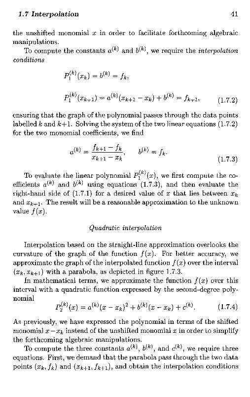
the unshifted monomial x in order to facilitate forthcoming algebraicmanipulations.

To compute the constants a^ and b^k\ we require the interpolationconditions

Pik\xk)=bW = fk,

Pj* Wi) ^ a(*Wi - Xk) + bW = A+i, (1.7.2)

ensuring that the graph of the polynomial passes through the data pointslabelled k and k+l. Solving the system of the two linear equations (1.7.2)for the two monomial coefficients, we find

(1.7.3)

(k}To evaluate the linear polynomial P± '(a;), we first compute the co-efficients a,№ and &W using equations (1.7.3), and then evaluate theright-hand side of (1.7.1) for a desired value of x that lies between xk

and xjb+i. The result will be a reasonable approximation to the unknownvalue f ( x ) .

Quadratic interpolation

Interpolation based on the straight-line approximation overlooks thecurvature of the graph of the function f ( x ) . For better accuracy, weapproximate the graph of the interpolated function f ( x ) over the interval(xk,xk+i) with a parabola, as depicted in figure 1.7.3.

In mathematical terms, we approximate the function f ( x ) over thisinterval with a quadratic function expressed by the second-degree poly-nomial

pW(x) - a№(x - xk)2 + bW(x - xk) + c«. (1.7.4)

As previously, we have expressed the polynomial in terms of the shiftedmonomial x - xk instead of the unshifted monomial x in order to simplifythe forthcoming algebraic manipulations.

To compute the three constants a^k\ b^k\ and c^k\ we require threeequations. First, we demand that the parabola pass through the two datapoints (xk,fk) and (#&+!? A+I)? and obtain the interpolation conditions

Figure 1.7.3 Local approximation of a function with a parabolic inter-polating function represented by the thick dashed line.

(1.7.5)

One more data point is required, and we may choose either the backwardpoint (#fc_i , / fc_i ) , or the forward point (x/c+25/fc+2)- The backwardchoice provides us with the condition

"(1.7.6)With the choice expressed by equations (1.7.5) and (1.7.6), the coef-

ficients of the binomial are found to be

(1.7.7)

where(1.7.8)

are the lengths of the backward and forward intervals.When the data points are spaced evenly, /i/c-i = hk — /i, we obtain

the simplified expressions

c(k) _ f

-fk' (1.7.9)

To evaluate P2 (^)? we ^TS^ compute the coefficients c№\ b^ andc^ using the preceding equations, and then evaluate the right-hand sideof (1.7.4). The result will be an improved approximation to f ( x ) .

1.7.2 Interpolation in two dimensions

Consider now a function / of two independent variables x and y. Forthe present puposes, a function of two variables is an engine that receivesthe pair of numbers x and y and produces the new number /(#,y).

Assume that we are given the values of the function f ( x , y ) at thenodes of a two-dimensional grid defined by the intersections of the re-level lines Xi, where i = 1,2, . . . , Nx + 1, and the y-level lines y^, wherej — 1,2, . . . , Ny + 1, as shown in figure 1.7.1(b). A grid-node is definedby the values of the indices i and j forming the ordered integer doublet(i,j), as illustrated in figure 1.7.1(b). The value of the function f ( x , y )at the ( i , j ) node is equal to f(x^yj}. Our goal is to compute the valueof / at a point ( x , y ) that is not necessarily a node.

Suppose that the value of x lies inside the kxth ^-interval confinedbetween the Xkx and Xkx+i x-level lines, and the value of y lies insidethe kyth y-interval confined between the y^y and yky+i y-level lines, asshown in figure 1.7.4. The values of kx and ky may be found by themethods discussed in Section 1.7.1 for one-dimensional interpolation.

Bilinear interpolation

An approximation to /(#, y) may be obtained by replacing the un-k k

known function /(x,y) with the function PB£ y(x,y) defined over therectangular domain that is confined between the a>level lines x = X k x ,x = Xkx+I, and the y-level lines y = yky, and y = y^+i- The bilinear

function P^ y(x,y) is endowed with the following properties:

k k1. For a fixed value of x, call it XQ, the function PB

X£ y(x$,y} varieslinearly with respect to y.

Figure 1.7.4 Bilinear interpolation of a scalar function through a rect-angular grid.

k k2. For a fixed value of y, call it yo? the function PQ^ y(x,yo) varieslinearly with respect to x.

3. The following four interpolation conditions ensuring that the bilin-ear function reproduces the neighboring grid values are met:

(1.7.10)

The first and second of the above properties require that the bilinearfunction have the functional form

(1.7.11)

To evaluate the four constants axx' y', bx

x' y', Oyx' y', and byxi y , we use

the four interpolation conditions (1.7.10), finding

(1.7.12)where we have introduced the position-dependent interpolation weights

(1.7.13)

The numerators AQQ, AIQ, An? and AU are the areas of the four sub-rectangles depicted in figure 1.7.4, given by

A)O = (zkx+i - x)(yky+i - y), Aw = (x- xkx)(yky+i - y),

An = (fffcx+i ~ x ) ( y - yky), AH = (x- x k x ) ( y - yky), 7

The denominator A is the area of the interpolation rectangle, given by

A = (xkx+i ~ %kx)(yky+i ~ yky)' (1.7.15)

It is reassuring to observe that the sum of the four interpolationweights given in (1.7.13) is equal to unity independent of the values of xand y,

WOQ(X, y) + WIQ(X,y) + WQI(X,y) + wn(x,y) = 1. (1.7.16)

This property guarantees that, if the four grid values

f ( x k x , y k y ] , f ( x k x , V k y + i ) , / (a?fa+i>y*»)> /(***+!> Mby+i)

are the same, equal to a, then bilinear interpolation based on (1.7.12)produces

A* kPBL y (xi y) = a (^QO + WIO + WQI + Wn) = a, (1.7.17)

as required.

1.7.3 Interpolation of the velocity in a two-dimensional flow

Returning to fluid mechanics, we consider a two-dimensional flow inthe xy plane, and specify the values of the x and y velocity componentsUx and Uy at the nodes of a two-dimensional Cartesian grid. To obtainthe corresponding values at an arbitary point (x, y), we employ bilinearinterpolation, finding

(1.7.18)and

(1.7.19)Our ability to interpolate the velocity components at any point in a

flow from specified grid values allows us to generate particle paths andstreamlines without having available explicit expressions for the velocityin analytical form. In practice, the grid values are computed by solv-ing the equations governing the motion of the fluid using a variety ofnumerical methods, as will be discussed later in this text.

Problems

Problem 1.7.1 Quadratic interpolation.Solve the linear system of three equations (1.7.5) and (1.7.6) to derive

formulas (1.7.7). Hint: Compute first the coefficient c^ using the firstof equations (1.7.5).

Problem 1.7.2 Forward-point parabolic interpolation.Consider the parabolic interpolation of a function of one variable

/(x), as discussed in the text. Forward interpolation uses the interpola-tion condition

(1.7.20)

in place of (1.7.6). Derive expressions for the coefficients c№\ b^k\ andc^ in terms of the grid values /^, /fc+i, and /^+2, and the interval sizeshk and /ifc+i- Then derive simplified expressions when h^ and /ifc+i areequal to h.

Problem 1.7.3 Trilinear interpolation.Consider a function of three variables /(#, y, 2). Extend the method

of bilinear interpolation of a function of two variables discussed in thetext, to the method of trilinear interpolation that generates the value of/ at an arbitrary point (x^y^z) using the values of / at the nodes of athree-dimensional Cartesian grid. The interpolation formula should bethe counterpart of (1.7.12) with properly defined interpolation weights.

Computer problems

Problem c. 1.7.1 Bilinear interpolation.Directory 02-grids/rec-2d of FDLIB contains a program that inter-

polates the x and y components of the velocity and draws the velocityvector field over a rectangular domain confined between ax < x < bx

and ay < y < by. The interpolation is based on specified values of thevelocity at the nodes of a uniform Nx x Ny Cartesian grid, as shown infigure 1.7.5.

(a) Run the program for a velocity field of your choice offered in themain, confirm that the interpolated values are identical to the specifiedgrid values, and prepare a plot of the velcocity vector field similar tothat displayed in figure 1.7.5.

(b) Enhance the menu with a new flow of your choice; plot and discussthe structure of the velocity field.

Problem c.1.7.2 Streamlines by interpolation.Directory 02-grids/rec-2d-strmll of FDLIB contains a program that

generates streamlines originating from specified points in a rectangulardomain of a two-dimensional flow. The velocity components are com-puted by bilinear interpolation based on specified grid values.

(a) Run the program for a velocity field of your choice offered in themain menu, generate, plot, and discuss the streamline pattern.

(b) Enhance the main menu with a new flow of your choice, plot anddiscuss the streamline pattern.

Figure 1.7.5 Bilinear interpolation of a velocity vector field through aCartesian grid in a two-dimensional flow.

2.1 Fundamental modes of fluid parcel motion2.2 Fluid parcel expansion2.3 Fluid parcel rotation and vorticity2.4 Fluid parcel deformation2.5 Numerical differentiation2.6 Areal and volumetric flow rate2.7 Mass flow rate, mass conservation,

and the continuity equation2.8 Properties of point particles2.9 Incompressible fluids and stream functions

2.10 Kinematic conditions at boundaries

We continue the study of kinematics by considering, in more detail,the behavior of fluid parcels, by deriving expressions for the volumetricand mass flow rate across surfaces drawn in a fluid, and by developingnumerical methods for evaluating kinematical variables defined in termsof derivatives or integrals of the velocity. Conservation of mass requiredby thermodynamics, and physical conditions imposed at boundaries in-troduce mathematical constraints that motivate the description of a flowin terms of ancillary functions that expedite analysis and numerical com-putation.

2,1 Fundamental modes of fluid parcel motion

In Chapter 1, we pointed out that the nature of the motion of asmall fluid parcel is determined by the relative motion of point particlesresiding within the parcel and over its boundary. If, for example, thevelocity of all point particles is nearly the same, that is, variations in thepoint particle velocity are small compared to the average velocity, then

Chapter 2

Fluid Motion: More on Kinematics

the parcel exhibits rigid-body translation. Significant variations in thepoint particle velocity generate more general types of motion includinglocal rotation, deformation, and isotropic expansion.

To study the relative motion of point particles in the vicinity of acertain point XQ = (XQ ,yo ?£( ) )? we consider differences in correspondingcomponents of the velocity evaluated at a point x = (#, y, z) that liesclose to XQ, and at the chosen point XQ. If the differences are smallcompared to the distance between the points x and XQ, both measuredin proper units, the relative motion is negligible. If the differences aresubstantial, the relative motion is significant and needs to be properlyanalyzed.

2.1.1 Function linearization

To prepare the ground for this analysis, we consider a scalar functionof three independent variables that receives a triplet of numbers (x, y, z)and produces the number f(x,y,z). If the function / is locally wellbehaved, and the point x lies near the point XQ, then the value /(#, y, z)is expected to be close to the value / ( X Q ^ Q , ZQ). Stated differently, inthe limit as all three scalar differences X - X Q , y — UQ, and z — ZQ tend tovanish, meaning that x tends to XQ, the difference in the function valuesf(x,y,z) — /(XQ^Q^ZQ) will also tend to vanish.

Now, the variable point x may approach the fixed point XQ frommany different directions. Selecting the direction that is parallel to thex axis, we set x = (x ,yo?^o)? and consider the limit of the difference/(#, yo>2o) — /(XQ^Q^ZQ) as x — XQ tends to zero. Because the function/ has been assumed to be well behaved, the ratio of the differences

(2.1.1)

tends to a finite number defined as the first partial derivative of the func-tion / with respect to the variable x evaluated at the point XQ, denotedby (df /OX)(XQ). Elementary calculus ensures that the partial derivativemay be computed using the usual rules of differentiation of a functionof one variable with respect to x, regarding the other independent vari-ables as constant. For example, if / = xyz, then d f / d x = yz, and(df/dx)(xQ) = yQZQ,

Setting the fraction shown in (2.1.1) equal to (df/dx)(XQ), and solv-ing the resulting equation for /(#,3/0? ^Q), we find

(2.1.2)

It is important to bear in mind that this equation is exact only in thelimit as Ax = X-XQ tends to zero. For small but non-infinitesimal valuesof Ax, the difference between the left- and right-hand side is on the orderof Ax2, which, however, is small compared to Ax. For example, if Ax isequal to 0.01 is some units, then Ax2 is equal to 0.0001 in correspondingunits.

The point x may also approach the point XQ along the y or z axis,yielding the counterparts of (2.1.2),

(2.1.3)

and

(2.1.4)

Combining the arguments that led us to equations (2.1.2)-(2.1.4), we letthe point x approach the point XQ from an arbitrary direction, and derivethe approximation

(2.1.5)

We pause to emphasize that relation (2.1.5) is exact only in the limitas all three differences Ax = x — XQ, Ay = y — yo, and Az = z — ZQ tendto zero. For small but non-infinitesimal values of any of these differences,the left-hand side of (2.1.5) differs from the right-hand side by an amountthat is generally on the order of the maximum of Ax2, Ay2 or Az2.

Equation (2.1.5) can be made exact for any value of Ax, Ay, or Az,by adding to the right-hand side a term called the remainder. Clearly,as all three differences Ax, Ay, and Az tend to zero, the remaindermust vanish. Elementary calculus shows that when Ax, Ay, and Az aresufficiently small, the remainder may be expressed as an infinite seriesinvolving products of powers of Ax, Ay, and Az, called the Taylor seriesof the function / about the point XQ.

The process of deriving (2.1.5) is called linearization of the function/ about the point XQ. The linearized form (2.1.5) states that, in the

immediate vicinity of a point XQ, any regular function resembles a linearfunction of the shifted monomials Ax, Ay, and Az. If all three firstpartial derivatives vanish at the point XQ, then / behaves like a quadraticfunction; this, however, is an exception.

Gradient of a scalar function

To economize our notation, we introduce the gradient of the function/, denoted by V/ defined as the vector of the three partial derivatives,

(2.1.6)

where ex, ey, and ez are the unit vectors along the x,y, and z axes.The symbol V is a vector operator called the del or gradient operator,defined as

(2.1.7)

Unlike a regular vector, V may not stand alone but must operate on ascalar function of position from the left to acquire a meaningful inter-pretation.

Inner vector product

As a second preliminary, we introduce the inner product of two three-dimensional vectors f = (fxifyifz) and g = (gx>9y>9z) defined as thescalar

f ' g = fx 9x + fy 9y + fz 9z- (2.1.8)

In index notation,

f ' S = fi9i, (2.1.9)

where summation of the repeated index i is implied over x, y, and z, asrequired by Einstein's repeated-index summation convention: if an indexappears twice in a product, then summation of that index is implied overits range.

It can be shown using elementary trigonometry that the inner prod-uct defined in (2.1.8) is equal to the product of (a) the length of the firstvector f, (b) the length of the second vector g, and (c) the cosine of theangle subtended between the two vectors. If the angle is equal to Tr/2,that is, the two vectors are orthogonal, the cosine of the angle is equal to

zero, and the inner product vanishes. If the angle is equal to zero, thatis, the two vectors are parallel, the inner product is equal to the productof the lengths of the two vectors. If both f and g are unit vectors, thatis, their lengths are equal to one unit of length, then the inner productis equal to the cosine of the subtended angle.

Linearized expansion in compact form

Subject to the preceding definitions, equation (2.1.5) may be writtenin the compact vector form

/(x) ~ /(X0) + (x- X0) - (V/)XO, (2.1.10)

where the subscript XQ denotes that the gradient V/ is evaluated at thepoint XQ. The second term on the right-hand side of (2.1.10) is the innerproduct of (a) the relative position vector X - X Q , and (b) the gradientvector V/.

2.1.2 Velocity gradient tensor

To derive the linearized form of the velocity field in the vicinity ofthe point XQ, we identify the function / with the #, y, or z component ofthe velocity, Ux, uy, or uz, and obtain

(2.1.11)Collecting these equations into the unified vector form, we obtain

u(x) ~ u(x0) + (x - X0) • A(X0), (2.1.12)

where A is a 3 x 3 matrix called the velocity gradient tensor, defined as

(2.1.13)

The notation A(XQ) in (2.1.12) emphasizes that the nine components ofthe velocity gradient tensor are evaluated at the chosen point XQ aroundwhich linearization has taken place.

As an example, the velocity gradient corresponding to the velocityfield expressed by equations (1.4.7) is given by the matrix A defined as

(2.1.14)

Placing the point XQ at the location ( X O , T / O ? ^ O ) — ( I 5 O 5 O ) , we obtain

(2.1.15)

Thus, in the vicinity of the point (1,0,0), the flow expressed by equations(1.4.7) may be approximated with a linear flow expressed by

(2.1.16)

The right-hand sides of equations (2.1.16) are linear functions of thespatial coordinates x, y, and z.

Tensorial nature of a matrix

The velocity gradient tensor is a matrix containing the three firstpartial derivatives of the three components of the velocity with respectto x, y, and z, a total of nine scalar elements. Why have we called thismatrix a tensor?

A tensor is a matrix whose elements are physical entities evaluatedwith reference to a chosen system of Cartesian or polar coordinates. Ifthe coordinate system is changed, for example, by translation or rota-tion, then the elements of the matrix will also change to reflect the newdirections. This change is analogous to that undergone by the compo-nents of the position or velocity vector, occurring by referring to a newsystem of coordinates, as discussed in Section 1.5.

Now, if the elements of the matrix corresponding to the new systemare related to the elements corresponding to the old system by certain

rules discussed in texts of matrix calculus, then the matrix is called atensor. Establishing whether or not a matrix is a tensor is important inderiving physical laws relating matrices with different physical interpre-tations.

2.1.3 Relative motion of point particles

According to equation (2.1.12), the motion of a point particle that isclose to the point XQ is governed by the equation

(2.1.17)

where X is the position of the point particle, and u is the point-particlevelocity, equal to the local and instantaneous fluid velocity. The firstterm on the right-hand side of (2.1.17) states that a point particle locatedat X translates with the velocity of the point particle located at XQ.The second term expresses the relative motion with respect to the pointparticle located at XQ. Different velocity gradient tensors A(XQ) representdifferent types of relative motion; our goal is to establish the nature ofthis motion in terms of the components of A(XQ).

2.1.4 Rotation, deformation, and expansionin two-dimensional flow

To begin, we consider a two-dimensional flow in the xy plane, andintroduce the 2 x 2 velocity gradient tensor

(2.1.18)

In Section 1.6, we studied the velocity field associated with the linearflow expressed by equation (1.6.33). Comparing equations (2.1.12) and(2.1.18) with equation (1.6.33), we set

(2.1.19)

where all partial derivatives are evaluated at XQ.To study the properties of the linearized flow, we carry out the de-

composition shown in equation (1.6.34), setting

(2.1.20)

where

(2.1.21)

is a skew-symmetric matrix with zero trace called the vorticity tensor,

(2.1.22)

is a symmetric matrix with zero trace called the rate of deformationtensor, and the scalar

(2.1.23)

is the areal rate of expansion.

Expansion

The results of Section 1.6 suggest that a fluid parcel centered at thepoint XQ expands isotropically with an areal rate of expansion that isequal to the right-hand side of (2.1.23) evaluated at XQ, as illustrated infigure 2.1.1.

Rotation

Referring to equation (1.6.35), we find that a fluid parcel centered atthe point XQ rotates in the xy plane around the point XQ, with angularvelocity

(2.1.24)

where the right-hand side is evaluated at XQ, as shown in figure 2.1.1.When f2 is positive, the parcel rotates in the counter-clockwise direction,whereas when fi is negative, the parcel rotates in the clockwise direction.

Expansion Rotation Deformation

Figure 2.1,1 Expansion, rotation, and deformation of a small discoidalfluid parcel in a two-dimensional flow, occurring during an infinites-imal period of time.

Deformation

The discussion in Section 1.6 suggests that the flow associated withthe rate of deformation tensor E expresses pure deformation, as illustrat-ed in figure 2.1.1. To compute the rate of deformation G, we search forthe eigenvalues of E. Denoting Exx = E\\, and similarly for the othercomponents, and taking into account that, by definition, Exx + Eyy = O,and Exy — Eyx, we find

(2.1.25)

The corresponding eigenvectors define the principal directions of the rateof strain. It can be shown that, because E is symmetric, the two eigevec-tors are mutually orthogonal.

Each one of the two eigenvalues of the rate of strain tensor expressesthe rate of deformation of a circular fluid parcel centered at the pointXQ, in the direction of the respective eigenvector. A theorem of matrixcalculus requires that the sum of the eigenvalues be equal to the sumof the diagonal elements of E, which is equal to zero. Because of thisproperty, the deformation conserves the area of the parcel during themotion.

2.1.5 Three-dimensional flow

Extending the preceding analysis to three-dimensional flow, we de-compose the velocity gradient tensor into three parts, as

Expansion Rotation Deformation

Figure 2.1.2 Expansion, rotation, and deformation of a small spher-ical fluid parcel in a three-dimensional flow, occurring during aninfinitesimal period of time.

(2.1.26)

where

(2.1.27)

is the skew-symmetric vorticity tensor,

(2.1.28)

is the symmetric and traceless rate of deformation tensor, and the scalarcoefficient

(2.1.29)

is the volumetric rate of expansion.

The three terms on the right-hand side of (2.1.26) express, respec-tively, isotropic expansion, rotation, and pure deformation, as illustratedin figure 2.1.2. Because of the fundamental significance of these motionsin fluid mechanics, these terms will be given individual attention in thenext three sections.

Problems

Problem 2.1.1 Inner vector product.Prove the intepretation of the inner vector product described after

equation (2.1.9).

Problem 2.1.2 Decomposition of a linearized flow.Linearize the velocity described by equations (1.5.2) around the origin

of the y axis, and decompose the velocity gradient tensor of the linearizedflow into the three modes shown on the right-hand side of (2.1.26).

Problem 2.1.3 Decomposition of a linearized flow.Decompose the velocity gradient tensor of the linearized flow ex-

pressed by equations (2.1.16) into the three modes shown on the right-hand side of (2.1.26).

Problem 2.1.4 Gradient in cylindrical polar coordinates.In the cylindrical polar coordinates depicted in figure 1.3.2, the gra-

dient of a scalar function / is defined by its cylindrical polar componentsFx, Ft,, and F^, as

V/ = Fx ex + FV eff + Fp e^. (2.1.30)

Using the transformation rules shown in equations (1.3.17), we find

(2.1.31)

To express the derivatives with respect to y and z in terms of derivativeswith respect to polar cylindrical coordinates, we use the chain rule ofdifferentiation along with the coordinate transformation rules (1.3.11)and (1.3.12), and find

(2.1.32)

(2.1.33)

Substitute relations (2.1.32) and (2.1.33) into the right-hand sides ofrelations (2.1.31), and thus derive the relations

(2.1.34)

Equations (2.1.34) illustrate that the polar components of the gradi-ent are equal to the partial derivatives with respect to the correspondingvariable, multiplied by an appropriate scaling factor.

Problem 2.1.5 Gradient in spherical polar coordinates.In the spherical polar coordinates depicted in figure 1.3.3, the gra-

dient of a scalar function / is defined by its spherical polar componentsFr, FQ, and F^, as

V/ - FT er + F6 ee + F^ ev. (2.1.35)

Working as in problem 2.1.4, show that

(2.1.36)

Note that the expression for F^ is consistent with that given in the thirdof relations (2.1.34), subject to the substitution a = r sin#.

Problem 2.1.6 Gradient in plane polar coordinates.In the plane polar coordinates depicted in figure 1.3.4, the gradient

of a scalar function / is defined by its plane polar components Fr andFe, as

V/ = F re r+F0e0. (2.1.37)

Working as in problem 2.1.4, show that

(2.1.38)

2.2 Fluid parcel expansion

Consider the velocity field associated with the third term on theright-hand side of (2.1.26), given by

(2.2.1)

Under the influence of this field, a spherical fluid parcel centered at thepoint XQ expands when the coefficient a(xo) is positive, or contractswhen the coefficient a(XQ) is negative, always maintaining the sphericalshape.

To see this more clearly, we consider the motion of a point particlethat lies at the surface of the spherical parcel. Using (2.2.1), we findthat the radius of the parcel a(t), is given by

(2.2.2)

Raising both sides of equation (2.2.2) to the third power, and multiplyingthe result by the factor 47T/3, we find that the ratio of the instantaneousto the initial parcel volume is given by

(2.2.3) .

This result explains why the constant a is called the rate of volumetricexpansion.

2.2.1 Divergence of the velocity field

The rate of expansion defined in equation (2.1.29) may be expressedin compact form that simplifies the notation. Taking the inner productof the del operator defined in (2.1.7) and the velocity, we find

(2.2.4)

In index notation,

(2.2.5)

where summation of the repeated index i is implied over x, y, and z.In the case of two-dimensional flow in the xy plane, the derivative withrespect to z does not appear.

Accordingly, we writea - V - u . (2.2.6)

The right-hand side of (2.2.6) is defined as the divergence of the velocity.

2.2.2 Solenoidal velocity fields

We have found that the rate of volumetric expansion at a point ina three-dimensional flow, or the areal rate of expansion at a point in atwo-dimensional flow, is equal to the divergence of the velocity evaluatedat that point. If the divergence of the velocity vanishes at every pointin the flow, with the physical consequence that no fluid parcel under-goes expansion but only translation, rotation, and deformation, then thevelocity field is called solenoidal.

Problem

Problem 2.2.1 Rate of expansion.Derive the rate of expansion of the flow described by equations (1.4.7),

and then evaluate it at the point XQ = (1,0,1).

2.3 Fluid parcel rotation and vorticity

Consider the velocity field associated with the first term on the right-hand side of (2.1.26), given by

uRatatim(x,ytz) = (x - X0) • 2(X0), (2 3 1}

where S is the vorticity tensor defined in equation (2.1.27).An areal fluid parcel in a two-dimensional flow occurring in the xy

plane may only rotate around the z axis. In contrast, a three-dimensionalfluid parcel in a three-dimensional flow may rotate around any arbitraryaxis that passes through the designated center of rotation XQ and pointsin an arbitrary direction. The direction, magnitude, and sense of therotation define the angular velocity vector fi whose components may be

deduced from the three upper triangular or three lower triangular entriesof the vorticity tensor shown on the left-hand side of (2.1.27), and aregiven by

(2.3.2)

where the right-hand sides are evaluated at the designated parcel centerXQ. As we look down into the vector fi from the tip of its arrow, thefluid rotates in the clockwise direction.

Equation (2.3.1) may be recast into a compact form in terms of theangular velocity vector, as

(2.3.3)

where $1 derives from the velocity by means of (2.3.2).The three components of the angular velocity vector arise by com-

bining selected partial derivatives of the components of the velocity ina particular fashion. Stated differently, the angular velocity vector fieldarises from the velocity field by operating on it with a differential op-erator, just as the rate of expansion arises from the velocity field byoperating on it with the divergence operator (V-), as discussed in Sec-tion 2.2.

2.3.1 Outer vector product

To identify the differential operator that generates the angular ve-locity field from the velocity field according to equations (2.3.2), weintroduce the outer vector product.

Consider a vector f = (/^, /^, /^), and another vector g = (gx, gy,gz}\the outer product of the first vector with the second vector, stated inthis particular order, is a new vector denoted by f x g, defined as

(2.3.4)

where ex, ey, and ez are the unit vectors along the #,y, and z axis.

Figure 2.3.1 The outer product of two vectors f and g is a new vectorperpendicular to their plane.

It can be shown that the vector f x g is normal to the plane definedby f and g, as illustrated in figure 2.3.1, and its magnitude is equal to theproduct of (a) the length of the vector f, (b) the length of the vector g,and (c) the absolute value of the sine of the angle 6 subtended betweenthe two vectors. The orientation of f x g is chosen such that, as we lookdown at the plane defined by f and g towards the negative direction off x g, the angle O measured in the counterclockwise direction from f isless than 180°. If 6 is equal to O or TT, that is, if the two vectors areparallel or anti-parallel, then the sine of the angle is equal to zero, andthe outer product vanishes. The directions indicated by the three vectorsf, g, and f x g, arranged in this particular order, form a right-handedsystem of axes. This is another way of saying that f x g arises from fand g according to the right-hand rule.

Using the definition of the cross product, we recast equation (2.3.3)into the form

u*otaiio"(z,M = ^ X ( X - X 0 ) , (2.3.5)

which is the classical definition of rigid-body rotation around the pointXQ with angular velocity fi, in agreement with the previously statedphysical interpretation.

2.3.2 Curl and vorticity

Taking the outer product of the del operator and the velocity field,we obtain the curl of the velocity defined as the vorticity,

(2.3.6)

Comparing equation (2.3.6) with equations (2.3.2), we find

n = 2"' (2.3.7)

which shows that the angular velocity vector is equal to half the vorticityvector, or half the curl of the velocity.

2.3.3 Irrotational flow

If the curl of a velocity field vanishes at every point in a flow, withthe consequence that no spherical fluid parcel undergoes rotation, thenthe velocity field is called irrotational. The properties and computationof irrotational flow will be discussed in Chapter 3, and then again inChapter 12 in the context of aerodynamics.

2.3.4 The alternating tensor

The long expression on the right-hand side of equation (2.3.4) defin-ing the outer vector product is cumbersome. To simplify the notation,we introduce the three-index alternating tensor e^, defined as follows:

1. K i = j, or j = /c, or k — i, then e^ = O. For example, exxy =tzyz — tzyy = O.

2. If i,j, and k are all different, then e^ = ±1. The plus sign applieswhen the triplet ijk is a cyclic permutation of xyz, and the minussign applies otherwise. For example, exyz = ezxy = eyzx = 1, but^xzy — ~1-

Two important properties of the alternating tensor stemming from itsdefinition are

tijk eljk — 2 Su, (2.3.8)

where summation of the repeated indices j and k is implied on the left-hand side, and

(2.3.9)

where summation of the repeated index k is implied on the left-handside. Kronecker's delta 6ij represents «the identity matrix: Sij = 1 ifi = j? or O if i ^ j. Additional properties of the alternating tensor arelisted in problem 2.3.2.

In terms of the alternating tensor, the ith component of the outerproduct f x g defined in equation (2.3.4) is given by

(f x g); = €ijk Jj Qk, (2.3.10)

where summation of the two repeated indices j and k is implied on theright-hand side.

Using the definition (2.3.6), we find that the ith component of thevorticity is given by

_ duk

^~^k Qx.' (2.3.11)

A straightforward manipulation of (2.3.11) provides us with an ex-pression for the vorticity vector in terms of the vorticity tensor

(2.3.12)

The converse relationship is (problem 2.3.3)

(2.3.13)


Consider a two-dimensional flow in the xy plane. Inspection of theright-hand side of (2.3.6) shows that the x and y components of thevorticity vanish, and the vorticity vector is parallel to the z axis andthus perpendicular to the plane of the flow,

u = uzez, (2.3.14)

where ez is the unit vector along the z axis. The scalar ujz is the strengthof the vorticity, defined as

(2.3.15)

Using the transformation rules discussed in Section 1.1, we find that,in the plane polar coordinates depicted in figure 1.1.4, the strength ofthe vorticity is given by

(2.3.16)


Consider next an axisymmetric flow without swirling motion, andrefer to the polar cylindrical coordinates (x, a, (p) depicted in figure 1.1.2,and to the spherical polar coordinates (r, #,</?) depicted in figure 1.1.3.A fluid patch that lies in a meridional plane over which (p is constant,is able to rotate only around an axis that is perpendicular to this planeand thus points in the direction of increasing or decreasing angle (p. Thisobservation suggests that the vorticity vector takes the form

w = a;y,ep, (2.3.17)

where e^ is the unit vector pointing in the meridional direction, and UJ^is the strength of the vorticity given by

(2.3.18)

Note that the expression in spherical polar coordinates given on theright-hand side of (2.3.18) is identical to that in plane polar coordinatesgiven in (2.3.16).

Problems

Problem 2.3.1 Properties of the outer vector product.(a) With the outer vector product defined in equation (2.3.4), show

that

f xg = - g x f . (2.3.19)

(b) The outer vector product of two vectors f and g may be identifiedwith the determinant of a matrix,

(2.3.20)

Show that this rule is consistent with the definition of the curl in (2.3.6).

Problem 2.3.2 Properties of Kronecker's delta and alternating tensor.Prove the properties:

Su = 3, eijk Sjk = O, CLJ Sjk = a*, AIJ 6jk = AM, , .

where Sij is Kronecker's delta representing the 3 x 3 identity matrix,summation is implied over a repeated index, a is an arbitrary vector andA is an arbitrary matrix.

Problem 2.3.3 Relation between the vorticity tensor and vector.Prove relation (2.3.13). Hint: Express the vorticity in terms of the

velocity as shown in (2.3.11), and then use property (2.3.9).

Problem 2.3.4 Solenoidal nature of the vorticity field.Show that V • u = O; that is, the vorticity field is solenoidal.

2.4 Fluid parcel deformation

Consider the velocity field associated with the second term on theright-hand side of (2.1.26), given by

Reformation^ z) = (x _ XQ) . ̂ ),

where E is the symmetric rate of deformation tensor defined in equation(2.1.28).

To develop insights into the nature of the motion described by (2.4.1),we consider a special case where E(XQ) is diagonal, given by

(2.4.2)

with the understanding that the right-hand side is evaluated at the pointXQ. The matrix (2.4.2) has three real eigenvalues that are equal to thediagonal elements; the corresponding eigenvectors point along the x,y,or z axes.

Cursory inspection reveals that, under the action of the flow de-scribed by (2.4.1) and (2.4.2), a spherical fluid parcel centered at thepoint XQ deforms to obtain an ellipsoidal shape while preserving its vol-ume, as illustrated in figure 2.1.2. The three eigenvalues of the rate ofdeformation tensor express the rate of deformation in the three principaldirections corresponding to the eigenvectors. If an eigenvalue is negative,then the parcel is compressed in the corresponding direction to obtainan oblate shape.

More generally, the rate of deformation tensor has three real eigen-values, AI, A2, and AS, that are found by setting the determinant of thematrix

(2.4.3)

equal to zero, and then computing the roots of the emerging cubicequation for A, as will be discussed later in this section. It can be shownthat, because E is symmetric, all three eigenvalues are real, and eacheigenvalue has a distinct corresponding eigenvector. Moreover, the threeeigevectors are mutually orthogonal, pointing in the principal directionsof the rate of strain.

Under the action of the flow (2.4.1), a spherical fluid parcel centeredat the point XQ deforms to obtain an ellipsoidal shape whose axes aregenerally inclined with respect to the #, y, and z axes. The three axes ofthe ellipsoid are parallel to the eigenvectors of E, and the respective ratesof deformation are equal to the corresponding eigenvalues. A theoremof matrix calculus states that the sum of the eigenvalues is equal to the

sum of the diagonal elements of E, which is equal to zero. Because ofthis property, the deformation conserves the parcel volume.

2.4.1 Computation of the rate of strain

Setting the determinant of the matrix (2.4.3) equal to zero, we obtainthe cubic equation

A3 + a\2 + bX + c = O, /2 4 ̂

where

a = -Trace(E) = -(Exx + Eyy + Ezz),

b — (EyyEZZ - EyZEZy) + (EXXEZZ — EXZEZX) + (EXXEyy ~ EXyEyX),

c = -Det(E),(2.4.5)

and Det stands for the determinant. Using Cardano's formulae, we findthat the three roots of (2.4.4), are given by

(2.4.6)

where

(2.4.7)

In the present case, because a = O, we obtain the simplified expres-sions

(2.4.8)

where

(2.4.9)

Once the eigenvalues have been found, the eigenvectors are computedby solving a homogeneous system of three equations for three unknowns.For example, the eigenvector e^1) = (ex , ey , e^ ' ) corresponding to theeigenvalue AI is found by solving the homogeneous system

(E - AiI) • eW = O, (2.4.10)

which can be restated as

(2.4.11)

To solve the system (2.4.11), we assign an arbitrary value to GZ on theright-hand sides, and solve the first two equations for ex , and ey ' using,for example, Cramer's rule. The solution is guaranteed to also satisfythe third equation. A solution will not exist when the eigenvector isperpendicular to the z axis, in which case ei ' is equal to zero. If thisoccurs, we simply transfer to the right-hand side the term involving exor ey , and solve for the other two components.

Problem

Problem 2.4.1 Properties of eigenvalues.(a) Confirm that the sum of the three eigenvalues given in (2.4.6) is

equal to the trace of E.(b) Confirm that the product of the three eigenvalues given in (2.4.6)

is equal to the determinant of E.(c) Confirm that, when E is diagonal, formulae (2.4.6) identify the

eigenvalues with the diagonal elements.

Computer problem

Problem c.2.4.1 Eigenvalues and eigenvectors.Directory Ol-num-meth/05-eigen of FDLIB contains program eigenSS

that computes the eigenvalues of a 3 x 3 matrix. Use the program to com-pute the eigenvalues and eigenvectors of the rate of deformation tensorcorresponding to the linearized flow (2.1.16) for a — ls~l and cdt — 2s"1.

2.5 Numerical differentiation

We have mentioned on an earlier occasion that, in practice, the com-ponents of the velocity field are hardly ever given in analytical form bymeans of analytical expressions. Instead, their values are either mea-sured in the laboratory with probes, or computed by numerical methodsat data points or grid nodes located in the domain of flow. The partialderivatives of the velocity are then recovered by a numerical procedurecalled numerical differentiation.

2.5.1 Numerical differentiation in one dimension

As a prelude to computing the partial derivatives of the componentsof the velocity from specified grid values, we consider computing the firstderivative of a function / of one independent variable x from specifiedgrid values. Assume that we are given the values of the function f ( x )at N + I nodes of a one-dimensional grid with nodes located at XI,i — 1 ,2 , . . . , N + 1, where x\ < x% < ... < #w+i, as shown in figure1.7.1 (a). Our goal is to compute the derivative df /dx at a point x thatlies within the kth interval subtended between the nodes XK and #fc+i.

First-order differentiation

A reasonable way of computing df /dx involves approximating thegraph of the function f ( x ) over the interval (xfaXk+i) with a straightline, as shown in figure 1.7.2, and then approximating df /dx with theslope. Using equations (1.7.1) and (1.7.3), we derive the finite-differenceapproximation

(2.5.1)

Identifying now the evaluation point x with the grid point x^, we obtainthe forward-difference approximation

(2.5.2)

Using, instead, the straight-line approximation for the k — 1 interval,we obtain the backward-difference approximation

(2.5.3)

Formulae (2.5.2) and (2.5.3) carry a comparable amount of error due tothe straight-line approximation.

To evaluate ^(#1), we use the forward difference; to evaluate ̂ (^ AM-I)we use the backward difference; to evaluate ^(xi) at an interior gridpoint, i = 2 , 3 , . . . , TV we use either the forward or the backward differ-ence approximation, whichever is more convenient or appropriate.

Second-order differentiation

Numerical differentiation based on linear interpolation discussed inthe preceding subsection neglects the curvature of the graph of the func-tion f ( x ) . To improve the accuracy, we approximate the graph of f ( x )over the interval (xk,Xk+i) with a parabola, as depicted in figure 1.7.3,and then approximate the slope of the function, df/dx, with the slopeof the parabola. Differentiating once the right-hand side of (1.7.4), wederive the second-order finite-difference approximation

(2.5.4)

where the coefficients a^ and b^ are given in (1.7.7).Identifying the evaluation point x with the grid point #&, we obtain

the centered-difference approximation

(2.5.5)

When the grid points are spaced evenly, x^ — x^-i — %k+i — xk = ^>where h is the grid spacing, we obtain the simple form

(2.5.6)

The parabolic approximation allows us to also obtain an estimatefor the second derivative d 2 f / d x 2 . Differentiating the right-hand side of(1.7.4) twice with respect to rrr, we derive the finite-difference approxi-mation

(2.5.7)

where the coefficient a^ is given in (1.7.7). When the grid points aredistributed evenly with spacing /i, we obtain the simpler form

(2.5.8)

2.5.2 Numerical differentiation in two dimensions

Consider now the computation of the first partial derivatives of afunction /(#, y) of two independent variables x and y, d f / d x and d f / d y ,given the values of the function at the nodes of a two-dimensional griddefined by the intersections of the re-level lines Xi, i = 1 ,2 , . . . , Nx + 1,and y-level lines y^, j — 1 ,2 , . . . , Ny + 1, as illustrated in figure 1.7.2.

Suppose that x lies within the kxth re-interval confined between theXkx and Xkx+I x-level lines, and y lies within the kyth y-interval confinedbetween the yky and y/^+i y-level lines.

First-order differentiation

Using the method of bilinear interpolation discussed in Section 1.7,we approximate the first partial derivatives of the function /(x,y) withthe partial derivatives of the bilinear function defined in equation (1.7.12).Considering the derivative with respect to x, we obtain the forward-difference approximation

(2.5.9)

Using expressions (1.7.13) and (1.7.14), we find

(2.5.10)

Recalling that A = (xkx+i-xkx)(yky+i-yky), as given in (1.7.15), we de-rive the first-order forward difference approximation for the southwesterngrid point,

(2.5.11)

A similar approximation of the y derivative yields

(2.5.12)

Second-order differentiation

Second-order centered-difference formulae for evaluating the first par-tial derivative of a function at a grid point may be derived on the basisof the one-dimensional formula (2.5.5). Using the expression for thecoeffient b^ given in equations (1.7.7), we obtain

(2.5.13)

The corresponding expression for the derivative with respect to y is

(2.5.14)

When the grid lines are spaced evenly, xkx -xkx_i = xkx+\-xkx = hx,and yky - yky-i = yky+i - yky = hy, we obtain the simpler forms

(2.5.15)

and

(2.5.16)

2.5.3 Numerical computation of the velocity gradientand related functions

The formulae derived previously in this section may be used to obtainapproximations to the elements of the velocity gradient tensor, rate ofdeformation tensor, vorticity tensor, vorticity vector, and rate of expan-sion, from specified values of the velocity at grid points. For illustration,we consider a two-dimensional flow and refer to a uniform grid withconstant x and y grid spacings equal to hx and hy.

Using the second-order centered-difference approximations (2.5.15)and (2.5.16), we find that the rate of expansion can be approximatedwith the finite difference formula

(2.5.17)

The corresponding finite-difference approximation for the strength ofthe vorticity is

(2.5.18)

Similar finite-difference approximations may be derived for the ele-ments of the rate of deformation tensor, and subsequently used to obtainapproximations to its eigenvalues and eigenevectors.

Problem

Problem 2.5.1 Numerical differentiation.Use formula (2.5.8) to evaluate the second derivative of the expo-

nential function f ( x ) = ex at x = O in terms of the values of f ( x ) atx = -h, O, h, for h = 0.16, 0.08, 0.04, 0.02, and 0.01. Then computethe error defined as the difference between the numerical and the exactvalue, plot it against h on a linear-log scale, and discuss the slope of thegraph.

Computer problem

Problem c.2.5.1 Numerical differentiation of a two-dimensional flow.Directory 02-.grids/rec-2d of FDLIB contains a program that com-

putes by interpolation: (a) the strength of the vorticity, (b) the rateof deformation tensor, and (c) the eigenvalues and eigenvectors of therate of deformation tensor, over a rectangular domain of flow confinedbetween ax < x < bx and ay < y < by. The input data specify thecomponents of the velocity at the nodes of a uniform TVx x Ny Cartesiangrid, as shown in figure 1.7.1(b).

(a) Run the program for two velocity fields offered in the main, pre-pare and discuss plots of the strength of the vorticity, eigenvalues, andeigenvectors of the rate of strain tensor.

(b) Enhance the menu with a new flow of your choice, and repeatpart (a).

2.6 Areal and volumetric flow rate

Consider a two-dimensional flow in the xy plane, and draw a linethat resides completely in the fluid. At any instant, point particles crossthe line, thereby generating a net, positive or negative, areal flow ratetowards a designated direction. Our goal is to quantify this flow rate interms of the shape of the line and the fluid velocity.

2.6.1 Unit tangent and unit normal vectors

Consider first an open line beginning at the point A and ending atthe point B, as shown in figure 2.6.1 (a). As a preliminary, we introducethe unit tangent vector, denoted by t = (tx,ty), defined as the vectorthat is tangential to the line at a point, and whose magnitude is equalto one unit of length; by definition, t^ + ty = 1. The direction of t ischosen such that, if we start traveling along the line from point A in thedirection of t, we will finally end up at point B.

Next, we introduce the unit normal vector, denoted by n = (nx,ny},defined as the vector that is perpendicular to the line at every point, andwhose magnitude is equal to one unit of length; by definition, n^.+ny = 1.The orientation of n is such that the tangent vector t arises by rotatingn around the z axis in the counterclockwise direction by an angle equaltO 7T/2.

Next Page

Computer problem

Problem c.2.5.1 Numerical differentiation of a two-dimensional flow.Directory 02-.grids/rec-2d of FDLIB contains a program that com-

putes by interpolation: (a) the strength of the vorticity, (b) the rateof deformation tensor, and (c) the eigenvalues and eigenvectors of therate of deformation tensor, over a rectangular domain of flow confinedbetween ax < x < bx and ay < y < by. The input data specify thecomponents of the velocity at the nodes of a uniform TVx x Ny Cartesiangrid, as shown in figure 1.7.1(b).

(a) Run the program for two velocity fields offered in the main, pre-pare and discuss plots of the strength of the vorticity, eigenvalues, andeigenvectors of the rate of strain tensor.

(b) Enhance the menu with a new flow of your choice, and repeatpart (a).

2.6 Areal and volumetric flow rate

Consider a two-dimensional flow in the xy plane, and draw a linethat resides completely in the fluid. At any instant, point particles crossthe line, thereby generating a net, positive or negative, areal flow ratetowards a designated direction. Our goal is to quantify this flow rate interms of the shape of the line and the fluid velocity.

2.6.1 Unit tangent and unit normal vectors

Consider first an open line beginning at the point A and ending atthe point B, as shown in figure 2.6.1 (a). As a preliminary, we introducethe unit tangent vector, denoted by t = (tx,ty), defined as the vectorthat is tangential to the line at a point, and whose magnitude is equalto one unit of length; by definition, t^ + ty = 1. The direction of t ischosen such that, if we start traveling along the line from point A in thedirection of t, we will finally end up at point B.

Next, we introduce the unit normal vector, denoted by n = (nx,ny},defined as the vector that is perpendicular to the line at every point, andwhose magnitude is equal to one unit of length; by definition, n^.+ny = 1.The orientation of n is such that the tangent vector t arises by rotatingn around the z axis in the counterclockwise direction by an angle equaltO 7T/2.

Previous Page

Figure 2.6.1 (a) An open line with end-points A and B, used to definethe local areal flow rate and flux in a two-dimensional flow. Whenthe end-points A and B coincide, we obtain the closed line shownin (b).

Consider now an infinitesimal section of the line beginning at thepoint x and ending at the point x + cbc, where the differential displace-ment dx = (dx^dy) is parallel to, and points in the direction of t. Thecomponents of the unit tangent and unit normal vector are given by

(2.6.1)

and

(2.6.2)

where

(2.6.3)

is the differential arc length of the infinitesimal section of the line.

2.6.2 Normal and tangential velocity

Consider next a group of adjacent point particles which, at a certaintime, are deployed over the infinitesimal arc length dl. During an in-finitesimal period of time dt, the point particles move to a new position,

thus allowing other point particles located behind or in front of them tocross the line into the other side. To compute the net area of fluid thathas crossed the infinitesimal arc length dl, we resolve the velocity of thepoint particles into a normal and a tangential component, writing

u = unn + utt. (2_e_4)

The normal and tangential velocities Un and Ut may be computed readilyin terms of the inner vector product defined in equation (2.1.8).

First, we note that, because t and n are mutually orthogonal, theirinner product vanishes,

t - n = n - t = 0. ( 265 )

To confirm this, simply substitute (2.6.1) and (2.6.2) into the right-handside of (2.1.8).

Second, we recall that the magnitudes of n and t are equal to unity,

n • n = 1, t • t — 1.(2.6.6)

To confirm this, we substitute (2.6.1) or (2.6.2) into the right-hand sideof (2.1.8), and use (2.6.3).

Third, we take the inner product of the unit normal vector with bothsides of (2.6.4), and use (2.6.5) and (2.6.6) to find

un = u • n = ux nx + Uy ny. /2 g y\

Finally, we take the inner product of the unit tangent vector withboth sides of (2.6.4), and use (2.6.5) and (2.6.6) to find

Ut = U-t=UXtX+Uy ty. /2 g g\

2.6.3 Local areal flow rate and flux

The local areal flow rate across the infinitesimal section rf/, defined asthe area of fluid that crosses this section during an infinitesimal periodof time, denoted by da/dt, is given by

da— = un a/,dt n ' (2.6.9)

Why have we selected the normal component of the velocity on the right-hand side of (2.6.9)? The answer becomes evident by observing that, ifthe normal component vanishes, then the particles move tangentially tothe line, in which case fluid does not cross the line.

The corresponding local areal flux, denoted by q, is defined as theratio of the local areal flow rate da/dt to the infinitesimal length of theline across which tansport takes place. Equation (2.6.9) shows that

(2.6.10)

that is, the local areal flux is equal to the normal component of the fluidvelocity.

Substituting (2.6.7) into (2.6.9), and using (2.6.2), we find

(2.6.11)

which allows us to evaluate the local areal flow rate in terms of thecomponents of the velocity.

2.6.4 Areal flow rate across a line

To compute the areal flow rate across the open line depicted in figure2.6.1 (a), denoted by Q, we subdivide the line into an infinite collectionof infinitesimal sections with differential length d/, and add all contribu-tions. In mathematical terms, we integrate the lo£al areal flux along theline with respect to arc length, finding

(2.6.12)

The expression on the right-hand side of (2.6.12) allows us to evaluateQ in terms of the geometry of the line and the two components of thevelocity. This integral representation is also applicable for the closed linedepicted in figure 2.6.1(b); in this case, the last point B simply coincideswith the first point A, yielding a closed integral.

2.6.5 Analytical integration

If the line has a simple shape, and the components of the velocityare known functions of position with simple forms, we may be able tocompute the integrals in (2.6.12) by analytical methods.

Consider, for example, a line that has the shape of a section of a circleof radius .R centered at the point xc, with end-points corresponding to thepolar angles OA and OB- In this case, x = xc+R cos 9 and y — yc+R sin#.Differentiating these equations with respect to 9, we find dx = -R sin Od6arid dy = R cos OdO. Substituting these expressions into the last integralin (2.6.12), we obtain

(2.6.13)

If the velocity components are available explicitly in terms of the angle0, then they may be substituted into (2.6.13) to yield an integral rep-resentation with respect to O. For example, if Ux — acos#/(27r r) andUy = asin#/(27rr), where a is a constant and r is the distance from theorigin,

(2.6.14)

If the circular segment forms a complete circle, and the integration isdone in the counterclockwise direction from OA — OQ to OB — 2TT — OQ,where OQ is an arbitrary angle, then Q = a independent of the radius R.

2.6.6 Numerical integration

Under most conditions, we will not be able to compute the line in-tegrals in (2.6.12) exactly by analytical methods, and we must resortto numerical approximations. To perform a numerical computation, wemark the location of the line with N + 1 sequential nodes denoted byX^, where i = 1 ,2 , . . . , N + 1, as depicted in figure 2.6.2. The first nodecoincides with the first point, A, and the last node coincides with thelast point, B. If the line is closed, the nodes numbered 1 and N + 1coincide.

Next, we approximate the shape of the line between two successivenodes numbered i and i + I with a straight segment passing throughthese nodes, denoted by EI, where E stands for "element". There are a

Figure 2.6.2 An array of points deployed along a section of a line inthe xy plane, used to compute the areal flow rate by numericalmethods.

total of N elements whose union forms a polygonal line, called a polyline,beginning at the first point A and ending at the last point B.

The key step in developing a numerical approximation is the replace-ment of the line integrals in (2.6.12) with the sum of integrals over theelements, and the approximation of the velocity components over eachelement with the average of the values at the element end-points. Withthese simplifications, the last integral in (2.6.12) takes the form

(2.6.15)

Writting out the sum, and rearranging, we find the equivalent expression

(2.6.16)

If the line is closed, in which case nodes 1 and TV + 1 coincide, thefirst and last contributions on the right-hand side of (2.6.16) combine toyield the simpler form

(2.6.17)

where the wrapped point numbered O coincides with the penultimatepoint numbered N.

The computation of the right-hand sides of (2.6.16) and (2.6.17) re-quires knowledge of the velocity components at the nodes; these areeither given explicitly or computed by interpolation from grid values, asdiscussed in Section 1.7.

2.6.7 The Gauss divergence theorem in two dimensions

Consider a closed loop in the xy plane, denoted by C, and a vectorfunction of position h = (hx,hy], where hx(x,y) and hy(x,y] are twoscalar functions. The normal component of h along C is given by theinner product

""n — "• ' U ~ MX ^x i hy fly /o a i o\

The divergence of h is a scalar function of position given by

(2.6.19)

The Gauss divergence theorem states that the line integral of hn

along C is equal to the integral of the divergence of h over the area Denclosed by (7,

(2.6.20)

where n is the unit vector normal to C pointing outward.Consider now the areal flow rate across a closed loop. Applying

(2.6.20) with h = u, we find that the flow rate across this loop is equalto the areal integral of the divergence of the velocity over D,

(2.6.21)

where the unit normal vector points outward, as shown in figure 2.6.1(b).The right-hand side of (2.6.21) allows us to compute the instantaneousflow rate across a closed loop in terms of the integral of the rate ofexpansion over the enclosed area.

Incompressible fluids

It is clear from expression (2.6.21) that, if the velocity field is solenoidal,that is, the divergence of the velocity V • u vanishes at every point, thenthe areal flow rate across any closed loop is equal to zero. In physicalterms, the fluid parcels deform and rotate but do not expand, and theamount of fluid entering the area enclosed by a stationary closed loop isequal to the amount of fluid exiting the loop during any period of time.


The preceding discussion for two-dimensional flow may be extendedin a straightforward fashion to three-dimensional flow. To carry out thisextension, we replace the line integrals along open or closed loops withsurface integrals over open or closed surfaces.

Working in this manner, we find, for example, that the flow rate Qacross an open or closed surface H is given by the surface integral

(2.6.22)

The unit normal vector n and the differential area of a surface elementdS are depicted in figure 2.6.3.

The Gauss divergence theorem in three dimensions

Consider a closed surface denoted by H, and a vector function ofposition h = (hx,hy,hz). The normal component of h over H is givenby the inner product

hn = h • n = hxnx + hyny + hznz, /2 g 23)

and the divergence of h is given by

(2.6.24)

Figure 2.6.3 Illustration of (a) an open surface in a three-dimensionalflow bounded by the closed line C, and (b) a closed surface enclos-ing the volume R, used to define the areal flow rate and establishthe Gauss divergence theorem.

The Gauss divergence theorem states that the surface integral of hn

over H is equal to the integral of V • h over the volume R enclosed byH,

(2.6.25)

where n is the unit vector normal to H pointing outward, and dV —dx dy dz is the differential volume expressed in Cartesian coordinates.

Consider now the flow rate across the closed surface H, given in(2.6.22). Applying (2.6.25) with h = u, we find

(2.6.26)

This exression shows that, if the velocity field is solenoidal, the volumet-ric flow rate across any closed surface enclosing fluid alone is required tovanish.


Next, we consider a meridional plane of an axisymmetric flow, anddraw a line beginning at the point A and ending at the point B, asillustrated in figure 2.6.4. The flow rate across the axisymmetric surfacethat arises by rotating the line around the x axis is given by

Figure 2.6.4 An axisymmetric surface whose trace in a meridionalplane is an open line beginning at the point A and ending at thepoint B.

(2.6.27)

where dl is the differential arc length along the generating line. Expres-sion (2.6.27) arises by adding the fluxes across all elementary axisymmet-ric surfaces confined between two parallel planes that are perpendicularto the x axis and are separated by the infinitesimal distance dx corre-sponding to the arc length dl, taking into consideration that the surfacearea of an elementary surface centered at a ring of radius a is equal to27T<7d/.

Computer problem

Problem c.2.6.1 Flow rate across an ellipse.Consider a closed loop in the xy plane having the shape of a horizontal

ellipse centered at the point xc, with major and minor semi-axes equalto a and b. The elliptical shape is described in parametric form bythe equations x — xc + a cos x and y = yc + bs'm x, where x is thenative parameter of the ellipse ranging between O and 2?r. The velocitycomponents are given by Ux = a cos 6/ (2 TV r) and uy = a sin 9/ (2 TT r),where a is a constant, and (r, O) are plane polar coordinates in the xyplane with origin at the center of the ellipse.

Write a program that computes the flow rate across the ellipse usinga numerical method based on equation (2.6.17). Perform computationsfor two ellipses with aspect ratios of your choice, in each case for N =8,16, 32, and 64, and discuss your results.

2.7 Mass flow rate, mass conservation,and the continuity equation

In Section 1.5, we defined a point particle as an idealized entity arisingin the limit as the size of a small fluid parcel becomes decreasingly smalland eventually infinitesimal. In this limit, the ratio between the massof the parcel and the volume of the parcel tends to a non-zero and non-infinite value defined as the fluid density p.

To signify that the density is a function of position and time, wewrite p(x,y,z,t) or p(x,i), with the understanding that the density ata particular point in a flow is equal to the density of the point particlethat happens to be at that point at the current time.

2.7.1 Mass flux and mass flow rate

Consider a two-dimensional flow in the xy plane, and draw a linebeginning at the point A and ending at the point B, as illustrated infigure 2.6.1(a). At any instant, point particles cross this line, therebygenerating a net mass flow rate toward a specified direction. Our goalis to quantify this flow rate in terms of the shape of the line and thedistribution of the velocity and density in the flow.

Repeating the analysis of Section 2.6, we find that the mass fluxacross an infinitesimal section of a line is given by the following counter-part of equation (2.6.10),

Qm — P unt (271)

where Un is the component of the velocity normal to the line. The massflow rate across a line beginning at the point A and ending at the pointB is given by the following counterpart of equation (2.6.12),

(2.7.2)

The integrals in (2.7.2) may be computed by analytical or numericalmethods, as discussed in Section 2.6.

2.7.2 Mass flow rate across a closed line

Correspondingly, the mass flow rate outward from a closed line maybe expressed in terms of a closed line integral, as

(2.7.3)

where the unit normal vector n points into the exterior of the area en-closed by the line, as depicted in figure 2.6.1(b).

The Gauss divergence theorem expressed by equation (2.6.20) statesthat the line integral in (2.7.3) is equal to the following integral of thedivergence of the velocity multiplied by the fluid density over the areaD enclosed by the line,

(2.7.4)

where

(2.7.5)

For future reference, we expand the derivatives of the products onthe left-hand side of (2.7.5) using the rules of product differentiation,finding

(2.7.6)

We have introduced the vector of the first partial derivatives of the den-sity,

(2.7.7)

defined as the gradient of the density.

2.7.3 Mass conservation

The first thermodynamic principle requires that the rate of changeof the mass residing within an area D that is enclosed by a stationary

closed line be equal to the mass flow rate inward across the line, orequivalently, to the negative of the mass flow rate outward across theline. If the outward mass flow rate is positive, then the rate of thechange of mass enclosed by the line is negative reflecting a reduction intime. In terms of the areal mass flow rate defined in equation (2.7.3)and expressed in the form of an areal integral in equation (2.7.4),

(2.7.8)

Since the area D is fixed in space, we can interchange the order of timedifferentiation and space integration on the left-hand side of (2.7.8), andthen combine the two integrals to find

(2.7.9)

Moreover, since the shape of the area D is arbitrary, the integrand onthe right-hand side of (2.7.9) must vanish, yielding a partial differentialequation expressing mass conservation,

(2.7.10)

called the continuity equation. This nomenclature is meant to empha-size that, in the absence of sources or sinks, mass neither appears nordisappears in the flow, and the fluid must move in a continuous fashion.

Combining equations (2.7.6) and (2.7.10), we derive an alternativeform of the continuity equation,

(2.7.11)

involving the density gradient and the rate of expansion.


The preceding discussion for two-dimensional flow may be generalizedin a straightforward fashion to three-dimensional flow. To carry out thisextension, we replace the line integrals with surface integrals over a closedor open surface. The mass flow rate Q7n across an open or closed surfaceR depicted in figure 2.6.3 is given by the surface integral

(2.7.12)

If the surface is closed and the unit normal vector points outward, asshown in figure 2.6.3(b), we may use the divergence theorem to recastthe surface integral on the right-hand side of (2.7.12) into an integral ofthe rate of expansion over the volume R enclosed by the surface,

(2.7.13)

The continuity equation expressed by (2.7.10) or (2.7.11) stands true,with the understanding that Vp is the three-dimensional density gradientwith components

(2.7.14)

2.7.5 Evolution equation for the density

The continuity equation may be regarded as an evolution equation forthe density, determined by the velocity. To see this, we recast equation(2.7.10) into the form

(2.7.15)

Evaluating the right-hand side of (2.7.15) at a certain point in terms ofthe instantaneous velocity and density, we obtain an expression for thecurrent and local temporal rate of change of the density.

Consider, for example, the change in density occurring during a smalltime interval At following the present time t. Evaluating both sides ofequation (2.7.15) at the point x, and approximating the right-hand sidewith a first-order forward finite difference, we find

(2.7.16)

where the right-hand side is evaluated at (x, t). Solving for p(x, t + At),we obtain

(2.7.17)

which provides us with an explicit expression for p(x, t + At) in terms ofvalues at the previous time t.

Finite-difference method

In practice, equation (2.7.15) is typically solved using a numericalmethod. Consider an idealized one-dimensional flow along the x axisrepresenting, for example, flow along a conduit with a known axial ve-locity u(x, t). The one-dimensional version of the continuity equation(2.7.15) reads

(2.7.18)

The solution is to be found over an interval that is confined withina < x < 6, subject to: (a) an initial condition that specifies the den-sity distribution at the designated origin of time, p(x,t = O), and (b)a boundary condition that specifies the density at the left end of thedomain of flow, x = a.

To compute a numerical solution, we divide the domain a < x < binto N intervals demarkated by the N + I nodes x^ i = 1 ,2, . . . , N + 1,as depicted in figure 1.7.1 (a). The first node coincides with the left end-point a, and the last node coincides with the right end-point b. Our goalis to generate the values of p at the nodes, at a sequence of time intervalsseparated by the time interval At.

To simplify the notation, we denote the density at the ith node at thekth time level corresponding to time tk = k At, by p\. Evaluating bothsides of (2.7.18) at the ith node at the kth time level, and approximatingthe time derivative on the left-hand side with a first-order forward differ-ence and the spatial derivative on the right-hand side with a first-orderbackward difference, we derive the finite-difference approximation

(2.7.19)

Solving for pf+1, we obtain

(2.7.20)

The numerical method involves the following steps:

1. Specify the initial values p® for i = 1, 2 , . . . , N + I.

2. Use equation (2.7.20) to compute p\ for i = 2 , 3 , . . . , TV + 1.

3. Use the left-end boundary condition to set the value of p\.

4. Stop, or return to step 2 and repeat.

Problems

Problem 2.7.1 Convection under constant velocity.(a) Show that when a fluid translates as a rigid body, that is, the fluid

velocity u has the constant but possibly time-dependent value U(t), thecontinuity equation (2.7.10) simplifies to the linear convection equation

(2.7.21)

(b) Consider a steady flow where U is independent of time. In thiscase, if PQ(X.) is the density field at t — O, then

p(x, t ) = Po(X-U*) (2J_22)

will be the density field at any subsequent time t. To confirm this,we define the auxiliary variables Wx = x — Ux t, wy = y — Uy t, andwz = z — Uz t, and use the chain rule to write

(2.7.23)

Continuing in this manner, complete the proof.(c) The results of part (b) suggest that the density at the point

x — XQ — U t at time t is equal to the density at the point XQ at t = O.In physical terms, the density is "convected" by the uniform flow.

Consider the one-dimensional flow discussed in the text with u beinga constant, and sketch a profile for the density distribution along the xaxis at the initial time t = O and at a subsequent time.

Problem 2.7.2 Steady state.Consider a steady one-dimensional flow with a specified velocity u(x),

and derive an expression for the density distribution at steady state.Discuss the behavior of the density when the velocity vanishes at a point.

Computer problem

Problem c.2.7.1 Finite-difference method.Consider a steady, one-dimensional, periodic flow along the x axis

with velocity u(x) = C/(l + ecos(27rx/L)), where U is a constant velocity,e is a specified dimensionless constant, and L is the period. Write acomputer program that uses the numerical method discussed in the textto compute the evolution of the density over one spatial period I/, subjectto a uniform initial distribution. Run the program for e = 0.0, 0.2, 0.4,and 0.8, prepare graphs of the density distribution at different times,and discuss the behavior of the solution at long times.

2.8 Properties of point particles

The physical properties of a homogeneous fluid parcel consisting of asingle chemical species are determined by, and can be quantified in termsof, the number of molecules, the kinetic energy, the potential energy, andthe thermal energy of the molecules that comprise the parcel. Each oneof these physical properties is extensive, in the sense that the larger theparcel volume, the larger the magnitude of the physical property. As thesize of a parcel tends to zero, the ratio between the value of an extensiveproperty and the parcel volume tends to a limit that may be regardedas an intensive physical property of the point particle emerging fromthe parcel immediately before the molecular nature of the fluid becomesapparent.

For example, we have already seen that, as the volume of a parceltends to zero, the ratio of the mass of the parcel to the volume of theparcel tends to a finite limit defined as the fluid density, p. Similarly, theratio of the number of molecules residing within the parcel to the volumeof the parcel tends to the molecular number density, and the ratio of thepotential energy of the molecules to the volume of the parcel tends tothe specific potential energy.

2.8.1 The material derivative

To prepare the ground for establishing evolution laws governing themotion and physical state of a fluid, we seek corresponding laws de-termining the rate of change of physical and kinematical properties of

point particles moving with the local fluid velocity. Kinematical proper-ties include the velocity and its first time derivative defined as the pointparticle acceleration, the vorticity, and the rate of strain.

A key concept is the material derivative, defined as the rate of changeof a physical or kinematical property following a point particle. Our firstobjective is to derive an expression for the material derivative in termsof Eulerian derivatives; that is, partial derivatives with respect to timeand spatial coordinates.

Consider the material derivative of the density of a point parti-cle which, at a certain time to, is located at the point XQ. In three-dimensional flow, the density is a function of four independent variables:the three Cartesian coordinates (rr, y, z) determining position in space,and time t. We begin by linearizing the density field p(x,y,£, t ) aroundthe hyperpoint ( x o , j / 0 j ^ 0 ) ^ o ) ? as discussed in Section 2.1. Adding time-dependence to equation (2.1.5), and identifying the generic function /with the density, we obtain

(2.8.1)

Next, we bring the first term on the right-hand side, /0(0:0,3/0? ^o j * o ) > tothe left-hand side, and divide both sides of the resulting equation by thetime lapse t - to, to find

(2.8.2)

The second key step involves the judicious choice of the point x. Thispoint is selected so that, if a point particle is located at the position XQat time to, then the same point particle will be located at the positionx at the later time t. By definition then, the left-hand side of (2.8.2)reduces to the material derivative. Moreover, since the point particlemoves with the fluid velocity, the three fractions on the right-hand side

of (2.8.2) reduce to the three components of the fluid velocity ux, uy, anduz. Denoting the material derivative by -^, we write

(2.8.3)

Equation (2.8.3) allows us to compute the material derivative of thedensity in terms of Eulerian derivatives; that is, in terms of partial deriva-tives of the density with respect to time and spatial coordinates. Innumerical practice, the partial derivatives are computed using finite-difference approximations, as discussed in Section 2.5.

In terms of the density gradient defined in (2.7.14), equation (2.8.3)takes the simpler form

(2.8.4)

where both sides are evaluated at the arbitrarily chosen point XQ at thearbitrary time £Q.

The continuity equation

Comparing equation (2.8.4) with equation (2.7.11), we find that, interms of the material derivative of the density, the continuity equationtakes the form

(2.8.5)

which illustrates that the rate of change of the density of a point particleis determined by the local rate of expansion. The inverse interpretation,however, is physically more appropriate: the structure of the velocityfield is determined, in part, by the rate of change of the density of allpoint particles, as will be discussed in the next section.

2.8,2 Point particle acceleration

The acceleration of a point particle, denoted by a, is defined as therate of change of the point particle velocity. Invoking the definition ofthe material derivative, we find that the x component of a is equal tomaterial derivative of the x component of the point particle velocity,which is equal to the local fluid velocity; thus, ax = Dux/Dt\ similararguments reveal that ay = Duy/Dt and az — Duz/Dt.

Replacing p in equation (2.8.4) with Ux,uy, or uz, we find that thethree Cartesian components of the point particle acceleration are givenby

(2.8.6)

The three scalar equations (2.8.6) may be conveniently collected intothe compact vector form

(2.8.7)

where A = Vu is the velocity gradient tensor defined in equation (2.1.13),with components AIJ — duj/dxi. In index notation, the jth componentof (2.8.7) takes the form Duj/Dt — duj/dt + U{ duj/dxi, where summa-tion is implied over the repeated index i.

Cylindrical polar coordinates

In the system of cylindrical polar coordinates defined in figure 1.3.2,the point particle acceleration is expressed in terms of its cylindricalpolar components ax, aa, and a^, as

a = ax ex + aa ea + a^ e^.(Z.o.o)

Using the transformation rules shown in equations (1.3.17), we find

aa = costp ay + sin (p az, a^ — — sirup ay + cos (p az.(2.8.9)

Substituting the right-hand sides of the second and third of relations(2.8.6) into the right-hand sides of equations (2.8.9), and using the chainrule of differentiation to convert derivatives with respect to x,y, and z

to derivatives with respect to #, a, and (p in the resulting equations andin the first of (2.8.6), we obtain

(2.8.10)

Using the expression for the gradient of a function in cylindrical polar co-ordinates defined in equations (2.1.30) and (2.1.34), we recast equations(2.8.10) into the more compact form

(2.8.11)

These expressions illustrate that the polar cylindrical components of theacceleration are not simply equal to the material derivative of the corre-sponding polar components of the velocity.

Spherical polar coordinates

In the system of spherical polar coordinates depicted in figure 1.3.3,the point particle acceleration is expressed in terms of its spherical polarcomponents ar, a#, and a^, as

a = ar er + a# e# + a^ e^. (2.8.12)

Working as previously for the cylindrical polar coordinates, we find thesomewhat more involved expressions

(2.8.13)

Plane polar coordinates

In the system of plane polar coordinates depicted in figure 1.3.4,the point particle acceleration is expressed in terms of its plane polarcomponents ar and a#, as

a = ar er + CLQ 60. (2.8.14)

Working in the familiar way, we find

(2.8.15)

2.8.3 Point particle acceleration at a point with zero vorticity

If the components of the vorticity vector vanish at a point in theflow, then the velocity gradient tensor at that point is symmetric. Con-sequently, selected partial derivatives of the velocity must be such thatthe three terms enclosed by the parentheses on the right-hand side of(2.3.6) are equal to zero, yielding

(2.8.16)

The sum of the last three terms on the right-hand side of the first ofequations (2.8.6) may then be written as

(2.8.17)

Working in a similar manner with the y and z components, and collectingthe derived expressions into a vector form, we obtain

(2.8.18)

where u2 = v%. + Uy + u2z is the square of the magnitude of the velocity,

and Vu2 — (du2/dx^dii2/dy^du2/dz) is its gradient. The point particleacceleration may then be expressed in the alternative form

(2.8.19)

If the flow is steady, the first term on the right-hand side of (2.8.19)vanishes, and the point particle acceleration is equal to the gradient ofhalf the square of the magnitude of the local velocity, which is a measureof the local kinetic energy of the fluid: the acceleration points in thedirection of maximum change of kinetic energy indicated by the gradient.

In Chapter 6, we shall see that the simplified expression (2.8.19)serves as a point of departure for the theoretical analysis and numericalcomputation of irrotational flows.

Problems

Problem 2.8.1 Properties of the material derivative.Consider two scalar physical or kinematical fluid properties such as

the density or a component of the velocity, denoted, respectively, by /and g. Prove that the following usual rule of product differentiationapplies,

(2.8.20)

Problem 2.8.2 Mass and momentum of a small fluid parcel.(a) Consider a small fluid parcel with volume SVp and density p. By

requiring mass conservation and using the continuity equation (2.8.5),show that

(2.8.21)

which reinforces our interpretation of the divergence of the velocity asthe rate of volumetric expansion.

(b) The linear momentum of a fluid parcel is defined as the productof the mass of the percel 6mp = p SVP and velocity u. By requiring massconservation, show that the rate of change of the linear momentum canbe expressed in terms of the point particle acceleration in the form

(2.8.22)

Problem 2.8.3 Point particle acceleration in rotational flow.Show that the counterpart of equation (2.8.18) at a point where the

vorticity does not necessarity vanish, is

(2.8.23)

How does this expression simplify at a point where the velocity andvorticity point in the same direction?

Problem 2.8.4 Point particle motion in one-dimensional flow.Consider an idealized one-dimensional flow along the x axis with

velocity u(x,t) satisfying the inviscid Burgers equation

(2.8.24)

Explain why point particles in this flow travel with a time-independentvelocity that is equal to the velocity assigned at the initial instant; dif-ferent point particles may travel with different velocities.

2.9 Incompressible fluids and stream functions

If the volume of a fluid parcel is preserved as the parcel is convectedin a flow, then the fluid residing within the parcel is incompressible.In contrast, if the volume of the parcel changes in time, then the fluidresiding within the parcel is compressible. Conservation of mass requiresthat the mass of the fluid be conserved irrespective of whether the fluidis compressible or incompressible.

Since both the mass and volume of an incompressible fluid parcelare conserved during the motion, the density of the point particles com-prising the parcel must remain constant in time. Using the definition ofthe material derivative, we derive the mathematical statement of incom-pressibility

Dp-Ql==0, (2.9.1)

It is important to bear in mind that the density of an incompressible fluidis not necessarily uniform throughout the domain of flow. Different pointparticles may have different densities, but the density of each individualpoint particle must be conserved during the motion.

Using equation (2.9.1), we find that the continuity equation (2.8.5)for an incompressible fluid simplifies to

V ' u = °> (2.9.2)

stating that the velocity field is solenoidal, and the rate of expansionOL defined in equation (2.2.6) is equal to zero: an incompressible fluidparcel undergoes translation, rotation, and isochoric deformation, butnot expansion. "Isochoric" is composed from the Greek words KJO^ whichmeans equal, and the word X^P0S which means volume or space.

It is furthermore important to bear in mind that the stipulation(2.9.1) is the defining property of an incompressible fluid, and the sim-plified form of the continuity equation (2.9.2) is a mere consequence ofmass conservation.

2.9.1 Mathematical consequences of incompressibility

Equation (2.9.2) states that the x, y, and z components of the velocityof an incompressible fluid may not be prescribed arbitrarily, but must besuch that the differential constraint imposed on them by the requirementthat the velocity field be solenoidal is satisfied thoughout the domain of

flow at all times. In contrast, the three components of the velocity ofa compressible fluid may be arbitrary; the density of the point particleswill then be adjusted to ensure mass conservation, as dictated by thecontinuity equation.

A second consequence of incompressibility is that, because the evo-lution of the density is governed by the kinematic constraint (2.9.1), anequation of state relating pressure to density and temperature is not re-quired. The significance of this conseqeunce will be discussed in Chapters4 and 8 in the context of dynamics.

2.9.2 Stream function for two-dimensional flow

The continuity equation for two-dimensional flow in the xy plane,equation (2.9.2), takes the form

(2.9.3)

In computing the velocity field of an incompressible fluid using analyticalor numerical methods, it is convenient to have this constraint fulfilled atthe outset, so that we can concentrate on satisfying boundary conditionsand other restrictions that arise by balancing forces and torques, as willbe discussed in later chapters.

To achieve this, we express the two components of the velocity interms of a scalar function if) called the stream function, as

(2.9.4)

If the two velocity components derive from T/J by means of equations(2.9.4), then the satisfaction of the icompressibility constraint (2.9.3) isguaranteed. To see this, we substitute (2.9.4) into (2.9.3) and find

(2.9.5)

Since the order of partial differentiation with respect to the two inde-pendent spatial variables x and y is immaterial, the equality is satisfied.

Consider, for example, a two-dimensional flow with velocity compo-nents ux = G x and uy = —G y, where G is a constant. Substitutingthese expressions into (2.9.3) we confirm that the fluid is incompressible.The stream function corresponding to this flow is given by ̂ = Gxy + c,where c is an unspecified constant.

Uniqueness of the stream function

The example discussed in the last paragraph illustrates that thestream function of a specified two-dimensional flow is not unique. Curso-ry inspection of equation (2.9.4) shows that an arbitrary constant may beadded to a particular stream function to yield another perfectly accept-able stream function expressing the same flow. This ambiguity, however,is neither essential nor alarming. In performing analytical or numericalcomputation, the arbitrary constant simply provides us with one degreeof freedom that we may use to simplify numerical and algebraic manip-ulations.

Physical interpretation

Consider the areal flow rate Q across a line that begins at the pointA and ends at the point B, as illustrated in figure 2.6.1 (a). Substitutingexpressions (2.9.4) into the right-hand side of equation (2.6.12), we find

(2.9.6)

where ^A and ^B are the values of the stream function at points A andB. Equation (2.9.6) shows that the difference in the values of the streamfunction between two points is equal to the areal flow rate across a linethat begins at the first point and ends at the second point. Because thefluid is incompressible, the flow rate is independent of the actual shapeof the line, provided that the line begins and ends at the specified points.

Vorticity

The strength of the vorticity in two-dimensional flow was given inequation (2.3.15) in terms of derivatives of the velocity. Substitutingexpressions (2.9.4) into the right-hand side, we find

(2.9.7)

where V2 = d2/dx2 + 82/dy2 is the Laplacian operator, to be discussedfurther in Section 3.2. Thus, the strength of the vorticity is equal to thenegative of the Laplacian of the stream function. If the stream functionsatisfies Laplace's equation d2i/j/dx2 + d2fi^/dy2 = O, in which case thestream function is called harmonic, then the velocity field is solenoidaland the flow is irrotational.

Plane polar coordinates

Departing from equations (2.9.4) and (2.3.15), and using the rulesof coordinate transformation, we find that, in plane polar coordinates(r, #), the velocity components and strength of the vorticity are given by

(2.9.8)

The expression enclosed by the square brackets in the expression for thevorticity is the Laplacian of the stream function expressed in plane polarcoordinates.

2.9.3 Stream function for axisymmetric flow

Consider now an axisymmetric flow without swirling motion. Ex-pressing all dependent and independent variables in (2.9.2) in cylindricalpolar coordinates, and carrying out a fair amount of algebra using thechain rule, we find that the continuity equation takes the form of thefollowing constraint on the axial and radial components of the velocity,

(2.9.9)

To ensure the satisfaction of this equation, we express the axial and radialcomponents of the velocity in terms of the axisymmetric stream function^, also called the Stokes stream function, defined by the equations

(2.9.10)

Straightforward algebra shows that the velocity components given in(2.9.10) satisfy the continuity equation (2.9.9) for any choice of i/j.

Consider, for example, an axisymmetric flow with velocity compo-nents Ux — G x and ua = — ̂ G a, where G is a constant. Substitutingthese expressions into (2.9.9), we readily confirm that the left-hand sidevanishes and the fluid is incompressible. The corresponding stream func-tion is given by" -0 = ^G x cr2 + c, where c is an unspecified constant.

Physical interpretation

Working as previously for two-dimensional flow, we find that thevolumetric flow rate Q across an axisymmetric surface whose trace ina meridional plane starts at the point A and ends at the point B, asillustrated in figure 2.6.4, is equal to ^B-^A (problem 2.9.2). This resultis consistent with the dimensions of the axisymmetric stream function,evident from equations (2.9.10), velocity multiplied by length squared;in contrast, the two-dimensional stream function has units of velocitymultiplied by length.

Vorticity

The strength of the vorticity in an axisymmetric flow was given inequation (2.3.18) in terms of derivatives of the cylindrical polar compo-nents of the velocity. Using expressions (2.9.10), we find

(2.9.11)

where E2 is a second-order differential operator defined as

(2.9.12)

If the stream function is such that the right-hand side of (2.9.11) vanishesthroughout the domain of flow, then the flow is irrotational.

Spherical polar coordinates

Departing from equations (2.9.10) and (2.3.18), and using the rulesof coordinate transformation, we find that, in spherical polar coordinates(r, 0, <p), the velocity components are given by

(2.9.13)

and the strength of the vorticity is given by

(2.9.14)

where E2 is the second-order differential operator defined in (2.9.12); inspherical polar coordinates,

(2.9.15)

Problems

Problem 2.9.1 Stream function of two-dimensional flow.Derive the Cartesian components of the velocity and the strength of

the vorticity, and discuss the nature of the flow corresponding to thestream functions (a) ̂ - \ & 2/2

5 and (b) ̂ = ^ a (x2 — y2), where a is aconstant.

Problem 2.9.2 Stream function of axisymmetric flow.Substitute expressions (2.9.10) into the right-hand side of (2.6.27)

and perform the integration to show that Q = I/JB — V7A5 as stated in thetext.

2.10 Kinematic conditions at boundaries

In practice, a flow always occurs in a domain that is bounded by sta-tionary or moving surfaces with a variety of constitutions and physicalproperties. Examples include the flow in an internal combustion enginegenerated by the motion of an engine piston, the flow induced by themotion of an aircraft or ground vehicle, the flow induced by the sedi-mentation of an aerosol particle in the atmosphere, the flow induced bya small bubble rising in a carbonated beverage, and the flow inducedby the motion of an elephant running through the savannah to escape amouse.

In the context of flow kinematics, flow boundaries are classified intofour main categories as follows:

1. Impermeable solid boundaries. Examples include the surface of arigid or flexible solid body, such as a vibrating radio antenna or aswimming microorganism.

2. Permeable solid boundaries. Examples include the surface of aporous medium, such as a rock bed or a biological tissue composedof cells with gaps in the intervening spaces.

3. Sharp interfaces between immiscible fluids. Examples include thefree surface of the ocean, and the interface between oil and vinegarin salad dressing.

4. Diffuse interfaces between miscible fluids. Examples include thefuzzy edge of a river discharging into the ocean, and the ambiguousedge of a smoke ring rising in still air.

2.10.1 The no-penetration boundary condition

By definition, a point particle moving with the fluid velocity maynot cross an impermeable solid boundary or a sharp interface betweentwo immiscible fluids, but is required to lie on one side at all times. Asa consequence, the velocity of a point particle that lies on a stationaryor moving impermeable boundary or a sharp interface must be compat-ible with, but not necessarily equal to, the velocity of the boundary orinterface. To ensure this compatibility, we require the no-penetrationboundary condition.

The no-penetration condition at an impermeable boundary

Consider a flow that is bounded by an impermeable solid bound-ary. The no-penetration condition requires that the component of thefluid velocity normal to the boundary be equal to the component of theboundary velocity normal to its instantaneous shape; the tangential com-ponent of the velocity can be arbitrary. If, in particular, the boundaryis stationary, the normal component of the fluid velocity must vanish.

To derive the mathematical statement of the no-penetration condi-tion, we introduce the unit vector normal to the boundary at a point,denoted by n, and the velocity of the boundary v^, where the orienta-tion of n is left unspecified. If the boundary is stationary, the boundaryvelocity VB vanishes, and if the boundary translates as a rigid body, VB

is constant. If the boundary rotates or exhibit some type of deformation,then v5 is a function of position, as will be discussed later in this section.In all cases, the no-penetration boundary condition requires

u - n = v B - n , (2.10.1)

where both sides are evaluated at a point on the boundary.

Rigid-body motion

Consider an impermeable rigid boundary translating with velocityU^, and rotating around a specified center of rotation x# with angularvelocity fiB. The angular velocity vector $1B passes through the centerof rotation x#, and its magnitude and orientation express the speed anddirection of rotation. As we look down at the angular velocity vectorfrom above, the body rotates in the counterclockwise direction.

In terms of the velocity of translation and angular velocity of rota-tion, the velocity at a point x that lies on the boundary is given by theexpression

VB = UB + QB x (x - x*), (2.10.2)

where x denotes the outer vector product defined in equation (2.3.4). Incomponent form,

(2.10.3)

where ex, ey, and ez are the unit vectors parallel to the #,y, or z axis.In the case of two-dimensional flow in the xy plane, the z component

of the velocity vanishes, Uf = O, and the angular velocity vector isparallel to the z axis, fif = O, £1B = O, yielding the simplified form

(2.10.4)

The no-penetration boundary condition arises by substituting expres-sion (2.10.3) or (2.10.4) into the right-hand side of (2.10.1), respectively,for three-dimensional or two-dimensional flow. If the boundary is sta-tionary, v^ = O we obtain the simple form

u - n = O. (2.10.5)

The no-penetration condition in terms of the stream function

Consider an incompressible fluid in two-dimensional flow, and expressthe velocity in terms of the stream function i/j defined in equations (2.9.4).The no-penetration condition (2.10.1) requires

(2.10.6)

To this end, we use expressions (2.6.2) for the components of the normalvector in terms of differential displacements along the boundary, andobtain

(2.10.7)

where dl is the differential of the arc length measured along the boundaryfrom an arbitrary origin.

If the boundary is stationary, the right-hand side of (2.10.7) vanishes,leaving the condition d^/dl = O: the stream function over a stationaryimpermeable boundary is constant, and the no-penetration conditiontakes the form

V> = 1>o, (2-10.8)

where I/JQ is a constant that is either assigned arbitrarily or computed aspart of the solution.

Similar arguments reveal that the stream function is also constantover a stationary boundary in axisymmetric flow (problem 2.10.2(b)).

2.10.2 The no-penetration condition at a sharp interface

Consider now the no-penetration condition over a stationary or mov-ing sharp interface separating two immiscible fluids. Physical argumentsrequire that the normal component of the fluid velocity on one side of theinterface be equal to the normal component of the velocity on the otherside. To derive the mathematical statement of this condition, we intro-duce the velocity on one side of the interface, denoted by uW, and thevelocity on the other side of the interface, denoted by u^2), and require

•w ••=-«•». (,10,,where both sides of (2.10.9) are evaluated at a point on the interface,and the direction of the unit normal vector n is left unspecified.

Problems

Problem 2.10.1 Shifting the center of rotation.The center of rotation of a rigid body may be placed at any arbitrary

point. Suppose that we choose the point x7^ instead of the point x#discussed in the text. The counterpart of equation (2.10.2) is

v* = u" + n«x (x-xy. (2W10)

By setting the right-hand side of (2.10.10) equal to the right-hand sideof (2.10.2), derive expressions for UfB and $l'B in terms of UB and S1B,and vice versa.

Problem 2.10.2 Stream functions.(a) Use the no-penetration boundary condition to derive an expres-

sion for the stream function over a translating but non-rotating two-dimensional impermeable boundary.

(b) Show that the no-penetration condition over a stationary bound-ary in axisymmetric flow takes the form expressed by (2.10.8).

Chapter 3

Flow Computation based on Kinematics

3.1 Flow classification based on kinematics3.2 Irrotational flows and the velocity potential3.3 Finite-difference methods3.4 Linear solvers3.5 Two-dimensional point sources

and point-source dipoles3.6 Three-dimensional point sources

and point-source dipoles3.7 Point vortices and line vortices

Flows are classified according to the vorticity distribution as irro-tational flows wherein the vorticity vanishes throughout the domain offlow, vortex flows characterized by the presence of compact regions ofconcentrated vorticity in an otherwise irrotational fluid, and rotationalflows wherein the vorticity is significant throughout the domain of flow.In this chapter, we discuss the kinematical structure and mathematicaldescription of the simplest class of irrotational flows. Specifically, wedevelop finite-difference methods for computing the velocity field fromknowledge of the velocity distribution over the boundaries, and derivea class of elementary irrotational flows that serve as building blocks forgenerating desired solutions. Complementary building blocks associatedwith elementary vortex flows will provide us with additional degrees offreedom and will allow us to address more general configurations perti-nent to a broader class of flow conditions.

3.1 Flow classification based on kinematics

In Chapters 1 and 2, we have discussed general kinematical featuresof a flow with special reference to the motion of fluid parcels and in-

finitesimal point particles. Further progress can be made in two ways:we may either study flows on a case-by-case basis and then attempt gen-eralization by critical comparison; or we may establish a taxonomy, thatis, classify flows into general categories according to some sensible crite-ria. The second approach is desirable from the fundamental standpointof the physical scientist as well as from the practical standpoint of thecomputational scientist or engineer.

On the basis of kinematics alone, flows are classified into three maincategories including: (a) irrotational flows, (b) flows containing compactregions of intense vorticity, called vortices, embedded in an otherwiseperfectly or nearly irrotational fluid, and (c) rotational flows with dis-tributed vorticity.

3.1.1 Irrotational flows

The first category includes flows wherein the vorticity vector vanish-es, and thus the magnitude of the vorticity is equal to zero, throughoutthe domain of flow. According to our discussion in Chapter 2, a smallspherical fluid parcel in a three-dimensional irrotational flow, or a dis-coidal fluid parcel in a two-dimensional irrotational flow, translates anddeforms but does not rotate.

A perfectly irrotational flow is a mathematical idealization; in prac-tice, a small amount of vorticity is almost always present, and a real-lifenominally irrotational flow is nearly but not perfectly irrotational. Anexample of a nearly irrotational flow is high-speed flow past a slenderairfoil under conditions of no-stall, as will be discussed in Chapter 12 inthe context of aerodynamics.

3.1.2 Vortex flows

The second category includes flows that contain well-defined compactregions wherein the magnitude of the vorticity is significant, embeddedin an otherwise irrotational fluid. These vortical regions may not beneglected without introducing serious discrepancies and error, or withoutcompromising the physics of the flow under consideration. In practice,regions where the vorticity is significant appear in the form of narrowlayers, thin filaments, and compact structures including wakes behindbluff bodies, tornados and swirls. An example of a vortex flow familiar tothe aircraft traveler is the flow associated with a high-speed jet emergingfrom a turbine engine.

3.1.3 Rotational flows

The third category includes flows wherein the vorticity is significantthroughout the domain of flow. The distinction between vortex flowsand rotational flows is somewhat vague, and there are flows that maybe classified in either category. We shall see in subsequent chapters,however, that vortex flows may be analyzed and computed using a specialclass of numerical methods, called vortex methods for flow simulation,and the availability of these methods provides us with a distinguishing,albeit somewhat artificial criterion.

3.1.4 Flows in nature and technology

Flows in nature and technology are typically rotational; examplesinclude the flow due to a small particle settling in the atmosphere, theflow through a turbine engine, and blood flow in the heart and throughblood vessels and capillaries. High-speed flows tend to develop regions ofconcentrated vorticity and are typically classified as vortex flows. High-speed turbulent flows, in particular, contain random collections of rapidlyevolving vortices called eddies or coherent structures, embedded in a low-or moderate-vorticity background fluid.

Irrotational flows are simplified models of vortex flows that emergeby neglecting the regions of concentrated vorticity, or else by shifting theactual boundaries of the flow to the edges of the vortex regions, therebyplacing them outside the domain of flow.

A considerable amount of physical insight and experience is neces-sary in order to predict whether a flow will develop to become a nearlyirrotational flow, a rotational flow, or a vortex flow. Insights may begained by studying model problems that are amenable to analytical andsimple numerical methods, and also by analyzing the laws governing thegeneration and evolution of the vorticity field, to be discussed in futurechapters.

3.1.5 Flow computation

The difficulty of computing flows increases in the following ascendingorder: irrotational flows, vortex flows, and rotational flows; exceptionsto this general rule arise in special cases.

Our discussion of analytical and computational methods for flow com-putation begins in this chapter by considering the most amenable class

of irrotational flows. In the context of kinematics, the problem to besolved can be stated as follows: given the boundary geometry and thevelocity distribution over the boundaries, compute the structure of asteady irrotational flow or the evolution of an unsteady irrotational flowfrom a specified initial state.

3.2 Irrotational flows and the velocity potential

The vorticity of a three-dimensional flow was defined in equation(2.3.6) as the curl of the velocity. The scalar strength of the vorticity ofa two-dimensional flow was defined in equation (2.3.15), and the scalarstrength of the vorticity of an axisymmetric flow was defined in equation(2.3.18). If the flow is irrotational, the structure of the velocity fieldmust be such that the right-hand sides of these equations vanish.


Consider a two-dimensional irrotational flow in the xy plane. Set-ting the left-hand side of equation (2.3.15) equal to zero, we obtain aconstraint on selected partial derivatives of the velocity,

(3.2.1)

To compute a two-dimensional irrotational flow, we may either choose tocompute the two velocity components individually subject to constraintsimposed by the continuity equation and by the boundary conditions,while ensuring that (3.2.1) is fulfilled at every point in the flow, or we maychoose to satisfy (3.2.1) at the outset and then concentrate on fulfillingthe rest of the requirements. It should not be surprising that the secondapproach is much more expedient and has become the standard choice.

The velocity potential

The key idea is to introduce a new scalar function 0 called the velocitypotential, such that the two velocity components derive from (/> by therelations

(3.2.2)

In vector notation, equations (3.2.2) are expressed by the compact form

u = V0, (3.2.3)

where V</> = (dcfr/dx, d(f)/dy) is the two-dimensional gradient of the po-tential. The velocity, and thus the potential </>, is a function of position(x,y,z) and, in the case of unsteady flow, time t. Inspection of (3.2.2)reveals that the velocity potential has dimensions of velocity multipliedby length, which amounts to length squared divided by time.

It is straightforward to verify that, if the velocity components derivefrom (/) in terms of equations (3.2.2), then the irrotationality constraint(3.2.1) is automatically satisfied: substituting expressions (3.2.2) into(3.2.1), we find

(3.2.4)

Since the order of partial differentiation with respect to two independentspatial variables x and y may be interchanged, relation (3.2.1) is satisfied.Accordingly, an irrotational flow is also called a potential flow and vice-versa.

It is important to observe that the velocity potential of a certainirrotational flow is not defined uniquely. Given a particular potential,an arbitrary constant may be added to it to produce another perfectlyacceptable potential. This ambiguity, however, is neither essential noralarming. In performing analytical or numerical computation, the arbi-trary constant is determined by requiring a proper constraint, as will bediscussed in subsequent sections.

Given the velocity field of an irrotational flow, we may derive the cor-responding potential by integrating the system of differential equations(3.2.2), where the left-hand sides are treated as knowns. Consider, forexample, unidirectional streaming flow with velocity components givenby

UX = Vx, Uy = Vy, (3.2.5)

where Vx and Vy are two constant velocities. Integrating the first ofequations (3.2.2), we find that the potential must take the form (f> =% Vx + f(y}-> where f(y) is an unknown function of y. Differentiatingboth sides of this equation with respect to y, and using the second ofequations (3.2.2), we find df/dy = Vy, which may be integrated to givef(y} — y Vy + c, where c is an arbitrary constant. Combining theseexpresions, we find that the velocity potential corresponding to (3.2.5)is given by

</> = x Vx + y Vy + c. (3.2.6)

In agreement with our previous observation, the velocity potential isdefined uniquely only up to the arbitrary constant c.

Computation of the potential based on kinematics

The automatic satisfaction of (3.2.1) by use of the velocity potentialis helpful, but we still require one equation, or a system of equations, thatwill allow us to compute the potential. Normally, these equations wouldhave to be derived by considering the forces and torques exerted on thesurface and over the volume of small fluid parcels, as will be discussed insubsequent chapters with reference to the more general class of rotationalflows. Fortunately, in the case of irrotational flow, this is not necessary:Given the boundary distribution of the velocity, an irrotational flow maybe computed exclusively on the basis of kinematics.

3.2.2 Incompressible fluids and the harmonic potential

If the fluid is incompressible, conservation of mass requires that thevelocity field be solenoidal, which means that the velocity componentsmust satisfy the constraint expressed by the continuity equation (2.9.2)presented explicitly in (2.9.3) for two-dimensional flow. Substitutingexpressions (3.2.2) into (2.9.3), we find

(3.2.7)

which is Laplace's equation in two dimensions. It is convenient to definethe two-dimensional Laplacian operator, V2 = d^/dx2 + 92/<9y2, andrecast (3.2.7) into the more compact form

v2<£ = °- (3.2.8)

A function that satisfies Laplace's equation (3.2.7) or (3.2.8) is calledharmonic.

It is instructive to derive Laplace's equation working in vector nota-tion. Substituting (3.2.3) into (2.9.2), we find

V - u - V - (V0) = V2(/> = O, (3.2.9)

which identifies the Laplacian operator with the divergence of the gra-dient, V2 = V • V.

Laplace's equation (3.2.8) is a statement of mass conservation foran incompressible fluid. Although time does not appear explicitly inthis equation, the velocity field, and thus the velocity potential, willbe time-dependent when the flow is unsteady. The absence of explicittime dependence classifies the irrotational flow of an incompressible fluidas a quasi-steady flow, meaning that the instantaneous structure of theflow depends on the instantaneous boundary geometry and boundaryconditions, and is independent of the motion at previous times. Thus, ifall boundaries are stationary at a particular time, the fluid will also bestationary at that time, independent of the history of fluid and boundarymotion.

Laplace's equation arises in a broad range of contexts within andbeyond fluid mechanics. For example, it governs the steady-state distri-bution of temperature in a conductive material such as a fin or a coolingplate.


The foregoing analysis may be extended in a straightforward man-ner to three-dimensional flow. The velocity components of a three-dimensional flow derive from the velocity potential by the equations

(3.2.10)

The velocity components, and thus the potential </>, are functions ofposition ( x , y , z ) and, if the flow is unsteady, time t.

If the fluid is incompressible, the velocity potential is a harmonicfunction; that is, it satisfies the counterpart of Laplace's equation (3.2.9)for three-dimensional flow,

(3.2.11)

where V2 = d2/dx2 + 82/dy2 + d2/dz2 is the Laplacian operator inthree dimensions. A function that satisfies Laplace's equation is calledharmonic.

3.2.4 Boundary conditions

Viewed from a mathematical standpoint, Laplace's equation in twoor three dimensions is a second-order partial differential equation that isclassified as elliptic. One implication of this classification is that, in orderto compute the solution, we must have available one scalar boundarycondition for ^, one of its first partial derivatives, or a combinationthereof, along each boundary.

Impermeable boundaries

Over an impermeable solid boundary, we require the no-penetrationcondition discussed in Section 2.10. If the boundary is stationary, werequire the condition u • n = O, where n is the unit vector normal to theboundary pointing either into or outward from the domain of flow. Usingequations (3.2.2), we find that, in the case of two-dimensional flow,

(3.2.12)

This is a boundary condition for the normal component of the gradientof the potential, which is equal to the derivative with respect to distancenormal to the boundary, called a Neumann boundary condition. Becausethe right-hand side of (3.2.12) is equal to zero, this boundary conditionis homogeneous.

Permeable boundaries

Over a permeable boundary, we may specify the tangential compo-nent of the velocity and leave the normal component unspecified. Toimplement this condition in the case of two-dimensional flow, we intro-duce the unit vector tangential to the boundary, denoted by t, whosecomponents are given in equations (2.6.1). The tangential component ofthe velocity in the direction of t is given by the inner product

(3.2.13)

where / is the arc length measured in the direction of t.If the distribution of (/) over the boundary is known, the right-hand

side of (3.2.13) may be computed by differentiating the potential withrespect to arc length using analytical or numerical methods. This obser-vation suggests that, instead of specifying the tangential component of

the velocity, we may alternatively specify the boundary distribution ofthe potential. A boundary condition for the distribution of the potentialis a Dirichlet boundary condition.

A word of caution is in order here: if the flow is bounded by a numberof disconnected boundaries, replacing the boundary condition for thetangential velocity with a boundary condition for the distribution of thepotential is permissible only over one boundary, otherwise inconsistenciesmay arise.


Consider a three-dimensional irrotational flow, and introduce thecylindrical polar coordinates (x,a, (p) depicted in figure 1.3.2. Usingexpressions (2.1.34), we find that the cylindrical polar components ofthe velocity are given by

(3.2.14)

Laplace's equation for the harmonic potential reads

(3.2.15)

If the flow is axisymmetric, the velocity potential is a function of x anda but not of ^, as required for u^ to vanish.


Consider now a three-dimensional irrotational flow, and introducethe spherical coordinates (r, 0, (p) depicted in figure 1.3.3. Using relations(2.1.36), we find that the spherical polar components of the velocity aregiven by

(3.2.16)

Laplace's equation for the harmonic potential takes the form

(3.2.17)

If the flow is axisymmetric, the velocity potential is a function of r andO but not of <p, as required for u^ to vanish.


Consider finally a two-dimensional irrotational flow, and introducethe plane polar coordinates (r, O) depicted in figure 1.3.4. Using relations(2.1.38), we find that the plane polar components of the velocity are givenby

(3.2.18)

Laplace's equation for the harmonic potential takes the form

(3.2.19)

Problems

Problem 3.2.1 Deriving the velocity potential.(a) Consider a two-dimensional flow with velocity components given

by

Ux = V cos(kx) e~ky, Uy = -V s'm(kx) e~ky, (3.2.20)

where V and k are two constants. Confirm that this flow is irrotational,derive the corresponding velocity potential, and investigate whether ornot the potential is harmonic and explain why. Sketch the streamlinepattern, and discuss the structure of this flow and the physical interpre-tation of the constant k.

(b) Consider a three-dimensional flow with velocity components

(3.2.21)

where V,fcx, and ky, are three constants. This is the three-dimensionalversion of the two-dimensional flow discussed in (a). Confirm that thisflow is irrotational, derive the corresponding velocity potential, and in-vestigate whether or not the potential is harmonic and explain why.Discuss the structure of this flow and the physical interpretation of theconstants kx and ky.

(c) Explain why it is not possible to find a velocity potential for simpleshear flow along the x axis varying along the y axis, whose velocitycomponents are given by Ux = ky, uy — O, and uz — O, where k is aconstant with dimensions of inverse time called the shear rate.

Problem 3.2.2 Irrotational flow in cylindrical polar coordinates.Verify by direct substitution that the potential

(3.2.22)

where U and a are constants, satisfies Laplace's equation (3.2.15), anddiscuss the structure of the axisymmetric flow represented by this po-tential.

Problem 3.2.3 Irrotational flow in spherical polar coordinates.Verify by direct substitution that the potential

(3.2.23)

where U and a are constants, satisfies Laplace's euqation (3.2.17), anddiscuss the structure of the axisymmetric flow represented by this po-tential.

Problem 3.2.4 Irrotational flow in plane polar coordinates.Verify by direct substitution that the potential

(3.2.24)

where K, U and a are constants, satisfies Laplace's equation (3.2.19),and discuss the structure of the two-dimensional flow represented bythis potential.

3.3 Finite-difference methods

In practice, Laplace's equation for the harmonic potential is typicallysolved using numerical methods, with the finite-difference method beinga common choice. To illustrate the implementation of the method, weconsider two-dimensional potential flow in the xy plane within a rectan-gular domain confined between

ax < x < bx, ay <y < by, (3.3.1)

as illustrated in figure 3.3.1. The left, bottom, and right walls are im-permeable, whereas the top wall is exposed to an external flow.


Before attempting to compute the solution, we must decide on therequired boundary conditions. Over the left wall, the unit vector normalto the wall pointing into the flow is given by n == (1,0). According-ly, the no-penetration condition (3.2.12) provides us with the Neumannboundary condition

(3.3.2)

Over the bottom wall, the unit vector normal to the wall pointinginto the flow is given by n = (0,1). Accordingly, the no-penetrationcondition (3.2.12) provides us with the Neumann boundary condition

(3.3.3)

Over the right wall, the unit vector normal to the wall pointing in-to the flow is given by n — (-1,0). Accordingly, the no-penetrationcondition (3.2.12) provides us with the Neumann boundary condition

(3.3.4)

Over the top wall, we stipulate that the tangential component ofthe velocity is constant and equal to V] this is just one choice that weadopt for the purpose of illustration; other choices reflect different flowconditions. Since the top wall is parallel to the x axis, the unit tangentvector over it is given by t = (1,0). Accordingly, expression (3.2.13)provides us with the Neumann boundary condition

Figure 3.3.1 A Cartesian grid used to compute the harmonic poten-tial of an irrotational flow in a rectangular domain. The solu-tion is found by solving Laplace's equation using a finite-differencemethod.

r\ I

Ut = U'i=fa=V at y = by' (3.3.5)

Straightforward integration of (3.3.5) with respect to x shows that thiscondition is equivalent to the Dirichlet boundary condition

c/) = Vx + c at y = by, (33.6)

where c is an arbitrary constant that may be set equal to zero withoutany consequences on the structure of the flow.

The problem formulation is now complete, and we proceed to com-pute the solution. Our task is to solve Laplace's equation (3.2.7) subjectto the four boundary conditions expressed by equations (3.3.2)-(3.3.4),and (3.3.6).

3.3.2 Finite-difference grid

We begin implementing the finite-difference method by dividing thex interval (ax,bx) into Nx evenly spaced sub-intervals separated by thespacing Ao; = (bx - ax)/Nx, and draw vertical grid lines at x = x^ where

Xi = ax + (i- 1) Az, (3.3.7)

for i = 1 ,2 , . . . , Nx + 1, as shown in figure 3.3.1.Similarly, we divide the y interval (ay,by) into Ny evenly spaced

sub-intervals separated by the spacing AT/ = (by — ay)/Ny, and drawhorizontal grid lines at y = y^, where

Vj = ay + (J ~ 1J A2/> (3.3.8)

for j = 1 ,2 , . . . , Ny + 1, as shown in figure 3.3.1.The intersections of the vertical and horizontal grid lines define grid-

points or nodes. For convenience, we denote the value of the harmonicpotential (/> at the (i, j) node as

0t,j = 0(^2, j/j). (3.3.9)

The Dirichlet boundary condition (3.3.6) provides us with the values

4i,Ny+l = VXi. (3>3<1())

where we have set c = O. Our objective is to compute the remainingunknown values faj at the grid-points i — 1,2, ...,Nx + 1 and j =1,2 , . . . , Ny] a total of JV14 = (TVx + I)JV2, unknowns.

3.3.3 Finite-difference discretization

To build a system of equations for the unknowns, we require thesatisfaction of Laplace's equation (3.2.7) at the ( i , j ) grid-point, andapproximate the second partial derivatives with finite differences. Usingformula (2.5.8), we introduce the approximations

(3.3.11)

and

(3.3.12)

and transform the differential equation (3.2.7) to the algebraic equation

(3.3.13)

Rearranging the left-hand side, we obtain

&+ij -2(1+13) fa + fa-u + /3 (t>ij+l + /3 &j_i - O, (3.3.14)

where we have defined the square of the grid-spacing ratio,

(3.3.15)

We can apply equation (3.3.13), or its equivalent (3.3.14), at theinterior grid-points i = 2 ,3 , . . . , Nx and j — 2, 3 , . . . Ny, and thus obtainNfde = (Nx - I)(Ny - 1) finite-difference equations. But if we applythis equation at a boundary grid-point, we will find that one grid pointinvolved in the finite-difference approximation lies in the exterior of theflow domain, and is thus not defined. We must somehow generate anumber of

Nu - Nfde = (Nx + l)Ny - (Nx - I)(Ny -l)=Nx + 2Ny-l

(3.3.16)

additional equations.

The missing equations must originate from the Neumann boundaryconditions on the left, bottom, and right walls where the no-penetrationcondition is required. One way to implement these boundary conditionswith an error that is comparable to that of the finite-difference approxi-mations (3.3.11) and (3.3.12), is to extend the domain of solution beyondthe physical boundaries of the flow, and introduce the fictitious or phan-tom grid lines located at

x = XQ = ax - Ax, y = yQ = ay - Ay,

x = xNx+2 = bx + Ax. (3.3.17)

Having introduced these extensions, we may use the second-order finitedifference approximation (2.5.6) to recast the Neumann boundary con-ditions into the discrete form

(3.3.18)

for j — 1,. . . , Ny, corresponding to the left wall,

(3.3.19)

for i = 1 , . . . , Nx + 1, corresponding to the bottom wall, and

(3.3.20)

for j = 1 , . . . , Ny corresponding to the right wall.

Algebraic balance

To this end, we pause to count the number of unknowns and ensurethat it match the number of available equations. First, we note thatthe difference equation (3.3.13) or (3.3.14) may now be applied at theinterior and boundary nodes for i = 1 ,2 , . . . , Nx +1 and j = 1 ,2 , . . . , TV27,to yield (Nx + l)Ny equations. Adding to these equations the Nx+2Ny + lboundary conditions (3.3.18) - (3.3.20), we obtain (TVx + l)(Ny + 1) +2Ny equations. The total number of equations matches the numberof unknowns including the values of (f) at. the (Nx + I)TV27 interior andboundary nodes, and the values of 0 at the 2Ny + Nx +1 phantom nodes.

3.3.4 Compilation into a linear system of equations

To formalize the method, we collect the interior and boundary un-knowns into a long vector w consisting of row-blocks, beginning fromthe bottom,

(3.3.21)

Next, we apply the finite-difference equation (3.3.14) successively atthe boundary and interior nodes. Without loss of generality, we chooseto scan the grid points row-by-row starting from the bottom; a column-by-column compilation would also be acceptable.

Considering first the southwestern corner node (1, 1), we obtain thefinite-difference equation

(3.3.22)

Boundary condition (3.3.18) for j = 1 requires ^2,1 = 0o,i> and boundarycondition (3.3.17) for j = I requires 0i52 = </>i,o- Using these equationsto eliminate 0o,i and 0i?o in favor of $2,1 and (j)\^ on the right-hand sideof (3.3.22), we find

(3.3.23)

For future reference, we express this equation in the form of the innerproduct of a vector a^1'1) and the vector of unknowns w defined in equa-tion (3.3.21), as

a^1'1) - w - 0 , (3.3.24)

where we have introduced the vector

(3.3.25)

Each one of the Ny blocks on the right-hand side of (3.3.25) has TVx + 1entries.

Considering next the boundary node (2, 1), we obtain

03,1 -2(1+13) 02,1 + 01,1 + P 02,2 + P 02,0 = O.(3.3.26)

Boundary condition (3.3.19) applied for i = 2 requires 02,2 = 02,o- Usingthis equation to eliminate 02,o in favor of 02,2 on the right-hand side of(3.3.26), we find

03,1 ~ 2 (1 + /3) 02,1 + 01,1 + 2 /3 02,2 - O.( O.O.^ i )

For future reference, we express this equation in the form of the innerproduct

a^2'1) - w - 0 , (3.3.28)


(3.3.29)

Each one of the Ny blocks on the right-hand side of (3.3.29) has Nx + 1entries.

Continuing in this fashion, we build the rest of the vectors SL^^ fori = 1,2, . . . Nx + 1 and j — 1,2, . . . Ny - 1, until we reach the row cor-responding to j — Ny. In simplifying the finite-difference equations forthis row, we take into consideration not only the Neumann boundaryconditions (3.3.18) and (3.3.20) for the side walls, but also the Dirichletcondition (3.3.10) for the top wall. For example, considering the north-western node (1,JV27), we obtain the difference equation

(3.3.30)

which may be expressed in the form of the inner product

a< W. w = -0^X1,(3.3.31)


a^v) = [ o, 0,0, . . . O,

' * ' 5

0 , 0 , 0 , . . . O ,

/3 ,0 ,0 , . . .O ,

- 2 (1+ /3 ) , 2 ,0 , . . . , 0 ] . (3.3.32)

Finally, we collect equations (3.3.24), (3.3.28), (3.3.31) and theircounterparts for the rest of the interior and boundary nodes into a largesystem of equations,

A - w = b. (3.3.33)

The first row of the matrix A is the vector a^1'1) defined in (3.3.25); thesecond row is the vector a(2)1) defined in (3.3.29); subsequent rows havesimilar identities. The vector b on the right-hand side of (3.3.33) is givenby

b = [ 0,0,0, . . . O ,

. . . ,

0,0,0, . . . O,

-ft V X1, -ft V X2,... - 13 V XArx+I ]. (3.3.34)

Upon inspection, we find that the matrix A has the block tridiagonalform

" T D o oD T D O oO D T D O ... O

A= ,O O ... D T D OO O ... O D T D

- ° ° O ... O D T J (3335)

composed of Ny vertical and Ny horizontal partitions, subject to thefollowing definitions:

• T is a tridiagonal matrix with dimensions (Nx + 1) x (Nx + 1),defined as

" -2(1 + /?) 2 O O ... O O1 -2(1 + /?) 1 O ... O OO 1 -2(1 +/3) 1 ... O O

O O 1-2(1 + 0) 1O O O 2 -2(1 + 0) _

(3.3.36)

Note that the super- and sub-diagonal elements of T are equal tounity, except for the elements in the first the last row that are equalto 2.

• D is a diagonal matrix with dimensions (Nx +1) x (Nx +1), definedas

' /3 O O O ... O O -O /? O O ... O OO O /3 O ... O O

O O 0 / 3 0. 0 O O O /3 J (3.3.37)

Cursory inspection reveals that all elements of the matrix A areequal to zero, except for the elements along five diagonals. Because ofthe dominant presence of zeros, the matrix A is classified as sparse.

We have formulated the problem in terms of the linear system of e-quations (3.3.33) for the vector w defined in (3.3.21). Our next task is tosolve this system using a numerical method. Figure 3.3.2 displays the ve-locity vector field generated by solving system (3.3.33) using the methodof Gauss elimination discussed in Section 3.4, and then computing thecomponents of the velocity at the nodes by taking partial derivatives ofthe potential using finite-difference methods.

Problems

Problem 3.3.1 Explicit form of the linear system.Write out the explicit form of the linear system (3.3.33) for the dis-

cretization level Nx = 2 and Ny = 2.

Figure 3.3.2 Velocity vector field of two-dimensional potential flow ina rectangular cavity computed by the finite-difference method dis-cussed in the text.

Problem 3.3.2 Neumann boundary conditions all around.Derive the counterpart of the linear system (3.3.33) when the no-

penetration condition is required over all four walls. Specifically, writeout the components of the unknown vector w, constant vector b, andcoefficient matrix A in a form that is analogous to that displayed in(3.3.35). Then confirm that the sum of the elements in each row of thematrix A is equal to zero and, based on this result, explain why thematrix A is singular, that is, its determinant is equal to zero.

3.4 Linear solvers

In Section 3.3, we reduced the problem of solving Laplace's equationfor the harmonic potential in a rectangular domain, representing thedomain of a two-dimensional flow, to the problem of solving a linearsystem of equations (3.3.33) for the value of the potential at the nodesof a finite-difference grid. The reduction was done by replacing Laplace'sdifferential equation with an algebraic equation obtained using a finite-difference method. In this section, we discuss numerical methods for

solving the derived system of linear equations. Since numerical solutionsof linear systems are required in broad range of applications, we discussthe algorithms within a somewhat more generalized framework.

Consider a system of N linear algebraic equations for the ./V unknownscalars w i , w < 2 , . . . , WN,

AM WI + Ai)2 7i72 + . . . + Ai5AT-I WN-I + Ai5Ar wN = &i,

A2,l Wi + A2,2 W2 + . . . + A2,AT-1 ^TV-I + A2,AT WAT = 62,

. . . ,

AAT,I WI + AN^ W2 + . . . + AAT^-IWAT-I + AAT,AT WAT = &TV,(3.4.1)

where AJJ, for i = 1,2, . . . JV and j = 1 ,2 , . . . , N are given coefficients,and bi are given constants. In matrix notation, the system (3.4.1) takesthe compact form

A ' w = b' (3.4.2)

where A is the NxN coefficient matrix

AI,i Ai j2 ... AI}TV-I Ai5TvA2,l A2,2 . . . A2,TV-1 A2,TV

A =AAT-I,I AN-1,2 ••• AAT-I,AT-I AN-I,N

ATV,I ATv,2 ... ATV,TV-I ATV,TV J (3.4.3)

and b is the TV-dimensional vector

" 61 "b2

b =bN-i

bN \ (3.4.4)

The most general method of solving system (3.4.2) is by the methodof Gauss elimination.

3.4.1 Gauss elimination

The basic idea is to solve the first equation of (3.4.1) for the firstunknown #1, and use the expression for x\ thus obtained to eliminate x\from all subsequent equations. We then retain the first equation as is,

and replace all subsequent equations with their descendants that do notcontain x\.

At the second stage, we solve the second equation for the secondunknown #2, and use the expression for #2 ths obtained to eliminateX2 from all subsequent equations. We then retain the first and secondequations, and replace all subsequent equations with their descendantsthat do not contain x\ or x^. Continuing in this manner, we arrive atthe last equation, which contains only the last unknown XN.

Having completed the elimination, we compute the unknowns by themethod of backward substitution. First, we solve the last equation forXTV, which thus becomes a known. Second, we solve the penultimateequation for XN-I which also becomes a known. Continuing in the back-ward direction, we scan the reduced system until we have evaluated allunknowns.

Pivoting

Immediately before the mth equation has been solved for the mthuknown, where m = l,2, . . . , J V - 1 , the linear system has the form

(3.4.5)

where A^ ^ are intermediate coefficients and b^ are intermediate right-hand sides. The first equation of (3.4.5) is identical to the first equationof (3.4.1) for any value of ra; subsequent equations are different, exceptat the first step corresponding to m — 1.

A difficulty arises when the diagonal element Am,m is nearly or pre-cisely equal to zero, for then, we may no longer solve the mth equationfor xm, as required. The failure of the method, however, does not implythat the system does not have a solution. To circumvent this difficulty,we simply rearrange the equations or relabel the unknowns so as to bringthe rath unknown to the rath equation, using the method of pivoting. Ifthere is no way we can make this happen, then the matrix A is singular,and the linear system has either no solution or an infinite number ofsolutions.

In the method of row pivoting, potential difficulties are bypassed byswitching the rath equation in the system (3.4.5) with the subsequentfcth equation, where k > ra; the value k is chosen so that |AJ^| is themaximum value of the elements in the rath column below the diagonal,A^, for i > ra. If it happens that A^ = O for all i > ra, then thesystem under consideration does not have a unique solution: the matrixA is singular.

3.4.2 A menagerie of other methods

In practice, the size of the system (3.3.33) can be on the order of104 x 104 or higher, corresponding to discretization levels TVx and Ny onthe order of 102. For such large systems, the method of Gauss eliminationrequires a prohibitively long computational time. The practical need tosolve systems of large size has motivated the development of a host ofpowerful methods for general or specific applications.

For sparse systems of large size, an iterative solution is appropriate.The main idea is to split the coefficient matrix A into two matrices,writing

A - A' - A", (3.4.6)

and then recast the system (3.4.2) into the form

A / - x = A / / - x + b. (3A7)

The procedure involves guessing the solution x, computing the right-hand side of (3.4.7), and solving for x on the left-hand side. The ad-vantage of this approach is that, if the splitting (3.4.6) is done craftily,solving (3.4.7) is much easier to do than solving (3.4.2) for x on theleft-hand side. The computation is then repeated until the value of xused to compute the right-hand side of (3.4.7) is virtually identical tothat arising by solving the linear system (3.4.7). The iterative methodsof Jacobi and Gauss-Siedel fall into this category of methods.

A different class of iterative methods search for the solution vector xby making steps in the AT-dimensional space toward craftily designed oreven optimal directions. For example, directory Ol-num-meth/OSJin.eqof FDLIB contains programs that solve a linear system of equationsusing the method of conjugate or biconjugate gradients which fall intothe category of directional-search methods.

Computer problems

Problem c.3.4.1 Gauss elimination.Directory 01.num.meth/03Jin.eq of FDLIB includes the program

gel.f that solves a system of linear equations using the method of Gausselimination with row pivoting. Use the program to solve a system ofyour choice, and verify the accuracy of the solution.

Problem c.3.4.2 Irrotational flow in a cavity.Directory O7.ptf/cvt.2d of FDLIB includes a code that computes

potential flow in a rectangular cavity using the finite-difference methoddiscussed in Section 3.3.

(a) Run the code for a cavity with length to depth ratio equal to unity,and discretization level as high as you can afford. Prepare a velocity-vector plot, and discuss the structure of the flow.

(b) Repeat (a) for a cavity with length to depth ratio equal to 2.0,and discuss the dependence of the structure of the flow on the cavityaspect ratio.

3.5 Two-dimensional point sourcesand point-source dipoles

Laplace's equation for the harmonic velocity potential, equation (3.2.8)for two-dimensional flow or equation (3.2.11) for three-dimensional flow,has the distinctive property of being linear. This means that if <j>\ and 02are two harmonic potentials representing two elementary flows, a linearcombination of them,

(f) = a(/)i + b(/)2, (3.5.1)

where a and b are two constants, will also be a harmonic potential rep-resenting a hybrid flow.

3.5.1 Function superposition and fundamental solutions

The linearity of Laplace's equation allows us to generate a desiredsolution in exact or approximate fashion by the method of superposition.The key idea is to introduce a family of harmonic potentials playing therole of basis functions, also called fundamental solutions, and then use

them as building blocks to generate further solutions. For example, if01 and 02 are two such fundamental solutions, then a desired solutionmay be assumed in the form of the right-hand side of equation (3.5.1),and the two constants a and b may be adjusted to satisfy the boundaryconditions.

There are various families of fundamental solutions appropriate, forexample, for flows in infinite or semi-infinite domains, and for singly-,doubly-, or triply-periodic flows. The most general class of fundamentalsolutions consists of the fundamental singularities of potential flow.

3.5.2 Two-dimensional point source

Imagine that an incompressible fluid is being discharged into an in-finite pool through an infinite perforated cylinder, thereby generating aradial flow in the xy plane outward from the point of inlet. In planepolar coordinates centered at the point of discharge XQ = (#o,yo)? ^6

radial and polar components of the velocity at the point x = (x,y) aregiven by

(3.5.2)

where r — ̂ /(x — XQ)^ + (y — J/Q) ls the distance of the field point x fromthe point of discharge XQ, and m is a constant expressing the rate ofareal discharge; the units of m are velocity multipled by length. Theflow described by equations (3.5.2) is attributed to a two-dimensionalpoint source, and the rate of areal discharge m is the strength of thepoint source. If m is negative, we obtain a point source with negativestrength described as a point sink.

The radial velocity of the flow due to a point source was chosen todecay as the inverse of the distance from the point of discharge, r, forthe following reason. Since the fluid is incompressible, the flow rate Qacross any circular loop or radius R centered at the point of dischargemust be independent of the loop radius. To verify that the velocity field(3.5.2) satisfies this restriction, we use expression (2.6.13) and find

(3.5.3)

as required. If we had set for example, ur = ra/(27rr^), where the expo-nent k is not equal to unity, then the restriction of constant areal flowrate associated with an incompressible fluid would not be satisfied.

Singular behavior of the point source

As the distance from the point source r tends to zero, the right-handside of the radial velocity in (3.5.2) tends to infinity. This singular be-havior is a manifestation of the idealized nature of the flow due to a pointsource, and explains why the point source is classified as a singularity.

In practice, the flow expressed by (3.5.2) is valid only for r > 6,where b is the radius of the cylinder discharging the fluid. Extending thedomain of flow all the way up to the center of the cylinder located at XQ,we allow for the occurrence of a mathematical singularity.

Velocity potential

The velocity potential of a two-dimensional point source, denoted by^2D-PS^ -IS reiated to the velocity components according to equations(3.2.18),

(3.5.4)

Integrating the first of these equations, and using the second equationto evaluate the constant of integration, we find

(3.5.5)

Straightforwad differentiation confirms that (/)2D~PS satisfies Laplace'sequation in two dimensions at every point except at the singular pointXQ where the potential and its derivatives are not defined.

Cartesian components of the velocity

To derive the Cartesian components of the velocity, we take the par-tial derivatives of (f)2D~ps with respect to x or y, and find

(3.5.6)

The streamlines of the flow due to a point source are radial straight linesemanating from the singular point XQ.

Point source embedded in uniform flow

As an application, consider the superposition of (a) a uniform flowalong the x axis with velocity Vx, and (b) the flow due to a point sourcewith strength m situated at the origin, at XQ = O and yo = O. Using thepotential (3.2.6) for uniform flow with the constant c set equal to zero,and the potential (3.5.5) for the point source, we find that the potentialof the composite flow is given by

(3.5.7)

The associated Cartesian components of the velocity are given by

(3.5.8)

where a is an arbitrary length.To study the structure of the flow, we recast equations (3.5.8) into

the dimensionless forms

(3.5.9)

where we have defined the dimensionless variables

(3.5.10)

and we have introduced the dimensionless parameter

(3.5.11)

expressing the strength of the point source relative to the magnitude ofthe incident flow. Equations (3.5.9) reveal that the structure of the flowis determined by the value of the parameter /3.

Figure 3.5.1 illustrates the streamline pattern for ft = 0.25, revealingthat the potential (3.5.7) desribes uniform flow along the x axis past a

Figure 3.5.1 Streamline pattern of the flow due to the superpositionof (a) the flow due to a two-dimensional point source, and (b)streaming (uniform) flow along the x axis.

semi-infinite body whose surface may be identified with the two stream-lines emanating from the stagnation point on the x axis. Using the firstof equations (3.5.9), we find that the x component of the velocity onthe x axis vanishes when x = 6, where 0 = 1 + /3/6, or b = —/3. Thus,the larger the value of /3 expressing the strength of the point source, thefarther the stagnation point is located from the origin.

3.5.3 Two-dimensional point-source dipole

Consider next the flow due to the superposition of a point sourcewith strength ra located at the point (XQ + a ,yo)> and & point sink withstrength — ra located at the point (XQ — a,yo)5

as illustrated in figure3.5.2(a), where a is a specified distance. Using expression (3.5.5), wefind that the harmonic potential induced by these two singularities isgiven by

(3.5.12)

Figure 3.5.2 (a) A point source and a point sink merge to yield a point-source dipole. (b) Streamline pattern due to a two-dimensionaldipole pointing along the x axis.

The Cartesian components of the velocity are given by

(3.5.13)

Let us now hold the position of the field point (x, y] fixed, and reducethe distance between the two singularities; that is, let a tend to zero. Inthis limit, the flow due to the point sink tends to cancel the flow due tothe point source. But if the strength ra increases as the inverse of thedistance between the two singularities, 2a, then a nontrivial flow, calledthe flow due to a point-source dipole, will arise in the limit.

To derive the flow due to a point-source dipole, we recast the expres-sion on the right-hand side of (3.5.12) into the form

(3.5.14)

where we have introduced the dimensionless numbers

(3.5.15)

As the distance a becomes smaller than the distance between the pointsx and XQ, both e\ and 62 tend to zero.

Now, a Taylor series expansion of the logarithmic function Iu w aboutthe point W = I provides us with the approximations

In(I - ei) = -ei + . . . , In(I + C2) = e2 + . . . , (3.5.16)

Introducing these expressions into the right-hand side of (3.5.14), andneglecting the terms represented by the dots, we obtain the velocitypotential due to a point-source dipole located at the point (^o?yo) andoriented in the x direction,

(3.5.17)

where we have introduced the strength of the dipole

dx = 2ma. (3.5.18)

It is instructive to note that the potential due to a point-source dipoleoriented along the x axis arises by differentiating the potential due toa point source with respect to its x coordinate XQ: comparing (3.5.5),(3.5.17) and (3.5.18), we find

(3.5.19)

This property classifies the dipole as a derivative singularity descendingfrom the point source.

The components of the velocity associated with a dipole orientedalong the x axis are given by

(3.5.20)

and

(3.5.21)

The associated streamline pattern is shown in figure 3.5.2(b).Working in a similar fashion, we derive the flow due to a point-

source dipole with strength dy oriented along the y axis. The associatedharmonic potential is given by

(3.5.22)

where dy = 2ma. The corresponding velocity components are given by

(3.5.23)

and

(3.5.24)

The associated streamline pattern is found by rotating the pattern shownin figure 3.5.2(b) by 90° around the location of the dipole.

3.5.4 Flow past a circular cylinder

As an application, we consider the superposition of (a) uniform flowalong the x axis with velocity Vx, and (b) the flow due to a point-sourcedipole located at the origin and oriented along the x axis. Using thepotential (3.2.6) with c = O for the uniform flow, and the potential(3.5.17) with XQ = O and yo — O for dipole, we find that the potential ofthe composite flow is given by

(3.5.25)

where r = ^x2 + y2 is the distance of the field point (#, y) from thecenter of the cylinder, and O is the polar angle measured around thecenter of the cylinder, defined such that x = r cos 9.

Now, using the expression for the radial component of the velocityur in terms of the potential, given in the first of equations (3.2.18), wefind

(3.5.26)

The sum inside the parentheses on the right-hand side of (3.5.26) vanishesat the radial distance r = ^/—dx/(2^Vx). Conversely, if the strength ofthe dipole has the value

(3.5.27)

then the radial velocity will vanish at the radial distance r = a.It is evident then that the potential (3.5.25) with dx evaluated from

expression (3.5.27) describes uniform flow with velocity Vx past a circu-lar cylinder of radius a centered at the origin, with the no-penetrationcondition satisfied over the cylinder. Substituting (3.5.27) into (3.5.25),we derive the explicit solution

(3.5.28)

The corresponding Cartesian components of the velocity are given by

(3.5.29)

and the associated streamline pattern is shown in figure 3.5.3(a).

3.5.5 Point sources and point-source dipolesin the presence of boundaries

When the domain of flow is bounded by impermeable surfaces, theflow due to a point source or point-source dipole must be enhanced witha complementary flow whose purpose is to satisfy the no-penetrationboundary condition. For simple boundary geometries, the complemen-tary flow may be identified with the flow generated by singularities lo-cated at image positions; two examples will be given at the remainder ofthis section.

Directory 07-ptf/lgf.2d of FDLIB contains a collection of subroutinesthat evaluate the harmonic potential and associated velocity field forseveral boundary geometries.

Figure 3.5.3 Streamline pattern of (a) uniform flow past a circularcylinder with vanishing circulation around the cylinder, (b) uni-form flow past a sphere.

Point source above a plane

In the case of a point source placed above a plane wall located aty = w, the complementary flow is generated by the reflection of thepoint source with respect to the wall. If a primary point source withstrength m is located at the point (XQ,yo)> then an image point sourcewith equal strength is located at the point (XQ, 2w — yo). The streamlinepattern is depicted in figure 3.5.4(a).

Point source outside a circular cylinder

In the case of a point source placed outside a circular cylinder of ra-dius a centered at the point (#c, yc), the complementary flow is generatedby two image point sources. The first image point source is located at theinverse point of the primary point source with respect to the cylinder;if a primary point source with strength m is located at (XQ, yQ), then animage point source with the same strength is located at the point

2 2

XQ = XC + (XQ - X0) j2, VQ=VC + (yo - Vc) -^> (3.5.30)

where d = \/(XQ — xc)2 + (yo — VcY is the distance of the primary point

source from the center of the cylinder. The second image point sourceis located at the center of the cylinder, and its strength is equal to —m.Note that the sum of the strengths of the image singularities vanishes,thereby ensuring that fluid does not cross the surface of the cylinder.The streamline pattern of the induced flow is shown in figure 3.5.4(b).

Problems

Problem 3.5.1 Oblique streaming flow past a circular cylinder.Derive an expression for the harmonic potential and Cartesian com-

ponents of the velocity of oblique streaming flow with uniform velocityux — Vx, Uy = Vy past a circular cylinder of radius a centered at theorigin.

Problem 3.5.2 Flow due to a point-source dipole.Combining equations (3.5.17) and (3.5.22), we find that the harmonic

potential due to a potential dipole with vectorial strength d = (dx,dy)is given by

0 = d - &D~PSD, (3.5.31)

where the vector function 3>2D-pSD is defined as

Figure 3.5.4 Streamline pattern of the flow due to a two-dimensionalpoint source (a) above a plane wall, (b) in front of a circular cylin-der, and (c) between two parallel walls.

Figure 3.5.4 Continued.

(3.5.32)

The velocity field may be expressed in the corresponding form

(3.5.33)

where \J2D-PSD is a 2 x 2 matrix function of position.Using expressions (3.5.20), (3.5.21), (3.5.23), and (3.5.24), derive the

explicit form of the matrix U2D~F5jD.

Problem 3.5.3 Stream functions.Derive an expression for the stream function associated with (a) a

two-dimensional point source, and (b) a two-dimensional point-sourcedipole pointing in the x or y direction.

Computer problem

Problem c.3.5,1 Point source in a semi-infinite rectangular strip.Directory 04-various/strmll of FDLIB contains a program that gen-

erates streamline patterns of the flow induced by a point source for sev-eral boundary geometries. Three examples are illustrated in figure 3.5.4.Run the program to generate the streamline pattern of the flow due toa point source in a semi-infinite rectangular strip.

3.6 Three-dimensional point sourcesand point-source dipoles

The fundamental solutions described in Section 3.5 for two-dimensionalpotential flow may be extended in a straightforward fashion to three-dimensional flow.

3.6.1 Three-dimensional point source

The harmonic potential due to a three-dimensional point source ofstrength m located at the point XQ = (ô > 2/O5ô) is given by

(3.6.1)

where r = ^/(x - #o)2 + (y — yo)2 + (z - ô)2 is the distance of the fieldpoint x from the location of the point source XQ. The correspondingCartesian components of the velocity are given by

(3.6.2)

The streamlines are radial straight lines emanating from the singularpoint XQ.

3.6.2 Three-dimensional point-source dipole

The harmonic potential due to a three-dimensional point-source dipoleoriented along the x, y, or z axis is given, respectively, by

(3.6.3)

where dx, dy, and dz are the directional strengths of the dipole.The corresponding velocity components are found by straightforward

differentation. For a dipole oriented along the x axis,

(3.6.4)

The streamline pattern in the xy plane is qualitatively similar, but notidentical, to that shown in figure 3.5.2(b) for two-dimensional flow.

For a dipole oriented along the y axis,

(3.6.5)

For a dipole oriented along the z axis,

(3.6.6)

Expressions (3.6.4)-(3.6.6) may be placed into a compact vector-matrix form, as discussed in problem 3.6.1.

3.6.3 Flow past a sphere

As an application, we consider the superposition of (a) uniform flowalong the x axis with velocity Vx, and (b) the flow due to a three-dimensional point-source dipole located at the origin, XQ = O, yo — O,and ZQ — O, pointing along the x axis. Using expression (3.2.6) withc — O for the uniform flow, and expression (3.6.1) for the point-sourcedipole, we find that the potential of the composite flow is given by

(3.6.7)

where r = \7x2 H- y2 + z1 is the distance from the origin, and 9 is theazimuthal angle defined such that x — rcos#.

Using the first of equations (3.2.16), we find that the radial compo-nent of the velocity is given by

(3.6.8)

The sum within the parentheses on the right-hand side of (3.6.8) vanishesat the radial distance r — [—dx/(2TrVx)]

1/3. Conversely, if the strengthof the dipole has the value

dx = -^Vxa\ (3^9)

then the radial velocity will vanish at the radial distance r = a. Theseobservations suggest that the potential (3.6.7) with dx evaluated fromexpression (3.6.9) describes uniform flow along the x axis with velocity Vx

past a stationary sphere of radius a centered at the origin. Substituting(3.6.9) into (3.6.7), we obtain an explicit expression for the potential,

(3.6.10)


(3.6.11)

The streamline pattern in a meridional plane is shown in figure 3.5.3(b).

3.6.4 Point sources and point-source dipolesin the presence of boundaries

To account for the presence of boundaries, we introduce a comple-mentary flow in order to satisfy the no-penetration boundary condition,as discussed in Section 3.5.5 for two-dimensional flow. For simple bound-ary geometries, the complementary flow may be identified with the flowproduced by singularities located at image positions.

Directory 07-ptf/lgf.Sd of FDLIB contains a collection of subroutinesthat evaluate the velocity field for several boundary geometries. Figure3.6.1 (a) illustrates the streamline pattern of the flow due to a point sourcelocated above a plane wall, and figure 3.6.1(b) illustrates the streamlinepattern of the flow due to a point source located in front of a sphere. Inthe first case, the complementary flow is due to a reflected point source.

Problems

Problem 3.6.1 Flow due to a three-dimensional point-source dipole.Repeat problem 3.5.2 for the three-dimensional point-source dipole.

The result should be expressed in terms of a three-component vectorfunction &D-pSD and a 3 x 3 matrix function U3D~P5L>.

Figure 3.6.1 Streamline pattern in a meridional plane of the flow dueto a three-dimensional point source (a) above a plane wall, and (b)in front of a sphere.

Problem 3.6.2 Stream functions.Consider a system of cylindrical polar coordinates with origin at the

location of a three-dimensional point source or point-source dipole, andderive expressions for the axisymmetric stream function.

3.7 Point vortices and line vortices

Consider a long circular cylinder parallel to the z axis immersed inan infinite fluid, rotating around its axis at constant angular velocity,thereby generating a two-dimensional swirling flow. In plane polar coor-dinates with origin at the center of the cylinder located at XQ = (XQ,y'Q],the radial and polar components of the velocity are given by

U r ( ^ y ) = O , «,(*, „) = £!, (3? i )

where r = ^/(x — #o)2 + (y ~ ?/o)2 is the distance of the point where thevelocity is evaluated, x = (x,y), from the center of the cylinder, and Kis a constant with units of velocity multipled by length. The magnitudeand sign of tt express, respectively, the strength of the flow and thedirection of rotation. If K is positive, point particles in the flow rotatein the counter-clockwise direction around the cylinder; if K is negative,point particle rotate in the clockwise direction.

Note that the magnitude of the polar component of the velocity UQdecays like 1/r. In contrast, if the fluid rotated as a rigid body aroundthe point XQ with angular velocity fi, then UQ would be increasing linearlywith respect to radial distance r, as UQ — Or. Clearly, the velocity field(3.7.1) represents a flow that is different than rigid-body rotation.

3.7.1 Point vortex singularity

The flow described by equations (3.7.1) is physically meaningful onlyin the exterior of the cylinder. Neglecting the surface of the cylinderand extending the domain of flow all the way up to the center of thecylinder, we obtain a singular flow described as the flow due to a pointvortex with strength ^, as illustrated in figure 3.7.1 (a). The singularityoccurs because, as the distance from the point vortex, r, tends to zero,the magnitude of the velocity tends to become infinite.

Figure 3.7.1 (a) Two-dimensional, and (b) three-dimensional perspec-tive of a point vortex with positive strength representing a recti-linear line vortex parallel to the z axis.

3.7.2 Vorticity and circulatory motion

To confirm that the flow due to a point vortex is irrotational, wesubstitute expressions (3.7.1) into equation (2.3.16), and find that thestrength of the vorticity vanishes at every point in the flow, except atthe location of the point vortex XQ where a singularity appears. Thisbehavior is responsible for classifying the point vortex as a singularity oftwo-dimensional irrotational flow.

A seemingly paradoxical behavior has arisen: because the flow is ir-rotational at every point except at the location of the point vortex, smallcircular fluid parcels not containing the point vortex translate and defor-m but do not rotate around their center, and yet the fluid exhibits a netcirculatory motion. These two features, however, are not inconsistent,and their apparent but not essential contradiction serves to underscorethat global circulatory motion does not necessarily imply a rotationalflow.

3.7.3 The potential of irrotational circulatory flow

The occurrence of circulation has an important implication on thedescription of the flow in terms of the velocity potential. To see this, we

use equations (3.2.18) to find that the potential due to a point vortex,denoted by </>py, satisfies the equations

(3.7.2)

which may be integrated to yield

(3.7.3)

where 9 is the polar angle measured around the point vortex from anarbitrary orientation. An arbitrary but irrelevant constant may be addedto the right-hand side of (3.7.3).

As we move around the point vortex on a circular path in the coun-terclockwise direction, the potential increases in proportion to the angle9 according to equation (3.7.3). But then, as we approach the point ofdeparture, because 9 has increased by 2?r, the potential undergoes a jumpwith respect to the initial value, equal to K. We can continue travelingaround the point vortex for one more turn, only to find that each timewe perform a complete rotation, the potential undergoes a jump equalto K. This observation illustrates that the potential associated with apoint vortex is multi-valued. Moreover, since our point of departure isarbitrary, the potential is multi-valued at every point in the flow.

We have discovered, by example, that circulatory motion is associatedwith a multi-valued potential, and vice versa. In practice, a multi-valuedpotential is too ambiguous to handle by analytical or numerical methods.To circumvent this difficulty, we may proceed in two ways. In the firstapproach, we decompose the potential into an "easy to handle" multi-valued part and a "harder to get" complementary single-valued part;we specify the former, and obtain the latter by analytical or numericalcomputation. The implementation of this method will be discussed inChapter 12 in the context of aerodynamics. In the second approach,we introduce an artificial boundary residing in the fluid, called a branchcut, and work under the assumption that the potential on either side ofthis boundary has two different values. If the flow does not exhibit a netcirculatory motion, the two values are identical.

3.7.4 Flow past a circular cylinder with non-zero circulation

To illustrate the usefuleness of the point vortex singularity, we recon-sider the problem of uniform flow past a cylinder discussed in Section

3.5. Equation (3.5.28) provides us with the single-value harmonic poten-tial in the absence of circulatory motion around the cylinder. To allowfor circulatory motion, we add to the right-hand side of (3.5.28) the po-tential due to a point vortex situated at the center of cylinder given inequation (3.7.3), obtaining

(3.7.4)


(3.7.5)

The radial component ot the velocity ur — d(/)/c)r vanishes at the surfaceof the cylinder located at r — a, and the no-penetration condition isfulfilled, as required.

A simple rearrangement of (3.7.4) provides us with the dimensionlessform

(3.7.6)

where r = r/a is the dimensionless radial distance, with the value ofunity f — I corresponding to the surface of the cylinder, and

(3.7.7)

is the dimensionless circulation number. When /3 = 0, the circulationvanishes. Expression (3.7.6) reveals that the structure of the flow isdetermined by the value of the dimensionless parameter /3.

The tangential component of the velocity on the surface of the cylin-der is given by

(3.7.8)

The magnitude of UQ(T = a) vanishes when 6 = arcsin(—/3), and thissuggests that stagnation points occur on the surface on the cylinderwhen — 1 < /3 < 1. As /3 is raised from zero to unity, the stagnationpoints at 9 — O and TT move towards, and then merge at the lowest pointon the surface of the cylinder located at O = — TT/2. When /3 exceeds the

Figure 3.7.2 Streamline pattern of uniform flow past a circular cylinderwith different degrees of circulation around the cylinder determinedby the dimensionless parameter /5 defined in equation (3.7.7); (a)p = 0.5, (b) 1.0, and (c) 1.2. The streamline pattern for /3=0 isshown in figure 3.5.3(a).


value of unity, the merged stagnation point moves off the surface of thecylinder and into the flow. Streamline patterns for /3 = 0.5, 1.0, and 1.2illustrating this transition are shown in figure 3.7.2.

3.7.5 Circulation

Having discussed the occurrence of circulation around a cylinderplaced in a uniform flow, we proceed to extend the concept of circu-lation to more general flow configurations.

Consider a two-dimensional flow in the xy plane, and draw a simpleclosed loop within it. If the loop encloses fluid alone and no boundaries,then it is called reducible, whereas if the loop encloses fluid and one ormore boundaries, then it is called irreducible. The distinguishing featureof a reducible loop is that it can be shrunk to a point without crossingflow boundaries. A reducible and two irreducible loops are depicted infigure 3.7.3.

Select now a point on a reducible or irreducible loop, and introducethe unit tangent vector t = (ix, t y ) pointing in the counterclokwise direc-tion, as shown in figure 3.7.3. The inner product of the velocity and theunit tangent vector is given by the right-hand side of (2.6.8). The cir-

Figure 3.7.3 Examples of a reducible loop and two irreducible loops ina two-dimensional flow. The shaded areas represent flow bound-aries.

culation around the loop is defined as the line integral of the tangentialcomponent of the velocity with respect to arc length around the closedloop, /,

(3.7.9)

where L denotes the loop, and dl = ^/dx2 + dy2 is the differential arclength around the loop.

Reducible loops

Stokes's circulation theorem, to be discussed in Section 11.1, statesthat if a loop is reducible, and if no point vortices reside within the areaenclosed by the loop, then the circulation around the loop is equal to thestrength of the vorticity integrated over the area of fluid D enclosed bythe loop,

(3.7.10)

In this case, the right-hand sides of (3.7.9) and (3.7.10) are equal.One consequece of the Stokes circulation theorem is that, because the

strength of the vorticity in an irrotational flow vanishes at every point,

Reducible

IrreducibleIrreducible

the circulation around any reducible loop drawn in an irrotational flowis equal to zero. The important implications of this statement will bediscussed in Chapter 11 in the context of vortex dynamics.

Reducible loops enclosing point vortices

If a reducible loop encloses a collection of N point vortices withstrengths KI, /^2, • • • , KN, then the circulation around the loop is equal tothe sum of the strengths of the point vortices,

(3.7.11)

If some of the point vortices have positive strength and others havenegative strength, so that the net sum of the strengths is equal to zero,then the circulation around the loop vanishes.

As an example, we consider uniform flow past a circular cylinder de-scribed by the potential shown in equation (3.7.4). According to thepreceding discussion, the circulation around any loop that encloses thecylinder should be equal to K. To confirm this, we compute the circula-tion around a loop of radius R centered at the cylinder, and find

(3.7.12)

as expected.

Irreducible loops

If a loop encloses one or more flow boundaries, then the circulationaround the loop may have any value. In practice, this value is set inter-nally during the start up period when the flow develops from the stateof rest. The amount circulation established around a moving body is ofgreat significance in aerodynamics, as will be discussed in Chapter 12.

3.7.6 Line vortices in three-dimensional flow

Viewed from a three-dimensional perspective, a point vortex in thexy plane appears like a straight line vortex, also called a rectilinear line

Figure 3.7.4 Illustration of (a) an infinite, and (b) a closed line vortexin three-dimensional flow.

vortex parallel to the z axis, as shown in figure 3.7.1(b). Deforming thisrectilinear line vortex, or merging its two ends to form a closed loop,we obtain a curved three-dimensional line vortex in a three-dimensionalflow. An example familiar to smokers is a closed line vortex with acircular or wobbly shape, called a line vortex ring.

A line vortex may be infinite, as illustrated in figure 3.7.4(a), orclosed, as illustrated in figure 3.7.4(b), but may not end suddenly in theinterior of the fluid. In real life, of course, a fluid is always bounded,and an infinite line vortex must inevitably end at the boundaries ofthe flow. The analysis and computation of the flow associated with,and induced by three-dimensional line vortices defines an important fieldof fluid dynamics with important applications in turbulent motion andaerodynamics, as will be discussed in Chapters 11 and 12.

Problems

Problem 3.7.1 Stream function of a point vortex.Derive the stream function associated with a point vortex.

Problem 3.7.2 Circulation around a loop.Consider a closed loop that performs two turns around a point vortex

with strength K. Explain why the circulation around this loop is equalto 2«.

Problem 3.7.3 Point-vortex doublet.Just as the point-source dipole arises from a point source/sink dou-

blet, as discussed in Section 3.5, a point-vortex doublet arises from apoint vortex with positive strength and a point vortex with negativestrength of equal magnitude, in the limit as the distance between thetwo point vortices vanishes while their strength increases by the inverseproportion.

The harmonic potential associated with a point-vortex doublet ori-ented along the x or y axis is given, respectively, by

(3.7.13)

where Ax and A^ are the components of the vectorial strength of thepoint-vortex dipole in the x and y direction.

Carry out the differentiations on the right-hand sides of (3.7.13), andcompare the resulting expressions with those shown in equations (3.5.17)and (3.5.22) for the two-dimensional point-source dipole. On the basisof this comparison, establish a relationship between the flow due to apoint-vortex doublet and the flow due to a point-source dipole.

Problem 3.7.4 Loops in three-dimensional flow.(a) Consider a three-dimensional flow extending to infinity and bound-

ed internally by a toroidal boundary having the shape of a doughnut.Show that this flow contains irreducible loops that may not be shrunkto a point without crossing the boundaries.

(b) Invent another three-dimensional flow containing irreducible loops.

Chapter 4

Forces and stresses

4.1 Body forces and surface forces4.2 Traction and the stress tensor4.3 Traction jump across a fluid interface4.4 Stresses in a fluid at rest4.5 Viscous and Newtonian fluids4.6 Simple non-Newtonian fluids4.7 Stresses in polar coordinates4.8 Boundary condition on the tangential velocity4.9 Wall stresses in Newtonian fluids

In previous chapters, we have discussed the kinematic structure of aflow, but made no reference to the external action that is necessary forestablishing the flow or to the physical mechanism that is responsible forsustaining the motion. Consideration of these issues requires an under-standing of the hydrodynamic forces developing in a fluid as a result ofthe motion. In this chapter, we discuss the physical origin of these forcesand introduce constitutive equations relating the stresses developing atthe surface of infinitesimal fluid parcels to the parcel deformation. Insubsequent chapters, we shall use these constitutive equations to buildan integrated theoretical framework that will allow us to compute thestructure of a steady flow and the evolution of an unsteady flow from aspecified initial state.

4.1 Body forces and surface forces

Two types of forces are exerted on any piece of material: homoge-neous forces acting on its volume, and surface forces acting on its bound-aries. Establishing the origin of these forces is the subject of molecularphysics. A brief overview for fluids suffices for the purposes of our dis-cussion.

4.1.1 Body forces

A parcel of fluid, like any material, is subject to forces mediatedby an ambient gravitational, electrical, or electromagnetic field; the lasttwo types of forces arise only when the fluid is electrically charged, orelse contains molecules or particles of a polarized material. Under theinfluence of these fields, the molecules residing within the parcel are actedupon individually and independently by a force that may be constant orvary with position in the fluid. The sum of the forces exerted on theindividual molecules amounts to a net body force that is proportionalto the number of molecules residing within the parcel, and thus to theparcel volume.

Consider, for example, the force dFp exerted on a small fluid parcelwith volume dVp, density p, and mass dmp — pdVp, due to the gravita-tional field. By definition, the gravitational force is given by

dFp = gpdVp, ( 4 i i )

where g is the acceleration of gravity. The right-hand side of (4.1.1)has units of acceleration multiplied by mass which amounts to force.One distinguishing feature of the body force due to gravity is that it isindependent of the molecular motion: a certain mass of fluid weighs thesame independent of whether the fluid is stationary or flows.

4.1.2 Surface forces

A different kind of force arises at the surfaces of fluid parcels and atthe boundaries of a fluid. This surface force is responsible, for example,for the force exerted on the surface of a bubble rising through an ambientliquid due to buoyancy. More generally, a surface force is defined on anysurface drawn within the bulk of a fluid or over its boundary.

Understanding the physical origin of the surface forces requires con-sideration of molecular motions and necessitates a distinction betweengases and liquids. One key idea is the equivalence between local hydro-dynamic force and rate of exchange of momentum between adjacent fluidlayers due to molecular excursions.

To understand the origin of surface forces developing in a gas, wedraw a surface in its interior, and consider the momentum of the moleculescrossing the surface from either side. The momentum normal to the sur-face is responsible for a normal force. If the molecules move with different

average velocities on either side of the surface, where the average velocitycan be identified with the velocity of the fluid at the location where amolecule last underwent a collision with one of its peers, then the nettransport of tangential momentum due to this difference is responsiblefor a tangential surface force necessary to accelerate or decelerate themolecules. The effective force field due to the tangential surface forceslows down fast-moving molecules as they move towards regions of slowermoving fluid.

The physical origin of surface forces developing in a liquid is some-what different. The molecules of a liquid perform oscillatory motionsaround a mean position with an amplitude that is determined by theirdistance from the closely packed neighbors. Occasional excursions intovacant spots are responsible for momentum transport which may be at-tributed to the action of a surface force.

4.2 Traction and the stress tensor

Consider a small surface with area dS centered at the point x =(#,y,z), drawn within a stationary or moving fluid, as illustrated infigure 4.2.1 (a). The designated outer side of the surface is indicatedby the direction of the unit vector normal to the surface at the pointx, denoted as n. According to our discussion in Section 4.1, a bodyof fluid whose instantaneous boundary includes the small surface underconsideration experiences a surface force denoted as dFs. This surfaceforce may point in any direction, that is, it may have a component normalto the surface, and a component tangential to the surface.

The ratio between the surface force dFs and the area of the surfacedS is the average stress exerted on the surface. As the surface area dSbecomes infinitesimal, the average stress tends to a limit defined as thetraction exerted on the infinitesimal surface, denoted as f. Thus, bydefinition, the traction is given by the relation

dF^~ dS ' (4.2.1)

The three scalar components of the traction have units of force per areawhich amounts to stress. Rearranging equation (4.2.1), we obtain anexpression for the surface force exerted on an infinitesimal surface interms of the traction,

Figure 4.2.1 Illustration of (a) a small section of the surface of a fluidparcel used to define the hydrodynamic traction exerted on theparcel; (b) a thin layer of a fluid with a designated outer side; and(c) a thin layer of a fluid adjacent to a boundary used to define thehydrodynamic force exerted on the boundary.

dFs = f d S . (4.2.2)

It is clear from the definition (4.2.1) that the traction is physicallysignificant only when (a) the location, and (b) the side of the infinitesimalsurface upon which the traction is exerted are specified, respectively, interms of the coordinates of the center-point x and the orientation of theunit normal vector n. This requirement is signified by writing

f(*,n), (4.2.3)

where the parentheses enclose the arguments of the three scalar compo-nents of the traction. If the flow is unsteady, or the position or orienta-tion of the surface change in time, time should be added to the list ofarguments on the right-hand side of (4.2.3).

inward

outward

Figure 4.2.2 (a) A triangular fluid parcel in a two-dimensional flow,and (b) a polyhedral fluid parcel in a three-dimensional fluid, usedas devices for computing the traction exerted on an arbitrary sur-face in terms of the unit vector normal to the surface and the stresstensor.

4.2.1 The stress tensor

Consider the traction exerted on a small surface that is perpendicularto the x, y or z axis, where the normal vector points in the positivedirections of these axes, denoted, respectively, by

(4.2.4)

as depicted in figure 4.2.2. Stacking these vectors on top of one another

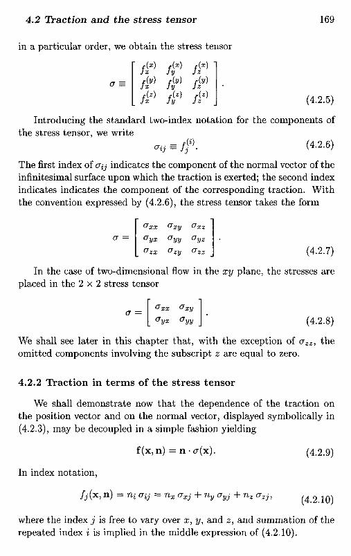
in a particular order, we obtain the stress tensor

(4.2.5)

Introducing the standard two-index notation for the components ofthe stress tensor, we write

^• = jf. (4-2.6)

The first index of O{j indicates the component of the normal vector of theinfinitesimal surface upon which the traction is exerted; the second indexindicates indicates the component of the corresponding traction. Withthe convention expressed by (4.2.6), the stress tensor takes the form

(4.2.7)

In the case of two-dimensional flow in the xy plane, the stresses areplaced in the 2 x 2 stress tensor

(4.2.8)

We shall see later in this chapter that, with the exception of azz, theomitted components involving the subscript z are equal to zero.

4.2.2 Traction in terms of the stress tensor

We shall demonstrate now that the dependence of the traction onthe position vector and on the normal vector, displayed symbolically in(4.2.3), may be decoupled in a simple fashion yielding

f(x,n) = n-a(x) . (4.2.9)

In index notation,

/j(x, nj = HI <Jij = nx oxj + Uy (jyj + nz GZJI (42 10)

where the index j is free to vary over x, y, and z, and summation of therepeated index i is implied in the middle expression of (4.2.10).

An important consequence of (4.2.9) is that, if the nine componentsof the stress tensor are known at a point, then the traction exerted onany infinitesimal surface centered at that point may be evaluated interms of the unit normal vector, merely by carrying out a vector-matrixmultiplication.

To confirm that expression (4.2.9) is consistent with the foregoingdefinitions, we choose n = (1,0,0) and carry out the vector-matrix mul-tiplication on the right-hand side of (4.2.10) to find f = f(x ', as required.Working in a similar fashion with n = (0,1,0) and n = (0,0,1), we findf = f(y) and f = f(z\ as required. It remains to show that (4.2.9) holdstrue for more general orientations of the unit normal vector n. For sim-plicity, we work out the proof for two-dimensional flow in the xy plane,with reference to the 2 x 2 stress tensor defined in (4.2.8).

We begin by considering a small area of fluid enclosed by an infinitesi-mal triangle with two sides perpendicular to the x and y axis, as depictedin figure 4.2.2(a). Newton's second law of motion requires that the rateof change of momentum of the fluid enclosed by the triangle be balancedby the forces exerted on it, including the body force and the surface forceassociated with the traction exerted on the three sides.

Now, the momentum of the parcel and the body force exerted on theparcel are both proportional to the area of the triangle, ^AxAy. The sur-face force exerted on the vertical side is equal to f^ Ay, the surface forceexerted on the horizontal side is equal to f^Ax, and the surface forceexerted on the slanted side is equal to f(s)A/, where A/ = >/Ax2 + Ay2.In the limit as Ax and Ay tend to zero, the fluid momentum and bodyforce become negligible compared to the surface forces exerted on thesides, and the sum of the three surface forces should vanish. Setting thex and y components of the sum equal to zero, we find

/W A/ + axx Ay + ayx Ax - O,

/W A/ + axy Ay + ayy Ax = O. (4^n)

Considering now the unit vector normal to the slanted side of the tri-angle pointing outward, denoted by n^, we use elementry trigonometryto write

(4.2.12)

Combining equations (4.2.11) and (4.2.12), we find

(4.2.13)

which are the x and y components of (4.2.9).An analogous proof can be worked out for three-dimensional flow, by

considering the forces exerted on the polyhedral fluid parcel illustratedin figure 4.2.2(b) (problem 4.2.1).

4.2.3 Traction on either side of a fluid surface

Consider now a thin layer of fluid with a designated outer side in-dicated by the direction of the unit normal vector n, and an opposinginner side indicated by the direction of the normal vector nmner = -n, asillustrated in figure 4.2.1(b). Balancing the rate of change of momentumof the fluid that resides within the layer with the forces exerted on it,and repeating the preceding arguments on the insignificance of the fluidmomentum and body forces compared to the surface forces, we derivethe force balance equation

f outer i finner n+ f =°> (4.2.14)

which is a statement of Newton's law of action and reaction: the forceexerted on one body by another is equal in magnitude and opposite indirection to that exerted on the second body by the first.

It is reassuring to confirm that expression (4.2.9) is consistent withthe physical law expressed by (4.2.14). Substituting the former into thelatter, we obtain

n*a + ninner.a = 0, (4.2.15)

which holds true in view of the definition uinner = -n. More generally,a prerequisite for the satisfaction of (4.2.14) is the property

f(x,-n) = -f(x,n), (4.2.16)

which is clearly shared by the right-hand side of (4.2.9)

4.2.4 Traction exerted on a boundary

Consider next a small fluid surface at the boundary of a flow. Theouter side of the surface is indicated by the unit normal vector nouiward

pointing into the boundary, as illustrated in figure 4.2.l(c). Newton'slaw of action and reaction requires that the traction exerted on the fluidsurface should balance the traction exerted by the fluid on the boundary,denoted by fB. Thus,

?B i „ outward _ nf +n ^ = 0' (4.2.17)

In terms of the inward unit normal vector pointing into the fluid, denotedby ninward = _noutward^ we obtain

cB ..inward* = n '^ (4.2.18)

Expression (4.2.18) allows us to compute the traction exerted on a bound-ary in terms of the stress tensor evaluated at the boundary.

4.2.5 Symmetry of the stress tensor

A fundamental law of mechanics originating from Newton's secondlaw of motion requires that the rate of change of angular momentum of afluid parcel be balanced by the torque exerted on it, including the torquedue to body forces and the torque due to surface forces. The torque withrespect to the point XQ due to a force F applied at the point x is definedby the outer vector product

T = (x - X0) x F. (4.2.19)

Applying this law for a rectangular fluid parcel whose sides are par-allel to the X, y, and 2, axes, we find, that, in the absence of a bodyforce that induces a torque, the tangential component of the traction inthe jthe direction exerted on the side that is perpendicular to the itheaxis must be equal to the tangential component of the traction in theithe direction exerted on the side that is perpendicular to the jth axis,otherwise an imbalanced asymmetry will arise (problem 4.2.2). Thus,

/J0=/?0. (4.2.20)

which states that the stress tensor is symmetric,

(Tij = aji. (4.2.21)

It is important to emphasize that the stress tensor is symmetric onlyin the absence of an externally induced torque; that is, in the absence ofan external force field causing point particles to spin around an axis. Inthe remainder of this book, we shall tacitly assume that this restrictionis satisfied.

Problems

Problem 4.2.1 Traction in three-dimensional flow.Prove expression (4.2.9) for three-dimensional flow. Hint: Perform a

force balance over the polyhedral volume depicted in figure 4.2.2(b).

Problem 4.2.2 Symmetry of the stress tensor.Prove the symmetry of the tensor for two-dimensional flow in the

absence of an externally induced torque.

4.3 Traction jump across a fluid interface

Equation (4.2.14) states that the traction exerted on one side of asurface drawn in a fluid is equal in magnitude and opposite in directionto that exerted on the other side. To derive this relation, we performed aforce balance over a thin fluid layer centered at the surface, consideringthe force exerted along the edges infinitesimal. If the fluid residing with-in the layer is homogeneous, then the edge force scales with the layerthickness and is negligible indeed compared to the surface force exertedon the sides.

If, however, the thin layer is centered at an interface between twodifferent fluids instead of a regular surface residing in a homogeneousfluid, differences in the magnitude of molecular forces on either sideof the layer generate an edge force that does not scale with the layerthickness. This edge force may be expressed in terms of the interfacialtension 7, defined as the force per unit length exerted around the edgeof a section of an interface.

Figure 4.3.1 Forces exerted on a thin fluid layer centered at (a) a two-dimensional, or (b) a three-dimensional interface, including thehydrodynamic force due to the fluid stresses, and the force due tothe surface tension, (c) The mean curvature of a three-dimensionalsurface is equal to the average of the directional curvatures in twoperpendicular planes containing the normal vector.

The interfacial tension pulls the interfacial layer in a direction thatis tangential to the interface and normal to the edges. The magnitude ofthe tension depends on the local temperature and molecular constitutionof the interface as determined, for example, by the concentration of asurface-active substance residing over interface, called a surfactant. Thehigher the temperature or the concentration of a surfactant, the lowerthe surface tension. Surfactants are often added to liquids to lower thesurface tension and achieve a desired effect: a dish or laundry detergentis a common household surfactant used to lower the strength of the forcesanchoring particles to a soiled surface.

Fluid 1

Fluid 2

Fluid 1

Fluid 2

4.3.1 Two-dimensional interfaces

Consider a small section of a two-dimensional interface with lengthA/, as illustrated in figure 4.3.1 (a). Surface tension pulls the layer fromthe two edges in directions that are tangential to the interface at the twoend-points A and B. Balancing the surface force due to the stress tensorand the edge forces, we obtain

(4.3.1)

where the unit normal vector n^ points into the fluid labelled 1, and theunit normal vector n^2) = — n^ points into the fluid labelled 2. Express-ing the second normal vector in terms of the first one, and rearrangingthe resulting expression, we find

(4.3.2)

If the surface tension is uniform, 7^ = 7^, and if the interface is flat, inwhich case tB — tA and the vectorial difference tB — tA is equal to zero,the right-hand side of (4.3.2) vanishes. Equation (4.3.2) then requiresthat the traction be continuous across the interface.

More generally, in the limit as the length of the segment A/ tends tozero, the right-hand side of (4.3.2) tends to the derivative of the product71 with respect to arc length / measured in the direction of the tangentvector t from an arbitrary origin,

(4.3.3)

Expanding out the derivative of the product on the right-hand side of(4.3.3), we find

(4.3.4)

The second term on the right-hand side of (4.3.4) contributes a tractiondiscontinuity that is tangential to the interface, known as the Marangonitraction. If the surface tension is constant, the Marangoni traction doesnot appear.

To interprete the first term on the right-hand side of (4.3.4), weconsider the difference between the two nearly equal tangent vectors tB

and tA. In the limit as A/ tends to zero, the difference between thesevectors tends to a new vector directed normal to the interface. Moreprecisely, in this limit,

(4.3.5)

where K is the positive or negative curvature of the interface. By defini-tion, K = 1/J?, where .R is the positive or negative radius of curvature ofthe interface. Substituting (4.3.5) into (4.3.4), and rearranging, we find

(4.3.6)

The first term on the right-hand side of (4.3.6) contributes a tractiondiscontinuity normal to the interface. If either the curvature of the in-terface or the surface tension vanishes, the normal stress is continuousacross the interface.

As an example, we consider the jump in traction across the interfacedepicted in figure 4.3.2. The origin of the Cartesian axes has been set ata point on the interface, the x axis has been positioned tangentially tothe interface, and the y axis has been positioned normal to the interfacepointing into fluid labelled 1. At the origin of the Cartesian axes, thecomponents of the unit normal vector n^ are given by njb = 0 andUy = 1, and the jump in traction is given by

(4.3.7)

where ex and e^ are, respectively, the unit vectors parallel to the x and yaxes. Observing that, at the origin, t = ex and n^1) = e^, and comparingthe right-hand sides of (4.3.7) and (4.3.6), we derive an expression forthe jump in the shear stress,

(4.3.8)

and another expression for the jump in the normal stress,

(4.3.9)

Figure 4.3.2 A local coordinate system with the x axis tangential to atwo-dimensional interface at a point, used to evaluate the jump intraction across the interface.

4.3.2 Three-dimensional interfaces

To derive the counterpart of the interfacial condition (4.3.6) for athree-dimensional interface, we consider a thin fluid layer straddling athree-dimensional interface, as illustrated in figure 4.3.l(b). Let n^1) bethe unit vector normal to the interface pointing into fluid 1, and e be theunit vector tangential to the layer edge. The surface tension pulls thelayer in the direction of the unit vector t that is tangential to the interfaceand normal to both n^ and e. Recalling the geometrical interpretationof the outer vector product discussed in Section 2.3, we write

* = e X n' (4.3.10)

Next, we balance the surface force due to the fluid stress and the edgeforce due to the surface tension, and find

(4.3.11)

where A5 is the surface area of the layer, and / is the arc length aroundthe layer edge C. Equation (4.3.11) is the three-dimensional counterpartof (4.3.1). Putting n(2) = — n^1) and rearranging, we find

(4.3.12)

It can be shown that, in the limit as A5 tends to zero and the loopC shrinks to a point, equation (4.3.12) reduces to

Fluid 1

Fluid 2

(4.3.13)where:

• ftm is the mean curvature of the interface.

• t' is the unit vector tangent to the interface pointing in the direc-tion along which the surface tension changes most rapidly.

• /' is the arc length measured in the direction of t'.

• dj/dlf is the corresponding maximum rate of change of the surfacetension with respect to arc length.

The first term on the right-hand side of (4.3.13) expresses a disconti-nuity in the normal direction; the second term expresses a discontinuityin the tangential direction identified as the Marangoni traction.

Mean curvature

To compute the mean curvature of a three-dimensional interface, weconsider the traces of the interface in two orthogonal planes that arenormal to the interface at a point and thus contain the normal vector,as depicted in figure 4.3.1(c). If KI and ^2 are the curvatures of the twotraces at that point, computed using formula (4.3.5) with the x and yaxes residing in the two planes, then the mean curvature of the interfaceis given by

(4.3.14)

A theorem due to Euler states that the mean value is independent ofthe orientation of the two planes, provided that the planes are mutuallyorthogonal. There is a particular orientation corresponding to maximumdirectional curvature KI, and a conjugate orthogonal orientation corre-sponding to minimum directional curvature /^; these are the principalcurvatures of the interface at the chosen point. The computation of themean curvature will be discussed further in chapter 5 in the context ofhydrostatics.

Problems

Problem 4.3.1 Curvature of an ellipse.A circle of radius a centered at the origin is described in parametric

form by the equations x — a cos 6 and y = a sin 0, where 6 is the polarangle varying between O and 2 TT. The components of the unit tangentvector pointing in the counter-clockwise direction are given by

(4.3.15)

where dl = ^dx2 + dy2 is the differential arc length measured in thecounter-clockwise direction. Using the parametric representation, wefind

dx = —a sin 9 d9, dy = a cos 6 dO, dl = a dO^(4.3.16)

yieldingtx = -sin#, ty = cos 9. (4.3.17)

Based on these formulas, we compute

(4.3.18)

Collecting the component equations (4.3.18), we derive the vector form

(4.3.19)

where n^ = (cos 0, sin#) is the unit vector normal to the circle pointinginto the exterior. Comparing (4.3.20) with (4.3.5), we deduce that n =I/a, thereby confirming that the curvature of the circle is equal to theinverse of its radius.

Consider a horizontal ellipse centered at the origin, described in para-metric form by the equations x — acosx and y = 6sin%, where x 'ls ̂ enatural parameter of the ellipse varying between O and 2 TT, and a, b arethe ellipse semi-axes. Repeat the preceding analysis to derive an expres-sion for the curvature in terms of a, 6, and x- Confirm that, as b tendsto a, the curvature of the ellipse reduces to that of a circle.

Problem 4.3.2 Mean curvature.(a) Based on formula (4.3.14) and its accompanying interpretation

discussed in the text, show that the mean curvature of a sphere of radiusa is equal to Km = I/a, whereas the mean curvature of a circular cylinderof radius a is equal to Km — l/(2a).

(b) The sphere and the circular cylinder are two examples of shapeswith constant mean curvature. Discuss one additional example.

Problem 4.3.3 Jump in traction in local coordinates.Derive the counterparts of equations (4.3.8) and (4.3.9) for a three-

dimensional interface.

Computer problems

Problem c.4.3.1 Computation of the curvature.Consider a line in the xy plane described by a set of TV + 1 marker

points with coordinates (xi,yi), i = 1,2, . . . ,JV + 1. An approximationto the components of the tangent vector at the ith point is provided bythe central-difference formulas

(4.3.20)

where

(4.3.21)

The derivatives of the components of the tangent vector with respect toarc length may be approximated with the corresponding formulas

(4.3.22)

The components of the outward normal vector at the marker points aregiven by

(4.3.23)

Write a computer program that reads or generates the coordinatesof a set of marker points, computes the right-hand sides of (4.3.2O)-(4.3.23), and then evaluates the curvature at the marker points from theexpression

(4.3.24)

which arises by taking the inner product of the unit normal vector andthe middle and right-hand side of (4.3.5).

Perform a series of computations with marker points distributedevenly along a circle, and compare the numerically computed curvatureswith the exact curvature derived in problem 4.3.1.

Problem c.4.3.2 Motion induced by curvature.Interfaces move under the influence of surface tension in a variety of

modes. In a simplified model, point particles distributed along a two-dimensional interface move normal to the interface with velocity thatis proportional to the local curvature. If X^ is the position of the ithmarker point, then the motion of the marker point is described by thevectorial differential equation

(4.3.25)

where t stands for time, n^1) is the outward normal vector, and K is thecurvature.

Write a program that computes the motion of marker points dis-tributed over an interface using the finite-difference approximations dis-cussed in problem c.4.3.1, and the modified Euler method for integratingin time the differential equations (4.3.25). Run the program to computethe evolution of marker points distributed along a circle or an ellipsewith axes ratio equal to 2.0, and discuss the nature of the motion.

4.4 Stresses in a fluid at restIf a fluid does not appear to execute macroscopic motion as seen

by a stationary observer, that is, the observable velocity vanishes, thenthe molecules are in a state of dynamic equilibrium determined by thephysical conditions prevailing in their immediate environment.

Consider a cubic fluid parcel with its six faces perpendicular to thex, y, or z axis, as illustrated in figure 4.4.1. In the absence of net fluidmotion, the traction exerted on the sides that are perpendicular to thex axis must be directed normal to this side, otherwise, an unresolvedtangential component pointing in a physically indeterminate directionwill arise. In the notation of Section 4.2,

(4.4.1)

Figure 4.4.1 The traction exerted on the three sides of a cubic parcelof a stationary fluid has only a normal component that is definedin terms of the thermodynamic pressure.

Similar arguments suggest that the tractions exerted on the sides thatare perpendicular to the y or z axes must be directed normal to thesesides, requiring that

/lw)=0, / M ^ O , /M = O, (4.4.2)

and42) = 0, /^ = O, / W ^ O . (4.4.3)

If the size of the cubic parcel is infinitesimal, the fluid residing insidethe parcel is perfectly or nearly homogeneous, and the nonvanishingcomponents of the tractions fx , fy , and fz must be identical. Bydefinition, the common value of these normal components is equal to thenegative of the pressure p,

f(x) __ f(y) _ f ( z ) —Jx -Jy -Jz — P' (4.4.4)

Thus, in hydrostatics, the stress tensor introduced in equation (4.2.7) isdefined exclusively in terms of the pressure, and is given by

" - p O O l F l O O "cr= O -p O = -p O 1 O .

O O -p J L 0 0 1 J (4A5)

In compact formtf = -pi, (4.4.6)

where I is the unit or identity matrix shown on the right-hand side of(4.4.5).

4.4.1 Traction on a surface

As an application, we use expression (4.4.6) to evaluate the tractionexerted on a surface drawn in a stationary fluid. Using formula (4.2.9),we find

f (x, n) = n • (-p I) = -p n • I = -p n. (4.4.7)

The last equality arises from the identity n • I = n. Equation (4.4.7)shows that the traction exerted on a surface in hydrostatics is directednormal to the surface; the tangential component vanishes.

4.4.2 Traction on a flow boundary

As a second application, we use (4.4.6) to evaluate the traction ex-erted on a boundary confining the fluid. Using formula (4.2.18), we find

{B = ninward . (_p j) = _p ^inward . j = _p ^inward ^

The last equality arises from the identity uinward-I = n

inward. Thus, thetraction exerted on a fluid boundary in hydrostatics is directed normalto the boundary; the tangential component vanishes.

4.4.3 Thermodynamics

The hydrostatic pressure distribution established in a fluid at restcannot be computed working exclusively in the context of fluid me-chanics. Additional information concerning the relationship between thedensity and the pressure for the particular fluid under consideration isrequired, and must be provided by thermodynamics.

For example, molecular thermodynamics states that the pressure ofa small parcel of gas is determined by (a) the number of molecules re-siding within the parcel expressed by the local density p, (b) the kineticenergy of the molecules expressed by the absolute temperature T, and(c) the nature and intensity of the intermolecular forces expressed byan intermolecular potential. In the case of an ideal gas, intermolecular

forces are negligible, and the pressure derives from the density and thetemperature in terms of the ideal gas law

(4.4.9)

where:

• M is the gramo-molecular mass, defined as the mass of one molewhich is comprised of a collection of NA molecules, where NA —6.022 x 1026 is Avogadro's number. The gramo-molecular weightof an element is equal to the atomic weight of the element listed inthe periodic table, expressed in grams.

• R is the ideal gas constant, equal to R — 8.314 x 103 kg m2/(sec2

kmole K).

• T is Kelvin's absolute temperature, equal to the Celsius centigradetemperature reduced by 273 units.

Liquids, on the other hand, are nearly incompressible, and thermo-dynamics allows us to compute their pressure under the assumption thatthe density is a function of temperature alone, independent of pressure.

The computation of the hydrostatic pressure distribution in gasesand liquids will be discussed in more detail in Chapter 5.

4.4.4 Jump in the hydrostatic pressure across an interface

Equations (4.3.6) and (4.3.13) provide us with expressions for thejump in the traction across a two- or three-dimensional interface. Ifthe two fluids on either side of the interface are stationary, then thecorresponding stress tensors are given by (4.4.6) with the superscript 1or 2 included to signify the choice of fluid, and the jump in the tractionis given by

(4.4.10)

Assuming that the surface tension is uniform, we compare the right-handside of (4.4.10) to the right-hand side of the force equilibrium equation(4.3.6) for a two-dimensional interface, finding

p(2) _p(i) =7 /^ (4.4.11)

Working in a similar fashion for a three-dimensional interface using(4.3.13), we find

p (2 ) -p ( i ) = 7 2K m , (4^2)

where Km is the mean curvature.We have found that the jump in pressure across a two- or three-

dimensional interface is equal to the product of the surface tension and,respectively, the curvature or twice the mean curvature of the interface.

As an application, we compute the jump in pressure across a sphericalinterface of radius a, representing the surface of a liquid drop or bubble.Designating the outer fluid as fluid 1 and the inner fluid as fluid 2, wefind that the mean curvature of the interface is equal to Km = I/a.Consequently, the pressure jump is given by p^ — p^ = 2 7/a.

Problems

Problem 4.4.1 Jump in pressure across a two-dimensional interface.Derive an expression for the jump in pressure across a circular inter-

face of radius a representing the trace of a cylindrical thread in the xyplane.

Problem 4.4.2 Curvature of a soap film.Explain why the mean curvature of a thin soap film confined between

two adjacent interfaces attached to a wire frame, must vanish.

4.5 Viscous and Newtonian fluids

In the absence of macroscopically observable fluid motion, the trac-tion exerted on a specified side of a small fluid surface is given by equation(4.4.7) in terms of the pressure. If the fluid exhibits macroscopic motion,this equation is modified in two ways: first, the normal component ofthe traction is enhanced with a new contribution that depends on thephysical properties of the fluid and the character of the local motion;second, a tangential component is established.

To understand how these new contributions arise, we consider thetractions developing in two complementary types of flow: an extensionalflow where the fluid is stretched and elongates, and a channel flow wherethe fluid is sheared due to boundary motion.

Figure 4.5.1 (a) Extension of a liquid bridge subtended between twocoaxial cylinders that are pulled apart along their axes; (b) shearflow in a two-dimensional channel confined between two parallelplates; the motion is due to the in-plane translation of the upperplate.

4.5.1 Extension of a thread

In one experiment, a thread of a liquid is suspended between tworods forming an axisymmetric bridge, and the rods are pulled apart withvelocity V thereby extending the thread, as ilustrated in figure 4.5.1 (a).A force is required to pull the rods apart and thus overcome the normalcomponent of the hydrodynamic traction, /x , imparted by the fluid tothe tips of the rods. The faster the rods are pulled apart, the higher themagnitude of the traction; the greater the distance between the rods,the lower the magnitude of the traction.

For most common fluids, a linear relationship exists between thetraction, the velocity of the rods, and the inverse of their distance, inthe form

f 0*0 — -<n + 9 LLeXt —tx ~ P * L> (4.5.1)

where p is the pressure discussed in Section 4.4 in the context of hydro-statics, V is the velocity of the rods, L is half the distance between therods, and \jfxi is a physical constant called the extensional viscosity ofthe liquid comprising the thread.

4.5.2 Shearing of a layer

In a second experiment, a fluid is placed in a channel that is confinedbetween two parallel plates. The upper plate translates in the x directionparallel to itself with constant velocity V, while the lower plate is heldstationary, as depicted in figure 4.5.l(b). A force in the x direction mustbe exerted on the upper plate to balance the tangential component of thetraction fx developing due to the fluid motion. The higher the velocityof the translating plate, the larger the magnitude of the traction; thegreater the distance between the two plates, the lower the magnitude ofthe traction.

For most common fluids, a linear relationship exists between thetraction, the velocity of the moving plate, and the inverse of the distancebetween the plates, /i,

f(y) - u** Y-Jx -V h* (4.5.2)

where p,sh is a physical constant associated with the fluid, called theshear viscosity.

4.5.3 Simple fluids

We have established that stresses develop in a fluid as a result ofthe motion. To proceed further, we consider the tractions developingon the surface of a small fluid parcel, and argue the following propertiescharacterizing a simple fluid:

• If the parcel translates or rotates as a rigid body, tractions do notdevelop over its surface.

• Tractions develop only when the parcel deforms.

• The distribution of traction over the parcel surface at a particularinstant in time depends only on the type and rate of deformationthat the parcel is undergoing at that particular time.

To this end, we recall the results of our analysis of kinematicsin Chapter 2: a small spherical fluid parcel in a flow deforms toobtain an ellipsoidal shape whose axes are parallel to the threeeigenvectors of the rate of deformation tensor defined in equation(2.1.28); the rates of deformation are equal to the correspondingeigenvalues.

With the above properties as a point of departure, we proceed torelate the stress tensor to the physical properties of the fluid and to thestructure of the velocity field by means of a constitutive equation.

4.5.4 Incompressible Newtonian fluids

The constitutive equation for an incompressible Newtonian fluid takesthe form

a = -pI + / /2 E, (4.5.3)

where p is the pressure, the coefficient /j, is the fluid viscosity, sometimescalled the dynamic viscosity, and E is the rate of deformation tensordefined in equation (2.1.28). Note that the Newtonian constitutive rela-tion respects the symmetry of the stress tensor discussed at the end ofSection 4.2.

Explicitly, the components of the stress tensor are given by the matrixequation

(4.5.4)

In the absence of flow, we recover the hydrostatic stress tensor definedin equation (4.4.6), involving the pressure.

Unidirectional shear flow

As an example, we consider the flow of a Newtonian fluid in a two-dimensional channel confined between two parallel plane walls, wherethe motion is generated by the translation of the upper plate, as de-picted in figure 4.5.1(b). Physical intuition suggests that, at low andmoderate velocities, the fluid will translate only in the x direction with aposition-dependent velocity Ux varying in the y direction; to signify thisdependence, we write ux(y).

Using equation (2.1.22), we find that the rate of deformation tensorfor this two-dimensional flow is given by

(4.5.5)

Substituting (4.5.5) into the right-hand side of (4.5.3), we obtain thestress tensor

(4.5.6)

The x component of the traction exerted on a fluid surface that isperpendicular to the y axis, identified as the shear stress, is given by

(4.5.7)

Physically, this traction is attributed to the friction experienced by ad-jacent fluid layers as they slide over one another with slightly differentvelocities.

4.5.5 Viscosity

Strictly speaking, the viscosity of a fluid is a proportionality coef-ficient relating the stress tensor to the rate of deformation tensor, asdepicted in equation (4.5.3). It is reassuring, however, to know that thismathematical definition, established by phenomenological observation,has a firm physical foundation. Thus, the viscosity is a genuine physicalconstant dependent on the local physical conditions including tempera-ture. The following table summarizes the viscosities of water and air atthree temperatures; cp stands for centipoise which is one hundredth ofthe viscosity unit poise defined as 1 g/(cm sec).

Viscosity, //

Temperature Water Air0C cp = 10~2g/(cm sec) cp

20 1.002 0.018140 0.653 0.019180 0.355 0.0209

As the temperature is raised, the viscosity of liquids is reduced,whereas the viscosity of gases increases. This dichotomy is a reflectionof the different physical mechanisms that are responsible for the devel-opment of stresses in these two fundamental classes of fluids. In the caseof liquids, the viscosity is due to occasional molecular excursions from amean position into neighboring empty sites. In the cases of gases, theviscosity is due to relentless molecular excursions from regions of highvelocity to regions of low velocity in the course of random motions dueto thermal fluctuations.

Viscosity of gases

To demonstrate the relation between molecular and macroscopic flu-id motion, we consider a gas undergoing unidirectional shear flow, andderive an expression for the viscosity in terms of molecular properties.In the simplest kinetic theory, the molecules are modeled as rigid spheresmoving with the local fluid velocity defined in Section 1.4, and with arandomly fluctuating component. The average magnitude of the fluctu-ating component is

(4.5.8)

where ks is Boltzmann's constant, T is the absolute temperature, andM is the molecular weight. In the course of the random motion, twomolecules occasionally collide after having travelled an average distanceequal to the mean free path, A.

Consider a macroscopically stationary gas with vanishing fluid veloc-ity. Using principles of statistical mechanics, we find that the numberof molecules crossing a unit surface area per unit time as a result of thefluctuating motion, denoted by Z, is proportional to (a) the number ofmolecules per unit volume defined as the number density n, and (b) theaverage magnitude of the fluctuating velocity v. It can be shown, inparticular, that

(4.5.9)

A molecule crossing the unit surface at a particular instant has collid-ed with another molecule at an average distance a above or below thesurface. Using principles of statistical mechanics, we find

(4.5.10)

where A is the mean free path. Relations (4.5.9) and (4.5.10) have beenderived taking into consideration that, since the molecules move ran-domly in all directions, only one component of the velocity brings themtoward the unit surface under consideration.

Relations (4.5.8)-(4.5.10) also hold true when the fluid exhibits amacroscopic motion, provided that the molecular velocity is computedrelative to the average velocity at the position where a molecule lastunderwent a collision.

Figure 4.5.2 shows a schematic illustration of the instantaneous distri-bution of molecules in a gas undergoing unidirectional shear flow. With-out loss of generality, we have assumed that the fluid velocity increasesin the positive direction of the y axis. In the course of the motion,molecules cross a horizontal plane corresponding to a certain value ofy, drawn with the heavy horizontal line, from either side. Because thex velocity of molecules crossing from above is higher than the x veloci-ty of molecules crossing from below, x momentum is transfered towardthe negative direction of the y axis. The rate of transer of x momen-tum across a surface that is perpendicular to the y axis amounts to thehydrodynamic traction fx .

Now, the rate of momentum transport defined in the preceding para-graph can be quantified by setting

(4.5.11)

where Ux is the fluid velocity, and the superscripts + and — indicatethat the underlying variable is evaluated at a distance equal to a aboveor below the transport surface. Effectively, the collection of moleculescrossing the y plane during a unit length of time are represented bymodel molecules with the following properties: (a) the model moleculeslast underwent a collision a distance a above or below the y plane, and(b) the model molecules move with an average velocity that is equal tothe local fluid velocity evaluated at the position of last collision.

Because the flow is undirectional, the average fluid velocity normalto a horizontal plane vanishes, and the number of molecules crossings they plane from either side per unit length of time are equal. Combiningequations (4.5.9)-(4.5.11), we find

(4.5.12)

Figure 4.5,2 A molecular model of the shear flow of a gas used to derivethe expression for the viscosity in terms of molecular properties,shown in equation (4.5.14).

Since a is small compared to the macroscopic length scale of the shearflow, we may approximate the fraction enclosed by the parentheses onthe right-hand side of (4.5.12) with a derivative, obtaining

(4.5.13)

Comparing equations (4.5.13) and (4.5.7), we now obtain an expres-sion for the fluid viscosity,

(4.5.14)

We have derived the Newtonian constitutive equation from molecularconsiderations and, in addition, we have obtained a prediction for theviscosity of a gas in terms of molecular properties.

4.5.6 Ideal fluids

If the viscosity of a fluid vanishes, the fluid is considered frictionlessand is called ideal. The stress tensor in an ideal fluid is given by thesimplified version of (4.5.3)

° =-Pi- (4.5.15)

It is important to bear in mind that absence of viscosity is a math-ematical idealization adopted only to facilitate the analysis. In the realworld, absence of viscosity should be interpreted as insignificance of hy-drodynamic stresses associated with the fluid viscosity. The formal re-quirement for viscous stresses to be negligible will be discussed in Chap-ter 6.

Problems

Problem 4.5.1 Flow in a channel.Consider steady unidirectional flow in a channel due to the transla-

tion of the upper wall, as depicted in figure 4.5.1(b).(a) Perform a force balance over a rectangular fluid layer confined

between two y levels to show that, when the pressure is uniform, theshear stress fx must be independent of y.

(b) Having established that fx is constant, solve the first-order d-ifferential equation (4.5.7) for Ux in terms of y subject to the boundaryconditions Ux (y = O) =0 and Ux (y — h) = V, and evaluate fx in termsof /^, V, and the channel width h.

Problem 4.5.2 Extensional flows.(a) Consider a two-dimensional extensional flow in the xy plane with

velocity components Ux = k x and uy — -k y, where A: is a constantwith dimensions of inverse time called the rate of extension. The corre-sponding pressure is constant. Confirm that the fluid is incompressible,sketch the streamline pattern, and evaluate the stress tensor.

(b) Repeat (a) for axisymmetric extensional flow whose Cartesianvelocity components are given by Ux — k x, uy — -^k y, and uz — — ̂ k z.

(c) The axisymmetric extensional flow describes the motion insidethe thread illustrated in figure 4.5.1 (a). Assuming that the fluid is New-tonian, compute the force necessary to pull the rods away with velocityV in terms of the half-length of the thread Z/, the fluid viscosity //, andthe cross-sectional area of the rods A.

4.6 Simple non-Newtonian fluids

The Newtonian constitutive equation for an incompressible fluid,shown in equation (4.5.3), describes the stresses developing in a fluidconsisting of small molecules. Fluids containing or consisting of macro-molecules, such as polymeric solutions and melts, and fluids containingsuspended rigid or deformable particles, such as pastes, bubbly liquids,and blood, exhibit more complicated behavior that is described by moreinvolved constitutive equations.

To derive constitutive equations for non-Newtonian fluids, we consid-er the motion of a fluid parcel and seek to establish a relation betweenthe instantaneous tractions exerted on the parcel surface and the his-tory of the parcel deformation. In the simplest class of materials, thetractions depend only on the instantaneous rate by which the parcel isdeforming, expressed by the rate of deformation tensor E. The distin-guishing feature of a non-Newtonian fluid is that the relation betweenthe stress tensor a and the rate of deformation tensor E is nonlinear.

4.6.1 Unidirectional shear flow

In the case of unidirectional shear flow, the Newtonian shear stress(4.5.7) can be generalized by allowing the viscosity to be a function ofthe shear rate dux/dy. If the viscosity is reduced as the shear rate israised, the fluid is called shear-thinning or pseudo-plastic] whereas ifthe viscosity is increased as the shear rate is raised, the fluid is calledshear-thickening or dilatant.

Physically, the dependence of the viscosity on the shear rate is at-tributed to changes in the configuration of molecules, changes in theshape and relative position of particles suspended in the fluid, or to thespontaneous formation of internal microstructure due to intermolecularforce fields and particle interactions.

4.6.2 Power-law fluids

The shear stress developing in a certain class of fluids in unidirec-tional shear flow is described by the Ostwald-de Waele model. In thismodel, the viscosity is proportional to the magnitude of the shear rateraised to a power,

(4.6.1)

where /^o is a constant, and n is the power-law exponent. When n — 1,we obtain a Newtonian fluid with viscosity /J.Q; n < 1 corresponds toshear-thinning fluids, and n > 1 corresponds to shear-thickening fluids.

Substituting (4.6.1) into (4.5.7), we derive an expression for the shearstress

(4.6.2)

Consider now flow in a channel generated by the translation of theupper wall with velocity F, as illustrated in figure 4.5.1(b). Performing aforce balance over a rectangular fluid layer, as discussed in problem 4.5.1,we find that, if the pressure is uniform, the shear stress is independentof y, and the right-hand side of (4.6.2) is constant.

Now, the fluid velocity at the upper wall located at y = h is equal tothe wall velocity F, and the velocity at the lower wall located at y = Ois required to vanish. Integrating equation dux/dy = c, where c is theconstant shear rate, and using the aforementioned boundary conditions,we find a linear velocity profile with shear rate dux/dy = V/h irrespectiveof the value of n.

Although the velocity profile is linear for any value of n, the magni-tude of the shear stress is a function of n, as shown in equation (4.6.2).This distinction emphasizes that the kinematic appearance of a flow doesnot necessarily reflect the magnitude of the stresses developing in thefluid. Two flows that are kinematically identical may support differentstresses.

4.6.3 Yield-stress fluids

A certain class of heterogeneous fluids, including pastes and concen-trated suspensions of fine particles, called Bingham plastics, flow onlywhen the shear stress established due to the motion lies above a certainthreshold. An idealized constitutive equation between stress and shearrate for this class of materials is

Figure 4.6.1 Rheological response of a Bingham plastic showing ayield-stress behavior in unidirectional flow.

(4.6.3)

where the constant TO is called the yield stress, and p, is the viscosity.The relation between the shear stress and the shear rate is representedby the solid line in figure 4.6.1.

Consider the familiar flow in a channel confined between two parallel-sided walls generated by imparting to the upper wall a force Fx parallel tothe x axis. If the fluid is a Bingham plastic whose rheological behavioris described by equations (4.6.3), a shear flow across the whole of thechannel will be established only when the externally imposed force F perunit length of the channel I/, counteracting the shear stress, ayx — F/L,is greater than the yield stress TQ.

Assuming that this occurs, we treat ayx as a constant, solve thesecond of equations (4.6.3) for dux/dy, and then integrate with respectto y subject to the boundary condition ux(y = O) = 0 to obtain thelinear velocity

(4.6.4)

The velocity of the upper wall is given by

(4.6.5)

Equation (4.6.5) allows to estimate the values of the physical constantsIJL and TQ from laboratory observation.

Problem

Problem 4.6.1 Yield-stress fluids.The relation between the shear stress and the shear rate for a class

of yield-stress fluids is described by the long-dashed line in figure 4.6.1,where the constant 7C is the critical shear rate. State the equationsdescribing this rheological behavior, and compute the shear stress es-tablished in a channel with parallel-sided walls, where the upper walltranslates with velocity F, while the lower wall is held stationary.

4.7 Stresses in polar coordinates

We have discussed tractions and stresses in Cartesian coordinates.In practice, it may be more convenient to work in cylindrical, spherical,or plane polar coordinates with the benefit of reduced algebraic manip-ulations. In this section, we define the components of the stress tensorin these polar coordinates, and relate them to the pressure and to thecorresponding components of the rate of deformation tensor using theconstitutive equation for incompressible Newtonian fluids.


Consider the system of cylindrical polar coordines (re, a, <p) depictedin figure 4.7.1. The traction f^ exerted on a small surface that is per-pendicular to the x axis, acting on the side facing the positive directionof the x axis, may be resolved into its cylindrical polar components as

(4.7.1)

Figure 4.7.1 Components of the stress tensor in cylindrical polar coor-dinates.

where ex, e<j, and e^ are unit vectors pointing, respectively, in the axial,radial, and meridional directions. Recall that the orientation of ex isconstant, whereas the orientation of ea and e^ changes with position inthe flow.

The traction f ̂ exerted on a small surface that is perpendicular tothe vectorial distance from the x axis, and is thus parallel to the axialand meridional directions at the designated center of the surface, maybe resolved into corresponding components as

£<'>=/M <* + #>«,+ /M V (4?_2)

Thirdly, the traction f &) exerted on a small surface that is normalto the meridional direction, may be resolved as

f (*0 = fM ex + f(v) e<r + /M v (4.7.3)

Stacking the coefficients of the unit vectors on the right-hand sidesof (4.7.1)-(4.7.3) on top of one another in a particular order, we obtainthe stress tensor in cylindrical polar coordinates,

f(x) Ax) Ax)Jx Ja J(p

°= /^ № 4ff) -. /£° № 4V) J (4.7.4)

To simplify the nomenclature, we introduce the standard two-indexnotation, writing

CW? = 4a), (4.7.5)

where Greek indices stand for #, a, or <p. With the convention expressedby (4.7.5), the stress tensor is given by

&XX &XV ®X(p

® — &ax &aa &cr(p

_ &<px VVO- °vv J (4.7.6)

The stress components for an incompressible Newtonian fluid derivefrom the constitutive equation (4.5.3) as

(4.7.7)

Note that the stress tensor remains symmetric in the cylindrical polarcoordinates.

Figure 4.7.2 Components of the stress tensor in spherical polar coor-dinates.


Consider the system of spherical polar coordines (r, 6, (p) depicted infigure 4.7.2. The traction f ̂ exerted on a small surface that is normal tothe vectorial distance from the origin, acting on the side of the surfacefacing away from the origin, may be resolved into its spherical polarcomponents as

f(r) = /W 6r + /W e, + /W e^ (4.7.8)

where ex, e#, and e^ are the unit vectors pointing in the radial, az-imuthal, and meridional directions.

The traction f ̂ exerted on a small surface that is perpendicularto the azimuthal direction corresponding to the angle 0, and is thusparallel to the radial and meridional directions, may be resolved in thecorresponding form

*•>-№ ++ &•, + #>•* (< ? g)

Thirdly, the traction f &) exerted on a small surface that is normal tothe meridional direction, and is thus parallel to the radial and azimuthaldirections, may be resolved as

fM = fM Gr + fM ee + fM «v (4-7.10)

Stacking the coefficients of the unit vectors on the right-hand sidesof (4.7.8)-(4.7.10) on top of one another in a particular order, we obtainthe stress tensor in spherical polar cordinates

f f(r) Ar) f(r) 1Jr JQ Jv

„= fW fW f(0)a — Jr Je J 9f(v) Av) Av) (4.7.11)Jr JQ J(p J ^ '

To simplify the nomenclature, we introduce the standard two-indexnotation, writing of the stress tensor, writing

cr^/f, (4-7.12)

where Greek indices stand for r, #, or (p. With the convention expressedby (4.7.12), the stress tensor is given by

arr OTQ arip

O = (JQr GQQ VQ^

Oyr 0(pQ &W (4.7.13)

The stress components for an incompressible Newtonian fluid derivefrom (4.5.3) as

(4.7.14)

Figure 4.7.3 Components of the stress tensor in plane polar coordi-nates.

Note that the stress tensor remains symmetric in the spherical polarcoordinates.


Consider finally a two-dimensional flow in the xy plane and refer tothe plane polar coordines (r, 9) depicted in figure 4.7.3. The tractionf(r) exerted on a small segment that is normal to the distance from theorigin, acting on the side facing away from the origin, may be resolvedinto its plane polar components as

f(r) = /r(r)er + /fl

(r)ee, (4.7.15)

where er and e# are the unit vectors pointing in the radial and polardirections.

The traction f^ exerted on a small surface that is normal to thedirection of the polar angle #, and is thus parallel to the distance fromthe origin, may be resolved as

f<'> =/rw * + /,<"«,. (4.7.16)

Stacking the coefficients of the unit vectors on the right-hand sidesof (4.7.15)-(4.7.16) on top of one another in a particular order, we obtainthe stress tensor in plane polar cordinates

(4.7.17)

To simplify the nomenclature, we introduce the usual two-index no-tation, writing

*a» = ff\ (4-7-18)

where Greek indices stand for r or 9. With the convention expressed by(4.7.18), the stress tensor is given by

(4.7.19)

The stress components for an incompressible Newtonian fluid derive fromthe constitutive equation (4.5.3) as

(4.7.20)

Note that the stress tensor remains symmetric in the plane polarcoordinates.

4.8 Boundary conditionon the tangential velocity

In Section 2.10, we discussed the no-penetration boundary conditionover impermeable solid boundaries and interfaces between immiscible flu-ids, involving the normal component of the fluid velocity. Viscous fluids,that is, all real fluids obey an additional boundary condition concerningthe tangential component of the velocity.

Under most conditions, the vast majority of fluids satisfy the no-slipboundary condition which requires that (a) the tangential componentof the fluid velocity over a solid boundary be equal to the tangentialcomponent of the boundary velocity, and (b) the tangential componentof the fluid velocity be continuous across an interface between two im-miscible fluids. Combined with the no-slip condition, the no-penetrationcondition requires that the fluid velocity be equal to the velocity of animpermeable solid boundary, and continuous across an interface.

The physical origin of the no-slip boundary condition over a solidsurface has not been established with certainty. One theory argues thatthe molecules of a fluid next to a solid surface are adsorbed onto the sur-face for a short period of time, and are then desorbed and ejected intothe fluid. This process slows down the fluid and renders the tangentialcomponent of the fluid velocity equal to the corresponding componentof the boundary velocity. Another theory argues that the true bound-ary condition is the condition of vanishing shear stress, and the no-slipboundary condition arises due to microscopic boundary roughness; thus,a perfectly smooth boundary would allow the fluid to slip.

In practice, the no-slip boundary condition has been confirmed inthe overwhelming majority of applications, and is the standard choice inmainstream fluid dynamics. Exceptions to the no-slip boundary condi-tion are found in the flow of rarified gases, in the flow of polymeric meltsat high pressure, and in the flow near a three-phase contact line where asolid meets two liquids or a gas and a liquid. Another exception occursfor a certain class of interfaces consisting of dual or multiple molecularlayers that may exhibit relative motion yielding a discontinous velocity.Finally, the no-slip boundary condition is sometimes relaxed in numeri-cal simulations to prevent the occurrence of singularities stemming fromexcessive idealization; one example is the development of infinite forceon a plate scraping fluid off a surface.

Problem

Problem 4.8.1 Flow in a channel with slip.Consider steady unidirectional flow in a channel with parallel walls

driven by the translation of the upper wall along the x axis with velocityV, as illustrated in figure 4.5.1(b); the lower wall is stationary. The fluidis allowed to slip over the lower wall so that the slip velocity Ux (y = O)

is related to the wall shear stress by

(4.8.1)

where I is a constant called the slip coefficient. When / = O, the slipvelocity vanishes and the no-slip boundary condition prevails.

In previous sections, we saw that, when the pressure is uniform, theshear stress ayx is constant and independent of y. Assuming that theno-slip condition applies at the upper wall, derive an expression for ayx

and for the velocity profile in terms of V, /i, /^, and /.

4.9 Wall stresses in Newtonian fluids

Combining the no-slip boundary condition discussed in Section 4.8with the no-penetration boundary condition discussed in Section 2.10,we may derive remarkably simple expressions for the Newtonian tractionexerted on a solid surface, amenable to simple physical interpretation.

Consider flow above a stationary flat solid surface located at y — O, asillustrated in figure 4.9.1. The no-slip boundary condition requires thatthe tangential components of the velocity, and thus their derivatives withrespect to x and z, vanish over the surface,

(4.9.1)

where the partial derivatives are evaluated at y = O. The no-penetrationcondition requires that the normal component of the velocity, and thusits derivatives with respect to x and z, also vanish over the surface,

(4.9.2)

where the partial derivatives are evaluated at y = O.

4.9.1 Shear stress

The two components of the Newtonian shear stress exerted on thesurface are given by

Figure 4.9.1 Flow over a plane wall where the no-slip boundary condi-tion is required. The wall shear stress is proportional to the slopeof the velocity with respect to distance normal to the wall; thenormal stress is equal to the negative of the pressure.

(4.9.3)

evaluated at y = O. Using (4.9.2) to simplify (4.9.3), we find

(4.9.4)

evaluated at y = O.Equations (4.9.4) show that the wall shear stress is simply equal to

the slope of the tangential velocity with respect to distance in the normaldirection, multiplied by the fluid viscosity.

4.9.2 Normal stress

The Newtonian normal stress exerted on the solid surface is given by

(4.9.5)

evaluated at j/ = O, where p is the pressure. Since the fluid has beenassumed incompressible, we may use the continuity equation (2.9.2) towrite

(4.9.6)

evaluated at y = O, and then invoke the first and fourth of equations(4.9.1) to find duy/dy — O. Expression (4.9.5) thus simplifies to

°yy = -P» (4.9.7)

which shows that the normal stress at a solid surface is equal to thenegative of the pressure.

4.9.3 Generalization

The results displayed in equations (4.9.4) and (4.9.7) remain valideven when the surface translates with a constant or time-dependent ve-locity. Moreover, these results also apply when the surface is curved,provided only that the y axis is defined to be normal to the surface atthe position when the shear or normal stress is evaluated.

Problem

Problem 4.9.1 Vorticity at a no-slip surface.Show that the component of the vorticity vector normal to an imper-

meable surface vanishes. Hint: Use the second and third of equations(4.9.1).

Chapter 5

Hydrostatics

5.1 Equilibrium of pressure and body forces5.2 Force exerted on immersed surfaces5.3 Archimedes' principle5.4 Shapes of two-dimensional interfaces5.5 A semi-infinite interface attached to an inclined plate5.6 Meniscus between two parallel plates5.7 A two-dimensional drop on a horizontal plate5.8 Axisymmetric shapes

The simplest state of a fluid is the state of rest: the macroscopicallyobserved velocity vanishes, and the forces developing in the fluid are de-scribed in terms of the pressure field established in response to a bodyforce. The subject of hydrostatics encompasses two main topics: thecomputation offerees exerted on immersed surfaces and submerged bod-ies, and the study of the shapes of interfaces separating two stationary,translating, or rotating fluids. The problem statement and mathematicalformulation in both cases is straightforward, but deriving solutions forall but the simplest configurations requires the use of numerical methodsfor solving algebraic, ordinary, and partial differential equations.

5.1 Equilibrium of pressure and body forces

Consider a parcel of a stationary fluid, as illustrated in figure 5.1.1 (a).Newton's second law of motion requires that, in the absence of a macro-scopically observable flow, the sum of the forces exerted on the parcelshould balance to zero. In Chapter 4, we saw that two kinds of forcesare exerted on the parcel: a body force due to the gravitational or someother force field mediated by long-range molecular interactions, and asurface force associated with the hydrodynamic traction.

Figure 5.1.1 (a) Schematic illustration of a parcel of a stationary flu-id with the unit normal vector pointing outward, (b) A parcelwith the shape of a rectangular parallelepiped serving as a controlvolume for deriving the differential equations of hydrostatics.

5.1.1 Body force

The body force due to gravity may be expressed as an integral overthe volume of the parcel involving the generally position-dependent den-sity p, in the form

(5.1.1)

where g = (gx,gy,9z) is the vectorial acceleration of gravity. On thesurface of the earth, the magnitude of g has the approximate value |g| =g = 9.80665 m/sec2.

5.1.2 Surface force

The surface force may be expresssed in terms of the traction f exertedon the surface of the parcel in the corresponding form

(5.1.2)

In the absence of observable fluid motion, the traction is due to thepressure alone pushing the surface of the parcel toward the interior. If n

is the unit vector normal to the surface of the parcel pointing outward,as illustrated in figure 5.1.1 (a), then

f=-pn. (5.1.3)

The minus sign on the right-hand side accounts for the opposite orienta-tions of the normal vector and of the normal traction due to the pressure.Substituting (5.1.3) into (5.1.2), we derive an expression for the surfaceforce in terms of the pressure,

(5.1.4)

5.1.3 Force equilibrium

Setting the sum of the body force given in (5.1.1) and the surfaceforce given in (5.1.4) equal to zero, we obtain the vectorial equilibriumcondition

(5.1.5)

whose three scalar components are

(5.1.6)

5.1.4 Equilibrium of an infinitesimal parcel

Consider now a small fluid parcel with the shape of a rectangularparallelepiped centered at the origin, as illustrated in figure 5.1.1(b).The six flat sides of the parcel are perpendicular to the rr, y, or z axis,the lengths of the three sides are, respectively, equal to Arc, Ay, and Az,and the volume of the parcel is equal to AV^ = Ars Ay Az.

Because the size of the parcel is small, variations in the density overthe volume of the parcel can be neglected, and the volume integrals onthe left-hand side of equations (5.1.6) may be approximated with theproducts

PQ gx AV, PQ gy AF, pQ 9z AF, ^ 1 _

where po is the density of the fluid evaluated at the center of the parcel,located at the origin.

Consider the surface integral on the left-hand side of the first ofequations (5.1.6). The x component of the normal vector vanishes onall sides, except on the two sides that are perpendicular to the x axis,located at x — ̂ Ax, and x — -^Ax, designated as the first and secondside. On the first side nx = 1, and on the second side nx = — 1. Becausethe size of the parcel is small, variations in pressure over each side maybe neglected, and the pressure over a side may be approximated withthe value at the side center. Subject to this approximation, the surfaceintegrals on the right-hand side of the first of equations (5.1.6) over thefirst and second side are, respectively, equal to

(5.1.8)

where the parentheses enclose arguments. Adding these two contribu-tions, we obtain

(5.1.9)

Next, we observe that, in the limit as Ax tends to zero, the ratio ofthe differences

(5.1.10)

tends to the partial derivative dp/dx evaluated at the origin, and thedifference (5.1.9) reduces to

(5.1.11)

Substituting (5.1.11) along with the first of the approximate forms(5.1.7) into the x component of the force balance (5.1.6), and simplifyingby eliminating AV on both sides, we obtain the differential equation

(5.1.12)

where the density and the partial derivative of the pressure are evaluatedat the origin. Since, however, the location of the origin is arbitrary,equation (5.1.12) is valid at every point in the fluid.

Working in a similar fashion with the second and third of the hydro-static equilibrium equations (5.1.6), we obtain the corresponding differ-ential equations

(5.1.13)

The three scalar equations (5.1.12) and (5.1.13) may be collected intothe compact vector form

PS = Vp, (5.1.14)

where Vp = (dp/dx^dp/dy^dp/dz) is the gradient of the pressure. Inphysical terms, the differential equation (5.1.14) expresses a balance be-tween gravitational and pressure force in hydrostatics.

Equation (5.1.14) provides us with a basis for computing the distri-bution of pressure and density in a fluid, subject to additional conditionsconcerning the physical properties of the fluid, as required by thermo-dynamics. Specifically, given the density field, or a relation between thedensity and the pressure, equation (5.1.14) allows us to compute the cor-reponding pressure and vice versa. To this end, we make a distinctionbetween compressible gases and incompressible liquids.

5.1.5 Gases in hydrostatics

The density of a gas is related to the pressure by means of an equationof state provided by thermodynamics. For an ideal gas,

(5.1.15)

where M is the gramo-molecular weight, and R is the ideal-gas constant,as discussed in Section 4.4. Substituting (5.1.15) into (5.1.14), and re-arranging, we obtain a vectorial equation involving the pressure andtemperature,

(5.1.16)

For example, the x component of equation (5.1.16) reads

(5.1.17)

Assuming now that the temperature of the fluid is uniform, we inte-grate (5.1.17) with respect to x and find

(5.1.18)

where /x(y, z) is an unknown function. Working in a similar fashion withthe y and z components of (5.1.16), always under the assumption thatthe temperature is uniform, we find

(5.1.19)

Comparing the last three equations, we obtain the pressure distribution

(5.1.20)

where c is a positive, possibly time-dependent, constant with units ofpressure, determined by requiring an appropriate boundary condition.

Expressing the term in the parentheses on the right-hand side of(5.1.20) in terms of the inner product of the gravity vector and theposition vector, and transferring the last term to the left-hand side, weobtain the compact form

(5.1.21)

which describes the pressure distribution in an ideal gas with uniformtemperature.

Pressure distribution in the atmosphere

As an application, we consider the pressure distribution in the at-mosphere, regarded as an ideal gas with molecular weight M = 28.97kg/kmole, at temperature 25° C corresponding to the absolute temper-ature T = 298 K. In Cartesian coordinates with origin at sea level, the yaxis pointing upward, and the x and z axes horizontal, the componentsof the acceleration of gravity vector are given by gx = O, gy = -#, andgz = O, where g = 9.80665 m/sec2. Equation (5.1.21) simplifies to

(5.1.22)

where c = PQ is the pressure at sea level. Solving for p, we find theexponentially decaying field

(5.1.23)

Taking P0 = 1.0 atm = 1.0133 x 105 Pascal = 1.0133 x 105kg m"1 sec~2,we find that the pressure at the elevation of y = 1000 m is equal to

(5.1.24)

The corresponding density distribution is found by substituting the pres-sure distribution (5.1.23) into the right-hand side of the equation of state(5.1.15).

5.1.6 Liquids in hydrostatics

Liquids at low and moderate pressures are nearly incompressible:the density is a physical constant dependent primarily on temperature.Working as in the case of gases, but treating the density as a constant, wefind that the pressure distribution is given by the counterpart of equation(5.1.21)

(5.1.25)

where c is a constant with units of pressure determined by requiring anappropriate boundary condition.

Figure 5.1.2 Illustration of a U-tube manometer. The pressure distri-bution in the fluid is described by the equations of hydrostaticseven when the fluid has a convoluted shape, as long as it remainscontinuous and it is not interrupted.

Pressure distribution in a pool

As an example, we consider the pressure distribution in a liquid poolwith a horizontal surface. In Cartesian coordinates with the y axis per-pendicular to the surface of the pool pointing in the vertical directionupward, and the x and z axes horizontal, the components of the acceler-ation of gravity vector are given by gx — O, gy = —g, and gz = O, whereg is the magnitude of the acceleration of gravity. In this case, equation(5.1.25) simplifies to

P= -pgy + c. (5.1.26)

Setting the origin of the y axis at the pool surface where the liquidpressure is equal to the atmospheric pressure P^tm? we find that theconstant c is equal to PAITH-

Manometer

The pressure distribution given in (5.1.25) is also valid even whenthe liquid occupies a convoluted domain, provided only that the liquidremains continuous and it is not interrupted. In practice, this propertyis exploited for computing the pressure difference across the two ends ofa tube in terms of the difference in the levels of a liquid column placedwithin the tube. A simple device that serves this purpose is the U-tubemanometer illustrated in figure 5.1.2.

The pressure distribution in the liquid inside the U-tube manometeris given by equation (5.1.26). Applying this equation at the two endsof the liquid located at y = y\ and 2/2, and subtracting the resultingexpressions, we find

&p • = P(VI) -p(y2) = pg(yz -yi). (5.1.27)

If the tube is exposed to the atmosphere at the first end, p(yi) = PAtm,then p(y<2) = PAITH + P 9 h where h = y\ - y<2 is the readily measurablerise of the liquid column in the manometer.

Problems

Problem 5.1.1 Hydrostatic pressure distribution.(a) Derive the pressure distribution in an incompressible liquid given

in equation (5.1.25).(b) Derive the pressure distribution in an ideal gas occupying the

semi-infinite region y > O, when the temperature decreases exponentiallyas T = T0 - AT (1 - e~a2/), where T0, AT, and a are three specifiedconstants. The gravity vector points in the negative direction of the yaxis.

Problem 5.1.2 Function of an aircraft altimeter.The temperature in the lower part of the troposhpere, extending 10

km above the surface of the earth, decreases at a nearly linear rate asT = TO — a y, where TQ is the temperature at the surface of the earthcorresponding to y = O, and a is the lapse rate; in North America, a =6.5 K/km.

(a) Assuming that the atmosphere behaves like an ideal gas, derivethe pressure distribution

>-M-fr?' (5.L28,

where PQ is the pressure at sea level, and evaluate the dimensionlessexponent

B- Mg

P = Ji^- (5.1-29)

(b) Show that, as a tends to zero, in which case the temperaturedistribution tends to become constant, the pressure distribution (5.1.28)reduces to that shown in (5.1.23).

Figure 5,2.1 Illustration of a surface that (a) contains or (b) is im-mersed in a stationary fluid.

Solving (5.1.28) for the elevation y, we find

(5.1.30)

This equation is used for calibrating aircraft altimeters, that is, for trans-lating pressure measured with a barometer into altitude.

Problem 5,1.3 How many molecules within a volume of gas?How many molecules are there within 1 cubic centimeter (1 milliliter)

of gas under atmospheric pressure and temperature 25° C?

5.2 Force exerted on immersed surfaces

To compute the hydrostatic surface force exerted on a surface thateither contains or is immersed in a stationary fluid, as illustrated in figure5.2.1 (a, b), we repeat the arguments the led us to equation (5.1.4), andfind

(5.2.1)

where n is the unit vector normal to the surface pointing into the fluid,and the integration is performed over the surface. To evaluate the right-hand side of (5.2.1), we must first compute the pressure distributionwithin the fluid as discussed in Section 5.1, and then compute the integralby analytical or numerical methods.

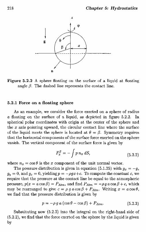
Figure 5.2.2 A sphere floating on the surface of a liquid at floatingangle /3. The dashed line represents the contact line.

5.2.1 Force on a floating sphere

As an example, we consider the force exerted on a sphere of radiusa floating on the surface of a liquid, as depicted in figure 5.2.2. Inspherical polar coordinates with origin at the center of the sphere andthe x axis pointing upward, the circular contact line where the surfaceof the liquid meets the sphere is located at O — ft. Symmetry requiresthat the horizontal components of the surface force exerted on the spherevanish. The vertical component of the surface force is given by

(5.2.2)

where nx = cos 9 is the x component of the unit normal vector.The pressure distribution is given in equation (5.1.25) with gx = —g,

gy = O, and gz = O, yielding p = —pgx+c. To compute the constant c, werequire that the pressure at the contact line be equal to the atmosphericpressure, p(x = a cos /3) — PAtm, and find PAITH — —pgacos/3 + c, whichmay be rearranged to give c = p g a cos /3 + PAITH- Writing x = acos#,we find that the pressure distribution is given by

p = -p g a (cos 6 - cos /3) + PAITH- (5.2.3)

Substituting now (5.2.3) into the integral on the right-hand side of(5.2.2), we find that the force exerted on the sphere by the liquid is givenby

(5.2.4)

To evaluate this integral, we note that the differential of the surface areaof the sphere may be expressed in the form dS — (ad(p)(adQ}, wherea — a sin 6 is the distance of a point on the surface of the sphere fromthe x axis, and (p is the meridional angle. Substituting this expressioninto the right-hand side of (5.2.4), and integrating with respect to </?, wefind

(5.2.5)

Next, we set sin 9 d6 = — dcos#, and carry out the integration on theright-hand side to find

'(5.2.6)

Working in a similar fashion, we find that the x component of theforce due to the atmospheric pressure exerted on the non-immersed partof the sphere, subtended between 9 = 0 and /3, is given by

(5.2.7)

Adding the two contributions (5.2.6) and (5.2.7), we obtain the buoyancyforce exerted on the sphere, given by

(5.2.8)

It can be shown by elementary trigonometry that the term enclosedby the square brackets on the right-hand side of (5.2.8) is equal to theimmersed volume of the sphere, that is, the volume of the sphere lyingunderneath the surface of the liquid, which is equal to the volume of thefluid displaced by the sphere. When the sphere is completely immersed,corresponding to ft = O, the term enclosed by the parantheses on theright-hand side of (5.2.8) is equal to 4, and the term enclosed by thesquare brackets is equal to the volume of the sphere, 47ra3/3.

Equation (5.2.8) states that the hydrostatic force exerted on a floatingsphere is equal in magnitude and opposite in direction to the weight ofthe fluid displaced by the sphere. In Section 5.3, we shall see that this is amore general result applicable to arbitrarily shaped floating or immersedbodies.

Computation of the floating angle

The floating angle /3 is determined by the weight of the sphere: theheavier the sphere, the smaller the angle. There is a critical weightwhere /3 becomes equal to zero and the sphere is completely submerged.To compute the floating angle corresponding to a certain weight W, weset W equal to the buoyancy force given in (5.2.8), and rearrange toobtain a cubic equation for cos/3,

(5.2.9)

where

(5.2.10)

is a dimensionless constant. We note that the fraction in the denominatorof (5.2.10) is equal to the volume of the sphere, and this suggests that,if the sphere is made of a homogeneous material of density p#, thens = PB/P is the density ratio. A neutrally buoyant sphere correspondsto s = 1, in which case cos/? = 1 and /3 = 0 satisfies equation (5.2.9), asexpected.

Newton's method

A variety of numerical methods are available for solving the nonlinearalgebraic equation (5.2.9). In practice, Newton's method strikes theoptimal balance between conceptual simplicity and numerical efficiency,and is a standard choice.

To formalize Newton's method in general terms, we define the vari-able q = cos/3, and express (5.2.9) in the generic form

f(q) = O, (5-2.11)

where, in the case of the floating sphere,

f(q)=q3-3q + 2(2s-l). (5.2.12)

The graph of the function f ( q ) for s = 0.25 is shown in figure 5.2.3. Therequisite value of q is located at the crossing of the graph of f ( q ) andthe q axis, denoted by Q, satisfying f ( Q ) = O.

To implement Newton's method, we make an initial guess for thedesired root Q, denoted by g(°), and then generate a sequence of im-provements working as follows. Near the point q(°\ the function f ( q )may be approximated with a linear function that arises by expandingf ( q ) in a Taylor series about q^\ and discarding all nonlinear terms toobtain the approximate form

Figure 5.2.2 Graph of the function f(q) defined in equation (5.2.12)whose root Q is required. To compute the root using Newton'smethod, we make an initial guess for Q, called g(°), and then im-prove it moving along the tangent to the graph toward the q axis.

(5.2.13)

The graph of this linear function is drawn with the straight line in figure5.2.2. Setting f(q) = O, solving for the q that is located within theparentheses on the right-hand side of (5.2.13), and denoting the solutionby q^l\ we obtain the improved value

(5.2.14)

In the case of the floating sphere, (df/dq)(q) = 3q2 - 3. The process isthen repeated yielding a sequence of successive approximations based onthe recursive formula

(5.2.15)

for k = O,1, Erroneously replacing the minus sign with a plus signon the right-hand side of (5.2.15) is a common source of frustration.

An error analysis shows that, as long as the initial quess q^ is suf-ficiently close to the root Q, the sequence defined by (5.2.15) convergesto Q, and the rate of convergence behaves as follows:

• If the graph of the function f ( q ) is not horizontal at the root,that is, (df/dq)q=Q / O, then the rate of convergence is quadratic,meaning that

q(k+i)-.Q~S(qW-Q)2J (5.2.16)

where S = ffl(Q)/[2ff(Q)} is an a priori unknown constant.

Equation (5.2.16) states that the magnitude of the error in thecurrent iteration, expressed by the left-hand side, is roughly equalto the square of the magnitude of the error in the previous iter-ation, multiplied by a constant. Consequently, if the initial errorg(°) - Q is sufficiently small, the magnitude of the error gW - Qwill keep decreasing during the iterations, no matter how large thevalue of the coefficient 5, as long as the initial guess is close to theroot for (5.2.16) to be valid.

• If the graph of the function f ( q ) is horizontal at the root, in whichcase (df/dq)q=Q = O and the root is multiple, the rate of conver-gence is linear, meaning that

,<»'>-«* =£V>-«>, (5.,17)

where m is the multiplicity of the root; for a double root, m = 2.

Equation (5.2.17) states that the magnitude of the error in thecurrent iteration is roughly equal to that in the previous iterationmultiplied by the positive coefficient (m — l)/m which is less thanunity for any value of m > 1. Consequently, the error \q№ —Q\ willkeep decreasing during the iterations as long as the initial guess isclose to the root for (5,2.17) to be valid.

Figure 5.2.3 A pycnometer is used to measure the specific gravity of aliquid, that is, the ratio between the density of the liquid and thedensity of water.

Problem

Problem 5.2.1 Pycnometer.A pycnometer is an antiquated device used for measuring the specific

gravity of a liquid, defined as the ratio of the density of the liquid andthe density of water. This is done by reading the level of the free-surfaceon a scale printed on a vertical tube attached to a spherical flask floatingon the liquid, as illustrated in figure 5.2.4. Pycnometer derives from theGreek word KVKVOTTITO. which means density. Derive an equation thatallows us to calibrate a pycnometer on the basis of the known density ofwater.

Computer problem

Problem c.5.2.1 Floating sphere.(a) Directory 00-num.men/04~nLeq of FDLIB includes the program

nonJinl.f that implements Newton's method for solving one nonlinearequation. Use the program to solve equation (5.2.9), and plot the float-ing angle /3 against the dimensionless parameter s defined in equation(5.2.10). Discuss the rate of convergence of the iterations in light ofequations (5.2.16) and (5.2.17).

(b) Directory OO-num-men/04-nLeq of FDLIB includes the programcubic.} that computes the three roots of a cubic equation using Cardano'sformulae. Use the program to solve equation (5.2.9), and plot the floatingangle /3 against the dimensionless parameter s.

5.3 Archimedes' principle

Consider the force exerted on a body with arbitrary shape immersedin a stationary fluid. Using equation (5.2.1), we find that the surfaceforce exerted on the body is given by

(5.3.1)

where n is the unit vector normal to the body pointing into the fluid.It would appear that the computation of the integral on the right-handside of (5.3.1) requires detailed knowledge of the geometry of the body;this is true when the fluid is incompressible. When, however, the fluidis incompressible, the integral may be evaluated in a generic fashionyielding a remarkably simple expression for the force in terms of thebody volume and fluid density.

Substituting the pressure distribution for an incompressible fluid giv-en in (5.1.25) into the right-hand side of (5.3.1), we find

(5.3.2)

A key observation in evaluating the integral is that the integrand is theproduct of the unit normal vector and a scalar function that is linearwith respect to the components of the position vector.

To see how the evaluation of the integral can be simplified, we consid-er a body having the shape of a rectangular parallelepiped, as illustratedin figure 5.1.1(b). The six flat sides of the body are perpendicular to thex, y, or z axis, the lengths of the edges are equal to Ax, Ay, and Az, andthe volume of the body is equal to VB — Ax Ay Az. The unit normalvector is constant over each one of the six sides; for example, over theside that is perpendicular to the x axis and faces the positive directionof the x axis, n = (1,0,0). Taking into consideration this and similarsimplifications, we evaluate the integral on the right-hand side of (5.3.2)without any approximation, and find

Fs = -pVBg, (5>3>3)

which expresses Archimedes's principle: the force exerted on an im-mersed body by the ambient fluid is equal in magnitude and opposite indirection to the weight of the fluid displaced by the body.

To compute the integral on the right-hand side of (5.3.2) over anarbitrarily shaped body, we subdivide the volume of the body into smallrectangular parallelepipeds, and approximate the surface of the bodywith the collection of the faces of the parallelepipeds that are wetted bythe fluid. Because of cancellations, the sum of the integrals over the facesof all elementary parallelepipeds is equal to the sum of the integrals ofthe faces that are wetted by the fluid. Summing the contributions, wefind that the force exerted on the body is given by (5.3.3) independent ofthe shape of the body: Archimedes's principles stands true for arbitrarilyshaped bodies.

5.3.1 The Gauss divergence theorem

Formula (5.3.3) may be derived in a more rigorous fashion usingthe Gauss divergence theorem in three dimensions stated in equation(2.6.25). Selecting hx = /, hy = O, and hz = O to form the vectorfunction h — (/, O, O), where / is a scalar function of position, we obtain

(5.3.4)

The complementary selections h = (O, /, O) and h = (O, O, /) yield thecorresponding identities

(5.3.5)

Relations (5.3.4) and (5.3.5) may be collected into the vector identity

(5.3.6)

where V/ = ( d f / d x , d f / d y , df/dz) is the gradient of /.

Comparing now (5.3.6) with (5.3.2), we set

/ = P (3x x + gy y + gz z] + P0, /5 3 ?x

computeV/ = P (gx, Qy, Qz) = Pg, (5.3.8)

and find that the surface force is given by

(5.3.9)

which reproduces and confirms equation (5.3.3).

5.3.2 Net force on a submerged body

If a body of volume VB consists of a homogeneous material withdensity PB, then the mass of the body is equal to ms = PB VB, and itsweight is equal to

W = PB^Bg, (5.3.10)

where g is the acceleration of gravity. Adding the weight of the body tothe buoyancy force given in (5.3.3), we find that the net force exerted onan immersed body is given by

F = F5 + W - (PB - p) VB g. ($3.11)

The density of a neutrally buoyant body is equal to the density of theambient fluid, and the right-hand side of (5.3.11) vanishes yielding a zeronet force.

Consideration of the moments of the traction exerted on the bodyreveals that the buoyancy force passes through the center of mass ofthe fluid displaced by the body, whereas the weight of the body passesthrough the center of mass of the body. If the former lies above thelatter, then the body is in a state of stable equilibrium and will remainstationary; otherwise, it will spontaneously rotate to reach a stable con-figuration.

Problem

Problem 5.3.1 Applications of the Gauss divergence theorem.(a) Apply (5.3.6) for a constant function / and discuss your result.(b) The center of gravity of a homogeneous body with uniform density

is defined in terms of a volume integral as

(5.3.12)

Show that an equivalent expression in terms of a surface integral is

(5.3.13)

5.4 Shapes of two-dimensional interfaces

Consider two superposed stationary incompressible fluids separatedby an infinite horizontal interface located at y = y/, as illustrated infigure 5.4.1. The upper fluid is designated as fluid 1, and the lower fluidis designated as fluid 2. Using the general expression for the pressuredistribution in an incompressible liquid given in equation (5.1.25), wefind that the pressure distributions in the two fluids are given by

P(l\y] = -Pi 9V+ ci, P(2)(y) = -P29V + C2. (5A.1)

The two constants c\ and C2 are related by the condition for the jump inthe traction across an interface with constant surface tension stated inequation (4.4.11). Since in this case the curvature of the interface van-ishes, K = O, condition (4.4.11) requires that the pressure be continuousacross the interface,

P(l](y = vi) = p(2)(y = y/). (5.4.2)

Substituting the pressure distributions (5.4.1) into (5.4.2), we find

-pi gyi + ci = -p2 gyi + C2, (5.4.3)

which may be rearranged to give

C2 = ci + (p2 - pi) g yi. (5.4.4)

Figure 5.4.1 An infinite horizontal interface separating two stationaryfluids.

One of the two constants c\ or 02 is determined by requiring an appro-priate boundary condition far from the interface, and the second followsfrom (5.4.4). For example, if the pressure on the upper side of the inter-face is equal to the atmospheric pressure PAtnn then c\ = PAtm + PiQViand C2 = PAtm + P2 9 Vi-

5.4.1 Static contact angle

In practice, the flat interface depicted in figure 5.4.1 terminates at aside wall, as illustrated in figure 5.4.2. Further examples of terminatedinterfaces are depicted in figure 5.5.1 illustrating a semi-infinite interfaceending at an inclined plate, in figure 5.6.1 illustrating a finite interfaceconfined between two parallel flat plates, and in figure 5.7.1 illustratingthe finite interface enclosing a drop attached to a horizontal plane.

The line where the two fluids meet at a solid surface is called thecontact line. In the case of two-dimensional or axisymmetric interfaces,the contact line is represented by the contact point, which is the traceof the contact line in the xy or a meridional plane, identified by a filledcircle in figures 5.5.1, 5.6.1, and 5.7.1.

The angle subtended between (a) the line that is normal to the con-tact line and tangential to the solid surface, and (b) the line that isnormal to the contact line and tangential to the interface, measured on

Fluid 1

Fluid 2

Figure 5.4.2 An interface ending at a contact line; a is the contactangle measured on the side of fluid numbered 2.

the side of fluid labelled 2, as illustrated in figure 5.4.2, is called the staticcontact angle. The static contact angle is a physical constant determinedby the prevailing physical conditions and physical properties of the solidand fluids. If fluid 1 wets the solid better than fluid 2 does, then thecontact angle is smaller than Tr/2; whereas if fluid 2 wets the solid betterthan fluid 1 does, the contact angle is larger than Tr/2 but less than themaximum possible value of TT.

If the side-wall illustrated in figure 5.4.2 is vertical, and the staticcontact angle is equal to Tr/2, the interface will remain flat all the wayup to the contact line. Under more general conditions, the interface willassume a curved shape with nonzero curvature established to satisfy thephysical requirement on the contact angle.

5.4.2 The Laplace-Young equation

To derive the equation governing the shape of a curved interface, wesubstitute the pressure distributions (5.4.1) into the interfacial condition(4.4.11), and find

-P2 g yi + C2 + PI g yi - ci = 7 *. ^A ̂

Rearranging, we obtain the Laplace-Young equation governing the shapeof a two-dimensional interface in hydrostatics,

Fluid 1

Fluid 2

(5.4.6)

where Ap = p% — pi, and B = (c<2 — ci)/7 is a constant with dimensionsof inverse length determined by requiring an appropriate boundary con-dition or global constraint. Implicit in (5.4.6) is the assumption that theacceleration of gravity points toward the negative direction of the y axis;for different orientations, straightforward modifications are necessary.

Assuming that the fluids are stably stratified, that is, p2 > pi orAp > O, we introduce the capillary length defined as

(5.4.7)

and recast equation (5.4.6) into the simpler form

(5.4.8)

For an air-water interface at 20° Celsius, 7 = 73 dynes/cm = 73 x 10~3

kg/sec2, pi—0.0 kg/m3, p2=1000.0 kg/m3, yielding a capillary length of2.72 mm.

The Laplace-Young equation (5.4.8) requires that the curvature of aninterface be a linear function of the elevation from a reference state. Anobvious solution arises by assuming that y/ is constant, and then settingB = yj/l2 to find ft = O. The flat shape of the interface computed inthis manner, however, will not necessarily conform with the boundarycondition on the static contact angle, and the obvious solution will notgenerally be admissible: the shape of the interface must be found sothat both (5.4.8) and the boundary condition on the contact angle aresatisfied.

Problem

Problem 5.4.1 Laplace-Young equation in three dimensions.Show that the counterpart of equation (5.4.8) for a three-dimensional

interface is(5.4.9)

where Km is the mean curvature.

Figure 5.5.1 A semi-infinite interface attached to an inclined plate. Farfrom the plate, the interface becomes horizontal.

5.5 A semi-infinite interfaceattached to an inclined plate

We begin the study of two-dimensional interfacial shapes by consid-ering a semi-infinite interface attached to a flat plate that is inclined atan angle /3 with respect to the horizontal, as illustrated in figure 5.5.1.Far from the plate, as x tends to infinity, the interface tends to becomehorizontal. The contact angle subtended between the inclined plate andthe tangent to the interface at the contact point is required to have theprescribed value a.

It will be convenient to set the origin of the y axis at the positionof the flat interface far from the plate, and describe the interface by theequation

yi = /(*)• (5.5.i)As x tends to infinity, the function f ( x ) tends to zero yielding a flatinterface. Since the curvature of the interface vanishes far from the plate,the constant B on the right-hand side of the Laplace-Young equation(5.4.8) must be equal to zero, yielding the simpler form

12 (5.5.2)

Fluid 1

Fluid 2

Our first task is to derive an expression for the curvature in terms of thefunction f ( x ) .

5.5.1 Curvature

Taking the inner product of equation (4.3.5) and the unit normalvector n^1), we find

(5.5.3)

When the interface does not turn upon itself but has the monotonicshape depicted in figure 5.5.1, we may write

(5.5.4)

where a prime denotes a derivative with respect to x. Substituting ex-pressions (5.5.4) into the right-hand side of (5.5.3), and simplifying, weobtain the desired expression for the curvature,

(5.5.5)

It will be useful to introduce the slope angle 9 shown in figure 5.5.1,defined by the equation

tan0 = /' (5.5.6)

and note that the fraction on the right-hand side of (5.5.5) is equal toI cos#|. The curvature of the interface is then given by the alternativeexpression

(5.5.7)

5.5.2 Governing equation

Combining (5.5.5), (5.5.7), and the Laplace-Young equation (5.5.2),we derive a differential equation governing the shape of the interface,

(5.5.8)

Integrating once with respect to x, we obtain

(5.5.9)

where C is an integration constant. Demanding that, as x tends toinfinity, 6 tends to TT and / tends to vanish, we find C = I .

5.5.3 Capillary rise

At the contact line located at x = O, the slope angle 9 defined inequation (5.5.6) takes the value

0CL = a + P- (5.5.10)

Evaluating (5.5.9) at x = O, setting C = I, and rearranging, we obtainan expression for the positive or negative capillary rise h = /(O),

A_ = l-|cos(a+ /?)|, (55n)

which shows that the maximum possible value of \h\ occurs when a. + /3is a multiple of ?r/2, and the maximum value is equal to \/2/.

5.5.4 Numerical formulation

To compute the shape of the interface, we set the left-hand side of(5.5.9) equal to the right-hand side with C = I , and rearrange to obtainthe first-order ordinary differential equation

(5.5.12)

where we have introduced the dimensionless function / = ///. The plusor minus sign on the right-hand side must be selected according to theexpected interface shape.

The preceding analysis assumes that the interface has a monotonicshape, and this requires that OCL lie in the range (?r/2, 3?r/2). Outside

this range, the capillary rise is given by equation (5.5.11), but with theminus sign replaced by a plus sign on the right-hand side.

When the shape of the interface is non-monotonic, which means thatthe interface becomes vertical at a point, the function f ( x ) is multi-valued, and the integration of (5.5.12) requires special attention. Tobypass this subtlety, we regard x along the interface as a function of theindependent variable /, and recast (5.5.12) into the form

(5.5.13)

The solution of (5.5.13) is to be found for |/| < |/i|, where \h\ is thecapillary rise computed from equation (5.5.11).

5.5.5 Numerical method

A numerical solution of (5.5.13) may be computed according to thefollowing steps:

1. Compute the angle QCL from equation (5.5.10).

2. Compute the capillary rise h using the formulae:

(5.5.14)

3. Integrate the differential equation (5.5.13) from / — h to O withinitial condition x(f = h) = O using, for example, the explicit Eulermethod or the explicit modified Euler method discussed in Section1.5. If h is negative, use a negative spatial step.

To implement the explicit Euler method, we select a small positiveor negative integration step A/ = h/N, where N defines the levelof numerical discretization, evaluate equation (5.5.13) at the point/, and approximate the derivative on the left-hand side with thefinite difference [x(f + A/) — x(/)]/A/. Rearranging, we obtain

(5.5.15)

The repetitive application of this formula, starting from / = hwhere x — O, generates a sequence of points distributed over theinterface.

To implement the explicit modified Euler method, we replace for-mula (5.5.15) with the slightly more involved formula

(5.5.16)

where ftmp = / + A/.

Computer problem

Problem c.5.5.1 Semi-infinite interface.Directory 05-hydrostat/men.2d-plate of FDLIB includes the main

program men-2d.plate that computes the shape of the semi-infinite in-terface discussed in the text. Run the program to generate a family ofshapes corresponding to a fixed value of the plate inclination angle /3 andvarious contact angles a, and another family of shapes corresponding toa fixed value of the contact angle and various plate inclination angles.Discuss the behavior of the capillary rise in each case.

5.6 A meniscus between two parallel plates

Consider an interface subtended between two parallel vertical platesthat are separated by the distance 26, as illustrated in figure 5.6.1. Thetwo contact points are at the same elevation, and the interface is sym-metric with respect to the mid-plane located at x = O.

It will be convenient to set the origin of the Cartesian axes on theinterface midway between the plates, and describe the position of theinterface by the equation y/ = f ( x ) . Outside and far from the plates,the interface assumes a horizontal shape located at y/ = —/i, where h isthe positive or negative capillary rise of the meniscus midway betweenthe plates. Our objective is to compute h along with the unknown shapeof the meniscus by solving the Laplace-Young equation (5.4.8). We beginby making several preliminary observations:

Figure 5.6.1 Illustration of a two-dimensional meniscus subtended be-tween two parallel vertical plates, for contact angle a less than7T/2. When a is greater than Tr/2, the meniscus submerges and thecapillary rise h is negative.

1. The choice of Cartesian axes requires that y/ = O at x = O; equation(5.4.8) then gives

«(°) = B- (5.6.1)

Because the interface is symmetric with respect to x = O, df/dx = Oat x = O, equation (5.5.5) gives

(5.6.2)


(5.6.3)

2. Evaluating (5.4.8) at a point outside and far from the plates wherethe curvature of the interface tends to vanish and y/ —> — /i, weobtain

Fluid 1

Fluid 2

(5.6.4)

Combining equations (5.6.2) - (5.6.4), we find

(5.6.5)

which shows that the capillary rise may be computed from knowl-edge of the curvature of the interface at the mid-point.

Proceeding now with the mathematical formulation, we substitutethe first expression for the curvature shown in (5.5.5) and the value ofB shown in (5.6.4) into the Laplace-Young equation (5.4.8), and rear-range to derive a second-order ordinary differential equation involvingthe capillary rise h as an unknown parameter,

(5.6.6)

The solution is to be found over the interval O < x < 6, subject to theboundary conditions

(5.6.7)

The third condition specifies the prescribed value of the contact angle. Ifa — 7T/2, all three boundary (5.6.7) are homogeneous, and the obvious so-lution h = O and / = O describes a flat non-elevated and non-submergedinterface.

5.6.1 Canonical form

To compute the solution under more general conditions, we recastthe second-order differential equation (5.6.6) involving the unspecifiedparameter h into the canonical form of a system of three first-orderdifferential equations. The word canonical derives from the Greek workKOLVOVIKO<; which means normal; in real life, normal is not necessarilydesirable. This is done by introducing the three new variables

9i = /> 92 = /', 9s = h, (5.6.8)

where q^ = f". Subject to these definitions, equation (5.6.6) is resolvedinto the three first-order component equations,

(5.6.9)

The third equation simply states that q% = h is a constant. In terms ofthe new variables, the boundary conditions (5.6.7) become

9i(O) = O, ^2(O) = O, q2(b) = cot a. (5.6.10)

If the value of #3 (O) = h were known, we would be able to integrate thesystem (5.6.9) from x = O to b using, for example, the explicit Euler orthe modified Euler method discussed in Sections 1.5 and 5.5.

Explicit Euler method

To implement the explicit Euler method, we recast the system (5.6.9)into the general symbolic form

(5.6.11)

where, in the present case,

(5.6.12)

Next, we evaluate equations (5.6.11) at a point x, select a small spatialstep Ax, and approximate the derivatives on the left-hand sides withfinite differences writing, for example, dq\/dx — (gi(x+Ax) —gi(x))/Ax.Solving for q\ (x + Ax), and repeating for the second and third equation,we find

qi (x + Ax) = qi (x) + Ax f i (qi (x), q2 (X] , q3 (x), x),

92 (x + Ax) = 92 (x) + Ax /2 (qi (x), 92 (x), 93 (x), x),

93(x + Ax) = 93(x) + Ax / 3 (qi (x) ,92(#) ,93 (x) ,x} . (5.6.13)

In vector notation,

q(x + Ax) - q(x) + Ax f (q(x), x), (5.6.14)

where we have defined the solution vector q = (91,92? 9s) and the cor-responding phase-space velocity vector f = (/i,/2,/3)- The repetitiveapplication of formula (5.6.14), starting from x = O, allows us to gener-ate a sequence of points distributed over the meniscus.

Explicit modified Euler method

To implement the explicit modified Euler method, we replace formula(5.6.14) with the union of a predictor and a corrector formula,

qtmP = q(x)+Axf(q(x) ,x) ,

q(x + Ax) - q(x)+Ax^[f (q(x) ,x)+f(q^ ,x + Ax)],(5.6.15)

where the superscript imp denotes a preliminary value computed by theexplicit Euler method. The first equation generates a provisional value,and the second equation advances the solution using the initial and theprovisional value.

5.6.2 The shooting method

Because, however, the value of h is unknown, the starting vector q(0)is not available, and the solution of (5.6.9) must be computed using aniterative method. The shooting method prescribes the obvious: guessthe value of 93(0) — /i, compute the solution of (5.6.9), and then checkwhether the third condition in (5.6.10) is fulfilled; if not, repeat thecomputation with an improved guess.

To improve the guess in a systematic fashion that guarantees rapidconvergence, we note that the value of q^(b) computed by solving equa-tions (5.6.9) is a function of the guessed value ^a(O) = /i; to signify thisdependence, we extend the list of arguments of q^ writing q<i(b\ h). Thethird of the boundary conditions (5.6.10) requires Q2(b]h) — cot a. — O,which means that h is a root of the objective function

Q(K) = #>(&; h) - cot a. (5.6.16)

The problem has been reduced to computing the solution of the algebraicequation

Q(K) = O, (5.6.17)

where the left-hand side is evaluated by integrating equations (5.6.9)with a specified value of h.

5.6.3 The secant method

The secant method provides us with a simple algorithm for solvingthe nonlinear algebraic equation (5.6.16) according to the following steps:

1. Select a value for h that approximates the root, called /i^, andcompute Q(Ii^) by solving (5.6.9).

A reasonable approximation may be obtained by assuming thatthe meniscus has a circular shape of radius R, which is positivewhen the interface is concave upward and negative when the inter-face is concave downward. Using elementary trigonometry, we findthat the prescribed boundary condition on the contact angle willbe satisfied when cos a = b/R, which may be rearranged to yieldthe approximation K ~ —1/R = —cosa/b. Combining equations(5.6.2) and (5.6.5), we obtain the desired educated guess

h ~ cos a. —.b (5.6.18)

Equation (5.6.18) reveals that the maximum possible value of \h\is equal to l2/b.

2. Select another value for h called M2), and compute Q(h№) bysolving (5.6.9).

3. Approximate the graph of the function Q(h) with a straight linepassing through the points computed in steps 1 and 2. The slopeof the approximating straight line is

(5.6.19)

4. Identify the improved value h^ with the root of the linear functiondescribing the approximating straight line. Elementary algebrashows that the root is given by

(5.6.20)

5. Repeat the computation with the pairs M2) and h^.

Computer problem

Problem c.5.6.1 Meniscus between plates.Directory O5.hydrostat/men.2d of FDLIB includes the main program

men,2d that computes the shape of a meniscus subtended between twoparallel plates. Run the program to generate a family of shapes cor-responding to a fixed value of the plate separation and various contactangles, and another family of shapes corresponding to a fixed value ofthe contact angle and various plate separations. Discuss the behavior ofthe capillary rise in each case.

5.7 A two-dimensional drop on a horizontal plane

Consider now a two-dimensional drop of a fluid labelled 2 restingabove, or hanging below, a horizontal plate while surrounded by a sta-tionary ambient fluid labelled 1, as illustrated in figure 5.7.1. The restingdrop shown in frame (a) is called a sessile drop, and the hanging dropshown in frame (b) is called a pendant drop. Our objective is to computethe shape of the interface for a specified value of the contact angle a anddrop area AD-

Figure 5.7.1 Illustration of a two-dimensional or axisymmetric dropresting on, or hanging below a horizontal plate called, respectively,a sessile or a pendant drop.

It will be convenient to introduce Cartesian axes with origin at theextreme point of the interface, and the x axis pointing normal to theinterface and into the ambient fluid, as depicted in figure 5.7.1 (a, b),respectively, for the sessile or pendant drop.

5.7.1 Parametric representation

One difference between the problem presently considered and theones discussed in preceding sections, is that, in the present case, neitherthe range of x nor the range of y is known over the span of the interface.To circumvent this difficulty, we describe the shape of the interface inparametric form in terms of the slope angle ^ defined in figure 5.7.1,increasing from O at the origin to a at the contact point.

Our objective is to compute the two scalar functions of 1/1 such thatthe x and y coordinates of a point at the interface are described by thefunctions

X = X(^), y = Y(*l>), (5.7.1)

for O < V < GL. To compute X(ijj) and Y(^), we require two ordinarydifferential equations and a suitable number of boundary conditions orglobal constraints.

5.7.2 Parametric equations

The first differential equation is the definition of the chosen parameterV> in terms of the interface slope,

(5.7.2)

One important benefit of the adopted parametrization is that the bound-ary condition for the contact angle at the contact point is satisfied au-tomatically and may be removed from further discussion.

The second differential equation must arise from the Laplace-Youngequation determing the jump in pressure across the interface. Workingas in Section 5.4, we find

(5.7.3)

where Ap = p% — p\\ the coefficient s\ is equal to 1 for a sessile dropor -1 for a pendant drop, reflecting the orientation of the gravity withrespect to the positive direction of the x axis. To simplify the notation,we introduce the capillary length

(5.7.4)

and recast (5.7.3) into the simpler form

(5.7.5)

where the coefficient 82 is equal to 1 when p2 > pi, or -1 when p^ < p\.Evaluating equation (5.7.5) at the origin, we find that the constant B isequal to the unknown curvature of the interface at the plane of symmetrylocated at y = O.

Considering now equation (5.5.5), we set /' = dY/dX, and use (5.7.2)to find

(5.7.6)

Substituting the right-hand side of (5.7.6) into the left-hand side of(5.7.5), we obtain

(5.7.7)

which may be rearranged to give the desired parametric dependence

(5.7.8)

where

(5.7.9)

To derive a corresponding parametric dependence for Y", we recast (5.7.2)into the form

(5.7.10)

Substituting (5.7.8) into (5.7.10), we find

(5.7.11)

Equations (5.7.8) and (5.7.11) provide us with the requisite system oftwo first-order differential equations involving the unspecified parameterJ5, to be solved subject to (a) the boundary conditions

X(Q) = O, y (O) = O, (5 7 12)

and (b) the constraint on the drop area AD,

2f°Jd* = A°' (5.7.13)

where x = —d describes the position of the plane.

5.7.3 The shooting method

Because the value of the constant B is a priori unknown, the solutionmust be found using an iterative method. The shooting method, com-bined with the secant method for improving the guess, provides us withan efficient algorithm. The numerical procedure involves the followingsteps:

1. Guess a value for B.

Since B is equal to the unkown curvature of the interface at themid-plane located at y = O, a reasonable guess can be obtainedby assuming that the interface has the shape of a section of acircle, and then computing the radius of the circle a according tothe specified values of the contact angle and drop area. Usingelementary trigonometry, we find

(5.7.14)

2. Integrate the system of equations (5.7.8) and (5.7.11) using, forexample, the explicit Euler method or the explicit modified Eulermethod discussed in Section 5.6.

3. Compute the integral on the right-hand side of (5.7.13) using thetrapezoidal rule, and then evaluate the objective function

(5.7.15)

4. Improve the value of B with the goal of driving the objective func-tion Q to zero using, for example, the secant method discussed inSection 5.6.

Problems

Problem 5.7.1 Two-dimensional drop on a horizontal plane.Derive formula (5.7.14).

Problem 5.7.2 Two-dimensional drop on an inclined plane.Formulate the problem of a pendant or sessile two-dimensional drop

attached to an inclined plane.

Computer problem

Problem c.5.7.1 Two-dimensional drop by numerical computation.Subdirectory 05-hydrostat/drop-2d of FDLIB includes the main pro-

gram drop.2d that computes the shape of a sessile or pendant two-dimensional drop using the shooting method discussed in the text. Run

the program to generate a family of shapes corresponding to a fixed val-ue of the drop area and various contact angles, and another family ofshapes corresponding to a fixed value of the contact angle and variousdrop areas. Discuss the computed interfacial shapes.

5.8 Axisyrnmetric shapes

To compute the shape of axisymmetric interfaces, we work as in thecase of two-dimensional interfaces discussed in the preceding sections.Additional considerations include certain subtleties in the computationof the mean curvature, and a more pronounced sensitivity of the numer-ical methods to the parameters of the computation. In this section, weillustrate the new features by discussing the axisymmetric versions of thetwo-dimensional problems considered in Sections 5.6 and 5.7.

5.8.1 A meniscus in a vertical capillary

Consider an axisymmetric meniscus inside a vertical cylindrical tubeof radius a, as illustrated in figure 5.8.1, which is the counterpart ofthe two-dimensional meniscus depicted in figure 5.6.1. In the cylindricalpolar coordinates depicted in figure 5.8.1, the interface is located at

x' = /(a)- (5.8.1)

Outside the tube, the interface assumes a horizontal shape with vanishingcurvature located at x = — h.

Laplace-Young equation

Working as in Section 5.4 but with the interfacial condition (4.4.12) inplace of (4.4.11), we derive the three-dimensional version of the Laplace-Young equation (5.4.6), given by

(5.8.2)

where Km is the interface mean curvature. The constant B is definedimmediately after equation (5.4.6), and is given in terms of the capillaryrise in equation (5.6.4).

Figure 5.8.1 Schematic illustration of an axisymmetric meniscus insidea vertical circular tube, for contact angle a greater than Tr/2.

Mean curvature

The mean curvature is the average of the two principal curvatures:one is the curvature of the trace of the interface in the ax plane, denotedby KI, and the second is the curvature of the trace of the interface inthe orthogonal plane, denoted by «2- Working as in Section 5.5, we findthat the first principal curvature is given by the following counterpart ofequation (5.5.5),

(5.8.3)

where a prime denotes a derivative with respect to a.It can be shown that the radius of curvature of the second principal

curvature, denoted by R<2, is equal to the signed distance between (a)the point where the curvature is evaluated, and (b) the intersection ofthe normal to the interface and the x axis, as illustrated in figure 5.8.1,

(5.8.4)

Fluid 1

Fluid 2

where 6 is the interface slope angle defined in figure 5.8.1, /' = tan#.For the submerged meniscus depicted in figure 5.8.1, O is negative andR<2 is positive.

Combining expressions (5.8.3) and (5.8.4), we find

(5.8.5)

Parametric representation

It is expedient to describe the shape of the interface in parametricform in terms of the slope angle 9 varying from O at the center of the tubeto 7T/2 - a at the inner wall of the tube, where a is the contact angle.The axial and radial position of a point at the interface is described,respectively, by the functions

x = X ( 6 ) , <r = S(0). (5-8-6)

Substituting the right-hand side of (5.8.5) into the left-hand side of theLaplace-Young equation (5.8.2), and rearranging, we find

(5.8.7)

where we have defined

(5.8.8)

Equation (5.8.7) governs the parametric representation of the radial po-sition a in terms of the slope angle 6. To derive a corresponding equationfor the axial position X, we combine the definition /' = tan# = dX/dEwith (5.8.7), and obtain

(5.8.9)

The boundary conditions require

S = O and X = O at 9 = O,(5.8.10)

and

E = a at 0 = 7T/2 - a.(5.8.11)

An apparent difficulty arises when we attempt to evaluate the func-tion $ defined in equation (5.8.8) at 9 = O corresponding to S = O:the second fraction on the right-hand side is undefined. Using, however,the PHopital rule, we find that, as 9 tends to zero, this ratio reducesto d#/dS. Substituting this asymptotic limit into (5.8.8) and the resultinto (5.8.7) and (5.8.9), we find the regularized initial conditions

(5.8.12)

which are used to start up the integration.

Solution by iteration

Since the value of the capillary rise h is a priori unknown, the solutionmust be found by iteration. The shooting method involves the followingsteps: guess the value of /i, compute the solution of (5.8.7) and (5.8.9)subject to the initial conditions (5.8.10), and check whether (5.8.11)is satisfied. If not, improve the guess using, for example, the secantmethod discussed in Section 5.6. A reasonable initial guess emerges byassuming that the meniscus has a spherical shape that is consistent withthe prescribed contact angle; using elementary trigonometry, we find

(5.8.13)

5.8.2 Drop on a plane

Consider next an axisymmetric drop of a fluid labelled 2, restingabove or hanging below a horizontal plane while surrounded by an am-bient fluid labelled 1, as illustrated in figure 5.7.1. We wish to computethe shape of the interface for a specified value of the contact angle a. anddrop volume VD.

Working as in the case of the two-dimensional drop discussed in Sec-tion 5.7, we describe the interface in parametric form in terms of theslope angle ifi defined in figure 5.7.1, as

(5.8.14)

where

(5.8.15)

The counterparts of equations (5.7.8) and (5.7.11) are

(5.8.16)

where

(5.8.17)

The boundary conditions are

X(O) = O, S(O) = O,(5.8.18)

and the constraint on the drop volume VD takes the form

(5.8.19)

where x = — d describes the position of the plane. At the axis of symme-try located at a — O, equations (5.8.16) are replaced by the regularizedforms

(5.8.20)

The solution of the parametric equations (5.8.16) can be found us-ing the shooting method discussed in Section 5.7 for the correspondingproblem in two dimensions. In the present case, the constant B is equalto twice the mean curvature of the interface at the x axis. A reason-able guess for B arises by assuming that the interface has the shape of asection of a sphere, and computing the radius of the sphere a to satisfythe constraints on the contact angle and drop volume. Using elementarytrigonometry, we find

(5.8.21)

and then set B = 2/a.

Problem

Problem 5.8.1 Drop on a plane.(a) Derive the regularized expressions (5.8.20) departing from equa-

tions (5.8.16) and (5.8.17).(b) Derive formula (5.8.21).

Computer problems

Problem c.5.8.1 Axisymmetric meniscus.Directory 05-hydrostat/men.ax of FDLIB includes the main program

men.ax that computes the shape of a meniscus. Run the program to gen-erate a family of shapes corresponding to a fixed value of the tube radiusand various contact angles, and another family of shapes correspondingto a fixed value of the contact angle and various tube radii. Discuss thebehavior of the capillary rise in each case.

Problem c.5.8.2 Axisymmetric drop.Directory 05-hydrostat/drop.ax of FDLIB includes the main program

drop-ax that computes the shape of a sessile or pendant axisymmetricdrop using the shooting method. Run the program to generate a familyof shapes corresponding to a fixed value of the drop volume and variouscontact angles, and another family of shapes corresponding to a fixed val-ue of the contact angle and various drop volumes. Discuss the computedinterfacial shapes.

Chapter 6

Equation of motion and vorticity transport

6.1 Newton's second law for the motion of a parcel6.2 Integral momentum balance6.3 Cauchy's equation of motion6.4 Euler's and Bernoulli's equations6.5 The Navier-Stokes equation6.6 Vorticity transport6.7 Dynamic similitude, the Reynolds number

and dimensionless numbers in fluid dynamics

Fluid flow is established in response to an external action mediatedby boundary motion, by the application of a surface force, or by the pres-ence of a body force. The evolution of a transient flow and the structureof a steady flow established after an initial start-up period are governedby two fundamental principles of thermodynamics and classical mechan-ics: mass conservation, and Newton's second law for the motion of fluidparcels. The implementation of Newton's law in fluid mechanics leadsto Cauchy's equation of motion, which provides us with an expressionfor the point particle acceleration in terms of the stresses, and to thevorticity transport equation governing the point particle rate of rota-tion. The derivation and intepretation of these equations in general andspecific forms, and their solution for simple flow configurations will bethe theme of our discussion.

6.1 Newton's second lawfor the motion of a parcel

Consider a fluid parcel in motion, as illustrated in figure 5.1.1 (a).Newton's second law of motion requires that the rate of change of thelinear momentum of the parcel, denoted by Mp, be equal to the sum of

the forces exerted on the parcel, including the body force due to gravitygiven in equation (5.1.1), and the surface force given in equation (5.1.2).Expressing these forces in terms of surface and volume integrals, weobtain

(6.1.1)

where f is the hydrodynamic traction exerted on the parcel surface. Ex-pressing further the traction in terms of the stress tensor, as shown inequation (4.2.9), we find

(6.1.2)

where the unit normal vector n points into the parcel exterior. Our nexttask is to relate the rate of change of the parcel momentum to the fluiddensity and velocity.

6.1.1 Rate of change of linear momentum

An expression for the linear momentum arises by subdividing theparcel into elementary subparcels of volume dVp and mass dmp = pdV,and then summing the contributions by integration, obtaining

(6.1.3)

where u is the fluid velocity. The rate of change of linear momentum isgiven by

(6.1.4)

Now, because the integration is over the volume of the parcel which isnot stationary but changes in time, interchanging the time differentiationand the volume integration on the right-hand side of (6.1.4) is permissibleonly if the time derivative is replaced by the material derivative D/Dtunder the integral sign. Thus,

(6.1.5)

Conservation of mass requires that the material derivative of the elemen-tary mass drrip vanish, yielding the simplified expression

(6.1.6)

6.1.2 Equation of parcel motion

Substituting the right-hand side of (6.1.6) into the left-hand side of(6.1.2), we obtain the desired equation of fluid parcel motion,

(6.1.7)

involving the point particle acceleration, the stress tensor, and the bodyforce. Explicitly, the x, y, and z components of (6.1.7) are given by

(6.1.8)

Equations (6.1.8) are valid irrespective of whether the fluid is compress-ible or incompressible.


The counterpart of equation (6.1.7) for two-dimensional flow in thexy plane is

(6.1.9)

Figure 6.1.1 Illustration of a fluid parcel with an instantaneous rect-angular shape, drawn with the solid line, in two-dimensional flow.The fact that the parcel generally deforms to obtain a warpedshape, drawn with the dashed line, does not prevent us from ap-plying Newton's law of motion in its integral form over the instan-taneous parcel shape.

where dA is the differential of the surface area, and dl is the differentialof the arc length along the contour of a parcel in the xy plane. Explicitly,the x and y components of (6.1.9) are given by

(6.1.10)

We note again that these equations are valid irrespective of whether thefluid is compressible or incompressible.

Motion of a rectangular pared

As an application, we consider the motion of a fluid parcel with aninstantaneous rectangular shape whose sides are parallel to the x or yaxes, as depicted in figure 6.1.1. It is important to note that the parcel

will remain rectangular only if the fluid exhibits rigid-body motion; undermore general conditions, the parcel will deform to obtain a warped shapedrawn with the dashed line in figure 6.1.1. The fact that the parcelwill generally deform, however, does not prevent us from evaluating theintegrals in (6.1.10) over the instantaneous rectangular shape.

For simplicity, we assume that the density of the fluid is uniform, andthe acceleration of gravity is constant. Taking into consideration thatthe unit normal vector is parallel to the x or y axis over each side, wefind that equations (6.1.10) assume the simpler forms

(6.1.11)

and

(6.1.12)

The first integral on the right-hand side of (6.1.11) involves normalstresses exerted on the vertical sides, and the second integral involvesshear stresses exerted on the horizontal sides; the converse is true for(6.1.12).

Steady unidirectional flow

In the case of steady unidirectional flow along the x axis, the pointparticles move along the x axis with constant velocity and vanishingacceleration, Du/Dt = O. The left-hand side of the equation of motion(6.1.9) vanishes, yielding a balance between the hydrodynamic and bodyforce,

(6.1.13)

Restricting our attention to Newtonian fluids and using the consti-tutive equation (4.5.4), we find the following:

• In the absence of axial and transverse stretching, dux/dx = O andduy/dy = O, the normal stresses axx and ayy are equal to thenegative of the pressure p, axx = <jyy = —p.

• The shear stresses axy — cryx are independent of streamwise posi-tion x, but may depend on the lateral position y.

Subject to these simplifications, the balance equations (6.1.11) and(6.1.12) reduce to

(6.1.14)

where Ax = x% - x\ and Ay = j/2 — J/i- The second of equations (6.1.14)is clearly satisfied when

(6.1.15)

reflecting the hydrostatic pressure variation. The first of equations (6.1.14)is satisfied when

(6.1.16)

where G is a free parameter called the modified pressure gradient. Phys-ically, G is determined by the physical mechanism driving the flow:

1. When G = O, the first of equations (6.1.16) shows that the pres-sure variation in the x direction is hydrostatic, and the secondof equations (6.1.16) shows that the shear stress ayx is constant,independent of y. This is the case of shear-driven flow.

2. When the streamwise pressure drop vanishes, px=x2,y = PX=XI,y? thefirst of equations (6.1.16) requires that G = pgx, and the secondof equations (6.1.16) shows that the difference in the shear stress(&yx)x,y=y2 ~ (cryx)x,y=y1 is equal to -p gx Ay. This is the case ofgravity-driven flow.

3. When the flow is horizontal, gx = O, the first of equations (6.1.16)shows that G is the negative of the streamwise pressure gradient,and the second of equation (6.1.16) shows that the difference inthe shear stress (&yx)x,y=y2 ~ (&yx)x,y=yi is equal to -G Ay. Thisis the case of pressure-driven flow.

Problem

Problem 6.1.1 Body force in terms of a surface integral.Show that the body force expressed by the second integral on the

right-hand side of (6.1.7) may be expressed as a surface integral in theform

(6.1.17)

Hint: Use the Gauss divergence theorem (2.6.25).

6.2 Integral momentum balanceConsider the integrand of the rate of the change of momentum on

the left-hand side of equation (6.1.7). Using the rules of product differ-entiation and the continuity equation (2.8.5), we write

(6.2.1)

where V-u = dux/dx+duy/dy+duz/dz is the divergence of the velocity.If the fluid is incompressible, the second term on the right-hand side of(6.2.1) is absent.

The x component of the vectorial expression (6.2.1) may be manip-ulated to give

(6.2.2)

where the time derivative d/dt is taken keeping the spatial position fixed.Combining the last four terms on the right-hand side of (6.2.2), we find

(6.2.3)

Working in a similar fashion with the y and z components of (6.2.1),we derive the corresponding expressions

(6.2.4)

and

(6.2.5)

6.2.1 Momentum tensor

To collect equations (6.2.3) - (6.2.5) into a unified form, we introducethe momentum tensor M^, defined as

MiJ = PUiUj, (6.2.6)

where the indices i and j range over x, y, and z or, correspondingly, 1,2, and 3. It is evident from the definition (6.2.6) that the tensor M issymmetric, Mij = M^.

Moreover, we introduce the divergence of the momentum tensor de-fined as a vector whose ith component is given by

(6.2.7)

where summation of the repeated index j is implied. For example, thex component of the divergence of M is given by

(6.2.8)

Subject to these definitions, equations (6.2.3) - (6.2.5) are expressedby the collective form

(6.2.9)

where i = £,y, or z. The corresponding vector form is

(6.2.10)

The right-hand sides of equations (6.2.9) and (6.2.10) involve Eulerianderivatives, that is, derivatives with respect to time and spatial coordi-nates.

6.2.2 Integral momentum balance

Substituting now (6.2.10) into the left-hand side of the equation ofparcel motion (6.1.7), we derive the alternative form

(6.2.11)

To this end, we use the Gauss diverence theorem stated in equation(2.6.25) to convert the volume integral of the divergence of the momen-tum tensor into a surface integral over the parcel volume, obtaining

(6.2.12)

where the unit normal vector n points outward from the parcel. In indexnotation,

(6.2.13)

where summation is implied over the repeated index j.

6.2.3 Control volumes

It is important to remember that equation (6.2.13) has originatedfrom Newton's second law for the motion of a fluid parcel. In the processof expressing the material derivative in terms of Eulerian derivativestaken with respect to time and position in space, however, the parcel

has lost its significance as a material body of fluid, and has becomerelevant only insofar as to define the volume that it occupies in space.

To signify the new interpretation, we rewrite (6.2.13) in identical for-m, except that the domain of integration is now called a control volume,denoted by CV. Using the definition of the momentum tensor shown in(6.2.6), we express the integral momentum balance in the form

(6.2.14)

The four integrals on the left- and right-hand side of (6.2.14) have thefollowing interpretation:

1. The first integral is the rate of change of the iih component of mo-mentum of the fluid residing inside the control volume. At steadystate, this term vanishes.

2. The scalar UjUj of the second integrand on the left-hand side of(6.2.14) is the component of the fluid velocity normal to the bound-ary of the control volume; accordingly, the corresponding integralexpresses the rate of convective transport of the ith component ofthe fluid momentum across the boundary of the control volume.

3. The first integral on the right-hand side of (6.2.14) is the ith com-ponent of the surface force exerted on the boundary of the controlvolume.

4. The second integral on the right-hand side of (6.2.14) is the ithcomponent of the body force exerted on the control volume.

We proceed now to discuss a particular application illustrating theusefulness of the integral momentum balance in engineering analysis.

6.2.4 Flow through a sudden enlargement 1

Consider steady flow in a duct through the sudden enlargement, asillustrated in figure 6.2.1, and identify the control volume with the sec-tion of the duct confined between the vertical planes labelled 1 and 2.

1ThIs example, and the one discussed in problem 6.2.1 was borrowed from thepioneering text by Bird, Stewart, and Lightfoot cited in the bibliography, where acollection of engineering problems are solved by use of integral mass, momentum, andenergy balances.

PIane l Plane 2

Figure 6.2.1 Simplified model of flow in a duct through a sudden en-largement. An integral momentum balance allows us to computethe pressure rise P^ — PI as a function of the inlet and outlet cross-sectional areas 5i and 52.

Assuming that the density of the fluid is uniform and the velocity profileis flat at the inlet and outlet, neglecting the shear stress at the walls,approximating the normal stress at the inlet and outlet with the negativeof the pressure, assuming that the pressure at the washer-shaped area isequal to the inlet pressure, and neglecting the effects of gravity, we findthat the integral momentum balance (6.2.14) at steady state simplifiesto

(6.2.15)

where Si and $2 are the cross-sectional areas of the inlet and outlet.The three terms on the right-hand side of (6.2.15) are approximations tothe first integral on the right-hand side of (6.2.14) for the outlet, washer-shaped area, and inlet. Mass conservation requires U\S\ = U^S^ solvingthis equation for C/i, and substituting the result into (6.2.15), we find anexpression for the pressure drop

(6.2.16)

which predicts a rise in pressure in agreement with laboratory observa-tion.

Figure 6.2.2 Schematic illustration of an ejector pump. The pressurerise P<2~Pi may be estimated by performing an integral momentumbalance.

Problem

Problem 6.2.1 Operation of an ejector pump.Figure 6.2.2 shows a schematic illustration of an ejector pump. At

plane 1, two fluid streams merge; one with uniform velocity Ui over across-sectional area Si, and the second with uniform velocity UQ over across sectional area SQ. At plane 2, the velocity profile is uniform overthe cross-sectional area S? = SQ + Si. The pressure is assumed to beuniform over the cross-section of the inlet and outlet, respectively, equalto PI and P2, and the fluid density is assumed to be uniform throughoutthe flow.

Derive an expression for the rise in pressure P^ — PI in terms ofp, UQ, Ui, SQ, and Si, similar to that shown in equation (6.2.16).

6.3 Cauchy's equation of motionEquation (6.1.7) contains two volume integrals and one surface inte-

gral over the boundary of a fluid parcel. If we managed to convert thesurface integral into a volume integral, we would be able to collect allintegrands into one common expression. Since the volume of the parcelis arbitrary, the unified integrand would have to vanish, providing uswith a differential equation.

Plane 1 Plane 2

6.3.1 Hydro dynamic volume force

Transforming the surface integral of the traction into a volume inte-gral can be done using, once again, the Gauss divergence theorem statedin equation (2.6.25). Identifying the vector h with each one of the threecolumns of the stress tensor, we obtain

(6.3.1)

In index notation,

(6.3.2)

where summation of the repeated index j is implied; the index i is freeto vary over x,y, or z.

The divergence of the stress tensor V • a under the integral sign onthe right-hand side of (6.3.1) or (6.3.2) is a vector denoted by

S - V ' a' (6.3.3)

with Cartesian components

(6.3.4)

Physically, S is the hydrodynamic force per unit volume of fluid; incontrast, the traction f is the hydrodynamic force per unit surface area.

6.3.2 Force on an infinitesimal parcel

To confirm identity (6.3.2), we consider a small fluid parcel with theshape of a rectangular parallelepiped centered at the origin, as illustratedin figure 5.1.1(b). The six flat sides of the parcel are perpendicularto the x, y, or z axis, the lengths of the three edges are, respectively,

equal to Ax, Ay, and Az, and the volume of the parcel is equal toAF = Ax Ay Az.

Consider the surface integral on the left-hand side of equation (6.3.2).Over the sides that are perpendicular to the x axis, located at x = ^r,and x = -^f, designated as the first and second side, the unit normalvector is parallel to the x axis; over the first side nx — 1, and over thesecond side nx = — 1. Because the size of the parcel is small, the stressesover each side may be approximated with the corresponding values atthe side center. Subject to this approximation, the surface integral onthe left-hand side over the first and second side take the forms

(6.3.5)

where the parentheses enclose the coordinates of the evaluation point.Adding the two contributions, and factoring out the common productAyAz, we obtain

(6.3.6)

Next, we observe that, in the limit as Ax tends to zero, the ratio ofthe differences

(6.3.7)

tends to the partial derivative daxi/dx evaluated at the origin. Corre-spondingly, the difference (6.3.6) reduces to

(6.3.8)

where the derivatives are evaluated at the origin.Working in a similar fashion with pairs of sides that are perpendicular

to the y or z axis, and summing the contributions, we find that the left-hand side of (6.3.2) takes the approximate form

(6.3.9)

where the quantity enclosed by the parentheses is evaluated at the origin.Expression (6.3.9) is an approximation to the volume integral on theright-hand side of (6.3.2), confirming the identity.

6.3.3 The equation of motion

Substituting now (6.3.1) into (6.1.7), consolidating the integrals, andarguing that, because the volume of integration is arbitrary, the com-posite integrand must vanish, we obtain Cauchy's differential equation

(6.3.10)

governing the motion of a compressible or incompressible fluid. In indexnotation,

(6.3.11)

where summation of the repeated index j is implied, and the index i isfree to vary over x, y, or z.

Using equations (2.8.7) and (6.2.10), we derive two equivalent formsof (6.3.10) involving Eulerian derivatives,

(6.3.12)

and

(6.3.13)

Explicitly, the three scalar components of (6.3.12) are given by

(6.3.14)

The terms enclosed by the parentheses on the left-hand sides are theCartesian components of the point particle acceleration; the right-handsides include the Cartesian components of the volume force due to thehydrodynamic stresses and the components of the body force.

We emphasize again that equations (6.3.10) - (6.3.13) are valid forboth compressible and incompressible fluids.

6.3.4 Evolution equations

Given the instantaneous velocity and stress fields, we may evaluatethe the right-hand sides of (6.3.10) and (6.3.12), as well as the secondterm on the left-hand side of (6.3.12), and thereby compute the rates ofchange Du/Dt and du/dt. This observation suggests that the equationof motion (6.3.10) is, in fact, an evolution equation for the point particlevelocity, and equation (6.3.12) is an evolution equation for the velocityat a fixed point in the flow.

A similar evolution equation for the density was derived in Chapter2 on the basis of the continuity equation, as shown in (2.7.15). The evo-lution equations for the density and velocity originate from fundamentalphysical laws: mass conservation is required by thermodynamics, andNewton's second law of motion expresses a fundamental law of classicalmechanics.


In the cylindrical polar coordinates illustrated in figure 1.3.2, thehydrodynamic volume force defined in equation (6.3.3) is expressed by

S - Ex ex + S^ eff + S^ e^. (6.3.15)

Using the rules of coordinate transformation and the chain rule of dif-ferentiation, we find

(6.3.16)

The cylindrical polar components of the equation of motion are

pax = Y>x +pgx, pap = Za +pga, p Q1^ = S^ + p #<p, (53^7)

where ax,aa, and a^ are the cylindrical polar components of the pointparticle acceleration given in equations (2.8.10).

Using the alternative expressions (2.8.11), we find

(6.3.18)

Centrifugal force

The first term on the right-hand side of the second of equations(6.3.18), PU^/a, is the centrifugal force familiar from classical mechanics.This term expresses an effective volume force in the a direction due tofluid motion in the meridional (p direction. The centrifugal force arises,for example, in the flow generated by the rotation of a circular cylinderabout its axis in a viscous liquid, as will be discussed in Section 7.5.

Coriolis force

The negative of the first term on the right-hand side of the third ofequations (6.3.18), pua u^/'a, is the Coriolis force. This term expressesan effective force in the (p direction when flow occurs in both the a and(p directions. The Coriolis force arises, for example, in the flow due to aspinning circular disk immersed in a tank of fluid.


In the spherical polar coordinates depicted in figure 1.3.3, the hydro-dynamic volume force defined in equation (6.3.3) is expressed by

E = Er er + £0 e# + S^ e<p. ,g g ig.

Using the rules of coordinate transformation and the chain rule of dif-ferentiation, we find

(6.3.20)

The spherical polar components of the equation of motion are

(6.3.21)

where a r ,a#, and a^ are the spherical polar components of the pointparticle acceleration given in equations (2.8.13).


In the plane polar coordinates depicted in figure 1.3.4, the hydrody-namic volume force defined in equation (6.3.3) is expressed by

S = S7. er + £0 e0. (6.3.22)

Using the coordinate transformation rules and the chain rule of differen-tiation, we find

(6.3.23)

The plane polar components of the equation of motion are

(6.3.24)

where ar and CIQ are the plane polar components of the point particleacceleration given in equations (2.8.15).

Alternative expressions are

(6.3.25)

involving, respectively, the centrifugal force and the negative of the Cori-olis force on the right-hand side.

6.3.8 Vortex force

Returning to equation (6.3.12), we replace the second term in theparentheses on the left-hand side with the right-hand side of (2.8.23),and find

(6.3.26)

whereU2 = U 2 + U 2 + U 2 (6-3-27)

is the square of the magnitude of the velocity. The third term on theleft-hand side of (6.3.26) is called the vortex force. This force appearswhen the vorticity vector is non-parallel to the velocity vector, otherwisetheir cross product will vanish. A flow wherein the vorticity vector isparallel to the velocity vector at every point, is called a Beltrami flow.

Problem

Problem 6.3.1 Beltrami flow.Explain why a two-dimensional or an axisymmetric flow cannot be a

Beltrami flow.

6.4 Euler's and Bernoulli's equations

Euler's equation derives from the equation of motion (6.3.10) by sub-stituting in it the simplest possible constitutive equation for the stress

tensor corresponding to an ideal fluid, expressed by (4.5.15). Considera-tion of the individual components of the volume force S, given in (6.3.4),shows that

(6.4.1)

The equation of motion (6.3.10) then reduces to the Euler equation

(6.4.2)

The associated Eulerian form is

(6.4.3)

Explicitly, the three Cartesian components of (6.4.3) are given by

(6.4.4)

The cylindrical, spherical, and plane polar components of Euler'sequation follow readily from equations (6.3.17), (6.3.21), and (6.3.24),by using the constitutive equations (4.7.7), (4.7.14), and (4.7.20) withvanishing fluid viscosity.

Using the expression for the point particle acceleration shown on theleft-hand side of equation (6.3.26), we find an alternative form of Euler'sequation in terms of the vortex force,

(6.4.5)

where u2 = u^ + Uy + u^ is the square of the magnitude of the velocity.


Euler's equation is a first-order differential equation for the velocityand the pressure in the spatial variables. To compute a solution, werequire one scalar boundary condition or two scalar jump conditionsinvolving the velocity or pressure along each boundary:

• Over an impermeable surface, we require the no-penetration con-dition.

• Over a free surface, we require that the pressure be equal to theambient pressure increased or decreased by an amount that is equalto the product of the surface tension and twice the local meancurvature.

• Over a fluid interface, we require a kinematic and a dynamic conti-nuity or jump condition. The kinematic condition requires that thenormal component of the fluid velocity remain continuous acrossthe interface. The dynamic condition requires that the pressureundergo a discontinuity by an amount that is equal to the productof the surface tension and twice the local mean curvature.

6.4.2 Bernoulli's equation for irrotational flow

If the flow is irrotational, the third term on the left-hand side of(6.4.5) vanishes. Expressing the velocity in terms of the gradient of thevelocity potential 0, as shown in equation (3.2.3) and more explicitlyin equations (3.2.10), we find that Euler's equation (6.4.5) assumes thesimplified form

(6.4.6)

The order of time and space differentiation in the gradient of the poten-tial may be freely switched in the first term on the left-hand side.

Assuming now that the density of the fluid is uniform, we expressthe acceleration of gravity as the gradient of the scalar s = g • x, writing

g = Vs = V(g • x) = V(gx x + gyy + gz z). (g.4.7)

Substituting this form into (6.4.6), and collecting all terms under thegradient, we find

(6.4.8)

Since the spatial derivatives of the scalar quanitity enclosed by theparentheses on the left-hand side vanish, this quantity must be spatiallyuniform but possibly time-dependent. On the basis of this argument,Euler's equation for irrotational flow reduces to Bernoulli's equation forthe irrotational flow of a uniform-density fluid,

(6.4.9)

where c(t) is an unspecified function of time.

Evolution of the potential

Bernoulli's equation (6.4.9) may be regarded as an evolution equa-tion for the harmonic potential: given the instantaneous velocity andpressure, we may evaluate the second, third, and fourth terms on theleft-hand side, compute the time derivative d(/)/dt, and advance the po-tential over a small period of elapsed time. The last term c(i) causes thepotential to increase or decrease uniformly at the same rate throughoutthe fluid. But since the velocity is computed by taking derivatives of thepotential with respect to the spatial coordinates, this uniform changedoes not affect the distribution of the velocity in the fluid.

In problems involving a free surface with a prescribed pressure on oneside, it is appropriate to convert the Eulerian time derivative d(f)/dt onthe left-hand side of (6.4.9) to the material derivative D(J)/Dt. Invokingthe definition of the material derivative, and expressing the velocity asthe gradient of the potential, as shown in equations (3.2.10), we find

(6.4.10)


(6.4.11)

which provides us with the rate of change of the potential following apoint particle.

Fluid sloshing in a tank

Consider, for example, the sloshing of a fluid in a container, asillustrated in figure 6.4.1. The pressure at the free surface on the side ofthe liquid, denoted by PFS, is related to the ambient pressure PAITH bythe dynamic boundary condition

PFS = PAim + 7 2 Km, /g 4 12)

Figure 6.4.1 Irrotational motion due to the sloshing of a fluid in a con-tainer. Bernoulli's equation provides us with an evolution equationfor the potential following the motion of point particles distributedover the free surface.

where 7 is the surface tension, and Km is the mean curvature of the freesurface. Applying equation (6.4.11) at a point on the free surface, andusing (6.4.12), we find that the rate of change of the potential followinga point particle is given by

(6.4.13)

Integrating this equation in time, we obtain a boundary condition forthe potential over the free surface.

6.4.3 Bernoulli's equation for steady irrotational flow

At steady state, the time derivative of the potential on the left-handside of (6.4.9) vanishes, yielding the best-known version of Bernoulli'sequation

(6.4.14)

The time-dependence of the constant c(t) on the right-hand side accountsfor a possible uniform change in the level of the pressure throughout thefluid.

The three terms on the right-hand side of the (6.4.14) express, re-spectively, the kinetic energy, the potential energy due to the pressure,

Figure 6.4.2 Illustration of gravity-driven drainage of a fluid from atank. The exit velocity may be computed using Bernoulli's equa-tion for irrotational flow, and is given by Toricceli's law.

and the potential energy due to the body force, all three per unit massof fluid. Bernoulli's equation requires that the sum of the three energiesbe uniform thoughout the domain of flow.

Toricelli's law

Bernoulli's equation allows us to carry out approximate engineeringanalyses of several classes of internal and external high-speed flows. Con-sider, for example, the gravity-driven drainage of a fluid from a tank, asillustrated in figure 6.4.2. If the rate of drainage is sufficiently slow, theflow may be assumed to be in a quasi-steady state; that is, the magni-tude of the time derivative is small compared to the rest of the termsin the unsteady Bernoulli equation (6.4.9), and the steady version ofBernoulli's equation (6.4.14) can be employed.

To compute the velocity at the point of drainage, denoted by C/, weevaluate the left-hand side of (6.4.14) first at the free surface and secondat the point of drainage, and set the two expressions equal. Consider-ing the velocity at the free surface negligible, and setting the pressureat the free surface and at the point of drainage equal to the ambient

Plane 1

Figure 6.4.3 Flow in a wind or water tunnel with a contraction thatdampens small perturbations.

atmospheric pressure, we derive Toricelli's law

U = ^Flgh, (6.4.15)

also describing the velocity of a rigid body in free gravitational fall.

Decay of perturbations in a wind or water tunnel

Wind and water tunnels are used widely in studies of high-speedflows. To obtain a desirable uniform velocity profile, the tunnel is de-signed with a smooth contraction upstream from a test section wheremeasurement or observation takes places, as illustrated in figure 6.4.3.

Consider a small perturbation of the otherwise flat upstream velocityprofile at plane 1, as illustrated in figure 6.4.3. The pressure is assumedto be uniform over any cross-section along the contraction. ApplyingBernoulli's equation (6.4.14) for the fluid outside or inside the perturbedregion, and neglecting the effects of gravity, we find

Test sectionPlane 2

(6.4.16)

Combining these equations to eliminate the pressure, and rearranging,we find

(6.4.17)

Figure 6.4.4 Irrotational free-surface flow of a horizontal stream overa hump.

Now, because the perturbation has been assumed small, the actualvelocities u\ and u^ may be replaced with the unperturbed velocitiesUi and C/2 in the numerator and denominator of the fraction on theright-hand side of (6.4.17), yielding

(6.4.18)

Combining the approximate mass balance Ui Si — C/2 82 with equation(6.4.18), and rearranging, we obtain

(6.4.19)

which shows that the relative amplitude of the perturbation decays likethe square of the contraction ratio 3%/Si, confirming that the contractionaids in the establishment of a uniform velocity profile.

Flow of a horizontal stream over a hump

As a third example, we consider steady two-dimensional irrotationalflow of a horizontal stream over a gently sloped hump, called the Venturiflume, as illustrated in figure 6.4.4. The free surface is located at y =h(x] + d(x), where h(x) is the height of the hump and d(x) is the depthof the stream. As x tends to plus or minus infinity, h(x) tends to zero.The profile of the streamwise velocity is assumed to be uniform acrossthe stream; thus, Ux = u(x).

Applying Bernoulli's equation (6.4.14) first at a point at the freesurface located far upstream, and second at an arbitrary point at thefree surface, neglecting the y component of the free-surface velocity andthe pressure drop across the free surface due to surface tension, andnoting that the gravitational acceleration vector is given by g = (O, -#),we find

(6.4.20)

where UQ is the upstream velocity, and do = d(x = -oo) is the upstreamdepth. Combining now the mass conservation equation UQC[Q = u(x)d(x)with equation (6.4.20) to eliminate u(x), and rearranging the resultingexpression, we derive a cubic equation for the reduced layer depth d(x) =d(z)/d0,

(6-4.21)

where h(x) = /i(x)/do is the reduced height of the hump. We haveintroduced the dimensionless ratio

(6.4.22)

expressing the relative magnitude of inertial and graviational forces,called the Proude number.

In practice, the Venturi flume is used to deduce the flow rate frommeasurements of the deflection of the free surface from the horizontalposition. As the Froude number tends to zero, gravitational forces dom-inate, and equation (6.4.21) has the obvious solution d(x) = 1 — h(x),which shows that the free surface tends to become flat. On the otherhand, as the Proude number tends to infinity, inertial forces dominate,and equation (6.4.21) has the obvious solution d(x) = 1, which showsthat the depth of the stream remains constant, and the free surface fol-lows the topography of the hump. Intermediate values of the Froudenumber yield free-surface profiles with a downward deflection (problemc.6.4.1).

6.4.4 Bernoulli's equation for steady rotational flow

Let us return to Euler's equation (6.4.5), and consider a rotationalflow at steady state. The time derivative on the left-hand side vanishes,yielding

Figure 6.4.5 A system of Cartesian coordinates with the x axis tangen-tial to a streamline, used to derive Bernoulli's equation for steadyrotational flow, equation (6.4.26).

(6.4.23)

where u2 = u% + Uy + u2z is the square of the magnitude of the velocity.

The x component of equation (6.4.23) reads

(6.4.24)

Next, we place the origin of the Cartesian axes at a point in thefluid, identify the streamline that passes through that point, and orientthe x axis tangentially to the streamline and thus parallel to the localvelocity, as illustrated in figure 6.4.5. By construction then, the y andz components of the velocity vanish at the origin, and the second andthird terms on the left-hand side of equation (6.4.24) are equal to zero.Taking advantage of these simplifications, we derive the reduced form

(6.4.25)

where the left-hand side is evaluated at the origin. Equation (6.4.25)states that the rate of change of the quantity enclosed by the parentheseson the left-hand side with respect to distance along the streamline should

vanish; thus, the quantity enclosed by the parentheses must remain con-stant along the streamline. An equivalent mathematical statement is

(6.4.26)

where the function /(x,y, z) remains constant along a streamline. Intwo-dimensional or axisymmetric flow, the function /(:r,y,z) may beconsidered as a function of the stream function if) which, by definition,is constant along a streamline.

Problems

Problem 6.4.1 Flow through a sudden enlargement.Consider the flow through a sudden enlargement depicted in figure

6.2.1. Use Bernoulli's equation to compute the rise in pressure P^ — PI,and compare your result to that shown in equation (6.2.16) obtained byan approximate integral momentum balance.

Problem 6.4.2 Bernoulli's equation for two-dimensional flow withuniform vorticity.

The velocity field u of a two-dimensional flow in the xy plane withuniform vorticity LJZ = Jl may be decomposed into the velocity fieldof a simpler two-dimensional flow with uniform vorcitity Q, denoted byv, and a potential flow expressed by the harmonic potential </>, so thatu — v + V</>. Two examples of simpler flows are the simple shear flowwith velocity v — (—fi j/, O), and a flow expressing rigid-body rotationwith velocity v = § (—y, x). Using this decomposition, derive Bernoulli'sequation

(6.4.27)

where ^ is the stream function and u = |u| is the magnitude of thevelocity of the decomposed flow.

Problem 6.4.3 Flow due to an unsteady point source or point vortex.(a) Discuss whether the flow due to a two- or three-dimensional point

source with time-dependent strength satisfies the Euler equation for in-viscid flow.

(b) Repeat (a) for a two-dimensional point vortex.

Problem 6.4.4 Force on a sphere in accelerating potential flow .Consider unsteady irrotational flow past a sphere that is held station-

ary in an accelerating stream with velocity Vx(t). The velocity potentialand Cartesian components of the velocity are given by equations (3.6.10)and (3.6.11). Use Bernouli's equation (6.4.9) to evaluate the pressure,and then compute the force exerted on the sphere by evaluating thesurface integral

(6.4.28)

where n is the unit vector normal to the sphere pointing into the fluid.Based on this result, evaluate the force exerted on a sphere held station-ary in a non-accelerating steady flow, and discuss the physical relevanceof the assumption of irrotational motion.

Computer problems

Problem c.6.4.1 Flow over a hump.Consider the flow of a horizontal stream over a hump illustrated in

figure 6.4.4. The height of the hump is described by the parabolic shapefunction h(x) — h$ [I - (x/a)2], for -a < x < a, where a is the half-length of the hump and /IQ is the maximum height. Substituting thisprofile into (6.4.21), we find

(6.4.29)

for -1 < x < 1, where x = x/a is the reduced distance from the mid-point. Compute and plot the reduced layer depth d against x for /IQ/do —0.01, 0.05, 0.10 and Fr = 0.01, 0.1, 10, 100, and discuss the free-surfaceshapes.

6.5 The Navier-Stokes equation

The Navier-Stokes equation derives from the equation of motion(6.3.10) using the constitutive equation for the stress tensor for an in-compressible Newtonian fluid, equation (4.5.3). If the viscosity of thefluid is uniform, the hydrodynamic volume force is given by

S = V - a = V - ( - p I + / i2E) = -Vp + /^ 2 V • E, (6.5.1)

where I is the identity matrix.Working in index notation, we find that the ith component of twice

the divergence of the rate of deformation tensor E on the right-hand sideof (6.5.1) is given by

(6.5.2)

where summation of the repeated index j is implied. The term enclosedby the parentheses on the right-hand side of (6.5.2) is equal to the diver-gence of the velocity; because the fluid has been assumed incompressible,this term is equal to zero. The first term on the right-hand side of (6.5.2)is the Laplacian of the ith component of the velocity,

(6.5.3)

Using these results to simplify expression (6.5.1), we find that thehydro dynamic volume force is given by

S EE V • a = -Vp + n V2U.(6.5.4)

Correspondingly, the equation of motion (6.3.10) reduces to the Navier-Stokes equation

(6.5.5)

which is distinguished from Euler's equation (6.4.2) by the presence ofthe viscous force represented by the product of the viscosity and theLaplacian of the velocity on the right-hand side.

The associated Eulerian form is

(6.5.6)

6.5.1 Pressure and viscous forces

The first term on the right-hand side of (6.5.6), equal to the negativeof the pressure gradient, represents the pressure force. The second term,equal to the Laplacian of the velocity multiplied by the viscosity, is theviscous force.

Working in index notation under the assumption that the fluid isincompressible and thus the velocity field is solenoidal, V • u = O, wefind that the Laplacian of the velocity is equal to the negative of the curlof the vorticity,

V2U = -V x a; (6-5.8)

(problem 6.5.1). An important consequence of this identity is that, ifthe flow is irrotational, or if the vorticity is constant, or if the vorticityfield is irrotational, then the viscous force vanishes even though the fluidmay not be inviscid. In this case, the Navier-Stokes equation reduces toEuler's equation which may be integrated to yield Bernoulli's equation(6.4.9) for irrotational flow, or equation (6.4.26) for steady rotationalflow.

A radially expanding or contracting bubble

An example of a viscous flow with non-zero viscous stresses but van-ishing viscous forces is provided by the irrotational flow generated by

whose three Cartesian components are:

(6.5.7)

the radial expansion or contraction of a spherical bubble with time-dependent radius a(t). The velocity may be represented in terms of athree-dimensional point source with time dependent strength m(i) placedat the bubble center. In spherical polar coordinates with the origin atthe bubble center, the velocity potential and radial component of thevelocity are given, respectively, by

(6.5.9)

where m(t) is the strength of the point source. The no-penetration con-dition at the surface of the bubble requires da/dt = ur(r — a), whichmay be rearranged to give an expression for the strength of the pointsource in terms of the bubble radius,

(6.5.10)

Substituting (6.5.10) into equations (6.5.9), we find

(6.5.11)

Referring now to Bernoulli's equation (6.4.9) for unsteady irrotationalflow, we compute the first and second terms on the left-hand side,

(6.5.12)

Substituting these expressions into Bernoulli's equation (6.4.9), and solv-ing for the pressure, we find

(6.5.13)

Far from the bubble, the first and second terms on the right-hand sideof (6.5.13) vanish, and the pressure is given by the linear and possiblytime-dependent distribution Poo(x

5 *) — P [c(t) + g • x],The normal stress arr undergoes a jump across the surface of the

bubble, as determined by the bubble radius and surface tension 7. Usingthe simplified version of the interfacial condition (4.3.13) for constantsurface tension, we find

(6.5.14)

where ps(t) is the pressure in the interior of the bubble, and Acm = I/a isthe mean curvature of the interface. Substituting the second of (6.5.11)into the Newtonian constitutive equation orr — -p + 2 p, dur/dr, andthe result into (6.5.14), we find

(6.5.15)

Finally, we apply (6.5.13) at the surface of the bubble, evaluate the pres-sure from (6.5.15), neglect hydrostatic variations over the diameter of thebubble, and rearrange the resulting expression to obtain the generalizedRayleigh equation

(6.5.16)

where x# is the location of the bubble center.Equation (6.5.16) is a second-order nonlinear ordinary differential

equation governing the evolution of the bubble radius. To compute thesolution, we require the initial bubble radius, the initial rate of expansionda/dt, and also the bubble pressure and pressure at infinity. The bubblepressure may be further related to the bubble volume by means of anappropriate equation of state provided by thermodynamics.


The Navier-Stokes equation is a second-order differential equationfor the velocity with respect to the spatial coordinates. To compute asolution, we require one scalar boundary condition for each componentof the velocity or traction over each boundary:

• Over an impermeable solid surface, we require the no-penetrationand no-slip boundary conditions.

• Over a free surface, we require that the normal component of thetraction be equal to the ambient pressure increased or decreasedby an amount that is equal to the product of the surface tensionand twice the local mean curvature, and the tangential componentvanish.

• Over a fluid interface, we require kinematic and dynamic conti-nuity or jump conditions. The kinematic condition requires thatall components of the velocity be continuous across an interface.The dynamic condition requires that the normal component of thetraction undergo a discontinuity by an amount that is equal to theproduct of the surface tension and twice the local mean curvature,and the tangential component of the traction undergo a discontinu-ity that is determined by the Marangoni tractions due to variationsin surface tension.


The cylindrical polar components of the hydrodynamic volume forcefor a Newtonian fluid arise by substituting the constitutive relations(4.7.7) into expressions (6.3.16). After a fair amount of algebra, we find

(6.5.17)

The cylindrical polar components of the Navier-Stokes equation ariseby substituting these expressions into the right-hand sides of (6.3.17) or(6.3.18).


The spherical polar components of the hydrodynamic volume forcearise by substituting the constitutive relations (4.7.14) into expressions(6.3.20). After a fair amount of algebra, we find

(6.5.18)

The Laplacian operator V2 in spherical polar coordinates was defined inequation (3.2.17). The spherical polar components of the Navier-Stokesequation arise by substituting these expressions into the right-hand sidesof (6.3.21).


The plane polar components of the hydrodynamic volume force ariseby substituting the constitutive relations (4.7.20) into expressions (6.3.23).The result is

(6.5.19)

The plane polar components of the Navier-Stokes equation arise by sub-stituting these expressions into the right-hand sides of (6.3.25).

Problems

Problem 6.5.1 Viscous force.Prove identity (6.5.8). Hint: Set the vorticity equal to the curl of

the velocity; express the curl of the vorticity in index notation; and thenuse identity (2.3.9).

Problem 6.5.2 Steady flow.Consider a flow at steady state. Explain why it is not generally

permissible to specify an arbitrary solenoidal velocity field that satisfiesthe boundary conditions, and then compute the pressure by solving theNavier-Stokes equation (6.5.6). Hint: Consider the conditions subject towhich the equation Vp = F, where F is a vector function, has a solution,and note that the curl of the gradient of a function vanishes, as shownin equation (6.6.10).

Problem 6.5.3 Expansion of a bubble.Show that, when the right-hand side of (6.5.16) vanishes and vis-

cous stresses and surface tension are insignificant, an exact solution toequation (6.5.16) is given by

(6.5.20)

6.6 Vorticity transport

In Section 6.3, we interpreted the equation of motion as an evolutionequation determining the rate of change of the velocity of a point par-ticle, or the rate of change of the fluid velocity at a fixed point in theflow. Descendant evolution equations governing the rate of change of thespatial derivatives of the velocity comprising the velocity gradient tensorand its symmetric and skew-symmetric components may be derived bystraightforward differentiation.

Of particular interest is the evolution of the skew-symmetric part ofthe velocity gradient tensor related to the vorticity as shown in equation(2.3.13). The availability of an evolution equation for the vorticity allowsus to study the rate of change of the angular velocity of a small fluidparcel as it translates and deforms while it is convected in a flow.


To begin, we consider the evolution of the strength of the vorticityuz in a two-dimensional flow, defined in terms of the velocity in equation(2.3.15). To derive an evolution equation for u;2, we divide both sidesof the equation of motion (6.3.12) by the density to remove it from

the left-hand side, and then take the y derivative of the x componentof the resulting equation and subtract it from the x derivative of thecorresponding y component. The result is

(6.6.1)

Expanding out the derivatives on the left-hand side, and using the conti-nuity equation dux/dx + duy/dy = O, we obtain the remarkably simplerform

(6.6.2)

The left-hand side of (6.6.2) expresses the material derivative of thevorticity which, according to equation (2.3.7), is equal to twice the rateof change of the angular velocity of a small fluid parcel.

Next, we expand out the derivatives on the right-hand side of (6.6.2),and expess the hydrodynamic volume force in terms of the stresses usingthe two-dimensional counterparts of equations (6.3.4), and thus obtainthe general form of the vorticity transport equation for an incompressiblefluid,

(6.6.3)

Baroclinic production of vorticity

The term enclosed by the first set of parentheses on the right-handside of (6.6.3) expresses generation of vorticity due to density inhomo-geneities, known as baroclinic production of vorticity. To illustrate thephysical mechanism that is responsible for this term, we consider a verti-cal column of fluid whose density increases upward in the direction of they axis, as depicted in figure 6.6.1; thus, dp/dy > O. The x componentof the hydrodynamic volume force E^ causes the column to accelerate inthe positive direction of the x axis; because the density and hence theinertia of the fluid increases with height, the top will accelerate less thanthe bottom. As a result, the column will buckle backwards exhibitingcounterclockwise rotation expressed by the second terms within the firstset of parentheses on the right-hand side of (6.6.3).

Figure 6.6.1 Vorticity is generated when a column of fluid that is heav-ier at the top buckles in acceleration under the influence of a volumeforce.

Inviscid fluids

If viscous forces are insignificant, the shear stresses vanish, the normalstresses are equal to the negative of the pressure, and the hydrodynamicvolume force is equal to the negative of the pressure gradient. Conse-quently, the term enclosed by the square brackets on the right-hand sideof (6.6.3) makes no contribution, and the term expressing baroclinic pro-duction obtains a simple form, yielding the vorticity transport equation

(6.6.4)

where ez is the unit vector along the z axis which is perpendicular tothe xy plane of the flow.

For a fluid with uniform density, equation (6.6.4) predicts

(6.6.5)

showing that a small fluid parcel rotates at a constant angular velocityas it is convected by the flow. The physical origin of this remarkablysimple result can be traced back to conservation of angular momentumin the absence of shear stresses imparting a torque.

Incompressible Newtonian fluids

Considering next the evolution of the vorticity in an incompressibleNewtonian fluid with uniform density and viscosity, we substitute theconstitutive equation for the stress tensor shown in equations (4.5.4) intothe right-hand side of (6.6.3), and simplify the resulting expression byuse of the continuity equation to derive the vorticity transport equation

(6.6.6)

where v = IJL/p is a physical constant called the kinematic viscosity.The following table displays the kinematic viscosities of water and air

at three temperatures. Note that the kinematic viscosity of air is higherthan that of water by two or three orders of magnitude. In contrast,the viscosity of water is higher than that of air by one or two orders ofmagnitude.

The right-hand side of (6.6.6) expresses diffusion of vorticity in the xyplane. Like temperature or concentration of a species, vorticity spreadsout from regions of highly rotational flow, that is, regions where smallspherical parcels exhibit intense rotation, to regions of weakly rotationalor irrotational flow. The actual mechanism by which this occurs willbe exemplified in subsequent chapters with reference to unsteady andboundary-layer flows.

Kinematic viscosity, v

Temperature Water Air0C IQ-2Cm2 sec l(T2cra2 sec

20 1.004 15.0540 0.658 18.8680 0.365 20.88


Next, we consider an axisymmetric flow without swirling motion, andrefer to the cylindrical polar coordinates (#, a, (p] depicted in figure 6.6.2.

Figure 6.6.2 The vorticity of a point particle in axisymmetric flow in-creases as the particle moves farther away from the axis of symme-try, due to vortex stretching.

Working as previously for two-dimensional flow, we derive the counter-part of the vorticity transport equation (6.6.6) for an incompressibleNewtonian fluid with uniform density and viscosity,

(6.6.7)

The second-order linear differential operator E2 on the right-hand sideof (6.6.7), defined in equations (2.9.12) and (2.9.15), is the counterpartof the Laplacian operator for two-dimensional flow shown in (6.6.6).

Vortex stretching

If viscous forces are negligible, the right-hand side of (6.6.7) vanishes,and the resulting vorticity transport equation for inviscid flow takes theform

(6.6.8)

This equation requires that the strength of the vorticity of a point par-ticle, Up, be proportional to the distance of the point particle from theaxis of symmetry, a, so that the ratio between them remains constantin time and equal to the initial value, as illustrated schematically in fig-ure 6.6.2. This fundamental evolution law expresses a physical processknown as vortex stretching. The significance of vortex stretching will bediscussed in Chapter 11 in the framework of vortex flows.


Generalizing the preceding discussion, we set out to derive an evo-lution equation for the vorticity vector of a three-dimensional flow. Forsimplicity, we restict our attention to incompresible Newtonian fluidsand assume that the density and viscosity are uniform throughout thedomain of flow. Our point of departure is the Navier-Stokes equation(6.4.2).

Using the expression for the point particle acceleration shown on theleft-hand side of equation (6.3.26), we find the following alternative formof the Navier-Stokes equation in terms of the vortex force,

(6.6.9)

where u2 = u*. + vfc + ILJ, is the square of the magnitude of the velocity.To derive an evolution equation for the vorticity, we take the curl of

both sides of equation (6.6.9). A vector identity states that the curl ofthe gradient of a smooth scalar function of position / vanishes,

V x V/ = O. (6.6.10)

The proof follows readily working in index notation: the ith componentof the left-hand side of (6.6.10) is given by

(6.6.11)

The symmetry of the second derivative on the right-hand side of (6.6.11),combined with the inherent antisymmetry of the alternating tensor, re-quires that the right-hand side vanish.

Using identity (6.6.10), we find that the curl of the second term onthe left-hand side of (6.6.9) and the curl of the first term on the right-hand side of (6.6.9) both vanish. Invoking the definition u = V x u, weobtain the vorticity transport equation for three-dimensional flow,

(6.6.12)

where v ~ IJL/p is the kinematic viscosity.The second term on the left-hand side of (6.6.12) can be manipu-

lated to acquire a physical interpretation. In index notation, the ithcomponent of the vector expressed by this term is given by

(6.6.13)

Using property (2.3.9), we recast the right-hand side of (6.6.13) into theform

(6.6.14)

An identity states that the divergence of the curl of a vector field vanish-es; a consequence of this identity is that the vorticity field is solenoidal(problem 2.3.4). Because the fluid has been assumed incompressible, thevelocity field is also solenoidal. Consequently, the second and third termson the right-hand side of (6.6.14) vanish. Substituting the result backinto equation (6.6.12), we find the desired vorticity transport equation

(6.6.15)

or in vector notation,

(6.6.16)

The left-hand side of (6.6.15) or (6.6.16) is the material derivative of thevorticity, that is, the rate of change of the vorticity following the motionof point particles.

Vorticity rotation and stretching

To understand the nature of the first term on the right-hand sideof (6.6.16), we consider a small material vector rfl, and label the firstpoint as A, and the last point as B. Using a Taylor series expansion, wefind that the difference in the velocity across the end-points is given byu5 — UA = d\ - Vu. Comparing this expression with the first term onthe right-hand side of (6.6.16), we find that the vorticity vector behaveslike a material vector convected by the fluid: it rotates and stretches orcompresses under the influence of the local flow.

In the case of two-dimensional flow, because the vorticity vector isnormal to the plane of the flow, neither rotation nor stretching or com-pression can take place. In the case of axisymmetric flow, because thevorticity vector points in the meridional direction, rotation is prohibit-ed, but stretching or compression can take place, as discusssed in Section6.6.2.

Persistence of irrotational motion in inviscid flow

One important consequence of (6.6.16) for inviscid fluids is that, if thevorticity of a point particle vanishes at the initial instant, it will vanishat all times. Thus, volumes of rotational fluid remain rotational, volumesof irrotational fluid remain irrotational, and the interface between themremains sharp and well-defined at all times.

Source of vorticity in viscous flow

In practice, a fluid flow is established from the state of rest; conse-quently, the initial vorticity distribution is equal to zero. Since the right-hand side of the vorticity transport equation (6.6.16) vanishes through-out the fluid, the initial rate of production of vorticity is equal to zero,and this seemingly suggests that the flow will remain irrotational at alltimes, which is known not to be true. The paradox is resolved by ob-serving that vorticity, like heat, enters the fluid by diffusion across theboundaries. The precise mechanism by which this occurs will be dis-cussed in Chapter 7.

Problems

Problem 6.6.1 Reduction to two-dimensional flow.Show that the vorticity transport equation (6.6.16) reproduces the

transport equation (6.6.6) for the strength of the vorticity uz of a two-dimensional flow.

Problem 6.6.2 Convection of vorticity.Prove the identity

dui duju* Wi = "j a£> ^6-6-17)which allows us to express the first term on the left-hand side of (6.6.16)in the alternative form (Vu) • u. Hint: Begin with the identity u x uj =U x V x u = O, and then work in index notation using identity (2.3.9).

6.7 Dynamic similitude, the Reynolds number,and dimensionless numbersin fluid dynamics

Consider streaming flow along the x axis with velocity U\ past astationary body with desingated size L\ as illustrated in figure 6.7.1(a),and another streaming flow along the x axis with velocity 172 past asecond body that arises by shrinking or expanding the first body by acertain factor, as illustrated in figure 6.7.1(b). If the surface of the firstbody is described by the equation

f(x,y,z) = 0, (W.I)

then, the surface of the second body is described by the equation

(6.7.2)

where

(6.7.3)

is a scaling factor.For example, if the first body is a sphere with diameter L\ centered

at the the point (xx^yc^zc)^ then

(6.7.4)

and

(6.7.5)

Setting the right-hand side of (6.7.5) equal to zero, we obtain the equa-tion of a sphere with diameter L^ centered at the point (a xc, a yc, a ZQ).

Both fluids are assumed to be incompressible and Newtonian. Let piand //i be the density and viscosity of the first fluid, and p% and /^2 bethe density and viscosity of the second fluid.

Figure 6.7.1 Flows in two similar domains. If the Reynolds numbersare equal, as shown in equation (6.7.6), the velocity and pressurefield of the second flow may be deduced from those of the first flowby rescaling, and vice versa.

6.7.1 Similitude and the Reynolds number

We will show that, when the values of the four control and physicalparameters characterizing the first flow, Li,C/i,pi, and p\, and the cor-responding values of the control and physical parameters characterizingthe second flow, Z/2, ^2>P2> &nd /^5 are related by the equations

(6.7.6)

then the structure of the second flow may be inferred from the structureof the first flow, and vice versa, by carrying out a simple computationdescribed as rescaling, as will be explained in the following subsection.

The ratio on the left-hand side of (6.7.6) is defined as the Reynoldsnumber of the first flow, and the the ratio on the right-hand side of(6.7.6) is defined as the Reynolds number of the second flow.

6.7.2 Rescaling

To deduce the structure of the second flow from the structure of thefirst flow, and vice versa, we introduce the dynamic pressure establisheddue to the flow, defined as the pressure deviation from the hydrostaticdistribution,

P?= Pi-Pi S'^ P2 =P2~ P 2 g - x , (6.7.7)

where the superscript D stands for "Dynamic" or, more accurately, "Hy-drodynamic". In the absence of an imposed flow, the pressure assumesits hydrostatic distribution, and the dynamic pressure vanishes though-out the fluid.

Consider an arbitrary point in the first flow, denoted by XI, and acorresponding point in the second flow whose coordinates are given by

X2 = Q f X i . (6.7.8)

Equations (6.7.1) and (6.7.2) ensure that, if XI lies at the surface of thebody in the first flow, then X2 will lie at the surface of the body in thesecond flow. In Section 6.7.3, we will show that, when relation (6.7.6)is fulfilled, the velocity and dynamic pressure at the second point in thesecond flow are related to those at the first point in the first flow by theequations

U2(X2) = (J ui(X2), P?(X2) -/352^f(X2), (6.7.9)

where we have defined the ratio of the velocities of the incident flow, £,the viscosity ratio A, and the density ratio /3,

A - U<2 \ - ^2 R- p2o = —, A = —, p = —. /fi 7 IQ\

Ui IJLI pi ^D . / . l u j

The equality of the Reynolds numbers expressed by (6.7.6) requires/3 6 a = A.

Relations (6.7.9) are also valid for unsteady flow, provided that thevelocity field of the first flow at the designated origin of time is relatedto the velocity of the second flow by the first of equations (6.7.9), andthe comparison is made at times ti and £2 related by

(6.7.11)

6.7.3 Dimensional analysis

To prove relations (6.7.9), we consider the Navier-Stokes equation(6.5.6) and the continuity equation V - U = O governing the structureand dynamics of the two flows with appropriate physical constants corre-sponding to the two fluids, subject to appropriate far-field and boundaryconditions, and work as follows.

First flow

Considering the first flow, we introduce the dimensionless indepen-dent variables

(6.7.12)

and the dimensionless dependent variables

(6.7.13)

Solving for the dimensional variables in terms of their dimensionlesscounterparts denoted by the hats, and substituting the result into theNavier-Stokes equation and into the continuity equation, we find

(6.7.14)

andV i - u i - 0 , (6.7.15)

where Re\ = pi Ui LI/HI is the Reynolds number of the first flow shownon the left-hand side of (6.7.6); we have introduced the dimensionlessgradient Vi = (d/dxi,d/dyi,d/dzi) and associated Laplacian operator

The far-field condition requires that, far from the body, the dimen-sionless velocity uxi tends to unity, whereas uyi and uzi tend to van-ish. The no-slip and no-penetration boundary conditions require thatthe velocity vanishes at points (o;,j/,z) that satisfy equation (6.7.1) or,equivalently, points (#1,3/1,21) that satisfy

/(Li £i, LI yi, LI 21) = O. (6.7.16)

Second flow

Considering next the second flow, we introduce the dimensionlessindependent variables

(6.7.17)


(6.7.18)

Solving for the dimensional variables in terms of their dimensionlesscounterparts, and substituting the result into the Navier-Stokes equa-tion and into the continuity equation, we find

(6.7.19)

andV2 • U2 = O, (6.7.20)

where Re2 = p2 U2 L2/'p>2 is the Reynolds number shown on the right-hand side of (6.7.6); we have introdued the dimensionless gradient V2 =(d/dx2,d/dy2,d/dz2) and associated Laplacian operator

V22 = (d2/dxld*/dyid2/dzl).

The far-field condition requires that, far from the body, the dimen-sionless velocity uX2 tends, to unity, whereas uy2 and uZ2 tend to van-ish. The no-slip and no-penetration boundary conditions require thatthe velocity vanishes at points ( x , y , z ) that satisfy equation (6.7.2) or,equivalently, points (£2, $2,^2) that satisfy

/(Li X2, LI 3/2, LI Z2) = O. (6.7.21)

Comparison

To this end, we compare one by one the equations and boundary con-ditions governing the two flows in the dimensionless variables indicatedby a hat, and deduce the following:

1. The Navier-Stokes equation (6.7.14) is identical to the Navier-Stokes equation (6.7.19) provided that the two Reynolds numbersare equal, as stated in (6.7.6).

2. The continuity equation (6.7.15) is identical to the continuityequation (6.7.20).

3. The far-field conditions are identical; both dimensionless velocitiestend to (1,0,0).

4. The boundary conditions on the first body described by (6.7.16) areidentical to the boundary conditions on the second body describedby (6.7.21).

These results suggest that, when the Reynolds numbers are equal,the values of the dimensionless dependent variables in the two flows atcorresponding dimensionless times and corresponding dimensionless po-sitions are equal. Setting, for example, P^(XI) — p® (£2), and using thedefinitions (6.7.13) and (6.7.18), we find the second of relations (6.7.9)subject to (6.7.10).

6.7.4 Structure of a flow as a function of the Reynolds number

Generalizing the preceding discussion, we consider a flow in a domainwith characteristic length scale L, identify an appropriate characteristicvelocity C/, and compute the Reynolds number

= pLU - LE.M v ' (6.7.22)

where v = fji/p is the kimematic viscosity. We then introduce the dimen-sionless independent variables

- _ x - -. y - _ z -_ tuX = L> y=L> Z=L> t = ^T> (6.7.23)


(6.7.24)

Solving for the dimensional variables in terms of their dimensionlesscounterparts, and substituting the result into the Navier-Stokes equa-tion and into the continuity equation, we find

(6.7.25)

and

V - u - 0 . (6.7.26)

Our earlier analysis suggests that the structure of the flow depends onL, C/, p and IJL collectively through the dimensionless Reynolds number,in the sense of dynamic similitude expressed by equations (6.7.9) and(6.7.10).

Characteristic scales

The choice of characteristic velocity and length scale may be obvi-ous in some cases but subtle in others. If all terms in the dimensionlessNavier-Stokes equation (6.7.25) are of order unity, then the Reynoldsnumber clearly expresses the relative importance of inertial forces, as-sumed to scale with p U2/L, and viscous forces, assumed to scale withIJL U/L2, so that their ratio is the Reynolds number defined in (6.7.22).If an alternative scaling for these forces is available on physical ground,then they should be used in place of a generic scaling that lacks physicalinsight.

Stokes flow

Inspecting the dimensionless Navier-Stokes equation (6.7.25), we notethat, when the Reynolds number is small, viscous forces dominate andthe left-hand side makes a negligible contribution. The dimensionlesspressure gradient also appears to make a negligible contribution in thislimit, but this is only a mathematical illusion: the dimensionless pressurearose from the arbitrary scaling shown in the last of equations (6.7.24),which may be contrasted with the physical scaling of the position vectorand velocity in terms of the unambiguous length and velocity scales

L and U. As a consequence, the dimensionless pressure gradient maybecome singular as the Reynolds number tends to vanish, suggestingthat an alternatice scaling is required. To prevent this occurrence, weretain the dimensionless pressure gradient in the dimensionless form ofthe Navier-Stokes equation.

Reverting to dimensional variables, we find that the Navier-Stokesequation reduces to the Stokes equation

O - -Vp + IJL V2U + p g, (6.7.27)

describing steady or unsteady creeping flows with negligible inertial forces.The analysis and computation of these flows will be the exclusive topicof our discussion in Chapter 9.

Flows at high Reynolds numbers

Inspecting (6.7.25), we find that when the Reynolds number is large,viscous forces are negligible and may be neglected throughout the do-main of flow. This, however, is permissible only when the velocity doesnot change rapidly over small distances across fluid layers that are thincompared to the global size of the boundaries, otherwise the precedingscaling with respect to U and L may not be valid. Such thin layerstypically occur along flow boundaries or interfaces between two adjacentstreams of the same or different fluids. In Chapter 10, we shall demon-strate that viscous forces may be substantial or even dominant withinthese layers, even though the bulk of the flow may occur at high Reynoldsnumbers.

Laminar and turbulent flows

When the Reynolds number exceeds a certain threshold, an unsteadysmall-scale motion characterized by rapid fluctuations in the velocityand vorticity field is spontaneously established. This turbulent motionis superposed on a steady or unsteady slower-evolving macroscopic orlarge-scale flow. Flows below the critical Reynolds number are calledlaminar to indicate that the streamlines are smooth, and flows abovethie critical Reynolds number are called turbulent to indicate that theinstantaneous streamlines are highly convoluted.

The transition from laminar to turbulent motion may occur by severalmechanisms including the amplificiation of internal waves. The criticalReynolds number where transition occurs may be estimated theoretically

by carrrying out a stability analysis, as will be discussed in Chapter 10.The dynamics of turbulent motion may be studied by several methodsincluding statistical analysis, nonlinear dynamical systems theory, andvortex dynamics, as will be discussed in Chapter 10.

6.7.5 Dimensionless numbers in fluid mechanics

We have demonstrated that two geometrically related flows occurringat the same Reynolds numbers are similar, in the sense that one maybe deduced from the other by rescaling. Arguments leading us to thisconclusion have been made with reference to a flow that is bounded by asolid surface over which the no-slip and no-penetration boundary condi-tions are required. Moreover, a time-independent velocity was imposedin the far-field boundary condition in lieu of a driving mechanism.

If the driving mechanism is time-dependent, or if the flow is boundedby fluid interfaces and free surfaces, additional conditions for dynamicsimilitude requiring the equality of further dimensionless numbers arerequired. These dimensionless numbers enter the problem formulationeither through the governing equations or through boundary and inter-facial conditions.

Frequency parameter for a time-dependent flow

An externally imposed time-dependent flow with a time scale T ischaracterized by the dimensionless frequency parameter

R_ L*^=TV (6.7.28)

where v is the kinematic viscosity. In the case of periodic flow withangular frequency u due, for example, to an oscillating pressure gradient,T may be identified with the period T = 2?r/a;.

Froude number

The relative importance of inertial and gravitational forces in a flowbounded by a free surface, such as the flow due to the propagation ofwater waves in the ocean, is determined by the Froude number

Fr = -?-,V^' (6.7.29)

where g is the acceleration of gravity. In the case of flow over a humpdiscussed in Section 6.4, the Froude number takes the specific form shownin equation (6.4.22).

Bond number

The relative importance of gravitational forces and surface tension ina fluid bounded by a free surface or interface is determined by the Bondnumber

Bo- P9L"Bo=~^~i (6.7.30)

where 7 is the surface tension (problem 6.7.3).

Weber number

The relative importance of inertial forces and surface tension in afluid bounded by a free surface or interface is determined by the Webernumber

H7 ?U2LWe = —7-- (6.7.31)

For example, the Weber number determines the deformation and natureof the flow around a bubble rising or convected at high speed throughan ambient liquid.

Problems

Problem 6.7.1 Characteristic scales.Identify the characteristic velocity scale /7, length scale L, and the

Reynolds number of (a) simple shear flow past a stationary particle, (b)flow due to the settling of a particle in the atmosphere, and (c) flow dueto a breaking wave in the ocean.

Problem 6.7.2 Reynolds number.Compute the Reynolds number of (a) an ant crawling, (b) a person

running, (c) a car moving at 100 km per hour, and (d) an elephantrunning across a plain at maximum speed.

Problem 6.7.3 Bond number in hydrostatics.Explain how the Bond number emerges from the scaling of the Laplace-

Young equation (5.4.6) in hydrostatics.

Chapter 7

Channel, tube, and film flows

7.1 Steady flow in a two-dimensional channel7.2 Steady film flow down an inclined plane7.3 Steady flow through a circular or annular tube7.4 Steady flow through channels and tubes

with various cross-sections7.5 Steady swirling flow7.6 Transient flow in a channel7.7 Oscillatory flow in a channel7.8 Transient and oscillatory flow in a circular tube

Having derived the equations governing the motion of an incompress-ible Newtonian fluid - by requiring mass conservation and Newton's sec-ond law for the motion of fluid parcels - and having established appropri-ate boundary and interfacial conditions, we proceed to derive analyticaland semi-analytical solutions for a common class of steady and unsteadyflows characterized by rectilinear or circular streamlines. The engineer-ing significance of these flows, combined with their ability to demonstratethe salient mechanisms by which momentum and vorticity are distribut-ed in a steady flow and transported in an unsteady flow, justify whythese flows receive special attention.

7.1 Steady flow in a two-dimensional channel

Consider flow in a two-dimensional channel confined between twoparallel walls that are inclined at an angle OQ with respect to the hor-izontal, and are separated by the distance 2/i, as illustrated in figure7.1.1. In the inclined system of Cartesian coordinates depicted in thisfigure, where the x axis is parallel to the walls, the components of thegravity vector are given by gx — g sin OQ and gy = -g cos OQ, where g is

Figure 7.1.1 Steady flow a channel confined between two parallel walls.

the acceleration of gravity. The lower wall translates parallel to itselfwith constant velocity Ui, and the upper wall translates parallel to itselfwith constant velocity £/2- The motion of the fluid is governed by theNavier-Stokes equation (6.5.5) whose Cartesian components are shownin equations (6.5.7).

7.1.1 Assumption of unidirectional flow

Our analysis will be based on the fundamental assumption of steadyunidirectional flow: the y and z velocity components vanish, uy = Oand uz = O, and the x component is independent of time, dux/dt =O. This asssumption precludes the occurrence of turbulent flow wherean unsteady small-scale three-dimensional motion is established. Thecontinuity equation for two-dimensional flow, dux/dx + duy/dy — O,requires Oux/dx = O, which states that the flow is fully developed. Thus,the axial velocity Ux is only a function of position across the channel, y.

7.1.2 Velocity profile

Simplifying the x and y components of the equation of motion shown

in (6.5.7) by discarding terms that are identically equal to zero, we find

(7.1.1)

The no-slip boundary condition at the two walls requires

Ux = Ui at y = -/i, Ux — C/2 at y = h. /7 -^ 2)

The second of equations (7.1.1) governs the pressure distribution inhydrostatics. It will be convenient to screen out the hydrostatic varia-tion, by expressing the pressure in the form

P = PQ-XX + P 9yV, (7.1.3)

where PQ is a constant and x 'ls the negative of the pressure gradientalong the x axis. The first of equations (7.1.1) then takes the form

(7.1.4)

Integrating twice this second-order linear ordinary differential equationwith respect to y, we find the parabolic profile

(7.1.5)

where A and B are two constants to be determined by requiring theno-slip boundary conditions (7.1.2). Solving for these constants, andsubstituting the results into (7.1.5), we derive the parabolic velocityprofile

(7.1.6)

It is instructive to identify three special cases of the most generalflow expressed by (7.1.6):

1. When x + P 9x — O, the last term on the right-hand side of (7.1.6)disappears, and the flow is driven by boundary motion in the shear-driven mode] this is the plane Couette flow.

2. When Ui = O and [/2 = O, and the channel is horizontal, gx = O,the flow is driven by an imposed pressure gradient along the x axisequal to the negative of x, in the pressure-driven mode] this is theHagen flow.

3. When Ui = O and U<2 = O, and also x — O, which means that thereis no pressure variation along the x axis, we obtain gravity-drivenflow,

Subroutine chan^2d in directory 04-various/unLflow of FDLIB eval-uates the velocity profile given in (7.1.6).

7.1.3 Shear stress

The shear stress axy arises by differentiating the velocity profile(7.1.6) with respect to y, and is given by

(7.1.7)

In gravity- and pressure-driven flow, the shear stress varies linearly acrossthe channel; in plane Couette flow, the shear stress is constant deter-mined by the velocities of, and distance between the two walls.

7.1.4 Flow rate

The flow rate along the x axis is found by integrating the velocityacross the channel, obtaining

(7.1.8)

As an example, consider a channel that is closed at two ends, sothat the flow rate vanishes, Q = O. Physically, the flow is driven by thetranslation of two moving belts identified with the lower and upper wall.Equation (7.1.8) shows that a pressure gradient will be established forthe right-hand side to vanish.

7.1.5 Two-layer flow

Next, we consider the flow of two superimposed layers with generallydifferent viscosities and densities, as illustrated in figure 7.1.2; the inter-face is located at y = y/. The lower layer is labelled as fluid 1, and theupper layer is labelled as fluid 2.

Working as in the case of single-fluid flow, we derive the pressuredistribution within each layer corresponding to (7.1.3),

Figure 7.1.2 Steady two-layer flow in a channel confined between twoparallel walls.

p(1) = P0 - X x + pi gy (y - y/),

p(2) = P0 - x x + p2 gy (y - yi). (7.1.9)

Note that the negative of the pressure gradient x must be the same inthe two fluids, otherwise the interfacial condition requiring continuity ofnormal stress, amounting to continuity of pressure, cannot be satisfied.

The velocity profile across each layer is governed by the counterpartsof equation (7.1.4) for each fluid,

(7.1.10)

To facilitate forthcoming algebraic manipulations, we integrate equations(7.1.10) twice with respect to y, and express the solutions in the form

(7.1.11)

where uj is the common velocity of the two fluids at the location of theinterface, and £1,^2 are the shear rates or slopes of the velocity on eitherside of the interface, defined as

(7.1.12)

To compute the three unknowns £1, £2? and ^/, we require: (a) the no-slip boundary condition at the lower and upper wall UX (y = —h) = Ui

/2\and Ux (y — h) = [/2, and (b) a condition expressing continuity of shearstress across the interface,

Mi £1=^26. (7.1.13)

After a fair amount of algebra, we find

(7.1.14)

and

(7.1.15)

where hi = h + y/ and h<2 = h — yi are the lower and upper layerthicknesses satisfying hi + h<2 = 2h. We have introduced the viscosity,density, and thickness ratio,

(7.1.16)

Subroutine chan.2d.2l in directory 04-various/unLflow of FDLIBevaluates the interfacial velocity, shear rates, velocity profile across thetwo layers, and the corresponding flow rates.

7.1.6 Multi-layer flow

Generalizing the flow configuration, we consider the flow of an ar-bitrary number of N superimposed layers, as illustrated in figure 7.1.3.The bottom layer is labelled as fluid 1, and the top layer is labelledas fluid N. The N-I interfaces separating the layers are located aty = yj\ where i = 1,2,. . . ,AT - 1.

The velocity profile across the ith layer is governed by the generalizedversion of equation (7.1.4)

Figure 7.1.3 Steady multi-layer flow in a channel confined between twoparallel walls. The numbers on the right are the interface labels.

(7.1.17)

where i = 1,2, . . . , N. Integrating equation (7.1.17) twice with respectto y, we derive the parabolic profile

(7.1.18)

where A^ and B^ are unknown constants to be determined by requir-ing: (a) the no-slip boundary condition at the lower and upper wall, (b)continuity of velocity across the interfaces expressed by

(7.1.19)

for i = 1,2,. . . ,7V — 1, and (c) continuity of shear stress across theinterfaces expressed by

(7.1.20)

for i = 1 , 2 , . . . ,AT- 1.

Substituting the profile (7.1.18) into (7.1.20), and solving for B^\we derive a recursion relation for JE?W,

(7.1.21)

where i = 1,2, . . . ,7V - 1.To this end, we introduce the shear rate at the upper wall,

(7.1.22)

Differentiating the profile (7.1.18) for i — N with respect to y, andevaluating the derivative at y = /i, we find

(7.1.23)

If we knew the value of a, we would be able to compute the coefficientJjW from (7.1.23), and then evaluate the rest of the coefficients B^for i — N - 1, . . . , 2,1, using the recursion relation (7.1.21). Once thishas been accomplished, we could compute A^ to satisfy the no-slipboundary condition at the bottom wall using the equation

(7.1.24)

and then evaluate the rest of the coefficients A^ by requiring continuityof velocity across each interface expressed by (7.1.19). In the end, theno-slip boundary condition at the upper wall would also be satisfied.Unfortunately, the value of a is not known a priori.

An expedient method of producing the value of a and simultaneouslycomputing the unknown coefficients of the velocity profiles may be de-vised on the basis of the no-slip boundary condition at the upper wall.We begin by expressing this condition in the form

(7.1.25)

Clearly, a is a root of the function /(a).A key observation is that f ( a ) is a linear function of a, and may

thus be expressed in the form

f ( a ) = Ca + D, (7.1.26)

whereC = /(!)- /(O), D = /(O). (7-L27)

The linear dependence shown in equation (7.1.26) becomes evident byobserving that, if we assign a certain value to a, we can use the proceduredescribed in the paragraph following equation (7.1.23) to evaluate thecoefficients of the velocity profiles across each layer, and then computethe left-hand side of (7.1.25) by linear algebraic manipulations.

Combining (7.1.26) and (7.1.27), we find that the required value ofOL satisfying /(a) = 0 is given by

(7.1.28)

The solution procedure involves evaluating /(O) and /(1), and then us-ing (7.1.28) to obtain a. The algorithm is implemented in subroutinechan-2d.ml in directory 04-various/unLflow of FDLIB.

Problems

Problem 7.1.1 Reduction to single-layer flow.(a) Verify that, when A — 1 and /3 = 1, expressions (7.1.14) and

(7.1.15) are consistent with the velocity profile (7.1.6) for single-fluidflow.

(b) Confirm that, when the densities and viscosities of all layers areidentical, the coefficients A^ and BW are all equal to those correspond-ing to single-fluid flow.

Problem 7.1.2 Integral momentum balance.Verify that the shear stress shown in (7.1.7) satisfies the integral

momentum balance over the rectangular fluid parcel drawn with thesolid line in figure 6.1.1.

Problem 7.1.3 Power-law fluids.Derive the counterpart of the velocity profile (7.1.7) for a power-law

fluid whose viscosity is a function of the shear rate, as shown in equation(4.6.1).

Figure 7.2.1 Gravity-driven flow of a film down an inclined plane.

Computer problem

Problem c.7.1.1 Multi-layer flow.

Use subroutine chan-2d.ml in directory 04-various/unLflow of FDLIBto compute and plot the velocity profile of a three-layer pressure-drivenflow of your choice. Then investigate and discuss the effect of the vis-cosity of each layer on the velocity profile.

7.2 Steady film flow down an inclined plane

Gravity-driven flow of a liquid film down an inclined plane is en-countered in a broad range of technologial applications, including pho-tographic and magnetic recording media coating.

Consider the flow of a film of thickness h down a plane wall that isinclined by the angle OQ with respect to the horizontal, as illustrated infigure 7.2.1. The no-slip boundary condition requires that the velocityvanish at the plane located at y — O; the free-surface condition requiresthat the shear stress vanish at the free-surface located at y = h.

Under the assumption of unidirectional flow, the motion of the fluidis governed by the simplified equations of motion (7.1.1) subject to the

aforementioned boundary and free-surface conditions expressed by

Ouxux = O at y = O, — = O at y = h. (7.2.1)

The pressure distribution is given by equation (7.1.3) with the pressuregradient x set equal to zero, yielding p(y) = PQ + p gy y, where gy =-g cos OQ. Setting the pressure at the free surface equal to the ambientatmospheric pressure, we obtain PAIW, — Po+P9yh or PQ = PAtm — p9yh,and then derive

p(y) = PAtm + P 9 cos 0Q (h - y ) . (7.2.2)

Working as previously for channel flow, we obtain the Nusselt velocityprofile

(7.2.3)

where gx = g sin OQ. This semi-parabolic profile is half the completeparabolic profile of pressure- or gravity-driven flow in a channel of width2/i, where the free surface is located at the centerline. The shear stressvaries linearly from a certain value at the wall to the required value ofzero at the free surface.

The flow rate arises by integrating the velocity across the film, ob-taining

(7.2.4)

where Ux (h) is the maximum velocity occurring at the free surface.Subroutine film.2d in directory 04-various/unLflow of FDLIB eval-

uates the velocity profile and flow rate given in (7.2.3) and (7.2.4).

7.2.1 Multi-film flow

Consider next the gravity-driven flow of an arbitrary number of Nsuperimposed films down an inclined plane, as illustrated in figure 7.2.2.In photographic film manufacturing, as many as thirteen films may flowdown an inclined plane to be deposited onto a moving support.

In our notation, the bottom film is labelled as fluid 1, and the toplayer is labelled as fluid N. The N-I interfaces separating the filmsare located at y = y}1', where i = 1 ,2 , . . . , JV- 1; the free surface islocated at y — y\ . The velocity profile across the ith film is governedby equation (7.1.17) with x set equal to zero. Integrating (7.1.17) twicewith respect to y, we derive the parabolic profile

Figure 7.2.2 Gravity-driven multi-film flow down an inclined plane.

(7.2.5)

where A^ and B^ are unknown constants to be determined by requir-ing (a) the no-slip boundary condition at the plane, (b) continuity ofvelocity at the interfaces expressed by equation (7.1.18), (c) continuityof shear stress at the interfaces expressed by equation (7.1.19), and (d)the condition of zero shear stress at the free surface; with reference toequation (7.1.22), a = O.

Knowledge of the value of the shear stress at the free surface allowsus to evaluate the coefficients B^ and A^l\ working as described in theparagraph following equation (7.1.22). The numerical method is imple-mented in subroutine films-2d located in directory 04-various/unLflowof FDLIB.

Wall shear stress

One interesting feature of the multi-film flow is that the wall shearstress and velocity profile across the first film that is adjacent to thewall, are independent of the viscosities of the rest of the films. To seethis, we write the velocity profile (7.2.5) for i = 1, and require the no-slip boundary condition to find A^1) = O. To compute B^l\ we performa force balance over a section of the composite film confined between

the planes x = x\ and x^. The balance requires that the force exertedby the shear stress at the wall and at the free surface counterbalancethe horizontal component of the weight of the fluid residing within thecontrol volume. We note that the shear stress at the free surface is equalto zero, and obtain

(7.2.6)

with the understanding that yy = O and y\ ' = h. Using the profile(7.2.5) for i = 1, we find

(7.2.7)

Setting the right-hand side of (7.2.6) equal to the right-hand side of(7.2.7), solving for J^W, and substituting the result into the profile (7.2.5)for i — 1, proves the stated independence of the first velocity profile andwall shear stress on the viscosity of the overlying fluids.

Problems

Problem 7.2.1 Multi-film flow.Confirm the independence of the wall shear stress on the viscosity

of the films that are not adjacent to the wall on the basis of (a) therecursion relation (7.1.21) for gravity-driven flow, and (b) the free-surfacecondition expressed by (7.1.23) with a = O.

Problem 7.2.2 Power-law fluids.Derive the counterpart of the velocity profile (7.2.3) for a power-law

fluid whose viscosity is a function of the shear rate, as shown in equation(4.6.1).

Computer problem

Problem c.7.2.1 Multi-film flow.Use subroutine films.2d in directory 04-various/unLflow of FDLIB

to compute and plot the velocity profile of a three-film flow of your choice.Investigate and discuss the effect of the density of each film.

Figure 7.3.1 Illustration of steady unidirectional flow through a circu-lar tube.

7.3 Steady flow through a circularor annular tube

The simplest conduit along which a fluid can be delivered is a cylin-drical tube of radius a, as illustrated in figure 7.3.1. To derive the velocityprofile, we introduce cylindrical polar coordinates with the x along thetube centerline. The assumption of unidirectional flow requires that thex component of the velocity is a function of distance a from the cen-terline of the tube, signified by writing ux(a], whereas the radial andmeridional velocity components ua and u^ vanish.

It will be convenient to screen out the hydrostatic pressure variationnormal to the x axis, by expressing the pressure in the form

P = P*-Xx + p(9yy + 9zz)> ,731,

where PQ is a constant, and % is the negative of the pressure gradientalong the x axis. Consideration of the individual terms on the left-handside of the x component of the equation of motion displayed in the firstof equations (6.3.17), shows that the left-hand side vanishes. Using the

first of expressions (6.5.17), and rearranging, we derive the simplifiedequation of motion

(7.3.2)

which is the counterpart of equation (7.1.4) for two-dimensional channelflow. The solution is subject to the no-slip boundary condition Ux = Oat a — a, and a regularity condition requiring that Ux be finite at thecenter line, a = O.

Two straightforward integrations of (7.3.2) with respect to a provideus with the velocity profile

(7-3.3)

where A and B are two constants. For the velocity to be finite at thecenterline, the constant B must be equal to zero. To evaluate the re-maining constant A, we require the no-slip condition at the tube, andthus obtain the Poiseuille parabolic profile

(7.3.4)

Maximum velocity occurs at the tube centerline, a = O. Subroutinetube.crc in directory 04-various/unLflow of FDLIB evaluates the veloc-ity profile described by (7.3.4).

7.3.1 Shear stress and integral momentum balance

The shear stress oax arises by differentiating the velocity profile(7.3.3) with respect to a, and is found to be a linear function of dis-tance from the centerline,

(7.3.5)

It is instructive to verify that this expression satisfies, and can bederived from, an integral momentum balance for a control volume thatis confined between two parallel planes located at x = x\ and x = #2>and two cylindrical surfaces located at a = a\ and a = a^- Because theflow is steady, the rate of change of linear momentum of the fluid withinthe control volume should vanish. Balancing the normal force exertedon the planar sides, the shear force exerted at the cylindrical sides, and

the body force, and noting that the normal viscous stress vanishes andthe normal stress over the planar sides is equal to the negative of thepressure, we find

(7.3.6)

Using (7.3.1) to express the pressure difference in terms of the pressuregradient X5 we find

(7.3.7)

Setting ai = O and solving for aaX(<y ^ we derive expression (7.3.5)evaluated at a — a^-

7.3.2 Flow rate

The flow rate along the tube arises by integrating the velocity overthe cross-section, finding

(7.3.8)

where ^x(O) is the maximum velocity occurring at the centerline. Themean velocity, defined as the ratio of the flow rate to the tube cross-sectional area, UMean = Q/(Ka?}, is equal to half the maximum velocity,UMean = ^x(O).

Equation (7.3.8) expresses Poiseuille's law, first established by lab-oratory observation. The data suggested that the flow rate through acircular tube subject to a constant pressure drop depends on the fourthpower of the tube diameter.

7.3.3 Flow through an annular tube

The velocity profile of the flow through an annular tube confinedbetween two coaxial cylinders with radii RI and R<2, illustrated in figure

Figure 7.3.2 Steady flow through an annular tube with translatingwalls.

7.3.2, may be derived by a straightforward generalization of the precedinganalysis. A new feautre is that the two cylinders are allowed to translateparallel to themselves along the x axis with respective velocities equalto Ui and U^.

Integrating (7.3.2) with respect to a, we find that the axial com-ponent of the velocity is given by (7.3.3). To evaluate the constantsA and B, we require the no-slip conditions Ux(a = R I ) = U\ andux(a = RZ] = t/2, and derive the velocity profile

(7.3.9)

The flow rate along the tube arises by integrating the velocity overthe annular cross-section confined between the two concentric cylinders,obtaining

(7.3.10)

Subroutine tube.ann in directory 04-various/unLflow of FDLIB evalu-ates the velocity profile and the flow rate given in (7.3.9) and (7.3.10).

When the width of the annulus R2-Ri is small compared to the innertube radius J?i, the curvature of the cylinders becomes insignificant, andequations (7.3.9) and (7.3.10) reduce to equations (7.1.6) and (7.1.8)with R2 - RI = Ih and y = a - \(Ri + R2) (problem 7.3.1).

7.3.4 Flow in a circular tube due to the translation of a sector

Earlier in this section, we considered pressure- and gravity-drivenflow through a circular tube. Suppose now that the axial pressure gradi-ent vanishes, the tube is horizontal, and the flow is driven by boundarymotion. If the whole of the surface of the tube translates parallel toitself with constant velocity, then the fluid will also translate with thesame uniform velocity in a plug-flow mode. If, however, only a sector ofthe tube confined between — a < (p < a translates with velocity C/, andthe rest of the tube is stationary, as illustrated in figure 7.3.3(a), then adistributed velocity field will be established.

Assuming that the flow is unidirectional, we set the radial and merid-ional components of the velocity equal to zero, U0- = O and u^ = O, andregard the axial component Ux as a function of distance from the tubecenterline, cr, and meridional angle, (p. The no-slip boundary conditionrequires ux(a = a, (p) = U for —a < (p < a, and ux(a = a, <p) = 0otherwise.

Consideration of the individual terms on the left-hand side of the xcomponent of the equation of motion, shown in the first of equations(6.3.17), reveals that the left-hand side vanishes. Using the first of ex-pression (6.5.17), treating the pressure as a constant, and rearranging,we derive the simplified form

Figure 7.3.3 (a) Unidirectional flow through a circular tube due to thetranslation of a sector with semi-angle a. (b) Discretization of thetube cross-section for the purpose of computing the flow rate usingthe mid-point rule.

(7.3.11)

where V2 is the Laplacian operator in the yz plane expressed in cylindri-cal polar coordinates. Laplace's equation (7.3.11) is to be solved subjectto the boundary conditions stated at the end of the last paragraph.

The solution may be found using a particular method for solvingLaplace's equation in two dimensions in the interior or exterior of a cir-cle subject to specified boundary conditions for the unknown function,expressed by the Poisson integral formula. For the problem under con-sideration, we find

(7.3.12)

Inspection of the right-hand side confirms that, as the semi-angle of thetranslating sector a tends to TT, the fluid tends to translate with uniformvelocity in a plug-flow mode (problem 7.3.2). Subroutine tube.crc-secin directory 04-various/uni-flow of FDLIB evaluates the velocity profilegiven in (7.3.12).

Flow rate

The flow rate through the tube arises by integrating the velocity overthe cross-section,

(7.3.13)

The integral on the right-hand side is not known in analytical form.To obtain a numerical approximation, we divide the integration domainwith respect to (p and a into N9 and N0- evenly-spaced intervals of equalsize A<£> = 2-K/Ny and Aa = a/Na, defining elemental cross-sectionalareas, as shown in figure 7.3.3(b), and approximate the velocity overeach elemental area with the value at the center. Replacing the doubleintegral in (7.3.13) with a double sum, we obtain

(7.3.14)

where

(7.3.15)

Equation (7.3.14) is an implementation of the mid-point rule for two-dimensional integration over a plane.

Problems

Problem 7.3.1 Reduction to channel flow.Show that, when the width of the annulus R2 — RI is small compared

to the inner radius RI, equations (7.3.9) and (7.3.10) reduce to equations(7.1.6) and (7.1.8) for flow in a channel of width 2h = R2 - RI, wherey = v-±(Ri +R2).

Problem 7.3.2 Flow in a tube due to a translating sector.Show that, as the translating sector semi-angle a tends to TT, the

right-hand side of (7.3.12) tends to the wall velocity U everywhere insidethe tube.

Problem 7.2.3 Axisymmetric film flow.A liquid film drains due to gravity downward along the surface of a

vertical circular rod of radius a. Show that, in cylindrical polar coordi-nates with the x axis coaxial with the rod pointing upward, the velocityprofile across the film is given by

ux = ̂ [a2-a2-2(a + h)2 InJ, (7^16)

where h is the film thickness.

Computer problems

Problem c.7.3.1 Flow in a circular tube due to the translation of asector.

Prepare and discuss a graph of the dimensionless mean velocity UMean -Q/(7ra2U) against the reduced semi-angle a/?r, using the numerical ap-proximation implemented in (7.3.14). Your results should be accurateto the third significant figure.

Problem c.7.3.2 Multi-layer tube flow.Subroutine tube-crc-ml in directory 04-various/unLflow of FDLIB

computes the velocity profile of muti-layer pressure-driven tube flow.The algorithm is similar to that discussed in Section 7.2 for film flow.Note that the interfaces will remain concentric and cylindrical only in theabsence of gravity, or when the fluid densities are identical; otherwise, hy-drostatic pressure variations will cause non-axisymmetric displacements.

(a) Outline and explain the numerical procedure implemented in thecode.

(b) Plot the velocity profile of a three-layer configuration of yourchoice.

(c) With reference to (b), investigate and discuss the effect of thelayer viscosities on the velocity profile.

Problem c.7.3.3 Multi-layer annular flow.Subroutine tube-ann.ml in directory 04-various/uni.flow of FDLIB

computes the velocity profile of a multi-layer annular flow. The algorithm

is similar to that discussed in Section 7.1 for multi-layer channel flow.Repeat the three parts of problem c.7.3.2.

7.4 Steady flow through channels and tubeswith various cross-sections

Thus far, we have considered channel and tube flow where the stream-wise velocity Ux is a function of lateral position, y, or distance from thetube centerline, a. In this section, we consider flow in a channel or tubewith arbitrary cross-section where the streamwise velocity is a function ofthe two spatial coordinates determining position over the cross-section,ux(y,z).

The assumption of unidirectional motion allows us to simplify thex, y, and z components of the equation of motion displayed in (6.5.7),obtaining

(7.4.1)

Without loss of generality, we have assumed that the acceleration ofgravity lies in the xy plane, that is, the z component vanishes.

The y and z components of system (7.4.1) are satisfied by the pressuredistribution (7.1.3). To also satisfy the x component, we require that thestreamwise velocity is a solution of the second-order partial differentialequation

(7.4.2)

which is a Poisson equation with a constant right-hand side; V2 =d2/dy2 + d2/dz2 is the Laplacian operator in the yz plane. The partialdifferential equation (7.4.2) is a generalization of the ordinary differentialequations (7.1.4) and (7.3.2) for two-dimensional or axisymmetric flow.In the remainder of this section, we shall derive solutions to (7.4.2) forseveral boundary geometries.

7.4.1 Flow through an elliptical tube

First, we consider flow through a straight tube with an ellipticalcross-section whose contour in the yz plane is described by the equation

(7.4.3)

where a and b are the ellipse semi-axes, as illustrated in figure 7.4.1 (a).The coordinates of a point on the elliptical contour may be identified bythe value of a parameter r? taking values in the range [0,2?r), as

y = a cosr], z = b sin 77. (7.4.4)

The no-slip boundary condition requires that Ux(y, z) = O for pairs (y, z)generated by (7.4.4), and thus satisfying /(y, z) = O according to (7.4.3).

Because f ( y , z ) is a quadratic function of y and 2, its Laplacian,defined after equation (7.4.2), is constant. Inspired by this observation,we express the velocity in the form Ux(y, z) = c/(y, z) which guaranteesthe satisfaction of the aforementioned no-slip boundary condition, andadjust the value of the constant c to also satisfy the Poisson equation(7.4.2). The result is the velocity distribution

(7.4.5)

Maximum velocity occurs at the tube centerline located at y = O andz = Q.

Flow rate

Taking advantage of the symmetry of the velocity profile with respectto the xy and xz planes, we express the axial flow rate as an integral ofthe velocity over the first quadrant, in the form

(7.4.6)

where ZMax is computed by solving equation (7.4.3) for z, yielding ZMax =b^/1 - y2/a2. Substituting the velocity profile (7.4.5) into the integrand,and carrying our the integration with respect to z, we find

Figure 7.4.1 Steady flow through a tube with (a) elliptical, (b) rectan-gular, and (c) equilateral triangle cross-section, (d) Flow betweentwo parallel plates moving over a plane wall regarded as a paintedsurface.

(7.4.7)

where we have set y = y/a = sin ̂ . Reference to standard tables ofintegrals reveals that the last integral in (7.4.7) is equal to 3?r/16. The

final expression for the flow rate is

(7.4.8)

As the second semi-axis b tends to become equal to the first semi-axis a, the cross-section of the tube tends to become circular, and theexpressions for the velocity distribution and flow rate reduce to thoseshown in equations (7.3.4) and (7.3.8) for Poiseuille flow.

Subroutine tube-ell in directory 04-various/unLflow of FDLIB eval-uates the velocity profile and the flow rate given in (7.4.5) and (7.4.8).

7.4.2 Flow through a rectangular tube

As a second case study, we consider flow through a tube whose cross-section is a rectangle with side-lengths equal to 2a and 2fr, as illustratedin figure 7.4. l(b). A standard method of solving the Poisson equation(7.4.2) involves expressing the velocity as the sum of a particular solutionUx(y,z) that satisfies the Poisson equation (7.4.2) but not all boundaryconditions, and a homogeneous solution u^(y^z) that satisfies Laplace'sequation V2U^ = O and boundary conditions that arise by requiring thatthe total velocity Ux = u% + u^ satisfies the no-slip boundary conditionover the four walls.

A convenient choice of a particular solution is

(7.4.9)

Requiring u% + u*f = O along the four walls, we derive boundary condi-tions for the homogeneous solution,

(7.4.10)

and(7.4.11)

To compute the homogeneous solution, we express it in the form ofa Fourier series with respect to 2, setting

(7.4.12)

where(7.4.13)

so that the expansion (7.4.12) satisfies the boundary conditions (7.4.11).The functions fn(y) will be computed so that the right-hand side of(7.4.12) satisfies Laplace's equation V2U^ — O, and respects the bound-ary conditions (7.4.10).

Taking the Laplacian of (7.4.12), we find

(7.4.14)

For the infinite sum on the right-hand side to vanish for any value of yand z, each term enclosed by the square brackets must be equal to zero,yielding

(7.4.15)

The general solution of this equation is

(7.4.16)

where An and Bn are constant coefficients. Discarding the hyperbolicsines to ensure that the functions fn(y) are even and the velocity profileis symmetric with respect to y = O, and substituting the result into(7.4.12), we find

(7.4.17)

To satisfy the remaining boundary conditions (7.4.10), we require

(7.4.18)

The left-hand side of (7.4.18) may be regarded as the Fourier series ofthe quadratic function with respect to z on the right-hand side.

The solution follows readily using the trigonometric identity

(7.4.19)

Multiplying both sides of (7.4.18) by cos(o:m z/b), integrating with re-spect to z from — b to &, using (7.4.19) to compute the integrals on theleft-hand side, and then switching m to n, we find

-\/ J_ r\ n rb -y

(7.4.20)

where we have introduced the intermediate variable 77 = am z/b. Substi-tuting expression (7.4.20) into (7.4.17), and adding to the homogeneoussolution the particular solution expressed by (7.4.9), we obtain the ve-locity distribution in the form of an infinite series,

(7.4.21)

Flow rate

The flow rate arises by integrating the velocity over the tube cross-section,

Q = ja_J_bu*(y^dydz- (7.4.22)

Substituting the profile (7.4.21) into the integrand, and carrying out theintegration, we find

(7.4.23)

Subroutine chan.rec in subdirectory 04-various/uni.flow of FDLIBevaluates the velocity profile, the flow rate, and the maximum velocityoccurring at the tube centerline.

7.4.3 Flow through a semi-infinite rectangular channel

As a third case study, we consider flow between two semi-infiniteparallel plates sliding with velocity U over a stationary flat surface, asillustrated in figure 7.4. l(d). The motion of the plates generates a unidi-rectional flow along the x axis, which may be regarded as a model of theflow occurring between two hairs of an idealized two-dimensional brushmoving over a painted surface.

In the absence of a pressure gradient and significant gravitation-al forces, the x component of the velocity satisfies Laplace's equationV2Ux = O, which arises from (7.4.2) by setting the right-hand side equalto zero. The no-slip boundary condition requires that the velocity van-ishes over the flat surface located at z = O, and has the constant value Uover the sliding plates located at y = ±a. Far from the painted surface,the fluid moves in a plug-flow mode with the plate velocity U.

To compute the solution, we use the method of Fourier expansionsdiscussed earlier for flow through a tube with rectangular cross-section.Requiring that, as z tends to infinity, Ux tends to C/, we obtain thecounterpart of (7.4.17),

(7.4.24)

where the coefficient an is defined in equation (7.4.13).Expansion (7.4.24) satisfies the no-slip condition at the side walls.

To also satisfy the no-slip condition at the painted surface, we require

(7.4.25)

Using the counterpart of the trigonometric identity (7.4.19),

(7.4.26)

and working as previously for flow in a rectangular channel, we find

(7.4.27)

Substituting this expression back into (7.4.24), we obtain the desiredvelocity distribution

(7.4.28)

As the two plates travel over the stationary surface, they leave behindan amount of fluid at the flow rate

(7.4.29)

Subroutine chan.brush in directory 04-various/unLflow of FDLIBevaluates the velocity field and flow rate given by (7.4.28) and (7.4.29).

Problems

Problem 7.4.1 Area of an ellipse.Show that the area of an ellipse with semi-axes a and b is equal to

Trafr.

Problem 7.4.2 Flow through a triangular tube.Consider pressure- or gravity-driven flow through a tube whose cross-

section is an equilateral triangle with side-length a, as illustrated in figure7.4. l(c). The origin is located at the centroid of the triangle, and the yaxis is parallel to the lower side.

(a) Confirm that the velocity distribution

(7.4.30)

satisfies the Poisson equation (7.4.2), and is consistent with the no-slipboundary condition along the three sides.

(b) Show that the flow rate is given by

(7.4.31)

(c) Compute the ratio of the flow rates through a circular tube anda triangular tube with the same cross-sectional areas, and discuss yourresults.

Computer problems

Problem c.7.4.1 Flow through an ellipse.Using the parametrization (7.4.4), we find that the differential arc

length along the contour of an ellipse is given by

(7.4.32)

where k2 = 1 — 62/a2; for convenience, and without loss of generality, wehave assumed b < a. The arc length of the ellipse is given by

(7.4.33)

When a = 6, whereupon k2 = O, we obtain the well-known result for thecircle, L = 2?ra.

The integral on the right-hand side of (7.4.33) is the complete ellipticintegal of the second kind. In Section 11.5, we shall see that this integralmay be evaluated using an efficient iterative method. As an alternative,we use the mid-point rule to approximate the integral with a sum,

(7.4.34)

where TV is a specified level of discretization, and T]I = (i - ^) ̂ -(a) Prepare a graph of the reduced arc length L/a against the axes

ratio 6/a, where O < b/a < 1. The value of TV in (7.4.34) should bechosen large enough so that the arc length is computed accurate to thethird decimal place.

(b) A gardener delivers water through a circular hose made of a flexi-ble but inextensible material. By pinching the end of the hose, she is ableto produce elliptical shapes of variable cross-section, while maintaining

Figure 7.5.1 Swirling flow between two rotating concentric cylinders:(a) single-fluid flow, and (b) multi-layer flow.

the perimeter of the hose constant. Prepare a plot of the delivered flowrate versus the aspect ratio of the cross-section for a certain pressuregradient, and discuss your results.

7.5 Steady swirling flow

In previous sections, we have considered steady unidirectional flowswith rectilinear streamlines. Because point particles travel on straightpaths with constant velocity, inertial forces vanish and the flow is gov-erned by the linear equation of motion expressing a balance between thepressure gradient, the viscous force, and the body force. In this section,we turn our attention to swirling flow with circular streamlines wherecentrifugal forces arise.

7.5.1 Flow between two concentric cylinders

Consider steady swirling flow between two infinite concentric cylin-ders with radii R\ and R^ rotating around their common axis with angu-lar velocities QI and J^5 as illustrated in figure 7.5.1 (a). The establishedcircular Couette flow is the counterpart of the plane Couette flow withrectilinear streamlines discussed in Section 7.1.

To compute the solution, we introduce cylindrical polar coordinateswith the x axis coaxial with the cylinders, and assume that the axialand radial components of the velocity vanish, ux = O and uff = O, andthe meridional component Uy is independent of the meridional angle y?,duy/d(p = O. Thus, Uy is only a function of distance from the x axis, a,and Duy/Dt = O, where DjDt is the material derivative. The no-slipboundary condition at the surface of the cylinders requires

Uy = RI fti at a — RI,

Uy = R<2 &2 at CT = #2- (j 5 ]\

In the case of steady swirling flow with circular streamlines, the cylin-drical polar components of the equation of motion displayed in equations(6.3.18) obtain the simplified form

(7.5.2)

To remove the hydrostatic pressure variation, we introduce the dynamipressure defined by pD = p - p (gx x + gy y + gz 2), and reduce the threedifferential equations (7.5.2) to the two ordinary differential equations

(7.5.3)

Straightfoward integration of the second of equations (7.5.3) with respectto a subject to the boundary conditions (7.5.1) provides us with thevelocity profile

(7.5.4)

where

(7.5.5)

The first term on the right-hand side of (7.5.4) expresses rigid-bodyrotation; the second term expresses swirling motion due to a point vor-tex situated at the cylinder axis. Subroutine tube-ann.sw in directory04-various/uni-flow of FDLIB evaluates the velocity profile given by(7.5.4). The pressure distribution follows by substituting (7.5.4) into thefirst of equations (7.5.3), and carrying out the integration with respectto a.

Equation (7.5.4) confirms that when !̂ 1 = fi2 = ^5 °r when the

radius of the inner cylinder vanishes, R\ = O, the fluid rotates as a rigidbody with angular velocity f2. In this case, the pressure distribution isreadily found to be

PD = P*+ \ptfa12, (7>5.6)

where PQ is a constant. Thus, rigid body rotation is associated witha quadratic pressure distribution with respect to radial position, estab-lished to counteract the centrifugal force due to inertia.

As the clearance of the channel R<2 - RI tends to become small com-pared to the inner radius R\, we obtain plane Couette in a channel withparallel-sided walls studied in Section 7.1 (problem 7.5.1).

Problems

Problem 7.5.1 Reduction to channel flow.Show that, when the width of the annulus R^ — RI is small compared

to the inner radius .Ri, equation (7.5.4) reduces to equation (7.1.6) forplane Couette flow in a channel with width 2h = R2 — RI, where y —(T-I(R1+R2).

Problem 7.5.2 Torque.Show that the torque exerted on either cylinder of a circular Couette

flow device is given by

TS2,,^ = -4,^;5ff§i, (757)

where the constant a is defined in (7.5.5).

Problem 7.5.3 Free surface of a rotating liquid.A certain amount of liquid is placed in a horizontal cylindrical con-

tainer that rotates as a rigid body with angular velocity fi about the x

axis pointing against the direction of gravity. Using equation (7.5.6), wefind that the pressure distribution in the liquid is given by

P = PG + g P ̂ 2 + P 9* x- (7.5.8)

(a) Show that, when the surface tension is insignificant, the shape ofthe free surface is described by the equation

ft2 a2

X = ̂ ~+C> (7-5.9)

where c is a constant, and g is the acceleration of gravity.(b) Derive a differential equation governing the shape of the free

surface in the presence of surface tension.

Computer problem

Problem c.7.5.1 Multi-layer annular flow.Subroutine tube.ann.sw.ml in directory 04-various/unLflow of FDLIB

computes the velocity profile of multi-layer swirling annular flow, as il-lustrated in figure 7.5.1(b). The algorithm is similar to that discussed inSection 7.1 for multi-layer channel flow.

(a) Outline and explain the numerical procedure implemented in thecode.

(b) Plot the velocity profile of a three-layer flow of your choice.

7.6 Transient flow in a channel

In the preceding sections, we have studied steady unidirectional flowswith rectilinear or circular streamlines. In the remainder of this chapter,we turn our attention to the corresponding unsteady flows produced bysudden or oscillatory boundary motion, tilting, or application of a pres-sure gradient. Our analysis will continue to be based on the assumptionof unidirectional motion with rectilinear or circular streamlines, but thevelocity will be allowed to change in time.

Figure 7.6.1 Transient Couette flow in a channel with parallel-sidedwalls due to the impulsive translation of the lower wall, at dimen-sionless times i = t v/d2 = 0.001, 0.005, 0.010, 0.020, 0.030,0.14, 0.15; the straight line is the linear profile established at longtimes.

7.6.1 Transient Couette flow

To begin, we consider flow in a two-dimensional channel with parallelwalls separated by the distance d, where the lower wall is suddenly set inmotion parallel to itself along the x axis with constant velocity t/, whilethe upper wall is held stationary, as illustrated in figure 7.6.1

Working as in Section 7.1, we find that, in the absence of a pressuregradient along the x axis, the pressure assumes its hydrostatic distribu-tion. The x component of the equation of motion provides us with apartial differential equation for the x component of the velocity,

(7.6.1)

which is to be solved subject to the initial condition

Ux = O for O < y < d at t = O, (7.6.2)

and to the no-slip boundary conditions

ux(y = O) = Cf, ux(y = d) = O, for t > O. (7-6.3)

At long times, we anticipate that the flow will reach a steady statewith a linear velocity profile given by

(7.6.4)

as discussed in Section 7.1.To compute the solution of (7.6.1), we consider the deviation of the

transient velocity from the linear profile established at steady state, andexpand it in a Fourier series with respect to y, obtaining

(7.6.5)

The arguments of the trigonometric functions on the right-hand sidewere designed to satisfy the boundary conditions (7.6.3) at all times. Tocompute the functions An(L), we substitute expansion (7.6.5) into thegoverning equation (7.6.1), and carry out the time and space differenti-ation to find

(7.6.6)

To ensure the satisfaction of this equality for any value of y, we set theexpression enclosed by the square brackets equal to zero, and therebyobtain a first-order linear differential equation for An(I] whose solutionis

(7.6.7)

where v = IJL/p is the kinematic viscosity, and bn is a constant. Substi-tuting expression (7.6.7) into (7.6.5), we find

(7.6.8)

To compute the constants 6n, we require that (7.6.8) satisfies theinitial condition (7.6.2),

(7.6.9)

The solution follows readily by use of the trigonometric identity

(7.6.10)

Multiplying the middle and right-hand side of (7.6.9) with sin(ra7ry/d),integrating with respect to y from O to d, using identities (7.6.10), andthen switching m to n, we find

(7.6.11)

The velocity profile (7.6.8) takes the final form

(7.6.12)

Subroutine chan-2d.imp in directory 04-various/uni-flow.u of FDLIBevaluates the velocity given in (7.6.12). A sequence of developing profilesof the reduced velocity u = ux/Uis shown in figure 7.6.1.

At long times, the summed terms on the right-hand side of (7.6.12)decay at an exponential rate, and the linear profile of the steady Couetteflow expressed by the first two terms within the angular brackets onthe right-hand side dominates. The elapsed time where steady flow hasvirtually been established, denoted by t5, may be estimated by settingthe magnitude of the argument of the exponential term on the right-handside of (7.6.12) equal to unity for the lowest value of n, n = 1, obtaining

(7.6.13)

Apart from the factor ?r2 in the denominator, this estimate could havebeen deduced at the outset on the basis of dimensional analysis.

Diffusion of vorticity

The strength of the vorticity in unidirectional flow is given by uz =—dux/dy. Differentiating both sides of (7.6.1) with respect to y, we findthat the evolution of the vorticity is governed by equation (7.6.1), withUx replaced by uz on both sides.

Figure 7.6.1 illustrates that, as soon as the lower wall begins trans-lating, a thin layer of highly rotational fluid is established near the wall.The vorticity then diffuses away from the wall to occupy the whole ofthe channel. When steady state has been established, the vorticity hasthe uniform value U/d. This process exemplifies how vorticity enters aflow across a boundary during a period of transient motion.

7.6.2 Flow due to the impulsive motion of a plate

A more detailed analysis of the transient Couette flow at short timesmay be carried out by neglecting the presence of the upper wall, andconcentrating on the behavior of the flow near the moving wall. Thisis done by setting d = oo in the initial condition (7.6.2) and boundaryconditions (7.6.3). Cursory inspection reveals that the Fourier-seriessolution (7.6.12) is no longer useful in this limit.

The absence of a length scale associated with a channel of infinitewidth suggests that the time and space dependencies must combine intoa unified variable which can be nondimensionalized by the kinematic vis-cosity. Recalling that the kinematic viscosity has units of length squareddivided by time, we introduce the dimensionless variable

= y

^ ~ v^T (7.6.14)

ranging from zero to infinity, and express the velocity in the form

My,*) = U f ( n ) , (7.6.15)

where /(77) is a function of a single variable. This functional form impliesthat the velocity, as seen by an observer who finds herself at the positiony = v/^, and is thus traveling upward with velocity dy/dt = y^/(4i),remains constant. The initial and boundary conditions are satisfied pro-vided that the function /(77) satisfies the boundary condition /(77 — O) =1, and the far-field condition /(77 = oo) = O.

Substituting (7.6.15) into (7.6.1), we find

(7.6.16)

Carrrying out the differentiations, we obtain the second-order nonlinearordinary differential equation

(7.6.17)

To compute the solution, we recast (7.6.17) into the form

(7.6.18)

which may be integrated to yield

(7.6.19)

where A is a constant. Carrying out a second integration, we find

(7.6.20)

where B is a new integration constant, q is a dummy variable of integra-tion, and v = q/2.

The integral on the right-hand side of (7.6.20) is not available inanalytical form. As an alternative, we express it in terms of the errorfunction defined as

(7.6.21)

or in terms of the complementary error function defined as

erfc(*) = l-erf(z). (7.6.22)

Graphs of these functions are shown in figure 7.6.2. As z tends to infinity,the error function tends to the asymptotic value of unity; correspond-ingly, the complementary error function tends to vanish.

The frequent occurrence of the error function in various branchesof mathematical physics has motivated its tabulation and representa-tion in terms of various approximations. Subroutine error.f in directory01.num.meth/12-spec.fnc of FDLIB evaluates the error function andthe complementary error function using an accurate algebraic approxi-mation.

Returning to (7.6.20), we express the right-hand side in terms of theerror function, and require /(77 = O) = 1, and f(r] = oo) = O to obtainA = -1/0F and B = 1, yielding the velocity profile

Figure 7.6.2 Graphs of the error function (solid line) and complemen-tary error function (dashed line) defined in equations (7.6.20) and(7.6.21), computed using algebraic approximations.

ux(y, t) = U /(T?) = U erfc(^). (7.6.23)

The accompanying vorticity profile is given by

(7.6.24)

This expression illustrates explicitly the singular nature of the vorticityat the initial instant, and the spreading of the vorticity away from themoving wall due to viscous diffusion at later times.

The wall shear stress is given by

(7.6.25)

This expression illustrates that an unphysical singularity occurs at theinitial instant, as soon as the plate starts moving. In reality, a plate can-not start moving with constant velocity in an impulsive fashion; instead,its velocty must increase gradually from zero to the final value over anon-infinitesimal period of time, however small.

e r f (z )

erfc(z)

Figure 7.6.3 Transient pressure- or gravity-driven flow in a channelwith parallel-sided walls separated by the distance d, due to thesudden application of a constant pressure gradient or sudden tilt-ing, at dimensionless times i = tv/d2 = 0.001, 0.005, 0.010, 0.020,0.030, . . . . The parabolic line corresponds to the Hagen flow es-tablished at long times.

7.6.3 Transient pressure- or gravity-driven flow

As a second case study, we consider flow in a channel with stationarywalls, where the motion is due to the sudden application of a constantpressure gradient or sudden tilting of the channel walls by a certain angle.

The x component of the equation of motion provides us with a partialdifferential equation for the x component of the velocity,

(7.6.26)

The pressure field is given by equation (7.1.3), where the pressure gra-dient % is a constant.

Working as in the case of transient Couette flow discussed previouslyin this section, and requiring that the velocity at the lower and upperwall vanishes at all times, we derive the transient velocity profile

(7.6.27)

Subroutine chan.2d-trans in subdirectory 04-various/uni-flow.u ofFDLIB evaluates the profile at a specified time. A sequence of developingprofiles of the dimensionless velocity u = Ux/U is shown in figure 7.6.3,where U is the maximum velocity of the steady Hagen flow establishedat long times.

Problems

Problem 7.6.1 Transient pressure-driven flow.Derive the transient velocity profile (7.6.27).

Problem 7.6.2 Flow due to a constant shear stress.Show that the velocity field due to the application of a constant

shear stress of magnitude T on the planar boundary of a semi-infinitefluid occupying the upper half-space y > O, is given by

(7.6.28)

where r? = y/^/^A. Discuss the asymptotic behavior at long times.

7.7 Oscillatory flow in a channel

In Section 7.6, we discussed transient Couette flow and transientpressure- or gravity-driven flow. In all cases, vorticity enters the flowthrough the boundaries, and then diffuses to occupy the whole of thedomain of flow. In this section, we consider the corresponding problemsfor oscillatory flow. The important new feature is that vorticity of al-ternating sign enters the flow across the boundaries, and cancellation bydiffusion prevents the establishment of motion far from the boundaries.

Figure 7.7.1 Velocity profiles of oscillatory Couette flow in a two-dimensional channel, at phase angles SIt — O, 0.25, 0.50, 0.75, 1.0,1.25, 1.50, 1.75, and 2.0, for Womersley number (a) NW = \/2, and(b) x/30.

7.7.1 Oscillatory Couette flow

Suppose that the lower wall of a two-dimensional channel oscillatesparallel to itself with velocity C7cos(fi£), while the upper wall is station-ary, thereby generating a time-periodic unidirectional flow, as illustratedin figure 7.7.1. The flow is governed by the unsteady diffusion equation(7.6.1), subject to the boundary conditions

ux(y = O) = U cos(fi*), ux(y = d) = O, /7 7 ̂

for t > O.

Anticipating that the flow will be periodic in time, we express thevelocity in the form

«a(y, t) = U [fc(y) cos(nt) + fs(y] sin(ta)]. ?

To compute the functions fc(y) and /5(y), we substitute (7.7.2) into(7.6.1), carry out the time differentiation, collect the coefficients of thesines and cosines, and then set the compiled expressions equal to zero toobtain two linear coupled ordinary differential equations,

(7.7.3)

where v = IJL/p is the kinematic viscosity.To expedite the solution, we introduce the imaginary unit i, defined

such that i2 = — 1, and the complex function

f(y) = fc(y) + ifs(y)' (7.7.4)

Subject to this definition, the two equations in (7.7.3) combine into thesingle complex form

(7.7.5)

The real and imaginary parts of the complex equation (7.7.5) are equal,respectively, to the second and first of equations (7.7.3). Moreover, usingthe Euler decomposition exp(—i ft i) = cos(ft t) - i sin(fi £), we find thatUx is given by the real part of the complex function

w(y, t) = U f(y) exp(-i ft i). (7.7.Q)

The imaginary part ofw(y, t) also satisfies the governing equation (7.6.1).The solution of (7.7.5) is readily found to be

(7.7.7)

where A and B are two complex constants, with the understanding that,if /3 is a positive or negative real number, then

(7.7.8)

The no-slip boundary conditions (7.7.1) require /(O) = 1 and f(d] = O.Using these equations to evaluate A and B, we find

B = I-A.(7.7.9)

Substituting these expressions into (7.7.6), and rearranging, we derivethe complex function

(7.7.10)

whose real and imaginary parts provide us with the velocity accord-ing to equations (7.7.4) and (7.7.2). Subroutine chan,2d.osc in directory04-various/unLflow-u of FDLIB evaluates the velocity profile for a spec-ified angular frequency and reduced temporal phase angle fl t.

The argument of the exponentials on the right-hand side of (7.7.10)suggests that the structure of the flow is determined by the reducedangular frequency expressed by the Womersley number

(7.7.11)

Figure 7.7.1 illustrates profiles of the dimensionless velocity u = ux/Uat fit = O, 0.25, 0.50, 0.75, 1.0, 1.25, 1.50, 1.75, and 2.0, for Nw = V%and \/30. When the Womersley number is small, the flow evolves inquasi-steady fashion, and the velocity profile is nearly linear at all times.As the Womersley number is raised, the motion is confined within aboundary layer close to the moving wall, and the rest of the fluid isvirtually stationary.

7.7.2 Rayleigh's oscillating plate

To investigate the behavior at high frequencies or large channel width-s, we consider the structure of the flow at large values of the Womersleynumber. In this limit, the second term in the numerator and the sec-ond term in the denominator on the right-hand side of (7.7.10) becomeexponentially small, leaving the simplified form

(7.7.12)

The associated velocity profile is given by

(7.7.13)

Subroutine plate^osc in directory 04-various/unLflow.u of FDLIB eval-uates thisvelocity profile at a specified time.

Expression (7.7.13) shows that the magnitude of the velocity decaysat an exponential rate with respect to distance from the oscillating wall.The region where substantial fluid motion is established is identified asthe Stokes boundary layer. A rough measure of the thickness of thisboundary layer, denoted by 5, is the distance where the magnitude ofthe argument of the exponential on the right-hand side of (7.7.13) isequal to unity, yielding

x ft"J = V7r (7-7-14)Aside from the factor 2 in the numerator, this estimate could have beendeduced at the outset on the basis of dimensional analysis.

Figure 7.7.2 Velocity profiles of pulsating pressure-driven flow in a two-dimensional channel, at phase angles fH = O, 0.25, 0.50, 0.75, 1.0,1.25, 1.50, 1.75, 2.0, for Womersley number (a) Nw = A/2, and (b)>/30.

7.7.3 Pulsating pressure-driven flow

As a last case study, we consider pulsating flow in a channel due toan oscillatory pressure gradient. The pressure field is given by equa-tion (7.1.3), where X-X sin(fit). Thus, the pressure gradient variesharmonically in time with angular frequency fi and amplitude X-

Working as previously for oscillatory Couette flow, we express thevelocity in the form

(7.7.15)

and introduce the complex function

f(y) = fc(y) + i /5(y), (7.7.16)which is required to satisfy the boundary conditions /(O) = 0 and f(d) =O. The solution is found to be

(7.7.17)

where the hyperbolic cosine of the complex argument on the right-handside is computed by decomposing it into real exponentials, and usingthe definition coshz = [exp(z) + exp(—z )} /2 in conjunction with (7.7.8).Subroutine chan.2d-wom in directory 04-various/uni.flow.u of FDLIBevaluates the velocity profile using the preceding expressions.

Figure 7.7.2 presents two time sequences of profiles of the dimension-less velocity u = Ux /U at a low and a moderate value of the Womersleynumber; U is the maximum velocity of the steady Hagen flow. At lowfrequencies, the motion is quasi-steady, and the velocity profile is nearlyparabolic at all times. At high frequencies, the flow consists of a coreoscillating in a plug-flow mode, and two Stokes boundary layers, oneattached to each wall (problem 7.7.2). One interesting feature of themotion is that, under certain conditions, the amplitude of the velocityat the edges of the boundary layers may exceed that in the central core.

Problems

Problem 7.7.1 Wall shear stress on an oscillating plate.(a) Derive the following expression for the shear stress exerted on an

oscillating plate corresponding to the velocity profile (7.7.13),

(7.7.18)

(b) Expression (7.7.18) reveals that the wall shear stress lags behindthe wall velocity by the phase 3?r/4, independent of the angular fre-quency. Does a similar independence arise in the case of channel flowwhere the velocity profile is given by (7.7.2), (7.7.4), and (7.7.10)?

Problem 7.7.2 Womersley flow.Show that, at high values of the Womersley number, equation (7.7.17)

assumes the approximate form

(7.7.19)

thereby confirming the development of a plug-flow core and two Stokesboundary layers, one attached to each wall.

7.8 Transient and oscillatory flowin a circular tube

The study of transient and oscillatory channel flow undertaken inSections 7.6 and 7.7 has revealed the physical mechanisms by which mo-mentum is transmitted, and vorticity diffuses away from planar bound-aries in an unsteady flow. In this section, we illustrate correspondingmechanisms for curved boundaries by studying unsteady unidirectionaltube flow.

7.8.1 Transient Poiseuille flow

First, we consider transient flow in a cylindrical tube of radius adue to the sudden application of a pressure gradient or due to suddenttilting, and describe the motion in cylindrical polar coordinates with thex axis along the tube centerline. The axial component of the velocity isa function of distance from the x axis and time, ux(a,i)\ the radial andmeridional components vanish. The pressure field is given by equation(7.3.1), where the axial pressure gradient x 'IS a constant. The no-slipboundary condition requires that the velocity vanish at the surface ofthe tube at all times, ux(a = a,t) = O.

Simplifying the x component of the equation of motion written incylindrical polar coordinates, we obtain a partial differential equationfor the axial velocity,

(7.8.1)

At the initial instant, the fluid is quiescent. At long times, we anticipatethat the flow will reach a steady state, and the velocity profile will assume

the parabolic form described by the Poiseuille solution (7.3.4), repeatedhere for ready reference,

(7.8.2)

To compute the solution of (7.8.1), we decompose the velocity intothe Poiseuille profile and a transient profile that decays at long times,

(7.8.3)

Substituting (7.8.3) into (7.8.1), we find that the transient componentu^ (a^ t) satisfies the homogeneous equation

(7.8.4)

where v = IJL/p is the kinematic viscosity.

Separation of variables

The solution of (7.8.4) may be found by the method of separation ofvariables based on the expansion

(7.8.5)

where Cn are constant coefficients, and ^n (0"), ^n(t) are unknown func-tions of their respective arguments. Substituting this expansion into(7.8.4), carrying out the differentiation, and rearranging, we obtain

(7.8.6)

For this equality to hold true for any value of a and t, the expressionenclosed by the square brackets on the right-hand side must vanish,yielding

(7.8.7)

where b^ is a positive constant; the right-hand side of (7.8.7) was de-signed to facilitate forthcoming algebraic manipulations. Rearrangingthe two equalities inherent in (7.8.7), we derive two ordinary differentialequations,

(7.8.8)

The solution of the first equation is readily found to be

il>n(t) = exp(-i/&*<),

which reveals that the transient flow decays in an exponential fashionwith respect to time.

Bessel functions

To find the solution of the second of equations (7.8.8), we introducethe Bessel function of the first kind JQ(Z) which, by definition, satisfiesthe zeroth-order Bessel equation

(7.8.10)

and is also required to be finite for every value of the real variable zbetween, and including, zero and infinity.

The frequent occurrence of JQ in various branches of mathemati-cal physics has motivated its tabulation and representation in termsof infinite series and approximations. Subroutine bess.JO in directory01-num.meth/12.spec.fnc of FDLIB evaluates JQ using an accurate al-gebraic approximation. The graph of JQ(^) is shown with the solid linein figure 7.8.1.

Replacing z in Bessel's equation (7.8.10) with 6na, and simplifying,we find that the function

<t>M = Mbn°] / 7 Q n\(r.o.lJJ

satisfies the second of equations (7.8.8), and is thus the desired solution.To satisfy the no-slip boundary condition, we require

<t>n(o>) = Jo(M) = 0,(f.ti.LZ)

Figure 7.8.1 Graphs of the Bessel functions JQ(^) and J\(z) drawn,respectively, with the solid and dashed line, arising in the compu-tation of transient tube flow.

which shows that bna is a root of JQ(Z), denoted by an. The first sevenroots are known to be:

ai = 2.4048, a2 = 5.5201, a3 = 8.6537, a4 = 11.7915,

0:5 = 14.9309, a6 = 18.0711, a7 = 21.2116. (7.3.13)

Accordingly, we set, ®>nbn = —. (7.8.14)

Substituting (7.8.14) into (7.8.11) and (7.8.9), and the result into (7.8.5),we derive the expansion

(7.8.15)

The representation (7.8.15) clearly satisfies the requirement that thetransient flow decays at long times. To also satisfy the initial conditionux(0, t — O) = O, we evaluate the decomposition (7.8.3) at t = O, and use(7.8.2) and (7.8.15) to obtain

(7.8.16)

The coefficients Cn must be such that this representation holds true forany value of a.

Orthogonality of the zeroth order Bessel functions

To extract the coefficients Cn from (7.8.16), we use the following or-thogonality property of the Bessel functions

' (7.8.17)

where J\ (z) is the Bessel function of the first kind. By definition, J\ (z)satisfies the differential equation

(7.8.18)

and is required to be finite for every value of z between, and including, ze-ro and infinity. Subroutine bess.Jl in directory 01-num-meth/12-spec-fncof FDLIB evaluates J\ using an accurate algebraic approximation. Thegraph of J\(z) is shown with the dashed line in figure 7.8.2.

Replacing z in identity (7.8.17) with a/a, and rearranging, we find

'(7.8.19)

Inspired by this identity, we multiply both sides of (7.8.16) by aJo(ama/a),integrate with respect to a from O to a, use the orthogonality property(7.8.19), and then switch ra to n to find

(7.8.20)

where we have set v = a/a. To compute the last integral, we replace zin Bessel's equation (7.8.10) with anv, and simplify to obtain

(7.8.21)

Note that the left- and thus the right-hand side of (7.8.21) vanishes whenv = O or 1. Integrating both sides of (7.8.21) with respect to v from O to1, we find

(7.8.22)

where the last expression was derived using the identity dJQ(Z)/dz —— .7i(z)- A similar computation yields

(7.8.23)

Substituting (7.8.22) and (7.8.23) into (7.8.20), we obtain the desiredresult

(7.8.24)

Finally, we substitute (7.8.24) into (7.8.15), and then into (7.8.3), andderive the velocity profile

(7.8.25)

Subroutine tube.crc.trans in directory 04-various/uni-flow-U of FDLIBevaluates the velocity described by (7.8.25). A time sequence of profilesis similar to that illustrated in figure 7.6.3 for channel flow.

7.8.2 Pulsating pressure-driven flow

Consider next pulsating flow in a circular tube due to an oscillatorypressure gradient. The no-slip boundary condition requires that thevelocity vanish at all times over the tube wall. The pressure field isgiven by equation (7.3.1), where X = X sin(fit): the pressure gradientvaries harmonically in time with angular frequency £1 and amplitude X-

Working as in Section 7.7 for pulsating channel flow, we express thevelocity in the form

(7.8.26)

and introduce the complex function

/M-AM+</•<•>. (7.8.27)

which is required to satisfy the boundary condition /(a) = O. The solu-tion is found to be

(7.8.28)

(problem 7.8.1), with the understanding that, if /3 is a positive real num-ber, then

(7.8.29)

where hero and beii are the zeroth order Kelvin functions. Subroutineber.bei-0 in directory Ol.num^meth/12-spec-fnc of FDLIB evaluates theKelvin functions using functional approximations. Graphs of these func-tions are displayed in figure 7.8.2.

The functional form of the arguments of the Bessel functions on theright-hand side of (7.8.28) suggests that the structure of the flow is de-termined by the reduced angular frequency expressed by the Womersleynumber

(7.8.30)

Figure 7.8.2 Graphs of the Kelvin functions bero(z) and bei$(z} plot-ted, respectively, with the solid and dashed line, arising in thecomputation of oscillatory tube flow.

which is the counterpart of the Womersley number for channel flow de-fined in equation (7.7.11).

Subroutine tube-.crc.wom in directory 04-various/uni.flow.u of FDLIBevaluates the velocity profile using the expressions presented in this sec-tion. A time sequence of profiles is similar to that displayed in figure7.7.3 for channel flow. At low frequencies, the flow is nearly quasi-steadyand the velocity profile is nearly parabolic. At high frequencies, the flowconsists of a central core oscillating in a plug-flow mode, and a Stokesboundary layer attached to the cylindrical wall. As in the case of channelflow, the amplitude of the velocity at the edge of the boundary layersmay exceed that in the central core.

7.8.3 Bessel functions

We have seen that Bessel functions arise in the computation of flowin an axisymmetric domain. In concluding this section, we state anorthogonality property that is useful in evaluating the coefficients ofBessel expansions; an example is shown in (7.8.14).

First, we note that, by definition, the pih order Bessel function ofthe first kind Jp(^), satisfies the pth order Bessel equation

(7.8.31)

and is required to be finite for every value of z between, and including,zero and infinity. The particular cases p = O and 1 are shown in equations(7.8.10) and (7.8.18).

The orthogonality property of the Bessel functions is stated as fol-lows: if Oin and am are two zeros of Jp(z), then

' (7.8.32)

It is illuminating to observe that the Bessel orthogonality property isanalogous to the Fourier orthogonality property exhibited by trigono-metric functions, as shown, for example, in equations (7.4.19).

Problems

Problem 7.8.1 Pulsating pressure-driven flow.Derive the velocity profile given by (7.8.26) - (7.8.28).

Problem 7.8.2 Transient swirling flow.(a) Show that the meridional velocity of an unsteady swirling flow

with circular streamlines satisfies the linear partial differental equation

(7.8.33)

where v = IJL/p is the kinematic viscosity.(b) Consider transient flow in the interior of a hollow circular cylin-

der of radius a filled with a fluid. At the origin of time, the cylinderstarts rotating suddenly around its axis with constant angular velocityfi. Derive the following expression for the transient profile

(7.8.34)

where an are the positive zeros of the Bessel function J\. At long times,the summed terms on the right-hand side of (7.8.34) vanish, leaving avelocity field that expresses rigid-body rotation.

Computer problem

Problem c.7.8.1 Transient swirling flow.Subroutine tube-crc.sw in directory 04-various/uni-flow.u of FDLIB

evaluates the velocity profile of transient swirling flow described by e-quation (7.8.34). Compute and plot profiles at a sequence of times, anddiscuss the consequences of truncating the infinite sum on the right-handside.

Chapter 8

Finite-Difference Methods

8.1 Choice of governing equations8.2 Unidirectional flow;

velocity/pressure formulation8.3 Unidirectional flow;

velocity/vorticity formulation8.4 Unidirectional flow;

stream function/vorticity formulation8.5 Two-dimensional flow;

stream function/vorticity formulation8.6 Velocity/pressure formulation8.7 Operator splitting and solenoidal projection

In previous chapters, we have discussed the equations governing thestructure of a steady flow and the evolution of an unsteady flow, and de-rived selected solutions for simple flow configurations by analytical andnumerical methods. To generate solutions for arbitrary boundary ge-ometries and flow conditions, it is necessary to develop general-purposenumerical methods. In this chapter, we discuss the choice of govern-ing equations and the implementation of finite-difference methods forincompressible Newtonian flow.

8.1 Choice of governing equations

General-purpose methods for computing the flow of an incompressiblefluid may be classified into two categories distinguished by the choice ofgoverning equations, as follows:

• In the first class of methods, the flow is described in terms of prima-ry variables including the velocity and the pressure. The structureof the velocity and pressure field in a steady flow, and the evolution

of the velocity and pressure field in an unsteady flow, are computedby solving the Navier-Stokes equation and the continuity equation,subject to appropriate boundary conditions, initial conditions, andpossibly supplementary constraints.

• In the second class of methods, the flow is computed on the basis ofthe vorticity transport equation. The numerical procedure involvestwo stages: compute the structure or evolution of the vorticity fieldusing the vorticity transport equation discussed in Section 6.6, andobtain the simultaneous structure or evolution of the velocity fieldby inverting the equation definining the vorticity

W = V x u , ( g l l )

subject to constraints imposed by the continuity equation andboundary conditions; by inverting (8.1.1), we mean solving for uin terms of LU. Descendant methods are distinguished by the par-ticular procedure used to recover the velocity field from the knownvorticity distribution.

The strengths and weaknesses of the aforementioned two generalclasses of methods will become apparent as we describe their imple-mentation. One appealing feature of the second class of methods basedon the vorticity transport equation is the lack of need to solve for thepressure, which is desirable when boundary conditions for the pressureare not specified and must be derived. Disadvantages include the needto derive boundary conditions for the vorticity.

Problem

Problem 8.1.1 Inversion of the vorticity.Show that, if u is a velocity field corresponding to a certain vorticity

field u;, then u + V/, where / is a smooth scalar function, correspondsto the same vorticity field. Explain why, for the velocity field to besolenoidal, V - U = O, the function / must be harmonic; that is, it mustsatisfy Laplace's equation V2/ = O.

Figure 8.2.1 A one-dimensional finite-difference used to compute thevelocity profile of unidirectional channel flow.

8.2 Unidirectional flow;velocity/pressure formulation

We begin developing finite-difference methods by considering thevelocity-pressure formulation for unidirectional flow in a channel confinedbetween two parallel walls located at y = O and y = /i, as illustrated infigure 8.2.1. The lower and upper wall move parallel to themselves alongthe x axis with generally time-dependent velocities U\(t] and U^(I).

Channel flow may occur under two complementary sets of conditionsreflecting the physical mechanism that drives the motion. In the firstcase, the flow rate along the channel Q(t) is specified, and the stream-wise pressure gradient dp(t)/dx is computed as part of the solution. Inthe second case, the pressure gradient is specified, and the flow rate iscomputed as part of the solution. In this section, we shall consider thecase of flow due to a specified, possibly time-dependent, pressure gra-dient. In Section 8.4, we shall consider the complementary case of flowsubject to a specified flow rate.

8.2.1 Governing equations

To set up the mathematical formulation, we consider the x compo-nent of the equation of motion which, in the case of unidirectional flow,simplifies to

(8.2.1)

where p is the fluid density, v is the kinematic viscosity, and gx is the xcomponent of the acceleration of gravity. Equation (8.2.1) is to be solvedsubject to a specified initial condition and to the possibly time-dependentvelocity boundary conditions

Ux(y = O) = C7i(t), ux(y = h) = CT2OO, (8.2.2)

requiring no-slip at the walls.

8.2.2 Explicit finite-difference method

To implement the finite-difference method, we divide the cross-sectionof the channel extending over O < y < h into N intervals defined by N+lgrid points, as shown in figure 8.2.1. For convenience, we denote the xcomponent of the velocity at the i grid point as Ui(t) = ux(yi,t).

Next, we evaluate both sides of (8.2.1) at the ith interior grid pointat time i, where i — 2,3, . . . ,A/", and approximate the time derivativeon the left-hand side with a first-order forward finite difference and thesecond derivative on the right-hand side with a second-order centeredfinite difference, to obtain the finite-difference equation, FDE,

(8.2.3)

Solving for Ui (t + At) on the left-hand side, we find

Ui(t + At) = a Ut_i(<) + (1 - 2 a) U1(L] + a t*t+i(<) -/-(t) + At gx,p ox(8.2.4)

for i = 2 ,3 , . . . N, where we have introduced the dimensionless ratio

(8.2.5)

called the numerical diffusivity. Equation (8.2.4) allows us to update thevelocity at the interior grid points explicitly starting from the specifiedinitial condition, and subject to the boundary conditions u\ (t + At) =Ui(t + At) and uN+i(t + At) = CT2(t + At).

Numerical stability

Numerical experimentation reveals that the explicit method of up-dating the velocity based on equation (8.2.4) is free of oscillations onlywhen the time step At is small enough so that the dimensionless numer-ical diffusivity a defined in (8.2.5) is less than 0.5. For larger time steps,the velocity profile develops unphysical oscillations of numerical naturethat are unrelated to the physics of the problem under consideration.Accordingly, the explicit finite-difference method is only conditionallystable.

8.2.3 Implicit finite-difference method

To avoid the restriction on the time step required for numerical sta-bility, we implement an implicit finite-difference method. This is doneby evaluating both sides of (8.2.1) at the ith interior grid point at timet H- At, where i = 2 ,3 , . . . , TV, and then approximating the time deriva-tive on the left-hand side with a first-order backward finite differenceand the second derivative on the right-hand side with a second-ordercentered finite difference, obtaining

(8.2.6)

Rearranging (8.2.6), we find

(8.2.7)

where a is the numerical diffusivity defined in equation (8.2.5). Equation(8.2.7) allows us to compute the velocity at the interior grid points at the

time level t + At in an implicit fashion which involves solving simulta-neously for all unknown grid values, subject to the boundary conditionsui(t + At) = Ui(t + At) and uN+i(t + At) = C72(* + At).

To formalize the implicit algorithm, we write equation (8.2.7) fori = 2, 3 , . . . , JV, and use the boundary conditions stated at the end ofthe last paragraph to obtain a system of TV - 1 linear equations for thevelocity at the N-I interior grid points at time t + At,

(8.2.8)

We have introduced the tridiagonal coefficient matrix

(8.2.9)

the vector of unknown velocities

(8.2.10)

and the known vectors

(8.2.11)

The numerical method involves solving the linear system (8.2.8) atthe time instant t to produce the velocity profile at the next time instantt + At, beginning from the specified initial state.

Numerical stability

Numerical experimentation reveals that the implicit method of up-dating the velocity based on equation (8.2.8) is free of numerical os-cillations irrespective of the size of the time step At. Accordingly, theimplicit finite-difference method is unconditionally stable and thus highlydesirable.

8.2.4 Steady state

To obtain the velocity profile at steady state, we return to equation(8.2.8) and set u(t + At) = u(t) = u to find

( A - I ) . u = b, (g^12)

where I is the unit matrix. Dividing the individual equations containedin (8.2.12) by a, we obtain the simpler form

C ' u = d> (8.2.13)

involving the tridiagonal coefficient matrix

(8.2.14)

the vector of unknown velocities at steady state

(8.2.15)

and the known vector

(8.2.16)

To compute the velocity profile at steady state, we merely solve thesystem of linear alegbraic equations (8.2.13) using a numerical method.

8.2.5 Thomas algorithm

The tridiagonal form of the matrix A displayed in (8.2.9), as well asof the matrix C displayed in (8.2.14), allows us to compute the solutionwith great efficiency using the legendary Thomas algorithm. To formalizethe numerical method in general terms, we consider the KxK linearsystem

D - X = S (8.2.17)

for the unknown vector x, where the vector s is assumed to be knownand the given matrix D has the tridiagonal form

" ai &i O O O ... O O O "C2 a2 62 O O ... O O O

D = = O C3 a3 63 O ... O O O

O O O O O ... CK-I CLK-I &#-iO O O O O ... O CK aK

(8.2.18)

Thomas's algorithm proceeds in two stages. At the first stage, thetridiagonal system (8.2.17) is transformed into the bidiagonal system

D'-x = y (8.2.19)

involving the bidiagonal coefficient matrix

" 1 di O O O . . . O O O"O 1 d2 O O ... O O O

,_ O O 1 d3 O ... O O O

O O O O O ... O 1 dK.iO O O O O ... O O 1

(8.2.20)

At the second stage, the bidiagonal system (8.2.19) is solved by back-ward substitution, which involves solving the last equation for the lastunknown XK, and then moving upward to computing the rest of theunknowns in a sequential fashion. The combined algorithm is as follows:

Reduction to bidiagonal:

Backward substitution :

XK = VKDoi = K - 1,1 (step= -1)

Xi = Vi- di Xi+i

End Do(8.2.21)

Thomas's algorithm is a special implementation of the inclusive methodof Gauss elimination discussed earlier in Section 3.4 for general linearsystems, designed to bypass unecessary multiplications by zeros.

Figure 8.2.2 A composite finite-difference grid with extended or phan-tom nodes used to compute the velocity profile in unidirectionaltwo-fluid channel flow.

8.2.6 Two-layer flow

A straightforward extension of the numerical methods described pre-visously in this section allows us to compute the evolution of a two-layerchannel flow, as illustrated in figure 8.2.2. Now, the channel is occupiedby a lower layer labelled 1 and an upper layer labelled 2, and the twolayers are separated by a flat interface located at y = y/, where y/ < h.The thickness of the lower layer is denoted by h\ = y/, and the thicknessof the upper layer is denoted by h^ = h — y j .

Interfacial conditions

At the interface, we require three conditions: continuity of velocity,continuity of shear stress, and continuity of normal stress. To satisfythe third condition, we require that the pressure gradient dp/dx has thesame value within both layers. Continuity of velocity and shear stress

Using the equation of motion (8.2.1), we find that if (8.2.22) is true atthe initial instant, it will also be true at all times provided that

(8.2.24)

Finite-difference implementation

We begin developing the finite-difference method by dividing the low-er layer into NI evenly spaced intervals defined by the NI +I grid pointsy\*, i = 1 ,2 , . . . , NI +1, and the upper layer into N% evenly spaced inter-

fcy\

vals defined by the N% + I grid points y\ , i — 1 ,2 , . . . , N% + 1, as shownin figure 8.2.2. Moreover, for reasons that will soon become apparent,we extend the domain of definition of each layer into the adjacent layerby one artificial grid point labelled NI+ 2 for the lower layer or O for theupper layer.

Approximating now the derivatives in (8.2.23) and (8.2.24) with cen-tered finite differences, we derive two equations relating the values of the

velocity at the extended nodes, ?%i+2 an(^ uo >

(8.2.25)

and

(8.2.26)

where we have denoted

(8.2.27)

require

and

(8.2.22)

(8.2.23)

and we have defined AT/I = hi/Ni and Ay2 = hz/N^. Setting Uw1+1 =(2}u\ , and introducing the ratios

(8.2.28)

we recast equations (8.2.25) and (8.2.26) into the form of a system oftwo linear equations for the velocity at the extended nodes,

/3 UJJJ+2 + A 42) = /3 «<J| + A 42), (8.2.29)

and

(8.2.30)

Solving for the velocity at the lower extended node, we find

(8.2.31)

where

(8.2.32)

When the physical properties of the layers are matched, A — 7 = S — 1,and the lower and upper grid sizes are equal, /3 = 1, then ^1+2 = *4

by equation (8.2.31), and UQ = U^1 by equation (8.2.29), as required.

Explicit method

Working as in the case of single-fluid flow discussed earlier, we derivethe explicit finite-difference equation

(8.2.33)

are the numerical diffusitivites for the lower and upper layer. The nu-merical procedure involves the following steps:

1. Compute the velocity at the extended node UN +% fr°m equation(8.2.31).

2. Use equation (8.2.33) to update the velocity at the grid points ofthe lower layer, i = 2 , . . . , TVi + 1.

3. Set t42) =!*$+!•

4. Use equation (8.2.34) to update the velocity at the internal gridpoints of the upper layer, for i = 2 , . . . , N^.

5. Use the boundary conditions to update the velocity at the lowerand upper wall.

6. Return to step 1 and repeat the computation for another step.

Problems

Problem 8.2.1 Steady state.Derive the system (8.2.12) departing from the explicit finite-difference

formula (8.2.3).

Problem 8.2.2 Two-layer channel flow.(a) Derive a system of finite-difference equations governing the ve-

locity profile of the two-layer channel flow at steady state.(b) Develop an implicit finite-difference method for computing the

evolution of the two-layer flow discussed in the text.

for the lower layer, and the corresponding equation

(8.2.34)

for the upper layer, where

(8.2.35)

Problem 8.2.3 Flow in a circular tube.Develop an explicit finite-difference method based on the velocity /

pressure formulation for computing the velocity profile developing in acircular tube due to a suddenly imposed constant pressure gradient.

Computer problems

Problem c.8.2.1 Thomas's algorithmSubdirectory Ol-num-meth/OSJin.eq of FDLIB includes the program

thomas that solves a tridiagonal system of linear equations using theThomas algorithm discussed in the text. Use the program to solve asystem of equations of your choice, and verify the accuracy of the solutionby confirming that it satisfies the chosen system of equations.

Problem c.8.2.2 Single-fluid channel flow.(a) Write a program that computes the evolution of the velocity pro-

file in a channel with stationary walls due to the sudden applicationof a constant pressure gradient, based on the explicit finite-differencemethod discussed in the text. Run the program for fluid properties andflow conditions of your choice, and for several sizes of the time stepcorresponding to numerical diffusivity a larger and lower than 0.5, anddiscuss the performance of the numerical method.

(b) Repeat (a) for the implicit finite-difference method discussed inthe text.

Problem c.8.2.3 Two-layer channel flow.Write a program that computes the evolution of the velocity profile

of two-layer flow in a channel with stationary walls due to the suddenapplication of a constant pressure gradient, based on the explicit finite-difference method discussed in the text. Run the program for fluid prop-erties and flow conditions of your choice and for several sizes of the timestep, and discuss the performance of the numerical method.

8.3 Unidirectional flow;velocity/vorticity formulation

In the case of unsteady unidirectional flow, the vorticity transportequation reduces to the unsteady diffusion equation for the strength of

the vorticity uz,

(8.3.1)

where v is the kinematic viscosity. Using the definition of the vorticityshown in equation (8.1.1), we find that the strength of the vorticity isrelated to the x component of the velocity Ux by the differential relation

(8.3.2)

Integrating (8.3.2) with respect to y from the lower wall up to an arbi-trary point, we obtain an integral representation for the velocity in termsof the vorticity,

(8.3.3)

Without loss of generality, we have chosen to satisfy the boundary condi-tion at the lower wall; it remains to ensure that the boundary conditionat the upper wall will also be satisfied.

The numerical method involves computing the evolution of the vor-ticity from a specified initial state using (8.3.1), and simultaneously re-covering the evolution of the velocity field based on equation (8.3.2) or itsintegrated version (8.3.3). Since the velocity does not appear in equation(8.3.1), the two steps are decoupled.

8.3.1 Boundary conditions for the vorticity

Now, because the unsteady diffusion equation (8.3.1) is a second-order differential equation with respect to y, two boundary conditionsfor the vorticity are required, one at each end of the solution domainlocated at y — O and h. These boundary conditions must be such that:(a) the integral condition

(8.3.4)

is observed so that the right-hand side of (8.3.3) satisfies the no-slipboundary condition Ux (y = h) = [/2, and (b) either the flow rate throughthe channel has a specified value Q(t), or the streamwise pressure gradi-ent has a specified value dp(t)/dx.

Considering flow subject to a specified pressure gradient, we recastthe x component of the equation of motion for unidirectional flow intothe form

(8.3.5)

Evaluating (8.3.5) at the lower and upper wall, and rearranging, weobtain boundary conditions for the slope of the vorticity,

(8.3.6)

Special attention must be payed to the case of impulsive motion. If awall moves suddenly in an impulsive fashion, with the velocity changingfrom one value to another over an infinitesimal period of time, the corre-sponding time derivative on the right-hand side of one or both of (8.3.6)will develop an infinite spike described by the Dirac delta function, tobe discussed in Chapter 11. This singular behavior is too demanding tobe handled by the numerical method.

To this end, we must investigate whether the vorticity boundary con-ditions (8.3.6) ensure the satisfaction of the integral constraint (8.3.4)which is necessary for the satisfaction of the no-slip boundary conditionat the upper wall. For this purpose, we integrate both sides of (8.3.1)with respect to y from O to /i, interchange the order of the integrationand time differentiation on the left-hand side, and use (8.3.6) to simplifythe right-hand side finding

(8.3.7)

Time-integration of (8.3.7) reproduces (8.3.4) up to a time-independentconstant that is determined by the initial state. Thus, if (8.3.4) is satis-fied at the initial instant, it will also be satisfied at all subsequent times.

8.3.2 Alternative set of equations

In a simpler approach, we take the derivative of (8.3.2) with respectto y, and derive the second-order equation

(8.3.8)

where q = dujz/dy is the slope of the vorticity. To compute the velocity,we integrate the second-order equation (8.3.8) with respect to y using thevelocity boundary conditions Ux (y = O) = U\ and Ux (y = h) = [/2- Theimportant benefit stemming from the use of (8.3.8) instead of (8.3.2), isthat, to compute the velocity, the slope of the vorticity q instead of thevorticity itself is required.

An evolution equation for q arises by differentiating both sides of(8.3.1) with respect to y, finding

(8.3.9)

Boundary conditions are provided by equations (8.3.6).In summary, the numerical procedure involves integrating in time

equation (8.3.9) from an initial state subject to the derived boundaryconditions (8.3.6), while simultaneously computing the velocity by solv-ing the second-order equation (8.3.8) subject to the velocity boundaryconditions Ux(y = O) — U\ and Ux(y — h) = U^-

Explicit finite-difference method

To implement a finite-difference method, we divide the flow domainO < y < h into -/V intervals separated by N + 1 grid points, as shownin figure 8.2.1, and evalute both sides of (8.3.9) at time t at the interiornodes corresponding to i = 2 , 3 , . . . , N. Approximating the time deriva-tive on the left-hand side with a first-order finite difference, and the yderivative on the left-hand side with a second-order finite difference, weobtain

(8.3.10)

where we have defined qi = q(yi). Solving for q^(t + At) on the left-handside, we find

qi(t + At) = agi-i(t) + (1 - 2 a) qi(t) + a qi+l(t),(o.o.llj

where a = v At/Ay2 is the numerical diffusivity. Equation (8.3.11)allows us to explicitly update the values of q at the grid points, subjectto boundary conditions for q\ and QN+I given by the right-hand sides ofequations (8.3.6).

The centered-difference discretization of equation (8.3.8) leads to thelinear system (8.2.13), where the coefficient matrix C is given in (8.2.14),and the constant vector on the right-hand side is given by

(8.3.12)

The linear system may be solved efficiently using Thomas's algorithm(8.2.21).

8.3.3 Comparison with the velocity-pressure formulation

Comparing the vorticity-velocity formulation discussed in this sec-tion with the velocity-pressure formulation discussed in Section 8.2, wefind that the latter is significantly simpler in development and imple-mentation. While this is undoubtedly true in the case of unidirectionalflow, we shall see later in this chapter that the vorticity-velocity is morecompetitive in the more general case of two- and three-dimensional flow.

Problems

Problem 8.3.1 Steady flow.Discuss the implementation of the velocity-vorticity formulation for

steady channel flow subject to a specified pressure gradient.

Problem 8.3.2 Two-layer flow.Develop the velocity-vorticity formulation for two-layer channel flow

discussed in Section 8.2.

Problem 8.3.3 Flow in a circular tube.Develop an explicit method based on the velocity-vorticity formula-

tion for computing the velocity profile developing in a circular tube dueto a suddenly imposed constant pressure gradient.

Computer problem

Problem c.8.3.1 Explicit finite-difference method.Write a program that computes the evolution of the velocity pro-

file in a channel with stationary walls due to the sudden application of aconstant pressure gradient, based on the explicit finite-difference methoddiscussed in the text. Run the program for fluid properties and flow con-ditions of your choice and for several sizes of the time step correspondingto numerical diffusivity a larger and lower than 0.5, and discuss the per-formance of the numerical method.

8.4 Unidirectional flowstream function/vorticity formulation

In Sections 8.2 and 8.3, we discussed methods for computing theevolution of the velocity profile in channel flow subject to a specifiedpressure gradient. In this section, we consider the complementary caseof flow subject to a specified flow rate, and develop a numerical methoddescending from the vorticity-velocity formulation.

For reasons that will soon become apparent, we introduce the streamfunction ip satisfying Ux = dip/dy. In the case of unidirectional flow,Ux and thus ^ is a function of y and t. The flow rate across a linebeginning and ending at two planes located at y = y\ and y% is equalto the difference in the corresponding values of the stream function,Q12 — ^ (2/2) — VKj/i); the flow rate through the channel is equal toQ = ijj(y = h) - ip(y = O). Using equation (8.3.2), we find that thestrength of the vorticity is related to the stream function by the equation

<92VUz — "TT^T-9V (8.4.1)

The numerical method involves computing the evolution of the vor-ticity from a specified initial state using (8.3.1), and simultaneously re-covering the evolution of the stream function using (8.4.1). Since equa-tions (8.3.1) and (8.4.1) are both of second order with respect to ?/, twoboundary conditions for the vorticity and two boundary conditions forthe stream function are required, one at each end of the solution domainlocated at y = O and h.

To this end, we note that adding to the stream function an arbitraryconstant does not affect the velocity, which means that the base level ofthe stream function may be arbitrary; accordingly, we stipulate 1/1 (y =O) = O, in which case if)(y — h) = Q(t). It is evident now that, byintroducing the stream function, we have considerably facilitated theimplementation of the condition on the flow rate.

8.4.1 Boundary conditions for the vorticity

The boundary conditions for the vorticity must involve the specifiedwall velocities Ui and [/2 by means of the no-slip boundary condition.To illustrate the implementation of this condition, we divide the flowdomain O < y < h into N intervals defined by N + 1 grid points, asshown in figure 8.2.1, and evalute both sides of (8.4.1) at time t at theboundary nodes corresponding to i — 1 and N +1. Approximating the yderivative on the left-hand side with a combination of finite differences,we obtain

(8.4.2)

and

(8.4.3)

where we have denoted UJi = wz(yi) and V^ = ^(Vi)-It is somewhat alarming to realize that the no-slip condition has been

implemented in an indirect fashion in terms of the vorticity. Specifically,it is not clear that solving (8.4.1) for the stream function and subse-quently differentiating it to compute the velocity will generate a velocityfield that is consistent with the prescribed velocity boundary conditions.Fortunately, a thorough analysis of the numerical method reveals thatthis will be the case except under unusual circumstances associated withsingular boundary conditions involving discontinuous behavior.

8.4.2 A semi-implicit method

Proceeding with the finite-difference method, we evaluate both sidesof (8.3.1) at the interior nodes corresponding to i = 2 , 3 , . . . , Af at time£, and approximate the time derivative on the left-hand side with a first-order finite difference, and the y derivative on the left-hand side with asecond-order second finite difference, obtaining

(8.4.4)

(8.4.5)

Solving for Wi(t + At), we find

where a = Atz^/Ay2 is the numerical diffusivity. Equation (8.4.5) allowsus to explicitly update the values of u at the interior grid points, subjectto boundary conditions for u\ and UN+I given by the right-hand sidesof (8.4.2) and (8.4.3); the stream function at time t is assumed to beknown.

Now, the implicit discretization of equation (8.4.1) leads to the linearsystem

C-^(* + At) =d, (8.4.6)

where the coefficient matrix C is given in (8.2.14), the vector ty is definedas

(8.4.7)

and the vector on the right-hand side of (8.4.6) is given by

(8.4.8)

The system (8.4.6) may be solved efficiently using Thomas's algorithm(8.2.21).

The numerical method involves the following steps:

1. Assign initial values to the stream function and vorticity at allnodes.

2. Compute the vorticity at the boundary nodes using (8.4.2) and(8.4.3).

3. Update the vorticity at the internal nodes using (8.4.5).

4. Update the stream function at the internal nodes by solving thelinear system (8.4.6).

5. Return to step 2 and repeat.

The velocity profile arises by numerically differentiating the stream func-tion with respect to y.

Problems

Problem 8.4.1 Steady flow.Develop a finite-difference method based on the stream function /

vorticity formulation for computing the velocity profile of steady channelflow subject to a specified flow rate.

Problem 8.4.2 Two-layer flow.Develop a finite-difference method based on the stream function /

vorticity formulation for unsteady two-layer channel flow discussed inSection 8.2.

Problem 8.4.3 Flow in a circular tube.Develop a finite-difference method based on the stream function/vorticit;

formulation for computing the developing velocity profile in a circulartube, subject to a specified flow rate.

Computer problem

Problem c.8.4.1 Explicit finite-difference method.Write a program that computes the evolution of the velocity pro-

file in a channel with stationary walls using the explicit finite-difference

method, subject to a flow rate that increases gradually toward a steadyvalue according to the equation

QM = Q0[I-exp(-^)], (849)

where Qo is the constant flow rate prevailing of long times, and /3 is adimensionless constant. Run the program for fluid properties and flowconditions of your choice, and for several sizes of the time step corre-sponding to a larger and lower than 0.5, and discuss the performance ofthe numerical method.

8.5 Two-dimensional flow;stream function/vorticity formulation

Having discussed finite-difference methods for unidirectional flow, weproceed to address the more general case of two-dimensional flow wherefurther considerations concerning the satisfaction of the continuity equa-tion and choice of boundary conditions arise. We begin in this section byconsidering the vorticity / stream function formulation, to be developedas an extension of the corresponding formulation for unidirectional flowdiscussed in Section 8.4.

Texts on computer language programming introduce elementary pro-gramming procedures by explaining the structure of a program entitled"world" which prints out the important message "Hello World". Cor-respondingly, texts on computational fluid dynamics explain elementarynumerical methods by discussing the prototypical example of flow in atwo-dimensional cavity driven by a moving lid, known as the "driven-cavity flow". We shall follow this time-honored tradition.

8.5.1 Flow in a cavity

Consider flow in a cavity driven by the motion of a lid translatingparallel to itself with a generally time-dependent velocity 17(t), as illus-trated in figure 8.5.1, and introduce the stream function defined by therelations Ux — dt/J/dy and uy = —d^/dx. The no-penetration conditionrequires that the component of the velocity normal to each one of thefour walls vanish. In terms of the stream function,

Figure 8.5.1 A finite-difference grid used to compute flow in a cavitydriven by a moving lid.

i/j = 0 over all walls, (8.5.1)

so that the tangential derivative of the stream function, being propor-tional the normal component of the velocity, vanishes. The zero on theright-hand side of (8.5.1) may be replaced by an arbitrary constant withno consequence on the structure of the flow.

The no-slip boundary condition requires that the tangential compo-nent of the velocity vanish over the bottom, left, and right walls, and beequal to U(i) on the upper wall. In terms of the stream function,

(8.5.2)

Based on the boundary conditions for the velocity, we may derivesimplified expressions for the boundary values of the strength of thevorticity, ujz = —dux/dy + duy/dx, in terms of the stream function. Forexample, taking into account that uy = O and thus duy/dx = O over

the bottom wall, we find cuz — —dux/dy = —d^ifj/dy1. Working in thisfashion, we find

at the top and bottom,

at the sides,(8.5.3)

which are simplified versions of the more general expression for the vor-ticity in terms of the stream function, ujz = —(d^^/dx2 + d2/i^/dy2}.

8.5.2 Finite-difference grid

To prepare the ground for the implementation of the finite-differencemethod, we discretize the rectangular solution domain into a uniformtwo-dimensional Cartesian grid consisting of Nx intervals in the x direc-tion and Ny intervals in the y direction, as shown in figure 8.5.1. The gridlines are separated by the uniform intervals Ax and Ay, called the gridsizes. The intersections of the grid lines define grid points labelled bythe integer pair (i, j), where i = 1 ,2 , . . . , Nx +1 and j — 1 ,2 , . . . , Ny +1.The side walls correspond to i = 1 and Nx + 1, and the bottom and topwalls correspond to j = 1 and Ny + 1.

The goal of the finite-difference method is to produce the values ofthe flow variables at the grid points. For simplicity, we denote

uitj = uz(xi,yj), *l>ij = tl>(xi,yj), /g 5 ̂

and similarly for others variables.

8.5.3 Unsteady flow

Following the general procedure of methods based on the vorticitytransport equation, we compute the evolution of the flow by advanc-ing the vorticity field using the vorticity transport equation for two-dimensional flow written in the form of an evolution equation for thevorticity,

(8.5.5)

subject to appropriate derived boundary conditions for the vorticity,while obtaining the simultaneous evolution of the stream function bysolving the Poisson equation

(8.5.6)

subject to specified boundary conditions for the stream function.A simple method of computing the evolution of the flow when the lid

starts translating suddenly from rest involves the following steps:

1. At the initial instant, set the stream function and velocity at allinterior and boundary grid points equal to zero. Then set the xcomponent of the velocity at the grid points over the lid equal toU(t = 0).

2. Differentiate the velocity to produce the vorticity using the defi-nition ujz = —dux/dy + duy/dx. For the interior grid points, usecentered differences, as shown in equation (2.5.18), to obtain

(8.5.7)

For the top wall, use backward differences to obtain

(8.5.8)

involving values at interior grid points. Over the bottom and sidewalls, use forward or backward differences to obtain

(8.5.9)

and

(8.5.10)

3. Integrate in time equation (8.5.5) to compute the vorticity at theinterior grid points at time t+At. Choosing a fully explicit method,we set

u)ij(t + At) = uitj(t) + %j)(t), (8.5.11)

where G^j)(t) is the right-hand side of (8.5.5) evaluated at the(i,j) grid point, at time t. To evaluate G^j)(t), we approximatethe first spatial derivatives and the Laplacian of the vorticity usingcentered differences. For example, the Laplacian of the vorticitymay be approximated with the finite-difference formula shown inequation (3.3.13), written for uz.

4. Solve the Poisson equation (8.5.6) for the stream function subjectto the boundary condition (8.5.1) using a slightly generalized ver-sion of the finite-difference method for Laplace's equation discussedin Section 3.3. Approximating the second derivatives with centereddifferences, we obtain the counterpart of equation (3.3.14)

V>i+i,j - 2 (1 + /3) if)itj + i/Ji-ij + /3 faj+i + 13 if>ij-i = -Az2 ujij,

(8.5.12)

where

(8.5.13)

5. Differentiate the stream function to compute the components ofthe velocity at time t + At at the interior grid points.

6. Return to step 2 and repeat the computation for another time step.

8.5.4 Steady flow

To compute the structure of a steady flow, we follow a modifiedapproach. In this case, the left-hand side of (8.5.5) vanishes, yielding adifferential relation between the velocity and the vorticity. Solving forthe Laplacian of the vorticity, we find

(8.5.14)

which may be regarded as a Poisson equation for the vorticity, forced bythe a priori unknown source function on the right-hand side. Computingthe flow in terms of the stream function and vorticity involves simulta-neously solving equations (8.5.6) and (8.5.14) according to the followingsteps:

1. Guess the distribution of the stream function and associated dis-tribution of the vorticity.

2. Solve the Poisson equation (8.5.6) for the stream function subjectto boundary condition (8.5.1).

3. Compute the right-hand side of (8.5.14).

4. Derive boundary conditions for the vorticity using the stream func-tion obtained at step 2.

5. Solve the Poisson equation (8.5.14) for the vorticity.

6. Check to see whether the vorticity computed at step 5 agrees withthat assigned in step 1 within a specified tolerance. If it does not,replace the latter with the former and return to step 2, otherwisestop.

The method is implemented according to the following steps:

1. Assign values to the stream function at all (TVx +1) x (Ny +1) inte-rior and boundary grid points, and to the vorticity at all Nx x Ny

interior grid points. A simple choice is to set them all equal tozero.

2. Solve the Poisson equation (8.5.6) subject to the boundary condi-tion (8.5.1) using an iterative method. To perform the iterations,we approximate the second derivatives with centered differencesand obtain equation (8.5.12), which we then express in the form

Rij EE î+ij-2(l+/3)îj+î-ij+l3iJij+i+/3îj-i + = O,

(8.5.15)

where Rij is defined as the residual. The iterative method involvescomputing a time-like sequence of grid values parametrized by theindex /, computed using the formula

(8.5.16)

for / = 1,2, . . . , where p\ is a specified relaxation factor used tocontrol the iterations.

3. Compute the vorticity at the boundary grid points taking intoconsideration the velocity boundary conditions. Considering thegrid points on the lid, we expand the stream function in a Taylorseries with respect to y about a top grid point, and evaluate theexpansion at the grid point immediately below, to obtain

(8.5.17)

Setting (dt{)/dy)i,Ny+i = C/, and Ui,Ny+i = -(d2^/0j/2)t,Wj,+i, asdiscussed in the paragraph following equation (8.5.2), and solvingfor o;i,jvy+i, we find

(8.5.18)

Working in a similar fashion, we derive analogous expressions forthe bottom, left, and right walls,

(8.5.19)

4. Differentiate the stream function to produce the velocity at the in-terior grid points subject to the no-penetration condition expressedby (8.5.1).

5. Differentiate the vorticity to produce its x and y derivatives at theinterior grid points subject to the boundary values computed atstep 3.

6. Compute the right-hand side of (8.5.14) at the interior grid points.

7. Solve equation (8.5.14) by iteration, as discussed in step 2. Thecounterparts of equations (8.5.15) and (8.5.16) are:

Rfi:j EE ^+ij-2(l+/3)^j+^_ij+/3^j+i+^j_i-Ax2^j = O,

(8.5.20)

and(m) (O , r/(o

"ij -^j+PaJV/, (8.5.21)

where NIJ is the right-hand side of (8.5.14) evaluated at the ( i , j )grid point, and p2 is a new relaxation factor.

Velocity vector fields computed using this method for Reynolds num-ber Re — I and 100 are shown in figure 8.5.2. As the Reynolds numberis raised, the center of the eddy developing inside the cavity is shiftedtoward the right wall due to the effects of fluid inertia.

8.5.5 Features of the stream function/vorticity formulation

The vorticity/stream function formulation is distinguished by thefollowing characteristics:

1. Since expressing the velocity in terms of the stream function en-sures the satisfaction of the continuity equation, the latter does notneed to be considered.

2. The pressure does not appear during the solution, which is highlydesirable: if we had to solve for the pressure, we would have toderive appropriate boundary conditions, as will be discussed inlater sections.

3. Enforcing the no-penetration and no-slip boundary conditions isdone in a sequential instead of a simultaneous fashion; the no-penetration condition is enforced in the process of solving for thestream function, and the no-slip condition is enforced in the processof deriving boundary conditions for the vorticity. In spite of thisdichotomy, the overall method is consistent.

Figure 8.5.2 Velocity vector field of steady flow in a square cavity driv-en by a moving lid at Reynolds number (a) Re = UL/v = 1, and(b) Re = 100, where U is the lid velocity and L is the cavity side-length. The flow was computed using program ll.fdm/cvt-sv ofFDLIB.

Problems

Problem 8.5.1 Computation of the pressure.Show that the pressure distribution in an incompressible fluid satisfies

Poisson's equation

(8.5.22)

Hint: Take the divergence of the Navier-Stokes equation and use thecontinuity equation.

Problem 8.5.2 Axisymmetric flow.Develop a finite-difference method based on the stream function /

vorticity formulation for flow in an axisymmetric cavity depressed on acircular cylinder, where the flow is driven by a sleeve sliding along thecylinder.

Computer problem

Problem c.8.5.1 Steady flow in a cavity.Subdirectory 11-fdm/cvt.sv of FDLIB contains a program that com-

putes steady flow in a rectangular cavity using the stream function /vorticity formulation discussed in the text. Run the program for twoflow conditions of your choice, prepare velocity vector fields, and discussthe performance of the numerical method and the changes in the struc-ture of the flow with increasing Reynolds number Re = UL/v, where Uis the lid velocity, L is the length of the top or bottom wall, and v is thekinematic viscosity.

8.6 Velocity/pressure formulation

The stream function/vorticity formulation discussed in Section 8.5 issimple and efficient, but its extension to three-dimensions and its gen-eralization to flows in the presence of interfaces are cumbersome. Tobe able to handle more general flow configurations, we develop a directformulation in primary variables including the velocity and the pressure.

To compute the evolution of an unsteady flow, we require an evolutionequation for the velocity and another evolution equation for the pressure.The former is provided by the Navier-Stokes equation written in the form

(8.6.1)

where we have introduced the nonlinear convective operator N and thelinear diffusive operator L, defined as

N(U) = - u - V u , L(u) = V2U. ( 8 6 2 )

If the fluid were compressible, the continuity equation would provideus with an evolution equation for the density, as shown in equations(2.7.10) and (2.7.11). An evolution equation for the pressure could thenbe obtained by introducing an equation of state relating the density tothe local pressure and temperature.

In the case of incompressible flow, an explicit evolution equation forthe pressure is not available. Instead, the continuity equation requiresthe kinematic constraint

V - u - 0 , (8.6.3)

which demands that the pressure field evolve so that the rate of expansionV • u vanishes throughout the domain of flow at all times. To translatethis requirement into a mathematical restriction, we take the divergenceof the Navier-Stokes equation (8.6.1), interchange the divergence withthe time derivative on the left-hand side, and thereby derive an evolutionequation for the rate of expansion,

(8.6.4)

Note that the divergence operator and the nonlinear operator N do notcommute on the right-hand side, V-N(U) ^= N(V • u). For simplicity, wehave assumed that the density and the viscosity are uniform throughoutthe domain of flow.

Equation (8.6.3) requires that the left-hand side of (8.6.4) shouldvanish at all times, and this will be true if the pressure satisfies thepressure Poisson equation, PPE,

V2p - p V - N(u) + /i V • L(U). (8>6<5)

It can be argued that, since the divergence and the linear operator Lcommute, V • L(u) = L(V • u), the last term on the right-hand side of(8.6.5) should be set equal to zero yielding the simplified pressure Poissonequation, SPPE,

V2P = P V - N ( U ) . (866)

In practice, however, the magnitude of the last term on the right-handside of (8.6.5) is non-zero due to numerical error associated with the ap-proximation of the partial derivatives with finite differences. It turns outthat the complete absence of this term, however small, may be detrimen-tal to the performance of the numerical method by fostering the growthof small oscillations. To avoid the onset of these oscillations, the PPE ispreferred over its simplified counterpart.

8.6.1 Alternative system of governing equations

The preceding discussion suggests a numerical procedure for com-puting the evolution of an unsteady flow based on equations (8.6.1) and(8.6.5) or (8.6.6): compute the evolution of the velocity using (8.6.1),while obtaining the simultaneous evolution of the pressure by solvingthe Poisson equation (8.6.5) or (8.6.6). The process is analogous to thatemployed in the stream function / vorticity formulation discussed inSection 8.5. One important difference is that, by employing the streamfunction, the satisfaction of the continuity equation (8.6.3) is guaranteed,independent of the magnitude of the numerical error.

To examine whether the velocity-pressure formulation ensures thesatisfaction of (8.6.3), we substitute (8.6.5) into the right-hand side ofthe PPE (8.6.4) and obtain the expected result

(8.6.7)

which ensures that, if the rate of expansion vanishes at the initial instantby a sensible choice of the initial condition, it will also vanish at all times.

Substituting (8.6.6) into the right-hand side of the SPPE (8.6.4), weobtain an unsteady diffusion equation for the rate of expansion,

(8.6.8)

which ensures that, if the rate of expansion vanishes at the initial instantby an appropriate choice of an initial condition, it will vanish at all timesprovided that the boundary values of the rate of expansion also vanishat all times. The additional condition underlines the importance of ac-curately satisfying mass conservation at the boundaries, and providesadditional justification as to why (8.6.5) is preferred over its simplifiedcounterpart (8.6.6).

8.6.2 Pressure boundary conditions

To solve the pressure Poisson equation, we require a boundary con-dition to be derived from specified boundary conditions for the veloci-ty. The pressure boundary condition emerges by evaluating the Navier-Stokes equation (8.6.1) at the boundaries, and then taking the innerproduct of both sides with the unit vector normal to the boundariespointing outward, n. The result is the Neumann boundary condition

(8.6.9)

where the left-hand side expresses the derivative of the pressure normal tothe boundaries, that is, the rate of change of the pressure with respect todistance normal to the boundaries. The right-hand side is then simplifiedby use of the no-slip and no-penetration boundary conditions.

For example, in the case of flow over a horizontal stationary walllocated at y = O, we require Ux — O and uy = O at y = O, and obtain

(8.6.10)

The left-hand side is the normal derivative of the pressure, and the right-hand side is the negative of the normal derivative of the vorticity multi-plied by the fluid viscosity.

8.6.3 Compatibility condition

The Poisson equation governing the pressure distribution in an in-compressible fluid is analogous to the Poisson equation governing thesteady-state distribution of temperature in a conductive medium identi-fied with the domain of flow, subject to a homogeneous heat productionterm expressed by the right-hand side. The boundary condition (8.6.9)

specifies the boundary distribution of heat flux in terms of the instan-taneous velocity. Now, physical reasoning suggests that a steady distri-bution of temperature will exist only if the total rate of heat productionis balanced by the total rate of heat removal across the boundaries, sothat heat does not accumulate to elevate the temperature.

In the case of two-dimensional flow, the mathematical expression ofthis requirement is the following compatibility condition: the areal in-tegral of the right-hand side of (8.6.5) or (8.6.6) over the domain offlow must be equal to the line integral of the right-hand side of (8.6.9) or(8.6.10) over the boundaries, otherwise a solution for the pressure cannotbe found. In the case of three-dimensional flow, the compatibility con-dition requires that the volume integral of the right-hand side of (8.6.5)or (8.6.6) over the domain of flow be equal to the surface integral ofthe right-hand side of (8.6.9) or (8.6.10) over the boundaries, otherwisea solution for the pressure cannot be found. In numerical practice, thiscompatibility condition is enforced either implicitly or explicitly depend-ing on the particular implementation of the numerical method.

Problem

Problem 8.6.1 Pressure boundary condition.Derive the pressure boundary condition (8.6.10).

8,7 Operator splitting and solenoidal projection

In practice, the velocity/pressure formulation is implemented in amanner that simplifies and, more important, expedites the numericalsolution. For illustration, we discuss the computation of an evolving two-dimensional flow; extensions to three dimensions are straightforward inprinciple and implementation.

In the most popular implementation of the velocity/pressure formu-lation, the Navier-Stokes equation (8.6.1) is decomposed into the twoconstituent equations

and

(8.7.1)

(8.7.2)

where the operators N and L are defined in equations (8.6.2). The right-hand sides of (8.7.1) and (8.7.2) arise by splitting the full Navier-Stokesoperator on the right-hand side of (8.6.1) into two parts, subject to thefollowing interpretation.

Consider the change in the velocity field over a small time intervalAt following the current time t. The decomposition (8.7.1) and (8.7.2)is inspired by the idea of updating the velocity in two sequential steps,where the first update is due to inertia and viscosity, and the secondupdate is due to the pressure gradient; the time is reset to t + At uponcompletion of the second step. We shall see that this decompositionsignificantly simplifies the implementation of the numerical method byallowing the convection-diffusion and pressure-gradient steps to be han-dled independently using appropriate numerical methods.

Certain ambiguities, however, arise. First, the boundary conditionsfor the velocity to be used for integrating (8.7.1) cannot be the same asthe specified boundary conditions, otherwise the second step mediatedby (8.7.2) will cause a departure. Second, the boundary conditions forthe pressure may no longer be computed from (8.6.9), and should bederived instead on the basis of equation (8.7.2).

The second observation suggests that p in equation (8.7.2) may nolonger be considered to be the hydrodynamic pressure, and should beregarded as a modified pressure whose role is to ensure that the velocityfield becomes solenoidal at the end of the second step. To make thisdistinction clear, we replace (8.7.2) with the equation

— - -Iy~di~~~P *' (8.7.3)

where x ig a projection function. Equation (8.7.3) receives the veloci-ty field delivered by the convection-diffusion equation (8.7.1), which isnot necessarily solenoidal, and removes the non-solenoidal componentby a process that is descibed as projection into the space of solenoidalfunctions.

The choice of boundary conditions for the projection function x hasbeen the subject of extensive discussion. It can be shown that the ho-mogeneous Neumann boundary condition, requiring that the derivativeof the projection function x with respect to distance normal to a bound-ary vanishes, is appropriate. The associated boundary conditions for thevelocity will be discussed later in this section.

Next, we discuss the implementation of numerical methods for car-rying out the convection-diffusion and projection steps expressed by e-quations (8.7.1) and (8.7.3).

8.7.1 Convection-diffusion step

To prevent numerical instabilities, we perform the convection-diffusionstep expressed by (8.7.1) using an implicit finite difference method, up-dating the velocity by solving linear systems of algebraic equations.

Evaluating the x and y components of equation (8.7.1) at the ( i , j )grid point at time t + At, and approximating the time derivatives withbackward differences and the spatial derivatives with differences of ourchoice, we derive a system of equations for the unknown velocity vectorcontaining the x and y velocity components at the grid points at timet + At. The size of the velocity vector is equal to twice the number ofgrid points. For a 32 x 32 grid, we obtain a velocity vector with nearly2000 unkowns and an equal number of equations whose solution requiresa prohibitive amount of computational effort.

As an alternative, we split the operator on the right-hand side of(8.7.1) into its two spatial components expressing covection-diffusion inthe x or y direction, given by

(8.7.4)

and

(8.7.5)

and advance the velocity over the time interval At in a sequential fashion.To achieve second-order accuracy, we discretize equation (8.7.4) using

the Crank-Nicolson method by (a) evaluating (8.7.4) at the (i,j) gridpoint at time t+ ^At, (b) approximating the time and space derivativeswith central differences, and (c) averaging the space derivatives over thetime levels t and t + At, to find

(8.7.6)

The asterisk designates the first intermediate velocity field. To simplifythe notation, we define

U^ = Uy(O, (8.7.7)

where the superscript n denotes the time level corresponding to time t.Rearranging equation (8.7.6), we derive the finite-difference equation

-(cx + Zax) UjI1J + 4(1 + ax) ujj + (cx - Zax) u*+lj-

- (cx + 2ax) UjL1J + 4(1 - ax) u?j - (cx - Zax) u?+1 j, (8.7.8)

involving the local x convection number

(8.7.9)

and the x diffusion number

(8.7.10)

The right-hand side of (8.7.8) may be computed from knowledge of thevelocity at the grid points at the nth time level, which is assumed to beavailable.

Evaluating (8.7.8) at grid points that lie along y grid lines correspond-ing to fixed values of j, we obtain tridiagonal systems of equations for thex and y components of the first intermediate velocity. The paramountadvantage of the method of directional splitting is that these tridiagonalsystems may be solved efficiently using the Thomas algorithm discussedin Section 8.2.5, subject to boundary conditions to be discussed shortly.

An analogous discretization of equation (8.7.5) yields

where

is the local y convection number, and

is the y diffusion number.

(8.7.11)

(8.7.12)

(8.7.13)

The double asterisk in (8.7.11) designates the second intermediate veloc-ity field.

The right-hand side of (8.7.11) may be computed from knowledgeof the first intermediate velocity delivered by equation (8.7.8). Evalu-ating (8.7.11) at grid points that lie along x grid lines corresponding tofixed values of i, we obtain tridiagonal systems of equations for the xand y components of the second intermediate velocity, which may besolved using the Thomas algorithm subject to boundary conditions tobe discussed shortly.

8.7.2 Projection step

Next, we advance the velocity field using the projection step (8.7.3),where the projection function is computed so as to satisfy the continuityequation at the end of this step. Evaluating (8.7.4) at the (i,j) gridpoint, and approximating the time derivative with a finite difference, wefind

(8.7.14)


(8.7.15)

The gradient on the right-hand side of (8.7.15) may be approximatedusing centered, forward, of backward differences.

To this end, we consider the continuity equation V • u — O, and usecentered differences to approximate the rate of expansion at the ( i , j )grid point with the discrete form

(8.7.16)

Evaluating (8.7.16) at the n + 1 time level corresponding to time t + At,requiring that the left-hand side vanishes, and using (8.7.15) to expressu(t + At) on the right-hand side in terms of (a) the second intermediatevelocity denoted by the double asterisk, and (b) the projection function,we find

(8.7.17)

The right-hand side of (8.7.17) is recognized as the discrete divergenceof the gradient of the projection function x-

Next, we consider grid points that are not adjacent to a wall, ap-proximate the partial derivatives of the right-hand side of (8.7.17) withcentered differences, and simplify to obtain

(8.7.18)

The right-hand side of (8.7.18) is recognized as the finite-difference ap-proximation of the Laplacian of x, computed with spatial intervals equalto 2 Ax and 2 Ay.

For points that are adjacent to a wall, we derive corresponding formu-las incorporating the homogeneous Neumann boundary condition. Forexample, applying (8.7.17) for i = 2 and j = 2, and setting (<9x/<9y)2,i =O and (dx/dx)i£ = O, we obtain

(8.7.19)

Returning to (8.7.17), we reduce the intervals of the centered spatialdifferences to Ax and Ay, and derive the alternative expression

5

(8.7.20)

which may be applied at all interior grid points. This finite-differenceequation could have been derived directly from (8.7.14) by taking thedivergence of both sides, and then approximating the emerging Laplacianof x on ^e right-hand side with the five-point formula, as shown in(8.7.20).

Evaluating (8.7.18) or (8.7.20) at the interior grid points, and thecounterparts of the former for the wall-adjacent points, and introduc-ing boundary conditions for x> we obtain a system of linear equationsfor the grid values of x> which is the counterpart of the linear systemdescending from the pressure Poisson equation discussed in Section 8.6.Having computed the grid values of the projection function, we return

to equation (8.7.15) and perform the final step, advancing the velocityto the n + 1 time level corresponding to time t + At.

It is important to note that the coefficient matrix of the linear systemassociated with (8.7.18) or (8.7.20) is independent of time, and this allowsus to either compute its inverse at the outset and then solve the systemat each step by simple matrix-vector multiplication, or else design anduse efficient custom-made iterative solution algorithms.

8.7.3 Boundary conditions for the intermediate velocity

To this end, we address the issue of boundary conditions for the in-termediate velocities denoted by a single or double asterisk. The choiceof these conditions stems from a key observation: because of the ho-mogeneous Neumann condition chosen for the projection function, theprojection step introduces a tangential but not a normal component ofboundary velocity. Accordingly, the boundary conditions for the inter-mediate velocity should be designed such that the tangential velocityintroduced by the projection step brings the total velocity to the speci-fied value. In practice, this can be done by estimating the magnitude ofthe intermediate slip velocity and then improving the guess by iteration,as will be explained later in this section.

8.7.4 Flow in a cavity

The implementation of the numerical method involves further consid-erations that are best illustrated with reference to the familiar problemof flow in a cavity driven by a translating lid.

Implementation of the homogeneous Neumann boundary conditionfor the projection function

Consider the implementation of the condition of zero normal deriva-tive of the projection function along the boundaries of the cavity il-lustrated in figure 8.5.1. Requiring dx/dy = O at the bottom and topwalls, and approximating the first derivative with a second-order forwardor backward finite differences, we find

(8.7.21)

and

(8.7.22)

Requiring dx/dx = O at the left and right walls, and approximating thefirst derivative with a second-order forward or backward finite-differenceformula, we find

(8.7.23)

and

(8.7.24)

Compatibility condition for system (8.7.18)

The linear system descending from (8.7.18) accompanied by the ho-mogeneous Neumann boundary conditions is singular, which means thatit has either no solution or an infinite number of solutions dependingon the right-hand side. If a multiplicity of solutions exists, then anyparticular solution may be altered by adding to it an arbitrary constantvector with equal elements, which means that the value of the projec-tion function at the grid points may be shifted by a physically irrelevantconstant. Reference to (8.7.15) ensures that this constant has no effecton the structure of the flow.

It can be shown that, when the discrete divergence of the secondintermediate velocity is computed using (8.7.16), the linear system hasa multiplicity of solutions; that is, the discrete form of the compatibilitycondition discussed at the end of Section 8.6 is fulfilled. A solution maythen be found by assigning an arbitrary value to one of the uknowns,discarding one equation, and solving the rest of the equations for theremaining unknowns. Unfortunately, the numerical solution computedin this manner is contaminated by artificial oscillations described as odd-even coupling.

Compatibility condition for system (8.7.20)

The linear system descending from (8.7.20) accompanied by the ho-mogeneous Neumann boundary conditions is also singular, reflecting thearbitrary level of the projection function. Unfortunately, when the dis-crete divergence of the second intermediate velocity is computed using

(8.7.16), the discrete form of the compatibility condition is not satis-fied, which means that one of the equations of the linear system maynot be fullfiled. Resisting the temptation to discard one equation, weimplement a more elegant approach which involves adding a small termto the right-hand side of (8.7.20), and then adjusting its magnitude tosatisfy the compatibility condition of the modified system of equationsobtained in this fashion. If A • x = b is the linear system correspondingto (8.7.20), then the modified system is

A - x - b + ec, (8.7.25)

where e is an a priori unknown constant, and c is a constant vector thatemerges by replacing the left-hand side of (8.7.17) with an arbitrary val-ue, while retaining the linear equations implementing the homogeneousNeumann boundary conditions. Our objective is to adjust the value ofthe constant c so that the system (8.7.25) has an infinite number ofsolutions, and this can be done working as follows:

1. Set the value of the last component of x equal to zero, discard thelast equation of A • x = b, solve the remaining equations, and callthe solution x^1). Then evaluate the difference r^ between theleft-hand side and the right-hand of the last equation.

2. Set the value of the last component of x equal to zero, discard thelast equation of A • x = c, solve the remaining equations, and callthe solution xRef. Then evaluate the difference rRef between theleft-hand side and the right-hand of the last equation.

3. The desired solution is

x = x« + cx^, (8-7.26)

where e = -rW /rRef.

Boundary conditions for the intermediate velocity

The boundary conditions for the intermediate velocity must be suchthat the right-hand side of (8.7.15) is consistent with the specified bound-ary conditions at time t+At. Requiring that the left-hand side of (8.7.15)vanishes over a stationary boundary, we obtain the boundary condition

(8.7.27)

Now, because the projection function was required to satisfy the homo-geneous Neumann boundary condition, the right-hand side of (8.7.27)has only a tangential component expressing a numerical wall slip. Anapparent difficulty in computing the tangential component of the bound-ary condition for the intermediate velocity is that the right-hand side of(8.7.27) is not available during the convection-diffusion step. One way tocircumvent this difficulty is to approximate the projection function withthat at the previous step, proceed to the projection step, and then im-prove the approximation by repeating the convection-diffusion step untilthe slip velocity has become sufficiently small.

Velocity vector fields of the developing flow at Reynolds number Re =I computed by the numerical discussed in this section are shown in figure8.7.1. During the early stages of the motion, the flow is similar to thatgenerated by the impulsive translation of a plate. At later times, a fullydeveloped recirculating flow is established.

8.7.5 Computation of the pressure

Two methods are available for recovering the pressure field, if desired.The first method involves combining, for example, equations (8.7.8),(8.7.11), and (8.7.15) to produce a relationship between un and u^n+1).Requiring that, in the limit as At tends to zero, this relationship reducesto a spatially discretized version of the Navier-Stokes equation, we derivean expression for an effective pressure. If the boundary conditions satis-fied by the effective pressure are consistent with the Neumann boundarycondition satisfied by the actual pressure, then the former can be ac-cepted as an approximation of the latter. The second method involvessubstituting the velocity into the Navier-Stokes equation, and solving theresulting equation for the pressure subject to the Neummann boundarycondition, as discussed in Section 8.6.2.

Problems

Problem 8.7.1 Singular system for the projection function.Show that equation (8.7.26) provides us with the solution of (8.7.25)

subject to the homogeneous Neumann boundary condition.

Figure 8.7.1 Velocity vector fields of the flow developing in a rectan-gular cavity due to the translation of the lid at Reynolds numberRe = U'Lj1V — 1, where U is the lid velocity, and L is the cavityside length, computed using program 11-fdm/cvt-pm of FDLIB.(a) Early, and (b) well-developed stages of the flow.

Computer problem

Problem c.8.7.1 Developing flow in a cavity.Subdirectory ll-fdm/cvt.pm of FDLIB contains a program that com-

putes the flow developing in a rectangular cavity using the projectionmethod discussed in the text. Run the program for two sets of con-ditions of your choice, prepare velocity vector fields, and discuss thestructure of the flow and the performance of the numerical method.

Chapter 9

Flow at Low Reynolds Numbers

9.1 Flow in narrow channels9.2 Film flow on a horizontal or down a plane wall9.3 Two-layer channel flow9.4 Flow due to the motion of a sphere9.5 Point forces and point sources in Stokes flow9.6 Two-dimensional flow9.7 Flow near corners

Newton's second law of motion requires that the rate of change ofmomentum of a fluid parcel be balanced by the body force exerted onits volume and the surface force exerted on its boundary. Under certainconditions, the rate of change of momentum is small compared to thebody and surface force, and may be neglected without introducing seriouserror. This occurs, in particular, when the viscosity of the fluid is high,when the density is small, when the velocity changes rapidly over asmall distance yielding a sharp spatial gradient, or when the velocityby which a fluid parcel is convected by the flow is sufficiently small. Theformal requirement for fluid inertia to be negligible is that a properlydefined Reynolds number be sufficiently small. How small it should be,depends on the particular problem under consideration. In this chapter,we consider a family of flows occurring at small Reynolds numbers, anddiscuss the solution of the simplified system of governing equations thatarises by dropping the inertial terms from the equation of motion. Thissimplification will allow us to address a multitude of physical problemsand obtain solutions by a host of analytical and numerical methods.

Figure 9.1.1 Schematic illustration of flow in a narrow channel: lubri-cation flow in a slider bearing with a curved upper surface.

9.1 Flow in narrow channels

We begin by considering steady, nearly unidirectional flow in a two-dimensional channel confined between a gently sloped upper surface anda perfectly flat lower surface, as illustrated in Figure 9.1.1. The flow isdriven by the translation of the upper wall parallel to itself with velocityV, and possibly by a pressure drop imposed across the length of thechannel subtended between x = O and L.

In the Cartesian system of coordinates depicted in figure 9.1.1, thelower wall is located at y = O, and the upper wall is located at y =h(x}\ if the channel width is constant, we obtain steady unidirectionalflow in a channel with parallel-sided walls considered earlier in Section7.1. Our present objective is to compute the velocity and pressure field,and also evaluate the force exerted on the walls, for more general flowconfigurations.


The motion of the fluid is governed by (a) the steady version of theNavier-Stokes equation for an incompressible fluid whose x and y scalarcomponents read

Our first task is to show that, under certain conditions, a number ofterms in equations (9.1.1) and (9.1.2) are negligible compared to others,and may thus be discarded yielding a simplified system of governingequations known as the equations of lubrication flow.

9.1.2 Scaling arguments

Consider the term dux/dx on the left-hand side of equation (9.1.1). Ifthe upper wall were perfectly flat and parallel to the lower wall, the flowwould be unidirectional and this term would be identically equal to zero.More generally, suppose that Ux(xi) is the maximum of the magnitudeof the x component of the velocity at a particular location x = x\, andUx(x<2) is the corresponding maximum at the location x = X2, where themaximum is defined with respect to y. Scaling arguments suggest thatthe magnitude of the term dux/dx is comparable to the magnitude ofthe ratio [Ux(X2) - Ux(xi)]/(x2 - X I ) .

To this end, we identify the distance X2-Xi with the length necessaryfor the difference Ux(X2] -Ux(x\) to become comparable to Ux (XI), andscale the partial derivative dux/dx with the ratio Ux(xi)/(x2 — XI). Ifthe upper wall were perfectly flat and parallel to the lower wall, then thedistance X2 — x\ would be infinite, and this ratio would vanish.

Similar arguments can be made to show that the term dux/dy evalu-ated at x = XI, scales with Ux(x\)/h(xi), the term d2ux/dx2 evaluatedat x = XI scales with Ux(x\)/(x2 — Xi)2, and the term d2ux/dy2 evalu-ated at x — XI, scales with Ux(xi)/h2(xi).

Next, we consider the continuity equation (9.1.3), and scale the par-tial derivative duy/dy evaluated at x = XI with U y ( x i ) / h ( x i ) , where

and

and (b) by the continuity equation

(9.1.1)

(9.1.2)

(9.1.3)

Uy (XI) is the maximum of the magnitude of the y component of the ve-locity at x = XI. The continuity equation requires that the magnitudeof duy/dy be comparable to the magnitude of dux/dx, which was foundto be of order Ux(xi)/(x2 - XI). This will be true only if Uy(xi) scaleswith Ux(xi) h(xi)/(x2 - XI).

9.1.3 Relative magnitudes

Using the preceding scalings, we find that the ratio of the magnitudeof the first term on the left-hand side of (9.1.1) to the magnitude of thepenultimate term on the right-hand side is

(9.1.4)

The ratio of the magnitude of the second term on the left-hand side of(9.1.1) to the magnitude of the penultimate term on the right-hand sideis

(9.1.5)

And the ratio of the magnitude of the second term on the right-hand sideof (9.1.1) to the magnitude of the penultimate term on the right-handside is

(9.1.6)

9.1.4 Equations of lubrication flow

The first fraction on the right-hand sides of (9.1.4) and (9.1.5) isthe local Reynolds number of the flow defined with respect to the localchannel width. If the magnitude of the local Reynolds number and themagnitude of the ratio H(XI)J(X^-XI) are such that the right-hand sidesof equations (9.1.4)-(9.1.6) are much smaller than unity, then the firstand penultimate terms on the right-hand side of (9.1.1) will dominatethe x component of the equation of motion, leading to the simplifiedform

(9.1.7)

which describes locally unidirectional flow.Consider next the distribution of the pressure. Equation (9.1.7) re-

quires that the magnitude of the term —dp/dx + p gx be comparable tothe magnitude of IJL d2ux/dy2, which scales with p, Ux(xi)/h2(xi). Con-sideration of the individual terms on both sides of the y component ofthe equation of motion (9.1.2) shows that the term -dp/dy + pgy scaleswith IJL Ux(xi)/[(x2 — x\)h(xi)\. It is evident then that, when the ratioh(xi)/(x2 — XI) is small, non-hydrostatic pressure variations in the y di-rection may be neglected. Accordingly, the y component of the equationof motion (9.1.2) reduces to

(9.1.8)

Differentiating (9.1.8) once with respect to x, we find that the axialpressure gradient dp/dx is independent of the lateral position y, and isonly a function of the axial position x.

Physically, the flow may be assumed to be locally unidirectional andparallel to the x axis. At every station rr, the upper and lower wallsappear to be parallel, separated by a distance that is equal to the localchannel width, h(x).

9.1.5 Lubrication in a slider bearing

As an application, we consider flow in the lubrication zone of a sliderbearing illustrated in figure 9.1.2. The lower wall is horizontal and theupper wall is gently sloped by the angle a. The pressure is held constantat either end of the lubrication zone extending from x = O to L. Forexample, if the fluid at one end of the lubrication zone is exposed to theatmosphere, then the pressure at that end is equal to the pressure ofthe atmosphere. Hydrostatic pressure variations in the y direction areassumed to be negligibly small.

Reviewing the scaling arguments discussed in Sections 9.1.2 and 9.1.3,we identify the distance #2 — #1 with the length of the lubrication zoneL. A special case arises when the two walls are parallel: the distance#2 — #1 becomes infinite, and no error is introduced by dropping theinertial terms in the equation of motion.

Figure 9,1.2 Lubrication flow in a slider bearing with a planar uppersurface.

Velocity and flow rate

Proceeding with the solution, we approximate tan a ~ a, and expressthe local channel width in the simplified form h(x) = /IQ — OL x, where/IQ = h(x = O) is the channel width at the beginning of the lubricationzone. Next, we use the velocity profile derived in Section 7.1 for flowin a two-dimensional channel with parallel-sided walls, and find that thesolution of (9.1.7) is given by

(9.1.9)

The local axial pressure gradient (dp/dx)(x) is an unknown that must becomputed as part of the solution. The local flow rate along the channelcorresponding to (9.1.9) is given by

(9.1.10)

A key observation is that, because in a stationary frame of referencethe flow is steady, the flow rate Q(x) is not only constant in time, but alsoindependent of the streamwise position x. To verify this statement, we

perform a mass balance over a control area confined between two cross-sections of the channel that are separated by an infinitesimal distance,and note that fluid neither enters nor escapes from the control volumethrough the bottom or top.

Computation of the pressure

Solving equation (9.1.10) for the axial pressure gradient, and substi-tuting h(x) — ho — ax for the channel width, we find

(9.1.11)

To compute the flow rate Q, we exercise our knowledge of the pres-sure at the two ends of the lubrication zone: equation (9.1.11) providesus with the local pressure gradient whose integral with respect to x acrossthe lubrication zone must produce a specified pressure drop. This math-ematical condition is a reflection of the physical environment in whichthe lubrication flow takes place. Performing the integration, we find

(9.1.12)

where Ap is the pressure drop.For simplicity, we assume that the end-pressures are equal, so that

Ap = O. Carrying out the integration on the right-hand side of (9.1.12),solving for Q, and then simplifying, we derive the expression

(9.1.13)

where hi = h$ — aL is the channel width at the end of the lubricationzone. Note that, if either /IQ or HL vanishes, in which case the channelis closed at one end, the flow rate is equal to zero, as expected.

Substituting the right-hand side of (9.1.13) for the flow rate into theright-hand side of (9.1.12), and carrying out the integration, we find thepressure distribution

It is reassuring to confirm that the second term on the right-hand side of(9.1.14) vanishes when x — L, yielding the specified zero pressure drop.

Lift force

The y component of the hydrodynamic force exerted on the uppersloped surface may be approximated with the integral

(9.1.15)

Substituting the pressure distribution (9.1.14) into the integrand, andcarrying out the integration, we find

(9.1.16)

We have introduced the geometrical factor

(9.1.17)

taking values in the range (—00,0) or (1, CXD); a negative value correspond-s to an upper wall sloping upward, and a positive value corresponds toan upper wall sloping downward. Values of K in the range [0,1] are pro-hibited by the requirement that the upper wall does not slope downwardso much as to touch the lower wall before the end of the lubrication zone.When, in particular, « = 1, the two walls meet at x = L, and the channelis closed at the right end.

In summary, we have derived expressions for the flow rate, pressuredistribution, and normal force given, respectively, by equations (9.1.13),(9.1.14), and (9.1.16), and this concludes the goal of our analysis. Tointerprete the results in physical terms, we restate expression (9.1.16) inthe form

(9.1.18)

(9.1.14)

Figure 9.1.3 Graph of the function G(K) expressing the hydrodynamiclift force exerted on the inclined plane shown in figure 9.1.1.

where the function G(ft), expressing the hydrodynamic lift or load force,is given by

(9.1.19)

Figure 9.1.3 displays the graph of G(K) in its domain of definition. Theresults show that the lubrication force is positive when the plane wallmoves towards the minimum gap, and negative when the plane wallmoves towards the maximum gap. In the former case, the lift force isable to balance the weight of an overlying object whose lower surface isrepresented by the inclined plane, provided that K is sufficiently close tounity. In the latter case, the lubrication force pulls the object towardthe plane wall closing the gap and choking the flow.

9.1.6 Flow in a wavy channel

The preceding analysis may be extended in a straightforward fashionto arbitrary channel geometries. A fundamental assumption is that the

Figure 9.1.4 Lubrication flow in a furrowed channel confined betweena plane and a wavy wall.

conditions for the right-hand sides of (9.1.4)-(9.1.6) to be small must besatisfied; that is, the local Reynolds number and the ratio h(xi)/(x<2—x\)must both be small.

Consider, for example, flow in a periodic channel confined between aplane and a wavy wall, as illustrated in figure 9.1.4. The local channelwidth is given by

(9.1.20)

where ho is the average channel width, L is the period, and a is theamplitude of the corrugations. The streamwise velocity and flow rateare given by equations (9.1.9) and (9.1.10), with h(x) given in (9.1.20).The counterpart of equation (9.1.11) is

(9.1.21)

and the negative of the pressure drop over one period is given by

(9.1.22)

Solving for Q, we find

(9.1.23)

which provides us with an expression for the flow rate in terms of thespecified wall velocity and pressure drop.

The definite integrals on the right-hand side of (9.1.23) are best com-puted by numerical methods. Interestingly, because the integrands areperiodic, best results are obtained by using the simplest algorithm ofnumerical integration expressed by the trapezoidal rule: divide the inte-gration domain (O, L) into N intervals of equal length Arr = L/AT, andintroduce the approximation

(9.1.24)

where X{ — (i — 1) Ax are the end-points of the intervals; similarly forthe integral in the denominator of (9.1.23). It can be shown that, as thenumber of divisions N becomes larger, the difference between the left-and right-hand side of (9.1.24), defined as the numerical error, decreasesfaster than any power of 1/JV, allowing for rapid convergence.

Once the flow rate has been found, the result may be substituted intothe right-hand side of (9.1.22), and the expression thus obtained maybe integrated by analytical or numerical methods to yield the pressuredistribution along the channel; the velocity follows from (9.1.9).

9.1.7 Dynamic lifting

An extension of the preceding analysis allows us to develop a methodof simulating the motion of a two-dimensional body pressing againsta horizontal wall that translates along the x axis with velocity F, asillustrated in figure 9.1.5. The clearance between the body and thetranslating wall is occupied by a lubricating fluid, with the lubricationzone extending from x — — b and a. This configuration serves as a two-dimensional model of the flow between a piston ring pressing against thecylinder of a combustion chamber in an internal combustion engine.

The lubrication flow generates a pressure field, and the associatedlifting force causes the body to move along the y axis with velocityVB = dc/dt, where c is the minimum film thickness; that is, the minimum

Figure 9.1.5 A two-dimensional body pressing against a sliding wallunder the influence of its weight. The lubrication force developingbetween the body and the wall repels the body away from the wall.

clearance between the body and the translating wall. Our objective isto compute the evolution of the function c(i) from a specified initialstate. Hydrostatic pressure variations in the y direction are assumed tobe negligibly small.

We begin by writing a mass balance for the lubricating fluid requiring,

(9.1.25)

Evaluating the flow rate from the right-hand side of (9.1.10), we derivea partial-differential equation for the pressure,

(9.1.26)

which is to be solved subject to the specified, and possibly time-dependent,boundary conditions p(x = —b) — Pi(t) and p(x = a) — Pz(I)* Thevertical velocity of the body VB = dc/dt is determined by the balancebetween the weight of the body, denoted by W', and the lifting force dueto the pressure, expressed by

(9.1.27)

The solution may be computed using the following algorithm:

1. Solve the following simplified version of equation (9.1.26),

(9.1.28)

subject to the required boundary conditions p(x — -b) = Pi(t)and p(x — a) = P*i(f), and call the solution p\(x).

2. Solve the following simplified version of equation (9.1.26),

(9.1.29)

subject to the homogeneous boundary conditions p(x = — b) = Oand p(x — a) = O, and call the solution P^(X].

3. Set

(9.1.30)

4. Substitute the pressure distribution (9.1.30) into the force balance(9.1.27), and carry out the integration to compute dc/dt.

5. Having evaluated dc/dt, update the minimum clearance c.


Straightforward substitution shows that the pressure distribution(9.1.30) satisfies the governing equation (9.1.26) and the pressure bound-ary conditions specified at either end.

Problems

Problem 9.1.1 Lubrication in a slider bearing.Confirm that the function G(K) defined in equation (9.1.19) satisfies

the symmetry property .ff(ft—0.5) = — H(0.5 — ft), and explain in physicalterms why.

Problem 9.1.2 Flow in a symmetric channel.Consider pressure-drive flow in a symmetric channel with stationary

wavy walls located at y — h(x) = ±(/IQ + a COS(ZKX/L)). Derive anexpression for the flow rate in terms of the pressure drop over one period.

Computer problems

Problem c.9.1.1 Flow in a wavy channel.(a) Consider flow in a channel confined between a plane and a wavy

wall, as discusssed in the text, driven by an imposed pressure drop;in this case, F = O. Prepare a graph of the dimensionless flow rateQ = 12//LQ/(/iQ AP) against the reduced amplitude a//io» and discussits functional form. The integral on the right-hand side of (9.1.23) shouldbe computed using the trapezoidal rule, as shown in equaton (9.1.24).

(b) Repeat (a) for flow driven by boundary motion, corresponding toAp = O. Prepare a graph of the dimensionless flow rate Q = 2,Qf(V /IQ)against the reduced amplitude a//io, and discuss its functional form.

Problem c.9.1.2 Dynamical simulation of the lifting of a body due tolubrication.

Directory 05Jub/bear.2d of FDLIB contains a program that simu-lates the lateral motion a body pressing against a translating wall, usingthe numerical method discussed in the text. The geometry of the bodyis specified by the lengths a, 6, and S defined in figure 9.1.5. In the finite-difference implementation, the left part of the lubrication zone, extendingover -b < x < O, is divided into M intervals, and the right part of thelubrication zone, extending over O < x < a, is divided into N intervals,as depicted at the bottom of figure 9.1.5. The derivatives with respect tox in equations (9.1.28) and (9.1.29) are approximated with second-orderfinite differences, yielding a tridiagonal systems of algebraic equationsfor the pressure at the nodes.

Run the program for two sets of conditions of your choice, preparea plot of the minimum film thickness as a function of time, and discussthe results of your simulations.

9.2 Film flow on a horizontalor down a plane wall

One distinguishing feature of the flow in narrow channels discussed inSection 9.1, is that the velocity profile may be approximated locally withthe parabolic profile corresponding to unidirectional flow in a channelconfined between two parallel plane walls. An analogous simplificationis possible in the case of a liquid film bounded by a free surface over whichthe shear stress is required to vanish, discussed in this section, and inthe case of a liquid layer bounded by a fluid interface, to be discussed inSection 9.3.

Consider the unsteady flow of a liquid film over a horizontal wall ordown an inclined plane wall, as illustrated in figure 9.2.1. In the inclinedsystem of coordinates depicted in this figure, the wall is located at y = O,and the free surface is located at y = h(x,t). The components of thegravity vector are given by

gx = g sin<90, gy = -g cos<90, (9.2.1)

where g is the acceleration of gravity, and OQ is the inclination angle ofthe wall; if the wall is horizontal, #o — O5 and if the wall is vertical,#o = 7T/2. The pressure above the film is assumed to be uniform andequal to the atmospheric pressure PAtm- Our objective is to derive adifferential equation governing the evolution of the film thickness h(x,i)from a specified initial configuration.


Repeating the scaling arguments of Section 9.1, we find that, whenthe free surface is gently sloped, that is, the magnitude of \dh/dx\ is uni-formly small, the x and y components of the equation of motion reduceto the lubrication equations (9.1.7) and (9.1.8). Integrating equation(9.1.8) with respect to y from an arbitrary location y up to the locationof the free surface, we find

Figure 9.2.1 Illustration of a viscous film flowing down an inclinedplane wall. The motion of the fluid is governed by the simplifiedequations of lubrication flow.

p(x,y, i) = PFS - pgy (h - y), (9.2.2)

where pps — P(X, V — h ( t ) , t ) is the pressure on the side of the liquid atthe free surface.

The simple form of the lubrication equation (9.1.7) allows us to pre-tend that the flow is locally unidirectional and parallel to the x axis.Approximating the velocity profile across the uneven film with the Nus-selt parabolic profile across a flat film with a planar free surface, givenin equation (7.2.3), we find

(9.2.3)

Note that the x dependence enters in a parametric fashion through thepressure gradient. The term enclosed by the first set of parentheses onthe right-hand side of (9.2.3) incorporates the effective body force dueto gravity and the streamwise pressure gradient due to surface tension,as will be discussed shortly. The flow rate is given by

(9.2.4)

Further analysis involves two key steps.

9.2.2 Evaluation of the pressure gradient

First, we observe that the normal stress undergoes a jump across theinterface due to the surface tension 7, as required by the interfacial con-dition (4.2.22). In the context of locally unidirectional flow, the normalstress can be approximated with the negative of the pressure, yieldingthe pressure jump condition

PFS = PAtm + 7 «• (9.2.5)

Moreover, the curvature of the mildly sloped free surface may be approx-imated with the simple form

(9.2.6)

Substituting (9.2.6) into (9.2.5), and the result into (9.2.2), we obtainthe pressure distribution inside the film in terms of the film thickness,

(9.2.7)

Substituting further (9.2.7) into the right-hand side of (9.2.4), we derivean expression for the flow rate in terms of the film thickness,

(9.2.8)

9.2.3 Mass balance

Second, we perform a mass balance over a control area that is con-fined between (a) two parallel planes that are normal to the plane walland are separated by an infinitesimal distance, (b) the correspondingsection of the evolving free surface, and (c) the wall. The mass balancesrequires that the rate of accumulation of mass within the contol volumebe equal to the difference between the flow rates into and out from thecontrol volume. In differential form,

(9.2.9)

9.2.4 Evolution equation for the film thickness

To complete the mathematical formulation, we substitute the right-hand side of (9.2.8) into the right-hand side of (9.2.9), and thus obtain apartial differential equation governing the evolution of the film thickness,

(9.2.10)

Several features of this equation are worth noting:

• Carrying out the differentiation with respect to x on the left-handside, we find that the fourth derivative d^h/dx4 springs off fromthe term involving the surface tension. Since (9.2.10) is a fourth-order equation, two boundary conditions at each end of the solutiondomain, involving /i, dh/dx, or d2h/dx2, are required. If the filmis periodic, the boundary conditions are replaced by periodicityconditions for the film thickness and its spatial derivatives.

In the absence of surface tension, 7 = 0, (9.2.10) becomes a second-order differential equation, in which case only one boundary con-dition at each end of the solution domain, involving h or dh/dx,is required. If the film is periodic, the boundary conditions arereplaced by periodicity conditions.

• Equation (9.2.10) is a first-order differential equation in time t. Tocompute the solution, an initial condition for h(x,t — O) at theorigin of computational time is required.

• Because of the presence of products of the film thickness h and itsspatial derivatives, equation (9.2.10) is highly nonlinear.

• At steady state, dh/dt = O, the shape of the free surface is de-scribed by the ordinary differential equation

(9.2.11)

Figure 9.2.2 A finite-volume grid used to compute the evolution of aperiodic film.

which admits the flat-film Nusselt solution derived in Section 7.2for constant film thickness.

9.2.5 Solution by the finite-volume method

Several numerical methods are available for solving the differential e-quation (9.2.10), including finite-difference, finite-volume, finite-element,and spectral methods. Finite-difference methods have been discussed onseveral previous occasions. To illustrate an alternative, we discuss theimplementation of an entry-level finite-volume method.

Consider the evolution of a film that is, and remains, spatially peri-odic with period L. To implement the finite-volume method, we dividethe computational domain extending from x — O to L into N intervals ofequal length Ax = L/N, also called finite volumes, as depicted in figure9.2.2. The end-points of the ith interval are denoted by xf — (i — I)Ax,and the mid-point is denoted by x^1 = (i — 0.5) Ax, where i = 1 ,2 , . . . , N.The values of the film-thickness corresponding to xf and xf4 are denot-ed, respectively, by hf and hf*.

The distinguishing feature of the finite-volume method is that thegoverning equation (9.2.10) is integrated over the length of each elementto eliminate the highest derivative. Considering the ith element, we write

(9.2.12)

Using the mid-point rule to approximate the integral on the left-handside of (9.2.12), we obtain

(9.2.13)

Approximating further the time-derivative on the right-hand side of(9.2.13) with a first-order forward-difference, we obtain

(9.2.14)

Next, we substitute (9.2.14) into (9.2.13) and the result into (9.2.12),and solve the emerging expression for h(xf4\t + A£), to find

(9.2.15)

where the right-hand side is evaluated at t.Finally, we express the values of the function h and its spatial deriva-

tives at the element end-points in terms of values at the mid-points usinga combination of averaging and finite-difference approximations, writing,for example,

(9.2.16)

The periodicity condition requires

Ma^i) = MzJv-i), h(x™} = h(x%),

h(x%+l) = h(x?), h(x%+2) = h(x?), (g 2 1?)

which allow the evaluation of the right-hand sides of (9.2.16) at the endsof the computational domain extending over one period.

The numerical procedure involves the following steps:

1. Specify the values of hf4 at the origin of computational time.

2. Choose a time step At.

3. Evaluate (9.2.16) and (9.2.17) at the element end-points.

4. Compute the right-hand side of (9.2.15), and thereby obtain theupdated value of the film thickness at the mid-points.

5. Return to step 3 and repeat for another step.

9.2.6 Multi-film flow

Consider now the more general case of several superimposed layersflowing down an inclined plane, as illustrated in figure 9.2.3. For this flowconfiguration to be stable, the density of the layers must be constant ordecrease with distance from the wall, otherwise a gravitational instabil-ity due to unstable density stratification, known as the Rayleigh-Taylorinstability, will arise. Multi-layer flows occur in the manufacturing ofphotographic films during the process of slide coating, as discussed inSection 7.2.1.

For the sake of generality, we allow the inclined plane to exhibitperiodic corrugations around a mean value. In the inclined system ofcoordinates defined in figure 9.2.3, the wall is described by the equationV = 2/0(^)5 and the interfaces are described by the equations y = yi(x, £),where i = 1,2, . . . T V ; the TVth interface is the free surface. The ithfilm is confined between the interfaces labelled i and the i — 1, with theunderstanding that the zeroth interface represents the wall.

When the wall and the interfaces are nearly flat, \dyi/dx\ < 1, fori = O ,1 , . . . TV, the flow inside each layer may be assumed to be locally

Figure 9.2.3 Multi-film flow down an inclined wall with periodic cor-rugations.

unidirectional along the x axis. The x and y components of the equationof motion then simplify to

(9.2.18)

where /^ and pi is the viscosity and density of the ith layer.Continuity of velocity across the interfaces requires

(9.2.19)

for i = 1 ,2 , . . . , JV — 1. The no-slip boundary condition at the wallrequires

41^y = Vo) = Q. (9>220)

Continuity of shear stress across the interfaces requires

(9.2.21)

with the understanding that /J.N+I — 0> which ensures that the shearstress vanishes at the free surface. Finally, a balance of the normalstresses on either side of the ith interface involving the interfacial tension7i, requires

(9.2.22)

where Ki is the curvature of the ith interface or free surface, with theunderstanding that p(N+l) = PAtm- The statement of the problem isnow complete, and we proceed to formulate the solution.

Pressure gradient

Our first task is to compute the pressure gradient on either side ofeach interface. We begin by integrating the second of equations (9.2.18)with respect to y from the ith interface up to an arbitrary point, anduse the interfacial condition (9.2.22) to find

p ( l ) ( x , y ) = p(l+l\x,y = yi) + 7. «» + pi gy [y - Vi(x}},

(9.2.23)

for i — 1, 2 , . . . , TV, with the understanding that p(N+l^ = PAtm-Next, we differentiate equation (9.2.23) with respect to x, and use

the chain rule to write

(9.2.24)

Evaluating dp^+^/dy from the second of equations (9.2.18), we obtain

(9.2.25)

Writing equation (9.2.25) for the interfaces numbered i, i + 1 , . . . , TV, andadding corresponding sides, we obtain

(9.2.26)

Finally, we introduce the familiar approximation KJ ~ -82yj/dx2, andobtain

(9.2.27)

The right-hand side of (9.2.27) may be evaluated from knowledge of theinstantaneous interfacial profiles.

Velocity profiles

The velocity profile inside the ith layer arises by integrating the firstof equations (9.2.18) with respect to y, obtaining

4° = MX) + Bi(x} y ~ Gi(x)y2, (9.2.28)


(9.2.29)

To compute the unknown functions AI(X) and BI(X), we use the inter-facial and wall conditions expressed by (9.2.19) - (9.2.21), and find thefollowing four relations:

Ai(x) + Bi(x) yi - Gi(x) y\ = Ai+l(x) + Bi+l(x) yi - Gw(x) yl

(9.2.30)

for t = 1 , 2 , . . . T V - I 5

AI (x) + BI (x) yo - Gi (x) yl = O, (9.2.31)

Hi (Bi(x) - 2 d(x) yi] = Hi+i [Bi+i(x) - 2 Gi+i(x) ^], (9.2.32)

andBN(x) = 2 GN(X) VN^ (9-2.33)

A straightforward substitution allows us to replace the recursion re-lation (9.2.33) with the explicit formula

(9.2.34)

for i = 1 ,2 , . . . , N - 1. Equations (9.2.33) and (9.2.34) provide us withexpressions for evaluating the coefficients BI(X). Once these are avail-able, AI(X) follows from (9.2.31), and the rest of the coefficients Ai(x)follow from (9.2.30).

Evolution equations

The counterpart of the mass balance equation (9.2.9) for the ith filmis

(9.2.35)

where hi is the film thickness, and

(9.2.36)

is the local flow rate. Writing equation (9.2.35) for i = 1,2,... N, andcombining the expressions thus obtained, we derive the evolution equa-tions

(9.2.37)

for i = 1 ,2 , . . . , TV. Substituting equation (9.2.27) into (9.2.29), the resultinto (9.2.36), and the outcome into (9.2.37), we derive a system of fourth-order nonlinear partial differential equations governing the evolution ofthe interfaces and free surface.

One-layer flow on a plane

In the case of one film, N = 1, and a plane wall correponding toyo = O, equations (9.2.33) and (9.2.31) yield BI(X) = 2 GI(X) yi andAI(X] = O. The evolution equation (9.2.37) then reduces to (9.2.10) forsingle-film flow.

Two-layer flow on a plane

In the case of two films, N — 2, and a plane wall correponding toyo = O, we find

(9.2.38)

where AI = /J2//Ji- Using (9.2.27) and (9.2.29), we obtain

and

(9.2.39)

(9.2.40)

where $\ = pz/pi- The evolution of the interfaces is governed by theequations

(9.2.41)

subject to a specified initial condition.

Numerical solution

The solution of equation (9.2.37) for i = 1,2, . . . J V , may be foundusing a standard finite difference method. An explicit finite differencemethod involves introducing a one-dimensional grid along the x axis,applying equations (9.2.37) at a grid point, evaluating the right-handsides by numerical differentiation, approximating the time derivativeson the left-hand side with forward differences using a sufficiently smalltime step At, and then advancing the position of the interfaces to a newposition (problem c.9.2.2).

Problem

Problem 9.2.1 Two-layer flow.Consider a two-layer flow with fluids of equal viscosity and density,

AI = 1 and fii = 1, in the absence of interfacial tension, 71 = O. Showthat the second of the evolution equations (9.2.41) reduces to (9.2.10) forsingle-film flow, and discuss the significance of the first of the evolutionequations (9.2.41).

Computer problems

Problem c.9.2.1 Finite-volume method for single-film flow.Write a computer code that uses the finite-volume method described

in the text to simulate the evolution of a periodic film resting on ahorizontal wall or flowing down an inclined wall. Compute the evolutionof a film with an initially sinusoidal free surface resting on a horizontalwall, investigate and discuss the effect of surface tension by numericalexperimentation.

Problem c.9.2.2 Multi-film flow.Directory O5.lub/films of FDLIB contains a computer code that

uses an explicit finite-difference method to simulate the evolution of anumber of superimposed films resting on a horizontal periodic wall orflowing down an inclined periodic wall, as discussed in the text. Runthe code for two multi-layer configuration of your choice involving ahorizontal and an inclined wall. Investigate and discuss the significanceof the interfacial tensions.

9.3 Two-layer channel flow

Multi-layer channel flows are encountered in the industrial processesof polymer co-extrusion and in the manufacturing of composites and lam-inated materials. Consider the unsteady flow of two superposed layers ina channel confined between two parallel plane walls that are separated bythe distance 2/i, as illustrated in figure 9.3.1; the lower layer is labelled1, and the upper layer is labelled 2. The flow is driven partly by the par-allel translation of the lower and upper walls with respective velocitiesequal to U\ and [/2, partly by a pressure gradient imposed along the xaxis, and partly by the gravitational body force. Our goal is to derive anevolution equation for the layer thicknesses, under the assumption thatthe interface is only gently sloped.

9.3.1 Equations of lubrication flow

We begin by describing the interface by the equation y = y/(#,£),and assume that the flow within each layer is governed by the following

Figure 9.3.1 Flow of two layers in a channel confined between twoparallel plane walls, driven by gravity, boundary motion, or animposed pressure gradient.

simplified x and y components of the equation of motion,

and

(9.3.1)

(9.3.2)

where the components of the acceleration of gravity are given in (9.2.1).The y component of the equation of motion states that the pressurewithin each layer changes in the y direction only because of gravity.

9.3.2 Velocity profiles

Integrating the first of equations (9.3.1) and (9.3.2) twice with respectto y, while treating the streamwise pressure gradient as a constant, weobtain the parabolic profile

(9.3.3)

for the lower fluid extending over — h < y < yi(x), and

(9.3.4)

for the upper fluid extending over yi(x) < y < /i, where uj is the apriori unknown streamwise velocity at the position of the interface, and£1 = (dux /dy)y=yi and £2 = (dux /dy}y=yi are the a priori unknownshear rates evaluated on either side of the interface. If the interface isflat, u/, £1 and £2 are given by expressions (7.1.14) and (7.1.15).

9.3.3 Shear rate and interface velocity

To compute the interfacial shear rates, we use the no-slip boundarycondition at the upper and lower wall, requiring UX (y = —h) = Ui andu(x\y = h) = Ui. Evaluating the velocity from (9.3.3) and (9.3.4), andsolving for the shear rates, we find

(9.3.5)

where /ii(x, t) = h + y/(x, t) and h^ (re, t) = h — yi(x, t) are the local andinstantaneous layer thicknesses. If the interface is flat, the streamwisepressure gradients are equal, and expressions (9.3.5) reduce to those givenin (7.1.15) with dp^/dx = dpW/dx = -*.

Substituting the right-hand sides of equations (9.3.5) into the equa-tion /^i£i = /^2^2 expressing continuity of shear stress across the interface,we find

(9.3.6)

where A = //2/Mi5 P = P2/Pi> and <5 = h^/hi is the ratio of the local layerthicknesses. If the interface is flat, the streamwise pressure gradientsare equal, and expression (9.3.6) reduces to that given in (7.1.14) withdpM/dx = dpW/dx = -x.

9.3.4 Streamwise pressure field

Next, we note that the pressure undergoes a jump across the interfacedue to the surface tension 7, and write

p^ (x, y = y/) = pW (x, y = yf) + 7 «, ,g 3 ̂

where K is the interfacial curvature. Adopting the familiar approximationK(X) ~ —d^h/dx2, and differentiating both sides of (9.3.7) with respectto x using the chain rule, we find

(9.3.8)

where both sides are evaluated at the interface. Using the second ofequations (9.3.1) and (9.3.2) to evaluate the derivatives of the pressurewith respect to y, and rearranging, we obtain

(9.3.9)

Substituting this expression into (9.3.6) to eliminate p&\ we derive analternative expression for the interfacial velocity

(9.3.10)

involving the pressure gradient in the lower layer and the instantaneousshape of the interface.

9.3.5 Flow rates and mass conservation

We proceed by integrating the velocity profiles (9.3.3) and (9.3.4)with respect to y over their respective domain of definition to derive thefollowing expressions for the streamwise flow rates

(9.3.11)

Using expressions (9.3.5) to eliminate the shear rates £1 and £2 from theright-hand sides, we find

(9.3.12)

A mass balance over a control area that is confined between (a) twoparallel planes that are normal to the channel walls and are separatedby an infinitesimal distance, (b) the enclosed sections of the walls, and(c) the enclosed section of the evolving interface, requires that the rateof accumulation of mass of each layer within this control area should beequal to the difference between the mass flow rates into and out fromthe control volume. In differential form,

(9.3.13)

(9.3.14)

Since h\ + h<2 — 2h is constant, dhi/dt + dh^/dt = O, and

where /(t) is an unspecified function of time. To compute this function,we use the expressions for the flow rates and interfacial velocity given inequations (9.3.12) and (9.3.10). Eliminating the pressure gradient in thesecond layer using expression (9.3.9), we find

(9.3.15)

where

and

(9.3.16)

(9.3.17)

Integrating both sides of (9.3.15) with respect to x over the lengthL, and solving for /(£), we find

(9.3.18)

where Ap = p(x = L) — p(x = O) is the negative of the pressure dropover the length L. The integrals on the right-hand side of (9.3.18) maybe computed from knowledge of the instantaneous shape of the interfaceusing numerical methods.

9.3.6 Evolution equation

Having obtained the function /(£), we evaluate the streamwise pres-sure gradient from (9.3.15), compute the interfacial velocity from (9.3.10),evaluate the flow rate Qi from the first of equations (9.3.12), and use thefirst of equations (9.3.13) to derive an expression for the rate of changeof the lower film thickness or interface position. Symbolically, we write

(9.3.19)

where F is a nonlinear function of its arguments defined implicitly interms of the aforementioned substitutions.

9.3.7 Numerical methods

Equation (9.3.19) may be solved using a standard finite differencemethod based on a one-dimensional grid with nodes deployed along thex axis. An explicit method involves applying (9.3.19) at a grid point at acertain time t, and approximating the time derivatives on the left-handside with a forward finite difference using a small time step At, obtaining

(9.3.20)

Evaluating the right-hand side by numerical differentiation, and solvingfor y/(x, t + At), we obtain the position of the interface at the new timet +At.

The explicit method requires a small time step to prevent the onsetof numerical instabilities manifested by growing oscillations in the po-sition of interfacial marker points. This restriction can be overcome byapplying equations (9.3.19) at a grid point at a certain time t + At, andapproximating the time derivatives on the left-hand side with a backwardfinite difference using a small time step At, to obtain

(9.3.21)

Evaluating the right-hand side by numerical differentiation, and solvingfor y/(t + At), we obtain a nonlinear system of algebraic equations forthe interface position at the nodes, at time t + At. A drawback of theimplicit method is that computing the solution of the nonlinear algebraicsystem at each time step requires a substantial amount of computationaleffirt.

Computer problem

Problem c.9.3.1 Two-layer flow in a channel.Directory 05-lub/chan.2d-2Lexp of FDLIB contains a program that

simulates the evolution of a periodic interface between two layers in achannel using an explicit finite difference method.

(a) Outline the numerical method implemented in the program.(b) Run the program for two sets of conditions of your choice, display

sequences of evolving profiles, and discuss the nature of the motion.

9.4 Flow due to the motion of a sphere

A variety of natural and engineering applications involve particle mo-tions in a viscous fluid. An elementary configuration involves a sphericalparticle settling with constant velocity under the influence of its weightin a virtually infinite quiescent ambient fluid, thereby generating an ax-isymmetric flow, as illustrated in figure 9.4.1.

When the radius of the particle a is small, or the fluid viscosityIJL is large, or the fluid density p is low, or the particle velocity U issmall, inertial forces near the particle are negligible, and the left-handside of the Navier-Stokes equation may be set equal to zero withoutintroducing serious error. The result is a simplified equation of motionwhich, together with the continuity equation, comprise the equations ofStokes or creeping flow, given by

(9.4.1)

and

(9.4.2)

The formal requirement for fluid inertia to be negligible is that theReynolds number, defined with respect to the particle radius, Re =apU/IJL, be small. We shall see, however, that this assumption doesnot guarantee that inertia will be uniformly negligible throughout thedomain of the flow and, in particular, far from the sphere. Having notedthis exception, we proceed to compute the solution on the assumptionthat inertia is negligible throughout the domain of flow, and then returnto assess the validity of our conclusions.

Next Page

(a) Outline the numerical method implemented in the program.(b) Run the program for two sets of conditions of your choice, display

sequences of evolving profiles, and discuss the nature of the motion.

9.4 Flow due to the motion of a sphere

A variety of natural and engineering applications involve particle mo-tions in a viscous fluid. An elementary configuration involves a sphericalparticle settling with constant velocity under the influence of its weightin a virtually infinite quiescent ambient fluid, thereby generating an ax-isymmetric flow, as illustrated in figure 9.4.1.

When the radius of the particle a is small, or the fluid viscosityIJL is large, or the fluid density p is low, or the particle velocity U issmall, inertial forces near the particle are negligible, and the left-handside of the Navier-Stokes equation may be set equal to zero withoutintroducing serious error. The result is a simplified equation of motionwhich, together with the continuity equation, comprise the equations ofStokes or creeping flow, given by

(9.4.1)

and

(9.4.2)

The formal requirement for fluid inertia to be negligible is that theReynolds number, defined with respect to the particle radius, Re =apU/IJL, be small. We shall see, however, that this assumption doesnot guarantee that inertia will be uniformly negligible throughout thedomain of the flow and, in particular, far from the sphere. Having notedthis exception, we proceed to compute the solution on the assumptionthat inertia is negligible throughout the domain of flow, and then returnto assess the validity of our conclusions.

Previous Page

Figure 9.4.1 Streamline pattern in a meridional plane of the axisym-metric Stokes flow due to the translation of a sphere in an infinitefluid.

9.4.1 Formulation in terms of the stream function

To simplify the process, we take advantage of the assumed axial sym-metry of the flow with respect to the direction of translation, and referto spherical polar coordinates with the x axis pointing in the directionof translation. Moreover, to bypass the computation of the pressure, wework with the vorticity transport equation (6.6.7) for the non-vanishingcomponent of the vorticity pointing in the azimuthal direction, u^. Inthe absence of fluid inertia, we obtain the simplified form

*V"V)=°. (9.4.3)

where a = r sin (p is the distance from the x axis; the second-order lineardifferential operator E2 was defined in equation (2.9.12) and (2.9.15).Expressing the strength of the vorticity in terms of the stream functionusing equation (2.9.11), we find

l*SMtftfV = 0. (944)

Our task is to solve the fourth-order differential equation (9.4.4) for thestream function in the flow regime confined between r = a and infinity,subject to appropriate boundary and far-field conditions.

On the surface of the sphere, located at r = a, the no-slip and no-penetration boundary conditions require that the fluid velocity be equalto the velocity of the sphere,

u(r = a) = Uex, (9A5)

where ex is the unit vector along the x axis. The far-field condition mustensure that, as r tends to infinity, the velocity tends to vanish so thatthe fluid becomes quiescent.

Using the relations between the velocity and the stream functionshown in equations (2.9.13), we find that, in terms of the stream function,the boundary and far-field conditions assume the forms

(9.4.6)

and

(9.4.7)

for m > 2. Condition (9.4.7) allows the stream function to diverge atinfinity, but requires that the rate of divergence be less than quadratic,otherwise the velocity will not decay.

Motivated by the functional form of the boundary conditions (9.4.6),we search for a solution by separation of variables, writing

(9.4.8)

The unknown function q(r] is required to satisfy the boundary conditions

(9.4.9)

and the far-field condition

(9.4.10)

for ra > 2. Substituting (9.4.8) into (9.4.4), and carrying out the differen-tiations, we derive the fourth-order linear ordinary differential equation

which may be decomposed into two second-order component equations,

(9.4.12)

The second equation merely defines the intermediate function w. Thegeneral solution of the first of equations (9.4.12) is readily found to bew = Ar2 + -B/r, where A and B are two constants. Substituting thisexpression into the second of equations (9.4.12), we obtain

(9.4.13)

The solution of (9.4.13) is the sum of (a) the general solution of thehomogeneous equation computed by setting the right-hand side equal tozero, given by q = CV2 + D/r, where C and D are two new constants,and (b) a particular solution found by inspection. The result is

(9.4.14)

To ensure the satisfaction of condition (9.4.10), we set A and C equal tozero. Substituting the remaining expression into the boundary conditions(9.4.9), and solving for the coefficients B and D, we find

(9.4.15)

Substituting these values into (9.4.14) and the result into (9.4.8), weobtain the desired stream function

(9.4.16)

The radial and azimuthal components of the velocity arise by substi-tuting (9.4.16) into equations (2.9.13), yielding

(9.4.11)

(9.4.17)

Substituting these expressions into the r and 9 spherical polar com-ponents of the Stokes equations, we derive expressions for the partialderivatives of the pressure dp/dr and dp/86. Integrating these expres-sions, we obtain the pressure distribution

(9.4.18)

where g = (gx,9y,9z) is the acceleration of gravity vector, and c is aconstant determined by the level of the pressure far from the sphere(problem 9.4.1).

9.4.2 Validity of the equations of creeping flow

To this end, we return to evaluate the assumptions under which thepreceding analysis is valid. Equations (9.4.17) reveal that, in the absenceof fluid inertia, the velocity decays like Ua/r far from the sphere; thecubic term f/(a/r)3 decays much faster and may be neglected. Differen-tiating this asymptotic form with respect to r, we find that the deriva-tive dur/dr involved in the nonlinear convective term on the left-handside of the Navier-Stokes equation decays like Ua/r2, and the deriva-tive d2ur/dr2 involved in the viscous term on the right-hand side of theNavier-Stokes equation decays like Ua/r3.

Furthermore, we note that the time derivative dur/dt scales withur/T, where T the characteristic time scale of the flow. In the absenceof time-dependence due to external action, T is comparable to the ratiobetween the distance from the center of the sphere and the velocity ofthe sphere, T — r/U.

Using the preceding scaling, we find that the ratio of the magnitudeof the nonlinear inertial term to the magnitude of the viscous term inthe equation of motion is on the order of

(9.4.19)

and the ratio of the magnitude of the time-dependent inertial term tothe magnitude of the viscous term is on the order of

(9.4.20)

We have introduced the global Reynolds number Re defined with respectto the radius of the sphere, and the local Reynolds number Rer definedwith respect to distance from the center of the sphere.

Equations (9.4.19) and (9.4.20) reveal that, for inertial forces to benegligible, both Re and Rer must be far less than unity. The formercan be made small by adjusting one of the flow constants involved in itsdefinition, including p, a, f/, and IJL. There is no way, however, that thelatter can be uniformly small throughout the domain of flow. Even if Reis exceedingly small, the ratio r/a will become arbitrary large far fromthe sphere, and the local Reynolds number Rer will increase linearlywith respect to distance rendering the effects of fluid inertia significant.

We conclude that the approximation of creeping flow ceases to beaccurate far from the sphere, with a disturbing consequence. If the gov-erning equations are not valid all the way up to infinity, requiring thefar-field boundary condition expressed by (9.4.7) may not be valid. For-tunately, a more detailed analysis using the method of matched asymp-totic expansions shows that retaining this far-field condition introducesan error that is comparable to that introduced by dropping the inertialterms in the equation of motion, which is of order Re.

9.4.3 Traction, force, and the Archimedes-Stokes law

Having derived expressions for the velocity and pressure fields, given,respectively, by equations (9.4.17) and (9.4.18), we proceed to evaluatethe traction on the surface of the sphere and then integrate it to computethe force. For simplicity, we assume that gravity is directed along the xaxis; that is, gx = g, gy — O, and gz = O, where g is the acceleration ofgravity.

Using the definition of the Newtonian stress tensor shown in equa-tions (4.6.7), we derive an expression for the normal component of thetraction

(9.4.21)

where the constant c is associated with the pressure, and an expressionfor the tangential component of the traction,

(9.4.22)

Note that, because of the no-slip boundary condition, viscous stresses donot contribute to the normal component of the traction, in agreementwith our discussion in Section 4.7.

Combining (9.4.21) and (9.4.22), we find that the traction exerted onthe surface of the sphere is given by

f = arr(r = a) er + are(r = a) ee, (9.4.23)

where er and e# are the unit vectors in the radial and azimuthal di-rections. Expressing er and e# in terms of Cartesian unit vectors usingrelations (1.3.26), substituting the results along with expressions (9.4.21)and (9.4.22) into equation (9.4.23), and simplifying the resulting expres-sion, we derive the remarkably simple result

(9.4.24)

which shows that, hydrostatic contributions aside, the traction over thesurface of the sphere points opposite to the direction of translation, andhas a uniform magnitude.

To compute the force exerted on the sphere, F, we integrate thetraction over the surface of the sphere. Noting that x = r cos #, we find

(9.4.25)

The first term on the right-hand side of (9.4.25) expresses Stokes'slaw. The second term is Archimedes's buoyancy force familiar from ourdiscussion in Chapter 5 of hydrostatics: the force exerted on an immersedbody is equal in magnitude and opposite in direction to the weight ofthe fluid displaced by the body.

9.4.4 Terminal velocity of a settling sphere

As an application of the Archimedes-Stokes law (9.4.25), we computethe terminal velocity of a sphere of density ps settling in an infiniteambient fluid along the x axis. Balancing the weight of the sphere andthe force given in (9.4.25), we find

(9.4.26)

Solving for C/, we find

(9.4.27)

In practice, this equation is used to estimate the viscosity of a fluid fromobservation of the terminal velocity of a sphere in a device called thefalling-ball viscometer.

Problems

Problem 9.4.1 Pressure distribution around a sphere.Derive the pressure distributon (9.4.18).

Problem 9.4.2 Flow past a stationary sphere.Consider steady uniform flow with velocity y along the x axis past

a stationary sphere, and derive expressions for the stream function, ve-locity components, pressure field, traction and force on the surface ofthe sphere. Show that, for the fluid inertia to be negligible, throughoutthe domain of flow, both Re and Rer defined in equations (9.4.19) and(9.4.20) must both be considerably less than unity.

9.5 Point forces and point sources in Stokes flow

Consider the stream function of the flow due to a translating sphere,given in equation (9.4.16). The right-hand side involves two terms thatdecay like the inverse or inverse cubic power of r/a. To make this dis-tinction clear, we recast equation (9.4.16) into the form

(9.5.1)

where

(9.5.2)

are two constant coefficients,

(9.5.3)

is the stream function associated with a fundamental solution of theequations of Stokes flow called the three-dimensional Stokeslet, as willbe discussed later in this section, and

(9.5.4)

is the stream function of irrotational flow representing the flow due to athree-dimensional point-source dipole pointing in the direction of the xaxis, as discussed in Section 3.6.

The expressions for the velocity, pressure, and stress, may be resolvedinto analogous component forms corresponding to the Stokeslet and po-tential dipole. For example, the Cartesian components of the velocityare given by

(9.5.5)

The first and second set of parentheses on the right-hand side of (9.5.5)represent, respectively, the velocity field due to a Stokeslet or a potentialdipole parallel to the x axis, both situated at the origin.

9.5.1 The Oseen tensor and the point force

Generalizing the expressions enclosed by the first set of parentheseson the right-hand side of (9.5.5), we derive the velocity field at the pointx = (x, y, z) due to a three-dimensional Stokeslet with vectorial strengths — (sx, Sy, sz) situated at the point XQ = (XQ,yo, ^c)5 given by

(9.5.6)

where S is the 3 x 3 Oseen tensor for three-dimensional flow, defined as

(9.5.7)

and r = ^/(x - Xo)2 + (y - yo)2 + (z - ^o)2 is the distance of the fieldpoint x from the location of the Stokeslet XQ. The three columns ofthe Oseen tensor represent, respectively, the x, y, and z components ofthe velocity associated with a Stokeslet of unit strength pointing in thedirection of the x, y, or z axis. The corresponding pressure field is givenby

(9.5.8)

where the dot denotes the inner vector product.It can be shown by direct substitution that the velocity (9.5.6) and

accompanying pressure field (9.5.8) satisfy the equations of Stokes flow(9.4.1) and (9.4.2) with the gravity term absent, for any Stokeslet strengthrepresented by the vector s, everywhere except at the point XQ where thevelocity and pressure become infinite. The streamline pattern in the xyplane induced by a Stokeslet pointing in the x direction is shown in figure9.5.1.

9.5.2 Force on a surface enclosing the Stokeslet

Consider a surface D enclosing the singular point XQ of a Stokeslet.It can be shown that the force exerted on this closed surface is given by

(9.5.9)

independent of the geometry of the surface; a is the stress tensor, andn is the unit vector normal to D pointing outward. The correspondingtorque with respect to the point XQ is equal to zero,

(9.5.10)

Figure 9.5.1 Streamline pattern in a meridional plane of the axisym-metric flow induced by a three-dimensional point force pointingalong the x axis.

The force and torque exerted on a closed surface that does not enclosethe singular point XQ, vanish.

Equation (9.5.9) illustrates that the Stokeslet expresses the flow dueto a three-dimensional point force applied at the singular point XQ. Inphysical terms, this flow may be identified with the flow induced by themotion of a small particle located at the point XQ; the strength of thepoint force counterbalances the force exerted on the particle due, forexample, to gravity.

9.5.3 Point source and point-source dipoles

It can be shown by straightforward susbstitution that the irrotationalvelocity field due to a point source or point-source dipole discussed inSection 3.6 also satisfies the equations of Stokes flow (9.4.1) and (9.4.2)with the gravity term absent, with a corresponding constant pressure.Further analysis reveals that the induced force and torque on a closedsurface vanish independent of whether the singular point XQ lies insideor outside the surface.

9.5.4 Flow representation in terms of singularities

We have discussed three singular fundamental solutions of the equa-tions of Stokes flow, including the point force, and point source, andthe point-source dipole. To this end, we employ these singularities togenerate desired solutions by linear superposition. The key idea is to ex-press a flow of interest in terms of a linear combination of singularities,and then compute the strengths in the singularities with the objectiveof satisfying the required boundary conditions. Linear superposition ispermissible by the linearity of the equations of Stokes flow, resulting bydropping the nonlinear convective terms in the equation of motion.

For example, we have already seen that the flow due to the translationof a sphere may be represented exactly by a point force and a point-sourcedipole placed at the center of the sphere, where the coefficients of thesingularities are given in equations (9.5.2). Using equation (9.5.9), wefind that the hydrodynamic force exerted on the sphere is given by

F = -87T// s = -6717/ U a ex, (9.5.11)

which is in agreement with expression (9.4.25) derived by a more detailedcomputation.

Exact representations, however, are rare, and we confine ourselves toderiving approximate solutions. Illustrative examples are discussed inthe remainder of this section.

9.5.5 Motion of a sphere alongthe axis of a tube in Poiseuille flow

Consider a spherical particle of radius a moving with velocity U alongthe axis of cylindrical tube of radius b under the action of pressure-driven flow, as illustrated in figure 9.5.2. In the absence of the sphere,the velocity profile is given by equation (7.3.4), repeated here for readyreference,

(9.5.12)

where the superscript "P" denotes the unpertubed parabolic flow, U^ax

is the maximum velocity at the centerline, and a = ^y2 + z2 = r sin 9is the distance from the x axis. The corresponding stream function isdefined by the equation

(9.5.13)

Figure 9.5.2 A sphere moving along the axis of a circular tube inPoiseuille flow.

Integrating with respect to cr, we find

(9.5.14)

where c is an unspecified constant.An approximate representation of the flow in the presence of the

sphere emerges by superposing the unperturbed parabolic flow, the flowdue to a point force, and the flow due to a point-source dipole, wherethe two singularities are located at the center of the sphere and pointalong the x axis. The composite stream function is given by

(9.5.15)

where Sx and dx are the unknown strengths of the singularities. Express-ing (9.5.3) and (9.5.4) in cylindrical polar coordinates, we find

(9.5.16)

and

(9.5.17)

where r = Vo;2 + a2.The boundary conditions require that the velocity at the surface of

the sphere be equal to u = Uex, where U is the velocity of the sphere, andex is the unit vector along the x axis. In terms of the stream function,

-o,(9.5.18)

where the derivative with respect to a is taken holding x constant, andvice versa.

Substituting (9.5.14), (9.5.16), and (9.5.17) into the right-hand sideof (9.5.15), and the resulting expression into the boundary conditions(9.5.18), and simplifying, we find

(9.5.19)

and

(9.5.20)

Using (9.5.20) to eliminate dx in favor of Sx from (9.5.19), we find

(9.5.21)

We note that, over the surface of the sphere, o = a sin 0, and find that it isimpossible to satisfy the boundary condition (9.5.21) all over the surfaceof the sphere, except in the absence of the parabolic flow, This difficultyunderlines the limitations of the approximate representation (9.5.15). Asa compromise, we require the satisfaction of (9.5.21) integrated over thesurface of the sphere.

Substituting a — a sin ̂ , and recalling that the integral of an ax-isymmetric function /(0) over the surface of the sphere is given by// /(0) dS = 2?ra2 /J1-/(0) sin0 d6, and the surface area of the sphereis equal to 4?ra2, we find

U 4 TT a2.(9.5.22)

Computing ̂ sin3 0 dO = |, and simplifying, we obtain

(9.5.23)

Now, according to (9.5.11), the x component of the hydrodynamicforce exerted on the sphere is given by

Fx = -SiTUsx. (9.5.24)

Using this expression to eliminate Sx in favor of Fx in (9.5.23), we obtain

(9.5.25)

which provides us with a relationship between the velocity profile of thePoiseuille flow determined by U^ax and 6, the force exerted on the sphereFx, and the velocity of the sphere U. If the tube is vertical with the xaxis pointing downward, a force balance over the sphere requires that Fx

be equal and opposite to the weight of the sphere minus the buoyancyforce, Fx = — ^j-a?(ps — p)g, where ps is the density of the sphere and gis the acceleration of gravity.

The second term on the left-hand side of (9.5.25) is a consequenceof Stokes's law given in (9.4.25). The first term on the left-hand sideexpresses the velocity of the sphere in terms of the maximum velocityof the unperturbed parabolic flow and the tube radius. This expressionshows that the velocity of a neutrally buoyant sphere lags behind thelocal fluid velocity U^ax by a factor that is determined by the ratio ofthe sphere to tube radius a/6.

An implicit approximation underlines the preceding derivations: theno-slip and no-penetration conditions on the surface of the tube werenot required. As a consequence, expression (9.5.25) is strictly valid fora sphere that is immersed in infinite parabolic flow; the presence of thetube in the preceding discussion is relevant only insofar as to establishthe curvature of the velocity profile.

Remarkably, in spite of the approximate satisfaction of the boundarycondition on the surface of the sphere expressed by (9.5.22), expression(9.5.25) turns out to be exact for infinite parabolic flow, but not forwall-bounded parabolic flow.

9.5.6 Integral representations

Consider an incident flow with velocity u°° past a stationary, trans-lating, or rotating particle, and discretize the surface of the particle intoa collection of N surface elements such as curved quadrilaterals or tri-angles, as illustrated in figure 9.5.3. An approximate representation of

Figure 9.5.3 Stokes flow past a particle may be represented by a super-position of point forces located at designated centers of boundaryelements.

the flow may be obtained by adding to the incident flow the flow due toa collection of point forces located at designated centers of the surfaceelements.

Expressing the Stokeslet in terms of the Oseen tensor, as shown inequation (9.5.6), we find that the velocity at a point x that lies in thefluid is given by

(9.5.26)

where x.^ is the designated center of the feth element, and F^) is thecorresponding vectorial strength of the point force.

Straightforward rearrangement of (9.5.26) yields

(9.5.27)

where AS^ is the surface area of the kth element, and we have definedthe average traction f^ = * ( fe )F( fe). In the limit as the number ofelements TV tends to infinity, and correspondingly the surface areas AS^)tend to zero, the sum on the right-hand side of (9.5.27) reduces to asurface integral yielding the integral representation

(9.5.28)

which expresses the flow in terms of a distribution of point forces overthe particle surface. It can be shown that the density of the distributionf is, in fact, the hydrodynamic traction exerted on the particle surface,f = <7-n, where n is the unit vector normal to the particle surface pointinginto the fluid.

The integral representation (9.5.28) suggests a practical method ofcomputing the flow: apply this equation at a point x on the particlesurface, use the required boundary conditions for the velocity to evalu-ate the left-hand side, and then solve the resulting integral equation forthe traction f. In practice, the solution is found numerically by approx-imating (9.5.28) with a discrete form in terms of boundary elements, asshown in equation (9.5.27). Identifying the point x in (9.5.27) with thedesignated center of each element, we obtain a system of linear equa-tions for the strengths of the point forces pW. The overall procedure isdescribed as a boundary-element/collocation method.

Problems

Problem 9.5.1 Force on a surface enclosing a Stokeslet.Verify relation (9.5.9) for a spherical surface centered at the singular

point XQ.

Problem 9.5.2 Point source.Verify that the force exerted on a spherical surface centered at a point

source vanishes. Recall that the pressure field associated with a point isuniform throughout the domain of a Stokes flow.

9.6 Two-dimensional Stokes flow

It would appear that the discussion of three-dimensional flow in Sec-tions 9.4 and 9.5 carries over to two-dimensional flow without any furtherdifficulties or added considerations. While this is ture, in general, there isone important exception: the flow due to the motion of a two-dimensional

body in an infinite and otherwise quiescent fluid is not defined, in thesense that a solution that satisfies the condition of vanishing velocityat infinity cannot be obtained. We shall consider this problematic casefirst, and then discuss flows that are well-defined.

9.6.1 Flow due to the motion of a cylinder

Consider the flow due to a circular cylinder of radius a translatingalong the x axis with velocity U'. If the Reynolds number Re = paU/^ issmall, then sufficiently close to the cylinder inertial forces are negligiblecompared to pressure and viscous forces, and the motion of the fluid isgoverned by the linear equations of Stokes flow. In Section 9.4, we em-phasized that the smallness of the Reynolds number does not guaranteethat inertial forces will be insignificant far from the cylinder, and theconsistency of a solution derived working exclusively on the equations ofStokes flow should be verified.

To bypass the computation of the pressure, we seek a solution basedon the vorticity transport equation for the strength of the vorticity uz,

(9.6.1)

where V2 = d2/dx2 + d2/dy2 is the two-dimensional Laplacian operator.In terms of the stream function, the strength of the vorticity is given byequation (2.9.7). Setting the right-hand side of (9.6.1) equal to zero, andsubstituting (2.9.7) into the right-hand side, we derive a fourth-orderlinear differential equation for the stream function,

O - -V2V2V^ = -VV, (9.6.2)

where

(9.6.3)

is the biharmonic operator in two dimensions. Our task is to solve thefourth-order differential equation (9.6.3) in the flow regime confined be-tween r = a and infinity, subject to appropriate boundary and far-fieldconditions.

Repeating the analysis of Section 9.4 for the analogous problem offlow due to a translating sphere, we find that, in terms of the stream

function, the boundary and far-field conditions in plane polar coordinates(r, 6) take the form

(9.6.4)

and

(9.6.5)

for m > 1. Condition (9.6.5) allows the stream function to diverge atinfinity, but requires that the rate of growth be less than linear for thevelocity to decay.

Motivated by the functional form of the boundary conditions (9.6.4),we seek a solution for the stream function by separation of variables inplane polar coordinates, writing

tl> = q(r) sine. (9.6.6)

The unknown function q(r) is required to satisfy the boundary conditions

q(r = a) = Ua, (9.6.7)

and the far-field condition

(9.6.8)

for m > 1.Equation (3.2.25) provides us with the Laplacian operator in planar

polar coordinates. The corresponding biharmonic operator is

(9.6.9)

Substituting (9.6.6) into (9.6.2), expressing the biharmonic operator inthe form provided by (9.6.9), and carrying out the differentiations, wederive the fourth-order linear ordinary differential equation

(9.6.10)

Working as in Section 9.4 for flow due to the motion of a sphere, wederive the general solution

(9.6.11)

where A, B, C and jD, are four constants. For the far-field condition(9.6.8) to be satisfied, A, 5, and C must all be equal to zero, and thisleaves us with only one coefficient to satisfy the two remaining boundaryconditions (9.6.7), which is impossible. Thus, the problem of flow dueto the motion of a cylinder in Stokes flow does not admit a solution.

To probe the origin of this catastrophe, we examine the magnitudeof the inertial and viscous terms in the equation of motion, as discussedin Section 9.4, and find that the approximations underlying the notionof creeping flow cease to be accurate far from the cylinder. As a con-sequence, requiring the far field condition (9.6.8) leads to irreconcilablebehavior. In the case of three-dimensional flow due to the motion of asphere, this difficulty is shielded by the decay of the flow due to a three-dimensional Stokeslet expressing a point force. In contrast, in the caseof two-dimensional flow, the velocity field due to a point force exhibits alogarithmic divergence contributed by the second term on the right-handside of (9.6.11), and a decaying solution cannot be found.

To remedy the situation, we use the method of matched asymptoticexpansions, dividing the flow into an inner regime where the motion ofthe fluid is governed by the equations of creeping flow with the boundaryconditions on the surface of the cylinder required, and an outer regimewhere the motion of the fluid is governed by another simplified system ofequations, called the equations of Oseen flow, with the far-field condition(9.6.8) required. Matching conditions arise by inspecting the functionalforms of the two solutions. The analysis involves sophisticated argumentsthat are outside the scope of an introductory exposition.

9.6.2 Flow due to the rotation of a circular cylinder

Not all problems of two-dimensional infinite flow are ill-posed, in thesense that a solution that satisfies the boundary and far-field conditionscannot be found. If the force exerted on the internal boundaries vanishes,then a perfectly acceptable solution can be found.

Consider, for example, the flow generated by a circular cylinder ofradius a rotating with angular velocity O about its center. The inducedflow is identical to that due to a point vortex with strength AC — 2?r Jl a2

placed at the center of cylinder, as discussed in Section 3.7. Using ex-pressions (3.6.1), we find that the velocity field is given by

(9.6.12)

The corresponding pressure field is uniform throughout the domain offlow.

To sustain the rotation of the cylinder, an external torque must beapplied counterbalancing the hydrodynamic torque due to the fluid mo-tion. The torque with respect to the center of the cylinder is given by

(9.6.13)

Substituting (9.6.12) into (4.6.19), we find that the stress componentare is given by —2/xfia3/r2. Substituting this expression into (9.6.13),setting dl = adO, and integrating with respect to 9 from O to 2?r, we find

T, =-47T/^ a2. (9614)

9.6.3 The Oseen tensor and the point force

The second term on the right-hand side of (9.6.11), involving the log-arithm, represents the flow due to a two-dimensional point force orientedalong the x axis. Differentiating with respect to x or y to obtain the cor-responding velocity field, and repeating for the y direction, we obtain thevelocity field at the point x = (#, y) due to a two-dimensional Stokesletwith vectorial strength s = ( s x ^ s y ) situated at the point XQ = (#o?yo)?expressed by

(9.6.15)

where S is the 2 x 2 Oseen tensor for two-dimensional flow defined as

(9.6.16)

Figure 9.6.1 Streamline pattern of the flow induced by a two-dimensional point force pointing along the x axis.

and T — \J(x — xo)2 + (y — yo)2 is the distance of the field point x fromthe location of the Stokeslet, XQ.

The two columns of the Oseen tensor represent, respectively, the xand y velocity components associated with a Stokeslet of unit strengthpointing in the direction of the x or y axis. The corresponding pressurefield is given by

(9.6.17)

where a dot denotes the inner vector product. The streamline patternof the flow uinduced by a two-dimensional Stokeslet oriented along thex axis is shown in figure 9.6.1.

Consider a closed contour C enclosing the singular point XQ. In canbe shown that the force exerted on the contour is given by

(9.6.18)

independent of the shape of the contour; a is the stress tensor, and n isthe unit vector normal to C pointing outward. The torque with respect

to the point XQ is equal to zero. The force and torque exerted on a closedcontour that does not enclose the singular point XQ, vanish. These resultsconfirm our earlier assertion that the two-dimensional Stokeslet expressesthe flow due to a two-dimensional point force.

Problem

Problem 9.6.1 Simple shear flow past a freely-suspended cylinder.Consider simple shear flow along the x axis past a circular cylinder

of radius a centered at the origin. The incident velocity field is givenby u°° = (fcy,0), where k is the shear rate. The cylinder rotates aboutits center with angular velocity fi = — jfc; if k is positive, the cylinderrotates in the clockwise direction. The components of the velocity fieldcorresponding to this flow are known to be

(9.6.19)

(a) Compute the associated pressure field to satisfy the Stokes equa-tions.

(b) Show that the torque exerted on the cylinder is equal to zero.

These results suggest that a freely-suspended cylinder rotates at anangular velocity that is equal to the negative of half the shear rate of thesimple shear flow.

9.7 Flow near corners

The boundaries of a flow often involve walls, interfaces, and dividingstreamlines that meet at sharp corners or cusps. Deep into the cornersand cusps, the magnitude of the velocity diminishes rapidly, fluid inertiabecomes negligible, and the Reynolds number of the local flow is small.The structure of the flow may then be studied in the context of Stokesflow, with the far flow playing the role of an external mechanism thatdetermines the intensity and selects the geometrical mode of the localflow.

Figure 9.7.1 The local Reynolds number of the flow near a corner issmall, and the motion of the fluid is governed by the equations ofStokes flow. Similarity solutions may be derived working in localplane polar coordinates.

9.7.1 Local solutions

Consider two-dimensional flow between two planes intersecting atan angle 2a, as illustrated in figure 9.7.1. To facilitate the impendingimplementation of the boundary conditions, we introduced plane polarcoordinates (r, O) with origin at the apex. Moreover, to bypass the com-putation of the pressure, we introduce the stream function ^ and expressit in the separated form

^ = q ( r ) f ( 0 ) . (9-7.1)

Note that (9.7.1) is a generalization of (9.6.6) describing flow due to themotion of a cylinder.

We begin by stipulating that the component functions q(r) and f ( 9 )exhibit, respectively, a power-law and an exponential dependence ontheir respective arguments,

Q(r) = rx, f ( 0 ) = Aexp(«0), (9.7.2)

where X and AV are two constants, and A is a constant coefficient.The exponent AC is allowed to be complex, expressed in the form

K — Kr+iKi, where i is the imaginary unit defined by the equation i2 = 1,and Acr and AC^ are two real constants. Using the Euler decomposition ofthe complex exponential, we write

/((9) = A exp(«r0) [cos(«i0) H- i sin(/^<9)], ,g 7 ̂

with the understanding that either the real or the imaginary part maybe selected on the right-hand side of (9.7.1).

Substituting (9.7.2) into (9.7.1), and the result into the biharmonicequation V4^ = O expressed in plane polar coordinates, as shown in(9.6.9), we derive a bi-quadratic algebraic equation for K parametrizedby the exponent A,

(9.7.4)

whose roots are found readily by use of the quadratic formula. Solvingfor K, substituting the result into (9.7.3), and rearranging the emergingexpression, we obtain the general solution

{ B sin(A0 - p) + C sin[(A - 2)9 -7] if A ̂ 0,1,2J3sin(20-j8) + C0 + £> if A = 0,2B sin(0 -p)+ CO sin(<9 - 7) if X = I (975)

where B, C are complex constants, and /3, 7 are real constants.A variety of flows may be generated by selecting, or solving for, the

exponent A. Examples will be illustrated in the remainder of this section.

9.7.2 Stagnation-point flow on a plane wall

First, we consider flow near a stagnation point on a plane wall, illus-trated in figure 9.7.2. The no-slip and no-penetration boundary condi-tions demand that / = O and df/dO = O at O = O and TT. The structureof the flow is determined by requiring that / = O along the dividingstreamline located at O = a, where the angle a is a free parameter.

Making the judicious selection A = 3, and using the general solutiongiven by the first of equations (9.7.5), we find

1(O) = B sin(3# - P) + C sin(0 - 7).(9.7.6)

Requiring the no-slip and no-penetration boundary conditions, and spec-ifying the orientation of the dividing streamline, we obtain a system of

Figure 9.7.2 Streamline pattern of flow in the neighborhood of a stag-nation point on a plane wall. The angle subtended between thedividing streamline and the wall is (a) a = yr/4, and (b) ?r/2.

three scalar homogenous equations for B and C involving the uknownparameters /3 and 7.

(9.7.7)

The first two equations in (9.7.7) require

tan£ = -3 tan7, (9.7.8)

and the second and third equations require

(9.7.9)

The system of equations (9.7.8) and (9.7.9) may be used to express/3 and 7 in terms of a. Using any one of equations (9.7.7) to expressB in terms of C, or vice versa, substituting the result into (9.7.6), andmaking use of the trigonometric identity sin3a = 3 sin a — 4 sin3 a, wherea is arbitrary, we derive the final form

/(0) = Gsin20sin(0-a), (Qj-10)

where G is an arbitrary constant. Substituting (9.7.10) into (9.7.1), weobtain the desired solution for the stream function,

i/j = Gr3 sin2 O sin(0 - a). (9.7.11)

The value of the constant G is determined by the strength of the flow farfrom the stagnation point. Streamline patterns for a = ?r/4 and ?r/2 aredepicted in figure 9.7.2. A distinguishing feature of Stokes flow is thatthe dividing streamlines are straight lines emanating from the stagnationpoint on the wall.

9.7.3 Flow near a corner

As a second application, we consider flow inside a corner that isconfined between two intersecting stationary planes located at O = ±a,

as illustrated in figure 9.7.1. The no-slip and no-penetration boundaryconditions require / = O and df /dO = O at 9 = ±a. We confine ourattention to flow that is antisymmetric will respect to the mid-planelocated at 9 — O, and require the condition df/dd — O at O — O, whichstates that the radial velocity vanishes at the mid-plane.

In this case, the value of the exponent A cannot be specified a priori,as in the case of stagnation-point flow discussed earlier, but must befound as part of the solution. Assuming that A ̂ O,1,2, we use the firstof equations (9.7.5), set /3 — ?r/2 and 7 = ?r/2 to satisfy the conditiondf/d0 = O at <9 = O, and find

/(0) - Qcos(A0) + Gcos[(A - 2)6], (9>7>12)

where Q and G are two constants. Requiring the boundary conditions/ — O and dj JdQ = O at 0 — ±a, we obtain a homogeneous system oftwo equations for the constants Q and G,

cos(Aa) cos[(A - 2)a] 1 [ Q 1 _ [ O 1Asin(Aa) (A - 2) sin[(A - 2)a] J ' [ G \ ~ [ O J * (9.7.13)

For a nontrivial solution to exist, the determinant of the coefficient ma-trix on the left-hand side must be equal to zero, yielding

cos(Aa)(A - 2) sin[(A - 2)a] - Asin(Aa) cos[(A - 2)a] = O, (9.7.14)

which may be restated in the form of the nonlinear algebraic equation

sin[2a(A - I)] = (1 - A) sin(2a). (9.7.15)

An obvious solution is A = 1. For this value, however, the third in-stead of the first of equations (9.7.5) should have been selected, and thisdisqualifies the obvious choice.

We anticipate that equation (9.7.15) will have a generally complexsolution for A, and write

X = Xr+i\i, (9.7.16)

where i is the imaginary unit. Substituting (9.7.16) into (9.7.15), andusing standard formulas of complex calculus, we derive a system of tworeal equations for the real components Xr and A^,

sin[2a(Ar - I)] cosh(2aA;) = (1 - A r) sin(2a),

sin[2a(Ar — I)] sinh(2aA^) = —Aisin(2a). f9 7 17)

To simplify the notation, we introduce the auxiliary variables

(9.7.18)

and express the system (9.7.17) in the more convenient form

/i ( f»f?) ^ sin £ cosh r/ + K £ = 0,

MM = cos^sinhr? + Kr1 = O. (9 7 19)

Using the first two equations of (9.7.18), we find

(9.7.20)

Our task is to solve the system of equations (9.7.19) for £ and 77, subjectto a specified value for K; that is, subject to a specified angle a.

Newton's method

The solution of the nonlinear algebraic equations must be found by it-eration: guess values for f and r? that allegedly satisfy equations (9.7.19),and then improve the guess in a sensible fashion.

In Newton's method, the solution is found by guessing the values£G and rjG, replacing the functions /i(£,??) and /2(£,??) with their lin-earized Taylor series expansion, and then solving a linear system forthe unknowns using elementary analytical or numerical methods. Thelinearized Taylor series expansion provides us with the approximations

(9.7.21)

Setting the right-hand sides equal to zero to satisfy (9.7.19), we find

(9.7.22)

The matrix on the left-hand side of (9.7.22) is the Jacobian of the alge-braic system (9.7.19). Newton's algorithm involves the following steps:

1. Guess the values £G and r)G.

2. Evaluate the right-hand side of (9.7.22) and the coefficient matrixon the left-hand side.

3. Solve the system of two linear equations (9.7.22) for the differencesA£ = £ - £G and Ary = TJ - r?G. Remember that £ and 77 areunknown.

4. Improve the guesses by replacing the guessed values with the newvalues

(9.7.23)

5. Return to step 2 and repeat the procedure with the new values of£ and 77.

It can be shown that the iterations converge as long as the initial guessis sufficiently close to the exact solution.

System (9.7.19) has a family of solution branches obtained by makingdifferent selections for the initial guess. The most physically relevantbranch is the one associated with the smallest value of A r, correspondingto the flow that decays at the lowest possible rate in the limit as thedistance from the apex r tends to zero.

Figure 9.7.3 shows graphs of the real and imaginary part of A plot-ted against the semi-angle a, computed using Newton's method. WhenOAIn < a < TT, A is real; the fluid moves uninterrupted along the walls,and regions of recirculating flow do not develop, as depicted in figure9.7.4(a). When O < a < 0.41?r, the exponent A is complex; the flowdevelops an infinite sequence of regions of recirculating fluid, also callededdies, as shown in figure 9.7.4(b).

Figure 9.7.3 The exponent A with the smallest real part for antisym-metric flow between two walls intersecting at the angle 2a. When0.417T < a. < TT, A is real; when O < a < 0.417T, A is complex.

Problem

Problem 9.7.1 Flow near a scraper.Derive a local solution for the flow near two intersecting plates, where

one of the plates is held stationary and the second moves parallel to itselfwith constant velocity. This idealized configuration is a model of the flowdue to a plate scrapping a fluid off a flat surface, viewed in a frame ofreference moving with the scraper.

Computer problem

Problem c.9.7.1 Computation of the exponent.Write a computer program that uses Newton's method to solve the

nonlinear algebraic system (9.7.19), and reproduce the graph shown infigure 9.7.3.

Figure 9.7.4 Streamline pattern of antisymmetric flow in a corner withhalf-angle (a) a = 135°, and (b) 10°.

Chapter 10

Flow at high Reynolds numbers

10.1 Changes in the structure of a flowwith increasing Reynolds number

10.2 Prandtl boundary-layer analysis10.3 Prandtl boundary layer on a flat surface10.4 Von Karman's integral method10.5 Instability of shear flows10.6 Turbulent motion10.7 Analysis of turbulent motion

Having discussed viscous flows at vanishing Reynolds numbers, weturn our attention to the diametrically opposite limit of inertia-dominatedflows at high Reynolds numbers. Examining the changes in the struc-ture of a flow with increasing Reynolds number, we encounter a broadvariety of protocols accompanied by a rich phenomenology. In all cases,when the Reynolds number exceeds a critical threshold, flow instabilityarises and a small-scale turbulent motion is established. The theoreticalstudy of the structure and dynamics of flows at high Reynolds numbersencompasses several complementary topics including potential-flow the-ory, boundary-layer theory, theory of hydrodynamic stability, theory ofturbulent motion, and dynamics of vortex motion. Potential flow wasconsidered in earlier sections; boundary-layer theory, hydrodynamic sta-bility, and turbulent motion will be discussed in this chapter; and vortexmotion will be the exclusive topic of Chapter 11.

10.1 Changes in the structure of a flowwith increasing Reynolds number

As the Reynolds number of a flow is raised by increasing, for example,the magnitude of the velocity, the structure of the flow changes in a waythat depends strongly on the particular flow configuration. Even thougha general statement regarding the protocol of change cannot be made,several generic features may be identified:

• As the Reynolds number is raised, diffusion of vorticity from theboundaries into the bulk of the flow is hindered by strong convec-tion along and toward the boundaries. As a result, the vorticitytends to be confined inside boundary layers and free shear layersdeveloping along fluid interfaces and free surfaces. Viscous forcesare significant inside the boundary and free shear layers, but maybe neglected outside their edges.

• Vorticity that has entered the flow by diffusion across the bound-aries may accumulate to form compact regions of rotational motionidentified as vortices. Vortices are typically generated behind bluffbodies and at the trailing edges of streamlined objects.

• Vortex interaction causes the flow to become unsteady in a regularor chaotic fashion. Spatial, temporal, and spatio-temporal chaos,may be established even at moderate Reynolds numbers.

• When the Reynolds number exceeds a critical threshold, small dis-turbances amplify, altering the local or even the global structureof the base flow.

• Instability is followed by transition leading to turbulent flow, where-upon a small-scale unsteady motion is superimposed on a large-scale steady or unsteady flow. The small-scale motion affects, andis affected significantly by the large-scale structure and global prop-erties of the flow.

Figure 10.1.1 illustrates the changes in the structure of streaming flowpast a circular cylinder with increasing Reynolds number Re = pDU/ p,,where D is the cylinder diameter, and U is the velocity of the incomingstream far from the cylinder. When the Reynolds number is less thanunity, inertial forces are negligible near the cylinder, the motion of thefluid is governed by the equations of Stokes flow, and the streamline

Figure 10.1.1 Illustration of the changes in the structure of streamingflow past a circular cylinder with increasing Reynolds numbers,showing boundary-layer separation and the development of a wake,after F. Homann (1936, Einfluss grosser Zahigkeit bei Stromung umZylinder, Forschg. Ing.-Wes. 7, 1-10).

pattern is symmetric with respect to the vertical plane that is normal tothe incident stream and passes through the center of the cylinder.

As the Reynolds number is raised, inertial forces become significant,and a boundary layer, identified as a region of increased vorticity, is es-tablished around the surface of the cylinder. The rotational fluid insidethe boundary layer is convected along the cylinder and accumulates be-hind it to form two regions of recirculating flow followed by a slenderwake.

Further increase in the Reynolds number causes the flow to becomeunstable. The pair of vortices developed behind the cylinder are sheddownstream in an alternating fashion at a frequency that depends weak-ly on the Reynolds number, only to be replaced by newly formed vor-

Figure 10.1.2 Drag coefficient of a circular cylinder held stationary instreaming flow, plotted against the Reynolds number defined withrespect to the cylinder diameter.

tices. The frequency of shedding, denoted by /, is expressed by thedimensionless Strouhal number St = fD/U\ in the case of a circularcylinder, St ~ 0.2. Far from the cylinder, the wake consists of two rowsof counter-rotating vortices arranged in a staggered formation known asthe von Karman vortex street. At even higher Reynolds numbers, tur-bulent motion is established, and the edges of the wake becomes blurredand less well-defined.

The changes in the structure of the flow described in the precedingparagraphs have a strong influence on the drag force exerted on thecylinder. Figure 10.1.2 shows a graph of the drag coefficient

(10.1.1)

where F is the drag force per unit length exerted on the cylinder, plottedagainst the Reynolds number on a log-log scale. In the limit of vanishingReynolds numbers, theoretical analysis shows that the drag force is givenby the modified Stokes law

(10.1.2)

Correspondingly, the drag coefficient is given by

(10.1.3)

The change in the functional form of the drag coefficient at a criticalReynolds number on the order of 103, shown in figure 10.1.2, is due tothe detachment of the boundary layer from the surface of the cylinder ata certain point on the rear surface of the cylinder, as will be discussedin Section 10.4, in a process that is described as flow separation. Whenthe Reynolds number becomes on the order of 105, the flow becomesturbulent and the boundary layer reattaches causing a sudden decline inthe drag coefficient.

The non-monotonic dependence of the drag coefficient on the Reynold-s number, illustrated in figure 10.1.2, is a manifestation of the complexityof fluid motion in the world of high-Reynolds-numbers flow.

Problem

Problem 10.1.1 Flow in a channel through an expansion.Consider flow through a channel with a sudden expansion, as illus-

trated in figure 6.2.1. Discuss the expected changes in the structure ofthe flow with increasing a properly defined Reynolds number.

10.2 Prandtl boundary-layer analysis

In Section 10.1, we identified a boundary layer as a region of increasedvorticity developing over a solid boundary in a high-Reynolds-numberflow. To make the concept of a boundary layer more specific, we considera model flow consisting of (a) an outer regime wherein the curl of thevorticity or the vorticity itself vanishes and the motion of the fluid isdescribed by the equations of inviscid flow, including Euler's equationand the continuity equation, and (b) a boundary layer wherein the curl ofthe vorticity is substantial and viscous forces are significant, as illustrated

Figure 10.2.1 Schematic illustration of a Prandtl boundary layer de-veloping around the surface of a two-dimensional curved body.

in figure 10.2.1. Wakes and regions of recirculating flow are allowed, butare significant only insofar as to determine the structure of the outerflow.

The slenderness of the boundary layer, compared to the typical sizeof the boundaries, allows us to simplify the equation of motion for theflow inside the boundary layer, and thereby derive approximate solutionsvalid in the asymptotic limit of high Reynolds numbers. To illustrate thephysical arguments involved in the formulation of boundary-layer theory,and simultaneously demonstrate the important mathematical simplifica-tions, we consider the boundary layer developing along a mildly-curvedtwo-dimensional rigid body that is held stationary in an incident irrota-tional flow, as depicted in figure 10.2.1. Extensions to axisymmetric andthree-dimensional configurations are straightforward.

10.2.1 Continuity equation

We begin the analysis by introducing Cartesian coordinates with thex axis tangential to the body at a point, and the y axis perpendicularto the body at that point, as shown in figure 10.2.1, and apply thecontinuity equation

dux duy =

dx dy (10.2.1)

at a point in the vicinity of the origin.

If L is the typical dimension of the body, and U represents the mag-nitude of the velocity of the incident irrotational flow, then we expectthat the magnitude of the derivative dux/dx inside the boundary layerwill be comparable to the ratio U/L. Moreover, if 8 is the designatedthickness of the boundary layer, defined as the region around the bodyacross which the vorticity undergoes a rapid variation and the magni-tude of viscous forces is significant, and V is typical of the magnitude ofcomponent of the velocity normal to the body at the edge of the bound-ary layer, we expect that the magnitude of the derivative duy/dy will becomparable to the ratio V/6. The continuity equation (10.2.1) requires

(10.2.2)

Next, we examine the two components of the equation in the vicinityof the origin, written for the dynamic pressure which incorporates thehydrostatic variation, defined as P = p — p g • x.

10.2.2 x-component of the equation of motion

Considering the x component of the Navier-Stokes equation,

(10.2.3)

we scale Ux with C/, dux/dx with J7/L, uy with F, dux/dy with J7/<J,the second derivative O2Ux/dx2 with U/L2, and O2Ux/dy2 with U/52.Moreover, we use the scaling shown in (10.2.2) to eliminate V in favorof C/, and find that the magnitude of the various terms is as shown bythe arrows underneath equation (10.2.3). The scaling of the first terminvolving the time derivative on the left-hand side is determined by thetemporal variation of the outer flow, which is left unspecified.

At this point, there is no obvious way of scaling the x derivative ofthe dynamic pressure gradient on the right-hand side of (10.2.3) on thebasis of kinematics.

The scalings shown underneath equation (10.2.3), combined with theassumption S < L, have two important consequences. First, the penulti-mate viscous term on the right-hand side is small compared to the last

viscous term and may be neglected, yielding the boundary-layer equation

(10.2.4)

Second, the magnitude of the last viscous term must be comparable tothe magnitude of the inertial terms on the left-hand side, requiring

(10.2.5)

where Re — ULfv is the Reynolds number defined with respect to thesize of the boundaries.

10.2.3 y-component of the equation of motion

Next, we consider the individual terms in the y component of theequation of motion

(10.2.6)

and scale uy with F, duy/dx with V/L, ux with C/, duy/dy with V/5,the second derivative d2uy/dx2 with V/L2, and d2uy/dy2 with V/82.Moreover, we express the kinematic viscosity v in terms of 8 using thefirst of equations (10.2.5), replacing it with US2/L, and find that themagnitude of the various terms is as shown by the arrows underneathequation (10.2.6).

The magnitude of all nonlinear convective and viscous terms is oforder S. Unless the magnitude of the temporal derivative on the left-hand side is of order unity, the dynamic pressure gradient across theboundary layer must also be of order 5, dP/dy ~ 5, and this suggeststhe leading-order approximation

(10.2.7)

Thus, non-hydrostatic pressure variations across the boundary layer arenegligible, and the dynamic pressure inside the boundary layer is pri-marily a function of arc length along the boundary.

10.2.4 Boundary-layer equations

To compute the streamwise pressure gradient, we evaluate the x com-ponent of the Euler equation (6.4.2) at the edge of the boundary layer,obtaining

(10.2.8)

where Ux is the tangential component of the velocity of the outer flow.The boundary-layer equation (10.2.4) then becomes

(10.2.9)

Equations (10.2.1) and (10.2.9) provide us with a system of twosecond-order, nonlinear partial-differential equations for Ux and uy, tobe solved subject to: (a) the no-slip and no-penetration boundary con-ditions requiring that Ux and uy vanish along the body, and (b) the far-field condition requiring that, as y/S tends to infinity, Ux tends to thetangential component of the outer velocity Ux. Because the boundary-layer equations do not involve the second partial derivative of uy withrespect to y, a far-field condition for uy is not required. The pressurefollows from knowledge of the structure of the outer flow and plays therole of a forcing function, computed by solving the equations governingthe structure of the outer irrotational flow.

10.2.5 Favorable and adverse pressure gradient

Considering a steady flow, we evaluate (10.2.9) at the origin, andenforce the no-slip and no-penetration conditions to obtain

(10.2.10)

which shows that the sign of the curvature of the velocity profile atthe boundary is opposite to the sign of the streamwise acceleration ofthe outer flow, dUx/dx. Thus, the flow inside the boundary layer in adecelerating outer flow, corresponding to dU/dx < O, reverses direction

causing convection of vorticity away from the boundary and consequentformation of vortices within the bulk of the fluid.

When dUx/dx > O, the pressure gradient is negative, dP/dx < O, andthe boundary layer is subjected to a favorable pressure gradient. In theopposite case dUx/dx < O, the pressure gradient is positive, dP/dx > O,and the boundary layer is subjected to an adverse pressure gradient.Equation (10.2.10) shows that an adverse pressure gradient promotesflow separation.

10.2.6 Boundary-layer equations in curvilinear coordinates

The Prandtl boundary-layer equation (10.2.9) was developed withreference to the local Cartesian system of axes shown in figure 10.2.1,and is valid at a point in the vicinity of the origin. To avoid redefiningthe Cartesian axes at every point along the boundary, we introduce acurvilinear coordinate system with the £ axis tangential to the boundaryand the 77 axis perpendicular to the boundary, as shown in figure 10.2.1,and denote the corresponding velocity components by u^ and uv.

Repeating the preceding arguments, we find that the boundary layerequations (10.2.1), (10.2.7), and (10.2.9) remain valid to leading-orderapproximation, provided that the Cartesian x and y coordinates arereplaced by corresponding arc lengths in the £ and 77 direction denoted,respectively, by I^ and /^. Equation (10.2.7), in particular, becomes

(10.2.11)

where R is the radius of curvature of the boundary. Thus, the dynamicpressure drop across the boundary layer is of order J, provided that Ris not too small; that is, povided that the boundary is not too sharplycurved. For simplicity, in the remainder of this chapter we shall denoteI^ and /77, respectively, by x and y.

10.2.7 Parabolization

The absence of a second partial derivative with respect to x rendersthe boundary-layer equation (10.2.9) a parabolic partial differential equa-tion with respect to x. This classification has important consequences onthe nature and method of computing the solution. Most important, thesystem of equations (10.2.1) and (10.2.9) may be solved using a marching

method with respect to x, beginning from a particular x station wherethe structure of the boundary layer is somehow known; examples will bediscussed in subsequent sections. In contrast, the Navier-Stokes equationis an elliptic partial differential equation with respect to x and y, andthe solution must by found simultaneously and at once at every point inthe flow, even when the velocity and pressure at the points of entranceare specified.

The parabolic nature of (10.2.9) with respect to x implies that, ifa perturbation is introduced at some point along the boundary layer,it will modify the structure of the flow downstream, but will leave theupstream flow unaffected. The absence of the second partial derivativewith respect to x due to the boundary-layer approximation precludes amechanism for upstream propagation.

10.2.8 Flow separation

Boundary-layer analysis for laminar flow is based on two key assump-tions: the Reynolds number is sufficiently large, but not so large thatthe flow becomes turbulent; and the vorticity remains confined insideboundary layers tha wrap around the boundaries.

The physical relevance of the second assumption depends on thestructure of the incident flow and the geometry of the boundaries. Stream-lined bodies allow laminar boundary layers to develop over a large por-tion, or even the whole, of their surface area, whereas bluff bodies causethe vorticity to concentrate within compact regions forming steady orunsteady wakes. For example, the alternating ejection of vortices of op-posite sign into the wake is responsible for the von Karman vortex streetillustrated in figure 10.1.1. These limitations should be born in mindwhen carrying out a boundary layer analysis.

10.3 Prandtl boundary layer on a flat surface

Having established simplified equations of motion for the flow inside aboundary layer over a solid surface, we proceed to derive solutions by an-alytical and numerical methods. First, we consider the simplest possibleboundary layer developing on a flat surface in a constant, accelerating,or decelerating flow.

10.3.1 Boundary layer on a semi-infinite plate

Consider the boundary layer established over a semi-infinite flat platethat is held stationary and parallel to an incident streaming flow withvelocity C/, as illustrated in figure 10.3.1 (a). Since the tangential velocityof the outer flow is constant, dUx(x)/dx = O, the boundary layer equation(10.2.9) for steady flow simplifies to the convection-diffusion equation

(10.3.1)

The problem has been reduced to solving the simplified equation of mo-tion (10.3.1) along with the continuity equation (10.2.1) for the velocitycomponents Ux and uy, subject to the no-slip, no-penetration, and far-field conditions.

Because the length of the plate is infinite, our only choice for thelength L introduced in Section 10.2 is the streamwise distance x. Thesecond of relations (10.2.5) then provides us with an expression for theboundary layer thickness in terms of the local Reynolds number Rex =VxIv,

(10.3.2)

Recall that this scaling arose by balancing the magnitudes of the inertialand viscous forces inside the boundary layer.

S elf-similarity

Blasius noted that computing the solution of the system of partialdifferential equations (10.2.1) and (10.3.1) may be reduced to solvinga single ordinary differential equation. To carry out this reduction, weassume that the flow develops in a self-similar manner, such that thestreamwise velocity profile across the boundary layer is a function of thescaled transverse position expressed by the similarity variable

(10.3.3)

according to the functional form

(10.3.4)

Figure 10.3.1 (a) Schematic illustration of a boundary layer developingalong a semi-infinite flat plate placed parallel to a uniform incidentstream, (b) Graphs of the self-similar streamwise velocity profileu/U = /' (solid line), and of its integral and derivative functions/ and /" (dashed and dotted line).

Streamline

Boundary layer

where F(TJ) is an unknown function. A key observation is that this self-similar streamwise profile derives from the stream function

(10.3.5)

where / is the indefinite integral or antiderivative of F, satisfying df/dr) =F. The principal advantage of using the stream function is that the con-tinuity equation is satisfied automatically and does not need to be furtherconsidered.

Differentiating (10.3.5) with respect to y or a:, we find

(10.3.6)

Substituting these expressions into the boundary layer equation (10.3.1),we obtain a third-order, nonlinear ordinary differential equation for thefunction /(77),

(10.3.7)

first derived by Blasius in 1908. Using the no-slip and no-penetrationconditions, and requiring that, far from the plate, the flow in the bound-ary layer reduces to the outer uniform flow, we obtain

(10.3.8)

and

(10.3.9)

These equations provide us with boundary and far-field conditions to beused in solving the Blasius equation (10.3.7).

Before proceeding to compute the solution, it is instructive to applythe Blasius equation (10.3.7) at the plate, and use the first of the bound-ary conditions (10.3.8) to find d3f/dr)3(r) = O) = O, which shows thatthe curvature of the streamwise velocity profile vanishes at the wall, inagreement with equation (10.2.10).

Solution of the Blasius equation

To solve the Blasius equation (10.3.6), we denote the first and secondderivative of the function / by g = df /drj and q = dg/drj — d^f/dr]2,and decompose the third-order equation into a system of three first-ordernonlinear equations,

(10.3.10)

This system is accompanied by the boundary conditions f(r) = Q) = 0,0(77 = O) = O, and g(rj = oo) = 1, stemming from (10.3.8) and (10.3.9).

Since boundary conditions are provided at both ends of the solutiondomain with respect to 77, extending from O to oo, we are faced witha two-point boundary value problem involving a third-order differentialequation. The solution may be computed using a shooting method ac-cording to the following steps:

1. Guess the value of q(rj = O) = 0(r/ = O).

2. Integrate the Blasius equation (10.3.7) from 77 = O to T] = oo subjectto the initial conditions (10.3.8) using the guessed value of g(r? = O).In practice, integrating up to 77 = 10 yields satisfactory accuracy.

3. Check whether the far-field condition g(rj = oo) = 1 is fulfilled; ifnot, improve the guess for q(r/ = O), and return to step 2.

The profile of the streamwise velocity u/U = /' = df /drj computedin this manner is shown with the solid line in figure 10.3.l(b), alongwith the profiles of / and /" = d2f/dr)2 drawn with the dashed anddotted lines. The numerical solution reveals that /"(O) = 0.332 andu/U = 0.99 when TJ = 4.9. Based on this result, we may define the 99%boundary-layer thickness

(10.3.11)

where Rex = Ux/v. The 99.5% boundary-layer thickness is defined ina similar fashion; the numerical solution shows that the correspondingcoefficient on the right-hand side of equations (10.3.11) is equal to 5.3.

Wall shear stress and drag force on the plate

The wall shear stress and drag force exerted on the wall are of partic-ular interest in the engineering design of equipment handling high-speedflows. According to the similarity solution, the wall shear stress is givenby

(10.3.12)

Thus, the wall shear stress takes an infinite value at the leading edge,and decreases like the inverse square root of streamwise distance or localReynolds number Rex along the plate. The physical significance of thesingular behavior at the origin, however, is diminished by the observationthat the assumptions that led us to the boundary-layer equations ceaseto be valid at the leading edge.

Even though the shear stress is infinite at the leading edge, theinverse-square-root singularity is integrable, and the drag force exert-ed on any finite section of the plate extending from the leading edge upto an arbitrary point is finite. Using the similarity solution, we find thatthe drag force exerted on both sides of the plate over a lengh extendingfrom the leading edge up to a certain distance x, is given by

(10.3.13)

Based on this expression, we define the dimensionless drag coefficient

(10.3.14)

The predictions provided by (10.3.13) and (10.3.14) agree well withlaboratory measurements up to about Rex = 1.2 x 105, whereupon theflow in the boundary layer develops a wavy pattern and ultimately be-comes turbulent. Above the critical value of Rex, the function Ci)(Rex)jumps to a different branch with a significantly higher value of CD-

Vorticity transport

Neglecting the velocity component along the y axis, we find that thestrength of the vorticity inside the boundary layer is given by

(10.3.15)

which shows that, at a particular location 77, the strength of the vorticitydecreases like the inverse of the local boundary-layer thickness due to thebroadening of the velocity profile. The streamwise rate of convection ofvorticity across a plane that is perpendicular to the plate is given by

(10.3.16)

which is independent of the downstream position x.One consequence of this result is that the flux of vorticity across the

plate is equal to zero, which is consistent with our earlier observation thatthe gradient of the vorticity vanishes, and viscous diffusion of vorticitydoes not occur at the wall, U df'"/dy = d2ux/dy2 = -dw/dy — O.Another consequence is that all convected vorticity is generated at theleading edge where the boundary-layer approximation ceases to be valid.Viscous stresses at the leading edge somehow generate the proper amountof vorticity needed for the self-similar flow to be established.

Displacement thickness

Because of the widening of the streamwise velocity profile in thestreamwise direction, the streamlines are deflected upward, away fromthe plate, as shown in figure 10.3.1 (a). Let us consider a streamlineoutside the boundary layer, described it by the equation y = g(x), andwrite a mass balance over a control area that is enclosed by (a) thestreamline, (b) a vertical plane at x = O, (c) a vertical plane located ata certain distance #, and (d) the plate. Taking into consideration thatthe streamwise velocity profile at the leading edge located at x = O isflat, we obtain

(10.3.17)

Straightforward rearrangement yields

(10.3.18)

Taking the limit as the streamline under consideration moves far fromthe plate, we find

\im[g(x) - 0(O)] = 8*(x), (10.3.19)

where we have introduced the displacement thickness

(10.3.20)

Using the numerical solution of the Blasius equation to evaluate theintegral on the right-hand side of (10.3.20), we derive the precise relation

(10.3.21)

which shows that the displacement thickness, like the 99% boundary-layer thickness, increases like the square root of the streamwise position.

Physically, the displacement thickness represents the vertical dis-placement of the streamlines far from from the plate with respect totheir elevation at the leading edge. Laboratory observation has shownthat the laminar boundary layer undergoes a transition to the turbulentstate when the displacement thickness reaches the value 6* ~ 600z//[7, atwhich point turbulent shear stresses become significant and the presentanalysis based on the assumption of laminar flow ceases to be accurate.

The displacement thickness describes the surface of a fictitious im-penetrable body held stationary in the incident irrotational flow. Animproved boundary-layer theory may be developed by replacing the tan-gential velocity of the outer flow along the plate, C/, with the correspond-ing tangential component of the velocity of the irrotational flow past thisfictitious body. The irrotational flow past the fictitious body must becomputed after the displacement thickness has been established, as dis-cussed in this section. This iterative improvement provides us with abasis for describing the flow in the context of asymptotic expansions.

Momentum thickness

It is both illuminating and useful to perform a momentum integralbalance over the control area used previously to define the displacementthickness. Since the upper boundary of the control volume is a stream-line, it does not contribute to the rate of momentum input. Assumingthat the normal stresses on the vertical sides are equal in magnitude andopposite in sign, which is justified by the assumption that the pressuredrop across the boundary layer is negligibly small, and neglecting thetraction along the top streamline, we obtain

(10.3.22)

where D(X) is the drag force exerted on both sides of the plate, definedin equation (10.3.13). Making the upper limits of integration equal, werecast (10.3.22) into the form

(10.3.23)

Taking now the limit as the streamline defining the top of the controlarea moves far from the plate, and using the definitions (10.3.19) and(10.3.20), we obtain the relation

D(x) = 2 p U2@(x), (10.3.24)

where © is the momentum thickness defined as

(10.3.25)

Using the numerical solution of the Blasius equation, we find

(10.3.26)

where fr(rj) — df/drj.

Shape factor

The ratio between the displacement and the momentum thickness,

(10.3.27)

is called the shape factor. Inspecting the definitions of 5* and 0 shown inequations (10.3.20) and (10.3.24), we find that the shape factor is greaterthan unity, as long as the u is less than U over a substantial portionof the boundary layer; the satisfaction of this restriction is expectedby physical intuition. The smaller the value of H, the more blunt thevelocity profile across the boundary layer. Substituting the right-handsides of expressions (10.3.21) and (10.3.25) into (10.3.27), we find that,for the boundary layer over a flat plate, H = 2.591.

Relation between the wall shear stress and momentum thickness

The momentum thickness is related to the wall shear stress, and viceversa, by the momentum integral balance expressed by (10.3.24): differ-entiating (10.3.13) with respect to rr, we find dD(x)/dx = 2 axy(x^ y = O);expressing the drag force in terms of the momentum thickness using(10.3.24), we obtain

(10.3.28)

Thus, if the shear stress is known, the momentum thickness may becomputed by integration; and if the momentum thickness is known, theshear stress may be computed by differentiation.

10.3.2 Von Karman's approximate method

Given the velocity profile across the boundary layer, we have twoways of computing the wall shear stress: directly by differentiation, orindirectly by evaluating the momentum thickness and then differentiat-ing it with respect to streamwise position x to obtain the shear stressaccording to equation (10.3.28). The indirect method is more forgiving,in the sense that it is less sensitive to the structure of the velocity profilenear the wall. For the velocity profile that arises by solving the Blasiusequation, the two methods are equivalent (problem 10.3.1).

Consider now a self-similar velocity profile with some reasonable forminvolving an unspecified function which is either obtained by exercisingphysical intuition or suggested by laboratory observation. Is it possibleto adjust the unspecified function so that the two methods of computingthe wall shear stress discussed in the preceding paragraph are equivalent?and, if the answer is affirmative, will the velocity profile obtained in thismanner be a good approximation to the exact solution?

To answer these questions, we consider the velocity profile

(10.3.29)

where(10.3.30)

and A(X) is an unspecified function playing the role of a boundary-layerthickness, similar to the 899 thickness introduced in equation (10.3.11).Note that the velocity distribution (10.3.29) conforms with the requiredboundary conditions /'(O) = O, //7/(0) = O, and /'(oo) = 1, where aprime denotes a derivative with respect to 77, but does not satisfy theBlasius equation.

Differentiating the profile (10.3.29) with respect to y, we obtain thewall shear stress

(10.3.31)

The displacement thickness, momentum thicknesses, and shape factordefined in (10.3.20), (10.3.24), and (10.3.27), are found to be

(10.3.32)

It is reassuring to observe that the shape factor is remarkably close tothat arising by solving the Blasius equation, H — 2.591.

Substituting the expressions for the momentum thickness and wallshear stress into the integral momentum balance (10.3.28), we obtain anordinary differential equation for A(X),

(10.3.33)

Rearranging, and integrating with respect to x subject to the initialcondition A = O at x = O, we find

(10.3.34)

Substituting now this expression back into (10.3.31) and into the firstand second of relations (10.3.32), we find

(10.3.35)

These expressions are in excellent agreement with their exact counter-parts shown in equations (10.3.12), (10.3.21), and (10.3.25). This kindof agreement, however, is fortuitous and atypical of the accuracy of theapproximate method (problem 8.2.2).

10.3.3 Boundary layers in accelerating or decelerating flow

Having examined the Blasius boundary layer developing along a flatplate that is aligned with a uniform incident flow, distinguished by theuniformity of the tangential velocity of the outer flow along the plate, weproceed to consider the more general case of Falkner-Skan boundary lay-ers developing in an accelerating or decelerating incident flow. Examplesof physical situations where these boundary layers occur are illustratedin figure 10.3.2.

We consider, in particular, an outer flow whose tangential velocityUx(x) exhibits a power-law dependence on streamwise distance x alonga flat plate,

Ux(x) = cxm, (10.3.36)

where c is a positive coefficient and m is a positive or negative exponent.When m = O, we recover the Blasius boundary layer over a flat plateat zero angle of attack; when m = 1, we obtain the boundary layer inorthogonal stagnation-point flow; intermediate values of m correspond tosymmetric flow past a wedge of semi-angle a = TTTTI/(ra+1), as illustratedin figure 10.3.2(a).

Differentiating (10.3.36) with respect to x, we obtain the streamwiseacceleration or deceleration of the outer flow,

(10.3.37)

Figure 10.3.2 Boundary layers developing in accelerating or decelerat-ing flow: (a, b) flow past a wedge, and (c) uniform flow past a flatplate at non-zero angle of attack.

Thus, the outer flow accelerates when m > O, and decelerates whenm < O. In the first case, conservation of mass expressed by the continuityequation requires that the y derivative of the velocity component normalto the wall, denoted by JT27, be negative, dUy/dy < O. Since Uy vanisheson the wall, it must be negative at the edge of the boundary layer; theassociated motion of the outer fluid toward the wall confines the vorticityand reduces the thickness of the boundary layer with respect to that ina non-accelerating flow.

Substituting (10.3.37) into the boundary-layer equation (10.2.9) atsteady state, we obtain the specific form

(10.3.38)

Working as in the case of the Blasius boundary layer, we identify thecharacteristic length L with the current streamwise position #, and use(10.3.2) to define the boundary layer thickness

Accelerating flow Decelerating flow

Decelerating flow

Accelerating flow

(10.3.39)

S elf-similarity

To this end, we assume that the velocity profile across the boundaryis self-similar, that is, Ux is a function of the similarity variable

(10.3.40)

and write ux(x, y) = Ux(x) F(TJ). This self-similar velocity profile can bederived from the stream function shown in (10.3.5), where F = df /drj andU = Ux(x) is given in (10.3.36). Differentiating (10.3.39) with respectto x, and using the relation

(10.3.41)

we obtain expressions for the two components of the velocity

(10.3.42)

Substituting these expressions into (10.3.38), we derive the Falkner-Skanordinary differential equation for the function /,

(10.3.43)

which is to be solved subject to the boundary conditions expressed by(10.3.8) and (10.3.9). When ra = O, we obtain the Blasius equation(10.3.7). Since boundary conditions are specified at both ends of thesolution domain (0,oo), we are faced with a two-point boundary-valueproblem involing a third-order differential equation.

The solution of the boundary-value problem may be found using theshooting method described earlier in this section for the Blasius equation.Convergence is achieved when /"(O) = 1.493 for m = 1.5, /"(O) = 1.232for m = 1, /"(O) - 0.675 for m = 0.25, /"(O) - 0.332 for m = 0.25, and/"(O) = O for m = - 0.0904. Figure 10.3.3 illustrates streamwise velocityprofiles expressed by the derivative /'(77) for several values of m. Notethat the profiles for m < O, corresponding to decelerating flow, exhibitan inflection point near the wall.

Figure 10.3.3 Velocity profiles across Falner-Skan boundary layers forseveral values of the acceleration parameter; from top to bottom,ra - 1.5, 1.0, 0.25. 0.0, and -0.0904.

Problems

Problem 10.3.1 Computation of the wall shear stress.Show that the wall shear stress computed directly by differentiating

the velocity profile across the Blasius boundary layer is the same as thatarising by evaluating the momentum thickness and then differentiatingit with respect to streamwise position x according to equation (10.3.28).

Problem 10.3.2 Von Karmaris method.Assume that the velocity profile across the Blasius boundary layer is

described by a hyperbolic tangent function Ux — [7tanh[y/A(o;)]. Showthat the effective boundary-layer thickness, wall shear stress, displace-ment thickness, and momentum thicknesses are given by the right-handsides of equations (10.3.34) and (10.3.35), except that the numerical coef-ficients are equal, respectively, to 2.553, 0.392, 1.770, and 0.783. Discussthe accuracy of these results with reference to the exact solution.

Problem 10.3.3 Orthogonal stagnation-point flow.The Falkner-Skan profile with m = 1 corresponds to irrotational

orthognal stagnation point flow against a flat plate.

Figure 10.3.4 The Sakiadis boundary layer developing on a semi-infinite translating belt.

(a) Derive the complete velocity field of the outer irrotational flow.(b) Show that the Falkner-Skan boundary-layer solution satisfies the

unsimplified Navier-Stokes equation, and it thus provides us with anexact solution.

Computer problems

Problem c. 10.3.1 Blasius boundary layer.Directory 10-bl/faLscan of FDLIB contains a program that solves

the Blasius and Falnker-Skan differential equations using the shootingmethod described in the text. Run the program to compute, and thenplot the velocity profiles shown in figure 10.3.1(b) and 10.3.3.

Problem c.10.3.2 Sakiadis's boundary layer.Consider flow due to the motion of a semi-infinite belt translating

along the x axis with velocity U normal to a vertical stationary wall, asillustrated in figure 10.3.4. A boundary layer identified by Sakiadis isestablished along the belt l.

1 Sakiadis, B. C. 1961, Boundary-layer behavior on continuous solid surfaces: I.Boundary-layer equations for two-dimensional and axisymmetric flow, A.I.Ch.E. J. 7,26-28; IL The boundary layer on a continuous flat surface, A.LCh.E. J. 7, 221-225

(a) Show that the flow in the boundary layer is governed by theBlasius equation (10.3.7) subject to the modified boundary conditions/ = O and /' = O at 77 = O, and f -> O as r? tends to infinity.

(b) Obtain the solution using a numerical method of your choice. Plotand discuss the streamwise velocity profile, the displacement thickness,the momentum thickness, and the shape factor. Hint: the shootingmethod converges when /"(O) = 0.44375.

(c) Deduce the nature of the flow field far from the moving belt.

10.4 Von Karman's integral method

In Section 10.3, we discussed methods for solving the boundary layerequations over a flat surface subject to a constant, accelerating, or decel-erating outer flow with a power-law dependence on streamwise position.To compute boundary layers developing over a curved surface and formore general types of outer flow, we resort to numerical methods.

Von Karman developed an elegant method of computing the flow in-side a two-dimensional boundary layer developing over a surface witharbitrary shape, based on an integral momentum balance. The formula-tion culminates in an ordinary differential equation for a properly definedboundary-layer thickness with respect to arc length along the surface.

To illustrate the method, we consider the boundary layer developingover a flat surface located at y = O, and introduce a control area that isconfined by (a) two vertical planes located at x\ and x%, (b) the planarsurface, and (c) a horizontal plane located at the elevation y = h. Con-sistent with our previous notation, we denote the tangential componentof the outer flow along the surface by Ux(x). For simplicity, we shallassume that the physical properties of the fluid are uniform throughoutthe domain of flow.

We begin by applying the x component of the integral momentumbalance (6.2.14) combined with the Newtonian constitutive equation forthe stress tensor. Neglecting the normal viscous stresses over the verticaland top planes, and considering the effects of gravity secondary, we find

(10.4.1)

Next, we take the limit as x\ tends to #2, recall that the pressure re-mains constant across the boundary layer, set ux(x,y = h) = Ux(x), andrearrange to obtain the integro-differential relation

(10.4.2)

To reduce the number of unknowns, we eliminate uy(x,y = h) in favorof Ux using the continuity equation, setting

(10.4.3)

Moreover, we use the x component of Euler's equation (6.4.3) to evaluatethe streamwise pressure gradient, finding

(10.4.4)

Substituting expressions (10.4.3) and (10.4.4) into (10.4.2), and rear-ranging, we find

(10.4.5)

which may be interpreted as an evolution law for the momentum deficitP(Ux-Ux).

To this end, we let the reduced height h/S tend to infinity, and usethe definitions of the displacement and momentum thickness stated inequations (10.3.20) and (10.3.25) to derive the von Karman integral mo-mentum balance

(10.4.6)

Rearranging, we obtain an expression for the wall shear stress in termsof the displacement and momentum thickness,

(10.4.7)

If the flow is steady, the first term on the right-hand side does not appear.It is reassuring to confirm that, when CJx is constant and independent ofx, equation (10.4.7) reduces to (10.3.28) describing the boundary layerdeveloping over a flat plate that is held stationary in an incident streamat zero angle of attack.

If fluid is injected into, or withdrawn from the flow through a porouswall with normal velocity V, the right-hand side of (10.4.7) contains theadditional term —V/UX, where V is positive in the case of injection andnegative in the case of suction.

10,4.1 The von Karman - Pohlhausen method

Von Karman and Pohlhausen developed an approximate method forcomputing the boundary layer thickness and associated structure of the

flow on the basis of the momentum integral balance (10.4.7). The mainidea was discussed in Section 10.3.2: assume a sensible velocity profileacross the boundary layer in the form Ux = F(TJ), where 77 = y/A(x) andA(X) is a boundary-layer thickness similar to the £99 boundary-layerthickness; then compute A(X) to satisfy the integral momentum balance(10.4.7).

The implementation of the method for flow over a flat plate at ze-ro angle of attack, where F(q) is a quarter of a period of a sinusoidalfunction, as shown in (10.3.30), was discussed in Section 10.3.2. In theremainder of this section, we illustrate the implementation of the methodfor more general types of steady flow.

10.4.2 Pohlhausen polynomials

Pohlhausen identified the velocity profile F (77) across the boundarylayer with a fourth-order polynomial, setting

(10.4.8)

where a(x),6(x),c(x), and d(x) are four position-dependent coefficientsto be computed as part of the solution. Note that the functional form(10.4.8) satisfies the no-slip boundary condition at the wall, correspond-ing to T] — O. To compute the four coefficients a, 6, c and d, we requirefour equations.

First, we demand that the overall velocity profile is continuous andhas smooth first and second derivatives at the edge of the boundary layer,corresponding to 77 = 1, and thus obtain the three conditions

(10.4.9)

A fourth condition arises by applying the boundary-layer equation(10.2.4) at the wall located at y = O, and then using the no-slip and no-penetration boundary conditions to set the left-hand side equal to zero.Evaluating the streamwise pressure gradient from (10.4.4) with the timederivative on the right-hand side set equal to zero, we find

(10.4.10)

Expressing now the velocity in terms of the function F(TJ) introduced in(10.4.8), we obtain

(10.4.11)

where

(10.4.12)

is a dimensionless function expressing the ratio of the magnitude of theinertial acceleration forces of the outer irrotational flow, to the mag-nitude of the viscous forces developing inside the boundary layer; ifdUx/dx = O, then A = O.

By definition, the effective boundary layer thicknesses A(X) is relatedto A(X) by

(10.4.13)

where Wx = dUx/dx.Requiring now that the Pohlhausen profile (10.4.8) satisfies equations

(10.4.9) and (10.4.11), we obtain

(10.4.14)

Substituting these expressions into (10.4.8), and rearranging, we obtainthe velocity profile in terms of the parameter A,

(10.4.15)

Program pohLpol in directory 10-bl/pohLpol of FDLIB computespolynomial profiles by evaluating the right-hand side of (10.4.15). Afamily of profiles corresponding to A = 20, 12 (heavy line), 6, O, -6, -12, and -15, is shown in figure 10.4.1. When A > 12, corresponding toa strongly accelerating external flow according to (10.4.12), the profileovershoots, placing a limit on the physical relevance of the fourth-orderpolynomial expansion. When A = —12, the slope of the velocity profileat the wall is equal to zero, suggesting that the flow is on the verge ofreversal. At that point, the approximations that led us to the boundary-layer equations cease to be valid, and the boundary layer is expected toseparate from the wall developing regions of recirculating flow.

Figure 10.4.1 Profiles of the Pohlhausen polynomials for A = 20, 12(heavy line), 6, O, -6, -12, -15.

The displacement thickness, momentum thickness, and wall shearstress may be computed in terms of A(O;) and A (re) using the profiles(10.4.15), and are found to be

(10.4.16)

Expressing A(O;) in terms of A (re) using the definition (10.4.13), we obtaincorresponding expressions in terms of A alone.

The key idea is to substitute expressions (10.4.16) into the momen-tum integral balance (10.4.7), and thus derive a first-order nonlinearordinary differential equation for A(X) with respect to x. Having solvedthis equation, we recover the boundary-layer thickness A(X) from thedefinition (10.4.13).

10.4.3 Numerical solution

To solve the von Karman boundary-layer equation, it is convenientto introduce the Holstein-Bohlen parameter defined as

(10.4.17)

whose physical interpretation is similar to that of A discussed after thedefinition (10.4.12). Using the expression for the momentum thicknessgiven in the second of equations (10.4.16), we obtain a relationship be-tween A and A,

(10.4.18)

The value A — -12 corresponds to A = -0.15673, whereupon the bound-ary layer is expected to separate according to figure 10.4.1.

To expedite the solution, we multiply both sides of the momentumintegral balance (10.4.7) at steady state with O, and rearrange to obtain

(10.4.19)

where H is the shape factor defined in (10.3.27), and S is the shearfunction defined as

(10.4.20)

Physically, the shear function expresses the ratio between the wall shearstress and the average value of the shear stress across the boundary layer;thus, it is another measure of the sharpness of the velocity profile acrossthe boundary layer. Using expressions (10.4.16), we find

(10.4.21)

where A can be expressed in terms of A using equation (10.4.18).

The numerical procedure involves the following steps:

1. Given the value of A at a particular position rr, compute the cor-responding value of A by solving the nonlinear algebraic equation(10.4.18).

2. Evaluate the functions 5 and H using expressions (10.4.21).

3. Compute the right-hand side of (10.4.19), and thus obtain the rateof change of the ratio on the left-hand side with respect to x.

4. Advance the value of A over a small increment Arc.


Evaluation at a stagnation point

The numerical integration typically begins at a stagnation pointwhere the tangential velocity Ux vanishes and the right-hand side of(10.4.19) is undefined. To avoid the occurrence of a singularity, we re-quire that the numerator be equal to zero at that point, and thus obtaina nonlinear algebraic equation for A. A physically acceptable solution isA = 7.052 corresponding to A — 0.0770. This value is used to initializethe computation.

To evaluate the right-hand side of (10.4.19) at a stagnation pointlocated at x = O, we denote the expression enclosed by the angularbrackets on the right-hand side by Q(X). Applying the !'Hospital rule toevaluate the fraction, we find

(10.4.22)

Combining the left-hand side with the first term within the square brack-ets on the right-hand side, we find

(10.4.23)

Evaluating the expression on the right-hand side using the definition ofQ(A), we obtain the required initial value

10.4.4 Boundary layer around a curved body

The Karman-Pohlhausen method was developed with reference to aplanar boundary where the x coordinate increases along the boundaryin the direction of the velocity of the outer flow. To tackle the moregeneral case of a curved boundary, we simply replace x with the arclength / measured along the boundary in the direction of the tangentialvelocity of the incident flow, and begin the integration from a stagnationpoint. A difficulty arises at the critical point where the accelerationdUi/dl vanishes or assumes an infinite value, but the ambiguity may beremoved by carrying out the integration at that point using the Falkner-Skan similarity solution with a proper value for the exponent m.

10.4.5 Boundary layer around a circular cylinder

As an application, we consider uniform flow past a stationary circularcylinder of radius a, with vanishing circulation around the cylinder, asshown at the top of figure 10.4.2. Far from the cylinder, the flow occurstoward the negative direction of the x axis, and the velocity tends to theuniform value -Uex, where U > O is the magnitude of the streaming flowand ex is the unit vector along the x axis. Using the velocity potentialfor irrotational flow past a circular cylinder given by equation (3.5.28)with Vx = — U, we find that the tangential component of velocity of theouter flow is given by

(10.4.24)

(10.4.25)

where 9 is the polar angle measured around the cylinder in the counter-clockwise direction, as shown in figure 10.4.2. The arc length around thecylinder, measured from the front stagnation point, is given by / = a 9.The required derivatives of the velocity with respect to arc length arethen

which is used to start up the computation.Graphs of the solution computed using program 10-bl/kp.cc of FDLIB

are shown in figure 10.4.2. The velocity profiles across the boundary lay-er at different stations around the cylinder may be inferred from thescaled profiles shown in figure 10.4.1, using the local value of A. The nu-merical solution reveals that A = -12 when 9 = 109.5°, at which pointthe shear stress vanishes and the boundary layer is expected to separate.Comparing this result with the experimentally observed value 9 = 80.5°,we find a serious disagreement attributed to the fact that, in practice,the outer flow deviates substantially from the potential flow distributiondescribed by (10.4.25) due to the presence of a wake. To improve thesolution, we may describe the tangential velocity Ue by interpolationbased on data gathered in the laboratory; when this is done, the resultsof the boundary-layer analysis are found to be in excellent agreementwith observation.

Problem

Problem 10.4.1 Von Karman's method for the Blasius boundary layer.Assume that the velocity profile across the Blasius boundary layer is

given by the Pohlhausen polynomial (10.4.15). Show that the effectiveboundary-layer thickness, wall shear stress, displacement thickness, andmomentum thicknesses are given by the right-hand sides of equations(10.3.34) and (10.3.35), except that the numerical coefficients are equal,respectively, to 5.863, 0.343, 1.751, and 0.685. Discuss the accuracy ofthese results with reference to the exact solution obtained by numericalmethods.

Equation (10.4.24) yields

(10.4.26)

(10.4.27)

Figure 10.4.2 Features of the Prandtl boundary layer around a cir-cular cylinder of radius a held stationary in an incident stream-ing flow with velocity C/, computed using the von Karman -Pohlhausen method. Distributions of the dimensionless parame-ters ^A (heavy solid line) and A (solid line); reduced boundary-layer thickness A = A*</[//*/a (dashed line); reduced displace-ment thickness 8* = 5*^U/v a (dotted line); reduced momentumthickness © = ©^/UJ17~a (long dashed line); reduced shear stressas = as^/oJJTU (dot-dashed line); shape factor 5 (heavy dashedline); and shear function H (heavy dotted line).

Computer problem

Problem c. 10.4.1 Boundary layer around a circular cylinder.Directory lO.bl/kp.cc of FDLIB contains a program that computes

the boundary layer around a circular cylinder using the numerical methoddiscussed in the text. Run the program and reproduce the graphs shownin figure 10.4.2.

10.5 Instability of shear flows

In Chapter 7, we derived exact solutions of problems involving vari-ous kinds of steady channel and tube flow, under one important assump-tion: the flow is steady and unidirectional with rectilinear or circularstreamlines. The physical relevance of this assumption is corroboratedby laboratory observation at small and moderate Reynolds numbers. Athigh Reynolds numbers, however, small perturbations inherent in any re-al flow amplify, initiating unsteady motion and possibly leading to a newsteady state that is different than that computed under the assumptionof unidirectional flow.

The following questions then arise: what is the threshold value of theReynolds number above which a flow becomes unstable, and what arethe salient modes of amplification? One way to answer these questionsis by carrying out a linear stability analysis.

10.5.1 Linear stability analysis

The main idea is to consider a certain flow of interest at steady state,introduce small perturbations, and describe the time evolution of theperturbations by solving simplified versions of the governing equationsthat arise by linearization.

To illustrate the procedure, we consider a steady unidirectional flowalong the x axis whose velocity, pressure, and vorticity are given by

(10.5.1)Next Page

Computer problem

Problem c. 10.4.1 Boundary layer around a circular cylinder.Directory lO.bl/kp.cc of FDLIB contains a program that computes

the boundary layer around a circular cylinder using the numerical methoddiscussed in the text. Run the program and reproduce the graphs shownin figure 10.4.2.

10.5 Instability of shear flows

In Chapter 7, we derived exact solutions of problems involving vari-ous kinds of steady channel and tube flow, under one important assump-tion: the flow is steady and unidirectional with rectilinear or circularstreamlines. The physical relevance of this assumption is corroboratedby laboratory observation at small and moderate Reynolds numbers. Athigh Reynolds numbers, however, small perturbations inherent in any re-al flow amplify, initiating unsteady motion and possibly leading to a newsteady state that is different than that computed under the assumptionof unidirectional flow.

The following questions then arise: what is the threshold value of theReynolds number above which a flow becomes unstable, and what arethe salient modes of amplification? One way to answer these questionsis by carrying out a linear stability analysis.

10.5.1 Linear stability analysis

The main idea is to consider a certain flow of interest at steady state,introduce small perturbations, and describe the time evolution of theperturbations by solving simplified versions of the governing equationsthat arise by linearization.

To illustrate the procedure, we consider a steady unidirectional flowalong the x axis whose velocity, pressure, and vorticity are given by

(10.5.1)

Previous Page

The superscript B designates the base flow whose stability is to be ex-amined, U(y) is the unperturbed velocity profile, and G is the negativeof the streamwise pressure gradient. Now, unless the velocity profile isparabolic, the base flow will not satisfy the steady version of the equationof motion. We will assume, however, that in such cases the base flowevolves at a rate that is much slower than that of the perturbations, andmay thus be considered to be in a quasi-steady state.

Next, we introduce a two-dimensional perturbation whose velocity,pressure, and vorticity are described by

(10.5.2)

where the superscript P designates the perturbation, the superscript Ddesignates the disturbance, and e is a dimensionless coefficient whosemagnitude is small compared to unity.

The complete flow arises by adding corresponding variables of thebase and perturbation flow shown in (10.5.1) and (10.5.2). For example,the x velocity component of the perturbed flow is

ux(x, y, t) = u%(y) + e u£(x, y, t). (10.5.3)

Substituting this sum and its counterparts into the vorticity transportequation for two-dimensional flow, equation (6.6.6), we obtain

(10.5.4)

where v is the kinematic viscosity. Since, at quasi-steady state, thevorticity of the base flow satisfies the steady version of the vorticity

transport equation for unidirectional flow, the sum of the first two termson the right-hand side of (10.5.4) is equal to zero.

Because e has been assumed small, quadratic terms that are propor-tional to e2 are small compared to linear terms that are proportional toe, and may be discarded from both sides of (10.5.4). Collecting the lin-ear terms, and setting their sum equal to zero, we obtain the linearizedvorticity transport equation

(10.5.5)

Subsituting into (10.5.5) the expressions for the base flow given in (10.5.1),we derive the more specific form

(10.5.6)

The problem has been reduced to solving the linear equation (10.5.6)for the disturbance flow, subject to a specified initial condition and ap-propriate boundary conditions.

10.5.2 Disturbance stream function

It is convenient to express the disturbance flow in terms of the dis-turbance stream function i / j D ( x , y , t ) defined by the equations

(10.5.7)

where V2 = d2/dx2+d2/dy2 is the Laplacian operator in two dimensions.Substituting these expressions into (10.5.6), and rearranging, we find

(10.5.8)

where V4 = V2V2 is the biharmonic operator in two dimensions.

10.5.3 Normal-mode analysis

To study the evolution of each and every possible disturbance is prac-tically impossible. As an alternative, we exploit the linearity of equation(10.5.8) and deduce the nature of the general solution corresponding toan arbitrary initial condition from the behavior of an infinite family ofsolutions corresponding to disturbances that are sinusoidal functions ofthe streamwise position x, called normal modes. The general solutionmay be constructed by linear superposition.

Consider a normal mode with wave length L and corresponding wavenumber k = 2ir/L. The disturbance stream function may be expressedin the form

il)D(x,y,i) = Xr(y,t) cos(fcc) +Xi(y,t) sin(fcc), (10.5.9)

where Xr(y>t) and Xi(y, t) are two real functions. To simplify the nota-tion, we introduce the complex function

x(y,t) = xr(y,t)-iXi(y,t), (10.5.10)where % is the imaginary unit defined by the equation i2 = -1, anduse the Euler decomposition of the imaginary exponential, exp(ifcx) =cos(fcx) + ism(kx) to recast (10.5.9) into the form

1>D(x,y,t) = Real{*D(*,y,*)}, (10.5.11)

where Real designates the real part of the complex quantity enclosed bythe angular brackets, and

VD(x, y, t) = X(y, t) exp(tfcc) (10.5.12)

is a complex stream function.To simplify the analysis, we require that the imaginary part of ^lD

also satisfies equation (10.5.8). Substituting (10.5.12) into (10.5.8), car-rying out the differentiation with respect to x, and noting that

we find

(10.5.13)

(10.5.14)

A solution of (10.5.14) may be found by expressing %(#,£) in theseparated form

X(V, *) = f(v) exp(-i o-t) = f(y) exp(-i kct), (10.5.15)

where f(y) is a complex function, a is a complex constant called thecomplex growth rate, and c = a/k is another complex constant called thecomplex phase velocity. Substituting (10.5.15) into (10.5.12), we derivethe corresponding complex disturbance stream function

V(x,y,t) = f(y) exp[i (kx - at)} = f(y) exp[ik(x - ct)].

(10.5.16)

Next, we decompose a and c into their real and imaginary parts, writing& = <?R + i & I and c = CR + i c/, where the subscripts R and / stand forReal and Imaginary, and obtain

*(z,y,*) = f(y) exp[i k(x- crt)]exp(cr/t). (10.5.17)

Expression (10.5.17) illustrates two important features:

• C7. is the real phase velocity of the disturbance. The crest or troughof the sinusoidal perturbation, but not the fluid itself, travels alongthe x axis with velocity cr.

• GI is the growth rate of the disturbance; if 07 is positive, the dis-turbance grows at an exponential rate in time; if cr/ is negative,the disturbance decays at an exponential rate in time; if cr/ = O,the amplitude of the disturbance remains constant in time. In thefirst case, the flow is unstable; in the second case, the flow is stable;and in the third case, the flow is neutrally stable.

10.5.4 Orr-Sommerfeld equation

To compute the function /(y), and simultaneously obtain the com-plex phase velocity c, we substitute (10.5.15) into (10.5.14), and rear-range the resulting expression to derive the Orr-Sommerfeld equation

(10.5.18)

A trivial solution is / = O. Nontrivial solutions expressing normalmodes exist for certain values of c that are the eigenvalues of the Orr-Sommerfeld equation. The main objective of linear stability analysis isto compute these eigenvalues, and thereby assess whether a normal modewill grow, decay, or remain constant in time.

10.5.5 Rayleigh's equation

When viscous forces are negligible, the left-hand side of the Orr-Sommerfeld equation (10.5.18) may be set equal to zero, yielding Rayleigh'sequation

(10.5.19)

also available in the alternative form

(10.5.20)

Because of the absence of viscous forces, the Rayleigh equation is asecond-order differential equation, whereas the inclusive Orr-Sommerfeldequation is a fourth-order differential equation. Both equations are lin-ear, but the coefficients multiplying the derivatives of the complex func-tion / are not necessarily constant.

10.5.6 Numerical solution of the Orr-Sommerfeldand Rayleigh equation

Analytical solutions to the Orr-Sommerfeld and Rayleigh equationare possible only for a limited class of purely viscous or inviscid flows.To study the stability of more general flows, we resort to numericalmethods.

To illustrate the implementation of finite-difference methods, we con-sider the stability of a shear flow in a channel confined between two par-allel walls located at y = -A and B, as illustrated in figure 10.5.1. As-suming that the effects of viscosity are negligible, we consider Rayleigh'sequation (10.5.19) and express it in the form

(10.5.21)

Figure 10.5.1 A finite-difference grid used to solve the Rayleigh equa-tion determining the growth rate of two-dimensional perturbationin unidirectional shear flow.

Note that the unknown eigenvalue c has been moved to the right-handside.

Next, we introduce a one-dimensional uniform grid of nodes separatedby the grid spacing Ay, located at ^, i — O ,1 , . . . , N +1, where yo = —Aand yN+i — B, as illustrated in figure 10.5.1. For simplicity, we denotethe value of / at the ith node by /;. To satisfy the no-penetrationcondition, we require that the stream function is constant over the lowerand upper walls, setting

/o = 0 and /^+1=O. (1Q522)

Because the values of the stream function over the two walls are equal,the disturbance flow will not generate a net flow rate in the stream-wise direction. Applying equation (10.5.21) at the ith node, wherei = 1,2,. . . , Af, and approximating the second derivative d^f/dy2 withcentrered differences, we obtain the difference equation

(10.5.23)

Denoting Ui = U(yi) and Ui = (d2C7/dy2)(^), and rearranging, weobtain

(10.5.24)

Applying equation (10.5.24) for i = 1,2, . . . ,7V, we obtain a system oflinear equations, which we then compile into the matrix form

A - f = C B ' f ' (10.5.25)

where

(10.5.26)

is the TV-dimensional solution vector, A is an TV x N tridiagonal matrixdefined as

(10.5.27)

and B is another NxN tridiagonal matrix defined as

(10.5.28)

Note that the elements of the matrix B are independent of the velocityprofile U(y).

Equation (10.5.25) presents us with a generalized algebraic eigenvalueproblem that can be stated as follows: compute the value of c so that(10.5.25) has a nontrivial solution for the vector f; that is, a solutionother than the null vector.

One way to compute the eigenvalue c is to recast equation (10.5.25)into the homogeneous equation

E * f = 0' (10.5.29)

where E is a tridiagonal matrix given by

(10.5.30)

For system (10.5.29) to have a nontrivial solution, the coefficient matrixE must be singular: the eigenvalue c must be such that the determinantof the complex matrix E is equal to zero. This observation provides uswith a basis for a numerical method involving the following steps:

1. Guess a complex value for c.

2. Compute the determinant of E using the algorithm discussed inthe following subsection.

3. Improve c to reduce the magnitude of the determinant.

The improvement in step 3 can be made using Newton's method,setting

(10.5.31)

The derivative in the denominator on the right-hand side of (10.5.31)may be approximated with a finite difference, setting

(10.5.32)

where e is a real or complex increment with small magnitude.

Determinant of a tridiagonal matrix

To compute the determinant of the tridiagonal matrix E, we use anefficient algorithm applicable to general tridiagonal matrices of the form

5

(10.5.33)

where a^,^, and Ci are real or complex constants.The algorithm involves computing the sequence of numbers Pi based

on the recursion relation

(10.5.34)

for i = 2 ,3 , . . . , AT; then Det(T) = PN.

Instability of a shear flow with hyperbolic tangent profile

As an example, we consider an inviscid shear flow with velocity profile

(10.5.35)

Figure 10.5.2 Instability of an inviscid shear flow whose velocity profileis descibed by equation (10.5.35). Graphs of the reduced imaginarypart of the phase velocity c/ = c//C/b (dashed lines) and reducedgrowth rate <j/ = 46a//C/o (solid lines) for A/b = B/b = 2.0, 2.5,3.0, 4.0, and 6.0 (heavy lines), in the regime of unstable wavenumbers.

where UQ is the uniform velocity of the flow far above and below theshear layer, and b is the shear layer half-thickness.

The dashed lines in figure 10.5.2 represent the dimensionless imagi-nary part of the phase velocity of unstable perturbations, c/ = c//Z7o, fora sequence of channel widths with A = B, computed using the numericalmethod discussed in this section, implemented in program 08-stab/sf-invof FDLIB\ the heavy line corresponds to A/b = B/b = 6.0. The solidlines represent the corresponding reduced growth rate 67 = 4 b CTJ/UQ.When the reduced wave number kb is larger than a critical value kbcr

that depends on A/6, the growth rate vanishes and the perturbationsare neutrally stable. As A/b tends to infinity, we obtain infinite shearflow in the absence of side walls; in this limit the critical wave numberfor neutral stability is known to be kbcr = 1.0.

The results in figure 10.5.2 suggest that the walls reduce the growthrate of the perturbations by restricting the lateral extent over whichnormal motions are allowed to develop. Maximum growth rate occurs ata certain wave number kbmax ~ 0.50; the corresponding perturbation is

expected to dominate the instability, and therefore spontaneously arisein a randomly perturbed flow.

Finite difference methods for the Orr-Sommerfeld equation

Finite-difference methods for the Orr-Sommerfeld equation may bedeveloped working along similar lines. The no-penetration and no-slipboundary conditions over a stationary solid surface require that theboundary values of / and its first derivative with respect to transversedistance y vanish. The discretization of the Orr-Sommerfeld equationyields a system of linear equations similar to that shown in (10.5.25). Inthe case of viscous flow, however, because of the presence of the fourthderivative f^v\ the matrix A is complex pentadiagonal; penta derivesfrom the Greek word irei/re which means five. The algebraic systemdescending from the finite-difference discretization may be placed in aform that is analogous to that shown in (10.5.29), where the matrix E isnow pentadiagonal. Unfortunately, the determinant of this matrix mayno longer be computed using an efficient numerical method.

To illustrate the effect of viscosity, we consider an infinite shear flowwhose velocity profile is described by equation (10.5.35). Figure 10.5.3shows a contour plot of the reduced growth rate 07 = &a//C/o in thekb — Re (wave number - Reynolds number) plane, where Re = UQ b/v.The contour 67 =0 corresponds to neutrally stable perturbations; a per-turbation whose wave number lies in the shaded area below this contouris unstable, and a perturbation whose wave number lies in the unshadedarea above this contour are stable. As the Reynolds number tends toinfinity, we recover the results presented in figure 10.5.2 for inviscid flow.Figure 10.5.3 reveals that the flow is unstable, no matter how small theReynolds number. The stabilizing effect of viscosity becomes evident byobserving that, as the Reynolds number is raised, the range of unsta-ble wave numbers (O, kbcr) expands, thereby allowing a wider range ofpertubations to grow at higher growth rates.

Problem

Problem 10.5.1 Instability of an inviscid shear flow.Consider an infinite shear flow whose velocity profile is described by

(10.5.35). Show that an eigenvalue and the corresponding eigenfunctionof Rayleigh's equation describing a neutrally stable perturbation is givenby c — O and f(y) — dsech(y/6), where d is an arbitrary constant.

Figure 10.5.3 Contour plot of the reduced growth rate <j/ = bcrj/Uo forviscous shear flow whose velocity profile is described by equation(10.5.35); the Reynolds number is defined as Re = UQ b/v.

Computer problem

Problem c.10.5.1 Instability of inviscid shear flows.Directory 08-stab/sf.inv of FDLIB includes the program sf-inv that

computes the complex phase velocity of perturbations using the finite-difference method discussed in the text.

(a) Consider a family of inviscid shear flows with velocity profile

(10.5.36)

where the parameter 6 takes values in the range [O, I]. The limiting valuesS=I and O correspond, respectively, to a shear layer with a hyperbolictangent velocity profile, and a symmetric wake with a Gaussian velocityprofile.

Assuming that the flow is confined between two parallel walls locat-ed at y = ±A where the no-penetration condition is required, use theprogram to generate a graph of a properly defined dimensionless growthrate versus the reduced wave number fc&, for 5 = 0, 0.50, and 1.0, ineach case for A/b = 2.0, 3.0, and 4.0, and discuss the results of yourcomputations.

Stable

Unstable

(b) Repeat (a) for a shear flow with velocity profile

(10.5.37)

where the parameter 5 takes values in the range [O, I]. The limiting values8 = 1 and O correspond, respectively, to a shear layer with a hyperbolictangent velocity profile and to the Bickley jet.

10.6 Turbulent motion

Turbulent flow is established when the Reynolds number Re = pVL/IJL,defined in an appropriate fashion for the particular flow under consid-eration, exceeds a certain threshold, usually on the order of 103; V is acharacteristic macroscopic velocity, and L is a characteristic macroscopiclength scale typically associated with the size of the boundaries. Both Vand L are classified as external scales. For example, in the case of tubeflow, V can be identified with the mean velocity or with the maximumvelocity occurring at the centerline, and L can be identified with thetube radius or diamenter.

Turbulence is characterized by random motion in both time and s-pace. Thus, a graph of a velocity component, denoted by v, plottedagainst time at a particular location in a turbulent flow reveals randomfluctuations, as illustrated in figure 10.6.1 (a). An analogous graph of vagainst the spatial coordinate a: at a particular instant in time revealssimilar random fluctuations, as illustrated in figure 10.6.1(b).

10.6.1 Transition

The transition from the laminar to the turbulent state with increas-ing Reynolds number is not sudden, but occurs through a sequence ofevents eventually leading to randomly fluctuating motion. For exam-ple, pressure-driven flow in a circular tube is laminar when the Reynoldsnumber, defined with respect to the tube radius and the maximum ve-locity at the centerline, is less than 1,100; transition occurs when theReynolds number lies in the range between 1,100 and 1,500; and fullydeveloped turbulent motion is established at higher Reynolds numbers.Wall roughness and entrance conditions affect the precise thresholds fortransition.

Figure 10.6.1 (a) Temporal, and (b) spatial variation of a velocity com-ponent in a turbulent flow; / is the scale of the energy-containingturbulent motion.

Figure 10.6.2 shows a recording of the streamwise component of thevelocity in streaming flow past a flat plate of length L, at a sequence ofincreasing Reynolds numbers defined with respect to the length of theplate 2. The velocity probe was placed 0.02 in above the plate and 56 inbehind the leading edge. The graphs illustrate the onset of oscillations,the development of turbulent spots, and the ultimate establishment ofturbulent motion.

Logistic mapping

A simple model illustrating the process of transition from simple tocomplex behavior is provided by the logistic mapping. Given a numberx(°), the logistic mapping generates a sequence of numbers x^l\x^\ ...computed by the recursion formula

X^1J = A x W ( I - X W ) , (10.6.i)

2Cebeci T., &; Smith, A. M. O. 1974, Analysis of Turbulent Boundary Layers,Academic Press.

Figure 10.6.2 Recording of the streamwise component of the velocityin flow past a flat plate at a sequence of increasing Reynolds num-bers RL defined with respect to the length of the plate, L. Thesignal shows the onset of oscillations, the development of turbulentspots, and the ultimate establishment of turbulent motion.

for k = 0,1,.. . , where A is a specified positive constant. The specialchoices x^ = O and (A - I)/A are the fixed points of the mapping; forthese choices, x^ — x^ for all fc, and the logistic sequence is stationary.

To illustrate the transition, we introduce the Xx plane, and performa series of computations according to the following steps:

1. Choose a value for A.

2. Select a value for x^ that lies between O and 1, but is not exactlyequal to O or 1.

Figure 10.6.3 Behavior of sequences generated by the logistic mapping(10.6.1), illustrating the process of transition: cascade of bifurca-tions in the Xx plane.

3. Compute a few hundred terms based on the logistic mapping (10.6.1).

4. Skip the first one hundred terms, and graph the rest of them in theXx plane with dots.


The result of this computation is shown in figure 10.6.3. As A israised, a cascade of bifurcations and a random behavior reminiscent ofturbulent motion is established.

10.6.2 Eulerian and Lagrangian turbulence

Point particles in a certain class of unsteady two-dimensional laminarflows, and steady or unsteady three-dimensional laminar flows, have beenobserved to move in a random fashion described as Lagrangian turbulentmotion. Fluid motion in a turbulent flow should be distinguished fromthe seemingly random motion of point particles in these laminar chaoticflows: a distinguishing feature of a turbulent flow is significant kinematicand molecular diffusion accompanied by high levels of viscous dissipation.

10.6.3 Nature of turbulent motion

Turbulence has defied a simple physical interpretation in terms ofelementary fluid motions. In the traditional approach, a turbulent flowis regarded as a random or stochastic process amenable to statisticalanalysis. Certain important features, however, distinguish the turbulentmotion from a generic random process, including the following:

• Turbulence is intermittent. A recording of the velocity at a certainpoint in a turbulent flow may appear regular for a period of time,only to be interrupted by periods of violent turbulent motion in anintermittent fashion.

• A turbulent flow contains small-scale short-lived, and large-scalelong-lived coherent motions associated with eddies and vorticeswith a well-defined structure. Examples include horse-shoe vorticesdeveloping near boundary layers and in regions of high shear rates.

• An intimate connection exists between vortex dynamics, to be dis-cussed in Chapter 11, and the dynamics of turbulent flow, but theprecise relationship remains unclear.

• Eddy motions in a turbulent flow carry turbulent kinetic energythat is distributed over a broad range of scales; from the externalscale L, to the energy dissipating Kolmogorov scale 77 to be definedlater in this section. Energy is transferred across the scales in theforward or backward direction, and a balance is achieved at dynam-ic equilibrium. The dynamics of, and distribution of energy amongthe length scales is not universal, but depends on the particularflow under consideration. Thus, the properties of wall-boundedturbulent shear flow are different than those of unbounded shearflow, and different than those of grid-turbulent flow generated be-hind a grid intercepting a high-speed flow. The diverse behaviorreflects differences in the physical mechanisms by which energy issupplied into a turbulent flow, only to be dissipated by the small-scale motion.

• The non-slip boundary condition sedates the turbulent motion neara wall where a viscous sublayer of unsteady laminar flow is estab-lished. A buffer zone separates the viscous sublayer from the regimeof fully-developed turbulent flow. Figure 10.6.4 shows the tempo-ral velocity signal of a turbulent flow at different radial positions

in a circular pipe of radius 15 cm, illustrating the cessation of theturbulent motion near the wall 3.

Figure 10.6.4 Temporal velocity fluctuations in turbulent pipe flow atdifferent distances from the wall, showing the presence of the lam-inar sublayer and buffer zone near the wall.

(a) T = O (on axis)

(b) T = 4.5 cm

(c) r = 7.5 cm

(d) r = 9.5 cm

(c)r= 14.5cm

3Corrsin, S. 1943, Investigation of flow in an axially asymmetric heated jet-air,NACA Rep. 3L23

10.6.4 Decomposition into mean and fluctuating components

One way to describe a turbulent flow is to decompose it into asmoothly varying or mean component, and a rapidly fluctuating com-ponent. The smoothly varying component may be identified with thetime average over a period of time to that is large compared to the timescale of the fluctuations, but small compared to the external time s-cale L/V. Thus, the mean velocity at the position x, designated by anoverbar, is defined as

(10.6.2)

The fluctuating velocity, designated by a prime, is defined by the decom-position

u(x,*)=u(x,*) + u'(x,*). (10.6.3)

The definition (10.6.2) implies that the time-average value of thefluctuating velocity vanishes by construction,

(10.6.4)

In contrast, the time average of the square of the x component of thefluctuating velocity,

(10.6.5)

is not equal to zero; similarly for the y and z components of the fluctu-ating velocity. In fact, the square root of these time averages, called theroot-mean-square values, RMS, normalized by an external velocity scaleF, expressed by the ratios

(10.6.6)

are measures of the intensity of the turbulent motion in the three spatialdirections.

Laboratory measurements have shown that the three intensities de-fined in (10.6.6) have different magnitudes, except in the idealized caseof isotropic turbulence occurring in the absence of boundaries. Nearly

isotropic turbulence may be realized in the laboratory by placing eightfans at the vertices of a cube, and turning them toward the cube cen-ter. In the case of channel or tube flow, the turbulence intensity inthe direction of the flow is significantly greater than that in directionsperpendicular to the flow, especially near the walls.

A single measure of the magnitude of the turbulent velocity fluctua-tions is provided by the velocity scale

(10.6.7)

In the case of isotropic turbulence, the three terms in the numerator onthe right-hand side are equal.

As an example, consider pressure-driven turbulent flow through acircular tube of radius a. Figure 10.6.5 shows a schematic illustrationof the mean velocity profile (solid line), distribution of the streamwiseturbulence intensity (dashed line), and distribution of the lateral turbu-lence intensity (dotted line); the intensities have been normalized by themaximum velocity at the centerline. The mean velocity profile may beapproximated with the algebraic form

(10.6.8)

where V = (UX)MCLX is the maximum mean velocity occurring at thecenterline, which may be contrasted with its parabolic counterpart shownin equation (7.3.4) for laminar flow.

10.6.5 Inviscid scales

A turbulent flow contains an infinite collection of interacting eddies,defined and regarded as elementary fluid motions. Inspecting the turbu-lence signal shown in figure 10.6.1(b), we identify spatial scales with abroad range of magnitudes. One important scale, classified as inviscid, isthe scale of the energy containing turbulent motion, denoted by /. Using/ and the magnitude of the velocity fluctuations u defined in (10.6.7), wededuce that the time scale of the energy containing eddies is comparableto l/u.

The actual size of / varies according to the particular flow underconsideration, as follows:

Figure 10.6.5 Turbulent flow in a circular tube: schematic illustra-tion of the mean velocity profile (solid line), and distributions ofthe streamwise (dashed line) and lateral (dotted line) turbulenceintensities, reduced by the maximum mean velocity at the center-line.

• In the case of boundary-layer flow, / is comparable to the localboundary-layer thickness.

• In the case of turbulent jet flow, / is comparable to the local jetdiameter.

• In the case of a wake, / is comparable to the local width of thewake.

• In the case of tube flow, I is comparable to the tube diameter.

• In the case of infinite shear flow over a wall, / in the buffer zone isproportional to the distance from the wall.

• In the case of free turbulence generated by placing a grid in auniform stream, / is comparable to the grid size behind the grid,and then it increases with downstream position.

10.6.6 Viscous scales

Energy is dissipated in a turbulent flow even if the mean flow has auniform velocity profile, and this requires external action to sustain the

motion. The rate of viscous dissipation, with units of kinetic energy permass per time, is denoted by e. One distinguishing property of turbulentflow is that dissipation occurs primarily due to the small-scale motion.

Kolmogorov argued that the rate of dissipation is determined by thefluid properties alone, and combined e with the kinematic viscosity z/ toform the Kolmogorov length scale

(10.6.9)

and accompanying Kolmogorov velocity scale

UK = (ve)l/4. (10.6.10)

The two scales are related by

(10.6.11)

The left-hand side of (10.6.11) defines the Reynolds number of the en-ergy dissipating motion; by design, this is equal to unity underlying thedominance of viscous forces responsible for converting kinetic to thermalenergy in a viscous flow.

10.6.7 Relation of inviscid and viscous scales

Conservation of energy requires that the rate of viscous dissipation escales as

(10.6.12)

Substituting this estimate into (10.6.9) and rearranging, we find

(10.6.13)

Now, the magnitude of the velocity fluctuations, w, is typically com-parable to the external velocity scale F, and the inviscid length scale / iscomparable to the external length scale L. As a result, the inverse of theratio on the right-hand side of (10.6.13) is comparable to the Reynoldsnumber Re — V L/v, yielding the scaling

(10.6.14)

Working in a similar fashion with (10.6.10), we find the scaling law

(10.6.15)

These equations allow us to estimate the scales of the energy-dissipatingmotion from measurable inviscid scales and the Reynolds number of theflow.

10.6.8 Fourier analysis

To analyze the distribution of energy across the scales of a turbulentflow, we decompose a recording of the velocity at a particular locationinto a Fourier series with respect to time, and then examine the magni-tude of the Fourier coefficients. In the laboratory, the velocity is typicallymeasured by two methods: hot-wire anemometry based on a calibrationthat associates velocity to heat loss from a small wire probe placed ina flow; o^td lo,ser-doppler velocimetry based on the scattering of a laserbeam caused by small particles that have been seeded into the flow.

To develop the Fourier decomposition, we consider a times series ofa function /(#), which is a sequence of values of the function recorded atevenly-spaced time intervals separated by the sampling time At. Supposethat the time series contains TV recordings corresponding to times O, At,2 At, . . . , (N — I)At. Using the Fourier representation theory, we assumethat /(TVAt) = /(O), and express the function f ( t ) over the time interval(0,T), where T = N At, in the form of a complete Fourier series

(10.6.16)

where M is a specified truncation level, p is an integer, and ap, bp arethe cosine and sine Fourier coefficients. The complex Fourier coefficientsare defined by

(10.6.17)

where i is the imaginary unit. In terms of the complex Fourier coeffi-cients, the Fourier series (10.6.16) can be recast into the more compactform

(10.6.18)

where the negative-indexed complex Fourier coefficients are given by

(10.6.19)

and an asterisk denotes the complex conjugate.Fourier theory provides us with a remarkably simple method for eval-

uating the Fourier coefficients. Denoting the data by fi = /(£/), whereJ1 = O, t2 = At , . . . , tN = (N - 1) At, we obtain 4

(10.6.20)

In practice, the number of data points TV can be on the order ofseveral thousand or even higher, and the direct evaluation of the sumson the right-hand sides of expressions (10.6.20) and (10.6.21) requires aprohibitive amount of computational time. Fortunately, the computa-tions can be expedited considerably by use of an ingenious algorithm forcomputing the Fourier coefficients, known as the Fast Fourier Transform,FFT. Subroutine fft in directory 13-turbo/stats of FDLIB performs theFFT of a time series whose size is a power of 2, that is TV = 2q where qis an integer.

10.6.9 Power spectrum

Taking the square of both sides of (10.6.18), expanding out the squareof the product on the right-hand side, integrating the resulting expressionwith respect to time from t = O to T = N At, and using trigonometricidentities to set the integral of a large number of terms equal to zero, wefind

(10.6.21)


4See, for example, C. Pozrikidis 1998, Numerical Computation in Science and En-gineering, Oxford University Press.

(10.6.22)

where |cp|2 — cp c* = 5 (a2 + 62) is the square of the magnitude of the

pth complex Fourier coefficient.

• A graph of the coefficients 2 \cp\2 against the angular frequency

ujp = 2 TT p/ At for p = 1,2, . . . , is the discrete temporal powerspectrum of the function f ( i ) . Of particular interest if the behaviorat high values of p corresponding to high angular frequencies.

• A graph of the coefficients 2 |cp|2 against the spatial wave number

kp = Up V = 2 TT p V/ At, where V is a specified velocity, is thediscrete power spectrum of the function /(t). Of particular interestis the behavior at high values of p corresponding to high wavenumbers.

Identifying now the generic function /(t) with the rr, y, or z compo-nent of the velocity, we obtain the discrete energy spectrum of a turbu-lent flow, which provides us with information on how kinetic energy isdistributed among the different scales. In practice, the discrete powerspectrum is computed by taking the Fourier transform of a time seriescomprised of sets of data points on the order of 212 = 4096. The pow-er spectrum computed using one data set shows large fluctuations. Toobtain a smooth spectrum, we average the Fourier coefficients over setscorresponding to different realizations or different time periods for thesame flow conditions.

As the sample size TV and total sampling time T = TVAt tend toinfinity, the sum on the right-hand side of (10.6.18) reduces to an infiniteFourier integral. Correspondingly, the right-hand side of (10.6.22) takesthe form

(10.6.23)

where Et(ui) and E(k) are the temporal and spatial energy density func-tions. Making a correspondence between (10.6.23) and (10.6.22), weobtain the relations

(10.6.24)

Figure 10.6.6 Stratified turbulent shear flow behind a vertical grid. Atime series of the velocity and temperature recorded by Kurt Kelleris placed in file keller.dat of directory 13.turbo /stats of FDLIB.

which allow us to prepare graphs and study the shape of the energydensity function. Taylor's hypothesis prescribes setting V equal to thelocal mean value of the streamwise velocity.

Problems

Problem 10.6.1 Turbulent mean velocity profile in tube flow.Consider turbulent flow in a tube whose mean velocity profile is given

by (10.6.8). Derive a relationship between the mean flow rate and themean velocity at the centerline, and compare it with its counterpart forlaminar flow.

Problem 10.6.2 Kolmogorov length scale for pipe flow.Laboratory data for turbulent flow in a circular tube with diameter

D has shown that (a) the length scale of the energy containing turbulentmotion / is comparable to D, and (b) the magnitude of the turbulentvelocity fluctuations in comparable to V, where V is the maximum meanvelocity occurring at the centerline. Based on this information, computethe Kolmogorov length and velocity scale for a tube with diameter .D=IOcm, at Reynolds number Re = U D/v = 106.

Computer problem

Problem c. 10.6.1 Stratified shear flow.Consider stratified turbulent shear flow behind a vertical grid, as

illustrated in figure 10.6.6, with mean velocity profile ux(y) and meantemperature field T(y). Kurt Keller recorded a time series of the x and yvelocity components and temperature at a point located 457.2 cm behindthe grid, at the sampling frequency 5 Khz corresponding to sampling time0.0002 s"1, for the following conditions: grid spacing 2.54 cm; meanshear rate dux/dy = —7.63 s"1; mean temperature gradient dT/dy =35.8 K m"1; local microscale Reynolds number Re = \ujv — 91.2,

where u = y u'% is the RMS value of the fluctuations of the streamwisecomponent of the velocity, and A is the Taylor microscale defined by therelation

(10.6.25)

The data are placed in the three columns of file keller.dat in directory13-turbo/stats of FDLIB. Use program stats in this directory to computeand plot (a) the mean and RMS values, and (b) the discrete powerspectrum of the x and y components of the velocity and temperature,and discuss the results of your computation.

10.7 Analysis of turbulent motion

Deriving exact solutions of the Navier-Stokes equation for turbulentflow is out of the question. Direct numerical simulation, DNS, on theother hand, is prohibited by pragmatic constraints associated with finitegrid-size: to capture the dynamics of a turbulent flow, we must resolvea prohibitively broad range of length scales. Progress can be made bydeveloping approximate models and phenomenological theories based onempirical correlations inspired by laboratory observation.

10.7.1 Reynolds stresses

A point of departure for developing phenomenological theories is thedecomposition of the velocity into a mean and a fluctuating component,as shown in equation (10.6.3). A similar decomposition of the pressureyields

(10.7.1)

where

(10.7.2)

is the mean pressure. Substituting the decompositions (10.6.3) and(10.7.2) into Cauchy's equation of motion (6.3.13), expanding out thederivatives of the products, taking the time average of both sides, andsimplifying, we derive a modified equation of motion for the mean com-ponent. The fluctuating component appears as an effective inertial hy-drodynamic volume force.

Considering, for example, the term d(p Ux uy}/dy on the left-handside of the x component of the equation of motion (6.3.13), we write

(10.7.3)

Taking the time average of both sides, defined in equations (10.6.2) and(10.7.2), and interchanging the order of time-averaging and space differ-entiation, we find

(10.7.4)

Because of (10.6.4), the second and third terms in the second line of(10.7.4) are equal to zero, leaving the simplified expression

(10.7.5)

Working in a similar fashion with the other terms on the left-handside of Cauchy's equation of motion, we derive an equation of motion forthe time-average variables

(10.7.6)

or

(10.7.7)

where OR is the Reynolds stress tensor with components

(10.7.8)

expressing the transfer of momentum from the i to the j direction, andvice versa, by turbulence fluctuations.

Phenomenological theories seek to establish a relationship betweenthe Reynolds stresses and the structure of the time-averaged flow. Oncethis is done, the averaged equation of motion (10.7.6) or (10.7.7) can besolved subject to the continuity equation

V ' a = °' (10.7.9)

to produce the velocity distribution in a turbulent flow.

10.7.2 Prandtl's mixing length model

Prandtl developed a theoretical model that relates the Reynoldsstresses to the velocity profile of the mean flow. Motivation for thismodel is provided by a tentative analogy between eddy motion in a tur-bulent flow and molecular motion in a gas. The derivation is analogousto that discussed in Section 4.4.5 concerning the fluid viscosity.

Consider unidirectional turbulent shear flow along the x axis withmean velocity profile Ux = U(y), as illustrated in figure 10.7.1. Supposenow that, because of the turbulent motion, a small fluid parcel withvolume 5VP initially located at y — y\ is displaced to the position y = y<2,where it travels in the streamwise direction with the new local velocity.The accompanying change in the x component of the momentum is

(10.7.10)

Figure 10.7.1 Profile of turbulent shear flow along the x axis, illustrat-ing the random displacement of a fluid parcel by a distance that iscomparable to PrandtPs mixing length.

Because the turbulent fluctuations have been assumed small, the totalvelocity has been approximated with the mean velocity to yield the ex-pression shown in the second line of (10.7.10).

Consider next the transport of momentum across a horizontal line atthe y elevation shown in figure 10.7.1. During a small period of time At,all parcels residing within a layer of thickess uy(y,t) At adjacent to thisline will cross the line to find themselves on the other side. The transportof x momentum over a horizontal length Ao; due to this motion is

(10.7.11)

Setting ^ SVp — uy(y, t) At Ax, we obtain

(10.7.12)

Averaging now this expression over all time intervals At, we find

(10.7.13)

According to Newton's second law of motion, this averaged transfer ofmomentum is tantamount to a force pointing in the x direction, expressedby the Reynolds shear stress a^y. Setting

(10.7.14)

we obtain

(10.7.15)

where we have defined Ay = 3/2 — Vi •The next key step is the scaling

(10.7.16)

where Ip is Prandt's mixing length. Substituting (10.7.16) into (10.7.15),we obtain the constitutive equation

(10.7.17)

The product of the first three terms on the right-hand side of (10.7.17)plays the role of an eddy viscosity first introduced by Boussinesq.

If the reader is overwhelmed by uneasiness regarding the physicalrelevance of the various steps involved in the preceding derivation, she isnot alone. Constitutive relations similar to that shown in (10.7.17) havebeen proposed by several authors on the basis of tentative analogies andlaboratory observation.

Logarithmic law in the outer layer of wall-bounded shear flow

As an application, we use Prandtl's mixing length model expressedby equation (10.7.17) to deduce the functional form of the velocity profilein a wall-bounded shear flow, away from the viscous sublayer and thebuffer zone. Assuming that the sign of dU/dy is positive, neglecting theviscous shear stress ^dU/dy in comparison to the Reynolds shear stress,and ignoring the variation of the shear stress in the y direction due to astreamwise pressure drop, we find

(10.7.18)

Figure 10.7.2 Wall-bounded turbulent shear flow: schematic illustra-tion of the distribution of the mean velocity in the dimensionlessvariables defined in equations (10.7.23).

where TW is the wall shear stress. Rearranging (10.7.18), we obtain

(10.7.19)

where u* is the friction velocity.Next, we set the Prandtl mixing length Ip proportional to the dis-

tance from the wall, setting Ip = Ky, where K is von Karman's dimen-sionless constant. For flow in a cirular tube, measurements suggest thatK ~ 0.36. Substituting the relation Ip — Ky into (10.7.19), taking thesquare root of the emerging equation, and rearranging, we find

(10.7.20)

Integrating both sides of (10.7.20) with respect to y, we find the loga-rithmic relationship

(10.7.21)

where A is a dimensionless constant.In dimensionless variables, expression (10.7.21) takes the form

(10.7.22)

where B is a dimensionless constant, and we have defined

(10.7.23)

Laboratory measurements have shown that equation (10.7.22) with B=3.6describes well the velocity profile for y+ > 26, as illustrated in figure10.7.2. In the viscous sublayer attached to the wall, laboratory datasuggest the linear relation U+ = y"*~, for O < y+ < 5. In the buffer zone,extending over 5 < y+ < 26, a more involved relation is required.

10.7.3 Correlations

One way of extracting information on the small-scale structure of aturbulent flow is by means of space-time correlations. Consider the ithecomponent of the fluctuating velocity at the point XI at time £, and thejth component of the fluctuating velocity at the point X2 at time t + T,where r is the time delay. The corresponding second-order space-timecorrelation is defined as

(10.7.24)

Two special correlations are of particular interest: the spatial correlationcorresponding to r = O, and the time-delayed correlation arising whenthe points XI and X2 coincide.

Taylor's frozen-field hypothesis provides us with a relationship be-tween the time-delayed and the spatial correlation: in a low-intensityturbulent flow, the mean velocity sweeps the turbulence so fast that theeddies do not evolve significantly during the time it takes them to crossa fixed point in space; that is, the velocity vector field appears to befrozen in time. If the mean velocity is in the direction of the x axis, wemay write

(10.7.25)

where ex is the unit vector along the x axis. This expression provides uswith a convenient method of obtaining the spatial correlation in termsof the more easily measured time-delayed counterparts.

The usefuleness of the second-order correlations lie in their ability toproduce information on the geometrical structure and dynamics of eddymotion in a turbulent flow. As the point X2 tends to the point XI, thelocal fluid motions are coordinated and the correlations are significant.As the points XI and X2 are moved far apart, the fluid motions becomeindependent or decorrelated, and the correlations decay to zero.

In the case of homogeneous turbulent flow, the correlations depend onthe vectorial distance between the points XI and X2, but not on the actuallocation of the two points; to signify this, we write jR^(x2 — xi,i,T).In the case of isotropic turbulent flow, the correlations depend on thescalar distance between the two points XI and X2; to signify this, wewrite -Ry(|x2 - XI | ,£ ,T) .

Evolution equations for the second-order correlations may be deriveddeparting from the Navier-Stokes equation. Just as the averaged Navier-Stokes equation (10.7.6) involves the Reynolds stresses, the evolutionequations for the second-order correlations involve third-order correla-tions defined as the time averages of products of three scalar fluctuatingvariables. An important field of study of turbulent flow seeks to re-late high-order correlations to the structure of the mean flow, therebyachieving closure.

Problem

Problem 10.7.1 Deissler correlation.Deissler replaced Prandtl's constitutive equation (10.7.17) with the

following more involved equation suggested by laboratory measurements,

(10.7.26)

where n = 0.124 is an experimentally determined dimensionless constant.Substitute this relation into (10.7.18), integrate to compute the velocityprofile, and then compare the oprofile with that shown in (10.7.22).

Computer problem

Problem c.10.7.1 Stratified shear flow.Compute, plot, and discuss the form of the time-delayed correlation

of the velocity components and temperature recorded in file keller.dat indirectory 13-turbo/stats of FDLIB.

Chapter 11

Vortex Motion

11.1 Vorticity and circulation in two-dimensional flow11.2 Motion of point vortices11.3 Two-dimensional flow with distributed vorticity11.4 Vorticity, circulation,

and three-dimensional flow induced by vorticity11.5 Axisymmetric flow induced by vorticity11.6 Three-dimensional vortex motion

Flows at high Reynolds numbers tend to develop islands of concen-trated vorticity, concisely called vortices, embedded in a low-vorticity orvirtually irrotational ambient fluid. The velocity field may be decom-posed into two constituents: an irrotational component prevailing in theabsence of the vortices, and a rotational component associated with thelocalized vorticity distribution. The latter may be expressed in the con-venient form of an integral over the volume occupied by the vortices,involving the vorticity distribution. At high Reynolds numbers, viscousforces are insignificant away from flow boundaries, and the vortices e-volve according to simplified rules dictated by the vorticity transportequation for inviscid fluids. In this chapter, we derive the integral repre-sentation of the velocity in terms of the vorticity, discuss the simplifiedlaws governing vortex motion in a flow with negligible viscous forces, anddevelop numerical methods for describing the dynamics of a prototypicalclass of vortex flows with specifically chosen vorticity distributions. Thestudy of these flows will allow us to develop insights into the dynamics ofmore high-Reylonds-number flows characterized by vortex interactions.

Figure 11.1.1 A closed loop in the xy plane, denoted by L, enclosingthe area D. The circulation around the loop is equal to the arealintegral of the strength of the vorticity, LJ z, over D.

11.1 Vorticity and circulationin two-dimensional flow

In Section 3.7, we defined the circulation around a closed loop in atwo-dimensional flow as the line integral of the tangential componentof the velocity with respect to arc length around the loop, as shown inequation (3.7.9), repeated here for ready reference,

(n.i.i)where L denotes the loop, dl = \/dx2 + dy2 is the differential of thearc length around the loop, and the unit tangent vector t points in thecounterclockwise direction along L, as illustrated in figure 11.1.1.

If the loop is reducible, that is, if it can be shrunk to a point withoutcrossing flow boundaries or singular points, we may use Stokes's circu-lation theorem to express the circulation around the loop as the arealintegral of the strength of the vorticity over the area D enclosed by theloop, as shown in equation (3.7.10), repeated here for ready reference,

(11.1.2)

(problem 11.1.1). With this expression as a point of departure, and usingthe vorticity transport equation discussed in Section 6.6, we shall nowderive an important theorem that considerably facilitates the study oftwo-dimensional vortex flow.

Consider a reducible material loop consisting of a fixed collection ofpoint particles with a permanent identity, as illustrated in figure 11.1.1.The fluid enclosed by the loop also has a permanent identity; that is, it iscomposed of the same collection of point particles at all times. The vor-ticity transport equation for a flow with uniform density and negligibleviscous forces requires that the point particles maintain their vorticity asthey move about the domain of flow, DUJZ/Dt — O, as shown in equation(6.6.5), where D/Dt is the material derivative. Moreover, because thefluid has been assumed incompressible, the area dx dy occupied by aninfinitesimal patch of fluid located inside the loop remains constant intime, D(dx dy)/Dt = O.

Combining these arguments, we find that the integral on the right-hand side of (11.1.2) remains constant in time. Formally, we write

(11.1.3)

We have found that, when viscous forces are negligible, the circulationaround a reducible material loop remains constant in time. In Section11.4, we shall see that the circulation around an irreducible loop alsoremains constant in time, and thus the vorticity of point particles residinginside any loop is preserved during the motion.

Problem

Problem 11.1.1 Stokes's circulation theorem.Prove that the circulation around a reducible loop can be expressed

in terms of the vorticity, as shown in equation (11.1.2). Hint: ApplyGauss's divergence theorem stated in equation (2.6.20) for the vectorfunctions h = (uy,O) and h = (0,^x).

11.2 Motion of point vortices

We begin the study of vortex dynamics by considering the motion ofpoint vortices in a flow with negligible viscous forces. Expressions (3.7.1)provide us with the plane polar component of the velocity induced at thepoint x = (x, y) by a point vortex with strength K located at the pointX0 = (#o?yo)' The corresponding Cartesian components of the velocityare given by

(11.2.1)

The denominator on the right-hand sides of equations (11.2.1) is thesquare of the distance of the field point x from the location of the pointvortex XQ. Since the numerator is a linear function of the difference inthe x or y coordinates, the velocity due to a point vortex decays like theinverse of the distance from the point vortex, in agreement with (3.7.1).

One may readily verify by straightforward differentiation that thestrength of the vorticity ujz = duy/dx — dux/dy vanishes everywhere inthe flow except at the location of the point vortex where the right-handsides of equations (11.2.1) and their derivatives are not defined. Dirac'sdelta function in two dimensions provides us with a convenient means ofexpressing this singular vorticity distribution in compact form using theconcept of generalized functions.

11.2.1 Dirac's delta function in a plane

To construct the Dirac delta function in two dimensions, we introducea family of test functions g\(x,y) parametrized by the variable A. Thetest functions are radially symmetric with respect to a specified point(#0, yo)> that is, they depend only on the distance between the field pointx and the chosen point XQ; they peak at the point (XQ, 2/0); they rapidlydecay to zero with distance from this point; and their areal integral overthe entire xy plane is equal to unity.

One such family of test functions is given by

(11.2.2)

Figure 11.2.1 A family of test functions described by equation (11.2.2),for A =1, 5, 10, 20, 30, and 40. In the limit as A tends to infinity,we obtain Dirac's delta function in two dimensions.

where r = ^(x - #o)2 + (y — 2/o)25 the graphs of these functions are dis-played in figure 11.2.1. Taking the limit as A tends to infinity, whereuponthe support of these functions shrinks down to zero, we obtain Dirac'sdelta function in the xy plane, denoted by S^(X-XQ, y-yo). By construc-tion then, 8<2(x — XQ,y — yo) is endowed with the following properties:

1. 6<2(x — XQ,y — yo) vanishes everywhere except at the point x = XQand y = yo, where it takes an infinite value.

2. The integral of the delta function over an area D that contains thepoint (XQ^yQ) is equal to unity

(11.2.3)

This property requires that the delta function in two dimensionshas units of inverse squared length.

3. The integral of the product of an arbitrary function f ( x , y ) andthe delta function over an area D that contains the point (XQ, yo)

is equal to value of the function at the singular point,

J^ 62(x - z0,y - yo) f ( x , y ) dx dy = /(ZQ, yo). (n 2 4,

Note that identity (11.2.3) arises from (11.2.4) by setting f ( x , y )equal to unity. The integral of the product of an arbitrary function/(#, y) and the delta function over an area D that does not containthe point (XQ,yo) *s equal to zero.

11.2.2 Vorticity associated with a point vortex

The vorticity distribution associated with the velocity field (11.2.1)may now be expressed in terms of the delta function in the compact form

uz(x,y) = ^S2(X- XQ, y -yo ) = «<$ 2(x-x 0) . /n 2 ̂

The strength of the point vortex, «, has units of circulation, velocitymultiplied by length, and the delta function has units of inverse lengthsquared; their product has units of velocity over length, which is consis-tent with the definition of the vorticity in terms of spatial derivatives ofthe velocity.

Reviewing the process by which the delta function arose from a familyof smooth functions with increasingly narrow supports and high peaks,we interprete a point vortex as an idealized vortex structure arising inthe limit as the size of a compact vortex region in the xy plane tends tozero, while the circulation around the vortex is held constant.

It is instructive to confirm equation (3.7.11), stating that the circu-lation around a closed loop that encloses a point vortex is equal to thestrength of the point vortex. Substituting (11.2.5) into the integrandon the right-hand side of (11.1.2), and using property (11.2.3), we findC = K.

11.2.3 Evolution of the point vortex strength

When viscous forces are negligible, the circulation around any mate-rial loop that encloses a point vortex, and therefore the strength of thepoint vortex, must remain constant in time,

(11.2.6)

Thus, the point vortex maintains its strength as it moves with the fluidvelocity in the domain of flow.

11.2.4 Velocity of a point vortex

The computation of the fluid velocity at the position of a point vortexis prohibited by the singular nature of the right-hand side of (11.2.1).To circumvent this difficulty, we observe that, although the fluid in thevicinity of a point vortex spins about the point vortex with a velocitythat increases like the inverse of the distance from the point vortex,radial symmetry prevents it from exhibiting a net translational motion.This observation suggests that the self-induced velocity of a point vortexvanishes; that is, a point vortex is convected with a velocity other thanthat associated with its own vorticity distribution. For example, a pointvortex embedded in uniform flow simply translates with the velocity ofthe uniform flow.

11.2.5 Motion of a collection of point vortices

A collection of N point vortices move under the influnce of theirmutually-induced velocity. The rate of change of position of the ithpoint vortex, (X^Yi), is governed by the differential equations

(11.2.7)

for i — 1,2 , . . . , N. Note that the sum over j excludes the term j = ito bypass the vanishing self-induced contribution. Equation (11.2.6) re-quires that the strength of each point vortex remain constant during themotion.

Equations (11.2.7) comprise a system of 2Af first-order differentialequations for the point vortex coordinates, (X^Yi). Having specified

the initial position, we may compute the subsequent motion using astandard method for solving ordinary equations, such as the explicitmodified Euler method discussed in earlier sections.

11.2.6 Presence of boundaries

When the domain of flow is bounded by impermeable surfaces, theright-hand sides of equations (11.2.1) and (11.2.6) must be modified withthe addition of a complementary flow whose purpose is to ensure the sat-isfaction of the no-penetration boundary condition. For simple boundarygeometries, the complementary flow may be identified with the flow in-duced by point vortices located at image positions.

Point vortex above a plane wall

The complementary flow of a point vortex above a plane wall placedat y — w is generated by reflecting the point vortex with respect tothe wall. If a primary point vortex with strength K, is located at thepoint (£o,2/o)> then an image point vortex with strength —K is locatedat (^Q5 2itf — yo)- The velocity field induced by the primary point vortexand its image is given by

(11.2.8)

The streamline pattern induced by the vortex pair is illustrated in figure11.2.2(a), and a subroutine that evaluates the velocity field is includedin subdirectory O9.vortex/pv of FDLIB.

The x component of the velocity induced by the image vortex at thelocation of the primary vortex is Vx = u(#o,yo) — ̂ /[47r(yo ~~ w}}> andthe y component vanishes, vy = uy(xQ,yo) = O. Thus, the primary pointvortex translates parallel to the wall with constant velocity.

Point vortex inside or outside a circular cylinder

The complentary flow of a point vortex located inside or outside acircular cylinder of radius a centered at the point (rcc, yc) is generated

Figure 11.2.2 Streamline pattern of the flow due to (a) a pair of pointvortices with opposite strength, (b) a point vortex inside a circularcylinder; (c) a point vortex outside a circular cylinder.


by an image point vortex located at the inverse point of the primarypoint vortex with respect to the cylinder. If a primary point vortexwith strength K is located at (0:0,2/0)5 then an image point vortex withstrength -K is located at

(11.2.9)

where d = \/(XQ - xc)2 + (yo - VcY is the distance of the primary point

vortex from the center of the cylinder. The velocity field induced by theprimary point vortex and its image is given by

(11.2.10)

The streamline pattern induced by the vortex pair is illustrated in figure11.2.2 (b, c), and a subroutine that evaluates the velocity field is includedin subdirectory O9.vortex/pv of FDLIB.

Examining the velocity induced by the image point vortex at thelocation of the primary vortex, we find that the latter rotates aroundthe center of the cylinder in the direction of the polar angle 9 measuredaround the center of the cylinder in the counterclockwise direction, withvelocity

(11.2.11)

11.2.7 A periodic array of point vortices

Consider a periodic array of a point vortices with identical strengthsdeployed along the x axis and separated by the distance a, as illustratedin figure 11.2.3. The rath point vortex is located at the position xm =XQ + raa, ym = yo> where (#o,yo) 'IS ^e position of a randomly chosenpoint vortex labelled O, and ra is an integer. If we attempt to computethe velocity induced by the array simply by summing the individualcontributions, we will encounter divergent infinite sums.

To overcome this difficulty, we consider the stream function corre-sponding to the velocity field induced by the individual point vortices,defined by the equations Ux = d^/dy and uy = —dif}/dx, and express itin the form

(11.2.12)

for ra = ±1, ±2,. . . , where T^n = (x - xm)2 + (y - ym)2 is the squareof the distance of the field point (x, y) from the location of the rathpoint vortex. The denominators of the fractions in the arguments ofthe logarithms on the right-hand sides of (11.2.12) have been chosenjudiciously to facilitate the forthcoming algebraic manipulations.

It is important to observe that, as ra tends to ±00, the fraction onthe right-hand side of the second of equations (11.2.12) tends to unityand its logarithm tends to vanish, thereby ensuring that remote pointvortices make small contributions. In contrast, if the denominators hadnot been included, remote point vortices would make contributions thatare proportional to the logarithm of the distance between a point vortexand the point (x, y) where the stream function is evaluated.

Figure 11.2.3 Streamline pattern of the flow due to an infinite arrayof point vortices evenly-spaced along the x axis.

Next, we express the stream function due to the infinite array as thesum of (a) a constant expressed by the term after the first equal signin equation (11.2.13), and (b) the individual stream functions stated inexpressions (11.2.12), obtaining

(11.2.13)

where II denotes the product. An identity allows us to compute the infi-nite product on the right-hand side of (11.2.13) in closed form, obtaining

(11.2.14)

Substituting the right-hand side of (11.2.14) into (11.2.13), we derive thedesired stream function

(11.2.15)

where k = 2?r/a is the wave number. Differentiating the right-hand sideof (11.2.15) with respect to x or y, we obtain the corresponding velocitycomponents

(11.2.16)

The streamline pattern due to the periodic array illustrated in figure11.2.3, and a subroutine that evaluates the velocity field is included insubdirectory 09-vortex/pv of FDLIB.

Because of symmetry, the velocity at the location of one point vortexinduced by all other point vortices vanishes, and the array is stationary.Far above or below the array, the x component of the velocity tends tothe value —K/a or Ac/a, while the y component vanishes at an exponen-tial rate. This behavior renders the infinite array a reasonable modelof the flow generated by the instability of a shear layer separating twostreams that merge at different velocities. The Kelvin-Helmholtz insta-bility causes the shear layer to roll up into compact vortices representedby the point vortices of the periodic array.

Motion of a collection of point vortices in periodic arrangement

The motion of a periodic collection of N point vortices, each repeat-ed in the x direction with period a, is governed by the counterpart ofequations (11.2.7) for periodic flow. Using the velocity field (11.2.16),we find

(11.2.17)

for i = 1 ,2, . . . , TV. The sum over j excludes the term j = i correspondingto the vanishing velocity induced by the host array. The strength of eachpoint vortex remains constant during the motion.

11.2.8 A point vortex between two parallel walls

The image system for a point vortex placed between two parallel wallsthat are separated by the distance /i, as illustrated in figure 11.2.4(a),consists of the reflections of the point vortex, and the reflections of thereflections of the point vortex with respect to both walls. The resultis an image system consisting of two infinite periodic arrays of pointvortices separated by the distance 2h. One array contains the primarypoint vortex, and the second array contains the reflection of the primaryarray with respect to one of the walls. The strength of the point vorticesin the second array is equal in magnitude and opposite in sign to that ofthe point vortices in the first array.

The stream function and velocity field may be deduced from expres-sions (11.2.15) and (11.2.16). A subroutine that evaluates the velocityis included in subdirectory 09-vortex/pv of FDLIB.

11.2.9 A point vortex in a semi-infinite strip

The image system of a point vortex placed between two parallel wallsthat are separated by the distance h and intersect at a right angle athird plane wall, thereby forming a semi-infinite rectangular strip, asillustrated in figure 11.2.4(b), consists of the image system associatedwith the two parallel walls discussed in Section 11.2.8, and the reflectionof the image system with respect to the intersecting wall. The strengthof the reflected point vortices is the negative of that of their images. Asubroutine that evaluates the velocity field is provided in subdirectory09-vortex/pv of FDLIB.

Problems

Problem 11.2.1 Dirac delta function in one dimension.The Dirac delta function in one dimension, denoted by Si (x — XQ), is

distinguished by the following properties:

Figure 11.2.4 Streamline pattern of the flow due to (a) a point vortexplaced between two parallel plane walls, and (b) a point vortex ina semi-infinite rectangular strip.

1. SI(X-XQ) vanishes everywhere except at the point x = XQ whereit becomes infinite.

2. The integral of the delta function over an interval / that containsthe point XQ is equal to unity,

(11.2.18)

This property reveals that the delta function in one dimension hasunits of inverse length.

3. The integral of the product of an arbitrary function /(#) and thedelta function over an interval / that contains the point XQ is equalto value of the function at the singular point,

(11.2.19)

The integral of the product of an arbitrary function f ( x ) and thedelta function over an interval / that does not contain the pointXQ vanishes. Note that identity (11.2.18) arises from (11.2.19) bysetting f ( x ) equal to unity.

(a) Show that 8\ arises from the family of test functions

(11.2.20)

in the limit as the parameter A tends to infinity.(b) Show that the test functions g\(r) defined in (11.2.2) derive from

the test functions q\ defined in (11.2.20) as

(11.2.21)

and explain why we may write

(11.2.22)

(c) Show that the integral of 61 (x — XQ) is the Heaviside functionthat is equal to zero when x < XQ or unity when x > XQ. Is there acorresponding Heaviside function in two dimensions?

Problem 11.2.2 Dirac delta function in three dimensions.State the distinguishing properties of the Dirac delta function in three

dimensions, and devise an appropriate family of test functions corre-sponding to those discussed in the text for the delta function in twodimensions.

Problem 11.2.3 A point vortex near a corner.Show that the image flow associated with a point vortex located

between two semi-infinite walls intersecting at right-angle is representedby three point vortices located at the reflections, and the reflection ofthe reflections of the primary vortex with respect to the two walls. Thenintroduce plane polar coordinates (r, O) with origin at the apex and thewalls located at O = O and ?r/2, and show that the primary point vortexmoves along a path described by r = c/sin(2#), where the constant c isdetermined by the initial position.

Problem 11.2.4 Point vortex between two parallel walls.Consider a point vortex between two parallel walls separated by the

distance h. Show that the point vortex travels parallel to the walls withvelocity

(11.2.23)

where k — TT//I, and 6 is the distance of the point vortex from the upperor lower wall. Confirm that, in the limit as b tends to zero, v tends tothe value K/(4?r6) corresponding to a point vortex above a plane wall.

Problem 11.2.5 Point vortex in a rectangular box.Discuss how the image system for a point vortex located in a semi-

infinite rectangular strip discussed in Section 11.2.9 can be extended todescribe flow in a rectangular box.

Computer problems

Problem c.11.2.1 Motion of a polygonal collection of point vortices.Subdirectory 09-vortex/pvm of FDLIB contains a program that sim-

ulates the motion of a collection of point vortices in an unbounded do-main of flow.

Run the program to simulate the motion of a collection of TV pointvortices with identical strengths placed at the vertices of an TV-sided

Figure 11.2.5 Stages in the evolution of a perturbed periodic array ofpoint vortices, showing periodic roll up and eventual disorganizedmotion; one period is shown.

regular polygon of radius a. Carry out simulations for TV = 2, 4, 8, and16, and discuss the nature of the motion at long times.

Problem c.11.2.2 Motion of a solitary collection of point vortices in abounded domain.

Subdirectory 09-vortex/pv of FDLIB contains a collection of sub-routines that generate the velocity field due to a point vortex in thepresence of boundaries with various geometries. With these subroutinesas a foundation class, modify the main program 09-vortex/pvm discussedin problem c.11.2.1 to include the presence of a boundary of your choice.Compute the motion of a collection of point vortices of your choice, anddiscuss the nature of the motion.

Problem c.11.2.3 Motion of a periodic collection of point vortices.Subdirectory 09-vortex/pvm-pr of FDLIB contains a program that

simulates the motion of a periodic row of point vortices perturbed fromthe planar configuration. The motion is known to suffer from severenumerical instabilities that cause the appearance of small-scale irreg-ularities at an early stage of the motion. One way to suppress theseinstabilities, is to smooth out the coordinates of the point vortices byreplacing them with weighted averages involving the neighbors. Thefive-point formula of Longuett-Higgins and Cokelet replaces the old po-sitions with the new positions, as

(11.2.24)

where / stands for x or y. Results of a simulation with smoothing appliedafter each time step are shown in figure 11.2.5.

Run the program to compute the motion subject to an initial condi-tion of your choice with and without smoothing, and discuss the natureof the motion in each case.

11.3 Two-dimensional flowwith distributed vorticity

Broadening the scope of our discussion, we consider two-dimensionalflow in the xy plane containing a non-infinitesimal region of concentratedvorticity embedded in a perfectly or nearly irrotational fluid, and sub-divide the vortex region into a collection of N parcels with small areas5Ai, where i = 1 ,2 , . . . , TV, as illustrated in figure 11.3.1. If Ui = uz(x.i)is the strength of the vorticity at the designated center of the ith parceldenoted by x^, then the strength of the parcel, defined as the integralof the vorticity over the area of the parcel, is approximately equal toKI = (jji 8Ai.

For the purpose of evaluating the velocity at a point in the flow, wenow replace the parcels with point vortices located at the designated par-cel centers. Using equations (11.2.1), we find that the velocity inducedby the collection of the point vortices is given by

Figure 11.3.1 A vortex in a two-dimensional flow is discretized intosmall parcels, and each parcel is replaced by a point vortex locatedat the designated parcel center. As the number of parcels tends toinfinity, the velocity induced by the point vortices is expressed bythe integral representation (11.3.2).

(11.3.1)

In the limit as the number of parcels JV tends to infinity, the sums reduceto areal integrals, yielding an integral representation for the velocity interms of the vorticity,

(11.3.2)

Equations (11.3.2) allow us to compute the velocity field associated witha specified distribution of vorticity in the xy plane. The stream functionis given by the corresponding representation

(11.3.3)

It is instructive to observe that the velocity field due to a pointvortex arises by substituting the singular vorticity distribution (11.2.5)into expressions (11.3.2), and then using property (11.2.4) to evaluatethe integrals. The delta function simply switches x1 to XQ and y' toyo, and thereby produces the flow due to a point vortex expressed by(11.2.1).

11.3.1 Vortex patches with uniform vorticity

Consider now a compact vortex with uniform vorticity fl enclosed bythe contour C, as illustrated in figure 11.3.2(a). Extracting the vorticityfrom the integral on the right-hand side of (11.3.3), we obtain the streamfunction

'(11.3.4)

By definition, the x and y components of the velocity derive from thestream function as Ux = d^/dy and uy = -d^/dx. Differentiating bothsides of (11.3.4) with respect to x or y, transferring the derivatives onthe right-hand sides into the integrals, and then writing

we obtain

(11.3.5)

(11.3.6)

These manipulations have been motivated by our ability to convertthe areal integral of the x or y derivative of a function over a regionidenified with the vortex, to a line integral along the boundary of thevortex. The conversion is done using the Gauss divergence theoremstated in equation (2.6.20) for an arbitrary vector function h = (hx, hy).Setting / I x -O and hy = \n[(x — xf)2 + (y — y7)2], we find

(11.3.7)

where ny is the y component of the unit vector normal to the vortexcontour C pointing outward from the vortex, and dl is the differentialarc length along C.

Working in a similar fashion for the y component of the velocity, wefind

T: / i ,/(_,

(11.3.8)

To recast the component equations (11.3.7) and (11.3.8) into a uni-fied vector form, we note that nx = ty and ny = —tx, where t = (tx->ty)is the unit vector tangent to the vortex contour oriented in the counter-clockwise direction, as shown in figure 11.3.2(a). The velocity inducedby the patch may now be expressed in the vector form

(11.3.9)

A collection of patches

If the flow contains a collection of M vortex patches with uniformvorticity fij, where / = 1,2,. . . M, then the velocity field arises by inte-grating around the contour of each individual patch, and then summingthe contributions according to the generalized version of (11.3.9)

(11.3.10)

where C\ is the contour of the lih patch.

Figure 11.3.2 Patches of constant vorticity in the xy plane of a two-dimensional flow: (a) solitary, (b) periodic, and (c) in the form ofperiodic vortex layers.

Periodic patches

To develop a contour integral representation of the flow induced by avortex patch that is repeated periodically in the x direction with period a,as illustrated in figure 11.3.2(b), we repeat the preceding analysis usingthe stream function of the flow induced by a periodic array of pointvortices given in (11.2.15). Straightforward generalization provides uswith the counterpart of (11.3.10) for a flow containing a collection of Mperiodic vortex patches,

(11.3.11)

where k = 2?r/a is the common wave number of the patches. For theconfiguration depicted in figure 11.3.2(b), M = I.

Periodic layers

A judicious rearrangement of (11.3.11) allows us to obtain a con-tour integral representation of the flow induced by a number of adjacentperiodic vortex layers with constant vorticity, as illustrated in figure11.3.2(c). To develop this representation, we identify one period of avortex layer with a periodic patch, and note that the contour integralsover periodic segments cancel. The result is the integral representation

(11.3.12)

with the understanding that QM+i — O? where P/ is one period of the/th contour, as illustrated in figure 11.3.2(c). A group of adjacent layerswith gradually varying uniform vorticity is a model of a shear layer withsmoothly varying vorticity separating two streams.

11.3.2 Contour dynamics

The vorticity transport equation (6.6.5) requires that, when viscousforces are insignificant, the vorticity inside a patch with uniform vorticityremain constant in time. To compute the evolution of the flow, it sufficesthen to pursue the motion of the vortex contour. This can be done by (a)tracing the contour with a collection of point particles, (b) evaluating thevelocity at the position of the point particles using the contour integralrepresentation, and (c) advancing the position of the point particles usinga numerical method for integrating ordinary differential equations.

Consider a solitary vortex patch immersed in an infinite fluid, asdepicted in figure 11.3.2(a). The numerical method involves the followingsteps:

1. Trace the vortex contour with N + I marker points located atX^ = (Xi, Yi), where i = 1 ,2 , . . . , N + 1; points numbered 1 andN + I coincide.

2. Describe the shape of the contour by interpolation. In the simplestapproach, the contour is approximated with the polygonal line con-necting successive marker points, consisely called a polyline.

3. Compute the velocity of each marker point by evaluating the in-tegral on the right-hand side of (11.3.9) for x = Xi and y = Yi,where i = 1,2,... N.

In the numerical method, the contour integral is replaced with thesum of integrals over the individual straight elements. Observingthat the unit tangent vector over the jth element is constant andequal to № = ^j-(Xj+I - Xj), where A/j is the element length,we write

(11.3.13)

where Ej denotes the jth element.

To facilitate the logistics, we introduce the dimensionless influ-ence coefficients Aj and recast equation (11.3.13) into the compactform

(11.3.14)


(11.3.15)

Because, as the integration point (xf^yr) approaches the evalu-ation point (Xi, Yi) the integrand diverges at a logarithmic rate,the integrals over the elements numbered i — 1 and i are singular.Fortunately, these integrals may be computed analytically, and theinfluence coefficients are found to be

(11.3.16)

for j = i — 1 or i, where

(11.3.17)

is the distance between the marker points (problem 11.3.1).

The rest of the integrals defining the influence coefficients arenon-singular and may be computed using standard numerical meth-ods. Choosing, for example, the trapezoidal rule, we replace theintegrand in (11.3.15) with the average of the values correspondingto the ends of the integration domain, finding

(11.3.18)

for j = l , . . . , t - 2 , i + ! , . . . ,AT.

4. Compute the motion of the marker points by integrating in timethe ordinary differential equations

(11.3.19)

If the flow contains a collection of vortex patches, the right-handside of (11.3.14) is summed over all contours to account for all inducedcontributions. Figure 11.3.3 illustrates stages in the evolution of threevortex patches computed using program 09-vortex/vp-2d of FDLIB.

574 Chapter 11: Vortex Motion

Figure 11.3.3 Evolution of three vortex patches computed using themethod of contour dynamics for two-dimensional flow, implement-ed in program 09-vortex/vp-2d of FDLIB. The dots around thecontours mark the adaptively redistributed marker points. Thethree vortices merge into a larger vortex with spiral filaments.

Periodic flow

To compute the evolution of a periodic flow, we replace equation(11.3.9) with its counterpart originating from equation (11.3.11). Inthe case of one vortex patch repeated in the x direction with period a,corresponding to M = 1, we find

(11.3.20)

where k — 2?r/a is the wave number.The periodic integrand in (11.3.20) exhibits a logarithmic singularity

over the two elements hosting a marker point. To remove this singularity,we add and subtract the non-periodic kernel corresponding to a solitarypoint vortex, writing

(11.3.21)

As x1 tends to Xi and y' tends to Y^, the fraction on the right-hand sideof (11.3.21) tends to a finite value, and the integral of the correspondinglogarithmic term may be computed using a standard numerical method.The improper integral of the last term on the right-hand side of (11.3.21)may be computed analytically, as discussed previously in this section fornon-periodic flow.

Figure 11.3.4 illustrates stages in the Kelvin-Helmholtz instability ofa periodic vortex layer, computed using program 09-vortex/vp.2d.pr ofFDLIB. The initially sinusoidal vortex contours roll up into a periodicsequence of compact vortices connected by thinning braids.

11.3.3 Gaussian integration quadrature

Various modifications of the basic procedure described in Section11.3.2 can be made to improve the accuracy of the numerical method.

Figure 11.3.4 The Kelvin-Helmholtz instability of an infinite vortexlayer with uniform vorticity computed by the method of contourdynamics, implemented in program 09.vortex/vL2d of FDLIB.

Consider, for example, the evaluation of the influence coefficients Ajdefined in equation (11.3.14) over non-singular elements. The trapezoidalrule expressed by (11.3.18) replaces the integral with a weighted averageof the values of integrand at the two end-points, where both weights areequal to 1/2. Generalizing this approximation, we evaluate the integralby a quadrature, which is weighted average of the integrand at craftilyselected quadrature points,

(11.3.22)

where TVg is a chosen number of quadrature points, and w^ are inte-gration weights. The base points (x^^yk) lie on element Ej, and theirposition is given by

(11.3.23)

where the scaled base-point positions t^ take values in the range [-1, I].The left extreme value t^ — -1 corresponds to x^ — X j , y^ -Yj, andthe right extreme value tfc = 1 corresponds to x^ = -Xj+i, y^ = YJ+I.The trapezoidal rule expressed by (11.3.18) corresponds to TVg = 2 withti = -1 and *2 = 1> and equal weights w\ = WZ = 1.0.

Handbooks of mathematical functions provide us with tables of theoptimal positioning of the base points, £&, and corresponding weights, i^,for a specified number of quadrature points TVg, where k = 1,2, . . . , NQ.The base points are the zeros of selected classes of orthogonal polyno-mials, and the weights arise by integrating interpolating polynomialsdefined in terms of the base points. For smooth integrands that do notexhibit singularities, the tables come under the header of the Gauss-Legendre quadrature. For integrands with integrable singularities, orintegrals over infinite domains, the tables come under different headers.

Directory Ql.numjmeth/07-integration of FDLIB includes subrou-tines that tabulate base points and weights, and programs that performnumerical integration.

Figure 11.3.5 A vortex contour may be approximated locally with acircular arc passing through three marker points.

11.3.4 Representation with circular arcs

To account for the curvature of a vortex contour, we replace thestraight segment connecting two adjacent marker points with a circulararc, as illustrated in figure 11.3.5. The backward arc passes throughthe trio of points numbered j — 1, j, and j + 1, and the forward arcpasses through the trio of points numbered j,j + 1, and j + 2. Each arcis specified by its center and radius, computed by solving a system oflinear equations using interpolation constraints. The blended arc arisesby averaging the geometrical properties of the forward and backwardarc.

The position of a point on the jth arc may be expressed in the para-metric form

x = xcj + RJ cos 9, y = yCj + Rj sin#, (11.3.24)

where (xCj, yCj) are the coordinates of the arc center, Rj is the arc radius,and the polar angle 6 varies between two limits corresponding to the arcend-points. The components of the unit tangent vector are given by

tx(0) = -±sin0, ty(0) = ±cos0, (11.3.25)

and the differential arc length is given by dl = ±jRj dO, where the plussign is chosen when the arc is traced in the counterclockwise directionfrom point j to point j' + 1, and the minus sign otherwise.

The x and y components of the integral on the right-hand side of(11.3.9) over the j arc, evaluated at the point (JQ5Yi), are given by

(11.3.26)

The integrals with respect to 9 on the right-hand sides may be computedusing, for example, the Gauss-Legendre quadrature.

When the evaluation point (X2-, Yi) lies on the jth arc, the integrandsin (11.3.26) are singular. To handle this special case, we express thecoordinates (Xi, YJ) in local plane polar coordinates, writing

Xi = xcj + Rj cos Oi, Yi = ycj + Rj sin^, (11.3.27)

and then substitute these expressions into (11.3.26), simplify, and rear-range to find

(11.3.28)

As the integration angle O tends to the evaluation angle Oi, the in-tegrands in (11.3.28) exhbibit a logarithmic singularity. To remove thissingularity, we manipulate the x component as follows,

(11.3.29)

Using the Taylor series expansion of the cosine with respect to 9 aboutthe point O^ we find that, as O tends to 0^, the fraction in the first integralon the right-hand side of (11.3.29) tends to the finite value of 0.5. Thus,this integral is non-singular and may be computed using a standardmethod. The second integral on the right-hand side is also non-singular.The singularity has been shifted to the third integral which, however,may be evaluated by analytical methods. The y component expressedby the second of equations (11.3.28) may be treated in a similar fashion.

An alternative method of computing the singular integrals (11.3.28)involves using a quadrature that is specifically designed for integrals witha logarihtmic singularity, as discussed in texts on numerical methodscited in the bibliography.

Problems

Problem 11.3.1 Influence coefficient over a singular element.(a) Derive the influence coefficients shown in (11.3.16). Hint: Work

in local Cartesian coordinates with the x axis tangential to the singularelement.

(b) Derive the analytical form of the last integral on the right-handside of (11.3.29).

(c) Derive the counterpart of (11.3.29) for the y component of theinduced velocity.

Problem 11.3.2 Periodic kernel.Evaluate the limit of the fraction after the logarithm on the right-

hand side of (11.3.21) as the integration point tends to the evaluationpoint.

Computer problems

Problem c.11.3.1 Motion of vortex patches.Subdirectory 09-vortex/vp-2d of FDLIB contains a program that

simulates the motion of vortex patches with uniform vorticity using themethod of contour dynamics discussed in the text. In the numericalimplementation, the contour of each patch is approximated with a col-lection of blended circular arcs. The marker points are redistributed

adaptively during the motion to capture the development of regions oflarge curvature and prevent point clustering and dilution.

Run the program to simulate the motion of an arrangement of yourchoice, and discuss the nature of the motion.

Problem c.11.3.2 Motion of vortex layers.Subdirectory 09.vortex/vL2d of FDLIB contains a program that sim-

ulates the motion of adjacent vortex layers with uniform vorticity usingthe method of contour dynamics discussed in the text. The numeri-cal method is similar to that described in problem c.11.3.2 for vortexpatches.

Run the program to simulate the motion of an arrangement of yourchoice, and discuss the nature of the motion.

11.4 Vorticity, circulation,and three-dimensional flowinduced by vorticity

The circulation around a loop L in three-dimensional flow is definedas the line integral of the tangential component of the velocity aroundthe loop,

(11.4.1)

where t = (tx,tyjtz) is the unit vector tangent to L, and dl = (dx2 +dy^ + dz2)1/*2 is the differential arc length around the loop measured froman arbitrary point, as depicted in figure 11.4.1. Th definition (11.4.1) isa generalization of that stated in equation (11.1.1) for two-dimensionalflow.

If the loop is reducible, that is, if it can be shrunk to a point withoutcrossing flow boundaries or singular lines, we may use Stokes's circulationtheorem to express the circulation around the loop as an integral ofthe component of the vorticity vector normal to any three-dimensionalsurface D bounded by the loop,

(11.4.2)

Figure 11.4.1 A closed loop in three-dimensional flow, L, enclosing anopen area, D. The circulation around the loop is equal to thesurface integral of the normal component of the vorticity, u • n,over D.

where dS is the differential surface area of D. The orientation of theunit normal vector n is such that, as we look down from the positivedirection of the normal vector, the unit tangent vector t points in adirection corresponding to counterclockwise rotation.

In the case of two-dimensional flow in the xy plane, the loop L andsurface D enclosed by L may be chosen to lie in the xy plane. The unitnormal vector n is then parallel to the z axis, and expression (11.4.2)reduces to (11.1.2) where the vorticity vector is given by u = ujz n.

11.4.1 Preservation of circulationin a flow with negligible viscous forces

To compute the rate of change of circulation around a material loopconsisting of a fixed collection of point particles with a permanent iden-tity, we take the time derivative of both sides of the definition (11.4.1),and find

(11.4.3)

where D/Dt is the material derivative.If viscous forces are negligible, we may use Euler's equation (6.4.2)

to express the first integral on the right-hand side of (11.4.3) in the form

(11.4.4)

Now, if X is the position of a point particle around the loop, thent = ^dX. Using this expression, and assuming that the fluid density isuniform throughout the domain of flow, we find

(11.4.5)

Because the loop is closed, the domain of integration may be regardedas periodic. Since the two integrands on the right-hand side of (11.4.5)are exact differentials, their integrals vanish.

Considering the second integral on the right-hand side of (11.4.3), weexpress it in the form

(11.4.6)

The material derivative D(dX.)/Dt expresses the rate of change of thecomponents of an infinitesimal material vector beginning at a certainpoint particle and ending at another point particle. If the two point par-ticles move with the same velocity, the material vector will simply trans-late, and D(dX.)/Dt = O. This observation suggests that D(dX.)/Dt isproportional to the local rate of change of the velocity with respect toarc length along the material vector. Using Taylor series expansions, wefind

(11.4.7)

Considering now the inner product on the right-hand side of (11.4.6), wewrite

(11.4.8)

Because the right-hand side of (11.4.8) is an exact differential, its lineintegral over the closed loop vanishes. Working in a similar mannerwith the projections of the y and z components, we find that the secondintegral on the right-hand side of (11.4.3) also vanishes, yielding theconservation law

dC =

dt ' (11.4.9)

which expresses Kelvin's circulation theorem: when viscous forces arenegligible, the circulation around a closed material loop in a three-dimensional flow remains constant in time.

11.4.2 Flow induced by vorticity

Given the velocity field, we may compute the associated vorticityfield using the definition of the vorticity

W S V X "' (11.4.10)

by analytical or numerical differentiation. Is there a way of doing theinverse, that is, expressing the velocity in terms of the vorticity?

In the case of two-dimensional flow, the velocity field associatedwith a specified vorticity distribution in the xy plane arises from theintegral representation (11.3.2). The corresponding formula for three-dimensional flow is

(11.4.11)

Figure 11.4.2 The flow induced by the rotation of a small fluid parcelis expressed by the Biot-Savart integral shown in (11.4.12).

In index notation,

(11.4.12)

The second set of parentheses in the numerators on the right-hand sidesof (11.4.11) and (11.4.12) enclose the arguments of the vorticity.

The numerator of the integrand in (11.4.11) consists of the crossproduct of (a) the vectorial distance between the evaluation point x =( x , y , z ) and the integration point x7 = ( x ' ^ y ' . z 1 ) , and (b) the vorticity.The denominator is the cubic power of the scalar distance between theevaluation point and the integration point, |x - x'|3. Thus, far from theintegration point x7, the integrand decays like 1/r2, where r = [(x —z')2 + (y-y')2 + (*-O2]1/2.

The physical interpretation of (11.4.11) becomes evident by replac-ing the integral with a sum of integrals over the volumes of elementaryfluid parcels. The velocity induced by each individual parcel due to itsrotation is illustrated in figure 11.4.2. The analogy with the magneticfield induced by an electrical current explains why the integral on theright-hand side of (11.4.11) is known as the Biot-Savart integral of vortexdynamics.

The integral representation (11.4.11) is applicable only for unbound-ed flow extending to infinity in all directions. In the presence of bound-aries, an additional complementary flow must be included to ensure

Figure 11.5.1 Illustration of an axisymmetric flow without swirlingmotion. The vorticity vector points in the meridional direction.

the solenoidality of the velocity field and the satisfaction of the no-penetration and no-slip boundary conditions.

11.5 Axisymmetric flow induced by vorticity

The vorticity of an axisymmetric vortex flow without swirling motionpoints in the direction of the meridional angle 92, as illustrated in figure11.5.1. The known orientation of the vorticity field and accompanyingaxial symmetry of the velocity allow us to simplify the volume integralon the right-hand side of (11.4.11), thereby deriving representations thatare more amenable to analytical and numerical methods.

In the cylindrical polar coordinates depicted in figure 11.5.1, the vor-ticity vector takes the form uj = M^(X,a] e^, where u^ is the scalarstrength of the vorticity, and e^ is the unit vector ponting in the di-rection of the meridional angle (p. The Cartesian components of thevorticity are given by

UJx = O, Uy = -U^ sin (p, cjz = U^ cos (p.(11.o.IJ

Considering the integral representation (11.4.11), we express the yand z coordinates of the evaluation point x and integration point x; in

terms of their cylindrical polar coordinates, writing

(11.5.2)

The square of the distance between these two points is given by

(11.5.3)

Expanding out the squares, and using elementary trigonometric identi-ties, we find

(11.5.4)

where (p = (p — (p1.Next, we consider the x component of (11.4.12), and express the

differential volume dxf dy1 dy1 in the alternative form dx' da' a1 d(p' toobtain

(11.5.5)

Substituting relations (11.5.1) and (11.5.2) into the numerator of theintegrand, simplifying by use of trigonometric identities, and rearranging,we find

(11.5.6)

where r is equal to the square root of the right-hand side of (11.5.4).To compute the a component of the velocity, we work in a similar

fashion departing from the equation U0- = uy cos(p + uz sin (p. The resultis

(11.5.7)

To simplify the notation, we recast equations (11.5.6) and (11.5.7)into the forms

(11.5.8)

We have introduced the integrals

(11.5.9)

(11.5.10)

(11.5.11)

and

where T] = <£/2, and

The integrals on the right-hand side of (11.5.9) and (11.5.10) arenot known in analytical form. To evaluate them, we express them interms of complete elliptic integrals of the first and second kind denoted,respectively, by F and E", defined as

(11.5.12)

The complete elliptic integrals may be evaluated efficiently by iterationor approximation, as will be discussed later in this section.

Referring to standard integration tables, we find that the integralson the right-hand side of (11.5.9) and (11.5.10) are given by

(11.5.13)

and

(11.5.14)

The derivation of these expressions concludes the analytical part of ourwork.

Evaluation of the complete elliptic integralsof the first and second kind

An efficient method of evaluating the complete integrals is based onthe following expressions involving rapidly converging infinite products,

where

The sequence Kv is computed using the recursive formula

(11.5.15)

(11.5.16)

(11.5.17)

Figure 11.5.2 Graphs of the complete elliptic integral of the first kind,E(k), drawn with the dashed line, and complete elliptic integralof the second kind, F(k), drawn with the solid line, defined inequations (11.5.12).

beginning with KQ = k. Graphs of the complete elliptic integrals com-puted using this method, implemented in subroutine elLint located indirectory 01-num.meth/12-spec.fnc of FDLIB, are shown in figure 11.5.2.

11.5.1 Line vortex ring

We are in a position now to evaluate the velocity field associatedwith a specified axisymmetric vorticity distribution on the basis of theintegral representations (11.5.8).

The simplest of vorticity distribution is associated with a line vortexring, which is the axisymmetric counterpart of the point vortex in two-dimensional flow. The strength of the vorticity in a meridional plane isexpressed by the generalized distribution

Uy(X, a) = ^S2(X - xr,a - oy), (11.5.18)

where 62 is the two-dimensional delta function in the xa plane; K is thestrength of the vortex ring, equal to the circulation around the ring;ar is the radius of the ring; and xr is the axial position of the ring.Substituting (11.5.18) into expressions (11.5.8), and using the distinctive

properties of the delta function discussed in Section 11.2 to evaluate theintegrals, we find

(11.5.19)

The streamline pattern of the flow induced by the ring is shown in figure11.5.3(a).

Motion in the presence of boundaries

In the presence of boundaries, the velocity field expressed by (11.5.19)must be enhanced with a complementary velocity that ensures the satis-faction of the no-penetration boundary condition at impermeable walls.For simple boundary geometries involving one or two parallel walls, thecomplementary flow may be expressed in terms of image vortex rings.

Figure 11.5.3(b-c) illustrates the streamline pattern of the axisym-metric flow induced by a vortex ring in front of a plane wall and inthe exterior of a sphere. Programs that evaluate the velocity field areprovided in directory 09-vortex/lvr of FDLIB. The streamline patternsshown in figure 11.5.3 were generated using program 04-various/strmllof FDLIB.

11.5.2 Vortex rings with finite core

Consider now the flow induced by a slender vortex ring of radiusar located at the axial position xr. We will assume that the ring hasa circular core of radius a, as illustrated in figure 11.5.4. It will beconvenient to introduce plane polar coordinates in a meridional planewith origin at the center of the core, denoted by (g, x), as depicted infigure 11.5.4. The vorticity is assumed to vanish outside the core; thatis, Uy = O when q > a.

Using expression (11.4.2), we find that the circulation around thecore is given by

(11.5.20)

Figure 11.5.3 Streamline pattern of the flow induced by a line vortexring (a) in an unbounded domain of flow, (b) in a semi-infinitedomain bounded by a plane wall, and (c) in the exterior of a sphere.


According to our earlier discussion, the circulation may be identified withthe conserved strength of the vortex ring, denoted by K.

Considering the integral representation for the velocity given in (11.5.8)we perform the integration in the plane polar coordinates (#, x) definedin figure 11.5.4, and find

(11.5.21)

Note that, because of the singular behavior of the complete elliptic in-tegral F ( k ) , the integrands in (11.5.21) exhibit a logarithmic singularitywhen the evaluation point (rr, a) lies inside the core.

The simplest way of evaluating the double integrals on the right-handsides of (11.5.21) is by the double-trapezoidal rule: divide the domain ofintegration with respect to q and x m^>° evenly spaced intervals definingcircular sectors, approximate the integrand over each sector with thevalue at the center, and add all contributions.

Figure 11.5.4 Illustration of a vortex ring of radius ay with a circularcore of radius a.

Figure 11.5.5 The reduced self-induced velocity of a vortex ring withradius ar and circulation AC, plotted against the reduced core ra-dius a = a/ar. The solid and dashed line correspond, respectively,to a ring with uniform or gradual vorticity distribution describedby equation (11.5.22) or (11.5.23). The dotted line representsHelmholtz's asymptotic prediction for small core radius, expressedby equation (11.5.24).

S elf-induced velocity

The self-induced velocity of a vortex ring propagating along the xaxis with velocity CTx, may be identified with the x component of thefluid velocity evaluated at the center of the vortex core, which may becomputed using the first of expressions (11.5.21) for x = xr and a — ar.

Figure 11.5.5 shows a graph of the dimensionless self-induced veloc-ity U = Ux ar/K, plotted against the reduced core radius a = a/oy,evaluated using the double-trapezoidal approximation described in thelast paragraph, neglecting the weak logarithmic singularity of the inte-grand. The numerical method is implemented in program 09-vortex/ringof FDLIB. The solid line corresponds to a core with uniform vorticity

(11.5.22)

and the dashed line corresponds to a core with distributed vorticity de-scribed by

(11.5.23)

for O < q < a, and u^ = O for q > a.The results show that, as the size of the core tends to zero while the

strength of the ring is held constant, the self-induced velocity obtainsincreasingly larger values irrespective of the form of the vorticity distri-bution over the core. Thus, the self-induced velocity of a line vortex ringwith infinitesimal core, which is the axisymmetric counterpart of a pointvortex, is not defined. We shall see later in this chapter that this is amore general result applicable to vortex filaments with non-rectilinearshapes.

An asymptotic analysis of the self-induced velocity in the limit ofsmall core size shows that, to leading order, the self-induced velocity ofa slender vortex ring is given by Helmholtz's formula

(11.5.24)

This formula explicitly illustrates that the self-induced velocity divergesat a logarithmic rate with respect to the reduced core radius a/ar. Thepredictions of (11.5.24), represented by the dotted line in figure 11.5.5,are in fair agreement with the exact values represented by the solid anddashed lines, even when the size of the core is not small compared to thering radius.

11.5.3 Motion of a collection of vortex rings

A vortex ring belonging to a collection of coaxial vortex rings trans-lates under the influence of its self-induced velocity as well as of thevelocity induced by its peers. When the ring core size is small, theself-induced velocity is given by Helmholtz's formula (11.5.24).

Now, the vorticity transport equation (6.6.7) requires that, as the ra-dius of a ring, ar changes during the motion, the strength of the vorticity,ofy, should increase or decrease by the same proportion. In response tothis change, the radius of the core, a, is adjusted to preserve the ringstrength and core volume,

-[(27TCJr)7ra2]= O. (11.5.25)

Expanding out the derivative on the left-hand side, and rearranging, weobtain an evolution equation for the core radius

(11.5.26)

where U0- = dar/dt is the rate of expansion of the ring centerline.Appending equation (11.5.26) to the equation of motion for the ring

centerline, we obtain a system of differential equations governing the ringaxial position, centerline, and core radius. A numerical method for in-tegrating this system in time is implemented in program 09-vortex/lvrmof FDLIB. Figure 11.5.6 shows stages in the motion of four vortex ringscomputed using this program. The simulation reveals that two neigh-boring vortex rings pass through one another in an alternating fashion,exhibiting a type of motion that can be described as leap-frogging.

11.5.4 Vortex patches in axisymmetric flow

Consider an axisymmetric flow containing an annular vortex whosevorticity is proportional to the distance from the x axis,

oV = fi<7, (11.5.27)

where £1 is a constant. The flow outside the vortex is assumed to beirrotational. Substituting the vorticity distribution (11.5.27) into theintegral representation (11.5.8), and using the Gauss divergence theorem,we derive a contour integral representation that is analogous to that for atwo-dimensional vortex patch with uniform vorticity discussed in Section11.2,

Figure 11.5.6 Motion of a collection of coaxial vortex rings computedusing program 09-vortex/lvrm of FDLIB, showing leap-frogging.

(11.5.28)

where C is the trace of the vortex contour in a meridional plane. Wehave introduced the integrals

(11.5.30)

where 77 = <p/2, k2 is defined in (11.5.11), and F(k) is the completeelliptic integral of the first kind defined in the first of equations (11.5.12).The integral on the right-hand side of (11.5.30) may be expressed in termsof complete elliptic integral of the first and second kind, as

(11.5.29)

and

(11.5.31)

11.5.5 Contour dynamics

The vorticity transport equation for axisymmetric flow with negligi-ble viscous forces, equation (6.6.8), requires that the vorticity inside anaxisymmetric patch whose vorticity distribution is linear with respect todistance from the x axis, a, remain linear at all times. To compute theevolution of the flow, it suffices then to simulate the motion of the vortexcontour using the counterpart of the contour dynamics formulation fortwo-dimensional flow discussed in Section 11.3.

Figure 11.5.7 Streamline pattern associated with Hill's spherical vor-tex, in a frame of reference translating with the vortex.

Problems

Problem 11.5.1 Velocity induced by vorticity.Derive the representation (11.5.7).

Problem 11.5.2 HiWs spherical vortex.Hill's spherical vortex is a paradigm of an axisymmetric vortex patch

with distributed vorticity. Inside the vortex, the strength of the vorticityis proportional to the distance from the x axis, cr, as shown in equation(11.5.27); outside the vortex, the flow is irrotational. The streamlinepattern in a frame of reference translating with the vortex is shown infigure 11.5.7. Hill's vortex is the extreme member of a family of vortexrings, arising in the limit as the core spreads out and the ring contourtouches and then extends over the x axis. The opposite extreme memberof this family is a line vortex ring with a core of infinitessimal radiusdiscussed in Section 11.5.1.

(a) Verify that, in a stationary frame of reference, the axisymmetricstream function of the flow inside and outside Hill's vortex is given,respectively, by

(b) Show that the velocity is continous across the spherical interface.(c) Explain why the unperturbed vortex translates along the x axis

with velocity U= ^ ft a2.

Problem 11.5.3 Contour dynamics for three-dimensional flow.Is it possible to derive a contour dynamics method for a three-dimensional

(non-axisymmetric) vortex flow?

Computer problems

Problem c.11.5.1 Motion of line vortex rings.Subdirectory 09-vortex/lvrm of FDLIB contains a program that sim-

ulates the motion of a collection of line vortex rings in an unboundeddomain of flow. Run the program to simulate the motion of a collectionof rings of your choice, and discuss the nature of the motion.

Problem c.11.5.2 Motion of vortex patches.Subdirectory 09-Vortex/vp.ax of FDLIB contains a program that

simulates the motion of a specified number of axisymmetric vortex patch-es using the method of contour dynamics. In the numerical method, thecontour of each patch is approximated with blended circular arcs, asdiscussed in Section 11.3. The marker points are redistributed adap-tively during the motion to capture the development of regions of highcurvature and prevent point clustering and dilution.

Run the program to simulate the motion of a patch of your choice,and discuss the nature of the motion.

11.6 Three-dimensional vortex motion

In previous sections, we have studied the dynamics of two-dimensionaland axisymmetric vortex flows using (a) the integral representation of

(11.5.32)

the velocity in terms of the vorticity expressed by the Biot-Savart in-tegral, and (b) simplified versions of the vorticity transport equationfor inviscid flow. Extensions to three dimensions are straightforward inprinciple, but subtle in numerical implementation.

11.6.1 Vortex particles

The vortex-particle method arises by replacing the Biot-Savart inte-gral shown in (11.4.11) with a sum of integrals over parcels of rotationalfluid, and then condensing the vorticity of each parcel into a designatedcenter. This approximation replaces the rotational fluid with a collectionof three-dimensional singularities called rotlets or vortons. The strengthof the vortons evolves according to rules stemming from the vorticitytransport equation for three-dimensional flow, expressing stretching andreorientation.

The vorton discretization is analogous to the point-vortex or circular-line-vortex discretization of two-dimensional or axisymmetric flow. Be-cause, however, the three-dimensional discretization breaks the continu-ity of the vortex lines, some fundamental difficulties arise in three dimen-sions. These difficulties, combined with high computational cost, explainwhy the vorton method is less attractive compared to its counterpartsfor two-dimensional and axisymmetric flow.

11.6.2 Line vortices and the local induction approximation

A simplified model of the self-induced motion of a three-dimensionalvortex filament with small core size, as illustrated in figure 11.6.1, canbe devised using our earlier results for vortex rings with small but non-infinitesimall core radius.

To compute the motion of the filament centerline, we evaluate thevelocity at the position of point particles distributed over the centerlineusing the Biot-Savart integral (11.4.11), and then advance the positionof the point particles using a standard numerical method. Our earlierdiscussion for vortex rings suggests that the self-induced velocity of thefilament is determined, primarily, by the ratio between the local filamentcore radius and the local radius of curvature of the centerline, as shownin equation (11.5.24). This observation provides us with a basis forcomputing the motion of the centerline according to the local inductionapproximation.

Figure 11.6.1 The motion of a thin vortex filament may be computedusing the local induction approximation expressed by equations(11.6.1) and (11.6.2).

In this approximation, the velocity at a point along the centerline isassumed to be parallel to the local unit binormal vector b, defined as thecross product of the unit tangent vector t and the unit normal vector n,

b = t x n . (11.6.1)

The unit tangent vector arises by differentiating the position vector xwith respect to arc length I along the centerline,

dxt = ̂ , (11.6.2)

and the unit normal vector arises by further differentiating the unit tan-gent vector with respect to arc length, obtaining

1 dtn = -Rdi- (U-6-3)

The scalar coefficient R is the radius of curvature of the filament center-line. The self-induced velocity of the filament is given by

u = ^>b> (11.6.4)

where K is the strength of the filament. The magnitude of the velocityUb derives from Helmholtz's formula (11.5.24) as

(11.6.5)

where a is the local filament core radius, allowed to vary with positionalong the centerline.

The vorticity transport equation requires that the vorticity insidethe filament core increase or decrease depending on whether the filamentcenterline undergoes stretching or compression. This constraint allows usto derive an evolution equation for the filament core radius, by requiringconservation of volume of rotational fluid composing the core. If Sl is aninfinitesimal arc length along the centerline corresponding to a materialsegment that begins and ends at two point particles, then conservationof volume requires

(11.6.6)

which is the counterpart of equation (11.5.25) for axisymmetric flow.Expanding out the derivative of the product on the right-hand side of(11.6.6), and rearranging, we obtain the evolution equation

(11.6.7)

which is the counterpart of equation (11.5.26) for axisymmetric flow.A numerical method for computing the evolution of the centerline of

a closed filament involves the following steps:

1. Trace the centerline with N + I marker points, and assign initialvalues to the core radius. Point 1 coincides with point N + 1.

2. Approximate the centerline over the interval subtended betweenpoints numbered i — I and i +1 with a circular arc passing throughthe three points labelled i — 1, i, and i + 1, and compute the arccenter and radius for i = 1,2,. . . N.

3. Compute the unit tangent, normal, and binormal vector at the ithmarker point using equations (11.6.1) - (11.6.3), for i = 1,2,.. . N.

4. Set the radius of curvature of the line vortex at each point equalto the radius of the arc, R.

5. Advance the position of the marker points with the velocity com-puted from (11.6.4).

6. Update the core radius by requiring conservation of volume ex-pressed by (11.6.6).

The motion of marker points computed using this method suffersfrom numerical instabilities that cause the onset of strong oscillations dueto the violent amplification of numerical or round-off error. Smoothingthe position of the marker points by the five-point formula (11.2.24)applied for the Cartesian coordinates of the marker points filters out theoscillations and allows the motion to be pursued for an extended periodof time.

Stages in the evolution of a closed line vortex computed using pro-gram 09-vortex/lvJia of FDLIB are shown in figure 11.6.2. The numer-ical method incorporates adaptive point redistribution to capture thedevelopment of regions of high curvature. The simulation shows thatthe ring travels while exhibiting wobbly oscillations familiar to the cigarsmoker.

Problem

Problem 11.6.1 LIA for a circular line vortex ring.Confirm that the local induction approximation consistently describes

the motion of a circular line vortex ring discussed in Section 11.5.

Computer problem

Problem c.11.6.1 Motion of line vortex.Subdirectory 09-vortex/lvJia of FDLIB contains a program that sim-

ulates the motion of a closed line vortex using the local induction ap-proximation. Run the program to simulate the evolution of a line vortexwith initial shape and core radius of your choice, and discuss the natureof the motion.

Figure 11.6.2 Stages in the evolution of a closed line vortex resemblinga smoke ring, computed by program 09-Vortex/lvJia of FDLIB.

Chapter 12

Aerodynamics

12.1 General features of flow past an aircraft12.2 Airfoils and the Kutta-Joukowski condition12.3 Vortex panels12.4 Vortex panel method12.5 Vortex sheet representation12.6 Point-source-dipole panels12.7 Point-source panels and Green's third identity

Flows past airplane wings and high-speed ground vehicles have cap-tured the attention of fluid dynamicists, applied mathematicians, andcomputational scientists and engineers, not only because of their obvi-ous technological significance, but also because of the opportunity theypresent to perform elegant mathematical analyses and develop realis-tic and efficient numerical models. Although these flows occur at highReynolds numbers, and often at transonic or supersonic speeds that arecomparable to or even exceed the speed of sound, the effects of viscos-ity are important in two ways. First, viscous stresses determine thedrag force exerted on the moving surfaces, and thus the energy requiredto sustain the motion; second, viscous stresses are responsible for theproduction of vorticity which generates circulation and thereby induceslift. A comprehensive analysis of a high-speed flow in aerodynamics in-corporates the effects of fluid compresibility and turbulent motion, andaccounts for the presence of boundary layers and regions of recirculat-ing flow. In this chapter, we discuss the most basic configuration byneglecting the presence of boundary layers and wakes, and by assumingthat the fluid is inviscid and incompressible. The simplified model, in-volving irrotational flow in the presence of global circulatory motion, isamenable to efficient numerical methods that illustrate the importanceof computational fluid dynamics in the practical field of aerodynamics.

Figure 12.1.1 Schematic illustration of flow past an aircraft in a frameof reference moving with the aircraft.

12.1 General features of flow past an aircraftFigure 12.1.1 shows a schematic illustration of flow past an aircraft

after it has taken off and travelled by a certain distance, in a frame ofreference moving with the aircraft. If the flow is subsonic, the followingfeatures are most significance:

• A thin vortex loop resembling a line vortex is established behindthe aircraft. The loop extends from the left wing tip, back at alength comparable to the distance that the aircraft has travelled,and then forward up to the right wing tip. The trailing vortexat the back of the loop was generated when the airplane startedmoving, and is accordingly called the starting vortex. The vortexloop may be extended artificially into the wings to form a closedline vortex.

The circulation around any closed loop that encloses the line vortexis constant, independent of the shape and location of the loop.Thus, the circulation around a simple loop that encloses a wingis equal to the circulation around a simple loop that encloses thetrailing vortex.

• Viscous stresses cause the vortex loop to diffuse and its vortex coreto be smeared out. The circulation around any loop that encloses

Startingvortex

the smeared vortex loop, however, is equal to the circulation arounda loop that encloses a wing, no matter how far the vorticity hasspread out.

• The circulation around a loop that encloses a wing is determinedby the speed of the aircraft and the geometry and orientation ofthe wings with respect to the incoming wind, as will be discussedin Section 12.2.

• If the aircraft suddenly changes its speed or direction of flight, anew vortex loop will be ejected, contributing an additional amountof circulation around the wings.

• Each wing experiences a lift force normal to the direction of flight,and a drag force parallel to the direction of flight. The later mustbe compensated by the thrust produced by the engines.

The lift force may be computed with surprisingly good accuracyby neglecting the effects of viscosity, and by assuming that the flowaround the airfoil is irrotational. To compute the drag force, wemay carry out a boundary-layer analysis of the basic irrotationalflow, as discussed in Chapter 10.

It is important to bear in mind that the main features of the flowpast an aircraft discussed in this section assume that the wings are onlyslightly tilted with respect to the direction of the incoming wind. Whenthis condition is not met, regions of recirculating flow develop over theupper surface of the airfoil, seriously affecting the structure of the flowand the performance of the aircraft.

To study the flow past the wings and compute the lift force perunit span exerted on them, we may assume that the flow is locally two-dimensional occurring in the xy plane that is normal to the line con-necting the wing tips. It turns out that neglecting the third dimensionprovides us with a theoretical model whose predictions are in good oreven excellent agreement with laboratory measurements conducted inwind tunnels. Accordingly, in the remainder of this chapter, we concen-trate on the two-dimensional flow, regarding the three-dimensional flowas an advanced topic suitable for a second course in aerodynamics.

Figure 12.2.1 An airfoil and its standard geometrical properties.

12.2 Airfoils and the Kutta-Joukowski condition

An airfoil is a section of a wing, as depicted in figure 12.2.1. Theshape of an airfoil is described by the following geometrical properties:

• The chord line, defined as the straight line connecting the leadingto the trailing edge.

• The chord, denoted by c, defined as the distance between the lead-ing and the trailing edge.

• The camber line, defined as the locus of points located halfwaybetween the upper and lower surface of the airfoil.

• The camber, defined as the maximum distance between the camberline and the chord line. When the camber vanishes, the airfoil issymmetric.

• The airfoil thickness distribution along the camber line.

The angle a subtended between the incoming wind and the chordline is called the angle of attack.

12.2.1 NACA airfoils

The National Advisory Committee for Aeronautics of the UnitedStates, NACA, the ancestor of today's NASA, has standardized airfoil

Thickness

camber

Leading edge

Camber lineChord line

Trailing edge

shapes to facilitate engineering design. NACA airfoils are produced byspecifying the geometry of the camber line, and then wrapping aroundthe camber line the airfoil contour to obtain a desired distribution of half-thickness. The dated four-digit NACA efgh airfoils, where e,/,g,/i arefour integers, has a camber of 0.0/ xc occurring at a distance 0.0/ xc fromthe leading edge, where c is the chord; the maximum airfoil thickness isO.gh x c. Modern five- and six-digit airfoils are coded with additionalgoemetrical and flow properties.

12.2.2 The Kutta-Joukowski theorem

It can be shown that the lift force per unit span exerted on an airfoil,Z/, is determined by the incoming wind speed, C/, and the circulationaround the airfoil, C, by means of the Kutta-Joukowski theorem ex-pressed by

L = -pUC, (12.2.1)

where p is the density of the fluid. Note that positive lift requires nega-tive circulation associated with clockwise rotation around the airfoil, asillustrated in figure 12.2.1. If the circulation vanishes, the lift force isequal to zero.

The Kutta-Joukowski can be proved most readily making use of thetheory of analytical functions of a complex variable, as discussed in thetexts cited in the bibliography.

Flow past a cylinder

To confirm the validity of the Kutta-Joukowski theorem, we consideruniform flow past a circular cylinder with radius a, as discussed in Section3.7. Applying Bernoulli's equation (6.4.14) at infinity and at a point onthe surface of the cylinder, and evaluating the tangential velocity on thesurface of the cylinder using formula (3.7.8), we derive an expression forthe surface pressure,

p(r = a) = P00 - 2p V* (sin/9 + /?)2, (12.2.2)

where P00 is the pressure at infinity, and /3 is the dimensionless circulationparameter defined in equation (3.7.7). In the absence of viscous stresses,the force per unit span exerted on the cylinder is given by

(12.2.3)

where dl = adO is the differential arc length around the cylinder, and n =(cos 0, sin O) is the unit vector normal to the cylinder pointing into thefluid. Substituting (12.2.2) into (12.2.3), and carrying out the integrationwith respect to 0, we find that the x component of the force vanishes,and the y component is given by L = 4:7rapV^/3. Recalling the definitionof/3 given in (3.7.7), we derive

L = -?V*^ (12.2.4)

which is in agreement with the Kutta-Joukowski theorem expressed by(12.2.1).

12.2.3 The Kutta-Joukowski condition

In the context of irrotational flow theory, the circulation aroundan airfoil, or any two-dimensional body, may be arbitrary. Kutta andJoukowski observed independently that, in practice, when the angle ofattack a is small, the flow on the upper side of an airfoil joins smoothlywith the flow on the lower side of the airfoil at the trailing edge. Thisobservation provides us with a physical basis for the Kutta-Joukowskicondition stipulating that the amount of circulation established aroundan airfoil is such that a singular flow is not established at the trailingedge. In the context of irrotational flow theory, the Kutta-Joukowskicondition requires that the fluid does not turn around a cornered orcusped trailing edge.

Considering the Kutta-Joukowski theorem expressed by (12.2.1), wesee that a well-designed arfoil should be able to produce a high degreeof circulation while minimizing the drag force exerted on the airfoil.

Problem

Problem 12.2.1 Flow past a cylinder.Carry out the integration in (12.2.3) with the pressure given in (12.2.2)

to derive expression (12.2.4).

Computer problem

Problem c. 12.2.1 Airfoil shapes by mapping.Airfoil shapes may be produced by mapping a closed contour in the

(£, TI) plane to the airfoil contour in the xy plane, using an appropriatemapping function. In theoretical aerodynamics, the mapping functionarises from a function of a complex variable /, by setting z = /(C), wherez = x + iy, £ = £ + i TJ are two complex variables, and i is the imaginaryunit. Joukowski's transformation employs the mapping function

A2

/(C) = CH--^ - , (12.2.5)

where A is a real constant. A circle in the £ plane passing throughthe point (-A,0) and enclosing the reflected point (A, O) is mapped toa cusped airfoil whose camberline and camber are determined by thelocation of the center of the circle in the £ plane.

Program 07-ptf/airf.2d/joukowski of FDLIB produces airfoil shapesusing the Joukowski mapping function (12.2.5). Run the program togenerate and graph several airfoil shapes of your choice.

12.3 Vortex panels

We begin the study of two-dimensional flow past an airfoil by intro-ducing a class of elementary flows associated with vortex panels. Our ul-timate objective is to use these elementary flows as fundamental buildingblocks for describing the flow past an airfoil with arbitary shape, wherethe circulaton around the airfoild is determined by the Kutta-Joukowskicondition.

In Section 3.7, we introduced the two-dimensional irrotational flowwith circulatory motion induced by a point vortex. The x and y com-ponents of the velocity at the point (#, y) due to a point vortex withstrength K located at the point (XQ, yo) were given in equations (11.2.1),repeated here for ready reference,

(12.3.1)

Figure 12.3.1 A collection of N point vortices deployed along the xaxis over the interval (a, b). As N tends to infinity, we obtain avortex panel.

The corresponding stream function and velocity potential are given, re-spectively, by

(12.3.2)

and

(12.3.3)

12.3.1 From point vortices to vortex panels

Consider a collection of N point vortices distributed evenly along thex axis over the interval (a, b), separated by the distance Aa; = (b — a)/N,as illustrated in figure 12.3.1. The ith point vortex is situated at theposition Xi — a + | Ax, yi = O, where i = 1,2,... TV, and its strength isequal to /^; the first point vortex is located at XI = a + \ Ax, and thelast point vortex is located at XN = b — \ Ax.

Superposing the stream functions associated with the individual pointvortices, we find that the stream function of the flow induced by the pointvortex collection is given by

(12.3.4)

which can be recast into the form

(12.3.5)

with the understanding that yi = O.In the limit as N tends to infinity, and correspondingly Ao; tends to

zero, while the strength of the point vortices is reduced so that the ratio7^ = KI/Ax remains constant, the sum on the right-hand side of (12.3.5)reduces to a line integral over the domain of distribution of the pointvortices, yielding the integral representation

(12.3.6)

with the understanding that yf = O. The right-hand side of (12.3.6)expresses the flow due to a two-dimensional finite vortex sheet or vortexpanel with strength density 7(2?), subtended between the points x = aand 6, as indicated by the superscript VP. The circulation around thepanel, defined as the strength of the panel, is equal to the line integralof the strength density,

(12.3.7)

Following the discussion in Section 3.7, we find that the circulationaround a closed loop that does not enclose the panel vanishes, whereasthe circulation around a simple closed loop that wraps around the panelonce is equal to the strength of the panel, Fp. If the strength of the panelis equal to zero, the circulation vanishes.

12.3.2 Vortex panels with constant strength density

Consider a vortex panel with constant strength density equal to 7^°);according to (13.3.7), the circulation around the panel is equal to Tp =(6 — a) 7^0). Using (12.3.6) with y' = O, we find that the stream functionof the induced flow is given by

(12.3.8)

The integral on the right-hand side of (12.3.8) may be computed in closedform with the aid of standard mathematical tables, and the result is

(12.3.9)

The velocity components are found by straightforward differentiation,and are given by

(12.3.10)

and

(12.3.11)

The streamline pattern induced by a vortex panel subtended betweenthe points x = — b and b is shown in figure 12.3.2. Far from the panel,the flow reduces to that due to a point vortex with strength K = Tp =7^°) (b - a) = 2 b 7^) situated at the origin.

Jump in velocity across the panel

Expression (12.3.11) shows that the y component of the velocity iscontinuous throughout the domain of flow as well as across the vortexpanel. In contrast, because of the presence of the inverse tangent functionon the right-hand side of (12.3.10), the x component of the velocityundergoes a discontinuity across the vortex panel. To demonstate thisjump, we evaluate the velocity at a point on the upper surface of thepanel, for a < x < b and y = +e, where e is a small positive number,and find

(12.3.12)

Figure 12.3.2 Streamline pattern of the flow induced by a vortex panelwith constant strength situated on the x axis over the interval-b < x < b.

independent of x, as long as a < x < b. The corresponding velocity at apoint on the lower surface of the panel, located at x < b and x > a, isgiven by

u^(x, -> 0-) = ~^~ [- arctan(H-oo) + arctan(-oo)]

(12.3.13)

independent of #, as long as a < x < b. Thus, as the vortex panelis crossed from the upper to the lower side, the velocity undergoes adiscontinuity whose magnitude is equal to the strength of the vortexsheet,

ux(x, -e) - ux(x, +e) = 7(0). (12.3.14)

In contrast, no discontinuity occurs when the x axis is crossed beyondthe edges of the vortex panel.

These observations identify a vortex sheet with a surface across whichthe tangential component of the velocity undergoes a discontinuity; themagnitude of the discontinuity is the strength of the vortex sheet.

13.3.3 Vortex panel with linear strength density

Next, we consider a vortex panel with linear strength density distri-bution given by

(12.3.15)

Using (13.2.7), we find that the circulation around the panel is given

(12.3.16)

Applying (12.3.6) with y' = O, and rearranging, we find that thestream function of the flow induced by the panel is given by

(12.3.17)

The first integral on the right-hand side of (12.3.17) is equal to theexpression enclosed by the square brackets following the fraction on theright-hand side of (12.3.9). The second integral is found with the helpof standard tables of integrals to be

(12.3.18)

Combining (12.3.8), (12.3.18), and (12.3.6), and consolidating variousterms, we find

(12.3.19)

where ^0) is given by (12.3.9), and

(12.3.20)

The velocity components may be resolved into the corresponding forms

401W) =40)(*,y) + 40O*, y)> (12.3.21)

and401)(*,y) = 4°)(*,y)+41^y), (12>3>22)

where ^0) and 4°} are given in (12.3.10) and (12.3.11). Tedious differ-entiation yields

(12.3.23)

and

(12.3.24)

Using these expressions, we find that, as the vortex panel is crossednormal to the x axis, the x component of the velocity undergoes a dis-continuity whose magnitude is equal to the local strength of the vortexsheet.

The streamline pattern of the flow induced by a vortex panel sub-tended between the points x = — b and 6, with linear strength density

Figure 12.3.3 Streamline pattern of flow due to a vortex panel withlinear strength distribution extending between x — — b and 6, forvanishing circulation around the panel.

distribution given by 7^) = —2j^/(b — a) = —7(^/6, is shown in figure12.3.3. Because the circulation around the panel vanishes, as requiredby equation (12.3.16), far from the panel the flow reduces to that dueto a point-vortex dipole situated at the center of the panel and pointingalong the x axis, which is identical to the flow due to a point-sourcedipole placed at the same location and pointing along the y axis.

Problem

Problem 12.3.1 Velocity potential due to vortex panels.Show that the velocity potentials corresponding to the stream func-

tions (12.3.9) and (12.3.20) are given, respectively, by

(12.3.25)

(12.3.26)

12.4 Vortex panel method

In Section 12.3, we considered the flow induced by vortex panelswith constant or linear density distributions. Having available theseelementary panel flows, we proceed to develop the vortex-panel methodthat allows us to compute irrotational flow past a two-dimensional airfoilwith the Kutta-Joukowski condition satisfied at the trailing edge.

The key idea is to represent the flow in terms of a superposition of(a) the incident streaming flow, and (b) a collection of flows induced byvortex panels with a priori unknown strength densities deployed aroundthe contour of an airfoil, and then compute the panel strength densitiesto satisfy the no-penetration boundary condition around the airfoil.

12.4.1 Contour discretization

Consider uniform flow with velocity U = (Ux, Uy], past an airfoil atangle of attack a, as illustated in figure 12.4.1. As a preliminary, wetrace the contour of the airfoil with N + I marker points distributedaround the airfoil in the clockwise sense, where points numbered 1 andN + I coincide with the trailing edge. A pair of successive points xWand x^+1) define a flat vortex panel labelled i. The collection of the Nvortex panels defines a polygonal contour which is an approximation tothe generally curved contour of the airfoil.

and

Figure 12.4.1 Discretization of the contour of an airfoil into flat panelsdefined by a sequence of marker points.

12.4.2 Flow representation

In the vortex-panel method, the velocity at the point (#, y) is ex-pressed by the superposition

(12.4.1)

where uW(sc,y) is the velocity induced by the ith vortex panel.In the implementation discussed in this section, we use panels with

linear strength density. The strength density of the ith panel varies in alinear fashion from the value 7$ assigned to the ith marker point, whichis the first point of the ith panel, to the value 7^+1 assigned to the i + 1marker point, which is the last point of the ith panel. The N+l a prioriunknown values 7^, i = 1,2, . . . , N + 1 must be computed to satisfy theno-penetration condition around the airfoil in some approximate fashion.

We proceed by observing that the velocity induced by the ith panel,denoted by u^(x, y), is determined by the position and strength densityof the panel at the two end-points. To signify this dependence, we write

(12.4.2)

where the superscript LVP stands for "linear vortex panel".

12.4.3 Panel-induced velocity in global coordinates

Our first task is to develop a numerical method for computing ULVP

as a function of its arguments listed in (12.4.2), using the formulas devel-oped in Section 12.3. For this purpose, we introduce a local coordinatesystem (#', y'} with the x1 axis passing through the two end points of theith panel, xW and x^+1), and set the origin at the first end-point xW, asdepicted in figure 12.4.1. The coordinates of a point in the local system(x',yf) are related to those in the global system (x,y) by the equations

(12.4.3)

where 0W is the inclination of the ith panel defined in figure 12.4.1.Next, we express the strength density of the ith panel in the linear

form

(12.4.4)

with the understanding that x'W = O, and require

(12.4.5)

to find

(12.4.6)

The length of the panel is given by z'^+1) = ^(xi+i - Xi)2 + (yi+i - yi)2.Reviewing the results of Section 12.3, we find that the xf and yf com-

ponents of the velocity induced by the ith panel are given by equations(12.3.21) and (12.3.22), subject to the following substitutions:

(12.4.7)

Carrying out some algebra, we find that the velocity components ofthe flow induced by the ith panel in the local frame are given by

(12.4.8)

where a*! , a^} , a^ , and a*!' are local influence coefficients given by

(12.4.9)

and we have defined

(12.4.10)

To obtain the velocity components in the global frame, we use theinverse of the coordinate transformation shown in (12.4.3), finding

(12.4.11)

Substituting expressions (12.4.8) into the right-hand sides of equations(12.4.11), and rearranging, we obtain explicit relations in terms of thestrength of the vortex sheet at the end points,

(12.4.12)

where ax 5 &z ,o,y , and ay are global influence coefficients givenby

(12.4.13)

Given the coordinates of the evaluation point (x,y), we evaluate thesecoefficients by carrying out the following steps:

1. Compute the panel inclination angle 0W and the panel length4 = x'(<+i) = y/(xw - XiY + (yi+l - y^.

2. Compute the local coordinates (x',y') using (12.4.3).

3. Compute the local influence coefficients using (12.4.9).

4. Compute the global influence coefficients using (12.4.13).

12.4.4 Velocity in terms of the strengthof the vortex panels at the nodes

Substituting expressions (12.4.12) into the right-hand side of (12.4.1),we obtain explicit expressions for the global components of the velocityin terms of the strength of the vortex panels at the nodes,

(12.4.14)

where we have introduced the new influence coefficients

(12.4.15)

The coefficients by are defined by corresponding expressions.

12.4.5 Point collocation

If we knew the strength of the vortex panels at the nodes, we coulduse equations (12.4.14) to evaluate the velocity at any point in the flow.The main idea underlying the vortex-panel method is that the N + 1

a priori unknown values 7^, i = 1,2, . . . , A T , should be computed tosatisfy the no-penetration condition

u(x) - n(x) = O, (12 416)

where the point x is located at the contour of the airfoil, and n is theunit vector normal to the contour of the airfoil.

In the panel-collocation method, TV equations emerge by requiringthe satisfaction of (12.4.16) at the mid-point of each panel, located at

(12.4.17)

where j = 1, 2 , . . . , N. Using (12.4.14) to express the velocity in termsof the strength of the vortex sheet, and rearranging, we find

(12.4.18)


(12.4.19)

It is important to bear in mind that, when i = j, the self-induced velocityis evaluated at the mid-point of the panel on the side of the flow. Withreference to equations (12.4.9), this means that y1 = O, c = O, andA0' = TT.

Applying equation (12.4.18) for j = 1,2,. . . JV, we obtain a systemof TV linear algebraic equations for the N + 1 unknowns 7^). One de-gree of freedom is available and can be used to arbitrarily specify theamount of circulation around the airfoil. In Section 12.2, we saw that,in practice, the circulation established around the airfoil is such thatthe Kutta-Joukowski condition is fulfilled at the trailing edge. In thepresent formulation, this condition is implemented by requiring that thestrength of the vortex sheet on the upper side of the airfoil at the trailingedge is equal in magnitude and opposite in sign to the strength of thevortex sheet on the lower side of the airfoil at the trailing edge. Themathematical statement of the Kutta-Joukowski condition is then

7d) = _7("+i). (12420)

Appending this equation to equation (12.4.18) written for j — 1, 2 , . . . , TV,we obtain the desired system of JV +1 equations for the N +1 unknowns7^). The solution may be computed using, for example, the method ofGauss elimination discussed in Section 3.4.

12.4.6 Pressure coefficient and lift force

Once the strength of the vortex sheet has been computed, the tangen-tial velocity, Ut = u-t, may be evaluated from the discrete representation(12.4.14), where t is the unit vector tangent to the airfoil pointing alongthe local x' axis. The circulation around the airfoil may be approximatedwith either one of the expressions

(12.4.21)

where A/W is the length of the ith panel. The second expression im-plements the trapezoidal rule for integrating the strength of the vortexsheet with respect to arc length around the airfoil.

The dimensionless pressure coefficient at the panel mid-points is de-fined by the expression

(12.4.22)

where P00 is the pressure at infinity, and U2 = U% + Uy.The distribution of the pressure coefficient and the streamline pat-

tern around a NACA airfoil computed by the linear vortex panel methoddescribed in this section, implemented in program 07-ptf/airf-2dJvp ofFDLIB, are illustrated in figure 12.4.2. High pressure coefficient corre-sponds to the lower surface of the airfoil, and low pressure coefficientcorresponds to the upper surface of the airfoil; the difference produces alift force.

In the absence of viscous stresses, the force exerted on the airfoil isgiven by the pressure integral

(12.4.23)

Figure 12.4.2 Distribution of the pressure coefficient around the upperand lower surface of a NACA airfoil for angle of attack 5°, comput-ed using the linear vortex panel method implemented in program07-ptf/airf.2dJvp of FDLIB.

where n is the unit vector normal to the airfoil pointing into the fluid.The last expression arises by noting that the integral of the unit normalvector over a closed contour vanishes. Using the trapezoidal rule toapproximate the two scalar components of the last integral, we find thefollowing expressions for the reduced x and y components of the force,

(12.4.24)

The reduced lift force with respect to the wind axis, defined as the com-ponent of the force that is normal to the direction of the incident flow,

is given byLw = Fy cos a - Fx sin a, (12.4.25)

where a is the angle of attack, as depicted in figure 12.4.1. According tothe Kutta-Joukowski theorem expressed by equation (12.2.1),

Lw = ~2 U' (12.4.26)

The difference in the values of the lift computed from (12.4.25) or (12.4.26)serves as an index of the accuracy of the numerical method.

Computer problem

Problem c.12.4.1 Linear vortex panel method.Program O7.ptf/airf.2d-lvp of FDLIB computes the flow past an air-

foil using the linear vortex panel method discussed in the text.(a) Run the code for an airfoil of your choice offered in the menu,

prepare graphs and discuss the distribution of the pressure coefficientand the streamline pattern.

(b) Evaluate the velocity at points inside, the airfoil and discuss yourresults.

12.5 Vortex sheet representation

Consider the vortex panel method for flow past a two-dimensionalairfoil discussed in Section 12.4. In the limit as the number of panels TVtends to infinity, the piecewise linear strengh distributions over the indi-vidual panels join to yield a smooth distribution defined over the airfoilcontour. Correspondingly, the sum on the right-hand side of equation(12.4.1) reduces to an integral with respect to arc length around the air-foil contour, representing the velocity induced by a vortex sheet with agenerally curved shape.

Generalizing expression (12.3.6), we find that the stream functionassociated with this vortex sheet is given by

(12.5.1)

where the integration is performed over the airfoil contour, and dlf =^dx'2 + dy'2 is the differential arc length around the airfoil measured inthe clockwise direction starting at the trailing edge.

Conversely, the vortex panel representation may be viewed as the re-sult of the discretization of the integral on the right-hand side of (12.5.1)into geometrical elements represented by the vortex panels. In Section12.4, we discussed straight elements with linear strength distribution.In more advanced implementations, curved elements - such as sectionsof a parabola and circular arcs - and quadratic or higher-order strengthdensity distributions are employed.

12.5.1 Internal flow

Although the vortex sheet representation is physically meaningfulonly when it is used to evaluate the stream function or the velocityat a point in the flow, nothing prevents us from using it to performcorresponding evaluations at a point inside the airfoil. When this isdone, we find that the stream function is constant, and the velocityvanishes inside the airfoil (problem c. 12.4.1).

To explain this result, we observe that the strength of the vortex sheetis computed to satisfy the no-penetration boundary condition. Becausethe normal component of the velocity is continuous across the vortexsheet, the interior flow occurs under vanishing normal boundary velocity.Since tangential velocity on the interior side of the airfoil is prohibitedby the condition of irrotational motion, the internal flow must vanish.

12.5.2 Thin airfoil theory

Consider flow past a thin cambered airfoil, as illustrated in figure12.5.1, and introduce a system of coordinates such that the leading edgelies at the origin of the x axis, and the trailing edge lies on the x at thepoint x = c. The camberline of the airfoil is described by the equation

y = er]c(x), (12.5.2)

where e is a small dimensionless number, and T]C(X) is the camberlineshape function required to satisfy ryc(0) = O and ryc(c) =0. If rjc = O forall x, then the camberline is flat.

Now, because both sides of the airfoil are close to the x axis, the cor-responding line integrals in (12.5.1) may be approximated with integrals

Figure 12.5.1 Illustration of the camberline of a thin airfoil, and defi-nition of variables used to develop the slender-airfoil theory.

with respect to x from x — O to c. Setting y1 = O, tracing the airfoil inthe clockwise direction beginning at the trailing edge, and noting thaton the upper side dl' = dx1 while on the lower side dl' = —dx1, we find

(12.5.3)

where the superscripts + and - denote, respectively, the upper and lowerside of the airfoil. Defining x = T+ ~~ 7~> we obtain a representationin terms of an effective flat vortex sheet subtended between the leadingand trailing edge,

(12.5.4)

The corresponding velocity potential is given by

(12.5.5)

Our goal is to compute the strength of the effective vortex sheet, \->to satisfy the no-penetration condition over the airfoil.

Velocity on either side of the vortex sheet

As a preliminary, we consider the velocity induced by the effectivevortex sheet on the upper and lower side of the airfoil. Consider first thelimit of the velocity potential as the point (rr, y) approaches the vortexsheet from the upper side, that is, as y -> 0+ with O < x > c. In thislimit, the inverse tangent function on the right-hand side of (12.5.5) isequal to zero when x1 < x, or TT when xf > x. Consequently, the potentialtakes the value

(12.5.6)

Differentiating both sides of (12.5.6) with respect to x, we find that thex component of the velocity is given by

(12.5.7)

Working in a similar fashion for the lower side, we find

(12.5.8)

The last two equations illustrate, once again, that the velocity undegoesa discontinuity whose magnitude is equal to the strength of the vortexsheet.

The y component of the velocity over the airfoil may be found bydifferentiating either (12.5.4) with respect to x, or (12.5.5) with respectto y. The result is

(12.5.9)

Unlike the x component of the velocity, the y component remains con-tinuous across the vortex sheet.

Asymptotics

To compute the strength of the effective vortex sheet, x> we requirethe no-penetration condition implemented through a series of approxi-mations that may appear drastic but have a solid theoretical foundation.

First, we replace the disturbance flow due to the airfoil with theflow due to the effective vortex sheet expressed by (12.5.4) or (12.5.5).Applying the no-penetration boundary condition at the camberline, weobtain

(12.5.10)

where n is the unit vector normal to the camberline on the upper sidepointing into the fluid. Using (12.5.2), we find

(12.5.11)

Because e has been assumed small, the denominators can be replaced byunity, yielding the simplified expressions

(12.5.12)

A second approximation arises by replacing the velocity on the upperside of the camberline with the velocity on the upper side of the effec-tive vortex sheet, given by (12.5.7) and (12.5.9). Substituting (12.5.12),(12.5.7), and (12.5.9) into (12.5.10), we find

(12.5.13)

Next, we confine our attention to flow that is nearly parallel to the xaxis, meaning that Uy is small compared to Ux. Writing Uy — tanaUx ~OL Ux, where a is the angle of attack, we obtain

(12.5.14)

Inspecting the various terms on the left-hand side of (12.5.14), wefind that the magnitude of x IS of order e or a, both of which have beenassumed small. Since x is negligible compared to Ux^ it may be discardedfrom the expression enclosed by the square brackets, leaving the equation

(12.5.15)

where O < x < c. The problem has been reduced to computing the func-tion x(x) that satisfies the integral equation of the first kind (12.5.15).

Solution by Fourier expansion

One way to solve equation (12.5.15) is by expanding the unknownfunction x m a Fourier series with respect to the angle 9 defined suchthat

(12.5.16)

and varying between O and TT, as illustrated in figure 12.5.1. The Kutta-Joukowski condition requires that the strength of the vortex sheet vanishat the trailing edge, and wind tunnel evidence reveals a large peak atthe leading edge. Accordingly, we express x as the sum of the singularfunction cot | and a sine fourier series, in the form

(12.5.17)

where ai are constant coefficients. Substituting (12.5.16) and (12.5.17)into (12.5.15), we find

(12.5.18)

The integrals on the left-hand side of (12.5.18) may be evaluated withthe aid of standard tables. First, we write cot(0'/2) = (1 + cos 9'}/ sin#',and find

(12.5.19)

Second, we find

(12.5.20)

Substituting these results into (12.5.18), we derive the remarkably simpleexpression

(12.5.21)

The left-hand side of (12.5.21) is the cosine Fourier expansion of theright-hand side with respect to 9. Multiplying both sides by cos(j#),where j is an integer, integrating with respect to O from O to TT, andusing the identity

(12.5.22)

we obtain the desired results

(12.5.23)

for i = 1,2,....Alternatively, we expand the camberline slope drjc/dx in a cosine

Fourier series with respect to 0,

(12.5.24)

substitute the right-hand side of (12.5.24) into (12.5.21), and set the sumof like Fourier coefficients equal to zero to obtain

(12.5.25)

for i = 1,2, These relations illustrate that only the leading coefficientao is a function of the angle of attack, and the rest of the coefficients aredetermined by the geometry of the camberline.

Lift, lift coefficient, and lift slope

To compute the lift force per unit span exerted on the airfoil, we usethe Kutta-Joukowski theorem expressed by equation (12.2.1), obtaining

(12.5.26)

Substituting expansion (12.5.17) into the right-hand side, and evaluatingthe integrals, we find that only two terms make a non-zero contribution,yielding

(12.5.27)

The lift coefficient is given by

(12.5.28)

In practical aerodynamics, the performance of an airfoil is characterizedby the lift slope defined as the slope dci/da\ the preceding results showthat the lift slope of a thin airfoil is constant and equal to 2?r, independentof the camber.

Pressure difference and moment

The difference in pressure on either side of the vortex sheet repre-senting the airfoil may be computed using Bernoulli's equation (6.4.14).Expressions (12.5.7) and (12.5.8) show that the velocity on the upperor lower side of the vortex sheet is, respectively, equal to Ux — ̂ x or

Ux + \X- Using Bernoulli's equation, we evaluate the pressure difference

(12.5.29)

The moment of the pressure forces with respect to the leading edgeis expressed by the integral

(12.5.30)

Substituting (12.5.29) and the expansion (12.5.17) into the right-handside, and evaluating the emerging definite integrals with the aid of stan-dard mathematical tables, we find

(12.5.31)

which shows that only three coefficients make a contribution to the mo-ment. The moment coefficient is defined by

(12.5.32)

The moment of the pressure forces with respect to an arbitrary pointlocated at x = d is given by

(12.5.33)

Substituting (12.5.27) and (12.5.31) into the right-hand side of (12.5.33),we find that, when d — c/4, the coefficient ao disappears, and M^ be-comes independent of the angle of attack a. Accordingly, the quarterchord moment, Mc/4, and associated moment coefficient

(12.5.34)

are used to characterize the performance of the airfoil.

Symmetric airfoils

Since the camber of a symmetric airfoil vanishes, we may set eithere = O or r]c(x) = O in the preceding equations.. Either way, equations(12.5.25) yield «o — ~& and Q.% — O for i = 1,2,..., and expansion(12.5.17) reduces to

(12.5.35)

The lift force and lift coefficient computed from equations (12,5.27) and(12.5.28) are given by

L = TT a. c p Ux, CL = 2 TT a. (125 36)

and the moment and moment coefficient computed from equations (12.5.31]and (12.5.32) are given by

M = —vrac2 p U%, CM — — — ot.^ x' 2 (12.5.37)

Problems

Problem 12.5.1 Thin airfoil with parabolic camber.Consider a thin airfoil with parabolic camberline described by the

shape function r)c(x) = 4x (1 - |) . Note that the camber is equal to ec.Show that the lift and moment coefficients are given by

CL = 2vr(a + 2e), CM = -|(« + 4e). (lg g 3g)

Note that the lift vanishes when a = — 2e.

Problem 12.5.2 NACA 23012 airfoilThe camber line of the NACA 23012 airfoil is described by

. _ f 2.6595(£3 - 0.6075£2 + 0.1147 x) for O < x < 0.2025y ~ \ 0.02208(1 - x) for 0.2025 < x < 1 '

(12.5.39)

where x = x/c and y = y/c. Derive expressions for the lift and momentcoefficients in terms of the angle of attack, and compare your resultswith experimental measurements for a = 4°, showing that CL = 0.55and cMc/4 = -0.01.

Computer problem

Problem c.12.5.1 Comparison with the vortex panel method.Consider the NACA 23012 discussed in problem 12.5.2. Run the code

airj.2dJ.vp in directory O7.ptf of FDLIB to compute the lift coefficientin wind axes, and compare the numerical results with the asympoticpredictions for small airfoil thickness.

12.6 Point-source-dipole panels

Consider the stream function of the flow induced by a vortex panelsituated on the x axis and subtended between the point x = a and &,as shown in equation (12.3.6). The distribution of circulation along thepanel, denoted by ju(x), is defined as the integral of the strength densityof the vortex sheet with respect to x from an arbitrary point x = d upto the point x, where x > a and x < 6,

(12.6.1)

Using the rules of integral differentiation, we find

dfji _^=7 ' (12.6.2)

Substituting the left-hand side of (12.6.2) into the integral in (12.3.6),and integrating by parts, we find

(12.6.3)

with the understanding that yf = O. Carrying out the differentiationunder the integral sign, we derive the final form

(12.6.4)

The three terms on the right-hand side of (12.6.4) have the followingphysical interpretation:

• The first term represents the flow due to a point vortex withstrength — IJL(X = a) placed at the first panel end-point, and thesecond term represents the flow due to a point vortex with strengthfj,(x = b) placed at the second panel end-point.

• Recalling that, by definition, ux = d^/dy and uy = -difr/dx, andcomparing the third term on the right-hand side of (12.6.4) withexpressions (3.5.23) and (3.5.24), we find that this term representsthe flow due to a distribution of point-source dipoles with strengthdensity JJL(X) oriented normal to the panel.

If fJ>(xf) is positive, the dipole at x1 points toward the positivedirection of the y axis; ii IJL(X'] is negative, the dipole at x1 pointstoward the negative direction of the y axis.

Denoting the stream function due to the point-source dipole distribu-tion by I/JSDP, where SDP stands for source-dipole panel, and rearrangingequation (12.6.4), we obtain

(12.6.5)

which establishes a correspondence between the flow due to a source-dipole panel and the flow due to a vortex panel, subject to relation(12.6.2).

We note, in particular, that the first term on the right-hand side of(12.6.5) represents the flow due to a point vortex with strength IJL(X = a)placed at the first panel end-point, and the second term represents theflow due to a point vortex with strength — IJL(X = b) placed at the secondpanel end-point.

12.6.1 Panels with constant source-dipole strength density

When the strength density of the source-dipole distribution over apanel is constant, the strength of the vortex sheet vanishes, and the lastterm on the right-hand side of (12.6.5) disappears. In this case, the flowdue to the panel is identical to the flow induced by two point vorticeswith strengths //(O) and —//(0) situated, respectively, at the first andsecond panel end-point.

Source-dipole panel method

The flow due to a point-source dipole panel may be used as a funda-mental building block for representing, and subsequently computing, theflow past an airfoil. To develop the source-dipole panel method, we work

by analogy with the vortex panel method discussed in Section 12.4, withsome variations. First, we trace the contour of the airfoil with N + Imarker points distributed in the clockwise sense, as illustrated in figure12.4.1. A pair of successive marker points xW and x^+1) define a flatsource-dipole panel labelled i.

In the source-dipole panel method, the velocity at the point ( x , y )located in the flow is described by the superposition of the incident flowand the flows induced by the N source-dipole panels. An additional de-gree of freedom is required to be able to arbitrarily specify the circulationaround the airfoil, and is provided by enhancing the source-dipole repre-sentation with an additional contribution associated with a point vortexof strength n located at the trailing edge. The composite representationis

(12.6.6)

where u^(x,y) is the velocity induced by the ith panel, and upv(x,y)is the velocity induced by the point vortex.

According to our earlier discussion, if the source-dipole strength isconstant over each panel, then the flow induced by the ith panel is i-dentical to the flow induced by two point vortices with strengths /^Wand —/^W located at the first and second panel end-points; /^W is theconstant value of the source dipole strength density over the ith panel.Consequently, the ith marker point, i = 2 ,3 , . . . , N, hosts two point-vortices: one with strength — /^-1) contributed by the i — I panel, andthe second with strength /zW contributed by the i panel, for a combinedstrength of ^W - IJL^~I\ The first marker point hosts three point vor-tices: one due to the first panel, a second due to the last panel, andthe circulation-producing point vortex at the trailing edge. The Kutta-Joukowski condition requires that the net strength of the trailing edgepoint vortex vanish,

M ( i ) _ M W + K = 0. (12.6.7)

The N -\- I unknowns, including i^l\i = 1,2, . . . ,N, and /s, may becomputed using the collocation method discussed in Section 12.3, incor-porating the Kutta-Joukowski condition (12.6.7).

12.6.2 Source-dipole panel with linear strength density

When the strength density of a source dipole panel varies in a linearfashion with respect to arc length, all three terms on the right-hand side

of (12.6.5) make a non-zero contribution. Expression (12.6.2) shows thatthe strength density of the equivalent vortex sheet is constant and equalto the slope of the dipole density over the panel.

In the linear source-dipole panel method, the flow is represented by asuperposition of the three components shown in equation (12.6.6), wherethe dipole density over the ith panel varies in a linear manner with re-spect to arc length from the initial value /^W to the final value //^+1).Summing up the flows due to the individual panels expressed by theright-hand side of (12.6.5), and consolidating the left- and right-panelpoint vortices at the panel end-points, we derive an equivalent repre-sentation in terms of point vortices and vortex panels with constantstrength. The uniform strength density of the ith vortex panel is equalto

(12.6.8)

where A/W is the panel length.Next, we observe that, because the dipole strength is continuous

around the approximate polygonal contour of the airfoil, as described bythe panels, the strength of the point vortices vanishes at all but the firstpoint where it takes the value /^1) - //(^+1) + AC. Thus, the linear source-dipole panel representation is equivalent to the constant vortex panelrepresentation supplemented by a point vortex at the trailing edge. Thestrength of the point vortex must vanish to satisfy the Kutta-Joukowskicondition at the trailing edge, as required by equation (12.6.7).

12.6.3 Source-dipole representation

As the number of panels N tends to infinity, the individual panelstrengh density distributions join to yield a smooth distribution definedaround the airfoil. Correspondingly, the sum on the right-hand side of(12.6.6) reduces to an integral with respect to arc length around theairfoil, yielding an integral representation in terms of a source-dipolesheet.

Equation (12.6.5) provides us with an expression for the stream func-tion associated with a source-dipole panel situated over the x axis, wherethe source-dipoles pointing along the y axis. Generalizing this expression,we find that the stream function associated with souce-dipole distribu-tion around the airfoil is given by

(12.6.9)

where dl1 = \/dxa + dyf2 is the differential arc length around the air-foil measured in the clockwise direction from a designated origin. Theassociated velocity potential is given by

(12.6.10)

The counterpart of the panel representation (12.6.6) is

(12.6.11)

where uSD(x,y) is the velocity corresponding to (12.6.9) and (12.6.10).The stream function and velocity potential are given by the correspond-ing expressions

(12.6.12)

and(12.6.13)

Conversely, the source-dipole panel representation may be regardedas the result of the discretization of the integral on the right-hand side of(12.6.9) or (12.6.10) into geometrical elements representing the source-dipole panels. In this section, we have discussed straight elements withconstant and linear strength density distributions. In more advancedimplementations, curved elements such as sections of a parabola andcircular arcs, and quadratic or higher-order strength density distributionsare employed.

12.6.4 Solution of the interior problem

Assume that the strength of the source-dipole sheet satisfying theno-penetration condition around the airfoil is available. For reasons dis-cussed in Section 12.3, if we evaluate the right-hand sides of (12.6.9)-(12.6.11) at a point located inside the airfoil, we will find that the velocityvanishes, and the stream function and potential take constant values.

This observation suggests an alternative method of computing thestrength density of the source dipoles: instead of using the Neumann no-penetration boundary condition, use the Dirichlet condition requiringthat the potential and stream function are constant along the interiorside of the airfoil.

Panels with constant strength density

To illustrate the implementation of the method, we discretize theairfoil contour into JV flat panels with constant strength density, as il-lustrated in figure 12.4.1. Identifying the flow induced by each panelwith the flow induced by two point vortices located at the end-points, asdiscussed earlier in this section, we obtain the discrete representation

(12.6.14)

where the angles 0jf', ff£\ and QT are defined in figure 12.4.1.To implement the collocation method, we evaluate (12.6.14) at the

mid-point of the j panel (XM ,y^), on the interior side of the airfoil.Noting that O^ = O and 0% = -TT, and assigning to the potential thereference value of zero, we derive the algebraic equation

(12.6.15)

where the primed sum signifies that the term i = j is excluded from thesummation. Rearranging (12.6.15), we derive a linear equation relatingthe panel source-dipole densities to the strength of the trailing-edge pointvortex,

(12.6.16)

Applying equation (12.6.16) for j = 1,2, . . . JV, and appending to theresulting system of equations the Kutta-Joukowski condition expressedby (12.6.7), we obtain a linear system for the JV + 1 unknowns ̂ l\i —1,2,. . . JV, and K.

Distribution of the potential over the airfoil

Inspecting the third term on the right-hand side of (12.6.14), we findthat the potential undergoes a discontinuity of magnitude -//W acrossthe ith panel. Since the potential inside the airfoil is constant and equalto zero, the potential on the exterior side of the panel must be equal to-AiW.

This result is valid in a more general context: the potential on theouter side of the airfoil is equal to the negative of the strength densityof the source dipoles. The tangential velocity may then be computed bynumerically differentiating IJL with respect to arc length along the airfoil.

Computer problem

Problem c. 12.6.1 Constant strength dipole panels.Program 07-ptf/airf-2d-cdp of FDLIB computes flow past an airfoil

using the constant-strength source-dipole-panel method.(a) Run the code for an airfoil of your choice, prepare graphs, and

discuss the distribution of the pressure coefficient.(b) Evaluate the velocity at points inside the airfoil, and discuss your

findings.

12.7 Point-source panelsand Green's third identity

In previous sections, we have discussed flow respresentations in termsof vortex panels and point-source dipole panels expressed, respectively,by equations (12.5.1) and (12.6.10) or (12.6.11). In this section, weintroduce a new representation in terms of a point source distribution.Working by analogy with (12.6.11), we find that the harmonic potentialof the induced flow is given by

(12.7.1)

where a is the strength density of the distribution.The point-source representation carries an important restriction: con-

servation of mass requires that the total strength of the point sources,

defined as the integral of the strength density a with respect to arc lengtharound the aifoil, vanishes, otherwise a net radial flow due to an effectivepoint source will arise. This restriction is satisfied automatically only inthe case of symmetric flow past a symmetric non-lifting airfoil at zeroangle of attack, and in the absence circulatory motion.

In spite of this limitation, the point-source representation is not with-out merits. Its usefuleness stems predominantly from Green's third iden-tity, to be discussed in Section 12.7.2, stating that a judicious combina-tion of the point source and source-dipole representation ensures the sat-isfaction of the condition of zero radial flow, and also allows the strengthdensities of the distributions to obtain simple physical interpretations.

12.7.1 Source panels with constant density

Consider a flat source panel with uniform strength density equal tocr(°) situated on the x axis, and subtended between x = a and b. Using(12.7.1) with yf = O, we find that the corresponding potential is given by

(12.7.2)

Note that this expression is identical to that for the stream functiondue to a vortex panel with constant strength density given in equation(12.3.8), subject to the substitution 7^°) = -CT^. Modifying (12.3.9)correspondingly, we find

(12.7.3)

The components of the velocity are found by straightforward differenti-ation, and are given by

(12.7.4)

Figure 12.7.1 Streamline pattern of the flow due to a point-source pan-el with constant strength density subtended between the pointsx = -b and b.

and

(12.7.5)

The streamline pattern of the flow induced by a panel is shown in figure12.7.1. Far from the panel, the flow reduces to that due to a point sourcewith strength a^ (b — a) situated at the origin.

Jump in velocity across the panel

Expression (12.7.4) shows that the y component of the velocity iscontinuous throughout the domain of flow and across the source panel.In contrast, because of the presence of the inverse tangent functions onthe right-hand side of (12.7.5), the y component of the velocity undergoesa discontinuity of magnitude <j(°) across the panel. Spefically, the ycomponent of the velocity on the upper or lower side of the panel, fora < x < 6, is given by

(12.7.6)

Inverse tangent functions also appear on the right-hand side of (12.7.3).Because, however, these functions are multiplied by y which is equal tozero over the panel, a discontinuity in the potential does not arise.

12.7.2 Green's third identity

The source panels may be used in the familiar way to develop a rep-resentation of the flow past a symmetric airfoil at zero angle of attack.The numerical implementation is analogous to that of the vortex panelmethod discussed in Section 12.3. A more interesting and more gen-eral representation stems from Green's third identity discussed in theremainder of this section.

Consider a control area in the xy plane bounded by a collection ofboundaries C, as illustrated in figure 12.7.2. Green's third identity statesthat the harmonic potential at a point x that lies inside the control areamay be represented in terms of a combined point-source / dipole-sourcedistribution, in the form

(12.7.7)

where N is the unit vector normal to the boundaries C pointing into thecontrol area, as shown in figure 12.7.2.

Comparing the two terms on the right-hand side of (12.7.7) with(12.7.1) and (12.6.11), we identify the strength density of the point-source distribution with the boundary values of the potential, and thestrength density of the source-dipole distribution with the boundary val-ues of the normal derivative of the potential.

Let us identify the control area with the area occupied by an airfoil,and apply Green's identity for the potential of the incident uniform flow.Writing N = — n, where n is the unit vector normal to the airfoil pointinginto the exterior, we obtain

(12.7.8)

Figure 12.7.2 A control area in the xy plane confined by a collectionof curves denoted by C, used to establish Green's third identity; Nis the unit vector normal to the boundaries pointing into the fluid.

where the point ( x , y ) is located in the interior of the airfoil.Now, equation (12.6.14) expresses a double-layer representation in

the form

(12.7.9)

where </>(+) is the potential on the exterior side of the airfoil. Since thepoint (x, y) is located in the interior of the airfoil, the left-hand side is aconstant that may be set equal to zero.

Combining equations (12.7.8) and (12.7.9), we obtain


(12.7.10)

(12.7.11)

Equation (12.7.10) is an integral equation for the dipole density IJL. Oncethis equation has been solved using, for example, a panel method, the po-tential on the exterior side of the airfoil may be computed from equation(12.7.11) as

*(+) = *<» -/i. (12,7.12)

Computer problems

Problem c.12.7.1 Source-dipole panel method.Program 07-ptf/airf.2d,csdp of FDLIB contains a code that com-

putes flow past an airfoil using a panel method based on equation (12.7.10).Run the code for an airfoil of your choice, prepare graphs, and discussthe distribution of the pressure coefficient around the airfoil.

Problem c.12.7.2 Constant source panel method.Write a code that computes flow past a symmetric airfoil at zero

angle of attack using the point-source panel method. Run the code foran airfoil of your choice, prepare graphs, and discuss the distribution ofthe pressure coefficient around the airfoil.

668 This page has been reformatted by Knovel to provide easier navigation.

Subject Index

Index terms Links

A acceleration 14 of a point particle 95

aerodynamics 606

airfoil 609 thin-airfoil theory 630

alternating tensor 65

Archimedis principle 224 451

atmospheric pressure distribution 214

Avogadro number 184

axisymmetric flow 17

extensional 193 flow rate in 86 stream function 104 vorticity of 67 292

interfaces 246

B baroclinic production of vorticity 289

bearing 414

Beltrami flow 270

Bernoulli's equations 272

669 Index terms Links


Bessel functions 356 358 361

Bickley jet 525

biharmonic operator 460

Bingham plastic 195

Biot-Savart integral 585

Blasius equation 486

body, force 165 neutrally-buoyant 226 rigid 3

Bond number 305

Boundary conditions,

Dirichlet 119 for Euler's equation 271 for the Navier-Stokes equation 285 Neumann 118 no-penetration 107 for the pressure 398 no-slip 204 slip 204

elements 458 layer,

Falkner-Skan 496 Prandtl 480 485 Sakiadis 500 Stokes 351

traction 172

Bubble, expanding 283

Buoyancy force 219

Burgers equation 100

Boussinèsq eddy viscosity 543



C capillary length 230 rise 233

Cauchy equation of motion 266

cavity flow 386 405

centrifugal force 268

CFDLAB 652

channel flow, finite-difference methods for 367 377 382

two-layer flow 373 436 steady 306 411

multi-layer 311 semi-infinite 333 two-layer 309 wavy 418

unsteady 339 346

circulation 159 549 581

circulatory flow 155

conjugate gradients 134

contact angle 228 line 228

continuum mechanics 20

contour dynamics, for axisymmetric flow 598 for two-dimensional flow 572

coordinates, Cartesian 4 cylindrical polar 6 plane polar 12 spherical polar 9



Coriolis force 269

corners, flow inside 465

correlations 545

Couette flow, circular 336 plane or rectilinear 310 339

Crank-Nicolson method 401

creeping flow 443

curl of a vector field 65

curvature of an ellipse 179 of an interface 232 247 of a line 176 of a surface 177

cylinder, circular, boundary layer around 509 flow past 476 potential flow past 143 156 Stokes flow due to the motion of 460

D deformation 3 of a fluid parcel 29 57 68

Deissler correlation 546

delta function 551 561

density 93

difference, backward 72 centered 73 forward 72

differentiation, numerical 72 of a function of two variables 74 125



dilatant fluid 194

dipole of a point source 139 of a point vortex 163

Dirac delta function 551 561

displacement thickness 491

divergence theorem 83 84 225 of a vector field 62

drop, resting on a plane 241 250

E eigenvalues and eigenvectors 35 69

Einstein summation convention 52

ellipse, curvature of 179

elliptic integrals 335 589

error function 344

Euler equation 270 method 21

modified 24 for a system of equations 238

equation of motion for a parcel 254 for a point particle 266

evolution equation, for the density 90 for the velocity 267 for the velocity potential 273 for the vorticity 288

expansion of a parcel 29 56 61



extensional flow 193

extensive property 93

F Falkner-Skan boundary layers 498

Fast Fourier transform 536

FDLIB 651 653

FFT 536

film flow, down an inclined plane 315 424 multi-layered 316 430

finite differences, see differences

finite difference methods, for the continuity equation 91 for Laplace's equation 122 for the Navier-Stokes equation 364

finite-volume method 428

flow rate, areal and volumetric 77 mass 87

flux, areal and volumetric 77 mass 87

force, body force 165 hydrodynamic volume force 264

in polar coordinates 267 surface force 165 on an immersed surface 217

Fourier decomposition 535

frequency parameter of a flow 304

friction velocity 544



Froude number 278 304

fundamental modes of parcel motion 49 solutions of Laplace's equation 135

G Gauss divergence theorem 83 84 225 elimination 132 quadrature 575 -Siedel method 134

gradient of a function 52 59 60

Green's third identity 648

growth rate of a perturbation 516

H Hagen flow, steady 308 transient 346 oscillatory 352

harmonic functions 116 117

Helmholtz velocity of a vortex ring 596

high-Reynolds-number flow 303 475

Hill's vortex 599

Holstein-Bohlen parameter 507

homogeneous boundary conditions 118

hump, flow over 277 281

hydrostatics 208 stress tensor in 182



I ideal fluid 192 gas law 184

incompressible fluid 101

inner vector product 52

instability of shear flows 512

integration, numerical 81

intensive property 93

interface, shape in hydrostatics 227 traction exerted on 171 traction jump across 173

interpolation of a function

of one variable 38 of two variables 43 of three variables 47

of the velocity 46

irreducible loop 159

irrotational flow 65 99 112 295

J Jacobi method 134

Joukowski transformation 611

K Kàrmàn, von constant 544 integral method 494 501 -Pohlhausen solution 503



Kàrmàn, von (Continued) vortex street 478

Kelvin circulation theorem 584 functions 360 -Helmholtz instability 560 575

kinematics 1 49 111

Kronecker delta 66

Kutta-Joukowski condition 611 theorem 610

L laminar flow 303

Laplace equation and operator 116 117

in polar coordinates 119 324 -Young equation 229

LIA 464

line vortex 161 601

linear equations 132 momentum 100 stability analysis 512

linearization of a function 50

local induction approximation 601

logarithmic law of the wall in turbulent flow 543

logistic mapping 526

lubrication flow 303



M manometer 215

Marangoni traction 175

mass conservation of 88 flow rate and flux 87

material derivative 88 parcel 27 surface 27

mean free path 3 190

meniscus 235 246

mid-point rule 325 335

momentum integral balance 258 of a parcel 100

rate of change of 253 tensor 259 thickness 493

N Navier-Stokes equation 281

neutrally-buoyant body 226

Newton's method

for a nonlinear equation 220 for two nonlinear equations 471 for eigenvalues 520

second law of motion for a parcel 252

Newtonian fluid 188

non-Newtonian fluid 194

Nusslet film 316 425



O operator splitting 399

Orr-Sommerfeld equation 516

oscillatory flow in a channel 347 in a tube 354 360

Oseen Flow 462 tensor 451 463

Ostwald - de Waele model 194

outer vector product 63

P panel method 620

parcel of a fluid 2 28 deformation 29 68 expansion 29 61 Newton's law for the motion of 252 rotation 28 55 62

phase velocity 516

pipe flow, see tube and channel flow through an enlargement 261

pivoting of a linear system 133

plane polar coordinates 12

path line 20

plastic fluid 194 flow due to the motion of 343

point force 450 463 particle 18



point (Continued) properties of 93

source 136 149 in bounded flow 144 152 panel 639 in Stokes flow 450 in uniform flow 138

source dipole 139 panel 640

vortex 154 551 dipole 163 periodic array of 558

Pohlhausen polynomials 504

Poiseuille flow 321

transient 354 oscillatory 360

law 321

potential of the velocity 114

power -law fluid 194 314 318 spectrum 536

Prandtl boundary layers 480 mixing length 541

pressure boundary conditions 398 in hydrostatics 183 force due to 283 Poisson equation 327

for the pressure 395 integral formula 324



pump, ejector 263

pycnometer 223

R Rayleigh equation of hydrodynamic stability 517 equation for an expanding bubble 285 -Taylor instability 430

reducible loop 160

rescaling 298

Reynolds decomposition 531 number 297 301 stresses 539

rigid body motion 3 108 rotation 2 108 translation 2 108

rotation matrix 33 of a parcel 28 62

rotational flow 113

rotlet 601

S Sakiadis boundary layer 500

scraper, flow due to the motion of 473

secant method 240

separation of a flow 478 485

simple fluid 187 shear flow 121 188 256



shape factor 493

shear function 507 -thinning and -thickening 194

shooting method 239 244 249 489

similitude 296

sloshing of a fluid 273

smoothing, numerical 566

solenoidal vector field 101 projection 399

solid 1

source, see point source

sparse matrix 130 134

sphere floating 218 potential flow past 151 281 Stokes flow due to the motion of 443

spherical polar coordinates 9

stability, hydrodynamic 512

stagnation point 18 Stokes flow 467

Stokes circulation theorem 549 boundary layer 351 flow 302 410 443 law 449

streaklines 25

stream function, for axisymmetric flow 104 no-penetration condition 109



stream function (Continued) for two-dimensional flow 102 -vorticity formulation 382 386

streamlines 18 25

stress 166 in polar coordinates 197 symmetry of 172 tensor 168

Strouhal number 478

surface force 165 material 27 tension 174

suspension 2

swirling flow 17 336 362

T tangent vector 77

Taylor hypothesis 538 545 microscale 539

tensor 54

thin-airfoil theory 632

Thomas algorithm 371 377

thread of a fluid, extending 186

Toricelli's law 275

traction 166 on a boundary 172 jump across an interface 173 on an interface 171

trapezoidal rule 420 593



tridiagonal matrix 371 determinant of 521

troposphere 216

tube flow, steady,

annular 321 339 circular 319 525 532 elliptical 328 rectangular 330 triangular 334

transient and oscillatory in a tube 354

turbulent flow 303 476 525

two-dimensional flow 17 vorticity of 67

U unidirectional flow, see channel and tube flow unit vectors 4

V vector inner product 52 outer product 63

velocity fluid 16 gradient tensor 53 of a molecule 5 potential 114 -pressure formulation 395

Venturi flume 277



viscosity 188 extensional 186 of a gas 190 shear 187

viscous force 283

vortex flow 112 force 270 layer 571 line 601 motion 548 panel 612 patch,

axisymmetric 596 two-dimensional 567 point- 154 551

ring, with finite-size core 591 line 590

sheet 614 629 stretching 292

vorticity 62 flow induced by 584 586 in terms of the stream function 103 transport equation 288

vorton 601

Y yield stress 196



W wall stress 205

Weber number 305

wind tunnel 276

Womersley number 350 360

fluid dynamics

Documents