Finite Difference Discretization of theBenjamin-Bona-Mahony-Burgers EquationKhaled Omrani,1 Mekki Ayadi1,2

1Institut Supérieur des Sciences Appliquées et de Technologie de Sousse,4003 Sousse Ibn Khaldoun, Tunisia

2Laboratoire de Génie Mécanique, Ecole Nationale d’Ingénieurs de Monastir,5019 Monastir, Tunisia

Received 20 November 2006; accepted 26 February 2007Published online 18 May 2007 in Wiley InterScience (www.interscience.wiley.com).DOI 10.1002/num.20256

Numerical solutions of the Benjamin-Bona-Mahony-Burgers equation in one space dimension are consid-ered using Crank-Nicolson-type finite difference method. Existence of solutions is shown by using theBrower’s fixed point theorem. The stability and uniqueness of the corresponding methods are proved by themeans of the discrete energy method. The convergence in L∞-norm of the difference solution is obtained.A conservative difference scheme is presented for the Benjamin-Bona-Mahony equation. Some numericalexperiments have been conducted in order to validate the theoretical results. © 2007 Wiley Periodicals, Inc.Numer Methods Partial Differential Eq 24: 239–248, 2008

Keywords: BBMB equation; difference scheme; L∞-convergence; stability

I. INTRODUCTION

The mathematical model of propagation of small-amplitude long waves in nonlinear dispersivemedia is described by the following Benjamin-Bona-Mahony-Burgers (BBMB) equation:

ut − uxxt − αuxx + ux + uux = 0, (x, t) ∈ � × (0, T ], (1.1a)

together with the boundary conditions

u(0, t) = u(1, t) = 0, t ∈ (0, T ], (1.1b)

and initial condition

u(x, 0) = u0(x), x ∈ �, (1.1c)

where � = (0, 1) and α > 0.

Correspondence to: Khaled Omrani, Institut Supérieur des Sciences Appliquées et de Technologie de Sousse, 4003 SousseIbn Khaldoun, Tunisia (e-mail: khaled.omrani@issatso.rnu.tn)

© 2007 Wiley Periodicals, Inc.

240 OMRANI AND AYADI

In the physical case, the dispersive effect of (1.1) is the same as the Benjamin-Bona-Mahony(BBM) equation

ut − uxxt + ux + uux = 0, (1.2)

while the dissipative effect is the same as the Burgers equation

ut − αuxx + ux + uux = 0. (1.3)

For more details on both the mathematical theory and the physical significance of Eqs. (1.1),(1.2), and (1.3), we refer the reader to [18], and the references therein. The BBMB problem hasbeen numerically tackled and investigated by many authors. A finite element Galerkin methodof Eq. (1.2) has been discussed by Raupp [9], Wahlbin [10], Ewing [11], and Arnold et al. [12].A spline collocation method for approximating the solutions of (1.1) and (1.2) can be found inManickam et al. [13]. The convergence of Galerkin-Crank-Nicolson method for the Eq. (1.2) hasbeen investigated by Omrani [14]. Kaya [15, 16] obtained solitary-wave solution of Eq. (1.2) byconsidering the Adomian decomposition scheme.

The main purpose of this manuscript is to study the existence and error estimates of the finitedifference approximate solutions of (1.1). The layout of this article is as follows. In Section II, thefinite difference method is derived using the Crank-Nicolson scheme and preliminary notationsare introduced. In Section III, the existence of the finite difference scheme solution is shown.Stability of the discretized BBMB Eq. (1.1) is also studied. In Section IV, the second-order errorestimate and uniqueness of the approximate solution are presented. In Section V, a conservativedifference scheme for the BBM Eq. (1.2) is obtained. Finally, in Section VI, the results of a numberof numerical experiments are given.

II. CRANK-NICOLSON-TYPE DISCRETIZATION

Let M , N be natural numbers and h = 1M+1 , k = T

N, xi = ih, i = 0, . . . , M + 1 and tn = nk,

tn+ 1

2= (

n + 12

)k. Denote un

i = u(xi , tn), un = (un0, . . . , un

M+1), n = 0, . . . , N .

Let W = {v = (v0, . . . , vM+1) ∈ RM+2 ; v0 = vM+1 = 0}, we define the difference operators

as, for a function φ ∈ W ,

∇−φi = φi − φi−1

h, ∇+φi = φi+1 − φi

h, ∇φi = φi+1 − φi−1

2h,

and

�φi = φi+1 − 2φi + φi−1

h2, ∂tφ

ni = φn+1

i − φni

k, φ

n+ 12

i = φn+1i + φn

i

2.

The continue problem (1.1a)–(1.1c) is therefore discretized using Crank-Nicolson-type finitedifference scheme:

∂tUni − �

(∂tU

ni

) + ∇Un+ 1

2i − α�U

n+ 12

i + 1

6h

(U

n+ 12

i−1 + Un+ 1

2i + U

n+ 12

i+1

)(U

n+ 12

i+1 − Un+ 1

2i−1

) = 0,

1 ≤ i ≤ M , 0 ≤ n ≤ N − 1, (2.1a)

Un0 = Un

M+1 = 0, 0 ≤ n ≤ N , (2.1b)

U 0i = u0(xi), 1 ≤ i ≤ M . (2.1c)

Numerical Methods for Partial Differential Equations DOI 10.1002/num

FINITE DIFFERENCE DISCRETIZATION OF BBMB EQUATION 241

This kind of spatial discretization of the term uux has been used in [17]–[20]. One possibility toget this discretization is to write the nonlinear term in the form 1

3uux + 13 (u

2)x and discretize eachone of these terms in the standard fashion for second-order schemes.

In order to study stability and convergence of the above difference scheme (2.1), we use thefollowing inner product and the corresponding norm,

(v, w)h = h

M∑i=1

viwi , ‖v‖h =√√√√h

M∑i=1

v2i , v, w ∈ W .

We also use the discrete H 1 seminorm | · |1,h, H 1-norm ‖ · ‖1,h, and L∞-norm ‖ · ‖∞,h definedrespectively by

|v|1,h =√√√√h

M∑i=0

(∇+vi)2, ‖v‖1,h =√

‖v‖2h + |v|21,h, ‖v‖∞,h = sup

1≤i≤M

|vi |.

Let ϕ : W × W −→ W be the bilinear function defined by

(ϕ(v, w))i = 1

6h(vi−1 + vi + vi+1)(wi+1 − wi−1).

Using the earlier notations and boundary conditions, we may easily see that the following Lemmaholds [19, 20].

Lemma 1. For all v, w ∈ W , we have

(∇v, v)h = 0 (2.2)

(�v, w)h = −h

M∑i=1

(∇+vi)(∇+wi) (2.3)

−(�v, v)h = |v|21,h (2.4)

(ϕ(v, v), v)h = 0 (2.5)

III. EXISTENCE AND STABILITY

A. Existence

In order to show existence of the approximation U 1, . . . , UN for the difference scheme (2.1), weshall use the following Brower-type Theorem [19].

Lemma 2. Let (H , (·, ·)h) be a finite dimensional inner product space, ‖ · ‖h the associatednorm. Suppose that g : H → H is continuous and there exists λ > 0 such that (g(x), x)h ≥ 0for all x ∈ H with ‖x‖h = λ. Then, there exists x∗ ∈ H such that g(x∗) = 0 and ‖x∗‖h ≤ λ

Theorem 1. The approximate solution Un of scheme (2.1) exists

Numerical Methods for Partial Differential Equations DOI 10.1002/num

242 OMRANI AND AYADI

Proof. For fixed n, we rewrite (2.1) in the form

2(U

n+ 12

i − Uni

) − 2�(U

n+ 12

i − Uni

) + k∇Un+ 1

2i − αk�U

n+ 12

i + kϕ(U

n+ 12

i , Un+ 1

2i

) = 0.

Let g : W −→ W be defined by

g(V ) = 2(V − Un) − 2�(V − Un) + k∇V − αk�V + kϕ(V , V ). (3.1)

Then, g is obviously continuous. Taking the inner product of Eq. (3.1) with V and using Lemma 1,we obtain

(g(V ), V )h = 2‖V ‖2h − 2(Un, V )h + 2|V |21,h − 2h

M∑i=1

(∇+Uni

)(∇+Vi) + αk|V |21,h.

Therefore, for α > 0, we have

(g(V ), V )h ≥ 2‖V ‖2h − (‖Un‖2

h + ‖V ‖2h

) + 2|V |21,h − (|Un|21,h + |V |21,h

) = ‖V ‖21,h − ‖Un‖2

1,h.

Hence, for ‖V ‖1,h = ‖Un‖1,h + 1, obviously (g(V ), V )h > 0 and from Lemma 2 we deduceexistence of V ∗ ∈ W such that g(V ∗) = 0. It is easily seen that Un+1 = 2V ∗ − Un satisfies(2.1).

B. Stability

We are now going to study the stability for BBMB Eq. (2.1).

Theorem 2. Assume that u0 ∈ H 10 (0, 1). Let Un be the solution of the difference scheme (2.1).

Then, there exists a positive constant c0 independent of h and of k such that

‖Un‖∞,h ≤ c0 (3.2)

Proof. Taking the inner product of (2.1a) with Un+ 12 and using Lemma 1, we obtain

1

2∂t‖Un‖2

h + 1

2∂t |Un|21,h + α

∣∣Un+ 12∣∣2

1,h= 0,

which, for α > 0, yields

1

2k

(‖Un+1‖21,h − ‖Un‖2

1,h

) ≤ 0.

Then, the use of the Gronwall’s discrete inequality ([21]–[23]) leads to the following inequality

‖Un‖1,h ≤ C(‖U 0‖1,h).

Finally, by applying discrete Sobolev inequality [24], we obtain

‖Un‖∞,h ≤ c0.

Numerical Methods for Partial Differential Equations DOI 10.1002/num

FINITE DIFFERENCE DISCRETIZATION OF BBMB EQUATION 243

IV. ERROR ESTIMATES AND UNIQUENESS

A. Error Estimates

We are now going to show that the approximate solution Un of (2.1) converges to the exact solutionun of Eq. (1.1).

Theorem 3. Assume that the solution u(x, t) of (1.1) is sufficiently smooth. Then, for small k, thedifference scheme (2.1) is convergent in L∞-norm with the convergence rate of order O(h2 + k2)

Proof. From Taylor expansion, we obtain

∂tuni − �

(∂tu

ni

) + ∇un+ 1

2i − α�u

n+ 12

i + ϕ(u

n+ 12

i , un+ 1

2i

) = rni ,

1 ≤ i ≤ M , 0 ≤ n ≤ N − 1, (4.1a)

un0 = un

M+1 = 0, 0 ≤ n ≤ N , (4.1b)

u0i = u0(xi), 1 ≤ i ≤ M , (4.1c)

where rn ∈ W is the consistency error of the method (2.1). It is shown in [25]–[30] that

maxi,n

|rni | ≤ C(h2 + k2). (4.2)

Set eni = un

i − Uni , 0 ≤ n ≤ N , 1 ≤ i ≤ M . Then, it follows from (2.1) and (4.1) that

∂teni − �

(∂te

ni

) + ∇en+ 1

2i − α�e

n+ 12

i = ϕ(U

n+ 12

i , Un+ 1

2i

) − ϕ(u

n+ 12

i , un+ 1

2i

) + rni ,

1 ≤ i ≤ M , (4.3a)

en0 = en

M+1 = 0, 0 ≤ n ≤ N , (4.3b)

e0i = 0, 1 ≤ i ≤ M . (4.3c)

Taking an inner product of (4.3a) with en+ 12 , and using (2.4), we obtain

1

2∂t‖en‖2

h + 1

2∂t |en|21,h + (∇en+ 1

2 , en+ 12)h+ α

∣∣en+ 12∣∣2

1,h

= (ϕ(Un+ 1

2 , Un+ 12 ), en+ 1

2)h− (

ϕ(un+ 1

2 , un+ 12), en+ 1

2)h+ (

rn, en+ 12)h. (4.4)

According to (2.2), we have

(∇en+ 12 , en+ 1

2)h

= 0. (4.5)

Numerical Methods for Partial Differential Equations DOI 10.1002/num

244 OMRANI AND AYADI

It follows from (2.5) and (19) that

(ϕ(Un+ 1

2 , Un+ 12), en+ 1

2)h− (

ϕ(un+ 1

2 , un+ 12), en+ 1

2)h

= (ϕ(en+ 1

2 , en+ 12), en+ 1

2)h− (

ϕ(en+ 1

2 , un+ 12), en+ 1

2)h− (

ϕ(un+ 1

2 , en+ 12), en+ 1

2)h

≤ C(∣∣en+ 1

2∣∣1,h

+ ∥∥en+ 12∥∥

h

)∥∥en+ 12∥∥

h

≤ C(∣∣en+ 1

2∣∣2

1,h+ ∥∥en+ 1

2∥∥2

h

). (4.6)

Using (4.4)–(4.6) and (4.2), we obtain for α > 0

1

2∂t‖en‖2

h + 1

2∂t |en|21,h ≤ C

(|en|21,h + |en+1|21,h + ‖en‖2h + ‖en+1‖2

h + (h2 + k2)2).

For k sufficiently small, and (4.3c), it follows from Gronwall’s discrete inequality that

‖en‖1,h ≤ C(h2 + k2).

Then, according to the discrete Sobolev inequality, we obtain

‖en‖∞,h ≤ C(h2 + k2).

B. Uniqueness

For k small enough (independent of h), we shall show global uniqueness of the approximationsU 1, U 2, . . . , UN satisfying (2.1).

Theorem 4. The discrete problem (2.1) admits a unique solution Un

Proof. Suppose that V 0 = u0 and let V 1, V 2, . . . , V N ∈ W satisfy

∂tVn − �(∂tV

n) + ∇V n+ 12 − α�V n+ 1

2 + ϕ(V n+ 12 , V n+ 1

2 ) = 0.

Setting En = V n − Un, n = 0, . . . , N , we obviously have

∂tEn − �(∂tE

n) + ∇En+ 12 − α�En+ 1

2 = ϕ(Un+ 12 , Un+ 1

2 ) − ϕ(V n+ 12 , En+ 1

2 ). (4.7)

Taking in (4.7) the inner product with En+ 12 and along the line of the proof of Theorem 3, using

the Schwarz inequality and Lemma 1, we obtain for α > 0

∂t‖En‖2h + ∂t |En|21,h ≤ C

(|En|21,h + |En+1|21,h + ‖En‖2h + ‖En+1‖2

h

).

Applying the discrete Gronwall’s inequality and since E0 = 0, we obtain for k sufficiently small‖En+1‖1,h = 0. The uniqueness follows.

Numerical Methods for Partial Differential Equations DOI 10.1002/num

FINITE DIFFERENCE DISCRETIZATION OF BBMB EQUATION 245

V. CONSERVATION OF ENERGY FOR THE BBM EQUATION

In this section, we propose the following conservative difference scheme for the BBM Eq. (1.2).

∂tUni − �

(∂tU

ni

) + ∇Un+ 1

2i + ϕ

(U

n+ 12

i , Un+ 1

2i

) = 0, 1 ≤ i ≤ M , 0 ≤ n ≤ N − 1, (5.1a)

Un0 = Un

M+1 = 0, 0 ≤ n ≤ N , (5.1b)

U 0i = u0(xi), 1 ≤ i ≤ M . (5.1c)

Theorem 5. Let Un be the solution of (5.1). Then the following conservation of energy holds

‖Un‖1,h = ‖U 0‖1,h, 0 ≤ n ≤ N (5.2)

Proof. Taking an inner product of (5.1a) with Un+ 12 , we obtain

1

2∂t‖Un‖2

h + 1

2∂t |Un|21,h + (∇Un+ 1

2 , Un+ 12 )h + (ϕ(Un+ 1

2 , Un+ 12 ), Un+ 1

2 )h = 0.

Using (2.2) and (2.5), we find

1

2∂t‖Un‖2

h + 1

2∂t |Un|21,h = 0.

Summation in temporal direction achieves the proof.

VI. NUMERICAL RESULTS

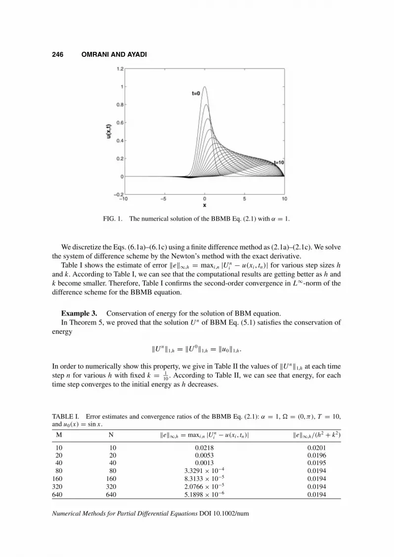
Example 1 (Approximate solution Un of the BBMB Eq. (2.1)). Below, we shall presentsome numerical experiments. We now consider the initial condition u0(x) = exp(−x2) and theinterval � = [−10, 10].

The behavior of the BBMB Eq. (2.1) is presented in Figure 1 from t = 0 to t = 10, for α = 1,h = 20

1024 , and k = 12 .

Example 2 (Error estimate and convergence). In order to numerically check theoreticalproperties in the previous section, we consider the inhomogeneous equation (the error estimateestablished in Theorem 3 also holds).

ut − uxxt − uxx + ux + uux = exp(−t)

[cos x − sin x + 1

2exp(−t) sin(2x)

],

x ∈ (0, π), t ∈ (0, T ], (6.1a)

with the boundary conditions

u(0, t) = u(π , t) = 0, t ∈ (0, T ], (6.1b)

and initial condition

u(x, 0) = sin x, x ∈ (0, π), (6.1c)

for which the exact solution is u(x, t) = exp(−t) sin x.

Numerical Methods for Partial Differential Equations DOI 10.1002/num

246 OMRANI AND AYADI

FIG. 1. The numerical solution of the BBMB Eq. (2.1) with α = 1.

We discretize the Eqs. (6.1a)–(6.1c) using a finite difference method as (2.1a)–(2.1c). We solvethe system of difference scheme by the Newton’s method with the exact derivative.

Table I shows the estimate of error ‖e‖∞,h = maxi,n |Uni − u(xi , tn)| for various step sizes h

and k. According to Table I, we can see that the computational results are getting better as h andk become smaller. Therefore, Table I confirms the second-order convergence in L∞-norm of thedifference scheme for the BBMB equation.

Example 3. Conservation of energy for the solution of BBM equation.In Theorem 5, we proved that the solution Un of BBM Eq. (5.1) satisfies the conservation of

energy

‖Un‖1,h = ‖U 0‖1,h = ‖u0‖1,h.

In order to numerically show this property, we give in Table II the values of ‖Un‖1,h at each timestep n for various h with fixed k = 1

10 . According to Table II, we can see that energy, for eachtime step converges to the initial energy as h decreases.

TABLE I. Error estimates and convergence ratios of the BBMB Eq. (2.1): α = 1, � = (0, π), T = 10,and u0(x) = sin x.

M N ‖e‖∞,h = maxi,n |Uni − u(xi , tn)| ‖e‖∞,h/(h

2 + k2)

10 10 0.0218 0.020120 20 0.0053 0.019640 40 0.0013 0.019580 80 3.3291 × 10−4 0.0194

160 160 8.3133 × 10−5 0.0194320 320 2.0766 × 10−5 0.0194640 640 5.1898 × 10−6 0.0194

Numerical Methods for Partial Differential Equations DOI 10.1002/num

FINITE DIFFERENCE DISCRETIZATION OF BBMB EQUATION 247

TABLE II. Conservation of energy for the solution of the BBM Eq. (5.1) when � = (0, π), u0(x) = sin x,and T = N = 10.

‖Un‖21,h

n M = 20 M = 40 M = 80 M = 160 M = 320 M = 640 M = 1280 M = 2560

0 2.9902 3.0643 3.1026 3.1220 3.1318 3.1367 3.1391 3.14041 3.1140 3.1296 3.1361 3.1390 3.1403 3.1410 3.1413 3.14142 3.1386 3.1407 3.1412 3.1414 3.1415 3.1416 3.1416 3.14163 3.1284 3.1346 3.1380 3.1397 3.1407 3.1411 3.1414 3.14154 3.1196 3.1304 3.1360 3.1388 3.1402 3.1409 3.1412 3.14145 3.1206 3.1317 3.1368 3.1392 3.1404 3.1410 3.1413 3.14146 3.1277 3.1358 3.1390 3.1404 3.1410 3.1413 3.1414 3.14157 3.1349 3.1394 3.1408 3.1413 3.1414 3.1415 3.1416 3.14168 3.1385 3.1408 3.1414 3.1415 3.1416 3.1416 3.1416 3.14169 3.1374 3.1398 3.1408 3.1412 3.1414 3.1415 3.1415 3.1416

10 3.1330 3.1374 3.1396 3.1406 3.1411 3.1413 3.1415 3.1415

VII. CONCLUSION

Applied to the BBMB equations, the Crank-Nicolson scheme has allowed obtaining a numericalproblem that is well posed: both stability and consistance are proved. Moreover, the numericalproblem has a second-order convergence in L∞-norm. For each step of time, a nonlinear problemis solved by using the exact Newton method. We have observed that the discretized problem iswell conditioned.

The particular case, α = 0, known as the BBM Equation, has also been studied and showedthat the energy is conserved. Finally, we conclude that the numerical computations consideredvalidate the theoretical results.

We express our gratitude to the anonymous referees for their constructive reviews of themanuscript and for helpful comments.

References

1. T. B. Benjamin, J. L. Bona, and J. J. Mahony, Model equations for long waves in nonlinear dispersivesystems, Philos Trans Roy Soc Lond A 272 (1972), 47–78.

2. J. L. Bona and R. smith, The initial-value problem for the Korteweg-de Vries equation, Philos TransRoy Soc Lond A 278 (1975), 555–601.

3. C. Yong, L. Biao, and Z. Hongqing, Exact solutions of two nonlinear wave equations with simulationterms of any order, Comm Nonlinear Sci Numer Simul 10 (2005), 133–138.

4. L. A. Medeiros and M. Milla Miranda, Weak solutions for a nonlinear dispersive equation, J Math AnalAppl 59 (1977), 432–441.

5. L. A. Medeiros and G. Perla Menzela, Existence and uniqueness for periodic solutions of theBenjamin-Bona-Mahony equation, SIAM J Math Anal 8 (1977), 792–799.

6. M. Mei, Large-time behavior of solution for generalized Benjamin-Bona-Mahony-Burgers Equations,Nonlinear Anal 33 (1998), 699–714.

7. D. H. Peregrine, Calculations of the development of an undular bore, J Fluid Mech 25 (1996), 321–326.

8. H. Zhang, G. M. Wei, and Y. T. Gao, On the general form of the Benjamin-Bona-Mahony equation influid mechanics, Czech J Phys 52 (2002), 344–373.

Numerical Methods for Partial Differential Equations DOI 10.1002/num

248 OMRANI AND AYADI

9. M. A. Raupp, Galerkin methods applied to the Benjamin-Bona-Mahony equation, Bol Soc Brazil Mat6 (1975), 65–77.

10. L. Wahlbin, Error estimates for a Galerkin method for a class of model equations for long waves, NumerMath 23 (1975), 289–303.

11. R. E. Ewing, Time-stepping Galerkin methods for nonlinear Sobolev partial differential equation, SIAMJ Numer Anal 15 (1978), 1125–1150.

12. D. N. Arnold, J. Douglas Jr., and V. Thomée, Superconvergence of finite element approximation to thesolution of a Sobolev equation in a single space variable, Math Comput 27 (1981), 737–743.

13. S. A. V. Manickam, A. K. Pani, and S. K. Chang, A second-order splitting combined with orthogonalcubic spline collocation method for the roseneau equation, Numer Methods Partial Diff Equat 14 (1998),695–716.

14. K. Omrani, The convergence of the fully discrete Galerkin approximations for the Benjamin-Bona-Mahony (BBM) equation, Appl Math Comput 180 (2006), 614–621.

15. D. Kaya and I. E. Inan, Exact and numerical traveling wave solutions for nonlinear coupled equationsusing symbolic computation, Appl Math Comput 151 (2004), 775–787.

16. D. Kaya, A numerical simulation of solitary-wave solutions of the generalized regularized long-waveequation, Appl Math Comput 149 (2004), 833–841.

17. R. D. Richtmyer and K. W. Morton, Difference methods for initial-value problems, 2nd ed., Wiley, NewYork, 1967.

18. B. Fornberg, On the instabilty of leap-flog and Crank-Nicolson approximations of a nonlinear partialdifferential equation, Math Comput 27 (1973), 45–57.

19. G. D. Akrivis, Finite difference discretization of the Kuramoto-Sivashinsky equation, Numer Math 63(1992), 1–11.

20. R. Kannan and S. K. Chung, Finite differnce approximate solutions for the two-dimensional Burger’ssystem, Comput Math Appl 44 (2002), 193–200.

21. T. F. Chan and L. Shen, Stability analysis of difference schemes for variable coefficient Schrödingertype equations, SIAM J Numer Anal 24 (1981), 336–349.

22. G. Ben-Yu, P. J. Pascual, M. J. Rodriguez, and L. Vázquez, Numerical solution of the Sine-Gordonequation, Appl Math Comput 18 (1986), 1–14.

23. L. Zhang and Q. Chang, A conservative numerical scheme for a class of nonlinear Schrödinger withwave operator, Appl Math Comput 145 (2003), 603–612.

24. Y. Zhou, Application of discrete functional analysis to the finite difference methods, InternationalAcademic Publishers, Beijing, 1990.

25. N. Khiari, T. Achouri, M. L. Ben Mohamed, and K. Omrani, Finite difference approximate solutionsfor the Cahn-Hilliard equation, Numer Methods Partial Differ Equat 23 (2007), 437–455.

26. K. Omrani, On the numerical Approach of the enthalpy method for the Stefan problem, Numer MethodsPartial Differ Equat 20 (2004), 527–551.

27. K. Omrani, A second order splitting method for a finite difference scheme for the Sivashinsky equation,Appl Math Lett 16 (2003), 441–445.

28. K. Omrani, Convergence of Galerkin approximations for the Kuramoto-Tsuzuki equation, NumerMethod Partial Differ Equat 21 (2005), 961–975.

29. K. Omrani, A second-order accurate difference scheme on nonuniform meshes for nonlinear heat-conduction equation, Far East J Appl Math 20 (2005), 355–365.

30. K. Omrani, Numerical methods and error analysis for the nonlinear Sivashinsky equation, Appl MathComput (2007), in press.

Numerical Methods for Partial Differential Equations DOI 10.1002/num