asymptotic behaviour of a generalized burgers' equation

J. Math. Pures Appl.,78, 1999,p. 633-666

ASYMPTOTIC BEHAVIOUR OF A GENERALIZEDBURGERS’ EQUATION

Guillermo REYES, Juan Luis VAZQUEZDepartamento de Matemáticas, Universidad Autónoma de Madrid, 28049 Madrid, Spain

Manuscript received 27 July 1998

ABSTRACT. – We consider the generalized Burgers equation:

ut =1(um)− ∂∂x1(uq),(GBE)

with exponentsm > 1 and q = m + (1/N). We study the large-time behaviour of nonnegative weaksolutions of the Cauchy problem posed inQ = RN × (0,∞) with integrable and nonnegative data. Weconstruct a uni-parametric familyUM of source-type solutions of (GBE) such that:

UM(·, t)→M δ(x) in D′(RN) as t→ 0,

and prove that they give the asymptotic behaviour of all solutions of the Cauchy problem. These specialsolutions have the following self-similar form:U(x, t) = t−αF(xt−β), with α = 1/((m − 1) + (2/N))andNβ = α. The criterion to choose the right member of the family is the following mass equality:M = ∫RN u0 dx. The construction of the familyUM and the proof of the asymptotic convergence inthis nonlinear, several dimensional setting needs a new method of asymptotic analysis. The results are thenextended to equations of the form

ut =1Φ(u)−∇ · F(u),whereΦ andF resemble the preceding power functions asu→ 0. In this more general case the asymptoticbehaviour is described by the same familyUM mentioned above. Elsevier, Paris

1. Introduction

This paper is devoted to study the qualitative properties and asymptotic behaviour of thenonnegative solutions to the Cauchy problem for the following diffusion-convection equation:

ut =1(um)− ∂

∂x1

(uq),(1.1)

posed inQ= (x, t): x ∈RN, t > 0, for all N > 1, with exponentsm,q such that:

m> 1, q =m+ 1/N.(1.2)

JOURNAL DE MATHÉMATIQUES PURES ET APPLIQUÉES. – 0021-7824/99/06 Elsevier, Paris

634 G. REYES, J.L. VAZQUEZ

J.M. Burgers [6,7] studied this equation in the simple case of linear diffusionm = 1 and onespace dimensionN = 1, so thatq = 2 and (1.1) becomes

ut + 2uux = uxx,(1.3)

as being the simplest one to combine typical convective nonlinearity with typical heat diffusion.Eq. (1.3) is therefore referred to as Burgers equation. It was probably first introduced by Bateman(1915). Burgers equation is relevant in many senses. It appears in Hydrodynamics when wemodel the propagation of perturbations in a weakly dissipative and weakly nonlinear fluid. Inthis caseu has the meaning of rescaled pressure (see [23]). It is also a simple model for thestatistical theory of turbulence [6,7].

The integration of Burgers equation (1.3) is simplified by the Cole–Hopf transformation whichallows to reduce it to the classical heat equation and obtain in such a way the general solution. Forthe details of such reduction see [33], where much more information about Burgers equation canbe found. In this way it is easy to prove that there exists a one-parameter family of self-similarsolutions of (1.3) of the form

U(x, t;M)= t−1/2FM(x/t1/2

),(1.4)

whereM > 0 is a constant to be determined through themasscondition∫U(x, t;M)dx =M.(1.5)

Such solutions are calledsource-type solutionsbecause they take a Dirac mass,M δ(x), asinitial data. They are important for the general theory because each of them gives the asymptoticbehaviour ast→∞ of the whole class of solutions of the Cauchy problem with initial data:

u(x,0)= u0(x), x ∈R,(1.6)

whereu0 is nonnegative, integrable and∫u0(x)dx =M. In Barenblatt’s terminology [4] the

solutions (1.4) represent theIntermediate Asymptoticsof the whole class of solutions.The same result is still true in several space dimensions,N > 1, puttingq = (N + 1)/N and

keeping linear diffusion,m= 1, but now there is no analogous transformation into the heat equa-tion and the proof has to use the machinery of infinite-dimensional dynamical systems. Aguirre,Escobedo and Zuazua proved in [1] that a suitable self-similar solution exists and then Escobedoand Zuazua [12] proved that this special solution gives the asymptotic behaviour for the solutionswith a whole class of initial data. In fact, in the work [12] the asymptotic behaviour was settledfor q > (N+1)/N . It was proved that whenq > (N+1)/N the diffusive part dominates for largetimes, and the asymptotic behaviour is given by the fundamental solution of the heat equation(such phenomenon is calledasymptotic simplification), while for q = (N + 1)/N no simplifi-cation occurs, and the large-time behaviour is given by a family of self-similar solutions of thecompleteequation (1.1). The range 1< q < 1+ 1/N has been studied in [13] and [14]. In thiscase the convective part dominates and the asymptotics is given by a self-similar solution of theequation with so-calledpartial diffusivity(diffusion in the direction of convection disappears).

We address here the situation for nonlinear diffusion,m> 1, and concentrate on Burgers case(1.2), where no asymptotic simplification occurs. It corresponds toq = (N + 1)/N whenm= 1,but the method used in [12] does not extend to the completely nonlinear case we consider here be-cause it uses heavily the functional properties of the Laplace operator as a linear operator. Hencethe interest in developing genuinely nonlinear methods, adapted to treat all these problems.

TOME 78 – 1999 –N 6

ASYMPTOTIC BEHAVIOUR OF A GENERALIZED BURGERS’ EQUATION 635

Through the rest of the paper we consider Eq. (1.1) with exponentsq andm, satisfying (1.2).We prove three main results. The first one is about the existence of suitable source-type solutions.

THEOREM 1.1. –For everyM > 0 there exists a unique self-similar solution of Eq.(1.1) ofthe form

U(x, t)= t−αF (xt−β),(1.7)

of the source-type class, i.e., ast→ 0

U(x, t;M)→M δ(x) in D′(RN

),(1.8)

whereF is a compactly supported function and the similarity exponents are

α = N

N(m− 1)+ 2, β = 1

N(m− 1)+ 2.(1.9)

The second result concerns the behaviour of general solutions of the Cauchy problem forEq. (1.1) for larget .

THEOREM 1.2 (Asymptotic behaviour). –Let u(x, t) be the weak solution of the Cauchyproblem for Eq.(1.1) with initial data u0 ∈ L1, u0 > 0. Let

∫u0(x)dx =M. Then, for every

p ∈ [1,∞]tα(p)

∥∥u(., t)−U(., t)∥∥Lp→ 0 ast→∞,(1.10)

whereU(x, t) is the unique self-similar solution with massM constructed in Theorem1.1 andα(p)= p

p−1α with α = NN(m−1)+2.

The construction of the familyUM and the proof of (1.10) are based on the use of theLyapunov method of asymptotic analysis. We start as in the works [30], [24] and [11], wherethe four-step technique introduced by Kamin and Vazquez [21] is followed. The main difficultyof the present analysis is the identification of the limit since a direct identification needs astrong uniqueness result for the source-type solution, a task that we will avoid. In this paper,identification is performed in two steps: (i) we prove that all possible limits must be self-similarand (ii) all possible limits are equal. For both (i) and (ii) we use a suitably constructed Lyapunovfunctional (Section 5). This method can have application to other evolution problems, cf. [32].

Let us mention that in one space dimension the above results have been proved as part of theworks [24] and [30], where the asymptotic behaviour of solutions to the Cauchy problem forequation

ut =(um)xx+ (uq)

x(1.11)

was settled in the ranges of exponentsm, q > 1.Since we are in the presence of slow diffusion,m> 1, our problem has theproperty of finite

propagation, i.e., solutions whose initial data have compact support remain compactly supportedfor any given timet > 0 (though the support eventually covers the whole space). This appliesin particular to the source-type solutions. We can also give an asymptotic estimate of the way inwhich the supports ofu andUM resemble for larget . LetΩU(t) be the support ofUM at timet and letΩu(t) be the support ofu. We recall the definition of the Hausdorff distance. LetΩ1andΩ2 be two closed subsets of a metric spaceE. LetDx,y be the set of all numbersd(x,Ω2)

with x ∈Ω1 andd(y,Ω1) with y ∈Ω2, d being the distance inE. Then the Hausdorff distancebetweenΩ1 andΩ2 is defined as follows:

dist(Ω1,Ω2)= supx∈Ω1,y∈Ω2

Dx,y.(1.12)

JOURNAL DE MATHÉMATIQUES PURES ET APPLIQUÉES


THEOREM 1.3. –Assume thatu is a solution as in Theorem1.2 and u0 is compactlysupported. Then the normalized Hausdorff distance betweenΩU(t) andΩu(t) goes to zero,that is

limt→∞

dist(ΩU(t),Ωu(t))

tβ= 0.(1.13)

The plan of the paper is as follows. In Sections 2 and 3 we study the question of existenceand uniqueness of a class of weak solutions of the Cauchy problem for Eq. (1.1). In Section4 we prove some fundamental estimates and properties of weak solutions which will be usefulin the asymptotic analysis. In Section 5, we develop the four-step technique for the proof ofTheorem 1.2. Section 6 is devoted to the proof of Theorem 1.1, which is an almost directconsequence of Theorem 1.2. Section 7 is devoted to prove Theorem 1.3, while in Section 8,we study the shape of the family of attractors, considering the limit casesM→ 0 andM→∞.As a consequence, we obtain the existence of a source-type solution for the equation with partialdiffusivity

ut =1y(um)− (uq)

x1(1.14)

where y = (x2, x3, . . . , xn). Finally, in Section 9, we extend our results to more generalnonlinearities both in the diffusive and in the convective terms of (1.1).

Notes. Eq. (1.1) is studied in the recent work [11] in several space dimensions in the rangeof exponentsm> 2, 1< q <m− 1. The asymptotic behaviour in this case is of a different type,purely convective.

The methods of this paper apply with very minor modifications to the linear-diffusion casem= 1, where the Lyapunov method has been applied by Zuazua [35]. The main difference is thatsolutions are always positive everywhere and the analysis of the support is replaced by suitabledecay asx→∞.

2. Existence of solutions

In this section we give a definition of weak solution for the Cauchy problem for Eq. (1.1) withinitial datau0 ∈ L1, u0 > 0, and proceed with its construction. The question of uniqueness isdiscussed later.

DEFINITION 2.1. –Let u0 ∈ L1(RN), u0 > 0. We say thatu(x, t) is a weak solution ofEq.(1.1)with initial datau0 if:

(W1) u is continuous and nonnegative inRN × (0,∞),(W2) u ∈ C([0,∞);L1(RN))∩L∞((τ,∞)×RN), ∀τ > 0,(W3) um ∈L2

loc((0,∞);H 1(RN)),(W4) for all 0< τ16 τ2<∞, all bounded open setsΩ ⊂ RN with smooth boundary and all

φ ∈ C∞(Ω × [τ1, τ2]), φ = 0 on∂Ω × [τ1, τ2], we have

τ2∫τ1

∫Ω

∇um.∇φ−uφt−uqφx1

dxdt =

∫Ω

u(τ1, x)φ(τ1, x)dx−∫Ω

u(τ2, x)φ(τ2, x)dx,

(W5) u(0)= u0, i.e.,u(t)→ u0 in L1(RN) ast→ 0.

TOME 78 – 1999 –N 6


Note. We will frequently use the notationu(t) to meanu(·, t), a function ofx for given t .C∞0 (Ω) denotes the space of smooth and compactly supported functions inΩ andBr(x0) standsfor the (open) ball with center inx0 and radiusr. The support (inx) of a functionu(x, t) fora fixed t will be denoted byΩu(t). The rest of the notations is rather standard: ByLp(Ω) wedenote the usual Lebesgue spaces and byH 1(Ω) the Sobolev spaceW1,2(Ω).

Next we prove the following:

THEOREM 2.1. –For everyu0 ∈ L1, u0 > 0, there exists a weak solution of Eq.(1.1) withinitial data u0 in the sense of previous definition.

Hui [18] proposes a weaker form of solution and proves existence and uniqueness for boundedintegrable data. The fact that our solutions have better regularity (they are energy solutions in theusual terminology) will be used in the sequel.The restriction of boundedness on the data is notnatural in our context. References to other existence results will be commented upon in Section 9and in the Appendix.

Proof. –We adopt a constructive method starting with regular problems to which standardtheory [26] can be applied, and obtaining estimates that allow to pass to the limit. Such aconstruction is carried out for the Porous Medium Equation in the survey paper [31]. Sinceour construction is very similar, we omit the details and emphasize the differences. A slightlydifferent approach is adopted in [25].

(1) As a first step, we construct a weak solution for the homogeneous Dirichlet problem. LetΩ be an open bounded set with smooth boundary, and letu0 ∈ C∞(Ω), u0> 0 andu0 vanishestogether with the first two derivatives on the boundary. DenoteQT =Ω × (0, T ) andQ=Q∞.Consider the approximate problems

unt =1(umn )− (uqn)x1 in QT ,un(x,0)= un0(x)= u0(x)+ 1/n,

un = 1/n on∂Ω × [0,∞).

These problems are essentially non-degenerate, and each one has solutionun ∈ C2,1x,t (Q).

By the Maximum Principle,un+1 6 un and 1/n 6 un 6M + 1/n, whereM = maxΩ u0. Weobtain a point-wise (andLp with 16 p <∞) limit u, such that 06 u 6M. Multiplying theequation byumn − (1/n)m and integrating inQT we obtain, as in [31, p. 359] a uniform (inTandn) control on∇umn (convection does not play any role). Hence, for some subsequence (notrelabeled),∇umn →∇um weakly inL2(Q), and the so-called Energy Estimate:

(m+ 1)

T∫0

∫Ω

∣∣∇um∣∣2 dx dt +∫Ω

um+1(x, T )dx 6∫Ω

um+10 (x)dx,(2.1)

holds in the limit. The convergences above allow to pass to the limit in (W4) of Definition 2.1(which is obviously satisfied by the classical solutionsun). Precisely, for eachφ ∈ C∞(Ω ×[τ1, τ2]) such thatφ = 0 on∂Ω × [τ1, τ2] with 06 τ16 τ2<∞ we have

τ2∫τ1

∫Ω

∇um.∇φ − uφt − uqφx1

dx dt =

∫Ω

u(x, τ1)φ(x, τ1)dx −∫Ω

u(x, τ2)φ(x, τ2)dx.(2.2)

It follows from the construction thatum ∈L2(0, T :H 10 (Ω)). It is clear from (2.1) that theLm+1

x

norm ofu decays in time. Multiplying by other powers ofu we obtain a “generalized” Energy



Estimate (see [31, p. 366]), from which follows theLp-norm decay∥∥u(., t)∥∥p6 ‖u0‖p,(2.3)

for all p > 1. Moreover, ifu0 > 0 in Ω , then the solution is positive and classical, that is,u ∈C∞(Q) ∩C(Q). Positivity can be settled by means of the following barrier (see [16]):

w(x, t)=(ρ2− |x|2)1/(m−1)e−σ t if |x|< ρ,0 elsewhere,

(2.4)

whereσ is a positive parameter suitably chosen. Precisely, we can chooseσ large enough in sucha way thatwx0 =w(x−x0, t) is a classical sub-solution of (1.1) in|x−x0|< ρ× (0,∞). Thisis true in the rangeq > (m+1)/2 (see [16] for details), hence forq =m+ 1/N . Moreover,wx0

vanishes on the lateral boundary of this region. For eachx0 ∈Ω we can chooseρ small enoughin order to haveu0 > wx0(0) in |x − x0| < ρ ⊂Ω . Hence, the classical Maximum Principleapplied toun yieldsun >wx0 in |x− x0|< ρ× (0,∞), and in the limitu>wx0 in this region.Then,un is bounded away from 0 inN = Bx0(r) × (0, T ) for somer > 0. By the regularitytheory of quasi-linear non-degenerate parabolic equations, we conclude thatu ∈ C∞(N) and theinitial data are taken continuously inBx0(r). From our approximation proccess it is also clearthatu vanishes continuosly onΣ = ∂Ω × (0, T ).

Since the constructed solution is a solution with “finite energy”, by the results of F. Otto [27]the Contraction Principle inL1 is valid in the following form:∫

Ω

|u1− u2|(x, t)dx 6∫Ω

|u10− u20|(x)dx,(2.5)

whereu1 andu2 denote the solutions with initial datau10 andu20 respectively.(2) Now we consider the initial value problem. As a first approximation, takeu0 ∈ L1(RN) ∩

L∞(RN)∩C∞(RN) andu0> 0 everywhere. Letζn(x) be a sequence of “cutoff functions”, suchthat ζn ∈ C∞0 (RN), 06 ζn 6 1, ζn = 1 in Bn−1(0), ζn = 0 in the complement ofBn(0) and itsderivatives up to second order are bounded inRN . Consider the sequence of problems:

unt =1(umn )− (uqn)x1 in Bn(0)× (0, T ),un(x,0)= u0.ζn,

un = 0 on∂Bn(0)× [0, T ).These problems can be solved as in the previous step, becauseun0 ∈ C∞0 (Ω). Since the initialdata are strictly positive, the solution is classical inBn(0)×(0, T ). Then, the Maximum Principlecan be applied and we obtain an ordered sequenceun 6 un+1 in RN × (0, T ) (We extend by0 eachun and keep the notation). The uniformity inn of estimates (2.1) and (2.3) allow usto obtain a limitu in L∞((0,∞);Lp(RN)) for all 16 p. This limit satisfies (W3) and (W4)of Definition (2.1) (in fact, (W3) is satisfied without subscript ‘loc’). Since the sequence ofapproximations is locally bounded below away from 0 for largen, it also satisfies (W1) byregularity theory.

Estimates (2.1) and (2.3) remain valid. Contraction inL1 holds in the limit. (W2) and (W5) inDefinition 2.1 are easily obtained as a consequence ofL1-contraction and approximation.

(3) Take nowu0 ∈ L1(RN) ∩ L∞(RN), u0 > 0. We may approximateu0 in L1 by un0 asin Step 2. Moreover, we can do it in such a way that‖un0‖1 6 ‖u0‖1 and‖un0‖∞ 6 ‖u0‖∞.

TOME 78 – 1999 –N 6


TheL1-contraction allows to obtain a limit inC([0,∞);L1(RN)) such thatu(0) = u0. Theuniformity of estimates (2.1) and (2.3) enables to pass to the limit in (W4) of Definition 2.1.(W1) is true thanks to the regularity theory of degenerate parabolic equations (see [9]).

(4) In order to extend our construction to data inL1(RN), we need anL∞-estimate fort > 0.We recall the so calledL1–L∞ regularizing effect for the Porous Medium equation:∥∥u(t)∥∥

L∞ 6 C‖u‖λL1t−α,(2.6)

with α = N/(N(m − 1) + 2) and λ = 2/(N(m − 1) + 2), which is valid for solutions withnonnegative integrable data. It turns out that, in our case, such an estimate is also valid, thanks toa symmetrization result due to Bénilan and Abourjaily [3], which enables to compare solutionsof Eq. (1.1) and solutions (with the same initial data) of the Porous Medium equation (which isthe symmetrized one). Although this result is proved for regular problems, it holds in our case byapproximation. For the sake of completeness, we reproduce it here.

THEOREM 2.2 (Theorem 1 of [3, p. 4]). –LetΩ be any open set inRN ,Q= (0, T )×Ω , leta :Q×RN+1→RN be a Carathéodory function and satisfy

a(t, x, k, ξ).ξ > σ(‖k‖)‖ξ‖2−F(t, x, k).ξ, ∀(t, x, k, ξ) ∈Q×RN+1

whereσ : R→ (0,∞) is Hölder continuous,F :Q×R→RN is Carathéodory and satisfies

sup|k|6R

∣∣F(., k)∣∣ ∈ L2(Q) ∀R > 0 and

div(kF (t, ., k)

)6 0 in D′(Ω) ∀(t, k) ∈ (0, T )×R.

Letu ∈C([0, T );L1(Ω))∩L2loc((0, T ;W1,2

0 (Ω)) with a(., u,∇u) ∈ L2loc((0, T );L2(Ω)) satisfy

ut = diva(., u,∇u) in D′(Q).

On the other hand letΩ be a ballB(0,R) ⊂ RN with |Ω |6 |Ω|, v0 ∈ L1(Ω) ∩ L∞(Ω) withv0= v0 andv be the solution of

vt =1φ(v) on (0, T )× Ω,v = 0 on (0, T )× ∂Ω, v(0, .)= v0 on Ω,

whereφ(v)= ∫ v0 α(k)dk. If∫Ω(|u0| − k)+ dx 6

∫Ω (v0− k)+ dx for anyk > 0, then∫

Ω

(|u(t)| − k)+ dx 6∫Ω

(v(t)− k)+ dx ∀(t, k) ∈ (0, T )×R+.(2.7)

Clearly, all the hypotheses of Theorem 2.2 hold in our case, and the symmetrized equation isthe Porous Medium equation. Applying this result inQ=RN × (0, T ), puttingk = C‖u‖λ

L1t−α

and taking the same initial data for (1.1) and the Porous Medium equation, we obtain the validityof (2.6) for the solutions of (1.1).

We also need the following important result:



THEOREM 2.3 (Conservation of mass). –Letu0 ∈L1(RN)∩L∞(RN). Then, for allt > 0 wehave ∫

RN

u(x, t)dx =∫

RN

u0(x)dx.(2.8)

(That is, theL1-norm of the solution is an invariant of the evolution.)

Proof. –Supposeu0 ∈ L1(RN) ∩L∞(RN) ∩C∞(RN). As a test function in the definition ofweak solution, takeφ(x, t)= ζn(x), whereζn(x) is as in Step 2 of our construction. We obtain

∫RN

u(x, τ )ζn(x)dx −∫

RN

u0ζn(x)dx =τ∫

0

∫RN

um(x, t)1ζn(x)− u(x, t)ζx1

dx dt .(2.9)

Notice that1ζn and ζn,x1 converge point-wise to 0 inRN , andζn converges to 1. By thedominated convergence theorem, we can pass to the limit in all the integrals. We obtain∫

RN

u(x, τ )dx −∫

RN

u0 dx = 0,(2.10)

which is the desired result. For general datau0 ∈ L1(RN) ∩ L∞(RN), we proceed byapproximation. 2

Take nowu0 ∈ L1(RN), u0 > 0. Consider the sequence of approximationsun0 ∈ L1(RN) ∩L∞(RN), such thatun0→ u0 in L1 and ‖un0‖L1 6 ‖u0‖L1. TheL1-contraction produces alimit in C([0,∞);L1(RN)). By (2.6), un(t) is uniformly bounded inRN × [τ1, τ2], with0< τ1 6 τ2. Thanks to this fact and the conservation of mass, the Energy Estimate (2.1) givesuniform estimates for∇umn in the same regions. We can pass to the limit in the weak formulationif τ1> 0. All the conditions (W1)–(W5) in Definition 2.1 are seen to hold. TheL1-contractionand the conservation of mass remain valid by approximation.

This ends the construction of the solution. Theorem 2.1 is proved.2

3. Uniqueness

The uniqueness of solutions of diffusive-convective equations of the form

ut =1Φ(u)− div(F(u)

)(3.1)

has been discussed by a number of authors, though the results do not exactly match the class ofsolutions we are dealing with. Here is the result that we need at this stage:

THEOREM 3.1. –There exists at most one solution to(1.1) with initial data u0 ∈ L1(RN),u0> 0 in the sense of Definition2.1.Moreover, for two solutionsu1, u2 with datau01 andu02respectively, we have: ∫

RN

|u1− u2|(x, t)dx 6∫

RN

|u10− u20|(x)dx.(3.2)

TOME 78 – 1999 –N 6


We will devote a final Appendix to explain the proof of this result in the context of a moregeneral class of equations of the form (3.1) and we will briefly discuss the correspondingliterature.

4. Properties of weak solutions

Before proceeding with the asymptotic study we need to establish a number of properties of theweak solution and its support. First of all, we state and prove an estimate for the time derivativeof the solution.

THEOREM 4.1. –For every weak solutionu the following estimate holds:

∥∥(um)t

∥∥L2(RN×(t,+∞)) 6 C4

(‖u‖1,m,N)t− α(2m−1)+12 , t > 0.(4.1)

Proof. –Let u denote the solution of the approximate problem for (1.1) (see Step 2 inSection 2) andQT = Ω × (0, T ) the corresponding bounded space-time domain. MultiplyingEq. (1.1) by(um)t and integrating inΩ by parts we obtain∫

Ω

∣∣(u(m+1)/2)t

∣∣2 dx + (m+ 1)2

8m

d

dt

∫Ω

∣∣∇um(x, t)∣∣2 dx = (m+ 1)2

4m

∫Ω

∣∣(um)t

(uq)x1

∣∣dx.Applying Young’s inequality in the last integral we get:

(m+ 1)2

4m

∫Ω

∣∣(um)t

(uq)x1

∣∣dx =C(m,N)∫Ω

uq+m−2|ux1||ut |dx

6 1

2

xΩ

∣∣(u(m+1)/2)t

∣∣2 dx +C1(m,N)

∫Ω

um−1∣∣(uq)

x1

∣∣2 dx.

Hence

1

2

∫Ω

∣∣(u(m+1)/2)t

∣∣2 dx + (m+ 1)2

8m

d

dt

∫Ω

∣∣∇um(x, t)∣∣2 dx 6 C1(m,N)

∫Ω

um−1∣∣(uq)

x1

∣∣2 dx.

The last term can be estimated as follows:∫Ω

um−1∣∣(uq)

x1

∣∣2 dx 6 C2(m,N)∥∥u(t)∥∥2q−(m+1)

∞∫Ω

∣∣∇(um)∣∣2 dx.

We get

1

2

∫Ω

∣∣(u(m+1)/2)t

∣∣2 dx + (m+ 1)2

8m

d

dt

∫Ω

∣∣∇um(x, t)∣∣2 dx

(4.2)

6 C3(m,N)∥∥u(t)∥∥2q−(m+1)

∞∫Ω

∣∣∇(um)∣∣2 dx.



In particular, we have

d

dt

∫Ω

∣∣∇um∣∣2 dx 6 C4(m,N)∥∥u(t)∥∥2q−(m+1)

∞∫Ω

∣∣∇(um)∣∣2 dx.(4.3)

Put, for simplicity

γ (t)=∫Ω

∣∣∇um(x, t)∣∣2 dx, t > 0.(4.4)

Integrating (4.3) int from t1 to t2 with 0 < t1 < t2, and taking into account (2.6) and(2.1) (observe that, since our solution is obtained as a monotone limit, (2.6) is valid for theapproximations), we obtain

γ (t2)6 γ (t1)+C5(m,N,‖u‖1

)t−α(2q−1)1 .

Now we integrate int1 from t2/2 to t2 and use (2.1) once again. This gives:

γ (t2)6 C6(m,N,‖u‖1

)t−αm−12 .(4.5)

Next we integrate (4.2) int from τ > 0 toT . We obtain

1

2

∫∫QTτ

∣∣(u(m+1)/2)t

∣∣2 dx dt + (m+ 1)2

8m

∫Ω

∣∣∇um(x,T )∣∣2 dx

6 (m+ 1)2

8m

∫Ω

∣∣∇um(x, τ )∣∣2 dx +C3(m,N,‖u‖1

)τ−α(2q−(m+1))

∫∫QTτ

∣∣∇(um)∣∣2 dx.

From the last inequality, (2.1) and (4.5) we infer∫∫QTτ

∣∣(u(m+1)/2)t

∣∣2 dx dt 6 C(m,N,‖u‖1

)τ−αm−1.(4.6)

The identity (um)t= (2m/(m+ 1)

)u(m−1)/2(u(m+1)/2)

t,(4.7)

combined with the last inequality and (2.6) gives the desired result for the approximate problems.Since the solution of the Cauchy problem can be obtained as a limit of such approximate solutionsand (4.1) holds uniformly for them, we get (4.1) passing to theL2-weak limit. The derivativeshould be understood in the sense of distributions. This estimate, together with (2.1), impliesum ∈H 1(RN × (t,+∞)) for all t > 0. 2

The following properties of the support can be found in [16] in one space dimension.

THEOREM 4.2 (Retention property). –Let u be a weak solution of problem(1.1) with u0 ∈C∞0 (RN). Suppose thatu(x0, t0) > 0 at some point(x0, t0), t0 > 0. Thenu(x0, t) > 0 for allt > t0.

TOME 78 – 1999 –N 6


We omit the proof, since it follows the one given by Gilding [16, p. 211], valid in the rangeq > (m+ 1)/2. As a consequence, the positivity set is expanding in time, i.e., fort2> t1> 0:

u(x, t1) > 0⊂ u(x, t2) > 0

.(4.8)

COROLLARY 4.1. –If the support of the solution is connected att1 > 0, then it staysconnected for allt > t1.

Proof. –Let t2> t1 be such that the positivity setu(x, t2) > 0 has a connected componentΩ ,disjoint from the one that contains the setu(x, t1) > 0. Then the Maximum Principle, appliedto the cylinderΩ × [t1, t2) gives a contradiction. (u= 0 in the lateral boundary of this cylinderby the retention property).2

THEOREM 4.3 (Penetration property). –Letu be a weak solution of problem(1.2)with initialdata inC∞0 (RN). Thensuppu(t) eventually reaches any pointx ∈RN .

The proof is based on comparison with the following explicit sub-solution with expandingsupport:

z(x, t)= σ(t + τ )−γ [ρ − x2(t + τ )−β] 1m−1+ ,(4.9)

where the positive parametersγ , β , ρ, σ andτ are chosen appropriately. See Kalashnikov [19]for the one-dimensional case.

We perform next a more delicate task, estimating the growth of the support.

THEOREM 4.4. –Let u be a solution of Eq.(1.1) with initial data in C∞0 (RN). Then, itssupport at timet > 0 is contained in the neighborhood of radiusCtβ of the initial support,whereC is some constant, depending only onm, N and‖u‖L1, andβ = 1/(N(m− 1)+ 2), asabove.

Proof. –This is proved by combining three arguments:(a) a result of Díaz and Véron [10], based on the local energy method introduced by Antontsev

(see [2]) in order to estimate the growth of the support in intervals of the form[t1, t2], 0< t1< t2.This estimate depends only on‖u‖1 and structural constants,

(b) the similarity properties of the equation, which allow to estimate the growth of the supportin any interval of the form[τ, t], with τ > 0, independently ofτ ,

(c) a comparison argument, in order to control the initial (in[0, τ ] with arbitrarily smallτ )growth of the support.

Let us see these results in detail.

LEMMA 4.1. –There existsε > 0 such that the growth of the support in the interval[1,1+ ε]is bounded by1. The value ofε depends only onm, N and‖u‖L1.

Proof. –We use theorem 2, p. 151 of the work [10]. The hypotheses of that result are satisfiedin our case withq = 1, M1 = 1, M2 = 1, β = 1, α = (1 − m)/2m < 0. We also need toslightly displace the origin of time, e.g., takingu(t) = u(t + τ ), τ > 0. The boundedness ofu, (2.6), guarantees condition (21) of p. 151. The theorem asserts that there exists a functionF(t, ρ) = C(ρ) tλ with C,λ > 0 and a timeT ∗ (depending only on structural constants) suchthat wheneveru0 vanishes in a ballBρ0(x0) thenu(t) vanishes a.e. in a smaller ballBρ1(x0),ρν1 = ρν0 − F(t, ρ0), for all t ∈ (0, T ∗) such that

ρν0 >F(t, ρ0).



More precisely,F(t, ρ0) is defined by:

F(t, ρ0)= C∗tλ minm+12m <τ61

Eγ (t, ρ0)

2mτ −m− 1max

(1, ρν−1

0

)max

(bµ(t, ρ0), b

η(t, ρ0))

(4.10)

whereC∗ > 0 depends only on the structure constants (herem, N and‖u‖1) and

σ = 1

m, λ= m+ 1

N(m− 1)+ 2(m+ 1), γ = 2τ − σ − 1

N(1− σ)+ 2(σ + 1),

µ= 2(1− τ )N(1− σ)+ 2(σ + 1)

, ν = 2(σ + 1)+N(1− σ)σ + 1

, η= 1− σ(σ + 1)

+ γ,

while

E(t, ρ)=t∫

0

∫Bρ(x0)

∣∣∇um∣∣2 dx ds,(4.11)

b(t, ρ)= ess sup0<τ<t

∫Bρ(x0)

∣∣u(τ, x)∣∣m+1 dx.(4.12)

If C∗ = 0, ρ1 = ρ0 and the result follows. SupposeC∗ > 0. We apply this result above to thesolutionv(x, t) = u(x, t + 1). Takeρ0 = 1 for simplicity. Using estimates (2.1) inRN × [1, t],(2.6) and (2.8) we have:

E(t,1)=t+1∫1

∫B1(x0)

∣∣∇um∣∣2 dx ds 6 C1(‖u‖1,m) ∀t > 0,(4.13)

b(t,1)= ess sup1<τ<t+1

∫B1(x0)

∣∣u(τ, x)∣∣m+1dx 6 C2

(‖u‖1,m) ∀t > 0.(4.14)

Therefore, puttingτ = 1:

F(ε,1)6 C3ελ

Eγ(1)(ε,1)

m− 1max

(1, bη(ε,1)

)6 Cελ for all ε > 0,(4.15)

whereC = C(m,‖u0‖1).Take nowε < T ∗ such that 1> Cελ (this implies 1> F(ε,1)). We deduce from the quoted

result that ifu(1)= 0 inB1(x0), then

u(t)= 0 in (1,1+ ε)×Bρ1(x0),(4.16)

whereρν1 = 1− F(ε,1) > 1− Cελ > 0. If x0 is not contained in the 1-neighborhood ofΩu(1)(recall thatΩu(t) denotes the support ofu at the timet), thenu = 0 in B1(x0). Consequently,by (4.16),u(1+ ε/2)= 0 inBρ1(x0). In particular,u(1+ ε/2)= 0 in x0. Therefore, the supportof the solution at time 1+ ε/2 is contained in a 1-neighborhood of the support at timet = 1.Lemma 4.1 is proved.2TOME 78 – 1999 –N 6


LEMMA 4.2. –The support of any solution at timet0> 0 is t contained in a neighborhood ofradiusCtβ0 of the support at any timeτ , with 0< τ < t0.

Proof. –The idea is to use the similarity properties of the equation to transform the interval[1,1+ ε] into the intervals[(1+ ε)−1,1], [(1+ ε)−2, (1+ ε)−1], and so on, converging tot = 0.Consider the rescaled solution

uλ(x, t)= λαu(λβx,λt

).(4.17)

uλ has the same mass asu. Therefore, by Lemma 4.1, the growth of its support in the interval[1,1+ ε] is less than 1. Takeλ = (1+ ε)−1. Then the growth of the support ofu(λβx, t) in[(1+ ε)−1,1] is less than 1, and this in turn implies that the growth of the support ofu in[(1+ ε)−1,1] is less than(1+ ε)−β . Repeating the same argument, we obtain that the growthof the support ofu in the interval[(1+ ε)−n, (1+ ε)−(n−1)] is less than(1+ ε)−nβ . Taking intoaccount that(1+ ε)−n→ 0 and that∑

(1+ ε)−nβ <∞,

it turns out that the growth of the support in any interval of the form(τ,1) is bounded by someconstant.

The next step is to transform the interval(0,1) into (0, t0). Consideruλ with λ= t0. Arguingas before, in any interval(τ, t0) the growth of the support ofu(λβx, t) is less thanC, which inturn implies that the growth of the support ofu in the same interval is less thanCtβ0 . 2

In the following lemma we study the initial growth of the support:

LEMMA 4.3. –Let (x0, t0) ∈RN × [0,∞) with u(x0, t0)= 0 andδ > 0 such that:

u(x, t0)6C|x − x0| 2m−1 in

|x − x0|6 δ.(4.18)

Then, there existst1> t0 such that:

u(x0, t)= 0 in [t0, t1].(4.19)

For the one-dimensional case, the proof is in Gilding [16]. His proof applies without changesto our case.

Combining Lemmata 4.1, 4.2 and 4.3, we prove Theorem 4.4 as follows: Fixδ > 0. By Lemma4.3, there existsτ > 0 such that

Ωu(τ)⊂(Ωu(0)

)δ

(4.20)

(Sδ denotes theδ-neighborhood of the setS). Now, applying Lemma 4.2, for anyt0> 0:

Ωu(t0)⊂(Ωu(τ)

)Ct

β

0.(4.21)

Combining both results, we obtain:

Ωu(t0)⊂(Ωu(0)

)δ+Ctβ0 .(4.22)

Now let δ→ 0 and we get the desired result, that is,

Ωu(t0)⊂(Ωu(0)

)Ct

β

0. 2(4.23)



5. Asymptotic behaviour

This section is devoted to the proof of our main result, Theorem 1.2.

Proof of Theorem 1.2. –As we said in the Introduction, we adopt the four-step method,introduced by Kamin and Vazquez [21].

Step 1. Rescaling. In view of the invariance properties of our equation, we consider thefollowing family of rescaled solutions:

uλ(x, t)= λαu(λβx,λt

)(5.1)

with α = N/N(m− 1)+ 2 andNβ = α. As it is easily seen by a change of variables, provingour main result is equivalent to proving that

uλ(., t0)−→ U(., t0) whenλ→∞,(5.2)

with convergence inLp(RN) at any fixedt0> 0.

Step 2. Uniform estimates and compactness.In this section we gather some estimateswhich will hold uniformly for all the family uλ. These estimates allow us to prove itscompactness in some functional space.

1. TheL1-estimate (Theorem 2.3)∥∥u(t)∥∥L1(RN) = C1, t > 0.(E1)

2. TheL∞-estimate (2.6)∥∥u(t)∥∥L∞(RN) 6 C2

(‖u‖1,m,N)t−α, t > 0.(E2)

3. The Energy estimate, applied inRN × (t,+∞) with t > 0, combined with estimates (E1)and (E2) gives ∥∥∇um∥∥

L2(RN×(t,+∞)) 6 C3(‖u‖1,m,N)t− αm2 , t > 0.(E3)

4. The estimate of(um)t in L2, proved in Section 4:∥∥(um)t

∥∥L2(RN×(t,+∞)) 6 C4

(‖u‖1,m,N)t− α(2m−1)+12 , t > 0.(E4)

It is an easy matter to check that the above estimates hold uniformly for the familyuλ. (E1)and (E2) give uniform bounds in allLp , p > 1. This fact, together with (E3) and (E4), implyboundedness ofumλ in H 1(RN × (t1,+∞)) for all t1> 0. It follows from Rellich–Kondrachovtheorem thatumλ is precompact inL2

loc(Q) and thereforeuλ is precompact inL1loc(Q). Denote

byU the limit of some convergent subsequenceuλn, λn→∞.

Step 3. Passage to the limit. Now we proceed to the analysis of the limit orbitsU(t). Firstof all, we observe that our estimates allow to pass to the limit in (W4) of Definition 2.1. Inparticular,U is a distributional solution of (1.1) inQ. The regularity theory of [9], applied to a

TOME 78 – 1999 –N 6


convergent subsequenceuλn, says that it is bounded in some Hölder spaceCε(Ω × [t1, t2]),0 < ε < 1, for each boundedΩ and 0< t1 < t2. By Ascoli–Arzelà’s theorem, some finersubsequence converges to a certain continuous functionU uniformly on compact subsets ofQ.

Next we state and prove some additional properties of these limit orbits, which will be usefulin the next step, and which have some interest by themselves.

THEOREM 5.1. –Letu be a weak solution of(1.1)with u0 ∈ C∞0 (RN). LetU be the limit ofsome convergent subsequence of scalingsuλn . Then the support ofU is:

(1) compact,(2) connected,(3) non-contracting.

Moreover,(4) mass(U)=mass(u),(5) U(0)=Mδ.Proof. – (1). Compactness of the support ofU is an easy consequence of Theorem 4.4.

First of all, we notice that the growth of the support fromt = 0 to t = t0 does not depend onλ.We have, for allt > 0

Ωuλ(t)⊂(Ωuλ(0)

)R(t)

with R(t)= Ctβ, β = 1/(N(m− 1)+ 2

).(5.3)

The uniform boundedness of the supports implies that some subsequenceuλn convergesuniformly toU in sets of the formRN × [t1, t2] with 0< t1< t2, in particularuλn(t) convergesuniformly toU(t) in RN for each fixedt > 0. Now take someλ∗ > 0. We have

ΩU(t)⊂⋃λn>λ∗

Ωuλn (t)⊂⋃λn>λ∗

(Ωuλn (0)

)R(t)= (Ωuλ∗ (0))R(t).(5.4)

Passing now to the limitλ∗ →∞ we obtain

ΩU(t)⊂ BR(t).(5.5)

Compactness is proved. Moreover, we have obtained an estimate on the rate of growth of thesupport.

(2) Connectedness. Suppose fort0 > 0 there is a connected componentG of the setU(t0) > 0 which does not contain the origin. Takeτ < t0 such that

ΩU(τ)∩G= ∅.(5.6)

(Such τ exists, because of the estimate of the support). Now consider the functionU(t) =U(t + τ ), which is again a weak solution of Eq. (1.1), in the cylinderG × [0, t0 − τ ]. In itslateral boundaryU = 0 by the retention property, and inG × 0, U = 0 by the assumptionabove. This contradicts the maximum principle. Therefore, every connected component ofU(t0) > 0 contains the origin. This implies that there is only one component andΩU = U > 0is connected.

(3) Expansion. We must show that, givent2> t1> 0, we will have

ΩU(t1)⊂ΩU(t2).(5.7)

This is a direct consequence of the retention property applied toU(t)=U(t + τ ).



(4)–(5). The fact that mass(U)=M is a consequence of the convergence ofuλ towardsUin L1(RN) for eacht > 0 (the compactness of the supports allows to change convergence inL1

loc(RN) for fixed t > 0 into convergence inL1(RN)). (5) follows from (4) and the estimate of

the support (R(t)→ 0 whent→ 0). Theorem 5.1 is proved.2Once we know that the limit orbit is a source-type solution, a standard way of identifying it

relies on proving that in our class of solutions there is a unique solution of the evolution problemwith initial data a Dirac delta (a unique source-type solution). This approach could be used in thepurely diffusive case (porous medium equation) thanks to Pierre’s uniqueness result for measuresas initial data, [28]. It was possible for thep-Laplacian equation because of the uniqueness resultof [21]. We will not attempt such a general result here and we will use a different way to arriveat the identification ofU as the unique self-similar solution. We even prove in the process thatsuch a solution exists. The following property is crucial in order to identify the limit orbits.

THEOREM 5.2. –For every initial data inC∞0 (RN), and every convergent subsequenceuλn,the limitU is self-similar.

Proof. –For the proof, we adopt theLyapunov approach, that is, we construct a suitablefunctional, decreasing along orbits. Such a construction is carried out for the Porous Mediumequation in the Notes [32], and for Eq. (1.1) with linear diffusion,m= 1, by Zuazua [35]. Themain difference of our case with respect to the Porous Medium case is that for the latter theasymptotic limit is knowna priori and has an explicit self-similar form (Barenblatt solutions),while here we need to prove the self-similarity of the limit orbits. It turns out that for this purposewe can use a Lyapunov functional which is very similar to the one used in [32], and the proof ofits properties is, with minor modifications, the same. In Step 4 (Theorem 5.3) we will make useof this approach again in order to identify the limit orbits.

For every weak solutionu(t) and fixedh > 0 we define the functionalJu(t)= Ju,h(t) by

Ju(t)=∫

RN

∣∣u(x, t)− uh(x, t)∣∣dx, t > 0,(5.8)

whereuh denotes the rescaled solution, that is,

uh(x, t)= hαu(hβx,ht

),(5.9)

with β = 1/(N(m− 1)+ 2) andα =Nβ . This functional measures thelack of self-similarityofu. Here are some properties ofJu.

LEMMA 5.1. –Ju(t) is monotonically non-increasing in t for everyu. Consequently, it has alimit whent→∞.

This lemma is a direct consequence of theL1-contraction, which is valid in our case (seeTheorem 3.2). We denoteJu(∞)= limt→∞ Ju(t).

LEMMA 5.2. –JU(t) is constant.

Proof. –We study the action ofJ on rescaled orbits. We have:

Juλ(t)=∫

RN

∣∣uλ(x, t)− (uλ)h(x, t)∣∣dx = ∫RN

∣∣uλ(x, t)− (uh)λ(x, t)∣∣dx = Ju(λt).TOME 78 – 1999 –N 6


Then:

limλ→∞Juλ(t)= lim

λ→∞Ju(λt)= Ju(∞) ∀t > 0.(5.10)

Now, Ju(t) depends continuously onu for the type of convergence that we have (recall thatuλ(t)→U(t) in L1(RN) for each fixedt > 0). Therefore,

JU(t)= Ju(∞). 2(5.11)

LEMMA 5.3. –For any orbit u(t) there exists a timet0 > 0 such thatJu(t) is strictlydecreasing in any time interval(t1, t2) with t0< t1< t2 unlessu= uh for all h > 0 in (t1, t2).

Proof. –Solutions of our problem have the property of penetration, that is, an initiallyconnected support grows and tends to occupy the whole space. If the initial support is notconnected, each component remains connected (Corollary to the retention property) and evolvesin the same way. Lett0 be such that the supports ofu(t0) anduh(t0) are connected and are notdisjoint. Lett1> t0. Consider the solutionw to our equation with data att = t1 given by

w(x, t1)=maxu(x, t1), v(x, t1)

(5.12)

wherev(t)= uh(t). By the maximum principle:

w(t)>maxu(t), v(t)

.(5.13)

We have the identities:

w(x, t1)− u(x, t1)=[v(x, t1)− u(x, t1)

]+,

w(x, t1)− v(x, t1)=[u(x, t1)− v(x, t1)

]+,

(5.14)

which imply:

J (t1)=∫ (

w(x, t1)− u(x, t1))dx +

∫ (w(x, t1)− v(x, t1)

)dx

and, because of (5.9), we have for allt > t1

J (t)6∫ (

w(x, t)− u(x, t))dx +∫ (

w(x, t)− v(x, t))dx ∀t > t1.(5.15)

Constancy ofJ in [t1, t2] implies constancy of both integrals in the last inequality, since both ofthem are non-increasing in time. This in turn implies:

w(t)=maxu(t), v(t)

in [t1, t2].(5.16)

We can use the strong maximum principle to conclude that since the supports ofu andv = uhare connected and not disjoint, and their masses coincide,

w(t)= u(t)= v(t) in [t1, t2]. 2(5.17)

We can now complete the proof of Theorem 5.2. Lemmata 5.2 and 5.3 imply thatJU(t)= 0 forlarget . SinceJU(t) is constant by Lemma 5.2, we haveJU(t)= 0. This in turn impliesU =Uh,for all h > 0. Therefore,U is self-similar and Theorem 5.2 is proved.2JOURNAL DE MATHÉMATIQUES PURES ET APPLIQUÉES


Step 4. Identification of the limit. In this step we prove that the constructed limit solutionU

is unique, in the sense that it does not depend on the convergent subsequenceuλn nor on theinitial data in the classC∞0 (RN).

Take some fixed initial data inC∞0 (RN) with connected support, and massM. LetU∗M denotethe limit of a certain convergent subsequenceu∗λn. We prove thatU∗M is the unique possiblelimit.

THEOREM 5.3. –For any u0 ∈ C∞0 (RN) with massM, U∗M is the limit of any convergentsubsequenceuλn.

Proof. –We use again the Lyapunov approach. This time we put, as in [32]:

J ∗u (t)=∫ ∣∣u(x, t)−U∗M(x, t)∣∣dx.(5.18)

Lemmata 5.1 and 5.2 of Step 3 are true for thisJ ∗ (use, in Lemma 5.2, the fact, proved above,thatU∗M is self-similar). Lemma 5.3 is also true, by virtue of the proved properties of the supportof U∗M . Therefore, limuλ =U∗M . 2

We can now give the proof of Theorem 1.2 for initial data in the classC∞0 (RN). According toTheorem 5.3, fort = 1 we have:

uλ(x,1)→ U∗M(x,1) in L1(RN ).(5.19)

Translating this result to the original orbit, we obtain:∥∥u(t)−U∗M(t)∥∥L1→ 0 whent→∞,(5.20)

which is the result of Theorem 1.2 forp = 1.

Uniform convergence. Once we identified the limit ofuλ in L1, we will have, for the typeof data we are considering (see Step 3)

uλ(1)→ U∗M(1) asλ→∞,uniformly in RN.(5.21)

Translating this result to the original orbit, we obtain

tα∥∥u(t)−U∗M(t)∥∥∞→ 0,(5.22)

with α =N/(N(m− 1)+ 2). This result, combined with the provedL1-convergence, gives (bysimple interpolation) the following convergence result in allLp with temporal rate of decay,depending onp:

tα(p)∥∥u(t)−U∗M(t)∥∥p→ 0(5.23)

with α(p)= pp−1α. Theorem 1.2 is proved for initial data inC∞0 (RN).

Extension to general data. The next step is to extend these results to data inL1(RN).We begin withL1-convergence. Thanks to theL1-contraction, we can use a density argument.Precisely, givenu0 ∈L1(RN), u0> 0 andε > 0, we chooseu′0 ∈ C∞0 (RN), u′0> 0, such that:∥∥u′0− u0

∥∥16 ε.(5.24)

TOME 78 – 1999 –N 6


Denote byu′(t) the solution with initial datau′0,M ′ = ∫RN u′0 dx. By the triangle inequality∥∥u(t)−U∗M(t)∥∥16

∥∥u(t)− u′(t)∥∥1+∥∥u′(t)−U∗M ′(t)∥∥1+

∥∥U∗M ′(t)−U∗M(t)∥∥1.(5.25)

By construction,|M −M ′|6 ‖u0− u′0‖16 ε. Hence‖U∗M ′ −U∗M‖16 ε. By theL1-contraction∥∥u(t)− u′(t)∥∥16

∥∥u(0)− u′(0)∥∥16 ε.(5.26)

Therefore, ∥∥u(t)−U∗M(t)∥∥16 2ε+ δ(t),(5.27)

whereδ(t)→ 0 whent→∞ according to previous result. Passing to the limitt→∞,

limt→∞

∥∥u(t)−U∗M(t)∥∥16 2ε.(5.28)

Sinceε > 0 is arbitrary, we conclude the proof forp = 1.

Uniform convergence with general data. Let UM denote the Barenblatt solution ofthe Porous Medium equation. Letuλ denote the rescaled family of solutions (the scalingparameters are the same as in our case). LetR be such that the support ofUM(1) is contained inBR(0). Clearly, as a result of the uniform convergence ofuλ towardsUM in compact subsets ofQ and theL1-convergence ofuλ(1) toUM(1), we know that, givenε > 0∫

RN−B(0,R)uλ(1)dx < ε,(5.29)

if λ is large enough. In the work [32] (Chapter 9, Theorem 3.2) the following result is proved:

PROPOSITION 5.2. –There is a functionC(ε) with C(ε)→ 0 asε→ 0 such that

uλ(x,1)6 C(ε) for |x|>R.(5.30)

This estimate is a consequence of the following result:

LEMMA 5.4. –For every solutionv of the initial value problem for the Porous Mediumequation inQ with initial data such that

0< ε 6 v0(x)6K and∫

RN

(v0(x)− ε

)dx 6 ε,(5.31)

we have theL∞-estimate

v(x, t)6C(ε,K) ∀t > 1/2,(5.32)

whereC is a continuous function such thatC(0,K)= 0.

We would like to have a result analogous to Lemma 5.4. It can be obtained by using againthe symmetrization result of [3]. Indeed, consider the solution to Eq. (1.1) with the same initialdata as in Lemma 5.4. Strict positivity of the data implies that in fact, we are dealing with anon-degenerate problem (modify the power functionr→ rm near the origin). The symmetrized



problem will be a non-degenerate problem which is equivalent to the Porous Medium equationwith initial data as above. Then, puttingk = C(ε,K) in Theorem 2.2, the validity of Lemma 5.4follows in our case.

The fact that Lemma 5.4 implies Proposition 5.2 can be proved exactly as in [32]. Proposition5.2 obviously gives the desired result, that is

uλ(1)→U∗M(1) whenλ→∞ uniformly in x.(5.33)

As for data inC∞0 (RN), a simple interpolation gives the convergence result in allLp-spaces.The main Theorem 1.2 is proved.2

6. Uniqueness of the source-type solution

The existence of the familyUM, M > 0 was established as a part of the proof of Theorem1.2. Let us worry about the question of uniqueness of such solutions and thus complete the proofof Theorem 1.1. Suppose that a nonnegative functionU : RN ×R+→R satisfies:

(S1) U ∈ C((0,+∞);L1)∩C(Q) ∩L∞((τ,+∞)×RN) for τ > 0.(S2) U is a weak solution of (1.1) in the sense that it satisfies (W1), (W3) and (W4) of

Definition 2.1.(S3) U is self-similar, that is, of the form (1.7).(S4)

∫RN U(x, t)φ(x)dx→Mφ(0) whent→ 0 for someM > 0 and allφ ∈D(RN).

Our goal is to prove thatU = UM , whereUM is the limit orbit with massM constructed inSection 5.

Proof of Theorem 1.1. –First of all, we observe that the values of the exponentsα andβ in(1.7) are uniquely determined. One relation betweenα andβ is obtained by substituting (1.7)in (1.1) and eliminatingt . Another relation is due to the fact that the mass

∫RN U dx must be

constant (as a consequence of (1.7)) and equal toM by (S4). In this way we obtain the followingvalues forα andβ :

α =N/(N(m− 1)+ 2), Nβ = α.(6.1)

Fix τ > 0. Since, by hypothesis,U(τ) ∈ L1(RN) ∩ L∞(RN), we can consider the Cauchyproblem for (1.1) with initial dataU(τ). Let w(x, t) be the weak solution of this problem. Byuniqueness,w(x, t)= U(t + τ ). Then, by the results of Section 5,

wλ(1)= Uλ(1+ τ/λ)→ UM(1) in L1(RN ).(6.2)

By the triangle inequality, and taking into account the self-similarity ofU ,∥∥U(1)−UM(1)∥∥L1 6∥∥U(1)− U(1+ τ/λ)∥∥

L1 +∥∥U(1+ τ/λ)−UM(1)∥∥L1(6.3)

= ∥∥U(1)− U(1+ τ/λ)∥∥L1 +

∥∥Uλ(1+ τ/λ)−UM(1)∥∥L1.

Now chooseλ (according to (6.1) and condition (S1) above) large enough such that∥∥Uλ(1+ τ/λ)−UM(1)∥∥L1 6 ε and∥∥U(1)− U(1+ τ/λ)∥∥

L1 6 ε,(6.4)

for arbitraryε > 0. (6.3) and (6.4) imply that

U (1)=UM(1).(6.5)

TOME 78 – 1999 –N 6


Since bothU andUM are self-similar with the same exponentsα andβ , the last equality impliesU =UM in Q, which was the assertion of Theorem 1.1.2

7. The shape and evolution of the support

In this section we investigate the evolution of the support of general compactly supportedsolutions, relating it to the shape of the support of the source-type solution with the same mass.Preliminary information on the form of the support is given in Sections 4 and 5.

We describe first the main properties of the support of the source-type solutionU =UM(x, t),M > 0. Since the source-type solution is self-similar the support at any timet > 0, ΩU(t), isrelated in a simple way to the support at timet = 1 by homothety:

ΩU(t)=ΩU(1) tβ,(7.1)

with the similarity exponentβ given in (1.9). We also know thatΩU(1) is a bounded set, hencethere exists a constantR(m,N,M) > 0 such that:

ΩU(1)⊂ BR(0).(7.2)

There is also a similar estimate from below. This is a consequence of the following facts: (i) thesolutionU at time t = 1 is a continuous function with massM > 0, hence there will be someballBr(x0) whereU > 0, (ii) the existence of sub-solutions (4.9) which penetrate into the wholespace means that for some later timet1> 1 a neighborhood of the origin will belong toΩU(t1),(iii) the self-similarity (7.1) implies then thatΩU(1) must also contain one such neighborhood.We conclude in this way that there exists another constantR′(m,N,M) > 0 such that:

BR′(0)⊂ΩU(1).(7.3)

By self-similarity the same estimates are true for the sett−βΩU(t) for everyt > 0. In the sequelwe take the optimal values ofR andR′, that is:

R1= infR > 0 such that (7.2) holds

,

R0= supR′ > 0 such that (7.3) holds

.

(7.4)

We observe that both radii depend on the massM and of course onm andN . When there isno convection the source-type solution is radially symmetric and thenR1= R0. In the presenceof convection we haveR0<R1.

Another interesting property of the support is itsstar-shapednessaround the origin: for everyx ∈ΩU(t) the whole segment joiningx with 0 lies inΩU(t). This property follows immediatelyfrom self-similarity (7.1) and retention, Theorem 4.2.

Now we are in a position to prove Theorem 1.3. It contains a delicate growth argument.

Proof of Theorem 1.3. –A lower bound for the extension of the supportΩ of u compared withΩU is an easy consequence of the asymptotic convergence ofu towardsU , Theorem 1.2, andthe continuity ofU . Therefore, we need only estimate the maximum distance from the points of∂Ωu(t) toΩU(t). Let us call this maximumexcess distancedu(t). It is a nonnegative quantity,and we need to prove that, once renormalized, it tends to zero:

du(t)= du(t)tβ→ 0 ast→∞.(7.5)



Observe that ifut1 is the rescaled version ofu that takes timet1 to 1, thendu(st1) = tβ1 dut1 (s)for everys > 0. It is convenient to use the normalized distance so that

du(st1)= dut1 (s), s > 0.(7.6)

In the following we will use such rescalings to make our basic calculations att = 1. Fornotational simplicity, we drop the subindexu and writed(s) andd(s) instead ofdu(s) anddu(s)respectively.

Basic distance calculation. We take a pointx0 which lies at a distanced(1) + δ > d(1)from the support ofΩU(1) and we consider the cylinderZ = Bδ/2(x0)× (1,1+ τ ). In view ofthe possible growth of the support ofU , cf. (7.1), this support and the cylinder will be disjointfor a time 0< τ < τ0(δ) if τ0 satisfies

R1(1+ τ )β −R16 d(1)+ δ/2.(7.7)

Since the leading-order term in the left-hand side expression isR1βτ as τ → 0, there existsτ1> 0 such thatR1(1+ τ )β − R1 6 2R1βτ for 0< τ < τ1. Then, forτ0(δ)=min(τ1, (d(1)+δ/2)/2R1β), (7.7) holds. According to Diaz–Véron’s estimate, Lemma 4.1, the functionu stillvanishes atx = x0 for t ∈ (1,1+ τ ) if F(τ, δ/2)6 (δ/2)ν . SinceF(τ, δ/2) can be estimated inthe formF(τ, δ) < Cτλ, we can chooseτ < τ0(δ) small enough, in order to have

d(1+ τ )6 d(1)+ δ/2.(7.8)

We also remark the following estimate from below ford(1+ τ ):d(1+ τ )> d(1)− 2R1βτ,(7.9)

valid for τ < τ1, which is a consequence of two facts: (i) the expansion of the support ofu and(ii) the fact that forτ < τ1, the support ofU grows less than 2R1βτ . A consequence of (7.8) and(7.9) is

LEMMA 7.1. –For a given solutionu, the normalized distanced is a continuous function from(0,∞) to [0,∞).

Proof. –Let t1 > 0. Considering the rescaled solutionut1, it will be enough to prove thecontinuity of d(s) at s = 1. (7.8) and (7.9) show thatd is continuous from the right ats = 1.Indeed, for d small enough, if we putCτλ = (δ/2)ν , both conditions [10] and (7.7) will besatisfied, sinceν/λ > 1. Therefore, for small enoughτ ,

d(1)− 2R1βτ 6 d(1+ τ )6 d(1)+Cτλ/ν(7.10)

and continuity from the right follows. In order to prove the continuity from the left, we observethat for arbitraryt > 0, (7.10) reads:

d(t)−Atβh6 d(t + h)6 d(t)+Btβhλ/ν,(7.11)

for 0< h< h0(t), whereh0 can be chosen uniformly for allt in sets of the form0< t0< t < t1,andA, B are positive constants. Therefore,d (and, consequently,d) is continuous. Lemma 7.1is proved. 2

Continuing the proof of Theorem 1.3, we have the following partial result:

TOME 78 – 1999 –N 6


LEMMA 7.2. –For any solutionu,

lim inft→∞ d(t)= 0.(7.12)

Proof. –The main idea for the proof is the observation that the functionF(τ, δ) can beestimated in the formCετλ, beingε the mass of the solution contained in the ballBδ/2(x0)

andC a structural constant. By the asymptotic convergence inL1 norm, given any solutionuand a numberε > 0 there exists a timet (ε) > 0 such that the mass ofu(t) contained in thecomplement ofΩU(t) is less thanε for all t > t (ε). By rescaling we may always take one suchtime, sayt1> t(ε), and make itt = 1 and then the previous assertion is true for allt > 1.

Taking this fact into account, it is not difficult to prove the lemma by contradiction. Supposethat such a limit isa > 0. Then for anyε > 0 very small there exists a timet0 large enough suchthat d(t) > a − ε and the condition of outer mass less thanε holds fort > t0. Moreover, for asequencetn→∞ we haved(tn)→ a. We rescale one suchtn > t0 to make it 1, hence we mayassume thata + ε > d(1)> a − ε > 0. If we takeτ0= (a − ε)/4R1β then (7.7) will be true forall d> 0. Puttingδ = 2(Cετλ)1/ν , the condition of [10] will hold, therefore:

d(1+ τ )6 d(1)+C ε1/ντλ/ν for all 0< τ < τ0,(7.13)

with arbitrarily smallε > 0. In terms of the renormalized distance, (7.22) reads:

d(1+ τ )6 d(1)

(1+ τ )β +Cε1/ντλ/ν

(1+ τ )β .(7.14)

For small values ofτ , say 0< τ 6 τ ′ we will have

d(1+ τ )6 d(1)(1− βτ/2)+Cε1/ντλ/ν.(7.15)

Moreover, by rescaling we conclude that the same happens for other initial times:

d(t1(1+ τ )

)6 d(t1)(1− βτ/2)+Cε1/ντλ/ν.(7.16)

If we choose nowε so small that

2ε+Cε1/ντ ′λ/ν < aβτ ′/2,(7.17)

then we will haved(1+ τ ′) < a − ε against the hypothesis. The claim is proved.2The last step is to prove that also lim supt→∞ d(t)= 0. Otherwise, there exists ana > 0 such

that for a sequencetn →∞ we haved(tn)→ a. By virtue of Lemma 7.2, there exists a setof disjoint intervals[t0n, t1n] with t0n→∞ such thatd(t0n) = a/3, d(t1n) = 2a/3 and fort0n < t < t1n, we havea/3< d(t) < 2a/3. There are two possibilities:

(1) ln = t1n/t0n contains a subsequence (not relabeled) with limit 1.(2) ln > 1+ r for some fixedr > 0 andn >N .If (1) holds, we taken large enough, so thatln = 1+ τ with τ < a/6R1β andCετλ < (δ/2)ν .

Then, by (7.8) withδ/26 a/3 we would haved(t1n) < 2a/3, false.In the second case, there is aτ < a/6R1β such thatt1n/(1+ τ ) > t0n for n > N . First, we

chooseε (and the correspondingt0n) such that (7.17) holds forτ . Consider, for suchn, the pointt∗ = t1n/(1+ τ ). Then, by the same argument as in the proof of Lemma (7.2), we will haved(t1n)= d(t∗(1+ τ )) < d(t∗)− ε < 2a/3, again false. Theorem 1.3 is proved.2JOURNAL DE MATHÉMATIQUES PURES ET APPLIQUÉES


COROLLARY 7.1. –Let r0(t) and r1(t) denote the minimal(respectively, the maximal)distance from∂Ωu to the origin. Then, ast→∞ we have

limr1(t)

tβ=R1(M), lim

r0(t)

tβ=R0(M).(7.18)

8. More on the shape of the self-similar solutions

In this section we discuss the change of shape of the family of self-similar solutionsUM asMvaries from 0 to infinity. A natural question in this context is the following: is the parameterM

scalable, i.e., is it possible to produce the whole familyUM out of a single universal function,e.g.,U1? We will see that the answer is negative. Moreover, it turns out that passing to the limitin the parameterM, we obtain the standard Barenblatt solution of the purely diffusive equation

ut =1um(8.1)

whenM → 0, while in the limitM→∞ we find a self-similar solution of the equation withpartial diffusivity

ut =1y(um)− (uq)

x1(8.2)

wherey = (x2, x3, . . . , xn). In this way, Burgers equation exhibits in itself the same phenomenonof asymptotic simplificationthat occurs when we consider Eq. (1.1) with exponentsq >m+1/N(supercritical or diffusive case) and 1< q < m + 1/N (sub-critical or convective case), thusestablishing a continuous connection between both cases.

First we consider the caseM→ 0. LetUM denote the self-similar source type solution withmassM, as above. Consider the following rescaled functions:

UM =M−2βUM(M(m−1)βx, t

),(8.3)

whereβ = 1/(N(m − 1) + 2), as above. It is clear that∫

RN UM dx = 1 for everyM > 0.Moreover,UM satisfies (in the weak sense of Section 6) the following equation, a perturbationof (1.1):

ut =1(um)−M1/N(uq)

x1.(8.4)

At this point, it is formally clear that, whenM→ 0, theUM ’s must converge to the self-similar(and source-type) solution of the Porous Medium equation with mass equal to 1. The rigorousjustification is based on the estimates proved in previous sections. Indeed, consider the familyUM, M > 0. As we noticed before,‖UM‖L1 = 1. An easy calculation shows that theL∞-estimate (E2) holds uniformly inM (for this purpose, it is relevant the exact dependence on‖u‖L1 in the estimate (E2), see (2.6)). Estimates (E3) and (E4) also hold uniformly. Then, arguingas in Section 5, we obtain a limitU in L1

loc(Q) for some subsequenceUMn with Mn→ 0. Thementioned estimates also allow to pass to the limit in (8.4). We thus obtain a self-similar andsource-type solution of the Porous Medium equation. By uniqueness (see [21]) it is the Barenblattsolution with mass 1.

Next, we consider the caseM →∞. This time, the appropriate rescaled functions are thefollowing:

UM =M−(1+1/N)UM(M−1/Nx, y,M−

N(m−1)N+1 t

).(8.5)

TOME 78 – 1999 –N 6


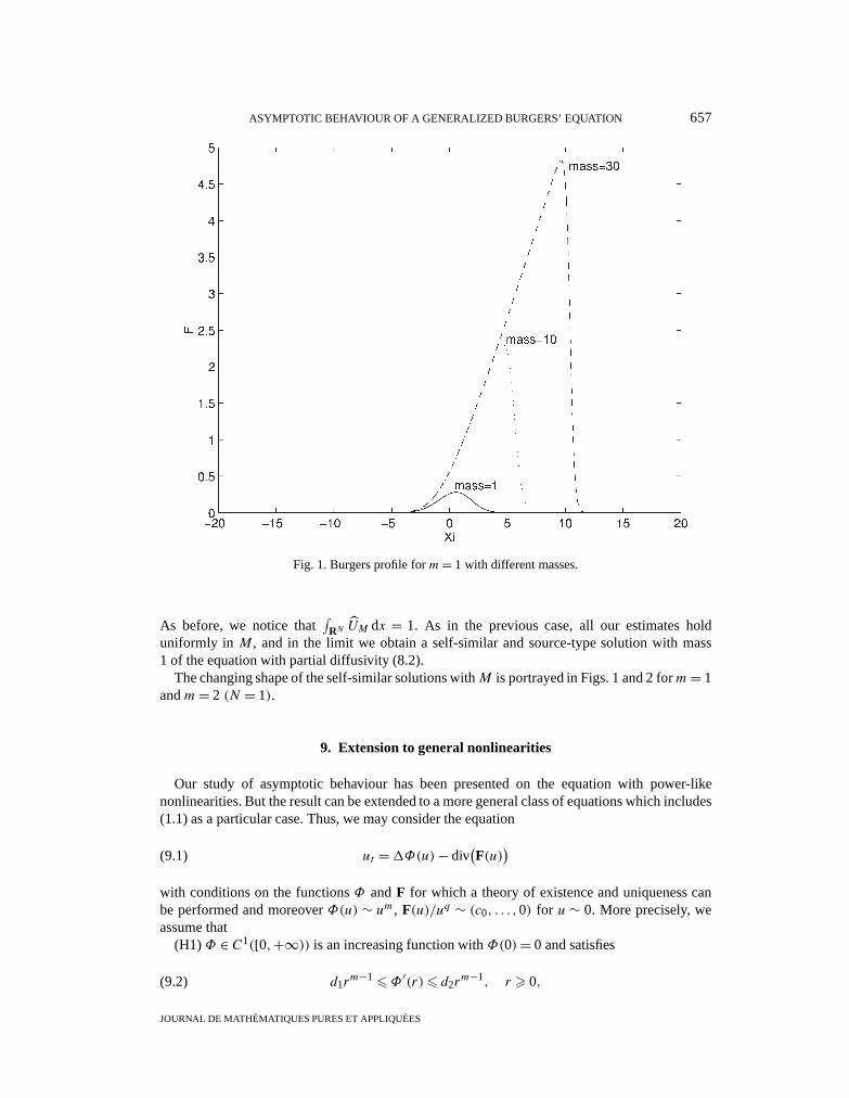
Fig. 1. Burgers profile form= 1 with different masses.

As before, we notice that∫

RN UM dx = 1. As in the previous case, all our estimates holduniformly in M, and in the limit we obtain a self-similar and source-type solution with mass1 of the equation with partial diffusivity (8.2).

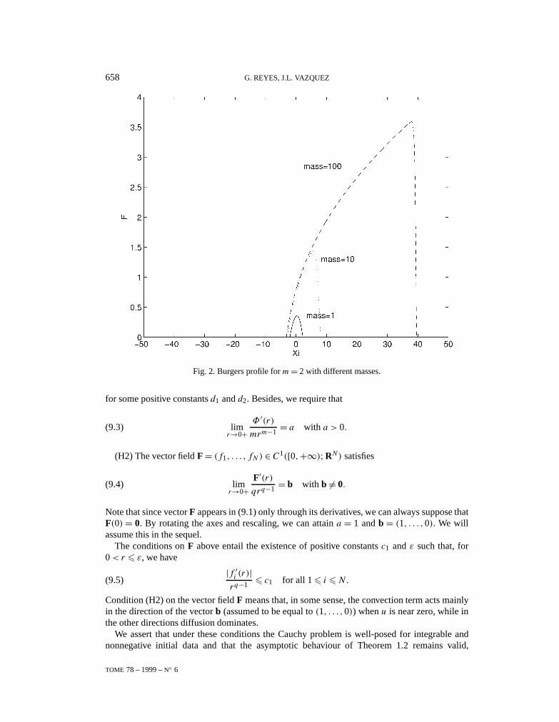
The changing shape of the self-similar solutions withM is portrayed in Figs. 1 and 2 form= 1andm= 2 (N = 1).

9. Extension to general nonlinearities

Our study of asymptotic behaviour has been presented on the equation with power-likenonlinearities. But the result can be extended to a more general class of equations which includes(1.1) as a particular case. Thus, we may consider the equation

ut =1Φ(u)− div(F(u)

)(9.1)

with conditions on the functionsΦ andF for which a theory of existence and uniqueness canbe performed and moreoverΦ(u) ∼ um, F(u)/uq ∼ (c0, . . . ,0) for u ∼ 0. More precisely, weassume that

(H1)Φ ∈ C1([0,+∞)) is an increasing function withΦ(0)= 0 and satisfies

d1rm−16Φ ′(r)6 d2r

m−1, r > 0,(9.2)



Fig. 2. Burgers profile form= 2 with different masses.

for some positive constantsd1 andd2. Besides, we require that

limr→0+

Φ ′(r)mrm−1

= a with a > 0.(9.3)

(H2) The vector fieldF= (f1, . . . , fN ) ∈ C1([0,+∞);RN) satisfies

limr→0+

F′(r)qrq−1 = b with b 6= 0.(9.4)

Note that since vectorF appears in (9.1) only through its derivatives, we can always suppose thatF(0)= 0. By rotating the axes and rescaling, we can attaina = 1 andb = (1, . . . ,0). We willassume this in the sequel.

The conditions onF above entail the existence of positive constantsc1 andε such that, for0< r 6 ε, we have

|f ′i (r)|rq−1 6 c1 for all 16 i 6N.(9.5)

Condition (H2) on the vector fieldF means that, in some sense, the convection term acts mainlyin the direction of the vectorb (assumed to be equal to(1, . . . ,0)) whenu is near zero, while inthe other directions diffusion dominates.

We assert that under these conditions the Cauchy problem is well-posed for integrable andnonnegative initial data and that the asymptotic behaviour of Theorem 1.2 remains valid,

TOME 78 – 1999 –N 6


theUM being the same self-similar solutions of (1.1) constructed above. We thus encounter aphenomenon ofasymptotic simplificationtowards a simpler equation. That is, the only relevantinformation aboutΦ andF for large times is their behaviour near 0. It is completely natural,since ast→∞, u goes to 0.

A theory of existence and uniqueness for Eq. (9.1) has been developed by different authorsunder different assumptions on the nonlinearities and the class of solutions, cf. [15,27,34,8].Similar (but stricter) power-like conditions are used in [11] and also in [14], where diffusion islinear,m= 1.

We may re-do the constructive existence proof and derivation of the main properties of thesolutions needed in the proof of the asymptotic behaviour by introducing minor modifications inthe definitions and proofs of preceding sections. Uniqueness of discussed in the Appendix. Forexample, in the definition of solution (Definition 2.1) we need only change condition (W4) into:

(W4′) For all 0< τ1 6 τ2 < ∞, all Ω ⊂ RN bounded with smooth boundary and allφ ∈L∞(Ω × [τ1, τ2]), φ = 0 on∂Ω × [τ1, τ2], we have

τ2∫τ1

∫Ω

∇Φ(u).∇φ − uφt − F.∇φdx dt =∫Ω

uφ dx

∣∣∣∣τ2τ1

.(9.6)

Existence of this class of solutions is obtained like in Section 2 since the corresponding referencesto [26,9,27] and [3] are still valid. In this way Theorem 2.1 applies. Let us worry about thefundamental estimates (E1)–(E4). The mass conservation (E1) can be proved in the same way asin Theorem 2.3. In fact, (E1) only depends on the divergence form of the right hand side in (9.1).Estimate (E2) is proved in [20] for general filtration equations of the type

ut =1Φ(u).(9.7)

Note. – In this general case, the constantC in (E2) depends also on the constantd1 in (9.2).Arguing as in Section 2, the validity of (E2) extends to Eq. (9.1).

Concerning the Energy estimate (E3), it can be obtained by the standard technique ofmultiplying Eq. (9.1) byΦ(u) and integrating by parts. We obtain

∞∫t

∫RN

∣∣∇Φ(u)∣∣2 dx dt 6 d2

m‖u0‖L1

∥∥u(t)∥∥mL∞,(9.8)

beingd2 the constant from (9.2). Taking into account theL∞-estimate (E2) we obtain the validityof (E3) for Eq. (9.1), with a constant depending ond1, d2,m, N , ‖u‖1 andt .

The L2-estimate of the time derivative (E4) partially uses the restrictions imposed on theconvection vectorF. We reproduce the main lines of the proof (compare with Theorem 4.1). Wemultiply (9.1) byΦ(u)t and integrate inΩ by parts. We get the following:

∫Ω

∣∣Ψ (u)t ∣∣2 dx + d

dt

∫Ω

∣∣∇Φ(u)∣∣2 dx =N∑i=1

∫Ω

Φ ′(u)f ′i (u)utuxi dx,(9.9)

whereΨ (r) = ∫ r0 √Φ ′(s)ds. Applying Young’s inequality to the right-hand side of (9.9), andtaking into account (9.2), (9.5), (E2) and the continuity off ′i we arrive at the following inequality,



analogous to (4.3):

d

dt

∫Ω

|∇Φ|2 dx 6 C(m,N,‖u‖1, d1, c

)∥∥u(t)∥∥2q−m+1∞

∫Ω

|∇Φ|2 dx,(9.10)

wherec is a positive constant such thatf ′i (u)/uq−1 < c for the values ofu(s), s > t > 0 (sucha constant exists by virtue of (9.5) and the continuity off ′i ). Next we derive an estimate for thequantity

γ ′(t)=∫Ω

∣∣∇Φ(u)∣∣2 dx,(9.11)

analogous to (4.5), the only difference being that the constant also depends ond1, d2 andc. Nextwe integrate int from t1> 0 to∞, use (9.9) and the estimate onγ ′ thus obtaining the estimate

∞∫t1

∫Ω

∣∣Ψ (u)t ∣∣2 dx dt 6 C(N,m,‖u‖1, d1, d2, c, t1

).(9.12)

The left inequality in (9.2) can be used in order to estimate from below the integral in the lefthand side of (9.12), and conclude as in Theorem 4.1. The only difference of this general casewith respect to the case of pure powers is that the constant in (E4) depends also ond1, d2 andc.

This is the asymptotic result for solutions of Eq. (9.1).

THEOREM 9.1. –LetΦ andF satisfy conditions(9.2)and(9.4), and letu0 ∈ L1(RN), u0> 0,∫u0 dx =M > 0. Then the weak solution of the Cauchy problem for Eq.(9.1)satisfies the thesis

of Theorem1.2, with the sameUM .

Proof. –We introduce the same family of rescalings (5.1) of Section 5.uλ satisfies thefollowing equation

uλt =1Φλ(uλ)− divFλ(uλ),(9.13)

where

Φλ(r)= λαmΦ(λ−αr

), Fλ(r)= λα−β+1F

(λ−αr

).(9.14)

It is easy to check that (9.2) holds for allΦλ with the same constantsd1 andd2 and that (9.5)is valid for all Fλ with λ> 1 with the sameε andc1. Therefore, since all theuλ have the samemass, all the estimates (E1)–(E4) are valid uniformly inλ. Arguing as in Section 5, Step 2, weobtain a convergent sequence inL1

loc((t0,+∞)× RN), which we denote againuλ. Let U bethe limit of this sequence. It is an easy matter to check that

Φλ(r)→ rm and Fλ(r)→ rq(9.15)

asλ→∞, and moreover, this convergence is uniform on compact subsets of[0,∞). Taking intoaccount these convergences, we can pass to the limit in the weak formulation, and we concludethatU satisfies (1.1) in the weak sense.

Another important property of the solutions of (9.1) is the fact that solutions with initiallycompact support have compact support for all timest > 0. This fact can be proved exactly as inSection 4, by using the energy method of Antontsev, since the necessary structural assumptions

TOME 78 – 1999 –N 6


are satisfied, by virtue of (9.2) and (9.4). This property enables to get convergence inL1 (notonly inL1

loc) for solutions withu0 ∈ C∞0 .The problem of the identification of the limit can be solved by means of the method of

asymptotic analysis of [17, pp. 443–446]. In the sequel, we adopt the notation of this work.First of all, we perform in (9.1) thecontinuousrescaling, corresponding to (5.1). It is given by

θ(ξ, τ )= tαu(ξtβ , t),(9.16)

whereτ = ln t , andα andβ are as in (5.1).θ(ξ, τ ) satisfies

θτ =1ξΦτ (θ)− divξ(Fτ (θ)

)+ αθ + βξ.∇ξ θ,(9.17)

with

Φτ (r)= eαmτΦ(re−ατ

), Fτ (r)= e(α−β+1)τF

(re−ατ

)(9.18)

(compare with (9.13) and (9.14)). We denote the (non-autonomous) operator in the right handside of (9.17) byB(θ, τ ). We also consider the following autonomous operator:

A(θ)=1ξθm −(θq)ξ1+ αθ + βξ∇ξ θ,(9.19)

which is the operator that appears in the equation forθ given by (9.16) whenu is a solution of(1.1). As a classS of solutions of (9.1), we take the class of solutions withu0 ∈ C∞0 (RN) and afixed massM = ∫ u0 dx > 0. The corresponding solutions of (9.17) are inC([0,∞);L1(RN)),have the same mass (which is conserved in time) and its supports are contained in some fixedball for all t > 0. As the ambient space we take the following closed subset ofL1:

X = u ∈L1(RN), u> 0 with fixed massM > 0.(9.20)

In order to reduce the asymptotics of the perturbed problem (9.17) to the asymptotics of thenon-perturbed one

θτ = A(θ),(9.21)

three basic conditions are imposed in the paper [17]. The first of them concerns the compactnessof the orbits in the classS of the perturbed equation

θτ = B(θ, τ )(9.22)

in X. It holds in our case, as a consequence of estimates (E1)–(E4) (more exactly, their translationin terms of θ ). (E4) implies equicontinuity of the setθs(τ )s>0 : [τ1, τ2] → L1(RN) with06 τ1< τ2, hence compactness inL∞loc([0,+∞);L1(RN)).

The second condition, i.e. the fact that the limits of all the convergent subsequencesθ(τ+ si)in L∞loc([0,+∞);L1(RN)) with si →∞ and θ ∈ S are solutions of (9.20), has been provedabove.

Finally, the third condition of uniform Lyapunov stability of the globalω-limit set of (9.20)(which in our case reduces to a point:Ω = FM , whereFM denotes the profile ofUM ), is aconsequence of theL1-contraction property enjoyed by the solutions of (1.1) shown in Section 3(this property is inherited by (9.20)). Therefore, the main result of [17], Theorem 3, is valid in ourcase. That is, theω-limit set of a solution of (9.21) in the classS is contained inΩ . Therefore,θ(ξ, τ )→ FM asτ →∞, which is the desired result.



For general initial data (with non-compact support) a final density argument is needed. Sinceit follows the lines of the argument used in Section 5, we omit the details.2

Appendix on uniqueness

We discuss in some detail the uniqueness of the solutions to Eq. (9.1) which includes as aparticular case (1.1). Our first result uses Kalashnikov’s duality proof for the porous mediaequation, which has been adapted by Hui [18] to the power case (1.1) and works for more generalnonlinearities. See also [5,29]. It is to be noted that no regularity is assumed onut .

THEOREM A1. – Suppose thatΦ satisfies assumption(H1) of Section8 with m > 1 and Fsatisfies(H2) with q > (m+ 1)/2. Then for everyu0 ∈ L∞(RN) ∩ L1(RN) there exists at mostone functionu ∈ L∞(0, T ;L1(RN))∩L∞(QT ) satisfying Eq.(9.1) in the sense:

τ∫0

∫Ω

∇Φ(u) · ∇φ− F · ∇φ− uφt

dx dt =∫Ω

u0(x)φ(x,0)dx−∫Ω

u(x, τ )φ(x, τ )dx.(A.1)

Proof. –Supposeu1 andu2 are two solutions with initial datau10 andu20 respectively. Takea testη ∈C∞(BR(0)× [0, T ]), R > 0, such thatη = 0 on∂BR(0)× [0, t]. Subtracting (A.1) foru1 andu2 and integrating by parts, we obtain∫

BR(0)

(u1− u2)(x, T )η(x,T )dx =∫

BR(0)

(u10− u20)(x)η(x,0)dx

+T∫

0

∫BR(0)

(u1− u2)(ηs +A1η+B∇η)dx ds −T∫

0

∫∂BR(0)

(um1 − um2

)∂η∂ν

dσ ds,(A.2)

where

A=Φ(u1)−Φ(u2)

u1− u2for u1 6= u2,

Φ ′(u1) for u1= u2,

(A.3)

and

B=

F(u1)− F(u2)

u1− u2for u1 6= u2,

F′(u1) for u1= u2.

(A.4)

LetC1 be such that

‖u1‖L∞,‖u2‖L∞ 6 C1.(A.5)

Then, applying the Cauchy mean value theorem toA and B, and taking into account theconditions imposed onΦ andF, there exist constantsk1 andk2 (depending ond1 andc1) suchthat

(Bj )2

2A6 k1C

2q−m−11 ,

Bj

A6 k2C

q−m1 , ∀j,(A.6)

(hereBj represents thej -th coordinate of vectorB.) Next, we construct suitable smoothapproximations ofA andB in BR × (0, T )). As in [18] we take sequences of smooth functions

TOME 78 – 1999 –N 6


Ai,R andBi,R such that

0< ci 6Ai,R 6 d2Cm−11 , 06 Bji,R 6 c1C

q−11 + 1,

Bj2i,R

2Ai,R6 k1C

2q−m−11 + 1= C2,

Bji,R

Ai,R6 k2C

q−m1 + 1= C3

(A.7)

and, moreover, the following convergences take place:

(Ai,R −A)A

1/2i,R

→ 0 and Bji,R −Bj → 0(A.8)

in L2(BR(0)× (0, T )) asi→∞ for all R > 0. Next we consider the dual problem:ηs +Ai,R1η+Bi,R.η− λη = 0 for (x, s) ∈BR(0)× (0, T ),η(x, s)= 0 for (x, s) ∈ ∂BR(0)× (0, T ),η(x,T )= θ(x) for x ∈ BR(0),

(A.9)

whereθ ∈ C∞0 (BR(0)), 06 θ 6 1. Problem (A.9) has a unique smooth solutionηi,R . By themaximum principle, 06 ηi,R 6 1. We need estimates of1ηi,R and∇ηi,R in L2(BR(0)× (0, T )).Such estimates are obtained in [2]. The basic estimate is the following:

T∫0

∫BR(0)

Ai,R(1ηi,R)2 dx ds + 2(λ−C2)

T∫0

∫BR(0)

‖∇ηi,R‖2 dx ds 6∫

BR(0)

‖∇θ‖2 dx.(A.10)

As in [18] (see also [29]), we introduce two suitable super-solutions of (A.9). The first of themhas the form

g(x, s)= eh(s)(

1+R20

1+ |x|2)β,(A.11)

whereh(x, s) = C′(T − s) andβ > 0. ChoosingC′ large enough, it is easy to check thatgis a super-solution of the dual equation and, moreover, it is greater thanηi,R in the parabolicboundary. Hence, by the maximum principle [26],g > ηi,R in BR(0)× (0, T ).

The second super-solution has the form

g∗(x, s)= aeh(s)Γ(|x|),(A.12)

where

Γ (r)= (R − r)−C3(R− r)2.(A.13)

Again, it is easy to show thatg∗ is a super-solution of (A.9) in the setBα = R−α < r < R, 0<s < T if we takeα = 1/2(C3+ n− 1). Moreover, if we put

a = (1+R20

)β/Γ (R − α)(1+ (R− α)2)β,(A.14)

we get the condition

g∗ = g in ∂BR−α × (0, T ).(A.15)



Therefore, since in the exterior boundary ofBα obviously ηi,R = 0 = g∗, by the maximumprinciple we haveg∗ > ηi,R in Bα . Then, the following estimate on the normal derivative ofηi,R holds:

‖∂ηi,R/∂ν‖L∞(∂BR(0)×(0,T )) 6 ‖∂g∗/∂ν‖L∞(∂BR(0)×(0,T )) 6CR−2β .(A.16)

Now, puttingη = ηi,R in (A.2), using (A.16) and (A.10) we proceed as in [18, p. 1691], thusobtaining, for allθ ∈ C∞0 (BR(0)), 06 θ 6 1,R > 2:∫

BR(0)

(u1− u2)(x, s)θ(x)dx 6∫Rn

(u10− u20)+(x)dx + 2C1

∥∥∥∥Ai,R −AA

1/2i,R

∥∥∥∥L2‖∇θ‖L2

+ (2C1/(2(λ−C2)

)1/2)‖Bi,R −B‖L2‖∇θ‖L2

+ λT∫

0

∫Rn

(u1− u2)+ dx ds +CRn−1−2βT .(A.17)

Choosing nowβ = n/2 and letting firsti →∞ and thenR →∞, λ→ C2, we get thefollowing:

∫Rn

(u1− u2)(x, s)θ(x)dx 6∫Rn

(u01− u02)+ dx +C2

T∫0

∫Rn

(u1− u2)+ dx ds.(A.18)

Next we putθ = χu1>u2∩BR−1 ∗ ρε , whereρε denotes a sequence of mollifiers. Letting nowε→ 0 andR→∞ we get

∫Rn

(u1− u2)+(x, s)dx 6∫Rn

(u01− u02)+ dx +C2

T∫0

∫Rn

(u1− u2)+ dx ds ∀s ∈ (0, T ).(A.19)

After a standard application of Gronwall’s inequality, and a similar argument for the negativepart ofu1− u2, we obtain the desired result:∫

Rn

|u1− u2|(x, s)dx 6 eC2t

∫Rn

|u01− u02|dx. 2(A.20)

We want to extend this result to the class of unbounded solutions considered in our paper.

THEOREM A2. – There exists at most one solution to Eq.(9.1) in the sense of Definition9.1.Moreover, the mapu0 7→ u(·, t) is a contraction inL1(RN).

Proof. –Takeu0 ∈ L1 and letu1(t) andu2(t) be two solutions. Fixedε > 0 by part (W2) ofthe definition of solution we can chooseτ small enough, such that∥∥ui(τ )− u0

∥∥L1 < ε for i = 1,2.(A.21)

Hence,‖u1(τ )− u2(τ )‖L1 < 2ε for τ small enough. Taking nowu1(τ ) andu2(τ ) as initial data,by Theorem A1 we will have:∥∥u1(t)− u2(t)

∥∥L1 < 2eC(t−τ )ε ∀t > τ.(A.22)

TOME 78 – 1999 –N 6


Sinceε is arbitrary, the previous inequality entails

u1(t)= u2(t) a.e.(A.23)

Therefore, all solutions coincide with the ones we have constructed before, for which we canprove that ∫

RN

|u1− u2|(x, t)dx 6∫

RN

|u10− u02|(x)dx.(A.24)

This result is proved by Otto [27] for bounded domains and we have obtained it in the limit.2Comment. Alternative proofs of uniqueness use Kruzhkov’s ideas [22] and apply to much

more general diffusive-convective equations. We refer to Carrillo’s unpublished work [8] fora very general result which covers also entropy solutions for purely convective equations (inbounded domains). See also [27], which is used in several instances in this paper. The presentduality method works only for diffusion-dominated equations but has the advantage of beingcomparatively simpler. On the other hand, a number of uniqueness proofs are based on the extraassumption thatu is a function of bounded variation, cf. [34,15].

Acknowledgment

The authors are grateful to J. Carrillo and M. Escobedo for information of their unpublishedworks.

REFERENCES

[1] J. AGUIRRE, M. ESCOBEDO and E. ZUAZUA, Self-similar solutions of a convection-diffusionequation and related elliptic problems,Comm. Partial Differential Equations15 (2) (1990) 139–157.

[2] S.N. ANTONTSEV, On the localization of solutions of nonlinear degenerate elliptic and parabolicequations,Soviet Math. Dokl.24 (1981) 420–424.

[3] PH. BÉNILAN and CH. ABOURJAILY, Symmetrization of quasi-linear parabolic problems, to appear.[4] G.I. BARENBLATT, Scaling, Self-Similarity and Intermediate Asymptotics, Cambridge Univ. Press,

Cambridge, 1996.[5] P. BÉNILAN , M.G. CRANDALL and M. PIERRE,Solutions of the porous medium inRN under optimal

conditions on the initial values,Indiana Univ. Math. J.33 (1984) 51–87.[6] J.M. BURGERS, A mathematical model illustrating the theory of turbulence,Adv. Appl. Mech.1 (1948)

171–199.[7] J.M. BURGERS, The Nonlinear Diffusion Equation, Reidel, Dordrecht, 1974.[8] J. CARRILLO, Entropy solutions for nonlinear degenerate problems, Preprint.[9] E. DIBENEDETTO, Degenerate Parabolic Equations, Springer, New York, 1993.

[10] J.I. DIAZ and L. VÉRON, Compacité du support des solutions d’équations quasi linéaires elliptiquesou paraboliques,C. R. Acad Sc. Paris, Série I297 (1983) 149–152.

[11] M. ESCOBEDO, E. FEIREISL and PH. LAURENÇOT, Large time behaviour for degenerate parabolicequations with dominating convective term, Preprint.

[12] M. ESCOBEDO and E. ZUAZUA, Large-time behaviour for solutions of a convection-diffusionequation inRN , J. Funct. Anal.100 (1991) 119–161.

[13] M. ESCOBEDO, J.L. VÁZQUEZ and E. ZUAZUA, Asymptotic behaviour and source-type solutions fora diffusion-convection equation,Arch. Rat. Mech. Anal.124 (1993) 43–65.

[14] M. ESCOBEDO, J.L. VÁZQUEZ and E. ZUAZUA, A diffusion-convection equation in several spacedimensions,Indiana Univ. Math. J.42 (1993) 1413–1440.



[15] G. GAGNEUX and M. MADAUNE-TORT, Analyse Mathématique des Modèles Non Linéaires del’Ingénieurie Petrolière, Springer, Berlin, 1996.

[16] B.H. GILDING, Properties of solutions of an equation in the theory of infiltration,Arch. Rat. Mech.Anal.65 (1977) 203–225.

[17] V.A. GALAKTIONOV and J.L. VAZQUEZ, Asymptotic behaviour of nonlinear parabolic equationswith critical exponents. A Dynamical Systems approach,J. Funct. Anal.100 (2) (1991) 435–462.

[18] K.M. HUI, Singular limit of solutions ofut =1um−A.∇(uq/q) asq→∞, Trans. Amer. Math. Soc.347 (5) (1995) 1687–1711.

[19] A.C. KALASHNIKOV , On the character of the propagation of perturbations in processes described byquasi-linear parabolic equations, in:Proceedings of Seminars dedicated to I.G. Petrovskii, Moscow,1975, pp. 135–144.

[20] T. KAWANAGO, EstimationLp–Lq des solutions deut =1Φ(u)+ f , C. R. Acad. Sci. Paris, Série I317 (1993) 821–824.

[21] S. KAMIN and J.L. VÁZQUEZ, Fundamental solutions and asymptotic behaviour for thep-Laplacianequation,Rev. Mat. Iberoamericana4 (1988) 339–354.

[22] S.N. KRUZHKOV, First-order quasi-linear equations in several independent variables,Math. USSRSbornik10 (1970) 217–243.

[23] L.D. LANDAU and E.M. LIFSHITZ, Mecánica de Fluidos, Reverté, Barcelona, 1991.[24] PH. LAURENÇOT and F. SIMONDON, Long-time behaviour for porous medium equations with

convection,Proc. Roy. Soc. Edinburgh Sect. A, to appear.[25] PH. LAURENÇOT, F. SIMONDON and G. REYES, Asymptotic behaviour of a convection-diffusion

equation inRN , in preparation.[26] O.A. LADYZHENSKAYA , V.A. SOLONNIKOV and N.N. URALTSEVA, Linear and Quasi-Linear

Equations of Parabolic Type, Transl. Math. Monogr., vol 23, Amer. Math. Soc., Providence, RI,1968.

[27] F. OTTO, L1-contraction and uniqueness for quasi-linear elliptic-parabolic equations, Preprint,Sonderforschungsbereich 256, University of Bonn (Germany), 1995.

[28] M. PIERRE, Uniqueness of the solutions ofut −1Φ(u)= 0 with initial datum a measure,NonlinearAnalysis, Theory, Methods and Applications6 (1982) 175–187.

[29] A. DE PABLO, J.L. VAZQUEZ, Travelling waves and finite propagation for a reaction-diffusionequation,J. Differential Equations93 (1991) 19–61.

[30] G. REYES, Asymptotic behaviour in convection-diffusion processes,Nonlinear Analysis, Theory andApplications, to appear.

[31] J.L. VÁZQUEZ, An introduction to the mathematical theory of the porous medium equation, in:ShapeOptimization and Free Boundaries, M.C. Delfour (Ed.), Math. and Phys. Sciences, Series C, vol.380, Kluwer, Dordrecht, 1992, pp. 347–389.

[32] J.L. VÁZQUEZ, Asymptotic behaviour for the porous medium equation in the whole space, Ph.D.Course notes, Universidad Autónoma de Madrid, 1997.

[33] G.B. WHITHAM , Linear and Nonlinear Waves, Wiley-Interscience, 1974.[34] J.-X. YIN, On the uniqueness and stability ofBV solutions for nonlinear diffusion equations,Comm.

Partial Differential Equations15 (1990) 1671–1683.[35] E. ZUAZUA, A Dynamical System approach to the self-similar large time behaviour in scalar

convection-diffusion equations,J. Differential Equations108 (1) (1994) 1–35.

TOME 78 – 1999 –N 6

asymptotic behaviour of a generalized burgers' equation

Documents