Applied Mathematics and Computation 170 (2005) 1365–1393

www.elsevier.com/locate/amc

A parameter-uniform implicitdifference scheme for solving

time-dependent Burgers� equations

Mohan K. Kadalbajoo a, K.K. Sharma b, A. Awasthi c,*

a Department of Mathematics, I.I.T-Kanpur, Kanpur 208 016, Indiab Department of Mathematics, Punjab University, Chandigarh 160 014, India

c Department of Mathematics, I.I.T-Kanpur, Kanpur 208 016, India

Abstract

A numerical study is made for solving one dimensional time dependent Burgers�equation with small coefficient of viscosity. Burgers� equation is one of the fundamental

model equations in the fluid dynamics to describe the shock waves and traffic flows. For

high coefficient of viscosity a number of solution methodology exist in the literature [6–

9] and [14] but for the sufficiently low coefficient of viscosity, the exist solution method-

ology fail and a discrepancy occurs in the literature. In this paper, we present a numer-

ical method based on finite difference which works nicely for both the cases, i.e., low as

well as high viscosity coefficient. The method comprises a standard implicit finite differ-

ence scheme to discretize in temporal direction on uniform mesh and a standard upwind

finite difference scheme to discretize in spacial direction on piecewise uniform mesh. The

quasilinearzation process is used to tackle the non-linearity. An extensive amount of

analysis has been carried out to obtain the parameter uniform error estimates which

show that the resulting method is uniformly convergent with respect to the parameter.

0096-3003/$ - see front matter � 2005 Elsevier Inc. All rights reserved.

doi:10.1016/j.amc.2005.01.032

* Corresponding author. Tel.: +915122597732; fax: +915122597500.

E-mail addresses: kadal@iitk.ac.in (M.K. Kadalbajoo), kapilks@ycos.com (K.K. Sharma),

ashishan@iitk.ac.in (A. Awasthi).

1366 M.K. Kadalbajoo et al. / Appl. Math. Comput. 170 (2005) 1365–1393

To illustrate the method, numerical examples are solved using the presented method and

compare with exact solution for high value of coefficient of viscosity.

� 2005 Elsevier Inc. All rights reserved.

Keywords: Burgers� equation; Euler implicit method; Quasilinearization; Shishkin mesh; Uniform

convergence

1. Introduction

In this paper, we examine the one dimensional time dependent Burgers�equation with small coefficient of viscosity. This is a homogeneous quasilinear

parabolic parabolic partial differential equation which is encountered in themathematical modeling of turbulent fluid and shock waves and considered as

one of the fundamental model equation in the fluid dynamics to describe the

shock waves and traffic flows. Such type of equations can be found in the paper

of Batman [1] in 1915. In 1948, Burgers [2] introduced this equation to capture

some features of turbulent fluid in a channel caused by the interaction of the

opposite effects of convection and diffusion.

The numerical solution of the convection dominating Burgers� equation in

one space dimension has been studied extensively. In 1972, Benton and Platz-man [3] published a number of distinct solutions to the initial value problems

for the Burgers� equation in the infinite domain as well as in the finite domain.

In 1996, Ozis and Ozdes [13] applied the variational method, from which they

succeeded to generate an approximate solution in the form of sequence solu-

tion which converges to the exact solution. In 1997, Mazzia and Mazzia [12]

converted Burgers� equation to a system of ordinary differential equations,

and then applied the transverse scheme in combination with boundary value

methods. In 1996, Mittal and Singhal [11] presented a numerical approxima-tion of the one dimensional Burgers� equations, they truncated one dimensional

Fourier expansion with time dependent coefficients and formulated as the

approximated problem which consisted of a system of non-linear ordinary dif-

ferential equations for the coefficients. They also extended their work to study

Burgers� equation with periodic boundary conditions.

For small values of the coefficient of viscosity �, one of the major difficulties

encountered is due to inviscid boundary layers produced by the steeping effect

of the non-linear advection term in Burgers� equation. In case where the coef-ficient of viscosity 610�5, the exact solution is not available and a discrepancy

exits in the literature see [16].

Here we construct the numerical method for solving the Burgers� equationwith small �, i.e., the coefficient of viscosity, whose convergence behavior in

the global maximum norm is parameter-uniform, i.e. �-uniform. We first semi

discretize the original non-linear Burgers�equation in the temporal direction by

M.K. Kadalbajoo et al. / Appl. Math. Comput. 170 (2005) 1365–1393 1367

backward Euler scheme with the constant time step which produces a set of sta-

tionary Burgers� equations. Then use the quasilinearization process [4] to line-

arize the stationary Burgers� equation obtained from semi discretization and

shown that the sequence of solutions of linearized problem converges quadrat-

ically to the solution of the original non-linear problem at each time step. For

totally discrete scheme, we discretize the set of linear problems resulting fromthe time semidiscretization using the simple upwind finite difference scheme

defined on an appropriate piecewise uniform mesh of Shishkin type. We

decompose the global error in two components, which are analyzed separately

and obtain parameter uniform error estimates for the totally discrete method.

Throughout the paper we denote C (sometimes subscripted), a generic posi-

tive constant independent of � and of the mesh.

2. The continuous problem

Consider the Burgers� equation

ouot

þ uouox

¼ �o2uox2

; ðx; tÞ 2 X � ð0; T �; ð2:1aÞ

where

X ¼ ð0; 1Þ;With initial condition

uðx; 0Þ ¼ f ðxÞ for 0 6 x 6 1; ð2:1bÞand boundary conditions

uð0; tÞ ¼ 0 uð1; tÞ ¼ 0 for 0 6 t 6 T ; ð2:1cÞwhere � > 0 is the coefficient of kinematic viscosity and the prescribed function

f(x) is sufficiently smooth.

We impose the compatibility conditions

f ð0Þ ¼ 0; f ð1Þ ¼ 0; ð2:2Þso that the data matches at the two corners (0,0) and (1,0) of the domainX � ½0; T �.

These conditions guarantee that there exits a constant C such that for

0 < � 6 1 and for all ðx; tÞ 2 X � ½0; T �, (see Bobisud [5]).

juðx; tÞ � f ðxÞj 6 Ct; t 2 ð0; T �; ð2:3Þ

juðx; tÞ � 0j 6 Cx; x 2 ð0; 1Þ; ð2:4ÞUsing the properties of norm, Eq. (2.3) is written as

juðx; tÞ � f ðxÞj 6 juðx; tÞ � f ðxÞj 6 Ct; t 2 ð0; T � ð2:5Þ

1368 M.K. Kadalbajoo et al. / Appl. Math. Comput. 170 (2005) 1365–1393

i.e.

juj 6 Ct þ jf jsince f(x) is sufficiently smooth and x and t also lie in the bounded interval, it is

clear with the above relations that the solution u is bounded i.e.

juðx; tÞj 6 C; ðx; tÞ 2 X � ½0; T �: ð2:6Þ

Lemma 1. By keeping x fixed along the line {(x, t):0 6 t 6 T} the bound of ut is

given by

jutðx; tÞj 6 C ð2:7Þ

Proof. We assume that the solution u(x, t) is sufficiently smooth in the domain

X � ½0; T � and by mean value theorem there exits a t* in the interval (t, t + k)

along the line {(x, t):0 6 t 6 T} such that

utðx; t�Þ ¼uðx; t þ kÞ � uðx; tÞ

k;

jutðx; t�Þj 62juðx; tÞj

k

ð2:8Þ

using Eq. (2.6), we get

jutðx; tÞj 6 C: ð2:9ÞSimilarly we get the bounds of the utt(x, t) and uttt(x, t) along the line,

{(x, t):0 6 t 6 T}, i.e. we have

oiuðx; tÞoti

���� ���� 6 C for i ¼ 0; 1; 2; 3: � ð2:10Þ

3. The time semidiscretization

We can write Eq. (2.1) in the following form:

ut ¼ �uxx � uux forðx; tÞ 2 X � ð0; T �:Discretizing the time variable by means of Euler implicit method with uniform

size Dt, we obtain

u0 ¼ f ðxÞ; ð3:11aÞ

ujþ1 � ujDt

¼ ½�uxx � uux�jþ1;¼ ½�ujþ1�xx � ujþ1½ujþ1�x 0 6 j 6 M � 1

ð3:11bÞ

M.K. Kadalbajoo et al. / Appl. Math. Comput. 170 (2005) 1365–1393 1369

with the boundary conditions

ujþ1ð0Þ ¼ 0; ujþ1ð1Þ ¼ 0 for j ¼ 0; 1; . . . ;M � 1: ð3:11cÞwhere uj+i is the solution of the above differential equation at the (j + 1)th time

step. The differential Eq. (3.11) can be written in the following form:

u0 ¼ f ðxÞ; ð3:12aÞ

��Dt½ujþ1�xx þ ½1þ Dt½ujþ1�x�ujþ1 ¼ uj; 0 6 j 6 M � 1 ð3:12bÞwith the boundary conditions,

ujþ1ð0Þ ¼ 0; ujþ1ð1Þ ¼ 0 for j ¼ 0; 1; . . . ;M � 1: ð3:12cÞEq. (3.12) is non-linear ordinary differential equation for each j lying between 0

to M � 1.

4. Quasilinearization

Using quasilinearization process we linearize the above non-linear ordinary

differential equations and followed by simplification yields

uðnþ1Þ0 ¼ f ðxÞ; ð4:13aÞ

��Dt uðnþ1Þjþ1

h ixxþ Dtðuðnþ1Þ

jþ1 ÞxuðnÞjþ1 þ 1þ DtðuðnÞjþ1Þx

h iuðnþ1Þjþ1

¼ uðnþ1Þj þ DtðuðnÞjþ1Þxu

ðnÞjþ1; 0 6 j 6 M � 1; ð4:13bÞ

with boundary conditions

uðnþ1Þjþ1 ð0Þ ¼ 0; uðnþ1Þ

jþ1 ð1Þ ¼ 0: ð4:13cÞ

with initial guess u(0) and n is the iteration index.

Using the notation u(n+1) = U the above equation can be written as

U 0 ¼ f ðxÞ ð4:14aÞ

��DtðUjþ1Þxx þ DtðuðnÞjþ1ÞðUjþ1Þx þ 1þ DtðuðnÞjþ1Þh i

Ujþ1

¼ Uj þ DtðuðnÞx Þjþ1uðnÞjþ1: ð4:14bÞ

For the simplicity we use the following notations:

1

Dtþ ðuðnÞjþ1Þx

� �¼ aðnÞðxÞ;

uðnÞjþ1 ¼ bðnÞðxÞ;

1370 M.K. Kadalbajoo et al. / Appl. Math. Comput. 170 (2005) 1365–1393

Uj

Dtþ uðnÞjþ1

� �xðuðnÞjþ1Þ

� �¼ F ðnÞðxÞ:

Using the above notations Eq. (4.14) can be written in the following form:

U 0 ¼ f ðxÞ ð4:15aÞ

� �ðUjþ1ðxÞÞxx þ bðnÞðxÞðUjþ1ðxÞÞx þ aðnÞðxÞUjþ1ðxÞ ¼ F ðnÞðxÞ;j ¼ 0ð1ÞM � 1: ð4:15bÞ

We assume that a is the lower bound of the b(n)(x), i.e.

bðnÞðxÞ P a > 0; x 2 X: ð4:16Þ

Writing Eq. (4.15) in the following form:

U 0 ¼ f ðxÞ;L�Ujþ1ðxÞ ¼ F ðnÞðxÞ; 0 6 j 6 M � 1;

ð4:17Þ

where

L�Ujþ1ðxÞ � ��ðUjþ1Þxx þ bðnÞðxÞðUjþ1ÞxðxÞ;þaðnÞðxÞUjþ1ðxÞ

with boundary conditions

Ujþ1ð0Þ ¼ 0; Ujþ1ð1Þ ¼ 0:

4.1. Convergence of quasilinearization process

For the sake of simplicity we consider the following form of equation:

ðUjþ1ÞxxðxÞ ¼ HðUjþ1Þ ð4:18Þwith boundary conditions

Ujþ1ð0Þ ¼ 0; Ujþ1ð1Þ ¼ 0:

We assume that U ð0Þjþ1ðxÞ be the initial guess. Consider the sequence obtained by

the following recurrence relation:

ðU ðnþ1Þjþ1 Þxx ¼ HðU ðnÞ

jþ1Þ þ ðU ðnþ1Þjþ1 � U ðnÞ

jþ1ÞHUjþ1ðU ðnÞ

jþ1Þ ð4:19Þ

with boundary conditions

U ðnþ1Þjþ1 ð0Þ ¼ 0; U ðnþ1Þ

jþ1 ð1Þ ¼ 0:

M.K. Kadalbajoo et al. / Appl. Math. Comput. 170 (2005) 1365–1393 1371

Subtracting the (n + 1)th equation from (n + 2)th equation, we have

U ðnþ2Þjþ1 � U ðnþ1Þ

jþ1

� �xx¼ HðU ðnþ1Þ

jþ1 Þ � HðU ðnÞjþ1Þ

� ðU ðnþ1Þjþ1 � U ðnÞ

jþ1ÞHUjþ1ðU ðnÞ

jþ1Þ þ HUjþ1ðU ðnþ1Þ

jþ1 Þ

� ðU ðnþ2Þjþ1 � U ðnþ1Þ

jþ1 Þ: ð4:20Þ

The above equation is a differential equation for ðU ðnþ2Þjþ1 � U ðnþ1Þ

jþ1 Þ, and convert-

ing into an integral equation, we have

ðU ðnþ2Þjþ1 � U ðnþ1Þ

jþ1 Þ ¼Z 1

0

Gðx; sÞ½HðU ðnþ1Þjþ1 Þ � HðU ðnÞ

jþ1Þ

� ðU ðnþ1Þjþ1 � U ðnÞ

jþ1ÞHUjþ1ðU ðnÞ

jþ1Þ þ HUjþ1

� ðU ðnþ1Þjþ1 ÞðU ðnþ2Þ

jþ1 � U ðnþ1Þjþ1 Þ�ds; ð4:21Þ

where the Green�s function

Gðx; sÞ ¼xðs� 1Þ; 0 6 x 6 s 6 1;

ðx� 1Þs; 0 6 s 6 x 6 1;

maxx;s

Gðx; sÞ ¼ 1

4:

ð4:22Þ

The mean-value theorem gives us

HðU ðnþ1Þjþ1 Þ ¼ HðU ðnÞ

jþ1Þ þ ðU ðnþ1Þjþ1 � U ðnÞ

jþ1ÞHUjþ1ðU ðnÞ

jþ1Þ

þðU ðnþ1Þ

jþ1 � U ðnÞjþ1Þ

2

2HUjþ1Ujþ1

ðhÞ; ð4:23Þ

where h lies between U ðnÞjþ1 and U ðnþ1Þ

jþ1 .

Using Eq. (4.23), Eq. (4.21) become

ðU ðnþ2Þ � U ðnþ1Þjþ1 Þ ¼

Z 1

0

Gðx; sÞ

�ðU ðnþ1Þ

jþ1 � U ðnÞjþ1Þ

2

2HUjþ1Ujþ1

ðhÞ þ HUjþ1ðU ðnþ1Þ

jþ1 ÞðU ðnþ2Þjþ1 � U ðnþ1Þ

jþ1 Þ" #

ds:

ð4:24ÞDefine

k ¼ maxjUjþ1j61

jHUjþ1Ujþ1ðUjþ1Þj and m ¼ max

jUjþ1j61jHUjþ1

ðUjþ1Þj: ð4:25Þ

1372 M.K. Kadalbajoo et al. / Appl. Math. Comput. 170 (2005) 1365–1393

Now Eq. (4.24) become

U ðnþ2Þjþ1 � U ðnþ1Þ

jþ1

� ���� ��� 6 1

4

Z 1

0

k2

U ðnþ1Þjþ1 � U ðnÞ

jþ1

� �2

þ m U ðnþ2Þjþ1 � U ðnþ1Þ

jþ1

��� ���� �ds:

ð4:26ÞTaking the maximum over x on both sides of the above inequality and aftersimplification, we have

maxx

ðU ðnþ2Þjþ1 � U ðnþ1Þ

jþ1 Þ��� ��� 6 k

8

1� m4

� maxx

ðU ðnþ1Þjþ1 � U ðnÞ

jþ1Þ2: ð4:27Þ

The inequality (4.27) shows that the convergence of quasilinearization processis quadratic.

4.2. Maximum principle [15]

Assume that any function W 2 C2ðXÞ satisfies w(0) P 0 and w(1) P 0. Then,

L�w(x) P 0 for all x 2 X implies that w(x) P 0 for all x 2 X.

Proof. Let x* be such that wðx�Þ ¼ minXwðxÞ and suppose that w(x*) < 0. It isclear that x* 62 {0,1}. Therefore wx(x*) = 0,wxx(x*) P 0, and

L�wðx�Þ ¼ ��wxxðx�Þ þ bðnÞðx�Þwxðx�Þ þ aðnÞðx�Þwðx�Þ; ð4:28Þsince a(n)(x) P 0 for all x 2 X therefore

L�wðx�Þ < 0;

which contradicts the assumption, therefore it follows that w(x*) P 0 and thus

w(x) P 0 for all x 2 X. h

4.3. Local error

The local truncation error is given by the following relation:

ejþ1 ¼ Uðtjþ1Þ � Ujþ1;

where Uj+i is the solution of the semidiscretized Eq. (4.14). With the help of this

local error at each time step, we will find the global error of the time discreti-

zation which is defined as

Ej � Uðx; tjÞ � UjðxÞ:

k Æ kh denotes the discrete maximum norm, given by

kxkh ¼ max16i6N

kxik

M.K. Kadalbajoo et al. / Appl. Math. Comput. 170 (2005) 1365–1393 1373

Theorem 1. If

okuðx; tÞokt

���� ���� 6 C; ðx; tÞ 2 X � ½0; T �; 0 6 k 6 2 ð4:29Þ

then the local and global error estimates satisfy the following estimates

kejþ1kh 6 CðDtÞ2: ð4:30Þ

kEjþ1kh 6 CDt for all j 6 T=Dt: ð4:31ÞTherefore, the time discretisation process is uniformly convergent of first-order.

Proof. The function Uj+1 satisfies

L�Ujþ1 ¼ F ðnÞðxÞ: ð4:32ÞLinearize the original problem by quasilinearization process, we have

oUot

¼ ��Uxx þ uðnÞUx þ uðnÞx U þ uðnÞðuðnÞÞx; ð4:33Þ

where

U ¼ uðnþ1Þ

Since the solution of Eq. (4.33) is smooth enough, it holds

UðtjÞ ¼ Uðtjþ1Þ � DtoUðtjþ1Þ

otþZ tj

tjþ1

ðtj � sÞ o2uot2

ðsÞds ð4:34Þ

Using Eq. (4.33), we have

UðtjÞ ¼ Uðtjþ1Þ � Dt �Uxx � uðnÞUx � uðnÞx U � uðnÞðuðnÞÞx�

ðtjþ1Þ

þZ tj

tjþ1

ðtj � sÞ o2UðsÞot2

ds: ð4:35Þ

Subtracting Eq. (4.14) from Eq. (4.35), we get

DtL�ejþ1 ¼ OðDtÞ2 ð4:36ÞSince the operator (DtL�) satisfies the maximum principle therefore

kðDtL�Þ�1kh 6 C1 ð4:37Þwhere C1 is a positive constant independent on Dt. Using the inequality (4.37)

we get

kejþ1kh 6 CðDtÞ2: ð4:38ÞUsing the local error estimates up to the jth time step we get the following glo-

bal error estimate at (j + 1)th time step:

1374 M.K. Kadalbajoo et al. / Appl. Math. Comput. 170 (2005) 1365–1393

kEjþ1kh ¼Xj

l¼1

el

����������h

; j 6 T=Dt;

6 ke1kh þ ke2kh þ . . .þ kejkh;6 C1ðj:DtÞ:Dt; using Eq:ð4:38Þ;6 C1TDt since jDt 6 T ;

¼ CDt;

ð4:39Þ

where C is a positive constant independent of � and Dt.

4.4. Bounds for U and its derivatives

Lemma 2. Let Uj+1(x) be the solution of Eq. (4.15), there exits a constant Csuch that

jUjþ1ðxÞj 6 C for all x 2 X: ð4:40Þ

Proof. By the construction of barrier functions we find the bounds of Uj+1(x),

w�ðxÞ ¼ Mð1þ xÞ � Ujþ1ðxÞ; ð4:41Þwhere M is a constant chosen sufficiently large such that

w�ð0Þ P 0; wð1Þ P 0;

L�w�ðxÞ ¼ MbðnÞðxÞ þ aðnÞðxÞð1þ xÞ � F ðnÞðxÞ; x 2 X:

Since x 2 X, and a(n)(x) P 0 therefore

L�w�ðxÞ P 0; x 2 X: ð4:42Þ

Using maximum principle for L� we have,

w�ðxÞ P 0; x 2 X

Mð1� xÞ � Ujþ1ðxÞ P 0;

jUjþ1ðxÞj 6 Mð1� xÞ; x 2 X

ð4:43Þ

and so

jUjþ1ðxÞj 6 C for all x 2 X:

Theorem 2. Let Uj+i be the the solution of Eq. (4.17), the bounds of its deriva-

tives are given by

jU ðkÞjþ1j 6 Cð1þ ��ke�að1�xÞ=�Þ for all x 2 X; k ¼ 1; 2; 3: ð4:44Þ

M.K. Kadalbajoo et al. / Appl. Math. Comput. 170 (2005) 1365–1393 1375

Proof. We find the bounds of the derivatives of Uj+i with the help of induction.

By the differentiating Eq. (4.15) k times w. r. t. x we have

L�UðkÞjþ1ðxÞ ¼ F kðxÞ for 0 6 k 6 3;

where

F 0 ¼ F

F k ¼ F ðkÞ �Xk�1

s¼0

k

s

� �bðk�sÞU ðsþ1Þ þ

k

s

� �aðk�sÞU ðsÞ

� �for 1 6 k 6 3:

Assume that for all l, 0 6 l 6 k, the following estimates hold:

jU ðlÞjþ1ðxÞj 6 C 1þ ��le

�að1�xÞ�

� �; x 2 X;

where a is the lower bound of b(n)(x).

From the above assumption we have

L�UðkÞjþ1 ¼ F k;

where

jU ðkÞjþ1ðxÞj 6 C 1þ ��ke

�að1�xÞ�

� �;

F kðxÞ 6 C 1þ ��ke�að1�xÞ

�

� �:

And at the boundaries we have

jU ðkÞjþ1ð0Þj 6 C 1þ ��ke

�a�

� ;6 Cð1þ ��ðk�1ÞÞ since e

�a� 6 1 6 ��1; ð4:45Þ

jU ðkÞjþ1ð1Þj 6 Cð1þ ��kÞ: ð4:46Þ

Since � 6 1, this implies that

��ðk�1Þ P 1 for 1 6 k 6 3:

Using the above fact in Eqs. (4.45) and (4.46),

jU ðkÞjþ1ð0Þj 6 C��ðk�1Þ; jU ðkÞ

jþ1ð1Þj 6 C��k:

Defining

hkðxÞ ¼1

�

Z 1

xF kðsÞe�ðAðxÞ�AðsÞÞ ds;

where

AðxÞ ¼Z 1

xbðnÞðsÞds:

1376 M.K. Kadalbajoo et al. / Appl. Math. Comput. 170 (2005) 1365–1393

The particular solution of

L�UðkÞjþ1 ¼ F k;

is given by

ðUjþ1ÞpðxÞ ¼ �Z 1

xhkðsÞds:

Its general solution can be written in the form of

U ðkÞjþ1 ¼ ðUjþ1ÞðkÞp þ ðUjþ1ÞðkÞh ;

where the homogeneous solution ðUjþ1ÞðkÞh satisfies

L�ðUjþ1ÞðkÞh ¼ 0;

ðUjþ1ÞðkÞh ð0Þ ¼ U ðkÞjþ1ð0Þ � ðUjþ1ÞðkÞp ð0Þ;

ðUjþ1ÞðkÞh ð1Þ ¼ U ðkÞjþ1ð1Þ:

Introducing the function

/ðxÞ ¼R 1

x e�AðsÞ=� dsR 1

0e�AðsÞ=� ds

;

we have, L�/ ¼ 0;/ð0Þ ¼ 1;/ð1Þ ¼ 0 and 0 6 /ðxÞ 6 1:Now ðUjþ1Þkh can be written as

ðUjþ1ÞðkÞh ðxÞ ¼ U ðkÞjþ1ð0Þ � ðUjþ1ÞðkÞp ð0Þ/ðxÞ þ U ðkÞ

jþ1ð1� /ðxÞÞ ð4:47Þ

The above leads the following expression for U ðkþ1Þjþ1 :

U ðkþ1Þjþ1 ¼ ðUjþ1Þðkþ1Þ

p þ ðUjþ1Þðkþ1Þh

¼ hkðxÞ þ ðUjþ1ð0Þ � ðUjþ1ÞðkÞp ð0ÞÞ/xðxÞ þ U ðkÞjþ1ð1Þð�/xðxÞÞ:

Since

/xðxÞ ¼�e�AðxÞ=�R 1

0eAðsÞ=� ds

;

the upper and lower bound of b(n)(x) lead the estimate

j/xðxÞj 6 C��1e�að1�xÞ=�:

Furthermore

jhkðxÞj 6 C��1

Z 1

xð1þ ��ke�að1�sÞ=�Þe�aðs�xÞ=� ds:

M.K. Kadalbajoo et al. / Appl. Math. Comput. 170 (2005) 1365–1393 1377

Evaluating the above integral exactly and estimating the terms in the resulting

expression gives

jhðkÞðxÞj 6 Cð1þ ��ðkþ1Þe�að1�xÞ=�Þ: ð4:48Þ

Since

ðUjþ1ÞðkÞp ð0Þ ¼ �Z 1

0

hkðsÞds;

Using Eq. (4.48) in the above expression and followed by a simplification gives

jðUjþ1ÞðkÞp ð0Þj 6Z 1

0

jhkðsÞjds;6 CZ 1

0

ð1þ ��ðkþ1Þe�að1�sÞ=�Þds;

¼ C 1þ ��k

að1� e�a=�Þ

� �;

6 C 1þ ��k

a

� �; since ð1� e�a=�Þ 6 1;

Since � 6 1, this implies that ��k P 1, 1 6 k 6 3, using this fact in the aboveexpression we have

jðUjþ1ÞðkÞp ð0Þj 6 C��k; jðUjþ1ÞðkÞp ð1Þj ¼ 0: ð4:49Þ

Differentiating Eq. (4.47) we have

jU ðkþ1Þjþ1 j 6 jhðkÞj þ jU ðkÞ

jþ1ð0Þj þ jðUjþ1ÞðkÞp ð0Þj þ jU ðkÞjþ1ð1Þj

� �jhxj: ð4:50Þ

Using the estimates of Eq. (4.49) yields

jU ðkþ1Þjþ1 j 6 Cð1þ ��ðkþ1Þe�að1�xÞ=�Þ: ð4:51Þ

5. The spatial discretization

5.1. Shishkin mesh

Shishkin meshes are piecewise-uniform meshes which condense approxi-

mately in the boundary layer regions as � ! 0; this is accomplished by the

use of transition parameter s, which depend naturally on �, crucially on N.

Thus for a given N and �, the interval [0,1], is divided into parts, [0,1 � s],[1 � s, 1] where the transition point s is given by

s � min1

2;C� logN

�the value of the constant C depends on which scheme is used.

1378 M.K. Kadalbajoo et al. / Appl. Math. Comput. 170 (2005) 1365–1393

Define

hi ¼2ð1�sÞ

N ; if i ¼ 1; 2; . . . ; N2;

2sN ; if i ¼ N

2þ 1; . . . ;N :

8<: ð5:52Þ

where N is the no discretization points and the set of mesh points XN ¼ fxigNi¼0

with

xi ¼2ð1� sÞN�1i; if i ¼ 0; 2; . . . ; N

2;

1� s þ 2sN�1ði� N2Þ if i ¼ N

2þ 1; . . . ;N :

(ð5:53Þ

Define

D�x U i;j ¼

Ui;j � Ui�1;j

hi;

d2xUi;j ¼

1

hi

U iþ1;j � Ui;j

hiþ1

� Ui;j � Ui�1;j

hi

� �;

�hi ¼ ðhi þ hiþ1Þ=2:Discretizing Eq. (4.15) by using standard upwind finite difference operator on

the piecewise uniform mesh XN ¼ fxigNi¼0 with xN = 1, we get

Ui;0 ¼ f ðxiÞ; xi 2 XN ; ð5:54aÞ

��d2xU i;jþ1 þ bðnÞi D�

x U i;jþ1 þ aðnÞi U i;jþ1 ¼ F ðnÞðxiÞ; xi 2 XN ð5:54bÞwith boundary conditions

U 0;jþ1 ¼ 0; UN ;jþ1 ¼ 0: ð5:54cÞThe finite difference operator in Eq. (5.54) defined by

LN� � ��d2

x þ bðnÞi D�x þ aðnÞi I : ð5:55Þ

5.2. Discrete maximum principle

Assume that the mesh function wi satisfies w0 P 0 and wN P 0. Then

LN� wi P 0 for 1 6 i 6 N � 1 implies that wi P 0 for all 0 6 i 6 N.

Proof. Let there exits an integer k such that wk = miniwi and suppose wk < 0.We have w0 P 0 and, wN P 0 therefore k 62 {0,N}.

Now we have

wkþ1 � wk P 0; wk � wk�1 < 0:

M.K. Kadalbajoo et al. / Appl. Math. Comput. 170 (2005) 1365–1393 1379

Therefore

LN� wk ¼ ��d2

xðwkÞ þ bðnÞðxkÞD�x wk þ aðnÞðxkÞwk

¼ � ��hk

wkþ1 � wk

hkþ1

� wk � wk�1

hk

� �þ bðnÞðxkÞ

wk � wk�1

hk

� �þ aðnÞðxkÞwk

< 0;

which contradicts the hypothesis, thus we have

wi P 0 for all 0 6 i 6 N : �

6. Error estimates and convergence analysis

To derive �-uniform error estimates, we need sharper bounds on the deriv-

atives of the solution U. We derive these using the following decomposition of

the solution into smooth and singular components

Ujþ1ðxÞ ¼ V jþ1ðxÞ þ W jþ1ðxÞ;where Vj+1 can be written in the form

V jþ1 ¼ V 0 þ �V 1 þ �2V 2

and V0,V1 and V2 are defined, respectively, to be the solutions of the problems

bðnÞðxÞV 0 þ aðnÞðxÞðV 0Þx ¼ F ðnÞðxÞ; V 0ð0Þ ¼ Ujþ1ð0Þ; ð6:56Þ

bðnÞðxÞV 1 þ aðnÞðxÞðV 1Þx ¼ �ðV 0Þxx; V 1ð0Þ ¼ 0; ð6:57Þ

��ðV 2Þxx þ bðnÞðxÞV 2 þ aðnÞðxÞðV 2Þx ¼ �ðV 1Þxx; V 2ð0Þ ¼ 0; V 2ð1Þ ¼ 0:

ð6:58Þthus the smooth component Vj+1 is the solution of

L�V jþ1 ¼ F ðnÞðxÞ; V jþ1ð0Þ ¼ V 0ð0Þ þ �V 1ð0Þ; V jþ1ð1Þ ¼ Ujþ1ð1Þð6:59Þ

and consequently the singular component Wj+1 is the solution of the homoge-

neous problem

L�W jþ1 ¼ 0; W jþ1ð0Þ ¼ 0; W jþ1ð1Þ ¼ Ujþ1ð1Þ � V jþ1ð1Þ: ð6:60Þ

Lemma 3. The bounds of Vj+1,Wj+1 and their derivatives are given as follows:

kV ðkÞjþ1k 6 Cð1þ �ð2�kÞÞ; k ¼ 0; 1; 2; 3; ð6:61aÞ

kW jþ1ðxÞk 6 Ce�að1�xÞ=� for all x 2 X; ð6:61bÞ

1380 M.K. Kadalbajoo et al. / Appl. Math. Comput. 170 (2005) 1365–1393

kW ðkÞjþ1ðxÞk ¼ C��k; k ¼ 1; 2; 3; ð6:61cÞ

where kÆk denotes the maximum norm taken over the appropriate domain of the

independent variable, given by

kf k ¼ maxx2X

jf ðxÞj:

Proof. Since V0 is the solution of the reduced problem which is the first order

linear differential Eq. (6.56), with bounded coefficients i.e. b(n)(x), a(n)(x) and

F(n)(x), therefore V0 is the bounded and the bound is independent of the �.Using the bounds of V0, a(n) and F(n) in Eq. (6.56) we get (V0)x is bounded

and independent of �.Differentiating Eq. (6.56) w.r.t. x we get the second order differential

equation, by using the bounds of V0, (V0)x, bðnÞx ; aðnÞx and F ðnÞ

x we get the

estimate for (V0)xx.

Similarly twice differentiating of Eq. (6.56) gives the third order differential

equation, by using the bounds of V0, (V0)x and (V0)xx we get the estimate for

(V0)xxx.

Thus we have

V ðkÞ0 6 C1; k ¼ 0; 1; 2; 3; ð6:62Þ

where C1 is a positive constant independent on the �.In the same fashion we get the bounds on V1 and its derivatives V ðkÞ

1 for

k = 1,2,3. Thus we have

V ðkÞ1 6 C2; k ¼ 0; 1; 2; 3; ð6:63Þ

where C2 is the positive constant independent on the �.Since V2 is the solution of Eq. (6.58), which is similar to Eq. (4.15) therefore

the estimates for the bounds on V2 and its derivatives are given by

V ðkÞ2 6 C3�

�ke�að1�xÞ=�; k ¼ 0; 1; 2; 3; ð6:64Þwhere C3 is positive constant independent on �.

V ðkÞjþ1 ¼ V ðkÞ

0 þ V ðkÞ1 þ V ðkÞ

2 ð6:65Þ

with the help of Eqs. (6.62), (6.63) and (6.64) the above equation can be written

as

V ðkÞjþ1 6 Cð1þ ��ke�að1�xÞ=�Þ; k ¼ 0; 1; 2; 3: ð6:66Þ

To obtain the required bounds on Wj+1 and its derivatives, we consider the bar-

rier functions defined as

w�ðxÞ ¼ Ce�að1�xÞ=� � W jþ1ðxÞ: ð6:67Þ

M.K. Kadalbajoo et al. / Appl. Math. Comput. 170 (2005) 1365–1393 1381

Now we have

w�ð0Þ ¼ Ce�a=� � W jþ1ð0Þ;¼ Ce�a=�; since W jþ1ð0Þ ¼ 0;P 0;

w�ð1Þ ¼ C � W jþ1ð1Þ: ð6:68ÞWe can choose the value C such that

w�ð1Þ ¼ C � W jþ1ð1Þ P 0; ð6:69Þ

L�w�ðxÞ ¼ ��w�

xxðxÞ þ bðnÞðxÞw�x ðxÞ þ aðnÞðxÞw�ðxÞ;

¼ � a2

�e�að1�xÞ=� þ bðnÞðxÞ a

�e�að1�xÞ=� þ aðnÞðxÞe�að1�xÞ=�;

¼ a�½�a þ bðnÞðxÞ�e�að1�xÞ=� þ aðnÞðxÞe�að1�xÞ=�; ð6:70Þ

since a is the minimum of b(n)(x), therefore

�a þ bðnÞðxÞ P 0

and a(n)(x) is non-negative, thus we have

L�w�ðxÞ P 0:

Since L� satisfies the maximum principle and we have shown that L�w±(x) P 0,

therefore

w�ðxÞ ¼ Ce�að1�xÞ=� � W jþ1ðxÞ P 0 for all x 2 X

or

kW jþ1ðxÞk 6 Ce�að1�xÞ=� for all x 2 XZ x

0

ðbðW jþ1ÞxÞðsÞds���� ���� ¼ ðbðnÞx W jþ1Þx0 �

Z x

0

ðbðnÞx ðW jþ1ÞxÞðsÞds���� ����;

¼ bðnÞx W jþ1ðxÞ �Z x

0

ðbðnÞx ðW jþ1ÞxÞðsÞds���� ����

6 Ce�að1�xÞ=�: ð6:71Þ

By mean-value theorem in the interval (0, �) there exist z 2 (0,�) such that

jW jþ1ðzÞj ¼W jþ1ð�Þ � W jþ1ð0Þ

�

���� ����;¼ W jþ1ð�Þ

�

���� ����6 C��1e�að1��Þ=�

6 C��1: ð6:72Þ

1382 M.K. Kadalbajoo et al. / Appl. Math. Comput. 170 (2005) 1365–1393

Integrating Eq. (6.60) w.r.t. x from 0 to x we have

� �ðW jþ1ÞxðxÞ þ �ðW jþ1Þxð0Þ þZ x

0

bðnÞðW jþ1ÞxðsÞds

þZ x

0

aðnÞW jþ1ðsÞds ¼ 0; ð6:73Þ

the above equation gives

j�ðW jþ1Þxð0Þj ¼ �ðW jþ1ÞxðzÞ �Z z

0

bðnÞðW jþ1ÞxðsÞds�Z z

0

aðnÞW jþ1ðsÞds���� ����;

ð6:74Þmaking use of Eqs. (6.71) and (6.72) we have

j�ðW jþ1Þxð0Þj 6 Ce�að1��Þ=�6 C: ð6:75Þ

Now Eq. (6.73) gives the following estimate with the help of the estimates give

by (6.71) and (6.75)

jðW jþ1ðxÞÞxj 6 C��1; x 2 X: ð6:76Þusing the above estimate in Eq. (6.60) we get the estimate for (Wj+1(x))xx i.e.

jðW jþ1Þxxj 6 C��2: ð6:77ÞSimilarly by differentiating Eq. (6.60) w.r.t. x and using the estimates given byEqs. (6.76) and (6.77) we get the estimate for (Wj+1)xxx. Thus we have

jW ðkÞjþ1j 6 C��k for k ¼ 1; 2; 3: � ð6:78Þ

Theorem 3. Let Uj+1(xi) be the solution of Eq. (4.15) and Ui, j+1 is the solution of

the discrete problem (5.54) at the point xi, at the (j + 1)th time label, there is a

constant C such that

kUi;jþ1 � Ujþ1ðxiÞkh 6 CN�1ðlogNÞ2 for i ¼ 1; 2; . . . ;N ;

where k Æ kh denotes the discrete maximum norm.

Proof. The solution Ui, j+1 of the discrete problem (5.54) at the ith point on the

(j + 1)th time level is decomposed as follows:

Ui;jþ1 ¼ V i;jþ1 þ W i;jþ1;

where Vi, j+1 is the solution of the in non-homogeneous problem,

LN� V i;jþ1 ¼ F ðnÞ; 1 6 i 6 N � 1;

V 0;jþ1 ¼ V jþ1ð0Þ; V N ;jþ1 ¼ V jþ1ð1Þð6:79Þ

M.K. Kadalbajoo et al. / Appl. Math. Comput. 170 (2005) 1365–1393 1383

and Wi, j+1 is the solution of the homogeneous problem

LN� W i;jþ1 ¼ 0; 1 6 i 6 N � 1;

W 0;jþ1 ¼ W jþ1ð0Þ; W N ;jþ1 ¼ W jþ1ð1Þ:ð6:80Þ

The error estimate can be written in the following form:

Ui;jþ1 � Ujþ1ðxiÞ ¼ ðV i;jþ1 � V jþ1ðxiÞÞ þ ðW i;jþ1 � W jþ1ðxiÞÞ; xi 2 XN:

The error of smooth and singular components can be estimated separately. h

Estimate the error of smooth component as follows:

LN� ðV i;jþ1 � V jþ1ðxiÞÞ ¼ F ðnÞ � LN

� ðV jþ1ðxiÞÞ; xi 2 XN

¼ ðL� � LN� ÞV jþ1ðxiÞ

¼ ��o2

ox2� d2

x

� �V jþ1ðxiÞ þ bðnÞðxiÞ

o

ox�D�

x

� �V jþ1ðxiÞ:

ð6:81Þ

Let xi 2 XN. Then for any function w 2 C2ðXÞ

D�x � o

ox

� �wðxiÞ

���� ���� 6 ðxi � xi�1Þkwð2Þk=2

and for any function w 2 C3ðXÞ

d2x �

o2

ox2

� �wðxiÞ

���� ���� 6 ðxiþ1 � xi�1Þkwð3Þk=3

for the proof of the above results are given in Lemma 4.1 [p. 21], of [10].

Using these results in Eq. (6.81) followed by simplification gives

jLN� ðV i;jþ1 � V jþ1ðxiÞÞj 6 Cðxiþ1 � xi�1Þ �jV ð3Þ

jþ1j þ jV ð2Þjþ1j

� �: ð6:82Þ

Since xi+1 � xi�1 6 2N�1 and using Lemma 3 for the estimates of V ð3Þjþ1 and V ð2Þ

jþ1

then we have

jLN� ðV i;jþ1 � V jþ1ðxiÞÞj 6 CN�1 ð6:83Þ

and using Lemma 3 [p. 60] of [10] we have

jðV i;jþ1 � V jþ1ðxiÞÞj 6 CN�1: ð6:84Þ

The estimation of the singular component of the error (Wi, j+1 �Wj+1(xi)),depends on the argument whether the value of transition parameter s = 1/2

or s ¼ ðC� logNÞ=a.

Case (i) (C� logN P 1/2, i.e., when the mesh is uniform).

The classical argument used in the estimation of the smooth component of

the error leads to

1384 M.K. Kadalbajoo et al. / Appl. Math. Comput. 170 (2005) 1365–1393

jLN� ðW i;jþ1 � W jþ1ðxiÞÞj ¼ Cðxiþ1 � xi�1Þ �jW ð3Þ

jþ1j þ jW ð2Þjþ1j

� �Since (xi+1 � xi�1) 6 2N�1, using Lemma 3 for the estimates of bounds of

W ð3Þjþ1; W ð2Þ

jþ1 lead to

jLN� ðW i;jþ1 � W jþ1ðxiÞÞj 6 C��2N�1:

In this case ��16 2C logN . Using the above inequality we obtained

jLN� ðW i;jþ1 � W jþ1ðxiÞÞj 6 CN�1ðlogNÞ2:

Using the Lemma 3 [p. 60] of [10] we get

jðW i;jþ1 � W jþ1ðxiÞÞj 6 CN�1ðlogNÞ2:

Case (ii) (C� logN < 1/2, i.e., when the mesh is piecewise uniform with the

mesh spacing 2(1 � s)/N in the subinterval [0,1 � s). and 2s/N in the subinter-

val [1 � s, 1]). Since by the Lemma 3 we have

jW jþ1ðxiÞj 6 Ce�að1�xiÞ=�; 1 6 i 6 N=2

Since exp{�a(1 � x)} is a increasing function for x in [0,1 � s]. Using this fact

in the above inequality we have

jW jþ1ðxiÞj 6 jW jþ1ð1� sÞ; 1 6 i 6 N=2

But in this case we have s = Ce logN. Using this value of s in the above inequal-

ity we get

jW jþ1ðxiÞj 6 CN�1; xi; 1 6 i 6 N=2 ð6:85ÞTo establish the similar bound on Wi, j+1, we construct a mesh function bW i;jþ1

with the help of Lemma 5 [p. 53] of [10] we get

jW i;jþ1j 6 j bW i;jþ1j; 0 6 i 6 N : ð6:86Þwhere bW i;jþ1 is the solution of the difference equation

��d2xbW i;jþ1 þ aD�

xbW i;jþ1 þ aðnÞðxiÞ bW i;jþ1 ¼ F ðnÞðxiÞ: ð6:87Þ

By Lemma 3 [p. 51] of [10] we have

j bW i;jþ1j 6 CN�1; 0 6 i 6 N=2: ð6:88Þ

Combining the inequalities (6.86) and (6.88) we have

jW i;jþ1j 6 CN�1; 0 6 i 6 N=2: ð6:89Þ

Using the inequalities (6.85) and (6.89) we get

jðW i;jþ1 � W jþ1ðxiÞÞj 6 CN�1; 0 6 i 6 N=2: ð6:90Þ

M.K. Kadalbajoo et al. / Appl. Math. Comput. 170 (2005) 1365–1393 1385

In the second subinterval [1 � s, 1], using the classical argument yields the fol-

lowing estimate of local truncation error for N/2 + 1 6 i 6 N � 1:

jLN� ðW i;jþ1 � W i;jþ1ðxiÞÞj 6 C��2jðxiþ1 � xi�1Þj: ð6:91Þ

Since (xi+1 � xi�1) = 4s/N, using this fact in the above inequality we get

jLN� ðW i;jþ1 � W jþ1ðxiÞÞj 6 4C��2sN�1: ð6:92Þ

Also we have

jW N ;jþ1 � W jþ1ð1Þj ¼ 0; ð6:93Þ

jW N=2;jþ1 � W jþ1ðxN=2Þj 6 jW N=2;jþ1j þ jW jþ1ðxN=2Þj ð6:94Þ

Using inequalities (6.85) and (6.89)in the above inequality we get

jW N=2;jþ1 � W jþ1ðxN=2Þj 6 CN�1: ð6:95Þ

Now introducing the barrier function

Ui ¼ ðxi � ð1� sÞÞC1��2sN�1 þ C2N�1;

N26 i 6 N :

For the suitable choice of C1 and C2, the mesh functions

w�i ¼ Ui � ðW i;jþ1 � W jþ1ðxiÞÞ;

N26 i 6 N : ð6:96Þ

UN=2 ¼ ðxN=2 � ð1� sÞÞC1��2sN�1 þ C2N�1 ¼ C2N�1; since xN=2 ¼ 1� s

ð6:97Þ

w�N=2 ¼ UN=2 � ðW N=2;jþ1 � W jþ1ðxN=2ÞÞ

P C2N�1 � ð�CN�1Þ using ð6:97Þ and ð6:95Þ;

¼ ðC2 � CÞN�1; choose C2 P C

P C3N�1;C3 ¼ ðC2 � CÞ a positive constant

P 0

w�N ¼ UN � ðW N ;jþ1 � W jþ1ðxN ÞÞ; ð6:98Þ

where

UN ¼ ðxN ð1� sÞÞC1��2sN�1 þ C2N�1

¼ C1��2s2N�1 þ C2N�1; since xN ¼ 1

P 0

ð6:99Þ

1386 M.K. Kadalbajoo et al. / Appl. Math. Comput. 170 (2005) 1365–1393

using the inequalities (6.93) and (6.99), in the inequality (6.98) we have

w�N P 0; ð6:100Þ

LN� w�

i ¼ LN� ðUi � W i;jþ1W jþ1ðxiÞÞ;

N2þ 1 6 i 6 N � 1; by (6.96)

¼ LN� Ui � LN

� ðW i;jþ1 � W jþ1ðxiÞÞP aðxi � sÞC1�

�2sN�1 þ C2N�1 � ð�4C��2sN�1Þ;¼ ðaðxi � sÞC1 � 4CÞ��2sN�1 þ C2N�1

P 0;

ð6:101Þsince xi P s and choose C1 very large such that (a(xi � s)C1 � 4C) P 0. Now

we have

w�N=2 P 0; w�

N P 0;

LN� w�

i P 0; N=2þ 1 6 i 6 N � 1:

Using discrete maximum principle for LN� on the interval [1 � s,1] gives

w�i P 0; N=2 6 i 6 N ð6:102Þ

Using the inequality (6.96)in the above inequality we have

Ui � ðW i;jþ1 � W jþ1ðxiÞÞ P 0;N=2 6 i 6 N ð6:103ÞThe above inequality implies that

jðW i;jþ1 � W jþ1ðxiÞj 6 Ui 6 C1��2s2N�1 þ C2N�1: ð6:104Þ

Since s = C�logN, using this fact in the above inequality, we have

jðW i;jþ1 � W jþ1ðxiÞÞj 6 C1ðlogNÞ2N�1 þ C2N�1

6 ðC1 þ C2ÞðlogNÞ2N�1; logN P 1: ð6:105Þ

Combining the error estimates in the subintervals [0, 1 � s] and [1 � s, 1] asgiven by the inequalities (6.90) and (6.105), we have

jðW i;jþ1 � W jþ1ðxiÞÞj 6 CðlogNÞ2N�1; N=2 6 i 6 N ð6:106Þ

Since

jUi;jþ1 � Ujþ1ðxiÞj 6 jV i;jþ1 � V jþ1ðxiÞj þ jW i;jþ1 � W jþ1ðxiÞj: ð6:107Þ

Using the inequalities (6.84) and (6.106) we get

jðUi;jþ1 � Ujþ1ðxiÞÞj 6 CN�1ðlogNÞ2: ð6:108Þ

M.K. Kadalbajoo et al. / Appl. Math. Comput. 170 (2005) 1365–1393 1387

The uniform convergence of the totally discrete scheme is obtained as follows.

Theorem 4. Let U(xi, tj+1) be the solution of the linearized problem (4.33) of Eq.

(2.1), Uj+1(xi) be the solution of the differential Eq. (4.15) and the Ui, j+1 be the

solution of the totally discrete Eq. (5.54). By Theorems 1 and 3, there exist a

constant C such that

kUðxi; tjþ1Þ � Ui;jþ1kh 6 CðDt þ N�1ðlogNÞ2Þ:

Proof. The proof of the above Theorem is just the consequence of the Theo-

rems 1 and 3,

kUðxi; tjþ1Þ � Ui;jþ1kh 6 kUðxi; tjþ1Þ � Ujþ1ðxiÞkh þ kUjþ1ðxiÞ � Ui;jþ1kh

6 C1Dt þ C2N�1ðlogNÞ2 using Theorems 1 and 3

6 CðDt þ N�1ðlogNÞ2Þ where C ¼ maxfC1;C2g:ð6:109Þ

7. Numerical results

In this section to illustrate the performance of the proposed method, we con-

sider the some test examples and compare the computed results with the exact

solution for the considered examples.

Example 1

ut þ uux ¼ uxx; ðx; tÞ 2 ð0; 1Þ � ð0; T � ð7:110aÞwith initial condition

uðx; 0Þ ¼ sinðpxÞ; 0 6 t 6 T ð7:110bÞ

and boundary conditions

uð0; tÞ ¼ 0; uð1; tÞ ¼ 0; 0 6 x 6 1: ð7:110cÞ

The numerical computations were done by using the uniform mesh. For the

comparison we compute the analytical and numerical solution at some mesh

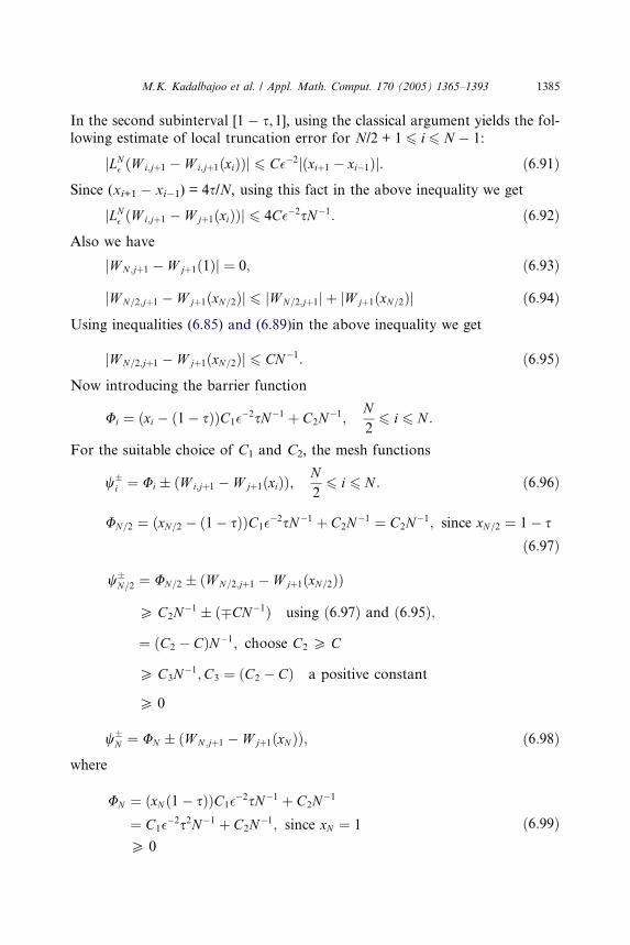
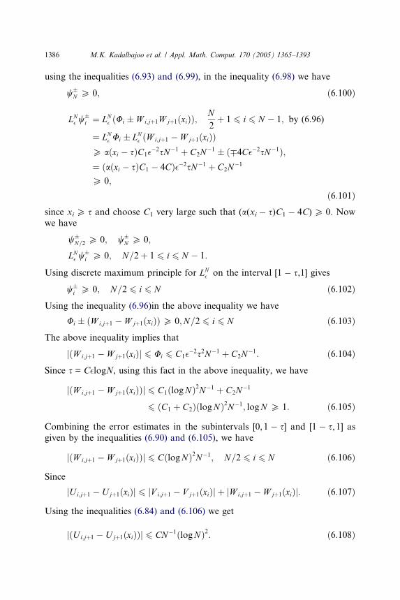
points for the given time step, Dt = 0.01. Tables 1 and 2 give the numerical

and exact values of the solution u for � = 1 and 0.1. The results by the proposed

method are in good agreement with exact solution.

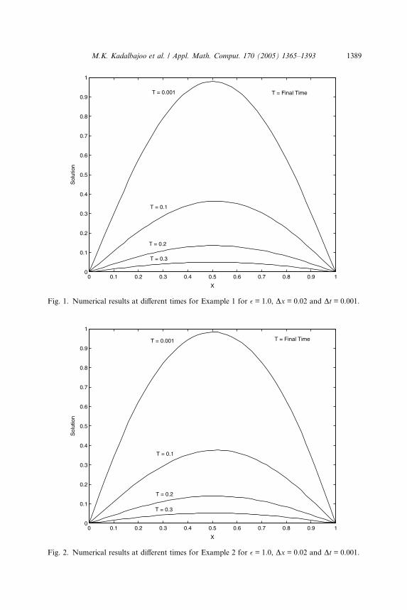
In Figs. 1 and 3, numerical results with uniform mesh are shown for Example

1 at different times for Dx = 0.02, Dt = 0.001, � = 1.0 and Dx = 0.02, Dt = 0.001,� = 0.1. These numerical predictions exhibit good physical behaviour.

Table 2

Comparison with exact solution for Example 1 with � = 0.1, T = 0.1 and time step Dt = 0.01

x Computed solution for different values of N Exact solution

8 16 32 64

0.000 0.000000 0.000000 0.000000 0.000000 0.000000

0.125 0.257761 0.265351 0.269246 0.271187 0.278023

0.250 0.484196 0.504004 0.514352 0.519585 0.534143

0.375 0.657091 0.692249 0.711395 0.721350 0.743852

0.500 0.754675 0.804818 0.833364 0.848611 0.877280

0.625 0.754136 0.813231 0.848258 0.867467 0.897099

0.750 0.633137 0.687764 0.721028 0.739558 0.761797

0.875 0.376760 0.408496 0.427982 0.438783 0.447836

1.000 0.000000 0.000000 0.000000 0.000000 0.000000

Table 1

Comparison with exact solution for Example 1 with � = 1.0, T = 0.1 and time step Dt = 0.01

x Computed solution for different values of N Exact solution

8 16 32 64

0.000 0.000000 0.000000 0.000000 0.000000 0.000000

0.125 0.121487 0.125104 0.127346 0.128578 0.135829

0.250 0.225959 0.233046 0.237412 0.239809 0.253638

0.375 0.298627 0.308467 0.314521 0.317851 0.336742

0.500 0.328236 0.339392 0.346287 0.350090 0.371577

0.625 0.308567 0.319105 0.325680 0.329320 0.350123

0.750 0.240241 0.248160 0.253236 0.256060 0.272582

0.875 0.131624 0.135849 0.138571 0.140092 0.149239

1.000 0.000000 0.000000 0.000000 0.000000 0.000000

1388 M.K. Kadalbajoo et al. / Appl. Math. Comput. 170 (2005) 1365–1393

The point wise errors by using non-uniform mesh of Shishkin type is shown

in Table 3. We show the error tables with N = 8 and Dt = 0.01 and we multiplyN and Dt remains same.

We compute point wise errors by

eN� ði; jÞ ¼ juNðxi; tjÞ � u2N ðxi; tjÞj;where superscript indicates the number of mesh points used in the spatial direc-tion, and tj = jDt and Dt is the time step.

For each �, the maximum nodal error is given by

E�;N ;Dt ¼ maxi;j

eN ;Dt� ði; jÞ

and for each N and Dt, the the � uniform maximum error is defined as

EN ;Dt ¼ max�

E�;N ;Dt:

The results are shown in Table 3.

0 0.1 0.2 0.3 0.4 0.5 0.6 0.7 0.8 0.9 10

0.1

0.2

0.3

0.4

0.5

0.6

0.7

0.8

0.9

1

X

Sol

utio

n

T = 0.001

T = 0.1

T = 0.2

T = 0.3

T = Final Time

Fig. 1. Numerical results at different times for Example 1 for � = 1.0, Dx = 0.02 and Dt = 0.001.

0 0.1 0.2 0.3 0.4 0.5 0.6 0.7 0.8 0.9 10

0.1

0.2

0.3

0.4

0.5

0.6

0.7

0.8

0.9

1

X

Sol

utio

n

T = 0.001

T = 0.1

T = 0.2

T = 0.3

T = Final Time

Fig. 2. Numerical results at different times for Example 2 for � = 1.0, Dx = 0.02 and Dt = 0.001.

M.K. Kadalbajoo et al. / Appl. Math. Comput. 170 (2005) 1365–1393 1389

0 0.1 0.2 0.3 0.4 0.5 0.6 0.7 0.8 0.9 10

0.1

0.2

0.3

0.4

0.5

0.6

0.7

0.8

0.9

1

X

Sol

utio

n

T = 0.01

T = 0.5

T = 1.0

T = 3.0

T = Final Time

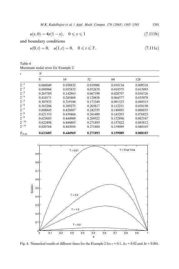
Fig. 3. Numerical results at different times for Example 1 for � = 0.1, Dx = 0.02 and Dt = 0.001.

Table 3

Maximum nodal errors for Example 1

� N

8 16 32 64 128

2�1 0.126549 0.070806 0.036909 0.018840 0.009518

2�2 0.123205 0.079446 0.050444 0.029792 0.015093

2�3 0.319113 0.177713 0.084627 0.036491 0.015093

2�4 0.460880 0.282160 0.149309 0.074455 0.035970

2�5 0.542130 0.344630 0.185675 0.098233 0.049515

2�6 0.582309 0.379252 0.211558 0.113234 0.058150

2�7 0.599244 0.397179 0.226394 0.119052 0.060987

2�8 0.604842 0.405218 0.234203 0.126925 0.065276

2�9 0.605793 0.407901 0.238113 0.131401 0.067698

2�10 0.605253 0.408168 0.239992 0.133786 0.069086

2�11 0.606854 0.411069 0.240708 0.134967 0.069745

EN,Dt 0.606854 0.411069 0.240708 0.134967 0.069745

1390 M.K. Kadalbajoo et al. / Appl. Math. Comput. 170 (2005) 1365–1393

Example 2

ut þ uux ¼ uxx; ðx; tÞ 2 ð0; 1Þ � ð0; T � ð7:111aÞwith initial condition

M.K. Kadalbajoo et al. / Appl. Math. Comput. 170 (2005) 1365–1393 1391

uðx; 0Þ ¼ 4xð1� xÞ; 0 6 x 6 1 ð7:111bÞand boundary conditions

uð0; tÞ ¼ 0; uð1; tÞ ¼ 0; 0 6 t 6 T : ð7:111cÞ

Table 4

Maximum nodal error for Example 2

� N

8 16 32 64 128

2�1 0.068049 0.038832 0.019986 0.010134 0.009518

2�2 0.098964 0.055833 0.032670 0.019375 0.015093

2�3 0.265789 0.142863 0.067190 0.028797 0.016726

2�4 0.410171 0.245469 0.129438 0.064377 0.035970

2�5 0.507933 0.319100 0.173349 0.091323 0.049515

2�6 0.565204 0.369275 0.205817 0.112251 0.058150

2�7 0.608845 0.420887 0.242355 0.140985 0.068855

2�8 0.621333 0.439466 0.261480 0.145203 0.076823

2�9 0.623685 0.444969 0.269322 0.152896 0.082167

2�10 0.622498 0.444803 0.271893 0.157022 0.085812

2�11 0.620764 0.443056 0.271884 0.159089 0.088103

EN,Dt 0.623685 0.444969 0.271893 0.159089 0.088103

0 0.1 0.2 0.3 0.4 0.5 0.6 0.7 0.8 0.9 10

0.1

0.2

0.3

0.4

0.5

0.6

0.7

0.8

0.9

1

X

Sol

utio

n

T = 0.01

T = 0.5

T = 1.0

T = 3.0

T = Final Time

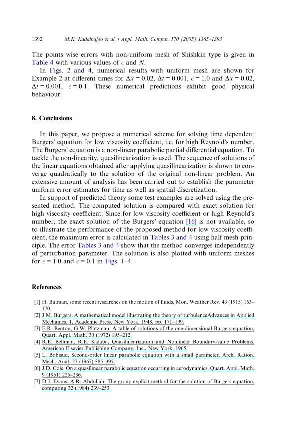
Fig. 4. Numerical results at different times for the Example 2 for � = 0.1, Dx = 0.02 and Dt = 0.001.

1392 M.K. Kadalbajoo et al. / Appl. Math. Comput. 170 (2005) 1365–1393

The points wise errors with non-uniform mesh of Shishkin type is given in

Table 4 with various values of � and N.

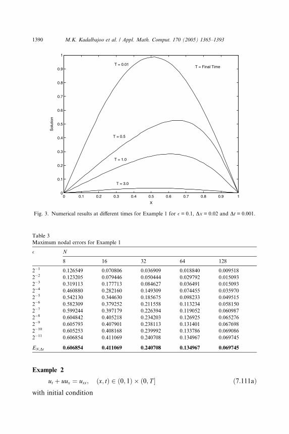
In Figs. 2 and 4, numerical results with uniform mesh are shown for

Example 2 at different times for Dx = 0.02, Dt = 0.001, � = 1.0 and Dx = 0.02,

Dt = 0.001, � = 0.1. These numerical predictions exhibit good physical

behaviour.

8. Conclusions

In this paper, we propose a numerical scheme for solving time dependent

Burgers� equation for low viscosity coefficient, i.e. for high Reynold�s number.

The Burgers� equation is a non-linear parabolic partial differential equation. To

tackle the non-linearity, quasilinearization is used. The sequence of solutions ofthe linear equations obtained after applying quasilinearization is shown to con-

verge quadratically to the solution of the original non-linear problem. An

extensive amount of analysis has been carried out to establish the parameter

uniform error estimates for time as well as spatial discretization.

In support of predicted theory some test examples are solved using the pre-

sented method. The computed solution is compared with exact solution for

high viscosity coefficient. Since for low viscosity coefficient or high Reynold�snumber, the exact solution of the Burgers� equation [16] is not available, soto illustrate the performance of the proposed method for low viscosity coeffi-

cient, the maximum error is calculated in Tables 3 and 4 using half mesh prin-

ciple. The error Tables 3 and 4 show that the method converges independently

of perturbation parameter. The solution is also plotted with uniform meshes

for � = 1.0 and � = 0.1 in Figs. 1–4.

References

[1] H. Batman, some recent researches on the motion of fluids, Mon. Weather Rev. 43 (1915) 163–

170.

[2] J.M. Burgers, A mathematical model illustrating the theory of turbulenceAdvances in Applied

Mechanics, 1, Academic Press, New York, 1948, pp. 171–199.

[3] E.R. Benton, G.W. Platzman, A table of solutions of the one-dimensional Burgers equation,

Quart. Appl. Math. 30 (1972) 195–212.

[4] R.E. Bellman, R.E. Kalaba, Quasilinearization and Nonlinear Boundary-value Problems,

American Elsevier Publishing Company, Inc., New York, 1965.

[5] L. Bobisud, Second-order linear parabolic equation with a small parameter, Arch. Ration.

Mech. Anal. 27 (1967) 385–397.

[6] J.D. Cole, On a quasilinear parabolic equation occurring in aerodynamics, Quart. Appl. Math.

9 (1951) 225–236.

[7] D.J. Evans, A.R. Abdullah, The group explicit method for the solution of Burgers equation,

computing 32 (1984) 239–253.

M.K. Kadalbajoo et al. / Appl. Math. Comput. 170 (2005) 1365–1393 1393

[8] E. Hopf, The partial differential equation ut + uux = muxx, Commun. Pure Appl. Math. 3 (1950)

201–230.

[9] S. Kutluay, A.R. Bahadir, A. Ozdes, Numerical solution of one-dimensional Burgers

equation: explicit and exact explicit finite difference methods, J. Comput. Appl. Math. 103

(1999) 251–261.

[10] J.J.H. Miller, E. O�Riordan, G.I. Shishkin, Fitted Numerical Methods for Singular

Perturbation Problems, World Scientific, Singapore, 1996.

[11] R.C. Mittal, P. Singhal, Numerical solution of Burgers equation, Commun. Numer. Methods

Eng. 9 (1993) 397–406.

[12] A. Mazzia, F. Mazzia, Higher order transverse schemes for the numerical solution of partial

differential equations, J. Comput. Appl Math. 82 (1997).

[13] T. Ozis, A. Ozdes, A direct variational methods applied to Burgers equation, J. Comput. Appl.

Math. 71 (1996) 163–175.

[14] T. Ozis, E.N. Aksan, A. Ozdes, A finite element approach for solution of Burgers� equation,Appl. Math. Comput. 139 (2003) 417–428.

[15] M.H. Protter, H.F. Weinberger, Maximum Principles in Differential Equations, Prentice Hall,

Inc., 1967.

[16] D.S. Zang, G.W. Wei, D.J. Kouri, D.K. Hoffman, Burgers� equation with high Reynolds

number, Phys. Fluids 9 (1997) 1853–1855.