IL NUOVO CIMENTO VoL 74 B, N. 1 11 Marzo 1983

C o n t i n u o u s a n d D i s c r e t e M a t r i x B u r g e r s ' H i e r a r c h i e s .

D. LEVI, O. ~AGINISCO a n d M. BRUSCHI

I s t i tu to di ~ i s i c a deU'Univers i th - 00185 R o m a , I t a l i a

I s t i tu to Naz iona le di _~isica Nuc lea te - Sezione di R o m a

(ricevuto il 29 Luglio 1982)

Summary. - - We derive two hierarchies of matrix nonlinear evolution equations which reduce to the Burgers' hierarchy in the scalar case and can be linearized by a matrix analogue of the tIopf-Cole transformation: for these hierarchies we display the associated class of B~icklund transformations and show some special kinds of explicit solutions. ]Kore- over, by exploiting a discrete version of the Hopf-Cole transformation, we are also able to construct two hierarchies of linearizable nonlinear difference evolution equations and to derive for them B~cklund trans- formations and explicit solutions.

PACS. 02.30. - Funct ion theory, analysis.

1 . - I n t r o d u c t i o n .

I t is well k n o w n (1) t h a t Burgers ' e q u a t i o n

can be l inear ized t h r o u g h the Hopf-Cole t r a n s f o r m a t i o n

(1.2) u = - 2 ~ / ~ ,

(1) G . B . WHITHA~I: L i n e a r and N o n l i n e a r Waves , Chapt. 4 (New York, ~7. Y., 1974).

3 - 1l Nveovo Oimento B. 33

~ D. LEVI, O. I~AGNISCO &II~ ~ . BRUSCHI

which maps it into the heat equation

(1.3) ~t = v~x .

More recently (~), it has been proved that Burgers ' equat ion is a member of a whole hierarchy of nonlinear evolution equat ions (NEEs) which can be linearized by the same ttopf-Cole t ransformation. I t seems thus worthwhile looking for a matr ix generalization of this hierarchy, i.e. for a class of non- Abelian NEEs which can be linearized by a Hopf-Cole- type t ransformation.

I n this work we exhibi t two classes of ma t r ix ~ E E s , both reducing to Burgers ' hierarchy in the scalar case, and two classes of matr ix nonlinear dif- ference evolution equations (NDEEs) which can be linearized by suitable analogues of the ttopf-Cole transformation.

At a first glance one can realize tha t these classes contain some physically interest ing equations, us, for instance, a dissipative version of the N-wave equat ion in the continuous case and a mat r ix Vol terra- type equation in the discrete case. We postpone to a subsequent paper a systematic investigation of all possible interesting reductions. For all these hierarchies of evolut ion equat ions we are able to construct the corresponding classes of Bi~cklund trans- format ions (BTs) which allow us to obtain different ladders of explicit solutions: shock-type solutions, soli ton-type solutions and rat ional solutions.

I n sect. 2 we display the two classes of NEEs together with their linearization. In sect. 3 we derive an extension of the classes given in the previous section, so as to include terms with linearly x-dependent coefficients. The corresponding ]3Ts and the nonlinear superposition principle (:NSP) are obtained in sect. 4, while sect. 5 is devoted to the s tudy of the discrete matr ix Burgers ' hierarchy, together with the associated BTs and :NSP.

Final ly in sect. 6 we solve the simplest nontr ivial BTs, bo th for the con- t inuous and for the discrete cases, and thus derive shock-type solutions, soli- t on - type solutions and rat ional solutions.

2 . - Matrix NEEs .

Le t us consider the linear problem

(2.1a) Z~ ~ 0 ,

(2.1b) L -~ ~x -- U ,

(2) D. V. CIIOODNOVSKY and G. V. CIt0ODNOVSKY: NUOVO Cimento B, 40, 339 (1977).

C O N T I N U O U S AND D I S C R E T E M A T R I X B U R G E R S ~ H I E R A R C H I E S 3 ~

V and U being N X N matrices, depending on two continuous variables x

and t (*). We look for evolution equat ions for U which can be cast in the Lax form (**)

(2.2) L,, = [L, M ] .

Equa t ion (2.2) is compat ible wi th V,t = - MV. Of course, since we are not dealing with a spectral problem, eq. (2.2) does

not define an isospectral deformat ion of 15. However , eq. (2.2) is a convenient s tar t ing point to derive an infinite set

of nonlinear par t ia l differential equat ions through a proper version of the

technique firstly in t roduced in ref. (3). Due to eqs. (2.1), (2.2) we can asser t t h a t the prob lem of finding a hieraTchy

of I~EEs for the field U amounts to determining a sequence of operators M such tha t the t ime evolution of U can be cast in the L a x form (2.2).

According to the s t ra tegy outl ined in ref. (a) and in the previous sentence, we assume a cer tain M , say MtJ), to be given, and look for a new M , say Mr

through the ansatz

(2.3) M(i+l) = LM(J) + F (J )~ + G (~) ,

/~(s) and G (r being N • N matrices, whose dependence upon U is to be deter- mined b y the requi rement tha t , if [L, M(J)] = V (j) is a pure mult ipl icat ion op- erator, the same be t rue for [L, M(~+~)] = V (j+~). B y imposing this condition,

one gets the two equations

(2 Aa)

(2.4b)

(j) (J) V +/~ ,x -4- [/~cJ), U] = 0 ,

V (~) - - U V C~ + ~'(J) U -4- G ~j~ + [G (j~, U] = V C~+~) . ~x ~x -- IZ

At this point , the usual procedure would be t ha t of solving first eq. (2.4a) to get /~J) in t e rms of the assumed known V (j), so t ha t eq. (2.4b) gives the re- quired recursion operator, which generates the hierarchy of evolution equa-

t ions: V(J+I) = ~q~V~J~. But , as eq. (2.4a) is not, in general, explicit ly solvable for/~J~, we h a v e to

look a t eqs. (2.4) f rom a different point of view, i.e. t o regard eq. (2.4a) as a prescript ion on the s t ructure of V~J); in this way we can de termine a recursion relation for/~(~) and G (j) th rough eq. (2.4b), by requiring t h a t V o'+1) has the same

(*) In the following, for notational convenience, the t-dependence will be often omitted. (**) Here and in the following, by the subscript t we mean partial derivative with respect to t, i.e. ,p,t = ~,/~t . (3) IV[. BRCSCnI and 0. RAG•ISCO: Zett. lVuovo Cimento, 29, 321 (1980).

3 6 D. LEVI , O. RAGNISCO and M. BRUSCHI

s t ruc ture as V u):

(2.5) V (~+1) = - ~l~J') + [U, ~(~+~)] do_,~,(~+l).

Inser t ing eq. (2.5) into eq. (2.4b) and tak ing into account eq. (2.4a), one gets

(2.6a)

the field G (j) being complete ly undetermined. I n order to get a recursion relat ion involving only the fields F(~), we made

two different choices for the fields G (~). As a first choice, we set G u) ---- 0, which yields

(2.6b) Z(J+~) _~ .~fl/v (~) ~SflZ (j) F (j) U/~) L Z (~)

As ~ fur ther choice, we set GtJ) --_ - - (U, F(~)}, which yields

(2.~c)

I t will be shown shor t ly t h a t the IqEEs corresponding to the recursion opera tors 5~1 and &f2 are bo th linearizable.

We are thus enabled to write down two classes of I~EEs for U, once we know u suitable s tar t ing point M (o).

Actual ly , for M (o) one can choose un a rb i t r a ry x- independent N x N mat r ix , which, for convenience, will be denoted as - - C o , yielding V (~ ----[L, M (~ ----

----- [U , Col.

One can thus solve eq. (2.4a), obtaining F (~ -~ Co as the s tar t ing point for i tera t ions (2.6).

Hence eqs. (2.5), (2.6a) allow us to construct the following class of I~EEs:

(2.7) U ~ = ~ ~e~)~ Ck ,

where Ck are a rb i t ra ry x- independent matrices. The first nontr ivial equation, which arises b y retaining just C1 r 0, reads

(2.8a) v , = g , c , + vice, g] .

Of course, eq. (2.8a) reduces to the linear wave equat ion if C1----I , where b y I we mean the iden t i ty h r • mat r ix . Moreover, by choosing U~----- -= o~iv~(x, t) and C~ = c~(~j, eq. (2.8a) reduces to a nonlinear N - w a v e equa-

CONTINUOUS AND DISCRETE MATRIX BURGERS' HI]~RARCHIES 37

tion p), reading 2~

(2.8b) vj,~ : cjv~,~ @ vj ~ VkC~k(C~ -- Cj), k = l

where, of course, ~ and c~ are scalar constants. This equation, which can be linearized, as will be shown in the following,

admits <( mult ishock ~ solutions, as occurs for a similar equation recently

investigated by REIMA~ST and KAUP (5) in the N = 3 case. In the N = 2 case, by introducing the s tandard basis of Pauli matrices a~ (] = 0, 1, 2, 3;

ao = I), we can decompose any matr ix U in the following way:

thus eq. (2.8a) reads

3

U ~ ~ u j o ' j ---- 'UoO' o -~- U ' { 7 ,

(2.Sc) u~ = cou~ + cuo,~ ~- iu~/~c ~- 2 i u o c A u - - 2 u A ( c A u ) .

As will be shown in sect. 6, this equation admits exact solutions, which exhibit

the same behaviour as those pertaining to the <( boomeron ~) equation, in-

vestigated in ref. (e). The fur ther equation obtains by retaining just C2 =/: 0 and is clearly a matr ix

version of Burgers ' equation

(2.9) U,t : (U,x~-- 2UU~)C2 -~ (U,~-- U2)[C2, U].

The third equation is rather messy for an arbi t rary C3; hence we write it

down only in the ease C3 = I :

(2.1o) u,~= ~,3x+ 3(u~ux-(vu,~),x).

I t can be considered as a matr ix version of the modified Korteveg-de Vries

equation with a dissipative extra term. We turn now to considering the second recursion formula, eq. (2.6b) ; assum-

ing the same start ing point p(o) = Co, we get the following class of evolution

equations:

(4) V. ]~. ZAKHAROV, S. V. 1V[ANAKOV, S. P. NOVIKOV and L. P. PITAIEVSKI: Theory o] Solitons: The Inverse Problem Method (Moscow, 1980). (5) A. REIMAN and D. KAUe: Phys. Fluids, 24, 228 (1981). (e) F. CALOGERO and A. DEGASPERIS: NUOVO Cimento B, 39, 1 (1977).

3 ~ D. L E u O. RAGNISCO a n d ~I. BRUSCIII

As an example we list here the simplest two equations belonging to this class. They read

(2.12a) U,t -~ - - C~ U,~ -[- U[C~, U] ,

(2.125) U,t = - - C2(U,~ q- 2U,~U) ~ [U, C2](U,~ q- U2).

Comparing the above equations with eqs. (2.8), (2.9), we notice tha t t hey differ only for some changes of sigrt and for the position of the constant matrices C~ and C~.

~Ve prove now tha t all equations of class (2.7) (respectively, (2.11)) can be linearized through a ma t r ix analogue of the Hopf-Cole t ransformat ion (1):

(2.13) U = ~f,~f-1,

which is nothing bu t eq. (2.1). For simplicity, and with no loss of generality, we restrict ourselves to the

case in which only one of the mat r ix coefficients C~ is different from zero. Indeed, i t is easy to see tha t , if (*)

(2.1~)

(respectively F (~) ~ (Lf2)~C~ ~ C~p,~v-~),

the corresponding evolution equat ion

(2.15)

linearizes to

(2.16)

(respectively U.t = Sf[(~a2)k C~:])

(respectively ~,t = -- C~F,~).

On the other hand, due to the recursion relations (2.6), eq. (2.14), once t rue for a given k, is obviously t rue for k ~ 1; thus formula (2.14) holds for any k, as it holds for k = 0.

This implies the following linearization for the whole class (2.7) (respec- t ively (2.11)) '.

(2.17) (~-~),~ = ~ (~o-1),~x C~ respectively ~,~ = -- ~ Ck~o,~ . k~O k=O

We can thus conclude tha t , to solve the Cauchy problem for a N E E per- tMning to class (2.7) (respectively (2.11)), one has first to determine ~o(x, to) by solving the linear problem (2.1) for the initial da tum Up(x)~ U(x, to);

(*) By ~0,~, we denote the k-th partial derivative of ~ with respect to x.

C O N T I N U O U S A N D D I S C R ~ T F , M A T R I X B U I ~ G E R S ~ H I E R A R C H I E S 39

t h en one has to evaluate ~(x, t) by solving the linear evolution equatio11 (2.17), and finally to recover U(x, t) by using again t ransformat ion (2.13).

We notice thuS, in the Abeliau case, both classes (2.7) and (2.11) collapse in to ]~urgers' h ierarchy first in t roduced by the Cuoo~)~ovsKY's (2).

3. - Extens ion to ~qEEs wi th x -dependent coefficients.

The classes of ~ E E s derived in the previous section can be extended so as to include x-dependent coefficients. These new equations r out to be also linearizable by t ransformat ion (2.13).

The two extended classes can be constructed according to the procedure given in ref. (7), through a suitable modification of the Lax equation (2.2); namely, one has to reql~ire tha t the operator L, given by eq. (2.1), evolve ac- .cording to

(3.1) L~ = [L, M] § N .

B y imposing tha t the r.h.s, of eq. (3.1) defines a pure multiplication op- erator , one gets the following two classes of ~ E E s :

k=O

k~O

As one can see at a first glance, the only difference with respect to classes (2.7), (2.11) consists in the presence of the linearly x-dependent terms xC~.

Both these classes can be linearized via t ransformat ion (2.13). Indeed, if one assumes for class (3.2a)

(3.3a) ~(k) = ( ~ l ) k XCk = ~)(X,~)--I ),t~X Ck

and for class (3.2b)

(3.3b) ~ ( ~ ) = ( . ~ ) * x r = r - 1 ,

the corresponding evolution equations (3.2a), (3.2b) linearize to

(3Aa) (~-').~ = (x~-l).,0x Ck,

(3.4b) Y),t ---- - - Q ( x ~ ) ) . k ~ .

(~) M. BRUSCHI and 0. RAGNISCO: Lett. Nuovo Cimento, 29, 321 (1980).

4 0 D. LEVI, 0. RAGNISC0 and ~ . BRUSCHI

On the other hand, assumptions (3.3), t r ivial ly t rue for k = 0, are easily seen to hold for k § 1, once holding for k, due to recursion relation (2.6).

Thus we can assert t ha t classes (3.2a), (3.2b), th rough position (2.13), lin- earize to

( 3 . 5 a ) (~ -1 ) , t = ~ (x~)-l),lc~cCk , k=o

Jp (3.5b) ~v,t = -- ~ Ck(xF),k..

k~O

The solution of the Cauchy problem for classes (3.2) can be accomplished by the procedures sketched at the end of the previous section, by noting tha t the linear evolution equations (3.5) can be still solved in closed form, for instance via Four ier transform. To end this section, we would like to point out tha t , to our knowledge, even in the Abelian case, this extension of Burgers ' h ierarchy to include linearly x-dependent coefficients has never been considered before.

4 . - BTs and NSP.

Given two linear problems of type (2.17), corresponding, respectively, t o the (~ potentials ~) U and U, we look for the class of matrices D and W, depending upon U, U and their derivatives, such tha t the following equat ion holds:

(4.1) L(~])D-- DL(U) : W.

The choice W : 0 corresponds to a Da rb o u x t ransformat ion between the (~ eigenfunctions )) of the two linear problems of t ype (2.1):

(4.2) L(~?)@ = 0 L(U)~ = 0 ,

(4.3) ~ = D ~ .

I t is worthwhile noticing tha t , in correspondence with eq. (4.3), by taking into account t ha t W depends on ~? and U, the equat ion W : 0 is a generally nonlinear functional relat ion between U and U, often called B~cldund trans-

formation. The problem of construct ing a class of BTs is t hen reduced to the construc-

t ion of a class of mat r ix pairs (D, W) satisfying eq. (4.1). Paraphrasing the procedure outlined in sect. 2 for the construct ion of the I~EEs, we set

(4.4) D ' = LC~)D § ~ § r

C O N T I N U O U S A N D :DISCRETE ~ A T R I X B U R G E R S ~ H I E R A R C H I E S 41

and require

(4.5) L(U)D ' - - D 'L (U) -~ W ' .

Imposing tha t W and W' be pure multiplication matr ix operators, we obtain from eqs. (4.1), (4.4), (4.5) the following two classes of Darboux matrices and BTs:

(4.6a) ~ [ ~..o (A~)k~k] = O , .

(4.65) D, = -- ~ (/1)k/Vk,

. g

. / [

(4.7b) D2 = -- ~ (A~)kFk, k=0

where /7~ are arbi t rary constant matrices and the operators ~, A~, A2 are defined as

(4.Sa)

(4.8b)

(4.Sc)

A ~ ' ~ ~,~ -- ~ tz ,

A~t~ ~ ~',~ + t ' U.

We show now that , under certain conditions, the functional relutions (4.6a) (respectively (4.7a)) provide auto-B~eklund transformations for the ~ E E s (2.7) (respectively (2.11)).

For simplicity, we restrict considerations to class (2.7), as all the proofs given for ~his case can be repeated with obvious modifications for cluss (2.11).

We thus assume tha t U, U evolve according to two (a priori different) equations of class (2.7), say

.A"

(4.9a) u,~ = ~ ~f [ (ze l (v ) )kc~] , k~0

(4.9b) U,~ ---- S7 2 [('s kCk] (S7 : ~9~ k=0

Through transformation (2.13) for U and the corresponding one for U, eqs. (4.9a)~ (4.9b) linearize to

(4.10a) (~-l),t --~ ~ (~-~),k~C~, k~0

.A"

( 4 . 1 0 b ) (v~-l),~ : ~ ( ~ - - a ) , l x 0 , �9

42 D. L E V I , O. RAGNISCO and M. B R U S C H I

I t is easy to prove by i terat ion that , in terms of v~, the matr ix D1, defined J /

by eq. (4.6b), takes the form D~ = v~ ~ (~-~),k~Nk, SO tha t eq. (4.3) becomes

J /

(4.11) ~f-~ = ~ (v~-~),k:Fk. k=O

Hence, if U and U evolve according to eq. (4.9) and consequently ~, v~ evolve ~ecording to eq. (4.10), iu order tha t eq. (4.3) (or equiwlen t ly eq. (4.11)) be fulfilled, we must huve

(4.12)

which implies

J / " j / ! ~ f ~4

~=0 j=O l=O j=O

and

~r d /

(4.13) ~ O._j~j = ~ FjC~_j for any s. i=O i=0

One obvious solution of these constraints is given by choosing ~k to be scalar constants and C~ ---- C~ (k ~ 1, 2, ..., Jff) ; these restrictions yield an auto-B$cklund transformation.

In the following we shall derive the nonlinear superposition principle; for the sake of simplicity, we shall derive it only for solutions of the class of ~TEEs (2.7). Analogous formulae will be valid for class (2.11) too.

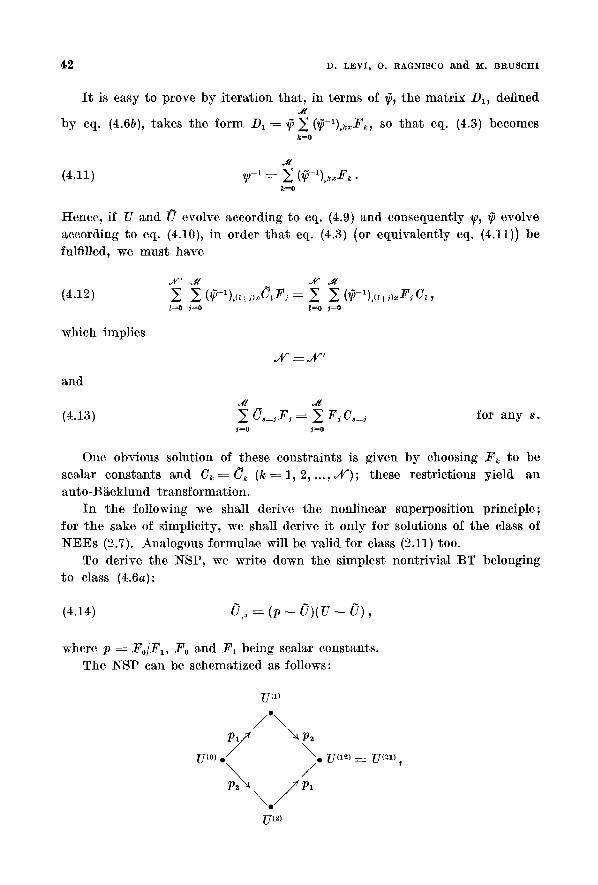
To derive the ~qSP, we write down the simplest nontrivial BT belonging to class (4.6a):

(4.14) O,, = (p - O ) ( ~ - ~ ) ,

where p ~ s F0 and F1 being scalar constants. The HSP can be schematized as follows:

V {1)

U ( ~ \ . V ( ~ ) = T/(~-" / \ . / /P '

C O N T I N U O U S A N D D I S C R E T E M A T R I X B U R G E R S ' I I I E R A R C t t I E S 4 3

i .e . , s ta r t ing f r o m a g iven solut ion of a T E E belonging to class (2.7), we get,

t h r o u g h t he B T (4.14) of p a r a m e t e r Pl , a new solut ion U (1) of t he same T E E :

(4.15a) U~I) (Pl U(1))(U(~ U(1))

cor responding to the D a r b o u x m a t r i x

(4.16a) D(l~ : U (1~ - - P l .

Ana logous ly we can cons t ruc t a new solut ion U (2) b y means of a B T of p a r a m e t e r p~:

(4.15b) Ulna= ( p ~ - Uc~)(U c~ - - U ~ ) ,

(4.16b) Dr176 = U(2) - - P2.

F r o m U (1), app ly ing eq. (4.14) wi th p a r a m e t e r p~, we get a new solut ion U(12):

(4.15c) U(I~) (P2 U(I"))(U~I) UCl~))

(4.16c) D (21) = U c12) - - p~.

Analogous ly , f rom U (2), a p p l y i n g (4.14) wi th p a r a m e t e r Pl , we get the solut ion U (21)

(4.15d) U(21),~ = (Pl - - U("I~)(U ('~) -- U (21)) ,

(4.16d) D ( I ~ ) ----- - - P l ~ - U(21~ �9

B y t ak ing in to accoun t eqs. (4.11), (4.3), it is easy to see t h a t the D a r b o u x m~triccs (4.16) fulfil t he fol lowing p e r m u t a b i l i t y cond i t ion :

(4A7) D~-I) D (1~ = D~I~) D ~~ ,

which implies, due to the uniqueness of the solut ion of t he BT (4.6), t h a t U (~2) = U(21); hence there follows t he nonl inear superpos i t ion principle

(4.18) U ( 2 ) P l - - U ( 1 ) P ~ = [ U (2) - - U (1) -~- P l - - P 2 ] U{12) ~

which, g iven two solut ions of a ) l E E of class (2.7), allows us to cons t ruc t a new

solut ion of the same equa t ion in an algebraic way. I n t e rms of the funct ions ~(1) ~(~) ~(1~) which l inearize the given T E E , the

H S P (4.18) becomes

(4.19) [~)(1)]--1 - - [~)(2)]--1 : ( P 2 - - P l ) [ ~ ) ( 1 2 ) ] - 1 ,

44 D. LEVI, O. RAGNISCO and M. BRUSCHI

which is just the usual linear superposition principle for the solutions of l inear evolution equations (2.17).

5, - The discrete matrix Burgers' hierarchy.

In this section (*) we introduce two classes of ma t r ix b~DEEs which are the discrete analogue of the ma t r ix Burgers ' hierarchies given in sect. 2 and 3. We shall prove tha t any equat ion belonging to these two classes of ~ D E E s reduces to a linear mat r ix difference evolution equat ion through a discrete version of the matr ix analogue of the Hopf-Cole t ransformat ion (2.13).

Le t us first introduce the two operators 5fl, ~ , depending on the field U(n), through the formulae

(5.1a)

(5.1b)

5f~/~'(n) ---- F (n ~- 1) U(n) -- U(n)_~(n),

~flF(n) ---~ ~ (n -~- 1) U(n).

~ o w we shall prove tha t the hierarchy of lqDEEs defined as

(5.2) ~ k ~ l

where Ak and B~ are a rb i t ra ry n-independent constant matrices, through the t ransformat ion

(5.3) U(n) ~-- r + 1)r

linearizes to

r162 JYl

(5.4) r -~ ~ Akr + k) + ~_ (n + k)Bkr + k) . k k

Indeed, if we define

(5.5a) F(k)(n) = (~fl)~(A~ + nB~),

i t is easy to prove by i terat ion that , in terms of the matr ix funct ion r defined by eq. (5.3), F(k)(n) takes the form

(5.6) F(~)(n) ~-- (A~ + (n + k)Bk)r -}- k)r �9

(*) Throughout this section any field, say ~, is a matrix of rank s depending on an integer variable ~t and on a continuous variable t, i .e . .F = F(n, t). For notational convenience the t-dependence will be mostly omitted.

C O N T I N U O U S A N D D I S C R E T E : ~ I A T R I X R U R G : E R S ~ H I E R A R C H I E S

Then~ by using eqs. (5.3), (5.6)~ it follows tha t the :NDEE

(5.7)

linearizes to

45

(5.8) r = (Ak § (n + k)Bk)r § k).

:Note tha t the class of :NDEEs (5.2) splits into two subclasses; when all Bk are zero~ we have the discrete analogue of class (2.7); when all Ak are zero~ we obtain a class of :NDEEs with n-dependent coefficients which is the discrete counterpar t of class (3.2a).

A different discrete mat r ix Burgers ~ hierarchy can be wri t ten as

k

where again A~ and Bk are a rb i t ra ry n-independent matrices and the two op- erators 5z~, ~ are defined as

(5.10a) Lf2F(n) = U(n)F(n + 1) -- ~(n) U(n),

(5.10b) .s : U(n)_~(n § 1).

Using now the t ransformat ion

(5.11) U(n) -~ v2-1(n)~f(n § 1)

and following the procedure used in the previous case, bu t start ing from the position

(5.12) E(~)(n) : (~f2)k(Ak + nB~) : (Ak + (n + k)B~)yF~(n)y~(n + k),

it is easy to prove tha t eq. (5.9) reduces to the linear difference evolution equat ion

(5.13) ~,~(n) = Z ~(n § k)A~ § • (n § k)~(n + k)B~. k k

Of course~ eq. (5.9) is the discrete analogue of eqs. (3.2b)~ (2.11). Analogously to the continuous case~ we can thus assert t ha t the solution

of the Cauchy problem for the :NDEEs (5.2) (respectively (5.9)) can be ac- complished by solving the two linear problems (5.3)~ (5.4) (respectively (5.11)~ (5.13)). I t is perhaps worthwhile noticing tha t eqs. (5.4)~ (5.13) can be indeed

~ 6 D. L ~ u O. RAGNISCO a n d ~ . B R U S C H I

explicit ly solved by the discrete version of the Fourier t ransform (8). Moreover, we point out tha t the two classes (5.2), (5.9) of course collapse, in the scalar case, into a single one, which, to our knowledge, in contrast to the continuous case, has never been derived.

Considering, for instance, class (5.2), we c~n derive some interesting equar by appropriute choices of the matr ix coefficients A~ and Bk.

B y just retaining A~ and B~ =/= 0, we get

(5.14) u,,(n) = {[A~ + (n § 2)B~] V(n § 1) -- U(n)[A~ + (n + 1)B~]} U(~).

This equation looks like a matr ix version of the generalized Volterra equa- t ion with n-dependent coefficients (9). In the subcase B~ ~ 0, A~ : ztI (~ being a scalar constant), the h-DEE (5.14) is consistent with the condition U(n § § 2) ~- U(n), giving rise to the following system of coupled nonlinear ordinary differential equations:

y,t ~- o~y(z -- y) , z,t = ocz(y -- z),

whose s t ructure recalls t ha t of the usual Vol terra-Lotka system~ although, of course, its solutions have a fairly different behaviour. As a second exampl% we exhibi t a differential-difference analogue of the mntr ix Burgers' equat ion (2.9) :

(5.15) U,t(n) -~ (A2 U(n § 2) -- U(n)A~) U(n § 1) U(n).

To end this section, we briefly write down the class of Darboux-B~cklund t ransformat ions associated to the 57DEEs (5.2), (5.9). To simplify the exposi- t ion, we consider just class (5.2).

Given two fields U(n), U(n) evolving according to the class of ~ D E E s (5.2)~ whose corresponding linearizing transformations are, respectively~

(5.16) r § 1) = v(n)r r + 1) = ~(n)~(n),

if the linearizing fields r ~{n) are related by the Darboux t ransformat ion

(5.17) r = D(n)~(n) ,

(s) D. LEVI: The spectral trans]orm as a tool ]or solving nonlinear discrete evolution equations, in Proceedings Jaca, •uesca, Spain, 1978, edited by A. :F. R/LNAI)A, .Lecture Notes in Physics, No. 98 (Berlin, 1978), p. 91. (9) M. WADXTI: Prog. Theor. Phys. Suppl., 59, 36 (1976); D. L~vI and O. RAG~Iseo: J. Phys. A, 12, L163 (1979).

CONTINUOUS AND DISCRETE I~fATRIX BURGERS' HIERA]~CHIES ~ 7

where D(n) is a mat r ix depending upon the fields U(n), ~](n), defined as

d /

(5.18) D(n) : ~ (A~)k2'~,

w h e r e / ~ ~re constant matrices, the BT reads

(5.19) Y21D(n) -~ O,

where the operators A~ and /2~ are defined as follows:

(5.20a)

(5.20b)

A~F(n) -~ F ( n ~ 1)U(n) ,

Y2~D(n) ~- D(n ~- 1) U(n) -- U ( n ) D ( n ) .

In terms of the linearizing fields r ~(n), the Darboux matr ix (5.18) reads

(5.21) D(n) = ~ r ~ ( n + k)~-l(n) k=0

and ~he BT (5.19) becomes

, A

I t is easy to show~ according to the procedure followed in the previous section~ t ha t a sufficient condition for eq. (5.19) to be an auto-BT is t ha t the coefficients P~ be scalar constants.

We display now, for completeness, the simplest nontr ivial example of uuto-BT, which one gets by retaining just/~o and _~. In this case the Darboux matr ix reads

(5.23)

and~ defining p as ~o/.F~, f rom eq. (5.19) we get

(5.24) p[0(n) - V(n)] § [0(~ § 1) - V(n)] ~(n) = o .

Following the procedure outl ined in the previous section~ one can derive also in the discrete case a ~SP , which reads

(5.25) p~ U~1~(n) - - p , U~2~(n) ~-- [p~ - - p~ -[- U(:~(n) - - U~l)(n)] Ur .

4 ~ D. L?EVI~ O. RAGNISCO and ~ . BRUSCHI

6 . - E x a c t s o l u t i o n s .

I n th is section, we shall t ake advantage of the BTs previously derived, to o b t a i n some explicit solutions of the continuous and discrete ma t r ix Burgers ' hierarchies. To simplify the exposition, we shall restr ict our discussion to the equat ions of classes (2.7), (5.2). Of course, analogous results will hold for clas- ses (2.11), (5.9).

S ta r t ing f rom the BT (4.14) and sett ing there U = 0, we get for the new U ( = U) the explicit expression

(6.1) v(x) = p ~;.[Vo(1 - exp [px]) + p exp [px] I ] -~ ,

where Uo = U(x = 0). An inspection of fo rmula (6.1) shows t h a t the solution U is singular for

finite x if a t least one of the eigenvalues of U,, say u, fulfills the following con- di t ions:

(6.2) ei ther u > m a x [O, p] or u < min [0, p ] .

I n the scalar case these singular solutions correspond to the so-called shock waves. I n the par t icular reduct ion which gives rise to eq. (2.8b), i.e. U , ( x ) -=

=-o~iv~(x), eq. (6.1) allows us to obtain the explicit form of the fields v~(x),

given b y

(6.3) v(x) = pv(0)[(1 - - exp [px]) r162 @ p exp [px]] -1 ,

where b y v(x) we denote the column vector of components v~(x) () = 1, ..., iV)

and b y a the row vector of components ~ (i = 1, ..., iV). I f condition (6.2) is not fulfilled, one has regular solutions which can be

wr i t t en in the fo rm

(6.4) U ( x ) = p I - - ~ 1 - ~ t g h ( x - - ~ ) P ,

where P is a project ion m a t r i x (P~ = P). I f U is a solution of eq. (2.8a), the pa r ame te r s ~ and P evolve in t ime ac-

cording to the equat ions

( 6 . 5 a )

(6.5b)

e,~p @ P C 1 P -= 0 ,

-P,t = p [ I - - P] C 1 P .

For simplicity, we shall show the explicit fo rm of ~ and P~ as a funct ion

CONTINUOUS AND DISCRETE MATRIX B U R G E R S ' HIERARCHIES 49

of time, only in the case of matrices of rank 2, where eq. (2.8a) becomes eq. (2.8e). In this case we can write

( 6 . 6 a ) / ) : �89 (no -[- n . r

(6.6b) C~ -~ eoo'o -~- c .o ' .

( n . n = 1 ) ,

I q ~ 1 7 6 1 7 6 ( i . e . ~ n 2 = l ) e n s u r e s t h a t P i s a p r ~ t = l

jection matr ix. With position (6.6) eqs. (6.5) become

(6.7a)

(6.7b) n t = p ( c - - n ( c . n) - - i n A c} .

To solve eqs. (6.5) (or equivalent ly eqs. (6.7)) and thus find an explicit solution U(x , t) of eq. (2.8c), we have to perform the analogue of the spectral t ransform which one uses to solve the Cauchy problem for, say, the Korteweg-de Vries equat ion (e), the role of the spectral da ta being p layed in our case by the linearizing ma t r ix ~-~.

Namely, s tar t ing from U(x, 0), one solves eq. (2.13) to find ~-~(x, 0) in terms of ~(0) and P(0); as the t ime evolution of ~-1 is linear and is given by eq. (2 .17) for Ck = bklC1, s tart ing f rom ~-l(x, 0), one can obtain ~-~(x,t) and consequently ~(t) and P(t):

(6.8)

~(t) = ~o -4- Cot + p - ~ log [cosh [p]cl(t -- to)] + c 'no sinh [p[c](t -- to)]],

n(t) = (cosh [p[c[(t -- to)] + (C'no) sinh [p[c[(t - - to)]} -~.

�9 { c [ c ' n o cosh [plc l ( t - to)] + sinh [plc l ( t - - to)]] +

+ i c A n o sinh [ p l c L ( t - to)] + [no -- ( c ' n o ) c ] eosh pIcL(t - - to)]},

where

c = c / I c I , no = n( t = O) , $o = ~(t = O) .

This solution has the same s t ructure as the solution of the << boomeron i> equation, which has been deeply invest igated by CALOGERO and DEGASPERIS (r to whose papers we refer the interested reader. A fur ther t y p e of solutions, derivable f rom eq. (4.14), are the rat ional solutions, which obtain from for- mula (6.1) in the limit p -+ 0 and read

(6.9) U ( x ) = U o [ I - - x V o ] -1 .

I t is worthwhile noticing tha t , by exploiting the 2qSP (4.18), one can, in

- I1 N u o v o O i m e n t o B .

~ 0 D. LEVI , O. RAGNISCO and ~ . BRUSCH~

an algebraic wuy~ obtain a whole ladder of solutions, i.e. mult ishock solutions, mul t ik ink solutions, mul t ipole solutions.

Similar results can be derived in the discrete case, by solving the first non- t r iv ia l BT (5.23). Iqow, however , in contras t wi th the continuous case, s tar t ing f rom the zero solution U(n) ~ O, one gets the cons tant scalar solution U(n) -~ -- cI; the discrete analogue of eq. (6.1) obta ins b y applying the B~eklund

t r ans fo rmat ion (5.23) to th is constant solution and rends

(6.10) U ( n ) : - - c I d-(U(O) d - c I ) { ( p ) ' I d - ( p - c ) - l ( U ( O ) d - c I ) [ ( p ) " - l ] } -~ .

B y introducing the new field var iable V(n) -~ p-l[ U(n) + vii and denot ing b y ~ the pa rame te r c/p, eq. (6.10) takes the s impler fo rm

(6.11) V(n) = V(O)[~"I + (1 - - ~,)-1(~," - - 1) V(O)] -~ .

F r o m eq. (6.11) it can be seen t ha t (~ singularities )) occur whenever an eigenvalue of V(O), say v, fulfils the condition

(6.12) v > m a x [0, y - - 1] or v < min [0, 7 - - 1] .

I t could also be interest ing to notice tha t , le t t ing 2 --> 1~ one gets the ra t ional solution

(6.13) v ( n ) = v ( 0 ) [ z - n v ( 0 ) ] -1 ,

which, in t e rms of the original field U(n), t akes the form

(6.14) U(n) -~ -- p[(n Jr 1) U(O) -{- np][nU(O) + (n -- 1)p] -~ .

Regular solutions~ analogously to the cont inuous case, arise when con- dit ions (6.12) are not fulfilled; t hey can be cast i a the fo rm

(6.15) U(n) ~- - - p { l - ~ �89 [ a ] - i ) [ i -~- tgh ( n a - ~)]P},

where ? ~ - e x p [a] and the scalar ~ and the project ion ma t r ix /) are t ime- dependent functions, whose explicit behaviour , depending, of cottrs% on the par t icu lar ~ D E E one is eonsidering~ can be recovered b y the same procedure we outl ined before for the continuous case. To end this section, let as jus t r e m a r k t h a t also in the discrete case, th rough the ~ S P (5.25), one can con- s truct , b y a purely algebraic procedure, a whole ladder of any of the th ree kinds of solutions one has displayed above.

CONTINUOUS AN]) DISCRETE m A T R I X BURG]]RS ~ HIERARCHI]]S 51

�9 R I A S S U N T O

In questo lavoro si derivano due gerarehie di equazioni di evoluzione nonlineari ma- triciali che possono essere linearizzate mediante un analogo matriciale della trasforma- zione di Itopf-Cole e si riducono nel caso scalare alla gi& nota gerarchia di Burgers. Per queste due gerarehie, come pure per le loro versioni discrete (anch'esse linearizza- bili) si ottengono le trasformazioni di B~icklund e si mostrano alcuni tipi significativi di soluzioni esplicite.

Pe31OMC He l lOI ly~IeH0.